ICON Model Tutorial

April 2019

Working with the ICON Model

Practical Exercises

for NWP Mode and ICON-ART

For NWP Mode: F. Prill, D. Reinert, D. Rieger, G. Zangl

For ICON-ART: J. Schroter, J. Forstner, S. Werchner,M. Weimer, R. Ruhnke, B. Vogel

Max-Planck-Institut für Meteorologie

Acknowledgments

Many people contributed to this manuscript.

The section on ICON physics was partly provided by J. Helmert (land-soil model TERRA,Section 3.8.10), D. Klocke (convection parameterization, Section 3.8.3), M. Kohler (cloud-cover parameterization and turbulence, Sections 3.8.4, 3.8.5), D. Mironov (summary ofsea-ice and lake model, Sections 3.8.8, 3.8.9), M. Raschendorfer (turbulence, Section 3.8.5),and A. Seifert (grid-scale microphysics parameterization, Section 3.8.2), DWD PhysicalProcesses Division.

Section 6.2 (ICON-LAM nudging) includes contributions by S. Borchert, DWD.

Section 9.3.3 (Visualization with R) has been contributed by J. Forstner, DWD PhysicalProcesses Division.

Chapter 10 was provided by the Institute of Meteorology and Climate Research at theKarlsruhe Institute of Technology (KIT).

Chapter 11 was in its original form provided by R. Potthast and A. Fernandez del Rio,DWD Data Assimilation Division.

S. Rast (MPI-M) provided useful specifics on the grid construction, internal representationof fields and other details, see Rast (2017), in particular in Ch. 8.

Contents

0. Preface 10.1. How This Document Is Organized . . . . . . . . . . . . . . . . . . . . . . . 10.2. How to Obtain a Copy of the ICON Model Code . . . . . . . . . . . . . . . 20.3. Further Documentation . . . . . . . . . . . . . . . . . . . . . . . . . . . . . 3

1. Installation of the ICON Model Package 51.1. The ICON Model Package . . . . . . . . . . . . . . . . . . . . . . . . . . . . 5

1.1.1. Directory Layout . . . . . . . . . . . . . . . . . . . . . . . . . . . . . 61.1.2. Libraries Needed for Data Input and Output . . . . . . . . . . . . . 7

1.2. Configuring and Compiling the Model Code . . . . . . . . . . . . . . . . . . 101.2.1. Computer Platforms . . . . . . . . . . . . . . . . . . . . . . . . . . . 101.2.2. Configuring and Compiling . . . . . . . . . . . . . . . . . . . . . . . 12

1.3. The DWD ICON Tools . . . . . . . . . . . . . . . . . . . . . . . . . . . . . 131.3.1. General Overview . . . . . . . . . . . . . . . . . . . . . . . . . . . . 131.3.2. Configuring and Compiling the DWD ICON Tools . . . . . . . . . . 14

2. Necessary Input Data 172.1. Horizontal Grids . . . . . . . . . . . . . . . . . . . . . . . . . . . . . . . . . 17

2.1.1. ICON Grid Files . . . . . . . . . . . . . . . . . . . . . . . . . . . . . 192.1.2. Download of Predefined Grids . . . . . . . . . . . . . . . . . . . . . . 212.1.3. Grid Generator: Invocation from the Command Line . . . . . . . . . 212.1.4. Grid Generator: Invocation via the Web Interface . . . . . . . . . . . 232.1.5. Which Grid File is Related to My Simulation Data? . . . . . . . . . 26

2.2. Initial Conditions . . . . . . . . . . . . . . . . . . . . . . . . . . . . . . . . . 272.2.1. Obtaining DWD Initial Data . . . . . . . . . . . . . . . . . . . . . . 272.2.2. Obtaining ECMWF IFS Initial Data . . . . . . . . . . . . . . . . . . 382.2.3. Remapping Initial Data to Your Target Grid . . . . . . . . . . . . . 40

2.3. Boundary Data Preparation for ICON-LAM . . . . . . . . . . . . . . . . . . 432.4. External Parameter Files . . . . . . . . . . . . . . . . . . . . . . . . . . . . 47

2.4.1. ExtPar Software . . . . . . . . . . . . . . . . . . . . . . . . . . . . . 492.4.2. Additional Information for Surface Tiles . . . . . . . . . . . . . . . . 502.4.3. Parameter Files for Radiation . . . . . . . . . . . . . . . . . . . . . . 50

3. Model Description 513.1. Governing Equations . . . . . . . . . . . . . . . . . . . . . . . . . . . . . . . 523.2. The Model Reference State . . . . . . . . . . . . . . . . . . . . . . . . . . . 553.3. Simplifying Assumptions in the Recent Model Version . . . . . . . . . . . . 563.4. Vertical Coordinates . . . . . . . . . . . . . . . . . . . . . . . . . . . . . . . 58

3.4.1. Terrain-following Hybrid Gal-Chen Coordinate . . . . . . . . . . . . 593.4.2. SLEVE Coordinate . . . . . . . . . . . . . . . . . . . . . . . . . . . . 60

i

ICON Model Tutorial

3.5. Temporal Discretization . . . . . . . . . . . . . . . . . . . . . . . . . . . . . 62

3.5.1. Basic Idea . . . . . . . . . . . . . . . . . . . . . . . . . . . . . . . . . 62

3.5.2. Implementation Details . . . . . . . . . . . . . . . . . . . . . . . . . 63

3.6. Tracer Transport . . . . . . . . . . . . . . . . . . . . . . . . . . . . . . . . . 68

3.6.1. Directional Splitting . . . . . . . . . . . . . . . . . . . . . . . . . . . 68

3.6.2. Horizontal Transport . . . . . . . . . . . . . . . . . . . . . . . . . . . 70

3.6.3. Vertical Transport . . . . . . . . . . . . . . . . . . . . . . . . . . . . 71

3.6.4. Reduced Calling Frequency . . . . . . . . . . . . . . . . . . . . . . . 74

3.6.5. Some Practical Advice . . . . . . . . . . . . . . . . . . . . . . . . . . 74

3.7. Physics-Dynamics Coupling . . . . . . . . . . . . . . . . . . . . . . . . . . . 77

3.7.1. ICON Time-Stepping . . . . . . . . . . . . . . . . . . . . . . . . . . 77

3.7.2. Isobaric vs. Isochoric Coupling Strategies . . . . . . . . . . . . . . . 79

3.8. ICON NWP-Physics in a Nutshell . . . . . . . . . . . . . . . . . . . . . . . 81

3.8.1. Radiation . . . . . . . . . . . . . . . . . . . . . . . . . . . . . . . . . 81

3.8.2. Cloud Microphysics . . . . . . . . . . . . . . . . . . . . . . . . . . . 81

3.8.3. Cumulus Convection . . . . . . . . . . . . . . . . . . . . . . . . . . . 83

3.8.4. Cloud Cover . . . . . . . . . . . . . . . . . . . . . . . . . . . . . . . 84

3.8.5. Turbulent Diffusion . . . . . . . . . . . . . . . . . . . . . . . . . . . 85

3.8.6. Sub-grid scale orographic drag . . . . . . . . . . . . . . . . . . . . . 89

3.8.7. Non-orographic gravity wave drag . . . . . . . . . . . . . . . . . . . 91

3.8.8. Lake Parameterization Scheme FLake . . . . . . . . . . . . . . . . . 94

3.8.9. Sea-Ice Parameterization Scheme . . . . . . . . . . . . . . . . . . . . 96

3.8.10. Land-Soil Model TERRA . . . . . . . . . . . . . . . . . . . . . . . . 97

3.8.11. Reduced Model Top for Moist Physics . . . . . . . . . . . . . . . . . 100

3.9. Variable Resolution Modeling . . . . . . . . . . . . . . . . . . . . . . . . . . 102

3.9.1. Parent-Child Coupling . . . . . . . . . . . . . . . . . . . . . . . . . . 103

3.9.2. Processing Sequence . . . . . . . . . . . . . . . . . . . . . . . . . . . 108

3.9.3. Vertical Nesting . . . . . . . . . . . . . . . . . . . . . . . . . . . . . 110

3.10. Reduced Radiation Grid . . . . . . . . . . . . . . . . . . . . . . . . . . . . . 111

4. Running Idealized Test Cases 1134.1. Namelist Input for the ICON Model . . . . . . . . . . . . . . . . . . . . . . 113

4.2. Jablonowski-Williamson Baroclinic Wave Test . . . . . . . . . . . . . . . . . 114

4.2.1. Main Switches for the Idealized Test Case . . . . . . . . . . . . . . . 114

4.2.2. Specifying the Computational Domain(s) . . . . . . . . . . . . . . . 117

4.2.3. Integration Time Step and Simulation Length . . . . . . . . . . . . . 118

5. Running Real Data Test Cases 1195.1. Model Initialization . . . . . . . . . . . . . . . . . . . . . . . . . . . . . . . . 119

5.1.1. Basic Settings for Running Real Data Runs . . . . . . . . . . . . . . 119

5.1.2. Starting from Uninitialized DWD Analysis . . . . . . . . . . . . . . 123

5.1.3. Starting from Uninitialized DWD Analysis with IAU . . . . . . . . . 124

5.1.4. Starting from Initialized DWD Analysis . . . . . . . . . . . . . . . . 125

5.1.5. Starting from IFS Analysis . . . . . . . . . . . . . . . . . . . . . . . 126

5.2. Starting or Terminating Nested Domains at Runtime . . . . . . . . . . . . . 126

6. Running ICON-LAM 1296.1. Limited Area Mode vs. Nested Setups . . . . . . . . . . . . . . . . . . . . . 129

ii

Contents

6.2. Nudging in the Boundary Region . . . . . . . . . . . . . . . . . . . . . . . . 130

6.3. Model Initialization . . . . . . . . . . . . . . . . . . . . . . . . . . . . . . . . 132

6.4. Reading Lateral Boundary Data . . . . . . . . . . . . . . . . . . . . . . . . 134

6.4.1. Naming Scheme for Lateral Boundary Data . . . . . . . . . . . . . . 135

6.4.2. Pre-Fetching of Boundary Data (Mandatory) . . . . . . . . . . . . . 137

7. Parallelization and Output 1397.1. Settings for the Model Output . . . . . . . . . . . . . . . . . . . . . . . . . 139

7.1.1. Output on Regular Grids and Vertical Interpolation . . . . . . . . . 141

7.1.2. Output Rank Assignment . . . . . . . . . . . . . . . . . . . . . . . . 142

7.2. Checkpointing and Restart . . . . . . . . . . . . . . . . . . . . . . . . . . . 143

7.3. Parallelization and Performance Aspects . . . . . . . . . . . . . . . . . . . . 145

7.3.1. Settings for Parallel Execution . . . . . . . . . . . . . . . . . . . . . 145

7.3.2. Mixed Single/ Double Precision in ICON . . . . . . . . . . . . . . . 148

7.3.3. Bit-Reproducibility . . . . . . . . . . . . . . . . . . . . . . . . . . . . 148

7.3.4. Basic Performance Measurement . . . . . . . . . . . . . . . . . . . . 148

8. Programming ICON 1518.1. Representation of 2D and 3D Fields . . . . . . . . . . . . . . . . . . . . . . 151

8.2. Data Structures . . . . . . . . . . . . . . . . . . . . . . . . . . . . . . . . . . 154

8.2.1. Description of the Model Domain . . . . . . . . . . . . . . . . . . . . 154

8.2.2. Date and Time Variables . . . . . . . . . . . . . . . . . . . . . . . . 156

8.2.3. Data Structures for Physics and Dynamics Variables . . . . . . . . . 157

8.2.4. Parallel Communication . . . . . . . . . . . . . . . . . . . . . . . . . 158

8.3. Implementing Own Diagnostics . . . . . . . . . . . . . . . . . . . . . . . . . 159

8.4. NWP Call Tree . . . . . . . . . . . . . . . . . . . . . . . . . . . . . . . . . . 163

9. Post-Processing and Visualization 1659.1. Retrieving Data Set Information . . . . . . . . . . . . . . . . . . . . . . . . 165

9.1.1. The ncdump Tool . . . . . . . . . . . . . . . . . . . . . . . . . . . . 165

9.1.2. CDO – Climate Data Operators . . . . . . . . . . . . . . . . . . . . 166

9.2. Plotting Data Sets on Regular Grids: ncview . . . . . . . . . . . . . . . . . 167

9.3. Plotting Data Sets on the Triangular Grid . . . . . . . . . . . . . . . . . . . 168

9.3.1. Visualization with Python . . . . . . . . . . . . . . . . . . . . . . . . 169

9.3.2. NCL – NCAR Command Language . . . . . . . . . . . . . . . . . . 174

9.3.3. Visualization with R . . . . . . . . . . . . . . . . . . . . . . . . . . . 176

9.3.4. GMT – Generic Mapping Tools . . . . . . . . . . . . . . . . . . . . . 179

10.Running ICON-ART 18310.1. General Remarks . . . . . . . . . . . . . . . . . . . . . . . . . . . . . . . . . 183

10.2. ART Directory Structure . . . . . . . . . . . . . . . . . . . . . . . . . . . . 183

10.3. Installation . . . . . . . . . . . . . . . . . . . . . . . . . . . . . . . . . . . . 185

10.4. Configuration of an ART Job . . . . . . . . . . . . . . . . . . . . . . . . . . 186

10.4.1. Recommended ICON Namelist Settings . . . . . . . . . . . . . . . . 186

10.4.2. ART Namelists . . . . . . . . . . . . . . . . . . . . . . . . . . . . . . 186

10.4.3. Tracer Definition with XML Files . . . . . . . . . . . . . . . . . . . . 189

10.4.4. Modes Definition with XML Files . . . . . . . . . . . . . . . . . . . . 190

10.4.5. Point Source Module: pntSrc . . . . . . . . . . . . . . . . . . . . . . 191

iii

ICON Model Tutorial

10.4.6. Volcanic Ash Control . . . . . . . . . . . . . . . . . . . . . . . . . . 19210.5. Output . . . . . . . . . . . . . . . . . . . . . . . . . . . . . . . . . . . . . . 193

11.ICON’s Data Assimilation System 19511.1. Data Assimilation . . . . . . . . . . . . . . . . . . . . . . . . . . . . . . . . 195

11.1.1. Variational Data Assimilation . . . . . . . . . . . . . . . . . . . . . . 19511.1.2. Ensemble Kalman Filter . . . . . . . . . . . . . . . . . . . . . . . . . 19711.1.3. Hybrid Data Assimilation . . . . . . . . . . . . . . . . . . . . . . . . 19711.1.4. Surface Analysis . . . . . . . . . . . . . . . . . . . . . . . . . . . . . 198

11.2. Assimilation Cycle at DWD . . . . . . . . . . . . . . . . . . . . . . . . . . . 198

Appendix A. The Computer System at DWD 201

Appendix B. Table of ICON Output Variables 203

Appendix C. Exercises 215C.1. Installation of the ICON Model Package . . . . . . . . . . . . . . . . . . . . 217C.2. Necessary Input Data . . . . . . . . . . . . . . . . . . . . . . . . . . . . . . 217C.4. Running Idealized Test Cases . . . . . . . . . . . . . . . . . . . . . . . . . . 221C.5. Running Real Data Test Cases . . . . . . . . . . . . . . . . . . . . . . . . . 225C.6. Running ICON-LAM . . . . . . . . . . . . . . . . . . . . . . . . . . . . . . . 234C.8. Programming ICON . . . . . . . . . . . . . . . . . . . . . . . . . . . . . . . 240C.10.Running ICON-ART . . . . . . . . . . . . . . . . . . . . . . . . . . . . . . . 243

Bibliography 247

Index of Namelist Parameters 255

iv

0. Preface

The ICON (ICOsahedral Nonhydrostatic) modeling framework (Zangl et al., 2015) is ajoint project between the Deutscher Wetterdienst (DWD) and the Max-Planck-Institutefor Meteorology (MPI-M) for developing a unified next-generation global numericalweather prediction (NWP) and climate modeling system.

The main goals formulated in the initial phase of the collaboration are

• better conservation properties than in the existing global models, with the obligatoryrequirement of exact local mass conservation and mass-consistent transport,

• better scalability on future massively parallel high-performance computing architec-tures,

• the availability of some means of static mesh refinement. ICON is capable of mixingone-way nested and two-way nested grids within one model application, combinedwith an option for vertical nesting. This allows the global grid to extend into themesosphere (which facilitates the assimilation of satellite data) whereas the nesteddomains extend only into the lower stratosphere in order to save computing time.

• applicability on a wide range of scales down to O(1 km) and beyond (which of courserequires a nonhydrostatic dynamical core).

The ICON modeling framework became operational in DWD’s forecast system in Jan-uary 2015. During the first six months only global simulations were executed with a hor-izontal grid spacing of 13 km and 90 vertical levels. Starting from July 21st, 2015, modelsimulations have been complemented by a nesting region over Europe. Finally, in Jan-uary 2018, the global 40 member ICON-EPS (Ensemble Prediction System) was releasedfor the operational service at DWD.

The model source code has been made available for scientific use under an institutionallicense since 2015.

0.1. How This Document Is Organized

Not all topics in this manuscript are covered during the workshop. Therefore, themanuscript can be used as a textbook, similar to a user manual for the ICON model.Readers are assumed to have a basic knowledge of the design and usage of numericalweather prediction models.

Even though the chapters in this textbook are largely independent, they should preferablynot be treated in an arbitrary order.

1

ICON Model Tutorial

• For getting started with the ICON model: read Chapters 1 – 5.

• New users who are interested in the regional model should read Chapter 6 in addition.

• More advanced topics are covered by Chapters 7 – 11.

Paragraphs describing common pitfalls and containing details for advanced users aremarked by the symbol .

At the end of the document a number of exercises is provided (see page 215). Theseexercises revisit the topics of the individual chapters and range from easy tests to thesetup of complex forecast simulations.

To some extent this document can also be used as a reference manual. We refer to theindex on page 255 for a quick look-up of namelist parameters.

0.2. How to Obtain a Copy of the ICON Model Code

The ICON model is distributed under an institutional license1. To obtain a grant oflicense that must be signed and returned to the DWD, please contact icon@dwd.de orfollow the information on the public ICON web site

https://code.mpimet.mpg.de/projects/iconpublic

Additionally, we have established the mailing list icon-community@mpimet.mpg.de to stayin touch with the ICON community. Please visit https://listserv.gwdg.de/mailman/

listinfo/icon-community and subscribe to this list in order to receive announcementsabout new releases and features.

Data Services

On the ICON web page under the mentioned URL you will also find the access to thegrid generator web service (see Section 2.1.4), and the web links to ICON’s officialgrid download site and GRIB2 definitions.

DWD has made a number of model forecast data sets publicly available, mostly freeof charge (with a retention of 48 h). This service has started in July 2017 and can bereached under https://opendata.dwd.de/weather/icon. See the content description un-der https://www.dwd.de/EN/ourservices/opendata/opendata.html for a list of spatialdata sets.

For further data requests with respect to DWD operational data products please contactdatenservice@dwd.de.

1An individual licensing procedure has not yet been released by April 2018.

2

0.3 Further Documentation

0.3. Further Documentation

The ICON model is accompanied by various other manuals and documentation. An ex-tensive list is available and constantly kept up-to-date in the documentation section of thepublic ICON web site

https://code.mpimet.mpg.de/projects/iconpublic

We restrict ourselves to a small subset in the following.

Scientific Documentation.

Up to now there is no comprehensive scientific documentation available. In this respect,we refer to the publication Zangl et al. (2015) and the references cited therein.

Recent information on ICON’s hydrostatic dynamical core and the LES model can befound in Wan et al. (2013), Dipankar et al. (2015), Heinze et al. (2017).

Detailed information and evaluation of the atmospheric component of ICON using theclimate physics package is given by Giorgetta et al. (2018), Crueger et al. (2018).

The extended modules for Aerosols and Reactive Trace gases (ART) are described inRieger et al. (2015), Schroter et al. (2018).

A description of the ocean component ICON-O within the ICON modeling system (whichis not covered by this tutorial) can be found in Korn (2017), Korn and Danilov (2017).

Technical Documentation.

For model users who intend to process data products of DWD’s operational runs, theDWD database documentation may be a valuable resource. It can be found (in Englishlanguage) on the DWD web site

www.dwd.de/SharedDocs/downloads/DE/

modelldokumentationen/nwv/icon/icon dbbeschr aktuell.pdf.

A complete list of namelist switches can be found in the namelist documentation

icon/doc/Namelist_overview.pdf

which is deployed together with the code.

The pre- and post-processing tools of the DWD ICON Tools collection are described inmore detail in the DWD ICON Tools manual, see Prill (2014).

Finally, please note the FAQ section on the ICON web site which covers a variety ofcommon pitfalls.

3

1.

Inst

alla

tio

n

1. Installation of the ICON Model Package

The purpose of this tutorial is to give you some practical experience in installing and run-ning the ICON model package. Exercises are carried out on the supercomputers at DWDbut the principal steps of the installation can directly be transferred to other systems.

1.1. The ICON Model Package

The source code for the ICON model package consists of the following three components:

• The ICOsahedral Nonhydrostatic model (ICON)The ICON code that is used for this tutorial has been derived from the ICON releasev2.3.00 with additional enhancements for ICON-LAM (state January 2019 ). It isclose to DWD’s currently operational icon-nwp version (see below for explanation).The code also contains the ocean model developed at MPI-M which is, however, notcovered by this tutorial.

• ICON-ART for aerosols and reactive trace gasesThe ART module, where ART stands for Aerosols and Reactive Trace gases, is anextension of the ICON model to enable the simulation of gases, aerosol particlesand related feedback processes in the atmosphere. The module is provided by theKarlsruhe Institute of Technology (KIT) and requires a separate license (see Sec-tion 10.1).

• DWD ICON ToolsThe ICON Tools are a set of command-line tools for remapping, extracting andquerying ICON data files. They are based on a common library and written inFortran 90/95 and Fortran 2003.

ICON-NWP code version: The versioning of ICON is a bit complex and reflects theparallel development in several “flavors” like “atmosphere”, “ocean”, and several more.There are four important branches tagging versions that reached certain milestones: icon-aes (atmosphere in the Earth system, mainly echam physics in the atmosphere), icon-nwp (numerical weather prediction, mainly dynamics and physics of the LEM and NWPconfigurations of the atmospheric model), icon-oes (ocean in the Earth system), icon-les(land in the Earth system). The common release version integrates the stable componentsof all branches.

Each tag contains all model components, but the latest tag of icon-aes may not containthe most recent developments of the ocean physics although these are already includedinto the latest icon-oes tag.

5

1.

Insta

llatio

n

ICON Model Tutorial

1.1.1. Directory Layout

Figure 1.1 shows a brief description of the directory structure of the ICON model and ofthe directories containing the test case data under the root tree.

icon tutorial

documentation

reference

test cases

case idealized

case realdata

case lam

icon

src

art

support

config

include

lapack

blas

externals

build

dwd icon tools

e. g. tutorial hand-outs

solutions to exercises, example output

test case 1: idealized experiment (see Ch. 4)

test case 2: real-data experiment (see Ch. 5)

test case 3: limited area experiment (see Ch. 6)

Fortran sources

ART code (see Ch. 10)

C99 support library and utility routines

platform configuration, see Section 1.2.1

C library interface

numerical utility library

numerical utility library

external submodules (calendar etc.)

build directory with sources and binary

utilities, e. g. for remapping data

Figure 1.1.: Directory structure of the ICON model and of the directories containing thetest case data under the root tree. Note that the ICON-ART source codemodules are distributed in a separate tarball.

The ICON model code is located in the directory icon. The most important subdirectoriesare described in the following:

Subdirectory build

Within the build directory, a subdirectory with the name of your computer ar-chitecture is created during compilation. When you open this newly created folderyou find a bin subdirectory containing the ICON binary icon and several othersubdirectories containing the compiled module files.

6

1.

Inst

alla

tio

n

1.1 The ICON Model Package

Subdirectory config

Inside the config directory, different machine-dependent configurations are storedin configuration script files (see Section 1.2.1).

Subdirectory src

Within the src directory we have the source code of ICON including the mainprogram and ICON modules. The modules are organized in several subdirectories:

The main program icon.f90 can be found inside the subdirectory src/drivers. Ad-ditionally, this directory contains the modules for a hydrostatic and a nonhydrostaticsetup.

The configuration of ICON run-time settings is implemented within the modulesinside src/configure_model and src/namelists. Modules regarding the configu-ration of idealized test cases can be found inside src/testcases.

The dynamics of ICON are implemented inside src/atm_dyn_iconam and the phys-ical parameterizations inside src/atm_phy_nwp. Surface parameterizations can befound inside src/lnd_phy_nwp.

Shared infrastructure modules for 3D and 4D variables are located withinsrc/shared. Routines that are primarily related to horizontal grids and 2D fields(e.g. external parameters) are stored within src/shr_horizontal.

Modules handling the parallelization can be found in src/parallel_infrastructure.

Input and output modules are stored in src/io.

The ICON code comes with its own LAPACK and BLAS sources. For performance reasons,these libraries may be replaced by machine-dependent optimizations. However, please notethat LAPACK and BLAS routines are not actively used by the nonhydrostatic model.

1.1.2. Libraries Needed for Data Input and Output

Especially for I/O tasks, the ICON model package requires external libraries. Two dataformats are implemented in the package to read and write data from or to disk: GRIB andNetCDF.

• GRIB (GRIdded Binary) is a standard defined by the World Meteorological Orga-nization (WMO) for the exchange of processed data in the form of grid point valuesexpressed in binary form. GRIB coded data consists of a continuous bit-stream madeof a sequence of octets (1 octet = 8 bits). Please note that the ICON model doessupport only the GRIB2 version of the standard.

• NetCDF (Network Common Data Form) is a set of software libraries and machine-independent data formats that support the creation, access, and sharing of array-oriented scientific data. NetCDF files contain the complete information about thedependent variables, the history, and the fields themselves. The NetCDF file formatis also used for the definition of the computational mesh (grid topology).For more information on NetCDF see http://www.unidata.ucar.edu.

7

1.

Insta

llatio

n

ICON Model Tutorial

To work with the formats described above the following libraries are utilized by the ICONmodel package. For this training course, the paths to access these libraries on the usedcomputer system are already specified in the Makefile.

The Climate Data Interfaces (CDI) – support/cdilib.c

This library has been developed and implemented by the Max-Planck-Institute for Mete-orology in Hamburg. It provides a C and Fortran interface to access climate and NWPmodel data. Among others, supported data formats are GRIB1/2 and NetCDF. A con-densed copy of the CDI is distributed together with the ICON model package. Note thatthe CDI are also used by the DWD ICON Tools.

For more information see https://code.mpimet.mpg.de/projects/cdi.

The ECMWF ecCodes package1 – libeccodes.a, libeccodes f90.a

The European Centre for Medium-Range Weather Forecasts (ECMWF) has developed anapplication programmers interface (API) to pack and unpack GRIB1 as well as GRIB2formatted data. For reading and setting meta-data, the ecCodes package uses the so-calledkey/value approach, which means that all the information contained in the GRIB messageis retrieved through alphanumeric names. Indirect use of this ecCodes library in the ICONmodel is implemented through the CDI.

In addition to the GRIB library, there are some command-line tools to provide an easy wayto check and manipulate GRIB data from the shell. Amongst them, the most importantones are grib ls and grib dump for listing the contents of a grib file, and grib set for(re)-setting specific key/value pairs.

For more information on ecCodes we refer to the ECMWF web page:

https://confluence.ecmwf.int/display/ECC

Installation: The source code for the ecCodes package can be downloadedfrom the ECMWF web page.

Please refer to the README for installing the ecCodes libraries, which is donewith a configure script. Check the following settings:

• The ecCodes package can make use of optional JPEG packing of theGRIB records, but this requires the installation of additional libraries.Since the ICON model does not apply this packing algorithm, the supportfor JPEG can be disabled during the configure step with the option--disable-jpeg.

1ecCodes is an evolution of the former GRIB-API software package. To facilitate the alternative useof both libraries, ICON implements only backward-compatible API function names. The GRIB-APIlibraries, however, would be libgrib api.a, libgrib api f90.a.

8

1.

Inst

alla

tio

n

1.1 The ICON Model Package

• To use statically linked libraries and binaries you should set the configureoption --enable-shared=no.

./configure --prefix=/your/install/dir \

--disable-jpeg --enable-shared=no

After the configuration has finished, the ecCodes library can be built withmake and then make install.

GRIB Definition Files

An installation of the ecCodes package always consists of two parts: First, there is thebinary compiled library itself with its functions for accessing GRIB files. But, second,there is the definitions directory which contains plain-text descriptions of meta data.

GRIB definition files are external text files which constitute a kind of parameter database.They describe the decoding rules and the keys which are used to identify the meteorologicalfields. For example, these definition files contain information about the variable short nameand the corresponding GRIB code triplet.

The DWD definition files for the ecCodes package can be obtained via

https://opendata.dwd.de/weather/lib/grib/

The new directory needs to be communicated to the ecCodes package at run-time bysetting the GRIB DEFINITION PATH environment variable:

export \

GRIB_DEFINITION_PATH=/your/path/definitions.edzw:/your/path/definitions

Here, the definitions directory provided by ECMWF is extended by DWD’s own instal-lation (definitions.edzw). Note that both paths have to be specified in this environmentvariable, and that definitions.edzw has to be the first! The current setting of the defi-nition files path can be displayed with the command-line tool codes info.

In contrast to the GRIB triplet, the short name, e.g., “T” for temperature, is not storedin data files. The definition file therefore constitutes an essential link: If the definitionfiles in two institutes are different from each other it is possible that the same datafile shows the record “OMEGA” on one site (our DWD system), while the same GRIBrecord bears the short name “w” on the other site (both have the same GRIB tripletdiscipline=0,parameterCategory=2,parameterNumber=8).

The ICON model accesses its input data by their name (”shortName” key). Therefore theDWD-specific definition files (”EDZW”=DWD Offenbach) are essential for the read-inprocess. In theory, the above situation could be solved by changing all field names in theICON name list setup, where possible. However, it is likely that further related errors mayfollow in the ICON model when this searches for a specific variable name. In this case youmight need to change the definition files after all.

9

1.

Insta

llatio

n

ICON Model Tutorial

Note that for writing GRIB2 files, the ICON model does not use DWD-specificshortNames. Therefore, the model output can be written in GRIB2 format without theproper definition files at hand.

The NetCDF library – libnetcdf.a

A special library, the NetCDF library, is necessary to write and read data using theNetCDF format. This library also contains tools for manipulating and visualizing thedata (ncdump utility, see Section 9.1.1).

If the library is not yet installed on your system, you can get the source code and docu-mentation from

http://www.unidata.ucar.edu/software/netcdf/index.html

This includes a description how to install the library on different platforms. Please makesure that the F90 package is also installed, since the model reads and writes grid datathrough the F90 NetCDF functions.

Note that there exists a restriction regarding the file size. While the classic NetCDF formatcould not deal with files larger than 2 GiB the new NetCDF-4/HDF5 format permitsstoring files as large as the underlying file system supports. However, NetCDF-4/HDF5files are unreadable to the NetCDF library before version 4.0.

1.2. Configuring and Compiling the Model Code

This section explains the configuration process of the ICON model. It is assumed that thelibraries and programs discussed in Section 1.1.2 are present on your computer system.For convenience, the compiler version and the ecCodes version are documented in the logoutput of each model run.

1.2.1. Computer Platforms

For a small number of HPC platforms settings are provided with the code, for example

Cray XC 40 cluster1 (“xce.dwd.de“)432 compute nodes Intel Haswell (24 cores/node, 64 GiB memory)864 compute nodes Intel Broadwell (36 cores/node, 64 GiB memory)

MPI: Cray MPICH 7.4.3

NetCDF: Version 4.3.2Compiler: Cray Fortran v8.4.1

1Currently position # 278 on Top500 list November 2018.

10

1.

Inst

alla

tio

n

1.2 Configuring and Compiling the Model Code

Fortran Compiler Working Version

GNU gcc v6.4.0

Cray ftn v8.4.1

Intel ifort v17.0.6

NAG nagfor v6.0.1064

Table 1.1.: Compiler versions which are known to successfully build the ICON code (stateJanuary 2019 )

HLRE-3 cluster2 “Mistral“ (DKRZ Hamburg)1550 compute nodes Intel Haswell (2 CPUs/node, 12 cores/CPU)1750 compute nodes Intel Broadwell (2 CPUs/node, 18 cores/CPU)

MPI: Intel MPI library 2017.0.098

NetCDF: Version 4.4.2Compiler: GNU compiler gcc 6.2.0

Both compiler setups are defined in the configuration file config/mh-linux.

Other architecture-dependent settings may be specified in the directory icon/config – inmost cases in the file config/mh-linux therein. To add a specific compiler or change yourcompiler flags, you have to enter the config/mh-OS according to your operating systemOS. Be warned that you need some knowledge about Unix / Linux, compilers and Makefilesto make the necessary adjustments w.r.t. the computing environment.

Due to the usage of modern Fortran 2003/2008 features, ICON places high demands onthe compilers. Please make also sure that a compatible compiler for the C99 routines inthe package is available. Both components, the Fortran parts and the C parts use a sourcepreprocessor. Table 1.1 provides a list of compilers which are known to successfully buildthe recent ICON code. There’s a good chance that more recent compiler versions mightwork as well. However, be aware that this is not necessarily the case. E.g. many of thenewer versions of the Cray compiler (ftn v8.4.1 < version < ftn 8.6.0) might haveissues.

Intel ifort compiler: When compiling with ifort before version 17.0.1, thedefault behavior is for the compiler not to use the Fortran rules for auto-matic allocation on intrinsic assignment. You will need to use an option like-assume realloc-lhs.

The ICON model supports different modes of parallel execution, see Section 7.3 for details:

• In the first place, ICON has been implemented for distributed memory parallel com-puters using the Message Passing Interface (MPI). MPI is a library specification,proposed as a standard by a broadly based committee of vendors, implementors,and users, see http://www.mcs.anl.gov/research/projects/mpi.

2Currently position # 64 on Top500 list November 2018.

11

1.

Insta

llatio

n

ICON Model Tutorial

• Moreover, on multi-core platforms, the ICON model can run in parallel using shared-memory parallelism with OpenMP. The OpenMP API is a portable, scalable tech-nique that gives shared-memory parallel programmers a simple and flexible inter-face for developing parallel applications on platforms ranging from embedded sys-tems and accelerator devices to multi-core systems and shared-memory systems, seehttp://openmp.org.

Finally, note that although ICON has been implemented for distributed memory parallelcomputers using the Message Passing Interface (MPI), the model can also be installedon sequential computers, where MPI and/or OpenMP are not available. Of course, thisexecution mode limits the model to rather small problem sizes.

1.2.2. Configuring and Compiling

Pre-compiled Binaries: Users of the Cray XC 40 system may find recentpre-compiled binaries in the following subdirectory:

~routfor/routfox/abs

Users of the ECMWF system may find recent pre-compiled binaries in thefollowing subdirectory:

/sc1/home/zde/routfox/abs

A configure file is provided that takes over the main work of generating the compilationsetup. This autoconf configuration is used to analyze the computer architecture (hard-ware and software) and sets user specified preferences, e.g. the compiler. As explained inSection 1.2.1 these preferences are read from config/mh-<OS>, where <OS> is the identifiedoperating system.

To configure the source code, please log into the Cray XC 40 login node xce and changeinto the subdirectory icon. Then type:

./configure --with-fortran=compiler

where compiler is gcc,nag,intel,pgi,cray. The default is gcc. Here, for the DWDplatform, please choose the option --with-fortran=cray. If the configuration processfails, take a look at the text file config.log that is created during the configurationprocess. This technical log file may contain hints on which particular library has beenfound missing.

With the Unix command make the programs are compiled and all object files are linkedto create the binaries. On most machines you can also compile the routines in parallelby using the GNU-make with the command gmake -j np, where np gives the number ofprocessors to use (np typically about 8).

During the compilation process, a subdirectory with the name of your computer architec-ture is created within the build directory. In this subdirectory, a bin subdirectory con-taining the binary icon and several further subdirectories containing the compiled module

12

1.

Inst

alla

tio

n

1.3 The DWD ICON Tools

files can be found. If problems occur during the linking process, check the prerequisitesthat have been outlined in Section 1.2.1.

If you wish to re-configure ICON it is advisable first to clean the old setup by giving:

make distclean

Some more details on configure options can be found in the help of the configure command:

./configure --help

Note for advanced users: Only the Cray XC 40 platform does not requirean explicit “--with-openmp” option for hybrid parallel binaries. If one uses,e.g., the Intel Fortran compiler, then this option is explicitly needed in theconfigure process.

1.3. The DWD ICON Tools

1.3.1. General Overview

The DWD ICON Tools provide a number of utilities for the pre- and post-processing ofICON model runs. All of these tools can run in parallel on multi-core systems (OpenMP)and some offer an MPI-parallel execution mode in addition. We give a short overview overseveral tools in the following and refer to the documentation Prill (2014) for details.

ICONGRIDGEN – Used in Section 2.1.3

The icongridgen tool is a simple grid generator. It creates icosahedral grids from scratch,which can be fed into the ICON model. Alternatively, an existing global or local grid fileis taken as input and parts of this input grid (or the whole grid) are refined via bisection.No storage of global grids is necessary and the tool also provides an HTML plot of thegrid.

ICONREMAP – Used in Sections 2.2.3, 2.3

The iconremap utility is especially important for pre-processing the initial data for thebasic test setups in this manuscript. iconremap (ICOsahedral N onhydrostatic modelREMAPping) is a utility program for horizontally interpolating ICON data onto regu-lar grids and vice versa. Besides, it offers the possibility to interpolate between triangulargrids of different grid spacing.

The iconremap tool reads and writes data files in GRIB2 or NetCDF file format. Fortriangular grids an additional grid file in NetCDF format must be provided.

13

1.

Insta

llatio

n

ICON Model Tutorial

Several interpolation algorithms are available: Nearest-neighbor remapping, radial basisfunction (RBF) approximation of scalar fields, area-weighted formula for scalar fields, RBFinterpolation for wind fields from cell-centered zonal, meridional wind components u, v tonormal and tangential wind components at edge midpoints of ICON triangular grids (andreverse), and barycentric interpolation.

Note that iconremap only performs a horizontal remapping, while the verticalinterpolation onto the model levels of ICON is handled by the model itself.

ICONSUB – Used in Section 2.3

The iconsub tool (ICOsahedral N onhydrostatic model SUBgrid extraction) allows “cut-ting” sub-areas out of ICON data sets.

After reading a data set on an unstructured ICON grid in GRIB2 or NetCDF file format,the tool comprises the following functionality: It may ‘cut out” a subset, specified by twocorners and a rotation pole (similar to the COSMO model). Alternatively, a boundaryregion of a local ICON grid, specified by parent-child relations, may be extracted. Thisexecution mode is especially important for the setup of the limited area model ICON-LAM.

Multiple sub-areas can be extracted in a single run of iconsub. Finally, the extracted datais stored in GRIB2- or NetCDF file format.

ICONGPI

The icongpi tool (ICOsahedral N onhydrostatic model Grid Point I nformation) is autility program for searching / accessing individual grid points of an ICON grid. It can beused to determine cells in a triangular grid corresponding to a given geographical positionand to determine the geographical position for a given cell index.

1.3.2. Configuring and Compiling the DWD ICON Tools

To compile the DWD ICON Tools binaries, log into the Cray XC 40 login node xce andchange into the subdirectory icontools by typing

cd dwd_icon_tools/icontools/

You get a list of available compile targets by typing make. The following output is exem-plary and may differ from your current version:

--------------------------------------------------------------------------------

DWD ICONTOOLS

A set of command-line tools for remapping, extracting and querying

14

1.

Inst

alla

tio

n

1.3 The DWD ICON Tools

ICON data files.

Available Makefile targets:

target name platform parallelization compiler

----------- -------- --------------- --------

local local DWD workstation, OpenMP gfortran

local_mpi local DWD workstation, OpenMP + MPI

ibmp7_mpi IBM Power 7, OpenMP + MPI XLF

cray_mpi Cray XE 6 / Cray XC 40, OpenMP + MPI Cray FTN

lce_intel lce OpenMP Intel

lce_intel_dbg lce with debugging flags OpenMP Intel

lce_intel_mpi lce OpenMP + MPI Intel

lce_intel_mpi_dbg lce with debugging flags OpenMP + MPI Intel

cca_intel_mpi cca ECMWF OpenMP + MPI Intel

fh2_intel_mpi FH2 KIT OpenMP + MPI Intel

uc1_intel_mpi UC1 KIT OpenMP + MPI Intel

knl_intel DWD KNL OpenMP Intel

nag_mpi Mistral DKRZ (experimental) OpenMP + MPI nagfor

gcc_mpi Mistral DKRZ (experimental) OpenMP + MPI gfortran

mistral_intel Mistral DKRZ (production) OpenMP + MPI intel

gfortran_openmpi_generic Generic target, adapt paths! OpenMP + OpenMPI gfortran

clean remove all object files, libraries and executables

--------------------------------------------------------------------------------

For example, the binary for the Cray XC 40 can be created by typing

make cray_mpi

ICON Tools Libraries: The DWD ICON Tools are divided into several inde-pendent libraries which can be linked against user applications.

First, there is a low-level API (interpolation, load grid, query point etc.)where all the necessary data is provided via subroutine interfaces. Second,there exists an over-arching libicontools.a sub-library which is used by thehigh-level API (iconremap, iconsub, icongpi, icongridgen) and handlesnamelists.

The DWD ICON utilities use the ecCodes package for reading data in GRIB2format. The ecCodes package is indirectly accessed by the Climate Data In-terface (CDI).

15

1.

Insta

llatio

n

2.

Inp

ut

Da

ta

2. Necessary Input Data

Before anything else, preparation isthe key to success.

Alexander Graham Bell

Besides the source code of the ICON package and the technical libraries, several datafiles are needed to perform runs of the ICON model. There are four categories of necessarydata: Horizontal grid files, external parameters, and data describing the initial state (DWDanalysis or ECMWF IFS data). Finally, running ICON in limited-area mode in additionrequires accurate boundary conditions sampled at regular time intervals.

2.1. Horizontal Grids

In order to run ICON, it is necessary to load the horizontal grid information as an inputparameter. This information is stored within so-called grid files. For an ICON run, atleast one global grid is required. For model runs with nested domains, additional grids arenecessary. Optionally, a reduced radiation grid for the global domain may be used (seeSection 3.10).

The following nomenclature has been established: In general, by RnBk we denote a gridthat originates from an icosahedron whose edges have been initially divided into n parts,followed by k subsequent edge bisections. See Figure 2.1 for an illustration of the gridcreation process. The total number of cells in a global ICON grid RnBk is given byncells := 20n2 4k. The cell circumcenters serve as data sites for most ICON variables. Asan exception, the orthogonal normal wind is given at the midpoints of the triangle edgesand is measured orthogonal to the edges.

The effective mesh size can be estimated as

∆x ≈ 5050/(n 2k) [km] . (2.1)

This formula is motivated as follows:

The average triangle area is calculated from the surface of the Earth divided by the numberof triangles of the grid. Then, we imagine a square with the same area and define its edgelength as the effective mesh size of the triangular grid. This results in

∆x =√Searth/ncells =

√4R2

earth π

ncells=Rearth

n 2k

√π

5≈ 5050/(n 2k) [km] ,

17

2.

Inp

ut

Da

ta

ICON Model Tutorial

Figure 2.1.: Illustration of the grid construction procedure. The original spherical icosa-hedron is shown in red, denoted as R1 B00 following the nomenclature de-scribed in the text. In this example, the initial division (n=2; black dotted),followed by one subsequent edge bisection (k=1) yields an R2 B01 grid (solidlines).

where Searth and Rearth define the Earth’s surface and radius, respectively.

Note that by construction, each vertex of a global grid is adjacent to exactly 6 triangularcells, with the exception of the original vertices of the icosahedron, the pentagon points,which are adjacent to only 5 cells.

Dual Hexagonal Grid

The centers of the equilateral triangles contained in each triangle of the original icosahe-dron after triangulation are defined by the intersection of the angle bisectors (which are atthe same time also altitudes) of the triangle. The centers of the triangles form a hexagonalgrid that is called to be dual to the grid of triangle vertices. On the ICON grid, the centersof the slightly distorted triangles form a dual grid of slightly distorted hexagons.

Spring Dynamics Optimization

This grid on the sphere will be optimized in a next step by so-called spring dynamics. Wegive the idea of the optimization only and refer to Tomita et al. (2002) for an in-depthdescription of the algorithm.

Imagine that we have a collection of springs all of them of the same strength and length.First, we attach a mass to each triangle vertex and fix it with glue on the circumscribedsphere. We replace each edge by one of the springs. Depending on the actual length of the

18

2.

Inp

ut

Da

ta

2.1 Horizontal Grids

edge, we have to tension some springs a bit more for the larger triangles, less for smallerones. Now, the glue is melted away and the vertices move until an equilibrium is reachedprovided that there is some friction of the mass points on the sphere.

By this procedure, we will obtain a slightly different grid of triangles which are still slightlydistorted and of unequal size, however, the vertices reached positions that reflect some“energy minimum”. These triangles are the basis of the ICON horizontal grid. Such a gridhas particularly advantageous numeric properties. The North and South Pole of the Earthare chosen to be located at two vertices of the icosahedron that are opposite to each other.

ICON “Nests”

ICON has the capability for running

• global simulations on a single grid,

• limited area simulations (see Chapter 6), and

• global or limited-area simulations with refined nests (so called patches or domains).

For the subtle difference between nested and limited-area setups the reader is referred toSection 6.1. Section 3.9.1 explains the exchange of information between domains.

Additional topological information is required for ICON’s refined nests: Each “parent”triangle is split into four “child” cells. In the grid file only child-to-parent relations arestored while the parent-to-child relations are computed in the model setup. The localnumbering of the four child cells (see Fig. 2.2) is also computed in the model setup.

The refinement information may be provided in a separate file (suffix -grfinfo.nc), whichhappens to be the case especially for legacy data sets. This optional grid connectivity fileacts as a fallback at model startup if the expected information is not found in the maingrid file.

Finally, note that the data points on the triangular grid are the cell circumcenters. There-fore the global grid data points are located closely to nest data points, but they do notcoincide exactly.

2.1.1. ICON Grid Files

The unstructured triangular ICON grid resulting from the grid generation process is rep-resented in NetCDF format. This file stores coordinates and topological index relationsbetween cells, edges and vertices.

The most important data entries of the main grid file are

• cell (INTEGER dimension)number of (triangular) cells

• vertex (INTEGER dimension)number of triangle vertices

19

2.

Inp

ut

Da

ta

ICON Model Tutorial

0

12

3 0

12

30

12

3

0

12

3

~en~et

Figure 2.2.: Illustration of the parent-child relationship in refined grids. Left: Trianglesubdivision and local cell indices. Right: The grids fulfill the ICON require-ment of a right-handed coordinate system [~et, ~en, ~ew]. Note: the primal tan-gent and the dual cell normal are aligned but do not necessarily coincide!

• edge (INTEGER dimension)number of triangle edges

• clon, clat (double array, dimension: #triangles, given in radians)longitude/latitude of the midpoints of triangle circumcenters

• vlon, vlat (double array, dimension: #triangle vertices, given in radians)longitude/latitude of the triangle vertices

• elon, elat (double array, dimension: #triangle edges, given in radians)longitude/latitude of the edge midpoints

• cell area (double array, dimension: #triangles)triangle areas

• vertex of cell (INTEGER array, dimensions: [3, #triangles])The indices vertex of cell(:,i) denote the vertices that belong to the triangle i.The vertex of cell index array is ordered counter-clockwise for each cell.

• edge of cell (INTEGER array, dimensions: [3, #triangles])The indices edge of cell(:,i) denote the edges that belong to the triangle i.

• clon/clat vertices (double array, dimensions: [#triangles, 3], given in radians)clon/clat vertices(i,:) contains the longitudes/latitudes of the vertices that be-long to the triangle i.

• neighbor cell index (INTEGER array, dimensions: [3, #triangles])The indices neighbor cell index(:,i) denote the cells that are adjacent to thetriangle i.

• zonal/meridional normal primal edge: (INTEGER array, #triangle edges)components of the normal vector at the triangle edge midpoints.

• zonal/meridional normal dual edge: (INTEGER array, #triangle edges)These arrays contain the components of the normal vector at the facets of the dualcontrol volume.Note that each facet corresponds to a triangle edge and that the dual normal matchesthe direction of the primal tangent vector but signs can be different.

20

2.

Inp

ut

Da

ta

2.1 Horizontal Grids

Figure 2.3.: Screenshots of the ICON download server hosted by the Max Planck Insti-tute for Meteorology in Hamburg.

2.1.2. Download of Predefined Grids

For fixed domain sizes and resolutions a list of grid files has been pre-built for the ICONmodel together with the corresponding reduced radiation grids and the external parame-ters.

The contents of the primary storage directory are regularly mirrored to a public web sitefor download, see Figure 2.3 for a screenshot of the ICON grid file server. The downloadserver can be accessed via

http://icon-downloads.mpimet.mpg.de

The pre-defined grids are identified by a centre number, a subcentre number and a num-berOfGridUsed, the latter being simply an integer number, increased by one with everynew grid that is registered in the download list. Also contained in the download list isa tree-like illustration which provides information on parent-child relationships betweenglobal and local grids, and global and radiation grids, respectively.

Note that the grid information of some of the older grids (no. 23 – 40) is split over twofiles: The users need to download the main grid file itself and a grid connectivity file (suffix-grfinfo.nc).

2.1.3. Grid Generator: Invocation from the Command Line

There are (at least) three grid generation tools available for the ICON model: One grid gen-eration tool has been developed at the Max-Planck-Institute for Meteorology by L. Linar-dakis1. Second, in former releases, the ICON model itself was shipped together with astandalone tool grid command. This program has finally been replaced by another gridgenerator which is contained in the DWD ICON Tools.

1see the repository https://code.mpimet.mpg.de/projects/icon-grid-generator.

21

2.

Inp

ut

Da

ta

ICON Model Tutorial

In this section we will discuss the grid generator icongridgen that is contained in theDWD ICON Tools, because this utility also acts as the backend for the publicly availableweb tool. The latter is shortly described in Section 2.1.4. It is important to note, however,that this grid generator is not capable of generating non-spherical geometries like torusgrids.

Minimum version required: Grid files that have been generated by theicongridgen tool contain only child-to-parent relations while the parent-to-child relations are computed in the model setup. Therefore these grids onlywork with ICON versions newer than ∼ September 2016.

Grid Generator Namelist Settings

The DWD ICON Tools utility icongridgen is mainly controlled using a Fortran namelist.

The command-line option that is used to provide the name of this file and other availablesettings are summarized via typing

icongridgen --help

The Fortran namelist gridgen nml contains the filename of the parent grid which is to berefined and the grid specification is set for each child domain independently. For example(COSMO-EU nest) the settings are

dom(1)%region_type = 3

dom(1)%lrotate = .true.

dom(1)%hwidth_lon = 20.75

dom(1)%hwidth_lat = 20.50

dom(1)%center_lon = 2.75

dom(1)%center_lat = 0.50

dom(1)%pole_lon = -170.00

dom(1)%pole_lat = 40.00

For a complete list of available namelist parameters we refer to the documentation (Prill(2014)).

The icongridgen grid generator checks for overlap with concurrent refinement regions,i.e. no cells are refined which are neighbors or neighbors-of-neighbors (more precisely:vertex-neighbor cells) of parent cells of another grid nest on the same refinement level.Grid cells which violate this distance rule are “cut out” from the refinement region. Thus,there is at least one triangle between concurrent regions.

Minimum distance between child nest boundary and parent boundary: Asecond, less well-known constraint sometimes leads to unexpected (or evenempty) result grids: In the case that the parent grid itself is a bounded re-gional grid, no cells can be refined that are part of the indexing region (ofwidth bdy indexing depth) in the vicinity of the parent grid’s boundary.

22

2.

Inp

ut

Da

ta

2.1 Horizontal Grids

Settings for ICON-LAM

When the grid generator icongridgen is targeted at a limited area setup (for ICON-LAM),two important namelist settings must be considered:

• Identifying the grid boundary zone. In Section 2.3 we will describe how to drivethe ICON limited area model. Creating the appropriate boundary data makes theidentification of a sufficiently large boundary zone necessary.

This indexing is enabled through the following namelist setting in gridgen nml:bdy indexing depth = 14.

This means that 14 cell rows starting from the nest boundary are marked and can beidentified in the ICON-LAM setup, which is described in Section 2.3. See Fig. 2.10for an illustration of such a boundary zone.

• Generation of a coarse-resolution radiation grid (see Section 3.10 for details).

The creation of a separate (local) parent grid with suffix *.parent.nc is enabledthrough the following namelist setting in gridgen nml:

dom(:)%lwrite parent = .TRUE.

Note that a grid whose child-to-parent indices are occupied by such a coarse gridcan no longer be used in a standard feedback-loop together with a global grid.

2.1.4. Grid Generator: Invocation via the Web Interface

A web service has been made available to help users with the generation of custom gridfiles. After entering grid coordinates through an online form, this web service creates acorresponding ICON grid file together with the necessary external parameter file.

You will need to log in via the user icon-web. For the necessary login password – or ifyou have trouble accessing the web service – please contact icon@dwd.de. Then, visit theweb page of the grid generator

https://webservice.dwd.de/cgi-bin/spp1167/webservice.cgi

The web form is more or less self-explanatory. The settings reflect the namelist parametersof the icongridgen grid generator tool that runs as the first stage of the web service. Theseare explained in the following. The second stage, the ExtPar tool, does not require furthersettings (with the exception of the surface tiles setting, see below).

The tool is capable of generating multiple grid files at once. Please note that the web-based grid generation submits a batch job to DWD’s HPC system and takessome time for processing! Due to limited computing resources a threshold is imposed:the maximum grid size which can be generated is 3 000 000 cells. Of course, larger gridsizes are allowed when using the grid generator apart from the the web interface.

Finally all results (and log files) are packed together into a ∗.tar.gz archive and theuser is informed via e-mail about its FTP download site. Additionally, a web browservisualization of the grids based on OpenStreetMap is provided, see Fig. 2.4.

23

2.

Inp

ut

Da

ta

ICON Model Tutorial

Figure 2.4.: Web browser screenshot of the web-based ICON grid generator tool.

Step 1: Choosing the Base Grid

The web-based generation of ICON grids and their corresponding external parameter(ExtPar) data sets starts from an “input file”, which can be chosen from a pull-downmenu with a pre-defined list of grids. These grids are identical to those of the downloadlist described in Section 2.1.2.

It is also possible to start from a ”synthetic” base grid RnBk by specifying n and k,following the algorithm by Sadourny et al. (1968), see p. 17.

Note that when starting from an already existing file, the base grid will not be modifiedby the grid generator, and it will not be stored together with the generator output. Theuser merely chooses a sub-region on the globe where the base grid is extracted and refined.The result grid will then have half of the grid size of the base grid.

Step 2: Specify Global Options

A number of options will be applied to all produced data sets (”global options”):

• ”centre”, ”subcentre”These numbers are stored in the output meta-data section for the identification ofthe originating / generating sub-center. The values are defined by the WMO, e.g.DWD: 78/0 (see WMO’s Common Code Table C-11 for additional values).

24

2.

Inp

ut

Da

ta

2.1 Horizontal Grids

• ”spring dynamics optimization”The ICON grids are based on the spherical icosahedron, but they are post-processedby an iterative algorithm inspired by elastostatics, see the explanation on “springdynamics optimization” in Section 2.1.

– ”max. number of iterations”maximum number of pseudo-time stepping steps of the elastostatics model.

– ”beta factor”stiffness coefficient of the elastostatics model.

– ”fixed lateral boundary”If this checkbox is set, then the boundary vertices of regional grids are notmoved during the optimization. Thus they will still coincide with vertices ofthe base grid.

Recommended: Do not alter the default settings unless you know the details of theunderlying algorithm.

• ”ExtPar: Tile Mode”The web-based generator can produce ExtPar data with and without additionalinformation for surface tiles (see the explanation on p. 50). The data files do notdiffer in the number of fields, but only in the way some fields are defined near coastalregions.

The – recommended – default has the tile data enabled. This setting can be changedby disabling the corresponding checkbox in the HTML form.

Step 3: Sub-domain Name and Parent Grid ID

By default, the web form contains only the input fields to specify a single grid. However,more domain specifications can be added to the generator by a click on the ”Add anotherdomain” button (or removed by clicking ”Remove latest domain”).

Numbering: In the web form the base grid is denoted by ”#1” while the created domainsare denoted by numbers ”#2”, ”#3” and so on.

In the simplest case the domains specify multiple nestson the same refined level. In this case, the ”parentgrid ID” is always set to ”1” (base grid).Besides, domains can be nested, for example

Germany → Europe → Global.

Then, the grid for Germany has ”parent grid ID=2”,and the Europe grid has ”parent grid ID=1”.The currently chosen hierarchy of grids is graphicallydepicted in the top right corner of the web form.

• ”domain name”Each domain requires a name (string) which will be used as a name prefix for theresulting files.

25

2.

Inp

ut

Da

ta

ICON Model Tutorial

• ”number of grid used”This setting will be written into the grid meta-data. It is part of a GRIB2 mech-anism to link data files to their underlying grid files, see also the explanation inSection 2.1.2. For regional domains which are not used operationally, we suggest tochoose arbitrary but distinguishable integer numbers.

• ”write parent grid”Enable this checkbox when your grid file is to be used with ICON-LAM and a reducedradiation grid. Note that in this case the grid cannot be used as a nest in standard(non-LAM) mode – see the corresponding remark in Section 2.1.3 above.

Step 4: Specify the Grid Type/Shape

• ”global”In this case, all cells of the base grid are refined, resulting in a grid with (4N)triangles if the base grids consists of N triangles. No further settings are required tospecify this grid.

• ”rectangular”This specifies a sub-region to be refined by a center latitude/longitude (in degrees)and a size of 2× ”half height” for the latitude and 2× ”half width” in terms of thelongitude.

– ”rotate” / ”north-pole”By default, the latitude-longitude coordinates for the rectangular refinementarea are based on the standard North Pole 90N0E. You may use, however, arotated pole similar to the grids of the COSMO model.

• ”circular”This defines a circular-shaped refinement region with a given center and radius (indegrees).

Finally, having filled out all necessary fields of the web form, click on the “Proceed” button.The grid generation job is inserted into DWD’s processing queue and you will be informedvia e-mail about its completion.

2.1.5. Which Grid File is Related to My Simulation Data?

ICON data files do not (completely) contain the description of the underlying grid. Thisis an important consequence of the fact that ICON uses unstructured, pre-generated com-putational meshes which are the result of a relatively complex grid generation process.Therefore, given a particular data file, one question naturally arises: Which grid file isrelated to my simulation data?

The answer to this question can be obtained with the help of two meta-data items whichare part of every ICON data and grid file (either a NetCDF global file attribute or aGRIB2 meta-data key):

26

2.

Inp

ut

Da

ta

2.2 Initial Conditions

• numberOfGridUsed

This is simply an integer number, as explained in the previous sections. ThenumberOfGridUsed helps to identify the grid file in the public download list. If thenumberOfGridUsed differs between two given data files, then these are not based onthe same grid file.

• uuidOfHGrid

This acronym stands for universally unique identifier and corresponds to a binarydata tag with a length of 128 bits. The UUID can be viewed as a fingerprint ofthe underlying grid. Even though this is usually displayed as a hexadecimal numberstring, the UUID identifier is not human-readable. Nevertheless, two different UUIDscan be tested for equality or inequality.

The meta-data values for numberOfGridUsed and uuidOfHGrid offer a way to track theunderlying grid file through all transformations in the scientific workflow, for example in

• external parameter files

• analysis data for forecast input

• data files containing the diagnostic output

• checkpointing files (restarting).

2.2. Initial Conditions

Global numerical weather prediction (NWP) is an initial value problem. The ability tomake a skillful forecast heavily depends on the accuracy with which the present atmo-spheric (and surface/soil) state is known. Running forecasts with a limited area model inaddition requires accurate boundary conditions sampled at regular time intervals.

Initial conditions are usually generated by a process called data assimilation2. Data as-similation combines irregularly distributed (in space and time) observations with a shortterm forecast of a general circulation model (e.g. ICON) to provide a ”best estimate” ofthe current atmospheric state. Such analysis products are provided by several global NWPcenters. In the following we will present and discuss the data sets that can be used to drivethe ICON model.

Each computational domain, i. e. also a nested sub-region, requires a separate initial datafile. A ”workaround” to start a nested simulation without the need to provide initialdata for the nest is discussed in Section 5.2. The basic preprocessing steps for ICON arevisualized in Figure 2.5.

2.2.1. Obtaining DWD Initial Data

The most straightforward way to initialize ICON is to make use of DWD’s analysis prod-ucts, which are generated operationally every 3 hours. They are available in GRIB2 format

2Note that for so-called idealized test cases no initial conditions must be read in. All necessary statevariables are preset by analytical values.

27

2.

Inp

ut

Da

ta

ICON Model Tutorial

initial data (forecast/analysis)

Driving Model / Data Assimilation

grid file

externalparameters

Grid Generator

iconsub remap

ExtPar

boundarygrid

ICON

xce remap inidata

remap

init

ial

dat

aFigure 2.5.: Basic preprocessing steps for ICON (without limited area mode) which in-

clude the generation of grids and external parameters as well as the remap-ping of initial conditions. The grid generation process is described in Sec-tions 2.1 – 2.4. The initial data processing is covered by Section 2.2.3.

on the native ICON grid. Deterministic analysis products are generated by a hybrid systemnamed EnVar which combines variational and ensemble methods. In addition, ensembleanalysis products are available from January 2018 onwards. See Chapter 11 for more in-formation on DWD’s data assimilation system.

Choosing the Initial Data

Basically, what can be thought of as the analysis consists of two different data products:a first guess file and an analysis file. The term first guess denotes a short-range forecastof the NWP model at hand, whereas the term analysis denotes all those fields which havebeen updated by the assimilation system.

Several combinations of these files exist, with specific pros and cons:

Uninitialized analysis for IAUThis product consist of a first guess file and an analysis file, with the latter contain-ing analysis increments. It is meant for starting the model in incremental analysisupdate (IAU) mode. IAU is a model internal filtering method for reducing spuriousnoise introduced by the analysis (see below).

28

2.

Inp

ut

Da

ta

2.2 Initial Conditions

While this initialization method performs best in terms of noise reduction, it bearsthe disadvantage that the corresponding analysis product cannot be interpolatedhorizontally in a straightforward manner. This prevents its use on custom targetgrids. The underlying reason is that the analysis product contains tiled surface data.Remapping of tiled data sets makes no sense, since the tile-characteristics can differsignificantly between a source and target grid cell. Only aggregated surface fields canbe remapped (see Section 3.8.10 for more details on the surface tile approach).

Uninitialized analysisThis product consists of a first guess file and an analysis file, with the latter con-taining full analysis fields instead of increments.

The model state is abruptly pulled towards the analyzed state right before the firsttime integration step. Thus, no noise filtering procedure is included. This conceptu-ally easy approach comes at the price of a massively increased noise level at modelstart. Due to the lack of tiled surface data, this product can be interpolated hori-zontally to arbitrary custom target grids without any hassle.

Initialized analysisThis product consists of a single file only, containing the analyzed state. First guessand analysis fields have already been merged and filtered by means of an asymmet-ric IAU. The noise level introduced by this product is very moderate. In addition,this product can also be interpolated horizontally to arbitrary custom target grids.

The level of spurious noise that emerges from each of these analysis products is comparedin Figure 2.6. It shows the area averaged absolute surface pressure tendency as a func-tion of simulation time, which is a measure of spurious gravity-noise induced by spuriousimbalances in the initial conditions. It is defined as⟨∣∣∣∣dpsdt

∣∣∣∣⟩ =1

A

∑i

∣∣∣∣dpsdt

∣∣∣∣∆ai=

1

A

∑i

(∑k|−g∇h · (ρvh) ∆zk|

)∆ai ,

with A denoting the earth’s surface and ∆ai denoting the area of the ith cell. The math-ematical steps to obtain the pressure tendency equation are discussed at the end of Sec-tion 3.3. The blue, green and red curves show results for the uninitialized analysis for IAU,the initialized analysis, and the uninitialized analysis, respectively. It can be seen that forthe uninitialized analysis the noise level at simulation start is significantly increased whencompared to the other two modes. It takes about two days of model forecast for the noiselevels to align. While the uninitialized analysis for IAU performs best in terms of noise-level, it has the disadvantage that some data fields cannot easily be interpolated in thehorizontal, such that the application of this mode is typically restricted to the horizontalgrid (13 km grid spacing) used operationally at DWD.

Important note: For external users we strongly recommend to use the initial-ized analysis for model initialization, since it constitutes a good compromisebetween accuracy and practicability.

29

2.

Inp

ut

Da

ta

ICON Model Tutorial

Figure 2.6.: Area averaged absolute surface pressure tendency in hPa as a function ofsimulation time. Curves differ in terms of the way the model is initialized,with the uninitialized analysis for IAU in blue, the uninitialized analysis inred and the initialized analysis in green.

Option 1: Uninitialized Analysis Product for IAU

In the incremental analysis update (IAU) method (Bloom et al., 1996, Polavarapu et al.,2004) the analysis increment is not added in one time step completely, but it is integrated

into the model integration and added to the model states x(b)k over an interval ∆t, which

by default is ∆t = 3 h. This method of tentatively pulling the model from its current state(first guess) towards the analyzed state acts as a low pass filter in frequency domain onthe analysis increments, such that small scale unbalanced modes are effectively filtered.

In the following, let us assume that we want to start a model forecast at 00 UTC. Techni-cally, the application of this method has some potential pitfalls, which the user should beaware of:

• The analysis file has to contain analysis increments (i.e. deviations from the firstguess) instead of full fields, with validity time 00 UTC. The only exceptions areFR ICE and T SEA (or alternatively T SO(0)), which must be full fields (see Table 2.1).

• The model must be started from a first guess which is shifted back in timeby 1.5 h w.r.t. the analysis. Thus, in the given example, the validity time ofthe first guess must be 22:30 UTC of the previous day. This is because “drib-bling” of the analysis increments is performed over the symmetric 3 h time window[00 UTC− 1.5h, 00 UTC + 1.5h]. See Section 5.1.3 for an illustration of this process.

30

2.

Inp

ut

Da

ta

2.2 Initial Conditions

Table 2.1 provides an overview of the fields contained in the uninitialized analysis productfor IAU for 00 UTC. Columns 1 to 3 show DWD’s GRIB2 shortName, the unit and ashort description of the fields, respectively. Columns 3 and 4 indicate, whether the field ispart of the first guess file and/or analysis file. The marker ⊗ highlights analysis incrementsas opposed to full fields. First guess fields which are optional for starting the model withIAU are highlighted in blue, with their scope being indicated in the description. If one ormore of these fields are not available, a cold-start of these fields is performed given thatthe parameterizations for which they are needed are activated.

As will be explained in Section 11.2, the atmospheric analysis is performed more frequentlythan the surface analysis. Therefore, the analysis product at times different from 00 UTCusually contains only a subset of the fields provided at 00 UTC. Consequently, Table 2.1will look different for non-00 UTC runs in such a way that the fields

FR ICE T SEA W SO

will not be provided in the analysis file and will instead be contained in the first guess file.

Table 2.1.: Content of the uninitialized analysis product for IAU, separated intofirst guess (FG) and analysis (ANA). Optional fields for model initializationare marked in blue. The marker ⊗ indicates analysis increments as opposedto full fields. Analysis fields highlighted in red are only available for 00 UTC.The validity date of the first guess is shifted back by 1.5 h w.r.t. the startdate.

shortName Unit Description SourceFG ANA

DEN kg m−3 air density ×P Pa pressure ⊗QC kg kg−1 cloud liquid water mass fraction ×QI kg kg−1 cloud ice mass fraction ×QR kg kg−1 rain water mass fraction ×QS kg kg−1 snow mass fraction ×QV kg kg−1 water vapor mass fraction × ⊗T K air temperature ⊗THETA V K virtual potential temperature ×TKE m2 s−2 turbulent kinetic energy ×U, V m s−1 horizontal velocity components ⊗VN m s−1 edge normal velocity component ×W m s−1 vertical velocity ×

ALB SEAICE % sea ice albedoscope: lprog albsi=.TRUE. (namelistlnd nml)

×

C T LK 1 shape factor w.r.t. temp. profile in thethermocline)

×

Continued on next page

31

2.

Inp

ut

Da

ta

ICON Model Tutorial

Table 2.1.: Continued from previous page

EVAP PL kg m−2 evaporation of plants (integrated since”nightly reset”)scope: itype trvg=3 (namelistlnd nml)

×

FRESHSNW 1 age of snow indicator × ⊗FR ICE 1 sea/lake ice fraction ×H ICE m sea ice depth ×H ML LK m mixed-layer thickness ×H SNOW m snow depth × ⊗HSNOW MAX m maximum snow depth reached within

current snow-cover periodscope: itype snowevap=3 (namelistlnd nml)

×

QV S kg kg−1 surface specific humidity ×RHO SNOW kg m−3 snow density ×SNOAG d duration of current snow-cover period

scope: itype snowevap=3 (namelistlnd nml)

×

SNOWC % snow cover ×T BOT LK K temperature at water-bottom

sediment interface×

T G K surface temperature ×T ICE K sea ice temperature ×T MNW LK K mean temperature of the water

column×

T SEA K sea surface temperature ×T SNOW K snow temperature ×T WML LK K mixed-layer temperature ×W I kg m−2 water content of interception layer ×Z0 m surface roughness length ×

T SO K soil temperature ×W SO kg m−2 soil water content (liq. + ice) × ⊗W SO ICE kg m−2 soil ice content ×

Option 2: Uninitialized Analysis Product

The uninitialized analysis can be used if, for some reason, the model should be startedwithout any noise filtering procedure. The first guess and analysis file are read in andmerged by the model, i.e. the model state is abruptly pulled towards the analyzed stateright before the first time integration step. This conceptually easy approach comes at theprice of a massively increased noise level at the beginning of the simulation.

32

2.

Inp

ut

Da

ta

2.2 Initial Conditions

The validity time of the first guess and analysis must match the model’s start date.Table 2.2 provides an overview of the fields contained in the uninitialized analysis productfor 00 UTC. Columns 3 and 4 again indicate, whether a specific field is contained in thefirst guess file and/or analysis file. Fields which are optional for starting the model arehighlighted in blue, with their scope being indicated in the description. If one or moreof these fields are not available, a cold-start of these fields is performed given that theparameterizations for which they are needed are activated.

As already explained in the previous section, the analysis at times different from 00 UTCwill only contain a subset of the fields provided at 00 UTC. Table 2.2 will differ for non-00 UTC runs in the way that the fields

FR ICE H ICE T ICE T SEA W SO

will not be available from the analysis file but from the first guess file.

Table 2.2.: Content of the uninitialized analysis product, separated into first guess(FG) and analysis (ANA). Optional fields for model initialization are markedin blue. Analysis fields highlighted in red are only available for 00 UTC.

shortName Unit Description SourceFG ANA

DEN kg m−3 air density ×P Pa pressure ×QC kg kg−1 cloud liquid water mass fraction ×QI kg kg−1 cloud ice mass fraction ×QR kg kg−1 rain water mass fraction ×QS kg kg−1 snow mass fraction ×QV kg kg−1 water vapor mass fraction ×T K air temperature ×THETA V K virtual potential temperature ×TKE m2 s−2 turbulent kinetic energy ×U, V m s−1 horizontal velocity components ×VN m s−1 edge normal velocity component ×W m s−1 vertical velocity ×

ALB SEAICE % sea ice albedoscope: lprog albsi=.TRUE.

(namelist lnd nml)

×

C T LK 1 shape factor w.r.t. temp. profile inthe thermocline)

×

EVAP PL kg m−2 evaporation of plants (integratedsince ”nightly reset”)scope: itype trvg=3 (namelistlnd nml)

×

FRESHSNW 1 age of snow indicator ×Continued on next page

33

2.

Inp

ut

Da

ta

ICON Model Tutorial

Table 2.2.: Continued from previous page

FR ICE 1 sea/lake ice fraction ×H ICE m sea ice depth ×H ML LK m mixed-layer thickness ×H SNOW m snow depth ×HSNOW MAX m maximum snow depth reached

within current snow-cover periodscope: itype snowevap=3 (namelistlnd nml)

×

QV S kg kg−1 surface specific humidity ×RHO SNOW kg m−3 snow density ×SNOAG d duration of current snow-cover

periodscope: itype snowevap=3 (namelistlnd nml)

×

T BOT LK K temperature at water-bottomsediment interface

×

T G K surface temperature ×T ICE K sea ice temperature ×T MNW LK K mean temperature of the water

column×

T SEA K sea surface temperature ×T SNOW K snow temperature ×T WML LK K mixed-layer temperature ×W I kg m−2 water content of interception layer ×W SNOW kg m−2 snow water equivalent ×Z0 m surface roughness length ×

T SO K soil temperature ×W SO kg m−2 soil water content (liq. + ice) ×W SO ICE kg m−2 soil ice content ×

Option 3: Initialized Analysis Product

The initialized analysis is strongly related to the uninitialized analysis for IAU. It is aby-product of starting the model from the latter. E.g. the initialized analysis at 00 UTC isgenerated by starting the model from the 22:30 UTC first guess, and adding the analysisincrements over an asymmetric time window of 1.5 h width until 00 UTC. Therefore thenoise level of the initialized analysis product is comparable to that of the uninitializedanalysis product for IAU.

For model initialization the validity time of the initialized analysis product must match themodel’s start date. Table 2.3 provides an overview of the fields contained in the initialized

34

2.

Inp

ut

Da

ta

2.2 Initial Conditions

analysis product for 00 UTC. Fields which are optional for starting the model are high-lighted in blue. If one or more of these fields are not available, a cold-start of these fieldsis performed given that the parameterizations for which they are needed are switched on.

Note that this product is also suitable for initializing COSMO limited area simulations. Tothis end it contains the atmospheric fields T, P, U, V rather than ICON’s set of prognosticatmospheric variables, i.e. THETA V, RHO, VN. For ICON, the necessary transformation isperformed automatically during startup.

For recent analysis dates (say August 2018 and later) this analysis productcontains both SMI and W SO. For previous analysis dates only W SO is available.ICON can read any of them, however SMI is preferred and W SO is the fallback.Whenever this analysis product needs to be remapped and SMI is not available,it is strongly recommended to manually convert W SO to SMI beforehand, sinceinterpolating W SO can lead to strong numerical artifacts. See Section 2.2.3 formore details.

Table 2.3.: Content of the initialized analysis product. Fields which are optional formodel initialization are marked in blue.

shortName Unit Description

P Pa pressureQC kg kg−1 cloud liquid water mass fractionQI kg kg−1 cloud ice mass fractionQR kg kg−1 rain water mass fractionQS kg kg−1 snow mass fractionQV kg kg−1 water vapor mass fractionT K air temperatureTKE m2 s−2 turbulent kinetic energyU, V m s−1 horizontal velocity componentsW m s−1 vertical velocity

ALB SEAICE % sea ice albedoscope: lprog albsi=.TRUE. (namelistlnd nml)

C T LK 1 shape factor w.r.t. temp. profile in thethermocline)

EVAP PL kg m−2 evaporation of plants (integrated since ”nightlyreset”)scope: itype trvg=3 (namelist lnd nml)

FRESHSNW 1 age of snow indicatorFR ICE 1 sea/lake ice fractionH ICE m sea ice depthH ML LK m mixed-layer thicknessH SNOW m snow depth

Continued on next page

35

2.

Inp

ut

Da

ta

ICON Model Tutorial

Table 2.3.: Continued from previous page

H SNOW MAX m maximum snow depth reached within currentsnow-cover periodscope: itype snowevap=3 (namelist lnd nml)

QV S kg kg−1 surface specific humidityRHO SNOW kg m−3 snow densitySNOAG d duration of current snow-cover period

scope: itype snowevap=3 (namelist lnd nml)T BOT LK K temperature at water-bottom sediment

interfaceT G K surface temperatureT ICE K sea ice temperatureT MNW LK K mean temperature of the water columnT SNOW K snow temperatureT WML LK K mixed-layer temperatureW I kg m−2 water content of interception layerW SNOW kg m−2 snow water equivalentZ0 m surface roughness length

SMI 1 soil moisture indexT SO K soil temperatureW SO kg m−2 soil water content (liq. + ice)W SO ICE kg m−2 soil ice content

HHL m vertical coordinate half level heights

Downloading Initial Conditions

ICON initial conditions are stored within DWD’s meteorological data management sys-tem SKY. Here, for better performance, meta and binary data are stored separately: Themeta data are stored in a relational database, sorted by data category and time. The bi-nary data are stored temporarily on a hard drive and subsequently moved into the DWD’stape archive using the archiving components in SKY.

A prerequisite for data retrieval is a valid account for the database “roma”. The databasecan be accessed in the following ways:

• If you already have access to DWD’s Linux cluster lce, please contactdatenservice@dwd.de, in order to get additional access to the database. Dataretrieval will then be possible by using either SKY’s query language directly, or byusing the PAMORE command-line tool (the latter will be explained below).

• An alternative way to get the data is to use the web-based PAMORE service, see

https://www.dwd.de/DE/leistungen/pamore/pamore.html

36

2.

Inp

ut

Da

ta

2.2 Initial Conditions

It is meant for external users which do not have direct access to DWD’s computersystems. It requires a user account, to this end please fill the registration form

Registration form for PAMORE web service

DWD’s operational analysis and forecast products for the ICON model arebeing stored to the SKY database since 2015-01-20. However, the set of datafields stored is subject to continuous changes and improvements. I.e. the in-clusion of additional fields has become necessary with the activation of moreadvanced physical parameterizations. The set of data fields of the early monthsis likely to be incomplete with regard to the initialization procedure that isexplained in this tutorial: For example, the surface tile approach (see Sec-tion 3.8.10) has been activated no earlier than December 2015.

Data retrieval with PAMORE via command-line. PAMORE (PArallel MOdel dataRE trieve from Oracle databases) is a high-level tool for the retrieval of (model) datafrom DWD’s meteorological data management system SKY.

In order to retrieve, for example, initial data from February 1, 2019 00 UTC, on the nativeICON grid the following command lines can be used for the different analysis products:

Uninitialized analysis for IAUGlobal domain with 13 km grid spacing

pamore -d 2019

year

02

month

01

day

00

hour

-lt m -iglo startdata -iau

Global domain (13 km) and nested EU domain (6.5 km)

pamore -d 2019020100 -lt m -iglo_eu_startdata -iau

Note that the EU domain lacks a separate analysis for the atmosphere. If required,it must be interpolated (horizontally) from the global domain.

Uninitialized analysisGlobal domain with 13 km grid spacing

pamore -d date -lt m -iglo_startdata

Global domain (13 km) and nested EU domain (6.5 km)

pamore -d date -lt m -iglo_eu_startdata

Here, date must be replaced by the desired date (see above).

Initialized analysisGlobal domain with 13 km grid spacing

pamore -d date -hstart 0 -hstop 0 -lt a \

-model iglo -iglo_startdata_0

37

2.

Inp

ut

Da

ta

ICON Model Tutorial

Nested EU domain (6.5 km):

pamore -d date -hstart 0 -hstop 0 -lt a \

-model ieu -iconlam_startdata_0

Please note that for the nested domain the optional input field TKE is not availableand that Z0 and H SNOW are only available since 2018-03-14.

A full set of command-line options can be obtained via pamore -h. Alternatively, they areaccessible on the web via

https://webservice.dwd.de/pamore.html

Important note: With the additional options

• -ires r2b06 and

• -enum num where num specifies an ensemble member (e.g. 3) or a rangeof ensemble members (e.g. 3− 8),

analysis products can also be picked from the LETKF analysis ensemble con-sisting of 40 members with 40/20 km horizontal grid spacing. Currently thisoption is not available for the initialized analysis.

Data retrieval with PAMORE via web The PAMORE web service allows the user-defined selection of model fields by navigating through a sequence of HTML forms.

For the specific task of retrieving ICON initial data, however, we strongly suggest not totake this path. Instead, you should make direct use of the above PAMORE command-linesand paste them into the HTML form. By this, you can minimize the risk of missing somefields.

After submitting your database request, the data will be extracted from the database andstored on an FTP server for download. Once your request has been processed, you willreceive an e-mail with informationabout the FTP server address and the path to yourdata.

2.2.2. Obtaining ECMWF IFS Initial Data

Model runs can also be initialized by “external” analysis files produced by the IntegratedForecast System (IFS) that has been developed and is maintained by the European Centrefor Medium-Range Weather Forecasts (ECMWF).

The ICON code contains a script for the automatic request for IFS data from theMARS data base. The Meteorological Archival and Retrieval System (MARS, seehttps://software.ecmwf.int/wiki/display/UDOC/MARS+user+documentation) is themain repository of meteorological data at ECMWF. A full list of recommended IFS anal-ysis fields is provided in Table 2.4.

The script for importing from MARS is located in the subdirectory

38

2.

Inp

ut

Da

ta

2.2 Initial Conditions

Figure 2.7.: Screenshot of the PAMORE web service. It shows the HTML form whereyou can place your PAMORE command line request directly.

icon/scripts/preprocessing/mars4icon_smi

Important note: The script mars4icon smi must be executed on the ECMWFcomputer system!

In order to retrieve, for example, T1279 grid data with 137 levels for the July 1, 2013, thefollowing command line is used:

./mars4icon_smi -r 1279 -l 1/to/137 -d 2013070100 -O -L 1 -o 20130701.grb -p 5

Further options are shown by typing ./mars4icon_smi -h

Note that prior to 2013-06-25 12 UTC, only 91 instead of 137 vertical levels were usedby the operational system at ECMWF. For more information, regarding changes in theECMWF model, see

https://www.ecmwf.int/en/forecasts/documentation-and-support/changes-ecmwf-model

Note that when initializing from “external” analysis files, ICON requires the soil moistureindex (SMI) and not the volumetric soil moisture content (SWV) as input. The conversionof SWV to SMI is currently performed as part of the MARS request (mars4icon smi).However, this conversion is not reflected in the variable short names. The fields containingSMI are still named SWVLx, with x denoting the surface layer index. The ICON model,however, expects them to be named SMIx. Therefore, the proper output name SMIx mustbe specified explicitly in the namelist input field nml of iconremap (see the examplenamelist on p. 42).

39

2.

Inp

ut

Da

ta

ICON Model Tutorial

Table 2.4.: Recommended IFS analysis fields on a regular lat-lon grid, as retrieved bythe script mars4icon smi. Optional fields are marked in blue.

shortName Unit DescriptionECMWF

U, V m s−1 horizontal velocity componentsOMEGA Pa s−1 vertical velocityT K TemperatureFI m2 s−2 geopotential (at model levels)QV kg kg−1 specific humidityCLWC kg kg−1 cloud liquid water contentCIWC kg kg−1 cloud ice contentCRWC kg kg−1 rain water contentCSWC kg kg−1 snow water content

SST K sea surface temperatureCI [0,1] sea-ice coverLNSP - logarithm of surface pressureZ m2 s−2 surface geopotentialTSN K snow temperatureSD m of water eqv. water content of snowRSN kg m−3 density of snowASN [0,1] snow albedoSKT K skin temperatureSTL[1/2/3/4] K soil temperature level 1/2/3/4SWVL[1/2/3/4] m3 m−3 soil moisture index (SMI) layer 1/2/3/4SRC m of water eqv. water content of interception storageLSM [0,1] land/sea mask

2.2.3. Remapping Initial Data to Your Target Grid

Often it is desirable to run ICON at horizontal resolutions which differ from those of theinitial data. One important application are high-resolution limited area runs, which startfrom operational ICON forecasts or analysis. In this case horizontal remapping of theinitial ICON data is necessary. Note that there is no need for vertical interpolation as aseparate pre-processing step. The ICON model itself will take care of interpolation of theinitial data onto the model levels, assumed that the user has provided the height level fieldHHL and set the appropriate namelist options (see the namelist parameter init mode).

We shortly describe the basic steps of remapping: After the successful download, theanalysis data must be interpolated from a regular or triangular grid onto the ICON targetgrid. To this end, the iconremap utility from the DWD ICON Tools will be used in batchmode. It is important to note that very large grids should always be processed MPI-parallelin batch mode.

A typical namelist for processing initial data has the following structure:

40

2.

Inp

ut

Da

ta

2.2 Initial Conditions

&remap_nml

in_grid_filename = INPUT GRID FILENAME

in_filename = INPUT FILENAME GRB

in_type = 1 ! 1: regular grid, 2: ICON grid

out_grid_filename = ICON GRIDFILE

out_filename = OUTPUT FILENAME NC

out_type = 2 ! ICON grid

out_filetype = 4 ! NetCDF format

/

! DEFINITIONS FOR INPUT DATA

!

&input_field_nml ! temperature

inputname = "T"

outputname = "T"

/

&input_field_nml ! horiz. wind comp. U

inputname = "U"

outputname = "U"

/

&input_field_nml ! horiz. wind comp. V

inputname = "V"

outputname = "V"

/

...

For each of the variables to be remapped, the script contains a namelist input field nml

which specifies details of the interpolation methods and the output name. In this example,the 3D temperature field and the horizontal wind components U, V are remapped from aregular grid onto a triangular ICON grid3. Variables are usually accessed through theirname (character string), but note that for GRIB1 input data the correct field parametermust be provided with the namelist parameter code.

A detailed documentation of the ICON remap command-line options and namelist param-eters can be found under dwd icon tools/doc/icontools doc.pdf, i. e. Prill (2014). Ifthe DWD ICON tools fail and if the cause of the error does not become clear from theerror message, you may increase the output verbosity by setting the command-line options-v, -vv, -vvv etc.

For both, DWD analysis data and ECMWF IFS data, the DWD ICON Tools containexample run scripts which performs the remapping. These files are

DWD initial data: dwd_icon_tools/icontools/xce_remap_inidata

ECMWF IFS data: dwd_icon_tools/example/runscripts/xce_ifs2icon.run

After adjusting the necessary file and directory names the scripts can be submitted to thePBS batch system of the Cray XC 40.

Some comments are in order for particular data fields:3Note that in this example, the GRIB2 input data file also contains the specification of the input grid.

Therefore the two namelist parameters INPUT GRID FILENAME and INPUT FILENAME GRB are identical!

41

2.

Inp

ut

Da

ta

ICON Model Tutorial

Fields SMI1, SMI2, SMI3, SMI4. As discussed in Section 2.2.2, care must be taken toproperly rename the fields SWVLx to SMIx in the case that ”external“ IFS analysis files areremapped. An example namelist input field nml is given below:

&input_field_nml ! soil moisture index layer 1

inputname = "SWVL1"

outputname = "SMIL1"

var_in_mask = "LSM" ! field to be used for masking

in_mask_threshold = 0.5 ! threshold for masking values of input grid

in_mask_below = .TRUE. ! values <= mask_theshold are masked on input grid

/

When remapping land surface fields, it is advisable to make use of the land sea maskinformation of the source grid (var in mask="FR LAND" in input field nml). By doingso, we mask out water points so that only land points contribute to the interpolationstencil, see the example above.

Important note: For simplicity, the script xce remap inidata interpolatesthe soil water content W SO directly. A more accurate and advisable approachwould be to interpolate the soil moisture index SMI instead (if available1), orto convert W SO to SMI beforehand. A short Fortran program smi_w_so.f90

which performs this conversion ships with the ICON code and can be foundin the subdirectory icon/scripts/postprocessing/tools.

If SMI instead of W SO is provided to ICON, it will automatically be convertedto W SO during setup.

Wind fields. For the wind fields, the standard remapping would interpolate the samplesfrom each component U, V separately. This approach has been chosen in the example scriptabove. However, the standard method completely decouples the components of the vectorfields. It does not take into account the fact that it is a vector-field tangent to the sphere.

Therefore ICON Tools are also capable of interpolating the edge-normal wind componentsvn. See the ICON Tools namelist documentation regarding the interpolation U, V ↔ vn.A special namelist parameter (RBF shape parameter) must be set for this vector fieldinterpolation with radial basis functions.

1Starting from 2018-03-14 (2018-07-11), DWD’s operational forecast products contain the soil moistureindex SMI on the EU domain (global domain) (vv=0 output, initialized analysis).

42

2.

Inp

ut

Da

ta

2.3 Boundary Data Preparation for ICON-LAM

2.3. Boundary Data Preparation for ICON-LAM

When running ICON in limited area mode (LAM), lateral boundary conditions mustbe provided. In real case applications these are time dependent and must be updatedperiodically by reading input files. To this end, forecast or analysis data sets from adriving model may be used which, however, need to be interpolated horizontally to theICON grid first.

In this section we briefly describe the process of generating these lateral boundary condi-tions (LBCs). Again, the basic preprocessing steps for ICON are visualized in Figure 2.8,where the additional preprocessing of boundary data constitutes the main difference toFigure 2.5.

Boundary Data Retrieval

The raw data files which are intended to be used as LBCs must contain one of the sets ofvariables depicted in Figure 2.9, on either a triangular ICON grid, or a regular latitude-longitude grid.

Optional fields are marked in light-gray. The fact that different sets of variables can beused, provides some flexibility in terms of the driving model. As indicated in Figure 2.9,sets I to III are typical for ICON, COSMO and IFS, respectively.

forecast/analysis initial data

Driving Model / Data Assimilation

local gridfile

externalparameters

Grid Generator

iconsub remap

ExtPar

boundarygrid

ICON-LAM

xce limarea xce remap inidata

remap

init

ial

dat

a

bou

nd

ary

dat

a

Figure 2.8.: Basic preprocessing steps for ICON-LAM (compare to Fig. 2.5). The gridgeneration process is described in Sections 2.1 – 2.4. The initial data pro-cessing is covered by Section 2.2.3. Finally, the script xce limarea for ex-tracting the boundary data is described in Section 2.3. This preprocessingstep is necessary for the limited area model ICON-LAM.

43

2.

Inp

ut

Da

ta

ICON Model Tutorial

Set I (e.g. ICON)U, Vor

VN

, W, THETA V, DEN, QV, QC, QI, QR, QS, HHL

Set II (e.g. COSMO)

U, V, W, T, P, QV, QC, QI, QR, QS, HHL

Set III (e.g. IFS)

U, V, OMEGA, T, PS, QV, QC, QI, QR, QS, GEOSP

Figure 2.9.: Sets of variables that may serve as lateral boundary conditions for ICON-LAM. DWD GRIB2 short names are used. Optional fields are marked ingray. PS denotes the surface pressure, or its logarithm, and GEOSP denotesthe surface geopotential. Blending of the sets is not allowed. Examples ofdriving models are given in brackets.

Important note: The 3D field HHL field (geometric height of model half levelsabove mean sea level) is constant data. It needs only be contained in the rawdata file whose validity date matches the envisaged model start date.

Similar to the retrieval of initial conditions in Section 2.2.1, it also possible to downloadthe lateral boundary data from the DWD database.

The following PAMORE command retrieves DWD forecast data for a time range of36 hours with a temporal resolution of 2 hours:

pamore -d 2018

year

09

month

22

day

12

hour

-hstart 0 -hstop 36 -hinc 2 -model ieu -ilam boundary

Here, the command-line arguments -hstart, -hstop, and -model have already been intro-duced for the initial data retrieval, see p. 37. The new, limited-area-specific command-linearguments are

• -ilam boundary

This parameter enables the variable set II (see Fig. 2.9) for lateral boundary condi-tions.

• -hinc hours

This optional argument specifies the temporal resolution of the data request.

ICON-LAM Preprocessing Script

The DWD ICON Tools contain a run script xce limarea which processes a whole directoryof data raw files (script variable“DATADIR”), mapping the fields onto the boundary zoneof a limited area grid.

44

2.

Inp

ut

Da

ta

2.3 Boundary Data Preparation for ICON-LAM

The output files are written to the directory specified in the variable OUTDIR. The inputfiles are read from DATADIR, therefore this directory should not contain other files andshould not be identical to the output folder.

The grid file names are specified by

INGRID="input_grid_file" # file name of input grid

LOCALGRID="grid_file.nc" # file name of limited-area (output) grid

After adjusting the necessary filenames INGRID and LOCALGRID and the input directoryname DATADIR in dwd_icon_tools/icontools/xce_limarea, this script performs thesteps described in the following two sections. The xce limarea script can be submittedto the PBS batch system of the Cray XC 40.

Step 1: Extract Boundary Region from the Local Grid File

In the first step the above ICON-LAM preprocessing script creates an auxiliary grid filewhich contains only the cells of the boundary zone. This step needs to be performed onlyonce before generating the boundary data.

We use the iconsub program from the collection of ICON Tools, see Section 1.3, with thefollowing namelist:

&iconsub_nml

grid_filename = "$LOCALGRID",output_type = 4,

lwrite_grid = .TRUE.,

/

&subarea_nml

ORDER = "$OUTDIR/grid_file_lbc.nc",grf_info_file = "$LOCALGRID",min_refin_c_ctrl = 1

max_refin_c_ctrl = 14

/

Then running the iconsub tool creates a grid file grid file lbc.nc for the boundarystrip. The cells in this boundary zone are identified by their value in a special meta-datafield, the refin c ctrl index, e. g. refin c ctrl = 1,...,14, see Figure 2.10.

The width of the extracted boundary strip is specified by the namelist param-eters min refin c ctrl and max refin c ctrl. The maximum allowed value formax refin c ctrl is given by max(refin c ctl) == bdy indexing depth, i.e. theboundary indexing depth that has been chosen when generating the limited area grid (seeSection 2.1.3). The width of the extracted boundary strip must be equal or larger thanthe width of the lateral nudging zone in the limited-area run for which it is foreseen. Asave setting would be max refin c ctrl = max(refin c ctl), as used in this example.

Note that step 1 is not allowed given that vertical boundary nudging is used in addition tolateral boundary nudging (nudge type=1 (namelist nudging nml)). In this case, boundarydata must be provided for the entire local (limited-area) grid, rather than for a boundarystrip, only (see Section 6.2).

45

2.

Inp

ut

Da

ta

ICON Model Tutorial

Figure 2.10.: Illustration of the ICON-LAM boundary zone. The cells are identified bytheir refin c ctrl index, e. g. refin c ctrl = 1,...,14.

Step 2: Creating Boundary Data

Any of the data sources explained in the Sections 2.2.1 and 2.2.2 can be chosen for theextraction of boundary data. To be more precise, boundary data originating from ICON,IFS, and COSMO have successfully been used. Data sets from other global or regionalmodels may work as well, but have not been tested yet.

We define the following namelist for the iconremap program from the collection of ICONTools. This happens automatically in our ICON-LAM preprocessing script:

&remap_nml

in_grid_filename = "$INGRID"in_filename = "input_data_file"

in_type = 2

out_grid_filename = "$OUTDIR/grid_file_lbc.nc"out_filename = "$OUTDIR/data_file_lbc.nc"out_type = 2

out_filetype = 4

/

46

2.

Inp

ut

Da

ta

2.4 External Parameter Files

Here, the data file input data file automatically iterates over all files in $DATADIR.The parameters in type=2 and out type=2 specify that both grids correspond to triangu-lar ICON meshes (in grid filename and out grid filename). Additionally, a namelistinput field nml is appended for each of the preprocessed variables.

With respect to the output filename data file lbc.nc it is a good idea to follow a con-sistent naming convention. See Section 6.4.1 on the corresponding namelist setup of theICON model.

Note that the input data file must contain only a single time step when running theiconremap tool. The iconremap tool therefore must be executed repeatedly in order toprocess the whole list of boundary data samples (this is automatically done within thexce limarea script).

After the specification of the filenames, the xce limarea script automatically adds remap-ping parameters for all variables of the Set I in Fig. 2.9. Regarding the HHL field an addi-tional remark is in order: Since this variable needs only be contained in the raw data filewhose validity date matches the envisaged model start date (see the remark above), weset this field as optional:

&input_field_nml

inputname = "HHL"

outputname = "z_ifc"

intp_method = 3

loptional = .TRUE.

/

Afterwards, the xce limarea script launches the call to the iconremap binary.

In this context the following technical detail may considerably speed up the preprocess-ing: The iconremap tool allows to store and load interpolation weights to and from aNetCDF file. When setting the namelist parameter ncstorage file (character string) inthe iconremap namelist remap nml, the remapping weights are loaded from a file with thisname. If this file does not exist, the weights are created from scratch and then stored forlater use. Note that for MPI-parallel runs of the iconremap tool multiple files are created.Re-runs require exactly the same number of processes.

2.4. External Parameter Files

External parameter fields describe various properties of the Earth’s surface and atmo-sphere, which can be assumed to be invariant during the course of a typical NWP forecast(i.e. a couple of days). Examples are the topography, the land-sea mask, the soil type andatmospheric aerosols. Most of the fields are constant in time while some are available on amonthly basis in order to represent the seasonal cycle. They are read by the model duringstartup. The full list of external parameter fields is given in Table 2.5.

47

2.

Inp

ut

Da

ta

ICON Model Tutorial

Table 2.5.: External parameter fields which are requested by ICON during startup (in alphabet-ical order). Fields marked in blue are not read by ICON in operational NWP runs.They are only requested, if the respective namelist parameter is set.

ShortName Description

AER SS12 Sea salt aerosol climatology (monthly mean)irad aero=6,9 (namelist radiation nml)

AER DUST12 Total soil dust aerosol climatology (monthly mean)irad aero=6,9 (namelist radiation nml)

AER ORG12 Organic aerosol climatology (monthly mean)irad aero=6,9 (namelist radiation nml)

AER SO412 Total sulfate aerosol climatology (monthly mean)irad aero=6,9 (namelist radiation nml)

AER BC12 Black carbon aerosol climatology (monthly mean)irad aero=6,9 (namelist radiation nml)

ALB DIF12 Shortwave (0.3− 5.0µm) albedo for diffuse radiation (monthly mean)albedo type=2 (namelist radiation nml)

ALB UV12 UV-visible (0.3− 0.7µm) albedo for diffuse radiation (monthly mean)albedo type=2 (namelist radiation nml)

ALB NI12 Near infrared (0.7−5.0µm) albedo for diffuse radiation (monthly mean)albedo type=2 (namelist radiation nml)

DEPTH LK Lake depth

EMIS RAD Surface longwave (thermal) emissivityl emiss=TRUE (namelist extpar nml)

FOR D Fraction of deciduous forestntiles=1 (namelist lnd nml)

FOR E Fraction of evergreen forestntiles=1 (namelist lnd nml)

FR LAKE Lake fraction (fresh water)

FR LAND Land fraction (excluding lake fraction but including glacier fraction)

FR LUC Land-use class fraction

HSURF Topographic height at cell centers

LAI MX Leaf area index in the vegetation phasentiles=1 (namelist lnd nml)

NDVI MAX Normalized differential vegetation index

NDVI MRAT Proportion of monthly mean NDVI to yearly maximum (monthly mean)

PLCOV MX Plant covering degree in the vegetation phasentiles=1 (namelist lnd nml)

ROOTDP Root depthntiles=1 (namelist lnd nml)

RSMIN Minimum stomatal resistancentiles=1 (namelist lnd nml)

SOILTYP Soil type

Continued on next page

48

2.

Inp

ut

Da

ta

2.4 External Parameter Files

Table 2.5.: Continued from previous page

SSO STDH Standard deviation of sub-grid scale orographic height

SSO THETA Principal axis-angle of sub-grid scale orography

SSO GAMMA Horizontal anisotropy of sub-grid scale orography

SSO SIGMA Average slope of sub-grid scale orography

T 2M CL Climatological 2m temperature (serves as lower boundary condition forsoil model)

T 2M CLIM Climatological 2m temperature (monthly mean)itype vegetation cycle>1 (namelist extpar nml)

TOPO CLIM Interpolated topographic height for T 2M CLIM dataitype vegetation cycle>1 (namelist extpar nml)

T SEA Sea surface temperature climatology (monthly mean)sstice mode=2 (namelist lnd nml)

Z0 Surface roughness length (over land), containing a contribution fromsubgrid-scale orography

itype z0=1 (namelist nwp phy nml)

2.4.1. ExtPar Software

The ExtPar software (ExtPar – External Parameters for numerical weather predictionand climate application) is able to generate external parameters for the different modelsGME, COSMO, HRM and ICON. Experienced users can run ExtPar on UNIX or Linuxsystems to transform raw data from various sources into domain-specific data files. ForICON, ExtPar will output the fields given in Table 2.5 in the NetCDF file format andGRIB2 on the native triangular grid. For a more detailed overview of ExtPar, the readeris referred to the User and Implementation Guide of ExtPar, Asensio and Messmer (2014),and, additionally Smiatek et al. (2008, 2016).

The ExtPar preprocessor is a COSMO software and not part of the ICON training courserelease. Still, the ExtPar tool can be accessed via the ICON grid generator web service(see Section 2.1.4). Similar as for the grid files, for fixed domain sizes and resolutions someexternal parameter files for the ICON model are available for download. For the NWPrelease these data are provided in the NetCDF file format and GRIB2.

Topography information: Please note the following remark:

The topography contained in the ExtPar data files is not identical to thetopography data which is eventually used by the model. This is because atstart-up, after reading the ExtPar data, the topography field is optionallyfiltered by a smoothing operator. Therefore, for post-processing purposes itis necessary to specify and use the topography height topography c (GRIB2

49

2.

Inp

ut

Da

ta

ICON Model Tutorial

short name HSURF) from the model output (cf. Section 7.1 and Appendix B).The same applies to the fields DEPTH LK, FR LAND, FR LAKE, and Z0.

2.4.2. Additional Information for Surface Tiles

ExtPar data files are available with and without additional information for surface tiles.See Section 3.8.10 for details on the tile approach.

ExtPar files suitable for the tile approach are indicated by the suffix tiles. They are alsoapplicable when running the model without tiles. ExtPar files without the suffix ” tiles”,however, must only be used when running the model without tiles (ntiles = 1, namelistlnd nml).

The data files do not differ in the number of fields, but rather in the way some fieldsare defined near coastal regions. Without the tiles suffix, various surface parameters(e.g. SOILTYP, NDVI MAX) are only defined at so-called dominant land points, i.e. at gridelements where the land fraction exceeds 50%. With the tiles suffix, however, theseparameters are additionally defined at cells where the land fraction is below 50%. By this,we allow for mixed water-land points. The same holds for the lake depth (DEPTH LK) whichis required by the lake parameterization. For files without the tiles suffix, DEPTH LK isonly defined at dominant lake points.

2.4.3. Parameter Files for Radiation

In addition to the ExtPar products, input fields for radiation are loaded into the ICONmodel. These constants fields are distributed together with the model code in the subdi-rectory icon/data.

rrtmg lw.nc

parameters for radiative transfer calculation used for the underlying RRTMG algo-rithm, thermal radiation.

ECHAM6 CldOptProps.nc

Cloud optical properties for liquid clouds at 30 wavelengths used for the underlyingRRTMG algorithm.

On default, ICON expects the RRTMG parameter files to be named as above. Renamingis possible, however the modified name must then be passed into ICON via the namelistparameters lrtm filename and cldopt filename in the namelist nwp phy nml.

50

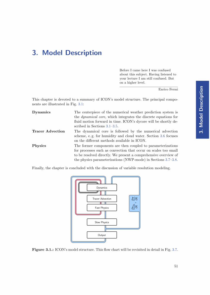
3.

Mo

del

Des

crip

tio

n

3. Model Description

Before I came here I was confusedabout this subject. Having listened toyour lecture I am still confused. Buton a higher level.

Enrico Fermi

This chapter is devoted to a summary of ICON’s model structure. The principal compo-nents are illustrated in Fig. 3.1:

Dynamics The centerpiece of the numerical weather prediction system isthe dynamical core, which integrates the discrete equations forfluid motion forward in time. ICON’s dycore will be shortly de-scribed in Sections 3.1–3.5.

Tracer Advection The dynamical core is followed by the numerical advectionscheme, e. g. for humidity and cloud water. Section 3.6 focuseson the different methods available in ICON.

Physics The former components are then coupled to parameterizationsfor processes such as convection that occur on scales too smallto be resolved directly. We present a comprehensive overview ofthe physics parameterizations (NWP-mode) in Sections 3.7–3.8.

Finally, the chapter is concluded with the discussion of variable resolution modeling.

DynamicsDynamics

Fast Physics

Tracer Advection

Slow Physics

Output

∂vn

∂t,∂π ∂t

Figure 3.1.: ICON’s model structure. This flow chart will be revisited in detail in Fig. 3.7.

51

3.

Mo

del

Descrip

tion

ICON Model Tutorial

3.1. Governing Equations

The equation system of the ICON model is based upon the prognostic variables suggestedby Gassmann and Herzog (2008). It describes a two-component system consisting of dryair and water, where water is allowed to occur in all three phases, including precipitatingdrops and ice particles.

As described in Wacker and Herbert (2003), an equation set for the mixture can be derivedby first introducing a reference velocity into the governing equations. The equations formomentum, mass and energy of the mixture, as given below, are then formed as a sum ofthe constituent-specific equation sets. The specific form of the governing equations for themixture depends on the choice of the reference velocity.

Here we have chosen the barycentric velocity as reference velocity. It is defined as

vb =

∑k ρkvk∑k ρk

,

with the partial density ρk of constituent k and its advective velocity vk. For simplicity,vb will be denoted as v in the following.

In order to separate turbulent fluctuations from the mean flow, a density weighted av-eraging (known as Hesselberg averaging) is applied. Every field φ is decomposed into adensity-weighted mean and a deviation (Hesselberg, 1925)

φ = φ+ φ′′ ,

with

φ =ρφ

ρ

and subsequent averaging. φ denotes the classical Reynolds average. More details ondensity-weighted average calculus can be found e.g. in Zdunkowski and Bott (2003).

The basic Hesselberg-averaged equation system, including the shallow atmosphere approx-imations, reads as follows

∂vn∂t

+∂Kh

∂n+ (ζ + f)vt + w

∂vn∂z

= −cpdθv∂π

∂n− F (vn) (3.1)

∂w

∂t+ vh · ∇w + w

∂w

∂z= −cpdθv

∂π

∂z− g (3.2)

cvdcpdRd

ρθv∂π

∂t= cpdπ

∂ρθv∂t

= −cpdπ∇ · (ρvθv) +Q (3.3)

∂ρ

∂t+∇ · (ρv) =

∑kσconvk (3.4)

∂ρqk∂t

+∇ · (ρqkv) = −∇ ·(Jzkk + ρq′′kv

′′)

+ σk (3.5)

52

3.

Mo

del

Des

crip

tio

n

3.1 Governing Equations

Prognostic equations are solved for the horizontal velocity component normal to the tri-angle edges vn (3.1), the vertical wind component w (3.2), virtual potential temperatureθv (3.3), the total density of the air mixture ρ (3.4), with

ρ =∑

kρk , (3.6)

and mass fractions (3.5)

qk = ρk/ρ . (3.7)

The index k ∈ d, v, c, i, r, s, g represents a specific constituent of the mixture. We use

k = d for dry air,

k = v for water vapor,

k = c for cloud water,

k = i for cloud ice,

k = r for rain,

k = s for snow, and

k = g for graupel.

Further explanation of symbols and variables is given in Table 3.1. Note that the corre-sponding data structures containing the physics and dynamics variables are outlined inSection 8.2.

The equation system (3.1)–(3.5) is supplemented by the lower boundary conditions

w|s =Ev −

∑kprec

Sk|sρ|s −

∑kprec

ρk|s(3.8)

Jzk|s =

Ek − ρkw|s, if k ≡ v−ρkw|s, if k ≡ non-prec. constituent

−Sk|s, if k ≡ prec. constituent

and the equation of state

p = Rd ρ T (1 + α) ,

with

α =

(RvRd− 1

)qv −

∑k 6=v,d

qk .

When expressed in terms of the prognostic variables, the equation of state reads

π =

(Rdρθvp00

) Rdcvd

(3.9)

In contrast to the original formulation by Gassmann and Herzog (2008), we make use ofthe two-dimensional rather than the three-dimensional Lamb transformation to convert

53

3.

Mo

del

Descrip

tion

ICON Model Tutorial

Table 3.1.: Explanation of symbols in the model equations

Symbol Description

∂∂n horizontal derivative in edge-normal direction

Kh = 0.5(v2n + v2

t

)horizontal component of the kinetic energy

ζ = (∇× v) · k vertical component of relative vorticity

f = 2Ω sinφ Coriolis parameter

π Exner function

cpd, cvd specific heat capacity for dry air at constantpressure/volume

F (vn) turbulent momentum fluxes

g acceleration of gravity

Q diabatic heat source

Jzk = ρk (wk − w) vertical diffusion flux for constituent k

σk internal conversion rate for kth constituent (i.e.conversion among different phases or particleforms)

σconvk internal conversion rate for kth constituent dueto convection only

ρq′′kv′′ turbulent flux of kth partial mass fraction

Ev = ρq′′vv′′|s surface evaporation flux

Sk = ρqkvTk sedimentation flux of kth constituent

vT terminal fall velocity of kth constituent

the nonlinear momentum advection term into a vector-invariant form. Vector-invariantmeans that no gradients of vectors appear in this equation, which avoids derivatives ofthe coordinate basis that would otherwise arise in an arbitrary coordinate frame from thenonlinear momentum advection term.

Note that we do not explicitly solve a prognostic equation for the density of dry air. FromEquation (3.6) it becomes clear that the partial density of one constituent (here ρd) canbe diagnosed, given that a prognostic equation for the total density and all but one partialdensities is solved. The reconstructed tangential velocity component is denoted as vt, andin accordance with the model code, it is assumed here that (vt, vn, w) form a right-handedsystem.

From the Equations (3.4), (3.5) for total density and partial densities some importantconstraints can be derived which must hold in the discretized analogue in order to achievemass conservation. First of all, the total density is defined as the sum of all partial densities,as shown by Eq. (3.6). From Eq. (3.7) it follows that

∑kqk = 1 .

54

3.

Mo

del

Des

crip

tio

n

3.2 The Model Reference State

Likewise, the prognostic equation for total density (3.4) should be obtained by summingthe budget equations (3.5) of all constituents. As a consequence the following constraintshold: ∑

kJk = 0 ,

∑kρq′′kv

′′ = 0 .

3.2. The Model Reference State

Dynamics in the atmosphere are characterized by small variations of thermodynamic quan-tities with respect to some background state. Therefore, like many other modeling frame-works, ICON makes use of an atmospheric reference state, i. e. the thermodynamic vari-ables are defined as the sum of a reference state and a deviation from that. The referencestate is assumed to be at rest and horizontally homogeneous, constant in time, dry andhydrostatically balanced.

Any grid-scale thermodynamic variable ψ can then be written as

ψ(λ, φ, z, t) = ψ0(z) + ψ′(λ, φ, z, t) .

The suffix 0 denotes the reference state while the prime denotes the grid-scale deviation.Thus, for the prognostic thermodynamic variables one gets

ρ(λ, φ, z, t) = ρ0(z) + ρ′(λ, φ, z, t)

π(λ, φ, z, t) = π0(z) + π′(λ, φ, z, t)

θv(λ, φ, z, t) = θv0(z) + θ′v(λ, φ, z, t) .

The background state components ρ0, π0, and θv0 are related by the equation of state (3.9)and are hydrostatically balanced, i. e.

π0 =

(Rdρ0θv0

p00

) Rdcvd

dπ0

dz= − g

cpdθv0(3.10)

The actual vertical reference profiles can be obtained by integration of Eq. (3.10) giventhat suitable boundary values are provided. The reference state in ICON is identical tothe state used by the COSMO model.

In a global model like ICON, the local deviation from such a horizontally homogeneousstate can be quite substantial. Therefore, no attempt is made to linearize any part of thegoverning equations with regard to this reference state as it is done in models based on theanelastic assumption. Instead, the main effect of introducing a reference state in a globalnonhydrostatic model like ICON is the removal of horizontal base-state pressure gradientterms in the equation of motion, i.e.

cpdθv∂π

∂n= cpdθv

∂π′

∂n.

55

3.

Mo

del

Descrip

tion

ICON Model Tutorial

This reduces the computational error in the calculation of the pressure gradient force incase of sloping coordinate surfaces. Having said that, this effect is of minor importance forICON, as by default the horizontal pressure gradient is evaluated truly horizontal alongsurfaces of constant height, rather than in terrain-following coordinates, along slopingcoordinate surfaces (Zangl, 2012).

Changing the discretization of the horizontal pressure gradient is possible with the namelistswitch igradp method (nonhydrostatic nml), but not recommended. Nevertheless, thereference state is still of some use for ICON. In the standard configuration of ICON,explicit use of the reference state is made when computing the advective horizontal fluxesfor ρ and θv.

With the base state at hand, the vertical acceleration due to the pressure gradient andgravity in Eq. (3.2) is rewritten as

−cpdθv∂π

∂z− g = −cpd

(θv0 + θ′v

) ∂ (π0 + π′)

∂z

= −cpd(θv∂π′

∂z+ θ′v

dπ0

dz

)− cpdθv0

dπ0

dz− g

(3.10)= −cpd

(θv∂π′

∂z+ θ′v

dπ0

dz

)

The vertical momentum equation finally reads

∂w

∂t+ vh · ∇w + w

∂w

∂z= −cpd

(θv∂π′

∂z+ θ′v

dπ0

dz

).

The perturbation fields π′ and θ′v are obtained from the predicted full fields and referencefields via ψ′ = ψ − ψ0.

3.3. Simplifying Assumptions in the Recent Model Version

The recent model version does not account for mass loss/gain due to precipita-tion/evaporation. In particular, the following assumptions are made:

The term∑

k σconvk on the r.h.s. of Eq. (3.4), which describes the net mass tendency of

the convection parameterization, is neglected. Thus the model neither accounts for massloss due to convective precipitation, nor mass re-distribution due to convective motions.The mass continuity equation takes the form

∂ρ

∂t+∇ · (ρv) = 0 . (3.11)

At the surface, the boundary condition for w, Eq. (3.8), is approximated as

ρw|s =∑

kρkwk|s = 0 , (3.12)

which in terrain-following coordinates translates to ρw|s = ρv · ∇h. h denotes the to-pography height. Thus, the simulated atmospheric system is assumed to be closed w.r.t.

56

3.

Mo

del

Des

crip

tio

n

3.4 Vertical Coordinates

total mass. The sedimentation fluxes at the surface Sk|s as well as the surface evaporationflux Ev|s, which appear in the partial mass continuity equations, are retained. In orderfor Eq. (3.12) to hold, the (implicit) assumption is that the corresponding mass loss/gaindue to sedimentation/evaporation is compensated by a fictitious flux of dry air across thesurface.

Away from the surface, the diffusion fluxes of all airborne constituents (except for dryair) are neglected. The diffusive fluxes of all precipitating constituents, however, are takeninto account. The continuity equation for the total mass is used in the form (3.11). SinceEq. (3.11) only holds if the constraint

∑k J

zk = 0 holds, again, the (implicit) assumption

made is that a fictitious diffusion flux of dry air counteracts the sedimentation fluxes suchthat the total mass in a volume moving with the barycentric velocity is conserved.

In summary, the simplifying assumptions can be characterized by the following (equivalent)statements:

• The current model version conserves the total air mass instead of the dry air mass.

• The precipitation mass sink and the evaporation mass source are neglected in thetotal mass budget of the model.

• The net mass gain or loss due to precipitation/evaporation does not affect the surfacepressure.

The latter point becomes obvious, when writing down the (hydrostatic) pressure tendencyequation and applying the approximations (3.11)–(3.12) (see also Wacker and Herbert(2003)). Starting from the hydrostatic equation ∂p

∂z = −ρg it follows:

∂

∂t

∫ 0

ps

dp = −g ∂∂t

∫ ∞zs

ρ dz

∂ps∂t

= g

∫ ∞zs

∂ρ

∂tdz

∂ps∂t

= −g∫ ∞zs

∇ · (ρv)−∑

kσconvk dz

∂ps∂t

= −g∫ ∞zs

∇h · (ρvh) dz + g (ρw) |s + gPconv|s

∂ps∂t

= −g∫ ∞zs

∇h · (ρvh) dz +

gρ|s

ρ|s −∑

kprec ρk|s

Ev − ∑kprec

Sk|s

+ gP

conv|s ,

with the convective surface precipitation flux

Pconv|s =

∫ ∞zs

∑kσconvk dz .

Thus, dynamical effects of the evaporation/precipitation mass source/sink are neglected.I.e. related pressure changes are ignored.

57

3.

Mo

del

Descrip

tion

ICON Model Tutorial

half level 1

half level 2

half level 3

half level 4w

w

vn ,ρ,θv

full level 1

full level 2

full level 3

full levels half levels

Figure 3.2.: Illustration of ICON’s vertical levels. With num lev layers, there arenum lev + 1 so-called half levels. The half levels k − 1/2, k + 1/2 encloselayer k at the centers of which are the corresponding full levels k, fork = 1, . . . , num lev. Layer 1 is at the top of the atmosphere and layer nat the bottom of the atmosphere. Half level num lev + 1 coincides with theEarth’s surface.

3.4. Vertical Coordinates

In a nonhydrostatic model, a vertical coordinate in terms of pressure does not make sensesince it cannot be taken for granted that the pressure is monotonously decreasing withincreasing altitude. In general, the air mass of an air column above a certain point cannot be calculated from the pressure at that point anymore. Instead, a geometric altitudegrid has to be used.

In ICON the choice is a height based coordinate system that follows the terrain andconsequently, the top and bottom triangle faces are inclined with respect to the tangentplane on a sphere. Due to the fact that the model levels gradually change into levels ofconstant height as the distance from the lower boundary increases, top and bottom trianglefaces of a grid box are also slightly inclined to each other. The exact altitude of each gridbox depends on the geographical position on the globe. The top and bottom faces arecalled half levels of the vertical grid, the center of the box is said to be at the full levelof the vertical grid, see Fig. 3.2 for an illustration. Note that the numbering of full andhalf levels is top-down, starting with l = 1 for the top half- and full level. A Lorenz-typestaggering is used in the vertical, which means that horizontal velocity, virtual potentialtemperature and density are defined at full levels, whereas vertical velocity is defined athalf levels.

58

3.

Mo

del

Des

crip

tio

n

3.4 Vertical Coordinates

When setting up an ICON simulation, the total number of vertical levels has to be specifiedfor each domain via

num lev (namelist run nml, list of integer value)Comma-separated list of integer values giving the number of vertical full levels foreach domain.

If the number of vertical levels is desired to vary between domains, setting the namelistparameter lvert nest (run nml) to .TRUE. is required. See Section 3.9.3 for more infor-mation on vertical nesting.

Two variants of a height-based terrain-following vertical coordinate are available in ICON.Both of which are briefly described below.

3.4.1. Terrain-following Hybrid Gal-Chen Coordinate

The terrain-following hybrid Gal-Chen coordinate (Simmons and Burridge, 1981) is an ex-tension of the classic terrain-following coordinate introduced by Gal-Chen and Somerville(1975). As shown by Klemp (2011), it can be expressed in the form

z(x, y, η) =(H −B′(η)h(x, y))

Hη +B′(η)h(x, y)

= η +B′(η)(

1− η

H

)h(x, y) , (3.13)

where z represents the height of the coordinate surfaces η, h(x, y) is the terrain height,and H denotes the domain height. With B′(η) = 1 the coordinate reverts to the classicformulation by Gal-Chen and Somerville (1975), i.e. the coordinate is terrain-following atthe surface (η = 0) and becomes flat at model top (η = H). By choosing B′ appropriately,a more rapid transition from terrain-following at the surface toward constant height canbe achieved. One popular choice is to set

B′(η)(

1− η

H

)= 1− η

zflat, with zflat < H

such that coordinate surfaces become constant height surfaces above z = zflat. Sometimes,Equation (3.13) is also written in the discretized form

zh(x, y, k) = A(k) +B(k)h(x, y) , k = 1, ..., num lev + 1 (3.14)

where k denotes the vertical level index and zh is the half level height.

Configuring the Hybrid Gal-Chen Coordinate

The main switch for selecting the Gal-Chen hybrid coordinate is

ivctype = 1 (namelist nonhydrostatic nml, integer value)

59

3.

Mo

del

Descrip

tion

ICON Model Tutorial

In that case the user has to provide the vertical coordinate table (vct) as an input file.The table consists of the A and B values (see Equation (3.14)) from which the half levelheights zh(x, y, k) can be deduced. A(k)[m] are fixed height values, with A(1) defining themodel top height H and A(num lev + 1) = 0 m. The dimensionless values B(k) control thevertical decay of the topography signal, with B(1) = 0 and B(num lev + 1) = 1. Thus, ateach horizontal grid point zh(x, y, 1) is the model top height, while zh(x, y, num lev + 1)is the surface height.

The structure of the expected input file is depicted in Table 3.2. Example files can befound in icon/vertical coord tables. The file must obey the following naming rule:atm hyb sz [nlev], where [nlev] must be replaced by the total number of full levels. ICONexpects the file to be located in the base directory from which the model is started. Notethat there is no namelist parameter with which the location and name of the file can bespecified. The namelist parameter vertical grid filename (grid nml), which one mightbe tempted to use for that purpose, is meant for something slightly different: Its purpose isto read in a vertical grid file (NetCDF format) that has been written to disc by a previousICON run.

# File structure

# --------------

# A and B values are stored in arrays vct_a(k) and vct_b(k).

# The files in text format are structured as follows:

#

# -------------------------------------

# | k vct_a(k) [m] vct_b(k) [] | <- first line of file = header line

# | 1 A(1) B(1) | <- first line of A and B values

# | 2 A(2) B(2) |

# | 3 A(3) B(3) |

# | . |

# | . |

# | nlev+1 A(nlev+1) B(nlev+1)| <- last line of A and B values

# |=====================================| <- lines from here on are ignored

# |Source: | by mo_hyb_params:read_hyb_params

# |<some lines of text> |

# |Comments: |

# |<some lines of text> |

# |References: |

# |<some lines of text> |

# -------------------------------------

Table 3.2.: Structure of vertical coordinate table as expected by the ICON model.

3.4.2. SLEVE Coordinate

In the case of a terrain-following hybrid Gal-Chen coordinate the influence of terrain on thecoordinate surfaces decays only linearly with height. The basic idea of the Smooth LevelVertical SLEVE coordinate (Schar et al., 2002, Leuenberger et al., 2010) is to increase

60

3.

Mo

del

Des

crip

tio

n

3.4 Vertical Coordinates

the decay rate, by allowing smaller-scale terrain features to be removed more rapidly withheight. To this end, the topography h(x, y) is divided into two components

h(x, y) = h1(x, y) + h2(x, y),

where h1(x, y) denotes a smoothed representation of h(x, y), and h2(x, y) = h(x, y) −h1(x, y) contains the smaller-scale contributions. The coordinate is then defined as

z(x, y, η) = η +B1(η)h1(x, y) +B2(η)h2(x, y) .

Different decay functions B1 and B2 are now chosen for the decay of the large- and small-scale terrain features, respectively. These functions are selected such that the influenceof small-scale terrain features on the coordinate surfaces decays much faster with heightthan their large-scale (well-resolved) counterparts. The squeezing of the model layers abovesteep mountains is limited automatically in order to prevent (nearly) intersecting layersthat would cause numerical instabilities.

Configuring the SLEVE Coordinate

The main switch for selecting the SLEVE vertical coordinate is

ivctype = 2 (namelist nonhydrostatic nml, integer value)

This is the default and recommended setting. The vertical grid is constructed during theinitialization phase of ICON, based on additional parameters defined in sleve nml. Herewe will only discuss the most relevant parameters. For a full list, the reader is referred tothe namelist documentation.

Namelist sleve nml:

top height (namelist sleve nml, real value)Height of model top.

flat height (namelist sleve nml, real value)Height above which the coordinate surfaces become constant height surfaces.

min lay thckn (namelist sleve nml, real value)Layer thickness of lowermost layer.

Note for advanced users: On default, a vertical stretching is applied suchthat coordinate surfaces become non-equally distributed along the vertical,starting with a minimum thickness of min lay thckn between the lower-most and second lowermost half-level. If constant layer thicknesses are de-sired, min lay thckn must be set to a value ≤ 0. The layer thickness is thendetermined as top height/num lev. Control output of the vertical layer dis-tribution is written to stderr.

61

3.

Mo

del

Descrip

tion

ICON Model Tutorial

3.5. Temporal Discretization

In this section we will focus on time differencing in isolation and will neglect any com-plexity due to space differencing. Before we dive into the (nasty) details of ICON’s timediscretization, let us take a step back and try to grasp the basic idea.

3.5.1. Basic Idea

Consider an arbitrary first-order ordinary differential equation of the form

dψ(~x, t)

dt= F (ψ(~x, t), t) . (3.15)

Here, ψ : R3×R→ Rq is the q-dimensional vector of state variables. In real applications,the vector-valued flux function F : Rq × R→ Rq might be very complex.

Let tn−m denote some time in the past and tn+1 some time in the future. Now we integrateEq. (3.15) from time tn−m to tn+1, which gives

ψ(~x, tn+1)− ψ(~x, tn−m) =

tn+1∫tn−m

F (ψ(~x, t), t) dt .

We can try to approximate the integral on the right hand side (r.h.s.) using some weightedaverage of F at known discrete time levels. In the following we will restrict ourselves tosimple two-level time-stepping schemes, i.e. we set m = 0 and only make use of F at thediscrete times tn and tn+1 (for a general survey of time-differencing schemes, see Randall(2017)). With this restriction we get

ψ(~x, tn+1)− ψ(~x, tn)

∆t= αFn+1 + βFn . (3.16)

The coefficients α and β must satisfy the so called consistency condition

α+ β = 1 ,

such that the r.h.s. of Eq. (3.16) represents some averaged F . Equation (3.16) represents awhole family of simple two-step schemes. For example, by choosing α = 0, β = 1 we arriveat the simple Euler forward scheme, while for α = 1, β = 0 we get the (implicit) Eulerbackward scheme, both of which are first order accurate. Choosing α = β = 0.5 leads tothe implicit trapezoidal scheme, which is of second order accuracy.

One way to avoid the implicity of the trapezoidal scheme while retaining higher orderis to switch to iterative schemes, also known as predictor-corrector schemes. This is theway pursued in ICON. The key idea of the predictor-corrector scheme is to replace theunwieldy Fn+1 by an estimate F ∗n+1 = F

(ψ∗n+1, tn+1

)with ψ∗n+1 computed by an explicit

scheme, e.g. a forward Euler scheme. The full predictor-corrector scheme reads

predictor : ψ∗(~x, tn+1) = ψ(~x, tn) + ∆tFn

corrector : ψ(~x, tn+1) = ψ(~x, tn) + ∆tF ∗n+1, Fn

α

(3.17)

62

3.

Mo

del

Des

crip

tio

n

3.5 Temporal Discretization

Here we have introduced the notation

x, yα := αx+ (1− α) y .

Note that for α = 1, Equation (3.17) is an imitation of the Euler backward scheme (termedMatsuno scheme, (Matsuno, 1966)), while for α = 0.5, it is an imitation of the trapezoidalscheme (termed Heun’s method). The Matsuno scheme has first-order accuracy, and Heun’smethod has second-order accuracy.

In simplified terms, the time integration scheme of ICON can be regarded asa mixture of the Matsuno scheme and the Heun scheme, as the coefficient αused by ICON varies between these two extremes.

3.5.2. Implementation Details

Now, in the terminology of the previous section, in ICON we have

ψ(~x, t) = [vn(~x, t), w(~x, t), ρ(~x, t), π(~x, t)]T .

Here, we have omitted the partial densities ρ qk from the vector of state variables. Theprognostic equation (3.5) is treated with a different time discretization, as will be explainedin Section 3.6.

For the sake of brevity we omit the notation for Reynolds- and Hesselberg averages. Thesubscripts n, n+ 1∗ and n+ 1 will be used to denote the current time level, the resultingtime level of the predictor step and the new time level, respectively. They should not beconfused with the subscript n used to denote the normal velocity component vn, or thehorizontal derivative in edge-normal direction ∂/∂n.

The time discretization complies with the explicit two-time level predictor-correctorscheme which was described in the previous section, except for those terms describing ver-tical sound-wave propagation. These terms, i.e. vertical derivatives of w and π are treatedimplicitly for reasons of numerical stability and efficiency. Below, the implicit terms are

marked in blue .

Predictor step:

vn+1∗n − vnn

∆t= −adv(vnn)− cpdθnv

∂π′,n

∂n+ F (vnn) (3.18)

wn+1∗ − wn∆t

= −adv(wn)− cpdθ′,nvdπ0

dz− cpdθ

nv

∂π′,n+1∗

∂z , ∂π′,n

∂z

η

(3.19)

ρn+1∗ − ρn∆t

= −∇h ·(vn+1∗n ρn

)− ∂

∂z

[wn+1∗ , wn

ηρn]

πn+1∗ − πn∆t

= −Rdcvd

(πn

ρnθnv

)[∇h ·

(vn+1∗n ρnθnv

)+ ∂

∂z

[wn+1∗ , wn

ηρnθnv

] ]+Qn (3.20)

63

3.

Mo

del

Descrip

tion

ICON Model Tutorial

with

adv(vnn) =∂Kn

h

∂n+ (ζn + f) vnt + wn

∂vnn∂z

adv(wn) = vnh · ∇wn + wn∂wn

∂z.

The terms F (vnn) and Qn denote diabatic momentum and exner pressure tendencies dueto slow physics processes, i.e. parameterized convection, orographic and non-orographicgravity waves and radiation. See Section 3.7.1 for more details on the distinction betweeenfast and slow physics processes.

The implicitness parameter η (with 0 ≤ η ≤ 1) for the vertically implicit sound wave solverhas a default value of η = 0.65 which is usually sufficient to ensure numerical stability inreal-case applications. If required, this value can be modified with the namelist parametervwind offctr (nonhydrostatic nml). Note that vwind offctr presents the off-centeringvwind offctr = η − 0.5 (i.e., the default is vwind offctr = 0.15). Its permissible rangeis given by

0 ≤ vwind offctr ≤ 0.5 .

Corrector step:

vn+1n − vnn

∆t= −

adv(vn+1∗

n ), adv(vnn)α

− cpdθn+1∗v , θnv

δ

∂π′,n+1∗

∂n,∂π′,n

∂n

δ

− Fd(vn+1∗n ) + F (vnn) (3.21)

wn+1 − wn∆t

= −

adv(wn+1∗), adv(wn)α

− cpdθ′,n+1∗v , θ′,nv

δ

dπ0

dz

− cpdθn+1∗v , θnv

δ

∂π′,n+1

∂z , ∂π′,n

∂z

η

ρn+1 − ρn∆t

= −∇h ·(vn+1n ρn

)− ∂

∂z

[wn+1, wn

η

ρn+1∗ , ρn

δ

]πn+1 − πn

∆t= −Rd

cvd

(πn

ρnθnv

)[∇h ·

(vn+1n ρnθnv

)+ ∂

∂z

[wn+1, wn

η

ρn+1∗ , ρn

δ

θn+1∗v , θnv

δ

] ]+Qn

The term Fd(vn+1∗n ) represents 4th order divergence damping which has been introduced

in order to control checkerboard noise.

The parameter α denotes the Matsuno parameter which was introduced in Section 3.5.1.With respect to the velocity, it can be used to make the explicit part of the corrector step

64

3.

Mo

del

Des

crip

tio

n

3.5 Temporal Discretization

resemble either a Matsuno-type scheme (α −→ 1) or Heun’s method (α −→ 0.5). Thedefault value of the Matsuno-parameter for velocity is given by α = 0.75.

A second Matsuno parameter 0 ≤ δ ≤ 1 exists for the thermodynamic variables ρ and θvn ,where the default value of the coefficient is δ = 0.4. The corresponding namelist parametersare named veladv offctr and rhotheta offctr in the namelist nonhydrostatic nml.Note again that both define the off-centering from 0.5 rather than the absolute value.

In order to close the system of equations, for both substeps (predictor and corrector), thequantity θv must be calculated from the state variables π and ρ. We explain this in thefollowing, using the notation πnew ≡ πn+1∗ or πnew ≡ πn+1 for the predictor and correctorstep.

Once the updated state vector

ψnew(~x, t) = [vnewn (~x, t), wnew(~x, t), ρnew(~x, t), πnew(~x, t)]T

is known, the virtual potential temperature θnewv is diagnosed from the linearized equation

of state (3.9)

πnew − πnπn

=Rdcvd

(ρθv)new − (ρθv)

n

(ρθv)n. (3.22)

The rationale behind that is as follows: Multiplying (3.22) by ∆t−1 and rearranging yields

(ρθv)new − (ρθv)

n

∆t=cvdRd

(ρnθnvπn

)πnew − πn

∆t. (3.23)

Thus, diagnosing θnewv from (3.22) can be interpreted as solving two prognostic equations

for the two thermodynamic variables π and θv, instead of one prognostic equation forπ and the equation of state. By doing so, ρθv is exactly conserved (in the absence ofdiabatic terms). The two prognostic equations are constrained by (3.23), i.e. the same fluxdivergence is used. As a side effect, however, the solution at a particular point in time isnot constrained by the equation of state (3.9) – only its time evolution is. This approachwas first described by Gassmann (2013).

Pragmatic Simplifications

A potential disadvantage of predictor-corrector schemes as compared to non-iterativeschemes is its computational expense. This is because the forcing terms (r.h.s.) mustbe evaluated twice per time step. Therefore, several terms have been simplified providedthat the simplification proved to not degrade the quality of the results significantly. Thefollowing pragmatic simplifications have been performed:

• The horizontal and vertical momentum advection at the predictor step is re-usedfrom the corrector step of the preceding time step. With time level n∗ denotingn+ 1∗ from the preceding time step this can be written as

Equation (3.18): adv(vnn) ' adv(vn∗n )

Equation (3.19): adv(wn) ' adv(wn∗)

65

3.

Mo

del

Descrip

tion

ICON Model Tutorial

By this, in each time step the momentum advection needs to be computed only once.

The first predictor step following the physics step represents an exception. At thistime level the momentum advection from the preceding corrector step does notprovide a suitable estimate, as the physics step might have changed vn considerably.

• Another simplification relates to the horizontal pressure gradient term which occursin the predictor and corrector step of vn. Using time level n in the predictor and aninterpolated value between n and n+1∗ in the corrector provides an effective dampingmechanism for horizontally propagating sound waves, without significantly impactinggravity waves. A very similar effect can be achieved by using the same horizontalpressure gradient in the predictor and corrector, however, with the pressure beingextrapolated in time.

Equation (3.18): cpdθnv

∂π′,n

∂n' cpdθnv

∂π′,n

∂n

Equation (3.21): cpd

θn+1∗v , θnv

δ

∂π′,n+1∗

∂n,∂π′,n

∂n

δ

' cpdθnv∂π′,n

∂n

By this, in each time step the horizontal pressure gradient needs to be computed onlyonce. The time level n at which the horizontal gradient is taken is an extrapolatedtime level using the levels n and n− 1:

π′,n = (1 + γ)π′,n − γπ′,n−1

The temporal extrapolation factor is chosen from the range γ ∈[

13 ,

23

], with the

default being γ = 1/3. The corresponding namelist parameter is named exner expol

(nonhydrostatic nml).

Vertically Implicit Solver

The solution to the predictor-corrector scheme described above is mostly straightforward,as the majority of terms are treated in an explicit manner. This, however does not hold forthe prognostic equation for vertical wind, since the solution for wn+1∗ depends on πn+1∗ ,which itself depends on wn+1∗ (see Equations (3.19) and (3.20)).

Before the exact solution method is derived below, the overall solution strategy can bedescribed as follows: First, π is eliminated from Eq. (3.19) by inserting the prognosticequation (3.20). Then this results in a linear system of equations for the unknown w’s inthe vertical direction. The derivation for the corrector step is basically identical and differsonly w.r.t. the time levels that are used for ρ and θv.

We start with the vertical discretization of (3.19) and (3.20). When using basic centereddifferences, and noting that ∂π/∂t = ∂π′/∂t this leads to

wn+1∗

k+1/2 = Zw explk+1/2 −∆tcpdθ

nv,k+1/2 η

π′,n+1∗

k − π′,n+1∗

k+1

∆zk+1/2(3.24)

π′,n+1∗

k = Zπ explk −∆t

Rdcvd

(πnk

ρnkθnv,k

)η

(wn+1∗ρnθnv )k−1/2 − (wn+1∗ρnθnv )k+1/2

∆zk, (3.25)

66

3.

Mo

del

Des

crip

tio

n

3.5 Temporal Discretization

with the shorthand notations Zw explk+1/2 and Zπ expl

k for the explicit parts

Zw explk+1/2 = wnk+1/2 −∆t

[adv(wn∗)k+1/2 + cpdθ

′,nv,k+1/2

dπ0

dz

∣∣∣∣k+1/2

+ cpdθnv,k+1/2(1− η)

π′,nk − π′,nk+1

∆zk+1/2

]and

Zπ explk = π′,nk −∆t

Rdcvd

(πnk

ρnkθnv,k

)[∇h ·

(vn+1∗ρnθnv

)k

+ (1− η)(wnρnθnv )k−1/2 − (wnρnθnv )k+1/2

∆zk

]+ ∆tQkn .

∆zk = zk−1/2 − zk+1/2 denotes the thickness of the kth

cell which is bounded by the halflevels k ± 1/2, whereas ∆zk+1/2 = zk − zk+1 denotes the thickness of the layer boundedby the full levels k and k + 1 (see also Figure 3.2).

As an intermediate step, we compute π′,n+1∗

k − π′,n+1∗

k+1 from Eq. (3.25):

π′,n+1∗

k − π′,n+1∗

k+1 = Zπ explk − Zπ expl

k+1 − ∆tRdcvd

η

[(wn+1∗ρnθnv )k−1/2

Γnk∆zk

− (wn+1∗ρnθnv )k+1/2

(Γnk

∆zk+

Γnk+1

∆zk+1

)+ (wn+1∗ρnθnv )k+3/2

Γnk+1

∆zk+1

]. (3.26)

Here we have introduced Γnk as an abbreviation for

Γnk =πnk

ρnkθnv,k

.

Inserting Eq. (3.26) into Eq. (3.24) and collecting terms proportional to wn+1∗

k−1/2, wn+1∗

k+1/2,

wn+1∗

k+3/2 on the left hand side leads to:

− wn+1∗

k−1/2

[∆t

cpdθnv,k+1/2

∆zk+1/2η∆t

Rdcvd

ρnk−1/2θnv,k−1/2η

Γnk∆zk

]︸ ︷︷ ︸

sub-diagonal

+ wn+1∗

k+1/2

[1 + ∆t

cpdθnv,k+1/2

∆zk+1/2η∆t

Rdcvd

ρnk+1/2θnv,k+1/2η

(Γnk

∆zk+

Γnk+1

∆zk+1

)]︸ ︷︷ ︸

main diagonal

− wn+1∗

k+3/2

[∆t

cpdθnv,k+1/2

∆zk+1/2η∆t

Rdcvd

ρnk+3/2θnv,k+3/2η

Γnk+1

∆zk+1

]︸ ︷︷ ︸

sup-diagonal

= Zw explk+1/2 −∆t

cpdθnv,k+1/2

∆zk+1/2η(Zπ explk − Zπ expl

k+1

)(3.27)

67

3.

Mo

del

Descrip

tion

ICON Model Tutorial

Equation (3.27) defines a linear system of equations from which the unknown verticalvelocities wn+1∗

k−1/2 can be computed. The system is tridiagonal and can be solved with

the Thomas algorithm (Press et al., 2007, p. 57), given that suitably defined boundaryconditions are provided. So far it is assumed that the upper and lower boundary areimpermeable w.r.t. to mass, i.e. we set wn+1∗

1/2 = wn+1∗

nlev+1/2 = 0. In case of vertical nesting,w at the upper boundary is interpolated from the parent domain.

3.6. Tracer Transport

Physically speaking, the tracer transport module predicts the large-scale re-distributionof tracers (e.g. water substances, aerosols, chemical species, . . . ) caused by air-motions.Mathematically (numerically) this is done by solving the partial mass continuity equa-tion (3.5) for each tracer, with sources and sinks being neglected, i.e.

∂ρqk∂t

+∇ · (ρqkv) = 0 (3.28)

The numerical solution of Eq. (3.28) is based on so-called space-time finite volume meth-ods. By space-time methods we refer to methods where the temporal and spacial dis-cretizations are combined rather than separated. Space-time methods are also known ascell-integrated semi-Lagrangian schemes. As will become clear, such schemes are neitherpurely semi-Lagrangian, nor Eulerian in the classical sense. They are Eulerian in thesense that the flux of mass through the stationary walls of grid cells is considered. Theyare, however, semi-Lagrangian in the sense that trajectory calculations are needed forflux computation. In the literature such schemes are sometimes termed Flux Form Semi-Lagrangian (FFSL). The specific implementation in ICON partly builds upon work byLauritzen et al. (2010, 2011a), Harris and Lauritzen (2010), Skamarock and Menchaca(2010), Miura (2007) for the horizontal and Colella and Woodward (1984) for the vertical.

As we are dealing with a Finite Volume (FV) discretization, it is worth noting that in thefollowing all scalar variables ψ, whose storage location is at the triangle cell circumcenter,are interpreted as cell averages rather than point values, i.e.

ψni =

1

∆Vi

∫∫∫Vi

ψ(x, y, z, tn) dV ,

with ∆Vi denoting the volume of the ith prismatic cell. Here and in the reminder of thisSection, the overbar denotes volume averages rather than Reynolds averages.

3.6.1. Directional Splitting

By integrating the continuity equation (3.28) in space over a prismatic grid cell (the so-called control volume) and in time over the time step ∆t, a solution to (3.28) can formallybe written as

ρqn+1i,k = ρqni,k + ∆t [H(qn) + V(qn)] , (3.29)

68

3.

Mo

del

Des

crip

tio

n

3.6 Tracer Transport

where H and V denote the horizontal and vertical transport operators acting on qn, andρqn+1i,k denoting the updated cell averaged partial density of constituent k at the time tn+1.

Instead of solving this somewhat unwieldy equation in one sweep, a fractional step ap-proach is taken in ICON such that separate equations for horizontal and vertical transportare solved consecutively. Of course, replacing equation (3.29) by some approximation in-volving the two subproblems

ρq∗i,k = ρqαi,k + ∆tV(qβ)

ρq∗∗i,k = ρqγi,k + ∆tH(qδ)

will inevitably result in a residual error. This error is known as the splitting error. Ondefault, the following approximation to (3.29) is used:

ρq∗i,k =ρqni,k + ∆tV (qn) (3.30)

ρqn+1i,k =ρq∗i,k + ∆tH (q∗) (3.31)

In order to maintain O[∆t2

]accuracy, the order of the operators is reversed on alternate

time steps. This might be regarded as a poor man’s Strang splitting (Strang, 1968). FullStrang-splitting of the form [V(∆t/2)][H(∆t)][V(∆t/2)] is also available as an option bychoosing lstrang=.FALSE. (namelist transport nml). Except for being more expensive(the vertical operator is called twice) no significant impact on the model results has beennoted so far.

A shortcoming of the splitting (3.30), (3.31) is that it does not preserve an initially uniformtracer field (e.g. q(x, y, z, t0) = 1) in a deformational non-divergent flow since there is notenough information available to correctly do the conversion ρq∗ −→ q∗. To do so, it isnecessary to keep track of the changes in partial density ρq that are solely a result of massconvergence/divergence in the directions of splitting. Therefore we follow the method ofEaster (1993) wherein the mass continuity equation (3.5) is simultaneously reintegratedwith that for partial mass:

ρq∗i,k =ρqni,k + ∆tV (qn)

ρ∗i,k =ρni,k + ∆tV (1)

q∗i,k =ρq∗i,kρ∗i,k

(3.32)

ρqn+1i,k =ρq∗i,k + ∆tH (q∗)

ρn+1i,k =ρ∗i,k + ∆tH (1)

qn+1i,k =

ρqn+1i,k

ρn+1i,k

(3.33)

Changes in partial density solely due to mass convergence/divergence are corrected for inequations (3.32) and (3.33). The key point here is that the intermediate density ρ∗ ratherthan ρn+1 or ρn is used to recover the mass fraction q∗ in (3.32). For re-integration ofthe mass continuity equation, the mass fluxes that have already been computed in thedynamical core are re-used.

69

3.

Mo

del

Descrip

tion

ICON Model Tutorial

3.6.2. Horizontal Transport

A rigorous derivation of the horizontal transport operator H(q) is beyond the scope of thisdocument. We will merely concentrate on the general concept and illustrate graphicallyhow the scheme works. The horizontal transport scheme belongs to the class of so-calledFlux Form Semi-Lagrangian (FFSL) schemes (Harris and Lauritzen, 2010). In the liter-ature such schemes are sometimes alternatively termed Incremental remapping schemes(Lipscomb and Ringler, 2005) or streamline subgrid integration method (Yeh, 2007).

Graphical Interpretation

Figure 3.3 provides a graphical interpretation of the FFSL-scheme. Black solid lines showthe triangular grid, with thick solid lines highlighting an arbitrary cell with area ∆Aifor which the scheme will be explained. In the following we will refer to this cell as theEulerian control volume (CV). The basic task is to compute the updated value ρqn+1

i forthat cell on the basis of the old values ρqni and the velocity fields vn and vn+1.

In order to set the stage, let us first take the Lagrangian viewpoint: Assume that the timedependent velocity field is known analytically such that we know the trajectories for all theair parcels which terminate at the walls of the Eulerian CV at the new time tn+1. As anexample, trajectories for the air parcels terminating at the CV vertices at tn+1 are depictedas gray lines. Accordingly we know the position of these air parcels at time tn which we willdenote as the starting points. By connecting the starting points we can construct the grayshaded area known as the Lagrangian CV. The latter encompasses all air parcels that aretransported into the Eulerian CV (i.e. the grid cell) during the time interval

[tn, tn+1

]. In a

standard semi-Lagrangian scheme the key task is to compute an estimate of the LagrangianCV (gray shaded), followed by a computation of the total tracer mass contained. Then,the solution ρqi

n+1 can easily be deduced from the Lagrangian finite-volume form of thecontinuity equation (3.28)

ρqn+1i ∆Ai = ρqni ∆ai ,

where ∆Ai and ∆ai denote the area of the Eulerian and Langrangian CV, respectively(see e.g. Lauritzen et al., 2011b). ρqni is the average tracer mass over the Lagrangian CVarea ai

ρqni =1

∆ai

∫∫ai

ρn(x, y)qn(x, y)dA .

As mentioned before, a more Eulerian rather than semi-Lagrangian viewpoint is taken inICON. Here we keep track of the flux of mass passing the Eulerian cell walls rather thanthe mass in the Lagrangian CV. This is where the yellow areas in Figure 3.3 enter thegame. We will refer to these as flux areas. Since the individual edges of the Lagrangian CVpass through the flux areas during

[tn, tn+1

], it is exactly the mass inside in the flux areas

that is swept across the Eulerian CV walls during one time step. Thus, starting from themass ρqni in the Eulerian CV and assuming that we know the shape as well as the tracermass contained in the (yellow) flux areas, we can compute the updated value ρqn+1

i .

70

3.

Mo

del

Des

crip

tio

n

3.6 Tracer Transport

Figure 3.3.: Graphical illustration of the FFSL scheme. Black solid lines show the tri-angular grid, with thick solid lines highlighting the Eulerian control volumeunder consideration. Grey area shows the Lagrangian control volume andyellow areas show the flux areas (departure region) for each cell wall.

Mathematically the scheme can be cast into the following form:

ρqn+1i = ρqni −

1

∆Ai

Ne∑e=1

sie Fie ,with Fie = 〈ρei 〉∫∫aei

qn(x, y) da , (3.34)

where Fie defines the total mass crossing the eth wall during ∆t and aei denotes the fluxarea for the eth wall. sei = ±1 distinguishes inward and outward directed fluxes.

Note that this Eulerian viewpoint is fully equivalent to the semi-Lagrangian viewpoint.It can be shown (Lauritzen et al., 2011b) that all areas involved in our quasi-Eulerianapproach (Eulerian CV plus flux areas) sum up to the Lagrangian CV.

Basic Algorithm

The numerical algorithm which solves Eq. (3.34) for a single Eulerian CV proceeds in 4major stages:

1. The flux area aei for each cell wall is reconstructed by means of backward trajectories.

2. For each Eulerian CV the unknown tracer subgrid distribution q(x, y, t0) is estimatedfrom the known cell averages qni of the CV itself and surrounding cells. Severalpolynomial reconstructions, from linear to cubic, are available.

3. The total mass Fie crossing the eth wall is estimated by numerically evaluating theintegral in Eq. (3.34). I.e. the estimated subgrid distribution q(x, y, t0) is integratedover the approximated departure region aei by means of Gauss quadrature.

4. The sum on the r.h.s. of Eq. (3.34) is evaluated which leads to the solution ρqn+1i .

3.6.3. Vertical Transport

A rigorous derivation of the vertical transport operator V(q) is beyond the scope of thisdocument. As for the horizontal operator H(q) we will concentrate on the basic concept.

71

3.

Mo

del

Descrip

tion

ICON Model Tutorial

Figure 3.4.: The Piecewise Parabolic Method (PPM). Left: Unknown subgrid distribu-tion q(z) gets approximated by piecewise parabolic interpolants which areC0 continuous at cell walls. Right: Polynomial reconstruction is filtered (op-tional) to render the scheme monotonous. Integration step: Sub-grid distri-bution is integrated over the “area” w∆t (dark blue) in order to determinethe mass which enters the kth cell during ∆t.

The vertical transport scheme is based on the Piecewise Parabolic Method (PPM) devel-oped by Colella and Woodward (1984). It is a finite volume scheme and thus inherentlymass conserving. It makes use of a piecewise parabolic function for approximating theunknown subgrid distribution of a 1D scalar field q(z). The function is forced to be con-tinuous at cell interfaces. Its construction is based on the known cell averages qk. The PPMscheme bears some conceptual resemblance to the horizontal FFSL transport scheme. Thebasic concept is depicted in Figure 3.4.

Step 1: The subgrid distribution q(ζ, k) is reconstructed cell-wise in a vertical columnby using the parabolic interpolant

q(ζ, k) = a0 + a1ζ + a2ζ2 , with ζ =

z − zk+1/2

∆zk. (3.35)

ζ is a dimensionless coordinate which is 1 at the grid cell top and 0 at its bottom. Specificto the PPM scheme is the way how this parabola is constructed. The unknown coefficientsai are derived from the 3 constraints∫ 1

0q(ζ, k)dζ = qk ,

q(ζ = 1, k) = qu = qk−1/2 ,

q(ζ = 0, k) = ql = qk+1/2 ,

(3.36)

which, vividly said, state that the polynomial must be mass conserving, and that thepolynomial equals qu and ql at its upper and lower end, respectively. qu = qk−1/2 andql = qk+1/2 are appropriately reconstructed estimates at the upper and lower half levelsand are shared between adjacent cells. By this, continuity of the reconstruction across cellsis enforced.

72

3.

Mo

del

Des

crip

tio

n

3.6 Tracer Transport

By applying the constraints (3.36) the parabolic interpolant (3.35) can finally be writtenas a function of the grid scale variables qk, qk+1/2, qk−1/2

q(ζ, k) = qk −∆qk

(1

2− ζ)− a6,k

(1

6− ζ + ζ2

), (3.37)

with

∆qk = qk−1/2 − qk+1/2

a6,k = 6qk − 3qk−1/2 − 3qk+1/2

The overall accuracy of the parabolic interpolant (3.37) strongly depends on the accuracyto which the edge values qk±1/2 are known. Edge estimates must be of at least third-orderin order for the interpolant to exactly reconstruct a parabola. Here we follow Colella andWoodward (1984) and compute fourth-order edge value estimates, as this turned out tobe beneficial to the overall accuracy of the scheme (see Lauritzen et al. (2011b, p. 228)).

An in-depth derivation of the edge-values is beyond the scope of this tutorial. Here wesimply note that the edge estimate qk+1/2 is computed from a cubic polynomial c(z)evaluated at zk+1/2. The cubic polynomial is constructed from the constraint that it mustbe mass conserving in each of the 4 cells surrounding half level zk+1/2 (likewise for qk−1/2,see e.g. Zerroukat et al. (2002)).

Step 2: As depicted in Figure 3.4, it is not guaranteed that the reconstruction pre-serves monotonicity or positive definiteness, especially near strong gradients. The schemecan optionally be made (semi-) monotonic or positive definite by filtering the polyno-mial reconstruction. The effect of a monotonic filter on the reconstructed parabolas isschematically depicted in Figure 3.4b. The filtering is controlled with the namelist switchitype vlimit (transport nml).

Step 3: In a last step, the mass that is swept across the cell wall during ∆t is computedby integrating the subgrid distribution q(ζ, k) over the (upwind) flux area.

Fk−1/2 =1

∆t

∫ zk−1/2

zk−1/2−wn+1/2k−1/2

∆tρ(z)q(z)dz , for w > 0 (3.38)

Vividly speaking, an estimate of the flux area can be gained by launching a backwardtrajectory at the given cell wall. In this 1D scheme, the flux area for the cell wall at zk−1/2

is simply given as −wn+1/2k−1/2∆t, where w is the vertical velocity provided by the dynamical

core.

For w > 0 integration of (3.38) finally leads to the time-averaged vertical flux

Fk−1/2 = ρk−1/2wk−1/2

[qk +

1

2∆qk

(1− Ck−1/2

)− 1

6a6,k

(1− 3Ck−1/2 + 2C2

k−1/2

)],

with the Courant number Ck−1/2 = wk−1/2∆t/∆zk.

In its base version, the PPM scheme has a Courant number limitation of |C| ≤ 1. It can,however, be easily extended to larger Courant numbers by breaking down the computationof the mass fluxes (3.38) into so-called integer and fractional fluxes (Lin and Rood, 1996).In its current form in ICON, the PPM scheme is stable up to |C| = 5.

73

3.

Mo

del

Descrip

tion

ICON Model Tutorial

3.6.4. Reduced Calling Frequency

Given that explicit time stepping is used, the continuity equation for air, the momentumand thermodynamic equation must obey the time-step restrictions imposed by the fastestwaves in the system (i.e. sound waves). While the continuity equation for air is inherentlycoupled to the momentum equations, passive tracer transport equations can be solved inisolation given prescribed winds and air densities.

Continuity equations for passive tracers lack fast wave modes (sound and gravity waves)and, thus, have less restrictive time step limitations. Given the large number of passivetracers in state of the art climate and NWP models, significant computational cost savingscan be obtained by sub-cycling the solution of the density, momentum and thermodynamicequation with respect to the tracer equations. Stated in another way, the tracer equationscan be integrated with a much larger time step. In doing so, care has to be taken in orderto maintain tracer-mass consistency.

In ICON, the number of times by which the integration of the continuity equation for air(and the entire dynamical core) is sub-cycled with respect to the tracer mass continuityequations is typically 5 (see Section 3.7.1). In order to preserve tracer-mass consistency, thetime-averaged rather than the instantaneous mass flux is passed to the transport module.Thus, 〈ρei 〉 in Eq. (3.34) can be expressed in terms of the time-averaged horizontal massflux 〈Fmie 〉 as

ρei = 〈Fmie 〉∆t lie

with ∆t denoting the time step for tracer transport and lie denoting the length of the eth

cell wall.

3.6.5. Some Practical Advice

Here we give some practical guidance on how to configure the tracer transport for stan-dard NWP runs. The most important namelist parameters are discussed along with rec-ommended settings.

The main switch for activating tracer transport is ltransport (run nml). Except forspecific idealized test cases (see Chapter 4) this switch should generally be set to .TRUE..The namelist run nml contains a second relevant parameter termed ntracer which ismeant for specifying the total number of tracers that shall be advected. We note, however,that this parameter has become obsolete, except for idealized cases. In real case runs,ICON takes care of initializing the correct number of tracers based on the selected physicspackages.

The namelist transport nml contains additional parameters for selecting the transportscheme and the type of limiter. This can be done individually for each tracer, for horizontaland vertical directions.

ihadv tracer (namelist transport nml, list of Integer values)Comma separated list of integer values, specifying the type of horizontal transportscheme. The ith entry corresponds to the ith tracer in ICON’s internal tracer list.Most relevant options are

74

3.

Mo

del

Des

crip

tio

n

3.6 Tracer Transport

1 1st order upwind2 MIURA (Miura (2007)-type with linear reconstruction)3 MIURA3 (Miura (2007)-type with cubic reconstruction)4 FFSL with quadratic or cubic reconstruction (depends on lsq high ord

(interpol nml))5 hybrid MIURA3/FFSL with quadratic or cubic reconstructionx2 Sub-cycling versions of MIURA (x = 2), MIURA3 (x = 3), FFSL (x = 4) and

hybrid MIURA3/FFSL (x = 5).

Sub-cycling means that the integration from tn to tn+1 is split into substeps to meetthe stability requirements. Sub-cycling is only applied above a certain height definedby hbot qvsubstep (nonhydrostatic nml). See Section 3.8.11.

FFSL and MIURA3 only differ w.r.t. the way the integration over the flux area isperformed. FFSL can cope with slightly larger Courant numbers while being some-what more expensive. Option 5 tries combine the improved stability of FFSL withthe speed of MIURA3 by calling FFSL only for those edges for which the horizontalCourant number exceeds a threshold.

ivadv tracer (namelist transport nml, list of Integer values)Comma separated list of integer values, specifying the type of vertical transportscheme. The ith entry corresponds to the ith tracer in ICON’s internal tracer list.Most relevant options are

1 1st order upwind3 PPM

itype hlimit (namelist transport nml, list of Integer values)Comma separated list of integer values, specifying the type of horizontal limiter. Theith entry corresponds to the ith tracer in ICON’s internal tracer list. Most relevantoptions are

0 no limiter3 monotonic Flux Corrected Transport (Zalesak, 1979)4 positive definite Flux Corrected Transport

itype vlimit (namelist transport nml, list of Integer values)Comma separated list of integer values, specifying the type of vertical limiter. Theith entry corresponds to the ith tracer in ICON’s internal tracer list. Most relevantoptions are

0 no limiter1 semi-monotonic reconstruction filter2 monotonic reconstruction filter4 positive definite Flux Corrected Transport

Example Settings for a Standard NWP Run

Valid settings for a standard NWP run with one-moment microphysics (i.e. 5 prognosticwater tracers) are depicted in Figure 3.5. Currently the mapping between the ith entry

75

3.

Mo

del

Descrip

tion

ICON Model Tutorial

! transport_nml: tracer transport --------------------------

&transport_nml

ihadv_tracer = 52, 2, 2, 2, 2 ! hor. transport selector

ivadv_tracer = 3, 3, 3, 3, 3 ! vert. transport selector

itype_hlimit = 3, 4, 4, 4, 4 ! hor. limiter

itype_vlimit = 1, 1, 1, 1, 1 ! vert. limiter

/

Figure 3.5.: Example namelist settings for tracer transport in a standard NWP run withone-moment microphysics without graupel (i.e. 5 tracers qv, qc, qi, qr, qs).

in the above namelist parameters and the ith entry in ICON’s internal tracer list is hardcoded. The order is as follows: qv, qc, qi, qr, qs, qg, i.e. the first entry relates to watervapor, the second one to cloud water, and so on. This can become unwieldy and errorprone if more than a handful of tracers is used. The ART-package alleviates this problemby providing a more elaborate way of configuring tracers which is based on XML files(see Section 10.4.3). Note, however that the configuration via XML files is restricted toART-specific tracers, only.

PPM is the method of choice in vertical direction for all tracers. In horizontal directionsMIURA is used for all tracers except vapor qv. A somewhat more accurate (and moreexpensive) scheme is selected for qv (hybrid MIURA3/FFSL). Note that sub-cycling isactivated for qv. This is crucial for numerical stability!

One might wonder why sub-cycling is only activated for qv. The reason is that withstandard NWP settings qv is the only tracer for which transport is activated all theway up to the model top where the highest wind speeds are typically encountered.For all other water tracers transport is switched off above a certain height defined byhtop moist proc(nonhydrostatic nml) (typically around 18 km) such that sub-cyclingis not strictly required (see Section 3.8.11).

Furthermore, note that if additional non-water tracers (e.g. purely diagnostic passive trac-ers or chemical tracers) are added, sub-cycling must be activated since htop moist proc

is only effective for water tracers.

In terms of limiters, the rule of thumb is that at least a positive definite limiter shouldbe used for all water tracers. Otherwise numerical instabilities will occur due to negativewater concentrations. For qv it is advisable to use a more stringent (albeit more expensive)monotonic limiter in order to reduce spurious condensation/evaporation emerging fromnonphysical over-/undershoots in qv.

76

3.

Mo

del

Des

crip

tio

n

3.7 Physics-Dynamics Coupling

simulation time

radiation

convection

non-orographic gravity wave drag

orographic gravity wave drag (SSO)

t= advectiont

τ

Figure 3.6.: ICON internal time stepping. Sub-cycling of dynamics with respect to trans-port, fast-physics, and slow-physics. ∆t denotes the time step for transportand fast physics and ∆τ denotes the short time step of the dynamical core.The time step for slow-physics can be chosen individually for each process.Details of the physics-dynamics coupling will be discussed in Chapter 3.8.

3.7. Physics-Dynamics Coupling

3.7.1. ICON Time-Stepping

For efficiency reasons, different integration time steps are applied depending on the processunder consideration. In the following, the term dynamical core refers to the numericalsolution of the dry Navier-Stokes equations, while the term physics refers to the diabatic,mostly sub-grid scale, processes that have to be parameterized. In ICON, the followingtime steps have to be distinguished:

∆t the basic time step specified via namelist variable dtime, which is usedfor tracer transport, numerical diffusion and the fast-physics parameter-izations.

∆τ the short time step used within the dynamical core; the ratio be-tween ∆t and ∆τ is specified via the namelist variable ndyn substeps

(namelist nonhydrostatic nml, number of dynamics substeps), whichhas a default value of 5.

∆ti,slow physics the process dependent slow physics time steps; they should be integermultiples of ∆t and are rounded up automatically if they are not.

An illustration of the relationship between the time steps can be found in Figure 3.6. Moredetails on the physics-dynamics coupling will be presented in Section 3.7.

ICON solves the fully compressible nonhydrostatic Navier-Stokes equations using a timestepping scheme that is explicit except for the terms describing vertical sound wave propa-gation. Thus, the maximum allowable time step ∆τ for solving the momentum, continuity

77

3.

Mo

del

Descrip

tion

ICON Model Tutorial

and thermodynamic equations is determined by the fastest wave in the system – the soundwaves. As a rule of thumb, the maximum dynamics time step can be computed as

∆τ = 1.8 · 10−3 ∆xs

m, (3.39)

where ∆x is the effective horizontal mesh size in meters (see Equation (2.1)). This impliesthat the namelist variable dtime should have a value of

∆t = 9 · 10−3 ∆xs

m,

unless ndyn substeps is set to a non-default value.

Historical remark: Note that historically, ∆τ rather than ∆t was used as basiccontrol variable specified in the namelist, as appears logical from the fact thata universal rule for the length of the time step exists for ∆τ only. This waschanged shortly before the operational introduction of ICON because it turnedout that an adaptive reduction of ∆τ is needed in rare cases with very largeorographic gravity waves in order to avoid numerical instabilities. To avoidinterferences with the output time control, the long time step ∆t was thentaken to be the basic control variable, which always remains unchanged duringa model integration. The adaptive reduction of ∆τ is now accomplished byincreasing the time step ratio ndyn substeps automatically up to a value of 8if the Courant number for vertical advection grows too large.

Additional time step restrictions for ∆t arise from the numerical stability of the horizontaltransport scheme and the physics parameterizations, in particular due to the explicitcoupling between the turbulent vertical diffusion and the surface scheme. Experience showsthat ∆t should not significantly exceed 1000 s, which becomes relevant when ∆x is largerthan about 125 km.

Even longer time steps than ∆t can be used for the so-called slow-physics parameteriza-tions, i.e. radiation, convection, non-orographic gravity wave drag, and orographic gravitywave drag. These parameterizations provide tendencies to the dynamical core, allowingthem to be called individually at user-specified time steps. The related namelist switchesare dt rad, dt conv, dt gwd and dt sso in nwp phy nml. If the slow-physics time stepis not a multiple of the advective time step, it is automatically rounded up to the nextadvective time step. A further recommendation is that dt rad should be an integer mul-tiple of dt conv, such that radiation and convection are called at the same time1. Thetime-splitting is schematically depicted in Figure 3.6.

For efficiency reasons, a distinction is made between so-called fast-physics processes (thosewhose time scale is comparable or shorter than the model time step), and slow-physicsprocesses whose time scale is considered slow compared to the model time step. Therelationship between the different time steps has already been explained in Section 3.7.1.

Fast-physics processes are calculated at every physics time step and are treated withtime splitting (also known as sequential-update split) which means that (with exceptions

1This behavior is automatically enforced in the current model version.

78

3.

Mo

del

Des

crip

tio

n

3.7 Physics-Dynamics Coupling

noted below) they act on an atmospheric state that has already been updated by thedynamical core, horizontal diffusion and the tracer transport scheme. Each process thensequentially updates the atmospheric variables and passes a new state to the subsequentparameterization.

The calling sequence is saturation adjustment → surface transfer scheme → land-surfacescheme → boundary-layer / turbulent vertical diffusion scheme → microphysics scheme,and again saturation adjustment in order to enter the slow-physics parameterizations withan adjusted state. The exceptions from the above-mentioned sequential splitting are thesurface transfer scheme and the land-surface scheme, which take the input at the ‘old’time level because the surface variables are not updated in the dynamical core and thesurface transfer coefficients and fluxes would be calculated from inconsistent time levelsotherwise. The coupling strategy is schematically depicted in Figure 3.7.

Slow-physics processes are treated in a parallel-split manner, which means that they arestepped forward in time independently of each other, starting from the model state pro-vided by the latest fast-physics process. In ICON convection, subgrid-scale cloud cover,radiation, non-orographic and orographic gravity wave drag are considered as slow pro-cesses. Typically, these processes are integrated with time steps longer than the (fast)physics time step. The slow-physics time steps can be specified by the user. The result-ing slow-physics tendencies ∂vn/∂t, ∂T/∂t and ∂qx/∂t with x ∈ [v, c, i] are passed to thedynamical core and remain constant between two successive calls of the parameterization(Figure 3.7). Since ICON solves a prognostic equation for π rather than T , the tempera-ture tendencies are converted into tendencies of the Exner function, beforehand. Ratherthan treating the moisture tendencies as a forcing term during tracer advection, they aretreated in a time-split manner and added to the updated moisture variables thereafter.

3.7.2. Isobaric vs. Isochoric Coupling Strategies

The physics-dynamics coupling in ICON differs from many existing atmospheric modelsin that it is performed at constant density (volume) rather than constant pressure. This isrelated to the fact that the total air density ρ is one of the prognostic variables, whereaspressure is only diagnosed for parameterizations needing pressure as input variable. Thus,it is natural to keep ρ constant in the physics-dynamics interface. As a consequence,heating rates arising from latent heat release or radiative flux divergences have to be con-verted into temperature changes using cv, the specific heat capacity at constant volume ofmoist air. Some physics parameterizations inherited from hydrostatic models, in which thephysics-dynamics coupling always assumes constant pressure, therefore had to be adaptedappropriately.

Moreover, it is important to note that the diagnosed pressure entering into a variety ofparameterizations is a hydrostatically integrated pressure rather than a nonhydrostaticpressure derived directly from the prognostic model variables2. This is motivated by thefact that the pressure is generally used in physics schemes to calculate the air mass repre-sented by a model layer, and necessitated by the fact that sound waves generated by the

2Note that the (surface) pressure available for output is as well the hydrostatically integrated pressurerather than a nonhydrostatic pressure derived directly from the prognostic model variables.

79

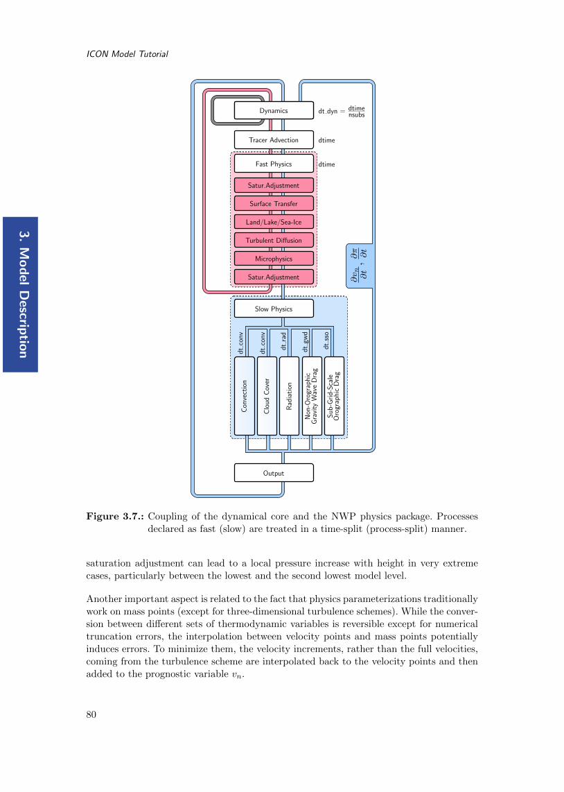
3.

Mo

del

Descrip

tion

ICON Model Tutorial

DynamicsDynamics

Fast Physics

Tracer Advection

Slow Physics

Satur.Adjustment

Surface Transfer

Land/Lake/Sea-Ice

Turbulent Diffusion

Microphysics

Satur.Adjustment

Output

Con

vect

ion

Clo

udC

over

Rad

iati

on

Non

-Oro

grap

hic

Gra

vity

Wav

eD

rag

Sub

-Gri

d-S

cale

Oro

grap

hic

Dra

g

dtco

nv

dtco

nv

dtra

d

dtgw

d

dtss

o

dtime

dtime

dt dyn = dtimensubs

∂vn

∂t,∂π ∂t

Figure 3.7.: Coupling of the dynamical core and the NWP physics package. Processesdeclared as fast (slow) are treated in a time-split (process-split) manner.

saturation adjustment can lead to a local pressure increase with height in very extremecases, particularly between the lowest and the second lowest model level.

Another important aspect is related to the fact that physics parameterizations traditionallywork on mass points (except for three-dimensional turbulence schemes). While the conver-sion between different sets of thermodynamic variables is reversible except for numericaltruncation errors, the interpolation between velocity points and mass points potentiallyinduces errors. To minimize them, the velocity increments, rather than the full velocities,coming from the turbulence scheme are interpolated back to the velocity points and thenadded to the prognostic variable vn.

80

3.

Mo

del

Des

crip

tio

n

3.8 ICON NWP-Physics in a Nutshell

3.8. ICON NWP-Physics in a Nutshell

An in-depth description of the physical parameterization package for NWP is beyond thescope of this document. However, the following section provides a short introduction tothe available parameterizations and references for further reading.

Table 3.3 contains a summary of physical parameterizations available in ICON (NWP-mode). In what follows, an outline (executive summary) of the parameterization schemesis given.

3.8.1. Radiation

The calculation of radiation is performed with RRTM (Rapid Radiative Transfer Model,Mlawer et al., 1997). RRTM operates on 30 spectral bands with 16 bands in the long-wavespectrum and 14 bands in the shortwave spectrum. It utilizes the correlated-k methodthat strongly reduces computational costs with an accuracy comparable to more detailedline-by-line models.

3.8.2. Cloud Microphysics

Section author

A. Seifert, DWD Physical Processes Division

In the exercises for Chapter 8 (see p. 240) we will investigate ICON’s physical parame-terizations by means of a custom diagnostic quantity. We restrict ourselves to the cloudmicrophysics parameterization, where some additional background information will be ofinterest.

Microphysical schemes provide a closed set of equations to calculate the formation andevolution of condensed water in the atmosphere. The most simple schemes predict only thespecific mass content of certain hydrometeor categories like cloud water, rain water, cloudice and snow. This is often adequate, because it is sufficient to describe the hydrologicalcycle and the surface rain rate, which is the vertical flux of the mass content. Microphysicalschemes of this category are called single-moment schemes.

In ICON two single-moment schemes are available, one that predicts the categories cloudwater, rain water, cloud ice and snow (inwp gscp=1 in the namelist nwp phy nml), andthe other that predicts in addition also a graupel category (inwp gscp=2). Graupel formsthrough the collision of ice or snow particles with supercooled liquid drops, a process calledriming.

Most microphysical processes depend strongly on particle size and although the mean sizeis usually correlated with mass content this is not always the case. Schemes that predictalso the number concentrations have the advantage that they provide a size information,which is independent of the mass content. Such schemes are called double-moment schemes,because both, mass content and number concentration, are statistical moments of theparticles size distribution.

81

3.

Mo

del

Descrip

tion

ICON Model Tutorial

Process Scheme Settings

Radiation RRTM (Rapid Radiative Transfer Model) inwp radiation=1

Mlawer et al. (1997), Barker et al. (2003)

PSRAD inwp radiation=3

Pincus and Stevens (2013)

Wave dissipation at critical level inwp gwd=1Non-orographicgravity wave drag

Orr et al. (2010)

Lott and Miller scheme inwp sso=1Sub-grid scaleorographic drag

Lott and Miller (1997)

Cloud cover Diagnostic PDF inwp cldcover=1

M. Kohler et al. (DWD)

All-or-nothing scheme (grid-scale clouds) inwp cldcover=5

Microphysics Single-moment scheme inwp gscp=1, 2

Doms et al. (2011), Seifert (2008)

Double-moment scheme inwp gscp=4

Seifert and Beheng (2006)

Convection Mass-flux shallow and deep inwp convection=1

Tiedtke (1989), Bechtold et al. (2008)

Turbulent transfer Prognostic TKE (COSMO) inwp turb=1

Raschendorfer (2001)

EDMF-DualM (Eddy-Diffusivity/Mass-Flux) inwp turb=3

Kohler et al. (2011), Neggers et al. (2009)

3D Smagorinsky diffusion (for LES) inwp turb=5

Land Tiled TERRA inwp surface=1

Schrodin and Heise (2001), Schulz et al. (2016)

Flake: Mironov (2008) llake=.TRUE.

Sea-ice: Mironov et al. (2012) lseaice=.TRUE.

Table 3.3.: Summary of ICON’s physics parameterizations for NWP, together with therelated namelist settings (namelist nwp phy nml). Parameterizations whichare used operationally (at 13 km horizontal grid spacing) are indicated by .

82

3.

Mo

del

Des

crip

tio

n

3.8 ICON NWP-Physics in a Nutshell

ICON does also provide a double-moment microphysics scheme (inwp gscp=4), whichpredicts the specific mass and number concentrations of cloud water, rain water, cloudice, snow, graupel and hail. This scheme is most suitable at convection-permitting orconvection-resolving scales, i.e., mesh sizes of 3 km and finer. Only on such fine meshesthe dynamics is able to resolve the convective updrafts in which graupel and hail form.On coarser grids the use of the double-moment scheme is not recommended.

To predict the evolution of the number concentrations the double-moment scheme includesvarious parameterizations of nucleation processes and all relevant microphysical interac-tions between these hydrometeor categories. Currently all choices regarding, e.g., cloudcondensation and ice nuclei, particle geometries and fall speeds etc. have to be set in thecode itself and can not be chosen via the ICON namelist.

3.8.3. Cumulus ConvectionSection author

D. Klocke, DWD Physical Processes Division

Convection is an important process in the atmosphere by contributing to forming the large-scale circulation to local heavy precipitation through thunderstorms. Parameterizations ofatmospheric moist convection provide the effect of an ensemble of sub-grid convectiveclouds on the model column as a function of grid-scale variables. The schemes verticallymix heat, moisture and momentum. They convert available potential energy into kineticenergy and produce precipitation as a result of atmospheric instability.

Three steps are taken. First, it is determined if the grid-scale conditions allow for theoccurrence of convection in the column, and a decision is taken if convection is triggered. Inthe second step, the tendencies of heat, moisture and momentum changes are determinedwith a cloud model, which represents an ascending parcel and its interactions with theenvironment. Finally the closure decides on the strength of the convection by determiningthe amount of energy to be converted, which is linked to precipitation amount generatedby the convection scheme.

In ICON a bulk mass flux convection scheme is available inwp convection=1(in thenamelist nwp phy nml), which treats three convective cloud types. Only one type - shallow,mid-level or deep convection - can exist at a time in a column, which is decided upon bythe trigger function. All three types of convection use a cloud model representing an as-cending plume mixing with its environmental air. The cloud base mass flux closure differsbetween the three convection types, with a CAPE (convective available potential energy)based closure for deep convection, a boundary layer equilibrium closure for shallow con-vection, and a large-scale omega (vertical velocity in pressure coordinates) based closurefor mid-level convection.

The full convection scheme can generally be used for horizontal grids coarser than 5 km,as some resolution dependent adjustments are implemented for grid spacings smaller than20 km. For convection permitting simulations (1−3 km horizontal grid spacing) the largestconvective clouds can be resolved by the model and the parameterization parts treatingdeep and mid-level convection can be switched off (lshallowconv only=.TRUE. in thenamelist nwp phy nml).

83

3.

Mo

del

Descrip

tion

ICON Model Tutorial

The implemented scheme represents a spin-off of the Tiedtke-Bechtold convection schemeused in the IFS model. For further reading we refer to Bechtold et al. (2008), Tiedtke(1989), Bechtold (2017), ECMWF (2017).

3.8.4. Cloud Cover

Section author

M. Kohler, DWD Physical Processes Division

To prepare optical properties of clouds for the radiative transfer it is necessary to determinethe best estimate of cloud cover, cloud water and cloud ice as well as the precipitationquantities, such as snow, rain and graupel if those are required by the radiation calculation.Note that there are various assumptions in the ICON model on the subgrid distributionof water, such as the up/down/subsidence regions in convection, a uniform distribution inmicrophysics, and a Gaussian distribution in turbulence.

The aim of the diagnostic cloud cover scheme is to combine information from the differentparameterizations mentioned above: turbulence, convection and microphysics. The tur-bulence scheme provides the sub-grid variability of water due to turbulent motions, theconvection scheme detrains cloud into the anvil and the microphysics scheme describes thesupersaturation due to ice, in other words, the distribution between ice and vapor in coldsituations.

The turbulent variability of water is at the moment prescribed by using a top-hat totalwater (the sum of water vapor qv, cloud water qc, and cloud ice qi) distribution with afixed width of 10% of total water. Work is in progress to replace this crude assumptionwith the total water variance from the turbulence scheme.

The split between water vapor and cloud ice as determined from the microphysics schemeis replicated in the diagnostic cloud scheme for the turbulent component of ice clouds.

The convective anvil is calculated by writing an equation for the evolution of cloud coverthat depends on the detrainment of volume (from the convection scheme) and a decayterm with a fixed decay time-scale (taken as 30 min). The diagnostic assumption meansthat we can neglect the tendency term on cloud cover so that we arrive simply at thediagnostic anvil cloud cover that is purely a function of detrainment and decay time-scale.The liquid and ice cloud water is taken also from the convective updraft properties.

In the end the turbulent and convective clouds are combined with a simple maximumfunction.

To emphasize, the cloud cover scheme takes into account the subgrid variability of waterand therefore the associated distribution in water vapor, cloud liquid water and cloud ice(optional 3D diagnostic output variables tot qv dia, tot qc dia, tot qi dia and theirvertically integrated counterparts tqv dia, tqc dia, tqi dia). They are not equal to theirprognostic grid-scale equivalents (standard output variables qv, qc, qi), yet the sum ofall three water quantities is kept the same. This cloud information is then passed to theradiation, where additional assumptions are made on the vertical overlap of clouds.

84

3.

Mo

del

Des

crip

tio

n

3.8 ICON NWP-Physics in a Nutshell

3.8.5. Turbulent Diffusion

Section authors

M. Kohler and M. Raschendorfer,DWD Physical Processes Division

TKE Scheme for Turbulence.

The TKE turbulence scheme consists of two components: one describing the free tropo-sphere, and the other for the surface layer.

TURBDIFF. The turbulence scheme TURBDIFF developed by Raschendorfer (2001) isbased on a 2nd-order closure on level 2.5 according to Mellor and Yamada (1982) (MY-scheme). In this scheme, all pressure correlation terms and dissipation terms, being presentin the system of 2nd-order equations for all the turbulent (co-)variances that can be builtfrom the dynamically active prognostic model variables, are expressed by the standardclosure assumptions according to Rotta (1951a,b) and Kolmogorov (1968) valid for quasi-isotropic turbulence. These dynamically active model variables are the horizontal windcomponents u and v, vertical wind speed w, a variable related to inner energy (like abso-lute temperature T , potential temperature θ or virtual potential temperature θv), specifichumidity qv and at least one cloud water variable qc (which is a mass fraction and may besplit into liquid ql and frozen qi cloud water).

Among these 2nd-order moments, only the trace of the turbulent stress tensor, which istwice the Turbulent Kinetic Energy (TKE), is described by a prognostic equation. Each ofthe remaining 2nd-order equations (for the elements of the remaining trace-less stress tensorand for the other 2nd- order moments) is simplified as diagnostic source term equilibriumbeing a linear equation in terms of the governing statistical moments.

Further, correlations between any model variable and source terms of scalar model vari-ables are neglected in these equations. However, by choosing quasi-conserved scalarvariables (total water content qt = qv + qc and liquid-water potential temperatureθl = θ − Lc

cpdqc), these correlations are taken into account implicitly as far as local con-

densation and evaporation within liquid non-precipitating clouds is concerned. Hence,TURBDIFF is a moist turbulence scheme, which includes the effect of these sub-grid scalephase transitions. The required conversion of turbulent fluxes of these conserved variablesinto those of absolute temperature, specific humidity and liquid water content is performedby means of turbulent saturation adjustment, assuming a Gaussian distribution-functionfor local saturation-deficiency according to Sommeria and Deardorff (1977).

Finally, application of the horizontal boundary layer approximation reduces the linearsystem of diagnostic 2nd-order equilibrium equations to a single column scheme withonly two equations for two diffusion coefficients (one for horizontal wind components andanother for scalar variables), which both are proportional to the square root of TKEand an integral turbulent length scale. This length-scale rises with height above groundaccording to Blackadar (1962) with a further limitation related to the horizontal grid scale.The desired vertical turbulent fluxes of any prognostic variable can then be calculated by

85

3.

Mo

del

Descrip

tion

ICON Model Tutorial

multiplying the (negative) vertical gradient of the latter with the associated diffusioncoefficient.

One main extension of TURBDIFF (compared with a moist MY-scheme) is the formalseparation of turbulence from a possible non-turbulent part of the subgrid-scale energyspectrum. This separation is related to additional scale-interaction terms in the prognosticTKE equation, which describe additional shear production of TKE by the action of othernon-turbulent sub-grid-scale flow patterns (such as wakes generated by sub-grid-scale orog-raphy, convective currents or separated horizontal circulations). Through this formalism,the scheme describes Separated Turbulence Interacting with non-turbulent Circulations(STIC), which allows for a consistent application of turbulence closure assumptions, eventhough other sub-grid-scale processes may be dominant within a grid cell. Due to thisextension, the scheme is applicable also above the boundary layer and for very stablestratification. The Eddy Dissipation Rate (EDR) calculated by TURBDIFF can even beused to forecast the intensity of Clear Air Turbulence (CAT).

TURBTRAN. The turbulence scheme TURBDIFF is closely related to the schemeTURBTRAN developed by Raschendorfer (2001) for the surface-to-atmosphere transfer(SAT), which calculates transport resistances for fluxes of prognostic model variables atthe surface of the Earth. Figure 3.8 illustrates the corresponding sub layers of the surfacelayer. In TURBTRAN, a constant flux approximation is applied to the sum of turbulentand laminar vertical fluxes within the transfer layer (between the rigid surface and thelowest atmospheric main level of the model). By application of the turbulence scheme atthe top of the lowest atmospheric layer as well as the bottom of this layer (which is the topof the near surface roughness layer being intersected by roughness elements), a verticalinterpolation function for the turbulent diffusion coefficient is derived between these twolevels and is extrapolated down to the rigid surface. With this preparation, a vertical in-tegration of the flux gradient representation across the transfer layer provides the desiredtransport resistances for the final bulk representation of SAT fluxes. With this formula-tion, scale interaction terms considered through STIC in the turbulence scheme also affectthe transfer resistances; and hence, some additional mixing is automatically introducedfor very large bulk Richardson numbers, as soon as non-turbulent sub-grid-scale motionsare present.

Further, with the described procedure, the determination of a specific roughness lengthfor scalars is substituted by a direct calculation of the partial resistance of scalar transferthrough the laminar layer and the roughness layer. This partial resistance is dependent onthe near-surface model variables, the aerodynamic roughness length and the Surface AreaIndex (SAI), which is a measure of the surface area enlargement by land use.

TURBDIFF and TURBTRAN are the default schemes for atmospheric turbulence andSAT, respectively, in ICON, and they correspond to inwp turb=1 (namelist nwp phy nml).While TURBTRAN provides the transfer resistances for scalars and horizontal wind com-ponents, the final surface fluxes of water vapor and sensible heat are determined in TERRAas a result of updated surface values for qv and (in case of the upcoming implicit treatmentof surface temperature) also for T . Based on these surface fluxes, an implicit equation forvertical diffusion is solved as a final part of TURBDIFF. In this procedure also horizontalmomentum and TKE is included, while for these 3 quantities the respective surface con-centration is used as a lower boundary condition. Currently, a lower zero-concentration

86

3.

Mo

del

Des

crip

tio

n

3.8 ICON NWP-Physics in a Nutshell

Figure 3.8.: Surface layer as described in the parameterization TURBTRAN of Raschen-dorfer (2001).

condition is applied for cloud-water and ice, which is always related to a downward flux forthese quantities. For vertical diffusion of passive tracers, the diffusion coefficient for scalarsis applied, and the lower boundary condition can be specified individually. Although theeffect of local condensation and evaporation is considered in the solution of 2nd orderequations, and hence, can amplify the intensity of turbulent vertical mixing, the directeffect of these additional thermodynamic source-terms in the grid-scale budgets of heat,water vapor and liquid water is not yet considered.

In the namelist turbdiff nml several parameters or selectors for optional calculationsrelated to both schemes can be specified. Through this, TURBDIFF can also be configuredas a 3D-turbulence scheme, calculating additionally horizontal shear and providing alsohorizontal diffusion coefficients.

DualM EDMF for Turbulence and Shallow Convection.

The Eddy Diffusivity Mass Flux (EDMF) approach - operational at ECMWF (Kohleret al., 2011) - is based on the decomposition of the turbulent transports proposed bySiebesma and Cuijpers (1995) into eddy diffusivity and mass-flux components. This isbased on the idea of unifying the eddy diffusivity and mass-flux concepts that are used inmany NWP and climate models within one unified solver. When generalizing to multipleupdrafts Mi one arrives at the following equation for the flux of a scalar quantity φ:

w′φ′ = −K∂φ

∂z+∑

iMi(φ

ui − φ).

Here, the mass flux is Mi = ai(wui − w) and K is the diffusion coefficient. The averaging

operators φui and φ

eact on the updraft and environment fractions, respectively.

87

3.

Mo

del

Descrip

tion

ICON Model Tutorial

To arrive at this equation two assumptions are applied: (i) updraft fraction is small a 1and (ii) the flux within the environment w′φ′e

ecan be approximated by K-diffusion.

The DualM framework by Neggers et al. (2009) postulates that two mass-fluxes are suf-ficient to treat the transition from a dry boundary layer to stratocumulus and shallowcumulus. In particular one dry mass-flux stops at cloud base, while the second moistmass-flux reaches to cloud top. The continuous area partitioning between the dry andmoist updraft is a function of moist convective inhibition above the mixed layer top. Up-draft initialization is a function of the updraft area fraction and is therefore consistentwith the updraft definition. It is argued that the model complexity thus enhanced is suffi-cient to allow reproduction of various phenomena involved in the cloudsubcloud coupling,namely (i) dry countergradient transport within the mixed layer that is independent ofthe moist updraft, (ii) soft triggering of moist convective flux throughout the boundarylayer, and (iii) a smooth response to smoothly varying forcings, including the reproductionof gradual transitions to and from shallow cumulus convection.

Smagorinsky-Lilly for LES Application

The 3D sub-grid model of Smagorinsky (1963) with the stability correction of Lilly (1962)is implemented for LES applications. This scheme writes the eddy viscosity Km as

Km = (Cs∆)2 |S|CB,

with the Smagorinsky constant Cs, the filter width ∆, the norm of the strain rate tensor|S| and the stability correction factor CB.

The filter width is taken to be ∆ = (∆x∆y∆z)13 . The strain rate tensor is defined as

Sij =1

2

(∂ui∂xj

+∂uj∂xi

),

whose calculation requires special care due to the triangular grid in ICON. A metriccorrection has been developed that treats the horizontal gradients over a sloped orographygiven a terrain-following coordinate correctly. The norm of Sij is

|S| =√

2SijSij .

The stability correction factor CB is given by

CB = (1− Ri /Prt)12

with the gradient Richardson number Ri = N2

|S| and the buoyancy frequency N2 = gθ0∂θv∂z .

The Smagorinsky constant usually has the value of Cs = 0.1−0.2. In the ICON implemen-tation Cs is set by default to smag constant=0.23 (namelist les nml) and the Prandtlnumber Prt to turb prandtl=0.333 (namelist les nml).

88

3.

Mo

del

Des

crip

tio

n

3.8 ICON NWP-Physics in a Nutshell

3.8.6. Sub-grid scale orographic drag

Section authors

J.-P. Schulz, DWD Numerical Models DivisionM. Kohler, DWD Physical Processes Division

S. Borchert, DWD Numerical Models Division

ICON treats the entire sub-grid scale orographic drag with one model based on the work ofLott and Miller (1997). Other NWP models treat scales smaller than ∼ 5 km with differentansatzes, for example with the help of turbulent orographic form drag formulations of theuse of an effective roughness length that determines the conductivity of the surface formomentum fluxes between the atmosphere and the Earth.

The motivation for the implementation of a sub-grid scale orographic drag model intoICON traces back to experience with the COSMO model. When the 7-km EU domainof the operational COSMO model at DWD was expanded in order to cover almost allEurope (see Schulz, 2006), it turned out that the surface pressure in the model forecastsbecame systematically biased. In particular, in wintertime high pressure systems of themodel atmosphere tended to develop a positive pressure bias, by 1 to 2 hPa after 48 h, lowpressure systems a negative bias (“highs too high, lows too low”). At the same time thewind speed tended to be overestimated by up to 1 m s−1 throughout the entire troposphere.The wind direction near the surface showed a positive bias.

The combination of these deficiencies led to the hypothesis that in the model there is toolittle surface drag, causing an underestimation of the cross-isobar flow in the planetaryboundary layer. Consequently, the solution would be to increase the surface drag in themodel. This may be accomplished, for instance, by introducing an envelope orography(Wallace et al., 1983, Tibaldi, 1986), but this has unfavorable effects, e.g., for the simulatedprecipitation. Another option is the inclusion of sub-grid scale orographic (SSO) effects,which were neglected in the COSMO model before. The SSO scheme by Lott and Miller(1997) was selected for this purpose. Its implementation in the COSMO-EU model isdescribed in Schulz (2008), and was later transferred to the ICON model.

The SSO scheme by Lott and Miller (1997) deals explicitly with a low-level flow whichis blocked when the sub-grid scale orography is sufficiently high. For this blocked flowseparation occurs at the mountain flanks, resulting in a form drag. The upper part ofthe low-level flow is lead over the orography, while generating gravity waves3. In order todescribe the low-level flow behavior in the SSO scheme a non-dimensional height Hn ofthe sub-grid scale mountain is introduced

Hn =NH

|U | = Fr−1 ,

where H is the maximum height of the mountain, |U | is the wind speed and N is theBrunt-Vaisala frequency of the incident flow. The latter is defined by

N =

√g

θ

∂θ

∂z,

3Propagating, coherent structures consisting of buoyancy and inertial oscillations.

89

3.

Mo

del

Descrip

tion

ICON Model Tutorial

SSO momentum

g r i d c e l l c o l u m n

gravity

waves

breaking

level

drag

drag

tune_grcrit

tune_gfrcrit

tune_gkwake

tune_gkdrag

S u b - g r i d s c a l e o r o g r a p h i c d r a g

drag

g r i d c e l l c o l u m n

launch

level

weather

gravity

waves

breaking

level

tune_gfluxlaun

Non-orograph ic g rav i t y wave d rag

Figure 3.9.: Left: Schematic illustration of the two elements of sub-grid scale orographicdrag: First, the low-level blocking, where the horizontal flow (orange) isforced to flow around the sub-grid scale orography (SSO, colored gray).Second, the gravity wave drag on the flow forced to overflow the SSO, and onthe flow at higher altitudes, where the radiated gravity waves (white-blue)break. (Following Figure 1 in Lott and Miller (1997).) Right: Schematicillustration of the non-orographic gravity wave drag.

where θ is the potential temperature, g the acceleration of gravity and z the height coor-dinate. Hn may be also regarded as an inverse Froude number Fr−1 of the system “flowround a mountain”.

A small Hn means that there is an unblocked regime, all the flow goes over the mountainand gravity waves (GWs) are forced by the vertical motion of the fluid. A large Hn meansthat there is a blocked regime, the vertical motion of the fluid is limited and part of the low-level flow goes around the mountain. The SSO scheme requires four external parameters,which are the standard deviation SSO STDH, the anisotropy SSO GAMMA, the slope SSO SIGMA

and the geographical orientation SSO THETA of the sub-grid scale orography. FollowingBaines and Palmer (1990) these are computed by ExtPar (see Section 2.4.1) from theGLOBE data set (GLOBE-Task-Team, 1999), which has a resolution of approximately1 km.

Four tuning parameters in the namelist nwp tuning nml control the SSO scheme (see Fig-ure 3.9). First, the critical Froude number Frc = tune gfrcrit, which has a twofoldeffect. The larger its value the higher the likelihood for low-level blocking to occur, sinceit is activated only where Fr < Frc. Conversely, where Fr > Frc all flow goes over themountain and the entire stress is associated with GW radiation. In addition, if blockingis active, Frc controls the thickness of the blocking layer relative to the mountain height(the larger Frc the larger the layer thickness). Its default value is 0.4. Operational sim-ulations with horizontal mesh sizes of 13 km and 40 km use the values 0.333 and 0.425,respectively. Second and third, the magnitudes of the SSO drag and the GW drag aredirectly proportional to the parameters tune gkwake and tune gkdrag, respectively. Thedefault values are 1.5 and 0.075. Different from this, operational simulations with 13 kmhorizontal mesh size use tune gkwake = 1.8 and tune gkdrag = 0.09. Finally, the criti-cal Richardson number Ric = tune grcrit is a control parameter for the onset of GW

90

3.

Mo

del

Des

crip

tio

n

3.8 ICON NWP-Physics in a Nutshell

breaking. If the Richardson number of the resolved atmospheric state plus the unresolvedGWs

Ri =N2

tot

|∂utot/∂z|2,

where u denotes the horizontal wind vector, falls below Ric, the flow configuration becomesunstable and the GWs break (partly). This process is accompanied by a drag effect on theresolved horizontal flow. Combined with the rule of thumb that Ri increases with height ifGWs are present, this means that the larger the value of Ric the lower the altitude wherethe radiated GWs tend to break and exert a drag. The default value is 0.25.

In order to assist numerical stability, the drag computed by the scheme is limited to aheight-dependent threshold (see Section 3.8.7 for some further details).

3.8.7. Non-orographic gravity wave drag

Section authors

M. Kohler, DWD Physical Processes DivisionS. Borchert, DWD Numerical Models Division

All kinds of (synoptic-scale) atmospheric flow structures (e.g., fronts, convection, jetstreams) can develop imbalances that force air parcels to oscillate (vertically) and ra-diate gravity waves (GWs). The interaction of these non-orographically forced GWs withthe atmospheric background flow is assumed to be significant in the middle and upperatmosphere, and is consequently of interest for models that cover this region (e.g., theoperational global ICON configuration with its model top at 75 km). If the synoptic scaleflow (be it resolved or unresolved by the model) would force GWs, whose horizontal andvertical wave lengths would be smaller than the horizontal and vertical grid mesh sizes,they cannot be resolved by the model. But yet this unresolved part of the GW spectrumcould have a significant impact on the resolved flow, and is therefore parameterized (seeFigure 3.9).

The parameterization implemented in ICON follows the ansatz of Scinocca (2003) andMcLandress and Scinocca (2005), which in turn is based on the work of Warner andMcIntyre (1996) to which the simplifying assumption of a hydrostatic, non-rotationalatmosphere has been applied. The parameters of this scheme have been optimized followingErn et al. (2006). Details can be found in Orr et al. (2010).

The mechanisms of non-orographic GW forcing can be relatively complex and are notcompletely understood. For this reason the parameterization considers a statistical meanof all sources of (upward propagating) GWs and represents them by prescribing GW-borne vertical fluxes of horizontal momentum at a launch level somewhere in the uppertroposphere. The magnitude of the integral of the momentum fluxes over the GW spectrumis assumed to be constant (i.e. independent of the geographic location and time), and canbe expressed by

ρF (cosϕi, sinϕi)|z=z0 = ρ0F0 (cosϕi, sinϕi) = ρw′u′∣∣z=z0

= ρw′|u′| (cosϕi, sinϕi)∣∣∣z=z0

,

91

3.

Mo

del

Descrip

tion

ICON Model Tutorial

where ρ is the air density, z0 denotes the launch level, w′ and u′ are GW-borne fluctu-ations of the vertical and horizontal wind components and (·) stands for a spatial av-erage over the grid cell size. The azimuthal angles relative to the West-East directionϕi ∈ 0(East), 90(North), 180(West), 270(South) are four horizontal directions of hor-izontal momentum sampled by the scheme. The magnitude ρ0F0 = tune gfluxlaun canbe set in namelist nwp tuning nml. Its default value is 0.0025 Pa.

Given the atmospheric state in a grid cell column and the spectral distribution of ρF atthe launch level, standard GW theories can be used, to integrate ρF vertically. The dragexerted on the resolved horizontal flow is then defined by the vertical divergence of themomentum flux(

∂u

∂t

)GW drag

=

[∂(u, v)

∂t

]GW drag

= −1

ρ

∂(ρF zonal, ρFmeridional)

∂z. (3.40)

Here, (·) denotes the integral over the GW spectrum. The right-hand side becomesnon-zero typically at altitudes, where the GWs break. Note, if the magnitude of thedrag computed by this scheme exceeds a prescribed, height-dependent threshold value|(∂u/∂t)GW drag|max(z), it is reduced to this value. This measure is to counteract numeri-cal instabilities caused by a too strong increase of the wind magnitude. It also applies towind tendencies from the SSO scheme described in Section 3.8.6.

The processes treated by this parameterization and the one described in Section 3.8.6are assumed to be irreversible and as such provide a source of heat. The correspondingtemperature tendency is derived from Gibbs equation (e.g. Falk, 1990)

δe = u · δp + Tδs+ · · · , (3.41)

which is one possible formulation of a fundamental relation F(e,p, s, . . .) = 0 defined tohold between energy density e, momentum density p, heat density s and the densities ofall other extensive state variables contained by the system4. In addition, δ denotes thedifference between two consecutive states, typically expanded by δ(·) = ∂(·)/∂tδt, whereδt is a time step. For the extensive variables on the right-hand side of Eq. (3.41) explicitbudget equations exist in the model in one form or another. In contrast, energy is notexplicitly budgeted, but its change is determined implicitly through Gibbs equation. Now,energy shall be a conserved quantity. Given that we know δp from the drag (3.40), whereasthe heat change δs is still unspecified, one possibility to ensure energy conservation is toequate the right-hand side of Eq. (3.41) to zero by5

δs = −u · δp + · · ·T

. (3.42)

4Extensive variables depend on the amount of substance, intensive variables do not. Example: if youmerge two identical systems to one single larger system, its velocity is still the same as with the twooriginal systems, whereas its momentum is twice as large, its temperature is still the same, whereas itsamount of heat is twice as large etc.

5Strictly speaking, this holds only, if we would give up the (arbitrary) distinction in what we call “modeldynamics” and “model physics” and treat both in a uniform, consistent way. In addition, time integra-tion would practically have to be limited to an explicit Euler method, since higher-order schemes mixup different states, which challenges energy conservation and the satisfaction of the integrability condi-tions on Gibbs equation, known as the Maxwell relations between the equations of state. Beyond thatimplicit methods violate causality. Of course, all that are unrealizable requirements on an operationalmodel for a long time to come.

92

3.

Mo

del

Des

crip

tio

n

3.8 ICON NWP-Physics in a Nutshell

Combined with the equations of state (and some simplifications) this can be formulatedas a temperature tendency, which reads(

∂T

∂t

)GW drag

= − u

cv·(∂u

∂t

)GW drag

= − 1

cv

[u

(∂u

∂t

)GW drag

+ v

(∂v

∂t

)GW drag

]

for the drag (3.40). However, one should keep in mind that the ansatz (3.42) is a “bruteforce method” applied for convenience. If we consider only state changes due to the pa-rameterization, the consequence of Eq. (3.42) is that the amount of energy contained in acell is “frozen”. This is because Eq. (3.42) does not only suppress energy sources, but alsoenergy fluxes between neighboring cells that could result from the parameterized process.Fluxes, however, are generally not in conflict with conservation principles, so Eq. (3.42)might be regarded as an unrealistic simplification. A more gentle approach would followfrom the general treatment of Gibbs equation in irreversible thermodynamics (e.g. Herbert,1975, Sievers, 1982). Given that the change of momentum follows from a flux divergenceδp = −∂F /∂zδt (compare Eq. (3.40)), Eq. (3.41) can be formulated as

δe = −δtu · ∂F∂z

+ · · · = −δt[∂(u · F )

∂z− F · ∂u

∂z

]+ · · · ,

to separate the energy flux u · F from the “actual” source term, which would then beadded to the heat sources, to satisfy energy conservation

δs = −δtFT· ∂u∂z

+ · · · . (3.43)

However, with respect to computational costs, the variant (3.43) is typically significantlymore expensive than Eq. (3.42)), which is the reason, why the latter is preferred.

The preceding considerations were guided by the focus on the energy and the demand forits conservation (the 1st law of thermodynamics). Another aspect comes into play, if weconsider heat and our experimental experience that it is not conserved, but can be pro-duced (the 2nd law of thermodynamics). If the drag (3.40) would be the only contributionto the right-hand side of Eq. (3.41) in addition to the contribution of heat, the 2nd lawwould require δs = −(δt/T )F · ∂u/∂z ≥ 0. This could only be satisfied, if F ∝ −∂u/∂z(the typical gradient ansatz, we know from the formulation of friction, for instance). Butthat changes, if we complement Gibbs equation by the contributions from the gravitywaves, turbulence etc., and allow for cross effects. Nevertheless, we should not expect thephysics parameterizations to satisfy the 2nd law, neither locally nor globally. On the onehand the 2nd law is usually not one of the guiding principles in their development, on theother hand the different treatment of what we call “model dynamics” and “model physics”,albeit necessary for computational efficiency, challenges both energy conservation and theindestructibleness of heat.

93

3.

Mo

del

Descrip

tion

ICON Model Tutorial

3.8.8. Lake Parameterization Scheme FLake

Section author

D. Mironov, DWD Physical Processes Division

Lakes significantly affect the structure and the transport properties of the atmosphericboundary layer. The interaction of the atmosphere with the underlying surface stronglydepends on the surface temperature.

In numerical weather prediction (NWP), a simplified approach is often taken that amountsto keeping the water surface temperature constant over the entire forecast period. Thisapproach is to some extent justified for ocean and seas. It is hardly applicable to lakes wherediurnal variations of the water surface temperature reach several degrees. The situation iseven more grave for frozen lakes as the diurnal variations of the ice surface temperaturemay exceed ten degrees.

Initialization of the NWP model grid boxes that contain water bodies also presents con-siderable difficulties. When no observational data for some grid boxes are available, thosegrid boxes are initialized by means of interpolation between the nearest grid-boxes forwhich the water surface temperature is known (the interpolation procedure may accountfor some other variables, e.g., two-meter temperature over land). Such procedure is ac-ceptable for sea points where large horizontal gradients of the water surface temperatureare comparatively rare, but it is hardly suitable for lakes. Lakes are enclosed water bodiesof a comparatively small horizontal extent. The lake surface temperature has little to dowith the surface temperature obtained by means of interpolation between the alien waterbodies.

In NWP, the lake surface temperature (i.e., the surface temperature of lake water or lakeice) is a major concern. It is this variable that communicates information between thelake and the atmosphere, whereas details of the vertical temperature distribution (e.g.,the temperature near the lake bottom) are of minor importance. Therefore, simplifiedlake models (parameterization schemes), whose major task is to predict the lake surfacetemperature, the lake freezing and the ice break-up, should be sufficient for NWP andrelated applications.

The NWP model ICON (as well as COSMO) utilizes the lake parameterization schemeFLake (Mironov, 2008, Mironov et al., 2010, 2012). FLake is based on a two-layer paramet-ric representation of the evolving temperature profile. The structure of the stratified layerbetween the upper mixed layer and the basin bottom, the lake thermocline, is describedusing the concept of self-similarity (assumed shape) of the temperature-depth curve. Thesame concept is used to describe the temperature structure of the thermally active upperlayer of bottom sediments and of the ice and snow cover. In this way, the problem ofsolving partial differential equations (in depth and time) for the temperature and turbu-lence quantities is reduced to solving ordinary differential equations (in time only) for thetime-dependent parameters that specify the temperature profile.

The approach is based on what is actually “verifiable empiricism”. However, it still incor-porates much of the essential physics and offers a very good compromise between physicalrealism and computational economy. FLake incorporates the heat budget equations for thefour layers in question, viz., snow, ice, water and bottom sediments, developed with due

94

3.

Mo

del

Des

crip

tio

n

3.8 ICON NWP-Physics in a Nutshell

regard for the volumetric character of the solar radiation heating. An entrainment equationis used to compute the depth of a convectively-mixed layer, and a relaxation-type equationis used to compute the wind-mixed layer depth in stable and neutral stratification. Simplethermodynamic arguments are invoked to develop the evolution equations for the ice andsnow depths.

Empirical constants and parameters of FLake are estimated, using independent empiricaland numerical data. They should not be re-evaluated when the scheme is applied to aparticular lake. In this way, the scheme does not require re-tuning, a procedure that mayimprove an agreement with a limited amount of data but should generally be avoided.Further information about FLake can be found at http://lakemodel.net.

FLake is activated within ICON if the namelist parameter llake (lnd nml) is set .TRUE.,which is the default operational setting at DWD.

FLake requires two external parameter fields. These are the fields of lake fraction (areafraction of a given numerical-model grid box covered by the lake water) and of lake depth.These external parameter fields are generated with the ExtPar software (see Section 2.4)using the Global Lake Database (Kourzeneva, 2010, Kourzeneva et al., 2012, Choulgaet al., 2014).

ICON makes use of a tile approach to compute the grid-box mean values of temperatureand humidity (and of other scalars) and the grid-box mean fluxes of momentum andscalars. FLake is applied to the ICON grid boxes whose lake fraction exceeds a thresholdvalue; otherwise the effect of sub-grid scale lakes is ignored. Currently, the value of 0.05 isused (see the namelist variable frlake thrhld (lnd nml)).

In the current ICON configuration, the lake depth is limited to 50 m. For deep lakes,the abyssal layer is ignored, a “false bottom” is set at a depth of 50 m, and the bottomheat flux is set to zero. The bottom sediment module is switched off, and the heat fluxat the water-bottom sediment interface (or at false bottom) is set to zero. The settinglflk botsed use=.FALSE. is hard-coded in mo data flake.f90.

Snow above the lake ice is not considered explicitly. The effect of snow is accounted forin an implicit manner through the temperature dependence of the ice surface albedo withrespect to solar radiation Mironov et al. (2012). There is no logical switch to deactivatethe snow module of FLake. It is sufficient to set the rate of snow accumulation to zero(hard-coded in mo flake.f90). Without explicit snow layer of the lake ice, the snow depthover lakes is set to zero and the snow surface temperature is set equal to the ice surfacetemperature.

The attenuation coefficient of lake water with respect to solar radiation is currently set toa default “reference” value for all lakes handled by ICON. It would be advantageous tospecify the attenuation coefficient as a global external parameter field. This can be donein the future as the information about the optical properties of lakes becomes available(not the case at the time being).

Generally, no observational data are assimilated into FLake, i.e., the evolution of the laketemperature, the lake freeze-up, and break-up of ice occur freely during the ICON runs.An exception are the Laurentian Great Lakes of North America. Over the LaurentianGreat Lakes, the observation data on the ice fraction (provided by the ICON surface

95

3.

Mo

del

Descrip

tion

ICON Model Tutorial

analysis scheme) are used to adjust the ice thickness, the ice surface temperature, and(as needed) the water temperature. See the subroutine flake init in mo flake.f90 fordetails. The use of the ice-fraction data over Great Lakes is controlled by the namelistparameter use lakeiceana (initicon nml).

Finally, a word of caution is in order. Running ICON with the lake parameterizationscheme switched off (llake=.FALSE.) is not recommended as this configuration has neverbeen comprehensively tested at DWD.

3.8.9. Sea-Ice Parameterization SchemeSection author

D. Mironov, DWD Physical Processes Division

A major task of the sea-ice parameterization scheme for NWP is to predict the existenceof ice within a given atmospheric-model grid box and the ice surface temperature. Thesea-ice scheme used within ICON NWP accounts for thermodynamic processes only, i.e.,no ice rheology is considered (cf. the sea-ice scheme for climate modeling). The hori-zontal distribution of the ice cover, i.e., the fractional area coverage of sea ice within agiven grid box, is governed by the data assimilation scheme. A detailed description ofthe sea-ice scheme for ICON NWP is given in Mironov et al. (2012), where a system-atic derivation of governing equations, an extensive discussion of various parameterizationassumptions and of the scheme disposable parameters, and references to relevant publica-tions can be found. Further comments can be found directly in the code, see the modulesrc/lnd_phy_schemes/mo_seaice_nwp.f90.

A distinguishing feature of the ICON NWP sea-ice scheme is the treatment of the heattransfer through the ice. As different from many other sea-ice schemes that solve theheat transfer equation on a finite difference grid, the present scheme uses the integral, orbulk, approach (cf. the lake parameterization scheme FLake, Section 3.8.8). It is based ona parametric representation (assumed shape) of the evolving temperature profile withinthe ice and on the integral heat budget of the ice slab. Using the integral approach, theproblem of solving partial differential equations (in depth and time) is reduced to solvingordinary differential equations (in time only) for the quantities that specify the evolvingtemperature profile. These quantities are the ice surface temperature and the ice thickness.

In the full-fledged scheme outlined in Mironov et al. (2012), provision is made to account forthe snow layer above the ice. Both snow and ice are modeled using the same basic concept,that is a parametric representation of the evolving temperature profile and the integralenergy budgets of the ice and snow layers (see Mironov (2008) for a detailed discussionof the concept). In the current ICON configuration, snow over sea ice is not consideredexplicitly. The effect of snow is accounted for implicitly (parametrically) through the icesurface albedo with respect to solar radiation.

A prognostic sea-ice albedo parameterization is used. The sea-ice surface albedo is com-puted from a relaxation-type rate equation, where the equilibrium albedo and the relax-ation (e-folding) time scale are computed as functions of the ice surface temperature. Inorder to account for the increase of the sea-ice albedo after snowfall events, the ice albedois relaxed to the equilibrium “snow-over-ice” albedo. The equilibrium snow-over-ice albedo

96

3.

Mo

del

Des

crip

tio

n

3.8 ICON NWP-Physics in a Nutshell

is computed as function of the ice surface temperature, and the relaxation time scale isrelated to the snow precipitation rate.

The horizontal distribution of the ice cover, i.e., the existence of sea ice within a givenICON grid box and the ice fraction, is governed by the data assimilation scheme (cf. thetreatment of lake ice). If an ICON grid box has been set ice-free during the initialization, noice is created over the forecast period. If observational data indicate open water conditionsfor a given grid box but there was ice in that grid box at the end of the previous ICONrun, ice is removed and the grid box is initialized as ice-free. The new ice is formedinstantaneously if the data assimilation scheme indicates that there is sea ice in a givengrid box, but there was no ice in that grid box in the previous model run. The newly formedice has the surface temperature equal to the salt-water freezing point. The thickness ofnewly formed ice is computed as function of the ice fraction.

ICON utilizes a tile approach to compute surface fluxes of momentum and scalars. For the“sea-water type” grid boxes, the grid-box mean fluxes are computed as a weighted mean offluxes over ice and over open water, using fractional ice cover fi and fractional open-watercover 1− fi as the respective weights. Sea ice in a given ICON grid box is only consideredif fi exceeds its minimum value of 0.015, otherwise the grid box is treated as ice free(see parameter frsi_min hard-coded in mo_seaice_nwp.f90). Likewise, the open-waterfraction less than frsi_min are ignored, and the grid box in question is treated as fullyice-covered (fi is reset to 1). The ice fraction is determined during the model initializationand is kept constant over the entire forecast period. If, however, sea ice melts away duringthe forecast, fi is set to zero and the grid box is treated as an open-water water grid boxfor the rest of the forecast period (prognostic ice thickness is limited from below by avalue of 0.05 m, i.e., a thinner ice is removed). The water-surface temperature of that gridbox is equal to the observed value from the analysis, or is reset to the salt-water freezingpoint. The latter situation is encountered when a grid box was entirely covered by ice atthe beginning of the forecast, but the ice melts away during the forecast.

In order to run ICON with the sea-ice parameterization scheme switched off, the namelistlogical switch lseaice (lnd nml) should set equal to .FALSE.. This configuration has notbeen comprehensively tested at DWD and is not recommended.

3.8.10. Land-Soil Model TERRASection author

J. Helmert, DWD Physical Processes Division

The soil-vegetation-atmosphere-transfer component TERRA (Schrodin and Heise, 2001,Heise et al., 2006) in the ICON model is responsible for the exchange of fluxes of heat,moisture, and momentum between land surface and atmosphere. It establishes the lowerboundary-condition for the atmospheric circulation model and considers the energy andwater budget at the land surface fractions of grid points. Based on a multi-layer concept forthe soil, TERRA considers the following physical processes at each of the tiled land-surfacecolumns, where an uniform soil type with physical properties is assumed:

Radiation

- Photosynthetically active radiation (PAR) is used for plant evapotranspiration

97

3.

Mo

del

Descrip

tion

ICON Model Tutorial

- Solar and thermal radiation budget is considered in the surface energy budget

Biophysical control of evapotranspiration

- Stomatal resistance concept controls the interchange of water between theatmosphere and the plant

- One-layer vegetation intercepts and hold precipitation and dew, which lowers waterinput to the soil and enhances evaporation

- Roots with root-density profile determines the amount of water available forevapotranspiration in the soil

- Bare-soil evaporation is considered for land-surface fractions without plants.

Heat and soil-water transport

- Implicit numerical methods are used to solve the vertical soil water transport andsoil heat transfer between the non-equidistant layers.

- In the operational model version seven layers are used in the soil.

- The lower boundary condition for the heat conduction equation is provided by theclimatological mean temperature.

- Surface and sub-surface runoff of water is considered.

- The lower boundary condition is given by a free-drainage formulation.

- A rise of groundwater into the simulated soil column is not represented.

- Soil heat conductivity depends on soil-water content (Schulz et al., 2016).

- Freezing of soil water and melting of soil ice is considered in hydraulic active soillayers.

Snow

- TERRA offers a one-layer snow model (operational in ICON-NWP) and amulti-layer snow model option (for experiments).

- A prognostic snow density, and snow melting process as well as the time dependentsnow albedo are considered

- Surface fractions partly covered with snow are divided in snow-free andsnow-covered parts (snow tiles)

Coupling to the atmosphere

- Application of the turbulence scheme at the lower model boundary

- Roughness length for scalars implicitly considered by calculation of an additionaltransport resistance throughout the turbulent and laminar roughness layer.

TERRA requires a number of external parameter fields, see Section 2.4 for details.

98

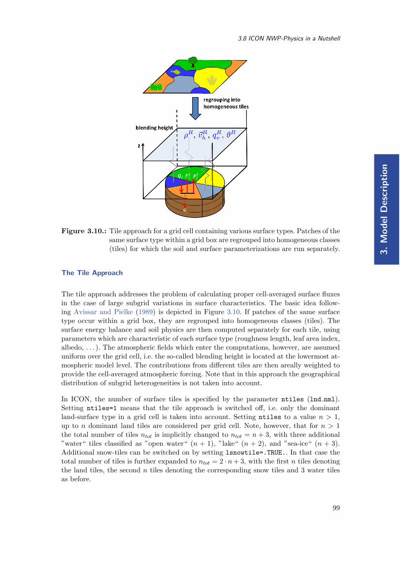
3.

Mo

del

Des

crip

tio

n

3.8 ICON NWP-Physics in a Nutshell

Figure 3.10.: Tile approach for a grid cell containing various surface types. Patches of thesame surface type within a grid box are regrouped into homogeneous classes(tiles) for which the soil and surface parameterizations are run separately.

The Tile Approach

The tile approach addresses the problem of calculating proper cell-averaged surface fluxesin the case of large subgrid variations in surface characteristics. The basic idea follow-ing Avissar and Pielke (1989) is depicted in Figure 3.10. If patches of the same surfacetype occur within a grid box, they are regrouped into homogeneous classes (tiles). Thesurface energy balance and soil physics are then computed separately for each tile, usingparameters which are characteristic of each surface type (roughness length, leaf area index,albedo, . . . ). The atmospheric fields which enter the computations, however, are assumeduniform over the grid cell, i.e. the so-called blending height is located at the lowermost at-mospheric model level. The contributions from different tiles are then areally weighted toprovide the cell-averaged atmospheric forcing. Note that in this approach the geographicaldistribution of subgrid heterogeneities is not taken into account.

In ICON, the number of surface tiles is specified by the parameter ntiles (lnd nml).Setting ntiles=1 means that the tile approach is switched off, i.e. only the dominantland-surface type in a grid cell is taken into account. Setting ntiles to a value n > 1,up to n dominant land tiles are considered per grid cell. Note, however, that for n > 1the total number of tiles ntot is implicitly changed to ntot = n + 3, with three additional”water“ tiles classified as ”open water“ (n + 1), ”lake“ (n + 2), and ”sea-ice“ (n + 3).Additional snow-tiles can be switched on by setting lsnowtile=.TRUE.. In that case thetotal number of tiles is further expanded to ntot = 2 · n+ 3, with the first n tiles denotingthe land tiles, the second n tiles denoting the corresponding snow tiles and 3 water tilesas before.

99

3.

Mo

del

Descrip

tion

ICON Model Tutorial

Figure 3.11.: Tile generation for ntiles=3, for the case of a heterogeneous land surface.Outer circles show the fractional areas covered by the respective surface-type for a given grid cell. Inner circles show the selected tiles. Please notethe re-scaling of fractional areas in the inner circle.

The process of tile generation in ICON works as follows:During the setup phase, all land-surface types within a grid box are ranked according tothe fractional area f they cover (see Figure 3.11, outer ring). For efficiency reasons, onlythe ntiles (typically about 3) dominating ones are represented by tiles, with the othersbeing discarded (inner ring). If a grid cell contains non-negligible water bodies (f > 5%),up to 3 more tiles are created (i.e. open water, lake, and sea-ice) even if they are notamong the dominating ones. By this approach, the surface types represented by tiles candiffer from grid cell to grid cell such that the full spectrum of surface types provided bythe land cover data set is retained.

If the model is initialized from horizontally interpolated initial data and ntiles > 1, atile coldstart becomes necessary. This can be done by setting ltile init=.TRUE. andltile coldstart=.TRUE. in the namelist initicon nml. Each tile is then initialized withthe same cell averaged value. Note that ltile init=.TRUE. is only necessary, if the initialdata come from a model run without tiles.

Important note:Naive horizontal interpolation of tile-based variables is incorrect, since thedominant tiles and/or their internal ranking will most likely differ betweensource and target cell. Only aggregated fields can be interpolated!

3.8.11. Reduced Model Top for Moist Physics

A notable means for improving the efficiency of ICON is depicted in Figure 3.12. Theswitch

100

3.

Mo

del

Des

crip

tio

n

3.8 ICON NWP-Physics in a Nutshell

top_height (TOA)

htop_moist_procmoist processes off

moist processes on

hbot_qvsubstep

z

Figure 3.12.: Moist physics are switched off above htop moist proc, while tracer sub-stepping is switched on above hbot qvsubstep. (Remark: hbot qvsubstep

is allowed to be lower than htop moist proc)

htop moist proc (namelist nonhydrostatic nml, floating-point value)

allows to switch off moist physics completely above a certain height. Moist physics in-clude saturation adjustment, grid scale microphysics, convection, cloud cover diagnos-tic, as well as the transport of all water species but moisture qv. Of course, moist pro-cesses should only be switched off well above the tropopause. The default setting ishtop moist proc=22500 m.

One variant of the implemented horizontal transport scheme for passive scalars is capableof performing internal substepping. This means that the transport time step ∆t is split inton (usually 2 or 3) substeps during flux computation. This proves necessary in regions wherethe horizontal wind speed exceeds a value of about 80 m s−1. In real case applications, thismostly happens in the stratosphere and mesosphere. The recommendation for ∆t givenin Section 3.7.1 then exceeds the numerical stability range of the horizontal transportscheme. To stabilize the integration without the need to reduce the time step globally,transport schemes with and without internal substepping can be combined. The switch

hbot qvsubstep (namelist nonhydrostatic nml, floating-point value)

indicates the height above which the transport scheme switches from its default versionto a version with internal substepping. The default value is hbot qvsubstep=22500 m.

Note that substepping is only performed for a particular tracer if a suitable horizontaltransport scheme is chosen. The horizontal transport scheme can be selected individuallyfor each tracer via the namelist switch ihadv tracer (transport nml). Variants of thetransport scheme with internal substepping are indicated by a two-digit number (i.e. 22, 32,42, 52). These variants mostly differ w.r.t. the accuracy of the polynomial reconstructionused for the flux estimation. A linear reconstruction is used by the variant 22, whereas 52uses a cubic reconstruction. See Section 3.6.5 for additional details regarding the transportalgorithm.

101

3.

Mo

del

Descrip

tion

ICON Model Tutorial

If moist physics are switched off above 22.5 km (default for NWP applications), internalsubstepping only needs to be applied for specific humidity qv, since the advection of allother moisture fields is switched off anyway. However, be aware that you must explicitlyenable internal substepping if moisture physics are not switched off, or if other (non-microphysical) tracers are added to the simulation (see, e.g., Chapter 10).

3.9. Variable Resolution Modeling

ICON has the capability for static mesh refinement in horizontal directions. This is realizedthrough a multi-grid approach which means that one or more additional high resolution(child) domains can be overlaid on coarser (parent) domains. In the following we will makefrequent use of the notion parent and child, in order to illustrate the relationship amongstmultiple domains.

lengthl

≈ l/2

The grid spacing factor between the parent domain and the child domain is fixed to afactor of 2, i.e. each parent triangle is split into 4 child triangles. Correspondingly, in caseof nested setups, the time step ∆t is multiplied by a factor of 0.5 for each nesting level.Note that the time step ∆t needs to be specified for the base (i.e. coarsest) domain only.The (hard-coded) adaption for nested regions is done automatically.

parent domainchild domain

feedback

The multi-grid approach easily allows for switching domains on or off at runtime, as well asintertwining 1-way and 2-way nested domains. 2-way as opposed to 1-way nesting meansthat the solution on the child domain is transferred back to the coarser parent domainevery time step by means of a feedback mechanism which is described below.

The multi-grid approach closely resembles traditional two-way nesting and has to be dis-tinguished from recent uni-grid approaches, where in special areas of interest more cellsare added to an existing grid (h-refinement). Atmospheric models capable of static h-refinement are e.g. CAM-SE (Zarzycki et al., 2014) and MPAS-A (Skamarock et al., 2012).The basic multi-grid example shown in Figure 3.13 contains one global domain and oneregional domain over Europe. It closely resembles the operational setup currently used atDWD.

102

3.

Mo

del

Des

crip

tio

n

3.9 Variable Resolution Modeling

3.9.1. Parent-Child Coupling

This section describes how the exchange of information between a parent and a childdomain is realized, and which information (i.e. which fields) is interchanged.

As shown in Figure 3.14, a nested domain can conceptually be split into three areas:A boundary interpolation zone (red), a nudging zone (blue) and a feedback zone (lightgray). Prognostic computations are restricted to the latter two. In case of 2-way nesting,the nudging zone does not exist and the feedback zone borders on the boundary zone.While the width of the boundary interpolation zone is fixed to 4 cell rows, the width of thenudging zone can be changed with the namelist switch nudge zone width (interpol nml).

Once the model state on the parent domain Mp has been updated from time step n ton+1, the statesMn

p andMn+1p are used to update the boundary zone on the child domain.

By this, the necessary lateral boundary data (forcing) can be provided for integrating themodel on the nested domain from state Mn

c to Mn+1c .

In the feedback zone, the updated model state of the child domain is transferred (inter-polated) back to the parent domain. By this, the parent and child domain remain closelycoupled, and the simulation on the parent domain can benefit from the high-resolutionresults of the child domain.

In the nudging zone, which is only active for 1-way nesting, upscaled prognostic fields ofthe child domain are nudged towards the model state of the parent domain. A similarmethod is applied in limited area mode (LAM). It is further explained in Section 6.2.

Further details on the boundary update and the feedback mechanism are given in thefollowing.

Figure 3.13.: Basic example of a multi-grid setup, consisting of a global ICON domainand a child domain over Europe with half grid spacing. This is similar tothe deterministic forecast setup that is operationally used at DWD with ahorizontal grid spacing of 13 km globally and 6.5 km in the child domain.

103

3.

Mo

del

Descrip

tion

ICON Model Tutorial

Boundary Update: Parent → Child

The overall task of the boundary update mechanism is to provide the child domain withup-to-date lateral boundary conditions at each child time step. Boundary conditions arerequired for the following set of prognostic variables: vn, w, ρ, θv, qk. In order to avoidthat interpolated values of ρ enter the solution of the continuity equation in the dynamicalcore, an extended set of variables is used in the boundary update mechanism, namely: vn,w, ρ, θv, qk, 〈Fm〉. Here, 〈Fm〉 = 〈ρvn〉 denotes a temporal average of the mass flux overthe dynamic substeps. Since the continuity equation is solved in flux form (see Eq. (3.4)),making use of 〈Fm〉 implies that interpolated values of ρ are not required for prognosingρ on the child domain.

In general, the boundary update works as follows: Let ψnp , ψn+1p denote any of the above

variables on the parent domain at time step n and n + 1, respectively. Once the modelstate on the parent domain Mp has been updated from n to n+ 1, the time tendency

∂ψp∂t

=ψn+1p − ψnp

∆tp

is diagnosed. Both, ψnp and the tendency∂ψp

∂t are then interpolated (downscaled) from theparent grid cells/edges to the corresponding cells/edges of the child’s boundary zone. WithIp→c denoting the interpolation operator, we get

ψnc = Ip→c(ψnp)

∂ψc∂t

= Ip→c(∂ψp∂t

)

Figure 3.14.: General structure of a nested domain. Red: boundary interpolation zoneconsisting 4 cell rows. Blue: nudging zone, which is only active for 1-waynesting. Light-gray: feedback zone. Prognostic computations are performedin the feedback and nudging zone.

104

3.

Mo

del

Des

crip

tio

n

3.9 Variable Resolution Modeling

Since the time step on the child domain ∆tc is only half of that on the parent domain, twointegration steps are necessary in order to reach the model state Mn+1

c . The interpolatedtendency is used to update the lateral boundary data after the first physics step andafter each dynamics substep. E.g. the lateral boundary conditions for the first and secondintegration step read ψnc and ψnc + 0.5 ∆tp∂ψ/∂t|c, respectively.

Note that in order to reduce interpolation errors above steep orography, for the thermody-namic variables ρ and θv perturbations from reference values, rather than the full valuesare interpolated to the child domain.

Regarding the interpolation operator Ip→c we distinguish between cell based and edge-based variables. For cell based variables a 2D horizontal gradient is reconstructed at theparent cell center by first computing edge-normal gradients at edge midpoints, followedby a 9-point reconstruction of the 2D gradient at the cell center based on radial basisfunctions (RBF, Narcovich and Ward (1994)). The interpolated value at the child cellcenter is then calculated as

ψc = ψp +∇ψp · d(p, c) ,

with ∇ψp denoting horizontal gradient at the parent cell center, and d(p, c) the distancevector between the parent and child cell center. The same operator is applied to cell basedtendencies.

Regarding the interpolation of edge based variables (i.e. ∂vn/∂t, ∂Fn/∂t, 〈Fm〉), we distin-guish between outer child edges that coincide with the edges of the parent cell, and innerchild edges.

outer child edges

inner child edges

Edge-normal vector components φ at the inner child edges are reconstructed by means ofa 5-point RBF reconstruction. The 5-point stencil comprises the edges of the two parentcells sharing the edge under consideration.

For the outer child edges a more elaborate reconstruction is applied, in order to assurethat the mass flux across the parent edge is equal to the sum of the mass fluxes acrossthe two child edges. To do so, we first reconstruct the vector quantity under considerationat the parent edge vertices using RBF, from which the gradient tangential to parent edgecan be computed. The edge-normal vector component at the child edge is then computedas

φc = φp +∇tφp · d(p, c) ,

with ∇tφp denoting the gradient of the edge-normal vector component tangent to theparent edge, and d(p, c) the distance vector between the parent and child edge midpoints.

105

3.

Mo

del

Descrip

tion

ICON Model Tutorial

Since d(p, c1) = −d(p, c2) holds on the ICON grid, with c1, c2 denoting the child cell’sedge midpoints, the above mentioned mass flux consistency is ensured.

The interpolated mass fluxes valid for the current time step can be re-computed from theinterpolated average mass flux 〈Fm〉c, and the corresponding time tendency. These areprescribed at the outermost edges which separate the boundary zone from the prognosticzone. Since the continuity equation is solved in flux form (see Eq. (3.4)), this implies thatinterpolated values of ρ are not required for prognosing ρ on the child domain.

Feedback: Child → Parent

If two-way nesting is selected (lfeedback=.TRUE., namelist grid nml), the model stateMn+1

p on the parent domain is relaxed towards the updated model state Mn+1c on the

child domain every physics time step. In the following we will refer to this as relaxation-type feedback. It is applied to the prognostic variables vn, w, θv, ρ as well as to theprognostic, non-sedimenting mass fractions qv, qc, qi

6. Let ψ denote any of the abovevariables. Conceptually, the method can be divided into three major steps:

1. Upscaling: The updated field ψn+1c on the child domain is interpolated (upscaled)

to the parent domain.

2. Increment computation: The difference between the solution on the parent do-main ψn+1

p and the upscaled solution ψn+1c→p is computed.

3. Relaxation: The solution on the parent domain is relaxed towards the solution onthe child domain. The relaxation is proportional to the increment computed in steptwo.

By way of example, we will mathematically describe the feedback mechanism for thevariables ρ and ρqk. Other variables are handled in a very similar manner.

The feedback mechanism for ρ can be cast into the following form:

ρ∗p = ρn+1p +

∆tpτfb

(Ic→p(ρn+1

c )− ρn+1p

)(3.44)

Here ρn+1p denotes the density in the parent cell, which has already been updated by

dynamics and physics. The superscript “∗“ indicates the final solution, which includes theincrement due to feedback. ∆tp is the fast physics time step on the parent domain, and τfbis a user-defined relaxation time scale which has a default value of τfb = 10800 s. This valueis motivated by the wish to exclude small scale transient features from the feedback, butto capture synoptic-scale features. The relaxation time scale can be adjusted by means ofthe namelist variable fbk relax timescale (gridref nml). Finally, Ic→p(ρn+1

c ) denotesa horizontal interpolation operator which upscales the child domain solution to the parentdomain.

6Note that when programming ICON the feedback mechanism can easily be switched on for additionaltracers by adding the meta-information lfeedback=.TRUE. to the corresponding add ref-call, see alsoSection 8.3.

106

3.

Mo

del

Des

crip

tio

n

3.9 Variable Resolution Modeling

The interpolation operator is defined as

Ic→p(ρn+1c ) =

∑4

i=1αi

(ρn+1c,i −∆ρcorr

),

with αi denoting the interpolation weight for the ith child cell. It basically performs aproper weighting of those 4 child cell center values that are connected to the parent cellunder consideration. Both bilinear and area-weighted interpolation methods are available,with the former being the default choice. In order to account for differences in the verticalposition of the child and parent cell circumcenters, the correction term ∆ρcorr has beenintroduced. At locations with noticeable orography, cell circumcenter heights at parentcells can differ significantly from those at child cells. If this is not taken into account, thefeedback process will introduce a non-negligible bias in the parent domain’s mass field.The correction term is given by

∆ρcorr =(1.05− 0.005 Ic→p(θ′n+1

v ))

∆ρref,p ,

with the difference in the reference density field

∆ρref,p =∑4

i=1(αiρref,c,i)− ρref,p ,

and the upscaled perturbation value of θv denoted by

Ic→p(θ′n+1v ) =

∑4

i=1αi

(θn+1v,c i − θv,ref i

).

The term ∆ρref,p, which is purely a function of the parent-child height difference can beregarded as a first order correction term. In order to minimize the remaining mass drift,the empirically determined factor (1.05− 0.005 Ic→p(θ′n+1

v ) was added, which introducesan additional temperature dependency. Note that the factor 0.005 is close to near surfacevalues of ∂ρ

∂θ which can be derived from the equation of state.

Care must be taken to ensure that the feedback process retains tracer and air mass con-sistency. To this end, feedback is not implemented for tracer mass fractions directly, butfor partial densities. In accordance with the implementation for ρ, we get

(ρqx)∗p = (ρqx)n+1p +

∆tpτfb

[Ic→p((ρqx)n+1

c )− (ρqx)n+1p

](3.45)

with

Ic→p((ρqx)n+1c ) =

∑4

i=1αi

(ρn+1c,i −∆ρcorr

)qx,c,i

Mass fractions are re-diagnosed thereafter:

qx,p =(ρqx)∗pρ∗p

When summing Eq. (3.45) over all partial densities, Eq. (3.44) for the total density isrecovered. Feedback of other prognostic variables is done in a very similar manner. Note,however, that for θv the upscaling is done for the perturbation from the reference state, inorder to reduce numerical errors over steep mountains. In the case of vn some numericaldiffusion is added to the resulting feedback increment in order to damp small-scale noise.

107

3.

Mo

del

Descrip

tion

ICON Model Tutorial

Figure 3.15.: Schematic of a global domain with two two-way nested domains nestedinto each other. The processing sequence for integrating the model fromtime step n to n+1, is shown in the flowchart at the lower left. Red arrowsindicate boundary data interpolation from parent to child, blue arrowsindicate the feedback operation from child to parent and black arrowsindicate the time integration on the respective domain.

3.9.2. Processing Sequence

So far, we concentrated on the information exchange between individual parent and childdomains. Nothing has been said about the processing sequence if more than one nesteddomain, or even repeatedly nested domains are involved. Figure 3.15 provides a commonexample where a global domain is accompanied by two two-way nested domains nestedinto each other. The global domain is schematically depicted at the bottom, whereas thenested domains are vertically staggered on top of it. The two blueish regions show theboundary interpolation zone of the nests and the feedback zone. The integration time stepon the global domain is ∆t, whereas the time step is reduced by a factor of 2 when movingto the next higher grid level.

The processing sequence for integrating the model from time step n to n + 1 is shownin the flowchart at the lower left. The various domains are ordered top to bottom. Thedots indicate the model state Mx for the different domains, red and blue arrows indicateboundary data interpolation and feedback, respectively, and black arrows indicate timeintegration.

The basic processing sequence is as follows:

• First, a single time step with ∆t is performed on the global domain which results inan updated model state indicated by the white circle.

• It is followed by boundary data interpolation to the first nested domain (red arrow).Then, the model is integrated on nested domain 1 over the time interval ∆t/2.

108

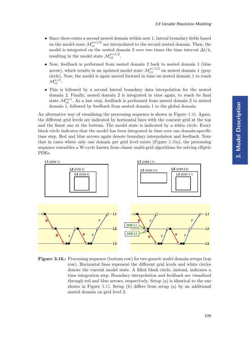
3.

Mo

del

Des

crip

tio

n

3.9 Variable Resolution Modeling

• Since there exists a second nested domain within nest 1, lateral boundary fields based

on the model stateMn+1/2c1 are interpolated to the second nested domain. Then, the

model is integrated on the nested domain 2 over two times the time interval ∆t/4,

resulting in the model state Mn+1/2c2 .

• Now, feedback is performed from nested domain 2 back to nested domain 1 (blue

arrow), which results in an updated model state Mn+1/2c1 on nested domain 1 (gray

circle). Now, the model is again moved forward in time on nested domain 1 to reachMn+1

c1 .

• This is followed by a second lateral boundary data interpolation for the nesteddomain 2. Finally, nested domain 2 is integrated in time again, to reach its finalstate Mn+1

c2 . As a last step, feedback is performed from nested domain 2 to nesteddomain 1, followed by feedback from nested domain 1 to the global domain.

An alternative way of visualizing the processing sequence is shown in Figure 3.16. Again,the different grid levels are indicated by horizontal lines with the coarsest grid at the topand the finest one at the bottom. The model state is indicated by a white circle. Everyblack circle indicates that the model has been integrated in time over one domain-specifictime step. Red and blue arrows again denote boundary interpolation and feedback. Notethat in cases where only one domain per grid level exists (Figure 3.16a), the processingsequence resembles a W-cycle known from classic multi-grid algorithms for solving ellipticPDEs.

Figure 3.16.: Processing sequence (bottom row) for two generic multi-domain setups (toprow). Horizontal lines represent the different grid levels and white circlesdenote the current model state. A filled black circle, instead, indicates atime integration step. Boundary interpolation and feedback are visualizedthrough red and blue arrows, respectively. Setup (a) is identical to the oneshown in Figure 3.15. Setup (b) differs from setup (a) by an additionalnested domain on grid level 2.

109

3.

Mo

del

Descrip

tion

ICON Model Tutorial

Nested Domain

Figure 3.17.: Illustration of ICON’s vertical nesting. Note that even when choosing dif-ferent numbers of vertical levels, vertical layers between the nested and theparent domain must match. Therefore, the nested domain may only havea lower top level height.

3.9.3. Vertical Nesting

The model top height can be chosen individually for each domain, with the constraintthat the height of the parent domain must be larger or at least equal to the height ofthe child domain. Thereby it is e.g. possible to combine a global domain which extendsinto the mesosphere with one or several child domains that only extend into the lowerstratosphere, see Figure 3.17.

However, it is not possible to choose different vertical level distributions for individualdomains. The level distribution is always defined by the global domain. Lower model topheights in child domains are realized by simply neglecting a certain number of levels atthe model top. Vertical refinement in the sense that vertical resolution is locally increasedin a child domain is so far not possible. One possible workaround might be to repeat themodel run with increased vertical resolution in limited area mode (see Chapter 6).

In order to reduce the top height for individual domains, the namelist parameter num lev

(run nml), which specifies the number of vertical levels in each domain, must be adapted. Inaddition, vertical nesting must be enabled by setting lvert nest=.TRUE.. See Section 3.4for details.

If vertical nesting is activated, boundary conditions are automatically provided for allprognostic variables at the uppermost half level of the nested domain. Several measuresare taken in order to avoid excessive reflections of vertically propagating sound and gravitywaves from the domain’s model top. Further details, however, are beyond the scope of thistutorial.

110

3.

Mo

del

Des

crip

tio

n

3.10 Reduced Radiation Grid

Figure 3.18.: Schematic showing how radiation is computed on a reduced (coarser) grid.

3.10. Reduced Radiation Grid

In real case simulations, radiation is one of the most time consuming physical processes.It is therefore desirable to reduce the computational burden without degrading the resultssignificantly. One possibility is to use a coarser horizontal grid for radiation than fordynamics.

The implementation is schematically depicted in Figure 3.18:

Step 1. Radiative transfer computations are usually performed every 30 minutes. Beforedoing so, all input fields required by the radiation scheme are upscaled to the nextcoarser grid level.

Step 2. Then the radiative transfer computations are performed and the resulting shortwave transmissivities τSW and long-wave fluxes FLW are scaled down to the fullgrid.

Step 3. In a last step we apply empirical corrections to τSW and FLW in order to incor-porate the high resolution information about albedo α and surface temperature Tsfcagain. This is especially important at land-water boundaries and the snow line, sincehere the gradients in albedo and surface temperature are potentially large.

The reduced radiation grid is controlled with the following namelist switches:

lredgrid phys= .FALSE./.TRUE. (namelist grid nml, logical value)If set to .TRUE. radiation is calculated on a coarser grid (i.e. one grid level higher)

radiation grid filename (namelist grid nml, string parameter)Filename of the grid to be used for the radiation model. Must only be specified forthe base domain, since for child domains the grid of the respective parent domain

111

3.

Mo

del

Descrip

tion

ICON Model Tutorial

serves as radiation grid. An empty string is required, if radiation is computed on thefull (non-reduced) grid.

Note that running radiation on a reduced grid is the standard setting for operationalruns at DWD. Using the reduced radiation grid is also possible for the limited area modeICON-LAM. In this case, both the computational grid and the reduced radiation grid areregional grids. Make sure to create the latter during the grid generation process by settingdom(:)%lwrite parent = .TRUE., see Section 2.1.3. Internally, the coarse radiation gridis denoted by the domain index 0.

112

4.

Idea

lized

Tes

ts

4. Running Idealized Test Cases

As opposed to real case runs, idealized test cases typically do not require any externalparameter or analysis fields for initialization. Instead, initial conditions are computedwithin the ICON model itself, based on analytical functions. These are either evaluatedpoint-wise at cell centers, edges, or vertices, or are integrated over the triangular controlvolume.

The ability to run idealized model setups serves as a simple means to test the correctnessof particular aspects of the model, either by comparison with analytic reference solutions(if they exist), or by comparison with results from other models. Beyond that, idealizedtest cases may help the scientist to focus on specific atmospheric processes.

ICON provides a set of pre-implemented test cases of varying complexity and focus, rangingfrom pure dynamical core and transport test cases to “moist” cases, including microphysicsand potentially other parameterizations. A complete list of available test cases can be foundin the namelist documentation, mentioned below.

4.1. Namelist Input for the ICON Model

In general, the ICON model is controlled by a so-called parameter file which uses FortranNAMELIST syntax. Default values are set for all parameters, so that you only have tospecify values that differ from the default.

Assuming that ICON has been compiled successfully, the next step is to adapt these ICONnamelists. The run scripts in this tutorial create a file NAMELIST NWP which contains alluser-defined namelist parameters, together with some substituted shell script variables.Discussing all available namelist switches is definitely beyond the scope of this tutorial.We will merely focus on the particular subset of namelist switches that is necessary tosetup an idealized model run. A complete list of namelist switches can be found in thenamelist documentation

icon/doc/Namelist_overview.pdf

Individual test cases can be selected and configured by namelist parameters of the namelistnh testcase nml. To run one of the implemented test cases, only a horizontal grid file hasto be provided as input. A vertical grid file containing the height distribution of verticalmodel levels is usually not required, since the vertical grid is constructed within the ICONmodel itself, based on the set of namelist parameters described in Section 3.4.

113

4.

Idea

lizedT

ests

ICON Model Tutorial

4.2. Jablonowski-Williamson Baroclinic Wave Test

From the set of available idealized test cases we choose the Jablonowski-Williamson baro-clinic wave test and walk through the procedure of configuring and running this test inICON.

The Jablonowski-Williamson baroclinic wave test (Jablonowski and Williamson, 2006) hasbecome one of the standard test cases for assessing the quality of dynamical cores. Themodel is initialized with a balanced initial flow field. It comprises a zonally symmetric basestate with a jet in the mid-latitudes of each hemisphere and a quasi realistic temperaturedistribution. Overall, the conditions resemble the climatic state of a winter hemisphere.This initial state is in hydrostatic and geostrophic balance, but is highly unstable withrespect to baroclinic instability mechanisms. Thus, it should remain stationary if no per-turbation is imposed.

To trigger the evolution of a baroclinic wave in the northern hemisphere, the initial condi-tions are overlaid with a weak (and unbalanced) zonal wind perturbation. The perturba-tion is centered at (20E, 40N). In general, the baroclinic wave starts growing observablyaround day 4 and evolves rapidly thereafter with explosive cyclogenesis around modelday 8. After day 9, the wave train breaks (see Figure 4.1). If the integration is contin-ued, additional instabilities become more and more apparent especially near the pentagonpoints (see Section 2.1), which are an indication of spurious baroclinic instabilities trig-gered by numerical discretization errors. In general, this test has the capability to assess

• the diffusivity of a dynamical core,

• the presence of phase speed errors in the advection of poorly resolved waves,

• the strength of grid imprinting.

In Jablonowski et al. (2008) it is suggested to add a variety of passive tracers to thebaroclinic wave test case, in order to investigate the general behavior of the advectionalgorithm. Questions that could be addressed are

• whether the advection scheme is monotone or positive-definite,

• how accurate or diffusive the advection scheme is,

• whether a constant tracer distribution is preserved (which checks for tracer-air massconsistency).

Four different tracer distributions are implemented, whose initial distributions are de-picted in Figure 4.2. See Jablonowski et al. (2008) for further information on the initialdistributions.

4.2.1. Main Switches for the Idealized Test Case

This section explains several namelist groups and main switches that are necessary forsetting up an idealized model run. Settings for the Jablonowski-Williamson test case aregiven in red.

114

4.

Idea

lized

Tes

ts

4.2 Jablonowski-Williamson Baroclinic Wave Test

Figure 4.1.: Surface Pressure and 850 hPa Temperature at day 9 for the Jablonowski-Williamson test case on a global R2B5 grid.

Namelist run nml:

ltestcase= .TRUE. (namelist run nml, logical value)This parameter must be set to .TRUE. for running idealized test cases.

iforcing= 0 (namelist run nml, integer value)Forcing of dynamics and transport by parameterized processes. If set to 0, forcingis switched off completely (pure dynamical core test case). This implies that allphysical parameterizations (see nwp phy nml) are switched off automatically. If setto 3, dynamics are forced by NWP-specific parameterizations. Individual physicalprocesses can be controlled via nwp phy nml, see also Table 3.3. In general, the settingof iforcing depends on the selected test case.

ldynamics= .TRUE. (namelist run nml, logical value)Main switch for the dynamical core. If set to .TRUE., the dynamical core isswitched on and details of the dynamical core can be controlled via dynamics nml,nonhydrostatic nml and diffusion nml. If set to .FALSE., the dynamical core isswitched off completely. This is rarely needed, but can be useful for idealized testsof physics packages with prescribed dynamical forcing.

ltransport= .FALSE./.TRUE. (namelist run nml, logical value)Main switch for the transport of passive tracers. If set to .TRUE., transport

115

4.

Idea

lizedT

ests

ICON Model Tutorial

Figure 4.2.: Initial tracer distributions which are available for the Jablonowski-Williamson test case. Tracer q3 only depends on the latitudinal position,and tracer q4 is constant.

is switched on and details of the transport schemes can be controlled viatransport nml (see Section 3.6.5 for additional help). If set to .FALSE., transportof passive tracers is switched off completely.

msg level (namelist run nml, integer value)You may increase the model output verbosity by setting this namelist parameter toa higher value (≤ 20). This option can be particularly useful if the ICON model runfails and the cause of the error still does not become clear from the error message.

Namelist nh testcase nml:

nh test name= ’jabw’ (namelist nh testcase nml, string parameter)Main switch for selecting a test case. nh test name=’jabw’ selects the Jablonowski-Williamson baroclinic wave test case.

Namelist extpar nml:

itopo= 0 (namelist extpar nml, integer value)If set to 1, the model tries to read topography data and external parameters fromfile. If set to 0, no input file is required for model initialization. Instead, all initialconditions are computed within the ICON model itself. Usually, itopo should be setto 0 for running idealized test cases.

116

4.

Idea

lized

Tes

ts

4.2 Jablonowski-Williamson Baroclinic Wave Test

4.2.2. Specifying the Computational Domain(s)

In the following we will explain how the Jablonowski-Williamson test case can be set upfor a global domain only and, in a second step, for a global domain with nests.

Namelist grid nml:

dynamics grid filename (namelist grid nml, list of string parameters)Here, the name(s) of the horizontal grid file(s) must be specified. For a global sim-ulation without nests, of course, only a single filename is required. For a globalsimulation with multiple nests a filename must be specified for each domain. Notethat each name must be enclosed by single quotation marks and that multiple namesmust be separated by a comma (see the example below).

dynamics parent grid id (namelist grid nml, list of integer values)Comma-separated list of integer values. For each domain, the grid ID of its parentdomain must be specified.

Grid IDs start with 1 and correspond to the list given by the namelist parameterdynamics grid filename. The grid ID 0 indicates that a domain has no parentdomain (i.e. the global domain). Therefore the parent grid file for domain i is givenby dynamics grid filename(dynamics parent grid id(i)).

Additional explanation and an example are given in Section 2.1.4 (“Step 3: Sub-domain Name and Parent Grid ID”).

Examples

Example 1: Settings for a global Jablonowski-Williamson test run without nest

dynamics grid filename = ’icon grid 0014 R02B05 G.nc’

dynamics parent grid id = 0

num lev = 40

Example 2: For a global Jablonowski-Williamson test run including a single nest

dynamics grid filename =

’icon grid 0014 R02B05 G.nc’,’icon grid 0014 R02B05 N06 1.nc’

dynamics parent grid id = 0,1

num lev = 40,40

Example 3: Settings for a global Jablonowski-Williamson test run including two nestson the same nesting level (i.e. combination of Figure 4.3)

dynamics grid filename =

’icon grid 0014 R02B05 G.nc’,’icon grid 0014 R02B05 N06 1.nc’,

’icon grid 0014 R02B05 N06 2.nc’

dynamics parent grid id = 0,1,1

num lev = 40,40,40

117

4.

Idea

lizedT

ests

ICON Model Tutorial

Figure 4.3.: Location of available nests for the baroclinic wave test case. The perturba-tion triggering the baroclinic wave is centered at (20E, 40N) (red circle).

Some additional information on the grid file naming convention can be found in Section 2.1.

4.2.3. Integration Time Step and Simulation Length

The integration time step and simulation length are defined as follows:

Namelist run nml:

dtime= 720 (namelist run nml, real value)Time step in seconds (for the top-most domain). Note that it is not necessary tospecify a time step for each domain. For each nesting level, the time step is auto-matically divided by a factor of two. More details on ICON’s time step will be givenin Section 3.7.1.

nsteps= 1200 (namelist run nml, integer value)Number of time steps.

Output is controlled by the namelist group output nml. It is possible to define more thanone output namelist and each output namelist has its own output file attached to it. Forexample, the run script that is used in Exercise C.4.1 contains three output namelists.The details of the model output specification are discussed in Section 7.1.

118

5.

Rea

l-D

ata

Tes

ts

5. Running Real Data Test Cases

In this chapter you will learn about how to initialize and run the ICON model in a realisticNWP setup. The namelist settings to start from a DWD Analysis and from an IFS Analysisare discussed.

5.1. Model Initialization

The necessary input data to perform a real data run have already been described inChapter 2. These include

• grid files, containing the horizontal grid information,

• external parameter files, providing information about the Earth’s soil and land prop-erties, as well as climatologies of atmospheric aerosols, and

• initial data (analysis) for atmosphere, land and sea.

ICON is capable of reading analysis data from various sources (see Section 2.2), includ-ing data sets generated by DWD’s Data Assimilation Coding Environment (DACE) andinterpolated IFS data. In the following we provide some guidance on how to set up realdata runs, depending on the specific data set at hand.

Note that ICON aborts during the setup phase, if any of the required input files has notbeen found.

Therefore, as a first step, check the filenames (and soft links) for the model input files,cf. Section 2. Also make sure that the input data and grid files match. For example, takea look at the global attributes number of grid used and uuidOfHGrid of the global gridfile. These values have to match the corresponding attributes of the external parametersand initial data file, see Section 2.1.5.

5.1.1. Basic Settings for Running Real Data Runs

Most of the main switches, that were used for setting up idealized test cases, are alsoimportant for setting up real data runs. As many of them have already been discussed inSection 4.1, we will concentrate on their settings for real data runs. Settings appropriatefor the exercises on this subject (see Ex. C.5.1) are highlighted in red.

119

5.

Rea

l-Da

taT

ests

ICON Model Tutorial

Specifying Model Start and End Dates (Namelist time nml)

For real case runs it is important that the user specifies the correct start date and time ofthe simulation. This is done with ini datetime string using the ISO8601 format.

ini datetime string= YYYY-MM-DDThh:mm:ssZ (namelist time nml)— This must exactly match the validity time of the analysis data set!

Wrong settings lead to incorrect solar zenith angles and wrong external parameter fields.Setting the end date and time of the simulation via end datetime string is optional. Ifend datetime string is not set, the user has to set the number of time steps explicitlyin nsteps (run nml), which is otherwise computed automatically.

In ICON there coexist two equally usable ways to control the experiment startand end date – without a compelling reason, though. These two alternativesare listed in the following.

Namelist run nml:

time step dtime modelTimeStep

Namelists time nml (left) and master time control nml (right):

experiment start ini datetime string experimentStartDate

experiment stop end datetime string experimentStopDate

Please note that the data types of the above-mentioned namelist parametersdiffer. The parameters that are listed on the right are consistently based uponthe ISO 8601 representations of dates and time spans. However, dtime mustbe specified in seconds.

General Settings (Namelist run nml)

ltestcase= .FALSE. (namelist run nml, logical value)This parameter must be set to .FALSE. for real case runs.

iforcing= 3 (namelist run nml, integer value)A value of 3 means that dynamics are forced by NWP-specific parameterizations.

ldynamics= .TRUE. (namelist run nml, logical value)The dynamical core must, of course, be switched on.

ltransport= .TRUE. (namelist run nml, logical value)Tracer transport must be switched on. This is necessary for the transport of cloudand precipitation variables. Details of the transport schemes can be controlled viathe namelist transport nml (see Section 3.6.5).

120

5.

Rea

l-D

ata

Tes

ts

5.1 Model Initialization

Specifying the Horizontal Grid (Namelist grid nml)

dynamics grid filename (namelist grid nml, list of string parameters)Here, the name(s) of the horizontal grid file(s) must be specified. For a global sim-ulation without nests, of course, only a single filename is required. For a globalsimulation with multiple nests, a filename must be specified for each domain. Notethat each name must be enclosed by single quotation marks and that multiple namesmust be separated by a comma (see Section 4.2.2 and the examples therein).

dynamics parent grid id (namelist grid nml, list of string parameters)Comma-separated list of integer values. For each domain, the grid ID of its parentdomain must be specified.

Grid IDs start with 1 and correspond to the list given by the namelist parameterdynamics grid filename. Additional explanation and an example are given in Sec-tion 2.1.4 (“Step 3: Sub-domain Name and Parent Grid ID”). If a domain has noparent domain this is indicated by the value 0 (e.g. the global domain).

radiation grid filename (namelist grid nml, string parameter)If the radiative transfer computation should be conducted on a coarser grid than thedynamics (one level coarser, effective mesh size 2∆x), the name(s) of the grid file(s)to be used for radiation must be specified here. See Section 3.10 for further details.

Specifying External Parameters (Namelist extpar nml)

itopo= 1 (namelist extpar nml, integer value)For real data runs this parameter must be set to 1. The model now expects one fileper domain from which it tries to read topography data and external parameters.

extpar filename (namelist extpar nml, string parameter)Filename(s) of input file(s) for external parameters. If the user does not providenamelist settings for extpar filename, ICON expects one file per domain to bepresent in the experiment directory, following the naming convention

extpar_filename = "extpar_<gridfile>.nc"

The keyword <gridfile> is automatically replaced by ICON with the grid filenamespecified for the given domain (dynamics grid filename). As opposed to the grid-file specification namelist variables (see above), it is not allowed to provide a comma-separated list. Instead, the usage of keywords provides full flexibility for defining thefilename structure.

By changing the above setting, the user has full flexibility with respect tothe filename structure. The following keywords are allowed for the namelistparameter extpar filename:

121

5.

Rea

l-Da

taT

ests

ICON Model Tutorial

<path> model base directory(namelist parameter model base dir, namelist master nml)

<gridfile> grid filename for the given domain (dynamics grid filename)<nroot> grid root division Rx (single digit)<nroot0> grid root division Rxx (two digits)<jlev> grid bisection level Byy (two digits)<idom> domain number (two digits).

Specifying the Initialization Mode (Namelist initicon nml)

ICON provides different real data initialization modes which differ in terms of the expectedinput fields and number of input files. Thereby ICON is able to handle analysis productsfrom different models. The mode in use is controlled via the namelist switch init mode.

init mode (namelist initicon nml, integer value)It is possible to

• start from (interpolated) uninitialized DWD analysis without the IAU proce-dure: init mode = 1

• start from interpolated IFS analysis: init mode = 2

• start atmosphere from interpolated IFS analysis and soil/surface from interpo-lated ICON/GME fields: init mode = 3

• start from non-interpolated, uninitialized DWD analysis, and make use of theIAU procedure to filter initial noise: init mode = 5

• start from interpolated initialized ICON analysis with subsequent verticalremapping: init mode=7

The most relevant modes are mode 1, 2, 5 and 7. They will be explained in more detailbelow.

ICON supports NetCDF and GRIB2 as input format for input fields. In this context it isimportant to note that the field names that are used in the input files do not necessarilycoincide with the field names that are internally used by the ICON model. To addressthis problem, an additional input text file is provided, a so-called dictionary file. Thisfile translates between the ICON variable names and the corresponding GRIB2/NetCDFshort names.

Generally the dictionary is provided via the following namelist parameter:

ana varnames map file (namelist initicon nml, string parameter)Filename of the dictionary for mapping between internal names and GRIB2/NetCDFshort names. An example can be found in icon/run/ana varnames map file.txt.

122

5.

Rea

l-D

ata

Tes

ts

5.1 Model Initialization

5.1.2. Starting from Uninitialized DWD Analysis

This analysis product is rarely the optimal choice for model initialization, as it generatesa significant amount of spurious noise during the first few hours of a model run (seeFigure 2.6). Nevertheless, this mode is described for completeness. The process of obtainingthe uninitialized DWD analysis for non-incremental update and its content is described inSection 2.2.1 (Option 2).

Model initialization is basically controlled by the following three namelist parameters:

init mode = 1 (namelist initicon nml, integer value)To start from uninitialized DWD analysis data (without incremental analysis up-date), the initialization mode must be set to 1.

In that case the ICON model expects two input files per domain. One containing theICON first guess (3 h forecast) fields, which served as background fields for the assimilationprocess. The other contains the analysis fields produced by the assimilation process. SeeTable 2.2 for a list of variables.

dwdfg filename (namelist initicon nml, string parameter)Filename of the DWD first guess input file.

dwdana filename (namelist initicon nml, string parameter)Filename of the DWD analysis input file.

Remember to make sure that the validity date for the first guess and analysis input file isthe same and matches the model start date given by ini datetime string.

Input filenames need to be specified unambiguously, of course. By default, if the user doesnot provide namelist settings for dwdfg filename and dwdana filename, the filenameshave the form

dwdfg_filename = "dwdFG_R<nroot>B<jlev>_DOM<idom>.nc"

dwdana_filename = "dwdana_R<nroot>B<jlev>_DOM<idom>.nc"

This means, e. g., that the first guess filename begins with “dwdFG ”, supplemented by thegrid spacing Rx Byy and the domain number DOMii . Filenames are treated case sensitively.1

By changing the above setting, the user has full flexibility with respect tothe filename structure. The following keywords are allowed for the namelistparameters dwdfg filename, dwdana filename and ifs2icon filename (forthe latter see Section 5.1.5):

<path> model base directory(namelist parameter model base dir, namelist master nml)

<nroot> grid root division Rx (single digit)<nroot0> grid root division Rxx (two digits)<jlev> grid bisection level Byy (two digits)<idom> domain number (two digits).

1More precisely this behavior depends on the file system: UNIX-like file systems are case sensitive, butthe HFS+ Mac file system (usually) is not.

123

5.

Rea

l-Da

taT

ests

ICON Model Tutorial

5.1.3. Starting from Uninitialized DWD Analysis with IAU

As described in Section 2.2.1, IAU is a means to reduce the initial noise which typicallyresults from small scale non-balanced modes in the analysis data set. Combining thisanalysis product with IAU is the preferred method in cases where the horizontal andvertical grid of the intended forecast run exactly match with that of the analysis. Sinceno horizontal interpolation is required, the forecast run can make use of the surface tileinformation which is specific to this analysis product. Moreover, this product exhibits thesmallest noise level during model start.

The process of obtaining the uninitialized analysis for IAU and its content is described inSection 2.2.1 (Option 1).

Model initialization is basically controlled by the following namelist parameters:

init mode = 5 (namelist initicon nml, integer value)To start from DWD analysis data with IAU, the initialization mode must be set to 5.

ICON again expects two input files. One containing the ICON first guess, which typicallyconsists of a 1.5 h forecast taken from the assimilation cycle (as opposed to a 3 h forecastused for the non-IAU case). The other contains the analysis fields (mostly increments)produced by the assimilation process. See Table 2.1 for a list of variables.

dwdfg filename (namelist initicon nml, string parameter)Filename(s) of the DWD first guess input file(s) for each domain. See Section 5.1.2for an explanation of the filename structure.

dwdana filename (namelist initicon nml, string parameter)Filename(s) of the DWD analysis input file(s) for each domain. See Section 5.1.2 foran explanation of the filename structure.

The behavior of the IAU procedure is controlled via the namelist switches dt iau anddt shift:

dt iau = 10800 (namelist initicon nml, real value)Time interval (in s) during which the IAU procedure (i.e. dribbling of analysis in-crements) is performed.

dt shift = -5400 (namelist initicon nml, real value)Time (in s) by which the model start is shifted ahead of the nominal model startdate given by ini datetime string. Typically dt shift is set to −0.5 ∗ dt iau suchthat dribbling of the analysis increments is centered around ini datetime string.

As explained in Section 2.2.1 and depicted in Figure 5.1, you have to make sure that thefirst guess is shifted ahead in time by −0.5 ∗ dt iau w.r.t. the analysis. The model starttime ini datetime string must match the validity time of the analysis.

124

5.

Rea

l-D

ata

Tes

ts

5.1 Model Initialization

Figure 5.1.: Schematic illustrating typical settings for a global ICON forecast run start-ing from a DWD analysis with IAU at 00 UTC. IAU is performed overa 3 h time interval (dt iau), with the model start being shifted ahead ofthe nominal start date by 1.5 h (dt shift). Validity date of first guess andanalysis is 22:30 UTC and 00 UTC, respectively.

5.1.4. Starting from Initialized DWD Analysis

The initialized analysis is the product of choice in cases where the horizontal and/or verti-cal grid of the intended model run differs from that of the analysis. Using the uninitializedanalysis for IAU is prohibited in such cases, as the horizontal interpolation of tiled sur-face fields makes no sense. Moreover, the initialized analysis product is less cumbersometo use, as it consists of a single file per domain, only. When compared to the standarduninitialized analysis product, spurious noise is significantly reduced (see Figure 2.6).

The process of obtaining the initialized analysis and its content is described in Section 2.2.1(Option 3).

Model initialization is basically controlled by the following namelist parameters:

init mode = 7 (namelist initicon nml, integer value)To start from initialized DWD analysis data, the initialization mode must be setto 7. If the number and or heights of the vertical levels differs between the modeland the analysis, the input fields are automatically remapped in the vertical duringread-in.

ICON expects a single input file:

125

5.

Rea

l-Da

taT

ests

ICON Model Tutorial

dwdfg filename (namelist initicon nml, string parameter)Filename(s) of the initialized DWD analysis input file(s) for each domain. Admit-tedly, the nomenclature “dwdfg” is a bit counter intuitive. See Section 5.1.2 for anexplanation of the filename structure.

Remember to make sure that the model start time given by ini datetime string matchesthe validity date of the input file.

5.1.5. Starting from IFS Analysis

No filtering procedure is currently available when starting off from interpolated IFS anal-ysis data. The model just reads in the initial data from a single file and starts the forecast.

The process of obtaining the IFS analysis and its content is described in Section 2.2.2.

init mode= 2 (namelist initicon nml, integer value)To start from interpolated IFS analysis data, the initialization mode must be setto 2.

ifs2icon filename (namelist initicon nml, string parameter)ICON expects a single file per domain from which interpolated IFS analysis canbe read. With this parameter, the filename can be specified. Note that for thisinitialization mode only input data in NetCDF format are supported. Similar tothe namelist parameters dwdfg filename and dwdana filename, which have beenexplained above in Section 5.1.2, the filenames have the form

ifs2icon_filename = "ifs2icon_R<nroot>B<jlev>_DOM<idom>.nc"

Remember to make sure that the model start time given by ini datetime string matchesthe validity date of the analysis input file.

5.2. Starting or Terminating Nested Domains at Runtime

Starting or terminating nested domains at runtime is possible by means of the namelistparameters start time and end time in the namelist grid nml. Model calculations forthe nested domain are performed if the simulation time of the parent domain is greater orequal to start time and less than end time.

start time (namelist grid nml, list of real values)Comma-separated list of integer values. For each domain, the start time relativeto the experiment start date can be specified in seconds. A value of 0 for the ithdomain means that it is started at experiment start date which is either definedby ini datetime string or experimentStartDate. If Incremental Analysis Up-date (IAU) is used, start time must be set equal to dt shift (initicon nml) (i.e.negative), in order for the nested domain to be active from the very beginning.

126

5.

Rea

l-D

ata

Tes

ts

5.2 Starting or Terminating Nested Domains at Runtime

end time (namelist grid nml, list of real values)Comma-separated list of integer values. For each domain, the end time relative tothe experiment start date can be specified in seconds. I.e. a value of 3600 specifiedfor the ith domain means that it is terminated one hour after experiment start.

As discussed in Section 2.2, initial data files are usually required for each nested domain.With only little loss of forecast skill, this rather tedious procedure can be overcome bystarting the nested domain(s) shortly after the global domain. In that case, nested domainsare initialized by parent-to-child interpolation of the prognostic fields. Note, however, thatsurface tile information will be lost. Surface fields on the child domain are initialized withaggregated values interpolated from the parent domain.

127

5.

Rea

l-Da

taT

ests

6.

Lim

ited

Are

aM

od

e

6. Running ICON-LAM

The most important first: Running the limited area (regional) mode of ICON does notrequire a separate, fundamentally different executable. Instead, ICON-LAM is quite similarto the other model components discussed so far: It is easily enabled by a top-level namelistswitch

Namelist grid nml: l limited area = .TRUE.

Other namelist settings must be added, of course, to make a proper ICON-LAM setup.This chapter explains some of the details.

Chapter Layout. Some of the preprocessing aspects regarding the regional mode havealready been discussed in Section 2.3. Based on these prerequisites the exercises in thischapter (see Ex. C.6.1) will explain how to actually set up and run limited area simulations.

In the following, technical details on the limited area mode are provided, in particular onhow to control the read-in of initial data and boundary data.

6.1. Limited Area Mode vs. Nested Setups

In Section 3.9.1 the nesting capability of ICON has been explained. Technically, the samecomputational grids may be used either for the limited area mode or the nested mode ofICON1. Furthermore, both ICON modes aim at simulations with finer grid spacing andsmaller scales. They therefore choose a comparable set of options out of the portfolio ofavailable physical parameterizations.

However, there exist some differences between the regional and the one-way nested mode:

• ICON-LAM is driven by externally supplied boundary data which may come froma global model or a coarser resolution LAM that has been run in advance – that’san obvious difference! During the simulation, boundary conditions are updated atregular time intervals by reading input files. Between two lateral boundary datasamples the boundary data is linearly interpolated.

• Lateral boundary updates happen (significantly) less frequently compared to one-way nesting.

• The driving model and the limited area model may run on different computer sites.Often they also differ in terms of the governing equations as well as numerical meth-ods used.

1Here, we do not take the reduced radiation grid into account, see Section 3.10. This serves to simplifythe discussion at this point.

129

6.

Lim

itedA

reaM

od

e

ICON Model Tutorial

• ICON-LAM allows for a more flexible choice of vertical levels: Nested domains maydiffer from the global, “driving” grid only in terms of the top level height, but verticallayers must match between the nested and the parent domain (see Section 3.9.3).In contrast to that, the limited area mode performs a vertical interpolation of itsboundary data. This is the default namelist parameter setting itype latbc=1 inthe namelist limarea nml. The level number and the level heights may therefore bechosen independently.

• ICON-LAM allows for a more flexible choice of the horizontal resolution. While fornested setups the increase in horizontal resolution per nesting level is constrained to afactor of 2, the resolution of the limited-area domain can be freely selected. However,resolution jumps much larger than a factor of ∼ 5 between the forcing data resolutionand the target resolution and should be avoided, since it will negatively impact theforecast quality.

6.2. Nudging in the Boundary Region

In order to prevent outward-propagating waves from reflecting back into the domain, asponge layer is implemented along the lateral boundaries. Within this sponge layer theinterior flow is relaxed towards the externally specified boundary data. In addition to thislateral boundary nudging, upper boundary nudging along the model top can be switchedon by choosing nudge type=1 (namelist nudging nml). The default value is 0, i.e. it isswitched off. Figure 6.1 schematically depicts the partitioning of the limited area domaininto the lateral boundary zone, labeled 0 , the adjacent lateral nudging zone 1 , the uppernudging zone 2 , the nudging overlap zone 3 and the “free” model atmosphere 4 . Inthe lateral boundary zone 0 , which has a fixed width of 4 cell rows, externally suppliedboundary data are simply prescribed.

The mathematical implementation of the sponge layer in the nudging zones follows thework by Davies (1976, 1983). An additional “forcing” term is added to the right hand sideof the prognostic equations for vn, θv, ρ, and qv:

ψ(t) = ψ∗(t) + αnudge∆t

∆τ[ψbc(t)− ψ∗(t)]︸ ︷︷ ︸

=δψ

,

where ψbc is the externally specified value of the prognostic variable ψ at time t, andαnudge is a relaxation coefficient. The nudging update ψ − ψ∗ depends on the time stepratio ∆t/∆τ (→ ndyn substeps), but not on the time step itself, so it might be thought ofas a kind of state “shift” from ψ∗ to ψ. The nudging coefficient αnudge gradually decreaseswith increasing distance from the boundary and is of the form

αnudge =

f0A0 exp(− |r−r0|µ

), if |r − r0| ≤ L (region 1 in Fig. 6.1)

B0

(z−zstartztop−zstart

)2, in region 2

maxf0A0 exp (· · · ) , B0 (· · · )2

, in region 3

0, in region 4

,

130

6.

Lim

ited

Are

aM

od

e

6.2 Nudging in the Boundary Region

1

2 3

height z

horizontal r

L i m i t e d a r e a d o m a i n

lateral boundary nudging

zone

upper boundary nudging zone

4

zstart = nudge_start_height

ztop = top_height

r0 + L

1

3 damp_height

0

lateral boundary

interpolation zone

0

sponge layer with Rayleigh damping of vertical velocity component

r0

grf_bdywidth_c = 4 cell rows L = nudge_zone_width = 8 cell rows

Figure 6.1.: Schematic illustration of the lateral boundary zone (blue) and the lateraland upper boundary nudging zones (gray) in the limited-area mode.

with A0 the maximum relaxation coefficient in the lateral nudging zone, L the widthof the lateral nudging zone given in units of cell rows, µ the e-folding width given inunits of cell rows, r the actual cell row index beginning with 1 in the outermost cellrow of the boundary zone, and r0 the cell row index at which the nudging zone starts(typically grf bdywidth c+1, see Figure 6.1). The parameters L, µ, and A0 can be spec-ified via nudge zone width, nudge efold width, and nudge max coeff in the namelistinterpol nml. The nudge zone width should at least comprise 8 (better 10) cell rows inorder to minimize boundary artifacts. The tuning factor f0 is either 1 for θv and ρ, or 0.5for vn and qv.

B0 is the maximum nudging coefficient in the upper boundary nudging zone be-tween the model top at height ztop (sleve nml: top height) and the nudgingstart height zstart (nudging nml: nudge start height). The value of B0 is con-trolled by max nudge coeff vn (nudging nml) for the horizontal wind vn, andmax nudge coeff thermdyn for θv and ρ.

Note that positive water vapor increments δψ = δqv > 0 are cut to zero in supersaturatedregions (qc > 0) in the lateral boundary nudging zone, in order to avoid an undesirablepositive feedback on the growth of the amount of cloud water. In addition, water vaporis not subject to nudging in the upper boundary nudging zone. If the nudging data fromthe driving model contain hydrostatic variables (i.e. hydrostatic pressure), it might bemore consistent to formulate the nudging in terms of the basic hydrostatic variables: pres-sure and temperature. This option is controlled by the namelist switch nudge hydro pres

(limarea nml), which applies to both lateral and upper boundary nudging. If set to .TRUE.

(default), nudging increments of the hydrostatic pressure and the temperature, δp and δT ,

131

6.

Lim

itedA

reaM

od

e

ICON Model Tutorial

are computed and transformed into virtual potential temperature and density incrementsfollowing the linear mapping

δρ = Xρδp+ YρδT + Zρδqv

δθv = Xθvδp+ YθvδT + Zθvδqv ,

which is motivated by the total differential of the thermodynamic state equations. Thefactors X, Y and Z are determined by the state before the nudging (ψ∗). Note again thatwater vapor increments are nonzero only in the lateral boundary nudging zone.

Important note: Independent of the upper boundary nudging is the treatmentof the vertical velocity component w along the model top: w and correspond-ing vertical mass fluxes are set to zero at the uppermost half level of thecomputational domain. Starting from the height specified by damp height

(nonhydrostatic nml), the vertical velocity is damped towards zero follow-ing the method proposed by Klemp et al. (2008).

If upper boundary nudging is switched on (nudging nml: nudge type=1),“lateral boundary” data (the driving data for the nudging) have to be pro-vided for the entire limited area domain rather than the lateral boundary re-gion, only. This mode requires the namelist parameter latbc boundary grid

(limarea nml) defining the grid file on which the lateral boundary data aredefined to be empty, i.e. latbc boundary grid=" ".

Running the model in regional mode is quite often accompanied by choosing a lower modeltop height compared to global simulations. In these cases, the neglected air mass abovemodel top can have a noticeable impact regarding the attenuation of the incoming solarirradiance and can be the source of a small but noticeable amount of downward long-waveirradiance. To account for that in a rather ad-hoc manner, an additional model layer abovemodel top can be added by setting latm above top=.TRUE. (namelist nwp phy nml). It isused by the radiation scheme, only. The additional layer has a (hard-coded) thickness of1.5 times the thickness of the uppermost model layer. Currently, temperature is linearlyextrapolated, assuming a vertical gradient of −5 K km−1. For ozone, aerosols and cloudfields, a simple no-gradient condition is assumed. Despite this rather ad-hoc solution, itis suggested to activate the additional layer. Please note that this option works only incombination with a reduced radiation grid.

6.3. Model Initialization

The necessary input data to perform a limited area run are basically identical to thoserequired for a global run (i.e. horizontal grid(s), initial conditions, external parameter; seeSection 5.1), with the exception that lateral boundary data are required in addition inorder to drive the model.

Technically it is possible to combine initial- and boundary data from different sources (e.g.one might take boundary data from IFS and initial data from ICON). In general, however,it is better to use boundary and initial data from the same source.

132

6.

Lim

ited

Are

aM

od

e

6.3 Model Initialization

Dependent on the available initial data, the following initialization modes can be used inlimited area mode:

init mode (namelist initicon nml, integer value)

init mode = 2 initialize limited area run from IFS data.This mode has already been described in Section 5.1.5 in the con-text of reading IFS analysis data.

init mode = 7 initialize limited area run from ICON data.This mode has already been described in Section 5.1.4 in the con-text of reading in DWD’s initialized analysis product.

Both modes have in common that the read-in process is followed by a vertical interpo-lation of the input fields to the target vertical grid. Thus the target vertical grid can bechosen independent of the vertical grid on which the input is defined. Note that in caseof init mode = 7 the vertical interpolation requires that the field HHL (vertical half levelheights) is contained in the initial data.

Specifics of init mode=2

• Only input data in NetCDF format are supported.

• A single input file per domain is expected, containing the analysis (or, more generally,the initial state). The filename must be provided for ifs2icon filename (see alsoSection 5.1.5).

• The required input fields are depicted in Figure 6.2.

AtmosphereU, V

or

VN

, W, T,

LNPS

or

PS

,

GEOSP

or

GEOP ML

, QV, QC, QI, QR, QS

Soil/Surface

SMIL1, SMIL2, SMIL3, SMIL4, STL1, STL2, STL3, STL4, LSM, CI,GEOP SFC, ALB SNOW, SST, SKT, T SNOW, W SNOW, RHO SNOW, W I

Figure 6.2.: Required variable set when initializing ICON-LAM from IFS data (i.e.init mode=2). Optional fields are marked in gray. Please note that althoughthe field is called W (vertical velocity) ICON expects the content of this fieldto be OMEGA (vertical wind in a pressure based coordinate system) in caseof init mode=2!

133

6.

Lim

itedA

reaM

od

e

ICON Model Tutorial

Specifics of init mode=7

• A single input file per domain is expected, containing the analysis (or, moregenerally, the initial state). The filename must be specified with the parameterdwdfg filename(initicon nml).

• As we do not make use of a second input file containing explicit analysis information,it is good practice to indicate this via the following namelist parameter.

lread ana (namelist initicon nml, logical value)By default, this namelist parameter is set to .TRUE.. If .FALSE., a separateanalysis file is not required. The filename of the first guess file is specified viathe dwdfg filename namelist option, see Section 5.1.2.

Note that in the recent ICON version lread ana=.FALSE. is set automatically forinit mode= 7, if it has been forgotten by the user.

• The required input fields are listed in Table 2.3. A valid option is to use DWD’sinitialized analysis product for initialization. See Section 2.2.1 for ways to obtain it.

6.4. Reading Lateral Boundary Data

The read-in of lateral boundary data is fortunately less cumbersome than the read-in ofinitial data, as it is based on a decision tree. The user is no longer required to select aspecific mode which (hopefully) fits the data at hand. Instead, ICON scans the boundarydata file and, dependent on its content, ICON diagnoses additional fields so as to obtainthe internally required set of variables. The decision tree is depicted in Figure 6.3. If theprovided data set does not match any of the trees, an error is thrown. As a result, ICONcan handle variable sets from hydrostatic models (e.g. IFS) as well as non-hydrostaticmodels (e.g. COSMO, ICON) without the assistance of the user.

As apparent from the decision tree, three different variable sets can be handled. See Fig-ure 2.9 for its specific content.

Important note: Boundary data sets originating from a non-hydrostatic modelwith height based vertical coordinates (e.g. COSMO or ICON) must containthe field HHL (vertical half level heights). It is required by the vertical inter-polation procedure. Note, however, that the field only needs to be present inthe boundary data set whose validity date equals the model start date.

Read-in of boundary data is controlled by the following namelist parameters:

The type of lateral boundary conditions is specified by

itype latbc (namelist limarea nml, Integer value)If set to 1 time-dependent boundary conditions are used. ICON then tries to readexternal data files at regular time intervals from a particular location specified by

134

6.

Lim

ited

Are

aM

od

e

6.4 Reading Lateral Boundary Data

HHL available?

RHO & THETA V available?

read:HHL, RHO, THETA V, W

yes

P, Tavailable?

• read HHL, P, T, W

yes

Error!

no

no

yes

PS, GEOP & T available?

read:PS, GEOP, OMEGA, T

yes

Error!

no

no

diagnose: P, T diagnose: P, HHL, W

Figure 6.3.: Read-in of lateral boundary data. Based on this decision tree, ICON inves-tigates the data file contents and diagnoses additional fields.The following fields are read additionally from file: velocity fields VN (or U,V) and mixing ratios QV, QC, QI (optional: QR, QS). The fields W and OMEGA areoptional; if they are unavailable, the vertical wind is initialized with zero.For the input from a pressure based coordinate system (right branch), notethat ICON expects the field OMEGA under the name W.

latbc filename and latbc path (see below).If set to 0, time-constant lateral boundary conditions are used which are derivedfrom the initial conditions.

Boundary data is read at regular time intervals. This is specified by the following namelistparameter:

dtime latbc (namelist limarea nml, floating-point value)Time difference in seconds between two consecutive boundary data sets. At inter-mediate times, boundary conditions are computed by linear interpolation in time.

6.4.1. Naming Scheme for Lateral Boundary Data

Naturally, the sequence of lateral boundary data files must satisfy a consistent namingscheme. It is a good idea to consider this convention already during the preprocessingsteps (see Section 2.3).

135

6.

Lim

itedA

reaM

od

e

ICON Model Tutorial

Filenames: latbc filename, latbc path (string parameters, limarea nml)By default, the filenames are expected to have the following form:

"prepiconR<nroot>B<jlev>_<y><m><d><h>.nc"

Here, several keywords are used which are further explained below. This namingscheme can be flexibly altered via the namelist parameter latbc filename (namelistlimarea nml) using the available keywords. The absolute path to the boundary datacan be specified with latbc path (string parameter, limarea nml).

By changing the above setting, the user has full flexibility with respect tothe filename structure. The following keywords are allowed for the namelistparameter latbc filename:

<nroot> grid root division Rx (single digit)<nroot0> grid root division Rxx (two digits)<jlev> grid bisection level Byy (two digits)<dom> domain number (two digits)<y> year (four digits)<m> month (two digits)<d> day in month (two digits)<h> hour (UTC) (two digits)<min> minutes (UTC) (two digits)<sec> seconds (UTC) (two digits)<ddhhmmss> elapsed days, hours, minutes and seconds since

ini datetime string or experimentStartDate (each two digits)<dddhh> elapsed days and hours since ini datetime string

or experimentStartDate (three digits day, two digits hours).

Field names: latbc varnames map file (namelist limarea nml, string)ICON supports NetCDF and GRIB2 as input format for boundary fields. Field namesin input files do not necessarily coincide with internal ICON field names. Hence, anadditional input text file (dictionary file) can be provided. This two-column filetranslates between the ICON variable names and the corresponding DWD GRIB2short names or NetCDF variable names.

Specifying a valid dictionary file is currently mandatory, if pre-fetching of boundarydata is selected num prefetch proc=1 (see below).

Boundary grid: latbc boundary grid (namelist limarea nml, string)As it has been explained in Section 2.3, the lateral boundary data can be defined onan auxiliary grid, which contains only the cells of the boundary zone for optimizationpurposes.If this is the case for the applied boundary data, the filename of this grid file mustbe specified with this namelist parameter.

136

6.

Lim

ited

Are

aM

od

e

6.4 Reading Lateral Boundary Data

6.4.2. Pre-Fetching of Boundary Data (Mandatory)

Pre-fetching strives to avoid blocking of the computation due to reading of boundarydata. The term denotes the reading of files ahead of time, i.e. the next input file will beprocessed simultaneously with the preceding compute steps. This avoids waiting for theI/O processes during the time consuming procedure of opening, reading and closing of theinput files.

num prefetch proc= 1 (namelist parallel nml, integer value)If this namelist option is set to 1, one MPI process will run exclusively for asyn-chronously reading boundary data during the limited area run. This setting, i.e. thenumber of pre-fetching processors, can be zero or one.

Enabling the pre-fetching mode is mandatory for the described LAM setup.

137

6.

Lim

itedA

reaM

od

e

7.

Par

alle

liza

tio

n&

I/O

7. Parallelization and Output

In this chapter we describe advanced settings for the namelist controlled model output.

In particular, the ICON model offers several options for internal post-processing, suchas the horizontal remapping of the prognostic output onto regularly spaced (“longitude-latitude”) grids and vertical interpolation, for example on pressure levels. Another type of“output products” is ICON’s checkpointing feature which allows to restart the executionfrom a pre-defined point using the data stored in a file.

The chapter is concluded by an overview of the different mechanisms for parallel executionof the ICON model. These settings become important for performance scalability whenincreasing the model resolution and core counts.

7.1. Settings for the Model Output

Model output is enabled via the namelist run nml with the main switch output. By settingthis string parameter to the value "nml", the output files and the fields requested for outputcan be specified by special namelists. In the following, this procedure will be described inmore detail.

In general the user has to specify five individual quantities to generate output of the model.These are:

a) The time interval between two model outputs.

b) The name of the output file.

c) The name(s) of the variable(s) to output.

d) The type of the vertical output grid (e. g. pressure levels or model levels).

e) The type of the horizontal output grid (i. e. ICON grid or geographical coordinates).

All of these parameters are set in the namelist output nml. Multiple instances of thisnamelist may be specified for a single model run, where each output nml creates a separateoutput file. The options d) and e) require an interpolation step. They will be discussed inmore detail in Section 7.1.1.

In the following, we give a short explanation for the most important namelist parameters:

output filename (namelist output nml, string parameter)This namelist parameter defines a prefix for the output filename (which may includethe directory path). The domain number, level type, file number and file formatextension will be appended to this prefix.

139

7.

Para

llelizatio

n&

I/O

ICON Model Tutorial

output bounds (namelist output nml, three floating-point values)This namelist parameter defines the start time and the end time for the modeloutput and the interval between two consecutive write events. The three valuesfor this parameter are separated by commas and, by default, they are specified inseconds.

ml varlist (namelist output nml, character string list)This parameter is a comma-separated list of variables or variable groups (the latterare denoted by the prefix “group:”). The ml varlist corresponds to model levels,but all 2D variables (for example surface variables) are specified in the ml varlist

as well. It is important to note that the variable names follow an ICON-internalnomenclature. The temperature field, for example, is denoted by the character string“temp”. A list of available output fields is provided in Appendix B.

Users can also specify the variable names in a different naming scheme, for exam-ple “T” instead of “temp”. To this end, a translation table (a two-column ASCIIfile) can be provided via the parameter output nml dict in the namelist io nml.An example for such a dictionary file can be found in the source code directory:run/dict.output.dwd.

m levels (namelist output nml, character string)This character string specifies a list of model levels for which the variables and groupsshould be written to output. Level ordering does not matter.Allowed is a comma- (or semicolon-) separated list of integers, and of integerranges like “10...20”. One may also use the keyword “nlev” to denote the maxi-mum integer (or, equivalently, “n” or “N”). Furthermore, arithmetic expressions like“(nlev - 2)” are possible.Basic example: m levels = "1,3,5...10,20...(nlev-2)"

dom (namelist output nml, integer values, comma-sep.)Related to setups with nests, i.e. multiple domains: This namelist parameter setsthe domains for which this namelist is used. If not specified (or specified as -1), thisnamelist will be used for all domains.

remap (namelist output nml, integer value: 0/1)This namelist parameter is related to the horizontal interpolation of the output toregular grids, see Section 7.1.1.

filetype (namelist output nml, integer value: 2/4)ICON offers the possibility to produce output either in NetCDF or GRIB2 format.This can be chosen by the namelist parameter filetype of the namelist output nml.Here, the value filetype=2 denotes the GRIB2 output, while the value filetype=4

denotes the NetCDF file format.

The namelist parameter output filename provides only partial controlover the resulting filename. Complete control over the resulting filenamecan be achieved with the namelist parameter filename format (namelistoutput nml, character string). By default, filename format is set to:

140

7.

Par

alle

liza

tio

n&

I/O

7.1 Settings for the Model Output

"<output_filename>_DOM<physdom>_<levtype>_<jfile>"

The following keywords are allowed for filename format (non-exhaustivelist):

<path> model base directory(namelist parameter model base dir, namelist master nml)

<physdom> domain number (two digits)<levtype> Level type (ML, PL, HL, IL)<datetime> Date and time using the ISO8601 format.<ddhhmmss> elapsed days, hours, minutes and seconds since

ini datetime string or experimentStartDate (each two digits)<jfile> Consecutive file id.

As it has been stated before, each output nml creates a separate output file. To be moreprecise, there are a couple of exceptions to this rule. First, multiple time steps can bestored in a single output file, but they may also be split up over a sequence of files (with acorresponding index in the filename), cf. the namelist parameter steps per file. Second,an instance of output nml may also create more than one output file if grid nests have beenenabled in the model run together with the global model grid, cf. the namelist parameterdom. In this case, each of the specified model domains is written to a separate output file.Finally, model output is often written on different vertical axes, e. g. on model levels andon pressure levels. The specification of this output then differs only in the settings for thevertical interpolation. Therefore it is often convenient to specify the vertical interpolationin the same output nml as the model level output, which again leads to multiple outputfiles.

7.1.1. Output on Regular Grids and Vertical Interpolation

Many diagnostic tools, e. g. to create contour maps and surface plots, require a regularlyspaced distribution of the data points. Therefore, the ICON model has a built-in out-put module for the interpolation of model data from the triangular mesh onto a regularlongitude-latitude grid. Further information on the interpolation methods can be foundin the database documentation (cf. Section 0.3). Furthermore, the model output can bewritten on a different vertical axis, e. g. on pressure levels, height levels or isentropes. Inthe following we will describe how to specify these options.

All of these parameters are set in the namelist output nml. As it was already mentionedin Section 7.1, multiple instances of this namelist may be specified for a single model run,where each output nml creates a separate output file.

The relevant namelist parameters for the horizontal interpolation of the output fields are:

remap (namelist output nml, integer value 0/1)Set this namelist parameter to the value 1 to enable horizontal interpolation ontoa regular grid. This option needs to be defined combination with reg lat def /reg lon def.

141

7.

Para

llelizatio

n&

I/O

ICON Model Tutorial

reg lat def / reg lon def (namelist output nml)Latitudes and longitudes for the regular grid points are each specified by three values:start, increment, end value; given in degrees. Alternatively, the user may set thenumber of grid points instead of an increment.

The relevant namelist parameters for the vertical interpolation of the output fields are:

hl varlist / pl varlist / il varlist (character string lists)Similar to the namelist parameter ml varlist mentioned above, these parametersare comma-separated lists of variables or variable groups. While the hl varlist

sets the output for height levels, pl varlist defines variables on pressure levels andil varlist specifies output on isentropic levels.

h levels / p levels / i levels (floating point values, comma-sep.)Comma separated list of height, pressure, and isentropic levels for which the variablesand groups specified in the above mentioned variable lists should be output. Heightlevels must be given in m, pressure levels in Pa and isentropes in K. Level orderingdoes not matter.

7.1.2. Output Rank Assignment

When a large number of different output files is written during the simulation, the task offormatting and writing may put an excessive load on the output processes. The number ofoutput processes which share this output load can be increased by setting the num io procs

(parallel nml) namelist parameter, see Section 7.3.1. If there exist multiple groups (e.g.output files, different variable sets, output intervals, interpolation grids) then these so-called streams will be distributed automatically over the available output processes.

stream partitions ml (namelist output nml, integer)It may be even useful to spread the files of a single stream over multiple outputprocesses. For example, when each output file is relatively large, then the subsequentfile of this stream can be written by a different output process in order to diminishthe risk of congestion. Please use the namelist parameter stream partitions ml toset the number of output processes among which the output files should be divided.

The distribution of output load using stream partitions ml is illustrated inFig. 7.1.

pe placement ml (namelist output nml, integer array)This array is related to the namelist parameters num io procs andstream partitions ml and allows for an even more fine-tuned distribution ofthe output workload. At most stream partitions ml different ranks can be speci-fied, ranging between 0 . . . (num io procs - 1). This explicitly assigns the outputstreams to specific PEs and facilitates a load balancing with respect to small andlarge output files.

142

7.

Par

alle

liza

tio

n&

I/O

7.2 Checkpointing and Restart

7.2. Checkpointing and Restart

There are many reasons why a simulation execution may be interrupted prematurely orunexpectedly. The checkpoint/restart option can save you from having to start the ICONmodel over from the beginning if it does not finish as expected. It allows you to restartthe execution from a pre-defined point using the data stored in a checkpoint file.

Activating the restart. The checkpoint/restart functionality is controlled by the follow-ing namelist parameters:

dt checkpoint (namelist io nml, floating-point value)This parameter specifies the time interval for writing restart files. The restart files arewritten in NetCDF format, and their names are specified by the namelist parameterrestart filename, see below.

Note that if the value of dt checkpoint resulting from the model default or user’sspecification is larger than dt restart (see below), then it will be automaticallyreset to dt restart, s. t. at least one restart file is generated during the restartcycle.

lrestart (namelist master nml, logical value)If this namelist parameter is set to .TRUE. then the current experiment is resumedfrom a restart file.

Instead of searching for a specific data filename, the model reads its restart data al-ways from a file with name restart atm DOM01.nc (analogously for nested domains).It is implicitly assumed that this file contains the newest restart data, because duringthe writing of the checkpoints this file is automatically created as a symbolic link tothe latest checkpoint file.

1 2 3 4 5

format + write

format + write

format + write

format + write

format + write

simulation time

...outputfiles

outputprocess 1

outputprocess 2

outputprocess 3

Figure 7.1.: Schematic illustrating the distribution of output load onto three outputprocesses, using num io procs=3 and stream partitions ml=3.

143

7.

Para

llelizatio

n&

I/O

ICON Model Tutorial

restart filename (namelist run nml, string parameter)This namelist parameter defines the name(s) of the checkpointing file(s). By default,the checkpoint files (not the symbolic link) have the form

gridfile_restart_atm_restarttime.nc

dt restart (namelist time nml, floating-point value)This parameter is in some ways related to the dt checkpoint parameter: It specifiesthe length of a restart cycle in seconds, i. e. it specifies how long the model runsuntil it saves its state to a file and stops. Later, the model run can be resumed, s. t.a simulation over a long period of time can be split into a chain of restarted modelruns.

Similar to the asynchronous output module, the ICON model (cf. Section 7.3) also offersthe option to reserve a dedicated MPI task for writing checkpoint files. This feature canbe enabled by setting the parameter num restart procs in the namelist parallel nml toan integer value larger than 0.

Restart modes. Different restart write modes are available, which allow for a distributedwriting and read-in of restart files, depending on the parallel setup. These different restartmodes are controlled via the namelist parameter restart write mode (io nml).

Allowed settings for restart write mode (character strings!) are:

"joint procs multifile"

All worker processes write restart files to a dedicated directory. Therefore, the di-rectory itself represents the restart data set. The information is stored in a way thatit can be read back into the model independent from the processor count and thedomain decomposition.

Read-in: All worker processes read the data in parallel.

"dedicated procs multifile"

In this case, all the restart data is first transferred to memory buffers in dedi-cated restart writer processes. After that, the work processes carry on with theirwork immediately, while the restart writers perform the actual restart writing asyn-chronously. Restart processes can parallelize over patches and horizontal indices.

Read-in: All worker processes are available to read the data in parallel (though thisis usually limited by the number of restart files).

"sync"

’Old’ synchronous mode. Process # 0 reads and writes restart files. All other pro-cesses have to wait.

"async"

’Old’ mode for asynchronous restart writing: Dedicated processes(num restart proc > 0) write restart files while the simulation continues. Restartprocesses can only parallelize over different patches.

Read-in: Processes # 0 reads while other processes have to wait.

144

7.

Par

alle

liza

tio

n&

I/O

7.3 Parallelization and Performance Aspects

" "

Fallback mode.If num restart proc (parallel nml) is set to 0, then this behaves like "sync",otherwise like "async".

7.3. Parallelization and Performance Aspects

As mentioned in Section 1.2.1, ICON can use two different mechanisms for parallel execu-tion:

a) OpenMP – Multiple threads are run in a single process and share the memory of asingle machine.An implementation of OpenMP ships with your Fortran compiler. OpenMP-parallelexecution therefore does not require the installation of additional libraries.

b) MPI – Multiple ICON processes (processing elements, PEs) are started simulta-neously and communicate by passing messages over the network. Each process isassigned a part of the grid to process.

These mechanisms are not mutually exclusive. A hybrid approach is also possible: Mul-tiple ICON processes are started, each of which starts multiple threads. The processescommunicate using MPI. The threads communicate using OpenMP.

7.3.1. Settings for Parallel Execution

Several settings must be adjusted to control the parallel execution:

Namelist parallel nml

First, we focus on some namelist settings for the distributed-memory MPI run.Processors are divided into

Worker PEs this is the majority of MPI tasks, doing the actual workI/O PEs dedicated output server tasks1

Restart PEs for asynchronous restart writing (see Section 7.2)Prefetch PE for asynchronous read-in of boundary data in limited area mode

(see Section 6.4.2)Test PE MPI task for verification of MPI parallelization (debug option)

The configuration settings are defined in the namelist parallel nml. To specify thenumber of output processes, set the namelist parameter num io procs to a valuelarger than 0, which reserves a number of processors for output. While writing, theremaining processors continuously carry out calculations. Conversely, setting thisoption to 0 forces the worker PEs to wait until output is finished. For the writingof the restart checkpoints (see Section 7.2), there exists a corresponding namelistparameter num restart procs.

1The notation “I/O” is justified by historical arguments. In the current version of ICON, these MPIprocesses exclusively operate as output servers.

145

7.

Para

llelizatio

n&

I/O

ICON Model Tutorial

During start-up, the model prints out a summary of the processor partitioning. Thisis often helpful to identify performance bottlenecks. First of all, the model log outputcontains a one-line status message:

Number of procs for

test: xxx, work: xxx, I/O: xxx, Restart: xxx, Prefetching: xxx

Afterwards, the sizes of grid partitions for each MPI process are summarized asfollows:

Number of compute PEs used for this grid: 118

# prognostic cells: max/min/avg xxx xxx xxx

Given the case that the partitioning process would fail, these (and the subsequentlyprinted) values would be grossly out of balance.

Batch queuing systemApart from the namelist settings, the user has to specify the computational resourcesthat are requested from the compute cluster. In addition to the number of MPI tasksand OpenMP threads, here the user has to set the number of cluster-connected nodes.

Increasing the number of nodes allows to use more computational resources, since asingle compute node comprises only a limited number of PEs and OpenMP threads.On the other hand, off-node communication is usually more expensive in terms ofruntime performance.

When using the qsub command to submit a script file, the queuing system PBSPro

allows for specification of options at the beginning of the file prefaced by the#PBS delimiter followed by PBS commands (see also the comments in Appendix A).For example, to run the executable in hybrid mode on 12 nodes with 4 OpenMPthreads/processes, set

#PBS -q xc_norm_h

#PBS -l select=12:ompthreads=4

#PBS -l place=scatter

#PBS -l walltime=01:00:00

#PBS -j oe

In more detail, the PBS keywords have the following meaning:

#PBS -q xc norm h Job for the (Haswell) compute nodes of the XC 40.

#PBS -l select=$NODES To specify the number of compute nodes.

#PBS -l place=pack If only one compute node is used.

#PBS -l place=scatter If more than one compute node are used.

#PBS -l walltime=... This directive specifies the maximum wall-clock time(real time) that a job should take.

#PBS -j oe Put standard error and log to the same device.

#PBS -N To give a special name to the job.

146

7.

Par

alle

liza

tio

n&

I/O

7.3 Parallelization and Performance Aspects

Application launch with aprun

Finally the user has to set the correct options for the application launcher, whichis the aprun command on the Cray XC 40 platform. Here we have the followingsyntax:

aprun -n total number of MPI tasks

-N number of MPI tasks/node

-d number of threads/MPI task

-j hyperthreading (enabled=2)

-m memory/task

command

Best Practice for Parallel Setups

ICON employs both distributed memory parallelization and shared memory paralleliza-tion, i.e. a “hybrid parallelization”. Only the former type actually performs a decompo-sition of the domain data, using the de-facto standard MPI. The shared memory paral-lelization, on the other hand, uses OpenMP directives in the source code. In fact, nearlyall DO loops that iterate over grid cells are preceded by OpenMP directives. For reasonsof cache efficiency the DO loops over grid cells, edges, and vertices are organized in twonested loops: “jb loops” and “jc loops”1 Here the outer loop (“jb”) is parallelized withOpenMP.

There is no straight-forward way to determine the optimal hybrid setup, except for theextreme cases: If only a single node is used, then the global memory facilitates a pureOpenMP parallelization. Usually, this setup is only feasible for very small simulations. If,on the other hand, each node constitutes a single-core system, a multi-threaded (OpenMP)run would not make much sense, since multiple threads would interfere on this single core.A pure MPI setup would be the best choice then.

In all of the other cases, the parallelization setup depends on the hardware platform andon the simulation size. In practice, 4 threads/MPI task have proven to be a good choiceon x86-based systems. This should be combined with the hyper-threading feature, i.e. afeature of the x86 architecture where one physical core behaves like two virtual cores.

Starting from this number of threads per task the total number of MPI tasks is thenchosen such that each node is used to an equal extent and the desired time-to-solution isattained – in operational runs at DWD this is ∼ 1 h. In general one should take care ofthe fact that the number of OpenMP threads evenly divides the number of cores per CPUsocket, otherwise inter-socket communication might impede the performance.

Finally, there is one special case: If an ICON run turns out to consume an extraordinarilylarge amount of memory (which should not be the case for a model with a decent memoryscaling), then the user can resort to “investing” more OpenMP threads than it is necessaryfor the runtime performance. Doing so, each MPI process would have more memory at itsdisposal.

1This implementation method is known as loop tiling, see also Section 8.3.

147

7.

Para

llelizatio

n&

I/O

ICON Model Tutorial

7.3.2. Mixed Single/ Double Precision in ICON

To speed up code parts strongly limited by memory bandwidth, an option exists to usesingle precision for variables that are presumed to be insensitive to computational accuracy– primarily the dynamical core and the tracer advection.

This affects most local arrays in the dynamical core routines, some local arrays in thetracer transport routines, the metrics coefficients, arrays used for storing tendencies ordifferenced fields (gradients, divergence etc.), reference atmosphere fields, and interpolationcoefficients. Prognostic variables and intermediate variables affecting the accuracy of massconservation are still treated in double precision.

To activate the mixed-precision option, the preprocessor flags -D__MIXED_PRECISION and-D__MIXED_PRECISION_2 need to be specified in the configuration settings used for gen-erating the Makefile. The latter flag is used for physics tendencies.

There exists a configure option which enables the above preprocessor flags:

./configure --enable-mixed

Note that interpolation to a latitude-longitude grid is not supported for single-precisionvariables; if you desire to output physics tendency fields on a regular grid for diagnosticpurposes, do not set -D__MIXED_PRECISION_2.

7.3.3. Bit-Reproducibility

Bit-reproducibility refers to the feature that running the same binary multiple times shouldideally result in bitwise identical results. Depending on the compiler and the compilerflags used this is not always true if the number of MPI tasks and/or OpenMP threadsis changed in between. Usually compilers provide options for creating a binary that of-fers bit-reproducibility, however this is often payed dearly by strong performance losses.With the Cray compiler, it is however possible to generate an ICON binary offering bit-reproducibility with only little performance loss. The ICON binary used in this workshopgives bit-reproducible results (will be checked in Exercise C.5.7).

Bit-reproducibility is generally an indispensable feature for debugging. It is helpful

• for checking the MPI/OpenMP parallelization of the code. If the ICON code doesnot give bit-identical results when running the same configuration multiple times,this is a strong hint for an OpenMP race condition. If the results change only whenchanging the processor configuration, this is a hint for a MPI parallelization bug.

• for checking the correctness of new code that is supposed not to change the results.

7.3.4. Basic Performance Measurement

The ICON code contains internal routines for performance logging for different parts(setup, physics, dynamics, I/O) of the code. These may help to identify performancebottlenecks. ICON performance logging provides timers via the two namelist parametersltimer and timers level (namelist run nml).

148

7.

Par

alle

liza

tio

n&

I/O

7.3 Parallelization and Performance Aspects

Note for advanced users: The built-in timer output is rather non-intrusive.It is therefore advisable to have it enabled also in operational runs.

With the following settings in the namelist run nml,

ltimer = .TRUE.

timers_level = 10

the user gets a sufficiently detailed output of wall clock measurements for different partsof the code:

--------------------------- ------- ------------- -------------

name # calls total min (s) total max (s)

--------------------------- ------- ------------- -------------

total 237 ... 903.085 903.089

L integrate_nh 170640 ... 884.128 892.143

L nh_solve 5972400 ... 401.055 428.694

L nh_solve.veltend 7166880 ... 36.469 51.376

...

physics 49678 ... 103.107 104.759

L nwp_radiation 10030 ... 40.402 42.985

L radiation 220674 ... 31.845 34.963

...

model_init 711 ... 59.875 59.876

...

Note that some of the internal performance timers are nested, e.g. the timer log forradiation is contained in physics, indicated by the “L” symbol. For correct interpreta-tion of the timing output and computation of partial sums one has to take this hierarchyinto account.

• The column ”total max (s)” contains the maximum timing in seconds(maximum over all MPI tasks, OpenMP master thread).

• The row ”model init” contains the measurements for the model setup (allocation,read-in, etc.).

• The row ”total” contains the model run-time, excluding the initialization and fi-nalization phase.

149

7.

Para

llelizatio

n&

I/O

8.

Pro

gra

mm

ing

ICO

N

8. Programming ICON

Just because something doesn’t dowhat you planned it to do doesn’tmean it’s useless.

Thomas Edison

The previous chapters’ topics have been guided by questions of how to run ICON simula-tions in various settings and how to control and understand the model’s characteristics. Inthis short chapter, instead, we will introduce ICON’s inner workings, i.e. the code layoutand the most important data structures.

The description is detailed enough to make it relatively easy for the reader to modify thecode. We exemplify this in Section 8.3 by implementing an own simple diagnostic.

8.1. Representation of 2D and 3D Fields

We begin with a suitable representation of two- and three-dimensional fields. Here, werefer to a discrete variable as a 2D field, if it depends on the geographical position only.A 3D field, in addition, contains a vertical dimension, associated with the grid column.

Indexing. Recalling the unstructured nature of ICON’s computational grids (see Sec-tion 2.1) there is no obvious order of the cells in a 2D array like indexing them accordingto longitudes and latitudes. Instead, we just order the cells in a deliberate way and indexthem in this order with ascending integer numbers. This means that our 2D field becomesa 1D array, referenced by the cell indices as subscript values.

Most arrays are associated with the centers of the triangular grid cells, but we do that ina similar way for the edges and vertices of the triangles. An extension to 3D fields, i. e.including a vertical dimension, results in 2D arrays, the first index being the cell (or edgeor vertex) index, the second index being the height level.

Blocking. For reasons of cache efficiency nearly all DO loops over grid cells, edges, andvertices are organized in two nested loops: “jb loops” and “jc loops”. Often, the outerloop (“jb”) is parallelized with OpenMP.

With respect to the data layout, this means that the long vector is split into severalchunks of a much smaller length nproma (this is a run-time parameter, defined in thenamelist parallel nml). We store the long vector in a 2D array, the first index counting

151

8.

Pro

gra

mm

ing

ICO

N

ICON Model Tutorial

Figure 8.1.: Illustration of the 2D field representation. The original spherical domain isdecomposed (light-gray: halo region). Afterwards, the long vector of gridcells is split into several chunks of a much smaller length nproma.

the elements in a block (line index ), the second index counting the blocks. The last blockmay be shorter since nproma is not necessarily a divisor of the number of cells. Theblocking procedure is illustrated in the lower half of Figure 8.1. There exist auxiliaryfunctions idx_no, blk_no and idx_1d, which help to calculate the blocked indices fromthe 1D array index and vice versa (declared in the module mo_parallel_config).

Finally, let us consider the 3D fields that were stored in 2D arrays, with the cell indexas the first dimension and the second being the vertical coordinate. These fields will bestored in 3D arrays with the first index counting the elements in a block, the secondindex counting the levels and the third index counting the blocks. The reason is that theblocks are often passed one by one to some subprograms which are called in a loop overthe blocks. Since Fortran stores arrays in column-major order, the data for a single jb isstored contiguously in memory. Thus we can pass this chunk of data to the subprogramswithout any reshape of the arrays.

Domain decomposition. Domain decomposition is, naturally, a prerequisite for scalabil-ity on modern parallel computers. For large scale realistic ICON setups and with opera-tional core counts in the range of tens of thousands, the use of persistent global-sized arraysis unacceptable. Each model domain is therefore distributed onto several processors1. Thismeans that we have only certain regions of a domain on each processor.

1In the following, we will use the generic term “Processing Element” (PE).

152

8.

Pro

gra

mm

ing

ICO

N

8.1 Representation of 2D and 3D Fields

Each processor’s region consists of an inner portion and a lateral boundary portion. Thelatter may be either a lateral boundary for the entire domain or a halo region, i. e. a lateralboundary of the partial domain which is overlaid with neighboring partial domains. Thehalo region (which is also known as a ghost-cell region) is illustrated in the upper half ofFigure 8.1.

The programmer is responsible for the distribution of the data among the processors andthe correct communication through MPI calls. This means that all halo regions have to beupdated by the neighboring partial domains. We will sketch this synchronization processin Section 8.2.4 below.

Keep in mind that it is the width of the halo region which defines a size limitfor your stencil calculations: It is not possible to include cells in a stencilwhich extend beyond the halo region!

Index ordering. After the domain decomposition, which takes place in the model ini-tialization phase, each PE performs a sorting of its locally allocated cells (and edges andvertices). This local index ordering is determined by the refin xxx ctrl index whichcounts the distance from the lateral boundary in units of cell/edge/vertex rows. In par-ticular, note the refin c ctrl array which already played a role for the preparation oflateral boundary input data, see Section 2.3. Portions of the triangular cells correspond todifferent values of refin c ctrl: the cell rows at the lateral boundary, the nudging zone,the inner cells, and the halo region. For a global domain only the two latter categoriesexist.

The lower part of Figure 8.2 visualizes the ordering of the grid portions in the index vector.It can be seen that the leftmost indices (i. e. the smallest subscripts) correspond to thelateral boundary region, followed by the prognostic cells. The sorting of these prognosticcells with respect to their cell row stops after the first cell row (denoted by “sorted” vs.“unsorted” in Fig. 8.2).

Thus the indices are ordered in such a way that typical iterations over grid portionslike prognostic cells, lateral boundary points etc. can be realized without conditionalstatements. Each portion is annotated by its start index, where the subscript corre-sponds to the refin cell ctrl value. For convenience, there exists the auxiliary functionget indices c (declared in the module mo loop indices) which helps to adjust the loopiteration accordingly: For a given value of refin c ctrl and a specific block index we getthe start and end indices to loop over.

Only the halo cells deserve some further remark (note the comment “when not overlappingwith lateral boundary“ in Fig. 8.2): In the special case, when no lateral boundary is present(global grid), the halo cells are stored in a contiguous fashion at the end of the index vector.When a lateral boundary is present, however, there exist some halo cells which also belongto the lateral boundary. These cells are then sorted into the leading part of the indexarray, since the ability to address boundary cells in a contiguous fashion is much moreimportant in practice.

153

8.

Pro

gra

mm

ing

ICO

N

ICON Model Tutorial

Figure 8.2.: Schematic illustration of ICON’s index ordering using the example of gridcells. – The sizes of the regions shown differ from the real situation!The upper part schematically shows the different parts of a computationaldomain, subdivided between two PEs: Each PE “owns” a subset of inte-rior cells (orange and blue area) and part of the lateral boundary (gray).The (purple) halo region is shared between the PEs. The lower part of theillustration depicts the index vector, see the explanation in the text.

8.2. Data Structures

8.2.1. Description of the Model Domain: t patch

The t_patch data structure contains all information about the grid coordinates and topol-ogy, as well as parallel communication patterns and decomposition information. It is de-clared in src/shr_horizontal/mo_model_domain.f90 as an array of length (# domains),where the coarsest base grid is denoted by the index 1, while the refined domains are de-noted by numbers 2, 3 and so on.

All contained data arrays and indices relate to the index/block ordering described inSection 8.1 and non-existent indices are denoted by -1. The most important contents ofthe t_patch data structure are

154

8.

Pro

gra

mm

ing

ICO

N

8.2 Data Structures

t_patch

grid_filename character string, containing grid file name

ldom_active indicator if current model domain is active,

see Section 5.2

parent_id domain ID of parent domain

child_id(1:n_childdom) list of child domain ID’s

n_patch_cells/edges/verts number of locally allocated cells, edges . . .

n_patch_XXXX_g global number of cells, edges and vertices

nblks_c/e/v number of blocks

npromz_c/e/v chunk length in last block

cells / edges / verts grid information, see below

comm_pat_c/e/v halo communication patterns, see Section 8.2.4...

The data members cells, edges, and verts, which are of the types t_grid_cells,t_grid_edges, and t_grid_vertices, respectively, give us information about the gridcells themselves, in particular about their geographical coordinates. For example,

t_grid_cells

center(:,:) longitude and latitude of cell circumcenters,

dimensions: [1:nproma, 1:nblks_c]

neighbor_idx(:,:,:) line indices of triangles next to each cell,

dimensions: [1:nproma, 1:nblks_c, 1:3]

decomp_info information on domain decomposition...

Essentially, all data arrays which are contained in the grid files and which are describedin Section 2.1.1 have a counterpart in this derived data type.

Besides, the data member decomp_info which separately exists for cells, edges and ver-tices, deserves additional comments. Its data type t_grid_domain_decomp_info is de-clared in /src/parallel_infrastructure/mo_decomposition_tools.f90:

t_grid_domain_decomp_info

glb_index(:) global index of local cell,

dimension: 1:n_patch_cells

decomp_domain(:,:) domain decomposition flag, 0: owned (for cells),

dimensions: [1:nproma, 1:nblks_c]

...

The global index is particularly useful to perform operations (or write out data) whichmust not depend on the parallel domain decomposition of the model run. The “ownerinfo” (decomp_domain) can be used to distinguish between prognostic cells and halo pointswhose values are just copied from adjacent PEs.

155

8.

Pro

gra

mm

ing

ICO

N

ICON Model Tutorial

8.2.2. Date and Time Variables

When installing own processes within ICON’s time loop, the question for the current(simulation) time naturally arises. All global date and time variables are contained inthe data structure time_config, which is of the derived data type t_time_config anddeclared in src/configure_model/mo_time_config.f90. The dates are initialized withthe corresponding namelist parameters given in Section 5.1.1.

t_time_config

tc_exp_startdate experiment start (tc means “time control”)

tc_exp_stopdate experiment stop

tc_startdate start of current simulation. In case of restartthis is the date at which the simulation hasbeen continued.

tc_stopdate end of single run

tc_current_date current model date...

The dates and time spans make use of the mtime calendar library2 which is preciseup to milliseconds without round-off errors. The mtime library resides in the directoryexternals/mtime. It is written in C and has a Fortran interface (module mtime).

We motivate the use of the mtime module by two examples. First, we perform a datecalculation, adding a time span of 1 day to a given date. We make use of two variables:mtime_date (TYPE(datetime), POINTER) and mtime_td (TYPE(timedelta), POINTER).

mtime_td => newTimedelta("P01D")

mtime_date => newDatetime("2014-06-01T00:00:00")

mtime_date = mtime_date + mtime_td

CALL datetimetostring(mtime_date, dstring)

WRITE (*,*) "2014-06-01T00:00:00 + 1 day = ", TRIM(dstring)

CALL deallocateDatetime(mtime_date)

CALL deallocateTimedelta(mtime_td)

As a second example, we demonstrate the mtime event mechanism which may be used tostart certain processes in the program. An event (TYPE(event), POINTER) is defined bya start date, a regular trigger interval and an end date. Besides, let RefDate denote theevent reference date (anchor date) in our example. Then the event triggers every RefDate

+ k ∗ interval, but only within the bounds given by startDate and endDate.

advectionEvent => newEvent(’advection’, RefDate, startDate, &

& endDate, interval)

IF (isCurrentEventActive(advectionEvent, current_date)) THEN

2The NWP mode uses the proleptic Gregorian calendar that is a backward extension of the Gregoriancalendar to dates before its introduction October 15, 1582.

156

8.

Pro

gra

mm

ing

ICO

N

8.2 Data Structures

WRITE (*,*) ’Calculate advection!’

ENDIF

CALL deallocateEvent(advectionEvent)

8.2.3. Data Structures for Physics and Dynamics Variables

On each model domain we need the same collection of 2D and 3D fields in or-der to describe the state of the atmosphere. These fields are collected in the datastructure t_nh_state. This derived type and the following types are declared insrc/atm_dyn_iconam/mo_nonhydro_types.f90.

First, the prognostic fields, which are integrated over time, are collected in the data struc-ture t_nh_prog. Elements of t_nh_prog are allocated for each time slice that is needed forthe time integration. For the nonhydrostatic time integration, the number of time slices istwo, time t for the current time and t+ ∆t for the prediction.

t_nh_prog

w orthogonal vertical wind [m s−1]

vn orthogonal normal wind [m s−1]

rho density [kg m−3]

exner Exner pressure

tke turbulent kinetic energy [m2 s−2]

tracer tracer concentration [kg kg−1]...

A global variable p_nh_state of type t_nh_state is instantiated in the module/src/atm_dyn_iconam/mo_nonhydro_state.f90. This is an array whose index corre-sponds to the model domain. The density of the atmosphere as state variable of thenonhydrostatic dynamical core is therefore given as

p_nh_state(domain)%prog(time slice)%rho(index,level,block)

Regarding the time slice argument, we briefly comment on ICON’s handling of the two-time-level scheme and the mechanism to avoid reallocation or unnecessary data copies:

For each prognostic variable in the two-time-level scheme, two arrays are pre-allocated:

p_nh_state%prog(1)%field(:,:)

p_nh_state%prog(2)%field(:,:)

Additionally, we introduce two global INTEGER index variables nnow and nnew which weinitialize at model start with

nnow = 1

nnew = 2

The result values of the integration scheme (time slice t+ ∆t) are stored on the nnew timelevel. We therefore access the data on this time level by

p_nh_state%prog(nnew)%field(:,:)

157

8.

Pro

gra

mm

ing

ICO

N

ICON Model Tutorial

While the calculations in the dynamical core fill this array with values, the prognosticstate of the ”old” time step can be accessed by

p_nh_state%prog(nnow)%field(:,:)

Then, at the end of each dynamic (sub-)step, the time step n+1 becomes the ”old” one,while the time step n is freed and can be used as the new working array for the timestep-ping. This operation does not require any copying but merely exchanges the roles of nnowand nnew:

CALL swap(nnow, nnew)

Alas, the whole process is complicated by the following two facts: First, nnow, nnew aredefined for each domain separately. The above examples therefore require the domain indexjg, i. e. nnow(jg), nnew(jg). Second, as it has been explained in Section 3.7.1, differentintegration time steps are applied for efficiency reasons. A separate nnow rcf/nnew rcf

accounting is required for the basic time step which is used for tracer transport, numericaldiffusion and the fast-physics parameterizations, to distinguish it from the short time stepused within the dynamical core3.

The data type t_nh_diag contains a collection of diagnostic fields, determined by allprognostic variables, boundary conditions and the compositions of the atmosphere.

t_nh_diag

u zonal wind [m s−1]

v meridional wind [m s−1]

temp temperature [K]

pres pressure [Pa]...

Similar to the prognostic fields, the domain-wise data of type t_nh_diag can be accessedvia p_nh_state(domain)%diag.

8.2.4. Parallel Communication

To simplify the data exchange between neighboring domain portions, ICON contains syn-chronization routines exchange_data, defined in the module

src/parallel_infrastructure/mo_communication.f90.

These take the specific halo region as an argument (data type t_comm_pattern) and severalexchange patterns are pre-defined for each domain (see the derived data type t_patch).For example, comm_pat_c, defines the halo communication for cells which are owned byneighboring processes. The subroutine call

CALL exchange_data(patch%comm_pat_c, array)

3Here, the suffix rcf stands for “reduced calling frequency”.

158

8.

Pro

gra

mm

ing

ICO

N

8.3 Implementing Own Diagnostics

would perform a typical synchronization of the halo regions.

As it has been noted in Section 7.3.1, there exist different process groups in ICON: I/O,restarting and computation. These groups are related to MPI communicators which aredefined in the module src/parallel_infrastructure/mo_mpi.f90. Probably the mostimportant MPI communicator in the ICON code is p_comm_work (which is identical to theresult of a call to get_my_mpi_work_communicator()). This is the MPI communicator forthe work group.

The work group has a total size of num_work_procs, where each process may inquire aboutits rank by calling get_my_mpi_work_id(). On a non-I/O rank, its work group comprisesall processes which take part in the prognostic calculations. It is therefore used by theexchange_data synchronization routine.

A final remark is related to the everlasting chit-chat of the status log (screen) out-put: The process_mpi_stdio_id is always the 0th process of the MPI communicatorprocess_mpi_all_comm, which is the MPI communicator containing all PEs that are run-ning this model component. A typical code line for printing out a message to screen wouldbe

IF (my_process_is_stdio()) write (0,*) "Hello world!"

With this, the message print-out would be suppressed on all PEs 1, 2, . . .

Of course, there already exists an auxiliary subroutine message() in ICON, whose exactpurpose is what we achieved manually above:

CALL message(’caller’, ’message text’)

The message() subroutine is located in the module mo_exception and restricts the print-out to PE #0. It takes the caller’s subroutine name as an additional argument.

8.3. Implementing Own Diagnostics

A thorough description of how to modify the ICON model and implement one’s owndiagnostics would certainly be a chapter in its own right. Here, we try to keep things assimple and short as possible with a view to the exercise Ex. C.8.3.

Adding new fields. ICON keeps so-called variable lists of its prognostic and diagnosticfields. This global registry eases the task of memory (de-)allocation and organizes thefield’s meta-data, e.g., its dimensions, description and unit. The basic call for registeringa new variable is the add var command (module mo var list). Its list of arguments israther lengthy and we will discuss them step by step.

First, we need an appropriate variable list to which we can append our new variable. Forthe sake of simplicity, we choose an existing diagnostic variable list, defined in the modulemo nonhydro state:

p_diag_list => p_nh_state_lists(domain)%diag_list

159

8.

Pro

gra

mm

ing

ICO

N

ICON Model Tutorial

The corresponding type definition can be found in the module mo nonhydro types. There,in the derived data type TYPE(t nh diag), we place a 2D variable pointer

REAL(wp), POINTER :: newfield(:,:)

which we can afterwards access as p nh state(domain)%diag%newfield.

Note that we did not allocate the variable so far.

Each ICON variable must be accompanied by appropriate meta-data. In this examplewe need to initialize GRIB and NetCDF variable descriptors for a variable located in thecell circumcenters (mass points). To keep this presentation as short as possible we haveomitted the necessary USE statements:

cf_desc = t_cf_var("newfield", "unit", "long name", DATATYPE_FLT32)

grib2_desc = grib2_var(discipline, parameterCategory, parameterNumber, &

DATATYPE_PACK16, GRID_UNSTRUCTURED, GRID_CELL)

The derived types t_cf_var and t_grib2_var are defined in the modulesmo_cf_convention and mo_grib2, respectively. The expression grib2_var is actu-ally a call to a constructor function, also defined in mo_grib2, which takes a triple ofintegers (discipline, parameterCategory, parameterNumber) as the field specifier.

Let us create an INTEGER array of length 2 with the name shape2d_c, denoting the di-mensions of the new variable. The dimensions of a 2D field will be explained below. Herewe take them as given:

shape2d_c = (/ nproma, nblks_c /)

Now, with the essential ingredients at hand, we define our new field by the following call.We will place it at the very end of the subroutine new nh state diag list in the modulemo nonhydro state.

CALL add_var( p_diag_list, ’newfield’, &

p_nh_state(domain)%diag%newfield, &

GRID_UNSTRUCTURED_CELL, ZA_SURFACE, &

cf_desc, grib2_desc, &

ldims=shape2d_c, lrestart=.FALSE. )

The INTEGER parameters GRID_UNSTRUCTURED_CELL and ZA_SURFACE define the type ofthe horizontal grid and the (trivial) vertical axis. From now on the new field can bespecified in the output namelists that were described in Section 7.1:

&output_nml

...

ml_varlist = ’newfield’

/

160

8.

Pro

gra

mm

ing

ICO

N

8.3 Implementing Own Diagnostics

Looping over the grid points. Of course, the newly created field ’newfield’ still needsto be filled with values. As explained in Section 8.1 above, nearly all DO loops that iterateover grid cells are organized in two nested loops: “jb loops” and “jc loops”. Here the outerloop (“jb”) is parallelized with OpenMP and limited by the cell block number nblks c.The innermost loop iterates between 1 and the block length nproma.

Since the ICON model is usually executed in parallel, we have to keep in mind that eachprocess can perform calculations only on a portion of the decomposed domain. Moreover,some of the cells between interfacing processes are duplicates of cells from neighboringsub-domains (so-called halo cells). Often it is not necessary to loop over these halo points,since they will be updated by the next parallel synchronization call.

The auxiliary function get indices c (declared in the module mo loop indices) helpsto adjust the loop iteration accordingly:

i_startblk = p_patch(domain)%cells%start_block(grf_bdywidth_c+1)

i_endblk = p_patch(domain)%cells%end_block(min_rlcell_int)

DO jb = i_startblk, i_endblk

CALL get_indices_c(IN

p_patch(domain),IN

jb,IN

i_startblk,IN

i_endblk,OUT

is,OUT

ie, &

IN

grf_bdywidth_c+1,IN

min_rlcell_int)

DO jc = is, ie

p_nh_state(domain)%diag%newfield(jc,jb) = ...

END DO

END DO

The constants grf bdywidth c and min rlcell int can be found in the modulesmo impl constants grf and mo impl constants, respectively. Note that these con-stants have to inserted in start block, end block and also in the argument list ofget indices c. A graphical interpretation of these constants is provided by Figure 8.2.The loop example therefore iterates over all prognostic cells (denoted by the blue area).

Loop exchange:: The special preprocessor flag LOOP EXCHANGE can be foundin numerous places of the ICON model code. It causes a loop interchangein many performance critical loops: If applied, the variable used in the innerloop switches to the outer loop.

Usually, this means that the loop over the vertical levels becomes the fastestrunning loop, compared to the iteration indices for the horizontal location.When arrays do not contain vertical levels, access to array elements may takeadvantage of the CPU cache.

Placing the subroutine call. Having encapsulated the computation together with the DO

loops in a custom subroutine, we are ready to place this subroutine call in between ICON’sphysics-dynamics cycle.

161

8.

Pro

gra

mm

ing

ICO

N

ICON Model Tutorial

Let us take a look at Figure 3.7: The outer loop “Dynamics→ Physics→ Output” is con-tained in the core module mo nh stepping inside the TIME LOOP iteration. For diagnosticcalculations it is important to have all necessary quantities available for input. On theother hand the result must be ready before the call to the output module,

CALL write_name_list_output(jstep)

The fail-safe solution here is to place the call immediately above this call.

Having inserted the call to the diagnostic field computation, we are done with the finalstep. Recompile the model code and you are finished!

Style recommendations: When writing your own extensions to ICON it isalways a good idea to keep an eye on the quality of your code.

Make sure that there is no duplicate functionality and try to improve thereadability of your subroutines through indentation, comments etc. Thiswill make it easier for other developers to understand and assimilate. Betterintroduce own modules with complete interfaces and avoid USEs and PUBLIC

fields.

A good starting point for your own project are the template files, givenin the subdirectory src/templates of the ICON source code. These provideexamples for modules, functions and subroutines.

Additional remarks: 3D fields, accumulated quantities. For the sake of brevity, onlythe simple case of two-dimensional fields has been discussed so far.

Three-dimensional fields would have an additional dimension for the column levels:

shape3d_c = (/ nproma, nlev, nblks_c /)

This information needs to be provided to the constructor add_var(...), together withan INTEGER parameter which indicates the type of the vertical axis: For example, thepre-defined ZA_HYBRID would correspond to the most common category of 3D fields, thehybrid coordinates for the full levels (see Section 3.4).

Furthermore, it is often necessary to reset accumulated quantities in regular intervals.This can be achieved by

action_list = actions(new_action(ACTION_RESET,interval))

For example, by setting interval = "PT06H", the respective field would be reset to zeroevery 6 hours.

CALL add_var( p_diag_list, ’newfield’, &

p_nh_state(domain)%diag%newfield, &

GRID_UNSTRUCTURED_CELL, ZA_HYBRID, &

cf_desc, grib2_desc, &

action_list=actions(new_action(ACTION_RESET,interval)), &

ldims=shape3d_c, lrestart=.FALSE. )

162

8.

Pro

gra

mm

ing

ICO

N

8.4 NWP Call Tree

8.4. NWP Call Tree

All of ICON’s NWP and infrastructure modules, however numerous they may be, canroughly be classified into an initialization phase, the time integration loop and the clean-up phase. In Figure 8.3 we restrict ourselves to the most important subprograms.

These are listed together with a short description of their location and purpose, which,of course, change gradually between released versions. We recommend to compare this tothe flow chart of processes in the physics-dynamics coupling, see Fig. 3.7.

163

8.

Pro

gra

mm

ing

ICO

N

ICON Model Tutorial

ICON NWP

init master control

initialization of general model variables.

read master namelist

read start/end date, set model componentand, if necessary, restart mode.

atmo model

the hydrostatic and nonhydrostatic models branch from this point.

construct atmo model

define the horizontal and vertical grids,detach dedicated processes for I/O.

read atmo namelists

read-in of namelists for atmospheric model.

atmo nonhydrostatic

construct atmo nonhydrostatic

NWP mode: allocate memory for the state variables,prepare initial conditions or read restart files,initialize I/O.

perform nh stepping

initialize physics schemes, initial output.

perform nh timeloop

outer time loop for nonhydrostatic model:perform IAU, read LAM boundary conditions,update time step, call integration for coarsest domain,compute diagnostics, write output

integrate nh

performs single time step.recursively called for nests.

perform dyn substepping

integrate dynamical core(perform dynamical core substepping).

step advection

time stepping for tracer transport.

nwp nh interface

physics packages control.

destruct atmo nonhydrostatic

destruct atmo model

drivers/mo master control.f90

namelists/mo master nml.f90

drivers/mo atmo model.f90

drivers/mo atmo model.f90

namelists/mo read namelists.f90

drivers/mo atmo nonhydrostatic.f90

drivers/mo atmo nonhydrostatic.f90

atm dyn iconam/mo nh stepping.f90

atm dyn iconam/mo nh stepping.f90

atm dyn iconam/mo nh stepping.f90

atm dyn iconam/mo nh stepping.f90

advection/mo advection stepping.f90

drivers/mo atmo nonhydrostatic.f90

drivers/mo atmo model.f90

atm phy nwp/mo nh interface nwp.f90

Figure 8.3.: Call tree of ICON’s NWP component (note that this list has been restrictedto the most important subroutines).

164

9.

Vis

ua

liza

tio

n

9. Post-Processing and Visualization

Oh my God! Look at that picture overthere! There’s the Earth coming up.Wow, is that pretty.

W. Anders, Apollo 8

ICON offers the possibility to produce output either in NetCDF or GRIB2 format. Manyvisualization environments such as GrADS, Matlab or R now include packages with whichNetCDF data files can be handled. The GRIB format, which is also commonly used inmeteorology, can be processed with these tools as well. However, since the standardizationof unstructured GRIB records is relatively new, many post-processing packages offer onlylimited support for GRIB data that has been stored on the triangular ICON grid.

Since the visualization of regular (lat-lon) grid data is relatively straightforward, we willrestrict ourselves in this course to a very simple program, ncview, which does not have alarge functionality but is an easy-to-use program for a quick view of NetCDF output files.It is therefore very useful for a first impression.

Model data that has been stored on the triangular ICON grid can be visualized with thePython programming language, the NCL scripting language, R or the Generic MappingTools (GMT). Section 9.3 contains some examples how to visualize NetCDF data setswithout the need of an additional regridding.

9.1. Retrieving Data Set Information

We begin with command-line utilities which provide a textual description of the data sets.For a quick overview of dimensions and variables, the command-line utility ncdump canbe used. This program will shortly be described first. More sophisticated tools exist, forcutting out subsets of data, e. g., and producing averages or time series. One of these toolsare the cdo utilities.

9.1.1. The ncdump Tool

The tool ncdump comes with the NetCDF library as provided by Unidata and generatesa text representation of a NetCDF file on standard output. The text representation is ina form called CDL (network Common Data form Language). ncdump may be used as asimple browser for NetCDF data files, to display the dimension names and sizes, variablenames, types and shapes, attribute names and values, and optionally, the data values

165

9.

Visu

aliza

tion

ICON Model Tutorial

themselves for all or selected variables in ASCII format. For example, to investigate thestructure of a NetCDF file, use

ncdump -h data-file.nc

Dimension names and sizes, variable names, dependencies and values of dimensions willbe displayed. To show the type version of a NetCDF file, type

ncdump -k data-file.nc

This gives information about the NetCDF base format of a specific file, for exampleNetCDF Classic Format, NetCDF 64-bit Offset Format or NetCDF-4 Format.

NetCDF data can also be redirected to a text file with

ncdump -b c data-file.nc > data-file.cdl

This produces an annotated CDL version of the structure and the data in the NetCDFfile data-file.nc. You can also save data for specified variables to text files just using:

ncdump -v variable data-file.nc > data-file.txt

For further information on working with ncdump see

http://www.unidata.ucar.edu/software/netcdf/ · · ·docs/netcdf utilities guide.html#ncdump guide

9.1.2. CDO – Climate Data Operators

The CDO (Climate Data Operators) are a collection of command-line operators to manipu-late and analyze NetCDF and GRIB data. The CDO package is developed and maintainedat MPI for Meteorology in Hamburg. Source code and documentation are available from

https://code.mpimet.mpg.de/projects/cdo

The tool includes more than 400 operators to print information about data sets, copy,split and merge data sets, select parts of a data set, compare data sets, modify datasets, arithmetically process data sets, to produce different kind of statistics, to detrendtime series, for interpolation and spectral transformations. The CDOs can also be used toconvert from GRIB to NetCDF or vice versa, although some care has to be taken there.

In particular, the ”operator” cdo infov writes information about the structure and con-tents of all input files to standard output. By typing

cdo infov data-file.nc

in the command-line for each field the following elements are printed: date and time,parameter identifier and level, size of the grid and number of missing values, minimum,mean and maximum. A variant of this CDO operator is

cdo sinfov data-file.nc

which prints out short information of each field.

166

9.

Vis

ua

liza

tio

n

9.2 Plotting Data Sets on Regular Grids: ncview

Remapping to Regular Grids with CDO. The CDO are, by the way, also capable ofremapping data to regular grids. Basically, two steps are necessary to process ICON output:

• In the first call of the CDO (”gencon”), coefficients are generated and stored to aseparate file:

cdo gencon,lat-lon_grid_description icon grid coefficient file

The generation of the interpolation weights may take some time.

• Afterwards, the interpolation is done with

cdo remap,grid description,coefficient file in file out file

Here, the file icon grid is a NetCDF file which contains the topological and geometricinformation about the triangular ICON grid. This grid information must correspond to thedata set in file and it is not part of the data set itself. Instead, it must be downloadedseparately from the web. See http://icon-downloads.mpimet.mpg.de/dwd_grids.xml

for the list of ”official” DWD ICON grids1.

The structure of the lon-lat grid description file is explained in the CDO documentation2.A global regular grid, for example, would be defined as

gridtype = lonlat

xsize = 1440

ysize = 721

xfirst = 0.00

xinc = 0.25

yfirst = -90.00

yinc = 0.25

Caveat: Alas, the CDO do not handle the entire set of GRIB2 meta-data correctly. Somemeta-data items, for example those which regard ensemble runs, still remain unsupported.However, this limitation does not matter if the desired output format is NetCDF andnot GRIB2, or if the processed data fields are rather standard. Alternatives for remappingICON data sets to lon-lat grids are the ”fieldextra” software (which is a COSMO software)or the DWD ICON Tools, which are internally used at DWD but lack official support.

9.2. Plotting Data Sets on Regular Grids: ncview

ncview is a visual browser for NetCDF format files developed by David W. Pierce. Usingncview you can get a quick and easy look at regular grid data in your NetCDF files.

Note for the DWD training course that the visualization tools (CDO, NCL, ncview) whichare described in this section are only available on the lce.dwd.de!

1Currently in operational use is the global grid #26 with 13 km horizontal grid spacing (http://icon-downloads.mpimet.mpg.de/grids/public/edzw/icon_grid_0026_R03B07_G.nc).

2Appendix D, https://code.mpimet.mpg.de/projects/cdo/embedded/index.html.

167

9.

Visu

aliza

tion

ICON Model Tutorial

Figure 9.1.: Screenshot of the ncview NetCDF plotting tool.

To install ncview on your local platform, see the ncview website:http://meteora.ucsd.edu/~pierce/ncview_home_page.html

You can run the program by typing:

ncview data-file.nc

which will open a new window with the display options. It is possible to view simple moviesof data, view along different dimensions, to have a look at actual data values at specificcoordinates, change color maps, invert data, etc., see the screenshot in Fig. 9.1.

If data-file.nc contains wildcards such as ’*’ or ’?’ then all files matching the descriptionare scanned, if all of the files contain the same variables on the same grid. Choose thevariable you want to view. Variables which are functions of longitude and latitude will bedisplayed in two-dimensional images. If there is more than one time step available you caneasily view a simple movie by just pushing the forward button. The appearance of theimage can be changed by varying the colors of the displayed range of the data set valuesor by adding/removing coastlines. Each one- or two-dimensional subset of the data canbe selected for visualization. ncview allows the selection of the dimensions of the fieldsavailable, e.g. longitude and height instead of longitude and latitude of 3D fields.

The pictures can be sent to Postscript (*.ps) output by using the function print. Becareful that whenever you want to close only a single plot window to use the close

button, because clicking on the -icon on the top right of the window will close all ncviewwindows and terminate the entire program!

9.3. Plotting Data Sets on the Triangular Grid

Let us now focus on ICON’s original computational mesh, the triangular grid. In thissection we will sketch several approaches for the visualization of data sets based on thetriangular cells.

168

9.

Vis

ua

liza

tio

n

9.3 Plotting Data Sets on the Triangular Grid

By now there is quite a number of scripting languages and visualization tools availablefor this task. We will present quick start examples for the Python programming language,NCL, R, and GMT. All these approaches have in common that the NetCDF grid file mustbe read in together with the data file.

9.3.1. Visualization with Python

The Python module PyNGL (pronounced “pingle”) is a Python language module forgenerating high-quality, 2D visualizations of scientific data. PyNIO is a Python moduleused for reading and writing NetCDF, GRIB, and HDF.

PyNGL is developed by the Computational and Information Systems Lab at the NationalCenter for Atmospheric Research (NCAR), see

https://www.pyngl.ucar.edu

In the following we will explain the basic usage of PyNGL in a step-by-step tutorial.

PyNGL Installation

PyNGL and PyNIO can be installed on Linux and MacOS systems via conda3, or itsslimmed-down version miniconda:

First, download the miniconda installer script to your machine. In our example we willinstall the stable release version for Linux x86 architectures. Visit the conda web page tofind out which version is the right one for your platform.

wget https://repo.anaconda.com/miniconda/Miniconda3-latest-Linux-x86_64.sh

bash Miniconda3-latest-Linux-x86_64.sh

source /e/uhome/fprill/miniconda3/etc/profile.d/conda.sh

Once miniconda is installed, we use the conda command to install the PyNGL and PyNIOPython packages:

conda create --name pyn_env --channel conda-forge pyngl

conda install --name pyn_env --channel conda-forge pynio

Now, you can activate Python environment via

conda activate pyn_env

and the newly installed packages PyNGL and PyNIO are ready to use.

3Conda is an open source package management system see https://conda.io.

169

9.

Visu

aliza

tion

ICON Model Tutorial

PyNGL Step-by-step Tutorial

In the following we provide a detailed step-by-step tutorial for producing graphics froman ICON data set. To this end, we create a file visualization tutorial.py where asequence of commands can be stored and executed with

python visualization_tutorial.py

We begin by loading some Python modules which provide high-level functions for plottingand numerical computations

# load Python modules for plotting

import Ngl, Nio, numpy

These lines also contain a comment. Comment lines in Python are preceded by the hashsign ’#’.

Step 1: Reading Grid Coordinates From File. Since the ICON model uses an unstruc-tured grid topology, we open and read such a topology file, stored in NetCDF format, bythe following commands:

gridfile = Nio.open_file("gridfile.nc")

print(gridfile)

The print command lists all variables that have been found in the NetCDF file as textualoutput. For the ICON grid, the vertex positions of the grid triangles are of special interest.They are stored as longitude/latitude positions in the vlon, vlat fields (this is explained inmore detail in Section 2.1.1, page 19). For PyNGL we convert from steradians to degrees:

vlon = numpy.rad2deg( gridfile.variables["vlon"][:] )

vlat = numpy.rad2deg( gridfile.variables["vlat"][:] )

Additionally, we load the vertex indices for each triangle edge of the icosahedral mesh.

edge_vertices = gridfile.variables["edge_vertices"][:]

The indices are stored in the grid file data set edge vertices and reference the corre-sponding vertices from vlon, vlat,

edge #i : (vlon[q1], vlat[q1]) — (vlon[q2], vlat[q2])

where

q1/2 := edge vertices[1/2, i]− 1

Note that by subtracting 1 we take the 0-based array indexing of Python into account.

170

9.

Vis

ua

liza

tio

n

9.3 Plotting Data Sets on the Triangular Grid

Step 2: Creating a Plot of the Triangular Grid. Producing graphics with PyNGL re-quires the creation of a so-called workstation, i.e. a description of the output device. Inthis example, this “device” will be an image file plot.png, but we could also define adifferent output format, e.g. PostScript "ps" instead.

wks = Ngl.open_wks("png","plot")

Then the map settings have to be defined and we collect these specifications in a “resourcedata structure” named config1. First of all, we disable the immediate drawing of the mapimage, since the ICON icosahedral grid plot will consist of two parts: the underlying mapand the grid lines. We do so by setting the resource attributes bglFrame and nglDraw toFalse.

We then define an orthographic projection centered over Europe. It is important that gridlines are true geodesic lines, otherwise the illustration of the ICON grid would containgraphical artifacts, therefore we set the parameter mpGreatCircleLinesOn.

config1 = Ngl.Resources()

config1.nglFrame = False

config1.nglDraw = False

config1.mpProjection = "Orthographic"

config1.mpGreatCircleLinesOn = True

config1.mpCenterLonF = 10

config1.mpCenterLatF = 50

Having completed the setup of the config1 data structure, we can create an empty mapby the following command:

map = Ngl.map(wks,config1)

Now, the edges of the ICON grid must be added to the plot. As described before, weconvert the indirectly addressed edge vertices into an explicit list of geometric segmentswith dimension 2 ∗ nedges:

ecx = numpy.ravel( vlon[ edge_vertices-1 ], order=’F’ )

ecy = numpy.ravel( vlat[ edge_vertices-1 ], order=’F’ )

This operation deserves additional comments: First of all, since the PyNGL plotting func-tion below will expect one-dimensional lists for its interface, we use the auxiliary functionnumpy.ravel for reshaping the array of lines. Second, with order=’F’ we define the arrayordering of vlon, vlat to be “Fortran-style”. Compared to Python (numpy) this is thetranspose memory layout.

Now, there exists an PyNGL high-level command for plotting lines, Ngl.add polyline.

171

9.

Visu

aliza

tion

ICON Model Tutorial

Figure 9.2.: The two plots generated by the Python example script in Section 9.3.1.

lines_cfg = Ngl.Resources()

lines_cfg.gsSegments = numpy.arange(0, edge_vertices.size, 2)

poly = Ngl.add_polyline(wks, map, ecx, ecy, lines_cfg)

The whole plotting process is then triggered by the command

Ngl.draw(map)

Ngl.frame(wks)

Ngl.end()

Here, the call to Ngl.end() terminates the PyNGL script. The first of the resulting imagefiles plot.000001.png will contain an illustration similar to Fig. 9.2 (left part).

Step 3: Loading a Data Set from a Second File. We now assume that the data setsproduced by the ICON model have been stored in NetCDF format. This allows to visualizethe unstructured data without additional Python packages. As a second file we opensuch a NetCDF data set datafile.nc in read-only mode and investigate its data settopography c:

datafile = Nio.open_file("datafile.nc")

topo = datafile.variables["topography_c"]

print(topo)

The final step of this exercise is the creation of a contour plot from the data contained indatafile. As it has been stated by the previous call to print, the data sites for the fieldtopography c are the triangle circumcenters, located at clon, clat.

clon = numpy.rad2deg( gridfile.variables["clon"][:] )

clat = numpy.rad2deg( gridfile.variables["clat"][:] )

172

9.

Vis

ua

liza

tio

n

9.3 Plotting Data Sets on the Triangular Grid

For a basic contour plot, a cylindrical equidistant projection with automatic adjustmentof contour levels will do. It is important to specify the two additional arguments sfXArrayand sfYArray.

config2 = Ngl.Resources()

config2.mpProjection = "CylindricalEquidistant"

config2.cnFillOn = True

config2.cnLinesOn = False

config2.cnLineLabelsOn = False

config2.sfXArray = clon

config2.sfYArray = clat

Afterwards, we generate the plot (image file plot.000002.png) with a call toNgl.contour map.

map = Ngl.contour_map(wks,topo,config2)

Note that this time it is not necessary to launch additional calls to draw and frame, sincethe default options in config2 are set to immediate drawing mode.

You may wonder why the plot has a rather smooth appearance without any indicationof the icosahedral triangular mesh. What happened is that PyNGL generated its ownDelaunay triangulation building upon the cell center coordinates provided via clon, clat.Thus, we are unable to locate and investigate individual ICON grid cells. In order tovisualize individual cells, we need to additionally load the vertex coordinates qof eachtriangle into PyNGL. This information is also available from the grid file and is stored inthe fields clon vertices, clat vertices.

clonv = numpy.rad2deg( gridfile.variables["clon_vertices"][:] )

clatv = numpy.rad2deg( gridfile.variables["clat_vertices"][:] )

clon_vertices = clonv

clat_vertices = clatv

config2.sfXCellBounds = clon_vertices

config2.sfYCellBounds = clat_vertices

config2.cnFillMode = "CellFill"

By choosing the CellFill mode, it is ensured that every grid cell is filled with a singlecolor.

Afterwards we generate the plot once more with a call to Ngl.contour map.

map = Ngl.contour_map(wks,topo,config2)

Do you see the difference?

173

9.

Visu

aliza

tion

ICON Model Tutorial

9.3.2. NCL – NCAR Command Language

The NCAR Command Language (NCL) is an interpreted language designed specificallyfor scientific data analysis and visualization. It is built on top of the same ”resource model”used in the PyNGL Python package.

NCL allows convenient access to data in a variety of formats such as NetCDF andGRIB1/2, among others. It has many features common to modern programming lan-guages, such as types, variables, operators, expressions, conditional statements, loops, andfunctions and procedures, see https://www.ncl.ucar.edu for details.

Besides an interactive mode, NCL allows for script processing (recommended). NCL scriptsare processed on the command-line by typing

ncl filename.ncl

For visualizing ICON data on the native triangular grid, we recommend using NCL 6.2.0or higher.

Note that NCAR has recently made the decision to adopt Python as the scripting lan-guage platform of choice for future development of analysis and visualization tools. NCL’sgraphics routines will have continued development through the PyNGL Python package.

NCL Quick-Start Example

The following example script creates a temperature contour plot with NCL (see Figure 9.3):

begin

; Open model level output file

File = addfile( "JABW_DOM01_ML_0001.nc", "r" )

; read grid information (i.e. coordinates of cell centers and vertices)

rad2deg = 45./atan(1.) ; radians to degrees

clon = File->clon * rad2deg ; cell center, lon (ncells)

clat = File->clat * rad2deg ; cell center, lat (ncells)

vlon = File->clon_bnds * rad2deg ; cell vertices, lon (ncells,3)

vlat = File->clat_bnds * rad2deg ; cell vertices, lat (ncells,3)

; read data

;

temp_ml = File->temp(:,:,:) ; dims: (time,lev,cell)

print("max T " + max(temp_ml) )

print("min T " + min(temp_ml) )

; create plot

;

wks = gsn_open_wks("ps","outfile")

gsn_define_colormap(wks,"testcmap") ; choose colormap

174

9.

Vis

ua

liza

tio

n

9.3 Plotting Data Sets on the Triangular Grid

ResC = True

ResC@sfXArray = clon ; cell center (lon)

ResC@sfYArray = clat ; cell center (lat)

ResC@sfXCellBounds = vlon ; define triangulation

ResC@sfYCellBounds = vlat ; define triangulation

ResC@cnFillOn = True ; do color fill

ResC@cnFillMode = "cellfill"

ResC@cnLinesOn = False ; no contour lines

; plot temperature level

plot = gsn_csm_contour_map(wks,temp_ml(0,80,:),ResC)

end

To open a data file for reading, the function addfile returns a file variable referenceto the specified file. Second, for drawing graphics, the function gsn open wks creates anoutput resource, where the “ps”, “pdf” or “png” format are available. Third, the commandgsn csm contour map creates and draws a contour plot over a map.

Loading the coordinates of the triangle cell centers into NCL (resources sfXArray andsfYArray) is essential for visualizing ICON data on the native grid. Loading the vertexcoordinates of each triangle (resources sfXCellBounds and sfYCellBounds), however, isoptional. If not given, a Delaunay triangulation will be performed by NCL, based on thecell center information. If given, the triangles defining the mesh will be deduced by sortingand matching vertices from adjacent cell boundaries. If you are interested in the correctrepresentation of individual cells, the resource sf[X/Y]CellBounds should be set.

Creating a plot can get very complex depending on how you want to look at your data.Therefore we refer to the NCL documentation that is available online under

Figure 9.3.: ICON temperature field on a specific model level produced with the aboveNCL script.

175

9.

Visu

aliza

tion

ICON Model Tutorial

http://www.ncl.ucar.edu

Note that there is another NCL example contained in the course material, which veryclosely resembles the steps explained in the PyNGL tutorial in Section 9.3.1. For theexercises in this tutorial we refer to the prepared NCL scripts. These files are stored inthe subdirectory test cases/casexx together with the model run scripts.

9.3.3. Visualization with R

Section authors

J. Forstner and M. Kohler,DWD Physical Processes Division

R is a free software environment for statistical computing and graphics. R is availableas free software under the terms of the Free Software Foundations GNU General PublicLicense. More Information can be found here:

https://www.r-project.org

To start R in an interactive mode simply type

R

on the command line. Afterwards R commands can be entered, which are then interpretedline by line. R can be extended (easily) via packages. Additional packages have to beinstalled via the R command

install.packages("package_name")

For the compilation of some packages it might be necessary to provide specific (develop-ment) libraries on the system and to give information about the include and library pathsas additional arguments to that command.Most packages are available through the CRAN family of internet sites. An exception tothis is the gribr package, which is used in the example script below to read in GRIB2data:

https://github.com/nawendt/gribr

This package uses and therefore needs a recent installation of ecCodes (it is not workingwith the GRIB API). Additional information about (other) prerequisites and the instal-lation of the package can be found on the given website.

Besides an interactive mode, R allows for script processing (recommended). R scripts areprocessed on the command-line by typing

Rscript filename.R

As default a PDF named Rplots.pdf will be created.

176

9.

Vis

ua

liza

tio

n

9.3 Plotting Data Sets on the Triangular Grid

Figure 9.4.: ICON 2 m temperature field produced with the given example script for R.

R Quick-Start Example

The following example script icon native 4 tutorial.R can be found in the tarball di-rectory scripts. It creates a global temperature contour plot with R (see Figure 9.4):

# ... on LCE, as a prerequisite issue the following module commands

# module unload oracle R eccodes

# module load unsupported oracle/18.3.0.0 R/3.5.1

# module load eccodes/2.9.0 eccodes/R-gribr-2.9.0-prerelease

# --------------------------------------------------------------

# load necessary libraries

library(gribr)

library(RNetCDF)

library(data.table)

library(ggplot2)

library(dplyr)

library(colorRamps)

# --- setup ----------------------------------------------------

shortName <- "T_2M"

title <- paste(shortName," ICON (R2B6)\n")

177

9.

Visu

aliza

tion

ICON Model Tutorial

# data file names

grid <- "./icon_grid_0024_R02B06_G.nc"

data <- "./T_2M.R2B06_ICON_global.grb"

# --- icon grid ------------------------------------------------

ncHandle <- open.nc(grid)

# function to convert coordinates in degress

rad2deg <- function(rad) (rad * 180) / (pi)

# get longitudes and latitudes of triangle vertices of a cell

vlon <- rad2deg(var.get.nc(ncHandle,"clon_vertices"))

vlat <- rad2deg(var.get.nc(ncHandle,"clat_vertices"))

close.nc(ncHandle)

# --- icon data ------------------------------------------------

gribHandle <- grib_open(data)

# select the grib record based on a given list of keys

gribRecord <- grib_select(gribHandle, list(shortName = shortName))

grib_close(gribHandle)

# create a data table with data to plot - ids and values are tripled

DT <- data.table(lon = as.vector(vlon),

lat = as.vector(vlat),

id = rep(1:(dim(vlon)[2]) , each=3),

var = rep(gribRecord$values, each=3))

# --- domain and edges -----------------------------------------

# Global

xrange <- c(-180., 180.)

yrange <- c( -90., 90.)

# select the subset of ids in the domain

usedIDs <- unique(DT[lon%between%xrange & lat%between%yrange]$id)

# use only the respective subset of the data

DT <- DT[id %in% usedIDs]

# special treatment for the cells near the date line

# ... when the 3 corners on opposite sides of the date line move one corner

IDsR = DT[,list( (max(lon)-min(lon))>200 & mean(lon)>0.0 ), by=id][V1==T]$id

IDsL = DT[,list( (max(lon)-min(lon))>200 & mean(lon)<0.0 ), by=id][V1==T]$id

DT[id %in% IDsR & lon < 0.0, lon := lon + 360.0]

DT[id %in% IDsL & lon > 0.0, lon := lon - 360.0]

# ... copy triangles by 360deg to fill holes near date line

DTT <- DT[id%in%IDsR]

DTT[lon > 0.0, lon := lon - 360.0]

178

9.

Vis

ua

liza

tio

n

9.3 Plotting Data Sets on the Triangular Grid

DTT$id <- DTT$id + max(DT$id)

DT <- rbind(DT, DTT)

DTT <- DT[id%in%IDsL]

DTT[lon < 0.0, lon := lon + 360.0]

DTT$id <- DTT$id + max(DT$id)

DT <- rbind(DT, DTT)

# --- plot data using ggplot2 with geom_polygon ----------------

# landscape mode

pdf(paper="a4r", width=11.692, height=8.267)

# create the plot object

pp <- ggplot() +

geom_polygon(data = DT, aes(x = lon, y = lat, group = id, fill = var)) +

borders(colour = "black", xlim = xrange, ylim = yrange) +

scale_fill_gradientn(colours = matlab.like(100)) +

coord_cartesian(xlim = xrange,ylim = yrange, expand = FALSE) +

scale_x_continuous(breaks = seq(xrange[1], xrange[2],20)) +

scale_y_continuous(breaks = seq(yrange[1], yrange[2],15)) +

theme_bw() +

labs(x="longitude", y="latitiude", fill="[K]") +

theme(axis.text = element_text(size=14),

axis.title = element_text(size=16),

plot.title = element_text(size=16, hjust=0),

legend.title = element_text(size=16),

legend.text = element_text(size=14)) +

ggtitle(paste0(title,

" min: ", round(min (DT$var, na.rm=TRUE),3), ", ",

" max: " , round(max (DT$var, na.rm=TRUE),3), ", ",

"mean: " , round(mean(DT$var, na.rm=TRUE),3), ", ",

" std: " , round(sd (DT$var, na.rm=TRUE),3)))

# issue the plot object

pp

9.3.4. GMT – Generic Mapping Tools

GMT is an open source collection of command-line tools for manipulating geographic andCartesian data sets and producing PostScript illustrations ranging from simple x-y plotsvia contour maps to 3D perspective views. GMT supports various map projections andtransformations and facilitates the inclusion of coastlines, rivers, and political boundaries.GMT is developed and maintained at the University of Hawaii, and it is supported by theNational Science Foundation.

To install GMT on your local platform, see the GMT website:

http://gmt.soest.hawaii.edu

Since GMT is comparatively fast, it is especially suited for visualizing high resolutionICON data on the native (triangular) grid. It is capable of visualizing individual grid cells

179

9.

Visu

aliza

tion

ICON Model Tutorial

and may thus serve as a helpful debugging tool. So far, GMT is not capable of readingICON NetCDF or GRIB2-output offhand. However, CDO can be used to convert yourdata to a format readable by GMT.

From your NetCDF output, you should first select your field of interest and pick a singlelevel at a particular point in time:

cdo -f nc selname,VNAME -seltimestep,ITIME -sellevidx,ILEV \ICON OUTPUT.nc ICON SELECTED.nc

Now this file must be processed further using the outputbounds command from CDO,which finally leads to an ASCII file readable by GMT.

cdo -outputbounds ICON SELECTED.nc > ICON SELECTED.gmt

The output looks as follows:

# Generated by CDO version 1.6.3

#

# Operator = outputbounds

# Mode = horizonal

#

# File = NWP_DOM01_ML_0006_temp.nc

# Date = 2012-01-04

# Time = 00:00:00

# Name = temp

# Code = 0

# Level = 80

#

> -Z254.71

-155.179 90

36 89.5695

108 89.5695

-155.179 90

> -Z255.276

36 89.5695

36 89.1351

72 89.2658

36 89.5695

...

For each triangle, it contains the corresponding data value (indicated by -Z) and vertexcoordinates.

As a starting point, a very basic GMT script is added below. It visualizes the content oftest.gmt on a cylindrical equidistant projection including coastlines and a colorbar. Anexample plot based on this script is given in Figure 9.5.

#!/bin/bash

# Input filename

180

9.

Vis

ua

liza

tio

n

9.3 Plotting Data Sets on the Triangular Grid

INAME="test.gmt"

# Output filename

ONAME="test.ps"

# generate color palette table (min/max/int)

makecpt -Cpolar -T"235"/"305"/"5" > colors.cpt

# draw triangle and take fill color from colors.cpt

psxy $INAME \

-Rd -Jq0/1:190000000 -Ccolors.cpt -X3.2 -Y4. -K > $ONAME

# visualize coastlines

pscoast -Rd -Jq0/1:190000000 -Dc -W0.25p,black -K -O >> $ONAME

# plot colorbar

psscale -D11c/14c/18c/1.0ch -Ccolors.cpt -E -B:"T":/:K: -U -O>> $ONAME

Note: In order to get filled polygons, the -L option must be added to psxy. The purposeof -L is to force closed polygons, which is a prerequisite for polygon filling. However, in thelatest release of GMT (5.1.2) adding this option results in very large output files whoserendering is extremely slow. Thus, the -L option was omitted here so that only triangleedges are drawn and colored.

Figure 9.5.: ICON temperature field on a specific model level produced with the aboveGMT script.

181

9.

Visu

aliza

tion

10

.IC

ON

-AR

T

10. Running ICON-ART

In this lesson you will learn how to run the package for Aerosols and Reactive TraceGases, ICON-ART (Rieger et al., 2015, Schroter et al., 2018).

10.1. General Remarks

ICON-ART is an extension of the ICON model that was developed at the Institute ofMeteorology and Climate Research (IMK) at the Karlsruhe Institute of Technology (KIT).It allows the online calculation of reactive trace substances and their interaction with theatmosphere. The interfaces to the ART code are part of the official ICON code.

In order to obtain the ART code, the institution that wants to use ICON-ART has to signan additional license agreement with Karlsruhe Institute of Technology (KIT). Furtherinformation can be found on the following website:

http://icon-art.imk-tro.kit.edu

After you have signed the license agreement, you will be provided with a compressed filewith the recent source code of ART which is called ART-v<X>.<YY>.tar.gz. <X> and <YY>

indicate the version number.

10.2. ART Directory Structure

The ART directory contains several subdirectories. The purposes of those subdirectoriesare explained in the following.

The Directory aerosol dynamics

ICON-ART solves the diffusion equation of aerosol. For this purpose, the following pro-cesses have to be considered: Advection1, turbulent diffusion1, changes due to subgrid-scale convective transport1, sedimentation, washout, coagulation, condensation from thegas-phase, radioactive decay, and emissions2. With a few exceptions (marked by 1 and2), the modules calculating the tendencies due to these processes are stored within theaerosol dynamics folder. Additionally, routines calculating diagnostic properties thatare needed as input for the aerosol process parameterizations are stored within this folder.

The exceptions are the following:

183

10

.IC

ON

-AR

T

ICON Model Tutorial

• 1: The tendencies due to these processes are calculated within the ICON code. Thisis part of the tracer framework of ICON.

• 2: The emission routines are an important source for atmospheric aerosol. ART offersthe option to easily plug in new emission schemes. In order to keep clarity withinthe folders, emissions routines get their own folder emissions (see below).

The Directory chemistry

ICON-ART solves the diffusion equation of gaseous tracers. Besides advection, turbulentdiffusion and subgrid-scale convective transport which are treated by the ICON tracer-framework, this includes also chemical reactions. The chemistry directory contains theroutines to calculate chemical reaction rates of gaseous species.

The Directory emissions

Within the emissions directory, emission routines for aerosol and gaseous species arestored.

The Directory externals

Within the externals directory, code from external libraries is stored (i.e. cloudj, meci-con).

The Directory io

The io directory contains input and output routines.

The Directory chem init

The chem init directory contains routines needed for an initialization of ICON-ARTtracers with Mozart results.

The Directory phy interact

Modules within the phy interact directory treat the direct interaction of aerosol particlesand trace gases with physical parameterizations of ICON. Examples are the interaction ofaerosols with clouds (i.e. the two-moment microphysics) and radiation.

184

10

.IC

ON

-AR

T

10.3 Installation

The Directory runctrl examples

The runctrl examples directory contains the following subdirectories

emiss ctrl storage of example emission files for volcanic emissions, radioactive release

init ctrl location of coordinate file for MOZART initialisation and initialisation table forLINOZ (linearized ozone) algorithm

photo ctrl location of CloudJ Input files (Cross sections, Q-Yields)

run scripts runscripts for testsuite and training course testcases

xml ctrl storage of basic .xml files for tracer registration and system files (.dtd)

The Directory shared

The shared directory contains a collection of routines that do not fit into other categories.This applies mostly to initialization and infrastructure routines.

The Directory tools

The tools directory contains helpful tools for ART developers (e.g. a generalized clippingroutine).

10.3. Installation

In this section, a brief description of how to compile ICON-ART is given. The user hasto do the same steps as compiling ICON with a few additions. The reader is referred toSection 1.2.2 in order to compile ICON successfully. First, the art.tar.gz file has to beuncompressed. You will obtain a directory, which should be copied inside the ICON sourcedirectory $ICON-DIR/src/. In the following, we refer to this directory $ICON-DIR/src/art

as $ARTDIR .

If you have compiled ICON without ART before, you have to do clean up first:

make distclean

In order to compile ICON-ART, an additional flag has to be set at the configurationcommand:

./configure --with-fortran=cray --with-art

By setting --with-art a compiler flag -D ICON ART is set. This flag tells the preprocessorto compile the code inside the ART interfaces and hence connect the ICON code with theART code. As soon as the configuration is finished, you can start to compile the ICON-ART code:

./build_command

185

10

.IC

ON

-AR

T

ICON Model Tutorial

10.4. Configuration of an ART Job

10.4.1. Recommended ICON Namelist Settings

It is necessary for the user to choose the ICON settings carefully to obtain a stable ICON-ART simulation with scientifically reasonable results. Hence, the user should pay specialattention to the namelist parameters listed in table 10.1.

Table 10.1.: Recommended ICON namelist settings for ART tracers.

Parameter Value Namelist Description

dtime - run nml If facing stability problems,it is recommended to use ashorter time step as recom-mended by operational setups(e.g. 3

5 ·dtimeoper).

ndyn substeps - run nml There is no need to call the dy-namics more often than in oper-ational setup. Adjust it accord-ing to your dtime choice.

10.4.2. ART Namelists

ICON-ART has an own namelist to modify the setup of ART simulations at runtime. Themain switch for ART, lart, is located inside run nml. The namelist for the other ARTswitches is called art nml.

A naming convention is used in order to represent the type of data. An INTEGER namelistparameter starts with iart , a REAL namelist parameter start with rart , a LOGICAL

namelist parameter starts with lart , and a CHARACTER namelist parameter starts withcart .

The ICON-ART namelist is located in the module src/namelists/mo art nml.f90. Gen-eral namelist parameters are listed and explained within Table 10.2. Namelist parametersfor ART input are listed within Table 10.3. Namelist parameters related to atmosphericchemistry are listed within Table 10.4. Namelist parameters related to aerosol physics arelisted within Table 10.5.

186

10

.IC

ON

-AR

T

10.4 Configuration of an ART Job

Table 10.2.: General namelist parameters to control the ART routines. These switchesare located inside art nml. The only exception is the lart switch which islocated in the run nml.

Namelist Parameter Default Description

lart .FALSE. Main switch which enables the ARTmodules. Located in the namelistrun nml.

lart chem .FALSE. Enables chemistry. The chemical mech-anism and the according species are setvia iart chem mechanism.

lart pntSrc .FALSE. Enables point sources for passivetracer. The sources are controledvia cart pntSrc xml. See also Sec-tion 10.4.5.

lart aerosol .FALSE. Main switch for the treatment of atmo-spheric aerosol.

lart passive .FALSE. Main switch for the treatment of passivetracer.

lart diag out .FALSE. If this switch is set to .TRUE., diagnos-tic output fields are available. Set it to.FALSE. when facing memory problems.

Table 10.3.: Namelist parameters to control ART input. These switches are located insideart nml. For details regarding the tracer and modes initialization with XMLfiles, see Section 10.4.3.

cart chemistry xml ’’ Path and file name to the XML file forspecifying chemical tracer. See also Sec-tion 10.4.3.

cart aerosol xml ’’ Path and file name to the XML file forspecifying aerosol tracer. See also Sec-tion 10.4.3.

cart passive xml ’’ Path and file name to the XML file forspecifying passive tracer. See also Sec-tion 10.4.3.

cart modes xml ’’ Path and file name to the XML file forspecifying aerosol modes. See also Sec-tion 10.4.4.

cart pntSrc xml ’’ Path and file name to the XML file forspecifying point source emissions. Seealso Section 10.4.5.

187

10

.IC

ON

-AR

T

ICON Model Tutorial

Table 10.4.: Namelist parameters related to atmospheric chemistry. These switches arelocated inside art nml.

Namelist Parameter Default Description

iart chem mechanism 0 Sets the chemical mechanism and takescare of the allocation of the accordingspecies. Possible values:0: Stratosph. short-lived Bromocarbons.1: Simplified OH chemistry, takes pho-tolysis rates into account2: Full gas phase chemistry

Table 10.5.: Namelist parameters related to aerosol physics. These switches are locatedin art nml .

Namelist Parameter Default Description

iart seasalt 0 Treatment of sea salt aerosol. Possiblevalues:0: No treatment.1: As specified in Lundgren et al. (2013).

iart volcano 0 Treatment of volcanic ash particles. Pos-sible values:0: No treatment.1: 1-moment treatment. As described inRieger et al. (2015).2: 2-moment treatment.

cart volcano file ’’ Path and filename of the input file forthe geographical positions and the typesof volcanoes.

188

10

.IC

ON

-AR

T

10.4 Configuration of an ART Job

10.4.3. Tracer Definition with XML Files

The definition of tracers in ICON-ART is done with the use of three XML files. A des-tinction between aerosol, chemical and passive tracers is made. Aerosol tracers are definedby an XML file specified with the namelist switch cart aerosol xml containing all liquidand solid particles participating in aerosol dynamics. Chemical tracers are defined by anXML file via cart chemistry xml and cover gaseous substances participating in chemicalreactions. Passive comprises all gaseous, liquid and solid tracers that are only participatingin transport processes. These are specified with the XML file cart passive xml. With thefollowing example XML file, two passive tracers called trPASS1 and trPASS2 are defined:

<?xml version="1.0" encoding="UTF-8"?>

<!DOCTYPE tracers SYSTEM "tracers.dtd">

<tracers>

<passive id="trPASS1">

<transport type="char">stdaero</transport>

<unit type="char">kg kg-1</unit>

</passive>

<passive id="trPASS2">

<transport type="char">stdaero</transport>

<unit type="char">kg kg-1</unit>

</passive>

</tracers>

Additionally, each tracer gets two different meta data. Firstly, transport defines a templateof horizontal and vertical advection schemes and flux limiters, in this example the templatestdaero is used. A description of available transport templates is given below. Secondly, aunit is specified, which will also be added as meta data to any output of the tracer. Note,that the type of meta data has to be specified. In this example, both meta data are oftype character (”char”). For other meta data you could also choose integer (”int”) or real(”real”).

Passive Tracers

For passive tracers, the only required meta data is unit (char). You can find an exam-ple for the passive tracer XML file at the runctrl examples/xml ctrl folder namedtracers passive.xml.

Chemical Tracers

For chemical tracers, the only required meta data is unit (char). Usually, mol weight(molecular weight, real) is also needed, although it is technically not required. You canfind an example for the chemical tracer XML file at the runctrl examples/xml ctrl

folder named tracers chemtracer.xml.

189

10

.IC

ON

-AR

T

ICON Model Tutorial

Aerosol Tracers

For aerosol tracers, there is a list of necessary meta data specifications: the meta data unit(char), moment (int), mode (char), sol (solubility, real), rho (density, real) and mol weight(molecular weight, real) are required. You can find an example for the aerosol tracer XMLfile at the runctrl examples/xml ctrl folder named tracers aerosol.xml.

Available Transport Templates

Currently, there are three different transport templates available: off, stdaero andstdchem. These templates avoid the necessity to add a tracer advection scheme andflux limiter for each single tracer in the namelist. Hence, the values of the namelist para-meters ihadv tracer, ivadv tracer, itype hlimit and itype vlimit are overwrittenby the template. Specific information concerning the advection schemes mentioned in thefollowing can be found in Section 3.6.

Specifying off, all advective transport for this tracer is turned off (i.e. ihadv tracer andivadv tracer are set to 0).

The transport template stdaero uses a combination of Miura and Miura with subcy-cling for the horizontal advection (i.e. ihadv tracer = 22), 3rd order piecewise parabolicmethod handling CFL >1 for vertical advection (i.e. ivadv tracer = 3) in combina-tion with monotonous flux limiters (i.e. itype hlimit = 4 and itype vlimit = 4). Thismeans that the conservation of linear correlations is guaranteed which is important formodal aerosol with prognostic mass and number and diagnostic diameter. By this, thediameter of aerosol does not change due to transport.

The transport template stdchem uses the same advection schemes as stdaero (i.e.ihadv tracer = 22 and ivadv tracer = 3). However, the considerably faster positivedefinite flux limiters are used (i.e. itype hlimit = 3 and itype vlimit = 2). By this,the mass is still conserved. However, the conservation of linear correlations is traded for afaster computation of the advection.

As you might have noticed in the previous section, the choice of a transport template isnot required at the tracer definition. If no transport template is chosen, stdaero is usedas default template.

10.4.4. Modes Definition with XML Files

Similar to the previously described tracer definition with XML files, aerosol modesare also defined with XML files. The according namelist parameter specifying theXML file is called cart modes xml. An example file modes.xml is provided in therunctrl examples/xml ctrl folder. The definition of a mode is done as shown in thefollowing example:

<?xml version="1.0" encoding="UTF-8"?>

<!DOCTYPE modes SYSTEM "modes.dtd">

190

10

.IC

ON

-AR

T

10.4 Configuration of an ART Job

<modes>

<aerosol id="seasa">

<kind type="char">2mom</kind>

<d_gn type="real">0.200E-6</d_gn>

<d_gm type="real">0.690E-6</d_gm>

<sigma_g type="real">1.900E+0</sigma_g>

<rho type="real">2.200E+3</rho>

</aerosol>

</modes>

In this example, a mode called seasa is defined with 2 prognostic moments (2mom). Theinitial number and mass diameters (d gn and d gm) as well as the geometric standarddeviation (sigma g) and density (rho) are specified. For an aerosol tracer, that shall beassociated to this mode, the meta data mode has to be set to seasa at the tracer defini-tion (see previous section). In general, all available modes are listed in the example filemodes.xml. Hence, it is highly recommended to adapt this file according to your simulationsetup.

10.4.5. Point Source Module: pntSrc

ICON-ART provides a module which adds emissions from point sources to existing tracers.The namelist switches associated to this module are lart passive, lart pntSrc andcart pntSrc xml (see Section 10.4.2).

The prerequisite is that you have added a passive tracer via an XML file using the namelistparameter cart passive xml. Starting from this point, point sources can be added usingan XML file specified via cart pntSrc xml. Additionally, you have to set lart passive

and lart pntSrc to .TRUE.. Inside the XML file specified via cart pntSrc xml, you canadd point sources following the subsequent example:

<?xml version="1.0" encoding="UTF-8"?>

<!DOCTYPE tracers SYSTEM "pntSrc.dtd">

<sources>

<pntSrc id="RNDFACTORY">

<substance type="char">testtr</substance>

<lon type="real">8.00</lon>

<lat type="real">48.00</lat>

<source_strength type="real">1.0</source_strength>

<height type="real">10.</height>

<unit type="char">kg s-1</unit>

</pntSrc>

</sources>

The options you can specify here have the following meaning:

191

10

.IC

ON

-AR

T

ICON Model Tutorial

• pntSrc id: The name of the point source. This information is actually not used inthe ICON-ART code and serves only for a better readability of the XML file. Hence,also multiple point sources with the same id are technically allowed.

• substance: This is the name of the substance, the point source emission is addedto. Here you have to specify the very same name of the tracer that you have specifiedin the cart passive xml file.

• lon: Geographical longitude of the point source in degrees east.

• lat: Geographical latitude of the point source in degrees north.

• source strength: The source strength of the point source in the unit specifiedbelow.

• height: The height of the point source in meters above ground.

• unit: The unit of the source strength. Note, that currently every unit different fromkg s-1 will lead to a model abort, as no unit conversion is implemented so far.

Via the XML file you can also specify multiple point sources. By this, you can either addpoint sources to different tracers or specifying mutiple source for a single tracer with forexample differing source strenghts.

10.4.6. Volcanic Ash Control

If volcanic eruptions should be considered the switch iart volcano has to be set. Forthe 1-moment description of volcanic ash, i.e. six monodisperse size bins for the numberconcentrations, the integer value is 1. For the 2-moment description where 3 lognormalmodes are used, the switch has to be set to 2.Further input is necessary to define the appropriate volcano(s):

• volcano list whatyouwant.txt has to contain information for the initializa-tion of each volcano. The path including filename has to be set in thenamelist (cart volcano file). The line(s) for the volcano(s) of interest canbe copied from the file of2009-1133 table3 EDITED HISTORICAL.txt in therunctrl examples/emiss ctrl folder. In Figure 10.1 an example is given. Thefirst column contains an ID of the volcano which is not read but needed due toformat specifications. The next column contains the name of the volcano. It isfollowed by information on its location. There the correct longitude and latitudemust be present. Afterwards information on the volcano type is given.

Figure 10.1.: Example for the content of volcano list name.txt.

With this setup ICON-ART performs a simulation with the standard parameters for therespective volcano type.

192

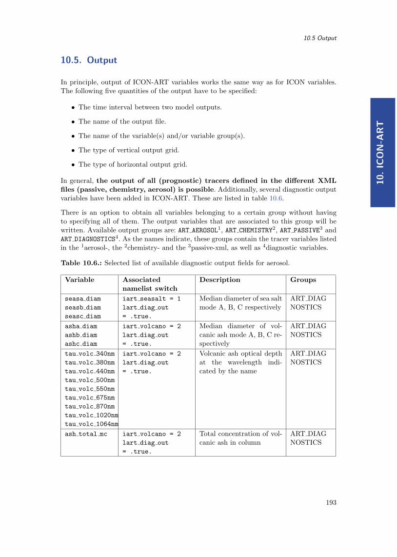
10

.IC

ON

-AR

T

10.5 Output

10.5. Output

In principle, output of ICON-ART variables works the same way as for ICON variables.The following five quantities of the output have to be specified:

• The time interval between two model outputs.

• The name of the output file.

• The name of the variable(s) and/or variable group(s).

• The type of vertical output grid.

• The type of horizontal output grid.

In general, the output of all (prognostic) tracers defined in the different XMLfiles (passive, chemistry, aerosol) is possible. Additionally, several diagnostic outputvariables have been added in ICON-ART. These are listed in table 10.6.

There is an option to obtain all variables belonging to a certain group without havingto specifying all of them. The output variables that are associated to this group will bewritten. Available output groups are: ART AEROSOL1, ART CHEMISTRY2, ART PASSIVE3 andART DIAGNOSTICS4. As the names indicate, these groups contain the tracer variables listedin the 1aerosol-, the 2chemistry- and the 3passive-xml, as well as 4diagnostic variables.

Table 10.6.: Selected list of available diagnostic output fields for aerosol.

Variable Associatednamelist switch

Description Groups

seasa diam

seasb diam

seasc diam

iart seasalt = 1

lart diag out

= .true.

Median diameter of sea saltmode A, B, C respectively

ART DIAGNOSTICS

asha diam

ashb diam

ashc diam

iart volcano = 2

lart diag out

= .true.

Median diameter of vol-canic ash mode A, B, C re-spectively

ART DIAGNOSTICS

tau volc 340nm

tau volc 380nm

tau volc 440nm

tau volc 500nm

tau volc 550nm

tau volc 675nm

tau volc 870nm

tau volc 1020nm

tau volc 1064nm

iart volcano = 2

lart diag out

= .true.

Volcanic ash optical depthat the wavelength indi-cated by the name

ART DIAGNOSTICS

ash total mc iart volcano = 2

lart diag out

= .true.

Total concentration of vol-canic ash in column

ART DIAGNOSTICS

193

10

.IC

ON

-AR

T

11

.D

ata

Ass

imila

tio

n

11. ICON’s Data Assimilation System

In this chapter you will get to know basic components of the ICON data assimilationsystem. It consists of a whole collection of programs and modules both for the atmosphericvariables of the model as well as for soil, snow, ice and sea surface, all collected into theData Assimilation Coding Environment (DACE).

11.1. Data Assimilation

Numerical weather prediction (NWP) is an initial value problem. The ability to make askillful forecast heavily depends on an accurate estimate of the present atmospheric state,known as analysis. In general, an analysis is generated by combining, in an optimal way,all available observations with a short term forecast of a general circulation model (e.g.ICON).

Stated in a more abstract way, the basic idea of data assimilation is to fit model states x toobservations y. Usually, we do not observe model quantities directly or not at the modelgrid points. Here, we work with observation operators H which take a model state andcalculate a simulated observation y = H(x). In terms of software, these model opera-tors can be seen as particular modules, which operate on the ICON model states. Theiroutput is usually written into so-called feedback files, which contain both the real obser-vation ymeas with all its meta data (descriptions, positioning, further information) as wellas the simulated observation y = H(x).

However, data assimilation cannot be treated at one point in time only. The informationpassed on from the past is a crucial ingredient for any data assimilation scheme. Thus,cycling is an important part of data assimilation. It means that we

1. Carry out the core data assimilation component to calculate the so-called analy-sis x(a), i.e. a state which best fits previous information and the observations y,

2. Propagate the analysis x(a)k to the next analysis time tk+1. Here, it is called first

guess or background x(b)k+1.

3. Carry out the next analysis by running the core data assimilation component, gen-

erating x(a)k+1, then cycling the steps.

See Figure 11.1 for a schematic of the basic assimilation process.

11.1.1. Variational Data Assimilation

The basic 3D-VAR step minimizes the functional

µ(x) := ‖x− x(b)‖2B−1 + ‖y −H(x)‖2R−1 , (11.1)

195

11

.D

ata

Assim

ilatio

n

ICON Model Tutorial

Figure 11.1.: Basic ICON cycling environment using 3DVar. Observations are mergedwith a background field taken from a 3 h forecast (first guess) of the ICONmodel. Courtesy of R. Potthast, DWD.

where B is the background state distribution covariance matrix which is making surethat the information which is available at some place is distributed into its neighborhoodproperly, and R is the error covariance matrix describing the error distribution for theobservations. The minimizer of (11.1) is given by

x(a) = x(b) +BHT (R+HBHT )−1(y −H(x(b)). (11.2)

The background or first guess x(b) is calculated from earlier analysis by propagating themodel from a state xk−1 at a previous analysis time tk−1 to the current analysis timetk. In the data assimilation code, the minimization of (11.1) is not carried out explicitlyby (11.2), but by a conjugate gradient minimization scheme, i.e. in an iterative manner,first solving the equation

(R+HBHT )zk = y −H(x(b)k )

in observation space calculating zk at time tk, then projecting the solution back into modelspace by

δxk = x(a)k − x

(b)k = BHT zk.

We call δxk the analysis increment.

The background covariance matrix B is calculated from previous model runs by statisticalmethods. We employ the so-called NMC method initially developed by the US weather

196

11

.D

ata

Ass

imila

tio

n

11.1 Data Assimilation

bureau. The matrix B thus contains statistical information about the relationship betweendifferent variables of the model, which is used in each of the assimilation steps.

11.1.2. Ensemble Kalman Filter

To obtain a better distribution of the information given by observations, modern data as-similation algorithms employ a dynamical estimator for the covariance matrix (B-matrix).Given an ensemble of states x(1), ..., x(L), the standard stochastic covariance estimator cal-culates an estimate for the B-matrix by

B =1

L− 1

∑L

`=1(x

(`)k − xk)(x

(`)k − xk)T , (11.3)

where x denotes the mean defined by

xk =1

L

∑L

`=1x

(`)k , k ∈ N.

This is leading us to the Ensemble Kalman Filter (EnKF), where an ensemble is employedfor data assimilation and the covariance is estimated by (11.3). Here, we use the nameEnKF (ensemble Kalman filter) as a generic name for all methods based on the aboveidea.

In principle, the EnKF carries out cycling as introduced above, just that the propagation

step carries out propagation of a whole ensemble of L atmospheric states x(a,`)k from time tk

to time tk+1, and the analysis step has to generate L new analysis members, called theanalysis ensemble based on the first guess or background ensemble x(b,`), ` = 1, ..., L.

Usually, the analysis is carried out in observation space, where a transformation is carriedout. Also, working with a low number of ensemble members as it is necessary for large-scaledata assimilation problems, we need to suppress spurious correlations which arise from anaive application of Eq. (11.3). This technique is known as localization, and the combinedtransform and localization method is called localized ensemble transform Kalman filter(LETKF), first suggested by Hunt et al. (2007).

The DWD data assimilation coding environment (DACE) provides a state-of-the-art im-plementation of the LETKF which is equipped with several important ingredients suchas different types of covariance inflation. These are needed to properly take care of themodeling error. The original Kalman filter itself does not know what error the model hasand thus by default under-estimates this error, which is counter-acted by a collection oftools.

11.1.3. Hybrid Data Assimilation

The combination of variational and ensemble methods provides many possibilities to fur-ther improve the state estimation of data assimilation. Based on the ensemble Kalmanfilter LETKF the data assimilation coding environment provides a hybrid system EnVar,the ensemble variational data assimilation.

197

11

.D

ata

Assim

ilatio

n

ICON Model Tutorial

The basic idea of EnVar is to use the dynamical flow dependent ensemble covariance matrixB as a part of the three-dimensional variational assimilation. Here, localization is a crucialissue, since in the LETKF we localize in observation space, but 3D-VAR employs B instate space. Localization is carried out by a diffusion-type approximation in DACE.

The cycling for the EnVar needs to cycle both the ensemble x(`), ` = 1, ..., L and onedeterministic state xdet. The resolution of the ensemble can be lower than the full deter-ministic resolution. By default we currently employ a 40 km grid spacing for the ensembleand a 13 km global grid spacing for the deterministic state. The ensemble B matrix isthen carried over to the finer deterministic resolution by interpolation. See Section 11.2for more details on the operational assimilation system at DWD.

11.1.4. Surface Analysis

DACE provides additional modules for Sea Surface Temperature (SST) analysis, Soil Mois-ture Analysis (SMA) and snow analysis. Characteristic time scales of surface and soilprocesses are typically larger than those of atmospheric processes. Therefore, it is oftensufficient to carry out surface analysis only every 6 to 24 hours.

11.2. Assimilation Cycle at DWD

The Assimilation cycle iterates the steps described in Section 11.1: updating a short-range ICON forecast (first guess) using the observations available for that time windowto generate an analysis, from which then a new updated first guess is started.

The core assimilation for atmospheric fields is based on a hybrid system (EnVar) as de-scribed in Section 11.1.3. At every assimilation step (every 3 h) an LETKF is ran usingan ensemble of ICON first guesses. Currently, the ensemble consists of 40 members with ahorizontal grid spacing of 40 km and a 20 km nest over Europe. A convex linear combina-tion of the 3D-VAR climatological and the LETKF’s (flow dependent) covariance matrixis then used to run a deterministic 3D-VAR analysis at 13 km horizontal grid spacing.

In addition, the above mentioned surface modules are ran: Sea Surface Temperature (SST)analysis, Soil Moisture Analysis (SMA) and snow analysis.

Note that for the ICON-EU nest no assimilation of atmospheric fields is conducted. Insteadthe necessary atmospheric analysis increments are interpolated from the underlying globalgrid. Together with the available first guess fields on the nest they form the nest analysis.A separate surface analysis, however, is conducted.

The deterministic as well as the ensemble analysis is generated 8 times a day. Based onthe former, deterministic forecasts are launched at approx. 13 km horizontal grid spacingglobally with a 6.5 km nest over Europe. The maximum forecast time of the whole systemis limited to +30 h lead time at 03/09/15/21 UTC. Otherwise, the system is integrated upto +120 h while at 00/12 UTC the integration on the global domain (only) is prolonged to+180 h lead time.

198

11

.D

ata

Ass

imila

tio

n

11.2 Assimilation Cycle at DWD

Since the beginning of 2018 ICON ensemble forecasts are conducted as well. On the basisof the analysis ensemble 40 short to medium forecasts at 40 km globally and 20 km nestedover Europe are run 8 times a day. The maximum forecast times are equivalent to those ofthe deterministic system (see above). The primary purpose of the ensemble forecasts is toestimate the forecast uncertainty, which arises due to uncertainties in the initial conditionsand the model error.

The input, output and processes involved in the assimilation cycle are briefly describedbelow:

Atmospheric Analysis

Fields modified by the atmospheric analysis: (see Appendix B for a description ofeach variable) t, p, u, v, qv.

Grid(s) on which it is performed: global

Carried out at every assimilation time step (3 h) using the data assimilation algorithmsdescribed in the previous sections.

Main input: First guess, observations, previous analysis error, online bias correction files.

Main output: Analysis of the atmospheric fields, analysis error, bias correction files,feedback files with information on the observation, its departures to first guess and analysis.

The system can make use of the following observations: radiosondes, weather stations,buoys, aircraft, ships, radio occultations, AMV winds and radiances. Available generalfeatures of the module are variational quality control and (variational) online bias correc-tion. Regarding EnKF specifics, different types of inflation techniques, relaxation to priorperturbations and spread, adaptive localization, SST perturbations and SMA perturba-tions are available.

Snow Analysis

Fields modified by the snow analysis: (see Appendix B for a description of eachvariable) freshsnow, h snow, rho snow, t snow, w i, w snow.

Grid(s) on which it is performed: global, EU-nest

Carried out at each assimilation time step (3 h).

Main input: SYNOP snow depth observations if the coverage is sufficient. If this is notthe case, more sources of information are looked for until the number of observations is highenough, namely (and in this order), precipitation and 2 m temperature, direct observations(wwreports) and the NCEP external snow analysis.

Main output: Analysis of the snow fields.

199

ICON Model Tutorial

Sea Surface Temperature Analysis

Fields modified by the SST analysis: (see Appendix B for a description of eachvariable) fr seaice, h ice, t ice, t so.

Grid(s) on which it is performed: global, EU-nest

Carried out only once a day, at 0 UTC.

Main input: NCEP analysis from the previous day (which uses satellite, buoy and shipobservations, to be used as a first guess), ship and buoy observations available since thetime of the NCEP analysis.

Main output: Sea surface temperature analysis and estimated error.

Soil Moisture Analysis

Fields modified by the SMA analysis: (see Appendix B for a description of eachvariable) w so.

Grid(s) on which it is performed: global, EU-nest

Carried out only once a day, at 0 UTC.

Main input: Background fields for relevant fields at every hour since last assimilation,2 m-temperature analysis (see below) to be used as observations.

Main output: Soil moisture analysis and estimated error.

2m-Temperature Analysis

Although carried out only at 0 UTC, it is run for several time steps in between to providethe output (2 m temperature) needed by the SMA analysis. Uses observations from SYNOPstations on land and METAR information from airports.

200

A.

DW

DH

PC

Sys

tem

A. The Computer System at DWD

Available Platforms at DWD

The NWP exercises will be mainly carried out on the Cray XC 40 supercomputer systemat DWD. This system consists of several compute nodes with corresponding service nodes.

• xce00.dwd.de, xce01.dwd.de:These are the login nodes, which run a SUSE Linux Enterprise (SLES) Linux. Thenodes are used for compiling and linking, preparation of data and basic editingwork. They are not used for running parallel programs, but jobs can be submittedto the Cray XC 40 compute nodes.

• Cray XC 40:The Cray XC 40 has 432 compute nodes, where each node is equipped with 2 IntelHaswell processors with 12 cores and a second node partition with 864 Intel Broad-well nodes. Each Haswell node therefore has 24 computational cores (Broadwell: 36).These nodes cannot be accessed interactively, but only by batch jobs. Such jobscan use up to 62 GByte of main memory per node, which is about 2.5 GByte percore (Broadwell: 1.7 GByte). For normal test jobs it should be enough to use 10-15nodes (depending on the chosen grid resolution).

• lce00.dwd.de, lce01.dwd.de:Tools for the visualization of meteorological fields (CDO, NCL, ncview) areonly available on the pre-/post-processing cluster lce. This cluster comprises 66Haswell batch nodes, but we will only use the login nodes lce00, lce01 during thecourse.

There is a common filesystem across all nodes and every user has three different maindirectories:

• /e/uhome/username ($HOME)Directory for storing source code and scripts to run the model. This is a Panasas filesystem suitable for many small files.

• /e/uwork/username ($WORK)Directory for storing larger amounts of data.

• /e/uscratch/username ($SCRATCH)Directory for storing very large amounts of data. For the $WORK and the $SCRATCH

filesystem there is a common quota for every user of 2.5 TByte.

201

A.

DW

DH

PC

System

ICON Model Tutorial

The Batch System for the Cray XC 40

Jobs for the Cray XC 40 system have to be submitted with the batch system PBS. Thesebatch jobs may either be launched from the Linux cluster lce or from the XC 40 loginnodes xce00/01. Together with the source code of the programs we provide some runscripts in which all necessary batch commands are set.

Here are the most important commands for working with the PBS:

qsub job name to submit a batch job to PBS. This is done in the runscripts.

qstat to query the status of all batch jobs on the XC 40. Youcan see whether jobs are Q (queued) or R (running). Youhave to submit jobs to the queue xc norm h.

qstat -u user to query the status of all your batch jobs on the machine.

qdel job nr@machine to cancel your job(s) from the batch queue of a machine.The job nr is given by qstat -w.

qcat -f job nr@machine To follow stdout and stderr interactively.

In your run scripts, execution begins in your home directory, regardless of what directoryyour script resides in or where you submitted the job from. You can use the cd commandto change to a different directory. The environment variable $PBS O WORKDIR makes it easyto return to the directory from which you submitted the job:

cd $PBS_O_WORKDIR

202

B.

Ou

tpu

tV

aria

ble

s

B. Table of ICON Output Variables

The following table contains the NWP variables available for output1. Please note that thefield names are following an ICON-internal nomenclature, see Section 7.1 for details. Thelist also contains tile-based fields (suffix t 1, t 2, . . .) which are summarized as t *.

By ”ICON-internal” variable names, we denote those field names that are pro-vided as the string argument name to the subroutine calls CALL add_var(...) andCALL add_ref(...) inside the ICON source code. These subroutine calls have the pur-pose to register new variables, to allocate the necessary memory, and to set the meta-datafor these variables.

Variable Name GRIB2 Name Description

acdnc ndcloud Cloud droplet number concentration

adrag_u_grid Zonal resolved surface stress mean since model start

adrag_v_grid Meridional resolved surface stress mean since model start

aer_bc aer_bc Black carbon aerosol

aer_du aer_dust Total soil dust aerosol

aer_or aer_org Organic aerosol

aer_ss aer_ss Sea salt aerosol

aer_su aer_so4 Total sulfate aerosol

aercl_bc Black carbon aerosol climatology

aercl_du Total soil dust aerosol climatology

aercl_or Organic aerosol climatology

aercl_ss Sea salt aerosol climatology

aercl_su Total sulfate aerosol climatology

alb_dif alb_dif Shortwave albedo for diffuse radiation

alb_si alb_seaice Sea ice albedo (diffuse)

albdif_t_* alb_rad Tile-based shortwave albedo for diffusive radiation

albdif alb_rad Shortwave albedo for diffuse radiation

albni_dif alb_ni Near IR albedo for diffuse radiation

albnirdif_t_* alb_ni Tile-based near IR albedo for diffuse radiation

albnirdif alb_ni Near IR albedo for diffuse radiation

albnirdir alnip Near IR albedo for direct radiation

albuv_dif alb_uv UV visible albedo for diffuse radiation

albvisdif_t_* alb_uv Tile-based UV visible albedo for diffusive radiation

albvisdif alb_uv UV visible albedo for diffuse radiation

albvisdir aluvp UV visible albedo for direct radiation

alhfl_bs alhfl_bs Latent heat flux from bare mean since model start

alhfl_pl alhfl_pl Latent heat flux from plantmean since model start

alhfl_s alhfl_s surface latent heat flux mean since model start

aqhfl_s evapt surface moisture flux mean since model start

Continued on next page

1The Table B.1 in this Appendix is based on the revision state 77cdb449 (2019-02-27).

203

B.

Ou

tpu

tV

ariab

les

ICON Model Tutorial

Table B.1 – Continued from previous page

Variable Name GRIB2 Name Description

ashfl_s ashfl_s Surface sensible heat flux mean since model start

asob_s asob_s Surface net solar radiation mean since model start

asob_t asob_t TOA net solar radiation mean since model start

asod_t sodt_rad Top down solar radiation mean since model start

asodifd_s aswdifd_s Surface down solar diff. rad. mean since model start

asodifu_s aswdifu_s Surface up solar diff. rad. mean since model start

asodird_s aswdir_s Surface down solar direct rad.mean since model start

asou_t uswrf Top up solar radiation mean since model start

astr_u_sso lgws Zonal sso surface stress mean since model start

astr_v_sso mgws Meridional sso surface stress mean since model start

aswflx_par_sfc apab_s Downward PAR flux mean since model start

athb_s athb_s Surface net thermal radiation mean since model start

athb_t athb_t TOA net thermal radiation mean since model start

athd_s athd_s Surface down thermal radiationmean since model start

athu_s athu_s Surface up thermal radiation mean since model start

aumfl_s aumfl_s U-momentum flux flux at sumean since model start

avg_qc tqc_dia Tci specific cloud water content (diagnostic) avg

avg_qi tqi_dia Tci specific cloud ice content (diagnostic) avg

avg_qv tqv_dia Column integrated water vapour (diagnostic) avg

avmfl_s avmfl_s V-momentum flux flux at sumean since model start

c_t_lk c_t_lk Shape factor (temp. profile in lake thermocline)

cape_ml cape_ml Cape of mean surface layer parcel

cape cape_con Conv avail pot energy

cin_ml cin_ml Convective inhibition of mean surface layer parcel

clch clch High level clouds

clcl clcl Low level clouds

clcm clcm Mid level clouds

clct_avg clct Total cloud cover time avg

clct_mod clct_mod Modified total cloud cover for media

clct clct Total cloud cover

clc clc Cloud cover

cldepth cldepth Modified cloud depth for media

cloud_num Cloud droplet number concentration

con_gust Convective contribution to wind gust

cosmu0 uvcossza Cosine of solar zenith angle

ddt_adv_q Advective tracer tendency

ddt_exner_phy Exner pressure physical tendency

ddt_grf_q Tracer tendency for grid refinement

ddt_pres_sfc dpsdt Surface pressure tendency

ddt_qc_conv Convective tendency of cloud water mass density

ddt_qc_gscp Microphysics tendency of specific cloud water

ddt_qc_turb Turbulence tendency of specific cloud water

ddt_qi_conv Convective tendency of cloud ice mass density

ddt_qi_gscp Microphysics tendency of specific cloud ice

ddt_qi_turb Turbulence tendency of specific cloud ice

ddt_qr_conv Convective tendency of rain mass density

ddt_qr_gscp Microphysics tendency of rain

Continued on next page

204

B.

Ou

tpu

tV

aria

ble

s

Table B.1 – Continued from previous page

Variable Name GRIB2 Name Description

ddt_qs_conv Convective tendency of snow mass density

ddt_qs_gscp Microphysics tendency of snow

ddt_qv_conv Convective tendency of absolute humidity

ddt_qv_gscp Microphysics tendency of specific humidity

ddt_qv_turb qtendt Turbulence tendency of specific humidity

ddt_temp_drag ttends Sso + gwdrag temperature tendency

ddt_temp_dyn Dynamical temperature tendency

ddt_temp_gscp Microphysical temperature tendency

ddt_temp_pconv dt_con Convective temperature tendency

ddt_temp_radlw thhr_rad Long wave radiative temperature tendency

ddt_temp_radsw sohr_rad Short wave radiative temperature tendency

ddt_temp_turb ttendts Turbulence temperature tendency

ddt_tke_hsh dtke_hsh TKE tendency horizonzal shear production

ddt_tke_pconv dtke_con TKE tendency due to sub-grid scale convection

ddt_tke tketens Tendency of turbulent velocity scale

ddt_u_gwd ewgd GWD tendency of zonal wind

ddt_u_pconv du_con Convective tendency of zonal wind

ddt_u_sso du_sso Sso tendency of zonal wind

ddt_u_turb utendts Turbulence tendency of zonal wind

ddt_v_gwd nsgd GWD tendency of meridional wind

ddt_v_pconv dv_con Convective tendency of meridional wind

ddt_v_sso dv_sso Sso tendency of meridional wind

ddt_v_turb vtendts Turbulence tendency of meridional wind

ddt_vn_adv Advective normal wind tendency

ddt_vn_phy Normal wind physical tendency

ddt_w_adv Advective vertical wind tendency

depth_lk depth_lk Lake depth

dgeopot_mc fi Geopotential difference between half levels

div_ic Divergence at half levels

div rdiv Divergence

dp_bs_lk Depth of thermally active layer of bot. sediments.

dpres_mc Pressure thickness

drag_u_grid Zonal resolved surface stress

drag_v_grid Meridional resolved surface stress

dtheta_v_ic_ubc Potential temperature at child upper boundary

dvn_ie_int Normal velocity at parent interface level

dvn_ie_ubc Normal velocity at child upper boundary

dw_ubc Vertical velocity at child upper boundary

dwdx Zonal gradient of vertical wind

dwdy Meridional gradient of vertical wind

dyn_gust Dynamical gust

eai (evaporative) earth area index

emis_rad emis_rad Longwave surface emissivity

exner_dyn_incr Exner dynamics increment

exner_pr exner Exner perturbation pressure

exner_ref_mc Reference atmosphere field exner

exner exner Exner pressure

Continued on next page

205

B.

Ou

tpu

tV

ariab

les

ICON Model Tutorial

Table B.1 – Continued from previous page

Variable Name GRIB2 Name Description

fetch_lk fetch_lk Wind fetch over lake

fis fis Geopotential (s)

for_d for_d Fraction of deciduous forest

fr_glac Fraction glacier

fr_lake fr_lake Fraction lake

fr_land fr_land Fraction land

fr_seaice fr_ice Fraction of sea ice

frac_t_* fr_luc Tile point area fraction list

freshsnow_t_* freshsnw Indicator for age of snow in top of snow layer

freshsnow freshsnw Weighted indicator for age of snow in top of snow layer

gamso_lk Attenuation coefficient of lake water with respect to sol.rad.

geopot_agl_ifc fi Geopotential above groundlevel at cell center

geopot_agl fi Geopotential above groundlevel at cell center

geopot fi Geopotential at full level cell centre

graupel_gsp_rate prg_gsp Gridscale graupel rate

graupel_gsp grau_gsp Gridscale graupel

grf_tend_mflx Normal mass flux tendency (grid refinement)

grf_tend_rho Density tendency (grid refinement)

grf_tend_thv Virtual potential temperature tendency (grid refinement)

grf_tend_vn Normal wind tendency (grid refinement)

grf_tend_w Vertical wind tendency (grid refinement)

gust vmax_10m Gust at 10 m

gz0_t_* z0 Tile-based roughness length times gravity

gz0 z0 Roughness length

h_b1_lk h_b1_lk Thickness of the upper layer of the sediments

h_ice h_ice Sea/lake-ice depth

h_ml_lk h_ml_lk Mixed-layer thickness

h_snow_lk Depth of snow on lake ice

h_snow_si Depth of snow on sea ice

h_snow_t_* h_snow Snow height

h_snow h_snow Weighted snow depth

hbas_con hbas_con Height of convective cloud base

hdef_ic Deformation

hfl_q Horizontal tracer flux

hmo3 Height of O3 maximum (Pa)

htop_con htop_con Height of convective cloud top

htop_dc htop_dc Height of top of dry convection

hzerocl hzerocl Height of 0 deg C level

k400 Level index corresponding to the HAG of the 400hPalevel

k800 Level index corresponding to the HAG of the 800hPalevel

k850 Level index corresponding to the HAG of the 850hPalevel

k950 Level index corresponding to the HAG of the 950hPalevel

Continued on next page

206

B.

Ou

tpu

tV

aria

ble

s

Table B.1 – Continued from previous page

Variable Name GRIB2 Name Description

ktype Type of convection

lai lai Leaf Area Index

lc_class_t_* luc Tile point land cover class

lhfl_bs_t_* Tile-based latent heat flux from bare soil

lhfl_bs Latent heat flux from bare soil

lhfl_pl_t_* Tile-based latent heat flux from plants

lhfl_pl Latent heat flux from plants

lhfl_s_t_* lhfl_s Tile-based surface latent heat flux

lhfl_s lhfl_s Surface latent heat flux

lw_emiss emis_rad Longwave surface emissivity

lwflxall nlwrf Longwave net flux

mask_mtnpoints_g Mask field for mountain points

mask_mtnpoints Mask field for mountain points

mass_fl_e_sv Storage field for horizontal mass flux at edges

mass_fl_e Horizontal mass flux at edges

ndvi_max NDVI yearly maximum

ndviratio ndviratio (monthly) proportion of actual value/maximum NDVI(at init time)

o3 o3 Ozone mixing ratio

omega_z relv Vertical vorticity

pat_len Length scale of sub-grid scale roughness elements

plcov_t_* plcov Plant covering degree in the vegetation phase

plcov plcov Plant covering degree in the vegetation phase

prec_con_rate_avg cprat Convective precip rate, time average

prec_con prec_con Convective precip

prec_gsp_rate_avg lsprate Gridscale precip rate, time average

prec_gsp prec_gsp Gridscale precip

pref_aerdis Reference pressure used for vertical distribution ofaerosol optical depths

pres_ifc p Pressure at half level

pres_msl pmsl Mean sea level pressure

pres_sfc ps Surface pressure

pres p Pressure

pv pot_vortic Potential vorticity

q_int Q at parent interface level

q_ubc Q at child upper boundary

qcfl_s Surface cloud water deposition flux due to diffusion

qc qc Specific cloud water content

qg qg Specific graupel content

qhfl_s_t_* evapt Tile based surface moisture flux

qhfl_s evapt Surface moisture flux

qifl_s Surface cloud ice deposition flux due to diffusion

qi qi Specific cloud ice content

qr qr Rain mixing ratio

qs qs Snow mixing ratio

qv_2m qv_2m Specific water vapor content in 2m

Continued on next page

207

B.

Ou

tpu

tV

ariab

les

ICON Model Tutorial

Table B.1 – Continued from previous page

Variable Name GRIB2 Name Description

qv_s_t_* qv_s Specific humidity at the surface

qv_s qv_s Specific humidity at the surface

qv qv Specific humidity

rain_con_rate_3d prr_con 3d convective rain rate

rain_con_rate prr_con Convective rain rate

rain_con rain_con Convective rain

rain_gsp_rate prr_gsp Gridscale rain rate

rain_gsp rain_gsp Gridscale rain

rain_upd Rain in updroughts

rcld Standard deviation of the saturation deficit

rh_2m_land relhum_2m_l Relative humidity in 2m over land fraction

rh_2m relhum_2m Relative humidity in 2m

rho_ic den Density at half level

rho_ref_mc Reference atmosphere field density

rho_ref_me Reference atmosphere field density

rho_snow_t_* rho_snow Snow density

rho_snow rho_snow Weighted snow density

rho den Density

rootdp rootdp Root depth of vegetation

rsmin rsmin Minimal stomata resistence

rstom rstom Stomatal resistance

runoff_g_t_* watr Soil water runoff; sum over forecast

runoff_g runoff_g Weighted soil water runoff; sum over forecast

runoff_s_t_* watr Surface water runoff; sum over forecast

runoff_s runoff_s Weighted surface water runoff; sum over forecast

sai Surface area index

shfl_s_t_* shfl_s Tile-based surface sensible heat flux

shfl_s shfl_s Surface sensible heat flux

slope_angle Slpe angle

slope_azimuth Slpe azimuth

smi smi Soil moisture index

snow_con_rate_3d prs_con 3d convective snow rate

snow_con_rate prs_con Convective snow rate

snow_con snow_con Convective snow

snow_gsp_rate prs_gsp Gridscale snow rate

snow_gsp snow_gsp Gridscale snow

snowfrac_lc_t_* snowc Tile-based snow-cover fraction

snowfrac_lcu_t_* Tile-based snow-cover fraction

snowfrac_lc snowc Snow-cover fraction

snowfrac_t_* Local tile-based snow-cover fraction

snowfrac Snow-cover fraction

snowlmt snowlmt Height of snow fall limit above MSL

sob_s_t_* sobs_rad Tile-based shortwave net flux at surface

sob_s sobs_rad Shortwave net flux at surface

sob_t sobt_rad Shortwave net flux at TOA

sod_t sodt_rad Downward shortwave flux at TOA

sodifd_s swdifds_rad Shortwave diffuse downward flux at surface

Continued on next page

208

B.

Ou

tpu

tV

aria

ble

s

Table B.1 – Continued from previous page

Variable Name GRIB2 Name Description

soiltyp soiltyp Soil type

sou_s swdifus_rad Shortwave upward flux at surface

sou_t uswrf Shortwave upward flux at TOA

sp_10m sp_10m Wind speed in 10m

sso_gamma sso_gamma Anisotropy of sub-gridscale orography

sso_sigma sso_sigma Slope of sub-gridscale orography

sso_stdh_raw Standard deviation of sub-grid scale orography

sso_stdh sso_stdh Standard deviation of sub-grid scale orography

sso_theta sso_theta Angle of sub-gridscale orography

str_u_sso lgws Zonal sso surface stress

str_v_sso mgws Meridional sso surface stress

swflx_par_sfc pabs_rad Downward photosynthetically active flux at surface

t_2m_land t_2m_l Temperature in 2m over land fraction

t_2m t_2m Temperature in 2m

t_b1_lk t_b1_lk Temperature at the bottom of the upper layer of thesediments

t_bot_lk t_bot_lk Temperature at the water-bottom sediment interface

t_bs_lk Clim. temp. at bottom of thermally active layer ofsediments

t_cl t_2m_cl CRU near surface temperature climatology

t_g_t_* t_g Weighted surface temperature

t_g t_g Weighted surface temperature

t_ice t_ice Sea/lake-ice temperature

t_mnw_lk t_mnw_lk Mean temperature of the water column

t_s_t_* t_s Temperature of ground surface

t_seasfc t_sea Sea surface temperature

t_snow_lk Temperature of snow on lake ice

t_snow_si Temperature of snow on sea ice

t_snow_t_* t_snow Temperature of the snow-surface

t_snow t_snow Weighted temperature of the snow-surface

t_so_t_* t_so Soil temperature (main level)

t_so t_so Weighted soil temperature (main level)

t_s t_s Weighted temperature of ground surface

t_wml_lk t_wml_lk Mixed-layer temperature

tai Transpiration area index

tch_t_* tch Tile-based turbulent transfer coefficients for heat

tch tch Turbulent transfer coefficients for heat

tcm_t_* tcm Tile-based turbulent transfer coefficients for momentum

tcm tcm Turbulent transfer coefficients for momentum

td_2m_land td_2m_l Dew-point in 2m over land fraction

td_2m td_2m Dew-point in 2m

temp_ifc t Temperature at half level

tempv vtmp Virtual temperature

temp t Temperature

tfh Factor of laminar transfer of scalars

tfm Factor of laminar transfer of momentum

tfv_t_* nswrs Tile-based laminar reduction factor for evaporation

tfv Laminar reduction factor for evaporation

Continued on next page

209

B.

Ou

tpu

tV

ariab

les

ICON Model Tutorial

Table B.1 – Continued from previous page

Variable Name GRIB2 Name Description

thb_s_t_* thbs_rad Tile-based longwave net flux at surface

thb_s thbs_rad Longwave net flux at surface

theta_ref_ic Reference atmosphere field theta

theta_ref_mc Reference atmosphere field theta

theta_ref_me Reference atmosphere field theta

theta_v_ic theta_v Virtual potential temperature at half levels

theta_v theta_v Virtual potential temperature

thu_s thus_rad Longwave upward flux at surface

tke tke Turbulent kinetic energy

tkr_t_* Tile-based turbulent reference surface diffusion coefficient

tkred_sfc Reduction factor for minimum diffusion coefficients

tkr Turbulent reference surface diffusion coefficient

tkvh tkvh turbulent diffusion coefficients for heat

tkvm tkvm turbulent diffusion coefficients for momentum

tmax_2m tmax_2m Max 2m temperature

tmin_2m tmin_2m Min 2m temperature

topography_c hsurf Geometric height of the earths surface above sea level

tot_prec_rate_avg tot_pr Total precip rate, time average

tot_prec tot_prec Total precip

tot_qc_dia qc_dia Total specific cloud water content (diagnostic)

tot_qi_dia qi_dia Total specific cloud ice content (diagnostic)

tot_qv_dia qv_dia Total specific humidity (diagnostic)

tqc_dia tqc_dia Total column integrated cloud water (diagnostic)

tqc tqc Total column integrated cloud water

tqg tqg Total column integrated graupel

tqi_dia tqi_dia Total column integrated cloud ice (diagnostic)

tqi tqi Total column integrated cloud ice

tqr tqr Total column integrated rain

tqs tqs Total column integrated snow

tqv_dia tqv_dia Total column integrated water vapour (diagnostic)

tqv tqv Total column integrated water vapour

tracer_vi_avg Average of vertically integrated tracers

trsolall Shortwave net tranmissivity

tsfc_ref Reference surface temperature

tsfctrad Surface temperature at trad

tvh_t_* Tile-based turbulent transfer velocity for heat

tvh Turbulent transfer velocity for heat

tvm_t_* Tile-based turbulent transfer velocity for momentum

tvm Turbulent transfer velocity for momentum

u_10m_t_* u_10m Tile-based zonal wind in 2m

u_10m u_10m Zonal wind in 10m

umfl_s_t_* umfl_s U-momentum flux at the surface

umfl_s umfl_s U-momentum flux at the surface

u u Zonal wind

v_10m_t_* v_10m Tile-based meridional wind in 2m

v_10m v_10m Meridional wind in 10m

vfl_q Vertical tracer flux

Continued on next page

210

B.

Ou

tpu

tV

aria

ble

s

Table B.1 – Continued from previous page

Variable Name GRIB2 Name Description

vio3 tozne Vertically integrated ozone amount

vmfl_s_t_* vmfl_s V-momentum flux at the surface

vmfl_s vmfl_s V-momentum flux at the surface

vn_ie vn Normal wind at half level

vn vn Velocity normal to edge

vor relv Vorticity

vt vt Tangential-component of wind

vwind_expl_wgt Explicit weight in vertical wind solver

vwind_impl_wgt Implicit weight in vertical wind solver

v v Meridional wind

w_concorr_c Contravariant vertical correction

w_i_t_* w_i Weighted water content of interception water

w_i w_i Weighted water content of interception water

w_snow_t_* w_snow Water equivalent of snow

w_snow w_snow Weighted water equivalent of snow

w_so_ice_t_* w_so_ice Ice content

w_so_ice w_so_ice Ice content

w_so_t_* w_so Total water content (ice + liquid water)

w_so w_so Total water content (ice + liquid water)

ww ww Significant weather

w w Vertical velocity

z_ifc hhl Geometric height at half level center

z_mc h Geometric height at full level center

List of ICON Variable Groups

The "group:" keyword for the namelist parameters ml varlist, hl varlist, pl varlist

(namelist output nml) can be used to activate a set of common variables for output atonce. The following lists contain the variables for each of these groups (empty groups andgroups with only a single entry are omitted).

Group ADDITIONAL_PRECIP_VARS

cape, clct, clct_mod, prec_con_rate_avg, prec_gsp_rate_avg, tqc_dia, tqi_dia,tqv_dia

Group ATMO_DERIVED_VARS

div, omega_z, vor

Group ATMO_ML_VARS

pres, qc, qg, qi, qr, qs, qv, temp, tke, u, v, w

Group ATMO_PL_VARS

qc, qg, qi, qr, qs, qv, temp, tke, u, v, w

Group ATMO_ZL_VARS

pres, qc, qg, qi, qr, qs, qv, temp, tke, u, v, w

Group CLOUD_DIAG

clc, tot_qc_dia, tot_qi_dia, tot_qv_dia

211

B.

Ou

tpu

tV

ariab

les

ICON Model Tutorial

Group DWD_FG_ATM_VARS

pres, pres_sfc, qc, qg, qi, qr, qs, qv, rho, t_2m, td_2m, temp, theta_v, tke, u, u_10m, v,v_10m, vn, w, z_ifc

Group DWD_FG_SFC_VARS

alb_si, c_t_lk, fr_land, fr_seaice, freshsnow, gz0, h_ice, h_ml_lk, h_snow,hsnow_max, plantevap, qv_s, rho_snow, snow_age, snowfrac_lc, t_bot_lk, t_g, t_ice,t_mnw_lk, t_seasfc, t_snow, t_so, t_wml_lk, w_i, w_snow, w_so, w_so_ice

Group DWD_FG_SFC_VARS_T

freshsnow_t_*, h_snow_t_*, plantevap_t_*, qv_s_t_*, rho_snow_t_*,snowfrac_lc_t_*, t_g_t_*, t_snow_t_*, t_so_t_*, w_i_t_*, w_snow_t_*,w_so_ice_t_*, w_so_t_*

Group ICON_LBC_VARS

pres, qc, qi, qr, qs, qv, temp, tke, u, v, w, z_ifc

Group LAND_TILE_VARS

h_snow_t_*, plantevap_t_*, qv_s_t_*, rho_snow_t_*, snowfrac_lc_t_*,snowfrac_t_*, t_g_t_*, t_s_t_*, t_snow_t_*, t_so_t_*, w_i_t_*, w_snow_t_*,w_so_ice_t_*, w_so_t_*

Group LAND_VARS

qv_s, rho_snow, snowfrac, snowfrac_lc, t_g, t_snow, t_so, w_i, w_snow, w_so, w_so_ice

Group LATBC_PREFETCH_VARS

pres, pres_sfc, qc, qi, qr, qs, qv, rho, temp, theta_v, u, v, vn, w, z_ifc

Group MODE_COMBINED_IN

fr_seaice, freshsnow, h_ice, h_snow, qv_s, rho_snow, t_g, t_ice, t_snow, t_so, w_i,w_snow, w_so

Group MODE_COSMO_IN

alb_si, freshsnow, h_ice, qv_s, rho_snow, t_g, t_ice, t_snow, t_so, w_i, w_snow, w_so

Group MODE_DWD_ANA_IN

fr_seaice, freshsnow, h_ice, h_snow, pres, qv, t_ice, t_seasfc, t_snow, t_so, temp, u,v, w_so

Group MODE_DWD_FG_IN

alb_si, c_t_lk, gz0, h_ml_lk, hsnow_max, plantevap, qc, qg, qi, qr, qs, qv_s, rho,rho_snow, snow_age, t_bot_lk, t_g, t_mnw_lk, t_so, t_wml_lk, theta_v, tke, vn, w, w_i,w_snow, w_so_ice, z_ifc

Group MODE_IAU_ANAATM_IN

pres, qc, qi, qv, temp, u, v

Group MODE_IAU_ANA_IN

fr_seaice, freshsnow, h_snow, pres, qc, qi, qv, t_seasfc, t_so, temp, u, v, w_so

Group MODE_IAU_FG_IN

alb_si, c_t_lk, freshsnow, gz0, h_ice, h_ml_lk, h_snow, hsnow_max, plantevap, qc, qg,qi, qr, qs, qv, qv_s, rho, rho_snow, snow_age, snowfrac_lc, t_bot_lk, t_g, t_ice,t_mnw_lk, t_snow, t_so, t_wml_lk, theta_v, tke, vn, w, w_i, w_so, w_so_ice

212

B.

Ou

tpu

tV

aria

ble

s

Group MODE_IAU_OLD_ANA_IN

fr_seaice, freshsnow, h_snow, pres, qv, rho_snow, t_seasfc, t_so, temp, u, v, w_snow,w_so

Group MODE_IAU_OLD_FG_IN

alb_si, c_t_lk, gz0, h_ice, h_ml_lk, qc, qi, qr, qs, qv, qv_s, rho, t_bot_lk, t_g,t_ice, t_mnw_lk, t_snow, t_so, t_wml_lk, theta_v, tke, vn, w, w_i, w_so, w_so_ice

Group MODE_INIANA

alb_si, c_t_lk, fr_land, fr_seaice, freshsnow, gz0, h_ice, h_ml_lk, h_snow,hsnow_max, plantevap, pres, qc, qi, qr, qs, qv, qv_s, rho_snow, smi, snow_age,t_bot_lk, t_g, t_ice, t_mnw_lk, t_snow, t_so, t_wml_lk, temp, tke, u, v, w, w_i,w_snow, w_so_ice, z_ifc

Group NH_PROG_VARS

exner, rho, theta_v, vn

Group PBL_VARS

alhfl_s, aqhfl_s, ashfl_s, gust10, lhfl_bs, lhfl_s, qhfl_s, qv_2m, shfl_s, t_2m,t_2m_land, tch, tcm, td_2m, td_2m_land, tkr, tkvh, tkvm, tvh, tvm, u_10m, v_10m

Group PHYS_TENDENCIES

ddt_temp_drag, ddt_temp_radlw, ddt_temp_radsw, ddt_temp_turb, ddt_u_gwd,ddt_u_sso, ddt_u_turb, ddt_v_gwd, ddt_v_sso, ddt_v_turb

Group PRECIP_VARS

graupel_gsp, prec_con, prec_gsp, rain_con, rain_gsp, snow_con, snow_gsp, tot_prec

Group RAD_VARS

albdif, albnirdif, albvisdif, asob_s, asob_t, asod_t, asodifd_s, asodifu_s,asodird_s, asou_t, aswflx_par_sfc, athb_s, athb_t, athd_s, athu_s, sob_s,sob_s_t_*, sob_t, sod_t, sodifd_s, sou_s, sou_t, swflx_par_sfc, thb_s, thb_s_t_*,thu_s

Group SNOW_VARS

rho_snow, t_snow

213

B.

Ou

tpu

tV

ariab

les

C.

Exe

rcis

es

C. Exercises

On the following pages a number of exercises is provided. These exercises revisit the topicsof the individual chapters and range from easy tests to the setup of complex forecastsimulations.

Ex. C.1.1: Installation of the model package

Ex. C.4.1: Running idealized test casesEx. C.4.2: Nested sub-domains

Ex. C.4.3: Tracer advection

Ex. C.2.1: Grid generator and ExtPar web interface

Ex. C.2.2: Retrieving DWD analysis data Ex. C.2.3: Retrieving IFS data

Ex. C.5.1:Global ICON forecastfrom DWD analysis

Ex. C.5.2: Time-stepping

Ex. C.5.3: Run-time performance

Ex. C.5.4: Parallel scaling

Ex. C.5.5: Writing output for driving ICON-LAMEx. C.5.6: Spin-up effects

Ex. C.5.7: Bit-reproducibility

Ex. C.2.4: Preparation of limited area run

Ex. C.6.1: Limited area run Ex. C.6.2: Modifying the temporal resolution

Ex. C.6.3: Driving ICON-LAM by DWD Data

Ex. C.8.1: Allocating Additional Fields

Ex. C.8.2: Looping over grid points

Ex. C.8.3: Implementing own diagnostics

Installation

Idealized

Tests

Real Data

Runs

ICON-LAM

Programming

ICON

215

C.

Exercises

ICON Model Tutorial

List of Exercises

Installation of the ICON Model Package 217Exercise 1.1 . . . . . . . . . . . . . . . . . . . . . . . . . . . . . . . . . . . . . . . 217

Necessary Input Data 217Exercise 2.1: Grid Generator and ExtPar Web Interface . . . . . . . . . . . . . . 218Exercise 2.2: Retrieving DWD Analysis Data . . . . . . . . . . . . . . . . . . . . 218Exercise 2.3: Retrieving IFS Data . . . . . . . . . . . . . . . . . . . . . . . . . . . 219Exercise 2.4: Preparation of Limited Area Runs . . . . . . . . . . . . . . . . . . . 220

Running Idealized Test Cases 221Exercise 4.1: Jablonowski-Williamson Test Case . . . . . . . . . . . . . . . . . . . 221Exercise 4.2: Nested Sub-Domain . . . . . . . . . . . . . . . . . . . . . . . . . . . 223Exercise 4.3: Tracer Advection . . . . . . . . . . . . . . . . . . . . . . . . . . . . 224

Real Data Test Cases 225Exercise 5.1: Starting a Global ICON Forecast from DWD Analysis . . . . . . . . 226Exercise 5.2: Time-stepping . . . . . . . . . . . . . . . . . . . . . . . . . . . . . . 227Exercise 5.3: Run-Time Performance . . . . . . . . . . . . . . . . . . . . . . . . . 228Exercise 5.4: Parallelization . . . . . . . . . . . . . . . . . . . . . . . . . . . . . . 228Exercise 5.5: Writing Output for Driving a Limited Area Simulation . . . . . . . 230Exercise 5.6: A Deeper Look into Spin-Up Effects . . . . . . . . . . . . . . . . . . 231Exercise 5.7: Checking for Bit-Reproducibility . . . . . . . . . . . . . . . . . . . . 234

Limited Area Mode 234Exercise 6.1: Limited Area Run . . . . . . . . . . . . . . . . . . . . . . . . . . . . 234Exercise 6.2: Modifying the Temporal Resolution . . . . . . . . . . . . . . . . . . 237Exercise 6.3: Driving ICON-LAM by DWD Data . . . . . . . . . . . . . . . . . . 237

Programming ICON 240Exercise 8.1: Allocating Additional Fields . . . . . . . . . . . . . . . . . . . . . . 240Exercise 8.2: Looping Over Grid Points . . . . . . . . . . . . . . . . . . . . . . . 241Exercise 8.3: Implementing New Diagnostics . . . . . . . . . . . . . . . . . . . . . 242

Running ICON-ART 243Exercise 10.1: Point Sources in ICON-ART LAM . . . . . . . . . . . . . . . . . . 243Exercise 10.2: Very Short-lived Substances . . . . . . . . . . . . . . . . . . . . . . 243Exercise 10.3: Volcano Eruption . . . . . . . . . . . . . . . . . . . . . . . . . . . . 244Exercise 10.4: Sea Salt Aerosol . . . . . . . . . . . . . . . . . . . . . . . . . . . . 245

216

C.

Exe

rcis

es

C.1 Installation of the ICON Model Package

C.1. Installation of the ICON Model Package

For practical work during these exercises, you need information about the use of thecomputer systems and from where you can access the necessary files and data. Please takea look at Appendix A to get information on how to use DWD’s supercomputer and runtest jobs.

In this exercise we will extract and build the ICON model and its pre-processing tools:

EX 1.1

Log into the Cray XC 40 login node “xce” and install the ICON model in the$WORK directory of your Cray XC 40 user account. For that you have to do thefollowing:

• The necessary files for the ICON tutorial can be found in the subdirectory

/e/uwork/trng024/packages

Copy the tar-file icon tutorial.tar.gz into your $WORK directory.

• Change into your $WORK directory and extract the compressed tar file to yieldthe directory structure depicted in Figure 1.1 containing the ICON sourcesand test data.

• Follow the instructions in Section 1.2.2 to configure and compile the ICONmodel on the Cray XC 40 platform.

Note:Note that you can also compile the routines in parallel by using theGNU-make with the command gmake -j np

Install also the DWD ICON Tools:

• Change into the subdirectory dwd icon tools and build the DWD ICONTools according to Section 1.3.2.

C.2. Necessary Input Data

In the following exercises, you will deal with the necessary preparatory steps for performingglobal real case ICON runs.

Preparation of Global Runs

In this exercise we will generate the necessary grids and external parameter files using theICON web service (see Section 2.1.4):

217

C.

Exercises

ICON Model Tutorial

EX 2.1

Grid generator and ExtPar web interface:

• Open the DWD grid generator and ExtPar web interface

https://webservice.dwd.de/cgi-bin/spp1167/webservice.cgi

in your web browser.

• Select a sequence of three grids: Domain #0– reduced radiation grid, domain #1 – globalgrid, domain #2 – refined region overEurope.Make sure that you set the “parent grid ID”appropriately.

• For the reduced radiation grid, select a“synthetic grid” with R3B05 resolution.Select global refinement for the domain #1.

• Specify the R3B07 grid, domain #2, as a regular-shaped refinement regionover Europe, see the illustration on the right or Fig. C.1:Center lon/lat: 19.5 / 50.0 deg, half width lon/lat: 44.5 / 21.5 deg.

• Submit the web form – but do not forget to provide your e-mail address! Waitfor the job to finish, this may take some time. Afterwards, pick the generateddata according to the download information that you have received via e-mail.

• Copy and rename the grid files s. t. the file names match the nomenclatureiconR<nroot>B<jlev>_DOM<idom>.nc, see Section 5.1.2.Rename the ExtPar data to extpar_DOM<idom>.nc.

• Take a look at the grid data and the external parameters using the ncdump

utility, see Section 9.1.1 for details. Find out whether the external parameterfields are defined at the grid vertices, edge midpoints or cells.

In this exercise we will retrieve and pre-process DWD analysis data for global forecastruns:

EX 2.2

Retrieving initialized DWD analysis data:

• Request native analysis data from DWD’s meteorological data managementsystem SKY for the date 2017-06-01T00:00:00 at a horizontal grid spacing of13 km using the PAMORE tool, see Section 2.2.1:

pamore -d date -hstart 0 -hstop 0 -lt a -model iglo \-iglo startdata 0

• Take a look at the data with the grib ls command-line tool.

218

C.

Exe

rcis

es

C.2 Necessary Input Data

• Export the environment variable GRIB DEFINITION PATH with the setting

GRIB_DEFINITION_PATH=/usr/local/pkg/grib_api/definitions/

· · · release/$GRIB_API_VERSION/definitions

and run grib ls once more. Are there any differences w.r.t. the displayedshort names? See Section 1.1.2 for an explanation.

Remapping of initial data:

• Create a copy of the run script

dwd icon tools/icontools/xce remap inidata

which performs the task of remapping the variables of an uninitialized analysisproduct (Table 2.2).

• Adapt the set of variables which is to be remapped for initialized analysisproducts, according to Table 2.3, i. e. replace the fields VN, THETA V, DEN by thefields T, U, V, P.

• Submit the script to the batch system. Afterwards repeat the remappingprocedure for the 13 km nest (R3B07) over Europe.

• Copy and rename the remapped analysis files s. t. the file names match thenomenclature dwdANA_R<nroot>B<jlev>_DOM<idom>.grb, see Section 5.1.2.

In this exercise we will prepare the initial data for ICON to start from an IFS analysis:

EX 2.3

Retrieving IFS data:

• Download – This step has to be executed on the ECMWF site:Start the mars4icon script and download an IFS analysis file for the date2017-01-12T00:00:00, see Section 2.2.2.

• Interpolate the data horizontally from the lat/lon grid onto the triangularICON grid using iconremap. The run script

dwd icon tools/example/runscripts/xce ifs2icon.run

will do this job.Fill in the name of the IFS file by setting in grid filename and in filename.Further help on iconremap can be found in Section 2.2.3.

• Submit the iconremap job to the Cray XC 40.

• List the fields contained in the output file using cdo and/or ncdump. Comparethis to Table 2.4. Besides, find out which field(s) are not defined on cellcircumcenters.

219

C.

Exercises

ICON Model Tutorial

Preparation of Limited Area Runs

Note:The following exercise requires a number of data files which are produced as modeloutput in the real data exercise, Ex. C.5.5.

In this exercise we will pre-process the initial and boundary data for ICON limited arearuns:

EX 2.4

Local grid file and its external parameters:

• In the directory case lam/input you find an archive file which is the result ofthe web-based grid generator described in Section 2.1.4.

Uncompress this file and visualize its content with the NCL filecase lam/plot grid.ncl.See Figure C.3 for a reference (without highlighted boundary).

• Investigate the grid file with the ncdump utility (see Section 9.1.1): How many

triangle cells are contained in the local grid? – Answer: cells

Remapping of initial data:

The directory “lam forcing” generated by the real case run contains a file with theprefix init, which will serve as initial conditions for the limited area run. Remapthe data onto the local grid.

The subdirectory case lam contains a script xce remap inidata which will do theremapping.

• Insert the path to the ICON Tools binaries, and

• adapt the path to the input data file (directory “lam forcing” generated byreal case run).

Inspect the local (TARGET) grid file and the grid which was used in Ex. C.5.5 forcreating the initial data (SOURCE).

• Identify the grid spacing of both grids in ICON’s RxBy nomenclature. (Youcould make use of ncdump.)

SOURCE grid remap data TARGET grid

−→

• If the source grid has a horizontal grid spacing of ≈ 13 km, what is the gridspacing of your local (TARGET) grid in km, given the RxBy expressionsidentified above (see Eq. 2.1)?

– Answer: TARGET grid res. km

Submit the script to the batch system.

• Check the result: The remapping script should have created a file with prefixinit in case lam/output.

220

C.

Exe

rcis

es

C.4 Running Idealized Test Cases

Remapping of boundary data:

• The subdirectory case lam contains a copy of the DWD ICON Tools scriptxce limarea, see Section 2.3. Open this script and

– insert the path to the ICON Tools binaries,

– adapt the path to input data files (directory “lam forcing” generated byreal case run).

• Submit the script to the batch system.

• Check the result: Visualize the boundary data with the NCL scriptcase lam/plot boundary data.ncl.

• Investigate the files: How many cells are contained in the boundary grid?

– Answer: cells

• When looking at the set of boundary data variables, do you have any idea forfurther improvement in terms of storage space?

– Answer:

C.4. Running Idealized Test Cases

In this exercise you will learn how to set up idealized runs in ICON with and withoutnested domains.

Job submission to the Cray XC 40 can be performed on the Linux cluster lce. Note,however, that visualization tools (CDO, NCL, ncview) are only available onthe lce!

Running the Jablonowski-Williamson Test Case

In this exercise we will set up the Jablonowski-Williamson baroclinic wave test in ICON:

EX 4.1

Preparations:

Retrieve the necessary grid file from the ICON download server (see Section 2.1.2):

• Open the download page for the pre-defined ICON gridshttp://icon-downloads.mpimet.mpg.de in your web browser.

• Pick the R2B05 grid no. 14 from the list and right-click on the hyperlink forthe grid file, then choose ”copy link location”.

221

C.

Exercises

ICON Model Tutorial

• Open a terminal window, login into the Linux cluster lce, and change into thesubdirectory test cases/case idealized/input. Download the grid file intothis subdirectory by typing

wget link location -e http-proxy=ofsquid.dwd.de:8080.

Run the Jablonowski-Williamson (JW) test case without nested domains:

• Change into the run script directory test cases/case idealized. The runscript is named run ICON R02B05 JW.

• Fill in the name of the ICON model binary (including the path) and severalmissing namelist parameters. I.e. set ltestcase, ldynamics, iforcing,nh test name and itopo. See Section 1.1.1 for the location of your ICONmodel binary and Section 4.2.1 for additional help on the namelist parameters.

• Submit the job to the Cray XC 40, using the PBS command qsub.

• Check the job status via qstat and qcat (see Section A).

Inspecting the output:

• Go to the output directory of case idealized. You will find three NetCDFoutput files with (a) model level output on the native (triangular) grid, (b)pressure level output on the native grid, (c) model level output interpolatedonto a regular lat-lon grid.

• Have a closer look to the different output files and their internal structure tofind out which one is which. We suggest to use the tools cdo and ncdump asdescribed in Section 9.1.What output interval (in h) has been used for model level output on the

triangular grid? – Answer: h

• Visualize the output with one of the tools described in Section 9. An NCLscript named JW plot.ncl is available in test cases/case idealized.

• Compare the output of the NCL script with the reference JABW DOM01.ps

given in the subdirectory reference.

• Modify the NCL script by setting lfocus sh=True and re-run. This willbasically re-create the first set of plots, but with a focus on the southernhemisphere and different contours.

• Is the flow still purely zonal after 9 days? Describe what you see. Do you havean explanation for the observed behavior?

– Answer:

222

C.

Exe

rcis

es

C.4 Running Idealized Test Cases

Nested Sub-Domains

In this exercise we will repeat the run of the previous exercise (Jablonowski-Williamsonbaroclinic wave test) with a nested sub-domain:

EX 4.2

• Go to the run script directory.The run script for a nested grid experiment is termed run ICON R02B05N6 JW.

• Fill in the name of your ICON model binary and missing namelist parameters.I.e. extend

– dynamics grid filename,

– num lev (run nml) and

– dynamics parent grid id (grid nml),

see Section 4.2.2 for additional help. The same output fields as for the globaldomain will be generated for the regional domain(s).

The grid files of the nested domains have already been prepared for you. Theyare stored in the subdirectory test cases/case idealized/input. Thelocation of the prepared nests is depicted in Figure 4.3.Feel free to add one or both nests to your global domain.

• Submit the job to the Cray XC 40.

• After the job has finished, visualize the output on the global domain as well ason nest(s) using one of the tools described in Section 9. When using NCL(JW plot.ncl), you will have to adapt workdir and domain nr.

• Compare the results on the global domain with those of the previous exercise.Does the global domain output differ? If so, do you have an explanation forthis?

– Answer:

Additional question: setting the parent grid ID.

The figure to the right depicts analternative nest configuration, inwhich two domains are nested intoeach other. How does the correctsetting for dynamics parent grid id

look like, given that the grid files areordered as follows

dynamics grid filename = ’gridFileA’,’gridFileB’,’gridFileC’

– Answer: dynamics parent grid id =

223

C.

Exercises

ICON Model Tutorial

Optional Exercise: Tracer Advection

The JW test case provides a set of four pre-defined idealized tracer fields (see Figure 4.2).Here, you will learn how to enable and control the transport of passive tracers in idealizedtests. See Section 3.6.5 for details on the configuration of the tracer transport for standardNWP runs.

EX 4.3

• Enable tracer advection:

– Go to the directory test cases/case idealized and open the run scriptrun ICON R02B05N6 JW.

– Enable the transport module by setting the main switch ltransport

to .TRUE..

– Enable (uncomment) the namelist transport nml, which specifies detailsof the applied transport scheme.

– Select one or more tracers from the set of pre-defined tracer distributions(see Figure 4.2). A specific distribution can be selected by adding therespective tracer number (1,2,3, or 4) to tracer inidist list (namelistnh testcase nml, comma-separated list of integer values).

• Extend the output namelist

– Add the selected tracer fields to the list of output fields in the namelistsoutput nml (namelist parameters ml varlist and pl varlist).

For idealized test cases, tracer fields are named qx, where x is equal to thesuffix specified via the namelist variable tracer names (namelisttransport nml, comma-separated list of string parameters). The nth entryin tracer names specifies the suffix for the nth entry intracer inidist list.If nothing is specified, tracer fields are named qx, where x is a numberindicating the position of the tracer within the ICON-internal 4D tracercontainer.

• Visualization: Enable lplot transport in your NCL script. You can also havea quick look using ncview.

• Have a look at tracer q4. Initially it is constant (= 1) everywhere. Ideally, aninitially constant tracer should stay constant for all times, no matter howcomplicated the flow.Does ICON preserve a constant tracer in a run without nest?

– Answer:

Does ICON preserve a constant tracer in a run with nest?

– Answer:

• Avoid non-physical negative values for tracer q1.

224

C.

Exe

rcis

es

C.5 Running Real Data Test Cases

– Every transport scheme that is more than first order accurate generatesspurious over- and undershoots in the advected quantity. E.g. have a lookat tracer q1. You will notice that spurious negative values emerge aftersome time. In NWP runs, such negative values can lead to numericalinstabilities and must be avoided.

– Switch on appropriate filter/limiter such that the transport scheme for q1becomes at least positive definite (i.e. q1(t) ≥ 0 ∀ t). See Section 3.6.5 foradditional help. Repeat the run to confirm that your settings are valid.Document your settings:

– Answer: itype hlimit =

– Answer: itype vlimit =

C.5. Running Real Data Test Cases

In this exercise you will learn how to start ICON from DWD analysis data and how toperform a multi-day forecast with 26 km grid spacing globally and 13 km over Europe.Another practical aim of this exercise is to create raw data for driving a limited areaICON run. Further use of this data will be made in Ex. C.6.1.

The configuration and compilation of the ICON code has to be done on the Cray XC 40login node xce. Job submission to the Cray XC 40 can be performed on either the loginnode xce or the Linux cluster lce. Note, however, that visualization tools (CDO,NCL, ncview) are only available on the Linux cluster lce!

Input Data

The exercises in this section require a number of grid files, external parameters and inputdata. This data is already available in the directory case realdata/input. Their creationprocess is explained in Ex. C.2.1 and C.2.2 (see p. 218).

On default, ICON expects the input data to be located in the experiment directory (termed$EXPDIR in the run scripts). The run script creates symbolic links in the experimentdirectory, which point to the input files.

Note:Note that the names originating from the database requests (see Section 2.2.1) differfrom the file names above. The input files have to be renamed in this case in orderto match the default filename structure expected by the model.

225

C.

Exercises

ICON Model Tutorial

Starting a Global ICON Forecast from DWD Analysis

In this exercise you will learn how to run ICON in real data mode:

EX 5.1

Open the ICON run script case realdata/run ICON R03B06 dwdini and preparethe script for running a global 72 hour forecast on an R3B06 grid with 26 kmhorizontal grid spacing without nest. The start date is

2017-01-12T00:00:00 , i.e. January 12, 2017.

Basic settings

• Fill in the missing namelist parameters ini datetime string,end datetime string, ltestcase, ldynamics, ltransport, iforcing, anditopo for real data runs (see Section 5.1.1).

• For better runtime performance, switch on asynchronous output by setting thenumber of dedicated I/O processors (num io procs) to a value larger than 0(e. g. 1). See Section 7.3.1 for more details on the asynchronous output module.

Specifying the input data

• The grid file(s) to be used are already specified in the run script (seedynamics grid filename, radiation grid filename).

• Note that – funnily enough – the initialized analysis file is provided via thenamelist parameter dwdfg filename, see Section 5.1.4.

Due to the appropriate choice of the file names in the experiment directory,ICON is able to locate the analysis data sets automatically without specifyingthe namelist variable dwdfg filename. However, it is given in the run scriptfor reference, using the keyword nomenclature mentioned in Section 5.1.2.

Have a look at these settings and try to understand how these keywords work.

Which of the following filenameswould be accepted by the ICONmodel?

dwdANA R3B06.grb

dwdANA R2B6 DOM01.grb

dwdANA R9B02 DOM02.grb

dwdana R2B06 DOM01.grb

• Specify the name of the external parameter file (extpar filename). Instead ofspecifying the full name, try to make use of the keyword idom.

Settings for the Initialized Analysis Data

• Choose the appropriate initialization mode init mode for starting the modelfrom DWD initial analysis data (see Section 5.1.4).

226

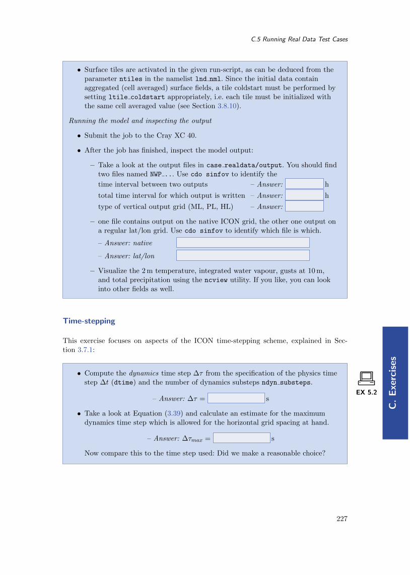
C.

Exe

rcis

es

C.5 Running Real Data Test Cases

• Surface tiles are activated in the given run-script, as can be deduced from theparameter ntiles in the namelist lnd nml. Since the initial data containaggregated (cell averaged) surface fields, a tile coldstart must be performed bysetting ltile coldstart appropriately, i.e. each tile must be initialized withthe same cell averaged value (see Section 3.8.10).

Running the model and inspecting the output

• Submit the job to the Cray XC 40.

• After the job has finished, inspect the model output:

– Take a look at the output files in case realdata/output. You should findtwo files named NWP ... Use cdo sinfov to identify the

time interval between two outputs – Answer: h

total time interval for which output is written – Answer: h

type of vertical output grid (ML, PL, HL) – Answer:

– one file contains output on the native ICON grid, the other one output ona regular lat/lon grid. Use cdo sinfov to identify which file is which.

– Answer: native

– Answer: lat/lon

– Visualize the 2 m temperature, integrated water vapour, gusts at 10 m,and total precipitation using the ncview utility. If you like, you can lookinto other fields as well.

Time-stepping

This exercise focuses on aspects of the ICON time-stepping scheme, explained in Sec-tion 3.7.1:

EX 5.2

• Compute the dynamics time step ∆τ from the specification of the physics timestep ∆t (dtime) and the number of dynamics substeps ndyn substeps.

– Answer: ∆τ = s

• Take a look at Equation (3.39) and calculate an estimate for the maximumdynamics time step which is allowed for the horizontal grid spacing at hand.

– Answer: ∆τmax = s

Now compare this to the time step used: Did we make a reasonable choice?

227

C.

Exercises

ICON Model Tutorial

Parallelization and Run-Time Performance

In this exercise you will learn how to specify the details of the parallel execution. We willuse the ICON timer module for basic performance measuring.

EX 5.3

Performance assessment using the timer output:

• Open your run script from the previous Exercise C.5.1 and enable the ICONroutines for performance logging (timers). To do so, follow the instructions inSection 7.3.4.

• Repeat the model run.

• At the end of the model run, a log file is created. It can be found in your basedirectory case realdata. Scroll to the end of this file. You should find wallclock timer output comparable to that listed in Section 7.3.4. Try to identify

the total run-time – Answer: s

the time needed by the radiation module – Answer: s

This exercise focuses on the mechanisms for parallel execution of the ICON model. Thesesettings become important for performance scalability when increasing the model resolu-tion and core counts:

EX 5.4

Changing the number of MPI tasks: In case your computational resources aresufficient, one possibility to speed up your model run is to increase the number ofMPI tasks.

• Create a copy of your run script run ICON R03B06 dwdini namedrun ICON R03B06 dwdini fast. In order to avoid overwriting your old results,replace the output directory name (EXPDIR) by exp02 dwdini fast.

• Double the total number of MPI tasks compared to your previous job andre-submit. In more detail, do the following:

– Your old script (run ICON R03B06 dwdini) ran the executable in hybridmode on 25 nodes using 12 MPI tasks/node and 4 OpenMP threads/MPItask with hyper-threading enabled.

– Your new script (run ICON R03B06 dwdini fast) should run theexecutable in hybrid mode on 50 nodes using 12 MPI tasks/node and 4OpenMP threads/MPI task with hyper-threading enabled.

You need to adjust both the PBS settings and the aprun command. SeeSection 7.3.4 for additional help.

• Compute the speedup that you gained from doubling the number of MPI tasks.

228

C.

Exe

rcis

es

C.5 Running Real Data Test Cases

Figure C.1.: Computational grid with a two-way nested region over Europe (yellow shad-ing). The outline of the COSMO-EU domain (formerly used operationallyby DWD) is shown in red for comparison.

– Compare the timer output of the dynamical core, nh solve, and thetransport module, transport, with the timer output of your previous run.

nh solve

25 nodesnh solve

50 nodes

s s

transport

25 nodestransport

50 nodes

s s

What do you think is a more sensible measure of the effective cost: totalmin or total max?

– Answer:

– Which speedup did you achieve and what would you expect from“theory”?

– Answer: Speedup achieved = T25nodesT50nodes

=

– Answer: Speedup expected =

229

C.

Exercises

ICON Model Tutorial

Writing Output for Driving a Limited Area Simulation

In this exercise you will learn about some of the output capabilities of ICON. We will setup a new output namelist and generate a data set which enables us to drive a limited areaversion of ICON as described in Chapter 6.

EX 5.5

In order to achieve a somewhat higher spatial resolution at acceptable costs, we willswitch on a two-way nested region over Europe with a horizontal grid spacing of13 km (see Figure C.1):

• Create a copy of your run script run ICON R03B06 dwdini namedrun ICON R03B06N7 dwdini. Alternatively, you may adopt the settings of thereference version reference/case2/run ICON R03B06 dwdini.

• In order to avoid overwriting your old results, replace the output directoryname (EXPDIR) by exp02 dwdini lamforcing.

• Activate the nest, by extending the list of horizontal grids to be used(dynamics grid filename) and the parent grid IDsdynamics parent grid id (grid nml).

• In order to save some computational resources, the nested region should have areduced model top height and comprise only the lowermost 60 vertical levels ofthe global domain (instead of 90 levels). Please extend num lev (run nml)accordingly.

Adding a new output namelist:

• The run script contains two commented-out output namelists. One is meantfor writing forcing (boundary) data, the other for writing initial data fordriving a limited area run. Activate the namelists and fill in the missingparameters. See Section 7.1 for additional details regarding output namelists.Forcing data should be written

– in GRIB2 format

– for the EU-nest only

– 2-hourly from the start until 48 hours forecast time

– with one output step per file

– on the native (triangular) grid

– into the subdirectory “lam forcing” of your output directoryexp02 dwdini lamforcing, using the filename prefix “forcing”. If thesubdirectory does not exist, please create.

– containing model level output forU, V, W, PRES, TEMP, QV, QC, QI, QR, QS, HHL.

230

C.

Exe

rcis

es

C.5 Running Real Data Test Cases

– Take a look at the available ICON variable groups listed in Appendix B. Isthere an output group that can be used instead of the list of variables? Ifyes, which group?

– Answer:

– Is there also an ICON variable group that writes all variables needed toinitialize an ICON-LAM simulation? If yes, which group?

– Answer:

• Submit the job to the Cray XC 40.

Check the correctness of your output files:

• You should find 25 files in your output directory “lam forcing”. Apply thecommand cdo sinfov data-file.grb > data-file.sinfov to the last file. Comparewith the reference output in Table C.1 to see whether your output namelist iscorrect.

Optional: A Deeper Look into Spin-Up Effects

Depending on the data set used to initialize the model, spin up effects may become visibleduring the first few hours of a forecast. This is especially true if third party (i.e. non-native) analysis data sets are used. Here we will have a look into the spin up behaviorwhen ICON is started from native vs. non-native analysis. As an example for a popularnon-native analysis, we will choose data from the IFS.

EX 5.6

• Run the NCL script case realdata/water budget.ncl, to get a deeperinsight into the model’s spin up properties and water budget when startedfrom DWD analysis. The script generates time series of vertically integratedwater vapour tqv and condensate tqx from the model level output incase realdata/output/exp02 dwdini.

Compare the results to Figure C.2 which shows the corresponding results whenICON is started from IFS analysis. Note that Figure C.2 has been producedfor a longer time range.

Which analysis data set leadsto an increased spin up/downin this particular case?

native analysis (DWD)

non-native analysis (IFS)

The additional NCL plots will give you some insight into the globalatmospheric water budget

dQtdt

= P − E +R ,

231

C.

Exercises

ICON Model Tutorial

Table C.1.: Reference output for Ex. C.5.5. Structure and content of fileforcing ML 20170114T000000Z.grb

File format : GRIB2

-1 : Institut Source Ttype Levels Num Points Num Dtype : Parameter name

1 : DWD unknown instant 60 1 172740 1 P16 : U

2 : DWD unknown instant 60 1 172740 1 P16 : V

3 : DWD unknown instant 61 2 172740 1 P16 : W

4 : DWD unknown instant 60 1 172740 1 P16 : P

5 : DWD unknown instant 60 1 172740 1 P16 : T

6 : DWD unknown instant 60 1 172740 1 P16 : QV

7 : DWD unknown instant 60 1 172740 1 P16 : QC

8 : DWD unknown instant 60 1 172740 1 P16 : QI

9 : DWD unknown instant 60 1 172740 1 P16 : QR

10 : DWD unknown instant 60 1 172740 1 P16 : QS

11 : DWD unknown instant 61 3 172740 1 P16 : HHL

Grid coordinates :

1 : unstructured : points=172740

grid : number=99 position=1

uuid : 890df70c-a566-3b91-438f-f527deb82760

Vertical coordinates :

1 : generalized_height : levels=60

height : 1.5 to 60.5 by 1

bounds : 1-2 to 60-61 by 1

zaxis : number = 4

uuid : a0919ba7-df84-ce2b-c4c2-3c215c033520

2 : generalized_height : levels=61

height : 1 to 61 by 1

zaxis : number = 4

uuid : a0919ba7-df84-ce2b-c4c2-3c215c033520

3 : generalized_height : levels=61

height : 0.5 to 30.5 by 0.5

bounds : 1-0 to 61-0 by 0.5

zaxis : number = 4

uuid : a0919ba7-df84-ce2b-c4c2-3c215c033520

Time coordinate : 1 step

RefTime = 2017-01-12 00:00:00 Units = minutes Calendar = proleptic_gregorian

YYYY-MM-DD hh:mm:ss YYYY-MM-DD hh:mm:ss YYYY-MM-DD hh:mm:ss YYYY-MM-DD hh:mm:ss

2017-01-14 00:00:00

where Qt is the vertically integrated atmospheric water content and dQt/dt isthe rate of change over time. P is the amount of total precipitation, E is thetotal evaporation, and R is a residuum. Is the budget closed (i.e. is R = 0 inyour model run)?

232

C.

Exe

rcis

es

C.5 Running Real Data Test Cases

Figure C.2.: Time series of area averaged column integrated specific moisture 〈tqv〉 (top)and condensate classes 〈tqx〉 (bottom) for a 7-day forecast started fromIFS analysis fields. Start date was 2017-01-12T00:00:00. A spin up in 〈tqv〉and initial adjustments in 〈tqx〉 is clearly visible.

233

C.

Exercises

ICON Model Tutorial

Optional: Checking for Bit-Reproducibility

In this exercise we test the ICON model for bit-reproducibility, i. e. the feature that runningthe same binary multiple times results in bitwise identical results.

EX 5.7

• Compare the model level output of run ICON R03B06 dwdini with the outputthat was produced by your modified script run ICON R03B06 dwdini fast.You can use cdo infov data-file.nc for getting information about the contentsof your output file. You should dump this information into text files,

cdo infov data-file.nc > data-file.infov

so that you can compare them later on. Due to the limited number of digitsprinted by CDO, this is no check for bit-reproducibility in a strictmathematical sense, however experience showed that cdo infov is veryreliable in revealing reproducibility issues.

• Now compare the model level output produced by your modified scriptrun ICON R03B06N7 dwdini with the output produced byrun ICON R03B06 dwdini. Is the result different from the previouscomparison? Do you have an explanation for this?

Hint: For a convenient comparison of ASCII files you may use the tkdiff

utility.

C.6. Running ICON-LAM

The exercises in this section require a number of grid files, external parameters and inputdata. In particular, initial data and driving boundary data are required. Both were pro-duced in the real data exercise, Ex. C.5.5. The preprocessing of this data is explained inEx. C.2.4 (see p. 220).

Running ICON in Limited Area Mode

In this exercise we will run ICON in limited area mode. The model will be driven by initialand boundary data which have been produced in Ex. C.2.4.

EX 6.1

Open the run script case lam/run ICON R3B08 lam and prepare it for running a48 hour forecast on a limited area grid over Germany (see Figure C.3). Asfor the global run, the start date is

2017-01-12T00:00:00 , i.e. January 12, 2017.

The run script is geared up insofar as all soft-links which specify the model binary,grids, initial and boundary data are already set. Your main task will be to set upthe ICON namelists for a limited area run.

234

C.

Exe

rcis

es

C.6 Running ICON-LAM

Figure C.3.: Illustration of the local grid used in Exercises C.6.1–C.8.3. The horizontalgrid spacing is ≈ 6.5 km (which corresponds to R3B08 in ICON nomen-clature). The boundary region is highlighted, where nudging towards thedriving data is performed. The driving data for this test case has beencreated in Ex. C.2.4.

Basic settings:

• Set the correct start and end date:ini datetime string, end datetime string.

• Switch on the limited area mode by setting l limited area and init mode

(see Section 6.3).

Initial data:

• Specify the initial data file via dwdfg filename. Since we do not make use ofadditional analysis information from a second data file, remember to setlread ana accordingly (see Section 6.3).

• Specify a dictionary file for the initial data via ana varnames map file (seeSection 5.1.1).Hint: Take a closer look at case lam/run ICON R3B08 lam, where a link to thecorrect dictionary is already set.

235

C.

Exercises

ICON Model Tutorial

The dictionary has the purpose to translate the variable names in the GRIB2or NetCDF input file into the ICON internal variable names. According to thedictionary used for this exercise, what are the internal variable names and theGRIB2/NetCDF variable names for

– Pressure:GRIB2/NetCDF: ICON internal:

– Temperature:

GRIB2/NetCDF: ICON internal:

– Half level height:

GRIB2/NetCDF: ICON internal:

Boundary data:

• Specify the lateral boundary grid and data via latbc boundary grid,latbc path and latbc filename. For the latter you will have to make use ofthe keywords <y>, <m> <d> and <h> (see Section 6.4.1).

• What is the time interval between two consecutive boundary data files?The command cdo sinfov may be helpful.

– Answer: s

Set the namelist parameter dtime latbc accordingly.

• Inspect the number of vertical levels in a boundary data file. Is it differentfrom the number of vertical levels that is used by the model itself?

– Answer:

Running the model and inspecting the output

• Extend the lat-lon output namelist by the 2 m temperature, surface pressure,mean sea level pressure, and 10 m gusts. See Appendix B for variable namesand description.

• Submit the job to the Cray XC 40.

• After the job has finished, inspect the model output. You should find multiplefiles in the output directory case lam/output/exp03 R3B08 dwdlam whichcontain hourly output on model levels remapped to a regular lat-lon grid.

– Take a look at the output fields by using ncview. How would youcharacterize the overall weather situation for that time period?

southfoehn over the alpine region

strong frontal system passing over Germany

weak frontal system passing over Germany

anticyclonic situation with very calm winds

236

C.

Exe

rcis

es

C.6 Running ICON-LAM

Temporal Resolution of the Boundary Data

By playing around with the temporal resolution of the boundary data you will get someidea how this might affect your simulation results.

EX 6.2

Create a copy of your run script run ICON R3B08 lam and name itrun ICON R3B08 lam lowres. Replace the output directory name (EXPDIR) byexp03 R3B08 dwdlam lowres in order to avoid overwriting your results.

• Halve the time resolution of your forcing (boundary) data, see Section 6.3 forthe namelist parameter. Write down your chosen value:

– Answer: s

• Submit the job to the Cray XC 40.

• Compare the results with your previous run. Does the time frequency withwhich the boundary data are updated have a significant impact on the results?You can visualize cross sections with the NCL scriptcase lam/plot cross section.ncl and/or make use of ncview.

Driving ICON-LAM by DWD Data

This exercise is similar to the previous exercise C.6.1 inasmuch as we will run ICON inlimited area mode again. However, rather than using initial and boundary data that havebeen created in one of the previous exercises, we will initialize and drive ICON-LAM byofficial DWD analysis and forecast data. This setting might be closer to what you willencounter when you run ICON-LAM at your home institution.

The data products for this particular exercise will be provided. Note, however, thatPAMORE data requests in general require registration via datenservice@dwd.de.

EX 6.3

In the subdirectory

/e/uwork/trng024/packages/pamore data

you will find the raw data for an ICON limited area run consisting of an initializedanalysis and two-hourly forecasts. This data set has been downloaded from theDWD database with the help of the PAMORE tool, see Section 2.2.1 for details.

• For the sake of simplicity, link the above directory into case lam/input_dwd.

• Take a look at the data with the grib ls and/or cdo command-line tool. Findout about the analysis date and the time range of the data set.

• Imagine that your boss at home asks you to retrieve this data set from theDWD database . . .

237

C.

Exercises

ICON Model Tutorial

Write down the PAMORE commands which you would have to insert into thePAMORE web form. See Section 2.2.1 and 2.3 for help.

– Analysis:

– Forecasts:

• Export the environment variable GRIB DEFINITION PATH with the setting

GRIB_DEFINITION_PATH=/usr/local/pkg/grib_api/definitions/

· · · release/$GRIB_API_VERSION/definitions

and run grib ls once more. Are there any differences w.r.t. the displayedshort names? See Section 1.1.2 for an explanation.

Remapping of initial data:

In order to use the DWD initialized analysis for your LAM run, it must beremapped to your limited area grid.

• Determine the source grid on which the raw data are defined. Write down thegrid identifier numberOfGridUsed.

– Answer: numberOfGridUsed=

• Retrieve the matching grid file from the ICON download server (seeSection 2.1.2):

– Open the download page for the pre-defined ICON gridshttp://icon-downloads.mpimet.mpg.de in your web browser.

– Pick the matching grid number from the list and right-click on thehyperlink for the grid file, then choose ”copy link location”.

– Open a terminal window, login into the Linux cluster lce, and change intothe subdirectory case lam/input dwd. Download the grid file into thissubdirectory by typingwget link location -e http-proxy=ofsquid.dwd.de:8080.

– Write down the resolution in ICON’s RxBy nomenclature.

– Answer: RxBy=

• Create a copy of the remapping script xce remap inidata located in thesubdirectory case lam.

• Open the script and adapt

– the path to the input data file that has been retrieved from the DWDdatabase (directory case lam/input_dwd/pamore_data).

– the file name of the input grid.

– the output directory such as not to overwrite your previous initial data.You might store your output in a new sub-directory output dwd locatedinside the base directory “case lam”.

238

C.

Exe

rcis

es

C.6 Running ICON-LAM

• Submit the script to the batch system.

Remapping of the lateral boundary conditions:

In contrast to the previous ICON-LAM exercises we will interpolate the forcingdata onto the full limited area grid instead of the lateral boundary strip only.

Can you think of simulations where such a setting is required?

– Answer:

Create a copy of the remapping script for boundary data xce limarea:

• Open this script and adapt the path to your input data files (directory“case lam/input_dwd/pamore_data”), the file name of the input grid as wellas the output directory (“case lam/output_dwd”).

• Adapt the script such that the AUXGRID auxiliary grid (boundary strip) is nolonger used but the full limited area grid (LOCALGRID).

Submit the script to the batch system.

Small consistency check: How many grid cells do you expect in the output files?

– Answer: cells

Running the model

Create a copy of the run script case lam/run ICON R3B08 lam and prepare it forrunning a 36 hour forecast on the same limited area grid over Germany as usedin Ex. C.6.1 (see Figure C.3). In order to avoid overwriting your old results, replacethe name of the output directory.

Initial and boundary data:As we will use a new set of initial and boundary data, several changes are necessary:

• Change the settings for the analysis input files (initial data).

• Specify the lateral boundary data via latbc path and latbc filename. Forthe latter you will have to make use of the keyword <ddhhmmss> (seeSection 6.4.1).

• Check whether the time interval between consecutive boundary data files is setcorrectly (dtime latbc).

Submit the job to the Cray XC 40.

Did your run finish successfully?

239

C.

Exercises

ICON Model Tutorial

C.8. Programming ICON

Allocating Additional Fields

In this exercise we learn how to allocate new ICON variables. As a by-product we willvisualize ICON’s domain decomposition.

EX 8.1

This requires to modify the ICON code, where details are given in Section 8.3.

Remember to create a fully copy of your src directory. Subsequent exercises willbe based upon the unmodified sources!

Step-by-step checklist

In the subdirectory src/atm dyn iconam:

a) Open the module mo nonhydro types.

Insert a new 2D variable pointer process_idof type REAL(wp) to the derived type TYPE(t nh diag).

Gotit?

Didit!

b) Open the module mo nonhydro state.

At the end of the subroutine new nh state diag list:initialize meta-data variables for NetCDF and also for GRIB2 withdiscipline = parameterCategory = parameterNumber = 255

and place the add var call for the new field.

Gotit?

Didit!

c) Now, after the add_var call, the new field has been allocated.Fill the data array with a constant value:

· · · process id(:,:) = get_my_mpi_work_id()Gotit?

Didit!

This auxiliary function from mo_mpi returns the MPI rankof the processor (see Section 8.2.4).

d) Open the namelist of the previous test case C.6.1 and insert the new fields inthe lat-lon output specification.

Compile and run the model.Visualize the results (ncview).

Please answer the following questions:

• Why is the output field not a constant value?

– Answer:

• Take a closer look at the data: Can you guesswhy the output field does not only containinteger values?

– Answer:

240

C.

Exe

rcis

es

C.8 Programming ICON

Looping Over Grid Points

In this exercise we will implement the technical setup for the calculation of new diagnosticfields:

EX 8.2

In this exercise we will implement the technical setup for the calculation of thefollowing new diagnostic fields (2D variables):

RHI MAX: Relative humidity over ice (hourly maximum in the column, [%])

QI MAX: Maximum cloud ice content (hourly max. in the column,[

kgkg

])

Again, this requires to modify the ICON code.

• Repeat the steps a) – b) of Exercise C.8.1 and allocatetwo new 2D variables RHI MAX, QI MAX.

Gotit?

Didit!

• Open the module mo nh stepping

(subdirectory src/atm dyn iconam).

Create an (empty) subroutine calculate diagnostics

and place a call to this subroutineimmediately before the call to the output routine.

Gotit?

Didit!

• Fill your subroutine with a 2D loop over all prognostic grid points,see p. 161 for help.Use this loop to initialize the fields to a constant value.

p nh state(jg)%diag%RHI MAX(jc,jb) = 2.0_wp

p nh state(jg)%diag%QI MAX(jc,jb) = 2.0_wp

All other values should be set to 1.0 wp.

How many triangle rows do you expect to have the value 1 in the output?

– Answer: rows.

• Open the namelist of the previous test case C.6.1 and insert the new fields inthe lat-lon output specification.

• Compile and run the model. Visualize the results (ncview).

• Final question: Instead of the value 2.0_wp we’d now like to initialize RHI_MAX

with the lower-most level of the (diagnostic) temperature field.How could we achieve this?

– Answer:

241

C.

Exercises

ICON Model Tutorial

Implementing New Diagnostics

In this exercise we will calculate the new 2D diagnostic fields RHI MAX, QI MAX:

EX 8.3

• Modify the subroutine calculate diagnostics:Instead of initializing the fields to a constant value as in Ex. C.8.2, add a loopover the vertical model levels for every prognostic grid point.

• Then fill your subroutine with the calculation of the two new quantities.Three hints:

– The module mo util phys (subdirectory src/atm phy nwp)may offer some help with respect to RHI MAX.

– Exner pressure field: values for domain “jg” are accessed viap_nh_state%prog(nnow(jg))%exner(:,:,:).

– 3D tracer field QI (same for QV): values for domain “jg” are accessed viap nh state%prog(nnow rcf(jg))%tracer ptr(iqi)%p 3d(:,:,:).The constants iqv, iqi can be found in mo_run_config.

• Revisit the add_var calls of the quantities RHI MAX, QI MAX: specify an hourlyreset, see p. 162 for an explanation.

• Open the namelist of the previous test case C.6.1 and insert the new fields inthe output specification.

Compile and run the model. Visualize the results (ncview).

242

C.

Exe

rcis

es

C.10 Running ICON-ART

C.10. Running ICON-ART

In order to start with the exercises, you have to copy and unpack the ART code insideyour ICON source directory as described in section 10.3.

You will find the ART code at:/e/uwork/trng024/packages/art.tar.gz.Folders with the input data for all ART exercises can be found at:/e/uwork/trng024/packages/ART-INPUT.

After you have copied the source code, you have to install ICON-ART. For this purpose,proceed as described in Section 10.3. After a successful compilation of ICON-ART, youcan start with the experiments, that were prepared for this purpose:

Point Sources in ICON-ART LAM

EX 10.1

In this exercise, you will learn to add your own tracers with emissions from pointsources. You are free to choose the tracer(s) to transport and the location of thepoint source(s).

In order to perform the simulation, you have to do the following steps:

• Inside $ARTDIR/runctrl examples/run scripts you will find the run scriptfor this test case called exp.art.trng19.case1.pntSrc

• inside the ART-INPUT folder you will find a folder called CASE1-PNTSRC

containing all input data required for this test case

• Edit the run script according to the namelist parameters you find inSection 10.4. You will find a ? at all places where you have to edit something.

• Create the XML files that are needed to define tracers (see section 10.4.3) andpoint sources (see section 10.4.5).

• Submit the job.

• Visualize your results using ncview.

Very Short-lived Substances

EX 10.2

Biogenic emitted Very Short-lived Substances (VSLS) have a short chemical lifetimein the atmosphere compared to tropospheric transport timescales. As the ocean isthe main source of the most prominent VSLS, bromoform (CHBr3) anddibromomethane (CH2Br2), this leads to large concentration gradients in thetroposphere. The tropospheric depletion of CHBr3 is mainly due to photolysis,whereas for CH2Br2 the loss is dominated by oxidation by the hydroxyl radical

243

C.

Exercises

ICON Model Tutorial

(OH) both contributing to the atmospheric inorganic bromine (Bry) budget. Oncereleased, active bromine radicals play a significant role in tropospheric as well asstratospheric chemistry as they are in particular involved in ozone destroyingcatalytic cycles. Although the bromine budget in the stratosphere is dominated bythe release of Bry from long-lived source gases (e.g. halons) which is relatively wellunderstood the contribution of biogenic VSLS to stratospheric bromine is stilluncertain.

In this exercise the fast upward transport of both VSLS from the lower boundaryinto the upper troposphere / lower stratosphere (UTLS) due to the super-typhoonHaiyan will be simulated.

In order to perform the simulation, you have to do the following steps:

• Inside the ART-INPUT folder you will find a folder called CASE2-VSLScontaining all input data required for this test case.

• Inside $ARTDIR/runctrl examples/run scripts you will find the run scriptfor this test case called exp.art.trng19.case2.vsls. Edit the run scriptaccording to the namelist parameters you find in Section 10.4. You will find a ?at all places where you have to edit something.

• Create the XML file that is needed to define tracers (see section 10.4.3). Forthis configuration, you will have to add tracers for CHBr3 and CH2Br2.

• Don’t forget to modify your output namelist accordingly.

• Submit the job.

• Visualize your results using ncview.

Volcano Eruption

EX 10.3

The eruption of a volcano can have a significant radiative impact as well as animpact on air traffic. In this example, you will simulate the dispersion of volcanicash particles. Within ICON-ART, you have the choice of treating volcanic ash asmonodisperse tracers or with prognostic mass and number (i.e. 2-moment aerosol).In this example, we will make use of the 2-moment description. In order to performthe simulation, you have to do the following steps:

• Inside the ART-INPUT folder you will find a folder called CASE3-VOLCcontaining all input data required for this test case.

• Inside $ARTDIR/runctrl examples/run scripts you will find the run scriptfor this test case called exp.art.trng19.case3.volc. Edit the run scriptaccording to the namelist parameters you find in Section 10.4. You will find a ?at all places where you have to edit something. For cart volcano file, youcan use the file ART-INPUT/CASE2-VOLC/volcano list Eyjafjoell.txt.

244

C.

Exe

rcis

es

C.10 Running ICON-ART

• Create the XML file that is needed to define tracers (see section 10.4.3). Youalso have to create an XML file specifying the aerosol modes in the simulation(see section 10.4.4). For the 2-moment description of volcanic ash, you willneed the modes asha, ashb and ashc and the according tracers.

• You can use the namelist switch lart diag out to obtain diagnosticalproperties like aerosol optical depth and median diameters.

• Don’t forget to modify your output namelist accordingly.

• Submit the job.

• Visualize your results using ncview.

Sea Salt Aerosol

EX 10.4

Sea salt aerosol is one of the main contributors to natural atmospheric aerosol.With its high hygroscopicity it is a very efficient cloud condensation nuclei (CCN).Within ICON-ART, sea salt aerosol is described as a log-normally distributedaerosol in three modes with prognostic mass mixing ratios and prognostic numbermixing ratios. This simulation includes also a nested domain covering Europe andNorth Africa with a higher spatial resolution. In order to perform the simulation,you have to do the following steps:

• Inside the ART-INPUT folder you will find a folder called CASE4-SEAScontaining all input data required for this test case.

• Inside $ARTDIR/runctrl examples/run scripts you will find the run scriptfor this test case called exp.art.trng19.case4.seas. Edit the run scriptaccording to the namelist parameters you find in section 10.4. You will find a ?at all places where you have to edit something.

• Create the XML file that is needed to define tracers (see section 10.4.3). Youalso have to create an XML file specifying the aerosol modes in the simulation(see section 10.4.4). For the 2-moment description of sea salt, you will need themodes seasa, seasb and seasc and the according tracers.

• Don’t forget to modify your output namelist accordingly.

• Submit the job.

• Visualize your results using ncview.

245

C.

Exercises

Bibliography

Asensio, H., and M. Messmer, 2014: External Parameters for Numerical Weather Pre-diction and Climate Application: EXTPAR v2.0.2 User and Implementation Guide.Consortium for Small-scale Modeling (COSMO), URL http://www.cosmo-model.org/content/model/modules/Extpar 201408 user and implementation manual.pdf.

Avissar, R., and R. Pielke, 1989: A parameterization of heterogeneous land surfaces foratmospheric numerical models and its impact on regional meteorology. Mon. WeatherRev., 117, 2113–2136.

Baines, P., and T. Palmer, 1990: Rationale for a new physically based parameterization ofsub-grid scale orographic effects. Tech. Rep. 169, European Centre for Medium-RangeWeather Forecasts, 11 pp. URL http://www.ecmwf.int.

Barker, H. W., G. L. Stephens, P. T. Partain, and Coauthors, 2003: Assessing 1D at-mospheric solar radiative transfer models: Interpretation and handling of unresolvedclouds. J. Clim., 16 (16), 2676–2699, doi:10.1175/1520-0442(2003)016〈2676:ADASRT〉2.0.CO;2.

Bechtold, P., 2017: Atmospheric moist convection. Meteorological Training Course LectureSeries, ECMWF, 1–78, URL https://www.ecmwf.int/sites/default/files/elibrary/2017/16953-atmospheric-moist-convection.pdf.

Bechtold, P., M. Kohler, T. Jung, F. Doblas-Reyes, M. Leutbecher, M. J. Rodwell,F. Vitart, and G. Balsamo, 2008: Advances in simulating atmospheric variability withthe ECMWF model: From synoptic to decadal time-scales. Q. J. R. Meteorol. Soc.,134 (634), 1337–1351, doi:10.1002/qj.289.

Blackadar, A. K., 1962: The vertical distribution of wind and turbulent exchange in aneutral atmosphere. J. Geophys. Res., 67, 3095–3102.

Bloom, S. C., L. L. Takacs, A. M. D. Silva, and D. Ledvina, 1996: Data assimilation usingincremental analysis updates. Mon. Weather Rev., 124, 1256–1270.

Choulga, M., E. Kourzeneva, E. Zakharova, and A. Doganovsky, 2014: Estimation of themean depth of boreal lakes for use in numerical weather prediction and climate mod-elling. Tellus A, 66, 21 295, doi:10.3402/tellusa.v66.21295.

Colella, P., and P. R. Woodward, 1984: The piecewise parabolic method (ppm) for gas-dynamical simulations. J. Comput. Phys., 54, 174–201.

Crueger, T., and Coauthors, 2018: ICON-A, the atmosphere component of the ICONearth system model: II. model evaluation. J. Adv. Model Earth Sy., 10 (7), 1638–1662,doi:10.1029/2017MS001233.

247

ICON Model Tutorial

Davies, H., 1976: A lateral boundary formulation for multi-level prediction models. Q. J.R. Meteorol. Soc., 102, 405–418, doi:10.1002/qj.49710243210.

Davies, H., 1983: Limitations of some common lateral boundary schemes used in re-gional NWP models. Mon. Weather Rev., 111, 1002–1012, doi:10.1175/1520-0493(1983)111〈1002:LOSCLB〉2.0.CO;2.

Dipankar, A., B. Stevens, R. Heinze, C. Moseley, G. Zangl, M. Giorgetta, and S. Brdar,2015: Large eddy simulation using the general circulation model ICON. J. Adv. ModelEarth Sy., 7 (3), 963–986, doi:10.1002/2015MS000431.

Doms, G., and Coauthors, 2011: A Description of the Nonhydrostatic Regional COSMOModel. Part II: Physical Parameterization. Consortium for Small-Scale Modelling, URLhttp://www.cosmo-model.org.

Easter, R. C., 1993: Two modified versions of Bott’s positive-definite numerical advectionscheme. Mon. Weather Rev., 121, 297–304.

ECMWF, 2017: PART IV: PHYSICAL PROCESSES, chap. Convection, 75–95. IFS Doc-umentation, ECMWF.

Ern, M., P. Preusse, and C. D. Warner, 2006: Some experimental constraints for spectralparameters used in the warner and mcintyre gravity wave parameterization scheme.Atmos. Chem. Phys., 6 (12), 4361–4381, doi:10.5194/acp-6-4361-2006.

Falk, G., 1990: Physik: Zahl und Realitat; die begrifflichen und mathematischen Grund-lagen einer universellen quantitativen Naturbeschreibung; mathematische Physik undThermodynamik. Birkhauser Verlag, Basel.

Gal-Chen, T., and R. Somerville, 1975: On the use of a coordinate transformation for thesolution of the Navier-Stokes equations. J. Comput. Phys., 17, 209–228.

Gassmann, A., 2013: A global hexagonal C-grid non-hydrostatic dynamical core (ICON-IAP) designed for energetic consistency. Q. J. R. Meteorol. Soc., 139 (670), 152–175,doi:10.1002/qj.1960.

Gassmann, A., and H.-J. Herzog, 2008: Towards a consistent numerical compressiblenon-hydrostatic model using generalized Hamiltonian tools. Q. J. R. Meteorol. Soc.,134 (635), 1597–1613.

Giorgetta, M., and Coauthors, 2018: ICON-A, the Atmosphere Component of the ICONEarth System Model: I. Model Description. J. Adv. Model Earth Sy., 10 (7), 1613–1637,doi:10.1029/2017MS001242.

GLOBE-Task-Team, 1999: The Global Land One-kilometer Base Elevation (GLOBE) Dig-ital Elevation Model, version 1.0. Tech. rep., National Oceanic and Atmospheric Ad-ministration. URL http://www.ngdc.noaa.gov/mgg/topo/globe.html.

Harris, L. M., and P. H. Lauritzen, 2010: A flux-form version of the conservative semi-lagrangian multi-tracer transport scheme (CSLAM) on the cubed sphere grid. J. Com-put. Phys., 230, 1215–1237.

248

Bibliography

Heinze, R., and Coauthors, 2017: Large-eddy simulations over Germany using ICON: acomprehensive evaluation. Q. J. R. Meteorol. Soc., 143 (702), 69–100.

Heise, E., B. Ritter, and R. Schrodin, 2006: Operational implementation of the multilayersoil model. COSMO Technical Reports No. 9, Consortium for Small-Scale Modelling,19pp, URL http://www.cosmo-model.org.

Herbert, F., 1975: Irreversible Prozesse der Atmosphare - 3. Teil. Beitr. Phys. Atmos., 48,1–29.

Hesselberg, A., 1925: Die Gesetze der ausgeglichenen atmospharischen Bewegungen. Beitr.Phys. Atmos., 12, 141160.

Hunt, B. R., E. Kostelich, and I. Szunyogh, 2007: Efficient data assimilation for spatiotem-poral chaos: A Local Ensemble Transform Kalman Filter. Physica D, 230, 112–126.

Jablonowski, C., P. Lauritzen, R. Nair, and M. Taylor, 2008: Idealized test cases for thedynamical cores of Atmospheric General Circulation Models: A proposal for the NCARASP 2008 summer colloquium. National Center for Atmospheric Research (NCAR).

Jablonowski, C., and D. L. Williamson, 2006: A baroclinic instability test case for atmo-spheric model dynamical cores. Q. J. R. Meteorol. Soc., 132, 2943–2975.

Klemp, J., 2011: A terrain-following coordinate with smoothed coordinate surfaces. Mon.Weather Rev., 139, 2163–2169.

Klemp, J., J. Dudhia, and A. Hassiotis, 2008: An upper gravity-wave absorbing layer forNWP applications. Mon. Weather Rev., 136 (10), 3987–4004.

Kohler, M., M. Ahlgrimm, and A. Beljaars, 2011: Unified treatment of dry convective andstratocumulus-topped boundary layers in the ECMWF model. 137, 43–57.

Kolmogorov, A. N., 1968: Local structure of turbulence in an incompressible viscous fluidat very high reynolds numbers. Sov. Phys. Usp., 10 (6), 734.

Korn, P., 2017: Formulation of an unstructured grid model for global ocean dynamics. J.Comput. Phys., 339 (C), 525–552, doi:10.1016/j.jcp.2017.03.009.

Korn, P., and S. Danilov, 2017: Elementary dispersion analysis of some mimetic discretiza-tions on triangular C-grids. J. Comput. Phys., 330, 156 – 172, doi:https://doi.org/10.1016/j.jcp.2016.10.059.

Kourzeneva, E., 2010: External data for lake parameterization in Numerical Weather Pre-diction and climate modeling. Boreal Env. Res., 15, 165–177.

Kourzeneva, E., H. Asensio, E. Martin, and S. Faroux, 2012: Global gridded dataset of lakecoverage and lake depth for use in numerical weather prediction and climate modelling.Tellus A, 64, 15 640, doi:10.3402/tellusa.v64i0.15640.

Lauritzen, P. H., C. Erath, and R. Mittal, 2011a: On simplifying ’incremental remap’-basedtransport schemes. J. Comput. Phys., 230, 7957–7963.

Lauritzen, P. H., C. Jablonowski, M. A. Taylor, and R. D. Nair, 2011b: Numerical Tech-niques for Global Atmospheric Models. 1st ed., Springer, 556 pp.

249

ICON Model Tutorial

Lauritzen, P. H., R. D. Nair, and P. A. Ullrich, 2010: A conservative semi-Lagrangianmulti-tracer transport scheme (CSLAM) on the cubed-sphere grid. J. Comput. Phys.,229, 1401–1424.

Leuenberger, D., M. Koller, and C. Schar, 2010: A generalization of the SLEVE verticalcoordinate. Mon. Weather Rev., 138, 3683–3689.

Lilly, D. K., 1962: On the numerical simulation of buoyant convection. Tellus, 14 (2),148–172, doi:10.1111/j.2153-3490.1962.tb00128.x.

Lin, S.-J., and R. B. Rood, 1996: Multidimensional flux-form semi-lagrangian trans-port schemes. Mon. Weather Rev., 124 (9), 2046–2070, doi:10.1175/1520-0493(1996)124〈2046:MFFSLT〉2.0.CO;2.

Lipscomb, W. H., and T. D. Ringler, 2005: An incremental remapping transport schemeon a spherical geodesic grid. Mon. Weather Rev., 133, 2335–2350.

Lott, F., and M. J. Miller, 1997: A new subgrid-scale orographic drag parametrization: Itsformulation and testing. Q. J. R. Meteorol. Soc., 123 (537), 101–127, doi:10.1002/qj.49712353704.

Lundgren, K., B. Vogel, H. Vogel, and C. Kottmeier, 2013: Direct radiative effects of seasalt for the mediterranean region under conditions of low to moderate wind speeds. J.Geophys. Res., 118 (4), 1906–1923.

Matsuno, T., 1966: Numerical integrations of the primitive equations by a simulated back-ward difference method. Journal of the Meteorological Society of Japan. Ser. II, 44 (1),76–84, doi:10.2151/jmsj1965.44.1 76.

McLandress, C., and J. F. Scinocca, 2005: The GCM response to current parameterizationsof nonorographic gravity wave drag. J. Atmos. Sci., 62 (7), 2394–2413, doi:10.1175/JAS3483.1.

Mellor, G. L., and T. Yamada, 1982: Development of a turbulence closure model for geo-physical fluid problems. Rev. Geophys., 20 (4), 851–875, doi:10.1029/RG020i004p00851.

Mironov, D., E. Heise, E. Kourzeneva, B. Ritter, N. Schneider, and A. Terzhevik, 2010:Implementation of the lake parameterisation scheme FLake into the numerical weatherprediction model COSMO. Boreal Env. Res., 15, 218–230.

Mironov, D., B. Ritter, J.-P. Schulz, M. Buchhold, M. Lange, and E. Machulskaya, 2012:Parameterisation of sea and lake ice in numerical weather prediction models of theGerman weather service. Tellus A, 64 (0), doi:10.3402/tellusa.v64i0.17330.

Mironov, D. V., 2008: Parameterization of lakes in numerical weather prediction. Descrip-tion of a lake model. COSMO Technical Report, Consortium for Small-Scale Modelling,41 pp. URL http://www.cosmo-model.org.

Miura, H., 2007: An upwind-biased conservative advection scheme for spherical hexagonal-pentagonal grids. Mon. Weather Rev., 135, 4038–4044.

Mlawer, E. J., S. J. Taubman, P. D. Brown, M. J. Iacono, and S. A. Clough, 1997: Radiativetransfer for inhomogeneous atmospheres: RRTM, a validated correlated-k model for thelongwave. J. Geophys. Res.: Atmos., 102 (D14), 16 663–16 682, doi:10.1029/97JD00237.

250

Bibliography

Narcovich, F. J., and J. D. Ward, 1994: Generalized Hermite interpolation via matrix-valued conditionally positive definite functions. Math. Comp., 63, 661–687, doi:10.1090/S0025-5718-1994-1254147-6.

Neggers, R. A. J., M. Kohler, and A. C. M. Beljaars, 2009: A dual mass flux frameworkfor boundary layer convection. Part I: Transport. J. Atmos. Sci., 66 (6), 1465–1487,doi:10.1175/2008JAS2635.1.

Orr, A., P. Bechtold, J. Scinocca, M. Ern, and M. Janiskova, 2010: Improved middle at-mosphere climate and forecasts in the ECMWF model through a nonorographic gravitywave drag parameterization. J. Clim., 23 (22), 5905–5926, doi:10.1175/2010JCLI3490.1.

Pincus, R., and B. Stevens, 2013: Paths to accuracy for radiation parameterizations inatmospheric models. J. Adv. Model Earth Sy., 5 (2), 225–233, doi:10.1002/jame.20027.

Polavarapu, S., S. Ren, A. M. Clayton, D. Sankey, and Y. Rochon, 2004: On the rela-tionship between incremental analysis updating and incremental digital filtering. Mon.Weather Rev., 132, 2495–2502.

Press, W. H., S. A. Teukolsky, W. T. Vetterling, and B. P. Flannery, 2007: NumericalRecipes. 3rd ed., Cambridge University Press, 1235 pp.

Prill, F., 2014: DWD ICON Tools Documentation. Deutscher Wetterdienst (DWD),dwd icon tools/doc/icontools doc.pdf.

Randall, D. A., 2017: A survey of time-differencing schemes for the oscillation and de-cay equations. An Introduction to Numerical Modelling of the Atmosphere, ColoradoState University, 63–104, URL http://kiwi.atmos.colostate.edu/group/dave/at604pdf/AT604 LaTeX Book.pdf.

Raschendorfer, M., 2001: The new turbulence parameterization of LM. COSMO NewsLetter No. 1, Consortium for Small-Scale Modelling, 89–97, URL http://www.cosmo-model.org.

Rast, S., 2017: Using and programming ICON – a first introduction. Max PlanckInstitute for Meteorology, URL https://code.mpimet.mpg.de/attachments/download/15898/icon lecture 2016.pdf, course at Hamburg University 2017.

Rieger, D., and Coauthors, 2015: ICONART 1.0 a new online-coupled model systemfrom the global to regional scale. Geosci. Model Dev., 8 (6), 1659–1676, doi:10.5194/gmd-8-1659-2015.

Rotta, J., 1951a: Statistische Theorie nichthomogener Turbulenz. J. Z. Physik, 129 (6),547–572, doi:10.1007/BF01330059.

Rotta, J., 1951b: Statistische Theorie nichthomogener Turbulenz. J. Z. Physik, 131 (1),51–77, doi:10.1007/BF01329645.

Sadourny, R., A. Arakawa, and Y. Mintz, 1968: Integration of the nondivergent barotropicvorticity equation with an icosahedral-hexagonal grid for the sphere. Mon. WeatherRev., 96 (6), 351–356, doi:10.1175/1520-0493(1968)096〈0351:IOTNBV〉2.0.CO;2.

251

ICON Model Tutorial

Schar, C., D. Leuenberger, O. Fuhrer, D. Luthi, and C. Girard, 2002: A new terrain-following vertical coordinate formulation for atmospheric prediction models. Mon.Weather Rev., 130, 2459–2480.

Schrodin, R., and E. Heise, 2001: The Multi-Layer Version of the DWD Soil ModelTERRA LM. Tech. Rep. 2, Consortium for Small-Scale Modelling, 1–16 pp. URLhttp://www.cosmo-model.org.

Schroter, J., and Coauthors, 2018: ICON-ART 2.1: a flexible tracer framework and itsapplication for composition studies in numerical weather forecasting and climate simu-lations. Geosci. Model Dev., 11 (10), 4043–4068, doi:10.5194/gmd-11-4043-2018.

Schulz, J.-P., 2006: The new Lokal-Model LME of the German Weather Service. COSMONews Letter No. 6, Consortium for Small-Scale Modelling, 210–212, URL http://www.cosmo-model.org.

Schulz, J.-P., 2008: Introducing sub-grid scale orographic effects in the cosmo model.COSMO News Letter No. 9, Consortium for Small-Scale Modelling, 29–36, URL http://www.cosmo-model.org.

Schulz, J.-P., G. Vogel, C. Becker, S. Kothe, U. Rummel, and B. Ahrens, 2016: Evaluationof the ground heat flux simulated by a multi-layer land surface scheme using high-quality observations at grass land and bare soil. Meteorol. Z., 25 (5), 607–620, doi:10.1127/metz/2016/0537.

Scinocca, J. F., 2003: An accurate spectral nonorographic gravity wave drag param-eterization for general circulation models. J. Atmos. Sci., 60 (4), 667–682, doi:10.1175/1520-0469(2003)060〈0667:AASNGW〉2.0.CO;2.

Seifert, A., 2008: A revised cloud microphysical parameterization for COSMO-LME.COSMO News Letter No. 7, Proceedings from the 8th COSMO General Meeting inBucharest, 2006, Consortium for Small-Scale Modelling, 25–28, URL http://www.cosmo-model.org.

Seifert, A., and K. D. Beheng, 2006: A two-moment cloud microphysics parameterizationfor mixed-phase clouds. Part 1: Model description. Meteorol. Atmos. Phys., 92 (1),45–66, doi:10.1007/s00703-005-0112-4.

Siebesma, A. P., and J. W. M. Cuijpers, 1995: Evaluation of parametric assumptions forshallow cumulus convection. J. Atmos. Sci., 52, 650–666.

Sievers, U., 1982: Thermodynamics of the turbulent atmosphere and parameterization offluxes. Beitr. Phys. Atmos., 55, 189–200.

Simmons, A., and D. Burridge, 1981: An energy and angular-momentum conserving finite-difference scheme and hybrid vertical coordinates. Mon. Weather Rev., 109, 758–766.

Skamarock, W., J. B. Klemp, M. G. Duda, L. D. Fowler, S. Park, and T. D. Ringler,2012: A Multiscale Nonhydrostatic Atmospheric Model Using Centroidal Voronoi Tes-selations and C-Grid Staggering. Mon. Weather Rev., 140, 3090–3105, doi:10.1175/MWR-D-11-00215.1.

252

Bibliography

Skamarock, W. C., and M. Menchaca, 2010: Conservative transport schemes for sphericalgeodesic grids: High-order reconstructions for forward-in-time schemes. Mon. WeatherRev., 138, 4497–4508.

Smagorinsky, J., 1963: General Circulation Experiments with the Primitive Equations.Mon. Weather Rev., 91, 99, doi:10.1175/1520-0493(1963)091〈0099:GCEWTP〉2.3.CO;2.

Smiatek, G., J. Helmert, and E.-M. Gerstner, 2016: Impact of land use and soil dataspecifications on COSMO-CLM simulations in the CORDEX-MED area. Meteorol. Z.,25 (2), 215–230, doi:10.1127/metz/2015/0594.

Smiatek, G., B. Rockel, and U. Schattler, 2008: Time invariant data preprocessor for theclimate version of the COSMO model (COSMO-CLM). Meteorol. Z., 17 (4), 395–405,doi:10.1127/0941-2948/2008/0302.

Sommeria, G., and J. W. Deardorff, 1977: Subgrid-Scale Condensation in Models of Non-precipitating Clouds. J. Atmos. Sci., 34 (2), 344–355, doi:doi:10.1175/1520-0469(1977)034〈0344:SSCIMO〉2.0.CO;2.

Strang, G., 1968: On the construction and comparison of difference schemes. SIAM J.Numer. Anal., 5 (3), 506–517, doi:10.1137/0705041.

Tibaldi, S., 1986: Envelope orography and maintenance of quasi-stationary waves in theECMWF model. Adv. Geophys., 29, 339–374.

Tiedtke, M., 1989: A comprehensive mass flux scheme for cumulus parameteriza-tion in large-scale models. Mon. Weather Rev., 117 (8), 1779–1800, doi:10.1175/1520-0493(1989)117〈1779:ACMFSF〉2.0.CO;2.

Tomita, H., M. Satoh, and K. Goto, 2002: An optimization of the icosahedral grid modifiedby spring dynamics. J. Comput. Phys., 183 (1), 307–331, doi:10.1006/jcph.2002.7193.

Wacker, U., and F. Herbert, 2003: Continuity equations as expressions for local balancesof masses in cloudy air. Tellus A, 55, 247–254.

Wallace, J., S. Tibaldi, and A. Simmons, 1983: Reduction of systematic forecast errorsin the ECMWF model through the introduction of an envelope orography. Q. J. R.Meteorol. Soc., 109, 683–717.

Wan, H., and Coauthors, 2013: The ICON-1.2 hydrostatic atmospheric dynamical core ontriangular grids Part 1: Formulation and performance of the baseline version. Geosci.Model Dev., 6 (3), 735–763, doi:10.5194/gmd-6-735-2013.

Warner, C. D., and M. E. McIntyre, 1996: On the propagation and dissipation of gravitywave spectra through a realistic middle atmosphere. J. Atmos. Sci., 53 (22), 3213–3235,doi:10.1175/1520-0469(1996)053〈3213:OTPADO〉2.0.CO;2.

Yeh, K.-S., 2007: The streamline subgrid integration method: I. quasi-monotonic secondorder transport schemes. J. Comput. Phys., 225, 1632–1652.

Zalesak, S. T., 1979: Fully multidimensional flux-corrected transport algorithms for fluid.J. Comput. Phys., 31, 335–362.

253

ICON Model Tutorial

Zangl, G., 2012: Extending the Numerical Stability Limit of Terrain-Following Coor-dinate Models over Steep Slopes. Mon. Weather Rev., 140, 3722–3733, doi:10.1175/MWR-D-12-00049.1.

Zangl, G., D. Reinert, P. Ripodas, and M. Baldauf, 2015: The ICON (ICOsahedralNon-hydrostatic) modelling framework of DWD and MPI-M: Description of the non-hydrostatic dynamical core. Q. J. R. Meteorol. Soc., 141, 563–579.

Zarzycki, C., M. N. Levy, C. Jablonowski, J. R. Overfelt, M. A. Taylor, and P. Ullrich, 2014:Aquaplanet experiments using CAM’s variable resolution dynamical core. J. Clim., 27,5481–5503, doi:10.1175/JCLI-D-14-00004.1.

Zdunkowski, W., and A. Bott, 2003: Dynamics of the atmosphere: A course in theoreticalmeteorology. 1st ed., Cambridge University Press, 719 pp.

Zerroukat, M., N. Wood, and A. Staniforth, 2002: SLICE: A Semi-Lagrangian InherentlyConserving and Efficient scheme for transport problems. Q. J. R. Meteorol. Soc., 128,2801–2820, doi:10.1256/qj.02.69.

254

Index of Namelist Parameters

The following index contains only namelist parameters covered by this tutorial. Pleasetake a look at the document

icon/doc/Namelist overview.pdf

for a complete list of available namelist parameters for the ICON model. ICON-ARTspecific namelists are described in the ICON-ART documentation.

initicon nml (Namelist), 123

albedo type, 48ana varnames map file, 122, 235art nml (Namelist), 186

bdy indexing depth, 22, 23

cart volcano file, 244cldopt filename, 50

damp height, 132diffusion nml (Namelist), 115dom, 140, 141dt checkpoint, 143, 143, 144dt conv, 78, 78dt gwd, 78dt iau, 124, 124, 125dt rad, 78, 78dt restart, 143, 144dt shift, 124, 124, 125, 126dt sso, 78dtime, 77, 118, 120, 227dtime latbc, 135, 236, 239dwdana filename, 123, 123, 124, 126dwdfg filename, 123, 123, 124, 126, 134,

226, 235dynamics grid filename, 117, 117, 121, 122,

223, 226, 230dynamics nml (Namelist), 115dynamics parent grid id, 117, 117, 121,

223, 230

end datetime string, 120, 120, 226, 235

end time, 126, 127exner expol, 66experimentStartDate, 120, 126, 136, 141experimentStopDate, 120extpar filename, 121, 121, 226extpar nml (Namelist), 48, 49, 116, 121

fbk relax timescale, 106filename format, 140, 140, 141filetype, 140, 140flat height, 61frlake thrhld, 95

grid nml (Namelist), 60, 106, 111, 117, 121,126, 127, 129, 223, 230

gridgen nml (Namelist), 22, 23gridref nml (Namelist), 106

h levels, 142hbot qvsubstep, 75, 101, 101hl varlist, 142, 142htop moist proc, 76, 101, 101

i levels, 142iart seasalt, 193iart volcano, 193iforcing, 115, 115, 120, 222, 226ifs2icon filename, 123, 126, 133igradp method, 56ihadv tracer, 74, 101il varlist, 142, 142in filename, 219in grid filename, 47, 219

255

ICON Model Tutorial

in type, 47ini datetime string, 120, 120, 123, 124, 126,

136, 141, 226, 235init mode, 40, 122, 122–126, 133, 133, 134,

226, 235initicon nml (Namelist), 96, 100, 122–126,

133, 134input field nml (Namelist), 39, 41, 42, 47interpol nml (Namelist), 75, 103, 131inwp cldcover, 82inwp convection, 82, 83inwp gscp, 81, 81, 82, 82, 83inwp gwd, 82inwp radiation, 82inwp sso, 82inwp surface, 82inwp turb, 82, 86io nml (Namelist), 140, 143, 144irad aero, 48itopo, 116, 116, 121, 222, 226itype hlimit, 75, 225itype latbc, 130, 134itype snowevap, 32, 34, 36itype trvg, 32, 33, 35itype vegetation cycle, 49itype vlimit, 73, 75, 225itype z0, 49ivadv tracer, 75ivctype, 59, 61

l emiss, 48l limited area, 129, 235lart, 186lart diag out, 193, 245latbc boundary grid, 132, 136, 236latbc filename, 135, 136, 136, 236, 239latbc path, 135, 136, 136, 236, 239latbc varnames map file, 136latm above top, 132ldynamics, 115, 120, 222, 226les nml (Namelist), 88lfeedback, 106limarea nml (Namelist), 130–132, 134–136llake, 82, 95, 96lnd nml (Namelist), 31–36, 48–50, 95, 97,

99, 227lprog albsi, 31, 33, 35lread ana, 134, 134, 235

lredgrid phys, 111

lrestart, 143

lrtm filename, 50

lseaice, 82, 97

lshallowconv only, 83

lsnowtile, 99

lsq high ord, 75

lstrang, 69

ltestcase, 115, 120, 222, 226

ltile coldstart, 100, 227

ltile init, 100

ltimer, 148

ltransport, 74, 115, 120, 224, 226

lvert nest, 59, 110

lwrite parent, 23, 112

m levels, 140

master nml (Namelist), 122, 123, 141, 143

master time control nml (Namelist), 120

max nudge coeff thermdyn, 131

max nudge coeff vn, 131

max refin c ctrl, 45, 45

min lay thckn, 61, 61

min refin c ctrl, 45

ml varlist, 140, 140, 142

model base dir, 122, 123, 141

modelTimeStep, 120

msg level, 116

ncstorage file, 47

ndyn substeps, 77, 78, 130, 227

nh test name, 116, 116, 222

nh testcase nml (Namelist), 113, 116, 224

nonhydrostatic nml (Namelist), 56, 59, 61,64–66, 75–77, 101, 115, 132

nproma, 151, 152

nsteps, 118, 120

ntiles, 48, 50, 99, 99, 100, 227

ntracer, 74

nudge efold width, 131

nudge hydro pres, 131

nudge max coeff, 131

nudge start height, 131

nudge type, 45, 130, 132

nudge zone width, 103, 131

nudging nml (Namelist), 45, 130–132

num io procs, 142, 143, 145, 226

num lev, 59, 61, 110, 223, 230

256

INDEX OF NAMELIST PARAMETERS

num prefetch proc, 136, 137num restart proc, 144, 145num restart procs, 144, 145nwp phy nml (Namelist), 49, 50, 78, 81–83,

86, 115, 132nwp tuning nml (Namelist), 90, 92

out grid filename, 47out type, 47output, 139output bounds, 140output filename, 139, 140output nml (Namelist), 118, 139–142, 211,

224output nml dict, 140

p levels, 142parallel nml (Namelist), 137, 142, 144, 145,

151pe placement ml, 142pl varlist, 142, 142

radiation grid filename, 111, 121, 226radiation nml (Namelist), 48reg lat def, 141, 142reg lon def, 141, 142remap, 140, 141remap nml (Namelist), 47restart filename, 143, 144restart write mode, 144, 144rhotheta offctr, 65run nml (Namelist), 59, 74, 110, 115, 116,

118, 120, 139, 144, 148, 149, 186,223, 230

sleve nml (Namelist), 61, 131smag constant, 88sstice mode, 49start time, 126, 126steps per file, 141stream partitions ml, 142, 142, 143

time nml (Namelist), 120, 144timers level, 148top height, 61, 131tracer inidist list, 224, 224tracer names, 224, 224transport nml (Namelist), 69, 73–75, 101,

116, 120, 224

tune gfluxlaun, 92tune gfrcrit, 90tune gkdrag, 90, 90tune gkwake, 90, 90tune grcrit, 90turb prandtl, 88turbdiff nml (Namelist), 87

use lakeiceana, 96

var in mask, 42veladv offctr, 65vertical grid filename, 60vwind offctr, 64, 64

257