
Missing numbers progress monitoring test level 5a - Eldorado
Upload
khangminh22Category
view
1download
0
INTERNATIONAL CONFERENCE ON HIGH SPEED FORMINGICHSF2012
5th InternatIonal
ConferenCe on
HIgH Speed formIng
Dortmund, Germany
april 24th – 26th 2012
HIGH SPEED FORMING 2012
PROCEEDINGS OF THE
5th INTERNATIONAL CONFERENCE
APRIL 24 - 26, 2012
DORTMUND, GERMANY
Edited by:
A. E. Tekkaya G. S. Daehn
M. Kleiner
In cooperation with:


v
Preface
Since the first ICHSF, which was held in Dortmund, this biannual conference has grown into one of the major events for high speed forming technologies and its applications. The conference is organized as a joint event of the Institute of Forming Technology and Lightweight Construction of TU Dortmund University and the Department of Materials Science and Engineering of the Ohio State University.
Like its four predecessors, the ICHSF 2012 shall provide an international forum for the exchange of experience and knowledge to scientists, manufacturers, industrial operators as well as other interested persons. The large number of international participants from 12 different countries emphasizes the demand for discussions in this niche technology. Accordingly, the conference will serve as a platform to present research results regarding the process technologies, tools and equipment, energy, materials and measurement techniques, modeling and simulation, and industrial applications.
We would like to take this opportunity to cordially thank the authors and co-authors, the scientific committee as well as all participants of the conference for their valuable contributions.
We are particularly honored to welcome you to Dortmund.
Dortmund, April 2012
A. E. Tekkaya G. S. Daehn

vi

vii
Scientific Committee: Chairmen A. Erman Tekkaya Germany
Glenn S. Daehn USA
Members
Charlotte Beerwald Germany
Prashant. P. Date India
Sergey Golovashchenko USA
Marian Gutierrez Spain
Stefan Hiermaier Germany
Werner Homberg Germany
Hoon Huh Korea
Mehrdad Kashani Japan
Matthias Kleiner Germany
Erhardt Lach France
R. S Lee Taiwan
Paulo Martins Portugal
Reimund Neugebauer Germany
Ralf Schäfer Germany
Eckhart Uhlmann Germany
Frank Vollertsen Germany
Michael Worswick Canada
viii
© 2012, Organizing committee of the 5th International Conference on High Speed Forming, April 24 – 26 2012, Technische Universität Dortmund, Faculty of Mechanical Engineering, Institute of Forming Technology and Lightweight Construction and Department of Materials Science and Engineering of the Ohio State University. All rights reserved, No part of this publication may be reproduced, stored in a retrieval system or transmitted in any form by any means, electronic, mechanical, photocopying, recording or otherwise, without the written prior permission of the authors/publisher.
The articles, diagrams, captions and photographs in this publication have been supplied by the contributors or delegates of the Conference. While every effort has been made to ensure accuracy, the editors and the organizing committee do not under any circumstances accept responsibility for errors, omissions or infringements.
Institute of Forming Technology and Lightweight Construction Technische Universität Dortmund Prof. Dr.-Ing. M. Kleiner Prof. Dr.-Ing. A. E. Tekkaya
Department of Materials Science and Engineering 477 Watts Hall 2041 College Rd. Columbus, OH 43210

ix
Table of Contents
Preface....................................................................................................................................v
Session 1 Innovative Processes – A
Investigation of Magnetic Pulse Deformation of Powder Parts V. Mironov, M. Kolbe, V. Zemchenkov, A. Shishkin ........................................................... 3
Online Measurement of the Radial Workpiece Displacement in Electromagnetic Forming Subsequent to Hot Aluminum Extrusion A. Jäger, A. E. Tekkaya .................................................................................................... 13
Some Aspects Regarding the Use of a Pneumomechanical High Speed Forming Process W. Homberg, E. Djakow, O. Akst ...................................................................................... 23
Pressure Fields Repeatability at Electrohydraulic Pulse Loading in Discharge Chamber with Single Electrode Pair J. San Jose, I. Perez, M. K. Knyazyev, Y. S. Zhovnovatuk .............................................. 33
Session 2 Innovative Processes – B
Coining of Micro Structures with an Electromagnetically Driven Tool E. Uhlmann, C. König, A. Ziefle, L. Prasol ........................................................................ 45
Space-Time-Controlled Multi-Stage Pulsed Magnetic Field Forming and Manufacturing Technology Liang Li, Xiaotao Han, Tao Peng, Hongfa Ding, Tonghai Ding, Li Qiu, Zhongyu Zhou, Qi Xiong ................................................................................................................... 53
Produce a large aluminium alloy sheet metal using electromagnetic-incremental (EM-IF) forming method: Experiment and Numerical simulation Xiaohui Cui, Jianhua Mo, Jianjun Li, Jian Zhao, Shijie Xiao............................................. 59
x
Session 3 Process Analysis
Experimental Investigation and Analysis on Electromagnetic Compression Forming Processed Aluminum Alloy Tubes S.Rajiv, K. S. Sundaram, Pablo Pasquale......................................................................... 73
Experimental Study and Numerical Simulation of Electromagnetic Tube Expansion J. Shang, S. Hatkevich, L. Wilkerson................................................................................. 83
Analysis of Contact Stresses in High Speed Sheet Metal Forming Processes R. Ibrahim, S.Golovashchenko, A. Mamutov, J. Bonnen, A. Gillard, L. Smith ................. 93
Effect of Workpiece Motion on Forming Velocity in Electromagnetic Forming Li Qiu, Xiaotao Han, Qi Xiong, Zhongyu Zhou, Liang Li ................................................. 103
Session 4 Tools and Machines
Rapidly Vaporizing Conductors Used for Impulse Metalworking A. Vivek, G. Taber, J.R. Johnson, G.S. Daehn ............................................................... 115
An Electromagnetically Driven Metalworking Press G. A. Taber, B. A. Kabert, A. T. Washburn, T. N. Windholtz, C. E. Slone, K. N. Boos, G. S. Daehn .................................................................................................. 125
A Study on Contour on Workpiece According to the Shape of Forming Coil in EMF Process J. Y. Shim, B. Y. Kang, D. H. Park, Y. Choi, I. S. Kim..................................................... 135
Session 5 Material Testing
Compression Testing using a Cam-Driven Electromagnetic Machine C.M.A Silva, P.A.R. Rosa, P.A.F. Martins ....................................................................... 145
Development of a Pneumatic High-Speed Nakajima Testing Device M. Engelhardt, H. von Senden genannt Haverkamp, C. Klose, Fr.-W. Bach ................. 155
Comparison of Dynamic Hardening Equations for Metallic Materials with the Variation of Crystalline Structures K. Ahn, H. Huh, L. Park.................................................................................................... 165

xi
Session 6 Joining and Welding – A
Dissimilar Metal Joining: Macro- and Microscopic Effects of MPW G. Göbel, E. Beyer, J. Kaspar, B. Brenner ..................................................................... 179
Robot Automated EMPT Sheet Welding R. Schäfer, P. Pasquale .................................................................................................. 189
Process Model and Design for Magnetic Pulse Welding by Tube Expansion V. Psyk, G. Gerstein, B. Barlage, B. Albuja, S. Gies, A. E. Tekkaya, F.-W. Bach ......... 197
Assessment of Gap and Charging Voltage Influence on Mechanical Behaviour of Joints Obtained by Magnetic Pulse Welding R. Raoelison, M. Rachik, N. Buiron, D. Haye, M. Morel, B. Dos Sanstos, D. Jouaffre, G. Frantz ...................................................................................................... 207
Session 7 Joining and Welding – B
Simulation of Electromagnetically Formed Joints R. Neugebauer, V. Psyk, C. Scheffler ............................................................................. 219
Electromagnetic Pulse Crimping of Axial Form Fit Joints K. Faes, O. Zaitov, W. De Waele .................................................................................... 229
Influencing Factors on the Strength of Electromagnetically Produced Form-Fit Joints Using Knurled Surfaces C. Weddeling, S. Gies, J. Nellesen, L. Kwiatkowski, W. Tillmann, A. E. Tekkaya......... 243
Laser Impact Welding – Process Introduction and Key Variables H. Wang, D. Liu, G. Taber, J. C. Lippold, G. S. Daehn .................................................. 255
Session 8 Formability
Coil Development for Electromagnetic Corner Fill of AA 5754 Sheet J. Imbert, M. Worswick .................................................................................................... 267
Exceeding the Forming Limit Curve with Deep Drawing Followed by Electromagnetic Calibration O. K. Demir, L. Kwiatkowski, A. Brosius, A. E. Tekkaya ................................................ 277
Study on the Formability & Shape Conformity of Mg & Al-alloy sheets in Warm condition by Electromagnetic Forming M. Singhal, P.P. Date ...................................................................................................... 283
Pulsed magnetic forming of the magnesium alloy AZ31 – Comparison to quasi-static forming E. Uhlmann, L. Prasol, C. König, A. Ziefle ...................................................................... 293

xii
Session 9 Simulation and Optimization
Coupled FEM-Simulation of Magnetic Pulse Welding for Nonsymmetric Applications E. Uhlmann, A. Ziefle, C. König, L. Prasol....................................................................... 303
Numerical Simulation of Magnetic Pulse Welding: Insights and Useful Simplifications J. Körner, G. Göbel, B. Brenner, E. Beyer....................................................................... 315
Combined Simulation of Quasi-Static Deep Drawing and Electromagnetic Forming by Means of a Coupled Damage–Viscoplasticity Model at Finite Strains Y. Kiliclar, O. K. Demir, I. N. Vladimirov, L. Kwiatkowski, A. Brosius, S. Reese, A. E. Tekkaya ................................................................................................................... 325
Numerical Identification of Optimum Process Parameters for Combined Deep Drawing and Electromagnetic Forming M. Stiemer, F. Taebi, M. Rozgic, R. Appel ...................................................................... 335

SESSION 1
INNOVATIVE PROCESSES - A
1

2
Investigation of Magnetic Pulse Deformation of Powder Parts
V. Mironov1, M. Kolbe2, V. Zemchenkov3, A. Shishkin4 1,3,4 Riga Technical University, BF, LV-1048, Riga, Latvia, [email protected]
2 Westsächsische Hochschule Zwickau, Institut für Produktionstechnik, Zwickau, Germany. [email protected]
Abstract
Current article covers basics of powder compaction by electromagnetic impulse field and research results of sintered Fe powder part deformation process. This work is a joint research carried out by Riga Technical University (Latvia) and the Westsächsische Hochschule Zwickau (Germany).
Keywords
Deformation of powder parts, powder compression
1. Introduction
Assembling operations performed by electromagnetic pulsed treatment (TEMIF - treatment by electromagnetic impulsed field) are the most common technological processes where pulsed electromagnetic fields are used. TEMIF application allows to produce one-piece compounds (mostly cylindrical shape) with variable density, as well as to obtain joints that resist to axial and torsional loads [1].
Assembling is performed by simultaneous deformation of joined parts, or by plastic deformation of one workpiece in flutes or cutouts of other workpiece [2].
For the first time crimping process of steel powder parts to the mandrel for obtaining a permanent joint was described in [3]. This method has proved effectiveness for worm wheel blanks manufacturing, tools processing, and tools for thermoplastics moulding [4].
In [5], [6] application of the TEMIF method for obtaining compounds made of powder parts on the basis of Fe-C (WC-Co) alloys is described. Meanwhile, the following paper [7] focuses on forming processes of pre-sintered preforms made of Fe-C-Cu materials. Analysis and modelling of the TEMIF processes are presented in [8]. In the same time, practical applications of TEMIF for manufacturing of parts made of various powder materials were presented in [9],[10], [11].
3
“5th International Conference on High Speed Forming - 2012”
2. Basics of Powder Compaction
"Pulse compaction" is defined as a process for compacting powder under the influence of pulsed loads. These procedures are divided into explosive compacting, magnetic force compacting and electro-hydraulic compacting. For unsintered work pieces were achieved theoretical densities of 75% to 95% and 1.5 - 1.8 times more compressive strength. [10].The following describes the magnetic force of compaction using the effect of the electromagnetic pressure on the powder to be compacted. The direct magnetic force compaction - a driver of electrically conductive material is used. Does the electromagnetic pressure work on tool parts, which are accelerated due to the energy input and hitting the powder, the indirect magnetic force compaction is used. The magnetic force compaction is a very complex process with many influencing factors on the compaction results (Figure 1).
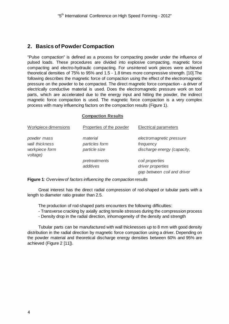
Compaction Results Workpiece dimensions Properties of the powder Electrical parameters powder mass material electromagnetic pressure wall thickness particles form frequency workpiece form particle size discharge energy (capacity, voltage) pretreatments coil properties additives driver properties gap between coil and driver
Figure 1: Overview of factors influencing the compaction results
Great interest has the direct radial compression of rod-shaped or tubular parts with a length to diameter ratio greater than 2.5.
The production of rod-shaped parts encounters the following difficulties: - Transverse cracking by axially acting tensile stresses during the compression process - Density drop in the radial direction, inhomogeneity of the density and strength
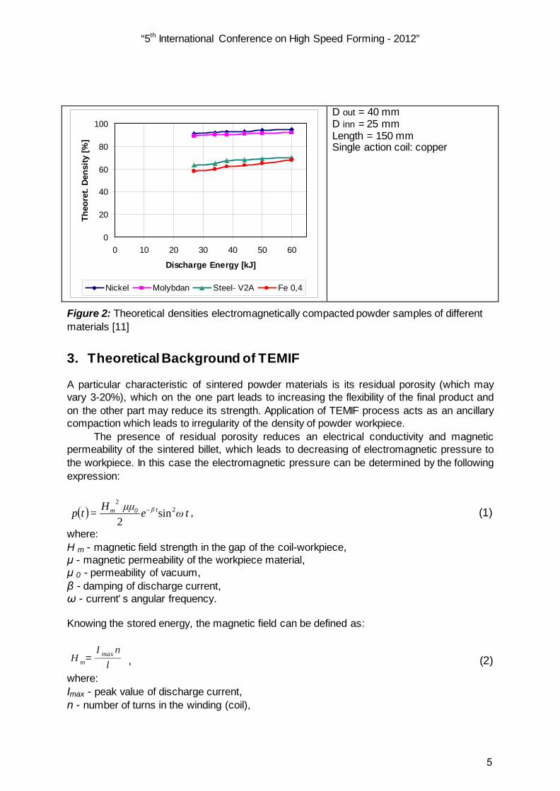
Tubular parts can be manufactured with wall thicknesses up to 8 mm with good density
distribution in the radial direction by magnetic force compaction using a driver. Depending on the powder material and theoretical discharge energy densities between 60% and 95% are achieved (Figure 2 [11]).
4
“5th International Conference on High Speed Forming - 2012”
0
20
40
60
80
100
0 10 20 30 40 50 60
Discharge Energy [kJ]
Theo
ret.
Dens
ity [%
]
Nickel Molybdan Steel- V2A Fe 0,4
D out = 40 mm D inn = 25 mm Length = 150 mm Single action coil: copper
Figure 2: Theoretical densities electromagnetically compacted powder samples of different materials [11]
3. Theoretical Background of TEMIF
A particular characteristic of sintered powder materials is its residual porosity (which may vary 3-20%), which on the one part leads to increasing the flexibility of the final product and on the other part may reduce its strength. Application of TEMIF process acts as an ancillary compaction which leads to irregularity of the density of powder workpiece.
The presence of residual porosity reduces an electrical conductivity and magnetic permeability of the sintered billet, which leads to decreasing of electromagnetic pressure to the workpiece. In this case the electromagnetic pressure can be determined by the following expression:
( ) t ωeμμH=tp t β0m 22
sin2
− , (1)
where: H m - magnetic field strength in the gap of the coil-workpiece, μ - magnetic permeability of the workpiece material, μ 0 - permeability of vacuum, β - damping of discharge current, ω - current' s angular frequency. Knowing the stored energy, the magnetic field can be defined as:
H m=I max n
l , (2) where: Imax - peak value of discharge current, n - number of turns in the winding (coil),
5

“5th International Conference on High Speed Forming - 2012”
l - length of winding. The magnitude of electromagnetic pressure on the powder workpiece can be determined as:
( ) 22
22
sinω4l
ktkeμμnI=tp 1t β0max − , (3)
where: k 1 - factor, which takes into account a magnetic field pressure decrement (due to porosity) to the powder body, k 2 - factor, which takes into consideration the effect of the gap between coil and workpiece. Pressure required for plastic deformation of powder workpiece pd , can be expressed as:
pd= 2σ s ln(c0
c ), (4) where: σ s – tensile strength of powder workpiece, C0, C - initial and final density of powder workpiece.
4. Experimental Studies of TEMIF
Experimental studies were carried out on the equipment BBC-60 of the WHZ Zwickau (Figure 3). Main parameters of BBC-60 are given in Table 1.
a) Control panel b) Power unit
Figure 3: Components of the BBC-60 (Westsächsische Hochschule Zwickau)
6

“5th International Conference on High Speed Forming - 2012”
Storage capacity, μF 7,71-308,4 (stepped) Operating voltage, kV 10-20 (through 1 kV) Charging time, s 20
Charging current, mA 320 (max) Stored energy, kJ 1,5-60 Discharge current (in short-circuited mode) (max), kA
1250 (at 308.4 μF, 20 kV)
Discharge current (min), kA 60 (at 7.71 μF, 10 kV) The frequency of discharge (min.), kHz 37 (at 308.4 μF) Discharge frequency (max.), kHz 125 (at 7.71 μF)
Power (of power supply), kW 10
Table 1. Main parameters of BBC-60 Solenoid-type single-action coils made of insulated copper wire are shown on Figure 4a).
There is no mechanical banding for such coils, so they were destroyed during the passage of the impulsed current. Since the coils have a certain weight, the inertia processes takes some time before its destruction. Such a very short time period is sufficient for acceleration of workpiece deformation.
Single-action coils are cheap and easy for wiring. Yet their effectiveness in some cases is higher than for reusable coils. Single-action coils are very convenient for experiments to set the parameters for subsequent series production. For safety reasons coils were placed in a special reusable protective case, and experiments were conducted inside of protective chamber (Figure 4b).
a) General view of single-action coil with powder billet inside
b) Use of protective case and chamber
Figure 4: Single-action coils for TEMIF of powder workpiece
Coil parameters are listed in Table 2.
7

“5th International Conference on High Speed Forming - 2012”
Wire diameter (with insulation), mm 5,5 Diameter of Conductor (Copper), mm 3.5 Number of turns 5
Inductance, μH 0.04
Table 2: Parameters of the single-action coils
For TEMIF experiments we have chosen a ferrous powder PM-28N (produced by Höganäs AB (Sweden)), which is used for manufacturing of sintered bearings. Main parameters of powder parts for TEMIF process are listed in Table. 3.
Density, g/cm3 6.0-6.6 Porosity, % 18-23.
Hardness, HB 90-120 Chemical composition, % C = 0,6; Ni = 2,5-4,0;
Cu = 1,5; Mo = 0,5; Fe – rest.
Dimensions (External diam. X Internal diam. X Height), mm
40x30x13 and 80x70x19 (55)
Table 3: The parameters of powder parts for TEMIF process
Powder parts used in experiments have been exposed to sintering at 1150 oC in endogas atmosphere.
Two TEMIF options were used: (a) - powder parts free radial deformation, and (b) - press-fitting on a steel mandrel; Hardness of the mandrel after heat-hardening - HRC 56-58, surface roughness 0.1 (Figure 5a). A special set of experiments was carried out with mandrel made of sintered powder (Figure 5b).
a) Powder parts on the steel mandrel b) Two coaxially placed powder parts
Figure 5: Powder parts before TEMIF process
8
“5th International Conference on High Speed Forming - 2012”
The experiments were carried out by varying different parameters of BBC-60: operating voltage from 10 to 15 kV, discharge frequency from 37 to 125 kHz, and the discharge energy level from 10 to 18 kJ.
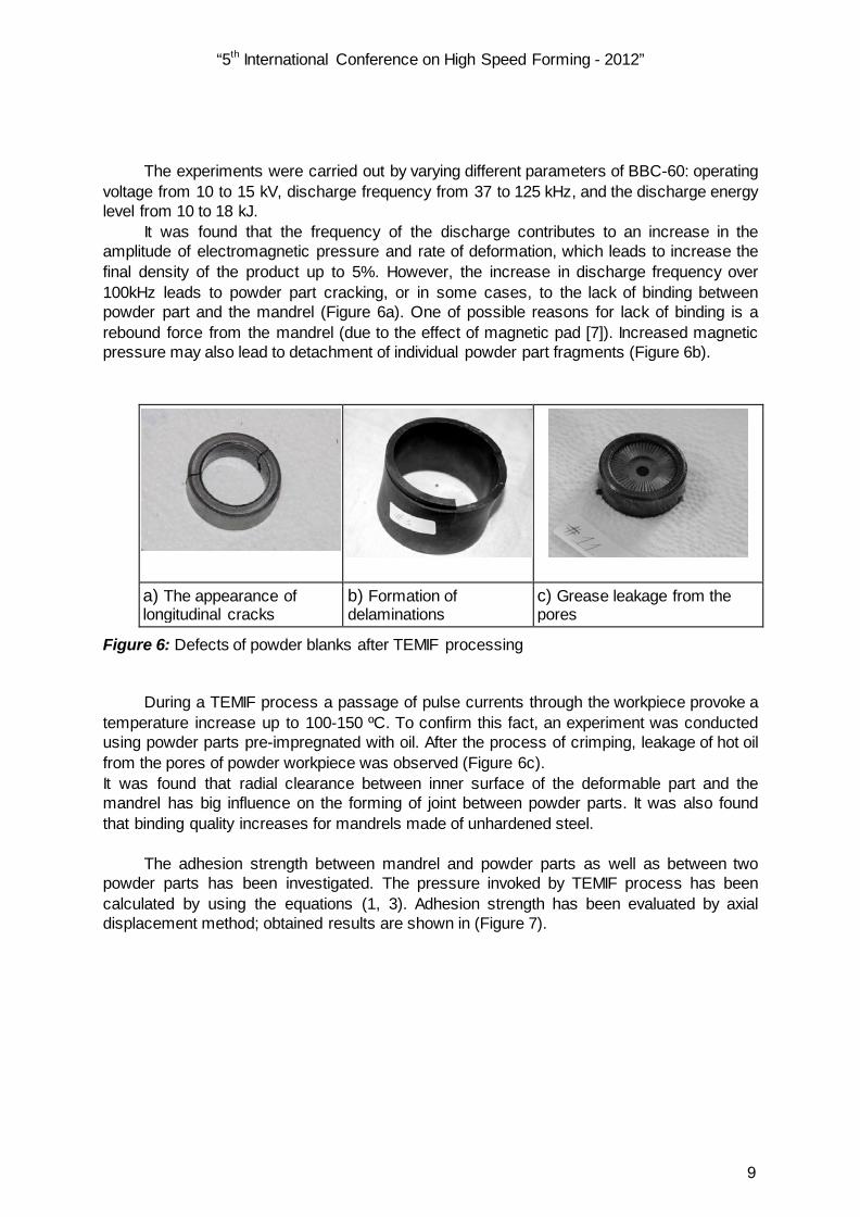
It was found that the frequency of the discharge contributes to an increase in the amplitude of electromagnetic pressure and rate of deformation, which leads to increase the final density of the product up to 5%. However, the increase in discharge frequency over 100kHz leads to powder part cracking, or in some cases, to the lack of binding between powder part and the mandrel (Figure 6a). One of possible reasons for lack of binding is a rebound force from the mandrel (due to the effect of magnetic pad [7]). Increased magnetic pressure may also lead to detachment of individual powder part fragments (Figure 6b).
a) The appearance of longitudinal cracks
b) Formation of delaminations
c) Grease leakage from the pores
Figure 6: Defects of powder blanks after TEMIF processing
During a TEMIF process a passage of pulse currents through the workpiece provoke a
temperature increase up to 100-150 ºC. To confirm this fact, an experiment was conducted using powder parts pre-impregnated with oil. After the process of crimping, leakage of hot oil from the pores of powder workpiece was observed (Figure 6c). It was found that radial clearance between inner surface of the deformable part and the mandrel has big influence on the forming of joint between powder parts. It was also found that binding quality increases for mandrels made of unhardened steel.
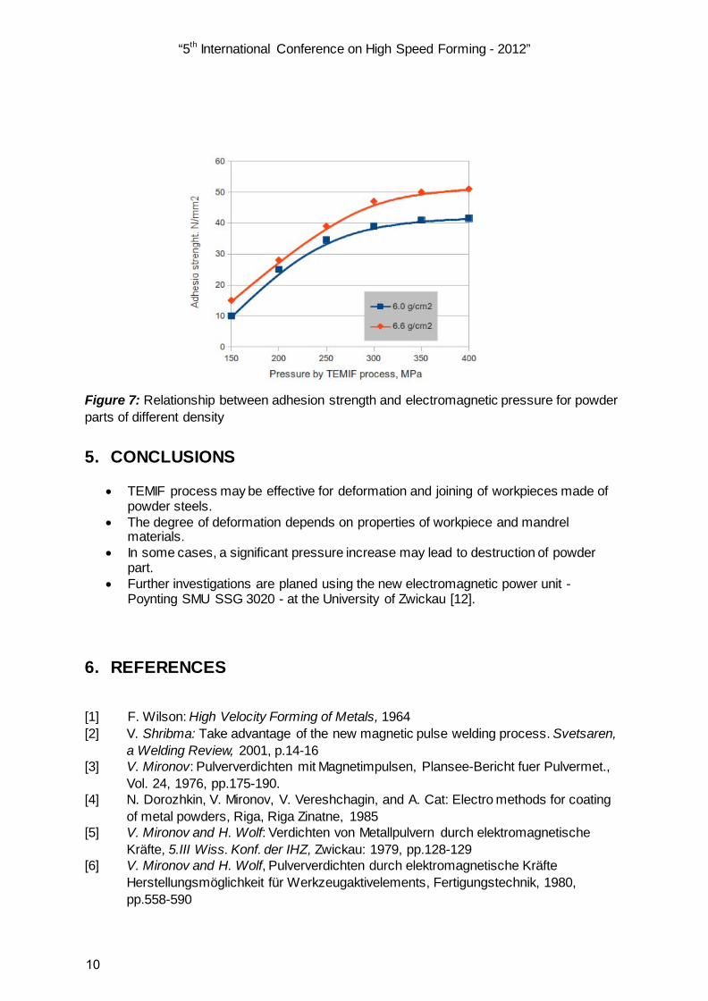
The adhesion strength between mandrel and powder parts as well as between two powder parts has been investigated. The pressure invoked by TEMIF process has been calculated by using the equations (1, 3). Adhesion strength has been evaluated by axial displacement method; obtained results are shown in (Figure 7).
9
“5th International Conference on High Speed Forming - 2012”
Figure 7: Relationship between adhesion strength and electromagnetic pressure for powder parts of different density
5. CONCLUSIONS
• TEMIF process may be effective for deformation and joining of workpieces made of powder steels.
• The degree of deformation depends on properties of workpiece and mandrel materials.
• In some cases, a significant pressure increase may lead to destruction of powder part.
• Further investigations are planed using the new electromagnetic power unit - Poynting SMU SSG 3020 - at the University of Zwickau [12].
6. REFERENCES
[1] F. Wilson: High Velocity Forming of Metals, 1964 [2] V. Shribma: Take advantage of the new magnetic pulse welding process. Svetsaren,
a Welding Review, 2001, p.14-16 [3] V. Mironov: Pulververdichten mit Magnetimpulsen, Plansee-Bericht fuer Pulvermet.,
Vol. 24, 1976, pp.175-190. [4] N. Dorozhkin, V. Mironov, V. Vereshchagin, and A. Cat: Electro methods for coating
of metal powders, Riga, Riga Zinatne, 1985 [5] V. Mironov and H. Wolf: Verdichten von Metallpulvern durch elektromagnetische
Kräfte, 5.III Wiss. Konf. der IHZ, Zwickau: 1979, pp.128-129 [6] V. Mironov and H. Wolf, Pulververdichten durch elektromagnetische Kräfte
Herstellungsmöglichkeit für Werkzeugaktivelements, Fertigungstechnik, 1980, pp.558-590
10
“5th International Conference on High Speed Forming - 2012”
[7] V. Mironov, V. Zemchenkov, and V. Lapkovsky: Model of the Magnetic packings of dispersed materials," Transactions of the VŠB-Technical University of Ostrava, 2009, pp.249-253
[8] A. Mamalis, D. Manolakos, A. Kladas, and A. Koumoutsos: Electromagnetic forming and powder processing: Trends and developments, Applied Mechanics Reviews, vol. 57, 2004, p.299
[9] B. Chelluri and E. Knoth: Powder Forming Using Dynamic Magnetic Compaction, 4th International Conference on High Speed Forming, 2010, pp.26-34
[10] H. Wolf: Application of Electromagnetic Forces for Powder Compaction and Joints,Proc. of the 7th International Conference of High Energy Rate Fabrication, Leeds, UK: 1981
[11] M. Meinel: Magnetkraftverdichten, Verfahren des Impulsverdichtens – einige technologische Aspekte, Kolloquium Elektromagnetische Umformung, Uni Dortmund, WHZ Zwickau, 2001
[12] Ch. Beerwald: Anlage zur elektromagnetischen Umformung –SMU SSG 3020, Poynting GmbH Dortmund, 2010, www.poynting.de
11

“5th International Conference on High Speed Forming - 2012”
12
Online Measurement of the Radial Workpiece Displacement in Electromagnetic Forming Subsequent to Hot Aluminum Extrusion*
A. Jäger1, A. E. Tekkaya1
1 Institute of Forming Technology and Lightweight Construction, TU Dortmund University, Germany
Abstract
Electromagnetic compression was integrated into the process chain of hot metal extrusion in order to reduce the cross section of the workpiece locally. To integrate both processes, a tool coil for electro-magnetic compression is positioned behind the die exit and coaxially to the extrudate. Additionally, a counter die in the shape of a mandrel can be mounted to the mandrel of a porthole extrusion die, which extends into the working area of the tool coil. Experiments were conducted on hollow profiles which were compressed by electromagnetic forming subsequent to extrusion. Due to an extremely short processing time of the high speed forming process, a compensation of the relative speed between the workpiece and the tooling can be ignored. For determine the workpiece displacement during the electromagnetic forming process, a new measuring strategy based on the Photon Doppler Velocimetry was developed.
Keywords
Electromagnetic forming, High speed forming, On-line measurement
* This work is based on the results of the subproject A2 of the DFG SFB / TR30; the authors would like to thank the German Research Foundation (DFG) for its financial support
13

5th International Conference on High Speed Forming – 2012
1 Introduction
Hot metal extrusion is used to produce straight, semi-finished products in mass production [1] with a constant cross section over the length and homogeneous mechanical and microstructural properties [2]. Frequently aluminum sections are used as construction elements. As, in general, the loading conditions of structure elements in technical constructions differ locally, the constant cross section, which is attributed to the peculiarity of the extrusion process itself, mostly represents a compromise between the functionality and the component design. This may result in local oversizing and excessive use of resources. A local adaption of the geometry could be suitable in order to adapt the locally specific demands on the structure properties. For this reason, the development of innovative forming technologies is indispensable in order to manufacture products with graded properties as well as locally adapted geometric shapes.
In order to modify the geometry of a tubular extrudate locally, electromagnetic compression was integrated as a hot forming operation into the process chain of hot metal extrusion. By process integration of both processes the heat of extrusion is used for the successive forming operation.
2 Description of the Concept
While hot metal extrusion is used to produce tubular semi-finished products with a constant cross section quasi continuously, electromagnetic compression can be used to reduce a workpiece’s cross sections locally. To integrate both processes, a tool coil for compression was positioned behind the die exit and coaxially to the extrudate in order to reduce the workpiece cross section locally (Figure 1). Due to the favourable relation between resulting exit speed in extrusion (typical 50 m/min) and the processing time in electromagnetic compression (typical 100 µs), a longitudinal translation between the workpiece and the tool coil during the compression process can be neglected. Therefore, the application of electromagnetic compression subsequent to extrusion is possible without a compensation of the relative speed between the workpiece and the tooling. The tool coil can be placed stationary behind the die exit.
Figure 1: Concept of extrusion and integrated electromagnetic compression (longitudinal section, schematic)[3]
14

5th International Conference on High Speed Forming – 2012
To achieve a more defined geometry, in comparison to a free forming operation, and to increase the geometrical complexity of locally compressed areas, a counter die in the shape of a mandrel can be used. This is mounted to the mandrel of a porthole extrusion die and extended into the tool coil [4].
3 Setup and First Trials
For the evaluation of the concept, a test rig was built (Figure 2). In order to reduce the workpiece cross section locally different solenoid tool coils (Poynting GmbH), connected to a 32 kJ pulse power generator (Maxwell-Magneform series 7000), were positioned behind the die exit of a 250-t direct extrusion press (Collin PLA250t). To adapt the tool coil and the extrudate geometry, field shapers made out of a CuCrZr-alloy or an EN AW-6060 alloy, insulated with a polyimide foil, were used. Beyond shaping and concentrating of the electromagnetic field, by using a field shaper also an overheating of the tool coil by thermal radiation of the processed hot extrudate is prevented. Guiding rollers made out of brass are arranged pairwise at the inlet and runout side of the tool coil to assure a uniform air gap between the field shaper and the workpiece. For heat treating of the extruded and subsequently hot deformed workpieces made of heat treatable alloys, an additional quenching setup using air atomized water mist as a coolant was integrated behind the coil. The whole setup is designed compactly in order to ensure that the temperature of the extruded aluminum does not decrease too much before the subsequent forming and heat treatment operation.
Figure 2: Setup for hot extrusion and subsequent electromagnetic compression [3]
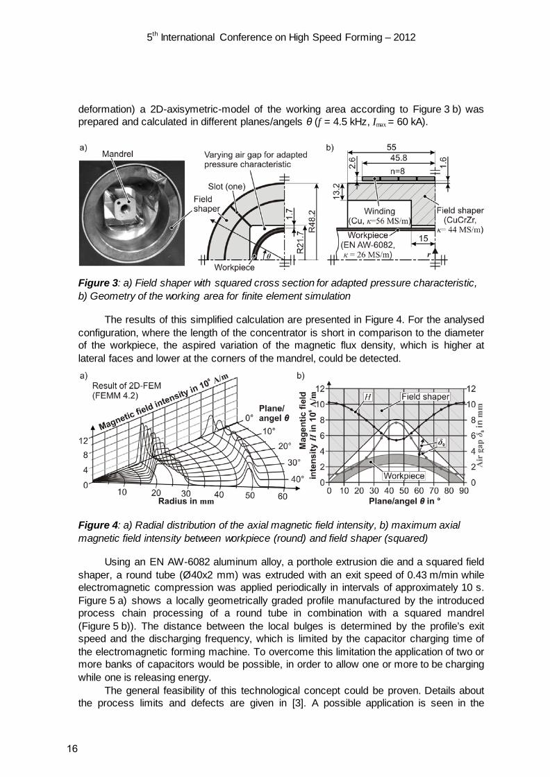
In order to expand the range of geometrical shapes with cross-sections other than that of the extruded aluminum, a mandrel can be used to define the cross section geometry. A squared mandrel for the processing of a round tube was chosen and specially designed to prevent force fit between the workpiece and the die. To prevent a force fit between the extrudate and the mandrel, the corners of the mandrel are chamfered with a radius of 5 mm and a draft angle of 0.5° in extrusion direction is applied. Additionally, a squared field shaper in combination with the round tube was used to adapt the air gap between the field shaper and the workpiece (Figure 3 a)) and accordingly the pressure. For proving this concept, a simplified finite element simulation of the magnetic field was carried out using FEMM 4.2 developed by Meeker [7]. For calculation of the electromagnetic field distribution in the initial condition (neglecting the effect of
15
5th International Conference on High Speed Forming – 2012
deformation) a 2D-axisymetric-model of the working area according to Figure 3 b) was prepared and calculated in different planes/angels θ (f = 4.5 kHz, Imax = 60 kA).
Figure 3: a) Field shaper with squared cross section for adapted pressure characteristic, b) Geometry of the working area for finite element simulation
The results of this simplified calculation are presented in Figure 4. For the analysed configuration, where the length of the concentrator is short in comparison to the diameter of the workpiece, the aspired variation of the magnetic flux density, which is higher at lateral faces and lower at the corners of the mandrel, could be detected.
Figure 4: a) Radial distribution of the axial magnetic field intensity, b) maximum axial magnetic field intensity between workpiece (round) and field shaper (squared)
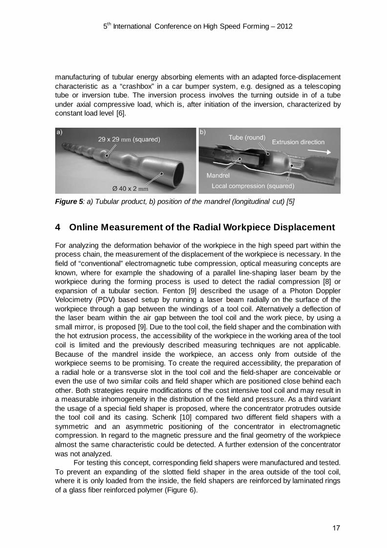
Using an EN AW-6082 aluminum alloy, a porthole extrusion die and a squared field shaper, a round tube (Ø40x2 mm) was extruded with an exit speed of 0.43 m/min while electromagnetic compression was applied periodically in intervals of approximately 10 s. Figure 5 a) shows a locally geometrically graded profile manufactured by the introduced process chain processing of a round tube in combination with a squared mandrel (Figure 5 b)). The distance between the local bulges is determined by the profile’s exit speed and the discharging frequency, which is limited by the capacitor charging time of the electromagnetic forming machine. To overcome this limitation the application of two or more banks of capacitors would be possible, in order to allow one or more to be charging while one is releasing energy.
The general feasibility of this technological concept could be proven. Details about the process limits and defects are given in [3]. A possible application is seen in the
16
5th International Conference on High Speed Forming – 2012
manufacturing of tubular energy absorbing elements with an adapted force-displacement characteristic as a “crashbox” in a car bumper system, e.g. designed as a telescoping tube or inversion tube. The inversion process involves the turning outside in of a tube under axial compressive load, which is, after initiation of the inversion, characterized by constant load level [6].
Figure 5: a) Tubular product, b) position of the mandrel (longitudinal cut) [5]
4 Online Measurement of the Radial Workpiece Displacement
For analyzing the deformation behavior of the workpiece in the high speed part within the process chain, the measurement of the displacement of the workpiece is necessary. In the field of “conventional” electromagnetic tube compression, optical measuring concepts are known, where for example the shadowing of a parallel line-shaping laser beam by the workpiece during the forming process is used to detect the radial compression [8] or expansion of a tubular section. Fenton [9] described the usage of a Photon Doppler Velocimetry (PDV) based setup by running a laser beam radially on the surface of the workpiece through a gap between the windings of a tool coil. Alternatively a deflection of the laser beam within the air gap between the tool coil and the work piece, by using a small mirror, is proposed [9]. Due to the tool coil, the field shaper and the combination with the hot extrusion process, the accessibility of the workpiece in the working area of the tool coil is limited and the previously described measuring techniques are not applicable. Because of the mandrel inside the workpiece, an access only from outside of the workpiece seems to be promising. To create the required accessibility, the preparation of a radial hole or a transverse slot in the tool coil and the field-shaper are conceivable or even the use of two similar coils and field shaper which are positioned close behind each other. Both strategies require modifications of the cost intensive tool coil and may result in a measurable inhomogeneity in the distribution of the field and pressure. As a third variant the usage of a special field shaper is proposed, where the concentrator protrudes outside the tool coil and its casing. Schenk [10] compared two different field shapers with a symmetric and an asymmetric positioning of the concentrator in electromagnetic compression. In regard to the magnetic pressure and the final geometry of the workpiece almost the same characteristic could be detected. A further extension of the concentrator was not analyzed.
For testing this concept, corresponding field shapers were manufactured and tested. To prevent an expanding of the slotted field shaper in the area outside of the tool coil, where it is only loaded from the inside, the field shapers are reinforced by laminated rings of a glass fiber reinforced polymer (Figure 6).
17
5th International Conference on High Speed Forming – 2012
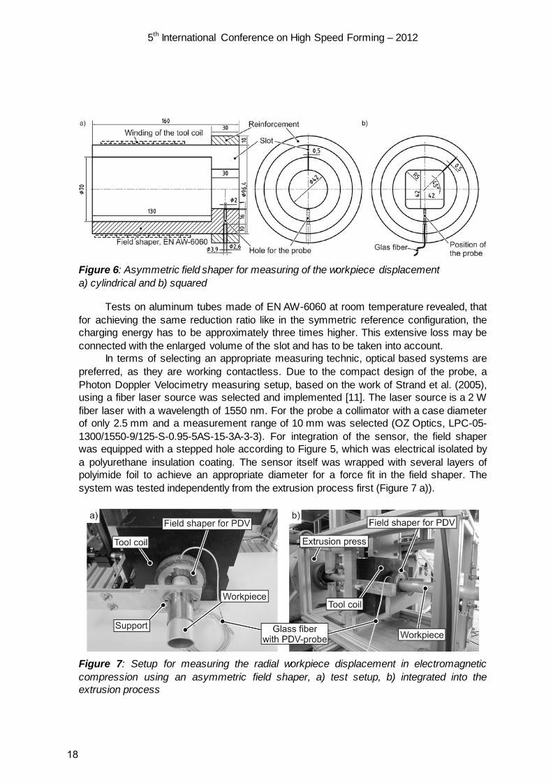
Figure 6: Asymmetric field shaper for measuring of the workpiece displacement a) cylindrical and b) squared
Tests on aluminum tubes made of EN AW-6060 at room temperature revealed, that for achieving the same reduction ratio like in the symmetric reference configuration, the charging energy has to be approximately three times higher. This extensive loss may be connected with the enlarged volume of the slot and has to be taken into account.
In terms of selecting an appropriate measuring technic, optical based systems are preferred, as they are working contactless. Due to the compact design of the probe, a Photon Doppler Velocimetry measuring setup, based on the work of Strand et al. (2005), using a fiber laser source was selected and implemented [11]. The laser source is a 2 W fiber laser with a wavelength of 1550 nm. For the probe a collimator with a case diameter of only 2.5 mm and a measurement range of 10 mm was selected (OZ Optics, LPC-05-1300/1550-9/125-S-0.95-5AS-15-3A-3-3). For integration of the sensor, the field shaper was equipped with a stepped hole according to Figure 5, which was electrical isolated by a polyurethane insulation coating. The sensor itself was wrapped with several layers of polyimide foil to achieve an appropriate diameter for a force fit in the field shaper. The system was tested independently from the extrusion process first (Figure 7 a)).
Figure 7: Setup for measuring the radial workpiece displacement in electromagnetic compression using an asymmetric field shaper, a) test setup, b) integrated into the extrusion process
18

5th International Conference on High Speed Forming – 2012
The signals for determining the velocity of the workpiece and for the current (detected by a Rogowski-coil) are detected and recorded parallel on an oscilloscope (LeCroy waveRunner 104MXi 1GHz Oscilloscope 10 GS/s). For analyzing the velocity signal, represented by the beat frequency as the difference between the emitted light and the Doppler-shifted light reflected from the specimens’ surface [11], a Fourier transformation in Matlab using the implemented “spectrogram”-function is run. It results in a plot of a time variant frequency distribution. In Figure 8 a) an example of a determined spectrogram is given. Due to multiple reflections between the specimen and the probe, beside the intrinsic signal integer multiple ones of it can appear which complicates the automatic compilation. The radial workpiece velocity is calculated by multiplying the beat frequency by the half of the frequency of the laser wavelength (Figure 8 b)).
Figure 8: Example for the analysis of the Photon Doppler Velocimetry (PDV) a) spectrogram of the beat frequency, b) absolute value of the radial workpiece velocity
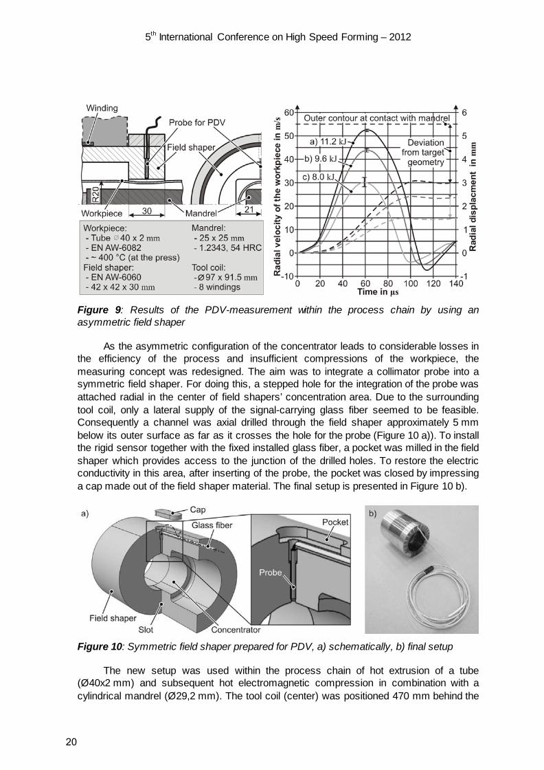
The developed measuring setup was tested within the process chain. While in applying the cylindrical field shaper in combination with a cylindrical mandrel (Ø29.2 mm) adequate forming results could be achieved, the squared version worked insufficient. In Figure 9 the results of the velocity measurements and details of the parameter in processing of a round tube (Ø40x2 mm) subsequent to hot extrusion by using the asymmetric field shaper with a squared cross section (Figure 5 b)) in combination with a squared mandrel are summarized. Limited by the insulation of the used tool coil, even at the highest applicable charging energy of 11 kJ, the workpiece touches the mandrel only locally, while the side faces are not getting into contact. In comparison: By using a symmetrical field shaper, a charging energy of only 8 kJ is sufficient to achieve a full contact between the workpiece and the mandrel.
19
5th International Conference on High Speed Forming – 2012
Figure 9: Results of the PDV-measurement within the process chain by using an asymmetric field shaper
As the asymmetric configuration of the concentrator leads to considerable losses in the efficiency of the process and insufficient compressions of the workpiece, the measuring concept was redesigned. The aim was to integrate a collimator probe into a symmetric field shaper. For doing this, a stepped hole for the integration of the probe was attached radial in the center of field shapers’ concentration area. Due to the surrounding tool coil, only a lateral supply of the signal-carrying glass fiber seemed to be feasible. Consequently a channel was axial drilled through the field shaper approximately 5 mm below its outer surface as far as it crosses the hole for the probe (Figure 10 a)). To install the rigid sensor together with the fixed installed glass fiber, a pocket was milled in the field shaper which provides access to the junction of the drilled holes. To restore the electric conductivity in this area, after inserting of the probe, the pocket was closed by impressing a cap made out of the field shaper material. The final setup is presented in Figure 10 b).
Figure 10: Symmetric field shaper prepared for PDV, a) schematically, b) final setup
The new setup was used within the process chain of hot extrusion of a tube (Ø40x2 mm) and subsequent hot electromagnetic compression in combination with a cylindrical mandrel (Ø29,2 mm). The tool coil (center) was positioned 470 mm behind the
20
5th International Conference on High Speed Forming – 2012
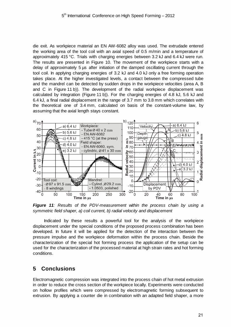
die exit. As workpiece material an EN AW-6082 alloy was used. The extrudade entered the working area of the tool coil with an axial speed of 0.5 m/min and a temperature of approximately 415 °C. Trials with charging energies between 3.2 kJ and 6.4 kJ were run. The results are presented in Figure 10. The movement of the workpiece starts with a delay of approximately 5 µs after initiation of the damped oscillating current through the tool coil. In applying charging energies of 3.2 kJ and 4.0 kJ only a free forming operation takes place. At the higher investigated levels, a contact between the compressed tube and the mandrel can be detected by sudden drops in the workpiece velocities (area A, B and C in Figure 11 b)). The development of the radial workpiece displacement was calculated by integration (Figure 11 b)). For the charging energies of 4.8 kJ, 5.6 kJ and 6.4 kJ, a final radial displacement in the range of 3.7 mm to 3.8 mm which correlates with the theoretical one of 3.4 mm, calculated on basis of the constant-volume law, by assuming that the axial length stays constant.
Figure 11: Results of the PDV-measurement within the process chain by using a symmetric field shaper, a) coil current, b) radial velocity and displacement
Indicated by these results a powerful tool for the analysis of the workpiece displacement under the special conditions of the proposed process combination has been developed. In future it will be applied for the detection of the interaction between the pressure impulse and the workpiece deformation within the process chain. Beside the characterization of the special hot forming process the application of the setup can be used for the characterization of the processed material at high strain rates and hot forming conditions.
5 Conclusions
Electromagnetic compression was integrated into the process chain of hot metal extrusion in order to reduce the cross section of the workpiece locally. Experiments were conducted on hollow profiles which were compressed by electromagnetic forming subsequent to extrusion. By applying a counter die in combination with an adapted field shaper, a more
21
5th International Conference on High Speed Forming – 2012
defined geometry can be achieved and the geometrical complexity of locally compressed areas can be increased. For analyzing the deformation behavior of the workpiece in the electromagnetic forming part of the process chain, specially designed field shapers for the online measurement of the radial velocity of the workpiece on the basis of the Photon Doppler Velocimetry were developed and tested successfully. A tool for the analysis of the workpiece displacement under the special conditions of the proposed process chain has been developed. This offers the potential to analyze the interaction between the pressure impulse and the workpiece deformation within the process chain in future.
References
[1] Laue, K. Stenger, H.: Strangpressen, Aluminium Verlag, Düsseldorf, p. 1, 1976. [2] Hall, D. D., Mudawar, I.: Optimization of Quench History of Aluminium parts for
Superior Mechanical Properties, International Journal of Heat and Mass Transfer 39 (1), p. 81-95, 1996.
[3] Jäger, A., Risch, D., Tekkaya, A. E.: Thermo-mechanical processing of aluminum profiles by integrated electromagnetic compression subsequent to hot extrusion, Journal of Materials Processing Technology 211 (5), Special Issue: Impulse Forming, p. 936-943, 2011.
[4] Jäger, A., Risch, D., Tekkaya, A. E.: Patent application DE 10 2009 039 759 A1. Verfahren und Vorrichtung zum Strangpressen und nachfolgender elektromagnetischer Umformung, 31 August 2009.
[5] Jäger, A., Ben Khalifa, N., Psyk, V., Tekkaya, A. E.: Thermo-mechanical Processing of Aluminum Profiles Subsequent to Hot Extrusion, steel research international, Special edition: International Conference on Technology of Plasticity, ICTP, Aachen, Germany, 2011, p. 280-285.
[6] Guist, L.R., Marble, D.P.: Prediction of the inversion load. NASA Technical Note 3622, 1966.
[7] Meeker, D., www.femm.info/wiki/homepage, 2010. [8] Bauer, D.: Messung der Umformkraft und der Formänderung bei der
Hochgeschwindigkeitsumformung rohrförmiger Werkstücke durch magnetische Kräfte, Bänder Bleche Rohre 6 (10), p. 575-577, 1965.
[9] Fenton, G.: Dynamic Characterization of Powdered Ceramics, In: Proceedings of the 4th International Conference on High Speed Forming - ICHSF 2010, Columbus, Ohio, USA, 2010, p. 275-284.
[10] Schenk, H.: Untersuchungen von einfachen und zusammengesetzten Feldkonzentratoren für die Umformung von Rohren mit magnetischen Kräften, Bänder Bleche Rohre, 10 (4), p. 226-230, 1969.
[11] Strand, O.T., Berzins, L.V., Goosman, D.R., Kuhlow, W.W., Sargis, P.D., Whitworth, T.L.: Velocimetry using heterodyne techniques In: Proceedings of the 26th International Congress on High-Speed Photography and Photonics, 2005, p. 593-599.
22
Some aspects regarding the use of a pneumomechanical high speed forming process
W. Homberg, E. Djakow, O. Akst
Chair of Manufacturing and Forming Technology (LUF), Paderborn University, Paderborn Germany
Abstract
A promising approach to the production of thin-walled workpieces in high strength materials is the use of a special pneumomechanical high-speed-forming process. This process uses a pneumatically accelerated plunger that dives into a pressure chamber filled with the working media in order to generate a short pressure pulse. Ways in which the pressure pulse can be influenced include e.g. varying the type of working media, the density of the working media, the accelerating pressure distance and the plunger geometry. The influence of these parameters on the process formed the subject of intense technological research at the Chair of Forming and Machining Technology (LUF) at Paderborn University. The results of these investigations were used to achieve an appropriate process and tool design for the pneumomechanical high-speed forming process. It thus proved possible to manufacture complex workpieces and geometrical details from thin-walled, high strength stainless steel or aluminium alloys that cannot be produced by conventional stamping processes. Because of the high uniformity of the pressure distribution in the radial direction, it is possible to achieve just small dimensional or geometrical deviations in respect of the desired shape of the workpiece. The planned paper will present results of the basic research conducted into pneumomechanical high-speed-forming as well as a comparison with electrohydraulic forming.
Keywords
Pneumomechanical Forming, Electro Hydraulic Forming, High Speed Hydroforming
23
5th International Conference on High Speed Forming – 2012
1 Introduction
The technology of high-speed forming has been familiar since the 19th century already. Intensive research related to this technological field has been conducted in the United States, Germany and the Soviet Union, in particular, starting in 1955 [1]. The high speed forming process includes all those manufacturing processes in which the necessary forming energy is released very quickly and then rapidly transferred to the workpiece. The total time taken by a typical high speed forming process ranges from a few microseconds to 1000 microseconds. An important characteristic of a process of this kind is that it will allow very high pressures to be achieved, permitting the manufacture of small, sharp contoured geometrical details. Using the high speed technology it is also possible to achieve very high strain rates during forming, often with beneficial effects on formability. Several working principles, including use of a explosive, electrohydraulic and pneumomechanical compression, are used for pressure pulse generation in both research work and industrial practice [2, 3]. An energy level of up to 250 kJ and pressures of up to 25 GPa are possible [6, 9].
Electrohydraulic forming (EHF), as one key process, is characterized by an electric discharge process using a special electrode arrangement inside a liquid working medium. The electric discharge is used to create a short pressure pulse or shock wave inside a discharge chamber in order to deform the workpiece. Typical process times are a few microseconds [7].
The first experiments with EHF were performed in the 1940s. The further development of electrohydraulic forming began in the 1960s, described among others by Bruno (1968) and Wilson (1964). Scientists in Germany, the USSR, the USA, Japan and other countries have developed a large number of experimental electro-hydraulic setups. So far, EHF technology has been successfully used for deep drawing, calibration, expansion and joining processes, for example. A major advantage of the electrohydraulic method is the possibility of repeating the discharge process in order to achieve greater deformation [10, 11, 12]. Recent results published in Eguia [6] and Homberg [4] inter alia show that the reproducibility of the high voltage underwater discharge can be increased by using an ignition wire. This wire vaporizes during the process and promotes the formation of a plasma channel [6, 9]. Current research work being performed in the USA is focused on extending the forming limits by comparison to conventional forming processes. The use of EHF for manufacturing automotive sheet metal parts has thus been examined by Golovashchenko [8]. He used a special electrohydraulic setup in a two-step method to extend the capability of conventional stamping technology for parts with deep cavities and sharp radii. In the first forming step, a conventional quasi static forming process like deep drawing is used to produce a preform. In the second step, a pressure pulse generated with the help of the underwater discharge process is used to calibrate the desired geometry. Golovashchenko and also [6, 9] are using a multi electrode arrangement to better control the deformation process and enhance the pressurized area. The results of the experiments performed show that the use of the multi chamber forming tool and electrode arrays permits the efficient production of large-scale geometries [8, 12].
Another interesting method for the generation of shock waves is the pneumomechanical method, where a pneumatically accelerated plunger dives into a closed cavity, thereby generating a short pressure pulse. The plunger is accelerated by compressed air inside a pipe. A major advantage of the pneumomechanical method (PMF) is the
24

5th International Conference on High Speed Forming – 2012
possibility of generating high pressure pulses with a high reproducibility. The first known prototype machine based on this working principle was developed by Tomigana and Takamatsu in 1964 [5]. An initial investigation showed that pressures up to 900 MPa and energies of 26 kJ in the working media were possible. Furthermore, the research showed that inertia effects supported the locking of the tool, so that only low locking forces are necessary. To manufacture parts with complex and sharp formed geometries it was also useful to employ several strokes or a pressurization cycles. With this setup, it was even possible to manufacture complex parts. Typical process times are just a few milliseconds. A further development of this setup was presented by Kosing and Skews in [13]. Another pneumomechanical setup was used by Frolov for forming and cutting procedures like stretch drawing and cutting. For the cutting procedures, the plunger was used as a stamp, with no working media in the chamber. The cutting result depends on the attainable energies as well as on the blank properties like blank thickness [14]. So far the pneumomechanical method has only been used for the production of small tube and sheet metal parts.
To summarize, it can be said that quite a lot of research has been conducted into the use of EHF and PMF. There has been no adequate comparison of the two processes, however, especially regarding the production of sharp contoured geometrical details.
2 Experimental setup
To realize the desired comparison between EHF and PMF two different experimental setups were used. Apart from an electrohydraulic setup, use was made of a special pneumomechanical setup, in particular.
2.1 Pneumomechanical setup
The experimental setup used at the LUF for the high speed forming of sheet metal parts with the help of a pneumatically accelerated plunger consists of a pressure generation unit, a vertically arranged acceleration tube and the die with the necessary base plates. Inside the tube, a plunger is accelerated by the compressed gas. The accelerated plunger dives into the water-filled cavity of the die and brings about the desired deformation of the sheet metal there. The maximum acceleration pressure is 1.5 MPa, the length of the acceleration tube is 5.1 m, and the diameter used is 38 mm. At the lower end of the tube there is a device for measuring the plunger speed in order to determine the plunger energy. The pressure measurements inside the pressurized areas of the tool were performed using a high-frequency ICP pressure sensor (109C11) from PCB, New York, USA.
2.2 Spark gap setup
The investigations regarding the electrohydraulic forming were performed using a laboratory setup from Poynting GmbH. This consists of a capacitor bank, a switch, a discharge chamber, a forming tool, and an underwater spark gap, which was fitted with an ignition wire for reliable or improved discharge behavior (see also [4]). The power unit consists of two capacitor banks, with a capacity of 14.1 μF (per capacitor) and a maximum charging voltage of 18.5 kV, so that the maximum charging energy of the system was 4.5 kJ. The distance between the pressure sources and the sheet metal was determined by the arrangement of the electrodes in the pressure chamber, with a minimum of 87 mm. The pressure chamber
25

5th International Conference on High Speed Forming – 2012
was adjusted adaptively to the existing lower half of the tool in the pneumomechanical experimental setup. In order to achieve a more reproducible spark discharge and to minimize the number of failed attempts, the discharge was initiated by the ignition wire. As the ignition wire was 0.1 mm thick and 10 mm long, stainless steel wire was used.
Fig. 1: Pneumomechanical setup: 1 – pressure generation unit; 2 – lever valve; 3 - release mechanism; 4 – plunger; 5 – acceleration tube; 6 – light barrier; 7- SAE flange; 8 - pressure chamber; 9 – working medium; 10 - membrane pressure gauge (die); 11 - lower tooling adaptor; 12 – vacuum connection; 13 – sensor adapter; 14 – pressure transducer (PCB 109C11 p=0-5500bar). Spark gap setup (wire configuration): a – mass electrode; b - discharge chamber adapter; c – insulated electrode; d - discharge chamber; e – wire; f - working medium; g – die; h – die spacer ring; i – vacuum connection; j - spacer ring 40 mm in height
3 Results and Discussion
One important aim of the technological research conducted at the LUF was a detailed analysis of the influence and interaction of the process parameters with the pressure height and distribution during pneumomechanical high speed forming, and a comparison with electrohydraulic forming. Initially, the pneumomechanical forming process was therefore examined with regard to the influence of parameters such as the working media density, the accelerating distance and the plunger geometry on the pressure height and the pressure distribution. In order to determine the pressure distribution and height, use is made of a
26
5th International Conference on High Speed Forming – 2012
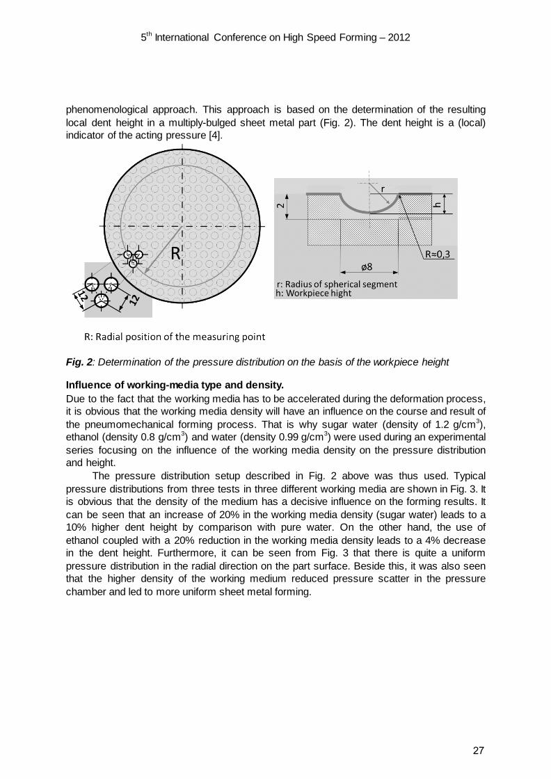
phenomenological approach. This approach is based on the determination of the resulting local dent height in a multiply-bulged sheet metal part (Fig. 2). The dent height is a (local) indicator of the acting pressure [4].
Fig. 2: Determination of the pressure distribution on the basis of the workpiece height
Influence of working-media type and density. Due to the fact that the working media has to be accelerated during the deformation process, it is obvious that the working media density will have an influence on the course and result of the pneumomechanical forming process. That is why sugar water (density of 1.2 g/cm3), ethanol (density 0.8 g/cm3) and water (density 0.99 g/cm3) were used during an experimental series focusing on the influence of the working media density on the pressure distribution and height.
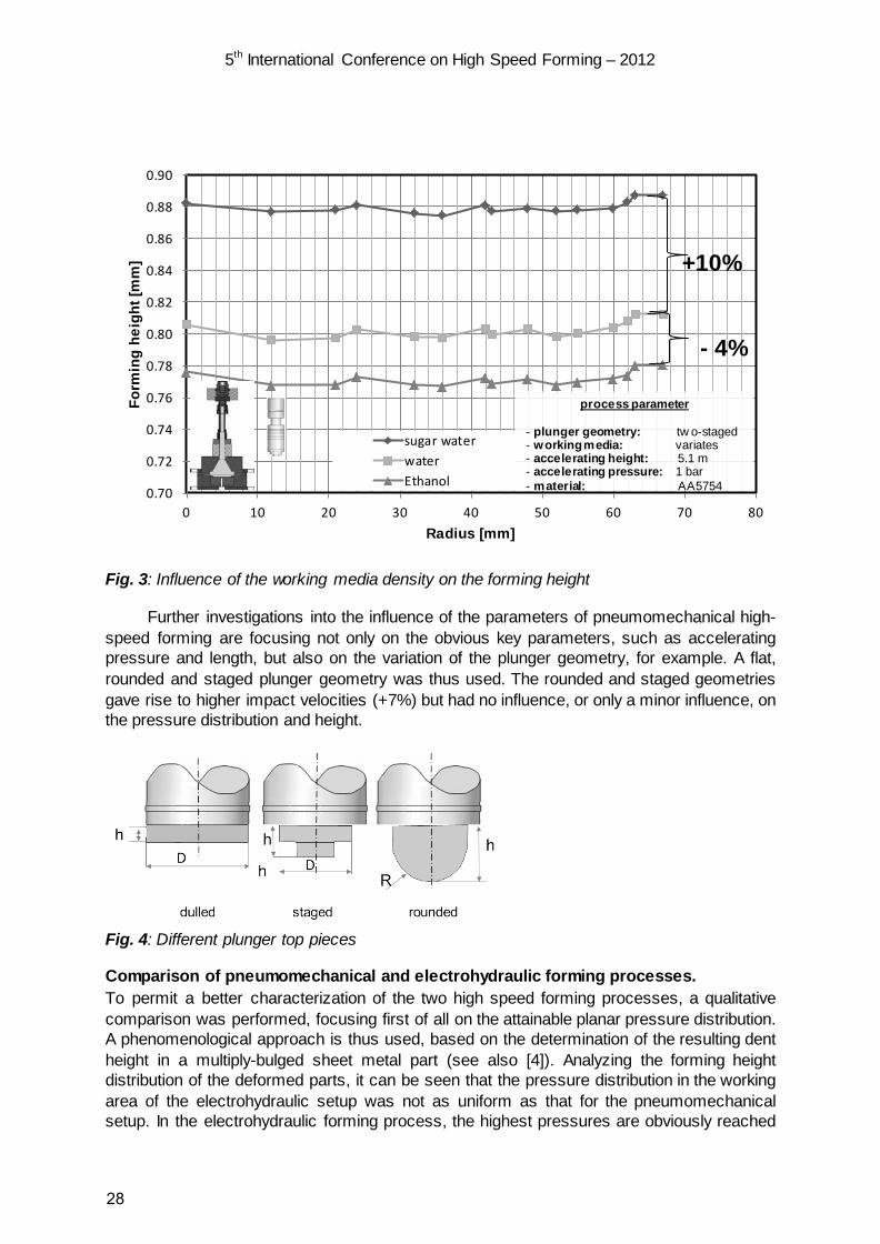
The pressure distribution setup described in Fig. 2 above was thus used. Typical pressure distributions from three tests in three different working media are shown in Fig. 3. It is obvious that the density of the medium has a decisive influence on the forming results. It can be seen that an increase of 20% in the working media density (sugar water) leads to a 10% higher dent height by comparison with pure water. On the other hand, the use of ethanol coupled with a 20% reduction in the working media density leads to a 4% decrease in the dent height. Furthermore, it can be seen from Fig. 3 that there is quite a uniform pressure distribution in the radial direction on the part surface. Beside this, it was also seen that the higher density of the working medium reduced pressure scatter in the pressure chamber and led to more uniform sheet metal forming.
27
5th International Conference on High Speed Forming – 2012
Fig. 3: Influence of the working media density on the forming height
Further investigations into the influence of the parameters of pneumomechanical high-speed forming are focusing not only on the obvious key parameters, such as accelerating pressure and length, but also on the variation of the plunger geometry, for example. A flat, rounded and staged plunger geometry was thus used. The rounded and staged geometries gave rise to higher impact velocities (+7%) but had no influence, or only a minor influence, on the pressure distribution and height.
Fig. 4: Different plunger top pieces
Comparison of pneumomechanical and electrohydraulic forming processes. To permit a better characterization of the two high speed forming processes, a qualitative comparison was performed, focusing first of all on the attainable planar pressure distribution. A phenomenological approach is thus used, based on the determination of the resulting dent height in a multiply-bulged sheet metal part (see also [4]). Analyzing the forming height distribution of the deformed parts, it can be seen that the pressure distribution in the working area of the electrohydraulic setup was not as uniform as that for the pneumomechanical setup. In the electrohydraulic forming process, the highest pressures are obviously reached
0.70
0.72
0.74
0.76
0.78
0.80
0.82
0.84
0.86
0.88
0.90
0 10 20 30 40 50 60 70 80
Form
ing
heig
ht [m
m]
Radius [mm]
sugar waterwaterEthanol
+10%
- 4%
process parameter
- plunger geometry: tw o-staged - working media: variates - accelerating height: 5.1 m - accelerating pressure: 1 bar - material: AA5754
28

5th International Conference on High Speed Forming – 2012
in the center, or just below the ignition wire, and also in the outer region of the workpiece (see Fig. 5).
This fairly high uniformity is perhaps caused by the geometry employed for the pressure chamber and the position of the spark gap inside. There is potential for unifying the pressure distribution by optimizing the pressure chamber geometry and the spark gap arrangement. Further experiments with the pneumomechanical setup showed that, in addition to quite a uniform pressure distribution, good or slightly better repeatability is possible. The scatter of the forming height during repeatedly-performed forming operations was 2% for the pneumomechanical forming process and 4.5% for electrohydraulic forming. Reducing these deviations is the subject of current research work looking into the further influence of process parameters and developing improved process strategies.
Fig.5: Distribution of the forming height above the sheet by electrohydraulic und pneumomechanical forming
Unfortunately, with the pneumomechanical experimental setup employed, it is not possible to perform multiple forming steps or pressurizations in a single operation as is possible with electrohydraulic forming. Also, the handling of the experimental setup is quite time consuming and ought to be covered in further research work at the LUF.
Ongoing research is focusing on the manufacture of a complex, v-shaped part geometry (a groove) with sharp radii using the above-mentioned processes. This work was similarly aimed at comparing the two processes. Use was thus made of blanks in aluminum (AA 1050) with an initial thickness of 0.5 mm. The experiments showed that the production of sharply contoured components with help of the two high-speed processes is possible in an efficient manner. Using the pneumomechanical setup, it was feasible to achieve bottom radii
0.65
0.70
0.75
0.80
0.85
0.90
0.95
0 10 20 30 40 50 60 70 80
Form
ing
heig
ht [m
m]
radius [mm]
process parameter pneumo-mech.
- plunger geometry: tw o-staged - accelerating height: 5.1 m - accelerating pressure: 1 bar - kinetic energy : 0.3 kJ - blank material: AA5754 - blank diameter: 220 mm - blank thickness: 0.5 mm
process parameter elctro-hydr.
- capacity: 1.0 kJ - distance betw. electrodes I
E: 6.6 mm
- distance betw. pressure source and sheet metal: 120 mm - shot ignition lag: 5 µs - blank material: AA5754 - blank diameter: 220 mm - blank thickness: 0.5 mm
pneumomechanical
electrohydraulical with wire
[Pressure 185bar] [Pressure 190bar]
[Pressure 205bar]
[Pressure 200bar]
29

5th International Conference on High Speed Forming – 2012
of rB=0.2 mm (E=2.8 kJ) as can be seen in Fig. 5. The scatter or deviations in the bottom radii over the groove length are pleasantly low, and hence the uniform pressure distribution in the pneumomechanical process produced a geometrical deviation of less than 0.08 mm over the entire length. Bottom radii like this cannot be produced by conventional sheet metal forming operations, nor do these operations have the potential to achieve this.
The electrohydraulic setup made it possible to achieve smaller bottom radii rB=0.18 mm with a lower charging energy (E=1.5 kJ) but, unfortunately, this was associated with the occurrence of a crack in the corner region between the sheet metal and the flange.
Fig. 6: Forming strongly contoured workpieces by the pneumomechanical forming process
The non-uniform pressure distribution with electrohydraulic forming led to some higher geometrical deviations in the edge and in the forming height over the entire length. Reducing these deviations and further investigating the influence of process parameters on the microstructure is subject of current research work at the LUF.
4 Conclusion
The subject of this present paper is the influence of significant process parameters, such as the working media density, on pressure distribution when using the pneumomechanical and electrohydraulic forming high speed processes. These results showed that varying the working media density, for example, can effectively increase the pressure effect during forming. A comparison of electrohydraulic and pneumomechanical forming, which was also performed on the basis of extensive research work, showed that is possible to achieve sharp edged (r<S0) workpiece geometries with the aid of the two above-mentioned processes which cannot be achieved with the conventional process. These processes thus hold a high potential for producing complex geometries through the optimal use of the formability of the material employed. To conclude, pneumomechanical and electrohydraulic forming processes are a highly innovative and efficient forming technique, which provides an opportunity to expand the forming limits of conventional metal forming processes such as deep drawing.
30

5th International Conference on High Speed Forming – 2012
References
[1] Wilson, F.: High Velocity Forming of Metals. Prentice-Hall International, London, 1964 [2] Lange, K.; Müller, H.; Zeller, R.; Herlan, Th.: Hochleistungs-, Hochenergie-,
Hochgeschwindigkeitsumformung. In: Lange, K. (Hrsg.): Umformtechnik – Handbuch für Industrie und Wissenschaft, Bd. 4: Sonderverfahren, Prozesssimulation, Werkzeugtechnik, Produktion, Springer-Verlag, Berlin 1993,.
[3] Cole, R.H.: Underwater Explosions. Princeton University Press, 1948 [4] Homberg, W.; Beerwald, C.; Pröbsting, A.: “Investigation of the Electrohydraulic
Forming Process with respect to the Design of Sharp Edged Contours”. Proceedings ICHSF 2010, Ohio USA
[5] Tominga, H.; Takamatsu, M.: Hydropunch, a pneumatic-hydraulic-forming machine.2. International Conference of the Center for High Energy Forming, Estes Park, USA 1969
[6] Eguia, I.; Jose, J. S.; Knyazyev, M.; Zhovnovatyuk, Y.; Pressure Field Stabilisation in High-Voltage Underwater Pulsed Metal Forming Using Wire-Initiadet Discharges. Key Engineering Materials Vol. 473, Sheet Metall, 2011
[7] Beerwald, C.: Grundlagen der Prozessauslegung und –gestaltung bei der Elektro-magnetischen Umformung, Dr.-Ing. Dissertation, Dortmund, Shaker Verlag, Aachen 2005, ISBN 3-8322-4421-2
[8] Golovashchenko, S.F., Bessonov, N.M., Ilinich, A.M.: Two-step method of forming complex shapes from sheet metal, Journal of Materials Processing Technology, Volume 211, Issue 5, 1 May 2011, P 875-885
[9] Krasik, Y. E.; Grinenko, A.; Sayapin, A.; Efimov, S.; Fedotov, A.; Gurovich, V. Z.; Orekshin, V. I.: Underwater Electrical Wire Explosion and Its Applications, IEEE Transactions on Plasma Science. Vol. 36, No. 2, April 2008
[10] Haeusler, J.; März, G.: Vorrichtung zum Umformen zylindrischer Werkstücke durch Unterwasser-Funkenentladung einer Kondensatorbatterie. Deutsches Patentamt Offenlegungsschrift 1902246, 1970
[11] Müller, W.: Der Ablauf einer elektrischen Drahtexplosion, mit Hilfe der Kerr Zellen-Kamera Untersucht. Zeitschrift für Physik, Bd.149, S. 397-411, 1957
[12] Thewes, R.: Hydro-Pulseforming-eine vorteilhafte Alternative zum Umformen von Blechplatinen. Hydroumformung von Blechen, Rohren und Profilen. Band 6, Fellbach 2010
[13] Frolov, E-A: Technologiceskie vozmoznosti processa impulsnoj stampovki elasticnoj sredoi. Kuznecno-stampovocnoe proizvodstvo, obrabotka materialov davleniem. Band 36, Heft 9, Moskau 1994
[14] Kosing, O.E., Skews, B. W.: The use of liquid shock waves for metal forming; 21st International Symposium on Shock Waves, Great Keppel Island, Australia, 1997
31

5th International Conference on High Speed Forming – 2012
32
Pressure Fields Repeatability at Electrohydraulic Pulse Loading in Discharge Chamber with Single Electrode Pair J. San Jose1, I. Perez1, M. K. Knyazyev2, Ya. S. Zhovnovatuk2 1 Transport Unit, Tecnalia Research & Innovation, Spain 2 Department of Aircraft Engine Technology, National Aerospace University “KhAI”, Ukraine
Abstract
The paper is devoted to improvements in technology of electrohydraulic impact forming (EHF) via investigation of stability of high-voltage underwater discharges and pressure fields they generate along surface of a sheet blank.
The experimental research is held with use of conical discharge chamber equipped with one pair of electrodes. Measurements of pressure fields along round flat area are based on application of multi-point membrane pressure gauge (MPG). The tests conditions include wide range of spark gaps with four levels of charge voltage and energy.
The investigation results showed strong influence of geometric parameters of dis-charge work volume and electric parameters of discharge circuit on repeatability of pressure fields. The spark gap value should be in severe correlation with distance to a sheet blank and dimensions of a loaded area. Parameter “normalised spark gap” is proposed for determina-tion of geometric characteristics of discharge volume.
The results confirm the validity of charge voltage-to-spark gap ratio of 1 kV/mm rec-ommended for approximate setting the gap in order to ensure high pressure generation. This ratio is also good for repeatability of pressure fields and can be also expended. The factors that influence the stability of discharge parameters, shock wave generation and pressure fields are analysed.
Keywords
Pressure, Impact, Stability
1 Introduction Electrohydraulic impact forming is one of the methods of metalworking. Therefore proper pressure distribution along sheet blank surface plays a leading role in deformation process and quality of sheet components produced. Another aspect is a stability of pressure fields generated by high-voltage underwater discharges in order to obtain the same pressure distributions from one discharge to another at permanent electric parameters and, hence, the
33
5th International Conference on High Speed Forming – 2012
same sheet blank shape at a certain stage of forming process. Many factors influence stability of shock wave pressure at non-initiated discharges:
efficiency variations of energy evolving in a discharge channel, variations in shape and position of discharge channel relative to electrodes, discharge chamber walls and a blank surface, condition of work surfaces of electrodes, etc.
Previous investigations [1, 2] showed instability of pressure fields generated by non-initiated and wire initiated discharges that result in instability of sheet blank deformation under the same discharge conditions. The problem of repeatability of pressure fields for discharges initiated with aluminium and copper wires was earlier investigated in the work [3].
In this work a research of stability of pressure fields generated by discharge chamber of conical shape equipped with one pair of electrodes has been carried out. Conical discharge chambers with single electrode pair are rather typical for manufacture of small-size sheet components under small-batch production conditions. The purpose of work is an experimental determination of electric and geometric parameters, at which stability (repeatability) of pressure fields will be the highest at non-initiated discharges.
Methods of mathematic statistics are used to process experimental pressure data. Coefficient of variation is chosen for estimation of pressure fields’ repeatability under the same test conditions.
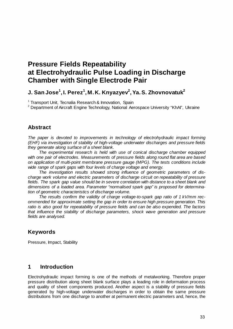
2 Experimental Setup and Measuring Procedure Tests have been carried out in the technological unit of experimental electrohydraulic installation UEHSh-2 equipped with conical discharge chamber (Figure 1) of 170 mm exhaust hole diameter. Loaded area was limited by spacer rings with internal diameters D = 150 mm.
The clamping force of tooling pack was applied via columnar frame by hydraulic cylinder with power of 60 kN. Water supply and air evacuation were realised with holes in the discharge chamber adaptor 2 (ref. Figure 1).
The intended spark gap value l was set up with threads performed in sleeves of electrodes and discharge chamber holes (Figure 2). Distance H between electrodes (discharge channel) and membrane 11 was approximately 110 mm with slight deviations when changing electrodes positions for spark gap setting. These deviations were taken into account when making a processing of tests data.
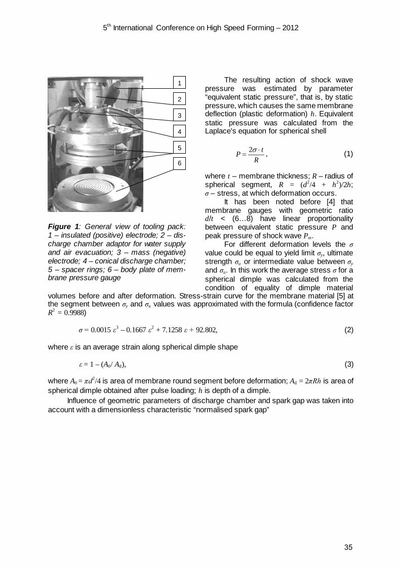
During the tests performance the discharge generator provided the following electrical parameters: voltage V = (10–30) kV, capacitance C = 33.2 µF, charged energy E = (1.66–14.94) kJ, inductance L = 0.5 µH.
Measurements of pressure fields were performed based on application of multi-point membrane pressure gauge (MPG) methodology [4]. Diameters of holes in MPG body (d = 6 mm) and thickness of membrane (A5052-O, thickness t = 1.0 mm) were selected of such values to record only the pressure of shock waves to exclude influence of hydraulic flows and pressure of vapour-gas bubble.
34
5th International Conference on High Speed Forming – 2012
Figure 1: General view of tooling pack: 1 – insulated (positive) electrode; 2 – dis-charge chamber adaptor for water supply and air evacuation; 3 – mass (negative) electrode; 4 – conical discharge chamber; 5 – spacer rings; 6 – body plate of mem-brane pressure gauge
1
2
3
4
5
6
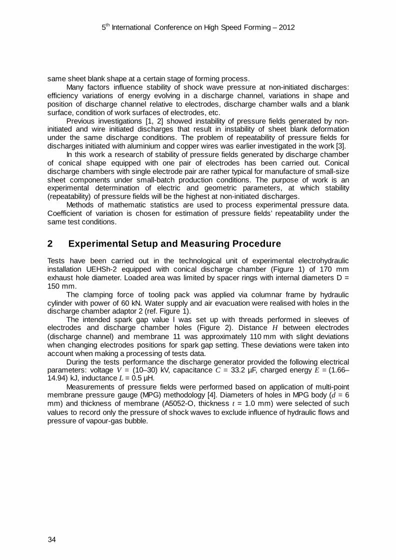
The resulting action of shock wave pressure was estimated by parameter “equivalent static pressure”, that is, by static pressure, which causes the same membrane deflection (plastic deformation) h. Equivalent static pressure was calculated from the Laplace's equation for spherical shell
RtP ⋅
=σ2 , (1)
where t – membrane thickness; R – radius of spherical segment, R = (d2/4 + h2)/2h; σ – stress, at which deformation occurs.
It has been noted before [4] that membrane gauges with geometric ratio d/t < (6…8) have linear proportionality between equivalent static pressure P and peak pressure of shock wave Pm.
For different deformation levels the σ value could be equal to yield limit σy, ultimate strength σu or intermediate value between σy and σu. In this work the average stress σ for a spherical dimple was calculated from the condition of equality of dimple material
volumes before and after deformation. Stress-strain curve for the membrane material [5] at the segment between σy and σu values was approximated with the formula (confidence factor R2 = 0.9988)
σ = 0.0015 ε3 – 0.1667 ε2 + 7.1258 ε + 92.802, (2)
where ε is an average strain along spherical dimple shape
ε = 1 – (A0/ Ad), (3)
where A0 = πd2/4 is area of membrane round segment before deformation; Ad = 2πRh is area of spherical dimple obtained after pulse loading; h is depth of a dimple.
Influence of geometric parameters of discharge chamber and spark gap was taken into account with a dimensionless characteristic “normalised spark gap”
35

5th International Conference on High Speed Forming – 2012
24
DHlln ⋅⋅⋅
=π
, (4)
where D is diameter of rigid side walls of work volume (diameter of hole in tooling rings). For the test tooling configuration D = 150 mm (ref. Figure 2).
Analysis of preliminary tests and previous literature sources allowed developing the formula (4): increase of spark gap l and distance H, reduce of loaded area limited by diameter D should improve uniformity of the pressure distribution along loaded area. It was supposed that the increase of combined parameter ln would improve repeatability characteristic too.
3 Tests Results and Data Processing The values of dimples depths hi were measured and pressure values Pi were calculated from formulas (1), (2), (3) for each i point of a membrane after impact loading at selected test conditions. Then the following parameters were calculated: - Average pressure for each i point (i = 1…127) of MPG membrane for the m quantity of pressure fields under the same test conditions (m = 3-6)
∑=
=m
jiji.ave P
mP
1
1 ; (5)
2
3
1
4
6
7
9
11 H 8
10
l
Figure 2: Test diagram: 1 – mass (negative) electrode; 2 – upper adaptor; 3 – insu-lated (positive) electrode; 4 – discharge chamber; 6 – studs, nuts, washers; 7 – spacer ring of 55 mm in height; 8 – spacer rings with 150 mm hole diameter; 9 – membrane pressure gauge body; 10 – lower adaptor; 11 – membrane; l – spark gap; H – distance between discharge channel and pressure gauge
36

5th International Conference on High Speed Forming – 2012
- Standard deviation of pressure value in each i point
( )∑=
−=m
ji.aveiji PP
mS
1
21 ; (6)
- Coefficient of variation in each i point for the same series of tests
%P
SCi.ave
iVi 100⋅= ; (7)
- Maximum Cmax and minimum Cmin values of variation coefficient selected from 127 points along loaded area for the series of tests; - Average value of variation coefficient among n = 127 points for the series of tests
∑=
=n
iiave.V C
nC
1
1 . (8)
In comparison with a standard deviation the coefficient of variation CV gives not
absolute, but relative measure of scatter of parameter values in its statistical population. The larger the CV, the population is less homogeneous. A population is considered to be homogeneous at CV = (0-30) %, intermediate – at CV = (30-50) % and non-homogeneous (heterogeneous) – at CV = (50-100) %. Variation coefficient can be equal to more than 100 %, if a population is extra heterogeneous.
Due to its properties coefficient of variation was selected as a basic parameter for estimation of repeatability of pressure fields obtained in several tests under the same conditions. Values of average variation coefficient 10 % and less were accepted as a satisfactory level of repeatability.
Tests conditions and results of data processing are submitted in Table 1.The parameter Pmax-ave is the average maximum pressure and parameter Save is the average standard deviation obtained in m number of pressure fields under the same test conditions. They additionally characterise pressure fields in a manufacturing aspect.
Figures 3 and 4 represent a top view of membrane, where pressure field and variation coefficient distribution maps are shown. Small zone of increased values of variation coefficient near to insulated electrode end in Fig. 4 in comparison with the zone increased pressure in Fig. 3 shows instability of discharge channel position from one discharge to another. But this level of instability does not influence greatly the repeatability of pressure on the rest area. This means that the length of discharge channel should be in geometric correlation with discharge chamber dimensions and sizes of loaded area for higher stability.
The pressure fields in tests No. 13 also demonstrate good level of uniformity
37
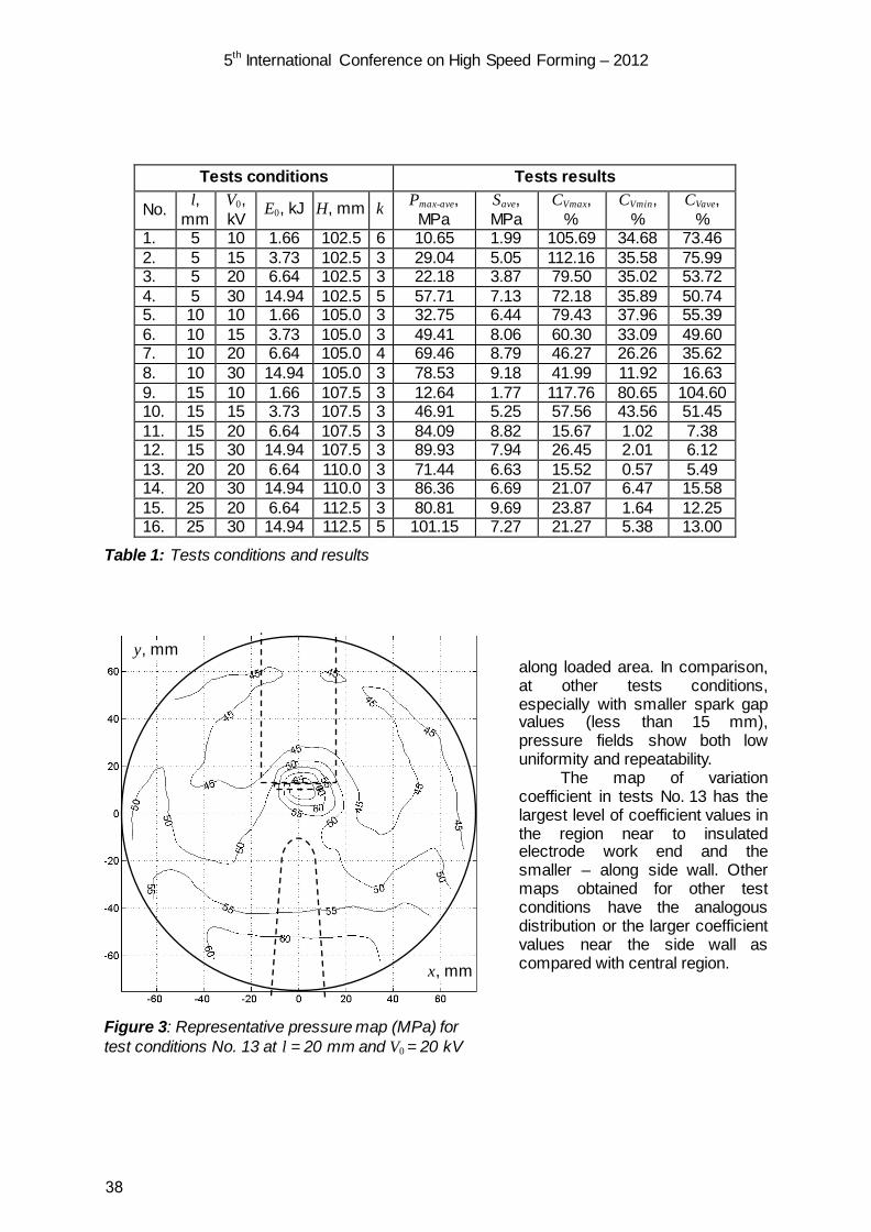
5th International Conference on High Speed Forming – 2012
Tests conditions Tests results
No. l, mm
V0, kV
E0, kJ H, mm k Pmax-ave, MPa
Save, MPa
CVmax, %
CVmin, %
CVave, %
1. 5 10 1.66 102.5 6 10.65 1.99 105.69 34.68 73.46 2. 5 15 3.73 102.5 3 29.04 5.05 112.16 35.58 75.99 3. 5 20 6.64 102.5 3 22.18 3.87 79.50 35.02 53.72 4. 5 30 14.94 102.5 5 57.71 7.13 72.18 35.89 50.74 5. 10 10 1.66 105.0 3 32.75 6.44 79.43 37.96 55.39 6. 10 15 3.73 105.0 3 49.41 8.06 60.30 33.09 49.60 7. 10 20 6.64 105.0 4 69.46 8.79 46.27 26.26 35.62 8. 10 30 14.94 105.0 3 78.53 9.18 41.99 11.92 16.63 9. 15 10 1.66 107.5 3 12.64 1.77 117.76 80.65 104.60 10. 15 15 3.73 107.5 3 46.91 5.25 57.56 43.56 51.45 11. 15 20 6.64 107.5 3 84.09 8.82 15.67 1.02 7.38 12. 15 30 14.94 107.5 3 89.93 7.94 26.45 2.01 6.12 13. 20 20 6.64 110.0 3 71.44 6.63 15.52 0.57 5.49 14. 20 30 14.94 110.0 3 86.36 6.69 21.07 6.47 15.58 15. 25 20 6.64 112.5 3 80.81 9.69 23.87 1.64 12.25 16. 25 30 14.94 112.5 5 101.15 7.27 21.27 5.38 13.00
Table 1: Tests conditions and results
along loaded area. In comparison, at other tests conditions, especially with smaller spark gap values (less than 15 mm), pressure fields show both low uniformity and repeatability.
The map of variation coefficient in tests No. 13 has the largest level of coefficient values in the region near to insulated electrode work end and the smaller – along side wall. Other maps obtained for other test conditions have the analogous distribution or the larger coefficient values near the side wall as compared with central region.
Figure 3: Representative pressure map (MPa) for test conditions No. 13 at l = 20 mm and V0 = 20 kV
y, mm
x, mm
38

5th International Conference on High Speed Forming – 2012
4 Discussion
When analysing the tests results, many factors should be taken into account that influence repeatability of pressure fields. Electric parameters of discharge circuit (V0, E0, l) influence stability of a discharge channel, its configuration in a spark gap between electrodes ends, efficiency of electric energy evolving and its transformation into energy of pressure. Geometric parameters of discharge work volume (H, D, l, shapes of discharge chamber and side walls, configurations of electrodes and condition of their work ends) determine length of discharge channel, its position relative to loaded area, distribution of direct shock waves, conditions for reflected shock waves and their interaction with direct shock
waves, conditions for interaction of direct and reflected shock waves with side walls near to loaded area, and finally influence the resulting pressure distributions and their repeatability. Value of spark gap l influences both the efficiency of electric discharge, because it determines initial resistance of discharge circuit, and geometric characteristics, because it determines length of discharge channel in its ratio with loaded area limited by diameter D and distance H.
In common action the influence of mentioned significant and other factors is described by curves depicted in Figure 5. The curves are concave by shape and have minimum values at certain values of normalised spark gap. Both increments and decrements of spark gap from this certain value will cause enlarge of instability of pressure fields.
The curves evidently show that satisfactory level of repeatability (CVave ≤ 10 %) can be achieved only at voltage of 20 kV and more. This is confirmed by tests data of Table 1 for tests 11 to 16 with the value CVmax < 30 % peculiar to homogeneous populations of data. The highest level of repeatability was obtained in the tests Nos 11, 12 and 13 with the CVave values 7.38, 6.12 and 5.49 respectively at spark gap values of 15 and 20 mm, charge voltage values of 20 and 30 kV and charge energy of 6.64 and 14.94 kJ. Tests conditions, which are able to generate pressure fields with high repeatability, are also characterised by high level of pressure values Pmax-ave (ref. Table 1).
Figure 4: Map of variation coefficient (%) for test conditions No. 13 with 3 pressure maps processed
y, mm
x, mm
39
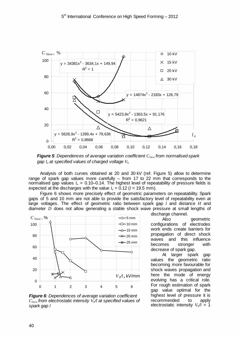
5th International Conference on High Speed Forming – 2012
Analysis of both curves obtained at 20 and 30 kV (ref. Figure 5) allow to determine range of spark gap values more carefully – from 17 to 22 mm that corresponds to the normalised gap values ln = 0.10–0.14. The highest level of repeatability of pressure fields is expected at the discharges with the value ln = 0.12 (l = 19.5 mm).
Figure 6 shows more precisely effect of geometric parameters on repeatability. Spark gaps of 5 and 10 mm are not able to provide the satisfactory level of repeatability even at large voltages. The effect of geometric ratio between spark gap l and distance H and diameter D does not allow generating a stable shock wave pressure at small lengths of
discharge channel. Also geometric
configurations of electrodes work ends create barriers for propagation of direct shock waves and this influence becomes stronger with decrease of spark gap.
At larger spark gap values the geometric ratio becoming more favourable for shock waves propagation and here the mode of energy evolving has a critical role. For rough estimation of spark gap value optimal for the highest level of pressure it is recommended to apply electrostatic intensity V0/l = 1
y = 34381x2 - 3634,1x + 149,94R2 = 1
y = 14874x2 - 2183x + 126,79
y = 5423,8x2 - 1363,5x + 91,176R2 = 0,9621
y = 5628,9x2 - 1289,4x + 79,636R2 = 0,86680
20
40
60
80
100
0,00 0,02 0,04 0,06 0,08 0,10 0,12 0,14 0,16 0,18
l n
C Vave , % 10 kV
15 kV
20 kV
30 kV
Figure 5: Dependences of average variation coefficient CVave from normalised spark gap ln at specified values of charged voltage V0
Figure 6: Dependences of average variation coefficient CVave from electrostatic intensity V0/l at specified values of spark gap l
0
20
40
60
80
100
0 1 2 3 4 5 6
V 0/l , kV/mm
C Vave , % 5 mm
10 mm
15 mm
20 mm
25 mm
40

5th International Conference on High Speed Forming – 2012
kV/mm. For optimisation of repeatability characteristic it is appeared that this ratio should be 1.33 and more, up to 2, for spark gap of 15 mm. For spark gap of 25 mm good repeatability is obtained even at V0/l = 0.8 kV/mm. Large CVave values at 15 mm gap and V0/l = (0.67–1.0) kV/mm are explained by harmful effect of small geometric length of discharge channel and its low stability because of low electrostatic intensity and energy density per 1 mm of the gap.
Considering influence of electric parameter V0 (and, hence, charge energy, because E0
= CV02/2) it is possible to estimate its quantitative characteristic (Figure 7). Though the low
level of approximation reliability is evident, the tendency of repeatability increase with the voltage rise is observed. The highest level of repeatability of pressure fields is expected at the discharges with voltage of 27 kV and energy of 12.1 kJ.
Finally the analysis led to a conclusion that stable pressure fields under this discharge chamber conditions can be obtained at relatively large spark gaps, charge voltages and energies.
The problem of repeatability at small spark gaps and small voltages can be solved with taking into account geometric parameters of discharge volume. Complex parameter ln equals (0.10–0.14) at the condition of CVave ≤ 10 %. Using the formula (4) the optimised diameter of loaded area can be determined as D = 108 mm at the same distance H = 110 mm and ln = 0.12, spark gap of 10 mm. For these conditions the optimised voltage equals 13.5 kV and energy – 3.02 kJ. These changes should be accompanied with proportional decrease of electrodes dimensions.
If, for example, it is necessary to select spark gap of 30 mm and diameter D = 200 mm, the distance will be H = 126 mm (V0 = 40.5 kV, E0 = 27.2 kJ). Of course, these estimations are to be checked during further investigations.
In comparison with wire-initiated discharges the stability of non-initiated discharges is much lower. In the work [3] the tests were carried out in the same discharge chamber with the same distance H at voltage of 20 kV and energy of 6.64 kJ. Here also the dependency of pressure fields’ stability from wire diameter and material nature is evident: at aluminium wire of 0.75 mm diameter the CVave =
1.65 % and at 1.00 mm – CVave = 4.43 %; at copper wire of 0.72 mm diameter the
CVave = 3.0 % and at 0.90 mm – CVave = 8.26 %.
5 Conclusions The investigation results showed strong influence of geometric parameters of discharge work volume and electric parameters of discharge circuit on repeatability of pressure fields. In particular the spark gap value should be in severe correlation with distance to a sheet blank and dimensions of a loaded area. Here the parameter “normalised spark gap” is proposed for determination of geometric characteristics of discharge volume.
y = 0,2315x2 - 12,362x + 182,12R2 = 0,6176
0
20
40
60
80
100
5 10 15 20 25 30 35
V 0, kV
C Vave , %
Figure 7: Dependency of average variation coeffi-cient CVave from charge voltage V0 for all tests
41

5th International Conference on High Speed Forming – 2012
Voltage and energy of discharge have optimal values. All deviations (both positive and negative) of their values from the optimums cause increasing instability of discharge channel position and, hence, low repeatability of pressure fields.
For the specified geometric parameters of discharge chamber at the condition of average variation coefficient value being of up to 10 % (satisfactory level of repeatability) the following electric parameters are recommended: range of spark gap is 17 to 22 mm, voltage range of 20 to 30 kV and charge energy range of 6.64 to 14.94 kJ.
The further investigations with discharge chambers of other geometric parameters for verification of the proposed method are planned.
References [1] Vohnout, V.J.; Fenton, G.; Daehn, G. S.: Pressure heterogeneity in small displacement
electrohydraulic forming processes. Proceedings of the 4th International Conference on High Speed Forming “ICHSF2010”, Columbus, Ohio, March 9-10, (2010), p. 65-74.
[2] Homberg, W.; Beerwald, C.; Pröbsting, A.: Investigation of the Electrohydraulic Form-ing Process with respect to the Design of Sharp Edged Contours. Proceedings of the 4th International Conference on High Speed Forming “ICHSF2010”, Columbus, Ohio, March 9-10, (2010), p. 58-64.
[3] Eguia, I.; San José, J.; Knyazyev, M.K.; Zhovnovatuk, Ya.S.: Pressure Field Stabiliza-tion in High-Voltage Underwater Pulsed Metal Forming Using Wire-Initiated Discharg-es. Key Engineering Materials, Vol. 473, 2011, p. 965-972.
[4] Knyazyev, M.K.; Zhovnovatuk, Ya.S.: Measurements of Pressure Fields with Multi-Point Membrane Gauges at Electrohydraulic Forming. Proceedings of the 4th Interna-tional Conference on High Speed Forming “ICHSF2010”, Columbus, Ohio, March 9-10, (2010), p. 75-82.
[5] http://products.asminternational.org/datasheets/metaview.do?record=8555&da tabase=datasheets
42

SESSION 2
INNOVATIVE PROCESSES - B
43

44

Coining of Micro Structures with an Electromagnetically Driven Tool*
E. Uhlmann1, C. König1, A. Ziefle1, L. Prasol1
1 Institute for Machine Tools and Factory Management, TU Berlin, Germany
Abstract
For coining micro structures into high-grade steel 1.4301 a highly dynamic tool system based on a pulsed magnetic field inside a cylindrical coil was developed. Two kinds of structures were coined at different tool velocities. The coining results were evaluated regarding geometrical accuracy, material flow behaviour and energy input. In addition the high velocity process was compared to a quasi-static process. By increasing the coining velocity to 30 m/s the accuracy of the quasi-static process can be reached. The energy that is needed for reaching a similar result is less for coining at high velocities. The tool velocity also influences the flow behaviour of the workpiece material.
Keywords
High speed forming, Impact, Coining
1 Introduction
Complexity and variety of micro components in electronics, precision engineering, micro system technology and medical engineering increase constantly. At the same time the number of applications of such components is rising. Production processes have to meet the requirements of these tendencies and must be suitable for mass production. Forming with its optimal utilization of material and high productivity offers potentials for excellent
* This work is based on the results of the research project “Entwicklung und Analyse eines neuartigen und innovativen Verfahrens für die Mikroumformung höchstfester Werkstoffe”; the authors would like to thank the DFG for its financial support
45
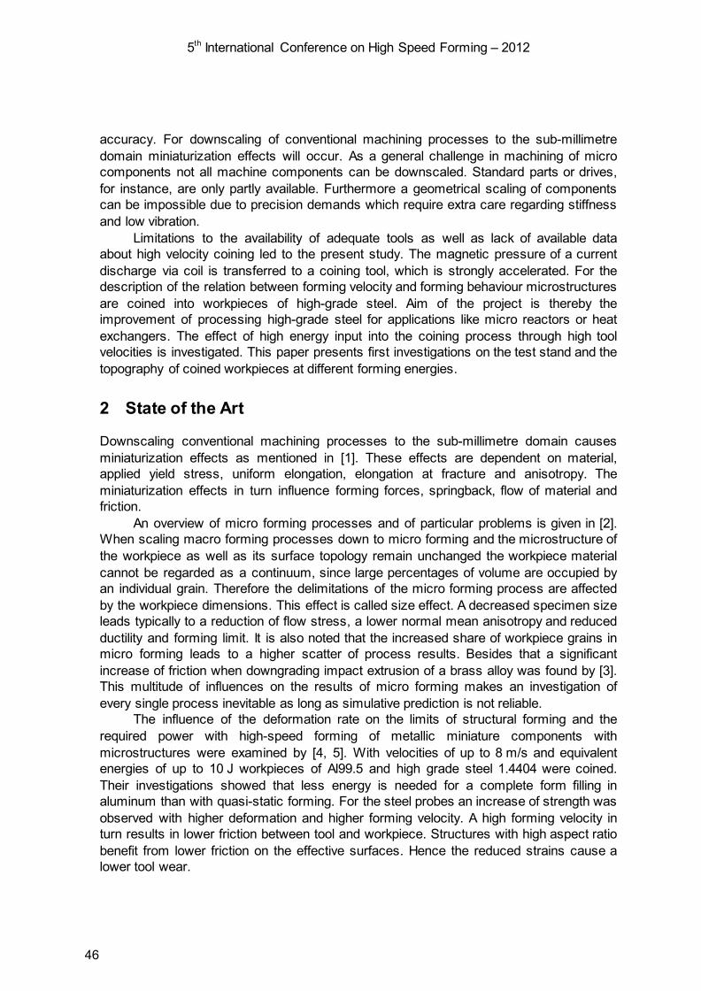
5th International Conference on High Speed Forming – 2012
accuracy. For downscaling of conventional machining processes to the sub-millimetre domain miniaturization effects will occur. As a general challenge in machining of micro components not all machine components can be downscaled. Standard parts or drives, for instance, are only partly available. Furthermore a geometrical scaling of components can be impossible due to precision demands which require extra care regarding stiffness and low vibration.
Limitations to the availability of adequate tools as well as lack of available data about high velocity coining led to the present study. The magnetic pressure of a current discharge via coil is transferred to a coining tool, which is strongly accelerated. For the description of the relation between forming velocity and forming behaviour microstructures are coined into workpieces of high-grade steel. Aim of the project is thereby the improvement of processing high-grade steel for applications like micro reactors or heat exchangers. The effect of high energy input into the coining process through high tool velocities is investigated. This paper presents first investigations on the test stand and the topography of coined workpieces at different forming energies.
2 State of the Art
Downscaling conventional machining processes to the sub-millimetre domain causes miniaturization effects as mentioned in [1]. These effects are dependent on material, applied yield stress, uniform elongation, elongation at fracture and anisotropy. The miniaturization effects in turn influence forming forces, springback, flow of material and friction.
An overview of micro forming processes and of particular problems is given in [2]. When scaling macro forming processes down to micro forming and the microstructure of the workpiece as well as its surface topology remain unchanged the workpiece material cannot be regarded as a continuum, since large percentages of volume are occupied by an individual grain. Therefore the delimitations of the micro forming process are affected by the workpiece dimensions. This effect is called size effect. A decreased specimen size leads typically to a reduction of flow stress, a lower normal mean anisotropy and reduced ductility and forming limit. It is also noted that the increased share of workpiece grains in micro forming leads to a higher scatter of process results. Besides that a significant increase of friction when downgrading impact extrusion of a brass alloy was found by [3]. This multitude of influences on the results of micro forming makes an investigation of every single process inevitable as long as simulative prediction is not reliable.
The influence of the deformation rate on the limits of structural forming and the required power with high-speed forming of metallic miniature components with microstructures were examined by [4, 5]. With velocities of up to 8 m/s and equivalent energies of up to 10 J workpieces of Al99.5 and high grade steel 1.4404 were coined. Their investigations showed that less energy is needed for a complete form filling in aluminum than with quasi-static forming. For the steel probes an increase of strength was observed with higher deformation and higher forming velocity. A high forming velocity in turn results in lower friction between tool and workpiece. Structures with high aspect ratio benefit from lower friction on the effective surfaces. Hence the reduced strains cause a lower tool wear.
46

5th International Conference on High Speed Forming – 2012
The influence of high forming velocities on formability of metals was also investigated by [6]. The investigated materials however were an aluminium alloy, a titanium alloy and a magnesium alloy. Effects of high forming velocities are beside lower friction on effective surfaces a lower elongation at fracture, a rising strain rate sensitivity as well as a higher instability of material. Strain rate sensitivity means a strong relation between yield strength and strain rate. The dependence of yield strength of different steel alloys on strain rates between 0.005 s-1 and 200 s-1 was investigated by [7]. The results for steel 1.4301 show an increase of yield strength of 310 MPa to 405 MPa as shown in Figure 1.
Figure 1: Strain-rate sensitivity for high-grade steel 1.4301 based on [7]
All investigated alloys showed a similar behaviour. The ductility in turn decreased as strain rates rose from 0.005 s-1 to 1 s-1. This characteristic was observed for austenitic stainless steels. Other alloys either showed no significant change or a dramatic in- or decrease of elongation at a strain rate rise from 100 s-1 to 200 s-1.
Despite different materials were examined in the mentioned works they agree that the heat generated by the deformation cannot dissipate within the process due to high forming velocity. This leads to thermally activated processes inside the material. The acceleration of tools, e.g. for coining, cutting or riveting, offers potentials for improved processing of high-grade steels [8].
3 Experimental Setup
To improve micro coining of high strength steels the effect of high energy input into the process through high tool velocities is investigated. The forming behaviour depends strongly on the forming velocity. Thermally activated processes take place since the heat, generated during forming, cannot dissipate into to whole workpiece. Ductility and yield strength show a clear dependency on the strain rate as shown in Figure 1 and also the characteristics of friction between tool and workpiece change at high tool velocities. Since micro structures have a high amount of active surfaces this becomes especially relevant.
The coining tool is applied to a projectile which is located inside a cylindrical tool coil. The discharge of a pulsed current via the coil is used to accelerate the tool to high
47

5th International Conference on High Speed Forming – 2012
velocities. The necessary energy is stored in capacitors and is unloaded as an alternating current. The implicated magnetic field around the tool coil induces eddy currents in the projectile opposite to the discharge current. These shield the magnetic field of the tool coil in a way that the orthogonal Lorentz force can be used to accelerate the projectile as shown in Figure 2. The force vectors inside the projectile are orthogonal to the magnetic field lines. Since the Lorentz force appears inside the projectile due to the induced current Figure 2 shows only a facilitated model. The projectile is accelerated by the axial component of the force vectors. The radial components would compress the projectile; therefore it has to be designed as solid body to be able to resist deformation. The discharge current is alternating which leads to several impulses that accelerate the projectile as long as it is still located inside the tool coil.
Figure 2: Coil accelerator with electrically conductive projectile
The duration of the accelerating impulses depends on the frequency fD of the discharge current according to equation (1), including the overall inductivity L and the capacity C.
fD = 12∙π ∙ 1
L∙C (1)
The tools are placed underneath the workpiece as shown in Figure 3. The workpiece is pushed into the tool through the impulse of the projectile that is transmitted by the push rod. The impulse depends on the accelerated mass and its velocity. A part of it is transformed into deformation work and results in a coined surface of the workpiece. Another part is stored inside the system in form of vibration. But the highest amount is stored as elastic deformation of the system and released to push back the projectile. The velocity of the projectile is measured with a position sensitive device (PSD) which detects the position of the projectile at any time by laser shading. The velocity between workpiece and tool, coining velocity vc, is calculated following the conservation of momentum as in (2) with the mass of the projectile mp and the mass of the push rod mpr.
vc = mP∙vP mpr (2)
48

5th International Conference on High Speed Forming – 2012
The impact is registered by a force measurement system which shows the duration of the impulse flow into the workpiece what leads to its deformation. With this setup velocities of up to 35 m/s were reached. They are limited only due to limitations of the stiffness of the test stand. The impulse duration was in each case about tI = 60 µs.
Figure 3: Prototypical coining apparatus (left) and schematic presentation (right)
The investigated structures are struts with a height of hs = 0.4 mm and two different aspect ratios. Figure 4 shows the two investigated structures. Both structures cover an area of 10 x 10 mm². Structure 1 has eight struts and nine grooves; structure 2 has 14 struts and 15 grooves.
Figure 4: Strut structures used for coining
Plates of steel 1.4301 were coined at velocities of vc = 18 m/s, vc = 22 m/s and vc = 30 m/s. For a qualification of the high velocity coining results coinings at a tool velocity of vc = 1.67 · 10-5 m/s were performed on a material testing machine. The results are given as “quasi-static” in the following. All coinings were done with both structures. The coined workpieces were scanned with an optical surface measurement system. The scanned geometries were evaluated by geometrical criteria and related to the coining tool they were made with. Also the deformation of the workpiece and its flow of material were investigated through the data of the surface scans.
4 Experimental Results
To investigate the accuracy of the coining results at different energies the geometries were measured and compared to each tool. Criteria were the angle between surface and
Structure 1, aspect ratio 0.85 Structure 2, aspect ratio 1.45
49

5th International Conference on High Speed Forming – 2012
flank of the struts α, the strut height hs, the strut width ws and the groove width wg as shown in Figure 5.
Figure 5: Profile of a coining tool of structure 1 with criteria for accuracy evaluation (left) and coined workpiece (right)
wg and ws were taken at 50 % of the strut height hs. The struts of the tools correlate to the grooves of the coinings. The correlations of the geometrical criteria of the coined structures from the tool structures are given in Figure 6. The coining results at a coining velocity vc = 18 m/s of structure 1 were not evaluable due to a very low forming depth. 100 % on the ordinate corresponds to the tool geometry. The higher the column the better is the correlation of the criterion of the coined structure with the one of the tool structure.
Figure 6: Correlations of the geometrical criteria of the coinings with the tool structure
50
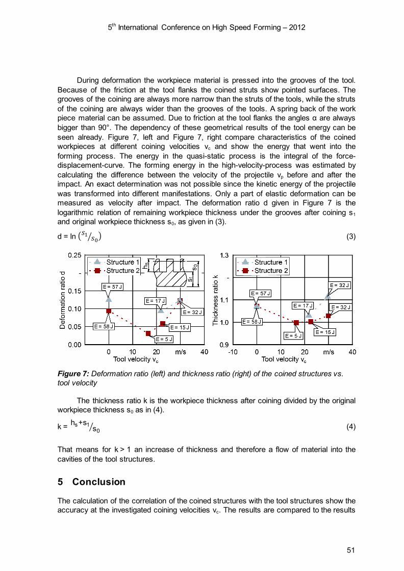
5th International Conference on High Speed Forming – 2012
During deformation the workpiece material is pressed into the grooves of the tool. Because of the friction at the tool flanks the coined struts show pointed surfaces. The grooves of the coining are always more narrow than the struts of the tools, while the struts of the coining are always wider than the grooves of the tools. A spring back of the work piece material can be assumed. Due to friction at the tool flanks the angles α are always bigger than 90°. The dependency of these geometrical results of the tool energy can be seen already. Figure 7, left and Figure 7, right compare characteristics of the coined workpieces at different coining velocities vc and show the energy that went into the forming process. The energy in the quasi-static process is the integral of the force-displacement-curve. The forming energy in the high-velocity-process was estimated by calculating the difference between the velocity of the projectile vp before and after the impact. An exact determination was not possible since the kinetic energy of the projectile was transformed into different manifestations. Only a part of elastic deformation can be measured as velocity after impact. The deformation ratio d given in Figure 7 is the logarithmic relation of remaining workpiece thickness under the grooves after coining s1 and original workpiece thickness s0, as given in (3).
d = ln 𝑠1 𝑠0 (3)
Figure 7: Deformation ratio (left) and thickness ratio (right) of the coined structures vs. tool velocity
The thickness ratio k is the workpiece thickness after coining divided by the original workpiece thickness s0 as in (4).
k = hs+s1 s0 (4)
That means for k > 1 an increase of thickness and therefore a flow of material into the cavities of the tool structures.
5 Conclusion
The calculation of the correlation of the coined structures with the tool structures show the accuracy at the investigated coining velocities vc. The results are compared to the results
51
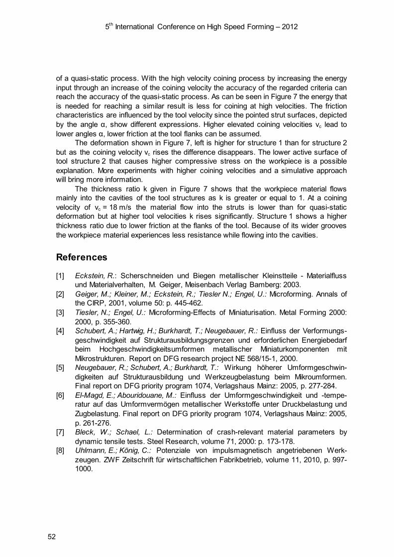
5th International Conference on High Speed Forming – 2012
of a quasi-static process. With the high velocity coining process by increasing the energy input through an increase of the coining velocity the accuracy of the regarded criteria can reach the accuracy of the quasi-static process. As can be seen in Figure 7 the energy that is needed for reaching a similar result is less for coining at high velocities. The friction characteristics are influenced by the tool velocity since the pointed strut surfaces, depicted by the angle α, show different expressions. Higher elevated coining velocities vc lead to lower angles α, lower friction at the tool flanks can be assumed.
The deformation shown in Figure 7, left is higher for structure 1 than for structure 2 but as the coining velocity vc rises the difference disappears. The lower active surface of tool structure 2 that causes higher compressive stress on the workpiece is a possible explanation. More experiments with higher coining velocities and a simulative approach will bring more information.
The thickness ratio k given in Figure 7 shows that the workpiece material flows mainly into the cavities of the tool structures as k is greater or equal to 1. At a coining velocity of vc = 18 m/s the material flow into the struts is lower than for quasi-static deformation but at higher tool velocities k rises significantly. Structure 1 shows a higher thickness ratio due to lower friction at the flanks of the tool. Because of its wider grooves the workpiece material experiences less resistance while flowing into the cavities.
References
[1] Eckstein, R.: Scherschneiden und Biegen metallischer Kleinstteile - Materialfluss und Materialverhalten, M. Geiger, Meisenbach Verlag Bamberg: 2003.
[2] Geiger, M.; Kleiner, M.; Eckstein, R.; Tiesler N.; Engel, U.: Microforming. Annals of the CIRP, 2001, volume 50: p. 445-462.
[3] Tiesler, N.; Engel, U.: Microforming-Effects of Miniaturisation. Metal Forming 2000: 2000, p. 355-360.
[4] Schubert, A.; Hartwig, H.; Burkhardt, T.; Neugebauer, R.: Einfluss der Verformungs-geschwindigkeit auf Strukturausbildungsgrenzen und erforderlichen Energiebedarf beim Hochgeschwindigkeitsumformen metallischer Miniaturkomponenten mit Mikrostrukturen. Report on DFG research project NE 568/15-1, 2000.
[5] Neugebauer, R.; Schubert, A.; Burkhardt, T.: Wirkung höherer Umformgeschwin-digkeiten auf Strukturausbildung und Werkzeugbelastung beim Mikroumformen. Final report on DFG priority program 1074, Verlagshaus Mainz: 2005, p. 277-284.
[6] El-Magd, E.; Abouridouane, M.: Einfluss der Umformgeschwindigkeit und -tempe-ratur auf das Umformvermögen metallischer Werkstoffe unter Druckbelastung und Zugbelastung. Final report on DFG priority program 1074, Verlagshaus Mainz: 2005, p. 261-276.
[7] Bleck, W.; Schael, L.: Determination of crash-relevant material parameters by dynamic tensile tests. Steel Research, volume 71, 2000: p. 173-178.
[8] Uhlmann, E.; König, C.: Potenziale von impulsmagnetisch angetriebenen Werk-zeugen. ZWF Zeitschrift für wirtschaftlichen Fabrikbetrieb, volume 11, 2010, p. 997-1000.
52
Space-Time-Controlled Multi-Stage Pulsed Magnetic Field Forming and Manufacturing Technology*
Liang Li1, 2,*, Xiaotao Han1, 2, Tao Peng1, 2, Hongfa Ding1, 2, Tonghai Ding1, 2, Li Qiu1, 2, Zhongyu Zhou1, 2, Qi Xiong1, 2 1 Wuhan National High Magnetic Field Center, Huazhong University of Science and Technology, Wuhan, China 2 State Key Laboratory of Advanced Electromagnetic Engineering and Technology, Huazhong University of Science and Technology, Wuhan, China
Abstract
Electromagnetic forming (EMF) is a high strain-rate forming method where a pulsed electromagnetic force is applied to a conductive metallic workpiece. To improve the performance of the EMF system, the current problems which restrict its extensive application have been analyzed. To this end, a space-time-controlled EMF technology with multi-stage and multi-direction coils system has been developed. In our new EMF system, the magnetic field generated by driving coils is much higher than in conventional EMF due to introducing design methods developed for non-destructive pulsed high field magnets. This technology enables the forming of complex, large-scale sheets and tubes that may be difficult to deform by conventional methods, as well as controlling particular properties of the work pieces.
Keywords
Electromagnetic forming, space-time-controlled, multi-stage, multi-direction, driving coil
1 Introduction
In the EMF process, the work piece is accelerated by the electromagnetic force between the driving current and the eddy current [1]. Compared with traditional quasi-static forming methods, EMF technology is quite beneficial due to high-speed deformation and non- * The authors would like to thank National Basic Research Program of China (973 Program): 2011CB012800 (2011CB012801) for its financial support
53
5th International Conference on High Speed Forming – 2012
contact processes; this can provide a substantial increase in the forming limit for high-strength materials, improved formability, improved strain distribution, reduction in wrinkling, active control of spring-back and the possibility of local coining and embossing [2].
The EMF technology is well known with a lot of published research dating back to the 1960’s, but the application of the technology is still quite limited in industry. This was primarily focused on the study of macro-deformation behavior and the dynamic numerical simulation of the EMF process [3]. However, two problems which restricted its extensive application have not yet been solved: 1) How to generate stronger pulsed electromagnetic force (i.e., the design of high-field drive coils). The performance of the conventional electromagnetic forming is limited by the strength of the pulsed driving coil and by its power supply. The maximum magnetic field strength generated by conventional driving coils is normally relatively low, and the energy of the capacitor bank used for this purpose is mostly less than 100 kJ due to the strength of the coil in the conventional EMF system. Therefore it is difficult to further improve the forming speed, range and depth which has restricted its extensive application in the high speed forming process. 2) How to generate the space-time-controlled multi-stage electromagnetic force in the EMF process. For a single coil system, the Lorenz force on the work piece decreases rapidly with increasing distance from the driving coil. Thus the conventional single coil system can only be applied to form small or thin-walled workpieces. In order to meet the requirements for larger size and more complex structures of the forming materials, multi-coil systems should be proposed and designed. Thus in future research more attention should be paid to space-time-controlled methods of generating the electromagnetic forceby multi-stage pulsed magnets.
With the ongoing development of non-destructive pulsed high field magnet technology, magnetic fields in excess of 80 T have been achieved by using new materials, inserting internal reinforcement between the conductor layers, increasing the energy of the power supply, and new schemes of coil design [4]-[7]. The improved pulsed magnetic field associated with the multi-stage magnet, modular power supplies, timing control and a series of new technologies has introduced a new work pattern and design method for the development of EMF systems, which may greatly improve the efficiency of EMF technology in forming large-scale and deep-drawn components, large panels, and shaped tubes.
In this paper, we propose a Space-Time-Controlled Multi-Stage Pulsed Magnetic Field (Stic-Must-PMF) forming and manufacturing technology to improve the performance of the EMF system by applying the design methods of a high-field pulsed magnet system, which is based on strategically placed multiple coils where each coil can be addressed individually by its associated power supply with precise timing control. The magnetic flux density of these coils can be in the range 40-80 T.
2 Concept and Design of the Stic-Must-Pmf Forming System
The Stic-Must-PMF system contains multiple pulsed electromagnetic coils and several sets of pulsed power systems. Each coil is energized by a pulsed power system that can be controlled independently according to the required magnetic field direction and special functions. The magnetic flux density of these coils can be in the range 40-80 T by using
54
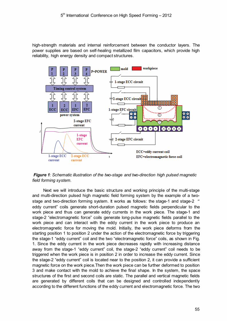
5th International Conference on High Speed Forming – 2012
high-strength materials and internal reinforcement between the conductor layers. The power supplies are based on self-healing metallized film capacitors, which provide high reliability, high energy density and compact structures.
Figure 1: Schematic illustration of the two-stage and two-direction high pulsed magnetic field forming system.
Next we will introduce the basic structure and working principle of the multi-stage and multi-direction pulsed high magnetic field forming system by the example of a two-stage and two-direction forming system. It works as follows: the stage-1 and stage-2 “eddy current” coils generate short-duration pulsed magnetic fields perpendicular to the work piece and thus can generate eddy currents in the work piece. The stage-1 and stage-2 “electromagnetic force” coils generate long-pulse magnetic fields parallel to the work piece and can interact with the eddy current in the work piece to produce an electromagnetic force for moving the mold. Initially, the work piece deforms from the starting position 1 to position 2 under the action of the electromagnetic force by triggering the stage-1 “eddy current” coil and the two “electromagnetic force” coils, as shown in Fig. 1. Since the eddy current in the work piece decreases rapidly with increasing distance away from the stage-1 “eddy current” coil, the stage-2 “eddy current” coil needs to be triggered when the work piece is in position 2 in order to increase the eddy current. Since the stage-2 “eddy current” coil is located near to the position 2, it can provide a sufficient magnetic force on the work piece.Then the work piece can be further deformed to position 3 and make contact with the mold to achieve the final shape. In the system, the space structures of the first and second coils are static. The parallel and vertical magnetic fields are generated by different coils that can be designed and controlled independently according to the different functions of the eddy current and electromagnetic force. The two
55

5th International Conference on High Speed Forming – 2012
“eddy current” coils are relatively small which not only reduces the time constant of the circuit that can easily generate the short-pulse field and strong eddy current in the work piece, but also the coils located in the different positions can be timingly and independently controlled .The “electromagnetic force” coils are arranged according to the work piece forming requirements to ensure a continuous electromagnetic force on the work piece.
3 Key Issues to be Solved
The electromagnetic forming technology based on the pulsed high magnetic field involves a combination of electromagnetism, materials science and manufacturing technology. As it is a novel technology system, there are still many critical issues that must be attended to:
(1) The effects of the pulsed magnetic field and pulsed electromagnetic force on the flow behavior and forming mechanisms of the metals have not yet been fully clarified. Since the foundational theories of the technology are still imperfect at present, there are few theoretical guidance on 1) how to apply the pulsed electromagnetic force efficiently on the metal workpiece, 2) how to ensure that the pulsed electromagnetic force has beneficial effects on the workpiece for the metal flow, material evolution and service performance.
(2) The experimental platform of the multi-stage and multi-direction pulsed high magnetic field system is not yet perfect and few experimental data are available. Meanwhile, the conventional unipolar pulsed magnetic field forming technology for single-process can only give a reference on the trend for test data and criteria, but cannot provide technical support for work pieces with complex shape. These will cause the lack of evaluation criteria for the forming limit and forming structure.
The solution to these problems can provide technical support for the development of pulsed magnetic field technology in general and play an important role in promoting the development of electromagnetism, materials science and materials manufacturing technology.
4 Possible Solutions
According to the above key issues, we should establish a new theoretical framework of flexible forming with control of properties and performance using the space-time-controlled multi-stage pulsed magnetic field manufacturing technology. We can mainly look for a breakthrough in the Stic-Must-PMF forming system in the following areas:
(1) The effective regulation of the magnetic field and electromagnetic force for the multi-stage and multi-direction pulsed high magnetic field system.
To be specific, we mainly undertake research on the laws of the space-time distribution of the strong space-time-controlled multi-stage pulsed magnetic field, the influence of the vertical field, the parallel field and the equivalent frequency of a pulse on the eddy current and electromagnetic force, and the control of the force field in forming.
(2) The magnetic field penetration, eddy current distribution and the energy conversion law involved in the forming of complex structures.
It is important to establish the three-dimensional distribution model of magnetic field penetration and eddy current in the forming process. On basis of this, we can investigate
56
5th International Conference on High Speed Forming – 2012
the effects of the action time of magnetic field, materials and the structure of the work piece on the magnetic field penetration and eddy current distribution.The coupling mechanism of the magnetic field distribution, eddy current distribution and the motional electromagnetic force can be obtained as well.
(3) Modelling and design criteria for the multi-stage and multi-direction pulsed high magnetic field system.
In this section, we should develop the geometric models, physical models, mathematical models and virtual design technology of the whole system and subsystems of the multi-stage and multi-direction pulsed high magnetic field coils. Then an optimization design method of the coil structure under the electromagnetic-thermal-mechanical coupling action can be proposed. Furthermore, the optimization techniques for the combination of the power system and the coil system should be studied with a view to an accurate control for the repeatable pulse charge and the pulsed waveform control technology.
(4) To build the experimental platform of multi-stage and multi-direction high pulsed magnetic field system for large-scale and complex work pieces.
To verify the simulation result and provide data for optimization design, it is necessary to produce EMF prototypes and set up the experimental test platform based on the design principles and structural layout optimization of space-time-controlled multi-stage pulsed magnetic field facility. Then a number of experiments can be studied to achieve a more comprehensive understanding of plastic flow, diffusion bonding, microstructure evolution, and defect production and propagation in metal alloys upon deformation induced by the space-time-controlled multi-stage pulsed magnetic field.
5 Conclusion
The EMF technology has a long and significant history. However the technology has never quite taken its place among mainstream manufacturing methods. In this paper, we present the Stic-Must-PMF forming and manufacturing system to solve current problems of the EMF technology in forming large-scale deep drawing components, multilayered hollow plates, large panels, and shaped tubes in aerospace engineering. In the proposed system, the forming coils can generate higher pulsed magnetic fields and have a longer working life as compared to conventional forming coils due to introducing the internal reinforcement technology that is used widely in pulsed magnet design. Further, parallel and vertical magnetic fields can be generated and controlled independently which can improve the ability of manufacturing and control of electromagnetic forming of large-scale and complex work pieces by using the multi-stage and multi-directional coil system. This could transform the electromagnetic forming technology from its traditional role of aided forming to a direct integrated forming technology. It could lead to major advances in aerospace engineering in manufacturing large-scale and complex parts and components made from sheets and tubes.
57

5th International Conference on High Speed Forming – 2012
References
[1] V.S. Balanethiram, G.S. Daehn. Hyperplasticity: increased forming limits at high
work-piece velocity [J]. Scripta metallurgica. 1994, 30: 515-520. [2] J.D. Thomas, M. Seth, G.S. Daehn, et al. Forming limits for electromagnetically
expanded aluminum alloy tubes: Theory and experiment [J]. Acta Materialia. 2007, 55(8): 2863-2873.
[3] C.N. Okoye, J.H. Jiang, Z.D. Hu. Application of Electromagnetic-Assisted Stamping (EAMS) Technique in Incremental Sheet Metal Forming [J]. International Journal of Machine Tools & Manufacture, 2006, 46(11): 1248-1252.
[4] F. Herlach, L. Li, N. Harrison, et al. Approaching 100 T with wire wound coils [J]. IEEE Trans. Magn. 1996, 32(4): 2507-2510.
[5] L. Li, F. Herlach. Deformation analysis of pulsed magnets with internal and external reinforcement [J]. Meas. Sci. Technol. 1995, 6: 1035-1042.
[6] L. Li, B. Lesch, Y. Eyssa, et al. Insert Coil Design of the first 100 T Non-destructive magnet [J]. IEEE Transactions on Applied Superconductivity. 2000, 10(1): 518-521.
[7] L. Li, B. Lesch, V. Cochran, et al. High performance pulsed magnets with high strength and high modulus internal reinforcement [J]. IEEE Transactions on Applied Superconductivity. 2000, 10(1): 542-545.
58
Produce a large aluminium alloy sheet metal using
electromagnetic-incremental (EM-IF) forming method: Experiment and Numerical simulation*
Xiaohui Cui, Jianhua Mo, Jianjun Li, Jian Zhao, Shijie Xiao
State Key Laboratory of Material Processing and Die and Mould Technology, Huazhong University of Science and Technology, Wuhan 430074, PR China
Abstract
The conventional electromagnetic forming processing can’t shape large parts due to limitation of the strength of working coil and the capacity of capacitor bank. In this paper, a novel technology named electromagnetic-incremental forming (EMIF) has been proposed. A small working coil moves along the special motion trail and many small electromagnetic pulses energy are used to form a larger aluminum alloy sheet. The effect of vent holes, discharge voltage on sheet final profiles are analyzed. In addition, two discharge times with varying value of discharge voltage is used to obtain better final sheet profiles. The effect of the previous discharge on the second one is also analyzed. Then, a 3D sequential coupling method is used to calculate the magnetic force on the sheet and analyze the forming process. In the latter deformation, the deformation information is also considered from the former one, such as the deflection, velocity, stress, strain, et al. The simulation values are in better agreement with the experimental ones. This work demonstrates that the new technology offers an ability to form large and complex components with a small working coil and small discharging energy of the electromagnetic machine. Moreover, the simulation method can be used for more complex forming system.
Keywords
Electromagnetic-incremental forming, Flexible manufacturing, 3D numerical simulation * This work was supported by the National nature Science Foundation of China (No. 50875093) and the Major Sate Basic Research Development Program of China (973 Program) (No. 2011CB012802)
59

5th International Conference on High Speed Forming – 2012
1. Introduction
Up to now, EMF technology is mainly used for tube bulging, tube compression and tube connection, which has met the industry requirements to some extent. However, for electromagnetic sheet forming, some simple and small parts can only be produced using EMF method. There are some reasons: (1) the magnetic forces in the first current pulse have played a leading role in the sheet forming, while the sheet will make a large deformation for a long time due to inertial effect. It is difficult to control the final deformation results to desired shapes using the conventional electromagnetic forming method, limiting the applications in industry; (2) the bound effect will appear when the sheet impact on a die in a very high speed. It will affect the dimensional accuracy of sheet metal parts; (3) Due to the limitation of strength of the working coil and the capacity of capacitor bank, the electromagnetic forces cannot be arbitrarily enlarged to form large parts [1].
For conventional electromagnetic sheet forming process, the coil stays in a fixed position and the sheet metal deforms in an electric discharge. Aimed to produce large and complex parts for industry application, Multi-step EMF technology may be needed. Vohnout [2] successfully adopted the matched tool-electromagnetic (MT-EM) method to produce an aluminum alloy door panel. Plane strain values in excess of 25%were observed, which are larger than those in conventional stamping. Kamal [3] used electromagnetic forces in a two-step to make a good phone face. In the first step, the uniform pressure electromagnetic actuator is to obtain a very fine surface detail in the part according to the features in the forming die. In the second step, the electromagnetic flanging is used to get greater depth to the phone. However, the simulation approach is not used to analyze the forming processes and obtained optimum parameters for this technology. Shang [4] proposed a new approach, electromagnetically assisted sheet metal stamping, to increase the draw depth of a formed panel. He used multi current pulses (24 pulses) and small discharge energy (5.2KJ) to stretch the bottom area of a panel with small strain by electromagnetic forces. The results show that EMAS did dramatically increase the draw depth without lubrication (44% from 44.0mm to 63.5mm). However, the coil and the punch just move in the direction of drawing depth. If the working coil can move to a special position along three-dimension trajectories, large and deep drawing parts will be produced. In addition, a reasonable numerical simulation method must be proposed to analyze the effect of optimum coil structures, discharge current, motion trajectory and other important parameters on the forming process.
In this paper, based on the electromagnetic assisted sheet metal stamping and single point incremental forming, a new technology is proposes, electromagnetic-incremental forming (EMIF). A small coil and small forming equipment is used to form a lager al-alloy boss. Moreover, a new simulation method is proposed to analyze the magnetic forces and forming process. The effect of the sheet deformation on magnetic analysis is considered. It also puts forward experiment and numerical simulation to prove the feasibly of the new method.
60
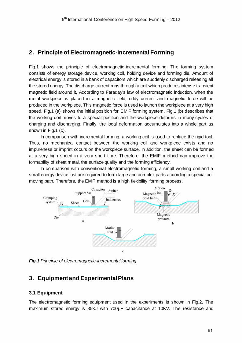
5th International Conference on High Speed Forming – 2012
2. Principle of Electromagnetic-Incremental Forming
Fig.1 shows the principle of electromagnetic-incremental forming. The forming system consists of energy storage device, working coil, holding device and forming die. Amount of electrical energy is stored in a bank of capacitors which are suddenly discharged releasing all the stored energy. The discharge current runs through a coil which produces intense transient magnetic field around it. According to Faraday’s law of electromagnetic induction, when the metal workpiece is placed in a magnetic field, eddy current and magnetic force will be produced in the workpiece. This magnetic force is used to launch the workpiece at a very high speed. Fig.1 (a) shows the initial position for EMIF forming system. Fig.1 (b) describes that the working coil moves to a special position and the workpiece deforms in many cycles of charging and discharging. Finally, the local deformation accumulates into a whole part as shown in Fig.1 (c).
In comparison with incremental forming, a working coil is used to replace the rigid tool. Thus, no mechanical contact between the working coil and workpiece exists and no impureness or imprint occurs on the workpiece surface. In addition, the sheet can be formed at a very high speed in a very short time. Therefore, the EMIF method can improve the formability of sheet metal, the surface quality and the forming efficiency.
In comparison with conventional electromagnetic forming, a small working coil and a small energy device just are required to form large and complex parts according a special coil moving path. Therefore, the EMIF method is a high flexibility forming process.
Fig.1 Principle of electromagnetic-incremental forming
3. Equipment and Experimental Plans
3.1 Equipment
The electromagnetic forming equipment used in the experiments is shown in Fig.2. The maximum stored energy is 35KJ with 700μF capacitance at 10KV. The resistance and
61

5th International Conference on High Speed Forming – 2012
inductance for the circuit are 4.41mΩ and 13.3μH, respectively. A 6-turn flat spiral coil in conjunction with capacitor banks was used to make the sheet deforms by magnetic force. The section area of the coil is 3mm×6mm. The coil has an inner radius of 12.25mm and a coil separation of 6.2mm.
(a) (b)
Fig.2 EMF equipment (a) Capacitor bank and vacuum switch (b) Working coil
3.2 Experimental Program
3.2.1 Plan 1
Fig.3 (a) shows the forming system. The coil and the forming die is fixed using screw bolts and nuts. The coil center offset a distance of 60mm from the sheet center (Fig. 3 (b)). Aluminium alloy (AA 3003) sheets were prepared to carry out the sheet forming test. The thickness of the sheet is 1mm. Fig.3 (c) shows the final sheet profile in the condition of discharge voltage is 2400V. It can be seen that a concave pit occurs at the detail region. It may be the air resistance generated by the sheet deforms in a high speed, which affects the sheet deformation.
62

5th International Conference on High Speed Forming – 2012
60
(a) (b)
(c)
Fig.3 Plan 1 (a) Schemes of forming system (b) Relative position of the coil and sheet (c) Final sheet profile in 2400V discharge voltage
In order to prove the air resistance which can affect the sheet deformation, two different die structures are used in experiment test (Fig.4): (1) There isn’t a hole in the die; (2) Four circular holes with the diameter of 12mm at the die bottom surface, which is used to reduce the effect of the air resistance on forming process. In plan 1, the effect of vent holes, discharge voltage on sheet final profiles are analyzed. In addition, two discharge times with varying value of discharge voltage is used to obtain better final sheet profiles. The effect of the previous discharge on the second one is also analyzed.
(a) (b )
Fig.4 Two different die structures (a) No vent holes at the die bottom surface (b) Four circular holes at the die bottom surface
(1) Effect of vent holes on sheet forming
Fig.5 shows the effect of vent holes on sheet forming. In the condition of no vent hole on the
63

5th International Conference on High Speed Forming – 2012
die, the maximum displacement is 6.9mm. If there are four circular holes at the die bottom surface, the maximum displacement is 7.45mm. This shows that a high air pressure is created by the sheet deforms in a high velocity, which hinder and slow the deformation speed. However, with or without vent holes, the sheet cannot stick onto the die bottom surface and the die side surface. This may be the discharge voltage is not big enough to make the sheet impact with the die.
Fig.5 Effect of vent holes on sheet forming
(2) Effect of discharge voltage on sheet forming
The die has four vent holes are used, Fig.6 shows the effect of discharge voltage on sheet forming. When the discharge voltage is 2000V, the sheet has a maximum displacement at the location of 49mm away from the center. When the discharge voltage is 2400V, the maximum displacement is 8.2mm at the location of 60mm away from the center, while the displacement at the location of 49mm away from the center is less than its surrounding area. The reason may be the discharge voltage is too big to make the sheet impact with the die in a high speed and the bound effect appears at the location of 50mm away from the center. However, the sheet sticks onto the die side surface better in a high discharge voltage than the one in the low discharge voltage.
Fig.6 Effect of discharge voltage on sheet forming
(3) Effect of the previous discharge on the second one
According to the experimental results shown in Fig.6, we can conclude that there is an optimum discharge voltage which corresponding to the sheet impact with the die bottom surface and no bound effect appears. However, it will increase the complexity to control the technical parameters for EMIF process. Therefore, the discharging times are increased and
64

5th International Conference on High Speed Forming – 2012
the multi-times with varying value of discharge voltage is proposed. Fig.7 shows the final sheet profiles when the discharge times is set to 2. In the first step, large displacements lower than the die depth can be obtained using a small discharge voltage. In the second step, larger electromagnetic forces are used to get greater depth, which make the sheet stick onto the die bottom surface and the die side surface in a high discharge voltage. Under the condition of same discharge voltages, a rough shape is obtained and the sheet doesn’t stick onto the die surface when the die has no vent hole. If the same vent holes is used, a rough profile and a concave pit occur at the location of about 50mm away from the sheet center when the discharge voltage are 2400V used in the first step and 4000V used in second step. If the discharge voltage with 2000V use in the first step and 4000V used in second step, a smooth profile has been obtained and the sheet stick onto the die side surface better. However, the displacement in some regions is less than the depth of the die, which reduces the product accuracy. There are two reasons: (a) the number and the dimension of the vent holes don’t meet all air out of the die, which causes the remained air still hides the sheet deformation; (b) the designed coil structure and the distance between the coil center and the sheet center is not reasonable.
Fig.7 Effect of the previous discharge on the second one
3.2.2 Plan 2
Based on experiment results shown in Fig.5, Fig.6 and Fig.7, the die structure in Fig.4 (b) and the two discharge times in one fixed position with 2000V add 2400V discharge voltages are used in EMIF process. Fig.8 shows the motion trajectory and the coil position. The coil moves to four different positions to form a whole large al-alloy part. In this paper, the move angle is set to 90° and the distances between the coil center and the sheet center are all set to 60mm.
Fig.8 Experiment program of EMIF
65
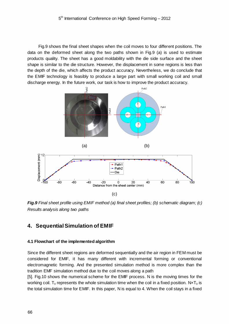
5th International Conference on High Speed Forming – 2012
Fig.9 shows the final sheet shapes when the coil moves to four different positions. The data on the deformed sheet along the two paths shown in Fig.9 (a) is used to estimate products quality. The sheet has a good moldability with the die side surface and the sheet shape is similar to the die structure. However, the displacement in some regions is less than the depth of the die, which affects the product accuracy. Nevertheless, we do conclude that the EMIF technology is feasibly to produce a large part with small working coil and small discharge energy. In the future work, our task is how to improve the product accuracy.
(a) (b)
(c)
Fig.9 Final sheet profile using EMIF method (a) final sheet profiles; (b) schematic diagram; (c) Results analysis along two paths
4. Sequential Simulation of EMIF
4.1 Flowchart of the implemented algorithm
Since the different sheet regions are deformed sequentially and the air region in FEM must be considered for EMIF, it has many different with incremental forming or conventional electromagnetic forming. And the presented simulation method is more complex than the tradition EMF simulation method due to the coil moves along a path [5]. Fig.10 shows the numerical scheme for the EMIF process. N is the moving times for the working coil. T0 represents the whole simulation time when the coil in a fixed position. N×T0 is the total simulation time for EMIF. In this paper, N is equal to 4. When the coil stays in a fixed
66

5th International Conference on High Speed Forming – 2012
position, the simulation time for sheet forming in 2000V and 4000V are 1000μs and 1000μs, respectively. In other words, T0 is equal to 2000μs.
The FEM software ANSYS/EMAG is used to analyze the magnetic force on the sheet. Then the force is imported into ANSYS/LSDYNA using solid 164 element type to predict the sheet forming process. When the coil moves to a special position, the sequential coupling method is used to calculate the magnetic force on the sheet and predict the forming process again. In the latter deformation, the deformation information is also considered from the former one, such as the deflection, velocity, stress, strain, et al. According to the deformation characteristics, the EMIF process can be regard as a “multi-step” forming process using a single coil.
Yes
Electromagnetic model and
mechanical model
Input the electromagnetic
model
Calculate magnetic force T=(i-1)*T0+Δt, 1≤i≤n Calculate magnetic
force
Export magnetic force
Save the data for text format
Input the mechanical
model
Boundary condition
Calculate the deformation of the
workpiece
Restart
Import magnetic force
Meshes updated
T<n×T0T≠i×T0
T<n×T0T=i×T0
Moving coil
T=n×T0ENDNo
YesNo
Fig.10 Flowchart of the implemented algorithm
4.2 Simulation results
When the coil moves to four different positions at different time, Fig.11 and Fig.12 show the deformed sheet meshes and magnetic force on the sheet at different time, respectively. In the simulation process, the effects of the sheet deformation and the coil moving on magnetic field analysis are both considered. This shows the simulation method has high computation accuracy for EMIF process. In addition, the simulation method can also be used for more complex 3D forming system, which solves the bottleneck problem in numerical simulation of electromagnetic forming.
(a) (b)
(c) (d)
Fig.11 Deformed sheet at different time (a)t=150μs, (b)t=2150μs, (c)t=4150μs, (d)t=6150μs
67
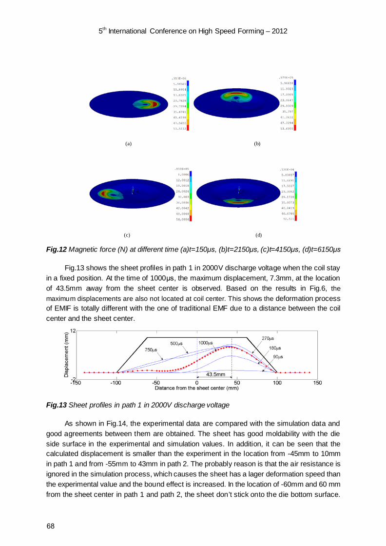
5th International Conference on High Speed Forming – 2012
(a) (b)
(c) (d)
Fig.12 Magnetic force (N) at different time (a)t=150μs, (b)t=2150μs, (c)t=4150μs, (d)t=6150μs
Fig.13 shows the sheet profiles in path 1 in 2000V discharge voltage when the coil stay in a fixed position. At the time of 1000μs, the maximum displacement, 7.3mm, at the location of 43.5mm away from the sheet center is observed. Based on the results in Fig.6, the maximum displacements are also not located at coil center. This shows the deformation process of EMIF is totally different with the one of traditional EMF due to a distance between the coil center and the sheet center.
Fig.13 Sheet profiles in path 1 in 2000V discharge voltage
As shown in Fig.14, the experimental data are compared with the simulation data and good agreements between them are obtained. The sheet has good moldability with the die side surface in the experimental and simulation values. In addition, it can be seen that the calculated displacement is smaller than the experiment in the location from -45mm to 10mm in path 1 and from -55mm to 43mm in path 2. The probably reason is that the air resistance is ignored in the simulation process, which causes the sheet has a lager deformation speed than the experimental value and the bound effect is increased. In the location of -60mm and 60 mm from the sheet center in path 1 and path 2, the sheet don’t stick onto the die bottom surface.
68
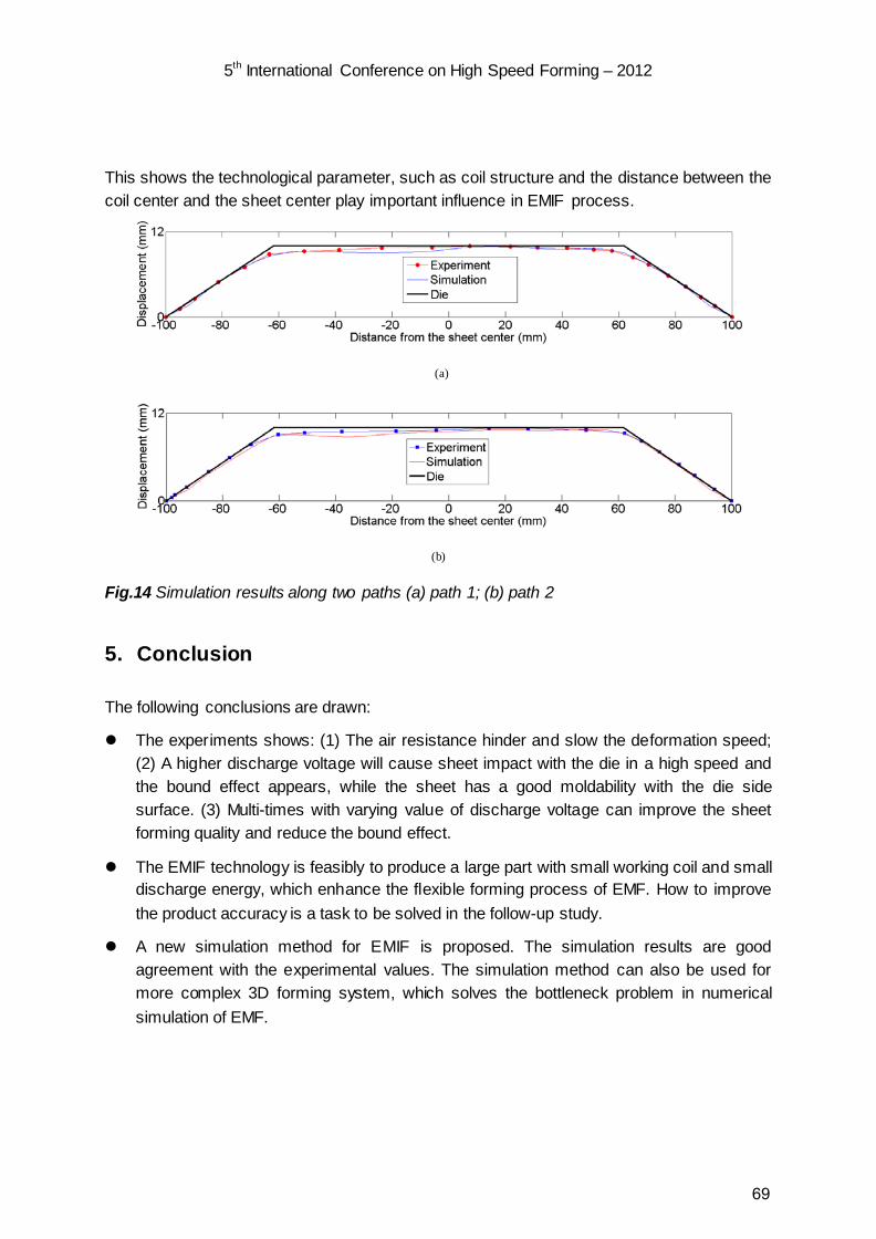
5th International Conference on High Speed Forming – 2012
This shows the technological parameter, such as coil structure and the distance between the coil center and the sheet center play important influence in EMIF process.
(a)
(b)
Fig.14 Simulation results along two paths (a) path 1; (b) path 2
5. Conclusion
The following conclusions are drawn:
The experiments shows: (1) The air resistance hinder and slow the deformation speed; (2) A higher discharge voltage will cause sheet impact with the die in a high speed and the bound effect appears, while the sheet has a good moldability with the die side surface. (3) Multi-times with varying value of discharge voltage can improve the sheet forming quality and reduce the bound effect.
The EMIF technology is feasibly to produce a large part with small working coil and small discharge energy, which enhance the flexible forming process of EMF. How to improve the product accuracy is a task to be solved in the follow-up study.
A new simulation method for EMIF is proposed. The simulation results are good agreement with the experimental values. The simulation method can also be used for more complex 3D forming system, which solves the bottleneck problem in numerical simulation of EMF.
69
5th International Conference on High Speed Forming – 2012
References
[1] Okoye, C, N.; Jiang, J, H.; Hu, Z, D.: Application of electromagnetic-assisted stamping (EMAS) technique in incremental sheet metal forming. International Journal of Machine Tool and Manufacture, 46 (11): pp. 1248-1252, 2006.
[2] Vohnout V.: A hybrid quasi-static process for forming large sheet metal parts from aluminium alloys [D]. Ohio: The Ohio State University, 1998.
[3] Manish, K.; Shang, J.; Cheng, V.; Hatkevich, S.; Daehn, G, S.; Agile manufacturing of a micro-embossed case by a two-step electromagnetic forming process. Journal of Materials Processing Technology, 190 (1-3): pp. 41-45, 2007.
[4] Shang, J, H.; Daehn G.: Electromagnetically assisted sheet metal stamping. Journal of Materials Processing Technology, 211 (5): pp. 868-874, 2011.
[5] Cui, X, H.; Mo, J, H.; Xiao, S, J.; Du, E, H.: Numerical simulation of electromagnetic sheet bulging based on FEM. The International Journal of Advanced Manufacturing Technology, 57(1-4): pp.127-134, 2011.
70

SESSION 3
PROCESS ANALYSIS
71

72

Experimental Investigation and Analysis on Electromagnetic Compression Forming Processed Aluminum Alloy Tubes S.Rajiv1, K. Shanmuga Sundaram1, Pablo Pasquale2 1 Department of Mechanical Engineering, Anna University, Chennai, India 2 CEO and Co-Founder, PST Products GmbH, D-63755 Alzenau, Germany
Abstract
The electromagnetic forming process is high-velocity manufacturing techniques that use electromagnetic forces to shape tube and sheet metal parts. Aluminum alloys are widely used in engineering structures and components where light- weight and corrosion re-sistance are required. Electromagnetic forming process are successfully employed for the materials that are difficult to form by conventional methods because of spring back, as this process achieves large amount of plastic deformation without spring back. In addition, elec-tromagnetic forming improves mechanical properties of the materials, especially, its hard-ness, and also increases the rate of production. In this paper, the experimental investigation and analysis on electromagnetic compression forming of aluminum alloy AA6101 tubes is presented. Aluminum alloy tubes of outer diameter 40 mm and wall thickness of 2 mm with a nominal tensile strength of 214 MPa were electromagnetically compressed using a 4 turn helical actuator that discharges energies up to 20 kJ. It is found that a maximum of 15.85% reduction in outer diameter could be achieved during electromagnetic forming at 18 kJ with an approximate discharge current of 160 kA. The post- forming hardness, micro structure and deformed grain size were also studied. The experimental results were correlated with mathematical analysis using MATLAB and also with simulation using ANSYS. The compari-son of analytical results with experiment and simulation showed good.
Keywords
Forming, Electromagnetic forming, Deformation, Analysis
73

5th International Conference on High Speed Forming – 2012
1 Introduction
High-velocity electromagnetic forming (EMF) can be a flexible and cost-effective alternative to the conventional metal stamping and forming processes. The circuit of the EMF consists of an EMF machine, part, transmission lines and buses, field shaper and primary coil. The coil is the main tool, whose structural and electrical parameters play an important role in the space distribution of magnetic field, and the peak value and width of the magnetic pressure pulse acting on the part [1-2].In EMF a large capacitor bank is connected in series with a forming coil. Discharging the capacitor bank through the coil results in a large transient cur-rent, which in turn induces electric currents in the nearby metallic workpiece. The resulting Lorentz forces cause workpiece motion which caused result in plastic deformation. The input electric energy can be precisely controlled, making the process repeatable, and the non-contact loading allows the use of single side tooling [3].
Metals of high electrical conductivity and of low mechanical strength can be formed by means of pulsed magnetic fields being produced by the sudden discharge from capacitor bank. This technique is especially suitable for the compression of tubes by means of com-pression coils, i.e. by cylindrical coils surrounding the tubular work piece [4]. Aluminum (Al) and magnesium (Mg) are engineering materials that have high electrical conductivity, low melting point, high vapor pressure, high affinity for oxygen and low-yield strength. Application of heat often leads to serious defects, and hence they are appropriate work materials for electromagnetic forming (EMF) which can be conducted at room temperature [5]. Aluminum, being a light weight material, has wide applications in automobile and aerospace industries. However, formability and weldability still remain major issues for aluminum. Nevertheless, while forming aluminum alloys using high-energy rate forming methods, the formability of aluminum can be significantly increased [6].
In this work, the study on effect of energy level on the magnetic field in electromagnetic tube compression forming is presented. The diameter of aluminum alloy 6101 tubes are formed using standard electromagnetic compression forming equipment manufactured by PSTProducts, GmbH,Alzenau Germany. The changes in tube outer diameter,post-forming hard-ness and microstructure were measured using standard equipments. A sequential coupled FEA simulation was attempted to simulate the electromagnetic tube compression using the FEA Multi-physics software ANSYS 13.0. The effects of tube deformation were taken into account during the coupling between the magnetic and the structural analysis. The results on changes in tubes outer diameter with time are presented. The simulation showed good agreement with experimental and mathematical analysis carried out using MATLAB 2010.
2 Overview of the compression experiments
The Aluminum alloy AA6101 tubes of outer diameter 40 mm and wall thickness of 2 mm were selected to study their response to compression forming using EMF.The properties of the alloy are summarised in Table 1.
The experimental setup consisted of a coil, a split field shaper and a specimen holder, which allows for aligning the tube and insert inside the coil, as shown in Figure 1. The ma-chine had maximum charging capacity of 20 kJ and a discharge circuit frequency of 6.5 kHz. The coil was designed with 4 turns and rectangular cross section with dimensions of 26 mm in width and 10 mm in height. The total capacitance of the capacitor banks was 400 µF. The
74
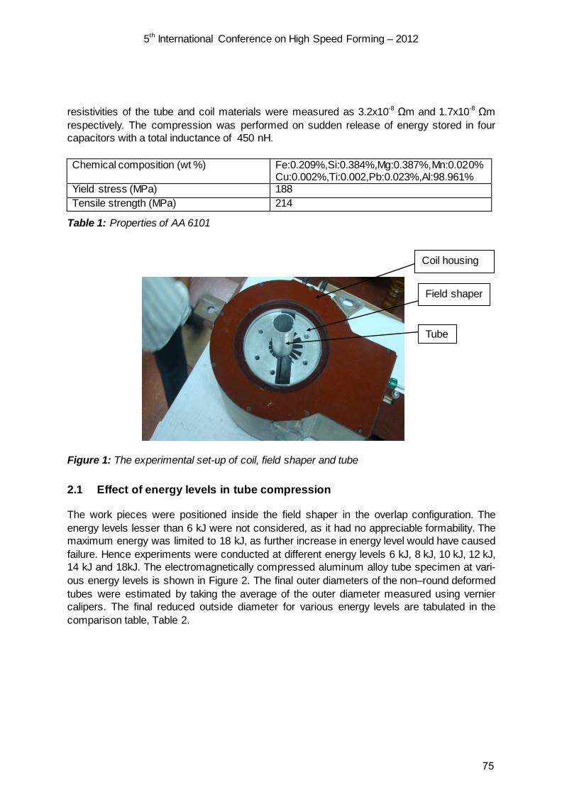
5th International Conference on High Speed Forming – 2012
resistivities of the tube and coil materials were measured as 3.2x10⁻⁸ Ωm and 1.7x10⁻⁸ Ωm respectively. The compression was performed on sudden release of energy stored in four capacitors with a total inductance of 450 nH.
Chemical composition (wt %) Fe:0.209%,Si:0.384%,Mg:0.387%,Mn:0.020%
Cu:0.002%,Ti:0.002,Pb:0.023%,Al:98.961% Yield stress (MPa) 188 Tensile strength (MPa) 214
Table 1: Properties of AA 6101
Figure 1: The experimental set-up of coil, field shaper and tube
2.1 Effect of energy levels in tube compression
The work pieces were positioned inside the field shaper in the overlap configuration. The energy levels lesser than 6 kJ were not considered, as it had no appreciable formability. The maximum energy was limited to 18 kJ, as further increase in energy level would have caused failure. Hence experiments were conducted at different energy levels 6 kJ, 8 kJ, 10 kJ, 12 kJ, 14 kJ and 18kJ. The electromagnetically compressed aluminum alloy tube specimen at vari-ous energy levels is shown in Figure 2. The final outer diameters of the non–round deformed tubes were estimated by taking the average of the outer diameter measured using vernier calipers. The final reduced outside diameter for various energy levels are tabulated in the comparison table, Table 2.
Coil housing
Field shaper
Tube
75

5th International Conference on High Speed Forming – 2012
2.2 Microstructural Observations
The microstructures of the parent material and the compressed tube material formed by electromagnetic compression were observed using optical microscope. The image of the microstructure of parent material and electromagnetic compression formed at an energy level of 18 kJ are displayed in Figure 3 & 4 respectively. The parent material of the tube does not show any grain flow along the longitudinal section whereas all the electromagnetically formed tube showed banding of grains along the direction of forming.
The grain size of the specimen before forming is lower as compared to the grain size of the specimen after EMF process. This in turn had caused an increase in the mechanical properties specifically the hardness in the electromagnetically processed alloy as shown in comparison table, Table 3.
Figure 2: Electromagnetically deformed tube specimen at various energy levels
Figure 3: Longitudinal section of parent alloy
76

5th International Conference on High Speed Forming – 2012
Figure 4: Longitudinal section of EMF specimen at 18 kJ
2.3 Hardness Measurements
In order to investigate the hardness of the tube, Vickers hardness measurements were per-formed using a Wilson Wolpert Micro Hardness tester with a test load of 0.5 kg and an inden-tation time of 12 sec. The measured hardness image of Scanning Electron Microscope of the electromagnetic compression formed aluminum alloy specimen is shown in Figure 5. The hardness of the aluminum alloy materials were measured well outside the deformed zone. The electromagnetically formed zone shows an increase in hardness relative to the base materials. This can be attributed due to the severe plastic deformation or new fine-grained microstructure produced by electromagnetically formed zone. The measured post formed hardness of the tube for various energy levels are shown in the Table 3.
Figure 5: SEM micrograph of aluminum alloy specimen for measuring Vickers hardness
3. Finite Element Analysis of the Compression Process
The simulation of the electromagnetic compression process was carried out using ANSYS 13.0 by assuming: (a) the solenoid coil to be concentric with the tube and (b) without any field shaper between the coil and tube. An Axisymmetric 2D model was considered for both magnetic and structural analysis. The Plane 13-2D, 4 Node solid element was considered,
77

5th International Conference on High Speed Forming – 2012
as it can support both magnetic and structural analysis. The element had degrees of freedom UX,UY,and current density (AZ) for magnetic analysis and UX and UY for structural analysis.
Figure 6: Boundary Conditions for Magnetic Analysis Figure 7: Boundary Conditions for Structural Analysis
The aluminum alloy work piece and the current carrying coil is modeled in 2D consider-ing rectangular cross section for both the coil and the work piece. All the edges of the air medium is constrained for flux lines and the input energy is applied in the coil as shown in Figure 6. The size of the air medium is 100x200 mm.The various energy levels were given as input to carry out the magnetic analysis.The boundary conditions for structural analysis is illustrated in Figure 7. The resulting magnetic force simulated from the magnetic analysis is sequentially coupled to carry out the structural analysis. The Figure 8 shows the deformed tube at an energy level of 18 kJ after the analysis.There was reduction in outer diameter of 6.309 mm at 9 µs in the radial direction. The reduction in final outside diameter for various energy levels are tabulated in Table 2.
Force applied
X and Y displacement constraint
Magnetic flux lines
Input energy
78

5th International Conference on High Speed Forming – 2012
Figure 8: The sectional view of the deformed tube for an energy level of 18 kJ at 9 µs
4 Mathematical analysis of the Compression Process
The MATLAB 2010 software was used to analyse the electromagnetic process. A simple mathematical expression used to calculate the decrease in the diameter (δ) of the tube is given below [7].
−
−+
×
= γδ 22
22
2 dDdD
EDP
(1)
Where, D is the Outside diameter of the tube, P is the magnetic Pressure,P=F/A,F-magnetic force and A-surface area. d is the Inside diameter of the tube, E is the Young’s modulus of the tube material, γ is the Magnetic permeability of the tube material. A code in MATLAB was developed based on the below algorithm.
Initialise the Variables Set the Input Variables Fix Constants Code the equation in MATLAB format and get the output result for the mathematical expression. For dual cases , ‘if’ command is used For thin walled ‘if’ is pre-set and for thick walled ‘else if’ is pre-set and is set as a loop. Output parameters are obtained in the form of text followed by the value string format
79
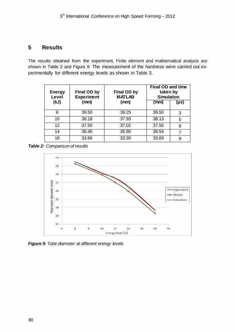
5th International Conference on High Speed Forming – 2012
5 Results
The results obtained from the experiment, Finite element and mathematical analysis are shown in Table 2 and Figure 9. The measurement of the hardness were carried out ex-perimentally for different energy levels as shown in Table 3.
Table 2: Comparison of results
Figure 9: Tube diameter at different energy levels
Energy Level (kJ)
Final OD by Experiment
(mm)
Final OD by
MATLAB (mm)
Final OD and time taken by
Simulation (mm) (µs)
6 39.50 39.25 39.50 3 10 38.18 37.93 38.13 5 12 37.50 37.02 37.56 6 14 36.45 35.95 36.54 7 18 33.66 33.30 33.69 9
80

5th International Conference on High Speed Forming – 2012
Table 3: Vickers hardness at different energy levels
The microstructure analysis of the compressed tube using optical microscope has showed elongation and new grain formation along the longitudinal direction of the tube. The Vickers hardness measured using micro hardness tester has also showed an increase in hardness of the tube with increase in energy level. It is easy to infer that with increase in energy level, the resulting compression (reduction in outer diameter) is more and the entire process has been carried out in less than a second. As the entire forming has been done in quick timing, no spring back was observed. The simulation carried out using the Finite element and mathe-matical analysis software showed very good agreement with the experimental result. It is inferred from the experiment that, the use of electromagnetic forming technique is advanta-geous in compression forming applications as reflected from the results.
6 Conclusions
In this study, electromagnetic compression forming experiments were performed to investi-gate the deformation behaviour and mechanical properties of aluminium alloy tubes of 40 mm outside diameter and 2 mm wall thickness. It is observed from the experiment that by increasing the forming energy there is increase in reduction in diameter during compression process. It is also observed that as the energy level is increased, the value of the hardness too is increased. The measured values of Vickers hardness show an increase of 10.0 HV at the highest energy level. This has proved that the use of EMF technology would increase the mechanical properties of the alloy. The Plane 13-2D 4 noded element used in the sequential coupled electromagnetic analysis simulated the process very accurately.
Acknowledgements
The authors would like to thank PSTProducts, GmbH, Alzenau, Germany for providing the experimental work support.
References
[1] Kleiner, M.; Beerwald, C.; Homberg, W.: Analysis of process parameters and forming mechanisms within electromagnetic forming process. CIRP Annals−Manufacturing Technol-ogy, 2005, 54(1), p.225−228.
Energy Level (kJ)
Deformation by Experi-
ment (mm)
Vickers Hardness
(HV)
6 0.50 74.9 10 1.82 76.3 12 2.50 77.2 14 3.55 78.7 18 6.34 83.7
81

5th International Conference on High Speed Forming – 2012
[2] EL-Azab, A.; Garnich, M.; Kapoora, A.: Modeling of the electromagnetic forming of sheet metals: State-of-the-art and future needs. Journal of Materials Processing Technology, 2003, 142, p.744−754. [3] Balanethiram, V.; Daehn, G.: Enhanced formability of interstitial free iron at high strain rates. Scripta Metallurgica et Materialia, 1992, 27, p.1783–1788. [4] Jablonski, J.; Winkler, R.: Analysis of the electromagnetic forming process. Int. J. Mech. Sci. 1978, (20), p. 315–325. [5] Plum, MM,: Maxwell Laboratories Inc. Electromagnetic forming, metals handbook, 9th ed. 14 ASM Metals Park, OH; 1996. [6] Balanethiram, V.: Hyperplasticity: enhanced formability of sheet metals at high velocity. PhD thesis, Material science and engineering.Columbus, OH, USA: The Ohio State University, 1996. [7] Srinath L S.: Advanced Mechanics of Solids.Tata McGraw-Hill Publishing Company limited, India, 2003.
82
Experimental Study and Numerical Simulation of Electromagnetic Tube Expansion*
J. Shang1, S. Hatkevich1, L. Wilkerson1
1 American Trim LLC, Lima, OH, U.S.A
Abstract
Material constitutive models are important to predict deformation behaviour of materials. To identify parameters of constitutive models for high-strain-rate forming, appropriate methods are needed to investigate the dynamic behaviour of materials. Electromagnetic forming is a high-velocity and high-strain-rate forming process in which velocities of up to 300 m/s and strain rates of more than 103 s−1 can be achieved. Recently, the development of Photon Doppler Velocimetry (PDV) enables the accurate measurement of high velocity, and the electromagnetism module of LS-DYNA allows the reliable simulation of electromagnetic forming. In this study, PDV and LS-DYNA were applied to investigate the electromagnetic tube expansion of Al 6061-T6. The experimental and simulation results are presented and discussed to study the dynamic behaviour of Al 6061-T6 and to verify constitutive model parameters for it.
Keywords
Forming, Simulation, Modelling
* The authors would like to thank Professor Glenn Daehn and Mr. Geoffrey Taber of the Ohio State University for the velocity measurement using PDV, and Pierre L'eplattenier of Livermore Software Technology Corporation for LS-DYNA software support.
83

5th International Conference on High Speed Forming – 2012
1 Introduction
Material constitutive models are used to describe the mechanical behaviour by mathematical formulation of the relationship between strain, stress and other variables. Suitable constitutive models with proper parameters are critical to perform numerical analysis and to predict material deformation. For high-strain-rate deformation, constitutive models should include the term to describe the effect of strain rate. There are several techniques to obtain the experimental data on constitutive properties at high strain rate, such as dropweight machines, split Hopkinson pressure bars, Taylor impact and shock loading by plate impact [1]. In 1965, Niordson [2] pioneered the experimental investigation of high strain rate tests with electromagnetically driven ring expansion. In the 1980s, Gourdin [3] extended the capability of electromagnetically driven ring expansion by using Velocity Interferometer Systems for Any Reflector (VISARs) to measure the ring expansion velocity. Velocity measurement coupled with theoretical models allowed for the deformation behavior to be studied at high strain rates in ring expansion experiments. This test was also used to investigate ductility and fragmentation at high strain rates [4, 5]. But VISARs are difficult to use routinely for velocity measurements and therefore this test was not widely used. Recently, Daehn [6] proposed to apply electromagnetically driven ring expansion for determination of the high-strain-rate constitutive properties with the help of the cutting edge technology, Photon Doppler Velocimetry (PDV), which has the capability to accurately measure the ring expansion velocity and also is easy to apply. Johnson [7] furthered the development with Fully Instrumented Ring Expansion (FIRE) system with electromagnetic actuator and exploding wire actuator.
Moreover, an electromagnetism (EM) module has been developed by LSTC for the numerical simulation of electromagnetic forming [8]. In this module, the electric current going through the actuator (coil) can be set as the input and then the workpiece deformation (such as strain, strain rate, stress, velocity…) can be calculated if the material properties are known. In the case of electromagnetic ring expansion, the ring expansion velocity can be measured using PDV and the electric current can be measured using a Rogowski coil. Therefore, EM module can be applied to calculate the expansion velocity with the measured current as input, and the predicted expansion velocity can be compared to the measured velocity, which will help identify constitutive models used in the finite element simulation. Henchi [9] proposed to apply LS-OPT to determine the constitutive properties by optimizing the parameters of Johnson-Cook model with the combination of EM simulation and PDV measurements.
In this paper, a typical EM expansion experiment with Al6061-T6 tube is presented. Then the simulation results using the EM module with several constitutive models of Al6061-T6 are presented and compared to the velocity measurements. The better agreement between the numerical results and the experiment results should indicate the more appropriate constitutive model. In this way, the proper parameters for the Johnson-Cook constitutive models of Al6061-T6 can be verified.
2 Experiment Setup and Results
Figure 1 shows the schematic layout of the EM tube expansion experiment. The capacitor bank used in this experiment was a 16kJ Magneform machine with the maximum charging
84

5th International Conference on High Speed Forming – 2012
voltage of 8.66kV, a total capacitance of 426µF and an internal inductance of around 100nH. A 3-turn coil was connected to the capacitor bank to generate electromagnetic forces to expand the tube outwards. The coil was made of Cu with 61mm outer diameter, 6.3mm x 6.3mm square cross section and a 3.6mm pitch. The Al6061-T6 tubes used here have 63.5mm outer diameter, 0.89mm wall thickness and 45mm length.
During the EM tube expansion tests, two PDV probes were applied to measure the expansion velocities, shown in Figure 1. Probe A aimed at the middle of the 3-turn coil, which was to capture the maximum expansion velocity. Probe B was 10mm away from Probe A, which was to get more velocity data for study. The measurement principles of PDV can be found in other papers [6, 7]. Moreover, a Rogowski coil was applied to measure the electric current going through the 3-turn coil during EM tube expansion tests.
Figure 2 is the measured current trace and velocities in the case of 0.8kJ Al6061-T6 tube expansion (the charging voltage is 1.93 kV). The measurements show that the electric current in the 3-turn coil reached the peak value of 63.5kA at 18.0 µs. At the position corresponding to Probe A, the Al tube was accelerated to the peak velocity of 72.7m/s within 24.5µs and then decelerated to the velocity of 4.7m/s at 51.5µs. After that, the Al tube began to vibrate and decay to become stationary.
Figure 1: Schematic layout of EM tube expansion experiments
3 Numerical Simulation
3.1 Model
The numerical simulation was performed using the EM module available in the “beta” 980 version of LS-DYNA. In this module, Finite Element Method (FEM) is coupled with Boundary Element Method (BEM) to compute magnetic field, electric field and induced current by solving Maxwell equations in eddy-current approximation. FEM is applied to solve Maxwell equations for the solid conductors and BEM is used for the surrounding air. The detailed introduction of this module can be found in [8].
Charging
System Capacitor bank
High current switch
Coil
+
+ +
Tube
+
+ +
Rogowski Coil
PDV Probe B
PDV Probe A
85

5th International Conference on High Speed Forming – 2012
-40
-20
0
20
40
60
80
-50 50 150 250 350 450
Time (micro-second)
Vel
ocity
(m/s
)
-40
-20
0
20
40
60
80
Cur
rent
(kA
)
Velocity BVelocity ACurrent
Figure 2: Measured current trace and velocities for 0.8 kJ Al 6061-T6 tube expansion
Figure 3: 2D axisymmetric model of the 3-turn Cu coil, Al 6061-T6 tube and G10 holder at initial time (left) and at the end of simulation (right)
A 2D axisymmetric model was built for the numerical simulation, shown in Figure 3. Figure 3 also shows the positions where the velocities were measured. There are three
Position for Velocity B measurement
Position for Velocity A measurement
Velocity A
Current
Velocity B
G10 holder
Cu 3-turn coil
Al tube
Axisymmetric axe
86

5th International Conference on High Speed Forming – 2012
parts: the 3-turn Cu coil, the Al6061-T6 tube and the G10 holder. The 3-turn Cu coil and the Al tube were meshed using eight-node hexagonal solid elements, which are required for the solid conductors in EM module. The G10 holder was meshed with shell elements since G10 Garolite is non-conductive material.
The G10 holder was modelled as a rigid body since it did not have plastic deformation. The 3-turn Cu coil was modelled as elastic material because it did not have plastic deformation during the 0.8kJ EM tube expansion. But for the Al6061-T6 tube, high strain rates and large deformations were involved. Therefore, the Al6061-T6 tube was modelled using the Johnson-Cook strength model, which has the following form [10]:
(1)
where A is yield stress, B is hardening constant, C is strain rate sensitivity, n is hardening exponent, m is thermal softening exponent and Tm is melting temperature. From the literature, four parameter sets of Johnson-Cook strength model for Al6061-T6 were found and listed in Table 1. For each set of parameters, an EM simulation for the case of 0.8 kJ Al6061-T6 tube expansion were performed.
A (MPa) B (MPa) C n m Tm (K)
Model 1 [11] 324 114 0.002 0.42 1.34 925
Model 2 [12] 275 500 0.02 0.3 1.0 925
Model 3 [13] 293 121.3 0.002 0.23 1.34 925
Model 4 [14] 289.6 203.4 0.011 0.35 1.34 925
Table 1: Parameters of Johnson-Cook strength model for Al6061-T6
3.2 Simulation results and comparison
Figure 4 and Figure 5 show the experimental and numerical simulation results of Velocity A and Velocity B respectively. From two figures, it can be seen that the simulations using Model 2 and Model 4 have large difference from the measurements. But the simulations using Model 1 and Model 3 agree well with the measurements in both figures. The peak velocity of Velocity A in the measurement has 2.4% difference from the one predicted with Model 3 and 3.5% difference from the one predicted with Model 1. For the case of Velocity B, the measured peak velocity has the same value as the one predicted with Model 3 and 2.0% difference from the one predicted with Model 1.
Figure 6 shows the effective plastic strain rate and the effective plastic strain at the position where Velocity A was measured, according to the numerical simulation using Model 3 for 0.8kJ tube expansion case. The peak effective plastic strain rate was 2170 s-1 at 25.0µs when the effective plastic strain was 0.022, which is truly a high strain rate. The peak effective plastic strain was 0.06. It should be noted that this experiment applied low energy to expand the Al tube. Much larger expansion velocity and strain rate could be reached if increasing energy or using different set-ups. In this paper, the main purpose
])(1)[ln1)(( m
roomm
roomn
TTTT
CBA−−
−++= εεσ
87
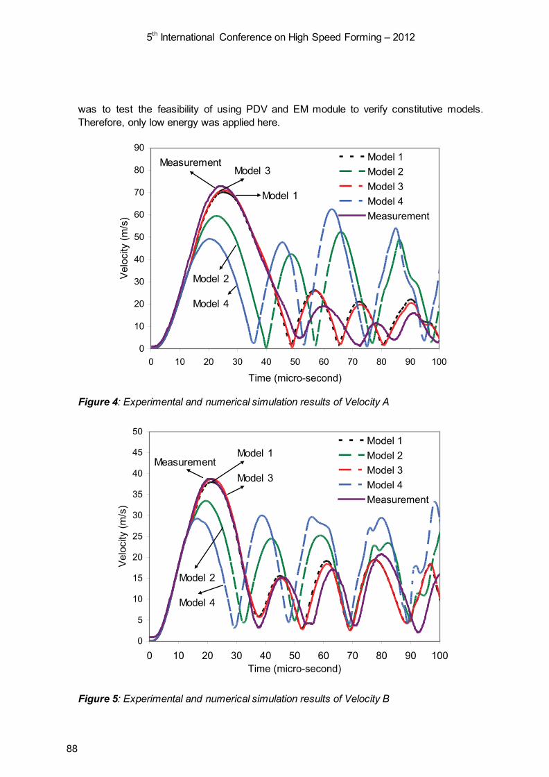
5th International Conference on High Speed Forming – 2012
was to test the feasibility of using PDV and EM module to verify constitutive models. Therefore, only low energy was applied here.
0
10
20
30
40
50
60
70
80
90
0 10 20 30 40 50 60 70 80 90 100
Time (micro-second)
Velo
city
(m/s
)
Model 1Model 2Model 3Model 4Measurement
Figure 4: Experimental and numerical simulation results of Velocity A
0
5
10
15
20
25
30
35
40
45
50
0 10 20 30 40 50 60 70 80 90 100Time (micro-second)
Velo
city
(m/s
)
Model 1Model 2Model 3Model 4Measurement
Figure 5: Experimental and numerical simulation results of Velocity B
Measurement Model 3
Model 1
Model 2
Model 4
Model 1
Model 3
Model 2
Model 4
Measurement
88

5th International Conference on High Speed Forming – 2012
0
500
1000
1500
2000
2500
0 10 20 30 40 50 60 70 80 90 100
110
120
130
140
150Time (micro-second)
Effe
ctiv
e pl
astic
stra
in ra
te (/
s)
0
0.01
0.02
0.03
0.04
0.05
0.06
0.07
0.08
Effe
ctiv
e pl
astic
stra
in
Effective plastic strain rate
Effective plastic strain
Figure 6: Effective plastic strain and strain rate for 0.8 kJ Al 6061-T6 tube expansion
0
100
200
300
400
500
600
700
0 0.01 0.02 0.03 0.04 0.05 0.06 0.07
Effective plastic strain
Effe
ctiv
e st
ress
(MPa
)
Model 1Model 2Model 3Model 4
Figure 7: Comparison of stress-strain plots during EM forming with different models
89

5th International Conference on High Speed Forming – 2012
Figure 7 is the comparison of the stress-strain plots in the 0.8kJ EM tube expansion using different models listed in Table 1. It shows that using Model 1 and 3, the effective stress had small increase with the effective plastic strain, which indicated the low strain rate sensitivity. But using Model 2 and 4, the effective stresses were much higher than the ones using Model 1 and 3.
In this study, 2D axisymmetric simulation was used instead of 3D simulation to save computational time. For a spiral coil, there are some simplifications in order to assume 2D axisymmetric case, which may bring in errors. But in this study, 2D axisymmetric simulation results agreed well with the measurement results. Therefore, 2D axisymmetric simulation should be sufficient for the tube expansion with the 3-turn coil in this study.
3.3 Discussion
The comparisons show that the parameters in Model 1 and Model 3 are suitable for Al 6061-T6, but those in Model 2 and Model 4 are not correct. From Table 1, both Model 1 and Model 3 have the same value of the strain rate sensitivity C, which is 0.002. Model 2 and Model 4 have much larger values of the strain rate sensitivity C. Aluminium is traditionally considered to have low strain rate sensitivity. Therefore, the experimental and numerical simulation results in this paper verified this statement, i.e. Al 6061-T6 has low strain rate sensitivity within the range of 0~2170 s-1 strain rate. As it is known, the values of strain rate sensitivity are relative to the strain rates. Researchers [15, 16] have reported that the strain rate sensitivity increases at strain rates above 1000 s-1 for aluminium and aluminium alloys. In this study, the peak strain rate was 2170 s-1 and the strain rate sensitivity was small for Al6061-T6. It is possible that the strain rate sensitivity of Al6061-T6 will increase if the strain rate is larger than 2170 s-1, such as 10,000 s-1. More experiments are needed to test this statement.
Moreover, the value of hardening exponent n in Model 1 is almost twice of that in Model 3. But both Models predicted the expansion velocities that agreed well with the measurements. So the strain rate hardening has much larger effects than strain hardening in EM Al tube expansion due to high strain rate.
Although the work in this study verified the low value of the strain rate sensitivity for Al6061-T6, the exact value could not be determined only using EM tube expansion tests and numerical simulation by LS-DYNA EM module. Henchi [9] applied LS-OPT to optimize the parameters of Johnson-Cook strength model by several experiments of same material at different energy levels. This could be the way to determine the constitutive properties without utilizing other experimental techniques.
4 Conclusion
Both experiments and numerical simulation of EM Al6061-T6 tube expansion were performed. The PDV technique provides accurate measurements of expansion velocities. The comparisons between EM tube expansion simulation and PDV measurements show the excellent capability of LS-DYNA EM module for EM forming simulation. The
90

5th International Conference on High Speed Forming – 2012
combination of PDV and EM module simulation can be applied to verify the parameters of constitutive models in high strain rate and is beneficial for the study of the dynamic behaviour at high strain rates.
References
[1] Field, J.; Walley, S.; Proud, W.; Goldrein, H.; Siviour, C.: Review of experimental techniques for high rate deformation and shock studies. International Journal of Impact Engineering 30 (2004), p.725–775.
[2] Niordson, F. L.: A Unit for Testing Materials at High Strain Rate. Experimental Mechanics, 5 (1965), p. 23-32
[3] Gourdin, W. H.: Analysis and Assessment of Electromagnetic Ring Expansion as a High-Strain-Rate Test. Journal of Applied Physics, 65(1989), p. 411-422
[4] Grady, D. E.; Benson, D. A.: Fragmentation of Metal Rings by Electromagnetic Loading. Experimental Mechanics, 23(1983), p. 393-400
[5] Rusinek, A.; Zaera, R.: Finite element simulation of steel ring fragmentation under radial expansion. International Journal of Impact Engineering, 34(2007), p. 799-822
[6] Daehn, S.; Zhang, Y.; Golowin, S., et al.: Coupling Experiment and Simulation in Electromagnetic Forming Using Photon Doppler Velocimetry. Proceedings of 4th International Conference on High Speed Forming, Dortmund, Germany, 2008, p. 35-44
[7] Johnson, J.; Taber, G.; Daehn, G., et al.: Constitutive relation development through the FIRE test. Proceedings of 4th International Conference on High Speed Forming, Columbus, OH, 2010, p. 295-306
[8] L’Eplattenier, P.; Ashcraft, C.; Ulacia, I.: An MPP version of the Electromagnetism module in LS-DYNA for 3D Coupled Mechanical-Thermal-Electromagnetic simulation. Proceedings of 4th International Conference on High Speed Forming, Columbus, OH, 2010, p.250-263.
[9] Henchi, I.; L’Eplattenier, P.; Daehn, G.; Zhang, Y.; Vivek, A.; Stander, N.: Material constitutive parameter identification using an electromagnetic ring expansion experiment coupled with LS-DYNA and LS-OPT. Proceedings of 10th international LS-DYNA users conference, Dearborn, 2008, p.14-1~14-10
[10] Johnson, G.; Cook, W.: A constitutive model and data for metals subjected to large strains, high strain rates and high temperatures. Proceedings seventh International Symposium on ballistics, The Hague, The Netherlands, 1983.
[11] Corbett, B.: Numerical simulations of target hole diameters for hypervelocity impacts into elevated and room temperature bumpers. International Journal of Impact Engineering 33 (2006), p. 431-440.
[12] Elsen, A.; Ludwig, M.; Schaefer, R.; Groche, P.: Fundamentals of EMPT-Welding. Proceedings of 4th International Conference on High Speed Forming, Columbus, OH, 2010, p.117-126.
91

5th International Conference on High Speed Forming – 2012
[13] Rule, W.: A numerical scheme for extracting strength model coefficients from Taylor test data. International Journal of Impact Engineering 19 (1997), p.797-810.
[14] Fish, J.: Al 6061-T6 - elastomer impact simulations. Technical report, 2005. [15] Holt, D.L.; Babcock, S. G.; Green, S. J.; Maiden, C. J.: The strain-rate dependence
of the flow stress in some aluminium alloys. Transactions of the ASM: transactions quarterly 60(1967), p.152–159
[16] Tanaka, K.; Nojima, T.: Strain rate change tests of aluminium alloys under high strain rate. Proceedings of the 19th Japan congress on materials research, Tokyo, Japan, 1975, p. 48–51
92

Analysis of Contact Stresses in High Speed Sheet Metal Forming Processes*
R. Ibrahim1, S. Golovashchenko2, A. Mamutov1, J. Bonnen2, A. Gillard2, L. Smith1
1 Department of Mechanical Engineering, Oakland University, Rochester, USA 2 Ford Research & Advanced Engineering, Dearborn, USA
Abstract
In high speed metal forming, determination of contact stresses applied to forming dies is necessary in order to identify the requirements to the die material. Contact stresses greatly control the die design due to their effects on die durability. Very high contact stresses and fracture under impulsive loading have been reported in literature on contact type of high speed forming. In pulsed forming operations using electro-hydraulic forming (EHF), a work piece is often accelerated into the die cavity of a desired shape resulting in a substantial impact pressure on the die. Contact algorithm and mesh size play an essential role in providing accurate results in such high speed processes. Using the soft contact model with an appropriate control of the penetration value provided stable and consistent contact stresses.
Keywords
High Speed Forming, Die Stress, Contact
*Disclaimer: This report is prepared as an account of work sponsored by an agency of the United States Government. Neither the United States Government nor any agency thereof, nor any of their employees, makes any warrantee, express or implied any legal liability or responsibility for the accuracy, completeness, or usefulness of any information, apparatus, product, or process disclosed, or represents that its use wouldn't infringe any privately owned rights. Reference herein to any specific commercial product, process or service by trade name, trademark, manufacturer, or otherwise does not necessarily constitute or imply its endorsement or recommendation or favouring by the United States Government or any agency thereof. The views and opinions of authors expressed herein do not necessarily state or reflect those of the United States Government or any agency thereof.
93
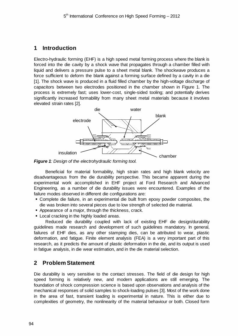
5th International Conference on High Speed Forming – 2012
1 Introduction
Electro-hydraulic forming (EHF) is a high speed metal forming process where the blank is forced into the die cavity by a shock wave that propagates through a chamber filled with liquid and delivers a pressure pulse to a sheet metal blank. The shockwave produces a force sufficient to deform the blank against a forming surface defined by a cavity in a die [1]. The shock wave is produced in a fluid filled chamber by the high-voltage discharge of capacitors between two electrodes positioned in the chamber shown in Figure 1. The process is extremely fast; uses lower-cost, single-sided tooling; and potentially derives significantly increased formability from many sheet metal materials because it involves elevated strain rates [2].
Figure 1: Design of the electrohydraulic forming tool.
Beneficial for material formability, high strain rates and high blank velocity are disadvantageous from the die durability perspective. This became apparent during the experimental work accomplished in EHF project at Ford Research and Advanced Engineering, as a number of die durability issues were encountered. Examples of the failure modes observed in different die configurations are: Complete die failure, in an experimental die built from epoxy powder composites, the
die was broken into several pieces due to low strength of selected die material. Appearance of a major, through the thickness, crack. Local cracking in the highly loaded areas.
Reduced die durability coupled with lack of existing EHF die design/durability guidelines made research and development of such guidelines mandatory. In general, failures of EHF dies, as any other stamping dies, can be attributed to wear, plastic deformation, and fatigue. Finite element analysis (FEA) is a very important part of this research, as it predicts the amount of plastic deformation in the die, and its output is used in fatigue analysis, in die wear estimation, and in the die material selection.
2 Problem Statement
Die durability is very sensitive to the contact stresses. The field of die design for high speed forming is relatively new, and modern applications are still emerging. The foundation of shock compression science is based upon observations and analysis of the mechanical responses of solid samples to shock-loading pulses [3]. Most of the work done in the area of fast, transient loading is experimental in nature. This is either due to complexities of geometry, the nonlinearity of the material behaviour or both. Closed form
die blank
electrode
insulation chamber
water
94

5th International Conference on High Speed Forming – 2012
analytical solutions are generally rare and apply only to some small subset of the overall problem. Numerical solutions, in the form of finite difference and finite element codes, have been successfully used in the past. However, the computer codes available for dynamic analysis are quite complex [3]. Considerable experience with both the codes and the physical problems they are intended to solve is vital. There are several occurrences where different users with different backgrounds get quite different results. Codes have a number of free parameters that must be set by users. This is a major requirement that if not met properly, incorrect physics is being computed and correlation between calculations and experiments is rare.
Further, for each calculation the user must be sure to use an appropriate mesh that should provide converging solution. Once the mesh is chosen, an appropriate artificial viscosity should be selected to avoid damping the solution and artificial ringing. In dynamic calculations, the location of the stress or pressure gradient is a function of time as well as the space. In many instances wave propagation and their reflection from material interfaces and geometric boundaries control the response.
3 Limiting Stress in High Rate Forming Impact
3.1 Determination of Correct Impact Stresses
The most popular method of modeling contact interaction is based on the geometrical analysis of mutual position of boundary nodes of each mesh [2]. At every integration step, it is being verified whether a boundary node of the blank has penetrated through the certain element of the surface mesh of the die. If it happens, it is necessary to make certain corrections bringing the node back on the surface of the die and let the node slide along the die’s surface instead of penetrating through this surface. A significant downside of this approach is in occasional penetration of the node through the surface. It usually happens due to insufficient accuracy of calculations and logical gaps in the contact algorithm. As soon as the blank’s node penetrates into the die’s surface, it is unable to return back, and further calculations are erroneous.
Several simulations were run for the test problems for which the analytical solutions exist: elastic impact of steel bar to steel bar and steel bar to steel sheet plate impact were simulated according to the schematic in Figure 2. In this elastic impact the contact stress is vc∆= ρσ where ρ is the material density, c is the elastic wave speed, and v∆ is the change in particle velocity [4].
Figure 2: Sheet plate, meshed with shell elements impacting a bar meshed with tetrahedral elements.
100mm
10X10 mm
Stationary bar Sheet plate, t= 2mm Moving at V=100m/s
Selected element on the Stationary bar
95

5th International Conference on High Speed Forming – 2012
For common steel at impact velocity of 100m/s this stress value is around 2GPa. Initial attempts to analyze these problems showed excessive contact stresses. Figure 3 shows that unphysical stress values can substantially exceed 2GPa.
Figure 3: Unphysical peak in contact pressure in element A of the impacted bar
Those incorrect reported values cannot be carried over for further design steps. Simulation parameters and model formulation must be revised, and solution correctness judged. The analytical solution for this impact test is presented in the following section.
3.2 Modelling of Dynamic Problems
Electro-hydraulic forming of sheet metals is a dynamic problem. In simulations of such physical problems it becomes necessary to recognize two important factors: The rate at which our observed phenomenon changes; The fact that information is propagated at a finite speed
In mechanical systems, this means taking into account both strain rate and wave propagation effects, [3].
Waves in rods and rod-like structures have been considered to create a state of uniaxial stress. In this configuration, however it is impossible to reach very high tri-axiality stress states. With velocity increases, 2D and 3D effects begin to dominate the rod deformation. Plasticity and material failure govern the magnitude of the stress the rod can carry. Typical idealized stress-strain curves used in computations for materials in such configurations are derived from typical uniaxial stress experiments routinely performed under quasi-static loading conditions.
In order to examine other possible states of die material in pulsed forming conditions, we need to achieve higher level of stresses: we study a thin plate, known as the flyer striking a thicker plate. Waves will radiate into the stationary plate and the flyer plate in the thickness direction as well as in the transverse direction. However, until these reflect from the lateral boundary and return to the centre, a state of uniaxial strain (but 3D stress) will exist there. This change in geometry can achieve hydrodynamic stress state (or pressures) substantially higher than strength of the material at high strain rates.
96

5th International Conference on High Speed Forming – 2012
3.3 Shock Waves in Solids
Uniaxial strain state can be visualized where the deformation is restricted to one dimension such as in the case of plane waves propagating through a material dimensions, and constraints are such that the lateral strains are equal to zero, see [5], [6], and [7], for more detailed description.
Figure 4: Schematic of Stress-strain curve for uniaxial tensile test (upper) vs. Stress-strain curve for uniaxial strain states (lower).
The following expression for 1σ can be obtained as in [3]:
01011 32
32
)21(3YKYE
+=+−
= εεν
σ (1)
where)21(3 ν−
=EK is the bulk modulus, 1σ is the max principal stress, 1ε is the
corresponding principal strain and Y0 is the static yield strength. In terms of pressure the above equation is expressed as
01 34 YP +=σ (2)
This is the stress-strain relation for the uniaxial strain loading described in [3]. For
uniaxial stress state, stress-strain relation is 11 εσ E= with the relation taking the form reported in a typical uniaxial tensile test shown in Figure 4. Thus, the most important difference between the uniaxial stress and uniaxial strain states is the bulk compressibility. In this case the stress continues to increase regardless of the yield stress or strain hardening. The stress-strain curve takes the form shown in Figure 4.
For the case of elastic 1 D strain we obtain
Uniaxial Strain Curve
HELσ Uniaxial Stress Curve
)1)(21()1(νν
ν+−
−=Slope
ESlope = 0Y
Stress
Strain
97
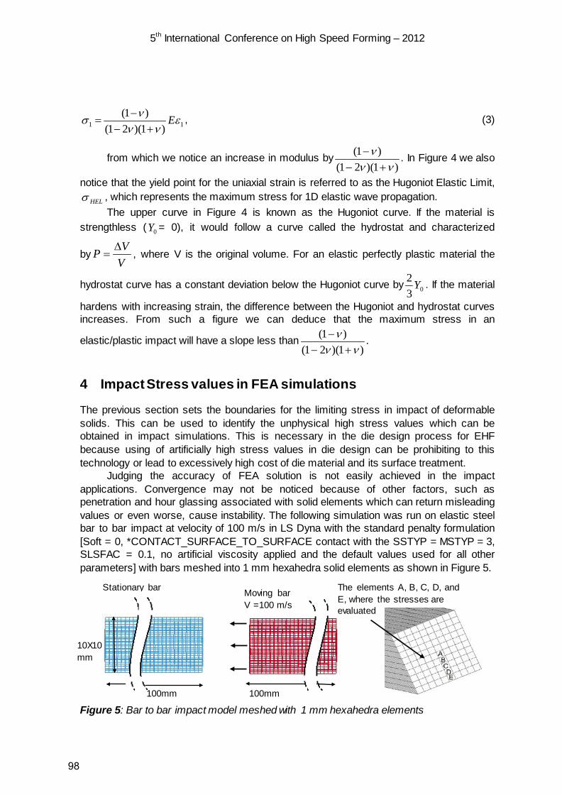
5th International Conference on High Speed Forming – 2012
11 )1)(21()1( ενν
νσ E+−
−= , (3)
from which we notice an increase in modulus by)1)(21(
)1(νν
ν+−
− . In Figure 4 we also
notice that the yield point for the uniaxial strain is referred to as the Hugoniot Elastic Limit, HELσ , which represents the maximum stress for 1D elastic wave propagation.
The upper curve in Figure 4 is known as the Hugoniot curve. If the material is strengthless ( 0Y = 0), it would follow a curve called the hydrostat and characterized
byVVP ∆
= , where V is the original volume. For an elastic perfectly plastic material the
hydrostat curve has a constant deviation below the Hugoniot curve by 032 Y . If the material
hardens with increasing strain, the difference between the Hugoniot and hydrostat curves increases. From such a figure we can deduce that the maximum stress in an
elastic/plastic impact will have a slope less than)1)(21(
)1(νν
ν+−
− .
4 Impact Stress values in FEA simulations
The previous section sets the boundaries for the limiting stress in impact of deformable solids. This can be used to identify the unphysical high stress values which can be obtained in impact simulations. This is necessary in the die design process for EHF because using of artificially high stress values in die design can be prohibiting to this technology or lead to excessively high cost of die material and its surface treatment.
Judging the accuracy of FEA solution is not easily achieved in the impact applications. Convergence may not be noticed because of other factors, such as penetration and hour glassing associated with solid elements which can return misleading values or even worse, cause instability. The following simulation was run on elastic steel bar to bar impact at velocity of 100 m/s in LS Dyna with the standard penalty formulation [Soft = 0, *CONTACT_SURFACE_TO_SURFACE contact with the SSTYP = MSTYP = 3, SLSFAC = 0.1, no artificial viscosity applied and the default values used for all other parameters] with bars meshed into 1 mm hexahedra solid elements as shown in Figure 5.
Figure 5: Bar to bar impact model meshed with 1 mm hexahedra elements
10X10 mm
Stationary bar Moving bar V =100 m/s
100mm 100mm
The elements A, B, C, D, and E, where the stresses are evaluated
98

5th International Conference on High Speed Forming – 2012
The pattern of the stresses doesn’t agree with the analytical solution of 2 GPa contact stress. According to Figure 6 a maximum stress appeared near the edges. It should be emphasized that the solution was very sensitive to contact type used.
Figure 6: Bar to bar impact with incorrect stress values distribution at selected elements
Consistent stress values, as shown in Figure 7, were achieved with one side of contact formulated into segments SSTYP = 0 and the other as a part type MSTYP = 3. Searching for the penetrating nodes and contact force update were required to be at high frequency. In LS Dyna bucket sorting identifies the nearest segment for each slave node. Number of cycles between bucket sorts was set to 1. For the same reason, the number of cycles between contact force update for penalty formulation was also set to 1. Those options help to keep penetration at the minimum level.
Figure 7: Bar to bar impact with uniform stress values distribution
99
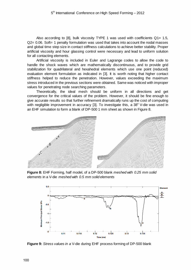
5th International Conference on High Speed Forming – 2012
Also according to [8], bulk viscosity TYPE 1 was used with coefficients Q1= 1.5, Q2= 0.06. Soft= 1 penalty formulation was used that takes into account the nodal masses and global time step size in contact stiffness calculations to achieve better stability. Proper artificial viscosity and hour glassing control were necessary and lead to uniform solution for all contacting elements.
Artificial viscosity is included in Euler and Lagrange codes to allow the code to handle the shock waves which are mathematically discontinuous, and to provide grid stabilization for quadrilateral and hexahedral elements which use one point (reduced) evaluation element formulation as indicated in [3]. It is worth noting that higher contact stiffness helped to reduce the penetration. However, values exceeding the maximum stress introduced in the previous sections were obtained. Same was noticed with improper values for penetrating node searching parameters.
Theoretically, the ideal mesh should be uniform in all directions and get convergence for the critical values of the problem. However, it should be fine enough to give accurate results so that further refinement dramatically runs up the cost of computing with negligible improvement in accuracy [3]. To investigate this, a 38o V-die was used in an EHF simulation to form a blank of DP-500 1 mm sheet as shown in Figure 8.
Figure 8: EHF Forming, half model, of a DP-500 blank meshed with 0.25 mm solid elements in a V-die meshed with 0.5 mm solid elements
Figure 9: Stress values in a V-die during EHF process forming of DP-500 blank
100
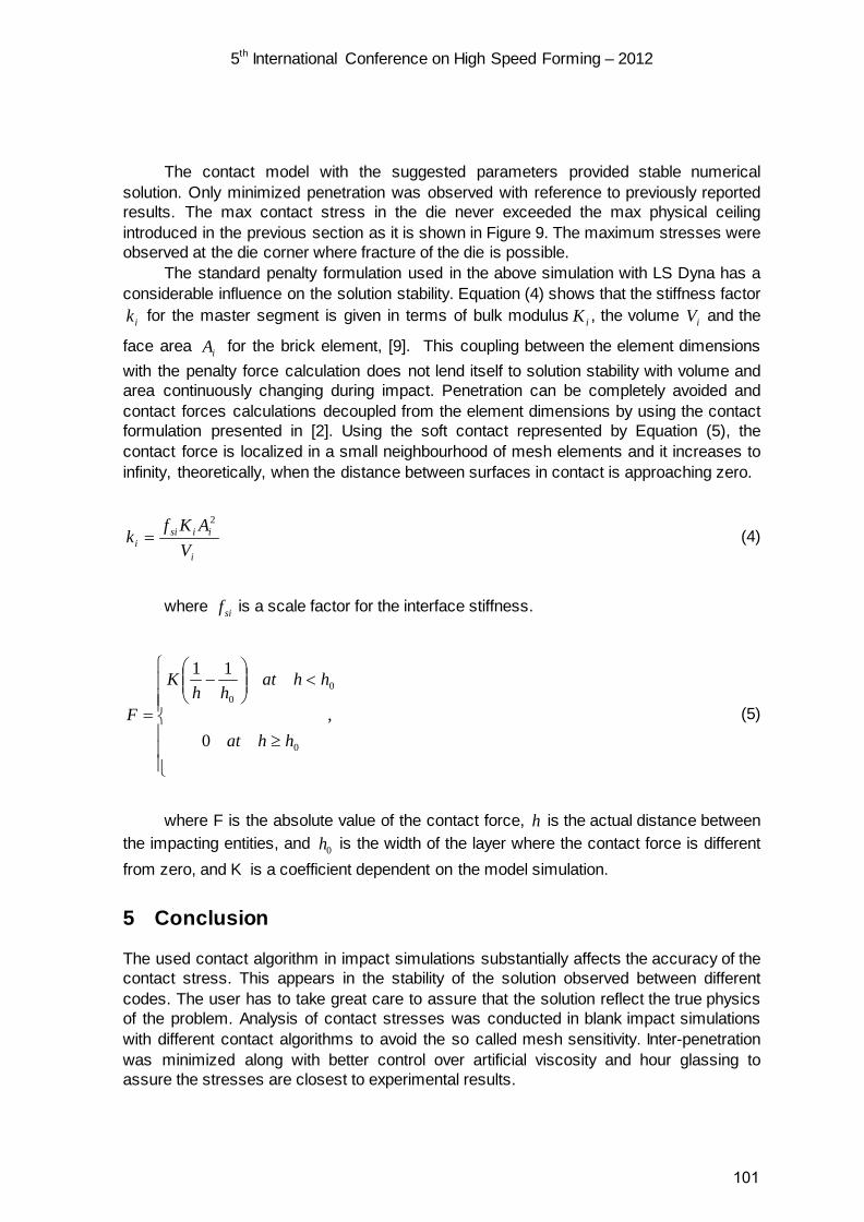
5th International Conference on High Speed Forming – 2012
The contact model with the suggested parameters provided stable numerical solution. Only minimized penetration was observed with reference to previously reported results. The max contact stress in the die never exceeded the max physical ceiling introduced in the previous section as it is shown in Figure 9. The maximum stresses were observed at the die corner where fracture of the die is possible.
The standard penalty formulation used in the above simulation with LS Dyna has a considerable influence on the solution stability. Equation (4) shows that the stiffness factor
ik for the master segment is given in terms of bulk modulus iK , the volume iV and the
face area iA for the brick element, [9]. This coupling between the element dimensions with the penalty force calculation does not lend itself to solution stability with volume and area continuously changing during impact. Penetration can be completely avoided and contact forces calculations decoupled from the element dimensions by using the contact formulation presented in [2]. Using the soft contact represented by Equation (5), the contact force is localized in a small neighbourhood of mesh elements and it increases to infinity, theoretically, when the distance between surfaces in contact is approaching zero.
i
iisii V
AKfk
2
= (4)
where sif is a scale factor for the interface stiffness.
≥
<
−
=
0
00
0,
11
hhat
hhathh
K
F (5)
where F is the absolute value of the contact force, h is the actual distance between
the impacting entities, and 0h is the width of the layer where the contact force is different from zero, and K is a coefficient dependent on the model simulation.
5 Conclusion
The used contact algorithm in impact simulations substantially affects the accuracy of the contact stress. This appears in the stability of the solution observed between different codes. The user has to take great care to assure that the solution reflect the true physics of the problem. Analysis of contact stresses was conducted in blank impact simulations with different contact algorithms to avoid the so called mesh sensitivity. Inter-penetration was minimized along with better control over artificial viscosity and hour glassing to assure the stresses are closest to experimental results.
101

5th International Conference on High Speed Forming – 2012
References
[1] Bruno, E.J., 1968, High-velocity forming of metals. American Society of Tool and Manufacturing Engineers, Dearborn, Michigan, USA
[2] Golovashchenko, S.; Bessonov, N.; Davies, R.: Analysis of Blank-Die Contact Interaction in Pulsed Forming Processes. Proceedings of 3rd International Conference ICHSF'2008, Dortmund, Germany, p.3-12.
[3] Zukas, J. A. (2004).: Introduction to hydrocodes. Amsterdam: Elsevier. [4] Johnson, W. (1972): Impact Strength of Materials. Edward Arnold, London, UK. [5] Graham, R. A.(1992): Solids Under High-Pressure Shock Compression. New York:
Springer- Verlag. [6] Meyers, M.A. (1994).: Dynamic Behaviour of Materials. New York: Wiley [7] Drumheller, D.S. (1998): Introduction to Wave Propagation in Nonlinear Fluids and
Solids. Cambridge: Cambridge U. Press. [8] LS-Dyna Keyword Manual, Version 971. [9] Hallquist, John O., “LS-DYNA Theory Manual," Livermore Software Technology
Corp., March 2006.
102

Effect of Workpiece Motion on Forming Velocity in
Electromagnetic Forming*
Li Qiu1, 2, Xiaotao Han1, 2, *, Qi Xiong1, 2, Zhongyu Zhou1, 2, Liang Li1, 2
1 Wuhan National High Magnetic Field Center, Huazhong University of Science and
Technology, Wuhan, China 2 State Key Laboratory of Advanced Electromagnetic Engineering and Technology, Huazhong
University of Science and Technology, Wuhan, China
Abstract
The effect of workpiece motion on the forming velocity is analysed by the finite element
method. To study the two factors of workpiece displacement and motional electromotive force,
a static model, an incomplete motional model and a complete motional model are created.
The incomplete motional model is simulated by the finite element software COMSOL, while
the complete motional model is simulated by another finite element software Flux. To ensure
the correctness of the model, the static model is created by both softwares. For the specific
system treated in this paper, the results show that when the workpiece velocity is below 100
m/s, the workpiece displacement has only a small effect on the forming velocity. But when the
workpiece velocity is above 200 m/s, the effect of the workpiece displacement on the forming
velocity must be taken into account in the finite element model of the electromagnetic forming
process.
Keywords
Electromagnetic sheet metal forming, Forming Velocity, Workpiece displacement, Finite
element model.
* Financial support was provided by the National Basic Research Program of China (973
Program): 2011CB012800(2011CB012801). The authors thank Professor Fritz Herlach for
technical discussions.
103
5th International Conference on High Speed Forming – 2012
1 Introduction
Electromagnetic forming (EMF) is a high-speed metal forming technology where the
workpiece is deformed by a pulsed electromagnetic force [1]. Compared with conventional
metal forming, electromagnetic forming can improve the formability of many metals [2]-[3].
Hence, electromagnetic forming as a novel metal forming technology is widely studied [4]. In
EMF processing, the eddy current in the workpiece is generated due to induced electromotive
force and motional electromotive force. The induced electromotive force is generated by the
change of the magnetic flux density, while the motional electromotive force is generated by
the motion of the workpiece.
J. Unger et al developed a 3D finite element model for the EMF process which consists
of a carefully chosen discretization, a data transfer method for both, the electromagnetic loads
and the mechanical deformation to utilize an efficient solid shell formulation and a termination
criterion for the electromagnetic part of the model [5]. However, the model is quite
complicated and the effect of the workpiece motional electromotive force on forming velocity
is not considered. Li Qiu et al find that electromagnetic energy is transformed into kinetic
energy due to the workpiece motional electromotive force [6]. This model is based on lumped
parameters and includes many assumed conditions.
The effect of the workpiece motion on the forming velocity involves both the workpiece
displacement and the motional electromotive force. The workpiece displacement causes the
electromagnetic force to decrease, while the motional electromotive force hinders the
workpiece motion. To analyse the two factors, a static model, an incomplete motional model
and a complete motional model are created in this paper. The static and the incomplete
motional model are not correct regarding the physics. By comparing the results of the three
models, the effect of the workpiece motion on the forming velocity is obtained.
2 Basic Theory
The basic setup treated in this paper and the parameters are shown in Figure 1. The tool coil is a
spiral coil and the number of turns is 10. Because of the geometric symmetry, the model is
simplified to 2D axisymmetric model. In the electromagnetic sheet metal forming process, the
eddy current in the workpiece is generated by the change of the magnetic flux density and the
motion of the workpiece:
rzz Bvt
BE
(1)
104

5th International Conference on High Speed Forming – 2012
EJ (2)
JB (3)
Figure 1: Electromagnetic sheet metal forming
E is the electric field, B is the magnetic flux density, v is the velocity of the workpiece, J is the
current density, σ is the conductivity of the workpiece and the subscript r, φ, and z indicate the
radial, hoop, and axial components respectively. The two terms on the right hand side of
equation (1) reflect the effect of induced electromotive force and motional electromotive force
on the electric field respectively.
The electromagnetic force acting on the workpiece is determined by both the eddy
current and the magnetic flux density:
rz BJF (4)
The workpiece is accelerated by the electromagnetic force following Newton's Second
Law of Motion and Acceleration:
t
z
t
zz
z
V
z
dvS
,dav
,madVF
0
0 (5)
105
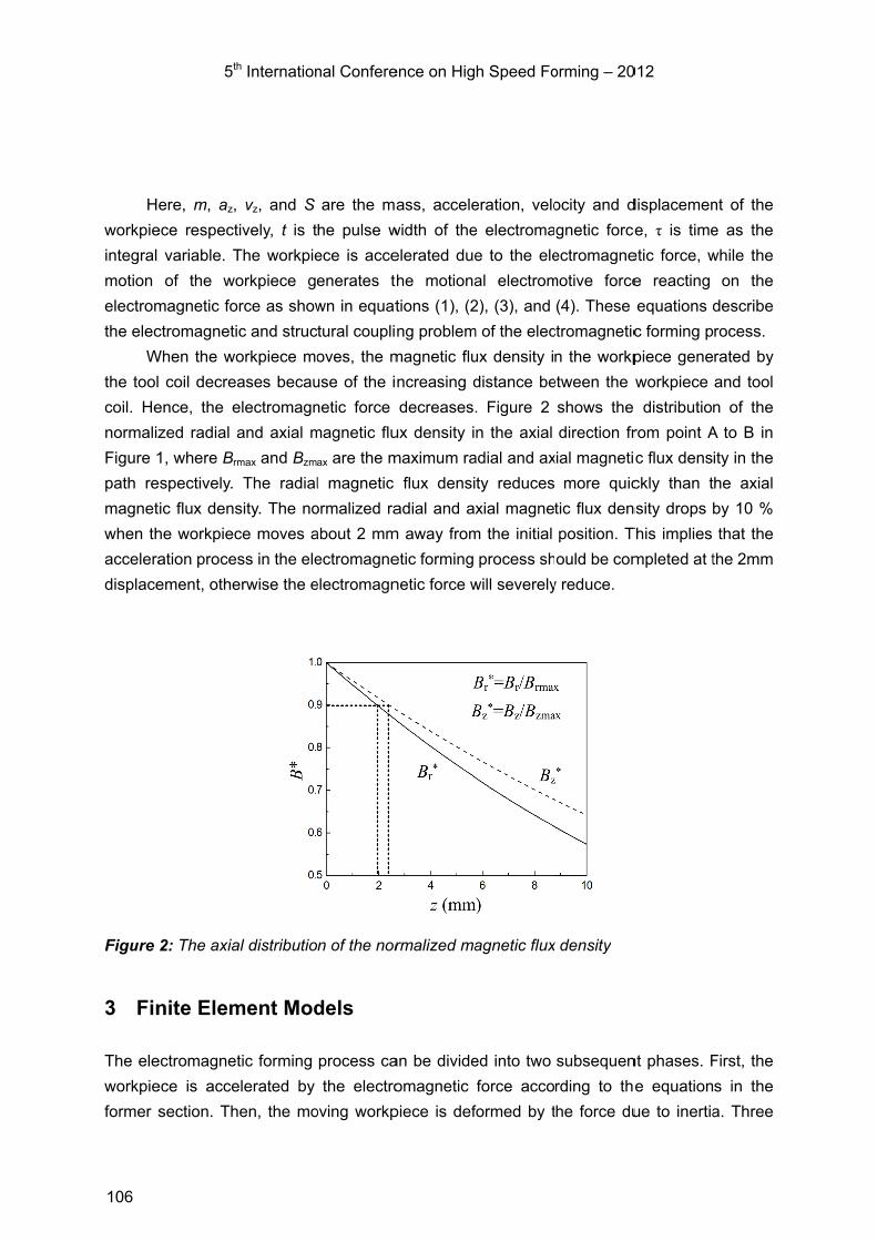
H
workpie
integral
motion
electrom
the elec
W
the tool
coil. He
normaliz
Figure 1
path re
magnet
when th
accelera
displace
Figure
3 Fin
The ele
workpie
former s
5th
ere, m, az,
ece respect
variable. T
of the wo
magnetic fo
ctromagneti
When the wo
coil decrea
ence, the e
zed radial a
1, where Brm
espectively.
tic flux dens
he workpiec
ation proces
ement, othe
2: The axia
nite Elem
ectromagnet
ece is acce
section. Th
h Internation
vz, and S
tively, t is t
The workpie
orkpiece g
rce as show
c and struc
orkpiece mo
ases becau
electromagn
and axial m
max and Bzm
The radial
sity. The no
ce moves a
ss in the ele
erwise the e
al distributio
ment Mod
tic forming
elerated by
hen, the mo
nal Confere
are the ma
he pulse w
ece is acce
enerates th
wn in equat
tural coupli
oves, the m
use of the i
netic force
magnetic flu
ax are the m
l magnetic
ormalized ra
about 2 mm
ectromagne
electromagn
n of the nor
dels
process ca
the electro
oving workp
ence on Hig
ass, accele
width of the
elerated due
he motiona
tions (1), (2
ng problem
magnetic flu
ncreasing d
decreases.
ux density i
maximum ra
flux densi
adial and ax
m away from
etic forming
netic force w
rmalized ma
an be divide
omagnetic
piece is def
h Speed Fo
eration, velo
e electroma
e to the ele
al electrom
2), (3), and
m of the elec
ux density i
distance be
. Figure 2
n the axial
adial and ax
ty reduces
xial magne
m the initial
process sh
will severely
agnetic flux
ed into two
force acco
formed by t
orming – 20
ocity and d
gnetic force
ectromagne
motive force
(4). These
ctromagnetic
n the workp
etween the
shows the
direction fr
xial magneti
more quic
tic flux den
position. T
ould be com
y reduce.
x density
subsequen
rding to th
the force du
012
displacemen
ce, τ is time
etic force, w
e reacting
equations d
c forming p
piece gene
workpiece
distributio
rom point A
c flux dens
ckly than t
nsity drops b
This implies
mpleted at t
nt phases. F
e equation
ue to inertia
nt of the
e as the
while the
on the
describe
rocess.
rated by
and tool
n of the
A to B in
ity in the
he axial
by 10 %
that the
the 2mm
First, the
s in the
a. Three
106

5th International Conference on High Speed Forming – 2012
finite element models reflecting different conditions are created to analyse the first phase of
the electromagnetic forming process in this paper. Table 1 lists the parameters used in the
finite element models. In order to simplify the analysis of the effect of workpiece motion on
velocity, the finite element models are simplified by the assumptions shown as follows:
a. The current load is a half sine wave with the peak current Imax and the pulse width tc.
b. The workpiece is treated as a rigid body in the acceleration process.
c. There is no other force except the electromagnetic force.
Current Pulse
Peak current Imax (kA) 20
Pulse width tc (μs) 80
Coil
Material Copper
Resistivity ρc (Ωm) 1.67×10⁻⁸
Relative permeability μrc 1
Cross section (mm×mm) 4×6
Number of turns N 10
Height hc (mm) 6
Workpiece
Material Aluminum
Density ρw (kg/m3) 2700
Resistivity ρew (Ωm) 2.83×10⁻⁸
Relative permeability μrw 1
Thickness hw (mm) 2
Radius R (mm) 50
Distance between coil and workpiece d (mm) 1
Table 1: The parameters used in this paper
107
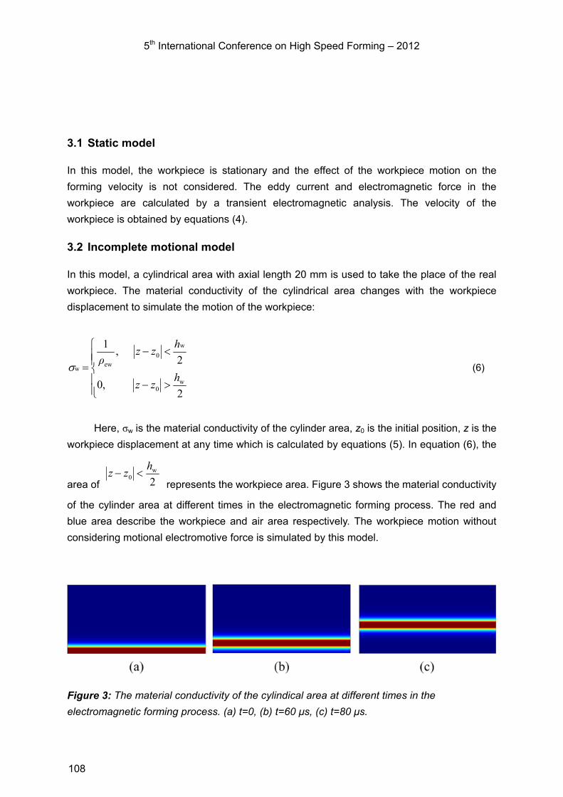
5th International Conference on High Speed Forming – 2012
3.1 Static model
In this model, the workpiece is stationary and the effect of the workpiece motion on the
forming velocity is not considered. The eddy current and electromagnetic force in the
workpiece are calculated by a transient electromagnetic analysis. The velocity of the
workpiece is obtained by equations (4).
3.2 Incomplete motional model
In this model, a cylindrical area with axial length 20 mm is used to take the place of the real
workpiece. The material conductivity of the cylindrical area changes with the workpiece
displacement to simulate the motion of the workpiece:
2,0
2,
1
w0
w
0ew
w
hzz
hzz
ρ (6)
Here, σw is the material conductivity of the cylinder area, z0 is the initial position, z is the
workpiece displacement at any time which is calculated by equations (5). In equation (6), the
area of 2w
0
hzz
represents the workpiece area. Figure 3 shows the material conductivity
of the cylinder area at different times in the electromagnetic forming process. The red and
blue area describe the workpiece and air area respectively. The workpiece motion without
considering motional electromotive force is simulated by this model.
Figure 3: The material conductivity of the cylindical area at different times in the
electromagnetic forming process. (a) t=0, (b) t=60 μs, (c) t=80 μs.
108
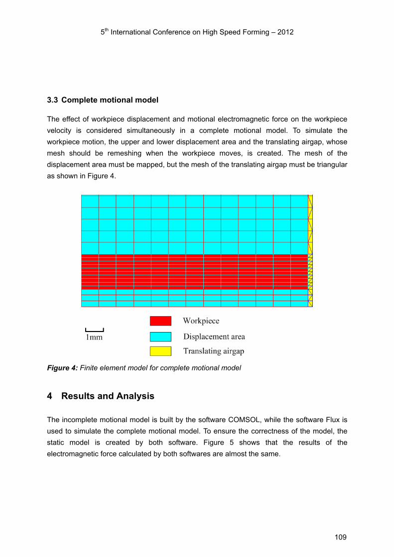
5th International Conference on High Speed Forming – 2012
3.3 Complete motional model
The effect of workpiece displacement and motional electromagnetic force on the workpiece
velocity is considered simultaneously in a complete motional model. To simulate the
workpiece motion, the upper and lower displacement area and the translating airgap, whose
mesh should be remeshing when the workpiece moves, is created. The mesh of the
displacement area must be mapped, but the mesh of the translating airgap must be triangular
as shown in Figure 4.
Figure 4: Finite element model for complete motional model
4 Results and Analysis
The incomplete motional model is built by the software COMSOL, while the software Flux is
used to simulate the complete motional model. To ensure the correctness of the model, the
static model is created by both software. Figure 5 shows that the results of the
electromagnetic force calculated by both softwares are almost the same.
109

5th International Conference on High Speed Forming – 2012
Figure 5: The results for the electromagnetic force by both COMSOL and Flux
Figure 6 shows the forming velocity of the three models at different peak current. When Imax is
20 kA, the results of static model and incomplete motional model almost coincide. The
workpiece displacement has little effect on the forming velocity when the velocity is below 100
m/s. In this case, the effect of the workpiece displacement on the forming velocity can be
ignored. When Imax is 36 kA, the results of the three models are different. That means when
the velocity is above 200 m/s, the electromagnetic force decreases quickly because of the
rapid movement of the workpiece. In this case, the finite element model of the
electromagnetic forming must include the effect of the workpiece displacement on the forming
velocity.
110

5th International Conference on High Speed Forming – 2012
Figure 6: The forming velocity of the three models at different current. (a) Imax=20 kA, (b)
Imax=36 kA
5 Conclusion
To analyse the effect of the workpiece motion on the forming velocity, three finite element
models, including a static model, an incomplete motional model and a complete motional
model, are built by two different finite element softwares. In the static model, the effect of the
workpiece motion on forming velocity is not considered. The workpiece motion without
considering motional electromotive force is simulated by the incomplete motional model. The
complete motional model, simultaneously considering the workpiece displacement and the
motional electromotive force, is simulated by the finite element software Flux. The results
show that the effect of the workpiece displacement on the forming velocity must be
considered in the finite element model of the electromagnetic forming process, when the
workpiece velocity is above 200 m/s in the specific case treated in this paper.
References
[1] N. Takatsu, M. Kato, K. Sato, and T. Tobe: High-Speed Forming of Metal Sheets by
Electromagnetic Force. Japan Society Mechanical Engineering International Journal,
Series III, vol. 31, no. 1, pp. 142-148, 1988.
[2] J. M. Imbert, S. L. Winkler, M. J. Worswick, D. A. Oliveira, and S. Golovashchenko: The
Effect of Tool-Sheet Interaction on Damage Evolution in Electromagnetic Forming of
111

5th International Conference on High Speed Forming – 2012
Aluminum Alloy Sheet. Journal of Engineering Materials and Technology, vol. 127, pp.
145-153, Jan. 2005.
[3] M. Seth, V. J. Vohnout, and G. S. Daehn: Formability of steel sheet in high velocity
impact. Journal of Materials Processing Technology, vol. 168, pp. 390-400, 2005.
[4] V. Psyk, D. Risch, B. L. Kinsey, A. E. Tekkaya, and M. Kleiner: Electromagnetic forming –
A review. Journal of Materials Processing Technology, vol. 211, pp. 787-829, 2011.
[5] J. Unger, M. Stiemer, M. Schwarze, B. Svendsen, H. Blum, S. Reese: Strategies for 3D
simulation of electromagnetic forming processes. Journal of Materials Processing
Technology, vol. 199, pp. 341-362, 2008.
[6] Li Qiu, Yiliang Lv, Chengxi Jiang, Xiaotao Han and Liang Li: Numerical Analysis of the
Workpiece Velocity in Electromagnetic Forming Process. Advanced Materials Research.
Vols. 314-316, pp. 634-638, 2011.
112

SESSION 4
TOOLS AND MACHINES
113

114
Rapidly Vaporizing Conductors Used for Impulse Metalworking* A. Vivek, G. Taber, J.R. Johnson, G.S. Daehn
Dept. of Materials Science and Engineering, The Ohio State University, 2041, College Road, Columbus, OH, 43201, USA
Abstract
Forming, cutting and welding of metal by impulse has significant advantages, in that short time scales change the fundamental nature of the forming process and short duration impulses can be used with much lighter and more agile equipment because large static forces do not need to be resisted. Impulse forming is most commonly executed using electromagnetic forming. The application of electromagnetic forming is limited at high energies and large numbers of operations by the availability of long-lived electromagnetic coils (or actuators, as they are sometimes referred to). Low-cost, disposable actuators have been suggested as one method to treat this issue. Here we propose the use of low-cost foils or wires that are intentionally vaporized by a pulsed electric current to create an intense mechanical impulse. Here, a simple cutting and welding experiment is demonstrated as driven using a vaporized aluminum foil and further original experiments study the expansion of simple copper tubes using the impulse developed from copper and aluminum wires that are vaporized using capacitor bank discharge with nominal charged voltages between 3.4 kV and 6.7 kV, and peak currents between 60 kA and 150 kA delivered with rise times on the order of 20 µs. This gives some guidance on how forming operations may be designed and fruitful avenues for further research.
Keywords
Impulse forming, Bridgewire, PDV
1 Introduction * This work was partially supported by two programs: Sandia National Laboratories through Jerry Stofleth, and The Alcoa Foundation program on Sustainable and Actionable Solutions on Lightweight Vehicle Structures.
115
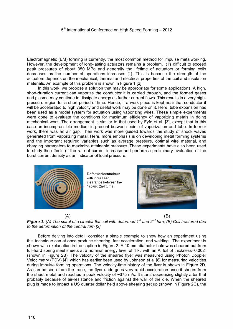
5th International Conference on High Speed Forming – 2012
Electromagnetic (EM) forming is currently, the most common method for impulse metalworking. However, the development of long-lasting actuators remains a problem. It is difficult to exceed peak pressures of about 350 MPa and generally the lifetime of actuators or forming coils decreases as the number of operations increases [1]. This is because the strength of the actuators depends on the mechanical, thermal and electrical properties of the coil and insulation materials. An example of this problem is shown in Figure 1 [2].
In this work, we propose a solution that may be appropriate for some applications. A high, short-duration current can vaporize the conductor it is carried through, and the formed gases and plasma may continue to dissipate energy as further current flows. This results in a very high-pressure region for a short period of time. Hence, if a work piece is kept near that conductor it will be accelerated to high velocity and useful work may be done on it. Here, tube expansion has been used as a model system for actuation using vaporizing wires. These simple experiments were done to evaluate the conditions for maximum efficiency of vaporizing metals in doing mechanical work. The arrangement is similar to that used by Fyfe et al. [3], except that in this case an incompressible medium is present between point of vaporization and tube. In former work, there was an air gap. Their work was more guided towards the study of shock waves generated from vaporizing metal. Here, more emphasis is on developing metal forming systems and the important required variables such as average pressure, optimal wire material, and charging parameters to maximize attainable pressure. These experiments have also been used to study the effects of the rate of current increase and perform a preliminary evaluation of the burst current density as an indicator of local pressure.
Figure 1. (A) The spiral of a circular flat coil with deformed 1st and 2nd turn, (B) Coil fractured due to the deformation of the central turn [2]
Before delving into detail, consider a simple example to show how an experiment using this technique can at once produce shearing, fast acceleration, and welding. The experiment is shown with explanation in the caption in Figure 2. A 10 mm diameter hole was sheared out from full-hard spring steel sheets at a nominal energy level of 4 kJ with an Al foil of thickness=0.002” (shown in Figure 2B). The velocity of the sheared flyer was measured using Photon Doppler Velocimetry (PDV) [4], which has earlier been used by Johnson et al [8] for measuring velocities during impulse forming operations. The velocity-time history of the flyer is shown in Figure 2D. As can be seen from the trace, the flyer undergoes very rapid acceleration once it shears from the sheet metal and reaches a peak velocity of ~375 m/s. It starts decreasing slightly after that probably because of air-resistance and friction against the wall of the die. When the sheared plug is made to impact a US quarter dollar held above shearing set up (shown in Figure 2C), the
116
5th International Conference on High Speed Forming – 2012
flyer not only shears a 10 mm hole in the quarter, but also welds with the impact surface of the quarter as shown in Figure 2 (F,G). This example is intended to demonstrate the versatility of this method as a means to work metal which may be extended to many other operations and geometries.
Figure 2: (A) Schematic representation of the shearing set up, (B) Schematic of the dogbone shaped aluminum foil, (C) the top view of experimental set-up, (D) PDV trace of the sheared spring steel flyer showing a peak velocity of 375 m/s, (E) Sheared quarter dollar and the plug, (F) Sheared spring steel sheet, (G) cross-section of the quarter plug welded with the sheared flyer.
2 Experimental Procedure
Tube expansion experiments were used as a model system to gain phenomenological understanding of vaporizing metal and to find the conditions for attaining the highest pressure to drive metallic workpieces. All the experiments are based on the simple circuit shown in Figure 3. A large amount of charge stored in a capacitor bank flows across a thin conductor, which can vaporize it. With rapid discharge from the capacitor bank, high currents can be developed before the wire vaporizes, storing some inductive and thermal energy [5,6]. This stored energy along with the gases produced by vaporization of conductor material and their subsequent reactions create a high pressure on the surrounding material.
117
5th International Conference on High Speed Forming – 2012
Figure 3. Schematic drawing for rapidly vaporizing bridge-wire circuit.
2.1 Capacitor banks
Two capacitor banks were used for charge storage. The first one (capacitor bank 1), is a commercial design from Maxwell-Magneform. It has a maximum capacity of 16 kJ at a maximum charging voltage of 8.66 kV. As will be seen later, only a fraction of the maximum energy was used in all the experiments. This unit has 8 capacitors, each triggered by two ignitron switches. This unit has a total capacitance of 426 µF and internal inductance of 100 nH and a primary circuit resistance of about 10 mΩ. This gives a rise time in shorted circuit of about 12 µs. All 8 capacitors were used in the circuit in these experiments.
The second capacitor bank (capacitor bank 2), developed at OSU has a maximum capacity of 24 kJ at a charging voltage of 10.9 kV. This unit has 4 capacitors divided into sets of two, which can be triggered separately using spark gap switches. In the present work, all of the capacitors were engaged in the circuit. Total capacitance of the unit is 404 µF, which is lower than the first bank. Inductance of capacitor bank 2 is 100 nH and its dynamic resistance is 4 mΩ. The short circuit rise time of this bank is 10 µs. However, a relatively high inductance connection was used to adapt the experiment to this capacitor bank, and gave a measured rise time of about 35 µs, much larger than that for the other system.
2.2 Experimental assembly
Copper alloy 122 tubes of 25.4 mm (1”) inner diameter, 28.57 mm (1.125”) outer diameter, and 76.2 (3”) length were annealed and quenched to provide a soft and uniform starting tube condition. This alloy is quite commonly used in plumbing pipe and tube, water and gasoline lines. A tensile test was conducted in the hoop direction of the tube and it was found that the yield strength of the material was 105 MPa while the ultimate tensile strength was 206 MPa. Uniform strain of 38% and total elongation to failure of 43% were also obtained. Corona dope was applied at the ends of the tube to prevent current shorting to the specimen. A durometer 80A urethane rod with diameter=25.4 mm (1”) and length=78.74 mm (3.1”) was inserted into the tube as shown in Figure 4. Aluminum and copper wires of diameter= 1.524 mm (0.06”) were inserted in a matching hole drilled through the center of the elastomer rod. The horizontal terminals of the capacitor bank are vertically aligned using a unique apparatus known as the FIRE (fully instrumented ring expansion), system developed by Johnson et al. [7].
118
5th International Conference on High Speed Forming – 2012
Figure 4. Assembly of aluminum wire, elastomer and copper tube.
Figure 5. (A) Actual experimental set up for instrumented tube expansion using vaporizing metal (B) schematics for the experimental setup and velocity measurement using PDV.
119
5th International Conference on High Speed Forming – 2012
2.3 Instrumentation and measurements
Current-time and voltage-time histories were recorded using a Rogowski probe and a 1000:1 voltage probe respectively in conjunction with an oscilloscope which acquires data at 5 Gs/s. Tube velocity was measured using the photon doppler velocimetry (PDV) technique recently developed by Strand et al. [4] with the OSU implementation described separately [8]
The probes were protected from direct impact by any tube fragments through using a periscopic adaptation as described in detail by Vivek et al. [9]. The schematic is shown in Figure 5(B). 2 PDV probes were directed towards the wall of the tube and were 120° apart from each other to assess expansion symmetry. The maximum diameter at the middle of the tube was measured using vernier calipers. A simple calculation can be done to estimate the sustained initial pressure on the inside wall of the tube. Based simply on using Newton’s second law and ignoring the plastic resistance of the tube, the rate of acceleration can be equated to the pressure inside the tube as:
t
xP
(1)
where ρ is density, x is the rate of acceleration and t is the tube thickness. The rate of acceleration can be easily estimated from the PDV data. In each experiment, efficiency is estimated which is the ratio of the maximum kinetic energy imparted to the tube and the electrical energy stored in the capacitor bank prior to discharge. The tube attains peak velocity before significant deformation occurs. This gives us a conservative estimate of efficiency, since initial potential energy is neglected.
To study the effect of current rise time on the efficiency, similar experiments were done on capacitor bank 2 at 9.6 kJ. Single-channel PDV was implemented along with current and voltage measurement. Experiments with copper wires were done on capacitor bank 1 and one-channel PDV was used.
3. Results
3.1 Aluminum wire
3.1.1 Capacitor bank 1
The specifics of the results from capacitor bank 1 are shown in Table 1. A sample trace for these experiments is shown in Figure 6. The final configuration of the tube is also inset in the figure. That experiment studied a tube that was expanded using an aluminum wire with a diameter of 1.524 mm at a 9.6 kJ energy level, the tube fractured as shown in Figure 6. At an input energy of 8 kJ the tube expanded without fracturing. The expansion was relatively uniform along the length of the tube, except at the ends that flared outward. The efficiency of this process has been calculated based on the conversion of input electrical energy into kinetic energy of the tube. This energy converts into potential energy, i.e. plastic work, during expansion of tube. The time period required for current to reach its peak value was in the range of 16-18 µs.
120
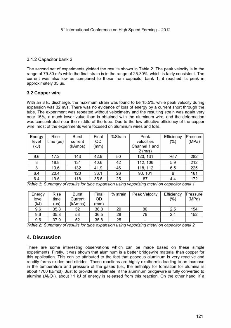
5th International Conference on High Speed Forming – 2012
3.1.2 Capacitor bank 2
The second set of experiments yielded the results shown in Table 2. The peak velocity is in the range of 79-80 m/s while the final strain is in the range of 25-30%, which is fairly consistent. The current was also low as compared to those from capacitor bank 1; it reached its peak in approximately 35 µs.
3.2 Copper wire
With an 8 kJ discharge, the maximum strain was found to be 15.5%, while peak velocity during expansion was 32 m/s. There was no evidence of loss of energy by a current short through the tube. The experiment was repeated without velocimetry and the resulting strain was again very near 15%, a much lower value than is obtained with the aluminum wire, and the deformation was concentrated near the middle of the tube. Due to the low effective efficiency of the copper wire, most of the experiments were focused on aluminum wires and foils.
Energy level (kJ)
Rise time (µs)
Burst current
(kAmps)
Final OD
(mm)
%Strain Peak velocities
Channel 1 and 2 (m/s)
Efficiency (%)
Pressure (MPa)
9.6 17.2 143 42.9 50 123, 131 >6.7 282
8 18.8 131 40.6 42 112, 106 5.9 212 8 19.6 132 41.9 46 118, 112 6.5 225
6.4 20.4 120 36.1 26 90, 101 6 161 6.4 19.6 118 35.6 25 87 4.4 172
Table 1: Summary of results for tube expansion using vaporizing metal on capacitor bank 1
Energy level (kJ)
Rise time (µs)
Burst Current (kAmps)
Final OD
(mm)
% strain Peak Velocity Efficiency (%)
Pressure (MPa)
9.6 35.8 52 36.8 29 80 2.5 154 9.6 35.8 53 36.5 28 79 2.4 152 9.6 37.9 52 35.8 25 - -
Table 2: Summary of results for tube expansion using vaporizing metal on capacitor bank 2
4. Discussion
There are some interesting observations which can be made based on these simple experiments. Firstly, it was shown that aluminum is a better bridgewire material than copper for this application. This can be attributed to the fact that gaseous aluminum is very reactive and readily forms oxides and nitrides. These reactions are highly exothermic leading to an increase in the temperature and pressure of the gases (i.e., the enthalpy for formation for alumina is about 1700 kJ/mol). Just to provide an estimate, if the aluminum bridgewire is fully converted to alumina (Al2O3), about 11 kJ of energy is released from this reaction. On the other hand, if a
121
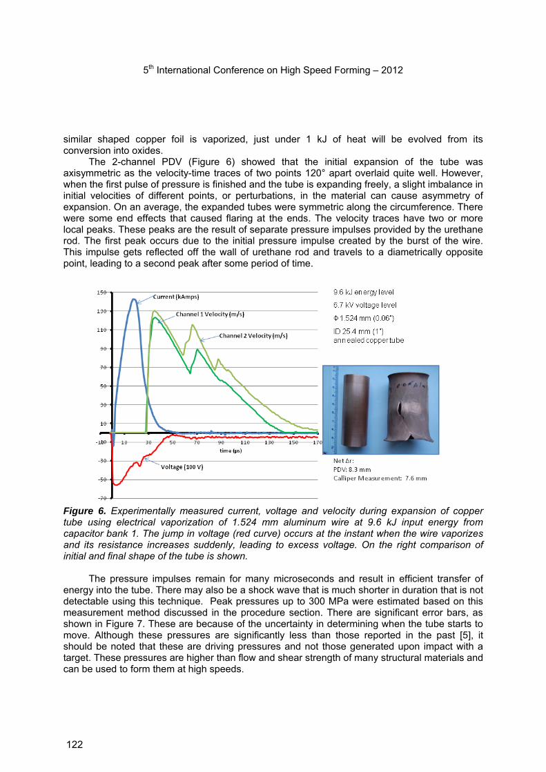
5th International Conference on High Speed Forming – 2012
similar shaped copper foil is vaporized, just under 1 kJ of heat will be evolved from its conversion into oxides.
The 2-channel PDV (Figure 6) showed that the initial expansion of the tube was axisymmetric as the velocity-time traces of two points 120° apart overlaid quite well. However, when the first pulse of pressure is finished and the tube is expanding freely, a slight imbalance in initial velocities of different points, or perturbations, in the material can cause asymmetry of expansion. On an average, the expanded tubes were symmetric along the circumference. There were some end effects that caused flaring at the ends. The velocity traces have two or more local peaks. These peaks are the result of separate pressure impulses provided by the urethane rod. The first peak occurs due to the initial pressure impulse created by the burst of the wire. This impulse gets reflected off the wall of urethane rod and travels to a diametrically opposite point, leading to a second peak after some period of time.
Figure 6. Experimentally measured current, voltage and velocity during expansion of copper tube using electrical vaporization of 1.524 mm aluminum wire at 9.6 kJ input energy from capacitor bank 1. The jump in voltage (red curve) occurs at the instant when the wire vaporizes and its resistance increases suddenly, leading to excess voltage. On the right comparison of initial and final shape of the tube is shown.
The pressure impulses remain for many microseconds and result in efficient transfer of energy into the tube. There may also be a shock wave that is much shorter in duration that is not detectable using this technique. Peak pressures up to 300 MPa were estimated based on this measurement method discussed in the procedure section. There are significant error bars, as shown in Figure 7. These are because of the uncertainty in determining when the tube starts to move. Although these pressures are significantly less than those reported in the past [5], it should be noted that these are driving pressures and not those generated upon impact with a target. These pressures are higher than flow and shear strength of many structural materials and can be used to form them at high speeds.
122
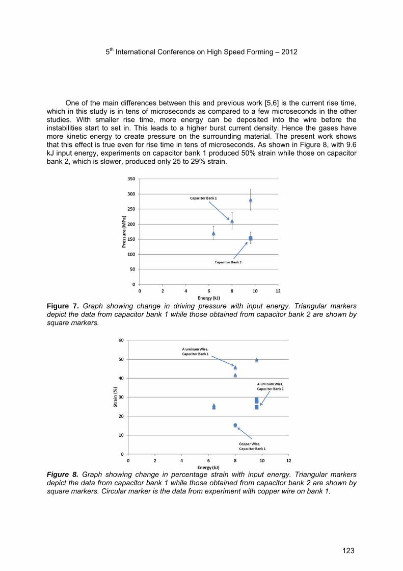
5th International Conference on High Speed Forming – 2012
One of the main differences between this and previous work [5,6] is the current rise time, which in this study is in tens of microseconds as compared to a few microseconds in the other studies. With smaller rise time, more energy can be deposited into the wire before the instabilities start to set in. This leads to a higher burst current density. Hence the gases have more kinetic energy to create pressure on the surrounding material. The present work shows that this effect is true even for rise time in tens of microseconds. As shown in Figure 8, with 9.6 kJ input energy, experiments on capacitor bank 1 produced 50% strain while those on capacitor bank 2, which is slower, produced only 25 to 29% strain.
Figure 7. Graph showing change in driving pressure with input energy. Triangular markers depict the data from capacitor bank 1 while those obtained from capacitor bank 2 are shown by square markers.
Figure 8. Graph showing change in percentage strain with input energy. Triangular markers depict the data from capacitor bank 1 while those obtained from capacitor bank 2 are shown by square markers. Circular marker is the data from experiment with copper wire on bank 1.
123
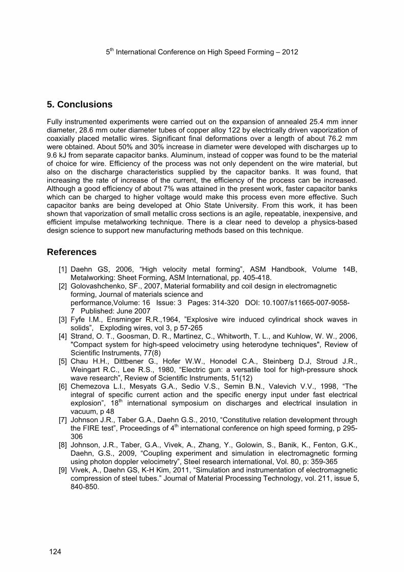
5th International Conference on High Speed Forming – 2012
5. Conclusions
Fully instrumented experiments were carried out on the expansion of annealed 25.4 mm inner diameter, 28.6 mm outer diameter tubes of copper alloy 122 by electrically driven vaporization of coaxially placed metallic wires. Significant final deformations over a length of about 76.2 mm were obtained. About 50% and 30% increase in diameter were developed with discharges up to 9.6 kJ from separate capacitor banks. Aluminum, instead of copper was found to be the material of choice for wire. Efficiency of the process was not only dependent on the wire material, but also on the discharge characteristics supplied by the capacitor banks. It was found, that increasing the rate of increase of the current, the efficiency of the process can be increased. Although a good efficiency of about 7% was attained in the present work, faster capacitor banks which can be charged to higher voltage would make this process even more effective. Such capacitor banks are being developed at Ohio State University. From this work, it has been shown that vaporization of small metallic cross sections is an agile, repeatable, inexpensive, and efficient impulse metalworking technique. There is a clear need to develop a physics-based design science to support new manufacturing methods based on this technique.
References
[1] Daehn GS, 2006, “High velocity metal forming”, ASM Handbook, Volume 14B, Metalworking: Sheet Forming, ASM International, pp. 405-418.
[2] Golovashchenko, SF., 2007, Material formability and coil design in electromagnetic forming, Journal of materials science and performance,Volume: 16 Issue: 3 Pages: 314-320 DOI: 10.1007/s11665-007-9058-7 Published: June 2007
[3] Fyfe I.M., Ensminger R.R.,1964, ”Explosive wire induced cylindrical shock waves in solids”, Exploding wires, vol 3, p 57-265
[4] Strand, O. T., Goosman, D. R., Martinez, C., Whitworth, T. L., and Kuhlow, W. W., 2006, "Compact system for high-speed velocimetry using heterodyne techniques", Review of Scientific Instruments, 77(8)
[5] Chau H.H., Dittbener G., Hofer W.W., Honodel C.A., Steinberg D.J, Stroud J.R., Weingart R.C., Lee R.S., 1980, “Electric gun: a versatile tool for high-pressure shock wave research”, Review of Scientific Instruments, 51(12)
[6] Chemezova L.I., Mesyats G.A., Sedio V.S., Semin B.N., Valevich V.V., 1998, “The integral of specific current action and the specific energy input under fast electrical explosion”, 18th international symposium on discharges and electrical insulation in vacuum, p 48
[7] Johnson J.R., Taber G.A., Daehn G.S., 2010, “Constitutive relation development through the FIRE test”, Proceedings of 4th international conference on high speed forming, p 295-306
[8] Johnson, J.R., Taber, G.A., Vivek, A., Zhang, Y., Golowin, S., Banik, K., Fenton, G.K., Daehn, G.S., 2009, “Coupling experiment and simulation in electromagnetic forming using photon doppler velocimetry”, Steel research international, Vol. 80, p: 359-365
[9] Vivek, A., Daehn GS, K-H Kim, 2011, “Simulation and instrumentation of electromagnetic compression of steel tubes.” Journal of Material Processing Technology, vol. 211, issue 5, 840-850.
124

An Electromagnetically Driven Metalworking Press*
G. A. Taber, B. A. Kabert, A. T. Washburn, T. N. Windholtz, C. E. Slone, K. N. Boos and G. S. Daehn
Department of Materials Science and Engineering, The Ohio State University, Columbus Ohio, USA
Abstract
A small press operated by electromagnetic repulsion and driven by a pulse power supply was constructed at The Ohio State University. This design that applies kinetic energy rather than static force to do work on materials is much lighter and potentially much less expensive than traditional hydraulic, mechanical or servo presses. Performance of the kinetic press is compared to traditional presses in the applications of powder compaction and forming. The results tend to indicate that modest impact speeds of 3 to 18 m/s can improve performance in these manufacturing operations as compared to traditional low-speed machines.
Keywords
Manufacturing, forming, powder
1 Introduction
This work explores the potential in several applications of equipment that is based on kinetic energy instead of static forces. This work will show that because forces are resisted for very short periods of time, modestly sized dynamic equipment can do the work of much more massive equipment [1].
* This work was partially supported by GM R&D through Dr. John Bradley and the Alcoa Foundation.
125

5th International Conference on High Speed Forming – 2012
This paper first reviews the pertinent background in dynamic presses, design of an electromagnetic press and operational characterization procedures are introduced next, followed by short reports of common materials processing operations that could be carried out with a kinetic press. Finally conclusions are given.
2 Background
2.1 Kinetic Presses While most presses are designed to transmit forces that vary slowly with time onto a workpiece to form, cut or consolidate, another approach is to impart kinetic energy to a ram and use the kinetic energy to perform the operation, in a manner similar to a hammer. Possibly the earliest common use of this approach is represented by the gravity-based drop hammer approach. The basic concept of this and other kinetic presses is shown in Figure 1.
Here a ram of a given mass is accelerated over a relatively long distance (from the x=0 to x=c position) using a modest force and then interacts with the workpiece over the distance x=c to the final point, f.
(1)
This provides the same kind of mechanical advantage that is used in hammers and allows much greater output forces, Fout as compared to the input force, Fin. This can allow great force to be transmitted to a workpiece using very simple and lightweight presses.
Another characteristic of this mode of forming is that deformation can take place at relatively high strain rates. The formation of channel-like features in sheet metal as considered in Figure 1 is developed from a flat sheet and this feature has a depth, d, and requires and produces an average Mises strain, ε .
Figure 1: Schematic representation of a kinetic press created by press with ram/tool impacting workpiece. Schematic of flat sheet before and after forming in feature of depth, d.
126

5th International Conference on High Speed Forming – 2012
The approximate averaged strain rate that will be developed can be represented as:
ε ≈ εΔt
≈ ε vmax
2d (2)
where Δt is the approximate time duration of the forming process and vmax is the speed of the punch or tool at impact. For example if a feature is 1mm deep and this produces an average Mises strain of about unity, a typical press which typically have speeds well under 10 cm/s will produce a strain rate under 25 s-1, whereas a punch speed of 10 m/s will give a strain rate near 2.5 x 10³ s-1, and a punch speed over 100 m/s provides strain rates over 2.5 x 10⁴ s-1.
These higher strain rates can produce significantly increased material flow strength, increased strain rate sensitivity and the strain-hardening rate may also be increased. Much work shows that material behavior can change markedly at strain rates above about 103 s-1.
While impulse-based presses are not typical mainstream items in manufacturing, several companies have produced commercial equipment for cutting, forming and powder consolidation based on these principles. LMC, Inc., uses a spring-driven concept [1] that is claimed to reach forming speeds up to 100 m/s [2], but few details are available in the open literature.
Another approach primarily for use in shearing was brought to market as the Lourdes Press, and later revised and offered as the Netronics Bullet Press [3]. This uses magnetic solenoids to drive a relatively traditional die set to a high speed and punching or shearing is done at relatively high speeds. Whereas traditional punching typically takes place well below 10 cm/s, the Bullet press produces tool speeds up to approximately 4 m/s [4]. This high speed approach has been shown to reduce the energy needed to punch sheet metal and produces reduced burr [5]. The work of Klepaczko, in particular, has provided a compelling and complete picture of how increasing punch speed can reduce the required shearing energy and produce different sheared surfaces as compared to quasi-static shearing [6, 7].
Another company, Morphic [8, 9, 10, 11] has developed a hydraulically driven approach to high strain rate forming. They have focused on the application to forming fuel cell plates and while details are not readily apparent in technical journals, from the patents and other public statements, it is clear that the approach again relies on high velocity impact (often simultaneous balanced by impact from both sides of the workpiece, to reduce vibration and need for large systems) and from this generates high pressures, with claims up to “4 GPa in a fraction of a second” [12]. While it appears this technique is commercial, or in the early stages of commercialization, there is little detailed information on the speeds reached by this equipment or on the effects on formability or shearing.
3 The OSU Electromagnetically Driven Press
3.1 Design and Construction In order to test the capabilities of a modest-velocity kinetic press, a simple electromagnetically driven metalworking press was designed and built at The Ohio State University. The EM press utilizes a 4 turn planar spiral primary copper coil with a 165mm outside diameter closely coupled
127
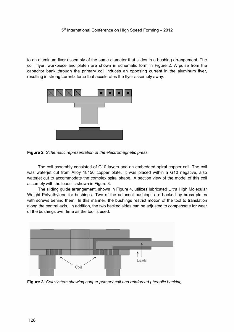
5th International Conference on High Speed Forming – 2012
to an aluminum flyer assembly of the same diameter that slides in a bushing arrangement. The coil, flyer, workpiece and platen are shown in schematic form in Figure 2. A pulse from the capacitor bank through the primary coil induces an opposing current in the aluminum flyer, resulting in strong Lorentz force that accelerates the flyer assembly away.
Figure 2: Schematic representation of the electromagnetic press
The coil assembly consisted of G10 layers and an embedded spiral copper coil. The coil was waterjet cut from Alloy 18150 copper plate. It was placed within a G10 negative, also waterjet cut to accommodate the complex spiral shape. A section view of the model of this coil assembly with the leads is shown in Figure 3.
The sliding guide arrangement, shown in Figure 4, utilizes lubricated Ultra High Molecular Weight Polyethylene for bushings. Two of the adjacent bushings are backed by brass plates with screws behind them. In this manner, the bushings restrict motion of the tool to translation along the central axis. In addition, the two backed sides can be adjusted to compensate for wear of the bushings over time as the tool is used.
Figure 3: Coil system showing copper primary coil and reinforced phenolic backing
128

5th International Conference on High Speed Forming – 2012
The flyer assembly can also be seen In Figure 4. The aluminum flyer is bolted to the tool post that slides in the bushing arrangement and has a stroke distance of up to 18mm.
Figure 4: EM Press bushing, post and flyer assembly section view, with adjustable UHMW bushing on the right
The tool post has an alignment pattern and hole on the end to allow for interchangeable tooling to be utilized, including adapters to accommodate standardized punch and die equipment. A retraction spring is used to return the tool to its initial position after each stroke. The full EM Press is shown in Figure 5.
Figure 5: Actual embodiment of the high-speed press and 3-D CAD rendering.
Flyer
Tool post
Fixed Bushing Adjustable Bushing
129
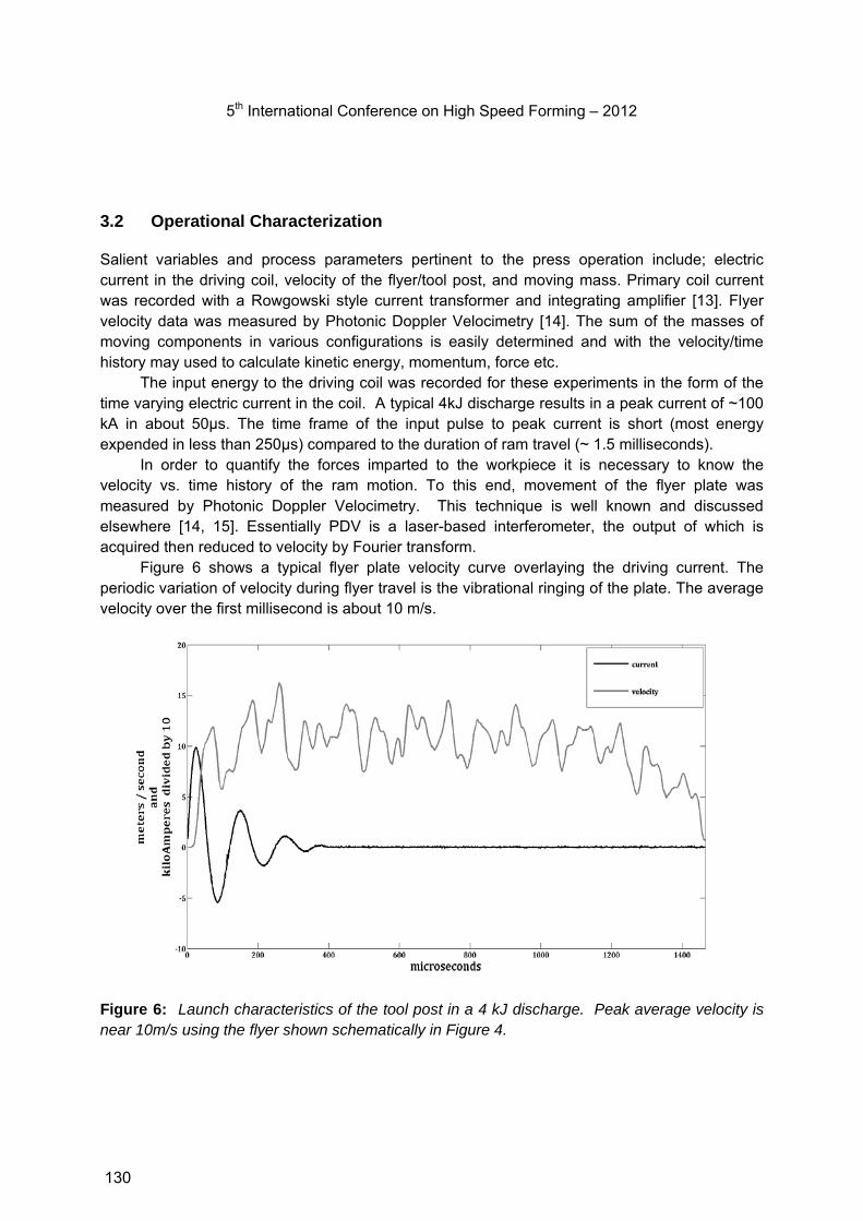
5th International Conference on High Speed Forming – 2012
3.2 Operational Characterization
Salient variables and process parameters pertinent to the press operation include; electric current in the driving coil, velocity of the flyer/tool post, and moving mass. Primary coil current was recorded with a Rowgowski style current transformer and integrating amplifier [13]. Flyer velocity data was measured by Photonic Doppler Velocimetry [14]. The sum of the masses of moving components in various configurations is easily determined and with the velocity/time history may used to calculate kinetic energy, momentum, force etc.
The input energy to the driving coil was recorded for these experiments in the form of the time varying electric current in the coil. A typical 4kJ discharge results in a peak current of ~100 kA in about 50µs. The time frame of the input pulse to peak current is short (most energy expended in less than 250µs) compared to the duration of ram travel (~ 1.5 milliseconds).
In order to quantify the forces imparted to the workpiece it is necessary to know the velocity vs. time history of the ram motion. To this end, movement of the flyer plate was measured by Photonic Doppler Velocimetry. This technique is well known and discussed elsewhere [14, 15]. Essentially PDV is a laser-based interferometer, the output of which is acquired then reduced to velocity by Fourier transform.
Figure 6 shows a typical flyer plate velocity curve overlaying the driving current. The periodic variation of velocity during flyer travel is the vibrational ringing of the plate. The average velocity over the first millisecond is about 10 m/s.
Figure 6: Launch characteristics of the tool post in a 4 kJ discharge. Peak average velocity is near 10m/s using the flyer shown schematically in Figure 4.
130

5th International Conference on High Speed Forming – 2012
Ram velocity increases fairly linearly with input energy. Figure 8 is a graph of input energy and velocity. The maximum input energy used was 7.2 kJ resulting is a velocity of 16.1 m/s.
Figure 7: Ram velocity as a function of input energy using the more robust flyer plate shown in Figure 4.
4 Applications
The press has been used in a variety of applications. In particular, the processes of powder consolidation, sheet metal forming, coining and shearing have been examined. In this short paper we will highlight applications in powder consolidation and sheet forming.
4.1 Powder consolidation
There is considerable interest in the consolidation of powders. Recent developments allow the production of new classes of low-cost powders that can be effectively consolidated. Work was done by Kabert using the EM press for the consolidation of titanium powders starting with roll compacted sheets of Armstrong processed powder [16]. Figure 8 shows the classical problem, which is that large static pressure is needed to produce densities near the theoretical density. Here we briefly demonstrate the advantages of velocity. Further detail is available in the thesis of Kabert [16].
The EM press may be operated cyclically with the rate limited by the charge time of the capacitor bank and cooling limitations of the coil. In the application of consolidating roll compacted sheets of titanium powder, a flat tool steel attachment with a 38mm square face was attached to the flyer assembly. A flat steel backing block was used as a die. 25mm squares of material were impacted repeatedly with charge energies of 0.96 kJ, 1.28kJ or 1.92kJ. Each sample was struck 20 times at the same energy. Thickness measurements were taken with a ball micrometer after strokes 1, 3, 5, 10 and 20 to observe the results throughout the process. Two different flyers and ram combinations were used. First, a low mass system resembling that seen in Figure 2 was used. This had a total ram and flyer mass of 0.96 kg, but was prone to fatigue damage. A more massive flyer was designed and created from high strength, as shown in Figures 4 and 5. As detailed in Kabert’s thesis, at a given capacitor bank discharge energy, these rams had similar kinetic energies, but the lighter system had higher velocity.
131

5th International Conference on High Speed Forming – 2012
Results for compaction of roll-compacted commercial purity and 6Al-4V titanium powders are marked respectively CPARM and 64 ARM in Figure 9. Both the light (flyer 1) and heavier flyers were used and multiple strokes were used to compact the powders. These results show two things clearly: 1) that significant consolidation is possible with this approach using multiple strokes, reaching densities that would be require well over 500 MPa in conventional compaction and 2) increasing velocity is more important than increasing kinetic energy. Significantly higher compaction densities were seen with the less massive flyer at higher velocity, when launched with the same energy.
Figure 8: Density as a function of pressure for the compaction of partially-dense roll compacted sheet in compression between flat platens. CPARM refers to commercial purity powder, and 64 is a Ti-6Al-4V alloy, both from the Armstrong powder production method.
Figure 9: Compacted densities as a function of number of strokes for roll compacted partially dense titanium sheets.
132

5th International Conference on High Speed Forming – 2012
4.2 Sheet metal forming
Single-Sided die urethane pad sheet metal forming with the EM press has been investigated by Windholtz [17] by plane-strain stretch forming into a channel. This shape is exemplified in many important practical features – stiffening ribs in structural parts, heat exchangers and fuel cell plates. Again, a short example of some results from a more comprehensive forthcoming M.S. thesis is shown here. In that work, a range a velocities and materials were considered in channel forming. Figure 10 shows 0.381 thick H-19 3003 aluminum formed into a sinusoidal die using a polyurethane pad. Both a simple steel die was used, and one coated with BN lubricant. For both a quasi-static press and the high-speed press the force or energy was increased just to the point where failure was seen and the greatest depth that could be obtained without failure was sought. Results from that study are shown below. In all cases, the urethane pad effectively locked the sheet to the flat surface of the die and all deformation was in near plane-strain stretching. The electromagnetic press formed aluminum sheet to a 30% greater depth before failure compared to static methods of urethane pad forming, and there was a similar increase in strains to failure. Impact velocity was about 10 m/s. Figure 10 shows cross sectional views of the formed metal and dies under different conditions.
Figure 10: Cross-sections of 3003 H-19 aluminum stretched into channels in nearly plane strain using a urethane pad and a one-sided steel die. Conditions with inputs just prior to and just after failure are noted in each case.
EM Press - Failure
Quasi-Static
Quasi-Static - Failure Quasi-Static - Failure
EM Press
EM Press - Failure
EM Press
Quasi-Static
Dry Lubricated
133

5th International Conference on High Speed Forming – 2012
5 Conclusions & Issues
In several operational respects the electromagnetic press is comparable or superior to methods based on other types of equipment. In particular, this work demonstrated enhanced plasticity of sheet aluminum by urethane pad forming in comparison to quasi-static methods and improved consolidation in high speed impact pressing versus quasi-static conventional pressing.
There are high accelerations associated with this device that induce severe shock loads to the apparatus. For example, a 4kJ input to the driving coil accelerates the tool post to 10m/s in about 50µs, which is 200,000G. In the application of coining, acceleration on impact can be more than double that. Such loading must be considered in the design in order to minimize fatigue and stress concentrations. Work in improving the robustness of this class of equipment is underway.
References
[1] US Patent 4245493, January 1981 [2] http://www.lmcpress.com/news/r_and_d_100.php [3] http://www.netronicsresearch.com/ [4] Grunbaum, Martin. 1996. Influence of High Cutting Speed on the Quality of Blanked Parts.
The Ohio State University. Columbus, Ohio: Ohio State University. [5] MacIsaac, Jamie D, Jr. 1996. Ultra High-Speed Blanking Forces. Columbus, Ohio: Ohio
State University. [6] Klepaczko JR., “An experimental technique for shear testing at high and very high strain
rates; the case of mild steel”, International Journal of Impact Engineering, 15, 1994, 25. [7] Klepaczko JR, Klosak M, “Numerical study of the critical impact velocity in shear”, Eur J
Mech A/Solids 1999;18:93. [8] US Patent 6782795 [9] US Patent 7104190 [10] US Patent 6862912 [11] US Patent 7694613 [12] http://www.morphic.se/en/Cellimpact/Method/ [13] http://homepage.ntlworld.com/rocoil/index.htm [14] Johnson, J. R., Taber, G., Vivek, A., Zhang, Y., Golowin, S., Banik, K., Fenton, G. K. &
Daehn, G. S. 2009. Coupling Experiment and Simulation in Electromagnetic Forming Using Photon Doppler Velocimetry. Steel Research International, 80, 359-365.
[15] Kabert, B. A. 2011. High Strain Rate Consolidation and Forming of Armstrong and HDH Titanium Powder and Sheet Material. Columbus, Ohio: Ohio State University.
[16] Strand, O. T., Goosman, D. R., Martinez, C., Whitworth, T. L. & Kuhlow, W. W. 2006. Compact system for high-speed velocimetry using heterodyne techniques. Review of Scientific Instruments, 77,
[17] Windholtz, T. N., unpublished work in progress, personal communication.
134

A Study on Contour on Workpiece According to the Shape of Forming Coil in EMF Process
J. Y. Shim1, B. Y. Kang1, D. H. Park2 , Y. Choi1 and I. S. Kim3
1 Environmentally Materials & Components Centre, KITECH, Korea 2 Welmate Co.,Ltd., Korea 3 Department of Mechanical Engineering, Mokpo National Univ., Korea
Abstract
Aluminium alloys is desirable for the automotive and electronic appliances industries due to their high strength-to-weight ratio, corrosion resistance and weldability. However applications of the aluminium alloys were very difficult because aluminium alloys formability is very low at room temperature, despite their advantages. One of the high speed forming technologies is Electromagnetic Metal Forming (EMF), which can be useful forming method for low formability light-weight materials such as aluminium, magnesium alloys in overcoming the limitations of conventional forming methods. EMF process refers to the high velocity and high strain rate deformation of low-formability materials driven by electromagnetic forces that are generated by the rapid discharge current through forming coil. This technology depends on the properties of the sheet metal, as well as the process factors such as electromagnetic force in a practical forming operation. Moreover selection of proper shape of forming coil is most important to achieve the desired deformation using the EMF process. Therefore, the purpose of this study is to analyse of the dynamic behaviours on workpiece according to various forming coil shape with aluminium alloys. To achieve these objectives, a magnetic pulse forming system consisting of a 24kJ electromagnetic power source and a bar-type and helical-type forming coil was employed in an experiment. Then, deformation depth was measured for analyse dynamic behaviours on workpiece. The results showed that as the electromagnetic force increases, surface damage to part of the workpiece will increase and according to the shape of forming coil, distribution of electromagnetic force applied on workpiece is changed in EMF process.
Keywords
Aluminium alloys, Forming, Electromagnetic Metal Forming(EMF), Electromagnetic force
135
5th International Conference on High Speed Forming – 2012
1 Introduction
Aluminium alloys is useful light-weight materials which have been employed in many forms such as sheet, plate, bar and rod in various areas of industry and especially in the automotive and small digital electronic product industries. Aluminium alloys also has many advantages included corrosion resistance and very good thermal and electrical conductivities. Although the aluminium alloys has high strength-to-weight ratio and good corrosion resistance, the low formability of aluminium sheets limited their use in some products with bending radius in the corner part is small. For expanding use of these aluminium alloys in many areas, however, there have been challenging formability problems for aluminium alloys to overcome. The formability of the aluminium alloys at room temperatures is generally lower than at both cryogenic and elevated temperatures [1-3]. For this reason, hot press forming is utilized as the forming process for aluminium alloys. However, hot press forming is not easy to determine the proper temperature of the die and considerably long process times is required for the post-process after forming. Therefore, it is necessary to develop an effective forming technology for aluminium alloys that can be used at room temperature.
Generally, a high current impulse in EMF has been passed through a forming coil by the discharge of a capacitor bank. The current in the forming coil also produced a transient primary magnetic field around the forming coil[4]. The change in this field induces an eddy current in the workpiece and an associated secondary magnetic field. The two fields are repulsive and the force of magnetic repulsion causes the collision between workpiece and die. When the stress arising from repulsive magnetic pressure exceeds the yielding point of the workpiece, plastic deformation of the workpiece begins. Because this repulsive force causes a rapid motion of the workpiece, light-weight material’s formability is to improve instantaneous [4-7]. So EMF technology allows product designs which cannot be solved with conventional processes such as press forming. Moreover, this process is environmentally friendly forming process because environment pollutant such as lubricant, polyethylene etc does not need to use.
EMF has so far been studied many experimental and numerical analysis not only to promote increased formability, suppress wrinkling and reduced spring back, but also to improve the surface finish by Daehn et al. [6]. Balanetihiram et al. [7] represented the improvement of formability as follow; (1) The workpiece constitutive behaviour changes at high-strain rates, leading to an increase in the rate of strain hardening and/or rate sensitivity (2) It is possible that inertial effects promote more diffuse neck development, hence leading to higher ductility (3) The collusion with die causes the material to plastically spread radially in a process that may be thought of as “inertial ironing”. During the past few years, several experimental and numerical studies have been performed for the EMF process. Furth and Waniek[8-9] attempted to develop an analytical method using firstly. In that study, basic equations that describe the physical phenomena on EMF process established. Also Takatsu et al.[10] described the basic equations to simulate the electromagnetic free bulging of a fleet sheet. Work by Fenton and Daehn[11-12] demonstrated that a two-dimensional Arbitary Lagrangian Eularian(ALE) finite difference code has accurately been employed to predict the dynamics of the EMF process. With the development of commercial finite element codes, another approach has been proposed by Oliveira et al.[13] which developed a simple
136

5th International Conference on High Speed Forming – 2012
‘loosely coupled’ model to simulate sheet EMF process. Shortly afterward, stiemer et al.[14] proposed a ‘fully coupled’ model to simulate the EMF process. The ‘loosely coupled model or the ‘fully coupled’ allows accurate simulations of the EMF sheet process.[15] In that study, they investigated dynamic behaviour of aluminium alloy sheet with double spiral coil and then, major and minor engineering strains of workpiece predicted using the numerical FE-model. Also Bendjima[16] considered force due to motion of the workpiece utilizing two-dimensional finite element techniques to model the transient phenomena in EMF. As experimental works, Imbert et al.[17] examined the effect between tool and sheet interaction on damage evolution in EMF through free-form and conical die experiments. Kamal et al.[18] examined aluminium micro-embossed cell phone case by a two-step EMF process using uniform pressure (UP) actuator. In the first, an attempt has been made to form as enclosure body in single step using the UP actuator and then the fundamental embossing characteristic of the UP actuator system are demonstrated with very simple flat forming coil. As mentioned above, studies of EMF process has been focused on development of FE-model for prediction the forming process and process optimization for application of aluminium alloys. However, these experimental and numerical studies did not compare the dynamic behaviours of workpiece according to various forming coil shapes. Therefore, this study concentrated on analysis of the contour on workpiece when employed the various shape forming coil with aluminium alloys in EMF process. In order to achieve this objective, EMF was performed using a bar-type forming and helical-type forming coil and 0.5mm Al5053 sheet at various charged voltages, and then the results were compared through measurements of the deformation of depth on workpiece.
2 Experimental Works
2.1 Experimental Setup and Procedure
As shown in Figure 1, EMF system which manufactured by WELMATE CO.,LTD. for this study includes a magnetic pulse power source which consists of a capacitor bank with a maximum charging energy of 24kJ, a forming coil and a die.
Figure 1: Set up for this study
137
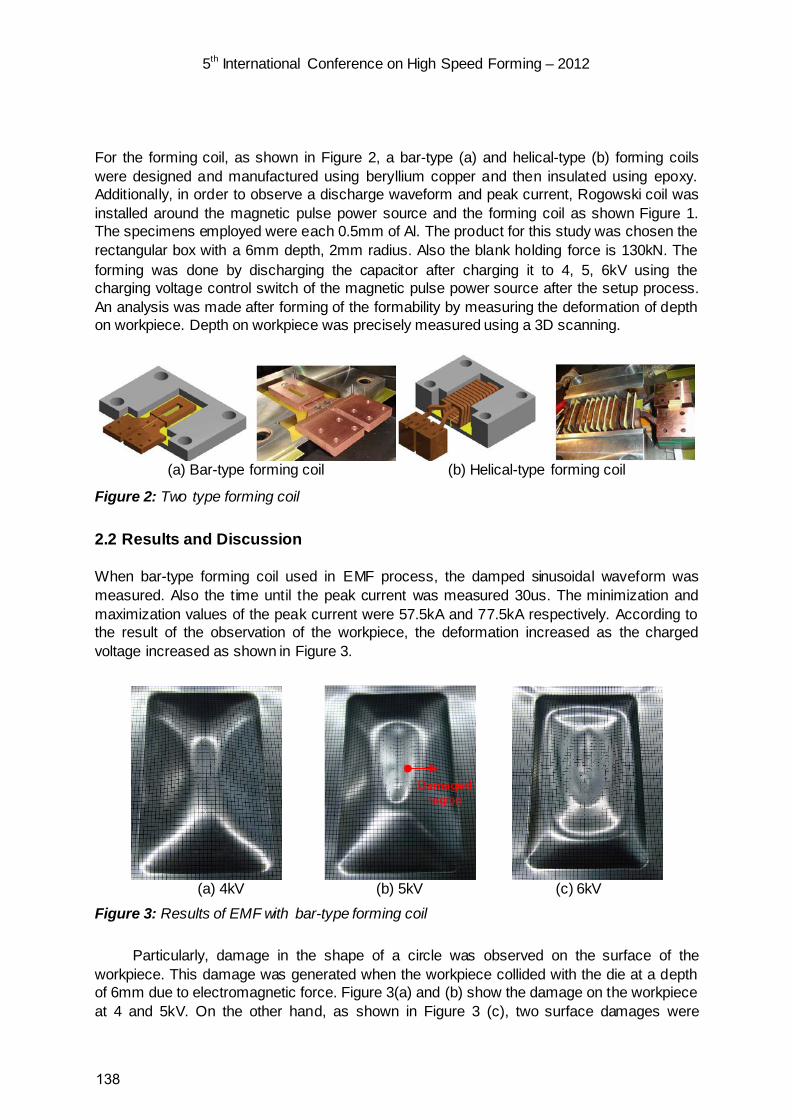
5th International Conference on High Speed Forming – 2012
For the forming coil, as shown in Figure 2, a bar-type (a) and helical-type (b) forming coils were designed and manufactured using beryllium copper and then insulated using epoxy. Additionally, in order to observe a discharge waveform and peak current, Rogowski coil was installed around the magnetic pulse power source and the forming coil as shown Figure 1. The specimens employed were each 0.5mm of Al. The product for this study was chosen the rectangular box with a 6mm depth, 2mm radius. Also the blank holding force is 130kN. The forming was done by discharging the capacitor after charging it to 4, 5, 6kV using the charging voltage control switch of the magnetic pulse power source after the setup process. An analysis was made after forming of the formability by measuring the deformation of depth on workpiece. Depth on workpiece was precisely measured using a 3D scanning.
(a) Bar-type forming coil (b) Helical-type forming coil
Figure 2: Two type forming coil
2.2 Results and Discussion
When bar-type forming coil used in EMF process, the damped sinusoidal waveform was measured. Also the time until the peak current was measured 30us. The minimization and maximization values of the peak current were 57.5kA and 77.5kA respectively. According to the result of the observation of the workpiece, the deformation increased as the charged voltage increased as shown in Figure 3.
(a) 4kV (b) 5kV (c) 6kV
Figure 3: Results of EMF with bar-type forming coil
Particularly, damage in the shape of a circle was observed on the surface of the workpiece. This damage was generated when the workpiece collided with the die at a depth of 6mm due to electromagnetic force. Figure 3(a) and (b) show the damage on the workpiece at 4 and 5kV. On the other hand, as shown in Figure 3 (c), two surface damages were
138

5th International Conference on High Speed Forming – 2012
observed at 6kV, and the damage was more serious on the inside than it was on outside. The electromagnetic force affecting the workpiece increases according to the increase of the charged voltage and the surface damage from the rebound after the collision between the workpiece and the die. This rebound on workpiece was reported by Beerwald et al.[19] which predicted the workpiece collides with the die by electromagnetic force at the point of the initiation of deformation. And Kamal [20] reported that air caused the rebound at the workpiece and the subsequent collision with the die. As mentioned earlier, magnetic pulse forming process is very fast and the process ends in less than 100us. When instantaneously electromagnetic force is applied the workpiece, the air present in the die does not have enough time and area to leave the die and thus causes the rebound and the consequent surface damage. However, the perfected theoretical analysis for rebound effect hasn’t been established yet.
When helical-type forming coil used in EMF process, the damped sinusoidal waveform was also measured. But the time until the peak current was observed 100us by Rogowski coil and the minimization and maximization values of the peak current were 85.2 and 98kA respectively. Figure 4 shows the result of deformation on workpiece after EMF process with helical-type forming coil. The deformation increased as the charged voltage increased. But deformation is tending more uniform than deformation when used bar-type forming coil. Especially, there is no rebound on workpice at 6kV as shown Figure 4(c).
(a) 4kV (b) 5kV (c) 6kV
Figure 4: Results of EMF with helical-type forming coil
To analyze the dynamic behaviour on workpiece with two type forming coil, deformation depth was measured at 4kV and 5kV in the direction of the x-path from the center of workpiece. Figures 5 and 6 shows the deformation height on workpiece in EMF with bar-type and helical-type forming coil at 4kV and 5kV respectively. As shown in Figures 5 and 6, the deformation increased according as the charged voltage increases. Especially, when charged voltage was at 4kV, the rebound was not observed, but hardly gets the rectangular box shape. Also the curve which used helical-type forming coil was more fluent than curve with bar-type forming coil in EMF. According to these results, helical-type forming coil is more effective than bar-forming coil in EMF. These results represent that the shape of forming coil is most important factor in EMF process. Distributions of electromagnetic force to apply on workpiece were changed by the shape of forming coil and then it lead to different dynamic behaviours on workpiece.
139

5th International Conference on High Speed Forming – 2012
Figure 5: Deformation depth on workpiece at 4kV
Figure 6: Deformation depth on workpiece at 5kV
3 Conclusions
This research was concentrated analysis of the contour on workpiece when employed the bar-type and helical-type forming with aluminum alloys in EMF process and reached with the following conclusion.
(1) Surface damage from the rebound after the collision between workpiece and die was observed on workpiece in EMF with bar-type forming coil especially the number of rebound was increased as charged voltage increases.
140
5th International Conference on High Speed Forming – 2012
(2) To achieve successful forming for rectangular box product, helical-type forming coil is more effective than bar-type forming coil in EMF process.
(3) According to the shape of forming coil, distributions of electromagnetic force on workpiece have been changed in EMF process because non-uniform of distributions of electromagnetic force was lead to non-uniform forming.
References
[1] Serkan T.; Fahrettin O.; Ilyas K.: Review of warm forming of aluminium–magnesium alloys. Journal of materials processing technology, Vol. 207, p. 1–12, 2008.
[2] Wang H.; Luo Y.;Friendman P.; Chen M.; Gao L.: Warm forming behavior of high strength aluminum alloy AA7075. Trans. Nonferrous Met. Soc. China, Vol. 22, p. 1-7, 2012.
[3] Bolt, P.J.: Feasibility of warm drawing of aluminium products. J. Mater. Process. Technol., Vol. 115, p. 118-121, 2001.
[4] Yuan Z.; Sudarsanam S. B.; Curtis P.; Michael B.; John K.; Mike L.; Daehn, G.S.: Application of high velocity impact welding at varied different length scales. Journal of Materials Processing Technology, Vol. 211, p. 944–952, 2011.
[5] Jianhui S.; Daehn, G. S: Electromagnetically assisted sheet metal stamping. Journal of Materials Processing Technology, Vol. 211, p. 868–874, 2011.
[6] Daehn, G. S.; Vohnout V.J.; DuBois, L.: Improved formability with electromagnetic forming: fundamentals and a practical example. In: Sheet Metal Forming Technology. The Minerals Metals & Materials Society, p.105–116, 1999.
[7] Balanethiram, V.S.; Daehn, G. S.: Hyperplasticity-increased forming limits at high workpiece velocities. Scr. Metall., Vol. 31, p.515–520. 1994.
[8] H.P. Furth; R.Waniek: Production and use of high transient magnetic field. I. Rev. Sci. Instr., Vol. 27, p. 195. 1966.
[9] H.P. Furth, R.Waniek: Production and use of high transient magnetic field. Il. Rev. Sci. Instr., Vol. 28, p. 949. 1957.
[10] Takatsu N.; Kato M.; Sato K.; Tobe T.: High speed forming of metal sheets by electromagnetic forces. International J. Japanese Society for Mechanical Engineering, Vol. 60, p.142-150, 1988.
[11] G.K. Fenton: Development of numerical tools to model plasticity in aluminium due to electromagnetic forces. Master’s Thesis, Department of Materials Science and Engineering, OSU, p. 28-69, 1996.
[12] G.K. Fenton; Daehn, G. S.: Modeling of electromagnetically formed sheet metal. J. Mater. Process. Technol., Vol. 5. p. 6-16, 1998.
[13] Oliveira DA; Worswick Mj; Finn M; Newman D: Electromagnetic forming of aluminium alloy sheet: free-form and cavity fill experiments and model. J. Materials Processing Technology, Vol. 170, p. 350-362, 2005.
[14] Stiemer M; UngerJ.; Svendsen B.; Blum H.: Algorithmic formulation and numerical implementation of coupled electromagnetic-inelastic continuum models for electromagnetic metal forming. J. Numerical Methods in Engineering, Vol. 68, p.1301-1329, 2006.
141

5th International Conference on High Speed Forming – 2012
[15] J.P.M. Correia; M. A. Siddiqui; S. Ahzi, S. Belouettar; R. Davies: A simple model to simulate electromagnetic sheet free bulging process. J. Mechanical Sciences, Vol. 50, p.1466-1475, 2008
[16] B. Bendjima: Finite element modelling of electromagnetic phenomena related to electromagnetic forming, Doctoral Thesis, Univ. Nantes, p. 34-61, 1997.
[17] J. Imbert; S. Winkler; M. J. Worswick; D.A. Oliveira; S. Golovashchenko: The effect of tool/sheet interaction on damage evolution in electromagnetic forming of aluminium alloy sheet. ASME Int. J. Eng. Mater. Technol., p. 145-153, 2005.
[18] M. Kamal;, J. Shang; V. Cheng; S. Hatkevich; Daehn, G. S: Agile manufacturing of a micro-embossed case by a two-step electromagnetic forming process. J. Materials Processing Technology, Vol. 190, p. 41-50, 2007.
[19] M. Kleiner; C. Beerwald; W. Homberg: Analysis of process parameters and forming mechanisms within the electromagnetic forming process. International Institution for Production Engineering Research, p. 225-228, 2005.
[20] M. Kamal: A uniform pressure electromagnetic actuator for forming flat sheets. Master’s Thesis, Department of Materials Science and Engineering, OSU, p. 77-78, 2005.
142

SESSION 5
MATERIAL TESTING
143

144

Compression Testing using a Cam-Driven Electromagnetic Machine
C.M.A Silva1, P.A.R. Rosa1, P.A.F. Martins1
1 IDMEC, Instituto Superior Técnico, Technical University of Lisbon, Portugal
Abstract
This paper presents new equipment for the compression testing of materials under high rates of loading. The equipment consists of an electromagnetic actuator, a fixed housing containing two flat compression platens, a translating cam and a follower. The electromagnetic actuator makes possible reaching high strain rates with a very precise control of the impact velocity and of the energy transmitted to the translating cam. The cam profile enables compression testing to be performed under the strain-rate vs. strain loading paths that are commonly found in manufacturing in order to meet the machine-tool and process combined specifications. The equipment was designed, fabricated and instrumented by the authors and, besides giving constructive details for those readers that may be interested in developing a low-cost equipment for compression testing at high rates of loading, the paper also puts emphasis on the flexibility and adequacy of its operative conditions for determining the mechanical behaviour of Aluminium AA1050-O under different testing conditions.
Keywords
Compression testing, Electromagnetic, Flow curve.
1 Introduction
The flow curve at the appropriate rates of loading is very important to describe the hardening behaviour during plastic deformation in terms of strain, strain-rate and temperature, to set-up the non-linear constitutive equations of metal plasticity and to establish the feasibility window and effectiveness of manufacturing processes. However, despite this importance, the flow curve is not always accessible in conditions similar to real manufacturing due to difficulties in replicating the operative conditions, namely the combined evolution and range of strains and strain-rates.
In case of strain-rates, for example, the widely available universal testing machines can only perform mechanical characterization of materials at quasi-static or low rate
145

5th International Conference on High Speed Forming – 2012
loading conditions ( ~10-3 to 10 s-1) and commercially available drop weight testing systems are only adequate for medium rates of loading ( ~1 to 103 s-1). Special purpose testing equipment based on split Hopkinson pressure bars, which is adequate for high rates of loading ( ~103 to 104 s-1), and Taylor impact systems, which are necessary for even higher rates of loading ( > 104 s-1), are not readily available to purchase or guaranteed to the majority of researchers.
However, even if equipment for testing at high rates of loading is available, a frequently ignored and mismanaged technical issue is the adequacy of testing conditions to the operational settings of the machine-tools where manufacturing processes will take place. In fact, despite theoretical claims on transferability of results often requiring mechanical testing of materials with different strain and strain-rate loading profiles to provide the same stress response for a given value of strain and strain rate, it is known that the flow curves obtained under testing with unclear conditions lead to non-unique and non-representative responses for the same material [1]. Not only time history of strain and strain-rate influences stress response [2] as it is relevant to determine crystallographic textures resulting from manufacturing processes [3].
Vc
wB
E
VAB
Ve
AWorkpiece
Cutting ToolE
A' C
C
B' D
A
C
A'
A
t
ri
reBD
V
(a) (b)
h
h i
V
Effe
ctiv
e S
trai
n R
ate
(s-1
)
Effective Strain
Blanking
ForgingMetal Cuttin
g
(c) (d)
Figure 1: (a) Metal cutting, (b) blanking and (c) forging together with a schematic representation of the (d) corresponding strain-rate vs. strain loading paths.
As a result of this, mechanical characterization of materials requires a deep insight into the machines and deformation mechanics of the processes prior to choosing the most appropriate equipment and operative testing conditions [4]. Taking metal cutting as an example, the synergism between the mechanical behaviour of materials and the machine-tools requires a good understanding of the displacement-time relationship of the cutting tool and of its influence in the rate dependent variables of the process. Because strain-rate growths with the level of strain as material moves from the undeformed region to the shear plane (a very narrow plastic deformation zone around AB in Figure 1a) and decreases while material moves away from the shear plane up the rake face of the tool,
146
5th International Conference on High Speed Forming – 2012
the resulting strain-rate vs. strain loading path for a typical flow route (refer to E in Figure 1a) is plotted in Figure 1d.
This means that the typical strain-rate vs. strain loading paths of metal cutting are significantly different from those obtained with commercially available testing equipment for medium and high rates of loading. In case of split Hopkinson pressure bars, for example, strain-rate vs. strain loading paths are characterized by an approximately constant level of strain-rate [5], similar to that plotted for blanking in Figures 1b and 1d, while in case of drop-height testing systems the strain-rate vs. strain loading paths are similar to that of forging (Figures 1c and 1d).
The abovementioned difficulties in obtaining the flow curves at appropriate rates of loading and the aforesaid synergism between material testing and real manufacturing conditions, justify the following two-fold objective of this paper; (i) the development of an innovative cam-driven electromagnetic machine for the compression testing of materials under high rates of loading and (ii) the identification of new testing methodologies based on the selection of the strain-rate vs. strain loading paths that can easily and effectively replicate the strain-rate vs. strain loading paths found in real manufacturing.
2 Cam-Driven Electromagnetic Testing Machine
Figure 2 shows the equipment that was designed and fabricated by the authors. Three main groups of components can be identified; (i) basic structural parts, (ii) specific mechanical parts and (iii) specific electrical and electromagnetic parts. The design of the basic and specific parts will be described in what follows.
2.1 Basic Structural Parts
Basic structural parts comprise the support frame and fixing accessories that are independent of the type of testing conditions and materials to be characterized. The support frame accounts for the installation of the specific mechanical, electrical and electromagnetic parts. The overall length of the frame was chosen so that larger compression housings and longer actuators can be added in the future with the objective of enlarging the size of the test specimens and increasing the velocity and kinetic energy of the ram.
2.2 Specific Mechanical Parts
Specific mechanical parts comprise a fixed housing containing two flat compression platens, a translating cam and a follower whose design depends on the operative conditions of manufacturing to be replicated.
The compression platens are made from a cold working tool steel DIN 120WV4 hardened and tempered to 60 HRc. The translating cam and the follower are made from steel DIN 14NiCr14 and DIN 100Cr6, respectively. The clearance fit for the cam-follower system is H7/f7 (ISO) and the individual parts were manufactured in a CNC machining centre. Final manual grinding and polishing was necessary to eliminate small surface errors and imperfections that although being imperceptible to eye could cause high stress and vibrations in the cam follower. Protection of the sliding elements of the cam system was performed by means of a PTFE (Teflon added) oil based lubricant.
147

5th International Conference on High Speed Forming – 2012
(a) (b)
FollowerCompression platens
Eddy-current displacement sensor
Load cell
Cam Profile Test specimen
Vx
Vy
Lower compression platen
(c)
Figure 2: (a) Cam-driven electromagnetic testing machine, (b) detail of the fixed housing and (c) schematic drawing showing the translating cam, the follower, the compression platens, the load cell and the displacement sensor.
The surface contour of the cam (cam profile) is to be designed with the objective of synchronizing the performance of the testing machine with that of the machine-tool where manufacturing will take place. The follower traces the cam profile and converts horizontal movement (x) of the ram to vertical displacement (y) of the lower compression platen (Figure 2c). The conversion of movement is schematically illustrated in Figure 3a.
In case of the cam shown in Figure 3b, the profile (hereafter designated as ‘logistic profile’) is characterized by an entry dwell followed by a rise contour and a final dwell towards the uppermost profile of the cam. The vertical displacement y of the follower as a function of the horizontal displacement x of the ram is depicted in Figure 3c.
The velocity yv of the follower is directly related to the first derivative of the displacement curve because the velocity of the ram xv is approximately constant in the working region of the cam follower (
avgxv =10 m/s), refer to the region located in-between
the dashed vertical lines in Figure 3d),
dx
dyv
dx
dyv
dt
dyv avg
xxy (1)
The leftmost region in Figure 3d, characterized by a sharp increase in the velocity of the ram, results from the initial acceleration due to the pressure generated by the coils inside the electromagnetic actuator. There is no vertical movement of the cam follower along this region and, therefore, there is no compression of the upset test specimen. The rightmost region in Figure 3d unveils part of the deceleration of the ram after the follower
148

5th International Conference on High Speed Forming – 2012
has reached the uppermost profile of the cam. Again, there is no compression of the upset test specimen along this region.
As a result of this, the vertical movement of the cam follower leading to upset compression only takes place at the region placed in-between the dashed vertical lines in Figure 3d, hereafter named as the ‘working region of the cam profile’. This justifies the reason why subsequent figures showing the displacement of the ram as the horizontal axis (x-axis) are frequently limited to the working region of the cam profile.
Vy
Vx
(a) (b)
(c) (d)
Figure 3: (a) Schematic representation of the cam profile and follower, (b) photograph of the logistic cam, (c) cam profile and pressure angle and (d) velocity of the ram avgxv =10 m/s in the working region of the cam follower.
The acceleration ya of the cam follower is computed from the variation in the velocity yv (assuming the above mentioned approximation of xv ) and the kinematic analysis of the follower shown in Figure 4a allows us to conclude that the cam utilized in the experiments provides the maximum velocity at the point of inflection located near the maximum slope of the cam profile.
(a) (b)
Figure 4: (a) Velocity and acceleration of the follower and (b) jerk in the working region of the cam-driven electromagnetic testing machine equipped with a logistic cam.
y
xo
Working region of the cam follower
149

5th International Conference on High Speed Forming – 2012
Acceleration is approximately constant at the entry dwell of the cam profile and presents an abrupt change from positive and to negative values at the midpoint. Along the entry dwell of the cam, jerk is approximately null (Figure 4b).
The small values of acceleration at the entry dwell of the logistic cam profile combined with the fact that pressure angles of the follower are kept below 30º [6] ( max =22.5º, Figure 3c), help keeping inertia forces at a small level and justify the reason why the proposed testing equipment worked smoothly without shocks and vibrations while performing material testing at high rates of loading.
The logistic cam profile allows replicating material flow conditions in conditions similar to those found in metal cutting processes [5]. However, because the cam system is flexible and its profile depends on the operative conditions to be replicated, it is easy to change the kinematics of the proposed equipment in order to replicate another manufacturing process, machine-tool or material testing equipment. For instance, replacing the logistic cam by a ‘root type cam’ allows the machine to replicate the kinematics of a split Hopkinson pressure bar (Figure 5).
(a)
(b) (c)
Figure 5: (a) Photograph of the root type cam, (b) cam profile and pressure angle and (c) velocity and acceleration of the follower in the working region of the cam-driven electromagnetic testing machine equipped with a root type cam.
2.3 Specific Electric and Electromagnetic Parts
Specific electrical and electromagnetic parts include the eddy-current displacement sensor, the force transducer and the components that provide the energy to the electromagnetic actuator, e.g. the electrical circuits for charging and firing the bank of capacitors and the coils that generate the pressure for accelerating the ram linked to one end of the translating cam.
The vertical movement of the cam follower is transformed into compression of the test specimen via the lower flat platen. The vertical displacement of the lower flat platen is measured by a eddy-current displacement sensor and the resulting force is measured by means of a load cell connected to the upper compression platen (Figure 2c).
The electromagnetic actuator consists of electrical circuits for charging and firing the banks of energy-storage capacitors (each with 6 mF) and a series of coils that generate
150
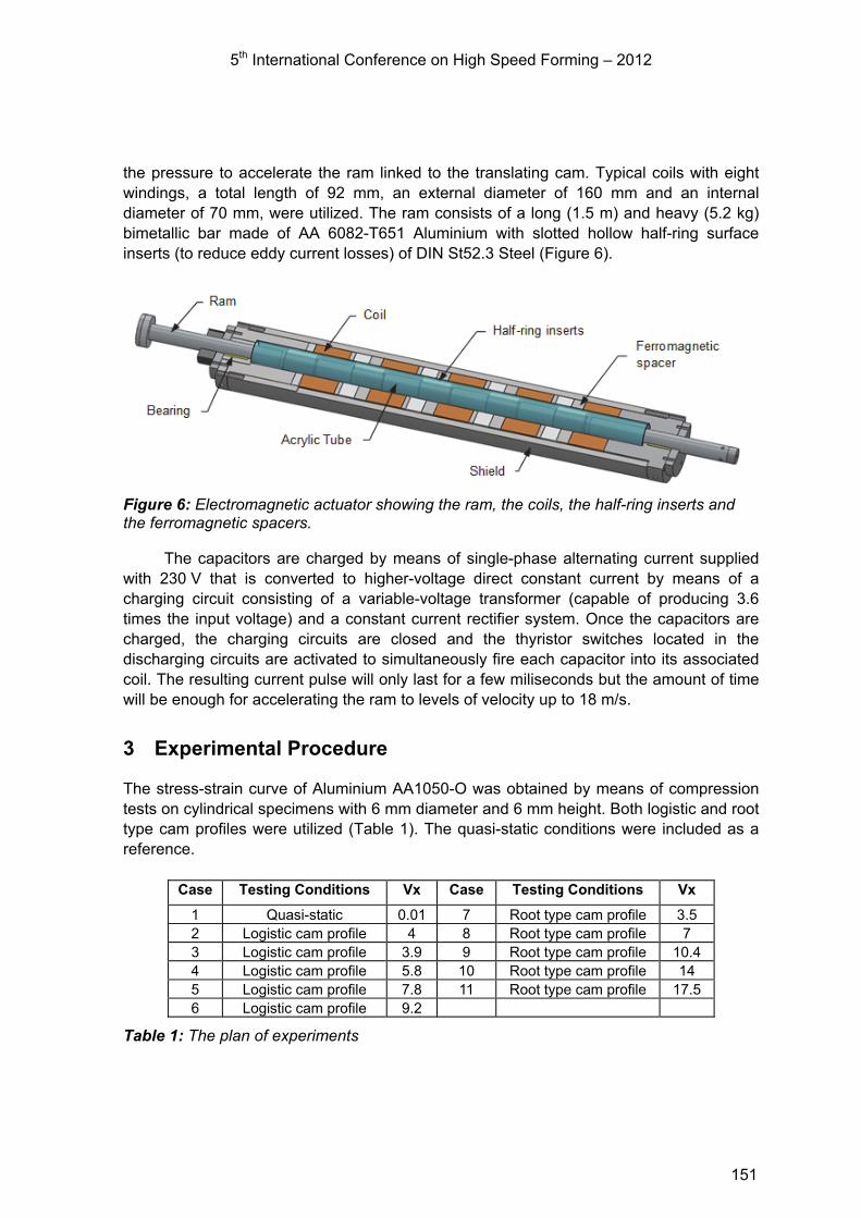
5th International Conference on High Speed Forming – 2012
the pressure to accelerate the ram linked to the translating cam. Typical coils with eight windings, a total length of 92 mm, an external diameter of 160 mm and an internal diameter of 70 mm, were utilized. The ram consists of a long (1.5 m) and heavy (5.2 kg) bimetallic bar made of AA 6082-T651 Aluminium with slotted hollow half-ring surface inserts (to reduce eddy current losses) of DIN St52.3 Steel (Figure 6).
Figure 6: Electromagnetic actuator showing the ram, the coils, the half-ring inserts and the ferromagnetic spacers.
The capacitors are charged by means of single-phase alternating current supplied with 230 V that is converted to higher-voltage direct constant current by means of a charging circuit consisting of a variable-voltage transformer (capable of producing 3.6 times the input voltage) and a constant current rectifier system. Once the capacitors are charged, the charging circuits are closed and the thyristor switches located in the discharging circuits are activated to simultaneously fire each capacitor into its associated coil. The resulting current pulse will only last for a few miliseconds but the amount of time will be enough for accelerating the ram to levels of velocity up to 18 m/s.
3 Experimental Procedure
The stress-strain curve of Aluminium AA1050-O was obtained by means of compression tests on cylindrical specimens with 6 mm diameter and 6 mm height. Both logistic and root type cam profiles were utilized (Table 1). The quasi-static conditions were included as a reference.
Case Testing Conditions Vx Case Testing Conditions Vx
1 Quasi-static 0.01 7 Root type cam profile 3.5 2 Logistic cam profile 4 8 Root type cam profile 7 3 Logistic cam profile 3.9 9 Root type cam profile 10.4 4 Logistic cam profile 5.8 10 Root type cam profile 14 5 Logistic cam profile 7.8 11 Root type cam profile 17.5 6 Logistic cam profile 9.2
Table 1: The plan of experiments
151

5th International Conference on High Speed Forming – 2012
4 Results and Discussion
Figure 7 shows the variation of force with displacement obtained from test cases 3 and 8 in Table 1. Results show that on contrary to root type cam profiles (and split Hopkinson pressure bars), there are no ‘saw tooth’ oscillations when using a logistic cam profile (case 3). This is attributed to a smooth transition between the entry dwell and the profile of
the cam and to a low value of the maximum pressure angle ( max = 22.5º, Figure 3c). The oscillations in the root type cam profile are attributed to inertia forces and stress
wave propagation under impact loading as well as to an initial value of the maximum
pressure angle very close to 30º ( max = 28º, Figure 5b).
Figure 7: Experimental evolution of the force vs. displacement for logistic and root type cam profiles.
The experimental strain-rate vs. strain loading paths for the selected testing conditions performed with the cam-driven electromagnetic testing machine equipped with a logistic cam profile are plotted in Figure 8a.
(a) (b)
Figure 8: Mechanical testing of Aluminium AA1050-O using a logistic cam. (a) Strain-rate vs. strain loading paths. (b) Material stress response with respect to strain and strain-rate (experimental data and fitting).
152

5th International Conference on High Speed Forming – 2012
The three-dimensional flow surface plotted in Figure 8b in which stress, strain and strain-rate are the leading axis results from fitting experimental data to the following mathematical material model that was developed by the authors [5],
DlnCBeA nm (2)
where, the constants m,D,C,B,A and n are to be determined from experimental data.
The model given by equation (2) is appropriate for cold forming operating conditions and includes well-known material models such as Ludwik-Holloman, Voce and Johnson-Cook (isothermal), among others, as special cases. Another advantage of this model is the ability for exhibiting material flow softening at high values of strain. Flow softening is responsible for diminishing the resistance to plastic deformation due to rearrangement of dislocations under dynamic recrystallization and is known to cause a significant influence in the deformation mechanics of metal cutting, namely chip formation [7].
(a) (b)
Figure 9: Mechanical testing of Aluminium AA1050-O using a root type cam. (a) Strain-rate vs. strain loading paths. (b) Material stress response with respect to strain and strain-rate (experimental data and fitting).
Figure 10: Experimental stress–strain curves after mathematical fitting for different values of strain-rate.
Figure 9a provides similar results for the root type cam. As seen, the strain-rate vs. strain loading paths obtained with this type of cam are near horizontal lines and similar to
153

5th International Conference on High Speed Forming – 2012
those commonly attained with Hopkinson pressure bars. The three-dimensional flow surface resulting from these experiments is plotted in Figure 9b.
The differences between the flow surfaces obtained from material testing with logistic and root type cams are made clear by analysing a selection of intersections of the three-dimensional flow surfaces with constant strain-rate planes ( Cte ). The flow curves resulting from these intersections are plotted in Figure 10 and indicate that major differences are due to flow softening in close agreement with the aforementioned capability of the logistic cam profile to model metal cutting conditions.
5 Conclusions
The proposed cam-driven electromagnetic testing machine is capable of operating across a broad range of operative conditions found in real manufacturing processes. Variations in cam profiles, modifications in the individual coils of the actuator, which can be easily changed or temporarily switched off during testing, and changes in the operating voltage of the charging and discharging circuits (that influence the kinetic energy of the ram) can be easily and effectively performed in order to achieve different strain vs. strain-rate loading paths.
Experiments show that the proposed machine equipped with a logistic cam is capable of diminishing ‘saw tooth’ oscillations in the experimental recordings of force that are typical of split Hopkinson pressure bars and root type cam profiles. Moreover logistic cam profiles in conjunction with the proposed material model are able to successfully model flow softening that is commonly found in metal cutting applications.
References
[1] Banabic D., Bunge H.-J., Pöhlandt K., Tekkaya A. E., Formability of metallic materials, Springer-Verlag, Berlin, 2000.
[2] Silva C. M. A., Rosa P. A. R. and Martins P. A. F., Mechanical characterization of materials for bulkf using a drop weight testing machine, Journal of Mechanical Engineering Science, 2010, 224, p. 1795-1804.
[3] Guo Y., Saldana C., Mann J. B., Saoubi R. M., Chandrasek S, Deformation and microstructure in machining, Advanced Materials Research, 2011, 223, p.325-331.
[4] Field J. E., Walley S. M., Proud W. G., Goldrein H. T., Siviour C. R., Review of experimental techniques for high rate deformation and shock studies, International Journal of Impact Engineering, 2004, 30, p. 725–775.
[5] Silva C. M. A., Rosa P. A. R., Martins P. A. F., Electromagnetic cam driven compression testing equipment”, Experimental Mechanics, 2011 (on-line first).
[6] Rothbart H. A., Cam design handbook. McGraw Hill, New York, 2004. [7] Sima M., Özel T., Modified material constitutive models for serrated chip formation
simulations and experimental validation in machining of titanium alloy Ti-6Al-4V. International Journal of Machine Tools and Manufacture, 2010, 50, p. 943–960.
154
Development of a Pneumatic High-Speed Nakajima Testing Device*
M. Engelhardt1, H. von Senden genannt Haverkamp1, C. Klose1, Fr.-W. Bach1
1 Institute of Materials Science, Leibniz University Hannover, Germany
Abstract
Forming limit diagrams are an essential tool for describing the formability of sheet materials in the deep-drawing process. Here, the well known and frequently employed procedures are the Nakajima and the Marciniak-Tests. Whereas these procedures' standardisation is quite advanced in the quasi-static range, numerous different test procedures exist in the range of elevated forming speeds. In the first part of this work, an overview of the various procedures is given for generating forming limit diagrams in the high speed range. In the second part, a pneumatically operated testing device is introduced which was developed at the Institute for Material Science for performing Nakajima-Tests in the high speed range. Using this device, standard specimens can be dynamically formed according to the Nakajima-Test. The testing device is to be employed for scientifically exploring the deformation mechanisms operating at very high forming speeds. The testing device’s mode of functioning is demonstrated by means of forming discs of an EN AW-6082 aluminium alloy sheet. In doing this, the testing apparatus is mainly characterised by holding the testing conditions constant during the tests: This particularly concerns the velocity of the tool for forming the sheet discs.
Keywords
Forming Limit Diagram, High-speed Nakajima Test, Aluminium Alloy EN AW-6082
* This work is based on the results of Paketantrag 343 “Entwicklung einer Methoden-planung für die Hochgeschwindigkeitsblechumformung ”: The authors would like to thank the German Research Foundation (DFG) for its financial support.
155
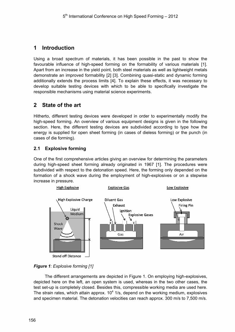
5th International Conference on High Speed Forming – 2012
1 Introduction
Using a broad spectrum of materials, it has been possible in the past to show the favourable influence of high-speed forming on the formability of various materials [1]. Apart from an increase in the yield point, both steel materials as well as lightweight metals demonstrate an improved formability [2] [3]. Combining quasi-static and dynamic forming additionally extends the process limits [4]. To explain these effects, it was necessary to develop suitable testing devices with which to be able to specifically investigate the responsible mechanisms using material science experiments.
2 State of the art
Hitherto, different testing devices were developed in order to experimentally modify the high-speed forming. An overview of various equipment designs is given in the following section. Here, the different testing devices are subdivided according to type how the energy is supplied for open sheet forming (in cases of dieless forming) or the punch (in cases of die forming).
2.1 Explosive forming
One of the first comprehensive articles giving an overview for determining the parameters during high-speed sheet forming already originated in 1967 [1]. The procedures were subdivided with respect to the detonation speed. Here, the forming only depended on the formation of a shock wave during the employment of high-explosives or on a stepwise increase in pressure.
Figure 1: Explosive forming [1]
The different arrangements are depicted in Figure 1. On employing high-explosives, depicted here on the left, an open system is used, whereas in the two other cases, the test set-up is completely closed. Besides this, compressible working media are used here. The strain rates, which attain approx. 104 1/s, depend on the working medium, explosives and specimen material. The detonation velocities can reach approx. 300 m/s to 7,500 m/s.
156
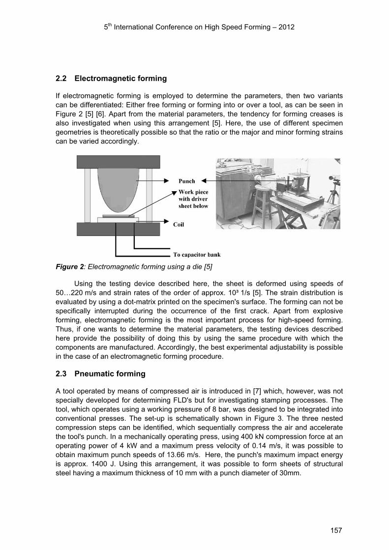
5th International Conference on High Speed Forming – 2012
2.2 Electromagnetic forming
If electromagnetic forming is employed to determine the parameters, then two variants can be differentiated: Either free forming or forming into or over a tool, as can be seen in Figure 2 [5] [6]. Apart from the material parameters, the tendency for forming creases is also investigated when using this arrangement [5]. Here, the use of different specimen geometries is theoretically possible so that the ratio or the major and minor forming strains can be varied accordingly.
Figure 2: Electromagnetic forming using a die [5]
Using the testing device described here, the sheet is deformed using speeds of 50…220 m/s and strain rates of the order of approx. 10³ 1/s [5]. The strain distribution is evaluated by using a dot-matrix printed on the specimen's surface. The forming can not be specifically interrupted during the occurrence of the first crack. Apart from explosive forming, electromagnetic forming is the most important process for high-speed forming. Thus, if one wants to determine the material parameters, the testing devices described here provide the possibility of doing this by using the same procedure with which the components are manufactured. Accordingly, the best experimental adjustability is possible in the case of an electromagnetic forming procedure.
2.3 Pneumatic forming
A tool operated by means of compressed air is introduced in [7] which, however, was not specially developed for determining FLD's but for investigating stamping processes. The tool, which operates using a working pressure of 8 bar, was designed to be integrated into conventional presses. The set-up is schematically shown in Figure 3. The three nested compression steps can be identified, which sequentially compress the air and accelerate the tool's punch. In a mechanically operating press, using 400 kN compression force at an operating power of 4 kW and a maximum press velocity of 0.14 m/s, it was possible to obtain maximum punch speeds of 13.66 m/s. Here, the punch's maximum impact energy is approx. 1400 J. Using this arrangement, it was possible to form sheets of structural steel having a maximum thickness of 10 mm with a punch diameter of 30mm.
157
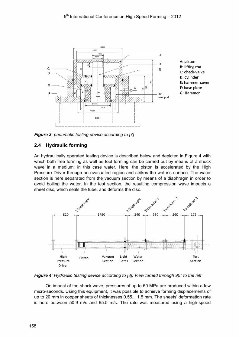
5th International Conference on High Speed Forming – 2012
Figure 3: pneumatic testing device according to [7]
2.4 Hydraulic forming
An hydraulically operated testing device is described below and depicted in Figure 4 with which both free forming as well as tool forming can be carried out by means of a shock wave in a medium; in this case water. Here, the piston is accelerated by the High Pressure Driver through an evacuated region and strikes the water’s surface. The water section is here separated from the vacuum section by means of a diaphragm in order to avoid boiling the water. In the test section, the resulting compression wave impacts a sheet disc, which seals the tube, and deforms the disc.
Figure 4: Hydraulic testing device according to [8]; View turned through 90° to the left
On impact of the shock wave, pressures of up to 60 MPa are produced within a few micro-seconds. Using this equipment, it was possible to achieve forming displacements of up to 20 mm in copper sheets of thicknesses 0.55... 1.5 mm. The sheets' deformation rate is here between 50.9 m/s and 95.5 m/s. The rate was measured using a high-speed
158
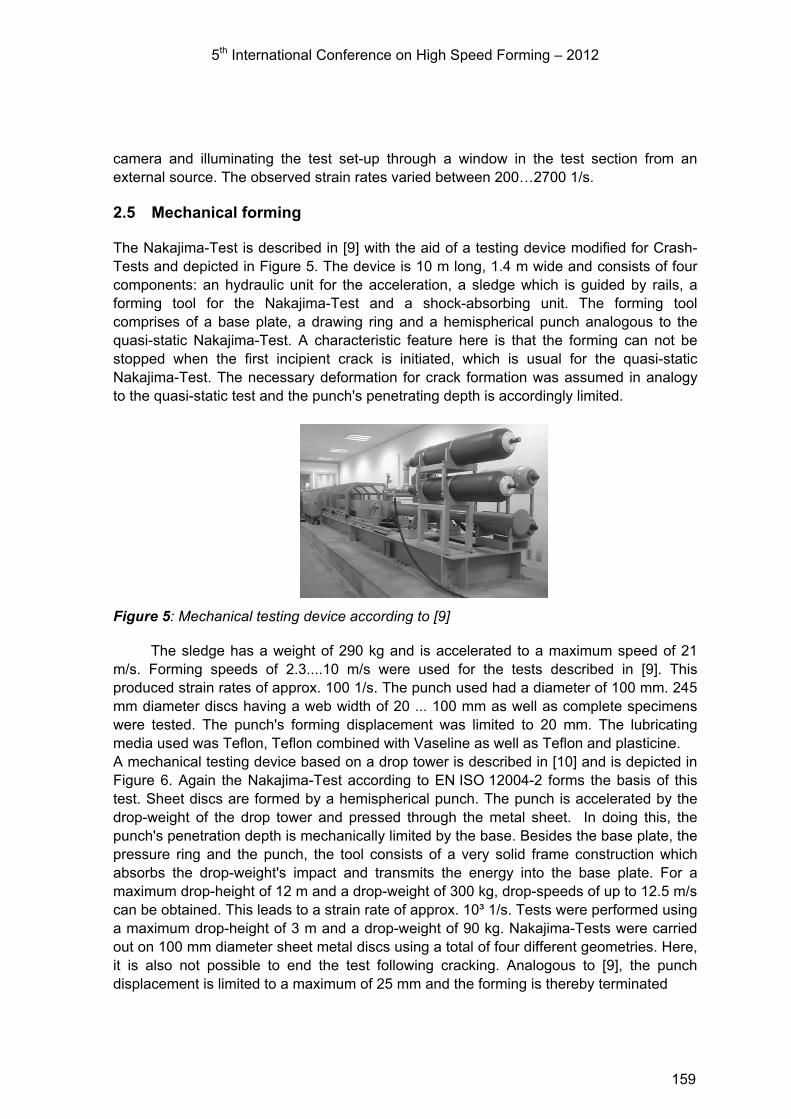
5th International Conference on High Speed Forming – 2012
camera and illuminating the test set-up through a window in the test section from an external source. The observed strain rates varied between 200…2700 1/s.
2.5 Mechanical forming
The Nakajima-Test is described in [9] with the aid of a testing device modified for Crash-Tests and depicted in Figure 5. The device is 10 m long, 1.4 m wide and consists of four components: an hydraulic unit for the acceleration, a sledge which is guided by rails, a forming tool for the Nakajima-Test and a shock-absorbing unit. The forming tool comprises of a base plate, a drawing ring and a hemispherical punch analogous to the quasi-static Nakajima-Test. A characteristic feature here is that the forming can not be stopped when the first incipient crack is initiated, which is usual for the quasi-static Nakajima-Test. The necessary deformation for crack formation was assumed in analogy to the quasi-static test and the punch's penetrating depth is accordingly limited.
Figure 5: Mechanical testing device according to [9]
The sledge has a weight of 290 kg and is accelerated to a maximum speed of 21 m/s. Forming speeds of 2.3....10 m/s were used for the tests described in [9]. This produced strain rates of approx. 100 1/s. The punch used had a diameter of 100 mm. 245 mm diameter discs having a web width of 20 ... 100 mm as well as complete specimens were tested. The punch's forming displacement was limited to 20 mm. The lubricating media used was Teflon, Teflon combined with Vaseline as well as Teflon and plasticine. A mechanical testing device based on a drop tower is described in [10] and is depicted in Figure 6. Again the Nakajima-Test according to EN ISO 12004-2 forms the basis of this test. Sheet discs are formed by a hemispherical punch. The punch is accelerated by the drop-weight of the drop tower and pressed through the metal sheet. In doing this, the punch's penetration depth is mechanically limited by the base. Besides the base plate, the pressure ring and the punch, the tool consists of a very solid frame construction which absorbs the drop-weight's impact and transmits the energy into the base plate. For a maximum drop-height of 12 m and a drop-weight of 300 kg, drop-speeds of up to 12.5 m/s can be obtained. This leads to a strain rate of approx. 10³ 1/s. Tests were performed using a maximum drop-height of 3 m and a drop-weight of 90 kg. Nakajima-Tests were carried out on 100 mm diameter sheet metal discs using a total of four different geometries. Here, it is also not possible to end the test following cracking. Analogous to [9], the punch displacement is limited to a maximum of 25 mm and the forming is thereby terminated
159
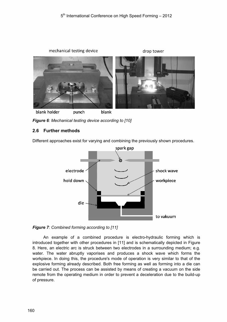
5th International Conference on High Speed Forming – 2012
Figure 6: Mechanical testing device according to [10]
2.6 Further methods
Different approaches exist for varying and combining the previously shown procedures.
Figure 7: Combined forming according to [11]
An example of a combined procedure is electro-hydraulic forming which is introduced together with other procedures in [11] and is schematically depicted in Figure 8. Here, an electric arc is struck between two electrodes in a surrounding medium; e.g. water. The water abruptly vaporises and produces a shock wave which forms the workpiece. In doing this, the procedure's mode of operation is very similar to that of the explosive forming already described. Both free forming as well as forming into a die can be carried out. The process can be assisted by means of creating a vacuum on the side remote from the operating medium in order to prevent a deceleration due to the build-up of pressure.
160
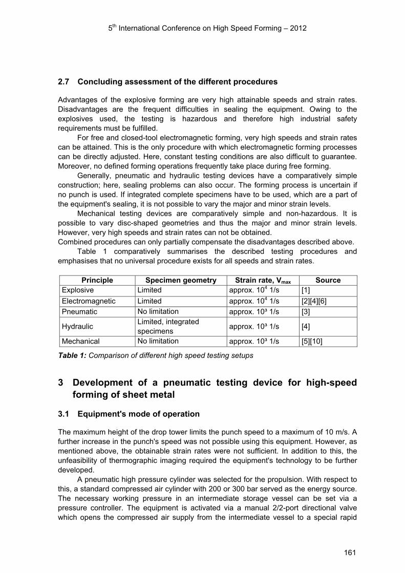
5th International Conference on High Speed Forming – 2012
2.7 Concluding assessment of the different procedures
Advantages of the explosive forming are very high attainable speeds and strain rates. Disadvantages are the frequent difficulties in sealing the equipment. Owing to the explosives used, the testing is hazardous and therefore high industrial safety requirements must be fulfilled.
For free and closed-tool electromagnetic forming, very high speeds and strain rates can be attained. This is the only procedure with which electromagnetic forming processes can be directly adjusted. Here, constant testing conditions are also difficult to guarantee. Moreover, no defined forming operations frequently take place during free forming.
Generally, pneumatic and hydraulic testing devices have a comparatively simple construction; here, sealing problems can also occur. The forming process is uncertain if no punch is used. If integrated complete specimens have to be used, which are a part of the equipment's sealing, it is not possible to vary the major and minor strain levels.
Mechanical testing devices are comparatively simple and non-hazardous. It is possible to vary disc-shaped geometries and thus the major and minor strain levels. However, very high speeds and strain rates can not be obtained. Combined procedures can only partially compensate the disadvantages described above.
Table 1 comparatively summarises the described testing procedures and emphasises that no universal procedure exists for all speeds and strain rates.
Principle Specimen geometry Strain rate, Vmax Source
Explosive Limited approx. 104 1/s [1]
Electromagnetic Limited approx. 104 1/s [2][4][6]
Pneumatic No limitation approx. 10³ 1/s [3]
Hydraulic Limited, integrated specimens
approx. 10³ 1/s [4]
Mechanical No limitation approx. 10³ 1/s [5][10]
Table 1: Comparison of different high speed testing setups
3 Development of a pneumatic testing device for high-speed forming of sheet metal
3.1 Equipment's mode of operation
The maximum height of the drop tower limits the punch speed to a maximum of 10 m/s. A further increase in the punch's speed was not possible using this equipment. However, as mentioned above, the obtainable strain rates were not sufficient. In addition to this, the unfeasibility of thermographic imaging required the equipment's technology to be further developed.
A pneumatic high pressure cylinder was selected for the propulsion. With respect to this, a standard compressed air cylinder with 200 or 300 bar served as the energy source. The necessary working pressure in an intermediate storage vessel can be set via a pressure controller. The equipment is activated via a manual 2/2-port directional valve which opens the compressed air supply from the intermediate vessel to a special rapid
161
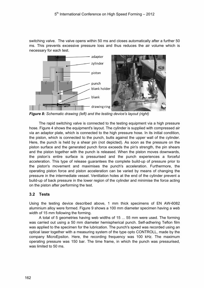
5th International Conference on High Speed Forming – 2012
switching valve. The valve opens within 50 ms and closes automatically after a further 50 ms. This prevents excessive pressure loss and thus reduces the air volume which is necessary for each test.
Figure 8: Schematic drawing (left) and the testing device's layout (right)
The rapid switching valve is connected to the testing equipment via a high pressure
hose. Figure 4 shows the equipment's layout. The cylinder is supplied with compressed air via an adaptor plate, which is connected to the high pressure hose. In its initial condition, the piston, which is connected to the punch, butts against the upper wall of the cylinder. Here, the punch is held by a shear pin (not depicted). As soon as the pressure on the piston surface and the generated punch force exceeds the pin's strength, the pin shears and the piston together with the punch is released. When the piston moves downwards, the piston’s entire surface is pressurised and the punch experiences a forceful acceleration. This type of release guarantees the complete build-up of pressure prior to the piston's movement and maximises the punch's acceleration. Furthermore, the operating piston force and piston acceleration can be varied by means of changing the pressure in the intermediate vessel. Ventilation holes at the end of the cylinder prevent a build-up of back pressure in the lower region of the cylinder and minimise the force acting on the piston after performing the test.
3.2 Tests
Using the testing device described above, 1 mm thick specimens of EN AW-6082 aluminium alloy were formed. Figure 9 shows a 100 mm diameter specimen having a web width of 15 mm following the forming.
A total of 5 geometries having web widths of 15 ... 55 mm were used. The forming was carried out using a 50 mm diameter hemispherical punch. Self-adhering Teflon film was applied to the specimen for the lubrication. The punch's speed was recorded using an optical laser together with a measuring system of the type opto CONTROLL, made by the company MicroEpsilon. Here, the recording frequency was 100 kHz. The maximum operating pressure was 150 bar. The time frame, in which the punch was pressurised, was limited to 50 ms.
162
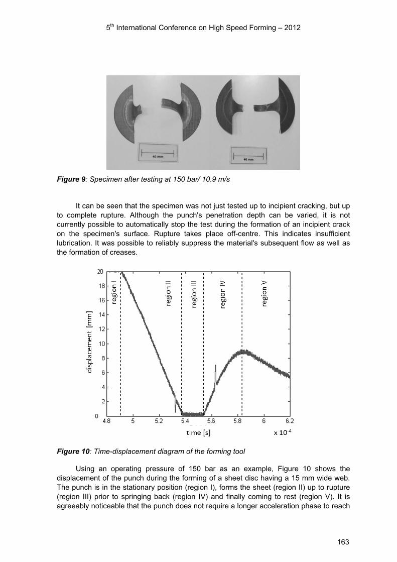
5th International Conference on High Speed Forming – 2012
Figure 9: Specimen after testing at 150 bar/ 10.9 m/s
It can be seen that the specimen was not just tested up to incipient cracking, but up
to complete rupture. Although the punch's penetration depth can be varied, it is not currently possible to automatically stop the test during the formation of an incipient crack on the specimen's surface. Rupture takes place off-centre. This indicates insufficient lubrication. It was possible to reliably suppress the material's subsequent flow as well as the formation of creases.
Figure 10: Time-displacement diagram of the forming tool
Using an operating pressure of 150 bar as an example, Figure 10 shows the displacement of the punch during the forming of a sheet disc having a 15 mm wide web. The punch is in the stationary position (region I), forms the sheet (region II) up to rupture (region III) prior to springing back (region IV) and finally coming to rest (region V). It is agreeably noticeable that the punch does not require a longer acceleration phase to reach
163

5th International Conference on High Speed Forming – 2012
its final speed of 10.9 m/s and is not significantly decelerated during the forming process. The spring-back / post oscillations, which can be repeated several times according to the pressure, were a nuisance.
4 Summary
Numerous different equipment designs currently exist for determining material parameters in the high speed forming range. Only the mechanically and pneumatically operated testing devices currently offer the necessary flexibility for determining FLD's. However, these devices are frequently impaired by comparatively low forming speeds. Taking this into consideration, we produced our own equipment design that is characterised by particularly very stable forming conditions which are otherwise only obtained during quasi-static forming.
References
[1] Wood, W.W.: Experimental Mechanics at Velocity Extremes – Very High Strain Rates; Experimental Mechanics; 1967, S. 441-446.
[2] El-Magd, E.: Abouridouane, M.: Einfluss der Umformgeschwindigkeit und -temperatur auf das Umformvermögen metallischer Werkstoffe; Zeitschriftenartikel; Zeitschrift für Metallkunde 94. Jg., Nr. 6, 2003.
[3] El-Magd, E.; Abouridouane, M.: Characterization, modelling and simulation of deformation and fracture behaviour of the light-weight wrought alloys under high strain rate loading; Zeitschriftenartikel; International Journal of Impact Engineering Vol. 32, No. 5, 2006.
[4] Siegert K.; Vulkan M.: Superplastische Umformung von Aluminium-Blechen mit nachfolgendem hydromechanischem tiefziehen. In: 8. Sächsische Fachtagung Umformtechnik ISBN: 3-86012-158-8, S. 251-271, 2001.
[5] Seth, M.; Vohnout, V. J.; Daehn, G. S.; Formability of steel sheet in high velocity impact. Journal of Materials Processing Technology 168 (2005) 390–400
[6] Fr.-W. Bach, M. Rodman, A. Rossberg, J. Weber, L. Walden; Verhalten von Aluminiumwerkstoffen bei der elektromagnetischem Umformung. 2. KOLLOQUIUM ELEKTROMAGNETISCHE UMFORMUNG
[7] Yaldız, S.; Saglam, H.; Ünsacar, F.; Isık, H.; Design and applications of a pneumatic accelerator for high speed punching. Materials and Design 28 (2007) 889–896
[8] Kosing, O. E.; Skews; B. W.; A Investigation of high-speed forming of circular plates in a liquid shock tube. Int. J. Impact Engng Vol. 21, No. 9, pp. 801-816, 1998
[9] Kim, S.B.; Huh, H.; Bok, H.H.; Moon, M.B.: Forming limit diagram of auto-body steel sheets for high-speed sheet metal forming. Journal of Materials Processing Technology 211 (2010) 851–862
[10] M. Engelhardt, H. von Senden genannt Haverkamp, Y.Kiliclar, M. Schwarze, I. Vladimirov, D. Bormann, F.-W. Bach, S. Reese; Characterisation and Simulation of High-Speed deformation processes. 4th International Conference on High Speed Forming – 2010, Columbus
[11] A.A. Tamhane, M. Padmanabhan, G. Fenton, M. Altynova and G.S. Daehn; Opportunities in High-Velocity Forming of Sheet Metal. Metal Forming Magazine
164

Comparison of Dynamic Hardening Equations for Metallic Materials with the Variation of Crystalline Structures
K. Ahn1, H. Huh1, L. Park2 1 KAIST, Daejeon, Korea 2 ADD, Daejeon, Korea
Abstract
This paper is concerned with dynamic hardening equations of metallic materials with various crystalline structures. The dynamic response of metallic materials is indispensable for analysis of high speed metal forming process. There is, however, no unique equation which can represent the dynamic hardening characteristics of all kinds of materials although various dynamic hardening equations have been suggested by many researchers. Dynamic hardening equations reported have been investigated using the dynamic hardening characteristics of three kinds of materials: 4340Steel (BCC); OFHC (FCC); and Ti6Al4V (HCP). Dynamic hardening characteristics of each material have been obtained by uniaxial tensile tests and SHPB tests. Uniaxial tensile tests have been performed with the variation of the strain rate from 0.001/sec to 100/sec and SHPB tests have been conducted at the strain rate ranged up to 4000/sec. Several existing models have been constructed and evaluated for Johnson-Cook model, Zerilli-Armstrong model, Preston-Tonks-Wallace model, modified Johnson-Cook model, and modified Khan-Huang model using test results of three materials. Strain rate hardening and thermal softening effect during the deformation process were investigated for accurate application of hardening equations. The most applicable equation for each material has been suggested by comparison of constructed results.
Keywords
Dynamic hardening equation, Strain rate sensitivity, High speed tensile test
1 Introduction
The deformation behavior of metallic materials at high strain rates has been investigated for the past several decades and high speed forming is the recent megatrend especially for automobile industries, defense industries and so on. Accurate understanding of material properties at various strain rates is necessary to guarantee the reliability of the analysis at high speed conditions such as high speed forming and deformation analysis. When a metallic material deforms under the dynamic loading, the inertia effect and the stress wave
165
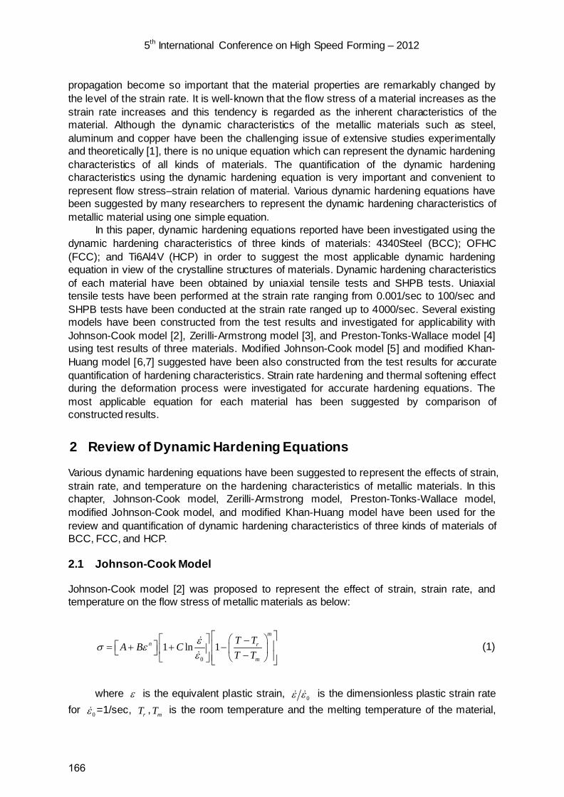
5th International Conference on High Speed Forming – 2012
propagation become so important that the material properties are remarkably changed by the level of the strain rate. It is well-known that the flow stress of a material increases as the strain rate increases and this tendency is regarded as the inherent characteristics of the material. Although the dynamic characteristics of the metallic materials such as steel, aluminum and copper have been the challenging issue of extensive studies experimentally and theoretically [1], there is no unique equation which can represent the dynamic hardening characteristics of all kinds of materials. The quantification of the dynamic hardening characteristics using the dynamic hardening equation is very important and convenient to represent flow stress–strain relation of material. Various dynamic hardening equations have been suggested by many researchers to represent the dynamic hardening characteristics of metallic material using one simple equation.
In this paper, dynamic hardening equations reported have been investigated using the dynamic hardening characteristics of three kinds of materials: 4340Steel (BCC); OFHC (FCC); and Ti6Al4V (HCP) in order to suggest the most applicable dynamic hardening equation in view of the crystalline structures of materials. Dynamic hardening characteristics of each material have been obtained by uniaxial tensile tests and SHPB tests. Uniaxial tensile tests have been performed at the strain rate ranging from 0.001/sec to 100/sec and SHPB tests have been conducted at the strain rate ranged up to 4000/sec. Several existing models have been constructed from the test results and investigated for applicability with Johnson-Cook model [2], Zerilli-Armstrong model [3], and Preston-Tonks-Wallace model [4] using test results of three materials. Modified Johnson-Cook model [5] and modified Khan-Huang model [6,7] suggested have been also constructed from the test results for accurate quantification of hardening characteristics. Strain rate hardening and thermal softening effect during the deformation process were investigated for accurate hardening equations. The most applicable equation for each material has been suggested by comparison of constructed results.
2 Review of Dynamic Hardening Equations
Various dynamic hardening equations have been suggested to represent the effects of strain, strain rate, and temperature on the hardening characteristics of metallic materials. In this chapter, Johnson-Cook model, Zerilli-Armstrong model, Preston-Tonks-Wallace model, modified Johnson-Cook model, and modified Khan-Huang model have been used for the review and quantification of dynamic hardening characteristics of three kinds of materials of BCC, FCC, and HCP.
2.1 Johnson-Cook Model
Johnson-Cook model [2] was proposed to represent the effect of strain, strain rate, and temperature on the flow stress of metallic materials as below:
0
1 ln 1m
n r
m
T TA B CT T
εσ εε
− = + + − −
(1)
where ε is the equivalent plastic strain, 0ε ε is the dimensionless plastic strain rate
for 0ε =1/sec, rT , mT is the room temperature and the melting temperature of the material,
166
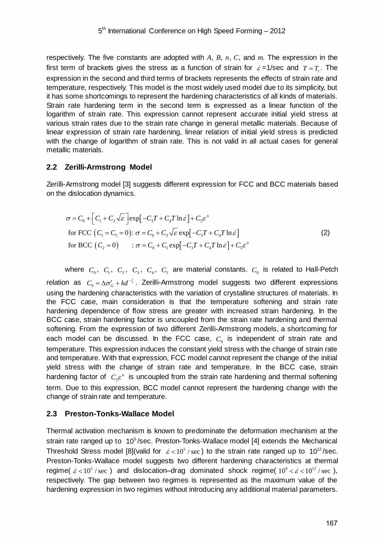
5th International Conference on High Speed Forming – 2012
respectively. The five constants are adopted with A, B, n, C, and m. The expression in the first term of brackets gives the stress as a function of strain for ε =1/sec and rT T= . The expression in the second and third terms of brackets represents the effects of strain rate and temperature, respectively. This model is the most widely used model due to its simplicity, but it has some shortcomings to represent the hardening characteristics of all kinds of materials. Strain rate hardening term in the second term is expressed as a linear function of the logarithm of strain rate. This expression cannot represent accurate initial yield stress at various strain rates due to the strain rate change in general metallic materials. Because of linear expression of strain rate hardening, linear relation of initial yield stress is predicted with the change of logarithm of strain rate. This is not valid in all actual cases for general metallic materials.
2.2 Zerilli-Armstrong Model
Zerilli-Armstrong model [3] suggests different expression for FCC and BCC materials based on the dislocation dynamics.
[ ]( ) [ ]( ) [ ]
0 1 2 3 4 5
1 5 0 2 3 4
2 0 1 3 4 5
exp ln
for FCC 0 : exp ln
for BCC 0 : exp ln
n
n
C C C C T C T C
C C C C C T C T
C C C C T C T C
σ ε ε ε
σ ε ε
σ ε ε
= + + − + +
= = = + − +
= = + − + +
(2)
where 0C , 1C , 2C , 3C , 4C , 5C are material constants. 0C is related to Hall-Petch
relation as 12
0 GC kdσ −′= ∆ + . Zerilli-Armstrong model suggests two different expressions using the hardening characteristics with the variation of crystalline structures of materials. In the FCC case, main consideration is that the temperature softening and strain rate hardening dependence of flow stress are greater with increased strain hardening. In the BCC case, strain hardening factor is uncoupled from the strain rate hardening and thermal softening. From the expression of two different Zerilli-Armstrong models, a shortcoming for each model can be discussed. In the FCC case, 0C is independent of strain rate and temperature. This expression induces the constant yield stress with the change of strain rate and temperature. With that expression, FCC model cannot represent the change of the initial yield stress with the change of strain rate and temperature. In the BCC case, strain hardening factor of 5
nC ε is uncoupled from the strain rate hardening and thermal softening term. Due to this expression, BCC model cannot represent the hardening change with the change of strain rate and temperature.
2.3 Preston-Tonks-Wallace Model
Thermal activation mechanism is known to predominate the deformation mechanism at the strain rate ranged up to 510 /sec. Preston-Tonks-Wallace model [4] extends the Mechanical Threshold Stress model [8](valid for 510 / secε < ) to the strain rate ranged up to 1210 /sec. Preston-Tonks-Wallace model suggests two different hardening characteristics at thermal regime( 510 / secε < ) and dislocation–drag dominated shock regime( 9 1210 10 / secε< < ), respectively. The gap between two regimes is represented as the maximum value of the hardening expression in two regimes without introducing any additional material parameters.
167

5th International Conference on High Speed Forming – 2012
Preston-Tonks-Wallace model can be represented as below:
( )
( ) ( )( ) ( )
( )( )
0
0
5
ˆˆ0 ˆ ˆˆ
ˆ0
9 12
At thermal regime 10 / sec
1ˆˆˆ : ln 1 1 exp expˆ exp 1
At shock regime 10 10 / sec
ˆˆ : constant
s y
y s y
y
s y s
y s
s y
ps pp s p
t tt t t
t
β
ε
θyt t tt
ε
t t y x
−− −
−
• <
= + − − − − × − − − −
• < <
= = ×
(3)
where t is the normalized flow stress( ˆ / Gt t= where t is the shear stress and G is
the shear modulus), and ˆst , ˆyt are the normalized work hardening saturation stress and
normalized shear stress, respectively. y is plastic strain and the variables, p , θ , and 0s are dimensionless material constants. ˆst and ˆyt are represented as
( ) ( )0 0ˆˆ lns s s s erf Tt κ γx y∞
= − − (4)
( ) ( )0 0ˆˆ lny y y y erf Tt κ γx y∞
= − − (5)
where the material constants 0s and s∞ are the values of ˆst at the absolute zero
temperature and very high temperature, respectively. 0y and y∞ have analogous
interpretations. κ and γ are dimensionless material constants. Scaled temperature T is
defined by mT T where mT is the melting temperature. y γx is the dimensionless strain rate variable.
Since this paper deals with the hardening characteristics of metallic materials at the strain rate range up to 4000/sec, Preston-Tonks-Wallace model at shock regime has not been constructed.
2.4 Modified Johnson-Cook Model
Modified Johnson-Cook model [5] is developed by modification of the strain rate hardening term of Johnson-Cook model. Linear expression of strain rate hardening term in Johnson-Cook model is substituted by the exponential expression as below:
0
1 ln 1p m
n r
m
T TA B CT T
εσ εε
− = + + − −
(6)
where 0 0.001 / secε = (reference strain rate). General metallic materials show the
exponential relation of the initial yield stress to the logarithm of strain rate. Modified Johnson-Cook model can represent the yield stress change with respect to the strain rate more
168

5th International Conference on High Speed Forming – 2012
accurately than Johnson-Cook model. Modified Johnson-Cook model, however, still express the flow stress change with respect to strain rate by simple scaling of strain hardening curve at the reference strain rate(0.001/sec). It shows deviation from dynamic characteristics of general metallic materials.
2.5 Modified Khan-Huang Model
Khan-Huang model [9] is suggested to describe the change of strain hardening due to the change of strain rate.
1
0 ln 60
0
ln1 1 where 10 / secln
n mn C pr
pm
T TA B e DD T T
εεσ ε − = + − − = −
(7)
Strain hardening term in the first bracket is described by function of strain and strain
rate which can induce the increase or decrease of strain hardening due to the change of strain rate. Modified Khan-Huang model [6] is suggested by modification of the strain rate hardening term in Khan-Huang model as done in modified Johnson-Cook model.
1
0 90
0 0
ln1 1 ln 1 where 10 / secln
n p mn pr
pm
T TA B C DD T Tε εσ ε
ε
− = + − + − = −
(8)
3 Experiments
Dynamic hardening characteristics of three kinds of materials: 4340Steel (BCC); OFHC (FCC); Ti6Al4V (HCP) have been obtained by uniaxial tensile tests and SHPB tests. Uniaxial tensile tests at the quasi-static strain rate(0.001~0.01/sec) have been conducted using INSTRON5583 Universal Testing Machine. A servo-hydraulic type high speed material testing machine is used for the dynamic material tests at the intermediate strain rates ranging from 0.1 to 100/sec. A split Hopkinson pressure bar has been used for the tests at the strain rates over 1000/sec.
3.1 Dynamic Tensile Tests at Intermediate Strain Rates
A servo-hydraulic type high speed material testing machine is utilized for the dynamic material test at intermediate strain rates [10,11]. The maximum velocity and load of the apparatus are 7800 mm/s and 30 kN, respectively. The load is acquired from a piezoelectric-type load cell and the displacement is obtained from an LDT(linear displacement transducer). The machine is equipped with a gripper fixture specially designed to obtain the constant tensile velocity during the test and to reduce the noise in data acquisition from the load cell. The high speed material testing machine and the specimen used in the experiment are illustrated in Figure 1. The dimension of a specimen is determined from finite element analysis for the gauge section to be uniformly elongated at intermediate strain rate [12].
Tensile tests were conducted for the three materials at the strain rate ranged from 0.1/sec to 100/sec. Tensile tests at the quasi-static state from 0.001 to 0.01/sec were conducted using the UTM. Tests were repeated five times for each condition. Stress–strain curves of three materials are obtained at various strain rates as shown in Figure 2. Test
169
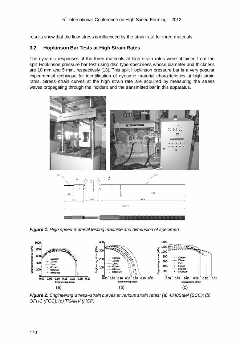
5th International Conference on High Speed Forming – 2012
results show that the flow stress is influenced by the strain rate for three materials.
3.2 Hopkinson Bar Tests at High Strain Rates
The dynamic responses of the three materials at high strain rates were obtained from the split Hopkinson pressure bar test using disc type specimens whose diameter and thickness are 10 mm and 5 mm, respectively [13]. This split Hopkinson pressure bar is a very popular experimental technique for identification of dynamic material characteristics at high strain rates. Stress–strain curves at the high strain rate are acquired by measuring the stress waves propagating through the incident and the transmitted bar in this apparatus.
Figure 1: High speed material testing machine and dimension of specimen
0.00 0.05 0.10 0.15 0.20 0.25 0.300
200
400
600
800
1000
Engi
neer
ing
stre
ss [M
Pa]
Engineering strain
100/sec 10/sec 1/sec 0.1/sec 0.01/sec 0.001/sec
0.00 0.05 0.10 0.15 0.20 0.25 0.300
100
200
300
400
Engi
neer
ing
stre
ss [M
Pa]
Engineering strain
100/sec 10/sec 1/sec 0.1/sec 0.01/sec 0.001/sec
0.00 0.03 0.06 0.09 0.12 0.150
200400600800
100012001400
Engi
neer
ing
stre
ss [M
Pa]
Engineering strain
100/sec 10/sse 1/sec 0.1/sec 0.01/sec 0.001/sec
(a) (b) (c)
Figure 2: Engineering stress–strain curves at various strain rates: (a) 4340Steel (BCC); (b) OFHC (FCC); (c) Ti6Al4V (HCP)
170
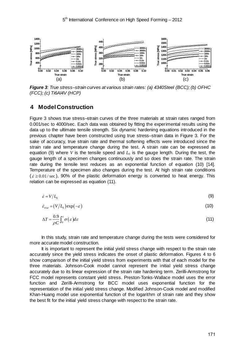
5th International Conference on High Speed Forming – 2012
0.00 0.02 0.04 0.06 0.08 0.100
400
600
800
1000
1200
1400
True
stre
ss [M
Pa]
True strain
3500/s 2000/s 100/s 10/s 1/s 0.1/s 0.01/s 0.001/s
0.00 0.02 0.04 0.06 0.08 0.100
280
320
360
400
440
True
stre
ss [M
Pa]
True strain
4000/s 3000/s 100/s 10/s 1/s 0.1/s 0.01/s 0.001/s
0.00 0.01 0.02 0.03 0.04 0.05 0.060
1000110012001300140015001600
True
stre
ss [M
Pa]
True strain
3000/s 2000/s 100/s 10/s 1/s 0.1/s 0.01/s 0.001/s
(a) (b) (c)
Figure 3: True stress–strain curves at various strain rates: (a) 4340Steel (BCC); (b) OFHC (FCC); (c) Ti6Al4V (HCP)
4 Model Construction
Figure 3 shows true stress–strain curves of the three materials at strain rates ranged from 0.001/sec to 4000/sec. Each data was obtained by fitting the experimental results using the data up to the ultimate tensile strength. Six dynamic hardening equations introduced in the previous chapter have been constructed using true stress–strain data in Figure 3. For the sake of accuracy, true strain rate and thermal softening effects were introduced since the strain rate and temperature change during the test. A strain rate can be expressed as equation (9) where V is the tensile speed and L0 is the gauge length. During the test, the gauge length of a specimen changes continuously and so does the strain rate. The strain rate during the tensile test reduces as an exponential function of equation (10) [14]. Temperature of the specimen also changes during the test. At high strain rate conditions ( 0.01 / secε ≥ ), 90% of the plastic deformation energy is converted to heat energy. This relation can be expressed as equation (11).
0V Lε = (9)
( ) ( )0 exptrue V Lε ε= − (10)
( )0
0.9T dC
εσ ε ε
ρ∆ = ∫ (11)
In this study, strain rate and temperature change during the tests were considered for
more accurate model construction. It is important to represent the initial yield stress change with respect to the strain rate
accurately since the yield stress indicates the onset of plastic deformation. Figures 4 to 6 show comparison of the initial yield stress from experiments with that of each model for the three materials. Johnson-Cook model cannot represent the initial yield stress change accurately due to its linear expression of the strain rate hardening term. Zerilli-Armstrong for FCC model represents constant yield stress. Preston-Tonks-Wallace model uses the error function and Zerilli-Armstrong for BCC model uses exponential function for the representation of the initial yield stress change. Modified Johnson-Cook model and modified Khan-Huang model use exponential function of the logarithm of strain rate and they show the best fit for the initial yield stress change with respect to the strain rate.
171
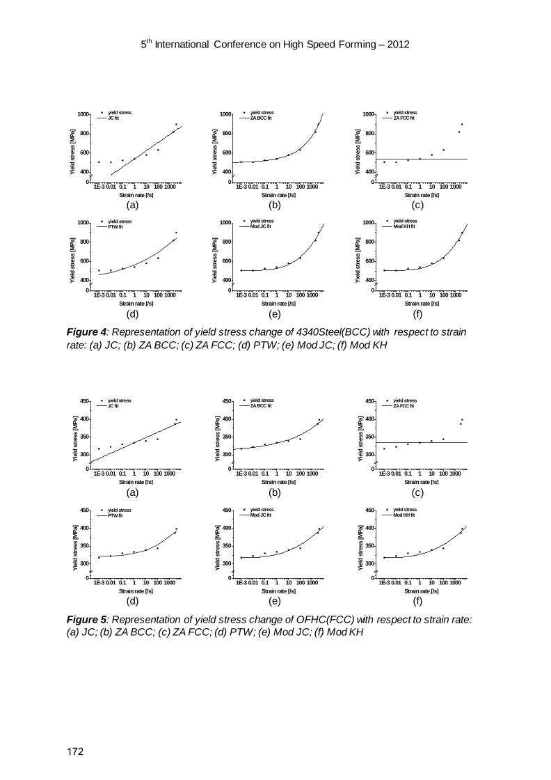
5th International Conference on High Speed Forming – 2012
1E-3 0.01 0.1 1 10 100 10000
400
600
800
1000 yield stress JC fit
Yiel
d st
ress
[MPa
]
Strain rate [/s] 1E-3 0.01 0.1 1 10 100 1000
0
400
600
800
1000 yield stress ZA BCC fit
Yiel
d st
ress
[MPa
]
Strain rate [/s] 1E-3 0.01 0.1 1 10 100 1000
0
400
600
800
1000 yield stress ZA FCC fit
Yiel
d st
ress
[MPa
]
Strain rate [/s] (a) (b) (c)
1E-3 0.01 0.1 1 10 100 10000
400
600
800
1000 yield stress PTW fit
Yiel
d st
ress
[MPa
]
Strain rate [/s] 1E-3 0.01 0.1 1 10 100 1000
0
400
600
800
1000 yield stress Mod JC fit
Yiel
d st
ress
[MPa
]
Strain rate [/s] 1E-3 0.01 0.1 1 10 100 1000
0
400
600
800
1000 yield stress Mod KH fit
Yiel
d st
ress
[MPa
]
Strain rate [/s] (d) (e) (f)
Figure 4: Representation of yield stress change of 4340Steel(BCC) with respect to strain rate: (a) JC; (b) ZA BCC; (c) ZA FCC; (d) PTW; (e) Mod JC; (f) Mod KH
1E-3 0.01 0.1 1 10 100 10000
300
350
400
450 yield stress JC fit
Yiel
d st
ress
[MPa
]
Strain rate [/s] 1E-3 0.01 0.1 1 10 100 1000
0
300
350
400
450 yield stress ZA BCC fit
Yiel
d st
ress
[MPa
]
Strain rate [/s] 1E-3 0.01 0.1 1 10 100 1000
0
300
350
400
450 yield stress ZA FCC fit
Yiel
d st
ress
[MPa
]
Strain rate [/s] (a) (b) (c)
1E-3 0.01 0.1 1 10 100 10000
300
350
400
450 yield stress PTW fit
Yiel
d st
ress
[MPa
]
Strain rate [/s] 1E-3 0.01 0.1 1 10 100 1000
0
300
350
400
450 yield stress Mod JC fit
Yiel
d st
ress
[MPa
]
Strain rate [/s] 1E-3 0.01 0.1 1 10 100 1000
0
300
350
400
450 yield stress Mod KH fit
Yiel
d st
ress
[MPa
]
Strain rate [/s] (d) (e) (f)
Figure 5: Representation of yield stress change of OFHC(FCC) with respect to strain rate: (a) JC; (b) ZA BCC; (c) ZA FCC; (d) PTW; (e) Mod JC; (f) Mod KH
172
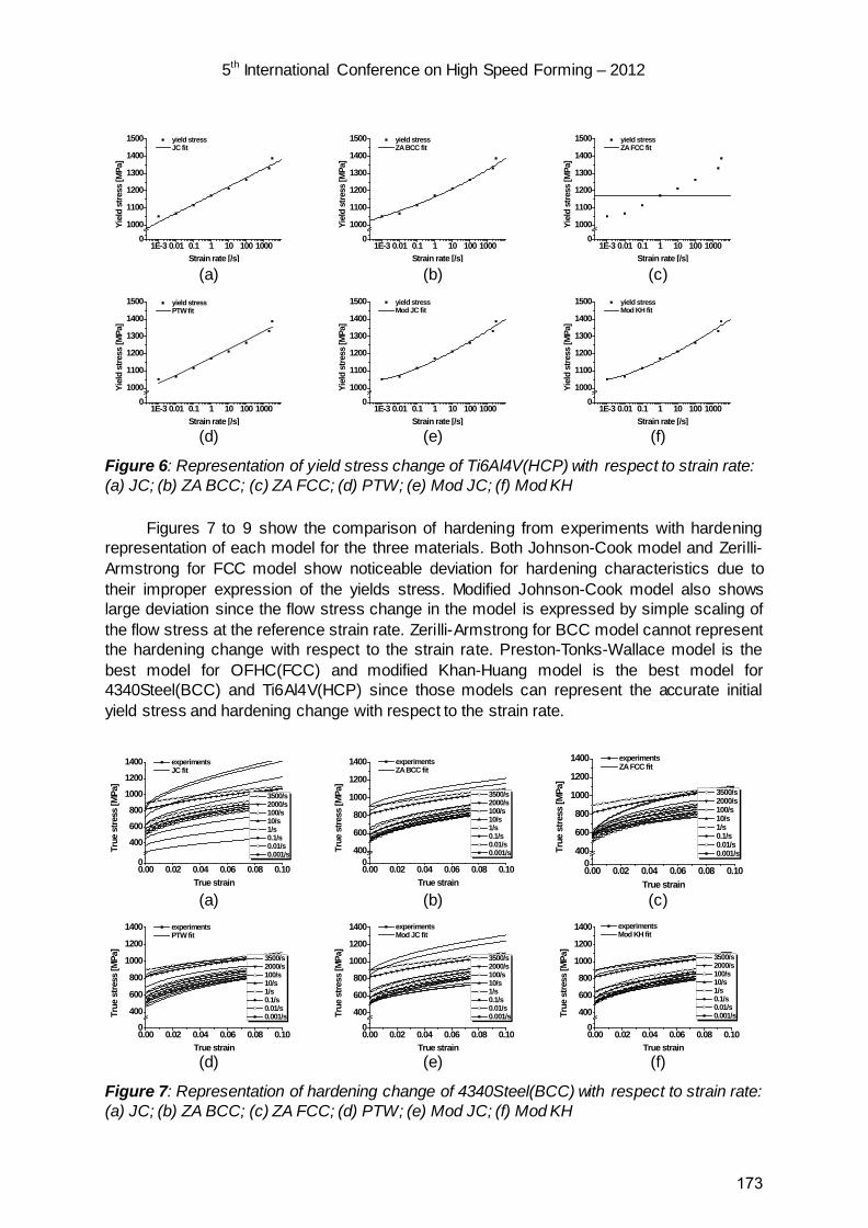
5th International Conference on High Speed Forming – 2012
1E-3 0.01 0.1 1 10 100 10000
1000
1100
1200
1300
1400
1500 yield stress JC fit
Yiel
d st
ress
[MPa
]
Strain rate [/s] 1E-3 0.01 0.1 1 10 100 1000
01000
1100
1200
1300
1400
1500 yield stress ZA BCC fit
Yiel
d st
ress
[MPa
]
Strain rate [/s] 1E-3 0.01 0.1 1 10 100 1000
01000
1100
1200
1300
1400
1500 yield stress ZA FCC fit
Yiel
d st
ress
[MPa
]
Strain rate [/s] (a) (b) (c)
1E-3 0.01 0.1 1 10 100 10000
1000
1100
1200
1300
1400
1500 yield stress PTW fit
Yiel
d st
ress
[MPa
]
Strain rate [/s] 1E-3 0.01 0.1 1 10 100 1000
01000
1100
1200
1300
1400
1500 yield stress Mod JC fit
Yiel
d st
ress
[MPa
]
Strain rate [/s] 1E-3 0.01 0.1 1 10 100 1000
01000
1100
1200
1300
1400
1500 yield stress Mod KH fit
Yiel
d st
ress
[MPa
]
Strain rate [/s] (d) (e) (f)
Figure 6: Representation of yield stress change of Ti6Al4V(HCP) with respect to strain rate: (a) JC; (b) ZA BCC; (c) ZA FCC; (d) PTW; (e) Mod JC; (f) Mod KH
Figures 7 to 9 show the comparison of hardening from experiments with hardening representation of each model for the three materials. Both Johnson-Cook model and Zerilli-Armstrong for FCC model show noticeable deviation for hardening characteristics due to their improper expression of the yields stress. Modified Johnson-Cook model also shows large deviation since the flow stress change in the model is expressed by simple scaling of the flow stress at the reference strain rate. Zerilli-Armstrong for BCC model cannot represent the hardening change with respect to the strain rate. Preston-Tonks-Wallace model is the best model for OFHC(FCC) and modified Khan-Huang model is the best model for 4340Steel(BCC) and Ti6Al4V(HCP) since those models can represent the accurate initial yield stress and hardening change with respect to the strain rate.
0.00 0.02 0.04 0.06 0.08 0.100
400
600
800
1000
1200
1400 experiments JC fit
True
stre
ss [M
Pa]
True strain
3500/s 2000/s 100/s 10/s 1/s 0.1/s 0.01/s 0.001/s
0.00 0.02 0.04 0.06 0.08 0.100
400
600
800
1000
1200
1400 experiments ZA BCC fit
True
stre
ss [M
Pa]
True strain
3500/s 2000/s 100/s 10/s 1/s 0.1/s 0.01/s 0.001/s
0.00 0.02 0.04 0.06 0.08 0.100
400
600
800
1000
1200
1400 experiments ZA FCC fit
True
stre
ss [M
Pa]
True strain
3500/s 2000/s 100/s 10/s 1/s 0.1/s 0.01/s 0.001/s
(a) (b) (c)
0.00 0.02 0.04 0.06 0.08 0.100
400
600
800
1000
1200
1400 experiments PTW fit
True
stre
ss [M
Pa]
True strain
3500/s 2000/s 100/s 10/s 1/s 0.1/s 0.01/s 0.001/s
0.00 0.02 0.04 0.06 0.08 0.100
400
600
800
1000
1200
1400 experiments Mod JC fit
True
stre
ss [M
Pa]
True strain
3500/s 2000/s 100/s 10/s 1/s 0.1/s 0.01/s 0.001/s
0.00 0.02 0.04 0.06 0.08 0.100
400
600
800
1000
1200
1400 experiments Mod KH fit
True
stre
ss [M
Pa]
True strain
3500/s 2000/s 100/s 10/s 1/s 0.1/s 0.01/s 0.001/s
(d) (e) (f)
Figure 7: Representation of hardening change of 4340Steel(BCC) with respect to strain rate: (a) JC; (b) ZA BCC; (c) ZA FCC; (d) PTW; (e) Mod JC; (f) Mod KH
173

5th International Conference on High Speed Forming – 2012
0.00 0.02 0.04 0.06 0.08 0.100
280
320
360
400
440
experiments JC fit
True
stre
ss [M
Pa]
True strain
4000/s 3000/s 100/s 10/s 1/s 0.1/s 0.01/s 0.001/s
0.00 0.02 0.04 0.06 0.08 0.100
320
360
400
440
experiments ZA BCC fit
True
stre
ss [M
Pa]
True strain
4000/s 3000/s 100/s 10/s 1/s 0.1/s 0.01/s 0.001/s
0.00 0.02 0.04 0.06 0.08 0.100
320
360
400
440
experiments ZA FCC fit
True
stre
ss [M
Pa]
True strain
4000/s 3000/s 100/s 10/s 1/s 0.1/s 0.01/s 0.001/s
(a) (b) (c)
0.00 0.02 0.04 0.06 0.08 0.100
320
360
400
440
experiments PTW fit
True
stre
ss [M
Pa]
True strain
4000/s 3000/s 100/s 10/s 1/s 0.1/s 0.01/s 0.001/s
0.00 0.02 0.04 0.06 0.08 0.100
320
360
400
440
experiments Mod JC fit
True
stre
ss [M
Pa]
True strain
4000/s 3000/s 100/s 10/s 1/s 0.1/s 0.01/s 0.001/s
0.00 0.02 0.04 0.06 0.08 0.100
320
360
400
440
experiments Mod KH fit
True
stre
ss [M
Pa]
True strain
4000/s 3000/s 100/s 10/s 1/s 0.1/s 0.01/s 0.001/s
(d) (e) (f)
Figure 8: Representation of hardening change of OFHC(FCC) with respect to strain rate: (a) JC; (b) ZA BCC; (c) ZA FCC; (d) PTW; (e) Mod JC; (f) Mod KH
0.00 0.01 0.02 0.03 0.04 0.05 0.060
1000110012001300140015001600 experiments
JC fit
True
stre
ss [M
Pa]
True strain
3000/s 2000/s 100/s 10/s 1/s 0.1/s 0.01/s 0.001/s
0.00 0.01 0.02 0.03 0.04 0.05 0.060
1000110012001300140015001600 experiments
ZA BCC fit
True
stre
ss [M
Pa]
True strain
3000/s 2000/s 100/s 10/s 1/s 0.1/s 0.01/s 0.001/s
0.00 0.01 0.02 0.03 0.04 0.05 0.060
1000110012001300140015001600 experiments
ZA FCC fit
True
stre
ss [M
Pa]
True strain
3000/s 2000/s 100/s 10/s 1/s 0.1/s 0.01/s 0.001/s
(a) (b) (c)
0.00 0.01 0.02 0.03 0.04 0.05 0.060
1000110012001300140015001600 experiments
PTW fit
True
stre
ss [M
Pa]
True strain
3000/s 2000/s 100/s 10/s 1/s 0.1/s 0.01/s 0.001/s
0.00 0.01 0.02 0.03 0.04 0.05 0.060
1000110012001300140015001600 experiments
Mod JC fit
True
stre
ss [M
Pa]
True strain
3000/s 2000/s 100/s 10/s 1/s 0.1/s 0.01/s 0.001/s
0.00 0.01 0.02 0.03 0.04 0.05 0.060
1000110012001300140015001600 experiments
Mod KH fit
True
stre
ss [M
Pa]
True strain
3000/s 2000/s 100/s 10/s 1/s 0.1/s 0.01/s 0.001/s
(d) (e) (f)
Figure 9: Representation of hardening change of Ti6Al4V(HCP) with respect to strain rate: (a) JC; (b) ZA BCC; (c) ZA FCC; (d) PTW; (e) Mod JC; (f) Mod KH
Figure 10 shows the quantitative evaluation of each model for both the initial yield stress and hardening representation. For all kinds of materials, Johnson-Cook and Zerilli-Armstrong for FCC model induce large deviation for the initial yield stress and hardening representation. Modified Johnson-Cook model is enhanced for the yield stress representation although hardening representation still shows improper results. Zerilli-Armstrong for BCC model can represent the accurate hardening characteristics of a material when hardening does not show much change with respect to the strain rate like Ti6Al4V. Preston-Tonks-Wallace and modified Khan-Huang model can represent the change of hardening and the initial yield stress accurately. Figure 11 shows the material coefficients for each model constructed.
174

5th International Conference on High Speed Forming – 2012
Figure 10: Quantitative evaluation of each constructed results
Figure 11: Material coefficients for each constructed model
5 Conclusions
This paper is concerned with the characteristics of various dynamic hardening equations in view of the dynamic behavior of the three kinds of materials. The dynamic response at the intermediate strain rate is obtained from the high speed tensile test and that at the high strain rate from the split Hopkinson pressure bar test. It is important to investigate the initial yield stress and the hardening characteristics of each dynamic hardening equation in order to quantify the dynamic hardening characteristics of metallic materials. Four kinds of famous dynamic hardening equations were investigated and evaluated for its applicability. Two kinds of modified dynamic hardening equations developed by KAIST were also investigated. Preston-Tonks-Wallace model is the best model for OFHC(FCC), and modified Khan-Huang model is the best model for 4340Steel(BCC) and Ti6Al4V(HCP). Johnson-Cook model and Zerilli-Armstrong model have significant shortcomings in representation of the initial yield stress and hardening characteristics. Modified Johnson-Cook model also shows improper results for hardening characteristics. Zerilli-Armstrong for BCC model is limited for the
175

5th International Conference on High Speed Forming – 2012
material in which hardening does not change with respect to the strain rate. Modified Khan-Huang model and Preston-Tonks-Wallace model afford good representation of the initial yield stress and the hardening change with respect to the strain rate.
References
[1] Mayers M.: Dynamic Behavior of Materials. John Wiley & Sons, New York. 1994. [2] Johnson G. R.; Cook W. H.: A constitutive model and data for metals subjected to large
strains, high strain rates and high temperatures. Proceedings of the Seventh International Symposium on Ballistics, The Hague, The Netherland, 1983, p.541-547.
[3] Zerilli F. J.; Armstrong R. W.: Dislocation-mechanics-based constitutive relations for material dynamics calculations. Journal of Applied Physics, Vol.61, 1987, p.1816-1825.
[4] Preston D. L.; Tonks D. L.; Wallace D. C.: Model of plastic deformation for extreme loading conditions. Journal of Applied Physics, Vol.93, 2003, p.211-220.
[5] Kang W. J.; Cho S. S.; Huh H.; Chung D. T.: Modified Johnson-Cook model for vehicle body crashworthiness simulation. International Journal of Vehicle Design, Vol.21, 1999, p.424-435.
[6] Lee H. J.; Song J. H.; Huh H.: Dynamic tensile tests of auto-body steel sheets with the variation of temperature. Solid State Phenomena, Vol.116-117, 2006. p.259-262.
[7] Huh H.; Lee H. J.; Song J. H.: Dynamic hardening equation of the auto-body steel sheet with the variation of temperature. International Journal of Automotive Technology, Vol.13, 2012. p.43-60.
[8] Follansbee P. S.; Kocks U. F.: A constitutive description of the deformation of copper based on the use of the mechanical threshold stress as an internal state variable. Acta Metallurgica, Vol.36, 1988, p.81-93.
[9] Khan A. S.; Huang S.: Experimental and theoretical study of mechanical behavior of 1100 aluminum in the strain rate range 10-5-104s-1. International Journal of Plasticity, Vol. 8, 1992, p.397-424.
[10] Huh H.; Lim J. H.; Park S. H.: High speed tensile test of steel sheets for the stress-strain curve at the intermediate strain rate. International Journal of Automotive Technology, Vol.10, 2009, p.195-204.
[11] Huh H.: Kim S. B.: Song J. H.: Lim J. H.: Dynamic tensile characteristics of TRIP-type and DP-type steel sheets for an auto-body. International Journal of Mechanical Sciences, Vol.50, 2008, p.918-931.
[12] Song J. H.: Huh H.: Dynamic material property of the sinter-forged Cu-Cr alloys with the variation of chrome content. Transactions of KSME(A), Vol.30, 2006, p.670-677.
[13] Huh H.; Kang W. J.; Han S. S.: A tension split Hopkinson bar for investigating the dynamic behavior of sheet metals. Experimental Mechanics, Vol.42, 2002, p.8-17.
[14] Gao Y.; Wagoner R. H.: A simplified model of heat generation during the uniaxial tensile test. Metallurgical Transactions A, Vol.18A, 1987, p.1001-1009.
176

SESSION 6
JOINING AND WELDING - A
177

178
Dissimilar Metal Joining: Macro- and Microscopic Effects of MPW* Göbel, Gunther1; Beyer, Eckard1,2
; Kaspar, Jörg1; Brenner, Berndt1; 1 Fraunhofer Institute for Material and Beam Technology (IWS), Dresden, Germany 2 Institute of Surface and Manufacturing Technology, Technical University Dresden, Germany
Abstract
Magnetic pulse welding (MPW) can offer unique advantages over other joining techniques when applied correctly. Especially for dissimilar metal welding it has several advantages due to its very low heat input and short process times. Due to the high demands of the process on the welding system properties, it is vital to understand the process as detailed as possible to reduce system-related challenges and costs.
The paper discusses similarities and dissimilarities to other high velocity joining processes like explosion welding. Specific aspects of MPW, like its special transient nature are presented and their impact on welding parameters are explained. Using results of example welds on similar and dissimilar metal joints, microscopic and macroscopic effects of part geometry, metallurgical behaviour and pulse parameters are shown.
Concerning microscopic effects, the question is discussed whether interfaces of dissimilar metals can fully be free of intermetallics. This is a relevant question in relation to achievable joint strength, joint ductility and even electric conductivity. Here evidence of recent SEM and TEM analysis is presented. Conclusions are drawn with respect to optimal process conditions and practical geometric relations on the macroscopic scale.
Keywords
Welding, Interface, Analysis
*The authors would like to thank the European Regional Develop- ment Fund (ERDF) and the State of Saxony for its financial support. The authors also thank the team of the Dresden High Magnetic Field Laboratory of the Helmholtz-Zentrum Dresden-Rossendorf for the Pulse-Generator development.
179
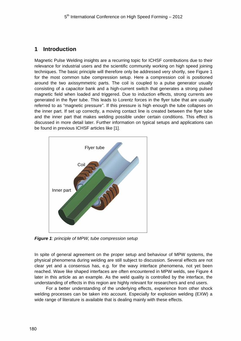
5th International Conference on High Speed Forming – 2012
1 Introduction
Magnetic Pulse Welding insights are a recurring topic for ICHSF contributions due to their relevance for industrial users and the scientific community working on high speed joining techniques. The basic principle will therefore only be addressed very shortly, see Figure 1 for the most common tube compression setup. Here a compression coil is positioned around the two axissymmetric parts. The coil is coupled to a pulse generator usually consisting of a capacitor bank and a high-current switch that generates a strong pulsed magnetic field when loaded and triggered. Due to induction effects, strong currents are generated in the flyer tube. This leads to Lorentz forces in the flyer tube that are usually referred to as “magnetic pressure”. If this pressure is high enough the tube collapses on the inner part. If set up correctly, a moving contact line is created between the flyer tube and the inner part that makes welding possible under certain conditions. This effect is discussed in more detail later. Further information on typical setups and applications can be found in previous ICHSF articles like [1].
Figure 1: principle of MPW, tube compression setup
In spite of general agreement on the proper setup and behaviour of MPW systems, the physical phenomena during welding are still subject to discussion. Several effects are not clear yet and a consensus has, e.g. for the wavy interface phenomena, not yet been reached. Wave like shaped interfaces are often encountered in MPW welds, see Figure 4 later in this article as an example. As the weld quality is controlled by the interface, the understanding of effects in this region are highly relevant for researchers and end users.
For a better understanding of the underlying effects, experience from other shock welding processes can be taken into account. Especially for explosion welding (EXW) a wide range of literature is available that is dealing mainly with these effects.
Coil
Flyer tube
Inner part
180

5th International Conference on High Speed Forming – 2012
In this paper it is discussed whether findings from EXW can be directly applied on MPW or which differences exist. This question is important if further theories like useful parameter windows are derived from existing data.
2 Magnetic Pulse Welding – comparable to other shock welding techniques?
As already discussed in [2] explosion welding (EXW) is usually considered to be a very similar process to magnetic pulse welding as it is also based on a local moving pressure shock effect. On EXW usually a wavy interface is generated between two flat and smooth plates. Here the (still solid!) material obviously has acted like a fluid under the intense pressure at the welding front. Such a wavy interface is seen in MPW too which suggests the same physical background.
Due to its history, explosion welding (EXW) was earlier analysed scientifically than MPW. Especially the wavy interface effect was studied in great detail, leading to several theories of its origin. The main theories are the “Indentation mechanism” [3], “Karman vortex street analogy” [4], “Helmholtz instability mechanism” [5], “stress wave mechanism” [6], and “mechanism of vibration in the plastic state” [7]. A detailed discussion of their background and assumptions would be out of the scope of this paper. Comparisons can already be found in the literature: [7-11] are examples how their perception evolved from 1975 to 2011. According to previous research at the IWS some evidence points to the fact that stress waves play a role: the wave formation could be influenced by changing the thickness of the inner (not the flyer!) part. This influence would be hard to explain using theories based on quasi-fluid flow effects at the interface, as no changes were made here. But it would support the stress wave mechanism theory: As stress waves travel back and forth through the inner part core a feedback into the welding process can be expected even if no other material property was changed.
Figure 2: jet formation theory
Consensus of most theories is the presence of a metal-gas jet at the moving welding front, Figure 2. This jet is caused by the intense pressure at the collision point of two surfaces [12]. It is understood that this jet cleans the contaminated and oxidised surfaces directly at the front and makes the welding of the two surfaces possible. It is understood that the jet
vC
Collision line
Jet
Welded area
Magnetic pressure Flyer-tube Coil
Inner part
181

5th International Conference on High Speed Forming – 2012
is only formed in a certain speed range of the moving front. Besides the front velocity vC other parameters have also been found to be relevant for jet creation, especially the angle between the two colliding surfaces. A so called “welding window” is formed by vC and , see example in Figure 3. In each source [8,14-17] this influence is discussed and different experimental data is contributed.
vC (m/s)
Figure 3: Example welding window for explosion welding, governed by velocity vC and surface angle from [17], a possible weld path of a MPW process is added (qualitatively)
Several authors discuss their findings with respect to these process properties which makes a comparison of MPW and EXW results possible. Interestingly, significant differences in the welding windows for a wide range of materials are found. E.g. according to [13, 18, 19] impact velocities for MPW are in the range of vI=30-250 m/s, while EXW sources point out much higher values in the range of vI=300-650 m/s [16,20-23]. As the welding window is usually expressed using the resulting front velocities vC instead of vI, the mentioned values must be converted using
vC = vI/tan
As the surface angle is in the same range for both processes (typical are around 10° for MPW), it becomes clear that the vC- welding windows are also set apart by a factor of 2. Recent MPW literature reports relatively high velocities for MPW [24] with vi up to 320 m/s. Nevertheless these values only reach the lowest end values from EXW.
It could be argued that MPW still follows identical physical effects but operates at a lower parameter range of a generally large window. However, as wavy interfaces are only associated with higher speeds for EXW [12], and waves are commonly encountered in MPW too, further explanations are needed. As this comparison indicates it is questionable if EXW and MPW physics are really comparable and if EXW parameter windows should be used as a basis for MPW tasks.
182

5th International Conference on High Speed Forming – 2012
However, the formation of wavy interfaces in both processes underlines their general relation. Therefore possible causes are proposed to explain the speed differences.
First it must be pointed out that MPW is, unlike EXW, a highly transient process. The stages of the process are as follows: 1 Acceleration of the flyer part due to the magnetic pulse 2 First contact of the flyer on the fixed part 3 Start of deformation of flyer along fixed part 4 Start of jet, start of bonding 5 Continuous movement of welding front along part 6 Decay of magnetic pulse (due to higher coil distance as well as end of pulse) less
driving force for deformation 7 End of jet when welding window is left 8 End of deformation
It is clear that a wave formation can, if it happens at all, only take place in stage 5 and 6 during the continuous movement when a jet is present. As the angle of collision can also change due to the deformation behaviour of the flyer, the strong difference to EXW is visible: instead of a constant vC and , both parameters change along the weld.
It must be considered that measuring MPW impact speeds or travel speeds is far more complicated than measuring vC for EXW (where a high-speed recording of the explosion front is sufficient). Therefore it is possible that reduced speeds already occur during stage 6, leading possibly to lower relevant vC values for MPW.
However, a different explaination can be found in the actual nature of the wavy initiation. Here two different ranges are discussed in the literature: One high speed velocity range, where waves appear also on originally smooth sheets and a lower speed range, which can be achieved by adding disturbances to EXW processes. (Changes to vC are achieved by influencing the explosive burning velocity via its chemical composition).
These ranges have been proposed earlier by [25] who added wires between the otherwise flat parts during preparation of EXW experiments. The wire was positioned orthogonal to the welding direction and was hit by the moving front during welding. When welding at lower speeds where usually no waves would occur, the wire was able to trigger a wave formation. This leads to the assumption that metastable wave formation is possible, if a (strong enough) perturbation exists in the process. This is also in discussion to explain hypervelocity gauging properties. Hypervelocity gauging is another high speed impact process based on fast sliding of two surfaces that causes local welding/ripping features e.g. on rocket sleds or rail guns [10]. A unified theory for both processes can be achieved according to [10] if a metastable instability is considered.
As most EXW information on required speeds for wavy interfaces are based on the overcritical “fully unstable” mechanism on undisturbed flat sheets, it could be concluded that MPW, as a very transient process, should be able to produce waves at much lower front velocities by means of a metastable initiation. Due to the very short total weld length, the initiation is probably already a result of the impact itself in stage 2. Perturbances are expected furthermore due to small symmetry errors (usually caused by not fully symmetric field formers) or by the changing deformation of the flyer along the path.
183

5th International Conference on High Speed Forming – 2012
Besides this different velocity range for wave formation, the welding window position seems to be different for EXW and MPW, as stated from the literature research above. It can be concluded that a direct transfer of EXW knowledge is not advisable and differences of the processes should be studied in more detail. Therefore additional research is planned on these discrepancies to find possible explanations.
To increase knowledge of the physical background, it is proposed by the authors that further research on MPW parameter windows should include as many details as possible on the path of the process within the plane of vC and . Here pointwise information, as usually seen in literature, is not sufficient to describe MPW processes. By comparing the whole process path in the vC and plane, a much better understanding of the influence of different pulse systems, part designs or pulse properties should be possible.
Also the state of contamination was found to be important for the total position of the welding window [17] and should be documented. A thinner contamination layer requires only a weaker jet to clean it. Thus, the lower limit of the welding window is shifted to reduced speeds, making welds possible with less initial pulse energy.
Figure 4: typical wave pocket with intermetallics
Based on theoretical considerations as well as experimental experience the following conclusion can be drawn so far:
if large impact velocities cannot be reached (e.g. due to pulse generator restrictions), higher angles should be used to stay in the parameter window
to increase weld length the impact point parameters of a flyer material in a MPW process should be in the far right corner of the vC- plane, to be able to use a long path during stage 6 (decay of deformation speed leading to a slowing down of vC)
including perturbations in the surface can be used to trigger wave formations if strong intermetallics cannot be avoided, (artificially triggered) waves could
be used to “localize” oxides in pockets within the waves, see Figure 4 the surface of the part should be as clean as possible, so already low-energy
jets are sufficient to clean the surfaces from all remaining contamination
184
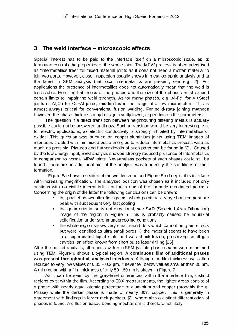
5th International Conference on High Speed Forming – 2012
3 The weld interface – microscopic effects
Special interest has to be paid to the interface itself on a microscopic scale, as its formation controls the properties of the whole joint. The MPW process is often advertised as “intermetallics free” for mixed material joints as it does not need a molten material to join two parts. However, closer inspection usually shows in metallographic analysis and at the latest in SEM analysis that local intermetallics are present, see e.g. [2]. For applications the presence of intermetallics does not automatically mean that the weld is less stable. Here the brittleness of the phases and the size of the phases must exceed certain limits to impair the weld strength. As for many phases, e.g. Al2Fe3 for Al+Steel joints or Al2Cu for Cu+Al joints, this limit is in the range of a few micrometers. This is almost always critical for conventional fusion welding. For solid-state joining methods however, the phase thickness may be significantly lower, depending on the parameters.
The question if a direct transition between neighbouring differing metals is actually possible could not be answered until now. Such a transition would be very interesting, e.g. for electric applications, as electric conductivity is strongly inhibited by intermetallics or oxides. This question was pursued on copper-aluminium joints using TEM images of interfaces created with minimized pulse energies to reduce intermetallics process-wise as much as possible. Pictures and further details of such parts can be found in [2]. Caused by the low energy input, SEM analysis showed strongly reduced presence of intermetallics in comparison to normal MPW joints. Nevertheless pockets of such phases could still be found. Therefore an additional aim of the analysis was to identify the conditions of their formation. Figure 5a shows a section of the welded zone and Figure 5b-d depict this interface with increasing magnification. The analyzed position was chosen as it included not only sections with no visible intermetallics but also one of the formerly mentioned pockets. Concerning the origin of the latter the following conclusions can be drawn:
the pocket shows ultra fine grains, which points to a very short temperature peak with subsequent very fast cooling
the grain orientation is not directional, see SAD (Selected Area Diffraction) image of the region in Figure 5 This is probably caused be equiaxial solidification under strong undercooling conditions
the whole region shows very small round dots which cannot be grain effects but were identified as ultra small pores the material seems to have been in a superheated liquid state and was shock-frozen, preserving small gas cavities, an effect known from short pulse laser drilling [26]
After the pocket analysis, all regions with no (SEM-)visible phase seams were examined using TEM. Figure 6 shows a typical region. A continuous film of additional phases was present throughout all analysed interfaces. Although the film thickness was often reduced to very low values of 0,05 – 0,2 µm, it never fell below values smaller than 30 nm. A thin region with a film thickness of only 50 - 60 nm is shown in Figure 7.
As it can be seen by the gray-level differences within the interface film, distinct regions exist within the film. According to EDX measurements, the lighter areas consist of a phase with nearly equal atomic percentage of aluminium and copper (probably the -Phase) while the darker phase is made of nearly 80% copper. This is generally in agreement with findings in larger melt pockets, [2], where also a distinct differentiation of phases is found. A diffusion based bonding mechanism is therefore not likely.
185

5th International Conference on High Speed Forming – 2012
Figure 5 SEM/TEM images Al+Cu joint with small intermetallic phase pocket, (a): SEM-overview, (b): TEM-Detail phase pocket, (c):grain structure, (d): close up grains
Figure 6: Continuous intermetallic film (arrows) Figure 7: Ultra-thin interface region
Al
Cu
20µm
500 nm 100 nm
Al
500 nm
c) d)
a) b) Al
Cu
Cu
186
5th International Conference on High Speed Forming – 2012
4 Conclusions
From the theoretical analysis of the process as well as the experimental analysis the following conclusions can be drawn: Although generally agreed, the effects and process internals of explosion welding
should not be directly transferred to magnetic pulse welding as the parameter windows seems to differ in regard to the collision velocity
A different wave formation initiation effect is a likely explanation that both EXW and MPW can show wavy interfaces in spite of different welding front velocities
A metastable wave initiation mechanism is proposed for MPW as this explains the occurrence at lower collision velocities
As MPW is highly transient in nature and the total weld length extremely short in comparison to EXW, the initial impact or changes and asymmetries along the weld line may already serve as a triggering disturbance for the metastable wave formation
To enhance the understanding of MPW and to help application oriented research, further studies on the process path in the vC- plane should be carried out
The analysis of low-energy Al+Cu magnetic pulse welds suggests that the idea of an “intermetallics free” joining process cannot be maintained for the MPW process as continuous films were found along all interfaces
In accordance with previous publications it can be concluded that solid state diffusion is not dominating in the bonding mechanism
References
[1] Shribman, V.: Magnetic Pulse welding for dissimilar and similar materials. Proc. of
the 3rd International Conference on High Speed Forming, Dortmund, 2008, p. 13-22. [2] Göbel, G.; Kaspar, J.; Herrmannsdörfer, T.; Brenner, B.; Beyer, E.:Insights into
intermetallic phases on pulse welded dissimilar metal joints. 4th International Conference on High Speed Forming, Columbus, Ohio, USA, 08.-10. März 2010
[3] Bahrani, A. S.; Black, T.J.; Crossland, B.: The Mechanics of Wave Formation in Explosive Welding. Proc. of Royal Society Series A 296, 1976, p. 23.
[4] Cowan G. R.; Bergmann O. R.; Holtzman A. H.: Mechanics of Bond Wave Formation in Explosive Cladding of Metals. Met. Transactions 2, 1971, p. 3145.
[5] Hunt, J. N.: Wave Formation in Explosive Welding. Phil. Mag. 17, 1968, p. 669-680. [6] El-Sobky, H.; Blazynsky, T. Z.: Experimental investigation of the mechanism of
explosive welding be means of a liquid analogue. Proc. 5th International Conference on “High Energy Rate fabrication”, Denver, Colorado, 1975, p. 1-21.
[7] Patwardhan, W. D.: Mechanism of wave formation at explosion bonded metal surfaces. Tran. of the Indian Institute of Metals, Vol. 36, 1983, 407-409.
[8] Carpenter, S. H.; Wittman, R. H.: Explosive Welding. Annu. Reviews Mater. Sci. 1975.5, 1975, p. 177-199.
[9] Tabatabee, M.:Impact Wave Process Modeling and Optimization in high Energy Rate Explosive Welding. PhD Thesis, Västerås, ISSN 1651-9256, (2009)
187
5th International Conference on High Speed Forming – 2012
[10] Watt, T.J.; Bourell, D.L.: Sliding Instabilities and Hypervelocity Gouging. IEEE Trans. On Plasma Science, Vol. 39, No. 1, (2011)
[11] Mousavi, A. A.; Al-Hassani, S. T.: Simulation of wave and jet formation in explosive/impact welding. Proc. of the 7th Conference on “Engineering Systems Designs and Analysis”, Manchester, U K., 2004, p. 265-274.
[12] Bergmann, O. R.: The Scientific Basis of Metal Bonding with Explosives. “High Energy Rate Fabrication – 1984”, The 8th Int. ASME Conf., 1984, p. 197-202.
[13] Watanabe, M.; Kumai, S.: High-Speed Deformation and Collision Behavior of Pure Aluminum Plates in Magnetic Pulse Welding. Materials Transactions, Vol. 50, No. 8pp. 2035 to 2042, The Japan Institute of Light Metals, (2009)
[14] Deribas,A.A.:Treatment of Materials by Expolsive Energy. Fizika Goreniya i Vzryva, Vol. 23, No. 5, 1985, pp. 130-137 (1988)
[15] Kojima, M.; Tamaki, K.; Furuta, T.:Effect of Collision Angle on the Result of Electromagnetic Welding of Aluminum. Trans. Japan Welding Soc., vol. 20, No. 2, pp. 36-42, (1989)
[16] Sartangi,P. F.; Akbari Mousavi, S. A. A.: Experimental Investigations on explosive cladding of cp-titanium / AISI stainless steel. Materials Science Forum Vols. 580-582, pp 629-632 (2008)
[17] Grignon, F. ;Benson, D. ;Vecchio, K.S.; Meyers, M.A.: Explosive welding of aluminum to aluminum: analysis, computations and experiments. International Journal of Impact Engineering 30 (2004), pp. 1333–1351
[18] Psyk, V.; Gershteyn, G.; Demir, O.K.; Brosius, A.; Tekkaya, A.E.; Schaper, M.; Bach, F.-W.: Process Analysis and Physical Simulation of Electromagnetic Joining of Thin-Walled parts. ICHSF 2008, Dortmund, 11.-12.3.2008
[19] Kore, S.D.;Date, P.P.; Kulkarni, S.V.: Electromagnetic impact welding of aluminum to stainless steel sheets. Journal of Materials Processing Technology Volume 208, Issues 1-3, 21 Nov. 08, Pages 486-493 (2008)
[20] Bergmann, R.; Cowan, G. R.; Holtzman, A.H.: Experimental Evidence of Jet Formation During Explosion Cladding. Transactions Metallurgical Society AIME, Vol. 236, pp. 646-653. (1966)
[21] Chizari, M. ;Al-Hassani, S.; Barrett, L.M.: Effect of flyer shape on the bonding criteria in impact welding of plates. J. of Mat. Proc. Tec. 209 (1) (2009), pp. 445–454.
[22] Botros, K.K.; Groves,T.K.: Characteristics of the wavy interface and the mechanism of its formation in high-velocity impact welding. J. Appl. Phys. 51 (7), July 1980, 3715-3721 (1980)
[23] Ghaderi, S.H.; Mori,A.; Hokamoto, K.: Explosive Joining of Magnesium Alloy AZ31 and Aluminum. Materials Science Forum Vol. 566, pp 291-296 (2008)
[24] Zhang, Y.; Babu, S.; Daehn, G. S. Impact Welding in a Variety of Geometric Configurations. ICHSF2010, March 9.-10.2010, Columbus, OH, USA, pp 97 - 107.
[25] Pai, V.V. Luk’yanov, Y. L.; Kuz’min, G. E. ; Yakovlev, I. V. :Wave formation in a high-velocity symmetric impact of metal plates,” Combustion, Explosion, Shock Waves, vol. 42, no. 5, pp. 611–616, (2006)
[26] Kaspar, J; Luft, A.; Nolte, S. ; Will, M.; Beyer, E.: Laser helical drilling of silicon wafers with ns to fs pulses: Scanning electron microscopy and transmission electron microscopy characterization of drilled through-holes. Journal of Laser Application 18 (2006) 2, pp. 85-92
188

Robot automated EMPT sheet welding
R. Schäfer1, P. Pasquale1
1 PSTproducts Gmbh, Germany
Abstract
Many industrial applications require sheet to sheet or sheet to tube joints. The electromagnetic pulse technology is capable to produce these kinds of joints. In literature many examples of sheet to sheet solid state welding between similar and dissimilar metals are presented and analyzed in detail. However, the most of the presented welding applications, which are very focussed on the academic level, are simple specimens for example for tensile test. These specimens are usually very small in their dimensions and therewith capable to be welded with the help of stationary EMPT coils. In contrast to this approach the majority of typical industrial applications demand the ability of manufacturing several welds in different positions on the same assembly application comparable to the spot welding process of an automotive car body. Here several spot welds are realised in a variety of positions by a robot mounted spot welding gun. The use of a stationary coil is no option here. A first step in manufacturing complex assemblies by EMPT was done by PSTproducts by welding a car- shaped space frame. Within this project substantial knowledge has been generated with respect to non stationary EMPT coils and the flexibility of the cables connecting the coil with the pulse generator. The results were transferred into the next step, the development of an EMPT robotic welding head. This report details requirements and possibilities of robot automated EMPT sheet welding with respect to complex structures.
Keywords
Automation, Robotic, Welding
1 Introduction
Fusion welding processes are widely adopted within production technology. However, these processes are not capable for joining metals of strongly different melting points. For example Aluminium melts at temperatures above 660°C, whereas iron melts at temperatures 1536°C [1]. Because of this large melting point discrepancy the creation of an aluminum-steel weld puddle is hindered [1]. Moreover, during solidification brittle
189
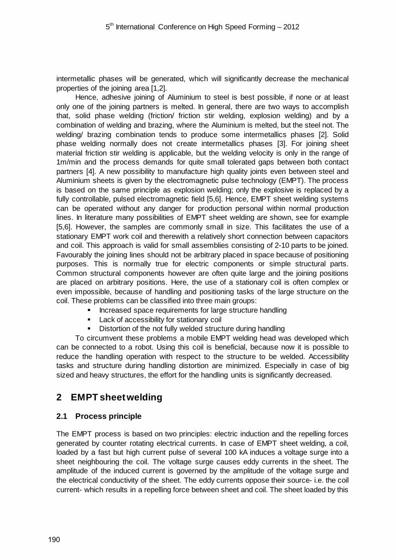
5th International Conference on High Speed Forming – 2012
intermetallic phases will be generated, which will significantly decrease the mechanical properties of the joining area [1,2].
Hence, adhesive joining of Aluminium to steel is best possible, if none or at least only one of the joining partners is melted. In general, there are two ways to accomplish that, solid phase welding (friction/ friction stir welding, explosion welding) and by a combination of welding and brazing, where the Aluminium is melted, but the steel not. The welding/ brazing combination tends to produce some intermetallics phases [2]. Solid phase welding normally does not create intermetallics phases [3]. For joining sheet material friction stir welding is applicable, but the welding velocity is only in the range of 1m/min and the process demands for quite small tolerated gaps between both contact partners [4]. A new possibility to manufacture high quality joints even between steel and Aluminium sheets is given by the electromagnetic pulse technology (EMPT). The process is based on the same principle as explosion welding; only the explosive is replaced by a fully controllable, pulsed electromagnetic field [5,6]. Hence, EMPT sheet welding systems can be operated without any danger for production personal within normal production lines. In literature many possibilities of EMPT sheet welding are shown, see for example [5,6]. However, the samples are commonly small in size. This facilitates the use of a stationary EMPT work coil and therewith a relatively short connection between capacitors and coil. This approach is valid for small assemblies consisting of 2-10 parts to be joined. Favourably the joining lines should not be arbitrary placed in space because of positioning purposes. This is normally true for electric components or simple structural parts. Common structural components however are often quite large and the joining positions are placed on arbitrary positions. Here, the use of a stationary coil is often complex or even impossible, because of handling and positioning tasks of the large structure on the coil. These problems can be classified into three main groups:
Increased space requirements for large structure handling Lack of accessibility for stationary coil Distortion of the not fully welded structure during handling
To circumvent these problems a mobile EMPT welding head was developed which can be connected to a robot. Using this coil is beneficial, because now it is possible to reduce the handling operation with respect to the structure to be welded. Accessibility tasks and structure during handling distortion are minimized. Especially in case of big sized and heavy structures, the effort for the handling units is significantly decreased.
2 EMPT sheet welding
2.1 Process principle
The EMPT process is based on two principles: electric induction and the repelling forces generated by counter rotating electrical currents. In case of EMPT sheet welding, a coil, loaded by a fast but high current pulse of several 100 kA induces a voltage surge into a sheet neighbouring the coil. The voltage surge causes eddy currents in the sheet. The amplitude of the induced current is governed by the amplitude of the voltage surge and the electrical conductivity of the sheet. The eddy currents oppose their source- i.e. the coil current- which results in a repelling force between sheet and coil. The sheet loaded by this
190

5th International Conference on High Speed Forming – 2012
force (“commonly: magnetic pressure”) is called flyer. Figure 1 illustrates the general setup and the eddy currents induced into the work piece.
Figure 1: Eddy currents induced in work piece
Accomplishing an EMPT weld requires a specific material flow of the flyer. A flat impact of the flyer on the second work piece – the so called target- will cause a rebound, but not a weld. For welding, the contact area between flyer and target should increase during the process. For accomplishing this, two general options are useful:
The use of spacers between flyer and target (see figure 2, left)
The use of a bead imprinted in the flyer before the EMPT process, which is flattened by the coil (see figure 2, right)
The material flow generated by either of the two options causes a superposition of normal and tangential contact stresses in the interfacial zone of both contact partners [6]. The amplitude of the contact stresses is several times beyond the yield strength of the work piece material. Contact stresses and inertia effects cause a high hydrostatic pressure and deviatoric pressure stress combination. Numerical simulation gives evidence, that the hydrostatic pressure’ amplitude near the point of first contact is several 1000 N/mm². Because of this, the material behaviour becomes similar to that of a fluid, i.e. metals can suffer straining of 100-200%. It is important to mention, that no melting effects are identifiable. Figure 3 illustrates the stress situation near the point of first contact. The deviatoric stress components cause formation of a wave in front of the first contact point and the hydrostatic stresses increase the material’s formability.
The straining of the material in the interfacial zone reaches values of 100-200%, resulting in a chipping of the oxide layers covering the metal surfaces. The high contact normal pressure forces an intimate contact between both work pieces; a metallic bond is accomplished.
191
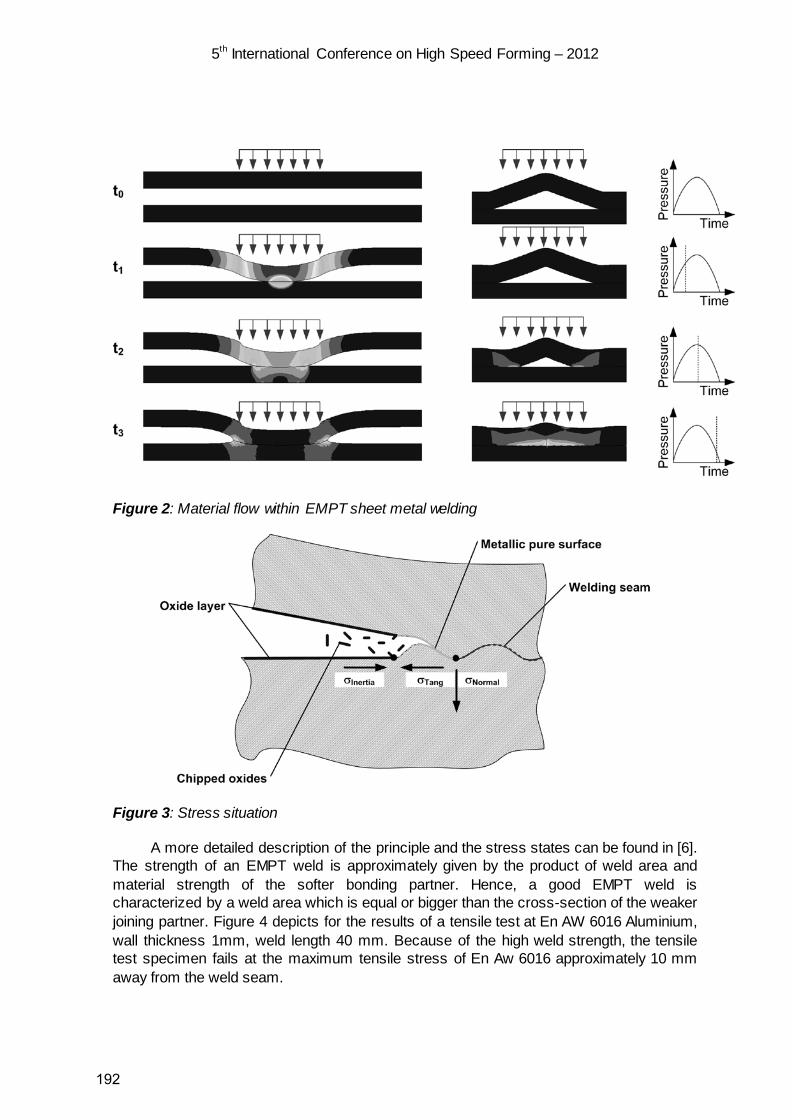
5th International Conference on High Speed Forming – 2012
Figure 2: Material flow within EMPT sheet metal welding
Figure 3: Stress situation
A more detailed description of the principle and the stress states can be found in [6]. The strength of an EMPT weld is approximately given by the product of weld area and material strength of the softer bonding partner. Hence, a good EMPT weld is characterized by a weld area which is equal or bigger than the cross-section of the weaker joining partner. Figure 4 depicts for the results of a tensile test at En AW 6016 Aluminium, wall thickness 1mm, weld length 40 mm. Because of the high weld strength, the tensile test specimen fails at the maximum tensile stress of En Aw 6016 approximately 10 mm away from the weld seam.
192

5th International Conference on High Speed Forming – 2012
Figure 4: Tensile test results with respect to 1mm wall thickness Al 6016 specimen.
2.2 Stationary EMPT sheet welding coil
Academic and industrial papers present some approaches of EMPT sheet welding samples. Commonly these samples are limited to a size spectrum between some millimetres and 1 meter. Normally only simple subassemblies are welded with the help of those stationary coils. The number of sheet joined within one pulse varies between two and ten layers. Flyer material is normally of a good electrical conductivity, for example Aluminium and Copper. The flyer wall thickness ranges from 10µm to 2.5 mm. Figure 5 illustrates a variety of samples.
Figure 5: EMPT Sheet welding samples accomplished with the help of stationary coils
193

5th International Conference on High Speed Forming – 2012
Experimental work has shown, that joining of larger subassemblies is possible in case all welding positions are positioned in one plane, see Figure 6. In contrast to other solid state welding techniques there is no need for a support which loads the joining area with static force. For EMPT welding the support can be represented by the inertia of a 10-20 kg mass.
Figure 6: EMPT welding of larger subassemblies
2.3 Robotic EMPT sheet welding coil
As mentioned in paragraph 2.2 the use of stationary EMPT sheet welding coils facilitates joining of a broad range of subassemblies. However, complex assemblies like the spaceframe structure shown in Figure 7 are hard to handle for EMPT welding by a stationary coil.
Figure 7: EMPT welded space frame
194

5th International Conference on High Speed Forming – 2012
Within the prototyping process of the space frame a special coil has been
developed. For first tests, this coil is connected to the structure by C-clamps. Welding trials proofed the industrial feasibility of this coil concept with respect to welding results and handling issues. Based on this experience, the coil concept is upgraded for direct use with a robot. A Reis RV 130-130 robot is used to position the coil above the welding area. A hybrid plate ensures on the one hand electric isolation of the coil via the robot, and on the other hand absorption of mechanical impulses generated by the coil.
The PSTproducts specific cables allow a curvature radius of ~500mm under cyclic loading. Due to that, a cable duct directly fixed at the robot boom would limit the mobility of the system. Hence, an auxiliary cable jack is used to ensure relatively big curvature radius of the cables and therewith small cable bending forces.
Figure 8 illustrates a robot pulse generator configuration. The reaction forces of the welding process are absorbed by the mass of the coil adaptation plate of the robot. The Reaction forces on the work piece are absorbed by the work piece. Figure 9 details the robotic assembly of a subassembly. Here, the components are fixed with the help of a positioning unit. The impact forces acting on the components during welding are absorbed by the mass of the positioning unit (see figure 9)
Figure 8: Robotic EMPT sheet welding coil for large assembly manufacturing
195
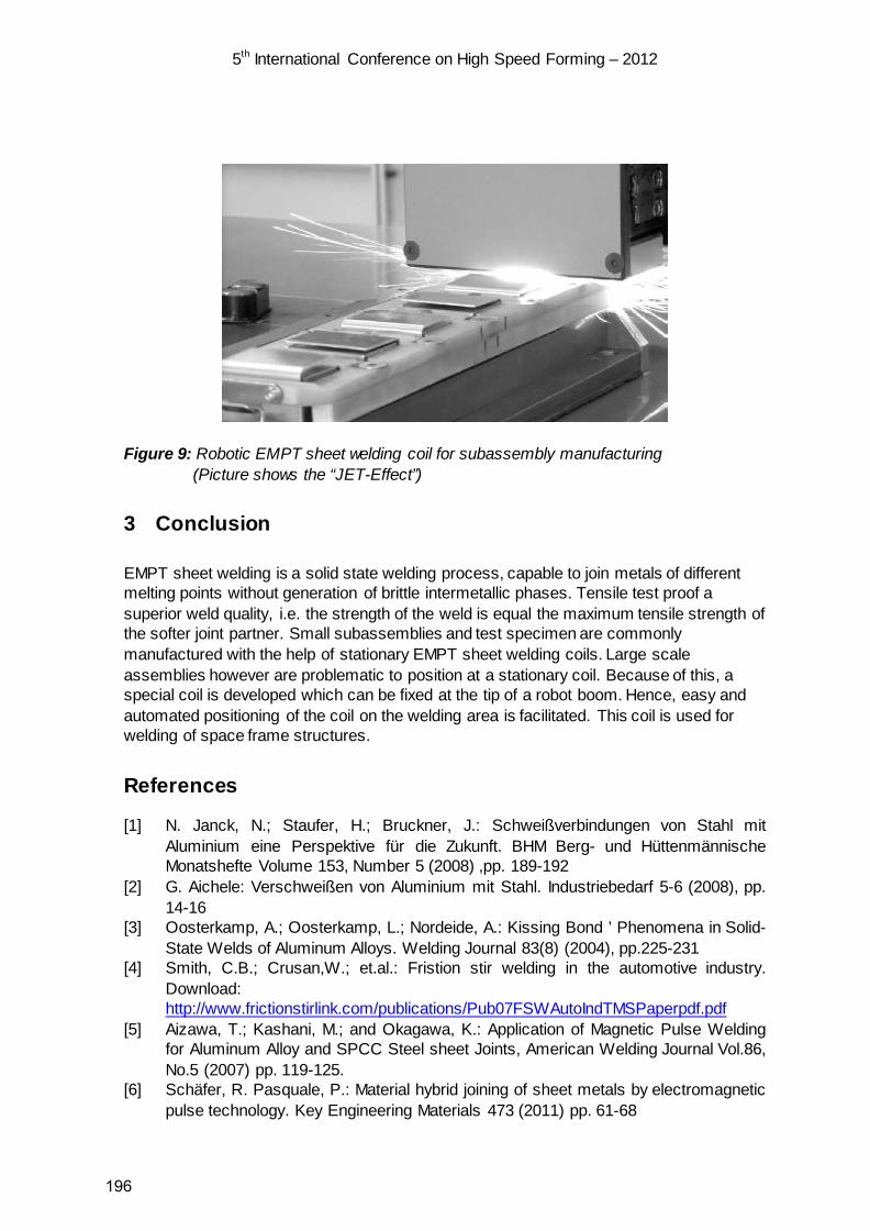
5th International Conference on High Speed Forming – 2012
Figure 9: Robotic EMPT sheet welding coil for subassembly manufacturing (Picture shows the “JET-Effect”)
3 Conclusion
EMPT sheet welding is a solid state welding process, capable to join metals of different melting points without generation of brittle intermetallic phases. Tensile test proof a superior weld quality, i.e. the strength of the weld is equal the maximum tensile strength of the softer joint partner. Small subassemblies and test specimen are commonly manufactured with the help of stationary EMPT sheet welding coils. Large scale assemblies however are problematic to position at a stationary coil. Because of this, a special coil is developed which can be fixed at the tip of a robot boom. Hence, easy and automated positioning of the coil on the welding area is facilitated. This coil is used for welding of space frame structures.
References
[1] N. Janck, N.; Staufer, H.; Bruckner, J.: Schweißverbindungen von Stahl mit Aluminium eine Perspektive für die Zukunft. BHM Berg- und Hüttenmännische Monatshefte Volume 153, Number 5 (2008) ,pp. 189-192
[2] G. Aichele: Verschweißen von Aluminium mit Stahl. Industriebedarf 5-6 (2008), pp. 14-16
[3] Oosterkamp, A.; Oosterkamp, L.; Nordeide, A.: Kissing Bond ’ Phenomena in Solid-State Welds of Aluminum Alloys. Welding Journal 83(8) (2004), pp.225-231
[4] Smith, C.B.; Crusan,W.; et.al.: Fristion stir welding in the automotive industry. Download: http://www.frictionstirlink.com/publications/Pub07FSWAutoIndTMSPaperpdf.pdf
[5] Aizawa, T.; Kashani, M.; and Okagawa, K.: Application of Magnetic Pulse Welding for Aluminum Alloy and SPCC Steel sheet Joints, American Welding Journal Vol.86, No.5 (2007) pp. 119-125.
[6] Schäfer, R. Pasquale, P.: Material hybrid joining of sheet metals by electromagnetic pulse technology. Key Engineering Materials 473 (2011) pp. 61-68
196

Process Model and Design for Magnetic Pulse Welding by Tube Expansion*
V. Psyk1*, G. Gerstein2, B. Barlage1, B. Albuja1, S. Gies.1, A. E. Tekkaya1, F.-W. Bach2 1 Institute of Forming Technology and Lightweight Construction, TU Dortmund, Germany 2 Institute of Materials Science, Leibniz Universität Hannover, Germany
Abstract
In this paper a design methodology for magnetic pulse welding processes is presented. To examine fundamental correlations of part- and process-parameters, a model experiment is used. Different impacting conditions are tested and the effect on the joint quality is evaluated by metallographic analysis. Conclusions regarding suitable impacting parameters are drawn. Electromagnetic expansion tests are carried out in parallel with the aim of adjusting the impacting parameters via typical process parameters. Therefore, the forming velocity is measured online and the impacting angle is varied via the geometry of the joining zone. To verify that the tendencies observed in the model experiment occur also in magnetic pulse welding, the influence of the impacting parameters on the joint quality is investigated for magnetic pulse welded tubes, too. Finally, the results of both investigation paths are combined and serve as a basis for target-oriented design of magnetic pulse forming processes.
Keywords
Magnetic pulse welding, model experiment, metallographic evaluation
* The presented work was performed in the project “Investigation of the complex interdependencies during electromagnetic tube forming” TE 508/19-1 and BA 851/103-1. The authors wish to thank the German Research Foundation DFG for the financial support. * At Fraunhofer Institute for Machine Tools and Forming Technology, Germany since August 2011.
197
5th International Conference on High Speed Forming – 2012
1 Introduction
In these days an enterprise’s reputation and position at the market does not depend on the product quality and image exclusively but politics and society demand for more efficient and economical products especially because of the steadily shrinking resources and for reasons of environmental protection [1]. These requirements concern the whole life cycle of a product [2]. Consequently, the ecological footprint, which evaluates the ecological effects of an activity or product, has become an important characteristic for many institutions and companies [3].
This affects especially but not exclusively the mobility industry. Here, the development of new and improved driving concepts as hybrid and electric ones are an important step to reduce emissions, but also the consequent implementation of lightweight construction concepts significantly contributes to reducing the ecological footprint [1]. These concepts include among other aspects weight reduction via substitution of conventional materials by typical light weight materials as e.g. light metal alloys and fibre-reinforces plastics. According to [4], maximum effect can be achieved if the best fitting material with regard to the special load and function is applied for every component. Although there are some impressive examples for multi-material design as the Audi R8 Spyder and the Boeing 787 Dreamliner, such implementation examples are far away from being the standard. One reason is that the joining of dissimilar materials still leads to severe problems when applying conventional i.e. usually thermal joining technologies as welding and soldering. While connections of metal to non-metal components are normally not possible at all, even joining of some similar and especially of dissimilar metallic components entails difficulties and can lead to microstructural defects as softening or formation of oxidic or intermetallic phases [5].
To avoid these problems, solid state welding techniques can be applied, because they are carried out without large heating and melting of the workpiece. Among these techniques magnetic pulse welding is a promising example, because it can be used for connecting profile shaped as well as sheet metal components of similar and dissimilar metallic materials at room temperature and without additives and it can be automated easily [6].
2 Principle of and Design Strategy for Magnetic Pulse Welding
Analogue to electromagnetic forming, magnetic pulse welding uses the energy density of pulsed magnetic fields to exert a so-called magnetic pressure to workpieces ideally made of an electrically highly conductive material and accelerate them accordingly without mechanical contact. More detailed information about the process principle and variants of electromagnetic forming is given e.g. in [6]. In magnetic pulse welding the accelerated workpiece approximates the joining partner at very high velocity in the magnitude of 102 m/s to atomic distance. During collision the joining partners behave like highly viscous fluids and – provided that the process parameters are adequately chosen – an intermetallic joint characterized by a typically but not necessarily wavy weld seam results. Magnetic pulse welding was mentioned in literature for the first time in the patent by Lysenko et al. [7].
198
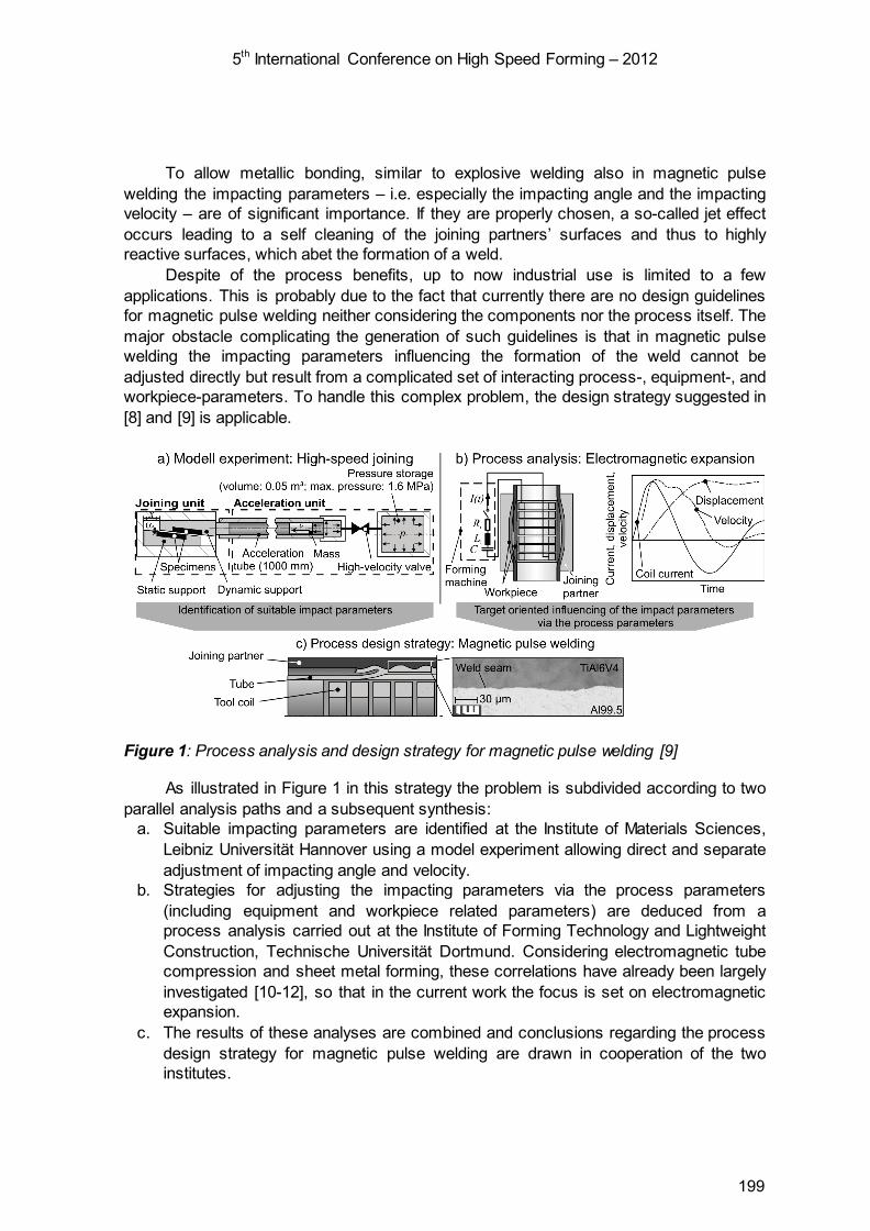
5th International Conference on High Speed Forming – 2012
To allow metallic bonding, similar to explosive welding also in magnetic pulse welding the impacting parameters – i.e. especially the impacting angle and the impacting velocity – are of significant importance. If they are properly chosen, a so-called jet effect occurs leading to a self cleaning of the joining partners’ surfaces and thus to highly reactive surfaces, which abet the formation of a weld.
Despite of the process benefits, up to now industrial use is limited to a few applications. This is probably due to the fact that currently there are no design guidelines for magnetic pulse welding neither considering the components nor the process itself. The major obstacle complicating the generation of such guidelines is that in magnetic pulse welding the impacting parameters influencing the formation of the weld cannot be adjusted directly but result from a complicated set of interacting process-, equipment-, and workpiece-parameters. To handle this complex problem, the design strategy suggested in [8] and [9] is applicable.
Figure 1: Process analysis and design strategy for magnetic pulse welding [9]
As illustrated in Figure 1 in this strategy the problem is subdivided according to two parallel analysis paths and a subsequent synthesis:
a. Suitable impacting parameters are identified at the Institute of Materials Sciences, Leibniz Universität Hannover using a model experiment allowing direct and separate adjustment of impacting angle and velocity.
b. Strategies for adjusting the impacting parameters via the process parameters (including equipment and workpiece related parameters) are deduced from a process analysis carried out at the Institute of Forming Technology and Lightweight Construction, Technische Universität Dortmund. Considering electromagnetic tube compression and sheet metal forming, these correlations have already been largely investigated [10-12], so that in the current work the focus is set on electromagnetic expansion.
c. The results of these analyses are combined and conclusions regarding the process design strategy for magnetic pulse welding are drawn in cooperation of the two institutes.
199

5th International Conference on High Speed Forming – 2012
3 Model experiment
The setup of the model experiment for high-speed joining is shown in Figure 1a. A detailed description of the setup and the process principle can be found e.g. in [9], so that in the following only the most relevant aspects with regard to the impacting parameter adjustment are described before focussing on the experimental results.
3.1 Adjustment of the impacting parameters
In the model experiment the specimens are fixed to the static and the dynamic support – two tapered components whose tapering angle directly corresponds to the impacting angle. Thus, the impacting angle can be varied stepwisely by using different supports.
The impacting velocity is the dynamic support’s velocity during collision. It can be adjusted via the pneumatic drive of the machine and depends on the applied mass. The energy source in the setup is pneumatic pressure storage. Opening the high-velocity valve releases the pressure und accelerates a mass to a velocity vm. The mass flies through an acceleration tube until it impacts to the dynamic support. The kinetic energy of the mass is partly transferred to the support, which is accordingly accelerated to a velocity vs and impacts with the static support. The transfer of the kinetic energy and the according impulse depends on the mass properties. If the mass weight is too small it bounces from the dynamic support without significantly accelerating it. Therefore, in many cases increasing the mass weight improved the welding quality. Moreover, the mass material must not be too soft because otherwise the kinetic energy of the mass is transferred to deformation energy. For example in case of lead masses – which appeared to be well-suited because of their high density and weight – large plastic deformation of the mass occurred, and consequently the efficiency of the support acceleration was reduced. On the other hand, the acceleration tube might be damaged if the mass is too hard. Experience has shown that in many cases brass is a well suited mass material. During the experiments the impacting velocity was measured by an optical technology [9].
3.2 Investigation results
In the experiments different material combinations have been regarded. The impacting angle and velocity were varied and the resulting joints were evaluated by metallographic analyses. In the following, general influences are shown on the basis of representative joining results and suitable impacting parameters for different material combinations are listed in Table 1. Thus, the essential investigation results of this analysis path are excerpted.
In Figure 2 the influence of the impacting angle is shown on the example of different copper-copper and aluminium-aluminium joints. It can be seen especially in the first row, which gives a good overview of nearly the complete joining area, that an impacting angle of 3.5° leads to the best joining result while the weld quality is lower in case of 2° and 6° angles. In the following rows a larger magnification was used to give a more precise view of the weld seam. However, in these pictures it was not possible to consider the complete joining area. Therefore, the area of highest welding quality was chosen in order to compare different specimens.
200
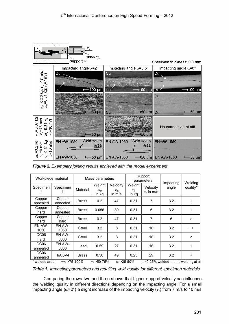
5th International Conference on High Speed Forming – 2012
Figure 2: Exemplary joining results achieved with the model experiment
Workpiece material Mass parameters Support parameters Impacting
angle Welding quality* Specimen
I Specimen
II Material Weight
mm in kg
Velocity vm
in m/s
Weight ms
in kg
Velocity vs in m/s
Copper annealed
Copper annealed Brass 0.2 47 0.31 7 3.2 +
Copper hard
Copper annealed Brass 0.056 89 0.31 6 3.2 +
Copper hard
Copper hard Brass 0.2 47 0.31 7 6 o
EN AW- 1050
EN AW- 1050 Steel 3.2 8 0.31 16 3.2 ++
DC06 hard
EN AW-6060 Steel 3.2 8 0.31 16 3.2 o
DC06 annealed
EN AW-6060 Lead 0.59 27 0.31 16 3.2 +
DC06 annealed TiAl6V4 Brass 0.56 49 0.25 29 3.2 +
* welded area: ++: >75-100% +: >50-75% o: >25-50% -: >0-25% welded --: no welding at all
Table 1: Impacting parameters and resulting weld quality for different specimen materials
Comparing the rows two and three shows that higher support velocity can influence the welding quality in different directions depending on the impacting angle. For a small impacting angle (α=2°) a slight increase of the impacting velocity (vs) from 7 m/s to 10 m/s
201
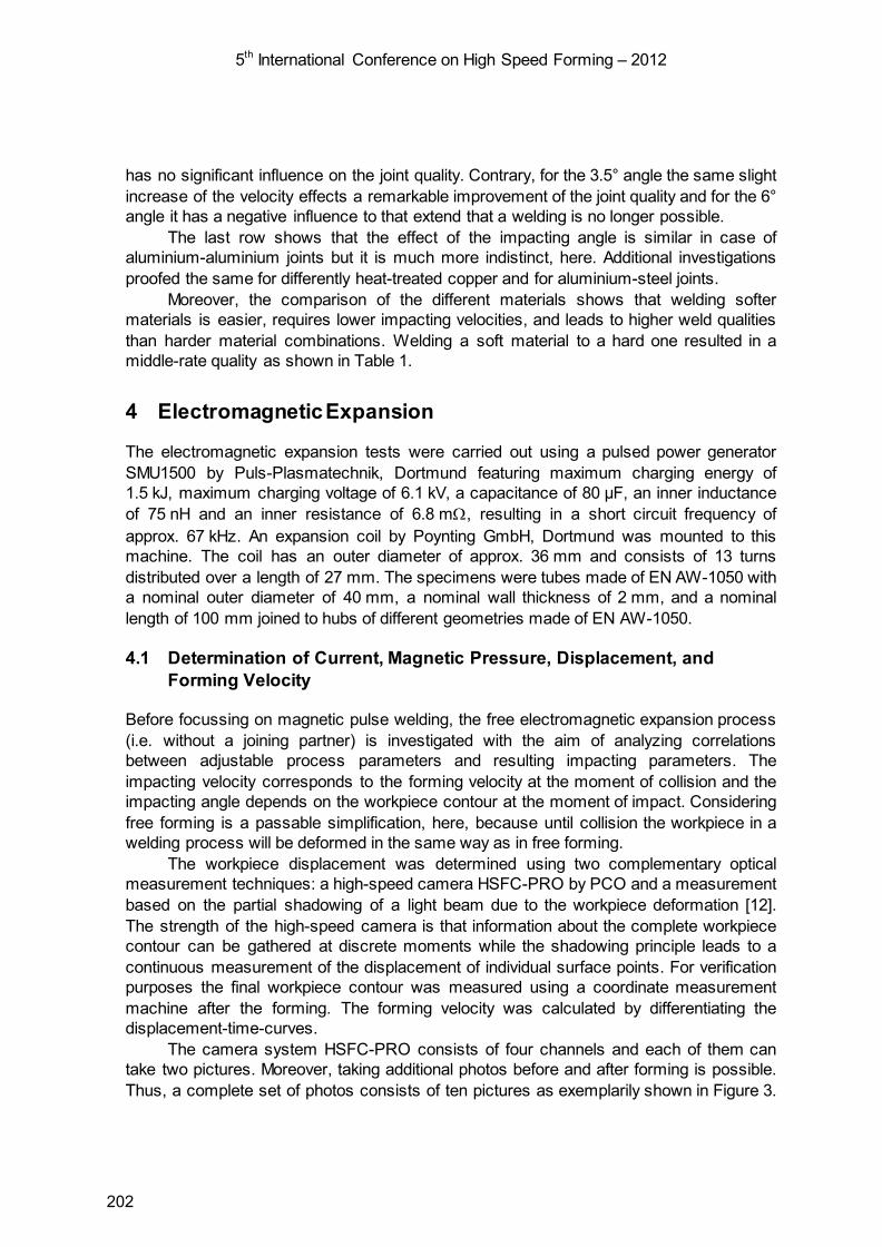
5th International Conference on High Speed Forming – 2012
has no significant influence on the joint quality. Contrary, for the 3.5° angle the same slight increase of the velocity effects a remarkable improvement of the joint quality and for the 6° angle it has a negative influence to that extend that a welding is no longer possible.
The last row shows that the effect of the impacting angle is similar in case of aluminium-aluminium joints but it is much more indistinct, here. Additional investigations proofed the same for differently heat-treated copper and for aluminium-steel joints.
Moreover, the comparison of the different materials shows that welding softer materials is easier, requires lower impacting velocities, and leads to higher weld qualities than harder material combinations. Welding a soft material to a hard one resulted in a middle-rate quality as shown in Table 1.
4 Electromagnetic Expansion
The electromagnetic expansion tests were carried out using a pulsed power generator SMU1500 by Puls-Plasmatechnik, Dortmund featuring maximum charging energy of 1.5 kJ, maximum charging voltage of 6.1 kV, a capacitance of 80 µF, an inner inductance of 75 nH and an inner resistance of 6.8 mΩ, resulting in a short circuit frequency of approx. 67 kHz. An expansion coil by Poynting GmbH, Dortmund was mounted to this machine. The coil has an outer diameter of approx. 36 mm and consists of 13 turns distributed over a length of 27 mm. The specimens were tubes made of EN AW-1050 with a nominal outer diameter of 40 mm, a nominal wall thickness of 2 mm, and a nominal length of 100 mm joined to hubs of different geometries made of EN AW-1050.
4.1 Determination of Current, Magnetic Pressure, Displacement, and Forming Velocity
Before focussing on magnetic pulse welding, the free electromagnetic expansion process (i.e. without a joining partner) is investigated with the aim of analyzing correlations between adjustable process parameters and resulting impacting parameters. The impacting velocity corresponds to the forming velocity at the moment of collision and the impacting angle depends on the workpiece contour at the moment of impact. Considering free forming is a passable simplification, here, because until collision the workpiece in a welding process will be deformed in the same way as in free forming.
The workpiece displacement was determined using two complementary optical measurement techniques: a high-speed camera HSFC-PRO by PCO and a measurement based on the partial shadowing of a light beam due to the workpiece deformation [12]. The strength of the high-speed camera is that information about the complete workpiece contour can be gathered at discrete moments while the shadowing principle leads to a continuous measurement of the displacement of individual surface points. For verification purposes the final workpiece contour was measured using a coordinate measurement machine after the forming. The forming velocity was calculated by differentiating the displacement-time-curves.
The camera system HSFC-PRO consists of four channels and each of them can take two pictures. Moreover, taking additional photos before and after forming is possible. Thus, a complete set of photos consists of ten pictures as exemplarily shown in Figure 3.
202

5th International Conference on High Speed Forming – 2012
In the following the notation t=∞ is used to indicate measurement data taken after the forming process is finished because an exact temporal correlation is not possible.
Figure 3: Set of high-speed photos taken during an electromagnetic expansion process
To get more detailed information about the forming stages it is possible to focus on a shorter time interval and compose the complete deformation course from pictures taken in different experiments. Tests have shown that the repeatability is sufficiently high to justify this procedure especially in the time-sequence relevant with regard to the subsequent joining tests. In case of large deformations and especially if cracking occurs, material inhomogeneities in the semi-finished parts influence the contour significantly, so that the repeatability is not guaranteed any longer.
In Figure 4 exemplary measurement results of the acting loads – characterized by coil current and resulting magnetic pressure – and the resulting workpiece deformation – quantified via displacement and velocity of the workpiece surface – are shown. According to [12] the magnetic pressure can be used as an abstract description of the acting loads which does not include any equipment- or setup-related parameters. The calculation of the magnetic pressure is based on a finite element simulation of the magnetic field carried out with the special purpose FE-programm FEMM by David Meeker [13], here. To consider interdependencies between the magnetic pressure and the workpiece deformation, the pressure was calculated for a short time-interval only. Then the workpiece contour was updated according to the measured deformation.
By comparing the temporary development of the curves it can clearly be recognized that due to the strong deformation of the workpiece the pressure collapses faster compared to the first half-wave of the coil current – a behaviour well known from electromagnetic sheet metal forming (e.g. [6, 12]) – and that no noteworthy pressure is exerted during the subsequent half waves of the current. As long as the pressure acts, the workpiece is accelerated. After the decay of the pressure inertia effects continue the deformation but at decreasing velocity. Considering the forming stages, it can be recognized that the displacement of the surface points in the middle area of the coil (i.e. for z-values of about 0-6 mm) is almost parallel to the initial geometry as already observed
203
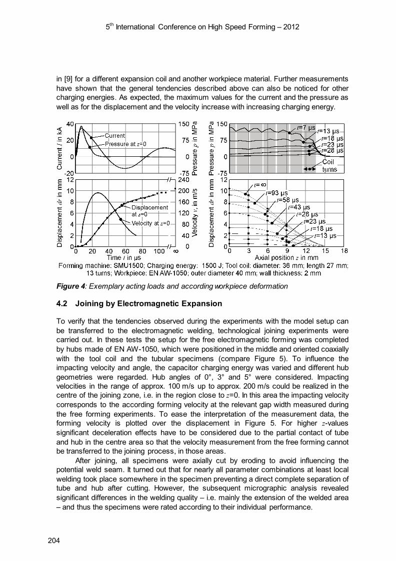
5th International Conference on High Speed Forming – 2012
in [9] for a different expansion coil and another workpiece material. Further measurements have shown that the general tendencies described above can also be noticed for other charging energies. As expected, the maximum values for the current and the pressure as well as for the displacement and the velocity increase with increasing charging energy.
Figure 4: Exemplary acting loads and according workpiece deformation
4.2 Joining by Electromagnetic Expansion
To verify that the tendencies observed during the experiments with the model setup can be transferred to the electromagnetic welding, technological joining experiments were carried out. In these tests the setup for the free electromagnetic forming was completed by hubs made of EN AW-1050, which were positioned in the middle and oriented coaxially with the tool coil and the tubular specimens (compare Figure 5). To influence the impacting velocity and angle, the capacitor charging energy was varied and different hub geometries were regarded. Hub angles of 0°, 3° and 5° were considered. Impacting velocities in the range of approx. 100 m/s up to approx. 200 m/s could be realized in the centre of the joining zone, i.e. in the region close to z=0. In this area the impacting velocity corresponds to the according forming velocity at the relevant gap width measured during the free forming experiments. To ease the interpretation of the measurement data, the forming velocity is plotted over the displacement in Figure 5. For higher z-values significant deceleration effects have to be considered due to the partial contact of tube and hub in the centre area so that the velocity measurement from the free forming cannot be transferred to the joining process, in those areas.
After joining, all specimens were axially cut by eroding to avoid influencing the potential weld seam. It turned out that for nearly all parameter combinations at least local welding took place somewhere in the specimen preventing a direct complete separation of tube and hub after cutting. However, the subsequent micrographic analysis revealed significant differences in the welding quality – i.e. mainly the extension of the welded area – and thus the specimens were rated according to their individual performance.
204
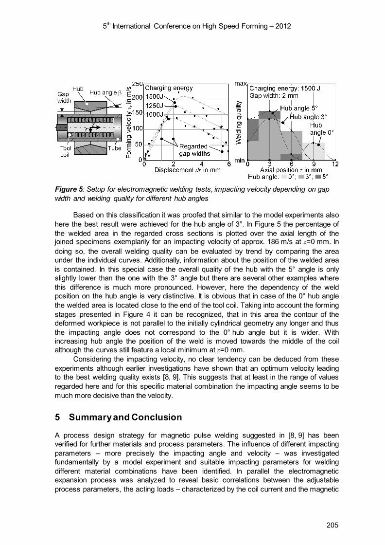
5th International Conference on High Speed Forming – 2012
Figure 5: Setup for electromagnetic welding tests, impacting velocity depending on gap width and welding quality for different hub angles
Based on this classification it was proofed that similar to the model experiments also here the best result were achieved for the hub angle of 3°. In Figure 5 the percentage of the welded area in the regarded cross sections is plotted over the axial length of the joined specimens exemplarily for an impacting velocity of approx. 186 m/s at z=0 mm. In doing so, the overall welding quality can be evaluated by trend by comparing the area under the individual curves. Additionally, information about the position of the welded area is contained. In this special case the overall quality of the hub with the 5° angle is only slightly lower than the one with the 3° angle but there are several other examples where this difference is much more pronounced. However, here the dependency of the weld position on the hub angle is very distinctive. It is obvious that in case of the 0° hub angle the welded area is located close to the end of the tool coil. Taking into account the forming stages presented in Figure 4 it can be recognized, that in this area the contour of the deformed workpiece is not parallel to the initially cylindrical geometry any longer and thus the impacting angle does not correspond to the 0° hub angle but it is wider. With increasing hub angle the position of the weld is moved towards the middle of the coil although the curves still feature a local minimum at z=0 mm.
Considering the impacting velocity, no clear tendency can be deduced from these experiments although earlier investigations have shown that an optimum velocity leading to the best welding quality exists [8, 9]. This suggests that at least in the range of values regarded here and for this specific material combination the impacting angle seems to be much more decisive than the velocity.
5 Summary and Conclusion
A process design strategy for magnetic pulse welding suggested in [8, 9] has been verified for further materials and process parameters. The influence of different impacting parameters – more precisely the impacting angle and velocity – was investigated fundamentally by a model experiment and suitable impacting parameters for welding different material combinations have been identified. In parallel the electromagnetic expansion process was analyzed to reveal basic correlations between the adjustable process parameters, the acting loads – characterized by the coil current and the magnetic
205
5th International Conference on High Speed Forming – 2012
pressure –, the resulting workpiece deformation – characterized by the forming stages and the velocity –, and the according impacting parameters during magnetic pulse welding. The comparison of model experiment and technological investigations shows that the general trends regarding the impacting parameters’ influence on the weld are transferable and concerning the impacting angle even the quantitative values are similar. However, the required impacting velocities during magnetic pulse welding are significantly higher than in the model experiment. This might be attributed to the differencies in the specimen size and the impacting mass. In the model experiment specimen size and welding zone are drastically smaller, but the impacting masses – also including the mass of the supports – are much higher.
References
[1] Neugebauer, R.; Putz, M.; Schieck, F.; Treppe, F.; Sterzing, A.: Ressourceneffiziente Karosserieherstellung. In: Manufacture of Car Bodies – Sustainable and Efficient, The 6th Chemnitz Car Body Colloquium CBC 2011, pp. 39-67.
[2] Heizmann, J.: Nachhaltige Produktion in der Automobilindustrie. In: Manufacture of Car Bodies – Sustainable and Efficient, The 6th Chemnitz Car Body Colloquium CBC 2011, pp. 69-81.
[3] Giljum, S.; Hammer, M.; Stocker, A.; Lackner M.: Wissenschaftliche Untersuchung und Bewertung des Indikators " Ökologischer Fußabdruck". Umweltbundesamt, 12 2007.
[4] Lesemann, M.; Sahr, C.; Hart, S.; Taylor, R.: SuperaLIGHT-CAR – The Multi Material Car Body. In: Proceedings of the 7th LS-DYNA Anwenderforum, 2008.
[5] Bargel, H.-J.; Schulze, G.: Werkstoffkunde. 10. Auflage. Springer Verlag, 2008. [6] Psyk, V.; D. Risch, B.L. Kinsey, A.E. Tekkaya, M. Kleiner: Electromagnetic Forming
– A Review. Journal of Materials Processing Technology 211 (2011), pp. 787-829. [7] Lysenko, N.; Ermolaev, V. V.; Dudin, A. A.: U.S. Patent 3,520,049, 1970. [8] Psyk, V.; Gershteyn, G.; Demir, O. K.; Brosius, A.; Tekkaya, A. E.; Schaper, M.;
Bach, F.-W.: Process Analysis and Physical Simulation of Electromagnetic Joining of Thin-Walled parts. In: Proceedings of the 3rd International Conference on High Speed Forming – ICHSF 2008, pp. 181-190, 2008.
[9] Psyk, V.; Gershteyn, G.; Barlage, B.; Weddeling, C.; Albuja, B.; Brosius, A.; Tekkaya, A. E.; Bach, F.-W.: Process Design for the Manufacturing of Magnetic Pulse Welded Joints. Key Engineering Materials Vol. 473, S. 243-250, 2011. DOI: 10.4028/www.scientific.net/KEM.473.243.
[10] Psyk, V.: Prozesskette Krümmen – Elektromagnetisch Komprimieren – Innenhochdruckumformen für Rohre und profilförmige Bauteile. Dr.-Ing. Dissertation, TU Dortmund.
[11] Risch, D.: Energietransfer und Analyse der Einflussparameter bei der form-gebundenen elektromagnetischen Blechumformung. Dr.-Ing. Dissertation, TU Dortmund.
[12] Beerwald, C.: Grundlagen der Prozessauslegung und –gestaltung bei der elektromagnetischen Umformung. Dr.-Ing. Dissertation, TU Dortmund.
[13] http://www.femm.info/wiki/HomePage (shown on 03.01.2012).
206

Assessment of Gap and Charging Voltage Influence on Mechanical Behaviour of Joints Obtained by Magnetic Pulse Welding*
R. Raoelison1, M. Rachik1, N. Buiron1, D. Haye2, M. Morel2, B. Dos Sanstos2, D. Jouaffre2, G. Frantz3
1 Laboratoire Roberval, Université de Technologie de Compiègne, France, 2 PFT INNOVALTECH, Saint-Quentin, France, 3 LTI, UPJV, Amiens, France.
Abstract
This work investigates the study of the experimental weldability in magnetic pulse welding process of a one material assembly (aluminium AA6060T6) and a dissimilar metal couple (aluminium6060T6/copper). The weld quality is defined using a destructive process allowing measuring the weld dimension. A diagram charging voltage-air gap is used to establish the variance of weldability. With the criterion of width of the weld, this representation is able to determine the operational weldability window. The lower boundary is defined by the case of bad weld, i.e. an insufficient bonding, and the upper boundary by defective welds, i.e. a weld susceptible to crack. The weld is able to undergo a plastic deformation prior to failure. A large weld is more potentially ductile. A numerical modelling of a mechanical destructive push out test could be helpful to characterise the weld in a quantitative manner. Finally, the material dissymmetry as considered in this study notably reduces the weldability window because of intermetallic phase at the welded interface. For this case, the weld is found to have a rather brittle behaviour.
Keywords
Cold welding, Condition, Damage.
* This work is based on the results of the project MSIM; the authors would like to thank Le Conseil Régional de Picardie for its financial support.
207
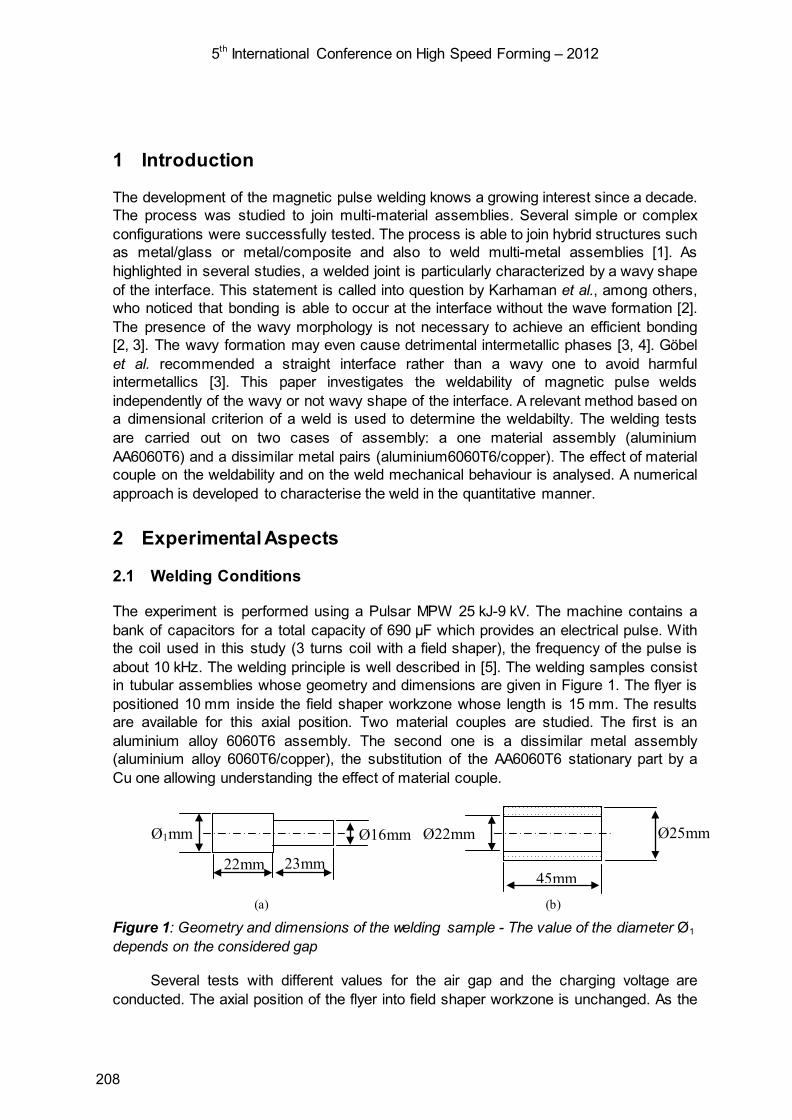
5th International Conference on High Speed Forming – 2012
1 Introduction
The development of the magnetic pulse welding knows a growing interest since a decade. The process was studied to join multi-material assemblies. Several simple or complex configurations were successfully tested. The process is able to join hybrid structures such as metal/glass or metal/composite and also to weld multi-metal assemblies [1]. As highlighted in several studies, a welded joint is particularly characterized by a wavy shape of the interface. This statement is called into question by Karhaman et al., among others, who noticed that bonding is able to occur at the interface without the wave formation [2]. The presence of the wavy morphology is not necessary to achieve an efficient bonding [2, 3]. The wavy formation may even cause detrimental intermetallic phases [3, 4]. Göbel et al. recommended a straight interface rather than a wavy one to avoid harmful intermetallics [3]. This paper investigates the weldability of magnetic pulse welds independently of the wavy or not wavy shape of the interface. A relevant method based on a dimensional criterion of a weld is used to determine the weldabilty. The welding tests are carried out on two cases of assembly: a one material assembly (aluminium AA6060T6) and a dissimilar metal pairs (aluminium6060T6/copper). The effect of material couple on the weldability and on the weld mechanical behaviour is analysed. A numerical approach is developed to characterise the weld in the quantitative manner.
2 Experimental Aspects
2.1 Welding Conditions
The experiment is performed using a Pulsar MPW 25 kJ-9 kV. The machine contains a bank of capacitors for a total capacity of 690 µF which provides an electrical pulse. With the coil used in this study (3 turns coil with a field shaper), the frequency of the pulse is about 10 kHz. The welding principle is well described in [5]. The welding samples consist in tubular assemblies whose geometry and dimensions are given in Figure 1. The flyer is positioned 10 mm inside the field shaper workzone whose length is 15 mm. The results are available for this axial position. Two material couples are studied. The first is an aluminium alloy 6060T6 assembly. The second one is a dissimilar metal assembly (aluminium alloy 6060T6/copper), the substitution of the AA6060T6 stationary part by a Cu one allowing understanding the effect of material couple.
Ø22mm Ø25mm
45mm
Ø16mm Ø1mm 22mm
23mm
(a) (b)
Figure 1: Geometry and dimensions of the welding sample - The value of the diameter Ø1 depends on the considered gap
Several tests with different values for the air gap and the charging voltage are conducted. The axial position of the flyer into field shaper workzone is unchanged. As the
208
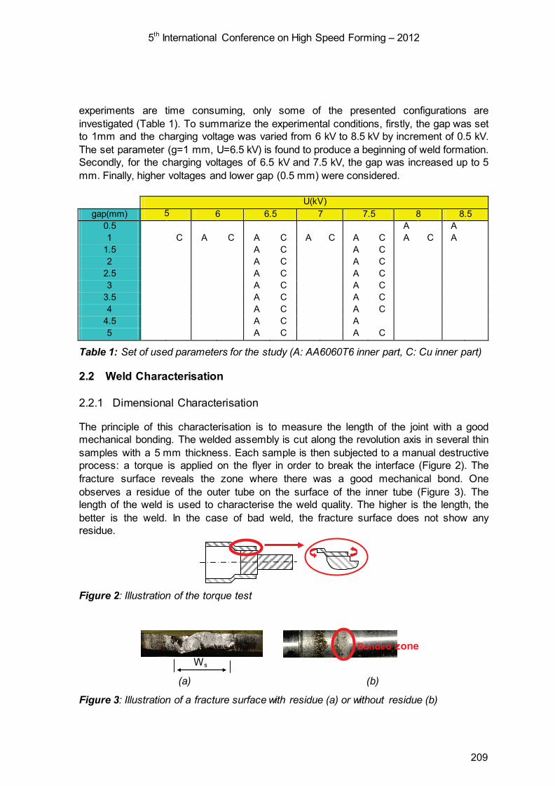
5th International Conference on High Speed Forming – 2012
experiments are time consuming, only some of the presented configurations are investigated (Table 1). To summarize the experimental conditions, firstly, the gap was set to 1mm and the charging voltage was varied from 6 kV to 8.5 kV by increment of 0.5 kV. The set parameter (g=1 mm, U=6.5 kV) is found to produce a beginning of weld formation. Secondly, for the charging voltages of 6.5 kV and 7.5 kV, the gap was increased up to 5 mm. Finally, higher voltages and lower gap (0.5 mm) were considered.
U(kV)
gap(mm) 5 6 6.5 7 7.5 8 8.5 0.5 A A 1 C A C A C A C A C A C A
1.5 A C A C 2 A C A C
2.5 A C A C 3 A C A C
3.5 A C A C 4 A C A C
4.5 A C A 5 A C A C
Table 1: Set of used parameters for the study (A: AA6060T6 inner part, C: Cu inner part)
2.2 Weld Characterisation
2.2.1 Dimensional Characterisation
The principle of this characterisation is to measure the length of the joint with a good mechanical bonding. The welded assembly is cut along the revolution axis in several thin samples with a 5 mm thickness. Each sample is then subjected to a manual destructive process: a torque is applied on the flyer in order to break the interface (Figure 2). The fracture surface reveals the zone where there was a good mechanical bond. One observes a residue of the outer tube on the surface of the inner tube (Figure 3). The length of the weld is used to characterise the weld quality. The higher is the length, the better is the weld. In the case of bad weld, the fracture surface does not show any residue.
Figure 2: Illustration of the torque test
(a) (b)
Figure 3: Illustration of a fracture surface with residue (a) or without residue (b)
Ws Bonded zone
209

5th International Conference on High Speed Forming – 2012
2.2.2 Mechanical Characterisation
A push out test is used to characterise the mechanical features of the weld. The test was performed to specifically load the interface until the rupture of the weld [6]. After welding, the outer tube is machined to keep only the welded part identified by the dimensional characterisation described above. A compression force is applied on the inner tube while the outer tube is contained inside a steel hollow piece (Figure 4). As the welded interface is not parallel to the load direction, it is submitted to combined shear and separation but shear is dominant. After the rupture of the interface, the outer tube is completely pushed out. The analysis of the measured force-displacement curve allows also characterising the mechanical behaviour of the weld.
Inner tube
Flyer Weld
Compression
Figure 4: Illustration of the push-out test [6]
3 Numerical Aspects
To characterise the weld in a quantitative manner, a finite element model is used to analyse the push out test. Abaqus software is used for this purpose. The meshed finite element model is described in Figure 5. The flyer and the fixed part are discretized using for nodded axisymmetric solid element (CAX4R). The welded interface is modelled using cohesive elements. The other parts involved in the test are considered as rigid body.
Figure 5: Illustration of the meshing for the F.E modelling
For the constitutive modelling, the flyer and the fixed part behaviour are described using simple J2 elastic-plastic model with isotropic work hardening. The interface behaviour is described using a linear traction separation model associated with a progressive damage model. To define the parameters that characterise the interface, the damage initiation and the damage evolution models used in this work are briefly recalled in the following section.
Cohesive element
CAX4R element
210

5th International Conference on High Speed Forming – 2012
3.1 Damage Initiation
The material degradation process is assumed to begin when the stress or the strain met a certain criteria. In this work, the maximum nominal stress criterion is used:
0 0 0max , , 1n s t
n s t
t t tt t t
=
(1)
nt is nominal stress in the direction normal to the interface, and ont peak value. st and tt
are the nominal stress in the first and second shear direction. Likewise, ost and o
tt are their respective peak value. The overall objective of this model is to predict the damage initiation of reliable welded joint. For this reason, the discontinuities inherent to the welding process are not taken into account as initial damage.
3.2 Damage Evolution
A simple linear damage evolution is considered to describe the progressive damage at the interface. A criterion of energy dissipated due to failure is used to the definition of the damage evolution. The scalar damage variable, namely D, is a function of the effective displacement at the interface:
( )( )
max 0
max 0
fm m m
fm m m
Dδ δ δ
δ δ δ
−=
− (2)
maxmδ is the maximum value of the effect displacement reached during the loading history,
and 0mδ the effective displacement at damage initiation. f
mδ is the effective displacement at damage initiation at complete failure which is defined as a function of the fracture energy as follows:
0
2 cf
meff
GT
δ = (3)
0
effT is the effective traction at damage initiation and cG the fracture energy that is the input damage parameter to describe the damage evolution.
After the damage initiation, the stress components of the traction-separation model are degraded by the damage evolution as follows:
( ) ,1 0
,n n
nn
D t tt
t − ≥=
(4)
( ) ,1s st D t= − (5)
211

5th International Conference on High Speed Forming – 2012
( ) ,1t tt D t= − (6) where the notation t means stress components calculated by the traction-separation behaviour for the current strains without damage. The set of parameters describing the interface behaviour i.e. the nominal peak stresses and the fracture energy are adjusted to reproduce the experimental evolution of the measured push-out force versus displacement.
4 Results and Discussion
4.1 Weld Characteristic
The weldability study of the aluminium AA6060T6 assembly allows providing further insights into the features a weld. The dimensional characterisation highlights four weld kinds that are obtained by increasing the air gap value rather than the charging voltage. There is a bad weld, a thin ring-shaped weld, a large and potentially ductile weld and lastly, a large joint with discontinuous voids. The bad weld is a case of an insufficient bonding. The interfacial bond breaks while the welded assembly is cut in the revolution axis because of the relaxation of the residual stress in the outer part due to the shrinking occurring within the compression of the outer tube. The fracture surface looks like an adhesive fracture (Figure 6a). The destructive torque test reveals as a beginning of a good bonding, a thin weld with a ring shape (Figure 6b). With the gap increase, the weld becomes larger and the fracture surface after the torque test shows an area with a circular path (Figure 6c). Indeed, the interfacial residue reveals a rotational deformation under the action of the torque load. Then, the weld is potentially ductile. Above a critical air gap value, it has been observed that the welded interface contains discontinuous voids (Figure 7). This damage is attributable to a strong interfacial shearing due to high impact velocity occurring at high gap. This defect decreases the effective bonding surface and creates crack initiations that could be detrimental to the integrity of the joint.
(a) (b) (c)
Figure 6: Illustration of a bad weld (a), a thin ring-shaped weld (b) and a large weld (c)
Figure 7: Illustration of a welded interface with discontinuous voids
The typical mechanical behaviour of the weld previously identified is compared in Figure 8. The push out test has evidenced an elastic-plastic behaviour of both thin and large weld. This result proves that the interface is able to undergo plastic deformation prior to failure. The large weld is more potentially ductile. Moreover, a good weld reveals a ductile damage behaviour. If the joint contains discontinuous voids, the weld still has a
212

5th International Conference on High Speed Forming – 2012
plastic behaviour but the rupture occurs brutally. The measured force quickly collapses during the failure.
0
5
10
15
20
0 0,5 1 1,5 2 2,5
Ucolumn(mm)
F(kN)
Large weldThin weldWeld with voids
Figure 8: Illustration of the typical behaviour of the identified weld –The non linear response at the beginning of the measure is attributable to the contact accommodation
The numerical model of the push-out test predicts the force/displacement response prior to failure (Figure 9). The simulation does not account for the initial curve due to sliding at the contact surfaces. The numerical result is also able to reproduce the failure response of the weld as shows the Figure 9. The numerical model is currently developed to accurately predict the weld mechanical behaviour. This strategy may be helpful to found quantitative correlations between the joining process parameters, the structure of the interface and its mechanical behaviour.
0
2
4
6
8
0 0,1 0,2 0,3 0,4 0,5
U (mm)
F (kN)
Experiment
Simulation
Figure 9: Illustration of a comparison between the numerical and the experimental result
4.2 Weldability Window
In impact welding, as the precise mechanism of the weld formation is still misunderstood, the elaboration of weldability window remains problematic. Deribas et al. [7] suggested a weld lobe depending on the collision angle and the impact velocity. The authors used as weld criterion the formation of the interfacial wavy shape that is found to be predicted by this couple of parameters. Zhang et al. [8] brought an experimental approach to build such a weldability window by measuring the welding velocity and deducing the collision angle. The operational window is obtained for a range of low value of the collision angle. Uhlmann and Ziefle [9] claimed that weld formation depends on several parameters and could occur even at high collision angle. Situations of low collision angle without weld formation have also been observed. Dhanesh et al [10] used numerical simulation to build weldability windows for sheet metal joining taking into account several process parameters. In our study, a practical way to define the weldability is suggested. The weld
213
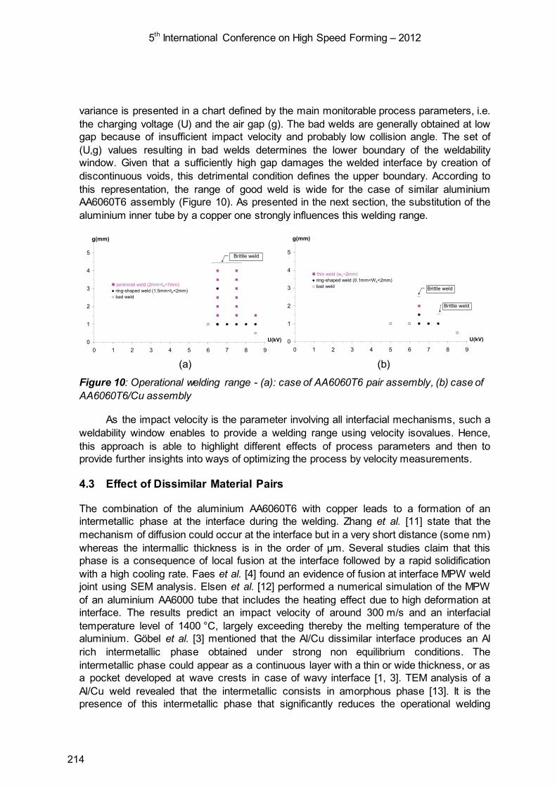
5th International Conference on High Speed Forming – 2012
variance is presented in a chart defined by the main monitorable process parameters, i.e. the charging voltage (U) and the air gap (g). The bad welds are generally obtained at low gap because of insufficient impact velocity and probably low collision angle. The set of (U,g) values resulting in bad welds determines the lower boundary of the weldability window. Given that a sufficiently high gap damages the welded interface by creation of discontinuous voids, this detrimental condition defines the upper boundary. According to this representation, the range of good weld is wide for the case of similar aluminium AA6060T6 assembly (Figure 10). As presented in the next section, the substitution of the aluminium inner tube by a copper one strongly influences this welding range.
(a) (b)
Figure 10: Operational welding range - (a): case of AA6060T6 pair assembly, (b) case of AA6060T6/Cu assembly
As the impact velocity is the parameter involving all interfacial mechanisms, such a weldability window enables to provide a welding range using velocity isovalues. Hence, this approach is able to highlight different effects of process parameters and then to provide further insights into ways of optimizing the process by velocity measurements.
4.3 Effect of Dissimilar Material Pairs
The combination of the aluminium AA6060T6 with copper leads to a formation of an intermetallic phase at the interface during the welding. Zhang et al. [11] state that the mechanism of diffusion could occur at the interface but in a very short distance (some nm) whereas the intermallic thickness is in the order of µm. Several studies claim that this phase is a consequence of local fusion at the interface followed by a rapid solidification with a high cooling rate. Faes et al. [4] found an evidence of fusion at interface MPW weld joint using SEM analysis. Elsen et al. [12] performed a numerical simulation of the MPW of an aluminium AA6000 tube that includes the heating effect due to high deformation at interface. The results predict an impact velocity of around 300 m/s and an interfacial temperature level of 1400 °C, largely exceeding thereby the melting temperature of the aluminium. Göbel et al. [3] mentioned that the Al/Cu dissimilar interface produces an Al rich intermetallic phase obtained under strong non equilibrium conditions. The intermetallic phase could appear as a continuous layer with a thin or wide thickness, or as a pocket developed at wave crests in case of wavy interface [1, 3]. TEM analysis of a Al/Cu weld revealed that the intermetallic consists in amorphous phase [13]. It is the presence of this intermetallic phase that significantly reduces the operational welding
0
1
2
3
4
5
0 1 2 3 4 5 6 7 8 9
U(kV)
g(mm)
thin weld (ws~2mm) ring-shaped weld (0.1mm<Ws<2mm) bad weld Brittle weld
Brittle weld
0
1
2
3
4
5
0 1 2 3 4 5 6 7 8 9
U(kV)
g(mm)
perennial weld (2mm<ts<7mm) ring-shaped weld (1.5mm<ts<2mm) bad weld
Brittle weld
214
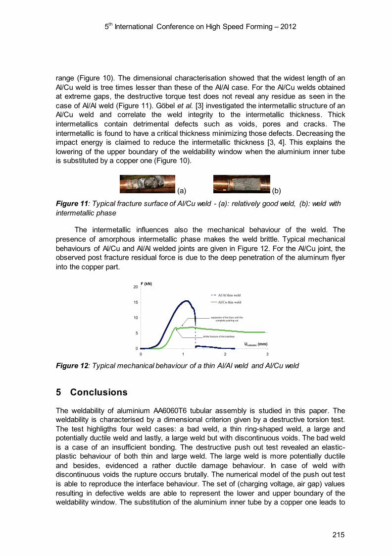
5th International Conference on High Speed Forming – 2012
range (Figure 10). The dimensional characterisation showed that the widest length of an Al/Cu weld is tree times lesser than these of the Al/Al case. For the Al/Cu welds obtained at extreme gaps, the destructive torque test does not reveal any residue as seen in the case of Al/Al weld (Figure 11). Göbel et al. [3] investigated the intermetallic structure of an Al/Cu weld and correlate the weld integrity to the intermetallic thickness. Thick intermetallics contain detrimental defects such as voids, pores and cracks. The intermetallic is found to have a critical thickness minimizing those defects. Decreasing the impact energy is claimed to reduce the intermetallic thickness [3, 4]. This explains the lowering of the upper boundary of the weldability window when the aluminium inner tube is substituted by a copper one (Figure 10).
(a) (b)
Figure 11: Typical fracture surface of Al/Cu weld - (a): relatively good weld, (b): weld with intermetallic phase
The intermetallic influences also the mechanical behaviour of the weld. The presence of amorphous intermetallic phase makes the weld brittle. Typical mechanical behaviours of Al/Cu and Al/Al welded joints are given in Figure 12. For the Al/Cu joint, the observed post fracture residual force is due to the deep penetration of the aluminum flyer into the copper part.
0
5
10
15
20
0 1 2 3
Ucolumn (mm)
F (kN)
Al/Al thin weld
Al/Cu thin weld
brittle fracture of the interface
expansion of the flyer until the complete pushing out
Figure 12: Typical mechanical behaviour of a thin Al/Al weld and Al/Cu weld
5 Conclusions
The weldability of aluminium AA6060T6 tubular assembly is studied in this paper. The weldability is characterised by a dimensional criterion given by a destructive torsion test. The test highligths four weld cases: a bad weld, a thin ring-shaped weld, a large and potentially ductile weld and lastly, a large weld but with discontinuous voids. The bad weld is a case of an insufficient bonding. The destructive push out test revealed an elastic-plastic behaviour of both thin and large weld. The large weld is more potentially ductile and besides, evidenced a rather ductile damage behaviour. In case of weld with discontinuous voids the rupture occurs brutally. The numerical model of the push out test is able to reproduce the interface behaviour. The set of (charging voltage, air gap) values resulting in defective welds are able to represent the lower and upper boundary of the weldability window. The substitution of the aluminium inner tube by a copper one leads to
215
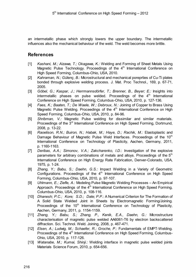
5th International Conference on High Speed Forming – 2012
an intermetallic phase which strongly lowers the upper boundary. The intermetallic influences also the mechanical behaviour of the weld. The weld becomes more brittle.
References
[1] Kashani, M.; Aizawa, T.; Okagawa, K.: Welding and Forming of Sheet Metals Using Magnetic Pulse Technology. Proceedings of the 4th International Conference on High Speed Forming, Columbus-Ohio, USA, 2010.
[2] Kahraman, N.; Gülenç, B.: Microstructural and mechanical poreprties of Cu-Ti plates bonded through explosive welding process. J. Mat. Proc Technol., 169, p. 67-71, 2005.
[3] Göbel, G.; Kaspar, J.; Herrmannsdörfer, T.; Brenner, B., Beyer; E.: Insights into intermetallic phases on pulse welded. Proceedings of the 4th International Conference on High Speed Forming, Columbus-Ohio, USA, 2010, p. 127-136.
[4] Faes, K.; Baaten, T.; De Waele, W.; Debroux, N.: Joining of Copper to Brass Using Magnetic Pulse Welding. Proceedings of the 4th International Conference on High Speed Forming, Columbus-Ohio, USA, 2010, p. 84-96.
[5] Shribman, V.: Magnetic Pulse welding for dissimilar and similar materials. Proceedings of the 3rd International Conference on High Speed Forming, Dortmund, 2008, p. 13-22.
[6] Raoelison, R.N.; Buiron, N.; Habak, M.; Haye, D.; Rachik, M.: Elastoplastic and Damage Behaviour of Magnetic Pulse Weld Interfaces. Proceedings of the 10th International Conference on Technology of Plasticity, Aachen, Germany, 2011, p. 1160-1163.
[7] Deribas, A.A.; Simonov, V.A.; Zakcharenko, I.D.: Investigation of the explosive parameters for arbitrary combinations of metals and alloys. Proceedings of the 5th International Conference on High Energy Rate Fabrication, Denver-Colorado, USA, 1975, p. 1-24.
[8] Zhang, Y.; Babu, S.; Daehn, G.S.: Impact Welding in a Variety of Geometric Configurations. Proceedings of the 4th International Conference on High Speed Forming, Columbus-Ohio, USA, 2010, p. 97-107.
[9] Uhlmann, E.; Ziefle, A.: Modeling Pulse Magnetic Welding Processes – An Empirical Approach. Proceedings of the 4th International Conference on High Speed Forming, Columbus-Ohio, USA, 2010, p. 108-116.
[10] Dhanesh; P.C.; Kore; S.D.; Date; P.P.: A Numerical Criterion for The Formation of A Solid State Welded Joint in Sheets by Electromagnetic Forming/Joining. Proceedings of the 10th International Conference on Technology of Plasticity, Aachen, Germany, 2011, p. 1154-1159.
[11] Zhang, Y.; Babu, S.; Zhang, P., Kenik, E.A., Daehn, G.: Microstructure characterisation of magnetic pulse welded AA6061-T6 by electron backscattered diffraction. Sci. Technol. Weld. Joining, 2008, p. 467-471.
[12] Elsen, A.; Ludwig, M.; Schaefer, R.; Groche, P.: Fundamentals of EMPT-Welding. Proceedings of the 4th International Conference on High Speed Forming, Columbus-Ohio, USA, 2010, p. 117-126.
[13] Watanabe, M.; Kumai, Shinji.: Welding interface in magnetic pulse welded joints Materials Science Forum, 2010, p. 654-656.
216

SESSION 7
JOINING AND WELDING - B
217

218

Simulation of electromagnetically formed joints
R. Neugebauer1, V. Psyk1, C. Scheffler2 1 Fraunhofer Institute of Machine Tools and Forming Technology, Chemnitz, Germany 2 Institute for Machine Tools and Forming Technology, Chemnitz University of Technology, Germany
Abstract
The most important application of electromagnetic forming (EMF) is joining by compression of tubular workpieces. The process simulation of such high speed forming steps must consider numerous mechanical, electrical, and electro-magnetic material characteristics and sometimes a even thermal dependency generally resulting in highly nonlinear computations. One of the most important interactions of the physical fields is the mutual dependency between the acting loads and the deformation. Consequently, a coupled field simulation of structure and magnetic field is demanded. In this paper an exemplary industrial joint produced by EMF is regarded. By comparative electromagnetic field simulations it is proved that the influence of the non-linear permeability of ferromagnetic materials in EM-forming problems is small. A three-dimensional coupled simulation of the joining process is carried out by help of an EM-module in a beta version of the LS-DYNA structural explicit code. To evaluate the quality of the resulting joint already in the virtual process design, the maximum transmittable moment is computed. An experimental verification of the forming and the testing procedure concludes the paper.
Keywords
Electromagnetic forming, Coupled Simulation, Strain rate, Permeability
1 Introduction
Already in the 1970s Bühler et al. claimed joining of tubular components to be the most promising application field of electromagnetic forming (EMF) [1] and this trend has not changed up to now. A comprehensive overview of literature related to EMF including early work as well as recent publications about joining by EMF is given in [2]. As mentioned in this survey, tubes and hollow profiles can be connected to an outer joining partner (hub) by expansion or to an inner joining partner (mandrel or shaft) by compression, whereby the latter case is more common.
219
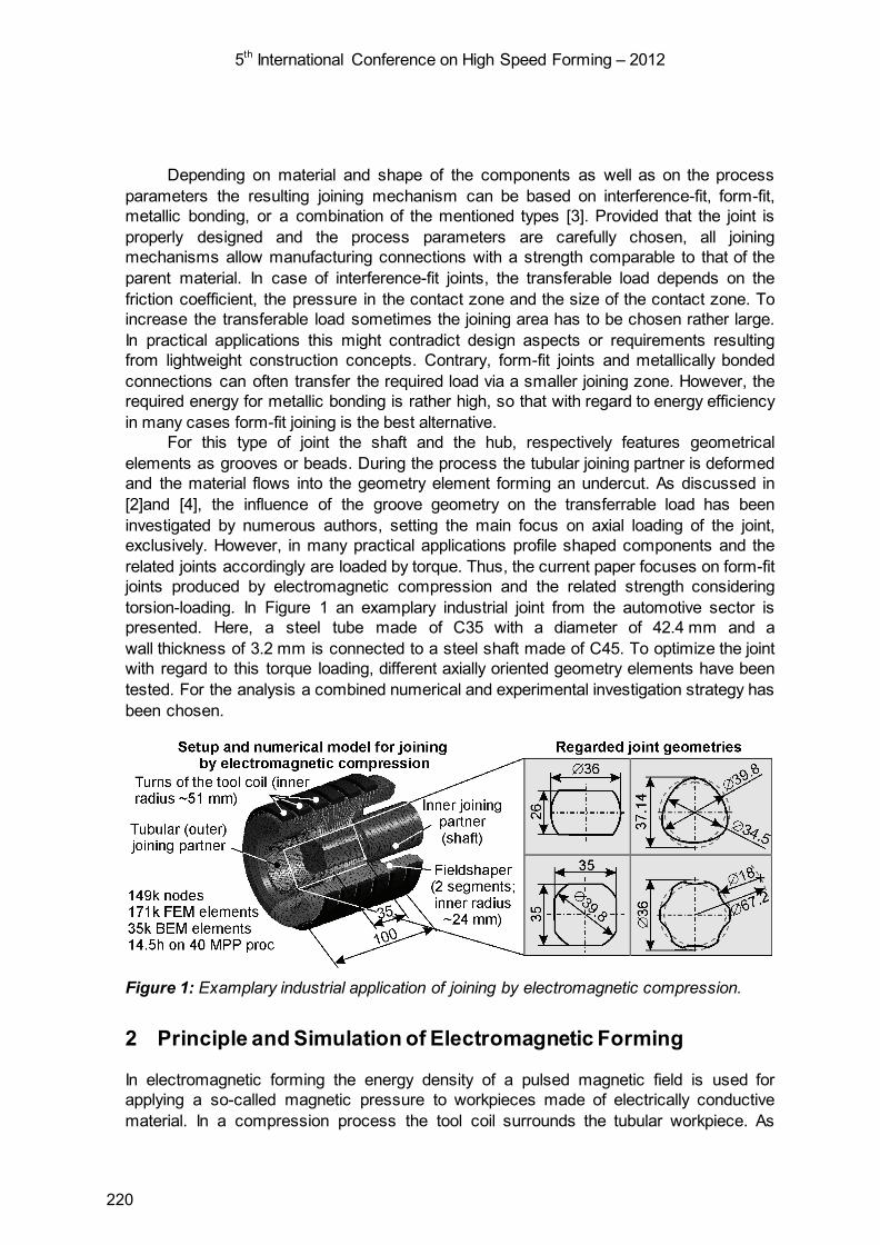
5th International Conference on High Speed Forming – 2012
Depending on material and shape of the components as well as on the process parameters the resulting joining mechanism can be based on interference-fit, form-fit, metallic bonding, or a combination of the mentioned types [3]. Provided that the joint is properly designed and the process parameters are carefully chosen, all joining mechanisms allow manufacturing connections with a strength comparable to that of the parent material. In case of interference-fit joints, the transferable load depends on the friction coefficient, the pressure in the contact zone and the size of the contact zone. To increase the transferable load sometimes the joining area has to be chosen rather large. In practical applications this might contradict design aspects or requirements resulting from lightweight construction concepts. Contrary, form-fit joints and metallically bonded connections can often transfer the required load via a smaller joining zone. However, the required energy for metallic bonding is rather high, so that with regard to energy efficiency in many cases form-fit joining is the best alternative.
For this type of joint the shaft and the hub, respectively features geometrical elements as grooves or beads. During the process the tubular joining partner is deformed and the material flows into the geometry element forming an undercut. As discussed in [2]and [4], the influence of the groove geometry on the transferrable load has been investigated by numerous authors, setting the main focus on axial loading of the joint, exclusively. However, in many practical applications profile shaped components and the related joints accordingly are loaded by torque. Thus, the current paper focuses on form-fit joints produced by electromagnetic compression and the related strength considering torsion-loading. In Figure 1 an examplary industrial joint from the automotive sector is presented. Here, a steel tube made of C35 with a diameter of 42.4 mm and a wall thickness of 3.2 mm is connected to a steel shaft made of C45. To optimize the joint with regard to this torque loading, different axially oriented geometry elements have been tested. For the analysis a combined numerical and experimental investigation strategy has been chosen.
Figure 1: Examplary industrial application of joining by electromagnetic compression.
2 Principle and Simulation of Electromagnetic Forming
In electromagnetic forming the energy density of a pulsed magnetic field is used for applying a so-called magnetic pressure to workpieces made of electrically conductive material. In a compression process the tool coil surrounds the tubular workpiece. As
220

5th International Conference on High Speed Forming – 2012
illustrated in Figure 1 the setup can be completed by a so-called fieldshaper and for joining purposes a joining partner is positioned inside the workpiece. Discharging a capacitor battery through the coil leads to a damped sinusoidal coil current and an according magnetic field which extends mainly in the air gaps between coil and fieldshaper, the individual fieldshaper segments, and fieldshaper and workpiece. Due to the deformation of the tube, the gap volume increases and consequently the energy density i.e. the magnetic pressure that is the source of the deformation decreases.
This interdependency between acting loads and resulting workpiece deformation is one of the most important points when simulating EMF and related joining or cutting processes. To obtain an accurate model of the complete process, different physical effects as mechanical material characteristics like the strain rate dependant flow curve, electrical and electro-magnetic properties and in some cases even a thermal dependency have to be considered, generally resulting in highly nonlinear computations. Consequently, the simulation of EMF is an extremely complex problem and numerous authors have been presenting different numerical simulation tools to solve it (e.g. [5]-[8]). Details about these developments can be found e.g. in [2].
Although many of the described simulation tools include the most important physical aspects and lead to good qualitative and quantitative results as verified in experimental investigations, up to now a fully developed and commercially available solution is still lacking. Consdidering this special aspect, the developments of L’Epplattenier et al. (see [9]) have currently reached the highest stage of development and have been used successfully by many researchers. Similarly, also in this work the numerical analysis of the joining process is based on this tool offering the additional benefit of performing the torque simulation directly after EMF keeping the initial stress / strain in the elements.
3 Simulation
3.1 Permeability influence
In the work mentioned above mainly workpieces made of aluminium alloys are regarded. One reason for this is the their high electrical conductivity which enables high process efficiency during EMF. However, in industrial applications steel materials have been and will continue being used frequently and requests for forming and joining steel by EMF are common despite of the comparably low electrical conductivity. Thus, the influence of the ferromagnetic properties of many steels is an issue in the electromagnetic simulation.
One aspect is the magnetic hysteresis which exists in particular for steel materials because of the high energy dissipation caused through the reversal of magnetization. In general this is difficult to model due to the dependency on the material history (similar to plastic material behavior in continuum mechanics). However, as it can be seen from Figure 2, hysteresis is not significant in the field intensity range usually used for EMF and that is why it is rightfully neglected in many cases.
221

5th International Conference on High Speed Forming – 2012
Figure 2: Left: Nonlinear B-H characteristic (magnetization curve) used in the simulation and computed relative permeability. Right: Hysteresis curve of an unalloyed steel [10].
In most of the EMF simulations simplifications considering the relative permeability µr are made. Assuming that it is isotropic, is valid in most cases and therefore not reviewed, here. Accordingly the µr tensor of second order becomes a scalar.
Moreover, the permeability is often neglected or considered as constant. To investigate if this simplification is admissible for EMF, a magnetic nonlinear simulation with the model described above was set up in ANSYS. An imposed current of 50 kA and a frequency of 10 kHz (both are typical values for EMF) were assumed and axisymmetric plane 233 elements with a nodal based magnetic vector potential formulation were used.
In Figure 2 a typical initial magnetization curve of a steel, similar to C35E, is displayed. The relation of H-dependency and isotropic, i.e. scalar, permeability is given by
HB dHHd r 0)()( µµ= (1)
where H is the magnetic field intensity vector (H the norm of H), B the magnetic field density vector, µr the isotropic relative permeability and µ0 the magnetic field constant 4π.10-7H/m. By plotting the computed µr over it becomes obvious that µr varies between 1 and about 1200 (see Figure 2). Due to magnetic saturation the permeability tends to 1 for high values of the field intensity. According to [11], the maximum of permeability is shifted to higher H-values if the carbon portion is increased and if the material is hardened but they are still much lower than the typical magnitude during EMF which is in the range of 105 up to 108 depending on the current, coil and tool geometry as shown in Figure 3.
Thus, it can be expected that the magnetic material behavior is in good approximation linear with µr=1. This assumption was proofed by comparisons of field lines or the spatially distributed µr-values. The field line plots for linear and nonlinear magnetization shown in Figure 3 (for reasons of symmetry only one quarter of the cross section is shown, here) do not differ significantly from each other implying a great similarity of the fields. This becomes obvious as well by depicting the computed µr over the modelling region (Figure 4). For high current amplitudes (i.e. approx. 30-200 kA) µr is equal 1 almost everywhere in the workpiece and the tool has no influence (see Figure 4a).
Contrary, for smaller currents (e.g. a 5 kA amplitude ) a permeability distribution in the workpiece with values >>1 results (see Figure 4b) implying a mandatory consideration of nonlinear magnetization, but usually such small currents are not relevant in EMF.
222
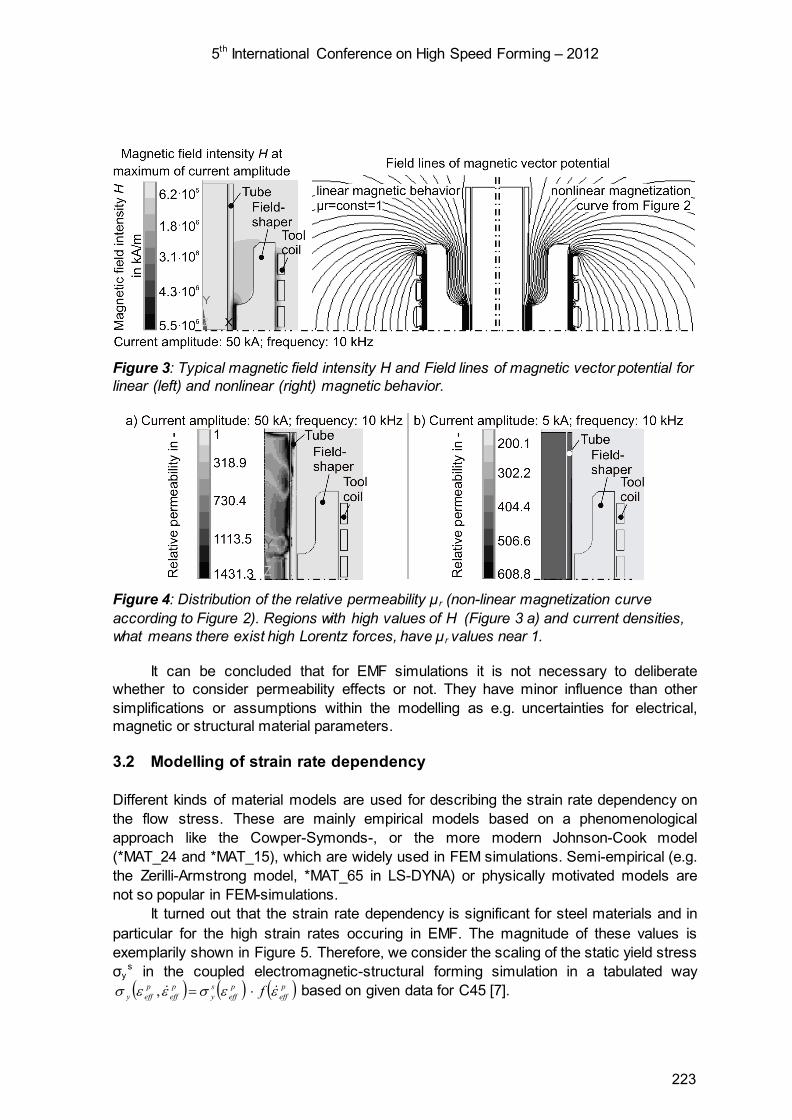
5th International Conference on High Speed Forming – 2012
Figure 3: Typical magnetic field intensity H and Field lines of magnetic vector potential for linear (left) and nonlinear (right) magnetic behavior.
Figure 4: Distribution of the relative permeability µr (non-linear magnetization curve according to Figure 2). Regions with high values of H (Figure 3 a) and current densities, what means there exist high Lorentz forces, have µr values near 1.
It can be concluded that for EMF simulations it is not necessary to deliberate whether to consider permeability effects or not. They have minor influence than other simplifications or assumptions within the modelling as e.g. uncertainties for electrical, magnetic or structural material parameters.
3.2 Modelling of strain rate dependency
Different kinds of material models are used for describing the strain rate dependency on the flow stress. These are mainly empirical models based on a phenomenological approach like the Cowper-Symonds-, or the more modern Johnson-Cook model (*MAT_24 and *MAT_15), which are widely used in FEM simulations. Semi-empirical (e.g. the Zerilli-Armstrong model, *MAT_65 in LS-DYNA) or physically motivated models are not so popular in FEM-simulations.
It turned out that the strain rate dependency is significant for steel materials and in particular for the high strain rates occuring in EMF. The magnitude of these values is exemplarily shown in Figure 5. Therefore, we consider the scaling of the static yield stress σy
s in the coupled electromagnetic-structural forming simulation in a tabulated way ( ) ( ) ( )p
effp
effsy
peff
peffy f εεσεεσ ⋅=, based on given data for C45 [7].
223

5th International Conference on High Speed Forming – 2012
Figure 5: Left: Strain rate distribution during EMF. Maximum values are around 16000s-1. Right: Scaling factor for the static yield stress considering strain rate dependency.
3.3 Coupled Electromagnetic Simulation
One essential step forwards in electromagnetic field simulation is the coupling of the electromagnetic equations with the structural equations. In the LS-DYNA 980 beta version, an electromagnetism module (EM) is under development, which allows the coupled computing of highly nonlinear transient problems in time domain [9]. Furthermore, the explicit structural solver is particularly suitable to handle problems, like EMF, with physical (material) and geometric (contact) nonlinearities.
The FEM approach of this EM-Module bases on a method which was developed by Rieben et. al. [12] and uses a new high-order spatial discretization for the finite element problem. This FEM approach was later introduced in the FEMSTER package [13] which provides a general modular FE class library for hexahedrons, prisms and tetrahedrons. Because of the correct modelling of conditions like jump discontinuities and the divergence-free properties of the magnetic and electric fields together with the implicit unconditionally stable time integration algorithm which is charge and energy conservative, this mixed finite element method is perfectly suited for the time dependent coupled Maxwell equations, i.e. the Ampere and Faraday law.
Another characteristic in LS-DYNA’s EM-module is the use of a special boundary element (BEM) formulation known as indirect BEM for solving the Maxwell equations in insulator regions, i.e. regions without (eddy) currents. Thus, meshing of non-conductors like the air is not necessary preventing element distortion during forming. The BEM-formulation of air is particularly suitable due to the linear magnetic characteristic (µr=1).
A coupling to the mechanical equations is applied in every time step by help of the computed Lorentz force which acts on the nodes of the mesh. This can be regarded as weak coupling. To consider the feedback of the deformed structure on the magnetic field the FEM and BEM matrices of the magnetic equation system are recomputed in every n-th mechanical timestep. The frequency of the matrix update depends on the influence of the deformed structure and can often be set around every 100th mechanical timestep because of the small mechanical steps in explicit FEM dynamics.
There exist several formulations for solving the electromagnetic field equations [14]. On of the most common is the A, ϕ -A formulation, what means to describe the Maxwell equations for insulator regions through the magnetic vector potential A and for conductive regions through the magnetic vector potential + the electric scalar potential ϕ . Thus, the constraints (e.g. the divergence condition) could be incorporated easily and the number of
224
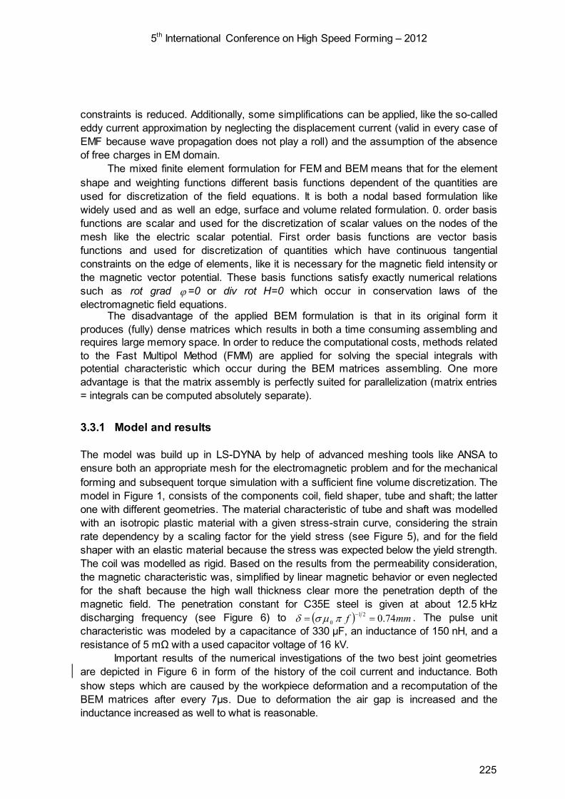
5th International Conference on High Speed Forming – 2012
constraints is reduced. Additionally, some simplifications can be applied, like the so-called eddy current approximation by neglecting the displacement current (valid in every case of EMF because wave propagation does not play a roll) and the assumption of the absence of free charges in EM domain.
The mixed finite element formulation for FEM and BEM means that for the element shape and weighting functions different basis functions dependent of the quantities are used for discretization of the field equations. It is both a nodal based formulation like widely used and as well an edge, surface and volume related formulation. 0. order basis functions are scalar and used for the discretization of scalar values on the nodes of the mesh like the electric scalar potential. First order basis functions are vector basis functions and used for discretization of quantities which have continuous tangential constraints on the edge of elements, like it is necessary for the magnetic field intensity or the magnetic vector potential. These basis functions satisfy exactly numerical relations such as rot grad ϕ=0 or div rot H=0 which occur in conservation laws of the electromagnetic field equations.
The disadvantage of the applied BEM formulation is that in its original form it produces (fully) dense matrices which results in both a time consuming assembling and requires large memory space. In order to reduce the computational costs, methods related to the Fast Multipol Method (FMM) are applied for solving the special integrals with potential characteristic which occur during the BEM matrices assembling. One more advantage is that the matrix assembly is perfectly suited for parallelization (matrix entries = integrals can be computed absolutely separate).
3.3.1 Model and results
The model was build up in LS-DYNA by help of advanced meshing tools like ANSA to ensure both an appropriate mesh for the electromagnetic problem and for the mechanical forming and subsequent torque simulation with a sufficient fine volume discretization. The model in Figure 1, consists of the components coil, field shaper, tube and shaft; the latter one with different geometries. The material characteristic of tube and shaft was modelled with an isotropic plastic material with a given stress-strain curve, considering the strain rate dependency by a scaling factor for the yield stress (see Figure 5), and for the field shaper with an elastic material because the stress was expected below the yield strength. The coil was modelled as rigid. Based on the results from the permeability consideration, the magnetic characteristic was, simplified by linear magnetic behavior or even neglected for the shaft because the high wall thickness clear more the penetration depth of the magnetic field. The penetration constant for C35E steel is given at about 12.5 kHz discharging frequency (see Figure 6) to ( ) mmf 74.021
0 == −πµσδ . The pulse unit characteristic was modeled by a capacitance of 330 µF, an inductance of 150 nH, and a resistance of 5 mΩ with a used capacitor voltage of 16 kV.
Important results of the numerical investigations of the two best joint geometries are depicted in Figure 6 in form of the history of the coil current and inductance. Both show steps which are caused by the workpiece deformation and a recomputation of the BEM matrices after every 7µs. Due to deformation the air gap is increased and the inductance increased as well to what is reasonable.
225
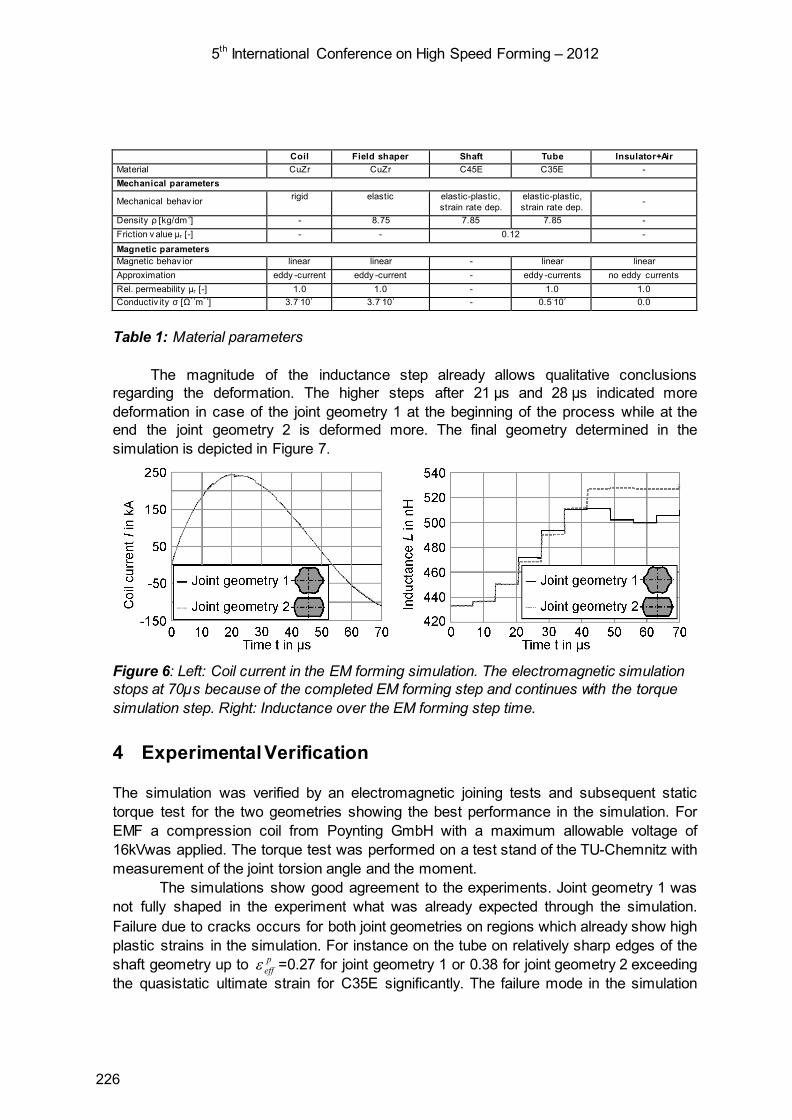
5th International Conference on High Speed Forming – 2012
Coil Field shaper Shaft Tube Insulator+Air Material CuZr CuZr C45E C35E - Mechanical parameters
Mechanical behav ior rigid elastic elastic-plastic, strain rate dep.
elastic-plastic, strain rate dep.
-
Density ρ [kg/dm3] - 8.75 7.85 7.85 - Friction v alue µr [-] - - 0.12 -
Magnetic parameters Magnetic behav ior linear linear - linear linear Approximation eddy -current eddy -current - eddy -currents no eddy currents Rel. permeability µr [-] 1.0 1.0 - 1.0 1.0 Conductiv ity σ [Ω-1m-1] 3.7.107 3.7.107 - 0.5.107 0.0
Table 1: Material parameters
The magnitude of the inductance step already allows qualitative conclusions regarding the deformation. The higher steps after 21 µs and 28 µs indicated more deformation in case of the joint geometry 1 at the beginning of the process while at the end the joint geometry 2 is deformed more. The final geometry determined in the simulation is depicted in Figure 7.
Figure 6: Left: Coil current in the EM forming simulation. The electromagnetic simulation stops at 70µs because of the completed EM forming step and continues with the torque simulation step. Right: Inductance over the EM forming step time.
4 Experimental Verification
The simulation was verified by an electromagnetic joining tests and subsequent static torque test for the two geometries showing the best performance in the simulation. For EMF a compression coil from Poynting GmbH with a maximum allowable voltage of 16kVwas applied. The torque test was performed on a test stand of the TU-Chemnitz with measurement of the joint torsion angle and the moment.
The simulations show good agreement to the experiments. Joint geometry 1 was not fully shaped in the experiment what was already expected through the simulation. Failure due to cracks occurs for both joint geometries on regions which already show high plastic strains in the simulation. For instance on the tube on relatively sharp edges of the shaft geometry up to p
effε =0.27 for joint geometry 1 or 0.38 for joint geometry 2 exceeding the quasistatic ultimate strain for C35E significantly. The failure mode in the simulation
226
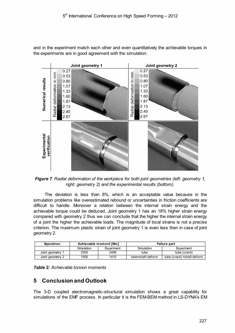
5th International Conference on High Speed Forming – 2012
and in the experiment match each other and even quantitatively the achievable torques in the experiments are in good agreement with the simulation.
Figure 7: Radial deformation of the workpiece for both joint geometries (left: geometry 1, right: geometry 2) and the experimental results (bottom).
The deviation is less than 8%, which is an acceptable value because in the simulation problems like overestimated rebound or uncertainties in friction coefficients are difficult to handle. Moreover a relation between the internal strain energy and the achievable torque could be deduced. Joint geometry 1 has an 18% higher strain energy compared with geometry 2 thus we can conclude that the higher the internal strain energy of a joint the higher the achievable loads. The magnitude of local strains is not a precise criterion. The maximum plastic strain of joint geometry 1 is even less then in case of joint geometry 2.
Specimen Achievable moment [Nm] Failure part Simulation Experiment Simulation Experiment
Joint geometry 1 2300 2408 tube tube (crack) Joint geometry 2 1500 1415 tube+shaft deform. tube (crack) +shaft deform.
Table 2: Achievable torsion moments
5 Conclusion and Outlook
The 3-D coupled electromagnetic-structural simulation shows a great capability for simulations of the EMF process. In particular it is the FEM-BEM method in LS-DYNA’s EM
227

5th International Conference on High Speed Forming – 2012
module which is perfectly suited because of advantages like no air/insulator mesh. One drawback is that large-scale problems must be handled with parallel processing due to the high computational cost or memory requirements (here 35GB for EM system). Computations considering the permeability of steel materials show, that a disregard is quite acceptable in general for EMF forming simulations. The experiments show that an optimization of the joint geometry is necessary to avoid regions of plastic strain peaks which are accountable for crack initiation. One possibility to reduce high local plastic strains is to round the sharp edges on the longitudinal grooves.
References
[1] Bühler, H., von Finckenstein, E., 1971. Bemessung von Sickenverbindungen für ein Fügen durch Magnetumformung, 104. Werkstatt und Betrieb, 45–51.
[2] Psyk, V., Risch, D., Kinsey, B.L., Tekkaya, A.E., Kleiner, M., 2011. Electromagnetic forming - a review. Journal of Materials Processing Technology 211, 787–829.
[3] Neugebauer, R.; Bouzakis, K.-D.; Denkena, B.; Klocke, F.; Sterzing, A.; Tekkaya, A.E.; Wertheim, R.: Velocity effects in metal forming and machining processes. Annals of the CIRP Vol. 60/2/2011.
[4] Weddeling, C., Woodward, S., Marré, M., Nellesen, J., Psyk, V., Tekkaya, A.E., Tillmann, W., 2011. Influence of Groove Characteristics on Strength of Form-fit Joints. Journal of Materials Processing Technology 211 (5), 925–935.
[5] Takata, N.; Kato, M.; Sato, K.; Tobe, T.: High-speed forming of metal sheets by electromagnetic forces. Japan Soc. Mech. Eng. Int. Journal 31, pp. 142-150, 1988.
[6] Kleiner, M.; Brosius, A.: Determination of Flow Curves at High Strain Rates using the Electromagnetic Forming Process and an Iterative Finite Element Simulation Scheme, Annals of the CIRP Vol. 55/1/2006.
[7] Prof. Dr. L. W. Meyer et al: Werkstoffverhalten bei hohen Dehnungsgeschwindig-keiten. Oral presentation, Workshop Impulsumformung, IUL Dortmund, 12.03.2009.
[8] Taebi, F.; Demir, K.; Stiemer, M.; Psyk, V. Kwiatkowski, L.; Brosius, A.; Blum, H.; Tekkaya, A. E.: Dynamic forming limits and numerical optimization of combined quasi-static and impulse magnetic forming. Comp. Mat. Sc. 54 (2012), pp 293-302.
[9] L’Eplattenier, et. al. Introduction of an Electromagnetism Module in LS-DYNA for Coupled Mechanical-Thermal-Simulations, steel research int. 80 (2009), No. 5
[10] http://users.physik.fu-berlin.de/~herold/HYS.pdf., 01.2012 [11] http://www.ndt.net/article/dgzfp03/papers/p12/p12.htm, 01.2012 [12] Rieben, R.N., Rodrigue, G.H., White, D.A., A high order mixed vector finite element
method for solving the time dependent Maxwell equations on unstructured grids. J. of Com. Phys. 204 (2005), pp. 490-519.
[13] Castillo, P., Rieben, R., White, D., FEMSTER: An Object-Oriented Class Library of High-Order Discrete Differential Forms. In: Transactions on Mathematical Siftware, ACM, Vol. 31, No. 4, Dec. 2005, pp. 425-457.
[14] Bíró, O., Preis, K., On the Use of the Magnetic Vector Potential in the Finite Element Analysis of Three-Dimensional Eddy Currents. In: IEEE Trans. on Magn., Vol. 25 1989.
228

Electromagnetic pulse crimping of axial form fit joints *
K. Faes1, O. Zaitov1, W. De Waele2
1 Belgian Welding Institute, Ghent, Belgium. 2 Laboratory Soete, Ghent University, Ghent, Belgium
Abstract
Electromagnetic pulse crimping of form fit joints was investigated using tubes in the aluminium alloy EN AW-6060, with a diameter of 50 mm and a wall thickness of 1,5 mm. First the influence of the charging voltage and the geometrical groove parameters on the deformation behaviour and localised thickness reduction of the tube wall was investigated. The experimental results provided data for optimising the groove design.
The Design of Experiments method was used to optimise the shape and dimensions of the internal workpieces with a double groove design. Results of tensile tests on the crimp joints allowed determining the most important parameters for the groove design. Based on these observations an optimal double groove joint design was proposed. The deformation and failure behaviour of the crimp joints during tensile testing were experimentally studied using the digital image correlation technique. This technique was used to measure the local and global deformation of the joint. Failure mechanisms include pull-out, local shearing and fracture of the tube. Three main failure modes were observed.
Keywords
Electromagnetic joining, Axial crimp joints, Design of Experiments
* This work is based on the results of the CorNet collective research project “PULSCRIMP”; the authors would like to thank IWT (Agency for Innovation by Science and Technology) for its financial support.
229

5th International Conference on High Speed Forming – 2012
1 Electromagnetic Pulse Joining
The electromagnetic pulse technology uses magnetic forces to deform and/or join work-pieces. The energy stored in a capacitor bank is discharged rapidly through a magnetic coil. Typically a ring-shaped coil is placed over a tubular workpiece. When deforming tubular products, the magnetic field produced by the coil generates eddy currents in the tube. These currents, in turn, produce their own magnetic field. The forces generated by the two magnetic fields oppose each other. Consequently, a repelling force between the coil and the tube is created. As a consequence, the tube is collapsed onto an internal workpiece, creating a crimp joint or a welded joint. In the electromagnetic pulse crimping process, no atomic bond is obtained; these joints obtain their strength from the combination of an interference and a form fit. A special profiled internal workpiece is therefore used.
2 Literature Survey
In [1] the influence of the groove shape of form fit joints was investigated. Three different shapes were taken into account; triangular, circular and rectangular grooves (see Figure 1). Joints with triangular grooves were always the weakest. The explanation was that in this case the angle α is larger than for rectangular or circular grooves. This results in a lower degree of tube deformation at the groove edge, and thus a smaller tensile force is required to initiate pull-out of the tube from the groove.
Circular grooves result in a smaller angle α than the rectangular grooves, but the latter requires a larger pull-out force, due to the larger amount of shearing of the tube at the groove edges. This provides a better interlock of the tube in the groove. Joints formed with rectangular grooves always exhibit the highest joint strength, which was experimentally verified [1].
Figure 1: Radioscopic images after deformation [1]
The strength of form fit joints with rectangular grooves strongly depends on 3 factors determining the groove geometry: the depth, width and the groove edge radius. Deeper grooves will lead to higher joint strengths [2,3], but increasing the groove depth too much
230
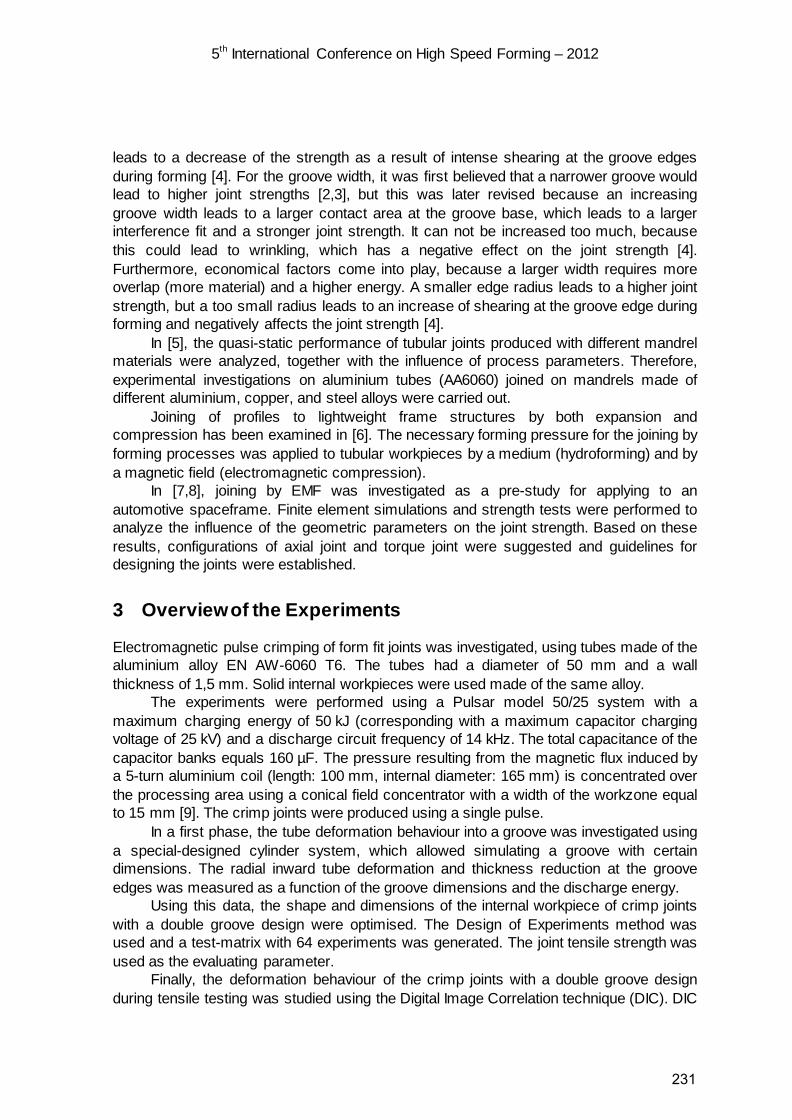
5th International Conference on High Speed Forming – 2012
leads to a decrease of the strength as a result of intense shearing at the groove edges during forming [4]. For the groove width, it was first believed that a narrower groove would lead to higher joint strengths [2,3], but this was later revised because an increasing groove width leads to a larger contact area at the groove base, which leads to a larger interference fit and a stronger joint strength. It can not be increased too much, because this could lead to wrinkling, which has a negative effect on the joint strength [4]. Furthermore, economical factors come into play, because a larger width requires more overlap (more material) and a higher energy. A smaller edge radius leads to a higher joint strength, but a too small radius leads to an increase of shearing at the groove edge during forming and negatively affects the joint strength [4].
In [5], the quasi-static performance of tubular joints produced with different mandrel materials were analyzed, together with the influence of process parameters. Therefore, experimental investigations on aluminium tubes (AA6060) joined on mandrels made of different aluminium, copper, and steel alloys were carried out.
Joining of profiles to lightweight frame structures by both expansion and compression has been examined in [6]. The necessary forming pressure for the joining by forming processes was applied to tubular workpieces by a medium (hydroforming) and by a magnetic field (electromagnetic compression).
In [7,8], joining by EMF was investigated as a pre-study for applying to an automotive spaceframe. Finite element simulations and strength tests were performed to analyze the influence of the geometric parameters on the joint strength. Based on these results, configurations of axial joint and torque joint were suggested and guidelines for designing the joints were established.
3 Overview of the Experiments
Electromagnetic pulse crimping of form fit joints was investigated, using tubes made of the aluminium alloy EN AW-6060 T6. The tubes had a diameter of 50 mm and a wall thickness of 1,5 mm. Solid internal workpieces were used made of the same alloy.
The experiments were performed using a Pulsar model 50/25 system with a maximum charging energy of 50 kJ (corresponding with a maximum capacitor charging voltage of 25 kV) and a discharge circuit frequency of 14 kHz. The total capacitance of the capacitor banks equals 160 µF. The pressure resulting from the magnetic flux induced by a 5-turn aluminium coil (length: 100 mm, internal diameter: 165 mm) is concentrated over the processing area using a conical field concentrator with a width of the workzone equal to 15 mm [9]. The crimp joints were produced using a single pulse.
In a first phase, the tube deformation behaviour into a groove was investigated using a special-designed cylinder system, which allowed simulating a groove with certain dimensions. The radial inward tube deformation and thickness reduction at the groove edges was measured as a function of the groove dimensions and the discharge energy.
Using this data, the shape and dimensions of the internal workpiece of crimp joints with a double groove design were optimised. The Design of Experiments method was used and a test-matrix with 64 experiments was generated. The joint tensile strength was used as the evaluating parameter.
Finally, the deformation behaviour of the crimp joints with a double groove design during tensile testing was studied using the Digital Image Correlation technique (DIC). DIC
231

5th International Conference on High Speed Forming – 2012
provides results concerning displacement and strains, which can be used to have an idea about the load distribution over the 2 grooves during tensile testing.
4 Free Deformation Experiments
4.1 Introduction
During exploratory crimp joint experiments, it was observed that it is a challenge to determine the appropriate energy settings (capacity charging voltage) for a given groove design. If the voltage level is set too low, the tube will not deform into the groove and the connection will hardly have any strength. On the other hand, if too much energy is used, the tube will deform too much into the groove, and thickness reduction at the groove edges will be too severe and the internal workpiece will act as a cutting tool. Therefore it was be helpful to compose graphs which relate the radial inward tube displacement and tube wall thickness reduction at the groove edges with the applied energy level. This provides a first estimate of the charging voltage level to be applied.
In order to be able to generate these graphs with low material resources and with a low processing and evaluation time, a test setup inspired on [1] was designed and built. The system offered the flexibility to simulate a large amount of grooves, without manufacturing an internal workpiece for every test condition. The 3 parameters which were varied during these experiments are: the groove edge radius: set at 0,5 mm, 1,0 mm and 1,5 mm, the groove width: varied between 6 and 14 mm, with a 2 mm interval, the applied charging voltage: it was observed that 5 kV (2 kJ) was the minimum
charging voltage required to deform the utilised tubes. This charging voltage was used as the lower value. The maximum voltage that could be applied without cutting the tube varied between 10 and 13 kV, depending on the combination of the previous 2 parameters.
For each of the 132 samples produced, the largest radial inward displacement and
the tube wall thickness reduction at the groove edges were measured. It should be noted that the radial inward displacement was never restricted (free deformation).
Mechanical interlock behind the groove edge is the most important strengthening mechanism for a crimp joint. It is therefore important to be able to estimate tube thickness reduction at the edge of a groove. Each of the deformed tubes was cross-sectioned and the tube wall thickness was measured at four locations: the 2 upper edges and the 2 lower edges. See Figure 2 for an example of such measurements at the 2 upper edges. The average of these four values was determined in order to exclude measurement inaccuracies.
The relationship between the groove width and the radial inward displacement is directly proportional: a larger radial inward displacement is measured when the groove width is larger. This can be explained by considering the tube as a beam imposed on two supports. If these supports are close together (i.e. a small groove width), the tube is stiff and it is difficult to deform the tube into the groove. If the supports are more separated, the tube is slender and less stiff and it is easier to deform the tube into the groove. In
232

5th International Conference on High Speed Forming – 2012
Figure 3 (left), the results are shown for a groove edge radius of 0,5 mm. It was also observed that the groove edge radius has a very limited influence on the radial inward tube displacement.
Figure 2 : Measurement of the radial inward displacement and the wall thickness reduction at the edges of the upper half of a cross sectioned deformed tube
More thickness reduction of the deformed tube occurs at the groove edge when the
charging voltage is higher. The cause of this is the larger radial inward displacement when the voltage is higher. A remarkable trend was observed when relating the amount of thickness reduction to the groove width: first the thickness reduction increases when the groove width increases. It reaches a maximum and then the thickness reduction starts to decline again as the groove width further increases. In Figure 3 (right), the results are shown for a groove edge radius of 0,5 mm. This is an interesting observation, especially when keeping in mind that the radial inward displacement linearly increases with the groove width (see Figure 3, left). The explanation for this trend can be found in the relationship between shearing and bending deformation of the tube for different groove widths. If the groove width is small, bending of the tube into the groove is limited, and the radial inward displacement is mostly achieved by shearing at the groove edges. This causes fairly large thickness reduction for a relatively small radial inward displacement. As the groove width increases, the radial inward displacement is larger and the thickness reduction increases until a maximum is a reached. This is because the part of the displacement due to bending is still small and the larger radial inward displacement requires more shearing at the edges.
If the groove width further increases, the tube bending starts to have a significant effect. A part of the radial inward displacement into the groove is then realised by bending, which does not cause thickness reduction at the groove edges. The remaining energy after bending of the tube is then used to realise the rest of the radial inward displacement by shearing at the groove edges. As the groove width increases, a greater part of the radial inward displacement is done by bending and a smaller part by shearing at the groove edges. This explains how a larger radial inward displacement is possible in combination with a declining percentage of thickness reduction.
233
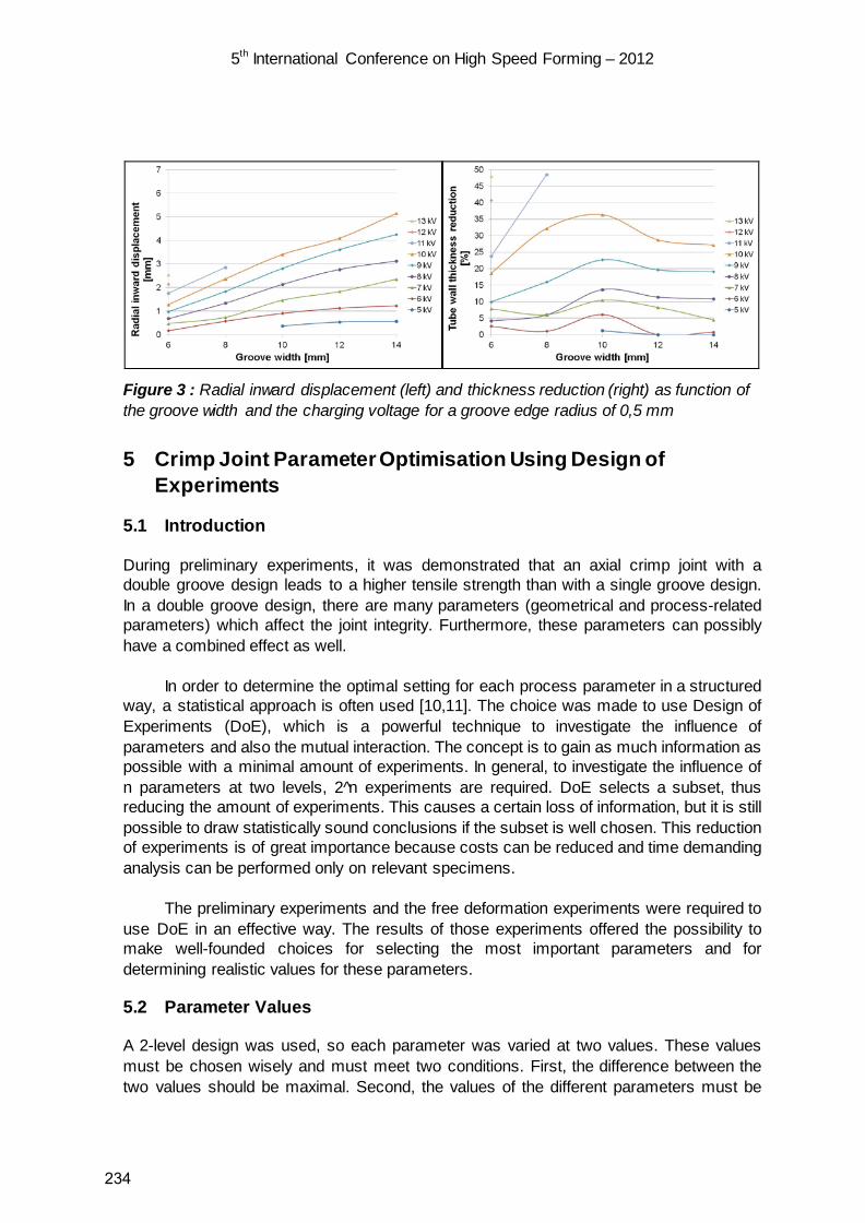
5th International Conference on High Speed Forming – 2012
Figure 3 : Radial inward displacement (left) and thickness reduction (right) as function of the groove width and the charging voltage for a groove edge radius of 0,5 mm
5 Crimp Joint Parameter Optimisation Using Design of Experiments
5.1 Introduction
During preliminary experiments, it was demonstrated that an axial crimp joint with a double groove design leads to a higher tensile strength than with a single groove design. In a double groove design, there are many parameters (geometrical and process-related parameters) which affect the joint integrity. Furthermore, these parameters can possibly have a combined effect as well.
In order to determine the optimal setting for each process parameter in a structured
way, a statistical approach is often used [10,11]. The choice was made to use Design of Experiments (DoE), which is a powerful technique to investigate the influence of parameters and also the mutual interaction. The concept is to gain as much information as possible with a minimal amount of experiments. In general, to investigate the influence of n parameters at two levels, 2 n experiments are required. DoE selects a subset, thus reducing the amount of experiments. This causes a certain loss of information, but it is still possible to draw statistically sound conclusions if the subset is well chosen. This reduction of experiments is of great importance because costs can be reduced and time demanding analysis can be performed only on relevant specimens.
The preliminary experiments and the free deformation experiments were required to
use DoE in an effective way. The results of those experiments offered the possibility to make well-founded choices for selecting the most important parameters and for determining realistic values for these parameters.
5.2 Parameter Values
A 2-level design was used, so each parameter was varied at two values. These values must be chosen wisely and must meet two conditions. First, the difference between the two values should be maximal. Second, the values of the different parameters must be
234
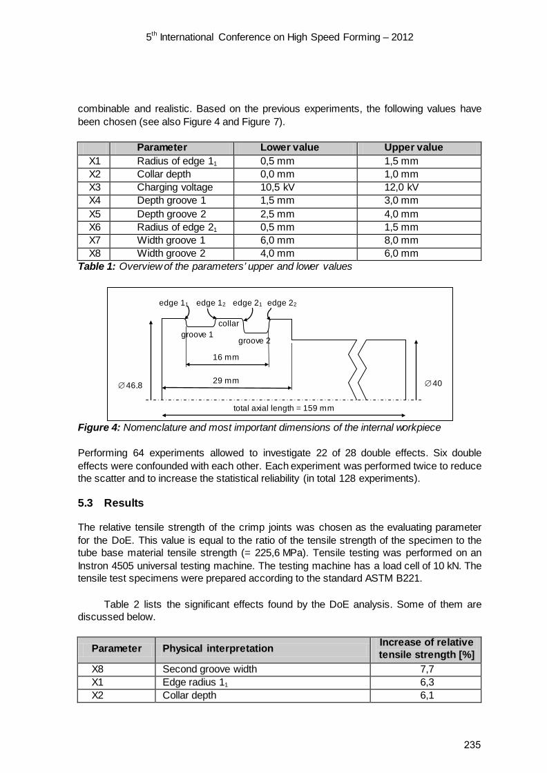
5th International Conference on High Speed Forming – 2012
combinable and realistic. Based on the previous experiments, the following values have been chosen (see also Figure 4 and Figure 7).
Parameter Lower value Upper value X1 Radius of edge 11 0,5 mm 1,5 mm X2 Collar depth 0,0 mm 1,0 mm X3 Charging voltage 10,5 kV 12,0 kV X4 Depth groove 1 1,5 mm 3,0 mm X5 Depth groove 2 2,5 mm 4,0 mm X6 Radius of edge 21 0,5 mm 1,5 mm X7 Width groove 1 6,0 mm 8,0 mm X8 Width groove 2 4,0 mm 6,0 mm
Table 1: Overview of the parameters’ upper and lower values
Figure 4: Nomenclature and most important dimensions of the internal workpiece Performing 64 experiments allowed to investigate 22 of 28 double effects. Six double effects were confounded with each other. Each experiment was performed twice to reduce the scatter and to increase the statistical reliability (in total 128 experiments).
5.3 Results
The relative tensile strength of the crimp joints was chosen as the evaluating parameter for the DoE. This value is equal to the ratio of the tensile strength of the specimen to the tube base material tensile strength (= 225,6 MPa). Tensile testing was performed on an Instron 4505 universal testing machine. The testing machine has a load cell of 10 kN. The tensile test specimens were prepared according to the standard ASTM B221.
Table 2 lists the significant effects found by the DoE analysis. Some of them are discussed below.
Parameter Physical interpretation Increase of relative tensile strength [%]
X8 Second groove width 7,7 X1 Edge radius 11 6,3 X2 Collar depth 6,1
16 mm
29 mm
total axial length = 159 mm
∅46,8
∅40
groove 1 groove 2
collar
edge 11 edge 22 edge 12 edge 21
235

5th International Conference on High Speed Forming – 2012
X4 Depth first groove 5,8 X6 Edge radius 21 3,7 X2*X3 Collar depth and applied voltage 3,6 X2*X8 Collar depth vs. second groove width 2,9 X3*X4 Applied voltage and first groove depth 2,7 X3*X5*X7 - 2,5 X3 Applied voltage 2,3 X1*X3*X7 - 2,1 X2*X7 Collar depth and first groove width 2,1 X4*X8 First groove depth and second groove width 1,9 X1*X2*X3 - 1,9 X3*X6*X7 - 1,9 X4*X7 First groove depth vs. first groove width 1,7 X4*X6 First groove depth vs. edge radius 21 1,6
Table 2: Significant effects of the parameters Second groove width (parameter X8) A width of the second groove equal to 6 mm instead of 4 mm resulted in a higher joint tensile strength. A large groove width is needed to create a better ‘filling’ of the groove. The width of the second groove should always be chosen large enough to allow a sufficient deformation of the tube into the groove. When the distance between the two supports increases, the tube can more easily be deformed between the supports. The angle θ in Figure 5 provides an indication for the mechanical interlock. The smaller the angle θ, the more mechanical interlock is possible. Also, as was concluded during the free deformation experiments, a short groove will cause more shearing which results in more tube wall thickness reduction than with a long groove.
Figure 5: Influence of the groove width on the mechanical interlock
Edge radius 11 (parameter X1) In contrast to what initially was thought, a small edge radius is desired for edge 11. The first edge bears the major part of the axial load and thus there is a need for a good mechanical interlock. A sharp edge cannot be defined in values, but it can be stated that for this design, it is better to use an edge radius of 0,5 mm than an edge radius of 1,5 mm.
Short groove: Long groove:
236

5th International Conference on High Speed Forming – 2012
Collar depth (parameter X2) For the optimal design, the collar depth must be chosen equal to 1 mm. During the tensile tests, it was demonstrated that all designs with a sunken collar had a higher tensile strength than those without. This can be attributed to the fact that with a sunken collar, the tube first deforms into the gap covering the two grooves and later, when making contact with the collar, starts deforming in each groove separately (see Figure 6). When the tube deforms into a large gap, it acts like a beam imposed onto two supports with a large distance between the supports, under a vertical evenly distributed load (the magnetic repulsive force from the coil). In Figure 6.A, the tube is divided into two beams imposed onto two supports, each with a small gap length. The tube experiences more shearing stress and less bending moment than in Figure 6.B. For an equal applied voltage and similar groove geometries in A and B, thickness reduction in edge 11 and edge 22 will be less excessive in case B.
It should be noted that in case A, the area of largest radial displacement of the deformed tube is approximately in the middle of each groove, while in case B this area of the tube is found closer to the central collar. The dotted vertical lines below the right part of Figure 6 indicate the position of these zones of maximal radial displacement. When these lines are positioned closer to the collar, a stronger mechanical interlock is obtained in the second groove. On the other hand, less mechanical interlock is obtained in the first groove, but this negative effect is compensated with less thickness reduction at edge 11.
Figure 6: A sunken collar leads to less thickness reduction and better interlock at the second groove.
Depth of the first groove (parameter X4) It was found that it is beneficial to have a small depth of the first groove. This can be explained by the fact that the thickness reduction at edge 11 will be less and so a sharper edge radius 11 can be allowed. This is beneficial because it creates a stronger mechanical interlock. Edge radius 21 (parameter X6) Again, a sharp edge 21 is desirable to create mechanical interlock in the second groove.
A)
B)
237

5th International Conference on High Speed Forming – 2012
Collar depth and applied voltage (parameters X2*X3) This second order effect contains the collar depth (parameter X2) and the applied voltage (parameter X3). As can be seen in Figure 6, when using a sunk collar, a high voltage is required to first bend the tube into the large gap covering the two grooves and to subsequently sufficiently deform the tube in each groove separately, while consuming some of the energy for the deformation of the central collar.
Collar depth and second groove width (parameters X2*X8) As already described above, with a sunken collar the zone of maximal radial displacement is closer to the collar. This induces an increase of mechanical interlock at the second groove. Furthermore, when a larger second groove is present, the tube more easily deforms into the second groove, increasing the mechanical interlock even more. The increase of mechanical interlock due to a larger second groove in combination with a sunken collar also involves minimisation of the tube wall thickness reduction at the edges.
Charging voltage and first groove depth (parameters X3*X4) A shallow first groove in combination with a large charging voltage is preferred over a deep first groove in combination with the same large charging voltage, because there will be more contact and thus more interference fit when the groove is shallow.
Charging voltage (parameter X3) It is clear that a larger charging voltage causes more deformation and more filling of the tubes into the grooves, which results in more mechanical interlock and possibly some interference fit on the bottom of the grooves as well.
The following second order effects are less significant and are not discussed in detail: Collar depth and first groove width (parameters X2*X7) Depth of first groove and width of second groove (parameters X4*X8) Depth of first groove and width of first groove (parameters X4*X7) Depth of first groove and edge 21 (parameters X4*X6)
5.4 Conclusion
To propose a suitable design for a double grooved axial crimp joint providing a sufficient tensile strength, the following points of attention should be kept in mind: the critical zone where most crimp joints fail is located at edge 11. Therefore, tube wall thickness reduction should be minimised in this location, but keeping in mind that some thickness reduction is inevitable.
A wide shallow first groove with a sharp edge 11 is beneficial to obtain a higher tensile strength. The sharp edge is required to create interlock, while the groove width and shallow depth create a good filling and minimise tube thickness reduction. It is important to have a central collar which is sunk below the specimen surface to further minimise the tube thickness reduction at edge 11 and 22 and to better distribute the tensile strength over the two grooves. With a sunken central collar, the mechanical interlock in the second groove is increased. It is also preferred that the second groove is wide, with a
238

5th International Conference on High Speed Forming – 2012
sharp edge 21. The second groove width should be long enough so the tube can easily deform into the groove and realise a good filling.
In Figure 7, the parameters of the optimal design of the internal workpiece are indicated in bold. With these parameters, the tensile strength of the crimp joint was equal to the tensile strength of the tube base material.
X3 : voltage X2 X1
X4
X7 X8
X5 L 1.5 U 3.0
L 6.0 U 8.0
L 0.5 U 1.5
L 0.0 U 1.0
L 4.0 U 6.0
L 2.5 U 3.5
L 10.5 U 12.0
X6 L 0.5 U 1.5
Figure 7: Parameters (in mm) used in the DoE test matrix (in mm and kV), with the lower (L) and the upper (U) values. The optimal values are marked in bold.
6 Failure Modes
6.1 Introduction
The Digital Image Correlation (DIC) technique was used to investigate the failure behaviour of the axial joints with a double groove design subjected to an axial load. The DIC method allows deducing the material displacement during tensile testing by tracking the deformation of a random speckle pattern by acquired digital images. The image analysis process can be understood as a pattern recognition technique, which searches locally the random speckle pattern by comparing the images of the deformed with the reference state. By using two synchronised cameras which acquire images of the loaded specimen from different viewing angles, it is possible to determine both the three-dimensional displacement and deformation as a function of time [12].
Figure 8: Detail of the test specimen with white layer and black speckle pattern
After tensile tests were performed on the first series of 64 experiments of the DoE, the relative tensile strength versus displacement curves were analysed and 32 interesting crimp joints were selected to be analysed with the DIC technique during the second series
239

5th International Conference on High Speed Forming – 2012
of tensile tests. It was found that the failure behaviour of the crimp joints can be divided into 3 main failure modes: Failure mode 1: the tube tears at edge 11 at the complete circumference. Failure mode 2: the tube tears at edge 21 at the complete circumference. Failure mode 3: the tube is pulled of the internal workpiece, and no tearing occurs.
In failure mode 1, the tube wall thickness reduction near groove edge 11 and the
amount of load taken up by the second groove determines the joint tensile strength. After the tube breaks at edge 11, the joint can no longer bear a load.
It was also observed that failure mode 1 can be divided into 3 subgroups: Subgroup 1: These crimp joints have an inappropriate design of the first groove. As a
consequence, the tube wall thickness reduction at edge 11 is too excessive and the second groove doesn’t bear any part of the load. Based on the tensile tests performed during the DoE-experiments, it was found that in this case the average relative tensile strength was equal to 74%.
Subgroup 2: These crimp joints have a better design of the first groove, allowing also the second groove to bear part of the load. The internal parts however didn’t have a sunken collar. The average relative tensile strength was equal to 80%.
Subgroup 3: These crimp joints have an even better design of the first groove, as well as a sunken collar with a depth of 1 mm, which causes less thickness reduction at groove edge 11 and which allows the second groove to bear a larger part of the load. The average relative tensile strength was in this case 91%.
In failure mode 2, the tube wall thickness reduction near groove edge 21
determines the tensile strength, until the tube breaks at this edge. This corresponds with point A in Figure 9, and with Figure 11 (graphically showing the Z-displacement for a crimp joint failed by failure mode 2). It was observed that the connection still has some strength after this fracture (point B). This is because at this moment the load-bearing mechanism changes: the tube now needs to be pulled out of the first groove without thickness reduction, and thus is the load-bearing capacity is determined by the tube interlock in the first groove in combination with the relative axial displacement between the tube and the internal workpiece at the edge 11. The curve of the relative tensile strength versus displacement increases then to a second (lower) maximum (see point C in Figure 9 and Figure 12). Point C corresponds with maximal interlocking. Thereafter, the load decreases to zero, since the tube experiences little resistance when the displacement further increases. The tube which was originally deformed into the first groove is almost completely pushed back to its original position before the crimping operation. The average relative tensile strength of the joints which failed by failure mode 2 was equal to 75,3%.
In failure mode 3 no tearing occurs, and thus it is the radial inward tube displacement into both grooves in combination with the axial displacement of the tube relative to the internal workpiece which is of importance. The average relative tensile strength of these joints was 66,4%.
240

5th International Conference on High Speed Forming – 2012
Figure 9: Relative tensile strength versus
displacement curve of a joint failed by failure mode 2
Figure 10: The tube gets pulled out of
groove 1 and 2
Figure 11: The tube tears at edge 21
Figure 12: The tube is pulled out of the first
groove (without thickness reduction or fracture)
7 Conclusion
Electromagnetic pulse crimping of form fit joints was investigated using tubes in the aluminium alloy EN AW-6060. The tube deformation behaviour for a single groove design was investigated using a cylinder system which allowed to simulate a groove with certain dimensions. It was concluded that the relationship between the groove width and the radial inward displacement is directly proportional and that a higher capacitor charging voltage leads to a larger radial inward displacement. A remarkable trend was observed when relating the tube wall thickness reduction to the groove width: initially thickness reduction increases, but as the groove width increases, thickness reduction declines again. This was explained by looking at the ratio of shearing and bending.
The Design of Experiments method was used to optimise the shape and dimensions of the internal workpieces with a double groove design. A test-matrix with 64 experiments was generated. The tensile strength of the crimp joints was chosen as the evaluation parameter. An optimal design was proposed, which had a statistically expected tensile strength equal to the tensile strength of the tube base material. The optimal design
A
B
C
241

5th International Conference on High Speed Forming – 2012
includes a shallow, long first groove with sharp edges, a sunken central collar and a long and deeper second groove with sharp edges.
The deformation behaviour of the crimp joints with a double groove design during tensile testing was studied using the Digital Image Correlation technique. Three main failure modes were observed. The failure mode in which the tube tears at the first edge of the first groove occurred most during the performed experiments and resulted in the highest tensile strength.
References
[1] Weddeling, C., Woodward, S., Marré, M., Nellesen, J., Psyk, V., Tekkaya, E., Tillmann, W.: Influence of groove characteristics on strength of form-fit joints. Journal of Materials Processing Technology, Vol. 211, Issue 5, 2011, p. 925 -935.
[2] Bühler, H., von Finckenstein, E., Fügen durch Magnetumformung. Werkstatt und Betrieb 101, 1968: p. 671-675.
[3] Golavashchenko, S. Methodology of design of pulsed electromagnetic joining of tubes. Proceedings of the TMS Symposium "Innovations in Processing and Manufacturing of Sheet Materials". 2001. New Orleans, LA, USA.
[4] Park, Y., Kim, H., Oh, S., Design of axial/torque joints made by electromagnetic forming. Thin walled structures 43, 2005: p. 826-844.
[5] Barreiro, P., Schulze, V., Löhe, D., Marre, M., Beerwald, C., Homberg, W., Kleiner, M.: Strength of Tubular Joints Made by Electromagnetic Compression at Quasi-static and Cyclic Loading. High Speed Forming 2006, Proceedings of the 2nd International Conference, Dortmund, 20.-21.03.2006, p. 107-116.
[6] Marré, M., Brosius, A, Tekkaya, A.E. Joining by Compression and Expansion of (None-) Reinforced Profiles. Advanced Materials Research Vol. 43, 2008, p. 57-68
[7] Park, Y.-B., Kim, H.-Y., Oh, S.-I. Design and Strength Evaluation of Structural Joint Made by Electro-Magnetic Forming (EMF). Proceedings of the 8th International Conference on Numerical Methods in Industrial Forming Processes. AIP Conference Proceedings, Vol. 712, p. 1476-1484 (2004).
[8] Park, Y.-B., Kim, H.-Y., Oh, S.-I. Joining of thin-walled aluminum tube by electromagnetic forming (EMF). International Journal of Automotive Technology, Vol. 6, No. 5, p. 519-527 (2005).
[9] Faes, K.; Baaten, T.; De Waele, W.; Debroux, N.: Joining of Copper to Brass Using Magnetic Pulse Welding. Proceedings of the International Conference of High Speed Forming, Columbus, Ohio, 9 - 10 March 2010.
[10] Altekar, M., et al.: Assay Optimization: A Statistical Design of Experiments Approach. Journal of the Association for Laboratory Automation, 2006. 11(1): p. 33-41.
[11] Bahloul, R., et al., Sheet metal bending optimisation using response surface method, numerical simulation and design of experiments. International Journal of Mechanical Sciences, 2006. 48(9): p. 991-1003.
[12] Sutton, M.A., Orteu, J., Schreier, H.W., Image correlation for shape, motion and deformation measurements, Springer Science, 2009. ISBN 978-0-387-78746-6.
242

Influencing Factors on the Strength of Electromagnetically Produced Form-Fit Joints using Knurled Surfaces*
C. Weddeling1, S. Gies1, J. Nellesen2, L. Kwiatkowski1, W. Tillmann2, A. E. Tekkaya1
1 Institute of Forming Technology and Lightweight Construction, TU Dortmund University, Dortmund, Germany
2 Institute of Materials Engineering, TU Dortmund University, Dortmund, Germany
Abstract
Joining by electromagnetic forming is a non-contact assembling method that is especially suitable for connections in aluminum space frame structures. By reason of increased joint strength along with lower charging energies, form-fit connections are favored over interference-fit connections for this joining process. In contrast to conventional form-fit concepts, in which the inner joining partner has grooves or pockets, the use of knurled surfaces offers several advantages like easier machinability or the resistance against combined axial and torsional loadings. The objective of this paper is to identify the influencing geometry and process parameters on the joint strength of tubular joints using mandrels with knurled surfaces, with tube and mandrel being made of the same aluminum alloy AA6060-T6. For that reason, experimental studies were conducted: In addition to pull-out tests to determine the axial strength of joints, first computed tomographic images and, afterwards, micrographs of joined components were produced to analyze the contact zone between tube and mandrel and the deformation behavior of the inner joining partner by non-destructive and destructive means. Based on the detailed knowledge of the influencing variables, guidelines for joint and process design are derived.
Keywords
Lightweight frame structures, Joining by electromagnetic forming, Form-fit joints
* This paper is based on investigations of the Collaborative Research Center SFB/TR10 subproject A10 “Joining by Forming” which is kindly supported by the German Research Foundation (DFG). The high-performance microfocus computertomography system used in this work could be purchased in the scope of the DFG project INST 212/209-1 FUGG, which is gratefully acknowledged as well.
243

5th International Conference on High Speed Forming – 2012
1 Introduction
To reconcile the increasing pursuit of individual mobility in modern societies [1] with the efforts in environmental protection in terms of strict emission standards, innovative vehicle concepts are required. No matter whether these concepts are based on fuel-efficient combustion engines or electric powertrains, they mainly depend on lightweight constructions to achieve a reduction of the car’s total weight [2]. Space frame structures made of extruded aluminum profiles are a promising approach to reach this aim. The high rigidity in relation to their weight as well as the nearly unlimited variety of profile geometries are inherent advantages of this technology [3, 4]. However, the production of high-strength joints still remains one of the most challenging problems within the manufacturing process of suchlike aluminum structures. Joining by electromagnetic forming is an alternative to conventional thermal and mechanical joining technologies. It does not require any additional joining elements, and microstructural transformations, that might be caused by excessive heat input during welding operations, do not occur.
2 State of the Art
Electromagnetic forming (EMF) also known as Electromagnetic Pulse Forming Technology (EMPT) is a non-contact forming process using pulsed magnetic fields to create the required forces for workpiece deformation [5]. As these forces increase with rising electrical conductivity of the workpiece, especially copper and aluminum are suitable materials for this forming process. Depending on geometry and positioning of workpiece and tool coil, the process can either be used for expansion or compression of profiles with closed cross section or for sheet metal forming. The experimental setup for tube compression is shown in Figure 1 while the following explanation of the working mechanism is valid for the other process variants in analogous manner, too.
Figure 1: Process mechanism of electromagnetic tube compression
244

5th International Conference on High Speed Forming – 2012
The setup for electromagnetic forming basically consists of the magnetic pulse generator, the tool coil and the workpiece to be deformed [6]. The pulse generator can be described as an oscillating circuit characterized by its capacity C, the inductance Li and the resistance Ri. The forming process is initiated by closing the high current switch of the pulse generator leading to a sudden discharge of the energy stored in the capacitor C. This discharge causes a damped sinusoidal current I1(t) (see Figure 1b) running through the windings of the tool coil, that generates a time- and position-dependent magnetic field H(r,z,t) between tool coil and workpiece. This magnetic field induces an eddy current into the workpiece whose direction is opposed to the coil current I1(t). In consequence of the opposing current flows, a repulsive force is generated between workpiece and tool coil. If the stresses inside the workpiece caused by this repulsive force exceed the yield strength of the workpiece material, plastic deformation of the tube occurs [5].
2.1 Joining by Electromagnetic Forming
The working mechanism of the electromagnetic forming process described above can be used for forming, cutting and joining purposes, whereas the latter is the main field of application for this technology [7]. Depending on the dominating locking mechanism, joints produced by electromagnetic forming can be classified into form-fit joints, interference-fit joints and joints based on metallic bonding [8]. In case of interference-fit joints an interference pressure between the inner and the outer joining partner is generated as the complete elastic springback of the elastically deformed joining partner is restrained due to the plastic deformation of the other joining partner [9]. Metallic bonding between the joining partners is generated if the impact velocity is high enough, leading to the formation of interatomic forces between the colliding surfaces. Form-fit joints are based on normal forces between interlocking surfaces. Hence, one joining partner has to be equipped with grooves, pockets or any other indentations, that can be used to form an undercut. Investigations on the effect of circumferential grooves in tubular joints [8, 10, 11, 12] demonstrated the effectiveness of such geometric elements to increase the axial joint strength in comparison to dominant interference-fit connections. However, these investigations also revealed crucial disadvantages of this concept. These include material thinning due to the large amount of plastic deformation to reach a filling of the groove as well as necking and shearing of the tube material at the grooves edges [8]. An alternative interlock mechanism to avoid these disadvantages are surfaces with a knurled structure (see Figure 1a). Additionally, this concept leads to a simultaneous increase of axial and torsional connection strength.
Eguia et al. [13] investigated the influence of knurled surfaces on the axial strength of electromagnetically crimped tubular joints. The outer joining partner, made of the aluminum alloy AA6061-T6, had an outer diameter of 28.5 mm and a wall thickness of 1.47 mm. Massive mandrels made of low carbon steel were used as inner joining partner, whose surface was structured with a cross knurl pattern. Within their joining experiments Eguia et al. not only varied the knurling pitch tK but also the length of the knurling zone lK, the charging energy EC as well as the initial gap a0 between tube and mandrel (see Figure 1a). The determination of the connection strength revealed that a fine knurl leads to higher axial strengths than a knurling pattern with a coarse pitch. As expected, an increasing knurling length results in rising joint strength whereas strength and knurling length did not correlate in a proportional manner. A doubling of the knurling length lk increased the joint
245
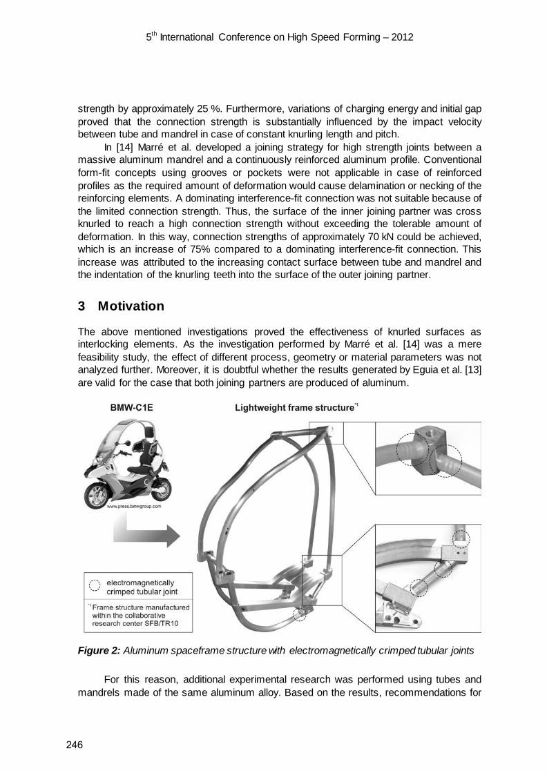
5th International Conference on High Speed Forming – 2012
strength by approximately 25 %. Furthermore, variations of charging energy and initial gap proved that the connection strength is substantially influenced by the impact velocity between tube and mandrel in case of constant knurling length and pitch.
In [14] Marré et al. developed a joining strategy for high strength joints between a massive aluminum mandrel and a continuously reinforced aluminum profile. Conventional form-fit concepts using grooves or pockets were not applicable in case of reinforced profiles as the required amount of deformation would cause delamination or necking of the reinforcing elements. A dominating interference-fit connection was not suitable because of the limited connection strength. Thus, the surface of the inner joining partner was cross knurled to reach a high connection strength without exceeding the tolerable amount of deformation. In this way, connection strengths of approximately 70 kN could be achieved, which is an increase of 75% compared to a dominating interference-fit connection. This increase was attributed to the increasing contact surface between tube and mandrel and the indentation of the knurling teeth into the surface of the outer joining partner.
3 Motivation
The above mentioned investigations proved the effectiveness of knurled surfaces as interlocking elements. As the investigation performed by Marré et al. [14] was a mere feasibility study, the effect of different process, geometry or material parameters was not analyzed further. Moreover, it is doubtful whether the results generated by Eguia et al. [13] are valid for the case that both joining partners are produced of aluminum.
Figure 2: Aluminum spaceframe structure with electromagnetically crimped tubular joints
For this reason, additional experimental research was performed using tubes and mandrels made of the same aluminum alloy. Based on the results, recommendations for
246

5th International Conference on High Speed Forming – 2012
process and joint design will be derived. The spaceframe structure depicted in Figure 2 may be cited as an example for a lightweight construction with suchlike tubular joints.
4 Experimental Procedure
Following the experimental design of Eguia et al. [13], knurling pitch tK, knurling length lK, charging energy EC and initial gap a0 were varied. Additionally, for reason of weight reduction, the effect of different mandrel stiffnesses was investigated using hollow mandrels with varying inner diameter. Both joining partners were produced of the same aluminum alloy AA6060-T6. In this way, the amount of interference fit was decreased [8] so that the resulting joint strength could be mainly attributed to the form fit caused by the knurled surface. The tube had an outer diameter of DO,i = 40 mm and a wall thickness of sO = 2 mm. The surface of the mandrel was structured with a cross knurl pattern according to DIN 82 as depicted in Figure 1a. Figure 3 summarizes all investigated combinations of the geometry and process parameters. Additionally interference-fit connections were produced using mandrels with a smooth surface.
Figure 3: Summary of investigated parameter combinations (see Figure 1a)
For the joining experiments, a ten-turn compression coil with an effective length of lC = 60 mm and an inner diameter of 40 mm was used. The coil was connected to a Maxwell Magneform pulse generator with a capacity of C = 363 μF, an inner resistance of Ri = 5.4 mΩ and an inner inductance of Li = 78 nH. Prior to the joining experiments, free tube compression experiments were conducted to measure the compression speed as a function of displacement using the Photon Doppler Velocimetry (PDV) [15]. In this way, the joint strength can be correlated to the collision velocity between tube and mandrel.
The joint quality was determined by pull-out test using a Zwick Z250 tensile testing machine. The pull-out speed was set to a constant value of 0.1 mm/s. The connection strength was defined as force for which the first relative movement between the two joining partners occurs [8, 10], whereas a plastic elongation of 0.01 % was defined as threshold value for the allowed relative movement. Additionally, micrographs of the joined components were produced to investigate the deformation behavior of the knurling teeth. For that purpose, slices with a thickness of 10 mm out of the middle of the joining zone were grinded, polished and subsequently analyzed by optical microscopy.
Before performing the destructive pull-out tests, the joining regions of the specimens were imaged in 3D by X-ray micro computed tomography in order to analyze the
247
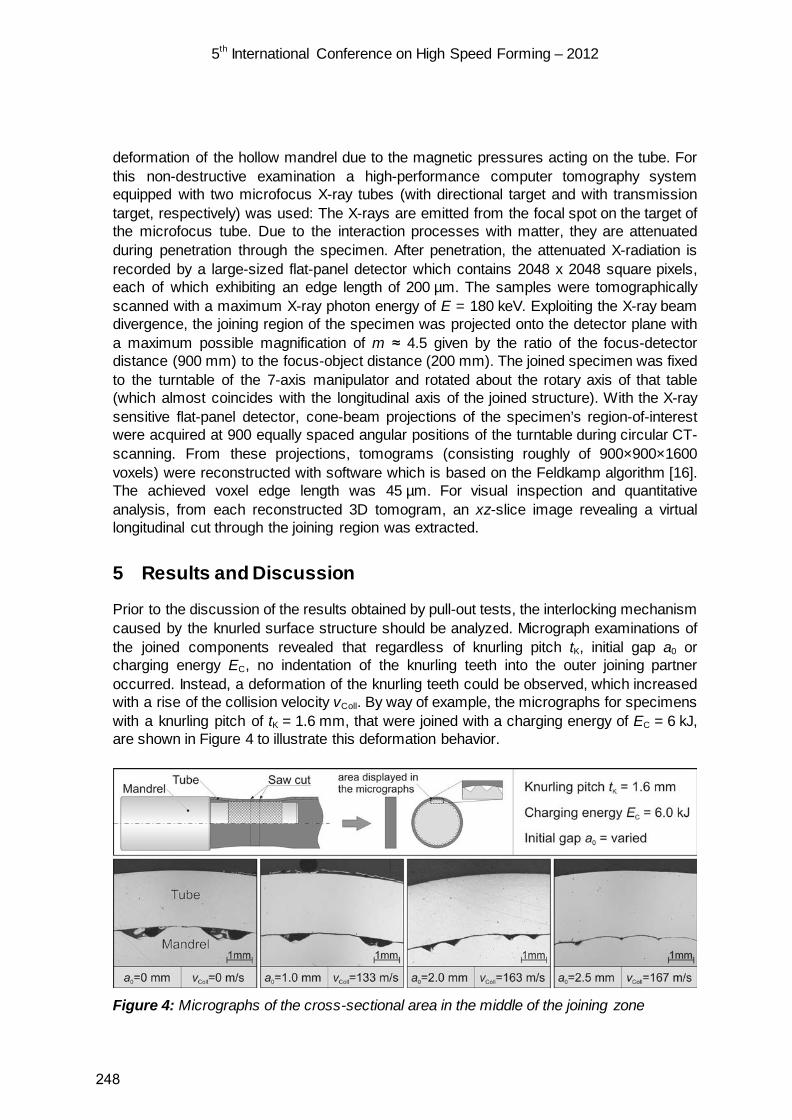
5th International Conference on High Speed Forming – 2012
deformation of the hollow mandrel due to the magnetic pressures acting on the tube. For this non-destructive examination a high-performance computer tomography system equipped with two microfocus X-ray tubes (with directional target and with transmission target, respectively) was used: The X-rays are emitted from the focal spot on the target of the microfocus tube. Due to the interaction processes with matter, they are attenuated during penetration through the specimen. After penetration, the attenuated X-radiation is recorded by a large-sized flat-panel detector which contains 2048 x 2048 square pixels, each of which exhibiting an edge length of 200 µm. The samples were tomographically scanned with a maximum X-ray photon energy of E = 180 keV. Exploiting the X-ray beam divergence, the joining region of the specimen was projected onto the detector plane with a maximum possible magnification of m ≈ 4.5 given by the ratio of the focus-detector distance (900 mm) to the focus-object distance (200 mm). The joined specimen was fixed to the turntable of the 7-axis manipulator and rotated about the rotary axis of that table (which almost coincides with the longitudinal axis of the joined structure). With the X-ray sensitive flat-panel detector, cone-beam projections of the specimen’s region-of-interest were acquired at 900 equally spaced angular positions of the turntable during circular CT-scanning. From these projections, tomograms (consisting roughly of 900×900×1600 voxels) were reconstructed with software which is based on the Feldkamp algorithm [16]. The achieved voxel edge length was 45 µm. For visual inspection and quantitative analysis, from each reconstructed 3D tomogram, an xz-slice image revealing a virtual longitudinal cut through the joining region was extracted.
5 Results and Discussion
Prior to the discussion of the results obtained by pull-out tests, the interlocking mechanism caused by the knurled surface structure should be analyzed. Micrograph examinations of the joined components revealed that regardless of knurling pitch tK, initial gap a0 or charging energy EC, no indentation of the knurling teeth into the outer joining partner occurred. Instead, a deformation of the knurling teeth could be observed, which increased with a rise of the collision velocity vColl. By way of example, the micrographs for specimens with a knurling pitch of tK = 1.6 mm, that were joined with a charging energy of EC = 6 kJ, are shown in Figure 4 to illustrate this deformation behavior.
Figure 4: Micrographs of the cross-sectional area in the middle of the joining zone
248
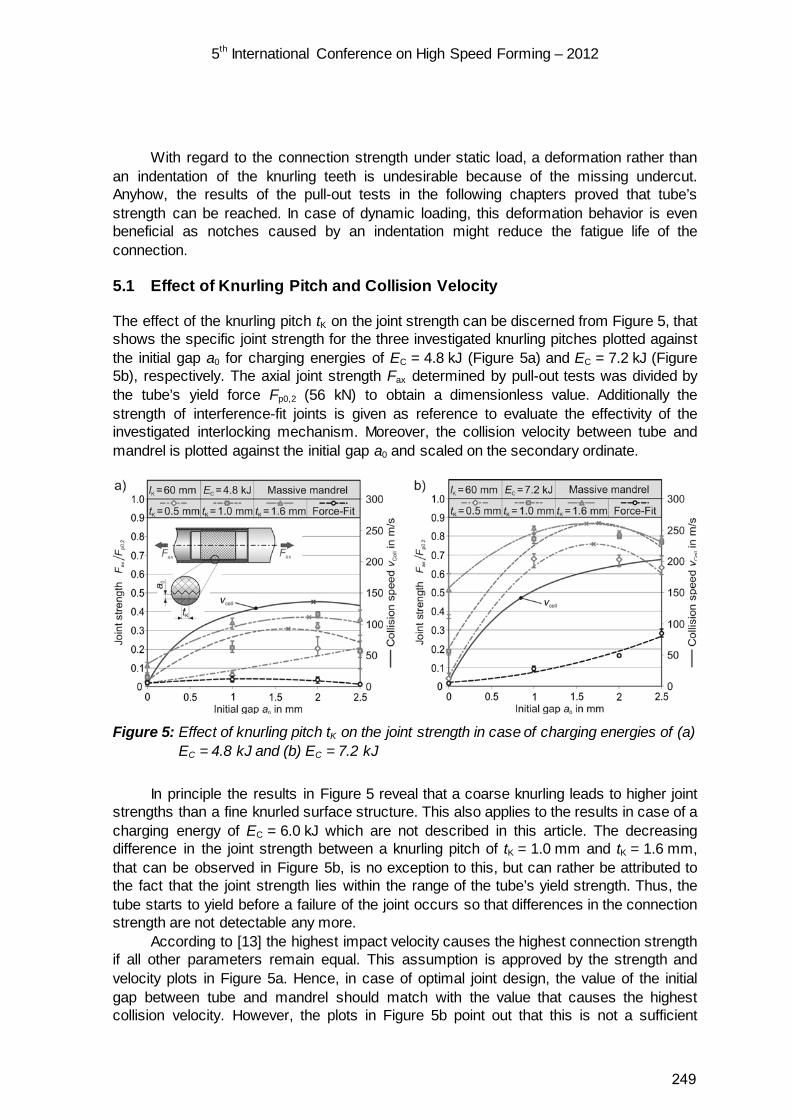
5th International Conference on High Speed Forming – 2012
With regard to the connection strength under static load, a deformation rather than an indentation of the knurling teeth is undesirable because of the missing undercut. Anyhow, the results of the pull-out tests in the following chapters proved that tube’s strength can be reached. In case of dynamic loading, this deformation behavior is even beneficial as notches caused by an indentation might reduce the fatigue life of the connection.
5.1 Effect of Knurling Pitch and Collision Velocity
The effect of the knurling pitch tK on the joint strength can be discerned from Figure 5, that shows the specific joint strength for the three investigated knurling pitches plotted against the initial gap a0 for charging energies of EC = 4.8 kJ (Figure 5a) and EC = 7.2 kJ (Figure 5b), respectively. The axial joint strength Fax determined by pull-out tests was divided by the tube’s yield force Fp0,2 (56 kN) to obtain a dimensionless value. Additionally the strength of interference-fit joints is given as reference to evaluate the effectivity of the investigated interlocking mechanism. Moreover, the collision velocity between tube and mandrel is plotted against the initial gap a0 and scaled on the secondary ordinate.
Figure 5: Effect of knurling pitch tK on the joint strength in case of charging energies of (a)
EC = 4.8 kJ and (b) EC = 7.2 kJ
In principle the results in Figure 5 reveal that a coarse knurling leads to higher joint strengths than a fine knurled surface structure. This also applies to the results in case of a charging energy of EC = 6.0 kJ which are not described in this article. The decreasing difference in the joint strength between a knurling pitch of tK = 1.0 mm and tK = 1.6 mm, that can be observed in Figure 5b, is no exception to this, but can rather be attributed to the fact that the joint strength lies within the range of the tube’s yield strength. Thus, the tube starts to yield before a failure of the joint occurs so that differences in the connection strength are not detectable any more.
According to [13] the highest impact velocity causes the highest connection strength if all other parameters remain equal. This assumption is approved by the strength and velocity plots in Figure 5a. Hence, in case of optimal joint design, the value of the initial gap between tube and mandrel should match with the value that causes the highest collision velocity. However, the plots in Figure 5b point out that this is not a sufficient
249

5th International Conference on High Speed Forming – 2012
condition to guarantee the highest connection strength as the point of maximum joint strength and maximum collision velocity diverge from each other significantly.
For a more detailed analysis of the correlation between connection strength and collision velocity, Figure 6 can be used. It shows the specific connection strength plotted against the collision velocity in case of a knurling pitch of tK = 1.0 mm. In comparison to Figure 5, the effect of charging energy EC and initial gap a0 on the collision velocity can be analyzed separately. The diagram reveals that a rising collision velocity caused by an increase of the charging energy leads to an increasing connection strength in any case. If the increase of the collision velocity is caused by an increasing gap size, the joint strength is affected by two additional effects. On the one hand the gap size is increased by decreasing the outer diameter of the mandrel, which lessens the area of contact between the two joining partners and has a negative impact on the connection strength. On the other hand, roundness measurements on joined specimens proved that an increased gap size results in an increasing roundness deviation, that may lower the connection strength as well.
Figure 6: Effect of the collision velocity on the joint strength (tK = 1 mm, lK = 60 mm)
Consequently, an increase of the gap size only results in a rise of the connection strength if the positive effect of increasing collision velocity predominates the negative effects of decreasing contact area and increasing roundness deviation.
With regard to the results in Figure 6, this condition is met for a change of the gap size from a0 = 1 mm to a0 = 2 mm as an increase of the connection strength can be observed for all charging energies. Augmenting the gap size from a0 = 2.0 mm to a0 = 2.5 mm only leads to a slight increase of the collision velocity that cannot compensate the negative effects mentioned above and thus causes a decrease of the joint strength. Based on this result it can be concluded that in case of small collision velocity gradients, rather smaller gap sizes should be preferred as the advantage of the slight increase of velocity is completely eroded by the negative effects of decreasing contact area and increasing roundness deviation.
250
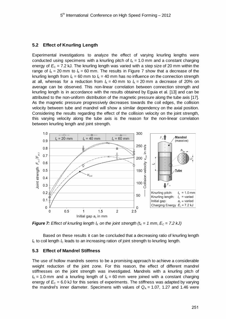
5th International Conference on High Speed Forming – 2012
5.2 Effect of Knurling Length
Experimental investigations to analyze the effect of varying knurling lengths were conducted using specimens with a knurling pitch of tK = 1.0 mm and a constant charging energy of EC = 7.2 kJ. The knurling length was varied with a step size of 20 mm within the range of lK = 20 mm to lK = 60 mm. The results in Figure 7 show that a decrease of the knurling length from lK = 60 mm to lK = 40 mm has no influence on the connection strength at all, whereas for a reduction from lK = 40 mm to lK = 20 mm a decrease of 20% on average can be observed. This non-linear correlation between connection strength and knurling length is in accordance with the results obtained by Eguia et al. [13] and can be attributed to the non-uniform distribution of the magnetic pressure along the tube axis [17]. As the magnetic pressure progressively decreases towards the coil edges, the collision velocity between tube and mandrel will show a similar dependency on the axial position. Considering the results regarding the effect of the collision velocity on the joint strength, this varying velocity along the tube axis is the reason for the non-linear correlation between knurling length and joint strength.
Figure 7: Effect of knurling length lK on the joint strength (tK = 1 mm, EC = 7.2 kJ)
Based on these results it can be concluded that a decreasing ratio of knurling length lK to coil length lC leads to an increasing ration of joint strength to knurling length.
5.3 Effect of Mandrel Stiffness
The use of hollow mandrels seems to be a promising approach to achieve a considerable weight reduction of the joint zone. For this reason, the effect of different mandrel stiffnesses on the joint strength was investigated. Mandrels with a knurling pitch of tK = 1.0 mm and a knurling length of lK = 60 mm were joined with a constant charging energy of EC = 6.0 kJ for this series of experiments. The stiffness was adapted by varying the mandrel’s inner diameter. Specimens with values of QA = 1.07, 1.27 and 1.46 were
251
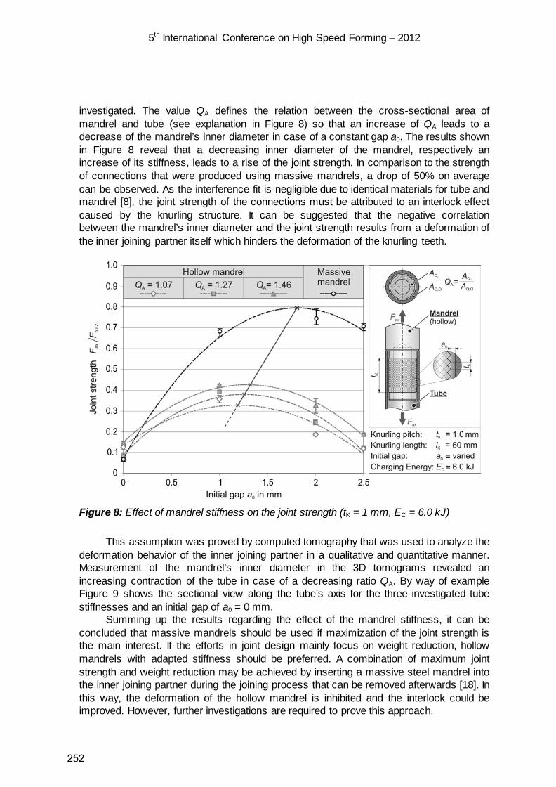
5th International Conference on High Speed Forming – 2012
investigated. The value QA defines the relation between the cross-sectional area of mandrel and tube (see explanation in Figure 8) so that an increase of QA leads to a decrease of the mandrel’s inner diameter in case of a constant gap a0. The results shown in Figure 8 reveal that a decreasing inner diameter of the mandrel, respectively an increase of its stiffness, leads to a rise of the joint strength. In comparison to the strength of connections that were produced using massive mandrels, a drop of 50% on average can be observed. As the interference fit is negligible due to identical materials for tube and mandrel [8], the joint strength of the connections must be attributed to an interlock effect caused by the knurling structure. It can be suggested that the negative correlation between the mandrel’s inner diameter and the joint strength results from a deformation of the inner joining partner itself which hinders the deformation of the knurling teeth.
Figure 8: Effect of mandrel stiffness on the joint strength (tK = 1 mm, EC = 6.0 kJ)
This assumption was proved by computed tomography that was used to analyze the deformation behavior of the inner joining partner in a qualitative and quantitative manner. Measurement of the mandrel’s inner diameter in the 3D tomograms revealed an increasing contraction of the tube in case of a decreasing ratio QA. By way of example Figure 9 shows the sectional view along the tube’s axis for the three investigated tube stiffnesses and an initial gap of a0 = 0 mm.
Summing up the results regarding the effect of the mandrel stiffness, it can be concluded that massive mandrels should be used if maximization of the joint strength is the main interest. If the efforts in joint design mainly focus on weight reduction, hollow mandrels with adapted stiffness should be preferred. A combination of maximum joint strength and weight reduction may be achieved by inserting a massive steel mandrel into the inner joining partner during the joining process that can be removed afterwards [18]. In this way, the deformation of the hollow mandrel is inhibited and the interlock could be improved. However, further investigations are required to prove this approach.
252
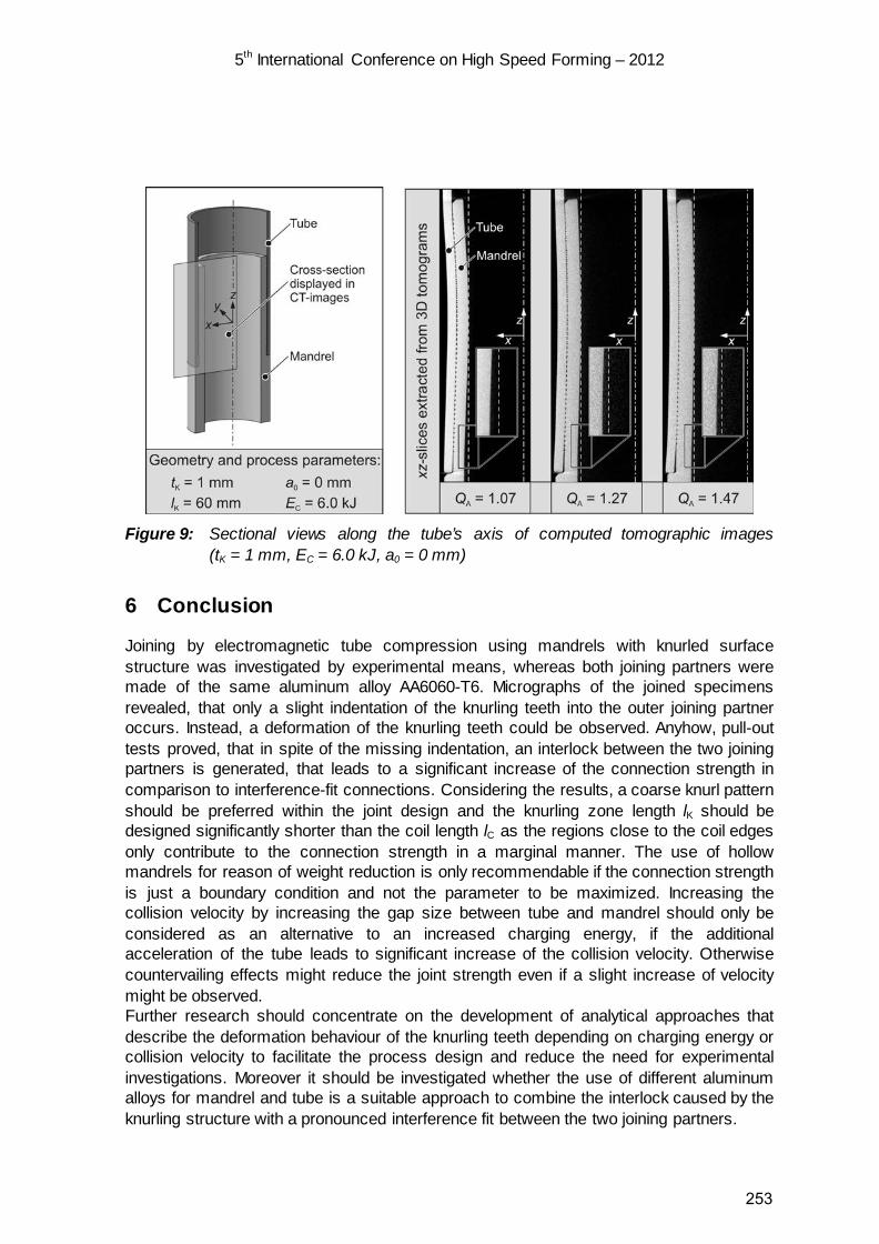
5th International Conference on High Speed Forming – 2012
Figure 9: Sectional views along the tube’s axis of computed tomographic images
(tK = 1 mm, EC = 6.0 kJ, a0 = 0 mm)
6 Conclusion
Joining by electromagnetic tube compression using mandrels with knurled surface structure was investigated by experimental means, whereas both joining partners were made of the same aluminum alloy AA6060-T6. Micrographs of the joined specimens revealed, that only a slight indentation of the knurling teeth into the outer joining partner occurs. Instead, a deformation of the knurling teeth could be observed. Anyhow, pull-out tests proved, that in spite of the missing indentation, an interlock between the two joining partners is generated, that leads to a significant increase of the connection strength in comparison to interference-fit connections. Considering the results, a coarse knurl pattern should be preferred within the joint design and the knurling zone length lK should be designed significantly shorter than the coil length lC as the regions close to the coil edges only contribute to the connection strength in a marginal manner. The use of hollow mandrels for reason of weight reduction is only recommendable if the connection strength is just a boundary condition and not the parameter to be maximized. Increasing the collision velocity by increasing the gap size between tube and mandrel should only be considered as an alternative to an increased charging energy, if the additional acceleration of the tube leads to significant increase of the collision velocity. Otherwise countervailing effects might reduce the joint strength even if a slight increase of velocity might be observed. Further research should concentrate on the development of analytical approaches that describe the deformation behaviour of the knurling teeth depending on charging energy or collision velocity to facilitate the process design and reduce the need for experimental investigations. Moreover it should be investigated whether the use of different aluminum alloys for mandrel and tube is a suitable approach to combine the interlock caused by the knurling structure with a pronounced interference fit between the two joining partners.
253
5th International Conference on High Speed Forming – 2012
References
[1] Wegerdt, C.; Thoms, V.; Franke, R.; Carstensen, H.: Mechanische Fügetechnik. Tagungsband der 72. Tagung des Wissenschaftlichen Rates der AiF, Düsseldorf, 1999, p. 6.1-6.20.
[2] Nationale Plattform Elektromobilität: Zweiter Bericht der Nationalen Plattform Elektromobilität, Berlin, 2011.
[3] Schönherr, M.: Formgebung durch den Strang. Maschinenmarkt, 2003, Issue 11, p. 24-26.
[4] Fouhy, K.: Alu-Strangpressprofile optimal herstellen. Maschinenmarkt, 2003, Issue 11, p. 3.
[5] v. Finckenstein, E.: Ein Beitrag zur Hochgeschwindigkeitsumformung rohrfömiger Werkstücke durch magnetische Kräfte. In: Fortschritt Berichte VDI-Z, Reihe 2, Nr. 17, VDI-Verlag, Düsseldorf, 1967.
[6] Winkler, R.: Hochgeschwindigkeitsbearbeitung. VEB Verlag Technik, Berlin, 1973. [7] Lange, K.: Umformtechnik – Band 4: Sonderverfahren, Prozesssimulation,
Werkzeugtechnik, Produktion. 2. Auflage, Springer Verlag, Berlin, 1993. [8] Weddeling, C.; Woodward, S. T.; Marré, M.; Nellesen, J.; Psyk, V.; Tekkaya, A. E.;
Tillmann, W.: Influence of groove characteristics on strength of form-fit joints. Journal of Materials Processing Technology, 211 (2011), Issue 5, p. 925-935.
[9] Bühler, H.; Bauer, D.: Ein Beitrag zur Magnetumformung rohrförmiger Werkstücke. Werkstatt und Betrieb, 110 (1968), Issue 9, p. 513 – 516.
[10] Bühler, H.; v. Finckenstein, E.: Fügen durch Magnetumformung – Lösekräfte von Sickenverbindungen aus Stahl. Werkstatt und Betrieb, 101 (1968), Issue 11, p. 671-675.
[11] Golovashchenko, S.: Methodology of Design of Pulsed Electromagnetic Joining of Tubes. Proceedings of the TMS Symposium “Innovations in Processing and Manufacturing”, New Orleans, LA, USA, 2001, p. 283-299.
[12] Park, Y.-B.; Kim, H.-Y.; Oh, S.-I.: Design of axial/torque joint made by electromagnetic forming. Thin Walled Structures, 43 (2005), p. 826-844.
[13] Eguia, I.; Zhang, P.; Daehn, G. S.: Improved Crimp-Joining of Aluminum Tubes onto Mandrels with Undulating Surfaces. Proceedings of the 1st International Conference on High Speed Forming 2004 (ICHSF), Dortmund, 2004, p. 161-170.
[14] Marré, M.; Brosius, A.; Tekkaya, A. E.: Joining by Compression and Expansion of (None-) Reinforced Profiles. Advanced Materials Research, 43 (2008), p. 57 – 68.
[15] Vivek, A.; Kim, K.-H.; Daehn, G. S.: Simulation and instrumentation of electromagnetic compression of steel tubes. Journal of Materials Processing Technology, 211 (2011), p.840-850.
[16] Feldkamp, L. A.; Davis, L. C.; Kress, J. W.: Practical cone-beam algorithm. Journal of the Optical Society of America, 1 (1984), Issue 6, p. 612 – 619.
[17] Beerwald, C.: Fundamentals for Process Dimensioning and Design of Electromagnetic Forming (in German). Dr.-Ing. Thesis, Universität Dortmund, 2004.
[18] Weddeling, C.; Woodward, S.; Nellesen, J.; Psyk, V.; Marré, M.; Brosius, A.; Tekkaya, A. E.; Daehn, G. S.; Tillmann, W.: Development of design principles for form-fit joints in lightweight frame structures. Proceedings of the 4th International Conference on High Speed Forming 2010 (ICHSF), Dortmund, 2010, p. 137 – 148.
254
Laser Impact Welding – Process Introduction and Key Variables
H. Wang1, D. Liu1, G. Taber1, J. C. Lippold1, G. S. Daehn1
1Department of Materials Science & Engineering, The Ohio State University, United States
Abstract
Laser impact welding is a solid-state, collision-based welding process. In this process, laser-generated optical energy is converted to kinetic energy through the ablation at the surface and confinement of the gas generated between a flyer and backing plate. The launch of the flyer can be affected by many factors, for example, backing material, ablative layer, and flyer thickness. In this paper, the effect of three backing materials: glass, polycarbonate and cellophane tape, were studied with different laser spot size and commercially pure aluminum alloy 1100 was used as the flyer. The results show that glass can provide the most efficient launches, but is damaged. Polycarbonate is a good compromise between efficiency and robustness. Welding is possible between many similar and dissimilar material pairs. In this study, commercially pure nickel was joined to commercially pure nickel. There are several possible geometric arrangements of the target relative to the flyer. With flat targets, metallurgical bonding takes place along the edges of the spot, and jet was observed in the center of the spot. Corrugated targets provide more surface area for metallurgical bonding. In this paper, the flyer launch velocity-time profile is also demonstrated using a photon Doppler velocimetry technique.
Keywords
Laser impact welding, energy efficiency, Jet, impact angle, impact velocity
255
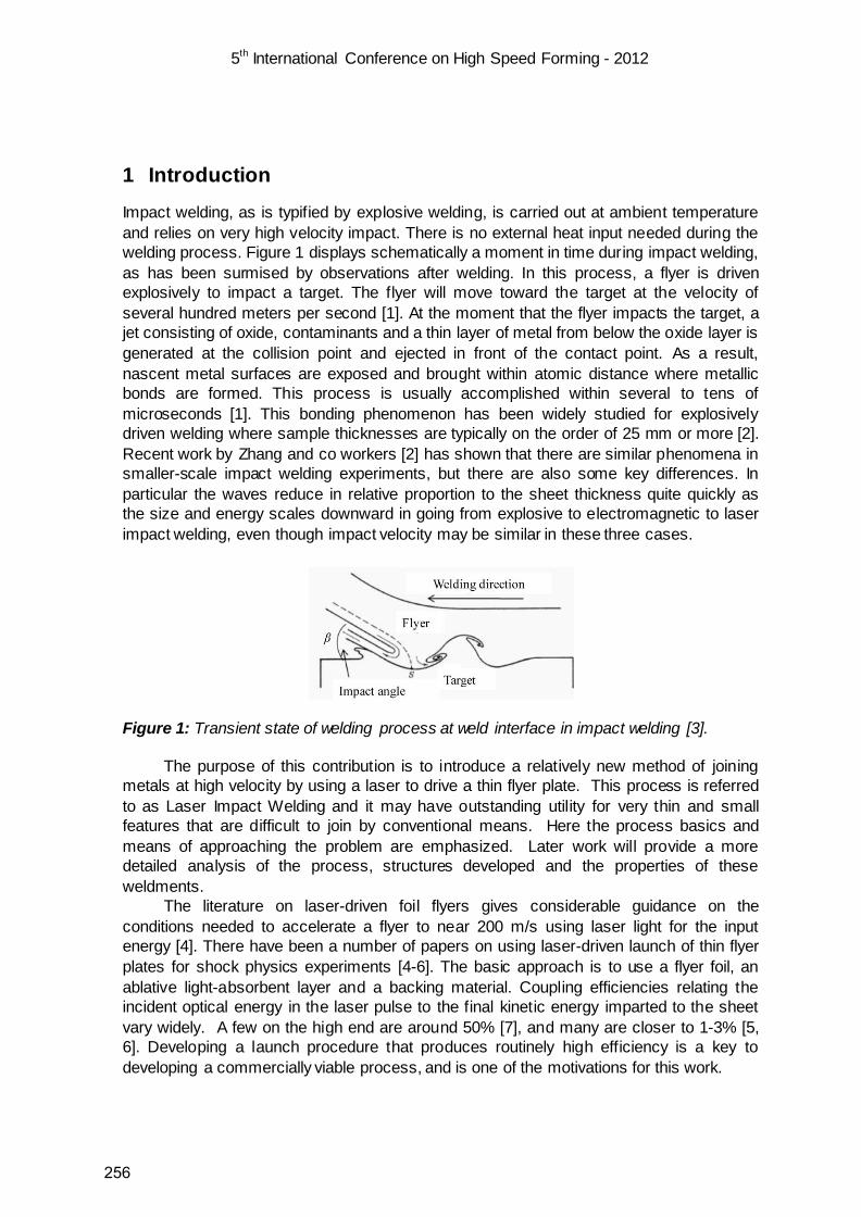
5th International Conference on High Speed Forming - 2012
1 Introduction Impact welding, as is typified by explosive welding, is carried out at ambient temperature and relies on very high velocity impact. There is no external heat input needed during the welding process. Figure 1 displays schematically a moment in time during impact welding, as has been surmised by observations after welding. In this process, a flyer is driven explosively to impact a target. The flyer will move toward the target at the velocity of several hundred meters per second [1]. At the moment that the flyer impacts the target, a jet consisting of oxide, contaminants and a thin layer of metal from below the oxide layer is generated at the collision point and ejected in front of the contact point. As a result, nascent metal surfaces are exposed and brought within atomic distance where metallic bonds are formed. This process is usually accomplished within several to tens of microseconds [1]. This bonding phenomenon has been widely studied for explosively driven welding where sample thicknesses are typically on the order of 25 mm or more [2]. Recent work by Zhang and co workers [2] has shown that there are similar phenomena in smaller-scale impact welding experiments, but there are also some key differences. In particular the waves reduce in relative proportion to the sheet thickness quite quickly as the size and energy scales downward in going from explosive to electromagnetic to laser impact welding, even though impact velocity may be similar in these three cases.
Figure 1: Transient state of welding process at weld interface in impact welding [3].
The purpose of this contribution is to introduce a relatively new method of joining metals at high velocity by using a laser to drive a thin flyer plate. This process is referred to as Laser Impact Welding and it may have outstanding utility for very thin and small features that are difficult to join by conventional means. Here the process basics and means of approaching the problem are emphasized. Later work will provide a more detailed analysis of the process, structures developed and the properties of these weldments.
The literature on laser-driven foil flyers gives considerable guidance on the conditions needed to accelerate a flyer to near 200 m/s using laser light for the input energy [4]. There have been a number of papers on using laser-driven launch of thin flyer plates for shock physics experiments [4-6]. The basic approach is to use a flyer foil, an ablative light-absorbent layer and a backing material. Coupling efficiencies relating the incident optical energy in the laser pulse to the final kinetic energy imparted to the sheet vary widely. A few on the high end are around 50% [7], and many are closer to 1-3% [5, 6]. Developing a launch procedure that produces routinely high efficiency is a key to developing a commercially viable process, and is one of the motivations for this work.
256

5th International Conference on High Speed Forming - 2012
Laser shock peening is a related commercially practiced method for engineering the microstructure and state of residual stress at the surface of a part [8-10]. In a typical application, a component is given an optically absorbing coating and either placed under water, or a water stream moves over the part surface. Intense laser pulses ablate a small region of the surface and the high-pressure pulse locally deforms the surface of the material. This method is significant in that the technical objectives are very similar to those in laser-driven collision welding – a brief, large, local mechanical impulse is desired [5].
This paper presents an overview of the potential and challenges related to laser impact welding, and reviews the experimental methodologies that are being developed at The Ohio State University.
2 Methods and Results
The Nd:YAG laser source used in this study was a Continuum PowerliteTM Precision II Scientific System. The maximum energy available is 3J with a wavelength of 1064nm. It can provide optical pulses at 10HZ, each with pulse duration of 8ns. The low-divergence output beam has a diameter of 12.5 mm. For these experiments, an anti-reflection lens was used to focus the beam to nearly a point, but at a 2 Joule output if the beam diameter is reduced beyond about 1.6 mm, the optical energy density is so high that the air can be ionized. Therefore, larger beam diameters should be used. By changing the distance between the focus lens and the experimental setup, as illustrated in Figure 2, the diameter of the beam, which is incident on the flyer plate, can be changed In this experiment, three different beam diameters were investigated, namely 2mm, 4mm, 6mm, corresponding to energy and power densities of 9.6×10⁵, 2.4×10⁵ and 1.1×10⁵ J/m2 and 1.2×10¹¹, 3.0×10¹⁰ and 1.3×10¹⁰ kW/m2, respectively.
Figure 2: Effect of varied experimental position relative to the lens to vary spot size and power density.
Three experimental approaches have been developed for welding, as shown in
Figure 3. Each produces different weld patch geometries. In each case the laser passes through the transparent backing and vaporizes the ablative layer. This separates the flyer and backing, and due to conservation of momentum, the flyer moves much faster than the more massive backing. The flyer moves to the target with a bulged shape and upon collision, if an appropriate combination of impact velocity and angle exists, bonding will
257

5th International Conference on High Speed Forming - 2012
occur. This work will focus on the use of flat and corrugated targets. Prior work at Ohio State has demonstrated that angled target plates will also produce satisfactory welds.
a b c
Figure 3: Three modes of developing laser impact weld targets: a) flat, b) angled and c) corrugated.
2.1 Effect of backing material on launch efficiency
The backing material attached to the flyer plate has an effect on the energy efficiency. The backing material must be transparent to the laser and confine the plasma that is generated by the ablative material. Three backing materials were studied in this experiment, 1) conventional soda-lime glass microscope slides (1mm thick), 2) polycarbonate (0.5mm thick), and 3) clear tape (Scotch packing tape with thickness of 0.07mm).
The experimental setup is shown in Figure 4. Commercially pure, 1100 aluminum flyer plate (0.076 mm thick) was painted with black RUST-OLEUM™ enamel aerosol paint, and was attached to the backing material with cyanoacrylate adhesive (Loctite 380). The backing material was attached to the holder with double-sided cellophane tape.
Figure 4: Experimental setup for launching efficiency experiments
Figure 5 shows one of the examples of energy efficiency experiments by changing backing material at 2mm and 4mm laser spot size position. With polycarbonate, the first hole is bigger than the other two. That was caused by the detachment of the flyer from the backing material after the first shot. Therefore, for the second and third shot, the plasma is not confined as effectively as the first one by the backing material. This result demonstrates that the important role of the backing material in the launching efficiency. The hole sizes indicate that clear tape is the least effective backing material. This can be
258
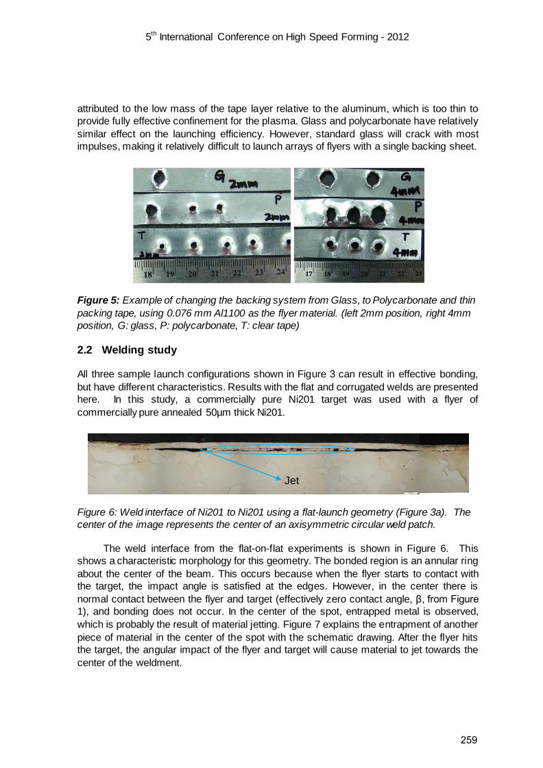
5th International Conference on High Speed Forming - 2012
attributed to the low mass of the tape layer relative to the aluminum, which is too thin to provide fully effective confinement for the plasma. Glass and polycarbonate have relatively similar effect on the launching efficiency. However, standard glass will crack with most impulses, making it relatively difficult to launch arrays of flyers with a single backing sheet.
Figure 5: Example of changing the backing system from Glass, to Polycarbonate and thin packing tape, using 0.076 mm Al1100 as the flyer material. (left 2mm position, right 4mm position, G: glass, P: polycarbonate, T: clear tape)
2.2 Welding study
All three sample launch configurations shown in Figure 3 can result in effective bonding, but have different characteristics. Results with the flat and corrugated welds are presented here. In this study, a commercially pure Ni201 target was used with a flyer of commercially pure annealed 50µm thick Ni201.
Figure 6: Weld interface of Ni201 to Ni201 using a flat-launch geometry (Figure 3a). The center of the image represents the center of an axisymmetric circular weld patch.
The weld interface from the flat-on-flat experiments is shown in Figure 6. This shows a characteristic morphology for this geometry. The bonded region is an annular ring about the center of the beam. This occurs because when the flyer starts to contact with the target, the impact angle is satisfied at the edges. However, in the center there is normal contact between the flyer and target (effectively zero contact angle, β, from Figure 1), and bonding does not occur. In the center of the spot, entrapped metal is observed, which is probably the result of material jetting. Figure 7 explains the entrapment of another piece of material in the center of the spot with the schematic drawing. After the flyer hits the target, the angular impact of the flyer and target will cause material to jet towards the center of the weldment.
Jet
259

5th International Conference on High Speed Forming - 2012
Figure 7: Schematic for explanation of jet formation
Machining easily produces corrugated targets. In this case, the interaction of impact angle and bonding can be investigated. The weld interface between a pure nickel, 50µm thick flyer and corrugated target is shown in Figure 8. This shows that at shallow angles, such as around 8°, bonding is achieved, while at larger angles (on the order of 30°, there is no bonding, and possibly no contact during impact. Normal impact, will not cause welding as was shown in Figure 6.
Figure 8: Weld interface with corrugated target joining NI201 to Ni 201
2.3 Impact velocity measurement
Aside from impact angle impact velocity is one of the critical parameters that determines if collision welding will take place. Photon Doppler Velocimetry (PDV) [11] was used to measure the velocity time profile and potential the impact velocity for one launch configuration. Figure 9 shows velocity-time profiles for experiments with the parameters shown in Table I and permanent (Sharpie pen) ink and tape and water as backing media. This experiment was done using similar equipment to that described in this paper at the facilities of LSP Technologies, Inc in Dublin, Ohio with their laser system and assistance.
Step 1
Step 2
Step 3
Step 4
Step 5
260

5th International Conference on High Speed Forming - 2012
Exp. No. flyer Energy Spot size Flyer thickness Backing
1 Al6061-T6 6.5J 4mm 635µm water
2 Al6061-T6 6.5J 4mm 635µm Clear tape
Table 1: Experimental parameters for impact velocity measurement
The launch velocity as a function of time was measured using water and clear tape as backings. Figure 9 shows the measured velocity and displacement. From Figure 9, it can be seen that full velocity can be achieved within 0.2µs. The terminal velocity is much higher with water as the backing material than with clear tape. Again, the cellophane tape does not have sufficient areal mass to provide effective backing. The important observation is that in both cases the peak velocity of the flyer is reached after less than 30 µm of displacement. This potentially allows a variety of configurations that will allow bonding to occur with very little initial standoff between the flyer and target.
Figure 9: Impact velocity and displacement with (a) water and (b) transparent tape as the backing.
(a) (b)
261

5th International Conference on High Speed Forming - 2012
3 Prognosis and Approach for Process Development This process has great practical potential. Nearly arbitrary dissimilar metals can be bonded with one another. Pulsed lasers that provide pulse energies of about 5 joules or less are commercially available. These will operate easily at 10 Hz. This much energy will allow a metallurgical patch of a couple square millimeters in extent to be created with a metal flyer on the order of 150µm. This gives great practical potential for creating large arrays of solid-state metallurgical welds between dissimilar metals, and this process has the potential to be scaled to almost arbitrarily small length scales. One of the key challenges is the development of methods to fabricate flyer/backer systems on a large scale. Some initial ideas on this are presented here.
As shown in Figure 10, several layers (backer, absorbing layer, protective layer, flyer sheet) can be laminated together with properly cut and aligned sheets using adhesives. With a CNC profile cutter shapes can easily be cut in planar sheets (Silhouette Cameo is for example inexpensive and precise), many samples can be cut in one step. This array of samples can be attached to the CNC controlled 3-axis stage (shown in Figure 10) for laser impact experiments. This will be used in an automated manner with the laser to create samples for the statistical study of sample strength and properties. This also demonstrates a potential approach for manufacturing.
Figure 10: Array of samples from CNC cutter, and (right) a 3 Degree of Freedom CNC stage in the laser experimental chamber.
262
5th International Conference on High Speed Forming - 2012
4 Conclusions Laser impact welding is an easily practiced form of solid state welding that will allow the metallurgical bonding between almost arbitrary pairs of dissimilar metals. The key features of the approach along with a development path have been described here. An approach to create large numbers of samples using CNC cutting and motion control is described and it is suggested that polycarbonate or other transparent polymers may become effective backing materials. The fact that full flyer velocity can be achieved over a very short distance suggests that many geometric arrangements may be possible for impact welding.
A facility to study this process has been developed and some promising initial results from that facility are presented here.
5 Acknowledgements This work and the related development of facilities was supported by the Air Force
Research Laboratory through the Intelligent Manufacturing Initiative, the NSF I/UCRC for Integrated Materials Joining Science for Energy Applications (CIMJSEA), Medtronic, Inc. and The Alcoa Foundation.
References
[1] Crossland. B.: Explosive welding of metals and its application, Oxford University
Press, New York, 1982. [2] Zhang, Y.; Babu, S. S.; Prothe, C.; Blakely, M.; Kwasegroch, J.; LaHa, M.; Daehn, S.
G.: Application of high velocity impact welding at varied different length scales. Journal of Materials Processing Technology, 2011(5), p.944-952.
[3] Bahrani, A. S.; Black, T. J.; Crossland, B.: Mechanics of wave formation in explosive welding. Proceedings of the Royal Society of London Series a-Mathematical and Physical Sciences, 1967, p.123-136.
[4] Tanaka, A. K.; Hara, M.; Ozaki, N.; Sasatani, Y.; Anisimov I. S.: Multi-layered flyer accelerated by laser induced shock waves, Physics of Plasmas, 2000(2), p.676-680.
[5] Swift, D. C.; Niemczura, J. G.; Paisley, D. L.; Johnson, R. P.; Luo, S. N.; Tierney, T. E.: Laser-launched flyer plates for shock physics experiments, Review of Scientific Instruments, 2005(9), 093907.
[6] Cogan, S. ; Shirman, E.; Haas, Y.: Production efficiency of thin metal flyers formed by laser ablation, Journal of Applied Physics, 2005(11), 113508.
[7] Miller, C. W.: Set-up and evaluation of laser-driven miniflyer system, Georgia Institute of Technology, 2009.
[8] Montross S. C.; Wei, T.; Ye L., Clark G.; Mai Y-W.: Laser shock processing and its effects on microstructure and properties of metal alloys: a review. International Journal of Fatigue 24, 2002, p. 1021–1036.
263

5th International Conference on High Speed Forming - 2012
[9] Fairand P. B.; Wilcox A. B.; Gallagher J. W.; Williams N. D.: laser shock-induced microstructural and mechanical property changes in 7075 aluminum. Journal of Applied Physics, 1972(9), p.3893-3895.
[10] Fabbro R.; Peyre P.; Berthe L.; Scherpereel X.: Physics and applications of laser-shock processing. Journal of Laser Applications, 1998(12), p.265-279.
[11] Strand, O. T.; Goosman, D. R.; Martinez, C.; Whitworth, T. L.: Compact system for high-speed velocimetry using heterodyne techniques, Review of Scientific Instruments, 2006(8), 083108.
264

SESSION 8
FORMABILITY
265

266
Coil Development for Electromagnetic Corner Fill of AA 5754 Sheet* J. Imbert1, M. Worswick1
1 Department of Mechanical and Mechatronics Engineering, University of Waterloo, Waterloo, Ontario, Canada
Abstract
Electromagnetic (EM) forming is a high-speed forming process that uses the forces induced on a conductive workpiece by a transient high frequency magnetic field to form the workpiece into a desired shape. It has been reported by several researchers that EM forming (EMF) increases the formability of hard-to-form aluminum alloy sheet under certain circumstances. EMF can be combined with conventional forming (e.g. stamping) operations to create a hybrid forming operation that exploits the strengths of each process. One such operation is the “corner fill” operation, which consists in pre-forming sheet using conventional forming and then using EMF to reduce the radii of different features on the part to values that could not be obtained with conventional forming. This paper describes the development of a coil used for a hybrid operation that consisted on pre-forming AA 5754 1 mm into a v-shape with a 20 mm outer radius and then reducing or “sharpening” the radius to 5 mm using EMF. The coil is one of the most important components of an EMF operation, since it is the means of delivering the energy to the workpiece. Coils are subjected to very high stresses and are typically the element of an EMF operation that will fail first. One successful and four unsuccessful coils designs are presented. The successful coil was a single loop design, with the section closest to the part narrowed to increase the current density. The simplicity of the shape was chosen for its current flow characteristics and for its structural strength.
Keywords
Forming, high, speed
* The authors would like to thank the Natural Science and Engineering Research Council of Canada and the Ontario Research Fund for their financial support
267

5th International Conference on High Speed Forming – 2012
1 Introduction
Electromagnetic (EM) forming is a high-speed forming process that uses the forces induced on a conductive workpiece by a transient high frequency current to form the workpiece into a desired shape. EM forming (EMF) can be combined with conventional forming (e.g. stamping) operations to create a hybrid forming operation that exploits the strengths of each process. One such operation is the “corner fill” operation, which consists in pre-forming sheet using conventional forming and then using EMF to reduce the radius of different features on the part to values that could not be obtained with conventional forming. Figure 1 illustrates the process with the corner fill operation used for this research, in which a sheet is formed with a conventional tool comprising a die and a punch and then an EMF operation is used to sharpen or “fill” the corner.
Figure 1: Schematic of the hybrid forming operation which consists of a) conventional forming to produce b) a pre-formed blank with a radius of 20 mm that is then subjected to c) an EM corner fill operation to produce d) the final sample shape.
Despite the interest shown on this subject by researchers in both academia and industry, there have been few works published on the subject of hybrid forming. Daehn et al. [1] determined it was feasible to form the sharp features of the aluminum panel using EMF. Oliveira [2] studied corner fill numerically for an axi-symmetric geometry and found that the induced force distribution had a significant effect on the final shape of the material in the corner. Psyk et al. [3,4] studied sharpening of a feature on a representative full-scale automotive stamping and found that the process was feasible. Liu et al. [5] showed that EMF could be used for sharpening corners on axisymmetric deep drawn parts, similar to the ones used in LDR tests. Golovashchenko [6] conventionally pre-formed blanks and then used EM and electrohydraulic forming to sharpen the corners. It was reported that EMF could be used to form two dimensional radii, but not three-dimensional ones, where electrohydraulic forming was required [6].
The hybrid operation reported here consisted of pre-forming the material using a v-channel tool to an outside radius of 20 mm while allowing draw-in and then reducing the radius to 5 mm using EM forming without draw-in. Figure 2 shows the ideal pre-formed and final sample shapes used for this work. The experiment was designed so that the pre-formed part could not be formed to a 5 mm outer radius using a conventional stamping operation if the material was not allowed to draw into the die. This simulated a multi-step forming process in which the material within a larger part is constrained from drawing-in to sharpen a corner feature, in which case an EM forming step can be a means to sharpen corner radii. The results of the corner fill experiments have been reported by Imbert [7] and Imbert and Worswick [8]. A sample formed using the successful coil design is shown in Figure 3.
268
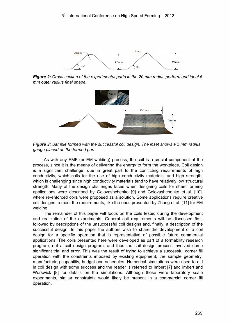
5th International Conference on High Speed Forming – 2012
Figure 2: Cross section of the experimental parts in the 20 mm radius perform and ideal 5 mm outer radius final shape.
Figure 3: Sample formed with the successful coil design. The inset shows a 5 mm radius gauge placed on the formed part.
As with any EMF (or EM welding) process, the coil is a crucial component of the process, since it is the means of delivering the energy to form the workpiece. Coil design is a significant challenge, due in great part to the conflicting requirements of high conductivity, which calls for the use of high conductivity materials, and high strength, which is challenging since high conductivity materials tend to have relatively low structural strength. Many of the design challenges faced when designing coils for sheet forming applications were described by Golovashchenko [9] and Golovashchenko et al. [10], where re-enforced coils were proposed as a solution. Some applications require creative coil designs to meet the requirements, like the ones presented by Zhang et al. [11] for EM welding.
The remainder of this paper will focus on the coils tested during the development and realization of the experiments. General coil requirements will be discussed first, followed by descriptions of the unsuccessful coil designs and, finally, a description of the successful design. In this paper the authors wish to share the development of a coil design for a specific operation that is representative of possible future commercial applications. The coils presented here were developed as part of a formability research program, not a coil design program, and thus the coil design process involved some significant trial and error. This was the result of trying to achieve a successful corner fill operation with the constraints imposed by existing equipment, the sample geometry, manufacturing capability, budget and schedules. Numerical simulations were used to aid in coil design with some success and the reader is referred to Imbert [7] and Imbert and Worswick [8] for details on the simulations. Although these were laboratory scale experiments, similar constraints would likely be present in a commercial corner fill operation.
269
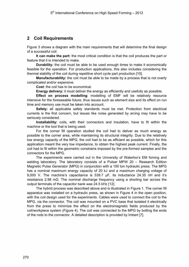
5th International Conference on High Speed Forming – 2012
2 Coil Requirements
Figure 3 shows a diagram with the main requirements that will determine the final design of a successful coil:
It can make the part: the most critical condition is that the coil produces the part or feature that it is intended to make.
Durability: the coil must be able to be used enough times to make it economically feasible for the operation. For production applications, this also includes considering the thermal stability of the coil during repetitive short cycle part production [10].
Manufacturability: the coil must be able to be made by a process that is not overly complicated and/or expensive.
Cost: the coil has to be economical. Energy delivery: it must deliver the energy as efficiently and usefully as possible. Effect on process modelling: modelling of EMF will be relatively resource
intensive for the foreseeable future, thus issues such as element size and its effect on run time and memory use must be taken into account.
Safety: all applicable safety standards must be met. Protection from electrical currents is the first concern, but issues like noise generated by arcing may have to be seriously considered.
Installability: coils, with their connectors and insulation, have to fit within the machine or the tool that is being used.
For the corner fill operation studied the coil had to deliver as much energy as possible to the corner area, while maintaining its structural integrity. Due to the relatively low energy capacity of the MPG, the coil had to be as efficient as possible, which for this application meant the very low impedance, to obtain the highest peak current. Finally, the coil had to fit within the geometric constrains imposed by the pre-formed samples and the connectors for the MPG.
The experiments were carried out in the University of Waterloo’s EM foming and welding laboratory. The laboratory consists of a Pulsar MPW 20 – Research Edition Magnetic Pulse Generator (MPG) in conjunction with a 100 ton hydraulic press. The MPG has a nominal maximum energy capacity of 20 kJ and a maximum charging voltage of 9,000 V. The machine’s capacitance is 539.7 μF, its inductance 24.35 nH and it’s resistance 2.98 mΩ. The nominal discharge frequency using a shorting bar across the output terminals of the capacitor bank was 24.5 kHz [12].
The hybrid process was described above and is illustrated in Figure 1. The corner fill apparatus was installed on a hydraulic press, as shown in Figure 4 in the open position, with the coil design used for the experiments. Cables were used to connect the coil to the MPG, via the connector. The coil was mounted on a PVC base that isolated it electrically from the press to minimize the effect on the electromagnetic fields produced by the coil/workpiece system (Figure 4). The coil was connected to the MPG by bolting the ends of the rods to the connector. A detailed description is provided by Imbert [7].
270

5th International Conference on High Speed Forming – 2012
Figure 4: EM corner fill apparatus showing a) the coil and die with a partial view of the press a), the apparatus b) without, , and c) with the coil.
3 Unsuccessful Coil Designs
Four coil designs were tested that proved inadequate for the task, before a successful design was developed. They are presented here in chronological order of development. The first design was the simplest concept and what many would consider for a first attempt, a helical coil. A coil made from wound 12.7 mm (0.5 in) copper cable was tried with no success since the sample sheets did not show any deformation. A simulation of the coil illustrates one reason why the design was not successful (Figure 5). The current flows on the inside of the coil, , thus taking it away from the workpiece and reducing the induced forces. The fact that a significant amount of the current would travel on the inside of the helix was known, but this the design was tried because in principle it met many of the requirements; it was easy to make, affordable, easily installed, easy to model, and apparently safe. Where it failed was that it could not make the part, because it could not deliver the energy to where it was needed.
Figure 5: Simulation of a helical coil with a workpiece. Contours are of current density.
A coil made from wound copper wire was designed and tested (Figure 6). The coil was based on an axi-symmetric design presented by Oliveira [2] that provided an area of relative uniform current distribution on the workpiece by moving the dead-spot away from the area to be formed. To achieve this result in a coil for a linear corner fill, copper wires were shaped in the form of concentric U shapes so that all the wires at the top of the coil would have current flowing in the same direction. The current would flow back on the side of the coils, thus moving the dead spot away from the workpiece. Figure 6 also shows an idealized coil with the current directions.
(a) (c)
(b)
271
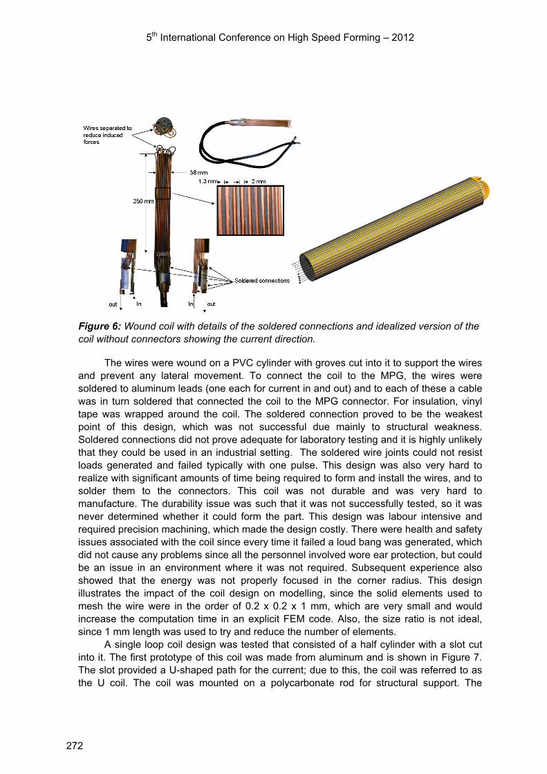
5th International Conference on High Speed Forming – 2012
Figure 6: Wound coil with details of the soldered connections and idealized version of the coil without connectors showing the current direction.
The wires were wound on a PVC cylinder with groves cut into it to support the wires and prevent any lateral movement. To connect the coil to the MPG, the wires were soldered to aluminum leads (one each for current in and out) and to each of these a cable was in turn soldered that connected the coil to the MPG connector. For insulation, vinyl tape was wrapped around the coil. The soldered connection proved to be the weakest point of this design, which was not successful due mainly to structural weakness. Soldered connections did not prove adequate for laboratory testing and it is highly unlikely that they could be used in an industrial setting. The soldered wire joints could not resist loads generated and failed typically with one pulse. This design was also very hard to realize with significant amounts of time being required to form and install the wires, and to solder them to the connectors. This coil was not durable and was very hard to manufacture. The durability issue was such that it was not successfully tested, so it was never determined whether it could form the part. This design was labour intensive and required precision machining, which made the design costly. There were health and safety issues associated with the coil since every time it failed a loud bang was generated, which did not cause any problems since all the personnel involved wore ear protection, but could be an issue in an environment where it was not required. Subsequent experience also showed that the energy was not properly focused in the corner radius. This design illustrates the impact of the coil design on modelling, since the solid elements used to mesh the wire were in the order of 0.2 x 0.2 x 1 mm, which are very small and would increase the computation time in an explicit FEM code. Also, the size ratio is not ideal, since 1 mm length was used to try and reduce the number of elements.
A single loop coil design was tested that consisted of a half cylinder with a slot cut into it. The first prototype of this coil was made from aluminum and is shown in Figure 7. The slot provided a U-shaped path for the current; due to this, the coil was referred to as the U coil. The coil was mounted on a polycarbonate rod for structural support. The
272
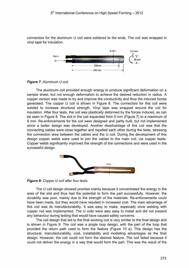
5th International Conference on High Speed Forming – 2012
connectors for the aluminum U coil were soldered to the ends. The coil was wrapped in vinyl tape for insulation.
Figure 7: Aluminum U coil.
The aluminum coil provided enough energy to produce significant deformation on a sample sheet, but not enough deformation to achieve the desired reduction in radius. A copper version was made to try and improve the conductivity and thus the induced forces generated. The copper U coil is shown in Figure 8. The connectors for this coil were welded to increase structural strength. Vinyl tape was wrapped around the coil for insulation. After four tests, the coil was plastically deformed by the forces induced, as can be seen in Figure 8. The slot in the coil expanded from 5 mm (Figure 7) to a maximum of 9 mm. Re-enforcements for the coil were designed and partly built, but not implemented since a better design was developed. Another disadvantage of this coil was that the connecting cables were close together and repelled each other during the tests, stressing the connection area between the cables and the U coil. During the development of this design copper welds were used to join the cables to the main coil, via copper leads. Copper welds significantly improved the strength of the connections and were used in the successful design.
Figure 8: Copper U coil after four tests.
The U coil design showed promise mainly because it concentrated the energy in the area of the slot and thus had the potential to form the part successfully. However, the durability was poor, mainly due to the strength of the materials. Re-enforcements could have been made, but they would have resulted in increased cost. The main advantage of this coil was its manufacturability. It was easy to make, especially once welding with copper rod was implemented. The U coils were also easy to install and did not present any behaviour during testing that would have caused safety concerns.
The coil design that led to the final working coil is very similar to the final design and is shown in Figure 9. The coil was a single loop design, with the part of the loop that provided the return path used to form the feature (Figure 10 a). This design has the structural, manufacturability, cost, installability and modelling advantages as the final design. However, the coil could not form the desired feature. The coil failed because it could not deliver the energy in a way that would form the part. This was the result of the
273

5th International Conference on High Speed Forming – 2012
width of the coil, which has an area wider than the equivalent area in the successful design, which led to a lower current density and lower induced forces on the workpiece. Also, part of the induced forces acted directly against material supported by the die and produced no deformation (Figure 10-a). A less obvious, but very important, difference was that the connectors for this coil were soldered to the coil and not welded. This resulted in a significantly weaker joint that failed during testing.
Figure 9: Coil that led to the successful design.
Figure 10: Simplified induced force distribution for a) the unsuccessful and b) successful coil design.
4 Successful Coil Design
Illustrations of the successful coil are shown in Figure 11. The coil is very similar to the last coil described, but with the section that is closest to the part narrowed to increase the current density, as illustrated in Figure 10-b and Figure 11-a,b (for more details on the numerical results, see [8]). The simplicity of the shape was chosen not only for its current flow characteristics, but also because it had significant structural strength once it was assembled for use with the connectors and an internal support. Part of the structural strength came from the clamping pressure applied by the press, which acted in such a way as to prevent the coil from moving.
Figure 11: The successful coil shown with the predicted current density a) with and b) without a sample. A detailed drawing is shown in c). All dimensions in mm.
Current in
Current out
274

5th International Conference on High Speed Forming – 2012
Solid copper rods were used to connect the coil to the connectors to the MPG to increase the structural integrity of the coil. Cables were tried first but during each pulse the cables were accelerated resulting in dynamic loads on the soldered joints that caused their failure. The rods were stiffer than the cables and they could be welded to the coil using an TIG welding process, which resulted in a much stronger connection. The space within the coil was filled with a polycarbonate rod for structural support. Figure 12 shows the coil with the connectors and the polycarbonate rod. The whole coil assembly was insulated from the sheet and the rest of the apparatus. To insulate the coil, it was wrapped in two layers of vinyl tape with a layer of polyamid Kapton® in between. The total thickness of the insulation was approximately 1 mm. The connecting rods were wrapped in vinyl tape to prevent arcing between the rods and the metal in the MPG connector and the die.
Figure 12: a) top and b) bottom view of the coil showing the types of joints used. The material that can be seen inside the coil in a) is a polycarbonate rod.
This coil met all the requirements that are outlined above. Most importantly it made the part and was durable enough so that it did not have to be replaced for the duration of the experimental program, which consisted of 37 tests, 20 of which were performed at 7,500 V. No damage was observed on the coil after the experiments were completed. A rough estimate of the efficiency of the coil was calculated by using the nominal charge energy of 15.1 kJ and the predicted plastic work expended during forming, which resulted in an efficiency of 2.5% [7]. If the power calculated from the current profile is used, the efficiency was 3.2% [7]. The estimated efficiency is low, but it is comparable with the estimates presented by Belyy et al. [13].
This design proved suitable for the experimental program, but it would have to be developed further for larger scale production. The energy delivery efficiency and the durability would have to be improved to make it more suited for production. Providing for a return path for the induced current could improve the efficiency of the coil [14]. The durability could be improved by providing a stronger polymer base that could support the lateral loads on the part of the coil that is interacting with the workpiece. The energy delivery efficiency could be improved by reducing the impedance of the connectors, for example by having a form of concentric connector, analogous to low impedance cables.
5 Conclusions
One successful and four unsuccessful coil designs for an EM corner fill operation were presented in this paper. The coils presented show the evolution of the design and how it progressed to meet the necessary requirements for an EM forming coil. The paper shows
275

5th International Conference on High Speed Forming – 2012
how all the requirements must be met for a coil to be successful and how basic concepts such as strength or materials, manufacturability and cost can play a significant role, even in a research environment. In the end the coil must make the part, but it has to be able to deliver the forming energy, manufacturable, affordable, installable, durable, safe and, increasingly, amenable to modelling.
References
[1] Daehn, G.S.; Vohnout, V.J. and DuBois, L., “Improved Formability with
Electromagnetic Forming: Fundamentals and Practical Example”, http://www.ecr6.ohio-state.edu/~daehn/overview/index.htm, Ohio State University, date not available.
[2] Oliveira, D.A. Electromagnetic Forming of Aluminum Alloy Sheet: Experiment and Model. Masters of Applied Science thesis, University of Waterloo, 2002.
[3] Psyk, V.; Beerwald, C.; Henselek, A.; Homberg, W.; Brosius, A. and Kleiner, M., 2007. Integration of Electromagnetic Calibration into the Deep Drawing Process of an Industrial Demonstrator Part, Key Engineering Materials, v. 344, 435-442.
[4] Psyk, V.; Risch ,D.; Beerwald, C.; and Tekkaya, A.E., 2008. “Investigation of Combined Electromagnetic and Conventional Forming”, IDDRG 2008 Int. Research Conf., Olofstrom, Sweden, Asnafi, N. ed., 487-498.
[5] Liu, D.; Li, C. and Yu, H., 2009. Numerical Modelling and Deformation Analysis for Electromagnetically Assisted Deep Drawing of AA 5052 Sheet, Trans. of the Nonferrous Met. Soc. of China, v. 19, 1294-1302.
[6] Golovashchenko, S.F., 2010 “Electrohydraulic Forming for Automotive Applications”, 4th Int. Conf. on High Speed Forming, G. Daehn ed., March 9-10,, Columbus, OH.
[7] Imbert, J., 2010. Hybrid Electromagnetic Forming of Aluminum Alloy Sheet. University of Waterloo Ph.D. thesis, http://uwspace.uwaterloo.ca/handle/10012/5517.
[8] Imbert, J and Worswick, M, 2011. Electromagnetic Reduction of Pre-Formed Radius on AA 5754 Sheet. J. Mat. Proc. Tech., v. 211, 896-908.
[9] Golovashchenko, S., 2007. Material Formability and Coil Design in Electromagnetic Forming, J. Mat.Eng. Per., v.16, n. 3, 314-320.
[10] Golovashchenko, S., Besonov, N., Davies, R., 2006. “Design and Testing of Coils for Pulsed Electromagnetic Forming”, 2nd Int. Conf. on High Speed Forming, M. Kleiner ed., March 20-21, Dortmund, Germany, 141-151
[11] Zhang., Y., Babu. S., Daehn, G.S., 2010. “Impact Welding in a Variety of Geometric Configurations”, 4th Int. Conf. on High Speed Forming, G. Daehn ed., March 9-10 2010, Columbus, OH, 97-107
[12] Pulsar. Contact information currently unavailable. [13] Belyy, I.V.; S.M. Fertik and Khimenko, L.T., 1977. “Electromagnetic Metal Forming
Handbook”. Translation by Altynova, M.M. 1996, available from the Hyperplastic Forming Consortium at the Ohio State University.
[14] Personal communication with Prof. G, Daehn, September, 2010.
276
Exceeding the Forming Limit Curve with Deep Drawing Followed by Electromagnetic Calibration*
O. K. Demir, L. Kwiatkowski, A. Brosius, A. E. Tekkaya
Institute of Forming Technology and Lightweight Construction, TU Dortmund, Germany
Abstract
We show that the materials quasi-static forming limit curve (FLC) can be exceeded by the process chain composed of deep drawing followed by electromagnetic forming. We form circular cups as close as possible to the FLC by deep drawing. These cups are then further formed (calibrated) by electromagnetic forming. The electromagnetic forming takes place in the punch edge radius region. The results show significant amount of material in this region exceeding the FLC by means of the process chain. Further research is needed to reveal the factors leading to this increase in forming limits.
Keywords
Process chain, Forming limits, Electromagnetic forming
1 Introduction
The forming potentials of the conventional one-step processes cannot satisfy the increasing demand for complex metal formed parts. In order to increase the forming potential, these processes may be combined with unconventional processes, comprising a process chain. Process chains composed of deep drawing and electromagnetic forming process are delivering promising results in that sense.
The process chain deep drawing followed by electromagnetic calibration was proposed in 1998 by Vohnout [1]. He demonstrated the advantage of the chain. In 2007
* This work is based on the results of the German Research Foundation (DFG) project Te 508/10-1 (PAK343); the authors would like to thank DFG for its financial support
277
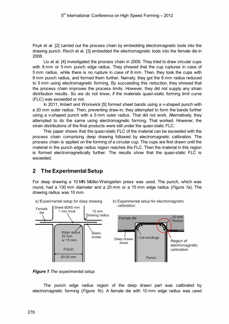
5th International Conference on High Speed Forming – 2012
Psyk et al. [2] carried out the process chain by embedding electromagnetic tools into the drawing punch. Risch et al. [3] embedded the electromagnetic tools into the female die in 2008.
Liu et al. [4] investigated the process chain in 2009. They tried to draw circular cups with 8 mm or 5 mm punch edge radius. They showed that the cup ruptures in case of 5 mm radius, while there is no rupture in case of 8 mm. Then, they took the cups with 8 mm punch radius, and formed them further. Namely, they got the 8 mm radius reduced to 5 mm using electromagnetic forming. By succeeding this reduction, they showed that the process chain improves the process limits. However, they did not supply any strain distribution results. So we do not know, if the materials quasi-static forming limit curve (FLC) was exceeded or not.
In 2011, Imbert and Worswick [5] formed sheet bands using a v-shaped punch with a 20 mm outer radius. Then, preventing draw-in, they attempted to form the bands further using a v-shaped punch with a 5 mm outer radius. That did not work. Alternatively, they attempted to do the same using electromagnetic forming. That worked. However, the strain distributions of the final products were still under the quasi-static FLC.
This paper shows that the quasi-static FLC of the material can be exceeded with the process chain comprising deep drawing followed by electromagnetic calibration. The process chain is applied on the forming of a circular cup. The cups are first drawn until the material in the punch edge radius region reaches the FLC. Then the material in this region is formed electromagnetically further. The results show that the quasi-static FLC is exceeded.
2 The Experimental Setup
For deep drawing a 10 MN Müller-Weingarten press was used. The punch, which was round, had a 130 mm diameter and a 20 mm or a 15 mm edge radius (Figure 1a). The drawing radius was 10 mm.
Figure 1 The experimental setup
The punch edge radius region of the deep drawn part was calibrated by
electromagnetic forming (Figure 1b). A female die with 10 mm edge radius was used
278
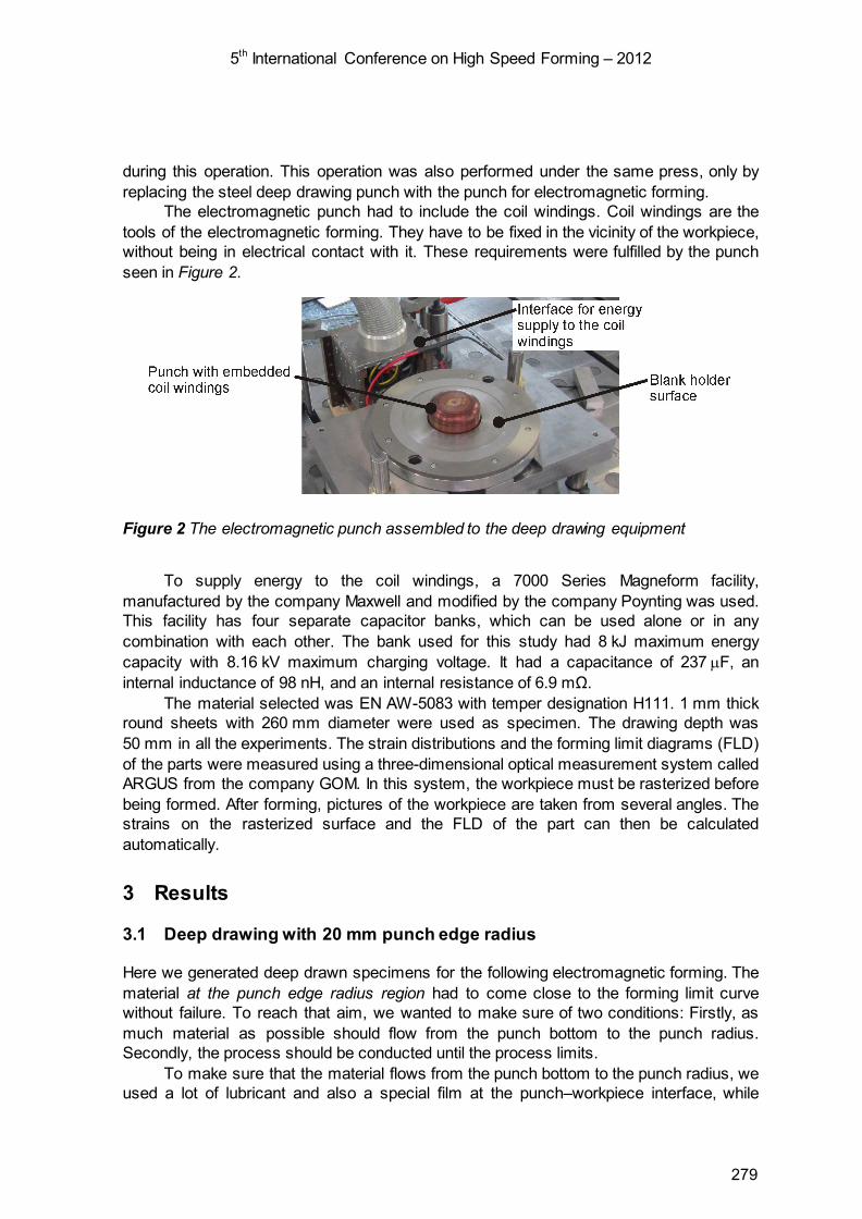
5th International Conference on High Speed Forming – 2012
during this operation. This operation was also performed under the same press, only by replacing the steel deep drawing punch with the punch for electromagnetic forming.
The electromagnetic punch had to include the coil windings. Coil windings are the tools of the electromagnetic forming. They have to be fixed in the vicinity of the workpiece, without being in electrical contact with it. These requirements were fulfilled by the punch seen in Figure 2.
Figure 2 The electromagnetic punch assembled to the deep drawing equipment
To supply energy to the coil windings, a 7000 Series Magneform facility,
manufactured by the company Maxwell and modified by the company Poynting was used. This facility has four separate capacitor banks, which can be used alone or in any combination with each other. The bank used for this study had 8 kJ maximum energy capacity with 8.16 kV maximum charging voltage. It had a capacitance of 237 µF, an internal inductance of 98 nH, and an internal resistance of 6.9 mΩ.
The material selected was EN AW-5083 with temper designation H111. 1 mm thick round sheets with 260 mm diameter were used as specimen. The drawing depth was 50 mm in all the experiments. The strain distributions and the forming limit diagrams (FLD) of the parts were measured using a three-dimensional optical measurement system called ARGUS from the company GOM. In this system, the workpiece must be rasterized before being formed. After forming, pictures of the workpiece are taken from several angles. The strains on the rasterized surface and the FLD of the part can then be calculated automatically.
3 Results
3.1 Deep drawing with 20 mm punch edge radius
Here we generated deep drawn specimens for the following electromagnetic forming. The material at the punch edge radius region had to come close to the forming limit curve without failure. To reach that aim, we wanted to make sure of two conditions: Firstly, as much material as possible should flow from the punch bottom to the punch radius. Secondly, the process should be conducted until the process limits.
To make sure that the material flows from the punch bottom to the punch radius, we used a lot of lubricant and also a special film at the punch–workpiece interface, while
279
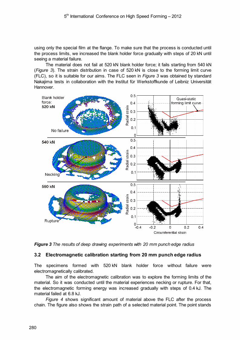
5th International Conference on High Speed Forming – 2012
using only the special film at the flange. To make sure that the process is conducted until the process limits, we increased the blank holder force gradually with steps of 20 kN until seeing a material failure.
The material does not fail at 520 kN blank holder force; it fails starting from 540 kN (Figure 3). The strain distribution in case of 520 kN is close to the forming limit curve (FLC), so it is suitable for our aims. The FLC seen in Figure 3 was obtained by standard Nakajima tests in collaboration with the Institut für Werkstoffkunde of Leibniz Universität Hannover.
Figure 3 The results of deep drawing experiments with 20 mm punch edge radius
3.2 Electromagnetic calibration starting from 20 mm punch edge radius
The specimens formed with 520 kN blank holder force without failure were electromagnetically calibrated.
The aim of the electromagnetic calibration was to explore the forming limits of the material. So it was conducted until the material experiences necking or rupture. For that, the electromagnetic forming energy was increased gradually with steps of 0.4 kJ. The material failed at 6.8 kJ.
Figure 4 shows significant amount of material above the FLC after the process chain. The figure also shows the strain path of a selected material point. The point stands
280
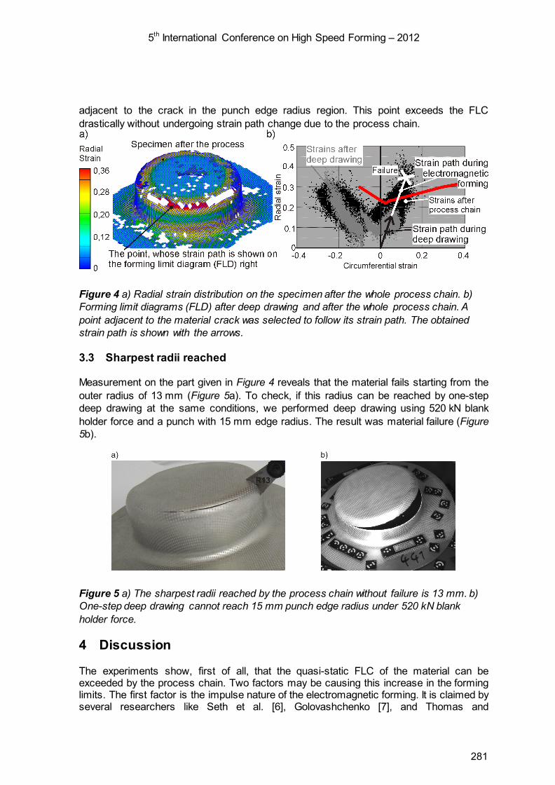
5th International Conference on High Speed Forming – 2012
adjacent to the crack in the punch edge radius region. This point exceeds the FLC drastically without undergoing strain path change due to the process chain.
Figure 4 a) Radial strain distribution on the specimen after the whole process chain. b) Forming limit diagrams (FLD) after deep drawing and after the whole process chain. A point adjacent to the material crack was selected to follow its strain path. The obtained strain path is shown with the arrows.
3.3 Sharpest radii reached
Measurement on the part given in Figure 4 reveals that the material fails starting from the outer radius of 13 mm (Figure 5a). To check, if this radius can be reached by one-step deep drawing at the same conditions, we performed deep drawing using 520 kN blank holder force and a punch with 15 mm edge radius. The result was material failure (Figure 5b).
Figure 5 a) The sharpest radii reached by the process chain without failure is 13 mm. b) One-step deep drawing cannot reach 15 mm punch edge radius under 520 kN blank holder force.
4 Discussion
The experiments show, first of all, that the quasi-static FLC of the material can be exceeded by the process chain. Two factors may be causing this increase in the forming limits. The first factor is the impulse nature of the electromagnetic forming. It is claimed by several researchers like Seth et al. [6], Golovashchenko [7], and Thomas and
281
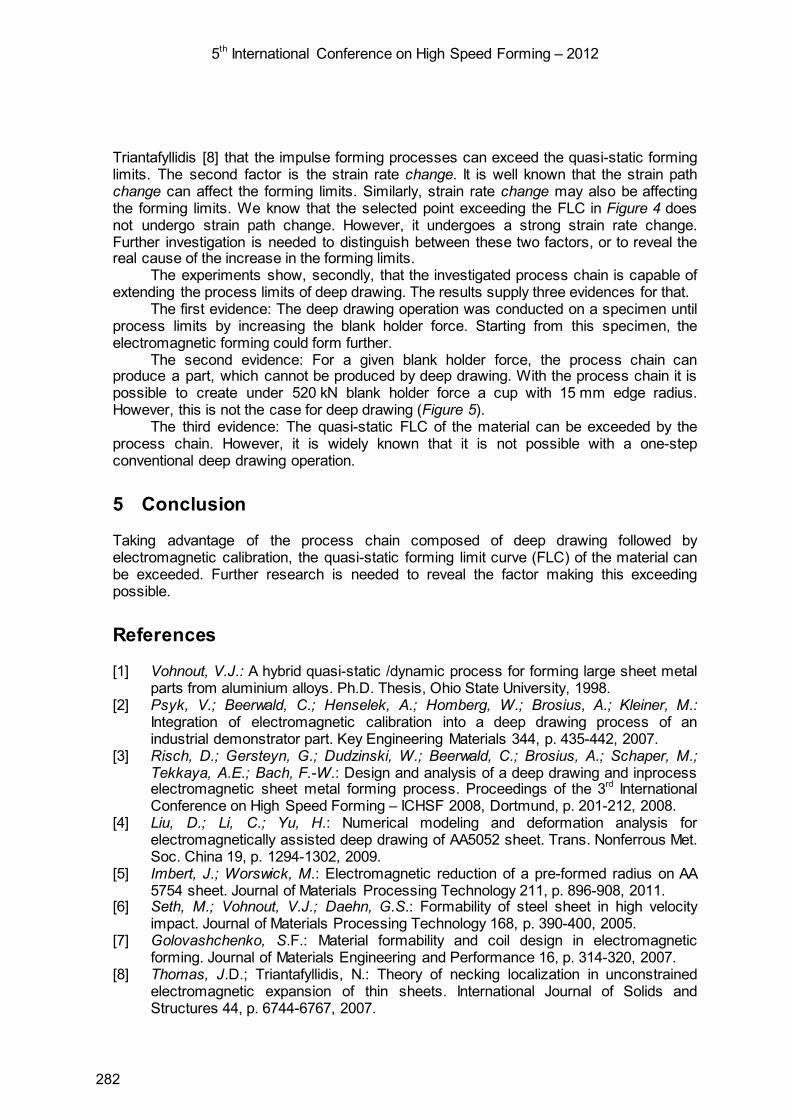
5th International Conference on High Speed Forming – 2012
Triantafyllidis [8] that the impulse forming processes can exceed the quasi-static forming limits. The second factor is the strain rate change. It is well known that the strain path change can affect the forming limits. Similarly, strain rate change may also be affecting the forming limits. We know that the selected point exceeding the FLC in Figure 4 does not undergo strain path change. However, it undergoes a strong strain rate change. Further investigation is needed to distinguish between these two factors, or to reveal the real cause of the increase in the forming limits.
The experiments show, secondly, that the investigated process chain is capable of extending the process limits of deep drawing. The results supply three evidences for that.
The first evidence: The deep drawing operation was conducted on a specimen until process limits by increasing the blank holder force. Starting from this specimen, the electromagnetic forming could form further.
The second evidence: For a given blank holder force, the process chain can produce a part, which cannot be produced by deep drawing. With the process chain it is possible to create under 520 kN blank holder force a cup with 15 mm edge radius. However, this is not the case for deep drawing (Figure 5).
The third evidence: The quasi-static FLC of the material can be exceeded by the process chain. However, it is widely known that it is not possible with a one-step conventional deep drawing operation.
5 Conclusion
Taking advantage of the process chain composed of deep drawing followed by electromagnetic calibration, the quasi-static forming limit curve (FLC) of the material can be exceeded. Further research is needed to reveal the factor making this exceeding possible.
References
[1] Vohnout, V.J.: A hybrid quasi-static /dynamic process for forming large sheet metal parts from aluminium alloys. Ph.D. Thesis, Ohio State University, 1998.
[2] Psyk, V.; Beerwald, C.; Henselek, A.; Homberg, W.; Brosius, A.; Kleiner, M.: Integration of electromagnetic calibration into a deep drawing process of an industrial demonstrator part. Key Engineering Materials 344, p. 435-442, 2007.
[3] Risch, D.; Gersteyn, G.; Dudzinski, W.; Beerwald, C.; Brosius, A.; Schaper, M.; Tekkaya, A.E.; Bach, F.-W.: Design and analysis of a deep drawing and inprocess electromagnetic sheet metal forming process. Proceedings of the 3rd International Conference on High Speed Forming – ICHSF 2008, Dortmund, p. 201-212, 2008.
[4] Liu, D.; Li, C.; Yu, H.: Numerical modeling and deformation analysis for electromagnetically assisted deep drawing of AA5052 sheet. Trans. Nonferrous Met. Soc. China 19, p. 1294-1302, 2009.
[5] Imbert, J.; Worswick, M.: Electromagnetic reduction of a pre-formed radius on AA 5754 sheet. Journal of Materials Processing Technology 211, p. 896-908, 2011.
[6] Seth, M.; Vohnout, V.J.; Daehn, G.S.: Formability of steel sheet in high velocity impact. Journal of Materials Processing Technology 168, p. 390-400, 2005.
[7] Golovashchenko, S.F.: Material formability and coil design in electromagnetic forming. Journal of Materials Engineering and Performance 16, p. 314-320, 2007.
[8] Thomas, J.D.; Triantafyllidis, N.: Theory of necking localization in unconstrained electromagnetic expansion of thin sheets. International Journal of Solids and Structures 44, p. 6744-6767, 2007.
282
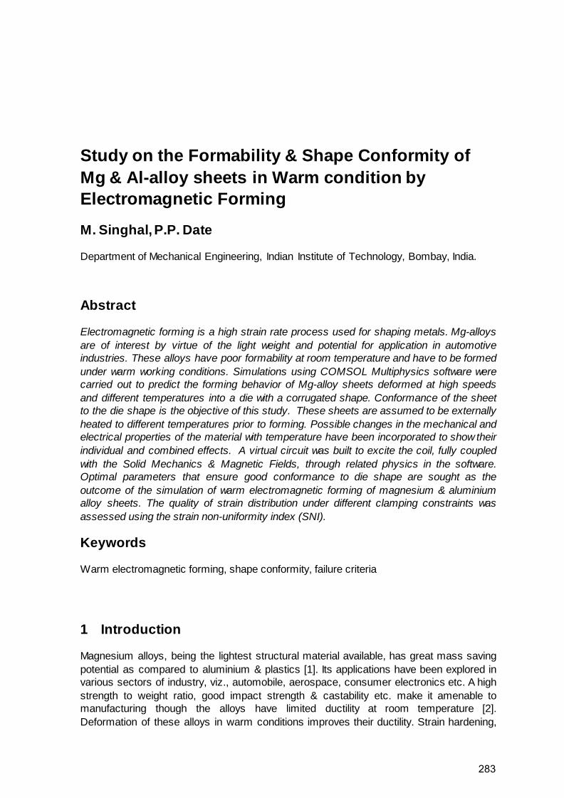
Study on the Formability & Shape Conformity of Mg & Al-alloy sheets in Warm condition by Electromagnetic Forming
M. Singhal, P.P. Date
Department of Mechanical Engineering, Indian Institute of Technology, Bombay, India.
Abstract
Electromagnetic forming is a high strain rate process used for shaping metals. Mg-alloys are of interest by virtue of the light weight and potential for application in automotive industries. These alloys have poor formability at room temperature and have to be formed under warm working conditions. Simulations using COMSOL Multiphysics software were carried out to predict the forming behavior of Mg-alloy sheets deformed at high speeds and different temperatures into a die with a corrugated shape. Conformance of the sheet to the die shape is the objective of this study. These sheets are assumed to be externally heated to different temperatures prior to forming. Possible changes in the mechanical and electrical properties of the material with temperature have been incorporated to show their individual and combined effects. A virtual circuit was built to excite the coil, fully coupled with the Solid Mechanics & Magnetic Fields, through related physics in the software. Optimal parameters that ensure good conformance to die shape are sought as the outcome of the simulation of warm electromagnetic forming of magnesium & aluminium alloy sheets. The quality of strain distribution under different clamping constraints was assessed using the strain non-uniformity index (SNI).
Keywords
Warm electromagnetic forming, shape conformity, failure criteria
1 Introduction
Magnesium alloys, being the lightest structural material available, has great mass saving potential as compared to aluminium & plastics [1]. Its applications have been explored in various sectors of industry, viz., automobile, aerospace, consumer electronics etc. A high strength to weight ratio, good impact strength & castability etc. make it amenable to manufacturing though the alloys have limited ductility at room temperature [2]. Deformation of these alloys in warm conditions improves their ductility. Strain hardening,
283

5th International Conference on High Speed Forming – 2012
grain growth, dynamic recovery (DRV) and dynamic recrystallization (DRX) together influence the mechanical properties. The activation of non-basal slip systems and DRX are the major contributing mechanisms leading to softening at elevated temperatures [3].
Ulacia et.al. [4] found experimentally that deformation in Al increases at high temperature with an increase in the discharge energy. At a given discharge energy, deformation was found to decrease with increasing temperature presumably due to a lower electrical conductivity of the material leading to a lower Lorentz force despite small softening of the material. In contrast, experimental research of Murakoshi et.al. [5] showed increasing deformation of Mg sheets with increasing temperature.
In the present study, simulation of deformation of two different materials, namely, Magnesium and Aluminium into a multi-impression die at two levels of discharge energies and temperatures were studied using the COMSOL software. Two end-constraints (viz., fully free, fully constrained) have been deployed to study their effect on the extent of cavity filling by the sheet. The geometry of deformation considered is shown in figure 1a and 1b. The coupling of three physics, viz., the virtual electrical circuit, corresponding Lorentz forces generated and the consequent plastic deformation is schematically shown in figure 2. The Cowper-Symonds (CS) model was used to characterize the constitutive equation for the Magnesium alloy (Table 1) and the Johnson-Cook model for Aluminium alloy (Table 2). In the present work, anisotropy has not been considered because at high temperature prismatic < > and pyramidal < > slip planes get activated and hence the observed improvement in formability and reduction in anisotropy [6]. The high strain rate deformation occurring in the electromagnetic forming process converts 90-95% of the plastic work to heat. Since process time is very small (~50 µsec), this small adiabatic heating adds to the thermal softening. In the present study, this adiabatic thermal softening is neglected. The optimum factor level settings for maximum cavity filling and minimum non-uniformity in strain distribution over the deforming sheet are the expected outcomes of the study.
2 Simulation Procedure
2.1 Die-Sheet Configuration
The 3D setup of die, sheet and coils is realized in 2D axisymmetric mode (figure 1). The die considered has 4 regular cavities with a die entry radius of 6mm and die cavity width of 12 mm. The sheet thickness is 1 mm for all the simulations. The copper coil considered has a rectangular section (8 mm x 10 mm) with a radius of 2 mm at all the corners. Each turn is aligned with the centre of each cavity to maximise cavity filling. All gaps between elements of the configuration are assumed to be filled with ambient air.
2.2 Numerical Model
COMSOL Multiphysics is used in the present study as a numerical analysis tool which couples all the physics involved (viz., Virtual Circuitry, Electromagnetics, Solid Mechanics and Thermal Strains).
284
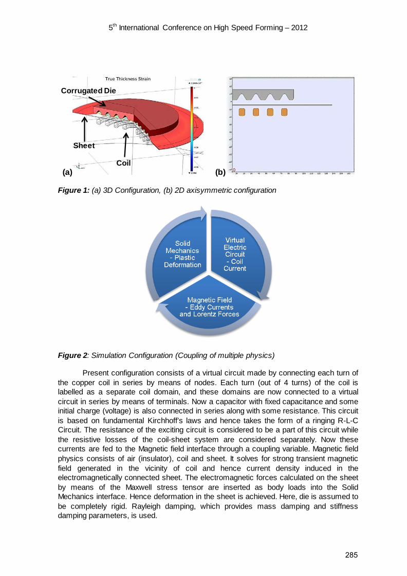
5th International Conference on High Speed Forming – 2012
(a) (b)
Figure 1: (a) 3D Configuration, (b) 2D axisymmetric configuration
Figure 2: Simulation Configuration (Coupling of multiple physics)
Present configuration consists of a virtual circuit made by connecting each turn of the copper coil in series by means of nodes. Each turn (out of 4 turns) of the coil is labelled as a separate coil domain, and these domains are now connected to a virtual circuit in series by means of terminals. Now a capacitor with fixed capacitance and some initial charge (voltage) is also connected in series along with some resistance. This circuit is based on fundamental Kirchhoff’s laws and hence takes the form of a ringing R-L-C Circuit. The resistance of the exciting circuit is considered to be a part of this circuit while the resistive losses of the coil-sheet system are considered separately. Now these currents are fed to the Magnetic field interface through a coupling variable. Magnetic field physics consists of air (insulator), coil and sheet. It solves for strong transient magnetic field generated in the vicinity of coil and hence current density induced in the electromagnetically connected sheet. The electromagnetic forces calculated on the sheet by means of the Maxwell stress tensor are inserted as body loads into the Solid Mechanics interface. Hence deformation in the sheet is achieved. Here, die is assumed to be completely rigid. Rayleigh damping, which provides mass damping and stiffness damping parameters, is used.
Corrugated Die
Sheet
Coil
285
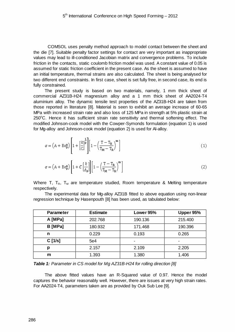
5th International Conference on High Speed Forming – 2012
COMSOL uses penalty method approach to model contact between the sheet and the die [7]. Suitable penalty factor settings for contact are very important as inappropriate values may lead to ill-conditioned Jacobian matrix and convergence problems. To include friction in the contacts, static coulomb friction model was used. A constant value of 0.05 is assumed for static friction coefficient in the present case. As the sheet is assumed to have an initial temperature, thermal strains are also calculated. The sheet is being analysed for two different end constraints. In first case, sheet is set fully free, in second case, its end is fully constrained.
The present study is based on two materials, namely, 1 mm thick sheet of commercial AZ31B-H24 magnesium alloy and a 1 mm thick sheet of AA2024-T4 aluminium alloy. The dynamic tensile test properties of the AZ31B-H24 are taken from those reported in literature [8]. Material is seen to exhibit an average increase of 60-65 MPa with increased strain rate and also loss of 125 MPa in strength at 5% plastic strain at 250oC. Hence it has sufficient strain rate sensitivity and thermal softening effect. The modified Johnson-cook model with the Cowper-Symonds formulation (equation 1) is used for Mg-alloy and Johnson-cook model (equation 2) is used for Al-alloy.
Where T, TR, TM are temperature studied, Room temperature & Melting temperature respectively.
The experimental data for Mg-alloy AZ31B fitted to above equation using non-linear regression technique by Hasenpouth [8] has been used, as tabulated below:
Table 1: Parameter in CS model for Mg AZ31B-H24 for rolling direction [8]
The above fitted values have an R-Squared value of 0.97. Hence the model captures the behavior reasonably well. However, there are issues at very high strain rates. For AA2024-T4, parameters taken are as provided by Ouk Sub Lee [9].
Parameter Estimate Lower 95% Upper 95% A [MPa] 202.768 190.136 215.400 B [MPa] 180.932 171.468 190.396 n 0.229 0.193 0.265 C [1/s] 5e4 - - p 2.157 2.109 2.205 m 1.393 1.380 1.406
286

5th International Conference on High Speed Forming – 2012
Table 2: Parameters in JC model for AA2024-T4 [9]
At high temperature, different mechanical and electrical properties of the material also vary significantly. All these properties such as electrical conductivity, young’s modulus, coefficient of thermal expansion [7, 10-12] at high temperature are considered.
3 Failure Criteria Based on Strain Distribution
As discussed by Hasenpouth [8], in simulations, the fitted material models were not able to predict the necking of the samples. So in the present study, a Thickness strain non-uniformity based failure criterion is introduced. Namely, the “Strain Non-uniformity Index” [13-15] is used to represent quality of strain distribution. This factor is the outcome of a combined effect of geometric, material and process parameters on the strain distribution. This is given by the difference between Peak thickness Strain and Average thickness strain of the formed part, computed at every time step. The corresponding curvature (K) of the strain peaks is also calculated as given by equation 3.
This curvature in terms of the SNI is given by equation 4.
Where L is the length of the sheet for which strain distribution is considered, &
are Fourier coefficients. The derivation of the same will be given elsewhere [15]. High curvature value
represents a sharp peak and the strain is more likely to localize there. This way, failure of a material can be pre-empted by this strain distribution based method. Hence, SNI combined with curvature of the peak completes a tool to predict the failure of the deforming sheet. The critical value of curvature at the strain peak and SNI can be determined from experiments.
To start with, thickness strain distribution data from the simulations is fitted into a Fourier series of appropriate order (about 850 in the present study). The R squared values obtained for the fits are all greater than 0.9970. Then Central difference numerical differentiation technique with 8th order accuracy was applied to obtain the curvature at the peaks. Here, many peaks may not be captured until enough numbers of data points are present to define a particular peak. Hence additional numbers of intermediate data points
A [MPa] B [MPa] N C m
390 1980 0.4890 0.0140 0.6 0.0001 298 775
287
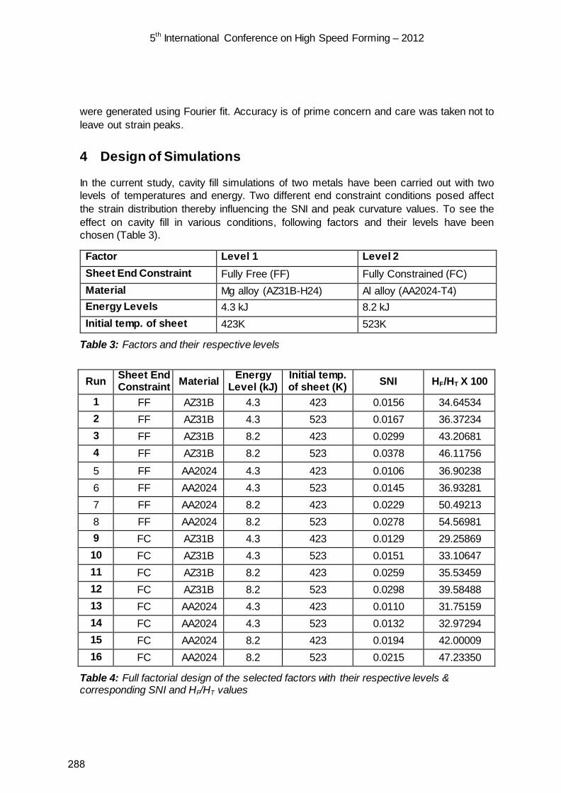
5th International Conference on High Speed Forming – 2012
were generated using Fourier fit. Accuracy is of prime concern and care was taken not to leave out strain peaks.
4 Design of Simulations
In the current study, cavity fill simulations of two metals have been carried out with two levels of temperatures and energy. Two different end constraint conditions posed affect the strain distribution thereby influencing the SNI and peak curvature values. To see the effect on cavity fill in various conditions, following factors and their levels have been chosen (Table 3).
Table 3: Factors and their respective levels
Table 4: Full factorial design of the selected factors with their respective levels & corresponding SNI and HF/HT values
Factor Level 1 Level 2 Sheet End Constraint Fully Free (FF) Fully Constrained (FC) Material Mg alloy (AZ31B-H24) Al alloy (AA2024-T4) Energy Levels 4.3 kJ 8.2 kJ Initial temp. of sheet 423K 523K
Run Sheet End Constraint Material Energy
Level (kJ) Initial temp. of sheet (K) SNI HF/HT X 100
1 FF AZ31B 4.3 423 0.0156 34.64534 2 FF AZ31B 4.3 523 0.0167 36.37234 3 FF AZ31B 8.2 423 0.0299 43.20681 4 FF AZ31B 8.2 523 0.0378 46.11756
5 FF AA2024 4.3 423 0.0106 36.90238 6 FF AA2024 4.3 523 0.0145 36.93281 7 FF AA2024 8.2 423 0.0229 50.49213 8 FF AA2024 8.2 523 0.0278 54.56981 9 FC AZ31B 4.3 423 0.0129 29.25869 10 FC AZ31B 4.3 523 0.0151 33.10647 11 FC AZ31B 8.2 423 0.0259 35.53459 12 FC AZ31B 8.2 523 0.0298 39.58488 13 FC AA2024 4.3 423 0.0110 31.75159 14 FC AA2024 4.3 523 0.0132 32.97294 15 FC AA2024 8.2 423 0.0194 42.00009 16 FC AA2024 8.2 523 0.0215 47.23350
288
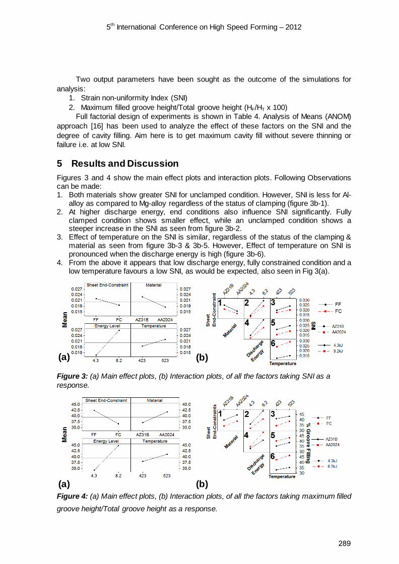
5th International Conference on High Speed Forming – 2012
Two output parameters have been sought as the outcome of the simulations for analysis:
1. Strain non-uniformity Index (SNI) 2. Maximum filled groove height/Total groove height (HF/HT x 100)
Full factorial design of experiments is shown in Table 4. Analysis of Means (ANOM) approach [16] has been used to analyze the effect of these factors on the SNI and the degree of cavity filling. Aim here is to get maximum cavity fill without severe thinning or failure i.e. at low SNI.
5 Results and Discussion Figures 3 and 4 show the main effect plots and interaction plots. Following Observations can be made: 1. Both materials show greater SNI for unclamped condition. However, SNI is less for Al-
alloy as compared to Mg-alloy regardless of the status of clamping (figure 3b-1). 2. At higher discharge energy, end conditions also influence SNI significantly. Fully
clamped condition shows smaller effect, while an unclamped condition shows a steeper increase in the SNI as seen from figure 3b-2.
3. Effect of temperature on the SNI is similar, regardless of the status of the clamping & material as seen from figure 3b-3 & 3b-5. However, Effect of temperature on SNI is pronounced when the discharge energy is high (figure 3b-6).
4. From the above it appears that low discharge energy, fully constrained condition and a low temperature favours a low SNI, as would be expected, also seen in Fig 3(a).
Figure 3: (a) Main effect plots, (b) Interaction plots, of all the factors taking SNI as a response.
Figure 4: (a) Main effect plots, (b) Interaction plots, of all the factors taking maximum filled
groove height/Total groove height as a response.
(a)
(a)
(b)
(b)
289

5th International Conference on High Speed Forming – 2012
Figure 5: (a) & (c) SNI plots, (b) & (d) Curvature plots for runs with Mg-alloy & Al-alloy respectively for fully free end condition.
5. Filling is better with an unclamped condition. The cavity filling depth is equally
sensitive to the status of clamping in case of the two materials. However, Aluminium shows higher depth of filling compared to Mg alloy irrespective of clamping conditions as seen from figure 4b-1.
6. With increasing discharge energy, increase in cavity filling is more rapid for an unclamped condition as seen from figure 4b-2.
7. Sheet in a fully clamped condition shows rapid die filling with increase in temperature. That is, die filling is more sensitive to temperature when the sheet is fully clamped (figure 4b-3).
8. With increase in discharge energy, groove filling in Al is far superior to that of Mg with smaller increase in strain non-uniformity (figure 3b-4 & 4b-4).
9. Cavity filling in Al improves at high temperatures particularly when energy is high, This improvement in deformation of Al with increase in temperature at high energy can be attributed to an inherently high electrical conductivity, decreasing flow strength with temperature and a relatively insignificant reduction in induced forces due to lower electrical conductivity at high temperatures.
10. Sensitivity of die filling to temperature increases with an increase in discharge energy. Die filling is better if temperature is increased. (figure 4b-6)
11. For better die filling, a high discharge energy, unclamped condition and high temperature are recommended. This is also confirmed by figure 4a.
12. From figures 5 & 6, conclusions emerge to be consistent with those from ANOM analysis discussed. Increase in SNI & Curvature values is very sensitive to increase in
(a) (b)
(c) (d)
290
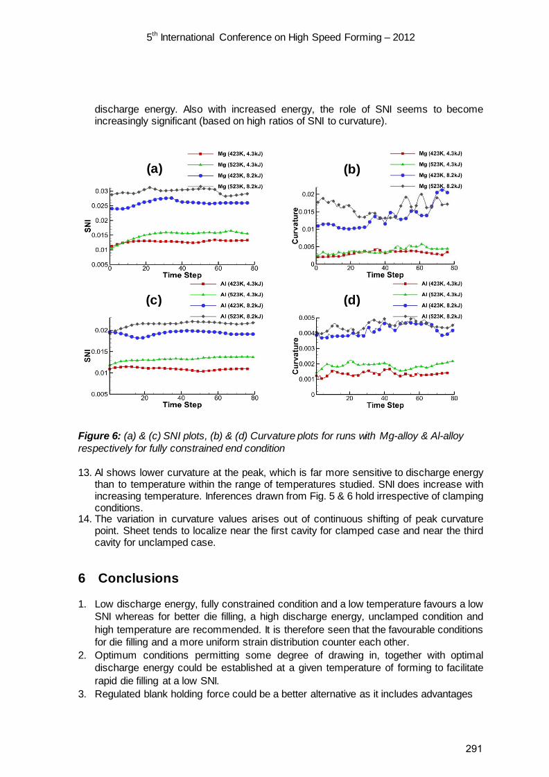
5th International Conference on High Speed Forming – 2012
discharge energy. Also with increased energy, the role of SNI seems to become increasingly significant (based on high ratios of SNI to curvature).
Figure 6: (a) & (c) SNI plots, (b) & (d) Curvature plots for runs with Mg-alloy & Al-alloy respectively for fully constrained end condition
13. Al shows lower curvature at the peak, which is far more sensitive to discharge energy than to temperature within the range of temperatures studied. SNI does increase with increasing temperature. Inferences drawn from Fig. 5 & 6 hold irrespective of clamping conditions.
14. The variation in curvature values arises out of continuous shifting of peak curvature point. Sheet tends to localize near the first cavity for clamped case and near the third cavity for unclamped case.
6 Conclusions
1. Low discharge energy, fully constrained condition and a low temperature favours a low SNI whereas for better die filling, a high discharge energy, unclamped condition and high temperature are recommended. It is therefore seen that the favourable conditions for die filling and a more uniform strain distribution counter each other.
2. Optimum conditions permitting some degree of drawing in, together with optimal discharge energy could be established at a given temperature of forming to facilitate rapid die filling at a low SNI.
3. Regulated blank holding force could be a better alternative as it includes advantages
(a) (b)
(c) (d)
291

5th International Conference on High Speed Forming – 2012
of both clamped (uniformity in filling) & unclamped (higher depth of filling). 4. Effect of decrease in deformation with increased temperature becomes more and
more immaterial if discharge energy used is near upper bound value of discharge energy to form a sample at the given temperature without failure.
5. The critical value of SNI and curvature may be verified experimentally. References
[1] Luo, A.: Magnesium: current and potential automotive applications. JOM 2002, v.54, p.42-48.
[2] Watarai, H.: Trends of Research and Development for Magnesium Alloys – Reducing the Weight of Structural Materials in Motor Vehicles. Science and Technology Trends, Quarterly Review, No. 18, 2006, p.84-97.
[3] Wu, H. Y., Lin, F. Z.: Mechanical properties and strain-hardening behavior of Mg alloy AZ31B-H24 thin sheet. Materials Science and Engineering A, v.527(4-5), 2010, p.1194-1199.
[4] Ulacia, I., Arroyo, A., Eguia, I., Hurtado, I., Gutierrez, M. A.: Warm Electromagnetic Forming of AZ31B Magnesium Alloy Sheet. In: Proc. of 4th Int. Conf. High Speed Forming, 2010, p.159-168.
[5] Murakoshi, Y., Katoh, M., Matsuzaki, K., Saigo, M.: High Velocity sheet bulge forming of magnesium alloy by electromagnetic forming. In: Proc. 9th Int. Conf. Tech. Plasticity, 2008, p.1010-1015.
[6] Ulacia, I., Imbert, J., Salisbury, C. P., Arroyo, A., Hurtado, I., Worswick, M. J.: Electromagnetic Forming of AZ31B Magnesium Alloy Sheet : Experimental Work and Numerical Simulation, In: Proc. of 3rd Int. Conf. High Speed Forming, 2008, p.191-200.
[7] COMSOL Multiphysics User’s Guide, 2011. [8] Hasenpouth, D.: Tensile High Strength Behavior of AZ31B Magnesium alloy Sheet,
M.S. Thesis, University of Waterloo, Canada, 2010. [9] Lee, O. S., Choi, H., Kim, H.: High-temperature dynamic deformation of aluminum
alloys using SHPB. Journal of Mechanical Science and Technology, v.25(1), 2010, p.143-148.
[10] Military Handbook-5H, Metallic Materials and Elements for Aerospace Vehicle Structures. Dec. 1998, p.3-68.
[11] Busk, R.S.: Magnesium and its alloys, Magnesium Products Design, Pub. Marcel Dekker, Inc., 1987.
[12] Lalpoor, M., Eskin, D. G., Katgerman, L.: Cold-cracking assessment in AA7050 billets during DC-casting by thermo-mechanical simulation of residual thermal stresses and application of fracture mechanics. Metall. Mater. Trans. A, 40(13), 2009, p.3304–33.
[13] Desai, S., Date, P.: On the quantification of strain distribution in drawn sheet metal products. Journal of Materials Processing Technology, v.177(1-3), 2006, p.439-443.
[14] Date, P. P., Desai, S. G.: Strain distribution based formability criteria in sheet metal forming of drawn automotive components, Symposium on Automotive Sheet Metal Forming, (Ed : D. Bhattacharjee), Tata Steel, Jamshedpur, India, 2007.
[15] Date, P. P.: Unpublished work, 2012. [16] Montgomery, D. C.: Design and Analysis of Experiments, Pub. John Wiley & Sons,
Inc. 1997.
292

Pulsed magnetic forming of the magnesium alloy AZ31 – Comparison to quasi-static forming*
E. Uhlmann1, L. Prasol1, C. König1, A. Ziefle1
1 Institute for Machine Tools and Factory Management, TU Berlin, Germany
Abstract
Magnesium alloy AZ31 metal sheets were formed at room temperature with a pulsed magnetic field induced by a flat coil. For this a die with variable die radius and inside diameter was used. The forming results were evaluated regarding to deformation, die radius, inside diameter, micro hardness, texture examination of forming area and energy input. In addition high velocity forming process was compared to a quasi-static forming process at room temperature. Therefore an experimental setup with an adapted punch was constructed. Punch geometry was defined in dependence of the high velocity forming structure of a sample at well-defined energy input. By comparing texture and micro hardness at forming area a distinction of high-speed forming process and quasi-static process is determined.
Keywords
Magnesium, Impulse, Forming
1 Introduction
Application of lightweight components, e.g. magnesium alloys, aluminium alloys or CFRP composites are increasing constantly in many manufacturing areas. The constantly increasing technological development of electromobility offers potential for lightweight
* This work is based on the results of the research project “Impulsmagnetische Flachum-formung von Magnesiumblechen bei niedrigen Umformtemperaturen”; the authors would like to thank the DFG for its financial support
293
5th International Conference on High Speed Forming – 2012
components in cars. In this case a significant reduction of car body weight is possible as mentioned in [1]. Production processes have to meet the requirements of these tendencies and must be suitable for mass production. Forming with the optimal utilization of material and high productivity offers potential for excellent accuracy. Forming of magnesium alloys is accomplished at high temperatures currently. A general challenge in forming of magnesium alloys will be in realizing forming process at lower temperature. Therefore the influence of further process variables, e. g. strain rates, should be investigated.
The comparison of high-speed forming and quasi-static forming of magnesium alloy AZ31 with an exact distinction between both processes led to the present study. For the description of the relation between energy input and deformation AZ31 metal sheets are formed in a die with different die radius. As a result a punch was designed in dependence of the forming geometry of the high-speed process. The comparison of both processes at defined deformation is the aim of the investigation. This paper presents investigations on the comparison of high-speed forming and quasi-static forming of magnesium alloy AZ31.
2 State of the Art
Magnesium and its alloys e. g. AZ31 have hexagonal crystal lattice. Due to the crystal lattice there are three linear independent sliding systems at room temperature. Von Mises criterion indicates that a homogenous deformation requires at least five linear independent sliding systems [2]. Therefore magnesium and its alloys accomplish low deformability at room temperature. Once temperature of 220 °C has been reached further glide planes in the pyramid plane are being activated. In this case deformability of magnesium and its alloys increase rapidly [3,4,5,6,7].
In addition to forming temperature, strain rates play a decisive role in forming processes. In contrast to low strain rates, high strain rates improve forming conditions of several metals e. g. magnesium alloys. Short process time on the order of 50 µs to 200 µs causes quasi-adiabatic process characteristics which increase ductility of magnesium and its alloys [8] and leads to higher deformation in comparison to low strain rate deformation. During deformation the generated heat cannot dissipate quickly enough into the whole sample and leads to local increasing of ductility in deformation area. Through this additional slip planes in the hexagonal lattice can be activated. A homogeneous deformation of the workpiece without failure can be realized because there are at least five independent slip systems now [9].
The characteristics of magnesium alloy AZ80 in dependence of forming temperature and strain rate was determined by [10]. It was discoverd that stress resistance increases rapidly, both rolling and transversal direction, at high strain rates independently from forming temperature as shown in figure 1. At low strain rates which occurs in conventional forming processes deformation is dominated by forming temperature. With increasing strain rates deformation is dominated by hardening and the influence of warming is less. At strain rates of 1000 s-1 quasi-adiabatic characteristics dominates forming process and leads to a significant increase of stress resistance as shown in figure 1.
The studies conducted so far show a strain rate dependency of magnesium alloys. The influence of different strain rates at various forming processes for production of identical structures will be studied in this investigation.
294

Figu
3
A coforminputformis usgeomcons
Figu
The The the dforcespee
5
ure 1: Strain
Experim
omparison ing is invest, coil geoing machin
sed. To commetry with structed to c
ure 2: Exper
The dischnecessary magnetic fidischarge ce appears aed forming
10
10
0
Com
pres
sion
yiel
dpo
int
40
20
%
a)
5th Internatio
n rate sensit
ental Se
of pulsed tigated. Themetry, inside FA-60-14
mpare both defined in
compare bo
rimental set
harge of a penergy is seld around
current. By at the surfacan experim
0-4
St
10-3 10-
onal Confer
tivity of com
tup
magnetic fe high-speede diamete
440-SW Mahigh-speed
nside diamth forming p
tup for high
pulsed currestored in cathe flat coilthis the ma
ce of the womental setup
train rate φ
-2 10-1 100
rence on Hi
mpression y
forming of ed forming cer and dieagnepuls frod forming a
meter andprocesses a
-speed form
ent is used apacitors anl induces edagnetic fieldorkpiece andp for quasi-
s101 102
igh Speed F
yield point at
magnesiumcharacterist
e radius. Tom the firm and quasi-stis requiredas shown in
ming (a) and
to accelerand is unloaddy currentd of the flatd leads to d-static form
s-1
104
PrCo
WoMa
b)
Forming – 2
t varying tem
m alloy AZtics dependherefore thElmag Inc.
tatic formind. An expen figure 2.
d quasi-stat
ate the worded as an ts in the wot coil is shiedeformationing is deve
20 °C100 °C150 °C200 °C250 °C 300 °C
rocess:ompression
orkpiece:agnesium al
2012
mperatures
Z31 to quad strongly onhe electrom., San Diegg, a defineerimental s
tic forming (
rkpiece intoalternating
orkpiece oppelded. The
n. In additioneloped as s
test
lloy AZ80
s [8]
asi-static n energy magnetic go, USA, d punch setup is
(b)
the die. current.
posite to Lorentz
n to high shown in
295

figureforceidenthigh-frictiostrainGermlubric
roomradiu
Figu
2 b). forcemaxihigh-confi
Figuwork
Df
tid
5
e 2 b). Fore and frictitical. The d-speed defoon between/compressmany, with cated with g
Punch gem temperatuus rdie = 10 m
ure 3: Creat
The workThe aimed
e maximumimum at the-speed defoiguration of
ure 4: Illustrkpiece durin
70
6
2
0
Def
orm
atio
n d F
mm
5th Internatio
r this, bounon betwee
difference bormation is n punch a
sion testing a mechan
grease to meometry is aure at energmm as show
tion of punc
piece is pod deformatioms in both e top of theormation octhe circular
ration of mang dischargi
80
X-c
90
onal Confer
ndary condin workpiec
between borealized w
and workpmachine Z
ical punch.minimize frict
adapted to gy input E =wn in Figure
ch geometry
ositioned in on with iden
processese mechanicccurs outsidr coil leads
ximum maging process
100
coordinate
110
rence on Hi
itions like ice and dieth variants
without anypiece. The ZA 150, fro. Establishition. high-speed
= 2.5 kJ wite 3. For exp
y in depende
experimenntical formins. The quacal punch. de the centto force min
gnetic presss of the capa
mm0 13
igh Speed F
nside diame in both e
is determimechanicaquasi-stati
om the firm ng compar
d forming gth inside diaperiments a
ence of high
ntal setups g geometry
asi-static deIn contrast tre of the cnimum in th
sure pmag (t)acitors at pr
DeformCreate
Process:High-spee
Process pE = dinside = rdie =
30
Forming – 2
meter, die raexperimentaned in the l punch anic forming Zwick Gm
rative condi
geometry oameter dinsid
circular coi
h-speed for
as shown y is distingueformation to this the
coil as showe coil centr
at the surfarocess time
mation after hed punch geo
ed forming
parameter:2.5 kJ50 mm10 mm
2012
adius, blanal setups mforming zod thereforeis realize
bH & Co. Kitions the p
of the work
de = 50 mm il was used
rming deform
in Figure 2ished from exhibits thforce max
wn in figurere.
face of the e t = 60 µs
high-speed foometry
k holder must be one. The e without ed by a KG, Ulm, punch is
piece at and die
.
rmation
2 a) and different
he force imum of e 4. The
orming
296
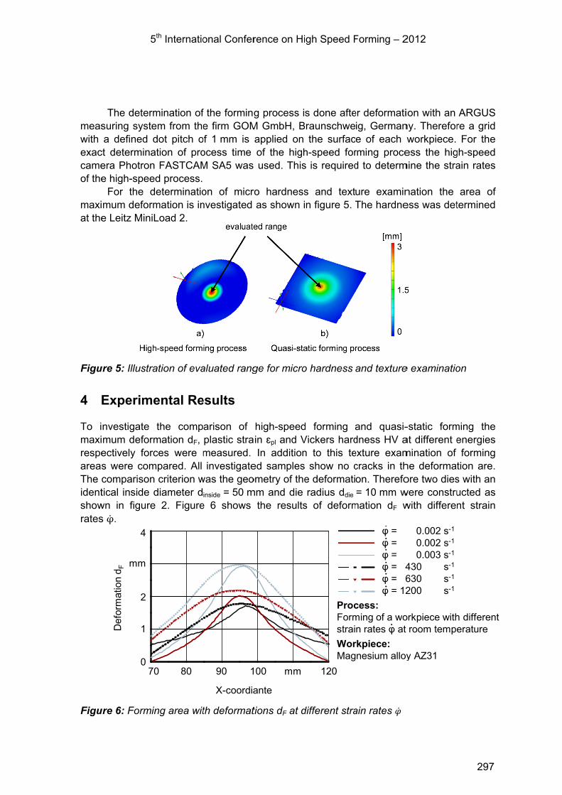
measwith exaccameof the
maxiat the
Figu
4
To imaxirespeareasThe identshowrates
Figu
5
The detersuring systea defined
ct determinaera Photrone high-spee
For the dimum defore Leitz Mini
ure 5: Illustr
Experim
nvestigate imum deforectively fors were comcomparisontical inside
wn in figures φ.
ure 6: Formi
7
1
0
Def
orm
atio
n d F
4
mm
2
5th Internatio
mination ofem from thedot pitch oation of pron FASTCAMed process. determinatiormation is iniLoad 2.
ration of eva
ental Re
the comprmation dF, rces were mmpared. All n criterion wdiameter d
e 2. Figure
ing area wit
70 80
onal Confer
f the forminge firm GOM
of 1 mm is ocess timeM SA5 was
on of micronvestigated
aluated rang
esults
arison of plastic strameasured.investigate
was the geo
inside = 50 me 6 shows
th deformat
X-coordia
90 1
rence on Hi
g process iM GmbH, Bapplied on of the high used. This
ro hardnessas shown i
ge for micro
high-speedin ԑpl and VIn addition
ed samplesometry of themm and die
the results
tions dF at d
ante
mm00
igh Speed F
s done afteBraunschwe
the surfach-speed fors is required
s and textn figure 5. T
o hardness
d forming aVickers hardn to this te show no ce deformatiradius ddie
s of deform
different stra
120
ProcFormstrai
WorMag
Forming – 2
er deformatiig, Germane of each wrming proced to determ
ure examinThe hardne
and texture
and quasi-dness HV aexture examcracks in thon. Therefo= 10 mm w
mation dF w
ain rates
φ = φ = φ = φ = 4φ = 6φ = 12
cess:ming of a won rates φ at
rkpiece:nesium alloy
2012
ion with an ny. Thereforworkpiece. ess the hig
mine the stra
nation the ess was det
e examinatio
-static format different emination of he deformatore two dieswere construwith differen
0.002 s-1
0.002 s-1
0.003 s-1
430 s-1
630 s-1
200 s-1
orkpiece withroom tempe
y AZ31
ARGUS re a grid For the
gh-speed ain rates
area of termined
on
ming the energies forming
tion are. s with an ucted as nt strain
h different erature
297

5th International Conference on High Speed Forming – 2012
There were several deformations dF performed. Due to the force maximum of both forming processes there is a difference in the course of deformation along the X-coordinate as shown in figure 6. The quasi-static deformation shows the force maximum at the top of the punch which leads to the highest deformation dF in the area from x = 95 mm to x = 97 mm. Outside this area the course falls off steeply because the material is drawn while deformation. In contrast to this the high-speed deformation leads to a course which falls off slightly while the maximum deformations dF also were measured in the area of x = 93 mm to x = 95 mm. This course is based on the fact that the deformation of outer areas takes place at first. The inner area follows the outer area due to the mass inertial and leads to a plastic deformation with a superposition of an elastic oscillation of this area. The duration of this entire process, plastic and elastic vibrations, takes up to tP = 140 µs while the duration of the quasi-static deformation takes up to tp = 30 s.
The following table 1 shows the maximum plastic strain ԑpl (von Mises) in the evaluated area. The measured maximum plastic strain ԑpl for quasi-static forming is significantly larger at each deformation dF than for high-speed forming. The differences in maximum plastic strain ԑpl result from the acting forces in the forming area. With the increase of the deformation dF larger forces were applied with the result that the friction between punch and workpiece increased. In contrast to this the maximum plastic strain ԑpl
which occurs in high-speed forming processes is less because the maximum acting forces appear in the outer area. Thus, the same deformations dF are obtained at different plastic strains ԑpl.
Table 1: Measured maximum plastic strain ԑpl in the area of maximum deformation dF (as shown in figure 5) for both processes
Due to the time-dependent process and the associated process behaviour there are differences in the investigated material properties at the same deformation dF. Figure 7 shows the influence of strain rates φ on the Vickers hardness HV.
At low strain rates φ the calculated Vickers hardness is 74 HV up to 77 HV while at high strain rates φ the Vickers hardness increases to 83 - 88 HV. Therefore an average difference of Vickers hardness of 11 HV is resulting. With respect to the initial hardness of 63 HV thus follows an increase in hardness of about 19% at a quasi-static deformation. At the high-speed deformation there is an increase in the hardness of about 37%.
Deformation dF Maximum plastic strain ԑpl
1.7 mm 8.0 %
2.0 mm 11.5 %
2.9 mm not measurable
Deformation dF Maximum plastic strain ԑpl
1.8 mm 3.8 %
2.2 mm 4.8 %
3.0 mm 6.0 %
Quasi-static forming High-speed forming
298

5th International Conference on High Speed Forming – 2012
Figure 7: Measured Vickers hardness of AZ31 in dependence of strain rate after forming process
In correlation with a higher Vickers hardness HV the pulsed magnetic deformed workpieces show a fine microstructure. In contract, the quasi-static deformed workpieces show a coarser microstructure which correlates with lower Vickers hardness HV. Figure 8 a) shows the texture examination of deformation dF = 2.0 mm at strain rate φ = 0.002 s- 1. In figure 8 b) the texture examination of deformation dF = 2.2 mm at strain rate φ = 630 s-1 is shown.
a) b)
Figure 8: Texture examination of deformed areas: a) quasi-static deformation b) high-speed deformation
5 Conclusion
The comparison of pulsed magnetic forming and quasi-static forming of the magnesium alloy AZ31 at room temperature shows significant differences between both processes. Two experimental setups were realized to produce comparable forming geometries. Both experimental setups have the same physical boundary conditions such as blank holder force and friction conditions between workpiece and die.
The identical deformations dF in dependence of different strain rates φ were realized at different forming depths. The courses of the deformations dF differ due to the process-dependent force maximum in the forming zone. Different plastic strains ԑpl occur in the
10-4
76
72
Strain rate φ
Vic
kers
har
dnes
s
s-1
92
80
HV
10-3 10-2 10-1 100 101 102 104
84
Quasi-static formingHigh-speed forming
Process:Forming of a workpiece with different strain rates φ at room temperature
Workpiece:Magnesium alloy AZ31
Tool:Zwick/Roell Z150 testing machineElmag FA-60-1440-SW-Magnepuls
299
5th International Conference on High Speed Forming – 2012
investigated area at different deformations dF in dependence of the process. In further studies with a modified flat coil which offers the force maximum in the area of maximum deformation dF more accurate results will be achieved. In addition further studies with higher strain rates will be carried out. Furthermore, for comparison a simulative investigation of the entire process will be done.
The resulting Vickers hardness HV shows a significant dependency of strain rates φ at different deformations dF. The Vickers hardness HV of pulsed magnetic formed samples is 15% higher in comparison to quasi-static formed samples. The evaluation of texture examination of both deformation areas indicates that at high-speed deformation in contrast to quasi-static deformation a fine-grained microstructure is formed. Fine-grained structures exhibit general a higher hardness which was confirmed with these studies. The influence of higher strain rates φ on the microstructure will be considered in further studies.
References
[1] Kopp, G.; Beeh, E.: Magnesium macht´s möglich – Super Light Car – Leichtbau durch Multi-Material-Design mit integrierten Funktionen. DLR-News, 2009, p. 28-31.
[2] Von Mises, Richard.: Probability, Statistics and Truth. Volume 2, Dover Publications Inc., United States, 1981.
[3] Bach, F. W.; Behrens, B. A.; Rodmann, M.; Roßberg, A.; Vogt, O.; Huinink, T.: Werkstoff- und Verfahrenstechnische Entwicklung von wirkmedienbasierten Umformprozessen für Magnesiumbleche. Final report on DFG priority program 1098, 2006, p. 115-137.
[4] Doege; E.: Umformverhalten von Magnesiumblechen. Neuere Entwicklungen in der Blechumformung, International Conference, MATINFO Werkstoff-Informationsge-sellschaft, Frankfurt a. M., Germany, 2000,p. 387-410.
[5] Pircher, H.; Weber, M.; Kawalla, R.: Magnesium für den Karosseriebau. SFU, Sächsische Fachtagung Umformtechnik, volume 9, p. 221-231
[6] Viehweger, B.; Richter, G.; Düring, M.; Karabet, A.; Sviridov, A.; Hartmann, H.; Richter, U.: Hydromechanisches Tiefziehen und Hochdruckumformung als Verfahren zur Herstellung komplexer Bauteile aus Magnesiumblechen des Typs AZ31B-0. Materialwissenschaften und Werkstofftechnik, volume 35, booklet 7, Weinhein: Wiley-VCH Verlag GmbH & Co. KGaA, 2004, p. 440-446
[7] Viehweger, B.; Richter, G.; Karabet, A.: Tiefziehen von Blechen der Mg-Legierung AZ31, hergestellt aus stranggegossenem Ausgangsmaterial. Metall – Internationale Fachzeitschrift für Metallurgie, volume 59, booklet4, 2005, p. 207-212
[8] Uhlmann, E.; Prasol, L.: Hochfeste und hybride Materialien. Proceedings of the 31. EFB colloquium, T32, Bad Boll, Germany, 2011, p.127-144
[9] von Mises, Richard: „Probability, Statistics and Truth“, 2. editon, Dover Publications Inc., United States, 1981
[10] E-Magd, E.; Abouridouane, M.: Einfluss der Umformgeschwindigkeit und -tempe-ratur auf das Umformvermögen metallischer Werkstoffe unter Druckbelastung und Zugbelastung. Final report on DFG priority program 1074, Verlagshaus Mainz: 2005.
300

SESSION 9
SIMULATION AND OPTIMIZATION
301

302

Coupled FEM-Simulation of Magnetic Pulse Welding for Nonsymmetric Applications*
E. Uhlmann1, A. Ziefle1, C. König1, L. Prasol1
1 Institute for Machine Tools and Factory Management, TU Berlin, Germany
Abstract
Pulse magnetic welding can be seen as a well developed manufacturing process. However, the realization of this technology implies a high degree of knowledge concerning the intrinsic mechanisms of current transmission and force generation and accordingly a high potential of optimization can be expected. Modelling pulse magnetic forming processes requires a transient electromagnetic calculation in order to obtain the generated currents and forces. The prediction of the deforming result requires an explicit structural simulation, as the forming process is conducted in timescales of a few 100 µs. A close investigation of the relevant physical entities is carried out with ANSYS Workbench and ANSYS Emag. Furthermore, the results of the Emag calculations are used as boundary conditions for explicit structural simulations with ANSYS AUTODYN in order to predict the needed charging energy for a joining process. For validation, a comparison between simulated and measured results with respect to magnetic flux density and discharge current is shown.
Keywords
fem, pulse magnetic welding, parameter controlled bonding
* This work is partly based on the results of the research project “Modellierung und Analyse des Magnetimpulsschweißens mit dem Ziel der Prozessparameteroptimierung”; the authors would like to thank the DFG for its financial support
303
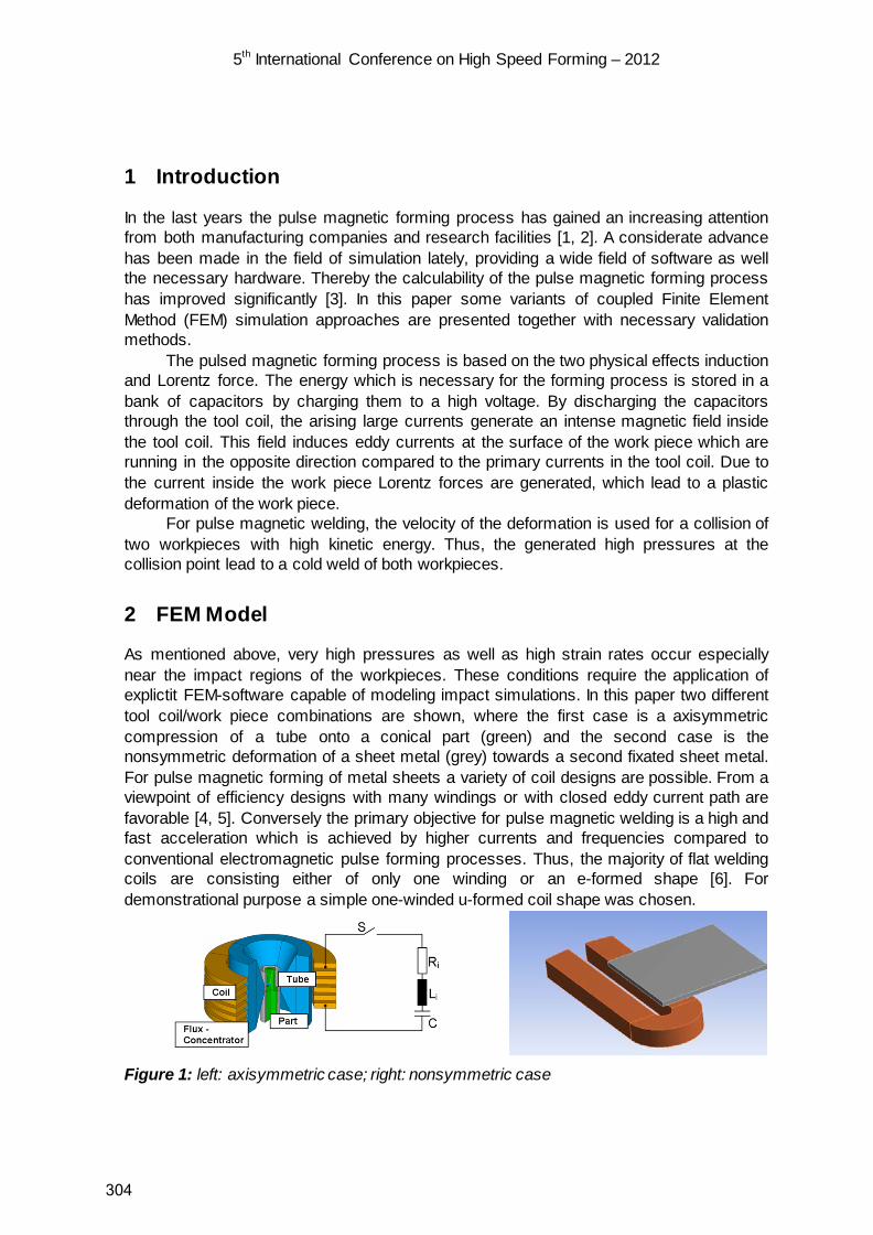
5th International Conference on High Speed Forming – 2012
1 Introduction
In the last years the pulse magnetic forming process has gained an increasing attention from both manufacturing companies and research facilities [1, 2]. A considerate advance has been made in the field of simulation lately, providing a wide field of software as well the necessary hardware. Thereby the calculability of the pulse magnetic forming process has improved significantly [3]. In this paper some variants of coupled Finite Element Method (FEM) simulation approaches are presented together with necessary validation methods.
The pulsed magnetic forming process is based on the two physical effects induction and Lorentz force. The energy which is necessary for the forming process is stored in a bank of capacitors by charging them to a high voltage. By discharging the capacitors through the tool coil, the arising large currents generate an intense magnetic field inside the tool coil. This field induces eddy currents at the surface of the work piece which are running in the opposite direction compared to the primary currents in the tool coil. Due to the current inside the work piece Lorentz forces are generated, which lead to a plastic deformation of the work piece.
For pulse magnetic welding, the velocity of the deformation is used for a collision of two workpieces with high kinetic energy. Thus, the generated high pressures at the collision point lead to a cold weld of both workpieces.
2 FEM Model
As mentioned above, very high pressures as well as high strain rates occur especially near the impact regions of the workpieces. These conditions require the application of explictit FEM-software capable of modeling impact simulations. In this paper two different tool coil/work piece combinations are shown, where the first case is a axisymmetric compression of a tube onto a conical part (green) and the second case is the nonsymmetric deformation of a sheet metal (grey) towards a second fixated sheet metal. For pulse magnetic forming of metal sheets a variety of coil designs are possible. From a viewpoint of efficiency designs with many windings or with closed eddy current path are favorable [4, 5]. Conversely the primary objective for pulse magnetic welding is a high and fast acceleration which is achieved by higher currents and frequencies compared to conventional electromagnetic pulse forming processes. Thus, the majority of flat welding coils are consisting either of only one winding or an e-formed shape [6]. For demonstrational purpose a simple one-winded u-formed coil shape was chosen.
Figure 1: left: axisymmetric case; right: nonsymmetric case
304
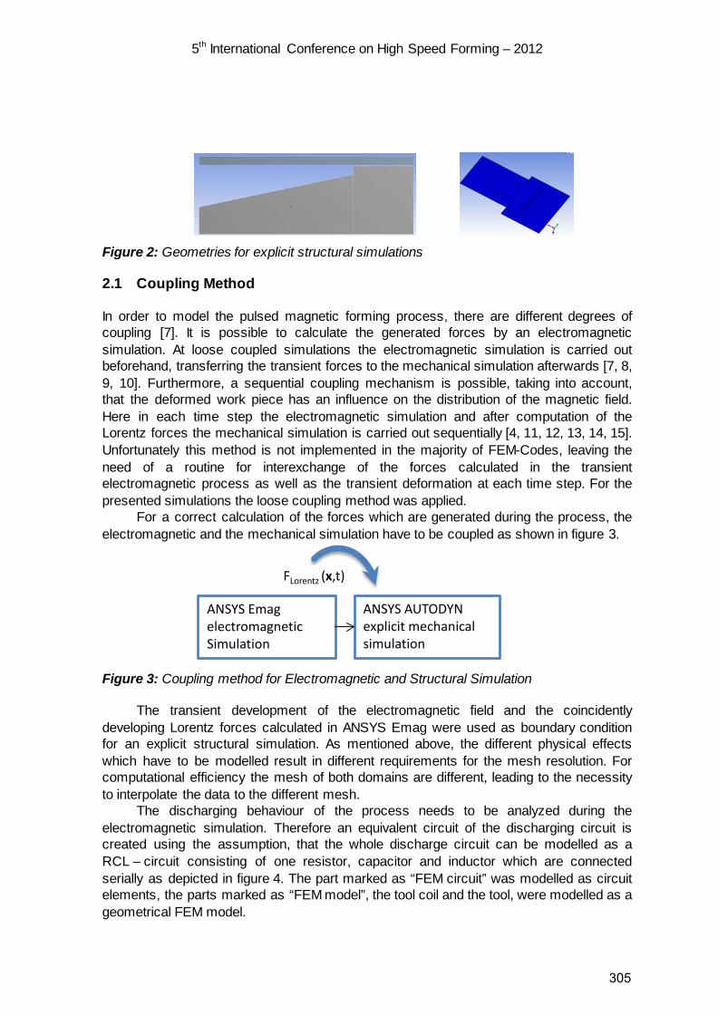
5th International Conference on High Speed Forming – 2012
Figure 2: Geometries for explicit structural simulations
2.1 Coupling Method
In order to model the pulsed magnetic forming process, there are different degrees of coupling [7]. It is possible to calculate the generated forces by an electromagnetic simulation. At loose coupled simulations the electromagnetic simulation is carried out beforehand, transferring the transient forces to the mechanical simulation afterwards [7, 8, 9, 10]. Furthermore, a sequential coupling mechanism is possible, taking into account, that the deformed work piece has an influence on the distribution of the magnetic field. Here in each time step the electromagnetic simulation and after computation of the Lorentz forces the mechanical simulation is carried out sequentially [4, 11, 12, 13, 14, 15]. Unfortunately this method is not implemented in the majority of FEM-Codes, leaving the need of a routine for interexchange of the forces calculated in the transient electromagnetic process as well as the transient deformation at each time step. For the presented simulations the loose coupling method was applied.
For a correct calculation of the forces which are generated during the process, the electromagnetic and the mechanical simulation have to be coupled as shown in figure 3.
ANSYS EmagelectromagneticSimulation
FLorentz (x,t)
ANSYS AUTODYNexplicit mechanicalsimulation
Figure 3: Coupling method for Electromagnetic and Structural Simulation
The transient development of the electromagnetic field and the coincidently developing Lorentz forces calculated in ANSYS Emag were used as boundary condition for an explicit structural simulation. As mentioned above, the different physical effects which have to be modelled result in different requirements for the mesh resolution. For computational efficiency the mesh of both domains are different, leading to the necessity to interpolate the data to the different mesh.
The discharging behaviour of the process needs to be analyzed during the electromagnetic simulation. Therefore an equivalent circuit of the discharging circuit is created using the assumption, that the whole discharge circuit can be modelled as a RCL – circuit consisting of one resistor, capacitor and inductor which are connected serially as depicted in figure 4. The part marked as “FEM circuit” was modelled as circuit elements, the parts marked as “FEM model”, the tool coil and the tool, were modelled as a geometrical FEM model.
305

5th International Conference on High Speed Forming – 2012
2.2 Setup electromagnetic model
As only the discharging process is relevant for the forming behaviour, the charging circuit was neglected. Inner inductivity Li and inner resistance Ri were measured at the specific pulse forming machine by carrying out short circuit tests without tool coil. For this purpose a short circuit connection was used instead of a tool coil as it is further described in [16].
charging unit capacitor bank tool coil tool
FEM circuit FEM model Figure 4: Equivalent circuit diagram
Another important aspect which needs to be considered already at the meshing stage is the skin effect δ defined by:
µκπ=
f21δ (6)
In order to accurately model the eddy currents on the surface of solid conductors it is necessary to at least resolve the skin depth with two element layers.
2.3 Setup explicit structural model
For explicit structural simulations one of the most important aspects is the relation between smallest element size and biggest possible time step through the courant condition:
cΔxΔt min
max ≤ (6)
Here maxt∆ is the biggest possible time step permitting to model events approaching with
longitudinal sound speed c through a mesh with the minimum element size of minx∆ .
Choosing a larger time step or a finer grid violating equation 6 will result in poor simulation results. Good care is also needed for a perceptive net design. Because very high deformations will occur during the collision process between both workpieces, the net needs to be prepared by initially meshing the layers in the surface of the collision side “deformed” to the contrarious direction.
306

5th International Conference on High Speed Forming – 2012
3 Simulation
3.1 Axisymmetric Case
Most compression coils can be described with axisymmetric conditions. This way a considerable reduction of computation time can be achieved. Details for used materials and applied boundary conditions are referred to in table 1.
Magnetic flux density [ T ]
2.743e1 2.438e12.133e11.829e11.524e11.219e19.143e06.010e03.048e00.195e-5
Magnetic force [ N ]
1.003e4 8.915e37.800e36.686e35.572e34.457e33.343e32.229e31.114e30.000e0
Figure 5: Results of electromagnetic simulation; left: magnetic flux density B; right: magnetic force Fmag
In figure 5 the total magnetic flux density is plotted on the left hand side. By application of the fieldformer the magnetic field between fieldformer and work piece is significantly higher than between fieldformer and tool coil. Accordingly the magnetic field inside the workpiece is almost completely vanished. On the right hand side of figure 5 the force exposure of tool coil, fieldformer and workpiece is shown. As the current density j is high in regions very close to the surfaces due to the above mentioned skin effect, also the Lorentz force Fmag mainly takes effect there according to the definition
BjmagF ×= . (7)
Pressure [ Pa ]
1.767e91.538e91.310e91.082e98.532e86.249e83.966e81.682e8-6.010e7-2.884e8
Figure 6: Pressure at axisymmetric case
307
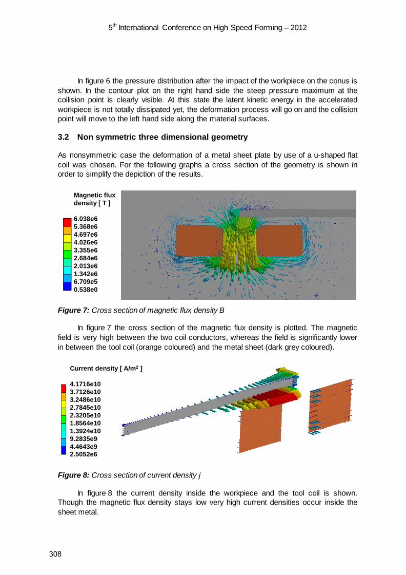
5th International Conference on High Speed Forming – 2012
In figure 6 the pressure distribution after the impact of the workpiece on the conus is shown. In the contour plot on the right hand side the steep pressure maximum at the collision point is clearly visible. At this state the latent kinetic energy in the accelerated workpiece is not totally dissipated yet, the deformation process will go on and the collision point will move to the left hand side along the material surfaces.
3.2 Non symmetric three dimensional geometry
As nonsymmetric case the deformation of a metal sheet plate by use of a u-shaped flat coil was chosen. For the following graphs a cross section of the geometry is shown in order to simplify the depiction of the results.
Magnetic flux density [ T ]
6.038e65.368e64.697e64.026e63.355e62.684e62.013e61.342e66.709e50.538e0
Figure 7: Cross section of magnetic flux density B
In figure 7 the cross section of the magnetic flux density is plotted. The magnetic field is very high between the two coil conductors, whereas the field is significantly lower in between the tool coil (orange coloured) and the metal sheet (dark grey coloured).
Current density [ A/m2 ]
4.1716e10 3.7126e103.2486e102.7845e102.3205e101.8564e101.3924e109.2835e94.4643e92.5052e6
Figure 8: Cross section of current density j
In figure 8 the current density inside the workpiece and the tool coil is shown. Though the magnetic flux density stays low very high current densities occur inside the sheet metal.
308
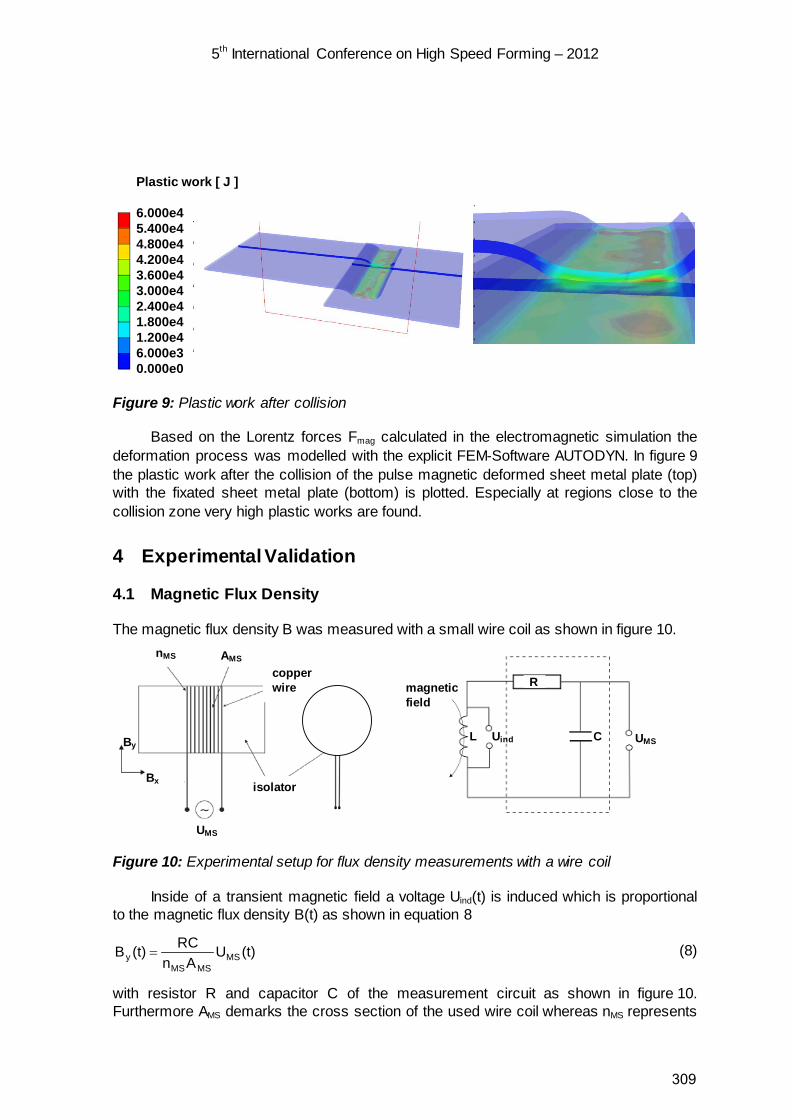
5th International Conference on High Speed Forming – 2012
Plastic work [ J ]
6.000e45.400e44.800e44.200e43.600e43.000e42.400e41.800e41.200e46.000e30.000e0
Figure 9: Plastic work after collision
Based on the Lorentz forces Fmag calculated in the electromagnetic simulation the deformation process was modelled with the explicit FEM-Software AUTODYN. In figure 9 the plastic work after the collision of the pulse magnetic deformed sheet metal plate (top) with the fixated sheet metal plate (bottom) is plotted. Especially at regions close to the collision zone very high plastic works are found.
4 Experimental Validation
4.1 Magnetic Flux Density
The magnetic flux density B was measured with a small wire coil as shown in figure 10.
copperwire
Bx
By
isolator
nMS AMS
UMS
magneticfield
UMS
R
CUindL
Figure 10: Experimental setup for flux density measurements with a wire coil
Inside of a transient magnetic field a voltage Uind(t) is induced which is proportional to the magnetic flux density B(t) as shown in equation 8
(t)UAn
RC(t)B MSMSMS
y = (8)
with resistor R and capacitor C of the measurement circuit as shown in figure 10. Furthermore AMS demarks the cross section of the used wire coil whereas nMS represents
309

5th International Conference on High Speed Forming – 2012
the number of windings. The coil was calibrated by use of a hall sensor at magnetic flux densities of B = 1 T. The advantages of the wire coil are the usability at high frequencies f and high magnetic flux densities B. As disadvantage only the component of the magnetic flux density parallel to the wire coil axis can be measured. As the orientation of the flux density vector is approximately parallel to the tool coil axis it can be assumed that
(t)B(t)By ≈ (9)
The validation was carried out using the same tool coil without workpiece and without fieldformer using the charging energy WE = 1 kJ and the capacity C = 240 µF.
-80 -40 0 mm 800,0
0,4
0,8
T
1,6
C = 240 µFWE = 1 kJ
Magentic flux density on tool coil axis
mag
netic
flux
den
sity
B y
y-axis
simulation hall sensor wire coil
1.6
0.8
0.4
T
mag
netic
flux
den
sity
B y,m
ax(y
)
time t
mag
netic
flux
dens
ityB y
(t)
By,max(t)
0
Figure 11: Measured and simulated magnetic flux density on the rotational axis of the tool coil
On the lower right hand side of figure 11 the local variation in time of the magnitude of the magnetic flux density B is shown. On the left hand side the development of By ,max(y), representing the maximum value of By at the location y over the tool coil axis is compared for both simulated and measured data. The hall sensor was also used for reference measurements. The results show excellent agreement to the simulated values regarding the amplitude as well as the position.
4.2 Discharge Current
The discharge current I was measured by use of a rogowski coil. By measuring the generated voltage after a passive integrator circuit, a voltage Urog(t) proportional to the current I(t) is measured with the following correlation
(t)UmI(t) rog= (9)
310

5th International Conference on High Speed Forming – 2012
0 20 40 µs 80
-60
0
kA
120
C = 33 µFWE = 8.81kJ
Discharge current in simulation and experiment
disc
harg
e cu
rrent
I
time t
experimental simulation
Figure 12: Discharge Current for axisymmetric case
In figure 12 simulated and measured discharge current are compared for the axisymmetric case. Whereas the current amplitude shows a very good accordance, the frequency of the simulated current is slightly higher than the experiment. This is due to the changing inductivity of the real system. The distance between workpiece and field former is increasing during the deformation process resulting in a change of the mutual inductance.
5 Conclusions
In this paper a short explanation of the pulse magnetic forming process was given. Furthermore the pulse magnetic forming machine was modelled with an equivalent discharge circuit, permitting to accurately simulate the discharging process depending on the capacity and charge voltage of the capacitor bank as well as on the inner resistance and inductivity of the pulse magnetic forming machine. The mentioned parts were modelled as FEM circuit, whereas the tool coil and the work piece are modelled as FEM model. Two geometries were presented including an axisymmetric compression case as well as a nonsymmetric metal sheet deformation process. The results enable a good qualitative and quantitative assessment of the inherent physical processes and enable to conduct an optimisation of geometry in order to maximize the effectiveness of the process. Location and quantity of acting forces as well as the development of current density and magnetic flux density can be analyzed. The pressure as well as the calculated plastic work are important process indicators and can eventually be used as welding criterion. The simulations were validated with magnetic flux density measurements as well as current measurements. The magnetic flux density measurements were conducted with a wire coil sensor and a hall sensor, the current measurements with a rogowski coil. Altogether a variety of approaches for simulation of pulsed magnetic forming processes were presented together with necessary validation methods.
311

5th International Conference on High Speed Forming – 2012
References
[1] Zittel, R.: „A Historical Review of High Speed Metal Forming“. Proceedings of 4th international conference on high speed forming, 2010, Columbus, pp 2-15.
[2] Shribman, V.: “Magnetic Pulse Welding for Dissimilar and Similar Materials“. Proceedings of 3rd international conference on high speed forming, 2008, Dortmund, pp 13-22.
[3] Stiemer, M.; Unger, J.; Blum, H.; Svendsen, B.: „Fast Algorithms for the Simulation of Electromagnetic Metal Forming“. Proceedings of 3rd international conference on high speed forming, 2008, Dortmund, pp 129-140.
[4] Uhlmann, E.; Ziefle, A.: „Modeling Pulse Magnetic Welding Processes – An Empirical Approach“. Proceedings of 4th international conference on high speed forming, 2010, Columbus, pp 108-116.
[5] Srinivasan, S.; Wang, H.; Taber, G.A.; Daehn, G.S.: „Dimensional control and formability in impact forming“. Proceedings of 4th international conference on high speed forming, 2010, Columbus, pp 239-249.
[6] Aizawa, T.; Kashani, M.; Okagawa, K.: “Application of magnetic pulse welding for aluminum alloys and SPCC steel sheet joints”. Welding Journal Vol. 86, 2007, pp 119-124.
[7] Bartels, G.;Schätzing, W.;Scheibe, H.-P.;Leone, M.: “Simulation Models of the Electromagnetic Forming Process”. 2nd Euro-Asian Pulsed Power Conference, 2008, Vilnius, pp 1128-1129.
[8] Schätzing, W.; Scheibe, H.-P.; Wollenberg, G.: „Berechnung des magnetischen Druckes bei der Magnetumformung“. Tagungsband zum Kolloquium "Elektromagnetische Umformung", 2001, pp 33-38.
[9] Uhlmann, E.; Ziefle, A.: „Lösungsansätze zur Darstellung des impulsmagnetischen Schweißprozesses mittels gekoppelter FEM-Simulation“. Proceedings of Berliner Runde, 2009, pp 13-22.
[10] Schätzing, W.; Scheibe, H.-P.; Wollenberg, G.: „Untersuchungen zur Magnetumformung mit ANSYS“. Tagungsband zum 17. CAD-FEM Users' Meeting III, 1999, Sonthofen, pp 33-40.
[11] Haiping, Y.U.;Chufeng, L.I.; Jianghua, D.E.N.G.: “Sequential coupling simulation for electromagnetic-mechanical tube compression by finite element analyse”. Journal of Material Processing Technology, 2008, Vol. 209, pp 707-713.
[12] Haiping, Y.U.; Chufeng, L.I.: “Effects of current frequency on electromagnetic tube compression”. Journal of Material Processing Technology, 2009, Vol. 209, pp 1053-1059
[13] Bartels, G.; Schätzing, W.; Scheibe, H.-P.; Leone, M.: „Models for Electromagnetic Metal Forming”. Proceedings of the 3rd International Conference on High Speed Forming, Dortmund, 2008, pp 121-128.
[14] Demir, O.K.; Psyk, V.; Tekkaya, A.E.: “Simulation of tube wrinkling in electromagnetic compression”. Prod. Eng. Res. Devel., 2010, Vol. 4, pp 421-426.
[15] Brosius, A.: “Verfahren zur Ermittlung dehnratenabhängiger Fließkurven mittels elektromagnetischer Rohrumformung und iterative Finite-Elemente-Analysen”. Dissertation, 2005, Technische Universität Dortmund.
[16] Uhlmann, E.; Ziefle, A.: „Simulation approaches for pulse magnetic forming“. Prod. Eng. Vol. 5. Issue 6, pp 659-665.
312
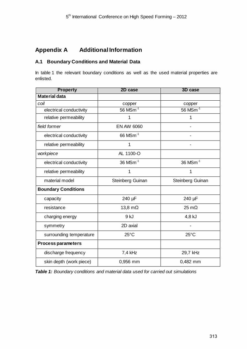
5th International Conference on High Speed Forming – 2012
Appendix A Additional Information
A.1 Boundary Conditions and Material Data
In table 1 the relevant boundary conditions as well as the used material properties are enlisted.
Property 2D case 3D case
Material data coil copper copper
electrical conductivity 56 MSm-1 56 MSm-1 relative permeability 1 1
field former EN AW 6060 -
electrical conductivity 66 MSm-1 -
relative permeability 1 -
workpiece AL 1100-O
electrical conductivity 36 MSm-1 36 MSm-1
relative permeability 1 1
material model Steinberg Guinan Steinberg Guinan
Boundary Conditions
capacity 240 µF 240 µF
resistance 13,8 mΩ 25 mΩ
charging energy 9 kJ 4,8 kJ
symmetry 2D axial -
surrounding temperature 25°C 25°C
Process parameters
discharge frequency 7,4 kHz 29,7 kHz
skin depth (work piece) 0,956 mm 0,482 mm
Table 1: Boundary conditions and material data used for carried out simulations
313

5th International Conference on High Speed Forming – 2012
314

Numerical Simulation of Magnetic Pulse Welding: Insights and Useful Simplifications
Julia Körner1; Gunther Göbel1; Berndt Brenner1; Eckhard Beyer2
1 Fraunhofer Institute for Material and Beam Technology (IWS), Dresden, Germany 2 Institute of Surface and Manufacturing Technology, Technical University Dresden, Germany
Abstract
The increasing demand for the use of lightweight materials and part designs, especially in the automotive industry, is a driving factor for the development of new joining techniques. One of the main challenges is joining of dissimilar materials. Magnetic pulse welding (MPW), a high-velocity, cold forming technique is a possible solution, as it is known for its ability to join dissimilar metals. To determine the potential of this technology for a certain application, simulation techniques have become a major part of the research process.
This paper shows some ways how to use simulation tools effectively to analyse the coil and the field shaper-geometry as well as to study their effect on the workpiece. The predictability of current distributions, resulting magnetic pressures and general process efficiency are discussed. Furthermore it is described which simplifications may be applied in order to reduce the simulation time for transient calculations. Especially aspects of the transient force evolution during a pulse are discussed and comparisons to simplified time-harmonic results are given.
Keywords
Simulation, Modelling, Finite Element Method (FEM)
1 Introduction
Electromagnetic pulse forming is a high-velocity, cold-forming technique with great potential for joining dissimilar materials. The use of tailored materials, e.g. to save weight, optimize strength or increase conductivity, is an ongoing trend in the industry. E.g. in the automotive industry this technology becomes more and more important. To determine its potential for a certain application, simulation techniques have become a major part of the research process.
315
5th International Conference on High Speed Forming – 2012
Since in most cases an accurate model produces high computational costs, both time and capacity, it is essential to optimize the simulation process. Usually the models are simplified to a 2D-description, calculated as time-harmonic processes or in case of a symmetric structure only a part of it is evaluated.
With advanced computer technology it is possible to simulate 3D-models with a high level of details to gain insights into the realistic behaviour of a system.
The aim of this work is to examine some aspects of transient and time-harmonic calculations for MPW in detail. This is expected to lead to a better understanding of the usually applied simplifications. Details of the effects on a workpiece such as current distributions and magnetic pressure evaluation are discussed as well as the influence of meshing.
2 Transient Evaluation Regarding the Magnetic Pressure
The applicable magnetic pressure is an important parameter of an MPW system and it depends on the current distribution of the system. Therefore a transient (time dependent) calculation was carried out to determine the current distribution in the forming coil as well as the magnetic pressure distribution on the workpiece. The finite element (FEM) simulation tool Comsol Multiphysics was used to obtain those results. Comsol Multiphysics is a powerful simulation tool for solving electromagnetic problems. It is useful to calculate electromagnetic (current distributions, impedance and admittance matrices, magnetic field etc.) as well as mechanical aspects (deformation, strain) with good accuracy in different ways [1].
2.1 The Model
The model consists of a forming coil, field shaper and workpiece (Figure 1) which is a common arrangement for magnetic pulse welding (MPW). Usually the coil consists of more than one turn but here a relatively simple geometry is chosen to reduce the simulation time. This simplification is valid since it only influences the absolute values.
The field shaper which is needed to concentrate the magnetic flux for maximum deformation of the workpiece features a simple symmetric geometry. The tubular workpiece is placed in the middle. Furthermore a cubic element with small conductivity is created around the configuration to set a finite volume for the calculation and to reach convergence in the equations.
In addition boundary conditions have to be set. The forming coil is driven by a capacitor bank, forming an oscillating circuit. The best way would be to use a coupled circuit-simulation plus FEM simulation as this would also model the feedback of the process into the generator correctly. According to IWS experience, such a complex simulation can be avoided for lower frequencies and simpler setups. Instead a time-varying potential is applied directly as an input to the coil and losses along the cables and in all parts of the system are taken into account. Therefore the maximum value of the potential and damping factors are adapted accordingly.
The frequency is chosen from a MPW suitable range, usually between 5 kHz and 25 kHz. The potential follows a cosine function to create the situation of a capacitor switched on at some point which will immediately lead to high voltage at the coil’s port.
316
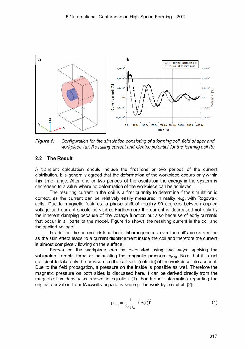
5th International Conference on High Speed Forming – 2012
Figure 1: Configuration for the simulation consisting of a forming coil, field shaper and workpiece (a). Resulting current and electric potential for the forming coil (b)
2.2 The Result
A transient calculation should include the first one or two periods of the current distribution. It is generally agreed that the deformation of the workpiece occurs only within this time range. After one or two periods of the oscillation the energy in the system is decreased to a value where no deformation of the workpiece can be achieved.
The resulting current in the coil is a first quantity to determine if the simulation is correct, as the current can be relatively easily measured in reality, e.g. with Rogowski coils. Due to magnetic features, a phase shift of roughly 90 degrees between applied voltage and current should be visible. Furthermore the current is decreased not only by the inherent damping because of the voltage function but also because of eddy currents that occur in all parts of the model. Figure 1b shows the resulting current in the coil and the applied voltage. In addition the current distribution is inhomogeneous over the coil’s cross section as the skin effect leads to a current displacement inside the coil and therefore the current is almost completely flowing on the surface.
Forces on the workpiece can be calculated using two ways: applying the volumetric Lorentz force or calculating the magnetic pressure pmag. Note that it is not sufficient to take only the pressure on the coil-side (outside) of the workpiece into account. Due to the field propagation, a pressure on the inside is possible as well. Therefore the magnetic pressure on both sides is discussed here. It can be derived directly from the magnetic flux density as shown in equation (1). For further information regarding the original derivation from Maxwell’s equations see e.g. the work by Lee et al. [2].
( )2
0mag B(t)
μ21p ⋅⋅
= (1)
x
z y
a b
317
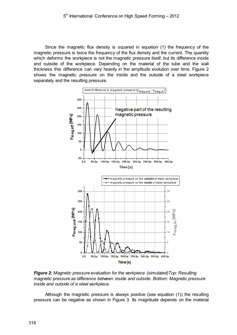
5th International Conference on High Speed Forming – 2012
Since the magnetic flux density is squared in equation (1) the frequency of the magnetic pressure is twice the frequency of the flux density and the current. The quantity which deforms the workpiece is not the magnetic pressure itself, but its difference inside and outside of the workpiece. Depending on the material of the tube and the wall thickness this difference can vary heavily in the amplitude evolution over time. Figure 2 shows the magnetic pressure on the inside and the outside of a steel workpiece separately and the resulting pressure.
Figure 2: Magnetic pressure evaluation for the workpiece (simulated)Top: Resulting magnetic pressure as difference between inside and outside. Bottom: Magnetic pressure inside and outside of a steel workpiece.
Although the magnetic pressure is always positive (see equation (1)) the resulting pressure can be negative as shown in Figure 3. Its magnitude depends on the material
318
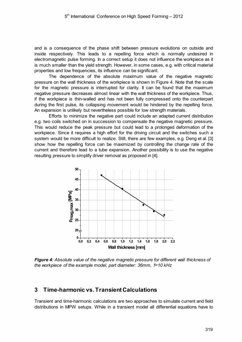
5th International Conference on High Speed Forming – 2012
and is a consequence of the phase shift between pressure evolutions on outside and inside respectively. This leads to a repelling force which is normally undesired in electromagnetic pulse forming. In a correct setup it does not influence the workpiece as it is much smaller than the yield strength. However, in some cases, e.g. with critical material properties and low frequencies, its influence can be significant.
The dependence of the absolute maximum value of the negative magnetic pressure on the wall thickness of the workpiece is shown in Figure 4. Note that the scale for the magnetic pressure is interrupted for clarity. It can be found that the maximum negative pressure decreases almost linear with the wall thickness of the workpiece. Thus, if the workpiece is thin-walled and has not been fully compressed onto the counterpart during the first pulse, its collapsing movement would be hindered by the repelling force. An expansion is unlikely but nevertheless possible for low strength materials.
Efforts to minimize the negative part could include an adapted current distribution e.g. two coils switched on in succession to compensate the negative magnetic pressure. This would reduce the peak pressure but could lead to a prolonged deformation of the workpiece. Since it requires a high effort for the driving circuit and the switches such a system would be more difficult to realize. Still, there are few examples, e.g. Deng et al. [3] show how the repelling force can be maximized by controlling the change rate of the current and therefore lead to a tube expansion. Another possibility is to use the negative resulting pressure to simplify driver removal as proposed in [4].
0,0 0,2 0,4 0,6 0,8 1,0 1,2 1,4 1,6 1,8 2,0 2,20
20
25
30
35
40
45
50
p mag
,max
[MPa
]
Wall thickness [mm]
Figure 4: Absolute value of the negative magnetic pressure for different wall thickness of the workpiece of the example model, part diameter: 36mm, f=10 kHz
3 Time-harmonic vs. Transient Calculations
Transient and time-harmonic calculations are two approaches to simulate current and field distributions in MPW setups. While in a transient model all differential equations have to
319

5th International Conference on High Speed Forming – 2012
be solved for each predefined time step, only one solution is needed in the time-harmonic case. This reduces the calculation time tremendously.
In time-harmonic systems the amplitude of the applied parameter (e.g. the potential) and the frequency are defined and a model is solved that approximates the pulse as a continuous sine wave. In a transient system an arbitrary function can be applied.
Furthermore, the initial conditions are much different: the transient calculation can start with a system where all variables are zero, i.e. no currents or fields exist. In contrast the time-harmonic assumes a continuous process, therefore no real “start time” exists (steady-state system). The considered pulse is than approximated by using the evolution during one period, starting at the point where the potential is at maximum (=capacitor was fully charged).
One might think that therefore a time-harmonic system disregards important aspects of reality, e.g. the correct initial slope. So a time-harmonic and a transient calculation are compared using the simulation tool Comsol Multiphysics. The model geometry is the same as shown in Figure 1. Although real pulses are always damped, here for the transient case an undamped cosine function was used for the potential applied to the coil for a direct comparison. For simplicity no deformations were taken into account. Important MPW process parameters like the current distribution in coil and workpiece and the magnetic pressure are evaluated. The results for the transient and the time-harmonic evaluation are surprisingly consistent. Figure 5a and 5b show the current distribution in coil and workpiece for both approaches obtained by integration over a predefined cross section. For the coil there is only a slight difference in the first half-wave because the current is starting from zero as explained above.
For the workpiece both calculation results are also in good agreement except for the first half-wave where a significant difference in amplitude is visible. This is an effect of the coupling and therefore also dependent on the material of the workpiece.
Figure 5c shows the magnetic field outside of the workpiece and Figure 5d the magnetic pressure at the same position, both compared for transient and time-harmonic analysis. Again the results are primarily different in absolute amplitude of the first pulse.
From those examples it can be seen that time-harmonic calculations are sufficient to determine some important parameters of MPW processes although MPW pulses are highly transient in nature. The time-harmonic system provides fairly accurate results for coil amplitude and field distribution but disregards initial effects. Furthermore it is clear that it cannot represent highly damped systems, as only undamped (continuous) pulsing can be simulated.
320
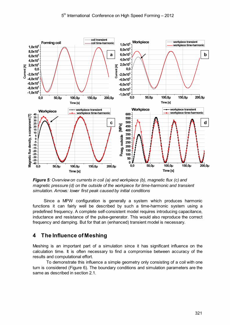
5th International Conference on High Speed Forming – 2012
Figure 5: Overview on currents in coil (a) and workpiece (b), magnetic flux (c) and magnetic pressure (d) on the outside of the workpiece for time-harmonic and transient simulation. Arrows: lower first peak caused by initial conditions
Since a MPW configuration is generally a system which produces harmonic functions it can fairly well be described by such a time-harmonic system using a predefined frequency. A complete self-consistent model requires introducing capacitance, inductance and resistance of the pulse-generator. This would also reproduce the correct frequency and damping. But for that an (enhanced) transient model is necessary.
4 The Influence of Meshing
Meshing is an important part of a simulation since it has significant influence on the calculation time. It is often necessary to find a compromise between accuracy of the results and computational effort.
To demonstrate this influence a simple geometry only consisting of a coil with one turn is considered (Figure 6). The boundary conditions and simulation parameters are the same as described in section 2.1.
0,0 50,0µ 100,0µ 150,0µ 200,0µ-1,0x10⁶-8,0x10⁵-6,0x10⁵-4,0x10⁵-2,0x10⁵
0,02,0x1054,0x1056,0x1058,0x1051,0x106 Workpiece
Curr
ent [
A]
Time [s]
workpiece transient workpiece time-harmonic
0,0 50,0µ 100,0µ 150,0µ 200,0µ-1,0x10⁶-8,0x10⁵-6,0x10⁵-4,0x10⁵-2,0x10⁵
0,02,0x1054,0x1056,0x1058,0x1051,0x106
Forming coil
Curr
ent [
A]
Time [s]
coil transient coil time-harmonic
0,0 50,0µ 100,0µ 150,0µ 200,0µ0
50100150200250300350400450500550600
Workpiece
p mag
, out
side
[M
Pa]
Time [s]
workpiece transient workpiece time-harmonic
0,0 50,0µ 100,0µ 150,0µ 200,0µ-40-35-30-25-20-15-10-505
10152025303540
Workpiece
Magn
etic
flux d
ensit
y, x-
com
pone
nt [T
]
Time [s]
workpiece transient workpiece time-harmonic
a b
c d
321
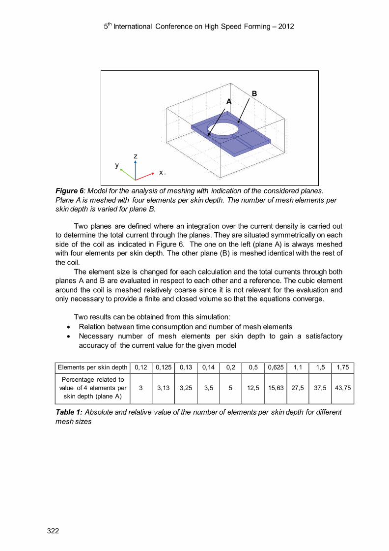
5th International Conference on High Speed Forming – 2012
Figure 6: Model for the analysis of meshing with indication of the considered planes. Plane A is meshed with four elements per skin depth. The number of mesh elements per skin depth is varied for plane B.
Two planes are defined where an integration over the current density is carried out to determine the total current through the planes. They are situated symmetrically on each side of the coil as indicated in Figure 6. The one on the left (plane A) is always meshed with four elements per skin depth. The other plane (B) is meshed identical with the rest of the coil.
The element size is changed for each calculation and the total currents through both planes A and B are evaluated in respect to each other and a reference. The cubic element around the coil is meshed relatively coarse since it is not relevant for the evaluation and only necessary to provide a finite and closed volume so that the equations converge.
Two results can be obtained from this simulation:
• Relation between time consumption and number of mesh elements • Necessary number of mesh elements per skin depth to gain a satisfactory
accuracy of the current value for the given model
Table 1: Absolute and relative value of the number of elements per skin depth for different mesh sizes
Elements per skin depth 0,12 0,125 0,13 0,14 0,2 0,5 0,625 1,1 1,5 1,75
Percentage related to value of 4 elements per
skin depth (plane A) 3 3,13 3,25 3,5 5 12,5 15,63 27,5 37,5 43,75
A B
x
z y
x
322

5th International Conference on High Speed Forming – 2012
0 5 10 15 20 25 30 35 40 45 500,0
0,4
0,8
1,2
1,6
2,0
2,4
2,8
Error Calculation Time
Ideality of meshing [%]
Varia
tion
of c
urre
nts
in th
e pl
anes
[%]
0
200
400
600
800
1000
1200
1400
Figure 7: Discrepancy of currents in the two planes and calculation time for different mesh sizes (f = 10 kHz)
It is commonly considered that three to five elements per skin depth are required for a good accuracy of the results [5] [6]. Due to that fact the current through plane A with four (second order) elements per skin depth is taken as reference for the evaluation.
The mesh of plane A is kept constant with four elements per skin depth while the mesh for the other parts of the geometry is refined after each calculation. Table 1 shows the increase of the number of second order mesh elements per skin depth in absolute value and with reference to plane A. However, the increase is not linear as predefined mesh sizes of the simulation program are used.
After each simulation for the different meshes the total currents in plane A and B are calculated by integration over the cross section of each plane. The current through plane A is constant while the current through plane B varies and converges to the value of plane A.
The variation of the currents in the predefined planes is calculated with equation (2) so that the difference is expressed by a percentage value.
100I
IIV
APlane
BPlaneAPlaneI ⋅
−= (2)
Figure 7 shows that the difference in the currents decreases with an increasing
number of elements per skin depth which is not surprising. The interesting fact is that already with one (2nd order) element per skin depth one gets a fairly good accuracy of the current calculation for this type of model. In addition Figure 7 shows the necessary calculation time. It can be found that the simulation time for one element per skin depth is only about a third of the time needed for a calculation with two elements. But the error in the calculated value is smaller than 0.5%. The variations of the current distributions in the planes in the left half of Figure 7 should also be considered. They show that a small number of elements per skin depth,
Cal
cula
tion
time
[s]
323

5th International Conference on High Speed Forming – 2012
although they only lead to a small percentage difference from the current value obtained with four elements per skin depth, have a significant uncertainty.
That leads to the following conclusion: For the given model it is sufficient to choose a relatively coarse mesh with only one to one point five elements per skin depth to be able to analyse the currents. The increase in accuracy which could be achieved with a finer mesh is very small compared to the increase in calculation time. Note that a special geometry and only current distribution are discussed here. The results might be different when regarding other parameters and geometries. But as currents and their distribution are a vital part of coil simulation, this is an important aspect.
5 Conclusions
This work describes effects occurring during an electromagnetic pulse forming process with special regard to the repelling force as a consequence of the evolution of the magnetic pressure during a pulse. This knowledge is useful to either improve the usage of driver materials or to create a compensation to prevent energy loss. Furthermore it is explained in which cases time-harmonic calculations are sufficient since they take much less time even for complex 3D-structures.
Another important part of a simulation is the meshing. It is shown that for typical 3D-coil models for MPW fine meshes strongly increase the simulation time but only attain a small increase in accuracy. Therefore the correlation between simulation time and accuracy is shown on the basis of current densities and hints are given how to find the fitting trade-off between those quantities.
References
[1] N.N: Manual Comsol Multiphysics 3.5a: AC/DC Module: “Inductance of a coil”, (2010)
[2] Lee, Sung Ho; Lee, Dong Nyung: Estimation of the magnetic pressure in tube expansion by electromagnetic forming; Journal of Materials Processing Technology (1996); Volume 57; p. 311 - 315
[3] Deng, Jianghua; Li, Chunfeng; Zhao, Zhiheng; Tu, Fang; Yu, Haiping: Numerical simulation of magnetic flux and force in electromagnetic forming with attractive force; Journal of Materials Processing Technology (2007); Volume 184; p. 190-194
[4] Patent DE 19602951 – C1 (07.12.2000). Magnet-Physik Dr. Steingroever GmbH [5] Lotfi, Ashraf W.; Lee, Fred C.: Two-Dimensional Skin Effect in Power Foils for High-
Frequency Applications; IEEE Transaction on Magnetics (1995); Volume MAG-31; p. 1003 - 1006
[6] Rodger, David: Experience with hierarchical finite elements in 2D Electromagnetics; IEEE Transaction on Magnetics (1987); Volume MAG-23; p. 3560 - 3562
324

Combined simulation of quasi-static deep drawing and electromagnetic forming by means of a coupled damage–viscoplasticity model at finite strains Y. Kiliclar1, O. K. Demir2, I. N. Vladimirov1, L. Kwiatkowski2, A. Brosius2, S. Reese1, A. E. Tekkaya2
1 Institute of Applied Mechanics, RWTH Aachen University, Germany 2 Institute of Forming Technology and Lightweight Construction, TU Dortmund, Germany
Abstract
The combination of quasi-static and electromagnetic pulse forming increases the formability of sheet metal forming processes. A cooperation between the institute of Applied Mechanics (IFAM) of the RWTH Aachen and the Institute of Forming Technology and Lightweight Construction (IUL) of the TU Dortmund is investigating these processes both experimentally and by simulation for the deep-drawing process of a cross-shaped cup. Aim of the work is to show and prove that with this forming strategy we obtain a more sharpened radius of the cup edges.The combined deformation process is simulated by means of finite elements using a material model developed in [1,2]. A recently proposed finite strain anisotropic viscoplastic model, taking combined nonlinear kinematic and isotropic hardening into account, is coupled with ductile damage in the context of continuum damage mechanics. For the simulation, the evolution equations for the internal variables of the constitutive model are numerically integrated in an explicit manner and the model is then implemented as a user material subroutine in the commercial finite element package LS-Dyna.
Keywords
Modelling, Deep drawing, Damage
1 Introduction
To cope with the ever higher complexity of new sheet metal designs is a challenge. Focusing on the reduction of the weight of parts and the emission during the production leads to improved forming strategies [3]. A major issue is the insufficient formability at
325
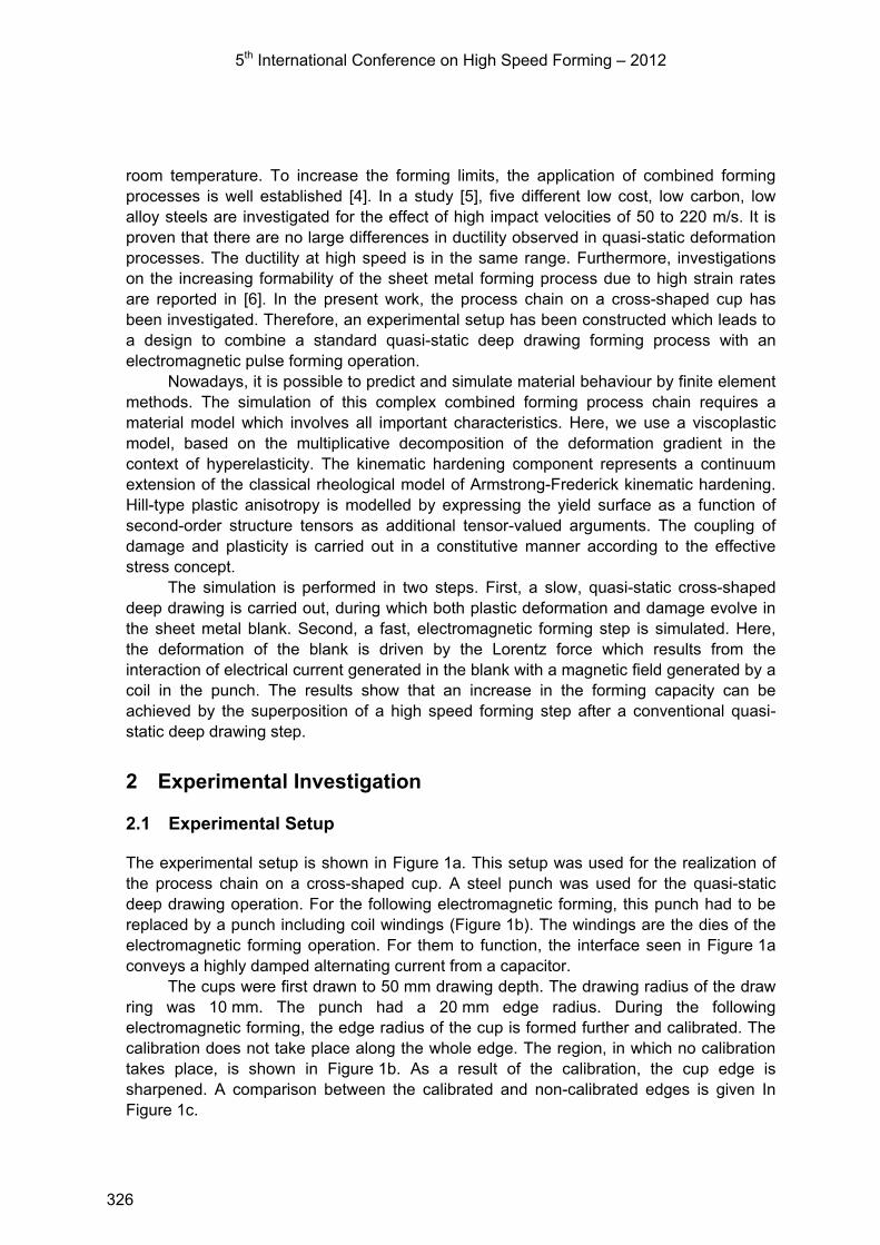
5th International Conference on High Speed Forming – 2012
room temperature. To increase the forming limits, the application of combined forming processes is well established [4]. In a study [5], five different low cost, low carbon, low alloy steels are investigated for the effect of high impact velocities of 50 to 220 m/s. It is proven that there are no large differences in ductility observed in quasi-static deformation processes. The ductility at high speed is in the same range. Furthermore, investigations on the increasing formability of the sheet metal forming process due to high strain rates are reported in [6]. In the present work, the process chain on a cross-shaped cup has been investigated. Therefore, an experimental setup has been constructed which leads to a design to combine a standard quasi-static deep drawing forming process with an electromagnetic pulse forming operation.
Nowadays, it is possible to predict and simulate material behaviour by finite element methods. The simulation of this complex combined forming process chain requires a material model which involves all important characteristics. Here, we use a viscoplastic model, based on the multiplicative decomposition of the deformation gradient in the context of hyperelasticity. The kinematic hardening component represents a continuum extension of the classical rheological model of Armstrong-Frederick kinematic hardening. Hill-type plastic anisotropy is modelled by expressing the yield surface as a function of second-order structure tensors as additional tensor-valued arguments. The coupling of damage and plasticity is carried out in a constitutive manner according to the effective stress concept.
The simulation is performed in two steps. First, a slow, quasi-static cross-shaped deep drawing is carried out, during which both plastic deformation and damage evolve in the sheet metal blank. Second, a fast, electromagnetic forming step is simulated. Here, the deformation of the blank is driven by the Lorentz force which results from the interaction of electrical current generated in the blank with a magnetic field generated by a coil in the punch. The results show that an increase in the forming capacity can be achieved by the superposition of a high speed forming step after a conventional quasi-static deep drawing step.
2 Experimental Investigation
2.1 Experimental Setup
The experimental setup is shown in Figure 1a. This setup was used for the realization of the process chain on a cross-shaped cup. A steel punch was used for the quasi-static deep drawing operation. For the following electromagnetic forming, this punch had to be replaced by a punch including coil windings (Figure 1b). The windings are the dies of the electromagnetic forming operation. For them to function, the interface seen in Figure 1a conveys a highly damped alternating current from a capacitor.
The cups were first drawn to 50 mm drawing depth. The drawing radius of the draw ring was 10 mm. The punch had a 20 mm edge radius. During the following electromagnetic forming, the edge radius of the cup is formed further and calibrated. The calibration does not take place along the whole edge. The region, in which no calibration takes place, is shown in Figure 1b. As a result of the calibration, the cup edge is sharpened. A comparison between the calibrated and non-calibrated edges is given In Figure 1c.
326

5th International Conference on High Speed Forming – 2012
Figure 1: a) Experimental setup to realize the process chain on cross-shaped cups b) The punch head with coil windings for electromagnetic calibration at the punch edges c) A comparison between the calibrated and non-calibrated edges
2.2 Material Characterization
The quasi-static flow curve and the Lankford coefficients of the material aluminum EN AW 5083 were obtained by standard tensile tests. For the flow curves at high strain rates, high speed tensile tests were performed at the company Nordmetall GmbH [7]. The strain rate reached in these experiments was about 1000 s-1. The experiments showed a negligible difference between quasi-static and high-speed flow curves. Hence, the quasi-static flow curves were used for simulations of both deep drawing and electromagnetic forming.
3 Simulation Results
3.1 Material Modelling
A continuum mechanical extension of the classical rheological model of Armstrong-Frederick kinematic hardening can be achieved by the triple multiplicative split 𝐅 =𝐅e 𝐅pe 𝐅pi of the plastic deformation gradient into “elastic” and “inelastic” parts [8].
The Helmholtz free energy per unit undeformed volume ψ is additively decomposed into the three parts ψ = ψe(𝐂e) + ψkin𝐂pe + ψiso(κ). The macroscopic elastic material properties are described by the first part ψe. The second term ψkin corresponds to the elastic energy stored in dislocation fields due to kinematic hardening and vanishes if the kinematic hardening is zero. The third term represents elastic energy due to isotropic
327
5th International Conference on High Speed Forming – 2012
hardening, where κ is the isotropic hardening variable. The Helmholtz free energy is a function of the elastic right Cauchy-Green tensor 𝐂e = 𝐅eT𝐅e = 𝐅p−T𝐂𝐅p−1 and the elastic part of the plastic right Cauchy-Green tensor defined as 𝐂pe = 𝐅peT 𝐅pe = 𝐅pi−T𝐂𝐅pi−1. Inserting this in the Clausius-Duhem inequality −ψ + 𝐒 ∙ (1 2⁄ ) ≥ 0 results in a relation for the second Piola-Kirchhoff stress tensor 𝐒. The derivation of the material model is suitably carried out in the intermediate configuration. For the numerical implementation of the constitutive equations it is, however, more appropriate to work in the undeformed or reference configuration. The material model is summarized as follows.
• Second Piola-Kirchhoff stress tensor
𝐒 = 11−D
2𝐅p−1∂ψe∂𝐂e
𝐅p−T (1)
Here D denotes the isotropic ductile damage variable. Its evolution equation is defined in eq. (5).
• Back stress tensor
𝐗 = 2𝐅pi−1 ∂ψkin
∂𝐂pe𝐅pi−T (2)
• Stress-like quantities
𝐘 = 𝐂𝐒 − 𝐂p𝐗, 𝐘kin = 𝐂p𝐗 (3)
Y is a stress-like quantity variable resulting from the pullback of the Mandel type tensor into the reference configuration.
• Evolution equations
p = λ sym(𝐂p(A[𝐘D)T+(𝐀 T[𝐘D])T)D
𝐘D∙(𝐀[(𝐘D)T], pi = 2λ b
c𝐘kinD 𝐂pi, κ = 2
3λ (4)
The superscript D denotes the deviator part of a tensor, λ is the plastic multiplier and the square brackets denotes the mapping of the second-order tensor by means of the fourth-order tensor 𝐀. 𝐂pi is inelastic plastic part of the right Cauchy-Green tensor. The isotropic hardening variable is defined by κ.
• Scalar isotropic ductile damage variable
D = λ23
11−D
Ysk
H(κ−pD) (5)
328
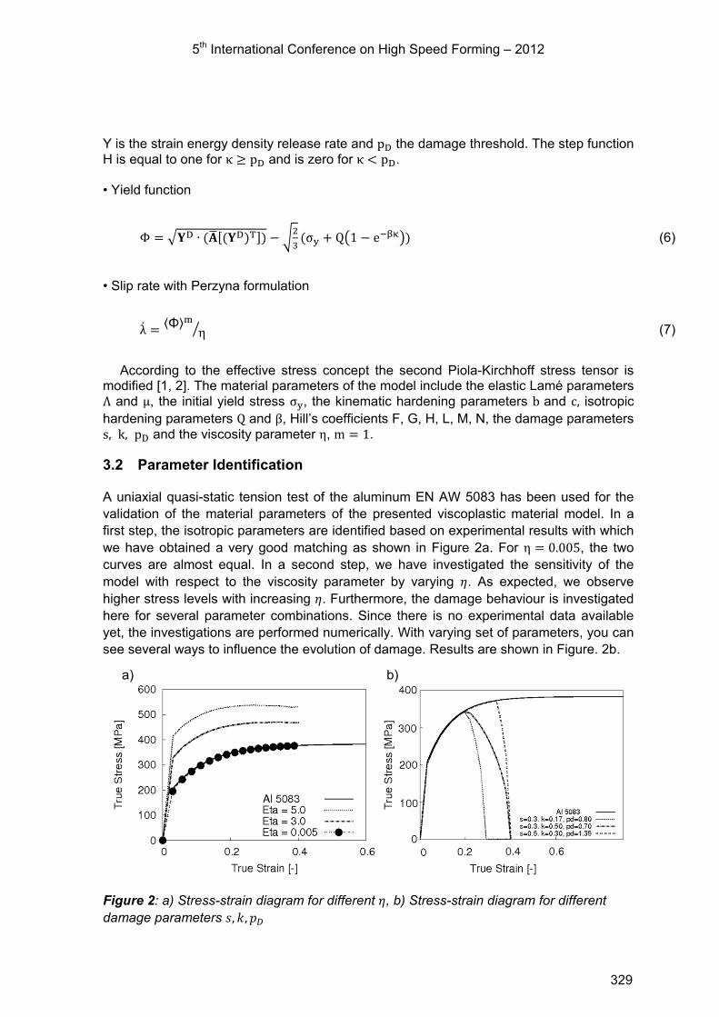
5th International Conference on High Speed Forming – 2012
Y is the strain energy density release rate and pD the damage threshold. The step function H is equal to one for κ ≥ pD and is zero for κ < pD.
• Yield function
Φ = 𝐘D ∙ (𝐀[(𝐘D)T]) − 23
(σy + Q1 − e−βκ) (6)
• Slip rate with Perzyna formulation
λ = ⟨Φ⟩mη (7)
According to the effective stress concept the second Piola-Kirchhoff stress tensor is modified [1, 2]. The material parameters of the model include the elastic Lamé parameters Λ and µ, the initial yield stress σy, the kinematic hardening parameters b and c, isotropic hardening parameters Q and β, Hill’s coefficients F, G, H, L, M, N, the damage parameters s, k, pD and the viscosity parameter η, m = 1.
3.2 Parameter Identification
A uniaxial quasi-static tension test of the aluminum EN AW 5083 has been used for the validation of the material parameters of the presented viscoplastic material model. In a first step, the isotropic parameters are identified based on experimental results with which we have obtained a very good matching as shown in Figure 2a. For η = 0.005, the two curves are almost equal. In a second step, we have investigated the sensitivity of the model with respect to the viscosity parameter by varying 𝜂. As expected, we observe higher stress levels with increasing 𝜂. Furthermore, the damage behaviour is investigated here for several parameter combinations. Since there is no experimental data available yet, the investigations are performed numerically. With varying set of parameters, you can see several ways to influence the evolution of damage. Results are shown in Figure. 2b.
Figure 2: a) Stress-strain diagram for different 𝜂, b) Stress-strain diagram for different damage parameters 𝑠, 𝑘,𝑝𝐷
a) b)
329

5th International Conference on High Speed Forming – 2012
3.3 Finite Element Simulation
The previously described experimental setup has been transferred into a finite element model. A quarter model due to symmetry was used for the simulations where tools and dies were modelled as rigid bodies. As the friction coefficient between the workpiece and the die µfric = 0.06 was used. 26820 brick elements with 8 nodes and single integration points have been used to model the blank. The deep drawing simulation was performed using the three-dimensional (3D) explicit finite element solver of the commercial software LS-DYNA.
The simulation of the following electromagnetic forming represents a coupled field problem which consists of an electromagnetic and a mechanical part. The electromagnetic problem was solved by the 3D electromagnetic module of the commercial software ANSYS. Then, the mechanical problem was handled with the LS-DYNA explicit solver. A step-by-step coupling between the two solvers was performed by an in-house code developed at the IUL of TU Dortmund. The final setup is shown in Figure 3.
Figure 3: Simulation assembly
The simulation of the coupling of both quasi-static and electromagnetic forming processes is a major issue and has been solved in two steps. At first, the standard deep drawing process is done in a quasi-static manner. When we reach the final punch stroke at the end of the simulation, the stresses and strains are transferred to the second, electromagnetic forming step. With respect to the user material, we have to take all history variables into account which have to be transferred too. A method which is offered by LS-Dyna is a “dynain” file which contains the output information at any requested step.
As a test case, the method is tried and tested on an academic one element example for tensile loading. At first, the element is under load until reaching a defined total process time. Then the variables are stored and transferred and the second simulation step is continuing from the last deformed state. As shown in Figure 4, the method is working very well.
Punch
Blank holder Workpiece
Die
330
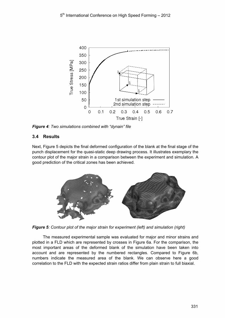
5th International Conference on High Speed Forming – 2012
Figure 4: Two simulations combined with “dynain” file
3.4 Results
Next, Figure 5 depicts the final deformed configuration of the blank at the final stage of the punch displacement for the quasi-static deep drawing process. It illustrates exemplary the contour plot of the major strain in a comparison between the experiment and simulation. A good prediction of the critical zones has been achieved.
Figure 5: Contour plot of the major strain for experiment (left) and simulation (right)
The measured experimental sample was evaluated for major and minor strains and plotted in a FLD which are represented by crosses in Figure 6a. For the comparison, the most important areas of the deformed blank of the simulation have been taken into account and are represented by the numbered rectangles. Compared to Figure 6b, numbers indicate the measured area of the blank. We can observe here a good correlation to the FLD with the expected strain ratios differ from plain strain to full biaxial.
331

5th International Conference on High Speed Forming – 2012
Figure 6: Comparison of FLD between experiment and simulation
As already shown by the experimental investigations which were presented in Figure 1c, an increase of the total deformation is shown in Figure 7 which can be achieved by the superposition of a high speed forming step after a conventional quasi-static deep drawing step. As a result of the simulation, the distribution plot of the equivalent plastic strain after deep drawing and electromagnetic forming depicts a sharpening of the radius on each corner. It shows a good result regarding the formability.
Figure 7: Distribution of equivalent plastic strain after (left) deep drawing and (right) electromagnetic forming
4 Summary
In this paper, we investigate the finite element simulation of the process chain quasi-static deep drawing – electromagnetic forming by means of a new coupled damage-viscoplasticity model for large deformations. For this purpose, a recently proposed finite strain anisotropic viscoplastic model, taking combined nonlinear kinematic and isotropic hardening into account, is coupled with ductile damage in the context of continuum damage mechanics. The coupling of damage and plasticity is carried out in a constitutive manner according to the effective stress concept.
The numerical examples investigate the potential of the constitutive framework regarding the simulation of the forming limits. In particular, the coupled material model is
a) b)
332

5th International Conference on High Speed Forming – 2012
applied to the combined quasi-static – electromagnetic simulation of the cross-shaped cup deep drawing process. For this purpose, the evolution equations for the internal variables of the constitutive model are numerically integrated in an explicit manner and the model is then implemented as a user material subroutine in the commercial finite element package LS-Dyna. The results show that an increase in the total deformation can be achieved by the superposition of a high speed forming step after a conventional quasi-static deep drawing step.
5 Acknowledgement
This work is based on the results of PAK343 “Methodenplanung für quasistatisch-dynamisch kombinierte Umformprozesse”. The authors would like to thank the “Deutsche Forschungsgemeinschaft (DFG)” for its financial support.
References
[1] Vladimirov, I. N.; Kiliclar, Y.; Tini. V.; Reese, S.: Constitutive modelling of anisotropy, hardening and failure of sheet metals, Key Engineering Materials, 2011, Vol. 473, pp. 631-636.
[2] Vladimirov, I. N.; M. P. Pietryga, M. P.; Reese, S.: Prediction of forming limit diagrams at fracture by an anisotropic finite plasticity model with ductile damage, steel research international, special issue ICTP2011, 2011, pp. 883-888.
[3] Bull, M.; Chavakari, R.; Mascarin, A.: Benefit analysis: Use of aluminum structures in conjunction with alternative power-train technologies in automobiles. IBIS Associates, Inc for the Aluminum Association, 2008
[4] Imbert, J. M.; Winkler, S. L.; Worswick, M. J.; Oliveira, D. A.; Golovaschenko, S.: The effect of tool-sheet interaction on damage evolution in electromagnetic forming of aluminum alloy sheet. Journal of Engineering Materials and Technology, 2005, Vol. 127, pp. 145-153
[5] Seth, M; Vohnout, V. J.; Daehn, G. S.: Formability of steel sheet in high velocity impact. Journal of Materials Processing Technology, 2005, Vol. 168, pp. 390-400
[6] Balanethirama, V. S.; Daehn, G. S.: Hyperplasticity: Increased forming limits at high workpiece velocity. Scripta Metallurgica et Materialia, 1994, Vol. 30, pp. 515-520
[7] www.nordmetall.net [8] Vladimirov, I. N.; M. P. Pietryga, M. P.; Reese, S.: On the modelling of nonlinear
kinematic hardening at finite strains with application to springback – comparison of time integration algorithms, International Journal for Numerical Methods in Engineering, 2008, Vol. 75, pp. 1-28
333

5th International Conference on High Speed Forming – 2012
334

Numerical Identification of Optimum Process Pa-rameters for Combined Deep Drawing and Elec-tromagnetic Forming*
M. Stiemer1, F. Taebi2, M. Rozgic1, R. Appel1
1 Institute for the Theory of Electrical Engineering, Helmut-Schmidt-University / University of the Federal Armed Forces Hamburg, Germany
2 Chair of Scientific Computation, TU-Dortmund, Germany
Abstract
In this paper, a method is presented for the virtual process design of combinations of deep drawing and electromagnetic forming. With suitably chosen parameters, such process combinations of a quasi-static and an impulse forming process extend forming limits of classical, purely quasi-static forming. To determine parameters leading to the desired forming result, a numerical optimization algorithm is employed. The parameters to be ad-justed comprise parameters of the triggering current, such as frequency, amplitude, damp-ing, etc., geometric parameters of the tool coil and parameters of the deep drawing pro-cess, as, e.g., drawing radii or tribological parameters. To reduce the required number of evaluations of the target function, a gradient based numerical optimization scheme is em-ployed following directions of decent in the parameter space. The quality of a given pa-rameter set is determined by computing the distance of the simulated forming result to the prescribed ideal shape via a finite element simulation. Forming limits are incorporated by so called forming limit surfaces as constraints to the optimization process, considering rate dependence and prestrain in the second impulse forming step.
Keywords
Electromagnetic forming, Process combinations, Numerical optimization
*This work is based on the results of the research project PAK343-2; the authors would like to thank the German Research Foundation (DFG) for its financial support. Further, the authors are indebted to the Institute of Forming Technology and Lightweight Construction (IUL) at the TU-Dortmund, particularly to Koray Demir, for providing the experimental data this work is based on.
335

5th International Conference on High Speed Forming – 2012
1 Introduction
Deep drawing is one of the most frequently utilized industrial forming methods. Usually it is driven by the pressure exerted on a metal sheet by a punch. Forming is guided by a die and the material's flow is controlled by the blank holder force, the radius of the drawing ring at the flange, the bottom radius of the punch, the geometrical details of the drawing ring, the punch, and the die, and finally the friction between the work piece and the tool. The material flow of the sheet metal results from stretch-compression loading and stretch-bending loading or a combination of both. Deep drawing can be considered as a quasi-static forming process, i.e., inertial forces need not be considered. While many forming operations can be carried out by deep drawing, recent industrial requirements aim at form-ing methods with allow for a higher material formability. On the one hand this is a conse-quence of an interest in high-tensile materials, particularly for safety reasons. On the other hand the demand for light-weight constructed work pieces requires forming methods for more complicated geometries. In addition to this, the increasing competition in forming technology leads to the demand of more efficient production methods, particularly allowing for a reduction of production time and costs. Deep drawing on its own has not the poten-tial to meet all these requirements. Using deep drawing as part of a process chain may help to extend forming limits. However, increased production time and costs have to be avoided at the same time. Therefore, integration of post-processing steps into the deep-drawing process is desirable. An option to meet both demands is combining deep drawing with electromagnetic forming.
Electromagnetic forming (EMF) is an impulse forming method in which strain rates over 1000 s-1 are achieved. It is driven by the Lorentz force, a material body force that re-sults from the interaction of a pulsed magnetic field with eddy currents induced in the work piece by the magnetic field itself. The energy transferred by the Lorentz force is, however, not immediately transformed into plastic work. A great portion of it is stored as kinetic en-ergy in the work piece, which then leads to deformation by inertial forces [1]. The magnet-ic field is generated by a tool coil adjacent to the work piece, which is excited by the dis-charging current of a capacitor bank. Typically, a current of several 10000 Ampère is gen-erated within a time comparable to 10 µs, leading to magnetic flux densities in the order of 1-10 Tesla in the gap between tool coil and work piece. The whole forming process takes about 100 µs. As an individual forming process, EMF has already been scientifically stud-ied in the 1960's, as described, e.g., by [2]. EMF possesses a huge potential to extend forming limits of classical techniques, particularly as part of a process chain [3]. In such a combination, all advantages of this forming method can take effect: Above all, an in-creased formability enables the extension of classical forming limits (e.g., [3,4]). Further, by a suitable design of the tool coil, loads can be applied locally and, hence, the spectrum of applicable load distributions is enormously extended. Next, tool coils can often com-pletely be integrated into other forming tools, such that fully integrated multi-stage process combinations become possible (e.g., Figure 4 on the left hand side). Finally, the process only takes about 100 µs, such that the additional time required for a subsequent electro-magnetic calibration step can be neglected. For detailed information as well as recent re-sults on EMF and its use in process chains we refer to [5].
Recent experimental results show that such process combinations, indeed, lead to an extension of classical forming limits (e.g., [3] or [4]). As an example, compare Figure 1 and Figure 2. These show results of experiments carried out at the Institute of Forming
336

5th International Conference on High Speed Forming – 2012
Technology and Lightweight Construction (IUL) at the TU-Dortmund (e.g., [4]). The right hand side of Figure 1 shows a forming limit diagram determined after a single deep draw-ing step. The left hand side of Figure 2 displays the corresponding diagram after a subse-quent step of electromagnetic forming. Obviously, in the area of combined forming an amount of stretch has been achieved after EMF that exceeds the quasi-static formability. Forming limit diagrams are a frequently used indicator for material formability in quasi-static forming methods. In these diagrams the two principal strains (Eigenvalues of the true- or Hencky strain) in the sheet metal plane are compared to each other. In a diagram with the second principal Hencky strain on the abscissa (minor strain) and the first princi-pal strain on the ordinate (major strain), a curve is inserted separating stress states lead-ing to material failure from those without damage. To determine this curve, it is observed, when fracture occurs first. Although in deep drawing mechanical failure is usually defined via necking, we consider the forming limit curve for fracture, since we are interested in a comparison to high speed forming limits: In the case of the high strain rates typical of elec-tromagnetic forming, emerging material failure cannot be observed accurately enough to capture necking before fracture occurs. To achieve consistency in the performed simula-tions and experiments we, hence, focus on fracture. Moreover, experimental data ob-tained so far give no information if necking at high strain rates occurs at all. It is remarka-ble that a similar discussion has arisen in a completely different field of forming technolo-gy: In single point incremental forming, it has also been impossible to clarify whether necking occurs before fracture so far. This discussion has, among others, led to the theory of fracture forming lines (see [6]).
Obviously, the construction of a forming limit curve depends on a very particular load situation, which does not apply if prestrain and rate dependence have a significant in-fluence on the forming result. This is the reason, why classical forming limit diagrams cannot be used for the prediction of forming limits in case of nonlinear load paths or dy-namic loading. We will address this issue in Chapter 3.
Figure 1: Right: Major and minor strain after deep drawing for the grid points marked on the surface of a work piece as displayed on the left. Brightness is related to major strain in both diagrams [4].
Figures 1 and 2 have been produced by the ARGUS-system (Gesellschaft für
OptischeMesstechnik). The principle idea to extend quasi-static forming limits is now to leave those load paths relevant in deep drawing and replace them by highly nonlinear and
337

5th International Conference on High Speed Forming – 2012
strain-rate-dependent ones, as demonstrated in the preceding example. Experimental re-sults show, however, that process parameters have to be carefully adjusted to gain an in-crease in formability with this approach. Hence, it is desirable to be able to predict those parameters that lead to an increased formability. Moreover, such a method reduces ex-pensive experiments and development time for new products. This is a motivation for the use of numerical methods to identify suited process parameters leading to an extended formability.
Figure 2: Left: Major and minor strain after EMF for grid points marked on the surface of the work piece (brightness according to major strain). Right: Corresponding distribution of major strain on the work piece (same brightness scale) [4].
2 Parameter Identification and Mathematical Optimization
The identification of optimum process parameters for process combinations as described in the introduction is based on the following three pillars:
• A finite element simulation of all steps of the combined process, i.e., of deep drawing and of EMF. It provides data required for the computation of the target function, rating the quality of the forming result.
• A numerical optimization method, which iteratively selects parameters that lead to better values of the target function. It uses information provided by the val-ues of the target function known so far.
• A method to implement forming limits relevant for the chosen load paths as constraints for the optimization method. Particularly, prestrain and rate de-pendence have to be considered.
We will discuss the third point in Chapter 3, while the first and the second are con-sidered now. The developed method can basically be applied to a large class of combined forming settings and large numbers of parameters to be identified. However, a large part of the development of an all-round tool for virtual process design is still work in progress: So far, a complete finite element simulation of a combined forming process consisting of deep drawing and subsequent electromagnetic calibration has been implemented in an axisymmetric context and two parameters of the triggering current of the tool coil have been identified simultaneously in good quality. Although the work performed so far repre-sents only a beginning, it already led to an improvement in forming technology, since it helped to identify process parameters extending quasi-static forming limits. Further, since
338
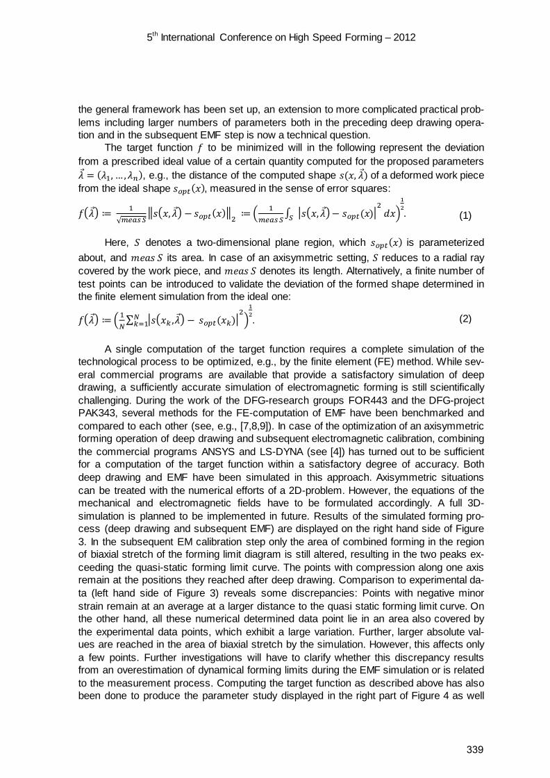
5th International Conference on High Speed Forming – 2012
the general framework has been set up, an extension to more complicated practical prob-lems including larger numbers of parameters both in the preceding deep drawing opera-tion and in the subsequent EMF step is now a technical question.
The target function 𝑓 to be minimized will in the following represent the deviation from a prescribed ideal value of a certain quantity computed for the proposed parameters 𝜆 = (𝜆1, … ,𝜆𝑛), e.g., the distance of the computed shape 𝑠(𝑥, 𝜆) of a deformed work piece from the ideal shape 𝑠𝑜𝑝𝑡(𝑥), measured in the sense of error squares:
𝑓𝜆 ≔ 1√𝑚𝑒𝑎𝑠 𝑆
𝑠𝑥,𝜆 − 𝑠𝑜𝑝𝑡(𝑥)2 ≔ 1
𝑚𝑒𝑎𝑠 𝑆∫ 𝑠𝑥,𝜆− 𝑠𝑜𝑝𝑡(𝑥)
2 𝑑𝑥𝑆
12.
Here, 𝑆 denotes a two-dimensional plane region, which 𝑠𝑜𝑝𝑡(𝑥) is parameterized
about, and 𝑚𝑒𝑎𝑠 𝑆 its area. In case of an axisymmetric setting, 𝑆 reduces to a radial ray covered by the work piece, and 𝑚𝑒𝑎𝑠 𝑆 denotes its length. Alternatively, a finite number of test points can be introduced to validate the deviation of the formed shape determined in the finite element simulation from the ideal one:
𝑓𝜆 ≔ 1𝑁∑ 𝑠𝑥𝑘 ,𝜆 − 𝑠𝑜𝑝𝑡(𝑥𝑘)
2𝑁𝑘=1
12.
A single computation of the target function requires a complete simulation of the
technological process to be optimized, e.g., by the finite element (FE) method. While sev-eral commercial programs are available that provide a satisfactory simulation of deep drawing, a sufficiently accurate simulation of electromagnetic forming is still scientifically challenging. During the work of the DFG-research groups FOR443 and the DFG-project PAK343, several methods for the FE-computation of EMF have been benchmarked and compared to each other (see, e.g., [7,8,9]). In case of the optimization of an axisymmetric forming operation of deep drawing and subsequent electromagnetic calibration, combining the commercial programs ANSYS and LS-DYNA (see [4]) has turned out to be sufficient for a computation of the target function within a satisfactory degree of accuracy. Both deep drawing and EMF have been simulated in this approach. Axisymmetric situations can be treated with the numerical efforts of a 2D-problem. However, the equations of the mechanical and electromagnetic fields have to be formulated accordingly. A full 3D-simulation is planned to be implemented in future. Results of the simulated forming pro-cess (deep drawing and subsequent EMF) are displayed on the right hand side of Figure 3. In the subsequent EM calibration step only the area of combined forming in the region of biaxial stretch of the forming limit diagram is still altered, resulting in the two peaks ex-ceeding the quasi-static forming limit curve. The points with compression along one axis remain at the positions they reached after deep drawing. Comparison to experimental da-ta (left hand side of Figure 3) reveals some discrepancies: Points with negative minor strain remain at an average at a larger distance to the quasi static forming limit curve. On the other hand, all these numerical determined data point lie in an area also covered by the experimental data points, which exhibit a large variation. Further, larger absolute val-ues are reached in the area of biaxial stretch by the simulation. However, this affects only a few points. Further investigations will have to clarify whether this discrepancy results from an overestimation of dynamical forming limits during the EMF simulation or is related to the measurement process. Computing the target function as described above has also been done to produce the parameter study displayed in the right part of Figure 4 as well
(1)
(2)
339
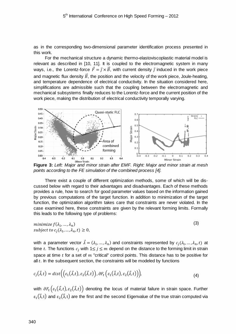
5th International Conference on High Speed Forming – 2012
as in the corresponding two-dimensional parameter identification process presented in this work.
For the mechanical structure a dynamic thermo-elastoviscoplastic material model is relevant as described in [10, 11]. It is coupled to the electromagnetic system in many ways, i.e., the Lorentz-force 𝐹 = 𝚥 ×𝐵 , with current density 𝚥 induced in the work piece and magnetic flux density 𝐵 , the position and the velocity of the work piece, Joule-heating, and temperature dependence of electrical conductivity. In the situation considered here, simplifications are admissible such that the coupling between the electromagnetic and mechanical subsystems finally reduces to the Lorentz-force and the current position of the work piece, making the distribution of electrical conductivity temporally varying.
Figure 3: Left: Major and minor strain after EMF. Right: Major and minor strain at mesh points according to the FE simulation of the combined process [4].
There exist a couple of different optimization methods, some of which will be dis-cussed below with regard to their advantages and disadvantages. Each of these methods provides a rule, how to search for good parameter values based on the information gained by previous computations of the target function. In addition to minimization of the target function, the optimization algorithm takes care that constraints are never violated. In the case examined here, these constraints are given by the relevant forming limits. Formally this leads to the following type of problems:
𝑚𝑖𝑛𝑖𝑚𝑖𝑧𝑒 𝑓(𝜆1, … , 𝜆𝑛) 𝑠𝑢𝑏𝑗𝑒𝑐𝑡 𝑡𝑜 𝑐𝑗(𝜆1, … ,𝜆𝑛, 𝑡) ≥ 0, with a parameter vector 𝜆 = (𝜆1, … , 𝜆𝑛) and constraints represented by 𝑐𝑗(𝜆1, … ,𝜆𝑛, 𝑡) at time 𝑡. The functions 𝑐𝑗 with 1≤ 𝑗 ≤ 𝑚 depend on the distance to the forming limit in strain space at time 𝑡 for a set of 𝑚 "critical" control points. This distance has to be positive for all 𝑡. In the subsequent section, the constraints will be modeled by functions 𝑐𝑗, 𝑡 = 𝑑𝑖𝑠𝑡𝜀1𝜆,𝑡, 𝜀2𝜆, 𝑡 , 𝜕𝐹𝑡 𝜀1,𝑡, 𝜀2𝜆, 𝑡,
with 𝜕𝐹𝑡 𝜀1𝜆, 𝑡,𝜀2,𝑡 denoting the locus of material failure in strain space. Further
ε1λ , t and ε2λ , t are the first and the second Eigenvalue of the true strain computed via
(3)
(4)
340

5th International Conference on High Speed Forming – 2012
finite-element-simulation for the parameter vector 𝜆 at time 𝑡. In Figure 4, a two-parameter optimization of a typical forming situation is presented: The tool coil is integrated in the punch, wound around it several times, as presented on the left hand side of Figure 4. After the punch stroke, the tool coil is excited by the discharging current of a capacitor bank. This leads to a pulsed loading of this area predominantly in radial direction, strongly ac-celerating the area of the work piece close to the coil. The right hand side of Figure 4 shows the target function in Equation (2) as a function of the parameters angular frequen-cy 𝜔 and the amplitude 𝐼0 of the triggering current 𝐼(𝑡) = 𝐼0𝑒𝛽𝑡 cos(𝜔𝑡+𝜑) of the tool coil. The optimization method is searching for the parameter values (𝜔, 𝐼0) min-imizing 𝑓. It can be seen that in the examined area many local minima of the target func-tion lie close together. This makes the optimization problem difficult. Identification of these two parameters has been chosen as a first test example. Our further plans include opti-mizing the coil geometry as well as the number of coil windings, which have been deter-mined experimentally in the examples presented in this work. Up to now, the mathemati-cal optimization is only performed for the EMF parameters. This would be sufficient if the observations in [3] are true for larger classes of forming operations: Then, the quasi-static forming step can be adjusted such that the quasi-static forming limit is reached and the af-terwards performed optimization of the parameters of the EMF will eventually extend the forming limit. However, in [3] only a particular two stage forming operation has been ex-amined. We hope that an application of the here presented method to problems including parameters of both the deep drawing and the EMF process will help to clarify this interest-ing issue. Details of the optimization process are given in Chapter 4.
Figure 4: Target-function landscape showing the dependence of the quality of the forming result on two input parameters for the combined process displayed on the left.
To compute the target function in this example the axisymmetric mechanical struc-ture is discretized by a mesh consisting of 1780 quadratic solid elements in 5 layers in each case. For the electromagnetic field computation an additional mesh in the air region between punch and forming tool has been constructed. The coupled simulation has been
(5)
× 105 × 105
341

5th International Conference on High Speed Forming – 2012
carried out in 55 up to 60 time steps with a length of 1 µs each. As material, the aluminum alloy EN AA-5083 has been employed. Further details on the geometric parameters are given below.
In Figure 5, the overall organization of the optimization procedure including the op-timization loop itself, the choice of initial parameters, the computation of the forming limits and its implementation as constraints, and the evaluation of the target function via a cou-pled finite-element simulation is displayed. Below the SQP optimization method, employed for computing the optimum parameters for the forming process displayed in Figure 4, is discussed as well as the determination of the constraints. In an earlier approach [4], the program IPOPT [12], an implementation of an interior point method, has been used.
Figure 5: Setup of the numerical optimization framework for the process combination un-der consideration.
An optimization method provides a strategy to search for good values in the pa-rameter space. While global methods gather information of the whole parameter space, local methods search better parameter values in the neighborhood of their initial values. Well known examples of global methods are evolutionary methods, such as genetic algo-rithms, or simulated annealing. Examples for local methods are the Nelder-Mead simplex-search ([13], see [14] for the identification of a free electromagnetic forming process of sheet metal with this method) or methods that are based on directions of descent. Very ef-ficient methods of this type are obtained by applying algorithms for quadratic programming to second order approximations of the target function and the constraints, as done in the SQP-method (sequential quadratic programming, see below). Another type of descent methods is based on so called interior-point (IP) methods. Both IP-methods and the SQP-method require much less function evaluations to find a local minimum nearby than other methods. The reason for this is that they are more directed than the global methods men-tioned above by utilizing the broader information provided by a direction of descent. How-ever, to compute such directions of descent, a linearization of the target function is re-quired. For the optimization of technological processes, a consistent linearization of its analytical description is not appropriate. First, this requires very complicated computations including second order derivatives of the stress-strain-relation employed in the material description. Second, a consistent linearization would only be valid for an individual pro-
342

5th International Conference on High Speed Forming – 2012
cess. Therefore, the optimization method would not be robust in the sense that it applies reliably to a large class of forming processes. Hence, linearizations of the process de-scription with respect to the parameters are here computed numerically. The SQP-method, utilized to find the minimum of the target function displayed on the right hand side of Figure 4, is based on the idea to solve a sequence of quadratic sub-problems in order to determine the descent direction in every step. These quadratic programs take the form min𝑑 ℒ𝜆𝑘,𝜉𝑘+ ∇ℒ𝜆𝑘 ,𝜉𝑘
𝑇𝑑 + 1
2𝑑𝑇∇𝜆𝜆2 𝑘 ,𝜉𝑘
𝑠. 𝑡. 𝑐𝜆𝑘+ ∇𝑐𝜆𝑘𝑇 ≥ 0,
for every iteration 𝑘. Here ℒ𝜆,𝜉 = 𝑓𝜆− 𝜉𝑇𝑐(𝜆) denotes the Lagrangian and 𝜉 a vector of Lagrangian multipliers. The constraints have been gathered to the vector 𝑐(𝜆) = (𝑐1(𝜆), … ,𝑐𝑚(𝜆))𝑇. With every solution of Equation (6) a search direction 𝑑 is calculated. Then, a one-dimensional minimum along this direction is determined. This can be considered as a Newton step in order to optimize the target function 𝑓. Here, the implementation of the SQP-method provided by MATLAB [15] has been employed. To organize the whole optimization framework as shown in Figure 4, var-ious software components have to be linked, such as LS-DYNA, ANSYS, and MATLAB. This has been achieved by extensive scripting techniques, which have been implemented in the scripting language Ruby here.
The derivatives of the target function with respect to the parameters to be identified required for a gradient based optimization method are computed numerically in this work. It has often been argued that numerically determined derivatives are not sufficiently accu-rate for mathematical optimization algorithms. Indeed, as an inverse problem, optimization problems are often badly conditioned. On the other hand, the decrease of the target func-tion during optimization is monitored. Further, if the applied method of descent does not yield further improvement, simulation data, such as mesh-size or step-size for the deter-mination of numerical derivatives can be adapted a posteriori by the algorithm. In future implementations it is also planned to choose the model for the determination of the con-straints, i.e., the forming limits, adaptively: An algorithmic control of numerical parameters and of the accuracy of the employed model formulation, based on data collected during the optimization process, will then lead to increased efficiency without reducing the accu-racy of the identified optima. Further, it makes the optimization scheme more robust in the sense, that a larger class of problems can be treated without cumbersome adaptations. As an example for an adaptive choice of different models - which is, however, not imple-mented, yet - consider the situation displayed in Figure 6: Two different models are as-sumed exemplarily, which can be chosen algorithmically according to the numerical needs: a damage model as provided by Lemaitre (see [16]) and the forming limit surface (FLS) discussed in the subsequent section (see Figure 7), representing a less precise, but computationally fast way to incorporate forming limits as constraints. Far away from the minimum the fast method is used while close to the area of the minimum the precise, but costly constraints are applied.
(6)
(7)
343

5th International Conference on High Speed Forming – 2012
Figure 6: The target function for two parameters: The adaptive choice of constraints takes place in the marked regions of the target function surface. Far away from the minimum the fast evaluation method with the FLS is chosen, close to the minimum a costly but accurate damage model is applied.
The development of auto-adaptive methods of this type represents work in progress. A significant increase in efficiency is gained by computing all function values required for the linearization in parallel. If sufficient computational resources are available, even more evaluation of the target function can be carried out in parallel at the same time allowing for the determination of higher order approximations to the required derivatives.
3 Dynamic Forming Limits as Constraints in Optimization
The above described optimization methods require an efficient way to determine the rele-vant forming limits for each load path resulting from the particular choice of parameters due to the optimization method. This, however, requires a fast accessible computational method to estimate the distance to the point of material failure at any stage of the current-ly active load path considering the current strain rate. There are two well-known methods to obtain this information: The use of a damage model with identified model parameters or the use of forming limit diagrams. The first alternative, on the one hand, is in many cases too time-consuming. Usually, a set of damage variables is introduced and their evolution is tracked by a system of Gauss-point-based ordinary differential equations to be solved any time the material model is evaluated in the finite-element-simulation. Such models are, e.g., the Gurson-Nedleman-Tvergard- or the Lemaitre-model [16]. A classical forming limit diagram (FLD), on the other hand, is neither able to account for the material's load history during the forming process nor the dependence of the material's response on the
× 105 × 105
344

5th International Conference on High Speed Forming – 2012
strain rate. Hence, conventional FLDs are not suited to predict forming limits of combina-tions of deep drawing and electromagnetic forming. To obtain a sufficiently fast method that can efficiently be incorporated in the SQP- or IP-method, that accounts for strain his-tory and strain rate dependence, the classical FLD can be extended to a forming limit sur-face (FLS) [4,17,18]. To represent the relevant forming limits for a process combination of, e.g., a quasi-static and an impulse forming method, a third axis is added to a classical FLD. On this third axis, in addition to major and minor strain a parameter is considered that may represent the accumulated strain in a critical region of the work piece at the in-stant of switching from the quasi-static to the dynamical process. The forming limit curve corresponding to this amount of accumulated strain and the strain rate of the subsequent impulse forming operation is inserted for this parameter. Figure 7 shows such a forming limit surface. It allows for consideration of prestrain and rate dependence in the second forming step.
Figure 7: The forming limit surface (FLS). The distance of the major strain as a function of minor strain and strain rate to the surface acts as a constraint in the optimization.
The most direct way to construct an FLS is to experimentally determine forming limit curves (FLCs) at different strain rates and a certain state of previously accumulated strain. Hence, accumulated strain is automatically considered in a correct way. For such meas-urements, a high speed Nagazima test can be performed after previous deep drawing. From the measurement results, the FLS is then constructed by a mathematical approxi-mation technique, e.g., least-square-approximation by two-dimensional spline functions. In a case where sufficient experimental information was not available, in [4] an FLS has been derived from a quasi-static FLC with the help of a modified Johnson-Cook type fail-ure model (see [19]) presented and identified by Clausen et al. [20]. For further infor-mation on FLSes, see [4].
4 Results and Experimental Validation
The efficiency of the presented method has been proved in several practical situations [4]. A significant improvement of the target function value could be obtained by use of the nu-merical method compared to a purely experimental identification of parameter values. The
345
5th International Conference on High Speed Forming – 2012
numerical computations and accompanying experiments have been carried out for sheet metal discs of 130 mm diameter and a thickness of 1 mm. The drawing distance amounts to 55 mm and the drawing radius to 10 mm. The blank holder force is set to 300 kN. The-se values have also been chosen for computing the target-function-landscape displayed in Figure 4 and Figure 6. Material data of EN AA-5083 have been employed, and the punch's bottom radius has been set to r = 20 mm. The blank holder force and the friction (a Coulomb-friction model with a friction factor µ = 0.04 in the flange region and µ = 0.0 elsewhere) were set to a value that would lead to material failure in a single deep drawing process. The goal was now to manufacture a part without failure, but with strains at the punch's bottom radius, exceeding the conventional forming limits due to stretching. By a preceding experimental study, the optimum number of coil winding was experimentally identified as N = 6. While in [4] 𝜔,𝜑 and 𝛽 in the representation of the input current 𝐼(𝑡) = 𝐼0𝑒𝛽𝑡 cos(𝜔𝑡+𝜑), 𝑤𝑖𝑡ℎ 𝜔 = 3.8007 ∙ 105𝑠−1,𝜑 = −1.35381 𝑟𝑎𝑑, 𝛽 = −15467.3𝑠−1, have been taken from measurements, in the current work, only 𝜑 and 𝛽 have been pre-scribed and both 𝜔 and 𝐼0 have been simultaneously identified by a two-parameter opti-mization. Looking at Figure 4 and Figure 6 reveals that it was a challenging task for the optimization method to find the correct local minimum belonging to the optimum value of the target function. While for the fixed value ω = 3.8007 ∙ 105s−1 the experimentally identi-fied optimum for 𝐼0 was 101 533 kA, we obtain a smaller deviation between simulated shape and ideal shape for the simultaneously identified values ω ≈ 3.8485 ∙ 105s−1 and 𝐼0 ≈ 110 000 kA. Clearly, the simultaneous identification of two parameters leads to better results than their successive identification.
5 Conclusions
In this paper a method for the computer aided design of process chains consisting of clas-sical quasi-static processes and EMF has been discussed in order to increase the classi-cal quasi-static forming limits. The use of an optimization scheme (here the SQP-method) based on a parallelly computed direction of descent renders the challenging task of com-putational optimization of process chains feasible. A forming limit surface was introduced to account both for the effects of strain rate and of accumulated strain during the first qua-si-static forming operation, which cannot be covered by a classical forming limit diagram. The information of the forming limit surface has been provided as constraints within the SQP method. The optimization method has successfully been applied to determine opti-mal parameters for a two-stage process chain proposed by [3]. In contrast to previous ap-proaches, two parameters have been optimized at the same time. Hence, the existing re-sults could be enhanced, and parameters for a larger extension of classical forming limits have been determined. The next steps are now
• to provide systematically measured experimental data for the construction of FLSes,
• application of the method to problems with more than two parameters to be identi-fied simultaneously,
• to compare the FLS-approach to represent material constraints with a more accu-rate one based on a damage model, and
(9)
346

5th International Conference on High Speed Forming – 2012
• to increase efficiency and accuracy by an algorithmic adaptive choice of the mesh- and the model.
Moreover, some questions to materials science have to be answered: • Do different load paths activate different microscopic damage-mechanisms? • In how far do these interact with respect to resulting macroscopic failure? • Which type of phenomenological damage model is adequate under this type of
"mixed loading"?
Finally, such methods as presented here will enable the virtual design of technologi-cal processes. This becomes an increasingly viable alternative to a purely experimentally based process layout. It decreases the number of experiments required, and hence, re-duces time and costs. In many industrial areas such as the automotive industry [21], these methods are nowadays being employed. Product-Lifecycle-Management [22, 23, 24] can be considered as another example. The methods described in this work lead to a powerful implementation of this future industrial design concept.
References
[1] Psyk, V.; Beerwald, C.; Henselek, A.; Homberg, W.; Brosius, A.; Kleiner, M.: Integra-tion of electro-magnetic calibration into a deep drawing process of an industrial de-monstrator part. Key Engineering Materials 344, 2007, p. 435-442.
[2] Daehn, G. S.: High-velocity metal forming, 2006. [3] Vohnout, V. J.: A Hybrid Quasi-Static / Dynamic Process for Forming Large Sheet
Metal Parts From Aluminum Alloys. PhD thesis, The Ohio State University, 1998. [4] Taebi, F.; Demir, O. K.; Stiemer, M.; Psyk, V.; Kwiatkowski, L.; Brosius, A.; Blum, H.;
Tekkaya, A. E.: Dynamic forming limits and numerical optimization of combined quasi-static and impulse metal forming. Computational materials Science 54, 2012, p. 293-302.
[5] Psyk, V.; Risch, D.; Kinsey, B. L.; Tekkaya, A. E.; Kleiner, M.: Electromagnetic form-ing - A review. J. Mat. Proc. Techn., 2011, p. 787-829.
[6] Silva, M. B.; Alves, L. M.; Alves, M. L.; Martins, P. A. F.: Fracture Forming Lines in Single Point Incremental Forming. In Proc. Int. Conf. IDDRG 2010, Graz, Austria, 2010, p. 451-460.
[7] Kleiner, M.; Brosius, A.; Blum, H.; Suttmeier, F.-T.; Stiemer, M.; Svendsen, B.; Un-ger, J.; Reese, S.: Benchmark problems for coupled electromagnetic-mechanical metal forming processes. Annals of the German Acad. Soc. for Prod. Eng. WGP 11(1), 2004, p. 85-90.
[8] Stiemer, M.; Unger, J.; Svendsen, B.; Blum, H.: Algorithmic formulation and numeri-cal implementation of coupled electromagnetic-inelastic continuum models for elec-tromagnetic metal forming. International Journal for Numerical Methods in Eng. 68(13), 2006, p. 1301-1328.
[9] Stiemer, M.; Unger, J.; Blum, H.; Svendsen, B.: An arbitrary Lagrangian Eulerian approach to the three dimensional simulation of electromagnetic forming. Comp. Meth. Appl. Mech. Engrg. 198(17-20), 2009, p. 1535-1547.
[10] Svendsen, B.; Chanda, T.: Continuum thermodynamic modeling and simulation of electromagnetic forming. Technische Mechanik 23, 2003, p. 103-112.
347
5th International Conference on High Speed Forming – 2012
[11] Svendsen, B.; Chanda, T.: Continuum thermodynamic formulation of models for electromagnetic thermoinlastic materials with application to electromagnetic metal forming. Cont. Mech. Thermodyn. 17, 2005, p. 1-16.
[12] Wächter, A.; Biegler, L. T.: On the implementation of a primal dual interior point filter line search algorithm for large-scale nonlinear programming. Math. Prog., 106(1), 2006, p. 25-57.
[13] Nelder, J. A.; Mead, R.: A simplex method for function minimization. Computer J. 7, 1965, p. 308-313.
[14] Blum, H.; Stiemer, M.; Suttmeier, F. T.; Svendsen, B.; Unger, J.: Coupled finite ele-ment simulation of electromagnetic sheet metal forming. In 2. Kolloquium Elektro-magnetische Umformung. Forschergruppe "Untersuchung der Wirkmechanismen der elektromagnetischen Blechumformung", 2003.
[15] MATLAB 2010b, MathWorks, Natick, MA, 2010. [16] Lemaitre, J.; Chaboche, J.-L.: Mechanics of solid materials. Cambridge University
Press, 1990. [17] Taebi, F.; Demir, O. K.; Stiemer, M.; Psyk, V.; Brosius, A.; Blum, H.; Tekkaya, A. E.:
Computational Design and Forming Limits of Process Chains Composed of Quasi-Static and Dynamic Processes. In: Proceedings of the 10th International Conference on Technology of Plasticity (ICTP), Aachen, 2011.
[18] Stiemer, M.; Brosius, A.; Tekkaya, A. E.: Leichtbau und hochfeste Werkstoffe for-dern die Umformtechnik heraus. MaschinenMarkt 37, 2011, p. 24 – 27.
[19] Johnson, G. R.; Cook, W. H.: Fracture characteristics of three metals subjected to various strains, strain rates, temperatures and pressures. Eng. Fracture Mechanics 21(1), 1985, p. 31-48.
[20] Clausen, A. H.; Børvik, T.; Hopperstad, O. S.; Benallal, A.: Flow and fracture charac-teristics of aluminum alloy AA5083-H116 as function of strain rate, temperature and triaxiality. Mat. Sci. and Eng. A 364, 2004, p. 260-272.
[21] Meinhardt, J.; von Wurmb, I.: Methodenplanung im Spannungsfeld zwischen Ent-wicklung und Produktion. In Bestform in Blech, 2004, p. 31-36.
[22] Spur, G.; Krause, F.-L.: Das virtuelle Produkt-Management der CAD Technik. Carl Hanser Verlag, 1997.
[23] Krause, F.-L.; Jansen, H.; et al.: Modules and tools for virtual product realization. In Proc. IX. Internationales Produktionstechnisches Kolloquium (PTK), 1998, p. 281-296.
[24] Lee, K.: Principles of CAD/CAM/CAE Systems. Addison Wesley, 1999.
348

INTERNATIONAL CONFERENCE ON HIGH SPEED FORMINGICHSF2012
Copyright: Stadt Dortmund
poynting
Sponsors and Partners
www.ichsf 2012.com
Copyright © 2022 FDOKUMEN