HYDROCYCLONE - MyCourses

Aalto University 1(17)

Chemical Engineering

15.9.2015

HYDROCYCLONE

1. General ............................................................................................................................................. 2

2. Calculations ...................................................................................................................................... 3

2.1 Mass Balance ............................................................................................................................. 3

2.2 Separation Efficiencies .............................................................................................................. 4

2.3 Cut Size ...................................................................................................................................... 4

2.3.1 Cut Size ............................................................................................................................... 5

2.3.2 Normal Acceleration ........................................................................................................... 5

2.3.3 Sinking Speed of a Particle in Liquid ................................................................................. 5

2.3.4 Length of Sinking................................................................................................................ 6

2.3.5 Residence Time ................................................................................................................... 6

2.3.6 Sinking Time of Particle ..................................................................................................... 7

2.4 Losses of Energy ........................................................................................................................ 7

2.4.1 Losses of Mechanical Energy in the Cyclone ..................................................................... 7

2.4.2 Losses in System ................................................................................................................. 8

2.4.3 Rise of Temperature in the System ................................................................................... 10

3. Equipment ...................................................................................................................................... 10

3.1 Hydrocyclones ......................................................................................................................... 10

3.2 Arrangements ........................................................................................................................... 10

3.3 Measuring Equipment .............................................................................................................. 10

4. Operating the Cyclone ................................................................................................................... 11

4.1 Starting the Work ..................................................................................................................... 11

4.2 Measurements .......................................................................................................................... 11

4.3 Ending the Work ...................................................................................................................... 11

5. Specification................................................................................................................................... 12

5.1 Calculations .............................................................................................................................. 12

5.2 Short Work ............................................................................................................................... 12

5.3 Extensive Work ........................................................................................................................ 12

6. Appendices ..................................................................................................................................... 12

7. References ...................................................................................................................................... 12

8. Nomenclature ................................................................................................................................. 12



15.9.2015

1. GENERAL

Hydrocyclones have been discussed for example in McCabe et al. (1993) in pages 1062-3 and in

Svarovsky (1984). Hydrocyclones are used in (Svarovsky, 1984, s. 1):

Clarification of slurry (removing solids) and thickening (removing liquids)

Sorting of solids

Washing of solids

Removing gases from liquid

Removing immiscible liquid from liquid

Hydrocyclone is a device where solid particles or immiscible liquids are separated from liquid

(which is usually water (hydro!)). Separation is based on density gradient between the liquid and the

matter to be separated. The separating force is radial acceleration caused by strong rotating motion.

Generally the device is a cyclone and the continuous phase is a fluid (gas or liquid). In figure 1 a

schema of a cyclone and its characteristic dimensions are shown. The double vortex of a cyclone is

illustrated in figure 2.

D

Do

l Di

Du

L

Figure 1. Dimensions of a cyclone. Figure 2. Double vortex

Feed containing solid particles divides into overflow, which has the main part of the fluid, and into

underflow, which contains the most of the solids. Separation depends on the size distribution of the

solids. This is characterized by the cut size, which is the size of a particle, which has equal probabil-

ity to end up either in overflow or underflow.

The advantages and disadvantages of hydrocyclone are (Svarovsky, 1984, p. 2):

They are very versatile.

They are simple and cheap to buy, install and operate.

They need only a little space.

Great shear forces are advantageous for example if dispersing clustered particles or handling

thixotropic liquids.

They are not flexible.

The resolution and power of separation is quite poor.

Great flow rate may cause weariness.

Great shear forces are disadvantageous because flocculation cannot be used to enhance the

separation.



15.9.2015

2. CALCULATIONS

Only simple mass balances are considered in this work. Then, separation power can be calculated

from the balances. Also the cut size or the dependency of separation power on particle size is stud-

ied based on a simple residence time theory. Finally energy balances are considered, that is how the

mechanical energy of a fluid changes into heat.

2.1 MASS BALANCE

The flow chart of a cyclone is shown in figure 3.

O, wO

U, wU

F, wF

Figure 3. Flow chart of a cyclone.

The concentrations of underflow U and overflow O are determined by weighing samples taken from

both of them before and after evaporation. Thus, the concentrations are obtained as mass fractions,

which are marked with w.

Since concentrations are given in mass fractions, all the flows O, U, and F (feed) are given in mass

flows. A volume flow rate FV is measured from the feed flow and it is converted to mass flow by

multiplying it with the density of the feed, which is assumed to be (accurate enough)

F = 1000 kg/m3 (1)

So, the mass flow rate is

FFVF (2)

Balance calculations are done in mass fraction coordinates where total flows F, O, and U are total

mass flows. Then the total mass balance and the solid mass balance for the process shown in figure

3 is:

UOF (3)

UOF UwOwFw (4)

After measurements only O and U remains unknown. These can be easily solved from equations (3)

and (4) by multiplying equation (3) with either -wO or -wU, and adding up the two equations gives

)()()()( OUOUOOOF wwUwwUwwOwwF (5a)

)()()()( UOUUUOUF wwOwwUwwOwwF (5b)

From these O and U are obtained:

Fww

wwU

OU

OF

)(

)(

(6a)



15.9.2015

Fww

wwO

UO

UF

)(

)(

(6b)

2.2 SEPARATION EFFICIENCIES

Separation efficiencies are usually expressed as a function of particle size. Here no size distribution

is measured, so the efficiencies are based only on total and solid balances. Depending on the use of

the cyclone, the efficiencies can be defined as follows:

OwE 1 UwE 2 (7a,b)

F

OE 3

F

O

Fw

OwE 4 (8a,b)

F

UE 5

F

U

Fw

UwE 6 (9a,b)

U

OE 7

U

O

Uw

OwE 8 (10a,b)

2.3 CUT SIZE

Flows inside the cyclone are considered to be as in figure 2 and the cross-section of the cyclone on

the height of the feed inlet as in figure 4.

ui

Di

D DO

Figure 4. Cross-section of a cyclone.

Feed (here a mixture of water and solid particles) incomes to the cyclone tangentially and is sucked

into rotating motion. In first stage it flows against the wall of the cyclone as a vortex to the bottom

of the cyclone where the underflow separates from the overflow and the underflow exits the cy-

clone. After this overflow, which has a diameter about the same size as the outlet pipe, flows as a

vortex upwards to the top of the cyclone where overflow exits the cyclone.

The essential thing for the separation in the cyclone is the first stage from the feed point to the bot-

tom of the cyclone. Next, only this stage is considered. According to the residence time –theory

(Svarovsky, 1984, 47) a particle ends up to underflow if it has enough time to move to the wall of

the cyclone. The time that can be taken to this transfer is called the residence time, which in this

case is the time elapsed when feed flows from feed point to the bottom of the cyclone. The driving

force of this transfer is the radial acceleration due to the vortex and the velocity of the transfer is the

sinking speed due to this acceleration. Since the sinking speed depends on the particle size the

probability of separation depends on particle size, too. This probability is handled with concept of

cut size.



15.9.2015

2.3.1 Cut Size

Cut size is defined as (Svarovsky, 1984, p 23):

Cut size dn is a diameter d for particles, which have a probability of n % to end up in un-

derflow.

So cut size d90 is a particle size, which has a probability of 90 % to end up in underflow.

A rough estimate for cut size is determined here from following condition with which the probabil-

ity of ending up in underflow can be calculated:

The probability of ending up in the underflow is n %,

if the particle sinks n % of the radial depth within the residence time.

Let’s assume that the vortex of the top of the cyclone is the annulus constrained by the diameters D

and Do, so the radial depth of the top is half of the difference of the diameters D and Do.

Now d100 is the size of particles, which sink 100 % of the distance from the inner diameter of the

vortex Do to the outer diameter of the vortex D (1.0*0.5(D-Do)) during the residence time. Respec-

tively d50 is half of that distance or 0.5*0.5(D-Do).

Svarovsky (1984, p 47-50) shows another way to apply the residence time –theory to calculate the

separation efficiency. Next, an example how to calculate a rough estimate for cut size dn can be cal-

culated, is shown.

2.3.2 Normal Acceleration

Separation in hydrocyclone is based on the normal acceleration of the vortex. Since the flows inside

the cyclone are known only qualitatively, it is reasonable to calculate the normal acceleration only

in the upper section of the cyclone when based on the inner diameter of the cyclone and on the ve-

locity of the incoming fluid.

Since the flow has a depth in the direction of the radius of the cyclone, the maximum acceleration is

greater than calculated here (if rotation speed remains the same, is the acceleration greater near the

inner wall than near the exterior wall where the radius is greater.) Also the cyclone narrows down-

ward, so the acceleration is greater in bottom.

Normal acceleration based on velocity ui of incoming liquid and the inner diameter D of the top is

obtained from equation (Alonso and Finn, 1980, p 98):

2/

222

D

u

R

vRa i (11)

2.3.3 Sinking Speed of a Particle in Liquid

The density gradient and normal acceleration in the direction of the radius of the cyclone produce a

force, which makes the particles to sink and end up into underflow. Although the acceleration is

great, are the particles so small that the sinking speed can be calculated from Stokes equation

(McCabe et al. (1993) page 160) in which case the Reynolds number needs to be smaller than 1.



15.9.2015

ad

upls

p

18

)( 2 0.1Re

ppl

p

du (12)

2.3.4 Length of Sinking

The radial depth of the flow in the top of the cyclone is S:

)(5.0 oDDS (13)

Length of sinking is a distance that a particle has to sink in order to end up in the exterior wall of

the cyclone. Here the length of sinking is defined as

)(5.0*01.0* on DDnS (14)

where S is the length of sinking and n is %.

This definition enables the definition of the cut size as it was defined earlier, in other words the

probabilities n of length of sinking Sn and the cut size dn are equal.

This means that cut size d100 is size of a particle which has a 100 % probability to end up into un-

derflow or it has enough time to sink trough the whole depth of the flow 0.5*(D-Do). Correspond-

ingly cut size d50 has time to sink half of the whole depth of the flow (0.5*0.5*(D-Do)).

2.3.5 Residence Time

Available time for sinking is the residence time, which in this case is the time in which the feed

flows from the inlet section to the bottom of the cyclone.

Let’s assume that:

The axial cross-sectional area of flow in the cyclone is the annulus constrained by diameters

D and Do.

The length of the flow is the length L of the cyclone.

Now the residence time in the cyclone can be calculated:

4

)( 22

O

FFA

DD

V

L

A

V

L

u

L

, (15)

where L is height of the cyclone from the inlet point to the bottom, uA is axial flow velocity, and A

is axial cross-sectional area of the flow in the top of the cyclone. Here axial is in the direction of

vertical axis of the cyclone.



15.9.2015

2.3.6 Sinking Time of Particle

When the particle diameter is known can the sinking time through the whole radial depth be calcu-

lated:

ad

DD

u

St

pls

o

p

p

18

)(

)(5.02

(16)

If tp < then particle has time to sink all the way to the exterior wall and ends up in the underflow.

Analogically with equation (16) the sinking time through a certain depth can be calculated:

ad

DDn

u

St

pls

o

np

nnp

18

)(

)(5.0*01.0*2

,

,

(17)

If tp,n < then within sinking time a particle sinks n % of the radial depth of the top of the cyclone,

so the particle has n % probability to end up into the underflow. If stating that tp,n = , a condition

for cut size dn is obtained:

ad

DDnt

pls

onp

18

)(

)(5.0*01.0*2,

, (18)

so

a

S

a

DDnd

ls

n

ls

op

)(

18

)(

18)(5.0*01.0*

. (19)

2.4 LOSSES OF ENERGY

2.4.1 Losses of Mechanical Energy in the Cyclone

The balance of mechanical energy between points a and b is

)(22

)()(

22

DEVICEPIPING

a

a

b

bababpp hhuu

zzgppW

, (20)

where h is the loss of mechanical energy per mass unit of the fluid due to friction. Applying

this equation to one process unit, which is a cyclone and has no pump, gives:

CYCLONEa

ab

babab huu

zzgpp

22)()(0

22

(21)

The losses of mechanical energy per mass unit of the fluid hCYCLONE caused by the cyclone can

be calculated from this equation. When this is known, the power losses Ph,CYCLONE caused by

this process unit can be calculated from equation:



15.9.2015

CYCLONECYCLONECYCLONEh hVhmP , (22)

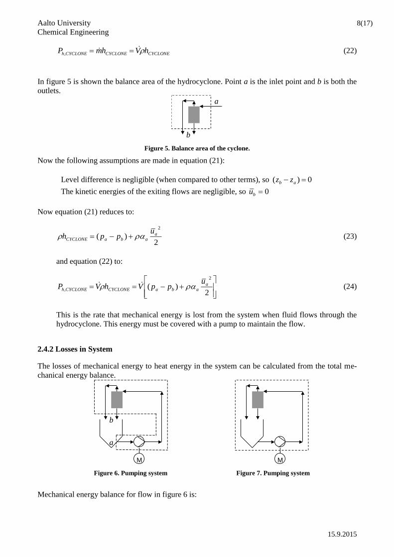
In figure 5 is shown the balance area of the hydrocyclone. Point a is the inlet point and b is both the

outlets.

b

a

Figure 5. Balance area of the cyclone.

Now the following assumptions are made in equation (21):

Level difference is negligible (when compared to other terms), so 0)( ab zz

The kinetic energies of the exiting flows are negligible, so 0bu

Now equation (21) reduces to:

2)(

2

aabaCYCLONE

upph (23)

and equation (22) to:

2)(

2

,

a

abaCYCLONECYCLONEh

uppVhVP (24)

This is the rate that mechanical energy is lost from the system when fluid flows through the

hydrocyclone. This energy must be covered with a pump to maintain the flow.

2.4.2 Losses in System

The losses of mechanical energy to heat energy in the system can be calculated from the total me-

chanical energy balance.

M

b

a

M

Figure 6. Pumping system Figure 7. Pumping system

Mechanical energy balance for flow in figure 6 is:



15.9.2015

)(22

)()(

22

CYCLONEPIPINGa

ab

bababpp hhuu

zzgppW

(25)

Now it is assumed that:

Level difference is negligible, so 0)( ab zz

Difference in kinetic energy in the balance boundaries is negligible, so 0 ba uu

Pressure in the feed tank on the suction height (in point a) is air pressure (in other words suc-

tion point is not in to deep), so 0)( ab pp because pressure in point b is air pressure.

Now equation (25) reduces to:

CYCLONEPIPINGpp hhW (26)

Besides these there are energy losses in the pump. These losses are taken into account with the me-

chanical efficiency of the pump. This loss of brake power in the pump is:

ppPUMPh WVP )1(, (27)

So, there are three different sources for mechanical energy losses in the system:

Losses of the cyclone: 2

)(

2

,

aabaCYCLONECYCLONEh

uppVhVP

Losses of the piping system: 2

2

,

u

D

LVhhVhVP iPIPINGPIPINGh

Losses of the pump: ppPUMPh WVP )1(,

From figure 7 can be seen that these three losses are equal to the brake power of the pump, since

there are no other source of mechanical energy in the system and the whole brake power is con-

sumed in the system:

PUMPhCYCLONEhPIPINGhB PPPP ,,, (28)

Brake power PB in the pump depends on the electrical power PE and the electrical efficiency E of

the pump:

E

BE

PP

(29)

The electrical power of the motor is marked on the rating plate.



15.9.2015

2.4.3 Rise of Temperature in the System

The losses of mechanical energy in the system are calculated above. Actually, the mechanical ener-

gy does not disappear but it only translates into heat. So, the power loss of mechanical energy is

equal to generation power of heat energy. Since the total losses of mechanical energy are equal to

the break power of the pump, it is obtained that:

EEBhGENH PPPP , (30)

If the fluid volume of the system is V, is the speed of temperature rise:

p

GENH

cV

P

dt

dT

, (31)

3. EQUIPMENT

3.1 HYDROCYCLONES

There are two hydrocyclone, delivered by Dorr-Oliver N.V in 1965, in the laboratory: A hydrocy-

clone “Dorrclone Type T 104 II” and a multicyclone “Multicyclone Type TM1-A10/15-80” which

has four hydrocyclones in parallel. For the present only the hydrocyclone is used to this laboratory

work. The cut-away drawing of the cyclone is shown in appendix 1.

According to the drawing H52910/2 of Dorr-Oliver the diameter of the top of the cyclone is

D = 25 mm, the length between the feed point and underflow exit point is L = 120 mm, and the di-

ameter of the overflow outlet pipe is Do = 9 mm. The diameter of the feed pipe is assumed to be Di

= 10 mm. The characteristics of the pump used in the equipment are shown in appendix 3. The di-

ameter of the impeller is 169 mm.

3.2 ARRANGEMENTS

Feed slurry is a mixture of water and calcium carbonate.

Properties of calcium carbonate are shown in appendix 2.

Solids content is about 2 w-% or about 20 g/l.

3.3 MEASURING EQUIPMENT

There are already attached in the laboratory equipment:

Rotameter

Pressure gauge

In the measuring range 35%-100% the rotameter gives the volume flow rate in percent of the max-

imum flow rate, which is 0,0015 m3/s.

Also

3+8*2 = 19 evaporating dishes



15.9.2015

thermometer

measuring tape

are needed for the work.

4. OPERATING THE CYCLONE

4.1 STARTING THE WORK

Close the bottom valve from the feed tank.

Fill up the feed tank to the level shown by the assistant.

Measure and write down the amount of water.

Open the pox water valve.

Close the control valve (gray).

Switch the pump on.

Open the recycle valve (red) a little in order to generate a flow.

Pour calcium carbonate an amount given by the assistant into the feed tank.

Recycle and mix a while.

Take three (3) samples from the mixture to an evaporating dish.

Measure the temperature of the mixture.

Write down time and initial temperature.

4.2 MEASUREMENTS

Adjust the flow rate to given value and close the recycling valve.

Let it stabilize for 1 minute.

Take a sample from both over- and underflow to an evaporating dish.

Write down the flow rate and pressure drop.

Measure the temperature of the mixture.

Write down time and temperature.

If temperature is greater than 50 ºC, open the cooling water valve.

Repeat 8 times in total.

4.3 ENDING THE WORK

Stop the pump.

Inform the assistant.

After permission empty and flush the feed tank.

Fill up the tank about to half way.

Switch the pump on and circulate the water for a while.

Stop the pump and empty the feed tank.

Close the pox water and cooling water valves.

Calculate the length of the piping system and its inner diameter.

Write down all friction losses due to valves, fittings etc.

Write down the electrical power of the motor of the pump.

Clean up the environment of the laboratory equipment and return all the things you have used

to where they belong.



15.9.2015

5. SPECIFICATION

5.1 CALCULATIONS

Calculations are done with MS-EXCEL workbook 13-sykl.xls.

5.2 SHORT WORK

Fill up the form.

Each member of the group shows calculations for different cases.

Show O/U, wO, and wU graphically as a function of the feed in an appendix.

Show the change of the most essential efficiency graphically as a function of the feed in an ap-

pendix.

Show the cut size d50 graphically as a function of feed in an appendix. Compare your results to

the data of appendix 2.

Only a qualitative incorrect estimate is required.

5.3 EXTENSIVE WORK

1. Make the calculations, fill up the form, and show the graphs as in brief work. The form is added

to the specification.

2. Euler number is defined (Svarovsky, 1984, page 8)

25.0 iu

pEu

Check, how the following correlation holds true for measurement data (Svarovsky, 1984, page 8) 3748.0Re38.24Eu

Assess the accuracy of four significant figures.

6. APPENDICES

1. A cut-away drawing of a hydrocyclone (Dorr-Oliver N.V. part list H.52752/4 31.10.1963)

2. Properties of calcium carbonate.

3. Characteristic of the pump.

7. REFERENCES

McCabe, W.L., 1993, Smith J.C. and Harriot, P., Unit Operations of Chemical Engineering, 5 edi-

tion, McGraw-Hill

Svarovsky, L., 1984, Hydrocyclones, Technomic Publ. Co. Inc., Lancaster, PA, USA

8. NOMENCLATURE

a acceleration, m2/s

cp heat capacity in constant pressure, J/kgK

dp particle diameter, m

dn diameter of a particle, which has a probability of n % to end up in underflow, m



15.9.2015

D inner diameter of the cyclone, m

Di inner diameter of the feed pipe, m

DO inner diameter of the overflow outlet pipe, m

DU inner diameter of the underflow outlet pipe, m

E efficiency, dimensionless

F feed flow rate, kg/s

h loss of mechanical energy per mass unit of the fluid, J/kg

m mass flow, m3/s

p pressure, Pa

p pressure difference OUT-IN, Pa

l “vortex finder” length, m

L length of the cyclone, m

O overflow rate, kg/s

Ph power loss, W

PH,GEN generation power of heat energy, heat power, W

Re Reynolds number, dimensionless

S distance, m

t time, s

u velocity, m/s

up particle velocity, m/s

up,n velocity of a particle, which diameter is dn, m/s

U underflow rate, kg/s

z height, m

V volume, m3

V volume flow rate, m3/s

w mass fraction, dimensionless

Subindexes

A axial

F feed

i inlet pipe

l liquid

n probability n%

p particle

s solid

Greek letters

factor of kinetic energy, dimensionless

density, kg/m3

viscosity, Pas

residence time, s

APPENDIX 1 14(17)

15.9.2015

APPENDIX 2 15(17)

15.9.2015

APPENDIX 3 16(17)

15.9.2015

HYDROCYCLONE - MyCourses

Documents

Transcript of HYDROCYCLONE - MyCourses