ealth Economics 3 f.6984) 63-75. North-Holland

ark C. GE Uniwrsity of Kentucky, Le&gto~ KY 405M-00~4, USA

The Ohio State ibivemity, Columbus, OH 43210, USA

Received September 1982, final version received September 1983

This paper examines the labor supply response of the wife to deterioration in the husband’s health. Unlike past cross-sectional studies, responses ow time are directly examined through the use of longitudinal data. The empirical results suggest that the magnitude and direction of the ruspcmse depend crucially on the attractiveness of transfers which the family may qualify for when the husband’s health deteriorates. Whun no transfers arL available the wife increases her market work in order to replace the lost earnings of the husbanct. However, as transfers become more attractive, the wife begins to reduce her labor supply, enablin,: her to spend r~ore time at home caring for her husband.

1. Intrduction

The economic misfortune of declining health manifests itself both in lost earning power and increased health-related expenditures. A f&n@ may adjust to a deterioration in the health of one member by reducLrrg expenditures on goods and services, drawing down accumulated savings, ano perhaps most importantly, altering the amount of time other family members spend engaged in household duties and market work. This paper focuses on adjustments in the family allocation of time by examining changes in the market work of wives in response to deterioration in their husbands’ health.

Previous research has inferred over time adjustments to health deteriora- tion from cross-sectional relationships between reported health and various measures of labor supply. For example, Parsons (1977), Theeuwes (198 I), and a (1983) find that wives with husbands ag amount of time or have a higher participation than wives wi among the wives of men in males. In .19&S, first year of the survey, wives w work-limiting he conditions were more likely to war on average worked more reporting no health problems.

0167-6296/84/$3.00 @ 1984, Elsevier Science Publishers

64 M.C. Berger and B.M. Fkisher, Husks health, wife’s labor supply

However, when the wives whose husbands were healthy in 1966 are followed over time, a strikingly different pattern emerges. From 1966 to 1970, in families in which the husband’s health deteriorated, wives reduced their weeks worked from a yearly average of 22 to 20. On the other hand, wives of husbands who remained healthy increased their average annual weeks worked from 20 to 21. Also, while the fraction of both groups participating in the labor force declined from 1966 to 1970, the proportion of wives with husbands experiencing a deterioration in-health dropped more than did that of wives with healthy husbands (0.53 to 0.49 vs. 0.49 to 0.48). Evidently, the responses to a decline in the quality of the husband’s health over time cannot be correctly inferred in a simple manner using cross-sectional data that compares families whose husbands are in good health with those whose husbands report a work-limiting health problem.

In order to avoid problems of population heterogeneity inherent in cross- sectional data, the empirical work here uses the NLS to observe the experiences of the same group Qf families over time. One potentially importtt factor considered is the z&activeness of transfer pyments which the family may qualify for after the kmband’s health deteriorates. The longitudinal analysis undertaken here should enhance the ability to evaluate programs and policies designed to aid families adjust to the economic misfortune of a husband’s illness or disability.

‘s SoPPlY -

Berkowitz et al. (5976), Parsons (1977) and Lambrinos (1981) all point out that when the husband’s health deteriorates, the direction of the labor supply adjustment by the wife is theoretically ambiguous. On the one hand, potential family income is reduced, because the wage the husband can command and the time that he can devote to market work is diminished.’ This tends to lower the marginal value of time spent at home by the wife and induces her to spend more time working in the market. On the other hand, after the onset of poor health, the husband may require nursing care, wKch

I tends to raise the value of the wife’s home time and causes h.er to spend less time,engaged in market work.

owever, another potentially important determinant of t.he wife’s labor terioration in the husband’s health is the availability en the husband suffers an accident or becomes ill,

es may qualify for one or more programs designed to assist those

“S~e~al studies have found that poor health is associated with lower wages, earnings levels, probabiliti~ of participation, and amounts of market work. Evidence of lower wages and/or

can be found in Davis (1972), Lee (1982), an4 Luft (1975). Studies which find bilities of partici Jobnsoll (1974,

ion, weeks worked, or hours worked include &rger (1983),

(1974), and ~h~uw~ (19~~~. rkowitz et al. (1976), Parsons (i377,1980), Schefller and Iden

MC. Bergs and B.?A. Fleisher, Husband’s health, wife’s labor supply 65

at low income levels or having work-limiting disabilities. Transfer income reduces the wife’s incentive to engage in market work by partially replacing the lost earnings of the husband and in some cases by lowering the effective wage received for market work.’

The influence of transfer income on the labor suoply of wives in the National Longitudinal Survey is readily apparent. Thniy-one percent of the families in which the husband developed a work-limiting health problem between 1966 and 1970 received transfer income in 1970, while only ten percent of families in which the husband remained healthy receive.1 such income. In families in which the husband’s health deteriorated and which received no transfer income in 1970, the average number of weeks worked annually by the wife remained unchanged at 23 from 1966 to 1970. On the other hand, wives in f;unilies which did receive some transfer income reduced their average annaal weeks worked from 15 to 16.

In order to examine the competing effects of lost husband’s earnings, increased demand for nursing, and availability of transfer income, consider the following simple model of the wife’s labor supply decision. Let W be the wife’s market wage, which for simplicity is assumed to be independent of the amount of her market work. W* is the marginal value of the wife’s home time (her home wage) and is postulated to be an increasing function of the amount of market work. The W* function is positively related to health maintenance time required by the husband (H), which is assumed to be exogenous. The home wage is also a positive function of the family’s full income, which is defined as

Fzi W&T-H)+ WT+I, (11

where W, is the husband’s market wage, T is total a,vailable hours, and I is family income from non-employment sources. The wife participates in the labor market if the market wage exceeds the reservation wage W& which is the home wage at zero hours of work. Utility maximization requires that the wife work zntil W= W*. For convenience, we assume that W*(L, H, F) is linear in hours of work. Equilibrium work hours, Lo, then become proportional to (W- Wg), with the factor of proportionality being the reciprocal of the slope of W*(L, H,F).3 Thus, we can analytically discuss the impact of changes in the family’s circumstances on the amount of market work in terms of the impact on the reservation nrage Wg. Am increase in

%ome transfer pay nuents result in not only an income effect but also a substitutioa effect, both sf wki& reduce: the incentive to work. For lexample, the income provided by AFDC payments reduces tke de’s incentive to work. But AFIX ‘taxes’ up to 2/3 of the wife’s market earnings, effectively fowiering her market wage and reinforcing the incentive to decrease market work.

‘See Heckman (1974) for a more formal derivation of this result.

66 MC. Berger and B.M. Flklsk, Hushand’s health, wife’s labor supply

results in a decrease in market work while the opposite occurs when IV,* falls.

If the family experiences no change in non-employment income, the full effect of a husband’s illness or accident on the wife’s reservation wage can be written as

dH. (2)

The net effect on the reservation wage and thus labor supply is ambiguous because while the first term is positive, the second term is negative. As the husband’s health deteriorates, the increase in his demand for nursing and other health maintenance raises the reservation wage of the wife (i%V*/iJH >O), while at the same time the decrease in his potential earnings tends to lower her reservation wage ((SV,IaH)( T - H) - IV'< 0). If the deterioration in the health of the husband also qualiCes the family

for assistance through transfer programs, the change in the wife’s reservation wage becomes

(3)

In this case dIV8 is less negative or more positive than in the absence of transfers since iV/3H ~0. In other words, any increase in the market work of the wife in response to lost potential earnings of the husband is dampened by the presence of transfer payments. In fact, as transfer payments become more attractive (ill/8H increases), it becomes more likely that the wife will decrease rather than increase her market work. If the increase in family non- employment income becomes large enough to equal the earnings loss of the

=(8VJMI)(T-H)-W,), then the direction of the wife’s nge is no longer ambiguous since family full income remains

constant. The wife then responds only to the ‘nursing’ effect and reduces her labor market activities.

Although the introduction of transfers does not clear up the ambiguity regarding the direction of the wife’s labor supply response to deterioration in the health of the husband, it does provide some valuable insights. The

ce of transfers increases the likelihood that the wife will reduce her et activities wh and encounters poor health. In fact, as

attractive and replace more of the lost usband, the reduction in the wife’s arket

MC. Berger and B.M. Fleidwr, Husband’s health, wife’s labor supply 67

activities increases, enabling her to spend more time at home providing care - for her husband.

3. Empirical moc!d

The empirical analysis focuses on men in the NLS during 1966 and

the labor market experiences of wives of 1970. In order to properly estimate the

labor supply response to a deterioration in the husband’s health, the sample contains only those wives whose husbands reported DO work-li&iting health condition in 1966. By 1970, some of these husbands developed health problems, thus permitting estimation of differences in over time adjustments between wives with husbands whose health deteriorated and those with husbands who remained healthy. Also excluded from the analysis are any families not responding to survey questions used to construct variable5 in the empirical model, leaving 1761 of the original 5020 NLS respondents.

The attractiveness of transfer programs is measured by the monthly average number of dollars of public assistance paid per poverty family by state in 1969 divided by the husband’s hourly wage in 1966, prior to the onset of any health problems. This ratio provides a direct measure of the attractiveness of public assistance in terms of replacement of the pre- disability earning power of the husband. Although this variable does not capture the attractiveness of all forms of transfers that may become avai- lable to families (e.g., workman’s compensation, social security disability payments), it is likely to be an adequate proxy for the overall attractiveness of available programs, especially among lower income families. In fact, deterioration in the health of the husband is much more likely to occur in lower socioeconomic groups, which suggests that the attractiveness of public assistance is relevant for many wives faced with the onset of poor health of ihe husband.4

The attractiveness of transfer programs is permitted to have a different impact on the labor supply of wives whose husband’s health has deteriorated. These families are more likely to become eligible for public assistance than are families in which the husband remains healthy. This is accomplished by constructing a variable which interacts the measure of deterioration in the health of the husband with the attractiveness of transfer payments.

The em.pirical model assumes weeks worked by wife i in 1970 are a function of previous labor market experience (proxied by weeks worked in

1966), and a vector of exogenous variables X, which includes measures of the husband’s health, the attractiveness of transfers, and other demo

41n a simultaneous investigation of health and wages using the NLS older male uhort, Lee (1982) finds that those at low wage and schooling levels are more likely to be in poor health. His reduced form estimates suggest that Mac s are more likely to be 0 served in poor health than whites.

68 MC. Berger and AM. Fleisber, Husband’s health, wife’s labor supply

labor market control variables,

where

Previous experience (WW66) is included in (4) since unobserved heter- ogeneity and state dependence, both of which tend to induce a positive cor- relation between current and past weeks worked, are likely to have im- portant impacts on the wife’s labor supply decisions But the inclusion of

66 also provides a convenient way *o examine differences in over time responses of wives to husbands’ health deterioration. In particular, differences in weeks worked in 1970 reflect differences in the labor supp!y response from 1966 to 1970 since weeks worked in 1966 are held constant.

The specification of the error term also incorporates unobserved heter- ogeneity by allowing for correlated errors across time for the same indi- vidual. However, this makes the task of estimating (4) more difficult since

W66 is correlated with 170, introducing simultaneity bias into OLS estimates.6 This potential problem is dealt with by obtaining au instrumental variables estimate of WW66 and using it in place of the actual value.

Another problem is that the reservation wage exceeds the market wage for non-participants, which means they maximize utility by not working, and the intersection of the home wage and market wage functions is not observed.

pants is the equilibrium amount of market work (L,) proportional to W- I+‘;. Thus, the WW70 equation is obviously misspecified if this problem is ignored and (4) is estimated for both participants and non- participants in 1970. One way to proceed is simply to estimate (4) for 1970

ants only. But as shown by Heckman (1980), this introduces sample on bias. This bias can be seen by examining the expected value of

7011 701 >O)=X,j!?+JJWW66, +E(q7o,I J-wwo, >O). (6)

sHeterogeneity refers to individual specific unobservable variables which are corre?ated with the labor supply decision. If these variables remain constant over time then a relationship between current and past participation appears. State dependence refers to changes in the probability of current participation (and also implicitly weeks worked) as a result of past decisions. Thus, those who worked a greater number of weeks in the past are more likely to do

present in data for older women

W621 + @ii. But

MC. Berger and . Fkisher, Ebband’s health, wife’s labor supply 69

Only if E(q70, be obtained fr sirice

701 > 0) = 0 can unbiased ulation parameter estimates sample of particigants. t this is not the case here

E(q70,I ww70, > 0) = a,& (7)

where a,7o is the variance of ~70 and 1 is the inverse of the now ills ratio.7 However, this type of selection bias can be controlled for Gi nsistent population parameter estimates can be obtained from a sample of

participants using a method su ted by Heckman (1979). He&man’s method involves estimating an equation explaining the

probability of selection into the sample (here, the probability of working in 1970) by means of probit analysis. The probit predicted values at each observation are used to generate estimates of A, which is then included as a variable in the weeks worked equation.8 With the addition of the estimated k the error term of the regression equation once again has an expected value of zero, allowing consistent population estimales of j? and y to be obtained.

The entire estimation procedure can be summarized as follows. A WW66 equation is estimated for workers in 1966 using the Heckman (1979) sample selection correction which involves also estimating a probit participation equation. These parameters are used to construct a predicted value of WW66 for all those who worked in 1970.9 The WW70 equation again employing the Heckman sample selection, correction.

is then estimated,

Table 1 presents estimates of the empirical model of the wife’s labor supply described in the previous section. In columns (1) and (2), estimates are presented which are not corrected for sample selection bias. Tn columns (3) and (4) however, .the Heckman (1979) sample selection correction procedure is used in order to obtain consistent population parameter estimates. Estimates of two dierent specifications of the wife’s labor supply equation

‘See Hcckman (1979,198O). The inverse of the Mills retie (A) equals &Z,)/( 1 -t?(Z,)) where q5 is the density function, 8 is the cumulative density function of the standard normal variabIe, and zi=(x,B+Yww66,)/ff~,4.

sThe predicted pr obit index at each observation is ac estimate of Zi which can then be used

up of wives with healthy husb generated using all of the parameter estimates the inverse of the Mills ratio and its discussion of the assumptions behind excluding or not parameter estimate in generating predicted values.

I.W.E:- B

70 M.C. Berger ad B.M. F&her, Husbarrss health, wife’s labor supply

Table 1

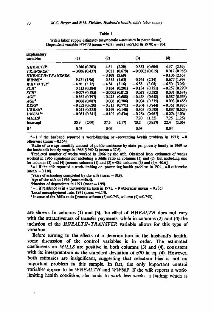
wife’s labor supply estimates (asymptotic r-statistics in parentheses). Dependent variable W W70 (mean = 42.9): weeks worked in 1970; n = 861.

fZ;w! (1) (2) (3) (4)

HHEALTHP TRANSFERb HHEALTH*TRANSFER ww66p” WHEALT.p SCH' SCH' AG@ AGE’ DEPS' UR3ANh 3NEiw MILUj Intercept R2

O.266 (0.203) -0.006 (0.437)

0.421 (1.96) -4.M) (3.12)

0.313 (0.384) -0.O07 (0.185) -0.552 (0.797)

oJl06 (0.887) -0.252 (0.620)

0.241 (0.225) -0.081 (0.341)

35.9 (2.09)

0.03

4.51 (2.20) 0.011 (0.67g)

-0.108 (2.69) 0.355 (1.65)

-4.54 (3.16) 0.164 (0.201)

-0.0OO5 (0.012) -0.475 (0.688)

O.OO6 (0.786) -0.313 (0.771)

0.149 (0.140) -0.102 (0.434)

37.3 (2.17)

0.04

0.833 (0.604) -0OO02 (0.015)

0.761 (2.24) - 6.58 (3.08) -0.134 (0.151)

0.027 (0.582) -0.458 (0.658)

0.004 (0.535) - 0.304 (0.744) -0.805 (0.598) -0.264 (0.962)

7.70 (1.32) 20.2 (0.957)

0.03

4.97 (2.39) 0.017 (0.988)

- 0.106 (2.65) 0.677 (1.99)

-6.50 (3.06) -0.257 (0.290)

0.031 (0.684) -0.387 (0.558)

oOO3 (0.455) -0.361 (0.885) -0.837 (0.624) -0.274 (1.00)

7.25 (1.25) 22.4 (1.06)

0.04

‘= 1 if the husband reported a work-limiting or -preventing bealth problem in 1971; =0 otherwise (mean=O.154).

bRatio of average monthly amount of public assistance by state per poverty family in 1969 to the husband’s hourly wage in 1966 (1969 $) (mean=376j.

‘Predicted number of weeks worked in 1966 by the wife. Obtained fron estimates of weeks worked in 1966 equations not including a Mills ratio in cohumns (1) and (2) but including one for columns (3) and (4) [means: cohunns (1) and (2)=40.9, columns (3) and (4)= 40.q.

d= 1 if the wife reported a work-limiting or -preventing health problem in 19i 1, =O otherwise (mean =O.l3O).

‘Years of schooling completed by the wife (mean = 10.9). ‘Age of the wife in 1966 (mean = 46.4). wumber of dependents in 1971 (mean= 1.99). h= 1 if residence is in a metropolitan area in 1971, =0 otherwise (mean =0.735). %ocal unemployment rate, 1971 (mean = 6.14). J Inverse of the Mills ratio [means: column (3) = 0.743, column (4) = 0.7431.

are shown. In co1 s (1) and (3), the effect of HHEALTH does not vary with the attracti of , wh.ile in columns (2) and (4) the inclus!on of the AL variable allows for this type of

fore turning to the effects of a deterioration in the husband’s health, of the control variables is in order. The estimated

sting that selection bias is not an

MC. Berger and B.M. F&her, Husband’s health, wife’s labor supply 71

both expected and consistent with previous research.l* The positive influence of WW66P implies that wives who are strongly attached to the labor force are likely to remain so over time, consistent with the existence of unobserved heterogeneity and state dependence.

In columns (1) and (3), a deterioration in the husband’s health has a positive but insignificant impact on the wife’s labor supply. Thus, after controlling for demographic characteristics and labor market conditions, the over time response appears to be similar to the responses inferred from cross-sectional data in previous studies.

However, the estimates in columns (2) and (4) show that the labor supply response of the wife to a deterioration in the husband’s health depends crucially on the attractiveness of transfers. The estimated coefficient on the HHEALTH*TRANSFER variable is negative and significant while that on HHEALTH is significantly positive. Taken together, the directions of the two estimated parameters imply that if transfer payments are relatively unattractive, the labor supply response of the wife when the husband’s health declines is positive, and that the response decreases and eventually turns negative as the amount of available transfsr payments increases, This result is consistent with the prediction made earlis. Wing the discussion of the wife’s labor supply response.

The coeficient on TRANSFER is insignificant, which is not surprising. This is especially true in columns (2) and (4) where it measures the effect of changes in transfers on the labor supply of wives whose husband’s health has not deteriorated. Since most families with healthy husbands are not eligible for transfer payments, an increase or decrease in their attractiveness has no effect on the labor supply of the wife.

The estimated coefficients in table 1 can be combined with values of TRANSFER to obtain estimates of the magnitude of the wife’s labor supply response to deterioration in the husband’s health under alternative amounts of available transfer payments. Using the consistent population parameter estimates in column (4), if no transfers are available (TRANSFER=O), the wife increases her market work by 4.97 weeks annuahy when the husband becomes ilf. or disabled.

The magnitude of the response diminishes when transfers replzce s the lost earnings of the husband. At the sample mean, where av transfers replace 37.6 hours of the husband’s market work wife i.ncreases her market work by only 0.98 wee

“See reverences cited in footnote 1. “Although section 1 emphasized the effect of transfers on the wife’s reservation wage (an

increase in transfers raises W$ and reduces t arket work), some transfers may affect the market wage as weil, as is mention Thus, the decrease in the wife’s labor supply response 5x1 4.91 to 0.98 brou

in her reservation wage.

72 MC. Be~er and B.M. Fleisher, Husband’s health, wife’s labor supply

worked remain c;>nstant when transfer payments equal 46.9 times the husband’s pm-disability hourly wage. In this case, the negative effects on the wife’s labor supply of the husband’s need for care and the availability of transfers are just balanced by the positive effect of the decrease in the busband’s earning power.

FinaIly, suppose transfer payments replace all of the pre-disability market earnings of the husband. Assuming an 8 hour work day and 21 working days ger month, TRANSFER equals 168 and the wife reduces her market work by 12.84 weeks per year. This is also an estimate of the ‘nursing’ effect that results from a deterioration in the husbands’ health [(CW*/iW) W in eq. (3)]. In other words, if family full income is held constant, the wife reduces her market work by almost 13 weeks per year when the husband’s health deteriorates in order to provide care for him at home.l*

In summary, the estimates in table 1 show that the response to a husband’s health problem by the wife over time is not the same for all families. ther, the response depends on the attractiveness of transfers. When transfers are relatively uncrrclcr -++ctive, the lost earnings of the husband causes the wife to increase her labor market activity. As transfer payments replace more of the lost earnings of the husband it becomes more likely that the wife decmases her market work.

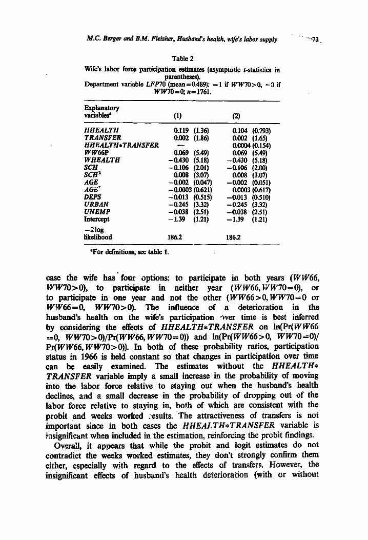
The estimates in table 1 come from a model explaining weeks worked by the wife. t are the same implications obtained when the labor force participati decision of the wife is examined directly? The effects of the husband’s health deterioration on the wife’s labor force participation can be derived from the probit- estimates used to construct the Mills ratio. These estimates are reported in table 2. When the HHEALTH*TRANSFER interaction variable is omitted, a deterioration in the husband’s health produces a weak increase in the probability of the wife participating in the labor force, a result consistent with the findings presented in table 1. However, when the interaction is added, both it and HHEALTH are insignificant, unlike in the weeks worked estimates. Thus the wife’s probability of participation is sot signilicantly affected by a deterioration in the husband’s health, regardless of whether or not transfer payments are available.

Similar results are obtained from a multinomial logit model of the wife’s labor force icipation in 1966 and 1970. This model provides parameter estimates w show the effect of changes in the explanatory variables on the log of the -ratio of the probability of one choice to another.13 In this

“This estimate assumes that t&e decline in family N1 income caused by a deterioration in the health of the husband is equal to his previous labor market earnings. Thus H increases by 168 and % remains the same or M bmses and W, demases such that their product equals the husband

%ee Sty market earnings. (1874) for a discussion of the multinominal logit model and its properties.

Tb=uwes (1981) uses the multinominal logit framework to examine the joint labor force participation decision of the husband and the wife.

MC. Berger und B.M. Fleisher, Husband’s health, wife’s labor supply * - .‘%.

Table 2

Wife’s labor force participation estimates (asymptotic t-statistics in parentlleses).

Department variable LFP70 (mean = 0.489): = 1 if WW70>0, = 9 if ww70=0; n=1761.

Explanatory vtiabl& (1) (2)

HHEALTH TRANSFER IiHEALTIhTRANSFER WW66P WHEALTH SCH &x2 AGE AGZ’ DEPS URBAN UNEMP Intercept

-21og likelihood

0.119 (1.36) 0.002 (1.86)

0.069 (5.49) -0.430 (5.18) -0.106 (2.01)

0.008 (3.07) -0.002 (0.047) - 0.0003 (0.621) -0.013 (0.515) -0.245 (3.32) -0.038 (2.51) - 1.39 (1.21)

186.2

0.104 (0.793) O.oM (1.65) 0.0004 (0.154) 0.069 (5.49)

-0.430 (5.18) -0.106 (2.00)

0.008 (3.07) -0.002 (0.051)

0.0003 (0.617) -0.013 (0.510) -0245 (3.32) -0.038 (2.51) -1.39 (1.21)

186.2

‘For definitions, see table 1.

case the wife has ’ four options: to participate in both years (WW66, lVw70>0), to participate in neither year (WW66, WW70=0), or to participate in one year and not the other (WW66>O,WW70=0 or I-VW66 = 0, WW70>0). The influence of a deterioration in the husband’s health on the wife’s participation pver time is best inferred by considering the effects of HHEALTH*TRANSFER on ln(Pr(WW66 ==0, WW7O>O)/Pr(WW66, WW70=0)) and ln(Pr(WW66>0, WW70=0)/ Pr(WW66, WW70>0)). In both of these probability ratios, participation status in 1966 is held constant so that changes in participation over time can be easily examined. The estimates without the HHEALTH+ TRANSFER variable imply a small increase in the probability of moving into the labor force relative to staying out when the husband’s health declines, and a small decrease in the probability of dropping out of the labor force relative to staying in, both of which are consistent with the probit ,and weeks worked ;-esults. The attractiveness of transfers is not important since in both cases the HHEAL *TRANSFER variable is insignificant when included in the estimation, reinforc

Overall, it appears that while the probit and contradict the weeks worked estimates, they don’t strongly co

.74-- MC. Berger and B.M. Fleiskr, Husband’s health, wife’s labor supply

transkrs) on the wife’s participation are not overly surprising given the evidence of unobserved heterogeneity between participants and non- participants found here. For participants, the number of weeks worked is determined by the equality of the market and home wages. The results in table 1 suggest that this equilibrium is sensitive to changes in the husband’s heal&, after taking into account differences in the effect of transfers by husband’s health status. For non-participants however, the reservation wage exceeds the market wage so the true intersection of the home and market wages is never observed. And for many wives, the d%erence between the re*rvation and market wages is undoubtably quite large. Thus, even the oamplete absence of transfers when the husband’s health deteriorates does not reduce the reservation wage enough to induce many wives to participate. There may also be fixed costs of participation which keep the reservation wage higher than otherwise and reduce the likelihood of observing any sig.nZcant movement into the labor force.14 Thus, while the effects of changes in the health of the husband after taking into account transfers are strong enough to sign&antly alter the amount of labor supplied by wives, they are not strong enough to significantly alter her decision of whether to enter or to leave the labor force.

5.S CORClUSiOaS

This paper examines the labor supply response by the wife over time to a deterioration in the husband’s health. Unlike previous studies using CTOSS-

sectional data, longitudinal data are used which allows over time responses to be examined directly.

The empirical results indicate that on average there is a small increase in the wife’s labor supply when the husband’s health declines. However, the direction and the magnitude of the response varies significantly across the sample depending on the attractiveness of transfer payments which the family may qualify for when the husband’s health becomes poor. As available payments increase relative to the husband’s pre-disability market wage, the tie eventually decreases instead of increases her market work. When this happens, the net loss in family income is small enough to be outweighed by the increase in the husband’s need for care at home, thus causing the wife to reduce her labor market activities.

owever, it is also found that the probability of participation is not significantly affected by deterioration in the health of the husband, regardless of the attractiveness of transfers. Apparently participants and non- participants come from different populations, and the effects of health

“For fdl analysis of the effects of fmed costs of participation on the labor supply behavior of married women, see Cogan (198 is empirical results su st that on average, fi c.osts

of married women.

MC. Berger and B.M. Neisher, Husband’s health, wife’s labor supply 75

deterioration of the husband combined with the availability of transfers itre

not strong enough to alter significantly the decision of whether or not to

work, even though among participants they do cause changes in the amount of market work.

One important implication of the findmgs here is that transfer payments that become available whenqhe husband’3 health deteriorates tend to work in the way that they were &tended. EQccifically, when transfer payments replace enough of the lost earnings of the husband, the wife is able to reduce her market work in order to care for the husband at home. While she may not drop out of the labor force entirely, the results here do suggest that increases in the attrac?iveness of transfers do significantly decrease the wife’s amount of market work when the husband’s health deteriorates.

eferences

Rerger, Mark C., i983, Labor supply and spouse’s health: The effects of illness, disability and mortality, Social Science Quarterly 64, no. 3,49&509.

Rerkowia Monroe and William G. Johnson, 1974, Health and labor force participation, Journal of Human Resources 9, no. 1,117-128.

Berkowitz, Monroe, William G. Johnson and Edward M. Murphy, 1976, Public policy toward disability (Praeger, New York).

Cogan, John F., 1981, Fixed costs and labor supply, Econometrica 49, no. 4,945963. Davis, J.M., 1972, Impact of health on earnings and labor market activity, Monthly Labor

Review 95, no. 10,46-4g. Duncan, Greogory M. and Duane E. Leigh, 1980, Wage determination in the union and

nonunion sectors: A sample seiectivity approach, Industrial and Labor Relations Review 34, no. 1, 24-34.

Heckman, James J., 1974, Shadow prices, market wages, and labor supply, Econometrica 42, no. 4,679-694.

Heckman, James J., 1978, Heterogeneity and state dependeuce in dynamic models of labor supply, unpublished paper (University of Chicago, Chicago, IL).

Heckman, James J., 1979, Sample selection bias as a specification error, Econometrica 47, no. 1, 153-161.

Heckman, James J., 1980, Sample selection bias as a specification error with an application to the estimation of labor supply functions, in: James P. Smith, ed., Female labor supply: Theory and estimation (Princeton University Press, Priiceton, NJ) 206-248.

Lambrinos, James, 1981, Health: A source of bias in labor supply models, Revview of Economics and Statistics 62, no. 2,206-212

Lee, Lung-Fei, 1982, Health and wage: A simultaneous equation model with multiple discrete indicators, International Economic Review 23, no. 1,199221.

Luft, Harold S., 1975, The impact of poor health on earnings, Review of Economics and statistics 57, no. 1,43-57.

McFadden, Daniel, 1974, Conditional logit analysis of qualitative choice behavior, in: Paul Zarembka, ed., Frontiers of econometrics (Academic Press, New York) 105-139.

Parsons, Donald O., 1977, Health, family structure, and labor supply, American Economic Review 67, no. 5,703-712.

Parsons, Donald O., 1980, The decline in mate labor force participation, Journal of Political Economy 88, no. 1,117-134.

Scheffler, Richard M. and George Zden, 1974, The effect of disability on labor supply, ~~dMst~a~ and Labor Relations Review 28, no. 1,122-132.

Theeuwes, J., 1981, Family labour force participation: ultinomial logit estimates, A~~~~~d Economics 13,4811-498.