Human Detection of Computer Simulation Mistakes in ...

HUMANDETECTIONOF COMPUTER SIMULATIONMISTAKESIN ENGINEERING EXPERIMENTS

by

TROY BRENDON SAVOIE

SUBMITTED TO THE DEPARTMENT OF MECHANICAL ENGINEERINGIN PARTIAL FULFILLMENT OF THE REQUIREMENTS FOR THE DEGREE OF

DOCTOR OF PHILOSOPHY IN MECHANICAL ENGINEERING

at the

MASSACHUSETTS INSTITUTE OF TECHNOLOGY

June 2010

©2010 Troy Brendon Savoie. All rights reserved.

e author hereby grants to MIT permission to reproduce and todistribute publicly paper and electronic copies of this thesis document in whole or in part

in any medium now known or hereaer created.

Signature of Author . . . . . . . . . . . . . . . . . . . . . . . . . . . . . . . . . . . . . . . . . . . . . . . . . . . . . . . . . . . . . . . .Department of Mechanical Engineering

May 18, 2010

Certied by . . . . . . . . . . . . . . . . . . . . . . . . . . . . . . . . . . . . . . . . . . . . . . . . . . . . . . . . . . . . . . . . . . . . . . .Daniel D. Frey

Associate Professor of Mechanical Engineering and Engineering Systemsesis Supervisor

Certied by . . . . . . . . . . . . . . . . . . . . . . . . . . . . . . . . . . . . . . . . . . . . . . . . . . . . . . . . . . . . . . . . . . . . . . .Brenan C. McCarragher

Charles Stark Draper Laboratoryesis Supervisor

Accepted by . . . . . . . . . . . . . . . . . . . . . . . . . . . . . . . . . . . . . . . . . . . . . . . . . . . . . . . . . . . . . . . . . . . . . . .David E. Hardt

Ralph E. and Eloise F. Cross Professor of Mechanical EngineeringChairman, Department Committee on Graduateeses

Human Detection of Computer Simulation Mistakesin Engineering Experiments

byTroy Brendon Savoie

Submitted to the Department of Mechanical Engineeringon May 18, 2010, in partial fulllment of the

requirements for the degree ofDoctor of Philosophy in Mechanical Engineering

Abstract

is thesis investigates the notion that the more complex the experimental plan, the less likely anengineer is to discover a simulation mistake in a computer-based experiment.e author used anin vitromethodology to conduct an experiment with 54 engineers completing a design task to ndthe optimal conguration for a device with seven two-level control factors. Participants workedindividually using a prescribed design approach dependent upon the randomly assigned experimentalcondition – an adaptive one-factor-at-a-time plan for the control group or a resolution III fractionalfactorial plan for the treatment group – with a awed computer simulation of the device.

A domain knowledge score was measured by quiz, and success or failure in discovering the aw wasmeasured by questioning during debrieng. About half (14 of 27) of the participants using the one-factor-at-a-time plan discovered the aw, while nearly none (1 of 27) using the fractional factorial plandid so. Logistic regression analysis of the dichotomous outcome on treatment condition and domainknowledge score showed that aw detection ability improved with increased domain knowledge, butthat an advantage of two standard deviations in domain knowledge was insucient to overcome thedisadvantage of using the fractional factorial plan.

Participant reactions to simulation results were judged by two independent raters for surprise as anindicator of expectation violation. Contingency analysis of the surprise rating results showed thatparticipants using the fractional factorial plan were signicantly less likely (risk ratio ≈ 0.57) to appearsurprised when the anomaly was elicited, but there was no dierence in tendency to display surpriseotherwise.

e observed phenomenon has ramications beyond simulation mistake detection. Cognitive psychol-ogists have shown that the most eective way to learn a new concept is to observe unexpected behavior,investigate the cause, then integrate the new concept into one’s mental model. If using a complexexperimental plan hinders an engineer’s ability to recognize anomalous data, the engineer risks losingopportunities to develop expertise. Initial screening and sensitivity analyses are recommended ascountermeasures when using complex experiments, but more study is needed for verication.

esis Supervisor: Daniel D. FreyTitle: Associate Professor of Mechanical Engineering and Engineering Systems

esis Supervisor: Brenan C. McCarragherTitle: Associate Director, Strategic Systems, Charles Stark Draper Laboratory

3

is page intentionally le blank.

4

Dedicated to the memory of my grandparents:

Ashton & Mabel Savoie Kenneth & Merle Elder

5


6

ose who bring sunshine into the lives ofothers cannot keep it from themselves.

James M. Barrie

Acknowledgments

It is amazing to think of the many ways that my degree candidacy was nearly derailed, only to havekey support – sometimes from the most unexpected places – exactly at the right moment to keep meon track.

I am especially grateful for guidance and inspiration from my advisor, Prof. Dan Frey. He gaveme the freedom to nd and pursue a topic that I am passionate about, then provided enthusiasticencouragement, punctual advice, and unwavering support through the end. Without question, thebest decision I made as a graduate student was asking Dan to be my advisor.

All of the work in this thesis was performed at the Charles Stark Draper Laboratory, Inc., as part ofan Internal Research and Development project. In addition to being an underappreciated nationalresource, Draper provides an ideal base from which to pursue graduate study on interesting andchallenging projects. I thank my rst technical supervisor there, Ed Lanzilotta, for bringing me intoDraper, helping me to nd an interesting topic, giving me pep talks when things weren’t going well,and helping to smooth the transition when he le Draper before my degree was nished. I thankBrenan McCarragher for agreeing to take over my research supervision at Draper for the remainderof my doctoral program; his experience in supervising past doctoral students and his uncanny abilityto quickly zero in on the nucleus of a problem were both assets to my development. I also thank JasjitHeckathorn for her help in nding a great supervisor, for patience when I experienced setbacks, andfor sustained condence in me throughout my stay at Draper.

e Education Oce at Draper was one of the most important factors in my success. I simply wouldnot have prevailed without the help of its fantastic director, Linda Fuhrman. She went above andbeyond by generously allowing me to conduct my human subjects experiment in the conference roomadjacent to her oce, providing crucial resources in support of that experiment, and ensuring that myfunding was extended during the entire eighteen-month period of time when I was “six months awayfrom graduating.” Linda’s assistant Gail DiDonato was also a great resource for me, from skillfullyhandling expired-badge emergencies to frequently locating and distributing free food to Draper’sock of hungry graduate students. I also appreciate the sound advice, administrative help and votesof condence from the former director of the Education Oce, George Schmidt, and the interimdirector, Milt Adams.

I would like to express my gratitude to Prof. Missy Cummings and Prof. Warren Seering for servingon my thesis committee. Missy’s expertise in statistics and human factors was invaluable, and herpresence in the committee meetings guaranteed spirited discussion. It was also a great pleasure tohave the perspective of Warren’s broad experience in engineering design methodology from equalparts academia and industry.

To the 64 engineers who volunteered for my experiment, I am most appreciative of your time andfor being good sports when I revealed the true objective of the study during the debrieng. Special

7

thanks go to Javier Garcia and Morris Vanegas, the two independent judges of each of the 385 videorecorded reactions.eir willingness to work odd hours in less than ideal locations allowed me to getthe nal analysis done on time.

I would not have dreamed of pursuing this degree without the encouragement of great teachers andmentors. At LSU, Profs. Warren Waggenspack and Robert Courter gave me early opportunitiesand guidance. At UT/Austin, Profs. Glenn Masada, Tess Moon, and Raul Longoria all inuencedmy decision to continue graduate study. Outside of academia, past supervisors Scott Fish of theInstitute for Advanced Technology and John Vranish of NASA’s Goddard Space Flight Center wereboth essential to my professional development.

One of the most pleasant surprises during my time here was the discovery that when things aren’tgoing well, there is a support structure at the Institute lled with caring people, ready to help in anyway possible. In the Course II Graduate Oce, Leslie Regan and Joan Kravit were unappable inhandling crises. It would be dicult to overstate how important they are to the well being of thedepartment’s graduate students. In the Oce of the Dean for Graduate Education, Dean Steve Lerman,Dean Blanche Staton and Dean Isaac Colbert were all wonderfully supportive in their handling ofunusual circumstances threatening to block my path to graduation.

While living in New England and studying at MIT has been an incredible adventure, it came at greatpersonal sacrice, and I would be remiss if I didn’t thank those closest to me who had to endurenearly the same level of sacrice: my wife Jackie and our beloved daughter Gabrielle, who both spentcountless evenings over the last few years accommodating my need for a quiet environment at home.ank you, girls.

Troy Brendon SavoieCambridge, MassachusettsMay 2010

8

Contents

Introduction . A Denition of Engineering Design Methodology . . . . . . . . . . . . . . . . . . . . . Motivation . . . . . . . . . . . . . . . . . . . . . . . . . . . . . . . . . . . . . . . . . . .

.. e evolution of planned experiments . . . . . . . . . . . . . . . . . . . . . . . .. Cause for shaken trust in computer simulations . . . . . . . . . . . . . . . . . .. Cognition and complexity . . . . . . . . . . . . . . . . . . . . . . . . . . . . . . .. Implications for computer experimentation in engineering design . . . . . .

. Proposed Study . . . . . . . . . . . . . . . . . . . . . . . . . . . . . . . . . . . . . . . . . .. Special considerations for one-factor-at-a-time approach . . . . . . . . . . . .

. Literature Review . . . . . . . . . . . . . . . . . . . . . . . . . . . . . . . . . . . . . . . .. eoretical Basis . . . . . . . . . . . . . . . . . . . . . . . . . . . . . . . . . . . .. Related Prior Work . . . . . . . . . . . . . . . . . . . . . . . . . . . . . . . . . .

. Research Summary . . . . . . . . . . . . . . . . . . . . . . . . . . . . . . . . . . . . . . .. Hypothesis . . . . . . . . . . . . . . . . . . . . . . . . . . . . . . . . . . . . . . .. Methodological Approach . . . . . . . . . . . . . . . . . . . . . . . . . . . . . . .. Main Contribution . . . . . . . . . . . . . . . . . . . . . . . . . . . . . . . . . .

. Structure of theesis . . . . . . . . . . . . . . . . . . . . . . . . . . . . . . . . . . . . .

Research Strategy . Overview . . . . . . . . . . . . . . . . . . . . . . . . . . . . . . . . . . . . . . . . . . . . . Analytical Methods . . . . . . . . . . . . . . . . . . . . . . . . . . . . . . . . . . . . . .

.. Logistic Regression . . . . . . . . . . . . . . . . . . . . . . . . . . . . . . . . . . .. Contingency Table Analysis . . . . . . . . . . . . . . . . . . . . . . . . . . . . .

. Experiment Size . . . . . . . . . . . . . . . . . . . . . . . . . . . . . . . . . . . . . . . . .. Sample Size Requirements for Statistical Power . . . . . . . . . . . . . . . . . .. Sample Size Requirements to Minimize Separation Artifacts . . . . . . . . . . .. Conclusion . . . . . . . . . . . . . . . . . . . . . . . . . . . . . . . . . . . . . .

. Conceptual Framework for Experiment . . . . . . . . . . . . . . . . . . . . . . . . . . .. Introduction . . . . . . . . . . . . . . . . . . . . . . . . . . . . . . . . . . . . . .. Eligibility of Human Subjects . . . . . . . . . . . . . . . . . . . . . . . . . . . . .. Physical Device to be Designed . . . . . . . . . . . . . . . . . . . . . . . . . . . .. Design Task . . . . . . . . . . . . . . . . . . . . . . . . . . . . . . . . . . . . . . .. Flaw in the Computer Simulation Results . . . . . . . . . . . . . . . . . . . . .

9

.. Experimental Treatment: Design Algorithms . . . . . . . . . . . . . . . . . . . .. Summary of Conceptual Framework . . . . . . . . . . . . . . . . . . . . . . .

. Replication, Randomization and Blocking . . . . . . . . . . . . . . . . . . . . . . . . . . Summary of Research Strategy . . . . . . . . . . . . . . . . . . . . . . . . . . . . . . . .

Experiments . Introduction . . . . . . . . . . . . . . . . . . . . . . . . . . . . . . . . . . . . . . . . . . . Pilot Study . . . . . . . . . . . . . . . . . . . . . . . . . . . . . . . . . . . . . . . . . . .

.. Experimental Protocol . . . . . . . . . . . . . . . . . . . . . . . . . . . . . . . . .. Results . . . . . . . . . . . . . . . . . . . . . . . . . . . . . . . . . . . . . . . . . .. Discussion . . . . . . . . . . . . . . . . . . . . . . . . . . . . . . . . . . . . . . .

. Main Study . . . . . . . . . . . . . . . . . . . . . . . . . . . . . . . . . . . . . . . . . . . .. Experimental Protocol . . . . . . . . . . . . . . . . . . . . . . . . . . . . . . . . .. Results . . . . . . . . . . . . . . . . . . . . . . . . . . . . . . . . . . . . . . . . .

Analysis . Measure of Success in Identifying Anomaly . . . . . . . . . . . . . . . . . . . . . . . .

.. Using Simple Proportions without Domain Knowledge . . . . . . . . . . . . . .. Using Logistic Regression with Domain Knowledge . . . . . . . . . . . . . . .

. Measure of Expectation Violation . . . . . . . . . . . . . . . . . . . . . . . . . . . . . . .. Interrater Reliability . . . . . . . . . . . . . . . . . . . . . . . . . . . . . . . . . .. Explanatory Variable: Comparison Elicits Anomaly . . . . . . . . . . . . . . . .. Contingency Table . . . . . . . . . . . . . . . . . . . . . . . . . . . . . . . . . .

Discussion . Main Findings . . . . . . . . . . . . . . . . . . . . . . . . . . . . . . . . . . . . . . . . .

.. Conrmatory Analysis of Debrieng Results . . . . . . . . . . . . . . . . . . . .. Exploratory Analysis of Surprise Rating Results . . . . . . . . . . . . . . . . .

. Limitations . . . . . . . . . . . . . . . . . . . . . . . . . . . . . . . . . . . . . . . . . . .

Conclusions and Suggested Future Work . Surprises and Conjectures . . . . . . . . . . . . . . . . . . . . . . . . . . . . . . . . . . . Implications of Observed Phenomenon . . . . . . . . . . . . . . . . . . . . . . . . . . . Suggested Future Work . . . . . . . . . . . . . . . . . . . . . . . . . . . . . . . . . . . .

Bibliography

Appendix A Mathematical Model of the Catapult Device

Appendix B Forms and Supplementary Materials for All Experiments

Appendix C Tabulated Experimental Data

10

List of Figures

- Generalized system attributes . . . . . . . . . . . . . . . . . . . . . . . . . . . . . . . . - Milestones in computer technology and experimental design methods . . . . . . . .

- Linear, loglinear and logistic regression on proportions . . . . . . . . . . . . . . . . . - Parameters in null hypothesis signicance testing . . . . . . . . . . . . . . . . . . . . . - Minimum sample size required for all possible eect sizes . . . . . . . . . . . . . . . . - Photograph of the Xpult catapult . . . . . . . . . . . . . . . . . . . . . . . . . . . . . . - Pareto chart of the control factor main eects in the catapult device . . . . . . . . . . - Spatial abstraction of 23 system for algorithm illustration . . . . . . . . . . . . . . . . - Illustration of the adaptive one-factor-at-a-time (aOFAT) algorithm . . . . . . . . . . - Illustration of the orthogonal-array-based, fractional factorial algorithm . . . . . . . - Monte Carlo analysis of the proposed design methods . . . . . . . . . . . . . . . . . .

- Participant ow diagram for the pilot study . . . . . . . . . . . . . . . . . . . . . . . . - Participant ow diagram for the main study . . . . . . . . . . . . . . . . . . . . . . . . - Demographics for the main study . . . . . . . . . . . . . . . . . . . . . . . . . . . . . .

- Histograms of domain knowledge score by treatment group . . . . . . . . . . . . . . . - Graphical user interface for rating participant reactions . . . . . . . . . . . . . . . . . - Decision rule for resolving disagreements between independent video raters . . . . .

- Odds ratios for participant detection of the anomaly . . . . . . . . . . . . . . . . . . . - Risk ratios for participant expressing surprise at the simulation result . . . . . . . . .

A- e Xpult catapult, showing component nomenclature . . . . . . . . . . . . . . . . . . A- Catapult angle denitions . . . . . . . . . . . . . . . . . . . . . . . . . . . . . . . . . . . A- Free body diagram of the catapult arm before the ball is launched . . . . . . . . . . . A- Free body diagram of the ball in ballistic ight . . . . . . . . . . . . . . . . . . . . . . A- Variation of air properties with ambient temperature and relative humidity . . . . . . A- Engineering constants in the modied catapult model . . . . . . . . . . . . . . . . . . A- Main eects from full factorial results . . . . . . . . . . . . . . . . . . . . . . . . . . . . A- Two-factor interactions from full factorial results . . . . . . . . . . . . . . . . . . . . . A- Two-factor interactions from full factorial results (continued) . . . . . . . . . . . . .

11


12

List of Tables

. Contingency Table for Calculating Risk Ratio . . . . . . . . . . . . . . . . . . . . . . . . A Convention for Eect Size Indices Suggested by Cohen . . . . . . . . . . . . . . . . . Example Usage of the aOFAT Design Algorithm . . . . . . . . . . . . . . . . . . . . . . Plackett-Burman L8 Orthogonal Array . . . . . . . . . . . . . . . . . . . . . . . . . . . . Example Usage of the PB-L8 Design Algorithm . . . . . . . . . . . . . . . . . . . . . . . Design Tables with Column Assignments for Flawed Control Factor . . . . . . . . . .

. Debrieng Results (Raw Counts) . . . . . . . . . . . . . . . . . . . . . . . . . . . . . . . Debrieng Results (Proportions with 95 Condence Intervals) . . . . . . . . . . . . . Logistic Regression Coecients for Subject Debrieng . . . . . . . . . . . . . . . . . . . Contingency Table for Independent Analysts’ Ratings of Subject Reactions . . . . . . . Full and Reduced Contingency Tables for Surprise Ratings . . . . . . . . . . . . . . . . Contingency Analysis of Surprise Rating Results . . . . . . . . . . . . . . . . . . . . .

A. Salient Features of the Simulation Model . . . . . . . . . . . . . . . . . . . . . . . . . . A. Control Factors for the Modied Catapult . . . . . . . . . . . . . . . . . . . . . . . . . A. Parameter Specications for the Modied Catapult . . . . . . . . . . . . . . . . . . . . A. Full Factorial Results for Catapult Simulation . . . . . . . . . . . . . . . . . . . . . . .

C. Participant Demographics . . . . . . . . . . . . . . . . . . . . . . . . . . . . . . . . . . C. Raw Data from Quiz for Domain Knowledge Score . . . . . . . . . . . . . . . . . . . . C. Raw Data from Distance Predictions and Surprise Ratings . . . . . . . . . . . . . . . C. Raw Data from Debrieng Questioning . . . . . . . . . . . . . . . . . . . . . . . . . .

13


14

Chapter 1

Introduction

1.1 A Definition of Engineering Design Methodology

e goal of the design engineer is to specify the structure of a product that will satisfy the end user’sfunctional requirements as completely as possible within the allocated budget and time. Engineeringdesign methodology is the scientic discipline concerned with creating and rening systematicapproaches that the design engineer can use to reach this goal.

In general, the engineering design process may be partitioned into three components: system design,parameter design and tolerance design. System design is the rst stage, where concepts for a productand its architecture are considered.is is the design step normally associated with brainstorming andinnovation. When the architecture is set, the settable parameters in the product are known. Parameterdesign is the second stage, where the designer determines which of these parameters are importantto the product’s performance. Tolerance design is the third stage, where the detailed design for theproduct is specied.e work in this thesis applies to the parameter design step in this view of theengineering design process.

In robust parameter design, one aims to congure a system1 such that the response to system input ison average close to the ideal response, with deviation from the ideal minimized in spite of system noise.Figure 1-1 illustrates the main attributes of a system: control factors, noise factors, input signal andresponse. Control factors represent design options that one may specify; for example, in the designof an automobile control factors would include fuel type, engine size, tire shape, suspension linkagegeometry, etc. Noise factors represent sources of variability over which one has little or no control. Inthe same example, this would include things like passenger and cargo weight, pavement-tire friction,road roughness, and wind load.e input signal in this example is the combination of steering wheel,

1Note that the denition of “system” that applies in most instances here is that of a single physical product; for example,a laptop is a computer system.

15

SystemInputSignal

NoiseFactors

ControlFactors

Output(Response)

Figure 1-1: Generalized system attributes

accelerator pedal and brake pedal positions.e system response would include things like the “ridecomfort” of the passengers, maximum acceleration, fuel economy, exhaust emissions, maximumspeed, braking distance and aesthetic appeal.rough experimentation, the design engineer evaluatesthe performance of the system in order to make informed design decisions.

Before the advent of formal design methodology, one would build a limited number of candidateprototypes with design options set at one or more “best guess” congurations based on past experienceand engineering judgment. Limits on development time and equipment spending meant that only asmall portion of the design space could be explored, and the result was oen a suboptimal design.Engineering design methodology applied to parameter design is about nding ways to explore thedesign space eciently to evaluate the eect of system parameters on performance.

1.2 Motivation

1.2.1 e evolution of planned experiments

e origin of modern, structured approaches to experimental design is widely attributed to the agri-culturally motivated work of Fisher (1926, 1935) more than 80 years ago, and development in thisarea remains active to this day (see for example Robinson et al. (2004)). Following Fisher’s work,signicant milestones in the theory of experimental design include Orthogonal Arrays (Plackett andBurman, 1946), Monte Carlo experiments (Metropolis and Ulam, 1949), Response Surface Methodol-ogy (Box and Wilson, 1951), Crossed Orthogonal Arrays and Signal-to-Noise Ratios (Taguchi, 1987;Phadke, 1989), Latin Hypercube Sampling (Mckay et al., 1979) and Hammersley Sequence Sampling(Kalagnanam and Diwekar, 1997). In general as experimental design theory progresses, more informa-tion about a system is obtained with fewer experiments; however, this eciency typically comes withthe price of increased complexity in the method.

16

1920 1930 1940 1950 1960 1970 1980 1990 2000

R. A. Fisher, Thearrangement of field

experiments

R. A. Fisher, TheDesign of Experiments

Plackett & Burman,orthogonal arrays

Metropolis & UlamMonte Carloexperiments

Box & Wilson,Response SurfaceMethodology

G. Taguchi,Crossed Arrays &

Signal-to-Noise Ratios

McKay, Beckman & Conover,Latin Hypercube Sampling

Kalagnanam & Diwekar,Hammersley Sequence

Sampling

Z1Computer ENIAC 1

transistor

FORTRAN

integratedcircuit

COBOL

mouse,BASIC

floppydisk

Unix

RAM

compactdisk, C

Ethernet

S

flashmemory

IBM PC,MS-DOS

GNU

AppleMacintosh

MicrosoftWindows

Web,Linux

R Java

Figure 1-2:Milestones in the development of computer technology (above time line) and experimentaldesign methods (below time line)

As one might expect, the physical experimentation at the beginning of this period gradually gave wayto the computational methods widely used today, and the focus in the design research community hasfollowed a similar trajectory. Figure 1-2 gives a time line showing the parallel development of computertechnology and experimental design methodology. Of note is that the last two experimental designmilestones shown on this time line were introduced specically for use with computer simulationdata.

In addition to the high cost of building prototype hardware, the combination of advances in computertechnology and compressed product development schedules has made physical experimentation ararely aorded luxury in design studies. A common theme among parameter design methods is thetreatment of the system as a black box, where the goal is to build understanding of the relationshipsamong the factors shown in gure 1-1 through targeted experimentation. e work in this thesisis focused on what happens in these sophisticated designed experiments when the black box is acomputer simulation of a mathematical model of the system under study (Koehler and Owen, 1996;Booker, 1998; Simpson et al., 2001; Giunta et al., 2003; Kleijnen et al., 2005).

1.2.2 Cause for shaken trust in computer simulations

Implicit in the increasing reliance on mathematical models is an understanding that the models mustaccurately represent the physical system under study2. Indeed, a focus on the need for validity of

2is does not mean that there is no place for uncertainty in simulation, rather that any existing uncertainty in a systemis accurately modeled as such.

17

computational models has led the American Institution of Aeronautics and Astronautics (AIAA) topublish the rst such standard, on verication and validation of computational uid dynamics simula-tions (AIAA Computational Fluid Dynamics Committee, 1998).e American Society of MechanicalEngineers (ASME) has formed committees to work on its own standards for both computational solidmechanics3 and computational uid dynamics and heat transfer4. A discussion of these and otherworldwide eorts to create such standards is given in Oberkampf et al. (2004, §4.4). Additionally,some researchers have proposed teaching standard methods of commercial soware development tophysical scientists and engineers to help reduce errors in their codes through an organized approachto troubleshooting (Wilson, 1996; Dubois, 2005).

Despite these and similar eorts, there are indications that errors in computer models in engineeringand science are fairly common. Hazelrigg (1999) contends that the majority of models used in supportof engineering design are either erroneous or used incorrectly. He also presents a convincing argumentthat predictivemodels such as those used in engineering design can never really be validated (Hazelrigg,2003). Hatton (1996) studied commercial soware used in scientic and engineering analyses andconcluded that errors in such soware are more prevalent than previously thought.ere are manyinfamous incidents whose causes were traced to errors in proprietary code. As a representative set ofspectacular failures, one need look no farther than NASA’s Moon and Mars programs. In the descentcontrol algorithm for the lunar lander during the Apollo 11 mission, the sign of the gravitational forcewas incorrect, making the moon’s gravity repulsive instead of attractive.e result was not a missionfailure, but the lander descended faster than intended as a result of this error (Neumann, 1995).eMars Climate Orbiter (MCO) is believed to have crashed into the surface of Mars due to a sowareerror:

e MCO [Mishap Investigation Board] has determined that the root cause for the loss ofthe MCO spacecra was the failure to use metric units in the coding of a ground sowarele, “Small Forces,” used in trajectory models. (JPL Special Review Board, 1999)

e Mars Polar Lander (MPL) suered a catastrophic failure on approach to Mars for a similar reason:

...the probable cause of the loss of MPL has been traced to premature shutdown of thedescent engines, resulting from a vulnerability of the soware to transient signals. (JPLSpecial Review Board, 2000)

To be fair, such problems are not limited to NASA, and many examples may be found in the literature(Lin, 1985; Elmer-Dewitt, 1990; Mellor, 1998; Stevenson, 1999).

3ASME Performance Test Code 60 Committee4ASME Performance Test Code 61 Committee

18

1.2.3 Cognition and complexity

It is well established that cognitive ability decreases with increasing task complexity (Miller, 1956;Pollack et al., 1959; Lloyd et al., 1960; Yntema, 1963; Venturino, 1997). Some have investigated dierentaspects of this phenomenon in the context of engineering design (Robertson et al., 1991; Hirschi andFrey, 2002; Ligetti and Simpson, 2005).is suggests a potential problem for today’s computer-savvydesign engineer; namely, that more of the engineer’s faculties are devoted to learning and using thetools of the trade and less are available for thinking about the problem fundamentally. Lendingcredence to this viewpoint, Turkle (2004) proclaims that “e tools we use to think change the waysin which we think” and provides an anecdote from a personal experience at MIT in the 1970’s:

At a lunch for new faculty members, several senior professors in engineering complainedthat the transition from slide rules to calculators had aected their students’ ability to dealwith issues of scale. When students used slide rules, they had to insert decimal pointsthemselves. e professors insisted that that required students to maintain a mentalsense of scale, whereas those who relied on calculators made frequent errors in orders ofmagnitude. Additionally, the students with calculators had lost their ability to do “backof the envelope” calculations, and with that, an intuitive feel for the material.

Professional societies have taken notice and are starting to address this.e mission statement for theDesign Process Subcommittee of AIAA’s Design Engineering Technical Committee (DETC) is givenby Briggs (2004) as follows:

Pursue design integration as a systems oriented approach to improving the design engi-neering process. Develop cost modeling information suitable for use in projects and inteaching design engineering in the classroom. Address the concern that increased computeruse and reliance on analytical tools results in a loss of physical judgment in design outcomes.(p. 1, emphasis added)

1.2.4 Implications for computer experimentation in engineering design

e preceding sections have established that the trend is to use more computer experimentation fordesign evaluation, but that simulation validity remains an area of concern, reected in recent activitiesto establish verication and validation standards. High-prole failures traced to errors in engineeringcomputer codes reveal that it is possible for such mistakes to go unnoticed throughout the entiredesign process.e ability to detect these types of blunders may be compromised when the nitecognition of the engineer is paired with experimental strategies of ever-increasing complexity.econuence of these factors should lead one to expect such failures to occur with greater frequency inthe future.

19

1.3 Proposed Study

Based on the preceding material, it seems reasonable to deduce that an engineer using a awedcomputer simulation for design space exploration would be less likely to discover the aw with acomplex experimental plan than with a simple experimental plan. In plans that attempt to builda surrogate mathematical model of the system under study, the most ecient algorithms requiremany control factor changes between successive trials. As the number of factor changes increases,the amount of information in the engineer’s working memory necessary to consider the changes willincrease. It also seems reasonable to predict that comparing a simple one-factor-at-a-time plan to anyof the more complex surrogate-model-building plans would elicit the phenomenon if it exists. Toinvestigate this, I propose an experimental approach using engineers to perform a design task using aawed computer simulation.e participants will not be told that there is a problem, they will beinstructed to use either a one-factor-at-a-time plan in the control group or a surrogate-model-buildingplan in the treatment group, and the outcome of the experiment will be a measure of whether thesubject identies the aw.

1.3.1 Special considerations for one-factor-at-a-time approach

In general, one-factor-at-a-time plans are not viewed favorably in the methodology literature. In awell-regarded textbook on experimental design, Wu and Hamada (2009) write:

is mode of investigation is referred to as the one-factor-at-a-time approach. It is usedexplicitly or implicitly in many investigations, especially by those who have not beenexposed to factorial experiments. By comparison with the factorial design method, it hasthe following disadvantages:

. It requires more runs for the same precision in eect estimation.

. It cannot estimate some interactions.

. e conclusions from its analysis are not general.

. It can miss optimal settings of factors.

ese concerns are valid, but one-factor-at-a-time experiments do oer advantages over other ap-proaches in certain situations. Others have specied conditions necessary to obtain advantages inoptimization (Friedman and Savage, 1947; Daniel, 1973; Frey et al., 2003; Frey and Jugulum, 2006), butin this thesis the focus is on the cognitive eects. In fact, Wu and Hamada (2009) acknowledge:

In spite of the criticisms made about the “one-factor-at-a-time” approach, it continues tobe used widely in practice. One reason is that investigators are accustomed to thinking

20

in terms of physical laws that govern phenomena which, from the viewpoint of cognitivepsychology, are understood most readily when all factors but one are held at constantlevels.

Finally, inspiration for including the one-factor-at-a-time approach in this study comes from Freyand Wang (2006):

It is also possible that adaptive OFAT will prove useful in computer experiments in whichsome model errors may be present, because physically reasonable predictions are mademore easily when only one factor is changed.

If the hypothesized phenomenon exists, it may turn out that eectively countering it requires onlyminor modications to the more complex methods. For example, Kleijnen et al. (2005) advocatechecking the signs of main eects and using preliminary analyses for screening and validation in anyexperimental design using simulation models.

1.4 L iterature Review

As inmany contemporary engineering problems, this study lies at the intersection of several disciplines.e application is engineering design methodology, but most of the prior applicable works are in therealms of experimental cognitive psychology and human factors research.

1.4.1 eoretical Basis

e process by which an engineer might detect an anomaly in computer code can be described in anabstract sense as follows.e engineer presumably has subject-matter expertise regarding behavior ofthe components of a device under design consideration.is expertise might be only at the level ofrst-order physics, but it is assumed that there is a basic threshold of competence required for one tobe compensated for performing such a task. Under this assumption, the engineer is likely capableof forming a mental model of probable behavior of the device. When observing the behavior of thedevice, whether a physical prototype or a computer simulation of it, the process of integrating theobserved results into the framework of the existing mental model may be considered a continuousinternal process of hypothesis generation and testing. When observed results are in opposition tothe mental model, the attentive engineer experiences an expectation violation and must resolve thediscrepancy before trust in the mental model is restored and work can continue. A central tenet ofthis thesis is that expectation violation, used interchangeably throughout this work with the termssurprise or expectancy disconrmation, is the trigger to starting an attributional search that will resultin discovery of the source of the awed observation.

21

e concept of a mental model was introduced by Craik (1943) in 1943, but lay dormant until it wasrevisited in the early 1980’s, separately by both Johnson-Laird (1983) and Gentner (1983). In theseworks, the mental model is discussed as a general internal representation of some external reality.In the 1990’s, Chinn and Brewer (1993, 1996) specically studied mental models in the context ofscientic decision making.ey ultimately proposed a taxonomy of responses by a scientist receivinganomalous data and found eight possibilities (Chinn and Brewer, 1998). In an abstract sense, thesituation of a scientist reacting to anomalous data is equivalent to that of a designer reacting tounexpected simulation results.

Klahr and Dunbar (1988) investigated scientic reasoning in a discovery task and found evidence tosupport their hypothesis that such an activity can be described as alternating searches in two internalspaces: one for generating hypotheses and the other for testing them. If one accepts the assertionthat an engineer thinking about a mathematical model of a physical device falls under the guise ofscientic reasoning, then this mode of operation applies here as well.

e last bit of theory necessary to support the process model mentioned above is whether an engineerwould experience an expectation violation and what the external manifestation of this emotion wouldentail. Gorsky and Finegold (1994) provides a clue to the rst question in a study of high schoolstudents learning scientic concepts. In this study, cognitive dissonance caused by the “juxtaposition ofopposing explanatory frameworks” was found to create disequilibrium in the subjects that was resolvedupon acceptance of the new concept.e manifestation of such a disequilibrium was addressed byStiensmeier-Pelster et al. (1995) who provided strong experimental evidence that surprise is causedby expectancy disconrmation. Furthermore, this group of studies found that “the data support ourhypothesis that surprise is ... an aective reaction to unexpectedness that precedes the attributionalprocess or more precisely, stimulates causal thinking.” (p. 29)

In summary, the literature cited above provides a theoretical basis of support for themajor assumptionsin the posited process model.is is important, as one must trust this logical sequence of events toaccept the ndings in the study. In particular, monitoring surprise as an indicator of the start of anattributional search is key.

1.4.2 Related Prior Work

is section identies prior studies that are similar to the situation of a design engineer reacting tounexpected simulation results. In many cases, there are parallel eorts to describe the human behaviorin a computer model for usage in articial intelligence applications (Davis, 1984; Simon, 1986). Herethe focus is primarily on the literature with actual human subjects testing.

One topic area rich in literature is that of a student learning about concepts that contradict his orher a priori knowledge. is is largely aimed at studying a student’s ability to comprehend ideas

22

that are counterintuitive or at least not normally encountered outside of formal schooling. Baker(1985) describes the general eld of reading comprehension monitoring as consisting of two distinctphases: evaluation (when the student recognizes he or she does not comprehend something in the text)and regulation (when the student proceeds with some action or thought to deal with the problem).According to Baker, the specic type of reading comprehension problem that would be applicable toour case would be that of a semantic type with a subtype of external consistency, described therein as“checking that the ideas in the text are consistent with what one already knows.”

In a recent study by Rapp (2008), subjects’ reading speeds were recorded for text passages containinghistorically inaccurate facts. One notable technique used in this work was the use of a normingstudy. e researchers assumed that the knowledge necessary for subjects to recognize externalinconsistencies was held by all. To validate this assumption, the norming study was run on a separatepopulation aer the main experiments, in which subjects were asked specically about the facts inquestion. e researchers set a lower limit of 70 correct responses to consider an item as beinga commonly known fact. Previously collected data related to those facts that did not meet thisrequirement were discarded in the analysis.

In the 1970’s, human subjects testing was used to study the ability of human operators to diagnose andtroubleshoot failures in automated systems, from pilots monitoring the autopilot (Gai and Curry, 1977)or attempting an instrument landing (Ephrath and Curry, 1977) to simply maintaining control in spiteof stability augmentation failures Sado (1962). Rue-Smith (1979) performed studies with three-mancivil air crews and found that increasing workload increased the number of errors made by the crew.Lest one think that pilots had a monopoly on cognitive psychologists’ attention during this timeperiod, van Eekhout and Rouse (1981) performed similar experimental research using engineeringcrews in the setting of a supertanker engine control room.

Another class of human subjects research addresses diagnosis of equipment problems by workers atthe level of electronics technicians (Rasmussen and Jensen, 1974) or automobile mechanics (Besnardand Cacitti, 2001).e conceptual dierence between this group of studies and the work in this thesisis that in those studies, the subject begins with knowledge of the problem symptoms, whereas thecurrent study assumes that the fundamental issue is recognizing that a problem exists in the rst place.

A group of research that is conceptually close to the work in this thesis is experimental research onscientists detecting anomalies in new data sets (Alberdi et al., 2000; Trickett et al., 2001). As is typicalof these types of studies, the focus was on case study of a few experts, with no possibility of drawingstatistical inferences in such a limited data set.

Finally, given the nancial incentives involved, it is no surprise that there has been much expenditureof energy and resources to investigate methods of debugging in soware development. On the surface,it may seem similar to this problem. However, the soware engineer knows that defects in code areinevitable, so much so that there is a metric specically for it: defect density, typically expressed in

23

defects per kLOC5 (McConnell, 1997). Finding and repairing soware defects is accepted as one ofthe primary roles of the soware development engineer, whereas this is not a central consideration ofthe engineer approaching a computer experiment as a user of the tool.

1.5 Research Summary

1.5.1 Hypothesis

e hypothesis under investigation here may be stated succinctly as follows.

When an engineer uses a awed computer simulation of a physical device together withan experimental plan for parameter design, the likelihood that the engineer identies theaw is decreased when the complexity of the experimental plan is increased.

e goal of this research is to perform a direct statistical test of the hypothesis, as described below.

1.5.2 Methodological Approach

e approach in this work is to design and execute an experimental plan to directly test the mainhypothesis. Taking a case-study based approach with a small number of subjects would be highlyunlikely to achieve statistical signicance.e study must necessarily be large (N > 30) to accomplishthis.

In planning the experiment, acceptable levels of Type I and Type II errors are rst chosen. Next,appropriate methods for analyzing the results are selected. With a few assumptions regarding eectsizes and uncertainty of potential rare event observations, a power analysis can be performed toidentify the minimum number of subjects needed to satisfy the statistical requirement.

One of the objectives of this work is to begin the process of establishing external validity. Satisfyingthis requires the use of human subjects from the population to which the results would apply: workingfull-time engineers. Many of the decisions regarding key aspects of the experiment are informed bythis choice.

Finally, a direct test of the hypothesis implies that any pair of engineering design methods used asa treatment variable must necessarily be asymmetrical in complexity. However, measures are takenwhere possible so that this asymmetry is minimized.

5kLOC = one thousand lines of code

24

1.5.3 Main Contribution

e main contribution of this thesis is to provide the rst direct experimental evidence supporting thenotion that the possibility of mistakes in computer simulations should be included in the discussionwhen selecting a method for parameter design.

On the periphery, there are key lessons learned in this work that should, if applied, increase theproductivity of investigators taking a similar tack to this problem in future experimental work.

1.6 Structure of the Thesis

• is chapter has provided a common frame of reference with which to consider the remainingmaterial.

• Chapter 2 presents a detailed exposition of each consideration in the approach to solving theproblem. A direct test of the hypothesis using a human subjects experiment is proposed, and allof the key decisions required in the design of this experiment are supported: analytical methods,statistical power analysis, design task, experimental methods, and randomization.

• Chapter 3 covers the experiments performed to test the main hypothesis. ere are self-contained formal experimental protocols for a two-part pilot study and the full main studyincluded.

• Chapter 4 is a technical analysis of the experimental data, including both conrmatory andexploratory components.

• Chapter 5 discusses the experimental results and also addresses limitations of the experimentalapproach.

• Chapter 6 summarizes the important ndings, discusses the implications, and gives suggestionsfor future related work.

• Appendix A provides the mathematical model and simulation results for the catapult devicethat is the target of the design task in the experiment.

• Appendix B includes copies of all graphical aids and numerical tables necessary to attempt anexact replication of each experiment.

25


26

Chapter 2

Research Strategy

2.1 Overview

At its core, this research aims to study the behavior of engineers performing a parameter design task.is aligns with the general class of behavioral experimentation that uses subject-matter experts asparticipants to perform a task requiring this expertise.ere are two approaches to performing thistype of study, each with its own strengths and weaknesses.

In the rst approach, the research takes place in the expert’s environment, with the investigatorobserving the participant’s behavior working on real problems.is tactic is preferred in case studiesfor its authenticity, but it is obviously not suited to controlled experimentation in which the investigatorwishes to make conclusions based on statistically signicant results. Using terminology adopted fromDunbar (1995), this type of behavioral experiment is labeled in vivo1 for the parallel with biologicalexperiments of this kind if one substitutes “living organism” with “authentic task.”

In the second approach, the research takes place in the investigator’s laboratory, with the subject-matterexpert performing a simulated task designed by the investigator to be a controlled approximation ofan authentic problem faced by the expert.is tactic sacrices a degree of realism for more control bythe investigator, so it is better suited to larger scale studies where the goal is a statistically signicantresult. Again adopting terminology from Dunbar, this type of behavioral experiment is labeled invitro2 for the parallel with biological experiments of this kind if one substitutes “laboratory work” with“simulated task.”

To test the main hypothesis, I propose a controlled in vitro experiment with engineers and engineeringschool upperclassmen as test subjects. e objective for the test subject in this experiment is toperform a parameter design optimization of a physical system using a computer model to evaluate

1In vivo is Latin for “within the living,” and is used to refer to experimentation on whole, living organisms.2In vitro is Latin for “within the glass,” meaning the test tube, a metaphor for laboratory work in general.

27

the performance of each conguration according to a prescribed scheme for exploring the designspace.ere are many factors that could be controlled in such an experiment:e qualications ofengineers selected as test subjects (area of specialization, earned degree(s), amount of post-degreeexperience, etc.), the energy domain of the physical device (mechanical, uidic, electromechanical,etc.), the number of congurable design parameters for the device, the number of possible settingsfor each design parameter, the delity of the computer model of the device, whether the computerexperiment contains an undisclosed aw and the type of aw if applicable, whether training in the useof the computer model is provided and the type of training if applicable, and the specic design spacesampling method to be used. To minimize confounding in the experimental data, I shall simplify ineach of these areas where possible.

In much of the research referenced in the preceding chapter, human subjects testing was performedwith a relatively small number of subjects. Such case-study approaches can reveal valuable qualitativeinformation, but typically there are too few subjects to claim statistical signicance.ese are calledhypothesis-generating experiments.

e aim of this work is to test the main hypothesis, and that will be done with a rigorous statisticalapproach in a hypothesis-driven experiment. To do so requires a priori specication of predictor(independent) and response (dependent) variables, a mathematical relationship between them, amethod for tting experimental data to the model and methods to verify the statistical signicance ofeect(s) and goodness of t of the model.

However, experiments that study the cognitive behavior of engineers using formal design methods arerare.ere is an opportunity here to discover other aspects of this situation that merit further study.us, there are really two components of this work. First, the rigor described above is implementedonly insofar as it applies to the hypothesis. Outside of the main analysis the experiment tends towarda hypothesis-generating mode, where the data are explored to elicit possible alternative models ofbehavior.

e most obvious example would be for the test subject characterization technical ability. It seemsreasonable to assume that this will have a strong impact on the outcome of the experiment. It wouldbe great to account for this in the model, but there are problems in doing so. As in any human subjectsexperiment, there is likely to be a wide range of technical ability in the sample.is could be addressedby identifying ability before the experiment using demographic data or a screening quiz, then usingthe result to assign treatment conditions to ensure balance. However, how exactly should technicalability be assessed? It is the opinion of this author that specic domain knowledge is most important,and demographic data such as degrees earned and years of experience may not correlate with this.Under such ambiguity, it does not seem wise to incorporate this into the criteria for experimentalsuccess, but it would be well suited for exploratory data analysis.

28

0 0.25 0.5 0.75 1

0

0.2

0.4

0.6

0.8

1

X

P Y=Prob

(Y∣ X)

Linear:PY = β0 + β1XLoglinear:

log(PY) = β′0 + β′1XLogistic:

log ( PY1−PY ) = β′′0 + β′′1 X

Figure 2-1: Linear, loglinear and logistic regression on proportions

2.2 Analytical Methods

is section discusses the methods to be used in this study for both conrmatory analysis and ex-ploratory analysis. Logistic regression is presented as ameans to perform a null hypothesis signicancetest . For exploratory analysis, methods for use with 2×2 contingency table data are given.2.2.1 Logistic Regression

Ignoring possible nuisance variables for the moment, the goal is to test the assertion that the indepen-dent variable (design method) is a statistically signicant predictor of the dependent variable (testsubject response).e independent variable may be coded as X = 0 for the simple design methodand X = 1 for the complex design method. e dependent or response variable is a dichotomousvariable – described further in the next chapter – coded as Y = 0 for failure to recognize a problemand Y = 1 for successfully recognizing a problem.us the predictor variable and response variableare both dichotomous. ere are various approaches one may take to analyze such data; the twomost prevalent in the literature seem to be proportional comparison and logistic regression. Whenanalyzing data from a dichotomous process, and a choice between proportional analysis with thearcsine transformation and logistic regression can be made, the “current recommendations leantoward logistic regression” (Cohen et al., 2003, p. 244).

e motivation for using logistic regression may be explained with the help of the illustration in

29

gure 2-1 on the preceding page, where X is the abscissa and PY , the probability of event Y = 1occurring, is the ordinate. In this example, both the independent variable X and the dependentvariable PY are continuous and shown for the range 0 to 1. An example pair of data points is shownat X = 0.25, PY = 0.2 and X = 0.75, PY = 0.8. If PY is a variable that is dened only from 0 to 1 (e.g.the probability of some event Y given X), then the grayed-out areas at the top and bottom of thisillustration represent unrealizable outcomes.

With the pair of data points shown as black dots, one can see that a linear regression t would protrudeinto the gray areas for very low or very high values of X.is would be of particular concern if theregression were used to t a model for prediction. A partial solution to this would be to t insteadthe logarithm of PY to a line. In this loglinear approach, values of PY less than zero are prevented,but values of PY greater than one are still possible. Finally, in the logistic approach one may t thelogarithm of the ratio PY/1−PY to a line. For PY = 0 this value is log 0 = −∞, and for PY = 1 it islog∞ =∞.us, the transformation allows an unconstrained linear regression while ensuring that0 ≤ PY ≤ 1. Note also that if PY is the probability of an event occurring, then PY/1−PY is the odds of theevent occurring.

Logistic regression is a special case of the generalized linear model, where a transformation on thedata is used to linearize the model. Here the transformation, or link function, is called the logit of Y .

loit(Y) = ln( Pr(Y = 1∣X)1 − Pr(Y = 1∣X)) = β0 + n∑

i=1 βiXi (.)

e expression in the parentheses for the logarithm is the odds of event Y occurring, so this equation isfor the log odds of the event as a linear function of n predictor variables Xi .e regression constants β0and βi are found using maximum likelihood estimation. If the equation is exponentiated, it becomes

odds = eβ0n∏i=1 e

β iX i (.)

is is a particularly enlightening expression, as the eect of each independent variable Xi is amultiplier eβ iX i that is directly proportional to the odds. If Xi is not a predictor of Y , then itsassociated regression coecient βi is zero (or close to it), which means the multiplication factor eβ iX i

is one (or close to it) and the odds is not changed by the presence of that factor in the regressionequation.

One oen hears the term odds ratio in discussion of logistic regression. In the case of a dichotomousindependent variable coded 0/1, the exponentiated regression coecient is the ratio of the oddswhen the variable is 1 to the odds when the variable is 0.is is simple to prove. From (.), if the

30

dichotomous predictor variable of interest is Xc , then the odds when Xc = 1 isodds∣Xc=1 = eβ0

c−1∏i=1 e

β iX i eβcn∏

j=c+1 eβ jX j (.)

and the odds when Xc = 0 isodds∣Xc=0 = eβ0

c−1∏i=1 e

β iX in∏

j=c+1 eβ jX j (.)

Taking the ratio and canceling terms leaves

odds∣Xc=1odds∣Xc=0 = eβc (.)

Note that the odds ratio and the exponentiated logistic regression coecient are only equivalent for adichotomous independent variable coded 0/1.

For a single-input, single-output regression, (.) reduces to

loit(Y) = β0 + β1 ⋅ X1 (.)

e null hypothesis here is that the predictor variable X1 has no inuence over the response variableY .is null hypothesis

H0 ∶ β1 = 0 (.)

is tested against the alternate hypothesis

H1 ∶ β1 > 0 (.)

using the likelihood ratio test.

In the likelihood ratio test, the test statistic is calculated as the ratio of the maximum likelihood of thenull hypothesis model

loit(Y) = β0 (.)

to the maximum likelihood of the alternate hypothesis model in (.).e test statistic G (Hosmer, Jr.and Lemeshow, 2000) is then calculated as

G = −2 ln [(likelihood without the variable)(likelihood with the variable) ] (.)

e likelihood values are usually given at the end of the iterative maximum likelihood estimationalgorithm in most soware packages that have the capability to perform logistic regression. Under the

31

null hypothesis, the test statistic G approaches the chi-square distribution with one degree of freedom,and a one-tailed test on this distribution may be used to decide to accept or reject the null hypothesis.

2.2.2 Contingency Table Analysis

e generalized 2×2 contingency table is shown in table 2.1. It is possible to calculate odds ratiosdirectly from the frequency data in this table. Morris and Gardner (1988) provide equations forestimating the odds ratio with a 95 condence interval.e odds ratio is

OR = odds(Success|Treatment)odds(Success|Control)

= n11/n10n01/n00 . (.)

e error associated with this value is estimated by assuming that the logarithm of the odds ratio isnormally distributed.e equation for the standard error of the logarithm of the odds ratio in thatcase is

SE(logOR) = √1n11

+ 1n01

+ 1n10

+ 1n00. (.)

e 95 condence interval for the odds ratio may be calculated by combining (.) and (.) toget

OR95 CI ∈ (elogOR−1.96⋅SE(logOR), elogOR+1.96⋅SE(logOR)) (.)

Although it is mathematically advantageous to work with the odds ratio, particularly in cases with oneor more continuous predictor variables as described in §2.2.1, there is a similar descriptive parameterthat may be calculated from 2×2 contingency data: the risk ratio.is parameter – also called therelative risk – is a ratio of probabilities rather than odds. It is a more intuitive alternative to the oddsratio, since the concept of probability may seem more natural than that of odds. e risk ratio isestimated from contingency table data (Morris and Gardner, 1988) as in table 2.1 according to

RR = Prob(Success|Treatment)Prob(Success|Control)

= n11/(n11+n10)n01/(n01+n00) . (.)

e error associated with this value is estimated by assuming that the logarithm of the risk ratio isnormally distributed.e equation for the standard error of the logarithm of the risk ratio in that

Table 2.1: Contingency Table for Calculating Risk Ratio

OutcomeGroup Success Failure Total

Treatment n11 n10 n11 + n10Control n01 n00 n01 + n00

32

case is

SE(logRR) = √1n11

− 1n11 + n10

+ 1n10

− 1n10 + n00

. (.)

e 95 condence interval for the risk ratio may be calculated by combining (.) and (.) to get

RR95 CI ∈ (elogRR−1.96⋅SE(logRR), elogRR+1.96⋅SE(logRR)) (.)

Although this section addressed calculation of the risk ratio specically for a 2×2 contingency table,this property may also be calculated for the more general case of more than one predictor variable,one or more of which may be continuous.is is exactly analogous to calculating the odds ratio byexponentiating the logistic regression coecients, but the risk ratio comes from the exponentiatedcoecients obtained through loglinear regression. For reasons discussed in §2.2.1, it is possible togenerate a physically unrealizable model using loglinear regression (see g. 2-1 on page 29). However,the risk ratio is a useful parameter if the data are dichotomous, it is not used to create a model forpredicting behavior, and the analysis is exploratory in nature.

2.3 Experiment Size

As discussed previously, the main hypothesis in this study will be assessed using null hypothesissignicance testing. In this approach, one assumes that the null hypothesis is true, then performs theexperiment. If the observed results are highly unlikely to be obtained under the null hypothesis, it isrejected in favor of the alternate hypothesis; otherwise, the null hypothesis should not be rejected. Ingeneral, there are three interconnected factors in a null hypothesis signicance test: the eect size, thecriterion for rejection of the null hypothesis, and the number of samples.e interdependence amongthese factors is illustrated in gure 2-2 on the following page. In this gure, each of the two plotsshows the probability density functions for the null hypothesis H0 and the alternate hypothesis H1. IfH0 is true and the experiment is repeated a large number of times, the density function on the leobtains for the histogram of the results. If H1 is true and the experiment is repeated a large number oftimes, the density function on the right obtains for the histogram of the results. However, the objectiveis to infer from a single experimental result whether the null hypothesis may be rejected.is is doneby comparing the result to the criterion, shown in the gure as the thick, downward-pointing arrows.If the observed result is on the le side of the criterion, there is not sucient evidence to rule out thenull hypothesis. If the observed result is on the right side of the criterion, it is very unlikely that thenull hypothesis is true. An error in inference occurs when the observed result and the true value areon opposite sides of the criterion. Referring to the shaded areas in gure 2-2, the Type I error rate α isequal to the normalized area under the H0 probability density curve for all values greater than thecriterion, and the Type II error rate β is equal to the normalized area under the H1 probability densitycurve for all values less than the criterion.

33

zcrσ

If no effect(H0)

Criterion

Reject H0Reject H1

If effect exists(H1)

α = 0.051.65σ

Prob

ability

Den

sity

zcrσ

If effect exists(H1)

If no effect(H0)

β = 0.10

Criterion

Reject H0Reject H1

1.28σ

Power = 90%

Sample Response (z score)

Prob

ability

Den

sity

Figure 2-2: Parameters in null hypothesis signicance testing

Many researchers stop here in reporting the results, and this is the basis for much criticism of nullhypothesis signicance testing.e central issue is that theremay be a high likelihood of a false positiveresult, unless it is explicitly considered during planning.is criticism may be eectively counteredby specifying the maximum tolerable Type II error rate β in calculating the required experiment sizeand by disclosing the observed eect size with condence limits in reporting the results, and this isthe approach taken here.

2.3.1 Sample Size Requirements for Statistical Power

In planning for the number of samples to be collected, one should consider the risk of making bothType I and Type II errors.e Type I error risk is typically specied by α = 0.05, meaning that therate of making the error of incorrectly rejecting a true null hypothesis is at most 5.e Type II errorrisk is typically specied by β = 0.20, meaning that the rate of making the error of failing to reject afalse null hypothesis is at most 20.is is a trade o between a 1-in-20 risk of nding eects that do

34

Table 2.2: A Convention for Eect Size Indices Suggested by Cohen (1988).

Eect Size h Examples of Proportion Pairs with this Dierence

small 0.2 (0.05, 0.10); (0.20, 0.29); (0.40, 0.50); (0.60, 0.70)medium 0.5 (0.05, 0.21); (0.20, 0.43); (0.40, 0.65); (0.60, 0.82)large 0.8 (0.05, 0.34); (0.20, 0.58); (0.40, 0.78); (0.60, 0.92)

not exist with a 1-in-5 risk of not nding eects that do exist.

e complement of the Type II error rate, 1 − β, is called the power of the experiment. It is the rate ofcorrectly rejecting a false null hypothesis. For the widely used value of β = 0.20, the experimentalpower is thus 0.80 or (more commonly) 80.ere is some criticism in the literature that this is abarely acceptable value, and that an experimental power of 90 or even 95 should be used (Mullerand Benignus, 1992). Here, I shall adopt the moderate approach to plan this experiment for 90power.

In addition to Type I and Type II errors, when planning for sample size onemust consider the expectedsize of the eect. Obviously, this is not known before the experiment, so it is simply a best guess. Manyresearchers follow the recommendations given by Cohen (1988) for a general “eect size index” hbased on the arcsine transformation of the proportion of successes in an observed group. Based on aliterature survey to study trends in reported eect sizes, Cohen suggests the values in table 2.2 as abasis for convention. In this study, I expect that roughly 3-in-5 subjects will detect a problem whenusing the simple design (X = 0)method and 1-in-5 subjects will detect a problem when using thecomplex design (X = 1)method. Such a pair of observed values of (0.2, 0.6) would mean h ≈ 0.8,which would be a “large” eect according to Cohen.

ere have been few studies done on power analysis in logistic regression, and no consensus on thebest approach to the task. Whittemore (1981) proposed a method of calculation that is based on usingthe Wald statistic for testing the regression coecients, but it assumed low overall response rates. Amore recent work by Hsieh et al. (1998) compared several methods for accuracy and concluded thata relatively simple equation gives good results for univariate logistic regression. For a design that isbalanced in the independent variable X, it is

n < 4P ⋅ (1 − P)(Z1−α +Z1−β

P1 − P2)2 (.)

where P is the overall event rate for a balanced design

P = P02+ P12

(.)

and P0 and P1 are the measured event rates for the population samples corresponding to X = 0 and

35

X = 1, respectively.e minimum required sample size for the entire range of possible response ratesis shown as a contour map in gure 2-3a on the next page.

2.3.2 Sample Size Requirements to Minimize Separation Artifacts

Another issue in using logistic regression is the problem of separation, where for instance the observedexperimental data produces a model in which the eect of one or more independent variables iscompletely predictable. For example, Y = 0 is observed for all X = 0, then the likelihood calculationwould nd Pr(Y = 0∣X = 0) = 0. is means that the log odds is −∞ and the logistic regressionmodel will not work since a nite solution for β0 does not exist.ere are various methods of dealingwith this situation in practice, but it would be better to avoid it if possible.

A similarly troublesome situation may arise when the response rate is low. In a widely cited article onthis topic, Peduzzi et al. (1996) found through Monte Carlo simulation that the accuracy of the logisticregression model is compromised when the minimum event count per covariate for any populationis lower than 10. Vittingho and McCulloch (2007) recently revisited this problem and found noappreciable degradation in performance for the logistic regression model when the event count pervariable is in the range of 5 to 9. However, I shall follow the more conservative advice of a minimumof 10. For the proposed univariate model, this requires observing at least 10 responses of Y = 0 and atleast 10 responses of Y = 1.Addressing this requires careful thought. e initial instinct may be to take the number of eventsY = 0 to be equal to N × Pr(Y = 0∣X = 0) plus N × (Pr(Y = 0∣X = 1), where N is the number of testsubjects assigned to each of the two treatment groups. Assuming the conditional probabilities arecorrect, this is in fact the expected value of the number of events Y = 0. However, there is uncertaintyassociated with these values given by their binomial probability distributions. To be reasonably certainthat the minimum event count will be reached, one must take into account this uncertainty. One adhocmethod for doing so would be to choose the sample size such that the sum of the lower boundariesof the 95 condence intervals for the expected number of successes in each treatment group is atleast 10. Using the expected value and variance from the binomial distribution, each asymmetricinterval is

n ⋅ p −Z0.95 ⋅√n ⋅ p ⋅ (1 − p) < Ns,95% < ∞ (.)

Solving for n such that the minimum value of Ns in the 95 condence interval is at most 10 gives thevalues shown as a contour map in gure 2-3b for all possible event rates.

36

N=

N=

N=

N=

N=

N=

N=

N= N

= N= N

= N= N

= N=

. . . . . . . . .

.

.

.

.

.

.

.

.

.

P (rate of event Y = when X = )

P (rateof

even

tY=w

henX=)

(a) Required for α = 0.05, β = 0.10

N =

N = N = N = N = N = N =

N = N =

N = N =

N = N =

N =

. . . . . . . . .

.

.

.

.

.

.

.

.

.

P (rate of event Y = when X = )P

(rateof

even

tY=w

henX=)

(b) Required for minimum event count of 10

Figure 2-3:Minimum sample size required for all possible eect sizes

37

2.3.3 Conclusion

e ethical consequences of improper sample size selection may be summarized as follows:

• If the experiment is sized such that it is overpowered, whereby an investigator plans for a smalleect but actually expects and ultimately observes a large eect, more human subjects weresubjected to testing than were actually necessary.is is considered to be ethically questionable(Bacchetti et al., 2005).

• If the experiment is sized such that it is underpowered, whereby the eect being tested existsand is important but smaller than the investigator estimated in planning, human participantshave again been subjected to unnecessary testing because the important eect was not found(Halpern et al., 2002).

e pair of contour maps in gure 2-3 illustrate the statistical consequences of sample size selection forthe conservative values of α = 0.05, β = 0.10 and Ns,min ≥ 10.e point P0 = 0.6, P1 = 0.2 is shownon each map and is a rough guess of the expected outcome of this experiment. For the simple designmethod X = 0, the guess is that 3-in-5 subjects will recognize anomalous results in the simulation data.is guess assumes that not all human subjects will be experts.ose with lesser domain knowledgemay have a dicult time recognizing aberrant behavior even with the simple design method. For thecomplex design method X = 1, the guess is that 1-in-5 subjects will recognize anomalous results in thesimulation data. It may be that a few test subjects are particularly good at recognizing patterns, or thata few test subjects take a lucky guess at the location of the problem, or that the method by which testsubjects are judged is slightly awed. For whatever reason, the author believes that there will be a fewtest subjects that are judged to locate the problem successfully.

e minimum sample size of 25, required to nd the estimated eect with 90 power, exceeds theminimum sample size of about 22 required to be reasonably assured of meeting the minimum eventcount requirement for a good logistic regression.erefore, the goal is to have 25 valid data pointsfor each of the two treatment groups, for a total of 50. It would be prudent to plan for the necessityof some data points to be discarded. For example, a test subject could choose to withdraw, or thetest administrator could make an error in executing the protocol. It is also good practice to pilot testthe protocol with a small number of human subjects. Altogether, the total number of test subjectsrequired for this experiment will be planned as 60: 50 valid points, six potentially discardable pointsand four pilot test points.

38

2.4 Conceptual Framework for Experiment

2.4.1 Introduction

is section discusses the specic concepts that must be addressed before detailed design of thishuman subjects experiment can be completed. According to the analysis in the preceding section, afairly large number of technically trained volunteers is required to be reasonably certain of a successfulexperiment.is requirement drives many of the decisions that follow in this section.

2.4.2 Eligibility of Human Subjects

As the statistical power analysis in §2.3 showed, approximately 60 volunteers are needed for thisexperiment. ese should come from a pool of candidates that have, at a minimum, the domainknowledge necessary to have engineering intuition about the physical system under design. Giventhe large number of test subjects required and the relatively sparse dissemination of formal design ofexperiments knowledge among engineers, it is not feasible to require test subjects to have this as well.

e author has limited access to a pool of approximately 800 technical personnel at an engineeringresearch and development company with current projects in nearly every industry in which engineersare employed.e benet of soliciting volunteers from this population is that there are a wide varietyof technical specialty areas, and a range of experience levels from current engineering undergraduatestudents to those with doctoral degrees and 40 years of experience. ere is some criticism (e.g.Wintre et al., 2001) that too many human subjects experiments rely on volunteers exclusively fromuniversity student populations, making broad interpretations questionable. By recruiting volunteersfrom the company described above, this potential problem is avoided.

Since there is such a wide array of technical expertise in the candidate population, required domainknowledge should be limited to the “greatest common denominator.” Regardless of discipline, prac-tically all candidates should have taken a college-level course in general physics for engineers andscientists. To enable the largest number of candidates from this population to participate, it seemsreasonable to require domain knowledge to be at the level required to pass such a course.

2.4.3 Physical Device to be Designed

e device described here is a physical object that is the target of the design task for human subjects inthis experiment. As the domain knowledge of test subjects is limited as described above, so should thecomplexity of this device be limited. A source of inspiration for this comes from the following devicesused to teach design of experiments using in-class demonstration: ball in funnel (Gunter, 1993), paper

39

airplane (Sarin, 1997), paper helicopter (Box, 1992), tabletop hockey (Anderson, 2009) and catapult(Antony, 2002).e selected device should be relatively simple to model mathematically yet not sosimple as to be a trivial problem. A device that meets this criteria is the catapult.

In many catapults used in teaching design of experiments, there are strong interactions between someof the control factors. Although instructive in that context, such strong interactions are perhaps notnecessary for this experiment and would only add confounding to the results. One catapult appears tobe designed such that only main eects are important if the congurations of interest are carefullyselected: the Xpult catapult shown in gure 2-4. According to the manufacturer,

e Xpult catapult is an instructional aid, developed by Professors Christian Terwieschand Karl Ulrich at the University of Pennsylvania, for teaching engineering, science,design of experiments, Taguchi methods, and problem solving.(Peloton Systems LLC.,2009)

Figure 2-4:e Xpult catapult (©Peloton Systems LLC. Used with permission.)

Operation of the catapult is simple: one clamps the base to a table, pulls back the metal arm, places atable tennis ball on the holder at the end of the arm, then releases the arm to propel the ball into aballistic trajectory. In its intended role as a tool for teaching statistical design methods, the device hasfour control factors:

1. Type of ball. Table tennis or perforated golf.

2. Number of rubber bands. 1, 2, or 3.

40

3. Pullback. Any position is possible on the continuum from 20° to 120°. Practically speaking,pullback can be limited to a much smaller range for high launch angles.

4. Launch angle. Indexed at 0°, 15°, . . . , 90°.

e canonical design task for this device is to nd a combination of the four control factor settingsthat will reliably hit a target or go into a bucket placed 96 inches horizontally from the catapult pivot.

2.4.4 Design Task

To avoid experimental bias introduced by an imbalance in resources required, and to satisfy therequirement of a nontrivial design task, the following virtual modications were made to the device:

1. e perforated golf ball was not used, due to the unnecessary complexity it adds to the systemregarding both the mathematical model and human predictive ability. Instead, another smoothtable tennis ball was used – one that is 10 larger in diameter but about 15 lighter in weight.

2. Choice of rubber bands was limited to 2 or 3.

3. Pullback was limited to two discrete positions: 30° or 40°.

4. Launch angle was limited to two indexed positions: 45° or 60°.

5. Material comprising the arm was introduced as a control factor: Aluminum or Magnesium.

6. Two ambient environmental conditions were introduced as controllable factors: temperature(32°F or 72°F) and relative humidity (25 or 75).

e three additional control factors, and the limitation of each control factor to two possible settings,makes this 27 system an appropriate choice for the design task. Another benet to using this cong-uration over the standard one is that it more closely reects the tendency of systems to have sparseeects (see eect sparsity principle in Wu and Hamada, 2009).e original four control factors eachaect the outcome signicantly, while two of the three added factors have very small eects on theoutcome.

e design task for the participants to complete is to nd the combination of control factor settings,from the set of 27 = 128 possible congurations described above, that results in the table tennis balllanding nearest the target distance of 96 inches from the catapult pivot point.e method used toperform this task is the treatment variable in this experiment, and both treatments are described in§2.4.6.

41

2.4.5 Flaw in the Computer Simulation Results

In carrying out the design task, participants are required to evaluate the response of the catapult foreach conguration of control factor settings prescribed by the specic design algorithm that has beenassigned. is evaluation is completed by recording the outcome of a computer simulation of thedevice in the appropriate conguration. In general, there are several conceivable situations in whichan engineer should suspect a problem with a simulation of a physical device:

. Accuracy. e magnitude of the response is not as expected. For example, if designing aconventional automobile and using the simulation to estimate the fuel economy, one shouldexpect the calculated result to be somewhere in the range of 10 to 40 miles per gallon (mpg)depending on the size of the vehicle and its engine. If the simulation instead returns a value of2 mpg or 200 mpg, one should be highly suspicious of the result and investigate further.

. Scale. In comparing the simulation results of two congurations of the device, the changein magnitude of the response is not as expected. For example, if designing a conventionalautomobile and using the simulation to estimate the range of the vehicle (i.e., total possibledistance traveled on a full tank of fuel) and only changing the size of the fuel tank, one shouldexpect the calculated range to be directly proportional to fuel tank size. If doubling the sizeof the fuel tank results in no appreciable change in the range from the simulation, one shouldsuspect a problem in the calculation.

. Sign. In comparing the simulation results of two congurations of the device, the direction ofthe change in magnitude of the response is not as expected. Using the preceding example, ifdoubling the size of the fuel tank results in a reduction in calculated range, one should suspect aproblem in the calculation.

e theory postulated in this thesis is that comparison between successive trials in the simpler designalgorithm is more likely to cause an engineer to recognize anomalous data from a computer simulation.In the rst situation above, one does not need to compare two congurations of the device for theproblem to become evident; thus, this type of problem is not of interest in this study.e second andthird situations require a comparison of congurations to become evident, and this is relevant sincethe number of conguration changes between successive simulations is dependent upon the choice ofdesign space sampling technique.

ere are conceivably many ways in which scale and sign problems can appear in simulation results.In fact, this would be an interesting treatment variable in an experiment similar to the one describedhere. One could insert a misplaced sign or decimal point, use inappropriate integration algorithmparameters (e.g. step size too large), or have an error in calculating contact between two physicalobjects (e.g. ball goes through a wall instead of bouncing o). Such a treatment variable would besecondary to the variable that directly tests the main hypothesis, so only one scale or sign problem

42

will be selected for this experiment. Furthermore, it should be obvious that the scale or sign problemmust be observable upon changing control factor settings.

e mathematical model of the catapult used in this task is presented in detail in Appendix A. For thecontrol factors and settings described in §2.4.3-2.4.4, the full factorial results are given in table A.4on page 123. e “main eects” calculated from these data are shown graphically in gure A-7 onpage 120 and as a Pareto chart in gure 2-5 on page 45. Reasoning for each of the eects is as follows:

• Type of table tennis ball.e choice is a “regulation” table tennis ball or a “large-ball” table tennisball. High quality table tennis balls are constructed of highly pressurized, gas-lled celluloidand standardized with tight tolerances for both diameter and weight.e regulation ball has adiameter of 40mm and a mass of 2.67 g, and the large-ball version has a diameter of 44mm anda mass of 2.30 g. Since the mass of either of these is only 4 to 8 of the mass of the catapultarm, the launch speeds should be nearly equal. However, during ballistic ight the aerodynamicdrag force on the larger ball is 20 greater at launch and is acting on a mass that is 14 lowerthan for the regulation ball. According to Newton’s Second Law of Motion, each of these factorswill cause the larger ball to decelerate more than the regulation ball.e full factorial resultsshow that, on average, the regulation ball travels about 7 inches farther than the large ball.

• Number of rubber bands.e choice is 2 or 3 rubber bands to be used as the propulsion for thecatapult. Rubber bands are typically dicult to model because of creep, temperature eectsand large manufacturing variations. Including these eects in the simulation model wouldadd unnecessary complexity for this experiment, so the rubber band is modeled here as asimple ideal spring governed by Hooke’s Law. Since the energy put into the system is directlyproportional to the equivalent spring constant, and the spring constant is directly proportionalto the number of rubber bands, one should expect a change from 2 to 3 to increase the ball’slanding distance by about 50.e full factorial results show that, on average, using 2 rubberbands the ball lands at about 76 inches and using 3 rubber bands it lands at about 108 inches.is is slightly less than a 50 increase, which is reasonable since the aerodynamic drag forceon the ball will be greater at the higher velocity attained using the extra rubber band.

• Arm material. e choice for the arm material is Magnesium or Aluminum. For the samegeometry, the former is about 34 g while the latter is about 53 g – an increase of just over 50.All else being equal, a higher mass moment of inertia about the catapult pivot will result ina lower launch velocity for the ball. e full factorial results show that, on average, using aMagnesium arm the ball lands at about 101 inches or using an Aluminum arm the ball lands atabout 82 inches.

• Launch angle.e choice for launch angle is 60° or 45°. Simple physics states that a 45° launchangle results in the longest distance a ballistic object will travel in a vacuum.e farther awayfrom this launch angle in either direction, the shorter the landing distance for the object.e

43

eect of drag on a ballistic trajectory is to decrease this optimal launch angle slightly, typicallybetween 45° and 40°.us, one can safely assume that changing the launch angle from 45° to60°will result in a shorter landing distance. e full factorial results show that the averagelanding distance goes from about 98 inches to about 85 inches.

• Pullback. e choice for pullback is 40° or 30°. One can deduce from the geometry of thedevice that a greater pullback will result in the rubber bands stretching more.e additionalkinetic energy that this imparts will cause the ball to travel farther. e full factorial resultsshow that the average landing distance goes from 105 inches for a 40° pullback to 78 inches fora 30° pullback.

• Ambient temperature. e choice for ambient temperature is 32°F or 72°F. Had it not beenexcluded from consideration, the greatest eect from temperature change would be in therubber band response. With the rubber band modeled as a spring, temperature most stronglyaects the density and viscosity of air (shown in g. A-5 on page 115) used in the aerodynamicforce calculations.e full factorial results show that the average landing distance goes fromabout 90.5 inches at 32°F to about 92.5 inches at 72°F.

• Relative humidity. e choice for relative humidity is 25 or 75. Changing humidity alsoaects the air density and viscosity (shown in g. A-5), but the eect is even more slight thanfor the change in ambient temperature.e full factorial results show that the average landingdistance goes from slightly more than 91 inches at 25 humidity to slightly less than 92 inchesat 75 humidity.3

Referring to gure 2-5 on the facing page, at the control factor levels for this experiment there are twolarge eects (number of rubber bands, pullback), three medium eects (arm material, launch angle,type of ball) and two nearly negligible eects (ambient temperature, relative humidity). One of thesecontrol factors must be tied to the intentional aw in the simulation.ere are several good reasonsto choose the arm material for this:

. Control factors related to mechanical components are more likely to be intuitive than thoserelated to the aerodynamic model.

. ere is potential for confusion between launch angle and pullback, since one is absolute andone is relative.

. Considering the type of ball requires thinking about at least three aspects of the simulation:launch speed, aerodynamic drag and momentum.

3is is not a typographical error. Increasing humidity decreases both the density and viscosity of air. It may help tounderstand this counterintuitive result by thinking of humid air as a mixture of dry air and water vapor. Water vapor (H2O =atomic weight 2×1+1×16 = 18) is less dense than dry air (78N2 + 21O2 = atomic weight 0.78×2×18+0.21×2×16 ≈ 35)so the mixture decreases in density as the component of water vapor increases when humidity increases.

44

RubberBands

Pullback

ArmMaterial

LaunchAngle

TypeofBall

Ambient Temperature

Relative

Humidity

0

10

20

30

40

50Effect

mag

nitude

(inch

es)

0%

20%

40%

60%

80%

100%

Cum

ulativecontrib

ution

Figure 2-5: Pareto chart of the control factor main eects in the catapult device

. e rubber band is such an obvious and dominating eect that it is dicult to imagine even anon-engineer failing to recognize a problem tied to it.

. e eect of the catapult arm material is the largest of the three moderately-sized eects.

ere is more than one way to tie an intentional aw to the arm material. Here it is done by switchingthe numerical value of the mass of the Aluminum arm with that of the Magnesium arm.us, in theerroneous simulation, the result provided to the test subject as the simulation result for a system withthe Aluminum arm will actually be the correct value for the system with the Magnesium arm, andvice versa.is type of usage mistake could occur in an otherwise valid simulation model if the modelconstants are not input correctly.

2.4.6 Experimental Treatment: Design Algorithms

Introduction

is section concerns the two design space exploration methods selected for use as the treatmentvariable.ere are several criteria that any design method used in this study should meet:

. e method should be easy to understand.ere are many existing formal methods of design

45

space exploration, with varying degrees of diculty in understanding them. Typically, as theeectiveness of the method increases, so does the complexity involved. is study requirestesting a rather large number of human subjects, individually and in person to ensure the study’sintegrity.is in eect limits the amount of time that may be spent with each subject. Further, ingeneral one cannot assume the test subjects have preexisting knowledge of the design methods.Since each subject must be trained on the design method to be used, the method must berelatively simple to allow both training and testing to be completed in a reasonable amount oftime. I anticipate each test subject’s available time for this test to be at most one hour.

. emethod should be easy to implement. Although there are many useful techniques that couldbe used when stepping through the design, one must balance between utility and complexity.For example, an oen-used technique in basic screening designs is to plot main eects andtwo-factor interaction eects so that a quick visual analysis is possible. To do that here, the testsubjects would have to construct such graphics by hand, or the process could be automatedusing the computer. In the rst case, this would add to both the method complexity and timerequired for both training and testing, and in the second case this would be removing part of theprocess from the test subject and possibly inducing complacency eects into the experiment.

. e method should be capable of meeting a design goal of nding the control factor settingsthat result in system performance close to a specied target response. is is a pragmaticrequirement resulting from the choice of physical system used for the design task, the Xpultcatapult. In this system, if the goal were, say, to maximize the distance of the ball’s rst landingpoint, one could use a knowledge of basic physics to determine the required congurationwithout any testing at all. is is due to the decoupled nature of the control factors in thesystem.e design goal in this case is to hit (or get as close as possible to) a specied targetposition. Incidentally, this is the way in which the developers of the Xpult (professors of businessadministration teaching experimental methods) intended the device to be used.

e methods to be used in this study are the adaptive one factor at a time (aOFAT) and the Plackett-Burman L8 orthogonal array (PB-L8) approach.e algorithm for each is described below. It is oenhelpful when discussing such algorithms to visualize a system with three two-level control factors as athree-dimensional space as shown in gure 2-6 on the next page. In this spatial abstraction, each factoris assigned to an axis, and position along the axis corresponds to the setting for the factor – minussigns and plus signs denote the nominal and alternate settings, respectively. Each of the corners of thiscube represents one possible conguration of the system.e algorithms will demonstrate methodsfor nding a set of optimal control factor settings without the brute-force approach of evaluatingevery possibility.

46

xy

z

Ex. 1 FactorA B C

Setting + – –

Ex. 2 FactorA B C

Setting – + +

–B +

–

C

+

–A

+

Figure 2-6: Spatial abstraction of 23 system for algorithm illustration

Adaptive One Factor at a Time

In the adaptive one factor at a time (aOFAT) method, given the set of control factors and their possiblesettings, the algorithm is:

. Select a starting conguration either at random or based upon a priori knowledge of the system.

. Evaluate the system response at the starting conguration.

. For each control factor in the system

(a) Select a new conguration by using the previously evaluated conguration with the bestperformance, changing only this factor’s setting to its alternate value.

(b) Evaluate the system response at the new conguration.

(c) If the performance improves at the new setting of this factor, keep it at this setting for theremainder of the experiment; otherwise, keep it at the original value for the remainder ofthe experiment.

. e conguration obtained aer stepping through each control factor exactly once is theoptimized result for this design approach.

is is illustrated graphically for a system with three two-level factors in gure 2-7 on the followingpage.e catapult to be congured in this design task has seven control factors, each with two levelsettings of interest (i.e., a 27 system). Using the aOFAT algorithm in this case requires eight trials

47

xy

z

1

2

3

4–

B +

–

C

+

–A

+

Do an experiment

If there is an improvement,retain the change

Change one factor

If the response gets worse,go back to the previous state

Stop after every factor hasbeen changed exactly once

Figure 2-7: Illustration of the adaptive one-factor-at-a-time (aOFAT) algorithm, adapted from Frey andWang (2006)

(initial conguration plus one iteration for each control factor).e performance of this algorithmcan depend upon the specic starting conguration chosen and the order in which control factors aretested. Table 2.3 shows an example of using the algorithm on the catapult system. In this example,the target landing position of the ball is 96 inches from the pivot, and the starting conguration andcontrol factor order were chosen at random with uniform probability. In the table, shading indicatescontrol factor values that have been selected using the aOFAT method.e optimized result is theconguration arbitrarily labeled in the full factorial results as number 44, in which the ball’s landingposition is about 2.5 inches away from the target. From the full factorial results, the globally optimal

Table 2.3: Example Usage of the aOFAT Design Algorithm

Trial Launch Relative Rubber Type of Pullback Ambient ArmMaterial Landing ErrorAngle Humidity Bands Table Tennis Ball Temperature Position

° % Regulation ° °F Magnesium . in −. in ° % Regulation ° °F Magnesium . in −. in ° % Regulation ° °F Magnesium . in −. in ° % Regulation ° °F Magnesium . in . in ° % Large-Ball ° °F Magnesium . in . in ° % Large-Ball ° °F Magnesium . in −. in ° % Large-Ball ° °F Magnesium . in . in ° % Large-Ball ° °F Aluminum . in . in

Result ° % Large-Ball ° °F Magnesium . in . in

e target landing position is inches. Error is dened here as the target minus actual landing position.

48

conguration is number 96, where the landing position is at 95.13 inches – slightly under one inch fromthe target.is example may lead one to expect reasonable results using the aOFAT algorithm.is isaddressed with a simple Monte Carlo analysis following the introduction of the Plackett-Burman L8method described next.

Plackett-Burman L8 Orthogonal Array

e adaptive nature of the aOFAT algorithm prevents us from being able to specify a priori allcongurations to be tested. However, in the Plackett-Burman approach this is precisely what isdone. For seven two-level control factors, the appropriate design matrix is the Plackett-Burman L8orthogonal array shown in table 2.4 on the following page. In the nomenclature of experimentaldesign methodology, this is a 27−4III design.Here one collects data for all eight trials before analyzing the results to develop a mathematical modelrelating the input (control factor settings) to the output (system response).e mathematical modelcan then be used as a surrogate in exploring the design space of the system. e main benet is agreat reduction in the size of the experiment, and the main drawback is that a good result will not beobtained if the mathematical model is not a good t for the system.

For simplicity in this experiment, test subjects are instructed to assume that a model containing only

xy

z

1

23

4–

B +

–

C

+

–A

+

Randomize levelsand column assignments

Follow prescription forconfigurations tested(trial order unimportant)

Plackett-Burman L3

FactorTrial A B C Outcome

1 – – – Y1

2 – + + Y2

3 + – + Y3

4 + + – Y4

Fit model after all trials run

Y = βo + βaA+ βbB + βcC

Ô⇒ βo = 14

4∑i=1

Yi

βa = 12 ( Y3+Y4

2 − Y1+Y22 )

etc.

Figure 2-8: Illustration of the orthogonal-array-based, fractional factorial algorithm

49

Table 2.4: Plackett-Burman L8 Orthogonal Array

Trial Control FactorA B C D E F G

1 −1 −1 −1 −1 −1 −1 −12 −1 −1 −1 +1 +1 +1 +13 −1 +1 +1 −1 −1 +1 +14 −1 +1 +1 +1 +1 −1 −15 +1 −1 +1 −1 +1 −1 +16 +1 −1 +1 +1 −1 +1 −17 +1 +1 −1 −1 +1 +1 −18 +1 +1 −1 +1 −1 −1 +1

main eects is sucient to represent this system. In this case, the system response is approximated by

Y (Xi) = β0 + 7∑i=1 βiXi (.)

where Xi represents the control factor settings for nominal (Xi = −1) or alternate (Xi = +1), and theconstants β0 and βi are obtained by analyzing the Plackett-Burman experimental results as follows:

β0 = 188∑j=1Yj (.)

βi = 12⎛⎜⎜⎜⎜⎝14∑Y(Xi = +1)´¹¹¹¹¹¹¹¹¹¹¹¹¹¹¹¹¹¹¹¹¹¹¹¹¹¹¹¹¹¹¹¹¹¹¹¹¹¹¹¹¹¹¸¹¹¹¹¹¹¹¹¹¹¹¹¹¹¹¹¹¹¹¹¹¹¹¹¹¹¹¹¹¹¹¹¹¹¹¹¹¹¹¹¹¹¶alternate mean

− 14∑Y(Xi = −1)´¹¹¹¹¹¹¹¹¹¹¹¹¹¹¹¹¹¹¹¹¹¹¹¹¹¹¹¹¹¹¹¹¹¹¹¹¹¹¹¹¹¹¸¹¹¹¹¹¹¹¹¹¹¹¹¹¹¹¹¹¹¹¹¹¹¹¹¹¹¹¹¹¹¹¹¹¹¹¹¹¹¹¹¹¹¶nominal mean

⎞⎟⎟⎟⎟⎠, ∀ i ∈ (1, 2, . . . , 7) (.)

As with the aOFAT algorithm, the performance of this algorithm can depend upon the specic startingconguration chosen and the order in which control factors are tested. Table 2.5 shows an example ofusing the algorithm on the catapult system.

Table 2.5: Example Usage of the PB-L8 Design Algorithm

Trial Launch Relative Rubber Type of Pullback Ambient ArmMaterial Landing ErrorAngle Humidity Bands Table Tennis Ball Temperature Position

1 60° 75% 3 Regulation 30° 72°F Magnesium 100.81 in −4.81 in2 60° 75% 3 Large-Ball 40° 32°F Aluminum 95.13 in 0.87 in3 60° 25% 2 Regulation 30° 32°F Aluminum 53.01 in 42.99 in4 60° 25% 2 Large-Ball 40° 72°F Magnesium 88.24 in 7.76 in5 45° 75% 2 Regulation 40° 72°F Aluminum 85.54 in 10.47 in6 45° 75% 2 Large-Ball 30° 32°F Magnesium 76.15 in 19.85 in7 45° 25% 3 Regulation 40° 32°F Magnesium 147.45 in −51.45 in8 45° 25% 3 Large-Ball 30° 72°F Aluminum 87.47 in 8.53 in

50

As in the example for the aOFAT algorithm, the target landing position of the ball is 96 inches fromthe pivot.e starting conguration and control factor order were chosen to be the same as in theaOFAT example. If the coecients are calculated with (.) and (.), the resulting equation forestimating the system response as a function of control factor settings is given by

Y (Xi) = 91.73 + 7.43X1 + 2.32X2 − 15.99X3 − 4.98X4 + 12.37X5 + 1.21X6 − 11.44X7 (.)

Using this equation to nd the optimal conguration settings results in choosing conguration 96,which coincides with the globally optimal conguration in the full factorial. In fact, the predictedresponse Y(Xi) is identical to the simulated response for conguration 96, since by chance it was oneof the eight trial congurations explicitly tested in this example and Y(Xi) is an exact t through theeight trial results. It must be noted that in general, there is error in the predicted response Y(Xi), themodel may not return the true optimal conguration, and the optimal conguration will probablynot appear in the small fraction of the full factorial that is tested.ese three coincidences aside, theperformance of the PB-L8 algorithm is investigated further with the following Monte Carlo analysis.

Feasibility of the Proposed Algorithms

e two examples discussed in the previous section performed well for that randomly chosen startingconguration. However, both of the algorithms are quite simple and not particularly well suited tooptimization around a target value. To check the performance over a wider range of starting values,I performed a Monte Carlo simulation with 100,000 iterations. For each iteration, one of the 128possible congurations of the 27 catapult is chosen at random with equal probability, then one ofthe two design methods described above is applied to nd the optimal conguration for the chosenstarting point.e results from this analysis are presented graphically as frequency plots in gure 2-9on the following page, which shows distribution around the target landing position of 96 inches foreach algorithm. ere appears to be a gap between 95 inches and 98 inches, in which no optimalcongurations were found.is is because no conguration exists in the full factorial with a landingposition in this range.

e two methods discussed in this section appear to meet the criteria for use in this study.ey arerelatively simple while still remaining eective in exploring the design space for an optimal value.

51

70 80 90 100 110 120 1300%

2%

4%

6%

8%

10%

12%

14%

96

Landing Position (inches from pivot)

Freq

uenc

yof

Outcome(N=10

0,00

0)

(a) aOFAT method without simulation error

70 80 90 100 110 120 1300%

2%

4%

6%

8%

10%

12%

14%

96

Landing Position (inches from pivot)

Freq

uenc

yof

Outcome(N=10

0,00

0)

(b) PB-L8 method without simulation error

Figure 2-9:Monte Carlo analysis of the proposed design methods

52

Randomization

Experimental bias in the two selected algorithms is ideally countered as follows:

. For each control factor, identication of one level as nominal and the other as alternate is set atrandom. Note that this is probabilistically equivalent to choosing the nominal conguration atrandom from the 128 possible permutations of this 27 system.

. For the aOFAT approach, the order in which control factors are considered is random.

. For the PB-L8 approach, assignment of control factors to specic columns in the L8 designmatrix is random.e order in which the trials are evaluated could also be randomized, but itwould not change the result in a computer experiment with a time-invariant simulation model.

In general, the eect of randomization in experimental protocols is to trade o reduced bias withincreased variance in the response.e randomization strategy described above would do this, butthere is one source of bias with the potential to dominate the results: a learning eect. is is awell-known phenomenon, in which a human subject performing a task becomes more procient atthe task with each iteration.is implies that the reaction to the intentional aw will likely vary withthe order of the trial in which it is encountered. Intuition here suggests that if the aw is encounteredduring the rst trial, the participant would be less likely to recognize aberrant behavior than if itoccurred during a later trial aer the participant has gained experience with the design process andknowledge about the physical device from earlier trials.

e purpose of this human subjects experiment is to introduce an intentional aw into the computersimulation results, then to assess the response of each participant to this stimulus. Each participantcompletes eight trials using the simulation data. For the aOFAT treatment condition, the participanthas one opportunity to observe isolated anomalous behavior: when the control factor related to theintentional aw is changed. Depending upon whether the setting is kept at the new value or revertsto the nominal value, there are also either 15 or 5 unique pairings of trials, respectively, in whichthe awed control factor is changed along with at least one other factor. For the PB-L8 treatmentcondition, there is no opportunity to observe isolated anomalous behavior, since any pair of trials inthis algorithm have four control-factor changes between them.ere are 16 unique pairings of trialsin which the control factor related to the intentional aw is changed; in all 16 cases, there are threeadditional factors changing along with the awed factor.

In both treatment conditions, it would be benecial to delay introduction of the aw until the latesttrial possible. For the aOFAT group, the aw could be introduced as late as the nal trial. However,the PB-L8 group could encounter evidence of the aw during the h trial at the latest.is situationwould occur if the awed control factor is assigned to the rst column in the L8 design table (seetable 2.4 on page 50). To reduce the inuence of the learning eect, trials for the aOFAT group should

53

Table 2.6: Design Tables with Column Assignments for Flawed Control Factor

(a) aOFAT

Control FactorsTrial A B C D E F G

– – – – – – – + – – – – – – + – – – – – + – – – – + – – – + – – + – +

(b) PB-L8

Control FactorsTrial A B C D E F G

– – – – – – – + – + – – + + + + + – + – – – + – – + + + + – – + + – + – – + + + + – – + + + – – + + + – + – + –

be ordered so that the aw is also rst encountered during the h trial.

ere are two other phenomena to take into account in this situation, both related to cognitive abilitywhen recalling items encountered serially.e primacy eect says that items at the beginning are moreeasily recalled. e reasoning for this is that at the start, one needs to consider a small number ofitems, whereas further into the task, earlier items are still being considered and are contributing to anoverload of working memory. In contrast, the recency eect says that items at the end are more easilyrecalled due to a disproportionate emphasis on recent observations. Taken together, the net eect isthat items in the middle are the least likely to be recalled.us, introducing the aw in the middle ofthe trials, as proposed above, should not result in undue inuence from either of these biases.

Finally, it would be benecial to match as many common elements between the two control groups aspossible.ese algorithms and the modications to the system were chosen so that the number oftrials would be equal. Assignment of control factor levels as nominal or alternate is random, but heldthe same for all participants. For simplicity, the order of control factor consideration for the aOFATgroup is from le to right across the design table. Aside from the requirement that the awed controlfactor be in the fourth column, assignment of control factors to columns is random, but held thesame for all participants. In a design table based on orthogonal arrays, columns may be rearrangedwithout aecting the orthogonality of the rows.e columns in the L8 design table are reordered suchthat the rst column replaces the fourth column and the other columns are shued at random.eresultant design tables for the aOFAT and PB-L8 algorithms to be used in this experiment are shownin table 2.6.

Table 2.6a shows a partial design table, as the aOFAT algorithm’s adaptivity precludes knowledge ofthe full design table prior to experimentation. Since the progression through factors is specied as leto right in the design table, the empty lower le triangular region represents all settings in the tablethat will be determined based on experimental feedback.

54

e shaded columns – shown as column D in each design table – are reserved for the awed controlfactor. As shown, the rst change in this control factor will occur during the h trial for both designs.During the rst four trials, the factor will be set at its nominal value. For the h trial, it is set at itsalternate value. For trials six through eight, it can be at either value for the aOFAT design, but it willremain at the alternate value for the PB-L8 design.

2.4.7 Summary of Conceptual Framework

e major decisions in specifying the conceptual framework for this experiment are as follows:

. e minimum eligibility for human participants is successful completion of a basic college-levelphysics course required of engineering and science undergraduates.

. e physical device to be congured in this design task is a 27 system derived from the Xpultcatapult, a commercial product used to teach experimental design and related concepts.

. e design task is to nd a conguration, out of 128 possibilities, that will result in the balllanding nearest 96 inches from the catapult pivot, using a specied design algorithm and resultsfrom a computer simulation of the physical device.

. e computer simulation used to generate these results contains a aw that is not revealed toparticipants: the mass property of the Aluminum arm is switched with that of the Magnesiumarm.

. e treatment variable in this experiment is the design algorithm, where the options are an adap-tive one-factor-at-a-time (aOFAT) approach or a simplied orthogonal-array-based approachusing the Plackett-Burman L8 design matrix (PB-L8).

2.5 Replication , Randomization and Blocking

is section describes the fundamental methods of addressing experimental variation in the context ofthis human subjects experiment. Replication, in which the entire experiment is performed again witha new group of participants, would allow estimation of the experimental error with higher condence.Given the large amount of resources required for one execution of this experiment, replication is aluxury that is not feasible here. Randomization in multiple aspects of the experimental protocol is acornerstone in countering unknown sources of bias or variation. It will be used where practical, asdescribed below. Blocking, in which experimental units (here, one human participant) are arrangedinto groups sharing some characteristic believed to aect the outcome, is a technique that may be usedwhen sources of bias or variation are known. Its eectiveness is dependent upon the within-blockvariation being much less than the between-block variation. Since this is a new experimental design

55

and there are no existing studies from which to estimate potential blocking factors, it will not be usedin this experiment.

A fully randomized study requires the application of randomization to the following: (1) assignment oftreatments to experimental units, (2) order of application of treatments, and (3) order of measurementof responses.e rst requirement is met by generating a randomized list of identication numbersto be assigned to subjects in order of participation.e rst digit in the number is 0 for the aOFATtreatment condition or 1 for the PB-L8 treatment condition. e second requirement is met byscheduling participants in the order in which they respond to the solicitation of volunteers.e noticewill be sent by electronic mail to approximately 800 engineers and scientists simultaneously, and theorder in which they choose to respond (if at all) is assumed to be random. e third requirementfor randomization concerns the order in which responses are measured. is would apply if theexperimental subjects all participated at the same time, but here the complexity of the experimentand high degree of involvement of the test administrator limits the experiment to one participant at atime. In this context, the order of measurement has no practical meaning.

2.6 Summary of Research Strategy

In this chapter, an approach to testing the main hypothesis in this study is described. To summarizein broad terms, this approach proposes a human subjects experiment using 60 working engineersto perform a design task in vitro. e design task is selecting one of 128 possible congurationsof a catapult with seven two-level control factors in order to hit a specied target. e treatmentcondition in this experiment is the experimental design used by participants, with half using anadaptive one-factor-at-a-time method and the other half using a fractional factorial, orthogonal-array-based method. Unknown to the participants, the computer simulation used to evaluate theperformance of the catapult contains an intentional aw. Each participant’s domain knowledge isassessed with a simple exercise before starting the design task, and the participant’s ability to discernthe location of the intentional aw is assessed during debrieng aer the design task. Finally, thepredictor variables representing design method and domain knowledge score are used in a logisticregression of the debrieng outcome to generate estimates of the eect of each as odds ratios. To beconsistent with the hypothesis, the ratio of odds of aw discovery as a function of design method usedshould be dierent from one in the sense of statistical signicance.

56

Chapter 3

Experiments

3.1 Introduction

is chapter describes the experimental protocol used to test the main hypothesis that choice of designmethod aects the ability to notice counterintuitive behavior in the results of a computer simulation.e initial protocol was executed as a pilot study using eight (8) test subjects. No statistical analysiswas performed with such a small sample size; rather, the qualitative results of this pilot study wereused to modify the protocol for the main study. us there is much redundancy between the twoprotocols; however, both are included in their entirety to accommodate readers who wish only to getthis information from this document.

3.2 Pilot Study

3.2.1 Experimental Protocol

e format used below follows the American Psychological Association’s Journal Article ReportingStandards (JARS).

Participant characteristics.

To be eligible for this study, participants must have the domain-specic knowledge necessary tounderstand mathematical models of simple mechanical dynamics and aerodynamics. It is assumedthat one who has passed a rst college-level course in physics for scientists and engineers has thisknowledge.

57

Sampling procedures.

To recruit, the author sent e-mail invitations to a small group of technical sta members of a nonprot,engineering design and development company that operates in a broad range of industries. Many inthis group participated in a prior human subjects experiment that the author conducted in March-April, 2007. e author specically chose candidates that he thought would be likely to volunteer.Under other circumstances, this would compromise experimental integrity; however, the purpose ofthis pilot study is to identify and eliminate aws in the procedure, rather than to generate data forstatistical analysis.

Eighty percent of those contacted agreed to participate in the pilot study. Since it was not publiclyadvertised, therewas no opportunity for self selection by participants.e experimentswere conductedduring normal business hours in a small conference room in the main building of the company wherethe participants are employed. Only the participant and the author were in the room during theexperiment.is pilot study was conducted on nonconsecutive dates starting on February 20, 2009,and ending on March 18, 2009. ere was no promise of compensation for participating in theexperiment. As an expression of gratitude, the author gave each of the participants a snack uponcompletion.

To meet ethics standards, the protocol for this experiment was reviewed and approved by MIT’sCommittee on the Use of Humans as Experimental Subjects (COUHES), 77 Massachusetts Avenue,Room E25-143B, Cambridge, MA 02139.e protocol number assigned by COUHES to identify itis 0709002385. Administration of the experiment was monitored for safety by Dr. Robert Najjar,Director of Environmental Health and Safety, Charles Stark Draper Laboratory, 555 Technology Square,Cambridge, MA 02139.

Sample size, power, and precision.

e results of this pilot study were considered only qualitatively; sample power and precision aremeaningless in this context. Sample size is the smallest number required to identify and x problemsin the procedure. From past experience, this number was assumed to be eight (8).

Measures and covariates.

e nuisance variable “technical ability” is measured through a survey administered aer the partici-pant grants informed consent.e dependent variable “response to evidence of error” is measured viaprotocol analysis (Ericsson and Simon, 1993) on the written results obtained with the Predict-Observe-Explain technique introduced by White and Gunstone (1992, p. 44):

58

Prediction-Observation-Explanation, which we abbreviate to POE, probes understandingby requiring students to carry out three tasks. First they must predict the outcome ofsome event, and must justify their prediction; then they describe what they see happen;and nally they must reconcile any conict between prediction and observation.

ere was no explicit method for enhancing the quality of data measurement, aside from using thesame test administrator for all collected data.

Research design.

Each participant is randomly assigned to a treatment condition using the following simple method.A sequence of 5-digit identication numbers is created using a random-number generator.e rstdigit is either 0 or 1 with equal probability and indicates whether the participant uses the aOFATdesign (for 0) or the PB-L8 design (for 1).e second through h digits comprise an (possibly zero-padded) integer selected with uniform probability from [0, 9999] without replacement. Participantsare assigned an identication number from this sequence in the chronological order in which theyparticipate in the experiment.e author generated the list of random identication numbers andcoordinated the testing schedule. Masking was not possible since the treatment variable determineswhich training is required.

Experimental manipulations or interventions.

All participants are rst trained on the operation of the physical device under consideration, bylistening to a description of the device including the name of each component of the device, theintended operation of the device, and the factors that may be changed in the design task.e graphicalaids used by each participant in this pilot study include:

. the component diagram and modeling assumptions table on page 147,

. diagrams of the device illustrating pullback and launch angle on page 148,

. an engineering sketch of the device with all variables labeled and a table of numerical valuesand units for these variables on page 151, and

. plots of humid air viscosity and density as functions of ambient temperature and relativehumidity on page 152.

e participant is then instructed to provide, for each of the seven control factors, a prediction ofwhat will happen to the response of the device if the factor is changed from its nominal value to thealternate setting, the rationale supporting this prediction, and a level of condence in the prediction

59

on a scale of 1 to 5 in order of increasing condence. Next the participant is trained on the designmethod to be used, by being told the assumptions and level of delity of the computer simulation,then listening to an explanation of the design task.

Participants with identication numbers starting with 0 use the adaptive one-factor-at-a-time (aOFAT)method:








As an aid in understanding and implementing the aOFAT method, participants were also providedwith the sheet shown on page 155.e top half is a concise summary of the design algorithm, and thebottom is the design table that is used as a worksheet while stepping through the algorithm.

Participants with identication numbers starting with 1 use the Plackett-Burman L8 (PB-L8) method:

. Evaluate the system response at each of the 8 congurations prescribed by the L8 design matrix.

. Calculate the coecients in the linear model used to approximate the relationship between thecontrol factors and system response.

. Using the linear model, nd the conguration that results in the best system response.

. Optionally, check the system response for this conguration using the simulation results.

In either case, evaluating the system response means getting the computer simulation result froma lookup table of all possible results. For the PB-L8 design, the corresponding predicted responseusing the linear approximation is also provided in tabular form.is approach is taken to reduce thecomplexity of this experiment and the time required of each participant.

60

Assessed for eligibility (n=8)

Excluded (n=0)Not meeting inclusion criteria (n=0)Refused to participate (n=0)Other reasons (n=0)

Randomized (n=8)

Assigned to experimental group (n=4)Received experimental manipulation (n=4)Did not receive experimental manipulation(n=0)

Assigned to comparison group (n=4)Received comparison manipulation (n=4)Did not receive comparison manipulation(n=0)

Lost to follow-up (n=0)Discontinued participation (n=0)


Analyzed (n=4)Excluded from analysis (n=0)


Enrollm

ent

Assignmen

tFo

llow-up

Analysis

Figure 3-1: Participant ow diagram for the pilot study

Units of delivery and analysis.

Participants completed the design task individually. e qualitative analysis for this pilot test wasbased on both individual and group results. An example of using an individual result is where anunanticipated reaction occurs. An example of using the group result is in assessing the average timerequired for each participant.

3.2.2 Results

Participant demographics

e participant ow diagram for the pilot test is shown in gure 3-1.e format of the diagram is ahybrid of the participant ow diagrams proposed in the JARS (APA Publications and CommunicationsBoard Working Group on Journal Article Reporting Standards, 2008) and CONSORT (Moher et al.,2001) guidelines. Eight participants successfully completed the pilot study and have the followingcharacteristics:

. Gender. 7 male, 1 female.

61

. Age. All in the age group 25-35 years old.

. Education. All hold bachelor’s degrees, seven also hold master’s degrees, and one is a doctoralcandidate.

. Work experience. Two have 2-5 years experience, ve have 5-10 years experience and one has10-15 years experience. is is full-time technical work experience beyond completion of abachelor’s degree.

. DoE experience. Seven identied themselves as novices in using design of experiments methods,and one self identied as an intermediate.

. Simulation experience. One self identied as a novice in using computer simulation, two wereintermediates, two were experts and three were developers. Years of experience using simulationtools ranged from less than one to 10-15 years.

Data collection

One of the primary aspects of the protocol to be tested here was the collection of written data usingthe Predict-Observe-Explain (POE) method.e rst four subjects were instructed to write downthe prediction, condence level and reasoning before being told the outcome of each trial. Aer thedisclosure, they were asked to write down any reasons that might explain the dierence between thepredicted result and the observed result.

A surprising phenomenon seen in the rst four subjects was that the reaction to the anomalous resultwitnessed by the test administrator was sometimes quite dierent from what could be interpreted bythe written reaction. For example, one subject upon learning the anomalous result, said

Really, huh, so it decreased?. . .Huh?. . .Huh?. . .What did I miss?. . .Huh! I’m not surewhat I missed. . . .Hmm!. . . I really can’t explain the discrepancy, I’d like you to explain itto me aerwards.

However, this is what the subject wrote down aer expressing the above:

Nonlinear drag eects? (No, I can’t explain this.)

In this case, the verbal comments were far more revealing that the subject had indeed been surprisedby the result. e written comments seem like they could apply to a reaction to a slight error inprediction, rather than a large discrepancy in an unexpected direction.

Another negative consequence of using the POEwritten forms is that subjects were not fully complyingwith the instructions to ll out the form for each trial. In some cases, no reasoning was written forthe discrepancy at all. For the test administrator, having to check for compliance aer each trial was

62

disrupting the natural ow of the subject’s design experiment and adding to the time required tocomplete it.

Finally, having the additional paper forms for written POE responses (4 double-sided sheets) addedto a cluttered work surface that was impeding a smoothly running experiment.

For the above reasons, the written approach to collecting POE data was abandoned aer the rst foursubjects. For the second four subjects, the entire session (starting aer informed consent was granted)was recorded on video.is change was approved by the Institutional Review Board and requiredchanging the consent form signed by each participant.

Changes to graphical aids provided

Some participants attempted to calculate the length of the rubber bands as a function of pullback.While this is possible with the information provided, the complex geometry makes it a nontrivialcalculation. Since there are no losses modeled in the system prior to launch, a good estimate of thelaunch velocity of the ball may be calculated if one knows the length of the rubber band at pullback andat launch. Points in between are not required for this estimate. To allow for graphical estimation of thekey rubber band lengths, the six 1:5 scale drawings shown on page 187 were provided as a late additionto the pilot study (for the last four participants).e rubber band length depends only upon pullback;however, the launch angles were included here to convey more clearly the operation of the device atthese control factor settings. With the 12-inch ruler (1/32-inch resolution) provided, participants haveeverything necessary to determine graphically the length of the rubber band at release and at launch.

Participants referring to the plots for humid air properties seemed to have a dicult time distinguishingbetween the lines of constant relative humidity. For the second group of four subjects, the lines for 0,50 and 100 humidity were removed from the plots since these humidity points are not included inthe chosen control factor settings, the color coding of lines was removed, and the two remaining lineswere coded as solid and dashed.

3.2.3 Discussion

Modications to the experiment, based on lessons learned in this pilot study, are discussed in thissection and can be divided into the areas of improving data quality, improving experimental ow, andreducing participant time.

63

Improving data quality

Before this pilot test, the dependent variable “test subject response to anomalous data” was thought tobe best measured by protocol analysis on the written response just aer rst exposure to the anomalousbehavior as part of the Predict-Observe-Explain technique of probing understanding.e intentionwas to have protocol analysts judge each response according to the Chinn & Brewer taxonomy ofresponses to anomalous data. Based on participants’ responses, it seems that such an approach maynot work well.

e rst problem with the approach is that many participants, upon debrieng at the end, indicatedthat they did not consider the possibility that the simulation could be wrong, despite the administratoradvising them to treat the simulation as if they had received it from a colleague and were running itfor the rst time. In nearly every case, those that displayed signs of expectation violation assumedthat their own reasoning must have been incorrect. In the proposed dichotomous organization ofmeta response categories, this response would be classied the same as if the test subject had receivedresults that were expected.

e second problem with this approach is that there was a discrepancy between the verbal responseand the written response. is was addressed halfway through the pilot testing by adding videorecording of the participant to the protocol. Any protocol analysis intended to be performed on thewritten response would be performed on the video recording instead.

A key reason for judging participant response to every simulation result received was that it wasthought to be better to obtain some measure of suspicion right aer the anomalous data is rstencountered, rather than waiting until the end when the response may be forgotten. However, forthe pilot participants this seemed not to be the case. During the debrieng, there were two questionsasked before revealing the location of the aw:

. e administrator asked the participant, “Did you think the simulation results were reasonable?”

. ose who expressed doubt were asked to pinpoint the area of concern: “Which of the controlfactors do you think the problem is tied to?”

. To those who did not express doubt, the administrator then said, “ere is a problem in thesimulation. Knowing this now, which of the control factors do you think the problem is tiedto?”

A dependent variable based on the responses to the above questions would seem to be less ambiguousthan results based on verbal protocol analysis. Each participant would be classied according to thefollowing:

. Participant provided the correct location of the aw without being told there is a problem.

64

. Participant provided the correct location of the aw aer being told there is a problem.

. Participant did not provide the correct location of the aw at any time.

Moving forward to the main experiment then, there will be data used to generate two dierentdependent variables recorded:

. e verbal reaction to learning the result of each trial.is is worth analyzing in the future inan exploratory manner to determine if the Chinn & Brewer taxonomy may be useful in futureexperiments.

. A categorical variable “point at which the participant correctly identies the location of the aw”with categories “without being told there is a problem”, “aer being told there is a problem”, and“never”.is variable will be used to judge the success or failure of the hypothesis test. It doesnot change the sample size required.

Another benet of moving the success criteria to the end of the experiment is that it measuresparticipant response based on the entire design exercise rather than a small snippet. One of theprobable criticisms of judging participant response based solely on the reaction to a single trial is thatit biases the results in favor of the aOFAT algorithm. Participants using aOFAT have an opportunityto observe the anomaly in isolation: when comparing the two trials that dier by only the problematiccontrol factor. Participants using PB-L8 cannot observe the anomaly in isolation during progressionthrough trials; however, when the main eect coecients are calculated aer all trials are completed,an astute participant may notice that the sign of the coecient for the problematic control factor eectis opposite the value implied by the expected behavior. To repeat, moving the success criteria to theend of the experiment would be a fairer comparison.

Improving experimental ow

Experimental ow in this context means how quickly and completely does the participant understandthe physical device operation and the design task, how easily does the experiment transition from onetrial to the next, etc. Improvement here is attained through a simplied and clearer presentation ofgraphical aids.

In the pilot study, there were ve separate reference sheets:

. A component diagram and modeling assumptions table, held by the administrator.

. Two diagrams showing the dierence between launch angle and pullback, held by the adminis-trator.

65

. An engineering sketch, a modeling parameters table and a control factors table, held by the testsubject.

. Six scale drawings of the catapult in positions of interest to determine graphically the rubberband stretch, held by the test subject.

. Humid air property plots, held by the test subject.

ese were condensed into one 17×11-inch sheet of paper by making the following changes:. On one side is the component diagram – a sketch with all components labeled according to thenomenclature to be used throughout the experiment.is side of the reference sheet is shownon page 211 in Appendix B.

. On the other side is the table of modeling assumptions, a table showing the control factorsettings, and a 1/2-scale drawing showing control factor options and all non-geometric modelingdata.is side of the reference sheet is shown split over pages 212 and 213 in Appendix B.

Having all of the reference material on one oversized, double-sided sheet avoids much of the clutterand subsequent confusion in the experiment.

Some of the information presented in the pilot study should really be coming from the participant’sown domain knowledge instead.e following changes were made to remedy this:

. e humid air property plots are excluded.

. e ball nomenclature was modied.e “regulation table tennis” ball is now referred to asthe “white” ball, and the “large-ball table tennis” ball is now referred to as the “orange” ball.is change makes it easier to identify which ball is being discussed, and it removes a potentialemphasis on the size of the ball over the mass of the ball.

. e six scaled drawings for graphical estimation of rubber band length are excluded.e sameinformation can be estimated from the provided 1/2-scale drawing with the proper domainknowledge.

Reducing participant time

One of the primary objectives of this pilot study was to determine how to conduct the experiment,particularly the more complex PB-L8 treatment condition, in a reasonable amount of time. eexperiment requires a relatively large sample size (n ≈ 50) from a relatively small population (N ≈800), and one may reasonably assume that recruiting would be easier for a shorter time commitment.In addition, the complexity dierence between the methods – an unavoidable consequence of the

66

main hypothesis – implies that the time commitment will be asymmetrical depending upon treatmentcondition.

A measure of the time required to teach naïve subjects how to perform a simple Taguchi method usingthe well-known paper helicopter experiment is claimed by Antony and Antony (2001) to be aboutsix hours. For this experiment, each participant will have about one hour. Although the dierencebetween the six-hour estimate and the one-hour requirement is large, the gap can be closed by focusingon bottlenecks identied in the pilot run. Also, Antony teaches a method that considers variancethrough replication, the subjects are in a group as opposed to one on one, and the subjects mustphysically construct the prototype for each trial.

Four main categories of bottlenecks were identied during the pilot run.

. Assisting table lookup.

During the pilot test, some of the test subjects frequently referenced the L8 design table (i.e. thetable lled with “−1” and “+1”) while working through the design table lled with the actualcontrol factor settings.ese were on opposite sides of the same sheet of paper, and it becamea distraction to the subject.is problem was addressed by superimposing the “−1” and “+1”values onto the working design table with a diagonal oset, smaller font, and dierent color.e resulting table is included on page 222 in Appendix B.

While the Predict-Observe-Explain worksheets were removed for another reason as previ-ously discussed, this also solved the problem of subjects frequently switching between theseworksheets and the working design table to compare congurations.

In providing simulation results to the subject, the administrator looks up the values in a table ofall possible results. During the pilot testing, this was done by asking the subject to state verballyeach conguration option for the administrator to nd the correct value.is turned out to betime consuming and prone to error. To solve this problem, a marker with the design methodand trial number was placed in the margin next to the corresponding result, as shown in thetable starting on page 225 in Appendix B.

. Providing timely guidance. Although they were not specically instructed to do so, most subjectstalked out loud as they were stepping through the design. In some cases, the administratoroverheard facts regarding the modeling assumptions that were incorrect. For example, onesubject was considering the temperature dependence of the rubber band response, even thoughthe administrator explained during training that it would be modeled as an ideal spring. Toprevent a mistake due to failure to recall the assumptions, the administrator will repeat therelevant modeling assumption when necessary.

One calculation that seemed to delay progress was that of the rubber band displacement as a

67

function of pullback. All of the information necessary to make this calculation is provided, butthe geometry involved makes it a non-trivial problem. For example, one test subject attemptingthis required 45 minutes of calculation time. For the main experiment, the administrator willnote that this may be roughly estimated graphically using the scale drawing and provided ruler.

. Giving an anchor. It is well known that when making numerical predictions such as these, oneof the main strategies is to anchor and adjust (Tversky and Kahneman, 1974). In that scenario, amore easily remembered value (the anchor) is rst generated and then an estimate is made byadjusting from that value. Subjects in the pilot study seemed to have a particularly dicult timein predicting the value for the rst trial. Since the analysis requires only the subject’s responseat the end of the experiment and in the transition between trials, it makes sense to provide thisrst value up front. Subjects can then make adjustments to the provided value for the remainingseven trials.

. Assisting in PB-L8 design calculations.e design calculations for the PB-L8 algorithm are notdicult, but they are tedious, time consuming and prone to human error when performed byhand. To make this part of the process quicker and more reliable, several changes were made:

(a) A worksheet for the main eects coecient calculations is provided.is worksheet isshown on pages 231 and 232 in Appendix B.

(b) is calculation is now optional, but recommended if the participant does not fullyunderstand how the coecients are calculated. If the participant declines the manualcalculations, or aer they are performed, all of the correct values for these coecients areprovided by the administrator using the completed worksheet shown on pages 235 and236 in Appendix B.

(c) Instead of having the participant explore the design space manually with this main eectsequation, a precalculated table of all 128 congurations is provided.e table is sortedby increasing distance from the target position, and is shown on pages 243 and 244 inAppendix B.

ese changes take the tedium and chance for mistakes out of the process, and allow theparticipant to focus on understanding and applying the design method.

Conclusion

Making these changes to the experimental protocol should enhance the data quality through a moreobjective and fair measurement of the dependent variable, a clearer presentation of the device anddesign task, and speedier completion for each participant.

68

3.3 Main Study

3.3.1 Experimental Protocol

e format used below follows the American Psychological Association’s Journal Article ReportingStandards (JARS).

Participant characteristics.

To be eligible for this study, participants must have the domain-specic knowledge necessary tounderstand mathematical models of simple mechanical dynamics and aerodynamics. It is assumedthat one who has passed a rst college-level course in physics for scientists and engineers has thisknowledge.

Sampling procedures.

To recruit for this procedure, a person other than the author contacted approximately 750 potentialstudy participants by email, describing the experiment and inviting those interested to contact theauthor directly. All of those contacted are technical sta members of a nonprot, engineering designand development company that operates in a broad range of industries.e person who contactedthem is responsible for all educational activities at the company and is highly visible but not in aposition of authority over any of those solicited. Approval was sought and granted by the InstitutionalReview Board prior to this action.

56 out of approximately 750 contacted (≈ 7.5%) agreed to participate in the study. Since it wasnot advertised in any other manner, there was no opportunity for self selection by participants.e experiments were conducted during normal business hours in a small conference room in themain building of the company where the participants are employed. Only the participant and testadministrator were in the room during the experiment.is study was conducted on nonconsecutivedates starting on April 21, 2009, and ending on June 9, 2009. Participants in the study were oered aninternal account number to cover their time; most accepted but a few declined.ose who completedthe experiment (55 out of 56) were oered either a cookie or voucher for a drink in the company’scafeteria.

To meet ethics standards, the protocol for this experiment was reviewed and approved by MIT’sCommittee on the Use of Humans as Experimental Subjects (COUHES), 77 Massachusetts Avenue,Room E25-143B, Cambridge, MA 02139.e protocol number assigned by COUHES to identify itis 0709002385. Administration of the experiment was monitored for safety by Dr. Robert Najjar,

69

Director of Environmental Health and Safety, Charles Stark Draper Laboratory, 555 Technology Square,Cambridge, MA 02139.

Sample size, power, and precision.

e statistical power analysis was detailed in §2.3. It was determined that a sample size of 25 per each ofthe two treatment groups would be required to resolve a 3-in-5 chance of becoming aware of a problemversus a 1-in-5 chance.e error rates in this analysis were set at 5 for Type I error (α = 0.05) and10 for Type II error (β = 0.10). If the assumptions are correct, this means that the experiment ispowered at 90 to resolve the stated eect size. Another consideration is the minimum event countfor a good logistic regression t, and this was assumed to be 10 per covariate in the analysis in §2.3.

Measures and covariates.

e primary dependent variable is the response to debrieng at the conclusion of the experiment.Each participant is asked a series of questions:

. Did you think the simulation results were reasonable?

. ose who expressed doubt were asked to pinpoint the area of concern: “Which of the controlfactors do you think the problem is tied to?”

. To those who did not express doubt, the administrator then said, “ere is a problem in thesimulation. Knowing this now, which of the control factors do you think the problem is tiedto?”

If the participant’s answer to the second question is arm material, catapult arm, bar, Magnesiumversus Aluminum, etc. – any wording that unambiguously means the control factor for choice ofarm material in the catapult – then the participant is categorized as being aware of the issue (Y = 1);otherwise, the participant is categorized as not becoming aware of the issue unprompted (Y = 0).ese categorizations are made by the author using the video recording of the debrieng portion foreach participant.is is essentially a forced choice verbal response.

e exploratory nuisance variable “technical ability” is measured through a written survey adminis-tered aer the participant grants informed consent, and an exercise to test domain knowledge neededin this experiment.

70

Research design.

Each participant is randomly assigned to a treatment condition using the following simple method.A sequence of 5-digit identication numbers is created using a random-number generator.e rstdigit is either 0 or 1 with equal probability and indicates whether the participant uses the aOFATdesign (for 0) or the PB-L8 design (for 1).e second through h digits comprise an (possibly zero-padded) integer selected with uniform probability from [0, 9999] without replacement. Participantsare assigned an identication number from this sequence in the chronological order in which theyparticipate in the experiment.e author generated the list of random identication numbers andcoordinated the testing schedule. Masking is not possible since the treatment variable determineswhich training is required.

Experimental manipulations or interventions.

All participants are rst trained on the operation of the physical device under consideration, bylistening to a description of the device including the name of each component of the device, theintended operation of the device, and the factors that may be changed in the design task.e graphicalaids used by each participant in this study include:

. e catapult diagram with components labeled according to nomenclature to be used in theexperiment, shown on page 211 in Appendix B.

. e consolidated model reference sheet shown on pages 212 and 213 in Appendix B.

e participant is then instructed to provide, for each of the seven control factors, a prediction ofwhat will happen to the response of the device if the factor is changed from its nominal value to thealternate setting, the rationale supporting this prediction, and a level of condence in the predictionon a scale of 1 to 5 in order of increasing condence. Next the participant is trained on the designmethod to be used, by being told the assumptions and level of delity of the computer simulation,then listening to an explanation of the design task.

Participants with identication numbers starting with 0 use the adaptive one-factor-at-a-time (aOFAT)method:





71




As an aid in understanding and implementing the aOFAT method, participants were also providedwith the sheet shown on page 217 in Appendix B.e top half is a concise summary of the designalgorithm, and the bottom half is the design table that is used as a worksheet while stepping throughthe algorithm.

Participants with identication numbers starting with 1 use the Plackett-Burman L8 (PB-L8) method:

. Evaluate the system response at each of the eight congurations prescribed by the L8 designmatrix.

. Calculate the coecients in the linear model used to approximate the relationship between thecontrol factors and system response.

. Using the linear model, nd the conguration that results in the best system response.

. Optionally, check the system response for this conguration using the simulation results.

In either case, evaluating the system response means getting the computer simulation result from alookup table of all possible results. For the PB-L8 design, the estimated responses for the resultinglinear model are also provided in tabular form.is approach is taken to reduce the complexity ofthis experiment and the time required of each participant.

Units of delivery and analysis.

Participants were tested individually and in person by the author.

3.3.2 Results

Participant demographics

e participant ow diagram for the main experiment is shown in gure 3-2 on the next page.eformat of the diagram is a hybrid of the participant ow diagrams proposed in the JARS (APA Publica-tions and Communications Board Working Group on Journal Article Reporting Standards, 2008) and

72

Assessed for eligibility (n=56)

Excluded (n=0)Not meeting inclusion criteria (n=0)Refused to participate (n=0)Other reasons (n=0)

Randomized (n=56)

Assigned to comparison group (n=27)Received comparison manipulation (n=27)Did not receive comparison manipulation(n=0)

Assigned to experimental group (n=29)Received experimental manipulation (n=29)Did not receive experimental manipulation(n=0)



subject withdrew due to perceived poorperformance



one subject’s data set was incompletedue to recording equipment failure

Enrollm

ent

Assignmen

tFo

llow-up

Analysis

Figure 3-2: Participant ow diagram for the main study

CONSORT (Moher et al., 2001) guidelines. Fiy-six (56) engineers volunteered to participate in thisstudy. Of these, two data sets were discarded – one subject withdrew from the experiment and therewas a recording equipment malfunction for another subject. Demographic characteristics for the 54participants who successfully completed the study are shown in gure 3-3 on the following page.

e distribution of participants was fairly even in most categories except for gender, for which nearlyall participants (51 of 54) were male.

73

Female •••

Male ••••• ••••• ••••• ••••• ••••• ••••• ••••• ••••• ••••• ••••• •

< 25 ••••

25 - 35 ••••• ••••• ••••• •••

35 - 45 ••••• ••••

45 - 55 ••••• ••••• ••••

> 55 ••••• ••••

Some college ••

College graduate •••••

Some graduate school •••

Master’s degree ••••• ••••• ••••• ••••• ••••• •••

Some doctoral study ••

Doctorate ••••• ••••• ••••

< 1 •••••

1 - 2 •

2 - 5 ••••• •••••

5 - 10 ••••• ••••

10 - 15 ••••• •

15 - 20 •••

> 20 ••••• ••••• ••••• ••••• •

Novice ••••• ••••• ••••• ••••• ••••• ••••• •••••

Intermediate ••••• ••••• ••

Expert ••••• •

Novice ••••• ••

Intermediate ••••• ••••• ••••• •••

Expert ••••• ••••• •••••

Developer ••••• ••••• ••••

Gen

der

Age

HighestEd

ucation

Post-Colle

ge

Work

Experience

DoEEx

perience

Simulation

Experience

Figure 3-3: Demographics for the main study. Each dot represents one participant.

74

Chapter 4

Analysis

4.1 Measure of Success in Identifying Anomaly

e primary dependent variable to be analyzed is the debrieng result, one value for each of the 54valid participants. Disregarding the confounding factor domain knowledge for the moment, the resultsare shown in the 2×2 contingency table given as table 4.1.

Table 4.1: Debrieng Results (Raw Counts)

Identies Anomaly?No Yes

Condition aOFAT 13 14PB-L8 26 1

4.1.1 Using Simple Proportions without Domain Knowledge

e rst and most important eect to be considered is the proportion of each group that identiesthe anomaly without being told of its existence. For each of the values in the contingency table, thebinomial proportion and its 95 condence interval are calculated and shown in table 4.2 on thefollowing page.e condence intervals in this table were calculated with the so-called “exact” methodintroduced by Clopper and Pearson (1934).is method is called exact because it is based directly onthe binomial probability distribution rather than an approximation.e lower bound is p0 = 0 whenx = 0, or the solution for p0 in the equation

x∑k=0(

nk)pk0(1 − p0)n−k = α/2 (.)

75

Table 4.2: Debrieng Results (Proportions with 95 Condence Intervals)

Identies Anomaly?No Yes

Condition aOFAT 0.48 (0.29,0.68) 0.52 (0.32,0.71)

PB-L8 0.96 (0.81,1.00) 0.04 (0.00,0.19)

when x > 0. Similarly, the upper bound is p0 = 1 when x = n, or the solution for p0 in the equation

n∑k=x (

nk)pk0(1 − p0)n−k = α/2 (.)

when x < n. So for the Clopper-Pearson method, the 1 − α condence bounds are given by

p1−α,low =⎧⎪⎪⎪⎪⎨⎪⎪⎪⎪⎩0 if x = 0,[1 − n−x+1

xF2x ,2(n−x+1),1−α/2 ]−1 if x > 0. (.)

p1−α,hih =⎧⎪⎪⎪⎪⎨⎪⎪⎪⎪⎩

[1 − n−x(x+1)F2(x+1),2(n−x),α/2 ]−1

if x < n,

1 if x = n.(.)

with nomenclature adopted from Agresti and Coull (1998) such that Fa,b,c is the 1 − c quantile fromthe F distribution using a and b for degrees of freedom.

4.1.2 Using Logistic Regression with Domain Knowledge

In the literature survey, domain knowledge was identied as a probable confounding factor. To controlfor this, each subject was quizzed on the relative eect magnitude and direction for each of the sevencontrol factors in the catapult, when changed from its nominal setting to its alternate setting. A simpleindex representing domain-specic knowledge level can be constructed by assigning one point foreach control factor prediction in the correct direction. e magnitude predictions are subjectiveand are not used for this index. For a recent example of this approach to assessing domain-specicknowledge in a human-subjects experiment involving an engineering design task, see Klahr et al.(2007).

76

Distribution of the Domain Knowledge Score

Before usage in the regression for predicting debrieng result, the domain knowledge score is consid-ered alone to determine whether a bias may be introduced by an inequitable distribution of expertisebetween the two groups of subjects.e approach taken here is to assume a probability distributionfor each frequency response, formally test the assumption for each, then perform the appropriatecomparison between the two distributions.

ere are 27 test points from each of the two participant groups – one for each valid participant data set.e central limit theorem states that for a sample size greater than about 30, the sampling distributionof the mean is approximately normal (Spiegel and Stephens, 1998, p. 182). However, an interest in thedistribution of the scores themselves rather than the distribution of the mean of a sample of the scoresprecludes use of the central limit theorem in this situation. If a normal distribution is assumed, then atest of normality is necessary to verify the assumption.

Many tests of normality are available, each with various strengths and weaknesses.e test used hereis the D’Agostino-Pearson K2 omnibus test, which has the advantages of addressing skewness andkurtosis and performing well for sample sizes in the range of 20 ≤ n ≤ 200 (D’Agostino and Pearson,1973).e K2 statistic in this test is approximately χ2-distributed with two degrees of freedom. For aType I error rate α < 0.05, the critical value of K2 is 5.99. For the domain knowledge scores in theaOFAT group, K2 is 1.267. For the PB-L8 group, K2 is 4.899. In both cases, the null hypothesis cannotbe rejected at the 0.05 level, and the null hypothesis in this case is that the distribution is normal.

Figure 4-1 shows the domain knowledge scores as separate histograms for each test group, along withthe distributions that t these data. Now that it is known that the normality assumption likely holds, atwo-sample t test may be used to test for equal means.e test statistic is given by

t = x1 − x2√s21n1 + s22

n2

(.)

where xi is the sample mean, si is the sample standard deviation, and ni is the number of samples.For the domain knowledge score data, the test statistic was computed as t = 1.553. Using a two-tailedtest and the t distribution with ni − 1 = 26 degrees of freedom, the critical value for a signicancelevel of 0.05 is 2.056. For t values greater than the critical value, the data from the two samples areunlikely to be observed if the distributions are the same. Since the test statistic here is less than thecritical value, the null hypothesis that the means are equal cannot be rejected.

77

1 2 3 4 5 6 70

2

4

6

8

10

12

14

Domain Knowledge Score

Freq

uenc

yPB-L aOFAT

µ = 5.11σ = 0.97

µ = 4.70σ = 0.95

Figure 4-1: Histograms of domain knowledge score by treatment group

Performing the Logistic Regression

Table 4.3 shows the result of this regression.e two main eects were found to be signicant, but theinteraction between the eects was not. Interpretation of these results is in the next chapter.

Table 4.3: Logistic Regression Coecients for Subject Debrieng

Explanatory Variable Estimate Standard Error P-value 95% CI Odds Ratio

Intercept −0.105 0.438 0.810 (−0.965, 0.754) –XDM −3.518 1.155 0.002 (−5.782,−1.255) (0.003, 0.285)X′DKS 1.100 0.471 0.020 ( 0.176, 2.024) (1.193, 7.564)

As a measure of model t, the coecient of determination recommended by Menard (2000) wascalculated by

R2L = GM

D0. (.)

In this equation, D0 is the null deviance of the model calculated by −2 times the log likelihood of theintercept-only model. GM is the dierence between D0 and −2 times the log likelihood of the modelwith explanatory variables in place. R2L ranges in value from 0 for a completely ineective model to 1for a model that perfectly predicts the observed values. For this regression, D0 was 64.4 and GM was39.3, resulting in R2L = 0.390.

78

Figure 4-2: Graphical user interface for rating participant reactions.e image has been digitally alteredto protect the identity of the participant, but the video viewed by the independent raters was not obscuredin this manner.

4.2 Measure of Expectation Violation

One measure of participant behavior in reaction to the numerical simulation result is whether theparticipant expresses surprise, a well-known manifestation of expectation violation. As this is asubjective measure, it was obtained through ratings by independent judges. Two analysts, withcertication in “MIT Research Involving Human Subjects” and prior experience in a similar study,were hired for this task. e analysts worked alone, viewing the video recordings on a notebookcomputer using a custom graphical user interface that randomized the order in which responses wereshown, enforced viewing the entire response before entering a rating, and collected each rating on ave-point Likert scale. An example screen from this custom interface is shown in gure 4-2.

To use the rating data in any analysis, disagreements between raters must rst be resolved.e rule ofagreement used here is shown in gure 4-3 on the next page, where the outcome variable is collapsedinto a binomial in which Ys = 1 indicates that the raters agreed that the subject seemed surprised andYs = 0 indicates that the raters agreed that the subject did not seem surprised.

79

Rater A

Strongly Agree

Agree

Neutral

Disagree

Strongly Disagree

Rater B

Strongly Agree

Agree

Neutral

Disagree

Strongly Disagree

Raters AgreeSubject Surprised

(Ys = )

Raters AgreeSubject Not Surprised

(Ys = )

Figure 4-3: Decision rule for resolving disagreements between independent video raters. Combinationsthat cross the dashed line are discarded.

4.2.1 Interrater Reliability

ere are numerous measures of interrater reliability in the literature (Lombard et al., 2002; Sim andWright, 2005). Two are reported here: percent agreement and Cohen’s kappa. Percent agreementis the most widely reported measure in many elds (Lombard et al., 2002), with the advantages ofbeing intuitively appealing and trivial to calculate. Critics of percent agreement assert that it is notconservative enough since it does not account for the chance of random agreement. Cohen’s kappais the most widely reported measure in behavioral research and does take chance agreement intoaccount, but it has been criticized as being too conservative (Perreault, Jr and Leigh, 1989).

Two analysts each viewed and rated 385 video recorded reactions.e analysts agreed, according tothe decision rule in gure 4-3, on 319 of these.e agreement was therefore approximately 82.9. Itshould be noted that the raters agreed on 157 of 189 (83.1) reactions for the aOFAT treatment group,and they agreed on 162 of 196 (82.7) reactions for the PB-L8 treatment group.

e second measure of interrater reliability is Cohen’s kappa (Cohen, 1960).e equation for it is

κ = Po − Pc1 − Pc

(.)

where Po is the proportion of agreement in the ratings and Pc is the probability of chance agreementbetween the raters. Pc is calculated by assuming that each rater has an intrinsic tendency to answerone way or the other, estimable from the observed marginal proportions. For two raters, the equationfor calculating this is

Pc = PA(Y ′s = 1) ⋅ PB(Y ′

s = 1) + PA(Y ′s = 0) ⋅ PB(Y ′

s = 0) (.)

80

Table 4.4: Contingency Table for Independent Analysts’ Ratings of Subject Reactions

Rater A

Y ′s = 1 Y ′

s = 0Rater B Y ′

s = 1 148/385 (0.3844) 26/385 (0.0675) 174/385 (0.4519)

Y ′s = 0 40/385 (0.1039) 171/385 (0.4442) 211/385 (0.5481)

188/385 (0.4883) 197/385 (0.5117) 385/385 (1.0000)

where PA(Y ′s = 1) is the proportion that rater A chooses “strongly agree” or “agree”; PB(Y ′

s = 1) is theproportion that rater B chooses “strongly agree” or “agree”; PA(Y ′

s = 0) is the proportion that raterA chooses “neutral”, “disagree” or “strongly disagree”; and PB(Y ′

s = 0) is the proportion that rater Bchooses “neutral”, “disagree” or “strongly disagree”.is notation uses Y ′

s to indicate the response by asingle rater that would result in a resolved value of Ys if the decision rule for agreement is satised.For this data set, these values are shown in table 4.4. Substituting into (.), Pc is calculated to be0.5011. Finally, (.) may be used to calculate κ = 0.656.Cohen (1960) gives the standard error for κ as

σκ =¿ÁÁÀ Po (1 − Po)

N (1 − Pc)2 (.)

where N is the number of samples per rater. is is calculated as σκ = 0.0385, resulting in a 95condence interval for κ of (0.5805, 0.7315).To place the value of κ into context, one must also calculate the maximum achievable value κm, whichdepends on the relative tendencies of the raters according to

κm = PoM − Pc1 − Pc

(.)

where PoM is the sum of the minimum marginal proportions by category. Using the data in table 4.4,

PoM = min(0.4883, 0.4519) +min(0.5117, 0.5481) = 0.9636 (.)

which results in κm = 0.927.e marginally-permitted agreement indicated by Cohen’s kappa is theratio of κ to κm, which in this case is 0.708 (95 condence interval: 0.626, 0.789).

ere is no standard for what constitutes an acceptable level of agreement, but in a recent articleLombard et al. (2002) advise

Coecients of .90 or greater are nearly always acceptable, .80 or greater is acceptable inmost situations, and .70 may be appropriate in some exploratory studies for some indices.

81

Higher criteria should be used for indices known to be liberal (i.e., percent agreement)and lower criteria can be used for indices known to be more conservative (Cohen’s kappa,Scott’s pi, and Krippendor ’s alpha).

According to this advice, values of 0.829 for percent agreement and 0.708 forCohen’s kappa (marginallyadjusted) suggest that the interrater reliability is sucient for this exploratory portion of the analysis.

4.2.2 Explanatory Variable: Comparison Elicits Anomaly

e surprise ratings discussed above may be used to study the dierence in performance betweenthe two treatment groups. e key to this comparison is to determine whether the subjects weresurprised when they should have been or whether they were surprised when they should not havebeen.e subjects should presumably be surprised, assuming that prediction ability is sound, whenthe anomaly is elicited. In most cases in the experiment, when a subject makes a prediction it is basedon an anchor-and-adjust strategy (Tversky and Kahneman, 1974), where a previously revealed result isused as the anchor.e anomaly in the simulation is tied to one factor, and when the subject bases aprediction on a prior result with this factor at the other level, the anomaly is elicited. For the aOFATsubjects, the trial in which this happens is clear: the catapult arm material is only changed in onetrial. For the PB-L8 subjects, the nature of the design matrix is that there are four trials in which acomparison may be made between congurations that have opposite settings for the arm material.For this reason, the experiment’s administrator asked the subject aer each prediction to identifyany previous trial result(s) used to make the prediction.e answers provided were unambiguousfor 148 of the 162 PB-L8 data points that were agreed upon during independent rating. Added to the157 aOFAT data points, these 305 points form the variable comparison elicits anomaly indicated byXCEA = 0 when the anomaly is not elicited or XCEA = 1 when the anomaly is elicited.

4.2.3 Contingency Table

is section presents an analysis the contingency table with frequencies for Ys , XCEA and XDM , shownas table 4.5a on the next page. In contrast to the regression for debrieng results, which included acontinuous predictor variable, the data for this analysis include only dichotomous predictor variables.Although there is nothing precluding the use of such data in a loglinear or logistic regression, therisk or odds ratios of interest may be estimated directly from the contingency table, resulting in theidentical values as in the corresponding regressions.

Analysis of this table allows me to address the propriety of surprise response as a function of anomalyelicitation. Specically, I would like to know the relative risk of surprise when the anomaly is elicited,as a function of treatment group. Since surprise is amanifestation of expectation violation, participants

82

Table 4.5: Full and Reduced Contingency Tables for Surprise Ratings

(a) All responses

Anomaly Surprised?Elicited? No Yes

ConditionaOFAT No 79 52

Yes 4 22

PB-L8No 59 43Yes 24 22

(b) Anomaly elicted

Surprised?Condition Yes No

PB-L8 22 24aOFAT 22 4

(c)No anomaly elicited

Surprised?Condition Yes No

PB-L8 43 59aOFAT 52 79

showing surprise when the anomaly is present is somewhat analogous to a “hit” in a signal detectionexperiment. Table 4.5b is generated from the data in table 4.5a, to match the format shown in table 2.1on page 32 required for the risk ratio calculation with (.). Parameters calculated for the risk ratioin this case are shown in the middle row of table 4.6, where the additional parameters come from(.) and (.).

Extending the signal detection analogy, the hit rate is only half of the picture in characterizing detectionperformance.e other essential bit of information is the false alarm rate, wherein the subject judgesthe signal to be present when it is not. In this study, a false alarmwould roughly correspond to showingsurprise when the anomaly is not elicited. One may calculate the risk ratio for this case using thereduced contingency data shown in table 4.5c. Again using (.)–(.), the parameters of interestare calculated as the values shown in the bottom row of table 4.6.

Table 4.6: Contingency Analysis of Surprise Rating Results

RR logRR SE(logRR) logRR ± 1.96 ⋅ SE(logRR) RR95%CIPB-L8|anomalyaOFAT|anomaly 0.57 −0.57 0.18 [−0.91,−0.23] [0.40, 0.80]PB-L8|no anomalyaOFAT|no anomaly 1.06 0.06 0.16 [−0.25, 0.37] [0.91, 1.24]

83


84

Chapter 5

Discussion

5.1 Main Findings

ere were two dependent or response variables of interest in the main experiment: the debriengresult, one per subject, recorded aer the completion of the design task, and the independent judges’ratings of whether the subject seemed surprised, based on the video recorded reaction aer each ofthe 7 trials in which simulation results were predicted by the subject before being provided by theadministrator.

5.1.1 Conrmatory Analysis of Debrieng Results

e contingency data shown as table 4.1 on page 75 gives the unprocessed debrieng results. In theanalysis of these data, only the results taken before disclosure of the simulation aw were used, asdiscussed in §3.3.is represents the natural response of the subjects. Including the results obtainedaer disclosure would articially inate the estimated rate of detection for all subjects.

Before getting into the analysis, it is remarkable to consider only the simple 2×2 contingency datain table 4.1. Regardless of any analysis that is to follow, there is no more powerful support for thehypothesis than this: about half (14 of 27 ≈ 52) of the aOFAT group recognized the simulationproblem, while nearly none (1 of 27 ≈ 4) of the PB-L8 group did so.e data in table 4.1 are alsopresented as proportions with condence intervals in table 4.2 on page 76 for the complete picture ofthis contingency data.

While a proportional comparison could be used for a hypothesis test, the eect of domain knowledgewas included for signicance testing here. In the logistic regression of the debrieng outcome on bothdesign method XDM and normalized domain knowledge score X′DKS , calculation of the regression

85

XDKS+σXDKS

XDKS+2σXDKS

aOFATPB-L8

0.5 1 3 10 27 100 300 10000

0.2

0.4

0.6

0.8

1

1.2

Ratio for Odds of Identifying Anomaly

Prob

ability

Den

sity

Figure 5-1: Odds ratios for participant detection of the anomaly

coecients serves as the hypothesis test. From the results shown in table 4.3 on page 78, both designmethod and domain knowledge were statistically signicant predictors of the debrieng outcome.

In the logistic equation, the coecients are assumed to have a normal probability distribution. Whenconverting from the logit to the odds ratio (by exponentiation), the probability distribution becomesasymmetric. However, if plotted on a semilog axis as shown in gure 5-1, the odds ratios appearsymmetric and normally distributed.e abscissa indicates the odds ratio, and each plotted curveis labeled with a fraction that reveals the two characteristics that comprise the odds ratio for thatcurve: odds of a participant with the characteristic in the numerator detecting the simulation mistake,divided by the odds of a participant with the characteristic in the denominator detecting the simulationmistake. An odds ratio of 1, shown in gure 5-1 as the lemost dashed line, indicates that there is nodierence in performance with respect to the numerator and denominator characteristics – it is thenull hypothesis. Odds ratios to the le of 1 indicate that participants in the denominator performbetter, while odds ratios to the right of 1 indicate that participants in the numerator perform better.

Dichotomous predictor variables have only one curve when plotted in this manner; however, continu-ous predictor variables have innitely many such curves.ere are three probability distributionsshown in this gure: one relates the aOFAT group to the PB-L8 group, and the other two showthe eect of domain knowledge. e regression coecient for X′DKS is given in units of standarddeviations in table 4.3, because X′DKS is the normalized version of XDKS .e two curves selected torepresent domain knowledge show the eect of one-standard-deviation and two-standard-deviation

86

increases in XDKS on anomaly detection ability.

As one would expect, in this experiment a higher domain knowledge is shown to be an advantagein locating the simulation mistake. However, the largest advantage comes from choice of designmethod, with the aOFAT group bettering the PB-L8 group by a factor of 27 to 1.e trend shown inthe gure suggests that one would need an advantage of more than two standard deviations in domainknowledge to compensate for use of the more complex PB-L8 design.

5.1.2 Exploratory Analysis of Surprise Rating Results

Interpretation of Interrater Reliability Levels Attained

One thorny issue worth further exposition before getting into this exploratory analysis is whetherthe surprise rating results are suciently reliable. Both measures of inter rater reliability – percentagreement and Cohen’s kappa – suggested that these results were slightly better than the minimumthreshold for reliability. Placing the precise task for the raters into context shows that the reliability isactually quite good.

For this task, the most similar work described in the literature is the research in which photographs offacial expressions are viewed by subjects who judge the emotion depicted in the image. For a group ofstudies using the same methodology, a review article by Russell (1994) found the median percentageagreement for surprise was 87.5 for Western cultures (p. 130). It appears that our independent ratersperformed similarly, with a simple percentage agreement level of 83. However, the following detailsregarding the “standard method” (p. 109) used in that group of studies suggest that our raters in factdid very well in comparison:

. Preselection. Candidate photographs to be rated were selected from a large pool of photographs,and grounds for exclusion could be the investigator’s own intuition, or in some cases, “if theyfailed to achieve 70 agreement with prediction from a panel of 25 to 30 judges.” (p. 113)

. Posed expressions.Most of the photographswere of actors hired to pose expressions on command.Motley and Camden (1988) performed a study to investigate the dierence between posed andspontaneous expressions and found judgment accuracy for the former to be 81.4, while thelatter was 26.0.

. Forced choice.e task for raters was to view a photograph, then judge the emotion portrayedby selecting from a multiple-choice list of six dierent emotions possible. If there were anequal number of each emotion in the pool of photographs, this six-item forced-choice responsearticially inates the agreement proportion by about 1/6 ≈ 17% for choosing at random.

In contrast to those idyllic conditions, our raters were judging the natural reactions of engineers during

87

parts of an engineering task. It should be noted that engineers are not known for being particularlyemotionally demonstrative when grinding through technical work, and these engineers were not toldthat any measurement of their emotions would be attempted later.

Interpretation of Risk Ratio for Expressing Surprise

e debrieng results provide strong support for the hypothesis that a more complex experimentaldesign reduces the engineer’s ability to detect a simulation mistake, and now the surprise rating resultsare used to investigate this phenomenon more deeply. A rigorous approach to signicance testingwas used for the debrieng results – one in which the odds ratio was clearly the appropriate measure.However, odds is not the same as probability, and for the exploratory component considering thesurprise rating results, the more intuitive risk ratio is used. A simple thought experiment illustratesthe dierence between the odds ratio and the risk ratio:

Consider two subjects performing the same task independently: A, who is successful 50of the time, and B, who is successful 10 of the time. By frequentist logic the probabilityof success for A is 0.50 and for B is 0.10. If given ten opportunities to perform the task,A is expected to be successful ve times and to fail ve times, while B is expected to besuccessful once and to fail nine times.e odds of success for A is then 5:5, and for B is1:9.e odds ratio of success for A compared to B is 5/51/9 = 9, and the risk ratio of successfor A compared to B is 0.500.10 = 5.e issue to consider is this: when describing the relativeperformance, does one say A is nine times as capable as B or that A is ve times as capableas B? For one who observed A’s ve successes versus B’s one success in the same numberof tries, it would be unnatural to consider A to be nine times as capable as B.

Using the risk ratio as an intuitive measure of relative performance, the two most important questionsthat can be answered with the surprise rating results are: (1) Was the participant surprised when itwas appropriate? and (2) Was the participant surprised when it was not appropriate? Justication forasking these particular questions is given by noting parallels between this experiment and a signaldetection experiment.

A signal detection experiment is one in which a human subject is either presented with a stimulus(visual, aural, etc.) or not (background noise only), then asked to judge whether the stimulus is present.If the stimulus is present and the participant judges this correctly, this is called a hit. If the stimulus isnot present but the participant says it is, this is called a false alarm.e hit rate is the proportion ofstimulus-present trials that result in hits, and the false alarm rate is the proportion of stimulus-absenttrials that result in hits.ere are two other possible scenarios: amiss is when the stimulus is presentbut the participant says it is not, and a correct rejection is when the stimulus is not present and theparticipant judges this correctly.emiss rate is one minus the hit rate, and the correct rejection rate

88

PB-L8∣anomaly

aOFAT∣anomaly

PB-L8∣no anomaly

aOFAT∣no anomaly

1/4 1/2 1 2 40

1

2

3

Risk Ratio for Displaying Surprise

Prob

ability

Den

sity

Figure 5-2: Risk ratios for participant expressing surprise at the simulation result

is one minus the false alarm rate, so only the rst two rates are necessary to characterize detectionperformance fully. Good detection ability requires the hit rate to be higher than the false alarm rate.

In this experiment, the stimulus (the simulation mistake, if the anomaly is elicited) is presented ornot, and the reaction is judged for surprise. If the participant shows surprise when the anomaly iselicited, this suggests that the participant had a correct expectation that was violated – a hit. If theparticipant shows surprise when the anomaly is not elicited, this suggests that the participant did nothave the correct expectation – a false alarm.

Although they were calculated using the short cut equation given in (.), risk ratios may also becalculated by exponentiating the coecients in a loglinear regression, the same way that odds ratiosare calculated from the coecients of the logistic regression. is helps to explain why, as withthe odds ratio, the probability distribution for the risk ratio is asymmetric. However, if plotted ona semilog axis as shown in gure 5-2, the risk ratios appear symmetric and normally distributed.e abscissa indicates the risk ratio, and each plotted curve is labeled with a fraction that revealsthe two characteristics that comprise the risk ratio for that curve: probability of a participant withthe characteristic in the numerator detecting the simulation mistake, divided by the probability ofa participant with the characteristic in the denominator detecting the simulation mistake. A riskratio of 1, shown in the gure as the dashed line in the center, indicates that there is no dierence inperformance with respect to the numerator and denominator characteristics – it is the null hypothesis.Risk ratios to the le of 1 indicate that participants in the denominator perform better, while risk

89

ratios to the right of 1 indicate that participants in the numerator perform better.

From the curves shown in gure 5-2 on the preceding page, it appears that the aOFAT group is betterat correctly reacting to anomalous behavior, since the density curve for elicited anomalies is entirelyto the le of the dashed line. From the parallel with signal detection experiments, this is analogousto the aOFAT group having a higher hit rate than the PB-L8 group.e other curve shown in thisgure is the probability density of the risk ratio when no anomaly is elicited, and its position – nearlycentered on the dashed line representing the null hypothesis – indicates that neither experimentalgroup has an advantage in the analog to false-alarm performance in detection theory.

A partial explanation for this behavior was observed informally by the author over the course of theexperiment: some subjects did not put much eort into generating high-quality predictions, preferringinstead to guess “in the ballpark”. As a result, many of those predictions had signicant error. Bythe very denition of expectation violation, a large discrepancy between the predicted value andthe reported value should result in an expression of surprise, without regard to the correctness ofthe prediction.is is precisely what happened in a substantial portion of the responses where theanomaly was not elicited yet the participant reacted with surprise.

5.2 L imitations

is study required a compromise to include mainly participants from the population to which theresearch directly applies: full-time working professionals with degrees in engineering and science. Toaccommodate the busy schedules of the participants, and to limit expenses incurred by reimbursementof high hourly wages, the design task was limited to the minimum required for a hypothesis test.

e motivation of subjects for the design task in this study is likely not the same as motivation in thesubjects’ daily work. ere was nothing at stake for the subjects here except perhaps pride. If thisintroduced a bias, however, it would likely apply to all subjects, and since the analysis here focuseson the relative performance such an eect may not be important in this context. is is a knownlimitation in choosing an in vitromethodology over an in vivo approach.

In resolving independent analysts’ ratings of video recorded reactions, points of disagreement werediscarded, and the analysis was not changed to address the omitted data.ere is no clear agreementin the statistics research community on the best course of action for handling missing data. Someclaim that techniques for including this information in any analyses (e.g. multiple imputation) amountto fabricating data, while others claim that it requires a stronger assumption to discard the data than itdoes to account for missing values. If the recent literature on this is an accurate indicator, missingdata analysis as a valid approach does seem to be gaining momentum (Graham, 2009); however,commercial soware capability in this area appears to be scant.

90

Chapter 6

Conclusions and Suggested FutureWork

At the outset of this study, a literature review of the concepts involved suggested that a properlydesigned human subjects experiment would produce results consistent with the hypothesis thatcomplexity of experimental design hampers ability to recognize anomalous behavior, and the nalresults did not disappoint in this respect.e main uncertainty seemed to be in the exact magnitude ofthe dierence the design method would make.e answer to this question, while in line with a prioriestimates, was nevertheless stunning: about half of the one-factor-at-a-time designers successfullyrecognized the simulation problem, and nearly none of the fractional-factorial designers did so.isstudy was intended to expose this phenomenon, but not necessarily to investigate the specic cognitivemechanisms by which it occurs. However, I begin the discussion on those mechanisms with therst conjecture below.ere were also some interesting ndings on the periphery of these expectedresults, and much of the focus in this nal chapter is on those ndings and the implications of thephenomenon observed in this study.

6.1 Surprises and Conjectures

From the literature review, I deduced that an engineer using a more complex method would be lesslikely to discover a problem because of the increased strain on working memory. In an equivalentnon-experimental task, I would expect that upon noticing anomalous behavior, the engineer wouldcease working toward the design goal until the problem is resolved. In this controlled experiment,subjects were not permitted to do this. Because the conrmatory dependent variable was measuredduring the debrieng, the limitations of working memory do not fully explain the result.

Both groups encountered the anomaly during a sequence of trials, then were questioned at the end.e von Restor eect states that when considering items in a sequence, those that are distinctiveare more easily remembered than those that are not (von Restor, 1933; Hunt, 1995).is eect is

91

also called the isolation eect, as it was thought that an item being isolated from the others wouldproduce the eect. However, Green (1956) showed that the likely mechanism for the eect is anunexpected change – a surprise – encountered in the recalled item.e rst conjecture is that theone-factor-at-a-time designers were better at recalling the anomalous behavior during the debriengbecause they were more likely to be surprised when the anomaly was elicited, as seen in the surpriserating results.

For the overall results, I did not expect the rates of detection to be so low. Compared to the predictionsused for sample-size planning, the resulting detection rates do not appear dramatically lower. However,the predictions in those statistical power calculations were thought to be conservative estimates. Itwould not have been surprising for the detection rates to be higher, particularly considering thedemographics of the main study, in which 44 of 54 subjects had a master’s degree or higher in anengineering or science eld and 21 of 54 subjects had over 20 years of full-time working experience.e conjecture here is that the low overall performance was primarily due to weakness in domainknowledge and poor eort in making predictions.

Weakness in domain knowledge appeared to aect subjects in several ways. Some subjects recalledthe correct principles related to the counterintuitive behavior but missed key concepts in applyingthem. For example, when observing that increasing the mass of the catapult arm resulted in the balltraveling farther, several participants concluded that this was due to momentum transfer.e issue isthat if momentum is conserved when the ball transitions from the catapult arm into ballistic ight,then a heavier arm implies more momentum on the catapult side of this transition. Since the massof the ball does not change in this case, the velocity of the ball would increase to attain the highermomentum transferred by the heavier arm.e glaring weakness in this argument is that, in fact,momentum is not conserved since much of it is lost when the catapult arm crashes into the stopper tolaunch the ball.e ball’s momentum is no doubt the same at the instant before and aer launch, butall of the catapult arm’s momentum is lost when it is abruptly halted.

Another surprising facet to this domain-knowledge-weakness eect is that a deciency in theory thatonly mildly inuenced the outcome appeared to lower condence in areas that should have beenstrengths for some participants. For example, many participants admitted to a lack of condence inaerodynamics theory, but they generally concluded early on that changes to the ambient temperature orrelative humidity of the operating environmentwould have little impact on the outcome, in comparisonto the eects of the other control factors. Some subjects using the more complex algorithm, in whichenvironmental conditions were changing at the same time as the catapult arm, concluded that thecounterintuitive behavior must be caused by something they did not understand in the aerodynamics.

Physically plausible reasoning for the counterintuitive behavior was rare. For subjects using themethod with multiple factors changing at the same time, a convenient explanation was that therewere either interactions or misunderstood principles for one or more other factors involved. For

92

subjects using the one-factor-at-a-time approach, the isolated nature of the counterintuitive behaviorresulted in more explanations attempted. Of these, only one participant oered a physically plausibleexplanation, by reasoning through the eect of Magnus li on the ball.e observed behavior wasthat a heavier arm caused the ball to travel farther, and this was explained by correctly noting that theheavier arm would cause a lower ball speed at launch, but would also cause a lower ball spin at launch,which would in turn cause a lower Magnus force. Since the direction of the Magnus force is usually1

toward the direction of spin (thus, toward the ground for the top-spinning ball), a lower force meantthe ball would not be pushed down as quickly, and the subject’s reasoning was that this eect musthave been enough to compensate for the lower speed of the ball at launch.

In some cases, the eort put forth in making predictions seemed to lack rigor. Evidence in support ofthis claim includes the observed phenomenon of subjects predicting close to the provided answer butthen expressing surprise. Surprise is a manifestation of expectation violation, so a subject’s display ofsurprise in these cases implies that an expectation of poor prediction was violated.

6.2 Implications of Observed Phenomenon

It is clear that anomaly detection ability is severely compromised in a complex experimental plan.Such approaches oer great benets like eciency, robustness to noise and ability to resolve moreinteractions than with the simpler one factor at a time method. However, if this path is taken, oneshould be vigilant in rooting out aws before using the method, as these results suggest that anundiscovered simulation problem is unlikely to be detected during the experiment or its analysis.

Advice given by design methodologists usually excludes approaches specically geared toward discov-ering aws in the data. For example, in the single case study applying a fractional factorial design to acomputer simulation in Box et al. (1978, pp. 429-432), the authors advised skipping a one-factor-at-a-time sensitivity analysis, reasoning that since the complex simulation included statistical samplingto model variance in the system, a fractional factorial design would be necessary to evaluate thecontrol factor eects. Although the model had been veried using actual data, a counterintuitive maineect discovered in the post-experiment analysis caused the subject-matter experts to question thesimulation. Our results, however, suggest caution in placing trust in subject-matter experts to discoversimulation problems by only considering the control factor eects. In our study, 27 subject-matterexperts reviewed the control factor eects and could have noticed the problem by observing the wrongsign for the awed factor, yet only 1 of 27 was able to do so.

As is more typically the case, Johnson et al. (2008) issue the following caveat before getting into design

1In this case, the ball speed was low enough to encounter a bizarre eect seen only in smooth spheres in the subcriticalregime: a reversal of the normal direction of the Magnus force.is negates the creative argument of the participant, but infairness it is not a widely known phenomenon.

93

theory:

is research assumes that the computer simulation has been calibrated, veried, andvalidated, and that it can be used to make accurate predictions about the behavior of thephysical system it models. Once an adequate computer simulation model is obtained, thenext major consideration is to decide how experiments will be designed and carried out.

One notable exception to counter these two examples is found in Kleijnen et al. (2005), where severaltechniques for integrating validation exercises into early experimentation are provided. In particular,Kleijnen et al. advocate checking the signs of main eects in any experimental design using simulationmodels, and they also propose using preliminary sensitivity analyses (SA) and sequential bifurcation(SB) for combination screening and validation studies.is is sound advice, in the opinion of thisauthor. In fact, if the participants in this study were specically instructed to check eect signs forerrors, the outcome of the experiment may have been quite dierent.

e observed phenomenon has implications that go beyond computational mistakes, into the realm ofscientic learning. It is well known in that research community that scientic insight is built throughencountering anomalies and then focusing on the anomalous behavior until it is understood. In aresearch study with similarities to this one, Dunbar (1995) performed a series of in vitro experiments inwhich scientists were given a set of real data including an anomaly that led to an important discoveryin the original work.e scientist subjects in this experiment were instructed to perform the sametask as in the original work, then observed to determine whether they would pursue the anomaly orthe stated goal, and how this choice aected the ability to make the discovery. Dunbar found that:

When subjects maintained their initial goal they did not make a discovery. When subjectschanged their goal to one of exploring the cause of unexpected and/or inconsistentndings, they then made the discovery.

In the context of engineering design practice, these results suggest that ability to recognize and pursueexplanations for inconsistent behavior is the key to the conceptual change necessary to build expertisein the long run. Choosing a design method that hampers this ability means the engineer might missan opportunity to learn from the experience.

6.3 Suggested Future Work

e point of this study was to reveal another property of formal engineering design methods thatshould be considered when choosing a method to use with computer simulation. e problem ofcomputational mistakes in engineering design is signicant and growing, and it is important for thedesign research community to devote resources to better understanding and ultimately managing theproblem eectively.

94

e obvious next step is to replicate the experiment with a dierent population. Based on directexperience with recruiting and scheduling busy full-time engineers, this author’s recommendation isto repeat the experiment using engineering students as subjects.is is contrary to the numerousarticles in the experimental psychology literature lamenting the overuse of students as experimentalsubjects (Bodner, 2006; Wintre et al., 2001). However, if the results were found to be similar to thoseobtained in this study, then future studies may choose to avoid the high costs and logistical challengesinvolved in using experienced engineers.

e next recommendation, also aimed at improving the experimenter’s productivity, would be to testthe hypothesis that reaction time is a suitable surrogate variable to replace the independent analysts’ratings of subjects’ surprise response.e work by Meyer et al. (1997) suggests that this may be thecase.

ere are many avenues for expanding this experiment to investigate dierent aspects of the problem.e number of factors in the design space, strength of the eects, presence of strong interactionsor noise, and alternate design methods are all worthy candidates for further investigation.e awchosen for this experiment was an eect sign error, and a similar experiment using an eect scale errorwould be a valuable contribution. A simple substitution of the device under design to other populardevices used to demonstrate DOE, for instance the paper helicopter (Box, 1992) or ball and funnel(Gunter, 1993), might lead to further insight.

Another recommended study is to include in the complex approach one or more of the techniquessuggested by Kleijnen et al. (2005) for countering validity problems: checking the signs of the maineects or starting with a sensitivity analysis or sequential bifurcation.

Studying the eect of pairs of engineers working on the design task in tandem could be enlighteningin a similar experiment.ere are competing views in the literature regarding what eect this mighthave. Advocates of pair programming claim improved productivity (Cockburn and Williams, 2000),but the theory of social loang states that, at least in certain cases, the opposite eect occurs (Karauand Williams, 1993).

Finally, an intriguing aspect of this problemmight be the eect of specic personality traits on the abilityor willingness to detect anomalies in engineering design.is could be measured by administrationof a survey “instrument” during the experiment. Two potential candidates for this were identiedduring the literature search: the Curiosity and Exploratory Inventory (CEI) (Kashdan et al., 2004)and the Hurtt skepticism scale (Hurtt, 1999).

95


96

Bibliography

Agresti, A., and B. A. Coull, “Approximate Is Better than "Exact" for Interval Estimation of BinomialProportions,”e American Statistician, Vol. 52, No. 2, 1998, pp. 119–126.

AIAA Computational Fluid Dynamics Committee, “Guide for the Verication and Validation ofComputational Fluid Dynamics Simulations,” Standard AIAA-G-077-1998, American Institute ofAeronautics and Astronautics, Reston, VA, 1998.

Alberdi, E., D. H. Sleeman, and M. Korpi, “Accommodating Surprise in Taxonomic Tasks:e Role ofExpertise,” Cognitive Science, Vol. 24, No. 1, 2000, pp. 53–91.

Anderson, M. J., “Tabletop Hockey Meets Goals for Teaching Experimental Design,” URL: http://www.statease.com/pubs/hockey.pdf [accessed 02 December 2009].

Antony, J., “Training for Design of Experiments Using a Catapult,” Quality and Reliability EngineeringInternational, Vol. 18, 2002, pp. 29–35.

Antony, J., and F. J. Antony, “Teaching the Taguchi method to industrial engineers,” Work Study,Vol. 50, No. 4/5, 2001, pp. 141–149.

APAPublications andCommunications BoardWorkingGroup on Journal Article Reporting Standards,“Reporting Standards for Research in Psychology: Why DoWe Needem? What Mightey Be?”American Psychologist, Vol. 63, No. 9, 2008, pp. 839–851.

Bacchetti, P., L. E. Wolf, M. R. Segal, and C. E. McCulloch, “Ethics and Sample Size,” American Journalof Epidemiology, Vol. 161, No. 2, 2005, pp. 105–110.

Baker, L., “Dierences in the Standards Used by College Students to Evaluateeir Comprehensionof Expository Prose,” Reading Research Quarterly, Vol. 20, No. 3, 1985, pp. 297–313.

Besnard, D., and L. Cacitti, “Trouble-Shooting inMechanics: AHeuristicMatching Process,”Cognition,Technology &Work, Vol. 3, 2001, pp. 150–160.

Bodner, T. E., “Designs, Participants, andMeasurementMethods in Psychological Research,”CanadianPsychology, Vol. 47, No. 4, 2006, pp. 263–272.

Booker, A. J., “Design and Analysis of Computer Experiments,” in 7th AIAA/USAF/NASA/ISSMOSymposium on Multidisciplinary Analysis & Optimization, AIAA-98-4757, St. Louis, MO, September2-4, 1998, pp. 118–128.

97

http://www.statease.com/pubs/hockey.pdf

http://www.statease.com/pubs/hockey.pdf

Box, G. E. P., “George’s Column: Teaching Engineers Experimental Design with a Paper Helicopter,”Quality Engineering, Vol. 4, No. 3, 1992, pp. 453–459.

Box, G. E. P., W. G. Hunter, and J. S. Hunter, Statistics for Experimenters, John Wiley & Sons, 1978.

Box, G. E. P., and K. B. Wilson, “On the Experimental Attainment of Optimal Conditions,” Journal ofthe Royal Statistical Society, Series B (Methodological), Vol. 13, No. 1, 1951, pp. 1–45.

Briggs, C., “A Process for Design Engineering,” in AIAA Space 2004 Conference and Exhibit, San Diego,California, September 28-30, 2004, pp. 1–5.

Chinn, C. A., andW. F. Brewer, “e Role of Anomalous Data in Knowledge Acquisition: AeoreticalFramework and Implications for Science Instruction,” Review of Educational Research, Vol. 63, No. 1,1993, pp. 1–49.

—, “Mental Models in Data Interpretation,” in Proceedings of the 1996 Biennial Meetings of thePhilosophy of Science Association. Part I: Contributed Papers,e University of Chicago Press, Vol. 63,September 1996, pp. S211–S219.

—, “An Empirical Test of a Taxonomy of Responses to Anomalous Data in Science,” Journal ofResearch in Science Teaching, Vol. 35, No. 6, 1998, pp. 623–654.

Clopper, C. J., and E. S. Pearson, “e Use of Condence or Fiducial Limits Illustrated in the Case ofthe Binomial,” Biometrika, Vol. 26, No. 4, 1934, pp. 404–413.

Cockburn, A., and L. Williams, “e Costs and Benets of Pair Programming,” in Proceedings ofthe First International Conference on Extreme Programming and Flexible Processes in SowareEngineering (XP 2000), Addison-Wesley, 2000, pp. 223–247.

Cohen, J., “A coecient of agreement for nominal scales,” Educational and Psychological Measurement,Vol. 20, No. 1, 1960, pp. 37–46.

—, Statistical Power Analysis for the Behavioral Sciences, Lawrence Erlbaum Associates, 2nd ed.,1988.

Cohen, J., P. Cohen, S. G. West, and L. S. Aiken, Applied Multiple Regression / Correlation Analysis forthe Behavioral Sciences, Lawrence Erlbaum Associates, 3rd ed., 2003.

Craik, K.,e Nature of Explanation, Cambridge University Press, 1943.

D’Agostino, R., and E. S. Pearson, “Tests for Departure from Normality. Empirical Results for theDistributions of b2 and

√b1,” Biometrika, Vol. 60, No. 3, 1973, pp. 613–622.

Daniel, C., “One-at-a-Time Plans,” Journal of the American Statistical Association, Vol. 68, No. 342,1973, pp. 353–360.

Davis, R., “Diagnostic Reasoning Based on Structure and Behavior,” Articial Intelligence, Vol. 24,1984, pp. 347–410.

Dubois, P. F., “Maintaining Correctness in Scientic Programs,” IEEE Computing in Science andEngineering, Vol. 7, No. 3, 2005, pp. 80–85.

98

Dunbar, K., “How scientists really reason: Scientic reasoning in real-world laboratories,” inMecha-nisms of Insight, edited by R. J. Sternberg and J. Davidson, MIT Press, 1995.

Elmer-Dewitt, P., “Ghost in the Machine,” Time, Vol. 135, No. 5, 1990, pp. 58–59.

Ephrath, A. R., and R. E. Curry, “Detection by Pilots of System Failures During Instrument Landings,”IEEE Transactions on Systems, Man, and Cybernetics, Vol. SMC-7, No. 12, 1977, pp. 841–848.

Ericsson, K. A., and H. A. Simon, Protocol analysis: verbal reports as data, MIT Press, Cambridge, MA,1993.

Fisher, R. A., “e Arrangement of Field Experiments,” Journal of the Ministry of Agriculture of GreatBritain, Vol. 33, 1926, pp. 503–513.

—,e Design of Experiments, Oliver and Boyd, Edinburgh, 1935.

Frey, D. D., F. Engelhardt, and E. M. Greitzer, “A role for "one-factor-at-a-time" experimentation inparameter design,” Research in Engineering Design, Vol. 14, 2003, pp. 65–74.

Frey, D. D., and R. Jugulum, “e Mechanisms by Which Adaptive One-factor-at-a-time Experimen-tation Leads to Improvement,” Journal of Mechanical Design, Vol. 128, 2006, pp. 1050–1060.

Frey, D. D., and H. Wang, “Adaptive One-Factor-at-a-Time Experimentation and Expected Value ofImprovement,” Technometrics, Vol. 48, No. 3, 2006, pp. 418–431.

Friedman, M., and L. J. Savage, “Planning Experiments Seeking Maxima,” in Techniques of StatisticalAnalysis, edited by C. Eisenhart and M. W. Hastay, McGraw-Hill, New York, pp. 365–372, 1947.

Gai, E. G., and R. E. Curry, “Failure Detection by Pilots during Automatic Landing: Models andExperiments,” Journal of Aircra, Vol. 14, No. 2, 1977, pp. 135–141.

Gentner, D.,Mental Models, Lawrence Erlbaum Associates, 1983.

Giunta, A. A., S. F. W. Jr., and M. S. Eldred, “Overview of Modern Design of Experiments Methodsfor Computational Simulations,” in 41st AIAA Aerospace Sciences Meeting and Exhibit, AmericanInstitute of Aeronautics and Astronautics, Reno, Nevada, January 6-9, 2003, pp. 1–17.

Gorsky, P., andM. Finegold, “e role of anomaly and of cognitive dissonance in restructuring students’concepts of force,” Instructional Science, Vol. 22, 1994, pp. 75–90.

Graham, J. W., “Missing Data Analysis: Making It Work in the Real World,” Annual Review ofPsychology, Vol. 60, No. 1, 2009, pp. 549–576.

Green, R. T., “Surprise as a Factor in the von Restor Eect,” Journal of Experimental Psychology,Vol. 52, No. 5, 1956, pp. 340–344.

Gunter, B., “rough a Funnel Slowly With Ball Bearing and Insight to Teach Experimental Design,”e American Statistician, Vol. 47, No. 4, 1993, pp. 265–269.

Halpern, S. D., J. H. T. Karlawish, and J. A. Berlin, “e Continuing Unethical Conduct of Under-powered Clinical Trials,” Journal of the American Medical Association, Vol. 288, No. 3, 2002, pp.358–362.

99

Hatton, L., “e T Experiments: Errors in Scientic Soware,” IEEE Computational Science andEngineering, Vol. 4, No. 2, 1996, pp. 27–38.

Hazelrigg, G. A., “On the Role and Use of Mathematical Models in Engineering Design,” Transactionsof the ASME, Vol. 121, 1999, pp. 336–341.

—, “oughts on Model Validation for Engineering Design,” in Proceedings of the ASME DesignEngineering Technical Conference, Chicago, Illinois, Vol. 3, September 2-6, 2003, pp. 373–380.

Hirschi, N. W., and D. D. Frey, “Cognition and complexity: An experiment on the eect of couplingin parameter design,” Research in Engineering Design, Vol. 13, No. 3, 2002, pp. 123–131.

Hosmer, Jr., D. W., and S. Lemeshow, Applied Logistic Regression, John Wiley & Sons, 2nd ed., 2000.

Hsieh, F. Y., D. A. Bloch, and M. D. Larsen, “A Simple Method of Sample Size Calculation for Linearand Logistic Regression,” Statistics in Medicine, Vol. 17, 1998, pp. 1623–1634.

Hunt, R. R., “e subtlety of distinctiveness: What von Restor really did,” Psychonomic Bulletin &Review, Vol. 2, No. 1, 1995, pp. 105–112.

Hurtt, R. K., Skeptical About Skepticism: Instrument Development and Experimental Validation, Ph.D.thesis,e University of Utah, August 1999.

Johnson, R. T., D. C. Montgomery, B. Jones, and J. W. Fowler, “Comparing Designs for ComputerSimulation Experiments,” in Proceedings of the 2008 Winter Simulation Conference, 2008, pp. 463–470.

Johnson-Laird, P. N.,Mental Models: Toward a Cognitive Science of Language, Inference and Conscious-ness, Harvard University Press, 1983.

JPL Special Review Board, “Report on the Loss of the Mars Climate Orbiter Mission,” Tech. ReportJPL D-18441, NASA Jet Propulsion Laboratory, Pasadena, CA, November 1999.

—, “Report on the Loss of the Mars Polar Lander and Deep Space 2 Missions,” Tech. Report JPLD-18709, NASA Jet Propulsion Laboratory, Pasadena, CA, March 2000.

Kalagnanam, J. R., and U. M. Diwekar, “An ecient sampling technique for o-line quality control,”Technometrics, Vol. 39, No. 3, 1997, pp. 308–319.

Karau, S. J., and K. D. Williams, “Social Loang: A meta-analytic review and theoretical integration,”Journal of Personality and Social Psychology, Vol. 65, 1993, pp. 681–706.

Kashdan, T. B., P. Rose, and F. D. Fincham, “Curiosity and Exploration: Facilitating Positive SubjectiveExperiences and Personal Growth Opportunities,” Journal of Personality Assessment, Vol. 82, No. 3,2004, pp. 291–305.

Klahr, D., and K. Dunbar, “Dual Space Search During Scientic Reasoning,” Cognitive Science, Vol. 12,1988, pp. 1–48.

Klahr, D., L. M. Triona, and C. Williams, “Hands on What?e Relative Eectiveness of PhysicalVersus Virtual Materials in an Engineering Design Project by Middle School Children,” Research inScience Teaching, Vol. 44, No. 1, 2007, pp. 183–203.

100

Kleijnen, J. P. C., S. M. Sanchez, T. W. Lucas, and T. M. Cioppa, “State-of-the-Art Review: A User’sGuide to the Brave New World of Designing Simulation Experiments,” INFORMS Journal onComputing, Vol. 17, No. 3, 2005, pp. 263–289.

Koehler, J. R., and A. B. Owen, “Computer Experiments,” in Handbook of Statistics 13: Design andAnalysis of Experiments, edited by S. Ghosh and C. R. Rao, Elsevier Science, pp. 261–308, 1996.

Ligetti, C. B., and T. W. Simpson, “Metamodel-Driven Design Optimization Using Integrative Graphi-cal Design Interfaces: Results From a Job-Shop Manufacturing Simulation Experiment,” Journal ofComputing and Information Science in Engineering, Vol. 5, No. 1, 2005, pp. 8–17.

Lin, H., “e Development of Soware for Ballistic-Missile Defense,” Scientic American, Vol. 253,No. 6, 1985, pp. 46–53.

Lloyd, K. E., L. S. Reid, and J. B. Feallock, “Short-Term Retention as a Function of the Average Numberof Items Presented,” Journal of Experimental Psychology, Vol. 60, No. 4, 1960, pp. 201–207.

Lombard, M., J. Snyder-Duch, and C. C. Bracken, “Content Analysis in Mass Communication: As-sessment and Reporting of Intercoder Reliability,” Human Communication Research, Vol. 28, No. 4,2002, pp. 587–604.

McConnell, S., “Gauging Soware Readiness With Defect Tracking,” IEEE Soware, Vol. 14, No. 3,1997, pp. 135–136.

Mckay, M. D., R. J. Beckman, and W. J. Conover, “A Comparison ofree Methods for SelectingValues of Input Variables in the Analysis of Output from a Computer Code,” Technometrics, Vol. 21,No. 2, 1979, pp. 239–245.

Mellor, P., “AModel of the Problem or a Problemwith theModel?” Computing and Control EngineeringJournal, Vol. 9, No. 1, 1998, pp. 8–18.

Menard, S., “Coecients of Determination for Multiple Logistic Regression Analysis,”e AmericanStatistician, Vol. 54, No. 1, 2000, pp. 17–24.

Metropolis, N., and S. Ulam, “eMonte CarloMethod,” Journal of the American Statistical Association,Vol. 44, No. 247, 1949, pp. 335–341.

Meyer, W.-U., R. Reisenzein, and A. Schützwohl, “Toward a Process Analysis of Emotions:e Caseof Surprise,”Motivation and Emotion, Vol. 21, No. 3, 1997, pp. 251–274.

Miller, G. A., “e Magical Number Seven, Plus or Minus Two: Some Limits on Our Capacity forProcessing Information,”e Psychological Review, Vol. 63, No. 2, 1956, pp. 81–97.

Moher, D., K. F. Schulz, and D. Altman, “e CONSORT Statement: Revised Recommendations forImproving the Quality of Reports of Parallel-Group Randomized Trials,” JAMA, Vol. 285, No. 15,2001, pp. 1987–1991.

Morris, J. A., and M. J. Gardner, “Calculating Condence Intervals For Relative Risks (Odds Ratios)And Standardised Ratios And Rates,” British Medical Journal (Clinical Research Edition), Vol. 296,No. 6632, 1988, pp. 1313–1316.

101

Motley, M. T., and C. T. Camden, “Facial expression of emotion: A comparison of posed expressionsversus spontaneous expressions in an interpersonal communication setting.”Western Journal ofSpeech Communication, Vol. 52, 1988, pp. 1–22.

Muller, K. E., and V. A. Benignus, “Increasing Scientic PowerWith Statistical Power,”Neurotoxicologyand Teratology, Vol. 14, No. 3, 1992, pp. 211–219.

Neumann, P. G., Computer Related Risks, Addison-Wesley, January 1995.

Oberkampf, W. L., T. G. Trucano, and C. Hirsch, “Verication, validation, and predictive capabilityin computational engineering and physics,” Applied Mechanics Reviews, Vol. 57, No. 5, 2004, pp.345–384.

Peduzzi, P., J. Concato, E. Kemper, T. R. Holford, and A. R. Feinstein, “A simulation study of thenumber of events per variable in logistic regression analysis,” Journal of Clinical Epidemiology,Vol. 49, No. 12, 1996, pp. 1373–1379.

Peloton Systems LLC., “Xpult Experimental Catapult for design of experiments and Taguchi methods.”URL: http://www.xpult.com [accessed September 22, 2009].

Perreault, Jr, W. D., and L. E. Leigh, “Reliability Of Nominal Data Based On Qualitative Judgements,”Journal of Marketing Research, Vol. 26, No. 2, 1989, pp. 135–148.

Phadke, M. S., Quality Engineering Using Robust Design, Prentice Hall, Englewood Clis, New Jersey,1989.

Plackett, R. L., and J. P. Burman, “e Design of Optimal Multifactorial Experiments,” Biometrika,Vol. 33, No. 4, 1946, pp. 305–325.

Pollack, I., L. B. Johnson, and P. R. Kna, “RunningMemory Span,” Journal of Experimental Psychology,Vol. 57, No. 3, 1959, pp. 137–146.

Rapp, D. N., “How do readers handle incorrect information during reading?” Memory & Cognition,Vol. 36, No. 3, 2008, pp. 688–701.

Rasmussen, J., and A. Jensen, “Mental Procedures in Real-Life Tasks: A Case Study of ElectronicTrouble Shooting,” Ergonomics, Vol. 17, No. 3, 1974, pp. 293–307.

Robertson, D., K. Ulrich, and M. Filerman, “CAD and Cognitive Complexity: Beyond the DraingBoard Metaphor,”Manufacturing Review, Vol. 4, No. 3, 1991, pp. 194–204.

Robinson, T. J., C. M. Borror, and R. H. Myers, “Robust Parameter Design: A Review,” Quality andReliability Engineering International, Vol. 20, No. 1, 2004, pp. 81–101.

Rue-Smith, H. P., “A Simulator Study of the Interaction of Pilot Workload With Errors, Vigilance,and Decisions,” Tech. Report TM-78482, National Aeronautics and Space Administration, January1979.

Russell, J. A., “Is there universal recognition of emotion from facial expressions? A review of thecross-cultural studies.” Psychological Bulletin, Vol. 115, No. 1, 1994, pp. 102–141.

102

http://www.xpult.com

Sado, M., “A Study of a Pilot’s Ability to Control During Simulated Stability Augmentation SystemFailures,” Tech. Report TN D-1552, National Aeronatics and Space Administration, November 1962.

Sarin, S., “Teaching Taguchi’s Approach to Parameter Designs,” Quality Progress, Vol. 30, No. 5, 1997,pp. 102–106.

Sim, J., and C. Wright, “e Kappa Statistic in Reliability Studies: Use, Interpretation, and Sample SizeRequirements,” Physicalerapy, Vol. 85, No. 3, 2005, pp. 257–268.

Simon, H. A., “e Information Processing Explanation of Gestalt Phenomena,” Computers in HumanBehavior, Vol. 2, 1986, pp. 241–255.

Simpson, T. W., D. K. J. Lin, and W. Chen, “Sampling Strategies for Computer Experiments: Designand Analysis,” International Journal of Reliability and Applications, Vol. 2, No. 3, 2001, pp. 209–240.

Spiegel, M. R., and L. J. Stephens, Schaum’s Outline ofeory and Problems of Statistics, McGraw-Hill,3rd ed., 1998.

Stevenson, D. E., “A critical look at quality in large-scale simulations,” Computing in Science andEngineering, Vol. 1, No. 3, 1999, pp. 53–63.

Stiensmeier-Pelster, J., A. Martini, and R. Reisenzein, “e Role of Surprise in the Attribution Process,”Cognition and Emotion, Vol. 9, No. 1, 1995, pp. 5–31.

Taguchi, G., System of Experimental Design: Engineering Methods to Optimize Quality and MinimizeCosts, Quality Resources: A division of the Kraus Organization Limited, White Plains, NY; andAmerican Supplier Institute, Inc., Dearborn, MI, 1987.

Trickett, S. B., J. G. Traon, C. D. Schunn, and A. Harrison, “at’s Odd! How Scientists Respondto Anomalous Data,” in Proceedings of the 23rd Annual Conference of the Cognitive Science Society,edited by J. D. Moore and K. Stenning, Edinburgh, Scotland, August 1-4, 2001.

Turkle, S., “How Computers Change the Way Weink,”e Chronicle of Higher Education, Vol. 50,No. 21, 2004, pp. B26–B28.

Tversky, A., and D. Kahneman, “Judgment Under Uncertainty: Heuristics and Biases,” Science, Vol.185, No. 4157, 1974, pp. 1124–1131.

van Eekhout, J. M., and W. B. Rouse, “Human Errors in Detection, Diagnosis, and Compensation forFailures in the Engine Control Room of a Supertanker,” IEEE Transactions on Systems, Man, andCybernetics, Vol. SMC-11, No. 12, 1981, pp. 813–816.

Venturino, M., “Interference and Information Organization in Keeping Track of Continually ChangingInformation,” Human Factors, Vol. 39, No. 4, 1997, pp. 532–539.

Vittingho, E., and C. E. McCulloch, “Relaxing the Rule of Ten Events per Variable in Logistic andCox Regression,” American Journal of Epidemiology, Vol. 165, No. 6, 2007, pp. 710–718.

von Restor, H., “Analyse von Vorgängen im Spurenfeld: I. Über die Wirkung von Bereichsbildungenim Spurenfeld (Analysis of Processes in the Memory Trace: I. On the Eect of Region-Formationon the Memory Trace),” Psychologie Forschung, Vol. 18, 1933, pp. 299–342.

103

White, R., and R. Gunstone, Probing Understanding, Falmer Press, London, 1992.

Whittemore, A. S., “Sample Size for Logistic Regression with Small Response Probability,” Journal ofthe American Statistical Association, Vol. 76, No. 373, 1981, pp. 27–32.

Wilson, G. V., “What Should Computer Scientists Teach to Physical Scientists and Engineers?” IEEEComputational Science and Engineering, Vol. 3, No. 2, 1996, pp. 46–55.

Wintre, M. G., C. North, and L. A. Sugar, “Psychologists’ response to criticisms about research basedon undergraduate participants: A developmental perspective.” Canadian Psychology, Vol. 42, No. 3,2001, pp. 216–225.

Wu, C. F. J., and M. Hamada, Experiments: Planning, Analysis, and Parameter Design Optimization,John Wiley & Sons, Inc., 2nd ed., 2009.

Yntema, D. B., “Keeping Track of Severalings at Once,” Human Factors, Vol. 5, 1963, pp. 7–17.

104

Appendix A

Mathematical Model of the Catapult Device

°

°°

°°°°

°°°

°

°

°

Ball

Cup

Movable Arm

Rubber Band Pin

Rubber Band(s)

Stopper

Pullback Scale

Launch Angle Scale

Launch Angle Index Pin

Base Plate

Anchor Bar

Pivot Point

Figure A-1:e Xpult catapult, showing component nomenclature

105

°

°°

°°°°

°°°

°

°

°

θ

Pullback

Pullback Indicator

(a) Catapult device in the 30°-launch, 40°-pullback position

°

°°

°°°°

°°°

°

°

°

αℓ Launch Angle

Launch Angle Indicator

(b) Catapult device in the 30°-launch, 0°-pullback position

Figure A-2: Catapult angle denitions. Note that pullback is relative to the stopper and launch angle is relative to the horizon.

106

A.1 Overview

In the operation of the catapult, the dynamics of interest are dierent before and aer launch. Tolaunch, the catapult arm is pulled back to the desired position θo and then released. Energy storedin the rubber band(s) accelerates the catapult arm with the ball held in place by the cup. When thearm hits the stop, at the selected launch angle αℓ, the ball begins a ballistic trajectory with an initialdirection, speed and rotation.

Table A.1: Salient Features of the Simulation Model

from release to launch from launch to (rst) landing

Initial State released from rest at initial pullback launch speed, position & direction

Kinetic Energy arm (rigid body); ball (point mass) ball (point mass)

Potential Energy rubber band(s) (ideal spring); gravity gravity

Losses none aerodynamic drag; Magnus li dueto ball spin

Final State launch speed, position & direction landing position

A.2 Prelaunch Dynamics

For the prelaunch dynamics, there are several simplifying assumptions that we can make. First, sincethe ball and cup are very close together, we may lump them together into a single point mass at thelocation of their shared center of gravity. Second, the pivot point may be assumed to be frictionless.In reality, there is a small amount of friction present but it is much less than the other modeled eects.ird, we are ignoring any damping due to aerodynamic drag in prelaunch. Finally, we may assumethat the cup and the arm are both perfectly rigid (i.e., their elasticity is not modeled).

A free-body diagram of the arm with point mass is shown in gure A-3. Indicated here are the reactionforces at the pivot (Fpx , Fpy), the reaction torque at the pivot (τp), the gravitational forces on theball/cup point mass (Fbc) and the arm (Fa), and the input force from the rubber band (Frb). If wewere concerned with including the eects of pivot friction, we would need to know the reaction forcesat the pivot point to calculate the reaction torque (τp). Since we are neglecting friction, τp ≡ 0 andthese forces do not matter to the dynamics calculations at all.

We may calculate the rotational acceleration of the arm by summing the moments about the pivot:

∑ Mθ = (Ra × Fa) + (Rbc × Fbc) + (Rrbp × Frb) (A.)

107

x

y

Fa

Fbc

Frb

Fpy

Fpx

τp

Figure A-3: Free body diagram of the catapult arm before the ball is launched

Using lumped parameter modeling, we know that this moment sum is equal to

∑ Mθ = Iabcd2θdt2

(A.)

where Iabc is the second moment of inertia of the arm and point mass about the pivot point, and d2θdt2 is

the second derivative of the pullback θ with respect to time t. We have formulated these equations interms of the pullback, so here counterclockwise motion of the arm is considered to be in the positivedirection. We can combine the above equations into the state-space formulation

⎡⎢⎢⎢⎢⎣dθdtdωdt

⎤⎥⎥⎥⎥⎦ =⎡⎢⎢⎢⎢⎣

ω1

Iabc[(Ra × Fa) + (Rbc × Fbc) + (Rrbp × Frb)]

⎤⎥⎥⎥⎥⎦ (A.)

where ω is the rotational speed of the arm. Note that with the chosen sign convention, ω will alwaysbe less than or equal to zero aer release.

Next, we express all values in (A.) in terms of the engineering parameters given in table A.3 onpage 119. Starting with the moment of inertia about the pivot,

Iabc = Ia + Ibc = maL2a3

+ (mb +mc) (R2bc + L2bc) (A.)

where the oset for the equivalent point mass center of the ball plus cup may be calculated as

Lbc = Lbmb + Lcmc

mb +mc(A.)

108

For the gravitational forces, we have

Ra = −Ra sin (θ + αℓ) ı + Ra cos (θ + αℓ) ȷ (A.)

Fa = −ma ȷ (A.)

Rbc = ⎧⎩−Rbc sin (θ + αℓ) + Lbc cos (θ − αℓ)⎫⎭ ı + ⎧⎩Rbc cos (θ + αℓ) + Lbc sin (θ − αℓ)⎫⎭ ȷ (A.)

Fbc = −mbc ȷ (A.)

where ı and ȷ are the unit vectors parallel to the positive x and positive y axes, respectively, and = 32.174 f t/s2 is the specic force (force per unit mass) due to gravity.

For the rubber band force,

Rrbp = −Rrbp sin (θ + αℓ) ı + Rrbp cos (θ + αℓ) ȷ (A.)

∥Frb∥ = nrbkrb(∥Lrb(θ)∥−Lrb f ) (A.)

We can get the vector form of the latter equation by using the vector form of the rubber band length

Lrb(θ) = Lrbx ı + Lrby ȷ

= √L2rbx + L2rby

´¹¹¹¹¹¹¹¹¹¹¹¹¹¹¹¹¹¹¹¹¹¹¹¹¹¹¹¹¹¸¹¹¹¹¹¹¹¹¹¹¹¹¹¹¹¹¹¹¹¹¹¹¹¹¹¹¹¹¹¹¶magnitude

⋅⎡⎢⎢⎢⎢⎢⎣

1√L2rbx + L2rby

(Lrbx ı + Lrby ȷ)⎤⎥⎥⎥⎥⎥⎦´¹¹¹¹¹¹¹¹¹¹¹¹¹¹¹¹¹¹¹¹¹¹¹¹¹¹¹¹¹¹¹¹¹¹¹¹¹¹¹¹¹¹¹¹¹¹¹¹¹¹¹¹¹¹¹¹¹¹¹¹¹¹¹¹¹¹¹¹¹¹¹¹¹¹¹¹¹¹¹¹¹¹¹¹¹¹¹¹¹¹¹¹¹¹¹¹¹¹¹¸¹¹¹¹¹¹¹¹¹¹¹¹¹¹¹¹¹¹¹¹¹¹¹¹¹¹¹¹¹¹¹¹¹¹¹¹¹¹¹¹¹¹¹¹¹¹¹¹¹¹¹¹¹¹¹¹¹¹¹¹¹¹¹¹¹¹¹¹¹¹¹¹¹¹¹¹¹¹¹¹¹¹¹¹¹¹¹¹¹¹¹¹¹¹¹¹¹¹¹¹¶

unit vector

(A.)

where

Lrbx = Rrbh sin (ϕ − αℓ) + Rrbp sin (θ + αℓ) (A.a)

Lrby = Rrbh cos (ϕ − αℓ) − Rrbp cos (θ + αℓ) (A.b)

Substituting,

Frb = nrbkrb

⎡⎢⎢⎢⎢⎢⎣1 − ⎛⎜⎝

Lrb f√L2rbx + L2rby

⎞⎟⎠⎤⎥⎥⎥⎥⎥⎦(Lrbx ı + Lrby ȷ) (A.)

Evaluating the three cross products in Equation A.3 results in

Ra × Fa = maRa sin (θ + αℓ) k (A.)

Rbc × Fbc = mbc ⎧⎩Rbc sin (θ + αℓ) − Lbc cos (θ − αℓ)⎫⎭ k (A.)

Rrbp × Frb = −nrbkrbRrbp

⎡⎢⎢⎢⎢⎢⎣1 − ⎛⎜⎝


⎞⎟⎠⎤⎥⎥⎥⎥⎥⎦⎧⎪⎩Lrbx cos (θ + αℓ) + Lrby sin (θ + αℓ)⎫⎪⎭ k (A.)

109

where k is the unit vector parallel to the positive θ axis (i.e., out of the page for this right hand system).Substituting everything back into Equation A.3 and collecting terms, we get

dωdt

= 1maL2a3 + (mb +mc) (R2bc + L2bc)

⎧⎪⎪⎪⎨⎪⎪⎪⎩maRa sin (θ + αℓ)

+mbc ⎧⎩Rbc sin (θ + αℓ) − Lbc cos (θ − αℓ)⎫⎭−nrbkrbRrbp

⎡⎢⎢⎢⎢⎢⎣1 − ⎛⎜⎝


⎞⎟⎠⎤⎥⎥⎥⎥⎥⎦⎧⎪⎩Lrbx cos (θ + αℓ) + Lrby sin (θ + αℓ)⎫⎪⎭

⎫⎪⎪⎪⎬⎪⎪⎪⎭ (A.)

A.3 Ballistics Dynamics

At the point of launching, the dynamics of interest switches to the ballistics of the projectile (ball).e initial conditions for this simulation come from the last state of the catapult dynamics simulation:linear and rotational speeds at launch, direction of travel (launch angle) and position of the ball atlaunch.

Fb

FdFM α

α

v

Ω

τd

x

y

Figure A-4: Free body diagram of the ball in ballistic ight

A free-body diagram of the ball in free ight aer launch is shown in gure A-4. Indicated here arethe velocity vector (v) and rotational speed (Ω), gravitational force (Fb), aerodynamic drag force(Fd), aerodynamic drag torque (τd) and the Magnus force (FM) generated by the topspin. From the

110

free-body diagram, we see that simple Newtonian physics gives us

mbdvdt

= ∥FM∥sin α ı − cos α ȷ − ∥Fd∥cos α ı + sin α ȷ − ∥Fb∥ ȷ (A.)

is is largely an aerodynamics problem, and as is usually the case with such problems, the predictedbehavior is based on empirically generated formulas that apply under specic conditions. Of partic-ular importance here are the shape and surface roughness of the projectile, and the rotational andtranslational speed ranges of interest.e high-quality table tennis balls used here may be assumed tobe smooth spheres, and the operational regime of interest is about 175 to 300 RPM for rotation and 10to 25 /sec for translation.

e magnitude of the aerodynamic drag force is calculated as

∥Fd∥= 12ρ∥v∥2A ⋅ Cd (A.)

where ρ = ρ(RH, T) is the air density and A = π4 d2b is the projected area of the ball.e aerodynamic

drag coecient Cd is very much dependent upon the surface roughness of the ball and the Reynoldsnumber.e Reynolds number is the ratio of inertial forces to viscous forces and is given by

Re = ρ∥v∥dbµ

(A.)

where µ = µ(RH, T) is the dynamic viscosity of the air. To determine the working range of Reynoldsnumbers in the full factorial, we compute it for the ball at both launch and landing, nding that(1.0 × 104 < Re < 2.2 × 104). Knowledge of this working range is important, since the aerodynamicdrag coecient Cd can vary dramatically above the transition number of about 3 × 105. Since we areoperating well below this value, we can use a formula for drag coecient proposed by Cheng (2008)for smooth spheres in the subcritical region.

Cd = 24Re ⎧⎩1 + 0.27Re⎫⎭0.43 + 0.47⎧⎪⎪⎩1 − e−0.04Re0.38⎫⎪⎪⎭ (A.)

e Magnus force is orthogonal to both the translational velocity vector and the rotational velocityvector, and for a smooth rotating sphere is modeled as a typical li force:

∥FM∥= 12

ρ∥v∥2A ⋅ CM (A.)

where CM is the Magnus li coecient. Regrettably, there is not universal agreement on the correctexpression for CM for a smooth sphere. Many researchers have studied the Magnus eect for golf balls(Davies, 1949; Bearman and Harvey, 1976), baseballs (Briggs, 1959; Watts and Ferrer, 1987; Nathan,2008) and other sports balls (Mehta, 1985; Mehta and Pallis, 2001). However, there is a curious

111

phenomenon unique to smooth spheres rotating at relatively low speeds: the direction of the Magnusforce is reversed.is was rst mentioned in the pioneering work byMaccoll (1928) and independentlyconrmed by both Davies (1949) and Briggs (1959). Loth (2008) reviewed the results of these andother authors, then proposed the approximation

CM ≈ min [0.25 tanh(Ω⋆ − 0.5) − 0.1, 0.5Ω⋆ ] (A.)

whereΩ⋆ = Ωdb∥v∥ (A.)

is called the spin number and is the ratio of the velocity gradient across the sphere to the translationalvelocity of its center. Equation A.24 is intended for smooth spheres at subcritical Reynolds numbersgreater than about 4 × 104, since the data upon which it is based was collected at Reynolds numbersin this range. Our case is slightly outside this region (1 × 104 < Re < 2.2 × 104), but in the absence ofan alternative we will use the above expression for the Magnus li coecient. However, we can makea simplication to Equation A.24 by noting that there are two regions of behavior divided by the pointwhere 0.25 tanh(Ω⋆ − 0.5) − 0.1 = 0.5/Ω⋆.is occurs at Ω⋆ ≈ 3.37, so that

CM ≈ ⎧⎪⎪⎪⎨⎪⎪⎪⎩0.25 tanh(Ω⋆ − 0.5) − 0.1 ∶ Ω⋆ < 3.370.5Ω⋆ ∶ Ω⋆ ≥ 3.37 (A.)

If we again look at the results over the full factorial, we see that the spin number Ω⋆ ranges fromabout 0.18 to 0.30. Since we only operate in the "lower" region, we can simply use the expression

CM ≈ 0.25 tanh(Ω⋆ − 0.5) − 0.1 (A.)

Finally, the magnitude of the gravitational force is

∥Fb∥= mb (A.)

Substituting everything back into Equation A.19 and collecting terms, we get

dvxdt

= π8

ρ∥v∥2d2bmb

⎧⎪⎪⎨⎪⎪⎩(0.25 tanh(Ω⋆ − 0.5) − 0.1) sin α

− [ 24Re

(1 + 0.27Re)0.43 + 0.47(1 − e−0.04Re0.38)] cos α⎫⎪⎪⎬⎪⎪⎭ (A.a)

112

dvydt

= −π8

ρ∥v∥2d2bmb

⎧⎪⎪⎨⎪⎪⎩(0.25 tanh(Ω⋆ − 0.5) − 0.1) cos α

+ [ 24Re

(1 + 0.27Re)0.43 + 0.47(1 − e−0.04Re0.38)] sin α⎫⎪⎪⎬⎪⎪⎭ −mb (A.b)

where we have used the orthogonal decomposition of velocity v = vx ı + vy ȷ.

Two key properties in the above aerodynamics of the ball in ight are the air density and dynamicviscosity. Since we have elected to use ambient temperature and relative humidity as control factors,we must consider that the density and viscosity are dependent upon the ambient conditions, and wedo so in the analysis that follows.

e equation for the density of humid air is

ρ = pairRairT

+ pvapRvapT

(A.)

where

pair = partial pressure of dry airRair = ideal gas constant for dry air = 1716 ⋅lb/slug⋅Rpvap = partial pressure of water vaporRvap = ideal gas constant for water vapor = 2760 ⋅lb/slug⋅R

T = ambient temperatureIn order to calculate the partial pressures in the above expression, we must rst calculate the saturationpressure psat , which is the pressure above which water vapor would begin to condense.e saturationpressure is a function of only the ambient temperature (Alduchov and Eskridge, 1996):

psat = 0.08861 × 104.253T−136.1/225.3+0.5556T (A.)

where the units of psat are psi and the units of T are degrees Fahrenheit.e partial pressures are thencalculated as

pvap = RH100

⋅ psat (A.a)

pair = po − pvap (A.b)

where RH is relative humidity expressed as per cent and can be any value in the range 0 to 100 andpo = 14.696psi is the ambient pressure at sea level. Figure A-5b illustrates the relationship betweenambient temperature, relative humidity and air density. In this gure it is clear that humid air density

113

is much more strongly dependent upon temperature than upon relative humidity.

e equation for the viscosity of humid air is (Tsilingiris, 2008)

µ = [1 − (RH100)( psat

po )][1 − (RH

100)( psatpo )] + (RH

100)( psatpo )Φav

⋅ µair + (RH100)( psat

po )(RH100)( psat

po ) + [1 − (RH100)( psat

po )]Φva

⋅ µvap (A.)where the viscosities of dry air and pure water vapor are given by

µair = µre f⎧⎪⎪⎪⎪⎪⎪⎩T + 459.67

Tre f

⎫⎪⎪⎪⎪⎪⎪⎭3/2 ⎧⎪⎪⎪⎪⎪⎩

Tre f + ST + 459.67 + S

⎫⎪⎪⎪⎪⎪⎭ (Fiore, 1966) (A.a)

µvap = 1.5344 × 10−7 + 4.6418 × 10−10 ⋅ T (Tsilingiris, 2008) (A.b)

e above equation for µair is called Sutherland’s equation, and the required constants for dry airare the reference viscosity µre f = 3.584 × 10−7 slug/⋅sec, the reference temperature Tre f = 492 °R andSutherland’s constant S = 198.6 °R. In both this equation and the equation for µvap, the temperature Tis in degrees Fahrenheit. In (A.33), Φav and Φva are called the interaction factors and are calculated by

Φav =√24

⎧⎪⎪⎪⎪⎪⎪⎩1 +MWair

MWvap

⎫⎪⎪⎪⎪⎪⎪⎭−1/2 ⎧⎪⎪⎪⎪⎪⎪⎩1 + ( µair

µvap)1/2(MWvap

MWair)1/4⎫⎪⎪⎪⎪⎪⎪⎭

2

(A.a)

Φva =√24

⎧⎪⎪⎪⎪⎪⎩1 +MWvap

MWair

⎫⎪⎪⎪⎪⎪⎭−1/2 ⎧⎪⎪⎪⎪⎪⎪⎩1 + ( µvap

µair)1/2( MWair

MWvap)1/4⎫⎪⎪⎪⎪⎪⎪⎭

2

(A.b)

where MWair = 28.96 kg/kmol and MWvap = 18.02 kg/kmol are the molecular weights of dry air andpure water vapor, respectively. Figure A-5a illustrates the relationship between ambient temperature,relative humidity and air viscosity. As was the case with humid air density, we see that humid airviscosity is also much more strongly dependent upon temperature than upon relative humidity.

A.4 Implementation

Here we explicitly consider the steps necessary to get from the input (xed parameters and controlfactor settings) to the output (ball landing position). e equations below requires units of massto be slugs, units of length to be feet and units of angles to be radians. Numerical values for allnecessary parameters are given in tables A.2 and A.3. It may also be helpful to reference gure A-6.e integration algorithm used is given in Algorithm 1.

I. Precalculate the aerodynamic constants that vary with control factor settings.

1) ρ = ρ(RH, T)

114

.

.

.

.

⋅−

RH = %RH = %

Ambient Temperature (°F)

Hum

idAirViscosity(sl

ug/ft

·sec)

(a) Ambient air viscosity (µ)

.

.

.

.

.

RH = %RH = %


Hum

idAirDensity(lb/ft

)

(b) Ambient air density (ρ)

Figure A-5: Variation of air properties with ambient temperature and relative humidity

115

a. Calculate the saturation vapor pressure psat(T) using Equation A.31.b. Calculate the partial pressure for water vapor pvap(psat , RH) using Equation A.32a.c. Calculate the partial pressure for dry air pair(pvap) using Equation A.32b.d. Calculate the density of humid air ρ(pair , pvap , T) using Equation A.30.

2) µ = µ(RH, T)a. Calculate the viscosities of dry air µair(T) and water vapor µvap(T) using Equa-tions A.34a-A.34b.

b. Calculate the interaction factors Φav(µair , µvap) and Φva(µair , µvap) using Equa-tions A.35a-A.35b.

c. Calculate the viscosity of humid air µ(µair , µvap , Φav , Φva , psat , RH) using Equa-tion A.33.

II. Solve the prelaunch dynamics equations to determine the linear and rotational launch speeds.

• Initial conditions: θ = θo, ω = 0.• Iterate the following until θ = 0:

– Calculate the x and y components of rubber band length Lrbx(θ) and Lrby(θ) usingEquations A.13a-A.13b.

– Using the updated values of θ, Lrbx and Lrby, solve the dierential equation for ωgiven by Equation A.18 and the dierential equation for θ given by dθ/dt = ω.

• e ball is launched at θ = 0, in the direction αℓ with linear speed calculated by therotational speed of the catapult arm at launch ωℓ times the x and y coordinates of theball’s center.e ball will continue to spin at ωℓ throughout the ballistic trajectory.

III. Solve the ballistics dynamics equations to determine the landing position of the ball.

• Initial conditions

– xo = Lb ⋅ cos αℓ − Rbc ⋅ sin αℓ

– yo = Lb ⋅ sin αℓ + Rbc ⋅ sin αℓ

– vxo = ωℓ ⋅ xo– vyo = ωℓ ⋅ yo

• Iterate the following until y = db/2:

116

– Calculate the magnitude of the velocity vector ∥v∥= √v2x + v2y.

– Calculate the Reynolds number Re(∥v∥) using Equation A.21.– Calculate the spin ratio Ω⋆(∥v∥) using Equation A.25, where the angular velocityΩ = −ωℓ is assumed constant from launch to landing.

– Calculate the direction of travel α = tan−1(vy/vx)– Using the updated values of ∥v∥, Re, Ω⋆ and α, solve the dierential equations for

vx and vy given by Equations A.29a-A.29b and the dierential equations for x and ygiven by dx/dt = vx and dy/dt = vy.

IV. e system response is the landing position of the ball; that is, the value of x upon reaching thevertical position y = db/2.

Algorithm 1 Fixed-Step Runge-Kutta (4,5) (Dormand-Prince) ODE Solution

Require: f (t, x) = dx/dt1: function RungeKutta45(xo , to , t f , δt)2: i ← 03: while ti < t f do

// Runge-Kutta (4,5) Dormand-Prince constants4: K1 ← δt ⋅ f (ti , xi)5: K2 ← δt ⋅ f (ti + ( 15) δt, xi + ( 15)K1)6: K3 ← δt ⋅ f (ti + ( 310) δt, xi + ( 340)K1 + ( 940)K2)7: K4 ← δt ⋅ f (ti + ( 45) δt, xi + ( 4445)K1 − ( 5615)K2 + ( 329 )K3)8: K5 ← δt ⋅ f (ti + ( 89) δt, xi + ( 193726561 )K1 − ( 253602187 )K2 + ( 644486561 )K3 − ( 212729)K4)9: K6 ← δt ⋅ f (ti + δt, xi + ( 90173168)K1 − ( 35533 )K2 + ( 463725247 )K3 + ( 49176)K4 − ( 510318656)K5)10: K7 ← δt ⋅ f (ti + δt, xi + ( 35384)K1 + ( 5001113)K3 + ( 125192)K4 − ( 21876784)K5 + ( 1184)K6)

// 5th-order Runge-Kutta (4,5) Dormand-Prince solution11: x(5)i+1 ← xi + ( 517957600)K1 + ( 7571

216695)K3 + ( 393640)K4 − ( 92097339200)K5 + ( 1872100)K6 + ( 140)K7// update variables

12: ti+1 ← ti + δt13: xi+1 ← x(5)i+114: i ← i + 115: end while16: return x(t)∀t ∈ to , t f 17: end function

117

°

°°

°°°°

°°°

°

°

°

Arm Centerline at Launch

Lrb(θ)

θ

αℓ

ϕ

R rbh

Rrbp

RaRbc

nrb, krb, Lrb f

rubber

band

parame

ters

ma

La

db

mb

L b

dc

mc

L c

Figure A-6: Engineering constants in the modied catapult model

118

Table A.2: Control Factors for the Modied Catapult

Control Factor "-1" Level "+1" Level

setting parameters setting parameters

launch angle 60° αℓ = 60° 45° αℓ = 45°ambient humidity 25% RH = 25% 75% RH = 75%type of regulation db = 1.575 in "large ball" db = 1.732 intable tennis ball mb = 0.094 oz mb = 0.081 oz

Lb = 1.432 in Lb = 1.599 inarm material aluminum ma = 1.840 oz magnesium ma = 1.186 oznumber of rubber bands 3 nrb = 3 2 nrb = 2ambient temperature 72°F T = 72°F 32°F T = 32°Finitial pullback 40° θo = 40° 30° θo = 30°

Table A.3: Parameter Specications for the Modied Catapult

Parameter Description Value

αℓ launch angle variesa

θ pullback variesa

µ dynamic viscosity of air function of RH and Tρ density of air function of RH and TCd aerodynamic drag coecient 0.5b

CM Magnus eect li coecient variesab

db ball diameter variesa

dc cup diameter 1.45 inkrb rubber band "spring constant" 0.5 lbf/inLa length of catapult arm 9.81 inLb ball c.g. oset length variesa

Lc cup c.g. oset length 0.516 inLrb length of rubber band(s) function of θLrb f "free" length of the rubber band 2.93 inb

ma mass of catapult arm variesa

mb mass of ball variesa

mc mass of cup 0.275 oznrb number of rubber bands variesa

Ra radial position of arm c.g. 4.66 inRbc radial position of ball and cup 8.75 inRrbp radial position of rubber band pin 3.33 inRrbh radial position of rubber band hole 1.72 inRH ambient relative humidity variesab

T ambient temperature variesab

ais value is either a control factor or directly dependent upon the value of a control factor.bis value is not shown in Figure A-6, but it is used in the simulation of the post launch dynamics.

119

A.5 Full Factorial Results with Chosen Control Factors

Using the model presented here, the control factors and their levels given in table A.2, and theparameter specications given in table A.3, we may calculate the response of the system (i.e., landingposition) for each conguration in the full factorial design space. It may be helpful to reference thelabeled engineering sketch of the catapult given in gure A-6.e numerical results of the full factorialresponse are given in table A.4. We may use the results to generate "main eects" plots for each of thecontrol factors, as shown in gure A-7. Here we see that the overall average landing position is about 92inches, and the relative importance of the control factors in decreasing order is (1) Number of RubberBands, (2) Pullback, (3) ArmMaterial, (4) Launch Angle, (5) Type of Ball, (6) Ambient Temperatureand (7) Relative Humidity. Another important consideration that may be visualized is the two-factor

Type ofBall

RubberBands

ArmMaterial

LaunchAngle

Pullback AmbientTemperature

RelativeHumidity

avg

regulation

large-ball

magnesium

aluminum

°

°

°

°

°F

°F

%

%

Land

ingPo

sition(in

ches)

Figure A-7:Main eects from full factorial results

interactions in the system. Again using the numerical results, we may construct “interaction eects”plots for each pair of control factors.ese are shown in gure A-8, grouped by each of the sevenfactors. Although convenient, there is obviously much redundant information presented here. Inthese interaction plots, four points are charted for each pairing of factors. If the factors are A and Bwith two levels each, we view the interactions by plotting the pair of lines (A1, B1) − (A1, B2) and(A2, B1)−(A2, B2), or the pair of lines (A1, B1)−(A2, B1) and (A1, B2)−(A2, B2). If no interactioneect is present, either of these pairs of lines will be parallel to each other. If an interaction eect ispresent, the stronger the interaction, the greater the degree to which the lines are not parallel. Inreviewing the ensemble of two-factor interaction plots shown in gure A-8, we can quickly see that allpairs of lines appear to be close to parallel.us, there are no strong two-factor interaction eectsin this system.is being the case, we can also assume that higher-order interaction eects and anyconfounding between interaction eects and main eects is negligible.

120

RubberBands

ArmMaterial

LaunchAngle


RelativeHumidity

avg

Land

ingPo

sition(in

ches)

Regulation Ball“Large-Ball” Ball

(a) Type of ball (blue=regulation, black=large-ball)

Type ofBall

ArmMaterial

LaunchAngle


RelativeHumidity

avg

Land

ingPo

sition(in

ches)

Rubber Bands Rubber Bands

(b)Number of rubber bands (blue=3, black=2)

Type ofBall

RubberBands

LaunchAngle


RelativeHumidity

avg

Land

ingPo

sition(in

ches)

Magnesium ArmAluminum Arm

(c) Arm material (blue=aluminum, black=magnesium)

Type ofBall

RubberBands

ArmMaterial


RelativeHumidity

avg

Land

ingPo

sition(in

ches)

° Launch Angle° Launch Angle

(d) Launch angle (blue=60°, black=45°)

Figure A-8: Two-factor interactions from full factorial results

121

Type ofBall

RubberBands

ArmMaterial

LaunchAngle

AmbientTemperature

RelativeHumidity

avg

Land

ingPo

sition(in

ches)

° Pullback° Pullback

(e) Pullback (blue=40°, black=30°)

Type ofBall

RubberBands

ArmMaterial

LaunchAngle

Pullback RelativeHumidity

avg

Land

ingPo

sition(in

ches)

°F Ambient Temperature°F Ambient Temperature

(f) Ambient temperature (blue=72°F, black=32°F)

Type ofBall

RubberBands

ArmMaterial

LaunchAngle


avg

Land

ingPo

sition(in

ches)

% Relative Humidity% Relative Humidity

(g) Relative humidity (blue=25, black=75)

Figure A-8: Two-factor interactions from full factorial results (continued)

122

Table A.4: Full Factorial Results for Catapult Simulation

TrialType of Rubber

ArmMaterialLaunch

PullbackAmbient Relative Landing

Table Tennis Ball Bands Angle Temperature Humidity Position

1 Regulation (white) 2 Magnesium 45° 30° 32°F 25 79.8 in

2 Large-Ball (orange) 2 Magnesium 45° 30° 32°F 25 76.1 in



5 Regulation (white) 2 Aluminum 45° 30° 32°F 25 62.1 in

6 Large-Ball (orange) 2 Aluminum 45° 30° 32°F 25 60.0 in



























123

Full Factorial Results for Catapult Simulation (continued)

TrialType of Rubber

ArmMaterialLaunch



































124


TrialType of Rubber

ArmMaterialLaunch



































125


TrialType of Rubber

ArmMaterialLaunch



































126

A.6 Catapult Model References

Alduchov, O. A., and R. E. Eskridge, “Improved Magnus Form Approximation of Saturation VaporPressure,” Journal of Applied Meteorology, Vol. 35, No. 4, 1996, pp. 601–609.

Bearman, P. W., and J. K. Harvey, “Golf Ball Aerodynamics,”e Aeronautical Quarterly, Vol. 27, 1976,pp. 112–122.

Briggs, L. J., “Eect of Spin and Speed on the Lateral Deection (Curve) of a Baseball; and the MagnusEect for Smooth Spheres,” American Journal of Physics, Vol. 27, 1959, pp. 589–596.

Cheng, N.-S., “Comparison of formulas for drag coecient and settling velocity of spherical particles,”Powder Technology, Vol. 189, No. 3, 2008, pp. 395–398.

Davies, J. M., “e Aerodynamics of Golf Balls,” Journal of Applied Physics, Vol. 20, No. 9, 1949, pp.821–828.

Fiore, A. W., “Viscosity of air,” Journal of Spacecra and Rockets, Vol. 3, No. 5, 1966, pp. 756–758.

Loth, E., “Li of a Solid Spherical Particle Subject to Vorticity and/or Spin,” AIAA Journal, Vol. 46,No. 4, 2008, pp. 801–809.

Maccoll, J. W., “Aerodynamics of a spinning sphere,”e Journal of the Royal Aeronautical Society,Vol. 32, 1928, pp. 777–798.

Mehta, R. D., “Aerodynamics of Sports Balls,” Annual Review of Fluid Mechanics, Vol. 17, 1985, pp.151–189.

Mehta, R. D., and J. M. Pallis, “Sports Ball Aerodynamics: Eects of Velocity, Spin and SurfaceRoughness,” inMaterials and Science in Sports, edited by F. H. Froes and S. J. Haake,e Minerals,Metals and Materials Society, San Diego, CA, 2001, pp. 185–197.

Nathan, A. M., “e eect of spin on the ight of a baseball,” American Journal of Physics, Vol. 76,No. 2, 2008, pp. 119–124.

Tsilingiris, P. T., “ermophysical and transport properties of humid air at temperature range between0 and 100°C,” Energy Conversion and Management, Vol. 49, 2008, pp. 1098–1110.

Watts, R. G., and R. Ferrer, “e lateral force on a spinning sphere: Aerodynamics of a curveball,”American Journal of Physics, Vol. 55, No. 1, 1987, pp. 40–44.

127


128

Appendix B

Forms and SupplementaryMaterials for AllExperiments

is appendix presents all paper materials used in conducting the pilot and main studies described inthis thesis. Forms that did not change in later versions of the experiment are not included more thanonce, but the following list of contents may be used as a guide to which forms were used in which ofthe experiments.

Contents

Pilot Study - First Group

Administrator Script . . . . . . . . . . . . . . . . . . . . . . . . . . . . . . . . . . . .

Consent Form . . . . . . . . . . . . . . . . . . . . . . . . . . . . . . . . . . . . . . . .

Demographic Data Form . . . . . . . . . . . . . . . . . . . . . . . . . . . . . . . . .

Administrator Graphical Aids . . . . . . . . . . . . . . . . . . . . . . . . . . . . . .

Participant Graphical Aids . . . . . . . . . . . . . . . . . . . . . . . . . . . . . . . .

Instructions & Design Table for Participants using aOFAT . . . . . . . . . . . . . .

Instructions & Design Table for Participants using PB-L8 . . . . . . . . . . . . . .

POEWorksheet for Participants using aOFAT . . . . . . . . . . . . . . . . . . . . .

POEWorksheet for Participants using PB-L8 . . . . . . . . . . . . . . . . . . . . . .

Tabulated Simulation Results . . . . . . . . . . . . . . . . . . . . . . . . . . . . . . .

129

Pilot Study - Second Group


Consent Form . . . . . . . . . . . . . . . . . . . . . . . . . . . . . . . . . . . . . . . .


Administrator Graphical Aids . . . . . . . . . . . . . . . . . . . . . . . . . . . . . .




Worksheet for Participants using PB-L8 . . . . . . . . . . . . . . . . . . . . . . . . .


Main Study


Consent Form . . . . . . . . . . . . . . . . . . . . . . . . . . . . . . . . . . . . . . . .





Worksheet for Participants using PB-L8 . . . . . . . . . . . . . . . . . . . . . . . . .


Filled-In Worksheet for Participants using PB-L8 . . . . . . . . . . . . . . . . . . .

Filled-In Design Table for Participants using PB-L8 . . . . . . . . . . . . . . . . . .

Tabulated Estimation Results . . . . . . . . . . . . . . . . . . . . . . . . . . . . . . .

130

Pilot StudyAdministrator Script

(2 pages)

131


132

Introduction

. Listen to a description of the experiment format

In this experiment, youll be performing a short design task for a simple congurable physical system, todetermine which conguration will best satisfy the design objective.

Aer the necessary paperwork has been completed, I’ll describe the congurable system, the design objectiveand the design method, then we’ll get started with the task.

. Read and sign the consent form

e consent form broadly describes the purpose and format of this experiment, and your rights and protectionsas a test subject. It is a requirement of the MIT Committee on the Use of Humans as Experimental Subjects(COUHES) that each test subject read and sign the consent form before proceeding.

A few highlights from the consent form are that

. As part of the data set, I will be recording everything we discuss following the initial paperwork. I’musing this digital recorder that generates and stores .mp les of the audio, which I will then transcribeinto a written version. e audio les will be kept secure by me until they are no longer needed, thendestroyed. e text transcript will not be connected to your name, only a random subject ID numberthat cannot be traced back to you. e text le is archived for ve years then destroyed per COUHESregulations.

. Results will be published only in aggregate form based on the statistics of all test subjects’ results.

. e results are condential. I am not allowed to speak about your performance with anyone.

. In order to use the data in any other way, I would rst contact you to request your permission.

. Provide information about your educational and work background (area of technical ex-pertise, degree(s) earned, years of full-time working experience) that may assist us in ana-lyzing the results.

I’m collecting demographic data that could potentially help to explain trends in the experimental results.Please provide as much detail as you feel comfortable doing.

i

Pilot Study - Administrator Script (Page 1 of 2)

133

Training

. Listen to a description of the physical device, its conguration options and the perfor-mance goal(s) to be achieved.

(Give the catapult overview sketch to the test subject, to reference while speaking about it.) e catapult is operatedto launch a table-tennis-sized ball:

. e ball is placed on the rim of the cup at the end of the catapult arm.

. e catapult arm is grasped just behind the cup and pulled back.

. e arm is released from rest, and the stretched rubber band(s) force the arm to be rotated until it hitsthe yellow stopper.

. e arm is prevented from rotating further, but the ball leaves the cup.

. Aer a short ight, the ball lands at some distance from the catapult.

We may control the settings of ve conguration options for the catapult and two for the ambient environmentin which it operates:

Launch Relative Rubber AmbientAngle Humidity Type of Ball ArmMaterial Bands Temperature Pullback

° % Regulation Table Tennis Aluminum °F °° % Large-Ball Table Tennis Magnesium °F °

To gauge your comfort level with the physics involved here, I’m going to go through each of these controlfactors one at a time, asking you to give a rough estimate of what you think will happen to the landing distancewhen going from one setting to the other. Your options are

Large Decrease Small Decrease Negligible Eect Small Increase Large Increase

Please briey give your reason for your answer, and how condent you are that it is correct, on a scale from to , being most condent.

ii

Pilot Study - Administrator Script (Page 2 of 2)

134

Pilot Study First GroupConsent Form

(4 pages)

135


136

CONSENT TO PARTICIPATE INNON-BIOMEDICAL RESEARCH

THE EFFECT OF EXPERIMENTAL DESIGNMETHOD ON ENGINEERINGJUDGMENT IN USING COMPUTER SIMULATIONS FOR DESIGN, Part II

You are asked to participate in a research study conducted by Dan Frey and Troy Savoie,from the Mechanical Engineering Department at the Massachusetts Institute of Technology(M.I.T.). e results of this study will contribute to research papers and a doctoral thesis.You were selected as a possible participant in this study because you are either an engineeror an engineering student with the appropriate technical background. You should read theinformation below, and ask questions about anything you do not understand, before decidingwhether or not to participate.

• PARTICIPATION ANDWITHDRAWAL

Your participation in this study is completely voluntary and you are free to choose whetherto be in it or not. If you choose to be in this study, you may subsequently withdraw from it atany time without penalty or consequences of any kind. e investigator may withdraw youfrom this research if circumstances arise which warrant doing so.

• PURPOSE OF THE STUDY

e purpose of this study is to understand certain aspects of using computer simulationswith structured design methods in optimizing a physical system. Further details about thenature of the study will be revealed at the end of your participation.

• PROCEDURES

If you volunteer to participate in this study, we would ask you to do the following things:

I. Introduction ( min)

a) Listen to a description of the experiment format.

b) Read and sign this consent form.

c) Provide information about your educational and work background (area of techni-cal expertise, degree(s) earned, years of full-time working experience) that mayassist us in analyzing the results.

II. Training ( min)

Pilot Study First Group - Consent Form (Page 1 of 4)

137

a) Listen to a description of the physical device, its conguration options and theperformance goal(s) to be achieved.

b) Listen to a description of the design space sampling method to be used.

III. Design Problem ( min) - For each experiment in the design method:

a) Study the system conguration,

b) Predict the performance in this conguration,

c) Explain the reasoning supporting the prediction,

d) Disclose your level of condence in the prediction,

e) Observe the outcome of the simulation results,

f) Discuss possible reasons for any dierences between your prediction and thesimulation results.

IV. Conclusion ( min)

a) Provide feedback regarding your experience in this study.

b) Discuss any questions you may have about the study.

c) Learn further details about the nature of the study.

Your participation in this study should take about one hour to complete.

• POTENTIAL RISKS ANDDISCOMFORTS

None.

• POTENTIAL BENEFITS

It is hoped you will nd your participation in this experiment interesting and educational.You will follow a specied method of experimental design and interact with a computersimulation of a physical system, therefore you may learn about these tools commonly usedby contemporary design engineers.

It is also hoped that this and subsequent experiments will help organizations (companies,governments, etc.) to make more eective use of simulations in making design decisions.

• PAYMENT FOR PARTICIPATION

None.


138

• CONFIDENTIALITY

Any information that is obtained in connection with this study and that can be identied withyou will remain condential and will be disclosed only with your permission or as requiredby law.

Any discussion between you and the test administrator will be recorded using a portabledigital recorder and saved as an audio le. is recording will begin aer this consent formhas been signed, and will continue through the end of your participation in the study. Youhave the right to listen to this audio recording and to edit parts or all of it at your discretion.e audio le will be used by the test administrator to create a text transcript of the discussion,and this text transcript will become part of the data set to be analyzed. e audio le will bedeleted aer the text transcript is created.

e data from this study will be associated with a subject number which helps us to link theexperimental results with your survey information (education, experience, etc). e recordswill be archived in a ling cabinet behind two locked doors for ve years and then will bedestroyed. e data will be used in research papers and a doctoral thesis, but only in theaggregate aer statistical analysis.

• IDENTIFICATIONOF INVESTIGATORS

If you have any questions or concerns about the research, please feel free to contact Daniel D.Frey who is the Principal Investigator. He can be reached at room -D, () -,and [email protected].

• EMERGENCY CARE AND COMPENSATION FOR INJURY

If you feel you have suered an injury, which may include emotional trauma, as a result ofparticipating in this study, please contact the person in charge of the study as soon as possible.

In the event you suer such an injury, M.I.T. may provide itself, or arrange for the provisionof, emergency transport or medical treatment, including emergency treatment and follow-upcare, as needed, or reimbursement for such medical services. M.I.T. does not provide anyother form of compensation for injury. In any case, neither the oer to provide medicalassistance, nor the actual provision of medical services shall be considered an admissionof fault or acceptance of liability. Questions regarding this policy may be directed to theM.I.T. Insurance Oce, () -. Your insurance carrier may be billed for the cost ofemergency transport or medical treatment, if such services are determined not to be directlyrelated to your participation in this study.


139

• RIGHTS OF RESEARCH SUBJECTS

You are not waiving any legal claims, rights or remedies because of your participation in thisresearch study. If you feel you have been treated unfairly, or you have questions regardingyour rights as a research subject, you may contact the Chairman of the Committee on theUse of Humans as Experimental Subjects, M.I.T., Room E-B, Massachusetts Ave,Cambridge, MA , phone () -.

SIGNATURE OF RESEARCH SUBJECT OR LEGAL REPRESENTATIVE

I understand the procedures described above. My questions have been answered to mysatisfaction, and I agree to participate in this study. I have been given a copy of this form.

Name of Subject

Signature of Subject or Legal Representative Date

Email address or telephone number(in case we need to contact you later regarding your participation in this study)

SIGNATURE OF INVESTIGATOR

In my judgment the subject is voluntarily and knowingly giving informed consent andpossesses the legal capacity to give informed consent to participate in this research study.

Signature of Investigator Date


140

Demographic Data Form(1 page)

141


142

Population Demographics. We would like to collect the following demographic information that may help explain trends in the data. isinformation is condential and will only be associated with the random subject identication number, which is not connected with your name.Any analysis based on this data will be published only in aggregate form.

. Do you have any limitation(s) in operating a basic calculator?

Yes No

. Is your vision / or correctible to / in both eyes?

Yes No

.What is your gender?

Female Male

. Into which of the following age groups do you t? Select the older group if you are on the boundary.

< - - - >. Education.

(a) Bachelor’s, please specify eld

In progress, percent complete: Completed, year:(b) Master’s, please specify eld

In progress, percent complete: Completed, year:(c) Doctorate, please specify eld

In progress, percent complete: Completed, year:(d) Other, please specify

In progress, percent complete: Completed, year:

. Experience.(a) How many years of full time engineering or science experience do you have?

< - - - - - > (b) In what eld is most of your full-time working experience?

. Experience using design of experiments.(a) How would you describe yourself in terms of experience using design of experiments?

Novice Intermediate Expert(b) Which of the following design methods have you used?

Screening Design Response Surface Design

Full Factorial Design Mixture Design

Space Filling Design Nonlinear Design

Taguchi Arrays Other, please specify

. Experience using computer simulations.(a) How would you describe yourself in terms of experience using computer simulation?

Novice Intermediate Experienced Developer(b) How many years of computer simulation experience do you have?

< - - - - - > (c) Which application(s) have you used for simulation?

Spreadsheet (e.g. Microso Excel)

Commercial engineering soware, please specify

High-level programming language, please specify

Other, please specify

. In which system of units are you more comfortable working?

English/American SI/metric equally comfortable in both

Test Subject ID:

Demographic Data Form

143


144

Pilot StudyAdministrator Graphical Aids

(2 pages)

145


146

°

°°

°°°°

°°°

°

°

°

Ball

Cup

Movable Arm

Rubber Band Pin

Rubber Band(s)

Stopper

Pullback Scale

Launch Angle Scale


Base Plate

Anchor Bar

Pivot Point

Table : Salient Features of the Simulation Model

from release to launch from launch to (rst) landing

Initial State released from rest at initial pullback launch speed, position & direction

Kinetic Energy arm (rigid body); ball (point mass) ball (point mass)

Potential Energy rubber band(s) (ideal spring); gravity gravity

Losses none aerodynamic drag; Magnus li due to ball spin

Final State launch speed, position & direction landing position

iii

Pilot Study - Administrator Graphical Aids (Page 1 of 2)

147

°°

°°°°°

°°°°

°

°

θ

Pullback

Pullback Indicator

(a) Catapult Device in the °-Launch, °-Pullback Position

°°

°°°°°

°°°°

°

°

αℓ Launch Angle

Launch Angle Indicator

(b) Catapult Device in the °-Launch, °-Pullback Position

Figure : Catapult angle denitions. Note that pullback is relative to the stopper and launch angle is relative to the horizon.

iv

PilotStudy-AdministratorG

raphicalAids(Page

2of2)

148

Pilot Study First GroupParticipant Graphical Aids

(2 pages)

149


150

TestSubjectID:

°

°°

°°°°

°°°

°

°

°

Arm Centerline at Launch

Lrb(θ)

θ

αℓ

ϕ

R rbh

Rrbp

RaRbc

nrb, krb, Lrb f

rubber

band

parame

ters

ma

La

db

mb

L b

dc

mc

L c

Figure : Engineering Schematic

Table : Parameter Specications

Parameter Description Value

αℓ launch angle variesaθ pullback variesaµ dynamic viscosity of air function of RH and Tρ density of air function of RH and Tϕ rubber band hole oset angle °Cd aerodynamic drag coecient .b

CM Magnus eect li coecient variesa ,bdb ball diameter variesadc cup diameter . inkrb rubber band "spring constant" . lbf/inLa length of catapult arm . inLb ball c.g. oset length variesaLc cup c.g. oset length . inLrb length of rubber band(s) function of θLrb f "free" length of the rubber band . inbma mass of catapult arm variesamb mass of ball variesamc mass of cup . oznrb number of rubber bands variesaRa radial position of arm c.g. . inRbc radial position of ball and cup . inRrbp radial position of rubber band pin . inRrbh radial position of rubber band hole . inRH ambient relative humidity variesa ,b

T ambient temperature variesa ,b

ais value is either a control factor or directly dependent upon the value of acontrol factor.

bis value is not shown in the gure at le, but it is used in the simulation ofthe post launch dynamics.

Table : Control Factors

Control Factor "-" Level "+" Level

setting parameters setting parameters

relative humidity % RH = % % RH = %initial pullback ° θo = ° ° θo = °type of ball "large ball" table tennis db = . in regulation table tennis db = . in

mb = . oz mb = . ozLb = . in Lb = . in

arm material magnesium ma = . oz aluminum ma = . ozlaunch angle ° αℓ = ° ° αℓ = °number of rubber bands nrb = nrb = ambient temperature °F T = °F °F T = °F

PilotStudyFirstG

roup-ParticipantG

raphicalAids(Page

1of2)

151

TestSubjectID:

.

.

.

.

⋅−


Hum

idAirViscosity(sl

ug/ft

·sec)

RH=%RH=%RH=%RH=%RH=%

(a) Ambient Air Viscosity (µ)

.

.

.

.

.

.


Hum

idAirDensity(lb/ft

)

RH=%RH=%RH=%RH=%RH=%

(b) Ambient Air Density (ρ)

Figure : Variation of air properties with ambient temperature and relative humidity.

PilotStudyFirstG

roup-ParticipantG

raphicalAids(Page

2of2)

152

Pilot StudyInstructions & Design Table for Participants using aOFAT

(1 page)

153


154

Test Subject ID:

Instructions

In the adaptive one factor at a time (aOFAT) method, given the set of control factors and their possible settings, we:




(a) Select a new conguration by using the best previous conguration and changing only this factor’s setting to itsalternate value.


(c) If the performance improves at the new setting of this factor, keep it at this setting for the remainder of the experiment;otherwise, keep it at the original value for the remainder of the experiment.

. e conguration obtained aer stepping through each control factor is the optimized result for this design approach.

For the selected system, the Xpult catapult, we have identied seven control factors, each with two level settings of interest (i.e., a system). Using the aOFAT algorithm in this case requires eight trials (initial conguration plus one iteration for each controlfactor).

In this experiment, each trial is an evaluation of the system response (i.e., the ball’s landing position) using the computer simulationof the catapult. Use the aOFAT Design Table below with the above algorithm to nd an optimal conguration for the catapult ifthe objective is to hit a target of inches.

aOFATDesign Table >>> Target Landing Position = inches <<<Trial

RelativePullback Type of Ball ArmMaterial

Launch Rubber Ambient LandingHumidity Angle Bands Temperature Position

% ° Large-Ball Table Tennis Magnesium ° °F


° Large-Ball Table Tennis Magnesium ° °F

⋮ Regulation Table Tennis Magnesium ° °F

⋮ ⋮ Aluminum ° °F

⋮ ⋮ ⋮ ° °F

⋮ ⋮ ⋮ ⋮ °F

⋮ ⋮ ⋮ ⋮ ⋮ °F

Best

Pilot Study - Instructions & Design Table for Participants using aOFAT

155


156

Pilot StudyInstructions & Design Table for Participants using PB-L8

(2 pages)

157


158

Test Subject ID:

Instructions

e objective here is to nd the combination of control factor settings that will result in the ball landing as close as possible tothe target distance of inches. is is a system (seven factors, each of which can be set at two possible values), so the totalnumber of unique combinations of control factors is = . Instead of testing the device at every possible combination, we testa small subset using orthogonal arrays to sample the design space. Orthogonality results in unique, non-redundant informationabout the system being learned in each trial. An appropriate set of arrays for a system is the Plackett-Burman L matrix, whichis shown below with random ordering of columns.

TrialControl Factor

X X X X X X X

− − − − − − − + − + − − + + + + + − + − − − + − − + + + + − − + + − + − − + + + + − − + + + − − + + + − + − + −

Here the "-" and "+" values indicate the "low" and "high" settings at which the control factors can be set. Note that "low" and"high" do not imply relative numerical values of the settings. In fact, each setting for the catapult system has been randomlyassigned to a "low" or "high" designation as shown in the table below.

Coded Relative Type of Launch Rubber AmbientSetting Humidity Pullback Table Tennis Ball ArmMaterial Angle Bands Temperature(X) (X) (X) (X) (X) (X) (X)− % ° Orange Magnesium ° °F+ % ° White Aluminum ° °F

Now if we evaluate the system response at the conguration shown in each row of the design matrix, we can create a simple linear

approximation of the system response

Y = β®average

+ βX + βX + βX + βX + βX + βX + βX´¹¹¹¹¹¹¹¹¹¹¹¹¹¹¹¹¹¹¹¹¹¹¹¹¹¹¹¹¹¹¹¹¹¹¹¹¹¹¹¹¹¹¹¹¹¹¹¹¹¹¹¹¹¹¹¹¹¹¹¹¹¹¹¹¹¹¹¹¹¹¹¹¹¹¹¹¹¹¹¹¹¹¹¹¹¹¹¹¹¹¹¹¹¹¹¹¹¹¹¹¹¹¹¹¹¹¹¹¹¹¹¹¹¹¹¹¹¹¹¹¹¹¹¹¹¹¹¹¹¹¹¹¹¹¹¹¹¹¹¹¹¹¹¹¹¹¹¹¹¹¹¹¹¹¹¹¹¹¹¹¸¹¹¹¹¹¹¹¹¹¹¹¹¹¹¹¹¹¹¹¹¹¹¹¹¹¹¹¹¹¹¹¹¹¹¹¹¹¹¹¹¹¹¹¹¹¹¹¹¹¹¹¹¹¹¹¹¹¹¹¹¹¹¹¹¹¹¹¹¹¹¹¹¹¹¹¹¹¹¹¹¹¹¹¹¹¹¹¹¹¹¹¹¹¹¹¹¹¹¹¹¹¹¹¹¹¹¹¹¹¹¹¹¹¹¹¹¹¹¹¹¹¹¹¹¹¹¹¹¹¹¹¹¹¹¹¹¹¹¹¹¹¹¹¹¹¹¹¹¹¹¹¹¹¹¹¹¹¹¹¹¶main effects

()

where Y is the estimate of the landing position Y in inches, and the X i values are each set at either − or +. Because the orthogonalarrays have the property of being balanced (each control factor setting appears in the same number of trials, ), we may calculate

the coecients in the above equation as

β =

∑j= Yj (Grand Mean) ()

βi =

⎧⎪⎪⎪⎪⎪⎪⎪⎩ ∑

j∣X i=+Yj −

∑j∣X i=−

Yj

⎫⎪⎪⎪⎪⎪⎪⎪⎭ (Main Eects) ()

Pilot Study - Instructions & Design Table for Participants using PB-L8 (Page 1 of 2)

159

Test Subject ID:

Note that subscript i refers to control factor number and subscript j refers to trial number. Once the coecients β − β areknown, we can use Equation to estimate the response at the system congurations that were not tested, allowing us to identifyone with performance close to the design goal.

e task in this experiment is therefore to

. Evaluate the system response at each of the required congurations in the design table, using the Predict-Observe-Explainformat for each trial.

. Use Equations and to calculate the coecients of the linear approximation of the system response. Note that a worksheetand basic calculator are provided to help with this step.

. Use Equation , repeated below the design table for convenience, to nd a combination of control factors that will result in asystem response close to the target value. Again, the calculator is provided for this.

. When an appropriate system conguration has been identied, record it at the bottom of the design table and evaluate thesystem response at this conguration to conrm that the actual response is close to the value predicted by the linear model.

PB-L Design Table >>> Target Landing Position = inches <<<Relative Launch Rubber Ambient Landing

Trial Humidity Pullback Type of Ball ArmMaterial Angle Bands Temperature Position(X) (X) (X) (X) (X) (X) (X) (Y) % ° Large-Ball Table Tennis Magnesium ° °F

% ° Regulation Table Tennis Magnesium ° °F



% ° Large-Ball Table Tennis Aluminum ° °F

% ° Regulation Table Tennis Aluminum ° °F



Best

Y = ´¹¹¹¹¹¹¹¹¹¹¹¹¹¹¹¸¹¹¹¹¹¹¹¹¹¹¹¹¹¹¶β

+´¹¹¹¹¹¹¹¹¹¹¹¹¹¹¹¸¹¹¹¹¹¹¹¹¹¹¹¹¹¹¶β

X + ´¹¹¹¹¹¹¹¹¹¹¹¹¹¹¹¸¹¹¹¹¹¹¹¹¹¹¹¹¹¹¶β

X + ´¹¹¹¹¹¹¹¹¹¹¹¹¹¹¹¸¹¹¹¹¹¹¹¹¹¹¹¹¹¹¶β

X + ´¹¹¹¹¹¹¹¹¹¹¹¹¹¹¹¸¹¹¹¹¹¹¹¹¹¹¹¹¹¹¶β

X + ´¹¹¹¹¹¹¹¹¹¹¹¹¹¹¹¸¹¹¹¹¹¹¹¹¹¹¹¹¹¹¶β

X + ´¹¹¹¹¹¹¹¹¹¹¹¹¹¹¹¸¹¹¹¹¹¹¹¹¹¹¹¹¹¹¶β

X + ´¹¹¹¹¹¹¹¹¹¹¹¹¹¹¹¸¹¹¹¹¹¹¹¹¹¹¹¹¹¹¶β

X

Pilot Study - Instructions & Design Table for Participants using PB-L8 (Page 2 of 2)

160

Pilot Study First GroupPOEWorksheet for Participants using aOFAT

(4 pages)

161


162

Planned Data Collection Test Subject ID:

. Evaluate the system response for the conguration required for Trial in the design plan:


Launch Rubber AmbientHumidity Angle Bands Temperature


(a) Predict. Based on what you have learned about this system so far, what would you predict the response to be for this conguration?Your prediction can be absolute (e.g. the landing position will be . inches) or relative (e.g. the landing position will be greaterthan in the conguration for a previous step).

Please explain your reasoning for the above prediction.

Please circle your level of condence in the above prediction on a -point scale:

no condence highest condence

(b) Observe. Use the computer simulation to determine the response for this conguration.

Landing position:

(c) Explain. If the response does not agree with your prediction, can you oer an explanation for the discrepancy?










Landing position:


Pilot Study First Group - POEWorksheet for Participants using aOFAT (Page 1 of 4)

163





° Large-Ball Table Tennis Magnesium ° °F






Landing position:





Regulation Table Tennis Magnesium ° °F






Landing position:



164





Aluminum ° °F






Landing position:





° °F






Landing position:



165





°F






Landing position:





°F






Landing position:



166

Pilot Study First GroupPOEWorksheet for Participants using PB-L8

(4 pages)

167


168











Landing position:











Landing position:


Pilot Study First Group - POEWorksheet for Participants using PB-L8 (Page 1 of 4)

169











Landing position:











Landing position:



170











Landing position:











Landing position:



171











Landing position:











Landing position:



172

Pilot StudyTabulated Simulation Results

(3 pages)

173


174

Table : Full Factorial Results for Catapult Simulation

TrialRelative

Pullback Type of Ball ArmMaterialLaunch Rubber Ambient Landing

Humidity Angle Bands Temperature Position

% ° Large-Ball Table Tennis Magnesium ° °F . in % ° Large-Ball Table Tennis Magnesium ° °F . in % ° Large-Ball Table Tennis Magnesium ° °F . in % ° Large-Ball Table Tennis Magnesium ° °F . in % ° Large-Ball Table Tennis Magnesium ° °F . in % ° Large-Ball Table Tennis Magnesium ° °F . in % ° Large-Ball Table Tennis Magnesium ° °F . in % ° Large-Ball Table Tennis Magnesium ° °F . in

% ° Large-Ball Table Tennis Aluminum ° °F . in % ° Large-Ball Table Tennis Aluminum ° °F . in % ° Large-Ball Table Tennis Aluminum ° °F . in % ° Large-Ball Table Tennis Aluminum ° °F . in % ° Large-Ball Table Tennis Aluminum ° °F . in % ° Large-Ball Table Tennis Aluminum ° °F . in % ° Large-Ball Table Tennis Aluminum ° °F . in % ° Large-Ball Table Tennis Aluminum ° °F . in % ° Regulation Table Tennis Magnesium ° °F . in % ° Regulation Table Tennis Magnesium ° °F . in % ° Regulation Table Tennis Magnesium ° °F . in % ° Regulation Table Tennis Magnesium ° °F . in % ° Regulation Table Tennis Magnesium ° °F . in % ° Regulation Table Tennis Magnesium ° °F . in % ° Regulation Table Tennis Magnesium ° °F . in % ° Regulation Table Tennis Magnesium ° °F . in

% ° Regulation Table Tennis Aluminum ° °F . in % ° Regulation Table Tennis Aluminum ° °F . in % ° Regulation Table Tennis Aluminum ° °F . in % ° Regulation Table Tennis Aluminum ° °F . in % ° Regulation Table Tennis Aluminum ° °F . in % ° Regulation Table Tennis Aluminum ° °F . in % ° Regulation Table Tennis Aluminum ° °F . in % ° Regulation Table Tennis Aluminum ° °F . in

% ° Large-Ball Table Tennis Magnesium ° °F . in % ° Large-Ball Table Tennis Magnesium ° °F . in % ° Large-Ball Table Tennis Magnesium ° °F . in % ° Large-Ball Table Tennis Magnesium ° °F . in % ° Large-Ball Table Tennis Magnesium ° °F . in % ° Large-Ball Table Tennis Magnesium ° °F . in % ° Large-Ball Table Tennis Magnesium ° °F . in % ° Large-Ball Table Tennis Magnesium ° °F . in % ° Large-Ball Table Tennis Aluminum ° °F . in % ° Large-Ball Table Tennis Aluminum ° °F . in % ° Large-Ball Table Tennis Aluminum ° °F . in

v

Pilot Study - Tabulated Simulation Results (Page 1 of 3)

175

Table : Full Factorial Results for Catapult Simulation (continued)

TrialRelative



% ° Large-Ball Table Tennis Aluminum ° °F . in % ° Large-Ball Table Tennis Aluminum ° °F . in % ° Large-Ball Table Tennis Aluminum ° °F . in % ° Large-Ball Table Tennis Aluminum ° °F . in % ° Large-Ball Table Tennis Aluminum ° °F . in % ° Regulation Table Tennis Magnesium ° °F . in % ° Regulation Table Tennis Magnesium ° °F . in % ° Regulation Table Tennis Magnesium ° °F . in % ° Regulation Table Tennis Magnesium ° °F . in % ° Regulation Table Tennis Magnesium ° °F . in % ° Regulation Table Tennis Magnesium ° °F . in % ° Regulation Table Tennis Magnesium ° °F . in % ° Regulation Table Tennis Magnesium ° °F . in % ° Regulation Table Tennis Aluminum ° °F . in % ° Regulation Table Tennis Aluminum ° °F . in % ° Regulation Table Tennis Aluminum ° °F . in % ° Regulation Table Tennis Aluminum ° °F . in % ° Regulation Table Tennis Aluminum ° °F . in % ° Regulation Table Tennis Aluminum ° °F . in % ° Regulation Table Tennis Aluminum ° °F . in % ° Regulation Table Tennis Aluminum ° °F . in % ° Large-Ball Table Tennis Magnesium ° °F . in % ° Large-Ball Table Tennis Magnesium ° °F . in % ° Large-Ball Table Tennis Magnesium ° °F . in % ° Large-Ball Table Tennis Magnesium ° °F . in % ° Large-Ball Table Tennis Magnesium ° °F . in % ° Large-Ball Table Tennis Magnesium ° °F . in % ° Large-Ball Table Tennis Magnesium ° °F . in % ° Large-Ball Table Tennis Magnesium ° °F . in % ° Large-Ball Table Tennis Aluminum ° °F . in % ° Large-Ball Table Tennis Aluminum ° °F . in % ° Large-Ball Table Tennis Aluminum ° °F . in % ° Large-Ball Table Tennis Aluminum ° °F . in % ° Large-Ball Table Tennis Aluminum ° °F . in % ° Large-Ball Table Tennis Aluminum ° °F . in % ° Large-Ball Table Tennis Aluminum ° °F . in % ° Large-Ball Table Tennis Aluminum ° °F . in % ° Regulation Table Tennis Magnesium ° °F . in % ° Regulation Table Tennis Magnesium ° °F . in % ° Regulation Table Tennis Magnesium ° °F . in % ° Regulation Table Tennis Magnesium ° °F . in % ° Regulation Table Tennis Magnesium ° °F . in % ° Regulation Table Tennis Magnesium ° °F . in

vi


176


TrialRelative



% ° Regulation Table Tennis Magnesium ° °F . in % ° Regulation Table Tennis Magnesium ° °F . in % ° Regulation Table Tennis Aluminum ° °F . in % ° Regulation Table Tennis Aluminum ° °F . in % ° Regulation Table Tennis Aluminum ° °F . in % ° Regulation Table Tennis Aluminum ° °F . in % ° Regulation Table Tennis Aluminum ° °F . in % ° Regulation Table Tennis Aluminum ° °F . in % ° Regulation Table Tennis Aluminum ° °F . in % ° Regulation Table Tennis Aluminum ° °F . in % ° Large-Ball Table Tennis Magnesium ° °F . in % ° Large-Ball Table Tennis Magnesium ° °F . in % ° Large-Ball Table Tennis Magnesium ° °F . in % ° Large-Ball Table Tennis Magnesium ° °F . in % ° Large-Ball Table Tennis Magnesium ° °F . in % ° Large-Ball Table Tennis Magnesium ° °F . in % ° Large-Ball Table Tennis Magnesium ° °F . in % ° Large-Ball Table Tennis Magnesium ° °F . in % ° Large-Ball Table Tennis Aluminum ° °F . in % ° Large-Ball Table Tennis Aluminum ° °F . in % ° Large-Ball Table Tennis Aluminum ° °F . in % ° Large-Ball Table Tennis Aluminum ° °F . in % ° Large-Ball Table Tennis Aluminum ° °F . in % ° Large-Ball Table Tennis Aluminum ° °F . in % ° Large-Ball Table Tennis Aluminum ° °F . in % ° Large-Ball Table Tennis Aluminum ° °F . in % ° Regulation Table Tennis Magnesium ° °F . in % ° Regulation Table Tennis Magnesium ° °F . in % ° Regulation Table Tennis Magnesium ° °F . in % ° Regulation Table Tennis Magnesium ° °F . in % ° Regulation Table Tennis Magnesium ° °F . in % ° Regulation Table Tennis Magnesium ° °F . in % ° Regulation Table Tennis Magnesium ° °F . in % ° Regulation Table Tennis Magnesium ° °F . in % ° Regulation Table Tennis Aluminum ° °F . in % ° Regulation Table Tennis Aluminum ° °F . in % ° Regulation Table Tennis Aluminum ° °F . in % ° Regulation Table Tennis Aluminum ° °F . in % ° Regulation Table Tennis Aluminum ° °F . in % ° Regulation Table Tennis Aluminum ° °F . in % ° Regulation Table Tennis Aluminum ° °F . in % ° Regulation Table Tennis Aluminum ° °F . in

vii


177


178

Pilot Study Second GroupConsent Form

(4 pages)

179


180








• PROCEDURES






II. Training ( min)

Pilot Study Second Group - Consent Form (Page 1 of 4)

181


b) Listen to a description of the design space sampling method to be used.














None.





None.


182

• CONFIDENTIALITY


Both video and audio of your participationwill be recorded using a digital video cameraand a digital audio recorder. ese recordings will begin aer this consent form has beensigned, and will continue through the end of your participation in the study. You have theright to view the video recording and listen to the audio recording and to edit parts or all ofthem at your discretion. ese recordings, together with any writings by you during yourparticipation, constitute the raw data for your participation in the experiment and will remaincondential.

e data from this study will be associated with a subject number which helps us to link theexperimental results with your survey information (education, experience, etc). e recordswill be archived in a ling cabinet behind two locked doors for ve years and then will bedestroyed. e data will be used in research papers and a doctoral thesis, but only in theaggregate aer statistical analysis.







183





Name of Subject







184

Pilot Study Second GroupParticipant Graphical Aids

(2 pages)

185


186

TestSubjectID:

°

°

°

°

°°

°

°°

°

°

°

°

(a) °-Launch, °-Pullback

°

°

°

°

°°

°

°°

°

°

°

°

(b) °-Launch, °-Pullback

°

°

°

°

°°

°

°°

°

°

°

°

(c) °-Launch, °-Pullback

°

°

°

°°

°°

°°

°

°

°

°

(d) °-Launch, °-Pullback

°

°

°

°°

°°

°°

°

°

°

°

(e) °-Launch, °-Pullback

°

°

°

°°

°°

°°

°

°

°

°

(f) °-Launch, °-Pullback

Figure : Catapult in various positions of interest (SCALE = :).

PilotStudySecond

Group

-ParticipantGraphicalA

ids(Page1of2)

187

TestSubjectID:

.

.

.

.

⋅−


Hum

idAirViscosity(sl

ug/ft

·sec)

RH=%RH=%

(a) Ambient Air Viscosity (µ)

.

.

.

.

.

.


Hum

idAirDensity(lb/ft

)

RH=%RH=%

(b) Ambient Air Density (ρ)

Figure : Variation of air properties with ambient temperature and relative humidity.

PilotStudySecond

Group

-ParticipantGraphicalA

ids(Page2of2)

188

Pilot Study Second GroupWorksheet for Participants using PB-L8

(2 pages)

189


190

PB-L Worksheet Test Subject ID:

Overall Average Response.

β = ( + + + + + + + )´¹¹¹¹¹¹¹¹¹¹¹¹¹¹¹¹¹¹¹¹¹¹¹¹¹¹¹¹¹¹¹¹¹¹¹¹¹¹¹¹¹¹¹¹¹¹¹¹¹¹¹¹¹¹¹¹¹¹¹¹¹¹¹¹¹¹¹¹¹¹¹¹¹¹¹¹¹¹¹¹¹¹¹¹¹¹¹¹¹¹¹¹¹¹¹¹¹¹¹¹¹¹¹¹¹¹¹¹¹¹¹¹¹¹¹¹¹¹¹¹¹¹¹¹¹¹¹¹¹¹¹¹¹¹¹¹¹¹¹¹¹¹¹¹¹¹¹¹¹¹¹¹¹¹¹¹¹¹¹¹¹¹¹¹¹¹¹¹¹¹¹¹¹¹¹¹¹¹¹¹¹¹¹¹¹¹¹¹¹¹¹¹¹¹¹¹¹¹¹¹¹¹¹¹¹¹¹¹¹¹¹¹¹¹¹¹¹¹¹¹¹¹¹¹¹¹¹¹¹¹¹¹¹¹¹¹¹¹¹¹¹¹¹¹¹¹¹¹¹¹¹¹¹¹¹¹¹¹¹¹¹¹¹¹¹¹¹¹¹¹¹¹¹¹¹¹¹¹¹¹¹¹¹¹¹¹¹¹¹¹¹¹¹¹¹¹¹¹¹¹¹¹¹¹¹¹¹¹¹¹¹¹¹¹¹¹¹¹¹¹¹¹¹¹¹¹¸¹¹¹¹¹¹¹¹¹¹¹¹¹¹¹¹¹¹¹¹¹¹¹¹¹¹¹¹¹¹¹¹¹¹¹¹¹¹¹¹¹¹¹¹¹¹¹¹¹¹¹¹¹¹¹¹¹¹¹¹¹¹¹¹¹¹¹¹¹¹¹¹¹¹¹¹¹¹¹¹¹¹¹¹¹¹¹¹¹¹¹¹¹¹¹¹¹¹¹¹¹¹¹¹¹¹¹¹¹¹¹¹¹¹¹¹¹¹¹¹¹¹¹¹¹¹¹¹¹¹¹¹¹¹¹¹¹¹¹¹¹¹¹¹¹¹¹¹¹¹¹¹¹¹¹¹¹¹¹¹¹¹¹¹¹¹¹¹¹¹¹¹¹¹¹¹¹¹¹¹¹¹¹¹¹¹¹¹¹¹¹¹¹¹¹¹¹¹¹¹¹¹¹¹¹¹¹¹¹¹¹¹¹¹¹¹¹¹¹¹¹¹¹¹¹¹¹¹¹¹¹¹¹¹¹¹¹¹¹¹¹¹¹¹¹¹¹¹¹¹¹¹¹¹¹¹¹¹¹¹¹¹¹¹¹¹¹¹¹¹¹¹¹¹¹¹¹¹¹¹¹¹¹¹¹¹¹¹¹¹¹¹¹¹¹¹¹¹¹¹¹¹¹¹¹¹¹¹¹¹¹¹¹¹¹¹¹¹¹¹¹¹¹¹¹¶

mean value over all trials

β =

. Relative Humidity

β =

⎧⎪⎪⎪⎪⎪⎪⎪⎩( + + + )´¹¹¹¹¹¹¹¹¹¹¹¹¹¹¹¹¹¹¹¹¹¹¹¹¹¹¹¹¹¹¹¹¹¹¹¹¹¹¹¹¹¹¹¹¹¹¹¹¹¹¹¹¹¹¹¹¹¹¹¹¹¹¹¹¹¹¹¹¹¹¹¹¹¹¹¹¹¹¹¹¹¹¹¹¹¹¹¹¹¹¹¹¹¹¹¹¹¹¹¹¹¹¹¹¹¹¹¹¹¹¹¹¹¹¹¹¹¹¹¹¹¹¹¹¹¹¹¹¹¹¹¹¹¹¹¹¹¹¹¹¹¹¹¹¹¹¹¹¹¹¹¹¹¹¹¹¹¹¸¹¹¹¹¹¹¹¹¹¹¹¹¹¹¹¹¹¹¹¹¹¹¹¹¹¹¹¹¹¹¹¹¹¹¹¹¹¹¹¹¹¹¹¹¹¹¹¹¹¹¹¹¹¹¹¹¹¹¹¹¹¹¹¹¹¹¹¹¹¹¹¹¹¹¹¹¹¹¹¹¹¹¹¹¹¹¹¹¹¹¹¹¹¹¹¹¹¹¹¹¹¹¹¹¹¹¹¹¹¹¹¹¹¹¹¹¹¹¹¹¹¹¹¹¹¹¹¹¹¹¹¹¹¹¹¹¹¹¹¹¹¹¹¹¹¹¹¹¹¹¹¹¹¹¹¹¹¶

mean response at "+" setting (%)

− ( + + + )´¹¹¹¹¹¹¹¹¹¹¹¹¹¹¹¹¹¹¹¹¹¹¹¹¹¹¹¹¹¹¹¹¹¹¹¹¹¹¹¹¹¹¹¹¹¹¹¹¹¹¹¹¹¹¹¹¹¹¹¹¹¹¹¹¹¹¹¹¹¹¹¹¹¹¹¹¹¹¹¹¹¹¹¹¹¹¹¹¹¹¹¹¹¹¹¹¹¹¹¹¹¹¹¹¹¹¹¹¹¹¹¹¹¹¹¹¹¹¹¹¹¹¹¹¹¹¹¹¹¹¹¹¹¹¹¹¹¹¹¹¹¹¹¹¹¹¹¹¹¹¹¹¹¹¹¹¹¹¸¹¹¹¹¹¹¹¹¹¹¹¹¹¹¹¹¹¹¹¹¹¹¹¹¹¹¹¹¹¹¹¹¹¹¹¹¹¹¹¹¹¹¹¹¹¹¹¹¹¹¹¹¹¹¹¹¹¹¹¹¹¹¹¹¹¹¹¹¹¹¹¹¹¹¹¹¹¹¹¹¹¹¹¹¹¹¹¹¹¹¹¹¹¹¹¹¹¹¹¹¹¹¹¹¹¹¹¹¹¹¹¹¹¹¹¹¹¹¹¹¹¹¹¹¹¹¹¹¹¹¹¹¹¹¹¹¹¹¹¹¹¹¹¹¹¹¹¹¹¹¹¹¹¹¹¹¹¶

mean response at "-" setting (%)

⎫⎪⎪⎪⎪⎪⎪⎪⎭=

⎧⎪⎪⎪⎪⎪⎪⎪⎩ − ⎫⎪⎪⎪⎪⎪⎪⎪⎭β =

. Pullback

β =

⎧⎪⎪⎪⎪⎪⎪⎪⎩( + + + )´¹¹¹¹¹¹¹¹¹¹¹¹¹¹¹¹¹¹¹¹¹¹¹¹¹¹¹¹¹¹¹¹¹¹¹¹¹¹¹¹¹¹¹¹¹¹¹¹¹¹¹¹¹¹¹¹¹¹¹¹¹¹¹¹¹¹¹¹¹¹¹¹¹¹¹¹¹¹¹¹¹¹¹¹¹¹¹¹¹¹¹¹¹¹¹¹¹¹¹¹¹¹¹¹¹¹¹¹¹¹¹¹¹¹¹¹¹¹¹¹¹¹¹¹¹¹¹¹¹¹¹¹¹¹¹¹¹¹¹¹¹¹¹¹¹¹¹¹¹¹¹¹¹¹¹¹¹¹¸¹¹¹¹¹¹¹¹¹¹¹¹¹¹¹¹¹¹¹¹¹¹¹¹¹¹¹¹¹¹¹¹¹¹¹¹¹¹¹¹¹¹¹¹¹¹¹¹¹¹¹¹¹¹¹¹¹¹¹¹¹¹¹¹¹¹¹¹¹¹¹¹¹¹¹¹¹¹¹¹¹¹¹¹¹¹¹¹¹¹¹¹¹¹¹¹¹¹¹¹¹¹¹¹¹¹¹¹¹¹¹¹¹¹¹¹¹¹¹¹¹¹¹¹¹¹¹¹¹¹¹¹¹¹¹¹¹¹¹¹¹¹¹¹¹¹¹¹¹¹¹¹¹¹¹¹¹¶

mean response at "+" setting (°)

− ( + + + )´¹¹¹¹¹¹¹¹¹¹¹¹¹¹¹¹¹¹¹¹¹¹¹¹¹¹¹¹¹¹¹¹¹¹¹¹¹¹¹¹¹¹¹¹¹¹¹¹¹¹¹¹¹¹¹¹¹¹¹¹¹¹¹¹¹¹¹¹¹¹¹¹¹¹¹¹¹¹¹¹¹¹¹¹¹¹¹¹¹¹¹¹¹¹¹¹¹¹¹¹¹¹¹¹¹¹¹¹¹¹¹¹¹¹¹¹¹¹¹¹¹¹¹¹¹¹¹¹¹¹¹¹¹¹¹¹¹¹¹¹¹¹¹¹¹¹¹¹¹¹¹¹¹¹¹¹¹¹¸¹¹¹¹¹¹¹¹¹¹¹¹¹¹¹¹¹¹¹¹¹¹¹¹¹¹¹¹¹¹¹¹¹¹¹¹¹¹¹¹¹¹¹¹¹¹¹¹¹¹¹¹¹¹¹¹¹¹¹¹¹¹¹¹¹¹¹¹¹¹¹¹¹¹¹¹¹¹¹¹¹¹¹¹¹¹¹¹¹¹¹¹¹¹¹¹¹¹¹¹¹¹¹¹¹¹¹¹¹¹¹¹¹¹¹¹¹¹¹¹¹¹¹¹¹¹¹¹¹¹¹¹¹¹¹¹¹¹¹¹¹¹¹¹¹¹¹¹¹¹¹¹¹¹¹¹¹¶

mean response at "-" setting (°)

⎫⎪⎪⎪⎪⎪⎪⎪⎭=

⎧⎪⎪⎪⎪⎪⎪⎪⎩ − ⎫⎪⎪⎪⎪⎪⎪⎪⎭β =

. Type of Ball

β =

⎧⎪⎪⎪⎪⎪⎪⎪⎩( + + + )´¹¹¹¹¹¹¹¹¹¹¹¹¹¹¹¹¹¹¹¹¹¹¹¹¹¹¹¹¹¹¹¹¹¹¹¹¹¹¹¹¹¹¹¹¹¹¹¹¹¹¹¹¹¹¹¹¹¹¹¹¹¹¹¹¹¹¹¹¹¹¹¹¹¹¹¹¹¹¹¹¹¹¹¹¹¹¹¹¹¹¹¹¹¹¹¹¹¹¹¹¹¹¹¹¹¹¹¹¹¹¹¹¹¹¹¹¹¹¹¹¹¹¹¹¹¹¹¹¹¹¹¹¹¹¹¹¹¹¹¹¹¹¹¹¹¹¹¹¹¹¹¹¹¹¹¹¹¹¸¹¹¹¹¹¹¹¹¹¹¹¹¹¹¹¹¹¹¹¹¹¹¹¹¹¹¹¹¹¹¹¹¹¹¹¹¹¹¹¹¹¹¹¹¹¹¹¹¹¹¹¹¹¹¹¹¹¹¹¹¹¹¹¹¹¹¹¹¹¹¹¹¹¹¹¹¹¹¹¹¹¹¹¹¹¹¹¹¹¹¹¹¹¹¹¹¹¹¹¹¹¹¹¹¹¹¹¹¹¹¹¹¹¹¹¹¹¹¹¹¹¹¹¹¹¹¹¹¹¹¹¹¹¹¹¹¹¹¹¹¹¹¹¹¹¹¹¹¹¹¹¹¹¹¹¹¹¶

mean response at "+" setting (White)

− ( + + + )´¹¹¹¹¹¹¹¹¹¹¹¹¹¹¹¹¹¹¹¹¹¹¹¹¹¹¹¹¹¹¹¹¹¹¹¹¹¹¹¹¹¹¹¹¹¹¹¹¹¹¹¹¹¹¹¹¹¹¹¹¹¹¹¹¹¹¹¹¹¹¹¹¹¹¹¹¹¹¹¹¹¹¹¹¹¹¹¹¹¹¹¹¹¹¹¹¹¹¹¹¹¹¹¹¹¹¹¹¹¹¹¹¹¹¹¹¹¹¹¹¹¹¹¹¹¹¹¹¹¹¹¹¹¹¹¹¹¹¹¹¹¹¹¹¹¹¹¹¹¹¹¹¹¹¹¹¹¹¸¹¹¹¹¹¹¹¹¹¹¹¹¹¹¹¹¹¹¹¹¹¹¹¹¹¹¹¹¹¹¹¹¹¹¹¹¹¹¹¹¹¹¹¹¹¹¹¹¹¹¹¹¹¹¹¹¹¹¹¹¹¹¹¹¹¹¹¹¹¹¹¹¹¹¹¹¹¹¹¹¹¹¹¹¹¹¹¹¹¹¹¹¹¹¹¹¹¹¹¹¹¹¹¹¹¹¹¹¹¹¹¹¹¹¹¹¹¹¹¹¹¹¹¹¹¹¹¹¹¹¹¹¹¹¹¹¹¹¹¹¹¹¹¹¹¹¹¹¹¹¹¹¹¹¹¹¹¶

mean response at "-" setting (Orange)

⎫⎪⎪⎪⎪⎪⎪⎪⎭=

⎧⎪⎪⎪⎪⎪⎪⎪⎩ − ⎫⎪⎪⎪⎪⎪⎪⎪⎭β =

Pilot Study Second Group - Worksheet for Participants using PB-L8 (Page 1 of 2)

191


. ArmMaterial

β =

⎧⎪⎪⎪⎪⎪⎪⎪⎩( + + + )´¹¹¹¹¹¹¹¹¹¹¹¹¹¹¹¹¹¹¹¹¹¹¹¹¹¹¹¹¹¹¹¹¹¹¹¹¹¹¹¹¹¹¹¹¹¹¹¹¹¹¹¹¹¹¹¹¹¹¹¹¹¹¹¹¹¹¹¹¹¹¹¹¹¹¹¹¹¹¹¹¹¹¹¹¹¹¹¹¹¹¹¹¹¹¹¹¹¹¹¹¹¹¹¹¹¹¹¹¹¹¹¹¹¹¹¹¹¹¹¹¹¹¹¹¹¹¹¹¹¹¹¹¹¹¹¹¹¹¹¹¹¹¹¹¹¹¹¹¹¹¹¹¹¹¹¹¹¹¸¹¹¹¹¹¹¹¹¹¹¹¹¹¹¹¹¹¹¹¹¹¹¹¹¹¹¹¹¹¹¹¹¹¹¹¹¹¹¹¹¹¹¹¹¹¹¹¹¹¹¹¹¹¹¹¹¹¹¹¹¹¹¹¹¹¹¹¹¹¹¹¹¹¹¹¹¹¹¹¹¹¹¹¹¹¹¹¹¹¹¹¹¹¹¹¹¹¹¹¹¹¹¹¹¹¹¹¹¹¹¹¹¹¹¹¹¹¹¹¹¹¹¹¹¹¹¹¹¹¹¹¹¹¹¹¹¹¹¹¹¹¹¹¹¹¹¹¹¹¹¹¹¹¹¹¹¹¶

mean response at "+" setting ( Aluminum)

− ( + + + )´¹¹¹¹¹¹¹¹¹¹¹¹¹¹¹¹¹¹¹¹¹¹¹¹¹¹¹¹¹¹¹¹¹¹¹¹¹¹¹¹¹¹¹¹¹¹¹¹¹¹¹¹¹¹¹¹¹¹¹¹¹¹¹¹¹¹¹¹¹¹¹¹¹¹¹¹¹¹¹¹¹¹¹¹¹¹¹¹¹¹¹¹¹¹¹¹¹¹¹¹¹¹¹¹¹¹¹¹¹¹¹¹¹¹¹¹¹¹¹¹¹¹¹¹¹¹¹¹¹¹¹¹¹¹¹¹¹¹¹¹¹¹¹¹¹¹¹¹¹¹¹¹¹¹¹¹¹¹¸¹¹¹¹¹¹¹¹¹¹¹¹¹¹¹¹¹¹¹¹¹¹¹¹¹¹¹¹¹¹¹¹¹¹¹¹¹¹¹¹¹¹¹¹¹¹¹¹¹¹¹¹¹¹¹¹¹¹¹¹¹¹¹¹¹¹¹¹¹¹¹¹¹¹¹¹¹¹¹¹¹¹¹¹¹¹¹¹¹¹¹¹¹¹¹¹¹¹¹¹¹¹¹¹¹¹¹¹¹¹¹¹¹¹¹¹¹¹¹¹¹¹¹¹¹¹¹¹¹¹¹¹¹¹¹¹¹¹¹¹¹¹¹¹¹¹¹¹¹¹¹¹¹¹¹¹¹¶

mean response at "-" setting (Magnesium)

⎫⎪⎪⎪⎪⎪⎪⎪⎭=

⎧⎪⎪⎪⎪⎪⎪⎪⎩ − ⎫⎪⎪⎪⎪⎪⎪⎪⎭β =

. Launch Angle

β =

⎧⎪⎪⎪⎪⎪⎪⎪⎩( + + + )´¹¹¹¹¹¹¹¹¹¹¹¹¹¹¹¹¹¹¹¹¹¹¹¹¹¹¹¹¹¹¹¹¹¹¹¹¹¹¹¹¹¹¹¹¹¹¹¹¹¹¹¹¹¹¹¹¹¹¹¹¹¹¹¹¹¹¹¹¹¹¹¹¹¹¹¹¹¹¹¹¹¹¹¹¹¹¹¹¹¹¹¹¹¹¹¹¹¹¹¹¹¹¹¹¹¹¹¹¹¹¹¹¹¹¹¹¹¹¹¹¹¹¹¹¹¹¹¹¹¹¹¹¹¹¹¹¹¹¹¹¹¹¹¹¹¹¹¹¹¹¹¹¹¹¹¹¹¹¸¹¹¹¹¹¹¹¹¹¹¹¹¹¹¹¹¹¹¹¹¹¹¹¹¹¹¹¹¹¹¹¹¹¹¹¹¹¹¹¹¹¹¹¹¹¹¹¹¹¹¹¹¹¹¹¹¹¹¹¹¹¹¹¹¹¹¹¹¹¹¹¹¹¹¹¹¹¹¹¹¹¹¹¹¹¹¹¹¹¹¹¹¹¹¹¹¹¹¹¹¹¹¹¹¹¹¹¹¹¹¹¹¹¹¹¹¹¹¹¹¹¹¹¹¹¹¹¹¹¹¹¹¹¹¹¹¹¹¹¹¹¹¹¹¹¹¹¹¹¹¹¹¹¹¹¹¹¶


− ( + + + )´¹¹¹¹¹¹¹¹¹¹¹¹¹¹¹¹¹¹¹¹¹¹¹¹¹¹¹¹¹¹¹¹¹¹¹¹¹¹¹¹¹¹¹¹¹¹¹¹¹¹¹¹¹¹¹¹¹¹¹¹¹¹¹¹¹¹¹¹¹¹¹¹¹¹¹¹¹¹¹¹¹¹¹¹¹¹¹¹¹¹¹¹¹¹¹¹¹¹¹¹¹¹¹¹¹¹¹¹¹¹¹¹¹¹¹¹¹¹¹¹¹¹¹¹¹¹¹¹¹¹¹¹¹¹¹¹¹¹¹¹¹¹¹¹¹¹¹¹¹¹¹¹¹¹¹¹¹¹¸¹¹¹¹¹¹¹¹¹¹¹¹¹¹¹¹¹¹¹¹¹¹¹¹¹¹¹¹¹¹¹¹¹¹¹¹¹¹¹¹¹¹¹¹¹¹¹¹¹¹¹¹¹¹¹¹¹¹¹¹¹¹¹¹¹¹¹¹¹¹¹¹¹¹¹¹¹¹¹¹¹¹¹¹¹¹¹¹¹¹¹¹¹¹¹¹¹¹¹¹¹¹¹¹¹¹¹¹¹¹¹¹¹¹¹¹¹¹¹¹¹¹¹¹¹¹¹¹¹¹¹¹¹¹¹¹¹¹¹¹¹¹¹¹¹¹¹¹¹¹¹¹¹¹¹¹¹¶


⎫⎪⎪⎪⎪⎪⎪⎪⎭=

⎧⎪⎪⎪⎪⎪⎪⎪⎩ − ⎫⎪⎪⎪⎪⎪⎪⎪⎭β =

. Number of Rubber Bands

β =

⎧⎪⎪⎪⎪⎪⎪⎪⎩( + + + )´¹¹¹¹¹¹¹¹¹¹¹¹¹¹¹¹¹¹¹¹¹¹¹¹¹¹¹¹¹¹¹¹¹¹¹¹¹¹¹¹¹¹¹¹¹¹¹¹¹¹¹¹¹¹¹¹¹¹¹¹¹¹¹¹¹¹¹¹¹¹¹¹¹¹¹¹¹¹¹¹¹¹¹¹¹¹¹¹¹¹¹¹¹¹¹¹¹¹¹¹¹¹¹¹¹¹¹¹¹¹¹¹¹¹¹¹¹¹¹¹¹¹¹¹¹¹¹¹¹¹¹¹¹¹¹¹¹¹¹¹¹¹¹¹¹¹¹¹¹¹¹¹¹¹¹¹¹¹¸¹¹¹¹¹¹¹¹¹¹¹¹¹¹¹¹¹¹¹¹¹¹¹¹¹¹¹¹¹¹¹¹¹¹¹¹¹¹¹¹¹¹¹¹¹¹¹¹¹¹¹¹¹¹¹¹¹¹¹¹¹¹¹¹¹¹¹¹¹¹¹¹¹¹¹¹¹¹¹¹¹¹¹¹¹¹¹¹¹¹¹¹¹¹¹¹¹¹¹¹¹¹¹¹¹¹¹¹¹¹¹¹¹¹¹¹¹¹¹¹¹¹¹¹¹¹¹¹¹¹¹¹¹¹¹¹¹¹¹¹¹¹¹¹¹¹¹¹¹¹¹¹¹¹¹¹¹¶

mean response at "+" setting ()

− ( + + + )´¹¹¹¹¹¹¹¹¹¹¹¹¹¹¹¹¹¹¹¹¹¹¹¹¹¹¹¹¹¹¹¹¹¹¹¹¹¹¹¹¹¹¹¹¹¹¹¹¹¹¹¹¹¹¹¹¹¹¹¹¹¹¹¹¹¹¹¹¹¹¹¹¹¹¹¹¹¹¹¹¹¹¹¹¹¹¹¹¹¹¹¹¹¹¹¹¹¹¹¹¹¹¹¹¹¹¹¹¹¹¹¹¹¹¹¹¹¹¹¹¹¹¹¹¹¹¹¹¹¹¹¹¹¹¹¹¹¹¹¹¹¹¹¹¹¹¹¹¹¹¹¹¹¹¹¹¹¹¸¹¹¹¹¹¹¹¹¹¹¹¹¹¹¹¹¹¹¹¹¹¹¹¹¹¹¹¹¹¹¹¹¹¹¹¹¹¹¹¹¹¹¹¹¹¹¹¹¹¹¹¹¹¹¹¹¹¹¹¹¹¹¹¹¹¹¹¹¹¹¹¹¹¹¹¹¹¹¹¹¹¹¹¹¹¹¹¹¹¹¹¹¹¹¹¹¹¹¹¹¹¹¹¹¹¹¹¹¹¹¹¹¹¹¹¹¹¹¹¹¹¹¹¹¹¹¹¹¹¹¹¹¹¹¹¹¹¹¹¹¹¹¹¹¹¹¹¹¹¹¹¹¹¹¹¹¹¶

mean response at "-" setting ()

⎫⎪⎪⎪⎪⎪⎪⎪⎭=

⎧⎪⎪⎪⎪⎪⎪⎪⎩ − ⎫⎪⎪⎪⎪⎪⎪⎪⎭β =

. Ambient Temperature

β =

⎧⎪⎪⎪⎪⎪⎪⎪⎩( + + + )´¹¹¹¹¹¹¹¹¹¹¹¹¹¹¹¹¹¹¹¹¹¹¹¹¹¹¹¹¹¹¹¹¹¹¹¹¹¹¹¹¹¹¹¹¹¹¹¹¹¹¹¹¹¹¹¹¹¹¹¹¹¹¹¹¹¹¹¹¹¹¹¹¹¹¹¹¹¹¹¹¹¹¹¹¹¹¹¹¹¹¹¹¹¹¹¹¹¹¹¹¹¹¹¹¹¹¹¹¹¹¹¹¹¹¹¹¹¹¹¹¹¹¹¹¹¹¹¹¹¹¹¹¹¹¹¹¹¹¹¹¹¹¹¹¹¹¹¹¹¹¹¹¹¹¹¹¹¹¸¹¹¹¹¹¹¹¹¹¹¹¹¹¹¹¹¹¹¹¹¹¹¹¹¹¹¹¹¹¹¹¹¹¹¹¹¹¹¹¹¹¹¹¹¹¹¹¹¹¹¹¹¹¹¹¹¹¹¹¹¹¹¹¹¹¹¹¹¹¹¹¹¹¹¹¹¹¹¹¹¹¹¹¹¹¹¹¹¹¹¹¹¹¹¹¹¹¹¹¹¹¹¹¹¹¹¹¹¹¹¹¹¹¹¹¹¹¹¹¹¹¹¹¹¹¹¹¹¹¹¹¹¹¹¹¹¹¹¹¹¹¹¹¹¹¹¹¹¹¹¹¹¹¹¹¹¹¶

mean response at "+" setting (°F)

− ( + + + )´¹¹¹¹¹¹¹¹¹¹¹¹¹¹¹¹¹¹¹¹¹¹¹¹¹¹¹¹¹¹¹¹¹¹¹¹¹¹¹¹¹¹¹¹¹¹¹¹¹¹¹¹¹¹¹¹¹¹¹¹¹¹¹¹¹¹¹¹¹¹¹¹¹¹¹¹¹¹¹¹¹¹¹¹¹¹¹¹¹¹¹¹¹¹¹¹¹¹¹¹¹¹¹¹¹¹¹¹¹¹¹¹¹¹¹¹¹¹¹¹¹¹¹¹¹¹¹¹¹¹¹¹¹¹¹¹¹¹¹¹¹¹¹¹¹¹¹¹¹¹¹¹¹¹¹¹¹¹¸¹¹¹¹¹¹¹¹¹¹¹¹¹¹¹¹¹¹¹¹¹¹¹¹¹¹¹¹¹¹¹¹¹¹¹¹¹¹¹¹¹¹¹¹¹¹¹¹¹¹¹¹¹¹¹¹¹¹¹¹¹¹¹¹¹¹¹¹¹¹¹¹¹¹¹¹¹¹¹¹¹¹¹¹¹¹¹¹¹¹¹¹¹¹¹¹¹¹¹¹¹¹¹¹¹¹¹¹¹¹¹¹¹¹¹¹¹¹¹¹¹¹¹¹¹¹¹¹¹¹¹¹¹¹¹¹¹¹¹¹¹¹¹¹¹¹¹¹¹¹¹¹¹¹¹¹¹¶

mean response at "-" setting (°F)

⎫⎪⎪⎪⎪⎪⎪⎪⎭=

⎧⎪⎪⎪⎪⎪⎪⎪⎩ − ⎫⎪⎪⎪⎪⎪⎪⎪⎭β =

Pilot Study Second Group - Worksheet for Participants using PB-L8 (Page 2 of 2)

192

Main StudyAdministrator Script

(7 pages)

193


194

Research Study:e Eect of Experimental Design Method onEngineering Judgment in Using Computer Simulations for Design

Troy Savoie

Spring

Introduction

. Listen to a description of the experiment format

ank you for volunteering to participate in this experiment, in which you’ll be performing ashort design task for a simple congurable physical system, to determine a conguration that willsatisfy the design objective.

For consistency between test subjects, I will be reading from a script for much of the experiment.Please feel free to interrupt me to ask questions if something is not clear.

Aer the necessary paperwork has been completed, I’ll describe the congurable system, thedesign objective and the design method, then we’ll get started with the task.

. Read and sign the consent form

is is the consent form. It broadly describes the purpose and format of the experiment, and yourrights and protections as a test subject. It is a requirement of the MIT Committee on the Use ofHumans as Experimental Subjects (COUHES) that each test subject read and sign the consentform before proceeding.

(Wait for test subject to complete consent form, and then sign and date the consent form.)

. Provide information about your educational and work background (area of technical ex-pertise, degree(s) earned, years of full-time working experience) that may assist us in ana-lyzing the results.

I’m collecting demographic data that could potentially help to explain trends in the experimentalresults. Again this is only connected to the randomly generated ID number. Please provide asmuch detail as you feel comfortable doing. (Wait for test subject to complete demographic dataform.)

i

Main Study - Administrator Script (Page 1 of 7)

195

. (Turn on the audio and video recorders.)

I am now turning on both the audio and video recorders. (Pause to turn on video, manually focusit and check framing, then turn on audio.)

. (Read opening statement for record keeping on recordings.)

is is test subject XXXXX, the date is XXX XX, , and the time is XX:XX AM/PM. Testsubject consent has been granted for participation in the experiment, including recording audioand video beginning now. As a condition for me to conduct this experiment here, the SecurityDepartment requires that I remind you to not discuss anything that is either classied or exportcontrolled during this session.

Training

. Listen to a description of the physical device, its conguration options and the perfor-mance goal(s) to be achieved.

e simple physical system that is the focus of the design task is this catapult device.

(Give the catapult overview sketch to the test subject, to reference while speaking about it.)

e important parts of the catapult are as follows.

. e anchor is a metal bar that is clamped to ground; for example, a table.

. e base plate is a metal plate that is pinned to the anchor in two places but can be reposi-tioned through rotation about its center by removing ...

. the launch angle index pin, which goes through the anchor bar and one of seven holes inthe base plate spaced °apart.

. e movable arm is a metal bar that freely rotates about the same pivot as the base plate,

. e stopper is a thick plastic washer that is bolted to the baseplate to stop the movable arm,

. One or more standard oce-supply-store rubber bands are threaded through a hole in thebase plate and connected to the movable arm by looping each end around ...

. the rubber band pin, which protrudes about a half inch on either side of the arm.

. e cup is a plastic, hollow half-cylinder bolted to the movable arm. Its inner diameter isslightly smaller than the diameter of ...

. the ball, which is a table tennis ball, also known as a "ping pong" ball.

ii


196

At rest, the catapult arm is held against the stopper by the rubber bands. In order to launch theball:

. First, select the launch angle by pinning the base plate through one of the seven holes. elaunch angle is dened counterclockwise with respect to the horizon as shown.

. Next, the catapult arm is grasped just behind the cup and pulled back to the desired initialpullback. is angle is also measured counterclockwise, but it is relative to the stopper,whereas the launch angle is relative to ground. Remember that the stopper will be reposi-tioned along with the base plate if a dierent launch angle is set.

. When the arm is pulled back to the desired position, the ball is placed on the rim of the cup.

. e arm is released from rest, and the stretched rubber band(s) pull the arm back againstthe stopper.

. e arm is prevented from rotating further, but the ball leaves the cup.

. Aer a short ight, the ball lands at some distance from the catapult.

. e landing distance, measured from the catapult pivot, is the metric that we use to quantifythe performance.

e idea is that we have this metric, landing distance, and we want to hit a certain target. Here weare not focused on maximizing performance, we just want to hit the target. e target in this caseis inches from the pivot. We have a number of conguration options for the system, and thedesign task is to nd one of those conguration options that will get us close to the target, ideallywithout having to sample the entire design space. e design space is dened as all permutationsof the system with the given control factors and their possible settings.

We can control the settings of ve conguration options for the catapult and two for the ambientenvironment in which it operates. For the catapult we can change the type of ball, the numberof rubber bands, the type of material used for the catapult arm, the launch angle, and the initialpullback. For the ambient environment we can change the air temperature and relative humidity.ese seven congurable parameters are called the control factors.

To assess your familiarity with the physics involved, I’ll go through each of the control factorsone at a time, asking you to give a rough estimate of what you think will happen to the landingdistance of the ball when you change the control factor from its nominal setting to its alternatesetting.

(Point to control factor table.)

is table gives the control factor names in the rst column, nominal setting for the control factorsin the second column and alternate setting for the control factors in the third column. Blue labelsare used here and in the relevant parts of the engineering sketch for quick reference. For this rsttask I’d like you to consider the case where all of the control factors are at the nominal setting andwe only consider one control factor - what happens when you change that control factor from itsnominal to its alternate setting? What eect do you think that will have on the landing distance

iii


197

of the ball? Here I am looking for qualitative answers: If you don’t think it will have much eect,"negligible eect" is a valid answer. Similarly, if you think the ball will go farther, whether youthink it will go a little farther or a lot farther would be a good thing to know. Also, please providethe rationale behind your judgment and a level of condence on a scale of to , with beingmost condent.

Before we proceed, let me point out a few things in the engineering sketch. e drawing isdimensionally accurate to one-half scale; if you want to know any specic lengths in the drawingthat are not given, use the provided ruler to measure the length and multiply the result by two toget the value. ere are two dierent ping-pong balls here: an orange one and a white one. Notonly are they dierent colors, they also have dierent properties. e diameter of the white ball isabout percent smaller than the diameter of the orange ball, but the mass of the white ball isabout percent larger than the mass of the orange ball. e specic values of these propertiesare printed on each of the balls for reference. Note that the mass of the cup is signicant as well.e mass of the arm for the two dierent material options is written on the arm for each of theoptions. is is the total mass of the arm; geometry remains exactly the same - only the materialused diers. In your consideration of the arm, you may assume it behaves as a rigid body andthat its elasticity does not inuence the outcome. For the rubber bands, it’s easiest to considerthem as ideal springs. is (point to text written next to spring) would be the equivalent springmodel for a single rubber band: there is a stiness and a free length. is should be all that youneed to know in order to make judgments about the eects of the control factors on the systemresponse. Do you have any questions before getting started? When you are ready, you may beginyour predictions for each of the control factors.

(Proceed through predictions for all seven control factors.)

.. e Adaptive One Factor at a Time (aOFAT) Approach

Next I will introduce the specic design algorithm to be used, which in this case is called AdaptiveOne Factor at a Time (aOFAT).is algorithm is a very simple approach, and one that is oenused by designers by default without specically calling it this. e approach is to start with someconguration of the system, which could be the designer’s guess at the optimum or a completelyrandom conguration. e system response is then obtained for this conguration; this is Trial .Next, for each control factor

. Start with the conguration in the set of previous trials that results in the best performance.

. Change the setting of the control factor under consideration to its alternate value.

. Evaluate the system response for this conguration.

When all control factors have been evaluated in this manner, the optimum result for this algorithmis the conguration specically tested that results in the best performance. Note that this algorithmrequires n + trials, where n is the number of two-level control factors in the system.

iv


198

.. e Plackett-Burman L (PBL) Approach

Now I will talk about the designmethod to be used. By designmethod, I mean a specic algorithmfor sampling the design space that will allow you to build a simple model of what is happening inthe design space. is will allow you to estimate what is happening at the points that you don’texplicitly sample. Specically, we’ll sample eight congurations in the design space. When I saydesign space here, in design of experiments this system would be called a system, because thereare seven control factors, each of which can be set at one of two levels. If there were three levels, itwould be a system, or if there were factors it would be a system. is is just nomenclatureused in design of experiments. is nomenclature is also practical in that it tells us the number ofpermutations possible in the system. In a system, there are possible congurations. Wecould evaluate the system over all congurations to determine the best one - this would be thebrute force approach. Using a design of experiments approach allows us to build a simple modelof the system by strategic sampling of the design space. In this case, we will evaluate the systemresponse at points, and the resulting model will allow us to estimate the system response at the other points in the design space. e system response in this case is the landing position ofthe ball as calculated by a computer simulation.

e model used in the simulation has the assumptions given in the top box of the informationsheet. ere are two distinct parts of the simulation. From the release of the arm until it hits thestopper we model the dynamics of the entire catapult device. When the catapult arm hits thestopper, the ball is launched and the dynamics of interest shis to the ball alone in free ight.

During the prelaunch simulation, the assumption for the initial state is that the catapult arm isreleased from rest at the initial pullback. e kinetic energy modeled is the arm as a rigid bodyand the ball and cup as point masses. e potential energy modeled are the rubber bands as idealsprings and also gravity. e model assumes no losses in this part of the simulation. e nalstate is the launch speed, position and direction of the ball.

During the postlaunch simulation, the initial state is simply equal to the nal state of the prelaunchsimulation. e kinetic energy modeled is the ball as a point mass in free ight. e potentialenergy modeled is due to gravity. Losses here are due to aerodynamic drag and the Magnus lifrom ball spin. e nal state is the landing position of the ball. e landing position of the ball isthe system response needed to evaluate performance.

I have developed a simulation of this system based on the described assumptions and using theparameters shown in the sketch. Instead of bringing a computer into the room and having yourun the simulation, which would increase the amount of time needed to complete this task, I haverun the simulation over all possible cases for this system. e results are in a lookup table,which I will use to give you the required result as needed to complete the design task. I wouldlike for you to consider this data as if you were generating it yourself by running this unfamiliarsimulation for the rst time.

e design method to be used is called fractional factorial. is is a generic term that simplymeans we are not evaluating the full factorial which would be all points in this case. Here we

v


199

are going to evaluate the system at of the points, so the design is a / fractional factorial.To determine which points to evaluate, we will use a set of orthogonal arrays that is very popularin Taguchi methods, the Plackett-Burman L design matrix. e design matrix is shown as atable here (point to matrix), where control factors are mapped to columns, table entries specifythe control factor setting ("-" is nominal and "+" is alternate), and each row corresponds toone evaluation of the system response (or trial in DoE nomenclature). For example, in trial allcontrol factors will be set at the nominal setting since all of the entries are "-" in the table. isdesign matrix is essentially a recipe for eciently gathering data regarding the average systemresponse over a broad range of control factor settings.

In order to use this information to estimate the system response at other points in the designspace, we need to choose a mathematical model for the estimate. Here we will use a simple linearequation in which we only consider the main eects in the system. is equation is shown here(point to equation), where the X’s are control factor settings and Y-hat is the estimate of the systemresponse Y. In our application, the X’s can be either "-" or "+"; we are not working in unitsassociated with each control factor, only the nondimensional terms that correspond to nominalor alternate settings. Y and Y-hat are in the units of the system response, which here is inches andcorresponds to landing distance of the ball with respect to the catapult pivot point. Beta-naughtis a constant with the same units as Y-hat. It corresponds to the overall average response of thesystem. Ideally we would calculate this value by averaging over all values in the full factorial.In our fractional factorial method, we are counting on the properties of balance and orthogonalityin the design matrix to allow us to average over our trial cases and still get a reasonable estimateof the overall average response. e coecients beta-one through beta-seven are called the maineect sizes and are in units of inches as well. e physical meaning of these coecients is that eachrepresents half of the estimated change in the system response if the corresponding control factoris changed from its nominal to its alternate conguration. Why half? Because changing X from"-" to "+" introduces a factor of into the response estimate. e main eect beta coecients arecalculated as follows: for each factor, its beta value is equal to one-half times the average responseat the alternate (+) setting minus the average response at the nominal (-) setting.

Technically speaking, we could calculate eight beta coecients exactly using any eight points inthe design space. However, we are using the points specied by the Plackett-Burman L designmatrix because of two nice properties: orthogonality and balance. First, each row in the designmatrix is orthogonal to the others. is ensures that there is no overlap in information gatheringin the experiment, as there would be if for example one row was a linear combination of two ormore of the other rows. Second, the matrix is balanced with respect to the control factor levels:each control factor is at the nominal setting in four rows and the alternate setting in four rows.e benet of this is a reduction in bias in calculating the main eect sizes (beta-one throughbeta-seven). If a control factor appeared in more trials at one setting than at the other, there wouldbe a bias toward this setting in the calculated coecient.

Once the eight beta coecients are calculated, the linear response estimate may be used to explorethe system response at all combinations of control factor settings. Now the entire design task isclear: To nd a conguration of the catapult, from the specied set of control factors and their

vi


200

settings, that will result in the ball hitting close to the target landing position, we evaluate thesystem response at the catapult congurations specied by the designmatrix, using the computersimulation to calculate the landing distance in each case. Next we calculate the coecients inthe linear equation for estimating the landing position. Finally, we use this linear equation toexplore the full -point design space to nd a conguration close to the target landing position.Performance of the selected conguration might then be veried using the computer simulation,since it is possible that the linear estimate of the system response is not a good estimate.

Design Problem

vii


201


202

Main StudyConsent Form

(4 pages)

203


204








• PROCEDURES






II. Training ( min)


Main Study - Consent Form (Page 1 of 4)

205

b) Answer questions to assess your comprehension of the device’s operation.

c) Listen to a description of the design space sampling method to be used.

d) Answer questions to assess your comprehension of the design space samplingmethod.














None.





None.


206

• CONFIDENTIALITY


Both video and audio of your participationwill be recorded using a digital video cameraand a digital audio recorder. ese recordings will begin aer this consent form has beensigned, and will continue through the end of your participation in the study. You have theright to view the video recording and listen to the audio recording and to edit parts or allof them at your discretion. ese recordings, together with any writing by you during yourparticipation, constitute the raw data for your participation in the experiment and will remaincondential.

ird-party access to the data is as follows. e Director of Environmental Health and Safetyat Draper Laboratory will have access to the data for the purpose of auditing to ensure thatthis experiment complies with applicable safety regulations. e professional videographer inDraper Laboratory Media Services will have access to the video recording for the purpose ofediting and then transferring onto a DVD-ROM disc. In addition, two paid assistants trainedin protocol analysis will have access to this DVD-ROM disc and a written transcript of theaudio recording for the purpose of independently analyzing the results. e data will be usedin research papers and a doctoral thesis, but only in the aggregate aer statistical analysis.

When not in use as described above, the records will be locked in a desk drawer at DraperLaboratory while the analysis and its documentation are underway. At the conclusion of thestudy, the records will be archived in a locked cabinet in the Principal Investigator’s oce atM.I.T. for a period of ve years and then will be destroyed.







207





Name of Subject







208

Main StudyParticipant Graphical Aids

(3 pages)

209


210

°

°°

°°°°

°°°

°

°

°

Ball

Cup

Movable Arm

Rubber Band Pin

Rubber Band(s)

Stopper

Pullback Scale

Launch Angle Scale


Base Plate

Anchor Bar

Pivot Point

Components of the Catapult Device

Main Study - Participant Graphical Aids (Page 1 of 3)

211

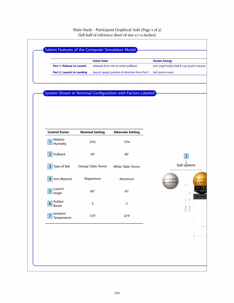
Initial State Kinetic Energy Potential Energy Losses Final State

Part 1: Release to Launch released from rest at initial pullback arm (rigid body); ball & cup (point masses) rubber band(s) (ideal spring); gravity none launch speed, position & direction

Part 2: Launch to Landing launch speed, position & direction from Part 1 ball (point mass) gravity aerodynamic drag; Magnus lift due to ball spin landing position

Salient Features of the Computer Simulation Model

Control Factor Nominal Setting Alternate Setting

RelativeHumidity1 25% 75%

Pullback2 30° 40°

Type of Ball3 Orange Table Tennis White Table Tennis

Arm Material4 Magnesium Aluminum

LaunchAngle5 60° 45°

RubberBands6 3 2

AmbientTemperature7 72°F 32°F

0°

15°

30°

45°

60°

75°90°

20°

40°

60°

80°

100°

120°

pullb

ack

pullback indicator

horizontal

launchangle

launch angle indicator

8.75 in

equival

entspr

ingfor

1 rubbe

r band

k =1.0

lbf/in,free

length

=1.5 in

9.81 in

0.5in

1.25

in

arm options Magnesium . ozAluminum . oz

d = 1.732 inm = 0.081 oz

d = 1.575 inm = 0.094 oz

ball options

d = 1.45 inm = 0.275 oz

2

3

4

5

6

SCALE=1/2

System Shown in Nominal Configuration with Factors Labeled

HYGROMETER

% relative humidity

0

10

20

30

40 50 60

70

80

90

100 THERMOMETER

°F temperature

-10

0

10

2030

40 50 6070

80

90

100

110

Environmental Conditions

1 7

Main Study - Participant Graphical Aids (Page 2 of 3)(le half of reference sheet of size 17×11 inches)

212

Initial State Kinetic Energy Potential Energy Losses Final State

Part 1: Release to Launch released from rest at initial pullback arm (rigid body); ball & cup (point masses) rubber band(s) (ideal spring); gravity none launch speed, position & direction

Part 2: Launch to Landing launch speed, position & direction from Part 1 ball (point mass) gravity aerodynamic drag; Magnus lift due to ball spin landing position

Salient Features of the Computer Simulation Model

Control Factor Nominal Setting Alternate Setting

RelativeHumidity1 25% 75%

Pullback2 30° 40°

Type of Ball3 Orange Table Tennis White Table Tennis

Arm Material4 Magnesium Aluminum

LaunchAngle5 60° 45°

RubberBands6 3 2

AmbientTemperature7 72°F 32°F

0°

15°

30°

45°

60°

75°90°

20°

40°

60°

80°

100°

120°

pullb

ack

pullback indicator

horizontal

launchangle

launch angle indicator

8.75 in

equival

entspr

ingfor

1 rubbe

r band

k =1.0

lbf/in,free

length

=1.5 in

9.81 in

0.5in

1.25

in

arm options Magnesium . ozAluminum . oz

d = 1.732 inm = 0.081 oz

d = 1.575 inm = 0.094 oz

ball options

d = 1.45 inm = 0.275 oz

2

3

4

5

6

SCALE=1/2

System Shown in Nominal Configuration with Factors Labeled

HYGROMETER

% relative humidity

0

10

20

30

40 50 60

70

80

90

100 THERMOMETER

°F temperature

-10

0

10

2030

40 50 6070

80

90

100

110

Environmental Conditions

1 7

Main Study - Participant Graphical Aids (Page 3 of 3)(right half of reference sheet of size 17×11 inches)

213


214

Main StudyInstructions & Design Table for Participants using aOFAT

(1 page)

215


216

Test Subject ID:

Instructions

In the adaptive one factor at a time (aOFAT) method, given the set of control factors and their possible settings, we:




(a) Select a new conguration by using the best previous conguration and changing only this factor’s setting to itsalternate value.


(c) If the performance improves at the new setting of this factor, keep it at this setting for the remainder of the experiment;otherwise, keep it at the original value for the remainder of the experiment.

. e conguration obtained aer stepping through each control factor is the optimized result for this design approach.

For the selected system, the Xpult catapult, we have identied seven control factors, each with two level settings of interest (i.e., a system). Using the aOFAT algorithm in this case requires eight trials (initial conguration plus one iteration for each controlfactor).

In this experiment, each trial is an evaluation of the system response (i.e., the ball’s landing position) using the computer simulationof the catapult. Use the aOFAT Design Table below with the above algorithm to nd an optimal conguration for the catapult ifthe objective is to hit a target of inches.

aOFATDesign Table >>> Target Landing Position = inches <<<Trial

RelativePullback

Type ofArmMaterial

Launch Rubber Ambient Landing PositionHumidity Table Tennis Ball Angle Bands Temperature (predicted) (simulation)

% ° Orange Magnesium ° °F . in

% ° Orange Magnesium ° °F

° Orange Magnesium ° °F

⋮ White Magnesium ° °F

⋮ ⋮ Aluminum ° °F

⋮ ⋮ ⋮ ° °F

⋮ ⋮ ⋮ ⋮ °F

⋮ ⋮ ⋮ ⋮ ⋮ °F

Best

Main Study - Instructions & Design Table for Participants using aOFAT

217


218

Main StudyInstructions & Design Table for Participants using PB-L8

(2 pages)

219


220

Test Subject ID:

Instructions

e objective here is to nd the combination of control factor settings that will result in the ball landing as close as possible tothe target distance of inches. is is a system (seven factors, each of which can be set at two possible values), so the totalnumber of unique combinations of control factors is = . Instead of testing the device at every possible combination, we testa small subset using orthogonal arrays to sample the design space. Orthogonality results in unique, non-redundant informationabout the system being learned in each trial. An appropriate set of arrays for a system is the Plackett-Burman L matrix, whichis shown below with random ordering of columns.

TrialControl Factor

X X X X X X X

− − − − − − − + − + − − + + + + + − + − − − + − − + + + + − − + + − + − − + + + + − − + + + − − + + + − + − + −

Here the "-" and "+" values indicate the "low" and "high" settings at which the control factors can be set. Note that "low" and"high" do not imply relative numerical values of the settings. In fact, each setting for the catapult system has been randomlyassigned to a "low" or "high" designation as shown in the table below.

Coded Relative Type of Launch Rubber AmbientSetting Humidity Pullback Table Tennis Ball ArmMaterial Angle Bands Temperature(X) (X) (X) (X) (X) (X) (X)− % ° Orange Magnesium ° °F+ % ° White Aluminum ° °F

Now if we evaluate the system response at the conguration shown in each row of the design matrix, we can create a simple linear

approximation of the system response

Y = β®average

+ βX + βX + βX + βX + βX + βX + βX´¹¹¹¹¹¹¹¹¹¹¹¹¹¹¹¹¹¹¹¹¹¹¹¹¹¹¹¹¹¹¹¹¹¹¹¹¹¹¹¹¹¹¹¹¹¹¹¹¹¹¹¹¹¹¹¹¹¹¹¹¹¹¹¹¹¹¹¹¹¹¹¹¹¹¹¹¹¹¹¹¹¹¹¹¹¹¹¹¹¹¹¹¹¹¹¹¹¹¹¹¹¹¹¹¹¹¹¹¹¹¹¹¹¹¹¹¹¹¹¹¹¹¹¹¹¹¹¹¹¹¹¹¹¹¹¹¹¹¹¹¹¹¹¹¹¹¹¹¹¹¹¹¹¹¹¹¹¹¹¹¸¹¹¹¹¹¹¹¹¹¹¹¹¹¹¹¹¹¹¹¹¹¹¹¹¹¹¹¹¹¹¹¹¹¹¹¹¹¹¹¹¹¹¹¹¹¹¹¹¹¹¹¹¹¹¹¹¹¹¹¹¹¹¹¹¹¹¹¹¹¹¹¹¹¹¹¹¹¹¹¹¹¹¹¹¹¹¹¹¹¹¹¹¹¹¹¹¹¹¹¹¹¹¹¹¹¹¹¹¹¹¹¹¹¹¹¹¹¹¹¹¹¹¹¹¹¹¹¹¹¹¹¹¹¹¹¹¹¹¹¹¹¹¹¹¹¹¹¹¹¹¹¹¹¹¹¹¹¹¹¹¶main effects

()

where Y is the estimate of the landing position Y in inches, and the X i values are each set at either − or +. Because the orthogonalarrays have the property of being balanced (each control factor setting appears in the same number of trials, ), we may calculate

the coecients in the above equation as

β =

∑j= Yj (Grand Mean) ()

βi =

⎧⎪⎪⎪⎪⎪⎪⎪⎩ ∑

j∣X i=+Yj −

∑j∣X i=−

Yj

⎫⎪⎪⎪⎪⎪⎪⎪⎭ (Main Eects) ()

Main Study - Instructions & Design Table for Participants using PB-L8 (Page 1 of 2)

221

Test Subject ID:

Note that subscript i refers to control factor number and subscript j refers to trial number. Once the coecients β − β areknown, we can use Equation to estimate the response at the system congurations that were not tested, allowing us to identifyone with performance close to the design goal.

e task in this experiment is therefore to

. Evaluate the system response at each of the required congurations in the design table, using the Predict-Observe-Explainformat for each trial.

. Use Equations and to calculate the coecients of the linear approximation of the system response. Note that a worksheetand basic calculator are provided to help with this step.

. Use Equation , repeated below the design table for convenience, to nd a combination of control factors that will result in asystem response close to the target value. Again, the calculator is provided for this.

. When an appropriate system conguration has been identied, record it at the bottom of the design table and evaluate thesystem response at this conguration to conrm that the actual response is close to the value predicted by the linear model.

PB-L Design Table >>> Target Landing Position = inches <<<Relative Launch Rubber Ambient Landing Position

Trial Humidity Pullback Type of Ball ArmMaterial Angle Bands Temperature (prediction) (simulation)(X) (X) (X) (X) (X) (X) (X) (Y) –% –° –Orange –Magnesium –° – –°F . in

+% –° + White –Magnesium –° + +°F

+% +° + White –Magnesium +° – –°F

–% +° –Orange –Magnesium +° + +°F

+% –° –Orange + Aluminum +° – +°F

–% –° + White + Aluminum +° + –°F

–% +° + White + Aluminum –° – +°F

+% +° –Orange + Aluminum –° + –°F

Best

Y = ´¹¹¹¹¹¹¹¹¹¹¹¹¹¹¹¸¹¹¹¹¹¹¹¹¹¹¹¹¹¹¶β

+´¹¹¹¹¹¹¹¹¹¹¹¹¹¹¹¸¹¹¹¹¹¹¹¹¹¹¹¹¹¹¶β

X + ´¹¹¹¹¹¹¹¹¹¹¹¹¹¹¹¸¹¹¹¹¹¹¹¹¹¹¹¹¹¹¶β

X + ´¹¹¹¹¹¹¹¹¹¹¹¹¹¹¹¸¹¹¹¹¹¹¹¹¹¹¹¹¹¹¶β

X + ´¹¹¹¹¹¹¹¹¹¹¹¹¹¹¹¸¹¹¹¹¹¹¹¹¹¹¹¹¹¹¶β

X + ´¹¹¹¹¹¹¹¹¹¹¹¹¹¹¹¸¹¹¹¹¹¹¹¹¹¹¹¹¹¹¶β

X + ´¹¹¹¹¹¹¹¹¹¹¹¹¹¹¹¸¹¹¹¹¹¹¹¹¹¹¹¹¹¹¶β

X + ´¹¹¹¹¹¹¹¹¹¹¹¹¹¹¹¸¹¹¹¹¹¹¹¹¹¹¹¹¹¹¶β

X

Main Study - Instructions & Design Table for Participants using PB-L8 (Page 2 of 2)

222

Main StudyTabulated Simulation Results

(3 pages)

223


224

Table : Full Factorial Results for Catapult Simulation

TrialRelative



% ° Orange Magnesium ° °F . in BOTH-1

% ° Orange Magnesium ° °F . in % ° Orange Magnesium ° °F . in % ° Orange Magnesium ° °F . in % ° Orange Magnesium ° °F . in % ° Orange Magnesium ° °F . in % ° Orange Magnesium ° °F . in % ° Orange Magnesium ° °F . in

% ° Orange Aluminum ° °F . in % ° Orange Aluminum ° °F . in % ° Orange Aluminum ° °F . in % ° Orange Aluminum ° °F . in % ° Orange Aluminum ° °F . in % ° Orange Aluminum ° °F . in % ° Orange Aluminum ° °F . in % ° Orange Aluminum ° °F . in % ° White Magnesium ° °F . in % ° White Magnesium ° °F . in % ° White Magnesium ° °F . in % ° White Magnesium ° °F . in % ° White Magnesium ° °F . in % ° White Magnesium ° °F . in % ° White Magnesium ° °F . in % ° White Magnesium ° °F . in

% ° White Aluminum ° °F . in % ° White Aluminum ° °F . in % ° White Aluminum ° °F . in % ° White Aluminum ° °F . in % ° White Aluminum ° °F . in % ° White Aluminum ° °F . in % ° White Aluminum ° °F . in PBL8-6

% ° White Aluminum ° °F . in % ° Orange Magnesium ° °F . in % ° Orange Magnesium ° °F . in % ° Orange Magnesium ° °F . in % ° Orange Magnesium ° °F . in % ° Orange Magnesium ° °F . in % ° Orange Magnesium ° °F . in % ° Orange Magnesium ° °F . in % ° Orange Magnesium ° °F . in PBL8-4

% ° Orange Aluminum ° °F . in % ° Orange Aluminum ° °F . in % ° Orange Aluminum ° °F . in

viii

Main Study - Tabulated Simulation Results (Page 1 of 3)

225


TrialRelative



% ° Orange Aluminum ° °F . in % ° Orange Aluminum ° °F . in % ° Orange Aluminum ° °F . in % ° Orange Aluminum ° °F . in % ° Orange Aluminum ° °F . in % ° White Magnesium ° °F . in % ° White Magnesium ° °F . in % ° White Magnesium ° °F . in % ° White Magnesium ° °F . in % ° White Magnesium ° °F . in % ° White Magnesium ° °F . in % ° White Magnesium ° °F . in % ° White Magnesium ° °F . in % ° White Aluminum ° °F . in % ° White Aluminum ° °F . in PBL8-7

% ° White Aluminum ° °F . in % ° White Aluminum ° °F . in % ° White Aluminum ° °F . in % ° White Aluminum ° °F . in % ° White Aluminum ° °F . in % ° White Aluminum ° °F . in % ° Orange Magnesium ° °F . in OFAT-2

% ° Orange Magnesium ° °F . in % ° Orange Magnesium ° °F . in % ° Orange Magnesium ° °F . in % ° Orange Magnesium ° °F . in % ° Orange Magnesium ° °F . in % ° Orange Magnesium ° °F . in % ° Orange Magnesium ° °F . in % ° Orange Aluminum ° °F . in % ° Orange Aluminum ° °F . in % ° Orange Aluminum ° °F . in % ° Orange Aluminum ° °F . in % ° Orange Aluminum ° °F . in % ° Orange Aluminum ° °F . in PBL8-5

% ° Orange Aluminum ° °F . in % ° Orange Aluminum ° °F . in % ° White Magnesium ° °F . in % ° White Magnesium ° °F . in % ° White Magnesium ° °F . in % ° White Magnesium ° °F . in PBL8-2

% ° White Magnesium ° °F . in % ° White Magnesium ° °F . in

ix


226


TrialRelative



% ° White Magnesium ° °F . in % ° White Magnesium ° °F . in % ° White Aluminum ° °F . in % ° White Aluminum ° °F . in % ° White Aluminum ° °F . in % ° White Aluminum ° °F . in % ° White Aluminum ° °F . in % ° White Aluminum ° °F . in % ° White Aluminum ° °F . in % ° White Aluminum ° °F . in % ° Orange Magnesium ° °F . in OFAT-3

% ° Orange Magnesium ° °F . in OFAT-8

% ° Orange Magnesium ° °F . in OFAT-7

% ° Orange Magnesium ° °F . in % ° Orange Magnesium ° °F . in OFAT-6

% ° Orange Magnesium ° °F . in % ° Orange Magnesium ° °F . in % ° Orange Magnesium ° °F . in % ° Orange Aluminum ° °F . in OFAT-5

% ° Orange Aluminum ° °F . in % ° Orange Aluminum ° °F . in PBL8-8

% ° Orange Aluminum ° °F . in % ° Orange Aluminum ° °F . in % ° Orange Aluminum ° °F . in % ° Orange Aluminum ° °F . in % ° Orange Aluminum ° °F . in % ° White Magnesium ° °F . in OFAT-4

% ° White Magnesium ° °F . in % ° White Magnesium ° °F . in % ° White Magnesium ° °F . in % ° White Magnesium ° °F . in PBL8-3

% ° White Magnesium ° °F . in % ° White Magnesium ° °F . in % ° White Magnesium ° °F . in % ° White Aluminum ° °F . in % ° White Aluminum ° °F . in % ° White Aluminum ° °F . in % ° White Aluminum ° °F . in % ° White Aluminum ° °F . in % ° White Aluminum ° °F . in % ° White Aluminum ° °F . in % ° White Aluminum ° °F . in

x


227


228

Main StudyWorksheet for Participants using PB-L8

(2 pages)

229


230



β = ( + + + + + + + )´¹¹¹¹¹¹¹¹¹¹¹¹¹¹¹¹¹¹¹¹¹¹¹¹¹¹¹¹¹¹¹¹¹¹¹¹¹¹¹¹¹¹¹¹¹¹¹¹¹¹¹¹¹¹¹¹¹¹¹¹¹¹¹¹¹¹¹¹¹¹¹¹¹¹¹¹¹¹¹¹¹¹¹¹¹¹¹¹¹¹¹¹¹¹¹¹¹¹¹¹¹¹¹¹¹¹¹¹¹¹¹¹¹¹¹¹¹¹¹¹¹¹¹¹¹¹¹¹¹¹¹¹¹¹¹¹¹¹¹¹¹¹¹¹¹¹¹¹¹¹¹¹¹¹¹¹¹¹¹¹¹¹¹¹¹¹¹¹¹¹¹¹¹¹¹¹¹¹¹¹¹¹¹¹¹¹¹¹¹¹¹¹¹¹¹¹¹¹¹¹¹¹¹¹¹¹¹¹¹¹¹¹¹¹¹¹¹¹¹¹¹¹¹¹¹¹¹¹¹¹¹¹¹¹¹¹¹¹¹¹¹¹¹¹¹¹¹¹¹¹¹¹¹¹¹¹¹¹¹¹¹¹¹¹¹¹¹¹¹¹¹¹¹¹¹¹¹¹¹¹¹¹¹¹¹¹¹¹¹¹¹¹¹¹¹¹¹¹¹¹¹¹¹¹¹¹¹¹¹¹¹¹¹¹¹¹¹¹¹¹¹¹¹¹¹¹¸¹¹¹¹¹¹¹¹¹¹¹¹¹¹¹¹¹¹¹¹¹¹¹¹¹¹¹¹¹¹¹¹¹¹¹¹¹¹¹¹¹¹¹¹¹¹¹¹¹¹¹¹¹¹¹¹¹¹¹¹¹¹¹¹¹¹¹¹¹¹¹¹¹¹¹¹¹¹¹¹¹¹¹¹¹¹¹¹¹¹¹¹¹¹¹¹¹¹¹¹¹¹¹¹¹¹¹¹¹¹¹¹¹¹¹¹¹¹¹¹¹¹¹¹¹¹¹¹¹¹¹¹¹¹¹¹¹¹¹¹¹¹¹¹¹¹¹¹¹¹¹¹¹¹¹¹¹¹¹¹¹¹¹¹¹¹¹¹¹¹¹¹¹¹¹¹¹¹¹¹¹¹¹¹¹¹¹¹¹¹¹¹¹¹¹¹¹¹¹¹¹¹¹¹¹¹¹¹¹¹¹¹¹¹¹¹¹¹¹¹¹¹¹¹¹¹¹¹¹¹¹¹¹¹¹¹¹¹¹¹¹¹¹¹¹¹¹¹¹¹¹¹¹¹¹¹¹¹¹¹¹¹¹¹¹¹¹¹¹¹¹¹¹¹¹¹¹¹¹¹¹¹¹¹¹¹¹¹¹¹¹¹¹¹¹¹¹¹¹¹¹¹¹¹¹¹¹¹¹¹¹¹¹¹¹¹¹¹¹¹¹¹¹¹¹¶

mean value over all trials

β =

. Relative Humidity

β =

⎧⎪⎪⎪⎪⎪⎪⎪⎩( + + + )´¹¹¹¹¹¹¹¹¹¹¹¹¹¹¹¹¹¹¹¹¹¹¹¹¹¹¹¹¹¹¹¹¹¹¹¹¹¹¹¹¹¹¹¹¹¹¹¹¹¹¹¹¹¹¹¹¹¹¹¹¹¹¹¹¹¹¹¹¹¹¹¹¹¹¹¹¹¹¹¹¹¹¹¹¹¹¹¹¹¹¹¹¹¹¹¹¹¹¹¹¹¹¹¹¹¹¹¹¹¹¹¹¹¹¹¹¹¹¹¹¹¹¹¹¹¹¹¹¹¹¹¹¹¹¹¹¹¹¹¹¹¹¹¹¹¹¹¹¹¹¹¹¹¹¹¹¹¹¸¹¹¹¹¹¹¹¹¹¹¹¹¹¹¹¹¹¹¹¹¹¹¹¹¹¹¹¹¹¹¹¹¹¹¹¹¹¹¹¹¹¹¹¹¹¹¹¹¹¹¹¹¹¹¹¹¹¹¹¹¹¹¹¹¹¹¹¹¹¹¹¹¹¹¹¹¹¹¹¹¹¹¹¹¹¹¹¹¹¹¹¹¹¹¹¹¹¹¹¹¹¹¹¹¹¹¹¹¹¹¹¹¹¹¹¹¹¹¹¹¹¹¹¹¹¹¹¹¹¹¹¹¹¹¹¹¹¹¹¹¹¹¹¹¹¹¹¹¹¹¹¹¹¹¹¹¹¶

mean response at "+" setting (%)

− ( + + + )´¹¹¹¹¹¹¹¹¹¹¹¹¹¹¹¹¹¹¹¹¹¹¹¹¹¹¹¹¹¹¹¹¹¹¹¹¹¹¹¹¹¹¹¹¹¹¹¹¹¹¹¹¹¹¹¹¹¹¹¹¹¹¹¹¹¹¹¹¹¹¹¹¹¹¹¹¹¹¹¹¹¹¹¹¹¹¹¹¹¹¹¹¹¹¹¹¹¹¹¹¹¹¹¹¹¹¹¹¹¹¹¹¹¹¹¹¹¹¹¹¹¹¹¹¹¹¹¹¹¹¹¹¹¹¹¹¹¹¹¹¹¹¹¹¹¹¹¹¹¹¹¹¹¹¹¹¹¹¸¹¹¹¹¹¹¹¹¹¹¹¹¹¹¹¹¹¹¹¹¹¹¹¹¹¹¹¹¹¹¹¹¹¹¹¹¹¹¹¹¹¹¹¹¹¹¹¹¹¹¹¹¹¹¹¹¹¹¹¹¹¹¹¹¹¹¹¹¹¹¹¹¹¹¹¹¹¹¹¹¹¹¹¹¹¹¹¹¹¹¹¹¹¹¹¹¹¹¹¹¹¹¹¹¹¹¹¹¹¹¹¹¹¹¹¹¹¹¹¹¹¹¹¹¹¹¹¹¹¹¹¹¹¹¹¹¹¹¹¹¹¹¹¹¹¹¹¹¹¹¹¹¹¹¹¹¹¶

mean response at "-" setting (%)

⎫⎪⎪⎪⎪⎪⎪⎪⎭=

⎧⎪⎪⎪⎪⎪⎪⎪⎩ − ⎫⎪⎪⎪⎪⎪⎪⎪⎭β =

. Pullback

β =

⎧⎪⎪⎪⎪⎪⎪⎪⎩( + + + )´¹¹¹¹¹¹¹¹¹¹¹¹¹¹¹¹¹¹¹¹¹¹¹¹¹¹¹¹¹¹¹¹¹¹¹¹¹¹¹¹¹¹¹¹¹¹¹¹¹¹¹¹¹¹¹¹¹¹¹¹¹¹¹¹¹¹¹¹¹¹¹¹¹¹¹¹¹¹¹¹¹¹¹¹¹¹¹¹¹¹¹¹¹¹¹¹¹¹¹¹¹¹¹¹¹¹¹¹¹¹¹¹¹¹¹¹¹¹¹¹¹¹¹¹¹¹¹¹¹¹¹¹¹¹¹¹¹¹¹¹¹¹¹¹¹¹¹¹¹¹¹¹¹¹¹¹¹¹¸¹¹¹¹¹¹¹¹¹¹¹¹¹¹¹¹¹¹¹¹¹¹¹¹¹¹¹¹¹¹¹¹¹¹¹¹¹¹¹¹¹¹¹¹¹¹¹¹¹¹¹¹¹¹¹¹¹¹¹¹¹¹¹¹¹¹¹¹¹¹¹¹¹¹¹¹¹¹¹¹¹¹¹¹¹¹¹¹¹¹¹¹¹¹¹¹¹¹¹¹¹¹¹¹¹¹¹¹¹¹¹¹¹¹¹¹¹¹¹¹¹¹¹¹¹¹¹¹¹¹¹¹¹¹¹¹¹¹¹¹¹¹¹¹¹¹¹¹¹¹¹¹¹¹¹¹¹¶


− ( + + + )´¹¹¹¹¹¹¹¹¹¹¹¹¹¹¹¹¹¹¹¹¹¹¹¹¹¹¹¹¹¹¹¹¹¹¹¹¹¹¹¹¹¹¹¹¹¹¹¹¹¹¹¹¹¹¹¹¹¹¹¹¹¹¹¹¹¹¹¹¹¹¹¹¹¹¹¹¹¹¹¹¹¹¹¹¹¹¹¹¹¹¹¹¹¹¹¹¹¹¹¹¹¹¹¹¹¹¹¹¹¹¹¹¹¹¹¹¹¹¹¹¹¹¹¹¹¹¹¹¹¹¹¹¹¹¹¹¹¹¹¹¹¹¹¹¹¹¹¹¹¹¹¹¹¹¹¹¹¹¸¹¹¹¹¹¹¹¹¹¹¹¹¹¹¹¹¹¹¹¹¹¹¹¹¹¹¹¹¹¹¹¹¹¹¹¹¹¹¹¹¹¹¹¹¹¹¹¹¹¹¹¹¹¹¹¹¹¹¹¹¹¹¹¹¹¹¹¹¹¹¹¹¹¹¹¹¹¹¹¹¹¹¹¹¹¹¹¹¹¹¹¹¹¹¹¹¹¹¹¹¹¹¹¹¹¹¹¹¹¹¹¹¹¹¹¹¹¹¹¹¹¹¹¹¹¹¹¹¹¹¹¹¹¹¹¹¹¹¹¹¹¹¹¹¹¹¹¹¹¹¹¹¹¹¹¹¹¶


⎫⎪⎪⎪⎪⎪⎪⎪⎭=

⎧⎪⎪⎪⎪⎪⎪⎪⎩ − ⎫⎪⎪⎪⎪⎪⎪⎪⎭β =

. Type of Ball

β =

⎧⎪⎪⎪⎪⎪⎪⎪⎩( + + + )´¹¹¹¹¹¹¹¹¹¹¹¹¹¹¹¹¹¹¹¹¹¹¹¹¹¹¹¹¹¹¹¹¹¹¹¹¹¹¹¹¹¹¹¹¹¹¹¹¹¹¹¹¹¹¹¹¹¹¹¹¹¹¹¹¹¹¹¹¹¹¹¹¹¹¹¹¹¹¹¹¹¹¹¹¹¹¹¹¹¹¹¹¹¹¹¹¹¹¹¹¹¹¹¹¹¹¹¹¹¹¹¹¹¹¹¹¹¹¹¹¹¹¹¹¹¹¹¹¹¹¹¹¹¹¹¹¹¹¹¹¹¹¹¹¹¹¹¹¹¹¹¹¹¹¹¹¹¹¸¹¹¹¹¹¹¹¹¹¹¹¹¹¹¹¹¹¹¹¹¹¹¹¹¹¹¹¹¹¹¹¹¹¹¹¹¹¹¹¹¹¹¹¹¹¹¹¹¹¹¹¹¹¹¹¹¹¹¹¹¹¹¹¹¹¹¹¹¹¹¹¹¹¹¹¹¹¹¹¹¹¹¹¹¹¹¹¹¹¹¹¹¹¹¹¹¹¹¹¹¹¹¹¹¹¹¹¹¹¹¹¹¹¹¹¹¹¹¹¹¹¹¹¹¹¹¹¹¹¹¹¹¹¹¹¹¹¹¹¹¹¹¹¹¹¹¹¹¹¹¹¹¹¹¹¹¹¶

mean response at "+" setting (White)

− ( + + + )´¹¹¹¹¹¹¹¹¹¹¹¹¹¹¹¹¹¹¹¹¹¹¹¹¹¹¹¹¹¹¹¹¹¹¹¹¹¹¹¹¹¹¹¹¹¹¹¹¹¹¹¹¹¹¹¹¹¹¹¹¹¹¹¹¹¹¹¹¹¹¹¹¹¹¹¹¹¹¹¹¹¹¹¹¹¹¹¹¹¹¹¹¹¹¹¹¹¹¹¹¹¹¹¹¹¹¹¹¹¹¹¹¹¹¹¹¹¹¹¹¹¹¹¹¹¹¹¹¹¹¹¹¹¹¹¹¹¹¹¹¹¹¹¹¹¹¹¹¹¹¹¹¹¹¹¹¹¹¸¹¹¹¹¹¹¹¹¹¹¹¹¹¹¹¹¹¹¹¹¹¹¹¹¹¹¹¹¹¹¹¹¹¹¹¹¹¹¹¹¹¹¹¹¹¹¹¹¹¹¹¹¹¹¹¹¹¹¹¹¹¹¹¹¹¹¹¹¹¹¹¹¹¹¹¹¹¹¹¹¹¹¹¹¹¹¹¹¹¹¹¹¹¹¹¹¹¹¹¹¹¹¹¹¹¹¹¹¹¹¹¹¹¹¹¹¹¹¹¹¹¹¹¹¹¹¹¹¹¹¹¹¹¹¹¹¹¹¹¹¹¹¹¹¹¹¹¹¹¹¹¹¹¹¹¹¹¶

mean response at "-" setting (Orange)

⎫⎪⎪⎪⎪⎪⎪⎪⎭=

⎧⎪⎪⎪⎪⎪⎪⎪⎩ − ⎫⎪⎪⎪⎪⎪⎪⎪⎭β =

Main Study - Worksheet for Participants using PB-L8 (Page 1 of 2)

231


. ArmMaterial

β =

⎧⎪⎪⎪⎪⎪⎪⎪⎩( + + + )´¹¹¹¹¹¹¹¹¹¹¹¹¹¹¹¹¹¹¹¹¹¹¹¹¹¹¹¹¹¹¹¹¹¹¹¹¹¹¹¹¹¹¹¹¹¹¹¹¹¹¹¹¹¹¹¹¹¹¹¹¹¹¹¹¹¹¹¹¹¹¹¹¹¹¹¹¹¹¹¹¹¹¹¹¹¹¹¹¹¹¹¹¹¹¹¹¹¹¹¹¹¹¹¹¹¹¹¹¹¹¹¹¹¹¹¹¹¹¹¹¹¹¹¹¹¹¹¹¹¹¹¹¹¹¹¹¹¹¹¹¹¹¹¹¹¹¹¹¹¹¹¹¹¹¹¹¹¹¸¹¹¹¹¹¹¹¹¹¹¹¹¹¹¹¹¹¹¹¹¹¹¹¹¹¹¹¹¹¹¹¹¹¹¹¹¹¹¹¹¹¹¹¹¹¹¹¹¹¹¹¹¹¹¹¹¹¹¹¹¹¹¹¹¹¹¹¹¹¹¹¹¹¹¹¹¹¹¹¹¹¹¹¹¹¹¹¹¹¹¹¹¹¹¹¹¹¹¹¹¹¹¹¹¹¹¹¹¹¹¹¹¹¹¹¹¹¹¹¹¹¹¹¹¹¹¹¹¹¹¹¹¹¹¹¹¹¹¹¹¹¹¹¹¹¹¹¹¹¹¹¹¹¹¹¹¹¶

mean response at "+" setting ( Aluminum)

− ( + + + )´¹¹¹¹¹¹¹¹¹¹¹¹¹¹¹¹¹¹¹¹¹¹¹¹¹¹¹¹¹¹¹¹¹¹¹¹¹¹¹¹¹¹¹¹¹¹¹¹¹¹¹¹¹¹¹¹¹¹¹¹¹¹¹¹¹¹¹¹¹¹¹¹¹¹¹¹¹¹¹¹¹¹¹¹¹¹¹¹¹¹¹¹¹¹¹¹¹¹¹¹¹¹¹¹¹¹¹¹¹¹¹¹¹¹¹¹¹¹¹¹¹¹¹¹¹¹¹¹¹¹¹¹¹¹¹¹¹¹¹¹¹¹¹¹¹¹¹¹¹¹¹¹¹¹¹¹¹¹¸¹¹¹¹¹¹¹¹¹¹¹¹¹¹¹¹¹¹¹¹¹¹¹¹¹¹¹¹¹¹¹¹¹¹¹¹¹¹¹¹¹¹¹¹¹¹¹¹¹¹¹¹¹¹¹¹¹¹¹¹¹¹¹¹¹¹¹¹¹¹¹¹¹¹¹¹¹¹¹¹¹¹¹¹¹¹¹¹¹¹¹¹¹¹¹¹¹¹¹¹¹¹¹¹¹¹¹¹¹¹¹¹¹¹¹¹¹¹¹¹¹¹¹¹¹¹¹¹¹¹¹¹¹¹¹¹¹¹¹¹¹¹¹¹¹¹¹¹¹¹¹¹¹¹¹¹¹¶

mean response at "-" setting (Magnesium)

⎫⎪⎪⎪⎪⎪⎪⎪⎭=

⎧⎪⎪⎪⎪⎪⎪⎪⎩ − ⎫⎪⎪⎪⎪⎪⎪⎪⎭β =

. Launch Angle

β =

⎧⎪⎪⎪⎪⎪⎪⎪⎩( + + + )´¹¹¹¹¹¹¹¹¹¹¹¹¹¹¹¹¹¹¹¹¹¹¹¹¹¹¹¹¹¹¹¹¹¹¹¹¹¹¹¹¹¹¹¹¹¹¹¹¹¹¹¹¹¹¹¹¹¹¹¹¹¹¹¹¹¹¹¹¹¹¹¹¹¹¹¹¹¹¹¹¹¹¹¹¹¹¹¹¹¹¹¹¹¹¹¹¹¹¹¹¹¹¹¹¹¹¹¹¹¹¹¹¹¹¹¹¹¹¹¹¹¹¹¹¹¹¹¹¹¹¹¹¹¹¹¹¹¹¹¹¹¹¹¹¹¹¹¹¹¹¹¹¹¹¹¹¹¹¸¹¹¹¹¹¹¹¹¹¹¹¹¹¹¹¹¹¹¹¹¹¹¹¹¹¹¹¹¹¹¹¹¹¹¹¹¹¹¹¹¹¹¹¹¹¹¹¹¹¹¹¹¹¹¹¹¹¹¹¹¹¹¹¹¹¹¹¹¹¹¹¹¹¹¹¹¹¹¹¹¹¹¹¹¹¹¹¹¹¹¹¹¹¹¹¹¹¹¹¹¹¹¹¹¹¹¹¹¹¹¹¹¹¹¹¹¹¹¹¹¹¹¹¹¹¹¹¹¹¹¹¹¹¹¹¹¹¹¹¹¹¹¹¹¹¹¹¹¹¹¹¹¹¹¹¹¹¶


− ( + + + )´¹¹¹¹¹¹¹¹¹¹¹¹¹¹¹¹¹¹¹¹¹¹¹¹¹¹¹¹¹¹¹¹¹¹¹¹¹¹¹¹¹¹¹¹¹¹¹¹¹¹¹¹¹¹¹¹¹¹¹¹¹¹¹¹¹¹¹¹¹¹¹¹¹¹¹¹¹¹¹¹¹¹¹¹¹¹¹¹¹¹¹¹¹¹¹¹¹¹¹¹¹¹¹¹¹¹¹¹¹¹¹¹¹¹¹¹¹¹¹¹¹¹¹¹¹¹¹¹¹¹¹¹¹¹¹¹¹¹¹¹¹¹¹¹¹¹¹¹¹¹¹¹¹¹¹¹¹¹¸¹¹¹¹¹¹¹¹¹¹¹¹¹¹¹¹¹¹¹¹¹¹¹¹¹¹¹¹¹¹¹¹¹¹¹¹¹¹¹¹¹¹¹¹¹¹¹¹¹¹¹¹¹¹¹¹¹¹¹¹¹¹¹¹¹¹¹¹¹¹¹¹¹¹¹¹¹¹¹¹¹¹¹¹¹¹¹¹¹¹¹¹¹¹¹¹¹¹¹¹¹¹¹¹¹¹¹¹¹¹¹¹¹¹¹¹¹¹¹¹¹¹¹¹¹¹¹¹¹¹¹¹¹¹¹¹¹¹¹¹¹¹¹¹¹¹¹¹¹¹¹¹¹¹¹¹¹¶


⎫⎪⎪⎪⎪⎪⎪⎪⎭=

⎧⎪⎪⎪⎪⎪⎪⎪⎩ − ⎫⎪⎪⎪⎪⎪⎪⎪⎭β =


β =

⎧⎪⎪⎪⎪⎪⎪⎪⎩( + + + )´¹¹¹¹¹¹¹¹¹¹¹¹¹¹¹¹¹¹¹¹¹¹¹¹¹¹¹¹¹¹¹¹¹¹¹¹¹¹¹¹¹¹¹¹¹¹¹¹¹¹¹¹¹¹¹¹¹¹¹¹¹¹¹¹¹¹¹¹¹¹¹¹¹¹¹¹¹¹¹¹¹¹¹¹¹¹¹¹¹¹¹¹¹¹¹¹¹¹¹¹¹¹¹¹¹¹¹¹¹¹¹¹¹¹¹¹¹¹¹¹¹¹¹¹¹¹¹¹¹¹¹¹¹¹¹¹¹¹¹¹¹¹¹¹¹¹¹¹¹¹¹¹¹¹¹¹¹¹¸¹¹¹¹¹¹¹¹¹¹¹¹¹¹¹¹¹¹¹¹¹¹¹¹¹¹¹¹¹¹¹¹¹¹¹¹¹¹¹¹¹¹¹¹¹¹¹¹¹¹¹¹¹¹¹¹¹¹¹¹¹¹¹¹¹¹¹¹¹¹¹¹¹¹¹¹¹¹¹¹¹¹¹¹¹¹¹¹¹¹¹¹¹¹¹¹¹¹¹¹¹¹¹¹¹¹¹¹¹¹¹¹¹¹¹¹¹¹¹¹¹¹¹¹¹¹¹¹¹¹¹¹¹¹¹¹¹¹¹¹¹¹¹¹¹¹¹¹¹¹¹¹¹¹¹¹¹¶

mean response at "+" setting ()

− ( + + + )´¹¹¹¹¹¹¹¹¹¹¹¹¹¹¹¹¹¹¹¹¹¹¹¹¹¹¹¹¹¹¹¹¹¹¹¹¹¹¹¹¹¹¹¹¹¹¹¹¹¹¹¹¹¹¹¹¹¹¹¹¹¹¹¹¹¹¹¹¹¹¹¹¹¹¹¹¹¹¹¹¹¹¹¹¹¹¹¹¹¹¹¹¹¹¹¹¹¹¹¹¹¹¹¹¹¹¹¹¹¹¹¹¹¹¹¹¹¹¹¹¹¹¹¹¹¹¹¹¹¹¹¹¹¹¹¹¹¹¹¹¹¹¹¹¹¹¹¹¹¹¹¹¹¹¹¹¹¹¸¹¹¹¹¹¹¹¹¹¹¹¹¹¹¹¹¹¹¹¹¹¹¹¹¹¹¹¹¹¹¹¹¹¹¹¹¹¹¹¹¹¹¹¹¹¹¹¹¹¹¹¹¹¹¹¹¹¹¹¹¹¹¹¹¹¹¹¹¹¹¹¹¹¹¹¹¹¹¹¹¹¹¹¹¹¹¹¹¹¹¹¹¹¹¹¹¹¹¹¹¹¹¹¹¹¹¹¹¹¹¹¹¹¹¹¹¹¹¹¹¹¹¹¹¹¹¹¹¹¹¹¹¹¹¹¹¹¹¹¹¹¹¹¹¹¹¹¹¹¹¹¹¹¹¹¹¹¶

mean response at "-" setting ()

⎫⎪⎪⎪⎪⎪⎪⎪⎭=

⎧⎪⎪⎪⎪⎪⎪⎪⎩ − ⎫⎪⎪⎪⎪⎪⎪⎪⎭β =


β =

⎧⎪⎪⎪⎪⎪⎪⎪⎩( + + + )´¹¹¹¹¹¹¹¹¹¹¹¹¹¹¹¹¹¹¹¹¹¹¹¹¹¹¹¹¹¹¹¹¹¹¹¹¹¹¹¹¹¹¹¹¹¹¹¹¹¹¹¹¹¹¹¹¹¹¹¹¹¹¹¹¹¹¹¹¹¹¹¹¹¹¹¹¹¹¹¹¹¹¹¹¹¹¹¹¹¹¹¹¹¹¹¹¹¹¹¹¹¹¹¹¹¹¹¹¹¹¹¹¹¹¹¹¹¹¹¹¹¹¹¹¹¹¹¹¹¹¹¹¹¹¹¹¹¹¹¹¹¹¹¹¹¹¹¹¹¹¹¹¹¹¹¹¹¹¸¹¹¹¹¹¹¹¹¹¹¹¹¹¹¹¹¹¹¹¹¹¹¹¹¹¹¹¹¹¹¹¹¹¹¹¹¹¹¹¹¹¹¹¹¹¹¹¹¹¹¹¹¹¹¹¹¹¹¹¹¹¹¹¹¹¹¹¹¹¹¹¹¹¹¹¹¹¹¹¹¹¹¹¹¹¹¹¹¹¹¹¹¹¹¹¹¹¹¹¹¹¹¹¹¹¹¹¹¹¹¹¹¹¹¹¹¹¹¹¹¹¹¹¹¹¹¹¹¹¹¹¹¹¹¹¹¹¹¹¹¹¹¹¹¹¹¹¹¹¹¹¹¹¹¹¹¹¶

mean response at "+" setting (°F)

− ( + + + )´¹¹¹¹¹¹¹¹¹¹¹¹¹¹¹¹¹¹¹¹¹¹¹¹¹¹¹¹¹¹¹¹¹¹¹¹¹¹¹¹¹¹¹¹¹¹¹¹¹¹¹¹¹¹¹¹¹¹¹¹¹¹¹¹¹¹¹¹¹¹¹¹¹¹¹¹¹¹¹¹¹¹¹¹¹¹¹¹¹¹¹¹¹¹¹¹¹¹¹¹¹¹¹¹¹¹¹¹¹¹¹¹¹¹¹¹¹¹¹¹¹¹¹¹¹¹¹¹¹¹¹¹¹¹¹¹¹¹¹¹¹¹¹¹¹¹¹¹¹¹¹¹¹¹¹¹¹¹¸¹¹¹¹¹¹¹¹¹¹¹¹¹¹¹¹¹¹¹¹¹¹¹¹¹¹¹¹¹¹¹¹¹¹¹¹¹¹¹¹¹¹¹¹¹¹¹¹¹¹¹¹¹¹¹¹¹¹¹¹¹¹¹¹¹¹¹¹¹¹¹¹¹¹¹¹¹¹¹¹¹¹¹¹¹¹¹¹¹¹¹¹¹¹¹¹¹¹¹¹¹¹¹¹¹¹¹¹¹¹¹¹¹¹¹¹¹¹¹¹¹¹¹¹¹¹¹¹¹¹¹¹¹¹¹¹¹¹¹¹¹¹¹¹¹¹¹¹¹¹¹¹¹¹¹¹¹¶

mean response at "-" setting (°F)

⎫⎪⎪⎪⎪⎪⎪⎪⎭=

⎧⎪⎪⎪⎪⎪⎪⎪⎩ − ⎫⎪⎪⎪⎪⎪⎪⎪⎭β =

Main Study - Worksheet for Participants using PB-L8 (Page 2 of 2)

232

Main StudyFilled-InWorksheet for Participants using PB-L8

(2 pages)

233


234


β = ( . + . + . + . + . + . + . + . )

)⌊⌊⌊⌊⌊⌊⌊⌊⌊⌊⌊⌊⌊⌊⌊⌊⌊⌊⌊⌊⌊⌊⌊⌊⌊⌊⌊⌊⌊⌊⌊⌊⌊⌊⌊⌊⌊⌊⌊⌊⌊⌊⌊⌊⌊⌊⌊⌊⌊⌊⌊⌊⌊⌊⌊⌊⌊⌊⌊⌊⌊⌊⌊⌊⌊⌊⌊⌊⌊⌊⌊⌊⌊⌊⌊⌊⌊⌊⌊⌊⌊⌊⌊⌊⌊⌊⌊⌊⌊⌊⌊⌊⌊⌊⌊⌊⌊⌊⌊⌊⌊⌊⌊⌊⌊⌊⌊⌊⌊⌊⌊⌊⌊⌊⌊⌊⌊⌊⌊⌊⌊⌊⌊⌊⌊⌊⌊⌊⌊⌊⌊⌊⌊⌊⌊⌊⌊⌊⌊⌊⌊⌊⌊⌊⌊⌊⌊⌊⌊⌊⌊⌊⌊⌊⌊⌊⌊⌊⌊⌊⌊⌊⌊⌊⌊⌊⌊⌊⌊⌊⌊⌊⌊⌊⌊⌊⌊⌊⌊⌊⌊⌊⌊⌊⌊⌊⌊⌊⌊⌊⌊⌊⌊⌊⌊⌊⌊⌊⌊⌊⌊⌊⌊⌊⌊⌊⌊⌊⌊⌊⌊⌊⌊⌊⌊⌊⌊⌊⌊⌊⌊⌊⌊⌊⌊⌊⌊⌊⌊⌊⌊⌊⌊⌊⌊⌊⌊⌊⌊⌊⌊⌊⌊⌊⌊⌊⌊⌊⌊⌊⌊⌊⌊⌊⌊⌊⌊⌊⌊⌊⌊⌊⌊⌊⌊⌊⌊⌊⌊⌊⌊⌊⌊⌊⌊⌊⌊⌊⌊⌊⌊⌊⌊⌊⌊⌊⌊⌊⌊⌊⌊⌊⌊⌊⌊⌊⌊⌊⌊⌊⌊⌊⌊⌊⌊⌊⌊⌊⌊⌊⌊⌊⌊⌊⌊⌊⌊⌊⌊⌊⌊⌊⌊⌊⌊⌊]⌊⌊⌊⌊⌊⌊⌊⌊⌊⌊⌊⌊⌊⌊⌊⌊⌊⌊⌊⌊⌊⌊⌊⌊⌊⌊⌊⌊⌊⌊⌊⌊⌊⌊⌊⌊⌊⌊⌊⌊⌊⌊⌊⌊⌊⌊⌊⌊⌊⌊⌊⌊⌊⌊⌊⌊⌊⌊⌊⌊⌊⌊⌊⌊⌊⌊⌊⌊⌊⌊⌊⌊⌊⌊⌊⌊⌊⌊⌊⌊⌊⌊⌊⌊⌊⌊⌊⌊⌊⌊⌊⌊⌊⌊⌊⌊⌊⌊⌊⌊⌊⌊⌊⌊⌊⌊⌊⌊⌊⌊⌊⌊⌊⌊⌊⌊⌊⌊⌊⌊⌊⌊⌊⌊⌊⌊⌊⌊⌊⌊⌊⌊⌊⌊⌊⌊⌊⌊⌊⌊⌊⌊⌊⌊⌊⌊⌊⌊⌊⌊⌊⌊⌊⌊⌊⌊⌊⌊⌊⌊⌊⌊⌊⌊⌊⌊⌊⌊⌊⌊⌊⌊⌊⌊⌊⌊⌊⌊⌊⌊⌊⌊⌊⌊⌊⌊⌊⌊⌊⌊⌊⌊⌊⌊⌊⌊⌊⌊⌊⌊⌊⌊⌊⌊⌊⌊⌊⌊⌊⌊⌊⌊⌊⌊⌊⌊⌊⌊⌊⌊⌊⌊⌊⌊⌊⌊⌊⌊⌊⌊⌊⌊⌊⌊⌊⌊⌊⌊⌊⌊⌊⌊⌊⌊⌊⌊⌊⌊⌊⌊⌊⌊⌊⌊⌊⌊⌊⌊⌊⌊⌊⌊⌊⌊⌊⌊⌊⌊⌊⌊⌊⌊⌊⌊⌊⌊⌊⌊⌊⌊⌊⌊⌊⌊⌊⌊⌊⌊⌊⌊⌊⌊⌊⌊⌊⌊⌊⌊⌊⌊⌊⌊⌊⌊⌊⌊⌊⌊⌊⌊⌊⌊⌊⌊⌊⌊⌊⌊⌊⌊⌊⌊⌊⌊⌊)mean value over all trials

β = .

. Relative Humidity

β =

)⌉⌉⌉⌉⌉⌉⌉]( . + . + . + . )

)⌊⌊⌊⌊⌊⌊⌊⌊⌊⌊⌊⌊⌊⌊⌊⌊⌊⌊⌊⌊⌊⌊⌊⌊⌊⌊⌊⌊⌊⌊⌊⌊⌊⌊⌊⌊⌊⌊⌊⌊⌊⌊⌊⌊⌊⌊⌊⌊⌊⌊⌊⌊⌊⌊⌊⌊⌊⌊⌊⌊⌊⌊⌊⌊⌊⌊⌊⌊⌊⌊⌊⌊⌊⌊⌊⌊⌊⌊⌊⌊⌊⌊⌊⌊⌊⌊⌊⌊⌊⌊⌊⌊⌊⌊⌊⌊⌊⌊⌊⌊⌊⌊⌊⌊⌊⌊⌊⌊⌊⌊⌊⌊⌊⌊⌊⌊⌊⌊⌊⌊⌊⌊⌊⌊⌊⌊⌊⌊⌊⌊⌊⌊⌊⌊⌊⌊⌊⌊⌊⌊⌊⌊⌊⌊⌊⌊⌊⌊⌊⌊⌊⌊⌊⌊⌊⌊⌊⌊]⌊⌊⌊⌊⌊⌊⌊⌊⌊⌊⌊⌊⌊⌊⌊⌊⌊⌊⌊⌊⌊⌊⌊⌊⌊⌊⌊⌊⌊⌊⌊⌊⌊⌊⌊⌊⌊⌊⌊⌊⌊⌊⌊⌊⌊⌊⌊⌊⌊⌊⌊⌊⌊⌊⌊⌊⌊⌊⌊⌊⌊⌊⌊⌊⌊⌊⌊⌊⌊⌊⌊⌊⌊⌊⌊⌊⌊⌊⌊⌊⌊⌊⌊⌊⌊⌊⌊⌊⌊⌊⌊⌊⌊⌊⌊⌊⌊⌊⌊⌊⌊⌊⌊⌊⌊⌊⌊⌊⌊⌊⌊⌊⌊⌊⌊⌊⌊⌊⌊⌊⌊⌊⌊⌊⌊⌊⌊⌊⌊⌊⌊⌊⌊⌊⌊⌊⌊⌊⌊⌊⌊⌊⌊⌊⌊⌊⌊⌊⌊⌊⌊⌊⌊⌊⌊⌊⌊)mean response at "+" setting (%)

− ( . + . + . + . )

)⌊⌊⌊⌊⌊⌊⌊⌊⌊⌊⌊⌊⌊⌊⌊⌊⌊⌊⌊⌊⌊⌊⌊⌊⌊⌊⌊⌊⌊⌊⌊⌊⌊⌊⌊⌊⌊⌊⌊⌊⌊⌊⌊⌊⌊⌊⌊⌊⌊⌊⌊⌊⌊⌊⌊⌊⌊⌊⌊⌊⌊⌊⌊⌊⌊⌊⌊⌊⌊⌊⌊⌊⌊⌊⌊⌊⌊⌊⌊⌊⌊⌊⌊⌊⌊⌊⌊⌊⌊⌊⌊⌊⌊⌊⌊⌊⌊⌊⌊⌊⌊⌊⌊⌊⌊⌊⌊⌊⌊⌊⌊⌊⌊⌊⌊⌊⌊⌊⌊⌊⌊⌊⌊⌊⌊⌊⌊⌊⌊⌊⌊⌊⌊⌊⌊⌊⌊⌊⌊⌊⌊⌊⌊⌊⌊⌊⌊⌊⌊⌊⌊⌊⌊⌊⌊⌊⌊⌊]⌊⌊⌊⌊⌊⌊⌊⌊⌊⌊⌊⌊⌊⌊⌊⌊⌊⌊⌊⌊⌊⌊⌊⌊⌊⌊⌊⌊⌊⌊⌊⌊⌊⌊⌊⌊⌊⌊⌊⌊⌊⌊⌊⌊⌊⌊⌊⌊⌊⌊⌊⌊⌊⌊⌊⌊⌊⌊⌊⌊⌊⌊⌊⌊⌊⌊⌊⌊⌊⌊⌊⌊⌊⌊⌊⌊⌊⌊⌊⌊⌊⌊⌊⌊⌊⌊⌊⌊⌊⌊⌊⌊⌊⌊⌊⌊⌊⌊⌊⌊⌊⌊⌊⌊⌊⌊⌊⌊⌊⌊⌊⌊⌊⌊⌊⌊⌊⌊⌊⌊⌊⌊⌊⌊⌊⌊⌊⌊⌊⌊⌊⌊⌊⌊⌊⌊⌊⌊⌊⌊⌊⌊⌊⌊⌊⌊⌊⌊⌊⌊⌊⌊⌊⌊⌊⌊⌊)mean response at "-" setting (%)

[⌉⌉⌉⌉⌉⌉⌉⌊=

)⌉⌉⌉⌉⌉⌉⌉] . − .[⌉⌉⌉⌉⌉⌉⌉⌊

β = .

. Pullback

β =

)⌉⌉⌉⌉⌉⌉⌉]( . + . + . + . )

)⌊⌊⌊⌊⌊⌊⌊⌊⌊⌊⌊⌊⌊⌊⌊⌊⌊⌊⌊⌊⌊⌊⌊⌊⌊⌊⌊⌊⌊⌊⌊⌊⌊⌊⌊⌊⌊⌊⌊⌊⌊⌊⌊⌊⌊⌊⌊⌊⌊⌊⌊⌊⌊⌊⌊⌊⌊⌊⌊⌊⌊⌊⌊⌊⌊⌊⌊⌊⌊⌊⌊⌊⌊⌊⌊⌊⌊⌊⌊⌊⌊⌊⌊⌊⌊⌊⌊⌊⌊⌊⌊⌊⌊⌊⌊⌊⌊⌊⌊⌊⌊⌊⌊⌊⌊⌊⌊⌊⌊⌊⌊⌊⌊⌊⌊⌊⌊⌊⌊⌊⌊⌊⌊⌊⌊⌊⌊⌊⌊⌊⌊⌊⌊⌊⌊⌊⌊⌊⌊⌊⌊⌊⌊⌊⌊⌊⌊⌊⌊⌊⌊⌊⌊⌊⌊⌊⌊⌊]⌊⌊⌊⌊⌊⌊⌊⌊⌊⌊⌊⌊⌊⌊⌊⌊⌊⌊⌊⌊⌊⌊⌊⌊⌊⌊⌊⌊⌊⌊⌊⌊⌊⌊⌊⌊⌊⌊⌊⌊⌊⌊⌊⌊⌊⌊⌊⌊⌊⌊⌊⌊⌊⌊⌊⌊⌊⌊⌊⌊⌊⌊⌊⌊⌊⌊⌊⌊⌊⌊⌊⌊⌊⌊⌊⌊⌊⌊⌊⌊⌊⌊⌊⌊⌊⌊⌊⌊⌊⌊⌊⌊⌊⌊⌊⌊⌊⌊⌊⌊⌊⌊⌊⌊⌊⌊⌊⌊⌊⌊⌊⌊⌊⌊⌊⌊⌊⌊⌊⌊⌊⌊⌊⌊⌊⌊⌊⌊⌊⌊⌊⌊⌊⌊⌊⌊⌊⌊⌊⌊⌊⌊⌊⌊⌊⌊⌊⌊⌊⌊⌊⌊⌊⌊⌊⌊⌊)mean response at "+" setting (°)

− ( . + . + . + . )

)⌊⌊⌊⌊⌊⌊⌊⌊⌊⌊⌊⌊⌊⌊⌊⌊⌊⌊⌊⌊⌊⌊⌊⌊⌊⌊⌊⌊⌊⌊⌊⌊⌊⌊⌊⌊⌊⌊⌊⌊⌊⌊⌊⌊⌊⌊⌊⌊⌊⌊⌊⌊⌊⌊⌊⌊⌊⌊⌊⌊⌊⌊⌊⌊⌊⌊⌊⌊⌊⌊⌊⌊⌊⌊⌊⌊⌊⌊⌊⌊⌊⌊⌊⌊⌊⌊⌊⌊⌊⌊⌊⌊⌊⌊⌊⌊⌊⌊⌊⌊⌊⌊⌊⌊⌊⌊⌊⌊⌊⌊⌊⌊⌊⌊⌊⌊⌊⌊⌊⌊⌊⌊⌊⌊⌊⌊⌊⌊⌊⌊⌊⌊⌊⌊⌊⌊⌊⌊⌊⌊⌊⌊⌊⌊⌊⌊⌊⌊⌊⌊⌊⌊⌊⌊⌊⌊⌊⌊]⌊⌊⌊⌊⌊⌊⌊⌊⌊⌊⌊⌊⌊⌊⌊⌊⌊⌊⌊⌊⌊⌊⌊⌊⌊⌊⌊⌊⌊⌊⌊⌊⌊⌊⌊⌊⌊⌊⌊⌊⌊⌊⌊⌊⌊⌊⌊⌊⌊⌊⌊⌊⌊⌊⌊⌊⌊⌊⌊⌊⌊⌊⌊⌊⌊⌊⌊⌊⌊⌊⌊⌊⌊⌊⌊⌊⌊⌊⌊⌊⌊⌊⌊⌊⌊⌊⌊⌊⌊⌊⌊⌊⌊⌊⌊⌊⌊⌊⌊⌊⌊⌊⌊⌊⌊⌊⌊⌊⌊⌊⌊⌊⌊⌊⌊⌊⌊⌊⌊⌊⌊⌊⌊⌊⌊⌊⌊⌊⌊⌊⌊⌊⌊⌊⌊⌊⌊⌊⌊⌊⌊⌊⌊⌊⌊⌊⌊⌊⌊⌊⌊⌊⌊⌊⌊⌊⌊)mean response at "-" setting (°)

[⌉⌉⌉⌉⌉⌉⌉⌊=

)⌉⌉⌉⌉⌉⌉⌉] . − .[⌉⌉⌉⌉⌉⌉⌉⌊

β = .

. Type of Ball

β =

)⌉⌉⌉⌉⌉⌉⌉]( . + . + . + . )

)⌊⌊⌊⌊⌊⌊⌊⌊⌊⌊⌊⌊⌊⌊⌊⌊⌊⌊⌊⌊⌊⌊⌊⌊⌊⌊⌊⌊⌊⌊⌊⌊⌊⌊⌊⌊⌊⌊⌊⌊⌊⌊⌊⌊⌊⌊⌊⌊⌊⌊⌊⌊⌊⌊⌊⌊⌊⌊⌊⌊⌊⌊⌊⌊⌊⌊⌊⌊⌊⌊⌊⌊⌊⌊⌊⌊⌊⌊⌊⌊⌊⌊⌊⌊⌊⌊⌊⌊⌊⌊⌊⌊⌊⌊⌊⌊⌊⌊⌊⌊⌊⌊⌊⌊⌊⌊⌊⌊⌊⌊⌊⌊⌊⌊⌊⌊⌊⌊⌊⌊⌊⌊⌊⌊⌊⌊⌊⌊⌊⌊⌊⌊⌊⌊⌊⌊⌊⌊⌊⌊⌊⌊⌊⌊⌊⌊⌊⌊⌊⌊⌊⌊⌊⌊⌊⌊⌊⌊]⌊⌊⌊⌊⌊⌊⌊⌊⌊⌊⌊⌊⌊⌊⌊⌊⌊⌊⌊⌊⌊⌊⌊⌊⌊⌊⌊⌊⌊⌊⌊⌊⌊⌊⌊⌊⌊⌊⌊⌊⌊⌊⌊⌊⌊⌊⌊⌊⌊⌊⌊⌊⌊⌊⌊⌊⌊⌊⌊⌊⌊⌊⌊⌊⌊⌊⌊⌊⌊⌊⌊⌊⌊⌊⌊⌊⌊⌊⌊⌊⌊⌊⌊⌊⌊⌊⌊⌊⌊⌊⌊⌊⌊⌊⌊⌊⌊⌊⌊⌊⌊⌊⌊⌊⌊⌊⌊⌊⌊⌊⌊⌊⌊⌊⌊⌊⌊⌊⌊⌊⌊⌊⌊⌊⌊⌊⌊⌊⌊⌊⌊⌊⌊⌊⌊⌊⌊⌊⌊⌊⌊⌊⌊⌊⌊⌊⌊⌊⌊⌊⌊⌊⌊⌊⌊⌊⌊)mean response at "+" setting (White)

− ( . + . + . + . )

)⌊⌊⌊⌊⌊⌊⌊⌊⌊⌊⌊⌊⌊⌊⌊⌊⌊⌊⌊⌊⌊⌊⌊⌊⌊⌊⌊⌊⌊⌊⌊⌊⌊⌊⌊⌊⌊⌊⌊⌊⌊⌊⌊⌊⌊⌊⌊⌊⌊⌊⌊⌊⌊⌊⌊⌊⌊⌊⌊⌊⌊⌊⌊⌊⌊⌊⌊⌊⌊⌊⌊⌊⌊⌊⌊⌊⌊⌊⌊⌊⌊⌊⌊⌊⌊⌊⌊⌊⌊⌊⌊⌊⌊⌊⌊⌊⌊⌊⌊⌊⌊⌊⌊⌊⌊⌊⌊⌊⌊⌊⌊⌊⌊⌊⌊⌊⌊⌊⌊⌊⌊⌊⌊⌊⌊⌊⌊⌊⌊⌊⌊⌊⌊⌊⌊⌊⌊⌊⌊⌊⌊⌊⌊⌊⌊⌊⌊⌊⌊⌊⌊⌊⌊⌊⌊⌊⌊⌊]⌊⌊⌊⌊⌊⌊⌊⌊⌊⌊⌊⌊⌊⌊⌊⌊⌊⌊⌊⌊⌊⌊⌊⌊⌊⌊⌊⌊⌊⌊⌊⌊⌊⌊⌊⌊⌊⌊⌊⌊⌊⌊⌊⌊⌊⌊⌊⌊⌊⌊⌊⌊⌊⌊⌊⌊⌊⌊⌊⌊⌊⌊⌊⌊⌊⌊⌊⌊⌊⌊⌊⌊⌊⌊⌊⌊⌊⌊⌊⌊⌊⌊⌊⌊⌊⌊⌊⌊⌊⌊⌊⌊⌊⌊⌊⌊⌊⌊⌊⌊⌊⌊⌊⌊⌊⌊⌊⌊⌊⌊⌊⌊⌊⌊⌊⌊⌊⌊⌊⌊⌊⌊⌊⌊⌊⌊⌊⌊⌊⌊⌊⌊⌊⌊⌊⌊⌊⌊⌊⌊⌊⌊⌊⌊⌊⌊⌊⌊⌊⌊⌊⌊⌊⌊⌊⌊⌊)mean response at "-" setting (Orange)

[⌉⌉⌉⌉⌉⌉⌉⌊=

)⌉⌉⌉⌉⌉⌉⌉] . − .[⌉⌉⌉⌉⌉⌉⌉⌊

β = .

xi

Main Study - Filled-In Worksheet for Participants using PB-L8 (Page 1 of 2)

235

. ArmMaterial

β =

)⌉⌉⌉⌉⌉⌉⌉]( . + . + . + . )

)⌊⌊⌊⌊⌊⌊⌊⌊⌊⌊⌊⌊⌊⌊⌊⌊⌊⌊⌊⌊⌊⌊⌊⌊⌊⌊⌊⌊⌊⌊⌊⌊⌊⌊⌊⌊⌊⌊⌊⌊⌊⌊⌊⌊⌊⌊⌊⌊⌊⌊⌊⌊⌊⌊⌊⌊⌊⌊⌊⌊⌊⌊⌊⌊⌊⌊⌊⌊⌊⌊⌊⌊⌊⌊⌊⌊⌊⌊⌊⌊⌊⌊⌊⌊⌊⌊⌊⌊⌊⌊⌊⌊⌊⌊⌊⌊⌊⌊⌊⌊⌊⌊⌊⌊⌊⌊⌊⌊⌊⌊⌊⌊⌊⌊⌊⌊⌊⌊⌊⌊⌊⌊⌊⌊⌊⌊⌊⌊⌊⌊⌊⌊⌊⌊⌊⌊⌊⌊⌊⌊⌊⌊⌊⌊⌊⌊⌊⌊⌊⌊⌊⌊⌊⌊⌊⌊⌊⌊]⌊⌊⌊⌊⌊⌊⌊⌊⌊⌊⌊⌊⌊⌊⌊⌊⌊⌊⌊⌊⌊⌊⌊⌊⌊⌊⌊⌊⌊⌊⌊⌊⌊⌊⌊⌊⌊⌊⌊⌊⌊⌊⌊⌊⌊⌊⌊⌊⌊⌊⌊⌊⌊⌊⌊⌊⌊⌊⌊⌊⌊⌊⌊⌊⌊⌊⌊⌊⌊⌊⌊⌊⌊⌊⌊⌊⌊⌊⌊⌊⌊⌊⌊⌊⌊⌊⌊⌊⌊⌊⌊⌊⌊⌊⌊⌊⌊⌊⌊⌊⌊⌊⌊⌊⌊⌊⌊⌊⌊⌊⌊⌊⌊⌊⌊⌊⌊⌊⌊⌊⌊⌊⌊⌊⌊⌊⌊⌊⌊⌊⌊⌊⌊⌊⌊⌊⌊⌊⌊⌊⌊⌊⌊⌊⌊⌊⌊⌊⌊⌊⌊⌊⌊⌊⌊⌊⌊)mean response at "+" setting ( Aluminum)

− ( . + . + . + . )

)⌊⌊⌊⌊⌊⌊⌊⌊⌊⌊⌊⌊⌊⌊⌊⌊⌊⌊⌊⌊⌊⌊⌊⌊⌊⌊⌊⌊⌊⌊⌊⌊⌊⌊⌊⌊⌊⌊⌊⌊⌊⌊⌊⌊⌊⌊⌊⌊⌊⌊⌊⌊⌊⌊⌊⌊⌊⌊⌊⌊⌊⌊⌊⌊⌊⌊⌊⌊⌊⌊⌊⌊⌊⌊⌊⌊⌊⌊⌊⌊⌊⌊⌊⌊⌊⌊⌊⌊⌊⌊⌊⌊⌊⌊⌊⌊⌊⌊⌊⌊⌊⌊⌊⌊⌊⌊⌊⌊⌊⌊⌊⌊⌊⌊⌊⌊⌊⌊⌊⌊⌊⌊⌊⌊⌊⌊⌊⌊⌊⌊⌊⌊⌊⌊⌊⌊⌊⌊⌊⌊⌊⌊⌊⌊⌊⌊⌊⌊⌊⌊⌊⌊⌊⌊⌊⌊⌊⌊]⌊⌊⌊⌊⌊⌊⌊⌊⌊⌊⌊⌊⌊⌊⌊⌊⌊⌊⌊⌊⌊⌊⌊⌊⌊⌊⌊⌊⌊⌊⌊⌊⌊⌊⌊⌊⌊⌊⌊⌊⌊⌊⌊⌊⌊⌊⌊⌊⌊⌊⌊⌊⌊⌊⌊⌊⌊⌊⌊⌊⌊⌊⌊⌊⌊⌊⌊⌊⌊⌊⌊⌊⌊⌊⌊⌊⌊⌊⌊⌊⌊⌊⌊⌊⌊⌊⌊⌊⌊⌊⌊⌊⌊⌊⌊⌊⌊⌊⌊⌊⌊⌊⌊⌊⌊⌊⌊⌊⌊⌊⌊⌊⌊⌊⌊⌊⌊⌊⌊⌊⌊⌊⌊⌊⌊⌊⌊⌊⌊⌊⌊⌊⌊⌊⌊⌊⌊⌊⌊⌊⌊⌊⌊⌊⌊⌊⌊⌊⌊⌊⌊⌊⌊⌊⌊⌊⌊)mean response at "-" setting (Magnesium)

[⌉⌉⌉⌉⌉⌉⌉⌊=

)⌉⌉⌉⌉⌉⌉⌉] . − .[⌉⌉⌉⌉⌉⌉⌉⌊

β = .

. Launch Angle

β =

)⌉⌉⌉⌉⌉⌉⌉]( . + . + . + . )

)⌊⌊⌊⌊⌊⌊⌊⌊⌊⌊⌊⌊⌊⌊⌊⌊⌊⌊⌊⌊⌊⌊⌊⌊⌊⌊⌊⌊⌊⌊⌊⌊⌊⌊⌊⌊⌊⌊⌊⌊⌊⌊⌊⌊⌊⌊⌊⌊⌊⌊⌊⌊⌊⌊⌊⌊⌊⌊⌊⌊⌊⌊⌊⌊⌊⌊⌊⌊⌊⌊⌊⌊⌊⌊⌊⌊⌊⌊⌊⌊⌊⌊⌊⌊⌊⌊⌊⌊⌊⌊⌊⌊⌊⌊⌊⌊⌊⌊⌊⌊⌊⌊⌊⌊⌊⌊⌊⌊⌊⌊⌊⌊⌊⌊⌊⌊⌊⌊⌊⌊⌊⌊⌊⌊⌊⌊⌊⌊⌊⌊⌊⌊⌊⌊⌊⌊⌊⌊⌊⌊⌊⌊⌊⌊⌊⌊⌊⌊⌊⌊⌊⌊⌊⌊⌊⌊⌊⌊]⌊⌊⌊⌊⌊⌊⌊⌊⌊⌊⌊⌊⌊⌊⌊⌊⌊⌊⌊⌊⌊⌊⌊⌊⌊⌊⌊⌊⌊⌊⌊⌊⌊⌊⌊⌊⌊⌊⌊⌊⌊⌊⌊⌊⌊⌊⌊⌊⌊⌊⌊⌊⌊⌊⌊⌊⌊⌊⌊⌊⌊⌊⌊⌊⌊⌊⌊⌊⌊⌊⌊⌊⌊⌊⌊⌊⌊⌊⌊⌊⌊⌊⌊⌊⌊⌊⌊⌊⌊⌊⌊⌊⌊⌊⌊⌊⌊⌊⌊⌊⌊⌊⌊⌊⌊⌊⌊⌊⌊⌊⌊⌊⌊⌊⌊⌊⌊⌊⌊⌊⌊⌊⌊⌊⌊⌊⌊⌊⌊⌊⌊⌊⌊⌊⌊⌊⌊⌊⌊⌊⌊⌊⌊⌊⌊⌊⌊⌊⌊⌊⌊⌊⌊⌊⌊⌊⌊)mean response at "+" setting (°)

− ( . + . + . + . )

)⌊⌊⌊⌊⌊⌊⌊⌊⌊⌊⌊⌊⌊⌊⌊⌊⌊⌊⌊⌊⌊⌊⌊⌊⌊⌊⌊⌊⌊⌊⌊⌊⌊⌊⌊⌊⌊⌊⌊⌊⌊⌊⌊⌊⌊⌊⌊⌊⌊⌊⌊⌊⌊⌊⌊⌊⌊⌊⌊⌊⌊⌊⌊⌊⌊⌊⌊⌊⌊⌊⌊⌊⌊⌊⌊⌊⌊⌊⌊⌊⌊⌊⌊⌊⌊⌊⌊⌊⌊⌊⌊⌊⌊⌊⌊⌊⌊⌊⌊⌊⌊⌊⌊⌊⌊⌊⌊⌊⌊⌊⌊⌊⌊⌊⌊⌊⌊⌊⌊⌊⌊⌊⌊⌊⌊⌊⌊⌊⌊⌊⌊⌊⌊⌊⌊⌊⌊⌊⌊⌊⌊⌊⌊⌊⌊⌊⌊⌊⌊⌊⌊⌊⌊⌊⌊⌊⌊⌊]⌊⌊⌊⌊⌊⌊⌊⌊⌊⌊⌊⌊⌊⌊⌊⌊⌊⌊⌊⌊⌊⌊⌊⌊⌊⌊⌊⌊⌊⌊⌊⌊⌊⌊⌊⌊⌊⌊⌊⌊⌊⌊⌊⌊⌊⌊⌊⌊⌊⌊⌊⌊⌊⌊⌊⌊⌊⌊⌊⌊⌊⌊⌊⌊⌊⌊⌊⌊⌊⌊⌊⌊⌊⌊⌊⌊⌊⌊⌊⌊⌊⌊⌊⌊⌊⌊⌊⌊⌊⌊⌊⌊⌊⌊⌊⌊⌊⌊⌊⌊⌊⌊⌊⌊⌊⌊⌊⌊⌊⌊⌊⌊⌊⌊⌊⌊⌊⌊⌊⌊⌊⌊⌊⌊⌊⌊⌊⌊⌊⌊⌊⌊⌊⌊⌊⌊⌊⌊⌊⌊⌊⌊⌊⌊⌊⌊⌊⌊⌊⌊⌊⌊⌊⌊⌊⌊⌊)mean response at "-" setting (°)

[⌉⌉⌉⌉⌉⌉⌉⌊=

)⌉⌉⌉⌉⌉⌉⌉] . − .[⌉⌉⌉⌉⌉⌉⌉⌊

β = .


β =

)⌉⌉⌉⌉⌉⌉⌉]( . + . + . + . )

)⌊⌊⌊⌊⌊⌊⌊⌊⌊⌊⌊⌊⌊⌊⌊⌊⌊⌊⌊⌊⌊⌊⌊⌊⌊⌊⌊⌊⌊⌊⌊⌊⌊⌊⌊⌊⌊⌊⌊⌊⌊⌊⌊⌊⌊⌊⌊⌊⌊⌊⌊⌊⌊⌊⌊⌊⌊⌊⌊⌊⌊⌊⌊⌊⌊⌊⌊⌊⌊⌊⌊⌊⌊⌊⌊⌊⌊⌊⌊⌊⌊⌊⌊⌊⌊⌊⌊⌊⌊⌊⌊⌊⌊⌊⌊⌊⌊⌊⌊⌊⌊⌊⌊⌊⌊⌊⌊⌊⌊⌊⌊⌊⌊⌊⌊⌊⌊⌊⌊⌊⌊⌊⌊⌊⌊⌊⌊⌊⌊⌊⌊⌊⌊⌊⌊⌊⌊⌊⌊⌊⌊⌊⌊⌊⌊⌊⌊⌊⌊⌊⌊⌊⌊⌊⌊⌊⌊⌊]⌊⌊⌊⌊⌊⌊⌊⌊⌊⌊⌊⌊⌊⌊⌊⌊⌊⌊⌊⌊⌊⌊⌊⌊⌊⌊⌊⌊⌊⌊⌊⌊⌊⌊⌊⌊⌊⌊⌊⌊⌊⌊⌊⌊⌊⌊⌊⌊⌊⌊⌊⌊⌊⌊⌊⌊⌊⌊⌊⌊⌊⌊⌊⌊⌊⌊⌊⌊⌊⌊⌊⌊⌊⌊⌊⌊⌊⌊⌊⌊⌊⌊⌊⌊⌊⌊⌊⌊⌊⌊⌊⌊⌊⌊⌊⌊⌊⌊⌊⌊⌊⌊⌊⌊⌊⌊⌊⌊⌊⌊⌊⌊⌊⌊⌊⌊⌊⌊⌊⌊⌊⌊⌊⌊⌊⌊⌊⌊⌊⌊⌊⌊⌊⌊⌊⌊⌊⌊⌊⌊⌊⌊⌊⌊⌊⌊⌊⌊⌊⌊⌊⌊⌊⌊⌊⌊⌊)mean response at "+" setting ()

− ( . + . + . + . )

)⌊⌊⌊⌊⌊⌊⌊⌊⌊⌊⌊⌊⌊⌊⌊⌊⌊⌊⌊⌊⌊⌊⌊⌊⌊⌊⌊⌊⌊⌊⌊⌊⌊⌊⌊⌊⌊⌊⌊⌊⌊⌊⌊⌊⌊⌊⌊⌊⌊⌊⌊⌊⌊⌊⌊⌊⌊⌊⌊⌊⌊⌊⌊⌊⌊⌊⌊⌊⌊⌊⌊⌊⌊⌊⌊⌊⌊⌊⌊⌊⌊⌊⌊⌊⌊⌊⌊⌊⌊⌊⌊⌊⌊⌊⌊⌊⌊⌊⌊⌊⌊⌊⌊⌊⌊⌊⌊⌊⌊⌊⌊⌊⌊⌊⌊⌊⌊⌊⌊⌊⌊⌊⌊⌊⌊⌊⌊⌊⌊⌊⌊⌊⌊⌊⌊⌊⌊⌊⌊⌊⌊⌊⌊⌊⌊⌊⌊⌊⌊⌊⌊⌊⌊⌊⌊⌊⌊⌊]⌊⌊⌊⌊⌊⌊⌊⌊⌊⌊⌊⌊⌊⌊⌊⌊⌊⌊⌊⌊⌊⌊⌊⌊⌊⌊⌊⌊⌊⌊⌊⌊⌊⌊⌊⌊⌊⌊⌊⌊⌊⌊⌊⌊⌊⌊⌊⌊⌊⌊⌊⌊⌊⌊⌊⌊⌊⌊⌊⌊⌊⌊⌊⌊⌊⌊⌊⌊⌊⌊⌊⌊⌊⌊⌊⌊⌊⌊⌊⌊⌊⌊⌊⌊⌊⌊⌊⌊⌊⌊⌊⌊⌊⌊⌊⌊⌊⌊⌊⌊⌊⌊⌊⌊⌊⌊⌊⌊⌊⌊⌊⌊⌊⌊⌊⌊⌊⌊⌊⌊⌊⌊⌊⌊⌊⌊⌊⌊⌊⌊⌊⌊⌊⌊⌊⌊⌊⌊⌊⌊⌊⌊⌊⌊⌊⌊⌊⌊⌊⌊⌊⌊⌊⌊⌊⌊⌊)mean response at "-" setting ()

[⌉⌉⌉⌉⌉⌉⌉⌊=

)⌉⌉⌉⌉⌉⌉⌉] . − .[⌉⌉⌉⌉⌉⌉⌉⌊

β = -.


β =

)⌉⌉⌉⌉⌉⌉⌉]( . + . + . + . )

)⌊⌊⌊⌊⌊⌊⌊⌊⌊⌊⌊⌊⌊⌊⌊⌊⌊⌊⌊⌊⌊⌊⌊⌊⌊⌊⌊⌊⌊⌊⌊⌊⌊⌊⌊⌊⌊⌊⌊⌊⌊⌊⌊⌊⌊⌊⌊⌊⌊⌊⌊⌊⌊⌊⌊⌊⌊⌊⌊⌊⌊⌊⌊⌊⌊⌊⌊⌊⌊⌊⌊⌊⌊⌊⌊⌊⌊⌊⌊⌊⌊⌊⌊⌊⌊⌊⌊⌊⌊⌊⌊⌊⌊⌊⌊⌊⌊⌊⌊⌊⌊⌊⌊⌊⌊⌊⌊⌊⌊⌊⌊⌊⌊⌊⌊⌊⌊⌊⌊⌊⌊⌊⌊⌊⌊⌊⌊⌊⌊⌊⌊⌊⌊⌊⌊⌊⌊⌊⌊⌊⌊⌊⌊⌊⌊⌊⌊⌊⌊⌊⌊⌊⌊⌊⌊⌊⌊⌊]⌊⌊⌊⌊⌊⌊⌊⌊⌊⌊⌊⌊⌊⌊⌊⌊⌊⌊⌊⌊⌊⌊⌊⌊⌊⌊⌊⌊⌊⌊⌊⌊⌊⌊⌊⌊⌊⌊⌊⌊⌊⌊⌊⌊⌊⌊⌊⌊⌊⌊⌊⌊⌊⌊⌊⌊⌊⌊⌊⌊⌊⌊⌊⌊⌊⌊⌊⌊⌊⌊⌊⌊⌊⌊⌊⌊⌊⌊⌊⌊⌊⌊⌊⌊⌊⌊⌊⌊⌊⌊⌊⌊⌊⌊⌊⌊⌊⌊⌊⌊⌊⌊⌊⌊⌊⌊⌊⌊⌊⌊⌊⌊⌊⌊⌊⌊⌊⌊⌊⌊⌊⌊⌊⌊⌊⌊⌊⌊⌊⌊⌊⌊⌊⌊⌊⌊⌊⌊⌊⌊⌊⌊⌊⌊⌊⌊⌊⌊⌊⌊⌊⌊⌊⌊⌊⌊⌊)mean response at "+" setting (°F)

− ( . + . + . + . )

)⌊⌊⌊⌊⌊⌊⌊⌊⌊⌊⌊⌊⌊⌊⌊⌊⌊⌊⌊⌊⌊⌊⌊⌊⌊⌊⌊⌊⌊⌊⌊⌊⌊⌊⌊⌊⌊⌊⌊⌊⌊⌊⌊⌊⌊⌊⌊⌊⌊⌊⌊⌊⌊⌊⌊⌊⌊⌊⌊⌊⌊⌊⌊⌊⌊⌊⌊⌊⌊⌊⌊⌊⌊⌊⌊⌊⌊⌊⌊⌊⌊⌊⌊⌊⌊⌊⌊⌊⌊⌊⌊⌊⌊⌊⌊⌊⌊⌊⌊⌊⌊⌊⌊⌊⌊⌊⌊⌊⌊⌊⌊⌊⌊⌊⌊⌊⌊⌊⌊⌊⌊⌊⌊⌊⌊⌊⌊⌊⌊⌊⌊⌊⌊⌊⌊⌊⌊⌊⌊⌊⌊⌊⌊⌊⌊⌊⌊⌊⌊⌊⌊⌊⌊⌊⌊⌊⌊⌊]⌊⌊⌊⌊⌊⌊⌊⌊⌊⌊⌊⌊⌊⌊⌊⌊⌊⌊⌊⌊⌊⌊⌊⌊⌊⌊⌊⌊⌊⌊⌊⌊⌊⌊⌊⌊⌊⌊⌊⌊⌊⌊⌊⌊⌊⌊⌊⌊⌊⌊⌊⌊⌊⌊⌊⌊⌊⌊⌊⌊⌊⌊⌊⌊⌊⌊⌊⌊⌊⌊⌊⌊⌊⌊⌊⌊⌊⌊⌊⌊⌊⌊⌊⌊⌊⌊⌊⌊⌊⌊⌊⌊⌊⌊⌊⌊⌊⌊⌊⌊⌊⌊⌊⌊⌊⌊⌊⌊⌊⌊⌊⌊⌊⌊⌊⌊⌊⌊⌊⌊⌊⌊⌊⌊⌊⌊⌊⌊⌊⌊⌊⌊⌊⌊⌊⌊⌊⌊⌊⌊⌊⌊⌊⌊⌊⌊⌊⌊⌊⌊⌊⌊⌊⌊⌊⌊⌊)mean response at "-" setting (°F)

[⌉⌉⌉⌉⌉⌉⌉⌊=

)⌉⌉⌉⌉⌉⌉⌉] . − .[⌉⌉⌉⌉⌉⌉⌉⌊

β = -.

xii

Main Study - Filled-In Worksheet for Participants using PB-L8 (Page 2 of 2)

236

Main StudyFilled-In Design Table for Participants using PB-L8

(1 page)

237


238

Relative Launch Rubber Ambient LandingTrial Humidity Pullback Type of Ball ArmMaterial Angle Bands Temperature Position(X) (X) (X) (X) (X) (X) (X) (Y) –% –° –Orange –Magnesium –° – –°F . in +% –° + White –Magnesium –° + +°F . in +% +° + White –Magnesium +° – –°F . in –% +° –Orange –Magnesium +° + +°F . in +% –° –Orange + Aluminum +° – +°F . in –% –° + White + Aluminum +° + –°F . in –% +° + White + Aluminum –° – +°F . in +% +° –Orange + Aluminum –° + –°F . in

Best

⧹Y = .)⌊⌊⌊⌊⌊⌊⌊⌊⌊⌊⌊]⌊⌊⌊⌊⌊⌊⌊⌊⌊⌊⌊)β

+ .)⌊⌊⌊⌊⌊⌊⌊⌊⌊⌊⌊]⌊⌊⌊⌊⌊⌊⌊⌊⌊⌊⌊)β

X+ .)⌊⌊⌊⌊⌊⌊⌊⌊⌊⌊⌊]⌊⌊⌊⌊⌊⌊⌊⌊⌊⌊⌊)β

X+ .)⌊⌊⌊⌊⌊⌊⌊⌊⌊⌊⌊]⌊⌊⌊⌊⌊⌊⌊⌊⌊⌊⌊)β

X+ .)⌊⌊⌊⌊⌊⌊⌊⌊⌊⌊⌊]⌊⌊⌊⌊⌊⌊⌊⌊⌊⌊⌊)β

X+ .)⌊⌊⌊⌊⌊⌊⌊⌊⌊⌊⌊]⌊⌊⌊⌊⌊⌊⌊⌊⌊⌊⌊)β

X+ -.)⌊⌊⌊⌊⌊⌊⌊⌊⌊⌊⌊]⌊⌊⌊⌊⌊⌊⌊⌊⌊⌊⌊)β

X+ -.)⌊⌊⌊⌊⌊⌊⌊⌊⌊⌊⌊]⌊⌊⌊⌊⌊⌊⌊⌊⌊⌊⌊)β

X

xiii

Main Study - Filled-In Design Table for Participants using PB-L8

239


240

Main StudyTabulated Estimation Results for Participants using PB-L8

(2 pages)

241


242

RelativePullback

Type ofArm Material

Launch Rubber Ambient Predicted PredictedHumidity Table Tennis Ball Angle Bands Temperature Landing Position Target Error

75% 30° White Aluminum 45° 3 72°F 96.00 in −0.00 in25% 40° Orange Magnesium 60° 2 72°F 95.71 in 0.29 in75% 30° Orange Magnesium 60° 2 72°F 96.47 in −0.47 in25% 40° White Aluminum 45° 3 72°F 95.24 in 0.76 in75% 40° White Aluminum 45° 3 72°F 96.88 in −0.88 in75% 40° Orange Aluminum 45° 2 32°F 94.85 in 1.15 in25% 30° Orange Magnesium 60° 2 72°F 94.83 in 1.17 in25% 30° White Magnesium 45° 3 32°F 97.20 in −1.20 in75% 40° Orange Magnesium 60° 2 72°F 97.35 in −1.35 in25% 30° White Aluminum 45° 3 72°F 94.36 in 1.64 in75% 30° Orange Aluminum 45° 2 32°F 93.97 in 2.03 in25% 40° White Magnesium 45° 3 32°F 98.08 in −2.08 in25% 40° Orange Aluminum 45° 2 32°F 93.21 in 2.79 in75% 30° White Magnesium 45° 3 32°F 98.84 in −2.84 in25% 30° Orange Aluminum 45° 2 32°F 92.33 in 3.67 in75% 40° White Magnesium 45° 3 32°F 99.72 in −3.72 in25% 30° White Aluminum 60° 2 32°F 100.63 in −4.63 in25% 30° Orange Aluminum 45° 2 72°F 100.83 in −4.83 in75% 40° White Magnesium 60° 3 72°F 90.88 in 5.12 in25% 40° White Aluminum 60° 2 32°F 101.51 in −5.51 in25% 40° Orange Aluminum 45° 2 72°F 101.71 in −5.71 in75% 30° White Magnesium 60° 3 72°F 90.00 in 6.00 in75% 30° White Aluminum 60° 2 32°F 102.27 in −6.27 in75% 30° Orange Aluminum 45° 2 72°F 102.47 in −6.47 in25% 40° White Magnesium 60° 3 72°F 89.24 in 6.76 in75% 40° White Aluminum 60° 2 32°F 103.15 in −7.15 in75% 40° Orange Magnesium 60° 2 32°F 88.85 in 7.15 in75% 40° Orange Aluminum 45° 2 72°F 103.35 in −7.35 in75% 40° White Aluminum 45° 3 32°F 88.38 in 7.62 in25% 30° White Magnesium 60° 3 72°F 88.36 in 7.64 in25% 30° Orange Magnesium 45° 2 32°F 103.68 in −7.68 in75% 30° Orange Magnesium 60° 2 32°F 87.97 in 8.03 in75% 30° White Aluminum 45° 3 32°F 87.50 in 8.50 in25% 40° Orange Magnesium 45° 2 32°F 104.55 in −8.55 in25% 40° Orange Magnesium 60° 2 32°F 87.21 in 8.79 in25% 40° White Aluminum 45° 3 32°F 86.74 in 9.26 in75% 30° Orange Magnesium 45° 2 32°F 105.32 in −9.32 in25% 30° Orange Magnesium 60° 2 32°F 86.33 in 9.67 in25% 30° White Magnesium 45° 3 72°F 105.70 in −9.70 in75% 40° Orange Aluminum 60° 2 72°F 86.01 in 9.99 in25% 30° White Aluminum 45° 3 32°F 85.86 in 10.14 in75% 40° Orange Magnesium 45° 2 32°F 106.20 in −10.20 in25% 40° White Magnesium 45° 3 72°F 106.58 in −10.58 in75% 30° Orange Aluminum 60° 2 72°F 85.13 in 10.87 in75% 30° White Magnesium 45° 3 72°F 107.34 in −11.34 in25% 40° Orange Aluminum 60° 2 72°F 84.37 in 11.63 in75% 40° White Magnesium 45° 3 72°F 108.22 in −12.22 in25% 30° Orange Aluminum 60° 2 72°F 83.49 in 12.51 in25% 30° White Aluminum 60° 2 72°F 109.13 in −13.13 in75% 40° Orange Magnesium 45° 3 72°F 82.58 in 13.42 in75% 40° White Magnesium 60° 3 32°F 82.38 in 13.62 in25% 40° White Aluminum 60° 2 72°F 110.01 in −14.01 in75% 30° Orange Magnesium 45° 3 72°F 81.70 in 14.30 in75% 30° White Magnesium 60° 3 32°F 81.50 in 14.50 in75% 30° White Aluminum 60° 2 72°F 110.77 in −14.77 in25% 40° Orange Magnesium 45° 3 72°F 80.94 in 15.06 in25% 40° White Magnesium 60° 3 32°F 80.74 in 15.26 in75% 40° White Aluminum 60° 2 72°F 111.65 in −15.65 in25% 30° Orange Magnesium 45° 3 72°F 80.06 in 15.94 in25% 30° White Magnesium 60° 2 32°F 111.97 in −15.97 in25% 30° White Magnesium 60° 3 32°F 79.86 in 16.14 in25% 30° Orange Magnesium 45° 2 72°F 112.18 in −16.18 in75% 40° White Aluminum 60° 3 72°F 79.53 in 16.47 in25% 40° White Magnesium 60° 2 32°F 112.85 in −16.85 in

Main Study - Tabulated Estimation Results for Participants using PB-L8 (Page 1 of 2)

243

RelativePullback

Type ofArm Material

Launch Rubber Ambient Predicted PredictedHumidity Table Tennis Ball Angle Bands Temperature Landing Position Target Error

25% 40° Orange Magnesium 45° 2 72°F 113.05 in −17.05 in75% 30° White Aluminum 60° 3 72°F 78.66 in 17.34 in75% 30° White Magnesium 60° 2 32°F 113.61 in −17.61 in75% 30° Orange Magnesium 45° 2 72°F 113.82 in −17.82 in25% 40° White Aluminum 60° 3 72°F 77.89 in 18.11 in75% 40° White Magnesium 60° 2 32°F 114.49 in −18.49 in75% 40° Orange Aluminum 60° 2 32°F 77.51 in 18.49 in75% 40° Orange Magnesium 45° 2 72°F 114.69 in −18.69 in25% 30° White Aluminum 60° 3 72°F 77.02 in 18.98 in75% 30° Orange Aluminum 60° 2 32°F 76.63 in 19.37 in25% 40° Orange Aluminum 60° 2 32°F 75.87 in 20.13 in25% 30° Orange Aluminum 60° 2 32°F 74.99 in 21.01 in75% 40° Orange Magnesium 45° 3 32°F 74.08 in 21.92 in25% 30° White Aluminum 45° 2 32°F 117.97 in −21.97 in75% 30° Orange Magnesium 45° 3 32°F 73.20 in 22.80 in25% 40° White Aluminum 45° 2 32°F 118.85 in −22.85 in25% 40° Orange Magnesium 45° 3 32°F 72.44 in 23.56 in75% 30° White Aluminum 45° 2 32°F 119.62 in −23.62 in25% 30° Orange Magnesium 45° 3 32°F 71.56 in 24.44 in25% 30° White Magnesium 60° 2 72°F 120.47 in −24.47 in75% 40° White Aluminum 45° 2 32°F 120.49 in −24.49 in75% 40° Orange Aluminum 45° 3 72°F 71.24 in 24.76 in75% 40° White Aluminum 60° 3 32°F 71.04 in 24.96 in25% 40° White Magnesium 60° 2 72°F 121.35 in −25.35 in75% 30° Orange Aluminum 45° 3 72°F 70.36 in 25.64 in75% 30° White Aluminum 60° 3 32°F 70.16 in 25.84 in75% 30° White Magnesium 60° 2 72°F 122.11 in −26.11 in25% 40° Orange Aluminum 45° 3 72°F 69.60 in 26.40 in25% 40° White Aluminum 60° 3 32°F 69.40 in 26.60 in75% 40° White Magnesium 60° 2 72°F 122.99 in −26.99 in25% 30° Orange Aluminum 45° 3 72°F 68.72 in 27.28 in25% 30° White Aluminum 60° 3 32°F 68.52 in 27.48 in25% 30° White Aluminum 45° 2 72°F 126.47 in −30.47 in75% 40° Orange Magnesium 60° 3 72°F 65.24 in 30.76 in25% 40° White Aluminum 45° 2 72°F 127.35 in −31.35 in75% 30° Orange Magnesium 60° 3 72°F 64.36 in 31.64 in75% 30° White Aluminum 45° 2 72°F 128.11 in −32.11 in25% 40° Orange Magnesium 60° 3 72°F 63.60 in 32.40 in75% 40° White Aluminum 45° 2 72°F 128.99 in −32.99 in75% 40° Orange Aluminum 45° 3 32°F 62.74 in 33.26 in25% 30° Orange Magnesium 60° 3 72°F 62.72 in 33.28 in25% 30° White Magnesium 45° 2 32°F 129.32 in −33.32 in75% 30° Orange Aluminum 45° 3 32°F 61.86 in 34.14 in25% 40° White Magnesium 45° 2 32°F 130.20 in −34.20 in25% 40° Orange Aluminum 45° 3 32°F 61.10 in 34.90 in75% 30° White Magnesium 45° 2 32°F 130.96 in −34.96 in25% 30° Orange Aluminum 45° 3 32°F 60.22 in 35.78 in75% 40° White Magnesium 45° 2 32°F 131.84 in −35.84 in75% 40° Orange Magnesium 60° 3 32°F 56.74 in 39.26 in75% 30° Orange Magnesium 60° 3 32°F 55.86 in 40.14 in25% 40° Orange Magnesium 60° 3 32°F 55.10 in 40.90 in25% 30° Orange Magnesium 60° 3 32°F 54.22 in 41.78 in25% 30° White Magnesium 45° 2 72°F 137.82 in −41.82 in75% 40° Orange Aluminum 60° 3 72°F 53.89 in 42.11 in25% 40° White Magnesium 45° 2 72°F 138.69 in −42.69 in75% 30° Orange Aluminum 60° 3 72°F 53.02 in 42.98 in75% 30° White Magnesium 45° 2 72°F 139.46 in −43.46 in25% 40° Orange Aluminum 60° 3 72°F 52.25 in 43.75 in75% 40° White Magnesium 45° 2 72°F 140.34 in −44.34 in25% 30° Orange Aluminum 60° 3 72°F 51.38 in 44.62 in75% 40° Orange Aluminum 60° 3 32°F 45.39 in 50.61 in75% 30° Orange Aluminum 60° 3 32°F 44.52 in 51.48 in25% 40° Orange Aluminum 60° 3 32°F 43.75 in 52.25 in25% 30° Orange Aluminum 60° 3 32°F 42.88 in 53.12 in

Main Study - Tabulated Estimation Results for Participants using PB-L8 (Page 2 of 2)

244

Appendix C

Tabulated Experimental Data

e raw data from the main experiment come from four source materials. For each participant, thereis a demographic survey, an audio recording, a video recording, and the predictions written in thedesign table during the exercise.ose sources were used to generate the four tables of raw data in thisappendix, and the data in these tables are used in the analyses for the main experiment. In each table,the randomly assigned subject identication numbers that link all of the results together are given.

Table C.1 on page 247 gives the answers to the demographic survey shown on page 143.e data inthis table were not used in the analyses but are provided here for completeness.

Table C.2 on page 249 gives the answers to the domain knowledge assessment quiz, administeredbefore the participant starts the design task. For each control factor in the 27 catapult, the participantwas asked to predict qualitatively what would happen to the ball’s landing distance if the factor ischanged from its nominal to its alternate value.e answers are given with respect to the landingdistance for the nominal conguration. In this simplied scoring approach, one point is given for eachprediction in the correct relative direction. Prediction magnitudes are not considered in assigningpoints. Each participant’s score is given at the end of the corresponding row, and the sums of individualscores for each factor are given in the last row of the table.

Table C.3 on page 253 gives the raw data collected during each of the 385 trials in the design task. Foreach trial, the participant is asked to predict the outcome of the simulation for a given congurationof the catapult.e participant may base this prediction upon one or more of the outcomes previouslyrevealed. For participants in the aOFAT group, there is only one comparison that makes sense for theanchor-and-adjust strategy used by most: the conguration that diers by only one control factorfrom the one being predicted. Participants in the PB-L8 group were asked which previous trial(s)were referenced to make the prediction. In this table, the rst two columns give the subject ID andtrial number.e third column gives the reference trial number(s). If only one trial was referenced,

245

its outcome value is given in the fourth column. If more than one trial was referenced, a simpleanchor-and-adjust strategy was not used and the value in the fourth column is unknown.e hcolumn gives the predicted outcome for the current trial, and the sixth column gives the providedsimulation answer for the current trial. e seventh trial indicates whether or not the anomaly iselicited: if the awed control factor is at the nominal value in the reference trial(s) but at the alternatevalue in the predicted trial, then the anomaly is elicited. e last four columns in this table givethe result of the ratings by independent judges for signs of surprise. First are the two ratings valuesselected from the ve choices, then whether the raters agreed according to the specied decision rule.If they did agree, the nal column gives the agreed-upon surprise assessment.

Table C.4 on page 273 gives the result of the debrieng questioning for each participant. If the awwas identied before the participant was told that there is a aw, the outcome is classied as an“Unprompted” discovery of the aw. If the aw was identied aer the participant was told that thereis a aw, the outcome is classied as a “Prompted” discovery. If the aw was not correctly identiedby the participant, the outcome is classied as “It wasn’t”.e table is divided into control group onthe le and treatment group on the right, and the number of checks in each column is provided in thelast row.

246

Table C.1: Participant Demographics

Subject Gender Age Highest Post BS Design of Expts. Simulation Simulation

ID Group Degree Work Years User Level User Level Exp. Years

01039 M 35-45 MS 10-15 Novice Developer 15-20


01083 M 45-55 MS+ >20 Novice Intermediate 5-10

01104 M 45-55 MS >20 Intermediate Intermediate 2-5

01153 M 45-55 BS >20 Expert Developer >20

01194 F 25-35 MS 2-5 Novice Intermediate 1-2


01231 M 45-55 MS >20 Novice Developer 2-5

01247 M 25-35 MS 5-10 Intermediate Intermediate 5-10

01295 M 35-45 PhD 5-10 Novice Developer 15-20

01317 M <25 BS- <1 Novice Novice <1

01335 M 25-35 MS+ 2-5 Novice Expert 5-10

01353 M 35-45 PhD 5-10 Novice Expert 2-5

01391 M 45-55 PhD >20 Expert Developer >20


01596 M >55 MS >20 Novice Expert 5-10

01757 M 25-35 PhD 5-10 Novice Expert 2-5

01785 M 45-55 BS >20 Intermediate Novice <1

01791 M 45-55 MS >20 Novice Intermediate 1-2


01797 M >55 PhD >20 Novice Developer >20

01820 M 25-35 PhD 2-5 Expert Intermediate 2-5

01858 M 35-45 BS 5-10 Expert Expert 2-5

01893 M >55 PhD >20 Novice Developer >20

01905 M 25-35 MS 5-10 Novice Expert 5-10

01957 M 45-55 MS >20 Novice Novice <1

01988 M >55 PhD >20 Novice Expert >20

11018 M >55 PhD >20 Novice Expert >20

11065 M 45-55 PhD 10-15 Novice Intermediate 1-2

11070 M 35-45 MS 10-15 Intermediate Novice <1

11094 F 25-35 MS 5-10 Novice Expert 5-10

247

Table C.1: Participant Demographics (continued)

Subject Gender Age Highest Post BS Design of Expts. Simulation Simulation

ID Group Degree Work Years User Level User Level Exp. Years


11112 M 45-55 PhD 10-15 Novice Intermediate –

11123 F 45-55 MS >20 Intermediate Novice <1

11130 M 35-45 MS 15-20 Novice Intermediate 5-10


11174 M 25-35 MS <1 Novice Intermediate 2-5

11199 M 45-55 MS >20 Novice Expert 5-10

11207 M 45-55 BS >20 Expert Expert 5-10

11257 M 45-55 MS >20 Novice Expert 5-10

11294 M 25-35 MS 10-15 Intermediate Expert 2-5

11363 M 45-55 MS >20 Intermediate Developer 15-20

11499 M 25-35 BS 5-10 Novice Novice <1


11572 M >55 MS >20 Expert Intermediate 10-15


11588 M 25-35 MS 2-5 Novice Intermediate 2-5

11711 M 45-55 PhD >20 Intermediate Developer 10-15

11881 M <25 BS+ <1 Intermediate Intermediate <1


11901 M <25 BS+ <1 Intermediate Intermediate <1

11972 M >55 MS >20 Novice Intermediate 5-10

11975 M <25 BS- 1-2 Novice Novice <1

11979 M 25-35 BS+ 2-5 Novice Novice 1-2

248

Table C.2: Raw Data from Quiz for Domain Knowledge Score.e correct answers are as follows and may be corroborated using the selected nominalconguration on page 212 and the main eects plot on page 120: Humidity – slightly farther, Pullback – farther, Type of Ball – farther, ArmMaterial – shorter,Launch Angle – farther, Rubber Bands – shorter, Temperature – slightly shorter. One point is given for each prediction in the correct direction.

Subject Humidity Pullback Type of Ball ArmMaterial Launch Angle Rubber Bands Temperature Total

ID Prediction : Score Prediction : Score Prediction : Score Prediction : Score Prediction : Score Prediction : Score Prediction : Score Score

01039 no change : 0 farther : 1 farther : 1 shorter : 1 shorter : 0 shorter : 1 no change : 0 4

01042 shorter : 0 farther : 1 farther : 1 shorter : 1 farther : 1 shorter : 1 shorter : 1 6

01083 no change : 0 farther : 1 farther : 1 shorter : 1 farther : 1 shorter : 1 shorter : 1 6


01153 shorter : 0 farther : 1 no change : 0 shorter : 1 farther : 1 shorter : 1 no change : 0 4

01194 no change : 0 farther : 1 no change : 0 shorter : 1 farther : 1 shorter : 1 no change : 0 4

01225 slightly shorter : 0 farther : 1 farther : 1 shorter : 1 farther : 1 shorter : 1 no change : 0 5


01247 slightly shorter : 0 farther : 1 shorter : 0 shorter : 1 farther : 1 shorter : 1 slightly shorter : 1 5

01295 slightly shorter : 0 farther : 1 farther : 1 shorter : 1 farther : 1 shorter : 1 no change : 0 5


01335 slightly shorter : 0 farther : 1 farther : 1 shorter : 1 farther : 1 shorter : 1 slightly farther : 0 5

01353 slightly shorter : 0 farther : 1 farther : 1 shorter : 1 farther : 1 shorter : 1 shorter : 1 6

01391 no change : 0 farther : 1 shorter : 0 shorter : 1 farther : 1 shorter : 1 no change : 0 4

01488 shorter : 0 farther : 1 farther : 1 shorter : 1 farther : 1 shorter : 1 farther : 0 5


01757 shorter : 0 farther : 1 slightly farther : 1 shorter : 1 farther : 1 shorter : 1 shorter : 1 6

01785 slightly shorter : 0 farther : 1 no change : 0 shorter : 1 farther : 1 shorter : 1 slightly farther : 0 4

249

Table C.2: Raw Data from Quiz for Domain Knowledge Score (continued)



01791 no change : 0 farther : 1 farther : 1 shorter : 1 farther : 1 shorter : 1 no change : 0 5

01794 slightly shorter : 0 farther : 1 farther : 1 shorter : 1 farther : 1 shorter : 1 slightly farther : 0 5

01797 no change : 0 farther : 1 farther : 1 shorter : 1 farther : 1 shorter : 1 shorter : 1 6

01820 shorter : 0 farther : 1 farther : 1 shorter : 1 shorter : 0 shorter : 1 shorter : 1 5

01858 shorter : 0 farther : 1 no change : 0 shorter : 1 shorter : 0 shorter : 1 no change : 0 3


01905 no change : 0 farther : 1 farther : 1 shorter : 1 farther : 1 shorter : 1 slightly shorter : 1 6

01957 shorter : 0 farther : 1 farther : 1 farther : 0 shorter : 0 shorter : 1 shorter : 1 4

01988 farther : 1 farther : 1 farther : 1 shorter : 1 farther : 1 shorter : 1 slightly shorter : 1 7





11097 shorter : 0 farther : 1 no change : 0 shorter : 1 farther : 1 shorter : 1 shorter : 1 5

11112 slightly farther : 1 farther : 1 farther : 1 shorter : 1 farther : 1 shorter : 1 shorter : 1 7

11123 no change : 0 farther : 1 shorter : 0 farther : 0 shorter : 0 shorter : 1 no change : 0 2




11199 no change : 0 farther : 1 shorter : 0 shorter : 1 farther : 1 shorter : 1 slightly shorter : 1 5

250

Table C.2: Raw Data from Quiz for Domain Knowledge Score (continued)



11207 shorter : 0 farther : 1 farther : 1 shorter : 1 shorter : 0 shorter : 1 shorter : 1 5

11257 shorter : 0 farther : 1 farther : 1 shorter : 1 farther : 1 shorter : 1 no change : 0 5

11294 slightly shorter : 0 farther : 1 shorter : 0 shorter : 1 farther : 1 shorter : 1 slightly farther : 0 4


11499 slightly shorter : 0 farther : 1 no change : 0 shorter : 1 farther : 1 shorter : 1 no change : 0 4

11539 slightly shorter : 0 farther : 1 no change : 0 shorter : 1 farther : 1 shorter : 1 slightly shorter : 1 5

11572 no change : 0 farther : 1 shorter : 0 shorter : 1 farther : 1 shorter : 1 slightly farther : 0 4

11576 slightly shorter : 0 farther : 1 farther : 1 n/a : 0 farther : 1 shorter : 1 shorter : 1 5

11588 slightly shorter : 0 farther : 1 farther : 1 farther : 0 farther : 1 shorter : 1 slightly farther : 0 4

11711 no change : 0 farther : 1 farther : 1 no change : 0 farther : 1 no change : 0 no change : 0 3



11901 shorter : 0 farther : 1 shorter : 0 shorter : 1 farther : 1 shorter : 1 shorter : 1 5



11979 shorter : 0 farther : 1 farther : 1 shorter : 1 shorter : 0 shorter : 1 no change : 0 4

Total : 2 : 54 : 36 : 49 : 47 : 53 : 26

251


252

Table C.3: Raw Data from Distance Predictions and Surprise Ratings

Subject Trial Reference Reference Predicted Simulation Anomaly Surprise Ratings

ID Number Trial(s) Distance Distance Distance Elicited? Rater A Rater B Agree? Surprised?

01039 2 1 75.87 76.00 75.97 no Agree Agree yes yes

01039 3 2 75.97 86.00 98.44 no Strongly Agree Strongly Agree yes yes

01039 4 3 98.44 115.00 106.84 no Neutral Disagree yes no

01039 5 3 98.44 70.00 118.03 yes Strongly Agree Strongly Agree yes yes

01039 6 3 98.44 70.00 113.96 no Strongly Agree Agree yes yes

01039 7 3 98.44 60.00 70.64 no Disagree Disagree yes no

01039 8 3 98.44 98.40 95.13 no Neutral Neutral yes no




01042 5 3 98.44 63.00 118.03 yes Neutral Strongly Disagree yes no

01042 6 3 98.44 110.00 113.96 no Neutral Strongly Disagree yes no


01042 8 3 98.44 96.00 95.13 no Strongly Disagree Disagree yes no


01083 3 2 75.97 82.00 98.44 no Agree Strongly Agree yes yes

01083 4 3 98.44 105.00 106.84 no Disagree Neutral yes no

01083 5 3 98.44 85.00 118.03 yes Strongly Agree Agree yes yes

01083 6 3 98.44 118.00 113.96 no Neutral Agree no –

253

Table C.3: Raw Data from Distance Predictions and Surprise Ratings (continued)








01104 5 3 98.44 90.00 118.03 yes Agree Agree yes yes





01153 3 2 75.97 87.40 98.44 no Agree Neutral no –










254






01194 8 3 98.44 98.00 95.13 no Agree Disagree no –


01225 3 2 75.97 87.40 98.44 no Neutral Strongly Agree no –


01225 5 3 98.44 63.00 118.03 yes Disagree Neutral yes no



01225 8 3 98.44 97.80 95.13 no Strongly Disagree Neutral yes no



01231 4 3 98.44 101.00 106.84 no Disagree Strongly Disagree yes no


01231 6 3 98.44 110.00 113.96 no Strongly Disagree Strongly Agree no –

01231 7 3 98.44 90.00 70.64 no Strongly Agree Neutral no –


01247 2 1 75.87 74.00 75.97 no Disagree Strongly Agree no –



255


















01317 5 3 98.44 70.00 118.03 yes Agree Strongly Agree yes yes






256



















01391 5 3 98.44 75.00 118.03 yes Strongly Agree Agree yes yes





257






01488 5 3 98.44 70.00 118.03 yes Neutral Agree no –


















258










01785 8 3 98.44 93.00 95.13 no Disagree Agree no –














259












01820 2 1 75.87 72.00 75.97 no Strongly Agree Neutral no –






01820 8 3 98.44 94.00 95.13 no Strongly Disagree Agree no –




01858 5 3 98.44 81.00 118.03 yes Neutral Neutral yes no


260






01893 2 1 75.87 75.90 75.97 no Strongly Agree Disagree no –


















261






01957 8 3 98.44 92.00 95.13 no Strongly Disagree Disagree yes no








11018 2 1 75.87 61.60 53.02 no Disagree Agree no –




11018 6 1 75.87 67.00 80.94 yes Agree Neutral no –






262




11065 5 <5 – 78.00 105.32 yes Strongly Agree Strongly Agree yes yes













11094 4 <4 – 84.00 79.86 no Disagree Agree no –


11094 6 2,5 – 72.00 80.94 – Agree Strongly Agree yes yes





263








11097 8 – – 90.00 88.38 – Agree Agree yes yes












11112 6 – – 90.00 80.94 – Neutral Strongly Disagree yes no


11112 8 – – 90.00 88.38 – Disagree Disagree yes no


264




11123 3 1,2 – 83.00 122.99 no Strongly Agree Strongly Agree yes yes




11123 7 – – 51.40 126.47 – Strongly Agree Strongly Agree yes yes

11123 8 – – 125.90 88.38 – Strongly Agree Strongly Agree yes yes









11138 3 1 75.87 108.80 122.99 no Agree Strongly Disagree no –






265









11174 7 1 75.87 85.00 126.47 yes Neutral Disagree yes no

11174 8 6,7 – 100.00 88.38 no Neutral Neutral yes no









11207 3 1 – 78.00 122.99 no Agree Agree yes yes

11207 4 1 – 72.00 79.86 no Disagree Strongly Disagree yes no

11207 5 1 – 66.00 105.32 no Strongly Agree Neutral no –

11207 6 1 – 72.00 80.94 no Disagree Disagree yes no

11207 7 1 – 72.00 126.47 no Strongly Disagree Disagree yes no

266




11207 8 1 – 72.00 88.38 no Neutral Disagree yes no


11257 3 <3 – 85.00 122.99 no Agree Strongly Agree yes yes







11294 3 <3 – 70.00 122.99 no Strongly Agree Strongly Agree yes yes

11294 4 <4 – 77.00 79.86 no Neutral Neutral yes no




11294 8 – – 92.00 88.38 – Neutral Neutral yes no






267














11539 3 <3 – 82.00 122.99 no Strongly Agree Strongly Agree yes yes










268










11576 5 3 122.99 100.00 105.32 yes Disagree Disagree yes no














269





11711 6 1 75.87 92.00 80.94 yes Disagree Strongly Disagree yes no






11881 5 3 122.99 74.00 105.32 yes Neutral Strongly Agree no –













270





11901 5 1,3 – 102.00 105.32 yes Neutral Neutral yes no



11901 8 7 126.47 85.00 88.38 no Strongly Disagree Neutral yes no




11972 5 <5 – 100.00 105.32 yes Neutral Agree no –

11972 6 – – 90.00 80.94 – Agree Disagree no –

11972 7 – – 95.00 126.47 – Agree Strongly Agree yes yes







11975 7 1 75.87 85.00 126.47 yes Disagree Strongly Agree no –



271






11979 5 4 79.86 90.00 105.32 yes Strongly Disagree Neutral yes no

11979 6 <5 – 87.00 80.94 yes Agree Agree yes yes

11979 7 – – 130.00 126.47 – Agree Strongly Agree yes yes

11979 8 – – 102.00 88.38 – Neutral Strongly Agree no –

272

Table C.4: Raw Data from Debrieng Questioning

(a) aOFAT

Subject How was the aw identied?

ID Unprompted Prompted It wasn’t

í í í í í í í í í í í í í í í í í í í í í í í í í í í

Total

(b) PB-L8

Subject How was the aw identied?

ID Unprompted Prompted It wasn’t

í í í í í í í í í í í í í í í í í í í í í í í í í í í

Total

273


274

Human Detection of Computer Simulation Mistakesin Engineering Experiments

Designed and typeset by the author using the LATEX typesetting system.

Composed in Minion Pro, the OpenType version of the serif typeface Miniondesigned by Robert Slimbach for Adobe Systems in 1989, andMyriad Pro, theOpenType version of the sans-serif typefaceMyriad designed by Robert Slimbachand Carol Twombly for Adobe Systems in 1992.

All gures without axes were created by the author using PGF/TikZ, a graphicssystem for use within LATEX created andmaintained by Till Tantau of theUniversityof Lübeck.

All gures with axes were created by the author using PGFPlots, a plotting packagefor use within LATEX created and maintained by Christian Feuersänger of theUniversity of Bonn.

275

Human Detection of Computer Simulation Mistakes in ...

Documents

Transcript of Human Detection of Computer Simulation Mistakes in ...