HSPA+ Evolution to Release 12
465
-
Upload
khangminh22 -
Category
Documents
-
view
1 -
download
0
Transcript of HSPA+ Evolution to Release 12


HSPA+EVOLUTION TO RELEASE 12

HSPA+EVOLUTION TO RELEASE 12PERFORMANCE AND OPTIMIZATION
Edited by
Harri HolmaNokia Siemens Networks, Finland
Antti ToskalaNokia Siemens Networks, Finland
Pablo TapiaT-Mobile, USA

This edition first published 2014© 2014 John Wiley & Sons, Ltd
Registered officeJohn Wiley & Sons Ltd, The Atrium, Southern Gate, Chichester, West Sussex, PO19 8SQ, United Kingdom
For details of our global editorial offices, for customer services and for information about how to apply forpermission to reuse the copyright material in this book please see our website at www.wiley.com.
The right of the author to be identified as the author of this work has been asserted in accordance with the Copyright,Designs and Patents Act 1988.
All rights reserved. No part of this publication may be reproduced, stored in a retrieval system, or transmitted, in anyform or by any means, electronic, mechanical, photocopying, recording or otherwise, except as permitted by the UKCopyright, Designs and Patents Act 1988, without the prior permission of the publisher.
Wiley also publishes its books in a variety of electronic formats. Some content that appears in print may not beavailable in electronic books.
Designations used by companies to distinguish their products are often claimed as trademarks. All brand names andproduct names used in this book are trade names, service marks, trademarks or registered trademarks of theirrespective owners. The publisher is not associated with any product or vendor mentioned in this book.
Limit of Liability/Disclaimer of Warranty: While the publisher and author have used their best efforts in preparingthis book, they make no representations or warranties with respect to the accuracy or completeness of the contents ofthis book and specifically disclaim any implied warranties of merchantability or fitness for a particular purpose. It issold on the understanding that the publisher is not engaged in rendering professional services and neither thepublisher nor the author shall be liable for damages arising herefrom. If professional advice or other expertassistance is required, the services of a competent professional should be sought.
Library of Congress Cataloging-in-Publication Data
HSPA+ Evolution to release 12 : performance and optimization / edited by Harri Holma, Antti Toskala, Pablo Tapia.pages cm
Includes index.ISBN 978-1-118-50321-8 (hardback)
1. Packet switching (Data transmission) 2. Network performance (Telecommunication) 3. Radio–Packettransmission. I. Holma, Harri, 1970– II. Toskala, Antti. III. Tapia, Pablo. IV. Title: HSPA plus Evolution torelease 12. V. Title: High speed packet access plus Evolution to release 12.
TK5105.3.H728 2014621.382′16–dc23
2014011399
A catalogue record for this book is available from the British Library.
ISBN: 9781118503218
Set in 10/12pt Times by Aptara Inc., New Delhi, India
1 2014
wiley_group
Typewritten Text

To Kiira and Eevi—Harri Holma
To Lotta-Maria, Maija-Kerttu and Olli-Ville—Antti Toskala
To Lucia—Pablo Tapia

Contents
Foreword xv
Preface xvii
Abbreviations xix
1 Introduction 1Harri Holma
1.1 Introduction 11.2 HSPA Global Deployments 11.3 Mobile Devices 31.4 Traffic Growth 31.5 HSPA Technology Evolution 51.6 HSPA Optimization Areas 71.7 Summary 7
2 HSDPA and HSUPA in Release 5 and 6 9Antti Toskala
2.1 Introduction 92.2 3GPP Standardization of HSDPA and HSUPA 92.3 HSDPA Technology Key Characteristics 102.4 HSDPA Mobility 162.5 HSDPA UE Capability 172.6 HSUPA Technology Key Characteristics 172.7 HSUPA Mobility 222.8 HSUPA UE Capability 232.9 HSPA Architecture Evolution 232.10 Conclusions 24
References 24
3 Multicarrier and Multiantenna MIMO 27Antti Toskala, Jeroen Wigard, Matthias Hesse, Ryszard Dokuczal, and MaciejJanuszewski
3.1 Introduction 27
viii Contents
3.2 Dual-Cell Downlink and Uplink 273.2.1 Dual-Cell Downlink 283.2.2 Dual-Cell HSUPA 32
3.3 Four-Carrier HSDPA and Beyond 333.4 Multiband HSDPA 363.5 Downlink MIMO 38
3.5.1 Space Time Transmit Diversity – STTD 393.5.2 Closed-Loop Mode 1 Transmit Diversity 393.5.3 2 × 2 MIMO and TxAA 403.5.4 4-Branch MIMO 42
3.6 Uplink MIMO and Uplink Closed-Loop Transmit Diversity 463.6.1 Uplink MIMO Channel Architecture 473.6.2 Scheduling and Rank Selection with Uplink MIMO 493.6.3 Uplink MIMO Performance Evaluation 50
3.7 Conclusions 52References 52
4 Continuous Packet Connectivity and High Speed Common Channels 53Harri Holma and Karri Ranta-aho
4.1 Introduction 534.2 Continuous Packet Connectivity (CPC) 54
4.2.1 Uplink DTX 554.2.2 Downlink DRX 584.2.3 HS-SCCH-Less Transmission 59
4.3 High Speed FACH 614.4 High Speed RACH 634.5 High Speed FACH and RACH Enhancements 664.6 Fast Dormancy 674.7 Uplink Interference Reduction 684.8 Terminal Power Consumption Minimization 724.9 Signaling Reduction 734.10 Latency Optimization 744.11 Summary 75
References 75
5 HSDPA Multiflow 77Thomas Hohne, Karri Ranta-aho, Alexander Sayenko, and Antti Toskala
5.1 Introduction 775.2 Multiflow Overview 77
5.2.1 Multiflow Principle 785.2.2 Multiflow Configurations 78
5.3 Multiflow Protocol Stack 805.4 Multiflow Impacts on UE Architecture 805.5 Uplink Feedback for Multiflow 81
5.5.1 HS-DPCCH Structure with Multiflow 815.5.2 Dynamic Carrier Activation 84
Contents ix
5.5.3 Timing of Uplink Feedback 845.5.4 HS-DPCCH Power Levels 86
5.6 RLC Impact 875.6.1 RLC Timer_Reordering 875.6.2 RLC Reset 88
5.7 Iub/Iur Enhancements 895.7.1 Flow Control 895.7.2 Multiflow Extensions 90
5.8 Multiflow Combined with Other Features 915.8.1 Downlink MIMO 915.8.2 Uplink Closed-Loop Transmit Diversity and Uplink MIMO 915.8.3 DTX/DRX 92
5.9 Setting Up Multiflow 935.10 Robustness 94
5.10.1 Robustness for RRC Signaling 945.10.2 Radio Link Failure 945.10.3 Robustness for User Plane Data 96
5.11 Multiflow Performance 965.11.1 Multiflow Performance in Macro Networks 965.11.2 Multiflow Performance with HetNets 96
5.12 Multiflow and Other Multipoint Transmission Techniques 1005.13 Conclusions 100
References 100
6 Voice Evolution 103Harri Holma and Karri Ranta-aho
6.1 Introduction 1036.2 Voice Quality with AMR Wideband 1036.3 Voice Capacity with Low Rate AMR 1066.4 VoIP Over HSPA 1076.5 Circuit-Switched Voice Over HSPA 1116.6 Voice Over HSPA Mobility 1126.7 Circuit-Switched Fallback 1146.8 Single Radio Voice Call Continuity 1156.9 Summary 116
References 116
7 Heterogeneous Networks 117Harri Holma and Fernando Sanchez Moya
7.1 Introduction 1177.2 Small Cell Drivers 1177.3 Base Station Categories 1187.4 Small Cell Dominance Areas 1197.5 HetNet Uplink–Downlink Imbalance 1227.6 HetNet Capacity and Data Rates 1247.7 HetNet Field Measurements 128
x Contents
7.8 Femto Cells 1307.9 WLAN Interworking 133
7.9.1 Access Network Discovery and Selection Function (ANDSF) 1337.9.2 Hotspot 2.0 1357.9.3 Differences between ANDSF and Hotspot 2.0 136
7.10 Summary 136References 137
8 Advanced UE and BTS Algorithms 139Antti Toskala and Hisashi Onozawa
8.1 Introduction 1398.2 Advanced UE Receivers 1398.3 BTS Scheduling Alternatives 1438.4 BTS Interference Cancellation 1458.5 Further Advanced UE and BTS Algorithms 1498.6 Conclusions 150
References 151
9 IMT-Advanced Performance Evaluation 153Karri Ranta-aho and Antti Toskala
9.1 Introduction 1539.2 ITU-R Requirements for IMT-Advanced 1539.3 3GPP Features to Consider in Meeting the IMT-Advanced Requirements 1559.4 Performance Evaluation 157
9.4.1 Eight-Carrier HSDPA 1579.4.2 Four-Antenna MIMO for HSDPA 1599.4.3 Uplink Beamforming, MIMO and 64QAM 1609.4.4 HSPA+ Multiflow 1629.4.5 Performance in Different ITU-R Scenarios 1639.4.6 Latency and Handover Interruption Analysis 164
9.5 Conclusions 168References 168
10 HSPA+ Performance 169Pablo Tapia and Brian Olsen
10.1 Introduction 16910.2 Test Tools and Methodology 17010.3 Single-Carrier HSPA+ 173
10.3.1 Test Scenarios 17310.3.2 Latency Measurements 17410.3.3 Good Signal Strength Scenario 17510.3.4 Mid Signal Strength Scenario 17710.3.5 Poor Signal Strength Scenario 17910.3.6 Summary of Stationary Tests 18210.3.7 Drive Test Performance of Single-Carrier HSPA+ 183
Contents xi
10.4 Dual-Cell HSPA+ 18810.4.1 Stationary Performance 18910.4.2 Dual-Carrier Drive Performance 19210.4.3 Impact of Vendor Implementation 196
10.5 Analysis of Other HSPA Features 19810.5.1 64 QAM Gains 19810.5.2 UE Advanced Receiver Field Results 20010.5.3 2 × 2 MIMO 20310.5.4 Quality of Service (QoS) 206
10.6 Comparison of HSPA+ with LTE 20910.7 Summary 211
References 212
11 Network Planning 213Brian Olsen, Pablo Tapia, Jussi Reunanen, and Harri Holma
11.1 Introduction 21311.2 Radio Frequency Planning 213
11.2.1 Link Budget 21511.2.2 Antenna and Power Planning 21911.2.3 Automatic Cell Planning (ACP) Tools 22211.2.4 Neighbor Planning 223
11.3 Multilayer Management in HSPA 22411.3.1 Layering Strategy within Single Band 22511.3.2 Layering Strategy with Multiple UMTS Bands 23011.3.3 Summary 233
11.4 RAN Capacity Planning 23311.4.1 Discussion on Capacity Triggers 23411.4.2 Effect of Voice/Data Load 23711.4.3 Uplink Noise Discussion 23811.4.4 Sector Dimensioning 24011.4.5 RNC Dimensioning 242
11.5 Packet Core and Transport Planning 24311.5.1 Backhaul Dimensioning 244
11.6 Spectrum Refarming 24611.6.1 Introduction 24611.6.2 UMTS Spectrum Requirements 24711.6.3 GSM Features for Refarming 24911.6.4 Antenna Sharing Solutions 249
11.7 Summary 250References 251
12 Radio Network Optimization 253Pablo Tapia and Carl Williams
12.1 Introduction 25312.2 Optimization of the Radio Access Network Parameters 254
12.2.1 Optimization of Antenna Parameters 255

xii Contents
12.2.2 Optimization of Power Parameters 25712.2.3 Neighbor List Optimization 26212.2.4 HS Cell Change Optimization 26512.2.5 IRAT Handover Optimization 26812.2.6 Optimization of Radio State Transitions 27112.2.7 Uplink Noise Optimization 275
12.3 Optimization Tools 28112.3.1 Geolocation 28412.3.2 User Tracing (Minimization of Drive Tests) 28512.3.3 Self Organizing Network (SON) Tools 286
12.4 Summary 292Reference 292
13 Smartphone Performance 293Pablo Tapia, Michael Thelander, Timo Halonen, Jeff Smith, and Mika Aalto
13.1 Introduction 29313.2 Smartphone Traffic Analysis 29413.3 Smartphone Data Consumption 29713.4 Smartphone Signaling Analysis 299
13.4.1 Smartphone Profiling 30113.4.2 Ranking Based on Key Performance Indicators 30213.4.3 Test Methodology 30313.4.4 KPIs Analyzed during Profiling 30413.4.5 Use Case Example: Analysis of Signaling by Various Mobile OSs 306
13.5 Smartphone Performance 30813.5.1 User Experience KPIs 31013.5.2 Battery Performance 31113.5.3 Coverage Limits for Different Services 31313.5.4 Effect of TCP Performance 31513.5.5 Web Browsing Performance 31813.5.6 Video Streaming 321
13.6 Use Case Study: Analysis of Smartphone User Experience in the US 33013.7 Summary 334
References 335
14 Multimode Multiband Terminal Design Challenges 337Jean-Marc Lemenager, Luigi Di Capua, Victor Wilkerson, Mikael Guenais,Thierry Meslet, and Laurent Noel
14.1 Cost Reduction in Multimode Multiband Terminals 34014.1.1 Evolution of Silicon Area and Component Count 34014.1.2 Transceiver Architecture Evolutions 34214.1.3 RF Front End 350
14.2 Power Consumption Reduction in Terminals 36914.2.1 Smartphone Power Consumption 36914.2.2 Application Engines 371
Contents xiii
14.2.3 Power Amplifiers 37814.2.4 Continuous Packet Connectivity 382
14.3 Conclusion 387References 389
15 LTE Interworking 393Harri Holma and Hannu Raassina
15.1 Introduction 39315.2 Packet Data Interworking 394
15.2.1 Example Trace of 3G to LTE Cell Reselection 39815.2.2 Example Trace of LTE to 3G Redirection 400
15.3 Circuit-Switched Fallback 40615.3.1 Example Circuit-Switched Fallback with Location Area Update 41015.3.2 Example Circuit-Switched Fallback without Location Area Update 413
15.4 Matching of LTE and 3G Coverage Areas 41515.5 Single Radio Voice Call Continuity (SRVCC) 41715.6 Summary 419
References 419
16 HSPA Evolution Outlook 421Antti Toskala and Karri Ranta-aho
16.1 Introduction 42116.2 HSPA-LTE and WLAN Interworking 42116.3 Scalable Bandwidth UMTS 42316.4 DCH Enhancements 42516.5 HSUPA Enhancements 42716.6 Heterogenous Networks 42816.7 Other Areas of Improvement for Release 12 and Beyond 43016.8 Conclusions 430
References 431
Index 433

Foreword
Our industry has undergone massive change in the last few years and it feels like onlyyesterday that T-Mobile USA, and the industry as a whole, was offering voice centric servicesand struggling to decide what to do about “data.” Once the smartphone revolution started andconsumption of new services literally exploded, wireless operators had to quickly overcomemany new challenges. This new era of growth in the wireless industry continues to create greatopportunity coupled with many new challenges for the wireless operators.
In my role of Chief Technical Officer at T-Mobile USA, I have enjoyed leading our companythrough a profound technology transformation over a very short period of time. We have rapidlyevolved our network from a focus on voice and text services, to providing support to a customerbase with over 70% smartphones and a volume of carried data that is growing over 100% yearon year. At the time of writing, we offer one of the best wireless data experiences in the USAwhich is one of the fastest growing wireless data markets in the world. We provide theseservices through a combination of both HSPA+, and more recently, LTE technologies.
Many wireless operators today have to quickly address how they evolve their network. Andwith consumer demand for data services skyrocketing, the decision and choice of technologypath are critical. Some operators may be tempted to cease investments in their legacy HSPAnetworks and jump straight to LTE. In our case, we bet heavily on the HSPA+ technologyfirst, and this has proved instrumental to our success and subsequent rollout of LTE. As youwill discover throughout this book, there are many common elements and similarities betweenHSPA+ and LTE, and the investment of both time and money into HSPA will more than payoff when upgrading to LTE. It certainly did for us.
Furthermore, industry forecasts indicate that by the end of the decade HSPA+ will replaceGSM as the main reference global wireless technology and HSPA+ will be used extensively tosupport global voice and data roaming. This broad-based growth of HSPA+ will see continueddevelopment of existing economies of scale for both infrastructure and devices.
This book provides a great combination of theoretical principles, device design, and practicalaspects derived from field experience, which will help not only tune and grow your HSPA+network, but also LTE when the time comes. The book has been written by 26 experts frommultiple companies around the world, including network infrastructure and chip set vendors,mobile operators, and consultancy companies.
As worldwide renowned experts, Harri and Antti bring a wealth of knowledge to explainall the details of the technology. They have helped create and develop the UMTS and HSPAtechnologies through their work at NSN, and more recently pushed the boundaries of HSPA+from Release 8 onward.

xvi Foreword
Pablo has been a key player to our HSPA+ success at T-Mobile, working at many levelsto drive this technology forward: from business case analysis and standardization, to leadingtechnology trials through design and optimization activities. His practical experience providesa compelling perspective on this technology and is a great complement to the theoreticalaspects explored in this book.
I hope you will find this book as enjoyable as I have, and trust that it will help advance yourunderstanding of the great potential of this key and developing technology.
Neville RayCTO
T-Mobile USA
Preface
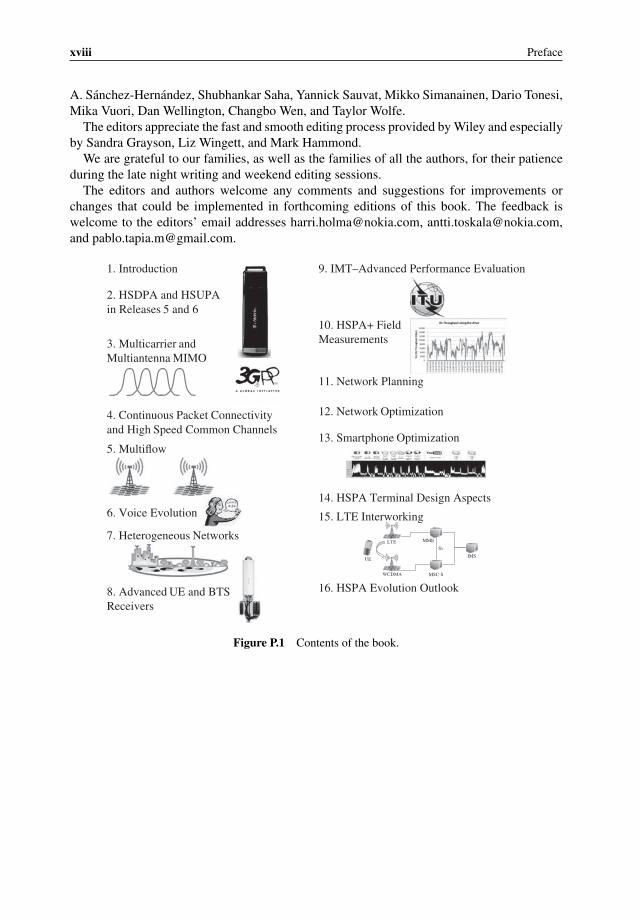
HSPA turned out to be a revolutionary technology, through making high-speed wide-areadata connections possible. HSPA is by far the most global mobile broadband technology andis deployed by over 500 operators. Data volumes today are substantially higher than voicevolumes and mobile networks have turned from being voice dominated to data dominated.The fast increase in data traffic and customer expectation for higher data rates require furtherevolution of HSPA technology. This book explains HSPA evolution, also called HSPA+.The book is structured as follows. Chapter 1 presents an introduction. Chapter 2 describesthe basic HSDPA and HSUPA solution. Chapter 3 presents multicarrier and multiantennaevolution for higher efficiency and higher data rates. Chapter 4 explains continuous packetconnectivity and high speed common channels. Multiflow functionality is described in Chapter5, voice evolution in Chapter 6, and heterogeneous networks in Chapter 7. Advanced receiveralgorithms are discussed in Chapter 8. ITU performance requirements for IMT-Advanced andHSPA+ simulation results are compared in Chapter 9. Chapters 10 to 13 present the practicalnetwork deployment and optimization: HSPA+ field measurements in Chapter 10, networkplanning in Chapter 11, network optimization in Chapter 12, and smartphone optimization inChapter 13. Terminal design aspects are presented in Chapter 14. The inter-working betweenLTE and HSPA is discussed in Chapter 15 and finally the outlook for further HSPA evolutionin Chapter 16. The content of the book is summarized here in Figure P.1.
Acknowledgments
The editors would like to acknowledge the hard work of the contributors from Nokia, fromT-Mobile USA, from Videotron Canada, from Teliasonera, from Renesas Mobile and from Sig-nals Research Group: Mika Aalto, Luigi Dicapua, Ryszard Dokuczal, Mikael Guenais, TimoHalonen, Matthias Hesse, Thomas Hohne, Maciej Januszewski, Jean-Marc Lemenager, ThierryMeslet, Laurent Noel, Brian Olsen, Hisashi Onozawa, Hannu Raassina, Karri Ranta-aho, JussiReunanen, Fernando Sanchez Moya, Alexander Sayenko, Jeff Smith, Mike Thelander, JeroenWigard, Victor Wilkerson, and Carl Williams.
We also would like to thank the following colleagues for their valuable comments:Erkka Ala-Tauriala, Amar Algungdi, Amaanat Ali, Vincent Belaiche, Grant Castle, CostelDragomir, Karol Drazynski, Magdalena Duniewicz, Mika Forssell, Amitava Ghosh, JukkaHongisto, Jie Hui, Shane Jordan, Mika Laasonen, M. Franck Laigle, Brandon Le, HenrikLiljestrom, Mark McDiarmid, Peter Merz, Randy Meyerson, Harinder Nehra, Jouni Parviainen,Krystian Pawlak, Marco Principato, Declan Quinn, Claudio Rosa, Marcin Rybakowski, David
xviii Preface
A. Sanchez-Hernandez, Shubhankar Saha, Yannick Sauvat, Mikko Simanainen, Dario Tonesi,Mika Vuori, Dan Wellington, Changbo Wen, and Taylor Wolfe.
The editors appreciate the fast and smooth editing process provided by Wiley and especiallyby Sandra Grayson, Liz Wingett, and Mark Hammond.
We are grateful to our families, as well as the families of all the authors, for their patienceduring the late night writing and weekend editing sessions.
The editors and authors welcome any comments and suggestions for improvements orchanges that could be implemented in forthcoming editions of this book. The feedback iswelcome to the editors’ email addresses [email protected], [email protected],and [email protected].
3. Multicarrier and
Multiantenna MIMO
1. Introduction
2. HSDPA and HSUPA
in Releases 5 and 6
5. Multiflow
6. Voice Evolution
7. Heterogeneous Networks
8. Advanced UE and BTS
Receivers
9. IMT–Advanced Performance Evaluation
4. Continuous Packet Connectivity
and High Speed Common Channels
10. HSPA+ FieldMeasurements
11. Network Planning
12. Network Optimization
13. Smartphone Optimization
14. HSPA Terminal Design Aspects
15. LTE Interworking
16. HSPA Evolution Outlook
Figure P.1 Contents of the book.
Abbreviations
3GPP Third Generation Partnership ProjectACK AcknowledgmentACL Antenna Center LineACLR Adjacent Channel Leakage RatioACP Automatic Cell PlanningADC Analog Digital ConversionAICH Acquisition Indicator ChannelAL Absorption LossesALCAP Access Link Control Application PartAM Acknowledged ModeAMR Adaptive MultirateANDSF Access Network Discovery and Selection FunctionANQP Access Network Query ProtocolANR Automatic Neighbor RelationsAPE Application EngineAPNS Apple Push Notification ServiceAPT Average Power TrackingaSRVCC Alerting SRVCCAWS Advanced Wireless ServicesBBIC Baseband Integrated CircuitBCH Broadcast ChannelBH Busy HourBiCMOS Bipolar CMOSBLER Block Error RateBOM Bill of MaterialBPF Band Pass FilterBSC Base Station ControllerBT BluetoothBTS Base StationCA Carrier AggregationCAPEX Capital ExpensesCCCH Common Control ChannelCDMA Code Division Multiple AccessCIO Cell Individual Offset
xx Abbreviations
CL Closed LoopCL-BFTD Closed Loop Beamforming Transmit DiversityCM Configuration ManagementCMOS Complementary Metal Oxide SemiconductorCoMP Cooperative MultipointCPC Continuous Packet ConnectivityC-PICH Common Pilot ChannelCPU Central Processing UnitCQI Channel Quality InformationCRC Cyclic Redundancy CheckCS Circuit-SwitchedCSFB CS FallbackCSG Closed Subscriber GroupCTIA Cellular Telecommunications and Internet AssociationDAC Digital Analog ConversionDAS Distributed Antenna SystemDASH Dynamic Adaptive Streaming over HTTPDC Direct CurrentDC Dual-CarrierDCA Direct Conversion ArchitectureDCH Dedicated ChannelDC-HSDPA Dual-Cell HSDPADC-HSPA Dual-Cell HSPADDR Double Data RateDF Dual FrequencyDFCA Dynamic Frequency and Channel AllocationDL DownlinkDM Device ManagementDMIPS Dhrystone Mega Instructions Per SecondDPCCH Dedicated Physical Control ChannelDRAM Dynamic Random Access MemoryDRX Discontinuous ReceptionDS Deep SleepDSL Digital Subscriber LineDSP Digital Signal ProcessingDTX Discontinuous TransmissionE-AGCH Enhanced Absolute Grant ChannelEAI Extended Acquisition IndicatorEc/No Energy per Chip over Interference and NoiseE-DCH Enhanced Dedicated ChannelEDGE Enhanced Data rates for GSM EvolutionE-DPCH Enhanced Dedicated Physical ChanneleF-DPCH Enhanced Fractional Dedicated Physical ChannelEGPRS Enhanced GPRSE-HICH E-DCH Hybrid ARQ Indicator ChanneleICIC Enhanced Inter-Cell Interference Cancellation
Abbreviations xxi
EIRP Equivalent Isotropical Radiated PowerEMI Electro-Magnetic InterferenceEPA Extended Pedestrian AEPC Evolved Packet CoreEPS Evolved Packet SystemE-RGCH Enhanced Relative Grant ChanneleSRVCC Enhanced SRVCCET Envelope TrackingEU European UnionE-UTRA Enhanced Universal Terrestrial Radio AccessEVM Error Vector MagnitudeFACH Forward Access ChannelFBI Feedback InformationFDD Frequency Division DuplexF-DPCH Fractional Dedicated Physical ChannelFE Front EndFE-FACH Further Enhanced Forward Access ChannelfeICIC Further Enhanced Inter-Cell Interference CoordinationFEM Front End ModuleFGA Fast Gain AcquisitionFIR Finite Impulse ResponseFM Frequency ModulationFOM Figure of MeritFS Free SpaceFTP File Transfer ProtocolGAS Generic Advertisement ServiceGCM Google Cloud MessagingGGSN Gateway GPRS Support NodeGoS Grade of ServiceGPEH General Performance Event HandlingGPRS General Packet Radio ServiceGPS Global Positioning SystemGPU Graphical Processing UnitGS Gain SwitchingGSM Global System for Mobile CommunicationsGSMA GSM AssociationGTP GPRS Tunneling ProtocolHARQ Hybrid Automatic Repeat-reQuestHD High DefinitionHDMI High Definition Multimedia InterfaceHDR High Dynamic RangeHEPA High Efficiency PAHLS HTTP Live StreamingHO HandoverHPF High Pass FilterH-RNTI HS-DSCH Radio Network Temporary Identifier
xxii Abbreviations
HSDPA High Speed Downlink Packet AccessHS-DPCCH High Speed Downlink Physical Control ChannelHS-DSCH High Speed Downlink Shared ChannelHS-FACH High Speed Forward Access ChannelHSPA High Speed Packet AccessHS-RACH High Speed Random Access ChannelHS-SCCH High Speed Shared Control ChannelHSUPA High Speed Uplink Packet AccessHTTP Hypertext Transfer ProtocolIC Integrated CircuitIEEE Institute of Electrical and Electronics EngineersIIP Input Intercept PointIIR Infinite Impulse ResponseILPC Inner Loop Power ControlIMEISV International Mobile Station Equipment Identity and Software VersionIMSI International Mobile Subscriber IdentityIMT International Mobile TelephonyIO Input–OutputIP Intellectual PropertyIP Internet ProtocolIQ In-phase/quadratureIRAT Inter Radio Access TechnologyISD Inter-Site DistanceISMP Inter-System Mobility PolicyISRP Inter-System Routing PolicyITU-R International Telegraphic Union Radiocommunications sectorJIT Just In TimeKPI Key Performance IndicatorLA Location AreaLAC Location Area CodeLAU Location Area UpdateLCD Liquid Crystal DisplayLDO Low Drop OutLNA Low Noise AmplifierLO Local OscillatorLS Light SleepLTE Long Term EvolutionMAC Medium Access ControlMAPL Maximum Allowable PathlossMBR Maximum BitrateMCL Minimum Coupling LossMCS Modulation and Coding SchemeMDT Minimization of Drive TestsMGW Media GatewayMIMO Multiple Input Multiple OutputMIPI Mobile Industry Processor Interface
Abbreviations xxiii
ML Mismatch LossMLD Maximum Likelihood DetectionMME Mobility Management EntityMMMB Multimode MultibandMMSE Minimum Mean Square ErrorMO Mobile OriginatedMOS Mean Opinion ScoreMP MultiprocessingMPNS Microsoft Push Notification ServiceMSC Mobile Switching CenterMSC-S MSC-ServerMSS Microsoft’s Smooth StreamingMSS MSC-ServerMT Mobile TerminatedNA North AmericaNACK Negative AcknowledgementNAIC Network Assisted Interference CancellationNAS Non-Access StratumNB NarrowbandNBAP NodeB Application PartNGMN Next Generation Mobile NetworkOEM Original Equipment ManufacturerOL Open LoopOLPC Open Loop Power ControlOMA Open Mobile AllianceOPEX Operational ExpensesOS Operating SystemOSC Orthogonal SubchannelizationOTA Over The AirPA Power AmplifierPAE Power Added EfficiencyPAM Power Amplifier ModulePAPR Peak to Average Power RatioPCB Printed Circuit BoardPCH Paging ChannelPDCP Packet Data Convergence ProtocolPDP Packet Data ProtocolPDU Payload Data UnitPIC Parallel Interference Cancellation (PIC)PICH Paging Indicator ChannelPLL Phase Locked LoopPLMN Public Land Mobile NetworkPM Performance ManagementPRACH Physical Random Access ChannelPS Packet SwitchedP-SCH Primary Synchronization Channel
xxiv Abbreviations
PSD Power Spectral DensityQAM Quadrature Amplitude ModulationQBE Quadband EGPRSQoE Quality of ExperienceQoS Quality of ServiceQPSK Quadrature Phase Shift KeyingQXDM Qualcomm eXtensible Diagnostic MonitorR99 Release 99RAB Radio Access BearerRAC Routing Area CodeRACH Random Access ChannelRAN Radio Access NetworkRANAP Radio Access Network Application PartRAT Radio Access TechnologyRB Radio BearerRET Remote Electrical TiltRF Radio FrequencyRFFE RF Front EndRFIC RF Integrated CircuitRLC Radio Link ControlRNC Radio Network ControllerROHC Robust Header CompressionRoT Rice over ThermalRRC Radio Resource ControlRRM Radio Resource ManagementRRSS Receiver Radio Signal StrengthRSCP Received Signal Code PowerRSRP Reference Signal Received PowerrSRVCC Reverse SRVCCRSSI Received Signal Strength IndicatorRTP Real Time ProtocolRTT Round Trip TimeRUM Real User MeasurementsRX ReceiveSAW Surface Acoustic WaveS-CCPCH Secondary Common Control Physical ChannelSCRI Signaling Connection Release IndicationSD Secure DigitalSD Sphere DecodingS-DPCCH Secondary Dedicated Physical Control ChannelS-E-DPCCH Secondary Dedicated Physical Control Channel for E-DCHS-E-DPDCH Secondary Dedicated Physical Data Channel for E-DCHSF Single FrequencySF Spreading FactorSFN System Frame NumberSGSN Serving GPRS Support Node
Abbreviations xxv
SHO Soft HandoverSI Status IndicationSIB System Information BlockSIC Successive Interference CancellerSIM Subscriber Identity ModuleSINR Signal to Interference and Noise RatioSIR Signal to Interference RatioSMSB Single Mode Single BandSNR Signal to Noise RatioSoC System on ChipSON Self-Organizing NetworkSRVCC Single Radio Voice Call ContinuityS-SCH Secondary Synchronization ChannelSSID Service Set IdentifierSTTD Space Time Transmit DiversitySW SoftwareTA Tracking AreaTAC Tracking Area CodeTAU Tracking Area UpdateTDD Time Division DuplexTD-SCDMA Time Division Synchronous Code Division Multiple AccessTFCI Transport Format Control IndicatorTIS Total Isotropic SensitivityTM Transparent ModeTRP Total Radiated PowerTRX TransceiverTTI Transmission Time IntervalTVM Traffic Volume MeasurementTX TransmitUARFCN UTRAN Absolute Radio Frequency Channel NumberUDP User Datagram ProtocolUE User EquipmentUHF Ultrahigh FrequencyUI User InteractionUL UplinkUM Unacknowledged ModeUMI UTRAN Mobility InformationUMTS Universal Mobile Telecommunications SystemURL Uniform Resource LocatorUSB Universal Serial BusU-SIM UMTS SIMUTRAN Universal Terrestrial Radio Access NetworkVAM Virtual Antenna MappingVCO Voltage Controlled OscillatorVIO Input Offset VoltageVoIP Voice over IP
xxvi Abbreviations
VoLTE Voice over LTEvSRVCC Video SRVCCVST Video Start TimeVSWR Voltage Standing Wave RatioWB WidebandWCDMA Wideband Code Division Multiple AccessWi-Fi Wireless FidelityWiMAX Worldwide Interoperability for Microwave AccessWLAN Wireless Local Area NetworkWPA Wi-Fi Protected AccessWW World WideXPOL Cross-PolarizedZIF Zero Insertion Force

1Introduction
Harri Holma
1.1 Introduction
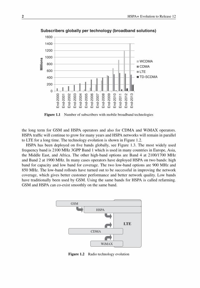
GSM allowed voice to go wireless with more than 4.5 billion subscribers globally. HSPAallowed data to go wireless with 1.5 billion subscribers globally. The number of mobilebroadband subscribers is shown in Figure 1.1. At the same time the amount of data consumedby each subscriber has increased rapidly leading to a fast increase in the mobile data traffic:the traffic growth has been 100% per year in many markets. More than 90% of bits in mobilenetworks are caused by data connections and less than 10% by voice calls. The annual growthof mobile data traffic is expected to be 50–100% in many markets over the next few years.Mobile networks have turned from voice networks into data networks. Mobile operators need toenhance network capabilities to carry more data traffic with better performance. Smartphoneusers expect higher data rates, more extensive coverage, better voice quality, and longerbattery life.
Most of the current mobile data traffic is carried by HSPA networks. HSPA+ is expected tobe the dominant mobile broadband technology for many years to come due to attractive datarates and high system efficiency combined with low cost devices and simple upgrade on topof WCDMA and HSPA networks. This book presents HSPA evolution solutions to enhancethe network performance and capacity. 3GPP specifications, optimizations, field performance,and terminals aspects are considered.
1.2 HSPA Global Deployments
More than 550 operators have deployed the HSPA network in more than 200 countries by2014. All WCDMA networks have been upgraded to support HSPA and many networks alsosupport HSPA+ with 21 Mbps and 42 Mbps. HSPA technology has become the main mobilebroadband solution globally. Long Term Evolution (LTE) will be the mainstream solution in
HSPA+ Evolution to Release 12: Performance and Optimization, First Edition.Edited by Harri Holma, Antti Toskala, and Pablo Tapia.© 2014 John Wiley & Sons, Ltd. Published 2014 by John Wiley & Sons, Ltd.
2 HSPA+ Evolution to Release 12
0
200
400
600
800
1000
1200
1400
1600
End
-200
0
End
-200
1
End
-200
2
End
-200
3
End
-200
4
End
-200
5
End
-200
6
End
-200
7
End
-200
8
End
-200
9
End
-201
0
End
-201
1
End
-201
2
End
-201
3
Mill
ion
s
Subscribers globally per technology (broadband solutions)
WCDMA
CDMA
LTE
TD-SCDMA
Figure 1.1 Number of subscribers with mobile broadband technologies
the long term for GSM and HSPA operators and also for CDMA and WiMAX operators.HSPA traffic will continue to grow for many years and HSPA networks will remain in parallelto LTE for a long time. The technology evolution is shown in Figure 1.2.
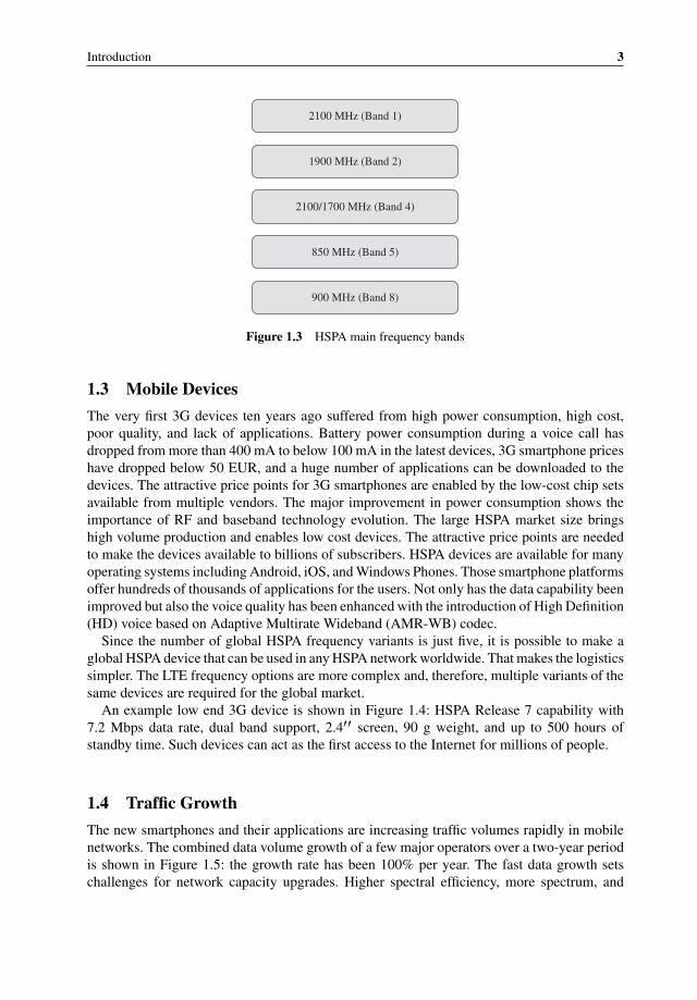
HSPA has been deployed on five bands globally, see Figure 1.3. The most widely usedfrequency band is 2100 MHz 3GPP Band 1 which is used in many countries in Europe, Asia,the Middle East, and Africa. The other high-band options are Band 4 at 2100/1700 MHzand Band 2 at 1900 MHz. In many cases operators have deployed HSPA on two bands: highband for capacity and low band for coverage. The two low-band options are 900 MHz and850 MHz. The low-band rollouts have turned out to be successful in improving the networkcoverage, which gives better customer performance and better network quality. Low bandshave traditionally been used by GSM. Using the same bands for HSPA is called refarming.GSM and HSPA can co-exist smoothly on the same band.
LTE
HSPA
GSM
CDMA
WiMAX
Figure 1.2 Radio technology evolution
Introduction 3
2100 MHz (Band 1)
2100/1700 MHz (Band 4)
1900 MHz (Band 2)
850 MHz (Band 5)
900 MHz (Band 8)
Figure 1.3 HSPA main frequency bands
1.3 Mobile Devices
The very first 3G devices ten years ago suffered from high power consumption, high cost,poor quality, and lack of applications. Battery power consumption during a voice call hasdropped from more than 400 mA to below 100 mA in the latest devices, 3G smartphone priceshave dropped below 50 EUR, and a huge number of applications can be downloaded to thedevices. The attractive price points for 3G smartphones are enabled by the low-cost chip setsavailable from multiple vendors. The major improvement in power consumption shows theimportance of RF and baseband technology evolution. The large HSPA market size bringshigh volume production and enables low cost devices. The attractive price points are neededto make the devices available to billions of subscribers. HSPA devices are available for manyoperating systems including Android, iOS, and Windows Phones. Those smartphone platformsoffer hundreds of thousands of applications for the users. Not only has the data capability beenimproved but also the voice quality has been enhanced with the introduction of High Definition(HD) voice based on Adaptive Multirate Wideband (AMR-WB) codec.
Since the number of global HSPA frequency variants is just five, it is possible to make aglobal HSPA device that can be used in any HSPA network worldwide. That makes the logisticssimpler. The LTE frequency options are more complex and, therefore, multiple variants of thesame devices are required for the global market.
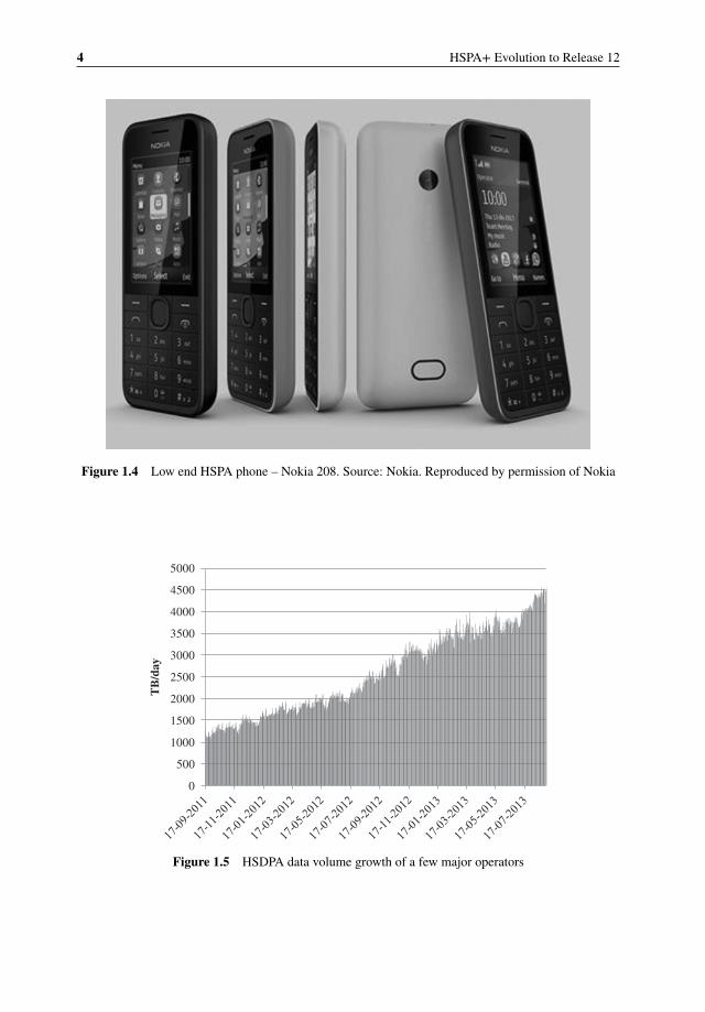
An example low end 3G device is shown in Figure 1.4: HSPA Release 7 capability with7.2 Mbps data rate, dual band support, 2.4′′ screen, 90 g weight, and up to 500 hours ofstandby time. Such devices can act as the first access to the Internet for millions of people.
1.4 Traffic Growth
The new smartphones and their applications are increasing traffic volumes rapidly in mobilenetworks. The combined data volume growth of a few major operators over a two-year periodis shown in Figure 1.5: the growth rate has been 100% per year. The fast data growth setschallenges for network capacity upgrades. Higher spectral efficiency, more spectrum, and
4 HSPA+ Evolution to Release 12
Figure 1.4 Low end HSPA phone – Nokia 208. Source: Nokia. Reproduced by permission of Nokia
0
500
1000
1500
2000
2500
3000
3500
4000
4500
5000
TB
/day
Figure 1.5 HSDPA data volume growth of a few major operators
Introduction 5
0
50
100
150
200
250
300
350
400
450
500
1 3 5 7 9 11 13 15 17 19 21 23 25 27 29 31 33 35 37 39 41 43 45 47 49
kB/H
SDSC
H
Different operators
Figure 1.6 Average data volume for HS-DSCH channel allocation
more base stations will be needed. If the traffic were to grow by 100% per year for a 10-yearperiod, the total traffic growth would be 1000 times higher.
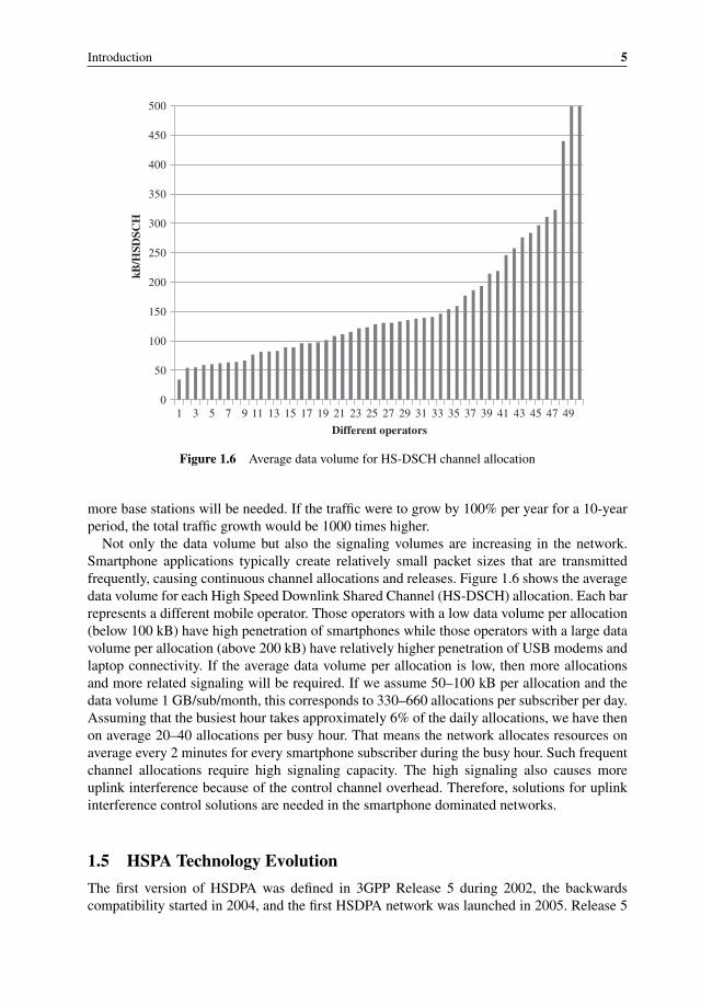
Not only the data volume but also the signaling volumes are increasing in the network.Smartphone applications typically create relatively small packet sizes that are transmittedfrequently, causing continuous channel allocations and releases. Figure 1.6 shows the averagedata volume for each High Speed Downlink Shared Channel (HS-DSCH) allocation. Each barrepresents a different mobile operator. Those operators with a low data volume per allocation(below 100 kB) have high penetration of smartphones while those operators with a large datavolume per allocation (above 200 kB) have relatively higher penetration of USB modems andlaptop connectivity. If the average data volume per allocation is low, then more allocationsand more related signaling will be required. If we assume 50–100 kB per allocation and thedata volume 1 GB/sub/month, this corresponds to 330–660 allocations per subscriber per day.Assuming that the busiest hour takes approximately 6% of the daily allocations, we have thenon average 20–40 allocations per busy hour. That means the network allocates resources onaverage every 2 minutes for every smartphone subscriber during the busy hour. Such frequentchannel allocations require high signaling capacity. The high signaling also causes moreuplink interference because of the control channel overhead. Therefore, solutions for uplinkinterference control solutions are needed in the smartphone dominated networks.
1.5 HSPA Technology Evolution
The first version of HSDPA was defined in 3GPP Release 5 during 2002, the backwardscompatibility started in 2004, and the first HSDPA network was launched in 2005. Release 5
6 HSPA+ Evolution to Release 12
14 Mbps
0.4 Mbps
Release 5
14 Mbps
5.7 Mbps
Release 6
28 Mbps
11 Mbps
Release 7 42 Mbps
11 Mbps
Release 8 84 Mbps
23 Mbps
Release 9 168 Mbps
23 Mbps
Release 10 336 Mbps
35 Mbps
Release 11
Figure 1.7 Peak data rate evolution in downlink and in uplink
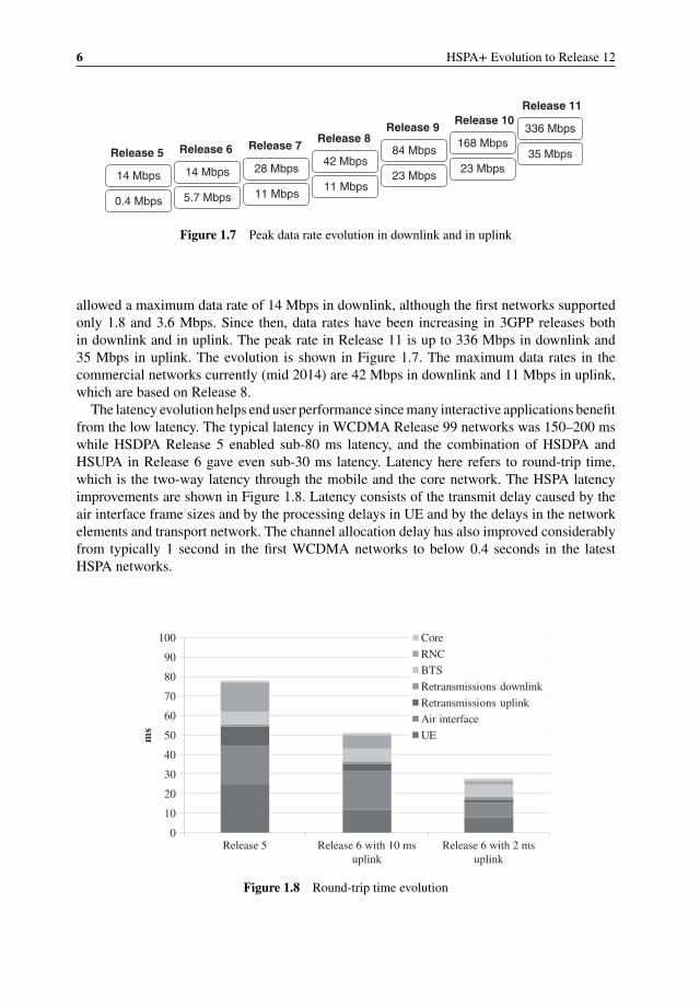
allowed a maximum data rate of 14 Mbps in downlink, although the first networks supportedonly 1.8 and 3.6 Mbps. Since then, data rates have been increasing in 3GPP releases bothin downlink and in uplink. The peak rate in Release 11 is up to 336 Mbps in downlink and35 Mbps in uplink. The evolution is shown in Figure 1.7. The maximum data rates in thecommercial networks currently (mid 2014) are 42 Mbps in downlink and 11 Mbps in uplink,which are based on Release 8.
The latency evolution helps end user performance since many interactive applications benefitfrom the low latency. The typical latency in WCDMA Release 99 networks was 150–200 mswhile HSDPA Release 5 enabled sub-80 ms latency, and the combination of HSDPA andHSUPA in Release 6 gave even sub-30 ms latency. Latency here refers to round-trip time,which is the two-way latency through the mobile and the core network. The HSPA latencyimprovements are shown in Figure 1.8. Latency consists of the transmit delay caused by theair interface frame sizes and by the processing delays in UE and by the delays in the networkelements and transport network. The channel allocation delay has also improved considerablyfrom typically 1 second in the first WCDMA networks to below 0.4 seconds in the latestHSPA networks.
0
10
20
30
40
50
60
70
80
90
100
Release 5 Release 6 with 10 ms
uplink
Release 6 with 2 ms
uplink
ms
Core
RNC
BTS
Retransmissions downlink
Retransmissions uplink
Air interface
UE
Figure 1.8 Round-trip time evolution
Introduction 7
1.6 HSPA Optimization Areas
A number of further optimization steps are required in HSPA to support even more usersand higher capacity. The optimization areas include, for example, installation of additionalcarriers, minimization of signaling load, optimization of terminal power consumption, lowband refarming at 850 and 900 MHz, control of uplink interference, and introduction of smallcells in heterogeneous networks. Many of these topics do not call for major press releases oradvanced terminals features but are quite important in improving end user satisfaction whilethe traffic is increasing.
The most straightforward solution for adding capacity is to add more carriers to the existingsites. This solution is cost efficient because existing sites, antennas, and backhaul solutionscan be reused. The load balancing algorithms can distribute the users equally between thefrequencies.
The limiting factor in network capacity can also be the signaling traffic and uplink interfer-ence. These issues may be found in smartphone dominated networks where the packet sizesare small and frequent signaling is required to allocate and release channels. The signalingtraffic can increase requirements for RNC dimensioning and can also increase uplink inter-ference due to the continuous transmissions of the uplink control channel. Uplink interferencemanagement is important, especially in mass arenas like sports stadiums. A number of efficientsolutions are available today to minimize uplink interference.
The frequent channel allocations and connection setups also increase the power consump-tion in the terminal modem section. Those solutions minimizing the transmitted interferencein the network tend to also give benefits in terms of power consumption: when the termi-nal shuts down its transmitter, the power consumption is minimized and the interference isalso minimized.
Low-band HSPA refarming improves network coverage and quality. The challenge is tosupport GSM traffic and HSPA traffic on the same band with good quality. There are attractivesolutions available today to carry GSM traffic in fewer spectra and to squeeze down HSPAspectrum requirements.
Busy areas in mobile networks may have such high traffic that it is not possible to providethe required capacity by adding several carriers at the macro site. One optimization step is tosplit the congested sector into two, which means essentially the introduction of a six-sectorsolution to the macro site. Another solution is the rollout of small-cell solutions in the formof a micro or pico base station. The small cells can share the frequency with the macro cellin co-channel deployment, which requires solutions to minimize the interference between thedifferent cell layers.
1.7 Summary
HSPA technology has allowed data connections to go wireless all over the world. HSPAsubscribers have already exceeded 1 billion and traffic volumes are growing rapidly. Thisbook presents the HSPA technology evolution as defined in 3GPP but also illustrates practicalfield performance and discusses many of the network optimization and terminal implementa-tion topics.

2HSDPA and HSUPA inRelease 5 and 6
Antti Toskala
2.1 Introduction
This chapter presents the Release 5 based High Speed Downlink Packet Access (HSDPA)and Release 6 based High Speed Uplink Packet Access (HSUPA). This chapter looks first atthe 3GPP activity in creating the standard and then presents the key technology componentsintroduced in HSDPA and HSUPA that enabled the breakthrough of mobile data. Basically,as of today, all networks have introduced as a minimum HSDPA support, and nearly all alsoHSUPA. Respectively, all new chip sets in the marketplace and all new devices support HSDPAand HSUPA as the basic feature set. This chapter also addresses the network architectureevolution from Release 99 to Release 7, including relevant core network developments.
2.2 3GPP Standardization of HSDPA and HSUPA
3GPP started working on better packet data capabilities immediately after the first version ofthe 3G standard was ready, which in theory offered 2 Mbps. The practical experience was,however, that Release 99 was not too well-suited for more than 384 kbps data connections, andeven those were not provided with the highest possible efficiency. One could have configured auser to receive 2 Mbps in the Dedicated Channel (DCH), but in such a case the whole downlinkcell capacity would have been reserved to a single user until the channel data rate downgradedwith RRC reconfiguration. The first studies started in 2000 [1], with the first specification in2002 for HSDPA and then 2004 for HSUPA, as shown in Figure 2.1.
While the Release 99 standard in theory allows up to 2 Mbps, the devices in the field wereimplemented only up to 384 kbps. With HSDPA in Release 5 the specifications have beenfollowed such that even the highest rates have been implemented in the marketplace, reaching
HSPA+ Evolution to Release 12: Performance and Optimization, First Edition.Edited by Harri Holma, Antti Toskala, and Pablo Tapia.© 2014 John Wiley & Sons, Ltd. Published 2014 by John Wiley & Sons, Ltd.
10 HSPA+ Evolution to Release 12
1.5 years
1.25 years
HSDPA
HSUPA2003 2004 2005 2006 2007
2 3
2 3
12002
1
1 1st Specification version published
2 Specification freeze
3 1st Devices in the market
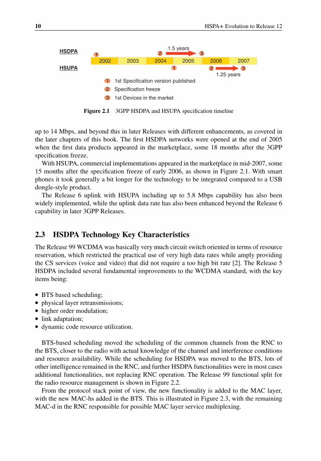
Figure 2.1 3GPP HSDPA and HSUPA specification timeline
up to 14 Mbps, and beyond this in later Releases with different enhancements, as covered inthe later chapters of this book. The first HSDPA networks were opened at the end of 2005when the first data products appeared in the marketplace, some 18 months after the 3GPPspecification freeze.
With HSUPA, commercial implementations appeared in the marketplace in mid-2007, some15 months after the specification freeze of early 2006, as shown in Figure 2.1. With smartphones it took generally a bit longer for the technology to be integrated compared to a USBdongle-style product.
The Release 6 uplink with HSUPA including up to 5.8 Mbps capability has also beenwidely implemented, while the uplink data rate has also been enhanced beyond the Release 6capability in later 3GPP Releases.
2.3 HSDPA Technology Key Characteristics
The Release 99 WCDMA was basically very much circuit switch oriented in terms of resourcereservation, which restricted the practical use of very high data rates while amply providingthe CS services (voice and video) that did not require a too high bit rate [2]. The Release 5HSDPA included several fundamental improvements to the WCDMA standard, with the keyitems being:
� BTS based scheduling;� physical layer retransmissions;� higher order modulation;� link adaptation;� dynamic code resource utilization.
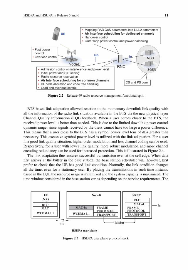
BTS-based scheduling moved the scheduling of the common channels from the RNC tothe BTS, closer to the radio with actual knowledge of the channel and interference conditionsand resource availability. While the scheduling for HSDPA was moved to the BTS, lots ofother intelligence remained in the RNC, and further HSDPA functionalities were in most casesadditional functionalities, not replacing RNC operation. The Release 99 functional split forthe radio resource management is shown in Figure 2.2.
From the protocol stack point of view, the new functionality is added to the MAC layer,with the new MAC-hs added in the BTS. This is illustrated in Figure 2.3, with the remainingMAC-d in the RNC responsible for possible MAC layer service multiplexing.
HSDPA and HSUPA in Release 5 and 6 11
• Mapping RAB QoS parameters into L1/L2 parameters• Air interface scheduling for dedicated channels• Handover control• Outer loop power control and power balancing
CS and PS core
NodeBRNC
SGSN
MSCIuIub
• Fast power control
• Overload control
• Admission control on interference and power level• Initial power and SIR setting• Radio resource reservation• Air interface scheduling for common channels• DL code allocation and code tree handling• Load and overload control
UE
Figure 2.2 Release 99 radio resource management functional split
BTS-based link adaptation allowed reaction to the momentary downlink link quality withall the information of the radio link situation available in the BTS via the new physical layerChannel Quality Information (CQI) feedback. When a user comes closer to the BTS, thereceived power level is better than needed. This is due to the limited downlink power controldynamic range, since signals received by the users cannot have too large a power difference.This means that a user close to the BTS has a symbol power level tens of dBs greater thannecessary. This excessive symbol power level is utilized with the link adaptation. For a userin a good link quality situation, higher order modulation and less channel coding can be used.Respectively, for a user with lower link quality, more robust modulation and more channelencoding redundancy can be used for increased protection. This is illustrated in Figure 2.4.
The link adaptation thus ensures successful transmission even at the cell edge. When datafirst arrives at the buffer in the base station, the base station scheduler will, however, firstprefer to check that the UE has good link condition. Normally, the link condition changesall the time, even for a stationary user. By placing the transmissions in such time instants,based in the CQI, the resource usage is minimized and the system capacity is maximized. Thetime window considered in the base station varies depending on the service requirements. The
WCDMA L1
UE
Iub/Iur
SRNCNodeB
Uu
MACRLC
NAS
HSDPA user plane
WCDMA L1
MAC-hs
TRANSPORT
FRAMEPROTOCOL
TRANSPORT
FRAMEPROTOCOL
MAC-dRLC
Iu
Figure 2.3 HSDPA user plane protocol stack

12 HSPA+ Evolution to Release 12
HSDPA UE withgood link quality
HSDPA UE withpoor link quality
NodeB
CQI feedback
CQI feedback
Transmissionwith 16QAM &little redundancy
Transmissionwith QPSK & lotof redundancy
Figure 2.4 HSDPA link adaptation
detailed scheduler implementation is always left for the network implementation and is notpart of the 3GPP specifications.
Transmission of a packet is anyway not always successful. In Release 99 a packet error in thedecoding would need a retransmission all the way from the RNC, assuming the AcknowledgedMode (AM) of RLC is being used. Release 5 introduced physical layer retransmission enablingrapid recovery from an error in the physical layer packet decoding.
The operation procedure for the physical layer retransmission is as follows:
� After transmission a packet is still kept in the BTS memory and removed only after positiveacknowledgement (Ack) of the reception is received.
� In case the packet is not correctly received, a negative acknowledgement (NAck) is receivedfrom the UE via the uplink physical layer feedback. This initiates retransmission, with thebase station scheduler selecting a suitable moment to schedule a retransmission for the UE.
� The UE receiver has kept the earlier packet in the receiver soft buffer and once the retrans-mission arrives, the receiver combines the original transmission and retransmission. Thisallows utilization of the energy of both transmissions for the turbo decoder process.
� The Hybrid Adaptive Repeat and reQuest (HARQ) operation is of stop and wait type. Once apacket decoding has failed, the receiver stops to wait for retransmission. For this reason oneneeds multiple HARQ processes to enable continuous operation. With HSDPA the numberof processes being configurable, but with the UE memory being limited, the maximum datarate is achieved with the use of six processes which seems to be adapted widely in practicalHSDPA network implementations.
The HSDPA HARQ principle is shown in Figure 2.5. From the network side, the extrafunctionality is to store the packets in the memory after first transmission and then be able todecode the necessary feedback from the UE and retransmit. Retransmission could be identical,or the transmitter could alter which bits are being punctured after Turbo encoding. Such away of operating is called incremental redundancy. There are also smaller optimizations,such as varying the way the bits are mapped to the 16QAM constellation points betweenretransmissions. The modulation aspects were further enhanced in Release 7 when 64QAMwas added. While the use of 16QAM modulation was originally a separate UE capability,today basically all new UEs support 16QAM, many even 64QAM reception as well.
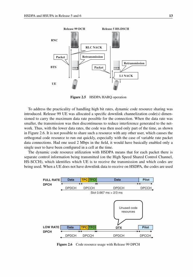
HSDPA and HSUPA in Release 5 and 6 13
UE
BTS
RNC
Release 5 HS-DSCHRelease 99 DCH
Packet Retransmission
RLC NACK
Retransmission
L1 NACK
Packet
Figure 2.5 HSDPA HARQ operation
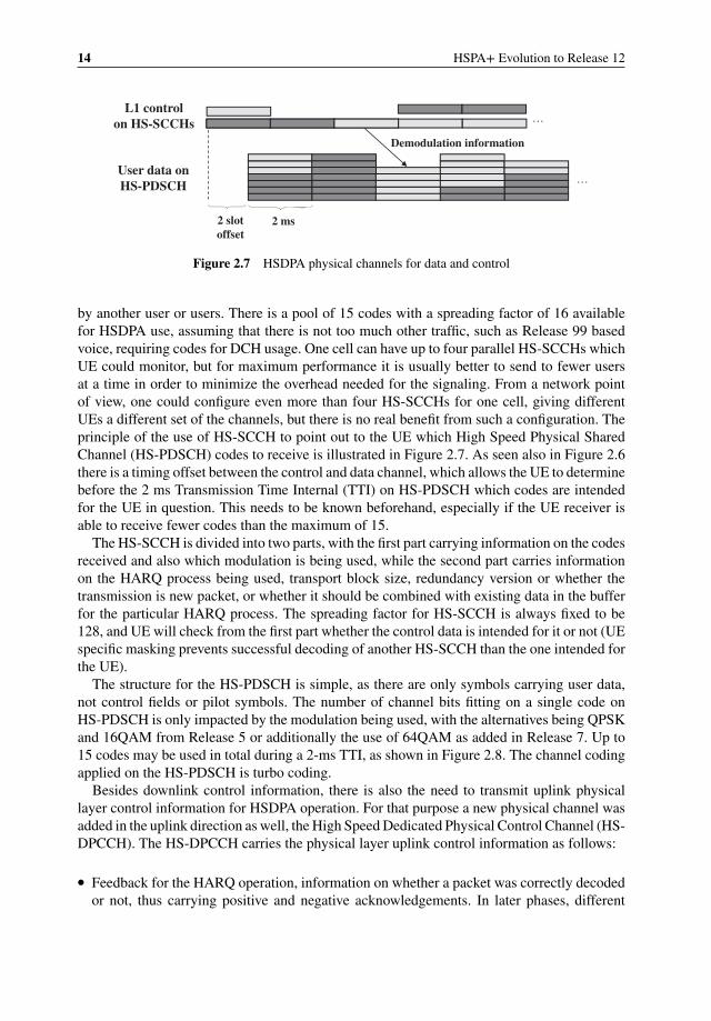
To address the practicality of handling high bit rates, dynamic code resource sharing wasintroduced. Release 99 UE was allocated a specific downlink channelization code(s) dimen-sioned to carry the maximum data rate possible for the connection. When the data rate wassmaller, the transmission was then discontinuous to reduce interference generated to the net-work. Thus, with the lower data rates, the code was then used only part of the time, as shownin Figure 2.6. It is not possible to share such a resource with any other user, which causes theorthogonal code resource to run out quickly, especially with the case of variable rate packetdata connections. Had one used 2 Mbps in the field, it would have basically enabled only asingle user to have been configured in a cell at the time.
The dynamic code resource utilization with HSDPA means that for each packet there isseparate control information being transmitted (on the High Speed Shared Control Channel,HS-SCCH), which identifies which UE is to receive the transmission and which codes arebeing used. When a UE does not have downlink data to receive on HSDPA, the codes are used
PilotData
DPDCHDPDCH DPCCH DPCCH
PilotData
Slot 0.667 ms = 2/3 ms
DPDCHDPDCH
Data
DPCCH DPCCH
FULL RATEDPCH
LOW RATEDPCH
DTX
Unused coderesources
TPC
TPC TFCI
TFCI
Figure 2.6 Code resource usage with Release 99 DPCH
14 HSPA+ Evolution to Release 12
2 ms
…
…
Demodulation information
L1 controlon HS-SCCHs
User data onHS-PDSCH
2 slotoffset
Figure 2.7 HSDPA physical channels for data and control
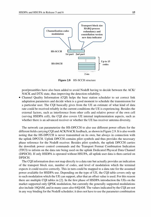
by another user or users. There is a pool of 15 codes with a spreading factor of 16 availablefor HSDPA use, assuming that there is not too much other traffic, such as Release 99 basedvoice, requiring codes for DCH usage. One cell can have up to four parallel HS-SCCHs whichUE could monitor, but for maximum performance it is usually better to send to fewer usersat a time in order to minimize the overhead needed for the signaling. From a network pointof view, one could configure even more than four HS-SCCHs for one cell, giving differentUEs a different set of the channels, but there is no real benefit from such a configuration. Theprinciple of the use of HS-SCCH to point out to the UE which High Speed Physical SharedChannel (HS-PDSCH) codes to receive is illustrated in Figure 2.7. As seen also in Figure 2.6there is a timing offset between the control and data channel, which allows the UE to determinebefore the 2 ms Transmission Time Internal (TTI) on HS-PDSCH which codes are intendedfor the UE in question. This needs to be known beforehand, especially if the UE receiver isable to receive fewer codes than the maximum of 15.
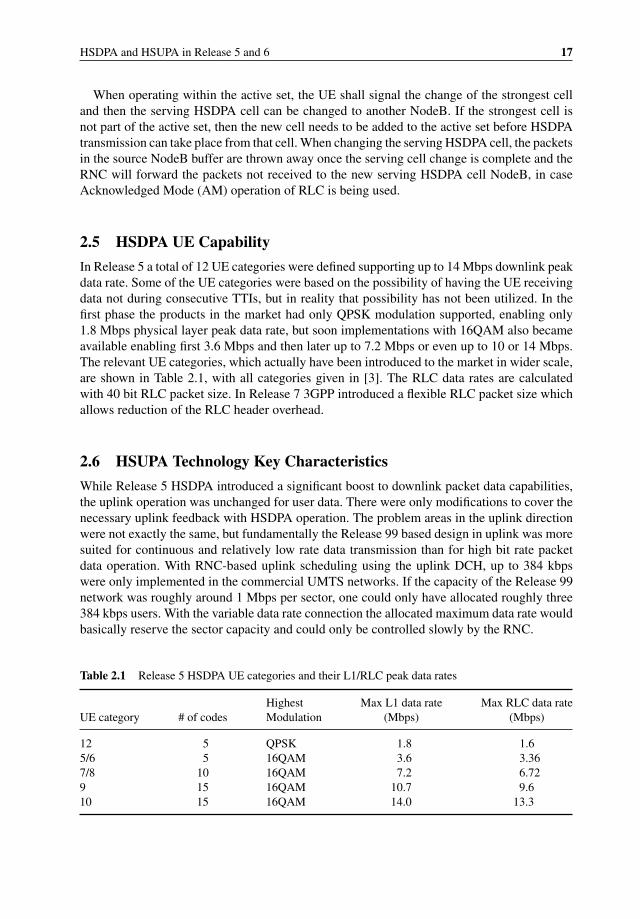
The HS-SCCH is divided into two parts, with the first part carrying information on the codesreceived and also which modulation is being used, while the second part carries informationon the HARQ process being used, transport block size, redundancy version or whether thetransmission is new packet, or whether it should be combined with existing data in the bufferfor the particular HARQ process. The spreading factor for HS-SCCH is always fixed to be128, and UE will check from the first part whether the control data is intended for it or not (UEspecific masking prevents successful decoding of another HS-SCCH than the one intended forthe UE).
The structure for the HS-PDSCH is simple, as there are only symbols carrying user data,not control fields or pilot symbols. The number of channel bits fitting on a single code onHS-PDSCH is only impacted by the modulation being used, with the alternatives being QPSKand 16QAM from Release 5 or additionally the use of 64QAM as added in Release 7. Up to15 codes may be used in total during a 2-ms TTI, as shown in Figure 2.8. The channel codingapplied on the HS-PDSCH is turbo coding.
Besides downlink control information, there is also the need to transmit uplink physicallayer control information for HSDPA operation. For that purpose a new physical channel wasadded in the uplink direction as well, the High Speed Dedicated Physical Control Channel (HS-DPCCH). The HS-DPCCH carries the physical layer uplink control information as follows:
� Feedback for the HARQ operation, information on whether a packet was correctly decodedor not, thus carrying positive and negative acknowledgements. In later phases, different
HSDPA and HSUPA in Release 5 and 6 15
2 ms
HS-SCCH
HS-DSCH
Channelization codesmodulation
Transport block sizeHARQ process
redundancy andconstellation versionnew data indicator
1st part 2nd part
…Up to 15
codes
Figure 2.8 HS-SCCH structure
post/preambles have also been added to avoid NodeB having to decide between the ACK/NACK and DTX state, thus improving the detection reliability.
� Channel Quality Information (CQI) helps the base station scheduler to set correct linkadaptation parameters and decide when is a good moment to schedule the transmission fora particular user. The CQI basically gives from the UE an estimate of what kind of datarate could be received reliably in the current conditions the UE is experiencing. Besides theexternal factors, such as interference from other cells and relative power of the own cell(serving HSDPA cell), the CQI also covers UE internal implementation aspects, such aswhether there is an advanced receiver or whether the UE has receiver antenna diversity.
The network can parameterize the HS-DPCCH to also use different power offsets for thedifferent fields carrying CQI and ACK/NACK feedback, as shown in Figure 2.9. It is also worthnoting that the HS-DPCCH is never transmitted on its own, but always in connection withthe uplink DPCCH. Uplink DPCCH contains pilot symbols and thus provides the necessaryphase reference for the NodeB receiver. Besides pilot symbols, the uplink DPCCH carriesthe downlink power control commands and the Transport Format Combination Indication(TFCI) to inform on the data rate being used on the uplink Dedicated Physical Data Channel(DPDCH). If only HSDPA is operated without HSUPA, all uplink user data is then carried onDPDCH.
The CQI information does not map directly to a data rate but actually provides an indicationof the transport block size, number of codes, and level of modulation which the terminalexpects it could receive correctly. This in turn could be mapped to a data rate for the assumedpower available for HSDPA use. Depending on the type of UE, the CQI table covers only upto such modulation which the UE can support, after that an offset value is used. For this reasonthere are multiple CQI tables in [2]. In the first phase of HSDPA introduction the UEs on themarket supported only QPSK modulation, but currently the generally supported modulationsalso include 16QAM, and in many cases also 64QAM. The values indicated by the CQI are notin any way binding for the NodeB scheduler; it does not have to use the parameter combination

16 HSPA+ Evolution to Release 12
HS-DPCCH
ACK/NACK Channel quality information
2 ms
DPCCH
DPDCH
Symbolalignment
Poweroffset
Figure 2.9 HS-DPCCH carrying ACK/NACK and CQI feedback
indicated by the CQI feedback. There are many reasons for deviation from the UE feedback,including sending to multiple UEs simultaneously or having actually different amounts ofpower available for HSDPA than indicated in the broadcasted value.
2.4 HSDPA Mobility
The mobility with HSDPA is handled differently from Release 99 based DCH. Since thescheduling decisions are done independently in the NodeB scheduler to allow fast reaction tothe momentary channel conditions, it would be difficult to follow the Release 99 soft handover(macro diversity) principle with combining time aligned identical transmission from multipleBTS sites. Thus the approach chosen is such that HSDPA data is only provided from a singleNodeB or rather by a single cell only, called the serving HSDPA cell. While the UE may stillhave the soft handover operation for DCH, the HSDPA transmission will take place from onlya single NodeB, as shown in Figure 2.10.
Iub
NodeB
RNC
NodeB
DCH &HS-HSDPA
DCHUE
Figure 2.10 Operation of HSDPA from a single NodeB only with DCH soft handover
HSDPA and HSUPA in Release 5 and 6 17
When operating within the active set, the UE shall signal the change of the strongest celland then the serving HSDPA cell can be changed to another NodeB. If the strongest cell isnot part of the active set, then the new cell needs to be added to the active set before HSDPAtransmission can take place from that cell. When changing the serving HSDPA cell, the packetsin the source NodeB buffer are thrown away once the serving cell change is complete and theRNC will forward the packets not received to the new serving HSDPA cell NodeB, in caseAcknowledged Mode (AM) operation of RLC is being used.
2.5 HSDPA UE Capability
In Release 5 a total of 12 UE categories were defined supporting up to 14 Mbps downlink peakdata rate. Some of the UE categories were based on the possibility of having the UE receivingdata not during consecutive TTIs, but in reality that possibility has not been utilized. In thefirst phase the products in the market had only QPSK modulation supported, enabling only1.8 Mbps physical layer peak data rate, but soon implementations with 16QAM also becameavailable enabling first 3.6 Mbps and then later up to 7.2 Mbps or even up to 10 or 14 Mbps.The relevant UE categories, which actually have been introduced to the market in wider scale,are shown in Table 2.1, with all categories given in [3]. The RLC data rates are calculatedwith 40 bit RLC packet size. In Release 7 3GPP introduced a flexible RLC packet size whichallows reduction of the RLC header overhead.
2.6 HSUPA Technology Key Characteristics
While Release 5 HSDPA introduced a significant boost to downlink packet data capabilities,the uplink operation was unchanged for user data. There were only modifications to cover thenecessary uplink feedback with HSDPA operation. The problem areas in the uplink directionwere not exactly the same, but fundamentally the Release 99 based design in uplink was moresuited for continuous and relatively low rate data transmission than for high bit rate packetdata operation. With RNC-based uplink scheduling using the uplink DCH, up to 384 kbpswere only implemented in the commercial UMTS networks. If the capacity of the Release 99network was roughly around 1 Mbps per sector, one could only have allocated roughly three384 kbps users. With the variable data rate connection the allocated maximum data rate wouldbasically reserve the sector capacity and could only be controlled slowly by the RNC.
Table 2.1 Release 5 HSDPA UE categories and their L1/RLC peak data rates
Highest Max L1 data rate Max RLC data rateUE category # of codes Modulation (Mbps) (Mbps)
12 5 QPSK 1.8 1.65/6 5 16QAM 3.6 3.367/8 10 16QAM 7.2 6.729 15 16QAM 10.7 9.610 15 16QAM 14.0 13.3
18 HSPA+ Evolution to Release 12
HSUPA UE with TXpower left and data inthe buffer
HSUPA UE withbuffer runningempty
NodeB
Feedback for power resourcesand buffer statusFeedback for power resources
and buffer status
Rate controlsignalling toincrease uplinkdata rate
Rate controlsignalling toreduce uplinkdata rate
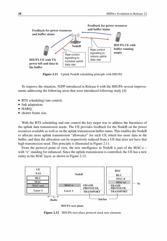
Figure 2.11 Uplink NodeB scheduling principle with HSUPA
To improve the situation, 3GPP introduced in Release 6 with the HSUPA several improve-ments addressing the following areas that were introduced following study [4]:
� BTS scheduling/ rate control;� link adaptation;� HARQ;� shorter frame size.
With the BTS scheduling and rate control the key target was to address the burstiness ofthe uplink data transmission needs. The UE provides feedback for the NodeB on the powerresources available as well as on the uplink transmission buffer status. This enables the NodeBto allocate more uplink transmission “allowance” for such UE which has more data in thebuffer, and then the allocation can be respectively reduced from a UE that does not have thathigh transmission need. This principle is illustrated in Figure 2.11.
From the protocol point of view, the new intelligence in NodeB is part of the MAC-e –with “e” standing for enhanced. Since the uplink transmission is controlled, the UE has a newentity in the MAC layer, as shown in Figure 2.12.
Layer 1
UE
Iub/Iur
RNCNodeB
Radio
MACRLC
NAS
HSUPA user plane
Layer 1
MAC-e
TRANSPORT
FRAMEPROTOCOL
TRANSPORT
FRAMEPROTOCOL
MAC-dRLC
IuMAC-es/e
MAC-es
Figure 2.12 HSUPA user place protocol stack new elements
HSDPA and HSUPA in Release 5 and 6 19
UEBTSRNC Part of activeset
Serving cell
Rate control
E-DCH dataPackets over Iub
Packet reordering
Corenetwork
Figure 2.13 HSUPA operation in soft handover
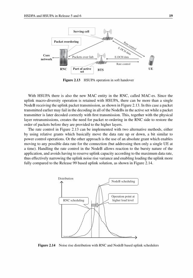
With HSUPA there is also the new MAC entity in the RNC, called MAC-es. Since theuplink macro-diversity operation is retained with HSUPA, there can be more than a singleNodeB receiving the uplink packet transmission, as shown in Figure 2.13. In this case a packettransmitted earlier may fail in the decoding in all of the NodeBs in the active set while a packettransmitter is later decoded correctly with first transmission. This, together with the physicallayer retransmissions, creates the need for packet re-ordering in the RNC side to restore theorder of packets before they are provided to the higher layers.
The rate control in Figure 2.13 can be implemented with two alternative methods, eitherby using relative grants which basically move the data rate up or down, a bit similar topower control operations. Or the other approach is the use of an absolute grant which enablesmoving to any possible data rate for the connection (but addressing then only a single UE ata time). Handling the rate control in the NodeB allows reaction to the bursty nature of theapplication, and avoids having to reserve uplink capacity according to the maximum data rate,thus effectively narrowing the uplink noise rise variance and enabling loading the uplink morefully compared to the Release 99 based uplink solution, as shown in Figure 2.14.
Operation point at
higher load levelRNC scheduling
DistributionNodeB scheduling
Figure 2.14 Noise rise distribution with RNC and NodeB based uplink schedulers
20 HSPA+ Evolution to Release 12
The following channels were introduced in the downlink direction to control the HSUPAoperation:
� The Enhanced DCH Relative Grant Channel (E-RGCH) is used to transfer relative grantsto control the uplink effective data rate up or down. The channel is not heavily coded asa decoding error simply causes the data rate to move to another direction. The NodeBreceiver in any case reads the rate information before decoding, thus there is no resultingerror propagation.
� The Enhanced DCH Absolute Grant Channel (E-AGCH) is used to transfer absolute grants.E-AGCH is more strongly coded and protected with CRC since a decoding error couldcause a UE to jump from the minimum data rate to the maximum data rate. Respectivelyonly one UE can be controlled at a time per E-AGCH.
� The Enhanced DCH HARQ Indicator channel (E-HICH) is used to inform the UE whetherthe uplink packet has been received correctly or not, since there is similar physical layerretransmission procedure introduced with HSUPA as with HSDPA.
In the uplink direction the following new channels were introduced:
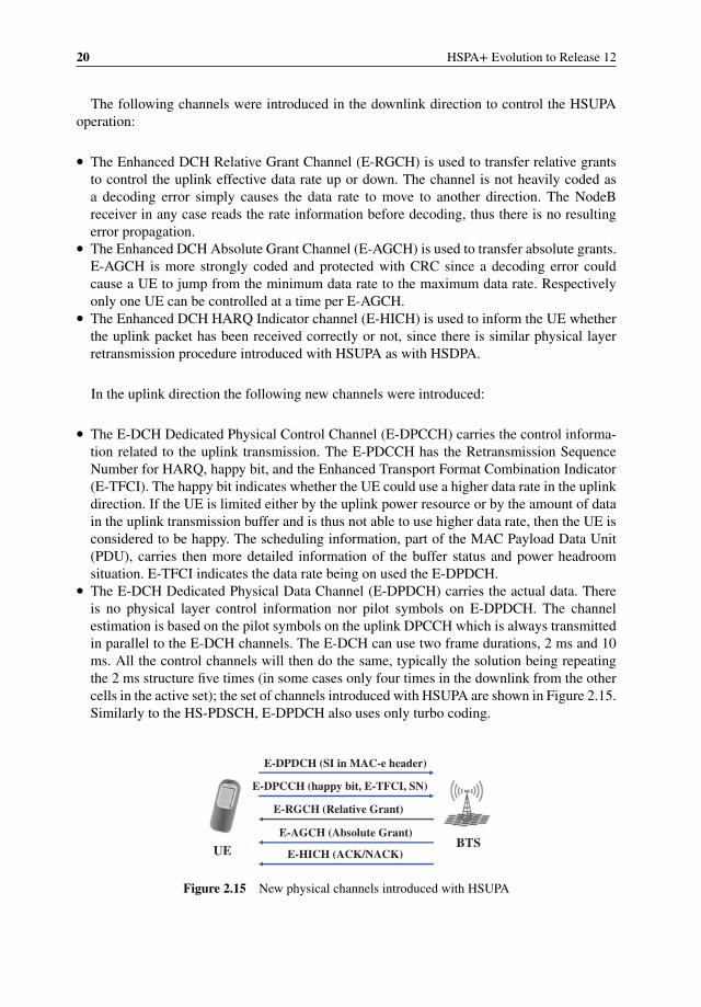
� The E-DCH Dedicated Physical Control Channel (E-DPCCH) carries the control informa-tion related to the uplink transmission. The E-PDCCH has the Retransmission SequenceNumber for HARQ, happy bit, and the Enhanced Transport Format Combination Indicator(E-TFCI). The happy bit indicates whether the UE could use a higher data rate in the uplinkdirection. If the UE is limited either by the uplink power resource or by the amount of datain the uplink transmission buffer and is thus not able to use higher data rate, then the UE isconsidered to be happy. The scheduling information, part of the MAC Payload Data Unit(PDU), carries then more detailed information of the buffer status and power headroomsituation. E-TFCI indicates the data rate being on used the E-DPDCH.
� The E-DCH Dedicated Physical Data Channel (E-DPDCH) carries the actual data. Thereis no physical layer control information nor pilot symbols on E-DPDCH. The channelestimation is based on the pilot symbols on the uplink DPCCH which is always transmittedin parallel to the E-DCH channels. The E-DCH can use two frame durations, 2 ms and 10ms. All the control channels will then do the same, typically the solution being repeatingthe 2 ms structure five times (in some cases only four times in the downlink from the othercells in the active set); the set of channels introduced with HSUPA are shown in Figure 2.15.Similarly to the HS-PDSCH, E-DPDCH also uses only turbo coding.
BTSUE
E-DPCCH (happy bit, E-TFCI, SN)
E-RGCH (Relative Grant)
E-AGCH (Absolute Grant)
E-DPDCH (SI in MAC-e header)
E-HICH (ACK/NACK)
Figure 2.15 New physical channels introduced with HSUPA
HSDPA and HSUPA in Release 5 and 6 21
The E-DPDCH carrying the actual data may use the spreading factor from 256 to as low as 2,and then also multicode transmission. Since a single code on the E-DPDCH is using basicallyonly the I or Q branch, there are two code trees then usable under a single scrambling code.Thus the peak data (without 16QAM) of 5.7 Mbps is obtained with the use of two spreadingcodes with spreading factor 2 and two codes with spreading factor 4. The network may selectwhich of the TTI values will be used, with 10 ms being better for coverage while 2 ms TTIoffers larger data rates. The TTI in use may be changed with the reconfiguration.
Originally the uplink modulation was not modified at all, since the use of QPSK (Dual-channel BPSK), as covered in [2], has lower energy per bit than use of higher order modulationsuch as 16QAM (which was introduced in Release 7). While in downlink direction the limitedpower control dynamic range causes devices to receive the signal with too good SINR whenclose to NodeB (“high geometry” region), the use of 16QAM or 64QAM comes more orless for free. In the uplink direction the power control dynamic range can be, and has to be,much larger to avoid the uplink near-far problem. The uplink fast closed-loop power controloperates as in Release 99, based on the uplink DPCCH signal received as well as typicallymonitoring the packet decoding performance (Block Error Rate, BLER). Therefore the uplinksignal received by the NodeB from the UE does not arrive with too high a power level, andthus changing to higher order modulation only increases the interference level for other usersfor a given data rate. The only situation when the use of 16QAM (or higher) modulation wouldmake sense would be a single user per cell situation. In such a case higher order modulationallows an increase in the peak data rate that is available with the uplink code resources undera single scrambling code. As discussed in Chapter 8, the use of an advanced BTS receiver candeal with the interference from other HSUPA users.
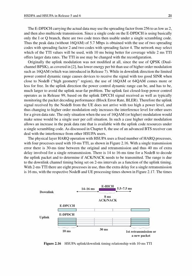
The physical layer HARQ operation with HSUPA uses a fixed number of HARQ processes,with four processes used with 10-ms TTI, as shown in Figure 2.16. With a single transmissionerror there is 30-ms time between the original and retransmission and thus 40 ms of extradelay involved for a single retransmission. There is 14 to 16-ms time for a NodeB to decodethe uplink packet and to determine if ACK/NACK needs to be transmitted. The range is dueto the downlink channel timing being set on 2-ms intervals as a function of the uplink timing.With 2-ms TTI there are eight processes in use, thus the extra delay for a single retransmissionis 16 ms, with the respective NodeB and UE processing times shown in Figure 2.17. The times
10 ms
E-DPCCH
30 ms
E-HICH
ACK/NACK
1st retransmission ora new packet
Uplink
Downlink
E-DPDCH
14–16 ms 5.5–7.5 ms
8 ms
Figure 2.16 HSUPA uplink/downlink timing relationship with 10-ms TTI

22 HSPA+ Evolution to Release 12
2 ms
E-DPCCH
14 ms (7 TTIs)
E-HICH
ACK/NACK
E-DPCCH
E-DCHUplink
Downlink
E-DCH
6.1–8.1 ms 3.5–5.5 ms
…
…
2 ms
1st retransmission ora new packet
NodeB decoding time UE processing time
Figure 2.17 HSUPA uplink/downlink relationship with 2-ms TTI
are shortened, which is partly compensated for as the - ms TTI has less room for channel bitsdue to shorter duration.
2.7 HSUPA Mobility
With HSUPA the active set is operated as in Release 99, with all the base stations in theactive set normally receiving the HSUPA transmission. However, there is only one servingcell (the same cell as providing the HSDPA data) which has more functionalities as part of therate control operation for the scheduling. Only the serving HSUPA cell will send the absolutegrants or relative grants which can increase the data rate. The other NodeBs in the active setwill only use relative grants to reduce the data rate if experiencing interference problems, asshown in Figure 2.18. All NodeBs in the active set try to decode the packets and will then sendfeedback on the E-HICH if packets were decoded correctly.
UEBTSRNCCorrectly decoded
packets
Serving cell
E-RGCH (Hold/Down)
E-DCH data
E-HICH (ACK/DTX)
Figure 2.18 HSUPA control channel operation with mobility
HSDPA and HSUPA in Release 5 and 6 23
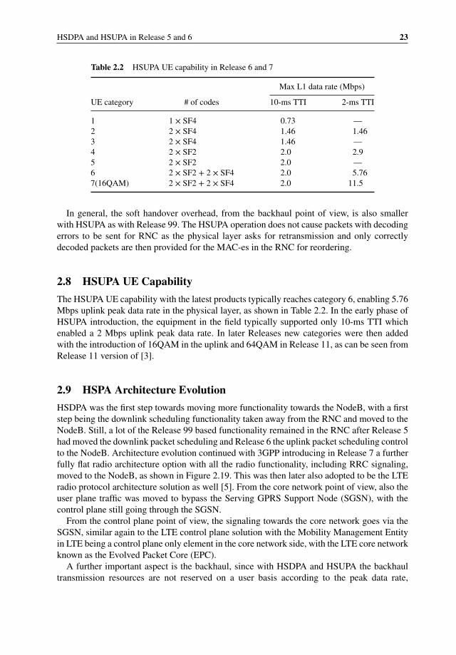
Table 2.2 HSUPA UE capability in Release 6 and 7
Max L1 data rate (Mbps)
UE category # of codes 10-ms TTI 2-ms TTI
1 1 × SF4 0.73 —2 2 × SF4 1.46 1.463 2 × SF4 1.46 —4 2 × SF2 2.0 2.95 2 × SF2 2.0 —6 2 × SF2 + 2 × SF4 2.0 5.767(16QAM) 2 × SF2 + 2 × SF4 2.0 11.5
In general, the soft handover overhead, from the backhaul point of view, is also smallerwith HSUPA as with Release 99. The HSUPA operation does not cause packets with decodingerrors to be sent for RNC as the physical layer asks for retransmission and only correctlydecoded packets are then provided for the MAC-es in the RNC for reordering.
2.8 HSUPA UE Capability
The HSUPA UE capability with the latest products typically reaches category 6, enabling 5.76Mbps uplink peak data rate in the physical layer, as shown in Table 2.2. In the early phase ofHSUPA introduction, the equipment in the field typically supported only 10-ms TTI whichenabled a 2 Mbps uplink peak data rate. In later Releases new categories were then addedwith the introduction of 16QAM in the uplink and 64QAM in Release 11, as can be seen fromRelease 11 version of [3].
2.9 HSPA Architecture Evolution
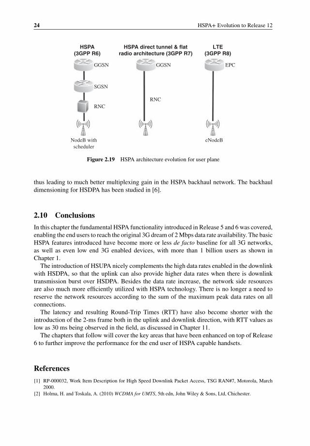
HSDPA was the first step towards moving more functionality towards the NodeB, with a firststep being the downlink scheduling functionality taken away from the RNC and moved to theNodeB. Still, a lot of the Release 99 based functionality remained in the RNC after Release 5had moved the downlink packet scheduling and Release 6 the uplink packet scheduling controlto the NodeB. Architecture evolution continued with 3GPP introducing in Release 7 a furtherfully flat radio architecture option with all the radio functionality, including RRC signaling,moved to the NodeB, as shown in Figure 2.19. This was then later also adopted to be the LTEradio protocol architecture solution as well [5]. From the core network point of view, also theuser plane traffic was moved to bypass the Serving GPRS Support Node (SGSN), with thecontrol plane still going through the SGSN.
From the control plane point of view, the signaling towards the core network goes via theSGSN, similar again to the LTE control plane solution with the Mobility Management Entityin LTE being a control plane only element in the core network side, with the LTE core networkknown as the Evolved Packet Core (EPC).
A further important aspect is the backhaul, since with HSDPA and HSUPA the backhaultransmission resources are not reserved on a user basis according to the peak data rate,
24 HSPA+ Evolution to Release 12
GGSN
SGSN
RNC
NodeB with
scheduler
eNodeB
RNC
GGSN EPC
HSPA(3GPP R6)
HSPA direct tunnel & flatradio architecture (3GPP R7)
LTE(3GPP R8)
Figure 2.19 HSPA architecture evolution for user plane
thus leading to much better multiplexing gain in the HSPA backhaul network. The backhauldimensioning for HSDPA has been studied in [6].
2.10 Conclusions
In this chapter the fundamental HSPA functionality introduced in Release 5 and 6 was covered,enabling the end users to reach the original 3G dream of 2 Mbps data rate availability. The basicHSPA features introduced have become more or less de facto baseline for all 3G networks,as well as even low end 3G enabled devices, with more than 1 billion users as shown inChapter 1.
The introduction of HSUPA nicely complements the high data rates enabled in the downlinkwith HSDPA, so that the uplink can also provide higher data rates when there is downlinktransmission burst over HSDPA. Besides the data rate increase, the network side resourcesare also much more efficiently utilized with HSPA technology. There is no longer a need toreserve the network resources according to the sum of the maximum peak data rates on allconnections.
The latency and resulting Round-Trip Times (RTT) have also become shorter with theintroduction of the 2-ms frame both in the uplink and downlink direction, with RTT values aslow as 30 ms being observed in the field, as discussed in Chapter 11.
The chapters that follow will cover the key areas that have been enhanced on top of Release6 to further improve the performance for the end user of HSPA capable handsets.
References
[1] RP-000032, Work Item Description for High Speed Downlink Packet Access, TSG RAN#7, Motorola, March2000.
[2] Holma, H. and Toskala, A. (2010) WCDMA for UMTS, 5th edn, John Wiley & Sons, Ltd, Chichester.

HSDPA and HSUPA in Release 5 and 6 25
[3] 3GPP Technical Specification, TS 25.306, “UE Radio Access capabilities”, version 5.15.0, March 2009.[4] RP-020658, 3GPP Study Item description “Uplink Enhancements for Dedicated Transport Channels”, Ericsson,
Motorola, Nokia, AT&T Wireless Services, September 2002.[5] Holma, H. and Toskala, A. (2011) LTE for UMTS, 2nd edn, John Wiley & Sons, Ltd, Chichester.[6] Toskala, A., Holma, H., Metsala, E. et al. (2005) Iub efficiency analysis for high speed downlink packet access
in WCDMA. Proceedings of the WPMC, Aalborg, Denmark, September 2005.

3Multicarrier and MultiantennaMIMO
Antti Toskala, Jeroen Wigard, Matthias Hesse, Ryszard Dokuczal, andMaciej Januszewski
3.1 Introduction
This chapter presents HSPA multicarrier and multiantenna Multiple Input Multiple Output(MIMO) capabilities introduced in Releases 7 onwards all the way to the ongoing Release 12work on uplink enhancements involving uplink multicarrier operation. Release 99 containedsupport for base station transmit diversity (both closed and open loop, as covered in [1]), butRelease 5 HSDPA and 6 HSUPA were basically designed around a single antenna, singlefrequency band, and single-carrier operation. This chapter first covers the multicarrier oper-ation introduced with dual-carrier downlink and then extends to more carriers in downlinkand also to the dual-carrier uplink operation. This chapter then continues with the multibandcapabilities and is concluded with MIMO operation introduced originally in Release 7 andfinalized with Release 11 uplink MIMO.
3.2 Dual-Cell Downlink and Uplink
Following the development of the baseband processing capabilities, including handling oflarger bandwidths, the work in 3GPP turned towards enabling a single device to use largerbandwidth than the original WCDMA bandwidth of 5 MHz. The definition of, for example,10 MHz bandwidth with the new chip rate was not a very attractive approach since that wouldhave been a non-backwards compatible solution, not allowing legacy devices to access such acarrier. Thus the direction chosen was to consider using multiple 5 MHz carriers for a singledevice, with the first step being a downlink dual carrier. Work on the uplink dual carrierlater followed. A similar approach is used in LTE as well, with the LTE-Advanced carrier
HSPA+ Evolution to Release 12: Performance and Optimization, First Edition.Edited by Harri Holma, Antti Toskala, and Pablo Tapia.© 2014 John Wiley & Sons, Ltd. Published 2014 by John Wiley & Sons, Ltd.
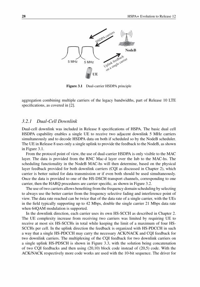
28 HSPA+ Evolution to Release 12
UE
5 MHz 5 MHz
NodeB
Figure 3.1 Dual-carrier HSDPA principle
aggregation combining multiple carriers of the legacy bandwidths, part of Release 10 LTEspecifications, as covered in [2].
3.2.1 Dual-Cell Downlink
Dual-cell downlink was included in Release 8 specifications of HSPA. The basic dual cellHSDPA capability enables a single UE to receive two adjacent downlink 5 MHz carrierssimultaneously and to decode HSDPA data on both if scheduled so by the NodeB scheduler.The UE in Release 8 uses only a single uplink to provide the feedback to the NodeB, as shownin Figure 3.1.
From the protocol point of view, the use of dual-carrier HSDPA is only visible to the MAClayer. The data is provided from the RNC Mac-d layer over the Iub to the MAC-hs. Thescheduling functionality in the NodeB MAC-hs will then determine, based on the physicallayer feedback provided for both downlink carriers (CQI as discussed in Chapter 2), whichcarrier is better suited for data transmission or if even both should be used simultaneously.Once the data is provided to one of the HS-DSCH transport channels, corresponding to onecarrier, then the HARQ procedures are carrier specific, as shown in Figure 3.2.
The use of two carriers allows benefiting from the frequency domain scheduling by selectingto always use the better carrier from the frequency selective fading and interference point ofview. The data rate reached can be twice that of the data rate of a single carrier, with the UEsin the field typically supporting up to 42 Mbps, double the single carrier 21 Mbps data ratewhen 64QAM modulation is supported.
In the downlink direction, each carrier uses its own HS-SCCH as described in Chapter 2.The UE complexity increase from receiving two carriers was limited by requiring UE toreceive at most six HS-SCCHs in total while keeping the limit of a maximum of four HS-SCCHs per cell. In the uplink direction the feedback is organized with HS-PDCCH in sucha way that a single HS-PDCCH may carry the necessary ACK/NACK and CQI feedback fortwo downlink carriers. The multiplexing of the CQI feedback for two downlink carriers ona single uplink HS-PDSCH is shown in Figure 3.3, with the solution being concatenationof two CQI feedbacks and then using (20,10) block code instead of (20,5) code. With theACK/NACK respectively more code works are used with the 10-bit sequence. The driver for
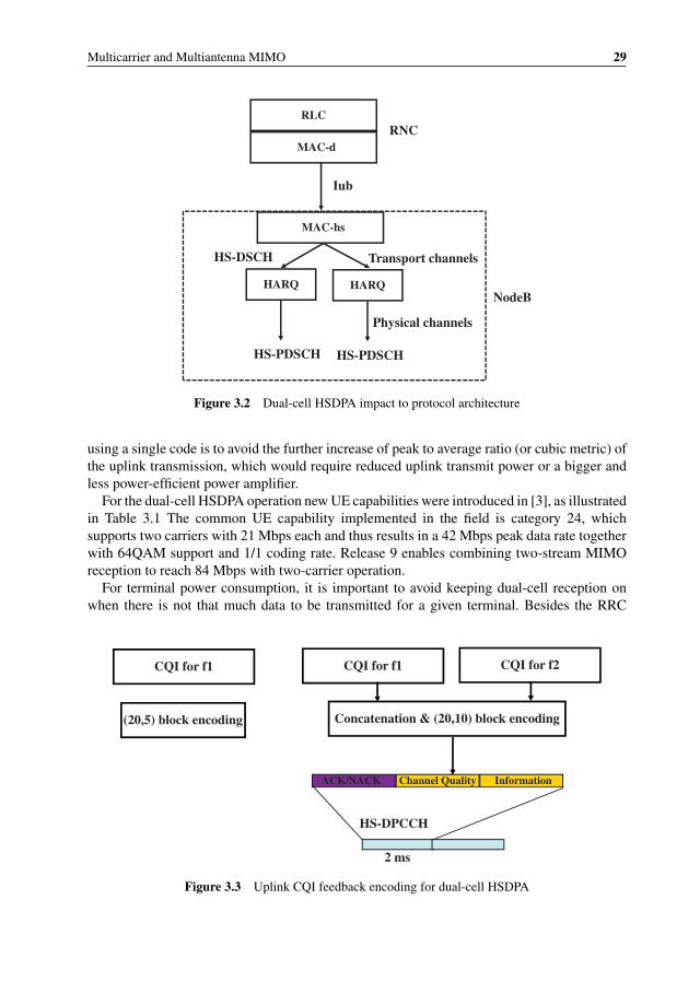
Multicarrier and Multiantenna MIMO 29
Transport channels
HARQ
Iub
MAC-hs
HARQ
HS-PDSCH HS-PDSCH
RNCMAC-d
RLC
Physical channels
HS-DSCH
NodeB
Figure 3.2 Dual-cell HSDPA impact to protocol architecture
using a single code is to avoid the further increase of peak to average ratio (or cubic metric) ofthe uplink transmission, which would require reduced uplink transmit power or a bigger andless power-efficient power amplifier.
For the dual-cell HSDPA operation new UE capabilities were introduced in [3], as illustratedin Table 3.1 The common UE capability implemented in the field is category 24, whichsupports two carriers with 21 Mbps each and thus results in a 42 Mbps peak data rate togetherwith 64QAM support and 1/1 coding rate. Release 9 enables combining two-stream MIMOreception to reach 84 Mbps with two-carrier operation.
For terminal power consumption, it is important to avoid keeping dual-cell reception onwhen there is not that much data to be transmitted for a given terminal. Besides the RRC
HS-DPCCH
2 ms
Concatenation & (20,10) block encoding
CQI for f1 CQI for f2
(20,5) block encoding
CQI for f1
ACK/NACK Channel Quality Information
Figure 3.3 Uplink CQI feedback encoding for dual-cell HSDPA
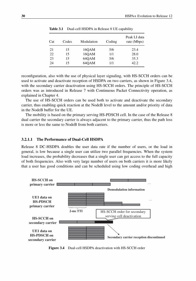
30 HSPA+ Evolution to Release 12
Table 3.1 Dual-cell HSDPA in Release 8 UE capability
Cat Codes Modulation CodingPeak LI datarate (Mbps)
21 15 16QAM 5/6 23.422 15 16QAM 1/1 28.023 15 64QAM 5/6 35.324 15 64QAM 1/1 42.2
reconfiguration, also with the use of physical layer signaling, with HS-SCCH orders can beused to activate and deactivate reception of HSDPA on two carriers, as shown in Figure 3.4,with the secondary carrier deactivation using HS-SCCH orders. The principle of HS-SCCHorders was as introduced in Release 7 with Continuous Packet Connectivity operation, asexplained in Chapter 4.
The use of HS-SCCH orders can be used both to activate and deactivate the secondarycarrier, thus enabling quick reaction at the NodeB level to the amount and/or priority of datain the NodeB buffer for the UE.
The mobility is based on the primary serving HS-PDSCH cell. In the case of the Release 8dual carrier the secondary carrier is always adjacent to the primary carrier, thus the path lossis more or less the same to NodeB from both carriers.
3.2.1.1 The Performance of Dual-Cell HSDPA
Release 8 DC-HSDPA doubles the user data rate if the number of users, or the load ingeneral, is low because a single user can utilize two parallel frequencies. When the systemload increases, the probability decreases that a single user can get access to the full capacityof both frequencies. Also with very large number of users on both carriers it is more likelythat a user has good conditions and can be scheduled using low coding overhead and high
2-ms TTI
…
…
Demodulation information
HS-SCCH onprimary carrier
UE1 data onHS-PDSCH
primary carrier
HS-SCCH onsecondary carrier
UE1 data onHS-PDSCH on
secondary carrierSecondary carrier reception discontinued
HS-SCCH order for secondary
serving cell deactivation
Figure 3.4 Dual-cell HSDPA deactivation with HS-SCCH order
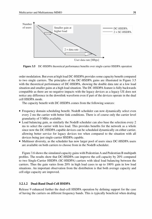
Multicarrier and Multiantenna MIMO 31
Number
of users
User data rate [Mbps]
DC-HSDPA
2 × SC-HSDPA
2 × data rate
Smaller gain at
higher load
Figure 3.5 DC-HSDPA theoretical performance benefits over single-carrier HSDPA operation
order modulation. But even at high load DC-HSDPA provides some capacity benefit comparedto two single carriers. The principles of the DC-HSDPA gains are illustrated in Figure 3.5with the theoretical performance of DC-HSDPA, showing the double data rate at a low loadsituation and smaller gains at a high load situation. The DC-HSDPA feature is fully backwardscompatible as there are no negative impacts with the legacy devices as a legacy UE does notnotice any difference in the downlink waveform even if part of the devices operate in the dualcell HSDPA mode.
The capacity benefit with DC-HSDPA comes from the following sources:
� Frequency domain scheduling benefit. NodeB scheduler can now dynamically select evenevery 2 ms the carrier with better link conditions. There is of course only the carrier levelgranularity of 5 MHz available.
� Load balancing gain, as similarly the NodeB scheduler can also base the selection every 2ms to select the carrier with less load. This provides benefits for the network as a wholesince now the DC-HSDPA capable devices can be scheduled dynamically on either carrier,allowing better service for legacy devices too when compared to the situation with alldevices being just single-carrier HSDPA capable.
� Multiuser diversity, as the scheduler has now larger pool of users since DC-HSDPA usersare available on both carriers to choose from in the NodeB scheduler.
Figure 3.6 shows the simulated capacity gains with Pedestrian A and Pedestrian B multipathprofiles. The results show that DC-HSDPA can improve the cell capacity by 20% comparedto two Single-Carrier HSDPA (SC-HSDPA) carriers with ideal load balancing between thecarriers. Thus the gain varies from 20% in high load cases to up to 100% gain in low loadsituations. An important observation from the distribution is that both average capacity andcell edge capacity are improved.
3.2.1.2 Dual-Band Dual-Cell HSDPA
Release 9 enhanced further the dual-cell HSDPA operation by defining support for the caseof having the carriers on different frequency bands. This is typically beneficial when dealing
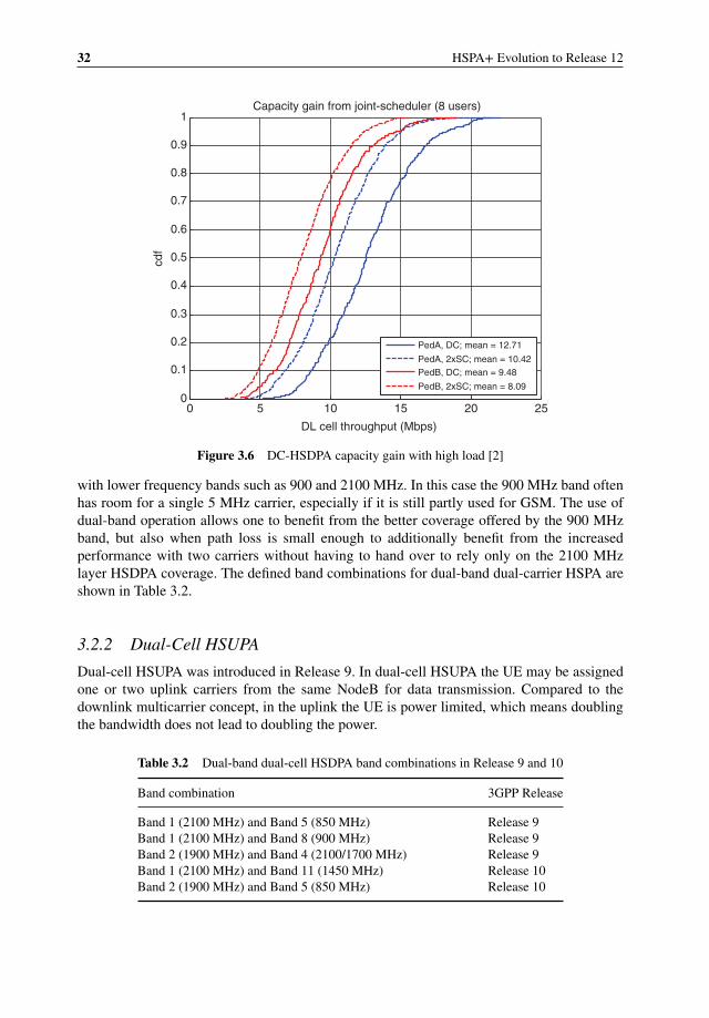
32 HSPA+ Evolution to Release 12
0 5 10 15 20 250
0.1
0.2
0.3
0.4
0.5
0.6
0.7
0.8
0.9
1
DL cell throughput (Mbps)
cdf
Capacity gain from joint-scheduler (8 users)
PedA, DC; mean = 12.71
PedA, 2xSC; mean = 10.42PedB, DC; mean = 9.48
PedB, 2xSC; mean = 8.09
Figure 3.6 DC-HSDPA capacity gain with high load [2]
with lower frequency bands such as 900 and 2100 MHz. In this case the 900 MHz band oftenhas room for a single 5 MHz carrier, especially if it is still partly used for GSM. The use ofdual-band operation allows one to benefit from the better coverage offered by the 900 MHzband, but also when path loss is small enough to additionally benefit from the increasedperformance with two carriers without having to hand over to rely only on the 2100 MHzlayer HSDPA coverage. The defined band combinations for dual-band dual-carrier HSPA areshown in Table 3.2.
3.2.2 Dual-Cell HSUPA
Dual-cell HSUPA was introduced in Release 9. In dual-cell HSUPA the UE may be assignedone or two uplink carriers from the same NodeB for data transmission. Compared to thedownlink multicarrier concept, in the uplink the UE is power limited, which means doublingthe bandwidth does not lead to doubling the power.
Table 3.2 Dual-band dual-cell HSDPA band combinations in Release 9 and 10
Band combination 3GPP Release
Band 1 (2100 MHz) and Band 5 (850 MHz) Release 9Band 1 (2100 MHz) and Band 8 (900 MHz) Release 9Band 2 (1900 MHz) and Band 4 (2100/1700 MHz) Release 9Band 1 (2100 MHz) and Band 11 (1450 MHz) Release 10Band 2 (1900 MHz) and Band 5 (850 MHz) Release 10
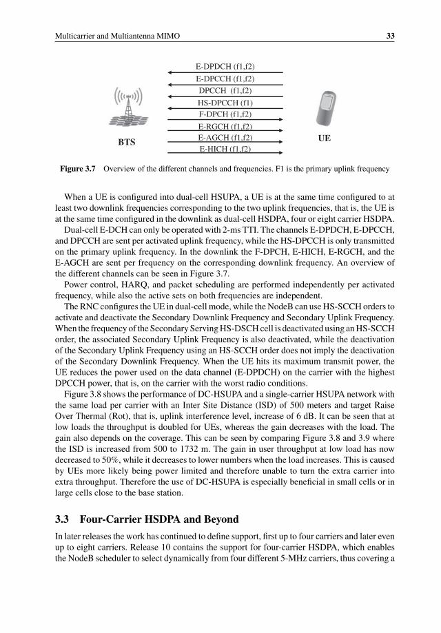
Multicarrier and Multiantenna MIMO 33
UEBTS
E-RGCH (f1,f2)
E-DPDCH (f1,f2)
E-HICH (f1,f2)
E-DPCCH (f1,f2)
HS-DPCCH (f1)
DPCCH (f1,f2)
F-DPCH (f1,f2)
E-AGCH (f1,f2)
Figure 3.7 Overview of the different channels and frequencies. F1 is the primary uplink frequency
When a UE is configured into dual-cell HSUPA, a UE is at the same time configured to atleast two downlink frequencies corresponding to the two uplink frequencies, that is, the UE isat the same time configured in the downlink as dual-cell HSDPA, four or eight carrier HSDPA.
Dual-cell E-DCH can only be operated with 2-ms TTI. The channels E-DPDCH, E-DPCCH,and DPCCH are sent per activated uplink frequency, while the HS-DPCCH is only transmittedon the primary uplink frequency. In the downlink the F-DPCH, E-HICH, E-RGCH, and theE-AGCH are sent per frequency on the corresponding downlink frequency. An overview ofthe different channels can be seen in Figure 3.7.
Power control, HARQ, and packet scheduling are performed independently per activatedfrequency, while also the active sets on both frequencies are independent.
The RNC configures the UE in dual-cell mode, while the NodeB can use HS-SCCH orders toactivate and deactivate the Secondary Downlink Frequency and Secondary Uplink Frequency.When the frequency of the Secondary Serving HS-DSCH cell is deactivated using an HS-SCCHorder, the associated Secondary Uplink Frequency is also deactivated, while the deactivationof the Secondary Uplink Frequency using an HS-SCCH order does not imply the deactivationof the Secondary Downlink Frequency. When the UE hits its maximum transmit power, theUE reduces the power used on the data channel (E-DPDCH) on the carrier with the highestDPCCH power, that is, on the carrier with the worst radio conditions.
Figure 3.8 shows the performance of DC-HSUPA and a single-carrier HSUPA network withthe same load per carrier with an Inter Site Distance (ISD) of 500 meters and target RaiseOver Thermal (Rot), that is, uplink interference level, increase of 6 dB. It can be seen that atlow loads the throughput is doubled for UEs, whereas the gain decreases with the load. Thegain also depends on the coverage. This can be seen by comparing Figure 3.8 and 3.9 wherethe ISD is increased from 500 to 1732 m. The gain in user throughput at low load has nowdecreased to 50%, while it decreases to lower numbers when the load increases. This is causedby UEs more likely being power limited and therefore unable to turn the extra carrier intoextra throughput. Therefore the use of DC-HSUPA is especially beneficial in small cells or inlarge cells close to the base station.
3.3 Four-Carrier HSDPA and Beyond
In later releases the work has continued to define support, first up to four carriers and later evenup to eight carriers. Release 10 contains the support for four-carrier HSDPA, which enablesthe NodeB scheduler to select dynamically from four different 5-MHz carriers, thus covering a
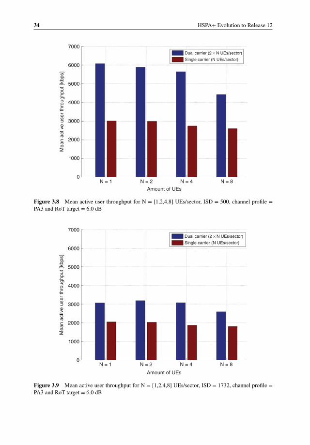
34 HSPA+ Evolution to Release 12
Dual carrier (2 × N UEs/sector)
Single carrier (N UEs/sector)
7000
6000
5000
4000
3000
2000
1000
0N = 1 N = 2
Amount of UEs
Mea
n ac
tive
user
thro
ughp
ut [k
bps]
N = 4 N = 8
Figure 3.8 Mean active user throughput for N = [1,2,4,8] UEs/sector, ISD = 500, channel profile =PA3 and RoT target = 6.0 dB
Dual carrier (2 × N UEs/sector)
Single carrier (N UEs/sector)
7000
6000
5000
4000
3000
2000
1000
0N = 1 N = 2
Amount of UEs
Mea
n ac
tive
user
thro
ughp
ut [k
bps]
N = 4 N = 8
Figure 3.9 Mean active user throughput for N = [1,2,4,8] UEs/sector, ISD = 1732, channel profile =PA3 and RoT target = 6.0 dB
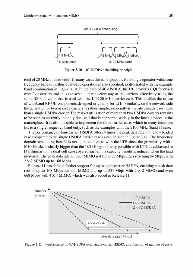
Multicarrier and Multiantenna MIMO 35
5 MHz 5 MHz 5 MHz5 MHz
Joint HSDPA scheduling
900 MHz band 2100 MHz band
Figure 3.10 4C-HSDPA scheduling principle
total of 20 MHz of bandwidth. In many cases this is not possible for a single operator within onefrequency band only, thus dual-band operation is also specified, as illustrated with the exampleband combination in Figure 3.10. In the case of 4C-HSDPA, the UE provides CQI feedbackover four carriers and thus the scheduler can select any of the carriers, effectively using thesame RF bandwidth that is used with the LTE 20 MHz carrier case. This enables the re-useof wideband RF UE components designed originally for LTE. Similarly, on the network sidethe activation of two or more carriers is rather simple, especially if the site already uses morethan a single HSDPA carrier. The market utilization of more than two HSDPA carriers remainsto be seen as currently the only dual-cell that is supported widely in the latest devices in themarketplace. It is also possible to implement the three-carrier case, which in many instancesfits to a single frequency band only, such as the examples with the 2100 MHz (band 1) case.
The performance of four-carrier HSDPA offers 4 times the peak data rate in the low loadedcase compared to the single HSDPA carrier case as can be seen in Figure 3.11. The frequencydomain scheduling benefit is not quite as high as with the LTE since the granularity with -MHz blocks is clearly bigger than the 180 kHz granularity possible with LTE, as addressed in[4]. Similar to the dual-cell case covered earlier, the capacity benefit is reduced when the loadincreases. The peak data rate without MIMO is 4 times 21 Mbps, thus reaching 84 Mbps, with2 × 2 MIMO up to 168 Mbps.
Release 11 has defined further support for up to eight-carrier HSDPA, enabling a peak datarate of up to 168 Mbps without MIMO and up to 334 Mbps with 2 × 2 MIMO and even668 Mbps with 4 × 4 MIMO, which was also added in Release 11.
Number
of users
User data rate [Mbps]
DC-HSDPA
2 × SC-HSDPA
4 × data rate
4C-HSDPA
Figure 3.11 Performance of 4C-HSDPA over single-carrier HSDPA as a function of number of users
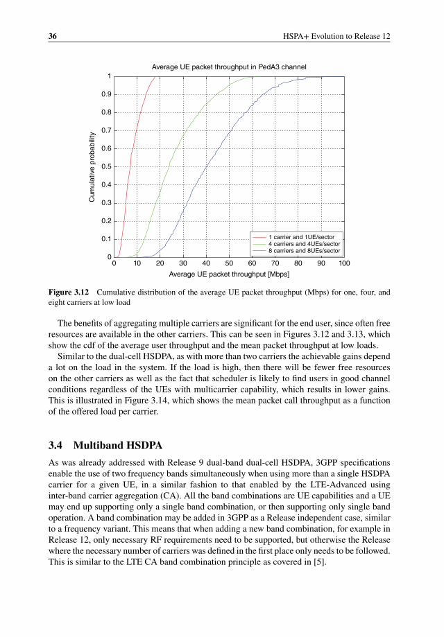
36 HSPA+ Evolution to Release 12
1 carrier and 1UE/sector4 carriers and 4UEs/sector8 carriers and 8UEs/sector
00
0.1
0.2
0.3
0.4
0.5
Cum
ulat
ive
prob
abili
ty
0.6
0.7
0.8
0.9
1
10 20 30 40 50
Average UE packet throughput [Mbps]
Average UE packet throughput in PedA3 channel
60 70 80 90 100
Figure 3.12 Cumulative distribution of the average UE packet throughput (Mbps) for one, four, andeight carriers at low load
The benefits of aggregating multiple carriers are significant for the end user, since often freeresources are available in the other carriers. This can be seen in Figures 3.12 and 3.13, whichshow the cdf of the average user throughput and the mean packet throughput at low loads.
Similar to the dual-cell HSDPA, as with more than two carriers the achievable gains dependa lot on the load in the system. If the load is high, then there will be fewer free resourceson the other carriers as well as the fact that scheduler is likely to find users in good channelconditions regardless of the UEs with multicarrier capability, which results in lower gains.This is illustrated in Figure 3.14, which shows the mean packet call throughput as a functionof the offered load per carrier.
3.4 Multiband HSDPA
As was already addressed with Release 9 dual-band dual-cell HSDPA, 3GPP specificationsenable the use of two frequency bands simultaneously when using more than a single HSDPAcarrier for a given UE, in a similar fashion to that enabled by the LTE-Advanced usinginter-band carrier aggregation (CA). All the band combinations are UE capabilities and a UEmay end up supporting only a single band combination, or then supporting only single bandoperation. A band combination may be added in 3GPP as a Release independent case, similarto a frequency variant. This means that when adding a new band combination, for example inRelease 12, only necessary RF requirements need to be supported, but otherwise the Releasewhere the necessary number of carriers was defined in the first place only needs to be followed.This is similar to the LTE CA band combination principle as covered in [5].
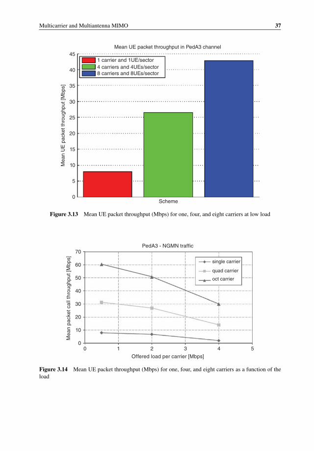
Multicarrier and Multiantenna MIMO 37
1 carrier and 1UE/sector4 carriers and 4UEs/sector8 carriers and 8UEs/sector
45
40
35
30
25
20
15
10
5
0Scheme
Mean UE packet throughput in PedA3 channel
Mea
n U
E p
acke
t thr
ough
put [
Mbp
s]
Figure 3.13 Mean UE packet throughput (Mbps) for one, four, and eight carriers at low load
single carrier
quad carrier
oct carrier
70
60
50
40
30
20
10
00 1 2
Offered load per carrier [Mbps]
Mea
n pa
cket
cal
l thr
ough
put [
Mbp
s]
PedA3 - NGMN traffic
3 4 5
Figure 3.14 Mean UE packet throughput (Mbps) for one, four, and eight carriers as a function of theload
38 HSPA+ Evolution to Release 12
Table 3.3 4/8-carrier HSDPA band combinations defined in 3GPP
Bands Release
Band 1 (2100 MHz) and Band 8 (900 MHz) Release 10Band 1 (2100 MHz) and Band 5 (850 MHz) Release 10Band 2 (1900 MHz) and Band 4 (2100/1700 MHz) Release 10Band 2 (1900 MHz) and Band 5 (850 MHz) Release 11
The band combinations so far defined in 3GPP in addition to the dual-carrier cases coveredin Table 3.2 are listed in Table 3.3, together with their corresponding Release. In all cases theuplink can be on either of the bands.
3.5 Downlink MIMO
Multiple transmit and receive antennas open the possibility of exploring the spatial dimension.In the following, different mechanisms for exploration are briefly summarized and then theirimplementation in HSPA is detailed.
Space-time coding, or Space-Time Transmit Diversity (STTD) in 3GPP, is an open-loopdiversity scheme which uses a constant coding scheme. Many different space-time codes aredescribed in literature, for example, space-time trellis codes, differential space-time codes,or space-time block codes. From a decoding perspective, orthogonal space-time block codesshow very low complexity. The Alamouti code [6] was proven to be the only orthogonalspace-time block code which provides full diversity and was included already in Release 5 ofthe HSPA standard.
An alternative group of MIMO schemes rely on feedback and are called closed-loop spatialmultiplexing. Within the closed-loop transmit diversity schemes, two different gain mecha-nisms are used, that is, array gain and multiplexing gain.
Array gain is sometimes called beamforming gain which may be misleading since noliteral beams are created. The schemes standardized in 3GPP for HSPA are rather adaptivespatial filters (pre-coders) which allow for a coherent superposition of the received signal fromdifferent transmit antennas based on the feedback of the receiver. The spatial filter adapts tothe fading channel over time and does not create a fixed beam towards a certain direction.Due to the coherent superposition, the received signal power is increased which is particularlyuseful under high interference at the cell edge.
Spatial multiplexing increases the number of streams transmitted in parallel over multipleantennas. The main challenge of the multiplexing scheme is the decoding, since all streamshave to be separated. Therefore, at least as many receive antennas are required as streams aremultiplexed and orthogonal pre-coding is used. Multiplexing multiple streams distribute theoverall transmit power equally between the streams and the power per stream is lower. Hence,the decoding of multiplexed streams require good to very good channel conditions which aretypically found in the cell center.
With spatial filtering (beamforming) providing gains at the cell edge and spatial multiplexingin the cell center, the combination of both is natural. However, there is a natural tradeoffbetween array gain and multiplexing gain [7]; for example, transmitting the maximum number
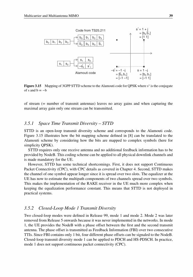
Multicarrier and Multiantenna MIMO 39
s = 1 –j= [b0 b1]= [–1 1]
s* = 1 + j= [b0 1] = [1 1]
–s* = –1 –j= [ 0 b1]= [–1 –1]
s1 s2–s*2 s*
1
s1 s2
b0 b1 b2 b3
b0 b1 b2 b3
2 b3 b0 1
Alamouti code
Code from TS25.211b–
b–
b–
b–
Figure 3.15 Mapping of 3GPP STTD scheme to the Alamouti code for QPSK where s∗ is the conjugateof s and b = −b
of stream (= number of transmit antennas) leaves no array gains and when capturing themaximal array gain only one stream can be transmitted.
3.5.1 Space Time Transmit Diversity – STTD
STTD is an open-loop transmit diversity scheme and corresponds to the Alamouti code.Figure 3.15 illustrates how the bit mapping scheme defined in [8] can be translated to theAlamouti scheme by considering how the bits are mapped to complex symbols (here forsimplicity QPSK).
STTD requires only one receive antenna and no additional feedback information has to beprovided by NodeB. This coding scheme can be applied to all physical downlink channels andis made mandatory for the UE.
However, STTD has some technical shortcomings. First, it does not support ContinuousPacket Connectivity (CPC), with CPC details as covered in Chapter 4. Second, STTD makesthe channel of one symbol appear longer since it is spread over two slots. The equalizer at theUE has now to estimate the multipath components of two channels spread over two symbols.This makes the implementation of the RAKE receiver in the UE much more complex whenkeeping the equalization performance constant. This means that STTD is not deployed inpractical systems.
3.5.2 Closed-Loop Mode 1 Transmit Diversity
Two closed-loop modes were defined in Release 99, mode 1 and mode 2. Mode 2 was laterremoved from Release 5 onwards because it was never implemented in the networks. In mode1, the UE provides the NodeB with a phase offset between the first and the second transmitantenna. The phase offset is transmitted as Feedback Information (FBI) over two consecutiveTTIs. Since FBI contains only 1 bit, four different phase offsets can be signaled to the NodeB.Closed-loop transmit diversity mode 1 can be applied to PDCH and HS-PDSCH. In practice,mode 1 does not support continuous packet connectivity (CPC).
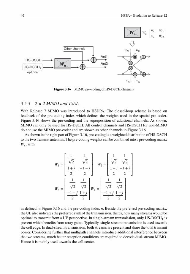
40 HSPA+ Evolution to Release 12
WnWnWWWW
Other channels
HS-DSCH
HS-DSCH2
Ant1
Ant2
optional
WnWnWWWW2221
1211
w
22w
w
21w
w
12w
w
11w
Wn
Figure 3.16 MIMO pre-coding of HS-DSCH channels
3.5.3 2 × 2 MIMO and TxAA
With Release 7 MIMO was introduced to HSDPA. The closed-loop scheme is based onfeedback of the pre-coding index which defines the weights used in the spatial pre-coder.Figure 3.16 shows the pre-coding and the superposition of additional channels. As shown,MIMO can only be used for HS-DSCH. All control channels and HS-DSCH for non-MIMOdo not use the MIMO pre-coder and are shown as other channels in Figure 3.16.
As shown in the right part of Figure 3.16, pre-coding is a weighted distribution of HS-DSCHto the two transmit antennas. The pre-coding weights can be combined into a pre-coding matrixWn, with
W1 =
⎡⎢⎢⎢⎢⎣
1√2
1√2
1 + j
2−1 − j
2
⎤⎥⎥⎥⎥⎦W2 =
⎡⎢⎢⎢⎢⎣
1√2
1√2
1 − j
2−1 + j
2
⎤⎥⎥⎥⎥⎦
W3 =
⎡⎢⎢⎢⎢⎣
1√2
1√2
−1 − j
21 + j
2
⎤⎥⎥⎥⎥⎦W4 =
⎡⎢⎢⎢⎢⎣
1√2
1√2
−1 + j
21 − j
2
⎤⎥⎥⎥⎥⎦
as defined in Figure 3.16 and the pre-coding index n. Beside the preferred pre-coding matrix,the UE also indicates the preferred rank of the transmission, that is, how many streams would beoptimal to transmit from a UE perspective. In single-stream transmission, only HS-DSCH1 ispresent which benefits from array gains. Typically, single-stream transmission is used towardsthe cell edge. In dual-stream transmission, both streams are present and share the total transmitpower. Considering further that multipath channels introduce additional interference betweenthe two streams, much better reception conditions are required to decode dual-stream MIMO.Hence it is mainly used towards the cell center.
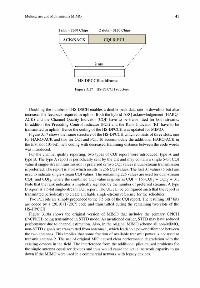
Multicarrier and Multiantenna MIMO 41
1 slot = 2560 Chips
HS-DPCCH subframe
ACK/NACK CQI & PCI
2 slots = 5120 Chips
2 ms
Figure 3.17 HS-DPCCH structure
Doubling the number of HS-DSCH enables a double peak data rate in downlink but alsoincreases the feedback required in uplink. Both the hybrid-ARQ acknowledgement (HARQ-ACK) and the Channel Quality Indicator (CQI) have to be transmitted for both streams.In addition the Precoding Control Indicator (PCI) and the Rank Indicator (RI) have to betransmitted in uplink. Hence the coding of the HS-DPCCH was updated for MIMO.
Figure 3.17 shows the frame structure of the HS-DPCCH which consists of three slots, onefor HARQ-ACK and two for CQI and PCI. To accommodate the additional HARQ-ACK inthe first slot (10-bit), new coding with decreased Hamming distance between the code wordswas introduced.
For the channel quality reporting, two types of CQI report were introduced: type A andtype B. The type A report is periodically sent by the UE and may contain a single 5-bit CQIvalue if single-stream transmission is preferred or two CQI values if dual-stream transmissionis preferred. The report is 8 bit which results in 256 CQI values. The first 31 values (5 bits) areused to indicate single-stream CQI values. The remaining 225 values are used for dual-streamCQI1 and CQI2, where the combined CQI value is given as CQI = 15×CQI1 + CQI2 + 31.Note that the rank indicator is implicitly signaled by the number of preferred streams. A typeB report is a 5-bit single-stream CQI report. The UE can be configured such that the report istransmitted periodically to create a reliable single-stream reference for the scheduler.
Two PCI bits are simply prepended to the 8|5 bits of the CQI report. The resulting 10|7 bitsare coded by a (20,10) | (20,7) code and transmitted during the remaining two slots of theHS-DPCCH.
Figure 3.18a shows the original version of MIMO that includes the primary CPICH(P-CPICH) being transmitted in STTD mode. As mentioned earlier, STTD may have reducedperformance due to channel estimation. Also, in the original MIMO scheme all non-MIMO,non-STTD signals are transmitted from antenna 1, which leads to a power difference betweenthe two antennas. This implies that some fraction of available transmit power is not used attransmit antenna 2. The use of original MIO caused clear performance degradation with theexisting devices in the field. The interference from the additional pilot caused problems forthe single antenna equalizer devices and thus would cause the actual network capacity to godown if the MIMO were used in a commercial network with legacy devices.
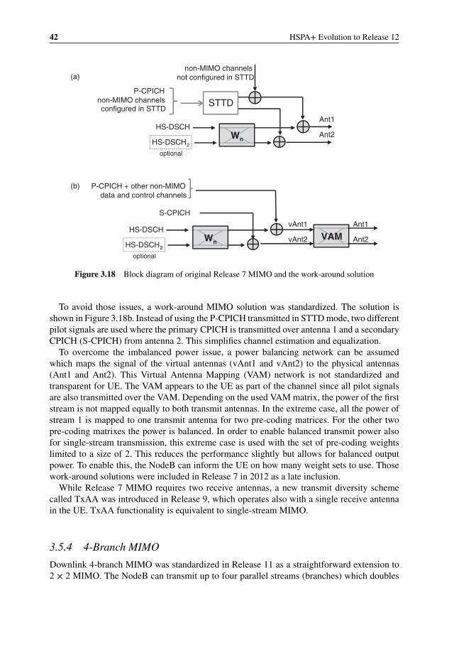
42 HSPA+ Evolution to Release 12
P-CPICHnon-MIMO channelsconfigured in STTD
WnWnWWWWHS-DSCH
HS-DSCH2
Ant1
Ant2
optional
STTD
P-CPICH + other non-MIMOdata and control channels
WnWnWWWWHS-DSCH
HS-DSCH2
vAnt1
vAnt2
optional
S-CPICH
VAMVAMVAMAAnt1
Ant2
non-MIMO channelsnot configured in STTD(a)
(b)
Figure 3.18 Block diagram of original Release 7 MIMO and the work-around solution
To avoid those issues, a work-around MIMO solution was standardized. The solution isshown in Figure 3.18b. Instead of using the P-CPICH transmitted in STTD mode, two differentpilot signals are used where the primary CPICH is transmitted over antenna 1 and a secondaryCPICH (S-CPICH) from antenna 2. This simplifies channel estimation and equalization.
To overcome the imbalanced power issue, a power balancing network can be assumedwhich maps the signal of the virtual antennas (vAnt1 and vAnt2) to the physical antennas(Ant1 and Ant2). This Virtual Antenna Mapping (VAM) network is not standardized andtransparent for UE. The VAM appears to the UE as part of the channel since all pilot signalsare also transmitted over the VAM. Depending on the used VAM matrix, the power of the firststream is not mapped equally to both transmit antennas. In the extreme case, all the power ofstream 1 is mapped to one transmit antenna for two pre-coding matrices. For the other twopre-coding matrixes the power is balanced. In order to enable balanced transmit power alsofor single-stream transmission, this extreme case is used with the set of pre-coding weightslimited to a size of 2. This reduces the performance slightly but allows for balanced outputpower. To enable this, the NodeB can inform the UE on how many weight sets to use. Thosework-around solutions were included in Release 7 in 2012 as a late inclusion.
While Release 7 MIMO requires two receive antennas, a new transmit diversity schemecalled TxAA was introduced in Release 9, which operates also with a single receive antennain the UE. TxAA functionality is equivalent to single-stream MIMO.
3.5.4 4-Branch MIMO
Downlink 4-branch MIMO was standardized in Release 11 as a straightforward extension to2 × 2 MIMO. The NodeB can transmit up to four parallel streams (branches) which doubles

Multicarrier and Multiantenna MIMO 43
the peak data rate per carrier. However, 4-branch MIMO only supports up to four carriersand hence the HSDPA peak data rate remains at 336 Mbit/s. Since a UE supporting 4-branchMIMO is assumed to have advanced receiver, the UE has to have the capability of decodingat least two streams (two Rx antennas) and has to support at least two carriers.
In practice it is expected that there will be more terminals with two receive antennas. Fourantennas will be only realistic in larger devices like tablets or laptops. Hence, the 4-branchMIMO design focuses more on optimizing 4 × 2 transmissions and enabling 4 × 4 MIMO. Themain limitation of transmitting up to four streams is to feedback CQI and HARQ ACK/NACKon the uplink HS-DPCCH especially since this channel also has to carry an extended pre-codingindex and rank index.
To limit the feedback in uplink, up to two transport blocks are bundled in codewords andthe CQI/HARQ ACK/NACK is transmitted only per codeword. This allows for transmittingfour transport blocks with the same amount of feedback as would be required for two transportblocks. The transport block bundling causes some limited performance loss since the wholecodeword has to be retransmitted when the transmission of only one transport block fails.Also the feedback of combined CQI values implies that for both transport blocks the samemodulation and coding is used even though they are transmitted over different layers whichmay have different quality. To obtain an equal performance for both transport blocks in onecodeword, the transport blocks are interleaved within the codeword. If one or two transportblocks are transmitted in parallel, each transport block is mapped to one codeword and noperformance reduction is observed. The codeword mapping is illustrated in Figure 3.19.
4-branch MIMO uses the same codebook for spatial pre-coding as LTE. The codebookhas 16 sets of pre-coding weights where the optimal set is chosen by the UE. The NodeB isinformed which set to use by the 4-bit pre-coding indicator (PCI). Figure 3.20 shows how 4-branch MIMO channels are combined with 2 × 2 MIMO, non-MIMO, and signaling channels.For legacy reasons, non-MIMO HS-DSCH and other signaling channels have to be transmittedtogether with the primary pilot (P-CPICH) over the first (virtual) antenna. The same appliesfor the first secondary pilot (S-CPICH1) and output of the 2 × 2 MIMO pre-coder Wn.
The 4-branch MIMO pre-coder Hn can multiplex one to four layers (streams). If only onelayer is transmitted, HS-DSCH can’t be combined with a not-present channel to one codewordand is transmitted only over layer 1. The same applies for HS-DSCH2.
The changes to HS-DPCCH are limited thanks to the introduction of codewords. TheHARQ-ACK feedback the CQI reports remain unchanged. Only the pre-coding indicator isextended from 2 to 4 bits and 2 bits are added to indicate that the Number of Transport BlocksPreferred (NTBP) are introduced which corresponds to the rank indicator in LTE. Those four
TrBlk 1
TrBlk 4
TrBlk 2
TrBlk 3
Codeword 1
Codeword 2
Codeword interleaver
Layer 1
Layer 2
Layer 3
Layer 4
Spa
tial
prec
oder
vAntenna 1
vAntenna 2
vAntenna 3
vAntenna 4
Codeword interleaver
Figure 3.19 Transport block to codeword mapping introduced to 4-branch MIMO to reduce feedback

44 HSPA+ Evolution to Release 12
WnWnWWWW
S-CPICH1
HS-DSCH
P-CPICHother channels
HS-DSCH
HS-DSCH2
1×1/1×2SIMO
2x2 MIMO
HnHnHH
HS-DSCH3
HS-DSCH2
HS-DSCH4
HS-DSCH1
S-CPICH2+D-CPICH1
4-branchMIMO
S-CPICH3+D-CPICH2
Layer 1
Layer 2
Layer 3
Layer 4
Ant1
Ant2
Ant3
Ant4
optional
optional
optional optional
Figure 3.20 4-branch MIMO block diagram with newly introduced pilot channels and the combinationwith 2 × 2 MIMO and non-MIMO
new bits can be accommodated in the HS-DPCCH by using a rate 1/2 convolutional code fortype A reports and rate 1/3 convolutional code for type B reports. Note that the increased errorprobability due to reduced coding protection has to be compensated by higher transmit power.
Since the channel between each transmit antenna and receive antenna has to be estimatedseparately, new pilot signals have to be introduced. Adding more pilots with similar power asthe P-CPICH would imply for four transmit antennas that 40% of the total power is used forpilot signals, which is clearly too much. Hence a different solution is used.
The common and secondary pilots are required for
1. channel quality measurement and2. channel estimation for demodulation.
While the channel quality measurement needs to be done every TTI to calculate the channelquality indicator (CQI), the channel estimation for demodulation is only needed when a datachannel is scheduled in downlink. Pilots for channel quality measurements require muchless power since the accuracy of the channel estimate needs to be much lower. The channelestimation for decoding directly influences the decoding and system performance.
According to the two different requirements, two different pilot signals are introduced for4-branch MIMO. New secondary CPICH channels are transmitted permanently over antenna3 and 4. The power of the newly introduced pilot channels is defined relative to P-CPICHand can vary from −12 to 0 dB (see Figure 3.21). The secondary pilot 2 and 3 are used tocalculate periodical CQI reports. In many cases the power of S-CPICH2/3 is also sufficient
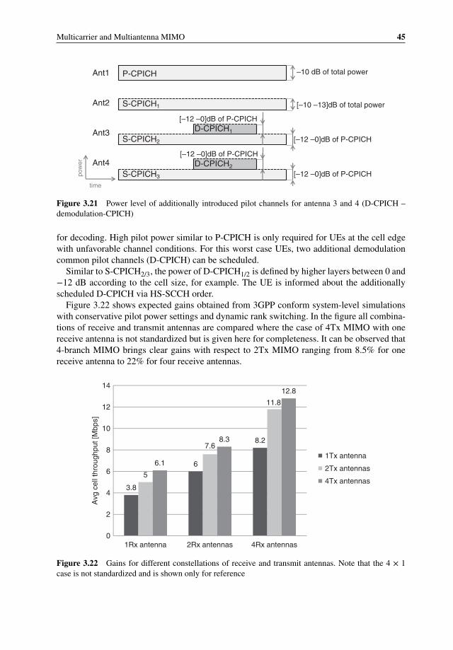
Multicarrier and Multiantenna MIMO 45
Ant1
Ant2
Ant3
Ant4
–10 dB of total power
[–10 –13]dB of total power
[–12 –0]dB of P-CPICH
[–12 –0]dB of P-CPICH
P-CPICH
[–12 –0]dB of P-CPICH
S-CPICH1
S-CPICH2
S-CPICH3
D-CPICH1
D-CPICH2
[–12 –0]dB of P-CPICH
pow
er
time
Figure 3.21 Power level of additionally introduced pilot channels for antenna 3 and 4 (D-CPICH –demodulation-CPICH)
for decoding. High pilot power similar to P-CPICH is only required for UEs at the cell edgewith unfavorable channel conditions. For this worst case UEs, two additional demodulationcommon pilot channels (D-CPICH) can be scheduled.
Similar to S-CPICH2/3, the power of D-CPICH1/2 is defined by higher layers between 0 and−12 dB according to the cell size, for example. The UE is informed about the additionallyscheduled D-CPICH via HS-SCCH order.
Figure 3.22 shows expected gains obtained from 3GPP conform system-level simulationswith conservative pilot power settings and dynamic rank switching. In the figure all combina-tions of receive and transmit antennas are compared where the case of 4Tx MIMO with onereceive antenna is not standardized but is given here for completeness. It can be observed that4-branch MIMO brings clear gains with respect to 2Tx MIMO ranging from 8.5% for onereceive antenna to 22% for four receive antennas.
3.8
6
8.2
5
7.6
11.8
6.1
8.3
12.8
0
2
4
6
8
10
12
14
1Rx antenna 2Rx antennas 4Rx antennas
Avg
cel
l thr
ough
put [
Mbp
s]
1Tx antenna
2Tx antennas
4Tx antennas
Figure 3.22 Gains for different constellations of receive and transmit antennas. Note that the 4 × 1case is not standardized and is shown only for reference
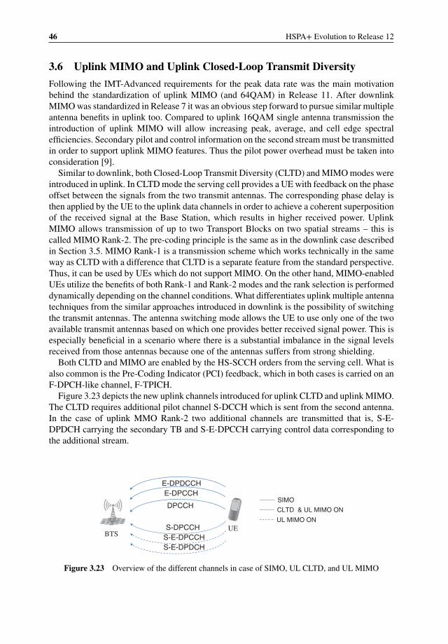
46 HSPA+ Evolution to Release 12
3.6 Uplink MIMO and Uplink Closed-Loop Transmit Diversity
Following the IMT-Advanced requirements for the peak data rate was the main motivationbehind the standardization of uplink MIMO (and 64QAM) in Release 11. After downlinkMIMO was standardized in Release 7 it was an obvious step forward to pursue similar multipleantenna benefits in uplink too. Compared to uplink 16QAM single antenna transmission theintroduction of uplink MIMO will allow increasing peak, average, and cell edge spectralefficiencies. Secondary pilot and control information on the second stream must be transmittedin order to support uplink MIMO features. Thus the pilot power overhead must be taken intoconsideration [9].
Similar to downlink, both Closed-Loop Transmit Diversity (CLTD) and MIMO modes wereintroduced in uplink. In CLTD mode the serving cell provides a UE with feedback on the phaseoffset between the signals from the two transmit antennas. The corresponding phase delay isthen applied by the UE to the uplink data channels in order to achieve a coherent superpositionof the received signal at the Base Station, which results in higher received power. UplinkMIMO allows transmission of up to two Transport Blocks on two spatial streams – this iscalled MIMO Rank-2. The pre-coding principle is the same as in the downlink case describedin Section 3.5. MIMO Rank-1 is a transmission scheme which works technically in the sameway as CLTD with a difference that CLTD is a separate feature from the standard perspective.Thus, it can be used by UEs which do not support MIMO. On the other hand, MIMO-enabledUEs utilize the benefits of both Rank-1 and Rank-2 modes and the rank selection is performeddynamically depending on the channel conditions. What differentiates uplink multiple antennatechniques from the similar approaches introduced in downlink is the possibility of switchingthe transmit antennas. The antenna switching mode allows the UE to use only one of the twoavailable transmit antennas based on which one provides better received signal power. This isespecially beneficial in a scenario where there is a substantial imbalance in the signal levelsreceived from those antennas because one of the antennas suffers from strong shielding.
Both CLTD and MIMO are enabled by the HS-SCCH orders from the serving cell. What isalso common is the Pre-Coding Indicator (PCI) feedback, which in both cases is carried on anF-DPCH-like channel, F-TPICH.
Figure 3.23 depicts the new uplink channels introduced for uplink CLTD and uplink MIMO.The CLTD requires additional pilot channel S-DCCH which is sent from the second antenna.In the case of uplink MMO Rank-2 two additional channels are transmitted that is, S-E-DPDCH carrying the secondary TB and S-E-DPCCH carrying control data corresponding tothe additional stream.
DPCCH
E‐DPCCH E‐DPDCCH
S‐DPCCHS‐E‐DPCCHS‐E‐DPDCH
UL MIMO ON
CLTD & UL MIMO ON
SIMO
BTSUE
Figure 3.23 Overview of the different channels in case of SIMO, UL CLTD, and UL MIMO

Multicarrier and Multiantenna MIMO 47
During the uplink MIMO Rank-2 studies it was decided to transmit dual TB independentlyover the spatial streams. It was also decided that each spatial stream use independent E-TFCselection (rate adaptation). This operation provides more flexibility and maximizes the achiev-able throughput. The drawback of this solution is the additional overhead of the schedulingand HARQ control information which is associated to each stream in uplink. In downlink foreach stream the E-TFC indicator (E-TFCI) and the ACK/NACK must be sent. The two trans-port blocks are acknowledged independently using the E-HICH channel, where two differentsignatures are configured on the same E-HICH code channel. There is only one inner and outerpower control loop for both streams.
However it was not the only scheme that was evaluated during the Rel-11 studies. Two othershad some benefits and drawbacks compared to the chosen one but based on the performanceresults were not selected. Nevertheless, in order to give some background short descriptionsare provided below [10]:
� Design #1 – single Transport Block Rank-2 transmission. Due to the fact that in this case itis sufficient to indicate a single E-TFC and transmission rank in uplink, there is low controlsignaling overhead. The main disadvantage of this approach is the low channel adaptationability, in a situation where there is strong imbalance between MIMO spatial streams, due tothe fact that all parameters for both spatial streams should be the same, that is, modulation,OVSF code allocation, bit mapping and power allocation.
� Design #2 – dual TB Rank-2 transmission, TBs interleaved between the two spatial channels.This option can be described as a hybrid between design #1 and the standardized designwhich was described in the paragraph above. Interleaving allows transmission of each TBover the same channel conditions. In terms of signaling, the HARQ overhead is the same asin the standardized solution. It was discarded because, similarly to design #1, this approachfacilitates less efficient scheduling.
It is worth noting that if the transmission of the TB on the secondary stream fails for whateverreason, uplink MIMO Rank-2 mode will be operated as it was uplink CLTD (or uplink MIMORank-1). More details about differences between uplink MIMO and beamforming CLTD arepresented in the figures in Section 3.6.1 below.
3.6.1 Uplink MIMO Channel Architecture
In order to benefit from uplink MIMO transmission there is a need to introduce new uplinkphysical channels that is, Secondary Dedicated Physical Control Channel (S-DPCCH), Sec-ondary Dedicated Physical Control Channel for E-DCH (S-E-DPCCH) and Secondary Dedi-cated Physical Data Channel for E-DCH (S-E-DPDCH) as they are shown in the Figure 3.24below.
Details about channel configuration of UL CLTD are presented below in Figure 3.25.As presented in the figures below, a UE is able to transmit data in an additional two instances
(depending on network conditions and UE capability):
1. UL-CLTD (Uplink MIMO Rank-1) – DPCCH, E-DPDCH, E-DPCCH and S-DPCCH2. Uplink MIMO (Rank-2) – DPCCH, E-DPDCH, E-DPCCH, S-DPCCH, S-E-DPCCH and
S-E-DPDCH.
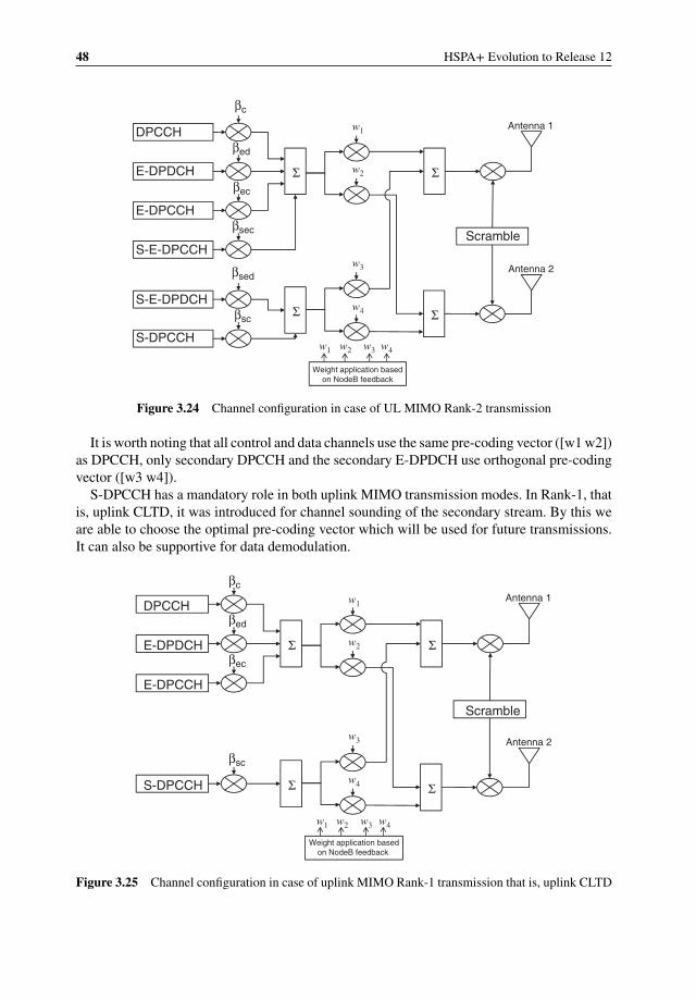
48 HSPA+ Evolution to Release 12
βc
βed
βec
S‐E‐DPCCH
E‐DPCCH
E‐DPDCH
DPCCH
βsec
S‐DPCCH
S‐E‐DPDCH
βsed
βsc
Σ
Σ
w1
w2
w2w1
w3
w3
w4
w4
Σ
Σ
Scramble
Antenna 1
Antenna 2
Weight application basedon NodeB feedback
Figure 3.24 Channel configuration in case of UL MIMO Rank-2 transmission
It is worth noting that all control and data channels use the same pre-coding vector ([w1 w2])as DPCCH, only secondary DPCCH and the secondary E-DPDCH use orthogonal pre-codingvector ([w3 w4]).
S-DPCCH has a mandatory role in both uplink MIMO transmission modes. In Rank-1, thatis, uplink CLTD, it was introduced for channel sounding of the secondary stream. By this weare able to choose the optimal pre-coding vector which will be used for future transmissions.It can also be supportive for data demodulation.
E‐DPCCH
E‐DPDCH
DPCCH
S‐DPCCH
Σ
Σ
Σ
Σ
Scramble
Antenna 1
Antenna 2
Weight application basedon NodeB feedback
βc
βed
βec
βsc
w1
w2
w3
w4
w1 w2 w3 w4
Figure 3.25 Channel configuration in case of uplink MIMO Rank-1 transmission that is, uplink CLTD
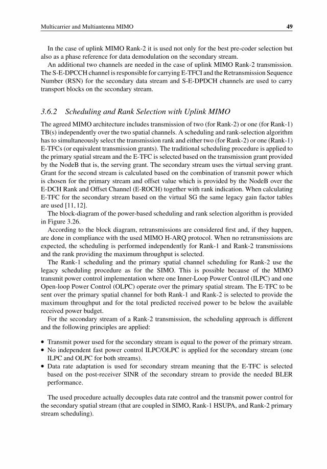
Multicarrier and Multiantenna MIMO 49
In the case of uplink MIMO Rank-2 it is used not only for the best pre-coder selection butalso as a phase reference for data demodulation on the secondary stream.
An additional two channels are needed in the case of uplink MIMO Rank-2 transmission.The S-E-DPCCH channel is responsible for carrying E-TFCI and the Retransmission SequenceNumber (RSN) for the secondary data stream and S-E-DPDCH channels are used to carrytransport blocks on the secondary stream.
3.6.2 Scheduling and Rank Selection with Uplink MIMO
The agreed MIMO architecture includes transmission of two (for Rank-2) or one (for Rank-1)TB(s) independently over the two spatial channels. A scheduling and rank-selection algorithmhas to simultaneously select the transmission rank and either two (for Rank-2) or one (Rank-1)E-TFCs (or equivalent transmission grants). The traditional scheduling procedure is applied tothe primary spatial stream and the E-TFC is selected based on the transmission grant providedby the NodeB that is, the serving grant. The secondary stream uses the virtual serving grant.Grant for the second stream is calculated based on the combination of transmit power whichis chosen for the primary stream and offset value which is provided by the NodeB over theE-DCH Rank and Offset Channel (E-ROCH) together with rank indication. When calculatingE-TFC for the secondary stream based on the virtual SG the same legacy gain factor tablesare used [11, 12].
The block-diagram of the power-based scheduling and rank selection algorithm is providedin Figure 3.26.
According to the block diagram, retransmissions are considered first and, if they happen,are done in compliance with the used MIMO H-ARQ protocol. When no retransmissions areexpected, the scheduling is performed independently for Rank-1 and Rank-2 transmissionsand the rank providing the maximum throughput is selected.
The Rank-1 scheduling and the primary spatial channel scheduling for Rank-2 use thelegacy scheduling procedure as for the SIMO. This is possible because of the MIMOtransmit power control implementation where one Inner-Loop Power Control (ILPC) and oneOpen-loop Power Control (OLPC) operate over the primary spatial stream. The E-TFC to besent over the primary spatial channel for both Rank-1 and Rank-2 is selected to provide themaximum throughput and for the total predicted received power to be below the availablereceived power budget.
For the secondary stream of a Rank-2 transmission, the scheduling approach is differentand the following principles are applied:
� Transmit power used for the secondary stream is equal to the power of the primary stream.� No independent fast power control ILPC/OLPC is applied for the secondary stream (one
ILPC and OLPC for both streams).� Data rate adaptation is used for secondary stream meaning that the E-TFC is selected
based on the post-receiver SINR of the secondary stream to provide the needed BLERperformance.
The used procedure actually decouples data rate control and the transmit power control forthe secondary spatial stream (that are coupled in SIMO, Rank-1 HSUPA, and Rank-2 primarystream scheduling).
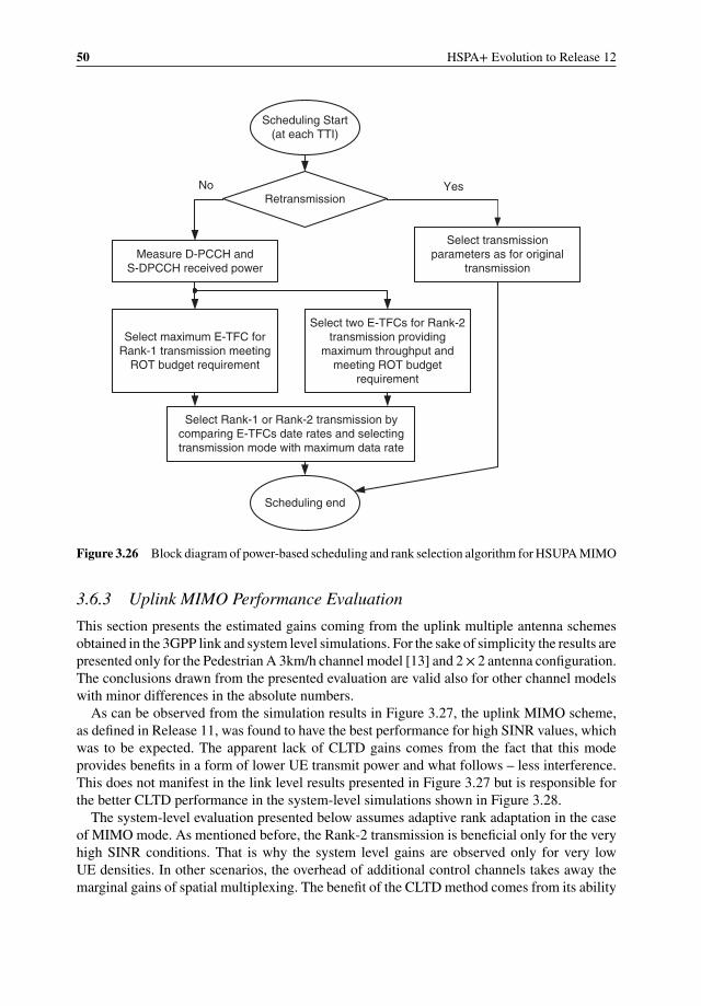
50 HSPA+ Evolution to Release 12
Scheduling Start(at each TTI)
Retransmission
Measure D-PCCH andS-DPCCH received power
No
Select maximum E-TFC forRank-1 transmission meeting
ROT budget requirement
Select two E-TFCs for Rank-2transmission providing
maximum throughput andmeeting ROT budget
requirement
Select Rank-1 or Rank-2 transmission bycomparing E-TFCs date rates and selectingtransmission mode with maximum data rate
Select transmissionparameters as for original
transmission
Scheduling end
Yes
Figure 3.26 Block diagram of power-based scheduling and rank selection algorithm for HSUPA MIMO
3.6.3 Uplink MIMO Performance Evaluation
This section presents the estimated gains coming from the uplink multiple antenna schemesobtained in the 3GPP link and system level simulations. For the sake of simplicity the results arepresented only for the Pedestrian A 3km/h channel model [13] and 2× 2 antenna configuration.The conclusions drawn from the presented evaluation are valid also for other channel modelswith minor differences in the absolute numbers.
As can be observed from the simulation results in Figure 3.27, the uplink MIMO scheme,as defined in Release 11, was found to have the best performance for high SINR values, whichwas to be expected. The apparent lack of CLTD gains comes from the fact that this modeprovides benefits in a form of lower UE transmit power and what follows – less interference.This does not manifest in the link level results presented in Figure 3.27 but is responsible forthe better CLTD performance in the system-level simulations shown in Figure 3.28.
The system-level evaluation presented below assumes adaptive rank adaptation in the caseof MIMO mode. As mentioned before, the Rank-2 transmission is beneficial only for the veryhigh SINR conditions. That is why the system level gains are observed only for very lowUE densities. In other scenarios, the overhead of additional control channels takes away themarginal gains of spatial multiplexing. The benefit of the CLTD method comes from its ability

Multicarrier and Multiantenna MIMO 51
00
2000
4000
6000
8000
10000
Thr
ough
put [
kbps
]
12000
14000
Link throughput as a function of Rx Ec/No: 1 × 2 SIMO, 2 × 2 CL-BFTD,and 2 × 2 MIMO, PA3 Channel
5 10Pre-receiver Rx Ec/No [dB]
15 20
SIMO
CLTD
MIMO
Figure 3.27 Link throughputs of different transmission modes, PedA 3 km/h, 2 × 2 (1 × 2) antennaconfiguration
0
2000
4000
6000
8000
10000
12000
Ave
rage
UE
thro
ughp
ut [k
bps]
410.250.0175
User density [UEs/sector]
SIMO
UL CLTD
UL MIMO
Figure 3.28 System level throughputs for different transmission modes, PedA 3 km/h, 2 × 2 (1 × 2)antenna configuration
52 HSPA+ Evolution to Release 12
to reach the same throughput by using less transmit power, therefore causing less interferenceto other UEs. This is why this scheme seems to be beneficial for all user densities. It shouldbe noted that the above evaluation assumes using an inter-stream interference cancellationreceiver in case of MIMO. The capability of cancelling the interference from the primarystream was proven to be of high importance for UL MIMO feasibility.
3.7 Conclusions
After the basic HSPA functionality created in Release 5 and 6, HSPA evolution has added alot of capabilities in both the multiantenna and also the multicarrier domain. While many ofthe other features in this chapter are still waiting for large scale implementation, the supportfor dual-cell HSDPA has been already widely deployed globally, and offers the 42 Mbps peakdata rate quite commonly. Globally, from all HSPA networks, roughly 1 out of 4 of HSPAnetworks will have enabled dual-carrier HSDPA by the end of 2013. The chips sets supportingdual-cell HSUPA have been also published, and are expected to be available during 2014 inthe marketplace, enabling uplink support of 11.5 Mbps. HSDPA MIMO has been deployedin some networks but was not widely rolled out due to the legacy UE issues as covered inSection 3.5.3. Combining downlink MIMO with dual-cell HSDPA would enable pushing thedata rates to 84 Mbps, doubling the currently achievable HSPA peak data rate in the marketby many handsets today. Similarly, the HSUPA MIMO has not attracted huge interest in themarket due to the highly limited use case with virtually no interfering users in a cell. Uplinkclosed-loop transmit diversity seems to have more potential in this respect. The 3GPP Release11 specifications define the necessary support to go beyond the 100 Mbps limit with HSPA too,assuming large enough spectrum availability. On the uplink side, the combination of uplink16QAM together with dual-cell HSUPA allows data rates of up to 22 Mbps to be reached.
References
[1] Holma, H. and Toskala, A. (2010) WCDMA for UMTS, 5th edn, John Wiley & Sons, Ltd, Chichester.[2] Morais de Andrade, D., Klein, A., Holma, H. et al. (2009) Performance Evaluation on Dual-Cell HSDPA
Operation. IEEE Vehicular Technology Conference Fall 2009, Anchorage, Alaska, 2009.[3] 3GPP Technical Specification, TS 25.306, “UE Radio Access capabilities”, v 8.12.0, Release 8, June 2012.[4] Holma, H. and Toskala, A. (2011) LTE for UMTS, 2nd edn, John Wiley & Sons, Ltd, Chichester.[5] Holma, H. and Toskala, A. (2012) LTE-Advanced, John Wiley & Sons, Ltd, Chichester.[6] Alamouti, S.M. (1998) A simple transmit diversity technique for wireless communications. IEEE Journal on
Selected Areas in Communications, 16(8), 1451–1458.[7] Zheng, L. and Tse, D.N.C. (2003) Diversity and multiplexing: a fundamental tradeoff in multiple-antenna
channels. IEEE Transactions on Information Theory, 49(5), 1073–1096.[8] 3GPP Technical Specification, TS25.211, “Physical channels and mapping of transport channels onto physical
channels”.[9] 3GPP Technical Report, TR 25.871 v.1.0.1, Release 11, May 2011.
[10] 3GPP Technical Report, TR 25.871 v11.0.0, Release 11, September 2011.[11] 3GPP Technical Specification, TS 25.321, “Enhanced uplink; Overall description Stage 2”, Release 11.[12] 3GPP Technical Document, R1-121733 Scheduling and Rank Selection for HSUPA MIMO, RAN1 #68bis.[13] 3GPP Technical Document, R1-112632 UL MIMO Link Level Evaluation, Nokia Siemens Networks, RAN1
#66.

4Continuous Packet Connectivityand High Speed Common Channels
Harri Holma and Karri Ranta-aho
4.1 Introduction
WCDMA Release 99 was designed for large file transfers, not for frequent and bursty trans-mission of small packets such as those created by smartphones, see Chapter 13. The WCDMAair interface design is circuit switched like dedicated channels that are not optimized for effi-ciency, for latency, nor for terminal power consumption. High Speed Downlink Packet Access(HSDPA) in Release 5 and High Speed Uplink Packet Access (HSUPA) in Release 6 improvedthe efficiency, data rates, and latency considerably by providing a true packet channel-basedradio interface. The limitation was still that a Dedicated Physical Control Channel (DPCCH)was required and setting up and releasing DPCCH takes time, adding to the connection setuplatency and limiting the number of users with simultaneously active radio connections. Wecould say that the Release 6 solution was still circuit-switched from the control channel pointof view.
Release 7 brings Continuous Packet Connectivity (CPC) which enables DiscontinuousTransmission (DTX) for the control channel. Release 8 brings for the first time a true packet-switched channel type in HSPA with High Speed Random Access Channel (HS-RACH) forthe uplink direction, called Enhanced Cell_FACH in 3GPP. The corresponding downlinkchannel High Speed Forward Access Channel (HS-FACH) was defined in Release 7. Theevolution of the packet transmission in HSPA improves the network efficiency, terminal powerconsumption, and end user latency and reduces signaling load. CPC and HS-FACH comple-ment each other nicely: CPC gives benefits also together with HS-FACH during Cell_DCHstate. Additionally, CPC terminal penetration is far higher than HS-FACH penetration. Thesepacket transmission improvements have changed WCDMA radio access from circuit-switchedto packet-switched, which is important for smartphones. These solutions are illustrated in
HSPA+ Evolution to Release 12: Performance and Optimization, First Edition.Edited by Harri Holma, Antti Toskala, and Pablo Tapia.© 2014 John Wiley & Sons, Ltd. Published 2014 by John Wiley & Sons, Ltd.
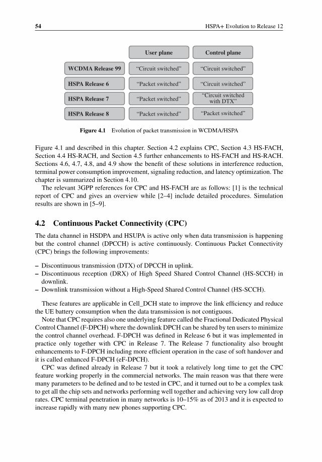
54 HSPA+ Evolution to Release 12
User plane
“Circuit switched”WCDMA Release 99
Control plane
“Circuit switched”
“Packet switched”HSPA Release 6 “Circuit switched”
“Packet switched”HSPA Release 7“Circuit switched
with DTX”
“Packet switched”HSPA Release 8 “Packet switched”
Figure 4.1 Evolution of packet transmission in WCDMA/HSPA
Figure 4.1 and described in this chapter. Section 4.2 explains CPC, Section 4.3 HS-FACH,Section 4.4 HS-RACH, and Section 4.5 further enhancements to HS-FACH and HS-RACH.Sections 4.6, 4.7, 4.8, and 4.9 show the benefit of these solutions in interference reduction,terminal power consumption improvement, signaling reduction, and latency optimization. Thechapter is summarized in Section 4.10.
The relevant 3GPP references for CPC and HS-FACH are as follows: [1] is the technicalreport of CPC and gives an overview while [2–4] include detailed procedures. Simulationresults are shown in [5–9].
4.2 Continuous Packet Connectivity (CPC)
The data channel in HSDPA and HSUPA is active only when data transmission is happeningbut the control channel (DPCCH) is active continuously. Continuous Packet Connectivity(CPC) brings the following improvements:
– Discontinuous transmission (DTX) of DPCCH in uplink.– Discontinuous reception (DRX) of High Speed Shared Control Channel (HS-SCCH) in
downlink.– Downlink transmission without a High-Speed Shared Control Channel (HS-SCCH).
These features are applicable in Cell_DCH state to improve the link efficiency and reducethe UE battery consumption when the data transmission is not contiguous.
Note that CPC requires also one underlying feature called the Fractional Dedicated PhysicalControl Channel (F-DPCH) where the downlink DPCH can be shared by ten users to minimizethe control channel overhead. F-DPCH was defined in Release 6 but it was implemented inpractice only together with CPC in Release 7. The Release 7 functionality also broughtenhancements to F-DPCH including more efficient operation in the case of soft handover andit is called enhanced F-DPCH (eF-DPCH).
CPC was defined already in Release 7 but it took a relatively long time to get the CPCfeature working properly in the commercial networks. The main reason was that there weremany parameters to be defined and to be tested in CPC, and it turned out to be a complex taskto get all the chip sets and networks performing well together and achieving very low call droprates. CPC terminal penetration in many networks is 10–15% as of 2013 and it is expected toincrease rapidly with many new phones supporting CPC.

Continuous Packet Connectivity and High Speed Common Channels 55
E-DPDCH
DPCCH
E-DPDCH
DPCCH
Release 6 without continuous packet connectivity
Release 7 with continuous packet connectivity
Figure 4.2 CPC concept in uplink
4.2.1 Uplink DTX
The CPC concept in uplink is illustrated in Figure 4.2. The uplink Enhanced DedicatedPhysical Data Channel (E-DPDCH) runs only when there is data transmission in uplink whileDPCCH runs also during data inactivity in Release 6. The typical inactivity timer before thechannel is released and the UE moved to Cell_FACH or to Cell_PCH is several seconds.CPC allows using discontinuous DPCCH transmission during data inactivity when DPCCHis transmitted only in short bursts. These short bursts of DPCCH are needed to maintain thelink synchronization and power control for instantaneous resumption of the data traffic. Thediscontinuous transmission brings two main benefits: less interference is created in the networkand less battery power is used by the terminal.
Typical CPC parameter values are shown in Table 4.1 both for 2-ms TTI and 10-ms TTI.Normally, 2-ms TTI is used as long as the uplink link budget allows 2-ms TTI transmission.If the signal level gets low, then the connection is reconfigured to 10-ms TTI.
Table 4.1 Typical CPC parameters (subframe = 2 ms)
Name 2-ms TTI 10-ms TTI
UE DTX Cycle 1 8 subframes 10 subframesUE DTX Cycle 2 16 subframes 20 subframesInactivity threshold for UE DTX Cycle 2 64 subframes 80 subframesUE DPCCH burst 1 1 subframe 1 subframeUE DPCCH burst 2 1 subframe 1 subframeUE DTX long preamble 4 slots 4 slotsInactivity threshold for UE DRX cycle 64 subframes 64 subframesUE DRX cycle 8 subframes 8 subframesMAC DTX cycle 8 subframes 10 subframesCQI feedback cycle with CPC 4 subframes 5 subframes
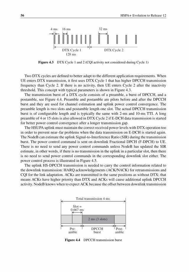
56 HSPA+ Evolution to Release 12
4 ms 16 ms 32 ms
DTX Cycle 1
128 ms DTX Cycle 2
Figure 4.3 DTX Cycle 1 and 2 (CQI activity not considered during Cycle 1)
Two DTX cycles are defined to better adapt to the different application requirements. WhenUE enters DTX transmission, it first uses DTX Cycle 1 that has higher DPCCH transmissionfrequency than Cycle 2. If there is no activity, then UE enters Cycle 2 after the inactivitythreshold. This concept with typical parameters is shown in Figure 4.3.
The transmission burst of a DTX cycle consists of a preamble, a burst of DPCCH, and apostamble, see Figure 4.4. Preamble and postamble are pilots before and after the DPCCHburst and they are used for channel estimation and uplink power control convergence. Thepreamble length is two slots and postamble length one slot. The actual DPCCH transmissionburst is of configurable length and is typically the same with 2-ms and 10-ms TTI. A longpreamble of 4 or 15 slots is also allowed in DTX Cycle 2 if E-DCH data transmission is startedfor better power control convergence after a longer transmission gap.
The HSUPA uplink must maintain the correct received power levels with DTX operation tooin order to prevent near–far problems when the data transmission on E-DCH is started again.The NodeB can estimate the uplink Signal-to-Interference Ratio (SIR) during the transmissionburst. The power control command is sent on downlink Fractional DPCH (F-DPCH) to UE.There is no need to send any power control commands unless NodeB has updated the SIRestimate, in other words, if there is no transmission in the uplink in a particular slot, then thereis no need to send power control commands in the corresponding downlink slot either. Thepower control process is illustrated in Figure 4.5.
The uplink HS-DPCCH transmission is needed to carry the control information related tothe downlink transmission: HARQ acknowledgements (ACK/NACK) for retransmissions andCQI for the link adaptation. ACKs are transmitted in the same positions as without DTX; thatmeans ACKs have higher priority than DTX and ACKs will cause additional uplink DPCCHactivity. NodeB knows when to expect ACK because the offset between downlink transmission
Slot = 0.667 ms
DPCCH burst
Pre-amble
Post-amble
Total transmission 4 ms
2 ms (3 slots)
Figure 4.4 DPCCH transmission burst
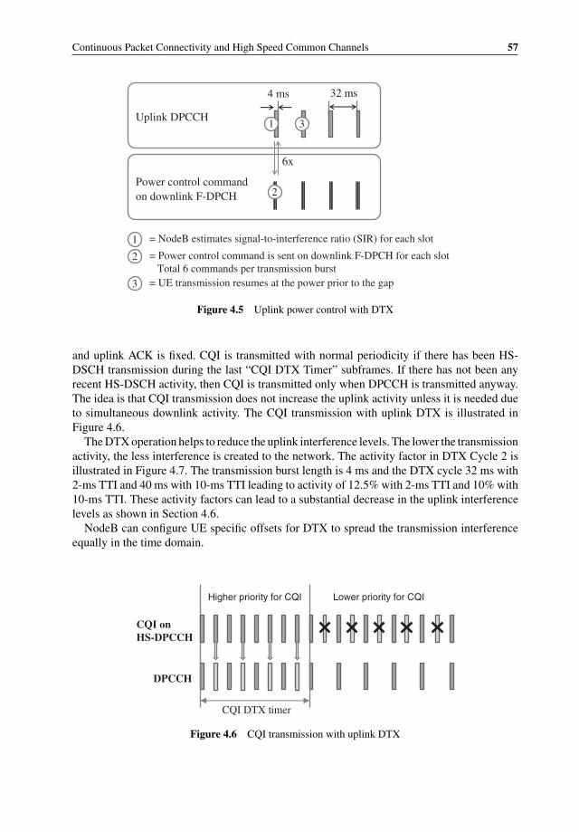
Continuous Packet Connectivity and High Speed Common Channels 57
4 ms 32 ms
Uplink DPCCH
Power control command
on downlink F-DPCH
1 = NodeB estimates signal-to-interference ratio (SIR) for each slot
2 = Power control command is sent on downlink F-DPCH for each slot
Total 6 commands per transmission burst
1 3
2
6x
3 = UE transmission resumes at the power prior to the gap
Figure 4.5 Uplink power control with DTX
and uplink ACK is fixed. CQI is transmitted with normal periodicity if there has been HS-DSCH transmission during the last “CQI DTX Timer” subframes. If there has not been anyrecent HS-DSCH activity, then CQI is transmitted only when DPCCH is transmitted anyway.The idea is that CQI transmission does not increase the uplink activity unless it is needed dueto simultaneous downlink activity. The CQI transmission with uplink DTX is illustrated inFigure 4.6.
The DTX operation helps to reduce the uplink interference levels. The lower the transmissionactivity, the less interference is created to the network. The activity factor in DTX Cycle 2 isillustrated in Figure 4.7. The transmission burst length is 4 ms and the DTX cycle 32 ms with2-ms TTI and 40 ms with 10-ms TTI leading to activity of 12.5% with 2-ms TTI and 10% with10-ms TTI. These activity factors can lead to a substantial decrease in the uplink interferencelevels as shown in Section 4.6.
NodeB can configure UE specific offsets for DTX to spread the transmission interferenceequally in the time domain.
CQI DTX timer
DPCCH
CQI on HS-DPCCH
Lower priority for CQI Higher priority for CQI
Figure 4.6 CQI transmission with uplink DTX
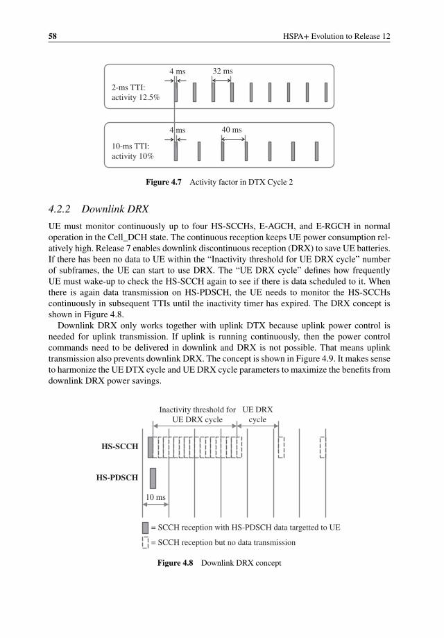
58 HSPA+ Evolution to Release 12
4 ms 32 ms
2-ms TTI: activity 12.5%
4 ms 40 ms
10-ms TTI:
activity 10%
Figure 4.7 Activity factor in DTX Cycle 2
4.2.2 Downlink DRX
UE must monitor continuously up to four HS-SCCHs, E-AGCH, and E-RGCH in normaloperation in the Cell_DCH state. The continuous reception keeps UE power consumption rel-atively high. Release 7 enables downlink discontinuous reception (DRX) to save UE batteries.If there has been no data to UE within the “Inactivity threshold for UE DRX cycle” numberof subframes, the UE can start to use DRX. The “UE DRX cycle” defines how frequentlyUE must wake-up to check the HS-SCCH again to see if there is data scheduled to it. Whenthere is again data transmission on HS-PDSCH, the UE needs to monitor the HS-SCCHscontinuously in subsequent TTIs until the inactivity timer has expired. The DRX concept isshown in Figure 4.8.
Downlink DRX only works together with uplink DTX because uplink power control isneeded for uplink transmission. If uplink is running continuously, then the power controlcommands need to be delivered in downlink and DRX is not possible. That means uplinktransmission also prevents downlink DRX. The concept is shown in Figure 4.9. It makes senseto harmonize the UE DTX cycle and UE DRX cycle parameters to maximize the benefits fromdownlink DRX power savings.
HS-SCCH
Inactivity threshold for
UE DRX cycle
HS-PDSCH
10 ms
UE DRX
cycle
= SCCH reception with HS-PDSCH data targetted to UE
= SCCH reception but no data transmission
Figure 4.8 Downlink DRX concept
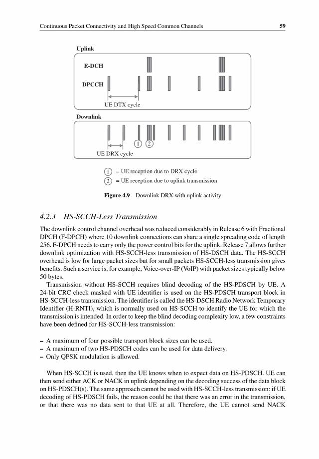
Continuous Packet Connectivity and High Speed Common Channels 59
DPCCH
E-DCH
UE DTX cycle
UE DRX cycle
Uplink
Downlink
1 2
1 = UE reception due to DRX cycle
2 = UE reception due to uplink transmission
Figure 4.9 Downlink DRX with uplink activity
4.2.3 HS-SCCH-Less Transmission
The downlink control channel overhead was reduced considerably in Release 6 with FractionalDPCH (F-DPCH) where 10 downlink connections can share a single spreading code of length256. F-DPCH needs to carry only the power control bits for the uplink. Release 7 allows furtherdownlink optimization with HS-SCCH-less transmission of HS-DSCH data. The HS-SCCHoverhead is low for large packet sizes but for small packets HS-SCCH-less transmission givesbenefits. Such a service is, for example, Voice-over-IP (VoIP) with packet sizes typically below50 bytes.
Transmission without HS-SCCH requires blind decoding of the HS-PDSCH by UE. A24-bit CRC check masked with UE identifier is used on the HS-PDSCH transport block inHS-SCCH-less transmission. The identifier is called the HS-DSCH Radio Network TemporaryIdentifier (H-RNTI), which is normally used on HS-SCCH to identify the UE for which thetransmission is intended. In order to keep the blind decoding complexity low, a few constraintshave been defined for HS-SCCH-less transmission:
– A maximum of four possible transport block sizes can be used.– A maximum of two HS-PDSCH codes can be used for data delivery.– Only QPSK modulation is allowed.
When HS-SCCH is used, then the UE knows when to expect data on HS-PDSCH. UE canthen send either ACK or NACK in uplink depending on the decoding success of the data blockon HS-PDSCH(s). The same approach cannot be used with HS-SCCH-less transmission: if UEdecoding of HS-PDSCH fails, the reason could be that there was an error in the transmission,or that there was no data sent to that UE at all. Therefore, the UE cannot send NACK
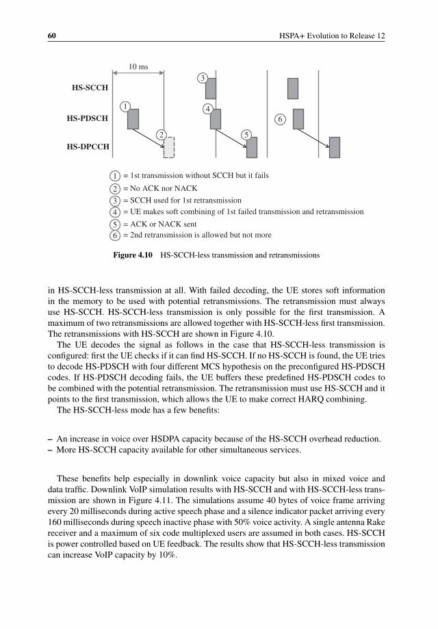
60 HSPA+ Evolution to Release 12
HS-SCCH
10 ms
HS-PDSCH
HS-DPCCH
1 = 1st transmission without SCCH but it fails
1
2 = No ACK nor NACK
2
3
3 = SCCH used for 1st retransmission
4
4 = UE makes soft combining of 1st failed transmission and retransmission
5
5 = ACK or NACK sent
6 = 2nd retransmission is allowed but not more
6
Figure 4.10 HS-SCCH-less transmission and retransmissions
in HS-SCCH-less transmission at all. With failed decoding, the UE stores soft informationin the memory to be used with potential retransmissions. The retransmission must alwaysuse HS-SCCH. HS-SCCH-less transmission is only possible for the first transmission. Amaximum of two retransmissions are allowed together with HS-SCCH-less first transmission.The retransmissions with HS-SCCH are shown in Figure 4.10.
The UE decodes the signal as follows in the case that HS-SCCH-less transmission isconfigured: first the UE checks if it can find HS-SCCH. If no HS-SCCH is found, the UE triesto decode HS-PDSCH with four different MCS hypothesis on the preconfigured HS-PDSCHcodes. If HS-PDSCH decoding fails, the UE buffers these predefined HS-PDSCH codes tobe combined with the potential retransmission. The retransmission must use HS-SCCH and itpoints to the first transmission, which allows the UE to make correct HARQ combining.
The HS-SCCH-less mode has a few benefits:
– An increase in voice over HSDPA capacity because of the HS-SCCH overhead reduction.– More HS-SCCH capacity available for other simultaneous services.
These benefits help especially in downlink voice capacity but also in mixed voice anddata traffic. Downlink VoIP simulation results with HS-SCCH and with HS-SCCH-less trans-mission are shown in Figure 4.11. The simulations assume 40 bytes of voice frame arrivingevery 20 milliseconds during active speech phase and a silence indicator packet arriving every160 milliseconds during speech inactive phase with 50% voice activity. A single antenna Rakereceiver and a maximum of six code multiplexed users are assumed in both cases. HS-SCCHis power controlled based on UE feedback. The results show that HS-SCCH-less transmissioncan increase VoIP capacity by 10%.
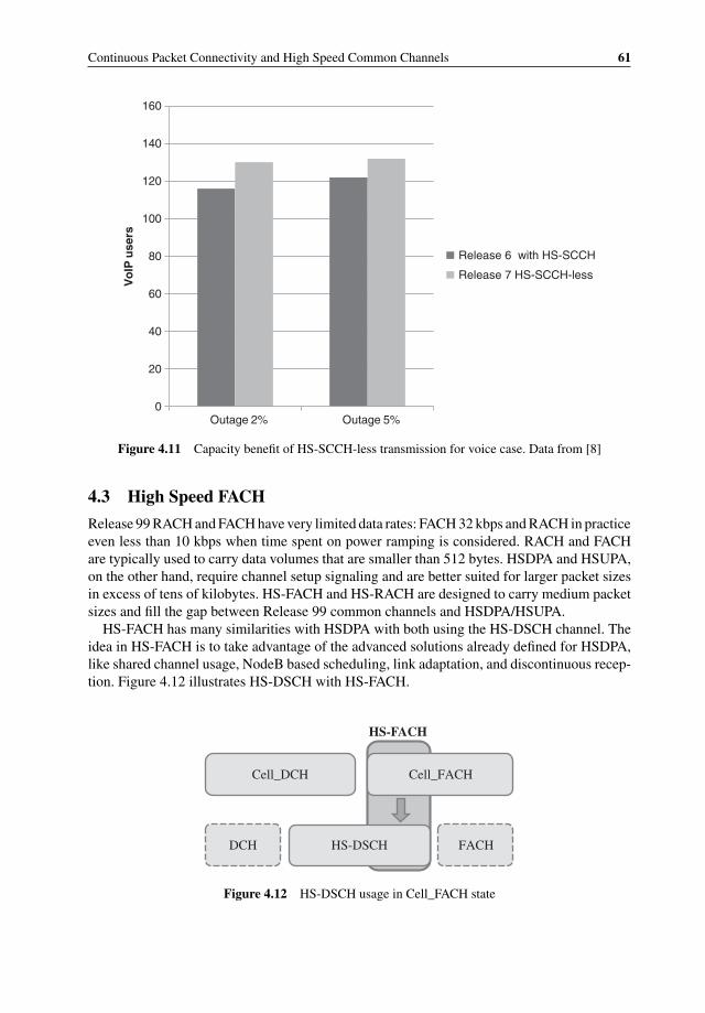
Continuous Packet Connectivity and High Speed Common Channels 61
0
20
40
60
80
100
120
140
160
Outage 2% Outage 5%
Vo
IP u
sers
Release 6 with HS-SCCH
Release 7 HS-SCCH-less
Figure 4.11 Capacity benefit of HS-SCCH-less transmission for voice case. Data from [8]
4.3 High Speed FACH
Release 99 RACH and FACH have very limited data rates: FACH 32 kbps and RACH in practiceeven less than 10 kbps when time spent on power ramping is considered. RACH and FACHare typically used to carry data volumes that are smaller than 512 bytes. HSDPA and HSUPA,on the other hand, require channel setup signaling and are better suited for larger packet sizesin excess of tens of kilobytes. HS-FACH and HS-RACH are designed to carry medium packetsizes and fill the gap between Release 99 common channels and HSDPA/HSUPA.
HS-FACH has many similarities with HSDPA with both using the HS-DSCH channel. Theidea in HS-FACH is to take advantage of the advanced solutions already defined for HSDPA,like shared channel usage, NodeB based scheduling, link adaptation, and discontinuous recep-tion. Figure 4.12 illustrates HS-DSCH with HS-FACH.
Cell_DCH
HS-DSCH
Cell_FACH
DCH FACH
HS-FACH
Figure 4.12 HS-DSCH usage in Cell_FACH state
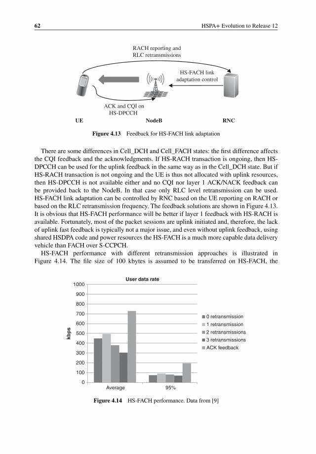
62 HSPA+ Evolution to Release 12
UE NodeB RNC
RACH reporting and
RLC retransmissions
HS-FACH link
adaptation control
ACK and CQI on
HS-DPCCH
Figure 4.13 Feedback for HS-FACH link adaptation
There are some differences in Cell_DCH and Cell_FACH states: the first difference affectsthe CQI feedback and the acknowledgments. If HS-RACH transaction is ongoing, then HS-DPCCH can be used for the uplink feedback in the same way as in the Cell_DCH state. But ifHS-RACH transaction is not ongoing and the UE is thus not allocated with uplink resources,then HS-DPCCH is not available either and no CQI nor layer 1 ACK/NACK feedback canbe provided back to the NodeB. In that case only RLC level retransmission can be used.HS-FACH link adaptation can be controlled by RNC based on the UE reporting on RACH orbased on the RLC retransmission frequency. The feedback solutions are shown in Figure 4.13.It is obvious that HS-FACH performance will be better if layer 1 feedback with HS-RACH isavailable. Fortunately, most of the packet sessions are uplink initiated and, therefore, the lackof uplink fast feedback is typically not a major issue, and even without uplink feedback, usingshared HSDPA code and power resources the HS-FACH is a much more capable data deliveryvehicle than FACH over S-CCPCH.
HS-FACH performance with different retransmission approaches is illustrated inFigure 4.14. The file size of 100 kbytes is assumed to be transferred on HS-FACH, the
User data rate
0
100
200
300
400
500
600
700
800
900
1000
Average 95%
kbp
s
0 retransmission
1 retransmission
2 retransmissions
3 retransmissions
ACK feedback
Figure 4.14 HS-FACH performance. Data from [9]
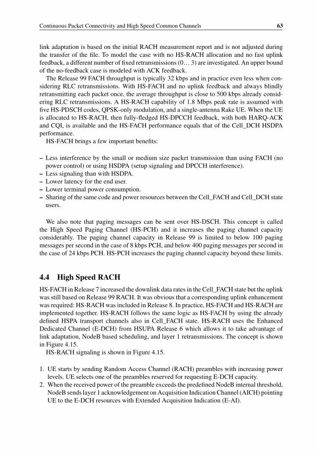
Continuous Packet Connectivity and High Speed Common Channels 63
link adaptation is based on the initial RACH measurement report and is not adjusted duringthe transfer of the file. To model the case with no HS-RACH allocation and no fast uplinkfeedback, a different number of fixed retransmissions (0… 3) are investigated. An upper boundof the no-feedback case is modeled with ACK feedback.
The Release 99 FACH throughput is typically 32 kbps and in practice even less when con-sidering RLC retransmissions. With HS-FACH and no uplink feedback and always blindlyretransmitting each packet once, the average throughput is close to 500 kbps already consid-ering RLC retransmissions. A HS-RACH capability of 1.8 Mbps peak rate is assumed withfive HS-PDSCH codes, QPSK-only modulation, and a single-antenna Rake UE. When the UEis allocated to HS-RACH, then fully-fledged HS-DPCCH feedback, with both HARQ-ACKand CQI, is available and the HS-FACH performance equals that of the Cell_DCH HSDPAperformance.
HS-FACH brings a few important benefits:
– Less interference by the small or medium size packet transmission than using FACH (nopower control) or using HSDPA (setup signaling and DPCCH interference).
– Less signaling than with HSDPA.– Lower latency for the end user.– Lower terminal power consumption.– Sharing of the same code and power resources between the Cell_FACH and Cell_DCH state
users.
We also note that paging messages can be sent over HS-DSCH. This concept is calledthe High Speed Paging Channel (HS-PCH) and it increases the paging channel capacityconsiderably. The paging channel capacity in Release 99 is limited to below 100 pagingmessages per second in the case of 8 kbps PCH, and below 400 paging messages per second inthe case of 24 kbps PCH. HS-PCH increases the paging channel capacity beyond these limits.
4.4 High Speed RACH
HS-FACH in Release 7 increased the downlink data rates in the Cell_FACH state but the uplinkwas still based on Release 99 RACH. It was obvious that a corresponding uplink enhancementwas required: HS-RACH was included in Release 8. In practice, HS-FACH and HS-RACH areimplemented together. HS-RACH follows the same logic as HS-FACH by using the alreadydefined HSPA transport channels also in Cell_FACH state. HS-RACH uses the EnhancedDedicated Channel (E-DCH) from HSUPA Release 6 which allows it to take advantage oflink adaptation, NodeB based scheduling, and layer 1 retransmissions. The concept is shownin Figure 4.15.
HS-RACH signaling is shown in Figure 4.15.
1. UE starts by sending Random Access Channel (RACH) preambles with increasing powerlevels. UE selects one of the preambles reserved for requesting E-DCH capacity.
2. When the received power of the preamble exceeds the predefined NodeB internal threshold,NodeB sends layer 1 acknowledgement on Acquisition Indication Channel (AICH) pointingUE to the E-DCH resources with Extended Acquisition Indication (E-AI).
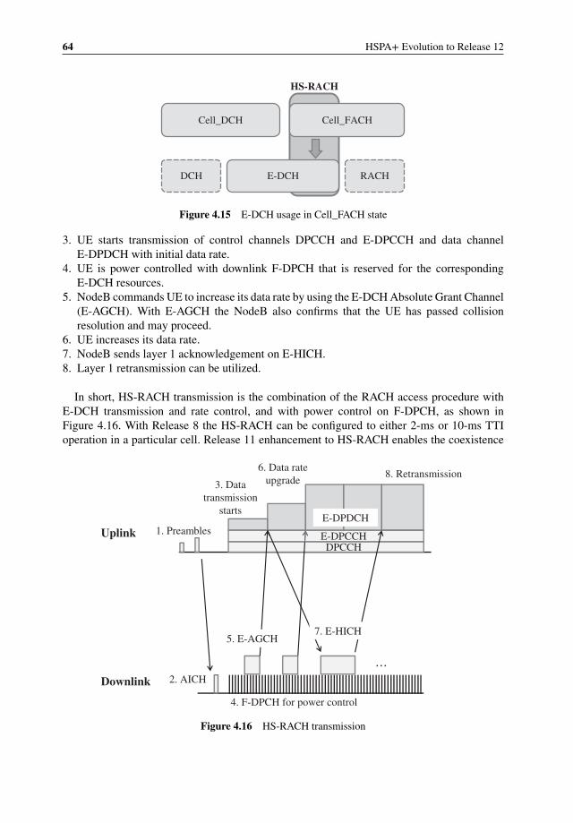
64 HSPA+ Evolution to Release 12
Cell_DCH
E-DCH
Cell_FACH
DCH RACH
HS-RACH
Figure 4.15 E-DCH usage in Cell_FACH state
3. UE starts transmission of control channels DPCCH and E-DPCCH and data channelE-DPDCH with initial data rate.
4. UE is power controlled with downlink F-DPCH that is reserved for the correspondingE-DCH resources.
5. NodeB commands UE to increase its data rate by using the E-DCH Absolute Grant Channel(E-AGCH). With E-AGCH the NodeB also confirms that the UE has passed collisionresolution and may proceed.
6. UE increases its data rate.7. NodeB sends layer 1 acknowledgement on E-HICH.8. Layer 1 retransmission can be utilized.
In short, HS-RACH transmission is the combination of the RACH access procedure withE-DCH transmission and rate control, and with power control on F-DPCH, as shown inFigure 4.16. With Release 8 the HS-RACH can be configured to either 2-ms or 10-ms TTIoperation in a particular cell. Release 11 enhancement to HS-RACH enables the coexistence
Uplink
Downlink
1. Preambles
2. AICH
DPCCH E-DPCCH
3. Data
transmission
starts
4. F-DPCH for power control
6. Data rate
upgrade8. Retransmission
E-DPDCH
…
5. E-AGCH 7. E-HICH
Figure 4.16 HS-RACH transmission
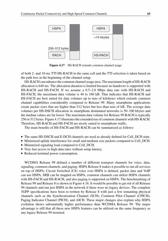
Continuous Packet Connectivity and High Speed Common Channels 65
RACH
256–512 bytes
>10 kbytes
HSPA
HS-RACH
HSPA
Figure 4.17 HS-RACH extends common channel usage
of both 2- and 10-ms TTI HS-RACH in the same cell and the TTI selection is taken based onthe path loss at the beginning of the channel setup.
HS-RACH can enhance the common channel usage area. The maximum length of HS-RACHallocation is 640 ms. The allocation duration is limited because no handover is supported withHS-RACH and HS-FACH. If we assume a 0.5–2.0 Mbps data rate with HS-RACH andHS-FACH, the maximum data volume is 40 to 160 kB. That indicates that HS-RACH andHS-FACH are best suited for data volumes up to tens of kilobytes which extends commonchannel capabilities considerably compared to Release 99. Many smartphone applicationscreate packet sizes that are higher than 512 bytes but less than tens of kB. The average datavolumes per HS-DSCH allocation in smartphone dominated networks is 50–100 kbytes andthe median values are far lower. The maximum data volume for Release 99 RACH is typically256 or 512 bytes. Figure 4.17 illustrates the extended use of common channels with HS-RACH.Therefore, HS-RACH and HS-FACH are nicely suited to smartphone traffic.
The main benefits of HS-FACH and HS-RACH can be summarized as follows:
� The same HS-DSCH and E-DCH channels are used as already defined for Cell_DCH state.� Minimized uplink interference for small and medium size packets compared to Cell_DCH.� Minimized signaling load compared to Cell_DCH.� Very fast access to high data rates without setup latency.� Reduced terminal power consumption.
WCDMA Release 99 defined a number of different transport channels for voice, data,signaling, common channels, and paging. HSPA Release 8 makes it possible to run all serviceson top of HSPA: Circuit Switched (CS) voice over HSPA is defined, packet data and VoIPcan use HSPA, SRB can be mapped on HSPA, common channels can utilize HSPA channelswith HS-FACH and HS-RACH, and also paging is supported on HSPA. The benchmarking ofRelease 99 and Release 8 is shown in Figure 4.18. It would be possible to get rid of all Release99 channels and run just HSPA in the network if there were no legacy devices. The complete3GPP specifications have been re-written by Release 8 with just a few remaining physicalchannels such as the Synchronization Channel (SCH), Common Pilot Channel (CPICH),Paging Indicator Channel (PICH), and AICH. These major changes also explain why HSPAevolution shows substantially higher performance than WCDMA Release 99. The majoradvantage is still that all these new HSPA features can be utilized on the same frequency asany legacy Release 99 terminal.
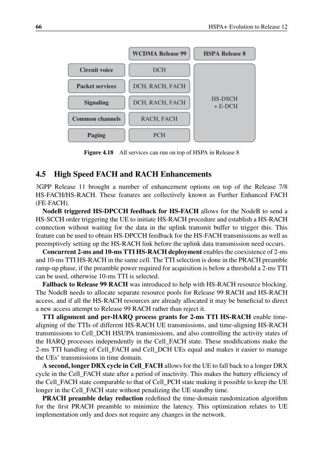
66 HSPA+ Evolution to Release 12
Circuit voice
Packet services
Signaling
WCDMA Release 99 HSPA Release 8
DCH
Common channels RACH, FACH
Paging PCH
HS-DSCH
+ E-DCHDCH, RACH, FACH
DCH, RACH, FACH
Figure 4.18 All services can run on top of HSPA in Release 8
4.5 High Speed FACH and RACH Enhancements
3GPP Release 11 brought a number of enhancement options on top of the Release 7/8HS-FACH/HS-RACH. These features are collectively known as Further Enhanced FACH(FE-FACH).
NodeB triggered HS-DPCCH feedback for HS-FACH allows for the NodeB to send aHS-SCCH order triggering the UE to initiate HS-RACH procedure and establish a HS-RACHconnection without waiting for the data in the uplink transmit buffer to trigger this. Thisfeature can be used to obtain HS-DPCCH feedback for the HS-FACH transmissions as well aspreemptively setting up the HS-RACH link before the uplink data transmission need occurs.
Concurrent 2-ms and 10-ms TTI HS-RACH deployment enables the coexistence of 2-msand 10-ms TTI HS-RACH in the same cell. The TTI selection is done in the PRACH preambleramp-up phase, if the preamble power required for acquisition is below a threshold a 2-ms TTIcan be used, otherwise 10-ms TTI is selected.
Fallback to Release 99 RACH was introduced to help with HS-RACH resource blocking.The NodeB needs to allocate separate resource pools for Release 99 RACH and HS-RACHaccess, and if all the HS-RACH resources are already allocated it may be beneficial to directa new access attempt to Release 99 RACH rather than reject it.
TTI alignment and per-HARQ process grants for 2-ms TTI HS-RACH enable time-aligning of the TTIs of different HS-RACH UE transmissions, and time-aligning HS-RACHtransmissions to Cell_DCH HSUPA transmissions, and also controlling the activity states ofthe HARQ processes independently in the Cell_FACH state. These modifications make the2-ms TTI handling of Cell_FACH and Cell_DCH UEs equal and makes it easier to managethe UEs’ transmissions in time domain.
A second, longer DRX cycle in Cell_FACH allows for the UE to fall back to a longer DRXcycle in the Cell_FACH state after a period of inactivity. This makes the battery efficiency ofthe Cell_FACH state comparable to that of Cell_PCH state making it possible to keep the UElonger in the Cell_FACH state without penalizing the UE standby time.
PRACH preamble delay reduction redefined the time-domain randomization algorithmfor the first PRACH preamble to minimize the latency. This optimization relates to UEimplementation only and does not require any changes in the network.
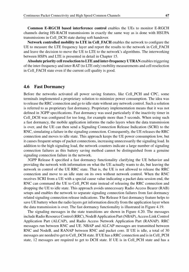
Continuous Packet Connectivity and High Speed Common Channels 67
Common E-RGCH based interference control enables the UEs to monitor E-RGCHchannels during HS-RACH transmissions in exactly the same way as is done with HSUPAtransmissions in Cell_DCH state during soft handover.
Network controlled mobility to LTE in Cell_FACH enables the network to configure theUE to measure the LTE frequency layer and report the results to the network in Cell_FACHand leave the decision to move the UE to LTE to the network’s algorithms. The interworkingbetween HSPA and LTE is presented in detail in Chapter 15.
Absolute priority cell reselection to LTE and inter-frequency UTRAN enables triggeringof the inter-frequency and inter-RAT (to LTE only) mobility measurements and cell reselectionin Cell_FACH state even if the current cell quality is good.
4.6 Fast Dormancy
Before the networks activated all power saving features, like Cell_PCH and CPC, someterminals implemented a proprietary solution to minimize power consumption. The idea wasto release the RRC connection and go to idle state without any network control. Such a solutionis referred to as proprietary fast dormancy. Proprietary implementation means that it was notdefined in 3GPP specifications. Fast dormancy was used particularly if the inactivity timer inCell_DCH was configured for too long, for example more than 5 seconds. When using sucha fast dormancy, the mobile application informs the radio layers when the data transmissionis over, and the UE can then send a Signaling Connection Release Indication (SCRI) to theRNC, simulating a failure in the signaling connection. Consequently, the UE releases the RRCconnection and moves to idle state. This approach keeps the UE power consumption low, butit causes frequent setups of packet connections, increasing unnecessarily the signaling load. Inaddition to the high signaling load, the network counters indicate a large number of signalingconnection failures as this battery saving method cannot be distinguished from a genuinesignaling connection failure in the network.
3GPP Release 8 specified a fast dormancy functionality clarifying the UE behavior andproviding the network with information on what the UE actually wants to do, but leaving thenetwork in control of the UE RRC state. That is, the UE is not allowed to release the RRCconnection and move to an idle state on its own without network control. When the RNCreceives SCRI from a UE with a special cause value indicating a packet data session end, theRNC can command the UE to Cell_PCH state instead of releasing the RRC connection anddropping the UE to idle state. This approach avoids unnecessary Radio Access Bearer (RAB)setups and enables the network to separate signaling connection failures from fast dormancyrelated signaling connection release indications. The Release 8 fast dormancy feature helps tosave UE battery when the radio layers get information directly from the application layer whenthe data transmission is over. The fast dormancy functionality is illustrated in Figure 4.19.
The signaling messages in the state transitions are shown in Figure 4.20. The messagesinclude Radio Resource Control (RRC), NodeB Application Part (NBAP), Access Link ControlApplication Part (ALCAP), and Radio Access Network Application Part (RANAP). RRCmessages run between RNC and UE. NBAP and ALCAP messages are transmitted betweenRNC and NodeB, and RANAP between RNC and packet core. If UE is idle, a total of 30messages are needed to get to Cell_DCH state. If UE has a RRC connection and is in Cell_PCHstate, 12 messages are required to get to DCH state. If UE is in Cell_PCH state and has a
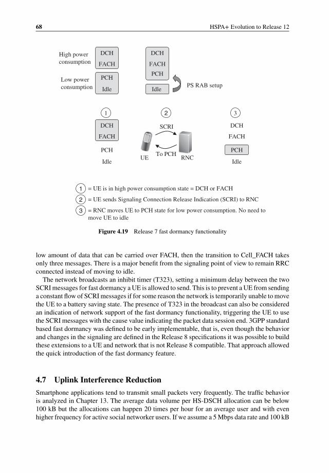
68 HSPA+ Evolution to Release 12
DCH
FACH
PCH
Idle
High power
consumption
Low power
consumption
DCH
FACH
PCH
Idle PS RAB setup
DCH
FACH
PCH
Idle
DCH
FACH
PCH
Idle
1
1 2 3
= UE is in high power consumption state = DCH or FACH
2 = UE sends Signaling Connection Release Indication (SCRI) to RNC
UE RNC
SCRI
To PCH
3 = RNC moves UE to PCH state for low power consumption. No need to
move UE to idle
Figure 4.19 Release 7 fast dormancy functionality
low amount of data that can be carried over FACH, then the transition to Cell_FACH takesonly three messages. There is a major benefit from the signaling point of view to remain RRCconnected instead of moving to idle.
The network broadcasts an inhibit timer (T323), setting a minimum delay between the twoSCRI messages for fast dormancy a UE is allowed to send. This is to prevent a UE from sendinga constant flow of SCRI messages if for some reason the network is temporarily unable to movethe UE to a battery saving state. The presence of T323 in the broadcast can also be consideredan indication of network support of the fast dormancy functionality, triggering the UE to usethe SCRI messages with the cause value indicating the packet data session end. 3GPP standardbased fast dormancy was defined to be early implementable, that is, even though the behaviorand changes in the signaling are defined in the Release 8 specifications it was possible to buildthese extensions to a UE and network that is not Release 8 compatible. That approach allowedthe quick introduction of the fast dormancy feature.
4.7 Uplink Interference Reduction
Smartphone applications tend to transmit small packets very frequently. The traffic behavioris analyzed in Chapter 13. The average data volume per HS-DSCH allocation can be below100 kB but the allocations can happen 20 times per hour for an average user and with evenhigher frequency for active social networker users. If we assume a 5 Mbps data rate and 100 kB

Continuous Packet Connectivity and High Speed Common Channels 69
From idle to DCH
1. RRC Connection Request (RRC) 2. Radio Link Setup (NBAP) 3. Radio Link Setup Response (NBAP) 4. Establish Requests (ALCAP) 5. Establish Confirm (ALCAP) 6. RRC Connection Setup (RRC) 7. NBAP Synchronization (NBAP) 8. RRC Connection Setup Complete (RRC) 9. Initial Direct Transfer RRC) 10. Initial UE Message (RANAP) 11. Common Id (RANAP) 12. Security Mode Command (RANAP) 13. Security Mode Command (RRC) 14. Security Mode Complete (RRC) 15. Security Mode Complete (RANAP) 16. Downlink Direct Transfer (RRC) 17. Uplink Direct Transfer (RRC) 18. RAB Assignment Req (RANAP) 19. GTP Tunnel Setup (RANAP) 20. RB Setup (RRC) 21. Radio Link Setup (NBAP) 22. Radio Link Setup Response (NBAP) 23. Establish Requests (ALCAP) 24. Establish Confirm (ALCAP) 25. Establish Requests (ALCAP) 26. Establish Confirm (ALCAP) 27. RB Setup Complete (RRC) 28. RANAP:RAB Assignment Resp (RANP) 29. Measurement Control (HO) (RRC) 30. Measurement Control (TVM) (RRC)
From PCH to DCH
1. Cell update with TVM (RRC) 2. Radio Link Setup (NBAP) 3. Radio Link Setup Response (NBAP) 4. Establish Requests (ALCAP) 5. Establish Confirm (ALCAP) 6. Establish Requests (ALCAP) 7. Establish Confirm (ALCAP) 8. CU confirm with RB reconfig (RRC) 9. NBAP Synchronization (NBAP) 10. RB reconfiguration complete (RRC) 11. Measurement Control (HO) (RRC) 12. Measurement Control (TVM) (RRC)
From PCH to FACH
1. Cell update (RRC) 2. Cell update confirm (RRC) 3. UMI confirm (RRC)
From idle Large packet from PCH Small packet from PCH
ALCAP = Access Link Control Application Part CU = Cell Update GTP = GPRS Tunneling Protocol HO = Handover NBAP = NodeB Application Part RAB = Radio Access Bearer RANAP = Radio Access Network Application Part RB = Radio Bearer RRC = Radio Resource Control UMI = UTRAN Mobility Information TVM = Traffic Volume Measurement
Figure 4.20 Signaling messages in state transitions
packet size, the transmission time is just 0.16 s. The typical inactivity timers are set to 2–10 swhich means that more than 90% of the time the uplink DPCCH is running without any dataactivity (Figure 4.21). This explains why networks with high smartphone penetration sufferfrom uplink interference effects: smartphone devices keep transmitting unnecessarily in theuplink direction while the channel is up.
One of the main benefits of CPC is the reduced uplink interference due to DTX. The activityfactors in Figure 4.7 are 12.5 and 10% for 2- and 10-ms TTIs. These activities would indicatein theory 8–10 times higher uplink capacity when the radio link is inactive and can fully utilizeDTX. In practice, the expected uplink capacity gain is lower because power control accuracyis sacrificed during DTX. In order to find out the realistic gains, field measurements were runwith a large number of terminals in Cell_DCH state but with very low activity. The maximumnumber of simultaneous users per cell is evaluated with 3 and 6 dB noise rises correspondingto 50 and 75% loadings. The testing was done with CPC off for all users and CPC on for allusers. The 2-ms case is shown in Figure 4.22 and 10-ms case in Figure 4.23. The maximum
2–10 s 0.16 s
DPCCH
Figure 4.21 DPCCH causes uplink interference with small packet sizes
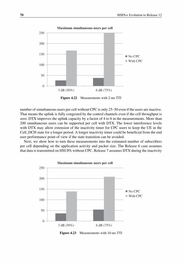
70 HSPA+ Evolution to Release 12
0
50
100
150
200
250
3 dB (50%) 6 dB (75%)
Maximum simultaneous users per cell
No CPC
With CPC
Figure 4.22 Measurements with 2-ms TTI
number of simultaneous users per cell without CPC is only 25–50 even if the users are inactive.That means the uplink is fully congested by the control channels even if the cell throughput iszero. DTX improves the uplink capacity by a factor of 4 to 6 in the measurements. More than200 simultaneous users can be supported per cell with DTX. The lower interference levelswith DTX may allow extension of the inactivity timer for CPC users to keep the UE in theCell_DCH state for a longer period. A longer inactivity timer could be beneficial from the enduser performance point of view if the state transition can be avoided.
Next, we show how to turn these measurements into the estimated number of subscribersper cell depending on the application activity and packet size. The Release 6 case assumesthat data is transmitted on HSUPA without CPC. Release 7 assumes DTX during the inactivity
0
50
100
150
200
250
3 dB (50%) 6 dB (75%)
Maximum simultaneous users per cell
No CPC
With CPC
Figure 4.23 Measurements with 10-ms TTI
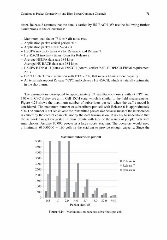
Continuous Packet Connectivity and High Speed Common Channels 71
timer. Release 8 assumes that the data is carried by HS-RACH. We use the following furtherassumptions in the calculations:
– Maximum load factor 75% = 6 dB noise rise.– Application packet arrival period 60 s.– Application packet size 0.5–64 kB.– HSUPA inactivity timer 4 s for Release 6 and Release 7.– HS-RACH inactivity timer 40 ms for Release 8.– Average HSUPA data rate 384 kbps.– Average HS-RACH data rate 384 kbps.– HSUPA E-DPDCH (data) vs. DPCCH (control) offset 9 dB. E-DPDCH Eb/N0 requirement
2 dB.– DPCCH interference reduction with DTX -75%, that means 4 times more capacity.– All terminals support Release 7 CPC and Release 8 HS-RACH, which is naturally optimistic
in the short term.
The assumptions correspond to approximately 37 simultaneous users without CPC and140 with CPC if they are all in Cell_DCH state, which is similar to the field measurements.Figure 4.24 shows the maximum number of subscribers per cell when the traffic model isconsidered. The maximum number of subscribers per cell with Release 6 is approximately500. The number is not sensitive to the transmitted packet size because most of the interferenceis caused by the control channels, not by the data transmission. It is easy to understand thatthe network can get congested in mass events with tens of thousands of people each withsmartphones. Assume 80 000 people in a large sports stadium. The operators would needa minimum 80 000/500 = 160 cells in the stadium to provide enough capacity. Since the
0
500
1000
1500
2000
2500
3000
3500
4000
4500
5000
0.5 1.0 2.0 4.0 8.0 16.0 32.0 64.0
Packet size [kB]
Maximum subscribers per cell
Release 6
Release 7
Release 8
Figure 4.24 Maximum simultaneous subscribers per cell
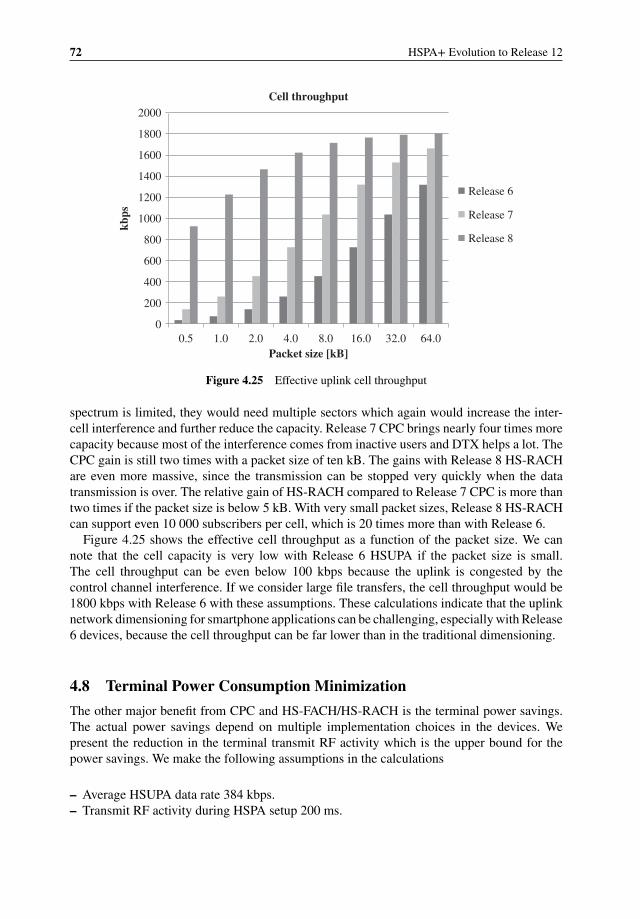
72 HSPA+ Evolution to Release 12
0
200
400
600
800
1000
1200
1400
1600
1800
2000
0.5 1.0 2.0 4.0 8.0 16.0 32.0 64.0
kbps
Packet size [kB]
Cell throughput
Release 6
Release 7
Release 8
Figure 4.25 Effective uplink cell throughput
spectrum is limited, they would need multiple sectors which again would increase the inter-cell interference and further reduce the capacity. Release 7 CPC brings nearly four times morecapacity because most of the interference comes from inactive users and DTX helps a lot. TheCPC gain is still two times with a packet size of ten kB. The gains with Release 8 HS-RACHare even more massive, since the transmission can be stopped very quickly when the datatransmission is over. The relative gain of HS-RACH compared to Release 7 CPC is more thantwo times if the packet size is below 5 kB. With very small packet sizes, Release 8 HS-RACHcan support even 10 000 subscribers per cell, which is 20 times more than with Release 6.
Figure 4.25 shows the effective cell throughput as a function of the packet size. We cannote that the cell capacity is very low with Release 6 HSUPA if the packet size is small.The cell throughput can be even below 100 kbps because the uplink is congested by thecontrol channel interference. If we consider large file transfers, the cell throughput would be1800 kbps with Release 6 with these assumptions. These calculations indicate that the uplinknetwork dimensioning for smartphone applications can be challenging, especially with Release6 devices, because the cell throughput can be far lower than in the traditional dimensioning.
4.8 Terminal Power Consumption Minimization
The other major benefit from CPC and HS-FACH/HS-RACH is the terminal power savings.The actual power savings depend on multiple implementation choices in the devices. Wepresent the reduction in the terminal transmit RF activity which is the upper bound for thepower savings. We make the following assumptions in the calculations
– Average HSUPA data rate 384 kbps.– Transmit RF activity during HSPA setup 200 ms.
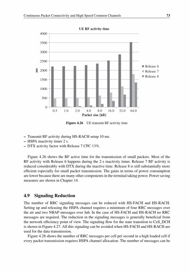
Continuous Packet Connectivity and High Speed Common Channels 73
0
500
1000
1500
2000
2500
3000
3500
4000
0.5 1.0 2.0 4.0 8.0 16.0 32.0 64.0
ms
Packet size [kB]
UE RF activity time
Release 6
Release 7
Release 8
Figure 4.26 UE transmit RF activity time
– Transmit RF activity during HS-RACH setup 10 ms.– HSPA inactivity timer 2 s.– DTX activity factor with Release 7 CPC 13%.
Figure 4.26 shows the RF active time for the transmission of small packets. Most of theRF activity with Release 6 happens during the 2-s inactivity timer. Release 7 RF activity isreduced considerably with DTX during the inactive time. Release 8 is still substantially moreefficient especially for small packet transmission. The gains in terms of power consumptionare lower because there are many other components in the terminal taking power. Power savingmeasures are shown in Chapter 14.
4.9 Signaling Reduction
The number of RRC signaling messages can be reduced with HS-FACH and HS-RACH.Setting up and releasing the HSPA channel requires a minimum of four RRC messages overthe air and two NBAP messages over Iub. In the case of HS-FACH and HS-RACH no RRCmessages are required. The reduction in the signaling messages is generally beneficial fromthe network efficiency point of view. The signaling flow for the state transition to Cell_DCHis shown in Figure 4.27. All this signaling can be avoided when HS-FACH and HS-RACH areused for the data transmission.
Figure 4.28 shows the number of RRC messages per cell per second in a high loaded cell ifevery packet transmission requires HSPA channel allocation. The number of messages can be
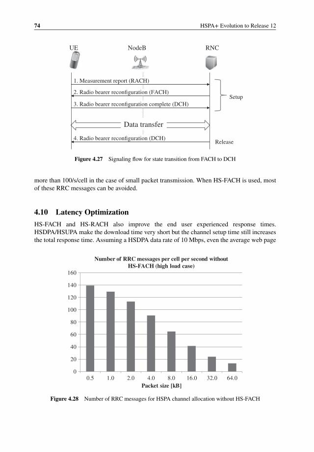
74 HSPA+ Evolution to Release 12
UE NodeB RNC
1. Measurement report (RACH)
2. Radio bearer reconfiguration (FACH)
3. Radio bearer reconfiguration complete (DCH)
4. Radio bearer reconfiguration (DCH)Release
Data transfer
Setup
Figure 4.27 Signaling flow for state transition from FACH to DCH
more than 100/s/cell in the case of small packet transmission. When HS-FACH is used, mostof these RRC messages can be avoided.
4.10 Latency Optimization
HS-FACH and HS-RACH also improve the end user experienced response times.HSDPA/HSUPA make the download time very short but the channel setup time still increasesthe total response time. Assuming a HSDPA data rate of 10 Mbps, even the average web page
0
20
40
60
80
100
120
140
160
0.5 1.0 2.0 4.0 8.0 16.0 32.0 64.0
Packet size [kB]
Number of RRC messages per cell per second withoutHS-FACH (high load case)
Figure 4.28 Number of RRC messages for HSPA channel allocation without HS-FACH
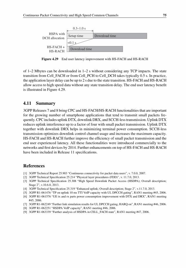
Continuous Packet Connectivity and High Speed Common Channels 75
Setup time Download time
0.3–1.0 s
Download time
<0.1 s
HSPA with
DCH allocation
HS-FACH +
HS-RACH
Figure 4.29 End user latency improvement with HS-FACH and HS-RACH
of 1–2 Mbytes can be downloaded in 1–2 s without considering any TCP impacts. The statetransition from Cell_FACH or from Cell_PCH to Cell_DCH takes typically 0.5 s. In practice,the application layer delay can be up to 2 s due to the state transition. HS-FACH and HS-RACHallow access to high speed data without any state transition delay. The end user latency benefitis illustrated in Figure 4.29.
4.11 Summary
3GPP Releases 7 and 8 bring CPC and HS-FACH/HS-RACH functionalities that are importantfor the growing number of smartphone applications that tend to transmit small packets fre-quently. CPC includes uplink DTX, downlink DRX, and SCCH-less transmission. Uplink DTXreduces uplink interference up to a factor of four with small packet transmission. Uplink DTXtogether with downlink DRX helps in minimizing terminal power consumption. SCCH-lesstransmission optimizes downlink control channel usage and increases the maximum capacity.HS-FACH and HS-RACH further improve the efficiency of small packet transmission and theend user experienced latency. All these functionalities were introduced commercially to thenetworks and first devices by 2014. Further enhancements on top of HS-FACH and HS-RACHhave been included in Release 11 specifications.
References
[1] 3GPP Technical Report 25.903 “Continuous connectivity for packet data users”, v. 7.0.0, 2007.[2] 3GPP Technical Specification 25.214 “Physical layer procedures (FDD)”, v. 11.7.0, 2013.[3] 3GPP Technical Specification 25.308 “High Speed Downlink Packet Access (HSDPA); Overall description;
Stage 2”, v.10.6.0, 2013.[4] 3GPP Technical Specification 25.319 “Enhanced uplink; Overall description; Stage 2”, v.11.7.0, 2013.[5] 3GPP R1-061476 “TP on uplink 10 ms TTI VoIP capacity with UL DPCCH gating”, RAN1 meeting #45, 2006.[6] 3GPP R1-061576 “UE tx and rx parts power consumption improvement with DTX and DRX”, RAN1 meeting
#45, 2006.[7] 3GPP R1-062249 “Further link simulation results for UL DPCCH gating, HARQ on”, RAN1 meeting #46, 2006.[8] 3GPP R1-062251 “HSDPA VoIP capacity”, RAN1 meeting #46, 2006.[9] 3GPP R1-063339 “Further analysis of HSDPA in CELL_FACH state”, RAN1 meeting #47, 2006.

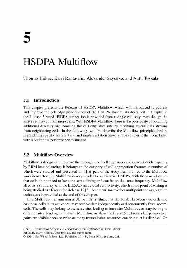
5HSDPA Multiflow
Thomas Hohne, Karri Ranta-aho, Alexander Sayenko, and Antti Toskala
5.1 Introduction
This chapter presents the Release 11 HSDPA Multiflow, which was introduced to addressand improve the cell edge performance of the HSDPA system. As described in Chapter 2,the Release 5 based HSDPA connection is provided from a single cell only, even though theactive set may contain more cells. With HSDPA Multiflow, there is the possibility of obtainingadditional diversity and boosting the cell edge data rate by receiving several data streamsfrom neighboring cells. In the following, we first describe the Multiflow principles, beforehighlighting specific architectural and implementation aspects. The chapter is then concludedwith a Multiflow performance evaluation.
5.2 Multiflow Overview
Multiflow is designed to improve the throughput of cell edge users and network-wide capacityby RRM load balancing. It belongs to the category of cell-aggregation features, a number ofwhich were studied and presented in [1] as part of the study item that led to the Multiflowwork item effort [2]. Multiflow is very similar to multicarrier HSDPA, with the generalizationthat cells do not need to have the same timing and can be on the same frequency. Multiflowalso has a similarity with the LTE-Advanced dual connectivity, which at the point of writing isbeing studied as a feature for Release 12 [3]. A comparison to other multipoint and aggregationtechniques is provided at the end of this chapter.
In a Multiflow transmission a UE, which is situated at the border between two cells andhas those cells in its active set, may receive data independently and concurrently from severalcells. The cells may belong to the same site, leading to intra-site Multiflow, or may belong todifferent sites, leading to inter-site Multiflow, as shown in Figure 5.1. From a UE perspective,gains are visible because twice as many transmission resources can be put at its disposal. On
HSPA+ Evolution to Release 12: Performance and Optimization, First Edition.Edited by Harri Holma, Antti Toskala, and Pablo Tapia.© 2014 John Wiley & Sons, Ltd. Published 2014 by John Wiley & Sons, Ltd.
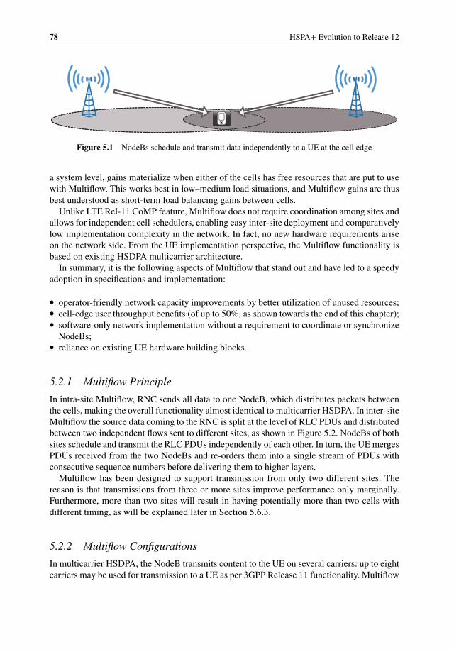
78 HSPA+ Evolution to Release 12
Figure 5.1 NodeBs schedule and transmit data independently to a UE at the cell edge
a system level, gains materialize when either of the cells has free resources that are put to usewith Multiflow. This works best in low–medium load situations, and Multiflow gains are thusbest understood as short-term load balancing gains between cells.
Unlike LTE Rel-11 CoMP feature, Multiflow does not require coordination among sites andallows for independent cell schedulers, enabling easy inter-site deployment and comparativelylow implementation complexity in the network. In fact, no new hardware requirements ariseon the network side. From the UE implementation perspective, the Multiflow functionality isbased on existing HSDPA multicarrier architecture.
In summary, it is the following aspects of Multiflow that stand out and have led to a speedyadoption in specifications and implementation:
� operator-friendly network capacity improvements by better utilization of unused resources;� cell-edge user throughput benefits (of up to 50%, as shown towards the end of this chapter);� software-only network implementation without a requirement to coordinate or synchronize
NodeBs;� reliance on existing UE hardware building blocks.
5.2.1 Multiflow Principle
In intra-site Multiflow, RNC sends all data to one NodeB, which distributes packets betweenthe cells, making the overall functionality almost identical to multicarrier HSDPA. In inter-siteMultiflow the source data coming to the RNC is split at the level of RLC PDUs and distributedbetween two independent flows sent to different sites, as shown in Figure 5.2. NodeBs of bothsites schedule and transmit the RLC PDUs independently of each other. In turn, the UE mergesPDUs received from the two NodeBs and re-orders them into a single stream of PDUs withconsecutive sequence numbers before delivering them to higher layers.
Multiflow has been designed to support transmission from only two different sites. Thereason is that transmissions from three or more sites improve performance only marginally.Furthermore, more than two sites will result in having potentially more than two cells withdifferent timing, as will be explained later in Section 5.6.3.
5.2.2 Multiflow Configurations
In multicarrier HSDPA, the NodeB transmits content to the UE on several carriers: up to eightcarriers may be used for transmission to a UE as per 3GPP Release 11 functionality. Multiflow
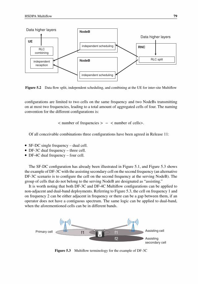
HSDPA Multiflow 79
UE
RNC
NodeB
RLC split
independent scheduling
Data higher layers
Data higher layers
NodeB
independent scheduling
independentreception
RLCcombining
Figure 5.2 Data flow split, independent scheduling, and combining at the UE for inter-site Multiflow
configurations are limited to two cells on the same frequency and two NodeBs transmittingon at most two frequencies, leading to a total amount of aggregated cells of four. The namingconvention for the different configurations is:
< number of frequencies > − < number of cells>.
Of all conceivable combinations three configurations have been agreed in Release 11:
� SF-DC single frequency – dual cell.� DF-3C dual frequency – three cell.� DF-4C dual frequency – four cell.
The SF-DC configuration has already been illustrated in Figure 5.1, and Figure 5.3 showsthe example of DF-3C with the assisting secondary cell on the second frequency (an alternativeDF-3C scenario is to configure the cell on the second frequency at the serving NodeB). Thegroup of cells that do not belong to the serving NodeB are designated as “assisting.”
It is worth noting that both DF-3C and DF-4C Multiflow configurations can be applied tonon-adjacent and dual-band deployments. Referring to Figure 5.3, the cell on frequency 1 andon frequency 2 can be either adjacent in frequency or there can be a gap between them, if anoperator does not have a contiguous spectrum. The same logic can be applied to dual-band,when the aforementioned cells can be in different bands.
f2
f1 f1Primary cell Assisting cell
Assistingsecondary cell
Figure 5.3 Multiflow terminology for the example of DF-3C
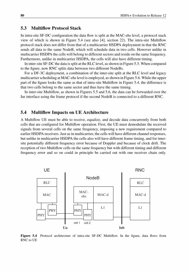
80 HSPA+ Evolution to Release 12
5.3 Multiflow Protocol Stack
In intra-site SF-DC configuration the data flow is split at the MAC-ehs level, a protocol stackview of which is shown in Figure 5.4 (see also [4], section 22). The intra-site Multiflowprotocol stack does not differ from that of a multicarrier HSDPA deployment in that the RNCsends all data to the same NodeB, which will schedule data in two cells. However unlike inmulticarrier HSDPA the cells will belong to different sectors and reside on the same frequency.Furthermore, unlike in multicarrier HSDPA, the cells will also have different timing.
In inter-site SF-DC the data is split at the RLC level, as shown in Figure 5.5. When comparedto the figure, now RNC splits data between two different NodeBs.
For a DF-3C deployment, a combination of the inter-site split at the RLC level and legacymulticarrier scheduling at MAC-ehs level is employed, as shown in Figure 5.6. While the upperpart of the figure looks the same as that of intra-site Multiflow in Figure 5.4, the difference isthat two cells belong to the same sector and thus have the same timing.
In inter-site Multiflow, as shown in Figures 5.5 and 5.6, the data can be forwarded over theIur interface using the frame protocol if the second NodeB is connected to a different RNC.
5.4 Multiflow Impacts on UE Architecture
A Multiflow UE must be able to receive, equalize, and decode data concurrently from bothcells that are configured for Multiflow operation. First, the UE must demodulate the receivedsignals from several cells on the same frequency, imposing a new requirement compared toearlier HSDPA receivers. Just as in multicarrier, the cells will have different channel responses,but unlike in multicarrier HSDPA the cells also will have different frame timing, and for inter-site potentially different frequency error because of Doppler and because of clock drift. Thereception of two Multiflow cells on the same frequency but with different timing and differentfrequency error and so on could in principle be carried out with one receiver chain only.
L1
RLC
MAC-d
L1
Iub
MAC
RLC
NodeB
RNCUE
Uu
cell 1 cell 2
PHY
PHY
PHY
PHY
MAC-
ehs MAC-d
Figure 5.4 Protocol architecture of intra-site SF-DC Multiflow. In the figure, data flows fromRNC to UE
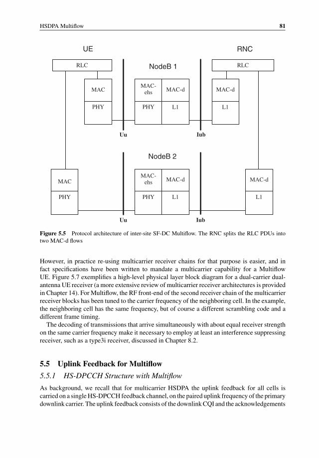
HSDPA Multiflow 81
L1
RLC
MAC-d
L1
Iub
MAC
RLC
L1L1
Iub
PHY
MAC
PHY
Uu
NodeB 1
NodeB 2
RNCUE
Uu
MAC-ehs MAC-d
MAC-dMAC-
ehs MAC-d
PHYPHY
Figure 5.5 Protocol architecture of inter-site SF-DC Multiflow. The RNC splits the RLC PDUs intotwo MAC-d flows
However, in practice re-using multicarrier receiver chains for that purpose is easier, and infact specifications have been written to mandate a multicarrier capability for a MultiflowUE. Figure 5.7 exemplifies a high-level physical layer block diagram for a dual-carrier dual-antenna UE receiver (a more extensive review of multicarrier receiver architectures is providedin Chapter 14). For Multiflow, the RF front-end of the second receiver chain of the multicarrierreceiver blocks has been tuned to the carrier frequency of the neighboring cell. In the example,the neighboring cell has the same frequency, but of course a different scrambling code and adifferent frame timing.
The decoding of transmissions that arrive simultaneously with about equal receiver strengthon the same carrier frequency make it necessary to employ at least an interference suppressingreceiver, such as a type3i receiver, discussed in Chapter 8.2.
5.5 Uplink Feedback for Multiflow
5.5.1 HS-DPCCH Structure with Multiflow
As background, we recall that for multicarrier HSDPA the uplink feedback for all cells iscarried on a single HS-DPCCH feedback channel, on the paired uplink frequency of the primarydownlink carrier. The uplink feedback consists of the downlink CQI and the acknowledgements
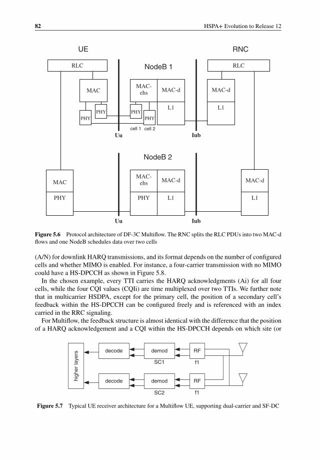
82 HSPA+ Evolution to Release 12
L1
RLC
MAC-d
L1
Iub
MAC
RLC
L1L1
Iub
PHY
MAC
PHY
Uu
NodeB 1
NodeB 2
RNCUE
Uucell 1 cell 2
PHY
PHY
PHY
PHY
MAC-ehs MAC-d
MAC-dMAC-
ehs MAC-d
Figure 5.6 Protocol architecture of DF-3C Multiflow. The RNC splits the RLC PDUs into two MAC-dflows and one NodeB schedules data over two cells
(A/N) for downlink HARQ transmissions, and its format depends on the number of configuredcells and whether MIMO is enabled. For instance, a four-carrier transmission with no MIMOcould have a HS-DPCCH as shown in Figure 5.8.
In the chosen example, every TTI carries the HARQ acknowledgments (Ai) for all fourcells, while the four CQI values (CQIi) are time multiplexed over two TTIs. We further notethat in multicarrier HSDPA, except for the primary cell, the position of a secondary cell’sfeedback within the HS-DPCCH can be configured freely and is referenced with an indexcarried in the RRC signaling.
For Multiflow, the feedback structure is almost identical with the difference that the positionof a HARQ acknowledgement and a CQI within the HS-DPCCH depends on which site (or
RF
RF
demoddecode
high
er la
yers
demoddecode
SC1
SC2 f1
f1
Figure 5.7 Typical UE receiver architecture for a Multiflow UE, supporting dual-carrier and SF-DC
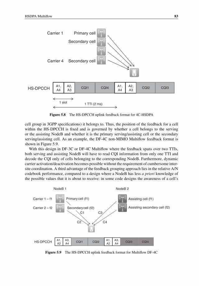
HSDPA Multiflow 83
Carrier 1 Primary cell
Secondary cell
A1,A4
A2,A3
CQI1 CQI4HS-DPCCHA1,A4
A2,A3
CQI2 CQI3
1 slot 1 TTI (2 ms)
Carrier 4 Secondary cell
Figure 5.8 The HS-DPCCH uplink feedback format for 4C-HSDPA
cell group in 3GPP specifications) it belongs to. Thus, the position of the feedback for a cellwithin the HS-DPCCH is fixed and is governed by whether a cell belongs to the servingor the assisting NodeB and whether it is the primary serving/assisting cell or the secondaryserving/assisting cell. As an example, the DF-4C non-MIMO Multiflow feedback format isshown in Figure 5.9.
With this design in DF-3C or DF-4C Multiflow where the feedback spans over two TTIs,both serving and assisting NodeB will have to read CQI information from only one TTI anddecode the CQI only of cells belonging to the corresponding NodeB. Furthermore, dynamiccarrier activation/deactivation becomes possible without the requirement of cumbersome inter-site coordination. A third advantage of the feedback grouping approach lies in the relative A/Ncodebook performance, compared to a design where a NodeB has less a priori knowledge ofthe possible values that it is about to receive: in some code designs the awareness of a cell’s
Carrier 1 – f1
Carrier 2 – f2
Primary cell (f1)
Secondarycell (f2)
Assisting cell (f1)
Assisting secondary cell (f2)
C1
C2
C3
C4
A1,A2
A3,A4
CQI1 CQI2HS-DPCCH A1,A2
A3,A4
CQI3 CQI4
NodeB 1 NodeB 2
Figure 5.9 The HS-DPCCH uplink feedback format for Multiflow DF-4C
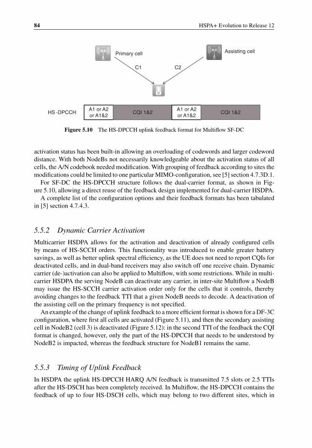
84 HSPA+ Evolution to Release 12
Primary cell Assisting cell
C1 C2
HS -DPCCHA1 or A2 or A1&2
CQI 1&2A1 or A2 or A1&2
CQI 1&2
Figure 5.10 The HS-DPCCH uplink feedback format for Multiflow SF-DC
activation status has been built-in allowing an overloading of codewords and larger codeworddistance. With both NodeBs not necessarily knowledgeable about the activation status of allcells, the A/N codebook needed modification. With grouping of feedback according to sites themodifications could be limited to one particular MIMO-configuration, see [5] section 4.7.3D.1.
For SF-DC the HS-DPCCH structure follows the dual-carrier format, as shown in Fig-ure 5.10, allowing a direct reuse of the feedback design implemented for dual-carrier HSDPA.
A complete list of the configuration options and their feedback formats has been tabulatedin [5] section 4.7.4.3.
5.5.2 Dynamic Carrier Activation
Multicarrier HSDPA allows for the activation and deactivation of already configured cellsby means of HS-SCCH orders. This functionality was introduced to enable greater batterysavings, as well as better uplink spectral efficiency, as the UE does not need to report CQIs fordeactivated cells, and in dual-band receivers may also switch off one receive chain. Dynamiccarrier (de-)activation can also be applied to Multiflow, with some restrictions. While in multi-carrier HSDPA the serving NodeB can deactivate any carrier, in inter-site Multiflow a NodeBmay issue the HS-SCCH carrier activation order only for the cells that it controls, therebyavoiding changes to the feedback TTI that a given NodeB needs to decode. A deactivation ofthe assisting cell on the primary frequency is not specified.
An example of the change of uplink feedback to a more efficient format is shown for a DF-3Cconfiguration, where first all cells are activated (Figure 5.11), and then the secondary assistingcell in NodeB2 (cell 3) is deactivated (Figure 5.12): in the second TTI of the feedback the CQIformat is changed, however, only the part of the HS-DPCCH that needs to be understood byNodeB2 is impacted, whereas the feedback structure for NodeB1 remains the same.
5.5.3 Timing of Uplink Feedback
In HSDPA the uplink HS-DPCCH HARQ A/N feedback is transmitted 7.5 slots or 2.5 TTIsafter the HS-DSCH has been completely received. In Multiflow, the HS-DPCCH contains thefeedback of up to four HS-DSCH cells, which may belong to two different sites, which in

HSDPA Multiflow 85
C1 C2
C3
A1,A2,A3 CQI1HS-DPCCH A1,A2,A3 CQI2 & CQI3
Note: joint coding of CQI2&3to maintain CQI grouping
Figure 5.11 DF-3C feedback with all carriers activated. In this Multiflow configuration the CQIs ofthe second TTI are jointly coded, as they belong to the same NodeB
turn in general will be unsynchronized. Furthermore, even in the intra-site Multiflow, cellsbelonging to different sectors may have a different timing, as configured by the so-calledT_cell parameter. An increase in the latency of the feedback transmission would result in areduction of the throughput or would require larger numbers of HARQ processes, neither ofwhich is desirable. Instead of increasing latency one could also speed up processing of theHARQ acknowledgments (and CQIs) for the cells that appear later. In the worst case, one celllags the other by 1.5 slots, and hence a new requirement was introduced for the UE to processthe downlink transmissions within 6 slots, instead of within 7.5 slots.
As the feedback for two different sites (or cell groups) is being bundled into one feedbackmessage, one of the cells can be defined as leading, and is referred to as the time referencecell, see Figure 5.13. In case the timing difference between cells becomes larger than 1.5 slots,for instance because of clock drift, the network will reconfigure the other cell to take the roleof time reference. To avoid a reconfiguration ping-pong effect when the timing difference is
C1 C2
C3
A1,A2,D CQI1HS-DPCCH A1,A2,D CQI2
deactivation orderissued by NodeB 2 only
X
NodeB 2NodeB 1
Figure 5.12 DF-3C feedback with one carrier deactivated
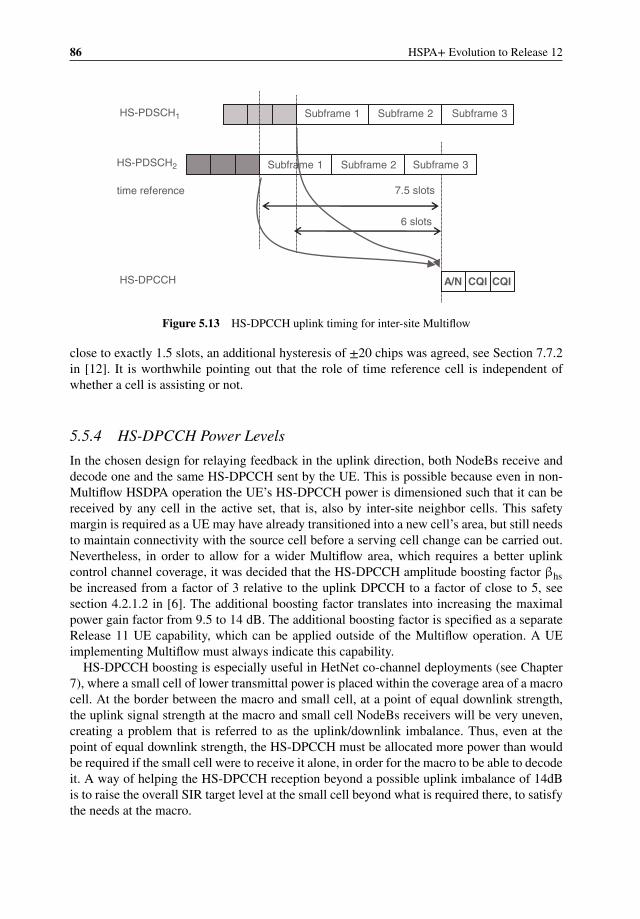
86 HSPA+ Evolution to Release 12
HS-PDSCH1 Subframe 1 Subframe 2 Subframe 3
HS-PDSCH2
time reference
Subframe 1 Subframe 2 Subframe 3
HS-DPCCH
6 slots
7.5 slots
A/N CQI CQI
Figure 5.13 HS-DPCCH uplink timing for inter-site Multiflow
close to exactly 1.5 slots, an additional hysteresis of ±20 chips was agreed, see Section 7.7.2in [12]. It is worthwhile pointing out that the role of time reference cell is independent ofwhether a cell is assisting or not.
5.5.4 HS-DPCCH Power Levels
In the chosen design for relaying feedback in the uplink direction, both NodeBs receive anddecode one and the same HS-DPCCH sent by the UE. This is possible because even in non-Multiflow HSDPA operation the UE’s HS-DPCCH power is dimensioned such that it can bereceived by any cell in the active set, that is, also by inter-site neighbor cells. This safetymargin is required as a UE may have already transitioned into a new cell’s area, but still needsto maintain connectivity with the source cell before a serving cell change can be carried out.Nevertheless, in order to allow for a wider Multiflow area, which requires a better uplinkcontrol channel coverage, it was decided that the HS-DPCCH amplitude boosting factor βhsbe increased from a factor of 3 relative to the uplink DPCCH to a factor of close to 5, seesection 4.2.1.2 in [6]. The additional boosting factor translates into increasing the maximalpower gain factor from 9.5 to 14 dB. The additional boosting factor is specified as a separateRelease 11 UE capability, which can be applied outside of the Multiflow operation. A UEimplementing Multiflow must always indicate this capability.
HS-DPCCH boosting is especially useful in HetNet co-channel deployments (see Chapter7), where a small cell of lower transmittal power is placed within the coverage area of a macrocell. At the border between the macro and small cell, at a point of equal downlink strength,the uplink signal strength at the macro and small cell NodeBs receivers will be very uneven,creating a problem that is referred to as the uplink/downlink imbalance. Thus, even at thepoint of equal downlink strength, the HS-DPCCH must be allocated more power than wouldbe required if the small cell were to receive it alone, in order for the macro to be able to decodeit. A way of helping the HS-DPCCH reception beyond a possible uplink imbalance of 14dBis to raise the overall SIR target level at the small cell beyond what is required there, to satisfythe needs at the macro.
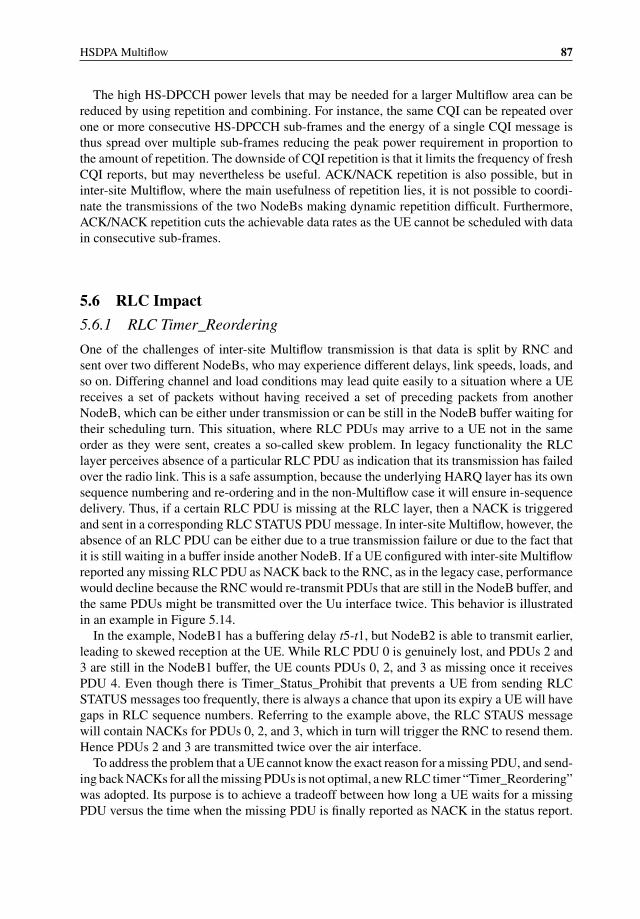
HSDPA Multiflow 87
The high HS-DPCCH power levels that may be needed for a larger Multiflow area can bereduced by using repetition and combining. For instance, the same CQI can be repeated overone or more consecutive HS-DPCCH sub-frames and the energy of a single CQI message isthus spread over multiple sub-frames reducing the peak power requirement in proportion tothe amount of repetition. The downside of CQI repetition is that it limits the frequency of freshCQI reports, but may nevertheless be useful. ACK/NACK repetition is also possible, but ininter-site Multiflow, where the main usefulness of repetition lies, it is not possible to coordi-nate the transmissions of the two NodeBs making dynamic repetition difficult. Furthermore,ACK/NACK repetition cuts the achievable data rates as the UE cannot be scheduled with datain consecutive sub-frames.
5.6 RLC Impact
5.6.1 RLC Timer_Reordering
One of the challenges of inter-site Multiflow transmission is that data is split by RNC andsent over two different NodeBs, who may experience different delays, link speeds, loads, andso on. Differing channel and load conditions may lead quite easily to a situation where a UEreceives a set of packets without having received a set of preceding packets from anotherNodeB, which can be either under transmission or can be still in the NodeB buffer waiting fortheir scheduling turn. This situation, where RLC PDUs may arrive to a UE not in the sameorder as they were sent, creates a so-called skew problem. In legacy functionality the RLClayer perceives absence of a particular RLC PDU as indication that its transmission has failedover the radio link. This is a safe assumption, because the underlying HARQ layer has its ownsequence numbering and re-ordering and in the non-Multiflow case it will ensure in-sequencedelivery. Thus, if a certain RLC PDU is missing at the RLC layer, then a NACK is triggeredand sent in a corresponding RLC STATUS PDU message. In inter-site Multiflow, however, theabsence of an RLC PDU can be either due to a true transmission failure or due to the fact thatit is still waiting in a buffer inside another NodeB. If a UE configured with inter-site Multiflowreported any missing RLC PDU as NACK back to the RNC, as in the legacy case, performancewould decline because the RNC would re-transmit PDUs that are still in the NodeB buffer, andthe same PDUs might be transmitted over the Uu interface twice. This behavior is illustratedin an example in Figure 5.14.
In the example, NodeB1 has a buffering delay t5-t1, but NodeB2 is able to transmit earlier,leading to skewed reception at the UE. While RLC PDU 0 is genuinely lost, and PDUs 2 and3 are still in the NodeB1 buffer, the UE counts PDUs 0, 2, and 3 as missing once it receivesPDU 4. Even though there is Timer_Status_Prohibit that prevents a UE from sending RLCSTATUS messages too frequently, there is always a chance that upon its expiry a UE will havegaps in RLC sequence numbers. Referring to the example above, the RLC STAUS messagewill contain NACKs for PDUs 0, 2, and 3, which in turn will trigger the RNC to resend them.Hence PDUs 2 and 3 are transmitted twice over the air interface.
To address the problem that a UE cannot know the exact reason for a missing PDU, and send-ing back NACKs for all the missing PDUs is not optimal, a new RLC timer “Timer_Reordering”was adopted. Its purpose is to achieve a tradeoff between how long a UE waits for a missingPDU versus the time when the missing PDU is finally reported as NACK in the status report.
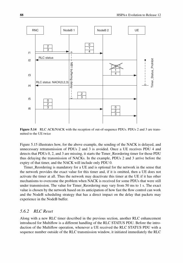
88 HSPA+ Evolution to Release 12
RNC NodeB 1 NodeB 2 UE
0
123 4
0
14
Tim
er_S
tatu
s_P
rohi
bit
RLC status: NACK(0,2,3)
23
NB
1buffering
delay
23
0
t1
t2
t6
t5
t3
t4
23
0
RLC status
Figure 5.14 RLC ACK/NACK with the reception of out-of-sequence PDUs. PDUs 2 and 3 are trans-mitted to the UE twice
Figure 5.15 illustrates how, for the above example, the sending of the NACK is delayed, andunnecessary retransmission of PDUs 2 and 3 is avoided. Once a UE receives PDU 4 anddetects that PDUs 0, 2, and 3 are missing, it starts the Timer_Reordering timer for those PDUthus delaying the transmission of NACKs. In the example, PDUs 2 and 3 arrive before theexpiry of that timer, and the NACK will include only PDU 0.
Timer_Reordering is mandatory for a UE and is optional for the network in the sense thatthe network provides the exact value for this timer and, if it is omitted, then a UE does notactivate the timer at all. Thus the network may deactivate this timer at the UE if it has othermechanisms to overcome the problem when NACK is received for some PDUs that were stillunder transmission. The value for Timer_Reordering may vary from 50 ms to 1 s. The exactvalue is chosen by the network based on its anticipation of how fast the flow control can workand the NodeB scheduling strategy that has a direct impact on the delay that packets mayexperience in the NodeB buffer.
5.6.2 RLC Reset
Along with a new RLC timer described in the previous section, another RLC enhancementintroduced for Multiflow is a different handling of the RLC STATUS PDU. Before the intro-duction of the Multiflow operation, whenever a UE received the RLC STATUS PDU with asequence number outside of the RLC transmission window, it initiated immediately the RLC
HSDPA Multiflow 89
RNC NodeB 1 NodeB 2 UE
0
123 4
0
14
Tim
er_S
tatu
s_P
rohi
bit
RLC status: NACK(0)
23
NB
1buffering
delay0
t1
t2
t6
t5
t3
t4
0
RLC status
Tim
er_R
eord
erin
g
Tim
er_S
tatu
s_P
rohi
bit
Figure 5.15 RLC ACK/NACK with the reception of out-of-sequence PDUs. Timer_Reordering elim-inates unnecessary re-transmissions
RESET procedure. This functionality was needed to achieve robust behavior: if a UE receivedan out-of-sequence status PDU it might be a sign of severe RLC state machine mismatches.However, with Multiflow the RNC may reply to the UE uplink traffic by sending the STATUSPDU message either over the serving, or assisting, or even both the serving and assisting links.Such RNC behavior may easily lead to a situation when RLC STATUS PDU messages arriveat the UE in a different order, thus triggering unnecessarily the RLC RESET operation. Itwas decided that the RNC should have the possibility of deciding flexibly how to send RLCfeedbacks and, as a result, it was agreed that for the inter-site Multiflow operation, no RLCRESET operation should be initiated under these circumstances. At the same time, a UE stillinitiates the RLC RESET procedure in case of intra-site Multiflow to be functionally close tothe multicarrier HSDPA.
5.7 Iub/Iur Enhancements
5.7.1 Flow Control
When the RNC provides data to a NodeB, it does so based on “credits” that the NodeB has givento the RNC. The NodeB’s credits are based on its buffer status. If the NodeB buffer is empty,
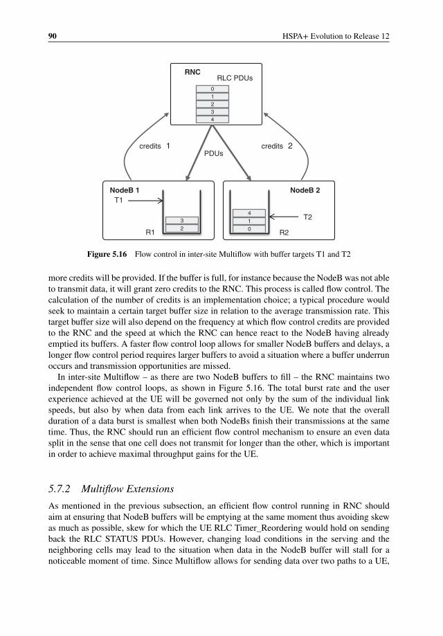
90 HSPA+ Evolution to Release 12
0
RNC
1234
RLC PDUs
credits 1 credits 2PDUs
2
3
NodeB 1
014
NodeB 2
R1 R2
T1
T2
Figure 5.16 Flow control in inter-site Multiflow with buffer targets T1 and T2
more credits will be provided. If the buffer is full, for instance because the NodeB was not ableto transmit data, it will grant zero credits to the RNC. This process is called flow control. Thecalculation of the number of credits is an implementation choice; a typical procedure wouldseek to maintain a certain target buffer size in relation to the average transmission rate. Thistarget buffer size will also depend on the frequency at which flow control credits are providedto the RNC and the speed at which the RNC can hence react to the NodeB having alreadyemptied its buffers. A faster flow control loop allows for smaller NodeB buffers and delays, alonger flow control period requires larger buffers to avoid a situation where a buffer underrunoccurs and transmission opportunities are missed.
In inter-site Multiflow – as there are two NodeB buffers to fill – the RNC maintains twoindependent flow control loops, as shown in Figure 5.16. The total burst rate and the userexperience achieved at the UE will be governed not only by the sum of the individual linkspeeds, but also by when data from each link arrives to the UE. We note that the overallduration of a data burst is smallest when both NodeBs finish their transmissions at the sametime. Thus, the RNC should run an efficient flow control mechanism to ensure an even datasplit in the sense that one cell does not transmit for longer than the other, which is importantin order to achieve maximal throughput gains for the UE.
5.7.2 Multiflow Extensions
As mentioned in the previous subsection, an efficient flow control running in RNC shouldaim at ensuring that NodeB buffers will be emptying at the same moment thus avoiding skewas much as possible, skew for which the UE RLC Timer_Reordering would hold on sendingback the RLC STATUS PDUs. However, changing load conditions in the serving and theneighboring cells may lead to the situation when data in the NodeB buffer will stall for anoticeable moment of time. Since Multiflow allows for sending data over two paths to a UE,
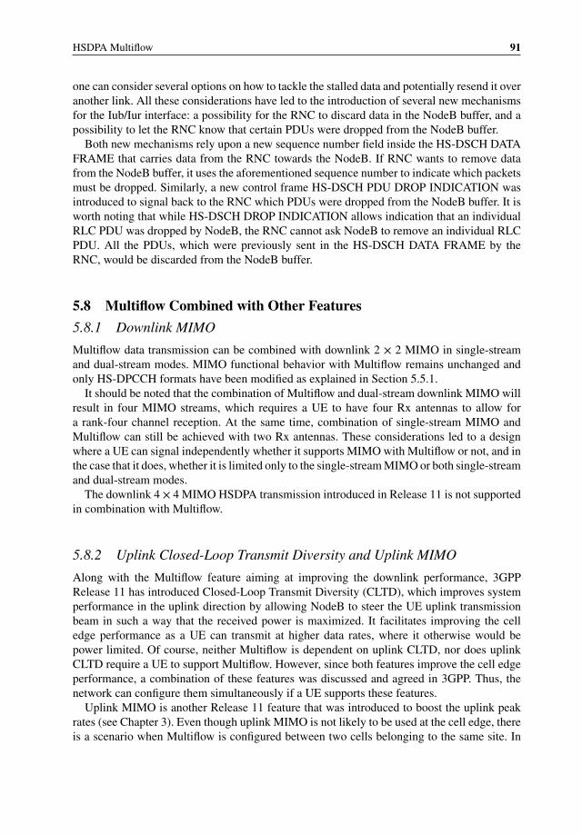
HSDPA Multiflow 91
one can consider several options on how to tackle the stalled data and potentially resend it overanother link. All these considerations have led to the introduction of several new mechanismsfor the Iub/Iur interface: a possibility for the RNC to discard data in the NodeB buffer, and apossibility to let the RNC know that certain PDUs were dropped from the NodeB buffer.
Both new mechanisms rely upon a new sequence number field inside the HS-DSCH DATAFRAME that carries data from the RNC towards the NodeB. If RNC wants to remove datafrom the NodeB buffer, it uses the aforementioned sequence number to indicate which packetsmust be dropped. Similarly, a new control frame HS-DSCH PDU DROP INDICATION wasintroduced to signal back to the RNC which PDUs were dropped from the NodeB buffer. It isworth noting that while HS-DSCH DROP INDICATION allows indication that an individualRLC PDU was dropped by NodeB, the RNC cannot ask NodeB to remove an individual RLCPDU. All the PDUs, which were previously sent in the HS-DSCH DATA FRAME by theRNC, would be discarded from the NodeB buffer.
5.8 Multiflow Combined with Other Features
5.8.1 Downlink MIMO
Multiflow data transmission can be combined with downlink 2 × 2 MIMO in single-streamand dual-stream modes. MIMO functional behavior with Multiflow remains unchanged andonly HS-DPCCH formats have been modified as explained in Section 5.5.1.
It should be noted that the combination of Multiflow and dual-stream downlink MIMO willresult in four MIMO streams, which requires a UE to have four Rx antennas to allow fora rank-four channel reception. At the same time, combination of single-stream MIMO andMultiflow can still be achieved with two Rx antennas. These considerations led to a designwhere a UE can signal independently whether it supports MIMO with Multiflow or not, and inthe case that it does, whether it is limited only to the single-stream MIMO or both single-streamand dual-stream modes.
The downlink 4 × 4 MIMO HSDPA transmission introduced in Release 11 is not supportedin combination with Multiflow.
5.8.2 Uplink Closed-Loop Transmit Diversity and Uplink MIMO
Along with the Multiflow feature aiming at improving the downlink performance, 3GPPRelease 11 has introduced Closed-Loop Transmit Diversity (CLTD), which improves systemperformance in the uplink direction by allowing NodeB to steer the UE uplink transmissionbeam in such a way that the received power is maximized. It facilitates improving the celledge performance as a UE can transmit at higher data rates, where it otherwise would bepower limited. Of course, neither Multiflow is dependent on uplink CLTD, nor does uplinkCLTD require a UE to support Multiflow. However, since both features improve the cell edgeperformance, a combination of these features was discussed and agreed in 3GPP. Thus, thenetwork can configure them simultaneously if a UE supports these features.
Uplink MIMO is another Release 11 feature that was introduced to boost the uplink peakrates (see Chapter 3). Even though uplink MIMO is not likely to be used at the cell edge, thereis a scenario when Multiflow is configured between two cells belonging to the same site. In
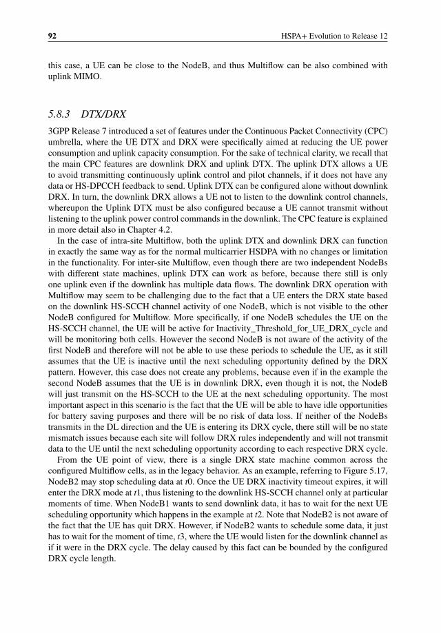
92 HSPA+ Evolution to Release 12
this case, a UE can be close to the NodeB, and thus Multiflow can be also combined withuplink MIMO.
5.8.3 DTX/DRX
3GPP Release 7 introduced a set of features under the Continuous Packet Connectivity (CPC)umbrella, where the UE DTX and DRX were specifically aimed at reducing the UE powerconsumption and uplink capacity consumption. For the sake of technical clarity, we recall thatthe main CPC features are downlink DRX and uplink DTX. The uplink DTX allows a UEto avoid transmitting continuously uplink control and pilot channels, if it does not have anydata or HS-DPCCH feedback to send. Uplink DTX can be configured alone without downlinkDRX. In turn, the downlink DRX allows a UE not to listen to the downlink control channels,whereupon the Uplink DTX must be also configured because a UE cannot transmit withoutlistening to the uplink power control commands in the downlink. The CPC feature is explainedin more detail also in Chapter 4.2.
In the case of intra-site Multiflow, both the uplink DTX and downlink DRX can functionin exactly the same way as for the normal multicarrier HSDPA with no changes or limitationin the functionality. For inter-site Multiflow, even though there are two independent NodeBswith different state machines, uplink DTX can work as before, because there still is onlyone uplink even if the downlink has multiple data flows. The downlink DRX operation withMultiflow may seem to be challenging due to the fact that a UE enters the DRX state basedon the downlink HS-SCCH channel activity of one NodeB, which is not visible to the otherNodeB configured for Multiflow. More specifically, if one NodeB schedules the UE on theHS-SCCH channel, the UE will be active for Inactivity_Threshold_for_UE_DRX_cycle andwill be monitoring both cells. However the second NodeB is not aware of the activity of thefirst NodeB and therefore will not be able to use these periods to schedule the UE, as it stillassumes that the UE is inactive until the next scheduling opportunity defined by the DRXpattern. However, this case does not create any problems, because even if in the example thesecond NodeB assumes that the UE is in downlink DRX, even though it is not, the NodeBwill just transmit on the HS-SCCH to the UE at the next scheduling opportunity. The mostimportant aspect in this scenario is the fact that the UE will be able to have idle opportunitiesfor battery saving purposes and there will be no risk of data loss. If neither of the NodeBstransmits in the DL direction and the UE is entering its DRX cycle, there still will be no statemismatch issues because each site will follow DRX rules independently and will not transmitdata to the UE until the next scheduling opportunity according to each respective DRX cycle.
From the UE point of view, there is a single DRX state machine common across theconfigured Multiflow cells, as in the legacy behavior. As an example, referring to Figure 5.17,NodeB2 may stop scheduling data at t0. Once the UE DRX inactivity timeout expires, it willenter the DRX mode at t1, thus listening to the downlink HS-SCCH channel only at particularmoments of time. When NodeB1 wants to send downlink data, it has to wait for the next UEscheduling opportunity which happens in the example at t2. Note that NodeB2 is not aware ofthe fact that the UE has quit DRX. However, if NodeB2 wants to schedule some data, it justhas to wait for the moment of time, t3, where the UE would listen for the downlink channel asif it were in the DRX cycle. The delay caused by this fact can be bounded by the configuredDRX cycle length.
HSDPA Multiflow 93
NodeB 1
NodeB 2
UE
t0 t3t2t1
data arrives
data arrives
Figure 5.17 DRX with inter-site Multiflow with two independent DRX state machines in the NodeBs
5.9 Setting Up Multiflow
As mentioned earlier, from a specification perspective Multiflow can be understood as anextension of multicarrier HSDPA. Thus, setting up a Multiflow connection is similar to con-figuring a multicarrier radio bearer (RB): in addition to the typical RB information of carrierfrequency, and other cell configurations, a few new information elements were added to theconfiguration.
In a typical sequence of events a UE would first carry out measurements and send reportson the strength of neighboring cells to the RNC. The RNC can – based on the measurementreport and load information of the neighboring cells that it has available – identify whichUEs would benefit from the Multiflow transmission. From there on, the RNC would proceedto perform radio link (re-)configurations of the involved NodeBs, as well as the UE. Inparticular the RNC will configure the NodeB with a “RL Addition” or “RL Reconfiguration”(or “RL Reconfiguration Prepare”) message, which carries the relevant parameters. The UEwill be configured by the RNC as part of an active set update or as part of a separate RB(re-)configuration. A schematic overview of the sequence of steps is shown in Figure 5.18, amore detailed view on RL and RB reconfiguration signaling flows applicable also to Multiflowis shown for instance in [4] Figure 9.5-1.
The new parameters required to configure a UE are contained within the new informa-tion element “Multiflow configuration info” (see section 10.3.6.31a in [7]). Those additionalMultiflow specific parameters are:
� Indication of the “cell group,” which is effectively an indication of whether the cell belongsto the serving or the assisting NodeB.
� Indication of which cell is a downlink time reference for the bundling of uplink feedback.
In inter-site Multiflow, the configuration sent by the RNC to a NodeB is not visible tothe other NodeB. However, both NodeBs require some information, and the configurationmessages were thus enhanced with following parameters (see section 9.2.2.170 in [8]):
� Indication on whether NodeB is a serving or assisting.� Total number of cells of the overall Multiflow configuration.

94 HSPA+ Evolution to Release 12
UE RNC
measurement report
ASU with configuration information orRB configuration information
NodeB 2NodeB 1
RL configuration information
decision to configureUE for MF
Figure 5.18 Configuring Multiflow
� Indication of which cell is the downlink time reference for the bundling of uplink feedback.For the non-time reference cell, RNC also indicates the timing offset.
� Indication of whether at least one cell in the other NodeB is configured in MIMO mode.Once at least one cell in any NodeB is configured with MIMO, the whole HS-DPCCHformat changes.
5.10 Robustness
5.10.1 Robustness for RRC Signaling
Multiflow data transmission can be applied to RLC acknowledged mode (AM) and RLCunacknowledged mode (UM). When illustrating the radio bearer to transport channel mappingfor inter-site Multiflow in Figure 5.19 it becomes apparent that Multiflow can be appliednot only to the user RBs, but also to signaling RBs (SRBs), which are mapped to eitherRLC-UM or RLC-AM (for a list of all SRBs see [7] section 6.3). The advantage of doingso lies in increasing the robustness of, for example, a serving cell change: a message for RBreconfiguration can be relayed not only over the one link, but also over the other if a first RLCtransmission failed. For the highest robustness the reconfiguration message could be relayedover both links from the beginning. Thus, a reconfiguration message would not reach the UEonly if both configured NodeBs have lost connectivity with the UE.
5.10.2 Radio Link Failure
In the UE a radio link failure (RLF) is declared if synchronization to the serving cell is lost andthe power control command carrying the F-DPCH signal level from the serving HS-DSCHcell falls below a fixed threshold for a given time duration, see [9] section 4.3.1.2. RLF leads to
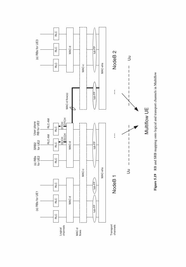
RLC
RLC
RLC
RLC
RLC
RLC
MA
C-d
MA
C-c
MA
C-d
MA
C-e
hs
Iub-
FP
Iub-
FP
Iub-
FP
(s)
RB
s fo
r U
E1 Nod
eB 1
Nod
eB 2
(s)
RB
sfo
rU
E2
Use
rpl
ane
RB
for
UE
2
Mul
tiflo
wU
E
Logi
cal
chan
nels
Tra
nspo
rtch
anne
ls
SR
B2
for
UE
2
RLC
RLC
RLC
MA
C-d
MA
C-c
MA
C-e
hs
Iub-
FP
Iub-
FP
(s)
RB
s fo
r U
E3
RLC
-AM
RLC
-AM
DC
CH
DT
CH
MA
C-d
flow
(s)
MA
C-d
flow
s
Uu
Uu
......
DC
CH
DT
CH
Fig
ure
5.19
RB
and
SRB
map
ping
onto
logi
cala
ndtr
ansp
ortc
hann
els
inM
ultifl
ow
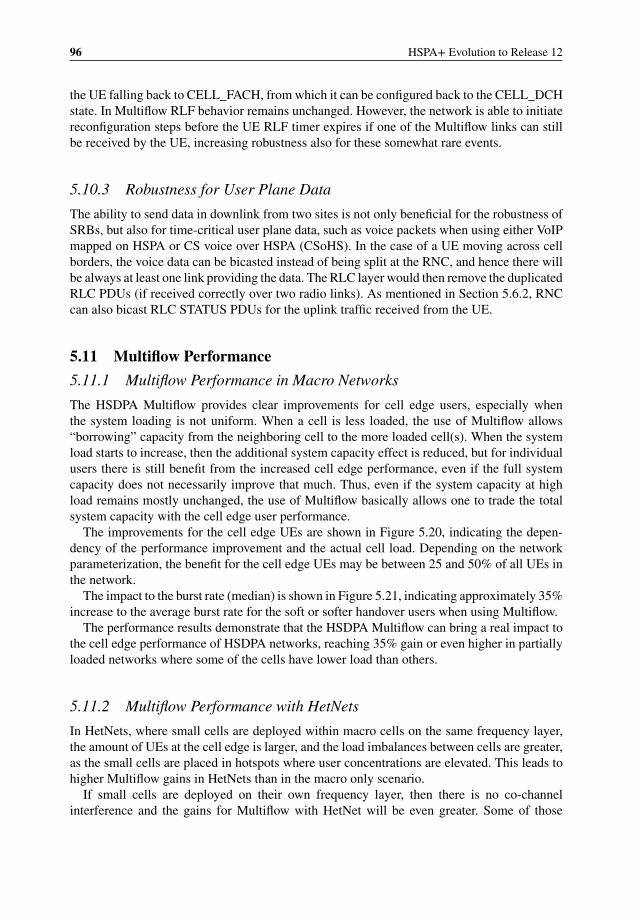
96 HSPA+ Evolution to Release 12
the UE falling back to CELL_FACH, from which it can be configured back to the CELL_DCHstate. In Multiflow RLF behavior remains unchanged. However, the network is able to initiatereconfiguration steps before the UE RLF timer expires if one of the Multiflow links can stillbe received by the UE, increasing robustness also for these somewhat rare events.
5.10.3 Robustness for User Plane Data
The ability to send data in downlink from two sites is not only beneficial for the robustness ofSRBs, but also for time-critical user plane data, such as voice packets when using either VoIPmapped on HSPA or CS voice over HSPA (CSoHS). In the case of a UE moving across cellborders, the voice data can be bicasted instead of being split at the RNC, and hence there willbe always at least one link providing the data. The RLC layer would then remove the duplicatedRLC PDUs (if received correctly over two radio links). As mentioned in Section 5.6.2, RNCcan also bicast RLC STATUS PDUs for the uplink traffic received from the UE.
5.11 Multiflow Performance
5.11.1 Multiflow Performance in Macro Networks
The HSDPA Multiflow provides clear improvements for cell edge users, especially whenthe system loading is not uniform. When a cell is less loaded, the use of Multiflow allows“borrowing” capacity from the neighboring cell to the more loaded cell(s). When the systemload starts to increase, then the additional system capacity effect is reduced, but for individualusers there is still benefit from the increased cell edge performance, even if the full systemcapacity does not necessarily improve that much. Thus, even if the system capacity at highload remains mostly unchanged, the use of Multiflow basically allows one to trade the totalsystem capacity with the cell edge user performance.
The improvements for the cell edge UEs are shown in Figure 5.20, indicating the depen-dency of the performance improvement and the actual cell load. Depending on the networkparameterization, the benefit for the cell edge UEs may be between 25 and 50% of all UEs inthe network.
The impact to the burst rate (median) is shown in Figure 5.21, indicating approximately 35%increase to the average burst rate for the soft or softer handover users when using Multiflow.
The performance results demonstrate that the HSDPA Multiflow can bring a real impact tothe cell edge performance of HSDPA networks, reaching 35% gain or even higher in partiallyloaded networks where some of the cells have lower load than others.
5.11.2 Multiflow Performance with HetNets
In HetNets, where small cells are deployed within macro cells on the same frequency layer,the amount of UEs at the cell edge is larger, and the load imbalances between cells are greater,as the small cells are placed in hotspots where user concentrations are elevated. This leads tohigher Multiflow gains in HetNets than in the macro only scenario.
If small cells are deployed on their own frequency layer, then there is no co-channelinterference and the gains for Multiflow with HetNet will be even greater. Some of those

HSDPA Multiflow 97
0 0.5 1 1.5 2 2.5 3 3.50
5
10
15
20
25
30
35
40
45
50Inter-site Multiflow
Cell load [Mbps]
Use
r bu
rst r
ate
gain
[%]
all UEsinter-site cell edge UEsintra-site cell edge UEs
Figure 5.20 Performance of Multiflow
scenarios require, however, that the NodeBs are able to receive the uplink of the UE on afrequency which is not paired to their downlink carrier. Even more importantly, it remainsto be seen whether operators will reserve a dedicated carrier for small cells only, rather thanconfigure macro stations as multicarrier cells.
A more detailed account of gains in Multiflow with HetNets is provided in Chapter 7.
Ave
rage
bur
st r
ate
[Mbp
s]
0
1
2
3
4
5
6
7
8
9
SHO UE SHO UE withMultiflow
Softer HO UE Softer HO UE withMultiflow
Figure 5.21 Median burst rate improvement with Multiflow
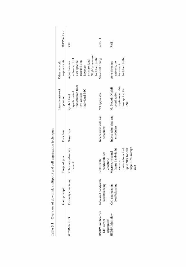
Tabl
e5.
1O
verv
iew
ofdo
wnl
ink
mul
tipoi
ntan
dce
llag
greg
atio
nte
chni
ques
Gai
npr
inci
ple
Ran
geof
gain
Dat
aflo
wIn
ter-
site
netw
ork
oper
atio
nO
ther
netw
ork
requ
irem
ents
3GPP
Rel
ease
WC
DM
ASH
OD
iver
sity
com
bini
ngR
obus
tnes
sdi
vers
itybe
nefit
Sam
eda
taSy
mbo
llev
elsy
nchr
oniz
edtr
ansm
issi
onfr
omtw
oce
llson
indi
vidu
alPS
C
Asy
nchr
onou
sne
twor
k,SH
Ous
er-s
peci
fictr
ansm
issi
onho
wev
ersy
nchr
oniz
ed.
Slig
htly
incr
ease
dba
ckha
ultr
affic
R99
HSD
PAm
ultic
arri
er,
LTE
carr
ier
aggr
egat
ion
Incr
ease
dba
ndw
idth
,lo
adba
lanc
ing
Scal
esw
ithba
ndw
idth
,see
Cha
pter
3
Inde
pend
entd
ata
and
sche
dule
rsN
otap
plic
able
Sam
ece
lltim
ing
Rel
8-11
HSD
PAM
ultifl
owC
ella
ggre
gatio
n,lo
adba
lanc
ing
Mac
roco
-cha
nnel
(sam
eba
ndw
idth
)sc
enar
io:
low
–med
ium
load
:up
to50
%fo
rce
lled
ge,1
0%av
erag
ega
in
Inde
pend
entd
ata
and
sche
dule
rsN
oN
odeB
–Nod
eBco
ordi
natio
nre
quir
emen
t,da
taflo
wsp
litin
the
RN
C
Asy
nchr
onou
sne
twor
k,no
incr
ease
inba
ckha
ultr
affic
Rel
11
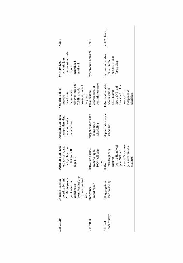
LTE
CoM
PD
ynam
icm
ultis
iteco
ordi
natio
nan
dM
IMO
(dyn
amic
poin
tsel
ectio
n,co
ordi
nate
dbe
amfo
rmin
g),u
pto
thre
ein
volv
edsi
tes
Dep
endi
ngon
mod
ean
dsc
enar
io,a
lso
for
high
load
s:up
to30
%fo
rce
lled
ge[1
0]
Dep
endi
ngon
mod
ein
depe
nden
tdat
a,bu
tcoo
rdin
ated
tran
smis
sion
Ver
yde
man
ding
inte
r-si
teco
ordi
natio
nre
quir
emen
ts,
how
ever
intr
a-si
teC
oMP
alre
ady
prov
ides
mos
tof
the
gain
s
Sync
hron
ized
netw
ork,
join
ttr
ansm
issi
onm
ode
requ
ires
cent
raliz
edba
seba
nd
Rel
11
LTE
feIC
ICIn
terf
eren
ceco
ordi
natio
nH
etN
etco
-cha
nnel
scen
ario
:up
to10
0%ce
lled
gega
ins
Inde
pend
entd
ata
but
coor
dina
ted
sche
dulin
g
Het
Net
feat
ure:
Coo
rdin
atio
nof
tran
smit
reso
urce
s
Sync
hron
ous
netw
ork
Rel
11
LTE
dual
conn
ectiv
ityC
ella
ggre
gatio
n,lo
adba
lanc
ing
Het
Net
inte
r-fr
eque
ncy
scen
ario
:lo
w–m
ediu
mlo
ad:
upto
50%
cell
edge
,20%
aver
age
gain
with
real
istic
back
haul
Inde
pend
entd
ata
and
sche
dule
rsH
etN
etfe
atur
e:da
taflo
wis
split
inR
LC
laye
rof
mac
roeN
Ban
dfo
rwar
ded
tolo
wpo
wer
eNB
.In
depe
nden
tsc
hedu
lers
Incr
ease
inba
ckha
ulor
X2
traf
ficbe
caus
eof
data
forw
ardi
ng
Rel
12pl
anne
d
100 HSPA+ Evolution to Release 12
5.12 Multiflow and Other Multipoint Transmission Techniques
The feature most similar to Multiflow is, as mentioned earlier, LTE dual connectivity, which isplanned for 3GPP Release 12. The similarity comes with the usage of independent schedulersand a data flow split across two sites, and that transmissions can occur on different carriers.The LTE Release 11 interference coordination scheme, feICIC, is benefitting specifically celledge users just as Multiflow does.
LTE CoMP – coordinated multipoint transmission/reception – has some similarity withMultiflow, in that several nodes may transmit to one receiver. LTE CoMP comprises a numberof schemes, ranging from dynamic coordinated transmission point selection to coordinatedjoint transmission from up to three sites. The gains for CoMP materialize from exploiting thelarge diversity of the channel as well as interference coordination. One of the prerequisites forLTE CoMP is a perfect backhaul that limits its practical use. Also the amount and the qualityof the feedback available from the UE diminishes the gains that can be achieved in reality.
In a comparison with other multipoint and cell aggregation techniques, HSDPA Multiflowis positioned as a very low complexity technique without additional spectrum requirements,providing gains for low–medium loads. LTE CoMP, on the other hand, takes the place ofmaximal complexity with benefits also for high loads. An overview of the techniques and theirrequirements and gains is shown in Table 5.1.
5.13 Conclusions
This chapter has introduced HSDPA Multiflow protocol and physical layer operation principlesas well as demonstrated the achievable capacity benefits. As the impacts to the UE and networkimplementation are reasonable and resulting performance benefits accrue especially to the cell-edge users, it is foreseen that HSDPA Multiflow will be an attractive feature to be adopted inthe marketplace.
As use of HSDPA Multiflow is fully backwards compatible, that is, it can be operated in anetwork with both Release 11 UEs and older ones, it can be rolled out gradually to the networkto boost the cell edge performance.
The LTE-Advanced carrier aggregation [11] has some similarity with the HSDPA Multiflow,only that the Release 10 carrier aggregation is done as intra-site aggregation and only as partof the Release 12 small cell evolution studies [3] the inter-site operation is expected to beintroduced as part of the dual connectivity in Release 12 specification, due by the end of 2014.
References
[1] 3GPP Technical Report, TR 25.872, “High Speed Packet Access (HSDPA) multipoint transmission”, Release 11,2011.
[2] 3GPP Tdoc, RP-111375, WI description “HSDPA Multiflow data transmission”, 2011.[3] 3GPP Technical Report, TR 36.842 “Study on small cell enhancements for E-UTRA and E-UTRAN - Higher-
layer aspects”, Release 12, December 2013.[4] 3GPP Technical Specification, TS 25.308, “HSDPA overall description”, Release 11. 11, March 2013.[5] 3GPP Technical Specification, TS 25.212, “Multiplexing and channel coding (FDD)”, Release 11, March 2013.[6] 3GPP Technical Specification, TS 25.213, “Spreading and Modulation (FDD), Release 11, March 2013.[7] 3GPP Technical Specification, TS 25.331, “Radio resource control protocol specification”, Release 11,
March 2013.

HSDPA Multiflow 101
[8] 3GPP Technical Specification, TS 25.433, “UTRAN Iub interface Node B Application Part (NBAP) signalling”,Release 11, September 2013.
[9] 3GPP Technical Specification, TS 25.214, “Physical layer procedures (FDD)”, Release 11, March 2013.[10] 3GPP Technical Report, TR 36.819, “Coordinated multi-point operation for LTE physical layer aspects”,
Release 11, September 2013.[11] Holma, H. and Toskala, A. (2012) LTE-Advanced, John Wiley & Sons, Ltd, Chichester.[12] 3GPP Technical Specification, TS 25.211, “Physical channels and mapping of transport channels onto physical
channels (FDD)”, Release 11, June 2013.


6Voice Evolution
Harri Holma and Karri Ranta-aho
6.1 Introduction
Circuit Switched (CS) voice was part of the WCDMA offering from Day 1 together with thePacket Switched (PS) data service. WCDMA voice uses Adaptive Multirate (AMR) codecwith a data rate of 12.2 kbps. In many developed countries more than 50% of mobile voiceminutes are now carried by WCDMA CS voice. The voice is still important from the operatorrevenue point of view even if data traffic is far higher than voice from the volume point ofview. The voice service keeps improving further: AMR wideband (AMR-WB) offers HighDefinition (HD) quality, lower rate AMR improves voice capacity, voice-over HSPA providesboth VoIP and CS voice capability, CS fallback from LTE to WCDMA CS voice enablesvoice services for LTE smartphones, and Single Radio Voice Call Continuity (SRVCC) bringshandover from VoIP to CS voice. These evolution steps are summarized in Figure 6.1 anddescribed in more detail in this chapter.
6.2 Voice Quality with AMR Wideband
AMR Wideband (AMR-WB) enhances voice quality by a higher voice sampling rate in voiceencoding. AMR Narrowband (AMR-NB) uses an 8 kHz sampling rate which enables an audiobandwidth of 300–3400 Hz, similar to traditional landline phones. AMR-WB uses 16 kHzwhich increases the audio bandwidth to 50–7000 Hz. Voice sounds substantially better whenthe low and high frequencies are reproduced. The audio bandwidth is illustrated in Figure 6.2.
AMR-WB codec can use data rates between 6.6 kbps and 23.85 kbps depending on thecompression level. The higher data rate gives slightly better voice quality while the low datarates provide higher voice capacity. The typical data rate is 12.65 kbps, which implies thatAMR-WB does not consume more capacity than AMR-NB: wideband audio with narrowbandradio. AMR-WB also supports voice activity detection and discontinuous transmission tominimize the average data rate. All AMR-WB data rates and the subset with Spreading Factor
HSPA+ Evolution to Release 12: Performance and Optimization, First Edition.Edited by Harri Holma, Antti Toskala, and Pablo Tapia.© 2014 John Wiley & Sons, Ltd. Published 2014 by John Wiley & Sons, Ltd.
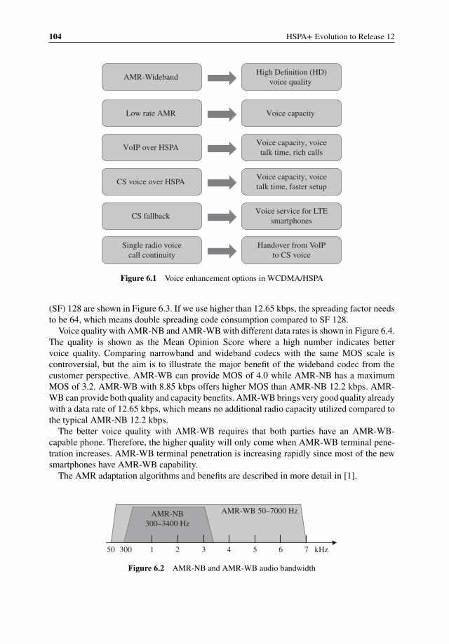
104 HSPA+ Evolution to Release 12
AMR-Wideband High Definition (HD)
voice quality
Low rate AMR Voice capacity
VoIP over HSPA Voice capacity, voice
talk time, rich calls
CS voice over HSPA Voice capacity, voice
talk time, faster setup
CS fallback Voice service for LTE
smartphones
Single radio voice
call continuity
Handover from VoIP
to CS voice
Figure 6.1 Voice enhancement options in WCDMA/HSPA
(SF) 128 are shown in Figure 6.3. If we use higher than 12.65 kbps, the spreading factor needsto be 64, which means double spreading code consumption compared to SF 128.
Voice quality with AMR-NB and AMR-WB with different data rates is shown in Figure 6.4.The quality is shown as the Mean Opinion Score where a high number indicates bettervoice quality. Comparing narrowband and wideband codecs with the same MOS scale iscontroversial, but the aim is to illustrate the major benefit of the wideband codec from thecustomer perspective. AMR-WB can provide MOS of 4.0 while AMR-NB has a maximumMOS of 3.2. AMR-WB with 8.85 kbps offers higher MOS than AMR-NB 12.2 kbps. AMR-WB can provide both quality and capacity benefits. AMR-WB brings very good quality alreadywith a data rate of 12.65 kbps, which means no additional radio capacity utilized compared tothe typical AMR-NB 12.2 kbps.
The better voice quality with AMR-WB requires that both parties have an AMR-WB-capable phone. Therefore, the higher quality will only come when AMR-WB terminal pene-tration increases. AMR-WB terminal penetration is increasing rapidly since most of the newsmartphones have AMR-WB capability.
The AMR adaptation algorithms and benefits are described in more detail in [1].
1 2 3 4 5 6 7 kHz
AMR-WB 50–7000 HzAMR-NB
300–3400 Hz
30050
Figure 6.2 AMR-NB and AMR-WB audio bandwidth
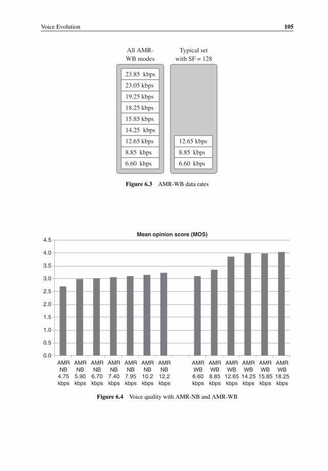
Voice Evolution 105
23.85 kbps
19.25 kbps
14.25 kbps
8.85 kbps
23.05 kbps
18.25 kbps
15.85 kbps
12.65 kbps
All AMR-
WB modes
Typical set
with SF = 128
6.60 kbps
8.85 kbps
12.65 kbps
6.60 kbps
Figure 6.3 AMR-WB data rates
0.0
0.5
1.0
1.5
2.0
2.5
3.0
3.5
4.0
4.5
AMR NB
4.75 kbps
AMR NB
5.90 kbps
AMR NB
6.70 kbps
AMR NB
7.40 kbps
AMR NB
7.95 kbps
AMR NB
10.2 kbps
AMR NB
12.2 kbps
AMR WB 6.60 kbps
AMR WB 8.85 kbps
AMR WB
12.65 kbps
AMR WB
14.25 kbps
AMR WB
15.85 kbps
AMR WB
18.25 kbps
Mean opinion score (MOS)
Figure 6.4 Voice quality with AMR-NB and AMR-WB
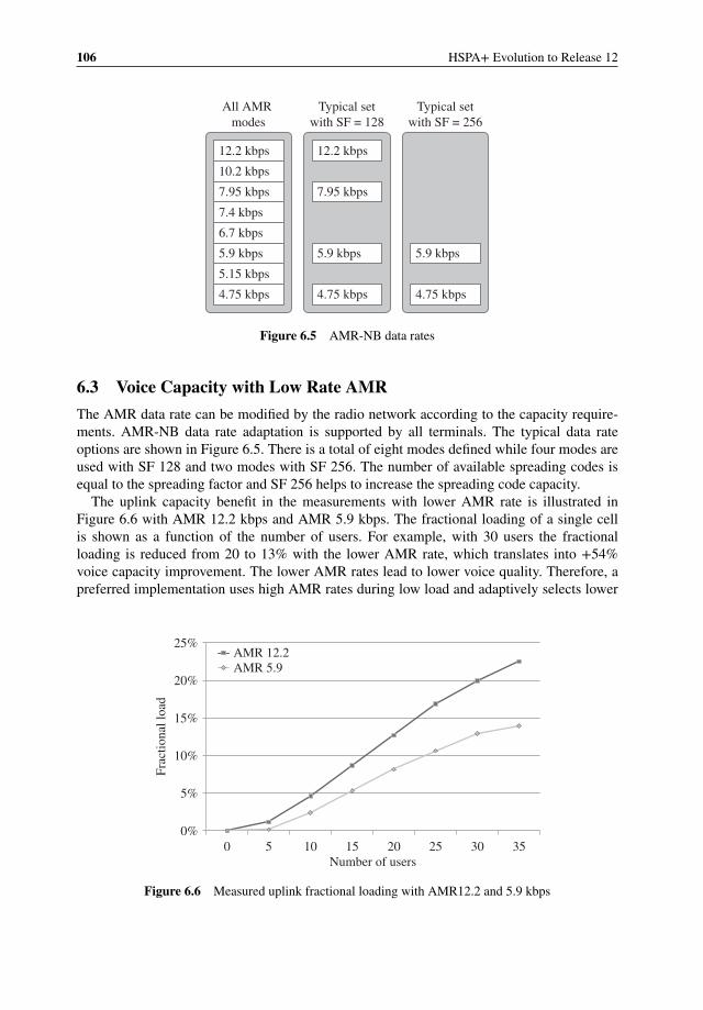
106 HSPA+ Evolution to Release 12
12.2 kbps
7.95 kbps
5.9 kbps
4.75 kbps
12.2 kbps
7.95 kbps
5.9 kbps
4.75 kbps
10.2 kbps
7.4 kbps
6.7 kbps
5.15 kbps
5.9 kbps
4.75 kbps
All AMR
modes
Typical set
with SF = 128
Typical set
with SF = 256
Figure 6.5 AMR-NB data rates
6.3 Voice Capacity with Low Rate AMR
The AMR data rate can be modified by the radio network according to the capacity require-ments. AMR-NB data rate adaptation is supported by all terminals. The typical data rateoptions are shown in Figure 6.5. There is a total of eight modes defined while four modes areused with SF 128 and two modes with SF 256. The number of available spreading codes isequal to the spreading factor and SF 256 helps to increase the spreading code capacity.
The uplink capacity benefit in the measurements with lower AMR rate is illustrated inFigure 6.6 with AMR 12.2 kbps and AMR 5.9 kbps. The fractional loading of a single cellis shown as a function of the number of users. For example, with 30 users the fractionalloading is reduced from 20 to 13% with the lower AMR rate, which translates into +54%voice capacity improvement. The lower AMR rates lead to lower voice quality. Therefore, apreferred implementation uses high AMR rates during low load and adaptively selects lower
0%
5%
10%
15%
20%
25%
0 5 10 15 20 25 30 35
Fra
ctio
nal
load
Number of users
AMR 12.2AMR 5.9
Figure 6.6 Measured uplink fractional loading with AMR12.2 and 5.9 kbps
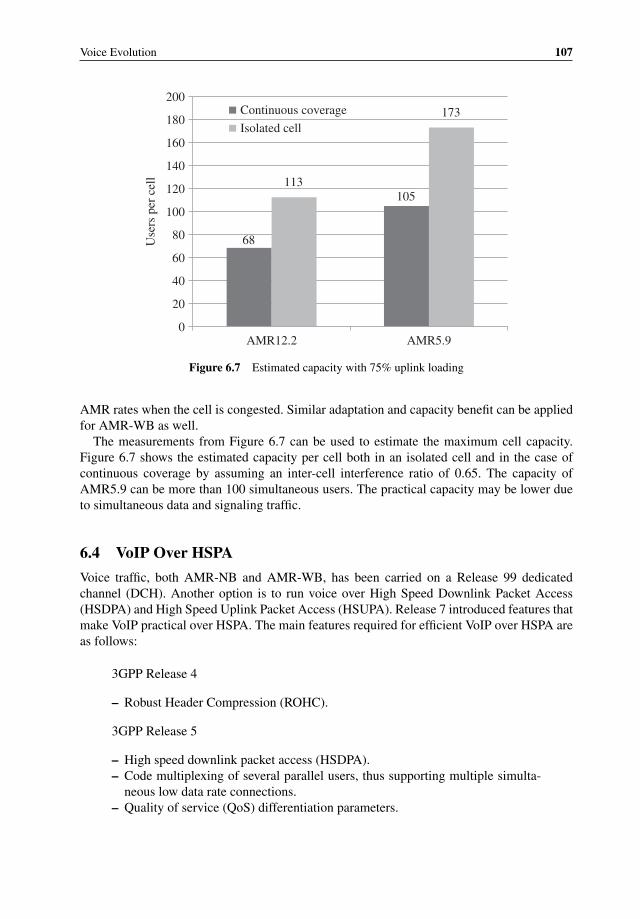
Voice Evolution 107
68
105113
173
0
20
40
60
80
100
120
140
160
180
200
AMR12.2 AMR5.9
Use
rs p
er c
ell
Continuous coverage
Isolated cell
Figure 6.7 Estimated capacity with 75% uplink loading
AMR rates when the cell is congested. Similar adaptation and capacity benefit can be appliedfor AMR-WB as well.
The measurements from Figure 6.7 can be used to estimate the maximum cell capacity.Figure 6.7 shows the estimated capacity per cell both in an isolated cell and in the case ofcontinuous coverage by assuming an inter-cell interference ratio of 0.65. The capacity ofAMR5.9 can be more than 100 simultaneous users. The practical capacity may be lower dueto simultaneous data and signaling traffic.
6.4 VoIP Over HSPA
Voice traffic, both AMR-NB and AMR-WB, has been carried on a Release 99 dedicatedchannel (DCH). Another option is to run voice over High Speed Downlink Packet Access(HSDPA) and High Speed Uplink Packet Access (HSUPA). Release 7 introduced features thatmake VoIP practical over HSPA. The main features required for efficient VoIP over HSPA areas follows:
3GPP Release 4
– Robust Header Compression (ROHC).
3GPP Release 5
– High speed downlink packet access (HSDPA).– Code multiplexing of several parallel users, thus supporting multiple simulta-
neous low data rate connections.– Quality of service (QoS) differentiation parameters.
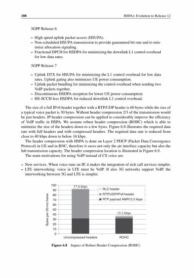
108 HSPA+ Evolution to Release 12
3GPP Release 6
– High speed uplink packet access (HSUPA).– Non-scheduled HSUPA transmission to provide guaranteed bit rate and to min-
imize allocation signaling.– Fractional DPCH for HSDPA for minimizing the downlink L1 control overhead
for low data rates.
3GPP Release 7
– Uplink DTX for HSUPA for minimizing the L1 control overhead for low datarates. Uplink gating also minimizes UE power consumption.
– Uplink packet bundling for minimizing the control overhead when sending twoVoIP packets together.
– Discontinuous HSDPA reception for lower UE power consumption.– HS-SCCH-less HSDPA for reduced downlink L1 control overhead.
The size of a full IPv6 header together with a RTP/UDP header is 60 bytes while the size ofa typical voice packet is 30 bytes. Without header compression 2/3 of the transmission wouldbe just headers. IP header compression can be applied to considerably improve the efficiencyof VoIP traffic in HSPA. We assume robust header compression (ROHC) which is able tominimize the size of the headers down to a few bytes. Figure 6.8 illustrates the required datarate with full headers and with compressed headers. The required data rate is reduced fromclose to 40 kbps down to below 16 kbps.
The header compression with HSPA is done on Layer 2 PDCP (Packet Data ConvergenceProtocol) in UE and in RNC, therefore it saves not only the air interface capacity but also theIub transmission capacity. The header compression location is illustrated in Figure 6.9.
The main motivations for using VoIP instead of CS voice are:
– New services. When voice runs on IP, it makes the integration of rich call services simpler.– LTE interworking: voice in LTE must be VoIP. If also 3G networks support VoIP, the
interworking between 3G and LTE is simpler.
0
10
20
30
40
50
60
70
80
90
100
Uncompressed headers ROHC
Byt
es p
er 2
0-m
s fr
ame
RLC header
RTP/UDP/IPv6 header
RTP payload AMR12.2 kbps
15.2 kbps
37.6 kbps
Figure 6.8 Impact of Robust Header Compression (ROHC)

Voice Evolution 109
RNC GGSNNodeBUE
Compressed IP headers Full IP headers
Iub
Figure 6.9 IP header compression between UE and RNC
– Higher spectral efficiency: voice over HSPA can support more users than voice over Release99 DCH.
– Longer talk time: discontinuous transmission and reception reduces UE power consumption.– Faster call setup: when signaling runs on top of HSPA, it becomes faster.
We will consider two topics in more detail: spectral efficiency and talk time of voice overHSPA. HSPA improves the efficiency of data transmission considerably due to advancedfeatures. The same features can also help in voice efficiency:
– UE equalizer can remove intra-cell interference. An equalizer is included in practice in allHSPA receivers but not in WCDMA receivers.
– UE inter-cell interference cancellation also known as the Type 3i receiver.– Layer 1 retransmissions can also be applied to voice, even if the delay budget is limited,
since the retransmission delay is only 16 ms.– HSDPA fast scheduling allows improvement in efficiency even with tough delay require-
ments.– Optimized Layer 1 control channel reduces control channel overhead. The downlink solution
is fractional DPCH and HS-SCCH-less transmission, and the uplink solution is discontinu-ous transmission.
– Uplink interference cancellation, which is typically implemented only for HSUPA, not forWCDMA.
The results of the system-level simulations are shown in Figure 6.10. Voice over HSPAcan provide up to 80–90% capacity benefit when all HSPA optimization features are included.These capacities are assumed to be uplink limited. The detailed simulation results are presentedin [2–4].
UE power consumption will benefit from running voice over HSPA. WCDMA uses contin-uous transmission and reception regardless of the voice activity. Voice over HSPA can utilizediscontinuous transmission (DTX) and discontinuous reception (DRX). These functionalitiesare explained in more detail in Chapter 4. The most efficient approach to minimize powerconsumption is DTX and DRX. That also explains why GSM terminals tend to have longertalk times than WCDMA terminals: GSM can use DTX and DRX while WCDMA cannot.
The power consumption improvements can be estimated from the required transmissionand reception activities. The estimated RF activity factors are shown in Table 6.1 for threedifferent cases: uplink voice while downlink is silent, downlink voice while uplink is silent, andsilence in both directions. The uplink activity is lower than the downlink because the downlink

110 HSPA+ Evolution to Release 12
0
20
40
60
80
100
120
140
160
180
200
AMR 12.2 AMR 5.9
Use
rs p
er c
ell
WCDMA
HSPA
Figure 6.10 Capacity benefit of voice over HSPA
reception is needed for the reception of the uplink power control commands. We assume thatvoice transmission in downlink has 45% probability, voice in uplink 45% probability, andsilence 10% probability. The average activity factors are 24% in uplink and 47% in downlink.The radio modem can utilize the inactivity periods for power savings. These activity factorsassume that each voice packet is transmitted separately. The RF activity can be further reducedby using packet bundling, where two voice packets are sent together over the air interface. Theactivity factors with power bundling are shown in Table 6.2. If voice over HSPA were used,the power consumption could potentially be 50% lower, providing up to two times longertalk time.
Table 6.1 Voice over HSPA RF activity factors. Adapted from Holma and Toskala, 2010 [5]
HSPA Uplink (%) Downlink (%) Probability (%)
Uplink voice, downlink silent 26 46 45Downlink voice, uplink silent 26 52 45Silent both directions 6 26 10Average activity 24 47
Table 6.2 Voice over HSPA RF activity factors with packet bundling. Adapted from Holma andToskala, 2010 [5]
HSPA Uplink (%) Downlink (%) Probability (%)
Uplink voice, downlink silent 14 40 45Downlink voice, uplink silent 15 27 45Silent both directions 6 26 10Average activity 14 33
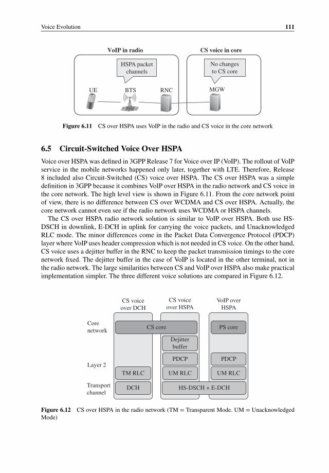
Voice Evolution 111
RNC MGWBTSUE
No changes
to CS coreHSPA packet
channels
VoIP in radio CS voice in core
Figure 6.11 CS over HSPA uses VoIP in the radio and CS voice in the core network
6.5 Circuit-Switched Voice Over HSPA
Voice over HSPA was defined in 3GPP Release 7 for Voice over IP (VoIP). The rollout of VoIPservice in the mobile networks happened only later, together with LTE. Therefore, Release8 included also Circuit-Switched (CS) voice over HSPA. The CS over HSPA was a simpledefinition in 3GPP because it combines VoIP over HSPA in the radio network and CS voice inthe core network. The high level view is shown in Figure 6.11. From the core network pointof view, there is no difference between CS over WCDMA and CS over HSPA. Actually, thecore network cannot even see if the radio network uses WCDMA or HSPA channels.
The CS over HSPA radio network solution is similar to VoIP over HSPA. Both use HS-DSCH in downlink, E-DCH in uplink for carrying the voice packets, and UnacknowledgedRLC mode. The minor differences come in the Packet Data Convergence Protocol (PDCP)layer where VoIP uses header compression which is not needed in CS voice. On the other hand,CS voice uses a dejitter buffer in the RNC to keep the packet transmission timings to the corenetwork fixed. The dejitter buffer in the case of VoIP is located in the other terminal, not inthe radio network. The large similarities between CS and VoIP over HSPA also make practicalimplementation simpler. The three different voice solutions are compared in Figure 6.12.
DCH
CS core
Transport channel
Layer 2
TM RLC
Dejitter
buffer
CS voiceover DCH
VoIP overHSPA
CS voiceover HSPA
UM RLC
PDCP
PS core
UM RLC
PDCP
HS-DSCH + E-DCH
Core network
Figure 6.12 CS over HSPA in the radio network (TM = Transparent Mode. UM = UnacknowledgedMode)
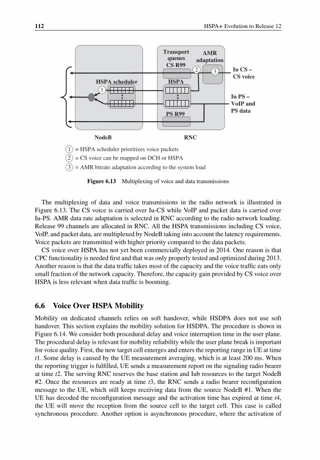
112 HSPA+ Evolution to Release 12
Iu CS –CS voice
Iu PS –VoIP andPS data
CS R99
AMRadaptation
Transportqueues
HSPA
PS R99
HSPA scheduler
NodeB RNC
1
1 = HSPA scheduler prioritizes voice packets
2 = CS voice can be mapped on DCH or HSPA
2 3
3 = AMR bitrate adaptation according to the system load
Figure 6.13 Multiplexing of voice and data transmissions
The multiplexing of data and voice transmissions in the radio network is illustrated inFigure 6.13. The CS voice is carried over Iu-CS while VoIP and packet data is carried overIu-PS. AMR data rate adaptation is selected in RNC according to the radio network loading.Release 99 channels are allocated in RNC. All the HSPA transmissions including CS voice,VoIP, and packet data, are multiplexed by NodeB taking into account the latency requirements.Voice packets are transmitted with higher priority compared to the data packets.
CS voice over HSPA has not yet been commercially deployed in 2014. One reason is thatCPC functionality is needed first and that was only properly tested and optimized during 2013.Another reason is that the data traffic takes most of the capacity and the voice traffic eats onlysmall fraction of the network capacity. Therefore, the capacity gain provided by CS voice overHSPA is less relevant when data traffic is booming.
6.6 Voice Over HSPA Mobility
Mobility on dedicated channels relies on soft handover, while HSDPA does not use softhandover. This section explains the mobility solution for HSDPA. The procedure is shown inFigure 6.14. We consider both procedural delay and voice interruption time in the user plane.The procedural delay is relevant for mobility reliability while the user plane break is importantfor voice quality. First, the new target cell emerges and enters the reporting range in UE at timet1. Some delay is caused by the UE measurement averaging, which is at least 200 ms. Whenthe reporting trigger is fulfilled, UE sends a measurement report on the signaling radio bearerat time t2. The serving RNC reserves the base station and Iub resources to the target NodeB#2. Once the resources are ready at time t3, the RNC sends a radio bearer reconfigurationmessage to the UE, which still keeps receiving data from the source NodeB #1. When theUE has decoded the reconfiguration message and the activation time has expired at time t4,the UE will move the reception from the source cell to the target cell. This case is calledsynchronous procedure. Another option is asynchronous procedure, where the activation of
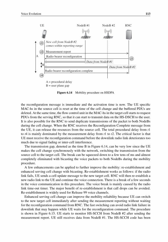
Voice Evolution 113
UE NodeB #1 NodeB #2 RNC
Measurement report
Radio bearer reconfiguration
Radio bearer reconfiguration complete
t2
t3
t4
A
B
A = procedural delayB = user plane gap
New cell from NodeB #2 comes within reporting range
t1
Data from NodeB #1
Data from NodeB #2
Figure 6.14 Mobility procedure on HSDPA
the reconfiguration message is immediate and the activation time is now. The UE specificMAC-hs in the source cell is reset at the time of the cell change and the buffered PDUs aredeleted. At the same time, the flow control unit in the MAC-hs in the target cell starts to requestPDUs from the serving RNC, so that it can start to transmit data on the HS-DSCH to the user.It is also possible for the RNC to send duplicate transmissions of the packet to both NodeBsduring the cell change. When the RNC receives the Reconfiguration Complete message fromthe UE, it can release the resources from the source cell. The total procedural delay from t1to t4 is mainly dominated by the measurement delay from t1 to t2. The critical factor is thatUE must receive the reconfiguration command before the downlink radio link deteriorates toomuch due to signal fading or inter-cell interference.
The transmission gap, denoted as the time B in Figure 6.14, can be very low since the UEmakes the cell change synchronously with the network, switching the transmission from thesource cell to the target cell. The break can be squeezed down to a few tens of ms and almostcompletely eliminated with bicasting the voice packets to both NodeBs during the mobilityprocedure.
A few enhancements can be applied to further improve the mobility: re-establishment andenhanced serving cell change with bicasting. Re-establishment works as follows: if the radiolink fails, UE sends a cell update message to the new target cell. RNC will then re-establish anew radio link to the UE and continue the voice connection. There is a break of a few secondsin the voice communication in this procedure. The voice break is mainly caused by the radiolink time-out timer. The major benefit of re-establishment is that call drops can be avoided.Re-establishment is widely used for Release 99 voice channels.
Enhanced serving cell change can improve the mobility reliability because UE can switchto the new target cell immediately after sending the measurement reporting without waitingfor the reconfiguration command from RNC. The fast switching can avoid radio link failure indownlink that may happen while UE waits for the reconfiguration command. The procedureis shown in Figure 6.15. UE starts to monitor HS-SCCH from NodeB #2 after sending themeasurement report. UE still receives data from NodeB #1. The HS-SCCH code has been
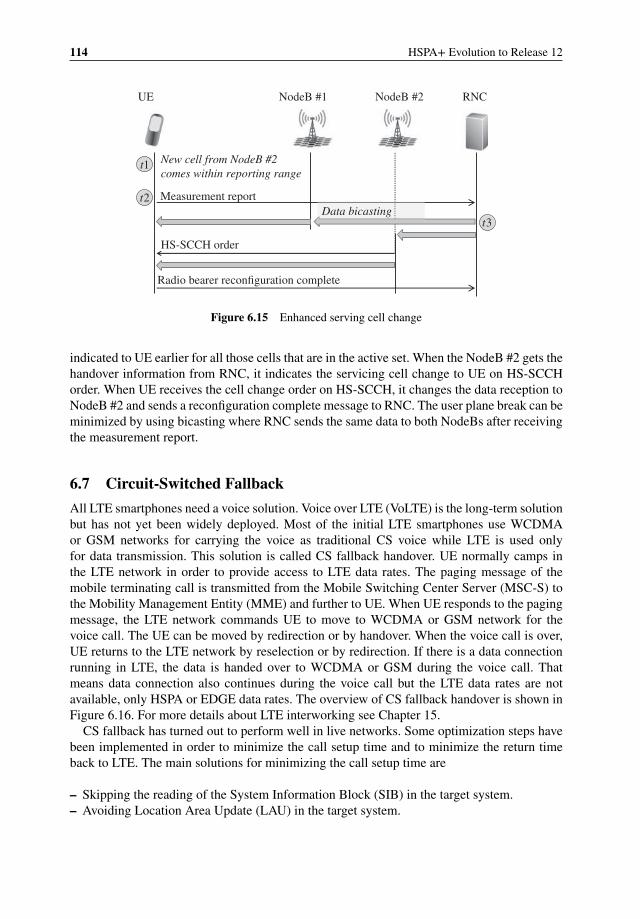
114 HSPA+ Evolution to Release 12
UE NodeB #1 NodeB #2 RNC
Measurement report
HS-SCCH order
Radio bearer reconfiguration complete
t2
t3
New cell from NodeB #2 comes within reporting range
t1
Data bicasting
Figure 6.15 Enhanced serving cell change
indicated to UE earlier for all those cells that are in the active set. When the NodeB #2 gets thehandover information from RNC, it indicates the servicing cell change to UE on HS-SCCHorder. When UE receives the cell change order on HS-SCCH, it changes the data reception toNodeB #2 and sends a reconfiguration complete message to RNC. The user plane break can beminimized by using bicasting where RNC sends the same data to both NodeBs after receivingthe measurement report.
6.7 Circuit-Switched Fallback
All LTE smartphones need a voice solution. Voice over LTE (VoLTE) is the long-term solutionbut has not yet been widely deployed. Most of the initial LTE smartphones use WCDMAor GSM networks for carrying the voice as traditional CS voice while LTE is used onlyfor data transmission. This solution is called CS fallback handover. UE normally camps inthe LTE network in order to provide access to LTE data rates. The paging message of themobile terminating call is transmitted from the Mobile Switching Center Server (MSC-S) tothe Mobility Management Entity (MME) and further to UE. When UE responds to the pagingmessage, the LTE network commands UE to move to WCDMA or GSM network for thevoice call. The UE can be moved by redirection or by handover. When the voice call is over,UE returns to the LTE network by reselection or by redirection. If there is a data connectionrunning in LTE, the data is handed over to WCDMA or GSM during the voice call. Thatmeans data connection also continues during the voice call but the LTE data rates are notavailable, only HSPA or EDGE data rates. The overview of CS fallback handover is shown inFigure 6.16. For more details about LTE interworking see Chapter 15.
CS fallback has turned out to perform well in live networks. Some optimization steps havebeen implemented in order to minimize the call setup time and to minimize the return timeback to LTE. The main solutions for minimizing the call setup time are
– Skipping the reading of the System Information Block (SIB) in the target system.– Avoiding Location Area Update (LAU) in the target system.

Voice Evolution 115
Paging in
LTE
GSM or WCDMA
MMELTEMSC-S
CS call setup
in GSM or
WCDMA
Figure 6.16 CS fallback handover from LTE to GSM/WCDMA
SIB reading can be avoided by providing the target cell SIB via LTE the network or providingthe SIB only after the call setup in the target system. UE may also store the target system SIBif CS fallback happens multiple times to the same cell. LAU can be avoided in the call setupby configuring the core network so that the same location area code is used by the target MSCand the MSC where the paging is coming from. With optimized CS fallback procedure theadditional call setup time can be below 1 s, which makes CS fallback performance in practicenearly as good as any WCDMA or GSM call.
The delay in getting UE back to LTE after the CS call can be minimized by using networkcontrolled redirection after the voice call to push UE back to the LTE network. The initialsolution used UE based reselection, which can cause 10 s or more delay when returning toLTE. When the redirection is implemented to the networks, the UE can instantaneously returnto LTE after the voice call.
GSM/WCDMA operators can select the target network to be either WCDMA or GSM.Most operators use WCDMA as the CS fallback target. The call setup time is lowest whenthe CS fallback is to WCDMA. Many WCDMA networks also use AMR-WB for the bestvoice quality. All WCDMA networks and UEs also support simultaneous voice and datatransmission. The network configuration for CS fallback to WCDMA is also simpler sinceonly the target frequency needs to be given to the UE. Some operators use GSM as the targetnetwork, mainly if the WCDMA network does not provide full coverage. The target system canalso be selected based on UE measurements: CSFB to WCDMA if the coverage is available.
6.8 Single Radio Voice Call Continuity
There may be a need to make a handover from VoIP to CS voice due to mobility. The typical usecase is handover from Voice over LTE (VoLTE) to CS voice in WCDMA when UE runs out ofLTE coverage area and there is no VoIP support in HSPA network. The handover functionalityfrom VoIP to CS domain is referred to as Single Radio Voice Call Continuity (SRVCC). Thesolution does not require UE capability to simultaneously signal on two different radio accesstechnologies – therefore it is called the single radio solution.
LTE eNodeB first triggers the UE to start inter-system measurements of the target WCDMAsystem and receives the measurement report. eNodeB then sends the handover request toMME, which triggers the SRVCC procedure via Sv interface to MSC-Server. Sv is a new

116 HSPA+ Evolution to Release 12
Figure 6.17 Single Radio Voice Call Continuity (SRVCC) from LTE to WCDMA
interface between MSC server and MME. The resources in the target cell are reserved and thenecessary information is provided for the UE via LTE access. When the SRVCC procedure hasbeen completed successfully, then VoIP connection remains from MSC towards the other sideof the ongoing session. The CS connection exists towards the WCDMA radio access network.SRVCC architecture is shown in Figure 6.17.
In the case of simultaneous voice and non-voice data connection, the handling of the non-voice bearer is done by the bearer splitting function in the MME. The process is done in thesame way as the normal inter-system handover for packet services.
In the case of roaming, the Visited PLMN controls the radio access and domain changewhile taking into account any related Home PLMN policies.
6.9 Summary
The WCDMA/HSPA system offers a comprehensive set of voice services. CS voice overWCDMA dedicated channels have been the baseline voice solution. Voice quality can beenhanced with AMR-Wideband codec and voice capacity can be improved with AMR-Narrowband lower codec rates. The voice service can also be provided over HSPA channelsboth as VoIP and as CS voice. The initial LTE smartphones typically use WCDMA CS voicewith CS fallback functionality. When voice over LTE service is started, it can be complementedwith the handover from VoLTE to WCDMA CS voice, called SRVCC.
References
[1] Holma, H., Melero, J., Vainio, J. et al. “Performance of Adaptive Multirate (AMR) Voice in GSM and WCDMA”,VTC 2003.
[2] Holma, H., Kuusela, M., Malkamaki, E. et al. “VoIP over HSPA with 3GPP Release 7”, PIMRC 2006, September2006.
[3] 3GPP Technical Report 25.903 “Continuous connectivity for packet data users”, v. 7.0.0, 2007.[4] NSN White paper “Long Term HSPA Evolution meets ITU IMT-Advanced requirements”, 2012.[5] Holma, H. and Toskala, A. (2010) WCDMA for UMTS – HSPA Evolution and LTE, 5th edn, John Wiley & Sons,
Ltd, Chichester.
7Heterogeneous Networks
Harri Holma and Fernando Sanchez Moya
7.1 Introduction
Heterogeneous Network (HetNet) refers to the joint optimization of different cell layers andtechnologies. Current mobile networks are based on wide area macro cells that provide severalhundred meters of coverage, even tens of kilometers, and normally use three sectors per site.Small cells can be added to provide more capacity and coverage. These small cells can beoutdoor small cells, public indoor small cells, or home or enterprise small cells. The outdoorsmall cells are often termed micro cells, indoor cells pico cells, and home small cells femtocells. The HetNet concept is shown in Figure 7.1.
The HetNet concept also considers the use of the different technologies GSM, HSPA, LTE,and WLAN together. This chapter focuses on HSPA small cell deployments together withexisting macro cells on WLAN interworking. Section 7.2 presents the drivers for the small cellrollouts. Section 7.3 shows the base station categories. Sections 7.4 and 7.5 present the mainchallenges with HSPA HetNets – interference management and link imbalance, Section 7.6studies the data rate and capacity benefits provided by the small cells, and Section 7.7 illustratesfield deployment result with HSPA small cells. Femto cell architecture and optimization arediscussed in Section 7.8 and WLAN interworking in Section 7.9. The chapter is summarizedin Section 7.10.
7.2 Small Cell Drivers
The introduction of small cells is driven by capacity and coverage requirements. As data trafficincreases in many HSPA networks, macro cells are getting congested and operators have usedall their spectrum resources in them. Capacity could be enhanced by adding new macro sitesor by adding new sectors to the existing macro sites. However, it may be difficult or expensiveto find a location for a new macro site or to add more antennas to the existing sites. Therefore,
HSPA+ Evolution to Release 12: Performance and Optimization, First Edition.Edited by Harri Holma, Antti Toskala, and Pablo Tapia.© 2014 John Wiley & Sons, Ltd. Published 2014 by John Wiley & Sons, Ltd.

118 HSPA+ Evolution to Release 12
Wide area macro cells with > 300 meter coverage
Outdoor small cells with 100–300 meter coverage
Public indoor cells with < 50 meter coverage
Home femto cells with coverage < 30 meters
Figure 7.1 HetNet concept
the most practical way of increasing network capacity may be to add new small base stations.The small cells can also be deployed to improve the coverage and increase local data rates.
Small cells have been discussed in the industry for a long time but it is only recently thatthe implementation of small cells has become simpler for operators: the small base stationproducts are very compact due to the evolution of digital and RF technologies, the networkconfiguration and optimization is becoming automatic with Self Organizing Network (SON)solutions, and attractive wireless backhaul options are emerging.
The need for small cells may be postponed by the availability of new spectrum and LTEradio, which provide a lot more capacity with existing macro sites. The problem may still bethat the LTE terminal penetration does not increase fast enough to migrate the traffic fromHSPA to LTE. Operators may need to build HSPA small cells even if their LTE network issitting empty in the same area.
7.3 Base Station Categories
3GPP has defined four base station categories with different RF requirements. The categoriesare defined with the maximum output powers and the Minimum Coupling Loss (MCL). MCLrefers to the minimum path loss between the base station antenna and UE antenna and it definesthe type of base station installation. High MCL requires that UE cannot get too close to thebase station antenna, which is typical for high mounted macro cell antennas. Low MCL meansthat UE can get very close to the base station antenna. The idea in categories is that some ofthe RF specifications can be relaxed for the low power base stations to enable even lower costimplementation. The sensitivity requirements are relaxed because the link budget is anywaylimited by the low power in downlink. Higher spurious emissions are allowed for the low powerproducts because there are no co-sited base stations with high sensitivity requirements. Some
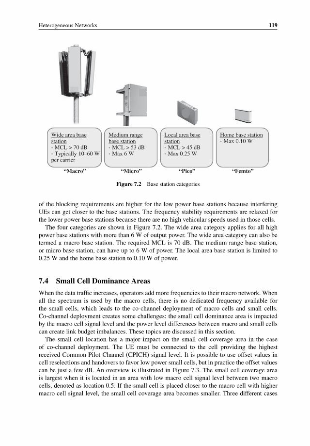
Heterogeneous Networks 119
Wide area base station MCL > 70 dB Typically 10–60 W
per carrier
Local area base station MCL > 45 dB Max 0.25 W
Home base station Max 0.10 W
Medium range base station MCL > 53 dB Max 6 W
“Macro” “Micro” “Pico” “Femto”
Figure 7.2 Base station categories
of the blocking requirements are higher for the low power base stations because interferingUEs can get closer to the base stations. The frequency stability requirements are relaxed forthe lower power base stations because there are no high vehicular speeds used in those cells.
The four categories are shown in Figure 7.2. The wide area category applies for all highpower base stations with more than 6 W of output power. The wide area category can also betermed a macro base station. The required MCL is 70 dB. The medium range base station,or micro base station, can have up to 6 W of power. The local area base station is limited to0.25 W and the home base station to 0.10 W of power.
7.4 Small Cell Dominance Areas
When the data traffic increases, operators add more frequencies to their macro network. Whenall the spectrum is used by the macro cells, there is no dedicated frequency available forthe small cells, which leads to the co-channel deployment of macro cells and small cells.Co-channel deployment creates some challenges: the small cell dominance area is impactedby the macro cell signal level and the power level differences between macro and small cellscan create link budget imbalances. These topics are discussed in this section.
The small cell location has a major impact on the small cell coverage area in the caseof co-channel deployment. The UE must be connected to the cell providing the highestreceived Common Pilot Channel (CPICH) signal level. It is possible to use offset values incell reselections and handovers to favor low power small cells, but in practice the offset valuescan be just a few dB. An overview is illustrated in Figure 7.3. The small cell coverage areais largest when it is located in an area with low macro cell signal level between two macrocells, denoted as location 0.5. If the small cell is placed closer to the macro cell with highermacro cell signal level, the small cell coverage area becomes smaller. Three different cases
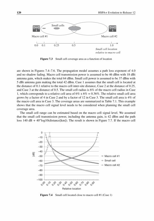
120 HSPA+ Evolution to Release 12
Macro cell #1 Macro cell #2
Small cells
0.5 0.0 0.25 1.0
Small cell locationrelative to macro cell
0.1
Figure 7.3 Small cell coverage area as a function of location
are shown in Figures 7.4–7.6. The propagation model assumes a path loss exponent of 4.0and no shadow fading. Macro cell transmission power is assumed to be 46 dBm with 18 dBiantenna gain, which makes the total 64 dBm. Small cell power is assumed to be 37 dBm with5 dBi antenna gain making the total 42 dBm. Case 1 assumes that the small cell is located atthe distance of 0.1 relative to the macro cell inter-site distance, Case 2 at the distance of 0.25,and Case 3 at the distance of 0.5. The small cell radius is 6% of the macro cell radius in Case1, which corresponds to a relative cell area of 6% x 6% = 0.36%. The relative small cell areagrows by a factor of 4 in Case 2 and by a factor of 12 in Case 3. The small cell area is 4% ofthe macro cell area in Case 3. The coverage areas are summarized in Table 7.1. This exampleshows that the macro cell signal level needs to be considered when planning the small cellcoverage area.
The small cell range can be estimated based on the macro cell signal level. We assumedthat the small cell transmission power, including the antenna gain, is 42 dBm and the pathloss 140 dB + 40∗log10(distance[km]). The result is shown in Figure 7.7. If the macro cell
–100
0.00
0.10
0.20
0.30
0.40
0.50
0.60
0.70
0.80
0.90
–90
–80
–70
–60
–50
–40
–30
–20
–10
0
[dB
]
Relative location
Macro cell #1
Small cell
Macro cell #2
Figure 7.4 Small cell located close to macro cell #1 (Case 1)
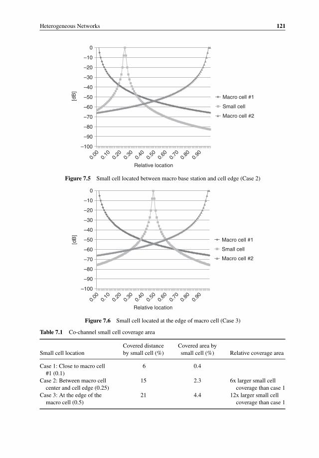
Heterogeneous Networks 121
[dB
]
Macro cell #1
Small cell
Macro cell #2
–100
–90
–80
–70
–60
–50
–40
–30
–20
–10
0
0.00
0.10
0.20
0.30
0.40
0.50
0.60
0.70
0.80
0.90
Relative location
Figure 7.5 Small cell located between macro base station and cell edge (Case 2)
[dB
]
Macro cell #1
Small cell
Macro cell #2
–100
–90
–80
–70
–60
–50
–40
–30
–20
–10
0
0.00
0.10
0.20
0.30
0.40
0.50
0.60
0.70
0.80
0.90
Relative location
Figure 7.6 Small cell located at the edge of macro cell (Case 3)
Table 7.1 Co-channel small cell coverage area
Small cell locationCovered distanceby small cell (%)
Covered area bysmall cell (%) Relative coverage area
Case 1: Close to macro cell#1 (0.1)
6 0.4
Case 2: Between macro cellcenter and cell edge (0.25)
15 2.3 6x larger small cellcoverage than case 1
Case 3: At the edge of themacro cell (0.5)
21 4.4 12x larger small cellcoverage than case 1
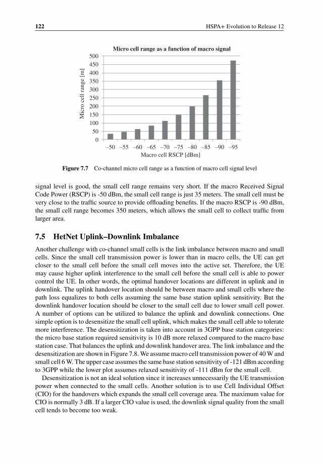
122 HSPA+ Evolution to Release 12
0
50
100
150
200
250
300
350
400
450
500
–50 –55 –60 –65 –70 –75 –80 –85 –90 –95
Mic
ro c
ell
range
[m]
Macro cell RSCP [dBm]
Micro cell range as a function of macro signal
Figure 7.7 Co-channel micro cell range as a function of macro cell signal level
signal level is good, the small cell range remains very short. If the macro Received SignalCode Power (RSCP) is -50 dBm, the small cell range is just 35 meters. The small cell must bevery close to the traffic source to provide offloading benefits. If the macro RSCP is -90 dBm,the small cell range becomes 350 meters, which allows the small cell to collect traffic fromlarger area.
7.5 HetNet Uplink–Downlink Imbalance
Another challenge with co-channel small cells is the link imbalance between macro and smallcells. Since the small cell transmission power is lower than in macro cells, the UE can getcloser to the small cell before the small cell moves into the active set. Therefore, the UEmay cause higher uplink interference to the small cell before the small cell is able to powercontrol the UE. In other words, the optimal handover locations are different in uplink and indownlink. The uplink handover location should be between macro and small cells where thepath loss equalizes to both cells assuming the same base station uplink sensitivity. But thedownlink handover location should be closer to the small cell due to lower small cell power.A number of options can be utilized to balance the uplink and downlink connections. Onesimple option is to desensitize the small cell uplink, which makes the small cell able to toleratemore interference. The desensitization is taken into account in 3GPP base station categories:the micro base station required sensitivity is 10 dB more relaxed compared to the macro basestation case. That balances the uplink and downlink handover area. The link imbalance and thedesensitization are shown in Figure 7.8. We assume macro cell transmission power of 40 W andsmall cell 6 W. The upper case assumes the same base station sensitivity of -121 dBm accordingto 3GPP while the lower plot assumes relaxed sensitivity of -111 dBm for the small cell.
Desensitization is not an ideal solution since it increases unnecessarily the UE transmissionpower when connected to the small cells. Another solution is to use Cell Individual Offset(CIO) for the handovers which expands the small cell coverage area. The maximum value forCIO is normally 3 dB. If a larger CIO value is used, the downlink signal quality from the smallcell tends to become too weak.
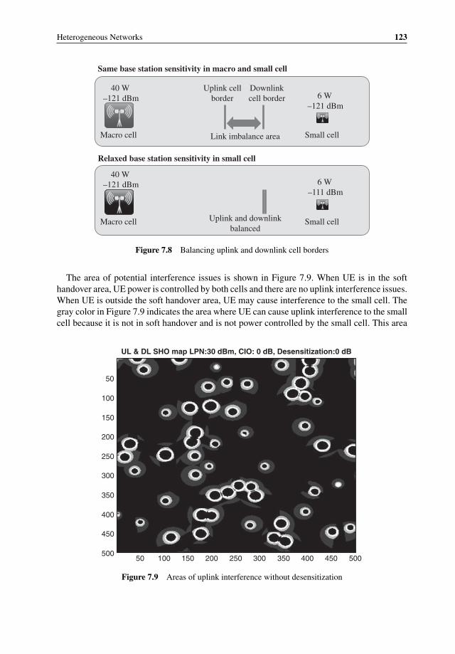
Heterogeneous Networks 123
Small cell Macro cell
Uplink cell border
Downlink cell border
40 W –121 dBm 6 W
–121 dBm
Link imbalance area
40 W –121 dBm 6 W
–111 dBm
Same base station sensitivity in macro and small cell
Small cell Macro cell
Relaxed base station sensitivity in small cell
Uplink and downlink balanced
Figure 7.8 Balancing uplink and downlink cell borders
The area of potential interference issues is shown in Figure 7.9. When UE is in the softhandover area, UE power is controlled by both cells and there are no uplink interference issues.When UE is outside the soft handover area, UE may cause interference to the small cell. Thegray color in Figure 7.9 indicates the area where UE can cause uplink interference to the smallcell because it is not in soft handover and is not power controlled by the small cell. This area
UL & DL SHO map LPN:30 dBm, CIO: 0 dB, Desensitization:0 dB
50 100 150 200 250 300 350 400 450 500
50
100
150
200
250
300
350
400
450
500
Figure 7.9 Areas of uplink interference without desensitization
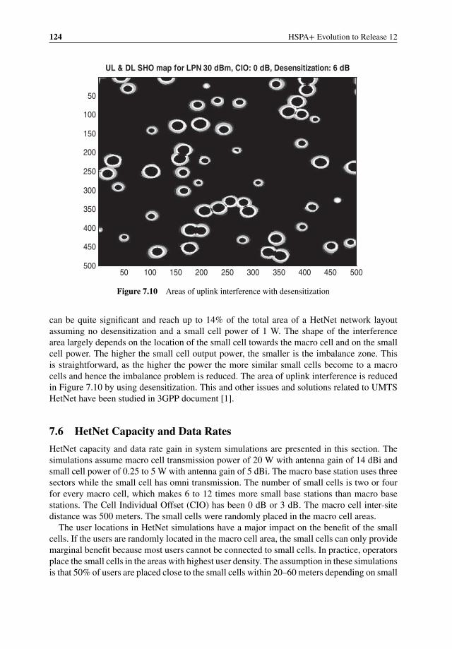
124 HSPA+ Evolution to Release 12
UL & DL SHO map for LPN 30 dBm, CIO: 0 dB, Desensitization: 6 dB
50 100 150 200 250 300 350 400 450 500
50
100
150
200
250
300
350
400
450
500
Figure 7.10 Areas of uplink interference with desensitization
can be quite significant and reach up to 14% of the total area of a HetNet network layoutassuming no desensitization and a small cell power of 1 W. The shape of the interferencearea largely depends on the location of the small cell towards the macro cell and on the smallcell power. The higher the small cell output power, the smaller is the imbalance zone. Thisis straightforward, as the higher the power the more similar small cells become to a macrocells and hence the imbalance problem is reduced. The area of uplink interference is reducedin Figure 7.10 by using desensitization. This and other issues and solutions related to UMTSHetNet have been studied in 3GPP document [1].
7.6 HetNet Capacity and Data Rates
HetNet capacity and data rate gain in system simulations are presented in this section. Thesimulations assume macro cell transmission power of 20 W with antenna gain of 14 dBi andsmall cell power of 0.25 to 5 W with antenna gain of 5 dBi. The macro base station uses threesectors while the small cell has omni transmission. The number of small cells is two or fourfor every macro cell, which makes 6 to 12 times more small base stations than macro basestations. The Cell Individual Offset (CIO) has been 0 dB or 3 dB. The macro cell inter-sitedistance was 500 meters. The small cells were randomly placed in the macro cell areas.
The user locations in HetNet simulations have a major impact on the benefit of the smallcells. If the users are randomly located in the macro cell area, the small cells can only providemarginal benefit because most users cannot be connected to small cells. In practice, operatorsplace the small cells in the areas with highest user density. The assumption in these simulationsis that 50% of users are placed close to the small cells within 20–60 meters depending on small
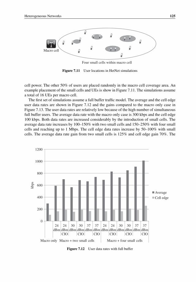
Heterogeneous Networks 125
Macro cell
Four small cells within macro cell
Figure 7.11 User locations in HetNet simulations
cell power. The other 50% of users are placed randomly in the macro cell coverage area. Anexample placement of the small cells and UEs is show in Figure 7.11. The simulations assumea total of 16 UEs per macro cell.
The first set of simulations assume a full buffer traffic model. The average and the cell edgeuser data rates are shown in Figure 7.12 and the gains compared to the macro only case inFigure 7.13. The user data rates are relatively low because of the high number of simultaneousfull buffer users. The average data rate with the macro only case is 300 kbps and the cell edge100 kbps. Both data rates are increased considerably by the introduction of small cells. Theaverage data rate increases by 100–150% with two small cells and 150–250% with four smallcells and reaching up to 1 Mbps. The cell edge data rates increase by 50–100% with smallcells. The average data rate gain from two small cells is 125% and cell edge gain 70%. The
0
200
400
600
800
1000
1200
24 dBm
24 dBm CIO
30 dBm
30 dBm CIO
37 dBm
37 dBm CIO
24 dBm
24 dBm CIO
30 dBm
30 dBm CIO
37 dBm
37 dBm CIO
Macro only Macro + two small cells Macro + four small cells
kbp
s
Average
Cell edge
Figure 7.12 User data rates with full buffer
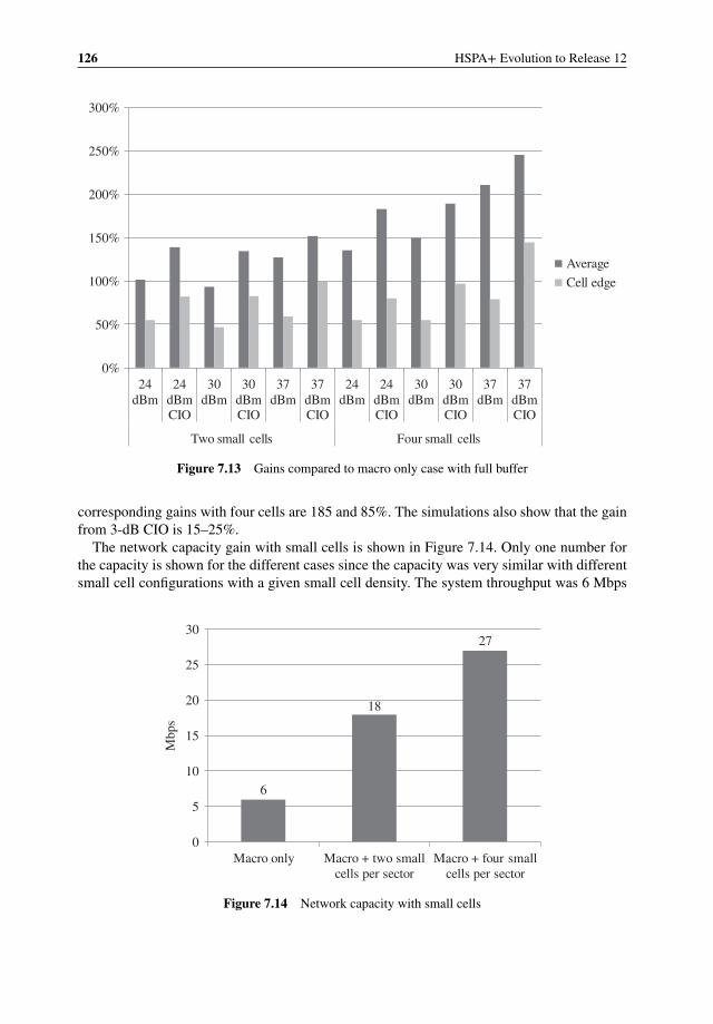
126 HSPA+ Evolution to Release 12
0%
50%
100%
150%
200%
250%
300%
24 dBm
24 dBm CIO
30 dBm
30 dBm CIO
37 dBm
37 dBm CIO
24 dBm
24 dBm CIO
30 dBm
30 dBm CIO
37 dBm
37 dBm CIO
Two small cells Four small cells
Average
Cell edge
Figure 7.13 Gains compared to macro only case with full buffer
corresponding gains with four cells are 185 and 85%. The simulations also show that the gainfrom 3-dB CIO is 15–25%.
The network capacity gain with small cells is shown in Figure 7.14. Only one number forthe capacity is shown for the different cases since the capacity was very similar with differentsmall cell configurations with a given small cell density. The system throughput was 6 Mbps
6
18
27
0
5
10
15
20
25
30
Macro only Macro + two small cells per sector
Macro + four small cells per sector
Mbps
Figure 7.14 Network capacity with small cells
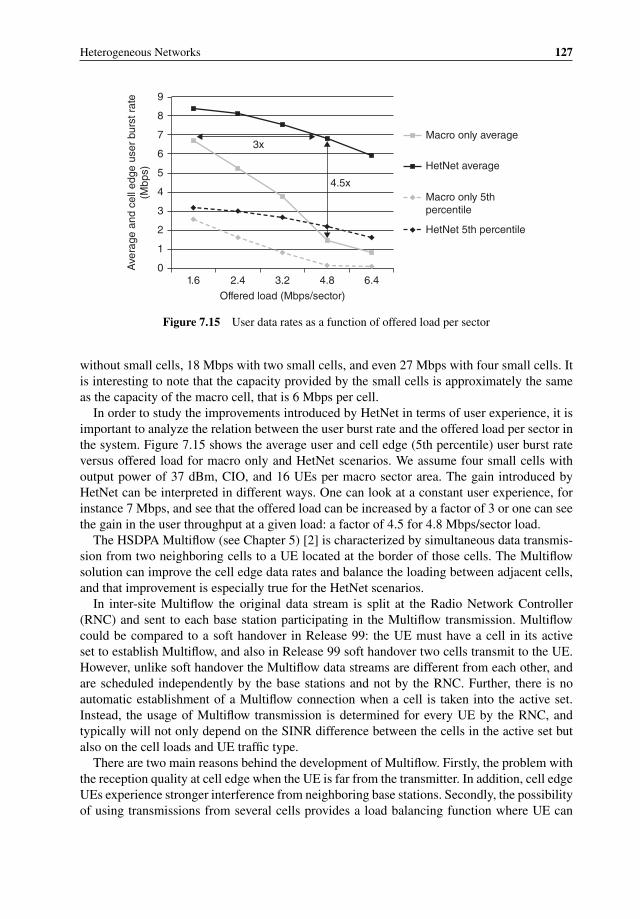
Heterogeneous Networks 127
1.60
1
2
3
4
5
63x
4.5x
Macro only average
Macro only 5thpercentile
HetNet average
HetNet 5th percentile
7
8
9
2.4 3.2
Offered load (Mbps/sector)
Ave
rage
and
cel
l edg
e us
er b
urst
rat
e(M
bps)
4.8 6.4
Figure 7.15 User data rates as a function of offered load per sector
without small cells, 18 Mbps with two small cells, and even 27 Mbps with four small cells. Itis interesting to note that the capacity provided by the small cells is approximately the sameas the capacity of the macro cell, that is 6 Mbps per cell.
In order to study the improvements introduced by HetNet in terms of user experience, it isimportant to analyze the relation between the user burst rate and the offered load per sector inthe system. Figure 7.15 shows the average user and cell edge (5th percentile) user burst rateversus offered load for macro only and HetNet scenarios. We assume four small cells withoutput power of 37 dBm, CIO, and 16 UEs per macro sector area. The gain introduced byHetNet can be interpreted in different ways. One can look at a constant user experience, forinstance 7 Mbps, and see that the offered load can be increased by a factor of 3 or one can seethe gain in the user throughput at a given load: a factor of 4.5 for 4.8 Mbps/sector load.
The HSDPA Multiflow (see Chapter 5) [2] is characterized by simultaneous data transmis-sion from two neighboring cells to a UE located at the border of those cells. The Multiflowsolution can improve the cell edge data rates and balance the loading between adjacent cells,and that improvement is especially true for the HetNet scenarios.
In inter-site Multiflow the original data stream is split at the Radio Network Controller(RNC) and sent to each base station participating in the Multiflow transmission. Multiflowcould be compared to a soft handover in Release 99: the UE must have a cell in its activeset to establish Multiflow, and also in Release 99 soft handover two cells transmit to the UE.However, unlike soft handover the Multiflow data streams are different from each other, andare scheduled independently by the base stations and not by the RNC. Further, there is noautomatic establishment of a Multiflow connection when a cell is taken into the active set.Instead, the usage of Multiflow transmission is determined for every UE by the RNC, andtypically will not only depend on the SINR difference between the cells in the active set butalso on the cell loads and UE traffic type.
There are two main reasons behind the development of Multiflow. Firstly, the problem withthe reception quality at cell edge when the UE is far from the transmitter. In addition, cell edgeUEs experience stronger interference from neighboring base stations. Secondly, the possibilityof using transmissions from several cells provides a load balancing function where UE can
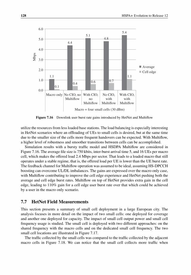
128 HSPA+ Evolution to Release 12
1.1
4.4
5.14.8
5.4
0.10.4 0.6 0.7
1.1
0.0
1.0
2.0
3.0
4.0
5.0
6.0
Macro only No CIO, noMultiflow
With CIO,no
Multiflow
No CIO,with
Multiflow
With CIO,with
Multiflow
Macro + four small cells (30 dBm)
Mb
ps
Average
Cell edge
Figure 7.16 Downlink user burst rate gains introduced by HetNet and Multiflow
utilize the resources from less loaded base stations. The load balancing is especially interestingin HetNet scenarios where an offloading of UEs to small cells is desired, but at the same timedue to the smaller size of the cells more frequent handovers can be expected. With Multiflow,a higher level of robustness and smoother transitions between cells can be accomplished.
Simulation results with a bursty traffic model and HSDPA Multiflow are considered inFigure 7.16. The average file size is 750 kbits, inter-burst arrival time 5, and 16 UEs per macrocell, which makes the offered load 2.4 Mbps per sector. That leads to a loaded macro that stilloperates under a stable regime, that is, the offered load per UE is lower than the UE burst rate.The feedback channel for Multiflow operation was assumed to be ideal, assuming HS-DPCCHboosting can overcome UL/DL imbalances. The gains are expressed over the macro only case,with Multiflow contributing to improve the cell edge experience and HetNet pushing both theaverage and cell edge burst rates. Multiflow on top of HetNet provides extra gain in the celledge, leading to 110% gain for a cell edge user burst rate over that which could be achievedby a user in the macro only scenario.
7.7 HetNet Field Measurements
This section presents a summary of small cell deployment in a large European city. Theanalysis focuses in more detail on the impact of two small cells: one deployed for coverageand another one deployed for capacity. The impact of small cell output power and small cellfrequency usage is studied. The small cell is deployed with two different approaches: on theshared frequency with the macro cells and on the dedicated small cell frequency. The twosmall cell locations are illustrated in Figure 7.17.
The traffic collected by the small cells was compared to the traffic collected by the adjacentmacro cells in Figure 7.18. We can notice that the small cell collects more traffic when
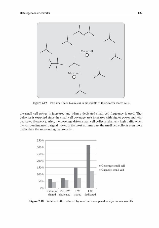
Heterogeneous Networks 129
Micro cell
Micro cell
Figure 7.17 Two small cells (=circles) in the middle of three-sector macro cells
the small cell power is increased and when a dedicated small cell frequency is used. Thatbehavior is expected since the small cell coverage area increases with higher power and withdedicated frequency. Also, the coverage driven small cell collects relatively high traffic whenthe surrounding macro signal is low. In the most extreme case the small cell collects even moretraffic than the surrounding macro cells.
0%
50%
100%
150%
200%
250%
300%
350%
250 mW shared
250 mW dedicated
1 W shared
1 W dedicated
Coverage small cell
Capacity small cell
Figure 7.18 Relative traffic collected by small cells compared to adjacent macro cells
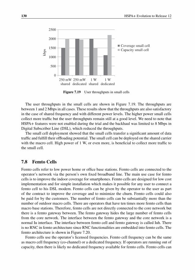
130 HSPA+ Evolution to Release 12
0
500
1000
1500
2000
2500
250 mWshared
250 mWdedicated
1 W shared
1 W dedicated
kb
ps
Coverage small cellCapacity small cell
Figure 7.19 User throughputs in small cells
The user throughputs in the small cells are shown in Figure 7.19. The throughputs arebetween 1 and 2 Mbps in all cases. These results show that the throughputs are also satisfactoryin the case of shared frequency and with different power levels. The higher power small cellscollect more traffic but the user throughputs remain still at a good level. We need to note thatHSPA+ features were not enabled during the trial and the backhaul was limited to 8 Mbps inDigital Subscriber Line (DSL), which reduced the throughputs.
The small cell deployment showed that the small cells transfer a significant amount of datatraffic and fulfill their offloading potential. The small cell can be deployed on the shared carrierwith the macro cell. High power of 1 W, or even more, is beneficial to collect more traffic tothe small cell.
7.8 Femto Cells
Femto cells refer to low power home or office base stations. Femto cells are connected to theoperator’s network via the person’s own fixed broadband line. The main use case for femtocells is to improve the indoor coverage for smartphones. Femto cells are designed for low costimplementation and for simple installation which makes it possible for any user to connect afemto cell to his DSL modem. Femto cells can be given by the operator to the user as partof the contract to improve the coverage and to minimize the churn. Femto cells could alsobe paid for by the customers. The number of femto cells can be substantially more than thenumber of outdoor macro cells. There are operators that have ten times more femto cells thanmacro base stations. Therefore, femto cells are not directly connected to the core network butthere is a femto gateway between. The femto gateway hides the large number of femto cellsfrom the core network. The interface between the femto gateway and the core network is anormal Iu interface. The interface between femto cell and femto gateway is called Iuh. Thereis no RNC in femto architecture since RNC functionalities are embedded into femto cells. Thefemto architecture is shown in Figure 7.20.
Femto cells use the operator’s licensed frequencies. Femto cell frequency can be the sameas macro cell frequency (co-channel) or a dedicated frequency. If operators are running out ofcapacity, then there is likely no dedicated frequency available for femto cells. Femto cells can
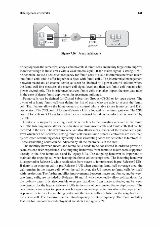
Heterogeneous Networks 131
DSLFemto
gateway
Core
networkFemto
IPIuIuh
Figure 7.20 Femto architecture
be deployed on the same frequency as macro cells if femto cells are mainly targeted to improveindoor coverage in those areas with a weak macro signal. If the macro signal is strong, it willbe beneficial to use a dedicated frequency for femto cells to avoid interference between macroand femto cells and to offer higher data rates with femto cells. The interference managementbetween macro and co-channel femto cells can be obtained by a power control solution wherethe femto cell first measures the macro cell signal level and then sets femto cell transmissionpower accordingly. The interference between femto cells may also impact the user data ratesin the case of dense femto deployment in apartment buildings.
Femto cells can be defined for Closed Subscriber Groups (CSGs) or for open access. Theowner of a home femto cell can define the list of users who are able to access the femtocell. That feature allows the home owners to control who is able to use femto cell and DSLconnection. The CSG control for pre-Release 8 UEs is located in the femto gateway. The CSGcontrol for Release 8 UEs is located in the core network based on the information provided bythe UE.
Femto cells support a listening mode which refers to the downlink receiver in the femtocell. The listening mode allows identification of those macro cells and femto cells that can bereceived in the area. The downlink receiver also allows measurement of the macro cell signallevel which can be used when setting femto cell transmission power. Femto cells are identifiedby dedicated scrambling codes. Typically, a few scrambling codes are dedicated to femto cells.These scrambling codes can be indicated by all the macro cells in the area.
The mobility between macro and femto cells needs to be considered in order to provide aseamless end-user experience. The outgoing handovers from femto to macro were supportedalready in the first femto cells and by legacy UEs. The outgoing handover is important tomaintain the ongoing call when leaving the femto cell coverage area. The incoming handoveris supported in Release 9, while reselection from macro to femto is used in pre-Release 9 UEs.If there is an ongoing call in pre-Release 9 UE when entering femto cell coverage area, thecall remains in the macro cell. When the call is over, the UE moves to femto cells by itselfwith reselection. The further mobility improvements between macro and femto, and betweentwo femto cells, are included in Releases 10 and 11 which eventually allow soft handover forthe mobility cases. It is also possible to support handover from macro to femto, and betweentwo femtos, for the legacy Release 8 UEs in the case of coordinated femto deployment. Thecoordinated case refers to open access hot spots and enterprise femtos where the deploymentis planned in terms of scrambling codes and the femto cells are listed in the neighborlist inthe macro cell. The handover can be intra-frequency or inter-frequency. The femto mobilityfeatures for uncoordinated deployment are shown in Figure 7.21.
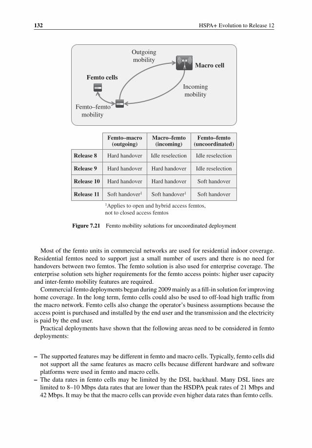
132 HSPA+ Evolution to Release 12
Macro cell
Femto cells
Femto–macro(outgoing)
Macro–femto(incoming)
Femto–femto(uncoordinated)
Hard handover Idle reselection Idle reselectionRelease 8
Hard handover Hard handover Idle reselectionRelease 9
Hard handover Hard handover Soft handoverRelease 10
Femto–femtomobility
Incoming mobility
Outgoing mobility
Soft handover1 Soft handover1 Soft handoverRelease 11
1Applies to open and hybrid access femtos,
not to closed access femtos
Figure 7.21 Femto mobility solutions for uncoordinated deployment
Most of the femto units in commercial networks are used for residential indoor coverage.Residential femtos need to support just a small number of users and there is no need forhandovers between two femtos. The femto solution is also used for enterprise coverage. Theenterprise solution sets higher requirements for the femto access points: higher user capacityand inter-femto mobility features are required.
Commercial femto deployments began during 2009 mainly as a fill-in solution for improvinghome coverage. In the long term, femto cells could also be used to off-load high traffic fromthe macro network. Femto cells also change the operator’s business assumptions because theaccess point is purchased and installed by the end user and the transmission and the electricityis paid by the end user.
Practical deployments have shown that the following areas need to be considered in femtodeployments:
– The supported features may be different in femto and macro cells. Typically, femto cells didnot support all the same features as macro cells because different hardware and softwareplatforms were used in femto and macro cells.
– The data rates in femto cells may be limited by the DSL backhaul. Many DSL lines arelimited to 8–10 Mbps data rates that are lower than the HSDPA peak rates of 21 Mbps and42 Mbps. It may be that the macro cells can provide even higher data rates than femto cells.
Heterogeneous Networks 133
– Soft handovers are typically not available between co-channel femto and macro cells. Thelack of soft handovers impacts the reliability of the mobility.
– A dedicated frequency for femto cells eats part of macro capacity and it is increasinglydifficult to allocate a dedicated femto frequency when the macro cell traffic increases.
– If a dedicated femto frequency is utilized, then CSFB with LTE phones gets more complex.The CSFB target need to be decided based on UE measurements between macro and femtofrequency.
– Different location areas are used in macro and femto cells. The UE performs a location areaupdate whenever moving between the layers. Attention is required to make sure that pagingmessages are not lost during the change of location area.
– The maximum number of users is typically limited in femto cells, which may cause problemsif using femto cells in large enterprises or in public premises.
– The femto and macro cells are typically provided by different vendors and the correspondingoperability tools are also different.
– The femto cell adds co-channel interference which may impact those UEs that are in weakmacro signal and are not able to connect to CSG femto cells.
Field experiences have shown that the femto solution works fine for enhancing indoorcoverage at homes or in small enterprises, while it is not practical to deploy femto solutionsoutdoors and in public premises. The outdoor solution needs a Iub/RNC connection for smoothmobility and interference control, more transmission power, higher capacity, and feature paritywith macro cells.
7.9 WLAN Interworking
WLAN (Wi-Fi) can complement mobile networks in carrying part of the data traffic andreducing the mobile network loading. In practice, all medium and high category mobiledevices have Wi-Fi radio, which enables efficient offloading of data traffic to Wi-Fi. Mostusers can configure the mobile device to use Wi-Fi at home and in the office but it tendsto be more complex to utilize public Wi-Fi networks. Mobile operators may also want tocontrol which Wi-Fi networks are utilized in order to guarantee adequate performance andcosts related especially to roaming hotspots. Two mainstream solutions are Access NetworkDiscovery and Selection Function (ANDSF) and Hotspot 2.0. ANDSF is standardized by3GPP while Hotspot 2.0 is defined by Wi-Fi Alliance with IEEE specifications. Both solutionsare described in this section.
7.9.1 Access Network Discovery and Selection Function (ANDSF)
ANDSF based selection between Wi-Fi and mobile networks follows the same logic as VisitedPLMN (VPLMN) selection in the case of mobile roaming. Most users are happy with automaticroaming network selection based on the operator priorities in the (U)SIM card. The UE usesthe highest priority network out of the currently available networks. But the user is still ableto override the automatic selection and select another mobile network.
3GPP has standardized ANDSF interfaces. The first version of ANDSF was included into3GPP Release 8 and was enhanced in later releases. The interfaces allow an operator to give

134 HSPA+ Evolution to Release 12
3GPP network
Wi-Fi
ANDSF
S14
Gateway
Figure 7.22 ANDSF architecture
Wi-Fi network selection policies to the terminals and define when and where to use 3GPP andWi-Fi networks. ANDSF architecture is shown in Figure 7.22. The ANDSF server providesthe priority information to the UE over the S14 interface. The S14 interface is defined basedon the Open Mobile Alliance (OMA) Device Management (DM) framework. The messagesare transferred on top of IP. In order to contact the ANDSF server, the UE needs an active dataconnection to the network. The most relevant 3GPP references are [3–5].
ANDSF can provide three kinds of information:
1. Inter-System Mobility Policy (ISMP) is the original network selection policy defined inRelease 8. The same network policy information is used for all the applications in the UE.It is possible to prioritize WLAN networks based on the Service Set Identifier (SSID). Anexample ISMP policy:(a) Priority 1: use WLAN with SSID "Operator own network."(b) Priority 2: use WLAN with SSID "Roaming partner network,"(c) Priority 3: use 3GPP radio access.
2. Access Network Discovery Information: the main use is to facilitate the terminal’s networkdiscovery process to allow the terminal to learn approved Wi-Fi networks and to avoidunnecessary scanning. By using validity conditions a UE can utilize, for example, associatedlocation information to optimize Wi-Fi scanning process and thus save battery.
3. Inter-System Routing Policy (ISRP): ISRP policies were added into ANDSF in Release 10.The idea is that it is possible to identify different applications and define separate networkpolicies for each application. For example, QoS aware applications may use only 3GPP orproven quality Wi-Fi networks.
ANDSF also offers the following flexibility:
– The ANDSF priority information can depend on the time of the day and on the location:offloading to Wi-Fi can be used in high traffic areas like stadiums or during the mobilenetwork’s busy hours.
– The ANDSF policy can also be given to the roaming users in addition to the operator’s ownsubscribers. The roaming case covers both own subscribers roaming in another network andother network subscribers roaming in this network.
– The initiation of the ANDSF session establishment is done by the UE. The session initiationtrigger can be based on expired ANDSF policy information, UE configuration, or someother implementation dependant trigger. Also, the ANDSF server may trigger UE to initiatethe session establishment. These two cases are called pull mode and push mode.

Heterogeneous Networks 135
Generic Advertisement Service (GAS)
IEEE 802.11
Access Network Query Protocol (ANQP)
Hotspot 2.0
Figure 7.23 Hotspot 2.0 protocols
7.9.2 Hotspot 2.0
Hotspot 2.0 is defined by the Wi-Fi alliance and leverages the IEEE 802.11u standard whichenables cellular-like roaming. Hotspot 2.0 is focused on enabling a mobile device to auto-matically discover those access points that have a roaming arrangement with the user’s homenetwork and then securely connect. Hotspot 2.0 is also known as Wi-Fi certified passpoint.The device can retrieve information on the access points before associating with an accesspoint and then select the most suitable access point based on this info. The Hotspot 2.0 Release1 specification has been completed and certified in 2013, see [6], while Release 2 is expectedduring 2014 [7]. A general description of Hotspot 2.0 is shown in [8].
The key protocols within 802.11u are Generic Advertisement Service (GAS) and AccessNetwork Query Protocol (ANQP). ANQP is a query and response protocol used between theWi-Fi network and the mobile device to discover information such as the network authen-tication types supported, venue name, roaming agreements in place, load, throughput of thebackhaul link, and other information useful in the network selection process. ANQP messagesare transferred over GAS. The Hotspot 2.0 protocols are shown in Figure 7.23. When a userwith a Hotspot 2.0-capable mobile device comes within a range of a Hotspot 2.0-capableaccess point, it will automatically open up a dialog with that access point to determine itscapabilities. This is done using ANQP packets, which allow the device to learn the capabilitiesof the access point. At this point, the device has not yet attached to the access point and doesnot yet have an IP address. The selection process can be influenced both by user preference andoperator policy. Automating this manual configuration and decision-making process makesWi-Fi usage simpler, and increases the use of Wi-Fi services. Another benefit is that Hotspot2.0 recommends use of Wi-Fi Protected Access (WPA2) enterprise security, which harmonizesthe technology landscape and leads to wider UE support of secure communication.
In short, Hotspot 2.0 works in practice as follows:
1. 802.11u-capable access point indicates Hotspot 2.0 support.2. Device selects access point.3. Device runs Access Network Query Protocol (ANQP) request.4. Access point responds with requested information.5. Device compares profile information against Hotspot 2.0 data from APs and selects the
most suitable network.
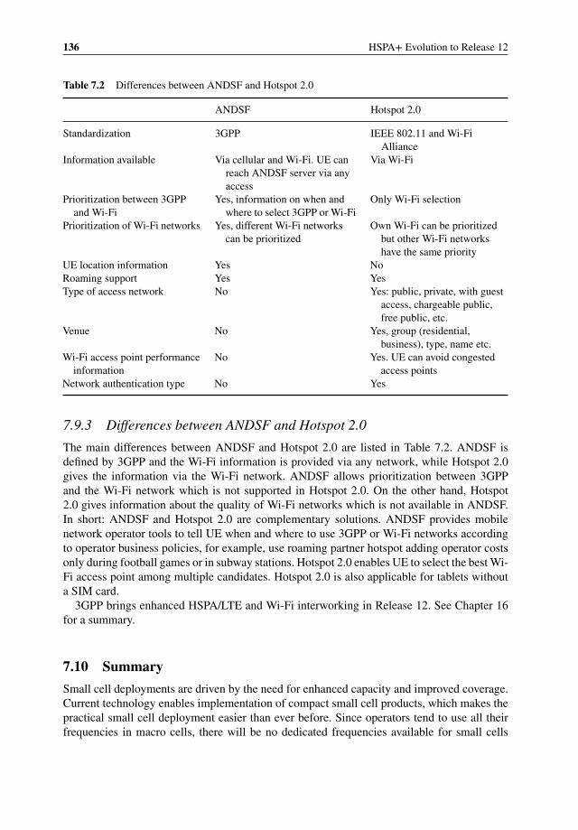
136 HSPA+ Evolution to Release 12
Table 7.2 Differences between ANDSF and Hotspot 2.0
ANDSF Hotspot 2.0
Standardization 3GPP IEEE 802.11 and Wi-FiAlliance
Information available Via cellular and Wi-Fi. UE canreach ANDSF server via anyaccess
Via Wi-Fi
Prioritization between 3GPPand Wi-Fi
Yes, information on when andwhere to select 3GPP or Wi-Fi
Only Wi-Fi selection
Prioritization of Wi-Fi networks Yes, different Wi-Fi networkscan be prioritized
Own Wi-Fi can be prioritizedbut other Wi-Fi networkshave the same priority
UE location information Yes NoRoaming support Yes YesType of access network No Yes: public, private, with guest
access, chargeable public,free public, etc.
Venue No Yes, group (residential,business), type, name etc.
Wi-Fi access point performanceinformation
No Yes. UE can avoid congestedaccess points
Network authentication type No Yes
7.9.3 Differences between ANDSF and Hotspot 2.0
The main differences between ANDSF and Hotspot 2.0 are listed in Table 7.2. ANDSF isdefined by 3GPP and the Wi-Fi information is provided via any network, while Hotspot 2.0gives the information via the Wi-Fi network. ANDSF allows prioritization between 3GPPand the Wi-Fi network which is not supported in Hotspot 2.0. On the other hand, Hotspot2.0 gives information about the quality of Wi-Fi networks which is not available in ANDSF.In short: ANDSF and Hotspot 2.0 are complementary solutions. ANDSF provides mobilenetwork operator tools to tell UE when and where to use 3GPP or Wi-Fi networks accordingto operator business policies, for example, use roaming partner hotspot adding operator costsonly during football games or in subway stations. Hotspot 2.0 enables UE to select the best Wi-Fi access point among multiple candidates. Hotspot 2.0 is also applicable for tablets withouta SIM card.
3GPP brings enhanced HSPA/LTE and Wi-Fi interworking in Release 12. See Chapter 16for a summary.
7.10 Summary
Small cell deployments are driven by the need for enhanced capacity and improved coverage.Current technology enables implementation of compact small cell products, which makes thepractical small cell deployment easier than ever before. Since operators tend to use all theirfrequencies in macro cells, there will be no dedicated frequencies available for small cells
Heterogeneous Networks 137
but instead small cells need to share the frequency with macro cells. Co-channel deploymentcreates some challenges, including the dominance areas and uplink–downlink balancing. Thesimulations show that small cell deployments can boost data rates considerably. Optimizedsmall cell rollout with four micro cells per macro sector can increase user data rates by a factorof 3.5x. Field measurements have also confirmed small cell benefits. Femto cells have beensuccessfully used for enhancing indoor coverage at homes and in small enterprises but femtocells are not suitable for outdoor deployment. Mobile operators can complement their cellularnetworks by offloading data traffic to Wi-Fi. ANDSF and Hotspot 2.0 solutions provide themeans for operators to control traffic offloading.
References
[1] 3GPP Technical Report 25.800 “UMTS Heterogeneous Networks”, v.12.0.0, 2013.[2] 3GPP Technical Specification 25.308 “High Speed Downlink Packet Access; Overall Description; Stage 2 (Rel
11)”, v.11.6.0, 2013.[3] 3GPP Technical Specification 23.402 “Architecture enhancements for non-3GPP accesses”, v.11.7.0, 2013.[4] 3GPP Technical Specification 24.312 “Access Network Discovery and Selection Function (ANDSF) Management
Object (MO)”, v.11.6.0, 2013.[5] 3GPP Technical Specification 24.302 “Access to the 3GPP Evolved Packet Core (EPC) via non-3GPP access
networks; Stage 3”, v.11.7.0, 2013.[6] Wi-Fi Alliance Hotspot 2.0 Certified Passpoint Release 1, 2013.[7] Wi-Fi Alliance Hotspot 2.0 Release 2, 2014.[8] “Hotspot 2.0 – Making Wi-Fi as easy to use and secure as cellular”, White paper, Ruckus Wireless, 2013.

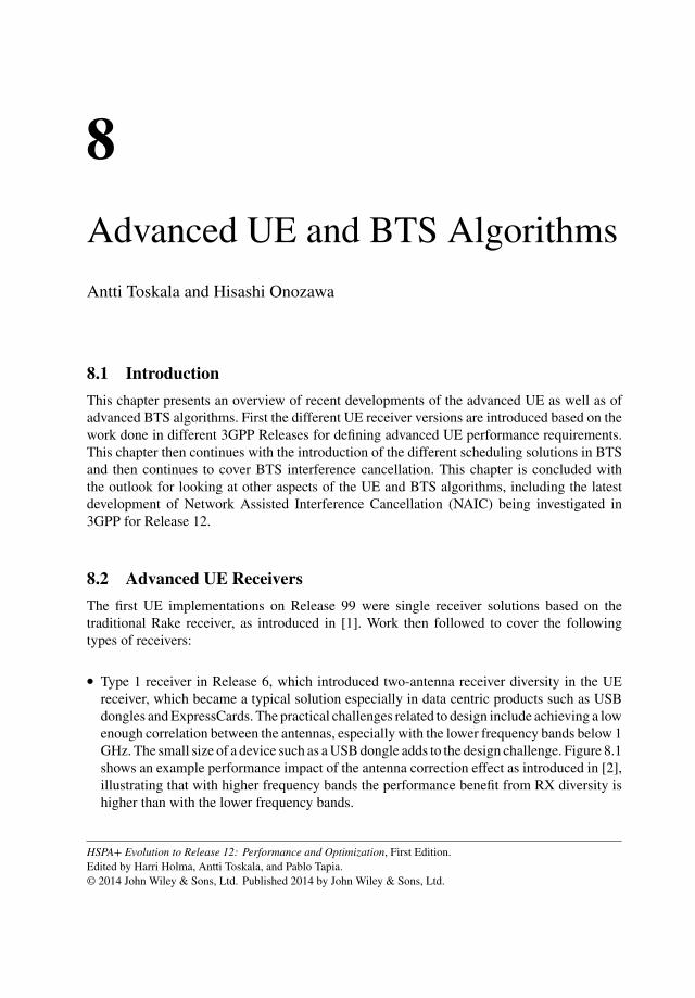
8Advanced UE and BTS Algorithms
Antti Toskala and Hisashi Onozawa
8.1 Introduction
This chapter presents an overview of recent developments of the advanced UE as well as ofadvanced BTS algorithms. First the different UE receiver versions are introduced based on thework done in different 3GPP Releases for defining advanced UE performance requirements.This chapter then continues with the introduction of the different scheduling solutions in BTSand then continues to cover BTS interference cancellation. This chapter is concluded withthe outlook for looking at other aspects of the UE and BTS algorithms, including the latestdevelopment of Network Assisted Interference Cancellation (NAIC) being investigated in3GPP for Release 12.
8.2 Advanced UE Receivers
The first UE implementations on Release 99 were single receiver solutions based on thetraditional Rake receiver, as introduced in [1]. Work then followed to cover the followingtypes of receivers:
� Type 1 receiver in Release 6, which introduced two-antenna receiver diversity in the UEreceiver, which became a typical solution especially in data centric products such as USBdongles and ExpressCards. The practical challenges related to design include achieving a lowenough correlation between the antennas, especially with the lower frequency bands below 1GHz. The small size of a device such as a USB dongle adds to the design challenge. Figure 8.1shows an example performance impact of the antenna correction effect as introduced in [2],illustrating that with higher frequency bands the performance benefit from RX diversity ishigher than with the lower frequency bands.
HSPA+ Evolution to Release 12: Performance and Optimization, First Edition.Edited by Harri Holma, Antti Toskala, and Pablo Tapia.© 2014 John Wiley & Sons, Ltd. Published 2014 by John Wiley & Sons, Ltd.
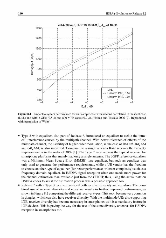
140 HSPA+ Evolution to Release 12
–8 –7 –6
Ec/Ior [dB]
–5 –4 –3–9200
400
600
800
Thr
ough
put [
kbps
]
1000
1200
1400
1600VehA 30 kmh, H-SET3 16QAM, Îor/Ioc of 10 dB
i.i.d.
Uniform PAS, 0.2λUniform PAS, 0.5λ
Figure 8.1 Impact to system performance for an example case with antenna correlation in the ideal case(i.i.d.) and with 2 GHz (0.5 𝜆) and 800 MHz cases (0.2 𝜆). (Holma and Toskala 2006 [2]. Reproducedwith permission of Wiley)
� Type 2 with equalizer, also part of Release 6, introduced an equalizer to tackle the intra-cell interference caused by the multipath channel. With better tolerance of effects of themultipath channel, the usability of higher order modulation, in the case of HSDPA 16QAMand 64QAM, is also improved. Compared to a single antenna Rake receiver the capacityimprovement is in the order of 30% [1]. The Type 2 receiver was the typical receiver forsmartphone platforms that mainly had only a single antenna. The 3GPP reference equalizerwas a Minimum Mean Square Error (MMSE) type equalizer, but such an equalizer wasonly used to generate the performance requirements, while a UE vendor has the freedomto choose another type of equalizer (for better performance or lower complexity) such as afrequency domain equalizer. In HSDPA signal reception often one needs more power forthe channel estimation than available just from the CPICH; thus, using the actual data onHSDPA codes to assist the estimation process was a possible approach too.
� Release 7 with a Type 3 receiver provided both receiver diversity and equalizer. The com-bined use of receiver diversity and equalizer results in further improved performance, asshown in Figure 8.2 comparing the different receiver types. This soon became very commonin dongles, which can also have receiver diversity. With the multimode UEs also supportingLTE, receiver diversity has become necessary in smartphones as it is a mandatory feature inLTE devices. This is paving the way for the use of the same diversity antennas for HSDPAreception in smartphones too.

Advanced UE and BTS Algorithms 141
0
500
1000
1500
2000
2500
3000
3500
4000
4500
1RX Rake 1RX Equalizer 2Rx Rake 2RX Equalizer
Throughput
kbps
Figure 8.2 Average downlink throughput with different type of UE receivers
The use of an advanced receiver is not necessarily applied to channels other than HS-PDSCH as 3GPP does not specify the advanced receiver performance. It is implementation-dependent if any type of receiver is applied to the Dedicated Channel (DCH). Thus, for agiven service running on HSDPA instead of on DCH, the performance would be boostedboth by the better receiver with diversity and due to the HSDPA features – including thelink adaptation and physical layer retransmissions as covered in Chapter 2.
� With the Type 3i receiver, the further element addressed is inter-cell interference. The Type3i receiver has a combination of receiver diversity, equalizer, and inter-cell interferencecancellation. This improves the performance, especially at the cell edge area when there isa dominant interfering cell. This is illustrated in Figure 8.3 with two different geometries
0
200
400
600
800
1000
1200
1400
1600
1800
2000
G = –3 dB G = 0 dB
kbps Type 3
Type 3i
Figure 8.3 Cell edge performance with and without UE interference cancellation
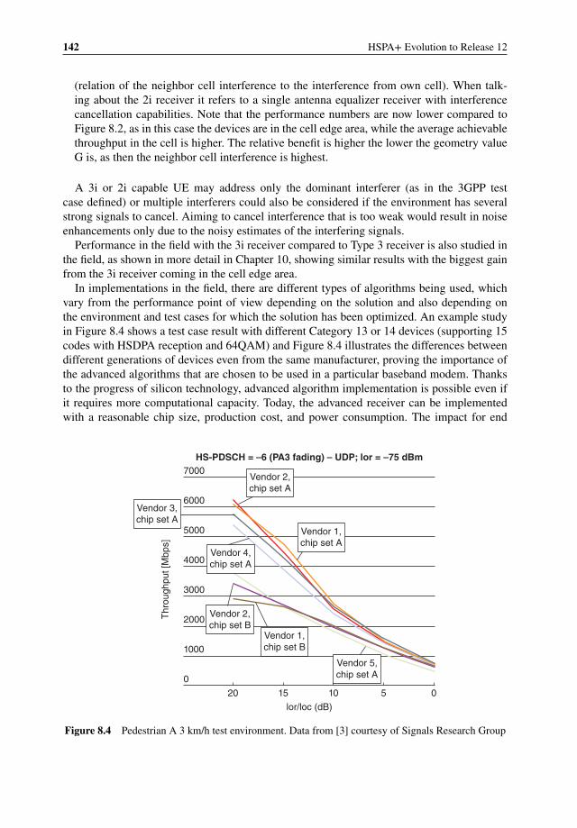
142 HSPA+ Evolution to Release 12
(relation of the neighbor cell interference to the interference from own cell). When talk-ing about the 2i receiver it refers to a single antenna equalizer receiver with interferencecancellation capabilities. Note that the performance numbers are now lower compared toFigure 8.2, as in this case the devices are in the cell edge area, while the average achievablethroughput in the cell is higher. The relative benefit is higher the lower the geometry valueG is, as then the neighbor cell interference is highest.
A 3i or 2i capable UE may address only the dominant interferer (as in the 3GPP testcase defined) or multiple interferers could also be considered if the environment has severalstrong signals to cancel. Aiming to cancel interference that is too weak would result in noiseenhancements only due to the noisy estimates of the interfering signals.
Performance in the field with the 3i receiver compared to Type 3 receiver is also studied inthe field, as shown in more detail in Chapter 10, showing similar results with the biggest gainfrom the 3i receiver coming in the cell edge area.
In implementations in the field, there are different types of algorithms being used, whichvary from the performance point of view depending on the solution and also depending onthe environment and test cases for which the solution has been optimized. An example studyin Figure 8.4 shows a test case result with different Category 13 or 14 devices (supporting 15codes with HSDPA reception and 64QAM) and Figure 8.4 illustrates the differences betweendifferent generations of devices even from the same manufacturer, proving the importance ofthe advanced algorithms that are chosen to be used in a particular baseband modem. Thanksto the progress of silicon technology, advanced algorithm implementation is possible even ifit requires more computational capacity. Today, the advanced receiver can be implementedwith a reasonable chip size, production cost, and power consumption. The impact for end
20
0
1000
2000
3000
4000
5000
6000
7000HS-PDSCH = –6 (PA3 fading) – UDP; lor = –75 dBm
15 10
lor/loc (dB)
5 0
Thr
ough
put[
Mbp
s]
Vendor 2,chip set A
Vendor 1,chip set A
Vendor 4,chip set A
Vendor 2,chip set B
Vendor 1,chip set B
Vendor 5,chip set A
Vendor 3,chip set A
Figure 8.4 Pedestrian A 3 km/h test environment. Data from [3] courtesy of Signals Research Group
Advanced UE and BTS Algorithms 143
user performance is significant as a modern device can provide double the data rate in goodconditions compared to the older generation device with the older chip set.
In low geometry regions, the performance is limited by Ioc rather than the multipathinterference. On the other hand, the equalizer algorithm and RF circuit linearity affect thethroughput in high geometry regions, where more performance difference is observed betweenchip sets.
From a smartphone point of view, most HSPA capable devices do not have receiver diversity,even though it is mandated for the LTE side as discussed earlier. When supporting the sameband for both LTE and HSPA the necessary antennas and RF components are also alreadyin place for HSPA receiver diversity, which is likely to make Type 3 or 3i more common insmartphone platforms too.
A further step in the receiver design is the MIMO receiver that is able to receive datafrom two different receiver branches, as discussed in Chapter 5. MIMO with HSDPA hasnot become commonly used in the devices, however, due to the problems caused for legacydevices before the introduction of the mitigation solutions discussed in Chapter 3. In thecase of MIMO, one may further consider more advanced algorithms such as the SuccessiveInterference Canceller (SIC) type of receiver. The simplest SIC receiver for two-stream MIMOis a single stage inter-stream canceller. The SIC receiver decodes the primary stream and thencancels it prior to decoding the secondary stream. The cancellation can be done using harddecisions or soft decisions. The soft decision has better reliability when the decoding ofthe primary stream fails but the implementation complexity is slightly high. This simpleversion of SIC gives most of the cancellation gain without increasing the number of Turbodecoder executions.
Also with MIMO, one can consider using Maximum Likelihood Detection (MLD). SinceMLD complexity is extremely high for higher order modulation with multiple streams, sim-plified algorithms such as Sphere Decoding (SD) and QR Decomposition Based M Algorithm(QRM-MLD) have been proposed. There are different possibilities for the inter-stream inter-ference cancellation with HSPA MIMO, such as those studied in [4] and references there in.
8.3 BTS Scheduling Alternatives
From a 3GPP point of view, the BTS scheduling implementation in terms of the kind ofalgorithm to use has been left for BTS vendor implementation; only the necessary signalingis specified to provide the scheduler with the necessary information both from the UE side,like the CQI feedback covered in Chapter 2, as well as information over the Iub interface, forexample on the UE capability and possible QoS parameters.
With the initial phase of HSDPA introduction in the field with the first Release 5 devices,the type of BTS scheduler was of no major importance. When the HSDPA penetration waslow, there were in many instances only a single UE in the cell, thus there was not much thescheduler could do than serve the single UE receiving data. In this case, the round robin typeof scheduling was able to reach reasonable performance. The basic idea with the round robinscheduler is to serve different users one by one (assuming there is data to be transmitted) ina cyclic manner. In many cases a carrier was also shared in the power domain with legacytraffic using DCH and there were also limitations in the code space available for HSDPA use.Figure 8.5 shows an example of round robin type scheduler functionality.
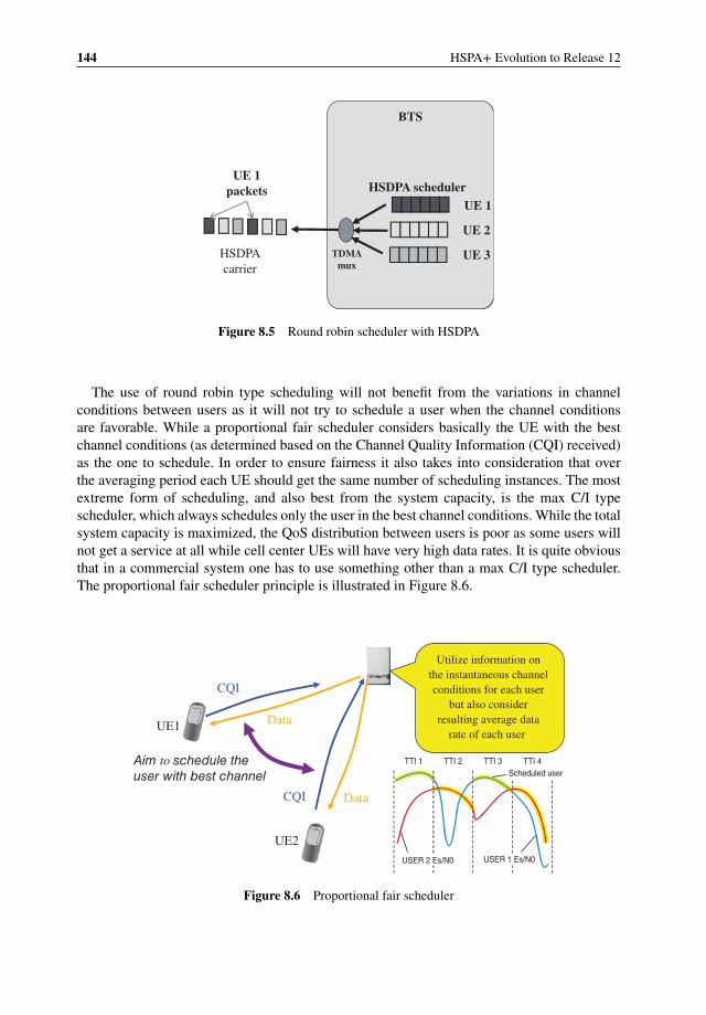
144 HSPA+ Evolution to Release 12
HSDPA scheduler
HSDPA
carrier
UE 1
UE 2
UE 3
UE 1 packets
BTS
TDMAmux
Figure 8.5 Round robin scheduler with HSDPA
The use of round robin type scheduling will not benefit from the variations in channelconditions between users as it will not try to schedule a user when the channel conditionsare favorable. While a proportional fair scheduler considers basically the UE with the bestchannel conditions (as determined based on the Channel Quality Information (CQI) received)as the one to schedule. In order to ensure fairness it also takes into consideration that overthe averaging period each UE should get the same number of scheduling instances. The mostextreme form of scheduling, and also best from the system capacity, is the max C/I typescheduler, which always schedules only the user in the best channel conditions. While the totalsystem capacity is maximized, the QoS distribution between users is poor as some users willnot get a service at all while cell center UEs will have very high data rates. It is quite obviousthat in a commercial system one has to use something other than a max C/I type scheduler.The proportional fair scheduler principle is illustrated in Figure 8.6.
UE2
CQI
CQI
Data
Data
UE1
Aim to schedule theuser with best channel
TTI 1 TTI 2 TTI 3 TTI 4
USER 1 Es/N0USER 2 Es/N0
Scheduled user
Utilize information on
the instantaneous channel
conditions for each user
but also consider
resulting average data
rate of each user
Figure 8.6 Proportional fair scheduler
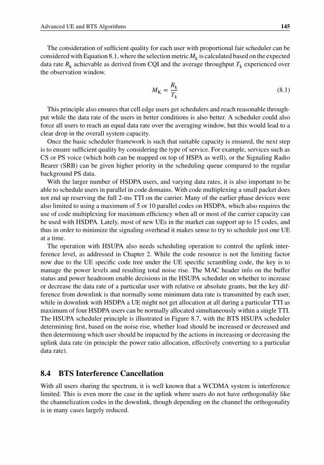
Advanced UE and BTS Algorithms 145
The consideration of sufficient quality for each user with proportional fair scheduler can beconsidered with Equation 8.1, where the selection metric Mk is calculated based on the expecteddata rate Rk achievable as derived from CQI and the average throughput Tk experienced overthe observation window.
MK =Rk
Tk(8.1)
This principle also ensures that cell edge users get schedulers and reach reasonable through-put while the data rate of the users in better conditions is also better. A scheduler could alsoforce all users to reach an equal data rate over the averaging window, but this would lead to aclear drop in the overall system capacity.
Once the basic scheduler framework is such that suitable capacity is ensured, the next stepis to ensure sufficient quality by considering the type of service. For example, services such asCS or PS voice (which both can be mapped on top of HSPA as well), or the Signaling RadioBearer (SRB) can be given higher priority in the scheduling queue compared to the regularbackground PS data.
With the larger number of HSDPA users, and varying data rates, it is also important to beable to schedule users in parallel in code domains. With code multiplexing a small packet doesnot end up reserving the full 2-ms TTI on the carrier. Many of the earlier phase devices werealso limited to using a maximum of 5 or 10 parallel codes on HSDPA, which also requires theuse of code multiplexing for maximum efficiency when all or most of the carrier capacity canbe used with HSDPA. Lately, most of new UEs in the market can support up to 15 codes, andthus in order to minimize the signaling overhead it makes sense to try to schedule just one UEat a time.
The operation with HSUPA also needs scheduling operation to control the uplink inter-ference level, as addressed in Chapter 2. While the code resource is not the limiting factornow due to the UE specific code tree under the UE specific scrambling code, the key is tomanage the power levels and resulting total noise rise. The MAC header info on the bufferstatus and power headroom enable decisions in the HSUPA scheduler on whether to increaseor decrease the data rate of a particular user with relative or absolute grants, but the key dif-ference from downlink is that normally some minimum data rate is transmitted by each user,while in downlink with HSDPA a UE might not get allocation at all during a particular TTI asmaximum of four HSDPA users can be normally allocated simultaneously within a single TTI.The HSUPA scheduler principle is illustrated in Figure 8.7, with the BTS HSUPA schedulerdetermining first, based on the noise rise, whether load should be increased or decreased andthen determining which user should be impacted by the actions in increasing or decreasing theuplink data rate (in principle the power ratio allocation, effectively converting to a particulardata rate).
8.4 BTS Interference Cancellation
With all users sharing the spectrum, it is well known that a WCDMA system is interferencelimited. This is even more the case in the uplink where users do not have orthogonality likethe channelization codes in the downlink, though depending on the channel the orthogonalityis in many cases largely reduced.
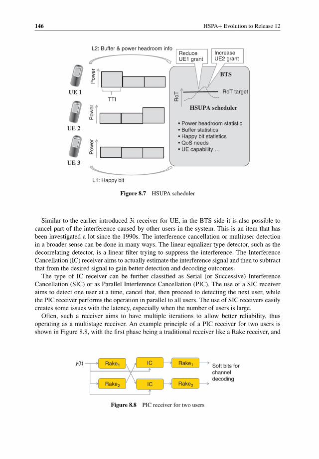
146 HSPA+ Evolution to Release 12
HSUPA scheduler
UE 1
BTS
Pow
erTTI
UE 2
Pow
er
UE 3
Pow
er
L2: Buffer & power headroom info
RoT target
RoT
ReduceUE1 grant
IncreaseUE2 grant
• Power headroom statistic• Buffer statistics• Happy bit statistics• QoS needs• UE capability …
L1: Happy bit
Figure 8.7 HSUPA scheduler
Similar to the earlier introduced 3i receiver for UE, in the BTS side it is also possible tocancel part of the interference caused by other users in the system. This is an item that hasbeen investigated a lot since the 1990s. The interference cancellation or multiuser detectionin a broader sense can be done in many ways. The linear equalizer type detector, such as thedecorrelating detector, is a linear filter trying to suppress the interference. The InterferenceCancellation (IC) receiver aims to actually estimate the interference signal and then to subtractthat from the desired signal to gain better detection and decoding outcomes.
The type of IC receiver can be further classified as Serial (or Successive) InterferenceCancellation (SIC) or as Parallel Interference Cancellation (PIC). The use of a SIC receiveraims to detect one user at a time, cancel that, then proceed to detecting the next user, whilethe PIC receiver performs the operation in parallel to all users. The use of SIC receivers easilycreates some issues with the latency, especially when the number of users is large.
Often, such a receiver aims to have multiple iterations to allow better reliability, thusoperating as a multistage receiver. An example principle of a PIC receiver for two users isshown in Figure 8.8, with the first phase being a traditional receiver like a Rake receiver, and
Rake1
Rake2
y(t) IC
IC
Rake1
Rake2
Soft bits forchanneldecoding
Figure 8.8 PIC receiver for two users
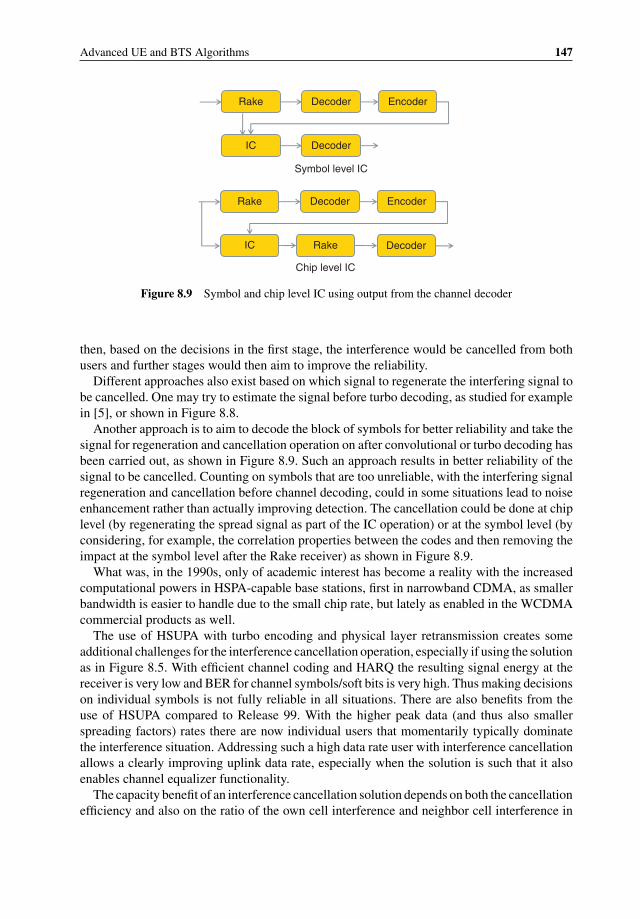
Advanced UE and BTS Algorithms 147
Rake Decoder Encoder
IC Decoder
Rake Decoder Encoder
IC DecoderRake
Symbol level IC
Chip level IC
Figure 8.9 Symbol and chip level IC using output from the channel decoder
then, based on the decisions in the first stage, the interference would be cancelled from bothusers and further stages would then aim to improve the reliability.
Different approaches also exist based on which signal to regenerate the interfering signal tobe cancelled. One may try to estimate the signal before turbo decoding, as studied for examplein [5], or shown in Figure 8.8.
Another approach is to aim to decode the block of symbols for better reliability and take thesignal for regeneration and cancellation operation on after convolutional or turbo decoding hasbeen carried out, as shown in Figure 8.9. Such an approach results in better reliability of thesignal to be cancelled. Counting on symbols that are too unreliable, with the interfering signalregeneration and cancellation before channel decoding, could in some situations lead to noiseenhancement rather than actually improving detection. The cancellation could be done at chiplevel (by regenerating the spread signal as part of the IC operation) or at the symbol level (byconsidering, for example, the correlation properties between the codes and then removing theimpact at the symbol level after the Rake receiver) as shown in Figure 8.9.
What was, in the 1990s, only of academic interest has become a reality with the increasedcomputational powers in HSPA-capable base stations, first in narrowband CDMA, as smallerbandwidth is easier to handle due to the small chip rate, but lately as enabled in the WCDMAcommercial products as well.
The use of HSUPA with turbo encoding and physical layer retransmission creates someadditional challenges for the interference cancellation operation, especially if using the solutionas in Figure 8.5. With efficient channel coding and HARQ the resulting signal energy at thereceiver is very low and BER for channel symbols/soft bits is very high. Thus making decisionson individual symbols is not fully reliable in all situations. There are also benefits from theuse of HSUPA compared to Release 99. With the higher peak data (and thus also smallerspreading factors) rates there are now individual users that momentarily typically dominatethe interference situation. Addressing such a high data rate user with interference cancellationallows a clearly improving uplink data rate, especially when the solution is such that it alsoenables channel equalizer functionality.
The capacity benefit of an interference cancellation solution depends on both the cancellationefficiency and also on the ratio of the own cell interference and neighbor cell interference in
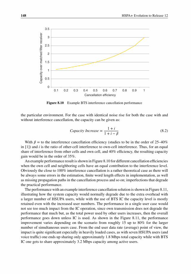
148 HSPA+ Evolution to Release 12
0
0.5
1
1.5
2
2.5
3
3.5
0.1 0.2 0.3 0.4 0.5 0.6 0.7 0.8 0.9 1
Cancellation efficiency
Cap
acity
ove
r m
atch
ed fi
lter
rece
iver
Figure 8.10 Example BTS interference cancellation performance
the particular environment. For the case with identical noise rise for both the case with andwithout interference cancellation, the capacity can be given as:
Capacity Increase = 1 + i1 + i − 𝛽
(8.2)
With 𝛽 = to the interference cancellation efficiency (studies to be in the order of 25–40%in [1]) and i is the ratio of other-cell interference to own-cell interference. Thus, for an equalshare of interference from other cells and own cell, and 40% efficiency, the resulting capacitygain would be in the order of 35%.
An example performance result is shown in Figure 8.10 for different cancellation efficiencieswhen the own cell and neighboring cells have an equal contribution to the interference level.Obviously the close to 100% interference cancellation is a rather theoretical case as there willbe always some errors in the estimation, finite word length effects in implementation, as wellas missing propagation paths in the cancellation process and so on; imperfections that degradethe practical performance.
The performance with an example interference cancellation solution is shown in Figure 8.11,illustrating how the system capacity would normally degrade due to the extra overhead witha larger number of HSUPA users, while with the use of BTS IC the capacity level is mostlyretained even with the increased user numbers. The performance in a single user case wouldnot see too much impact from the IC operation, since own transmission does not degrade theperformance that much but, as the total power used by other users increases, then the overallperformance goes down unless IC is used. As shown in the Figure 8.11, the performanceimprovement varies depending on the scenario from roughly 15 up to 80% for the largernumber of simultaneous users case. From the end user data rate (average) point of view, theimpact is quite significant especially in heavily loaded cases, as with seven HSUPA users (andvoice traffic) one ends up sharing only approximately 1.8 Mbps total capacity while with BTSIC one gets to share approximately 3.2 Mbps capacity among active users.
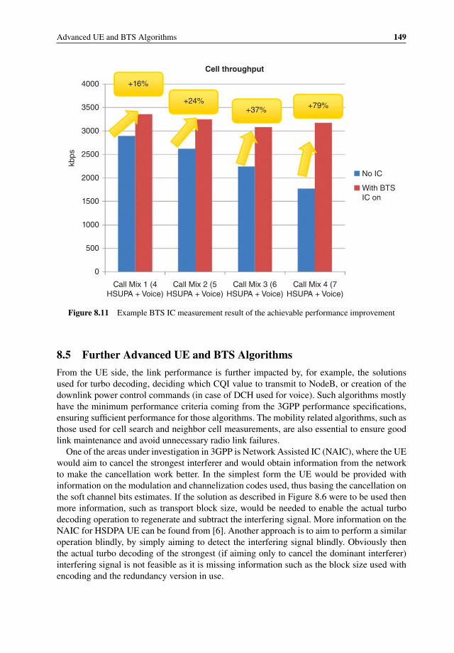
Advanced UE and BTS Algorithms 149
Call Mix 1 (4HSUPA + Voice)
Call Mix 2 (5HSUPA + Voice)
Call Mix 3 (6HSUPA + Voice)
Call Mix 4 (7HSUPA + Voice)
No IC
With BTSIC on
Cell throughput
+16%4000
3500
3000
2500
2000
kbps
1500
1000
500
0
+24%+37% +79%
Figure 8.11 Example BTS IC measurement result of the achievable performance improvement
8.5 Further Advanced UE and BTS Algorithms
From the UE side, the link performance is further impacted by, for example, the solutionsused for turbo decoding, deciding which CQI value to transmit to NodeB, or creation of thedownlink power control commands (in case of DCH used for voice). Such algorithms mostlyhave the minimum performance criteria coming from the 3GPP performance specifications,ensuring sufficient performance for those algorithms. The mobility related algorithms, such asthose used for cell search and neighbor cell measurements, are also essential to ensure goodlink maintenance and avoid unnecessary radio link failures.
One of the areas under investigation in 3GPP is Network Assisted IC (NAIC), where the UEwould aim to cancel the strongest interferer and would obtain information from the networkto make the cancellation work better. In the simplest form the UE would be provided withinformation on the modulation and channelization codes used, thus basing the cancellation onthe soft channel bits estimates. If the solution as described in Figure 8.6 were to be used thenmore information, such as transport block size, would be needed to enable the actual turbodecoding operation to regenerate and subtract the interfering signal. More information on theNAIC for HSDPA UE can be found from [6]. Another approach is to aim to perform a similaroperation blindly, by simply aiming to detect the interfering signal blindly. Obviously thenthe actual turbo decoding of the strongest (if aiming only to cancel the dominant interferer)interfering signal is not feasible as it is missing information such as the block size used withencoding and the redundancy version in use.
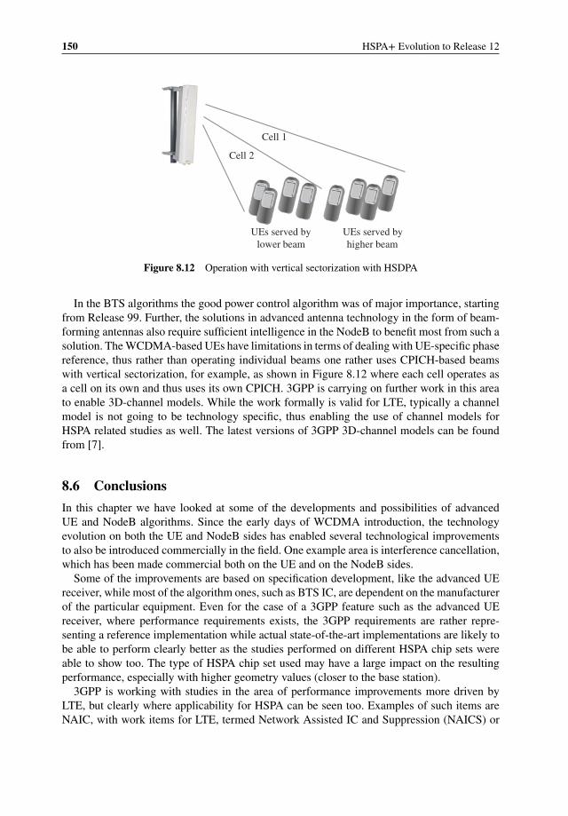
150 HSPA+ Evolution to Release 12
UEs served by
lower beam
UEs served by
higher beam
Cell 1
Cell 2
Figure 8.12 Operation with vertical sectorization with HSDPA
In the BTS algorithms the good power control algorithm was of major importance, startingfrom Release 99. Further, the solutions in advanced antenna technology in the form of beam-forming antennas also require sufficient intelligence in the NodeB to benefit most from such asolution. The WCDMA-based UEs have limitations in terms of dealing with UE-specific phasereference, thus rather than operating individual beams one rather uses CPICH-based beamswith vertical sectorization, for example, as shown in Figure 8.12 where each cell operates asa cell on its own and thus uses its own CPICH. 3GPP is carrying on further work in this areato enable 3D-channel models. While the work formally is valid for LTE, typically a channelmodel is not going to be technology specific, thus enabling the use of channel models forHSPA related studies as well. The latest versions of 3GPP 3D-channel models can be foundfrom [7].
8.6 Conclusions
In this chapter we have looked at some of the developments and possibilities of advancedUE and NodeB algorithms. Since the early days of WCDMA introduction, the technologyevolution on both the UE and NodeB sides has enabled several technological improvementsto also be introduced commercially in the field. One example area is interference cancellation,which has been made commercial both on the UE and on the NodeB sides.
Some of the improvements are based on specification development, like the advanced UEreceiver, while most of the algorithm ones, such as BTS IC, are dependent on the manufacturerof the particular equipment. Even for the case of a 3GPP feature such as the advanced UEreceiver, where performance requirements exists, the 3GPP requirements are rather repre-senting a reference implementation while actual state-of-the-art implementations are likely tobe able to perform clearly better as the studies performed on different HSPA chip sets wereable to show too. The type of HSPA chip set used may have a large impact on the resultingperformance, especially with higher geometry values (closer to the base station).
3GPP is working with studies in the area of performance improvements more driven byLTE, but clearly where applicability for HSPA can be seen too. Examples of such items areNAIC, with work items for LTE, termed Network Assisted IC and Suppression (NAICS) or
Advanced UE and BTS Algorithms 151
3D-channel modeling for enabling 3D-beamforming studies. These pave the way for newpotential enhancements that could be introduced in the networks, improving state-of-the-artHSPA network performance even further. More Release 12 items are covered in Chapter 15.
References
[1] Holma, H. and Toskala, A. (2010) WCDMA for UMTS, 5th edn, John Wiley & Sons, Ltd, Chichester.[2] Holma, H. and Toskala, A. (2006) HSDPA/HSUPA for UMTS, John Wiley & Sons, Ltd, Chichester.[3] Signals Ahead, Volume 7, No. 5 April 26, 2011, www.signalsresearch.com.[4] Yu, H., Shim, B. and Oh, T.W. (2012) Iterative interstream interference cancellation for MIMO HSPA+ system.
Journal of Communications and Networks, 14(3), 273–279.[5] Toskala, A., Hamalainen, S. and Holma, H. (1998) Link and system level performance of multiuser detection
CDMA uplink. Wireless Personal Communications: An International Journal Archive, 8(3), 301–320.[6] 3GPP Technical Report, TR 25.800, “Study on UMTS heterogeneous networks” v 12.0.0 September 2013.[7] 3GPP Technical Report, TR 36.873, “3D channel model for LTE”, v 2.0.0, March 2014.


9IMT-Advanced PerformanceEvaluation
Karri Ranta-aho and Antti Toskala
9.1 Introduction
This chapter presents a performance evaluation of HSPA Release 11 compared to the require-ments for IMT-Advanced as defined by the ITU-R. First the IMT-Advanced requirements arepresented and then the different features included in Release 11 3GPP specifications to addressthese requirements are briefly introduced to highlight how they help in achieving the improvedperformance. The achievable performance with different features is covered. This chapter isconcluded by benchmarking with the LTE and LTE-Advanced.
9.2 ITU-R Requirements for IMT-Advanced
The International Telegraphic Union Radiocommunications sector (ITU-R) [1] started theprocess for the new system, the International Mobile Telecommunications Advanced (IMT-Advanced), with a circular letter distributed in 2008. The circular letter was a call for radiotechnology proposals, in a similar fashion as had been done earlier for the IMT-2000 processin connection with the definition of 3G radio access solutions [2]. Now the ITU-R was callingfor proposals for radio technologies that could meet the requirements set for IMT-Advancedtechnology, widely termed the 4th generation (4G) mobile communication systems.
The ITU-R defined the requirements for the IMT-Advanced (4G) such that the systemshould be able to achieve the following [3]:
HSPA+ Evolution to Release 12: Performance and Optimization, First Edition.Edited by Harri Holma, Antti Toskala, and Pablo Tapia.© 2014 John Wiley & Sons, Ltd. Published 2014 by John Wiley & Sons, Ltd.

154 HSPA+ Evolution to Release 12
� Enable 100 Mbps peak data rate support for high mobility and up to 1 Gbps peak data ratefor the low mobility case.
� Allow inter-working with other radio access systems.� Enable high quality mobile services.� Capable of worldwide roaming.� Flexibility to allow cost efficient support of a wide range of services and applications.� Bandwidth scalability up to and including 40 MHz, with considerations up to 100 MHz.
Furthermore, there were more detailed performance requirements in the following areas:
� Peak spectral efficiency in downlink and uplink.� Cell spectral efficiency, ranging from 3 bits/s/Hz/cell in the indoor downlink scenario, to
0.7 bits/s/Hz/cell in the 120 km/h rural uplink scenario.� Cell edge user spectral efficiency, ranging from 0.1 bits/s/Hz/user in the indoor downlink
scenario, to 0.015 bits/s/Hz/user in the 120 km/h rural uplink scenario.� Mobility support with up to 350 km/h (smaller data rate allowed compared to the stationary
use case).� Latency requirements for the control plane to achieve 100 ms transition time between idle
and active state, and respectively to enable 10 ms user plane latency (in unloaded conditions).� Handover interruption of 27.5 ms for the intra-frequency case and 40 and 60 ms for the
inter-frequency within the band and between the bands respectively.� VoIP capacity, with the numbers of users ranging from 30 to 50 users per sector/MHz.
The requirements related to items such as peak spectral efficiency requirements or func-tional requirements such as achievable latency or handover interruption time can be inves-tigated relatively easy, while the requirements related to the average and cell edge spectralefficiency, with examples shown in Table 9.1, typically need detailed system-level studies withsimulations.
It was rather obvious that new features were needed on top of Release 10 HSPA in order tomeet some of these requirements with HSPA technology. As shown in the following chapters,the requirements for dealing with items such as handover delay or control plane latency were
Table 9.1 Summary of key ITU-R IMT-A requirements
System performance requirements ITU-R requirement
Downlink peak spectrum efficiency 15 bits/s/Hz (max 4 antennas)Uplink peak spectrum efficiency 6.75 bits/s/Hz (max 2 TX antennas)Downlink average cell spectral efficiency ≥1.1…3.0 bits/s/HzUplink average cell user spectral efficiency ≥0.7…2.25 bits/s/HzDownlink cell edge user spectral efficiency ≥0.04…0.1 bits/s/HzUplink cell edge user spectral efficiency ≥0.015…0.07 bits/s/HzUser plane latency ≤10 msControl plane latency ≤100 msHandover interruption ≤27.5…60 ms
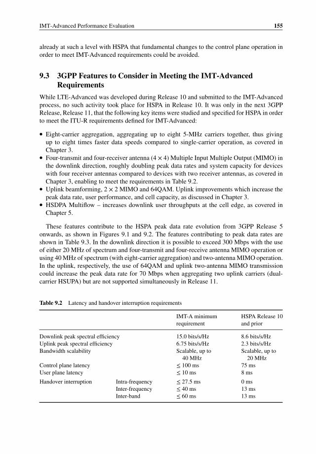
IMT-Advanced Performance Evaluation 155
already at such a level with HSPA that fundamental changes to the control plane operation inorder to meet IMT-Advanced requirements could be avoided.
9.3 3GPP Features to Consider in Meeting the IMT-AdvancedRequirements
While LTE-Advanced was developed during Release 10 and submitted to the IMT-Advancedprocess, no such activity took place for HSPA in Release 10. It was only in the next 3GPPRelease, Release 11, that the following key items were studied and specified for HSPA in orderto meet the ITU-R requirements defined for IMT-Advanced:
� Eight-carrier aggregation, aggregating up to eight 5-MHz carriers together, thus givingup to eight times faster data speeds compared to single-carrier operation, as covered inChapter 3.
� Four-transmit and four-receiver antenna (4 × 4) Multiple Input Multiple Output (MIMO) inthe downlink direction, roughly doubling peak data rates and system capacity for deviceswith four receiver antennas compared to devices with two receiver antennas, as covered inChapter 3, enabling to meet the requirements in Table 9.2.
� Uplink beamforming, 2 × 2 MIMO and 64QAM. Uplink improvements which increase thepeak data rate, user performance, and cell capacity, as discussed in Chapter 3.
� HSDPA Multiflow – increases downlink user throughputs at the cell edge, as covered inChapter 5.
These features contribute to the HSPA peak data rate evolution from 3GPP Release 5onwards, as shown in Figures 9.1 and 9.2. The features contributing to peak data rates areshown in Table 9.3. In the downlink direction it is possible to exceed 300 Mbps with the useof either 20 MHz of spectrum and four-transmit and four-receive antenna MIMO operation orusing 40 MHz of spectrum (with eight-carrier aggregation) and two-antenna MIMO operation.In the uplink, respectively, the use of 64QAM and uplink two-antenna MIMO transmissioncould increase the peak data rate for 70 Mbps when aggregating two uplink carriers (dual-carrier HSUPA) but are not supported simultaneously in Release 11.
Table 9.2 Latency and handover interruption requirements
IMT-A minimum HSPA Release 10requirement and prior
Downlink peak spectral efficiency 15.0 bits/s/Hz 8.6 bits/s/HzUplink peak spectral efficiency 6.75 bits/s/Hz 2.3 bits/s/HzBandwidth scalability Scalable, up to Scalable, up to
40 MHz 20 MHzControl plane latency ≤ 100 ms 75 msUser plane latency ≤ 10 ms 8 ms
Handover interruption Intra-frequency ≤ 27.5 ms 0 msInter-frequency ≤ 40 ms 13 msInter-band ≤ 60 ms 13 ms
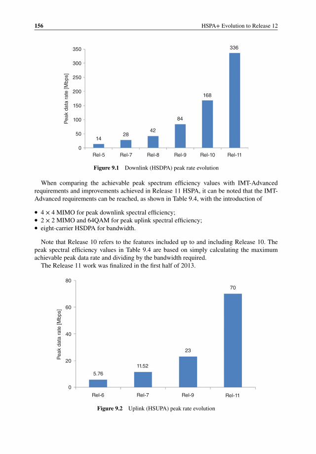
156 HSPA+ Evolution to Release 12
84
168
336
4228
14
Rel-50
50
100
150
200
250
300
350
Pea
k da
ta r
ate
[Mbp
s]
Rel-7 Rel-8 Rel-9 Rel-10 Rel-11
Figure 9.1 Downlink (HSDPA) peak rate evolution
When comparing the achievable peak spectrum efficiency values with IMT-Advancedrequirements and improvements achieved in Release 11 HSPA, it can be noted that the IMT-Advanced requirements can be reached, as shown in Table 9.4, with the introduction of
� 4 × 4 MIMO for peak downlink spectral efficiency;� 2 × 2 MIMO and 64QAM for peak uplink spectral efficiency;� eight-carrier HSDPA for bandwidth.
Note that Release 10 refers to the features included up to and including Release 10. Thepeak spectral efficiency values in Table 9.4 are based on simply calculating the maximumachievable peak data rate and dividing by the bandwidth required.
The Release 11 work was finalized in the first half of 2013.
Rel-6
5.76
0
20
40
60
80
11.52
23
70
Rel-7 Rel-11Rel-9
Pea
k da
ta r
ate
[Mbp
s]
Figure 9.2 Uplink (HSUPA) peak rate evolution
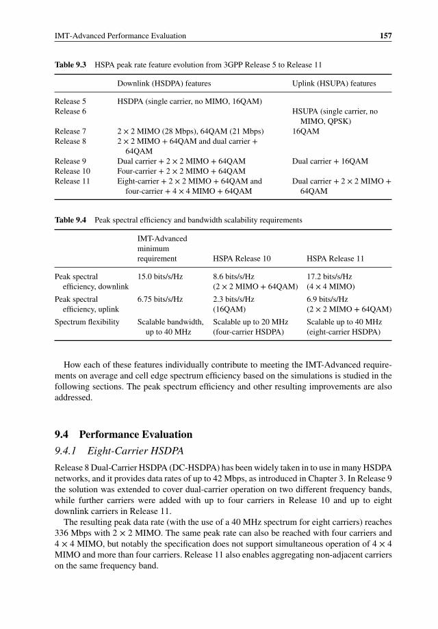
IMT-Advanced Performance Evaluation 157
Table 9.3 HSPA peak rate feature evolution from 3GPP Release 5 to Release 11
Downlink (HSDPA) features Uplink (HSUPA) features
Release 5 HSDPA (single carrier, no MIMO, 16QAM)Release 6 HSUPA (single carrier, no
MIMO, QPSK)Release 7 2 × 2 MIMO (28 Mbps), 64QAM (21 Mbps) 16QAMRelease 8 2 × 2 MIMO + 64QAM and dual carrier +
64QAMRelease 9 Dual carrier + 2 × 2 MIMO + 64QAM Dual carrier + 16QAMRelease 10 Four-carrier + 2 × 2 MIMO + 64QAMRelease 11 Eight-carrier + 2 × 2 MIMO + 64QAM and
four-carrier + 4 × 4 MIMO + 64QAMDual carrier + 2 × 2 MIMO +
64QAM
Table 9.4 Peak spectral efficiency and bandwidth scalability requirements
IMT-Advancedminimumrequirement HSPA Release 10 HSPA Release 11
Peak spectralefficiency, downlink
15.0 bits/s/Hz 8.6 bits/s/Hz(2 × 2 MIMO + 64QAM)
17.2 bits/s/Hz(4 × 4 MIMO)
Peak spectralefficiency, uplink
6.75 bits/s/Hz 2.3 bits/s/Hz(16QAM)
6.9 bits/s/Hz(2 × 2 MIMO + 64QAM)
Spectrum flexibility Scalable bandwidth,up to 40 MHz
Scalable up to 20 MHz(four-carrier HSDPA)
Scalable up to 40 MHz(eight-carrier HSDPA)
How each of these features individually contribute to meeting the IMT-Advanced require-ments on average and cell edge spectrum efficiency based on the simulations is studied in thefollowing sections. The peak spectrum efficiency and other resulting improvements are alsoaddressed.
9.4 Performance Evaluation
9.4.1 Eight-Carrier HSDPA
Release 8 Dual-Carrier HSDPA (DC-HSDPA) has been widely taken in to use in many HSDPAnetworks, and it provides data rates of up to 42 Mbps, as introduced in Chapter 3. In Release 9the solution was extended to cover dual-carrier operation on two different frequency bands,while further carriers were added with up to four carriers in Release 10 and up to eightdownlink carriers in Release 11.
The resulting peak data rate (with the use of a 40 MHz spectrum for eight carriers) reaches336 Mbps with 2 × 2 MIMO. The same peak rate can also be reached with four carriers and4 × 4 MIMO, but notably the specification does not support simultaneous operation of 4 × 4MIMO and more than four carriers. Release 11 also enables aggregating non-adjacent carrierson the same frequency band.
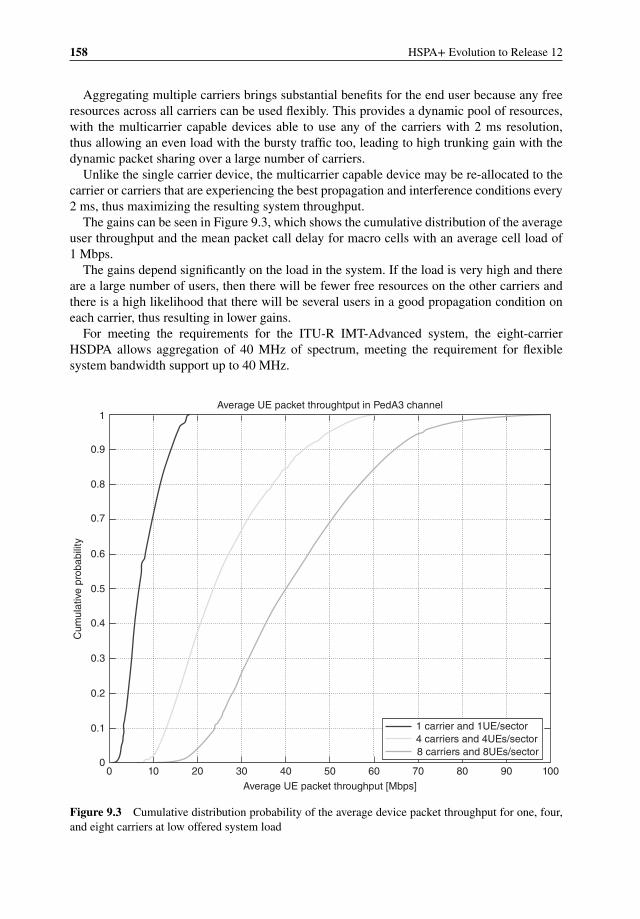
158 HSPA+ Evolution to Release 12
Aggregating multiple carriers brings substantial benefits for the end user because any freeresources across all carriers can be used flexibly. This provides a dynamic pool of resources,with the multicarrier capable devices able to use any of the carriers with 2 ms resolution,thus allowing an even load with the bursty traffic too, leading to high trunking gain with thedynamic packet sharing over a large number of carriers.
Unlike the single carrier device, the multicarrier capable device may be re-allocated to thecarrier or carriers that are experiencing the best propagation and interference conditions every2 ms, thus maximizing the resulting system throughput.
The gains can be seen in Figure 9.3, which shows the cumulative distribution of the averageuser throughput and the mean packet call delay for macro cells with an average cell load of1 Mbps.
The gains depend significantly on the load in the system. If the load is very high and thereare a large number of users, then there will be fewer free resources on the other carriers andthere is a high likelihood that there will be several users in a good propagation condition oneach carrier, thus resulting in lower gains.
For meeting the requirements for the ITU-R IMT-Advanced system, the eight-carrierHSDPA allows aggregation of 40 MHz of spectrum, meeting the requirement for flexiblesystem bandwidth support up to 40 MHz.
00
0.1
0.2
0.3
0.4
0.5
Cum
ulat
ive
prob
abili
ty
0.6
0.7
0.8
0.9
1
10 20 30 40 50
Average UE packet throughput [Mbps]
Average UE packet throughtput in PedA3 channel
60 70
1 carrier and 1UE/sector4 carriers and 4UEs/sector8 carriers and 8UEs/sector
80 90 100
Figure 9.3 Cumulative distribution probability of the average device packet throughput for one, four,and eight carriers at low offered system load
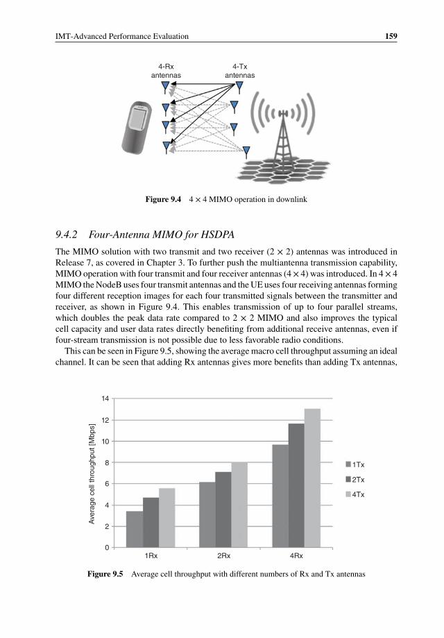
IMT-Advanced Performance Evaluation 159
4-Rxantennas
4-Txantennas
Figure 9.4 4 × 4 MIMO operation in downlink
9.4.2 Four-Antenna MIMO for HSDPA
The MIMO solution with two transmit and two receiver (2 × 2) antennas was introduced inRelease 7, as covered in Chapter 3. To further push the multiantenna transmission capability,MIMO operation with four transmit and four receiver antennas (4× 4) was introduced. In 4 × 4MIMO the NodeB uses four transmit antennas and the UE uses four receiving antennas formingfour different reception images for each four transmitted signals between the transmitter andreceiver, as shown in Figure 9.4. This enables transmission of up to four parallel streams,which doubles the peak data rate compared to 2 × 2 MIMO and also improves the typicalcell capacity and user data rates directly benefiting from additional receive antennas, even iffour-stream transmission is not possible due to less favorable radio conditions.
This can be seen in Figure 9.5, showing the average macro cell throughput assuming an idealchannel. It can be seen that adding Rx antennas gives more benefits than adding Tx antennas,
1Rx0
2
4
6
8
10
Ave
rage
cel
l thr
ough
put [
Mbp
s]
12
14
2Rx 4Rx
4Tx
2Tx
1Tx
Figure 9.5 Average cell throughput with different numbers of Rx and Tx antennas
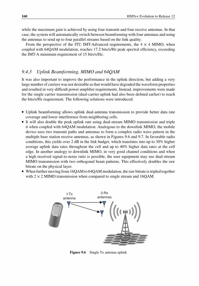
160 HSPA+ Evolution to Release 12
while the maximum gain is achieved by using four transmit and four receive antennas. In thatcase, the system will automatically switch between beamforming with four antennas and usingthe antennas to send up to four parallel streams based on the link quality.
From the perspective of the ITU IMT-Advanced requirements, the 4 × 4 MIMO, whencoupled with 64QAM modulation, reaches 17.2 bits/s/Hz peak spectral efficiency, exceedingthe IMT-A minimum requirement of 15 bits/s/Hz.
9.4.3 Uplink Beamforming, MIMO and 64QAM
It was also important to improve the performance in the uplink direction, but adding a verylarge number of carriers was not desirable as that would have degraded the waveform propertiesand resulted in very difficult power amplifier requirements. Instead, improvements were madefor the single carrier transmission (dual-carrier uplink had also been defined earlier) to reachthe bits/s/Hz requirement. The following solutions were introduced:
� Uplink beamforming allows uplink dual-antenna transmission to provide better data ratecoverage and lower interference from neighboring cells.
� It will also double the peak uplink rate using dual-stream MIMO transmission and tripleit when coupled with 64QAM modulation. Analogous to the downlink MIMO, the mobiledevice uses two transmit paths and antennas to form a complex radio wave pattern in themultiple base station receive antennas, as shown in Figures 9.6 and 9.7. In favorable radioconditions, this yields over 2 dB in the link budget, which translates into up to 30% higheraverage uplink data rates throughout the cell and up to 40% higher data rates at the celledge. In another analogy to downlink MIMO, in very good channel conditions and whena high received signal-to-noise ratio is possible, the user equipment may use dual-streamMIMO transmission with two orthogonal beam patterns. This effectively doubles the rawbitrate on the physical layer.
� When further moving from 16QAM to 64QAM modulation, the raw bitrate is tripled togetherwith 2 × 2 MIMO transmission when compared to single stream and 16QAM.
1-Txantenna
2-Rxantennas
Figure 9.6 Single Tx antenna uplink
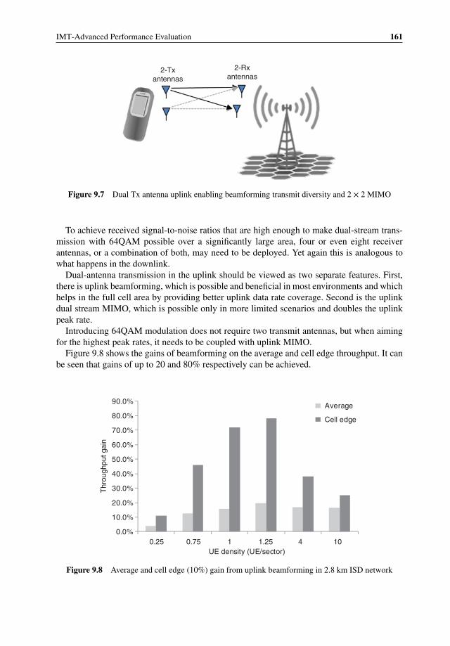
IMT-Advanced Performance Evaluation 161
2-Txantennas
2-Rxantennas
Figure 9.7 Dual Tx antenna uplink enabling beamforming transmit diversity and 2 × 2 MIMO
To achieve received signal-to-noise ratios that are high enough to make dual-stream trans-mission with 64QAM possible over a significantly large area, four or even eight receiverantennas, or a combination of both, may need to be deployed. Yet again this is analogous towhat happens in the downlink.
Dual-antenna transmission in the uplink should be viewed as two separate features. First,there is uplink beamforming, which is possible and beneficial in most environments and whichhelps in the full cell area by providing better uplink data rate coverage. Second is the uplinkdual stream MIMO, which is possible only in more limited scenarios and doubles the uplinkpeak rate.
Introducing 64QAM modulation does not require two transmit antennas, but when aimingfor the highest peak rates, it needs to be coupled with uplink MIMO.
Figure 9.8 shows the gains of beamforming on the average and cell edge throughput. It canbe seen that gains of up to 20 and 80% respectively can be achieved.
0.0%
10.0%
20.0%
30.0%
40.0%
50.0%
60.0%
70.0%
80.0%
90.0%
1041.2510.750.25
Thr
ough
put g
ain
UE density (UE/sector)
Average
Cell edge
Figure 9.8 Average and cell edge (10%) gain from uplink beamforming in 2.8 km ISD network
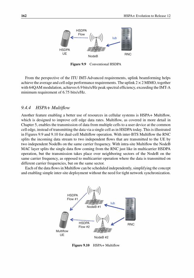
162 HSPA+ Evolution to Release 12
HSDPAFlow
HSDPAUE
NodeBRNC
Iub
Figure 9.9 Conventional HSDPA
From the perspective of the ITU IMT-Advanced requirements, uplink beamforming helpsachieve the average and cell edge performance requirements. The uplink 2× 2 MIMO, togetherwith 64QAM modulation, achieves 6.9 bits/s/Hz peak spectral efficiency, exceeding the IMT-Aminimum requirement of 6.75 bits/s/Hz.
9.4.4 HSPA+ Multiflow
Another feature enabling a better use of resources in cellular systems is HSPA+ Multiflow,which is designed to improve cell edge data rates. Multiflow, as covered in more detail inChapter 5, enables the transmission of data from multiple cells to a user device at the commoncell edge, instead of transmitting the data via a single cell as in HSDPA today. This is illustratedin Figures 9.9 and 9.10 for dual-cell Multiflow operation. With inter-BTS Multiflow the RNCsplits the incoming data stream to two independent flows that are transmitted to the UE bytwo independent NodeBs on the same carrier frequency. With intra-site Multiflow the NodeBMAC layer splits the single data flow coming from the RNC just like in multicarrier HSDPAoperation, but the transmission takes place over neighboring sectors of the NodeB on thesame carrier frequency, as opposed to multicarrier operation where the data is transmitted ondifferent carrier frequencies, but on the same sector.
Each of the data flows in Multiflow can be scheduled independently, simplifying the conceptand enabling simple inter-site deployment without the need for tight network synchronization.
HSDPAFlow #1
HSDPAFlow #2
MultiflowUE
NodeB #1
RNC
NodeB #2
Iub
Figure 9.10 HSPA+ Multiflow
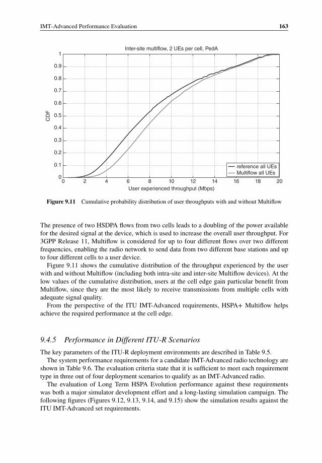
IMT-Advanced Performance Evaluation 163
00
0.1
0.2
0.3
0.4
0.5
CD
F
0.6
0.7
0.8
0.9
1
2 4 6 8 10User experienced throughput (Mbps)
Inter-site multiflow, 2 UEs per cell, PedA
12 14
reference all UEsMultiflow all UEs
16 18 20
Figure 9.11 Cumulative probability distribution of user throughputs with and without Multiflow
The presence of two HSDPA flows from two cells leads to a doubling of the power availablefor the desired signal at the device, which is used to increase the overall user throughput. For3GPP Release 11, Multiflow is considered for up to four different flows over two differentfrequencies, enabling the radio network to send data from two different base stations and upto four different cells to a user device.
Figure 9.11 shows the cumulative distribution of the throughput experienced by the userwith and without Multiflow (including both intra-site and inter-site Multiflow devices). At thelow values of the cumulative distribution, users at the cell edge gain particular benefit fromMultiflow, since they are the most likely to receive transmissions from multiple cells withadequate signal quality.
From the perspective of the ITU IMT-Advanced requirements, HSPA+ Multiflow helpsachieve the required performance at the cell edge.
9.4.5 Performance in Different ITU-R Scenarios
The key parameters of the ITU-R deployment environments are described in Table 9.5.The system performance requirements for a candidate IMT-Advanced radio technology are
shown in Table 9.6. The evaluation criteria state that it is sufficient to meet each requirementtype in three out of four deployment scenarios to qualify as an IMT-Advanced radio.
The evaluation of Long Term HSPA Evolution performance against these requirementswas both a major simulator development effort and a long-lasting simulation campaign. Thefollowing figures (Figures 9.12, 9.13, 9.14, and 9.15) show the simulation results against theITU IMT-Advanced set requirements.
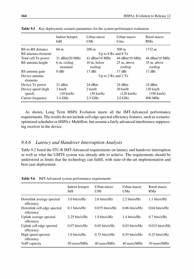
164 HSPA+ Evolution to Release 12
Table 9.5 Key deployment scenario parameters for the system performance evaluation
Indoor hotspotInH
Urban microUMi
Urban macroUma
Rural macroRMa
BS-to-BS distance 60 m 200 m 500 m 1732 mBS antenna elements Up to 8 Rx and 8 TxTotal cell Tx power 21 dBm/20 MHz 41 dBm/10 MHz 46 dBm/10 MHz 46 dBm/10 MHzBS antenna height 6 m, ceiling
mounted10 m, below
rooftop25 m, above
rooftop35 m, above
rooftopBS antenna gain 0 dBi 17 dBi 17 dBi 17 dBiDevice antenna
elementsUp to 2 Rx and 2 Tx
Device Tx power 21 dBm 24 dBm 24 dBm 24 dBmDevice speed (high
speed)3 km/h
(10 km/h)3 km/h
(30 km/h)30 km/h
(120 km/h)120 km/h
(350 km/h)Carrier frequency 3.4 GHz 2.5 GHz 2.0 GHz 800 MHz
As shown, Long Term HSPA Evolution meets all the IMT-Advanced performancerequirements. The results do not include cell edge spectral efficiency features, such as scenario-optimized scheduler or HSPA+ Multiflow, but assume a fairly advanced interference suppress-ing receiver in the device.
9.4.6 Latency and Handover Interruption Analysis
Table 9.2 listed the ITU-R IMT-Advanced requirements on latency and handover interruptionas well as what the UMTS system was already able to achieve. The requirements should beunderstood as limits that the technology can fulfill, with state-of-the-art implementation andbest case deployment.
Table 9.6 IMT-Advanced system performance requirements
Indoor hotspot Urban micro Urban macro Rural macroInH UMi UMa RMa
Downlink average spectralefficiency
3.0 bits/s/Hz 2.6 bits/s/Hz 2.2 bits/s/Hz 1.1 bits/s/Hz
Downlink cell edge spectralefficiency
0.1 bits/s/Hz 0.075 bits/s/Hz 0.06 bits/s/Hz 0.04 bits/s/Hz
Uplink average spectralefficiency
2.25 bits/s/Hz 1.8 bits/s/Hz 1.4 bits/s/Hz 0.7 bits/s/Hz
Uplink cell edge spectralefficiency
0.07 bits/s/Hz 0.05 bits/s/Hz 0.03 bits/s/Hz 0.015 bits/s/Hz
High speed spectralefficiency
1.0 bits/s/Hz 0.75 bits/s/Hz 0.55 bits/s/Hz 0.25 bits/s/Hz
VoIP capacity 50 users/MHz 40 users/MHz 40 users/MHz 30 users/MHz
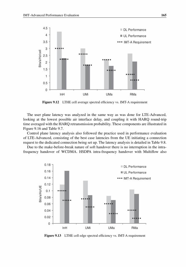
IMT-Advanced Performance Evaluation 165
0
0.5
1
1.5
2
2.5
3
3.5
4
4.5
RMaUMaUMiInH
Bits
/s/H
z/ce
ll
DL Performance
UL Performance
IMT-A Requirement
Figure 9.12 LTHE cell average spectral efficiency vs. IMT-A requirement
The user plane latency was analyzed in the same way as was done for LTE-Advanced,looking at the lowest possible air interface delay, and coupling it with HARQ round-triptime averaged with the HARQ retransmission probability. These components are illustrated inFigure 9.16 and Table 9.7.
Control plane latency analysis also followed the practice used in performance evaluationof LTE-Advanced, consisting of the best case latencies from the UE initiating a connectionrequest to the dedicated connection being set up. The latency analysis is detailed in Table 9.8.
Due to the make-before-break nature of soft handover there is no interruption in the intra-frequency handover of WCDMA. HSDPA intra-frequency handover with Multiflow also
0
0.02
0.04
0.06
0.08
0.1
0.12
0.14
0.16
0.18
RMaUMaUMiInH
Bits
/s/H
z/U
E
DL Performance
UL Performance
IMT-A Requirement
Figure 9.13 LTHE cell edge spectral efficiency vs. IMT-A requirement
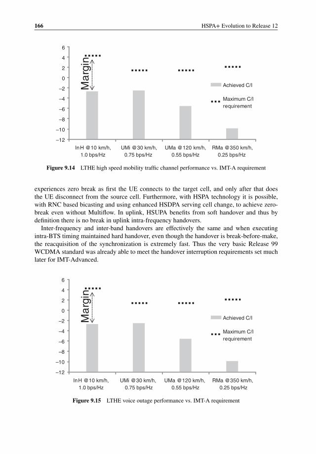
166 HSPA+ Evolution to Release 12
–12
–10
–8
–6
–4
–2
0
2
4
6
InH @10 km/h,1.0 bps/Hz
UMi @30 km/h,0.75 bps/Hz
UMa @120 km/h,0.55 bps/Hz
RMa @350 km/h,0.25 bps/Hz
Achieved C/I
Maximum C/Irequirement
Ma
rgin
Figure 9.14 LTHE high speed mobility traffic channel performance vs. IMT-A requirement
experiences zero break as first the UE connects to the target cell, and only after that doesthe UE disconnect from the source cell. Furthermore, with HSPA technology it is possible,with RNC based bicasting and using enhanced HSDPA serving cell change, to achieve zero-break even without Multiflow. In uplink, HSUPA benefits from soft handover and thus bydefinition there is no break in uplink intra-frequency handovers.
Inter-frequency and inter-band handovers are effectively the same and when executingintra-BTS timing maintained hard handover, even though the handover is break-before-make,the reacquisition of the synchronization is extremely fast. Thus the very basic Release 99WCDMA standard was already able to meet the handover interruption requirements set muchlater for IMT-Advanced.
–12
–10
–8
–6
–4
–2
0
2
4
6
InH @10 km/h,1.0 bps/Hz
UMi @30 km/h, 0.75 bps/Hz
UMa @120 km/h, 0.55 bps/Hz
RMa @350 km/h, 0.25 bps/Hz
Achieved C/I
Maximum C/I requirement
Ma
rgin
Figure 9.15 LTHE voice outage performance vs. IMT-A requirement
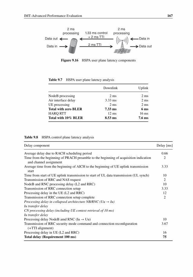
IMT-Advanced Performance Evaluation 167
2 msprocessing
2 msprocessing
Data in
Data outData in
Data out
1.33 ms control+ 2 ms TTI
2 ms TTI
Figure 9.16 HSPA user plane latency components
Table 9.7 HSPA user plane latency analysis
Downlink Uplink
NodeB processing 2 ms 2 msAir interface delay 3.33 ms 2 msUE processing 2 ms 2 msTotal with zero BLER 7.33 ms 6 msHARQ RTT 12 ms 16 msTotal with 10% BLER 8.53 ms 7.6 ms
Table 9.8 HSPA control plane latency analysis
Delay component Delay [ms]
Average delay due to RACH scheduling period 0.66Time from the beginning of PRACH preamble to the beginning of acquisition indication
and channel assignment2
Average time from the beginning of AICH to the beginning of UE uplink transmissionstart
3.33
Time from start of UE uplink transmission to start of UL data transmission (UL synch) 10Transmission of RRC and NAS request 2NodeB and RNC processing delay (L2 and RRC) 10Transmission of RRC connection setup 3.33Processing delay in the UE (L2 and RRC) 12Transmission of RRC connection setup complete 2Processing delay in collapsed architecture NB/RNC (Uu → Iu)Iu transfer delayCN processing delay (including UE context retrieval of 10 ms)Iu transfer delayProcessing delay NodeB amd RNC (Iu → Uu) 10Transmission of RRC security mode command and connection reconfiguration
(+TTI alignment)3.67
Processing delay in UE (L2 and RRC) 16Total delay (Requirement 100 ms) 75
168 HSPA+ Evolution to Release 12
9.5 Conclusions
In this chapter the features added in Release 11 HSPA to allow the IMT-Advanced requirementsto be met were analyzed. It could be concluded that with the introduction of
� eight-carrier aggregation, giving up to eight times better user performance;� 4× 4 MIMO in the downlink, increasing peak data rates, and improving system performance;� uplink beamforming, 2 × 2 MIMO and 64QAM; uplink improvements increase the peak
data rate, user performance, and cell capacity;� Multiflow – increases downlink user throughputs at the cell edge;
Release 11 HSPA, sometimes referred too as Long Term HSPA Evolution, can also meet thecriteria as IMT-Advanced technology as defined by the ITU-R. To meet the increased networkcapacity demand caused by growing mobile data traffic, HSPA has continued to be improvedin parallel with LTE and LTE-Advanced.
HSPA is currently the radio access technology serving the most wireless broadband usersworldwide and the load on the system is expected to increase further in the coming years, thuscreating demand for performance improvements in the future, facilitating introduction of newperformance improvements features to the commercial HSPA networks expected to be servingmore than 2 billion users worldwide by end of 2014.
References
[1] Holma, H. and Toskala, A. (2012) LTE Advanced: 3GPP Solution for IMT-Advanced, John Wiley & Sons, Ltd,Chichester.
[2] Holma, H. and Toskala, A. (2010) WCDMA for UMTS, 5th edn, John Wiley & Sons, Ltd, Chichester.[3] ITU-R report, M.2134, “Requirements related to technical performance for IMT-Advanced radio interface(s)”.
10HSPA+ Performance
Pablo Tapia and Brian Olsen
10.1 Introduction
HSPA+ is nowadays a mature network technology that has been deployed globally for anumber of years. Technologies such as 64QAM, Advanced Receivers, and Release 8 DualCell are well adopted today in a large number of network and devices.
This chapter analyzes the performance of various HSPA+ features in live network environ-ments with real traffic loads. The maturity of the tested networks helped achieve performancelevels that are close to the theoretical expectations from the technology itself, unlike previoushardware and software versions that often presented problems and design limitations. Even so,wide variations in performance amongst different infrastructure vendors can still be noticed, aswill be discussed in detail in Sections 10.3.7 and 10.4.3. In some cases, the scenarios analyzedpresent challenges due to coverage, traffic load, or interference, as can be expected from realnetwork deployments.
In the various sections, several test scenarios are analyzed, including different RF envi-ronments in stationary and mobile conditions. A detailed performance analysis is offered foreach scenario, focusing on special interest areas relevant to each particular case; special careis taken to analyze the behavior of the link adaptation mechanisms, which play an importantrole in optimizing the performance of the data transmission and thus the spectral efficiencyoffered by the technology.
In general, the results show that the HSPA+ technology can provide an excellent dataexperience both in terms of throughput – with typical downlink throughputs over 6 Mbpswith a single carrier configuration – and latency (typically under 60 ms). Networks withRelease 8 Dual Cell effectively double the downlink speeds, offering throughputs between5 and 30 Mbps, and latency as low as 30 ms. These performance levels are sufficient to offerany data service available today, including real-time services which have quite stringent delayrequirements.
HSPA+ Evolution to Release 12: Performance and Optimization, First Edition.Edited by Harri Holma, Antti Toskala, and Pablo Tapia.© 2014 John Wiley & Sons, Ltd. Published 2014 by John Wiley & Sons, Ltd.
170 HSPA+ Evolution to Release 12
This chapter also highlights some of the challenges that are present in real HSPA+ deploy-ments, including throughput fluctuations both in uplink and downlink, which makes it hard tooffer a consistent service experience across the coverage area. As will be discussed, some ofthese challenges can be mitigated by careful RF planning and optimization, while others canbe tackled with proper parameter tuning. In some cases, the technology presents limitationsthat cannot be easily overcome with current networks and devices, as is the case of uplinknoise instability due to the inherent nature of the HSUPA control mechanisms.
Another challenge that HSPA+ networks present is the delay associated with state transi-tions; while the connected mode latency can be very low, the transition between various RadioResource Control (RRC) states can hurt the user experience in the case of interactive appli-cations such as web browsing. Chapter 12 (Optimization) provides some guidelines aroundvarious RF and parameter optimizations, including tuning of the state transition parameters.
Finally, Section 10.6 provides a direct performance comparison between HSPA+ and LTEunder a similar network configuration, and shows that dual-carrier HSPA+ remains a seriouscompetitor of early versions of LTE, except in the case of uplink transmission, where the LTEtechnology is vastly superior.
10.2 Test Tools and Methodology
The majority of the performance measurements that are discussed in this chapter are extractedfrom drive tests. While network performance indicators are important to keep track of theoverall network health from a macroscopic point of view, these metrics are not very useful tocapture what end users really perceive. To illustrate what the HSPA+ technology can offer froma user point of view, the best course of action is to collect measurements at the terminal device.
There are many different choices of tools that collect terminal measurements, and withinthese tools, the amount of metrics that can be analyzed can sometimes be daunting; in thissection we provide some guidelines around test methodologies that can help simplify theanalysis of HSPA+ data performance.
The first step towards measuring performance is to select the right test tools. It is recom-mended that at least two sets of tools are used for this:
� A radio tracing tool that provides Layer 1 to Layer 3 measurements and signaling infor-mation, such as TEMS, QXDM, Nemo, or XCal. These tools can typically be seamlesslyconnected to devices that use Qualcomm chip sets, although the device may need a specialengineering code to enable proper USB debugging ports.
� An automatic test generation tool that is used to emulate different applications automatically,such as File Transfer Protocol (FTP) or User Datagram Protocol (UDP) transfers, webbrowsing, pings, and so on. These tools are a good complement to the radio tracing tooland typically provide application level Key Performance Indicators (KPIs), some Layer 3level information, and often offer options to capture IP packet traces. Example tools in thisspace are Spirent’s Datum, Swiss Mobility’s NxDroid, and AT4’s Testing App. A low costalternative to these tools is to use free application level tools, such as iPerf (for UDP) orFTP scripts, combined with Wireshark to capture Internet Protocol (IP) traces. CapturingIP packet traces is not recommended by default unless required for specific applicationperformance analysis or troubleshooting purposes.

HSPA+ Performance 171
Once the test tools are set up it is recommended to perform a series of quick tests toverify basic connectivity and performance. These could be done using an online tool such asSpeedTest or similar, or using a specific application test tool. Test values from Section 10.3.6can be used as a reference for expected throughput and latency values:
� UDP down and up transfers, to check that the terminal is using the HSDPA and HSUPAchannels and that the speeds that are obtained are aligned with the given radio conditions.
� 32-byte pings to verify low latency. These measurements should be performed with theterminal in CELL_DCH state; the state change can be triggered by the transmission of alarge chunk of data, and verified in the radio tracing tool.
Depending on the objective of the tests, it may be a good idea to lock the phone in 3G modeto avoid Inter Radio Access (IRAT) handovers and be able to measure the performance in thepoorer radio conditions. During the collection phase the amount of information that can beanalyzed is limited due to the real-time nature of the task, but it is nonetheless recommendedto monitor specific metrics such as:
Received Signal Code Power (RSCP) and Ec/NoAreas with poor radio signal (RSCP below−105 dBm or Ec/No below−12 dB) canbe expected to present various challenges such as low throughput, interruptions,radio bearer reconfigurations, or IRAT handovers.
Number of servers in the active setAreas with many neighbors may indicate pilot pollution. In these areas it iscommon to observe performance degradation, sometimes caused by a large amountof HS cell changes in the area due to ping-pong effects.
Used channel typeIf the used channel type is “Release 99” instead of HSDPA and HSUPA, therecould be a problem with the network configuration: channels not activated orconservative channel reconfiguration settings.
Instantaneous Radio Link Control (RLC) Level ThroughputLow throughputs in areas with good radio conditions need to be investigated,since these could indicate problems with the test tools, such as server overload.If the throughputs never reach the peaks it could indicate a problem with thenetwork configuration, for example 64QAM modulation not activated or improperconfiguration of the number of HS codes.
HS Discontinuous Transmission (DTX) or Scheduling RateThe scheduling rate indicates the number of Transmission Time Intervals (TTIs)that are assigned to the test device. A high DTX can be indicative of excessivenetwork load, backhaul restrictions, or problems with the test tool.
Figure 10.1 illustrates some of the most relevant metrics in an example test tool:
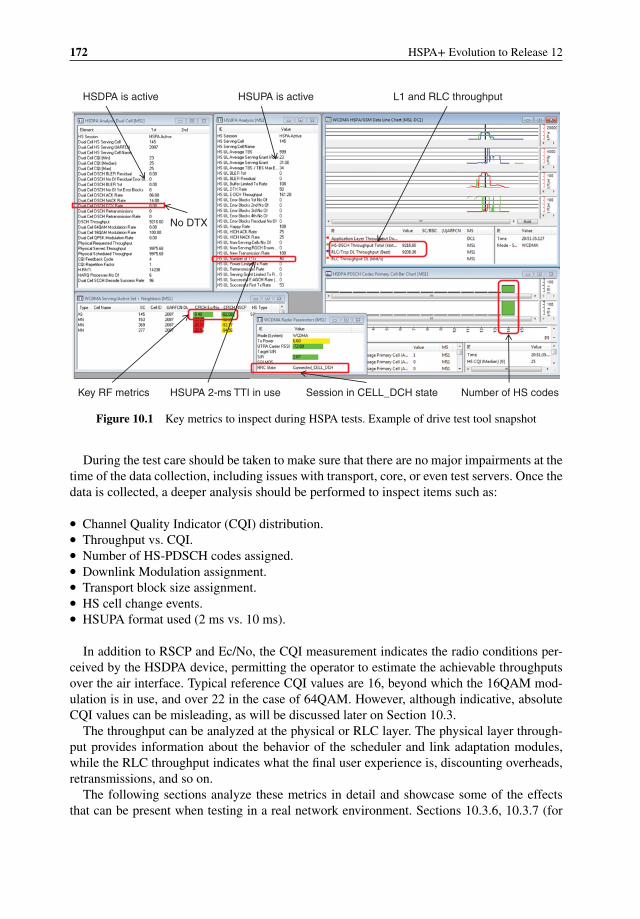
172 HSPA+ Evolution to Release 12
HSDPA is active HSUPA is active
Session in CELL_DCH stateKey RF metrics
No DTX
L1 and RLC throughput
Number of HS codesHSUPA 2-ms TTI in use
Figure 10.1 Key metrics to inspect during HSPA tests. Example of drive test tool snapshot
During the test care should be taken to make sure that there are no major impairments at thetime of the data collection, including issues with transport, core, or even test servers. Once thedata is collected, a deeper analysis should be performed to inspect items such as:
� Channel Quality Indicator (CQI) distribution.� Throughput vs. CQI.� Number of HS-PDSCH codes assigned.� Downlink Modulation assignment.� Transport block size assignment.� HS cell change events.� HSUPA format used (2 ms vs. 10 ms).
In addition to RSCP and Ec/No, the CQI measurement indicates the radio conditions per-ceived by the HSDPA device, permitting the operator to estimate the achievable throughputsover the air interface. Typical reference CQI values are 16, beyond which the 16QAM mod-ulation is in use, and over 22 in the case of 64QAM. However, although indicative, absoluteCQI values can be misleading, as will be discussed later on Section 10.3.
The throughput can be analyzed at the physical or RLC layer. The physical layer through-put provides information about the behavior of the scheduler and link adaptation modules,while the RLC throughput indicates what the final user experience is, discounting overheads,retransmissions, and so on.
The following sections analyze these metrics in detail and showcase some of the effectsthat can be present when testing in a real network environment. Sections 10.3.6, 10.3.7 (for

HSPA+ Performance 173
single carrier), and 10.4.1 and 10.4.2 (for dual cell), present performance summaries, includingreference throughput curves based on realistic expectations.
10.3 Single-Carrier HSPA+This section discusses the performance of HSPA+ Single Carrier with 64QAM and Type 3ireceivers. This configuration represents a common baseline for typical HSPA+ deployments;therefore a deep analysis of its performance can be used as a basis to understand more advancedfeatures, such as dual cell or 2 × 2 MIMO.
Downlink 64QAM was one of the first features to be available in HSPA+ networks anddevices since its definition in 3GPP Release 7 standards. It enables up to 50% faster downlinkdata transmissions in areas with a good Signal to Interference Ratio (SINR) thanks to a highermodulation and the utilization of bigger transport block sizes. HSPA+ mobile devices with64QAM are capable of theoretical speeds of 21 Mbps for single carrier devices, which inpractice provide around 16 Mbps of average IP level throughput in excellent radio conditions.To take full advantage of this feature it is recommended to combine it with an advanced receiver(Type 3i), that will increase the probability of utilizing the higher modulation. Section 10.5analyzes in detail the performance gains from 64QAM and Type 3i as compared to Release 6HSDPA.
Both these features are relatively simple to implement and are found today in all high endsmartphones, as well as in many low–medium end devices.
10.3.1 Test Scenarios
The performance of HSPA+ single carrier will be analyzed over multiple radio conditions,including stationary and mobility scenarios, based on measurements from a live network.
The network was configured with one transmit and up to four receive antennas, withadvanced uplink receiver features in use, including 4-Way Receive Diversity and UplinkInterference Cancellation. In the downlink direction, the HSDPA service was configured witha maximum of 14 PDSCH codes. The test device was a HSPA+ Cat 14 HSDPA (21 Mbps)and Cat 6 HSUPA (5.76 Mbps), featuring a Type 3i receiver.
The stationary results discussed in Sections 10.3.2 to 10.3.5 were obtained under variousscenarios with good, mid, and poor signal strength. The most relevant metrics are discussedto illustrate different characteristics of the HSPA+ service, such as the dependency on RSCPand CQI, the assignment of a certain modulation scheme, and others.
The different RF conditions discussed correspond to typical signal strength ranges that canoften be found in live networks, spanning from −80 dBm to −102 dBm of Received PilotSignal Power (RSCP). The test results were collected during a period of low traffic to be ableto show the performance of the technology independently from load effects.
Section 10.3.7 also analyzes the HSPA+ performance under mobility conditions. As willbe noted, the performance in stationary conditions is usually better than in mobile conditions,where effects from fading and HS cell changes can degrade the quality of the signal. Whileit is important to analyze both cases, it should be noted that the majority of data customersaccess their services while in stationary conditions, therefore stationary results are closer towhat customers can expect from the technology in practical terms.
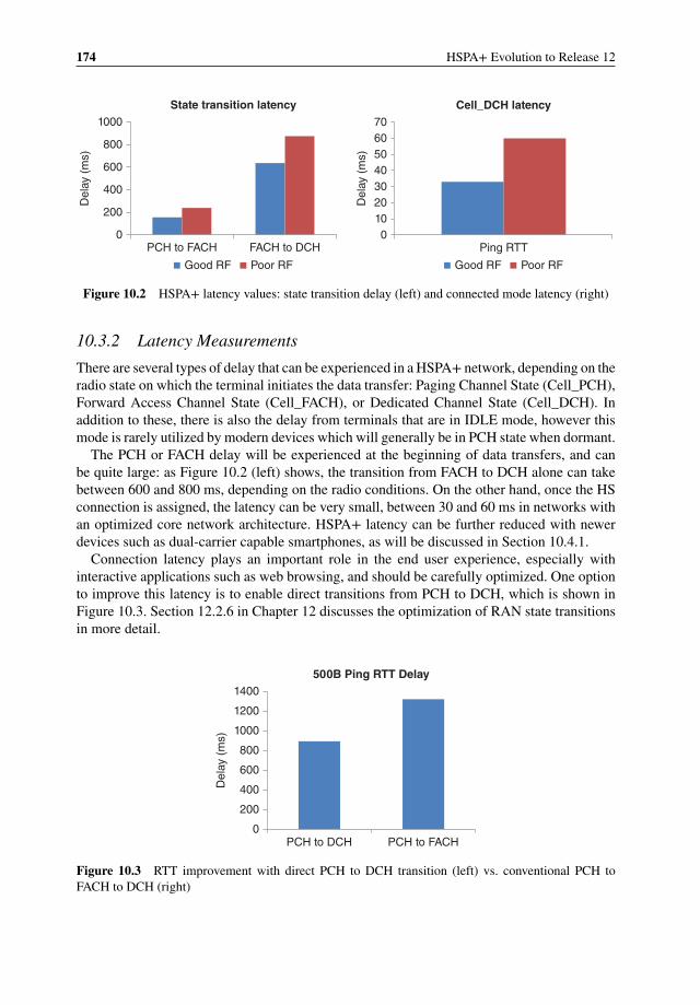
174 HSPA+ Evolution to Release 12
0
200
400
600
800
1000
PCH to FACH FACH to DCH
State transition latency
Good RF Poor RF Good RF Poor RF
010203040506070
Ping RTT
Del
ay (
ms)
Del
ay (
ms)
Cell_DCH latency
Figure 10.2 HSPA+ latency values: state transition delay (left) and connected mode latency (right)
10.3.2 Latency Measurements
There are several types of delay that can be experienced in a HSPA+ network, depending on theradio state on which the terminal initiates the data transfer: Paging Channel State (Cell_PCH),Forward Access Channel State (Cell_FACH), or Dedicated Channel State (Cell_DCH). Inaddition to these, there is also the delay from terminals that are in IDLE mode, however thismode is rarely utilized by modern devices which will generally be in PCH state when dormant.
The PCH or FACH delay will be experienced at the beginning of data transfers, and canbe quite large: as Figure 10.2 (left) shows, the transition from FACH to DCH alone can takebetween 600 and 800 ms, depending on the radio conditions. On the other hand, once the HSconnection is assigned, the latency can be very small, between 30 and 60 ms in networks withan optimized core network architecture. HSPA+ latency can be further reduced with newerdevices such as dual-carrier capable smartphones, as will be discussed in Section 10.4.1.
Connection latency plays an important role in the end user experience, especially withinteractive applications such as web browsing, and should be carefully optimized. One optionto improve this latency is to enable direct transitions from PCH to DCH, which is shown inFigure 10.3. Section 12.2.6 in Chapter 12 discusses the optimization of RAN state transitionsin more detail.
0
200
400
600
800
1000
1200
1400
PCH to DCH PCH to FACH
Del
ay (
ms)
500B Ping RTT Delay
Figure 10.3 RTT improvement with direct PCH to DCH transition (left) vs. conventional PCH toFACH to DCH (right)
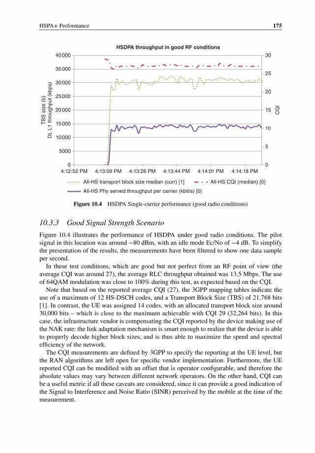
HSPA+ Performance 175
0
5
10
15
20
25
30
0
5000
10000
15000
20000
25000
30000
35000
40000
4:12:52 PM 4:13:09 PM 4:13:26 PM 4:13:44 PM 4:14:01 PM 4:14:18 PM
CQ
I
TB
S s
ize
(b)
DL
L1 th
roug
hput
(kb
ps)
HSDPA throughput in good RF conditions
All-HS transport block size median (curr) [1]
All-HS Phy served throughput per carrier (kbit/s) [0]
All-HS CQI (median) [0]
Figure 10.4 HSDPA Single-carrier performance (good radio conditions)
10.3.3 Good Signal Strength Scenario
Figure 10.4 illustrates the performance of HSDPA under good radio conditions. The pilotsignal in this location was around −80 dBm, with an idle mode Ec/No of −4 dB. To simplifythe presentation of the results, the measurements have been filtered to show one data sampleper second.
In these test conditions, which are good but not perfect from an RF point of view (theaverage CQI was around 27), the average RLC throughput obtained was 13.5 Mbps. The useof 64QAM modulation was close to 100% during this test, as expected based on the CQI.
Note that based on the reported average CQI (27), the 3GPP mapping tables indicate theuse of a maximum of 12 HS-DSCH codes, and a Transport Block Size (TBS) of 21,768 bits[1]. In contrast, the UE was assigned 14 codes, with an allocated transport block size around30,000 bits – which is close to the maximum achievable with CQI 29 (32,264 bits). In thiscase, the infrastructure vendor is compensating the CQI reported by the device making use ofthe NAK rate: the link adaptation mechanism is smart enough to realize that the device is ableto properly decode higher block sizes, and is thus able to maximize the speed and spectralefficiency of the network.
The CQI measurements are defined by 3GPP to specify the reporting at the UE level, butthe RAN algorithms are left open for specific vendor implementation. Furthermore, the UEreported CQI can be modified with an offset that is operator configurable, and therefore theabsolute values may vary between different network operators. On the other hand, CQI canbe a useful metric if all these caveats are considered, since it can provide a good indication ofthe Signal to Interference and Noise Ratio (SINR) perceived by the mobile at the time of themeasurement.
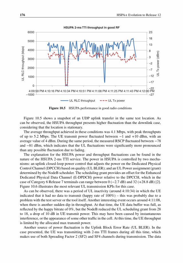
176 HSPA+ Evolution to Release 12
–27
–22
–17
–12
–7
–2
3
8
13
18
23
–1000
0
1000
2000
3000
4000
5000
6000
4:09:59 PM 4:10:16 PM 4:10:34 PM 4:10:51 PM 4:11:08 PM 4:11:25 PM 4:11:43 PM 4:12:00 PM
UL
Tx
pow
er (
dBm
)
UL
RLC
thro
ughp
ut (
kbps
)
HSUPA 2-ms TTI throughput in good RF
UL RLC throughput UL Tx power
Figure 10.5 HSUPA performance in good radio conditions
Figure 10.5 shows a snapshot of an UDP uplink transfer in the same test location. Ascan be observed, the HSUPA throughput presents higher fluctuation than the downlink case,considering that the location is stationary.
The average throughput achieved in these conditions was 4.1 Mbps, with peak throughputsof up to 5.2 Mbps. The UE transmit power fluctuated between −1 and +10 dBm, with anaverage value of 4 dBm. During the same period, the measured RSCP fluctuated between −78and −81 dBm, which indicates that the UL fluctuations were significantly more pronouncedthan any possible fluctuation due to fading.
The explanation for the HSUPA power and throughput fluctuations can be found in thenature of the HSUPA 2-ms TTI service. The power in HSUPA is controlled by two mecha-nisms: an uplink closed-loop power control that adjusts the power on the Dedicated PhysicalControl Channel (DPCCH) based on quality (UL BLER); and an UL Power assignment (grant)determined by the NodeB scheduler. The scheduling grant provides an offset for the EnhancedDedicated Physical Data Channel (E-DPDCH) power relative to the DPCCH, which in thecase of Category 6 Release 7 terminals can range between 0 (−2.7 dB) and 32 (+28.8 dB) [2].Figure 10.6 illustrates the most relevant UL transmission KPIs for this case.
As can be observed, there was a period of UL inactivity (around 4:10:34) in which the UEindicated that it had no data to transmit (happy rate of 100%) – this was probably due to aproblem with the test server or the tool itself. Another interesting event occurs around 4:11:08,when there is another sudden dip in throughput. At that time, the UE data buffer was full, asreflected by the happy bitrate of 0%, but the NodeB reduced the UL scheduling grant from 28to 18, a drop of 10 dB in UE transmit power. This may have been caused by instantaneousinterference, or the appearance of some other traffic in the cell. At this time, the UE throughputis limited by the allocated max transmit power.
Another source of power fluctuation is the Uplink Block Error Rate (UL BLER). In thecase presented, the UE was transmitting with 2-ms TTI frames during all this time, whichmakes use of both Spreading Factor 2 (SF2) and SF4 channels during transmission. The data
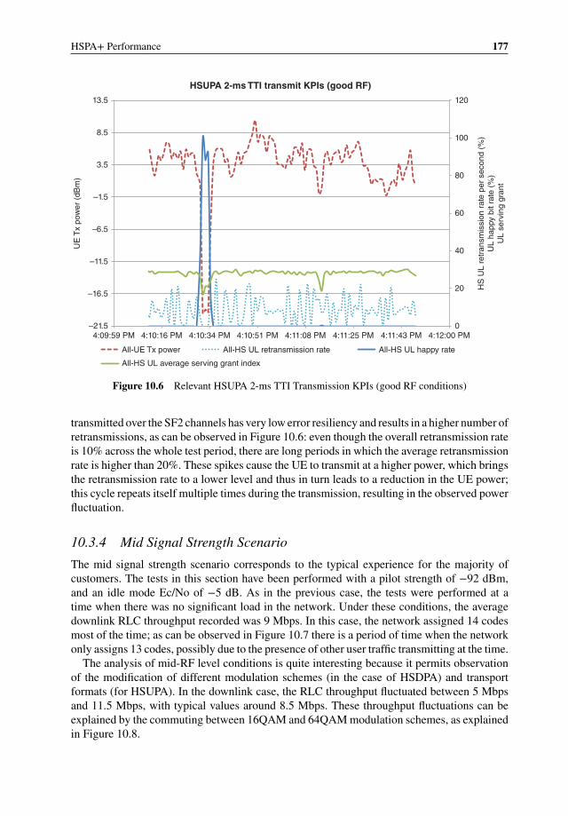
HSPA+ Performance 177
0
20
40
60
80
100
120
–21.5
–16.5
–11.5
–6.5
–1.5
3.5
8.5
13.5
4:09:59 PM 4:10:16 PM 4:10:34 PM 4:10:51 PM 4:11:08 PM 4:11:25 PM 4:11:43 PM 4:12:00 PM
HS
UL
retr
ansm
issi
on r
ate
per
seco
nd (
%)
UL
happ
y bi
t rat
e (%
)U
L se
rvin
g gr
ant
UE
Tx
pow
er (
dBm
)HSUPA 2-ms TTI transmit KPIs (good RF)
All-UE Tx power All-HS UL retransmission rate All-HS UL happy rate
All-HS UL average serving grant index
Figure 10.6 Relevant HSUPA 2-ms TTI Transmission KPIs (good RF conditions)
transmitted over the SF2 channels has very low error resiliency and results in a higher number ofretransmissions, as can be observed in Figure 10.6: even though the overall retransmission rateis 10% across the whole test period, there are long periods in which the average retransmissionrate is higher than 20%. These spikes cause the UE to transmit at a higher power, which bringsthe retransmission rate to a lower level and thus in turn leads to a reduction in the UE power;this cycle repeats itself multiple times during the transmission, resulting in the observed powerfluctuation.
10.3.4 Mid Signal Strength Scenario
The mid signal strength scenario corresponds to the typical experience for the majority ofcustomers. The tests in this section have been performed with a pilot strength of −92 dBm,and an idle mode Ec/No of −5 dB. As in the previous case, the tests were performed at atime when there was no significant load in the network. Under these conditions, the averagedownlink RLC throughput recorded was 9 Mbps. In this case, the network assigned 14 codesmost of the time; as can be observed in Figure 10.7 there is a period of time when the networkonly assigns 13 codes, possibly due to the presence of other user traffic transmitting at the time.
The analysis of mid-RF level conditions is quite interesting because it permits observationof the modification of different modulation schemes (in the case of HSDPA) and transportformats (for HSUPA). In the downlink case, the RLC throughput fluctuated between 5 Mbpsand 11.5 Mbps, with typical values around 8.5 Mbps. These throughput fluctuations can beexplained by the commuting between 16QAM and 64QAM modulation schemes, as explainedin Figure 10.8.

178 HSPA+ Evolution to Release 12
0
5
10
15
20
25
30
0
5000
10000
15000
20000
25000
30000
8:10:45 AM 8:10:54 AM 8:11:02 AM 8:11:11 AM 8:11:20 AM 8:11:28 AM
CQ
I#
HS
cod
es
TB
S s
ize
(b)
DL
L1 th
roug
hput
(kb
ps)
HSDPA throughput in mid RF conditions
All-HS Phy served throughput total (kbit/s)
All-HS transport block size median (curr) [1] All-HS CQI (median) [0]
Av code
Figure 10.7 HSDPA throughput in mid RF conditions
0
12.5
25
37.5
50
62.5
75
87.5
100
–105
–100
–95
–90
–85
–80
8:10:36 AM 8:10:45 AM 8:10:54 AM 8:11:02 AM 8:11:11 AM 8:11:20 AM 8:11:28 AM 8:11:37 AM
64Q
AM
mod
ulat
ion
rate
(%
)C
QI
RS
CP
(dB
m)
64QAM rate vs. RSCP, CQI
All-SAN CPICH RSCP [1] All-HS 64-QAM modulation rate [0]
All-HS CQI (median) [0]
Figure 10.8 64QAM modulation assignment with changing CQI values
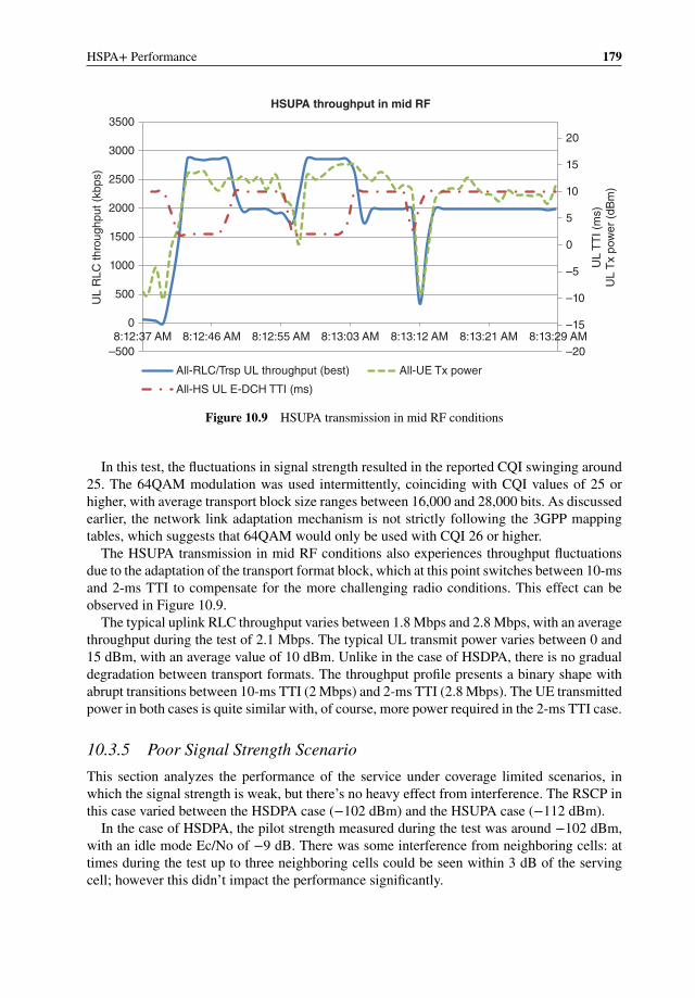
HSPA+ Performance 179
–20
–15
–10
–5
0
5
10
15
20
–500
0
500
1000
1500
2000
2500
3000
3500
8:12:37 AM 8:12:46 AM 8:12:55 AM 8:13:03 AM 8:13:12 AM 8:13:21 AM 8:13:29 AM
UL
TT
I (m
s)U
L T
x po
wer
(dB
m)
UL
RLC
thro
ughp
ut (
kbps
)HSUPA throughput in mid RF
All-RLC/Trsp UL throughput (best) All-UE Tx power
All-HS UL E-DCH TTI (ms)
Figure 10.9 HSUPA transmission in mid RF conditions
In this test, the fluctuations in signal strength resulted in the reported CQI swinging around25. The 64QAM modulation was used intermittently, coinciding with CQI values of 25 orhigher, with average transport block size ranges between 16,000 and 28,000 bits. As discussedearlier, the network link adaptation mechanism is not strictly following the 3GPP mappingtables, which suggests that 64QAM would only be used with CQI 26 or higher.
The HSUPA transmission in mid RF conditions also experiences throughput fluctuationsdue to the adaptation of the transport format block, which at this point switches between 10-msand 2-ms TTI to compensate for the more challenging radio conditions. This effect can beobserved in Figure 10.9.
The typical uplink RLC throughput varies between 1.8 Mbps and 2.8 Mbps, with an averagethroughput during the test of 2.1 Mbps. The typical UL transmit power varies between 0 and15 dBm, with an average value of 10 dBm. Unlike in the case of HSDPA, there is no gradualdegradation between transport formats. The throughput profile presents a binary shape withabrupt transitions between 10-ms TTI (2 Mbps) and 2-ms TTI (2.8 Mbps). The UE transmittedpower in both cases is quite similar with, of course, more power required in the 2-ms TTI case.
10.3.5 Poor Signal Strength Scenario
This section analyzes the performance of the service under coverage limited scenarios, inwhich the signal strength is weak, but there’s no heavy effect from interference. The RSCP inthis case varied between the HSDPA case (−102 dBm) and the HSUPA case (−112 dBm).
In the case of HSDPA, the pilot strength measured during the test was around −102 dBm,with an idle mode Ec/No of −9 dB. There was some interference from neighboring cells: attimes during the test up to three neighboring cells could be seen within 3 dB of the servingcell; however this didn’t impact the performance significantly.

180 HSPA+ Evolution to Release 12
0
5
10
15
20
25
0
2000
4000
6000
8000
10000
12000
14000
16000
18000
11:45:36 AM 11:45:53 AM 11:46:11 AM 11:46:28 AM 11:46:45 AM 11:47:02 AM 11:47:20 AM
CQ
I
TB
S s
ize
(b)
DL
RLC
thro
ughp
ut (
kbps
)HSDPA throughput in poor RF conditions
All-RLC/Trsp DL throughput (best)
All-HS transport block size median (curr) [1]
All-HS CQI (median) [0]
Figure 10.10 HSDPA performance in weak signal strength conditions
There was a significant fluctuation of signal strength at the test location, with RSCP valuesranging from −107 dBm to −95 dBm. In these conditions, the HSDPA throughput experiencedlarge variations, ranging between 2 and 6 Mbps. The changes in throughput can be explainedby the fluctuations in signal strength, which can indirectly be observed in the CQI changes inFigure 10.10.
The performance measurements under poor RF conditions are extracted from the periodwith the weakest radio conditions (average RSCP of −102 dBm). In this case, the average CQIwas 13, and the corresponding average throughput was 2.5 Mbps.
As in previous cases, the transport block sizes assigned were significantly higher thanexpected: in the worse radio conditions (CQI 13), the network assigns around 5000 bitsinstead of the 2288 bits from 3GPP mapping tables. Also, all 14 codes are used instead of the4 suggested by the standards. This results in an overall improved user experience at the celledge, in addition to significant capacity gains.
The variation in signal strength during this test permits showcasing the behavior of linkadaptation when switching between QPSK and 16QAM. As Figure 10.11 illustrates, duringthe tests there were a few occasions when the 16QAM modulation was used; these correspondto periods when the signal strength was stronger (typically over −98 dBm), with reported CQIvalues over 15. The QPSK modulation was used when the CQI value remained under 15.
In the case of HSUPA, the test conditions were quite challenging, with RSCP of −112 dBmand an idle mode Ec/No of −13 dB. Under these conditions, the UE was using the 10-ms TTItransport format and transmitting at full power all the time, as shown in Figure 10.12.
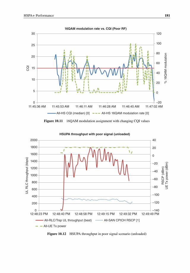
HSPA+ Performance 181
–20
0
20
40
60
80
100
120
0
5
10
15
20
25
30
11:45:36 AM 11:45:53 AM 11:46:11 AM 11:46:28 AM 11:46:45 AM 11:47:02 AM
% 1
6QA
M m
odul
atio
n
CQ
I16QAM modulation rate vs. CQI (Poor RF)
All-HS CQI (median) [0] All-HS 16QAM modulation rate [0]
Figure 10.11 16QAM modulation assignment with changing CQI values
–140
–120
–100
–80
–60
–40
–20
0
20
40
0
200
400
600
800
1000
1200
1400
1600
1800
2000
12:48:23 PM 12:48:40 PM 12:48:58 PM 12:49:15 PM 12:49:32 PM 12:49:49 PM
RS
CP
(dB
m)
UE
Tx
pow
er (
dBm
)
UL
RLC
thro
ughp
ut (
kbps
)
HSUPA throughput with poor signal (unloaded)
All-RLC/Trsp UL throughput (best) All-SAN CPICH RSCP [1]
All-UE Tx power
Figure 10.12 HSUPA throughput in poor signal scenario (unloaded)
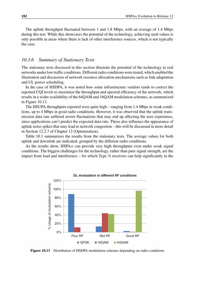
182 HSPA+ Evolution to Release 12
The uplink throughput fluctuated between 1 and 1.8 Mbps, with an average of 1.4 Mbpsduring this test. While this showcases the potential of the technology, achieving such values isonly possible in areas where there is lack of other interference sources, which is not typicallythe case.
10.3.6 Summary of Stationary Tests
The stationary tests discussed in this section illustrate the potential of the technology in realnetworks under low traffic conditions. Different radio conditions were tested, which enabled theillustration and discussion of network resource allocation mechanisms such as link adaptationand UL power scheduling.
In the case of HSDPA, it was noted how some infrastructure vendors tends to correct thereported CQI levels to maximize the throughput and spectral efficiency of the network, whichresults in a wider availability of the 64QAM and 16QAM modulation schemes, as summarizedin Figure 10.13.
The HSUPA throughputs reported were quite high – ranging from 1.4 Mbps in weak condi-tions, up to 4 Mbps in good radio conditions. However, it was observed that the uplink trans-mission data rate suffered severe fluctuations that may end up affecting the user experience,since applications can’t predict the expected data rate. These also influence the appearance ofuplink noise spikes that may lead to network congestion – this will be discussed in more detailin Section 12.2.7 of Chapter 12 (Optimization).
Table 10.1 summarizes the results from the stationary tests. The average values for bothuplink and downlink are indicated, grouped by the different radio conditions.
As the results show, HSPA+ can provide very high throughputs even under weak signalconditions. The biggest challenges for the technology, rather than pure signal strength, are theimpact from load and interference – for which Type 3i receivers can help significantly in the
0%
20%
40%
60%
80%
100%
120%
Poor RF Mid RF Good RF
% U
sage
of m
odul
atio
n sc
hem
e
DL modulation in different RF conditions
QPSK 16QAM 64QAM
Figure 10.13 Distribution of HSDPA modulation schemes depending on radio conditions
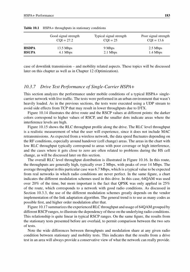
HSPA+ Performance 183
Table 10.1 HSPA+ throughputs in stationary conditions
Good signal strengthCQI = 27.2
Typical signal strengthCQI = 25
Poor signal strengthCQI = 13.6
HSDPA 13.5 Mbps 9 Mbps 2.5 MbpsHSUPA 4.1 Mbps 2.1 Mbps 1.4 Mbps
case of downlink transmission – and mobility related aspects. These topics will be discussedlater on this chapter as well as in Chapter 12 (Optimization).
10.3.7 Drive Test Performance of Single-Carrier HSPA+This section analyzes the performance under mobile conditions of a typical HSPA+ single-carrier network with live traffic. The tests were performed in an urban environment that wasn’theavily loaded. As in the previous sections, the tests were executed using a UDP stream toavoid side effects from TCP that may result in lower throughputs due to DTX.
Figure 10.14 illustrates the drive route and the RSCP values at different points: the darkercolors correspond to higher values of RSCP, and the smaller dots indicate areas where theinterference levels are high.
Figure 10.15 shows the RLC throughput profile along the drive. The RLC level throughputis a realistic measurement of what the user will experience, since it does not include MACretransmissions. As expected from a wireless network, the data speed fluctuates depending onthe RF conditions, especially around handover (cell change) areas. The areas in the chart withlow RLC throughput typically correspond to areas with poor coverage or high interference,and the cases where it gets close to zero are often related to problems during the HS cellchange, as will be discussed later on this section.
The overall RLC level throughput distribution is illustrated in Figure 10.16. In this route,the throughputs are generally high, typically over 2 Mbps, with peaks of over 14 Mbps. Theaverage throughput in this particular case was 6.7 Mbps, which is a typical value to be expectedfrom real networks in which radio conditions are never perfect. In the same figure, a chartindicates the different modulation schemes used in this drive. In this case, 64QAM was usedover 20% of the time, but more important is the fact that QPSK was only applied in 25%of the route, which corresponds to a network with good radio conditions. As discussed inSection 10.3.3, the use of the different modulation schemes greatly depends on the vendorimplementation of the link adaptation algorithm. The general trend is to use as many codes aspossible first, and higher order modulation after that.
Figure 10.17 summarizes the experienced RLC throughput and usage of 64QAM grouped bydifferent RSCP ranges, to illustrate the dependency of these on the underlying radio conditions.This relationship is quite linear in typical RSCP ranges. On the same figure, the results fromthe stationary tests presented before are overlaid, to permit comparison between the two setsof tests.
Note the wide differences between throughputs and modulation share at any given radiocondition between stationary and mobility tests. This indicates that the results from a drivetest in an area will always provide a conservative view of what the network can really provide.
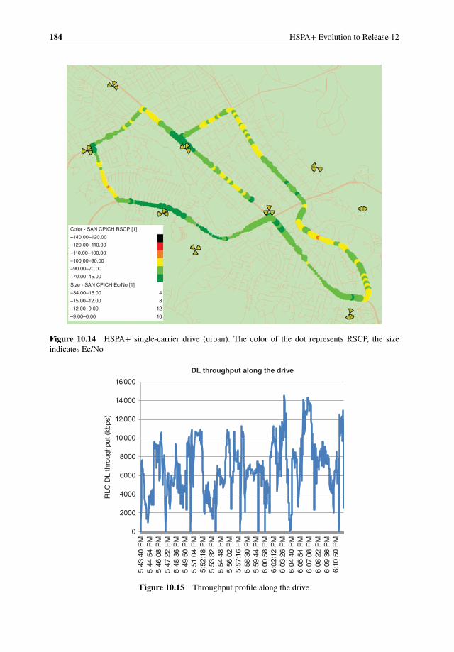
184 HSPA+ Evolution to Release 12
Color - SAN CPICH RSCP [1]
–140.00–120.00
–120.00–110.00
–110.00–100.00
–100.00–90.00
–90.00–70.00
–70.00–15.00
Size - SAN CPICH Ec/No [1]
–34.00–15.00
–15.00–12.00
–12.00–9.00
–9.00–0.00
4
8
12
16
Figure 10.14 HSPA+ single-carrier drive (urban). The color of the dot represents RSCP, the sizeindicates Ec/No
0
2000
4000
6000
8000
10000
12000
14000
16000
5:43
:40
PM
5:44
:54
PM
5:46
:08
PM
5:47
:22
PM
5:48
:36
PM
5:49
:50
PM
5:51
:04
PM
5:52
:18
PM
5:53
:32
PM
5:54
:48
PM
5:56
:02
PM
5:57
:16
PM
5:58
:30
PM
5:59
:44
PM
6:00
:58
PM
6:02
:12
PM
6:03
:26
PM
6:04
:40
PM
6:05
:54
PM
6:07
:08
PM
6:08
:22
PM
6:09
:36
PM
6:10
:50
PM
RLC
DL
thro
ughp
ut (
kbps
)
DL throughput along the drive
Figure 10.15 Throughput profile along the drive

HSPA+ Performance 185
0.00%
20.00%
40.00%
60.00%
80.00%
100.00%
120.00%
0 2000 4000 6000 8000 10000 12000 14000
CD
F (
%)
DL RLC throughput (kbps)
Throughput distribution along the drive
25%
54%
21%
Use of DL modulation schemes
QPSK 16QAM 64QAM
Figure 10.16 DL throughput distribution and DL modulation scheme used along the drive
0
10
20
30
40
50
60
70
80
90
100
0
2000
4000
6000
8000
10000
12000
14000
16000
–110 –100 –90 –80 –70 –60 –50 –40
Use
of 6
4QA
M m
odul
atio
n (%
)
DL
thro
ughp
ut (
kbps
)
RSCP (dBm)
Throughput and 64QAM vs. RSCP
Average RLC throughput (drive) Average RLC throughput (stationary)
Average share of 64QAM (stationary)Average share of 64QAM (drive)
Figure 10.17 Average throughput and 64QAM usage vs. RSCP for single carrier HSPA+
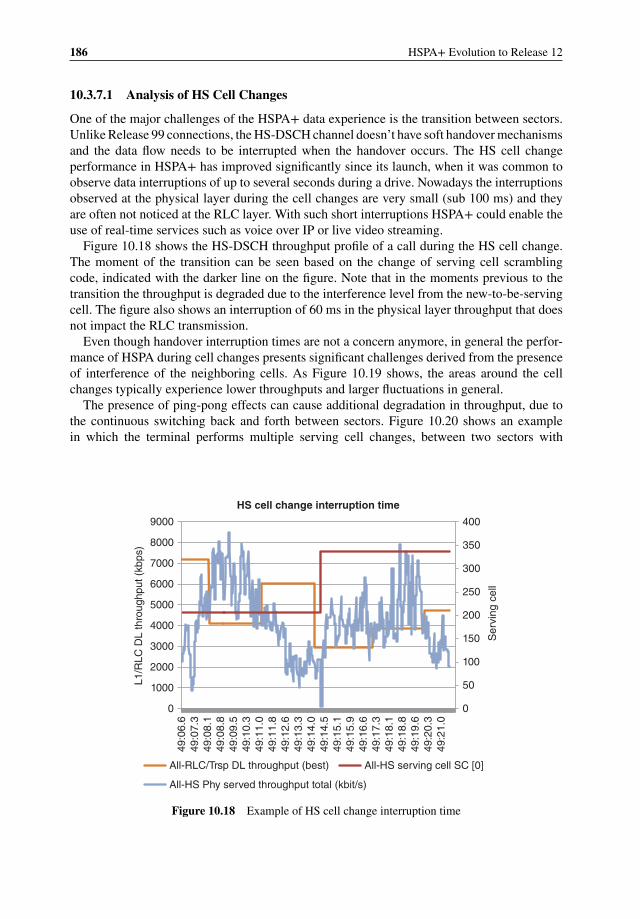
186 HSPA+ Evolution to Release 12
10.3.7.1 Analysis of HS Cell Changes
One of the major challenges of the HSPA+ data experience is the transition between sectors.Unlike Release 99 connections, the HS-DSCH channel doesn’t have soft handover mechanismsand the data flow needs to be interrupted when the handover occurs. The HS cell changeperformance in HSPA+ has improved significantly since its launch, when it was common toobserve data interruptions of up to several seconds during a drive. Nowadays the interruptionsobserved at the physical layer during the cell changes are very small (sub 100 ms) and theyare often not noticed at the RLC layer. With such short interruptions HSPA+ could enable theuse of real-time services such as voice over IP or live video streaming.
Figure 10.18 shows the HS-DSCH throughput profile of a call during the HS cell change.The moment of the transition can be seen based on the change of serving cell scramblingcode, indicated with the darker line on the figure. Note that in the moments previous to thetransition the throughput is degraded due to the interference level from the new-to-be-servingcell. The figure also shows an interruption of 60 ms in the physical layer throughput that doesnot impact the RLC transmission.
Even though handover interruption times are not a concern anymore, in general the perfor-mance of HSPA during cell changes presents significant challenges derived from the presenceof interference of the neighboring cells. As Figure 10.19 shows, the areas around the cellchanges typically experience lower throughputs and larger fluctuations in general.
The presence of ping-pong effects can cause additional degradation in throughput, due tothe continuous switching back and forth between sectors. Figure 10.20 shows an examplein which the terminal performs multiple serving cell changes, between two sectors with
0
50
100
150
200
250
300
350
400
0
1000
2000
3000
4000
5000
6000
7000
8000
9000
49:0
6.6
49:0
7.3
49:0
8.1
49:0
8.8
49:0
9.5
49:1
0.3
49:1
1.0
49:1
1.8
49:1
2.6
49:1
3.3
49:1
4.0
49:1
4.5
49:1
5.1
49:1
5.9
49:1
6.6
49:1
7.3
49:1
8.1
49:1
8.8
49:1
9.6
49:2
0.3
49:2
1.0
Ser
ving
cel
l
L1/R
LC D
L th
roug
hput
(kb
ps)
HS cell change interruption time
All-RLC/Trsp DL throughput (best)
All-HS Phy served throughput total (kbit/s)
All-HS serving cell SC [0]
Figure 10.18 Example of HS cell change interruption time
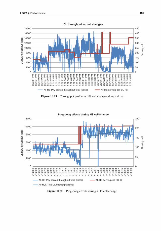
HSPA+ Performance 187
0
50
100
150
200
250
300
350
400
450
0
2000
4000
6000
8000
10000
12000
14000
16000
18000
6:00
:51
PM
6:01
:01
PM
6:01
:10
PM
6:01
:19
PM
6:01
:27
PM
6:01
:36
PM
6:01
:45
PM
6:01
:53
PM
6:02
:03
PM
6:02
:12
PM
6:02
:21
PM
6:02
:30
PM
6:02
:38
PM
6:02
:46
PM
6:02
:55
PM
6:03
:04
PM
6:03
:13
PM
6:03
:21
PM
6:03
:31
PM
6:03
:40
PM
6:03
:49
PM
6:03
:58
PM
6:04
:07
PM
6:04
:14
PM
6:04
:22
PM
6:04
:31
PM
6:04
:40
PM
6:04
:48
PM
6:04
:58
PM
6:05
:07
PM
6:05
:16
PM
6:05
:25
PM
6:05
:35
PM
6:05
:43
PM
Ser
ving
cel
l
L1/R
LC th
roug
hput
(kb
ps)
DL throughput vs. cell changes
All-HS Phy served throughput total (kbit/s) All-HS serving cell SC [0]
Figure 10.19 Throughput profile vs. HS cell changes along a drive
0
50
100
150
200
250
0
2000
4000
6000
8000
10000
12000
01:2
3.4
01:2
4.0
01:2
5.0
01:2
6.0
01:2
7.0
01:2
8.0
01:2
8.9
01:2
9.9
01:3
0.8
01:3
1.8
01:3
2.7
01:3
3.8
01:3
4.7
01:3
5.7
01:3
6.6
01:3
7.6
01:3
8.3
01:3
9.2
01:4
0.2
01:4
1.2
01:4
2.2
01:4
3.1
01:4
4.1
01:4
5.0
01:4
6.0
01:4
6.9
01:4
7.9
01:4
8.8
01:4
9.8
01:5
0.7
01:5
1.5
01:5
2.0
01:5
3.0
01:5
4.0
Ser
ving
cel
l
DL
RLC
thro
ughp
ut (
kbps
)
Ping-pong effects during HS cell change
All-HS Phy served throughput total (kbit/s)
All-RLC/Trsp DL throughput (best)
All-HS serving cell SC [0]
Figure 10.20 Ping-pong effects during a HS cell change
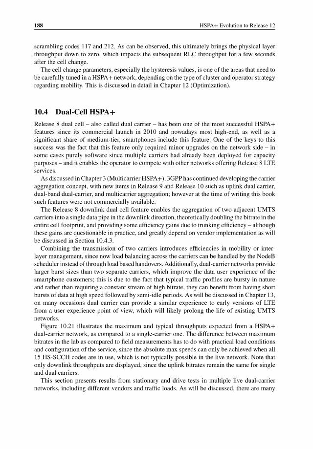
188 HSPA+ Evolution to Release 12
scrambling codes 117 and 212. As can be observed, this ultimately brings the physical layerthroughput down to zero, which impacts the subsequent RLC throughput for a few secondsafter the cell change.
The cell change parameters, especially the hysteresis values, is one of the areas that need tobe carefully tuned in a HSPA+ network, depending on the type of cluster and operator strategyregarding mobility. This is discussed in detail in Chapter 12 (Optimization).
10.4 Dual-Cell HSPA+Release 8 dual cell – also called dual carrier – has been one of the most successful HSPA+features since its commercial launch in 2010 and nowadays most high-end, as well as asignificant share of medium-tier, smartphones include this feature. One of the keys to thissuccess was the fact that this feature only required minor upgrades on the network side – insome cases purely software since multiple carriers had already been deployed for capacitypurposes – and it enables the operator to compete with other networks offering Release 8 LTEservices.
As discussed in Chapter 3 (Multicarrier HSPA+), 3GPP has continued developing the carrieraggregation concept, with new items in Release 9 and Release 10 such as uplink dual carrier,dual-band dual-carrier, and multicarrier aggregation; however at the time of writing this booksuch features were not commercially available.
The Release 8 downlink dual cell feature enables the aggregation of two adjacent UMTScarriers into a single data pipe in the downlink direction, theoretically doubling the bitrate in theentire cell footprint, and providing some efficiency gains due to trunking efficiency – althoughthese gains are questionable in practice, and greatly depend on vendor implementation as willbe discussed in Section 10.4.3.
Combining the transmission of two carriers introduces efficiencies in mobility or inter-layer management, since now load balancing across the carriers can be handled by the NodeBscheduler instead of through load based handovers. Additionally, dual-carrier networks providelarger burst sizes than two separate carriers, which improve the data user experience of thesmartphone customers; this is due to the fact that typical traffic profiles are bursty in natureand rather than requiring a constant stream of high bitrate, they can benefit from having shortbursts of data at high speed followed by semi-idle periods. As will be discussed in Chapter 13,on many occasions dual carrier can provide a similar experience to early versions of LTEfrom a user experience point of view, which will likely prolong the life of existing UMTSnetworks.
Figure 10.21 illustrates the maximum and typical throughputs expected from a HSPA+dual-carrier network, as compared to a single-carrier one. The difference between maximumbitrates in the lab as compared to field measurements has to do with practical load conditionsand configuration of the service, since the absolute max speeds can only be achieved when all15 HS-SCCH codes are in use, which is not typically possible in the live network. Note thatonly downlink throughputs are displayed, since the uplink bitrates remain the same for singleand dual carriers.
This section presents results from stationary and drive tests in multiple live dual-carriernetworks, including different vendors and traffic loads. As will be discussed, there are many
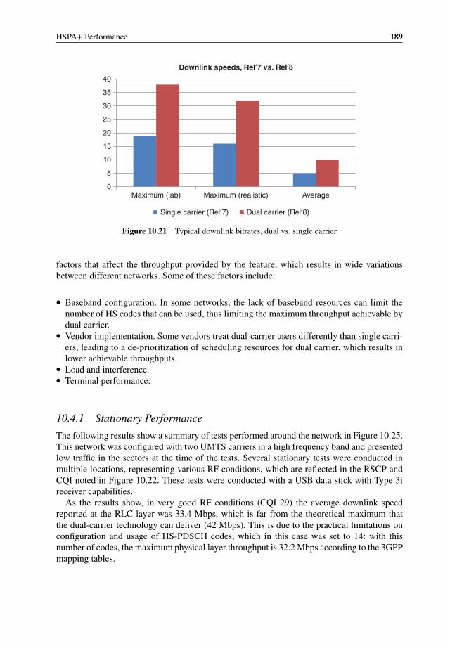
HSPA+ Performance 189
0
5
10
15
20
25
30
35
40
Maximum (lab) Maximum (realistic) Average
Downlink speeds, Rel′7 vs. Rel′8
Single carrier (Rel′7) Dual carrier (Rel′8)
Figure 10.21 Typical downlink bitrates, dual vs. single carrier
factors that affect the throughput provided by the feature, which results in wide variationsbetween different networks. Some of these factors include:
� Baseband configuration. In some networks, the lack of baseband resources can limit thenumber of HS codes that can be used, thus limiting the maximum throughput achievable bydual carrier.
� Vendor implementation. Some vendors treat dual-carrier users differently than single carri-ers, leading to a de-prioritization of scheduling resources for dual carrier, which results inlower achievable throughputs.
� Load and interference.� Terminal performance.
10.4.1 Stationary Performance
The following results show a summary of tests performed around the network in Figure 10.25.This network was configured with two UMTS carriers in a high frequency band and presentedlow traffic in the sectors at the time of the tests. Several stationary tests were conducted inmultiple locations, representing various RF conditions, which are reflected in the RSCP andCQI noted in Figure 10.22. These tests were conducted with a USB data stick with Type 3ireceiver capabilities.
As the results show, in very good RF conditions (CQI 29) the average downlink speedreported at the RLC layer was 33.4 Mbps, which is far from the theoretical maximum thatthe dual-carrier technology can deliver (42 Mbps). This is due to the practical limitations onconfiguration and usage of HS-PDSCH codes, which in this case was set to 14: with thisnumber of codes, the maximum physical layer throughput is 32.2 Mbps according to the 3GPPmapping tables.
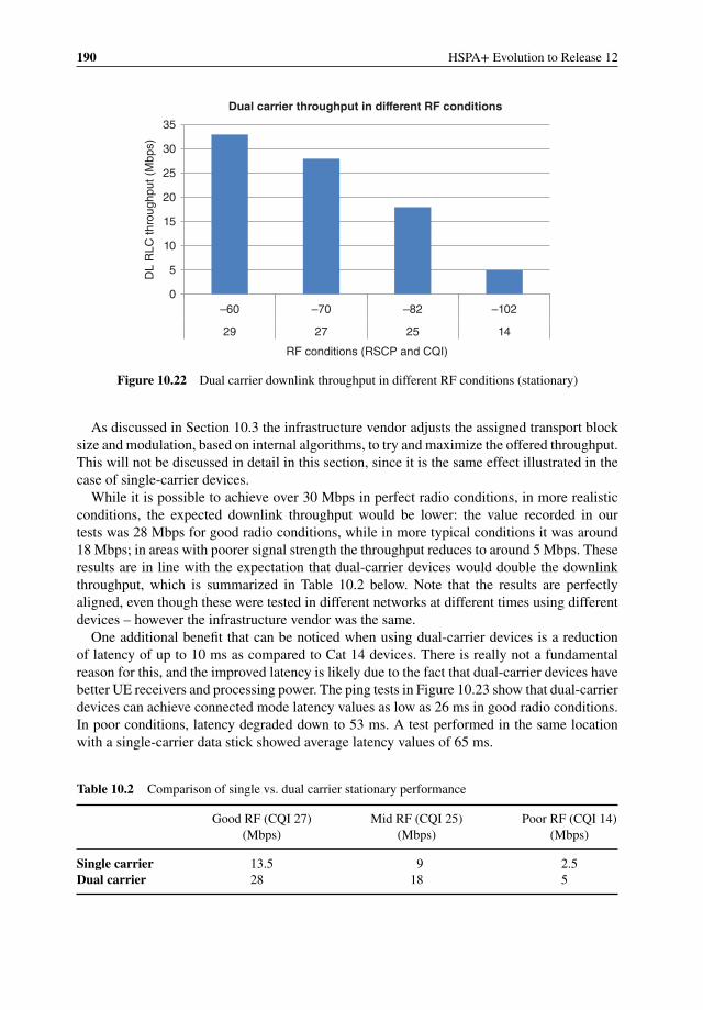
190 HSPA+ Evolution to Release 12
0
5
10
15
20
25
30
35
–102–82–70–60
14252729
DL
RLC
thro
ughp
ut (
Mbp
s)
RF conditions (RSCP and CQI)
Dual carrier throughput in different RF conditions
Figure 10.22 Dual carrier downlink throughput in different RF conditions (stationary)
As discussed in Section 10.3 the infrastructure vendor adjusts the assigned transport blocksize and modulation, based on internal algorithms, to try and maximize the offered throughput.This will not be discussed in detail in this section, since it is the same effect illustrated in thecase of single-carrier devices.
While it is possible to achieve over 30 Mbps in perfect radio conditions, in more realisticconditions, the expected downlink throughput would be lower: the value recorded in ourtests was 28 Mbps for good radio conditions, while in more typical conditions it was around18 Mbps; in areas with poorer signal strength the throughput reduces to around 5 Mbps. Theseresults are in line with the expectation that dual-carrier devices would double the downlinkthroughput, which is summarized in Table 10.2 below. Note that the results are perfectlyaligned, even though these were tested in different networks at different times using differentdevices – however the infrastructure vendor was the same.
One additional benefit that can be noticed when using dual-carrier devices is a reductionof latency of up to 10 ms as compared to Cat 14 devices. There is really not a fundamentalreason for this, and the improved latency is likely due to the fact that dual-carrier devices havebetter UE receivers and processing power. The ping tests in Figure 10.23 show that dual-carrierdevices can achieve connected mode latency values as low as 26 ms in good radio conditions.In poor conditions, latency degraded down to 53 ms. A test performed in the same locationwith a single-carrier data stick showed average latency values of 65 ms.
Table 10.2 Comparison of single vs. dual carrier stationary performance
Good RF (CQI 27)(Mbps)
Mid RF (CQI 25)(Mbps)
Poor RF (CQI 14)(Mbps)
Single carrier 13.5 9 2.5Dual carrier 28 18 5
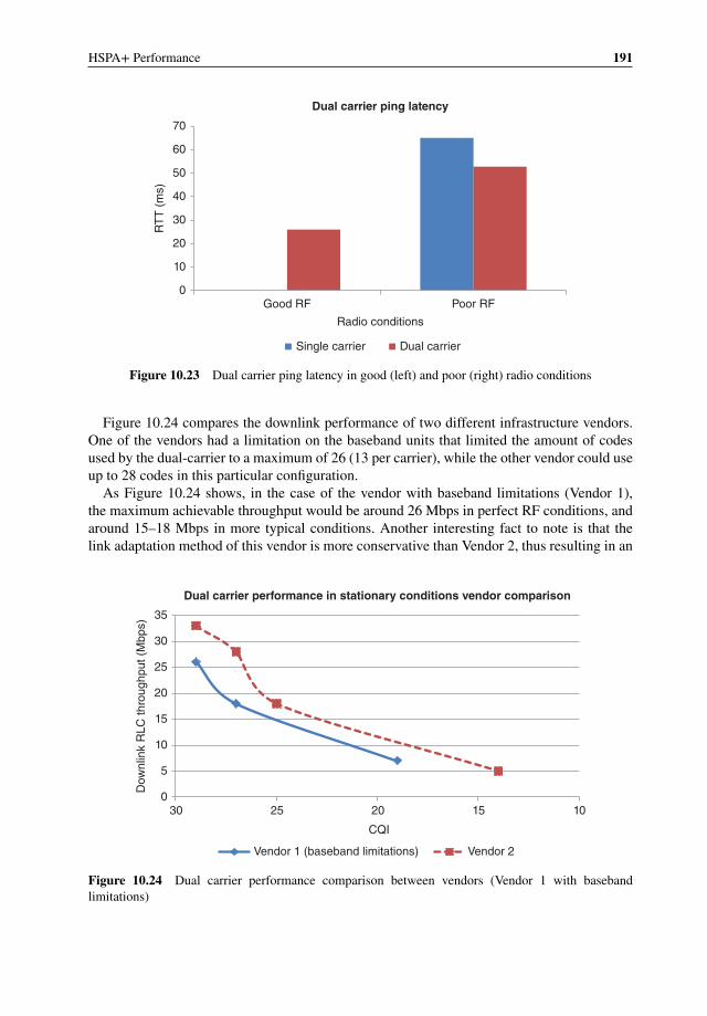
HSPA+ Performance 191
0
10
20
30
40
50
60
70
Good RF Poor RF
RT
T (
ms)
Radio conditions
Dual carrier ping latency
Single carrier Dual carrier
Figure 10.23 Dual carrier ping latency in good (left) and poor (right) radio conditions
Figure 10.24 compares the downlink performance of two different infrastructure vendors.One of the vendors had a limitation on the baseband units that limited the amount of codesused by the dual-carrier to a maximum of 26 (13 per carrier), while the other vendor could useup to 28 codes in this particular configuration.
As Figure 10.24 shows, in the case of the vendor with baseband limitations (Vendor 1),the maximum achievable throughput would be around 26 Mbps in perfect RF conditions, andaround 15–18 Mbps in more typical conditions. Another interesting fact to note is that thelink adaptation method of this vendor is more conservative than Vendor 2, thus resulting in an
0
5
10
15
20
25
30
35
1015202530
Dow
nlin
k R
LC th
roug
hput
(M
bps)
CQI
Dual carrier performance in stationary conditions vendor comparison
Vendor 1 (baseband limitations) Vendor 2
Figure 10.24 Dual carrier performance comparison between vendors (Vendor 1 with basebandlimitations)
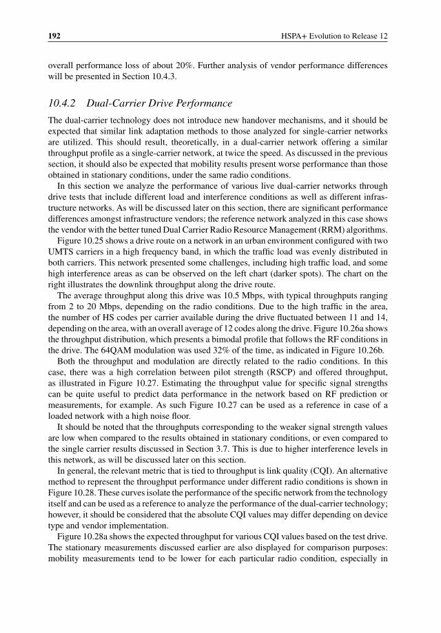
192 HSPA+ Evolution to Release 12
overall performance loss of about 20%. Further analysis of vendor performance differenceswill be presented in Section 10.4.3.
10.4.2 Dual-Carrier Drive Performance
The dual-carrier technology does not introduce new handover mechanisms, and it should beexpected that similar link adaptation methods to those analyzed for single-carrier networksare utilized. This should result, theoretically, in a dual-carrier network offering a similarthroughput profile as a single-carrier network, at twice the speed. As discussed in the previoussection, it should also be expected that mobility results present worse performance than thoseobtained in stationary conditions, under the same radio conditions.
In this section we analyze the performance of various live dual-carrier networks throughdrive tests that include different load and interference conditions as well as different infras-tructure networks. As will be discussed later on this section, there are significant performancedifferences amongst infrastructure vendors; the reference network analyzed in this case showsthe vendor with the better tuned Dual Carrier Radio Resource Management (RRM) algorithms.
Figure 10.25 shows a drive route on a network in an urban environment configured with twoUMTS carriers in a high frequency band, in which the traffic load was evenly distributed inboth carriers. This network presented some challenges, including high traffic load, and somehigh interference areas as can be observed on the left chart (darker spots). The chart on theright illustrates the downlink throughput along the drive route.
The average throughput along this drive was 10.5 Mbps, with typical throughputs rangingfrom 2 to 20 Mbps, depending on the radio conditions. Due to the high traffic in the area,the number of HS codes per carrier available during the drive fluctuated between 11 and 14,depending on the area, with an overall average of 12 codes along the drive. Figure 10.26a showsthe throughput distribution, which presents a bimodal profile that follows the RF conditions inthe drive. The 64QAM modulation was used 32% of the time, as indicated in Figure 10.26b.
Both the throughput and modulation are directly related to the radio conditions. In thiscase, there was a high correlation between pilot strength (RSCP) and offered throughput,as illustrated in Figure 10.27. Estimating the throughput value for specific signal strengthscan be quite useful to predict data performance in the network based on RF prediction ormeasurements, for example. As such Figure 10.27 can be used as a reference in case of aloaded network with a high noise floor.
It should be noted that the throughputs corresponding to the weaker signal strength valuesare low when compared to the results obtained in stationary conditions, or even compared tothe single carrier results discussed in Section 3.7. This is due to higher interference levels inthis network, as will be discussed later on this section.
In general, the relevant metric that is tied to throughput is link quality (CQI). An alternativemethod to represent the throughput performance under different radio conditions is shown inFigure 10.28. These curves isolate the performance of the specific network from the technologyitself and can be used as a reference to analyze the performance of the dual-carrier technology;however, it should be considered that the absolute CQI values may differ depending on devicetype and vendor implementation.
Figure 10.28a shows the expected throughput for various CQI values based on the test drive.The stationary measurements discussed earlier are also displayed for comparison purposes:mobility measurements tend to be lower for each particular radio condition, especially in

Col
or-S
AN
CP
ICH
Ec/
No[
1]
–34.
00–1
5.00
–15.
00–1
2.00
–12.
00–9
.00
–9.0
0–6.
00
–600
–0.0
0
Col
or-R
LC/T
rsp
DL
thro
ughp
ut (
best
)
(a)
(b)
0.00
–10.
00
10.0
0–20
0.00
200.
00–1
000.
00
1000
.00–
3000
.00
3000
.00–
5000
.00
5000
.00–
8000
.00
8000
.00–
1200
0.00
1200
0.00
–15
000.
00
1500
0.00
–80
000.
00
Fig
ure
10.2
5D
ualc
arri
erte
stm
etri
cs:E
c/N
o(a
)an
dth
roug
hput
(b)

194 HSPA+ Evolution to Release 12
0%
1%
2%
3%
4%
5%
6%
7%
8%
0.00%
20.00%
40.00%
60.00%
80.00%
100.00%
120.00%
0 5000 10000 15000 20000 25000 30000
Fre
quen
cy
Cum
mul
ativ
e
Throughput distribution along the drive
Cummulative Histogram
DL modulation distribution
QPSK 16QAM 64QAM
(a)
(b)
Figure 10.26 Distribution of throughput (a) and modulation schemes (b) along the drive
0
5000
10000
15000
20000
25000
–110–100–90–80–70–60–50
DL
RLC
thro
ughp
ut (
kbps
)
RSCP (dBm)
Throughput vs. RSCP (dual carrier)
(a)
0
20
40
60
80
100
120
–110–100–90–80–70–60–50
% 6
4QA
M m
odul
atio
n
RSCP (dBm)
64QAM modulation vs. RSCP (dual carrier)
(b)
Figure 10.27 Throughput (a) and use of 64QAM modulation (b) in different radio conditions
0
5000
10000
15000
20000
25000
30000
10 15 20 25 30
DL
RLC
thro
ughp
ut (
kbps
)
CQI
Throughput vs. CQImobile vs. stationary conditions
Stationary Drive test
0
20
40
60
80
100
120
10 12 14 16 18 20 22 24 26 28 30
DL
mod
ulat
ion
shar
e (%
)
CQI
DL modulation vs. CQI
16QAM 64QAM
(a) (b)
Figure 10.28 Dual carrier throughput (a) and modulation vs. CQI (b)
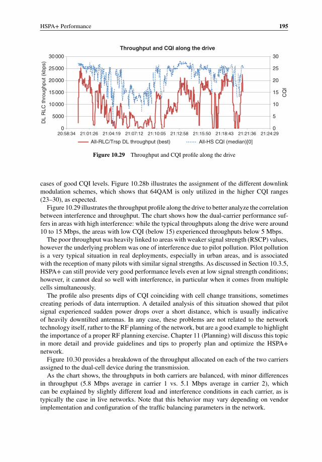
HSPA+ Performance 195
0
5
10
15
20
25
30
0
5000
10000
15000
20000
25000
30000
20:58:34 21:01:26 21:04:19 21:07:12 21:10:05 21:12:58 21:15:50 21:18:43 21:21:36 21:24:29
CQ
I
DL
RLC
thro
ughp
ut (
kbps
)Throughput and CQI along the drive
All-RLC/Trsp DL throughput (best) All-HS CQI (median)[0]
Figure 10.29 Throughput and CQI profile along the drive
cases of good CQI levels. Figure 10.28b illustrates the assignment of the different downlinkmodulation schemes, which shows that 64QAM is only utilized in the higher CQI ranges(23–30), as expected.
Figure 10.29 illustrates the throughput profile along the drive to better analyze the correlationbetween interference and throughput. The chart shows how the dual-carrier performance suf-fers in areas with high interference: while the typical throughputs along the drive were around10 to 15 Mbps, the areas with low CQI (below 15) experienced throughputs below 5 Mbps.
The poor throughput was heavily linked to areas with weaker signal strength (RSCP) values,however the underlying problem was one of interference due to pilot pollution. Pilot pollutionis a very typical situation in real deployments, especially in urban areas, and is associatedwith the reception of many pilots with similar signal strengths. As discussed in Section 10.3.5,HSPA+ can still provide very good performance levels even at low signal strength conditions;however, it cannot deal so well with interference, in particular when it comes from multiplecells simultaneously.
The profile also presents dips of CQI coinciding with cell change transitions, sometimescreating periods of data interruption. A detailed analysis of this situation showed that pilotsignal experienced sudden power drops over a short distance, which is usually indicativeof heavily downtilted antennas. In any case, these problems are not related to the networktechnology itself, rather to the RF planning of the network, but are a good example to highlightthe importance of a proper RF planning exercise. Chapter 11 (Planning) will discuss this topicin more detail and provide guidelines and tips to properly plan and optimize the HSPA+network.
Figure 10.30 provides a breakdown of the throughput allocated on each of the two carriersassigned to the dual-cell device during the transmission.
As the chart shows, the throughputs in both carriers are balanced, with minor differencesin throughput (5.8 Mbps average in carrier 1 vs. 5.1 Mbps average in carrier 2), whichcan be explained by slightly different load and interference conditions in each carrier, as istypically the case in live networks. Note that this behavior may vary depending on vendorimplementation and configuration of the traffic balancing parameters in the network.

196 HSPA+ Evolution to Release 12
0
2000
4000
6000
8000
10000
12000
14000
16000
20:58:34 21:01:26 21:04:19 21:07:12 21:10:05 21:12:58 21:15:50 21:18:43 21:21:36 21:24:29
Car
rier
Phy
thro
ughp
ut (
kbps
)
Throughput per carrier (dual carrier route)
All-HS-DSCH throughput per carrier (kbit/s)[0] All-HS-DSCH throughput per carrier (kbit/s)[1]
Figure 10.30 Throughput per carrier (dual-carrier transmission)
10.4.3 Impact of Vendor Implementation
During the stationary performance discussion it was noted how there were significant per-formance differences with different vendor suppliers, especially in the case of hardwarerestrictions (e.g., baseband limitations). This section analyzes further performance differ-ences between vendors that are rather related to the design of the radio resource managementmethodologies, in particular the NodeB scheduling function and link adaptation.
When analyzing the throughput profiles for two different infrastructure vendors, it wasfound that one vendor was outperforming the other by 20–30%, especially in the areas withmid to good radio conditions. Such a difference has a significant impact on user experienceand network capacity.
The difference between both vendors can be mostly explained by the strategies aroundlink adaptation, and in particular, the assignment of the downlink modulation schemes. AsFigure 10.31 shows, the vendor with the best performance assigns both the 16QAM and64QAM modulation schemes well before the other one.
Vendor 2 starts assigning the 16QAM modulation around CQI 16, while Vendor 1 doesn’treach the same threshold until CQI 20: that is, the first vendor starts transmitting at a faster
0
50
100
150
10 15 20 25 30
DL
mod
ulat
ion
shar
e (%
)
CQI
Vendor comparison (DL modulation)
16QAM Vendor 1 64QAM Vendor 1
16QAM Vendor 2 64QAM Vendor 2
Figure 10.31 Downlink modulation assignment with different vendors

HSPA+ Performance 197
0.00%
20.00%
40.00%
60.00%
80.00%
100.00%
120.00%
010
0020
0030
0040
0050
0060
0070
0080
0090
0010
000
1100
012
000
1300
014
000
1500
016
000
1700
018
000
1900
020
000
2100
022
000
2300
024
000
2500
026
000
2700
028
000
CD
F (
%)
DL RLC throughput (kbps)
Throughput distribution along the drivesingle carrier vs. dual carrier
Dual carrier Single carrier
Figure 10.32 Single carrier vs. dual carrier throughput distribution
rate with approximately 4 dB worse quality than the second. While an aggressive settingof the modulation could arguably result in higher error rate, such an effect is controlled byutilizing the NAK rate in the decision-making process of the algorithm. In a similar fashion,the 64QAM modulation is available with 2 dB of worse signal quality, and more importantlythe modulation is used at 100% rate when radio conditions are sufficiently good, which isnot the case for the other vendor.
Furthermore, when analyzing the behavior of Vendor 1 it was found that there are additionaleffects that degrade the performance of the dual carrier service. The following example presentsa comparison between a single carrier and dual carrier test drive in Vendor 1’s network. Thesame device was used for the tests, changing the terminal category from 24 to 14, and the samedrive route was followed (drive route from Figure 10.14). Figure 10.32 shows the throughputdistribution for both the single-carrier and dual-carrier device.
The results from this exercise show that the dual-carrier device only achieved 45% higherthroughput on average as compared to the single-carrier device; and even more important,in the lower throughput ranges (poor radio conditions), there was no noticeable differencebetween both devices.
When analyzing the reasons behind this behavior it was noted that this vendor prioritizesthe traffic from single-carrier devices over dual carrier to try and achieve the same levelof QoS independently of the terminal capabilities (in other vendor implementations it ispossible to select the priority of dual-carrier devices in the scheduler, rather than being hard-coded). That explains part of the problem, since the network was loaded at the time of thetests; as Figure 10.33 shows, the dual-carrier device experienced a higher DTX rate than the
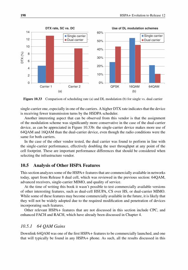
198 HSPA+ Evolution to Release 12
0
2
4
6
8
10
12
14
Carrier 1 Carrier 2
(a) (b)
DT
X (
%)
DTX rate, SC vs. DC
0%
10%
20%
30%
40%
50%
60%
QPSK 16QAM 64QAM
Use of DL modulation schemes
Single carrierDual carrier
Single carrierDual carrier
Figure 10.33 Comparison of scheduling rate (a) and DL modulation (b) for single vs. dual carrier
single-carrier one, especially in one of the carriers. A higher DTX rate indicates that the deviceis receiving fewer transmission turns by the HSDPA scheduler.
Another interesting aspect that can be observed from this vendor is that the assignmentof the modulation scheme was significantly more conservative in the case of the dual-carrierdevice, as can be appreciated in Figure 10.33b: the single-carrier device makes more use of64QAM and 16QAM than the dual-carrier device, even though the radio conditions were thesame for both carriers.
In the case of the other vendor tested, the dual carrier was found to perform in line withthe single-carrier performance, effectively doubling the user throughput at any point of thecell footprint. These are important performance differences that should be considered whenselecting the infrastructure vendor.
10.5 Analysis of Other HSPA Features
This section analyzes some of the HSPA+ features that are commercially available in networkstoday, apart from Release 8 dual cell, which was reviewed in the previous section: 64QAM,advanced receivers, single-carrier MIMO, and quality of service.
At the time of writing this book it wasn’t possible to test commercially available versionsof other interesting features, such as dual-cell HSUPA, CS over HS, or dual-carrier MIMO.While some of these features may become commercially available in the future, it is likely thatthey will not be widely adopted due to the required modification and penetration of devicesincorporating such features.
Other relevant HSPA+ features that are not discussed in this section include CPC, andenhanced FACH and RACH, which have already been discussed in Chapter 4.
10.5.1 64 QAM Gains
Downlink 64QAM was one of the first HSPA+ features to be commercially launched, and onethat will typically be found in any HSPA+ phone. As such, all the results discussed in this
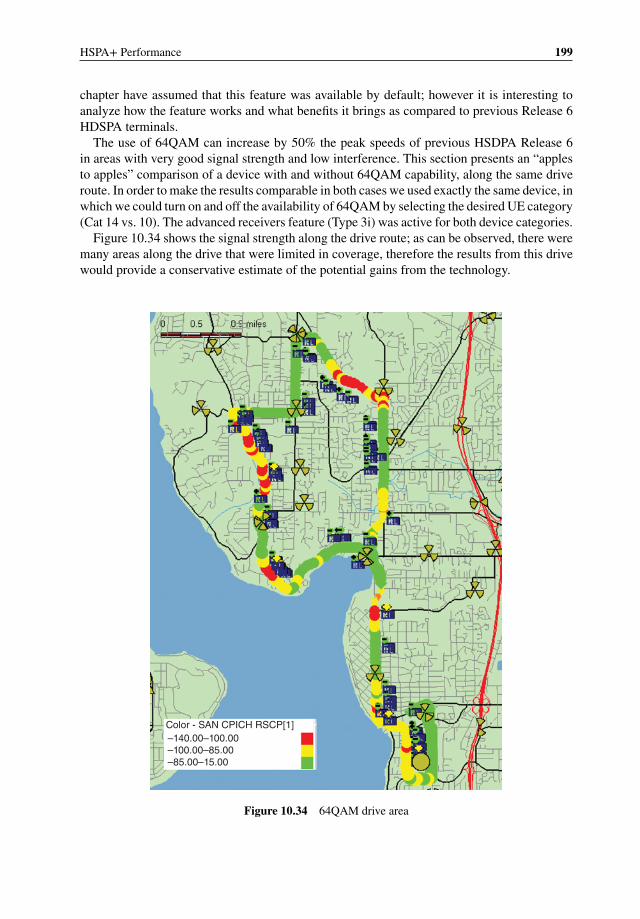
HSPA+ Performance 199
chapter have assumed that this feature was available by default; however it is interesting toanalyze how the feature works and what benefits it brings as compared to previous Release 6HDSPA terminals.
The use of 64QAM can increase by 50% the peak speeds of previous HSDPA Release 6in areas with very good signal strength and low interference. This section presents an “applesto apples” comparison of a device with and without 64QAM capability, along the same driveroute. In order to make the results comparable in both cases we used exactly the same device, inwhich we could turn on and off the availability of 64QAM by selecting the desired UE category(Cat 14 vs. 10). The advanced receivers feature (Type 3i) was active for both device categories.
Figure 10.34 shows the signal strength along the drive route; as can be observed, there weremany areas along the drive that were limited in coverage, therefore the results from this drivewould provide a conservative estimate of the potential gains from the technology.
Color - SAN CPICH RSCP[1]–140.00–100.00–100.00–85.00–85.00–15.00
Figure 10.34 64QAM drive area
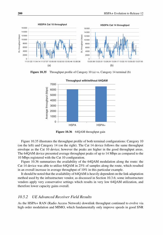
200 HSPA+ Evolution to Release 12
0
2000
4000
6000
8000
10000
12000
14000
16000
13:20:38 13:23:31 13:26:24 13:29:17 13:32:10 13:35:02 13:37:55
DL
thro
ughp
ut (
kbps
)
HSDPA Cat 14 throughput
0
2000
4000
6000
8000
10000
12000
14000
16000
11:51:22 11:54:14 11:57:07 12:00:00 12:02:53 12:05:46 12:08:38
DL
thro
ughp
ut (
kbps
)
HSDPA Cat 10 throughput
(a) (b)
Figure 10.35 Throughput profile of Category 10 (a) vs. Category 14 terminal (b)
0
1000
2000
3000
4000
5000
6000
7000
HSPA HSPA+
Ave
rage
thro
ughp
ut (
kbps
)
Throughput with/without 64QAM
Figure 10.36 64QAM throughput gain
Figure 10.35 illustrates the throughput profile of both terminal configurations: Category 10(on the left) and Category 14 (on the right). The Cat 14 device follows the same throughputenvelope as the Cat 10 device; however the peaks are higher in the good throughput areas.The 64QAM device presented average throughput peaks of up to 14 Mbps as compared to the10 Mbps registered with the Cat 10 configuration.
Figure 10.36 summarizes the availability of the 64QAM modulation along the route: theCat 14 device was able to utilize 64QAM in 25% of samples along the route, which resultedin an overall increase in average throughput of 10% in this particular example.
It should be noted that the availability of 64QAM is heavily dependent on the link adaptationmethod used by the infrastructure vendor, as discussed in Section 10.3.6; some infrastructurevendors apply very conservative settings which results in very low 64QAM utilization, andtherefore lower capacity gains overall.
10.5.2 UE Advanced Receiver Field Results
As the HSPA+ RAN (Radio Access Network) downlink throughput continued to evolve viahigh order modulation and MIMO, which fundamentally only improve speeds in good SNR
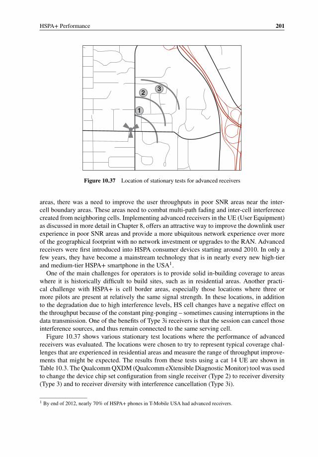
HSPA+ Performance 201
32
1
Figure 10.37 Location of stationary tests for advanced receivers
areas, there was a need to improve the user throughputs in poor SNR areas near the inter-cell boundary areas. These areas need to combat multi-path fading and inter-cell interferencecreated from neighboring cells. Implementing advanced receivers in the UE (User Equipment)as discussed in more detail in Chapter 8, offers an attractive way to improve the downlink userexperience in poor SNR areas and provide a more ubiquitous network experience over moreof the geographical footprint with no network investment or upgrades to the RAN. Advancedreceivers were first introduced into HSPA consumer devices starting around 2010. In only afew years, they have become a mainstream technology that is in nearly every new high-tierand medium-tier HSPA+ smartphone in the USA1.
One of the main challenges for operators is to provide solid in-building coverage to areaswhere it is historically difficult to build sites, such as in residential areas. Another practi-cal challenge with HSPA+ is cell border areas, especially those locations where three ormore pilots are present at relatively the same signal strength. In these locations, in additionto the degradation due to high interference levels, HS cell changes have a negative effect onthe throughput because of the constant ping-ponging – sometimes causing interruptions in thedata transmission. One of the benefits of Type 3i receivers is that the session can cancel thoseinterference sources, and thus remain connected to the same serving cell.
Figure 10.37 shows various stationary test locations where the performance of advancedreceivers was evaluated. The locations were chosen to try to represent typical coverage chal-lenges that are experienced in residential areas and measure the range of throughput improve-ments that might be expected. The results from these tests using a cat 14 UE are shown inTable 10.3. The Qualcomm QXDM (Qualcomm eXtensible Diagnostic Monitor) tool was usedto change the device chip set configuration from single receiver (Type 2) to receiver diversity(Type 3) and to receiver diversity with interference cancellation (Type 3i).
1 By end of 2012, nearly 70% of HSPA+ phones in T-Mobile USA had advanced receivers.
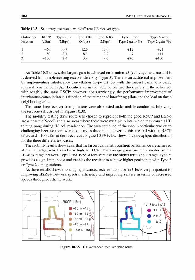
202 HSPA+ Evolution to Release 12
Table 10.3 Stationary test results with different UE receiver types
Stationarylocation
RSCP(dBm)
Type 2 Rx(Mbps)
Type 3 Rx(Mbps)
Type 3i Rx(Mbps)
Type 3 overType 2 gain (%)
Type 3i overType 2 gain (%)
1 −60 10.7 12.0 13.0 +12 +212 −80 8.3 8.9 9.2 +7 +113 −100 2.0 3.4 4.0 +70 +100
As Table 10.3 shows, the largest gain is achieved on location #3 (cell edge) and most of itis derived from implementing receiver diversity (Type 3). There is an additional improvementby implementing interference cancellation (Type 3i) too, with the largest gains also beingrealized near the cell edge. Location #3 in the table below had three pilots in the active setwith roughly the same RSCP; however, not surprisingly, the performance improvement ofinterference cancellation is a function of the number of interfering pilots and the load on thoseneighboring cells.
The same three receiver configurations were also tested under mobile conditions, followingthe test route illustrated in Figure 10.38.
The mobility testing drive route was chosen to represent both the good RSCP and Ec/Noareas near the NodeB and also areas where there were multiple pilots, which may cause a UEto ping-pong during HS cell reselection. The area at the top of the map in particular was quitechallenging because there were as many as three pilots covering this area all with an RSCPof around −100 dBm at the street level. Figure 10.39 below shows the throughput distributionfor the three different test cases.
The mobility results show again that the largest gains in throughput performance are achievedat the cell edge, which can be as high as 100%. The average gains are more modest in the20–40% range between Type 2 and Type 3i receivers. On the higher throughput range, Type 3iprovides a significant boost and enables the receiver to achieve higher peaks than with Type 3or Type 2 configurations.
As these results show, encouraging advanced receiver adoption in UEs is very important toimproving HSPA+ network spectral efficiency and improving service in terms of increasedspeeds throughout the network.
RSCP (dBm)
–65 to –45# of Pilots in AS
3 to 3
2 to 3
1 to 2
–80 to –65
–85 to –80
–90 to –85
–105 to –90
Figure 10.38 UE Advanced receiver drive route
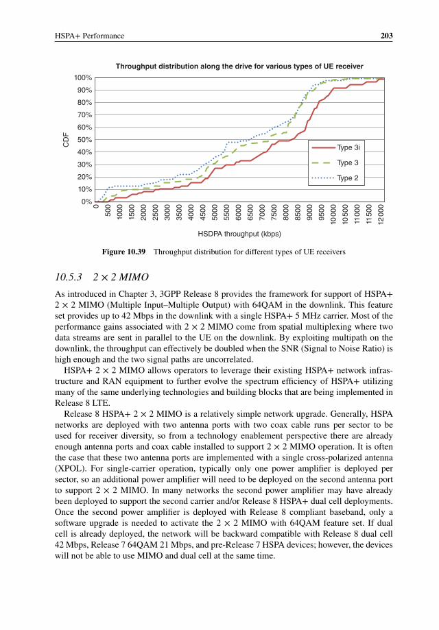
HSPA+ Performance 203
0%
10%
20%
30%
40%
50%
60%
70%
80%
90%
100%
CD
FThroughput distribution along the drive for various types of UE receiver
HSDPA throughput (kbps)
0
500
1000
1500
2000
2500
3000
3500
4000
4500
5000
5500
6000
6500
7000
7500
8000
8500
9000
9500
1000
0
1050
0
1100
0
1150
0
1200
0
Type 3i
Type 3
Type 2
Figure 10.39 Throughput distribution for different types of UE receivers
10.5.3 2 × 2 MIMO
As introduced in Chapter 3, 3GPP Release 8 provides the framework for support of HSPA+2 × 2 MIMO (Multiple Input–Multiple Output) with 64QAM in the downlink. This featureset provides up to 42 Mbps in the downlink with a single HSPA+ 5 MHz carrier. Most of theperformance gains associated with 2 × 2 MIMO come from spatial multiplexing where twodata streams are sent in parallel to the UE on the downlink. By exploiting multipath on thedownlink, the throughput can effectively be doubled when the SNR (Signal to Noise Ratio) ishigh enough and the two signal paths are uncorrelated.
HSPA+ 2 × 2 MIMO allows operators to leverage their existing HSPA+ network infras-tructure and RAN equipment to further evolve the spectrum efficiency of HSPA+ utilizingmany of the same underlying technologies and building blocks that are being implemented inRelease 8 LTE.
Release 8 HSPA+ 2 × 2 MIMO is a relatively simple network upgrade. Generally, HSPAnetworks are deployed with two antenna ports with two coax cable runs per sector to beused for receiver diversity, so from a technology enablement perspective there are alreadyenough antenna ports and coax cable installed to support 2 × 2 MIMO operation. It is oftenthe case that these two antenna ports are implemented with a single cross-polarized antenna(XPOL). For single-carrier operation, typically only one power amplifier is deployed persector, so an additional power amplifier will need to be deployed on the second antenna portto support 2 × 2 MIMO. In many networks the second power amplifier may have alreadybeen deployed to support the second carrier and/or Release 8 HSPA+ dual cell deployments.Once the second power amplifier is deployed with Release 8 compliant baseband, only asoftware upgrade is needed to activate the 2 × 2 MIMO with 64QAM feature set. If dualcell is already deployed, the network will be backward compatible with Release 8 dual cell42 Mbps, Release 7 64QAM 21 Mbps, and pre-Release 7 HSPA devices; however, the deviceswill not be able to use MIMO and dual cell at the same time.
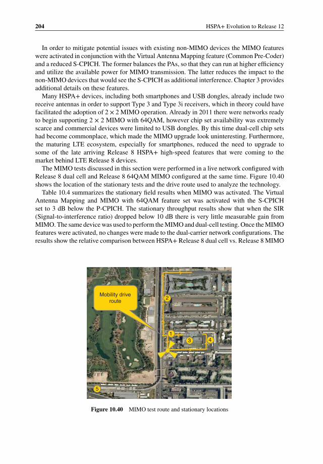
204 HSPA+ Evolution to Release 12
In order to mitigate potential issues with existing non-MIMO devices the MIMO featureswere activated in conjunction with the Virtual Antenna Mapping feature (Common Pre-Coder)and a reduced S-CPICH. The former balances the PAs, so that they can run at higher efficiencyand utilize the available power for MIMO transmission. The latter reduces the impact to thenon-MIMO devices that would see the S-CPICH as additional interference. Chapter 3 providesadditional details on these features.
Many HSPA+ devices, including both smartphones and USB dongles, already include tworeceive antennas in order to support Type 3 and Type 3i receivers, which in theory could havefacilitated the adoption of 2 × 2 MIMO operation. Already in 2011 there were networks readyto begin supporting 2 × 2 MIMO with 64QAM, however chip set availability was extremelyscarce and commercial devices were limited to USB dongles. By this time dual-cell chip setshad become commonplace, which made the MIMO upgrade look uninteresting. Furthermore,the maturing LTE ecosystem, especially for smartphones, reduced the need to upgrade tosome of the late arriving Release 8 HSPA+ high-speed features that were coming to themarket behind LTE Release 8 devices.
The MIMO tests discussed in this section were performed in a live network configured withRelease 8 dual cell and Release 8 64QAM MIMO configured at the same time. Figure 10.40shows the location of the stationary tests and the drive route used to analyze the technology.
Table 10.4 summarizes the stationary field results when MIMO was activated. The VirtualAntenna Mapping and MIMO with 64QAM feature set was activated with the S-CPICHset to 3 dB below the P-CPICH. The stationary throughput results show that when the SIR(Signal-to-interference ratio) dropped below 10 dB there is very little measurable gain fromMIMO. The same device was used to perform the MIMO and dual-cell testing. Once the MIMOfeatures were activated, no changes were made to the dual-carrier network configurations. Theresults show the relative comparison between HSPA+ Release 8 dual cell vs. Release 8 MIMO
Mobility driveroute 2
13 4
5
Figure 10.40 MIMO test route and stationary locations
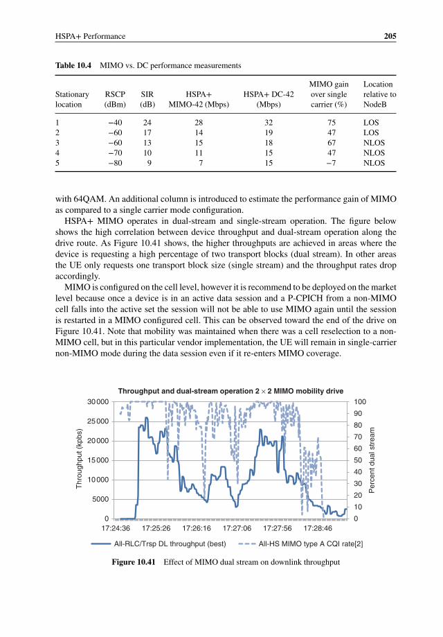
HSPA+ Performance 205
Table 10.4 MIMO vs. DC performance measurements
Stationarylocation
RSCP(dBm)
SIR(dB)
HSPA+MIMO-42 (Mbps)
HSPA+ DC-42(Mbps)
MIMO gainover singlecarrier (%)
Locationrelative toNodeB
1 −40 24 28 32 75 LOS2 −60 17 14 19 47 LOS3 −60 13 15 18 67 NLOS4 −70 10 11 15 47 NLOS5 −80 9 7 15 −7 NLOS
with 64QAM. An additional column is introduced to estimate the performance gain of MIMOas compared to a single carrier mode configuration.
HSPA+ MIMO operates in dual-stream and single-stream operation. The figure belowshows the high correlation between device throughput and dual-stream operation along thedrive route. As Figure 10.41 shows, the higher throughputs are achieved in areas where thedevice is requesting a high percentage of two transport blocks (dual stream). In other areasthe UE only requests one transport block size (single stream) and the throughput rates dropaccordingly.
MIMO is configured on the cell level, however it is recommend to be deployed on the marketlevel because once a device is in an active data session and a P-CPICH from a non-MIMOcell falls into the active set the session will not be able to use MIMO again until the sessionis restarted in a MIMO configured cell. This can be observed toward the end of the drive onFigure 10.41. Note that mobility was maintained when there was a cell reselection to a non-MIMO cell, but in this particular vendor implementation, the UE will remain in single-carriernon-MIMO mode during the data session even if it re-enters MIMO coverage.
0
10
20
30
40
50
60
70
80
90
100
0
5000
10000
15000
20000
25000
30000
17:24:36 17:25:26 17:26:16 17:27:06 17:27:56 17:28:46
Per
cent
dua
l str
eam
Thr
ough
put (
kpbs
)
Throughput and dual-stream operation 2 × 2 MIMO mobility drive
All-RLC/Trsp DL throughput (best) All-HS MIMO type A CQI rate[2]
Figure 10.41 Effect of MIMO dual stream on downlink throughput

206 HSPA+ Evolution to Release 12
100%
90%
80%
70%
60%
50%CD
F
40%
30%
20%
10%
0%0 2 4 6 8 10 12 14 16 18
RLC throughput (Mbps)
Dual carrier (DC)
Throughput distribution MIMO (5 MHz) vs. dual carrier (10 MHz)
2 × 2 MIMO (SC)
20 22 24 26 28 30 32 34
Figure 10.42 Throughput comparison, MIMO vs. dual carrier
Figure 10.42 compares the performance of HSPA+ MIMO (single carrier) with Release 8dual carrier, utilizing the same test device that was reconfigured from single-carrier 2 × 2MIMO mode to dual-carrier mode. On average dual carrier outperforms MIMO by 60–70%,with relatively small performance differences in areas with good SIR. In this case, most of thedrive was in fairly good radio conditions, so the throughput results may be slightly optimisticcompared to more challenging mobility conditions. As expected, at the lower throughputslevels there was little to no gain in MIMO performance and the test device performance wassimilar to what you would expect from a device not configured with MIMO operating on asingle HSPA+ 5 MHz carrier.
By estimating the single carrier performance based on the dual cell performance that wascollected in the field, MIMO shows an overall 15–25% improvement in spectral efficiency overRelease 7 HSPA+ with 64QAM. These measured gains are consistent with other simulationsand measurements [3].
10.5.4 Quality of Service (QoS)
The support of QoS is not a new item in HSPA+; however, normally the main differentiationfactor has been the Maximum Bitrate (MBR) for the connection. In practice, QoS can providean interesting feature toolset based on resource prioritization, to help the operator with itemssuch as:
� subscriber differentiation� application differentiation, and� fair network use policies.
The use of resource prioritization is not relevant in networks with low traffic loads; however,as traffic increases and certain areas of the network get congested, 3GPP QoS can help dealwith congestion in a cost efficient manner.
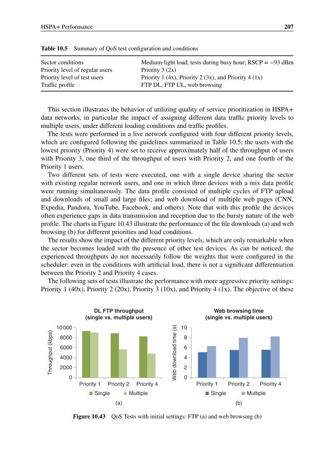
HSPA+ Performance 207
Table 10.5 Summary of QoS test configuration and conditions
Sector conditions Medium-light load; tests during busy hour; RSCP = −93 dBmPriority level of regular users Priority 3 (2x)Priority level of test users Priority 1 (4x), Priority 2 (3x), and Priority 4 (1x)Traffic profile FTP DL, FTP UL, web browsing
This section illustrates the behavior of utilizing quality of service prioritization in HSPA+data networks, in particular the impact of assigning different data traffic priority levels tomultiple users, under different loading conditions and traffic profiles.
The tests were performed in a live network configured with four different priority levels,which are configured following the guidelines summarized in Table 10.5: the users with thelowest priority (Priority 4) were set to receive approximately half of the throughput of userswith Priority 3, one third of the throughput of users with Priority 2, and one fourth of thePriority 1 users.
Two different sets of tests were executed, one with a single device sharing the sectorwith existing regular network users, and one in which three devices with a mix data profilewere running simultaneously. The data profile consisted of multiple cycles of FTP uploadand downloads of small and large files; and web download of multiple web pages (CNN,Expedia, Pandora, YouTube, Facebook, and others). Note that with this profile the devicesoften experience gaps in data transmission and reception due to the bursty nature of the webprofile. The charts in Figure 10.43 illustrate the performance of the file downloads (a) and webbrowsing (b) for different priorities and load conditions.
The results show the impact of the different priority levels, which are only remarkable whenthe sector becomes loaded with the presence of other test devices. As can be noticed, theexperienced throughputs do not necessarily follow the weights that were configured in thescheduler: even in the conditions with artificial load, there is not a significant differentiationbetween the Priority 2 and Priority 4 cases.
The following sets of tests illustrate the performance with more aggressive priority settings:Priority 1 (40x), Priority 2 (20x), Priority 3 (10x), and Priority 4 (1x). The objective of these
0
2000
4000
6000
8000
10000
Priority 1 Priority 2 Priority 4
Thr
ough
put (
kbps
)
DL FTP throughput(single vs. multiple users)
Single Multiple
0
2
4
6
8
10
Priority 1 Priority 2 Priority 4
Web
dow
nloa
d tim
e (s
)
Web browsing time(single vs. multiple users)
Single Multiple
(a) (b)
Figure 10.43 QoS Tests with initial settings: FTP (a) and web browsing (b)
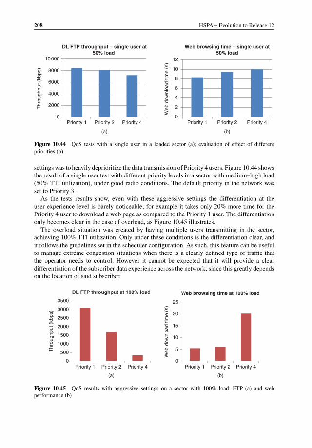
208 HSPA+ Evolution to Release 12
0
2000
4000
6000
8000
10000
Priority 1 Priority 2 Priority 4
Thr
ough
put (
kbps
)
DL FTP throughput – single user at50% load
0
2
4
6
8
10
12
Priority 1 Priority 2 Priority 4
Web
dow
nloa
d tim
e (s
)
Web browsing time – single user at50% load
(a) (b)
Figure 10.44 QoS tests with a single user in a loaded sector (a); evaluation of effect of differentpriorities (b)
settings was to heavily deprioritize the data transmission of Priority 4 users. Figure 10.44 showsthe result of a single user test with different priority levels in a sector with medium–high load(50% TTI utilization), under good radio conditions. The default priority in the network wasset to Priority 3.
As the tests results show, even with these aggressive settings the differentiation at theuser experience level is barely noticeable; for example it takes only 20% more time for thePriority 4 user to download a web page as compared to the Priority 1 user. The differentiationonly becomes clear in the case of overload, as Figure 10.45 illustrates.
The overload situation was created by having multiple users transmitting in the sector,achieving 100% TTI utilization. Only under these conditions is the differentiation clear, andit follows the guidelines set in the scheduler configuration. As such, this feature can be usefulto manage extreme congestion situations when there is a clearly defined type of traffic thatthe operator needs to control. However it cannot be expected that it will provide a cleardifferentiation of the subscriber data experience across the network, since this greatly dependson the location of said subscriber.
0
500
1000
1500
2000
2500
3000
3500
Priority 1 Priority 2 Priority 4
Thr
ough
put (
kbps
)
DL FTP throughput at 100% load
0
5
10
15
20
25
Priority 1 Priority 2 Priority 4
Web
dow
nloa
d tim
e (s
)
Web browsing time at 100% load
(a) (b)
Figure 10.45 QoS results with aggressive settings on a sector with 100% load: FTP (a) and webperformance (b)

HSPA+ Performance 209
10.6 Comparison of HSPA+ with LTE
The HSPA+ technology has continued to evolve over the years to provide potentially similardownlink air-interface speeds as LTE Release 8. In the USA, most LTE Release 8 deploymentshave initially been configured with 10 MHz of spectrum in the downlink. HSPA+ Release 8dual cell uses the same bandwidth configuration of 10 MHz in the downlink. Both technologiesalso utilize 64QAM in the downlink, so if 2 × 2 MIMO was for some reason disabled on LTE,they would in theory provide very similar peak speed performance in excellent RF conditions.So the real difference in performance between the two systems should consist of the gainsfrom 2 × 2 MIMO and any frequency domain scheduling gains that can be measured.
This section analyzes the performance of an experimental LTE system that is co-locatedwith an existing HSPA+ network configured with dual cell. In order to perform the testing andcompare the drive results a single drive was performed while collecting measurements on bothHSPA+ dual cell and LTE with 2 × 2 MIMO activated. The HSPA+ network is a commercialnetwork that has been in operation for a number of years, in which regular traffic load waspresent, while the LTE system was pre-commercial with no active LTE devices. HSPA+ dualcell and LTE Release 8 commercial dongles operating in the 2100 MHz band were utilized toperform this test. There is a one-to-one overlay in a relatively small geographic five-site clusterarea. Both HSPA+ and LTE share the same antennas and utilize the same frequency band, sothe coverage of the two systems should be very similar from a construction and deploymentperspective. The drive route was chosen so that the measurements would be taken inside theoverlay area. In an attempt to try and make the comparison between the two technologies asfair as possible, care was taken to only collect measurement data on the interior of the LTEcoverage area: driving areas that were on the fringe of the LTE coverage where no inter-siteinterference was present would yield an overly optimistic LTE performance compared to anHSPA+ network with more neighbors and hence more inter-site interference.
Figure 10.46 shows the results of a mobility drive that compares HSPA+ dual cell to LTEthat is using a 10 MHz downlink channel. The 2 × 2 LTE network achieved downlink peak
30000 to 4000020000 to 30000
40000 to 7000030000 to 4000020000 to 3000010000 to 20000
0 to 10000
(96)(136)(130)(156)(54)
10000 to 200000 to 10000
(3)(190)(307)(68)
(b)(a)
Figure 10.46 Mobility throughput (kbps): HSPA+ dual carrier (a); LTE 10 MHz (b)
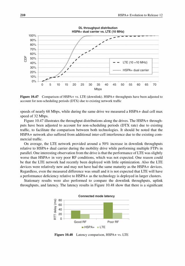
210 HSPA+ Evolution to Release 12
00%
10%
20%
30%
40%
50%
CD
F
60%
70%
80%
90%
100%
DL throughput distributionHSPA+ dual carrier vs. LTE (10 MHz)
5 10 15 20 25 30 35
Mbps
40 45 50 55 60
LTE (10 +10 MHz)
HSPA+ dual carrier
65 70
Figure 10.47 Comparison of HSPA+ vs. LTE (downlink). HSPA+ throughputs have been adjusted toaccount for non-scheduling periods (DTX) due to existing network traffic
speeds of nearly 68 Mbps, while during the same drive we measured a HSPA+ dual cell maxspeed of 32 Mbps.
Figure 10.47 illustrates the throughput distributions along the drives. The HSPA+ through-puts have been adjusted to account for non-scheduling periods (DTX rate) due to existingtraffic, to facilitate the comparison between both technologies. It should be noted that theHSPA+ network also suffered from additional inter-cell interference due to the existing com-mercial traffic.
On average, the LTE network provided around a 50% increase in downlink throughputsrelative to HSPA+ dual carrier during the mobility drive while performing multiple FTPs inparallel. One interesting observation from the drive is that the performance of LTE was slightlyworse than HSPA+ in very poor RF conditions, which was not expected. One reason couldbe that the LTE network had recently been deployed with little optimization. Also the LTEdevices were relatively new and may not have had the same maturity as the HSPA+ devices.Regardless, even the measured difference was small and it is not expected that LTE will havea performance deficiency relative to HSPA+ as the technology is deployed in larger clusters.
Stationary results were also performed to compare the downlink throughputs, uplinkthroughputs, and latency. The latency results in Figure 10.48 show that there is a significant
0
20
40
60
80
Good RF Poor RF
RT
T d
elay
(m
s)
Connected mode latency
HSPA+ LTE
Figure 10.48 Latency comparison, HSPA+ vs. LTE
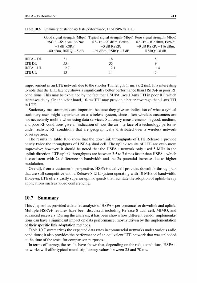
HSPA+ Performance 211
Table 10.6 Summary of stationary tests performance, DC-HSPA vs. LTE
Good signal strength (Mbps)RSCP: −65 dBm, Ec/No:
−3 dB RSRP:−80 dBm, RSRQ: −5 dB
Typical signal strength (Mbps)RSCP: −90 dBm, Ec/No:
−5 dB RSRP:−94 dBm, RSRQ: −7 dB
Poor signal strength (Mbps)RSCP: −102 dBm, Ec/No:−9 dB RSRP: −116 dBm,
RSRQ: −8 dB
HSPA+ DL 31 18 5LTE DL 55 35 9HSPA+ UL 2.7 2.1 1.4LTE UL 13 14 5
improvement in an LTE network due to the shorter TTI length (1 ms vs. 2 ms). It is interestingto note that the LTE latency shows a significantly better performance than HSPA+ in poor RFconditions. This may be explained by the fact that HSUPA uses 10-ms TTI in poor RF, whichincreases delay. On the other hand, 10-ms TTI may provide a better coverage than 1-ms TTIin LTE.
Stationary measurements are important because they give an indication of what a typicalstationary user might experience on a wireless system, since often wireless customers arenot necessarily mobile when using data services. Stationary measurements in good, medium,and poor RF conditions give an indication of how the air interface of a technology performsunder realistic RF conditions that are geographically distributed over a wireless networkcoverage area.
The results in Table 10.6 show that the downlink throughputs of LTE Release 8 providenearly twice the throughputs of HSPA+ dual cell. The uplink results of LTE are even moreimpressive; however, it should be noted that the HSPA+ network only used 5 MHz in theuplink direction. LTE uplink throughputs are between 3.5 to 7 times faster than HSPA+ whichis consistent with 2x difference in bandwidth and the 2x potential increase due to highermodulation.
Overall, from a customer’s perspective, HSPA+ dual cell provides downlink throughputsthat are still competitive with a Release 8 LTE system operating with 10 MHz of bandwidth.However, LTE offers vastly superior uplink speeds that facilitate the adoption of uplink-heavyapplications such as video conferencing.
10.7 Summary
This chapter has provided a detailed analysis of HSPA+ performance for downlink and uplink.Multiple HSPA+ features have been discussed, including Release 8 dual cell, MIMO, andadvanced receivers. During the analysis, it has been shown how different vendor implementa-tions can have a significant impact on data performance, mostly driven by the implementationof their specific link adaptation methods.
Table 10.7 summarizes the expected data rates in commercial networks under various radioconditions; it also provides the performance of an equivalent LTE network that was unloadedat the time of the tests, for comparison purposes.
In terms of latency, the results have shown that, depending on the radio conditions, HSPA+networks will offer typical round-trip latency values between 25 and 70 ms.
212 HSPA+ Evolution to Release 12
Table 10.7 Overall performance summary: stationary throughput tests
Good signalstrength (Mbps)
Typical signalstrength (Mbps)
Poor signalstrength (Mbps)
HSDPA single carrier 13.5 9 2.5HSDPA dual carrier 28 18 5HSUPA 4.1 2.1 1.4LTE 10 MHz downlink 55 35 9LTE 10 MHz uplink 13 14 5
Overall, the HSPA+ technology offers a compelling data performance even when comparedto LTE networks – furthermore, as will be discussed in more detail in Chapter 13, the qualityof experience offered to the end customer is still competitive with networks offering highernominal speeds.
References
[1] 3GPP TS 25.214: Physical Layer Procedures (FDD), Release 8.[2] 3GPP TS 25.213: Spreading and Modulation, Release 8.[3] “MIMO in HSPA; the Real-World Impact”, GSMA, July 2011.
11Network Planning
Brian Olsen, Pablo Tapia, Jussi Reunanen, and Harri Holma
11.1 Introduction
The proper planning of the HSPA+ is a very important activity that will determine to a largeextent the coverage, capacity, and quality of the service. No matter how much effort is investedin maintaining a network, if the original planning is flawed it will be a constant headache forthe engineering teams.
The main focus area when deploying HSPA+ are the radio nodes, including NodeB sitelocation and antenna and power configuration. This chapter provides practical guidelines totake into account when performing the RF planning, however it does not include the amountof detail that can be found in specialized RF planning books such as [1]. Although the mainemphasis is put on the Radio Access Network (RAN) nodes, basic considerations around coreand backhaul design are also discussed.
In addition to deployment aspects, the chapter also provides useful information to help man-age capacity growth, including multilayer management and network dimensioning guidelines.
11.2 Radio Frequency Planning
The performance at the radio layer has a direct impact on the experienced data rates on theapplication layer and, ultimately, on the experienced user data rate at the application layer. Thestronger and cleaner the signal, the higher the data rate that can be achieved; and vice versa, inchallenging radio conditions the throughput will be reduced since the physical layer adapts theModulation and Transport Format to avoid excessive packet loss. The radio signal is typicallymeasured in terms of Received Signal Code Power (RSCP) and interference levels: Energy perchip over Interference and Noise (Ec/No) for downlink and Received Signal Strength Indicator(RSSI) for uplink.
HSPA+ Evolution to Release 12: Performance and Optimization, First Edition.Edited by Harri Holma, Antti Toskala, and Pablo Tapia.© 2014 John Wiley & Sons, Ltd. Published 2014 by John Wiley & Sons, Ltd.
214 HSPA+ Evolution to Release 12
The main challenge when planning the radio network is to do so considering both coverageand interference performance, with consideration for future traffic growth. HSPA+ systemsutilize a single frequency reuse, which means that the same frequency is used in all adjacentsectors and therefore is highly susceptible to interference. Many of the problems found intoday’s networks can be tracked down to poor Radio Frequency (RF) planning. In many cases,the problems are masked by adding additional capacity or new sites to the network, but theywill eventually need to be addressed through proper optimization.
The placement and orientation of the antenna is the best tool the operator has to ensureproper RF planning, therefore this activity should be done very carefully. To help with thistask it is advisable to use network engineering tools like RF Planning and Automatic CellPlanning (ACP) tools, which will be covered in Section 11.2.3.
When configuring antenna parameters, the operator needs to strike a balance betweencoverage and capacity. When a technology is first deployed, the network needs to provideservice in as many locations as possible, so coverage will normally be the initial driver.Ensuring a good level of coverage with HSPA+ can be quite challenging, especially whenevolving the network from a previous GSM layout, since in UMTS/HSPA+ it is not possibleto use overlay (boomer) sites. Having sectors inside the coverage area of other sectors isvery harmful due to the single frequency reuse nature of the technology. Contrary to commonwisdom, in some cases, the coverage versus interference tradeoff will result in the reductionof transmit powers, or even the deactivation of certain sectors.
A second challenge when building a coverage layer is deciding the transmit power to beused. In dense urban areas, having too much signal strength beyond a certain point can actuallyhurt the network performance. The reason is that signals will propagate outside of the desiredcoverage zone and interfere with sectors in other places – this in turn may create the sensationof a “coverage hole” when in reality the problem is that the network is transmitting with toomuch power.
Along the same lines, UMTS networks experience so-called “cell breathing” when thenetwork gets loaded, which shrinks the effective coverage of the sectors due to an increaseof interference at the cell borders. The “more power is better” guiding principle doesn’talways apply, and often ends up causing significant performance degradation as networktraffic grows. This is why it’s important to try and design the network for a certain load target,for example 50%. To do this in practice the operator should use realistic traffic maps during theplanning stage.
Achieving pilot dominance is very important for the long-term health of the network. Welldefined cell boundaries will minimize problems related to pilot pollution and will enablea more gracious cell breathing as the network gets loaded. Figure 11.1 illustrates a net-work in which the original RF configuration (a) has been optimized to minimize interferencein the area (b). As the maps show, the optimized network has clearer sector boundaries,although these are still far from perfect in some areas given the challenges from the underlyingterrain.
Considering that every network is different, the operator needs to make the appropriatedecisions taking into account the terrain, the frequency bands in use (low bands are more proneto interference, high bands are more challenged in coverage), and the antenna configuration,among other issues. Since typically UMTS networks are uplink limited – both from coverageand interference points of view – one good idea is to explore the option to have additionalreceive antennas and enable the 4-Way Receive Diversity feature in the NodeB. This featurecan significantly improve uplink performance, as was discussed in Chapter 10.

Network Planning 215
(a) (b)
Figure 11.1 Example of poorly defined boundary areas (a) and optimized boundaries (b) in the samenetwork
In summary, below are a few guidelines to UMTS radio planning:
� Deploy based on traffic location: the closer the cell is to the traffic source, the lower theinterference introduced in the system, and the more efficient the air interface will be.
� Proper definition of cell boundaries, avoiding zones with pilot pollution by creating adominant sector in each particular area.
� Limit footprint of sectors: avoid overshooting sectors that can capture traffic outside theirnatural range. By the same token, do not abuse antenna downtilts, which are often usedas the only method to achieve interference containment and can create sudden attenuationareas within the cell footprint.
� Do not use excess power, try to serve the cell with the minimum power required to keepthe service at the desired quality level – taking into consideration service coverage insidebuildings.
� In case of overlaid GSM deployment, identify and correct harmful inherited configurationssuch as boomer sites, sectors that are pointing at each other, and unnecessary capacity sites.
11.2.1 Link Budget
The first step toward planning the radio network is to perform an estimation of the coveragearea that the technology can provide. While this is a complicated exercise that needs to considermany different factors, a first order approximation is to analyze the maximum pathloss thatcan be endured both in the uplink and downlink directions to achieve a certain level of quality.This is known as link budget calculation. This section will provide useful guidelines to helpcalculate the link budget for HSDPA and HSUPA, however more detailed explanation oncomputing link budget can be found in network planning books such as [1].
At a very high level, the link budget exercise will estimate the maximum pathloss permittedto transmit with a given quality; there will be many factors affecting the link budget, suchas technology, network configuration, type of data service, network load, and interferenceconditions. The link budget calculations for uplink and downlink are quite different, given
216 HSPA+ Evolution to Release 12
the different nature of the service: while HSUPA is transmitted over a dedicated channel thatis power controlled, the HSDPA service is carried over a shared channel whose power isdetermined based on operator configuration and load demands.
In practice, HSPA+ networks are UL coverage limited. Therefore, the first step to computethe link budget would be to estimate the cell range based on the required UL speed, andafterwards calculate the corresponding DL bitrate for that particular pathloss.
The following steps describe the generic process used to estimate the link budget on theuplink direction:
1. Determine required bitrate at cell edge.2. Estimate required signal quality for such bitrate (Eb/Nt). This is provided by link level
simulations – sample mapping values can be found in [2].3. Compute UE Equivalent Isotropical Radiated Power (EIRP) considering UE Max Transmit
power and a HSUPA back-off factor. Back-off factors for commercial power amplifiersrange from 2.5 dB for smaller bitrates, up to 0.5 dB for the higher bitrates.
4. Estimate the minimum required power at the BTS to receive the transmission at the givenbitrate (receive sensitivity):(a) calculate the noise floor of the system;(b) calculate UL noise rise based on target system load;(c) calculate the processing gain based on the target bitrate required;(d) estimate the UL noise increase in the cell when the UE will be transmitting at the
required bitrate;(e) compute the sensitivity considering all previous calculations.
5. Estimate the difference between the UE EIRP and the required sensitivity, consideringadjustment factors such as:(a) BTS antenna gain and cable losses;(b) fading margin;(c) soft handover gains.
Table 11.1 illustrates an example calculation for a network with a target 50% load.The maximum pathloss values provided are calculated for outdoor transmissions; in the case
of indoor, an additional in-building propagation loss should be subtracted, which is typically inthe 15–20 dB range. Other adjustments should also be taken into account: for example, the useof uplink advanced receivers, or receive diversity methods that were described in Chapter 8.
Once the Maximum Allowable Pathloss (MAPL) has been determined, the HSDPA linkbudget exercise will estimate the downlink bitrate that is possible at that particular cell location.The following steps summarize the process:
1. Determine power breakdown in the cell: overhead of control channels, power for voice,and available power for HSDPA.
2. Calculate the received signal levels for the HS-DSCH channel, own cell interference, andnoise:(a) calculate EIRP values considering BTS antenna gains, cable and feeder losses and
adjust with MAPL values;(b) calculate noise floor considering thermal noise density and UE noise figure.
3. Calculate the Geometry (G) factor at that particular location.4. Estimate SINR for the given G factor, and calculate the bitrate at that particular level based
on pre-defined mapping tables.
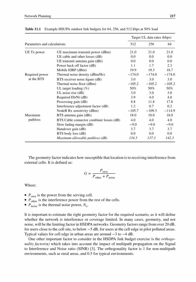
Network Planning 217
Table 11.1 Example HSUPA outdoor link budgets for 64, 256, and 512 kbps at 50% load
Target UL data rates (kbps)
Parameters and calculations 512 256 64
UE Tx power UE maximum transmit power (dBm) 21.0 21.0 21.0UE cable and other losses (dB) 0.0 0.0 0.0UE transmit antenna gain (dBi) 0.0 0.0 0.0Power back off factor (dB) 1.1 1.7 2.3Mobile EIRP (dBm) 19.9 19.3 18.7
Required powerat the BTS
Thermal noise density (dBm/Hz) −174.0 −174.0 −174.0BTS receiver noise figure (dB) 3.0 3.0 3.0Thermal noise floor (dBm) −105.2 −105.2 −105.2UL target loading (%) 50% 50% 50%UL noise rise (dB) 3.0 3.0 3.0Required Eb/Nt (dB) 3.9 4.0 4.8Processing gain (dB) 8.8 11.8 17.8Interference adjustment factor (dB) 1.2 0.7 0.2NodeB Rx sensitivity (dBm) −105.7 −109.3 −114.9
Maximumpathloss
BTS antenna gain (dBi) 18.0 18.0 18.0BTS Cable connector combiner losses (dB) 4.0 4.0 4.0Slow fading margin (dB) −9.0 −9.0 −9.0Handover gain (dB) 3.7 3.7 3.7BTS body loss (dB) 0.0 0.0 0.0Maximum allowable pathloss (dB) 134.3 137.3 142.3
The geometry factor indicates how susceptible that location is to receiving interference fromexternal cells. It is defined as:
G =Pown
Pother + Pnoise
Where:
� Pown is the power from the serving cell.� Pother is the interference power from the rest of the cells.� Pnoise is the thermal noise power, No.
It is important to estimate the right geometry factor for the required scenario, as it will definewhether the network is interference or coverage limited. In many cases, geometry, and notnoise, will be the limiting factor in HSDPA networks. Geometry factors range from over 20 dB,for users close to the cell site, to below −5 dB, for users at the cell edge in pilot polluted areas.Typical values for cell edge in urban areas are around −3 to −4 dB.
One other important factor to consider in the HSDPA link budget exercise is the orthogo-nality factor(𝛼) which takes into account the impact of multipath propagation on the Signalto Interference and Noise ratio (SINR) [3]. The orthogonality factor is 1 for non-multipathenvironments, such as rural areas, and 0.5 for typical environments.

218 HSPA+ Evolution to Release 12
The SINR will determine the achievable bitrate for the HSDPA service. In interferencelimited conditions, the SINR for HSDPA can be estimated as:
SINR = SF16 ×pHSDPA
(1 − 𝛼)Pown + Pother + Pnoise= SF16 ×
pHSDPA
PTOT BS
(1 − 𝛼 + 1
G
)
Where:
� SF16 is the processing gain corresponding to the spreading factor 16 (12 dB).� PTOT_BS is the total power transmitted by the BTS.� PHSDPA is the power available for the HS-DSCH channel.
The power allocated to the HSDPA service depends on the specific vendor implementation(static vs. dynamic allocation) and operator configuration. Nowadays, most HSDPA networksallocate the power dynamically, with a low power margin to maximize the bitrates in the sector.
Table 11.2 provides some example values for the required SINR to achieve certain downlinkbitrates, based on HSDPA Release 5 [4].
The HSDPA advanced receivers will significantly improve SINR, especially at challengingcell locations such as the ones found at cell borders in urban areas (low G factors).
Table 11.3 provides some example SINR and throughput under various network configura-tion and geometry factors, for a cell with a minimum HSUPA bitrate of 64 kbps (MAPL of142 dB). The maximum BTS power is set to 20 W.
Table 11.2 SINR requirement for various DL bitrates
SINRThroughputwith 5 codes
Throughputwith 10 codes
Throughputwith 15 codes
0 0.2 0.2 0.25 0.5 0.5 0.5
10 1.0 1.2 1.215 1.8 2.8 3.020 2.8 4.2 5.525 3.1 5.8 7.830 3.3 6.7 9.2
Table 11.3 Example cell edge DL bitrates for various HSDPAconfiguration scenarios, for MAPL = 142 dB and 𝛼 = 0.5
ConfigurationG-factor
(dB)HS power
(W)SINR(dB)
DL bitrate(Mbps)
1 14 12 12.3 2.02 14 7 10.0 1.23 0 7 5.6 0.64 −3 7 3.5 0.45 −3 12 5.8 0.6
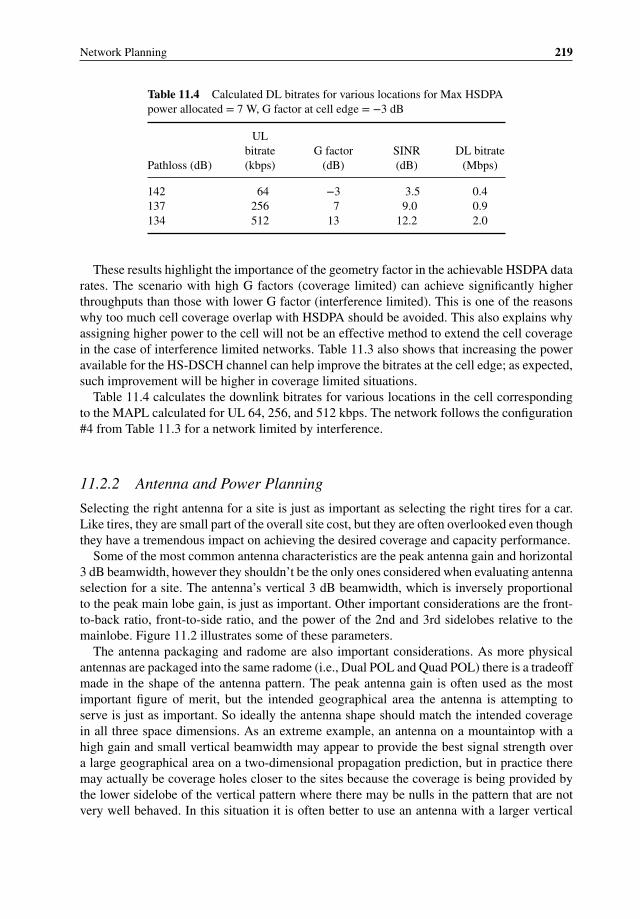
Network Planning 219
Table 11.4 Calculated DL bitrates for various locations for Max HSDPApower allocated = 7 W, G factor at cell edge = −3 dB
Pathloss (dB)
ULbitrate(kbps)
G factor(dB)
SINR(dB)
DL bitrate(Mbps)
142 64 −3 3.5 0.4137 256 7 9.0 0.9134 512 13 12.2 2.0
These results highlight the importance of the geometry factor in the achievable HSDPA datarates. The scenario with high G factors (coverage limited) can achieve significantly higherthroughputs than those with lower G factor (interference limited). This is one of the reasonswhy too much cell coverage overlap with HSDPA should be avoided. This also explains whyassigning higher power to the cell will not be an effective method to extend the cell coveragein the case of interference limited networks. Table 11.3 also shows that increasing the poweravailable for the HS-DSCH channel can help improve the bitrates at the cell edge; as expected,such improvement will be higher in coverage limited situations.
Table 11.4 calculates the downlink bitrates for various locations in the cell correspondingto the MAPL calculated for UL 64, 256, and 512 kbps. The network follows the configuration#4 from Table 11.3 for a network limited by interference.
11.2.2 Antenna and Power Planning
Selecting the right antenna for a site is just as important as selecting the right tires for a car.Like tires, they are small part of the overall site cost, but they are often overlooked even thoughthey have a tremendous impact on achieving the desired coverage and capacity performance.
Some of the most common antenna characteristics are the peak antenna gain and horizontal3 dB beamwidth, however they shouldn’t be the only ones considered when evaluating antennaselection for a site. The antenna’s vertical 3 dB beamwidth, which is inversely proportionalto the peak main lobe gain, is just as important. Other important considerations are the front-to-back ratio, front-to-side ratio, and the power of the 2nd and 3rd sidelobes relative to themainlobe. Figure 11.2 illustrates some of these parameters.
The antenna packaging and radome are also important considerations. As more physicalantennas are packaged into the same radome (i.e., Dual POL and Quad POL) there is a tradeoffmade in the shape of the antenna pattern. The peak antenna gain is often used as the mostimportant figure of merit, but the intended geographical area the antenna is attempting toserve is just as important. So ideally the antenna shape should match the intended coveragein all three space dimensions. As an extreme example, an antenna on a mountaintop with ahigh gain and small vertical beamwidth may appear to provide the best signal strength overa large geographical area on a two-dimensional propagation prediction, but in practice theremay actually be coverage holes closer to the sites because the coverage is being provided bythe lower sidelobe of the vertical pattern where there may be nulls in the pattern that are notvery well behaved. In this situation it is often better to use an antenna with a larger vertical
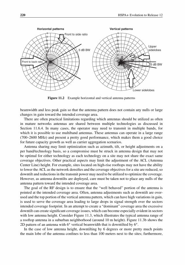
220 HSPA+ Evolution to Release 12
Horizontal patterns
Front to side ratio
Vertical patterns
Uppersidelobes
Lower sidelobes
3 dB BW
3 dB BW
0
–5
–10
–15
–20
–25
–30
–35
0
–5
–10
–15
–20
–25
–30
–35–40Front to back ratio
Figure 11.2 Example horizontal and vertical antenna patterns
beamwidth and less peak gain so that the antenna pattern does not contain any nulls or largechanges in gain toward the intended coverage area.
There are often practical limitations regarding which antennas should be utilized as oftenin mature networks antennas are shared between multiple technologies as discussed inSection 11.6.4. In many cases, the operator may need to transmit in multiple bands, forwhich it is possible to use multiband antennas. These antennas can operate in a large range(700–2600 MHz) and present a pretty good performance, which makes them a good choicefor future capacity growth as well as carrier aggregation scenarios.
Antenna sharing may limit optimization such as azimuth, tilt, or height adjustments on aper band/technology basis, so a compromise must be struck in antenna design that may notbe optimal for either technology as each technology on a site may not share the exact samecoverage objectives. Other practical aspects may limit the adjustment of the ACL (AntennaCenter Line) height. For example, sites located on high-rise rooftops may not have the abilityto lower the ACL as the network densifies and the coverage objectives for a site are reduced, sodowntilt and reductions in the transmit power may need to be utilized to optimize the coverage.However, as antenna downtilts are deployed, care must be taken not to place any nulls of theantenna pattern toward the intended coverage area.
The goal of the RF design is to ensure that the “well behaved” portion of the antenna ispointed at the intended coverage area. Often, antenna adjustments such as downtilt are over-used and the top portion of the vertical antenna pattern, which can have high variations in gain,is used to serve the coverage area leading to large drops in signal strength over the sectorsintended coverage footprint. In an attempt to create a “dominant” coverage area the excessivedowntilt can create significant coverage issues, which can become especially evident in sectorswith low antenna height. Consider Figure 11.3, which illustrates the typical antenna range ofa rooftop antenna in a suburban neighborhood (around 10 m height). Figure 11.3b shows the2D pattern of an antenna with 6◦ vertical beamwidth that is downtilted by 6◦.
In the case of low antenna height, downtilting by 6 degrees or more pretty much pointsthe main lobe of the antenna confines to less than 100 meters next to the sites; furthermore,
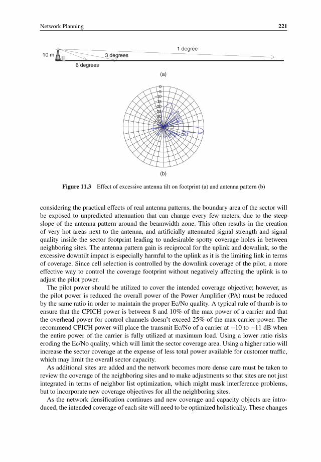
Network Planning 221
(a)
(b)
–50
–10–15–20–25–30–35
10 m1 degree
3 degrees
6 degrees
Figure 11.3 Effect of excessive antenna tilt on footprint (a) and antenna pattern (b)
considering the practical effects of real antenna patterns, the boundary area of the sector willbe exposed to unpredicted attenuation that can change every few meters, due to the steepslope of the antenna pattern around the beamwidth zone. This often results in the creationof very hot areas next to the antenna, and artificially attenuated signal strength and signalquality inside the sector footprint leading to undesirable spotty coverage holes in betweenneighboring sites. The antenna pattern gain is reciprocal for the uplink and downlink, so theexcessive downtilt impact is especially harmful to the uplink as it is the limiting link in termsof coverage. Since cell selection is controlled by the downlink coverage of the pilot, a moreeffective way to control the coverage footprint without negatively affecting the uplink is toadjust the pilot power.
The pilot power should be utilized to cover the intended coverage objective; however, asthe pilot power is reduced the overall power of the Power Amplifier (PA) must be reducedby the same ratio in order to maintain the proper Ec/No quality. A typical rule of thumb is toensure that the CPICH power is between 8 and 10% of the max power of a carrier and thatthe overhead power for control channels doesn’t exceed 25% of the max carrier power. Therecommend CPICH power will place the transmit Ec/No of a carrier at −10 to −11 dB whenthe entire power of the carrier is fully utilized at maximum load. Using a lower ratio riskseroding the Ec/No quality, which will limit the sector coverage area. Using a higher ratio willincrease the sector coverage at the expense of less total power available for customer traffic,which may limit the overall sector capacity.
As additional sites are added and the network becomes more dense care must be taken toreview the coverage of the neighboring sites and to make adjustments so that sites are not justintegrated in terms of neighbor list optimization, which might mask interference problems,but to incorporate new coverage objectives for all the neighboring sites.
As the network densification continues and new coverage and capacity objects are intro-duced, the intended coverage of each site will need to be optimized holistically. These changes
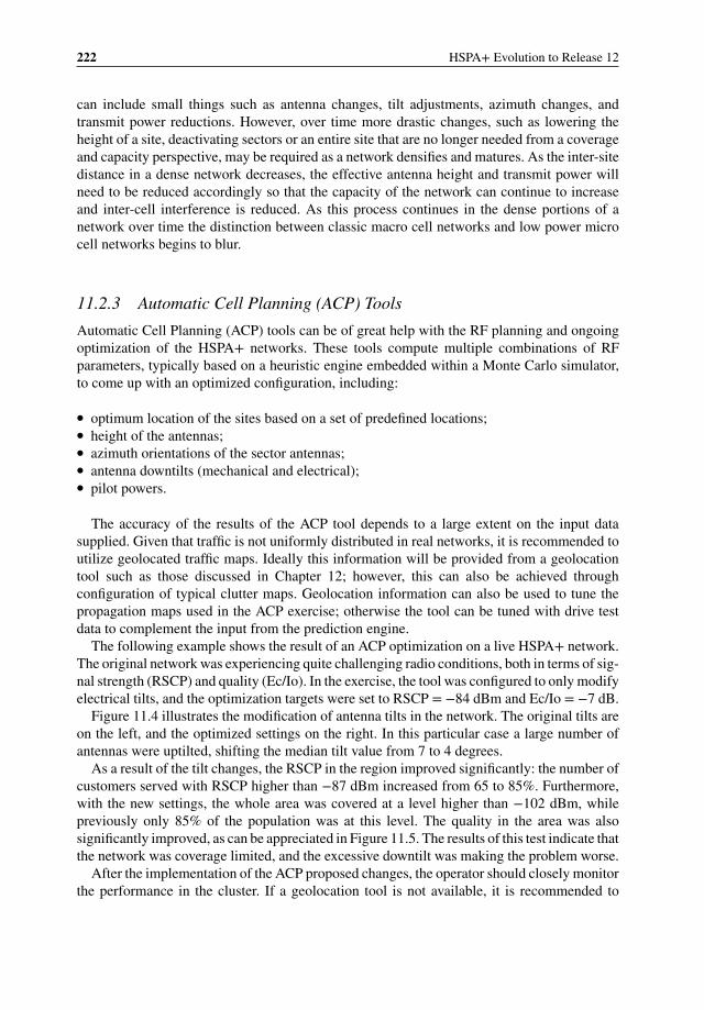
222 HSPA+ Evolution to Release 12
can include small things such as antenna changes, tilt adjustments, azimuth changes, andtransmit power reductions. However, over time more drastic changes, such as lowering theheight of a site, deactivating sectors or an entire site that are no longer needed from a coverageand capacity perspective, may be required as a network densifies and matures. As the inter-sitedistance in a dense network decreases, the effective antenna height and transmit power willneed to be reduced accordingly so that the capacity of the network can continue to increaseand inter-cell interference is reduced. As this process continues in the dense portions of anetwork over time the distinction between classic macro cell networks and low power microcell networks begins to blur.
11.2.3 Automatic Cell Planning (ACP) Tools
Automatic Cell Planning (ACP) tools can be of great help with the RF planning and ongoingoptimization of the HSPA+ networks. These tools compute multiple combinations of RFparameters, typically based on a heuristic engine embedded within a Monte Carlo simulator,to come up with an optimized configuration, including:
� optimum location of the sites based on a set of predefined locations;� height of the antennas;� azimuth orientations of the sector antennas;� antenna downtilts (mechanical and electrical);� pilot powers.
The accuracy of the results of the ACP tool depends to a large extent on the input datasupplied. Given that traffic is not uniformly distributed in real networks, it is recommended toutilize geolocated traffic maps. Ideally this information will be provided from a geolocationtool such as those discussed in Chapter 12; however, this can also be achieved throughconfiguration of typical clutter maps. Geolocation information can also be used to tune thepropagation maps used in the ACP exercise; otherwise the tool can be tuned with drive testdata to complement the input from the prediction engine.
The following example shows the result of an ACP optimization on a live HSPA+ network.The original network was experiencing quite challenging radio conditions, both in terms of sig-nal strength (RSCP) and quality (Ec/Io). In the exercise, the tool was configured to only modifyelectrical tilts, and the optimization targets were set to RSCP = −84 dBm and Ec/Io = −7 dB.
Figure 11.4 illustrates the modification of antenna tilts in the network. The original tilts areon the left, and the optimized settings on the right. In this particular case a large number ofantennas were uptilted, shifting the median tilt value from 7 to 4 degrees.
As a result of the tilt changes, the RSCP in the region improved significantly: the number ofcustomers served with RSCP higher than −87 dBm increased from 65 to 85%. Furthermore,with the new settings, the whole area was covered at a level higher than −102 dBm, whilepreviously only 85% of the population was at this level. The quality in the area was alsosignificantly improved, as can be appreciated in Figure 11.5. The results of this test indicate thatthe network was coverage limited, and the excessive downtilt was making the problem worse.
After the implementation of the ACP proposed changes, the operator should closely monitorthe performance in the cluster. If a geolocation tool is not available, it is recommended to
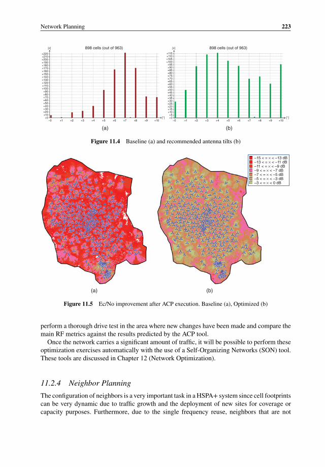
Network Planning 223
–0+0
+10+20+30+40+50+60+70+80+90
+100+110+120+130+140+150+160+170+180+190+200+210+220
898 cells (out of 963)[#]
[°]+1 +2
(a)
+3 +4 +5 +6 +7 +8 +9 +10
(b)
–0+0+5
+10+15+20+25+30+35+40+45+50+55+60+65+70+75+80+85+90+95
+100+105+110+115
898 cells (out of 963)[#]
[°]+1 +2 +3 +4 +5 +6 +7 +8 +9 +10
Figure 11.4 Baseline (a) and recommended antenna tilts (b)
–15 < = × < –13 dB–13 < = × < –11 dB–11 < = × < –9 dB–9 < = × < –7 dB–7 < = × < –5 dB–5 < = × < –3 dB–3 < = × < 0 dB
(a) (b)
Figure 11.5 Ec/No improvement after ACP execution. Baseline (a), Optimized (b)
perform a thorough drive test in the area where new changes have been made and compare themain RF metrics against the results predicted by the ACP tool.
Once the network carries a significant amount of traffic, it will be possible to perform theseoptimization exercises automatically with the use of a Self-Organizing Networks (SON) tool.These tools are discussed in Chapter 12 (Network Optimization).
11.2.4 Neighbor Planning
The configuration of neighbors is a very important task in a HSPA+ system since cell footprintscan be very dynamic due to traffic growth and the deployment of new sites for coverage orcapacity purposes. Furthermore, due to the single frequency reuse, neighbors that are not
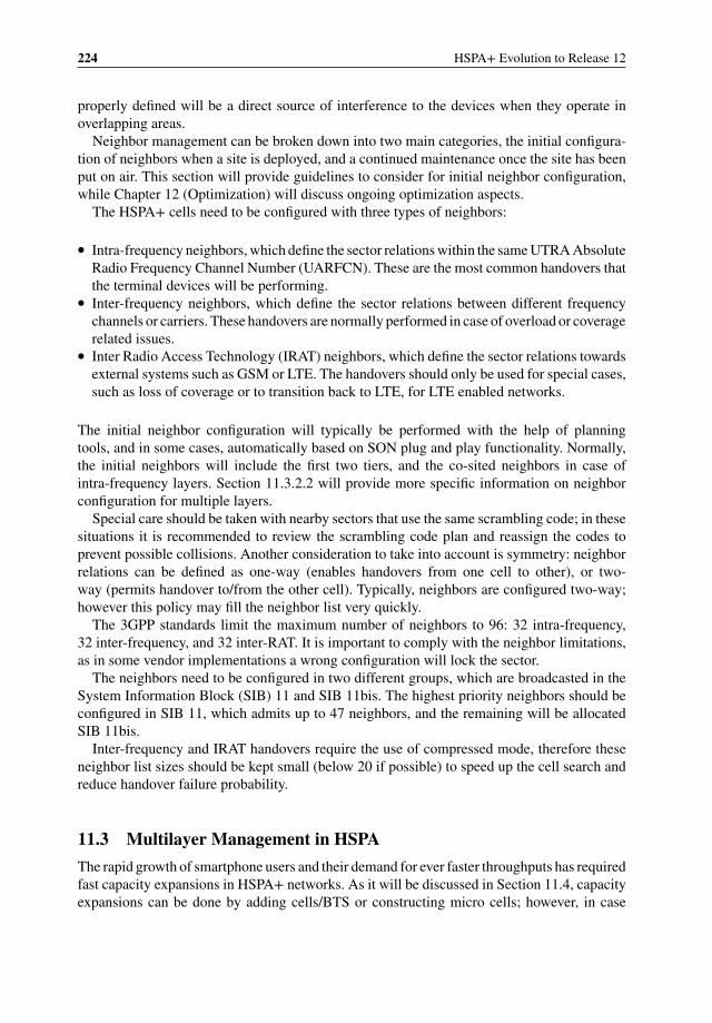
224 HSPA+ Evolution to Release 12
properly defined will be a direct source of interference to the devices when they operate inoverlapping areas.
Neighbor management can be broken down into two main categories, the initial configura-tion of neighbors when a site is deployed, and a continued maintenance once the site has beenput on air. This section will provide guidelines to consider for initial neighbor configuration,while Chapter 12 (Optimization) will discuss ongoing optimization aspects.
The HSPA+ cells need to be configured with three types of neighbors:
� Intra-frequency neighbors, which define the sector relations within the same UTRA AbsoluteRadio Frequency Channel Number (UARFCN). These are the most common handovers thatthe terminal devices will be performing.
� Inter-frequency neighbors, which define the sector relations between different frequencychannels or carriers. These handovers are normally performed in case of overload or coveragerelated issues.
� Inter Radio Access Technology (IRAT) neighbors, which define the sector relations towardsexternal systems such as GSM or LTE. The handovers should only be used for special cases,such as loss of coverage or to transition back to LTE, for LTE enabled networks.
The initial neighbor configuration will typically be performed with the help of planningtools, and in some cases, automatically based on SON plug and play functionality. Normally,the initial neighbors will include the first two tiers, and the co-sited neighbors in case ofintra-frequency layers. Section 11.3.2.2 will provide more specific information on neighborconfiguration for multiple layers.
Special care should be taken with nearby sectors that use the same scrambling code; in thesesituations it is recommended to review the scrambling code plan and reassign the codes toprevent possible collisions. Another consideration to take into account is symmetry: neighborrelations can be defined as one-way (enables handovers from one cell to other), or two-way (permits handover to/from the other cell). Typically, neighbors are configured two-way;however this policy may fill the neighbor list very quickly.
The 3GPP standards limit the maximum number of neighbors to 96: 32 intra-frequency,32 inter-frequency, and 32 inter-RAT. It is important to comply with the neighbor limitations,as in some vendor implementations a wrong configuration will lock the sector.
The neighbors need to be configured in two different groups, which are broadcasted in theSystem Information Block (SIB) 11 and SIB 11bis. The highest priority neighbors should beconfigured in SIB 11, which admits up to 47 neighbors, and the remaining will be allocatedSIB 11bis.
Inter-frequency and IRAT handovers require the use of compressed mode, therefore theseneighbor list sizes should be kept small (below 20 if possible) to speed up the cell search andreduce handover failure probability.
11.3 Multilayer Management in HSPA
The rapid growth of smartphone users and their demand for ever faster throughputs has requiredfast capacity expansions in HSPA+ networks. As it will be discussed in Section 11.4, capacityexpansions can be done by adding cells/BTS or constructing micro cells; however, in case
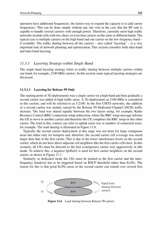
Network Planning 225
operators have additional frequencies, the fastest way to expand the capacity is to add carrierfrequencies. This can be done simply without any site visit in the case that the RF unit iscapable to handle several carriers with enough power. Therefore, currently most high trafficnetworks include cells with two, three, or even four carriers on the same or different bands. Thetypical case is multiple carriers on the high band and one carrier on the low frequency band –if available. The traffic sharing between all the carriers – also called “layering” – is a veryimportant task of network planning and optimization. This section considers both intra-bandand inter-band layering.
11.3.1 Layering Strategy within Single Band
The single band layering strategy refers to traffic sharing between multiple carriers withinone band, for example, 2100 MHz carriers. In this section some typical layering strategies arediscussed.
11.3.1.1 Layering for Release 99 Only
The starting point of 3G deployments was a single carrier on a high band and then gradually asecond carrier was added in high traffic areas. A 3G deployment on 2100 MHz is consideredin this section, and will be referred to as U2100. In the first UMTS networks, the additionof a second carrier was mainly caused by the Release 99 Dedicated Channel (DCH) trafficincrease. The load was shared equally between the two layers using, for example, RadioResource Control (RRC) connection setup redirection, where the RRC setup message informsthe UE to move to another carrier and therefore the UE completes the RRC setup in this othercarrier. The load in this context can refer to uplink noise rise or number of connected users,for example. The load sharing is illustrated in Figure 11.6.
Typically the second carrier deployment at this stage was not done for large contiguousareas but rather only for hotspots and, therefore, the second carrier cell coverage was muchlarger than that of the first carrier. This is due to the lower interference levels on the secondcarrier, which do not have direct adjacent cell neighbors like the first carrier cells have. In thisscenario, all UEs must be directed to the first (contiguous) carrier very aggressively in idlemode. To achieve this, a negative Qoffset2 is used for first carrier neighbors on the secondcarrier, as shown in Figure 11.7.
Similarly, in dedicated mode the UEs must be pushed to the first carrier and the inter-frequency handover has to be triggered based on RSCP threshold rather than Ec/No. Thereason for this is that good Ec/No areas in the second carrier can extend over several first
R99
f2
f1
R99 Equal load
sharing between
carriers
Figure 11.6 Load sharing between Release 99 carriers
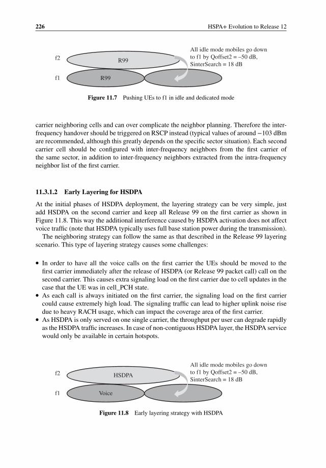
226 HSPA+ Evolution to Release 12
R99
R99
f2
f1
All idle mode mobiles go down
to f1 by Qoffset2 = –50 dB,
SinterSearch = 18 dB
Figure 11.7 Pushing UEs to f1 in idle and dedicated mode
carrier neighboring cells and can over complicate the neighbor planning. Therefore the inter-frequency handover should be triggered on RSCP instead (typical values of around −103 dBmare recommended, although this greatly depends on the specific sector situation). Each secondcarrier cell should be configured with inter-frequency neighbors from the first carrier ofthe same sector, in addition to inter-frequency neighbors extracted from the intra-frequencyneighbor list of the first carrier.
11.3.1.2 Early Layering for HSDPA
At the initial phases of HSDPA deployment, the layering strategy can be very simple, justadd HSDPA on the second carrier and keep all Release 99 on the first carrier as shown inFigure 11.8. This way the additional interference caused by HSDPA activation does not affectvoice traffic (note that HSDPA typically uses full base station power during the transmission).
The neighboring strategy can follow the same as that described in the Release 99 layeringscenario. This type of layering strategy causes some challenges:
� In order to have all the voice calls on the first carrier the UEs should be moved to thefirst carrier immediately after the release of HSDPA (or Release 99 packet call) call on thesecond carrier. This causes extra signaling load on the first carrier due to cell updates in thecase that the UE was in cell_PCH state.
� As each call is always initiated on the first carrier, the signaling load on the first carriercould cause extremely high load. The signaling traffic can lead to higher uplink noise risedue to heavy RACH usage, which can impact the coverage area of the first carrier.
� As HSDPA is only served on one single carrier, the throughput per user can degrade rapidlyas the HSDPA traffic increases. In case of non-contiguous HSDPA layer, the HSDPA servicewould only be available in certain hotspots.
HSDPA
Voice
f2
f1
All idle mode mobiles go down
to f1 by Qoffset2 = –50 dB,
SinterSearch = 18 dB
Figure 11.8 Early layering strategy with HSDPA
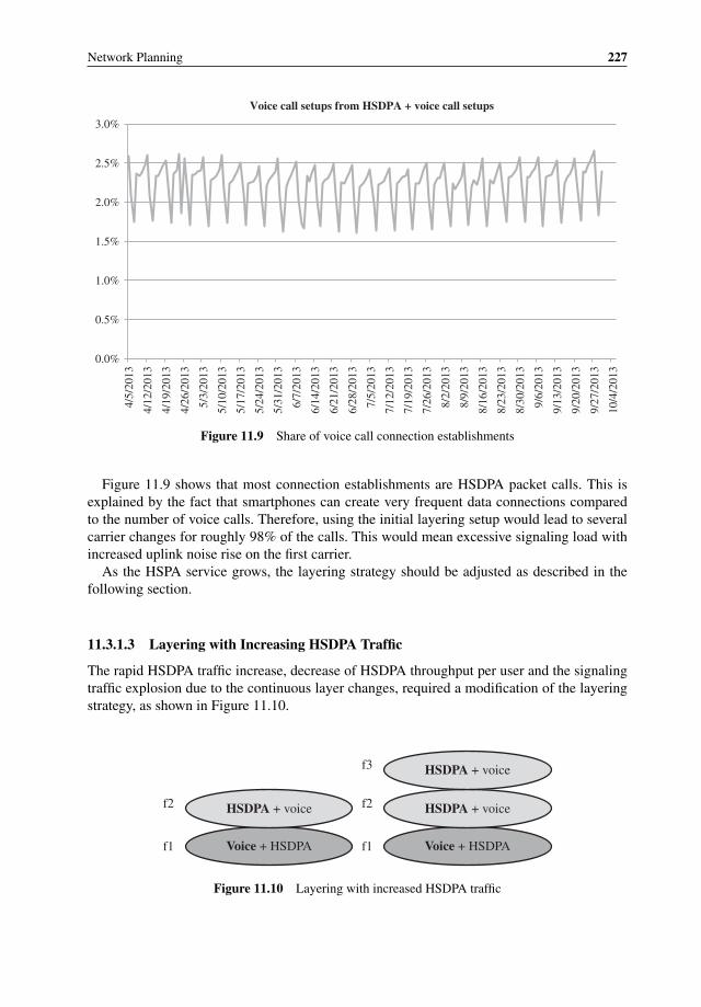
Network Planning 227
0.0%
0.5%
1.0%
1.5%
2.0%
2.5%
3.0%4/5
/2013
4/1
2/2
013
4/1
9/2
013
4/2
6/2
013
5/3
/2013
5/1
0/2
013
5/1
7/2
013
5/2
4/2
013
5/3
1/2
013
6/7
/2013
6/1
4/2
013
6/2
1/2
013
6/2
8/2
013
7/5
/2013
7/1
2/2
013
7/1
9/2
013
7/2
6/2
013
8/2
/2013
8/9
/2013
8/1
6/2
013
8/2
3/2
013
8/3
0/2
013
9/6
/2013
9/1
3/2
013
9/2
0/2
013
9/2
7/2
013
10/4
/2013
Voice call setups from HSDPA + voice call setups
Figure 11.9 Share of voice call connection establishments
Figure 11.9 shows that most connection establishments are HSDPA packet calls. This isexplained by the fact that smartphones can create very frequent data connections comparedto the number of voice calls. Therefore, using the initial layering setup would lead to severalcarrier changes for roughly 98% of the calls. This would mean excessive signaling load withincreased uplink noise rise on the first carrier.
As the HSPA service grows, the layering strategy should be adjusted as described in thefollowing section.
11.3.1.3 Layering with Increasing HSDPA Traffic
The rapid HSDPA traffic increase, decrease of HSDPA throughput per user and the signalingtraffic explosion due to the continuous layer changes, required a modification of the layeringstrategy, as shown in Figure 11.10.
Voice + HSDPA
HSDPA + voicef2
f1 Voice + HSDPA
HSDPA + voicef2
f1
HSDPA + voicef3
Figure 11.10 Layering with increased HSDPA traffic
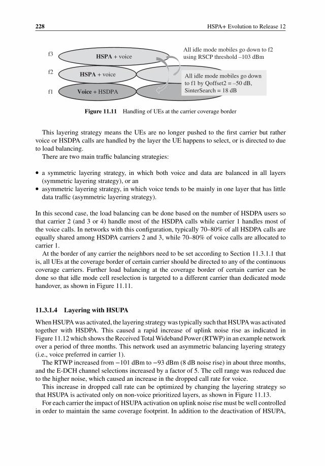
228 HSPA+ Evolution to Release 12
Voice + HSDPA
HSPA + voicef2
f1
HSPA + voicef3
All idle mode mobiles go down
to f1 by Qoffset2 = –50 dB,
SinterSearch = 18 dB
All idle mode mobiles go down to f2
using RSCP threshold –103 dBm
Figure 11.11 Handling of UEs at the carrier coverage border
This layering strategy means the UEs are no longer pushed to the first carrier but rathervoice or HSDPA calls are handled by the layer the UE happens to select, or is directed to dueto load balancing.
There are two main traffic balancing strategies:
� a symmetric layering strategy, in which both voice and data are balanced in all layers(symmetric layering strategy), or an
� asymmetric layering strategy, in which voice tends to be mainly in one layer that has littledata traffic (asymmetric layering strategy).
In this second case, the load balancing can be done based on the number of HSDPA users sothat carrier 2 (and 3 or 4) handle most of the HSDPA calls while carrier 1 handles most ofthe voice calls. In networks with this configuration, typically 70–80% of all HSDPA calls areequally shared among HSDPA carriers 2 and 3, while 70–80% of voice calls are allocated tocarrier 1.
At the border of any carrier the neighbors need to be set according to Section 11.3.1.1 thatis, all UEs at the coverage border of certain carrier should be directed to any of the continuouscoverage carriers. Further load balancing at the coverage border of certain carrier can bedone so that idle mode cell reselection is targeted to a different carrier than dedicated modehandover, as shown in Figure 11.11.
11.3.1.4 Layering with HSUPA
When HSUPA was activated, the layering strategy was typically such that HSUPA was activatedtogether with HSDPA. This caused a rapid increase of uplink noise rise as indicated inFigure 11.12 which shows the Received Total Wideband Power (RTWP) in an example networkover a period of three months. This network used an asymmetric balancing layering strategy(i.e., voice preferred in carrier 1).
The RTWP increased from −101 dBm to −93 dBm (8 dB noise rise) in about three months,and the E-DCH channel selections increased by a factor of 5. The cell range was reduced dueto the higher noise, which caused an increase in the dropped call rate for voice.
This increase in dropped call rate can be optimized by changing the layering strategy sothat HSUPA is activated only on non-voice prioritized layers, as shown in Figure 11.13.
For each carrier the impact of HSUPA activation on uplink noise rise must be well controlledin order to maintain the same coverage footprint. In addition to the deactivation of HSUPA,
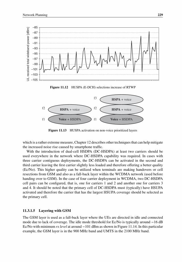
Network Planning 229
UL
rece
ived
tota
l wid
eban
d po
wer
[dB
m]
–105
–103
–101
–99
–97
–95
–93
–91
–89
–87
–85
Figure 11.12 HUSPA (E-DCH) selections increase of RTWP
Voice + HSDPA
HSPA + voicef2
f1 Voice + HSDPA
HSPA + voicef2
f1
HSPA + voicef3
Figure 11.13 HUSPA activation on non-voice prioritized layers
which is a rather extreme measure, Chapter 12 describes other techniques that can help mitigatethe increased noise rise caused by smartphone traffic.
With the introduction of dual-cell HSDPA (DC-HSDPA) at least two carriers should beused everywhere in the network where DC-HSDPA capability was required. In cases withthree carrier contiguous deployments, the DC-HSDPA can be activated in the second andthird carrier leaving the first carrier slightly less loaded and therefore offering a better quality(Ec/No). This higher quality can be utilized when terminals are making handovers or cellresections from GSM and also as a fall-back layer within the WCDMA network (used beforehanding over to GSM). In the case of four carrier deployment in WCDMA, two DC-HSDPAcell pairs can be configured, that is, one for carriers 1 and 2 and another one for carriers 3and 4. It should be noted that the primary cell of DC-HSDPA must (typically) have HSUPAactivated and therefore the carrier that has the largest HSUPA coverage should be selected asthe primary cell.
11.3.1.5 Layering with GSM
The GSM layer is used as a fall-back layer where the UEs are directed in idle and connectedmode due to lack of coverage. The idle mode threshold for Ec/No is typically around −16 dBEc/No with minimum rx level at around −101 dBm as shown in Figure 11.14. In this particularexample, the GSM layer is in the 900 MHz band and UMTS in the 2100 MHz band.
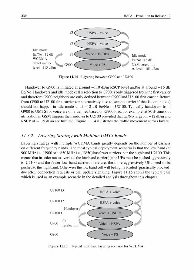
230 HSPA+ Evolution to Release 12
Voice + HSDPA
HSPA + voicef2
f1
HSPA + voicef3
Voice + PSG900
Idle mode:
Ec/No –16 dB,
GSM target min
rx level –101 dBm
Idle mode:
Ec/No –12 dB,
WCDMA
target min rx
level –115 dBm
Figure 11.14 Layering between G900 and U2100
Handover to G900 is initiated at around −110 dBm RSCP level and/or at around −16 dBEc/No. Handovers and idle mode cell reselection to G900 is only triggered from the first carrierand therefore G900 neighbors are only defined between G900 and U2100 first carrier. Returnfrom G900 to U2100 first carrier (or alternatively also to second carrier if that is continuous)should not happen in idle mode until −12 dB Ec/No in U2100. Typically handovers fromG900 to UMTS for voice are only defined based on G900 load, for example, at 80% time slotutilization in GSM triggers the handover to U2100 provided that Ec/No target of −12 dBm andRSCP of −115 dBm are fulfilled. Figure 11.14 illustrates the traffic movement across layers.
11.3.2 Layering Strategy with Multiple UMTS Bands
Layering strategy with multiple WCDMA bands greatly depends on the number of carrierson different frequency bands. The most typical deployment scenario is that the low band (at900 MHz i.e., U900 or at 850 MHz i.e., U850) has fewer carriers than the high band U2100. Thismeans that in order not to overload the low band carrier(s) the UEs must be pushed aggressivelyto U2100 and the fewer low band carriers there are, the more aggressively UEs need to bepushed to the high band. Otherwise the low band cell will be highly loaded (practically blocked)due RRC connection requests or cell update signaling. Figure 11.15 shows the typical casewhich is used as an example scenario in the detailed analysis throughout this chapter.
Voice + HSDPA
HSPA + voice
U2100 f1
HSPA + voice
Voice + PS
U900 Voice + HSPA
G900
U2100 f2
U2100 f3
Cell
reselection
Handover
Figure 11.15 Typical multiband layering scenario for WCDMA
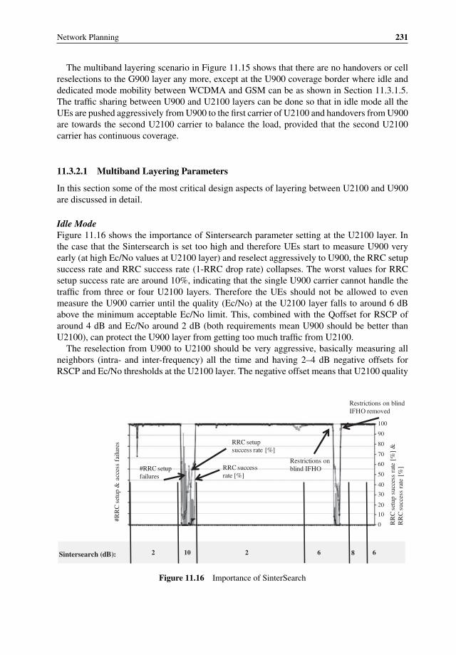
Network Planning 231
The multiband layering scenario in Figure 11.15 shows that there are no handovers or cellreselections to the G900 layer any more, except at the U900 coverage border where idle anddedicated mode mobility between WCDMA and GSM can be as shown in Section 11.3.1.5.The traffic sharing between U900 and U2100 layers can be done so that in idle mode all theUEs are pushed aggressively from U900 to the first carrier of U2100 and handovers from U900are towards the second U2100 carrier to balance the load, provided that the second U2100carrier has continuous coverage.
11.3.2.1 Multiband Layering Parameters
In this section some of the most critical design aspects of layering between U2100 and U900are discussed in detail.
Idle ModeFigure 11.16 shows the importance of Sintersearch parameter setting at the U2100 layer. Inthe case that the Sintersearch is set too high and therefore UEs start to measure U900 veryearly (at high Ec/No values at U2100 layer) and reselect aggressively to U900, the RRC setupsuccess rate and RRC success rate (1-RRC drop rate) collapses. The worst values for RRCsetup success rate are around 10%, indicating that the single U900 carrier cannot handle thetraffic from three or four U2100 layers. Therefore the UEs should not be allowed to evenmeasure the U900 carrier until the quality (Ec/No) at the U2100 layer falls to around 6 dBabove the minimum acceptable Ec/No limit. This, combined with the Qoffset for RSCP ofaround 4 dB and Ec/No around 2 dB (both requirements mean U900 should be better thanU2100), can protect the U900 layer from getting too much traffic from U2100.
The reselection from U900 to U2100 should be very aggressive, basically measuring allneighbors (intra- and inter-frequency) all the time and having 2–4 dB negative offsets forRSCP and Ec/No thresholds at the U2100 layer. The negative offset means that U2100 quality
Sintersearch (dB): 2 10 2 6 8 6
#R
RC
set
up &
acc
ess
failure
s
RR
C s
etu
p s
ucc
ess
rate
[%
] &
R
RC
succ
ess
rate
[%
]
100
90
80
70
60
50
40
30
20
10
0
RRC setup success rate [%]
RRC success rate [%]
#RRC setup failures
Restrictions on blind IFHO
Restrictions on blind IFHO removed
Figure 11.16 Importance of SinterSearch
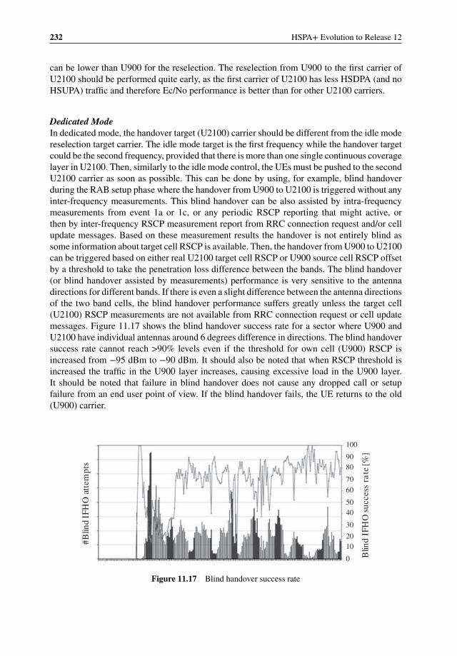
232 HSPA+ Evolution to Release 12
can be lower than U900 for the reselection. The reselection from U900 to the first carrier ofU2100 should be performed quite early, as the first carrier of U2100 has less HSDPA (and noHSUPA) traffic and therefore Ec/No performance is better than for other U2100 carriers.
Dedicated ModeIn dedicated mode, the handover target (U2100) carrier should be different from the idle modereselection target carrier. The idle mode target is the first frequency while the handover targetcould be the second frequency, provided that there is more than one single continuous coveragelayer in U2100. Then, similarly to the idle mode control, the UEs must be pushed to the secondU2100 carrier as soon as possible. This can be done by using, for example, blind handoverduring the RAB setup phase where the handover from U900 to U2100 is triggered without anyinter-frequency measurements. This blind handover can be also assisted by intra-frequencymeasurements from event 1a or 1c, or any periodic RSCP reporting that might active, orthen by inter-frequency RSCP measurement report from RRC connection request and/or cellupdate messages. Based on these measurement results the handover is not entirely blind assome information about target cell RSCP is available. Then, the handover from U900 to U2100can be triggered based on either real U2100 target cell RSCP or U900 source cell RSCP offsetby a threshold to take the penetration loss difference between the bands. The blind handover(or blind handover assisted by measurements) performance is very sensitive to the antennadirections for different bands. If there is even a slight difference between the antenna directionsof the two band cells, the blind handover performance suffers greatly unless the target cell(U2100) RSCP measurements are not available from RRC connection request or cell updatemessages. Figure 11.17 shows the blind handover success rate for a sector where U900 andU2100 have individual antennas around 6 degrees difference in directions. The blind handoversuccess rate cannot reach >90% levels even if the threshold for own cell (U900) RSCP isincreased from −95 dBm to −90 dBm. It should also be noted that when RSCP threshold isincreased the traffic in the U900 layer increases, causing excessive load in the U900 layer.It should be noted that failure in blind handover does not cause any dropped call or setupfailure from an end user point of view. If the blind handover fails, the UE returns to the old(U900) carrier.
100
90
80
70
60
50
40
30
20
10
0 Blin
d I
FH
O s
ucc
ess
rate
[%]
#B
lind
IF
HO
att
emp
ts
Figure 11.17 Blind handover success rate

Network Planning 233
Another possibility is to use compressed mode and actual inter-frequency measurementat the end of the packet call. This is done so that, instead of moving the UEs to Cell_PCH,URA_PCH, or idle mode, the UEs are ordered first to compressed mode and in the case that theU2100 carrier is found to have adequate RSCP and Ec/No the handover is executed instead ofmoving UE to cell_PCH, URA_PCH, or idle mode. This way the achievable handover successis around 98 – 99%.
Handovers from U2100 to U900 should only be done in the case of lack of coverage in theU2100 layer. And in the case of hotspot coverage for certain U2100 carriers, the handovershould be first done to the continuous coverage carrier within the U2100 layer before handoverto the U900 layer. The handover thresholds from U2100 to U900 are typically set to be similarto the previous chapter’s U2100 to G900 handover thresholds, as discussed in Section 11.3.1.5.
11.3.2.2 Neighbor Planning
The neighbor relations are planned so that from each U2100 carrier having continuous coveragethere are neighbors to the U900 carrier of the same sector (same BTS) and inter-BTS neighborsare only needed in the case that the antenna directions between the same sector bands are notthe same. Intra-band neighbors within the U2100 carriers of the same sector are not definedexcept in the case of U2100 channel border areas. This can be done provided that the trafficbetween the U2100 carriers is equally distributed. G900 neighbors are also only defined in thecase of U900 border.
11.3.3 Summary
The layering between different WCDMA carriers within the same band or different bandsshould try to balance the load between all the carriers. Load here can mean number of HSPAusers, voice erlangs, and signaling. It is especially important to monitor the signaling traffic(number of RRC connection requests and cell updates) which can increase rapidly and blockone of the carriers. Therefore, equal sharing of UEs among all carriers is mandatory. Thismeans that some parameter tuning needs to be performed from time to time as the totaltraffic increases.
11.4 RAN Capacity Planning
Capacity planning and system dimensioning is an important aspect when operating a wirelesscommunication service. A balance must be struck between over-dimensioning the system,leading to premature capital expenditures, and under-dimensioning the services provided,which can lead to poor customer experience and even customer churn. Historically, statis-tical models such as the Erlang B model have been used by wireless operators to estimatethe voice service GoS (Grade of Service) they are providing to their customers. Once itis forecasted that the BH (Busy Hour) erlangs of a cell may result in a blocking rate of1–2%, additional voice trunks or circuits are provisioned to improve the GoS below the tar-geted threshold. Dimensioning the data services is much more challenging due to their morebursty nature compared to voice and the fact that many different services can run over data
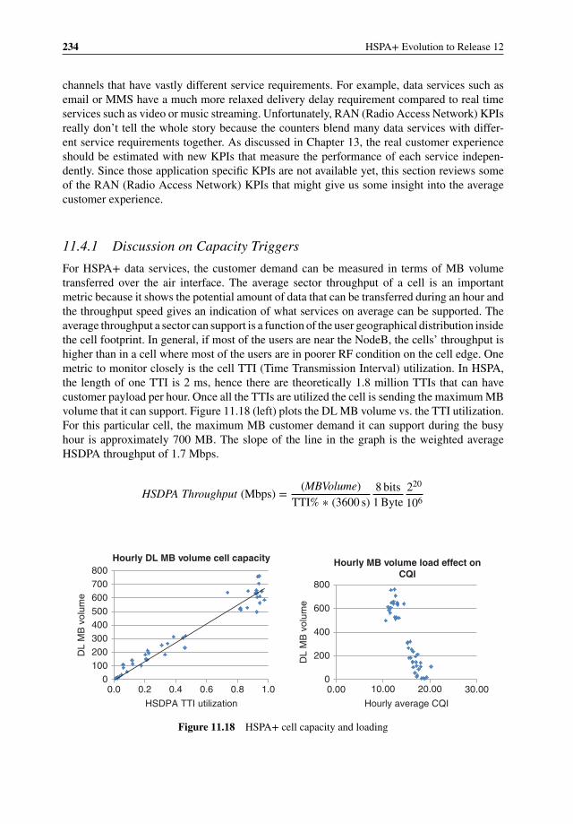
234 HSPA+ Evolution to Release 12
channels that have vastly different service requirements. For example, data services such asemail or MMS have a much more relaxed delivery delay requirement compared to real timeservices such as video or music streaming. Unfortunately, RAN (Radio Access Network) KPIsreally don’t tell the whole story because the counters blend many data services with differ-ent service requirements together. As discussed in Chapter 13, the real customer experienceshould be estimated with new KPIs that measure the performance of each service indepen-dently. Since those application specific KPIs are not available yet, this section reviews someof the RAN (Radio Access Network) KPIs that might give us some insight into the averagecustomer experience.
11.4.1 Discussion on Capacity Triggers
For HSPA+ data services, the customer demand can be measured in terms of MB volumetransferred over the air interface. The average sector throughput of a cell is an importantmetric because it shows the potential amount of data that can be transferred during an hour andthe throughput speed gives an indication of what services on average can be supported. Theaverage throughput a sector can support is a function of the user geographical distribution insidethe cell footprint. In general, if most of the users are near the NodeB, the cells’ throughput ishigher than in a cell where most of the users are in poorer RF condition on the cell edge. Onemetric to monitor closely is the cell TTI (Time Transmission Interval) utilization. In HSPA,the length of one TTI is 2 ms, hence there are theoretically 1.8 million TTIs that can havecustomer payload per hour. Once all the TTIs are utilized the cell is sending the maximum MBvolume that it can support. Figure 11.18 (left) plots the DL MB volume vs. the TTI utilization.For this particular cell, the maximum MB customer demand it can support during the busyhour is approximately 700 MB. The slope of the line in the graph is the weighted averageHSDPA throughput of 1.7 Mbps.
HSDPA Throughput (Mbps) = (MBVolume)TTI% ∗ (3600 s)
8 bits1 Byte
220
106
0100200300400500600700800
0.0 0.2 0.4 0.6 0.8 1.0
DL
MB
vol
ume
HSDPA TTI utilization
Hourly DL MB volume cell capacity
0
200
400
600
800
0.00 10.00 20.00 30.00
DL
MB
vol
ume
Hourly average CQI
Hourly MB volume load effect onCQI
Figure 11.18 HSPA+ cell capacity and loading

Network Planning 235
Customers waiting
Server 1
Server 2
Server C
Total average system delay (T)
Service time (1/μ)Wait time (W)
Figure 11.19 Generic queuing model
Figure 11.18 (right) shows the effect on the CQI (Channel Quality Index) beginningreported by the mobiles’ as more data is sent over the HSPA+ air interface and the systemloads up.
The TTI utilization is an indication that a cell is at its maximum capacity; however, whatwe really need to know in order to dimension the system is what the average user experienceis when the cell is loaded. Since the HSDPA air interface is a shared resource in the timedomain it is important to try to measure the throughput a typical user will see as other users areadded to the system. Measuring the delay of the entire system is the goal for data networks,so queuing models such as Erlang C may be utilized. There is one scheduler assigned percell on an HSPA+ NodeB, so essentially there is a single server and we can look at the TTIutilization in terms of erlangs of scheduler utilization and model the total system delay asan M/M/1 queue [5] which is a specific case of Erlang C where the number of servers orchannels is equal to one. Figure 11.19 illustrates the concept. For data traffic, we are interestedin the queuing delay because it will give us an indication of the entire systems’ performanceas perceived by the customer. For an M/M/1 queue the average total system delay (TA) can beexpressed as:
TA = WA + 1∕𝜇
WA =p
(1 − p)𝜇
Where WA is the wait time (queue time), 1/𝜇 is the average service time, and p is the serverutilization (TTI%). For an HSPA+ system, WA is the average time customer data is waiting tobe scheduled at the scheduler, the service time is the average time it takes to send the customerdata over the air interface. The service time is a function of the total time it takes to deliver
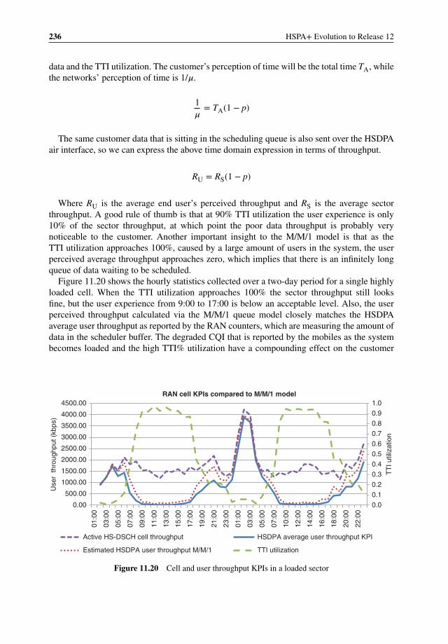
236 HSPA+ Evolution to Release 12
data and the TTI utilization. The customer’s perception of time will be the total time TA, whilethe networks’ perception of time is 1/𝜇.
1𝜇
= TA(1 − p)
The same customer data that is sitting in the scheduling queue is also sent over the HSDPAair interface, so we can express the above time domain expression in terms of throughput.
RU = RS(1 − p)
Where RU is the average end user’s perceived throughput and RS is the average sectorthroughput. A good rule of thumb is that at 90% TTI utilization the user experience is only10% of the sector throughput, at which point the poor data throughput is probably verynoticeable to the customer. Another important insight to the M/M/1 model is that as theTTI utilization approaches 100%, caused by a large amount of users in the system, the userperceived average throughput approaches zero, which implies that there is an infinitely longqueue of data waiting to be scheduled.
Figure 11.20 shows the hourly statistics collected over a two-day period for a single highlyloaded cell. When the TTI utilization approaches 100% the sector throughput still looksfine, but the user experience from 9:00 to 17:00 is below an acceptable level. Also, the userperceived throughput calculated via the M/M/1 queue model closely matches the HSDPAaverage user throughput as reported by the RAN counters, which are measuring the amount ofdata in the scheduler buffer. The degraded CQI that is reported by the mobiles as the systembecomes loaded and the high TTI% utilization have a compounding effect on the customer
0.0
0.1
0.2
0.3
0.4
0.5
0.6
0.7
0.8
0.9
1.0
0.00
500.00
1000.00
1500.00
2000.00
2500.00
3000.00
3500.00
4000.00
4500.00
01:0
0
03:0
0
05:0
0
07:0
0
09:0
0
11:0
0
13:0
0
15:0
0
17:0
0
19:0
0
21:0
0
23:0
0
01:0
0
03:0
0
05:0
0
07:0
0
10:0
0
12:0
0
14:0
0
16:0
0
18:0
0
20:0
0
22:0
0
TT
I util
izat
ion
Use
r th
roug
hput
(kb
ps)
RAN cell KPIs compared to M/M/1 model
Active HS-DSCH cell throughput HSDPA average user throughput KPI
Estimated HSDPA user throughput M/M/1 TTI utilization
Figure 11.20 Cell and user throughput KPIs in a loaded sector
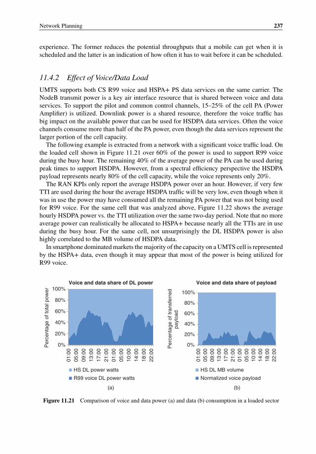
Network Planning 237
experience. The former reduces the potential throughputs that a mobile can get when it isscheduled and the latter is an indication of how often it has to wait before it can be scheduled.
11.4.2 Effect of Voice/Data Load
UMTS supports both CS R99 voice and HSPA+ PS data services on the same carrier. TheNodeB transmit power is a key air interface resource that is shared between voice and dataservices. To support the pilot and common control channels, 15–25% of the cell PA (PowerAmplifier) is utilized. Downlink power is a shared resource, therefore the voice traffic hasbig impact on the available power that can be used for HSDPA data services. Often the voicechannels consume more than half of the PA power, even though the data services represent thelarger portion of the cell capacity.
The following example is extracted from a network with a significant voice traffic load. Onthe loaded cell shown in Figure 11.21 over 60% of the power is used to support R99 voiceduring the busy hour. The remaining 40% of the average power of the PA can be used duringpeak times to support HSDPA. However, from a spectral efficiency perspective the HSDPApayload represents nearly 80% of the cell capacity, while the voice represents only 20%.
The RAN KPIs only report the average HSDPA power over an hour. However, if very fewTTI are used during the hour the average HSDPA traffic will be very low, even though when itwas in use the power may have consumed all the remaining PA power that was not being usedfor R99 voice. For the same cell that was analyzed above, Figure 11.22 shows the averagehourly HSDPA power vs. the TTI utilization over the same two-day period. Note that no moreaverage power can realistically be allocated to HSPA+ because nearly all the TTIs are in useduring the busy hour. For the same cell, not unsurprisingly the DL HSDPA power is alsohighly correlated to the MB volume of HSDPA data.
In smartphone dominated markets the majority of the capacity on a UMTS cell is representedby the HSPA+ data, even though it may appear that most of the power is being utilized forR99 voice.
(a) (b)
0%
20%
40%
60%
80%
100%
01:0
005
:00
09:0
013
:00
17:0
021
:00
01:0
005
:00
10:0
014
:00
18:0
022
:00
Per
cent
age
of to
tal p
ower
Voice and data share of DL power
HS DL power watts
R99 voice DL power watts
0%
20%
40%
60%
80%
100%
01:0
005
:00
09:0
013
:00
17:0
021
:00
01:0
005
:00
10:0
014
:00
18:0
022
:00P
erce
ntag
e of
tran
sfer
red
payl
oad
Voice and data share of payload
HS DL MB volume
Normalized voice payload
Figure 11.21 Comparison of voice and data power (a) and data (b) consumption in a loaded sector
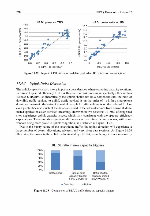
238 HSPA+ Evolution to Release 12
0.0
2.0
4.0
6.0
8.0
10.0
12.0
14.0
16.0
18.0
0.0 0.2 0.4 0.6 0.8 1.0
HS
DP
A D
L po
wer
(w
atts
)
HSDPA TTI utilization
HS DL power vs. TTI%
0.0
2.0
4.0
6.0
8.0
10.0
12.0
14.0
16.0
18.0
0 200 400 600 800
HS
DP
A D
L po
wer
(w
atts
)
HSDPA MB volume
HS DL power watts vs. MB
Figure 11.22 Impact of TTI utilization and data payload on HSDPA power consumption
11.4.3 Uplink Noise Discussion
The uplink capacity is also a very important consideration when evaluating capacity solutions.In terms of spectral efficiency, HSDPA Release 8 is 3–4 times more spectrally efficient thanRelease 6 HSUPA, so theoretically the uplink should not be a bottleneck until the ratio ofdownlink traffic payload to uplink traffic payload is on the order of 4 : 1. In a smartphonedominated network, the ratio of downlink to uplink traffic volume is on the order of 7 : 1 oreven greater because much of the data transferred in the network comes from downlink dom-inated applications such as video streaming. However, in live networks 30–60% of congestedsites experience uplink capacity issues, which isn’t consistent with the spectral efficiencyexpectations. There are also significant differences across infrastructure vendors, with somevendors being more prone to uplink congestion, as illustrated in Figure 11.23.
Due to the bursty nature of the smartphone traffic, the uplink direction will experience alarge number of bearer allocations, releases, and very short data sessions. As Figure 11.24illustrates, the power in the uplink is dominated by HSUPA, even though it is not necessarily
0%
20%
40%
60%
80%
100%
Traffic share Ratio of sitescapacity limited(RAN Vendor 2)
Ratio of sitescapacity limited(RAN Vendor 1)
UL:DL ratio in new capacity triggers
Downlink Uplink
Figure 11.23 Comparison of DL/UL traffic share vs. capacity triggers
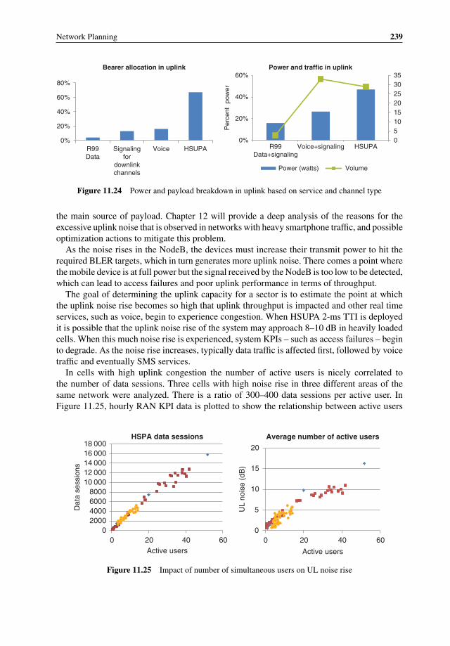
Network Planning 239
0%
20%
40%
60%
80%
R99Data
Signalingfor
downlinkchannels
Voice HSUPA
Bearer allocation in uplink
05101520253035
0%
20%
40%
60%
R99Data+signaling
Voice+signaling HSUPA
Per
cent
pow
er
Power and traffic in uplink
Power (watts) Volume
Figure 11.24 Power and payload breakdown in uplink based on service and channel type
the main source of payload. Chapter 12 will provide a deep analysis of the reasons for theexcessive uplink noise that is observed in networks with heavy smartphone traffic, and possibleoptimization actions to mitigate this problem.
As the noise rises in the NodeB, the devices must increase their transmit power to hit therequired BLER targets, which in turn generates more uplink noise. There comes a point wherethe mobile device is at full power but the signal received by the NodeB is too low to be detected,which can lead to access failures and poor uplink performance in terms of throughput.
The goal of determining the uplink capacity for a sector is to estimate the point at whichthe uplink noise rise becomes so high that uplink throughput is impacted and other real timeservices, such as voice, begin to experience congestion. When HSUPA 2-ms TTI is deployedit is possible that the uplink noise rise of the system may approach 8–10 dB in heavily loadedcells. When this much noise rise is experienced, system KPIs – such as access failures – beginto degrade. As the noise rise increases, typically data traffic is affected first, followed by voicetraffic and eventually SMS services.
In cells with high uplink congestion the number of active users is nicely correlated tothe number of data sessions. Three cells with high noise rise in three different areas of thesame network were analyzed. There is a ratio of 300–400 data sessions per active user. InFigure 11.25, hourly RAN KPI data is plotted to show the relationship between active users
02000400060008000
10 00012 00014 00016 00018 000
0 20 40 60
Dat
a se
ssio
ns
Active users
HSPA data sessions
0
5
10
15
20
0 20 40 60
UL
nois
e (d
B)
Active users
Average number of active users
Figure 11.25 Impact of number of simultaneous users on UL noise rise
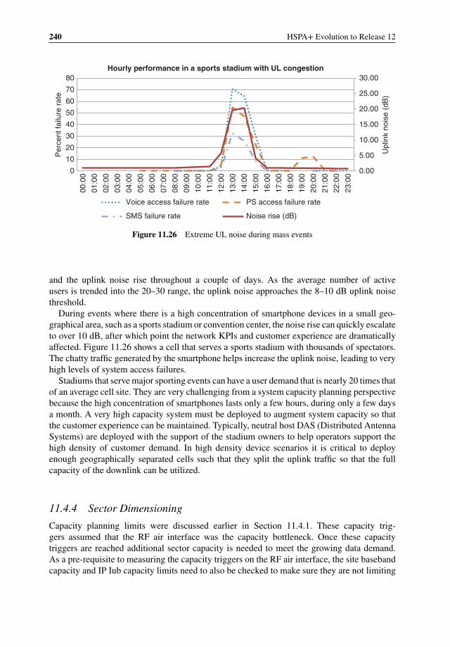
240 HSPA+ Evolution to Release 12
0.00
5.00
10.00
15.00
20.00
25.00
30.00
0
10
20
30
40
50
60
70
8000
:00
01:0
0
02:0
0
03:0
0
04:0
0
05:0
0
06:0
0
07:0
0
08:0
0
09:0
0
10:0
0
11:0
0
12:0
0
13:0
0
14:0
0
15:0
0
16:0
0
17:0
0
18:0
0
19:0
0
20:0
0
21:0
0
22:0
0
23:0
0
Upl
ink
nois
e (d
B)
Per
cent
failu
re r
ate
Hourly performance in a sports stadium with UL congestion
Voice access failure rate PS access failure rate
SMS failure rate Noise rise (dB)
Figure 11.26 Extreme UL noise during mass events
and the uplink noise rise throughout a couple of days. As the average number of activeusers is trended into the 20–30 range, the uplink noise approaches the 8–10 dB uplink noisethreshold.
During events where there is a high concentration of smartphone devices in a small geo-graphical area, such as a sports stadium or convention center, the noise rise can quickly escalateto over 10 dB, after which point the network KPIs and customer experience are dramaticallyaffected. Figure 11.26 shows a cell that serves a sports stadium with thousands of spectators.The chatty traffic generated by the smartphone helps increase the uplink noise, leading to veryhigh levels of system access failures.
Stadiums that serve major sporting events can have a user demand that is nearly 20 times thatof an average cell site. They are very challenging from a system capacity planning perspectivebecause the high concentration of smartphones lasts only a few hours, during only a few daysa month. A very high capacity system must be deployed to augment system capacity so thatthe customer experience can be maintained. Typically, neutral host DAS (Distributed AntennaSystems) are deployed with the support of the stadium owners to help operators support thehigh density of customer demand. In high density device scenarios it is critical to deployenough geographically separated cells such that they split the uplink traffic so that the fullcapacity of the downlink can be utilized.
11.4.4 Sector Dimensioning
Capacity planning limits were discussed earlier in Section 11.4.1. These capacity trig-gers assumed that the RF air interface was the capacity bottleneck. Once these capacitytriggers are reached additional sector capacity is needed to meet the growing data demand.As a pre-requisite to measuring the capacity triggers on the RF air interface, the site basebandcapacity and IP Iub capacity limits need to also be checked to make sure they are not limiting
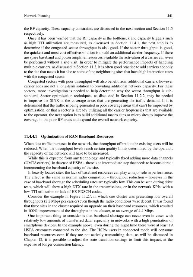
Network Planning 241
the RF capacity. These capacity constraints are discussed in the next section and Section 11.5respectively.
Once it has been verified that the RF capacity is the bottleneck and capacity triggers suchas high TTI utilization are measured, as discussed in Section 11.4.1, the next step is todetermine if the congested sector throughput is also good. If the sector throughput is good,the quickest and most cost effective solution is to add an additional carrier frequency. If thereare spare baseband and power amplifier resources available the activation of a carrier can evenbe performed without a site visit. In order to mitigate the performance impacts of handlingmultiple carriers, as discussed in Section 11.3, it is often good practice to add carriers not onlyto the site that needs it but also to some of the neighboring sites that have high interaction rateswith the congested sector.
Congested sectors with poor throughput will also benefit from additional carriers, howevercarrier adds are not a long-term solution to providing additional network capacity. For thesesectors, more investigation is needed to help determine why the sector throughput is sub-standard. Sector optimization techniques, as discussed in Section 11.2.2, may be neededto improve the SINR in the coverage areas that are generating the traffic demand. If it isdetermined that the traffic is being generated in poor coverage areas that can’t be improved byoptimization, or that a sector is already utilizing all the carrier frequencies that are availableto the operator, the next option is to build additional macro sites or micro sites to improve thecoverage in the poor RF areas and expand the overall network capacity.
11.4.4.1 Optimization of RAN Baseband Resources
When data traffic increases in the network, the throughput offered to the existing users will bereduced. When the throughput levels reach certain quality limits determined by the operator,the capacity of the network will have to be increased.
While this is expected from any technology, and typically fixed adding more data channels(UMTS carriers), in the case of HSPA+ there is an intermediate step that needs to be considered:incrementing the baseband capacity of the site.
In heavily loaded sites, the lack of baseband resources can play a major role in performance.The effect is the same as normal radio congestion – throughput reduction – however in thecase of baseband shortage the scheduling rates are typically low. This can be seen during drivetests, which will show a high DTX rate in the transmissions, or in the network KPIs, with alow TTI utilization or lack of HS-PDSCH codes.
Consider the example in Figure 11.27, in which one cluster was presenting low overallthroughputs (2.2 Mbps per carrier) even though the radio conditions were decent. It was foundthat three sites in the cluster required an upgrade on their baseband resources, which resultedin 100% improvement of the throughput in the cluster, to an average of 4.4 Mbps.
One important thing to consider is that baseband shortage can occur even in cases withrelatively low amounts of transferred data, especially in networks with a high penetration ofsmartphone devices. In the example above, even during the night time there were at least 19HSPA customers connected to the site. The HSPA users in connected mode will consumebaseband resources even if they are not actively transmitting data; as will be discussed inChapter 12, it is possible to adjust the state transition settings to limit this impact, at theexpense of longer connection latency.
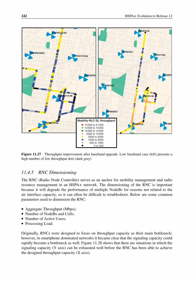
242 HSPA+ Evolution to Release 12
Mobility-RLC DL throughput
15000 to 2100012000 to 1500010000 to 12000
5000 to 100002000 to 50001000 to 2000
500 to 10000 to 500
Figure 11.27 Throughput improvement after baseband upgrade. Low baseband case (left) presents ahigh number of low throughput dots (dark gray)
11.4.5 RNC Dimensioning
The RNC (Radio Node Controller) serves as an anchor for mobility management and radioresource management in an HSPA+ network. The dimensioning of the RNC is importantbecause it will degrade the performance of multiple NodeBs for reasons not related to theair interface capacity, so it can often be difficult to troubleshoot. Below are some commonparameters used to dimension the RNC:
� Aggregate Throughput (Mbps);� Number of NodeBs and Cells;� Number of Active Users;� Processing Load.
Originally, RNCs were designed to focus on throughput capacity as their main bottleneck;however, in smartphone dominated networks it became clear that the signaling capacity couldrapidly become a bottleneck as well. Figure 11.28 shows that there are situations in which thesignaling capacity (Y axis) can be exhausted well before the RNC has been able to achievethe designed throughput capacity (X axis).
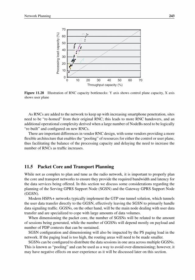
Network Planning 243
00
10
20
30
40
50
Pro
cess
ing
load
cap
acity
(%
)
60
70
10 20 30 40
Throughput capacity (%)
50 60 70
Figure 11.28 Illustration of RNC capacity bottlenecks: Y axis shows control plane capacity, X axisshows user plane
As RNCs are added to the network to keep up with increasing smartphone penetration, sitesneed to be “re-homed” from their original RNC; this leads to more RNC handovers, and anadditional operational complexity derived when a large number of NodeBs need to be logically“re-built” and configured on new RNCs.
There are important differences in vendor RNC design, with some vendors providing a moreflexible architecture that enables the “pooling” of resources for either the control or user plane,thus facilitating the balance of the processing capacity and delaying the need to increase thenumber of RNCs as traffic increases.
11.5 Packet Core and Transport Planning
While not as complex to plan and tune as the radio network, it is important to properly planthe core and transport networks to ensure they provide the required bandwidth and latency forthe data services being offered. In this section we discuss some considerations regarding theplanning of the Serving GPRS Support Node (SGSN) and the Gateway GPRS Support Node(GGSN).
Modern HSPA+ networks typically implement the GTP one tunnel solution, which tunnelsthe user data transfer directly to the GGSN, effectively leaving the SGSN to primarily handledata signaling traffic. GGSNs, on the other hand, will be the main node dealing with user datatransfer and are specialized to cope with large amounts of data volumes.
When dimensioning the packet core, the number of SGSNs will be related to the amountof sessions being generated, while the number of GGSNs will depend mostly on payload andnumber of PDP contexts that can be sustained.
SGSN configuration and dimensioning will also be impacted by the PS paging load in thenetwork. If the paging load is too high, the routing areas will need to be made smaller.
SGSNs can be configured to distribute the data sessions in one area across multiple GGSNs.This is known as “pooling” and can be used as a way to avoid over-dimensioning; however, itmay have negative effects on user experience as it will be discussed later on this section.
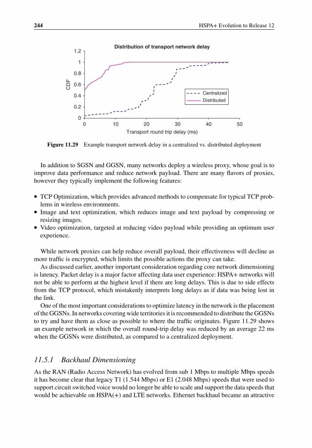
244 HSPA+ Evolution to Release 12
0
0.2
0.4
0.6
0.8
1
1.2
0 10 20 30 40 50
CD
F
Transport round trip delay (ms)
Distribution of transport network delay
Centralized
Distributed
Figure 11.29 Example transport network delay in a centralized vs. distributed deployment
In addition to SGSN and GGSN, many networks deploy a wireless proxy, whose goal is toimprove data performance and reduce network payload. There are many flavors of proxies,however they typically implement the following features:
� TCP Optimization, which provides advanced methods to compensate for typical TCP prob-lems in wireless environments.
� Image and text optimization, which reduces image and text payload by compressing orresizing images.
� Video optimization, targeted at reducing video payload while providing an optimum userexperience.
While network proxies can help reduce overall payload, their effectiveness will decline asmore traffic is encrypted, which limits the possible actions the proxy can take.
As discussed earlier, another important consideration regarding core network dimensioningis latency. Packet delay is a major factor affecting data user experience: HSPA+ networks willnot be able to perform at the highest level if there are long delays. This is due to side effectsfrom the TCP protocol, which mistakenly interprets long delays as if data was being lost inthe link.
One of the most important considerations to optimize latency in the network is the placementof the GGSNs. In networks covering wide territories it is recommended to distribute the GGSNsto try and have them as close as possible to where the traffic originates. Figure 11.29 showsan example network in which the overall round-trip delay was reduced by an average 22 mswhen the GGSNs were distributed, as compared to a centralized deployment.
11.5.1 Backhaul Dimensioning
As the RAN (Radio Access Network) has evolved from sub 1 Mbps to multiple Mbps speedsit has become clear that legacy T1 (1.544 Mbps) or E1 (2.048 Mbps) speeds that were used tosupport circuit switched voice would no longer be able to scale and support the data speeds thatwould be achievable on HSPA(+) and LTE networks. Ethernet backhaul became an attractive
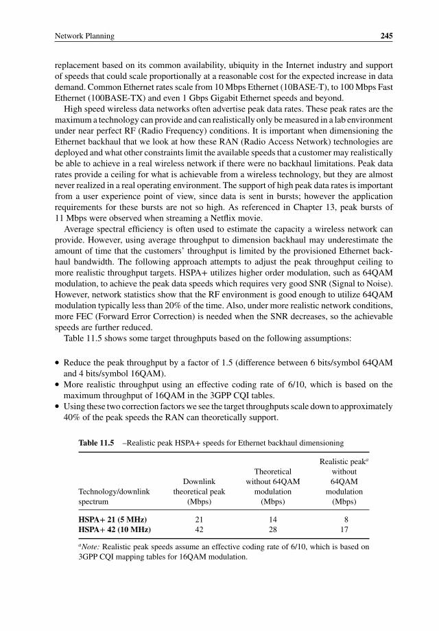
Network Planning 245
replacement based on its common availability, ubiquity in the Internet industry and supportof speeds that could scale proportionally at a reasonable cost for the expected increase in datademand. Common Ethernet rates scale from 10 Mbps Ethernet (10BASE-T), to 100 Mbps FastEthernet (100BASE-TX) and even 1 Gbps Gigabit Ethernet speeds and beyond.
High speed wireless data networks often advertise peak data rates. These peak rates are themaximum a technology can provide and can realistically only be measured in a lab environmentunder near perfect RF (Radio Frequency) conditions. It is important when dimensioning theEthernet backhaul that we look at how these RAN (Radio Access Network) technologies aredeployed and what other constraints limit the available speeds that a customer may realisticallybe able to achieve in a real wireless network if there were no backhaul limitations. Peak datarates provide a ceiling for what is achievable from a wireless technology, but they are almostnever realized in a real operating environment. The support of high peak data rates is importantfrom a user experience point of view, since data is sent in bursts; however the applicationrequirements for these bursts are not so high. As referenced in Chapter 13, peak bursts of11 Mbps were observed when streaming a Netflix movie.
Average spectral efficiency is often used to estimate the capacity a wireless network canprovide. However, using average throughput to dimension backhaul may underestimate theamount of time that the customers’ throughput is limited by the provisioned Ethernet back-haul bandwidth. The following approach attempts to adjust the peak throughput ceiling tomore realistic throughput targets. HSPA+ utilizes higher order modulation, such as 64QAMmodulation, to achieve the peak data speeds which requires very good SNR (Signal to Noise).However, network statistics show that the RF environment is good enough to utilize 64QAMmodulation typically less than 20% of the time. Also, under more realistic network conditions,more FEC (Forward Error Correction) is needed when the SNR decreases, so the achievablespeeds are further reduced.
Table 11.5 shows some target throughputs based on the following assumptions:
� Reduce the peak throughput by a factor of 1.5 (difference between 6 bits/symbol 64QAMand 4 bits/symbol 16QAM).
� More realistic throughput using an effective coding rate of 6/10, which is based on themaximum throughput of 16QAM in the 3GPP CQI tables.
� Using these two correction factors we see the target throughputs scale down to approximately40% of the peak speeds the RAN can theoretically support.
Table 11.5 –Realistic peak HSPA+ speeds for Ethernet backhaul dimensioning
Technology/downlinkspectrum
Downlinktheoretical peak
(Mbps)
Theoreticalwithout 64QAM
modulation(Mbps)
Realistic peaka
without64QAM
modulation(Mbps)
HSPA+ 21 (5 MHz) 21 14 8HSPA+ 42 (10 MHz) 42 28 17
aNote: Realistic peak speeds assume an effective coding rate of 6/10, which is based on3GPP CQI mapping tables for 16QAM modulation.

246 HSPA+ Evolution to Release 12
Table 11.6 Recommended backhaul dimensioning by technology
Technology/downlinkspectrum
Ethernetbackhaul typical
traffic (Mbps)
Ethernetbackhaul heavytraffic (Mbps)
HSPA+ 21 (5 MHz) 20 20HSPA+ 42 (10 MHz) 20 503–4 HSPA+ carriers 50 100
Backhaul is a shared resource between sectors of the same site, so there are trunkingefficiency gains that can be realized when HSPA+ is initially deployed and it is assumedthat only one sector will be in use during a given TTI (Time Transmission Interval).Table 11.6 shows some example backhaul dimensioning calculations. If we had used thetheoretical peak speeds to dimension the system we would need approximately 125 Mbps ofbackhaul to support a site that had HSPA+ 42 (dual carrier) on all three sectors. Based onthe example calculations, for the initial deployment of these high speed technologies they canrealistically be supported by as little as 1/7th of the maximum air interface speed summedacross a three sectored site. This assumes only one sector per site will be busy initially, butas the traffic grows multiple sectors may be utilized at the same time, so the backhaul willneed to be augmented accordingly to maintain an adequate Grade of Service (GoS) to thecustomers. However, care must be taken to also check that applications that customers areusing are actually requesting the peak speeds that the air interface is capable of supporting.Incremental capacity should also be added to support the control plane usage, but it is expectedthat this only adds as much as an additional 4–6% to the overall backhaul requirement.
11.6 Spectrum Refarming
11.6.1 Introduction
The concept of refarming is borrowed from agriculture, where many scattered plots of landare consolidated and redistributed among the owners. In wireless, refarming refers to theconsolidation of spectrum assets in preparation to their use for the new radio technology.The typical case is to deploy HSPA or LTE technology on the existing GSM frequencies at850/900 MHz and 1800/1900 MHz. The motivation for refarming is to get more spectrumfor growing HSPA traffic and to improve the HSPA coverage by using lower spectrum withbetter signal propagation. The North American and Latin American networks use 850 and1900 MHz refarming for HSPA, most European operators and some African operators havedeployed HSPA on 900 MHz band, and both 850 and 900 MHz frequencies are used for HSPAin Asia. Some of the 900 MHz networks are also new spectrum allocations, like the world’slargest UMTS900 network run by Softbank in Japan. The GSM 1800 MHz spectrum is alsobeing refarmed to enable LTE deployments.
Refarming UMTS to the low bands 850 and 900 MHz provides a major benefit in cov-erage. The typical coverage area of a three-sector base station in an urban area is shownin Figure 11.30. The coverage calculation assumes the Okumura-Hata propagation model, acorrection factor of 0 dB, a base station antenna height of 25 m, indoor loss of 15 dB, slowfading 8.0 dB, and required location probability of 95%. The antenna gain at low bands is
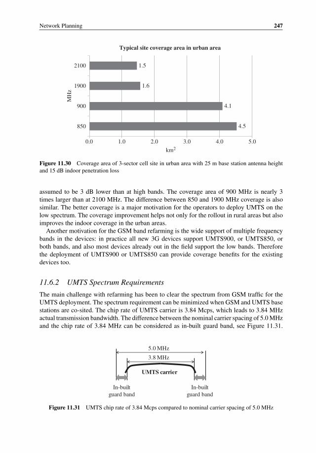
Network Planning 247
4.5
4.1
1.6
1.5
0.0 1.0 2.0 3.0 4.0 5.0
850
900
1900
2100
km2
MH
z
Typical site coverage area in urban area
Figure 11.30 Coverage area of 3-sector cell site in urban area with 25 m base station antenna heightand 15 dB indoor penetration loss
assumed to be 3 dB lower than at high bands. The coverage area of 900 MHz is nearly 3times larger than at 2100 MHz. The difference between 850 and 1900 MHz coverage is alsosimilar. The better coverage is a major motivation for the operators to deploy UMTS on thelow spectrum. The coverage improvement helps not only for the rollout in rural areas but alsoimproves the indoor coverage in the urban areas.
Another motivation for the GSM band refarming is the wide support of multiple frequencybands in the devices: in practice all new 3G devices support UMTS900, or UMTS850, orboth bands, and also most devices already out in the field support the low bands. Thereforethe deployment of UMTS900 or UMTS850 can provide coverage benefits for the existingdevices too.
11.6.2 UMTS Spectrum Requirements
The main challenge with refarming has been to clear the spectrum from GSM traffic for theUMTS deployment. The spectrum requirement can be minimized when GSM and UMTS basestations are co-sited. The chip rate of UMTS carrier is 3.84 Mcps, which leads to 3.84 MHzactual transmission bandwidth. The difference between the nominal carrier spacing of 5.0 MHzand the chip rate of 3.84 MHz can be considered as in-built guard band, see Figure 11.31.
3.8 MHz
5.0 MHz
In-built
guard band
In-built
guard band
UMTS carrier
Figure 11.31 UMTS chip rate of 3.84 Mcps compared to nominal carrier spacing of 5.0 MHz
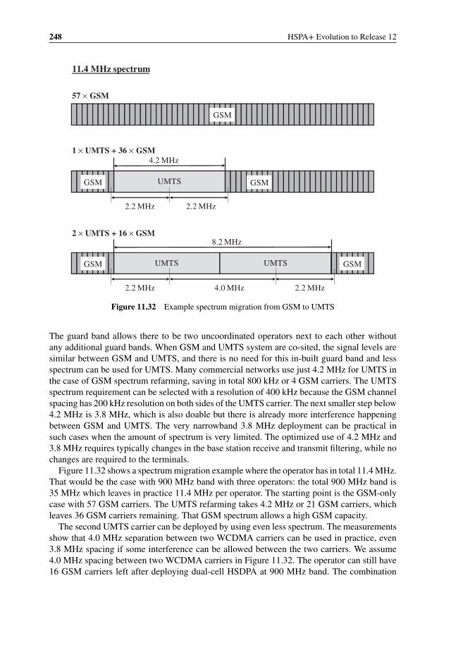
248 HSPA+ Evolution to Release 12
UMTS
8.2 MHz
GSM
2.2 MHz 4.0 MHz
UMTS
4.2 MHz
GSM
2.2 MHz 2.2 MHz
GSM
UMTS GSM
2.2 MHz
GSM
11.4 MHz spectrum
57 × GSM
1 × UMTS + 36 × GSM
2 × UMTS + 16 × GSM
Figure 11.32 Example spectrum migration from GSM to UMTS
The guard band allows there to be two uncoordinated operators next to each other withoutany additional guard bands. When GSM and UMTS system are co-sited, the signal levels aresimilar between GSM and UMTS, and there is no need for this in-built guard band and lessspectrum can be used for UMTS. Many commercial networks use just 4.2 MHz for UMTS inthe case of GSM spectrum refarming, saving in total 800 kHz or 4 GSM carriers. The UMTSspectrum requirement can be selected with a resolution of 400 kHz because the GSM channelspacing has 200 kHz resolution on both sides of the UMTS carrier. The next smaller step below4.2 MHz is 3.8 MHz, which is also doable but there is already more interference happeningbetween GSM and UMTS. The very narrowband 3.8 MHz deployment can be practical insuch cases when the amount of spectrum is very limited. The optimized use of 4.2 MHz and3.8 MHz requires typically changes in the base station receive and transmit filtering, while nochanges are required to the terminals.
Figure 11.32 shows a spectrum migration example where the operator has in total 11.4 MHz.That would be the case with 900 MHz band with three operators: the total 900 MHz band is35 MHz which leaves in practice 11.4 MHz per operator. The starting point is the GSM-onlycase with 57 GSM carriers. The UMTS refarming takes 4.2 MHz or 21 GSM carriers, whichleaves 36 GSM carriers remaining. That GSM spectrum allows a high GSM capacity.
The second UMTS carrier can be deployed by using even less spectrum. The measurementsshow that 4.0 MHz separation between two WCDMA carriers can be used in practice, even3.8 MHz spacing if some interference can be allowed between the two carriers. We assume4.0 MHz spacing between two WCDMA carriers in Figure 11.32. The operator can still have16 GSM carriers left after deploying dual-cell HSDPA at 900 MHz band. The combination
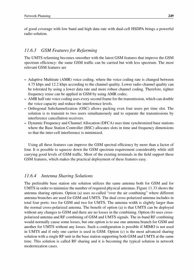
Network Planning 249
of good coverage with low band and high data rate with dual-cell HSDPA brings a powerfulradio solution.
11.6.3 GSM Features for Refarming
The UMTS refarming becomes smoother with the latest GSM features that improve the GSMspectrum efficiency: the same GSM traffic can be carried but with less spectrum. The mostrelevant GSM features are
– Adaptive Multirate (AMR) voice coding, where the voice coding rate is changed between4.75 kbps and 12.2 kbps according to the channel quality. Lower radio channel quality canbe tolerated by using a lower data rate and more robust channel coding. Therefore, tighterfrequency reuse can be applied in GSM by using AMR codec.
– AMR half rate voice coding uses every second frame for the transmission, which can doublethe voice capacity and reduce the interference levels.
– Orthogonal Subchannelization (OSC) allows packing even four users per time slot. Thesolution is to transmit to two users simultaneously and to separate the transmissions byinterference cancellation receivers.
– Dynamic Frequency and Channel Allocation (DFCA) uses time synchronized base stationswhere the Base Station Controller (BSC) allocates slots in time and frequency dimensionsso that the inter-cell interference is minimized.
Using all these features can improve the GSM spectral efficiency by more than a factor offour. It is possible to squeeze down the GSM spectrum requirement considerably while stillcarrying good levels of GSM traffic. Most of the existing terminals in the field support theseGSM features, which makes the practical deployment of these features easy.
11.6.4 Antenna Sharing Solutions
The preferable base station site solution utilizes the same antenna both for GSM and forUMTS in order to minimize the number of required physical antennas. Figure 11.33 shows theantenna sharing options. Option (a) uses so-called “over the air combining” where differentantenna branches are used for GSM and UMTS. The dual cross-polarized antenna includes intotal four ports: two for GSM and two for UMTS. The antenna width is slightly larger thanthe normal cross-polarized antenna. The benefit of option (a) is that UMTS can be deployedwithout any changes to GSM and there are no losses in the combining. Option (b) uses cross-polarized antenna and RF combining of GSM and UMTS signals. The in-band RF combiningwould normally cause some losses, but one option is to use one antenna branch for GSM andanother for UMTS without any losses. Such a configuration is possible if MIMO is not usedin UMTS and if only one carrier is used in GSM. Option (c) is the most advanced sharingsolution with a single RF unit in the base station supporting both GSM and UMTS at the sametime. This solution is called RF sharing and it is becoming the typical solution in networkmodernization cases.

250 HSPA+ Evolution to Release 12
GSM RF UMTS RF GSM RF UMTS RFGSM +
UMTS RF
Combiner
X
X
X
X
X
X
X
X
X X
X
X
X
X
X
X
X
X
X
X
Dual x-pol antenna x-pol antenna x-pol antenna
(a) Over the air combining with
separate antenna branches for
GSM and UMTS
(b) RF combining of GSM
and UMTS RF signals
(c) Shared multiradio RF for
GSM and UMTS
Figure 11.33 Antenna sharing options for GSM and UMTS
11.7 Summary
In this chapter we reviewed various topics covering key network deployment and dimensioningaspects.
Below are a summary of some of the most relevant considerations discussed:
� HSPA+ networks are typically limited in interference, and special care needs to be takento control the amount of power transmitted in the network. Lack of coverage should becompensated with different solutions depending on the type of network – urban (typicallylimited by interference) or suburban/rural (typically limited by power).
� Antenna tilts are a very important tool to configure and maintain RF performance; howeverdowntilting is often abused as the only way to achieve interference containment. Othermethods include reducing powers, or even eliminating unnecessary sectors that are notrequired.
� Multilayer configuration should be done carefully depending on the type of deploymentscenario: hotspots or continuous coverage zones, single or multiband, and so on.
� In networks with heavy smartphone penetration there are unexpected bottlenecks at the celllevel (uplink congestion) as well as the RNC level (signaling processing capacity).
� As GSM traffic is reduced it should be possible to repurpose that spectrum for HSPA+.New carriers can be allocated in blocks as low as 3.8 MHz.

Network Planning 251
References
[1] Chevallier, C., Brunner, C., Caravaglia, A. et al. (2006) WCDMA (UMTS) Deployment Handbook: Planning andOptimization Aspects, John Wiley & Sons, Ltd, Chichester.
[2] Qualcomm Engineering Services Group (ESG), “Aspects of HSUPA Network Planning”, Revision A (April 6,2007) (updated Sept 2008).
[3] Viterbi, A.J., Viterbi, A.M., and Zehavi, E. (1994) Other-cell interference in cellular power-controlled CDMA.IEEE Transactions on Communications, 42(234), Part 3, 1501–1504.
[4] Holma, H. and Toskala, A. (2006) HSDPA/HSUPA for UMTS. High Speed Radio Access for Mobile Communi-cations, 1st edn, John Wiley & Sons, Ltd, Chichester.
[5] Bi, Q. (2004) A Forward Link Performance Study of the 1xEV-DO Rev. 0 System Using Field Measurements andSimulations, Lucent Technologies.

12Radio Network Optimization
Pablo Tapia and Carl Williams
12.1 Introduction
To ensure an optimum operation of the HSPA+ technology the operator has to make a multitudeof decisions when planning and optimizing the network, considering multiple components:from the device to the network and up to the application servers. In a HSPA+ system thereare four main areas that the operator needs to address in order to achieve the desired serviceperformance:
� Radio network planning, such as the location of cell sites, orientation of antennas, transmitpower adjustments, and radio network capacity adjustments.
� Transport and core network planning, which will determine the latency and capacity ofthe backhaul and interconnection links, the location of the core network nodes, and thecorresponding core network capacity adjustments.
� Terminal devices. The devices are a major component of the experience of the customer,and care should be taken on the selection of the right hardware components such as CPUand memory, the optimization of transceiver and radio modem, selection and adaptation ofthe OS, and development and adjustment of apps.
� Soft parameters, which control the adjustment of radio and core functionality such asresource allocation, scheduling, and mobility management procedures.
When planning and optimizing the network, there will often be a tradeoff between quality,capacity, and cost. In some cases, if certain key guidelines are followed, tradeoffs are notnecessary and the operator will achieve the maximum potential of the technology with aminimum cost. This chapter will provide the operator with important HSPA+ guidelines, aswell as explain some of the tradeoffs that are possible when optimizing the HSPA+ technologyfrom a radio network standpoint; planning and optimization aspects for other parts of thesystem will be covered in other chapters: Chapter 11 (Network Planning) has already discussed
HSPA+ Evolution to Release 12: Performance and Optimization, First Edition.Edited by Harri Holma, Antti Toskala, and Pablo Tapia.© 2014 John Wiley & Sons, Ltd. Published 2014 by John Wiley & Sons, Ltd.
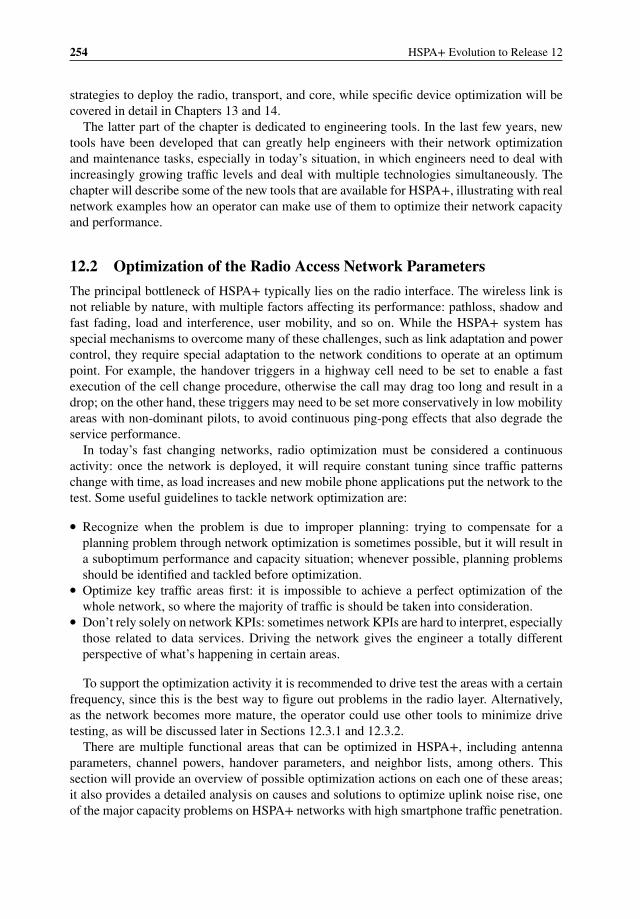
254 HSPA+ Evolution to Release 12
strategies to deploy the radio, transport, and core, while specific device optimization will becovered in detail in Chapters 13 and 14.
The latter part of the chapter is dedicated to engineering tools. In the last few years, newtools have been developed that can greatly help engineers with their network optimizationand maintenance tasks, especially in today’s situation, in which engineers need to deal withincreasingly growing traffic levels and deal with multiple technologies simultaneously. Thechapter will describe some of the new tools that are available for HSPA+, illustrating with realnetwork examples how an operator can make use of them to optimize their network capacityand performance.
12.2 Optimization of the Radio Access Network Parameters
The principal bottleneck of HSPA+ typically lies on the radio interface. The wireless link isnot reliable by nature, with multiple factors affecting its performance: pathloss, shadow andfast fading, load and interference, user mobility, and so on. While the HSPA+ system hasspecial mechanisms to overcome many of these challenges, such as link adaptation and powercontrol, they require special adaptation to the network conditions to operate at an optimumpoint. For example, the handover triggers in a highway cell need to be set to enable a fastexecution of the cell change procedure, otherwise the call may drag too long and result in adrop; on the other hand, these triggers may need to be set more conservatively in low mobilityareas with non-dominant pilots, to avoid continuous ping-pong effects that also degrade theservice performance.
In today’s fast changing networks, radio optimization must be considered a continuousactivity: once the network is deployed, it will require constant tuning since traffic patternschange with time, as load increases and new mobile phone applications put the network to thetest. Some useful guidelines to tackle network optimization are:
� Recognize when the problem is due to improper planning: trying to compensate for aplanning problem through network optimization is sometimes possible, but it will result ina suboptimum performance and capacity situation; whenever possible, planning problemsshould be identified and tackled before optimization.
� Optimize key traffic areas first: it is impossible to achieve a perfect optimization of thewhole network, so where the majority of traffic is should be taken into consideration.
� Don’t rely solely on network KPIs: sometimes network KPIs are hard to interpret, especiallythose related to data services. Driving the network gives the engineer a totally differentperspective of what’s happening in certain areas.
To support the optimization activity it is recommended to drive test the areas with a certainfrequency, since this is the best way to figure out problems in the radio layer. Alternatively,as the network becomes more mature, the operator could use other tools to minimize drivetesting, as will be discussed later in Sections 12.3.1 and 12.3.2.
There are multiple functional areas that can be optimized in HSPA+, including antennaparameters, channel powers, handover parameters, and neighbor lists, among others. Thissection will provide an overview of possible optimization actions on each one of these areas;it also provides a detailed analysis on causes and solutions to optimize uplink noise rise, oneof the major capacity problems on HSPA+ networks with high smartphone traffic penetration.
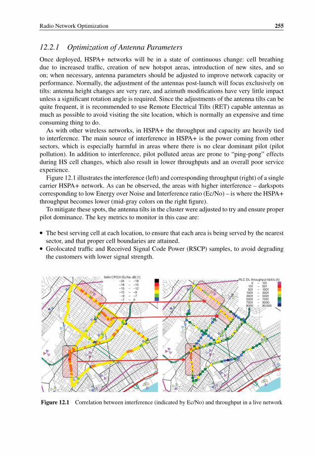
Radio Network Optimization 255
12.2.1 Optimization of Antenna Parameters
Once deployed, HSPA+ networks will be in a state of continuous change: cell breathingdue to increased traffic, creation of new hotspot areas, introduction of new sites, and soon; when necessary, antenna parameters should be adjusted to improve network capacity orperformance. Normally, the adjustment of the antennas post-launch will focus exclusively ontilts: antenna height changes are very rare, and azimuth modifications have very little impactunless a significant rotation angle is required. Since the adjustments of the antenna tilts can bequite frequent, it is recommended to use Remote Electrical Tilts (RET) capable antennas asmuch as possible to avoid visiting the site location, which is normally an expensive and timeconsuming thing to do.
As with other wireless networks, in HSPA+ the throughput and capacity are heavily tiedto interference. The main source of interference in HSPA+ is the power coming from othersectors, which is especially harmful in areas where there is no clear dominant pilot (pilotpollution). In addition to interference, pilot polluted areas are prone to “ping-pong” effectsduring HS cell changes, which also result in lower throughputs and an overall poor serviceexperience.
Figure 12.1 illustrates the interference (left) and corresponding throughput (right) of a singlecarrier HSPA+ network. As can be observed, the areas with higher interference – darkspotscorresponding to low Energy over Noise and Interference ratio (Ec/No) – is where the HSPA+throughput becomes lower (mid-gray colors on the right figure).
To mitigate these spots, the antenna tilts in the cluster were adjusted to try and ensure properpilot dominance. The key metrics to monitor in this case are:
� The best serving cell at each location, to ensure that each area is being served by the nearestsector, and that proper cell boundaries are attained.
� Geolocated traffic and Received Signal Code Power (RSCP) samples, to avoid degradingthe customers with lower signal strength.
SAN CPICH Ec/No dB [1]RLC DL throughput kbit/s [4]–34
–18–15–12–9–7
–18–15–12–9–70
––––––
0101501
10013001500170019000
1015011001300150017001900080000
––––––––
Figure 12.1 Correlation between interference (indicated by Ec/No) and throughput in a live network
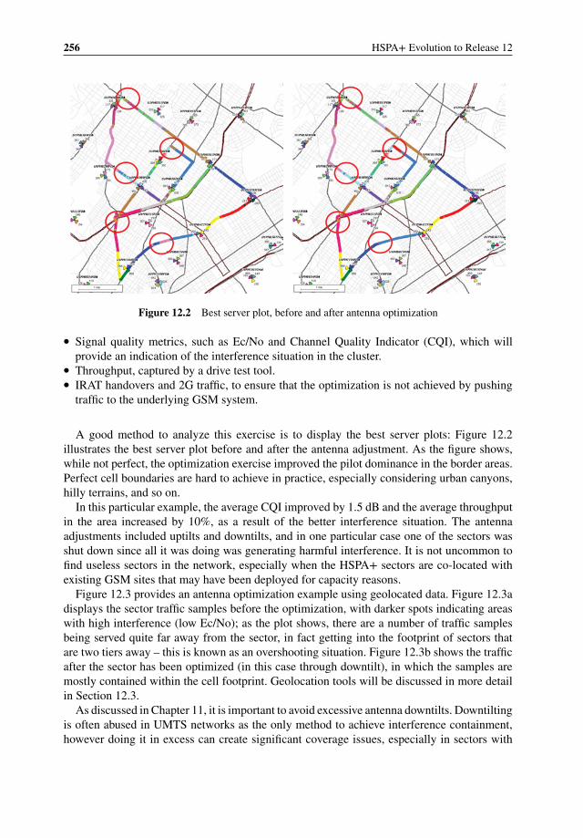
256 HSPA+ Evolution to Release 12
Figure 12.2 Best server plot, before and after antenna optimization
� Signal quality metrics, such as Ec/No and Channel Quality Indicator (CQI), which willprovide an indication of the interference situation in the cluster.
� Throughput, captured by a drive test tool.� IRAT handovers and 2G traffic, to ensure that the optimization is not achieved by pushing
traffic to the underlying GSM system.
A good method to analyze this exercise is to display the best server plots: Figure 12.2illustrates the best server plot before and after the antenna adjustment. As the figure shows,while not perfect, the optimization exercise improved the pilot dominance in the border areas.Perfect cell boundaries are hard to achieve in practice, especially considering urban canyons,hilly terrains, and so on.
In this particular example, the average CQI improved by 1.5 dB and the average throughputin the area increased by 10%, as a result of the better interference situation. The antennaadjustments included uptilts and downtilts, and in one particular case one of the sectors wasshut down since all it was doing was generating harmful interference. It is not uncommon tofind useless sectors in the network, especially when the HSPA+ sectors are co-located withexisting GSM sites that may have been deployed for capacity reasons.
Figure 12.3 provides an antenna optimization example using geolocated data. Figure 12.3adisplays the sector traffic samples before the optimization, with darker spots indicating areaswith high interference (low Ec/No); as the plot shows, there are a number of traffic samplesbeing served quite far away from the sector, in fact getting into the footprint of sectors thatare two tiers away – this is known as an overshooting situation. Figure 12.3b shows the trafficafter the sector has been optimized (in this case through downtilt), in which the samples aremostly contained within the cell footprint. Geolocation tools will be discussed in more detailin Section 12.3.
As discussed in Chapter 11, it is important to avoid excessive antenna downtilts. Downtiltingis often abused in UMTS networks as the only method to achieve interference containment,however doing it in excess can create significant coverage issues, especially in sectors with
Radio Network Optimization 257
(a) (b)
Figure 12.3 Analysis of geolocated samples from one sector before (a) and after (b) tilt optimization
low antenna height. Cell power adjustments can be used as a complement to antenna tilts toachieve a good delimitation of cell boundaries.
When downtilting or reducing the CPICH it is possible that the main KPIs show a perfor-mance improvement, however the sector may be losing coverage. It is important to monitor thetraffic and IRAT levels to prevent these situations, and if possible validate the new coveragefootprint with drive test data or with the help of geolocation tools.
12.2.2 Optimization of Power Parameters
One of the key parameter sets that need to be tuned in a HSPA+ network is the power assignedto the different physical channels. Typically in UMTS networks the operator can control thepower level assigned to the following channels:
� Common Pilot Channel (CPICH)� Downlink Common Control Channel (CCCH): Broadcast Channel (BCH), Acquisition
Indicator Channel (AICH), Paging Channel (PCH), Primary Synchronization Channel (P-SCH), Secondary Synchronization Channel (S-SCH), Paging Indicator Channel (PICH),and Forward Access Channel (FACH).
� Release 99 (R99) Dedicated Data Channels.� R99 Voice Channels.� HSDPA Channels: High Speed Shared Control Channel (HS-SCCH) and High Speed Down-
link Shared Channel (HS-DSCH).
12.2.2.1 Adjustment of Common Control Channels
The power allocation of the control channels needs to be done carefully since it will haveimplications for both coverage and capacity planning. The total amount of power available in
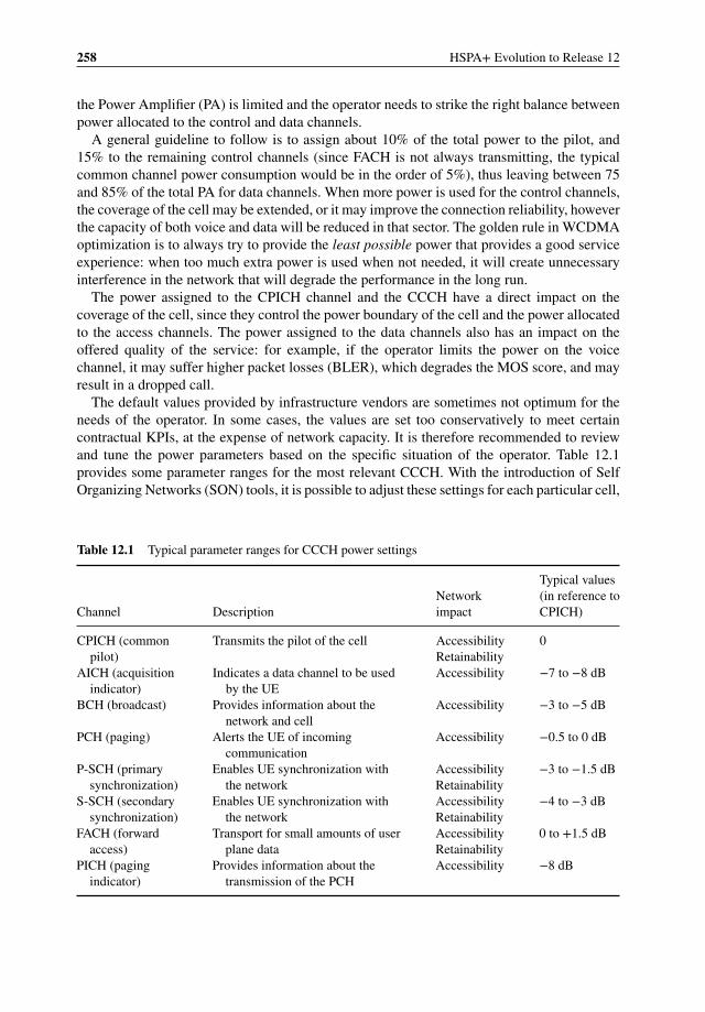
258 HSPA+ Evolution to Release 12
the Power Amplifier (PA) is limited and the operator needs to strike the right balance betweenpower allocated to the control and data channels.
A general guideline to follow is to assign about 10% of the total power to the pilot, and15% to the remaining control channels (since FACH is not always transmitting, the typicalcommon channel power consumption would be in the order of 5%), thus leaving between 75and 85% of the total PA for data channels. When more power is used for the control channels,the coverage of the cell may be extended, or it may improve the connection reliability, howeverthe capacity of both voice and data will be reduced in that sector. The golden rule in WCDMAoptimization is to always try to provide the least possible power that provides a good serviceexperience: when too much extra power is used when not needed, it will create unnecessaryinterference in the network that will degrade the performance in the long run.
The power assigned to the CPICH channel and the CCCH have a direct impact on thecoverage of the cell, since they control the power boundary of the cell and the power allocatedto the access channels. The power assigned to the data channels also has an impact on theoffered quality of the service: for example, if the operator limits the power on the voicechannel, it may suffer higher packet losses (BLER), which degrades the MOS score, and mayresult in a dropped call.
The default values provided by infrastructure vendors are sometimes not optimum for theneeds of the operator. In some cases, the values are set too conservatively to meet certaincontractual KPIs, at the expense of network capacity. It is therefore recommended to reviewand tune the power parameters based on the specific situation of the operator. Table 12.1provides some parameter ranges for the most relevant CCCH. With the introduction of SelfOrganizing Networks (SON) tools, it is possible to adjust these settings for each particular cell,
Table 12.1 Typical parameter ranges for CCCH power settings
Typical valuesNetwork (in reference to
Channel Description impact CPICH)
CPICH (commonpilot)
Transmits the pilot of the cell AccessibilityRetainability
0
AICH (acquisitionindicator)
Indicates a data channel to be usedby the UE
Accessibility −7 to −8 dB
BCH (broadcast) Provides information about thenetwork and cell
Accessibility −3 to −5 dB
PCH (paging) Alerts the UE of incomingcommunication
Accessibility −0.5 to 0 dB
P-SCH (primarysynchronization)
Enables UE synchronization withthe network
AccessibilityRetainability
−3 to −1.5 dB
S-SCH (secondarysynchronization)
Enables UE synchronization withthe network
AccessibilityRetainability
−4 to −3 dB
FACH (forwardaccess)
Transport for small amounts of userplane data
AccessibilityRetainability
0 to +1.5 dB
PICH (pagingindicator)
Provides information about thetransmission of the PCH
Accessibility −8 dB
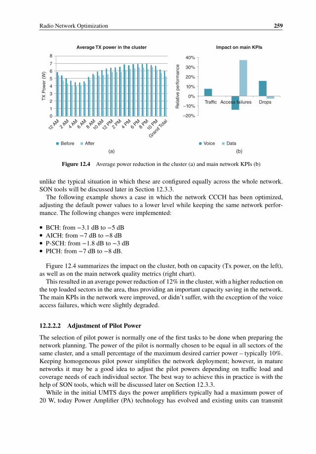
Radio Network Optimization 259
Traffic Access failures Drops
Rel
ativ
e pe
rfor
man
ce
–20%
(a) (b)
–10%
0%
10%
20%
30%
40%
Impact on main KPIs
0
12 A
M4 A
M2 A
M6 A
M8 A
M10
AM
12 P
M2
PM4
PM6
PM8
PM10
PM
Grand
Tota
l
1
2
3
4
5
6
7
8
TX
Pow
er (
W)
Average TX power in the cluster
Before After Voice Data
Figure 12.4 Average power reduction in the cluster (a) and main network KPIs (b)
unlike the typical situation in which these are configured equally across the whole network.SON tools will be discussed later in Section 12.3.3.
The following example shows a case in which the network CCCH has been optimized,adjusting the default power values to a lower level while keeping the same network perfor-mance. The following changes were implemented:
� BCH: from −3.1 dB to −5 dB� AICH: from −7 dB to −8 dB� P-SCH: from −1.8 dB to −3 dB� PICH: from −7 dB to −8 dB.
Figure 12.4 summarizes the impact on the cluster, both on capacity (Tx power, on the left),as well as on the main network quality metrics (right chart).
This resulted in an average power reduction of 12% in the cluster, with a higher reduction onthe top loaded sectors in the area, thus providing an important capacity saving in the network.The main KPIs in the network were improved, or didn’t suffer, with the exception of the voiceaccess failures, which were slightly degraded.
12.2.2.2 Adjustment of Pilot Power
The selection of pilot power is normally one of the first tasks to be done when preparing thenetwork planning. The power of the pilot is normally chosen to be equal in all sectors of thesame cluster, and a small percentage of the maximum desired carrier power – typically 10%.Keeping homogeneous pilot power simplifies the network deployment; however, in maturenetworks it may be a good idea to adjust the pilot powers depending on traffic load andcoverage needs of each individual sector. The best way to achieve this in practice is with thehelp of SON tools, which will be discussed later on Section 12.3.3.
While in the initial UMTS days the power amplifiers typically had a maximum power of20 W, today Power Amplifier (PA) technology has evolved and existing units can transmit
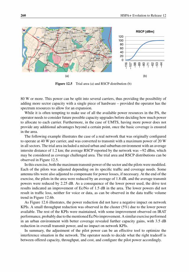
260 HSPA+ Evolution to Release 12
(a) (b)
020406080
100120
–116
–107 –98
–89
–80
–71
–62
–53
–44
RSCP [dBm]
Figure 12.5 Trial area (a) and RSCP distribution (b)
80 W or more. This power can be split into several carriers, thus providing the possibility ofadding more sector capacity with a single piece of hardware – provided the operator has thespectrum resources to allow for an expansion.
While it is often tempting to make use of all the available power resources in the PA, theoperator needs to consider future possible capacity upgrades before deciding how much powerto allocate to each carrier. Furthermore, in the case of UMTS, having more power does notprovide any additional advantages beyond a certain point, once the basic coverage is ensuredin the area.
The following example illustrates the case of a real network that was originally configuredto operate at 40 W per carrier, and was converted to transmit with a maximum power of 20 Win all sectors. The trial area included a mixed urban and suburban environment with an averageintersite distance of 1.2 km; the average RSCP reported by the network was −92 dBm, whichmay be considered as coverage challenged area. The trial area and RSCP distributions can beobserved in Figure 12.5.
In this exercise, both the maximum transmit power of the sector and the pilots were modified.Each of the pilots was adjusted depending on its specific traffic and coverage needs. Someantenna tilts were also adjusted to compensate for power losses, if necessary. At the end of theexercise, the pilots in the area were reduced by an average of 1.8 dB, and the average transmitpowers were reduced by 2.25 dB. As a consequence of the lower power used, the drive testresults indicated an improvement of Ec/No of 1.5 dB in the area. The lower powers did notresult in traffic loss, neither for voice or data, as can be observed in the data traffic volumetrend in Figure 12.6b.
As Figure 12.6 illustrates, the power reduction did not have a negative impact on networkKPIs. A small throughput reduction was observed in the cluster (5%) due to the lower poweravailable. The rest of the KPIs were maintained, with some improvement observed on IRATperformance, probably due to the mentioned Ec/No improvement. A similar exercise performedin an urban environment with better coverage revealed further capacity gains, with 3.5 dBreduction in overall transmit power, and no impact on network KPIs.
In summary, the adjustment of the pilot power can be an effective tool to optimize theinterference situation in the network. The operator needs to decide what the right tradeoff isbetween offered capacity, throughput, and cost, and configure the pilot power accordingly.
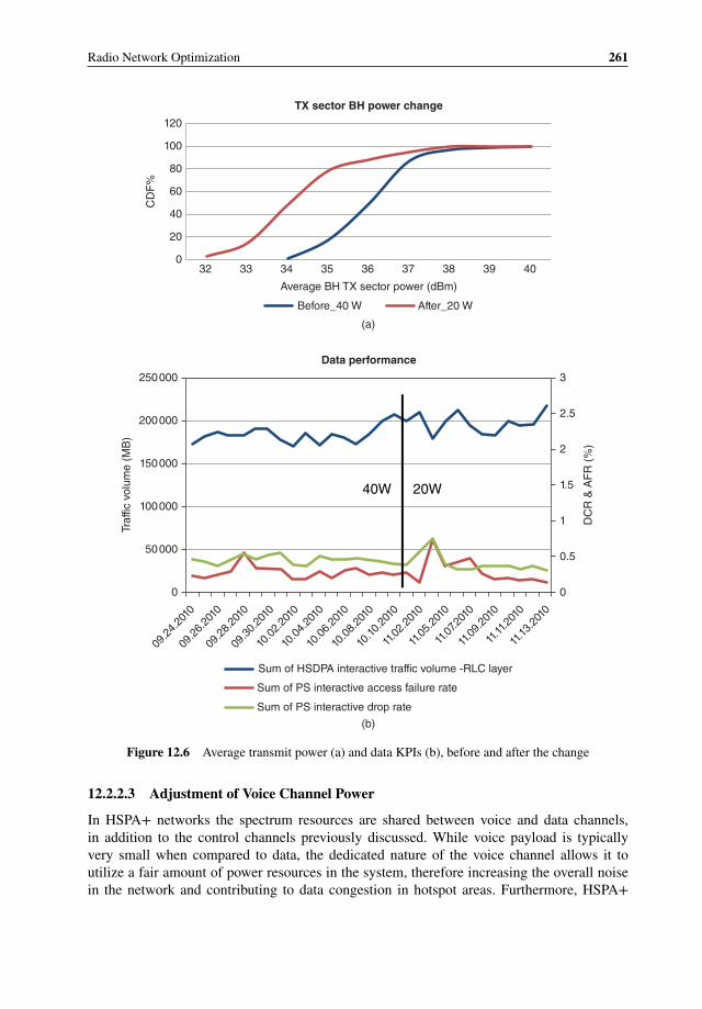
Radio Network Optimization 261
20W40W
Data performance
0
50000
100000
150000
200000
250000
0
0.5
1
1.5
2.5
2
3
0
20
40
60
80
100
120
32
09.2
4.20
10
09.2
6.20
10
09.2
8.20
10
09.3
0.20
10
10.0
2.20
10
10.0
4.20
10
10.0
6.20
10
10.0
8.20
10
10.10
.201
0
11.0
2.20
10
11.0
5.20
10
11.0
7.201
0
11.0
9.20
10
11.11
.201
0
11.13
.201
0
33 34 35 36
(a)
(b)
37 38 39 40
CD
F%
Traf
fic v
olum
e (M
B)
DC
R &
AF
R (
%)
Average BH TX sector power (dBm)
TX sector BH power change
Before_40 W After_20 W
Sum of HSDPA interactive traffic volume -RLC layer
Sum of PS interactive access failure rate
Sum of PS interactive drop rate
Figure 12.6 Average transmit power (a) and data KPIs (b), before and after the change
12.2.2.3 Adjustment of Voice Channel Power
In HSPA+ networks the spectrum resources are shared between voice and data channels,in addition to the control channels previously discussed. While voice payload is typicallyvery small when compared to data, the dedicated nature of the voice channel allows it toutilize a fair amount of power resources in the system, therefore increasing the overall noisein the network and contributing to data congestion in hotspot areas. Furthermore, HSPA+
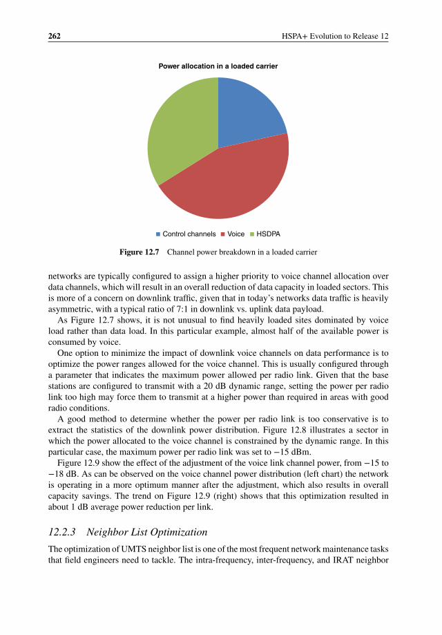
262 HSPA+ Evolution to Release 12
Power allocation in a loaded carrier
Control channels Voice HSDPA
Figure 12.7 Channel power breakdown in a loaded carrier
networks are typically configured to assign a higher priority to voice channel allocation overdata channels, which will result in an overall reduction of data capacity in loaded sectors. Thisis more of a concern on downlink traffic, given that in today’s networks data traffic is heavilyasymmetric, with a typical ratio of 7:1 in downlink vs. uplink data payload.
As Figure 12.7 shows, it is not unusual to find heavily loaded sites dominated by voiceload rather than data load. In this particular example, almost half of the available power isconsumed by voice.
One option to minimize the impact of downlink voice channels on data performance is tooptimize the power ranges allowed for the voice channel. This is usually configured througha parameter that indicates the maximum power allowed per radio link. Given that the basestations are configured to transmit with a 20 dB dynamic range, setting the power per radiolink too high may force them to transmit at a higher power than required in areas with goodradio conditions.
A good method to determine whether the power per radio link is too conservative is toextract the statistics of the downlink power distribution. Figure 12.8 illustrates a sector inwhich the power allocated to the voice channel is constrained by the dynamic range. In thisparticular case, the maximum power per radio link was set to −15 dBm.
Figure 12.9 show the effect of the adjustment of the voice link channel power, from −15 to−18 dB. As can be observed on the voice channel power distribution (left chart) the networkis operating in a more optimum manner after the adjustment, which also results in overallcapacity savings. The trend on Figure 12.9 (right) shows that this optimization resulted inabout 1 dB average power reduction per link.
12.2.3 Neighbor List Optimization
The optimization of UMTS neighbor list is one of the most frequent network maintenance tasksthat field engineers need to tackle. The intra-frequency, inter-frequency, and IRAT neighbor
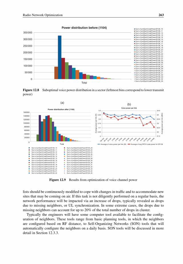
Radio Network Optimization 263
0Total
Power distribution before (1104) Sum of pmDpchCodePowerSf128_10Sum of pmDpchCodePowerSf128_11Sum of pmDpchCodePowerSf128_12Sum of pmDpchCodePowerSf128_13Sum of pmDpchCodePowerSf128_14Sum of pmDpchCodePowerSf128_15Sum of pmDpchCodePowerSf128_16Sum of pmDpchCodePowerSf128_17Sum of pmDpchCodePowerSf128_18Sum of pmDpchCodePowerSf128_19Sum of pmDpchCodePowerSf128_20Sum of pmDpchCodePowerSf128_21Sum of pmDpchCodePowerSf128_22Sum of pmDpchCodePowerSf128_23Sum of pmDpchCodePowerSf128_24Sum of pmDpchCodePowerSf128_25Sum of pmDpchCodePowerSf128_26Sum of pmDpchCodePowerSf128_27Sum of pmDpchCodePowerSf128_28Sum of pmDpchCodePowerSf128_29Sum of pmDpchCodePowerSf128_30Sum of pmDpchCodePowerSf128_31Sum of pmDpchCodePowerSf128_32Sum of pmDpchCodePowerSf128_33Sum of pmDpchCodePowerSf128_34Sum of pmDpchCodePowerSf128_35
50000
100000
150000
200000
250000
300000
350000
Figure 12.8 Suboptimal voice power distribution in a sector (leftmost bins correspond to lower transmitpower)
(a) (b)
22
21.5
22.5
23
23.5
24
24.5
0
29-Ja
n
30-Ja
n
31-Ja
n1-F
eb2-
Feb
3-Fe
b4-
Feb
5-Fe
b6-
Feb
7-Feb
8-Fe
b9-
Feb
10-F
eb
11-F
eb
12-F
eb
0.05
0.1
0.15
0.2
0.25
0.3
Ave
rage
pow
er p
er li
nk (
dBm
)
Ave
rage
pow
er p
er li
nk (
W)
Voice power per link
Average of voice power per link (W) Average of avg DPCH code power for SF128
Sum of pmDpchCodePowerSf128_10Sum of pmDpchCodePowerSf128_11Sum of pmDpchCodePowerSf128_12Sum of pmDpchCodePowerSf128_13Sum of pmDpchCodePowerSf128_14Sum of pmDpchCodePowerSf128_15Sum of pmDpchCodePowerSf128_16Sum of pmDpchCodePowerSf128_17Sum of pmDpchCodePowerSf128_18Sum of pmDpchCodePowerSf128_19Sum of pmDpchCodePowerSf128_20Sum of pmDpchCodePowerSf128_21Sum of pmDpchCodePowerSf128_22
Sum of pmDpchCodePowerSf128_23Sum of pmDpchCodePowerSf128_24Sum of pmDpchCodePowerSf128_25Sum of pmDpchCodePowerSf128_26Sum of pmDpchCodePowerSf128_27Sum of pmDpchCodePowerSf128_28Sum of pmDpchCodePowerSf128_29Sum of pmDpchCodePowerSf128_30Sum of pmDpchCodePowerSf128_31Sum of pmDpchCodePowerSf128_32Sum of pmDpchCodePowerSf128_33Sum of pmDpchCodePowerSf128_34Sum of pmDpchCodePowerSf128_35
0Total
Power distribution after (1104)
20000
40000
60000
100000
80000
120000
140000
160000
Figure 12.9 Results from optimization of voice channel power
lists should be continuously modified to cope with changes in traffic and to accommodate newsites that may be coming on air. If this task is not diligently performed on a regular basis, thenetwork performance will be impacted via an increase of drops, typically revealed as dropsdue to missing neighbors, or UL synchronization. In some extreme cases, the drops due tomissing neighbors can account for up to 20% of the total number of drops in cluster.
Typically the engineers will have some computer tool available to facilitate the config-uration of neighbors. These tools range from basic planning tools, in which the neighborsare configured based on RF distance, to Self-Organizing Networks (SON) tools that willautomatically configure the neighbors on a daily basis. SON tools will be discussed in moredetail in Section 12.3.3.

264 HSPA+ Evolution to Release 12
Initially, the neighbor lists should be configured based on planning information, and typicallyinclude at least the first and second tier neighbors. Neighbor lists don’t need to be reciprocal,but it’s a good idea to enforce reciprocity between different carriers of the same site to facilitatetraffic load balancing. Defining the right 2G neighbors is also very important, especially in thecase of rural sites.
Once the network has a sufficient amount of traffic, the neighbor lists should be maintainedbased on network statistics, such as handover attempts, success and failures, drop call rate,and so on. It is a good idea to activate detected set measurement, and make use of these reportsto identify missing neighbors. It is also important to keep the neighbor lists well pruned,and remove unused neighbors to leave room for possible new cells showing up in the future.Also, if an extended neighbor list is in use – that is, System Information Block (SIB) 11bisis broadcast – it is important to arrange these lists to keep high priority neighbors in SIB11and lower priority neighbors in SIB11bis. Note that SIB11bis can only be used by Release 6compliant terminals.
The engineer should also be on the lookout for possible handover problems due to wrongneighbor selection, as well as overshooting sectors, which will tend to generate handovers toan excessive amount of sectors. The incorrect neighbor problem can normally be fixed withscrambling code disambiguation, or ultimately with re-assignment of new scrambling codesfor those conflicting sectors. The overshooting sector problem should be tackled with properRF optimization.
Figure 12.10 shows an example of an RNC where a neighbor optimization exercise wasrun using a SON tool: once the optimization task started, the number of drops due to missingneighbors in the area was significantly decreased.
In general, it is hard to eliminate all missing neighbors due to constraints on neighborlist sizes. The different neighbor lists (intra-frequency, inter-frequency, and inter-RAT) allhave size limitations, as well as the overall combined list. Configuring more neighbors thanpermitted can create serious problems in the sector, derived from SIB11 congestion, which
0
20
40
60
80
100
120
140
160
2/19
/201
32/
20/2
013
2/21
/201
32/
22/2
013
2/23
/201
32/
24/2
013
2/25
/201
32/
26/2
013
2/27
/201
32/
28/2
013
3/1/
2013
3/2/
2013
3/3/
2013
3/4/
2013
3/5/
2013
3/6/
2013
3/7/
2013
3/8/
2013
3/9/
2013
3/10
/201
33/
11/2
013
3/12
/201
3
Num
ber
of d
rops
Reduction in drops due to missing neighbors
Figure 12.10 Neighbor optimization exercise in one RNC
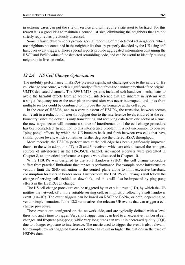
Radio Network Optimization 265
in extreme cases can put the site off service and will require a site reset to be fixed. For thisreason it is a good idea to maintain a pruned list size, eliminating the neighbors that are notstrictly required as previously discussed.
Some infrastructure vendors provide special reporting of the detected set neighbors, whichare neighbors not contained in the neighbor list that are properly decoded by the UE using softhandover event triggers. These special reports provide aggregated information containing theRSCP and Ec/No value of the detected scrambling code, and can be useful to identify missingneighbors in live networks.
12.2.4 HS Cell Change Optimization
The mobility performance in HSPA+ presents significant challenges due to the nature of HScell change procedure, which is significantly different from the handover method of the originalUMTS dedicated channels. The R99 UMTS systems included soft handover mechanisms toavoid the harmful effects from adjacent cell interference that are inherent in systems witha single frequency reuse: the user plane transmission was never interrupted, and links frommultiple sectors could be combined to improve the performance at the cell edge.
In the case of HSDPA, and to a certain extent of HSUPA, the transition between sectorscan result in a reduction of user throughput due to the interference levels endured at the cellboundary: since the device is only transmitting and receiving data from one sector at a time,the new target sector will become a source of interference until the cell change procedurehas been completed. In addition to this interference problem, it is not uncommon to observe“ping-pong” effects, by which the UE bounces back and forth between two cells that havesimilar power levels, which sometimes further degrade the offered HSPA throughput.
More recently, the HSDPA performance at the cell edge has been significantly improvedthanks to the wide adoption of Type 2i and 3i receivers which are able to cancel the strongestsources of interference in the HS-DSCH channel. Advanced receivers were presented inChapter 8, and practical performance aspects were discussed in Chapter 10.
While HSUPA was designed to use Soft Handover (SHO), the cell change proceduresuffers from practical limitations that impact its performance. For example, some infrastructurevendors limit the SHO utilization to the control plane alone to limit excessive basebandconsumption for users in border areas. Furthermore, the HSUPA cell changes will follow thechange of serving cell decided on downlink, and thus will also be impacted by ping-pongeffects in the HSDPA cell change.
The HS cell change procedure can be triggered by an explicit event (1D), by which the UEnotifies the network of a more suitable serving cell, or implicitly following a soft handoverevent (1A–1C). The event triggers can be based on RSCP or Ec/No, or both, depending onvendor implementation. Table 12.2 summarizes the relevant UE events that can trigger a cellchange procedure.
These events are configured on the network side, and are typically defined with a levelthreshold and a time to trigger. Very short trigger times can lead to an excessive number of cellchanges and frequent ping-pong, while very long times can result in decreased quality (CQI)due to a longer exposure to interference. The metric used to trigger the event is also relevant:for example, events triggered based on Ec/No can result in higher fluctuations in the case ofHSDPA data.
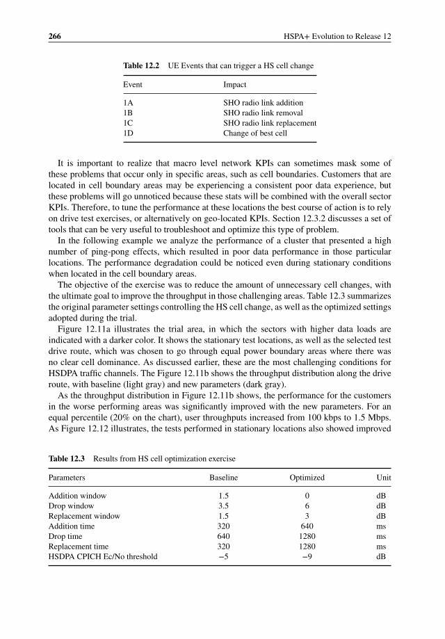
266 HSPA+ Evolution to Release 12
Table 12.2 UE Events that can trigger a HS cell change
Event Impact
1A SHO radio link addition1B SHO radio link removal1C SHO radio link replacement1D Change of best cell
It is important to realize that macro level network KPIs can sometimes mask some ofthese problems that occur only in specific areas, such as cell boundaries. Customers that arelocated in cell boundary areas may be experiencing a consistent poor data experience, butthese problems will go unnoticed because these stats will be combined with the overall sectorKPIs. Therefore, to tune the performance at these locations the best course of action is to relyon drive test exercises, or alternatively on geo-located KPIs. Section 12.3.2 discusses a set oftools that can be very useful to troubleshoot and optimize this type of problem.
In the following example we analyze the performance of a cluster that presented a highnumber of ping-pong effects, which resulted in poor data performance in those particularlocations. The performance degradation could be noticed even during stationary conditionswhen located in the cell boundary areas.
The objective of the exercise was to reduce the amount of unnecessary cell changes, withthe ultimate goal to improve the throughput in those challenging areas. Table 12.3 summarizesthe original parameter settings controlling the HS cell change, as well as the optimized settingsadopted during the trial.
Figure 12.11a illustrates the trial area, in which the sectors with higher data loads areindicated with a darker color. It shows the stationary test locations, as well as the selected testdrive route, which was chosen to go through equal power boundary areas where there wasno clear cell dominance. As discussed earlier, these are the most challenging conditions forHSDPA traffic channels. The Figure 12.11b shows the throughput distribution along the driveroute, with baseline (light gray) and new parameters (dark gray).
As the throughput distribution in Figure 12.11b shows, the performance for the customersin the worse performing areas was significantly improved with the new parameters. For anequal percentile (20% on the chart), user throughputs increased from 100 kbps to 1.5 Mbps.As Figure 12.12 illustrates, the tests performed in stationary locations also showed improved
Table 12.3 Results from HS cell optimization exercise
Parameters Baseline Optimized Unit
Addition window 1.5 0 dBDrop window 3.5 6 dBReplacement window 1.5 3 dBAddition time 320 640 msDrop time 640 1280 msReplacement time 320 1280 msHSDPA CPICH Ec/No threshold −5 −9 dB
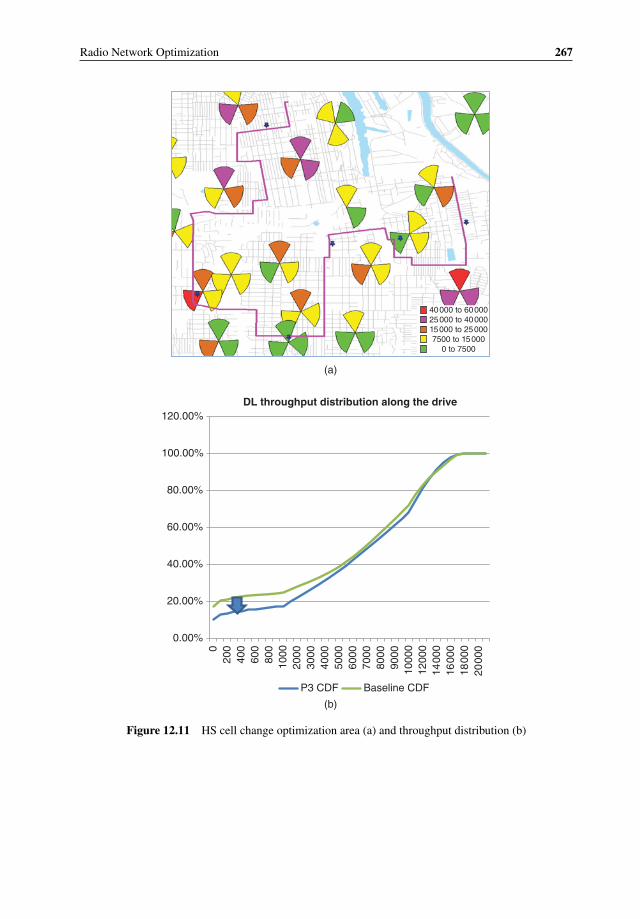
Radio Network Optimization 267
40000 to 6000025000 to 4000015000 to 250007500 to 15000
0 to 7500
0.00%
20.00%
(a)
(b)
40.00%
60.00%
80.00%
100.00%
120.00%
020
040
060
080
010
0020
0030
0040
0050
0060
0070
0080
0090
0010
000
1200
014
000
1600
018
000
2000
0
DL throughput distribution along the drive
P3 CDF Baseline CDF
Figure 12.11 HS cell change optimization area (a) and throughput distribution (b)

268 HSPA+ Evolution to Release 12
0
FTP_DL
(goo
d RF)
FTP_UL
(goo
d RF)
FTP_UL
(poo
r RF)
FTP_DL
(poo
r RF)
1
2
3
4
5
6
7T
hrou
ghpu
t (M
bps)
FTP throughputs (DL/UL)
Before
After
00.5
11.5
22.5
33.5
Web download(good RF)
Web download(poor RF)
Web
dow
nloa
d tim
e (s
)
Web download time
Before After
Figure 12.12 User experience improvement with new settings
performance for users in poor locations, both for simple download as well as web browsingperformance – on the other hand, users in good RF locations suffered a slight reduction inuplink throughput.
Other benefits from these settings included up to a 30% reduction in HS cell changes,reduction in SHO events and SHO overhead, and reduction of radio bearer reconfigurationsas well as R99 traffic.
It should be noted that these results may not be applicable to every network, since thesettings depend heavily on the underlying RF design, as well as the characteristics of thecluster. For example, these settings are not recommended for areas with high traffic mobility.
12.2.5 IRAT Handover Optimization
When UMTS networks were originally introduced, the use of Inter Radio Access Technology(IRAT) handovers was a simple and reliable mechanism to ensure service continuity in areaswith discontinuous 3G coverage. On the other hand, IRAT handovers introduce an additionalpoint of failure in the system, and result in a poorer customer experience as well as reducedsystem capacity since the underlying GSM system is not well suited to transfer high speeddata connections.
The use of IRAT handovers can often mask underlying RF performance issues in the networkthat are not reflected in the typical network indicators: users in areas with poor performancewill handover to GSM instead of dropping in UMTS – they may later on drop in GSM as well,but this drop is not considered in the UMTS optimization and this results in a poorly optimizednetwork exercise.
Frequent IRAT also increases the probability of missing paging. Call alerts may be missedwhen the devices are in the middle of a transition between technologies and the location areaupdate has not been completed. Although this problem can be mitigated with MSS pagingcoordination, this is a complicated problem to troubleshoot, since there are no counters thatkeep track of these events.
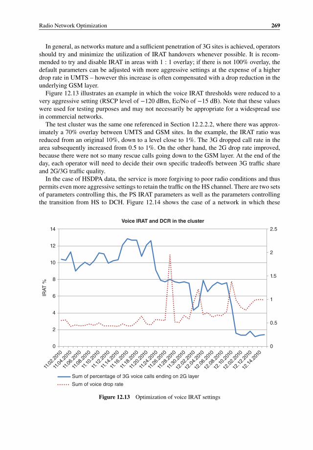
Radio Network Optimization 269
In general, as networks mature and a sufficient penetration of 3G sites is achieved, operatorsshould try and minimize the utilization of IRAT handovers whenever possible. It is recom-mended to try and disable IRAT in areas with 1 : 1 overlay; if there is not 100% overlay, thedefault parameters can be adjusted with more aggressive settings at the expense of a higherdrop rate in UMTS – however this increase is often compensated with a drop reduction in theunderlying GSM layer.
Figure 12.13 illustrates an example in which the voice IRAT thresholds were reduced to avery aggressive setting (RSCP level of −120 dBm, Ec/No of −15 dB). Note that these valueswere used for testing purposes and may not necessarily be appropriate for a widespread usein commercial networks.
The test cluster was the same one referenced in Section 12.2.2.2, where there was approx-imately a 70% overlay between UMTS and GSM sites. In the example, the IRAT ratio wasreduced from an original 10%, down to a level close to 1%. The 3G dropped call rate in thearea subsequently increased from 0.5 to 1%. On the other hand, the 2G drop rate improved,because there were not so many rescue calls going down to the GSM layer. At the end of theday, each operator will need to decide their own specific tradeoffs between 3G traffic shareand 2G/3G traffic quality.
In the case of HSDPA data, the service is more forgiving to poor radio conditions and thuspermits even more aggressive settings to retain the traffic on the HS channel. There are two setsof parameters controlling this, the PS IRAT parameters as well as the parameters controllingthe transition from HS to DCH. Figure 12.14 shows the case of a network in which these
0
0.5
1
1.5
2
2.5
0
11.0
2.20
10
11.0
4.20
10
11.0
6.20
10
11.0
8.20
10
11.10
.201
0
11.12
.201
0
11.14
.201
0
11.16
.201
0
11.18
.201
0
11.2
0.20
10
11.2
4.20
10
11.2
6.20
10
11.2
8.20
10
11.3
0.20
10
12.0
2.20
10
12.0
4.20
10
12.0
6.20
10
12.0
8.20
10
12.10
.201
0
12.0
2.20
10
12.12
.201
0
12.14
.201
0
2
4
6
8
10
12
14
IRAT
%
Voice IRAT and DCR in the cluster
Sum of percentage of 3G voice calls ending on 2G layer
Sum of voice drop rate
Figure 12.13 Optimization of voice IRAT settings
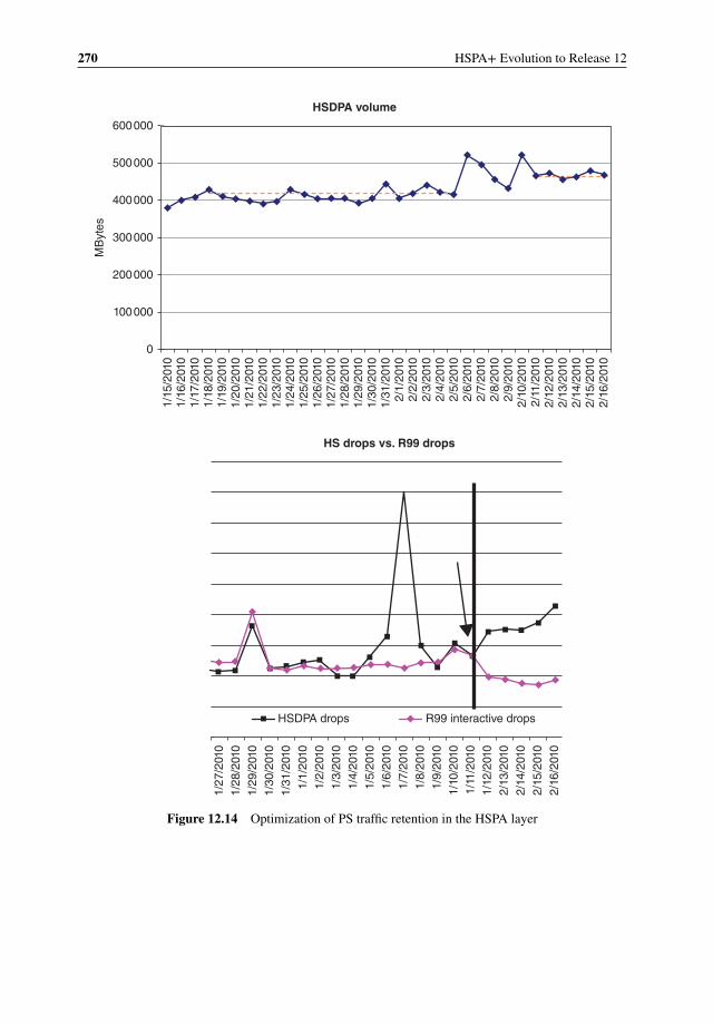
270 HSPA+ Evolution to Release 12
1/15
/201
01/
16/2
010
1/17
/201
01/
18/2
010
1/19
/201
01/
20/2
010
1/21
/201
01/
22/2
010
1/23
/201
01/
24/2
010
1/25
/201
01/
26/2
010
1/27
/201
01/
28/2
010
1/29
/201
01/
30/2
010
1/31
/201
02/
1/20
102/
2/20
102/
3/20
102/
4/20
102/
5/20
102/
6/20
102/
7/20
102/
8/20
102/
9/20
102/
10/2
010
2/11
/201
02/
12/2
010
2/13
/201
02/
14/2
010
2/15
/201
02/
16/2
010
0
MB
ytes
100000
200000
300000
400000
500000
600000
HSDPA volume
HS drops vs. R99 drops
1/27
/201
01/
28/2
010
1/29
/201
01/
30/2
010
1/31
/201
01/
1/20
101/
2/20
101/
3/20
101/
4/20
101/
5/20
101/
6/20
101/
7/20
101/
8/20
101/
9/20
101/
10/2
010
1/11
/201
01/
12/2
010
2/13
/201
02/
14/2
010
2/15
/201
02/
16/2
010
HSDPA drops R99 interactive drops
Figure 12.14 Optimization of PS traffic retention in the HSPA layer

Radio Network Optimization 271
settings have been aggressively adjusted:
� HS to DCH transitions due to poor quality OFF.� Ec/No service offset for Event 2D (used by compressed mode) from −1 dB to −3 dB.� RSCP service offset for Event 2D (used by compressed mode) from −6 dB to 0 dB.
By adjusting these settings the users will stay longer in HSDPA, thus avoiding unnecessarytransitions to R99 – which is a less efficient transport – or ultimately 2G. Figure 12.14 showsthe impact of the change on the overall HSDPA traffic volume (left), which increased by 12%;the chart on the right shows the impact of the change on PS drops. The overall packet droprate remains stable, although there was an increase in HSDPA drops that was offseted by areduction in R99 drops.
Nowadays, many operators have completely removed IRATs for data and some operatorsalso for voice, which has typically resulted in better KPIs, assuming that the UMTS coverageis sufficiently good. If IRAT is used for data, then it is normally triggered only by RSCP andnot by Ec/No.
12.2.6 Optimization of Radio State Transitions
Section 4.10 in Chapter 4, and Section 10.3 in Chapter 10 discussed how the delay in theradio state transitions has an important impact on the HSPA+ latency, and therefore on thefinal data service experienced by the customer. While packets on the DCH state enjoy a fasttransfer speed and a protocol architecture that minimizes latency, those packets transmittedover the FACH channel will be transferred at a very slow speed. Even worse is the case wherethe device is in a dormancy state, either IDLE or PCH, in which case there is an additionaldelay to set up the corresponding channel.
The following diagram (Figure 12.15a) illustrates the typical RRC state transitions in today’snetworks. The diagram does not include the IDLE state, since nowadays it is widely acceptedthat the default dormancy state should be Cell_PCH (either Cell_PCH or URA_PCH). This isdue to the fact that the transition from Cell_PCH is much faster than from IDLE, and involvesa significantly lower amount of signaling messages, as illustrated in Figure 12.15b.
When the UE is in the PCH state, a new data packet that needs to be transmitted caneither be sent via DCH – if the direct transition feature is activated and certain conditions aremet – or via FACH. To trigger a direct DCH transition the data volume should be larger thana certain threshold (B1, on the diagram); in certain implementations there is also a qualitycriterion, by which the direct transition is only triggered if the Ec/No is better than a certainthreshold. Figure 12.16 illustrates the result from a trial network in which different qualitythresholds were tried. As the threshold is relaxed, the amount of direct transitions increase,but there’s also an increase in upswitch failures.
When the UE is in FACH state, it will transmit at a very low bitrate, typically 32 kbps.If the application data volume increases beyond a threshold B1, a transition to DCH willbe triggered; this promotion time is quite slow and can take around 750 ms, so in generalthe operator should avoid entertaining continuous FACH<->DCH transitions. When there isno data to be transmitted, the UE will fall back to PCH (or IDLE) state after an inactivitytime (T2).
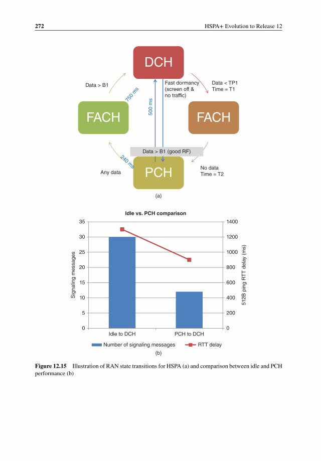
272 HSPA+ Evolution to Release 12
DCH
PCH
FACH FACH
Data > B1 Data < TP1Time = T1
750
ms
240 ms No dataTime = T2Any data
(a)
(b)
0
200
400
600
800
1000
1200
1400
0
5
10
15
20
25
30
35
Idle to DCH
512B
pin
g R
TT
del
ay (
ms)
Sig
nalin
g m
essa
ges
Idle vs. PCH comparison
Number of signaling messages RTT delay
PCH to DCH
500
ms
Fast dormancy(screen off &no traffic)
Data > B1 (good RF)
Figure 12.15 Illustration of RAN state transitions for HSPA (a) and comparison between idle and PCHperformance (b)
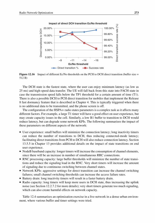
Radio Network Optimization 273
99.00%
99.20%
99.40%
99.60%
99.80%
100.00%
0.00%
5.00%
10.00%
15.00%
20.00%
–9 –11 –14 –16 Dire
ct tr
ansi
tion
succ
ess
rate
(%
)
Dire
ct tr
ansi
tions
to D
CH
Ec/No threshold
Impact of direct DCH transition Ec/No threshold
Direct transition % Success rate
Figure 12.16 Impact of different Ec/No thresholds on the PCH to DCH direct transition (buffer size =512 B)
The DCH state is the fastest state, where the user can enjoy minimum latency (as low as25 ms) and high-speed data transfer. The UE will fall back from this state into FACH state incase the transmission speed falls below the TP1 threshold for a certain amount of time (T1).There is also a possible DCH to PCH direct transition for mobiles that implement the Release8 fast dormancy feature that is described in Chapter 4. This is typically triggered when thereis no additional data to be transmitted, and the phone screen is off.
The configuration of the HSPA+ radio states parameters is a complex task as it affects manydifferent factors. For example, a large T1 timer will have a good effect on user experience, butmay create capacity issues in the cell. Similarly, a low B1 buffer to transition to DCH wouldreduce latency, but can degrade some network KPIs. The following summarizes the impact ofthese parameters on different aspects of the network:
� User experience: small buffers will minimize the connection latency; long inactivity timerscan reduce the number of transitions to DCH, thus reducing connected-mode latency;facilitating direct transitions from PCH to DCH will also reduce connection latency. Section13.5.5 in Chapter 13 provides additional details on the impact of state transitions on enduser experience.
� NodeB baseband capacity: longer timers will increase the consumption of channel elements,since there will be an increase in number of simultaneous RRC connections.
� RNC processing capacity: large buffer thresholds will minimize the number of state transi-tions and reduce the signaling load in the RNC. Very short timers will increase the amountof signaling due to continuous switching between channel states.
� Network KPIs: aggressive settings for direct transition can increase the channel switchingfailures; small channel switching thresholds can increase the access failure rates.
� Battery drain: long inactivity timers will result in a faster battery drain.� Radio capacity: long timers will keep more users in DCH state, thus increasing the uplink
noise (see Section 12.2.7.2 for more details); very short timers generate too much signaling,which can also create harmful effects on network capacity.
Table 12.4 summarizes an optimization exercise in a live network in a dense urban environ-ment, where various buffer and timer settings were tried.

274 HSPA+ Evolution to Release 12
Table 12.4 Effect of state transition settings on network KPIs
Parameter/KPI Set 1 Set 2 Set 3 Set 4 Set 5
T2 inactivity timer 5 s 3 s 3 s 5 s 5 sUL RLC buffer 512 bytes 512 bytes 256 bytes 512 bytes 1024 bytesDL RLC buffer 500 bytes 500 bytes 300 bytes 1000 bytes 1000 bytesPS AFR 1.40% 1.40% 1.70% 1.40% 1%PS DCR 0.35% 0.35% 0.35% 0.30% 0.40%Downswitch failure rate 2.50% 2.50% 2.50% 2% 3%Upswitch failure rate 2% 2% 2.50% 2.20% 1.50%FACH traffic 38 000.00 30 000.00 27 000.00 38 000.00 40 000.00Channel switching PCH to
FACH130 000.00 150 000.00 150 000.00 125 000.00 130 000.00
Channel switching FACHto HS
70 000.00 70 000.00 80 000.00 65 000.00 50 000.00
RNC processor load 15.50% 15% 16.50% 14.50% 14.50%
As previously discussed, the results show that there is a tradeoff between user experienceand network resources. Shorter buffers and timers result in higher signaling and processorload, and also revealed an increase in access failures due to upswitch failures. On the otherhand, as Figure 12.17 shows, the user experience – measured in this case as web downloadtime – is significantly improved with short buffers (33% web download time improvementwith 512 bytes as compared to 1024 bytes).
10000
90% web download time statistics1024 B vs. 512 B
9000
8000
7000
6000
5000
4000
3000
2000
1000
0
01-A
ug-1
205
-Aug
-12
09-A
ug-1
213
-Aug
-12
17-A
ug-1
221
-Aug
-12
25-A
ug-1
229
-Aug
-12
02-S
ep-1
206
-Sep
-12
10-S
ep-1
214
-Sep
-12
22-S
ep-1
226
-Sep
-12
30-S
ep-1
204
-Oct
-12
08-O
ct-1
212
-Oct
-12
16-O
ct-1
220
-Oct
-12
24-O
ct-1
228
-Oct
-12
01-N
ov-1
205
-Nov
-12
09-N
ov-1
213
-Nov
-12
17-N
ov-1
221
-Nov
-12
25-N
ov-1
229
-Nov
-12
Figure 12.17 Web browsing user experience improvement with shorter buffers
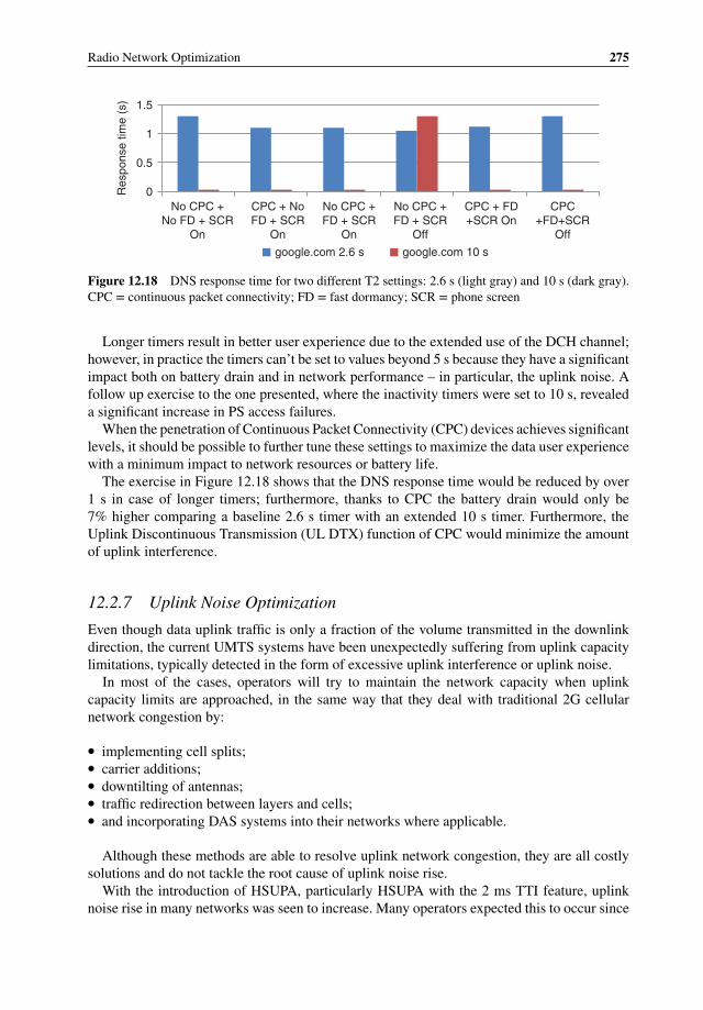
Radio Network Optimization 275
0
0.5
1
1.5
No CPC +No FD + SCR
On
CPC + NoFD + SCR
On
No CPC +FD + SCR
On
No CPC +FD + SCR
Off
CPC + FD+SCR On
CPC+FD+SCR
Off
Res
pons
e tim
e (s
)
google.com 2.6 s google.com 10 s
Figure 12.18 DNS response time for two different T2 settings: 2.6 s (light gray) and 10 s (dark gray).CPC = continuous packet connectivity; FD = fast dormancy; SCR = phone screen
Longer timers result in better user experience due to the extended use of the DCH channel;however, in practice the timers can’t be set to values beyond 5 s because they have a significantimpact both on battery drain and in network performance – in particular, the uplink noise. Afollow up exercise to the one presented, where the inactivity timers were set to 10 s, revealeda significant increase in PS access failures.
When the penetration of Continuous Packet Connectivity (CPC) devices achieves significantlevels, it should be possible to further tune these settings to maximize the data user experiencewith a minimum impact to network resources or battery life.
The exercise in Figure 12.18 shows that the DNS response time would be reduced by over1 s in case of longer timers; furthermore, thanks to CPC the battery drain would only be7% higher comparing a baseline 2.6 s timer with an extended 10 s timer. Furthermore, theUplink Discontinuous Transmission (UL DTX) function of CPC would minimize the amountof uplink interference.
12.2.7 Uplink Noise Optimization
Even though data uplink traffic is only a fraction of the volume transmitted in the downlinkdirection, the current UMTS systems have been unexpectedly suffering from uplink capacitylimitations, typically detected in the form of excessive uplink interference or uplink noise.
In most of the cases, operators will try to maintain the network capacity when uplinkcapacity limits are approached, in the same way that they deal with traditional 2G cellularnetwork congestion by:
� implementing cell splits;� carrier additions;� downtilting of antennas;� traffic redirection between layers and cells;� and incorporating DAS systems into their networks where applicable.
Although these methods are able to resolve uplink network congestion, they are all costlysolutions and do not tackle the root cause of uplink noise rise.
With the introduction of HSUPA, particularly HSUPA with the 2 ms TTI feature, uplinknoise rise in many networks was seen to increase. Many operators expected this to occur since
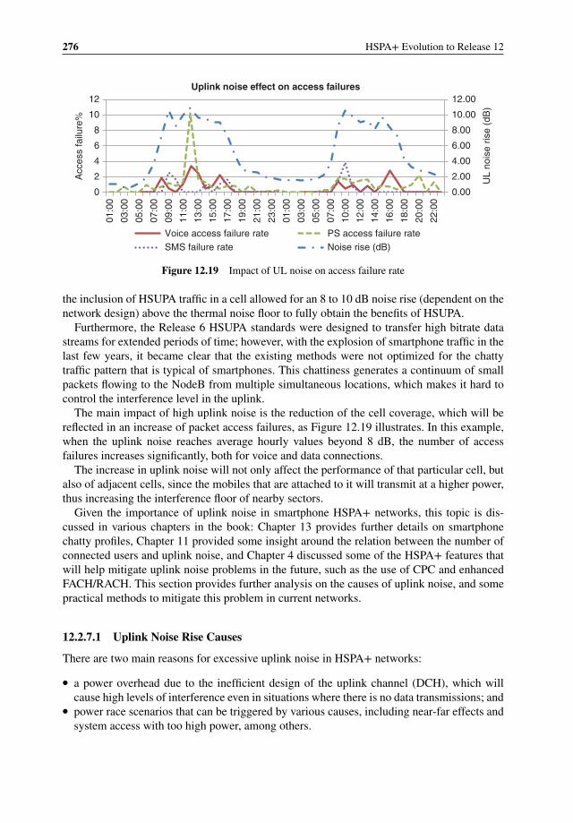
276 HSPA+ Evolution to Release 12
0.00
2.00
4.00
6.00
8.00
10.00
12.00
0
2
4
6
8
10
1201
:00
03:0
0
05:0
0
07:0
0
09:0
0
11:0
0
13:0
0
15:0
0
17:0
0
19:0
0
21:0
0
23:0
0
01:0
0
03:0
0
05:0
0
07:0
0
10:0
0
12:0
0
14:0
0
16:0
0
18:0
0
20:0
0
22:0
0
UL
nois
e ris
e (d
B)
Acc
ess
failu
re%
Uplink noise effect on access failures
Voice access failure rate PS access failure rateSMS failure rate Noise rise (dB)
Figure 12.19 Impact of UL noise on access failure rate
the inclusion of HSUPA traffic in a cell allowed for an 8 to 10 dB noise rise (dependent on thenetwork design) above the thermal noise floor to fully obtain the benefits of HSUPA.
Furthermore, the Release 6 HSUPA standards were designed to transfer high bitrate datastreams for extended periods of time; however, with the explosion of smartphone traffic in thelast few years, it became clear that the existing methods were not optimized for the chattytraffic pattern that is typical of smartphones. This chattiness generates a continuum of smallpackets flowing to the NodeB from multiple simultaneous locations, which makes it hard tocontrol the interference level in the uplink.
The main impact of high uplink noise is the reduction of the cell coverage, which will bereflected in an increase of packet access failures, as Figure 12.19 illustrates. In this example,when the uplink noise reaches average hourly values beyond 8 dB, the number of accessfailures increases significantly, both for voice and data connections.
The increase in uplink noise will not only affect the performance of that particular cell, butalso of adjacent cells, since the mobiles that are attached to it will transmit at a higher power,thus increasing the interference floor of nearby sectors.
Given the importance of uplink noise in smartphone HSPA+ networks, this topic is dis-cussed in various chapters in the book: Chapter 13 provides further details on smartphonechatty profiles, Chapter 11 provided some insight around the relation between the number ofconnected users and uplink noise, and Chapter 4 discussed some of the HSPA+ features thatwill help mitigate uplink noise problems in the future, such as the use of CPC and enhancedFACH/RACH. This section provides further analysis on the causes of uplink noise, and somepractical methods to mitigate this problem in current networks.
12.2.7.1 Uplink Noise Rise Causes
There are two main reasons for excessive uplink noise in HSPA+ networks:
� a power overhead due to the inefficient design of the uplink channel (DCH), which willcause high levels of interference even in situations where there is no data transmissions; and
� power race scenarios that can be triggered by various causes, including near-far effects andsystem access with too high power, among others.
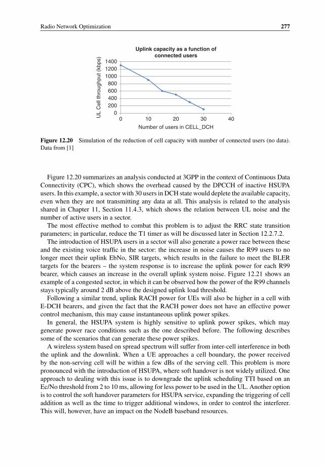
Radio Network Optimization 277
0200400600800
100012001400
0 10 20 30 40UL
Cel
l thr
ough
put (
kbps
)
Number of users in CELL_DCH
Uplink capacity as a function ofconnected users
Figure 12.20 Simulation of the reduction of cell capacity with number of connected users (no data).Data from [1]
Figure 12.20 summarizes an analysis conducted at 3GPP in the context of Continuous DataConnectivity (CPC), which shows the overhead caused by the DPCCH of inactive HSUPAusers. In this example, a sector with 30 users in DCH state would deplete the available capacity,even when they are not transmitting any data at all. This analysis is related to the analysisshared in Chapter 11, Section 11.4.3, which shows the relation between UL noise and thenumber of active users in a sector.
The most effective method to combat this problem is to adjust the RRC state transitionparameters; in particular, reduce the T1 timer as will be discussed later in Section 12.2.7.2.
The introduction of HSUPA users in a sector will also generate a power race between theseand the existing voice traffic in the sector: the increase in noise causes the R99 users to nolonger meet their uplink EbNo, SIR targets, which results in the failure to meet the BLERtargets for the bearers – the system response is to increase the uplink power for each R99bearer, which causes an increase in the overall uplink system noise. Figure 12.21 shows anexample of a congested sector, in which it can be observed how the power of the R99 channelsstays typically around 2 dB above the designed uplink load threshold.
Following a similar trend, uplink RACH power for UEs will also be higher in a cell withE-DCH bearers, and given the fact that the RACH power does not have an effective powercontrol mechanism, this may cause instantaneous uplink power spikes.
In general, the HSUPA system is highly sensitive to uplink power spikes, which maygenerate power race conditions such as the one described before. The following describessome of the scenarios that can generate these power spikes.
A wireless system based on spread spectrum will suffer from inter-cell interference in boththe uplink and the downlink. When a UE approaches a cell boundary, the power receivedby the non-serving cell will be within a few dBs of the serving cell. This problem is morepronounced with the introduction of HSUPA, where soft handover is not widely utilized. Oneapproach to dealing with this issue is to downgrade the uplink scheduling TTI based on anEc/No threshold from 2 to 10 ms, allowing for less power to be used in the UL. Another optionis to control the soft handover parameters for HSUPA service, expanding the triggering of celladdition as well as the time to trigger additional windows, in order to control the interferer.This will, however, have an impact on the NodeB baseband resources.

278 HSPA+ Evolution to Release 12
7/10
/201
17/
10/2
011
3:00
7/10
/201
1 6:
007/
10/2
011
9:00
7/10
/201
1 12
:00
7/10
/201
1 15
:00
7/10
/201
1 18
:00
7/10
/201
1 21
:00
7/11
/201
17/
11/2
011
3:00
7/11
/201
1 6:
007/
11/2
011
9:00
7/11
/201
1 12
:00
7/11
/201
1 15
:00
7/11
/201
1 19
:00
7/11
/201
1 22
:00
7/12
/201
1 1:
007/
12/2
011
4:00
7/12
/201
1 7:
007/
12/2
011
10:0
07/
12/2
011
13:0
07/
12/2
011
16:0
07/
12/2
011
19:0
07/
12/2
011
22:0
07/
13/2
011
1:00
7/13
/201
1 4:
007/
13/2
011
7:00
7/13
/201
1 10
:00
7/13
/201
1 13
:00
7/13
/201
1 16
:00
7/13
/201
1 19
:00
7/13
/201
1 22
:00
7/14
/201
1 1:
007/
14/2
011
4:00
7/14
/201
1 7:
007/
14/2
011
10:0
07/
14/2
011
13:0
07/
14/2
011
16:0
07/
14/2
011
19:0
07/
14/2
011
22:0
0
0
2
Time (hourly)
Measure R99 UL power above R99 load threshold
4
6
8
10
12
UL
pow
er a
bove
R99
thre
shol
d [d
B]
14
Figure 12.21 Additional uplink power used by R99 channels when HSUPA traffic is present
A similar problem is caused by building shadowing, where a UE is connected to one cellbut due to mobility and shadowing (such as moving around a building) finds itself within thefootprint of a new cell. This results in a significant amount of power being received in the newcell before the UE can enter into soft handover and the interference brought under control.
Figure 12.22 shows the results of this effect – a cell carrying no UE traffic and experiencinghigh uplink noise in the beginning part of the trace before the UE changes cells. A plot of theUE TX power during the cell change is shown in Figure 12.23.
In this example, prior to cell change the UE TX power ramps up to 14 dBm before reducingto −15 dBm post cell change.
In many cases, it is not possible to avoid those uplink spikes; however it is possible to controlhow the system deals with these spikes. Section 12.2.7.3 presents an example in which the
Figure 12.22 Power measurement from live sector showing near–far problem
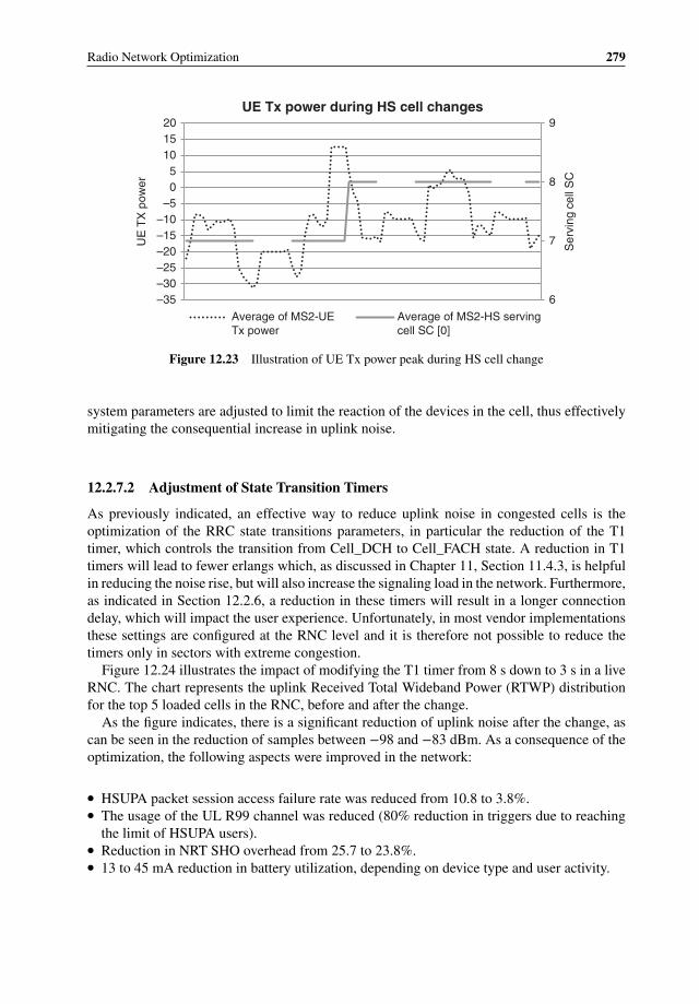
Radio Network Optimization 279
6
7
8
9
–35–30–25–20–15–10–505
101520
Ser
ving
cel
l SC
UE
TX
pow
er
UE Tx power during HS cell changes
Average of MS2-UETx power
Average of MS2-HS servingcell SC [0]
Figure 12.23 Illustration of UE Tx power peak during HS cell change
system parameters are adjusted to limit the reaction of the devices in the cell, thus effectivelymitigating the consequential increase in uplink noise.
12.2.7.2 Adjustment of State Transition Timers
As previously indicated, an effective way to reduce uplink noise in congested cells is theoptimization of the RRC state transitions parameters, in particular the reduction of the T1timer, which controls the transition from Cell_DCH to Cell_FACH state. A reduction in T1timers will lead to fewer erlangs which, as discussed in Chapter 11, Section 11.4.3, is helpfulin reducing the noise rise, but will also increase the signaling load in the network. Furthermore,as indicated in Section 12.2.6, a reduction in these timers will result in a longer connectiondelay, which will impact the user experience. Unfortunately, in most vendor implementationsthese settings are configured at the RNC level and it is therefore not possible to reduce thetimers only in sectors with extreme congestion.
Figure 12.24 illustrates the impact of modifying the T1 timer from 8 s down to 3 s in a liveRNC. The chart represents the uplink Received Total Wideband Power (RTWP) distributionfor the top 5 loaded cells in the RNC, before and after the change.
As the figure indicates, there is a significant reduction of uplink noise after the change, ascan be seen in the reduction of samples between −98 and −83 dBm. As a consequence of theoptimization, the following aspects were improved in the network:
� HSUPA packet session access failure rate was reduced from 10.8 to 3.8%.� The usage of the UL R99 channel was reduced (80% reduction in triggers due to reaching
the limit of HSUPA users).� Reduction in NRT SHO overhead from 25.7 to 23.8%.� 13 to 45 mA reduction in battery utilization, depending on device type and user activity.
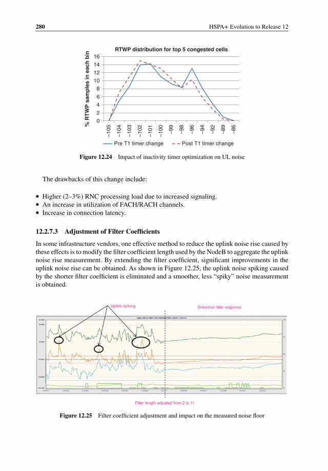
280 HSPA+ Evolution to Release 12
0
2
4
6
8
10
12
14
16
–105
–104
–103
–102
–101
–100 –99
–98
–96
–94
–92
–89
–86%
RT
WP
sam
ple
s in
eac
h b
in
RTWP distribution for top 5 congested cells
Pre T1 timer change Post T1 timer change
Figure 12.24 Impact of inactivity timer optimization on UL noise
The drawbacks of this change include:
� Higher (2–3%) RNC processing load due to increased signaling.� An increase in utilization of FACH/RACH channels.� Increase in connection latency.
12.2.7.3 Adjustment of Filter Coefficients
In some infrastructure vendors, one effective method to reduce the uplink noise rise caused bythese effects is to modify the filter coefficient length used by the NodeB to aggregate the uplinknoise rise measurement. By extending the filter coefficient, significant improvements in theuplink noise rise can be obtained. As shown in Figure 12.25, the uplink noise spiking causedby the shorter filter coefficient is eliminated and a smoother, less “spiky” noise measurementis obtained.
Uplink spiking Smoother filter response
Filter length adjusted from 2 to 11
Figure 12.25 Filter coefficient adjustment and impact on the measured noise floor
Radio Network Optimization 281
The modification of the filter coefficient has a direct impact on the PRACH outer loop powercontrol, and can introduce more stability into the system. If we refer to the initial PRACHpower calculation:
Preamble initial power = Pathloss + UL interference + Prach Required Received CI
The filter coefficient controls the way the UL interference component of this formula iscalculated by the NodeB and transmitted to the mobiles via the SIB7 information block. Aconservative setting of the filter coefficient makes the system less susceptible to instantaneousmodifications in uplink noise.
Statistical analysis of a real network has shown the following improvements in the RTWPwith the introduction of changing this value, as shown in Figure 12.26.
12.2.7.4 Adjustment of PRACH Parameters
Care should also be taken to tune the initial PRACH target settings. Lab testing has shownthat, when these values are not optimally adjusted, excessive spiking occurs when there aresmall coupling losses between the UE and the network as shown below in Figure 12.27
Many network operators approach PRACH power settings with the goal of ensuring reducedcall setup times. Their approach is therefore to maximize the power used in the initial PRACHsettings which ensures an access grant on the first attempt. In a spread spectrum network thisapproach has a negative impact on the uplink shared resource.
In a study conducted on a live network cell, adjusting the initial PRACH parameters showedimmediate relief from excessive uplink noise rise (Figure 12.28).
Table 12.5 defines the parameter sets that were used in the above study. PRACH optimizationneeds to be done cautiously as it has an impact on cell coverage and very aggressive valuescould result in missed calls. When analyzing different impacts, special care should be takento ensure that traffic is not being lost due to the smaller sector footprint. This can be checkedthrough drive tests or with the help of geolocation tools.
In this study, the biggest improvement occurred after step 1, the contributor to this change isthe required PRACH carrier to interference target. The other steps deal with further decreasingthe required carrier to interference ratio; however, not much further improvement is obtainedfor this change.
Combining the filter coefficient together with the PRACH settings, a significant amount ofthe noise that exists in the uplink can be controlled.
12.3 Optimization Tools
With the increase of technology complexity the planning and maintenance of the networkhas become increasingly difficult; however, new and powerful engineering tools have beendesigned to help the engineers in their daily tasks. In this section we discuss three of themost interesting tools that are available today, which can help operators improve their networkoperational efficiency and performance: geolocation, user tracing tools, and self-organizingnetwork (SON) tools.
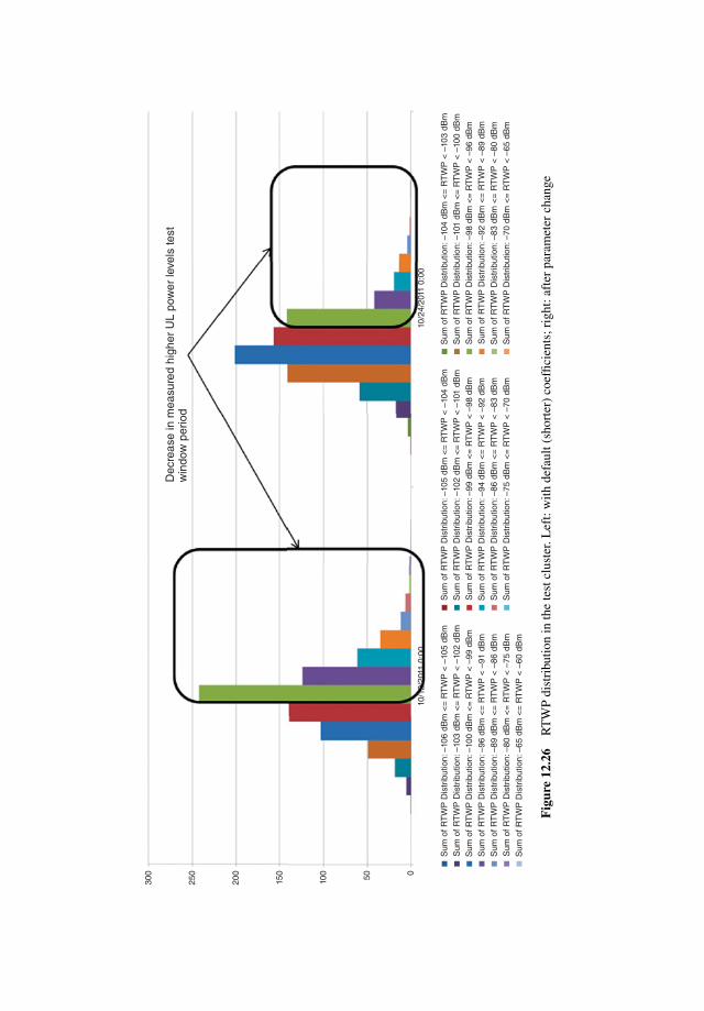
300
250
200
150
100 50 0
10/1
2/20
11 0
:00
10/2
4/20
11 0
:00
Dec
reas
e in
mea
sure
d hi
gher
UL
pow
er le
vels
test
win
dow
per
iod
Sum
of R
TW
P D
istr
ibut
ion:
–89
dB
m <
= R
TW
P <
–86
dB
m
Sum
of R
TW
P D
istr
ibut
ion:
–75
dB
m <
= R
TW
P <
–70
dB
m
Sum
of R
TW
P D
istr
ibut
ion:
–98
dB
m <
= R
TW
P <
–96
dB
m
Sum
of R
TW
P D
istr
ibut
ion:
–10
2 dB
m <
= R
TW
P <
–10
1 dB
m
Sum
of R
TW
P D
istr
ibut
ion:
–10
5 dB
m <
= R
TW
P <
–10
4 dB
mS
um o
f RT
WP
Dis
trib
utio
n: –
104
dBm
<=
RT
WP
< –
103
dBm
Sum
of R
TW
P D
istr
ibut
ion:
–10
0 dB
m <
= R
TW
P <
–99
dB
m
Sum
of R
TW
P D
istr
ibut
ion:
–94
dB
m <
= R
TW
P <
–92
dB
m
Sum
of R
TW
P D
istr
ibut
ion:
–83
dB
m <
= R
TW
P <
–80
dB
m
Sum
of R
TW
P D
istr
ibut
ion:
–65
dB
m <
= R
TW
P <
–60
dB
m
Sum
of R
TW
P D
istr
ibut
ion:
–10
3 dB
m <
= R
TW
P <
–10
2 dB
m
Sum
of R
TW
P D
istr
ibut
ion:
–99
dB
m <
= R
TW
P <
–98
dB
m
Sum
of R
TW
P D
istr
ibut
ion:
–92
dB
m <
= R
TW
P <
–89
dB
m
Sum
of R
TW
P D
istr
ibut
ion:
–80
dB
m <
= R
TW
P <
–75
dB
m
Sum
of R
TW
P D
istr
ibut
ion:
–10
6 dB
m <
= R
TW
P <
–10
5 dB
m
Sum
of R
TW
P D
istr
ibut
ion:
–10
1 dB
m <
= R
TW
P <
–10
0 dB
m
Sum
of R
TW
P D
istr
ibut
ion:
–96
dB
m <
= R
TW
P <
–91
dB
m
Sum
of R
TW
P D
istr
ibut
ion:
–86
dB
m <
= R
TW
P <
–83
dB
m
Sum
of R
TW
P D
istr
ibut
ion:
–70
dB
m <
= R
TW
P <
–65
dB
m
Fig
ure
12.2
6R
TW
Pdi
stri
butio
nin
the
test
clus
ter.
Lef
t:w
ithde
faul
t(sh
orte
r)co
effic
ient
s;ri
ght:
afte
rpa
ram
eter
chan
ge
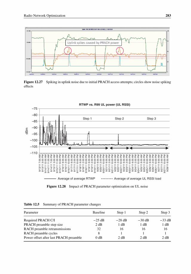
Radio Network Optimization 283
Figure 12.27 Spiking in uplink noise due to initial PRACH access attempts; circles show noise spikingeffects
–110
–105
–100
–95
–90
–85
–80
–75
9/13
/11
7:00
AM
9/13
/11
3:00
PM
9/14
/11
12:0
0 A
M9/
14/1
1 11
:00
AM
9/14
/11
7:00
PM
9/15
/11
3:00
AM
9/15
/11
11:0
0 A
M9/
15/1
1 10
:00
PM
9/16
/11
6:00
AM
9/16
/11
2:00
PM
9/16
/11
10:0
0 P
M9/
17/1
1 6:
00 A
M9/
17/1
1 2:
00 P
M9/
17/1
1 10
:00
PM
9/18
/11
6:00
AM
9/18
/11
2:00
PM
9/18
/11
10:0
0 P
M9/
19/1
1 6:
00 A
M9/
19/1
1 2:
00 P
M9/
19/1
1 10
:00
PM
9/20
/11
6:00
AM
9/20
/11
2:00
PM
9/20
/11
10:0
0 P
M9/
21/1
1 6:
00 A
M9/
21/1
1 2:
00 P
M9/
21/1
1 10
:00
PM
9/22
/11
6:00
AM
9/22
/11
2:00
PM
9/22
/11
10:0
0 P
M9/
23/1
1 6:
00 A
M9/
23/1
1 2:
00 P
M9/
23/1
1 10
:00
PM
9/24
/11
6:00
AM
9/24
/11
2:00
PM
9/24
/11
10:0
0 P
M9/
25/1
1 6:
00 A
M9/
25/1
1 2:
00 P
M9/
25/1
1 10
:00
PM
9/26
/11
6:00
AM
9/26
/11
2:00
PM
9/26
/11
10:0
0 P
M9/
27/1
1 6:
00 A
M9/
27/1
1 2:
00 P
M9/
27/1
1 10
:00
PM
9/28
/11
6:00
AM
dBm
RTWP vs. R99 UL power (UL RSSI)
Average of average RTWP Average of average UL RSSI load
Step 1 Step 2 Step 3
Figure 12.28 Impact of PRACH parameter optimization on UL noise
Table 12.5 Summary of PRACH parameter changes
Parameter Baseline Step 1 Step 2 Step 3
Required PRACH C/I −25 dB −28 dB −30 dB −33 dBPRACH preamble step size 2 dB 1 dB 1 dB 1 dBRACH preamble retransmissions 32 16 16 16RACH preamble cycles 8 1 1 1Power offset after last PRACH preamble 0 dB 2 dB 2 dB 2 dB
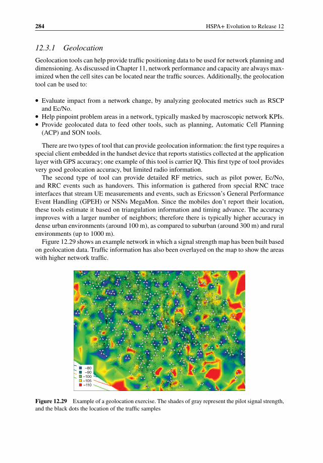
284 HSPA+ Evolution to Release 12
12.3.1 Geolocation
Geolocation tools can help provide traffic positioning data to be used for network planning anddimensioning. As discussed in Chapter 11, network performance and capacity are always max-imized when the cell sites can be located near the traffic sources. Additionally, the geolocationtool can be used to:
� Evaluate impact from a network change, by analyzing geolocated metrics such as RSCPand Ec/No.
� Help pinpoint problem areas in a network, typically masked by macroscopic network KPIs.� Provide geolocated data to feed other tools, such as planning, Automatic Cell Planning
(ACP) and SON tools.
There are two types of tool that can provide geolocation information: the first type requires aspecial client embedded in the handset device that reports statistics collected at the applicationlayer with GPS accuracy; one example of this tool is carrier IQ. This first type of tool providesvery good geolocation accuracy, but limited radio information.
The second type of tool can provide detailed RF metrics, such as pilot power, Ec/No,and RRC events such as handovers. This information is gathered from special RNC traceinterfaces that stream UE measurements and events, such as Ericsson’s General PerformanceEvent Handling (GPEH) or NSNs MegaMon. Since the mobiles don’t report their location,these tools estimate it based on triangulation information and timing advance. The accuracyimproves with a larger number of neighbors; therefore there is typically higher accuracy indense urban environments (around 100 m), as compared to suburban (around 300 m) and ruralenvironments (up to 1000 m).
Figure 12.29 shows an example network in which a signal strength map has been built basedon geolocation data. Traffic information has also been overlayed on the map to show the areaswith higher network traffic.
–80–90
–100–105–110
Figure 12.29 Example of a geolocation exercise. The shades of gray represent the pilot signal strength,and the black dots the location of the traffic samples
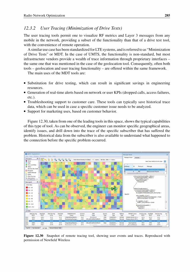
Radio Network Optimization 285
12.3.2 User Tracing (Minimization of Drive Tests)
The user tracing tools permit one to visualize RF metrics and Layer 3 messages from anymobile in the network, providing a subset of the functionality than that of a drive test tool,with the convenience of remote operation.
A similar use case has been standardized for LTE systems, and is referred to as “Minimizationof Drive Tests” or MDT. In the case of UMTS, the functionality is non-standard, but mostinfrastructure vendors provide a wealth of trace information through proprietary interfaces –the same one that was mentioned in the case of the geolocation tool. Consequently, often bothtools – geolocation and user tracing functionality – are offered within the same framework.
The main uses of the MDT tools are:
� Substitution for drive testing, which can result in significant savings in engineeringresources.
� Generation of real-time alerts based on network or user KPIs (dropped calls, access failures,etc.).
� Troubleshooting support to customer care. These tools can typically save historical tracedata, which can be used in case a specific customer issue needs to be analyzed.
� Support for marketing uses, based on customer behavior.
Figure 12.30, taken from one of the leading tools in this space, shows the typical capabilitiesof this type of tool. As can be observed, the engineer can monitor specific geographical areas,identify issues, and drill down into the trace of the specific subscriber that has suffered theproblem. Historical data from the subscriber is also available to understand what happened tothe connection before the specific problem occurred.
Figure 12.30 Snapshot of remote tracing tool, showing user events and traces. Reproduced withpermission of Newfield Wireless
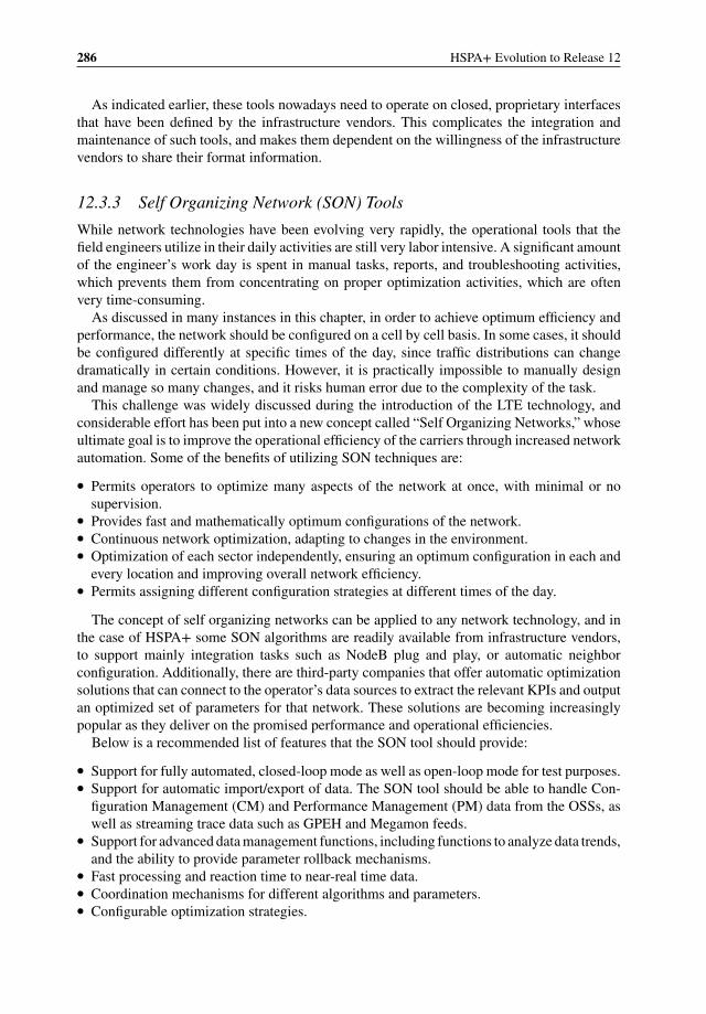
286 HSPA+ Evolution to Release 12
As indicated earlier, these tools nowadays need to operate on closed, proprietary interfacesthat have been defined by the infrastructure vendors. This complicates the integration andmaintenance of such tools, and makes them dependent on the willingness of the infrastructurevendors to share their format information.
12.3.3 Self Organizing Network (SON) Tools
While network technologies have been evolving very rapidly, the operational tools that thefield engineers utilize in their daily activities are still very labor intensive. A significant amountof the engineer’s work day is spent in manual tasks, reports, and troubleshooting activities,which prevents them from concentrating on proper optimization activities, which are oftenvery time-consuming.
As discussed in many instances in this chapter, in order to achieve optimum efficiency andperformance, the network should be configured on a cell by cell basis. In some cases, it shouldbe configured differently at specific times of the day, since traffic distributions can changedramatically in certain conditions. However, it is practically impossible to manually designand manage so many changes, and it risks human error due to the complexity of the task.
This challenge was widely discussed during the introduction of the LTE technology, andconsiderable effort has been put into a new concept called “Self Organizing Networks,” whoseultimate goal is to improve the operational efficiency of the carriers through increased networkautomation. Some of the benefits of utilizing SON techniques are:
� Permits operators to optimize many aspects of the network at once, with minimal or nosupervision.
� Provides fast and mathematically optimum configurations of the network.� Continuous network optimization, adapting to changes in the environment.� Optimization of each sector independently, ensuring an optimum configuration in each and
every location and improving overall network efficiency.� Permits assigning different configuration strategies at different times of the day.
The concept of self organizing networks can be applied to any network technology, and inthe case of HSPA+ some SON algorithms are readily available from infrastructure vendors,to support mainly integration tasks such as NodeB plug and play, or automatic neighborconfiguration. Additionally, there are third-party companies that offer automatic optimizationsolutions that can connect to the operator’s data sources to extract the relevant KPIs and outputan optimized set of parameters for that network. These solutions are becoming increasinglypopular as they deliver on the promised performance and operational efficiencies.
Below is a recommended list of features that the SON tool should provide:
� Support for fully automated, closed-loop mode as well as open-loop mode for test purposes.� Support for automatic import/export of data. The SON tool should be able to handle Con-
figuration Management (CM) and Performance Management (PM) data from the OSSs, aswell as streaming trace data such as GPEH and Megamon feeds.
� Support for advanced data management functions, including functions to analyze data trends,and the ability to provide parameter rollback mechanisms.
� Fast processing and reaction time to near-real time data.� Coordination mechanisms for different algorithms and parameters.� Configurable optimization strategies.

Radio Network Optimization 287
Table 12.6 Table with automated 3G strategies
Automated planning, configuration, and integration
NodeB integration support 3G automatic neighborsAutomatic NodeB rehomes Parameter consistency enforcement
Automated optimization
Cell outage detection and compensation Energy savings3G mobility optimization Automatic load balancingAutomatic CCCH optimization Coverage and interference optimization
Automated performance monitoring and troubleshooting
Automatic performance reports Real-time alertsDetection of crossed antenna feeders Cell outage detection and compensationAutomatic sleeping cell detection and resolution
12.3.3.1 SON Algorithms for HSPA+
The optimization algorithms will typically try to find a balance between coverage, capacity,and quality, depending on a certain policy that can usually be configured by the operator.To achieve this, the SON tool typically modifies network parameters that are configurablethrough the OSS, while for example, the Automatic Cell Planning (ACP) tool deals primarilywith RF parameters such as antenna tilts, azimuth, height, and so on. However, as SON toolshave become more sophisticated, the boundary between these tools has become blurred, andnow it is possible to find SON algorithms that optimize certain RF parameters, such as pilotpowers and antenna tilts. Table 12.6 summarizes some of the HSPA+ SON strategies that canbe found in today’s tools.
The following section provides a high-level description of the most interesting algorithmsfor automatic 3G optimization.
UMTS Automatic Neighbors (ANR)This algorithm configures neighbors of a 3G cell to try and minimize dropped calls due tomissing neighbors and UL sync issues. Most existing modules will configure intra-frequency,inter-frequency, and inter-RAT neighbors to GSM, and will keep the neighbor list within thelimits imposed by the technology or vendor implementation. In certain implementations, thismodule can operate in near real time taking input from RAN traces, which can be very helpfulduring cell outages.
Automatic Load BalancingThese algorithms will try and adjust the sector footprint, handover weights, and inter-layerconfiguration parameters to distribute the load in case of high congestion in one specifichotspot area. The goal is to maximize service availability (limit access failures) and increasethroughput fairness for all customers, irrespective of their geographical location. There are twoflavors of load balancing mechanisms, one that reacts quickly to sudden changes in traffic, andone that tries to adjust the network configuration based on long-term traffic characteristics.
288 HSPA+ Evolution to Release 12
Automatic Sleeping Cell ResolutionSleeping cells are sectors which stop processing traffic for no apparent reason, and for whichno alarm is generated. The sleeping cell detection algorithm identifies a sleeping cell based oncertain performance criteria and resets the cell accordingly.
Coverage and Interference OptimizationThis module adjusts the footprint of the cells by modifying antenna tilts (in case of RETcapable) and powers to (i) eliminate coverage holes in the area, (ii) minimize inter-sectorinterference, and (iii) minimize the amount of power used in the cluster. In some cases, thealgorithm will use geolocation information to improve the accuracy of the decision. If antennaports are being shared by more than one technology, then decisions for tilts need to be assessedfor all network layers that share that path.
12.3.3.2 Results from SON Trials
HSPA+ SON tools are commercially deployed in a number of networks today. The examplesin this section are extracted from test results of these tools in a live network.
The following example illustrates the use of a SON tool during a network recovery situation.The network presented was impacted by a heavy storm which caused a very large numberof cell outages in the area; when this happened, the number of drops due to bad neighborconfiguration skyrocketed and the engineers were spending a large amount of their timeconfiguring neighbor relations, which took away time from other network recovery efforts.Three days after the event, a SON tool was activated in the area, which took care of automaticneighbor configuration in the network. Figure 12.31 shows the relevant network statistics andtime savings.
As can be seen, the number of voice drops was dramatically reduced immediately after theactivation of the ANR solution. Due to the dramatic cell outage situation, the amount of dropsdue to missing neighbors accounted for almost 20% of the total number of drops; after thetool was activated, this percentage was reduced to less than 4%. And most importantly, asindicated on the chart on the right, all this improvement was obtained with no interventionfrom the engineering crew, except for the initial configuration required.
In the next example, a SON tool was activated in two live RNCs in a market for a month.Several SON algorithms were run continuously, including:
� automatic parameter enforcement;� plug and play (configuration of new sectors);� ANR;� coverage and interference optimization.
During the trial period, other RNCs in the market were used to track any possible changesin the network, such as natural traffic growth, seasonality effects, and so on.
Figure 12.32 shows the reduction in drops in one of the RNCs (RNC4) once the SON toolwas activated. It should be noted that the tool runs autonomously, gathering KPIs every 15 mininterval, and is capable of implementing parameter modifications at that rate if necessary. The

Radio Network Optimization 289
0
500
1000
1500
2000
2500
3000
0
10.2
9.20
12 0
0:00
:00
10.3
0.20
12 0
0:00
:00
10.3
1.20
12 0
0:00
:00
11.0
1.20
12 0
0:00
:00
11.0
2.20
12 0
0:00
:00
11.0
3.20
12 0
0:00
:00
11.0
4.20
12 0
0:00
:00
11.0
5.20
12 0
0:00
:00
11.0
6.20
12 0
0:00
:00
2000
4000
6000
8000
10000
12000
14000
16000
Mis
sing
nei
ghbo
r dr
ops
Tot
al v
oice
dro
ps
Voice drops after SON automation
Sum of voice drops Sum of voice drops due to missing neighbor
0%
20%
40%
60%
80%
100%
120%
Manual Neighborplanning tool
SON ANR
Time spent in neighbormanagement tasks
Figure 12.31 Results from SON ANR execution during massive cell outages situation
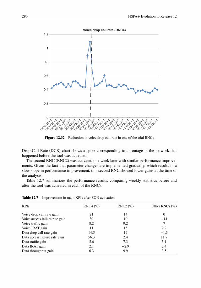
290 HSPA+ Evolution to Release 12
0
09.1
5.20
13
09.1
7.20
13
09.1
9.20
13
09.2
1.20
13
09.2
3.20
13
09.2
5.20
13
09.2
7.20
13
09.2
9.20
13
10.0
1.20
13
10.0
3.20
13
10.0
5.20
13
10.0
7.20
13
10.0
9.20
13
10.1
1.20
13
10.1
3.20
13
10.1
5.20
13
10.1
7.20
13
10.1
9.20
13
10.2
1.20
13
10.2
3.20
13
10.2
5.20
13
10.2
7.20
13
10.2
9.20
13
0.2
0.4
0.6
0.8
1
1.2Voice drop call rate (RNC4)
Figure 12.32 Reduction in voice drop call rate in one of the trial RNCs
Drop Call Rate (DCR) chart shows a spike corresponding to an outage in the network thathappened before the tool was activated.
The second RNC (RNC2) was activated one week later with similar performance improve-ments. Given the fact that parameter changes are implemented gradually, which results in aslow slope in performance improvement, this second RNC showed lower gains at the time ofthe analysis.
Table 12.7 summarizes the performance results, comparing weekly statistics before andafter the tool was activated in each of the RNCs.
Table 12.7 Improvement in main KPIs after SON activation
KPIs RNC4 (%) RNC2 (%) Other RNCs (%)
Voice drop call rate gain 21 14 0Voice access failure rate gain 30 10 −14Voice traffic gain 8.2 9.2 7Voice IRAT gain 11 15 2.2Data drop call rate gain 14.5 19 −1.3Data access failure rate gain 56.3 2.4 11.7Data traffic gain 5.6 7.3 5.1Data IRAT gain 2.1 −2.9 2.4Data throughput gain 6.3 9.9 3.5
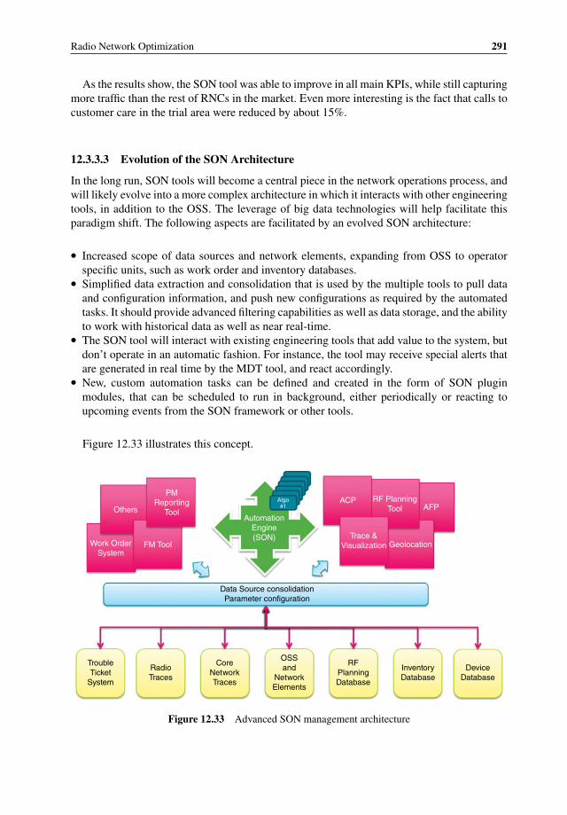
Radio Network Optimization 291
As the results show, the SON tool was able to improve in all main KPIs, while still capturingmore traffic than the rest of RNCs in the market. Even more interesting is the fact that calls tocustomer care in the trial area were reduced by about 15%.
12.3.3.3 Evolution of the SON Architecture
In the long run, SON tools will become a central piece in the network operations process, andwill likely evolve into a more complex architecture in which it interacts with other engineeringtools, in addition to the OSS. The leverage of big data technologies will help facilitate thisparadigm shift. The following aspects are facilitated by an evolved SON architecture:
� Increased scope of data sources and network elements, expanding from OSS to operatorspecific units, such as work order and inventory databases.
� Simplified data extraction and consolidation that is used by the multiple tools to pull dataand configuration information, and push new configurations as required by the automatedtasks. It should provide advanced filtering capabilities as well as data storage, and the abilityto work with historical data as well as near real-time.
� The SON tool will interact with existing engineering tools that add value to the system, butdon’t operate in an automatic fashion. For instance, the tool may receive special alerts thatare generated in real time by the MDT tool, and react accordingly.
� New, custom automation tasks can be defined and created in the form of SON pluginmodules, that can be scheduled to run in background, either periodically or reacting toupcoming events from the SON framework or other tools.
Figure 12.33 illustrates this concept.
PMReporting
ToolAutomation
Engine(SON)
ACPAFP
RF PlanningTool
GeolocationTrace &
Visualization
Data Source consolidationParameter configuration
TroubleTicket
System
CoreNetworkTraces
OSSand
NetworkElements
RFPlanningDatabase
InventoryDatabase
DeviceDatabase
RadioTraces
Algo#1Others
Work OrderSystem
FM Tool
Figure 12.33 Advanced SON management architecture
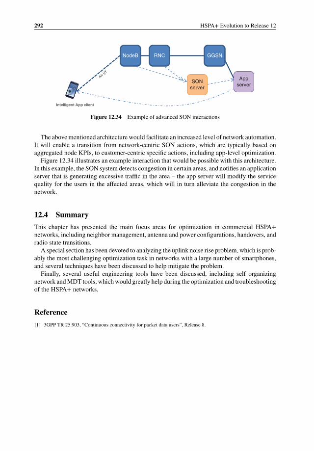
292 HSPA+ Evolution to Release 12
Intelligent App client
NodeB RNC GGSN
Appserver
SONserver
Figure 12.34 Example of advanced SON interactions
The above mentioned architecture would facilitate an increased level of network automation.It will enable a transition from network-centric SON actions, which are typically based onaggregated node KPIs, to customer-centric specific actions, including app-level optimization.
Figure 12.34 illustrates an example interaction that would be possible with this architecture.In this example, the SON system detects congestion in certain areas, and notifies an applicationserver that is generating excessive traffic in the area – the app server will modify the servicequality for the users in the affected areas, which will in turn alleviate the congestion in thenetwork.
12.4 Summary
This chapter has presented the main focus areas for optimization in commercial HSPA+networks, including neighbor management, antenna and power configurations, handovers, andradio state transitions.
A special section has been devoted to analyzing the uplink noise rise problem, which is prob-ably the most challenging optimization task in networks with a large number of smartphones,and several techniques have been discussed to help mitigate the problem.
Finally, several useful engineering tools have been discussed, including self organizingnetwork and MDT tools, which would greatly help during the optimization and troubleshootingof the HSPA+ networks.
Reference
[1] 3GPP TR 25.903, “Continuous connectivity for packet data users”, Release 8.

13Smartphone Performance
Pablo Tapia, Michael Thelander, Timo Halonen, Jeff Smith,and Mika Aalto
13.1 Introduction
In recent years the wireless industry has witnessed an impressive surge in smartphone anddata services adoption: in 2013, smartphones accounted for nearly 50% of worldwide handsetsales; however, in the USA alone this figure was even more dramatic, surpassing the 90%mark [1].
While the wide adoption of data services is quite positive to the operator from a revenuestandpoint, there are big challenges associated with the amount of traffic being generated bymodern smartphones. Smartphones are powerful computing devices with fast Internet accessspeeds that enable a similar connection experience to that of typical home computers. Suchperformance levels permit wireless customers to enjoy a wide range of wireless services,from typical web browsing to live streaming of high definition video, which entails a higherconsumption of data content overall. Furthermore, as will be analyzed later on this chapter, thebetter the device, the more data it is bound to consume, which puts operators in the difficultsituation of juggling the desire to satisfy their customers and the need to limit their impact onnetwork resources.
The resource consumption associated with increased smartphone penetration is not only tiedto the amount of data transferred, but also involves an even higher increase of network signaling:unlike typical computers, smartphones are always connected to the network, contributing tothe overall traffic with a myriad of small, intermittent packet flows that have put in checkmany of the design fundamentals of the original HSPA equipment, creating bottlenecks in thecontrol plane rather than in the user plane, as everyone expected. This chapter will analyzein detail how this signaling is generated, establishing comparison across different operatingsystems and applications, which are ultimately responsible for these harmful effects.
The second part of the chapter is focused around smartphone customer experience. Mostconsumers’ experience with mobile broadband stems from their use of a smartphone. As such,
HSPA+ Evolution to Release 12: Performance and Optimization, First Edition.Edited by Harri Holma, Antti Toskala, and Pablo Tapia.© 2014 John Wiley & Sons, Ltd. Published 2014 by John Wiley & Sons, Ltd.

294 HSPA+ Evolution to Release 12
from a mobile operator’s perspective they should place concerted effort on ensuring that theexperience is a good one. One common belief in the industry and among consumers is thata “faster network” provides a better user experience, meaning that a consumer’s experiencewith a smartphone will be inherently superior in an LTE network than an HSPA+/DC-HSDPAnetwork. The reality can be somewhat different.
The operator with the fastest network, as determined by measurements that focus solely onthroughput, will have an inherent advantage when it comes to marketing the service offering.However, the higher data speeds may not translate into a better user experience. In this case, theuser experience is defined by the parameters that the mobile data subscriber actually observeswhile using the smartphone. Examples include:
� Video playback start time and the amount of buffering that occurs during the video playback.� The battery drain on the device along the day.� The time required to begin interacting with a social networking service.� The time to load a certain web page, to name a few.
To varying degrees, the actual throughput capability of the underlying cellular networkimpacts these parameters. However, there is a diminishing return and beyond a certain thresholdhigher throughput is inconsequential. There are also other factors that influence the userexperience, and in many cases these factors have a greater influence on the outcome, meaningthat they undermine the potential benefits of having a faster network.
In this chapter we analyze in detail some of the key aspects that influence the end userexperience, and provide some guidelines about how smartphone performance can be tuned totake full advantage of the HSPA+ technology.
13.2 Smartphone Traffic Analysis
HSPA networks were not originally designed to carry traffic types such as those observedfrom smartphones today. Both downlink and uplink channels were conceived to transfer largevolumes of data very efficiently at high speed, however the traffic patterns observed in today’snetworks are somewhat different. Understanding the nature of smartphone traffic is importantto try and improve the efficiency of data transmission across the network.
Figure 13.1, from a network with a large penetration of smartphones, illustrates the shareof data consumption compared to the number of session requests, for uplink and downlinksessions. This chart shows the large asymmetry in data consumption between the uplink anddownlink directions, with most of the sessions initiated at the mobile device side.
In terms of actual content, it is worth differentiating between data volume and frequency ofaccess, which is tied to the popularity of one particular application. Figure 13.2 illustrates this.
As Figure 13.2a illustrates, a large part of the data volume is consumed by video content;however, although this service is quite popular, it is not as dominant in terms of frequencyof access. This is due to the nature of the video service, in which one single session willgenerate a significant amount of traffic, typically in the order of 200 MB per hour. On theother extreme, Internet searches are quite frequent but generate only a very small amount oftraffic. One interesting aspect to note is the popularity of social networking services, such asFacebook and Instagram, and how they are increasingly generating larger amounts of volumesdue to embedded multimedia sharing capabilities.
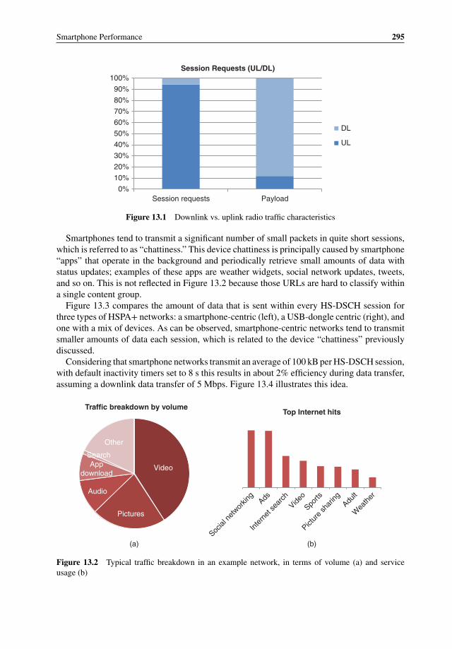
Smartphone Performance 295
0%
10%
20%
30%
40%
50%
60%
70%
80%
90%
100%
Session requests Payload
Session Requests (UL/DL)
DL
UL
Figure 13.1 Downlink vs. uplink radio traffic characteristics
Smartphones tend to transmit a significant number of small packets in quite short sessions,which is referred to as “chattiness.” This device chattiness is principally caused by smartphone“apps” that operate in the background and periodically retrieve small amounts of data withstatus updates; examples of these apps are weather widgets, social network updates, tweets,and so on. This is not reflected in Figure 13.2 because those URLs are hard to classify withina single content group.
Figure 13.3 compares the amount of data that is sent within every HS-DSCH session forthree types of HSPA+ networks: a smartphone-centric (left), a USB-dongle centric (right), andone with a mix of devices. As can be observed, smartphone-centric networks tend to transmitsmaller amounts of data each session, which is related to the device “chattiness” previouslydiscussed.
Considering that smartphone networks transmit an average of 100 kB per HS-DSCH session,with default inactivity timers set to 8 s this results in about 2% efficiency during data transfer,assuming a downlink data transfer of 5 Mbps. Figure 13.4 illustrates this idea.
Top Internet hits
Social
net
workin
gAds
Inte
rnet
sear
chVide
o
Sports
Pictur
e sh
aring
Adult
Wea
ther
Video
Pictures
Audio
Appdownload
Search
Other
Traffic breakdown by volume
(a) (b)
Figure 13.2 Typical traffic breakdown in an example network, in terms of volume (a) and serviceusage (b)
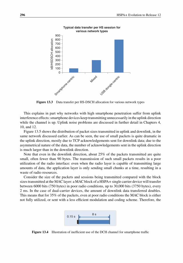
296 HSPA+ Evolution to Release 12
0
Smar
tpho
ne-c
entri
c
Mixe
d
USB don
gle-c
entri
c
100200300400500600700800900
kB/H
SD
SC
H a
lloca
tion
Typical data transfer per HS session forvarious network types
Figure 13.3 Data transfer per HS-DSCH allocation for various network types
This explains in part why networks with high smartphone penetration suffer from uplinkinterference effects: smartphone devices keep transmitting unnecessarily in the uplink directionwhile the channel is up. Uplink noise problems are discussed in further detail in Chapters 4,10, and 12.
Figure 13.5 shows the distribution of packet sizes transmitted in uplink and downlink, in thesame network discussed earlier. As can be seen, the use of small packets is quite dramatic inthe uplink direction, mostly due to TCP acknowledgements sent for downlink data; due to theasymmetrical nature of the data, the number of acknowledgements sent in the uplink directionis much larger than in the downlink direction.
Note that even in the downlink direction, about 25% of the packets transmitted are quitesmall, often fewer than 90 bytes. The transmission of such small packets results in a poorutilization of the radio interface: even when the radio layer is capable of transmitting largeamounts of data, the application layer is only sending small chunks at a time, resulting in awaste of radio resources.
Consider the size of the packets and sessions being transmitted compared with the blocksizes transmitted at the MAC layer: a MAC block of a HSPA+ single carrier device will transferbetween 6000 bits (750 bytes) in poor radio conditions, up to 30,000 bits (3750 bytes), every2 ms. In the case of dual-carrier devices, the amount of downlink data transferred doubles.This means that for 35% of the packets, even at poor radio conditions the MAC block is eithernot fully utilized, or sent with a less efficient modulation and coding scheme. Therefore, the
0.15 s8 s
Figure 13.4 Illustration of inefficient use of the DCH channel for smartphone traffic
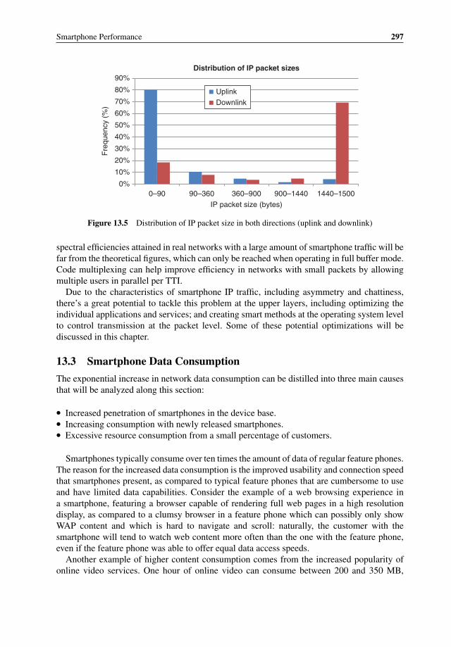
Smartphone Performance 297
0%
10%
20%
30%
40%
50%
60%
70%
80%
90%
0–90 90–360 360–900 900–1440 1440–1500
Fre
quen
cy (
%)
IP packet size (bytes)
Distribution of IP packet sizes
Uplink
Downlink
Figure 13.5 Distribution of IP packet size in both directions (uplink and downlink)
spectral efficiencies attained in real networks with a large amount of smartphone traffic will befar from the theoretical figures, which can only be reached when operating in full buffer mode.Code multiplexing can help improve efficiency in networks with small packets by allowingmultiple users in parallel per TTI.
Due to the characteristics of smartphone IP traffic, including asymmetry and chattiness,there’s a great potential to tackle this problem at the upper layers, including optimizing theindividual applications and services; and creating smart methods at the operating system levelto control transmission at the packet level. Some of these potential optimizations will bediscussed in this chapter.
13.3 Smartphone Data Consumption
The exponential increase in network data consumption can be distilled into three main causesthat will be analyzed along this section:
� Increased penetration of smartphones in the device base.� Increasing consumption with newly released smartphones.� Excessive resource consumption from a small percentage of customers.
Smartphones typically consume over ten times the amount of data of regular feature phones.The reason for the increased data consumption is the improved usability and connection speedthat smartphones present, as compared to typical feature phones that are cumbersome to useand have limited data capabilities. Consider the example of a web browsing experience ina smartphone, featuring a browser capable of rendering full web pages in a high resolutiondisplay, as compared to a clumsy browser in a feature phone which can possibly only showWAP content and which is hard to navigate and scroll: naturally, the customer with thesmartphone will tend to watch web content more often than the one with the feature phone,even if the feature phone was able to offer equal data access speeds.
Another example of higher content consumption comes from the increased popularity ofonline video services. One hour of online video can consume between 200 and 350 MB,
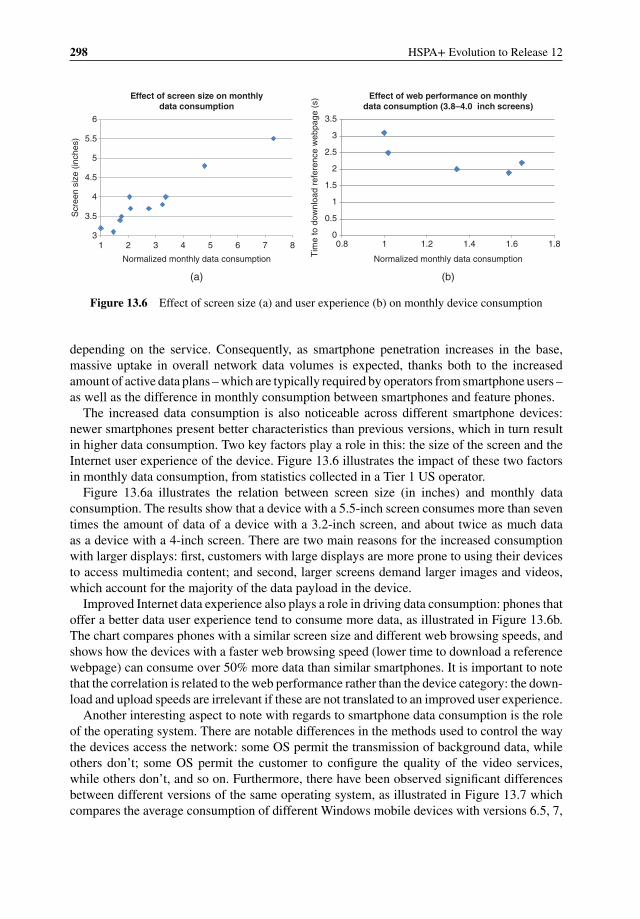
298 HSPA+ Evolution to Release 12
3
3.5
4
4.5
5
5.5
6
1 2 3 4 5 6 7 8
Scr
een
size
(in
ches
)
Normalized monthly data consumption
(a) (b)
Effect of screen size on monthlydata consumption
0
0.5
1
1.5
2
2.5
3
3.5
0.8 1 1.2 1.4 1.6 1.8
Tim
e to
dow
nloa
d re
fere
nce
web
page
(s)
Normalized monthly data consumption
Effect of web performance on monthlydata consumption (3.8–4.0 inch screens)
Figure 13.6 Effect of screen size (a) and user experience (b) on monthly device consumption
depending on the service. Consequently, as smartphone penetration increases in the base,massive uptake in overall network data volumes is expected, thanks both to the increasedamount of active data plans – which are typically required by operators from smartphone users –as well as the difference in monthly consumption between smartphones and feature phones.
The increased data consumption is also noticeable across different smartphone devices:newer smartphones present better characteristics than previous versions, which in turn resultin higher data consumption. Two key factors play a role in this: the size of the screen and theInternet user experience of the device. Figure 13.6 illustrates the impact of these two factorsin monthly data consumption, from statistics collected in a Tier 1 US operator.
Figure 13.6a illustrates the relation between screen size (in inches) and monthly dataconsumption. The results show that a device with a 5.5-inch screen consumes more than seventimes the amount of data of a device with a 3.2-inch screen, and about twice as much dataas a device with a 4-inch screen. There are two main reasons for the increased consumptionwith larger displays: first, customers with large displays are more prone to using their devicesto access multimedia content; and second, larger screens demand larger images and videos,which account for the majority of the data payload in the device.
Improved Internet data experience also plays a role in driving data consumption: phones thatoffer a better data user experience tend to consume more data, as illustrated in Figure 13.6b.The chart compares phones with a similar screen size and different web browsing speeds, andshows how the devices with a faster web browsing speed (lower time to download a referencewebpage) can consume over 50% more data than similar smartphones. It is important to notethat the correlation is related to the web performance rather than the device category: the down-load and upload speeds are irrelevant if these are not translated to an improved user experience.
Another interesting aspect to note with regards to smartphone data consumption is the roleof the operating system. There are notable differences in the methods used to control the waythe devices access the network: some OS permit the transmission of background data, whileothers don’t; some OS permit the customer to configure the quality of the video services,while others don’t, and so on. Furthermore, there have been observed significant differencesbetween different versions of the same operating system, as illustrated in Figure 13.7 whichcompares the average consumption of different Windows mobile devices with versions 6.5, 7,

Smartphone Performance 299
Windows phone 6.5 Windows phone 7 Windows phone 8
Monthly consumption comparison between variouswindows phone versions (same screen)
Figure 13.7 Data consumption differences based on OS version
and 8 – all of them with the same screen size (4.3 inch). In this case it can be observed thatWindows Phone 8 devices tend to consume much more data than their predecessors – in thisparticular case, mostly due to the default configuration of the video service quality.
Increased data consumption isn’t always good news for the customer nor the operator. Inthe case of customers, if they are not careful they can quickly consume their monthly dataquota if they access multimedia content frequently. For example, a typical Netflix movie canconsume about 500 MB in a regular smartphone, which means that customers with data plansof 2GB per month will run over their monthly quota after having watched just four movies.
For operators, increased data consumption will force additional network investments to copewith the capacity demands, or else face customer complaints due to performance degradationin the network. One interesting thing to note when analyzing customer consumption patterns isthe fact that not all customers access the network in the same manner; therefore it is good ideato classify customers based on typical monthly usage. Figure 13.8 illustrates the consumptionpatterns in an example network in which there are no data consumption limits.
As the figure shows, there is a minority of customers that consume an excessive amountof data: in this example, 2% of the users account for over 20% of the overall data transferredin the network. In order to minimize capacity investments, and at the same time preserve theservice satisfaction for the majority of the customers, the operator can implement differentdata control mechanisms to prevent harm from these excessive users, including data bitratecapping, blocking of certain operations such as peer-to-peer transfers, tethering, and so on.
In addition to volume consumption, the operator needs to analyze other forms of resourceconsumption by the smartphone devices, such as signaling. Sometimes it’s less harmful for thenetwork to transmit a large volume of data than a myriad small packets, as will be discussedin detail in the following sections.
13.4 Smartphone Signaling Analysis
The increased penetration of smartphone devices has caused a rapid increase in the signalingload at the network level. As Figure 13.9 illustrates, the growth in signaling traffic in many
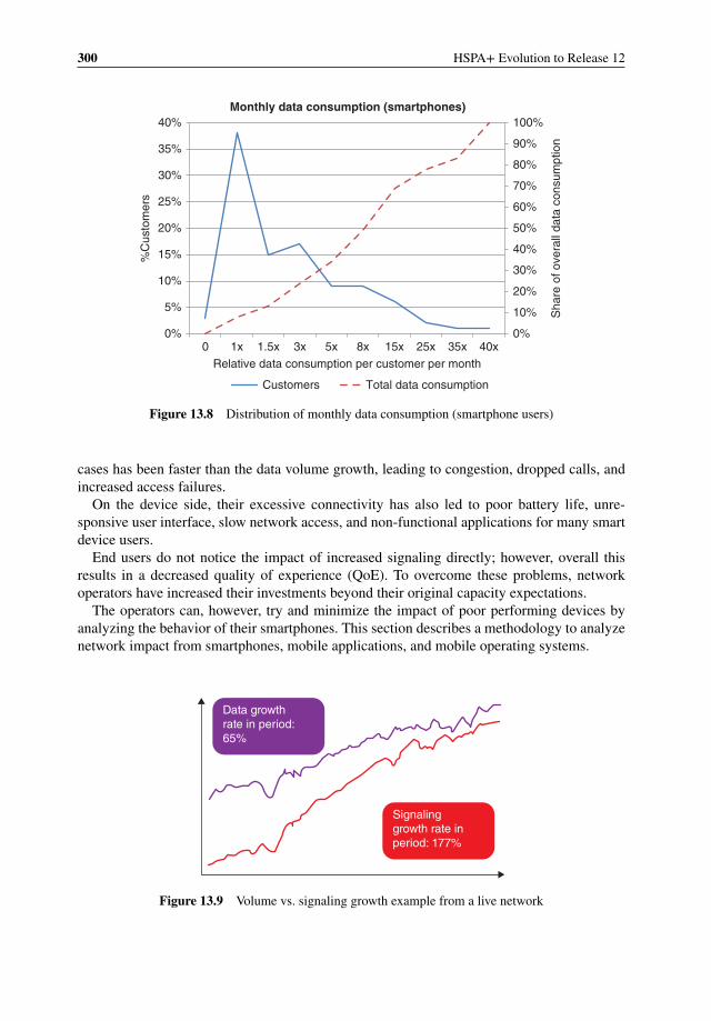
300 HSPA+ Evolution to Release 12
0%
10%
20%
30%
40%
50%
60%
70%
80%
90%
100%
0%
5%
10%
15%
20%
25%
30%
35%
40%
0 1x 1.5x 3x 5x 8x 15x 25x 35x 40x
Sha
re o
f ove
rall
data
con
sum
ptio
n
%C
usto
mer
s
Relative data consumption per customer per month
Monthly data consumption (smartphones)
Customers Total data consumption
Figure 13.8 Distribution of monthly data consumption (smartphone users)
cases has been faster than the data volume growth, leading to congestion, dropped calls, andincreased access failures.
On the device side, their excessive connectivity has also led to poor battery life, unre-sponsive user interface, slow network access, and non-functional applications for many smartdevice users.
End users do not notice the impact of increased signaling directly; however, overall thisresults in a decreased quality of experience (QoE). To overcome these problems, networkoperators have increased their investments beyond their original capacity expectations.
The operators can, however, try and minimize the impact of poor performing devices byanalyzing the behavior of their smartphones. This section describes a methodology to analyzenetwork impact from smartphones, mobile applications, and mobile operating systems.
Signalinggrowth rate inperiod: 177%
Data growthrate in period:65%
Figure 13.9 Volume vs. signaling growth example from a live network

Smartphone Performance 301
Applications
Operatingsystem
Applicationprocessor
Modemprocessor
• Application activity in foreground and background
• 3GPP features e.g. support for Rel-8 fast dormancy
• OS controlling execution of apps in foreground and background• OS controlling selected 3GPP features e.g. triggering fast dormancy
Smartphone
Figure 13.10 Components impacting smartphone performance
13.4.1 Smartphone Profiling
Smartphone profiling consists of the analysis of multiple protocol layers and their inter-related behavior in complex end-to-end systems. Promoting network friendly smart devicesand applications can help operators avoid unnecessary capacity expansions, as well as improveuser experience – which will in turn result in better customer loyalty. As will be discussedin more detail in the next section, the user experience depends on various factors, includingnetwork performance and the specific application being used. Even the battery life timeof a mobile device can be impacted by network features, as well as by well designed andimplemented applications. Figure 13.10 illustrates the various components that need to beconsidered when analyzing smartphone performance.
Some of the features that need to be taken into account when analyzing smartphone per-formance are standardized by 3GPP. Those features are implemented at the modem chip setlevel and are either fully controlled by its firmware or partially by the mobile OS. On the net-work side, the 3GPP features are split between access stratum (i.e., radio access network) andnon-access stratum (i.e., core network). A good example of one such feature is the so called“network controlled fast dormancy” or 3GPP Release 8 fast dormancy: when properly utilized,this feature can help optimize the amount of signaling caused by RRC state changes, at the sametime that the device battery life is extended by making a better use of the CELL_PCH state.
There are also important features that are implemented outside of the 3GPP domain, such asthe operating system of the device. One example of this is the implementation of OS keep-alivemessages required for push notification services. Always-on applications use push notificationservices, which send messages from the network servers to clients in mobile devices. Thesenotifications require persistent TCP connections, which again require periodical keep-alivemessages to keep the TCP connection established. The lower the keep-alive frequency is, thefewer transactions that generate additional RRC state changes and signaling.

302 HSPA+ Evolution to Release 12
The implementation of specific applications also plays an important role in user experienceand network resource consumption. For example:
� An application that displays advertisements can decide how frequently it fetches new adsfrom the network. A badly designed ad-funded application generates frequent networktransactions, and in the worst case synchronized transactions over the whole user base.
� The coding and packetization used to transmit Voice over IP (VoIP) data can impact theload in various packet forwarding network elements.
� Audio and video streaming apps can select different protocols to deliver the content overthe mobile network, and depending on the selected method user experience and battery lifetime varies. This specific example will be discussed in more detail in Section 13.5.6.5.
13.4.2 Ranking Based on Key Performance Indicators
To analyze smartphone performance, the devices will be profiled based on a set of keyperformance indicators that rank the network-friendliness of applications and smart deviceswith regards to key network domains like mobile device, radio, packet core, transport, and IPedge (firewalls, NATs, etc.).
The advised ranking-based methodology presented in this section enables mobile operatorsto find the ideal balance between the best user experience and the lowest impact on networkperformance.
Smart devices are tested with real applications or services such as Voice over IP (VoIP),mobile video, and social media in order to emulate as close as possible the behavior of a typicalsmartphone user. The smartphone profiling provides essential insight into the interactionbetween factors such as smartphone battery life and applications or operating systems. Forexample, Figure 13.11 illustrates a comparison between two different smartphones running asocial networking application.
Signalingload - core
Signalingload - radio
Powerconsumption
Data volumeData
sessions
Summary – Social networks
Smartphone BSmartphone A
Figure 13.11 Example profiling of a social networking app in two different smartphones
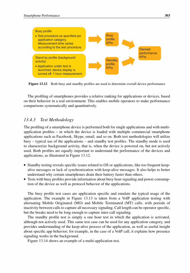
Smartphone Performance 303
BusyprofileKPIs
Busy profile
• Test procedure as specified per application category. Measurement time varies according to the test procedure.
Stand by profile (background activity)
• Application under test is launched, device display is turned off. 1 hour measurement.
DerivedperformanceKPIs
StandbyprofileKPIs
Figure 13.12 Both busy and standby profiles are used to determine overall device performance
The profiling of smartphones provides a relative ranking for applications or devices, basedon their behavior in a real environment. This enables mobile operators to make performancecomparisons systematically and quantitatively.
13.4.3 Test Methodology
The profiling of a smartphone device is performed both for single applications and with multi-application profiles – in which the device is loaded with multiple commercial smartphoneapplications such as Facebook, Skype, email, and so on. Both test methodologies will utilizebusy – typical use of the applications – and standby test profiles. The standby mode is usedto characterize background activity, that is, when the device is powered on, but not activelyused. Both profiles are equally important to understand the performance of the devices andapplications, as illustrated in Figure 13.12.
� Standby testing reveals specific issues related to OS or applications, like too frequent keep-alive messages or lack of synchronization with keep-alive messages. It also helps to betterunderstand why certain smartphones drain their battery faster than others.
� Tests with busy profiles provide information about busy hour signaling and power consump-tion of the device as well as protocol behavior of the applications.
The busy profile test cases are application specific and emulate the typical usage of theapplication. The example in Figure 13.13 is taken from a VoIP application testing withalternating Mobile Originated (MO) and Mobile Terminated (MT) calls, with periods ofinactivity between calls to capture all necessary signaling. Call length can be operator specific,but the breaks need to be long enough to capture inter-call signaling.
The standby profile test is simply a one hour test in which the application is activated,although not actively used. This same test case can be used for any application category, andprovides understanding of the keep-alive process of the application, as well as useful insightabout specific app behavior; for example, in the case of a VoIP call, it explains how presencesignaling works in the background.
Figure 13.14 shows an example of a multi-application test.
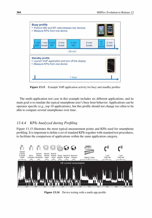
304 HSPA+ Evolution to Release 12
Busy profile• Perform MO and MT calls between two devices• Measure KPIs from one device
1 minMO
1 minbreak
2 minMT
2 minbreak
4 minMO
6 minbreak
MTNo
answer
2 minbreak
Standby profile• Launch VoIP application and turn off the display• Measure KPIs from one device
1 hour
~20 min
Figure 13.13 Example VoIP application activity for busy and standby profiles
The multi-application test case in this example includes six different applications, and itsmain goal is to emulate the typical smartphone user’s busy hour behavior. Applications can beoperator specific (e.g., top 10 applications), but this profile should not change too often to beable to compare several smartphones over time.
13.4.4 KPIs Analyzed during Profiling
Figure 13.15 illustrates the most typical measurement points and KPIs used for smartphoneprofiling. It is important to define a set of standard KPIs together with standard test procedures,to facilitate the comparison of applications within the same application category.
Figure 13.14 Device testing with a multi-app profile
1 minVoIP call
1 minVoIP callWatch a video
Search &browse
Search &browse
Checkweather
Send &receiveemail
Send &receiveemail
Uploada phototo socialmedia
Get acomment
Send &receive
comments
UE current consumption
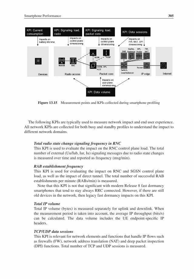
Smartphone Performance 305
Figure 13.15 Measurement points and KPIs collected during smartphone profiling
The following KPIs are typically used to measure network impact and end user experience.All network KPIs are collected for both busy and standby profiles to understand the impact todifferent network domains.
Total radio state change signaling frequency in RNCThis KPI is used to evaluate the impact on the RNC control plane load. The totalnumber of external (Uu/Iub, Iur, Iu) signaling messages due to radio state changesis measured over time and reported as frequency (msg/min).
RAB establishment frequencyThis KPI is used for evaluating the impact on RNC and SGSN control planeload, as well as the impact of direct tunnel. The total number of successful RABestablishments per minute (RABs/min) is measured.
Note that this KPI is not that significant with modern Release 8 fast dormancysmartphones that tend to stay always RRC connected. However, if there are stillold devices in the network, then legacy fast dormancy impacts on this KPI.
Total IP volumeTotal IP volume (bytes) is measured separately for uplink and downlink. Whenthe measurement period is taken into account, the average IP throughput (bits/s)can be calculated. The data volume includes the UE endpoint-specific IPheaders.
TCP/UDP data sessionsThis KPI is relevant for network elements and functions that handle IP flows suchas firewalls (FW), network address translation (NAT) and deep packet inspection(DPI) functions. Total number of TCP and UDP sessions is measured.
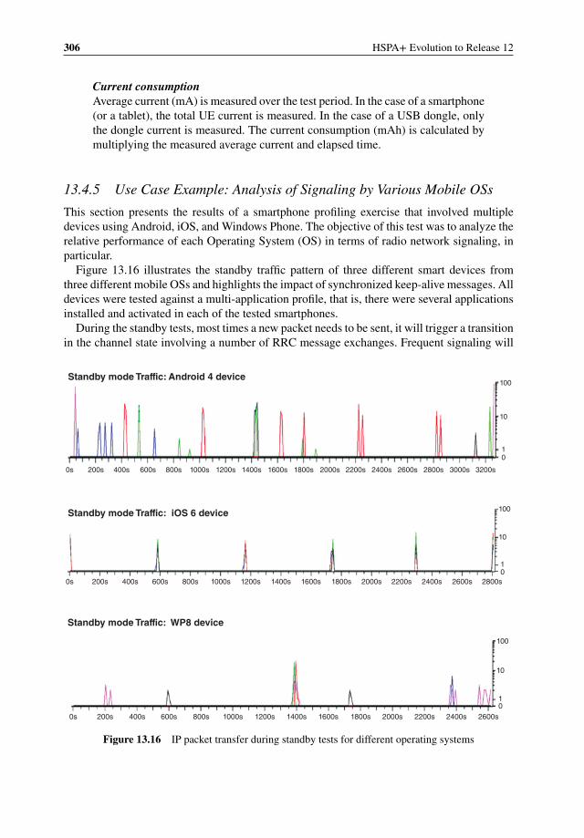
306 HSPA+ Evolution to Release 12
Current consumptionAverage current (mA) is measured over the test period. In the case of a smartphone(or a tablet), the total UE current is measured. In the case of a USB dongle, onlythe dongle current is measured. The current consumption (mAh) is calculated bymultiplying the measured average current and elapsed time.
13.4.5 Use Case Example: Analysis of Signaling by Various Mobile OSs
This section presents the results of a smartphone profiling exercise that involved multipledevices using Android, iOS, and Windows Phone. The objective of this test was to analyze therelative performance of each Operating System (OS) in terms of radio network signaling, inparticular.
Figure 13.16 illustrates the standby traffic pattern of three different smart devices fromthree different mobile OSs and highlights the impact of synchronized keep-alive messages. Alldevices were tested against a multi-application profile, that is, there were several applicationsinstalled and activated in each of the tested smartphones.
During the standby tests, most times a new packet needs to be sent, it will trigger a transitionin the channel state involving a number of RRC message exchanges. Frequent signaling will
0s 200s 400s 600s 800s 1000s 1200s 1400s 1600s 1800s 2000s 2200s 2400s 2600s 2800s 3000s 3200s
10
10
100Standby mode Traffic: Android 4 device
0s 200s 400s 600s 800s 1000s 1200s 1400s 1600s 1800s 2000s 2200s 2400s 2600s 2800s
10
10
100Standby mode Traffic: iOS 6 device
0s 200s 400s 600s 800s 1000s 1200s 1400s 1600s 1800s 2000s 2200s 2400s 2600s
10
10
100
Standby mode Traffic: WP8 device
Figure 13.16 IP packet transfer during standby tests for different operating systems
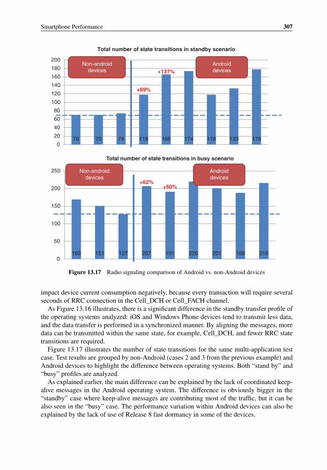
Smartphone Performance 307
70 70 74 118 166 174 118 133 1780
20
40
60
80
100
120
140
160
180
200
Total number of state transitions in standby scenario
Androiddevices
Non-androiddevices
+69%
+137%
169 151 127 207 191 220 201 188 2160
50
100
150
200
250
Total number of state transitions in busy scenario
Androiddevices
Non-androiddevices
+62%+50%
Figure 13.17 Radio signaling comparison of Android vs. non-Android devices
impact device current consumption negatively, because every transaction will require severalseconds of RRC connection in the Cell_DCH or Cell_FACH channel.
As Figure 13.16 illustrates, there is a significant difference in the standby transfer profile ofthe operating systems analyzed: iOS and Windows Phone devices tend to transmit less data,and the data transfer is performed in a synchronized manner. By aligning the messages, moredata can be transmitted within the same state, for example, Cell_DCH, and fewer RRC statetransitions are required.
Figure 13.17 illustrates the number of state transitions for the same multi-application testcase. Test results are grouped by non-Android (cases 2 and 3 from the previous example) andAndroid devices to highlight the difference between operating systems. Both “stand by” and“busy” profiles are analyzed.
As explained earlier, the main difference can be explained by the lack of coordinated keep-alive messages in the Android operating system. The difference is obviously bigger in the“standby” case where keep-alive messages are contributing most of the traffic, but it can bealso seen in the “busy” case. The performance variation within Android devices can also beexplained by the lack of use of Release 8 fast dormancy in some of the devices.
308 HSPA+ Evolution to Release 12
13.4.5.1 Discussion of the Results
All major smartphone operating systems include support for multitasking: when an applicationis switched from the foreground activity control, all operating systems suspend the app unlessthe app is specifically designed to run in the background. In the background, apps can performselected functions allowed by the operating system. For example, VoIP calls and music play-back can be executed in background; location tracking is another important function supportedin background execution. Background apps can make use of network connections and triggerdata transactions.
To better support network connectivity of background applications, all of the operatingsystems analyzed include a push notification service, which is based on a network serviceprovided by the OS vendor. Windows Phone, iOS, and Android devices can communicatewith Microsoft Push Notification Service (MPNS), Apple Push Notification service (APNs),and Google Cloud Messaging (GCM) respectively.
The multitasking capability of always-on apps and push notification services enables fre-quent data transactions even if the smartphone owner is not actively using the device. Theapplication developer is responsible for the app behavior and can significantly impact on thesignaling load as well as UE current consumption both in foreground and background periods.
The specific OS impacts the behavior of the persistent connection to the push notificationservice. OS vendors also define the policies for accepting apps to the application markets, aswell as whether the apps must use the push notification service provided by the OS vendor.Microsoft and Apple have tighter controls for app certification and usually all apps mustuse the centralized push notification service provided by the OS vendor. The Google andAndroid ecosystem leaves much more freedom for app developers to design networkingfeatures and publish apps, therefore GCM is not mandatory and many apps use their ownpersistent connections to application-specific servers. In practice, this means that WindowsPhone and iOS devices have better capability to control background activity and, for example,synchronize keep-alive and push notification transactions. Android devices tend to generatemore signaling traffic, because different always-on apps may generate independent, non-synchronized keep-alive and push notification transactions in background. At the time ofwriting this chapter, Google was actively working on improving these aspects with variousGCM and Android initiatives.
13.5 Smartphone Performance
All network operators strive to offer the best possible service experience to their customers;however, this goal is becoming increasingly challenging as data services become more promi-nent. Unlike in the case of voice, which was a relatively simple service to analyze, data servicesare more complex and often typical network KPIs do not provide the required observability tounderstand their performance. As will be discussed later in this section, there is not a single“data service” experience, rather a service experience linked to each individual data service:web browsing, video streaming, social networking, and so on.
Understanding the end user experience requires the analysis of multiple factors, from devicesto networks and services. Table 13.1 provides a list of some of the factors that play a role inthe customer experience with smartphone devices, broken down into two major categories:battery life and Service Quality of Experience (QoE).
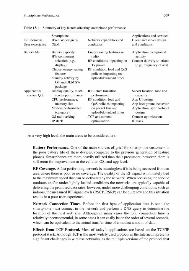
Smartphone Performance 309
Table 13.1 Summary of key factors affecting smartphone performance
E2E domainsUser experience
SmartphoneHW/SW design byOEM
Network capabilities andconditions
Applications and servicesClient and server designand conditions
Battery life Battery capacityHW component
selection (e.g.,display)
Chipset energy savingfeatures
Standby activity byOS and OEM SWpackage
Energy saving features inradio
RF conditions impacting onTx power
RF condition, load and QoSpolicies impacting onupload/download times
Application backgroundactivity
Content delivery solutions(e.g., frequency of ads)
Application/service QoE
Display quality, touchscreen performance
CPU performance,memory size
Modem performance(category)
OS multitaskingIP stack
RRC state transitionperformance
RF condition, load andQoS policies impactingon packet loss andupload/download times
TCP and contentoptimization
Server location, load andcapacity
App UI designApp background behaviorApplication layer protocol
designContent optimizationIP stack
At a very high level, the main areas to be considered are:
Battery Performance. One of the main sources of grief for smartphone customers isthe poor battery life of these devices, compared to the previous generation of featurephones. Smartphones are more heavily utilized than their precursors; however, there isstill room for improvement at the cellular, OS, and app level.
RF Coverage. A fast performing network is meaningless if it is being accessed from anarea where there is poor or no coverage. The quality of the RF signal is intimately tiedto the maximum speed that can be delivered by the network. When accessing the serviceoutdoors and/or under lightly loaded conditions the networks are typically capable ofdelivering the promised data rates; however, under more challenging conditions, such asindoors, the measured RF signal levels (RSCP, RSRP) can be quite low and this situationresults in a poor user experience.
Network Connection Times. Before the first byte of application data is sent, thesmartphone must connect to the network and perform a DNS query to determine thelocation of the host web site. Although in many cases the total connection time isrelatively inconsequential, in some cases it can easily be on the order of several seconds,which can be equivalent to the actual transfer time of a modest amount of data.
Effects from TCP Protocol. Most of today’s applications are based on the TCP/IPprotocol stack. Although TCP is the most widely used protocol in the Internet, it presentssignificant challenges in wireless networks, as the multiple versions of the protocol that
310 HSPA+ Evolution to Release 12
are “optimized” for wireless give testimony1. The variable nature of the air interfaceinterferes with the control mechanisms in TCP, which often results in reduced bitratesor data stalling situations.
Operating System Influences. The various operating systems have different ways tocontrol data transfer, which can affect network and device resource consumption. Also,in many cases the same application behaves entirely differently based on the underlyingoperating system. For example, a Facebook photo upload, operating on iOS, is fasterthan Facebook in Android due to the fact that the iPhone app resizes or compresses thepicture before uploading it to the network.
Application Characteristics. The characteristics of the application can be of paramountimportance when it comes to defining the user experience. “Chatty” applications, forexample, can require lots of back and forth interactions between the smartphone andthe network with only small amounts of data being transferred during each interaction.This situation can negate the benefits of an otherwise fast network. In this case, networklatency could have more influence on the user experience. The size and layout of a website can also influence the time required to download a web page. On the other hand,an application can also mask the true performance of a poor performing network andgive the user a far better experience than would otherwise be the case. For example, anapplication could upload content, such as a picture, in the background so the user isn’taware how long it takes. Alternatively, the application could use compression to reformatthe content of the transferred data and ultimately reduce the size of the uploaded pictureor the downloaded video.
Applications can also be optimized in other ways to provide a better user experience orto shorten the total user transaction time. For example, a robust predictive text algorithmor the use of voice recognition software could reduce the time required to perform asearch function or to enter a destination in a maps application. This capability wouldbe entirely independent of the network’s capabilities but from the user’s perspective itwould still lead to a better experience.
Understanding the behavior of each of these applications and their performance overthe wireless network is an important step towards the optimization of the smartphoneexperience. In this section we analyze two of the most common applications in usetoday, web browsing – which is the basis for most common “apps” – and the videostreaming service. As discussed earlier, these services represent the most popular trafficin terms of number of transactions and volume, respectively.
13.5.1 User Experience KPIs
In a world dominated by data services, defining the right measurements is a key step towardsunderstanding and maintaining proper customer experience. Previously used KPIs, such asaccess failures and drops, are not so meaningful when referring to data services, as in manycases a data drop will not even be noticed by the consumer. It is therefore important to definea new set of metrics that “make sense” from a data utilization point of view; these metrics will
1 TCP Vegas, New Reno, Hybla, BIC, Westwood, among others.

Smartphone Performance 311
have to be defined at the application level, such as the “time to access video content,” “time todownload a web page,” or the “number of rebuffering events” during a video playback.
These complex KPIs cannot be captured using typical counters, and require the deploymentof new elements, such as network probes, that can capture per-session data to extract thenecessary information. To complicate things further, the KPIs should be able to tell, in the caseof a performance issue, whether the problem lies in a specific radio network element or in otherpart of the communication path. There are various alternatives to implementing these new KPIs,including the use of network probes, leveraging special UE reports provided by applications(Real User Measurements – RUM), and the use of custom UE clients, such as carrier IQ.
Network probes require significant infrastructure and expense to instrument. To managescalability and cost, they are often deployed near the GGSN/PGW, or only at a few locations.Due to this placement well before the radio interface, they are often limited to connected userexperience and cannot measure the impact of connection setup latency or failures. This lackof visibility is significant as the setup latency and failures may have a much large impact onuser experience than round-trip delay. Core network probes are therefore good at detectingservice failures, or massive numbers of errors, but do not provide an accurate picture of userexperience. Alternatively, probes can be deployed at the last mile transport connection, whichcan capture the effects from the radio access network. This information can be combinedwith control plane traces from the RAN elements to provide an end-to-end picture of the dataconnection.
UE reports, also known as Real User Measurements (RUM), are often collected by websites, applications, and video services. These reports are often very specific to the serviceand can include time spent on a web page, application launch time, web page launch time,video start time, and various client parameters, to list a few. Since these are done directly onthe device, they sometimes include both connecting and connected latency; however, it reallydepends on the service’s goals. This information is not normally available to the carrier sothey must instrument their own RUM measurements.
Special UE clients, such as carrier IQ, can also be used to capture the customer experience atthe device side. This type of client can provide unique information, such as battery performance,that is otherwise not visible to the operator; these clients can also be developed to capturecertain data level KPIs; however, they are typically limited in the amount of information theycan capture.
13.5.2 Battery Performance
The battery consumption in smartphones is one of the key aspects affecting customer perceptionof the device. No matter how fast the device performs, if it can’t survive at least one day witha full charge, it will be a nuisance to the consumer, who will need to be continuously lookingfor ways to charge the phone. Such was the case with early HSPA+ smartphones, and hashappened as well to current LTE devices. Apart from the fact that customers tend to use theirsmartphones much more extensively than previous feature phones, there are clear outliers thathave a significant impact on battery performance, some of which can be mitigated by properdevice and operating system design.
Figure 13.18 illustrates the result of lab test performed by the T-Mobile validation team,considering a 24-h drain on an active user profile. The key elements involved in battery drainin this particular example are ordered from higher to lower.
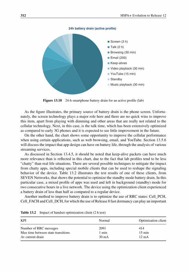
312 HSPA+ Evolution to Release 12
24h battery drain (active profile)
Screen (3 h)
Talk (2 h)
Browsing (30 min)
Email (200)
Keep-alives
Video playback (30 min)
YouTube (15 min)
Standby
Music playback (30 min)
Figure 13.18 24-h smartphone battery drain for an active profile (lab)
As the figure illustrates, the primary source of battery drain is the phone screen. Unfortu-nately, the screen technology plays a major role here and there are no quick wins to improvethis item, apart from playing with dimming and other areas that are really not related to thecellular technology. Next, in this case, is the talk time, which has been extensively optimizedas compared to early 3G phones and it is expected to see little improvement in the future.
On the other hand, the chart shows some opportunity to improve the cellular performancewhen using certain applications, such as web browsing, email, and YouTube. Section 13.5.6will discuss the impact that app design can have on battery life, through the analysis of variousstreaming services.
As discussed in Section 13.4.5, it should be noted that keep-alive packets can have muchmore relevance than is reflected in this chart, due to the fact that lab profiles tend to be less“chatty” than real life situations. There are several possible techniques to mitigate the impactfrom chatty apps, including special mobile clients that can be used to reshape the signalingbehavior of the device. Table 13.2 illustrates the test results of one of these clients, fromSEVEN Networks, that shows the potential to optimize the standby mode battery drain. In thisparticular case, a mixed profile of apps was used and left in background (standby) mode fortwo consecutive hours in a live network. The device using the optimization client experienceda battery drain of less than half as compared to a regular device.
Another method to improve battery drain is to optimize the use of RRC states: Cell_PCH,Cell_FACH and Cell_DCH, for which the use of Release 8 fast dormancy can play an important
Table 13.2 Impact of handset optimization client (2 h test)
KPI Normal Optimization client
Number of RRC messages 2091 414Max time between state transitions 1 min 15 minAv current drain 30 mA 12 mA
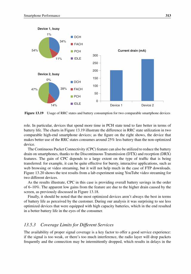
Smartphone Performance 313
0
50
100
150
200
250
300
Device 1 Device 2
Current drain (mA)
34%
11%
54%
1%
Device 1, busy
DCH
FACH
PCH
IDLE
39%
14%
47%
0%
Device 2, busy
DCH
FACH
PCH
IDLE
Figure 13.19 Usage of RRC states and battery consumption for two comparable smartphone devices
role. In particular, devices that spend more time in PCH state tend to fare better in terms ofbattery life. The charts in Figure 13.19 illustrate the difference in RRC state utilization in twocomparable high-end smartphone devices; as the figure on the right shows, the device thatmakes better use of the RRC states consumes around 25% less battery than the non-optimizeddevice.
The Continuous Packet Connectivity (CPC) feature can also be utilized to reduce the batterydrain on smartphones, thanks to the Discontinuous Transmission (DTX) and reception (DRX)features. The gain of CPC depends to a large extent on the type of traffic that is beingtransferred: for example, it can be quite effective for bursty, interactive applications, such asweb browsing or video streaming, but it will not help much in the case of FTP downloads.Figure 13.20 shows the test results from a lab experiment using YouTube video streaming fortwo different devices.
As the results illustrate, CPC in this case is providing overall battery savings in the orderof 6–10%. The apparent low gains from the feature are due to the higher drain caused by thescreen, as previously discussed in Figure 13.18.
Finally, it should be noted that the most optimized devices aren’t always the best in termsof battery life as perceived by the customer. During our analysis it was surprising to see lessoptimized devices that were equipped with high capacity batteries, which in the end resultedin a better battery life in the eyes of the consumer.
13.5.3 Coverage Limits for Different Services
The availability of proper signal coverage is a key factor to offer a good service experience:if the signal is too weak, or there’s too much interference, the radio layer will drop packetsfrequently and the connection may be intermittently dropped, which results in delays in the

314 HSPA+ Evolution to Release 12
0
50
100
150
200
250
300
CPC OFF CPC ON
Bat
tery
dra
in (
mA
)
Battery consumption for live streaming (YouTube)
Device 1
Device 2
Figure 13.20 Battery savings with CPC during YouTube playback
upper layers. In extreme cases, the application data transfer will not be possible and the devicewill show an error or the application will simply not respond to user actions.
As discussed earlier, not all data services are equal, and some are more resilient than otherswith regards to radio coverage. In Figure 13.21 we illustrate the results of a lab test in which weexecuted various smartphone applications at different combinations of signal strength (RSCP)and interference (Ec/No). The objective of the tests was to find the minimum RSCP and Ec/Noat which each service could operate. The app behavior at this point depends on the type ofservice: for example, for web browsing it would mean that the browser provides an error ordoesn’t show the page at all; for YouTube, the point where extreme rebuffering occurs, andfor Skype, the point at which the call is dropped.
–19
–18
–17
–16
–15
–14
–13
–12
–11
–10
–70
–75
–80
–85
–90
–95
–100
–105
–110
–115
–120
–125
–130
Ec/
No
(dB
)
RSCP & Ec/No limits for different servicesRSCP (dBm)
Web browsingYouTubeSkype
Figure 13.21 Limit RF conditions for different types of services
Smartphone Performance 315
As the test results show, data services can generally operate at very weak levels of signalstrength, as long as the interference levels are low; on RSCP levels under −100 dBm, theservices require a more stringent Ec/No. It should be noted that these were lab tests, and theabsolute values can only be taken as indicative.
In general, web browsing is the most resilient data service. It can operate at the lowest signallevels, and can also endure higher levels of interference: it can operate at about 1 dB lowerthan YouTube, and several dBs below the Skype levels in certain conditions. The behaviorof Skype is quite interesting, since it requires a cleaner signal than the other services; thisdifference is clearer in areas with mid signal strength, in which other services can operate with3–4 dB higher interference levels than Skype can endure.
This information is particularly interesting to operators when planning the network, orduring troubleshooting efforts. Typically, operators can get a relatively good estimate of theRF conditions of specific locations; however, it is much harder to understand what those meanin terms of customer experience. By using simple methods like the one described here theoperator can get a feeling for what services are available at which locations.
13.5.4 Effect of TCP Performance
The TCP protocol is the most popular transport protocol used in the IP stack. This protocolensures lossless, in-order delivery of data between two endpoints, and incorporates errorrecovery mechanisms, as well as congestion avoidance, to limit the packet loss in periods ofheavy load conditions in the link. The TCP protocol was not originally designed for wirelessenvironments, characterized by long and variable packet delays, and if not properly optimizedcan limit the potential offered by the HSPA+ technology.
To ensure correct packet delivery, TCP requires sending packet acknowledgements fromthe receiver, which also indicates to the sender the available buffer size in the receiver, calledthe “receive window.” Similarly, the sender keeps a “transmission window” also known as“congestion window” on its side until the packets have been properly acknowledged, in casethey need to be retransmitted. In networks with high latency, a small transmission windowcan result in a slower speed than the actual link could provide, since packets can take along time to be acknowledged by the receiver, thus resulting in the queuing of packets in thetransmitter. To help avoid this situation, the TCP parameters (in particular, the TCP windowsize of the receiver) should be adjusted according to the “bandwidth-delay product,” whichindicates the effective amount of bytes that the network is able to transmit at any given time.Some OS/TCP implementations, such as Windows Vista and Windows 8, have a built-in TCPwindows autotuning function which adjusts the TCP window size based on the end-to-endTCP flow and RTT. This approach has positive aspects, but it can also have side effects: suchalgorithms do not take the physical medium into account and could conflict with some radioresource scheduling algorithms which try to optimize the data throughput.
Another important effect introduced by TCP is the adaptation of the transmission windowto help mitigate congestion situations. To achieve this, the protocol includes two differentmechanisms: a probing mechanism called “TCP slow start” by which the transmissionwindow is increased as the initial set of packets get proper acknowledgment, and a congestionavoidance mechanism that adjusts the transmission window when packet losses are detected.The TCP slow start is used at the beginning of the transmission and after a packet has timedout. Figure 13.22 shows how the mechanism works during the FTP download of a file in aHSPA+ network.

316 HSPA+ Evolution to Release 12
Client receivewindow
Congestion window
User throughput
250000
200000
150000
100000
50000
017:26:30 17:26:35 17:26:40 17:26:45 17:26:50 17:26:55
Time
Figure 13.22 Illustration of TCP slow start during FTP downlink transfer
Considering the latency in typical HSPA+ networks, TCP slow start will limit the actualbitrates, especially in the case of transmission of small objects in which there is not sufficienttime to increase the window size before the file is transferred.
The TCP congestion avoidance mechanism, which is triggered when packet losses ortimeouts are detected, can also introduce unwanted effects in wireless. Packet losses, andespecially packet timeouts, are frequent in wireless environments, in which small fluctuationsof signal or load can cause significant delay variations on the link. When these occur, the TCPprotocol responds by reducing the bitrate, however the transient effect may already be goneand the connection speed will suffer unnecessarily.
In the last few years there has been a significant effort to optimize the performance of TCPover wireless, and multiple TCP versions have been developed: TCP Vegas, New Reno, Hybla,BIC, Cubic, and Westwood, among others. In addition to these protocol implementations, manyoperators have installed wireless proxies that implement proprietary TCP versions speciallydesigned for wireless. Given that operators do not have control over the TCP stack in theInternet servers, the use of wireless proxy is a practical approach to mitigate the challengesfrom TCP. Furthermore, these proxies have shown better performance in practice than theaforementioned protocols, as the next analysis illustrates.
Figure 13.23 summarizes a study performed in a live HSPA+ network with dual carrier.The test consisted in a single download of a HTTP file under good and poor radio conditions,using various versions of the TCP protocol: BIC, Cubic, Hybla, and FIT. A wireless proxy,implementing a proprietary version of TCP, was also tested as one additional test scenario.
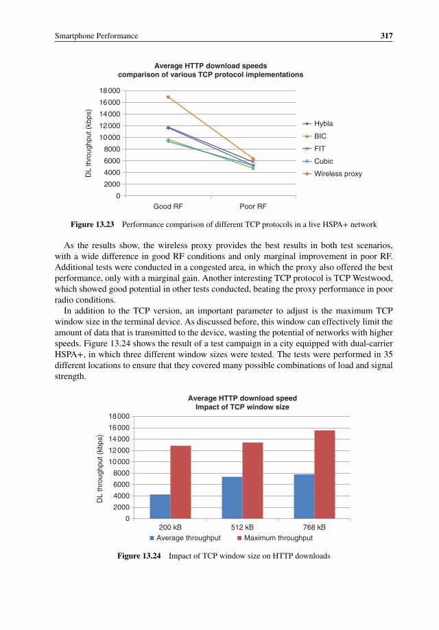
Smartphone Performance 317
0
2000
4000
6000
8000
10000
12000
14000
16000
18000
Good RF Poor RF
DL
thro
ughp
ut (
kbps
)
Average HTTP download speedscomparison of various TCP protocol implementations
Hybla
BIC
FIT
Cubic
Wireless proxy
Figure 13.23 Performance comparison of different TCP protocols in a live HSPA+ network
As the results show, the wireless proxy provides the best results in both test scenarios,with a wide difference in good RF conditions and only marginal improvement in poor RF.Additional tests were conducted in a congested area, in which the proxy also offered the bestperformance, only with a marginal gain. Another interesting TCP protocol is TCP Westwood,which showed good potential in other tests conducted, beating the proxy performance in poorradio conditions.
In addition to the TCP version, an important parameter to adjust is the maximum TCPwindow size in the terminal device. As discussed before, this window can effectively limit theamount of data that is transmitted to the device, wasting the potential of networks with higherspeeds. Figure 13.24 shows the result of a test campaign in a city equipped with dual-carrierHSPA+, in which three different window sizes were tested. The tests were performed in 35different locations to ensure that they covered many possible combinations of load and signalstrength.
0
2000
4000
6000
8000
10000
12000
14000
16000
18000
200 kB 512 kB 768 kB
DL
thro
ughp
ut (
kbps
)
Average HTTP download speedImpact of TCP window size
Average throughput Maximum throughput
Figure 13.24 Impact of TCP window size on HTTP downloads
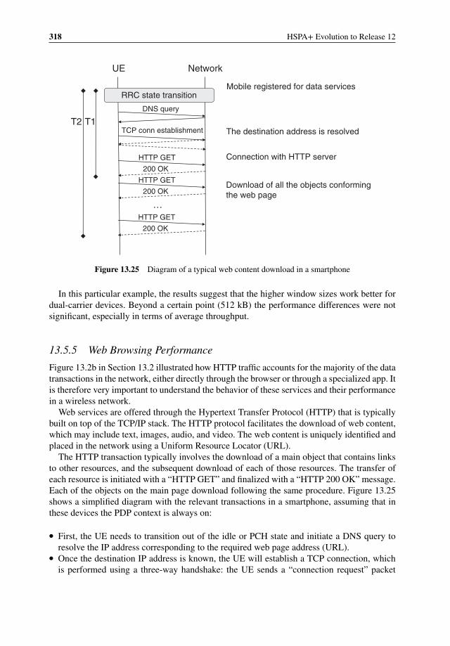
318 HSPA+ Evolution to Release 12
Mobile registered for data services
The destination address is resolved
Connection with HTTP server
Download of all the objects conforming the web page
UE Network
DNS query
TCP conn establishment
HTTP GET
…
T1T2
RRC state transition
200 OK
HTTP GET
200 OK
HTTP GET
200 OK
Figure 13.25 Diagram of a typical web content download in a smartphone
In this particular example, the results suggest that the higher window sizes work better fordual-carrier devices. Beyond a certain point (512 kB) the performance differences were notsignificant, especially in terms of average throughput.
13.5.5 Web Browsing Performance
Figure 13.2b in Section 13.2 illustrated how HTTP traffic accounts for the majority of the datatransactions in the network, either directly through the browser or through a specialized app. Itis therefore very important to understand the behavior of these services and their performancein a wireless network.
Web services are offered through the Hypertext Transfer Protocol (HTTP) that is typicallybuilt on top of the TCP/IP stack. The HTTP protocol facilitates the download of web content,which may include text, images, audio, and video. The web content is uniquely identified andplaced in the network using a Uniform Resource Locator (URL).
The HTTP transaction typically involves the download of a main object that contains linksto other resources, and the subsequent download of each of those resources. The transfer ofeach resource is initiated with a “HTTP GET” and finalized with a “HTTP 200 OK” message.Each of the objects on the main page download following the same procedure. Figure 13.25shows a simplified diagram with the relevant transactions in a smartphone, assuming that inthese devices the PDP context is always on:
� First, the UE needs to transition out of the idle or PCH state and initiate a DNS query toresolve the IP address corresponding to the required web page address (URL).
� Once the destination IP address is known, the UE will establish a TCP connection, whichis performed using a three-way handshake: the UE sends a “connection request” packet
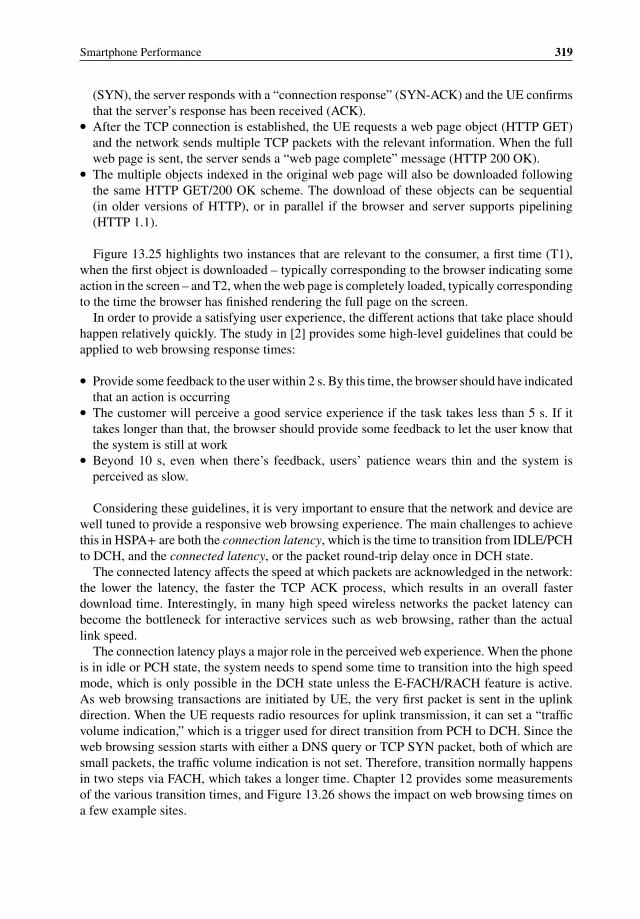
Smartphone Performance 319
(SYN), the server responds with a “connection response” (SYN-ACK) and the UE confirmsthat the server’s response has been received (ACK).
� After the TCP connection is established, the UE requests a web page object (HTTP GET)and the network sends multiple TCP packets with the relevant information. When the fullweb page is sent, the server sends a “web page complete” message (HTTP 200 OK).
� The multiple objects indexed in the original web page will also be downloaded followingthe same HTTP GET/200 OK scheme. The download of these objects can be sequential(in older versions of HTTP), or in parallel if the browser and server supports pipelining(HTTP 1.1).
Figure 13.25 highlights two instances that are relevant to the consumer, a first time (T1),when the first object is downloaded – typically corresponding to the browser indicating someaction in the screen – and T2, when the web page is completely loaded, typically correspondingto the time the browser has finished rendering the full page on the screen.
In order to provide a satisfying user experience, the different actions that take place shouldhappen relatively quickly. The study in [2] provides some high-level guidelines that could beapplied to web browsing response times:
� Provide some feedback to the user within 2 s. By this time, the browser should have indicatedthat an action is occurring
� The customer will perceive a good service experience if the task takes less than 5 s. If ittakes longer than that, the browser should provide some feedback to let the user know thatthe system is still at work
� Beyond 10 s, even when there’s feedback, users’ patience wears thin and the system isperceived as slow.
Considering these guidelines, it is very important to ensure that the network and device arewell tuned to provide a responsive web browsing experience. The main challenges to achievethis in HSPA+ are both the connection latency, which is the time to transition from IDLE/PCHto DCH, and the connected latency, or the packet round-trip delay once in DCH state.
The connected latency affects the speed at which packets are acknowledged in the network:the lower the latency, the faster the TCP ACK process, which results in an overall fasterdownload time. Interestingly, in many high speed wireless networks the packet latency canbecome the bottleneck for interactive services such as web browsing, rather than the actuallink speed.
The connection latency plays a major role in the perceived web experience. When the phoneis in idle or PCH state, the system needs to spend some time to transition into the high speedmode, which is only possible in the DCH state unless the E-FACH/RACH feature is active.As web browsing transactions are initiated by UE, the very first packet is sent in the uplinkdirection. When the UE requests radio resources for uplink transmission, it can set a “trafficvolume indication,” which is a trigger used for direct transition from PCH to DCH. Since theweb browsing session starts with either a DNS query or TCP SYN packet, both of which aresmall packets, the traffic volume indication is not set. Therefore, transition normally happensin two steps via FACH, which takes a longer time. Chapter 12 provides some measurementsof the various transition times, and Figure 13.26 shows the impact on web browsing times ona few example sites.
320 HSPA+ Evolution to Release 12
0
1
2
3
4
5
6
7
8
9
Expedia CNN Yahoo
Web
dow
nloa
d tim
e (s
)
Impact of state transition on webperformance (Chrome)
From PCHFrom DCH
Figure 13.26 Impact of RRC state transition of web performance. Light gray: session starting in PCH;Dark gray: session starting in DCH
As Figure 13.26 shows, the additional delay caused by RRC state transitions can be up to2 s, often representing a significant amount of the overall web download time. This impactcan be minimized using different techniques:
� Extending DCH hold timers, however this has negative impacts on battery life and potentiallydegradation of network KPIs, such as baseband resource consumption and access failures.The use of CPC should help counter these negative impacts.
� Extending FACH hold timers and activating the E-FACH/E-RACH feature if available.
RNC can furthermore use traffic profiling techniques and predict browsing transactionsbased on recent user activity, and use direct transition from PCH to DCH even if the UE doesnot set the traffic volume indicator.
Other important factors affecting the web experience are the performance of the device, theoperating system (including the default browser), and, to a lesser extent, the terminal category.Figure 13.27 shows a web download comparison for various popular web sites across multiplemobile operating systems: Android 4, iOS 5, and Windows Phone 8. Note that, at the time ofthe tests, the iPhone could not be tested with dual carrier in the trial network.
The web download results show how the operating system has a significant influence onperformance, often beyond the impact of the device category. In this example, the iOS devicetested didn’t support dual carrier, however it offered a better experience than the dual-carrierdevices while in good radio conditions. The effect of dual carrier can be noticed in the poorerRF conditions, where throughput becomes a limiting factor. The Windows Phone 8 device isthe one offering a better performance when considering both scenarios.
There are various reasons why Android presented a slower response in these tests, probablythe most relevant is the fact that the amount of data downloaded with Android was largerthan with other OS since different contents were served for different browsers. Also, thedefault browser included in Android phones (WebKit) is not well optimized for JavaScript,as Figure 13.28 (left) shows. On the other hand, Android OS offers an alternative browser,Chrome, which presents a significantly improved performance, as the same figure on the rightillustrates.
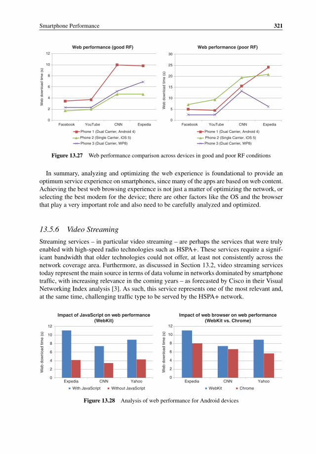
Smartphone Performance 321
0
2
4
6
8
10
12
Facebook YouTube CNN Expedia
Web
dow
nloa
d tim
e (s
)
Web performance (good RF)
Phone 1 (Dual Carrier, Android 4)
0
5
10
15
20
25
30
Facebook YouTube CNN Expedia
Web
dow
nloa
d tim
e (s
)
Web performance (poor RF)
Phone 1 (Dual Carrier, Android 4)
Phone 2 (Single Carrier, iOS 5) Phone 2 (Single Carrier, iOS 5)
Phone 3 (Dual Carrier, WP8) Phone 3 (Dual Carrier, WP8)
Figure 13.27 Web performance comparison across devices in good and poor RF conditions
In summary, analyzing and optimizing the web experience is foundational to provide anoptimum service experience on smartphones, since many of the apps are based on web content.Achieving the best web browsing experience is not just a matter of optimizing the network, orselecting the best modem for the device; there are other factors like the OS and the browserthat play a very important role and also need to be carefully analyzed and optimized.
13.5.6 Video Streaming
Streaming services – in particular video streaming – are perhaps the services that were trulyenabled with high-speed radio technologies such as HSPA+. These services require a signif-icant bandwidth that older technologies could not offer, at least not consistently across thenetwork coverage area. Furthermore, as discussed in Section 13.2, video streaming servicestoday represent the main source in terms of data volume in networks dominated by smartphonetraffic, with increasing relevance in the coming years – as forecasted by Cisco in their VisualNetworking Index analysis [3]. As such, this service represents one of the most relevant and,at the same time, challenging traffic type to be served by the HSPA+ network.
0
2
4
6
8
10
12
Expedia CNN Yahoo
Web
dow
nloa
d tim
e (s
)
Impact of JavaScript on web performance(WebKit)
With JavaScript Without JavaScript
0
2
4
6
8
10
12
Expedia CNN Yahoo
Web
dow
nloa
d tim
e (s
)
Impact of web browser on web performance(WebKit vs. Chrome)
WebKit Chrome
Figure 13.28 Analysis of web performance for Android devices
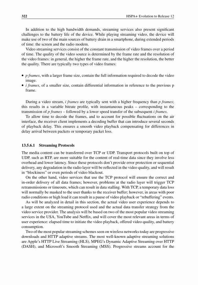
322 HSPA+ Evolution to Release 12
In addition to the high bandwidth demands, streaming services also present significantchallenges to the battery life of the device. While playing streaming video, the device willmake use of two of the main sources of battery drain in a smartphone, during extended periodsof time: the screen and the radio modem.
Video streaming services consist of the constant transmission of video frames over a periodof time. The quality of the video source is determined by the frame rate and the resolution ofthe video frames: in general, the higher the frame rate, and the higher the resolution, the betterthe quality. There are typically two types of video frames:
� p frames, with a larger frame size, contain the full information required to decode the videoimage.
� i frames, of a smaller size, contain differential information in reference to the previous pframe.
During a video stream, i frames are typically sent with a higher frequency than p frames;this results in a variable bitrate profile, with instantaneous peaks – corresponding to thetransmission of p frames – followed by a lower speed transfer of the subsequent i frames.
To allow time to decode the frames, and to account for possible fluctuations on the airinterface, the receiver client implements a decoding buffer that can introduce several secondsof playback delay. This ensures a smooth video playback compensating for differences indelay arrival between packets or temporary packet loss.
13.5.6.1 Streaming Protocols
The media content can be transferred over TCP or UDP. Transport protocols built on top ofUDP, such as RTP, are more suitable for the content of real-time data since they involve lessoverhead and lower latency. Since these protocols don’t provide error protection or sequentialdelivery, any degradation in the radio layer will be reflected in the video quality, and will resultin “blockiness” or even periods of video blackout.
On the other hand, video services that use the TCP protocol will ensure the correct andin-order delivery of all data frames; however, problems at the radio layer will trigger TCPretransmissions or timeouts, which can result in data stalling. With TCP, a temporary data losswill normally be masked to the user thanks to the receiver buffer; however, in areas with poorradio conditions or high load it can result in a pause of video playback or “rebuffering” events.
As will be analyzed in detail in this section, the actual video user experience depends toa large extent on the streaming protocol used and the actual data transfer strategy from thevideo service provider. The analysis will be based on two of the most popular video streamingservices in the USA, YouTube and Netflix, and will cover the most relevant areas in terms ofuser experience: elapsed time to initiate the video playback, offered video quality, and batteryconsumption.
Two of the most popular streaming schemes seen on wireless networks today are progressivedownloads and HTTP adaptive streams. The most well-known adaptive streaming solutionsare Apple’s HTTP Live Streaming (HLS), MPEG’s Dynamic Adaptive Streaming over HTTP(DASH), and Microsoft’s Smooth Streaming (MSS). Progressive streams account for the
Smartphone Performance 323
majority of video volume today, due to the popularity of YouTube; however, this is quickly shift-ing as even YouTube is changing their content to HTTP adaptive streaming, in particular HLS.
Progressive video streams are generally encoded into different formats (such as 240P, 360P,480P, 720P, 1080P), but only one quality and bitrate is downloaded at a time. This does notautomatically change or adjust based on congestion or the user’s available bandwidth.
HTTP Adaptive Streaming (HLS, Dash, MSS) video streams are encoded in many differentqualities and are delivered in chunks of 2 to 10 s of video. The video quality is adjusted bothup and down as conditions or available bandwidth fluctuates.
A common feature of all streaming services is an initial buffering of multimedia content atthe client, which tries to ensure smooth playback in the presence of bandwidth fluctuation andjitter. This buffering is visible to the user as start-up delay and referred to as “fast start.” Thename comes from the fact that this initially buffered data is typically downloaded using all theavailable bandwidth, while the rest of the video is downloaded using one of these techniquesaccording to the study in [4]:
� encoding rate streaming;� throttling;� buffer adaptive streaming;� rate adaptive streaming;� fast caching.
Encoding rate streaming means that after the fast start the client is able to receive data atthe encoding rate. For example, YouTube uses the encoding rate technique for HD video inthe case of Flash player in Android.
In the case of throttling, the server limits the rate. Throttling can be used, for example, withFlash players on Android or the YouTube app in iOS. Different throttling factors are useddepending on the client.
In buffer adaptive streaming, the client stops downloading when the receive buffer is fulland continues when the buffer drains to a certain threshold. The YouTube app and HTML5player in Android use the buffer adaptive technique.
In rate adaptive streaming, the client can switch dynamically between different video qual-ities depending on available throughput. HTTP Live Streaming (HLS) is one such technologyused by, for example, Netflix.
Fast caching downloads as fast as possible even the whole video. This is used, for example,in the YouTube client in the Windows Phone.
13.5.6.2 Video Start Time
Twenty percent of mobile users will abandon a video if it does not start within 10 s [5].The faster the network, the higher the abandonment rate, so in order to maintain customersatisfaction, it is important that video start time decreases as mobile network speeds increase.
Video Start Time (VST) is an important KPI, but is difficult (costly) to measure from acarrier perspective due to the complexity of the transaction, and it has to be tailored to thespecific service that one wants to be monitored. In this section we will discuss two of the mostpopular video services: YouTube and Netflix.
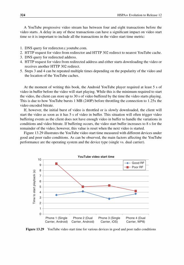
324 HSPA+ Evolution to Release 12
A YouTube progressive video stream has between four and eight transactions before thevideo starts. A delay in any of these transactions can have a significant impact on video starttime so it is important to include all the transactions in the video start time metric:
1. DNS query for redirector.c.youtube.com.2. HTTP request for video from redirector and HTTP 302 redirect to nearest YouTube cache.3. DNS query for redirected address.4. HTTP request for video from redirected address and either starts downloading the video or
receives another HTTP 302 redirect.5. Steps 3 and 4 can be repeated multiple times depending on the popularity of the video and
the location of the YouTube caches.
At the moment of writing this book, the Android YouTube player required at least 5 s ofvideo in buffer before the video will start playing. While this is the minimum required to startthe video, the client can store up to 30 s of video buffered by the time the video starts playing.This is due to how YouTube bursts 1 MB (240P) before throttling the connection to 1.25x thevideo encoded bitrate.
If, however, the initial burst of video is throttled or is slowly downloaded, the client willstart the video as soon as it has 5 s of video in buffer. This situation will often trigger videobuffering events as the client does not have enough video in buffer to handle the variations inconditions and video bitrate. If buffering occurs, the video start buffer increases to 8 s for theremainder of the video; however, this value is reset when the next video is started.
Figure 13.29 illustrates the YouTube video start time measured with different devices undergood and poor radio conditions. As can be observed, the main factors affecting the YouTubeperformance are the operating system and the device type (single vs. dual carrier).
0
1
2
3
4
5
6
7
8
9
10
Phone 1 (SingleCarrier, Android)
Phone 2 (DualCarrier, Android)
Phone 3 (SingleCarrier, iOS)
Phone 4 (DualCarrier, WP8)
Tim
e to
sta
rt p
layb
ack
(s)
YouTube video start time
Good RFPoor RF
Figure 13.29 YouTube video start time for various devices in good and poor radio conditions

Smartphone Performance 325
Netflix uses an adaptive stream: it adjusts the quality automatically based on measurementstaken by the client while downloading chunks of video data. The delivery mechanism forNetflix varies based on the operating system of the smartphone; this example illustrates thecase of an Android client:
1. DNS query for Netflix Content Distribution Network (CDN).2. HTTPS session where client sends capabilities.3. HTTPS session where server sends video bitrates and qualities based on #2.4. DNS query for Netflix CDN.5. Multiple HTTP sessions for isma and ismv files – isma are audio files and ismv are video
files.6. HTTP session for index file (.bif), which contains image previews used for fast forward
and rewind.
The Android Netflix player requires at least 120 s of video in the buffer for the video to start.
13.5.6.3 Impact of Network Proxy on Video Start Time
Network proxies are often introduced to manage and improve data user experience; however,they can have a degrading impact on video performance. Since video services can vary greatlyacross the same delivery technology, and proxies often apply the same policy per technology,these policies can negatively impact certain users, devices, and sometimes whole services ortechnologies. Testing for all scenarios to prevent this is not practical with such a broad rangeof variables so issues often go undetected for extended periods of time.
Two popular ways to manage video from the carrier side are just in time delivery (JIT) andtranscoding. These methods can be used together or separately and both aim to reduce overallvideo volume, but often have unintended tradeoffs.
Just in Time (JIT) delivery throttles the rate at which a video is downloaded to the clientso that just enough video is held in the client’s buffer to theoretically prevent buffering. Justin Time delivery’s main goal is to manage video “wastage,” or video downloaded and notconsumed, but has tradeoffs such as higher battery consumption, more rebuffering, longervideo start time, and less efficient delivery leading to spectral inefficiencies.
An extreme example of this is shown in Figure 13.30. In this example, video start time wasdelayed up to 30 s for longer videos as the proxy was applying buffer tuning before the videometadata was fully transferred. This caused over 50% of the impacted videos to be abandonedbefore the videos were able to start. It also caused buffering every few seconds once the videostarted as the buffer tuned rate did not allow for any variation in video bitrate. This is anextreme example but highlights the challenges faced when trying to apply a blanket policyacross technologies.
As revealed by the study in [5], JIT does not play an important role in high-speed networks,therefore its gains may be questionable in modern HSPA+ networks.
Transcoding reduces the video bitrate while attempting to keep a similar perceived quality.There are various techniques to accomplish this, including dropping frames, re-encoding thevideo into multiple formats, and so on. Transcoding requires significant hardware to process
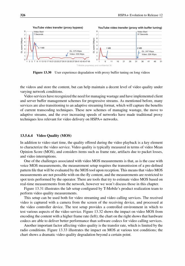
326 HSPA+ Evolution to Release 12
T-Mobile proprietary and confidential 30
0
1
2
3
4
5
6
7
8
1 6 11 16 21 26 31 36 41 46 51
DL
spee
d (M
bps)
YouTube video transfer (proxy with buffer tuning)Video Start37 Seconds
1 MB 2 MB
DL: 247 Kbps
Video: 226 Kbps
0
1
2
3
4
5
6
7
8
1 3 5 7 9 11 13 15 17 19 21 23 25 27 29 31 33 35 37 39 41 43 45 47 49
DL
spee
d (M
bps)
YouTube video transfer (proxy bypass)Video Start7 Seconds
2.7 MB
DL: 575 Kbps
Video: 226 Kbps
Figure 13.30 User experience degradation with proxy buffer tuning on long videos
the videos and store the content, but can help maintain a decent level of video quality undervarying network conditions.
Video services have recognized the need for managing wastage and have implemented clientand server buffer management schemes for progressive streams. As mentioned before, manyservices are also transitioning to an adaptive streaming format, which will capture the benefitsof current transcoding techniques. These new schemes of managing wastage, the move toadaptive streams, and the ever increasing speeds of networks have made traditional proxytechniques less relevant for video delivery on HSPA+ networks.
13.5.6.4 Video Quality (MOS)
In addition to video start time, the quality offered during the video playback is a key elementto characterize the video service. Video quality is typically measured in terms of video MeanOpinion Score (MOS), and considers items such as frame rate, artifacts due to packet losses,and video interruptions.
One of the challenges associated with video MOS measurements is that, as is the case withvoice MOS measurements, the measurement setup requires the transmission of a pre-definedpattern file that will be evaluated by the MOS tool upon reception. This means that video MOSmeasurements are not possible with on-the-fly content, and the measurements are restricted tospot tests performed by the operator. There are tools that try to estimate video MOS based onreal-time measurements from the network, however we won’t discuss those in this chapter.
Figure 13.31 illustrates the lab setup configured by T-Mobile’s product realization team toperform video quality measurements.
This setup can be used both for video streaming and video calling services. The receivedvideo is captured with a camera from the screen of the receiving device, and processed atthe video controller device. The test setup provides a controlled environment in which totest various aspects of the video service. Figure 13.32 shows the impact on video MOS fromencoding the content with a higher frame rate (left); the chart on the right shows that hardwarecodecs are able to deliver better performance than software codecs for video calling services.
Another important factor affecting video quality is the transfer rate, which is limited by theradio conditions. Figure 13.33 illustrates the impact on MOS at various test conditions; thechart shows a dramatic video quality degradation beyond a certain point.
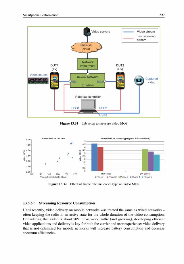
Smartphone Performance 327
Video servers Video stream
Test signalingstream
Networkcloud
NetworkimpairmentDUT1
(Tx)DUT2(Rx)
3G/4G Network
Emulator
Video lab controller
USB3
USB1
BS1 BS2
Video source
USB2
Capturedvideo
Figure 13.31 Lab setup to measure video MOS
00.5
11.5
22.5
33.5
44.5
5
HW codec SW codec
Vid
eo M
OS
Video MOS vs. codec type (good RF conditions)
Phone 1 Phone 2 Phone 3 Phone 4 Phone 5
2.00
2.50
3.00
3.50
4.00
4.50
5.00
120 140 160 180 200 220
Vid
eo M
OS
Video stream bit rate (kbps)
Video MOS vs. bit rate
Figure 13.32 Effect of frame rate and codec type on video MOS
13.5.6.5 Streaming Resource Consumption
Until recently, video delivery on mobile networks was treated the same as wired networks –often keeping the radio in an active state for the whole duration of the video consumption.Considering that video is about 50% of network traffic (and growing), developing efficientvideo applications and delivery is key for both the carrier and user experience: video deliverythat is not optimized for mobile networks will increase battery consumption and decreasespectrum efficiencies.
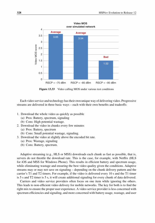
328 HSPA+ Evolution to Release 12
3.65 3.54
1.52
0
0.5
1
1.5
2
2.5
3
3.5
4
RSCP = –75 dBm RSCP = –85 dBm RSCP = –95 dBm
Vid
eo M
OS
sco
re
Video MOS over simulated network
Average Average
Bad
Figure 13.33 Video calling MOS under various test conditions
Each video service and technology has their own unique way of delivering video. Progressivestreams are delivered in three basic ways – each with their own benefits and tradeoffs:
1. Download the whole video as quickly as possible(a) Pros: Battery, spectrum, signaling(b) Cons: High potential wastage.
2. Download the video in chunks every few minutes(a) Pros: Battery, spectrum(b) Cons: Small potential wastage, signaling.
3. Download the video at slightly above the encoded bit rate.(a) Pros: Wastage, signaling(b) Cons: Battery, spectrum.
Adaptive streaming (e.g., HLS or MSS) downloads each chunk as fast as possible, that is,servers do not throttle the download rate. This is the case, for example, with Netflix (HLSfor iOS and MSS for Windows Phone). This results in efficient battery and spectrum usage,while eliminating wastage and ensuring the best video quality given the conditions. Adaptivestreams may or may not save on signaling – depending on the chunk delivery pattern and thecarrier’s T1 and T2 timers. For example, if the video is delivered every 10 s and the T1 timeris 5 s and T2 timer is 5 s, it will create additional signaling for every chunk of data delivered.
Carriers and video service providers often focus on one item while ignoring the others.This leads to non-efficient video delivery for mobile networks. The key for both is to find theright mix to ensure the proper user experience. A video service provider is less concerned withspectrum efficiencies and signaling, and more concerned with battery usage, wastage, and user
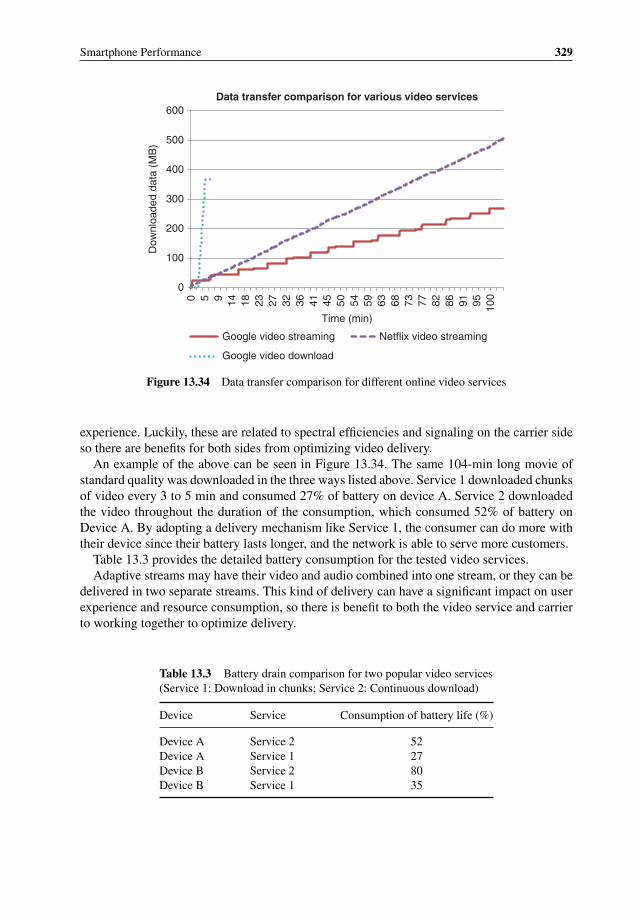
Smartphone Performance 329
0
100
200
300
400
500
600
0 5 9 14 18 23 27 32 36 41 45 50 54 59 63 68 73 77 82 86 91 95 100
Dow
nloa
ded
data
(M
B)
Time (min)
Data transfer comparison for various video services
Google video streaming Netflix video streaming
Google video download
Figure 13.34 Data transfer comparison for different online video services
experience. Luckily, these are related to spectral efficiencies and signaling on the carrier sideso there are benefits for both sides from optimizing video delivery.
An example of the above can be seen in Figure 13.34. The same 104-min long movie ofstandard quality was downloaded in the three ways listed above. Service 1 downloaded chunksof video every 3 to 5 min and consumed 27% of battery on device A. Service 2 downloadedthe video throughout the duration of the consumption, which consumed 52% of battery onDevice A. By adopting a delivery mechanism like Service 1, the consumer can do more withtheir device since their battery lasts longer, and the network is able to serve more customers.
Table 13.3 provides the detailed battery consumption for the tested video services.Adaptive streams may have their video and audio combined into one stream, or they can be
delivered in two separate streams. This kind of delivery can have a significant impact on userexperience and resource consumption, so there is benefit to both the video service and carrierto working together to optimize delivery.
Table 13.3 Battery drain comparison for two popular video services(Service 1: Download in chunks; Service 2: Continuous download)
Device Service Consumption of battery life (%)
Device A Service 2 52Device A Service 1 27Device B Service 2 80Device B Service 1 35
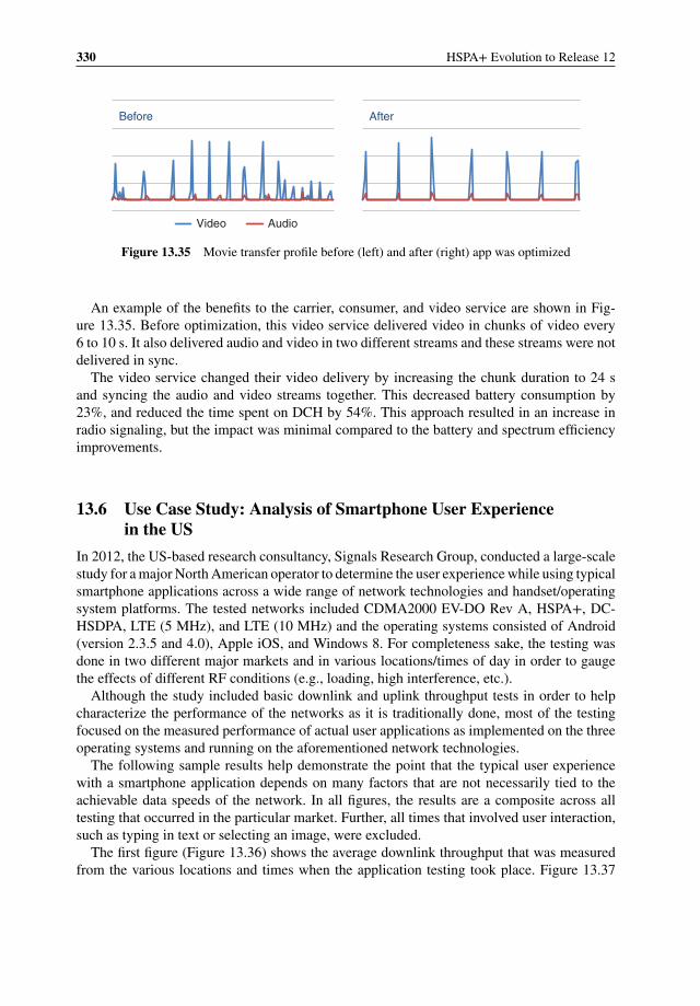
330 HSPA+ Evolution to Release 12
Video Audio
Before After
Figure 13.35 Movie transfer profile before (left) and after (right) app was optimized
An example of the benefits to the carrier, consumer, and video service are shown in Fig-ure 13.35. Before optimization, this video service delivered video in chunks of video every6 to 10 s. It also delivered audio and video in two different streams and these streams were notdelivered in sync.
The video service changed their video delivery by increasing the chunk duration to 24 sand syncing the audio and video streams together. This decreased battery consumption by23%, and reduced the time spent on DCH by 54%. This approach resulted in an increase inradio signaling, but the impact was minimal compared to the battery and spectrum efficiencyimprovements.
13.6 Use Case Study: Analysis of Smartphone User Experiencein the US
In 2012, the US-based research consultancy, Signals Research Group, conducted a large-scalestudy for a major North American operator to determine the user experience while using typicalsmartphone applications across a wide range of network technologies and handset/operatingsystem platforms. The tested networks included CDMA2000 EV-DO Rev A, HSPA+, DC-HSDPA, LTE (5 MHz), and LTE (10 MHz) and the operating systems consisted of Android(version 2.3.5 and 4.0), Apple iOS, and Windows 8. For completeness sake, the testing wasdone in two different major markets and in various locations/times of day in order to gaugethe effects of different RF conditions (e.g., loading, high interference, etc.).
Although the study included basic downlink and uplink throughput tests in order to helpcharacterize the performance of the networks as it is traditionally done, most of the testingfocused on the measured performance of actual user applications as implemented on the threeoperating systems and running on the aforementioned network technologies.
The following sample results help demonstrate the point that the typical user experiencewith a smartphone application depends on many factors that are not necessarily tied to theachievable data speeds of the network. In all figures, the results are a composite across alltesting that occurred in the particular market. Further, all times that involved user interaction,such as typing in text or selecting an image, were excluded.
The first figure (Figure 13.36) shows the average downlink throughput that was measuredfrom the various locations and times when the application testing took place. Figure 13.37
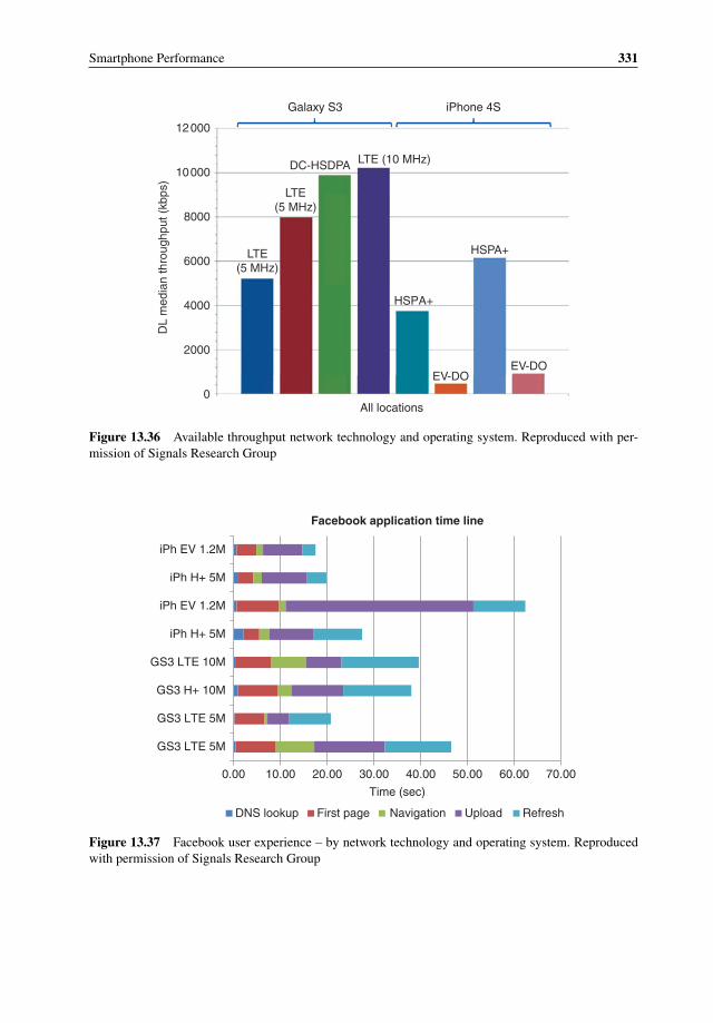
Smartphone Performance 331
DC-HSDPA LTE (10 MHz)
Galaxy S3
All locations
iPhone 4S
LTE(5 MHz)
HSPA+
LTE(5 MHz)
HSPA+
EV-DOEV-DO
12000
10000
8000
DL
med
ian
thro
ughp
ut (
kbps
)
6000
4000
2000
0
Figure 13.36 Available throughput network technology and operating system. Reproduced with per-mission of Signals Research Group
0.00 10.00 20.00 30.00 40.00 50.00 60.00 70.00
GS3 LTE 5M
GS3 LTE 5M
GS3 H+ 10M
GS3 LTE 10M
iPh H+ 5M
iPh EV 1.2M
iPh H+ 5M
iPh EV 1.2M
Time (sec)
Facebook application time line
DNS lookup First page Navigation Upload Refresh
Figure 13.37 Facebook user experience – by network technology and operating system. Reproducedwith permission of Signals Research Group

332 HSPA+ Evolution to Release 12
shows the various components that impacted the user experience while uploading an identicalpicture to Facebook. Several observations are worth mentioning:
� The average DC-HSDPA downlink throughput for all of the tests was on par with the 10MHz LTE network, just as HSDPA Cat 10 throughput with the iPhone was comparable withthe two 5 MHz LTE networks. Network loading and coverage considerations could havebeen contributing factors, but from the perspective of the user it doesn’t matter.
� The total time required to upload an identical Facebook picture was measurably shorter withthe legacy HSPA+ networks and one of the EV-DO networks than with the DC-HSDPA andLTE networks. The former used the iPhone 4 and the latter used the Galaxy S III (AndroidVersion 4.0).
� The better user experience with the iPhone 4 also extended to the initial steps during theprocess, namely the time from when the application was launched until the Facebook pageloaded on the mobile device.
The “secret” behind the stronger performance of the iPhone is shown in Figure 13.38. Inreality, the performances of the networks or the RF capabilities of the phones do not explainthe differences in the overall results. Instead, it is evident that the iPhone compressed the sizeof the picture before uploading it to the site. From the perspective of the user, the picturequality looks the same when viewed from the screen of the mobile device. However, the useralso perceives that the network was “faster,” even though it wasn’t. The figure also shows thatthe iPhone on the second EV-DO network didn’t compress the picture and this phenomenonalso explains the longer upload time.
3500
Galaxy S3 iPhone 4S
3000
2500
LTE 5
MHz
LTE 5
MHz
DC-HSDPA
LTE 10
MHz
EV-DO
HSPA+
DC-HSDPA
EV-DO
2000
1500UL
tota
l kby
tes
1000
500
0All locations
Figure 13.38 Facebook picture upload payload – by network technology and operating system. Repro-duced with permission of Signals Research Group

Smartphone Performance 333
Galaxy S3 iPhone 4S
LTE 5 MHz
LTE 5
MHz
DC-HSDPA
HSPA+
EV-DO DC-H
SDPA
EV-DO
10000
9000
8000
7000
6000
5000
DL
tota
l kby
tes
4000
3000
2000
All Locations
1000
0
LTE 10 MHz
Figure 13.39 YouTube video content vs. network technology – by network technology and operatingsystem. Reproduced with permission of Signals Research Group
It is also worth pointing out that the actual time required to upload the picture didn’tnecessarily impact the user experience. This situation exists because the picture is uploadedin the background, meaning that the user could switch to another application without havingto wait for the video to upload. Facebook does indicate when the picture or video is uploadedand the screen refreshes to reveal the uploaded content, but the user doesn’t have to wait forthese events to occur.
The study also found differences in the amount of transferred payload associated withdownloading and playing an identical YouTube video and loading an identical web site.In the case of YouTube (Figure 13.39), there seemed to be a strong relationship between thecapabilities of the network and the quality of the video. With LTE networks, YouTube delivereda higher quality video format, or at least the file size was larger, than it did with the other3G networks. In the case of one 5 MHz LTE network, the use of a third-party optimizationplatform could have reduced the video payload. From the perspective of the individuals whoconducted the tests, there wasn’t any perceived difference in the quality of the videos.
In the case of web page content, Apple’s decision to not support Flash in its browser actuallyhad at least one positive impact on the user experience. As shown in Figure 13.40, the sizeof the downloaded web pages was lower with iOS than it was with Android. Although theweb pages still generally loaded faster on the Galaxy S III devices that operated on the fasternetworks, the differences would have been even greater if the iPhone had downloaded thesame amount of web content.
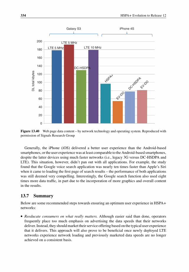
334 HSPA+ Evolution to Release 12
Galaxy S3 iPhone 4S
LTE 5 MHz
DC-HSDPA
HSPA+
EV-DO
DC-HSDPA
EV-DO
LTE 10 MHz
LTE 5 MHz200
160
180
140
120
100
DL
tota
l kby
tes
80
60
20
40
0
Figure 13.40 Web page data content – by network technology and operating system. Reproduced withpermission of Signals Research Group
Generally, the iPhone (iOS) delivered a better user experience than the Android-basedsmartphones, or the user experience was at least comparable to the Android-based smartphones,despite the latter devices using much faster networks (i.e., legacy 3G versus DC-HSDPA andLTE). This situation, however, didn’t pan out with all applications. For example, the studyfound that the Google voice search application was nearly ten times faster than Apple’s Siriwhen it came to loading the first page of search results – the performance of both applicationswas still deemed very compelling. Interestingly, the Google search function also used eighttimes more data traffic, in part due to the incorporation of more graphics and overall contentin the results.
13.7 Summary
Below are some recommended steps towards ensuring an optimum user experience in HSPA+networks:
� Reeducate consumers on what really matters. Although easier said than done, operatorsfrequently place too much emphasis on advertising the data speeds that their networksdeliver. Instead, they should market their service offering based on the typical user experiencethat it delivers. This approach will also prove to be beneficial once newly deployed LTEnetworks experience network loading and previously marketed data speeds are no longerachieved on a consistent basis.
Smartphone Performance 335
� Identify non-optimized applications and take corrective action. Operators need to invest timeand energy into studying how applications behave in their network. In many cases, simplefixes to the application are all that is required to transform a poor performing applicationinto a fully optimized application.
� Mandate new user experience KPIs to ecosystem device and OS partners. Device and OSpartners have a vested interest in delivering a good user experience, but they do not alwaysunderstand what it takes to deliver a compelling user experience that makes the most efficientuse of the available network resources.
� Minimize poor RF coverage areas. Leveraging the benefits of SON is perhaps the best wayto identify poor coverage areas. In this case “poor coverage” should equate to a minimumuser experience threshold not being achieved and not necessarily to a specific RF parameter,although the two could be correlated.
� Optimize the network parameter settings and the network architecture based on typical userbehavior. Moving popular content closer to the edge of the cell is one example. Adjustingnetwork timer settings (e.g., T1, T2, and T3) in order to minimize RRC state transition timeswithout sacrificing battery life is another example.
References
[1] Sharma, C. (2013), “US Wireless Data Market Update.Q4 2013 and 2013”.[2] Seow, S. (2008) Designing and Engineering Time, Pearson Education, Inc., Boston, MA.[3] Cisco (2012), “Cisco Visual Networking Index: Global Mobile Data Traffic Forecast Update, 2012–2017”.[4] Hoque, M., Siekkinen, M., Nurminen, J. Aalto, M. and Tarkoma, S. (2013) “Mobile Multimedia Streaming
Tecniques: QoE and Energy Consumption Perspective”, arXiv:1311.4317.[5] Shunmuga Krishnan, S. and Sitaraman, R. (2012) “Video stream quality impacts viewer behavior: inferring
causality using quasi-experimental designs”, Proceedings of the 2012 ACM conference on Internet measurementconference (IMC).

14Multimode Multiband TerminalDesign Challenges
Jean-Marc Lemenager, Luigi Di Capua, Victor Wilkerson,Mikael Guenais, Thierry Meslet, and Laurent Noel
The mobile phone industry has experienced unprecedented growth since it was first launchedover 20 years ago using 2G/ EDGE, GSM, GPRS (EGPRS) technologies. Combined with3G standards, such as WCDMA/HSPA, and more recently, 4G/LTE (FDD and TDD), mobilephone shipments have continuously beaten records, tripling volumes from 533 million devicesin 2003 to more than 1.8 billion devices in 2013. Looking ahead to 2017, it is expectedthat shipments of mobile phones will then reach 2.1 billion units worldwide [1]. Put intoperspective, this means that nearly 70 devices will be shipped every second! Beyond theseimpressive production volumes, the introduction of smartphones in 2007, unleashed by Apple’soriginal iPhone, is the other major factor that has completely reshaped the definition of mobileterminals. A high-end non touch-screen 2009 device would today be qualified as “featurephone” or “voice-centric phone.” The year 2013 was a key turning point in the history of thisindustry as the “data-centric / do-it-all” smartphone shipments exceeded the volumes for thesefeature phones. Based on current trends, what are now collectively called “smartphones” arelikely to transition to a market segmented into three retail price ranges: low end/cost (<100$),mid-end (<300$), and high-end super-phones (>500$). Given this expectation, it will becomedifficult to make a distinction between these segments, based on a common classification as“smartphones.” This is not unlike the trend seen in the world of PCs. In the high-end segment,the differentiator is likely to translate into a race to be the first to deliver new hardware (HW)or telecom features, such as being the first device to support LTE-Advanced. In the lower-endsegment, retail prices will be the primary differentiator.
The other key factor which has influenced the situation is the quick pace at which 3GPPhas been delivering new telecom features and air-interfaces, moving from the well establishedmono-mode EGPRS terminal, then to dual-mode EGPRS-WCDMA, and more recently to
HSPA+ Evolution to Release 12: Performance and Optimization, First Edition.Edited by Harri Holma, Antti Toskala, and Pablo Tapia.© 2014 John Wiley & Sons, Ltd. Published 2014 by John Wiley & Sons, Ltd.
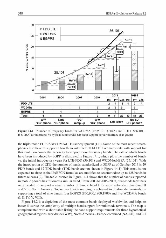
338 HSPA+ Evolution to Release 12
2001 2004 2007 20102013 2016?
MIN TYP MAX MIN TYP MAX
FDD LTE 2 4 13 4 9 14
WCDMA 1 3 5 2 3 5 5
EGPRS 4 4 4 4 4 4
Total 4 5 7 9 9 11 22 13 18 23WW
“2G” phoneEarly
“3G” phone“3G”
ramp-upWW
“3G” phone LTE todayNA-EU
LTE phone?
0
5
10
15
20
25
30N
umbe
r of
FD
D b
ands
FDD LTE WCDMA EGPRS
Rel’99
Rel’ 5
Rel’ 6
Rel’7
Rel’8
Rel’9
Rel’10
Rel’11
25.101
36.101
Figure 14.1 Number of frequency bands for WCDMA (TS25.101 -UTRA) and LTE (TS36.101 –E-UTRA) air interfaces vs. typical commercial UE band support per air interface (bar graph)
the triple-mode EGPRS/WCDMA/LTE user equipment (UE). Some of the most recent smart-phones also have to support a fourth air interface: TD-LTE. Commensurate with support forthis evolution comes the necessity to support more frequency bands. The rate at which bandshave been introduced by 3GPP is illustrated in Figure 14.1, which plots the number of bandsvs. the initial introductory years for LTE-FDD (36.101) and WCDMA/HSPA (25.101). Withthe introduction of LTE, the number of bands standardized at 3GPP as of October 2013 is 29FDD bands and 12 TDD bands (TDD bands are not shown in Figure 14.1). This trend is notexpected to abate as the UARFCN formulae are modified to accommodate up to 128 bands infuture releases [2]. The table inserted in Figure 14.1 shows that the number of bands supportedin mobile phones has followed a similar trend. From 2003 to 2006–2007, dual-mode terminalsonly needed to support a small number of bands: band I for most networks, plus band IIand V in North America. Today, worldwide roaming is achieved in dual-mode terminals bysupporting a total of nine bands: four EGPRS (850,900,1800,1900) and five WCDMA bands(I, II, IV, V, VIII).
Figure 14.2 is a depiction of the most common bands deployed worldwide, and helps tobetter illustrate the complexity of multiple band support for multimode terminals. The map iscomplemented with a short table listing the band support requirements for three hypotheticalgeographical regions: worldwide (WW), North America – Europe combined (NA-EU), and EU
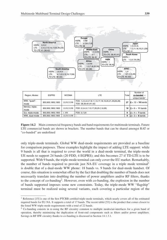
Multimode Multiband Terminal Design Challenges 339
Region, Modes EGPRS WCDMA LTE TotalNumber of
co-banded + unique bands*
WW, “quad”-mode
850,900,1800,1900 I,II,IV,V,VIIIFDD: 1,2,3,4,5,7,8,11,13,17,18,19,20,21,25(26,28)TDD: 38,39,40 (41,42)
27 6 + 12 = 18 bands
NA-EU, triple-mode
850,900,1800,1900 I,II,IV,V,VIII FDD: 2,3,4,5,7,13,17,20,25 (1,8,26) 18 5 + 6 = 11 bands
EU, triple-mode 850,900,1800,1900 I, VIII FDD: 3,7,20 9 3 + 4 = 7 bandsWW, dual-mode 850,900,1800,1900 I,II,IV,V,VIII - 9 3 + 3 = 6 bands
North AmericaHSPA: II,IV,VLTE: 2,4,5,7,12,13,17,25,26,(29)TD LTE: 41 (38,42)
South KoreaHSPA: ILTE: 1,3,5,7,8 (28)
EuropeHSPA: I,VIIILTE: 3,7,20 (1,8)TD-LTE: 38
AfricaHSPA: I,V,VIIILTE: 1,3,7 (8,20,28)TD-LTE: 40 (38)
IndiaHSPA: ITD-LTE: 38,40
APACHSPA: I, VLTE: 3,7 (1,5,28)TD-LTE: 40 (42)
South AmericaHSPA: I,II,IV,VLTE: 4,7, (2,5,12,13,17,28)TD-LTE: 38 (42)
JapanHSPA: I,VI,IX,XI,LTE: 1,3,11,18,19,21,(28)TD-LTE: 41
ChinaHSPA: ITD-LTE: 38,40 (41)
Middle-EastHSPA: I,II,V,VIIILTE: 3,7TD-LTE: 38,40
Figure 14.2 Main commercial frequency bands and band requirements for multimode terminals. FutureLTE commercial bands are shown in brackets. The number bands that can be shared amongst RAT or“co-banded” are underlined
only triple-mode terminals. Global WW dual-mode requirements are provided as a baselinefor comparison purposes. These examples highlight the impact of adding LTE support: while9 bands is all that is required to cover the world in a dual-mode terminal, the triple-modeUE needs to support 24 bands (20 FDD, 4 EGPRS); and this becomes 27 if TD-LTE is to besupported. With 9 bands, the triple-mode terminal can only cover the EU market. Remarkably,the number of bands required to provide just NA-EU coverage in a triple mode terminal1
is double that of a dual-mode WW phone: 18 bands vs. 9 bands for dual-mode handset. Ofcourse, this situation is somewhat offset by the fact that doubling the number of bands does notnecessarily translate into doubling the number of power amplifiers and/or RF filters, thanksto the concept of co-banding2. However, even with co-banding, the explosion in the numberof bands supported imposes some new constraints. Today, the triple-mode WW “flagship”terminal must be realized using several variants, each covering a particular region of the
1 Reference [15] is one of the first PTCRB certified triple-mode terminals, which nearly covers all of the estimatedrequired bands for EU-NA. It supports a total of 17 bands. The recent tablet [53] is the product that comes closest tothe listed WW triple-mode requirements with a total of 22 bands.2 Co-banding consists in re-using the RF circuitry common to multiple modes/air-interfaces for a given band ofoperation, thereby minimizing the duplication of front-end components such as filters and/or power amplifiers.Savings in RF HW circuitry thanks to co-banding is discussed in Section 14.1.3.1.
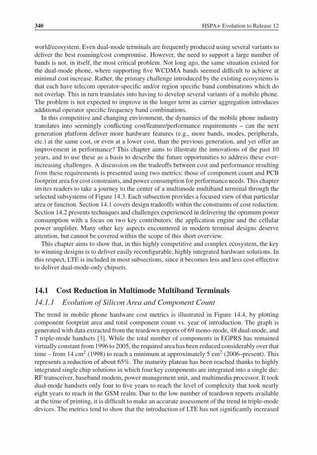
340 HSPA+ Evolution to Release 12
world/ecosystem. Even dual-mode terminals are frequently produced using several variants todeliver the best roaming/cost compromise. However, the need to support a large number ofbands is not, in itself, the most critical problem. Not long ago, the same situation existed forthe dual-mode phone, where supporting five WCDMA bands seemed difficult to achieve atminimal cost increase. Rather, the primary challenge introduced by the existing ecosystems isthat each have telecom operator-specific and/or region specific band combinations which donot overlap. This in turn translates into having to develop several variants of a mobile phone.The problem is not expected to improve in the longer term as carrier aggregation introducesadditional operator specific frequency band combinations.
In this competitive and changing environment, the dynamics of the mobile phone industrytranslates into seemingly conflicting cost/feature/performance requirements – can the nextgeneration platform deliver more hardware features (e.g., more bands, modes, peripherals,etc.) at the same cost, or even at a lower cost, than the previous generation, and yet offer animprovement in performance? This chapter aims to illustrate the innovations of the past 10years, and to use these as a basis to describe the future opportunities to address these ever-increasing challenges. A discussion on the tradeoffs between cost and performance resultingfrom these requirements is presented using two metrics: those of component count and PCBfootprint area for cost constraints, and power consumption for performance needs. This chapterinvites readers to take a journey to the center of a multimode multiband terminal through theselected subsystems of Figure 14.3. Each subsection provides a focused view of that particulararea or function. Section 14.1 covers design tradeoffs within the constraints of cost reduction.Section 14.2 presents techniques and challenges experienced in delivering the optimum powerconsumption with a focus on two key contributors: the application engine and the cellularpower amplifier. Many other key aspects encountered in modern terminal designs deserveattention, but cannot be covered within the scope of this short overview.
This chapter aims to show that, in this highly competitive and complex ecosystem, the keyto winning designs is to deliver easily reconfigurable, highly integrated hardware solutions. Inthis respect, LTE is included in most subsections, since it becomes less and less cost-effectiveto deliver dual-mode-only chipsets.
14.1 Cost Reduction in Multimode Multiband Terminals
14.1.1 Evolution of Silicon Area and Component Count
The trend in mobile phone hardware cost metrics is illustrated in Figure 14.4, by plottingcomponent footprint area and total component count vs. year of introduction. The graph isgenerated with data extracted from the teardown reports of 69 mono-mode, 48 dual-mode, and7 triple-mode handsets [3]. While the total number of components in EGPRS has remainedvirtually constant from 1996 to 2005, the required area has been reduced considerably over thattime – from 14 cm2 (1998) to reach a minimum at approximately 5 cm2 (2006–present). Thisrepresents a reduction of about 65%. The maturity plateau has been reached thanks to highlyintegrated single chip solutions in which four key components are integrated into a single die:RF transceiver, baseband modem, power management unit, and multimedia processor. It tookdual-mode handsets only four to five years to reach the level of complexity that took nearlyeight years to reach in the GSM realm. Due to the low number of teardown reports availableat the time of printing, it is difficult to make an accurate assessment of the trend in triple-modedevices. The metrics tend to show that the introduction of LTE has not significantly increased
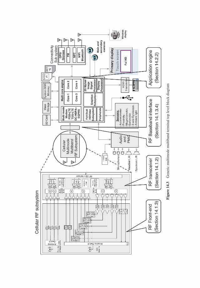
Fig
ure
14.3
Gen
eric
mul
timod
em
ultib
and
term
inal
top
leve
lblo
ckdi
agra
m
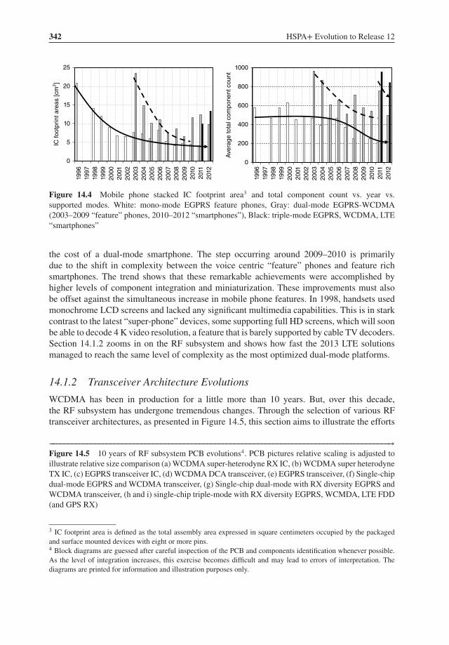
342 HSPA+ Evolution to Release 12
0
200
400
600
800
1000
1996
1997
1998
1999
2000
2001
2002
2003
2004
2005
2006
2007
2008
2009
2010
2011
2012
Ave
rage
tota
l com
pone
nt c
ount
0
5
10
15
20
25
1996
1997
1998
1999
2000
2001
2002
2003
2004
2005
2006
2007
2008
2009
2010
2011
2012
IC fo
otpr
int a
reas
[cm
2 ]
Figure 14.4 Mobile phone stacked IC footprint area3 and total component count vs. year vs.supported modes. White: mono-mode EGPRS feature phones, Gray: dual-mode EGPRS-WCDMA(2003–2009 “feature” phones, 2010–2012 “smartphones”), Black: triple-mode EGPRS, WCDMA, LTE“smartphones”
the cost of a dual-mode smartphone. The step occurring around 2009–2010 is primarilydue to the shift in complexity between the voice centric “feature” phones and feature richsmartphones. The trend shows that these remarkable achievements were accomplished byhigher levels of component integration and miniaturization. These improvements must alsobe offset against the simultaneous increase in mobile phone features. In 1998, handsets usedmonochrome LCD screens and lacked any significant multimedia capabilities. This is in starkcontrast to the latest “super-phone” devices, some supporting full HD screens, which will soonbe able to decode 4 K video resolution, a feature that is barely supported by cable TV decoders.Section 14.1.2 zooms in on the RF subsystem and shows how fast the 2013 LTE solutionsmanaged to reach the same level of complexity as the most optimized dual-mode platforms.
14.1.2 Transceiver Architecture Evolutions
WCDMA has been in production for a little more than 10 years. But, over this decade,the RF subsystem has undergone tremendous changes. Through the selection of various RFtransceiver architectures, as presented in Figure 14.5, this section aims to illustrate the efforts
−−−−−−−−−−−−−−−−−−−−−−−−−−−−−−−−−−−−−−−−−−−−−−−−−−−−−−−−−−−−−−−−−−−−−−−−−−−−−−−−−−−−−−−−→Figure 14.5 10 years of RF subsystem PCB evolutions4. PCB pictures relative scaling is adjusted toillustrate relative size comparison (a) WCDMA super-heterodyne RX IC, (b) WCDMA super heterodyneTX IC, (c) EGPRS transceiver IC, (d) WCDMA DCA transceiver, (e) EGPRS transceiver, (f) Single-chipdual-mode EGPRS and WCDMA transceiver, (g) Single-chip dual-mode with RX diversity EGPRS andWCDMA transceiver, (h and i) single-chip triple-mode with RX diversity EGPRS, WCMDA, LTE FDD(and GPS RX)
3 IC footprint area is defined as the total assembly area expressed in square centimeters occupied by the packagedand surface mounted devices with eight or more pins.4 Block diagrams are guessed after careful inspection of the PCB and components identification whenever possible.As the level of integration increases, this exercise becomes difficult and may lead to errors of interpretation. Thediagrams are printed for information and illustration purposes only.

Fig
ure
14.5
Dat
e20
0320
0720
0820
1120
1220
13P
CB
are
a (m
m2 )
1726
422
350
354
652
410
Sh
rin
k fa
cto
r4
55
34
TR
X IC
are
a (m
m2 )
108
7249
2748
25S
hri
nk
fact
or
1.5
2.2
42.
34.
3C
ompo
nent
cou
nt23
491
9890
250
145
Red
uct
ion
fac
tor
2.6
2.4
2.6
0.95
1.6
EG
PR
S b
ands
44
44
44
WC
DM
A b
ands
11
25
44
LTE
ban
ds4
6T
ota
l5
56
912
14
Antenna switch
RX
ch
ain
TX
ch
ain
WC
DM
A t
ran
scei
ver
900
850
1800
1900
Ban
d I
RX
ch
ain
TX
ch
ain
Inte
rsta
ge
SA
W f
ilter
s
Ban
d I
900
1800
1900
Antenna switch
RX
ch
ain
TX
ch
ain
RX
ch
ain
TX
ch
ain
ab c
g
h
Antenna switch
DR
Xch
ain
Div
ersi
ty F
EM
Ban
d 7
Antenna switch
Du
ple
xer–
Filt
er b
ank
PR
X
chai
n
TX
ch
ain
Fro
nt-
En
d M
od
ule
(F
EM
)
MM
MB
PA
MBan
d 1
7
Ban
d 5
Ban
d 1
Ban
d 2
Ban
d 4
EG
PR
S 9
00
EG
PR
S 1
800
MM
tra
nsc
eive
r
Ban
d 1
7
Ban
d 2
Ban
d I,
4
Ban
d 5
Antennaswitch
DR
X
chai
n
EG
PR
S 9
00
EG
PR
S 1
800
Ban
d 1
7
Ban
d 5
Ban
d 2
Ban
d I
Ban
d 4
AntennaSwitch
TX
ch
ain
PR
Xch
ain
MM
tra
nsc
eive
r
Antenna switchAntennaswitch
Ban
d I
Ban
d II
Ban
d IV
Ban
d V
Ban
d V
III
1800
Du
ple
xer–
filt
er b
ank
PR
Xch
ain
DR
Xch
ain
MM
tra
nsc
eive
r
Ban
d V
III
Ban
d I
900
850
1800
1900
PR
X
chai
n
TX
ch
ain
Antenna switch
MM
tra
nsc
eive
r
i
a
b
c
d
ef
g
hi
d
e
f
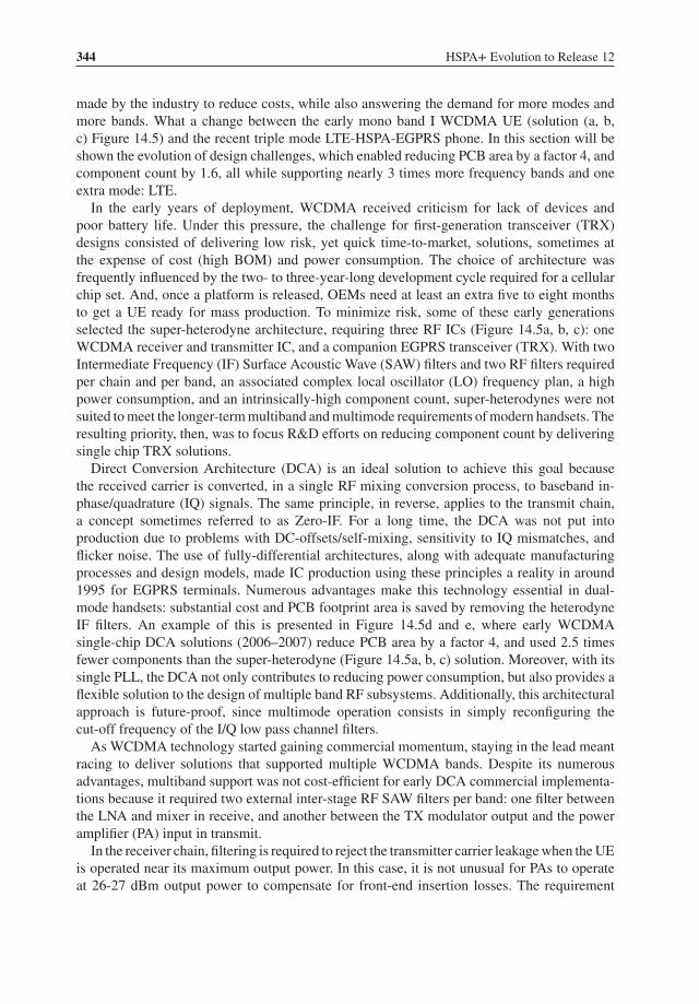
344 HSPA+ Evolution to Release 12
made by the industry to reduce costs, while also answering the demand for more modes andmore bands. What a change between the early mono band I WCDMA UE (solution (a, b,c) Figure 14.5) and the recent triple mode LTE-HSPA-EGPRS phone. In this section will beshown the evolution of design challenges, which enabled reducing PCB area by a factor 4, andcomponent count by 1.6, all while supporting nearly 3 times more frequency bands and oneextra mode: LTE.
In the early years of deployment, WCDMA received criticism for lack of devices andpoor battery life. Under this pressure, the challenge for first-generation transceiver (TRX)designs consisted of delivering low risk, yet quick time-to-market, solutions, sometimes atthe expense of cost (high BOM) and power consumption. The choice of architecture wasfrequently influenced by the two- to three-year-long development cycle required for a cellularchip set. And, once a platform is released, OEMs need at least an extra five to eight monthsto get a UE ready for mass production. To minimize risk, some of these early generationsselected the super-heterodyne architecture, requiring three RF ICs (Figure 14.5a, b, c): oneWCDMA receiver and transmitter IC, and a companion EGPRS transceiver (TRX). With twoIntermediate Frequency (IF) Surface Acoustic Wave (SAW) filters and two RF filters requiredper chain and per band, an associated complex local oscillator (LO) frequency plan, a highpower consumption, and an intrinsically-high component count, super-heterodynes were notsuited to meet the longer-term multiband and multimode requirements of modern handsets. Theresulting priority, then, was to focus R&D efforts on reducing component count by deliveringsingle chip TRX solutions.
Direct Conversion Architecture (DCA) is an ideal solution to achieve this goal becausethe received carrier is converted, in a single RF mixing conversion process, to baseband in-phase/quadrature (IQ) signals. The same principle, in reverse, applies to the transmit chain,a concept sometimes referred to as Zero-IF. For a long time, the DCA was not put intoproduction due to problems with DC-offsets/self-mixing, sensitivity to IQ mismatches, andflicker noise. The use of fully-differential architectures, along with adequate manufacturingprocesses and design models, made IC production using these principles a reality in around1995 for EGPRS terminals. Numerous advantages make this technology essential in dual-mode handsets: substantial cost and PCB footprint area is saved by removing the heterodyneIF filters. An example of this is presented in Figure 14.5d and e, where early WCDMAsingle-chip DCA solutions (2006–2007) reduce PCB area by a factor 4, and used 2.5 timesfewer components than the super-heterodyne (Figure 14.5a, b, c) solution. Moreover, with itssingle PLL, the DCA not only contributes to reducing power consumption, but also provides aflexible solution to the design of multiple band RF subsystems. Additionally, this architecturalapproach is future-proof, since multimode operation consists in simply reconfiguring thecut-off frequency of the I/Q low pass channel filters.
As WCDMA technology started gaining commercial momentum, staying in the lead meantracing to deliver solutions that supported multiple WCDMA bands. Despite its numerousadvantages, multiband support was not cost-efficient for early DCA commercial implementa-tions because it required two external inter-stage RF SAW filters per band: one filter betweenthe LNA and mixer in receive, and another between the TX modulator output and the poweramplifier (PA) input in transmit.
In the receiver chain, filtering is required to reject the transmitter carrier leakage when the UEis operated near its maximum output power. In this case, it is not unusual for PAs to operateat 26-27 dBm output power to compensate for front-end insertion losses. The requirement

Multimode Multiband Terminal Design Challenges 345
to support more bands, and in the case of LTE the need to support more complex carrieraggregation scenarios, results in increasing RF front-end insertion losses. This, in turn, meansthat the PA maximum output power requirements may exceed 27 dBm in certain platforms.Because duplexer isolation is finite, TX carrier leakage can reach the LNA input port witha power as high as −25 dBm. In the presence of this “jammer,” the mixer generates enoughbaseband products through second order distortion5 to degrade sensitivity, thereby partiallycontributing to a phenomenon known as UE self-desensitization, or “desense” [4]. In this case,and depending on system dimensioning assumptions, RX SAW-less operation sets a stringentmixer IIP2 requirement on the order of 48 to 53 dBm (LNA input-referred) [4].
In the transmitter chain, further UE self-desense occurs due to TRX and PA noise emissionsgenerated at the duplex distance. Depending on duplexer isolation, SAW-less operation setsTX noise requirements in the range of −160 dBc [4]. Meeting this requirement in bands withshort duplex distances, such as band 13 or 17, constitutes a serious challenge to both TRXand duplexer designers as performance may become dominated by PA ACLR emissions ratherthan the far out of band noise level. The duplexer high-Q factor often pushes designers totrade isolation against insertion loss. In these bands, 3GPP has introduced relaxations to easefactors related to these design constraints [5].
As the number of bands to be supported was increasing rapidly, the race towards continuouscost reduction called for novel TRX architectures that would enable both TX and RX SAW-lessoperation. For example, removing the interstage filters in a penta-band RF subsystem maysave the cost of a PA and the area of almost an entire RF transceiver6. SAW-less operationalso means that RF transmitter ports can be shared between several RF bands. For example, asingle low-band TX port could be used to support all UHF bands, for example, LTE bands 8,13, 17, and 20. Similarly, a high band port could be shared to support either WCDMA or LTEtransmissions in bands 1, 2, 3, 4. The SAW-less TX architecture is therefore the sine qua non toenable replacing discrete single-band PAs with a single multiband, multimode (MMMB) PA.The cost savings and design tradeoffs associated with the use of MMMB PAs are presented inSection 14.1.3.2 using a North American variant. Initial RX SAW-less commercial solutionsappeared around 2008 (Figure 14.5f). Some of the techniques developed to meet the high IIP2requirements range from careful design of fully differential structures, use of passive mixersor trap filters to reject TX leakage, as well as the integration of IIP2 calibration circuitry.
In contrast, TX SAW-less operation is more challenging and took a longer time to emergesince every block of the transmitter chain impacts the overall performance. The efforts requiredto meet the stringent −160 dBc requirement are illustrated in Figure 14.6a. This graph plotsUE self-desense in a SAW-less application using the reported band I TRX noise performance7.With a desense less than a decibel under typical duplexer isolation, TX SAW removal startedto become a reality around 2007–2008, and the first handsets using this technique made
5 Through third order distortion, TX leakage mixes with CW tones defined by 3GPP narrowband blocker tests in theLNA. Cases where blockers are injected at half and double duplex distance drive the LNA IIP3 requirements.6 Cost saving assumptions: SAW unit price of approximately 0.10 to 0.15$, total cost savings for penta-band estimatedat $1 to $1.50. PCB area assumptions: pi-matching network made up of three 0402 passives, SAW filter packages of1.1 × 0.9 mm and 1.1 × 1.4 mm. Area savings per filter: 3 to 4 mm2 based on [Figure 14.5h] PCB layout, total areasaved in a penta-band application: 30 to 40 mm2.7 Assumptions: 24 dBm UE output power, 52 dB duplexer TX to RX carrier rejection, 15 dB LNA gain, 4 dB NFreferred to LNA input, 0.2 dB allowed desensitization, 2.8 dB PA to antenna insertion losses, IMD2 rejection byanalog and digital filters of 3 dB, and 9 dB DC to IMD2 power ratio.
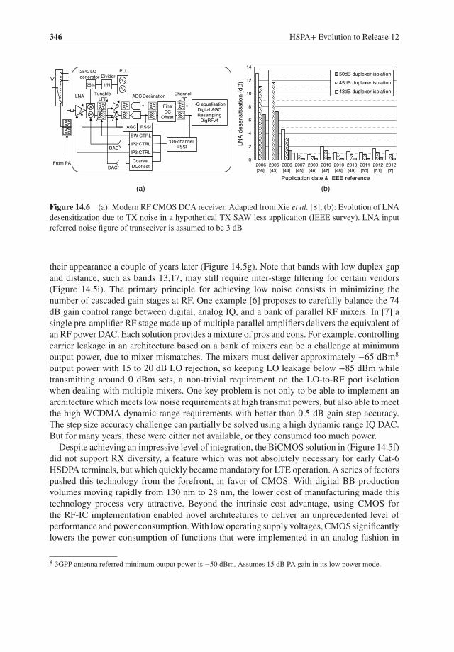
346 HSPA+ Evolution to Release 12
LNA
1/N
Divider
25%
PLL25% LOgenerator
Tunable LPF
ADC
RSSIAGC
IP2 CTRLDAC
DAC
‘On-channel’RSSI
BW CTRL
IP3 CTRL
Channel LPF
Decimation
From PA
Fine DC
Offset
I-Q equalisationDigital AGCResampling
DigRFv4
Coarse DCoffset
0
2
4
6
8
10
12
14
2012[7]
2012[51]
2011[50]
2010[49]
2010[48]
2010[47]
2009[46]
2007[45]
2006[44]
2006[43]
2006[36]
LNA
des
ensi
tisat
ion
(dB
)
Publication date & IEEE reference
50dB duplexer isolation
45dB duplexer isolation
43dB duplexer isolation
(b)(a)
Figure 14.6 (a): Modern RF CMOS DCA receiver. Adapted from Xie et al. [8], (b): Evolution of LNAdesensitization due to TX noise in a hypothetical TX SAW less application (IEEE survey). LNA inputreferred noise figure of transceiver is assumed to be 3 dB
their appearance a couple of years later (Figure 14.5g). Note that bands with low duplex gapand distance, such as bands 13,17, may still require inter-stage filtering for certain vendors(Figure 14.5i). The primary principle for achieving low noise consists in minimizing thenumber of cascaded gain stages at RF. One example [6] proposes to carefully balance the 74dB gain control range between digital, analog IQ, and a bank of parallel RF mixers. In [7] asingle pre-amplifier RF stage made up of multiple parallel amplifiers delivers the equivalent ofan RF power DAC. Each solution provides a mixture of pros and cons. For example, controllingcarrier leakage in an architecture based on a bank of mixers can be a challenge at minimumoutput power, due to mixer mismatches. The mixers must deliver approximately −65 dBm8
output power with 15 to 20 dB LO rejection, so keeping LO leakage below −85 dBm whiletransmitting around 0 dBm sets, a non-trivial requirement on the LO-to-RF port isolationwhen dealing with multiple mixers. One key problem is not only to be able to implement anarchitecture which meets low noise requirements at high transmit powers, but also able to meetthe high WCDMA dynamic range requirements with better than 0.5 dB gain step accuracy.The step size accuracy challenge can partially be solved using a high dynamic range IQ DAC.But for many years, these were either not available, or they consumed too much power.
Despite achieving an impressive level of integration, the BiCMOS solution in (Figure 14.5f)did not support RX diversity, a feature which was not absolutely necessary for early Cat-6HSDPA terminals, but which quickly became mandatory for LTE operation. A series of factorspushed this technology from the forefront, in favor of CMOS. With digital BB productionvolumes moving rapidly from 130 nm to 28 nm, the lower cost of manufacturing made thistechnology process very attractive. Beyond the intrinsic cost advantage, using CMOS forthe RF-IC implementation enabled novel architectures to deliver an unprecedented level ofperformance and power consumption. With low operating supply voltages, CMOS significantlylowers the power consumption of functions that were implemented in an analog fashion in
8 3GPP antenna referred minimum output power is −50 dBm. Assumes 15 dB PA gain in its low power mode.
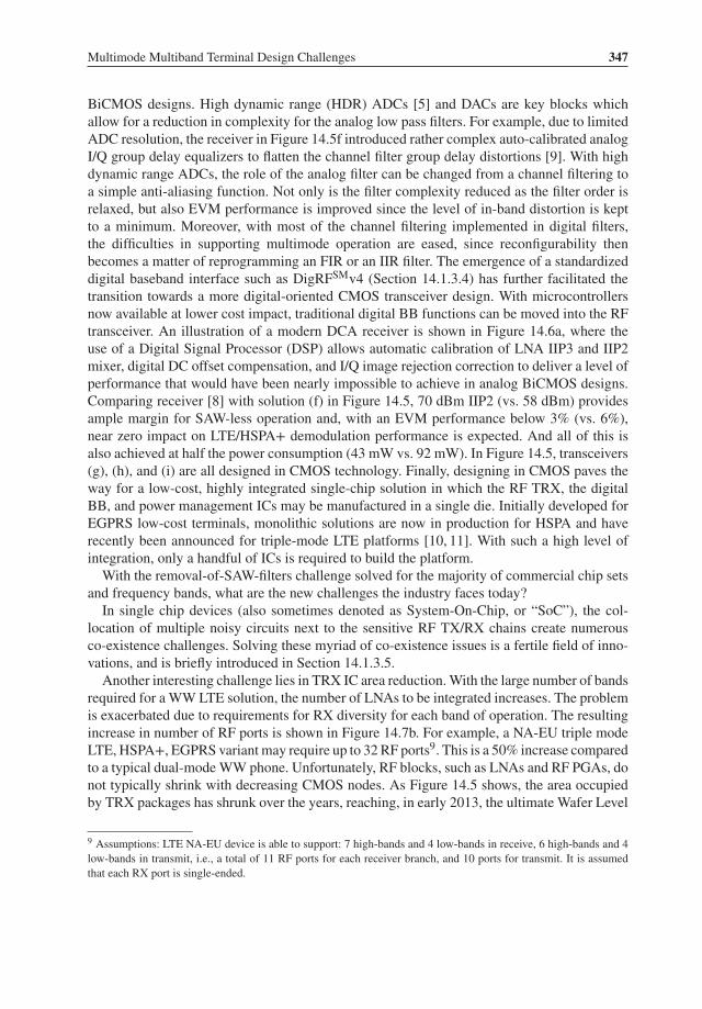
Multimode Multiband Terminal Design Challenges 347
BiCMOS designs. High dynamic range (HDR) ADCs [5] and DACs are key blocks whichallow for a reduction in complexity for the analog low pass filters. For example, due to limitedADC resolution, the receiver in Figure 14.5f introduced rather complex auto-calibrated analogI/Q group delay equalizers to flatten the channel filter group delay distortions [9]. With highdynamic range ADCs, the role of the analog filter can be changed from a channel filtering toa simple anti-aliasing function. Not only is the filter complexity reduced as the filter order isrelaxed, but also EVM performance is improved since the level of in-band distortion is keptto a minimum. Moreover, with most of the channel filtering implemented in digital filters,the difficulties in supporting multimode operation are eased, since reconfigurability thenbecomes a matter of reprogramming an FIR or an IIR filter. The emergence of a standardizeddigital baseband interface such as DigRFSMv4 (Section 14.1.3.4) has further facilitated thetransition towards a more digital-oriented CMOS transceiver design. With microcontrollersnow available at lower cost impact, traditional digital BB functions can be moved into the RFtransceiver. An illustration of a modern DCA receiver is shown in Figure 14.6a, where theuse of a Digital Signal Processor (DSP) allows automatic calibration of LNA IIP3 and IIP2mixer, digital DC offset compensation, and I/Q image rejection correction to deliver a level ofperformance that would have been nearly impossible to achieve in analog BiCMOS designs.Comparing receiver [8] with solution (f) in Figure 14.5, 70 dBm IIP2 (vs. 58 dBm) providesample margin for SAW-less operation and, with an EVM performance below 3% (vs. 6%),near zero impact on LTE/HSPA+ demodulation performance is expected. And all of this isalso achieved at half the power consumption (43 mW vs. 92 mW). In Figure 14.5, transceivers(g), (h), and (i) are all designed in CMOS technology. Finally, designing in CMOS paves theway for a low-cost, highly integrated single-chip solution in which the RF TRX, the digitalBB, and power management ICs may be manufactured in a single die. Initially developed forEGPRS low-cost terminals, monolithic solutions are now in production for HSPA and haverecently been announced for triple-mode LTE platforms [10, 11]. With such a high level ofintegration, only a handful of ICs is required to build the platform.
With the removal-of-SAW-filters challenge solved for the majority of commercial chip setsand frequency bands, what are the new challenges the industry faces today?
In single chip devices (also sometimes denoted as System-On-Chip, or “SoC”), the col-location of multiple noisy circuits next to the sensitive RF TX/RX chains create numerousco-existence challenges. Solving these myriad of co-existence issues is a fertile field of inno-vations, and is briefly introduced in Section 14.1.3.5.
Another interesting challenge lies in TRX IC area reduction. With the large number of bandsrequired for a WW LTE solution, the number of LNAs to be integrated increases. The problemis exacerbated due to requirements for RX diversity for each band of operation. The resultingincrease in number of RF ports is shown in Figure 14.7b. For example, a NA-EU triple modeLTE, HSPA+, EGPRS variant may require up to 32 RF ports9. This is a 50% increase comparedto a typical dual-mode WW phone. Unfortunately, RF blocks, such as LNAs and RF PGAs, donot typically shrink with decreasing CMOS nodes. As Figure 14.5 shows, the area occupiedby TRX packages has shrunk over the years, reaching, in early 2013, the ultimate Wafer Level
9 Assumptions: LTE NA-EU device is able to support: 7 high-bands and 4 low-bands in receive, 6 high-bands and 4low-bands in transmit, i.e., a total of 11 RF ports for each receiver branch, and 10 ports for transmit. It is assumedthat each RX port is single-ended.

348 HSPA+ Evolution to Release 12
Diversity receiver
Band “A”
Diplexer
Duplexer
Intra-band NC CA
Interband CA
Poweramplifier
Band “B”
DuplexerPower
amplifier
Switch
Switch
Band “A”
Band “B”Diplexer
0
QBE
Single-
band
WCDM
A
Triple-
band
WCDM
A
Penta
-ban
d W
CDMA
LTE N
A
LTE N
A-EU
5
10
15
20
25
30
35
40
Num
ber
of T
RX
RF
por
ts
DIVERSITY RX
PRIMARY RX
TRANSMITUL DL DL
(a) (b)
Figure 14.7 (a): Example RF front end complexity in supporting triple-mode and multiple downlinkonly carrier aggregation scenarios: contiguous and non-contiguous, intra and inter band. Only a pair ofbands is shown. (b): RF transceiver number of RF ports required per application
Packages (WLP), in which the package is basically the size of the active die (25 mm2). If pincount continues to grow, the modern RF CMOS transceiver package size may be dominatedby pin count. In solutions using differential LNAs, the RF ports of the NA_EU variant wouldrequire a total of 54 RF pins. With such a high number of ports, ensuring acceptable pin-to-pinisolation is also further complicated. Lastly, PCB routing becomes more complex becausehigh pin density packages often require additional PCB layers, which further raises the totalcost to manufacture.
Finally, the introduction of Carrier Aggregation (CA) adds complexity to the entire RFsubsystem as illustrated in Figure 14.7a. There are three categories of CA scenarios from 3GPP:inter-band, intra-band contiguous (IB-C-CA), and intra-band non-contiguous (IB-NC-CA).The immediate impact on TRX design is the need to support greater modulation bandwidth.The initial commercial deployments started in August 2013 with 10+10 MHz. The next phase,20+20, will start during 2014, thereby requesting UE receivers to support a total of 40 MHzBW. There are numerous interesting challenges associated with CA, but a detailed descriptionwould go far beyond the scope of this introduction. While most challenges impact the RF-FE linearity, filter rejection, and topology, the special case IB-NC-CA is problematic for thedesign of a single-chip TRX solution. In this CA category, the wanted downlink carriers maybe located at, or near, the edges of a given band as depicted in Figure 14.8. This situationcreates at least two types of new challenges.
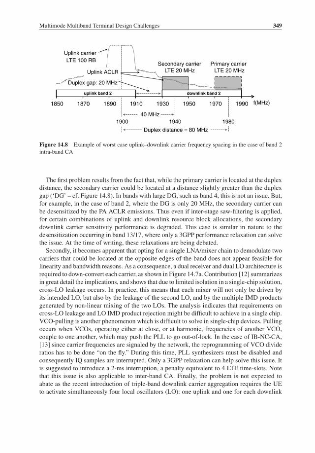
Multimode Multiband Terminal Design Challenges 349
1850 1870 1890 1910 1930 1950 1970 1990
Primary carrierLTE 20 MHz
Secondary carrierLTE 20 MHz
downlink band 2
1900 1940 198040 MHz
Duplex distance = 80 MHz
Uplink carrierLTE 100 RB
uplink band 2
Uplink ACLR
Duplex gap: 20 MHz
f(MHz)
Figure 14.8 Example of worst case uplink–downlink carrier frequency spacing in the case of band 2intra-band CA
The first problem results from the fact that, while the primary carrier is located at the duplexdistance, the secondary carrier could be located at a distance slightly greater than the duplexgap (‘DG’ – cf. Figure 14.8). In bands with large DG, such as band 4, this is not an issue. But,for example, in the case of band 2, where the DG is only 20 MHz, the secondary carrier canbe desensitized by the PA ACLR emissions. Thus even if inter-stage saw-filtering is applied,for certain combinations of uplink and downlink resource block allocations, the secondarydownlink carrier sensitivity performance is degraded. This case is similar in nature to thedesensitization occurring in band 13/17, where only a 3GPP performance relaxation can solvethe issue. At the time of writing, these relaxations are being debated.
Secondly, it becomes apparent that opting for a single LNA/mixer chain to demodulate twocarriers that could be located at the opposite edges of the band does not appear feasible forlinearity and bandwidth reasons. As a consequence, a dual receiver and dual LO architecture isrequired to down-convert each carrier, as shown in Figure 14.7a. Contribution [12] summarizesin great detail the implications, and shows that due to limited isolation in a single-chip solution,cross-LO leakage occurs. In practice, this means that each mixer will not only be driven byits intended LO, but also by the leakage of the second LO, and by the multiple IMD productsgenerated by non-linear mixing of the two LOs. The analysis indicates that requirements oncross-LO leakage and LO IMD product rejection might be difficult to achieve in a single chip.VCO-pulling is another phenomenon which is difficult to solve in single-chip devices. Pullingoccurs when VCOs, operating either at close, or at harmonic, frequencies of another VCO,couple to one another, which may push the PLL to go out-of-lock. In the case of IB-NC-CA,[13] since carrier frequencies are signaled by the network, the reprogramming of VCO divideratios has to be done “on the fly.” During this time, PLL synthesizers must be disabled andconsequently IQ samples are interrupted. Only a 3GPP relaxation can help solve this issue. Itis suggested to introduce a 2-ms interruption, a penalty equivalent to 4 LTE time-slots. Notethat this issue is also applicable to inter-band CA. Finally, the problem is not expected toabate as the recent introduction of triple-band downlink carrier aggregation requires the UEto activate simultaneously four local oscillators (LO): one uplink and one for each downlink
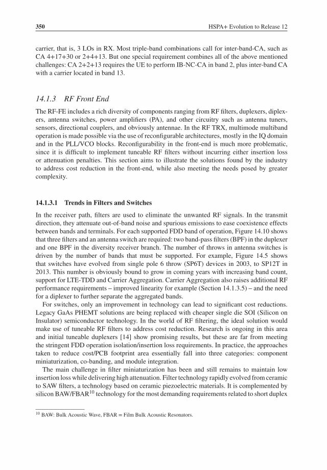
350 HSPA+ Evolution to Release 12
carrier, that is, 3 LOs in RX. Most triple-band combinations call for inter-band-CA, such asCA 4+17+30 or 2+4+13. But one special requirement combines all of the above mentionedchallenges: CA 2+2+13 requires the UE to perform IB-NC-CA in band 2, plus inter-band CAwith a carrier located in band 13.
14.1.3 RF Front End
The RF-FE includes a rich diversity of components ranging from RF filters, duplexers, diplex-ers, antenna switches, power amplifiers (PA), and other circuitry such as antenna tuners,sensors, directional couplers, and obviously antennae. In the RF TRX, multimode multibandoperation is made possible via the use of reconfigurable architectures, mostly in the IQ domainand in the PLL/VCO blocks. Reconfigurability in the front-end is much more problematic,since it is difficult to implement tuneable RF filters without incurring either insertion lossor attenuation penalties. This section aims to illustrate the solutions found by the industryto address cost reduction in the front-end, while also meeting the needs posed by greatercomplexity.
14.1.3.1 Trends in Filters and Switches
In the receiver path, filters are used to eliminate the unwanted RF signals. In the transmitdirection, they attenuate out-of-band noise and spurious emissions to ease coexistence effectsbetween bands and terminals. For each supported FDD band of operation, Figure 14.10 showsthat three filters and an antenna switch are required: two band-pass filters (BPF) in the duplexerand one BPF in the diversity receiver branch. The number of throws in antenna switches isdriven by the number of bands that must be supported. For example, Figure 14.5 showsthat switches have evolved from single pole 6 throw (SP6T) devices in 2003, to SP12T in2013. This number is obviously bound to grow in coming years with increasing band count,support for LTE-TDD and Carrier Aggregation. Carrier Aggregation also raises additional RFperformance requirements – improved linearity for example (Section 14.1.3.5) – and the needfor a diplexer to further separate the aggregated bands.
For switches, only an improvement in technology can lead to significant cost reductions.Legacy GaAs PHEMT solutions are being replaced with cheaper single die SOI (Silicon onInsulator) semiconductor technology. In the world of RF filtering, the ideal solution wouldmake use of tuneable RF filters to address cost reduction. Research is ongoing in this areaand initial tuneable duplexers [14] show promising results, but these are far from meetingthe stringent FDD operation isolation/insertion loss requirements. In practice, the approachestaken to reduce cost/PCB footprint area essentially fall into three categories: componentminiaturization, co-banding, and module integration.
The main challenge in filter miniaturization has been and still remains to maintain lowinsertion loss while delivering high attenuation. Filter technology rapidly evolved from ceramicto SAW filters, a technology based on ceramic piezoelectric materials. It is complemented bysilicon BAW/FBAR10 technology for the most demanding requirements related to short duplex
10 BAW: Bulk Acoustic Wave, FBAR = Film Bulk Acoustic Resonators.
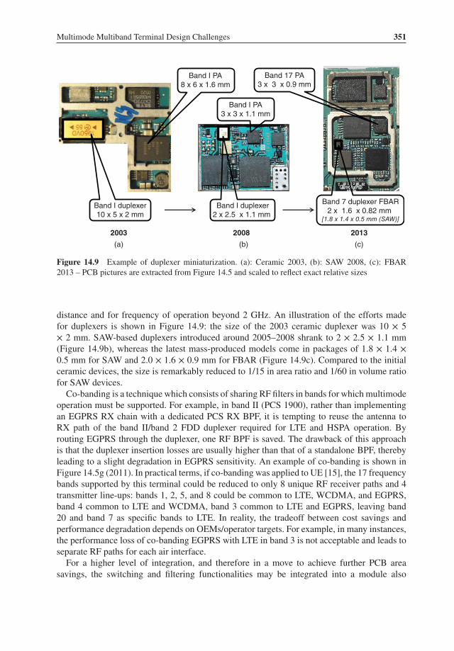
Multimode Multiband Terminal Design Challenges 351
Figure 14.9 Example of duplexer miniaturization. (a): Ceramic 2003, (b): SAW 2008, (c): FBAR2013 – PCB pictures are extracted from Figure 14.5 and scaled to reflect exact relative sizes
distance and for frequency of operation beyond 2 GHz. An illustration of the efforts madefor duplexers is shown in Figure 14.9: the size of the 2003 ceramic duplexer was 10 × 5× 2 mm. SAW-based duplexers introduced around 2005–2008 shrank to 2 × 2.5 × 1.1 mm(Figure 14.9b), whereas the latest mass-produced models come in packages of 1.8 × 1.4 ×0.5 mm for SAW and 2.0 × 1.6 × 0.9 mm for FBAR (Figure 14.9c). Compared to the initialceramic devices, the size is remarkably reduced to 1/15 in area ratio and 1/60 in volume ratiofor SAW devices.
Co-banding is a technique which consists of sharing RF filters in bands for which multimodeoperation must be supported. For example, in band II (PCS 1900), rather than implementingan EGPRS RX chain with a dedicated PCS RX BPF, it is tempting to reuse the antenna toRX path of the band II/band 2 FDD duplexer required for LTE and HSPA operation. Byrouting EGPRS through the duplexer, one RF BPF is saved. The drawback of this approachis that the duplexer insertion losses are usually higher than that of a standalone BPF, therebyleading to a slight degradation in EGPRS sensitivity. An example of co-banding is shown inFigure 14.5g (2011). In practical terms, if co-banding was applied to UE [15], the 17 frequencybands supported by this terminal could be reduced to only 8 unique RF receiver paths and 4transmitter line-ups: bands 1, 2, 5, and 8 could be common to LTE, WCDMA, and EGPRS,band 4 common to LTE and WCDMA, band 3 common to LTE and EGPRS, leaving band20 and band 7 as specific bands to LTE. In reality, the tradeoff between cost savings andperformance degradation depends on OEMs/operator targets. For example, in many instances,the performance loss of co-banding EGPRS with LTE in band 3 is not acceptable and leads toseparate RF paths for each air interface.
For a higher level of integration, and therefore in a move to achieve further PCB areasavings, the switching and filtering functionalities may be integrated into a module also
Band I PA8 x 6 x 1.6 mm
2008 2013
Band 17 PA3 x 3 x 0.9 mm
Band I PA3 x 3 x 1.1 mm
Band I duplexer10 x 5 x 2 mm
(a) (b) (c)
Band I duplexer2 x 2.5 x 1.1 mm
Band 7 duplexer FBAR2 x 1.6 x 0.82 mm
[1.8 x 1.4 x 0.5 mm (SAW)]
2003
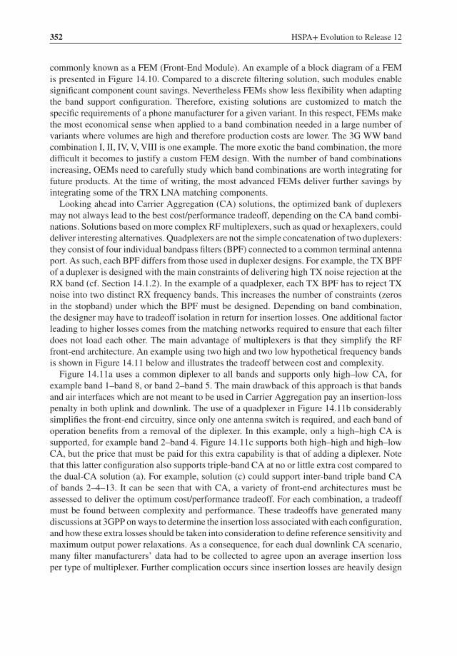
352 HSPA+ Evolution to Release 12
commonly known as a FEM (Front-End Module). An example of a block diagram of a FEMis presented in Figure 14.10. Compared to a discrete filtering solution, such modules enablesignificant component count savings. Nevertheless FEMs show less flexibility when adaptingthe band support configuration. Therefore, existing solutions are customized to match thespecific requirements of a phone manufacturer for a given variant. In this respect, FEMs makethe most economical sense when applied to a band combination needed in a large number ofvariants where volumes are high and therefore production costs are lower. The 3G WW bandcombination I, II, IV, V, VIII is one example. The more exotic the band combination, the moredifficult it becomes to justify a custom FEM design. With the number of band combinationsincreasing, OEMs need to carefully study which band combinations are worth integrating forfuture products. At the time of writing, the most advanced FEMs deliver further savings byintegrating some of the TRX LNA matching components.
Looking ahead into Carrier Aggregation (CA) solutions, the optimized bank of duplexersmay not always lead to the best cost/performance tradeoff, depending on the CA band combi-nations. Solutions based on more complex RF multiplexers, such as quad or hexaplexers, coulddeliver interesting alternatives. Quadplexers are not the simple concatenation of two duplexers:they consist of four individual bandpass filters (BPF) connected to a common terminal antennaport. As such, each BPF differs from those used in duplexer designs. For example, the TX BPFof a duplexer is designed with the main constraints of delivering high TX noise rejection at theRX band (cf. Section 14.1.2). In the example of a quadplexer, each TX BPF has to reject TXnoise into two distinct RX frequency bands. This increases the number of constraints (zerosin the stopband) under which the BPF must be designed. Depending on band combination,the designer may have to tradeoff isolation in return for insertion losses. One additional factorleading to higher losses comes from the matching networks required to ensure that each filterdoes not load each other. The main advantage of multiplexers is that they simplify the RFfront-end architecture. An example using two high and two low hypothetical frequency bandsis shown in Figure 14.11 below and illustrates the tradeoff between cost and complexity.
Figure 14.11a uses a common diplexer to all bands and supports only high–low CA, forexample band 1–band 8, or band 2–band 5. The main drawback of this approach is that bandsand air interfaces which are not meant to be used in Carrier Aggregation pay an insertion-losspenalty in both uplink and downlink. The use of a quadplexer in Figure 14.11b considerablysimplifies the front-end circuitry, since only one antenna switch is required, and each band ofoperation benefits from a removal of the diplexer. In this example, only a high–high CA issupported, for example band 2–band 4. Figure 14.11c supports both high–high and high–lowCA, but the price that must be paid for this extra capability is that of adding a diplexer. Notethat this latter configuration also supports triple-band CA at no or little extra cost compared tothe dual-CA solution (a). For example, solution (c) could support inter-band triple band CAof bands 2–4–13. It can be seen that with CA, a variety of front-end architectures must beassessed to deliver the optimum cost/performance tradeoff. For each combination, a tradeoffmust be found between complexity and performance. These tradeoffs have generated manydiscussions at 3GPP on ways to determine the insertion loss associated with each configuration,and how these extra losses should be taken into consideration to define reference sensitivity andmaximum output power relaxations. As a consequence, for each dual downlink CA scenario,many filter manufacturers’ data had to be collected to agree upon an average insertion lossper type of multiplexer. Further complication occurs since insertion losses are heavily design
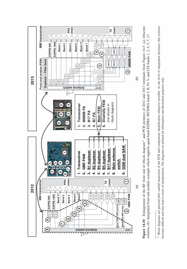
Fig
ure
14.1
0E
nlar
gem
ent
ofth
eR
Ffr
ont
end
of(b
lock
diag
ram
11an
dPC
Bpi
ctur
es)
of20
12an
d20
13te
rmin
als
from
Figu
re14
.5.
(a):
Dis
cret
eso
lutio
n,(b
):In
tegr
ated
fron
tend
mod
ule
exam
ple
whi
chsu
ppor
tsqu
ad-b
and
EG
PRS,
WC
DM
Aba
nds
I,II
,IV
,V,a
ndLT
Eba
nds
1,2,
4,5,
7,17
11B
lock
diag
ram
sar
egu
esse
daf
ter
care
ful
insp
ectio
nof
the
PCB
and
com
pone
nts
iden
tifica
tion
whe
neve
rpo
ssib
le.
As
the
leve
lof
inte
grat
ion
incr
ease
s,th
isex
erci
sebe
com
esdi
fficu
ltan
dm
ayle
adto
erro
rsof
inte
rpre
tatio
n.T
hedi
agra
ms
are
prin
ted
for
info
rmat
ion
and
illus
trat
ion
purp
oses
only
.
1.T
ran
scei
ver
2.Q
BE
PA
M
3.B
1 d
up
lexe
r 4.
B2
du
ple
xer
5.B
4 d
up
lexe
r 6.
B5
du
ple
xer
7.B
17 d
up
lexe
r 8.
Mai
n a
nte
nn
a sw
itch
9.
GS
M d
ual
SA
W
1.T
ran
scei
ver
2.M
MM
B P
A
3.
B17
PA
4.
B7
PA
5.
Mai
n F
EM
6.
Div
ersi
ty F
EM
(n
ot s
how
n in
bl
ock
diag
ram
)
EG
PR
S 9
00
EG
PR
S 1
800
Ban
d 1
7
Ban
d 5
Ban
d 2
Ban
d I
HB
LB
Ban
d 8
50–9
00 (E
GP
RS
)
Ban
d 1
800–
1900
(EG
PR
S)
Ban
d 4
Antenna switch SP9T
TX
ch
ain
PR
Xch
ain
QB
E P
AM
MM
tra
nsc
eive
r
1 2
3
4
5
6
7
8 9
6 4 3 5
8
9 7
2
1 1
2
3 4
Ban
d 7
Antenna switch SP10TDu
ple
xer
– F
ilter
ban
k
PR
X
chai
n
TX
ch
ain
SP
3TH
BSP
2T
SP
2T
Fro
nt
end
mo
du
le (
FE
M)
MM
MB
PA
M
Ban
d 1
7
Ban
d 5
Ban
d 1
Ban
d 2
Ban
d 4
EG
PR
S 9
00
EG
PR
S 1
800
MM
tra
nsc
eive
r
1 2
3
4 5
5 6
2012
20
13
(a)
(b)
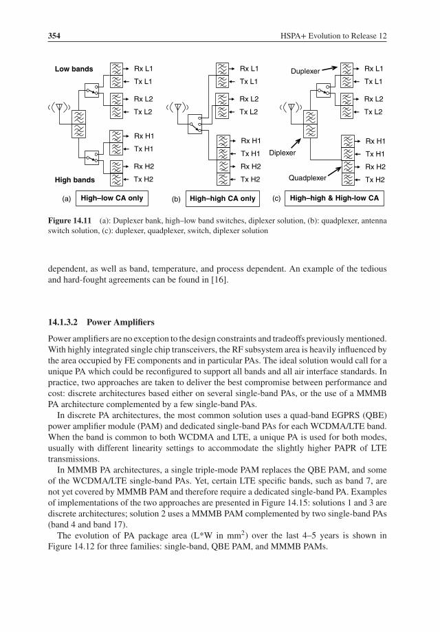
354 HSPA+ Evolution to Release 12
Tx L1
Rx L1
Tx L2
Rx L2
Tx H1
Rx H1
Tx H2
Rx H2
Tx H1
Rx H1
Tx H2
Rx H2
Tx H1
Rx H1
Tx H2
Rx H2
Low bands
High bands
High–low CA only High–high CA only High–high & High-low CA(a) (b) (c)
Tx L1
Rx L1
Tx L2
Rx L2
Tx L1
Rx L1
Tx L2
Rx L2
Diplexer
Quadplexer
Duplexer
Figure 14.11 (a): Duplexer bank, high–low band switches, diplexer solution, (b): quadplexer, antennaswitch solution, (c): duplexer, quadplexer, switch, diplexer solution
dependent, as well as band, temperature, and process dependent. An example of the tediousand hard-fought agreements can be found in [16].
14.1.3.2 Power Amplifiers
Power amplifiers are no exception to the design constraints and tradeoffs previously mentioned.With highly integrated single chip transceivers, the RF subsystem area is heavily influenced bythe area occupied by FE components and in particular PAs. The ideal solution would call for aunique PA which could be reconfigured to support all bands and all air interface standards. Inpractice, two approaches are taken to deliver the best compromise between performance andcost: discrete architectures based either on several single-band PAs, or the use of a MMMBPA architecture complemented by a few single-band PAs.
In discrete PA architectures, the most common solution uses a quad-band EGPRS (QBE)power amplifier module (PAM) and dedicated single-band PAs for each WCDMA/LTE band.When the band is common to both WCDMA and LTE, a unique PA is used for both modes,usually with different linearity settings to accommodate the slightly higher PAPR of LTEtransmissions.
In MMMB PA architectures, a single triple-mode PAM replaces the QBE PAM, and someof the WCDMA/LTE single-band PAs. Yet, certain LTE specific bands, such as band 7, arenot yet covered by MMMB PAM and therefore require a dedicated single-band PA. Examplesof implementations of the two approaches are presented in Figure 14.15: solutions 1 and 3 arediscrete architectures; solution 2 uses a MMMB PAM complemented by two single-band PAs(band 4 and band 17).
The evolution of PA package area (L*W in mm2) over the last 4–5 years is shown inFigure 14.12 for three families: single-band, QBE PAM, and MMMB PAMs.
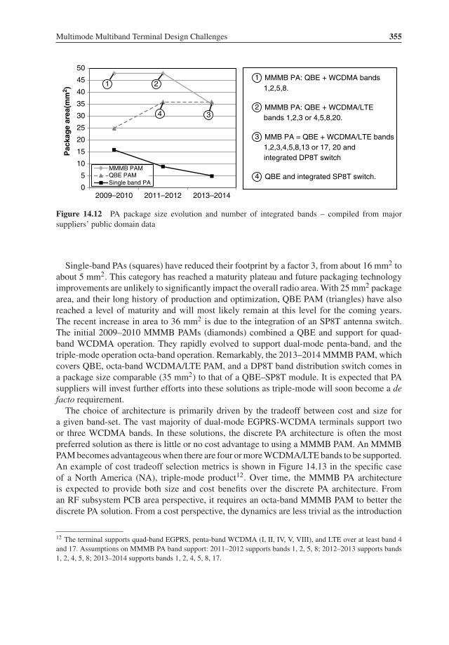
Multimode Multiband Terminal Design Challenges 355
MMMB PA: QBE + WCDMA bands 1,2,5,8.
MMMB PA: QBE + WCDMA/LTE bands 1,2,3 or 4,5,8,20.
MMB PA = QBE + WCDMA/LTE bands 1,2,3,4,5,8,13 or 17, 20 and integrated DP8T switch
QBE and integrated SP8T switch.0
5
10
15
20
25
30
35
40
45
50
2009–2010 2011–2012 2013–2014
Pac
kag
e ar
ea(m
m2 )
MMMB PAMQBE PAMSingle band PA
1 21
2
3
4
34
Figure 14.12 PA package size evolution and number of integrated bands – compiled from majorsuppliers’ public domain data
Single-band PAs (squares) have reduced their footprint by a factor 3, from about 16 mm2 toabout 5 mm2. This category has reached a maturity plateau and future packaging technologyimprovements are unlikely to significantly impact the overall radio area. With 25 mm2 packagearea, and their long history of production and optimization, QBE PAM (triangles) have alsoreached a level of maturity and will most likely remain at this level for the coming years.The recent increase in area to 36 mm2 is due to the integration of an SP8T antenna switch.The initial 2009–2010 MMMB PAMs (diamonds) combined a QBE and support for quad-band WCDMA operation. They rapidly evolved to support dual-mode penta-band, and thetriple-mode operation octa-band operation. Remarkably, the 2013–2014 MMMB PAM, whichcovers QBE, octa-band WCDMA/LTE PAM, and a DP8T band distribution switch comes ina package size comparable (35 mm2) to that of a QBE–SP8T module. It is expected that PAsuppliers will invest further efforts into these solutions as triple-mode will soon become a defacto requirement.
The choice of architecture is primarily driven by the tradeoff between cost and size fora given band-set. The vast majority of dual-mode EGPRS-WCDMA terminals support twoor three WCDMA bands. In these solutions, the discrete PA architecture is often the mostpreferred solution as there is little or no cost advantage to using a MMMB PAM. An MMMBPAM becomes advantageous when there are four or more WCDMA/LTE bands to be supported.An example of cost tradeoff selection metrics is shown in Figure 14.13 in the specific caseof a North America (NA), triple-mode product12. Over time, the MMMB PA architectureis expected to provide both size and cost benefits over the discrete PA architecture. Froman RF subsystem PCB area perspective, it requires an octa-band MMMB PAM to better thediscrete PA solution. From a cost perspective, the dynamics are less trivial as the introduction
12 The terminal supports quad-band EGPRS, penta-band WCDMA (I, II, IV, V, VIII), and LTE over at least band 4and 17. Assumptions on MMMB PA band support: 2011–2012 supports bands 1, 2, 5, 8; 2012–2013 supports bands1, 2, 4, 5, 8; 2013–2014 supports bands 1, 2, 4, 5, 8, 17.
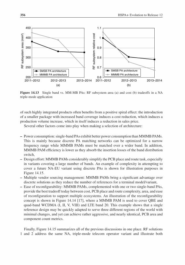
356 HSPA+ Evolution to Release 12
0.6
0.7
0.8
0.9
1
1.1
2011–2012 2012–2013 2013–2014
RF
sub
syst
em r
elat
ive
cost
SMSB PA architecture
MMMB PA architecture200
250
300
350
400
450
2011–2012 2012–2013 2013–2014
RF
sub
syst
em a
rea
(mm
²)
SMSB PA architectureMMMB PA architecture
(a) (b)
Figure 14.13 Single band vs. MM-MB PAs: RF subsystem area (a) and cost (b) tradeoffs in a NAtriple-mode application
of such highly integrated products often benefits from a positive spiral effect: the introductionof a smaller package with increased band coverage induces a cost reduction, which induces aproduction volume increase, which in itself induces a reduction in sales price.
Several other factors come into play when making a selection of architecture:
– Power consumption: single-band PAs exhibit better power consumption than MMMB PAMs.This is mainly because discrete PA matching networks can be optimized for a narrowfrequency range while MMMB PAMs must be matched over a wider band. In addition,MMMB PAM efficiency is lower as they absorb the insertion losses of the band distributionswitch,
– Design effort: MMMB PAMs considerably simplify the PCB place and route task, especiallyin variants covering a large number of bands. An example of complexity in attempting tocover a future NA-EU variant using discrete PAs is shown for illustration purposes inFigure 14.15.
– Multiple vendor sourcing management: MMMB PAMs bring a significant advantage overdiscrete solutions as they reduce the number of references for a terminal model/variant,
– Ease of reconfigurability: MMMB PAMs, complemented with one or two single-band PAs,provide the best tradeoff today between cost, PCB place and route complexity, area, and easeof reconfiguration to support multiple ecosystems. An illustration of the reconfigurabilityconcept is shown in Figure 14.14 [17], where a MMMB PAM is used to cover QBE andquad-band WCDMA (I, II, V, VIII) and LTE band 20. This example shows that a singlereference design may be quickly adapted to serve three different regions of the world withminimal changes, and yet can achieve rather aggressive, and nearly identical, PCB area andcomponent count metrics.
Finally, Figure 14.15 summarizes all of the previous discussions in one place. RF solutions1 and 2 address the same NA, triple-mode telecom operator variant and illustrate both
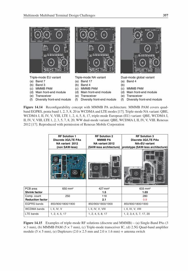
Multimode Multiband Terminal Design Challenges 357
Triple-mode EU variant(a) Band 7(b) Band 3(c) MMMB PAM (d) Main front-end module(e) Transceiver(f) Diversity front-end module
Triple-mode NA variant(a) Band 17(b) Band 4(c) MMMB PAM (d) Main front-end module(e) Transceiver(f) Diversity front-end module
Dual-mode global variant(a) Band 4(b)(c) MMMB PAM(d) Main front-end module(e) Transceiver(f) Diversity front-end module
b ca
e
d
f
b ca
e
d
f
a c
e
d
f
Figure 14.14 Reconfigurability concept with MMMB PA architecture. MMMB PAM covers quad-band EGPRS, penta band 1, 2, 5, 8, 20 in WCDMA and LTE modes [17]. Triple-mode NA variant: QBE,WCDMA I, II, IV, V, VIII, LTE 1, 2, 4, 5, 8, 17, triple-mode European (EU) variant: QBE, WCDMA I,II, IV, V, VIII, LTE 1, 2, 3, 5, 7, 8, 20, WW dual-mode variant: QBE, WCDMA I, II, IV, V, VIII. Renesas2012 [17]. Reproduced with permission of Renesas Mobile Corporation
Figure 14.15 Examples of triple-mode RF solutions (discrete and MMMB) – (a) Single-Band PAs (3× 3 mm), (b) MMMB PAM (5 × 7 mm), (c) Triple-mode transceiver IC, (d) 2.5G Quad-band amplifiermodule (5 × 5 mm), (e) Duplexers (2.0 × 2.5 mm and 2.0 × 1.6 mm) + antenna switch
RF Solution 1Discrete 3G/LTE PAs
NA variant 2012(non SAW-less)
RF Solution 2MMMB PA
NA variant 2012(SAW-less architecture)
RF Solution 3Discrete 3G/LTE PAs
NA+EU variantprototype (SAW-less architecture)
PCB areaShrink factor
650 mm² 427 mm²1.5
633 mm²1.03
Comp. countReduction factor
250 1192.1
2800.9
EGPRS bands 850/900/1800/1900 850/900/1800/1900 850/900/1800/1900
WCDMA bands I, II, IV, V I, II, IV, V, VIII I, II, IV, V, VIII
LTE bands 1, 2, 4, 5, 17 1, 2, 4, 5, 8, 17 1, 2, 3, 4, 5, 7, 17, 20
cb
a a
d
c ec
d
a
e
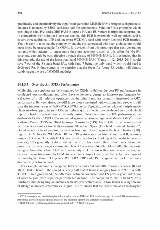
358 HSPA+ Evolution to Release 12
graphically and quantitatively the significant gains that MMMB PAMs bring to such products:the area is reduced by 150%, and uses half the components. Solution 3 is a prototype whichuses single-band PAs and a QBE PAM to target a NA and EU variant in triple-mode operation.In comparison with solution 1, one can see that this PCB is extremely well-optimized, and itcovers three additional LTE and one extra WCDMA band with nearly identical PCB metrics.Yet, it is easy to note that the complexity and the cost associated with such architecture wouldmost likely be unacceptable for OEMs. It is evident from this prototype that next-generationvariants which attempt to target more than one ecosystem, such as this effort for NA-EUcoverage, can only be cost effective through the use of MMMB PAMs. It is estimated that inthis example, the use of the latest octa-band MMMB PAM (Figure 14.12, 2013–2014) couldsave 7 out of the 8 single-band PAs, with band 7 being the only band which would need adedicated PA. It thus comes as no surprise that the focus for future PA design will almostsurely target the use of MMMB modules.
14.1.3.3 Over-the-Air (OTA) Performance
While chip set suppliers are benchmarked by OEMs to deliver the best RF performance inconducted test conditions, and often have to iterate a design to improve performance bya fraction of a dB, telecom operators, on the other hand, are primarily interested in OTAperformance. Between these, the OEMs are more concerned with ensuring their products willpass the impressive set of 3GPP/PTCRB/GCF tests. Typically, the test plan of a triple-modephone involves approximately 1500 tests, the majority of which are conducted tests, and whichtypically lead to several months of costly testing. When it comes to OTA performance, thedual-mode EGPRS/HSPA UE is measured against two simple Figures of Merit (FOM)13: TotalRadiated Power (TRP) and Total Isotropic Sensitivity (TIS). Each FOM is then re-measuredin different user interaction (UI) scenarios: UE in Free Space (FS), held in a hand phantom14,placed against a head phantom or held in hand and placed against the head phantom [18].Figure 14.16 plots the WCDMA TRP vs. TIS performance, in band V and band II, across asample of 30 class 3 recently PTCRB-certified smartphones. Looking at the conducted results(circles), UEs generally perform within 1 or 2 dB from each other in both axes. In outputpower, performance ranges across the class 3 tolerances (24 dBm +1/−3 dB), the majoritybeing calibrated to deliver 23 dBm. In sensitivity, all UEs pass with a comfortable margin, butbecause this metric is used by OEMs to benchmark chip set platforms, the performance spreadis much tighter than in TX power. With OTA TRP and TIS, the spread across UI increasesdramatically between bands.
For example, in band V the spread between conducted and BHHR varies between 10 and18 dB. But in band II, the spread is nearly half that of band V, ranging from 5 to 9 dB in bothTRP/TIS. In a given band, the difference between conducted and FS gives a good indicationof antenna gain, with superior performance in band II as compared to that in band V. Thisillustrates that designing an antenna with desired performance in low bands is a significantchallenge in modern smartphones. Figure 14.17b, shows that the task of the antenna designer
13 CTIA acronyms are used throughout this section, where TRP and TIS are the average of several 3D measurementsperformed across different spatial angles of the radiation sphere and different polarizations.14 Both left and right hand phantoms are defined in CTIA OTA test plan.
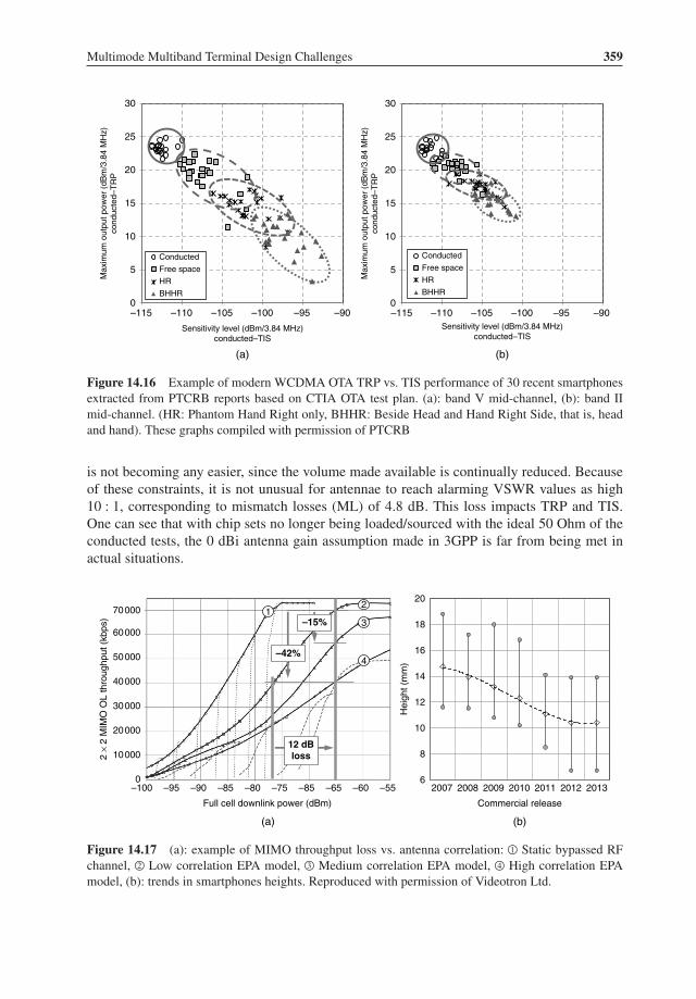
Multimode Multiband Terminal Design Challenges 359
0
5
10
15
20
25
30
–115 –110 –105 –100 –95 –90
Max
imum
out
put p
ower
(dB
m/3
.84
MH
z)co
nduc
ted–
TR
P
Sensitivity level (dBm/3.84 MHz)conducted–TIS
Conducted
Free space
HR
BHHR0
5
10
15
20
25
30
–115 –110 –105 –100 –95 –90
Max
imum
out
put p
ower
(dB
m/3
.84
MH
z)co
nduc
ted–
TR
P
Sensitivity level (dBm/3.84 MHz)conducted–TIS
Conducted
Free space
HR
BHHR
(a) (b)
Figure 14.16 Example of modern WCDMA OTA TRP vs. TIS performance of 30 recent smartphonesextracted from PTCRB reports based on CTIA OTA test plan. (a): band V mid-channel, (b): band IImid-channel. (HR: Phantom Hand Right only, BHHR: Beside Head and Hand Right Side, that is, headand hand). These graphs compiled with permission of PTCRB
is not becoming any easier, since the volume made available is continually reduced. Becauseof these constraints, it is not unusual for antennae to reach alarming VSWR values as high10 : 1, corresponding to mismatch losses (ML) of 4.8 dB. This loss impacts TRP and TIS.One can see that with chip sets no longer being loaded/sourced with the ideal 50 Ohm of theconducted tests, the 0 dBi antenna gain assumption made in 3GPP is far from being met inactual situations.
–15%
–42%
12 dBloss
12
3
4
6
8
10
12
14
16
18
20
2007–55–60–65–85–75–80
Full cell downlink power (dBm)
–85–90–95–1000
2 ×
2 M
IMO
OL
thro
ughp
ut (
kbps
)
10000
20000
30000
40000
50000
60000
70000
2008 2009 2010 2011 2012 2013
Hei
ght (
mm
)
Commercial release
(a) (b)
Figure 14.17 (a): example of MIMO throughput loss vs. antenna correlation: ⃝1 Static bypassed RFchannel, ⃝2 Low correlation EPA model, ⃝3 Medium correlation EPA model, ⃝4 High correlation EPAmodel, (b): trends in smartphones heights. Reproduced with permission of Videotron Ltd.
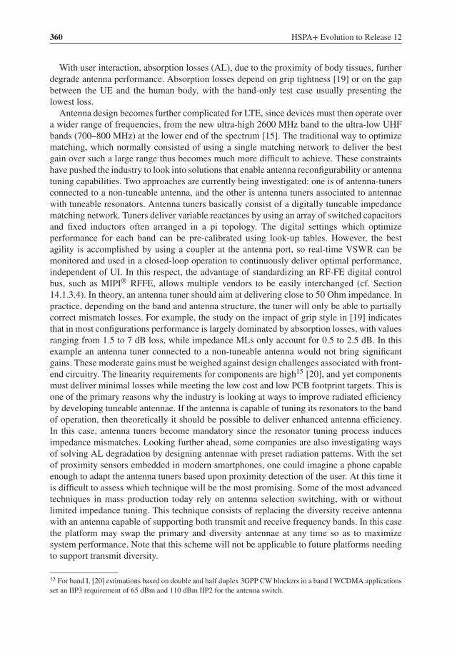
360 HSPA+ Evolution to Release 12
With user interaction, absorption losses (AL), due to the proximity of body tissues, furtherdegrade antenna performance. Absorption losses depend on grip tightness [19] or on the gapbetween the UE and the human body, with the hand-only test case usually presenting thelowest loss.
Antenna design becomes further complicated for LTE, since devices must then operate overa wider range of frequencies, from the new ultra-high 2600 MHz band to the ultra-low UHFbands (700–800 MHz) at the lower end of the spectrum [15]. The traditional way to optimizematching, which normally consisted of using a single matching network to deliver the bestgain over such a large range thus becomes much more difficult to achieve. These constraintshave pushed the industry to look into solutions that enable antenna reconfigurability or antennatuning capabilities. Two approaches are currently being investigated: one is of antenna-tunersconnected to a non-tuneable antenna, and the other is antenna tuners associated to antennaewith tuneable resonators. Antenna tuners basically consist of a digitally tuneable impedancematching network. Tuners deliver variable reactances by using an array of switched capacitorsand fixed inductors often arranged in a pi topology. The digital settings which optimizeperformance for each band can be pre-calibrated using look-up tables. However, the bestagility is accomplished by using a coupler at the antenna port, so real-time VSWR can bemonitored and used in a closed-loop operation to continuously deliver optimal performance,independent of UI. In this respect, the advantage of standardizing an RF-FE digital controlbus, such as MIPI® RFFE, allows multiple vendors to be easily interchanged (cf. Section14.1.3.4). In theory, an antenna tuner should aim at delivering close to 50 Ohm impedance. Inpractice, depending on the band and antenna structure, the tuner will only be able to partiallycorrect mismatch losses. For example, the study on the impact of grip style in [19] indicatesthat in most configurations performance is largely dominated by absorption losses, with valuesranging from 1.5 to 7 dB loss, while impedance MLs only account for 0.5 to 2.5 dB. In thisexample an antenna tuner connected to a non-tuneable antenna would not bring significantgains. These moderate gains must be weighed against design challenges associated with front-end circuitry. The linearity requirements for components are high15 [20], and yet componentsmust deliver minimal losses while meeting the low cost and low PCB footprint targets. This isone of the primary reasons why the industry is looking at ways to improve radiated efficiencyby developing tuneable antennae. If the antenna is capable of tuning its resonators to the bandof operation, then theoretically it should be possible to deliver enhanced antenna efficiency.In this case, antenna tuners become mandatory since the resonator tuning process inducesimpedance mismatches. Looking further ahead, some companies are also investigating waysof solving AL degradation by designing antennae with preset radiation patterns. With the setof proximity sensors embedded in modern smartphones, one could imagine a phone capableenough to adapt the antenna tuners based upon proximity detection of the user. At this time itis difficult to assess which technique will be the most promising. Some of the most advancedtechniques in mass production today rely on antenna selection switching, with or withoutlimited impedance tuning. This technique consists of replacing the diversity receive antennawith an antenna capable of supporting both transmit and receive frequency bands. In this casethe platform may swap the primary and diversity antennae at any time so as to maximizesystem performance. Note that this scheme will not be applicable to future platforms needingto support transmit diversity.
15 For band I, [20] estimations based on double and half duplex 3GPP CW blockers in a band I WCDMA applicationsset an IIP3 requirement of 65 dBm and 110 dBm IIP2 for the antenna switch.
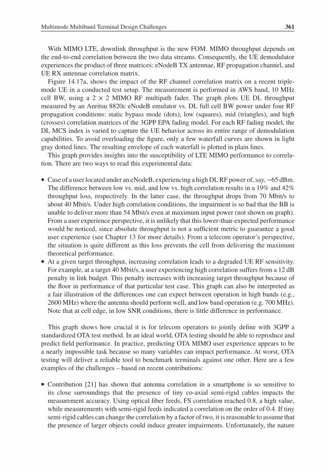
Multimode Multiband Terminal Design Challenges 361
With MIMO LTE, downlink throughput is the new FOM. MIMO throughput depends onthe end-to-end correlation between the two data streams. Consequently, the UE demodulatorexperiences the product of three matrices: eNodeB TX antennae, RF propagation channel, andUE RX antennae correlation matrix.
Figure 14.17a, shows the impact of the RF channel correlation matrix on a recent triple-mode UE in a conducted test setup. The measurement is performed in AWS band, 10 MHzcell BW, using a 2 × 2 MIMO RF multipath fader. The graph plots UE DL throughputmeasured by an Anritsu 8820c eNodeB emulator vs. DL full cell BW power under four RFpropagation conditions: static bypass mode (dots), low (squares), mid (triangles), and high(crosses) correlation matrices of the 3GPP EPA fading model. For each RF fading model, theDL MCS index is varied to capture the UE behavior across its entire range of demodulationcapabilities. To avoid overloading the figure, only a few waterfall curves are shown in lightgray dotted lines. The resulting envelope of each waterfall is plotted in plain lines.
This graph provides insights into the susceptibility of LTE MIMO performance to correla-tion. There are two ways to read this experimental data:
� Case of a user located under an eNodeB, experiencing a high DL RF power of, say,−65 dBm.The difference between low vs. mid, and low vs. high correlation results in a 19% and 42%throughput loss, respectively. In the latter case, the throughput drops from 70 Mbit/s toabout 40 Mbit/s. Under high correlation conditions, the impairment is so bad that the BB isunable to deliver more than 54 Mbit/s even at maximum input power (not shown on graph).From a user experience perspective, it is unlikely that this lower-than-expected performancewould be noticed, since absolute throughput is not a sufficient metric to guarantee a gooduser experience (see Chapter 13 for more details). From a telecom operator’s perspective,the situation is quite different as this loss prevents the cell from delivering the maximumtheoretical performance.
� At a given target throughput, increasing correlation leads to a degraded UE RF sensitivity.For example, at a target 40 Mbit/s, a user experiencing high correlation suffers from a 12 dBpenalty in link budget. This penalty increases with increasing target throughput because ofthe floor in performance of that particular test case. This graph can also be interpreted asa fair illustration of the differences one can expect between operation in high bands (e.g.,2600 MHz) where the antenna should perform well, and low band operation (e.g. 700 MHz).Note that at cell edge, in low SNR conditions, there is little difference in performance.
This graph shows how crucial it is for telecom operators to jointly define with 3GPP astandardized OTA test method. In an ideal world, OTA testing should be able to reproduce andpredict field performance. In practice, predicting OTA MIMO user experience appears to bea nearly impossible task because so many variables can impact performance. At worst, OTAtesting will deliver a reliable tool to benchmark terminals against one other. Here are a fewexamples of the challenges – based on recent contributions:
� Contribution [21] has shown that antenna correlation in a smartphone is so sensitive toits close surroundings that the presence of tiny co-axial semi-rigid cables impacts themeasurement accuracy. Using optical fiber feeds, FS correlation reached 0.8, a high value,while measurements with semi-rigid feeds indicated a correlation on the order of 0.4. If tinysemi-rigid cables can change the correlation by a factor of two, it is reasonable to assume thatthe presence of larger objects could induce greater impairments. Unfortunately, the nature

362 HSPA+ Evolution to Release 12
of interactions is so complex that no general rule governing the degradation of antennacorrelation can be drawn. For example, the study in [22] shows that a smartphone with goodFS performance can turn into a poor terminal in the presence of a human body – but the exactopposite is also true. The study in [23] goes a step further by measuring the impact of a realuser on antenna correlation vs. FS and phantom head. The study uses prototypes specificallydesigned to deliver high and low correlation performance in the 700 and 2600 MHz bands.Measurements demonstrate that the difference between high and low correlation decreaseswith UI, so much so that at 700 MHz, it becomes difficult to distinguish the two prototypesin the presence of a real person. This suggests that any ranking between good and baddevices based on FS and phantom head measurements might not be in agreement with themore subjective rankings resulting from actual use (see also [24]).
� In addition, antenna correlation varies vs. carrier frequency in a given band.� From the above results, it may be intuitively understood that the angle of arrival also plays
an important role. For example, one may expect that the use of phantom head only mightnot block as many incident waves as would be blocked by real person. This implies thatmeasuring user experience requires a 3D isotropic test setup. 3GPP is assessing three testmethods that could fulfill this requirement: anechoic, reverberation chambers, and a two-stage method. With their intrinsic 3D isotropic properties, reverberation chambers are anattractive solution to this problem.
� Another difference between lab measurements and practical user experience is that 3GPPtest cases do not include closed-loop interactions between a NodeB and UE. Good MIMOperformance is about making the best of the instantaneous radio conditions, either byusing frequency selective scheduling or by adapting rank. These closed-loop algorithmsare proprietary to each network equipment vendor and cannot be replicated using eNodeBemulators.
These are some of the complex challenges that OEMs, telecom operators, and chip setvendors are currently facing when it comes to defining OTA performance test cases. Not onlymust 3GPP assess and recommend test methods (AC, RC, or two-stage) but it must also definetest conditions and pass/fail criteria to provide operators with a reliable and realistic tool tobenchmark devices. Considering the complexity of the interactions between UE antennae andthe surroundings, this task is far from trivial.
14.1.3.4 RF Subsystem Control and IQ Interfaces
The conventional RF subsystem architecture relies on analog IQ RF-BB interfaces and a myriadof control interfaces specific to each of the RF-FE components. The primary disadvantages ofthis approach are twofold:
– The associated number of pins tends to be larger, which increases package size, cost, andfurther complicates PCB routing.
– Dealing with a wide variety of proprietary interfaces restricts the ease with which handsetmakers can “mix and match” RF-FE components, and often leads to software segmentation.
The example in Figure 14.18 shows a hypothetical downlink-only carrier aggregation RFsubsystem focusing on control and IQ interfaces only. In total, 47 pins are required. This

2
Div
ersi
ty r
ecei
ver
An
ten
na
tun
er**
Dip
lexe
r
Du
ple
xer
Inte
rban
dC
A
MM
-MB
PA
*
Du
ple
xer
AD
C
AD
C
AD
C
AD
C
DA
C
DA
C
AD
C
AD
C
AD
CIP
-IN
AD
C
ET
/AP
TD
C-D
C
DC
XO
Cry
stal
SY
SC
LK
SY
SC
LK
EN
Basebandmodem
3
TX IQ
SP
I
GPIO
SPI
DAC
DAC
GPIO
GPIO
34
4
3
2
33
to 5
Ban
dse
lect
swit
ches
e.g
. SP
10T
Sw
itch
e.g
. SP
5T2 2 2 2 2
2 2QP
-QN
IP-I
N
QP
-QN
IP-I
N
QP
-QN IP
-IN
QP
-QN
IP-I
N
QP
-QN
2
GPIO
GPIO
GPIO
Fig
ure
14.1
8LT
Ein
ter-
band
carr
iera
ggre
gatio
nhy
poth
etic
albl
ock
diag
ram
usin
gco
nven
tiona
lbus
es.P
inco
unt:
14(s
witc
hes)+
20(I
Q)+
8(P
A-C
TL
)+
3(S
PI)+
2(s
yscl
k)=
47pi
ns.I
nter
conn
ectf
orM
M-M
BPA
tem
pera
ture
sens
or(*
),an
dan
tenn
adi
rect
iona
lcou
pler
(**)
noti
nclu
ded.
For
illus
trat
ion
purp
oses
only
.Pin
coun
treq
uire
dfo
rR
Fsw
itch
cont
rolc
ould
bere
duce
dby
shar
ing
one
orse
vera
lset
sof
GPI
Olin
es
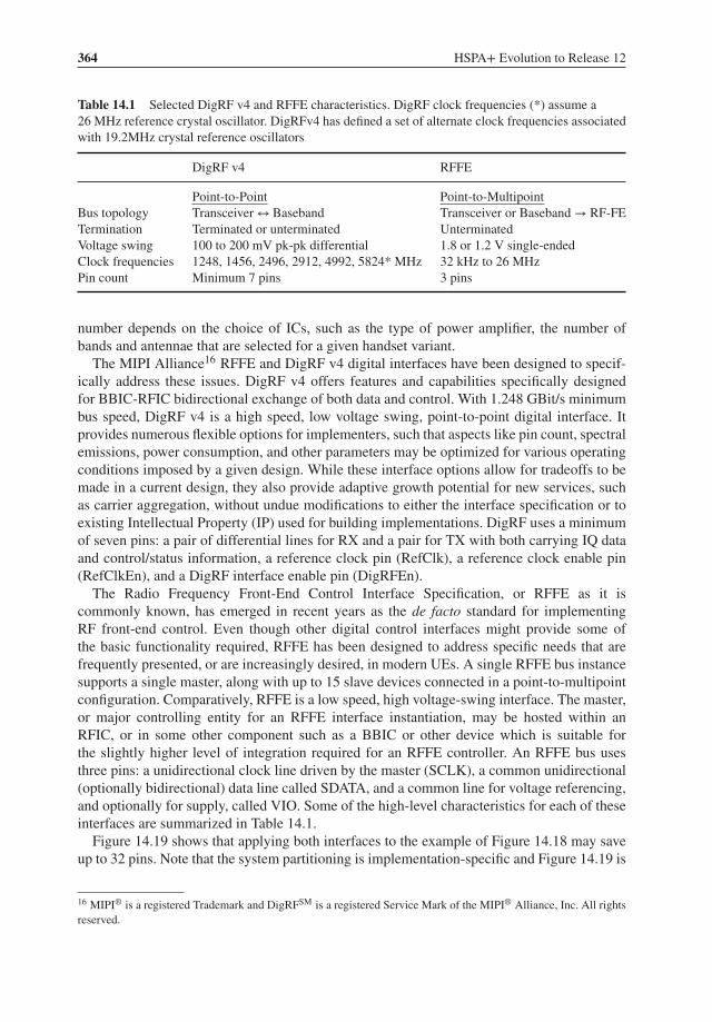
364 HSPA+ Evolution to Release 12
Table 14.1 Selected DigRF v4 and RFFE characteristics. DigRF clock frequencies (*) assume a26 MHz reference crystal oscillator. DigRFv4 has defined a set of alternate clock frequencies associatedwith 19.2MHz crystal reference oscillators
DigRF v4 RFFE
Point-to-Point Point-to-MultipointBus topology Transceiver ↔ Baseband Transceiver or Baseband → RF-FETermination Terminated or unterminated UnterminatedVoltage swing 100 to 200 mV pk-pk differential 1.8 or 1.2 V single-endedClock frequencies 1248, 1456, 2496, 2912, 4992, 5824* MHz 32 kHz to 26 MHzPin count Minimum 7 pins 3 pins
number depends on the choice of ICs, such as the type of power amplifier, the number ofbands and antennae that are selected for a given handset variant.
The MIPI Alliance16 RFFE and DigRF v4 digital interfaces have been designed to specif-ically address these issues. DigRF v4 offers features and capabilities specifically designedfor BBIC-RFIC bidirectional exchange of both data and control. With 1.248 GBit/s minimumbus speed, DigRF v4 is a high speed, low voltage swing, point-to-point digital interface. Itprovides numerous flexible options for implementers, such that aspects like pin count, spectralemissions, power consumption, and other parameters may be optimized for various operatingconditions imposed by a given design. While these interface options allow for tradeoffs to bemade in a current design, they also provide adaptive growth potential for new services, suchas carrier aggregation, without undue modifications to either the interface specification or toexisting Intellectual Property (IP) used for building implementations. DigRF uses a minimumof seven pins: a pair of differential lines for RX and a pair for TX with both carrying IQ dataand control/status information, a reference clock pin (RefClk), a reference clock enable pin(RefClkEn), and a DigRF interface enable pin (DigRFEn).
The Radio Frequency Front-End Control Interface Specification, or RFFE as it iscommonly known, has emerged in recent years as the de facto standard for implementingRF front-end control. Even though other digital control interfaces might provide some ofthe basic functionality required, RFFE has been designed to address specific needs that arefrequently presented, or are increasingly desired, in modern UEs. A single RFFE bus instancesupports a single master, along with up to 15 slave devices connected in a point-to-multipointconfiguration. Comparatively, RFFE is a low speed, high voltage-swing interface. The master,or major controlling entity for an RFFE interface instantiation, may be hosted within anRFIC, or in some other component such as a BBIC or other device which is suitable forthe slightly higher level of integration required for an RFFE controller. An RFFE bus usesthree pins: a unidirectional clock line driven by the master (SCLK), a common unidirectional(optionally bidirectional) data line called SDATA, and a common line for voltage referencing,and optionally for supply, called VIO. Some of the high-level characteristics for each of theseinterfaces are summarized in Table 14.1.
Figure 14.19 shows that applying both interfaces to the example of Figure 14.18 may saveup to 32 pins. Note that the system partitioning is implementation-specific and Figure 14.19 is
16 MIPI® is a registered Trademark and DigRFSM is a registered Service Mark of the MIPI® Alliance, Inc. All rightsreserved.
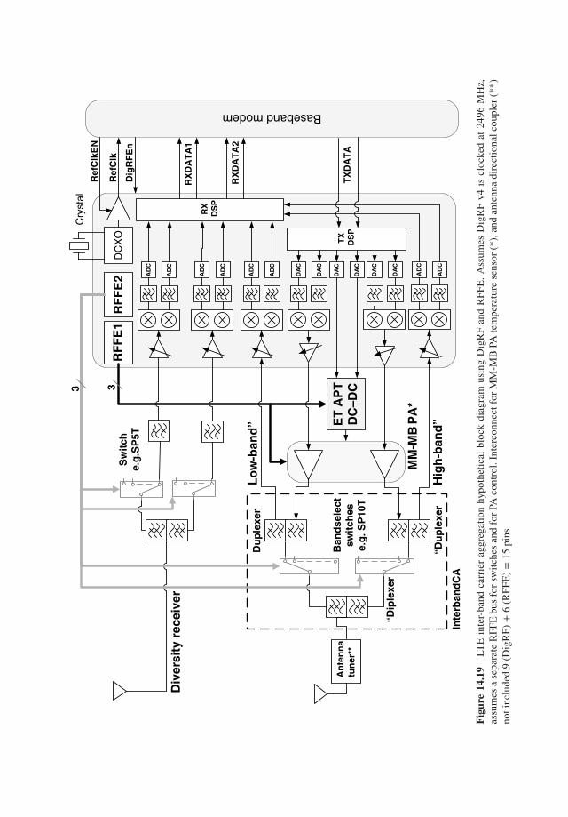
Div
ersi
ty r
ecei
ver
An
ten
na
tun
er**
Lo
w-b
and
”
“Dip
lexe
r
Du
ple
xer
Inte
rban
dC
A
MM
-MB
PA
*
Hig
h-b
and
”“D
up
lexe
r
Ban
dse
lect
swit
ches
e.g
. SP
10T
AD
C
AD
C
DA
C
DA
C
AD
C
AD
C
DA
C
DA
C
AD
C
AD
C
AD
C
AD
C
DA
C
DA
C
ET
AP
TD
C–D
C
RX
DS
P
TX
DS
P
RF
FE
1R
FF
E2
DC
XO
Cry
stal
Ref
Clk
Ref
Clk
EN
RX
DA
TA
1
TX
DA
TA
RX
DA
TA
2
Dig
RF
En
Baseband modem
3 3S
wit
che.
g.S
P5T
Fig
ure
14.1
9LT
Ein
ter-
band
carr
ier
aggr
egat
ion
hypo
thet
ical
bloc
kdi
agra
mus
ing
Dig
RF
and
RFF
E.
Ass
umes
Dig
RF
v4is
cloc
ked
at24
96M
Hz,
assu
mes
ase
para
teR
FFE
bus
for
switc
hes
and
for
PAco
ntro
l.In
terc
onne
ctfo
rM
M-M
BPA
tem
pera
ture
sens
or(*
),an
dan
tenn
adi
rect
iona
lcou
pler
(**)
noti
nclu
ded.
9(D
igR
F)+
6(R
FFE
)=
15pi
ns
366 HSPA+ Evolution to Release 12
only presented to illustrate cost/pin savings. If the RF IC is already pin count limited, it mightbe decided to “host” some, or all, of the RFFE buses either in the BBIC or in the PMIC.
Beyond these direct hardware savings, both interfaces provide additional advantages whichcan be of benefit to both component suppliers and platform designers.
With DigRF, IQ ADCs and DACs are located in the RF TRX. The BB IC may then becomea pure digital IC, which helps in decoupling the CMOS node used in each IC. The BB maythen be shrunk/ported to the latest CMOS node more easily, while the RF transceiver canremain in an “older” CMOS node which offers a more appropriate performance/cost/powerconsumption tradeoff specific to the needs of the RF IC. This is particularly important asthe latest, most advanced CMOS nodes rarely offer the design libraries required to simulateand design all portions of the complex RF transceiver. Further, the DigRF interface was alsodefined to assist handset makers to interface RF ICs and BB ICs from different suppliers,which allows more flexibility in component selection. DigRF also provides a standardizedand low pin count debug interface to monitor traffic at the IQ interface. Indeed, a number ofwell-known test equipment providers distribute systems to enable this capability. For chip setmakers, DigRF v4 is built upon MIPI’s M-PHY, a physical layer IP which, once developedfor DigRF, may be reused for other protocols and applications, since an increasing numberof applicable standards use the M-PHY physical layer. IP reuse is increasingly important inmeeting tough time-to-market deadlines. For example, future generations of DDR memoriescould make use of M-PHY, and an existing standard for FLASH already leverages M-PHY.
For RF front-end components, the current situation with regards to the types, numbers, andsuppliers of these is perhaps even more diverse and far-reaching. To handset makers, RFFEis a tool which considerably simplifies the selection, ease of integration, and swapping ofRF-FE components. To RF-FE IC makers, it offers increased opportunities to integrate withmany chip set platforms, while implementing a single, widely-deployed control interface.With a wide array of optional features, particularly for slaves, this ensures that a bus and, inparticular, the FE components may be optimized for the features implemented vs. cost and theimplementation technology. RFFE’s wide scope of applicability to FEMs provides increasedpotential for IP reuse of hardware and/or software.
As with any interfaces deployed in an RF-sensitive area, one must pay special attention tothe issues of EMI/co-existence management. The specifics of each of these interfaces leads todifferent co-existence challenges. The main issue with DigRF v4 in this respect is that even atits lowest operating clock frequency of 1248 MHz, the first spectrum lobe of a pair of lanesoverlaps all UHF cellular frequency bands. At 2496 MHz, it is nearly the entire set of 3GPPoperating bands which fall under the first lobe. In addition, with high duty cycle operation forstandards such as LTE, the probability of collision in the time domain is high. For example, inthe case of LTE single carrier 20 MHz operation, the load of a single RX pair of lanes rangesfrom 137% at 1248 MHz (and thus requires two pairs of lanes) to 67% at 2496 MHz usingone lane pair [5]. The inherent flat decay of the common mode PSD also poses some threats todifferential LNA input structures. Factors which tend to help in reducing co-existence issuesare that the interface may be operated using low voltage swings, in a controlled transmissionimpedance, and with bus routing that in most handset designs is unlikely to be routed at, ornear, the sensitive front-end components such as antennae. RF transceiver pin-to-pin isolationis therefore the main coupling mechanism.
With RFFE being a control interface only, the bus load is often bursty, with only rareinstances where higher bus loading might be required. Therefore, the probability of collision

Multimode Multiband Terminal Design Challenges 367
in the time domain is lowered. In addition, its relatively low frequency range of operation (32kHz to 26 MHz) is such that even the lowest cellular frequency bands, such as the LTE 700MHz bands, are located at the 28th and 22 500th harmonic of the extreme interface rates of26 MHz and 32 kHz, respectively. This provides plenty of “room” to implement spectrallyefficient pulse shaping techniques. Yet, in contrast to DigRF, RFFE voltage swing is higher,and its point-to-multipoint topology can lead to longer PCB traces, some of which may berouted close to sensitive front-end components. Further, since the bus is not designed to beterminated, its impedance is more difficult to control, and any reflections will tend to impair thedecay of spectral lobes. Because PSD decays slowly at high harmonic numbers, and pin-to-pinisolation decreases as operating frequency increases, RFFE co-existence issues may dominateabove 1 GHz of operation. The most sensitive victim of this may be GPS, which requiresaggressor noise PSD < −180 dBm/Hz to prevent less than 0.2 dB desense.
To help both chip set vendors and handset makers foresee co-existence issues in the earlyphase of product development, and to prepare for them, both DigRF and RFFE working groupsanticipated the need to include a set of EMI mitigation tools. These unique features providea rich, efficient, and yet relatively simple-to-implement set of techniques for reducing theassociated impacts in the frequency and the power domains.
Pulse shaping/slew rate control: Perhaps the most efficient of all EMI tools madeavailable to handset makers. This feature allows shaping of the rising and fallingedges of each transmitted bit so as to reduce the power spectral density (PSD) ofthe digital bit stream. This is available in both DigRF [5] and in RFFE.
Amplitude control: A simple and yet efficient way of reducing the aggressorPSD. This option is available in DigRF, and also to a certain extent in RFFE,where 1.2 V is also specified in addition to 1.8 V.
Clock dithering: A useful feature in cases when repetitive and frequent trans-missions of a given pulse pattern generate discrete spurs colliding with a cellularvictim. This can be the case, for example, for the DigRF training sequence trans-mitted at the beginning of each burst to ease clock recovery. This tool is availableas a part of the DigRF specification. It is also inherent in RFFE, where the masterclock may be dithered between messages, since the clock used for control infor-mation need not be related to RF data. Also in RFFE, the timing between messagesmay be randomized, offering some ability to affect the “signature” for both clockand data streams.
Alternate clock frequency: This feature is available in both interfaces and canbe used to either place the victim in the vicinity of a spectral “zero” or “null,”or by placing the victim under a higher order spectral lobe. For example, inDigRF v4, if GPS RX is desensitized when the bus is operated at 1248 MHz,the alternate clock rate of 1496 MHz places the GPS RX in close proximity ofthe first DigRF spectral null. In this instance, the aggressor PSD is significantlyreduced with minimal impact on DigRF performance. In RFFE the extent ofany harmonics is relatively narrow, and a slight change in the fundamental mayoften be utilized to move a resultant spike away from a specific band frequencyof interest.
368 HSPA+ Evolution to Release 12
With the increasing need for more reconfigurable RF subsystems, and the mounting com-plexity in RF-FEs, these interfaces offer handset designers effective means for the solution ofcomplex challenges. The ability to tailor them to specific needs provides component supplierswith an efficient method to achieve faster design cycles and to foster reuse. And, because EMIeffects have been taken into consideration from the outset, these interfaces provide featureswell-suited to the goals and situations of all those involved in UE design. The DigRF interfacewill be adding 4998 MHz operation as a means to extend applicability to the future higherbandwidth requirements of carrier aggregation. And work is underway on RFFE to furtherenhance interface throughput, which will help to improve critical timing, and provide evenmore bandwidth for increasingly complex RF-FEs. Thus both of these interfaces offer con-tinued promise for the future of handset design through cost minimization and complexityreduction, while also maximizing business opportunities.
14.1.3.5 Co-Existence Challenges
The principles of co-existence have been introduced in Section 14.1.2, where due to thefull duplex nature of WCDMA, a UE located at cell edge may be desensitized due to itsown transmitter being operated at maximum output power. In this relatively simple example,solutions range from the use of external SAW filters, to novel RF TRX architectures, and inthe most challenging cases to 3GPP relaxations.
Co-existence issues become significantly more complex when multiple radios start to inter-act with each other, or when a radio is operated in the presence of internal jammers that arenot enabled during conformance tests. For example, WCDMA receiver sensitivity may beimpacted by USB high speed harmonics during a UE to external PC media transfer. In SoCs,aggressors range from simple clock harmonics, to noisy high speed digital buses associatedwith DSP, CPUs, camera and display interfaces, high current rating DC–DC converters, USBand HDMi ports. As for victims, nearly all RF subsystems are susceptible to EMI interference.Further complexity arises from the fact that RF transmitter chains are not exempt from becom-ing victims of these digital aggressors. Desensitization occurs when aggressors collide withvictims in time, frequency, and power domains. In SoCs, both conducted and electromagneticcoupling may occur. The WCDMA UE RF self-desense is one example of conducted coupling.Coupling via power supply rails and/or ground currents is another. Electromagnetic couplingmay occur via pin-to-pin interactions, bonding wires, PCB track-to-track, and even antenna-to-antenna coupling. Problems are exacerbated when collisions occur between the cellular andthe connectivity radios. For example, the third harmonics of band 5 fall into WLAN 2.4 GHz,while the WLAN 5 GHz receiver might become victim of either band 2, or band 4 thirdharmonics, or band 5 seventh harmonics. The number of scenarios may become so great thatco-existence studies often have to be performed using a multidimensional systems analysis.This topic constitutes an excellent playing field for innovative mitigation techniques, whichcommonly fall into two categories:
� Improve victim’s immunity by increasing isolation in all possible domains: floor planoptimization, careful PCB layout, the use of RF and power supply filters as well as RFshielding. Victims may also be protected by ensuring non-concurrent operations in time.
Multimode Multiband Terminal Design Challenges 369
� Reduce the aggressor signal level. Slew rate and voltage swing control are two of the mostefficient techniques to reduce the level of interference at RF. Slew rate control consists inshaping the rising and falling edges of digital signals. This results in an equivalent low-pass filtering of the digital signal high-frequency content, and therefore helps to reduce theaggressor power spectral density in the victim’s bands. For example, DigRFSMv4 line driversare equipped with slew rate control as a tool to reduce EMI. Frequency evasion is anothercommonly used technique [25]. For example, if the harmonic of a digital clock is identified asa source of desensitization, it is tempting to slightly alter the clock frequency only when thevictim is tuned to the blocked channel. Frequency avoidance can be implemented by eithersimple frequency offset, or by dithering (e.g., DigRFSMv4, Section 14.1.3.4), frequencyhopping, or even by using direct sequence spreading of the clock.
The well-documented example of Band 4 (B4) – Band 17 (B17) carrier aggregation is agood illustration of co-existence issues within the cellular RF subsystem. B17 transmitterchain third harmonics (H3) can entirely overlap the B4 receiver frequency band. Nearly allcomponents in the RF-FE generate B17 H3, with the PA being, of course, the dominant source.It has been shown in [26] that the sole contribution of the PA would cause 36 to 43 dB B4 RXdesensitization, therefore calling for the insertion of a harmonic rejection filter. This mightnot solve the problem entirely since other sources of leakage, such as PCB coupling and TRXpin-to-pin isolation may dominate system performance [27]. Given reasonable PCB isolationand typical component contributions, B4 RX desense should not exceed 7 to 9 dB for 10 MHzand 5 MHz bandwidth operation respectively [28].
14.2 Power Consumption Reduction in Terminals
14.2.1 Smartphone Power Consumption
Poor battery life is probably at the top of the list of criticisms that smartphones face today.Users commonly have to recharge their terminals on a daily basis, and perhaps more oftenwith heavy usage. Such a need clearly affects the user’s experience. Figure 14.20 providessome of the factors to help illustrate the current experience. The bar graph on the left plotsthe evolution of the WCDMA subsystem power consumption for feature phones, comparedto a selection of recent smartphones. The measurements are performed with the LCD screen“switched-off,” and at minimum transmit output power, so as to minimize both the impactof the power amplifier and screen-related contributions. Not surprisingly, the trend in powerconsumption reduction is similar in both families of terminals. It is interesting to note thelatest generation of chip sets used in smartphones outperforms even the best cost-optimizedsolution of the recent feature phones. For example, phone F consumes nearly twice as muchas smartphone J.
The pie charts in Figure 14.20 show the impact of display-related contributors, such asscreen, backlighting, and application engine, on the overall power consumption over theduration of a WCDMA voice call. The voice call consumption is measured according to theGSMA TS09 guidelines. In feature phone F, 70% of the total power consumption is related tothe cellular subsystem, while screen-related activities only account for the remaining 30%. Insmartphone J, the situation is completely reversed: the “cellular”-“screen-related” contributionsplit is 30–70%. Despite its state-of-the-art cellular power consumption, the smartphone J total
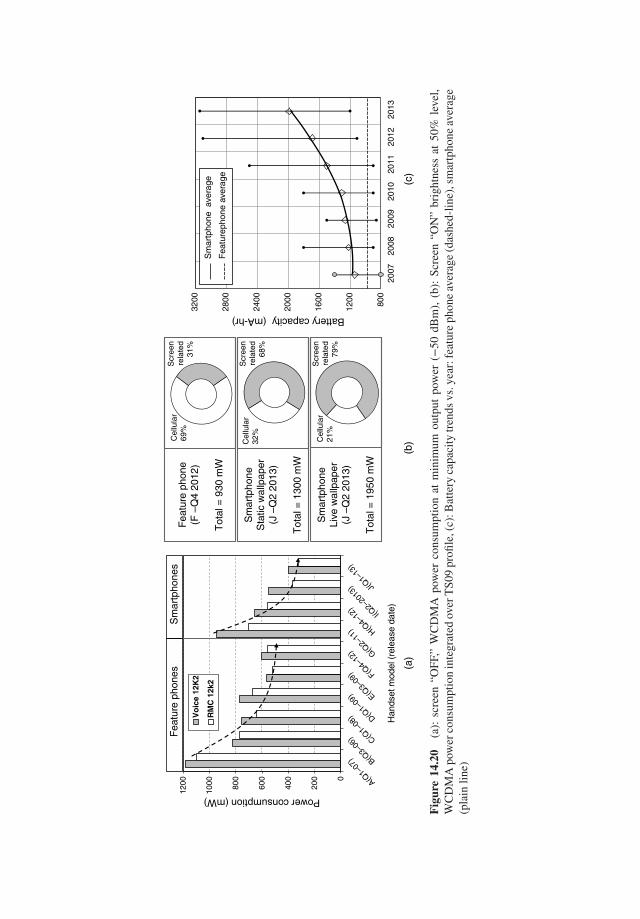
0 A(Q1–
07) B(Q
3–06
) C(Q1–
08) D(Q
1–09
) E(Q3–
09) F(Q
4–12
) G(Q2–
11) H(Q
4–12
)I(Q
2–20
13) J(
Q1–13
)
200
400
600
800
1000
1200
Power consumption (mW)
Han
dset
mod
el (
rele
ase
date
)
Vo
ice
12K
2
RM
C 1
2k2
Fea
ture
pho
nes
Sm
artp
hone
s
Scr
een
rela
ted
79%
Cel
lula
r21
%
Cel
lula
r32
%
Scr
een
rela
ted
68%
Cel
lula
r69
%
Scr
een
rela
ted
31%
Sm
artp
hone
Sta
tic w
allp
aper
(J –
Q2
2013
)
Tot
al =
130
0 m
W
Fea
ture
pho
ne(F
–Q
4 20
12)
Tot
al =
930
mW
Sm
artp
hone
Live
wal
lpap
er(J
–Q
2 20
13)
Tot
al =
195
0 m
W80
0
1200
1600
2000
2400
2800
3200
2007
2008
2009
2010
2011
2012
2013
Battery capacity (mA-hr)
Sm
artp
hone
ave
rage
Fea
ture
phon
e av
erag
e
(a)
(b)
(c)
Fig
ure
14.2
0(a
):sc
reen
“OFF
,”W
CD
MA
pow
erco
nsum
ptio
nat
min
imum
outp
utpo
wer
(−50
dBm
),(b
):Sc
reen
“ON
”br
ight
ness
at50
%le
vel,
WC
DM
Apo
wer
cons
umpt
ion
inte
grat
edov
erT
S09
profi
le,(
c):B
atte
ryca
paci
tytr
ends
vs.y
ear:
feat
ure
phon
eav
erag
e(d
ashe
d-lin
e),s
mar
tpho
neav
erag
e(p
lain
line)
Multimode Multiband Terminal Design Challenges 371
power consumption, particularly when used with a live (or animated) wallpaper, is doublethat of feature phone F. Feature phones are almost entirely designed with an eye towardscommunication functions, such as voice calls, SMSs, and MMSs. However, with smartphones,recent user activity statistics [29] show that users spend only 25% of their time making voicecalls. The remaining 75% of the user’s time is spent on activities such as video streaming,web surfing, gaming, or activities related to entertainment or social networking. Each of theseuse cases implies heavier screen activity. This serves to explain why the power consumptionis so high for smartphones. It also explains why, with nearly 2000 mAh battery capacity(Figure 14.20b), the modern smartphone, with its high resolution displays and more powerfulapplication engine, requires a battery nearly twice as large, and therefore heavier, than theaverage feature phone. It also helps to understand why, despite this fact, that battery life isstill a factor for users. And finally, the split between cellular and screen-related activity alsoexplains why advanced 3GPP battery saving features, such as continuous packet connectivity,with discontinuous reception and transmission (DRX, DTX), have a limited impact on userexperience. Section 14.2.2 highlights screen related contributors with a focus on the applicationengine. Techniques in mass production to improve the cellular power amplifier efficiency arepresented in Section 14.2.3. Challenges associated with the implementation of CPC DRX arepresented in Section 14.2.4.
With this high dependency on screen content and user activity, the estimation of battery lifehas become a rather complex task as the UE power consumption should now be assessed overa 24-hour user activity profile. The UE power consumption should then be assessed for eachsubsystem (WiFi, cellular, BT, FM, GPS), for each activity, and then could be finally averagedfor a given customer profile. An example of such a profile can be found in Chapter 13. Itis worth noting that, at the time of writing, the CTIA battery ad hoc group has launched aninitiative which aims at defining such profiles so that published battery life better reflects theend user experience.
14.2.2 Application Engines
Over the last 15 years, mobile phones have evolved from voice centric, low-resolution, andsmall display size “feature phones” to data-centric “smartphones.” With their high screenresolution and large size displays, smartphones have considerably improved web browsingand gaming user experience. Figure 14.21 shows that display size has gained on average 1inch over the last three years, with most devices now using between 4′′ and 6′′ displays. Atthe same time, display resolution has grown exponentially to reach the full HD resolutionof TV screens (1080 p). The growth in screen resolution has been one of the key drivers inthe race to deliver more processing power in graphic processor units (GPU) and applicationengines (APE).
As pointed out in Figure 14.20, screen-related activity dramatically increases the UE powerconsumption. Figure 14.22 provides a detailed breakdown of the “screen-related” contributionsvs. use case in a low-end Android smartphone. Camcorder, gaming, and video playbackestimations assume flight mode. HSPA+ data and WCDMA voice call assume the UE screenis in “off” state. The HSPA background emulates an email synchronization use case, usinga single carrier HSDPA cat 14, HSUPA cat 6, and an animated wallpaper identical to thatused in the pie chart in Figure 14.20. Summing all screen-related contributors associated with

372 HSPA+ Evolution to Release 12
0
500
1000
1500
2000
2500
2009 2010 2011 2012 2013 2014
Dis
play
Res
olut
ion
(Kilo
pix
els)
Commercial release
2.0
3.0
4.0
5.0
6.0
2007 2008 2009 2010 2011 2012 2013
Dis
play
siz
e (
inch
)
Commercial release
4th generation4th generation
3rd generation
3rd generation 2nd generation
2nd generation1st generation
1st generation
(a) (b)
Figure 14.21 (a) Display resolution for four generations of an iconic tier-one smartphone family, (b)Display size trend
the animated wallpaper use case, the cellular/screen-power consumption ratio is 40–60% and32–68% for HSPA background and voice call respectively. Zooming in on the screen-relatedcontributors, the screen and its backlight circuitry consume nearly as much as the whole DC–HSPA+ cellular subsystem. The second biggest contributor is the center of attention in thissection: the application engine (APE).
The APE CPU is in charge of two main tasks: general purpose processing and off-loadingof computing intensive tasks to the GPU. Both CPU and GPU performance has constantlyincreased over the last decade. Figure 14.23a shows that in the last three years, the growthhas risen exponentially, reaching near 35 000 Dhrystone Mega Instructions Per Second(DMIPS).
Relating user experience to APE processing power is not trivial, as performance experiencedby the end user depends on the nature of the tasks required by the application, its mapping toeither CPU, GPU, or both, and also the performance of external key components such as thedynamic random access memory (DRAM). For example, Figure 14.23b shows that doublingthe CPU performance from 750 to 1500 MHz on an Android dual core CPU platform reducesthe loading and initialization time of the Temple Run2 game by only a factor of 1.5. In otherwords, increasing the CPU/GPU clock frequency does not always result in a linear increase inperformance across all use cases. In this simple example, the interface bus speed, Double DataRate (DDR) DRAM, and IOs (eMMC, μSD) latencies may dominate the APE performanceperceived by the end user. The ever-increasing CPU and GPU operating clock frequencieshave pushed mobile phone DRAM vendors to reach an unprecedented level of performance.Recent DRAM can sustain transfer rates on the order of 17 GB/s. Despite this impressivelevel of performance, DDR may, under certain use cases, remain the performance bottleneckabove a certain CPU/GPU clock frequency. One illustration is presented in Figure 14.24bwhich shows that layout Vellamo scores increase linearly with CPU clock frequency. Vellamois a benchmark tool which measures HTML5 performance and user experience. However, theOcean zoomer and scroller scores in Figure 14.24a exhibit a performance floor. In this use case,increasing CPU clock frequency above 1 GHz does not significantly improve performance.
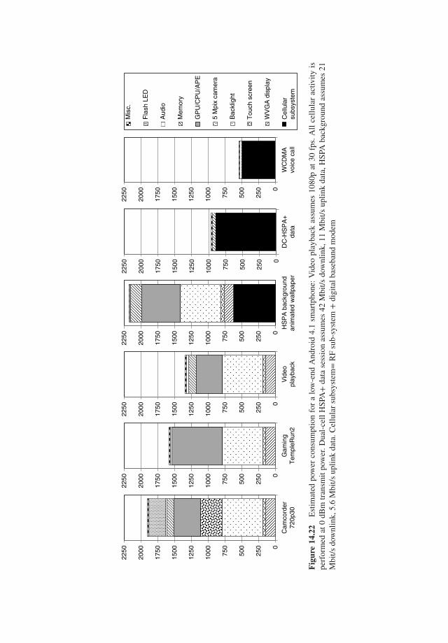
0
250
500
750
1000
1250
1500
1750
2000
2250
Cam
cord
er72
0p30
0
250
500
750
1000
1250
1500
1750
2000
2250
Gam
ing
Tem
pleR
un2
0
250
500
750
1000
1250
1500
1750
2000
2250
Vid
eopl
ayba
ck
0
250
500
750
1000
1250
1500
1750
2000
2250
0
250
500
750
1000
1250
1500
1750
2000
2250
DC
-HS
PA
+da
ta
0
250
500
750
1000
1250
1500
1750
2000
2250
WC
DM
Avo
ice
call
HS
PA
bac
kgro
und
anim
ated
wal
lpap
er
Mis
c.
Fla
sh L
ED
Aud
io
Mem
ory
GP
U/C
PU
/AP
E
5 M
pix
cam
era
Bac
klig
ht
Tou
ch s
cree
n
WV
GA
dis
play
Cel
lula
rsu
bsys
tem
Fig
ure
14.2
2E
stim
ated
pow
erco
nsum
ptio
nfo
ra
low
-end
And
roid
4.1
smar
tpho
ne:
Vid
eopl
ayba
ckas
sum
es10
80p
at30
fps.
All
cellu
lar
activ
ityis
perf
orm
edat
0dB
mtr
ansm
itpo
wer
.Dua
l-ce
llH
SPA+
data
sess
ion
assu
mes
42M
bit/s
dow
nlin
k,11
Mbi
t/sup
link
data
,HSP
Aba
ckgr
ound
assu
mes
21M
bit/s
dow
nlin
k,5.
6M
bit/s
uplin
kda
ta.C
ellu
lar
subs
yste
m=
RF
sub-
syst
em+
digi
talb
aseb
and
mod
em

374 HSPA+ Evolution to Release 12
15
20
25
30
35
40
45
50
55
60
350 550 750 950 1150 1350 1550
Ave
rage
initi
aliz
atio
n tim
e (
sec)
CPU max.clock frequency (MHz)
0
50
100
150
200
250
300
0
5000
10000
15000
20000
25000
30000
35000
40000
2007 2009 2011 2013 2015
AP
E G
PU
per
form
ance
(M
tri/s
)
AP
E-C
PU
Per
form
ance
(D
MIP
S)
Commercial release
CPU evolution
GPU evolution
(a) (b)
Figure 14.23 (a): CPU and GPU performance evolution over year. (b): TempleRun2 game applicationload and initialization time vs. CPU performance
In summary, user experience depends on many variables: intrinsic DDR, CPU and GPUperformance matters, but also the ability of the CPU to efficiently serve the GPU comesinto play.
Finally, user experience is also impacted by the way mobile applications are developed.The trend has evolved from pre-embedded, custom designed applications for a given terminalplatform, to the world of online application (market) stores. While it was possible to optimizeapplications for a certain handset prior to mass production, applications must now be developedfor a heterogeneous set of chip sets. The challenge in selecting CPU performance now consistsin tailoring the best performance power consumption tradeoff in anticipation of applicationsthat will be created after the handset has been commercialized.
0
2
4
6
8
10
12
14
16
350 550 750 950 1150 1350 1550
Vel
lam
o sc
ore
(low
eris
bet
ter)
CPU max. clock frequency (MHz)
Ocean zoomer (Speed)Ocean scroller (Load time)
0
20
40
60
80
100
120
350 550 750 950 1150 1350 1550
Vel
lam
o sc
ore
(hig
her
is b
ette
r)
CPU max. clock frequency (MHz)
DOM node surferRefloSurf wax binder
(a) (b)
Figure 14.24 (a): Vellamo HTML5 user experience benchmark. (b): Vellamo scripting and layoutperformance. Both measurements are performed using a high end, dual-core Android smartphone
Multimode Multiband Terminal Design Challenges 375
When it comes to increasing APE performance, three techniques are commonly used:
� Increase CPU clock speed. Increasing CPU clock to the 2 GHz mark while keeping powerconsumption reasonably low has been made possible thanks to the rapid CMOS technologyshrink over the last decade. Two key tools have made this achievement feasible: DigitalVoltage Frequency Scaling (DVFS) in hardware and Operating Processing Point (OPP) insoftware.
� Increase CPU pipeline length: this technique improved the DMIPS/MHz performance.In the example of the ARM17® CPU core family, performance has improved from 1.25DMIPS/MHz for the ARM1176TM to 3.5DMIPS/MHz for the Cortex®-A15 processor.
� Increase the number of cores per CPU. In 2011, the introduction of Multi Processing (MP)capable cores such as the ARM Cortex-A9 MP capable core, together with symmetricalmultiprocessing (SMP), enabled parallelizing of software processing on 2 to 4 Cortex®-A9cores. These recent advances multiply the theoretical maximum performance of the CPUby a factor of 4. Nevertheless, increasing the number of cores only makes sense if the OSkernel and the applications are designed to provide a high level of parallel tasking. ApplyingAmdahl’s law [30] to a quad-core CPU shows that performance gains become negligible ifless than 75% of parallelism is effective.
However, this increase in CPU performance comes at the expense of both static and dynamicpower consumption. ARM big.LITTLETM processing aims to deliver the best combinationof performance and power consumption by pairing two processors in a coherent system. Inthe first instance a “big” high-performance quad-core Cortex-A15 processor is paired with a“little” energy efficient, quad-core Cortex-A7 processor. The Dhrystone benchmark shows that“little” cores are 3.5 times more energy efficient than the “big” cores, while “big” cores are 1.9times more powerful. Ideally, demanding tasks would be scheduled on the “big” cores whileless-demanding and background tasks would be scheduled on the “little” cores to optimizepower consumption.
There are currently three possible modes of operation for ARM big.LITTLETM technology.The simplest approach called the “cluster migration” consists in creating two types of clusters:a cluster made up of a maximum of four “little” cores, and a cluster of up to four “big” cores.The software tasks are then either mapped to one cluster or another. This has the advantageof presenting a homogeneous set of processors to the programmers. The main disadvantage isthat, at best, only half of the total number of cores is active.
The second approach, called CPU migration, is slightly more complex. It consists in creatinglogical pairs made up of one “big” and one “little” physical core. The special case of a quad-coreAPE is shown in Figure 14.25a. Compared to cluster migration, this solution remains relativelysimple to operate as switching between physical cores can be done by the Linux governorusing both OPP, DVFS, and CPU cores hot-plugging techniques. The main drawback of theCPU migration approach is that it also uses only half of the available cores. Further, a workloadoscillating between low and high performance can lead to user experience degradation. Toavoid these oscillations, a hysteresis scheme is often implemented using OPP sticky points.
17 ARM and Cortex are registered trademarks of ARM Limited (or its subsidiaries) in the EU and/or elsewhere.big.LITTLE is a trademark ARM Limited (or its subsidiaries) in the EU and/or elsewhere. All rights reserved.
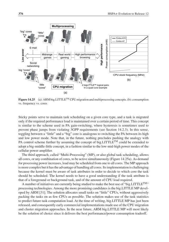
376 HSPA+ Evolution to Release 12
big “cores”
Pow
er c
onsu
mpt
ion
(mW
)
CPU clock frequency (MHz)
Cortex-A15
Cortex-A7
“big” cores
Hig
h p
erfo
rman
ce
“little”cores
Lo
w p
ow
er
Multiprocessing
CPU migration
zMidrange
gamesReal world
gamingHigh performance
browsing
Socialnetworking
little“cores”
2 bigLITTLE™ logical pairsIn a quad core example
(a)
(b)
Figure 14.25 (a): ARM big.LITTLETM CPU migration and multiprocessing concepts. (b): consumptionvs. frequency vs. cores
Sticky points serve to maintain task scheduling on a given core type, and a task is migratedonly if the required performance load is maintained over a certain period of time. This conceptis similar to the scheme used in PA gain-switching, where hysteresis is sometimes used toprevent phase jumps from violating 3GPP requirements (see Section 14.2.3). In this sense,toggling between a “little” and a “big” core is analogous to switching the PA between its highand low power mode. Note that, in the future, nothing precludes pushing the analogy withPA control scheme further by assuming the concept of big.LITTLETM could be extended toadopt a big-middle-little concept, in a fashion similar to the low-mid-high power modes of thecellular power amplifier.
The third approach, called “Multi-Processing” (MP), or also global task scheduling, allowsall cores, or any combination of cores, to be active simultaneously (Figure 14.25a). As demandfor processing power increases, load may be scheduled from one to all cores. The MP approachis more complex but it has the advantage of handling all cores. Its implementation is challengingbecause the kernel must be aware of task attributes in order to decide to which core the taskshould be scheduled. The kernel needs to have a good understanding if the task attribute isthat of a foreground or background task, and of the amount of CPU load required.
A number of initiatives are currently being studied to make the best use of “big.LITTLETM”processing technologies. Among the more promising candidates is the big.LITTLE MP devel-oped by ARM [31]. The solution allocates small tasks on “little” CPUs, without aggressivelypacking the tasks on as few CPUs as possible. The solution makes use of the task statisticsto predict future task computation load. At the time of writing, big.LITTLE MP has just beenreleased, and consequently early commercial implementations made use of the CPU migrationand cluster migration approaches. In the near future, ARM big.LITTLE MP will most likelybe the solution of choice since it delivers the best performance/power consumption tradeoff.
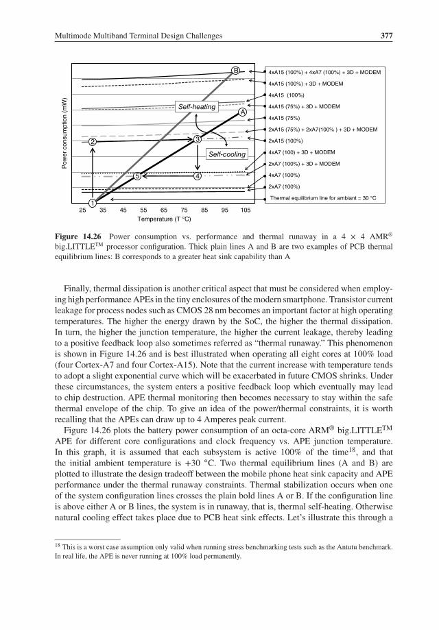
Multimode Multiband Terminal Design Challenges 377
25 35 45 55 65 75 85 95 105
Pow
er c
onsu
mpt
ion
(mW
)
Temperature (T °C)
4xA15 (100%) + 4xA7 (100%) + 3D + MODEM
4xA15 (100%) + 3D + MODEM
4xA15 (100%)
4xA15 (75%) + 3D + MODEM
4xA15 (75%)
2xA15 (75%) + 2xA7(100% ) + 3D + MODEM
2xA15 (100%)
4xA7 (100) + 3D + MODEM
2xA7 (100%) + 3D + MODEM
4xA7 (100%)
2xA7 (100%)
Thermal equilibrium line for ambiant = 30 °C
Self-cooling
2 3
45
1
A
B
Self-heating
Figure 14.26 Power consumption vs. performance and thermal runaway in a 4 × 4 AMR®
big.LITTLETM processor configuration. Thick plain lines A and B are two examples of PCB thermalequilibrium lines: B corresponds to a greater heat sink capability than A
Finally, thermal dissipation is another critical aspect that must be considered when employ-ing high performance APEs in the tiny enclosures of the modern smartphone. Transistor currentleakage for process nodes such as CMOS 28 nm becomes an important factor at high operatingtemperatures. The higher the energy drawn by the SoC, the higher the thermal dissipation.In turn, the higher the junction temperature, the higher the current leakage, thereby leadingto a positive feedback loop also sometimes referred as “thermal runaway.” This phenomenonis shown in Figure 14.26 and is best illustrated when operating all eight cores at 100% load(four Cortex-A7 and four Cortex-A15). Note that the current increase with temperature tendsto adopt a slight exponential curve which will be exacerbated in future CMOS shrinks. Underthese circumstances, the system enters a positive feedback loop which eventually may leadto chip destruction. APE thermal monitoring then becomes necessary to stay within the safethermal envelope of the chip. To give an idea of the power/thermal constraints, it is worthrecalling that the APEs can draw up to 4 Amperes peak current.
Figure 14.26 plots the battery power consumption of an octa-core ARM® big.LITTLETM
APE for different core configurations and clock frequency vs. APE junction temperature.In this graph, it is assumed that each subsystem is active 100% of the time18, and thatthe initial ambient temperature is +30 ◦C. Two thermal equilibrium lines (A and B) areplotted to illustrate the design tradeoff between the mobile phone heat sink capacity and APEperformance under the thermal runaway constraints. Thermal stabilization occurs when oneof the system configuration lines crosses the plain bold lines A or B. If the configuration lineis above either A or B lines, the system is in runaway, that is, thermal self-heating. Otherwisenatural cooling effect takes place due to PCB heat sink effects. Let’s illustrate this through a
18 This is a worst case assumption only valid when running stress benchmarking tests such as the Antutu benchmark.In real life, the APE is never running at 100% load permanently.
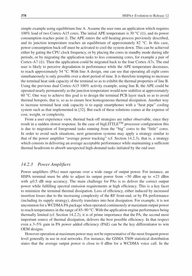
378 HSPA+ Evolution to Release 12
simple example using equilibrium line A. Assume the user runs an application which requires100% load of two Cortex-A15 cores. The initial APE temperature is 30 ◦C ( ⃝1 ), and its powerconsumption reaches point ⃝2 . The APE enters the self-heating process previously described,and its junction temperature reaches an equilibrium of approximately 82 ◦C. In this case,power consumption back-off must be activated to cool the system down. This can be achievedeither by gating the CPU clock frequency, or by placing the cores in standby mode during idleperiods, or by migrating the application tasks to less consuming cores, for example a pair ofCortex-A7 ( ⃝4 ). Then the application could be migrated back to the four Cortex-A7s. The enduser is likely to perceive degradation in performance while the APE temperature decreases,to reach approximately 54 ◦C. With line A design, one can see that operating all eight coressimultaneously is only possible over a short period of time. It is therefore tempting to increasethe terminal heat sink capacity of the terminal so as to exhibit the thermal properties of line B.Using the previous dual Cortex-A15 100% activity example, using line B, the APE could beoperated nearly permanently as the junction temperature would now stabilize at approximately60 ◦C. One way to achieve this goal is to design the terminal PCB layer stack so as to avoidthermal hotspots, that is, so as to ensure best homogeneous thermal dissipation. Another wayto increase terminal heat sink capacity is to equip smartphones with a “heat pipe” coolingsystem such as that implemented in [32]. But each of these solutions comes at the expense ofcost, weight, or complexity.
From a user experience view, thermal back-off strategies are rather observable, since theyresult in a sudden slower response. In the case of bigLITTLETM processor configuration thisis due to migration of foreground tasks running from the “big” cores to the “little” cores.In order to avoid such situations, next generation systems may apply a strategy similar tothat of the power amplifier “average power tracking” (cf. Section 14.2.3), that is, a strategywhich consists in delivering an average acceptable performance while maintaining a sufficientthermal headroom to absorb unexpected high-demand tasks initiated by the end user.
14.2.3 Power Amplifiers
Power amplifiers (PAs) must operate over a wide range of output power. For instance, anHSPA terminal must be able to adjust its output power from −50 dBm up to +23 dBmwith ±0.5 dB step accuracy. The main challenge for PAs is to deliver the correct outputpower while fulfilling spectral emission requirements at high efficiency. This is a key facetto minimize the terminal thermal dissipation. Loss of efficiency, either induced by increasedinsertion losses due to the increasing complexity of the RF front-end, or by PA performance(including its supply strategy), directly translates into heat dissipation. For example, it is notuncommon for a WCDMA PA package when operated continuously at maximum output powerto reach temperatures in the range of 85–90 ◦C. With the application engine performance beingthermally limited (cf. Section 14.2.2), it is of prime importance that the PA, the second mostimportant source of thermal dissipation, delivers the best possible efficiency. In that respecteven a 3–5% gain in PA power added efficiency (PAE) can be the key differentiator to winOEM designs.
However operation at maximum power may not be representative of the most frequent powerlevel generally in use in real networks. For instance, the GSMA TS09 statistical distributionstates that the average output power is close to 0 dBm for a WCDMA voice call. In the
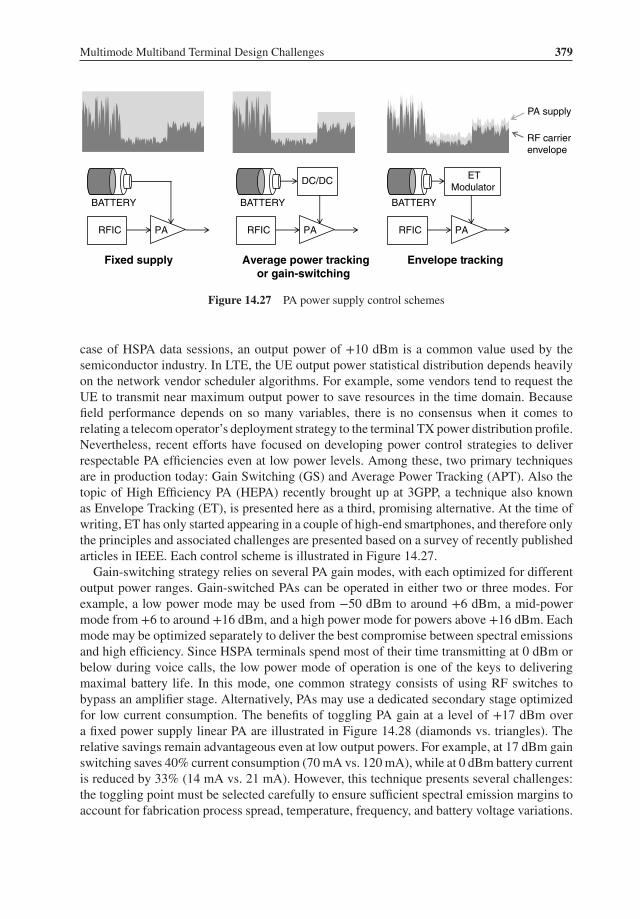
Multimode Multiband Terminal Design Challenges 379
RFIC PA
BATTERY
RFIC PA
BATTERY
DC/DC
RFIC PA
BATTERY
ETModulator
Fixed supply Average power trackingor gain-switching
Envelope tracking
PA supply
RF carrierenvelope
Figure 14.27 PA power supply control schemes
case of HSPA data sessions, an output power of +10 dBm is a common value used by thesemiconductor industry. In LTE, the UE output power statistical distribution depends heavilyon the network vendor scheduler algorithms. For example, some vendors tend to request theUE to transmit near maximum output power to save resources in the time domain. Becausefield performance depends on so many variables, there is no consensus when it comes torelating a telecom operator’s deployment strategy to the terminal TX power distribution profile.Nevertheless, recent efforts have focused on developing power control strategies to deliverrespectable PA efficiencies even at low power levels. Among these, two primary techniquesare in production today: Gain Switching (GS) and Average Power Tracking (APT). Also thetopic of High Efficiency PA (HEPA) recently brought up at 3GPP, a technique also knownas Envelope Tracking (ET), is presented here as a third, promising alternative. At the time ofwriting, ET has only started appearing in a couple of high-end smartphones, and therefore onlythe principles and associated challenges are presented based on a survey of recently publishedarticles in IEEE. Each control scheme is illustrated in Figure 14.27.
Gain-switching strategy relies on several PA gain modes, with each optimized for differentoutput power ranges. Gain-switched PAs can be operated in either two or three modes. Forexample, a low power mode may be used from −50 dBm to around +6 dBm, a mid-powermode from +6 to around +16 dBm, and a high power mode for powers above +16 dBm. Eachmode may be optimized separately to deliver the best compromise between spectral emissionsand high efficiency. Since HSPA terminals spend most of their time transmitting at 0 dBm orbelow during voice calls, the low power mode of operation is one of the keys to deliveringmaximal battery life. In this mode, one common strategy consists of using RF switches tobypass an amplifier stage. Alternatively, PAs may use a dedicated secondary stage optimizedfor low current consumption. The benefits of toggling PA gain at a level of +17 dBm overa fixed power supply linear PA are illustrated in Figure 14.28 (diamonds vs. triangles). Therelative savings remain advantageous even at low output powers. For example, at 17 dBm gainswitching saves 40% current consumption (70 mA vs. 120 mA), while at 0 dBm battery currentis reduced by 33% (14 mA vs. 21 mA). However, this technique presents several challenges:the toggling point must be selected carefully to ensure sufficient spectral emission margins toaccount for fabrication process spread, temperature, frequency, and battery voltage variations.
380 HSPA+ Evolution to Release 12
0
5
10
15
20
25
30
35
40
45
5 10 15 20 25 30
PA
E (
%)
Power amplifier output power (dBm)
APT Rel'99APT HSUPA[34] LTE 16QAM[35] LTE 16QAM[38] LTE 16QAMFS Rel'99
0
50
100
150
200
250
300
350
400
5 10 15 20 25 30
Bat
tery
cur
rent
(m
A)
Power amplifier output power (dBm)
Average power tracking (APT)
Gain switching (GS)
Fixed supply (FS)
(a) (b)
Figure 14.28 (a): APT, GS, FS PA battery current consumption for WCDMA rel’99 uplink trans-missions. (b): Comparison of APT, FS, and ET power added efficiencies vs. output power. ET curvesextracted from [34, 35, 38]
Additionally, mode toggling in most cases generates a sudden gain and phase jump. Bothimpairments are bounded by specific 3GPP test cases. Each gain step must be calibrated inmass production and compensated by the UE transmitter chain to meet the TPC accuracy of± 0.5 dB. Phase jumps must not exceed the phase discontinuity requirements [33] and maybe digitally corrected by application of I/Q constellation rotation. If the phase jump is below60 degrees, another simple technique consists in using separate threshold points for up anddown power control commands. The toggling points are separated by at least 6 dB, effectivelyresulting in a hysteresis scheme which provides compliance to 3GPP requirements.
Average Power Tracking (APT) is a technique in which either the PA supply is adjusted,or both supply and bias voltages are altered, according to the amplifier output power level.In this scheme, a DC–DC converter decreases the supply voltage as the UE output powerdecreases. APT can be seen as an extension of the GS strategy, where adjustments are made ona slot-by-slot basis to deliver the best performance tradeoff over the mid- to high-output powerrange. Implementing APT in an open-loop (OL) fashion delivers the best cost and simplicityof implementation, but calls for mass production calibration of gain steps associated to eachbias and supply setting. This technique may also be implemented in a closed-loop (CL)fashion, wherein the PA RMS output power is measured, digitally sampled, and comparedto the targeted TX power. This algorithm may apply one, or several, fine gain correctionsduring the first few microseconds of a timeslot to ensure the target value is met within 3GPPaccuracy requirements. Early implementations of this approach can be traced back to the firstfew generations of UEs (cf. Figure 14.5a, b and c), where the loop uses an RF directionalcoupler, a logarithmic RF power detector, a low-pass filter, and auxiliary ADC [4]. ModernCL implementations may replace the discrete power detector with a dedicated measurementreceiver embedded within the RF TRX. For low power levels, the loop may be disabled,
Multimode Multiband Terminal Design Challenges 381
leaving the PA to operate OL in its low power mode. The main challenge in CL APT consistsof ensuring that repetitive gain corrections do not impair the carrier’s modulation properties.One example of this is the case of HS-DPCCH burst transmissions which are not time-alignedto the slot boundaries of other uplink physical channels. Also, power detector linearity mustbe excellent across a wide range of environmental conditions. Yet, as of today, APT remainsthe most efficient technique. Figure 14.28a shows an example of current consumption savingswith APT (crosses). At 0 dBm, the savings are around 60% vs. a fixed supply. Even at highpower levels the current consumption is slightly decreased because some amplifiers may beable to operate at 3.2 V, which is a lower voltage than the nominal battery voltage of 3.8 V.
Finally, a third technique called Envelope Tracking (ET) has recently received much atten-tion. The concept, illustrated in Figure 14.27, consists in applying the smallest needed supplyvoltage in real-time, following the instantaneous envelope of the RF carrier. This may be seenas a real-time extension of APT. The current consumption gains are expected to be higherthan with APT because the supply voltage is continuously adjusted to its lowest possible levelwithout compromising the spectral emissions requirements. Interestingly, it enables bettersavings for high Peak-to-Average Power Ratio (PAPR) modulations, whereas APT efficiencydecreases as PAPR increases because it requires a higher supply voltage to avoid PA clipping ofthe envelope peaks. For example, Figure 14.28b shows that the impressive level of performanceachieved by the APT scheme for WCDMA rel’99 transmissions where the peak-to-averagepower ratio is typically 3 dB (at 0.1% probability of presence) and is noticeably degraded assoon as HSUPA transmissions occur (dashed-lines, cubic metric = 2). In this case, ET PAEexceeds that of HSUPA APT in the upper 6 to 7 dB output range.
However, ET implementation requires high-performance, high-speed DC–DC convertercores that are able to track the envelope of high bandwidth modulated carriers, such as LTE.The envelope being roughly the square of the IQ waveform, the bandwidth over which theDC–DC converter must deliver high efficiency becomes quite large. For instance, the envelopeof a 20 MHz LTE carrier occupies 40 MHz. Delivering high supply modulator efficienciesover a large bandwidth and a large range of output powers is the key to ET exceeding APTperformance. ET also requires tight time synchronization between the PA supply controlpath and the transceiver data IQ-to-RF path. Furthermore, high-speed supply modulators candegrade out-of-band noise emissions [37].
In both APT and ET, the total system efficiency is the product of PA and DC–DC converterefficiencies. In comparison to APT, the higher PA efficiency of ET is counter-balanced bya poorer DC–DC efficiency. It is easier to achieve high converter efficiency with APT thanwith ET, especially when ET is applied to a 20 MHz or greater modulation BW. TypicallyAPT DC–DC converter efficiency can reach 90%, as opposed to the 70–80% range typicalfor ET [38]. Some solutions use a dual-supply modulator architecture resulting in an overallperformance profile similar to that of GS (Figure 14.28 [38]). At the time of writing, it isdifficult to assess the exact gains of ET, since only a couple of terminals have enabled thisfeature. Generally, current consumption gains are expected for the highest 6 dB output powerlevels. Considering that ET is still in its infancy, and that great progress has been made inonly a couple of years (Figure 14.28 [34, 35, 38]), there are good reasons to believe that ETwill exceed APT performance levels. Since ET modulators may be entirely implemented inCMOS, this technology paves the way for commercial production of integrated linear CMOSPAs, provided that the cost of such products becomes attractive.
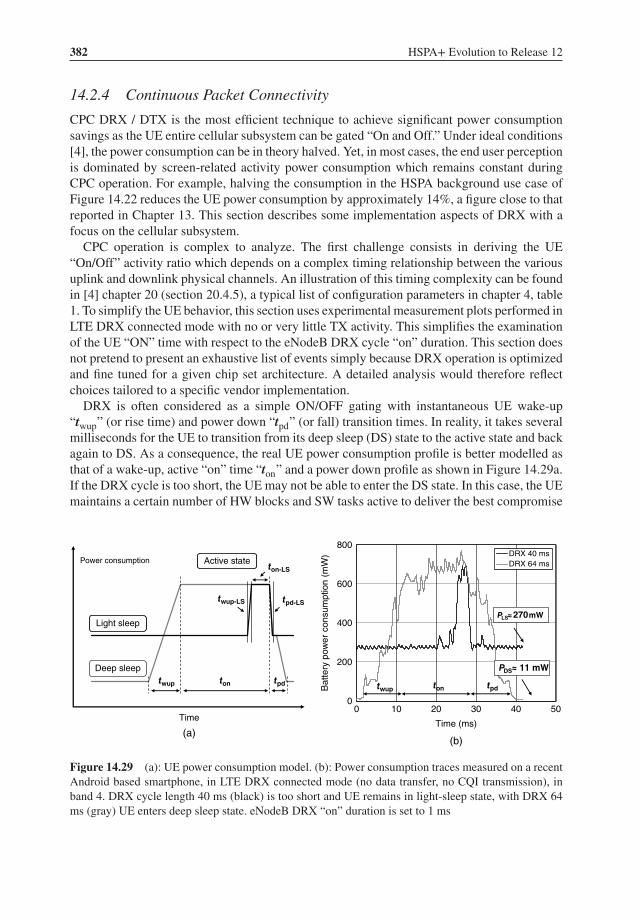
382 HSPA+ Evolution to Release 12
14.2.4 Continuous Packet Connectivity
CPC DRX / DTX is the most efficient technique to achieve significant power consumptionsavings as the UE entire cellular subsystem can be gated “On and Off.” Under ideal conditions[4], the power consumption can be in theory halved. Yet, in most cases, the end user perceptionis dominated by screen-related activity power consumption which remains constant duringCPC operation. For example, halving the consumption in the HSPA background use case ofFigure 14.22 reduces the UE power consumption by approximately 14%, a figure close to thatreported in Chapter 13. This section describes some implementation aspects of DRX with afocus on the cellular subsystem.
CPC operation is complex to analyze. The first challenge consists in deriving the UE“On/Off” activity ratio which depends on a complex timing relationship between the variousuplink and downlink physical channels. An illustration of this timing complexity can be foundin [4] chapter 20 (section 20.4.5), a typical list of configuration parameters in chapter 4, table1. To simplify the UE behavior, this section uses experimental measurement plots performed inLTE DRX connected mode with no or very little TX activity. This simplifies the examinationof the UE “ON” time with respect to the eNodeB DRX cycle “on” duration. This section doesnot pretend to present an exhaustive list of events simply because DRX operation is optimizedand fine tuned for a given chip set architecture. A detailed analysis would therefore reflectchoices tailored to a specific vendor implementation.
DRX is often considered as a simple ON/OFF gating with instantaneous UE wake-up“twup” (or rise time) and power down “tpd” (or fall) transition times. In reality, it takes severalmilliseconds for the UE to transition from its deep sleep (DS) state to the active state and backagain to DS. As a consequence, the real UE power consumption profile is better modelled asthat of a wake-up, active “on” time “ton” and a power down profile as shown in Figure 14.29a.If the DRX cycle is too short, the UE may not be able to enter the DS state. In this case, the UEmaintains a certain number of HW blocks and SW tasks active to deliver the best compromise
0
200
400
600
800
0 10 20 30 40 50
Bat
tery
pow
er c
onsu
mpt
ion
(mW
)
Time (ms)
DRX 40 msDRX 64 ms
Time
Power consumption Active state
Deep sleep
Light sleep
t t t
twup-LS
ton-LS
tpd-LS
P ≈ 270mW
P ≈ 11 mW
t t t
(a)(b)
Figure 14.29 (a): UE power consumption model. (b): Power consumption traces measured on a recentAndroid based smartphone, in LTE DRX connected mode (no data transfer, no CQI transmission), inband 4. DRX cycle length 40 ms (black) is too short and UE remains in light-sleep state, with DRX 64ms (gray) UE enters deep sleep state. eNodeB DRX “on” duration is set to 1 ms
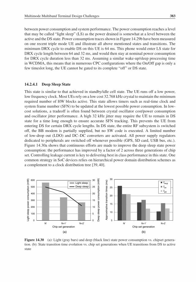
Multimode Multiband Terminal Design Challenges 383
between power consumption and system performance. The power consumption reaches a levelthat may be called “light sleep” (LS) as the power drained is somewhat at a level between theactive and the DS state. Power consumption traces shown in Figure 14.29b have been measuredon one recent triple mode UE and illustrate all above mentioned states and transitions. Theminimum DRX cycle to enable DS on this UE is 64 ms. This phone would enter LS state forDRX cycle length between 64 and 32 ms, and would then stay at nominal power consumptionfor DRX cycle duration less than 32 ms. Assuming a similar wake-up/sleep processing timein WCDMA, this means that in numerous CPC configurations where the On/Off gap is only afew timeslot long, the UE cannot be gated to its complete “off” or DS state.
14.2.4.1 Deep Sleep State
This state is similar to that achieved in standby/idle cell state. The UE runs off a low power,low frequency clock. Most UEs rely on a low cost 32.768 kHz crystal to maintain the minimumrequired number of HW blocks active. This state allows timers such as real-time clock andsystem frame number (SFN) to be updated at the lowest possible power consumption. In low-cost solutions, a tradeoff is often found between crystal oscillator cost/power consumptionand oscillator jitter performance. A high 32 kHz jitter may require the UE to remain in DSstate for a time long enough to ensure accurate SFN tracking. This prevents the UE fromentering DS for certain DRX cycle lengths. In DS state, the entire RF subsystem is switchedoff, the BB modem is partially supplied, but no SW code is executed. A limited numberof low-drop out (LDO) and DC–DC converters are activated. All power supply regulatorsdedicated to peripherals are switched off whenever possible (GPS, SD card, USB bus, etc.).Figure 14.30a shows that continuous efforts are made to improve the deep sleep state powerconsumption: the performance has improved by a factor of 2 across three generations of chipset. Controlling leakage current is key to delivering best in class performance in this state. Onecommon strategy in SoC devices relies on hierarchical power domain distribution schemes asa complement to a clock distribution tree [39, 40].
0
5
10
15
20
25
30
0
100
200
300
400
500
600
N' N+1' N+2'
Dee
p sl
eep
pow
er c
onsu
mpt
ion
(mW
)
Ligh
t sle
ep p
ower
con
sum
ptio
n (m
W)
Chip set generation
Light sleep Deep sleep
5
10
15
20
25
30
N' N+1' N+2'
App
roxi
mat
ive
tran
sitio
n tim
es (
ms)
Chip set generation
twup
ton
tpd
(a) (b)
Figure 14.30 (a): Light (gray bars) and deep (black line) state power consumption vs. chipset genera-tion. (b): State transition time evolution vs. chip set generations when UE transitions from DS to activestate
384 HSPA+ Evolution to Release 12
14.2.4.2 Light Sleep State
The cellular subsystem runs off a low phase noise reference clock, which, depending on chipset vendors, is either a 26 MHz or a 19.2 MHz crystal. Most of the BB modem LDOs andDC–DC converters are active and the modem executes SW code. In most implementations,the RF subsystem is switched off. Architectures which rely on “smart RF transceivers” maymaintain the TRX digital core active. The LS power consumption follows the general trendsin reducing the active state power consumption optimization across generations of platforms[41]. Figure 14.30a shows power consumption has nearly improved by a factor of 2 over threegenerations.
14.2.4.3 DS to Active State Transition (wake-up “twup”)
This transition is a complex cascade of HW and SW events to progressively bring all HWblocks to the active state, in the fastest (shortest rise time) and most power efficient way. Powersupplies rails, or power domains, are usually activated in a hierarchical scheme [39]. Whena large number of gates must be activated, the sequential power-up technique helps preventcurrent rush/surge issues [40] from occurring. Due to battery internal resistance, these surgesmay generate a drop in battery voltage which at low operating voltages could, for example,trigger a UE shutdown sequence if detected by the power management unit. The sequentialpower-up delay between successive domains depends on the nature of the activity of the blockbeing supplied. Delays range from 50–100 μs for digital PLL, 80–150 μs for RF LO PLLsynthesizers, to 500 μs DC–DC converter typical settling time, to 2 ms required to stabilizethe low phase noise reference clock oscillator (26 or 19.2 MHz). As soon as HW blocks aresupplied, numerous activities can be parallelized to minimize wake-up time (twup). The nearfactor of 2 reduction of twup achieved across three generations of triple mode UEs shown inFigure 14.30b shows that despite the complexity of the task, chip sets are able to continuouslyimprove performance.
14.2.4.4 Active State (“ton”) – Transition from DS
Several SW and HW tasks must be executed to prepare the subsystem for physical channeldemodulation/modulation. From a SW perspective, resuming the SW context requires fetchingdata in LP-DDR to fill up the processor local cache memory. Depending on the operatingsystem, and modem protocol stack complexity, this task can take several milliseconds. Froman RF subsystem point of view, multiple initialization tasks must be executed. Preparing thereceiver chain includes but is not limited to the following steps:
� Receiver self calibration (VCOs, channel filters).� Switch on local oscillator and tune RF PLL frequency.� Configure RX chain transceiver filters.� Set antenna switch to selected band of operation.� Switching on LNA and mixer.� Prepare AGC algorithm: initial fast gain acquisition or tracking mode?� Set the initial RX chain gain (LNA, mixer, I/Q analog VGAs).� Switch on I/Q ADC (in RF transceiver if digital IQ interface, in modem BB otherwise).
Multimode Multiband Terminal Design Challenges 385
Once the RF IC is ready, a critical algorithm to deliver a power efficient performanceis that of fast gain control, also sometimes referred to as fast gain acquisition (FGA). InWCDMA, this should ideally be completed within less than one timeslot (666.66 μs). FGAis common to compressed mode and DRX operation. Its goal is to ensure the I/Q ADC isoperated at its optimal back-off. Because of multipath fading, a compromise must be foundbetween RRSS (receiver radio signal strength) integration period to ensure good Ior powermeasurement accuracy, the number of gain corrections, gain step size boundaries, and initialgain settings to ensure convergence to the target ADC back-off across the entire UE dynamicrange in a minimum number of steps. Most chip sets manage to achieve this task using threegain adjustments. One of the challenges with FGA is that ZIF receiver self-mixing due touplink carrier leakage generates a time varying DC offset which, if not cancelled, could lead toerroneous Ior power measurements. DC offset compensation in WCDMA is often achieved viaan equivalent high-pass filtering function, either in analog IQ, digital IQ, or a combination ofcoarse analog IQ and fine digital IQ DC offset compensation. The higher the equivalent HPFcut-off frequency, the higher the EVM. Since, during FGA, only RRSS measurement accuracymatters (i.e., EVM is not a concern), fast DC settling time can be achieved by selecting ahigh cut-off frequency. Once FGA is completed, the DC offset compensation circuitry mustresume its low EVM, low cut-off frequency. The target ADC back-off can then be lockedthrough a standard AGC loop. Finally, the UE must perform RF channel estimation. With theintroduction of recent high-speed train fading profiles, the UE may have to adapt its channelestimation averaging time and update rate based on an estimation of its velocity. At high speed,a longer and more frequent channel estimation might be required. These are some of the keytasks the system must complete prior to demodulation.
14.2.4.5 LS to Active State Transition (“ton-LS”)
In most UEs, this task consists in activating the RF subsystem as the entire modem andSW code is active. The delays associated with this task are those of the previously listedsequence. The active time which follows a transition from LS state (“ton-LS”) should in theorybe shorter since the only tasks required are: program default gain, and frequency values,perform FGA, and channel estimation. In the example of Figure 14.29b, twup-LS lasts less than1 ms and ton-LS is approximately equal to 2.6 ms for an eNodeB DRX cycle “on duration”of 1 ms.
14.2.4.6 Active State to LS to DS Transition
Switching off the RF subsystem is more straightforward and faster than the activation pro-cedure. All blocks can be switched off nearly instantaneously. The remaining power-downdelays are SW stack-related.
Finally, Figure 14.31 shows the CPC battery savings that are achieved in practice on a recenttriple-mode UE operating in band 4. The measurements are performed using an Anritsu 8475aNodeB emulator during an FTP download sequence restricting the UE to operate in singlecell mode, HSDPA cat 14, HSUPA cat 6. CPC parameters are similar to those of Chapter 4,Table 4.1. It can be seen that despite large inactive gaps, the UE power consumption profile isfar from reaching the ideal DS power consumption. In this case, the UE power consumption

1
1.52
2.53
010
2030
4050
6070
8090
100
Battery power consumption (W)
Tim
e (m
s)
010
2030
4050
6070
8090
100
UE TX power (dBm/3.84 MHz)
Tim
e (m
s)
CP
C d
isab
led
CP
C e
nab
led
CP
C d
isab
led
CP
C e
nab
led
(a)
(b)
Fig
ure
14.3
1C
PCba
ttery
cons
umpt
ion
savi
ngs
and
UE
TX
pow
erga
ting
vs.t
ime
duri
ngan
FTP
file
dow
nloa
din
HSD
PAca
t14.
(a):
UE
TX
pow
erw
ithC
PCen
able
dvs
.CPC
disa
bled
.(b)
:UE
batte
rypo
wer
cons
umpt
ion
with
scre
en“s
witc
hed
OFF
”
Multimode Multiband Terminal Design Challenges 387
savings are 18% with screen “off,” and 7% when the screen is activated. The average downlinkMAC layer throughput is approximately 12 Mbit/s.
Figure 14.32 has been captured by stalling the FTP download process so as to minimizethe impact of background FTP server application SW tasks onto the cellular subsystem powerconsumption. The UE remains in CPC DTX DRX connected mode, with very few packetsto receive (near zero downlink throughput), or transmit. The graph shows the UE powerconsumption profile closely matching the UE TX power mask when CPC is activated. Thepower consumption bumps between two transmissions are likely related to DRX activity. Thescreen is “off” but the FTP server application is still running in the background. The UE powerconsumption savings are close to 51%.
14.3 Conclusion
The key to successful designs in the mobile terminal industry has always been, and still remains,to deliver a timely solution that meets the desired price/performance/power consumptiontradeoffs. However, it is important to note that the proper balance of these criteria is a goal thatremains constantly in flux, due to the ever-changing demands and expectations of the consumer.With the wide adoption of smartphones, this tradeoff becomes ever more difficult, as the numberof use cases has increased considerably. From an application engine standpoint the terminalmust support a wide range of additional performance requirements, from the lower demandsof texting/chatting applications, to the highly demanding 3D gaming, satellite navigation,augmented reality, or even video editing applications. The always-on requirement combinedwith the need to minimize product variants force transceiver designers to produce solutions thatmust be able to support as many of the 40 standardized frequency bands (29 FDD-LTE, 12 TD-LTE) as is possible. This, in turn, requires a multiplicity of implementation improvements,including antennae to deliver optimal efficiency across a wide range of frequency bands.From a power consumption point of view, and despite the availability of moderately highercapacity batteries, designers must deliver solutions that ensure at least a full day of use underthese demanding usage conditions. In this context, the traditional design challenges of earliergenerations of terminals are exacerbated as a consequence of the increasing device complexityand increased consumer expectations. Some of the resultant outcomes of this new usageparadigm for terminal designers include:
� OTA performance will have a major impact on MIMO user experience.� Cellular transceivers must be able to support a continuously increasing number of bands, as
well as the complex band combinations to support carrier-aggregation.� As a consequence, co-existence scenarios are becoming more complicated to resolve as the
number of radio-to-radio, as well as the number of digital-to-radio subsystems operatingsimultaneously increases.
� The limited thermal envelope of the device places severe constraints on how to best deliverexpected user experience across a wide range of use cases in a small form factor.
Admittedly these challenges present opportunities for innovation, and the industry has ahistory of embracing challenges, so there is reason to believe it will do so again and thus willfind innovative means to effectively solve these issues. This short introduction to this topic has
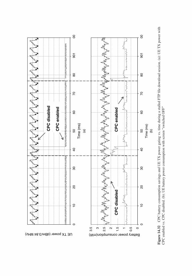
0
0.51
1.52
2.53
3.5
100
2030
4050
6070
8090
100
Battery power consumption(mW)
Tim
e (m
s)
100
2030
4050
6070
8090
100
UE TX power (dBm/3.84 MHz)
Tim
e (m
s)
CP
C d
isab
led
CP
C e
nab
led
CP
C d
isab
led
CP
C e
nab
led
(a)
(b)
Fig
ure
14.3
2C
PCba
ttery
cons
umpt
ion
savi
ngs
and
UE
TX
pow
erga
ting
vs.t
ime
duri
nga
stal
led
FTP
file
dow
nloa
dse
ssio
n.(a
):U
ET
Xpo
wer
with
CPC
enab
led
vs.C
PCdi
sabl
ed.(
b):U
Eba
ttery
pow
erco
nsum
ptio
nw
ithsc
reen
“sw
itche
dO
FF”
Multimode Multiband Terminal Design Challenges 389
attempted to highlight that one of the keys to delivering successful solutions has become torely more heavily upon reconfigurable hardware architectures in as many blocks and functionsas possible, such as:
� Use of hybrid CPUs in the application engine.� Extensive use of digital signal processing in the RF transceiver, thanks to the availabil-
ity of low power, high dynamic range ADCs and DACs, making the transceiver easilyreconfigurable to support multiple air interfaces.
� Tunable antennae to optimize performance across a wide range of operating frequencies.� Multimode, multiband power amplifiers.
The RF front end remains an area which still possesses less-than-optimal reconfigurability.Since today high performance dedicated RF filters and RF multiplexers are required per bandor for selected band combinations, this makes the cellular RF-FE one of the primary areaswhere substantial challenges lie ahead for next-generation platforms. And looking ahead tocarrier-aggregation, the RF front end will become even more complex, so there is a need toachieve greater reuse and reconfigurability in all areas.
Market segmentation does not help in this respect either, as platforms must be optimizedfor each market segment. A recent forecast indicates that low-end smartphones (<$200 price),and, to a certain extent mid-range devices ($200–300 retail price), are expected to dominatemarket growth, with 3x and 50% increase, respectively, by 2018. Therefore, most of thedesign tradeoffs which have been mentioned in this chapter must be re-assessed for eachmarket segment and appropriate changes must be made. This increases the R&D work loadfor terminal designs – all in an industry where meeting an aggressive time-to-market is aprimary key to success. The combination of all these constraints, as well as the pressure ofhuge production volumes, probably qualifies the design of the modern mobile terminal as oneof the most challenging design environments in the electronics industry.
To put this in perspective – how many terminal devices or chip sets will have been shippedthroughout the world by the time you read this sentence?
References
[1] Gartner press release (April 4, 2013), “Gartner Says Worldwide PC, Tablet and Mobile Phone CombinedShipments to Reach 2.4 Billion Units in 2013”, http://www.gartner.com/newsroom/id/2408515 (last checkedAugust 2013).
[2] R2-124396, “LS on extending E-UTRA band number and EARFCN numbering space”, 3GPP TSG RAN WG2Meeting #79bis, Bratislava, Slovakia, 8–12 October 2012.
[3] Graph compiled using data extracted off a total of 125 mobile phone teardown reports, mostly licensed fromUBM Techinsights (www.ubmtechinsights.com) and partially from ABI research (http://www.abiresearch.com).Breakdown: 69 monomode EGPRS teardown reports, 48 dual-mode EGPRS-WCDMA terminals, 7 triple-modeEGPRS-WCDMA-LTE terminals.
[4] Holma, H. and Toskala, A. (2010) WCDMA for UMTS: HSPA Evolution and LTE, 5th edn, chapter 20, JohnWiley & Sons, Ltd, Chichester.
[5] Holma, H. and Toskala, A. (2011) LTE for UMTS: Evolution to LTE-Advanced, 2nd edn, John Wiley & Sons,Ltd, Chichester.
[6] Jones, C., Tenbroek, B., Fowers, P. et al. (2007) Direct-Conversion WCDMA Transmitter with −163 dBc/HzNoise at 190 MHz Offset. Solid-State Circuits Conference, 2007. ISSCC 2007. Digest of Technical Papers.IEEE International, pp. 336–607.
390 HSPA+ Evolution to Release 12
[7] Kihara, T., Sano, T., Mizokami, M. et al. (2012) A multiband LTE SAW-less CMOS transmitter with source-follower-drived passive mixers, envelope-tracked RF-PGAs, and Marchand baluns. Radio Frequency IntegratedCircuits Symposium (RFIC), IEEE, pp. 399–402.
[8] Xie, H., Oliaei, O., Rakers, P. et al. (2012) Single-chip multiband EGPRS and SAW-less LTE WCDMA CMOSreceiver with diversity. IEEE Transactions on Microwave Theory and Techniques, 60(5), 1390–1396.
[9] Gaborieau, O., Mattisson, S., Klemmer, N. et al. (2009) A SAW-less multiband WEDGE receiver. Solid-StateCircuits Conference – Digest of Technical Papers, 2009. ISSCC 2009. IEEE International, pp. 114–115, 115a.
[10] Intel XMM6140 dual-mode EGPRS-HSDPA single-chip modem, power management unit, RF transceiversolution, http://www.intel.com/content/www/us/en/wireless-products/mobile-communications/mobile-phone-platforms.html.
[11] Broadcom BCM21892, “4G LTE Advanced FDD and TDD; 3G HSPA +and TD-SCDMA; 2G-EDGEModem with Integrated World-Band Radio”, February 2013, http://www.broadcom.com/products/Cellular/4G-Baseband-Processors/BCM21892.
[12] R4-121361, “LO coupling issues for NC intra-band CA”, 3GPP TSG-RAN WG4 Meeting #62bis, Jeju Island,Korea, 26–30 March, 2012.
[13] R4-131235, “Considerations for single-chip implementations of carrier aggregation”, 3GPP TSG-RAN WG4Meeting #66 Bis, Chicago, U.S.A, 15th April – 19th April, 2013.
[14] Abdelhalem, S.H., Gudem, P.S. and Larson, L.E. (2012) A tuneable differential duplexer in 90nm CMOS. RadioFrequency Integrated Circuits Symposium (RFIC), 2012 IEEE, pp. 101–104.
[15] Sony Mobile C6903 (PM-0450-BV), supported bands LTE: 1,2,3,4,5,7,8,20; HSPA+/UMTS:I,II,IV,V,VIII;GSM-GPRS-EDGE:850/900/1800/1900 MHz http://www.gsmarena.com/sony_xperia_z_ultra-5540.php (lastchecked Aug. 2013).
[16] R4-133985, ‘On the additional insertion-loss for CA_2A-4A’, TSG-RAN Working Group 4 (Radio) meeting#68, Barcelona, Spain, 19–23 August 2013.
[17] 2012 CES Innovations Design and Engineering Awards in category ‘Embedded Technologies’: Renesas SP2531(Pegastick) triple mode (EDGE,HSPA+,LTE) USB datacard, http://www.cesweb.org/cesweb/media/CESWeb/Innovation%20Awards/2012%20Innovations%20Honorees/Embedded%20Technologies/Pegastick.bmp.
[18] “Test Plan for Mobile Station Over the Air Performance, Method of Measurement for Radiated RF Power andReceiver Performance”, revision 3.2.1, CTIA – The Wireless Association®, March 2013.
[19] Pelosi, M., Franek, O., Knudsen, M.B. et al. (2010) Antenna Proximity Effects for Talk and Data Modes inMobile Phones. Antennas and Propagation Magazine, IEEE, pp. 15–27.
[20] Ranta, T., Ella, J. and Pohjonen, H. (2005) Antenna switch linearity requirements for GSM/WCDMA mobilephone front-ends. The European Conference on Wireless Technology 2005, pp. 23–26.
[21] Del Barrio, S.C. and Pedersen, G.F. (2012) Correlation Evaluation on Small LTE Handsets. Vehicular TechnologyConference (VTC Fall), 2012 IEEE, Quebec City, pp. 1–4.
[22] Yanakiev, B., Nielsen, J.O., Christensen, M. and Pedersen, G.F. (2012) On Small Terminal Antenna Correlationand Impact on MIMO Channel Capacity. IEEE Transactions on Antennas and Propagation, 689–699.
[23] R4-66AH-0003, “Effect of user-presence on MIMO OTA using an anechoic chamber and a reverberationchamber”, TSG-RAN Working Group 4 (Radio) Meeting #66 Ad hoc, Munich, Germany, 12–13 March, 2013.
[24] Boyle, K. and Leitner, M. (2011) Mobile phone antenna impedance variations with real users and phantoms.International Workshop on Antenna Technology (iWAT), 2011, pp. 420–423.
[25] Wu, T.-H., Chang, H.-H., Chen, S.-F. et al. (2013) A 65-nm GSM/GPRS/EDGE SoC with integrated BT/FM.IEEE Journal of Solid-State Circuits, 48(5), 1161–1173.
[26] R4-124113, “REFSENS analysis using MSD methodology for Band 4 and Band 17 carrier aggregation”, 3GPPTSG RAN WG4 Meeting #64, Qingdao, China, Aug., 13th – 17th, 2012.
[27] R4-121862, “Cross-coupling of Harmonics in case of band 17/4 Carrier Aggregation”, 3GPP TSG-RAN WG4Meeting #62bis, Jeju, Korea, March 26 – 30, 2012.
[28] R4-124359, “Interband CA Class A2 MSD”, TSG-RAN Working Group 4 (Radio) meeting #64 Qingdao,P.R.China, Aug 13th – 17th, 2012.
[29] Experian marketing (May 2013), John Fetto, “Americans spend 58 minutes a day on their smartphones”,http://www.experian.com/blogs/marketing-forward/2013/05/28/americans-spend-58-minutes-a-day-on-their-smartphones/ (last accessed August 2013).
[30] Cameron, K.W. and Ge, R. (2012) Generalizing Amdahl’s law for power and energy. IEEE Computer, 45(3).[31] Rasmussen, M. (2013) Using Task Load Tracking to Improve Kernel Scheduler Load Balancing. The Linux
Foundation Collaboration Summit, Apr 15–17 2013.
Multimode Multiband Terminal Design Challenges 391
[32] NEC Casio X medias N-06E product launched by NTTdocomo in July 2013, http://www1.medias.net/jp/sp/n06e, and http://www.gsmarena.com/nec_medias_x_has_a_watercooled_snapdragon_s4_pro_chipset-news-6043.php.
[33] 3GPP TS 25.101 V12.0.0 (2013-07), www.3gpp.org.[34] Honda, Y., Yokota, Y., Goto, N. et al. (2012) A wide supply voltage and low-rx noise envelope tracking supply
modulator IC for LTE handset power amplifiers. 2012 42nd European Microwave Conference (EuMC), 2012,pp. 1253–1256.
[35] Kim, D., Kang, D. and Jooseung, K. (2012) Wideband envelope tracking power amplifier for LTE application.Radio Frequency Integrated Circuits Symposium (RFIC), 2012 IEEE, pp. 275–278.
[36] Kaczman, D.L., Shah, M., Godambe, N. et al. (2006) A single-chip tri-band (2100, 1900, 850/800 MHz)WCDMA/HSDPA cellular transceiver. IEEE Journal of Solid-State Circuits, 41(5), 1122–1132. Noise at12.5 MHz offset is the only value published.
[37] R4-132882, “Envelope tracking measurement results”, 3GPP TSG RAN WG4 #67, 20 –24 May 2013, Fukuoka,Japan.
[38] Kim, J., Dongsu, K., Yunsung, C. et al. (2013) Envelope-tracking two-stage power amplifier with dual-modesupply modulator for LTE applications. IEEE Transactions on Microwave Theory and Techniques, 61, 543–552.
[39] Kim, G.S., Je, Y.H. and Kim, S. (2009) An adjustable power management for optimal power saving in LTEterminal baseband modem. IEEE Transactions on Consumer Electronics, 55(4), 1847–1853.
[40] Kanno, Y., Mizuno, H., Yasu, Y. et al. (2007) Hierarchical power distribution with power tree in dozens ofpower domains for 90-nm low-power multi-CPU SoCs. IEEE Journal of Solid-State Circuits, 42(1), 74–83.
[41] Lauridsen, M., Noel, L. and Mogensen, P.E. (2013) Empirical LTE Smartphone Power Model with DRXOperation for System Level Simulations. Vehicular Technology Conference (VTC Fall), 2013 IEEE.
[42] R4-120442, Way forward for inter-band CA Class A2. 3GPP TSG-RAN WG4 Meeting #62, Dresden, Germany,Feb 6th – 10th, 2012.
[43] Tomiyama, H., Nishi, C., Ozawa, N. et al. (2006) Low voltage (1.8 V) operation triple band WCDMA transceiverIC. Radio Frequency Integrated Circuits (RFIC) Symposium, 2006.
[44] Koller, R., Ruhlicke, T., Pimingsdorfer, D. and Adler, B. (2006) A single-chip 0.13 /spl mu/m CMOS UMTSW-CDMA multi-band transceiver. Radio Frequency Integrated Circuits (RFIC) Symposium, 2006.
[45] Jones, C., Tenbroek, B., Fowers, P. et al. (2007) Direct-Conversion WCDMA Transmitter with −163 dBc/HzNoise at 190 MHz Offset. Solid-State Circuits Conference, 2007.
[46] Sowlati, T., Agarwal, B., Cho, J. et al. (2009) Single-chip multiband WCDMA/HSDPA/HSUPA/EGPRStransceiver with diversity receiver and 3G DigRF interface without SAW filters in transmitter / 3G receiverpaths. Solid-State Circuits Conference, 2009, pp. 116–117, 117a.
[47] Huang, Q., Rogin, J., XinHua, C. et al. (2010) A tri-band SAW-less WCDMA/HSPA RF CMOS transceiver withon-chip DC-DC converter connectable to battery. Conference Digest of Solid-State Circuits (ISSCC), 2010,pp. 60–61.
[48] Tsukizawa, T., Nakamura, M., Do, G. et al. (2010) ISO-less, SAW-less open-loop polar modulation transceiverfor 3G/GSM/EDGE multi-mode/multi-band handset. Microwave Symposium Digest (MTT), 2010 IEEE,pp. 252–255. Transceiver.
[49] Hausmann, K., Ganger, J., Kirschenmann, M. et al. (2010) A SAW-less CMOS TX for EGPRS and WCDMA.Radio Frequency Integrated Circuit Symposium (RFIC), 2010, pp. 25–28.
[50] Giannini, V., Ingels, M., Sano, T. et al. (2011) A multiband LTE SAW-less modulator with −160 dBc/HzRX-band noise in 40 nm LP CMOS. Solid-State Circuits Conference Digest of Technical Papers (ISSCC), 2011IEEE, pp. 374–376.
[51] Oliaei, O., Kirschenmann, M., Newman, D. et al. (2012) A Multiband Multimode Transmitter without Driveramplifier. Solid-State Circuits Conference Digest of Technical Papers (ISSCC), 2012 IEEE, pp. 164–166.
[52] ABI Research, ‘Sub-$200 Smartphone Shipments to Exceed 750 Million in 2018’, Oyster Bay, New York –07 Aug 2013 press release, http://www.abiresearch.com/press/sub-200-smartphone-shipments-to-exceed-750-million.
[53] Apple A1475 supports a total of 22 bands. LTE Band 1, 2, 3, 4, 5, 7, 8, 13, 17, 18, 19, 20, 25;HSPA+/UMTS:I,II,IV,V,VIII; GSM-GPRS-EDGE:850/900/1800/1900 MHz.

15LTE Interworking
Harri Holma and Hannu Raassina
15.1 Introduction
Long Term Evolution (LTE) networks are being rapidly rolled out but the deployment processwill take some time. Therefore, there is a clear need for smooth interworking between 3G andLTE for coverage, capacity, and for service reasons. The interworking requires a number ofdifferent functionalities depending on the LTE use cases. We can differentiate the followingphases of LTE network deployment:
� Data only LTE network for USB modems but not for smartphones. The interworking forthe data connection is required from 3G to LTE when LTE coverage is available. Also thecoverage trigger from LTE to 3G is needed to transfer the connection to 3G when runningout of LTE coverage area.
� Data only LTE network, also for smartphones. The interworking solution for voice calls isrequired, Circuit Switched (CS) fallback, to move the UE from LTE to 3G when the voicecall is initiated.
� Enhanced interworking for data, including redirection and handovers to minimize the con-nection break during the data transition. The first phase of data interworking may rely onsimple functions based on reselections.
� Voice over LTE (VoLTE) to also carry voice in LTE requires interworking between Voiceover IP (VoIP) and CS voice when running out of LTE coverage area. This is called SingleRadio Voice Call Continuity (SRVCC).
The selection of the target system and target cell in the idle mode is done by the UE basedon the network parameters, and the UE has no freedom in the system selection. The idlemode parameters are typically defined so that the UE will camp in LTE as long as the LTEsignal level exceeds a predefined threshold. Also, network parameters typically allow the UEto move from 3G to LTE as soon as the LTE signal is strong enough. The network can move
HSPA+ Evolution to Release 12: Performance and Optimization, First Edition.Edited by Harri Holma, Antti Toskala, and Pablo Tapia.© 2014 John Wiley & Sons, Ltd. Published 2014 by John Wiley & Sons, Ltd.
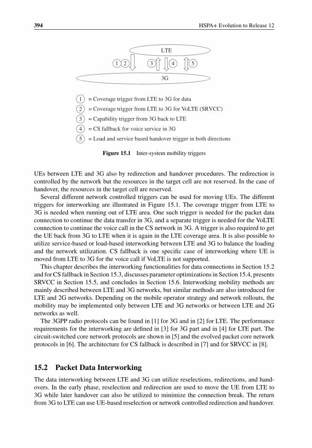
394 HSPA+ Evolution to Release 12
LTE
3G
= Coverage trigger from LTE to 3G for data
1
1
= Capability trigger from 3G back to LTE 3
= CS fallback for voice service in 3G 4
3 5 4
= Load and service based handover trigger in both directions 5
2
= Coverage trigger from LTE to 3G for VoLTE (SRVCC)2
Figure 15.1 Inter-system mobility triggers
UEs between LTE and 3G also by redirection and handover procedures. The redirection iscontrolled by the network but the resources in the target cell are not reserved. In the case ofhandover, the resources in the target cell are reserved.
Several different network controlled triggers can be used for moving UEs. The differenttriggers for interworking are illustrated in Figure 15.1. The coverage trigger from LTE to3G is needed when running out of LTE area. One such trigger is needed for the packet dataconnection to continue the data transfer in 3G, and a separate trigger is needed for the VoLTEconnection to continue the voice call in the CS network in 3G. A trigger is also required to getthe UE back from 3G to LTE when it is again in the LTE coverage area. It is also possible toutilize service-based or load-based interworking between LTE and 3G to balance the loadingand the network utilization. CS fallback is one specific case of interworking where UE ismoved from LTE to 3G for the voice call if VoLTE is not supported.
This chapter describes the interworking functionalities for data connections in Section 15.2and for CS fallback in Section 15.3, discusses parameter optimizations in Section 15.4, presentsSRVCC in Section 15.5, and concludes in Section 15.6. Interworking mobility methods aremainly described between LTE and 3G networks, but similar methods are also introduced forLTE and 2G networks. Depending on the mobile operator strategy and network rollouts, themobility may be implemented only between LTE and 3G networks or between LTE and 2Gnetworks as well.
The 3GPP radio protocols can be found in [1] for 3G and in [2] for LTE. The performancerequirements for the interworking are defined in [3] for 3G part and in [4] for LTE part. Thecircuit-switched core network protocols are shown in [5] and the evolved packet core networkprotocols in [6]. The architecture for CS fallback is described in [7] and for SRVCC in [8].
15.2 Packet Data Interworking
The data interworking between LTE and 3G can utilize reselections, redirections, and hand-overs. In the early phase, reselection and redirection are used to move the UE from LTE to3G while later handover can also be utilized to minimize the connection break. The returnfrom 3G to LTE can use UE-based reselection or network controlled redirection and handover.
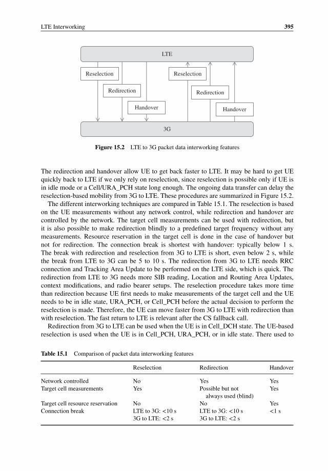
LTE Interworking 395
LTE
3G
Redirection
Handover
Reselection
Redirection
Handover
Reselection
Figure 15.2 LTE to 3G packet data interworking features
The redirection and handover allow UE to get back faster to LTE. It may be hard to get UEquickly back to LTE if we only rely on reselection, since reselection is possible only if UE isin idle mode or a Cell/URA_PCH state long enough. The ongoing data transfer can delay thereselection-based mobility from 3G to LTE. These procedures are summarized in Figure 15.2.
The different interworking techniques are compared in Table 15.1. The reselection is basedon the UE measurements without any network control, while redirection and handover arecontrolled by the network. The target cell measurements can be used with redirection, butit is also possible to make redirection blindly to a predefined target frequency without anymeasurements. Resource reservation in the target cell is done in the case of handover butnot for redirection. The connection break is shortest with handover: typically below 1 s.The break with redirection and reselection from 3G to LTE is short, even below 2 s, whilethe break from LTE to 3G can be 5 to 10 s. The redirection from 3G to LTE needs RRCconnection and Tracking Area Update to be performed on the LTE side, which is quick. Theredirection from LTE to 3G needs more SIB reading, Location and Routing Area Updates,context modifications, and radio bearer setups. The reselection procedure takes more timethan redirection because UE first needs to make measurements of the target cell and the UEneeds to be in idle state, URA_PCH, or Cell_PCH before the actual decision to perform thereselection is made. Therefore, the UE can move faster from 3G to LTE with redirection thanwith reselection. The fast return to LTE is relevant after the CS fallback call.
Redirection from 3G to LTE can be used when the UE is in Cell_DCH state. The UE-basedreselection is used when the UE is in Cell_PCH, URA_PCH, or in idle state. There used to
Table 15.1 Comparison of packet data interworking features
Reselection Redirection Handover
Network controlled No Yes YesTarget cell measurements Yes Possible but not
always used (blind)Yes
Target cell resource reservation No No YesConnection break LTE to 3G: <10 s
3G to LTE: <2 sLTE to 3G: <10 s3G to LTE: <2 s
<1 s
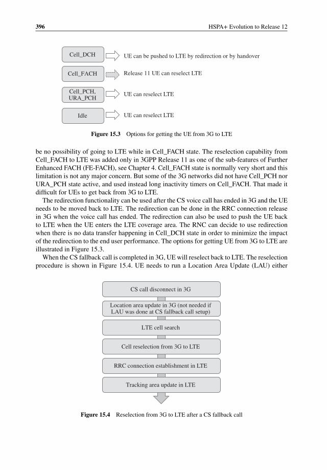
396 HSPA+ Evolution to Release 12
Cell_FACH
Cell_DCH
Idle
Cell_PCH, URA_PCH
UE can reselect LTE
UE can be pushed to LTE by redirection or by handover
UE can reselect LTE
Release 11 UE can reselect LTE
Figure 15.3 Options for getting the UE from 3G to LTE
be no possibility of going to LTE while in Cell_FACH state. The reselection capability fromCell_FACH to LTE was added only in 3GPP Release 11 as one of the sub-features of FurtherEnhanced FACH (FE-FACH), see Chapter 4. Cell_FACH state is normally very short and thislimitation is not any major concern. But some of the 3G networks did not have Cell_PCH norURA_PCH state active, and used instead long inactivity timers on Cell_FACH. That made itdifficult for UEs to get back from 3G to LTE.
The redirection functionality can be used after the CS voice call has ended in 3G and the UEneeds to be moved back to LTE. The redirection can be done in the RRC connection releasein 3G when the voice call has ended. The redirection can also be used to push the UE backto LTE when the UE enters the LTE coverage area. The RNC can decide to use redirectionwhen there is no data transfer happening in Cell_DCH state in order to minimize the impactof the redirection to the end user performance. The options for getting UE from 3G to LTE areillustrated in Figure 15.3.
When the CS fallback call is completed in 3G, UE will reselect back to LTE. The reselectionprocedure is shown in Figure 15.4. UE needs to run a Location Area Update (LAU) either
Location area update in 3G (not needed if LAU was done at CS fallback call setup)
CS call disconnect in 3G
RRC connection establishment in LTE
LTE cell search
Tracking area update in LTE
Cell reselection from 3G to LTE
Figure 15.4 Reselection from 3G to LTE after a CS fallback call
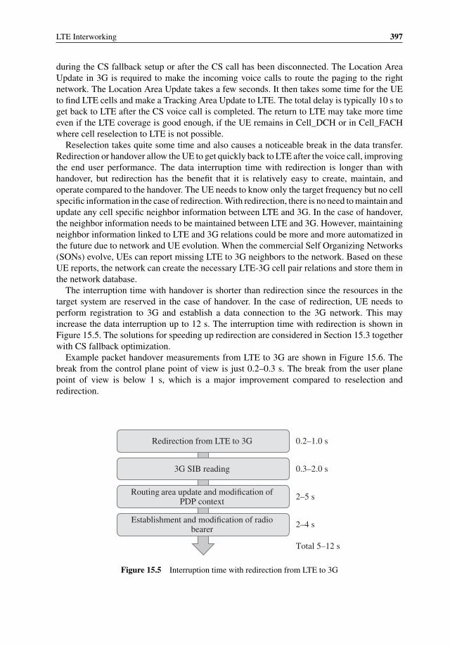
LTE Interworking 397
during the CS fallback setup or after the CS call has been disconnected. The Location AreaUpdate in 3G is required to make the incoming voice calls to route the paging to the rightnetwork. The Location Area Update takes a few seconds. It then takes some time for the UEto find LTE cells and make a Tracking Area Update to LTE. The total delay is typically 10 s toget back to LTE after the CS voice call is completed. The return to LTE may take more timeeven if the LTE coverage is good enough, if the UE remains in Cell_DCH or in Cell_FACHwhere cell reselection to LTE is not possible.
Reselection takes quite some time and also causes a noticeable break in the data transfer.Redirection or handover allow the UE to get quickly back to LTE after the voice call, improvingthe end user performance. The data interruption time with redirection is longer than withhandover, but redirection has the benefit that it is relatively easy to create, maintain, andoperate compared to the handover. The UE needs to know only the target frequency but no cellspecific information in the case of redirection. With redirection, there is no need to maintain andupdate any cell specific neighbor information between LTE and 3G. In the case of handover,the neighbor information needs to be maintained between LTE and 3G. However, maintainingneighbor information linked to LTE and 3G relations could be more and more automatized inthe future due to network and UE evolution. When the commercial Self Organizing Networks(SONs) evolve, UEs can report missing LTE to 3G neighbors to the network. Based on theseUE reports, the network can create the necessary LTE-3G cell pair relations and store them inthe network database.
The interruption time with handover is shorter than redirection since the resources in thetarget system are reserved in the case of handover. In the case of redirection, UE needs toperform registration to 3G and establish a data connection to the 3G network. This mayincrease the data interruption up to 12 s. The interruption time with redirection is shown inFigure 15.5. The solutions for speeding up redirection are considered in Section 15.3 togetherwith CS fallback optimization.
Example packet handover measurements from LTE to 3G are shown in Figure 15.6. Thebreak from the control plane point of view is just 0.2–0.3 s. The break from the user planepoint of view is below 1 s, which is a major improvement compared to reselection andredirection.
3G SIB reading
Redirection from LTE to 3G
Routing area update and modification of PDP context
Establishment and modification of radio bearer
0.2–1.0 s
Total 5–12 s
0.3–2.0 s
2–5 s
2–4 s
Figure 15.5 Interruption time with redirection from LTE to 3G
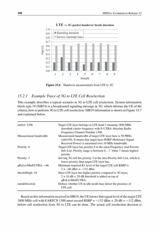
398 HSPA+ Evolution to Release 12
0.0
0.1
0.2
0.3
0.4
0.5
0.6
0.7
0.8
0.9
1.0
1 2 3 4 5 6 7 8 9
Gap
[s]
Sample
LTE -> 3G packet handover break duration
Signaling duration
Service interrupt time
Figure 15.6 Handover measurements from LTE to 3G
15.2.1 Example Trace of 3G to LTE Cell Reselection
This example describes a typical scenario in 3G to LTE cell reselection. System informationblock type 19 (SIB19) is a broadcasted signaling message in 3G, which informs the UE of thecriteria, how to perform 3G to LTE cell reselection. SIB19 information is shown in Figure 15.7and explained below.
earfcn: 1300 Target LTE layer belongs to LTE band 3 meaning 1800 MHzdownlink carrier frequency with E-UTRA Absolute RadioFrequency Channel Number 1300.
Measurement bandwidth: Measurement bandwidth of target LTE layer here is 50 PRBs(mbw50). It means that target layer RSRP (Reference SignalReceived Power) is measured over 10 MHz bandwidth.
Priority: 6 Target LTE layer has priority 6 in the eutra-Frequency And PriorityInfo List. Priority range is between 0…7. Value 7 means highestpriority
Priority: 3 Serving 3G cell has priority 3 in the utra-Priority Info List, which islower priority, than target LTE layer has.
qRxLevMinEUTRA: −66 Minimum required Rx level of the target LTE cell RSRP is2 × −66 dBm = −132 dBm
threshXhigh: 10 Since LTE layer has higher priority compared to 3G layer,2 × 10 dB = 20 dB threshold is added on top ofqRxLevMinEUTRA.
eutraDetection Defines whether UE in idle mode may detect the presence ofLTE cell.
Based on this information received in SIB19, the UE knows that signal level of the target LTE1800 MHz cell with EARFCN 1300 must exceed RSRP = −132 dBm + 20 dB = −112 dBm,before cell reselection from 3G to LTE can be done. The actual cell reselection decision is
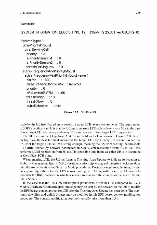
LTE Interworking 399
Figure 15.7 SIB19 in 3G
made by the UE itself based on its repetitive target LTE layer measurements. The requirementin 3GPP specification [1] is that the UE must measure LTE cells at least every 60 s in the caseof one target LTE frequency and every 120 s in the case of two target LTE frequencies.
The UE measurement logs from Anite Nemo outdoor tool are shown in Figure 15.8. Basedon log files, the test terminal measured the target LTE layer every 7th second. When theRSRP of the target LTE cell was strong enough, meaning the RSRP exceeding the threshold–112 dBm defined by network parameters in SIB19, cell reselection from 3G to LTE wasperformed. Cell reselection from 3G to LTE is possible only in the case that UE is in idle modeor Cell/URA_PCH-state.
When entering LTE, the UE performs a Tracking Area Update to indicate its location toMobility Management Entity (MME). Authentication, ciphering, and integrity checks are donewith the Authentication and Security Mode procedures. During these phases, the integrity andencryption algorithms for the EPS session are agreed. Along with these, the UE needs toestablish the RRC connection which is needed to maintain the connection between UE andLTE eNodeB.
In the case that the UE QoS subscription parameters differ in LTE compared to 3G, aModifyEPSBearerContextRequest-message may be sent by the network to the UE to modifythe EPS bearer context proper for LTE after the Tracking Area Update has been done. The max-imum downlink and uplink bitrates may be modified in this EPS bearer context modificationprocedure. The context modification does not typically take more than 0.5 s.
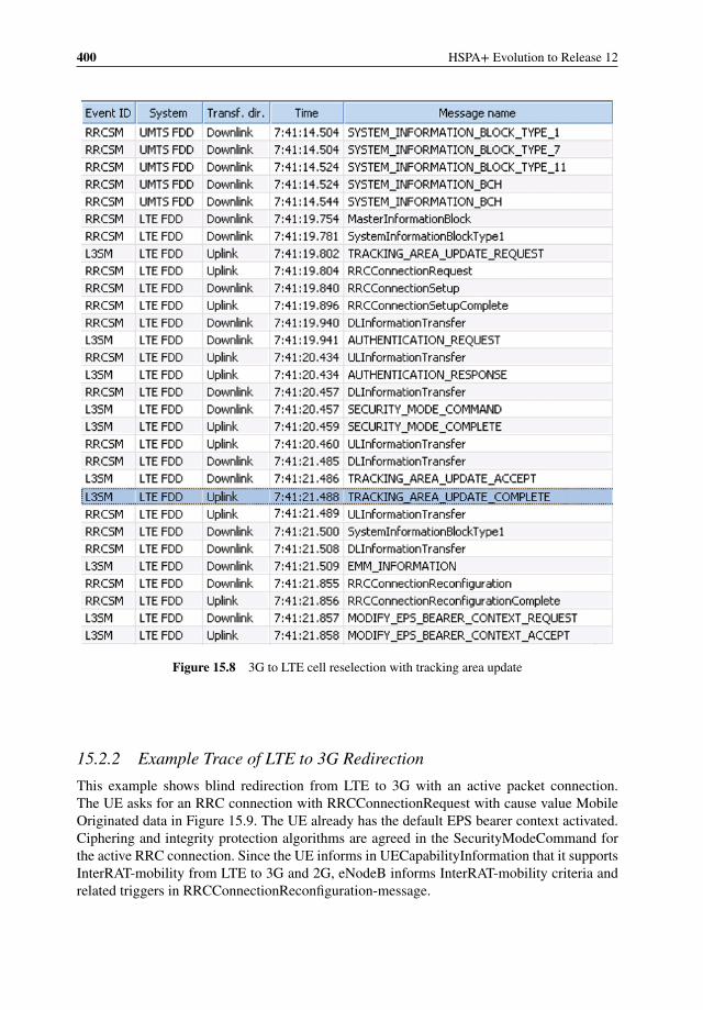
400 HSPA+ Evolution to Release 12
Figure 15.8 3G to LTE cell reselection with tracking area update
15.2.2 Example Trace of LTE to 3G Redirection
This example shows blind redirection from LTE to 3G with an active packet connection.The UE asks for an RRC connection with RRCConnectionRequest with cause value MobileOriginated data in Figure 15.9. The UE already has the default EPS bearer context activated.Ciphering and integrity protection algorithms are agreed in the SecurityModeCommand forthe active RRC connection. Since the UE informs in UECapabilityInformation that it supportsInterRAT-mobility from LTE to 3G and 2G, eNodeB informs InterRAT-mobility criteria andrelated triggers in RRCConnectionReconfiguration-message.
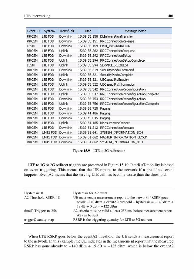
LTE Interworking 401
Figure 15.9 LTE to 3G redirection
LTE to 3G or 2G redirect triggers are presented in Figure 15.10. InterRAT-mobility is basedon event triggering. This means that the UE reports to the network if a predefined eventhappens. EventA2 means that the serving LTE cell has become worse than the threshold.
Hysteresis: 0 Hysteresis for A2 eventA2-Threshold RSRP: 18 UE must send a measurement report to the network if RSRP goes
below −140 dBm + eventA2threshold + hysteresis = −140 dBm +18 dB + 0 dB = −122 dBm
timeToTrigger: ms256 A2 criteria must be valid at least 256 ms, before measurement reportA2 can be sent
triggerQuantity: rsrp RSRP is the triggering quantity for LTE to 3G redirect
When LTE RSRP goes below the eventA2 threshold, the UE sends a measurement reportto the network. In this example, the UE indicates in the measurement report that the measuredRSRP has gone already to −140 dBm + 15 dB = −125 dBm, which is below the eventA2
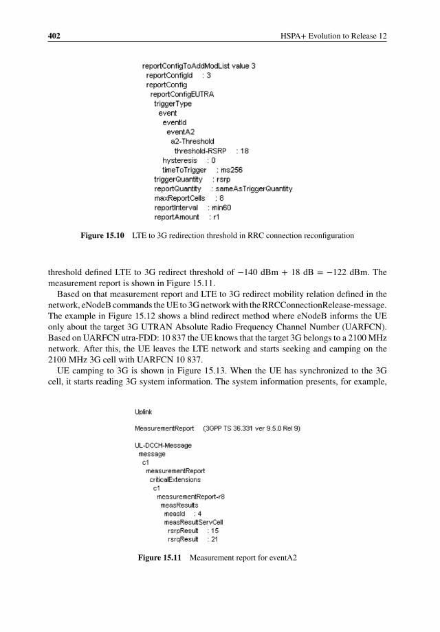
402 HSPA+ Evolution to Release 12
Figure 15.10 LTE to 3G redirection threshold in RRC connection reconfiguration
threshold defined LTE to 3G redirect threshold of −140 dBm + 18 dB = −122 dBm. Themeasurement report is shown in Figure 15.11.
Based on that measurement report and LTE to 3G redirect mobility relation defined in thenetwork, eNodeB commands the UE to 3G network with the RRCConnectionRelease-message.The example in Figure 15.12 shows a blind redirect method where eNodeB informs the UEonly about the target 3G UTRAN Absolute Radio Frequency Channel Number (UARFCN).Based on UARFCN utra-FDD: 10 837 the UE knows that the target 3G belongs to a 2100 MHznetwork. After this, the UE leaves the LTE network and starts seeking and camping on the2100 MHz 3G cell with UARFCN 10 837.
UE camping to 3G is shown in Figure 15.13. When the UE has synchronized to the 3Gcell, it starts reading 3G system information. The system information presents, for example,
Figure 15.11 Measurement report for eventA2

LTE Interworking 403
Figure 15.12 Redirect from LTE to 3G with RRC connection release
the following information to the UE: Idle mode mobility criteria in 3G presented in SIB3,3G to LTE mobility criteria in SIB19, and uplink interference information in SIB7. If thecamped 3G cell is the same cell where the UE last time camped in 3G, the UE may have storedpart of that specific 3G cell system information to its memory like the 3G cell neighboringcell information stored in SIB11. In this example, it can be seen that SIB11 is not read. Itis stored to the UE’s memory from the previous mobility session which was done to thissame 3G cell.
After all the relevant system information is received, UE can start RRC connection estab-lishment with cause value “registration.” That is needed for the Location and Routing AreaUpdates, presented in Figure 15.14, which are needed for the network to know that the UEis now in the 3G network under the specific 3G Location and Routing areas defined withLocation and Routing Area Codes (LAC, RAC). The UE identity is verified with IdentityRe-quests and indicated with International Mobile Subscriber Identity (IMSI) and InternationalMobile Station Equipment Identity and Software Version (IMEISV). Also, the authenticationand ciphering are handled and agreed with the related procedures. 3G mobility criteria andconnected mode neighbor lists are informed with MeasurementControl-messages. After theRouting Area Update is accepted, the UE context is modified with ModifyPDPContextRe-quest to meet the 3G QoS parameters, which are defined in the network based on customersubscription. For example, the maximum bitrates for downlink and uplink for 3G connectionare set here.
After the PDP context is modified, UE may send a ServiceRequest to the network includinginformation on active PDP context and pending uplink data. Pending data triggers the setupof radio bearer, which is modified with a RadioBearerReconfiguration to provide a packetdata connection. In this example, the packet data connection was reconfigured to the HSPAconnection with 21 Mbps downlink and 5.8 Mbps uplink capability. The data transfer cancontinue now. The 3G radio bearer setup is shown in Figure 15.15.
In this example, the data outage was around 10 s starting from LTE to 3G redirect trig-gered by RRC connection release in LTE and finally ending at RadioBearerReconfigurationin 3G.
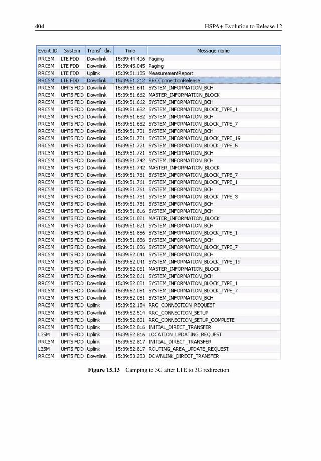
404 HSPA+ Evolution to Release 12
Figure 15.13 Camping to 3G after LTE to 3G redirection
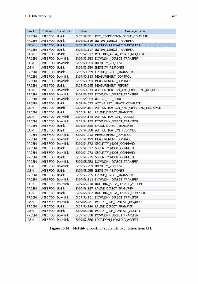
LTE Interworking 405
Figure 15.14 Mobility procedures in 3G after redirection from LTE
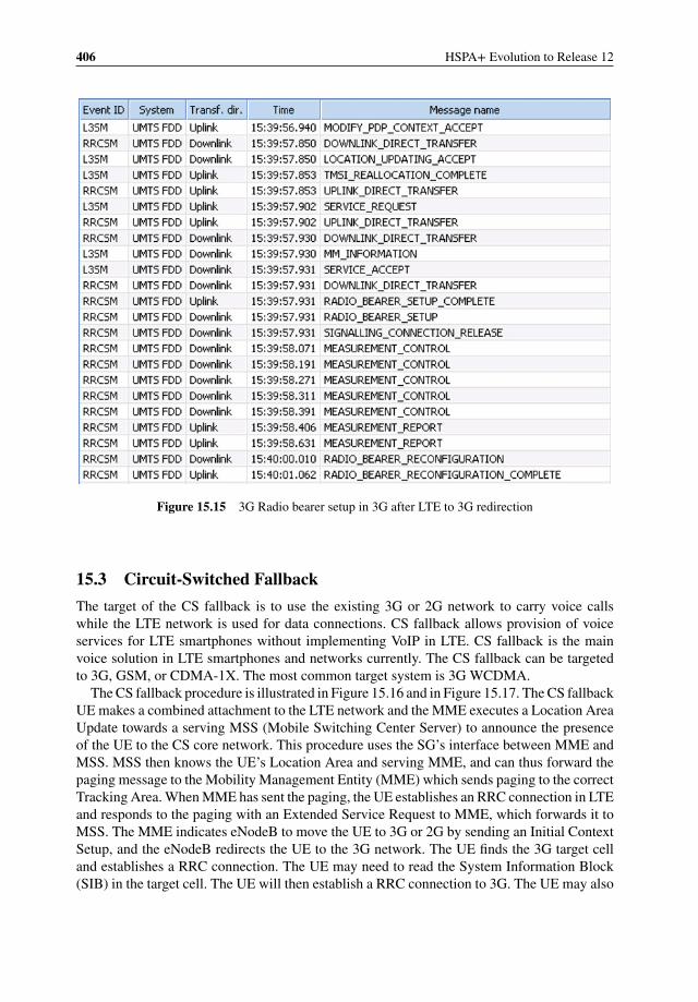
406 HSPA+ Evolution to Release 12
Figure 15.15 3G Radio bearer setup in 3G after LTE to 3G redirection
15.3 Circuit-Switched Fallback
The target of the CS fallback is to use the existing 3G or 2G network to carry voice callswhile the LTE network is used for data connections. CS fallback allows provision of voiceservices for LTE smartphones without implementing VoIP in LTE. CS fallback is the mainvoice solution in LTE smartphones and networks currently. The CS fallback can be targetedto 3G, GSM, or CDMA-1X. The most common target system is 3G WCDMA.
The CS fallback procedure is illustrated in Figure 15.16 and in Figure 15.17. The CS fallbackUE makes a combined attachment to the LTE network and the MME executes a Location AreaUpdate towards a serving MSS (Mobile Switching Center Server) to announce the presenceof the UE to the CS core network. This procedure uses the SG’s interface between MME andMSS. MSS then knows the UE’s Location Area and serving MME, and can thus forward thepaging message to the Mobility Management Entity (MME) which sends paging to the correctTracking Area. When MME has sent the paging, the UE establishes an RRC connection in LTEand responds to the paging with an Extended Service Request to MME, which forwards it toMSS. The MME indicates eNodeB to move the UE to 3G or 2G by sending an Initial ContextSetup, and the eNodeB redirects the UE to the 3G network. The UE finds the 3G target celland establishes a RRC connection. The UE may need to read the System Information Block(SIB) in the target cell. The UE will then establish a RRC connection to 3G. The UE may also
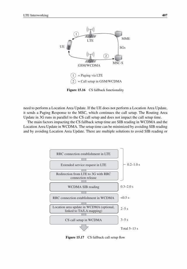
LTE Interworking 407
LTE
GSM/WCDMA MSC-S
MME
UE
= Paging via LTE
1
2
1
2 = Call setup in GSM/WCDMA
SGs
Figure 15.16 CS fallback functionality
need to perform a Location Area Update. If the UE does not perform a Location Area Update,it sends a Paging Response to the MSC, which continues the call setup. The Routing AreaUpdate in 3G runs in parallel to the CS call setup and does not impact the call setup time.
The main factors impacting the CS fallback setup time are SIB reading in WCDMA and theLocation Area Update in WCDMA. The setup time can be minimized by avoiding SIB readingand by avoiding Location Area Update. There are multiple solutions to avoid SIB reading or
Extended service request in LTE
RRC connection establishment in LTE
WCDMA SIB reading
RRC connection establishment in WCDMA
Location area update in WCDMA (optional, linked to TA/LA mapping)
CS call setup in WCDMA
0.3–2.0 s
2–5 s
0.2–1.0 s
<0.5 s
3–5 s
Total 5–13 s
Redirection from LTE to 3G with RRC connection release
Figure 15.17 CS fallback call setup flow
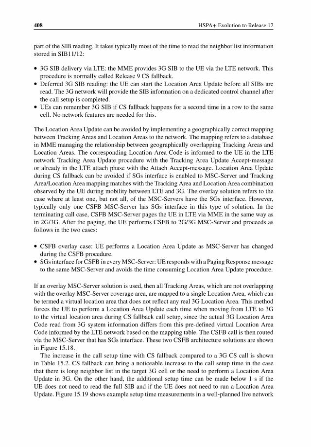
408 HSPA+ Evolution to Release 12
part of the SIB reading. It takes typically most of the time to read the neighbor list informationstored in SIB11/12:
� 3G SIB delivery via LTE: the MME provides 3G SIB to the UE via the LTE network. Thisprocedure is normally called Release 9 CS fallback.
� Deferred 3G SIB reading: the UE can start the Location Area Update before all SIBs areread. The 3G network will provide the SIB information on a dedicated control channel afterthe call setup is completed.
� UEs can remember 3G SIB if CS fallback happens for a second time in a row to the samecell. No network features are needed for this.
The Location Area Update can be avoided by implementing a geographically correct mappingbetween Tracking Areas and Location Areas to the network. The mapping refers to a databasein MME managing the relationship between geographically overlapping Tracking Areas andLocation Areas. The corresponding Location Area Code is informed to the UE in the LTEnetwork Tracking Area Update procedure with the Tracking Area Update Accept-messageor already in the LTE attach phase with the Attach Accept-message. Location Area Updateduring CS fallback can be avoided if SGs interface is enabled to MSC-Server and TrackingArea/Location Area mapping matches with the Tracking Area and Location Area combinationobserved by the UE during mobility between LTE and 3G. The overlay solution refers to thecase where at least one, but not all, of the MSC-Servers have the SGs interface. However,typically only one CSFB MSC-Server has SGs interface in this type of solution. In theterminating call case, CSFB MSC-Server pages the UE in LTE via MME in the same way asin 2G/3G. After the paging, the UE performs CSFB to 2G/3G MSC-Server and proceeds asfollows in the two cases:
� CSFB overlay case: UE performs a Location Area Update as MSC-Server has changedduring the CSFB procedure.
� SGs interface for CSFB in every MSC-Server: UE responds with a Paging Response messageto the same MSC-Server and avoids the time consuming Location Area Update procedure.
If an overlay MSC-Server solution is used, then all Tracking Areas, which are not overlappingwith the overlay MSC-Server coverage area, are mapped to a single Location Area, which canbe termed a virtual location area that does not reflect any real 3G Location Area. This methodforces the UE to perform a Location Area Update each time when moving from LTE to 3Gto the virtual location area during CS fallback call setup, since the actual 3G Location AreaCode read from 3G system information differs from this pre-defined virtual Location AreaCode informed by the LTE network based on the mapping table. The CSFB call is then routedvia the MSC-Server that has SGs interface. These two CSFB architecture solutions are shownin Figure 15.18.
The increase in the call setup time with CS fallback compared to a 3G CS call is shownin Table 15.2. CS fallback can bring a noticeable increase to the call setup time in the casethat there is long neighbor list in the target 3G cell or the need to perform a Location AreaUpdate in 3G. On the other hand, the additional setup time can be made below 1 s if theUE does not need to read the full SIB and if the UE does not need to run a Location AreaUpdate. Figure 15.19 shows example setup time measurements in a well-planned live network

LTE Interworking 409
MSC-S
MME LTE
GSM/WCDMA
MSC-S
SGs
MME LTE
GSM/WCDMA
MSC-S
SGs
Overlay CSFB solution
CSFB in every MSC-S
Figure 15.18 Overlay CSFB solution and CSFB in every MSC-S
Table 15.2 Call setup time increase with CS fallback
Location areaupdate avoided
With locationarea update
With 3G SIB reading 0.5–3.0 s 2.0–8.0 sSkip 3G SIB reading (Deferred
SIB or Release 9 CSFB)<1.0 s 1.5–6.0 s
0.0
1.0
2.0
3.0
4.0
5.0
6.0
7.0
8.0
9.0
10.0
1 2 3 4 5 6 7 8 9 10
s
Samples
Mobile originated CSFB call
CSFB
3G
Figure 15.19 CS fallback setup time measurements
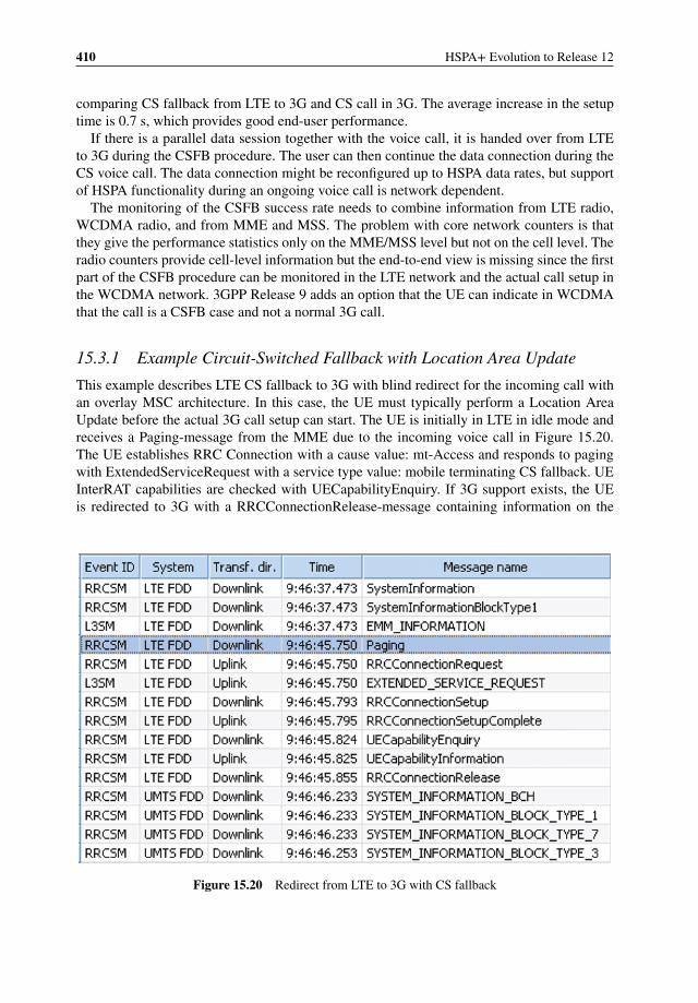
410 HSPA+ Evolution to Release 12
comparing CS fallback from LTE to 3G and CS call in 3G. The average increase in the setuptime is 0.7 s, which provides good end-user performance.
If there is a parallel data session together with the voice call, it is handed over from LTEto 3G during the CSFB procedure. The user can then continue the data connection during theCS voice call. The data connection might be reconfigured up to HSPA data rates, but supportof HSPA functionality during an ongoing voice call is network dependent.
The monitoring of the CSFB success rate needs to combine information from LTE radio,WCDMA radio, and from MME and MSS. The problem with core network counters is thatthey give the performance statistics only on the MME/MSS level but not on the cell level. Theradio counters provide cell-level information but the end-to-end view is missing since the firstpart of the CSFB procedure can be monitored in the LTE network and the actual call setup inthe WCDMA network. 3GPP Release 9 adds an option that the UE can indicate in WCDMAthat the call is a CSFB case and not a normal 3G call.
15.3.1 Example Circuit-Switched Fallback with Location Area Update
This example describes LTE CS fallback to 3G with blind redirect for the incoming call withan overlay MSC architecture. In this case, the UE must typically perform a Location AreaUpdate before the actual 3G call setup can start. The UE is initially in LTE in idle mode andreceives a Paging-message from the MME due to the incoming voice call in Figure 15.20.The UE establishes RRC Connection with a cause value: mt-Access and responds to pagingwith ExtendedServiceRequest with a service type value: mobile terminating CS fallback. UEInterRAT capabilities are checked with UECapabilityEnquiry. If 3G support exists, the UEis redirected to 3G with a RRCConnectionRelease-message containing information on the
Figure 15.20 Redirect from LTE to 3G with CS fallback
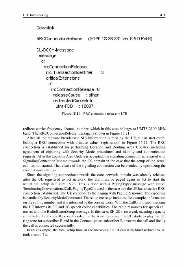
LTE Interworking 411
Figure 15.21 RRC connection release in LTE
redirect carrier frequency channel number, which in this case belongs to UMTS 2100 MHzband. The RRCConnectionRelease message is shown in Figure 15.21.
After all the relevant broadcasted SIB information is read by the UE, it can start estab-lishing a RRC connection with a cause value “registration” in Figure 15.22. The RRCconnection is established for performing Location and Routing Area Updates, includingagreement of ciphering with Security Mode procedures and identity and authenticationrequests. After the Location Area Update is accepted, the signaling connection is released withSignalingConnectionRelease towards the CS-domain in the case that the setup of the actualcall has not started. The release of the signaling connection can be avoided by optimizing thecore network settings.
Since the signaling connection towards the core network domain was already releasedafter the UE registered to 3G network, the UE must be paged again in 3G to start theactual call setup in Figure 15.23. This is done with a PagingType2-message with cause:TerminatingConversationalCall. PagingType2 is used in the case that the UE has an active RRCconnection established. The UE responds to the paging with PagingResponse. The cipheringis handled by SecurityModeCommand. The setup message includes, for example, informationon the calling number and it is informed by the core network. With the CallConfirmed-messagethe UE informs its 3G and 2G speech codec capabilities. The radio resources for speech callare set with the RadioBearerSetup-message. In this case, SF128 is reserved, meaning capacitysuitable for 12.2 kbps 3G speech codec. In the Alerting-phase, the UE starts to play the UEring tone for subscriber B and in the Connect-phase subscriber B answers the call and finallythe call is connected successfully.
In this example, the total setup time of the incoming CSFB call with blind redirect to 3Gtook around 7 s.
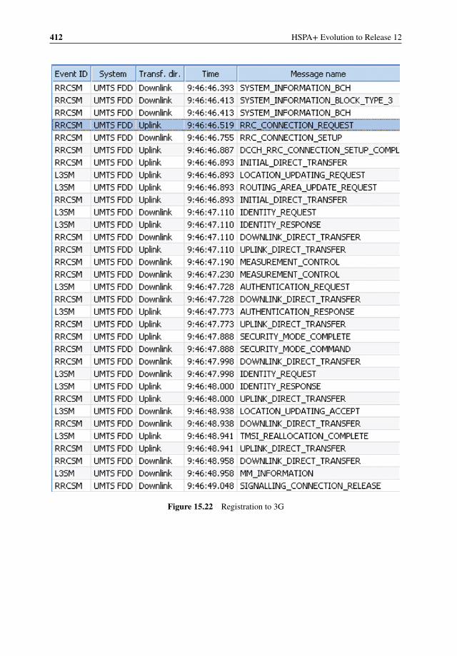
412 HSPA+ Evolution to Release 12
Figure 15.22 Registration to 3G
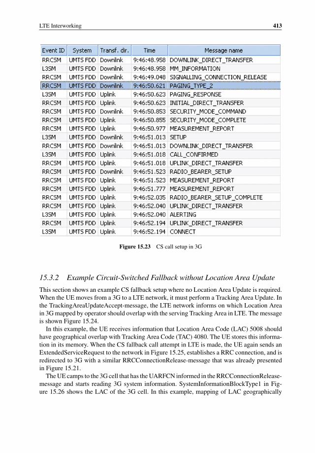
LTE Interworking 413
Figure 15.23 CS call setup in 3G
15.3.2 Example Circuit-Switched Fallback without Location Area Update
This section shows an example CS fallback setup where no Location Area Update is required.When the UE moves from a 3G to a LTE network, it must perform a Tracking Area Update. Inthe TrackingAreaUpdateAccept-message, the LTE network informs on which Location Areain 3G mapped by operator should overlap with the serving Tracking Area in LTE. The messageis shown Figure 15.24.
In this example, the UE receives information that Location Area Code (LAC) 5008 shouldhave geographical overlap with Tracking Area Code (TAC) 4080. The UE stores this informa-tion in its memory. When the CS fallback call attempt in LTE is made, the UE again sends anExtendedServiceRequest to the network in Figure 15.25, establishes a RRC connection, and isredirected to 3G with a similar RRCConnectionRelease-message that was already presentedin Figure 15.21.
The UE camps to the 3G cell that has the UARFCN informed in the RRCConnectionRelease-message and starts reading 3G system information. SystemInformationBlockType1 in Fig-ure 15.26 shows the LAC of the 3G cell. In this example, mapping of LAC geographically
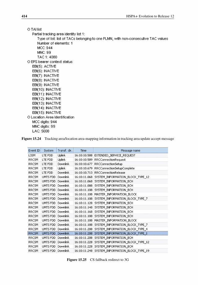
414 HSPA+ Evolution to Release 12
Figure 15.24 Tracking area/location area-mapping information in tracking area update accept-message
Figure 15.25 CS fallback redirect to 3G
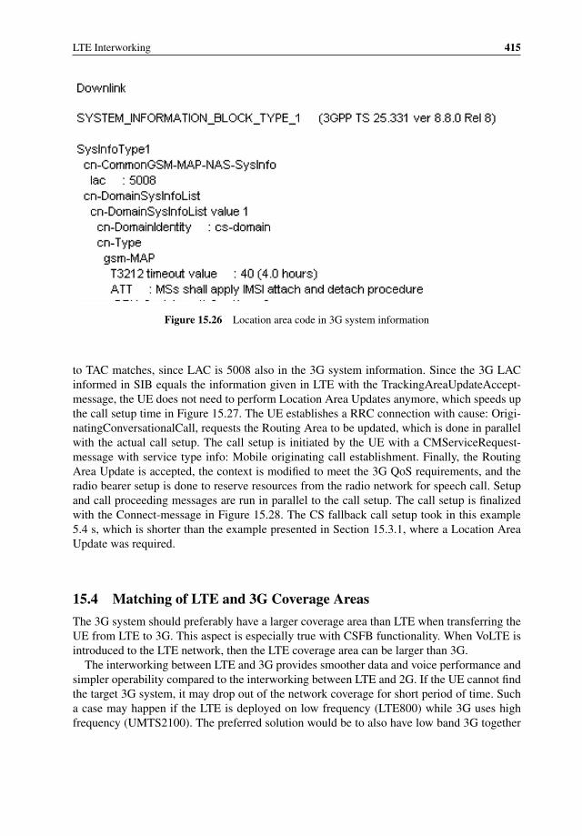
LTE Interworking 415
Figure 15.26 Location area code in 3G system information
to TAC matches, since LAC is 5008 also in the 3G system information. Since the 3G LACinformed in SIB equals the information given in LTE with the TrackingAreaUpdateAccept-message, the UE does not need to perform Location Area Updates anymore, which speeds upthe call setup time in Figure 15.27. The UE establishes a RRC connection with cause: Origi-natingConversationalCall, requests the Routing Area to be updated, which is done in parallelwith the actual call setup. The call setup is initiated by the UE with a CMServiceRequest-message with service type info: Mobile originating call establishment. Finally, the RoutingArea Update is accepted, the context is modified to meet the 3G QoS requirements, and theradio bearer setup is done to reserve resources from the radio network for speech call. Setupand call proceeding messages are run in parallel to the call setup. The call setup is finalizedwith the Connect-message in Figure 15.28. The CS fallback call setup took in this example5.4 s, which is shorter than the example presented in Section 15.3.1, where a Location AreaUpdate was required.
15.4 Matching of LTE and 3G Coverage Areas
The 3G system should preferably have a larger coverage area than LTE when transferring theUE from LTE to 3G. This aspect is especially true with CSFB functionality. When VoLTE isintroduced to the LTE network, then the LTE coverage area can be larger than 3G.
The interworking between LTE and 3G provides smoother data and voice performance andsimpler operability compared to the interworking between LTE and 2G. If the UE cannot findthe target 3G system, it may drop out of the network coverage for short period of time. Sucha case may happen if the LTE is deployed on low frequency (LTE800) while 3G uses highfrequency (UMTS2100). The preferred solution would be to also have low band 3G together
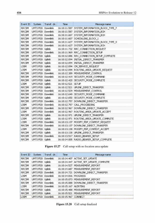
416 HSPA+ Evolution to Release 12
Figure 15.27 Call setup with no location area update
Figure 15.28 Call setup finalized
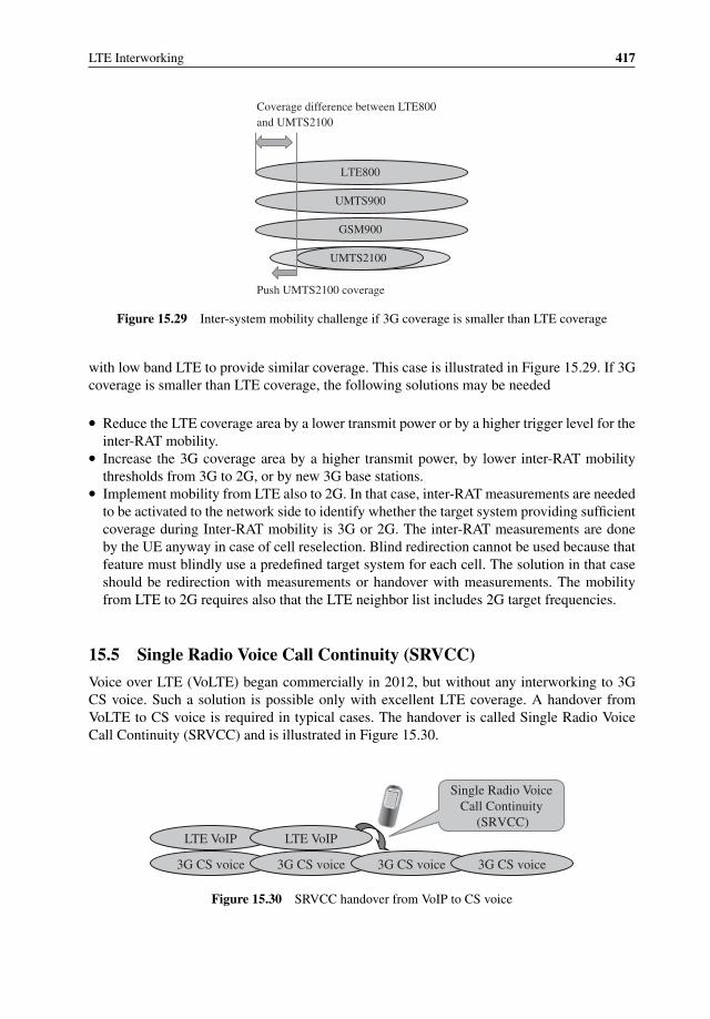
LTE Interworking 417
LTE800
UMTS900
UMTS2100
GSM900
Coverage difference between LTE800
and UMTS2100
Push UMTS2100 coverage
Figure 15.29 Inter-system mobility challenge if 3G coverage is smaller than LTE coverage
with low band LTE to provide similar coverage. This case is illustrated in Figure 15.29. If 3Gcoverage is smaller than LTE coverage, the following solutions may be needed
� Reduce the LTE coverage area by a lower transmit power or by a higher trigger level for theinter-RAT mobility.
� Increase the 3G coverage area by a higher transmit power, by lower inter-RAT mobilitythresholds from 3G to 2G, or by new 3G base stations.
� Implement mobility from LTE also to 2G. In that case, inter-RAT measurements are neededto be activated to the network side to identify whether the target system providing sufficientcoverage during Inter-RAT mobility is 3G or 2G. The inter-RAT measurements are doneby the UE anyway in case of cell reselection. Blind redirection cannot be used because thatfeature must blindly use a predefined target system for each cell. The solution in that caseshould be redirection with measurements or handover with measurements. The mobilityfrom LTE to 2G requires also that the LTE neighbor list includes 2G target frequencies.
15.5 Single Radio Voice Call Continuity (SRVCC)
Voice over LTE (VoLTE) began commercially in 2012, but without any interworking to 3GCS voice. Such a solution is possible only with excellent LTE coverage. A handover fromVoLTE to CS voice is required in typical cases. The handover is called Single Radio VoiceCall Continuity (SRVCC) and is illustrated in Figure 15.30.
LTE VoIP
3G CS voice
LTE VoIP
3G CS voice 3G CS voice 3G CS voice
Single Radio Voice
Call Continuity
(SRVCC)
Figure 15.30 SRVCC handover from VoIP to CS voice
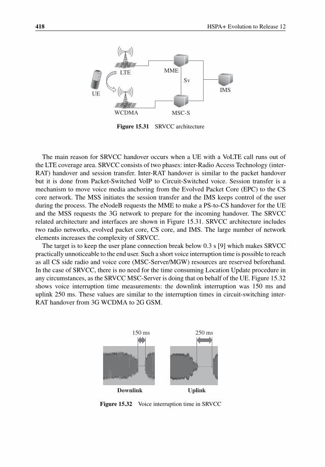
418 HSPA+ Evolution to Release 12
LTE
WCDMA
MME
MSC-S
IMSUE
Sv
Figure 15.31 SRVCC architecture
The main reason for SRVCC handover occurs when a UE with a VoLTE call runs out ofthe LTE coverage area. SRVCC consists of two phases: inter-Radio Access Technology (inter-RAT) handover and session transfer. Inter-RAT handover is similar to the packet handoverbut it is done from Packet-Switched VoIP to Circuit-Switched voice. Session transfer is amechanism to move voice media anchoring from the Evolved Packet Core (EPC) to the CScore network. The MSS initiates the session transfer and the IMS keeps control of the userduring the process. The eNodeB requests the MME to make a PS-to-CS handover for the UEand the MSS requests the 3G network to prepare for the incoming handover. The SRVCCrelated architecture and interfaces are shown in Figure 15.31. SRVCC architecture includestwo radio networks, evolved packet core, CS core, and IMS. The large number of networkelements increases the complexity of SRVCC.
The target is to keep the user plane connection break below 0.3 s [9] which makes SRVCCpractically unnoticeable to the end user. Such a short voice interruption time is possible to reachas all CS side radio and voice core (MSC-Server/MGW) resources are reserved beforehand.In the case of SRVCC, there is no need for the time consuming Location Update procedure inany circumstances, as the SRVCC MSC-Server is doing that on behalf of the UE. Figure 15.32shows voice interruption time measurements: the downlink interruption was 150 ms anduplink 250 ms. These values are similar to the interruption times in circuit-switching inter-RAT handover from 3G WCDMA to 2G GSM.
Downlink
150 ms 250 ms
Uplink
Figure 15.32 Voice interruption time in SRVCC
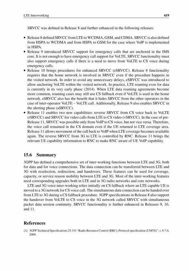
LTE Interworking 419
SRVCC was defined in Release 8 and further enhanced in the following releases:
� Release 8 defined SRVCC from LTE to WCDMA, GSM, and CDMA. SRVCC is also definedfrom HSPA to WCDMA and from HSPA to GSM for the case where VoIP is implementedin HSPA.
� Release 9 introduced SRVCC support for emergency calls that are anchored in the IMScore. It is not enough to have emergency call support for VoLTE, SRVCC functionality mustalso support emergency calls if there is a need to move from VoLTE to CS voice duringemergency calls.
� Release 10 brings procedures for enhanced SRVCC (eSRVCC). Release 8 functionalityrequires that the home network is involved in SRVCC even if the procedure happens inthe visited network. In order to avoid any unnecessary delays, eSRVCC was introduced toallow anchoring VoLTE within the visited network. In practice, LTE roaming even for datais currently in its very early phase (2014). When LTE data roaming agreements becomemore common, roaming cases may still use CS fallback even if VoLTE is used in the homenetwork. eSRVCC also has the benefit that it hides SRVCC from the other operators in thecase of inter-operator VoLTE – VoLTE call. Additionally, Release 9 also enables SRVCC inthe alerting phase (aSRVCC).
� Release 11 enables two new capabilities: reverse SRVCC from CS voice back to VoLTE(rSRVCC) and SRVCC for video calls from LTE to CS video (vSRVCC). In the case of pre-Release 11, SRVCC was possible only from VoIP to CS voice, but not vice versa. Therefore,the voice call remained in the CS domain even if the UE returned to LTE coverage area.Release 11 allows movement of the call back to VoIP when LTE coverage becomes availableagain. The reverse SRVCC from 3G to LTE is controlled by RNC. Release 11 brings therelevant UE capability information to RNC to make RNC aware of UE VoIP capability.
15.6 Summary
3GPP has defined a comprehensive set of inter-working functions between LTE and 3G, bothfor data and for voice connections. The data connection can be transferred between LTE and3G with reselection, redirection, and handovers. These features can be used for coverage,capacity, or service reason mobility between LTE and 3G. Most of the inter-working featuresneed corresponding upgrades both in LTE and in 3G radio networks and core networks.
LTE and 3G voice inter-working relies initially on CS fallback where an LTE capable UE ismoved to a 3G network for CS voice call. The simultaneous data connection can be handed overfrom LTE to 3G during a CS fallback procedure. 3GPP specifications in Release 8 also supportthe handover from VoLTE to CS voice in the 3G network called SRVCC with simultaneouspacket data session continuity. SRVCC functionality is further enhanced in Releases 9, 10,and 11.
References
[1] 3GPP Technical Specifications 25.331 “Radio Resource Control (RRC); Protocol specification (UMTS)”, v. 8.7.0,2009.

420 HSPA+ Evolution to Release 12
[2] 3GPP Technical Specifications 36.331 “Radio Resource Control (RRC); Protocol specification (LTE)”, v. 8.6.0,2009.
[3] 3GPP Technical Specifications 25.133 “Requirements for support of radio resource management (UMTS)”,v. 8.8.0, 2009.
[4] 3GPP Technical Specifications 36.133 “Requirements for support of radio resource management (LTE)”, v. 8.8.0,2009.
[5] 3GPP Technical Specifications 24.008 “Mobile radio interface Layer 3 specification”, v. 9.7.0, 2011.[6] 3GPP Technical Specifications 24.301 “Non-Access-Stratum (NAS) protocol for Evolved Packet System (EPS)”,
v. 9.7.0, 2011.[7] 3GPP Technical Specifications 23.272 “Circuit Switched (CS) fallback in Evolved Packet System (EPS)”,
v. 11.9.0, 2013.[8] 3GPP Technical Specifications 24.278 “Service requirements for the Evolved Packet System (EPS)”, v. 8.9.0,
2011.[9] 3GPP Technical Specifications 23.216 “Single Radio Voice Call Continuity (SRVCC)”, v. 11.9.0, 2013.
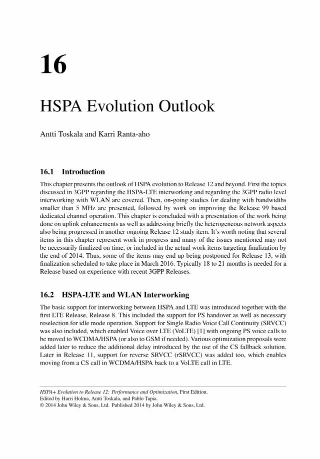
16HSPA Evolution Outlook
Antti Toskala and Karri Ranta-aho
16.1 Introduction
This chapter presents the outlook of HSPA evolution to Release 12 and beyond. First the topicsdiscussed in 3GPP regarding the HSPA-LTE interworking and regarding the 3GPP radio levelinterworking with WLAN are covered. Then, on-going studies for dealing with bandwidthssmaller than 5 MHz are presented, followed by work on improving the Release 99 baseddedicated channel operation. This chapter is concluded with a presentation of the work beingdone on uplink enhancements as well as addressing briefly the heterogeneous network aspectsalso being progressed in another ongoing Release 12 study item. It’s worth noting that severalitems in this chapter represent work in progress and many of the issues mentioned may notbe necessarily finalized on time, or included in the actual work items targeting finalization bythe end of 2014. Thus, some of the items may end up being postponed for Release 13, withfinalization scheduled to take place in March 2016. Typically 18 to 21 months is needed for aRelease based on experience with recent 3GPP Releases.
16.2 HSPA-LTE and WLAN Interworking
The basic support for interworking between HSPA and LTE was introduced together with thefirst LTE Release, Release 8. This included the support for PS handover as well as necessaryreselection for idle mode operation. Support for Single Radio Voice Call Continuity (SRVCC)was also included, which enabled Voice over LTE (VoLTE) [1] with ongoing PS voice calls tobe moved to WCDMA/HSPA (or also to GSM if needed). Various optimization proposals wereadded later to reduce the additional delay introduced by the use of the CS fallback solution.Later in Release 11, support for reverse SRVCC (rSRVCC) was added too, which enablesmoving from a CS call in WCDMA/HSPA back to a VoLTE call in LTE.
HSPA+ Evolution to Release 12: Performance and Optimization, First Edition.Edited by Harri Holma, Antti Toskala, and Pablo Tapia.© 2014 John Wiley & Sons, Ltd. Published 2014 by John Wiley & Sons, Ltd.
422 HSPA+ Evolution to Release 12
As part of the Release 12 studies, proposals addressing the following areas have been made,as covered in [1]:
� Improvements for the load balancing, aiming to address limitations in the current signalingwhere only one eNodeB load information can be provided at a time for a given RNC.
� Improvements in mobility signaling in the case of a multistandard BTS, to investigatewhether some of the steps could be optimized when it is known that both HSPA and LTEare provided by the same base station.
Besides interworking with HSPA, 3GPP has also been addressing the interworking between3GPP radio and WLAN networks. In 3GPP radio specifications, there has been no workdone so far with the radio level interworking between 3GPP radios (LTE and WCDMA) andWireless LAN (WLAN) networks. The key issue to address is how to ensure quality of serviceis retained when moving from a 3GPP network to WLAN network. Currently, if a UE movesfrom a 3GPP network to WLAN, the resulting quality may be much worse than that providedby a HSPA or LTE network due, for example, to limitations in the backhaul with WLAN orfor general load reasons. While at the moment there are no defined measures in RAN for howto fix the situation, such methods are not being specified in 3GPP.
The three different approaches originally considered were, as given in [2]:
� An Automatic Network Domain Selection Function (ANDSF) based solution, which wouldaim to extend the core network-based ANDSF solution. It has been suggested that a pureANDSF solution for providing the policies for the UE could not address the dynamicsituation on the radio side as ANDSF signaling comes from the core network side. ANDSFwas addressed in more detail in Chapter 7.
� The second approach considered is to provide in the RAN side (RRC) signaling offloadingrules including the WLAN Traffic Steering Indicator (WTSI). WTSI would indicate whetherto steer traffic to WLAN or whether to stay with 3GPP RAN instead. RAN side signalingcould provide the list of radio bearers to be offloaded (unless provided via ANDSF).The general principle is a UE receiving guidance from the RAN side on which accesspoints (WLAN SSID) to consider for offloading. Additionally, further information couldbe provided to help with the selection, such as what the signal strength in the 3GPP RANnetwork side should be, with the following quality measures to be considered: HSPA CPICHEc/No and CPICH Received Signal Code Power (RSCP) or on the LTE side the ReferenceSignal Received Power (RSRP) or Reference Signal Received Quality (RSRQ) as presentedin [3]. This approach was chosen as the basis for Release 12 RAN solution.
� The offloading from 3GPP RAN to WLAN could be done based on the dedicated trafficsteering commands from RAN. The commands could be derived UE measurements based onWLAN network quality and load. Such an approach with UE measurements and reportingis rather similar to radio handover type operations inside 3GPP RAN. Such an approachhas the greatest complexity impact on the network, especially if the RNC area has a largenumber of WLAN access points which would need to be controlled by RNC.
3GPP has already decided that there will not be, for example, an interface specified betweenWLAN AP and HSPA NodeB or RNC. Especially for an RNC it would not be desirable to
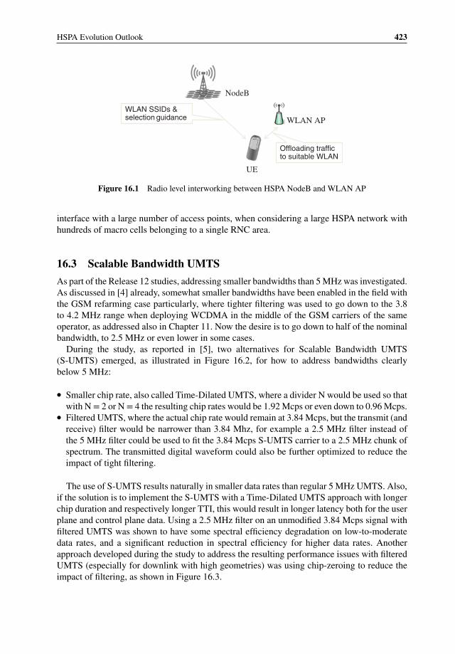
HSPA Evolution Outlook 423
WLAN SSIDs & selection guidance
UE
WLAN AP
NodeB
Offloading traffic to suitable WLAN
Figure 16.1 Radio level interworking between HSPA NodeB and WLAN AP
interface with a large number of access points, when considering a large HSPA network withhundreds of macro cells belonging to a single RNC area.
16.3 Scalable Bandwidth UMTS
As part of the Release 12 studies, addressing smaller bandwidths than 5 MHz was investigated.As discussed in [4] already, somewhat smaller bandwidths have been enabled in the field withthe GSM refarming case particularly, where tighter filtering was used to go down to the 3.8to 4.2 MHz range when deploying WCDMA in the middle of the GSM carriers of the sameoperator, as addressed also in Chapter 11. Now the desire is to go down to half of the nominalbandwidth, to 2.5 MHz or even lower in some cases.
During the study, as reported in [5], two alternatives for Scalable Bandwidth UMTS(S-UMTS) emerged, as illustrated in Figure 16.2, for how to address bandwidths clearlybelow 5 MHz:
� Smaller chip rate, also called Time-Dilated UMTS, where a divider N would be used so thatwith N = 2 or N = 4 the resulting chip rates would be 1.92 Mcps or even down to 0.96 Mcps.
� Filtered UMTS, where the actual chip rate would remain at 3.84 Mcps, but the transmit (andreceive) filter would be narrower than 3.84 Mhz, for example a 2.5 MHz filter instead ofthe 5 MHz filter could be used to fit the 3.84 Mcps S-UMTS carrier to a 2.5 MHz chunk ofspectrum. The transmitted digital waveform could also be further optimized to reduce theimpact of tight filtering.
The use of S-UMTS results naturally in smaller data rates than regular 5 MHz UMTS. Also,if the solution is to implement the S-UMTS with a Time-Dilated UMTS approach with longerchip duration and respectively longer TTI, this would result in longer latency both for the userplane and control plane data. Using a 2.5 MHz filter on an unmodified 3.84 Mcps signal withfiltered UMTS was shown to have some spectral efficiency degradation on low-to-moderatedata rates, and a significant reduction in spectral efficiency for higher data rates. Anotherapproach developed during the study to address the resulting performance issues with filteredUMTS (especially for downlink with high geometries) was using chip-zeroing to reduce theimpact of filtering, as shown in Figure 16.3.
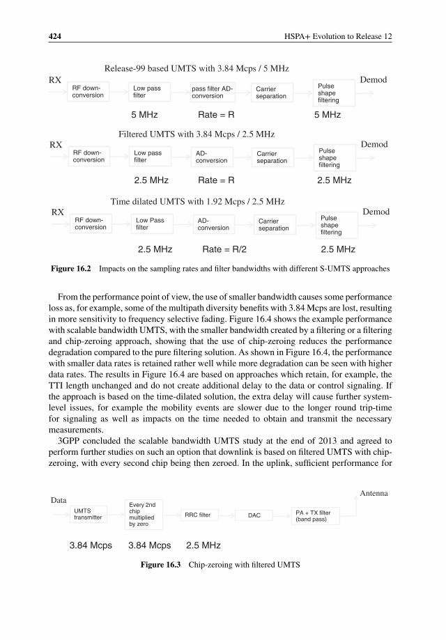
424 HSPA+ Evolution to Release 12
RF down-conversion
RX Low passfilter
AD-conversion
Carrier separation
Pulseshapefiltering
Demod
2.5 MHz Rate = R/2 2.5 MHz
RF down-conversion
RX Low passfilter
pass filter AD-conversion
Carrier separation
Pulseshapefiltering
Demod
Release-99 based UMTS with 3.84 Mcps / 5 MHz
5 MHz Rate = R 5 MHz
Filtered UMTS with 3.84 Mcps / 2.5 MHz
2.5 MHz Rate = R 2.5 MHz
RF down-conversion
RX Low Passfilter
AD-conversion
Carrier separation
Pulseshapefiltering
Demod Time dilated UMTS with 1.92 Mcps / 2.5 MHz
Figure 16.2 Impacts on the sampling rates and filter bandwidths with different S-UMTS approaches
From the performance point of view, the use of smaller bandwidth causes some performanceloss as, for example, some of the multipath diversity benefits with 3.84 Mcps are lost, resultingin more sensitivity to frequency selective fading. Figure 16.4 shows the example performancewith scalable bandwidth UMTS, with the smaller bandwidth created by a filtering or a filteringand chip-zeroing approach, showing that the use of chip-zeroing reduces the performancedegradation compared to the pure filtering solution. As shown in Figure 16.4, the performancewith smaller data rates is retained rather well while more degradation can be seen with higherdata rates. The results in Figure 16.4 are based on approaches which retain, for example, theTTI length unchanged and do not create additional delay to the data or control signaling. Ifthe approach is based on the time-dilated solution, the extra delay will cause further system-level issues, for example the mobility events are slower due to the longer round trip-timefor signaling as well as impacts on the time needed to obtain and transmit the necessarymeasurements.
3GPP concluded the scalable bandwidth UMTS study at the end of 2013 and agreed toperform further studies on such an option that downlink is based on filtered UMTS with chip-zeroing, with every second chip being then zeroed. In the uplink, sufficient performance for
3.84 Mcps 3.84 Mcps 2.5 MHz
UMTS transmitter
Data Every 2nd chip multiplied by zero
RRC filter DAC PA + TX filter (band pass)
Antenna
Figure 16.3 Chip-zeroing with filtered UMTS
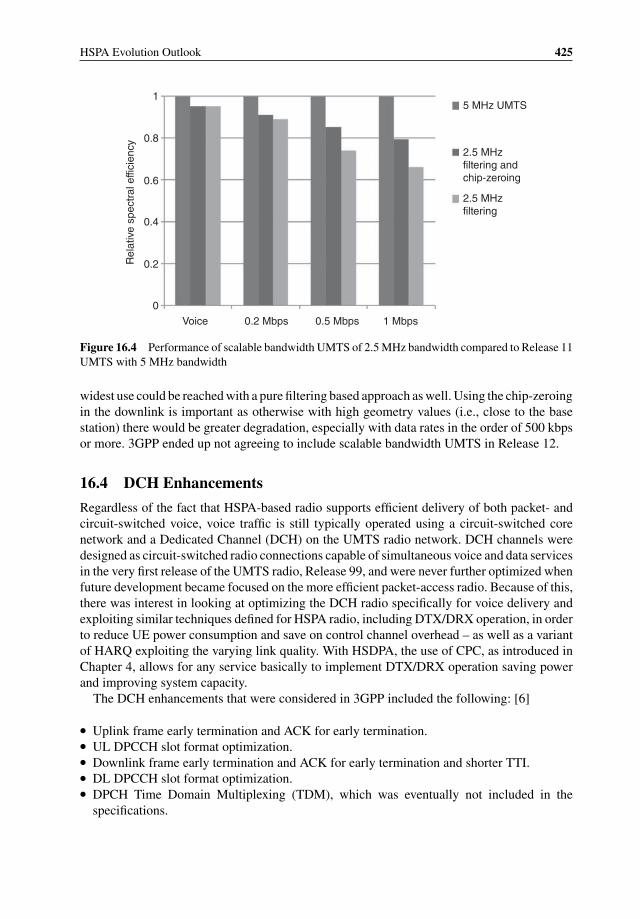
HSPA Evolution Outlook 425
1
0.8
0.4
0.6
0.2
0
Voice
Rel
ativ
e sp
ectr
al e
ffici
ency
0.2 Mbps 0.5 Mbps 1 Mbps
5 MHz UMTS
2.5 MHzfiltering andchip-zeroing
2.5 MHzfiltering
Figure 16.4 Performance of scalable bandwidth UMTS of 2.5 MHz bandwidth compared to Release 11UMTS with 5 MHz bandwidth
widest use could be reached with a pure filtering based approach as well. Using the chip-zeroingin the downlink is important as otherwise with high geometry values (i.e., close to the basestation) there would be greater degradation, especially with data rates in the order of 500 kbpsor more. 3GPP ended up not agreeing to include scalable bandwidth UMTS in Release 12.
16.4 DCH Enhancements
Regardless of the fact that HSPA-based radio supports efficient delivery of both packet- andcircuit-switched voice, voice traffic is still typically operated using a circuit-switched corenetwork and a Dedicated Channel (DCH) on the UMTS radio network. DCH channels weredesigned as circuit-switched radio connections capable of simultaneous voice and data servicesin the very first release of the UMTS radio, Release 99, and were never further optimized whenfuture development became focused on the more efficient packet-access radio. Because of this,there was interest in looking at optimizing the DCH radio specifically for voice delivery andexploiting similar techniques defined for HSPA radio, including DTX/DRX operation, in orderto reduce UE power consumption and save on control channel overhead – as well as a variantof HARQ exploiting the varying link quality. With HSDPA, the use of CPC, as introduced inChapter 4, allows for any service basically to implement DTX/DRX operation saving powerand improving system capacity.
The DCH enhancements that were considered in 3GPP included the following: [6]
� Uplink frame early termination and ACK for early termination.� UL DPCCH slot format optimization.� Downlink frame early termination and ACK for early termination and shorter TTI.� DL DPCCH slot format optimization.� DPCH Time Domain Multiplexing (TDM), which was eventually not included in the
specifications.
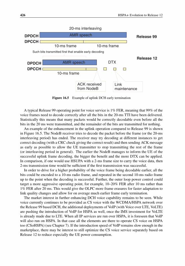
426 HSPA+ Evolution to Release 12
DPCCH DPDCH
20-ms interleaving
10-ms frame 10-ms frame
DTX
AMR speech Release 99
Release 12
DPCCH DPDCH
10-ms frame
AMR speech
ACK receivedfrom NodeB
Such bits transmitted first that enable early decoding
Link maintenance
Figure 16.5 Example of uplink DCH early termination
A typical Release 99 operating point for voice service is 1% FER, meaning that 99% of thevoice frames need to decode correctly after all the bits in the 20-ms TTI have been delivered.Statistically this means that many packets would be correctly decodable even before all thebits in the 20 ms were transmitted, and the remainder of the bits are transmitted for nothing.
An example of the enhancement in the uplink operation compared to Release 99 is shownin Figure 16.5. The NodeB receiver tries to decode the packet before the frame (or the 20-msinterleaving period) has ended. The receiver may try decoding at different instances to getcorrect decoding (with a CRC check giving the correct result) and then sending ACK messageas early as possible to allow the UE transmitter to stop transmitting the rest of the frame(or interleaving period in general). The earlier the NodeB manages to inform the UE of thesuccessful uplink frame decoding, the bigger the benefit and the more DTX can be applied.In comparison, if one would use HSUPA with a 2-ms frame size to carry the voice data, then2-ms transmission time would be sufficient if the first transmission was successful.
In order to drive for a higher probability of the voice frame being decodable earlier, all thebits could be encoded to a 10-ms radio frame, and repeated in the second 10-ms radio frameup to the point when the decoding is successful. Further, the outer loop power control couldtarget a more aggressive operating point, for example, 10–20% FER after 10 ms rather than1% FER after 20 ms. This would give the OLPC more frame erasures for faster adaptation tolink quality changes and allow for on average much earlier frame early termination.
The market interest in further enhancing DCH voice capability remains to be seen. Whilevoice currently continues to be provided as CS voice with the WCDMA/HSPA network overthe Release 99 based DCH, the additional deployments of VoIP (with Voice over LTE, VoLTE)are pushing the introduction of VoIP for HSPA as well, once the IMS investment for VoLTEis already made due to LTE. When all IP services are run over HSPA, it is foreseen that VoIPwill also run on HSPA. In that case all the elements are there to operate CS voice on HSPAtoo (CSoHSPA) (see Chapter 7). If the introduction speed of VoIP remains slow enough in themarketplace, there may be interest to still optimize the CS voice service separately based onRelease 12 to reduce especially the UE power consumption.
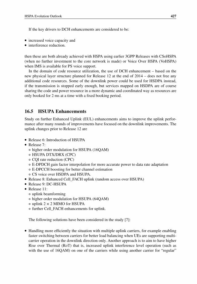
HSPA Evolution Outlook 427
If the key drivers to DCH enhancements are considered to be:
� increased voice capacity and� interference reduction.
then these are both already achieved with HSPA using earlier 3GPP Releases with CSoHSPA(when no further investment to the core network is made) or Voice Over HSPA (VoHSPA)when IMS is available for PS voice support.
In the domain of code resource utilization, the use of DCH enhancement – based on thenew physical layer structure planned for Release 12 at the end of 2014 – does not free anyadditional code resources. Some of the downlink power could be used for HSDPA instead,if the transmission is stopped early enough, but services mapped on HSDPA are of coursesharing the code and power resource in a more dynamic and coordinated way as resources areonly booked for 2 ms at a time with a fixed booking period.
16.5 HSUPA Enhancements
Study on further Enhanced Uplink (EUL) enhancements aims to improve the uplink perfor-mance after many rounds of improvements have focused on the downlink improvements. Theuplink changes prior to Release 12 are
� Release 6: Introduction of HSUPA� Release 7:◦ higher order modulation for HSUPA (16QAM)◦ HSUPA DTX/DRX (CPC)◦ CQI rate reduction (CPC)◦ E-DPDCH gain factor interpolation for more accurate power to data rate adaptation◦ E-DPCCH boosting for better channel estimation◦ CS voice over HSDPA and HSUPA.
� Release 8: Enhanced Cell_FACH uplink (random access over HSUPA)� Release 9: DC-HSUPA� Release 11:◦ uplink beamforming◦ higher order modulation for HSUPA (64QAM)◦ uplink 2 × 2 MIMO for HSUPA◦ further Cell_FACH enhancements for uplink.
The following solutions have been considered in the study [7]:
� Handling more efficiently the situation with multiple uplink carriers, for example enablingfaster switching between carriers for better load balancing when UEs are supporting multi-carrier operation in the downlink direction only. Another approach is to aim to have higherRise over Thermal (RoT) that is, increased uplink interference level operation (such aswith the use of 16QAM) on one of the carriers while using another carrier for “regular”
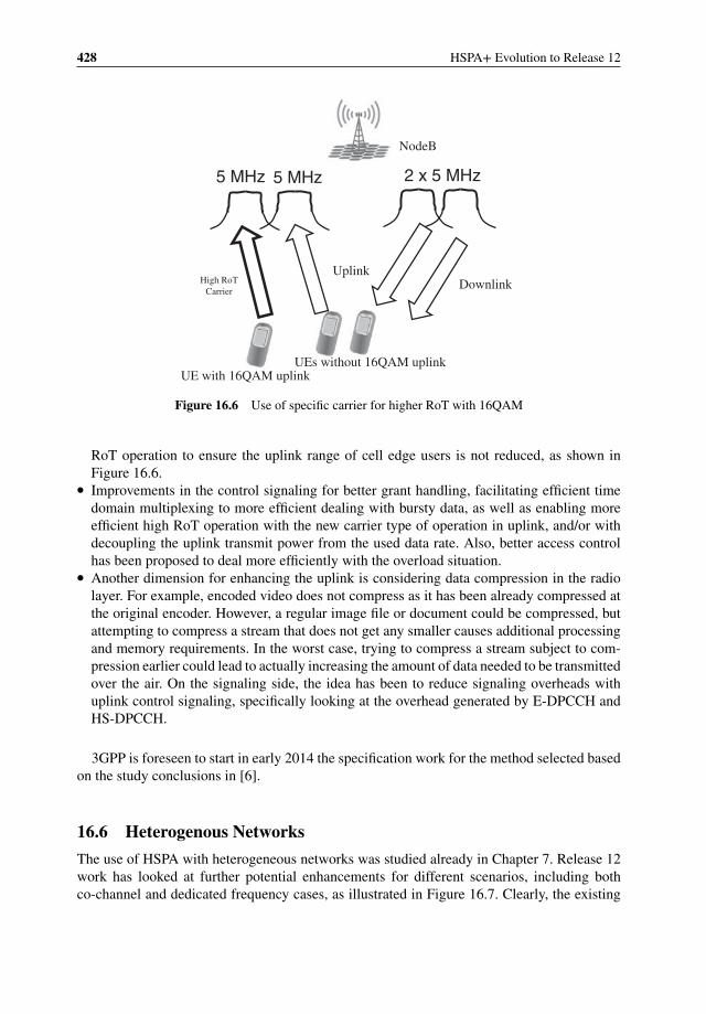
428 HSPA+ Evolution to Release 12
2 x 5 MHz 5 MHz
NodeB
UEs without 16QAM uplink
Downlink Uplink
5 MHz
High RoT
Carrier
UE with 16QAM uplink
Figure 16.6 Use of specific carrier for higher RoT with 16QAM
RoT operation to ensure the uplink range of cell edge users is not reduced, as shown inFigure 16.6.
� Improvements in the control signaling for better grant handling, facilitating efficient timedomain multiplexing to more efficient dealing with bursty data, as well as enabling moreefficient high RoT operation with the new carrier type of operation in uplink, and/or withdecoupling the uplink transmit power from the used data rate. Also, better access controlhas been proposed to deal more efficiently with the overload situation.
� Another dimension for enhancing the uplink is considering data compression in the radiolayer. For example, encoded video does not compress as it has been already compressed atthe original encoder. However, a regular image file or document could be compressed, butattempting to compress a stream that does not get any smaller causes additional processingand memory requirements. In the worst case, trying to compress a stream subject to com-pression earlier could lead to actually increasing the amount of data needed to be transmittedover the air. On the signaling side, the idea has been to reduce signaling overheads withuplink control signaling, specifically looking at the overhead generated by E-DPCCH andHS-DPCCH.
3GPP is foreseen to start in early 2014 the specification work for the method selected basedon the study conclusions in [6].
16.6 Heterogenous Networks
The use of HSPA with heterogeneous networks was studied already in Chapter 7. Release 12work has looked at further potential enhancements for different scenarios, including bothco-channel and dedicated frequency cases, as illustrated in Figure 16.7. Clearly, the existing
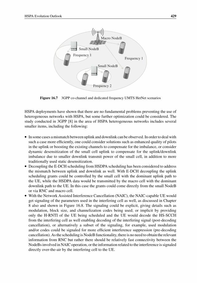
HSPA Evolution Outlook 429
Frequency 1
Macro NodeB
Frequency 2
Small NodeB
Small NodeB
Frequency 1
Figure 16.7 3GPP co-channel and dedicated frequency UMTS HetNet scenarios
HSPA deployments have shown that there are no fundamental problems preventing the use ofheterogeneous networks with HSPA, but some further optimization could be considered. Thestudy conducted in 3GPP [8] in the area of HSPA heterogeneous networks includes severalsmaller items, including the following:
� In some cases a mismatch between uplink and downlink can be observed. In order to deal withsuch a case more efficiently, one could consider solutions such as enhanced quality of pilotsin the uplink or boosting the existing channels to compensate for the imbalance, or considerdynamic desensitization of the small cell uplink to compensate for the uplink/downlinkimbalance due to smaller downlink transmit power of the small cell, in addition to moretraditionally used static desensitization.
� Decoupling the E-DCH scheduling from HSDPA scheduling has been considered to addressthe mismatch between uplink and downlink as well. With E-DCH decoupling the uplinkscheduling grants could be controlled by the small cell with the dominant uplink path tothe UE, while the HSDPA data would be transmitted by the macro cell with the dominantdownlink path to the UE. In this case the grants could come directly from the small NodeBor via RNC and macro cell.
� With the Network Assisted Interference Cancellation (NAIC), the NAIC-capable UE wouldget signaling of the parameters used in the interfering cell as well, as discussed in Chapter8 also and shown in Figure 16.8. The signaling could be explicit, giving details such asmodulation, block size, and channelization codes being used; or implicit by providingonly the H-RNTI of the UE being scheduled and the UE would decode the HS-SCCHfrom the interfering cell as well enabling decoding of the interfering signal (post-decodingcancellation), or alternatively a subset of the signaling, for example, used modulationand/or codes could be signaled for more efficient interference suppression (pre-decodingcancellation). As the scheduling is NodeB functionality, there is no need to obtain the relevantinformation from RNC but rather there should be relatively fast connectivity between theNodeBs involved in NAIC operation, or the information related to the interference is signaleddirectly over-the-air by the interfering cell to the UE.
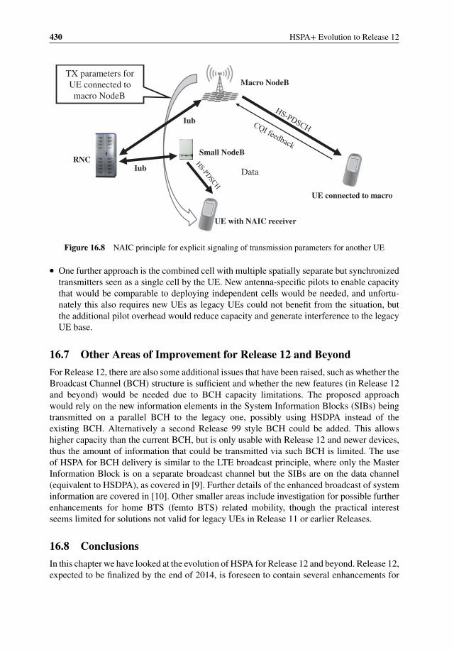
430 HSPA+ Evolution to Release 12
UE connected to macro
Small NodeB
TX parameters for
UE connected to
macro NodeB
Data
with NAIC receiver
Macro NodeB
RNC
Iub
Iub
UE
Figure 16.8 NAIC principle for explicit signaling of transmission parameters for another UE
� One further approach is the combined cell with multiple spatially separate but synchronizedtransmitters seen as a single cell by the UE. New antenna-specific pilots to enable capacitythat would be comparable to deploying independent cells would be needed, and unfortu-nately this also requires new UEs as legacy UEs could not benefit from the situation, butthe additional pilot overhead would reduce capacity and generate interference to the legacyUE base.
16.7 Other Areas of Improvement for Release 12 and Beyond
For Release 12, there are also some additional issues that have been raised, such as whether theBroadcast Channel (BCH) structure is sufficient and whether the new features (in Release 12and beyond) would be needed due to BCH capacity limitations. The proposed approachwould rely on the new information elements in the System Information Blocks (SIBs) beingtransmitted on a parallel BCH to the legacy one, possibly using HSDPA instead of theexisting BCH. Alternatively a second Release 99 style BCH could be added. This allowshigher capacity than the current BCH, but is only usable with Release 12 and newer devices,thus the amount of information that could be transmitted via such BCH is limited. The useof HSPA for BCH delivery is similar to the LTE broadcast principle, where only the MasterInformation Block is on a separate broadcast channel but the SIBs are on the data channel(equivalent to HSDPA), as covered in [9]. Further details of the enhanced broadcast of systeminformation are covered in [10]. Other smaller areas include investigation for possible furtherenhancements for home BTS (femto BTS) related mobility, though the practical interestseems limited for solutions not valid for legacy UEs in Release 11 or earlier Releases.
16.8 Conclusions
In this chapter we have looked at the evolution of HSPA for Release 12 and beyond. Release 12,expected to be finalized by the end of 2014, is foreseen to contain several enhancements for
HSPA Evolution Outlook 431
HSPA, some of them like radio level interworking with WLAN being common with LTE.Most of the solutions to improve interworking or HSPA-specific improvements to HSUPAoperation can be introduced in a backwards compatible way supporting both legacy and newerdevices, while some of the solutions being discussed relate to the heterogeneous networksor new bandwidth with scalable UMTS. The latter requires new UEs in the market beforethe solution can be used, as legacy UEs cannot access such a carrier. It remains to be seen ifthere is enough market interest to roll out solutions which would not allow the 1.5 billion UEsalready in the field to use the carrier. However, if some specific spectrum allocation does nothave room for two (or any) full carriers, then scalable bandwidth UMTS is an alternative to beconsidered if one does not want to consider the smaller bandwidth options enabled by LTE,as presented in [9]. Work on UE receiver improvements is expected to continue following thestudies on NAIC, which would enable better UE receiver performance regardless of whetherall UEs support such a feature or not.
Release 13 work is to be initiated at the end of 2014, with the target milestone set by 3GPP tobe March 2016. However, one may assume finalization around mid 2016 based on the roughly18 months Release duration, as with earlier 3GPP Releases.
3GPP is addressing further areas where performance could be improved with HSPA evo-lution work, but clearly increasing the peak data rate is no longer the focus in HSPA work.Rather it is addressing easy to deploy improvements for capacity issues, enabling HSPA tech-nology to be the workhorse for providing mobile broadband connectivity for roughly 3 billion(estimated) users globally by 2016.
References
[1] 3GPP Technical Report, TR 37.852, “RAN Enhancements for UMTS/HSPA and LTE Interworking”, Version1.0.0, December 2013.
[2] 3GPP Technical Report, TR 37.834, “Study on WLAN/3GPP Radio Interworking”, version 1.0.0, September2013.
[3] 3GPP Technical Document, R2-133192, “details of WLAN IW Solution 2”, NSN, Nokia Corporation, DeutscheTelekom, October 2013.
[4] Holma, H. and Toskala, A. (2010) WCDMA for UMTS, 5th edn, Wiley.[5] 3GPP Technical Report, TR 25.701, “Study of Scalable UMTS FDD Bandwidth”, version 12.0.0, September
2013.[6] 3GPP Technical Report, TR 25.702, “DCH Enhancements for UMTS”, version 12.0.0, September 2013.[7] 3GPP technical Report, TR 25.700, “Study on Further EUL Enhancements”, version 1.0.0, December 2013.[8] 3GPP technical report, TR 25.800 “UMTS Heterogeneous Networks”, version 12.0.0, September 2013.[9] Holma, H., and Toskala, A. (2011) LTE for UMTS, 2nd edn, Wiley.
[10] 3GPP Technical Report, TR 25.704, ”Study on Enhanced Broadcast of System Information”, version 12.0.0,December 2013.

Index
16QAM, 17, 21, 172, 178, 180–182, 185, 194,196, 198, 245, 246
64QAM, 169, 171–175, 178, 179, 181–186, 192,194–201, 203–206, 209, 245, 246
Absolute grant, 19Access Failure Rate (AFR), 231, 239, 240, 261,
273–279, 287, 290, 300, 310, 320Access Network Query Protocol (ANQP), 135ACK/NACK, 56, 59, 62, 175, 197Adjacent Channel Leakage Ratio (ACLR), 349Advanced Receivers, 139, 146AICH, 63, 65, 257–259ALCAP, 67AMR, 103, 248, 249AMR-WB, 3, 103Analog-Digital Converter (ADC), 347Android, 306–310, 320–325, 330, 331, 334ANDSF, 133, 422Application engines, 371ARM, 375Array gain, 38Assisting cell, 83Authentication, 398Automatic Cell Planning (ACP), 214, 222–224,
284, 287, 291Automatic Neighbor Relations (ANR), 287–289Average Power Tracking (APT), 379
Backhaul, 23, 171, 213, 244–246, 253Band combination, 32, 38Baseband, 142, 189, 191, 196, 204, 241, 242,
266, 273, 278, 320
Battery, 273, 274, 280, 294, 300–314, 320–330,335
Bi-CMOS, 346Bicasting, 113Big.little, 375Bill of Material (BOM), 344BLER, 176, 239, 258, 277Blind decoding, 59BTS-based scheduling, 10
Carrier Aggregation (CA), 36, 187, 188, 220CDMA, 2Cell change, 113, 171, 172, 183, 184, 186–188,
195Cell Individual Offset (CIO), 122Cell_FACH, 174, 198, 272–274, 307, 312, 313,
319, 320, 397Cell_PCH, 67, 174, 226, 233, 272–274, 301, 312,
313, 318–320, 395Channel allocation, 6, 73, 74Channel Quality Information (CQI), 11, 15, 56,
62, 172, 173, 175, 178–181, 183, 189–192,194–196, 205, 235, 236, 245, 246, 256, 266
Chatty Applications, 240, 276, 310, 312Chip-zeroing, 423Circuit Switched Fallback (CSFB), 114, 406Closed Subscriber Group, 131Closed-Loop Transmit Diversity (CLTD), 46Common pre-coder, see virtual antennaCoMP, 100Cortex processor, 375CPC, 53, 198, 274–277, 382CPICH, 65, 204, 205, 221, 257, 258, 267
HSPA+ Evolution to Release 12: Performance and Optimization, First Edition.Edited by Harri Holma, Antti Toskala, and Pablo Tapia.© 2014 John Wiley & Sons, Ltd. Published 2014 by John Wiley & Sons, Ltd.
434 Index
Cross-polarized (XPOL), 203, 249, 250CS voice, 103, 216, 226–231, 233, 234, 236–240,
244, 248, 249, 257–264, 269, 270, 276,277, 288–290
CS voice over HSPA, 111, 198CSFB, overlay, 408CSFB, Release 9, 408
D-CPICH, 45Deep sleep state, 383Deferred SIB reading, 408Desensitization, 122Digital-Analog Converter (DAC), 346DigRF, 347Direct conversion receiver, 344Direct Transition to DCH, 174, 270–274, 319, 320Display, 372Distributed Antenna Systems (DAS), 240, 276Domain Name Server (DNS), 274, 275, 305, 309,
318, 319, 324, 325, 332Dominance areas, 119, 214, 254–256, 262, 266DPCCH, 53, 69, 71, 176, 277Dropped Call Rate (DCR), 229, 233, 254, 261,
263, 269–271, 274, 287–290, 300, 314DRX, 54, 58DTC Cycle, 56DTX, 54, 55, 69, 108, 171, 172, 183, 197, 198,
209, 210, 241, 274Dual Cell, 27, 169, 173, 187, 188, 198, 203–211Dual-carrier HSDPA, 28Dual-carrier HSUPA, 32
E-AGCH, 20, 58, 64E-AI, 63E-DCH decoupling, 429E-DPCCH, 20E-DPDCH, 20E-FACH, 276, 319, 320E-HICH, 20, 64E-RGCH, 20, 58, 67E-ROCH, 49EDGE, 337eF-DPCH, 54Enhanced broadcast of system information, 430Enhanced serving cell change, 113Enhanced SR-VCC, 418Envelope Tracking (ET), 379Equalizer, 140Equivalent Isotropical Radiated Power (EIRP),
216, 217Error Vector Magnitude (EVM), 347
F-DPCH, 54, 64, 108FACH, 61, 257, 258, 270, 274, 280Fast dormancy, 67, 272–275, 301, 305, 307, 312Femto cells, 117, 119, 130File Transfer Protocol (FTP), 170, 207–209, 269,
313–316Filtered UMTS, 248, 423Flat architecture, 23, 76Flow control, 90Fractional-DPCH, 54, 64, 108Frame early termination, 425Frequency bands, 2, 339, 192, 209, 214, 225,
230–233, 247Frequency domain scheduling, 28, 209
Gateway GPRS Support Node (GGSN), 243, 244,292, 305, 311
Generic Advertisement Service (GAS), 135Geometry Factor, 217–219Graphic Processor Unit (GPU), 371GSM, 1, 337, 214, 215, 224, 230, 231, 246–251,
256, 267–270, 287
H-RNTI, 59Handover, 112, 188, 224, 225, 226, 228,
230–233, 243, 263, 284, 287, 395HARQ, 12HD voice, 3, 103Header compression, 106HetNet, 117Hotspot 2.0, 135HS Codes, 13, 171, 172, 178, 189, 192, 241HS-DPCCH, 14, 62, 66, 176, 277HS-DSCH channel allocation, 5, 14HS-FACH, 53, 61, 198, 276, 319, 320HS-PCH, 63HS-PDSCH, 172, 189, 241HS-RACH, 53, 63, 198, 276, 319, 320HS-SCCH, 13, 188, 257HS-SCCH order, 30, 33HS-SCCH-less, 54, 59HTTP Adaptive Streaming, 322, 323, 326, 327Hypertext Transfer Protocol (HTTP), 316–319,
322–325
Idle mode, 174–181, 226–233Imbalance uplink and downlink, 122IMEISV, 403IMSI, 403IMT-Advanced, 153Inactivity timer, 71, 273, 274, 280, 295

Index 435
Incremental redundancy, 12Inter Radio Access Technology (IRAT)
Handovers, 171, 224, 225, 230, 256, 267,268
Inter-system measurements, 397Inter-System Mobility Policy (ISMP), 134Inter-System Routing Policy (ISRP), 134Interference cancellation, 109, 141, 173, 202, 249Intermediate Frequency (IF), 344iOS, 306–310, 320–325, 330, 331, 334IP, 170, 173, 184, 241, 297, 302, 305, 307, 309,
315, 318
Key Performance Indicator (KPI), 237, 239, 274,305, 312, 323
Latency, 6, 63, 74, 165, 169–171, 174, 190, 191,210, 211, 242–244, 253, 270, 273, 280,310, 311, 315, 316, 319, 322
Light sleep state, 384Link adaptation, 11, 169, 172, 175, 178, 180, 181,
183, 191, 192, 196, 199, 211, 254Load balancing, 188, 228, 263, 287, 288Local area base station, 119Local Oscillator (LO), 344Location Area Update (LAU), 114, 133, 396, 403,
407, 409Long Term HSPA Evolution, 163Low Noise Amplifier (LNA), 344LTE, 27, 170, 187, 188, 203, 204, 209–212, 224,
244–247, 285, 286, 294, 311, 330–335,421
Maximum Allowable Pathloss (MAPL), 216–219Medium range base station, 119Micro cells, 117, 119, 222, 225, 241MIMO, 38, 173, 198, 199, 203–211, 250Minimum Coupling Loss (MCL), 118MIPI alliance, 360, 364MOS, 104Multiflow, 77, 122, 162Multipath, 203, 218
NBAP, 67Neighbors, 221, 224–226, 233, 254, 262–265,
286–292Network Assisted IC (NAIC), 149, 429
Operating System (OS), 253, 298–310, 315,320–325, 330, 331, 334, 335
Over-the-Air (OTA), 358
Parallel Interference Cancellation (PIC), 146PDCP, 108, 111Peak data rate evolution, 5Peak-to-Average Power Ratio (PAPR), 29, 381Phase Locked Loop (PLL), 350Physical layer retransmission, 12, 177, 283PICH, 65, 258, 259Pico cells, 117, 119Pilot, see CPICHPing-pong effects, 171, 187, 188, 202, 254, 255,
265, 266Postamble, 56Power amplifier, 203, 204, 216, 221, 236, 241,
258, 259, 354, 378Power consumption, 3, 63, 67, 72, 369PRACH, 281, 283Preamble, 56, 66Priority, see QoSProportional fair scheduler, 144
Quality of Service (QoS), 106, 197, 206–208,309
RACH, 61, 227, 277, 280Radio Network Controller (RNC), 10, 242, 243,
251, 264, 265, 273, 274, 279, 280, 284,290, 292, 305, 320
RANAP, 67Re-establishment, 113Receiver diversity, 139, 173, 202, 203, 214, 216Receiver Sensitivity, 216, 217Redirection, 226, 276, 395, 397, 400Refarming, 2, 7, 246–248Relative grant, 19, 176Remote Electrical Tilt (RET), 255, 288Reselection, 202, 206, 228, 230–232, 395, 398Reverse SR-VCC, 418, 421RF activity, 110RLC Throughput, 172, 175–197, 206ROHC, 106Round robin scheduler, 143RRC Connection, 231–233, 307RRC States, 270, 277, 279, 301, 307, 309, 313,
318, 320, 335
S-CCPCH, 62S-DPCCH, 47S-E-DPCCH, 47S-E-DPDCH, 47Scalable Bandwidth UMTS, 423SCH, 65, 257–259
436 Index
Scheduler, 143, 172, 176, 188, 197, 198, 208,209, 235, 236
SCRI, 67Security mode, 398Self Organizing Networks (SON), 223, 224, 258,
259, 263, 264, 281, 284–292, 335Serial Interference Cancellation (SIC), 146Serving GPRS Support Node (SGSN), 243, 244,
305Serving Grant, 49, 177Signalling, 63, 65, 73, 170, 227, 228, 231, 233,
239, 243, 244, 251, 270, 272–274, 279,280, 293, 299–308, 312, 327, 328, 330
Silicon area, 340SNR/SINR, 173, 175, 199, 203, 217–219, 241,
245Soft combining, 60Soft handover, 184, 216, 265, 266, 278Space-Time Transmit Diversity (STTD), 38Spatial filtering, 38Spatial multiplexing, 38, 203Sphere Decoding, 143Spreading Factor, 177, 218SR-VCC, 115, 417, 421Stadium, 71, 240Subcribers globally, 1Successive Interference Canceller (SIC), 143Surface Acoustic Wave (SAW) filter, 344System Information Block (SIB), 114, 224, 263,
281, 398
T323, 68TCP, 183, 244, 296, 301, 308, 310, 315–319, 322TCP Slow Start, 315, 316TD-SCDMA, 2Terminal category, 17, 23, 176, 197, 199, 201,
298, 309, 320Time reference cell, 85
Time-Dilated UMTS, 423Timer_Reordering, 88Tracking Area Update (TAU), 398, 403Transceiver architecture, 342Transport Block Size (TBS), 172, 173, 175, 178,
180, 190, 205TTI, 55, 66, 171, 172, 176–181, 208, 210,
234–241, 246, 276, 278, 297Type 3i receiver, 109, 173, 182, 189, 199–204,
265
UDP, 170, 171, 176, 183, 322Uplink interference, 7, 63, 65, 68, 170, 173, 181,
226–229, 238–240, 254, 273–283, 296Uplink transmission buffer status, 18, 176, 177URA_PCH, 395, 233, 270
Vertical sectorization, 150Video, 184, 211, 234, 238, 244, 293–295,
298–299, 302, 308, 310–313, 318,321–330, 333, 335
Video MOS, 326–329Video Rebuffering, 311, 314, 322, 325Video SR-VCC, 419Virtual antenna, 42, 204Voice capacity, 106, 249VoIP, 59, 103, 107, 302–304, 308VoLTE, 115
Web browsing, 170, 174, 207, 208, 267, 275, 293,297, 298, 308, 310, 312–315, 318–321, 334
Wi-Fi interworking, 133, 422Wide area base station, 119WiMAX, 2Wireless Proxy, 244, 316, 317, 325, 326WLAN interworking, 133, 422
Zero-IF, 344

WILEY END USER LICENSEAGREEMENT
Go to www.wiley.com/go/eula to access Wiley’s ebookEULA.