How Large is the Bias in Self-Reported Disability?†

Hugo Benıtez-SilvaSUNY-Stony Brook

Moshe Buchinsky‡

UCLA, NBER, and CREST-INSEE

Hiu Man ChanCharles River Associates

Sofia CheidvasserGoldman Sachs

and

John RustUniversity of Maryland and NBER

First Version: July, 1999Current Version: December, 2003

This is the Working Paper version of the article in the Journal of Applied Econometrics

† This work is made possible by research support from NIH grant AG12985-02. Benıtez-Silva is also grateful for the financialsupport of the “la Caixa Fellowship Program” in the early stages of this research. Buchinsky is grateful for the support from theAlfred P. Sloan Research Fellowship. We have benefited from feedback from participants of a Cowles Foundation Seminar, theNBER Summer Institute, the Hebrew University of Jerusalem, the University of California at San Diego, the conference on SocialInsurance and Pension Research in Aarhus, Denmark, comments by Franco Peracchi at the Conference on Reform of Social SecurityOrganized by the Fundacion BBV in Madrid, comments by Bent Jesper Christensen, and from the very able research assistanceof Paul Mishkin. We thank Joe Heckendorn, Dave Howell, Cathy Leibowitz and other members of the staff of the University ofMichigan Survey Research Center and the Health and Retirement Study staff for answering numerous questions.

‡ Corresponding author: Moshe Buchinsky, Department of Economics, University of California, Los Angeles, CA 90095-1477. e-mail: buchinsky@econ.ucla.edu.

Abstract

A pervasive concern with the use of self-reported health and disability measures in behavioral modelsis that they are biased and endogenous. A commonly suggested explanation is that survey respondentsexaggerate the severity of health problems and incidence of disabilities in order to rationalize laborforce non-participation, application for disability benefits and/or receipt of those benefits. This paperre-examines this issue using a self-reported indicator of disability status from the Health and Retire-ment Study (HRS). Using a bivariate probit model we test and are unable to reject the hypothesis thatthe self-reported disability measure is an exogenous explanatory variable in a model of an individual’sdecision to apply for DI benefits or Social Security Administration’s decision to award benefits. We fur-ther study a subsample of individuals who applied for Disability Insurance and Supplemental SecurityIncome benefits from the Social Security Administration (SSA) for whom we can also observe SSA’saward/deny decision. For this subsample we test and are unable to reject the hypothesis that self-reporteddisability is an unbiased indicator of the SSA’s decision, conditional on a vector of objectively measur-able health and socio-economic characteristics similar to the information used by the SSA in makingits award decisions. The conditional unbiasedness restriction implies that these two variables have thesame conditional probability distributions. Thus, our results indicate that disability applicants do notexaggerate their disability status—at least in anonymous surveys such as the HRS. Indeed, our resultsare consistent with the hypothesis that disability applicants are aware of the criteria and decision rulesthat SSA uses in making awards and act as if they were applying these same criteria and rules whenreporting their own disability status.

Keywords: Social Security, Disability, Health and Retirement Study, Conditional Moment Tests, En-dogeneity Test.JEL classification: H5

1 Introduction

There is substantial controversy in the literature over the use of self-reported variables, and particularly

health and disability indicators, as explanatory variables in economic and demographic models. These “sub-

jective” self-assessed measures have been found to be powerful predictors for a range of outcomes and be-

haviors. Examples of such phenomena are: Labor supply decisions (Stern 1989, Dwyer and Mitchell 1999),

and individuals’ decisions to apply for, and the government’s decision to award, disability insurance benefits

(DI) from the Social Security Administration (Benıtez-Silva et al. 1999). Indeed, these self-reported health

and disability indicators appear to function as approximate “sufficient statistics” in the sense that there are

only marginal increases in explanatory power from using additional, more objective, health and disability

indicators. One possible explanation for these findings is that the self-reported measures give individuals

latitude to summarize a much greater amount of information about their health and disabilities than can be

captured in the more objective, but very specific indices used in previous studies.

In contrast, there are also studies that provide evidence that self-reported health and disability measures

are biased and endogenous. The most commonly suggested explanation for these findings is that a survey

respondent may inflate the incidence and severity of health problems and disability in order to rationalize

labor force non-participation and/or receipt of disability benefits. Hence, the strong predictive power of self-

reported health and disability measures could be spurious, reflecting a classic form of endogeneity bias.1

This paper re-examines these issues using a self-reported disability status indicator from the Health and

Retirement Study (HRS). This is a binary indicator, referred to by the mnemonic hlimpw, denoted by d,

that takes the value 1 if the respondent answers yes to the following pair of questions: “Do you have any

impairment or health problem that limits the amount of paid work you can do? If so, does this limitation

keep you from working altogether?”

In order to measure the potential bias in self-reported disability d, we need a credible independent mea-

sure of disability status. While it appears very difficult to define an objective indicator of “true disability”,

the Social Security Administration (SSA) has a well established legal definition of disability: “The inability

to engage in any substantial gainful activity (SGA) by reason of any medically determinable physical or

mental impairment which can be expected to result in death or which has lasted or can be expected to last

1 As Bound (1989) noted, the direction of the bias resulting from self-reported health and disability measures is not alwaysclear. Stigma effects could lead respondents to understate or under-report health problems and disabilities. However, self-reportedmeasures can be viewed as noisy measures of “true” health and disability status, and these errors-in-variables typically result inunderestimates of the true behavioral impact. In the interest of brevity we do not provide a formal literature review in this versionof the paper, we refer the reader to Benıtez-Silva, Buchinsky, Chan, Cheidvasser, and Rust (2003), the on-line working paperversion of this paper, for a detailed discussion of the literature on testing endogeneity and bias of self-reported health and disabilityindicators. In this version of the paper we focus on testing the unbiasedness of a self-reported disability measure with respect to theSSA award decision.

1

for a continuous period of at least 12 months.” The essence of this definition of disability is sufficiently

similar to the definition of the self-reported indicator of disability from the HRS that it makes sense to use

the SSA’s award decision as a basis for evaluating the bias in self-reported disability d. This requires that

we focus on a further sub-sample of DI applicants for whom a final disability award decision could be as-

certained. As described in Benıtez-Silva et al. (1999), the DI award process is a multistage decision process

that allows for the possibility of several appeal stages. Using responses from the first three waves of the

HRS and information on the time limits allowed for filing appeals, we were able to determine whether an

applicant, who was rejected at any point in the award process, appealed, and if so, what the SSA’s final

award decision was. We denote the SSA’s ultimate award decision by a, and set a 1 if an applicant is

ultimately awarded DI benefits, and a 0 otherwise.

Panel A of Table 1 tabulates the actual count ofa d values for the entire available sample. The table

indicates that for most of the observations a d. However, this is not always the case. For some of the

observations d 1 and a 0, i.e., the individuals declare they cannot work, while the SSA decides they

can. For others d 0 and a 1, that is, the individuals declare they can work, yet they apply for, and are

awarded, disability benefits. Note that the two marginal distributions of a and d are very close, and one

cannot reject the hypothesis that they are the same. This indicates that overall, the individuals’ assessment

of their own health condition matches that of the SSA. In Panel B of Table 1, we report the predicted count

under independence of the SSA and the individuals’ decisions. A likelihood ratio test of the null hypothesis

of independence between a and d yields a χ2 statistic of 15.44 (1 degree of freedom, marginal significance

level 8 5 10 5), so there is strong evidence that individuals’ reports are correlated with SSA’s ultimate

award decision. While the degree of correlation has no implications on the bias of the two measures relative

to each other, it has important implications on the classification errors as is discussed in more detail below.

The primary focus of this paper is to test the hypothesis of rational unbiased reporting of disability

status, which we term the “RUR hypothesis”. This hypothesis reflects a belief that the way in which the

SSA implements its definition of disability, via its award decisions, sets a “social standard” for disability.

This standard becomes a matter of common knowledge for the individuals applying for disability benefits. It

is therefore of considerable interest to determine whether or not DI applicants agree with the SSA definition

of disability. In principle, it may be the case that: (a) the SSA is too “harsh” relative to the individual’s

assessment of his/her own condition; or (b) the DI applicants are systematically exaggerating their health

problems. In either case the rate of self-reported disability among DI applicants would exceed the fraction

of applicants who are ultimately awarded benefits.

2

We formulate the RUR hypothesis as the following conditional moment restriction(CM):

E a d x 0 (1)

or equivalently, since a and d are Bernoulli random variables,

Pra x Pr

d x

where x denotes a vector of objectively measurable health and socioeconomic characteristics, similar to the

information the SSA uses in making its award decisions. That is, RUR states that the conditional proba-

bility that a DI applicant will report being disabled is the same as the conditional probability that the SSA

will ultimately award him/her DI benefits. We test the conditional moment restriction underlying the RUR

hypothesis using non-parametric methods that do not make any assumptions about the functional form of

Pra x and Pr

d x . We are unable to reject the RUR hypothesis using several different versions of the

CM tests, including recently developed tests that have optimal rates of convergence against a broad class

of non-parametric alternatives. Since the power of these conditional moment tests can be low, given the

relatively low sample sizes, we also test a parametric version of the RUR hypothesis, where the conditional

probabilities are derived from the bivariate probit function

Pra x E I x βa εa 0 and

Prd x E I x βd εd 0

where I is the indicator function For this parametric model, the RUR hypothesis amounts to the restriction

that βa βd . Again, we are unable to reject the RUR hypothesis at conventional significance levels.

The parametric model suggests the following interpretation of the RUR hypothesis. Without loss of

generality, SSA’s ultimate award decision can be represented by an index rule depending on information

contained in the observed vector x, that is observed by the econometrician as well, and other information

εa, that is observed only by the SSA. The coefficient vector βa represents the weights the SSA assigns to

various health conditions and socioeconomic characteristics in coming up with an overall “disability score”

given by x βa εa. Only individuals with sufficiently high disability scores (i.e., x βa εa 0) are awarded

benefits. Similarly, the individual’s self-reported disability status can also be represented by an index rule

depending on x, a corresponding vector of weights βd , and private information εd that is observed only by

the individual. In general, the unobserved information of the SSA and the individual (i.e., εa and εd) may

be, but need not be, correlated.

The RUR hypothesis amounts to a rational expectations restriction that individuals use the same weight

vector as the government, i.e., βa βd , in deciding whether or not they are disabled. However, the indica-

tors a and d are not perfectly correlated, although they have identical conditional probability distributions,

3

because of the existence of individual’s private information εd , that is not observed by the SSA, and the

SSA’s “bureaucratic noise”, εa, that is not observed by the individual. If εa and εd are perfectly correlated,

then the SSA decision and the individual’s self assessment must be the same. Since the two error terms

are not perfectly correlated, we observe some “errors” in the SSA decisions, in that some of those that de-

clare themselves disabled are not awarded benefits (rejection error), while some that declare themselves fit

to work are awarded benefits (award error). These errors would be maximized if εa and εd were perfectly

negatively correlated.

It is clear that from an aggregate perspective disability is endogenous, since the implementation of the

award decisions by the SSA affects individuals’ self-perceptions of disability status. These self-perceptions

can in turn affect a wide range of behavior, including labor supply, retirement, and decisions about whether

to apply for DI benefits. However, it is also of interest to determine whether the self-reported disability

status can be treated as an exogenous variable from an individual standpoint. That is, given any particular

social standard for disability, is it the case that unobserved variables affecting an individual’s self-reported

disability are correlated with unobserved determinants of labor supply, retirement, and DI application de-

cisions? We test, and are unable to reject, the null hypothesis of exogeneity in the context of a parametric

model of simultaneous dummy endogenous variables introduced by Heckman (1978). Thus we conclude

that self-reported disability status can be used as an exogenous covariate to model disability application

decisions. Yet, in making predictions of the impact of change in the SSA’s DI award criteria, we need to

be careful when accounting for the endogenous feedback effects of changed self-perceptions of disability

status at an aggregate level.

While we acknowledge that DI applicants may have strong incentives to mis-report their health and

disability status to the SSA, our results are consistent with the common sense view that there is no reason

for respondents to mis-report their information in an anonymous non-governmental survey such as the HRS.

Respondents were given credible guarantees that their identities would not be revealed, so any information

they reported to the HRS could not have any impact on the status of a pending application for DI benefits.2

One indication of respondents’ confidence in these guarantees is provided by the fact that nearly 20% of DI

recipients reported that they do not have a health problem that prevents them from working. Furthermore,

approximately 5% of these recipients reported labor earnings in excess of the $500 per-month limit imposed

by the SSA.3 Either of these self-reports constitute prima facie evidence for termination of benefits. The

2 The conclusions of this paper are therefore relevant for any survey guaranteeing high degree of anonymity, such as thatprovided by the HRS.

3 The significant gainful activity (SGA) limit was $500 per month during the period of this study. It was increased to $700 onJuly 1, 1999, and to $740 as of January 1, 2001, as an additional work incentive. Since then it has been increased at the rate ofincrease of the national average wage index.

4

fact that such a high fraction of DI recipients reported potentially incriminating information provides strong

evidence that the HRS’s guarantee of anonymity was credible.4

Our finding of unbiased reporting of disability status has broader significance, since it supports the

hypothesis of truthful reporting by respondents in anonymous surveys, which is a fundamental premise un-

derlying virtually all empirical work in the social sciences. Additionally, from a methodological perspective,

our paper departs from the previous literature in this area by showing that it is possible to assess bias in self-

reported disability using non-parametric tests of conditional moment restrictions. Previous approaches, such

as Kreider (1999), required strong parametric functional form assumptions and behavioral restrictions that

lead to, what we view as, implausibly large and spurious estimated biases in self-reported disability. While

we do impose parametric functional form restrictions to obtain more powerful tests of the RUR hypothesis,

our basic conclusions do not depend on assumptions about particular parametric functional forms.

It is worthwhile emphasizing that the HRS data provide us with a unique opportunity to directly test for

the validity of a self-reported health measure, a task which is important for several reasons. The discussion

in the literature on the validity of such a measure has hardly reached a consensus. Yet, the literature largely

agrees about the important policy implications of using such a self-reported variable in empirical analyses.

A second motivation for the analysis carried out here is that this particular self-reported variable was shown

to be an approximate sufficient statistic for individuals’, as well as for the Social Security Administration

(SSA), decisions. This is of vital importance, since such a summary statistic can serve as a very powerful

state variable in a dynamic optimization model, which we are currently developing, for individuals at the

later part of their life cycle. Third, we also use this variable in a companion paper (see Benıtez-Silva,

Buchinsky, and Rust 2003) to provide an “audit” of the multistage application and appeal process used by

the SSA. Finally, the rise in self-reported variables in recent surveys, in the United States and elsewhere,

makes it necessary to develop a systematic framework for examining the validity of such self-reported

variables.

The remainder of the paper is organized as follows. Section 2 briefly summarizes previous approaches

to testing for endogeneity and bias in self-reported health and disability indicators. Section 3 describes the

HRS data and the construction of the ultimate award indicator a. Section 4 provides the results of a vari-

ety of tests of the unbiasedness of d, relative to a, while Section 5 provides the testing results of the RUR

hypothesis, using parametric models that allow for various forms of unobserved heterogeneity. Section 6

presents a classic test for the exogeneity of d following the approach of Heckman (1978). Section 7 sum-

4 It is possible that some DI recipients have experienced medical recoveries and were participating in the SSA’s “trial work”program, which allows them to work for up to nine months while continuing to receive DI benefits. However, since only less thanone percent of all DI beneficiaries actually take advantage of this trial work program, it is unlikely that they can have an effect onour findings.

5

marizes and offers some conclusions. A detailed description of the construction of the data set is provided

in Appendix A. Finally, Appendix B provides some technical details about the conditional moment tests

employed in Section 4.

2 Literature on the Validity of Self-Reported Health Measures

The validity of self-reported measures of certain variables has been the topic of many studies in recent

economic literature. This literature stems, in part, from the fact that there is an increasingly large number

of surveys that ask many questions about individuals’ self-assessment of, for example, their health, or labor

market opportunities. While in general these questions are regarded as very useful, they also raise a host

of potential problems. To date there seems to be very little agreement as to the validity of such measures.

The most important concern is about the potential endogeneity of these measures relative to the issue under

study.

Many previous researchers have suggested that the incidence of self-assessed disability may be inflated

due to the tendency of individuals to use health problems as a convenient rationalization for difficulties

in the labor market.5 For example, with respect to studying the application decision, if the respondent’s

self-reported disability status is merely a rationalization of the DI awards outcomes (e.g., reporting being

disabled if they apply for benefits), then unobserved factors affecting the application decision will also

affect self-reported disability status. This implies that self-reported disability is endogenous (i.e., correlated

with unobservable factors affecting the application or award decision), biasing the coefficients of interest.

Consequently, the large significant estimates of the impact of self-reported disability may not indicate that

this is a good measure of true health status, but merely that it is, essentially, a noisy measure of the dependent

variable.

Other researchers (e.g. Johnson 1977, Bazzoli 1985, and Bound et al. 1995) criticize the use of a variable

such as hlimpw in regression models of labor market participation, since health, measured as a condition

limiting work, can be considered as an endogenous regressor, or even the same measure as the dependent

variable. Hence, this measure may simply imply a tautological relationship between the health variable

and the retirement decision. Dwyer and Mitchell (1999) argue that additional problems can arise from the

fact that subjective health measures may actually be assessments of leisure preferences, rather than true

indicators of health status. That is, people who enjoy work tend to downplay health problems and postpone

5 For extended discussion of this “justification hypothesis” see Lambrinos (1981), Myers (1982), Parsons (1982), Baz-zoli (1985), Anderson and Burkhauser (1985), Stern (1989), Bound (1991), Kerkhofs and Lindeboom (1995), Blau et al. (1997),Kreider (1998), Bound et al. (1998a), Bound et al. (1998b), Kerkhofs et al. (1998), O’Donnell (1998), and Dwyer andMitchell (1999).

6

applying for DI benefits, while those who dislike work tend to apply soon after the onset of a sufficiently

severe medical condition.

There is a substantial literature that provides some evidence in favor of these types of biases. Par-

sons (1982) instruments self-reported health measures with future mortality and finds evidence supporting

the justification hypothesis. He concludes that the use of self-reported health will cause significant biases

in the coefficients of economic variables. Similar conclusions, using similar methods, were also reached by

Anderson and Burkhauser (1985). Bound et al. (1998a) criticized the use of mortality as an instrumental

variable, after finding evidence of endogeneity of mortality in these models stemming from measurement

error. Bazzoli (1985) finds that self-reported health status affects the retirement decision differently depend-

ing on whether the variable is measured before or after the decision in question takes place. For example,

self-reported health seems to have more significant effect when reported after retirement, lending support

to the justification hypothesis. However, the time elapsed between the two health measures, which can be

up to two years, may account for most of the difference. Finally, Blau et al. (1997) also find evidence of

endogeneity of self-reported health, using the dummy variable indicating whether a person is in poor health,

rather than the measure used here.

In contrast to the studies reported above, there are many other studies which found little evidence, or no

evidence at all, of endogeneity in self-reported disability measures. Stern (1989) finds very weak evidence

against the exogeneity of self-reported measures of disability in the labor force participation decision. Using

data from the Netherlands, Kerkhofs et al. (1998) find some evidence of endogeneity of self-reported health

limitation in the retirement decision, but little evidence in the DI decision. Using the HRS data, Dwyer and

Mitchell (1999) conclude that self-rated health measures (including self-reported work limitations) are not

endogenously determined with labor supply. Furthermore, they find no evidence to support the justification

hypothesis. Bound (1989b) also notes that: “when outside information on the validity of self-reported

measures of health is incorporated into the model, estimates suggest that the self-reported measure of health

perform better than have been believed.”

Evidence that there is a significant bias is seemingly apparent from the fact that 9.2% of the respondents

in wave one of the HRS reported health problems preventing work, whereas only 6.2% of the respondents

reported receiving DI benefits. Nevertheless, most of this discrepancy can be explained by accounting

for incomplete uptake and classification errors in the disability award process as explained in the example

presented below.

Note that the unconditional probability of being awarded benefits can be written as:

Pra 1 Pr a 1 d 1 apply Pr apply d 1 Pr d 1

7

Pr a 1 d 0 apply Pr apply d 0 Pr d 0 (2)

From the above we have Pr d 1 092. The results in Benıtez-Silva et al. (2003) suggest that

Pr a 1 d 1 apply 8 and Pr a 1 d 0 apply 6. Finally, we need to estimate the prob-

abilities that disabled and non-disabled individuals, respectively, will eventually apply for DI benefits.

A reasonable guess, based on Benıtez-Silva et al. (2003) results, would be Pr apply d 1 7 and

Pr apply d 0 02, respectively. With these values, equation (2) yields an estimate of Pra 1 062,

which is the same rate reported by HRS respondents in wave one. We note that the 9.2% disability rate from

the HRS is consistent with Burkhauser and Daly’s (1996) estimated disability rate of 9.2%, for working-age

males (25-61) in the Panel Study of Income Dynamics (PSID) data set for 1988. Using the 1987 Current

Population Survey (CPS) data set, Burkhauser, Haveman, and Wolfe (1993) estimated that 6.2% of working-

age individuals were disabled.6 Our estimate is also consistent with the actual (age/sex adjusted) take-up

rate provided in Lahiri et al. (1995), who used an exact match to the SSA disability records for a subset of

respondents in the 1992 SIPP survey.

Another concern about the reliability of self-reported health status might stem from measurement er-

ror due to misreporting of respondents. However, the hypothesis that individuals systematically misreport

their health and disability status in an anonymous, confidential survey does not seem highly plausible to

us. Specifically, we found a high degree of internal consistency in responses to questions across the various

sections of the HRS survey. For this to be consistent with systematic misreporting, the respondents had

to tightly coordinate their misreporting with other more “objective” reports, such as beginning and ending

dates of jobs, dates of application, receipt of DI benefits, etc. We further discuss this issue in the next sec-

tion where we compare the individuals reporting of labor market activities with their reporting of disability

incidences, which are reported in two different sections of the HRS. If we were to believe that respondents

are sophisticated enough to systematically misreport information in such a coordinated, internally consis-

tent manner, we must question virtually all of their survey responses, including all “objective” health and

functional status indicators. However, the literature rarely questions the validity of the “objective” health

status measures.7

Another frequent claim in the literature is that the respondents’ incentive to misreport disability status

to the SSA suggests a similar incentive to misreport to survey interviewers. This cannot be reconciled with

the HRS data, since nearly 20% of the HRS respondents who reported receiving DI benefits also indicated

6 The lower estimate of 6.2% resulted from a stricter definition of disability, including not working and receiving DI and othertypes of disability/welfare benefits.

7 Bound (1991) is an exception to this sweeping statement. He argues that part of the problem is that the objective healthvariables measure health, rather than work capacity. Bound also notes that misreporting of variables tends to have counteractingeffects.

8

that they did not have a health problem preventing work. This seems to provide evidence that individuals

felt sufficiently comfortable with the HRS interviewers to disclose private information that could potentially

lead to an audit and termination of benefits if revealed to the SSA.

The literature on the presence of reporting biases is much less extensive. One approach that has been

employed in this literature is to first assume that workers correctly report their disability status. The re-

sponses of workers are used to predict prevalence of disability among non-workers, who are more likely

to have incentive to misreport their disability status. Kreider (1998, 1999) uses this technique and finds

that the estimated model under-predicts the prevalence of disability among non-workers, and interprets this

difference as reporting bias.

Kreider’s approach to measuring the bias in self-reported disability in the sub-population of DI appli-

cants depends on the crucial assumption that the subpopulations of applicant and non-applicant use the same

rule for reporting disability. While Kreider (1999) estimates a bivariate probit model in which he controls

for sample selection into the working population, if the population of non-workers is different from the pop-

ulation of workers, he may be misinterpreting the inherent differences between the two subpopulations as

reporting bias. While Kreider (1999) expresses sound concern and skepticism about the potential usefulness

of self-reported health measures, his results hardly support this concern, since the reported estimates with

and without the control for potential bias are well within the sampling variation of each other.

Following Kreider (1998) we estimated a binary model of disability reporting on a subsample of indi-

viduals who never received and never applied for DI benefits. Not surprisingly and consistent with Kreider’s

results, we find that this estimated model severely under-predicts the prevalence of self-assessed disability

among the population of DI applicants. Moreover, this approach leads to the implausible prediction that

two-thirds of the DI applicants do not regard themselves as disabled.8 In contrast to Kreider, we do not

interpret these findings as evidence of systematic over-reporting of self-assessed disability among DI appli-

cants, but rather as an indication that we cannot reliably predict the incidence of self-assessed disability for

DI applicants using a model estimated on a subpopulation of non-applicants.

3 The Health and Retirement Study

The data for our study come from the first three interviews of the HRS, a nationally representative longitu-

dinal survey of 7,700 households whose heads were between the ages of 51 and 61 at the time of the first

interview in 1992 or 1993. Each adult member of the household was interviewed separately, yielding a total

of 12,652 individual records. Waves two and three were conducted in 1994/95 and 1996/97, respectively,

8 See Benıtez-Silva et al. (2003) for more details.

9

using computer assisted telephone interviewing (CATI) technology, allowing for better control of the skip

patterns and reduced recall errors. Deaths and sample attrition reduced the sample to 11,596 and 10,964

individuals, in waves two and three, respectively.9

The HRS has several advantages over the alternative sources of data previously used to analyze the DI

award process such as the SIPP data (e.g., Lahiri et al. 1995 or Hu et al. 1997). The HRS is a panel focusing

on older individuals, with separate survey sections devoted to health, disability, and employment. The

health section contains numerous questions on objective and subjective indicators of health status, as well as

questions pertaining to activities of daily living (ADLs), instrumental activities of daily living (IADLs), and

cognition variables. In the disability section of the survey, respondents were asked the dates they applied for

DI benefits or appealed a denial, and whether or not they were awarded benefits.

There are several limitations of the HRS data for studying the DI award system. First, unlike the SIPP

data, there is no match to the SSA Master Beneficiary Record so we are unable to verify individuals’ self-

reported information on dates of application and appeal for Social Security Disability Insurance (SSDI) and

Supplemental Security Income (SSI) benefits. Second, the HRS did not distinguish between SSI and SSDI

applications. Instead all questions combined the two programs into a single category denoted by “DI”.10

Finally, the HRS did not include appropriate follow-up questions that would have allowed us to determine

whether DI applications or appeals reported in previous surveys had been awarded or denied, or whether

they were still pending, resulting in potential censoring of information on appeals and re-applications. For-

tunately, we were able to rectify some of these censoring problems using other information in the HRS.11

Another potential problem is that of time aggregation. While individuals’ decisions as to when to apply

for (or appeal) disability benefits are made in continuous time, we observe their health variables at a few

discrete points in time, that are roughly two years apart. To most closely approximate an individuals’

characteristics at the time of application, we restrict our attention to the application/appeal episodes that

were initiated within a one-year window surrounding the interview date (six months before to six months

after), yielding a total of 393 observations.12

As already indicated, the two most important variables for our analysis are the self-reported disability

status (denoted by d) and the SSA award decision (denoted by a). As noted in the introduction, as a measure

9 Additional individuals, mostly new spouses of previous respondents, were added in waves two and three. We include theserespondents in our analysis, yielding a total of 13,142 individual records.

10 Stapleton et al. (1994) show that since the late 1980s, the trends in applications, awards, and acceptance rates for the SSI andSSDI programs have been very similar.

11 See the Appendix for some additional strategies used to resolve ambiguous cases.12 Given the panel nature of the HRS, we allow a single individual to yield several application episodes. We observe a maximum

of three application episodes per person in the data, but most individuals have only one episode. Experimentation with windowsof different length had some effect on the number of observations, but virtually no effect on the results reported below. Also, theone-year window was always formed for interviews that happened after the reported onset of disability.

10

of d, we use hlimpw, a dummy variable that takes the value one when the respondent reports a health

problem preventing all work, and zero otherwise. This variable best fits the SSA definition of disability

as the inability to engage in substantial gainful activity. One potentially important problem with these two

measures is that in some cases we observe the self-reported disability measure after the uncertainty of the

application process is resolved. This could be a source of endogeneity of the self-reported disability indicator

and under-rejection of the unbiasedness hypothesis if respondents’ self-reports are influenced by knowledge

of the SSA’s award decision. However, the majority of respondents, 61%, did not know the outcome of their

DI application when they reported their disability status, so the award decision could not have influenced

their reports. Among those who knew that they were awarded benefits, a high percentage, 68%, changed

their self-reported disability status from non-disabled to disabled in the survey after they found out about the

SSA’s award decision. However, 72% of this latter group experienced deteriorations in their health status

from the survey before the award to the survey after the award. Hence, it seems more likely that the changes

in reported disability were due to changes in health status rather than due to knowledge of SSA’s award

decision.

Some strong evidence about the quality of the HRS data is provided in Figure 1. This figure depicts the

average monthly labor force participation rates over a 24-month window surrounding the dates of disability

onset, DI application, and award of benefits (twelve months before to twelve months after each event). The

plots are computed based on data which come from different sections of the HRS survey. While the dates

of disability onset, application, and award were obtained from the disability section of the HRS, or, when

unavailable directly, were imputed using information from the income section and known dates, the monthly

labor force participation rates were constructed from responses to questions in the employment section of the

HRS.13 Since information on disability and labor force participation were taken from completely different

sections and questions in the HRS survey, there is no guarantee (other than accurate reporting on part of

respondents) that the dates of changes in labor force participation would match up with the dates of disability

onset.

Figure 1 shows that in fact these dates do match up very closely. We see a very dramatic drop in the

labor force participation rate, from over 60% to under 15%, in the month following the onset of disability.

The magnitude and abruptness of this change in labor force participation suggests that most disabilities have

sudden, acute impacts on labor supply as opposed to chronic health conditions that evolve more slowly and

13 The disability section of the HRS provides answers to the questions: “Do you have a health limitation that prevents youfrom working altogether?” and “When did it begin to prevent you from working altogether?” The employment section providesinformation regarding beginning and ending dates of jobs (including all intermediate jobs held between successive survey waves).Based on this information we were able to calculate monthly dummy variables indicating whether or not a respondent had beenworking in each month since January 1989. Consequently, we were able to construct the 24-month window in all cases in whichthe three events occurred after 1989.

11

lead to gradual withdrawal from the labor force. However, the steady decrease in participation rate in the

twelve months prior to the date of onset suggests that the disabilities of some individuals do indeed result in

gradual reductions in labor force participation, continuing to drop further after the date of disability onset.

The other two curves in Figure 1 do not show as dramatic a drop in the labor force participation rate in the

12 months before or after DI application and award. Nevertheless, labor force participation rates before and

after DI application (the dashed line) exhibits a pronounced kink in the month following the application,

flattening out at a participation rate of about 15%. Furthermore, labor force participation rates prior to DI

application are decreasing at an increasing rate, suggesting that many DI applicants are dropping out of the

labor force just prior to the filing of the DI application.

Finally, the dotted curve plots labor force participation rates before and after disability benefits are

awarded. After the award, participation rates are very low, approximately 5%. They are not exactly zero

for several reasons, including measurement error and the possibility that some DI beneficiaries are capable

of working and believe there is a low probability of being audited. There is also the potential for legitimate

labor supply during a “trial work period” lasting up to nine months, in which DI beneficiaries are allowed

to return to work without fear of immediate termination of benefits. Unfortunately, the HRS data do not

allow us to distinguish between those working as part of a legitimate trial work program and those that are

engaged in “black market” work that is unreported to the SSA.

These findings all seem to indicate that it is unlikely that HRS respondents systematically misreport

their health status. This is fortunate, since if were not the case, we might have reason to distrust other

self-reported data, even data about labor market participation, hours of work, etc.14

4 Conditional Moment Tests of Rational Unbiased Reporting

In this section we test whether or not the measure of “true disability” status d, as measured by hlimpw, is an

unbiased estimator of the SSA award decision a, that is, we test

E a d x 0 (3)

where x is the “publicly available” vector of characteristics of the applicant, observed by both the SSA and

the econometrician. Here we use a and d to denote the award and the self-reported health status, respectively.

The results of several alternative tests are provided in Tables 2 and 3. In Table 2 we report the results for the

14 As a diagnostic test, we verified that our conclusions are robust by screening out the 52% of the sample for which imputationson the dates of disability onset, application, or award were made. We found that the resulting curves were essentially identical tothe ones displayed in Figure 1, suggesting that our imputed dates are very good estimates of the true dates. A more direct validationwould require linkages to Social Security’s Disability Determination Services records, for which there is currently no access.

12

whole process, i.e., after all the appeals the individuals were entitled to were exhausted. In Table 3 we report

the results based on the outcomes after the initial decision by the Disability Determination Services (DDS).

If the RUR hypothesis holds, then we should not be able to reject the null hypothesis of unbiasedness for the

set of tests reported in Table 2. In contrast, we should be able to reject this hypothesis for the tests reported

in Table 3, since the latter statistics are not computed based on the SSA ultimate decisions. Since there are

very few multiple episodes, we treat all application episodes as uncorrelated.

We begin with the unconditional test of E a d 0 for the subset of 393 applicants discussed in

Section 3. We then proceed with a few conditional moment restrictions tests, i.e., E a d x 0 after

eliminating those applicants with missing values in any of the explanatory variables, leaving us with 356

observations.15

4.1 Moment Restriction Tests

The conditional restriction E a d x 0 implies that H E a d x 0, which, in turn, provides us

with a simple moment restriction test. Note that a consistent estimate for H is readily available byH 1

N

N

∑i 1

ai di xi where N denotes the total number of observations. By the central limit theorem we have that

N H H ! D#" N0 Ω , where Ω E $ a d 2

xx &% , with rankΩ k. Given a consistent estimate

for Ω, say Ω 1

N

N

∑i 1

ai di 2xix i

it follows then that under the null hypothesis of unbiasednessW N H Ω 1

H ! D'" χ2

k (4)

4.2 Ordinary Least-Squares (OLS) Test

In the OLS method we regressa d on the specified explanatory variables and test the hypothesis that all

regression coefficients are equal to zero.

We then provide more formal conditional moment tests, namely those proposed by Bierens (1990) and

Horowitz and Spokoiny (2001). Both tests are consistent against all non-parametric alternatives.16

15 All specifications in this section, except for the unconditional mean test, consist of the following explanatory variables: aconstant, age at application, age at application if 62 or older, income, number of hospitalizations and doctor visits in the previousyear, proportion of months worked in the last year, average number of hours worked per week in the three months following theapplication, and the dummy variables white, male, married, education beyond high school, stroke, psychological problems, arthritis,fracture, back problems, and finally difficulty walking around the room, sitting for a long time, getting out of bed, getting up froma chair, eating or dressing, and climbing stairs.

16 A more detailed description of both tests can be found in the on-line working paper version of this paper.

13

4.3 Bierens (1990) Test

The null hypothesis tested is PrE y x 0 1 where y a d and x is a vector of covariates. Bierens

shows that under the null hypothesis E y exp t x ( 0, for almost every t ) Rk. Moreover, this implies that

the statistic Wt N M

t 2 * s2 t has an asymptotic χ2 distribution with 1 degree of freedom (denoted by χ2

1), whereMt 1

N

N

∑i 1

yi exp + t φ xi -, s2 t 1

N

N

∑i 1

y2i exp + t φ xi -, 2 and φ

x arctan

x

where arctanx is operated coordinate wise. Since the test is consistent for any t, we can maximize

Wt

over all t in some subset T ) Rk to obtain t argmaxt . T

W

t

However, the resulting test statistic fort , i.e.,

W

t , does not have an asymptotic χ2

1 distribution under the

null hypothesis. This problem is overcome using the procedure provided in Theorem 4 of Bierens (1990) for

choosing some random t, say /t. The resulting test statisticW

/t has, again, a χ21 distribution. Nevertheless,

there are a number of arbitrary choices that one needs to make, which can considerably affect the results

of the test. To circumvent this problem we computed the test statisticW /t over a large number of random

choices of the arbitrary parameters and averaged the test statistic over all these choices.

4.4 Horowitz-Spokoiny (2001) Test

The Horowitz and Spokoiny (2001) test (HS test hereafter) is for a parametric null hypothesis of the form

yi f

xi θ εi, where f

xi θ is a known parametric model. Under the null hypothesis, that the parametric

model fxi θ is true, E

εi xi 0. In our case f

xi θ 0 0. One major advantage of this test relative to

others in the literature is that it allows for heteroskedasticity, σ2 xi 1 E ε2i xi , of an unknown form.

Consider first the statistic given by

Th Sh

N #

NhVh

where

ShN N

∑i 1

fhxi 2 2

Nh N

∑i 1

aii 3 hσ2Nxi and

Vh

2N

∑i 1

N

∑j 1

a2i j 3 hσ2

Nxi σ2

Nx j

fhxi is a non-parametric estimate for f

xi θ , ai j 3 h are some weights that depend on the distances between

xi and x j (for all i j 1 2444 N), and σ2N

xi is a consistent estimator for σ2 xi . Under some regularity

conditions, Th has an asymptotic distribution with zero mean and unit variance. The statistic HS proposed is

given by Tmax maxh . HN Th, where HN is a finite set of bandwidth values. However, Tmax need not have the

14

same distribution as Th. To circumvent this problem we compute the small sample distribution of Tmax using

a bootstrap procedure, using Andrews and Buchinsky (2000)’s recommendations for choosing the number

of bootstrap repetitions.

As indicated above, the results are summarized in Tables 2 and 3. All the test statistics reported in

Table 2, and their corresponding p-values, clearly indicate that one cannot reject the null hypothesis of

unbiasedness. The test that provides the lowest p-value is the Bierens test, but this test provides a lower

bound for the true rejection probability. When a small sample distribution of the test statistic is taken into

consideration, as in the HS test, the p-value is very high, making it impossible to reject the null hypothesis, at

any reasonable significance level. It is worth noting also that even the unconditional unbiasedness hypothesis

cannot be rejected at any conventional level.

As a sensitivity test we reran all the tests changing the set of conditioning variables, i.e., the variables

in x. The results remained virtually unchanged, meaning that the unbiasedness hypothesis holds intact. The

final set of conditioning variables, for which the test results are reported, were chosen to be the same as

those included in the analysis reported in the next section for the RUR model.

Recall that the test reported in Table 2 is for the ultimate award decision after all the stages of the appeal

process have been exhausted. If one considers carrying out the test using the a as they are revealed after

the first stage determination by the DDS, then we find that the results are very different, as is clear from

Table 3. In this case all the various tests indicate clear rejection of the null hypothesis of unbiasedness. This

is because the SSA decision at the first stage is often overturned by later appeals. The results indicate that

the SSA’s first stage determination is consistently below the individuals’ evaluation of their own disability.

This can be viewed as part of a deliberate strategy of the SSA to impose a barrier that induces self-selection

into the group of people who appeal an initial rejection.

Note that in our case both a and d are binary, so that testing for conditional unbiasedness is equivalent to

testing that the two marginal distributions of a and d, conditional on x, are the same. If a and d are not binary,

then the conditional distributions of a and d are not, in general, the same, even though E a d x 0 But, if the two distributions are the same then the unbiasedness condition obviously follows. The framework

presented here allows for testing equality of the marginal distributions in the binary case, as well as testing

conditional unbiasedness in general, without the binary restriction. It also may be readily extended to testing

for equality of conditional distributions in several more general cases. This is, for example, the case if a

and d are vectors of binary variables, or discrete random variables taking on a finite number of values. For

example, assume that a and d can take on J values a1 2444 aJ , and d1 2444 dJ , respectively. Let qa j 1 if a a j

and qa j 0, otherwise for j 1 2444 J. Similarly, let qd j

1 if d d j and qd j 0, otherwise for j 1 2444 J.

Then testing for equality of the marginal distributions of a and d amounts to testing E qa j qd j x 0 for

15

all j, j 1 2444 J. This requires a multivariate extension of the tests used here, e.g. in the moment restriction

test replacingait dit xit by the Kronecker product of qait qdit and xit everywhere, with qait and qdit the

appropriate J-vectors.17

5 Likelihood Ratio Tests of Rational Unbiased Reporting

As discussed before, both the hlimpw and the SSA decision variables are noisy measures of “true disability”.

The results of the previous section suggest that hlimpw is an unbiased estimator of the SSA overall decision.

However, one might feel uncomfortable in justifying the use of hlimpw as a measure of “true disability”

status based on the tests presented in the previous section alone. In particular, one might be concerned

about the power of the tests used, and more specifically, it might be argued that in small samples, these tests

may have no power at all. For this reason we introduce likelihood-based tests that rely on the particular

implications of the RUR hypothesis.

Without loss of generality, we may represent the SSA award decision by the index rule

a I x βa εa 0 5 (5)

where x is a vector of characteristics of the applicant that are observed by the SSA and the econometrician,

while βa is a vector of weights that the SSA assigns to these various characteristics in arriving at their award

decisions. The term εa is a scalar idiosyncratic random variable representing information known to SSA,

but unknown to the applicant and the econometrician. This term reflects the impact of “bureaucratic noise”

affecting the SSA award decision. Hence, the quantity x βa εa can be thought of as a “score” that SSA

assigns to an applicant, measuring the applicant’s overall level of disability on a continuous scale. Applicants

with sufficiently high scores are awarded benefits.

For individuals we use a similar model for the report of disability status, that is/d I x βd εd 0 (6)

where the vector x is the same set of “public information” used by the SSA. However, the parameter vector

βd is the set of weights that the applicant uses to convert this information into an overall summary mea-

sure of disability status. In general, βa and βd need not be equal. The random term εd represents private

idiosyncratic information that is known only to the individual, and not to the SSA or the econometrician.

17 In the HRS data there is a self-reported variable on the general health condition of the individuals. The variable, say ghealthtakes on the values: 1=excellent, 2=very good, 3=good, 4=fair, and 5=poor. In principle the method applied here for the examinationof the hlimpw variable can be applied to the ghealth as well. Unfortunately, we do not observe in the HRS data a similar variableas counterpart for the SSA evaluation of the individual’s general health condition, since the SSA is only interested in whether ornot the individual is entitled to DI benefits.

16

Our key hypothesis, the RUR hypothesis, is that DI applicants have a thorough understanding of the

award process, including full knowledge of the weights βa that the government places on the various char-

acteristics x, and that they use this knowledge in reporting their health status. That is,

βa βd (7)

As is commonly done in the literature on discrete choice models, we assume that both εa and εd have a

standard normal distribution, although they need not be independent. Specifically, we assume thatεa εd

have a bivariate normal distribution with correlation coefficient ρ ) 1 1 and variances standardized to 1.

We estimate two types of models. In the first model we allow only for one type of individuals in the

population. The second model allows for two types of individuals, and correspondingly allows for two types

of decision rules by the SSA.

5.1 One-type RUR Model

The one-type model is described by equations (5) and (6). The unrestricted bivariate probit (i.e., the model

with no constraints on the relation between βa and βd) has a likelihood function given by

LUa d βa βd ρ x 7686 I 2a 1 x βa u 0 I 2d 1 x βd v 0 φ

u v φ v dudv 6 b

a Φ x βa ρv 2a 1 *89 1 ρ2 ! φv dv (8)

where φu v denotes the conditional normal distribution of u, conditional on v. If d 1 then a x βd

and b ∞, while if d 0 then a ∞ and b x βd . We refer to this model as the unrestricted one-type

model. Since there are only four possible combinations for a and d, we can write the above likelihood in the

form of a multinomial distribution. Let p11 LU

a 1 d 1 βa βd ρ x , and define the dummy variable

m1 3 1 1 if a 1 and d 1, and m1 3 1 0 otherwise. Similarly, let p10, p01, and p00, denote the probabilities

of the events (a 1 d 0), (a 0 d 1), and (a 0 d 0), respectively, and let m1 3 0, m0 3 1, m0 3 0, be the

corresponding dummy variables, defined similarly to m1 3 1. Then

LUa d βa βd ρ x pm11

11 pm1010 pm01

01 pm0000

In order to compute the integrals in (8) we use a simulation estimator. This simulator, which is essentially

the Geweke-Hajivassilou-Keane (GHK) estimator, is given by

LUa d βa βd ρ x 1 Φ 1 2d x βd 1

Ns

Ns

∑j 1

Φ :; x βa ρξ j ! 2a 1 9 1 ρ2

<= where the sequence > ξ j ? Ns

j 1are i.i.d. draws from a truncated normal distribution (truncated between x βd

and ∞ if d 1 and between ∞ and x βd if d 0). A draw for ξ j is obtained by the probability integral

17

transformation ξ j Φ 1 + dΦ

x βd Φ 2d 1 x βd /u j , , where the sequence + /u j , Ns

j 1 are draws from

the uniform U0 1 distribution (with Ns

100).18

In the above formulation the individuals and the SSA can have two different coefficient vectors. The

formulation of the RUR model requires that the constraint in (7) holds. We estimate the one-type model

imposing this restriction; we refer to this model as the restricted one-type model.

The results for the restricted and unrestricted one-type models are presented in Table 4. Figure 2 depicts

the density for the x βa and x βd indices, for the SSA and the individuals, respectively. For the restricted

model Figure 2 depicts the common density for the x β index (where β βa βd). In addition, some

summary statistics for the estimates of the x βa and x βd indices for these two models are reported in Table 6.

Table 4 indicates that the estimated parameter vectorsβa and

βd are quite similar. A likelihood ratio

(LR) test yields a test statistic of 38.4, and does not allow us to reject the null hypothesis of equal parameter

vectors, at least at the 5% significance level. Also, while most of the coefficients have similar magnitudes

and signs, at least in some cases, the signs of the coefficients are counter-intuitive. Several subjective

measures such as back problems, fracture, psychological problems, and arthritis, significantly decrease the

SSA index. However, most of the measures of the individual’s ability to perform simple tasks seem to have

the expected effects. While for some of the coefficients the sign for the SSA and the individual’s parameter

vector are reversed, this merely indicates that the individuals’ evaluations of their own health conditions are

more dispersed than the corresponding evaluations by the SSA. Nevertheless, it provides no support to the

idea that individuals purposely overestimate their disability. This may stem from the fact that the variables

measure health conditions that in reality can have varying degrees of severity, but in the data are summarized

by a simple dummy variable.

The density estimates for the x β indices for the SSA and the individuals, provided in Figure 2, reveal a

clear picture. The mode of the density for the x βd index is about .9, while the mode for the x βa index is just

above .6. Yet, the probability of having an index greater than zero is almost the same, .839 and .861, for

the two indices, respectively. Nevertheless, there are some differences that are worth noting, and they are

summarized in Table 6. The mean for the SSA index is .667, while for the individuals it is .709. Even larger

differences are found between the medians of these distributions; .638 and .746, respectively. Furthermore,

the standard deviation of the SSA index is also smaller than that for the individuals’ index; .627 and .687

for the two indices, respectively. This merely indicates that based only on the publicly available information

the SSA is less able than the individuals themselves to distinguish between people who, conditionally on x,

look the same. It is important to note, though, that this is not a consequence of the individuals’ tendency to

18 These draws are obtained from the Tezuka deterministic sequence of the FINDER software of Papageorgiou and Traub (1996).

18

overestimate their disability relative to the social norm.

5.2 Two-type RUR Model

The results for the one-type model may also indicate that they are merely an artifact of heterogeneity among

the individuals. This is what we explore in the two-type model. The basic model is the same as for the one-

type model, only that here we allow for two types of individuals (denoted hereafter as Type I and Type II)

and, correspondingly, for two types of decision rules by the SSA. That is, for the individuals and the SSA

we have, respectively

d j I x β jd ε j

d 0 ! and (9)

a j I x β ja ε j

a 0 for j 1 2 (10)

We explicitly assume that the SSA correctly identifies the individual’s type, as do the individuals them-

selves.19 The econometrician knows neither the individual’s type, nor the proportion of each type in the

population. The latter is a parameter that is being estimated.

Similar to the definition of the probabilities defined above for the one-type model, let p j 3 11 LU

a j

1 d j

1 β ja β j

d ρ x , for j 1 2 and similarly for p j 3 10, p j 3 01, and p j 3 00 Let the dummy variables m1 3 1,

m1 3 0, m0 3 1, and m0 3 0 be the same as defined above for the one-type model. Furthermore, let η denote the

proportion of Type II individuals. Then the likelihood function is given by

LUa d βa βd ρ x

1 η pm111 3 11 pm10

1 3 10 pm011 3 01 pm00

1 3 00 η pm112 3 11 pm10

2 3 10 pm012 3 01 pm00

2 3 00 We call this model an unrestricted two-type model, since neither the coefficient vector β1

d is constrained

to equal β1a, nor is β2

d constrained to equal β2a. Similar to the one-type model we also estimate a restricted

two-type model in which we impose two sets of restrictions as implied by (7), that is, β1a β1

d and β2a β2

d .

The results for these two models are reported in Table 5 and are depicted in Figure 3. Summary statistics

for the estimated x β indices are provided in Table 6.

When testing the unrestricted two-type model against the unrestricted one-type model, we get a likeli-

hood ratio test statistic of 75.66, which clearly rejects the one-type model in favor of the two-type model.20

The likelihood ratio test statistic for testing the restricted version against the unrestricted version of the

two-type model is 68.11, with a p-value of .067. The results in Table 5 and a comparison of the graphs

19 The two types correspond to two different cases. There are some individuals for whom the decision is clear cut, while forothers it may be harder to reach a conclusion. Consequently, the decision of the SSA may involve more individual judgment andmore variation in the evaluation index x β.

20 This holds even if some of the insignificant variables are dropped from the estimation, strengthening the validity of this finding.

19

in Figures 3 and 4 for the two-type model, clearly indicate that Type I individuals are very different from

Type II individuals.21 Yet, the density plotted for each group traces the corresponding density for the SSA

quite closely. For the unrestricted model, the wider distribution for the latter group may reflect the fact that

in some cases it is very difficult for the individuals, as well as for the SSA, to evaluate the individuals’ dis-

ability status, insofar as it relates to the normative definition of disability. The estimated fraction of Type I

individuals is 58.9% under the unrestricted model and 52.6% under the restricted model. That is, the results

indicate that the evaluation for approximately 60% of the population is relatively straightforward, but for

approximately 40% it can be quite difficult. When comparing the coefficient estimates for the Type I group,

we note that they differ from those for the SSA by more than the results for the Type II group.

Similar to the one-type model, it might initially seem that the results for the unrestricted two-type model

indicate a violation of the unbiasedness hypothesis. A more careful examination indicates that this is not

so, at least for the Type I group. For the Type I group the probability of the x β index being above zero

is .80 for the SSA and .78 for the individuals. For the Type II these probabilities are somewhat farther

apart, namely .81 and .68, respectively. Note also that, even after taking into consideration the larger sample

variability for the coefficient estimates, it is transparent that both types of individuals tend to have larger

x β indices, in absolute value, than the SSA. As above, we interpret these results as suggesting that it is

somewhat harder for the SSA to distinguish between individuals with the same observable variables than it

is for the individuals themselves. The results of the restricted model are quite close to those obtained for the

unrestricted two-type model as is transparent from examination of the estimated densities (the dotted lines)

in Figures 3 and 4. In particular, for the Type I group the density for the restricted model (see Figure 3) is

quite close to the densities of the unrestricted model for the SSA, and especially close to the density of the

unrestricted model for the individuals.

6 Is Self-Reported Disability Exogenous?

In the previous two sections we provided a framework for testing the RUR hypothesis. Empirically two

important results were established. First, we provided strong evidence that the self-reported disability status

is an unbiased estimate of the SSA ultimate award decision. Second, we found that the individuals and the

SSA seem to operate according to well established rules in which the SSA and the individuals do not differ

in their evaluation, on average, of the individuals’ health condition. Both findings provide strong support for

the RUR hypothesis. In this section we go a step further and formally test the exogeneity of self-reported

21 Note that the densities are plotted for the x @ β ja and x @ β j

d (for j A 1 B 2) indices for the set of x’s that are observed in the data.

20

disability status, hlimpw, with respect to the individuals’ application decisions.

In previous work (Benıtez-Silva et al. 1999) we found that the self-reported disability status was a very

robust powerful predictor, and served as an approximate sufficient statistic, for both the individual’s appli-

cation/appeal decisions, as well as for the SSA award decisions. Nevertheless, as already been indicated in

Section 2, the exogeneity of a self-assessed disability measure is controversial. Specifically, endogeneity of

the self-reported regressor coupled with measurement error could lead to substantial biases in the estimated

coefficients of interest determining the individuals’ application decisions.

In general, the term endogeneity is meaningful only within a context of a particular behavioral model.

One cannot test for the endogeneity of any variable, allowing for arbitrary forms of misreporting of disability

and health status. To do that one must imposed the specific restrictions implied by the underlying behavioral

model. To formally test for the exogeneity of the hlimpw variable in the application decision, we adopt an

approach that was first suggested by Heckman (1978). We apply more general testing procedures, that apply

to this model, which were developed by Kiefer (1982), and Greene (1993).22

Heckman (1978) suggests a general two equation system for the bivariate probit model employed here:

y C1i z 1iβ1 diα1 u1i (11)

y C2i z 2iβ2 u2i (12)

where y C1i and y C2i are two continuous latent variables that are not directly observed. The variable di is a

dummy variable which takes the value di 1 if y C2i D 0, and the value di

0 otherwise. The vectors z1i and

z2i contain K1 and K2 exogenous regressors, respectively, with the corresponding vectors of parameters β1

and β2. The scalar parameter α1 simply allows for a structural shift for the subsample for whom di 1. The

joint density of the continuous random error components u1i and u2i, is assumed to be a bivariate normal

density with mean normalized to 0, variances normalized to 1, and correlation coefficient ρ ) 1 1 .In our case, the structural equation (11) represents the decision to apply for disability benefits; an indi-

vidual will apply for DI benefits if y C1i D 0. The structural equation (12) represents the hlimpw condition; an

individual states that he/she is disabled if y C2i D 0, that is di 1. In this model, independence of the probit

equations (i.e., ρ 0) is equivalent to exogeneity of y C2i, and hence the exogeneity of the self-reported health

status di.

Essentially the model in (11) and (12) represents a set of reduced form equations, while, as indicated

above, in order to test for exogeneity these equation must be structural equations. In Benıtez-Silva, et

al. (2001) we develop a comprehensive structural dynamic optimization model of retirement and disability.

22 This approach is also used in Benıtez-Silva (2000).

21

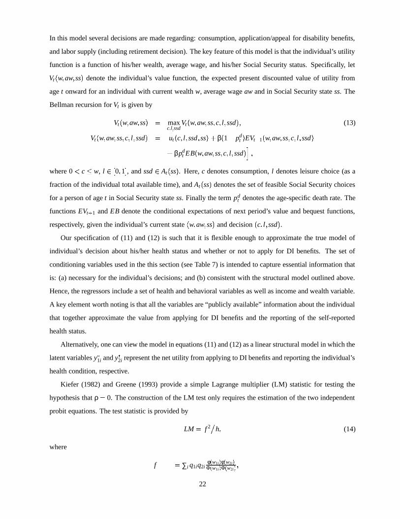
In this model several decisions are made regarding: consumption, application/appeal for disability benefits,

and labor supply (including retirement decision). The key feature of this model is that the individual’s utility

function is a function of his/her wealth, average wage, and his/her Social Security status. Specifically, let

Vtw aw ss denote the individual’s value function, the expected present discounted value of utility from

age t onward for an individual with current wealth w, average wage aw and in Social Security state ss. The

Bellman recursion for Vt is given by

Vtw aw ss max

c 3 l 3 ssdVtw aw ss c l ssd (13)

Vtw aw ss c l ssd ut

c l ssd ss β

1 pd

t EVt E 1w aw ss c l ssd βpd

t EBw aw ss c l ssd %1

where 0 F c G w, l )H 0 1 , and ssd ) Atss . Here, c denotes consumption, l denotes leisure choice (as a

fraction of the individual total available time), and Atss denotes the set of feasible Social Security choices

for a person of age t in Social Security state ss. Finally the term pdt denotes the age-specific death rate. The

functions EVt E 1 and EB denote the conditional expectations of next period’s value and bequest functions,

respectively, given the individual’s current statew aw ss and decision

c l ssd .

Our specification of (11) and (12) is such that it is flexible enough to approximate the true model of

individual’s decision about his/her health status and whether or not to apply for DI benefits. The set of

conditioning variables used in the this section (see Table 7) is intended to capture essential information that

is: (a) necessary for the individual’s decisions; and (b) consistent with the structural model outlined above.

Hence, the regressors include a set of health and behavioral variables as well as income and wealth variable.

A key element worth noting is that all the variables are “publicly available” information about the individual

that together approximate the value from applying for DI benefits and the reporting of the self-reported

health status.

Alternatively, one can view the model in equations (11) and (12) as a linear structural model in which the

latent variables y C1i and y C2i represent the net utility from applying to DI benefits and reporting the individual’s

health condition, respective.

Kiefer (1982) and Greene (1993) provide a simple Lagrange multiplier (LM) statistic for testing the

hypothesis that ρ 0. The construction of the LM test only requires the estimation of the two independent

probit equations. The test statistic is provided by

LM f 2 * h (14)

where

f ∑i q1iq2iφ I w1i J φ I w2i JΦ I w1i J Φ I w2i J

22

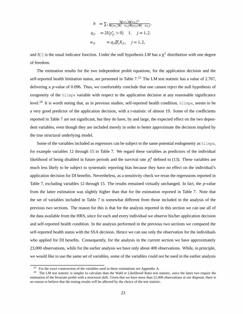
h ∑i K φ I w1i J φ I w2i J&L 2Φ I w1i J Φ I w1i J Φ I w2i J Φ I w2i J

q ji 2I

y C ji D 0 # 1 j 1 2

w ji q jiβ jX ji j 1 2

and I is the usual indicator function. Under the null hypothesis LM has a χ2 distribution with one degree

of freedom.

The estimation results for the two independent probit equations, for the application decision and the

self-reported health limitation status, are presented in Table 7.23 The LM test statistic has a value of 2.767,

delivering a p-value of 0.096. Thus, we comfortably conclude that one cannot reject the null hypothesis of

exogeneity of the hlimpw variable with respect to the application decision at any reasonable significance

level.24 It is worth noting that, as in previous studies, self-reported health condition, hlimpw, seems to be

a very good predictor of the application decision, with a t-statistic of almost 19. Some of the coefficients

reported in Table 7 are not significant, but they do have, by and large, the expected effect on the two depen-

dent variables, even though they are included merely in order to better approximate the decision implied by

the true structural underlying model.

Some of the variables included as regressors can be subject to the same potential endogeneity as hlimpw,

for example variables 12 through 15 in Table 7. We regard these variables as predictors of the individual

likelihood of being disabled in future periods and the survival rate pdt defined in (13). These variables are

much less likely to be subject to systematic reporting bias because they have no effect on the individual’s

application decision for DI benefits. Nevertheless, as a sensitivity check we reran the regressions reported in

Table 7, excluding variables 12 through 15. The results remained virtually unchanged. In fact, the p-value

from the latter estimation was slightly higher than that for the estimation reported in Table 7. Note that

the set of variables included in Table 7 is somewhat different from those included in the analysis of the

previous two sections. The reason for this is that for the analysis reported in this section we can use all of

the data available from the HRS, since for each and every individual we observe his/her application decision

and self-reported health condition. In the analysis performed in the previous two sections we compared the

self-reported health status with the SSA decision. Hence we can use only the observation for the individuals

who applied for DI benefits. Consequently, for the analysis in the current section we have approximately

23,000 observations, while for the earlier analysis we have only about 400 observations. While, in principle,

we would like to use the same set of variables, some of the variables could not be used in the earlier analysis

23 For the exact construction of the variables used in these estimations see Appendix A.24 The LM test statistic is simpler to calculate than the Wald or Likelihood Ratio test statistic, since the latter two require the

estimation of the bivariate probit with a structural shift. Given that we have more than 21,000 observations at our disposal, there isno reason to believe that the testing results will be affected by the choice of the test statistic.

23

for lack of variation in the subsample of 400 observations.

7 Summary and Conclusions

In this study we investigate a very specific question: Is self-reported disability systematically biased, relative

to the SSA measure of disability? Specifically, we use the respondents’ answer to the question, “Do you have

a health limitation that prevents you from working entirely?” (hlimpw) from the HRS. Similar questions

have become quite frequent in questionnaires of recent surveys. This puts us in the middle of an empirical

minefield, since there have been many conflicting empirical studies on the reliability of self-reported health

measures. Some claim that such measures are noisy, biased, and endogenous, and others find that they are

powerful, exogenous predictors of application, appeal, and labor supply decisions.

The key potential problem with such questions is that individuals might have incentives to strategically

answer these questions for various possible reasons, invalidating the use of these variables as explanatory

variables. The two most common reasons posted in the literature are: (a) individuals might feel obligated to

justify some of their observed actions; and (b) individuals might question the confidentiality of the survey.

But, there are many other possible incentives that would lead to strategic reporting of data, including data

that, by and large, we take for granted. We do not make any attempt in this paper to define “true disability”,

but rather accept the notion that disability is a subjective, socially determined concept, that may change,

and, in fact, does change, over time. We take the SSA’s definition of disability as the basis for the “social

standard” according to which individuals determine whether or not they are disabled. We use data from the

first three waves of the HRS to identify a sample of individuals who applied for DI or SSI benefits during

the years 1990-1996.

There are a number of motivations for this investigation. First, we want to provide a well defined frame-

work with which to investigate the validity of self-reported variables. Second, this particular variable was

shown to be an approximate sufficient statistic for individuals’, as well as for the Social Security Adminis-

tration (SSA), decisions. Such a summary statistic can serve as a very powerful state variable in a dynamic

optimization model, which we are currently developing. Third, we use this variable in a companion paper

(Benıtez-Silva, Buchinsky, and Rust 2003) to provide an “audit” of the multistage application and appeal

process used by the SSA. This variable provides the basis for estimating the magnitude of the SSA classifi-

cation errors of disabled and non-disabled people.

We investigate whether the SSA ultimate award decision is systematically biased relative to the indi-

vidual report of their hlimpw variable. Using a battery of unconditional and conditional (on individuals’

characteristics) tests, we conclude that applicants are, on average, no more optimistic or pessimistic about

24

their disability status than the SSA. One might claim that the reason we fail to reject the unbiasedness

hypothesis may be that our tests have low power, especially given the relatively few observations of DI

applicants in the HRS. However, when we use only the first stage outcome of the SSA, before the indi-

viduals had the chance to appeal the initial decision, we clearly reject the null hypothesis of unbiasedness.

Moreover, previous experience with other data sets suggests that when it is possible to independently verify

individuals’ survey responses, the answers are surprisingly accurate (e.g. Rust and Phelan 1997, and Lahiri

et al. 1995).

We then introduce the hypothesis of rational unbiased reporting (RUR) on a bivariate single index model

of disability reporting and award determination. Different versions of the same basic model allow for a few

types of individuals, as well as for a few SSA decision types. The core of the RUR hypothesis is that DI

applicants are fully informed about the rules governing the disability award process and criteria by which

applicants with varying characteristics are accepted or rejected. We give some strong evidence that the RUR

hypothesis is relevant for assessing the classification errors in SSA’s disability award process since it implies

that the applicants and the SSA agree on the definition of disability, even though there may be no agreement

over whether there exists an absolute, objective standard. The RUR models indicate that at least a large

fraction of the population truthfully report their health status. While there is also a considerable part of the

population that seems to inflate somewhat their evaluation of their disability, there is just as large a part of

the population that does exactly the opposite. Overall, the individuals’ evaluation of their disability is on

average the same as the SSA evaluation of that disability. The RUR model also seems to indicate that there

are a number of different groups of individuals that have very different qualitative behavior. We found that

in neither of the two groups in the two-group model was there any overall tendency to inflate the evaluation

of disability in the group as a whole.

After establishing the first two facts we proceed with the examination of whether or not the self-reported

measure is exogenous with respect to the individual’s application decision. Specifically, we test whether or

not hlimpw is an exogenous variable with respect to the individual’s application decision. Again, we are

unable to reject the hypothesis that hlimpw is an exogenous explanatory variable, and therefore conclude

that it can be used as a state variable for the application decision.

We do not think that our work will be the last word on this subject, nor do we believe that we can easily

convince a skeptic that self-reported disability status is a valid measure of “true disability”. However, we

provide a framework with which one can examine the validity of a self-reported health measure, or for this

matter any self-reported variable.

25

Appendix A—Data Appendix

Constructed variables:25

An important issue for the construction of the income and wealth variables is that HRS financial ques-tions were only answered by the primary respondent of the household, usually the financially knowledgeableperson of the family. Therefore, we had to merge this information in order to obtain the relevant values ofthese variables for the spouses.The definitions of the employment history and wealth variables are as follows:1. Respondent’s Income—the sum of the respondent’s earnings, and income from pensions, welfare, SocialSecurity and capital gains.2. Total hours worked in a given year—the sum of the respondent’s hours worked in that year on the currentjob, previous job, and any intermediate job (when applicable).3. Earnings in a given year—data from the income section, in some cases corrected using our calculationsof employment income as a sum of the respondent’s income earned in that year on the current job, previousjob, and any intermediate job (when applicable).4. We also construct monthly and annual indicators summarizing the respondent’s employment history.These variables are potentially important predictors of DI award decisions since they provide evidence ofan applicant’s ability to engage in substantial gainful activity. Specifically, any evidence of employmentsubsequent to the reported date of disability onset or the filing of an application for DI benefits could begrounds for immediate rejection at the first-stage “SGA screen” (see Benıtez-Silva et al. 1999). We con-structed employment histories using information on beginning and ending dates of employment spells inthe employment section of the HRS. In particular, we calculated for each individual in every year between1991 and 1996 annual hours worked and annual earnings. Monthly employment indicators for each monthbetween January 1989 and December 1996 were also calculated. We employed a battery of consistencychecks to validate the extensive number of calculations necessary to translate reported dates of beginningand leaving previously held jobs and “intermediate jobs” held between successive survey waves to deter-mine the time path of employment down to the finest possible time period allowed by the survey questions(i.e. monthly).5. Net Worth—net worth of all housing and non-housing assets (including vehicles, stocks, bonds, privatebusinesses, bank accounts, etc.).Imputations:

It is worthwhile to briefly summarize some of the imputations used in constructing the data extractwhich were carried out in an attempt to minimize the number of observations that were eliminated fromthe estimations. Imputations were performed only for dates of different events connected to the applicationand appeal process. It was common to find missing months of application, appeal, onset of disability, andthe starting point of receipt of DI benefits. In some cases even the year of the event was missing. In otherinstances the dates were not consistent with other information provided in the survey. Our imputations werecarried out in such a way as to avoid any systematic biases. If bounds on a missing date could be establishedand the year of application was known, we simply chose the midpoint of this window. When the year wasmissing we dropped that observation, unless we could unambiguously restore it given the other availableinformation. Although 52% of the observations pertaining to applicants had some imputations, a numberof internal consistency checks using independent information from the employment, disability, and incomesections of the HRS survey have shown that reported dates of disability onset, exit from the labor force, andreceipt of DI benefits match up in a predictable fashion.Construction of the data for the exogeneity tests:

We start by explaining the construction of the 32,869 observations for the individuals’ application deci-sion and the hlimpw condition. We assume that each individual makes a decision whether or not to apply

25 A more detailed explanation of the calculation algorithms is available from the authors upon request.

26

once in each wave. Individuals not applying are assumed to make their decision at the interview date. Forthose applying, the decision is assumed to have occurred on the date of the first application. Only individ-uals not currently receiving DI benefits and those without a pending application were assumed to make adecision. As a result, each individual has a maximum of three, and a minimum of zero application decisions.At each decision date we assigned the appropriate set of income, health and demographic variables to theindividual. In this assignment we matched each decision with the variables’ values obtained from closestinterview information. The only exception is for people who applied right after an interview at which theyhad reported not being disabled. In this case we assigned the data provided at the subsequent interview, evenif this was long after the application date.

Appendix B—Consistent Conditional Moment Test

Bierens (1990) Test:

This appendix presents the methods used in implementing the consistent conditional moment test, sug-gested in Bierens (1990). The test requires the challenging task of calculating t argmaxt . TW

t , and

then using Wt in a procedure that chooses between t and a fixed to depending on two parameters, γ D 0,

ρ ) 0 1 , used in Bierens’ Theorem 4, and on the number of observations n. In Theorem 5 Bierens suggests

a “quick-and-easy procedure” to findt, by simply maximizing the function over a collection of randomly

chosen vectors in T . However, we found this method to be extremely inefficient for the problem at hand,especially when the number of covariates and the dimension of the space over which t is chosen, increases.

More sophisticated methods greatly improved upon the results generated from as many as 5 millionrandom draws from the 26 dimensional cube. We first modified the algorithm slightly to search in smallregions surrounding vectors that achieved moderately high values of the function. Although still requiringa large number of random draws, this method generated substantially higher maxima. We then employed apolytopic method, as well as simulated annealing, to find maxima using as a starting point the result of ourmodified algorithm.26 Polytope algorithms proceed by constructing a simplex in Rn and replacing pointsin the simplex through a series of reflections. Simulated annealing relies on a Markov process to convergeto an extremum, choosing between uphill and downhill jumps probabilistically. These methods proved themost efficient, consistently converging to local maxima, depending on the starting value provided. Onlythe simulated annealing algorithm was able to achieve maxima superior to those generated by the modifiedrandom search technique. But as with the polytopic method, it consistently generated comparable results ina fraction of the time.

We must emphasize that our effort to find the global maximum of Wt plays against us when trying

not to reject the unbiasedness hypothesis. The higher the resulting Wt —other parameters fixed—the

more likely it is that we reject H0, or in other words, poor estimates of t tend to underestimate the χ2

statistic, leading to possible under-rejection of the null-hypothesis. The result reported in Table 3 is theproduct of averaging out one million calculations of the test statistic of interest. This allows our results tobe independent of lucky or unlucky draws of γ and ρ. In every draw, γ was chosen uniformly in the

0 40

interval, ρ was chosen uniformly in0 1 , and every ti ) 5 5 .27

Finally, Figure B.1 plots the resulting p-value of the test statistic for half a million draws of a fixed twhere each ti ) 5 5 . This gives us a simple approximation to how likely it is that our hypothesis is

26 See Judd (1998), and Press et al. (1992) for more on these techniques.27 We found the test to be relatively sensitive to the choice of γ. When γ is very small the test tends to reject the null hypothesis

given that the procedure suggested by Bierens in his Theorem 4 computes the test statistic using the maximum t. Given that thetheorem only requires γ to be positive we consider our method of randomly choosing the parameters and averaging many results ofthe test as a fair implementation of the test with our finite sample. Although it is possible to reject our null hypothesis if γ is chosenin a small enough positive interval we believe this would not be an appropriate application of Bierens’ results.

27

violated. We can see from the graph that most values of the test statistic do not lead to a rejection of theunbiasedness hypothesis.

Horowitz-Spokoiny (2001) Test:The test suggested by Horowitz and Spokoiny (2001) is for testing a conditional mean parametric func-

tion against a non-parametric alternative. In our case the parametric function is identically 0 under the nullhypothesis of unbiasedness, that is E

at dt xt 0. Therefore, the HS test is simplified considerably. We

detail below the procedure we used. Furthermore, we provide the information about the various subjectivechoices that are required for carrying out the above test.

Let x be a vector in the m Euclidean space, that is x ) ℜm and let the dependent variable y be defined byyit

ait dit (for simplicity we suppress the t subscript below). Then, in general,

yi f

xi θ εi

Under the null hypothesis Eεi xi 0. In our case f

xi θ M 0. The test allows for heteroskedastic error

and we denote the variance of the error term by σ2 xi E ε2i xi N

Under the alternative hypothesis we do not specify a conditional function, but rather estimate it non-parametrically. We employ a kernel smoother of the form

Whxi x j Kh

xi x j

∑nk 1 Kh

xi xk i j 1 2444 n

where Khλ K

λ O h , for some kernel function K

, and h is the kernel bandwidth (the choice of which isexplained below). We chose K

to be the multivariate normal kernel with the variance-covariance matrixas a diagonal matrix with the standard deviation of the elements in x on the diagonal.

For this kernel smoother, the non-parametric estimate for Eat dt x is given by

fhxi n

∑j 1

Whxi x j y j i 1 2444 n

where yi ait dit .

The core test statistic is then given by Shn ∑n

i 1fhxi 2 2 which is to be centered and studentized.

In order to do that some more notation is needed. Let Wh be the n n matrix whosei j elements are given

by Whxi x j and let Ah

W hWh.Now define

Th Sh

n #

NhVh

where

Nh n

∑i 1

aii 3 hσ2nxi

Vh 2

n

∑i 1

n

∑j 1

a2i j 3 hσ2

nxi σ2

nx j

and σ2nxi is a consistent estimator for σ2 xi , and is explained below.

Under some regularity conditions, Th has an asymptotic distribution with zero mean and unit variance.Nevertheless, the statistic HS suggested is given by Tmax

maxh . Hn Th where Hn is a finite set of bandwidthvalues. The construction of this set is explained below. The distribution of Tmax may be very different fromthe distribution of Th. To circumvent this problem we compute the small sample distribution of Tmax using abootstrap procedure as explained below.

28

Consistent estimator for σ2 xi :We use the estimator suggested by HS and outline below the construction of the estimator.Define the following recursion system

j1 argmin j 1 3 P P P 3 n QQ x1 x j QQ

and for any i D 1ji argmin j R j I 1 J 3 P P P 3 j I i 1 J QQ xi x j QQ

where S S denotes the euclidean distance. Then, a consistent estimator for σ2 xi is given byσ2 xi ∑n

k 1

yk y j I k J 2I

QQ xi x j QQ F bn ∑n

k 1 I QQ xi x j QQ F bn

where I denotes the usual indicator function and bn is a bandwidth that shrinks to 0 at an appropriate rate

as n " ∞.

Defining Hn:

The set Hn we use here is the same as is suggested by HS, that is, the geometric grid of the form

Hn > h : h hmaxal and h hmin l 0 1 2 244 ?

We use hmax 20, hmin

01, and a 95. This gives 73 points in Hn.

Bootstrapping the small sample distribution of Tmax:

We use the following three steps:Step 1: Sample randomly ε Ci , i 1 2444 n, from the normal distribution N 0 σ2

nxi T , and generate y Ci under

the null hypothesis, that is y Ci ε Ci , i 1 2444 n.Step 2: For the bootstrap data y Ci , i 1 2444 n, compute the estimate for σ2 xi . Use this estimate to constructN Ch and

V Ch , the bootstrap version of

Nh and

Vh, respectively. Construct the bootstrap version of the statistic

Tmax, say T Cmax.Step 3: For a test with significant level α, choose the critical value ta to be the 1 α quantile of theempirical distribution of T Cmax, that is obtained by repeating the first two steps a large number of times.

We chose the number of repetitions to be B 10 000.

29

References

Anderson , K.H., and R.V. Burkhauser (1985): “The Retirement-Health Nexus: A New Measure of an OldPuzzle,” Journal of Human Resources, 20 315–330.

Andrews, D.W.K., and M. Buchinsky (2000): “A Three-step Method for Choosing the Number of BootstrapRepetitions,” Econometrica, 68 23–51.

Bazzoli, G.J. (1985): “The Early Retirement Decision: New Empirical Evidence on the Influence ofHealth,” Journal of Human Resources, 20 214–234.

Benıtez-Silva, H. (2000): “Micro Determinants of Labor Force Status Among Older Americans,”http://ms.cc.sunysb.edu/ U hbenitezsilv/conf03.pdf

Benıtez-Silva, H., M. Buchinsky, and, J. Rust (2001): “Dynamic Structural Models of Retirement andDisability,” manuscript, Yale University.

Benıtez-Silva, H., M. Buchinsky, H-M. Chan, J. Rust, and S. Sheidvasser (1999): “An Empirical Analysisof the Social Security Disability Application, Appeal and Award Process,” Labour Economics 6 147–178.

Benıtez-Silva, H., M. Buchinsky, and J. Rust (2003): “How Large are the Classification Errors in the SocialSecurity Disability Award Process?” http://ms.cc.sunysb.edu/ U hbenitezsilv/dice.pdf

Bierens, H.J. (1990): “A Consistent Conditional Moment Test of Functional Form,” Econometrica, 58-61443–1458.

Blau, D.M., D.B. Gilleskie, and C. Slusher (1997): “The Effect of Health on Employment Transitions ofOlder Men,” manuscript, Department of Economics, University of North Carolina at Chapel Hill.

Bound, J. (1991): “Self-Reported Versus Objective Measures of Health in Retirement Models,” Journal ofHuman Resources, 26-1 106–138.

Bound, J. (1989a): “The Health and Earnings of Rejected Disability Insurance Applicants,” AmericanEconomic Review, 79 482–503.

Bound, J. (1989b): “Self-Reported Versus Objective Measures of Health in Retirement Models,” NBERWorking Paper No. 2997.

Bound, J., M. Schoenbaum, T. Steinbrickner, and T. Waidmann (1998a): “Modeling the Effect of Healthon Retirement Behavior,” manuscript, University of Michigan.

Bound, J., M. Schoenbaum, T. Steinbrickner, and T. Waidmann (1998b): “The Dynamic Effects of Healthon the Labor Force Transitions of Older Workers,” NBER Working Paper No. 6777.

Bound, J., M. Schoenbaum, and T. Waidmann (1995): “Race and Education Differences in DisabilityStatus and Labor Force Attachment,” Journal of Human Resources, 30-S 227–267.

Burkhauser, R.V. and M.C. Daly (1996): “Employment and Economic Well-Being Following the Onset ofa Disability; The Role for Public Policy,” in J. Mashaw, V. Reno, R.V. Burkhauser, and M. Berkowitz(eds.), Disability Work and Cash Benefits, Upjohn Institute for Employment Research, 59–102.

Burkhauser, R.V., R.H. Haveman, and B.L. Wolfe (1993): “How People with Disabilities Fare when PublicPolicies Change,” Journal of Policy Analysis and Management, 12-2 251–269.

30

Dwyer, D.S. and O.S. Mitchell (1999): “Health Problems as Determinants of Retirement: Are Self-ratedMeasures Endogenous?” Journal of Health Economics, 18-2 173–193.

Greene, W.H. (1993): Econometric Analysis, Second Edition, Prentice Hall, New Jersey.

Heckman, J.J. (1978): “Dummy Endogenous Variables in a Simultaneous Equation System,” Economet-rica, 46-6, 931–959.

Horowitz, J.L. and V.G. Spokoiny (2001): “An Adaptive, Rate-optimal Test of a Parametric Model Againsta Nonparametric Alternative,” Econometrica, 69-3 599–631.

Hu, J., K. Lahiri, D.R. Vaughan, and B. Wixon (1997): “A Structural Model of Social Security’s DisabilityDetermination Process,” ORES Working Paper No. 72, Office of Research and Evaluation Statistics,Social Security Administration, 500 E Street SW, Washington, D.C.

Johnson, W.G. (1977): “The Effect of Disability on Labor Supply: Comments,” Industrial and LaborRelations Review, 30 380–381.

Judd, K.L. (1998): Numerical Methods in Economics, Cambridge: MIT Press.

Kerkhofs, M. and M. Lindeboom, (1995): “Subjective Health Measures and State Dependent ReportingErrors,” Health Economics, 4, 221–235.

Kerkhofs, M., M. Lindeboom, and J. Theeuwes (1998): “Retirement, Financial Incentives and Health,”Labour Economics, 6, 203–227.

Kiefer, N.M. (1982): “Testing for Dependence in Multivariate Probit Models,” Biometrika, 69, 161–166.

Kreider, B. (1999): “Disability Applications: The Role of Measured Limitation on Policy Inferences,”manuscript, Department of Economics, University of Virginia.

Kreider, B. (1998): “Latent Work Disability and Reporting Bias,” manuscript, Department of Economics,University of Virginia.

Lahiri, K., D.R. Vaughan, and B. Wixon (1995): “Modeling SSA’s Sequential Disability DeterminationProcess Using Matched SIPP Data,” Social Security Bulletin, 58-4 3–42.

Lambrinos, J., (1981): “Health: A Source of Bias in Labor Supply Models,” Review of Economics andStatistics, 63-2 206–212.

Myers, R.J. (1982): “Why Do People Retire from Work Early?” Social Security Bulletin, 45 10–14.

O’Donnell, O. (1998): “The Effect of Disability on Employment Allowing for Work Incapacity,” WorkingPaper No. 98-13, University of Kent at Canterbury.

Papageorgiou, A. and J. Traub (1996): FINDER Software.

Parsons, D.O. (1996): “Imperfect ‘Tagging’ in Social Insurance Programs,” Journal of Public Economics,62 183–207.

Parsons, D.O. (1982): “The Male Labour Force Participation Decision: Health, Reported Health, andEconomic Incentives,” Economica, 49 81–91.

Press, W.H., S.A. Teukolsky, W.T. Vetterling, and B.P. Flannery (1992): Numerical Recipes: The Art ofScientific Computing. New York: Cambridge University Press.

31

Rust, J. and C. Phelan (1997): “How Social Security and Medicare Affect Retirement Behavior in a Worldof Incomplete Markets,” Econometrica, 65-4 781–831.

Stapleton, D., B. Barnow, K. Coleman, K. Dietrich, and G. Lo (1994): Labor Markets Conditions, Socioe-conomic Factors and the Growth of Applications and Awards for SSDI and SSDI Disability Benefits:Final Report, Lewin-VHI, Inc. and the Department of Health and Human Services, The Office of theAssistant Secretary for Planning and Evaluation.

Stern, S. (1989): “Measuring the Effects of Disability on Labor Force Participation,” Journal of HumanResources, 24 361–395.

32

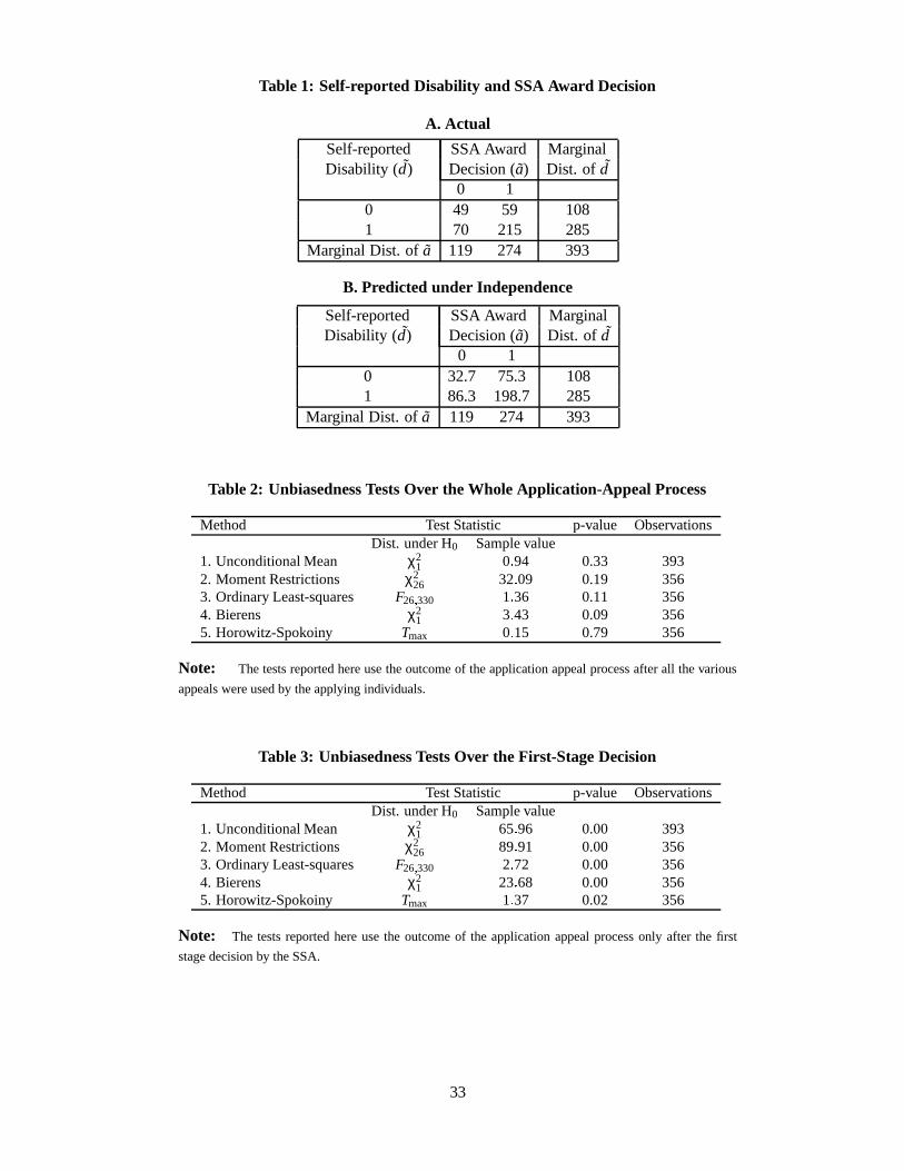
Table 1: Self-reported Disability and SSA Award Decision

A. Actual

Self-reported SSA Award MarginalDisability (d) Decision (a) Dist. of d

0 10 49 59 1081 70 215 285

Marginal Dist. of a 119 274 393

B. Predicted under Independence

Self-reported SSA Award MarginalDisability (d) Decision (a) Dist. of d

0 10 32.7 75.3 1081 86.3 198.7 285

Marginal Dist. of a 119 274 393

Table 2: Unbiasedness Tests Over the Whole Application-Appeal Process

Method Test Statistic p-value ObservationsDist. under H0 Sample value

1. Unconditional Mean χ21 0 V 94 0.33 393

2. Moment Restrictions χ226 32 V 09 0.19 356

3. Ordinary Least-squares F26 W 330 1 V 36 0.11 3564. Bierens χ2

1 3 V 43 0.09 3565. Horowitz-Spokoiny Tmax 0 V 15 0.79 356

Note: The tests reported here use the outcome of the application appeal process after all the various

appeals were used by the applying individuals.

Table 3: Unbiasedness Tests Over the First-Stage Decision

Method Test Statistic p-value ObservationsDist. under H0 Sample value

1. Unconditional Mean χ21 65 V 96 0.00 393

2. Moment Restrictions χ226 89 V 91 0.00 356

3. Ordinary Least-squares F26 W 330 2 V 72 0.00 3564. Bierens χ2

1 23 V 68 0.00 3565. Horowitz-Spokoiny Tmax 1 V 37 0.02 356

Note: The tests reported here use the outcome of the application appeal process only after the first

stage decision by the SSA.

33

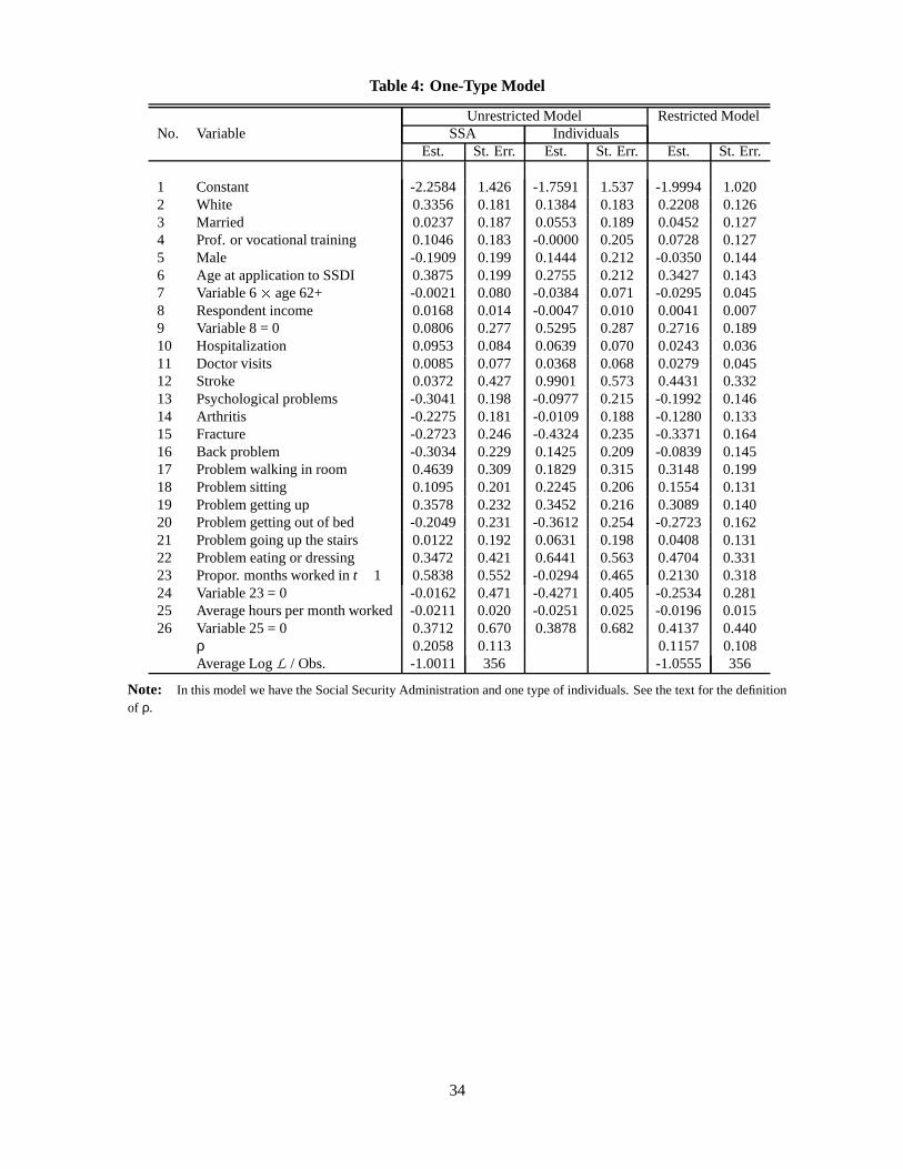
Table 4: One-Type Model

Unrestricted Model Restricted ModelNo. Variable SSA Individuals

Est. St. Err. Est. St. Err. Est. St. Err.

1 Constant -2.2584 1.426 -1.7591 1.537 -1.9994 1.0202 White 0.3356 0.181 0.1384 0.183 0.2208 0.1263 Married 0.0237 0.187 0.0553 0.189 0.0452 0.1274 Prof. or vocational training 0.1046 0.183 -0.0000 0.205 0.0728 0.1275 Male -0.1909 0.199 0.1444 0.212 -0.0350 0.1446 Age at application to SSDI 0.3875 0.199 0.2755 0.212 0.3427 0.1437 Variable 6 X age 62+ -0.0021 0.080 -0.0384 0.071 -0.0295 0.0458 Respondent income 0.0168 0.014 -0.0047 0.010 0.0041 0.0079 Variable 8 = 0 0.0806 0.277 0.5295 0.287 0.2716 0.18910 Hospitalization 0.0953 0.084 0.0639 0.070 0.0243 0.03611 Doctor visits 0.0085 0.077 0.0368 0.068 0.0279 0.04512 Stroke 0.0372 0.427 0.9901 0.573 0.4431 0.33213 Psychological problems -0.3041 0.198 -0.0977 0.215 -0.1992 0.14614 Arthritis -0.2275 0.181 -0.0109 0.188 -0.1280 0.13315 Fracture -0.2723 0.246 -0.4324 0.235 -0.3371 0.16416 Back problem -0.3034 0.229 0.1425 0.209 -0.0839 0.14517 Problem walking in room 0.4639 0.309 0.1829 0.315 0.3148 0.19918 Problem sitting 0.1095 0.201 0.2245 0.206 0.1554 0.13119 Problem getting up 0.3578 0.232 0.3452 0.216 0.3089 0.14020 Problem getting out of bed -0.2049 0.231 -0.3612 0.254 -0.2723 0.16221 Problem going up the stairs 0.0122 0.192 0.0631 0.198 0.0408 0.13122 Problem eating or dressing 0.3472 0.421 0.6441 0.563 0.4704 0.33123 Propor. months worked in t Y 1 0.5838 0.552 -0.0294 0.465 0.2130 0.31824 Variable 23 = 0 -0.0162 0.471 -0.4271 0.405 -0.2534 0.28125 Average hours per month worked -0.0211 0.020 -0.0251 0.025 -0.0196 0.01526 Variable 25 = 0 0.3712 0.670 0.3878 0.682 0.4137 0.440

ρ 0.2058 0.113 0.1157 0.108Average Log L / Obs. -1.0011 356 -1.0555 356

Note: In this model we have the Social Security Administration and one type of individuals. See the text for the definitionof ρ.

34

Table 5: Two-Type Model

Unrestricted Model Restricted ModelGroup1 Group2 Group1 Group2

No. Variable SSA Indiv. SSA Indiv.Est. St. Err. Est. St. Err. Est. St. Err. Est. St. Err. Est. St. Err. Est. St. Err.

1 Constant -2.430 3.561 -0.500 4.530 -1.314 6.839 -0.807 8.232 -2.982 3.971 -1.308 2.4112 White 0.476 0.464 0.453 0.620 -0.515 0.744 1.166 1.234 0.675 0.517 0.036 0.2973 Married 0.091 0.421 -0.048 0.626 0.002 0.845 0.308 0.841 -0.221 0.488 0.166 0.3094 Prof./voc. training 0.039 0.416 0.047 0.559 -0.126 0.772 0.033 0.829 0.027 0.439 -0.000 0.3255 Male -0.596 0.527 0.638 0.701 0.253 0.988 0.590 0.938 0.038 0.511 -0.203 0.3296 Age at application 0.403 0.444 0.362 0.639 0.081 0.740 0.443 0.913 0.562 0.549 0.330 0.3607 Var. 6 Z age 62+ -0.001 0.161 0.095 0.173 -0.039 0.766 -0.000 0.354 0.067 0.242 -0.110 0.1008 Respondent income 0.015 0.034 0.018 0.035 0.027 0.072 -0.087 0.112 0.019 0.029 -0.004 0.0199 Variable 8 = 0 0.000 0.801 0.000 1.314 2.178 0.992 -1.903 2.378 0.253 0.737 0.095 0.49910 Hospitalization 0.415 0.330 -0.125 0.180 0.032 0.300 0.294 0.421 0.200 0.296 0.001 0.14911 Doctor visits 0.209 0.217 -0.345 0.234 0.157 0.394 0.011 0.285 0.019 0.021 -0.016 0.01412 Stroke 0.000 1.174 0.217 3.992 1.955 1.465 0.253 1.511 0.067 1.148 -0.075 0.68713 Psych. problems -0.304 0.469 -0.393 0.725 -0.058 0.823 0.001 0.872 -0.589 0.544 -0.011 0.37114 Arthritis -0.551 0.446 0.563 0.605 -0.159 0.824 -0.040 0.803 -0.000 0.471 0.067 0.33015 Fracture 0.093 0.597 -0.762 0.902 -0.566 0.823 -0.934 1.408 -0.748 0.574 -0.115 0.34516 Back problem -0.282 0.481 -0.610 0.840 1.091 1.204 -0.184 0.962 -1.260 0.765 0.635 0.39817 Problem walking in room 0.208 0.712 1.319 1.069 0.088 2.252 0.769 1.280 -0.001 0.607 0.522 0.56018 Problem sitting -0.472 0.529 0.959 0.680 -0.513 0.961 1.200 1.352 0.250 0.456 0.263 0.29219 Problem getting up 0.753 0.601 0.000 0.633 0.800 0.948 -0.033 1.034 0.751 0.528 -0.136 0.35720 Problem getting out of bed -0.399 0.539 0.004 0.882 -0.000 0.815 -1.152 1.138 0.113 0.564 -0.449 0.37921 Problem going up the stairs -0.001 0.403 0.455 0.612 0.223 0.808 0.0978 0.806 -0.180 0.525 0.243 0.30722 Problem eating or dressing 1.477 1.328 -0.648 1.288 -0.202 1.529 2.357 1.285 0.312 1.347 0.425 1.16023 Prop. worked in t [ 1 0.962 1.366 -0.789 1.159 -0.265 2.985 -0.164 3.718 0.323 0.986 0.502 0.73924 Variable 23 = 0 -0.000 1.178 -0.946 1.015 -0.260 2.767 -1.131 3.422 0.750 1.009 -0.898 0.69925 Avg. hours/month worked -0.010 0.054 -0.101 0.059 -0.035 0.293 -0.085 0.184 -0.077 0.080 -0.021 0.02826 Variable 25 = 0 0.266 1.948 -0.212 1.763 0.186 5.362 -0.105 4.762 0.117 1.684 0.059 1.053

ρ 0.605 0.567 0.308 0.925 0.170 0.607 -0.501 1.257η 0.411 0.144 0.474 0.095Average Log L / Obs. -0.895 356 -0.999 356

Note: In the restricted model we have the Social Security Administration (SSA) and two types of individuals, whose coefficient vectors (with each group) are notconstrained to be the same. The restricted model imposes equality of the coefficient vector for the SSA and individuals within the same group. The quantity η is theproportion of Type II individuals. The quantity ρ is the correlation between the errors of the SSA and the individuals in each group. See the text for more detaileddefinition.

35

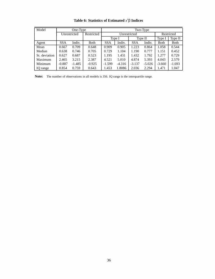
Table 6: Statistics of Estimated x β Indices

Model One-Type Two-TypeUnrestricted Restricted Unrestricted Restricted

Type I Type II Type I Type IIAgent SSA Indiv. Both SSA Indiv. SSA Indiv. Both BothMean 0.667 0.709 0.648 0.909 0.905 1.223 0.864 1.058 0.544Median 0.638 0.746 0.705 0.729 1.104 1.190 0.777 1.151 0.452St. deviation 0.627 0.687 0.523 1.195 1.431 1.432 1.792 1.277 0.729Maximum 2.465 3.215 2.387 4.521 5.010 4.874 5.393 4.043 2.579Minimum -0.887 -1.485 -0.925 -1.599 -4.316 -3.137 -5.026 -3.660 -1.693IQ range 0.854 0.759 0.643 1.453 1.8086 2.036 2.294 1.471 1.047

Note: The number of observations in all models is 356. IQ range is the interquartile range.

36

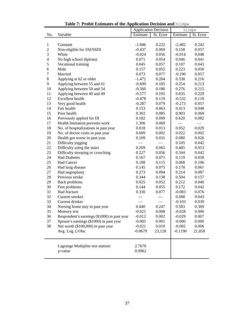
Table 7: Probit Estimates of the Application Decision and hlimpwApplication Decision hlimpw

No. Variable Estimate St. Error Estimate St. Error

1 Constant -1.846 0.222 -2.402 0.2422 Non-eligible for SSI/SSDI -0.437 0.069 0.158 0.0573 White -0.024 0.056 -0.014 0.0484 No high school diploma 0.071 0.054 0.046 0.0415 Vocational training 0.045 0.057 0.107 0.0436 Male 0.157 0.055 0.223 0.0507 Married 0.073 0.077 -0.190 0.0578 Applying at 62 or older -1.472 0.204 0.338 0.2169 Applying between 55 and 61 -0.699 0.185 0.254 0.21310 Applying between 50 and 54 -0.560 0.186 0.276 0.21511 Applying between 40 and 49 -0.577 0.195 0.035 0.22912 Excellent health -0.478 0.119 -0.532 0.11813 Very good health -0.287 0.079 -0.273 0.05714 Fair health 0.153 0.063 0.413 0.04815 Poor health 0.302 0.085 0.903 0.06916 Previously applied for DI 0.182 0.099 0.620 0.08217 Health limitation prevents work 1.306 0.069 — —18 No. of hospitalizations in past year 0.018 0.013 0.052 0.02919 No. of doctor visits in past year 0.009 0.002 0.022 0.00220 Health got worse in past year 0.109 0.031 0.080 0.02621 Difficulty jogging — — 0.105 0.04222 Difficulty using the stairs 0.209 0.065 0.485 0.05323 Difficulty stooping or crouching 0.227 0.056 0.344 0.04224 Had Diabetes 0.167 0.071 0.119 0.05825 Had Cancer 0.188 0.115 0.068 0.10626 Had lung disease 0.145 0.075 0.178 0.06127 Had angioplasty 0.273 0.094 0.214 0.08728 Previous stroke 0.344 0.138 0.504 0.15729 Back problems 0.025 0.052 0.212 0.04030 Feet problems 0.144 0.055 0.172 0.04231 Had fracture 0.330 0.077 -0.083 0.07632 Current smoker — — 0.088 0.04333 Current drinker — — -0.103 0.03934 Nursing home stay in past year 0.440 0.247 0.583 0.36935 Memory test -0.021 0.008 -0.028 0.00636 Respondent’s earnings ($1000) in past year -0.012 0.002 -0.029 0.00737 Spouse’s earnings ($1000) in past year -0.005 0.001 -0.000 0.00038 Net worth ($100,000) in past year -0.021 0.010 -0.002 0.006

Avg. Log L /Obs. -0.0679 23,128 -0.1190 21,858

Lagrange Multiplier test statistic 2.7670p-value 0.0962

37

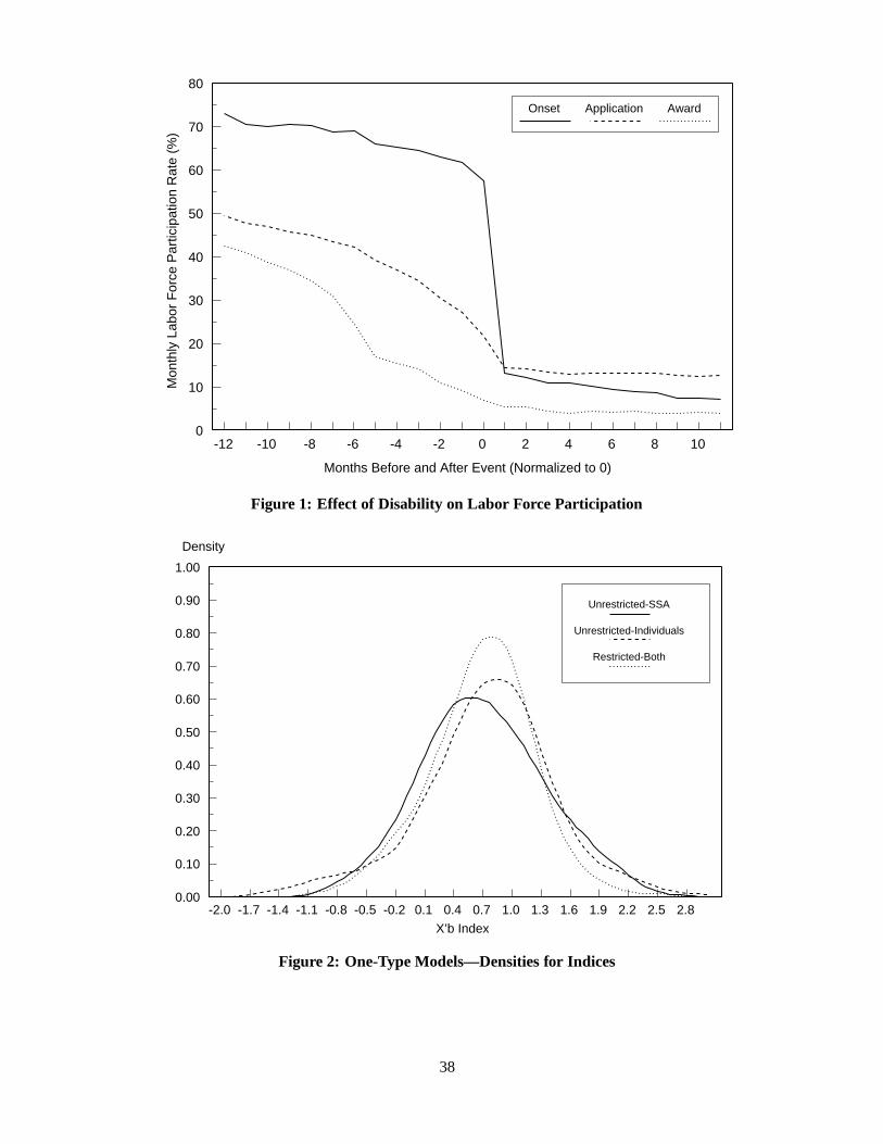
-12 -10 -8 -6 -4 -2 0 2 4 6 8 100

10

20

30

40

50

60

70

80

Months Before and After Event (Normalized to 0)

Mon

thly

Lab

or F

orce

Par

ticip

atio

n R

ate

(%)

Onset Application Award

Figure 1: Effect of Disability on Labor Force Participation

-2.0 -1.7 -1.4 -1.1 -0.8 -0.5 -0.2 0.1 0.4 0.7 1.0 1.3 1.6 1.9 2.2 2.5 2.80.00

0.10

0.20

0.30

0.40

0.50

0.60

0.70

0.80

0.90

1.00

X’b Index

Density

Unrestricted-SSA

Unrestricted-Individuals

Restricted-Both

Figure 2: One-Type Models—Densities for Indices

38

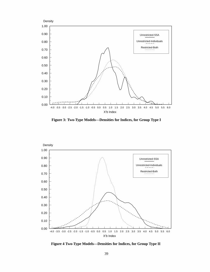
-4.0 -3.5 -3.0 -2.5 -2.0 -1.5 -1.0 -0.5 0.0 0.5 1.0 1.5 2.0 2.5 3.0 3.5 4.0 4.5 5.0 5.5 6.00.00

0.10

0.20

0.30

0.40

0.50

0.60

0.70

0.80

0.90

1.00

X’b Index

Density

Unrestricted-SSA

Unrestricted-Individuals

Restricted-Both

Figure 3: Two-Type Models—Densities for Indices, for Group Type I

-4.0 -3.5 -3.0 -2.5 -2.0 -1.5 -1.0 -0.5 0.0 0.5 1.0 1.5 2.0 2.5 3.0 3.5 4.0 4.5 5.0 5.5 6.00.00

0.10

0.20

0.30

0.40

0.50

0.60

0.70

0.80

0.90

1.00

X’b Index

Density

Unrestricted-SSA

Unrestricted-Individuals

Restricted-Both

Figure 4 Two-Type Models—Densities for Indices, for Group Type II

39

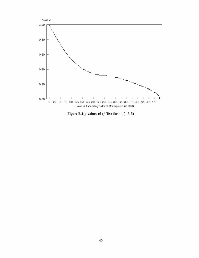
1 26 51 76 101 126 151 176 201 226 251 276 301 326 351 376 401 426 451 4760.00

0.20

0.40

0.60

0.80

1.00

Draws in Ascending order of Chi-squared (in ’000)

P-value

Figure B.1:p-values of χ2 Test for t ) 5 5

40