How do you persuade someone you don’t know?

Hyun Chang Yi∗†

March 17, 2013

Abstract

We examine the potential for communication via cheap talk between an

expert and a decision maker whose type (or preferences) is uncertain. The ex-

pert privately observes multiple aspects of an issue and persuades the decision

maker to choose an action in his favour by informing the decision maker about

the issue. The decision maker privately observes her type and chooses an ac-

tion. The optimal action for the decision maker depends upon her type and

the state of the issue. We find that, in one-way cheap talk games where only

the expert talks, the expert can always inform the decision maker in the form

of comparative statements and the decision maker can almost surely make an

informed decision. Furthermore, in two-way games where the decision maker

talks before the expert does, the decision maker can partially reveal her type

to the expert or public without information loss.

JEL classification: D82, C72

Keywords: Cheap Talk, Two-Sided Incomplete Information, Uncertain Type

∗Department of Economics, JG Smith Building, University of Birmingham, Edgbaston, Birm-ingham, B15 2TT, UK. Email: hxy107@bham.ac.uk†I am grateful to my PhD advisor Rajiv Sarin for his helpful comments and encouragement.

I also thank Joel Sobel, Marco Ottaviani, Indrajit Ray, Jaideep Roy and Alexander Brown forcomments.

1

1 Introduction

Suppose that a government official tries to persuade a legislator to pass a budget

for government spending. The official always prefers more spending to less, while

the more beneficial the spending is to the legislator’s favoured income class, the

bigger the spending that the legislator is willing to approve. The official has already

examined the spending and thus fully understands the redistributive effects of the

spending on each income class but does not know which income class is favoured by

the legislator. In contrast, the legislator does not have any information about the

way in which the spending could benefit her favoured income class.

In short, the official needs to persuade the legislator to approve as much spending

as possible, while not knowing whether the legislator is better or worse off with

the spending. Interestingly, information about the legislator’s preferences does not

help the official to persuade the legislator. If the official obtains information about

the legislator’s favoured income class, it becomes common knowledge1 that their

preferences are totally misaligned: the legislator wants to know the exact effect of

the spending on the class, while the official has no incentive to talk truthfully about

the spending.

This situation is not peculiar to communication between the official and the

legislator. In many instances, we have to persuade someone to choose a specific action

when we have no idea how the action could reward the person. Sellers persuade a

potential buyer to purchase as many products as possible while they know nothing

about aspect of the product the potential buyer values more than others. Lobbyists

persuade a policy maker to pass a bill while they know nothing about the policy

maker’s political position. In this paper, we examine possibilities for informative

communication through cheap talk in these circumstances.

1We assume that there is no way for the official to obtain information about the legislator’spreferences privately.

2

We analyse two-sided incomplete information cheap talk games between the ex-

pert and the decision maker. When the decision maker remains silent about her

private information, the game is one-way and proceeds as follows. First, the expert

privately observes the state of an issue while the decision maker privately observes

her type.2 Second, the expert sends a costless, non-verifiable message about the state

to the decision maker. Third, the decision maker updates her belief about the issue

and chooses an optimal action. The action determines the expert’s payoff, regardless

of the state of the issue and the decision maker’s type. A two-way game is a one-way

game augmented with the decision maker’s precommunication; after each player ob-

serves their private information, the decision maker talks before the expert does. In

each game, we find the following results.

First, the expert can always inform the decision maker in the form of comparative

statements, and the decision maker can almost surely3 make an informed decision.

The expert’s strategy could arbitrarily consist of many messages and, if his pref-

erences are convex (concave), the more messages are involved in his strategy, the

higher (lower) is his ex ante payoff. Second, the decision maker can partially reveal

her type without information loss. Furthermore, how the decision maker reveals her

type depends on how the expert informs the decision maker: if the expert divides

the decision maker’s types into left and right in the course of informing the decision

maker, the decision maker can reveal whether her type belongs to either the centre

or the periphery in a type space, and vice versa.

The present setup in which the decision maker’s preferences are not known to the

expert has not attracted many researchers. This is in part because, since the seminal

work by ?, most subsequent models in literature have been based on the assumption

that both the expert and the decision maker’s types (or preferences) are common

knowledge, in particular that the decision maker’s preferences are clearly understood

2The state of an issue is different from the standard term state of the world which resolves alluncertainty, in the literature. In the current setup, the state of the issue and the decision maker’stype together constitute the state of the world.

3with respect to a probability distribution of the decision maker’s type

3

by the expert. In this condition, although the information and the decision making

belong to two separate players, the common knowledge that their preferences are not

far apart from each other makes it possible for the expert to tell the decision maker

to choose an action favourable to the expert as well as the decision maker.

An exception, however, is the work of ?. He finds an example in which informative

communication could take place when an expert’s payoff depends only upon an action

chosen by a decision maker and the expert does not know how the decision maker’s

payoff is determined. The present paper generalises this idea and shows that an

expert can always send an informative message to the decision maker in more general

situations. Furthermore, we analyse preplay communication from the decision maker

to the expert. Other related models are as follows: two-sided incomplete information

in ? and ?, ?, ?, ?; uncertain experts’ preferences in ?, ?, ?, ?, ?, ?; and multi-

dimensional state space in ?, ?, ?.

?, ?, ?, ?, and ? assume that decision makers also have partial4 information about

the state of the world while their types (or preferences) are common knowledge.

They find that since the expert is reluctant to convey information that may not be

consistent with the decision maker’s information, private information obtained by

decision makers impedes communication between players. ? also examines two-way

communication where the decision maker talks before the expert does, and finds that

the decision maker cannot credibly reveal her information. ? examine a two-sided

incomplete information game where the expert has state-independent preferences

and the decision maker has partial information of the state. He shows that partial

information facilitates informative communication.5

?, ? and ? show that uncertainty over experts’ preferences facilitates informa-

tive communication between experts and decision makers. ? find that uncertainty

4In their studies, since the expert does not know what the decision maker observes, partialinformation functions as private information.

5The same feature arises in ?, where the ex post realised state which is publicly observed playsthe role of this partial information obtained by the decision maker. ? briefly discuss this result.

4

can improve communication compared to cases where the expert has a known but

intermediate bias. ? and ? show that revelation of the expert’s bias can harm com-

munication when the size of the possible bias is uncertain. These results are based

on the opposite setup in which the expert’s preferences are uncertain, but have a

similar implication: that incomplete information helps players communicate.

In ? and ?, an expert observes multiple issues or dimensions of an issue and

reports complete or partial rankings of them to a decision maker. In particular, the

expert’s strategy in the present paper is close to the one in ?. They find that the

combination of multi-dimensional information and state-independent preferences is

sufficient for the expert to credibly send comparative messages about states.

This paper is organised as follows. Section 2 explains how communication in an

example takes place, with more details. Section 3 formally presents a one-way cheap

talk game. Section 4 shows that the expert could inform and persuade the decision

maker in any one-way game. Section 5 presents a two-way cheap talk game and

constructs the equilibrium type-revealing strategies of the decision maker. Section

6 discusses some future works which this study suggests. The Appendix contains

proofs which are not provided in the text.

2 An Example

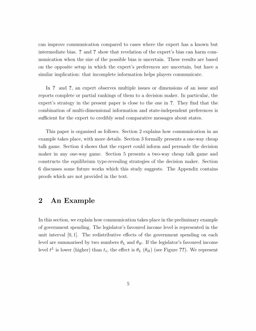
In this section, we explain how communication takes place in the preliminary example

of government spending. The legislator’s favoured income level is represented in the

unit interval [0, 1]. The redistributive effects of the government spending on each

level are summarised by two numbers θL and θH . If the legislator’s favoured income

level tL is lower (higher) than t1, the effect is θL (θH) (see Figure ??). We represent

5

t10

t1 tL

θ

θ∗H.4

θ∗L.2

(a) Realised State (θ∗L, θ∗H , t1) and Type tL

1

01θL

θH

“θL ≥ θH”

“θH > θL”

(θ∗L, θ∗H)

(b) Two Messages in State Space

Figure 1: Representation of State and Message

the effects by a step function

θ(tL) =

{θH if tL ≥ t1

θL if tL < t1.

After tL, t1, θL and θH are independently drawn from the common uniform distri-

bution on [0, 1], the legislator and the official privately observe tL and (θL, θH , t1),

respectively.

The legislator’s role is to choose the size of the government spending. The op-

timal size for the legislator is increasing linear in the effect of the spending on her

favoured income level. Thus, the legislator calculates the unbiased mean of the effect

based on her prior belief and messages from the official. In contrast, the official’s

payoff increases convexly (or concavely) in the size of the spending, regardless of the

redistributive effects. For simplicity, we assume that the optimal size is equal to the

effect and the official’s payoff is the square of it.

6

Consider what messages the official could send. First, if the official sends mean-

ingless messages to the legislator, his expected payoff is 1/4 because the unconditional

expected effects to any income level are the same as 1/2. Second, if the official sends

a message that maps each income level to an effect such as “the effects are θH for the

higher half of income levels and θL for the lower half.” This sort of message cannot

be credible because, if it is, the message has to be “the effect from the spending is 1

regardless of income levels” for any realised redistributive effects, and this incentive

to exaggerate the effects, in turn, makes the legislator doubt the official.

Now, consider comparative messages: “the effect to the high income class is

greater than to the low income class” and “the effect to the low income class is greater

than to the high income class” without specifying how income levels are divided into

high and low classes. These messages are depicted as the upper and lower triangles

in the state space in Figure ??. Then, given E[(θL, θH)|θL ≥ θH ] = (2/3, 1/3) and t1

is drawn from U [0, 1], the legislator’s estimate of the effect given the first message is

a function of her type

E[θ(tL)|θL ≥ θH ] =2

3(1− tL) +

1

3tL,

and the official’s expected payoff is

E[E[θ(tL)|θL ≥ θH ]2] =

∫ 1

0

(2

3(1− t) +

1

3t

)2

dt,

where the outer expectation on the left hand side is taken over the uniform distribu-

tion of the legislator’s type tL on [0, 1] and the value of the integral is 7/27. Similarly,

when the second message is sent, the estimate is 13(1 − tL) + 2

3tL and the official’s

payoff is the same as with the first message.

The official is indifferent between these two messages as long as the legislator

believes both to be true. Thus, it is incentive-compatible for the official to send

7

a true6 message between the two messages “θL ≥ θH” and “θH > θL,” and the

legislator would believe any message sent by the truthful strategy. Furthermore,

with this communication, the official’s expected payoff strictly increases. And, if

the policy maker’s type is not 1/2, her estimate is different from the unconditional

estimate or she is “informed” by the official’s message. This result is formulated in

Sections 3 and 4.

The other question that we address in this paper is whether the legislator may

reveal her favoured income level or class to the official or the public. She may want

to form a political party which represents her interests or get more support from the

income class. As we noted in the Introduction, we need to consider no case in which

the legislator fully reveals her preferences, because this makes it impossible for her

to obtain any information about the spending.

Suppose that the legislator reveals her favoured income level in a partial way,

such as “I work for households whose income levels are between the 25th and 75th

percentiles” or “below the 25th percentile or above the 75th percentile.” If these

statements are believed to be true by the official, the first statement updates the

official’s prior belief on types from U [0, 1] to U [.25, .75] and the second updates to

U([0, .25] ∪ [.75, 1]). Then, both statements preserve the indifference of the official

between the two comparative messages “θL ≥ θH” and “θH > θL” because the

legislator’s estimate and the updated probability distribution function of types are

symmetric about the median income level 1/2 for each statement. Thus, the legislator

is indifferent between partially revealing her preferences and keeping them private

because she can receive the same messages from the official. This result is formulated

in Section 5.

6“true” refers to the fact that the sent message is consistent with the realised state, not that themessage is equivalent to the state. In Figure ??, since the realised state (θ∗L, θ

∗H) is in the upper

triangle in the state space, the true message is “θL < θH .”

8

3 Model

In this section, we generalise the environment of the preliminary example. In ad-

dition, we formally describe the sources of uncertainty, how the expert talks to the

decision maker and how the decision maker responds to this.

We have two players, an expert and a decision maker, and two sources of uncer-

tainty, the decision maker’s type and the state of an issue.7 The decision maker’s

type is represented as t ∈ T = [t0, tN ] and the state is represented as a step function

θ(t) =∑N

i=1 θi1Ti(t) with N ≥ 2, where T1 = [t0, t1), T2 = [t1, t2), . . . , TN = [tN−1, tN ]

and 1Ti(t) is the indicator function defined on Ti for i = 1, . . . , N .8 Nature chooses

t, θ = {θ1, . . . , θN} and t = {t1, . . . , tN−1} according to differentiable distributions

G, F and H, respectively. F has full support on Θ = [θ, θ]N . t ∈ T ⊂ [t0, tN ]N−1

is an (N − 1)-tuple of ordered statistics obtained from a common uni-variable dis-

tribution H which has full support on T and ti is the ith largest of N − 1 random

variables that are identically and independently drawn from H. Let Hi denote the

distribution function of ti. The decision maker privately observes t while the expert

privately observes θ and t. Both players’ common prior belief is summarised by G,

F and H.

After the observation, the expert informs the decision maker about the realised

state (θ, t) via a costless, non-verifiable message. We assume that the expert sends

a noisy message by partitioning Θ into {Θ1, . . . ,ΘJ} for some J ≥ 2 instead of the

whole state space Θ×T .9 If the expert observes θ ∈ Θj for some j ∈ {1, . . . , J}, he

7As we noted in the Introduction, the state of an issue is not related with the decision maker’stype. The state itself does not completely resolve uncertainty in the current game, but the stateand the decision maker’s type together do.

8Many decisions made by economic agents such as firms and governments usually result indiscrete effects across individuals’ types. Some examples are second-degree price discrimination,tier rankings by credit rating agencies and discriminatory subsidies based on firm size or householdincome. However, even when the effects are inherently continuous, they could be well approximatedby a step function.

9Recall that the messages in the preliminary example were also generated by partitioning Θ.

9

randomly draws a state θ′ from Θj and sends it to the decision maker. This strategy

is equivalent to an abstract strategy in which, if a realised state is in Θj, the expert

sends a message mj from a message set M = {m1, . . . ,mJ} as long as mj is well

understood to imply that a realised state belongs to Θj ⊂ Θ.10 Then, a function

m : Θ→M such that m−1(mj) = Θj for any j fully describes the strategy generated

by {Θj}Jj=1. For simplicity, we assume that the expert sends messages in an abstract

way and, with a little abuse of notation, denote the strategy and a sent message by

M and mj (or m), respectively.

The expert has direct preferences over the decision maker’s estimate of the state.11

Let U be a convex (or concave) and monotone function that represents the expert’s

ex post payoff from the decision maker’s estimate. Then, since the expert does not

know the decision maker’s type, he chooses m from M to maximise his expected

payoff,

E[U(E[θ(t)|m])] =

∫T

U(E[θ(t)|m]) dG(t).

We can interpret U as a composite function U(e(t)) = A ◦ B(e(t)), where A is a

utility function that maps from the decision maker’s action to the expert’s utility

and B is a behaviour function that maps from the decision maker’s estimate to

behaviour. Thus, the expert has preferences over the decision maker’s action. This

payoff function is common knowledge.

This restriction can be justified by the observation that a message in the form of subsets of Θcould contain rich information about relations among θ1, . . . , θN while a similar message about tcould play a limited role because the relative sizes of t1, . . . , tN−1 are given as fixed. An alternativeapproach to support this restriction is that the expert can observe only θ.

10An expert in ? uses a mixed strategy described here. If a realised state belongs to an elementof an equilibrium partition of state space, the expert draws and sends an arbitrary state from theelement according to a predetermined probability distribution. In perfect Bayesian equilibrium,since the decision maker understands the expert’s whole strategy except for the realised state, thesent message or state implies that a realised state belongs to the same element of the equilibriumpartition as the sent state. Thus, the equilibrium partition fully describes the equilibrium strategy.

11In cheap talk literature, decision makers are assumed to take estimates of the true states asoptimal actions. Thus, it is usual that experts have direct preferences over estimates. For discussionof cases where decision makers’ estimates and actions are different, see ?.

10

Receiving a message from the expert, the decision maker estimates θ(t) based on

her priors F and H, the expert’s strategy M , and the sent message mj according to

Bayes’ rule. Let ej(t) = E[θ(t)|mj], e(t) = E[θ(t)|m], θj = E[θ|mj], θji = E[θi|mj],

and H0(t) = 1 and HN(t) = 0 for all t ∈ T . Then, the decision maker’s estimate

given mj can be represented in a sum of distribution functions of order statistics.

Lemma 1. ej(t) =∑N

i=1 θji (Hi−1(t)−Hi(t)).

Proof. By the law of iterated expectation, we have

ej(t) = E[θ(t)|mj] = E[E[θ(t)|θ]|mj]

= E[∑N

i=1 θi(Hi−1(t)−Hi(t))|mj]

=∑N

i=1 E[θi|mj](Hi−1(t)−Hi(t))

=∑N

i=1 θji (Hi−1(t)−Hi(t)),

where we want to show that the second equality holds. Since a realised event is either

t < ti−1, ti−1 ≤ t < ti, or ti ≤ t, it holds that Pr(ti−1 ≤ t and t < ti) = 1−Pr(ti−1 >

t) − Pr(ti ≤ t) = Hi−1(t) − Hi(t). And, by definition, Pr(t < t1) = 1 − H1(t) =

H0(t) − H1(t) and Pr(t ≥ tN−1) = HN−1(t) = HN−1(t) − HN(t). Thus, θ(t) equals

to θji with probability Hi−1(t) − Hi(t) for all i = 1, . . . , N and the second equality

follows.

Lemma ?? describes how the decision maker estimates the state when she believes

what a message m implies. Thus, when the an equilibrium consists of a truth-telling

strategy of the expert, the estimate function e(t) summarises the decision maker’s

behaviour in the game and determines the expert’s expected payoff in the equilibrium.

This leads us to focus on searching for equilibrium messages to construct equilibrium

strategies.

Example 1. Figure ?? depicts some exemplary estimate functions of the decision

maker for different priors H when (θ1, θ2) is drawn from U [0, 1]2 and the expert uses

the strategy described in the preliminary example. Thus, (θ11, θ12) = (2/3, 1/3) and

11

t

θ

10

1/3

1/2

2/3

e1(t)

e2(t)

(a) Uniform Distribution

t

θ

10

1/3

1/2

2/3

e1(t)

e2(t)

(b) Beta Distribution (2,2)

Figure 2: Estimates for Different Priors H

(θ21, θ22) = (1/3, 2/3). When t1 is from U[0,1], the decision maker’s estimates for each

message are e1(t) = 23(1−H(t))+ 1

3H(t) = 2/3−x/3 and e2(t) = 1

3(1−H(t))+ 2

3H(t) =

1/3+x/3 in Figure ??. For t1 from a beta distribution, the estimates are in Figure ??.

Until we discuss two-way games in which the decision maker talks first, we post-

pone specifying the decision maker’s payoff because the expert is concerned only

about the decision maker’s estimate and it is the expert’s message that characterises

equilibrium outcomes in one-way games. Instead, we define what we mean by “infor-

mative.” Naturally, if a message m from the expert alters the decision maker’s prior

belief, the message can be said to be informative. Formally, we define as follows.

Definition 1. A decision maker with type t is said to be informed by a message m

if E[θ(t)] 6= E[θ(t)|m], and an equilibrium is informative if E[θ(t)] 6= E[θ(t)|m] for a

non-negligible set of types with respect to G.

12

4 Equilibrium

In this section, we construct and characterise players’ equilibrium strategies in one-

way cheap talk games. Then, we provide some equilibria in the preliminary example

under different priors.

Let SN−1 denote the boundary of the N -dimensional unit ball BN ⊂ RN . Then

a hyperplane h(s, c) of orientation s ∈ SN−1 passing through an interior point c ∈ Θ

partitions Θ into two nonempty sets Θ+(s, c) and its complement Θ−(s, c),12 with

corresponding estimates θi(s, c) = E[θ|θ ∈ Θi(s, c)] for i = +,−. Hereafter, we omit

c for notational simplicity. Let Θ+ be in the half-space that contains the point s+ c.

As discussed above, a message set induced by a partition of the state space could

function as a strategy and each element of the partition is interpreted as a message.

Let πi be the coordinate map from Θ to Θi defined as πi(θ) = θi for all i =

1, . . . , N , and Π(N) be the set of all permutation functions defined on {1, . . . , N}.The following lemma shows that there exists a hyperplane such that two correspond-

ing estimates of θ are identical except for one coordinate.

Lemma 2. There exists s ∈ SN−1 such that for any p ∈ Π(N), πp(i)(θ+(s)) =

πp(i)(θ−(s)) for i = 1, . . . , N − 1.

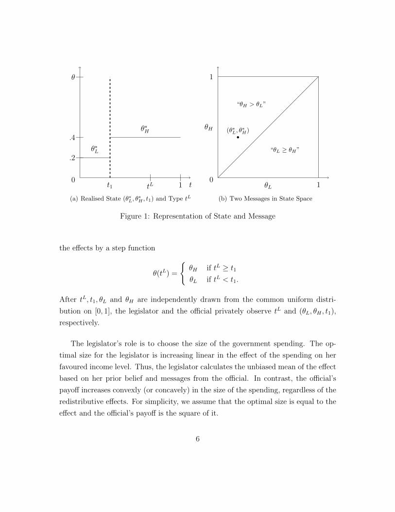
Suppose that a hyperplane passing through an interior point divides a two-

dimensional state space into two exclusive and exhaustive subsets. If we calculate

the expectations of θ within each subset and rotate the hyperplane around the inte-

rior point from 0 degrees to 360 degrees, the locus of the values draws an ellipse. In

Figure ??, h(s2, c) divides a two-dimensional space into Θ+(s2) and Θ−(s2) and the

corresponding estimates θ+(s2) and θ−(s2) coincide on the horizontal axis but not

on the vertical one.

12This construction of a partition of the state space was originally used in ?.

13

θ1

θ2

s2

“θ ∈ Θ+(s2)”

“θ ∈ Θ−(s2)”

h(s2, c)c

θ+(s2)

θ−(s2)

Figure 3: θ+1 (s2) = θ−1 (s2) at s2 ∈ SN−1

From Lemma ??, we can find a hyperplane such that the expert is indifferent

between two messages induced by the hyperplane. Let e+(t; s) and e−(t; s) denote

the estimate of θ(t) when the messages are Θ+(s) and Θ−(s), respectively.

Lemma 3. There exists s ∈ SN−1 such that E[U(e+(t; s))] = E[U(e−(t; s))].13

Last, we can easily check that E[θ(t)] is a convex combination of e+(t; s) and

e−(t; s) with weights P+(s) and P−(s) for any t, where Pi(s) ≡ Pr(θ ∈ Θi(s)) for

i = +,−.14 We have the first result.

Theorem 1. An informative cheap talk equilibrium always exists. In any informative

equilibrium, (1) if the expert’s preferences are convex (concave), he is ex ante better

(worse) off, and (2) the decision maker almost surely makes an informed decision.

13Since E[U(e+(t; s))] = E[U(e−(t; s))] is a continuous odd function of s, this lemma can beproved without Lemma ?? as in the proof of Theorem 1 of ?. However, the current approach betterillustrates the expert’s strategies and the proof of Proposition ??.

14For any t ∈ T , P+(s)e+(t; s) + P−(s)e−(t; s) =∑N

i=1(P+(s)θ+i (s) + P−(s)θ−i (s))(Hi−1(t) −Hi(t)) =

∑Ni=1 E[θi](Hi−1(t)−Hi(t)) = E[θ(t)].

14

Proof. Choose any c ∈ intΘ. Then, by Lemma ??, we can find s∗ ∈ SN−1 such

that E[U(e+(t; s∗))] = E[U(e−(t; s∗))]. Consider a simple strategy as follows. If the

expert observes θ ∈ Θ+(s∗) (Θ−(s∗)), the expert draws a state from Θ+(s∗) (Θ−(s∗))

according to a probability distribution on the subset and sends the decision maker the

drawn state. This fully specifies the expert’s strategy because Θ+(s∗)∪Θ−(s∗) = Θ.

Given this strategy, the decision maker estimates the expected θ(t) based on the

sent message. The estimate is e+(t; s∗) (e−(t; s∗)) if the alleged state is in Θ+(s∗)

(Θ−(s∗)). Since E[U(e+(t; s∗))] = E[U(e−(t; s∗))], the expert’s strategy maximises

his ex ante payoff.

Upon the strategy, the expert’s expected payoff is

E[U(e+(t; s∗))] = (P+(s∗) + P−(s∗))∫TU(e+(t; s∗)) dG(t)

=∫T

[P+(s∗)U(e+(t; s∗)) + P−(s∗)U(e−(t; s∗))] dG(t)

≥∫TU(P+(s∗)e+(t; s∗) + P−(s∗)e−(t; s∗)) dG(t)

= E[U(E[θ(t)])],

where the inequality holds if U is convex, and the last term is the expert’s expected

payoff without communication. Thus, the expert is not worse off with the commu-

nication for any realised state so long as U is convex. If U is strictly convex, the

expert is strictly better off with the equilibrium communication. The opposite holds

if U is (strictly) concave.

Now, consider a simultaneous equation system e+(t) = E[θ(t)] or∑N

i=1(θ+i −

µi)(Hi−1(t)−Hi(t)) = 0 for t ∈ T0 ⊂ T . Since H has full support on T , the problem

consists of |T0| equations. Thus, only when |T0| ≤ N does there exist a solution

{θi}Ni=1 such that∑N

i=1(θi − µi)(Hi−1(t) − Hi(t)) = 0 for t ∈ T0. Thus, we have

Pr[t ∈ T0] = 0. Since e+(t) 6= E[θ(t)] whenever t /∈ T0, the decision maker can make

an informed decision with probability 1. This completes the proof.

Given an equilibrium message, the decision maker makes an informed estimate for

almost every type. However, informed estimates are not always more favourable to

15

the expert than uninformed. Since the messages are describing how the state varies

across types, informed estimates by some types are higher than the uninformed and

others are lower than the uninformed. Thus, the expert’s ex post payoff increases

or decreases with the message, depending on the decision maker’s realised type.

For example, when U is increasing and convex, if an informed estimate is greater

(lower), the expert is ex post better (worse) off even though he is ex ante better off

with communication.

In fact, this heterogeneity of the decision maker’s response to a comparative

message makes it possible for the expert to construct two messages which reward

him equally. Since the expert does not know the decision maker’s type, the expert

can divide the decision maker’s types into two groups so that decision makers in

different groups respond to messages in opposite directions and the expert receives

the same expected payoff from two different messages. Thus, the expert can maximise

his payoff by sending any message that is consistent with the realised state and the

decision maker understands that the expert is inherently not biased to either message

and that the expert will send a true message.

At the same time, how the expert’s strategy divides the decision maker’s types

into subgroups affects not only the decision maker’s ex ante but also her ex post

behaviour. In a two-way game that we examine in the next section, since both

players’ strategies should be consistent with each other in equilibrium, the expert’s

equilibrium strategy restricts the way in which the decision maker reveals her type.

This strategic interdependence between players makes it necessary to further examine

the expert’s strategy. We define two strategies by the way in which each divides the

decision maker’s type into subgroups and show that the expert could use either of

the two strategies for any priors with N ≥ 3.

In the proof of Theorem ??, we have shown that there is only a finite number of

types for which the decision maker is not informed by the expert’s message. Actually,

there should exist at least one type for which the estimate function e(t) crosses over

16

the uninformed estimate function E[θ(t)]. Formally, we define a set of all those

types given M as T 0M ≡ {t ∈ T |ej(t) − E[θ(t)] = 0 and

d(ej(t)−E[θ(t)])dt

6= 0 for mj ∈M} ∩ intT . We characterise the expert’s strategy using this set, in particular when

the set has only one or two elements.

Definition 2. A strategy M is said to divide types into left and right if |T 0M | = 1,

and divide types into centre and periphery if |T 0M | = 2.

Since the decision maker’s estimate e(t) is a continuous function of t, the first

strategy divides the decision maker’s types into two halves, say, left and right. Given

a message from this strategy, the direction to which the decision maker’s estimate

is updated differs according to whether her type is close to the left end of the type

space or to the right end. And, if a message is sent from the second strategy, how

the decision maker’s estimate is updated depends upon whether her type is in the

centre of the type space or not.

Proposition 1. If F is invariant under any permutation of θ1, . . . , θN and N ≥ 3,

the expert’s equilibrium strategy can divide types either into left and right or into

centre and periphery.

In the preliminary example, this result implies that, no matter how complicated

are the redistributed effects of the government spending on each income class, the

official might try to persuade the legislator by truthfully stating either that “the

government spending will benefit the high income class rather than the low income

class” or that “it will benefit the middle income class more than others.” Given either

of these two statements, the official can expect bigger spending to be approved and

the legislator can make a more informed decision than before.

It is also noteworthy that the equilibrium strategies developed in Theorem ??

convey very coarse information about the state: the actual role of a sent message is

merely to tell which element of two subsets in a partition contains a realised state.

This observation raises the question whether we can find a finer partition of the state

17

space so that the expert is indifferent to all the messages generated by the partition.

If possible, the partition could constitute an equilibrium strategy. The following

result shows that this is the case.

Proposition 2. If A 2k-message informative cheap talk equilibrium always exists

for every k ≥ 1. If the expert’s preferences are convex (concave), his ex ante payoff

increases (decreases) with k.

This result is comparable to Theorem 4 in ?. We can construct a 22-message equi-

librium strategy from a 2-message strategy as follows. Given a 2-message strategy

that is induced by a 2-element partition {Θ1,Θ2}, we can get four estimates, e1+(t)

and e1−(t) from Θ1 and e2+(t) and e2−(t) from Θ2 such that E[U(e1+)] = E[U(e1−)]

and E[U(e2+)] = E[U(e2−)]. If the expert is indifferent to all four estimates, we have

found a 22-message equilibrium strategy. If not, we can make the messages that are

more favourable to the expert a bit noisier so that the resulting estimates become

less favourable and the expert becomes indifferent to all four estimates. Repeating

this, we can construct an equilibrium strategy with an arbitrary number of messages.

Theorem ?? implies there are infinitely many 2-message equilibrium strategies,

and Proposition ?? implies that, from any 2-message equilibrium strategy, we can

find an infinite sequence of equilibrium strategies with increasing number of messages,

and the expert’s expected payoff increases (decreases) with the number of messages

if U is convex (concave). This finding suggests it would be difficult to predict which

equilibrium strategy will be played in the real world, in particular if the expert’s

preferences are convex. We discuss this further in the Discussion section.

Example 2. We construct equilibrium strategies under different environments to

see the relation between the equilibrium strategy and the distribution of the decision

maker’s type. The equilibrium strategies for different distributions of income level

are depicted in Figure ??. The distribution functions are Beta(α, β) with different

sets of parameters, such as (1, 3), (2, 3) and (2, 2).15 In Beta(1,3), the population is

15The beta distribution is flexible in representing various distributions on the unit interval such

18

concentrated on low income levels or the distribution is skewed to the highest income

levels. In Beta(2,2), the population is symmetrically distributed and concentrated

on the middle class. All distributions are uni-modal.16 The other priors F and H

are fixed as U[0, 1]2 and Beta(2,2), respectively.

Each equilibrium has been solved numerically by searching for a slope ∆ ∈ [0, 2π]

such that the economist is indifferent between two messages generated by the hy-

perplane with the slope when the interior point c is fixed at (1/2, 1/2). Thus, given

an equilibrium slope ∆∗, two messages m+,m− are “θL − 12≤ tan ∆∗(θH − 1

2)” and

“θL − 12> tan ∆∗(θH − 1

2),” respectively. The solutions are as follows. First, when

α = 1 and β = 3, ∆ ≈ 110π, E[(θL, θH)|m+] = (0.4402, 0.7393) and E[(θL, θH)|m−] =

(0.5598, 0.2607). Second, when α = 2 and β = 3, ∆ ≈ 15π, E[(θL, θH)|m+] =

(0.3785, 0.7057) and E[(θL, θH)|m−] = (0.6215, 0.2943). Last, when α = 2 and β = 2,

∆ = 14π, E[(θL, θH)|m+] = (0.3333, 0.6667) and E[(θL, θH)|m−] = (0.6667, 0.3333).

The estimates derived from these are shown in the right-hand column of Figure ??.

Comparing the figures, a relation between the distribution of income levels and

the legislator’s estimate induced by the equilibrium messages is noticeable. As the

population is more concentrated on low income levels, the estimates e+(t) and e−(t)

by the legislator who favours the low income class move closer to the uninformed. For

a message m, we can interpret the difference between estimates with and without the

message |E[θ(t)|m)]−E[θ(t)]| as the amount of information contained in the message,

which is examined further in the next section. This suggests that a message from

the official is more valuable to the legislator who favours the high income class than

the low income class if the population is skewed to high income. The opposite also

holds true when the population is skewed to low income.

as uni-/bi-modal, skewed to the left/right and symmetric distributions.16See the graphs on the left in Figure ??.

19

t0 1 t0 1

θ

e+(t)

e−(t)

(a) α = 1, β = 3

t0 1 t0 1

θ

e+(t)

e−(t)

(b) α = 2, β = 3

t0 1 t0 1

θ

e+(t)

e−(t)

(c) α = 2, β = 2

Figure 4: Distributions of Types: Beta(α, β) and Equilibrium Outcomes

20

5 Revelation of the Decision Maker’s Type

In this section, we examine whether the decision maker might reveal her type in

two-way games. For this purpose, we specify the decision maker’s payoff when the

expert’s strategy is given. Then we analyse how the decision maker reveals her type

to the expert or the public.

We assume that the decision maker is rewarded according to the accuracy of her

estimate. We define the decision maker’s ex post payoff by−(θ(t)−e(t))2. The farther

a realised state is from her estimate, the lower her payoff is. The payoff depends only

upon the expert’s strategy because she mechanically updates her belief by Bayes’

Rule. Since a revelation of private information could change the expert’s strategy,

we need to define the decision maker’s payoff as a function of the expert’s strategy.

We assume that the decision maker is maximising her expected payoff. Given a

message m, the decision maker’s interim expected payoff is E[−(θ(t) − e(t))2|m] =

E[−(θ(t)− E[θ(t)|m])2|m] = −Var[θ(t)|m]. And, given the expert’s strategy M , the

decision maker’s expected payoff is E[−Var[θ(t)|m]].

We assume that the expert uses the 2-message strategies developed in Theo-

rem ??.17 Let M = {m+,m−} be an equilibrium strategy in a one-way game and

let σ2(t) denote the unconditional variance of θ(t) and Pi ≡ Pr(θ ∈ Θi) given M for

i = +,−. Without loss of generality, let E[θi] = 0 for all i = 1, . . . , N . Then, the

decision maker’s expected payoff from the expert’s strategy M is represented by a

function of her estimate e(t).

Lemma 4. E[−Var[θ(t)|m]] = Pi

Pjei(t)2 − σ2(t) for i 6= j.

Proof. By the law of total variance, the unconditional variance of the state for type

t is divided into two components as σ2(t) = E[Var[θ(t)|m]] + Var[E[θ(t)|m]]. The

17At the end of this section, we briefly examine the case where more than two messages areinvolved.

21

second term on the right hand side can be represented as follows.

Var[E[θ(t)|m]] = P+(e+(t)− E[θ(t)])2 + P−(e−(t)− E[θ(t)])2

= P+(∑N

i=1 θ+i (Hi−1(t)−Hi(t)))

2

+P−(∑N

i=1 θ−i (Hi−1(t)−Hi(t)))

2

= P+(∑N

i=1 θ+i (Hi−1(t)−Hi(t)))

2

+P−(−P+

P−

)2(∑N

i=1 θ+i (Hi−1(t)−Hi(t)))

2

= P+

P−

(∑Ni=1 θ

+i (Hi−1(t)−Hi(t))

)2where the third equality holds because P+θ+i + P−θ−i = 0 = µi for all i = 1, . . . , N

and the last equality holds because P+ + P− = 1. Therefore, we have the result.

Suppose that the decision maker can reveal her type in a particular way or keep it

private. Since the revelation of type could change the expert’s prior belief about the

distribution of types G, the expert’s equilibrium strategy also could change according

to his modified belief and send different messages. If the revelation changes the

expert’s equilibrium strategy such that the decision maker’s estimate moves closer

to the uninformed for some type, the decision maker of this type will choose not to

reveal it, because the revelation lowers her payoff. However, as long as her estimate

remains constant for all types, she may feel free to reveal her type.

Now, we describe a type-revealing strategy on the part of the decision maker.

The decision maker reveals her type through a partition of the type space T , say,

{T 1, . . . , TK} for some finite K ≥ 2. If the decision maker’s realised type t is in T k,

she sends a message nk from a message set N = {n1, . . . , nK}, where nk is understood

to imply that a realised type belongs to T k. Then, a function n : T → N such that

n−1(nk) = T k for any k fully describes the type-revealing strategy. For simplicity,

we denote the strategy and a message by N and nk (or n), respectively.

We characterise the decision maker’s type-revealing strategy in a similar way to

the expert’s strategy. Suppose that the decision maker reveals her type through a

22

partition N = {T 1, T 2}.

Definition 3. A type-revealing strategy of the decision maker is said to divide types

into left and right if T 1 and T 2 are intervals, and divide types into centre and pe-

riphery if T 1 is an interval contained in the interior set of T .

Given the decision maker’s strategy, a two-way game proceeds as follows. First,

the decision maker and the expert privately observe her type and the state of the

issue, respectively. Second, the decision maker sends a message about her type

according to a type-revealing strategy N . Third, after the revelation, a one-way

game follows: the expert informs the decision maker according to a strategy M , the

decision maker estimates the state and the estimate finalises both player’s payoffs.

In a two-way game, if a decision maker completely reveals her type, no commu-

nication can take place in a subsequent one-way game because the expert cannot

exploit the possibility of treating decision maker’s types differently, as explained in

the previous section. However, if only partial information is revealed so that the

decision maker’s type is still uncertain, there exists room for the expert to give type-

dependent information to the decision maker. Thus, the decision maker can partially

reveal her type at best. We define a type-revealing equilibrium and show that a

type-revealing equilibrium always exists.

Definition 4. An equilibrium in a two-way cheap game is type-revealing if N con-

tains a non-trivial, proper subset of T .

Theorem 2. For any informative cheap talk equilibrium in a one-way game, there

exists a type-revealing equilibrium in the two-way game in which the decision maker

partially reveals her type.

Proof. Let M be an 2-message informative equilibrium strategy in a one-way cheap

talk game, and messages in M lead to decision maker’s estimates e+(t) and e−(t).

Then, T 0M ∩ intT 6= ∅. Otherwise, it holds that e+(t) > E[θ(t)] > e−(t) or e−(t) >

23

t

θ

t0 = p t01 = q t02 = r

e+(t)

e−(t)

t∗1 t∗2

Figure 5: Construction of Revelation Strategy

E[θ(t)] > e+(t) for any t ∈ intT so that E[U(e+(t))] 6= E[U(e−(t))], which contradicts

that M constitutes an equilibrium.

Choose consecutive types p, q, r ∈ T 0M ∪ {t0, tN} such that q ∈ T 0

M \ {t0, tN} and

p < q < r, where t0 and tN are the end points of T (Figure ??). Then, the relative

sizes of e+(t) and e−(t) reverse only at q in (p, r). Suppose that e+(t) > e−(t) for

t ∈ (p, q) and e+(t) < e−(t) for t ∈ (q, r) and∫(p,r)

g(t)U(e+(t)) dt ≤∫(p,r)

g(t)U(e−(t)) dt.

Then, for any t∗1 ∈ (p, q), there exists t∗2 ∈ (q, r) such that∫(t∗1,t

∗2)

g(t)U(e+(t)) dt =

∫(t∗1,t

∗2)

g(t)U(e−(t)) dt

because e+ and e− are continuous functions.

Repeating this procedure, we can find a finite set of exclusive intervals {T1, . . . , Tp}such that

∫Tig(t)U(e+(t)) dt =

∫Tig(t)U(e−(t)) dt for i = 1, . . . , p, where 1 ≤ p ≤

24

|T 0M |. Consider a type-revealing strategyN which consists of a partition {T1, . . . , Tp, T\∪pi=1Ti} in which a decision maker, whose type belongs to one element of the parti-

tion, draws an arbitrary type from the subset according to a probability distribution

and sends it to the expert. Then, the expert is still indifferent between two mes-

sages in the original strategy M . Therefore, two strategies N and M constitute an

equilibrium in the two-way game.

Since there always exists an informative cheap talk equilibrium by Theorem ??,

a type-revealing equilibrium also always exists for any priors.

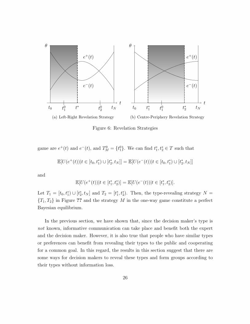
Figure ?? shows an equilibrium strategy in a two-way cheap talk game. The

decision maker’s estimates e+(t) and e−(t) are derived by an equilibrium strategy

M in a one-way game. Given the strategy M , we can find t∗ ∈ T such that

E[U(e+(t))|t ∈ [t0, t∗)] = E[U(e−(t))|t ∈ [t0, t

∗)] and E[U(e+(t))|t ∈ [t∗, tN ]] =

E[U(e−(t))|t ∈ [t∗, tN ]]. Let T 1 = [t0, t∗), T 2 = [t∗, tN ] and N = {n1, n2} be a

corresponding message set. If the decision maker’s type is in T 1 (T 2), she sends

n1 (n2), respectively. Then, message sets N and M constitute a perfect Bayesian

equilibrium and the decision maker’s ex ante payoff is the same as in the one-way

game.

In the proof of Theorem ??, we find that the size of T 0M plays a critical role

in forming a type-revealing strategy. The following result is immediate from the

observation.

Proposition 3. If the expert’s strategy divides types into left and right, the decision

maker’s type-revealing strategy cannot divide types into left and right but into centre

and periphery. And, if the expert’s strategy divides types into centre and periphery,

the decision maker’s strategy can divide types into left and right.

Figure ?? shows a type-revealing equilibrium strategy which divides types into

centre and periphery. As in Figure ??, the decision maker’s estimates in the one-way

25

t

θ

tNt0 t01 t02t∗

e+(t)

e−(t)

(a) Left-Right Revelation Strategy

t

θ

tNt0 t∗1 t∗2t01

e+(t)

e−(t)

(b) Centre-Periphery Revelation Strategy

Figure 6: Revelation Strategies

game are e+(t) and e−(t), and T 0M = {t01}. We can find t∗1, t

∗2 ∈ T such that

E[U(e+(t))|t ∈ [t0, t∗1) ∪ [t∗2, tN ]] = E[U(e−(t))|t ∈ [t0, t

∗1) ∪ [t∗2, tN ]]

and

E[U(e+(t))|t ∈ [t∗1, t∗2)] = E[U(e−(t))|t ∈ [t∗1, t

∗2)].

Let T1 = [t0, t∗1) ∪ [t∗2, tN ] and T2 = [t∗1, t

∗2). Then, the type-revealing strategy N =

{T1, T2} in Figure ?? and the strategy M in the one-way game constitute a perfect

Bayesian equilibrium.

In the previous section, we have shown that, since the decision maker’s type is

not known, informative communication can take place and benefit both the expert

and the decision maker. However, it is also true that people who have similar types

or preferences can benefit from revealing their types to the public and cooperating

for a common goal. In this regard, the results in this section suggest that there are

some ways for decision makers to reveal these types and form groups according to

their types without information loss.

26

Suppose that the redistributive effects in the preliminary example differ between

two income classes only. Then the official’s strategy is restricted to dividing types

into left and right, so that his message divides income levels into high and low income

classes.18 Given this, if the legislator wants to reveal her type for some reason, it is

best to say either “I represent the middle-income” or “I represent the high or the

low income class” to remain informed as before. Interestingly, in the latter case, the

legislators who represent high or low income classes cannot be distinguished by their

preferences. But suppose that the effects differ between more than three groups and

the economist’s message divides income levels into a middle-income class and the

rest. In this case, the legislator can say either “I represent the low income class” or

“I represent the high income class” and get informed as before.

We close this section with an example in which the decision maker could reveal

her type without information loss when the expert’s strategy consists of 2k messages

with k > 1. Generally, type-revealing strategies are hardly ever feasible if many

messages are involved in communication because a system of equations has to be

solved which has more constraints than variables; we need to find t∗1, . . . , t∗2I for some

I ∈ N such that E[U(e1(t))] = · · · = E[U(e2k(t))], where the expectations are taken

over ∪Ii=1[t2i−1, t2i). However, certain conditions, such as the uniform distribution of

priors and affine payoff functions, relax these constraints so that the decision maker

may reveal her type.

Example 3. Suppose that all priors F , H and G are uniform distributions on [0, 1]2,

[0, 1] and [0, 1], respectively; and that U is a linear function of e(t), say U(e(t)) =

ae(t) + b with a, b > 0.

For k=1, the hyperplane h(s∗, c) with s∗ = ( 1√(2),− 1√

(2)) and c = (1/2, 1/2)

induces two messages “θ ∈ Θ1” with θ1 = (2/3, 1/3) and “θ ∈ Θ2” with θ2 =

(1/3, 2/3), the lower half of the whole state space and the upper half in Figure ??.

The resulting estimates are e1(t) = 23− 1

3t and e2(t) = 1

3+ 1

3t, and the expert is

18Of course, even when the effects vary among more than two income classes, the economist’smessage could divide income levels into the lower and the higher.

27

h(s∗ , c

)

h(s∗ ,θ

1 )

h(s∗ ,θ

2 )

θ1 1

1

0

θ2

s ∗

θ1

θ1+

θ1−

θ2

θ2+

θ2−

Θ1+Θ1−Θ1

Θ2+

Θ2−

Θ2 c

(a) Messages in State Space

79

2645

1945

29

θ

tN = 1t0 = 0 12− t∗ 1

2+ t∗1

2

e2+(t)

e2−(t)

e1+(t)

e1−(t)

(b) Estimates and Revelation of Type

Figure 7: Revelation of Type for 2k-Message Strategy

indifferent between these two estimates.

For k=2, following the procedure described in the proof of Proposition ??, from

the lower triangle Θ1, we can find that the expert is indifferent between two messages

“θ ∈ Θ1+” with θ1+ = (7/9, 2/9) and “θ ∈ Θ1−” with θ1− = (26/45, 19/45) by

h(s∗,θ1) (Figure ??). Likewise, from the upper triangle Θ2, we can find two messages

“θ ∈ Θ2+” with θ2+ = (19/45, 26/45) and “θ ∈ Θ2−” with θ2− = (2/9, 7/9) by

h(s∗,θ2).

Then, all expected values of θ given each message, θ1+,θ1−,θ2+, and θ2−, lie on

the common straight line, θ1 + θ2 = 1. Given e(t) = θ1 + (θ2 − θ1)t, the expert’s

expected payoff is∫ 1

0a+ b(θ1 + (θ2 − θ1)t) dt = a+ b(θ1 + θ2)/2. Thus, the expert’s

payoffs from all four messages are the same as a + b/2. Furthermore, the expert’s

expected payoffs from those messages conditional on an interval (1/2− t∗, 1/2 + t∗)

for any t∗ ∈ (0, 1/2) are also the same as a+ b/2. Thus, a message set N induced by

a partition {(1/2− t∗, 1/2+ t∗), [0, 1]\(1/2− t∗, 1/2+ t∗)} can work as an equilibrium

28

type-revelation strategy.

This procedure can be repeated up to arbitrary k ∈ N. Therefore, in this uniform

environment, the decision maker may divide her type into centre and periphery even

when the expert uses a 2k-message strategy for arbitrary k.19

6 Discussion

We have examined how the expert and the decision maker communicate with each

other when the decision maker’s type is uncertain and the expert’s payoff depends

only upon the decision maker’s action, regardless of the realised state and the decision

maker’s type. There are two main results: (1) the expert can always inform the

decision maker in the form of comparative statements; and (2) the decision maker

may reveal her private type without loss of informative communication. However, we

have not fully exploited the potential for communication in this setup. This study

could be further developed in two directions.

The first is for refining equilibria. Studies in cheap talk games have paid much

attention to identifying equilibria which are optimal to the expert or the decision

maker and to predicting a specific equilibrium in the real world among (infinitely)

many equilibria.20 This paper has focused mainly on whether and how an expert and

a decision maker could talk to each other, but not on what messages would be sent

in an equilibrium in a certain environment. That is, there is no answer as to which

equilibrium strategies are optimal to players and more likely to be played. Never-

theless, two results of this paper are worth noticing for the prediction of equilibrium

19Actually, we can construct an equilibrium strategy which consists of an arbitrary number ofmessages, because subsets generated by arbitrary 45◦ straight lines in the state space have theirexpectations on the line, θ1 + θ2 = 1.

20In an effort to refine cheap talk equilibria, ? identify a condition on equilibrium payoffs, calledNITS (no incentive to separate), which selects an equilibrium strategy induced by the biggestpartition among CS equilibria.

29

outcomes.

One is that there exist infinitely many equilibria. In particular, there are infinitely

many 2-message equilibria that can be constructed from an arbitrary interior point

in the state space and infinite sequences of equilibria starting from each 2-message

equilibrium. The latter infinity is more problematic than the former in predicting

an equilibrium outcome if the expert’s preferences are strictly convex. Among 2-

message equilibria, we can expect to find an equilibrium that is most favourable

to the expert under certain conditions, whereas the expert cannot find an optimal

equilibrium strategy from the sequences of equilibria because the expert’s ex ante

payoff strictly increases with the number of messages if the preferences are strictly

convex.

The other is that the expert’s payoff is state-independent. This allows him to

commit to an equilibrium strategy. Suppose that the expert can declare which strat-

egy he will choose among infinitely many equilibrium strategies before a one-way

cheap talk game starts. Then, if he finds an optimal strategy which maximises his ex

ante payoff, declaring that the optimal strategy will be used and sending a message

according to the strategy constitute an equilibrium. Thus, once the expert finds

his optimal strategy in a certain environment,21 we could predict that the chosen

strategy would be played in equilibrium.

The second direction requires examining the relation between priors and commu-

nication. This paper does not fully discover the relation between players’ prior beliefs

about their environment and equilibrium outcomes. As we have briefly shown in the

government spending example, the distribution function of the decision maker’s type

determines how well she is informed in equilibrium; if the population is concentrated

around her type, she is less informed than otherwise.

This implies that the decision maker has preferences over the distribution of types.

21For example, concave preferences, deliberation costs or conventional communication protocolscould restrict the number of messages available in communication

30

That is, the decision maker prefers any distribution where the population is more

concentrated on other types than hers to the actual distribution. For example, as

shown in Section 4, if the decision maker is located in the left of the type space, she

prefers a distribution that has population concentrated on the right. Thus, she has

an incentive to disguise not her type but the distribution of types.22

Appendix

Proof of Lemma ??. First, note that, since F has full support on Θ, θ+(s) ∈intΘ+(s) and θ−(s) ∈ intΘ−(s) so that θ+(s) 6= θ−(s). Note next that for any

two opposite orientations −s, s ∈ SN−1, Θ+(s) = Θ−(−s) and Θ−(s) = Θ+(−s). It

follows that θ+(s) = θ−(−s), implying that a map ρ : SN−1 → RN−1 which consists

of ρi(s) = πi(θ−(s)) − πi(θ

+(s)) for i ∈ {p(j)|j = 1, . . . , N − 1 and p ∈ Π(N)} is

a continuous23 odd function of s for any p ∈ Π(N). By the Borsuk-Ulam theorem,

there exists sp ∈ SN−1 such that ρ(sp) = 0.

Proof of Lemma ??. Consider a function ∆(s) ≡∫T

[U(e+(t; s))−U(e−(t; s))] dG(t).

We need to find s∗ ∈ SN−1 that satisfies ∆(s∗) = 0. By Lemma ??, there exist

sN , s1 ∈ SN−1 such that θ+i (sN) = θ−i (sN) for i ∈ {1, . . . , N −1} and θ+i (s1) = θ−i (s1)

for i ∈ {2, . . . , N}. Since θ+(s) 6= θ−(s) for any s ∈ SN−1, θ+N(sN) 6= θ−N(sN) and

θ+1 (s1) 6= θ−1 (s1). Suppose that θ+N(sN) > θ−N(sN).24 Then, since H has full sup-

port on the type space, e+(t; sN) > e−(t; sN) for all t ∈ intT and ∆(sN) > 0 as in

Figure ??. Similarly, suppose θ+1 (s1) < θ−1 (s1). Then e+(t; s1) < e−(t; s1) for all

22In this case, common knowledge among players should be with respect to the probabilitiesassigned to several distributions of types not to each type itself.

23It can be simply shown that θ+(s) and θ−(s) are continuous functions of s by the dominatedconvergence theorem.

24If the inequality does not hold for sN , then the desired inequality holds for −sN .

31

t

θ

µθ

e−(t; sN )

e+(t; sN )

(a) sN

t

θ

µθe+(t; s1)

e−(t; s1)

(b) s1

Figure 8: Estimates induced by sN and s1

t ∈ intT and ∆(s1) < 0 as in Figure ??. Consider a continuous map s : [0, 1]→ SN−1

such that s(0) = sN and s(1) = s1. Then ∆(s(x)) is a continuous function such

that ∆(s(0)) > 0 and ∆(s(1)) < 0. By continuity, there exists x∗ ∈ (0, 1) such that

∆(s(x∗)) = 0.

Proof of Proposition ??. An interior point c ∈ intΘ and an orientation s ∈ SN−1

are represented in coordinates by c = (c1, . . . , cN) and s = (a1, . . . , aN). Then, (c, s)

define two subsets of the state space, Θ+ = {θ ∈ Θ|∑N

i=1 ai(θi − ci) ≥ 0} and

Θ− = {θ ∈ Θ|∑N

i=1 ai(θi − ci) < 0} and corresponding estimates e+(t; c, s) and

e−(t; c, s). Choose a > 0. Let ai = a for i = 1, . . . , n for some 1 < n < N and

ai = −1 for i = n + 1, . . . , N and e+(t; a) and e−(t; a) denote the estimates. Since

F is invariant, we have θ+i = θ+a > E[θi] for i = 1, . . . , n and θ+i = θ+−1 < E[θi] for

i = n+ 1, . . . , N . Thus, we have e+(t; a) = θ+a + (θ+−1− θ+a )Hn(t), which is decreasing

in t with e+(t0; a) > 0 > e+(tN ; a). Similarly, e−(t; a) = θ−a + (θ−−1− θ−a )Hn(t), which

is increasing in t with e−(t0; a) < 0 < e−(tN ; a). Suppose E[e+(t; a)] ≥ E[e−(t; a)]. If

E[e+(t; a)] = E[e−(t; a)], we have found a strategy which divides into left and right. If

E[e+(t; a)] > E[e−(t; a)], we can find a′ ∈ (0, a) such that E[e+(t; a′)] = E[e−(t; a′)].

For a strategy which divides types into centre and periphery, let ai = a for i =

32

n, . . . , n+k for some k ∈ N∪{0} such that n+k < N and ai = −1 for i = 1, . . . , n−1, n + k + 1, . . . , N . Then, e+(t; a) = θ+−1 + (θ+a − θ+−1)(Hn−1(t) −Hn+k(t)) is a uni-

modal function for ddt

(Hn−1(t)−Hn+k(t)) = (n+k)H(t)n−2h(t)(n−1n+k−H(t)k+1), where

dHdt

= h. Thus, once we find a′ such that E[e+(t; a′)] = E[e−(t; a′)] in the previous

manner, the corresponding strategy divides types into centre and periphery.

Proof of Proposition ??. The proposition is directly derived by Theorem ?? and

the inductive argument used in the proof of Theorem 4 in ?. We follow the proof in

? as closely as possible for the purpose of reference.

We prove the result by induction on k ≥ 1. Suppose, as part of the inductive

hypothesis, that we have a 2k-message equilibrium associated with a 2k-element

partition of Θ created by 2k − 1 hyperplanes. Identify the jth partition element µj

(a compact convex subset of Θ with nonempty interior) by the message mj and the

corresponding induced estimate by θj.25 We suppose that message mj is sent by all

θ ∈ intµj with probability pj ∈ (0, 1] which does not depend on θ. Message mj may

also be sent by other types θ /∈ µj with positive probability. Let zjin = E[θ|mj,θ ∈ µj]and zjout = E[θ|mj,θ /∈ µj], whenever defined. By the law of iterated expectations

θj is a probability weighted average of zjin and zjout, so that the line joining the

latter two points must pass through θj. Let ej(t) be the corresponding estimate

of θ(t) based on θj. Since we have an equilibrium for the current 2k messages,

E[U(e1(t))] = · · · = E[U(e2k(t))]. We proceed by induction on k by first creating

a 2k+1-element partition of Θ from the given 2k-element partition. Next, we adjust

the induced actions via mixed strategies in order to obtain an equilibrium with 2k+1

messages.

For each mj, consider a hyperplane through zjin ∈ intµj of orientation s ∈ SN−1

which splits µj into two regions µj+(s) and µj−(s) and expected values zj+in (s) and

zj−in (s). Relative to the original 2k-element partition, we think of this new 2k+1-

25So far, we have not distinguished a subset of state space µj and the corresponding message mj

because mj was sent if and only if θ ∈ µj . From now on, that mj was sent does not imply θ ∈ µj .

33

element partition where each corresponding message mj is split into two messages

mj+ and mj− such that (i) each θ ∈ µj sends message mj+ (resp., mj−) with the

same probability pj > 0 as the original message mj if θ ∈ µj+ (resp., µj−) and does

not send the other message mj− (resp., mj+); and (ii) each θ /∈ µj who sent mj

with positive probability now splits this probability equally between the messages

mj+ and mj−. Accordingly, the corresponding estimates can be written as θj+(s) =

E[θ|mj+] = πj+(s)zj+in (s) + (1−πj+(s))zjout and θj−(s) = E[θ|mj−] = πj−(s)zj−in (s) +

(1− πj−(s))zjout where the conditional probabilities are

πj+(s) = Pr[θ ∈ µj+(s)|mj+] =pj Pr[θ ∈ µj+(s)]

pj Pr[θ ∈ µj+(s)] + 12

Pr[mj,θ /∈ µj]

πj−(s) = Pr[θ ∈ µj−(s)|mj−] =pj Pr[θ ∈ µj−(s)]

pj Pr[θ ∈ µj−(s)] + 12

Pr[mj,θ /∈ µj].

Since µj+(−s) = µj−(s) for all s, we have πj+(−s) = πj−(s). Since in addition

zj+in (−s) = zj−in (s), it follows that θj+(−s) = θj−(s) for all s, and symmetrically

θj−(−s) = θj+(s). But then πi(θj+(s))− πi(θj−(s)) is a continuous odd function of

s for all i = 1, . . . , N , so that by the Borsuk-Ulam theorem there exists sj ∈ SN−1

such that πp(i)(θj+(sj))−πp(i)(θj(sj)) = 0 for i = 1, . . . , N−1 and for any p ∈ Π(N),

for each j = 1, . . . , 2k. Then, by Lemma ??, there exists sj∗ ∈ SN−1 such that

E[U(ej+(t; sj∗))] = E[U(ej−(t; sj∗))] for each j = 1, . . . , 2k. Furthermore, by the law

of iterated expectations, there exists δj ∈ (0, 1) such that θj = δjθj+(sj∗) + (1 −δj)θj−(sj∗) for each j. Since the orientation sj∗ will be fixed for all j for the remainder

of the proof we suppress it in what follows.

We assume that U is convex. If E[U(ej+)] = E[U(ej−)] does not vary with j, we

have created a 2k+1-message equilibrium. If not, suppose without loss of generality

that E[U(ej+)] = E[U(ej−)] is the lowest for j = 1. Since for the original 2k-message

equilibrium U(ej) did not depend on j, exploiting the convexity of U we have for all

j > 1,

E[U(ej+)] = E[U(ej−)] ≥ E[U(e1+)] = E[U(e1−)] ≥ E[U(e1)] = E[U(ej)].

34

zj+in zjin zj−in

θj+θj−

θj

zjout

zj+in zjin zj−in

θj+θj−

θj

zjout

zj+(α) zj−(α)

θ(qj)

θ(rj)

γ = 0 γ = 1

Figure 9: Mixed Message Construction from ?

For each j for which the first inequality holds with equality we do not alter the

probabilities with which the messages mj+ and mj− are sent. In contrast, for j for

which the first inequality is strict, we adjust the induced estimates after messagesmj+

and mj− respectively by suitably altering the probabilities by which these messages

are sent, as follows.26

First, since preferences are continuous, there must exist qj, rj ∈ (0, 1) and es-

timates θ(qj) = qjθj+ + (1 − qj)θj− and θ(rj) = rjθj+ + (1 − rj)θj− such that

E[U(e(qj))] = E[U(e(rj))] = E[U(e1+)] = E[U(e1−)] (Figure ??). Indeed, we must

have 1 > qj > δj > rj > 0, i.e., both θ(qj) and θ(rj) lie on the line joining θj+ and

θj− which passes through θj, on either side of θj. We wish to adjust the induced

estimates θ(qj) and θ(rj) after the respective messages mj+ and mj− by altering the

probabilities by which these messages are sent.

Let αj+pj (resp., αj−pj) be the probability with which any θ ∈ µj+ (resp., µj−)

26When U is concave, we suppose that E[U(ej+)] = E[U(ej−)] is the highest for j = 1. Then, wehave for all j > 1,

E[U(ej+)] = E[U(ej−)] ≤ E[U(e1+)] = E[U(e1−)] ≤ E[U(e1)] = E[U(ej)].

The rest of the proof is the same as for convex U .

35

sends message mj+ (resp., mj−), with the remaining probability (1 − αj+)pj (resp.,

(1 − αj−)pj) on the other message mj− (resp., mj+), αj+, αj− ∈ (0, 1). Similarly,

let θ /∈ µj, divide the probability with which they sent the original message mj

into the messages mj+ and mj− in the ratio γ/(1 − γ), γ ∈ (0, 1). We wish to find

αj+, αj−, and γ such that θ(qj) = E[θ|mj+] and θ(rj) = E[θ|mj−]. To this end,

produce the line joining zjout with θ(qj) utill it meets the line joining zj+in and zj−in(which must pass through zjin) to obtain the point zj+(α); similarly, obtain zj−(α).

Using Bayes’ Rule, it is not difficult to verify that there exist αj+, αj− ∈ (0, 1) such

that E[θ|mj+,θ ∈ µj] = zj+(α) and E[θ|mj−,θ ∈ µj] = zj−(α), implying that there

exists γ ∈ (0, 1) such that

θ(qj) = E[θ|mj+] = Pr[θ ∈ µj|mj+]zj+(α) + Pr[θ /∈ µj|mj+]zjout

θ(rj) = E[θ|mj−] = Pr[θ ∈ µj|mj−]zj−(α) + Pr[θ /∈ µj|mj−]zjout

and we suppress the details.

This completes the construction of informing strategies and induced estimates

that constitute a 2k+1-message equilibrium from a 2k-message equilibrium. Since,

by Theorem 1, such an equilibrium exists for the case k = 1, this completes the

induction.

Proof of Proposition ??. If T 0M = {t01} with t01 ∈ intT , the possible form of type-

revealing strategies is {T1, T \ T1} where t01 ∈ T1 ⊂ T and t0, tN /∈ T1. Therefore, if

T1 6= T , the strategy does not divide types into left and right.

If T 0M = {t01, t02} with t01, t

02 ∈ intT , there exists t∗ ∈ (t01, t

02) such that∫

(t0,t∗)

g(t)U(e+(t)) dt =

∫(t0,t∗)

g(t)U(e−(t)) dt.

Thus, the decision maker’s strategy N = {[t0, t∗), [t∗, tN ]} divides types into left and

right and constitutes an equilibrium.

36

References

Battaglini, Marco, “Multiple Referrals and Multidimensional Cheap Talk,” Econo-

metrica, July 2002, 70 (4), 1379–1401.

Chakraborty, Archishman and Rick Harbaugh, “Comparative Cheap Talk,”

Journal of Economic Theory, 2007, 132 (1), 70–94.

and , “Persuasion by Cheap Talk,” American Economic Review, 2010, 100 (5),

2361–2382.

Chen, Ying, “Communication with Two-Sided Asymmetric Information,” SSRN

eLibrary, February 2009.

and Wojciech Olszewski, “Effective Persuasion,” SSRN eLibrary, February

2011.

, Navin Kartik, and Joel Sobel, “Selecting Cheap-Talk Equilibria,” Econo-

metrica, 2008, 76 (1), 117–136.

Crawford, Vincent and Joel Sobel, “Strategic Information Transmission,”

Econometrica, 1982, 50 (6), 1431–1451.

de Barreda, Ines Moreno, “Cheap Talk with Two-Sided Private Information,”

Job Market Paper, London School of Economics and STICERD, 2010.

Dimitrakas, Vassilios and Yianis Sarafidis, “Advice from an Expert with Un-

known Motives,” mimeo, INSEAD, 2005.

Ishida, Junichiro and Takashi Shimizu, “Cheap Talk with an Informed Re-

ceiver,” ISER Discussion Paper, Institute of Social and Economic Research, Osaka

University, June 2011.

Lai, Ernest K, “Expert Advice for Amateurs,” mimeo, Lehigh University, August

2010.

37

Li, Ming and Kristof Madarasz, “When Mandatory Disclosure Hurts: Expert

Advice and Conflicting Interests,” Journal of Economic Theory, 2008, 139 (1),

47–74.

Morgan, John and Phillip Stocken, “An Analysis of Stock Recommendations,”

Rand Journal of Economics, 2003, 34 (1), 183–203.

Morris, Stephen, “Political Correctness,” Journal of Political Economy, April

2001, 109 (2), 231–265.

Ottaviani, Marco and Peter Sørensen, “Professional advice,” Journal of Eco-

nomic Theory, 2006, 126 (1), 120–142.

and , “Reputational Cheap Talk,” Rand Journal of Economics, 2006, 37 (1),

155–175.

Seidmann, Daniel, “Effective Cheap Talk with Conflicting Interests,” Journal of

Economic Theory, 1990, 50 (2), 445–458.

Sobel, Joel, “A Theory of Credibility,” Review of Economic Studies, October 1985,

52 (4), 557–573.

Watson, Joel, “Information Transmission When the Informed Party Is Confused,”

Games and Economic Behavior, 1996, 12 (1), 143–161.

38