
How do market reforms affect China's responsiveness to environmental policy
34
How do market reforms affect China’s responsiveness to environmental policy? B Karen Fisher-Vanden a, * , Mun S. Ho b a Dartmouth College, 6182 Fairchild Hall, Hanover, NH 03755, United States b Resources for the Future, United States Received 7 July 2004; received in revised form 21 April 2005; accepted 28 June 2005 Abstract A large percentage of total investment in China is allocated by the central government at below-market interest rates in pursuit of non-economic objectives. This has resulted in low rates of return and a high number of non-performing loans, threatening the future health of the Chinese economy. As a result, reform of capital markets is a high priority of the Chinese government. At the same time, the country is implementing various environmental policies to deal with serious pollution issues. In this paper we ask how reforms of the capital market will affect the functioning of a carbon tax. This allows us to assess how China’s willingness to join global efforts to reduce carbon emissions is influenced by China’s current efforts to reduce investment subsidies. We compare the costs of a carbon tax in a reformed economy with the costs of a carbon tax in the current subsidized economy. We find that in the subsidized economy the tax-interaction effect dampens the effect of a carbon tax resulting in smaller reductions in emissions than what would result in a reformed economy. Importantly, we also find that the effect on economic welfare from a carbon tax is lower in the subsidized economy; in fact, for lower levels of reductions, the carbon tax is actually welfare improving. These results have important implications for an economy undergoing economic transition. The carbon tax rate required to achieve a certain level of emission reductions will be higher in an economy with capital subsidies. However, the welfare implications 0304-3878/$ - see front matter D 2005 Elsevier B.V. All rights reserved. doi:10.1016/j.jdeveco.2005.06.004 B This work was supported by the Office of Science (BER), U.S. Department of Energy, Grant no. DE-FG02- 00ER63030. The authors would like to thank three anonymous referees for valuable comments on the original draft. * Corresponding author. Tel.: +1 603 646 0213; fax: +1 603 646 1682. E-mail address: [email protected] (K. Fisher-Vanden). Journal of Development Economics 82 (2007) 200 – 233 www.elsevier.com/locate/econbase
Transcript of How do market reforms affect China's responsiveness to environmental policy
Journal of Development Economics 82 (2007) 200–233
www.elsevier.com/locate/econbase
How do market reforms affect China’s
responsiveness to environmental policy?B
Karen Fisher-Vanden a,*, Mun S. Ho b
aDartmouth College, 6182 Fairchild Hall, Hanover, NH 03755, United StatesbResources for the Future, United States
Received 7 July 2004; received in revised form 21 April 2005; accepted 28 June 2005
Abstract
A large percentage of total investment in China is allocated by the central government at
below-market interest rates in pursuit of non-economic objectives. This has resulted in low rates of
return and a high number of non-performing loans, threatening the future health of the Chinese
economy. As a result, reform of capital markets is a high priority of the Chinese government. At
the same time, the country is implementing various environmental policies to deal with serious
pollution issues. In this paper we ask how reforms of the capital market will affect the functioning
of a carbon tax. This allows us to assess how China’s willingness to join global efforts to reduce
carbon emissions is influenced by China’s current efforts to reduce investment subsidies. We
compare the costs of a carbon tax in a reformed economy with the costs of a carbon tax in the
current subsidized economy. We find that in the subsidized economy the tax-interaction effect
dampens the effect of a carbon tax resulting in smaller reductions in emissions than what would
result in a reformed economy. Importantly, we also find that the effect on economic welfare from a
carbon tax is lower in the subsidized economy; in fact, for lower levels of reductions, the carbon
tax is actually welfare improving. These results have important implications for an economy
undergoing economic transition. The carbon tax rate required to achieve a certain level of emission
reductions will be higher in an economy with capital subsidies. However, the welfare implications
0304-3878/$ -
doi:10.1016/j.j
B This work
00ER63030. T
draft.
* Correspond
E-mail add
see front matter D 2005 Elsevier B.V. All rights reserved.
deveco.2005.06.004
was supported by the Office of Science (BER), U.S. Department of Energy, Grant no. DE-FG02-
he authors would like to thank three anonymous referees for valuable comments on the original
ing author. Tel.: +1 603 646 0213; fax: +1 603 646 1682.
ress: [email protected] (K. Fisher-Vanden).
K. Fisher-Vanden, M.S. Ho / Journal of Development Economics 82 (2007) 200–233 201
of the tax indicate that the current system with capital subsidies is highly distorting implying that
there is a high efficiency cost for the non-economic objectives the government is pursuing by
maintaining this system of subsidies.
D 2005 Elsevier B.V. All rights reserved.
JEL classification: O10; P21; D58; Q00
Keywords: China; Environmental taxation; Capital subsidies; Carbon emissions; Global climate change;
Computable general equilibrium
1. Introduction
Are economic reforms in developing countries helping or hindering pollution
reduction and the implementation of environmental policies? Since the initiation of
market reforms in 1978, the fast-growing Chinese economy has become significantly
less energy- and carbon-intensive despite increases in household consumption of energy
as a result of increased vehicle ownership and household appliance use. There are two
factors contributing to these intensity declines. First, technological change has occurred
within Chinese industry that has led to improvements in energy and carbon efficiency.
Second, structural change, the shift from heavy to light industry and the closure of
small enterprises, has also contributed to the decline in China’s aggregate energy-
intensity. Recent studies point to technological change as an important factor behind the
past decline in China’s energy-intensity (e.g., Fisher-Vanden et al., 2004; Garbaccio et
al., 1999; Lin and Polenske, 1995). However, structural change is expected to be the
largest contributor to any future decline as China dismantles the state-directed
component of the economy through capital market reforms and privatization of state-
owned enterprises.
Although the carbon intensity of the Chinese economy is falling, total carbon emissions
are higher due to increased economic growth as a result of market reforms (Fisher-Vanden,
2003). That is, although the amount of carbon used to produce a unit of output has
decreased with the implementation of market reforms, market reforms have also led to
efficiency gains, resulting in much higher total output. The increase in carbon emissions
due to higher output levels has overwhelmed the decline in carbon intensity. This suggests
that future market reforms are likely to lead to a much higher accumulation of carbon in
the atmosphere. China is currently the second largest emitter of carbon emissions and is
projected to close in on the number one emitter (the U.S.) in the next few decades
(USDOE, 2004). Although this seems to be bad news for the environment, this previous
analysis ignored the effect market reforms may have on the economy’s responsiveness to
international climate policies.
The goal of this paper is to compare how the responsiveness to a climate policy is
affected by efforts to reform the capital markets. On the one hand, a nonreformed economy
which, as shown in previous studies, is much more carbon-intensive and may have greater
opportunities for reducing carbon emissions. On the other hand, a more efficient reformed
economy may be more responsive to an increase in the price of energy as a result of a
carbon tax policy.
K. Fisher-Vanden, M.S. Ho / Journal of Development Economics 82 (2007) 200–233202
Although developing countries like China are unlikely to impose domestic carbon
reduction policies given their exemption from international climate treaties like the
Kyoto Protocol governing greenhouse gas emissions, they will face an opportunity cost
of emitting when an international emissions trading program is developed. Such a
program will likely allow countries facing a cap on emissions to purchase reductions
made in countries not facing a cap like China.1 If the Chinese government imposes this
opportunity cost in the form of a tax on carbon, then we should see reductions in
emissions through two channels. First, firms will attempt to substitute away from carbon-
intensive inputs, and second, consumers will substitute away from carbon-intensive
goods. Receipts from selling emission rights will raise income and consumption but
should shrink the size of carbon-intensive industries resulting in a change in the structure
of the economy.
In this paper we focus on only one market reform—capital market reform—due to its
important economic implications and likelihood of implementation in the near term.2 Prior
to 1978, China operated under a monobank system that passively collected household
savings and firms’ profits and distributed funds to enterprises based on priorities outlined
in the central plan. Since the initiation of market reforms in 1978, China has attempted to
move from a system of profit remittance to a system of taxes and retained profits. As
enterprises were able to retain more and more profits for investment purposes as a result of
these reforms, investment allocations from the state budget fell dramatically. However,
since the government controls the banks and routinely directs loans to be made based on
particular policy objectives or to keep money-losing state-owned enterprises afloat, the
majority of these domestic loans are not bmarketQ or bcommercialQ loans, but rather
government-directed bpolicyQ loans.Government-directed subsidized loans are financed by households who receive rates on
deposits that are lower than what would have prevailed if markets were allowed to operate.
Households continue to save despite these unfavorable terms due to the lack of other
available savings instruments in China, including capital controls on foreign exchange.
According to Lardy (1998), capital subsidies to loss-making state-owned enterprises are
large—since the late 1980s these subsidies amounted to at least 10% of GDP each year. As
a result of these nonmarket lending policies, a serious problem currently facing state-
owned commercial banks is the large and growing share of non-performing loans. Of total
loans outstanding in 1997, 27% were considered non-performing. Non-performing loans
have been rising 2% per year in recent years, threatening the financial health of state-
owned banks (Lardy, 1998). As a result, reform of the capital market has been a key focus
of the central government, with major reforms expected in the near future.
In this analysis we chose to focus on one environmental policy—carbon taxes—as an
illustrative example given China’s recent Environmental Tax Reform. We compare the
1 The Kyoto Protocol entered into force in February 2005. The European Union Emissions Trading System was
launched in January 2005, allowing member states to trade emission allowances and to purchases emission offsets
from countries outside of the EU. See Kruger and Pizer (2004).2 Price reform has almost completely been implemented for most commodities in China; however, privatization
has been slow in China due to issues such as the lack of government-provided social services that are currently
provided by state-owned enterprises.
K. Fisher-Vanden, M.S. Ho / Journal of Development Economics 82 (2007) 200–233 203
marginal cost of carbon emission reductions in a nonreformed economy with the marginal
cost of reductions in a reformed economy. We regard a nonreformed economy as one
where capital is subsidized in certain targeted industries and a reformed economy as one
where these subsidies do not exist. The nonreformed case represents the current situation
in China where government-supported industries and loss-making state-owned enterprises
receive loans at below-market interest rates.
Our research finds that a carbon tax imposed on a subsidized economy results in a tax–
subsidy interaction effect that dampens the economy’s responsiveness to the carbon tax
and leads to lower reductions in overall carbon emissions in both levels and percentage
terms. However, when we measure the impacts of the carbon tax in terms of welfare, the
results are striking. The marginal welfare cost associated with a given percentage reduction
in emissions is lower in the subsidized economy; in fact, for emissions reductions less than
7%, imposing a carbon tax in a subsidized economy is actually welfare improving
(ignoring the non-economic reasons for the subsidies). This is due to the fact that the
burden of the carbon tax is heavily placed on industries receiving capital subsidies. Since
these subsidies cause output to be artificially high in industries receiving the subsidies,
imposing a carbon tax reduces the size of these industries to a level that is closer to optimal
in an economy without subsidies. This reduces the level of subsidies paid by households.
For lower levels of emission reductions, this raises household income, consumption and
welfare.
These results are consistent with results documented in the environmental tax-
interaction literature (e.g., de Mooij and Bovenberg, 1998; Bovenberg and Goulder, 1997)
which find that the possibility of welfare improvements from the imposition of a pollution
tax is higher, the greater the extent to which the imposition of a new tax shifts the tax
burden from the overtaxed input factor to the undertaxed input factor. In our case, capital
in industries receiving the subsidies is undertaxed while capital in industries not receiving
the subsidies is overtaxed. Since the industries receiving these capital subsidies are also the
more carbon-intensive, a carbon tax shifts the tax burden onto subsidized capital, which is
undertaxed.
These results have important implications for an economy undergoing economic
transition. The carbon tax rate required to achieve a certain level of emission reductions
will be higher in an economy with capital subsidies. However, the welfare implications of
the tax indicate that the current system with capital subsidies is highly distorting implying
that there is a high efficiency cost for the non-economic objectives the government is
pursuing by maintaining this system of subsidies.
This paper is organized as follows. Section 2 presents the theoretical implications of
reform in order to understand the channels by which these reforms affect China’s marginal
cost of carbon abatement. Section 3 describes the numerical model used in the analysis and
Section 4 presents the results. Lastly, Section 5 offers concluding remarks.
2. Theory
The existence of capital subsidies can influence the effectiveness of a carbon tax by
altering the composition of output and relative factor prices. First, the existence of capital
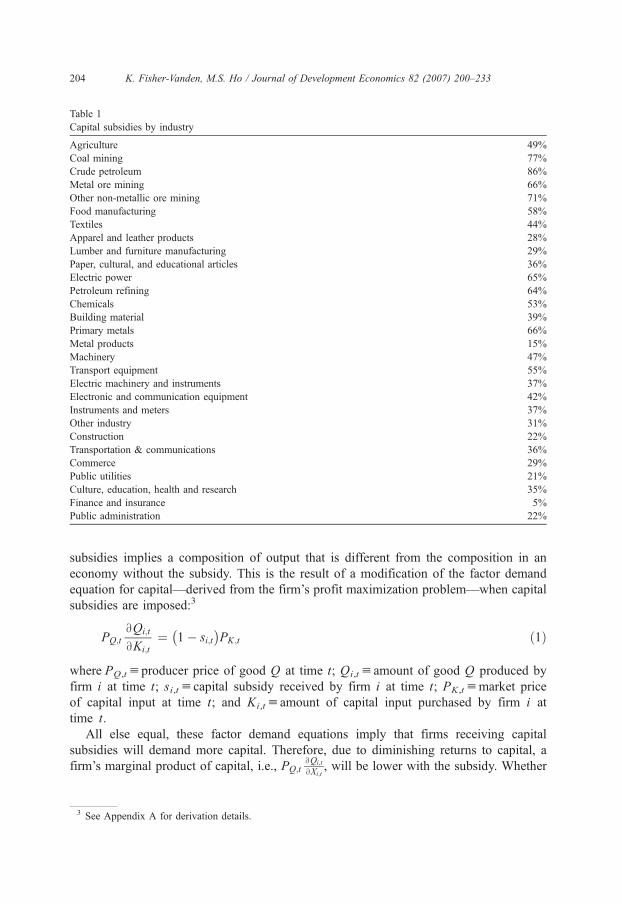
Table 1
Capital subsidies by industry
Agriculture 49%
Coal mining 77%
Crude petroleum 86%
Metal ore mining 66%
Other non-metallic ore mining 71%
Food manufacturing 58%
Textiles 44%
Apparel and leather products 28%
Lumber and furniture manufacturing 29%
Paper, cultural, and educational articles 36%
Electric power 65%
Petroleum refining 64%
Chemicals 53%
Building material 39%
Primary metals 66%
Metal products 15%
Machinery 47%
Transport equipment 55%
Electric machinery and instruments 37%
Electronic and communication equipment 42%
Instruments and meters 37%
Other industry 31%
Construction 22%
Transportation & communications 36%
Commerce 29%
Public utilities 21%
Culture, education, health and research 35%
Finance and insurance 5%
Public administration 22%
K. Fisher-Vanden, M.S. Ho / Journal of Development Economics 82 (2007) 200–233204
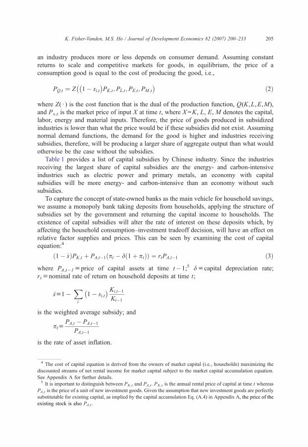
subsidies implies a composition of output that is different from the composition in an
economy without the subsidy. This is the result of a modification of the factor demand
equation for capital—derived from the firm’s profit maximization problem—when capital
subsidies are imposed:3
PQ;tBQi;t
BKi;t¼ 1� si;t� �
PK;t ð1Þ
where PQ,tuproducer price of good Q at time t; Qi,tuamount of good Q produced by
firm i at time t; si,tucapital subsidy received by firm i at time t; PK,tumarket price
of capital input at time t; and Ki,tuamount of capital input purchased by firm i at
time t.
All else equal, these factor demand equations imply that firms receiving capital
subsidies will demand more capital. Therefore, due to diminishing returns to capital, a
firm’s marginal product of capital, i.e., PQ;tBQi;t
BXi;t, will be lower with the subsidy. Whether
3 See Appendix A for derivation details.
K. Fisher-Vanden, M.S. Ho / Journal of Development Economics 82 (2007) 200–233 205
an industry produces more or less depends on consumer demand. Assuming constant
returns to scale and competitive markets for goods, in equilibrium, the price of a
consumption good is equal to the cost of producing the good, i.e.,
PQ;t ¼ Z 1� si;t� �
PK;t;PL;t;PE;t;PM ;t
� �ð2Þ
where Z(d ) is the cost function that is the dual of the production function, Q(K,L,E,M),
and Px,t is the market price of input X at time t, where X =K, L, E, M denotes the capital,
labor, energy and material inputs. Therefore, the price of goods produced in subsidized
industries is lower than what the price would be if these subsidies did not exist. Assuming
normal demand functions, the demand for the good is higher and industries receiving
subsidies, therefore, will be producing a larger share of aggregate output than what would
otherwise be the case without the subsidies.
Table 1 provides a list of capital subsidies by Chinese industry. Since the industries
receiving the largest share of capital subsidies are the energy- and carbon-intensive
industries such as electric power and primary metals, an economy with capital
subsidies will be more energy- and carbon-intensive than an economy without such
subsidies.
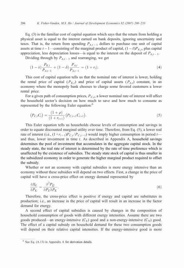
To capture the concept of state-owned banks as the main vehicle for household savings,
we assume a monopoly bank taking deposits from households, applying the structure of
subsidies set by the government and returning the capital income to households. The
existence of capital subsidies will alter the rate of interest on these deposits which, by
affecting the household consumption–investment tradeoff decision, will have an effect on
relative factor supplies and prices. This can be seen by examining the cost of capital
equation:4
ð1� s̄ÞPK;t þ PA;t�1 pt � d 1þ ptð Þð Þ ¼ rtPA;t�1 ð3Þ
where PA,t�1uprice of capital assets at time t�1;5 ducapital depreciation rate;
rtunominal rate of return on household deposits at time t;
s̄u1�Xi
1� si;t� � Ki;t�1
Kt�1
is the weighted average subsidy; and
ptuPA;t � PA;t�1
PA;t�1
is the rate of asset inflation.
5 It is important to distinguish between PK ,t and PA ,t. PK,t is the annual rental price of capital at time t whereas
PA ,t is the price of a unit of new investment goods. Given the assumption that new investment goods are perfectly
substitutable for existing capital, as implied by the capital accumulation Eq. (A.4) in Appendix A, the price of the
existing stock is also PA ,t.
4 The cost of capital equation is derived from the owners of market capital (i.e., households) maximizing the
discounted streams of net rental income for market capital subject to the market capital accumulation equation.
See Appendix A for further details.
K. Fisher-Vanden, M.S. Ho / Journal of Development Economics 82 (2007) 200–233206
Eq. (3) is the familiar cost of capital equation which says that the return from holding a
physical asset is equal to the interest earned on bank deposits, ignoring uncertainty and
taxes. That is, the return from spending PA,t� 1 dollars to purchase one unit of capital
assets at time t�1—consisting of the marginal product of capital, (1� s̄)PK,t, plus capital
appreciation, less depreciation losses—is equal to the interest on the deposit of PA,t� 1.
Dividing through by PA,t� 1 and rearranging, we get
ð1� s̄Þ PK;t
PA;t�1þ 1� dð Þ PA;t
PA;t�1¼ 1þ rtð Þ: ð4Þ
This cost of capital equation tells us that the nominal rate of interest is lower, holding
the rental price of capital (PK,t) and price of capital assets (PA,t) constant, in an
economy where the monopoly bank chooses to charge some favored customers a lower
rental price.
For a given path of consumption prices, PC,t, a lower nominal rate of interest will affect
the household sector’s decision on how much to save and how much to consume as
represented by the following Euler equation:6
PC;tCt
� �¼ 1þ qð Þ
1þ rtþ1ð Þ PC;tþ1Ctþ1� �
: ð5Þ
This Euler equation tells us households choose levels of consumption and savings in
order to equate discounted marginal utility over time. Therefore, from Eq. (5), a lower real
rate of interest (i.e., (1+ rt +1)PC,t /PC,t +1) would imply higher consumption in period t—
and thus, lower investment in time t. As described in Appendix A, household savings
determines the pool of investment that accumulates in the aggregate capital stock. In the
steady state, the real rate of interest is determined by the rate of time preference which is
unaffected by the existence of subsidies. The steady state stock of capital is thus smaller in
the subsidized economy in order to generate the higher marginal product required to offset
the subsidy.
Whether or not an economy with capital subsidies is more energy intensive than an
economy without these subsidies will depend on two effects. First, a change in the price of
capital will have a cross-price effect on energy demand represented by
BXE
BPK
¼ B2PQ
BPEBPK
: ð6Þ
Therefore, the cross-price effect is positive if energy and capital are substitutes in
production; i.e., an increase in the price of capital will result in an increase in the factor
demand for energy.
A second effect of capital subsidies is caused by changes in the composition of
household consumption of goods with different energy intensities. Assume there are two
goods produced—an energy-intensive (CE) good and a non-energy-intensive (CN) good.
The effect of a capital subsidy on household demand for these two consumption goods
will depend on their relative capital intensities. If the energy-intensive good is more
6 See Eq. (A.13) in Appendix A for derivation details.
K. Fisher-Vanden, M.S. Ho / Journal of Development Economics 82 (2007) 200–233 207
capital-intensive than the non-energy-intensive good, and firms producing this good do
not receive subsidies, then the higher rental price of capital will lead to a substitution
away from CE towards CN. However, if the energy-intensive good is more capital-
intensive and the firms producing this good receive subsidies, then the rental price of
capital paid by these firms is lower and the effect on the composition of output is
ambiguous.
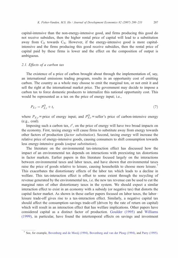
2.1. Effects of a carbon tax
The existence of a price of carbon brought about through the implementation of, say,
an international emissions trading program, results in an opportunity cost of emitting
carbon. The country as a whole may choose to emit the marginal ton, or not emit it and
sell the right at the international market price. The government may decide to impose a
carbon tax to force domestic producers to internalize this national opportunity cost. This
would be represented as a tax on the price of energy input; i.e.,
PE;t ¼ POE;t þ tc ð7Þ
where PE,tuprice of energy input; and POE,tu seller’s price of carbon-intensive energy
(e.g., coal).
Imposing such a carbon tax, tc, on the price of energy will have two broad impacts on
the economy. First, taxing energy will cause firms to substitute away from energy towards
other factors of production (factor substitution). Second, taxing energy will increase the
relative price of energy-intensive goods, causing consumers to shift consumption towards
less energy-intensive goods (output substitution).
The literature on the environmental tax-interaction effect has discussed how the
impact of an environmental tax depends on interactions with preexisting tax distortions
in factor markets. Earlier papers in this literature focused largely on the interactions
between environmental taxes and labor taxes, and have shown that environmental taxes
raise the price of goods relative to leisure, causing households to choose more leisure.7
This exacerbates the distortionary effects of the labor tax which leads to a decline in
welfare. This tax-interaction effect is offset to some extent through the recycling of
revenue generated by the environmental tax, i.e. the new tax revenue can be used to cut the
marginal rates of other distortionary taxes in the system. We should expect a similar
interaction effect to exist in an economy with a subsidy (or negative tax) that distorts the
capital factor market. As shown in these earlier papers focused on labor taxes, the labor–
leisure trade-off gives rise to a tax-interaction effect. Similarly, a negative capital tax
should affect the consumption–savings trade-off (driven by the rate of return on capital)
which will result in an interaction effect that has welfare implications. Other papers have
considered capital as a distinct factor of production. Goulder (1995) and Williams
(1999), in particular, have found the intertemporal effects on savings and investment
7 See, for example, Bovenberg and de Mooij (1994), Bovenberg and van der Ploeg (1994), and Parry (1995).
K. Fisher-Vanden, M.S. Ho / Journal of Development Economics 82 (2007) 200–233208
decisions to be important.8 We examine the implications of the environmental tax-
interaction literature below.
(1) Factor substitution
The extent of factor substitution resulting from the imposition of a carbon tax will
depend on changes in relative factor prices. Consider an ad valorem tax on the price
of energy in two economies—one with capital subsidies and one without. The direct
effect of the tax will cause a substitution to other factors of production such as
capital or non-energy materials. This also leads to an increase in the price of energy-
intensive goods relative to non-energy intensive goods. How does this affect the
supply of these factors?
From the cost of capital equation (Eq. (4)), we see that changes in the price of capital
9 The
is dete10 Sin
directly
substitu
quite li
carbon11 In a
from th
where
cost of
investm
the ste
8 See
assets and rental price of capital will change the rate of interest.9 If, after
incorporating general equilibrium effects, the short run rental price of capital
increases less than the price of capital assets with the carbon tax, then the short run
rate of interest will be lower.10 In an economy with subsidized capital (i.e., s N0),
however, this effect is dampened by the existence of the capital subsidy in the first
term of Eq. (4). Therefore, changes in the market rate of interest as a result of the
carbon tax will differ depending upon whether the economy includes a subsidy on
capital or not.
Differences in the impact of the carbon tax on the rate of interest between the two
economies means that the effect on savings and investment would be different. This
has implications for the future price of capital, and thus the future price of energy
relative to capital. Therefore, after incorporating general equilibrium effects, an
equal ad valorem carbon tax imposed in each economy—breformedQ and
bnonreformedQ—will have different effects on the substitution of non-energy factors
for energy.11
This factor substitution will have welfare implications as well. As discussed above in
relation to Eq. (1), the existence of a capital subsidy will result in a demand for
capital that is higher than what would be optimal if the subsidy did not exist. Factor
substitution away from energy towards capital could exacerbate this distortion in the
price of capital assets is determined by the market for investment goods whereas the rental price of capital
rmined by the factor market for capital.
ce investment goods are typically more energy intensive than consumption goods, a carbon tax would
affect the price of investment goods—i.e., the price of assets. The rental price of capital may rise due to
tion away from energy, but that depends on the relative intensities and other factor substitution. It is
kely that the price of assets would increase more than the rental price of capital with the imposition of a
tax.
model that includes intertemporal decision making, these short-run effects can be considered separately
e effects in the long run. As shown in Appendix A, imposing a carbon tax will result in a steady state
the stock of capital will adjust so that the real rate of return again equals the rate of time preference, q. Thecapital equation (4) must still hold in this new steady state, and thus changes in the long run price of
ent goods and rental price of capital would be different in the two economies. This results in differences in
ady state capital stocks, and differences in the substitution of other inputs for energy inputs.
also Bovenberg and Goulder (1997) and de Mooij and Bovenberg (1998).
12 Bov
zero or
K. Fisher-Vanden, M.S. Ho / Journal of Development Economics 82 (2007) 200–233 209
capital market, leading to lower welfare. This is consistent with the findings of de
Mooij and Bovenberg (1998) and Bovenberg and Goulder (1997) who find that
welfare improvements from the imposition of an environmental tax are only possible
in a situation where the environmental tax alleviates inefficiencies in the tax system.
However, factor substitution is not the only effect. Output substitution, discussed
below, will also have an effect which could offset the factor substitution effects.
(2) Output substitution
A carbon tax will also change the composition of aggregate output differently in a
reformed economy versus a nonreformed one. This occurs in two ways. First, the
intertemporal effects of the tax—through the rate of interest—will change the
household’s consumption–savings decision. As discussed above, short run changes
in the interest rate resulting from the carbon tax will differ in the two economies.
This implies that changes in the savings rate as a result of the carbon tax will be
different in the two economies. Since household savings is used to purchase
investment goods, a higher savings rate implies a higher composition of investment
goods in aggregate output. Since investment goods tend to be more energy-intensive
than consumption goods, an economy with a greater composition of investment
goods tends to be more energy-intensive.
Second, the imposition of a carbon tax affects the consumption choice between CE
and CN within a given time period. A carbon tax increases the purchase price of CE
relative to CN, causing households to substitute away from the consumption of CE.
Relative factor prices will differ between an economy with subsidized capital and an
economy without subsidized capital, leading to differences in the cost of producing
CE relative to CN. Assuming zero profits, this implies that relative prices of output
will also differ between the two economies, leading to differences in the composition
of aggregate consumption.
As shown in Table 1, the energy-intensive industries are also the industries receiving
the highest capital subsidies. Therefore, a reduction in the consumption of CE will
imply a reduction in the amount of total subsidies paid. Since households pay for
these subsidies through a lower average return to capital, a reduction in CE implies
an increase in household capital income, all else equal. However, imposing a carbon
tax adds a distortion to the economy which, unless compensated by a reduction in
another distortionary tax, will lead to lower real incomes.12 Depending upon which
effect dominates, welfare could be higher or lower.
As even the simple analytical model presented in this section illustrates, the
difference in responsiveness of a nonreformed versus reformed economy to a carbon
tax depends largely on complex interactions. Thus, to fully assess the differences in
the impact of a carbon tax in a reformed versus nonreformed economy requires a
model that can account for general equilibrium effects, including intertemporal
equilibrium. Although the above discussion helps narrow our focus on the most
important interactions driving the difference in responsiveness between the two
enberg and Goulder (1997), de Mooij and Bovenberg (1998), and Goulder (1995) were unable to achieve
negative marginal welfare cost with any alternative revenue recycling scheme.
K. Fisher-Vanden, M.S. Ho / Journal of Development Economics 82 (2007) 200–233210
economies, purely analytical methods cannot incorporate the necessary complexity
in a tractable manner, and thus a numerical approach is required. The next section
describes a numerical model of the Chinese economy developed to analyze the
effects of a carbon tax when capital is subsidized and when it is not.
3. Numerical model
The model used in this analysis is based on computable general equilibrium (CGE)
which means that the complex interactions between the four economic agents—producers,
households, government and the foreign sector—are explicitly modeled. The production
sector consists of 29 sectors consisting of agriculture, 21 bindustrialQ sectors (including fourenergy sectors and 17 non-energy sectors), construction, and six service sectors (see Table
1). Both direct and indirect effects of policy are captured. The household sector is modeled
in two stages. The first stage determines the household’s path of aggregate consumption and
savings by solving the intertemporal utility maximization problem described in Appendix
A. In the second stage, household demand of each of the 29 commodities is determined
given aggregate consumption from the first stage. The government sector collects taxes,
allocates subsidized capital, purchases goods and services and redistributes resources. The
foreign sector is modeled using the standard one-country Armington approach. Carbon
emissions are estimated in the model based on the amount and type of fossil fuel
consumed by each of the three domestic economic actors. Further details on the model
structure, features and base case assumptions are provided in Appendix B.
The primary source of data for model parameters is a social accounting matrix (SAM)
constructed using the official 1992 input–output tables for China, and supplemented by
data on government finances, trade, labor and energy.13 Projections of the Chinese labor
force are taken from World Bank (1990). Projections for the world price of oil are taken
from the U.S. Department of Energy/EIA (1999). Other future relative world prices are
assumed to be the same as in the base year.
To simulate the effects of a reduction of capital subsidies on the structure of the Chinese
economy, we must include industry-specific subsidy rates. As described in detail in
Appendix B, these subsidy rates were estimated based on survey data from the Chinese
Academy of Social Sciences that provide data on investment by source (i.e., central budget
allocations, local budget allocations, domestic loans, retained earnings, foreign investment,
and other). These data allow us to estimate the portion of an industry’s capital stock
receiving favorable loan terms. The resulting subsidy rates are provided in Table 1.
4. Numerical results
When comparing the effects of a carbon tax in a nonreformed economy with the effects
of a carbon tax in a reformed economy, we are interested in two impacts. First, we are
13 Details on the construction of the SAM are provided in Garbaccio et al. (2000).
K. Fisher-Vanden, M.S. Ho / Journal of Development Economics 82 (2007) 200–233 211
interested in the emission reductions generated by different carbon tax rates. This provides
us with a sense of the extent of the policy required to achieve a certain level of
environmental quality and a sense of the responsiveness of the economy (in terms of
reductions) to environmental policies. Second, we are also keenly interested in the welfare
implications of the tax since this would provide an indication of how willing the
government would be to implement such a policy. We examine both the carbon tax rates
required to achieve certain levels of emission reductions and associated welfare effects in
our analysis below. We begin with a brief description of the reference case and then
present results from the imposition of a carbon tax.
The literature on carbon taxes has been somewhat vague on the issue regarding the
precise measurement of the tax. We highlight this point by reporting two sets of results—
one using a unit carbon tax and one using an ad valorem carbon tax—in order to account
for differences in relative prices in the reformed and nonreformed economies.
4.1. Business-as-usual (BAU) scenario
Based on the model structure and assumptions outlined in the previous section, we
generate two bbusiness-as-usualQ (BAU) scenarios—one for an economy that includes
capital subsidies (the bNonreformQ case) and another for an economy that excludes these
subsidies (the bReformQ case). In the bNonreformQ scenario, the model includes industry-
specific capital subsidy rates (the s in Eqs. (1) and (4)) that are set based on the
information in Table 1. In the bReformQ scenario, on the other hand, the model assumes
these capital subsidy rates are zero. Therefore, the only difference in assumptions between
the two cases is the inclusion or exclusion of these capital subsidies; every other parameter
and exogenous variable is the same in both cases.14 These two BAU scenarios are used as
bases for comparison with simulations that include a carbon tax.
In the Reform case, the average annual growth rate of real GDP over the first 60 years is
5.3%, compared to an average annual growth rate of 4.5% in the Nonreform case. The
average annual growth of carbon emissions over this period is 3.4% in the Reform case
compared to 2.8% in the Nonreform case. Since the growth rate of GDP is larger than the
growth rate of carbon emissions in both cases, the carbon intensity of the Chinese
economy is falling over this time period. This fall in carbon intensity is larger in the
Reform case where the difference in growth rates between GDP and emissions is more
pronounced.15
4.2. Unit carbon tax
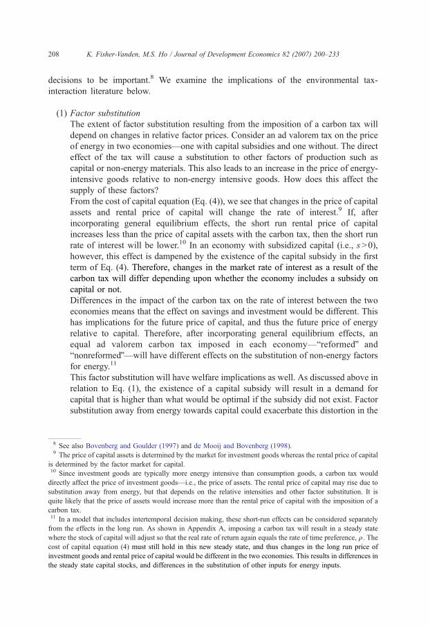
4.2.1. Effects on carbon emissions
To assess how the existence of a capital subsidy can affect the Chinese economy’s
responsiveness to environmental policy, we compare the schedule of carbon tax rates
14 It is important to note that revenues and government spending are endogenous and thus also differ in the two
cases.15 A detailed analysis of the effect of reforms on economic growth, energy use and carbon emissions in China
using a similar model is provided in Fisher-Vanden (2003).
$0
$5
$10
$15
$20
0 500 1000 1500 2000Reductions in Carbon Emissions in 2050
(Million tons carbon)
$/to
n c
arb
on
tax
No reform Reform
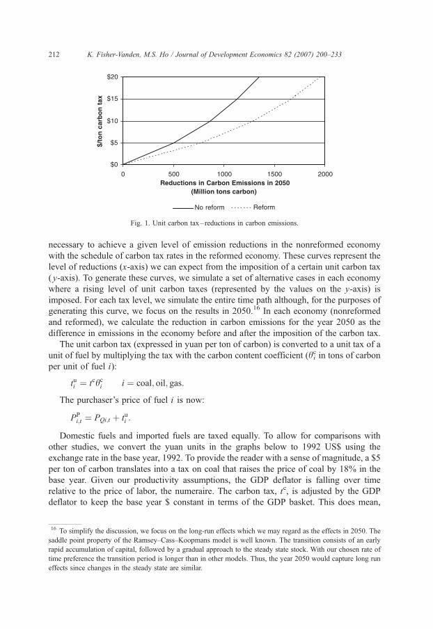
Fig. 1. Unit carbon tax–reductions in carbon emissions.
K. Fisher-Vanden, M.S. Ho / Journal of Development Economics 82 (2007) 200–233212
necessary to achieve a given level of emission reductions in the nonreformed economy
with the schedule of carbon tax rates in the reformed economy. These curves represent the
level of reductions (x-axis) we can expect from the imposition of a certain unit carbon tax
( y-axis). To generate these curves, we simulate a set of alternative cases in each economy
where a rising level of unit carbon taxes (represented by the values on the y-axis) is
imposed. For each tax level, we simulate the entire time path although, for the purposes of
generating this curve, we focus on the results in 2050.16 In each economy (nonreformed
and reformed), we calculate the reduction in carbon emissions for the year 2050 as the
difference in emissions in the economy before and after the imposition of the carbon tax.
The unit carbon tax (expressed in yuan per ton of carbon) is converted to a unit tax of a
unit of fuel by multiplying the tax with the carbon content coefficient (hic in tons of carbon
per unit of fuel i):
tui ¼ tchci i ¼ coal; oil; gas:
The purchaser’s price of fuel i is now:
PPi;t ¼ PQi;t þ tui :
Domestic fuels and imported fuels are taxed equally. To allow for comparisons with
other studies, we convert the yuan units in the graphs below to 1992 US$ using the
exchange rate in the base year, 1992. To provide the reader with a sense of magnitude, a $5
per ton of carbon translates into a tax on coal that raises the price of coal by 18% in the
base year. Given our productivity assumptions, the GDP deflator is falling over time
relative to the price of labor, the numeraire. The carbon tax, tc, is adjusted by the GDP
deflator to keep the base year $ constant in terms of the GDP basket. This does mean,
16 To simplify the discussion, we focus on the long-run effects which we may regard as the effects in 2050. The
saddle point property of the Ramsey–Cass–Koopmans model is well known. The transition consists of an early
rapid accumulation of capital, followed by a gradual approach to the steady state stock. With our chosen rate of
time preference the transition period is longer than in other models. Thus, the year 2050 would capture long run
effects since changes in the steady state are similar.
$0
$5
$10
$15
$20
0% 10% 20% 30% 40%
Percentage Reduction in Carbon Emissions in 2050
$/T
on
Car
bo
n T
ax
Reform No Reform
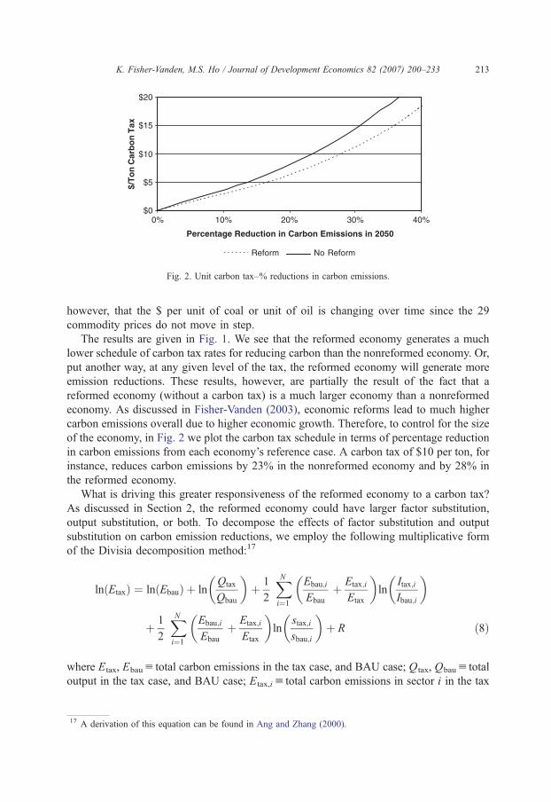
Fig. 2. Unit carbon tax–% reductions in carbon emissions.
K. Fisher-Vanden, M.S. Ho / Journal of Development Economics 82 (2007) 200–233 213
however, that the $ per unit of coal or unit of oil is changing over time since the 29
commodity prices do not move in step.
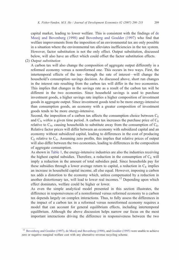
The results are given in Fig. 1. We see that the reformed economy generates a much
lower schedule of carbon tax rates for reducing carbon than the nonreformed economy. Or,
put another way, at any given level of the tax, the reformed economy will generate more
emission reductions. These results, however, are partially the result of the fact that a
reformed economy (without a carbon tax) is a much larger economy than a nonreformed
economy. As discussed in Fisher-Vanden (2003), economic reforms lead to much higher
carbon emissions overall due to higher economic growth. Therefore, to control for the size
of the economy, in Fig. 2 we plot the carbon tax schedule in terms of percentage reduction
in carbon emissions from each economy’s reference case. A carbon tax of $10 per ton, for
instance, reduces carbon emissions by 23% in the nonreformed economy and by 28% in
the reformed economy.
What is driving this greater responsiveness of the reformed economy to a carbon tax?
As discussed in Section 2, the reformed economy could have larger factor substitution,
output substitution, or both. To decompose the effects of factor substitution and output
substitution on carbon emission reductions, we employ the following multiplicative form
of the Divisia decomposition method:17
ln Etaxð Þ ¼ ln Ebauð Þ þ lnQtax
Qbau
� �þ 1
2
XNi¼1
Ebau;i
Ebau
þ Etax;i
Etax
� �ln
Itax;i
Ibau;i
� �
þ 1
2
XNi¼1
Ebau;i
Ebau
þ Etax;i
Etax
� �ln
stax;i
sbau;i
� �þ R ð8Þ
where Etax, Ebauu total carbon emissions in the tax case, and BAU case; Qtax, Qbauu total
output in the tax case, and BAU case; Etax,iu total carbon emissions in sector i in the tax
17 A derivation of this equation can be found in Ang and Zhang (2000).
K. Fisher-Vanden, M.S. Ho / Journal of Development Economics 82 (2007) 200–233214
case; Ebau,iu total carbon emissions in sector i in the BAU case; Itax, Ibauu total carbon
intensity (E /Q) in the tax case, and BAU case; Ii,tax, Ii,bauu total carbon intensity of
sector i in the tax case, and BAU case; stax,iu sector i’s share of total output in the tax
case; sbau,iu sector i’s share of total output in the BAU case; and Ruapproximation
residual.
The first two terms, which can be combined as ln�
Ebau
QbauQtax
�, represent carbon
emissions in the tax case, conditional on output in the tax case being produced at the
same carbon intensity as in the BAU case. The third term captures changes in carbon
emissions between the BAU and tax cases due to changes in industrial sector carbon
intensity. The fourth term represents changes in total carbon emissions due to changes
in the sectoral composition of total industrial output. Since this decomposition method
is an approximation, the last term captures the residual change.
The decompositions of the emission changes due to the imposition of a $10/ton
carbon tax for each economy are provided in Table 2. We see that in both cases,
within-industry reductions in carbon intensity is the primary factor driving the decline
in overall carbon emissions with the imposition of a carbon tax. In the Reform case,
the fall in output levels has a slightly larger contribution than in the Nonreform case,
although both are small—i.e., less than 4%. In addition, changes in the sectoral
composition of output plays a slightly larger role in the Nonreform case than in the
Reform case.
These results suggest that factor substitution plays a dominant role over structural
change and is more sensitive to increases in energy prices caused by the carbon tax.
Since the reduction in carbon emissions (in percentage terms) shown in Fig. 2 is much
larger for the Reform case, this would suggest that the change in the price of energy
relative to other inputs is much higher in the Reform case. As suggested in the
discussion of factor substitution in Section 2, the increase in the price of energy relative
to capital as a result of the carbon tax may be much lower in the Nonreform case due to the
interaction of the carbon tax with the capital subsidy that exists in the Nonreform case. To
Table 2
Unit carbon tax
Terms in Divisia equation Nonreform case Reform case
Level (billion
tons carbon)
Contribution to
decline in carbon
emissions
Level (billion
tons carbon)
Contribution to
decline in carbon
emissions
First term–BAU case carbon emissions 8.2122 8.4424
Second term—change in output levels �0.0082 3.09% �0.0128 3.91%
Third term—change in within industry
carbon intensity
�0.2424 90.88% �0.2959 90.32%
Fourth term— change in industry
composition of total output
�0.0161 6.03% �0.0189 5.77%
Sum 7.9454 8.1149
Compare 7.9455 8.1150
Residual 0.0001 0.0001
Divisia decomposition of steady state emissions (year 2050).
0%
2%
4%
6%
8%
10%
12%
2005 2010 2015 2020 2025 2030 2035 2040 2045 2050
Year
% D
iffe
ren
ce i
n P
rice
of
En
erg
y/P
rice
of
Cap
ital
Nonreform case Reform case
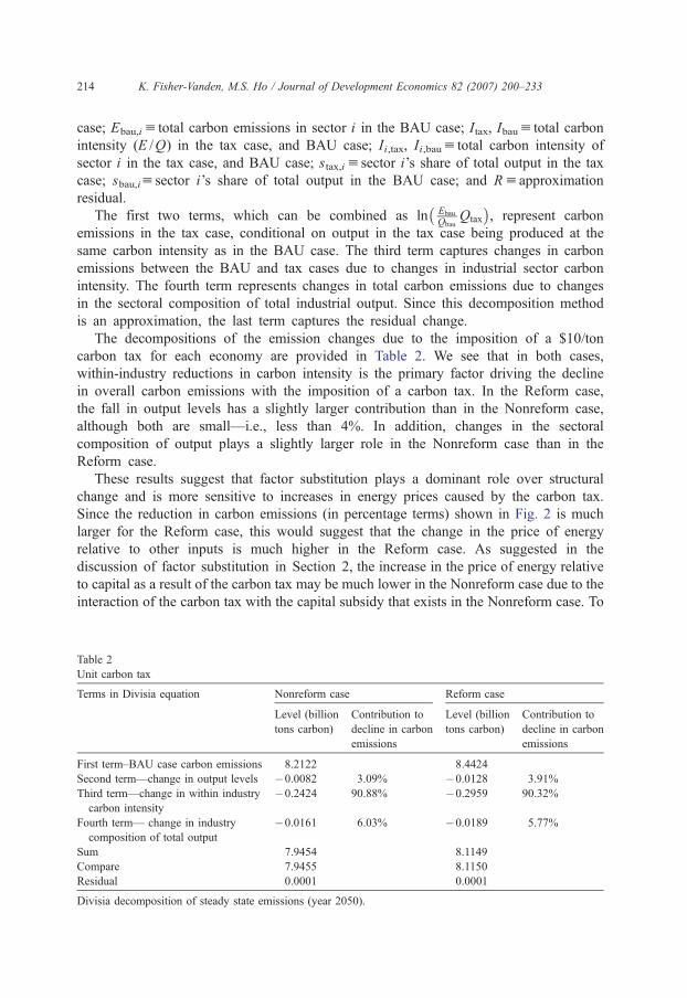
Fig. 3. Unit carbon tax–difference in relative prices.
K. Fisher-Vanden, M.S. Ho / Journal of Development Economics 82 (2007) 200–233 215
examine this closer, we compare the increase in the price of energy relative to capital in the
two cases.
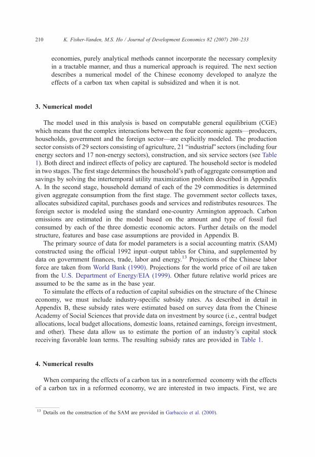
In Fig. 3 we plot the change in the ratio of the price of energy to the price of capital
as a result of a $10/ton carbon tax for the entire transition path of the two economies.18
In both cases, the increase in the relative price of energy as a result of the carbon tax
declines over time.19 Comparing the two cases, the increase in the relative price of
energy is significantly higher in the Reform case for all periods. This is consistent
with the outcome that the reformed economy exhibits a larger percentage drop in
emissions as a result of the carbon tax. But, how much of this is due to the fact that
the overall price level relative to the price of labor numeraire differs between the two
economies?
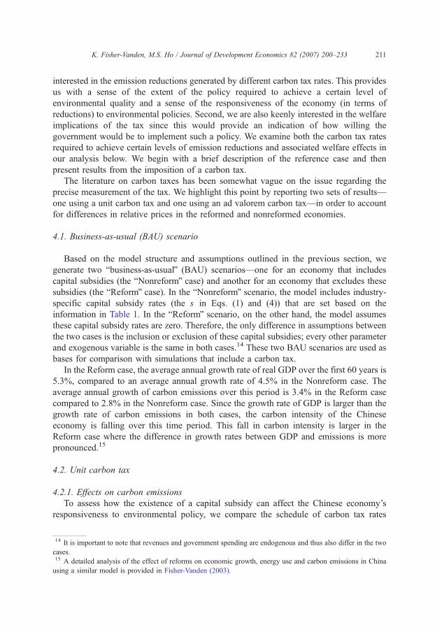
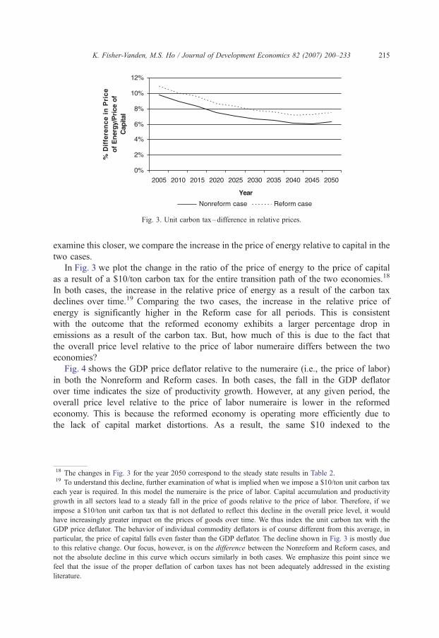
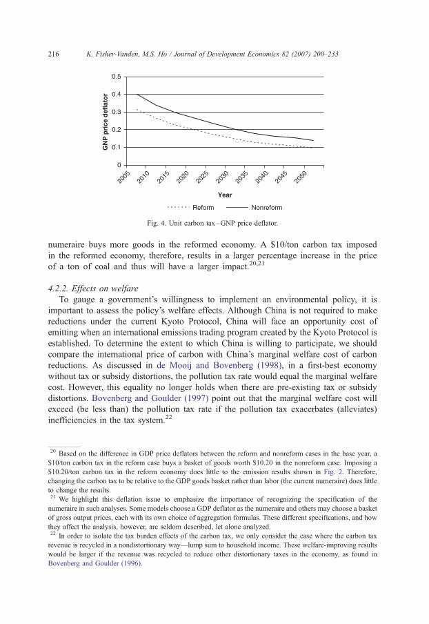
Fig. 4 shows the GDP price deflator relative to the numeraire (i.e., the price of labor)
in both the Nonreform and Reform cases. In both cases, the fall in the GDP deflator
over time indicates the size of productivity growth. However, at any given period, the
overall price level relative to the price of labor numeraire is lower in the reformed
economy. This is because the reformed economy is operating more efficiently due to
the lack of capital market distortions. As a result, the same $10 indexed to the
18 The changes in Fig. 3 for the year 2050 correspond to the steady state results in Table 2.19 To understand this decline, further examination of what is implied when we impose a $10/ton unit carbon tax
each year is required. In this model the numeraire is the price of labor. Capital accumulation and productivity
growth in all sectors lead to a steady fall in the price of goods relative to the price of labor. Therefore, if we
impose a $10/ton unit carbon tax that is not deflated to reflect this decline in the overall price level, it would
have increasingly greater impact on the prices of goods over time. We thus index the unit carbon tax with the
GDP price deflator. The behavior of individual commodity deflators is of course different from this average, in
particular, the price of capital falls even faster than the GDP deflator. The decline shown in Fig. 3 is mostly due
to this relative change. Our focus, however, is on the difference between the Nonreform and Reform cases, and
not the absolute decline in this curve which occurs similarly in both cases. We emphasize this point since we
feel that the issue of the proper deflation of carbon taxes has not been adequately addressed in the existing
literature.
0
0.1
0.2
0.3
0.4
0.5
2005
2010
2015
2020
2025
2030
2035
2040
2045
2050
Year
GN
P p
rice
def
lato
r
Reform Nonreform
Fig. 4. Unit carbon tax–GNP price deflator.
K. Fisher-Vanden, M.S. Ho / Journal of Development Economics 82 (2007) 200–233216
numeraire buys more goods in the reformed economy. A $10/ton carbon tax imposed
in the reformed economy, therefore, results in a larger percentage increase in the price
of a ton of coal and thus will have a larger impact.20,21
4.2.2. Effects on welfare
To gauge a government’s willingness to implement an environmental policy, it is
important to assess the policy’s welfare effects. Although China is not required to make
reductions under the current Kyoto Protocol, China will face an opportunity cost of
emitting when an international emissions trading program created by the Kyoto Protocol is
established. To determine the extent to which China is willing to participate, we should
compare the international price of carbon with China’s marginal welfare cost of carbon
reductions. As discussed in de Mooij and Bovenberg (1998), in a first-best economy
without tax or subsidy distortions, the pollution tax rate would equal the marginal welfare
cost. However, this equality no longer holds when there are pre-existing tax or subsidy
distortions. Bovenberg and Goulder (1997) point out that the marginal welfare cost will
exceed (be less than) the pollution tax rate if the pollution tax exacerbates (alleviates)
inefficiencies in the tax system.22
20 Based on the difference in GDP price deflators between the reform and nonreform cases in the base year, a
$10/ton carbon tax in the reform case buys a basket of goods worth $10.20 in the nonreform case. Imposing a
$10.20/ton carbon tax in the reform economy does little to the emission results shown in Fig. 2. Therefore,
changing the carbon tax to be relative to the GDP goods basket rather than labor (the current numeraire) does little
to change the results.21 We highlight this deflation issue to emphasize the importance of recognizing the specification of the
numeraire in such analyses. Some models choose a GDP deflator as the numeraire and others may choose a basket
of gross output prices, each with its own choice of aggregation formulas. These different specifications, and how
they affect the analysis, however, are seldom described, let alone analyzed.22 In order to isolate the tax burden effects of the carbon tax, we only consider the case where the carbon tax
revenue is recycled in a nondistortionary way—lump sum to household income. These welfare-improving results
would be larger if the revenue was recycled to reduce other distortionary taxes in the economy, as found in
Bovenberg and Goulder (1996).
-$5
$0
$5
$10
$15
$20
$25
0% 10% 20% 30% 40%
Percentage Reduction in Carbon Emissions in 2050
Mar
gin
al w
elfa
re c
ost
($/
ton
)
Reform Nonreform
Fig. 5. Unit carbon tax–marginal welfare cost.
K. Fisher-Vanden, M.S. Ho / Journal of Development Economics 82 (2007) 200–233 217
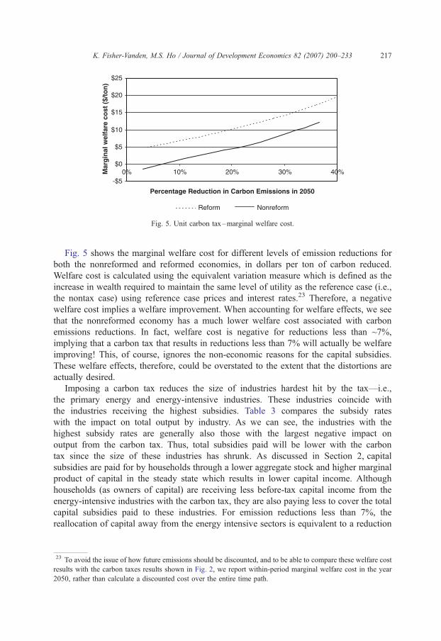
Fig. 5 shows the marginal welfare cost for different levels of emission reductions for
both the nonreformed and reformed economies, in dollars per ton of carbon reduced.
Welfare cost is calculated using the equivalent variation measure which is defined as the
increase in wealth required to maintain the same level of utility as the reference case (i.e.,
the nontax case) using reference case prices and interest rates.23 Therefore, a negative
welfare cost implies a welfare improvement. When accounting for welfare effects, we see
that the nonreformed economy has a much lower welfare cost associated with carbon
emissions reductions. In fact, welfare cost is negative for reductions less than ~7%,
implying that a carbon tax that results in reductions less than 7% will actually be welfare
improving! This, of course, ignores the non-economic reasons for the capital subsidies.
These welfare effects, therefore, could be overstated to the extent that the distortions are
actually desired.
Imposing a carbon tax reduces the size of industries hardest hit by the tax—i.e.,
the primary energy and energy-intensive industries. These industries coincide with
the industries receiving the highest subsidies. Table 3 compares the subsidy rates
with the impact on total output by industry. As we can see, the industries with the
highest subsidy rates are generally also those with the largest negative impact on
output from the carbon tax. Thus, total subsidies paid will be lower with the carbon
tax since the size of these industries has shrunk. As discussed in Section 2, capital
subsidies are paid for by households through a lower aggregate stock and higher marginal
product of capital in the steady state which results in lower capital income. Although
households (as owners of capital) are receiving less before-tax capital income from the
energy-intensive industries with the carbon tax, they are also paying less to cover the total
capital subsidies paid to these industries. For emission reductions less than 7%, the
reallocation of capital away from the energy intensive sectors is equivalent to a reduction
23 To avoid the issue of how future emissions should be discounted, and to be able to compare these welfare cost
results with the carbon taxes results shown in Fig. 2, we report within-period marginal welfare cost in the year
2050, rather than calculate a discounted cost over the entire time path.
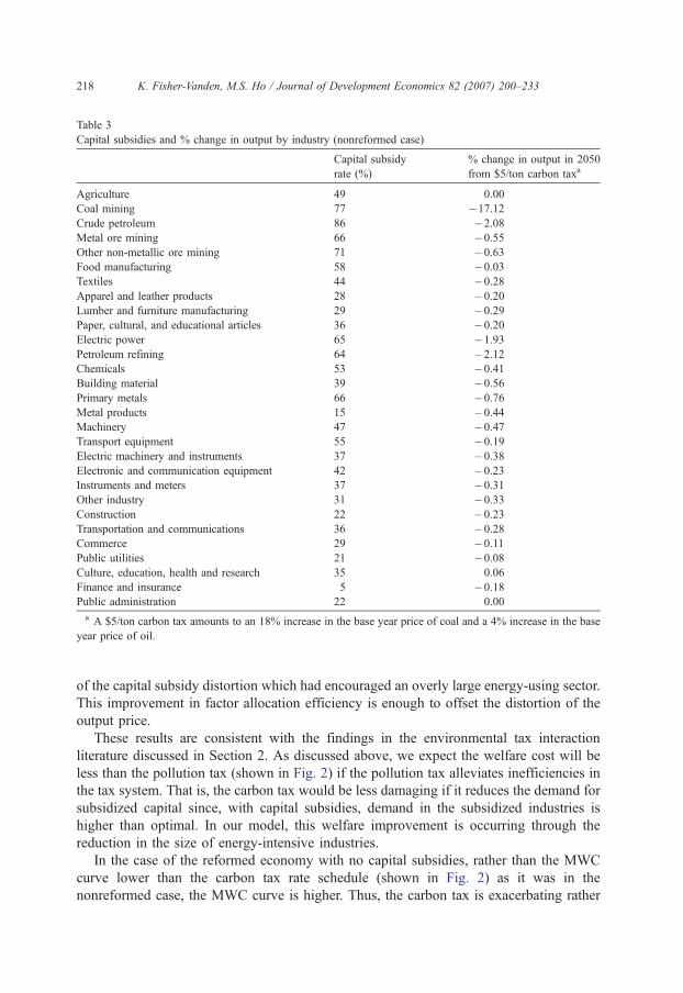
Table 3
Capital subsidies and % change in output by industry (nonreformed case)
Capital subsidy
rate (%)
% change in output in 2050
from $5/ton carbon taxa
Agriculture 49 0.00
Coal mining 77 �17.12Crude petroleum 86 �2.08Metal ore mining 66 �0.55Other non-metallic ore mining 71 �0.63Food manufacturing 58 �0.03Textiles 44 �0.28Apparel and leather products 28 �0.20Lumber and furniture manufacturing 29 �0.29Paper, cultural, and educational articles 36 �0.20Electric power 65 �1.93Petroleum refining 64 �2.12Chemicals 53 �0.41Building material 39 �0.56Primary metals 66 �0.76Metal products 15 �0.44Machinery 47 �0.47Transport equipment 55 �0.19Electric machinery and instruments 37 �0.38Electronic and communication equipment 42 �0.23Instruments and meters 37 �0.31Other industry 31 �0.33Construction 22 �0.23Transportation and communications 36 �0.28Commerce 29 �0.11Public utilities 21 �0.08Culture, education, health and research 35 0.06
Finance and insurance 5 �0.18Public administration 22 0.00
a A $5/ton carbon tax amounts to an 18% increase in the base year price of coal and a 4% increase in the base
year price of oil.
K. Fisher-Vanden, M.S. Ho / Journal of Development Economics 82 (2007) 200–233218
of the capital subsidy distortion which had encouraged an overly large energy-using sector.
This improvement in factor allocation efficiency is enough to offset the distortion of the
output price.
These results are consistent with the findings in the environmental tax interaction
literature discussed in Section 2. As discussed above, we expect the welfare cost will be
less than the pollution tax (shown in Fig. 2) if the pollution tax alleviates inefficiencies in
the tax system. That is, the carbon tax would be less damaging if it reduces the demand for
subsidized capital since, with capital subsidies, demand in the subsidized industries is
higher than optimal. In our model, this welfare improvement is occurring through the
reduction in the size of energy-intensive industries.
In the case of the reformed economy with no capital subsidies, rather than the MWC
curve lower than the carbon tax rate schedule (shown in Fig. 2) as it was in the
nonreformed case, the MWC curve is higher. Thus, the carbon tax is exacerbating rather
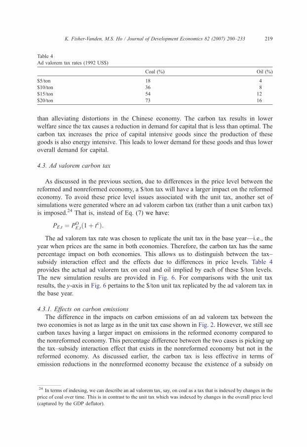
Table 4
Ad valorem tax rates (1992 US$)
Coal (%) Oil (%)
$5/ton 18 4
$10/ton 36 8
$15/ton 54 12
$20/ton 73 16
K. Fisher-Vanden, M.S. Ho / Journal of Development Economics 82 (2007) 200–233 219
than alleviating distortions in the Chinese economy. The carbon tax results in lower
welfare since the tax causes a reduction in demand for capital that is less than optimal. The
carbon tax increases the price of capital intensive goods since the production of these
goods is also energy intensive. This leads to lower demand for these goods and thus lower
overall demand for capital.
4.3. Ad valorem carbon tax
As discussed in the previous section, due to differences in the price level between the
reformed and nonreformed economy, a $/ton tax will have a larger impact on the reformed
economy. To avoid these price level issues associated with the unit tax, another set of
simulations were generated where an ad valorem carbon tax (rather than a unit carbon tax)
is imposed.24 That is, instead of Eq. (7) we have:
PE;t ¼ POE;t 1þ tcð Þ:
The ad valorem tax rate was chosen to replicate the unit tax in the base year—i.e., the
year when prices are the same in both economies. Therefore, the carbon tax has the same
percentage impact on both economies. This allows us to distinguish between the tax–
subsidy interaction effect and the effects due to differences in price levels. Table 4
provides the actual ad valorem tax on coal and oil implied by each of these $/ton levels.
The new simulation results are provided in Fig. 6. For comparisons with the unit tax
results, the y-axis in Fig. 6 pertains to the $/ton unit tax replicated by the ad valorem tax in
the base year.
4.3.1. Effects on carbon emissions
The difference in the impacts on carbon emissions of an ad valorem tax between the
two economies is not as large as in the unit tax case shown in Fig. 2. However, we still see
carbon taxes having a larger impact on emissions in the reformed economy compared to
the nonreformed economy. This percentage difference between the two cases is picking up
the tax–subsidy interaction effect that exists in the nonreformed economy but not in the
reformed economy. As discussed earlier, the carbon tax is less effective in terms of
emission reductions in the nonreformed economy because the existence of a subsidy on
24 In terms of indexing, we can describe an ad valorem tax, say, on coal as a tax that is indexed by changes in the
price of coal over time. This is in contrast to the unit tax which was indexed by changes in the overall price level
(captured by the GDP deflator).
$10
$20
$30
$40
$50
20% 30% 40% 50%
Percentage reduction in carbon emissions in 2050
$/to
n c
arb
on
tax
No Reform Reform
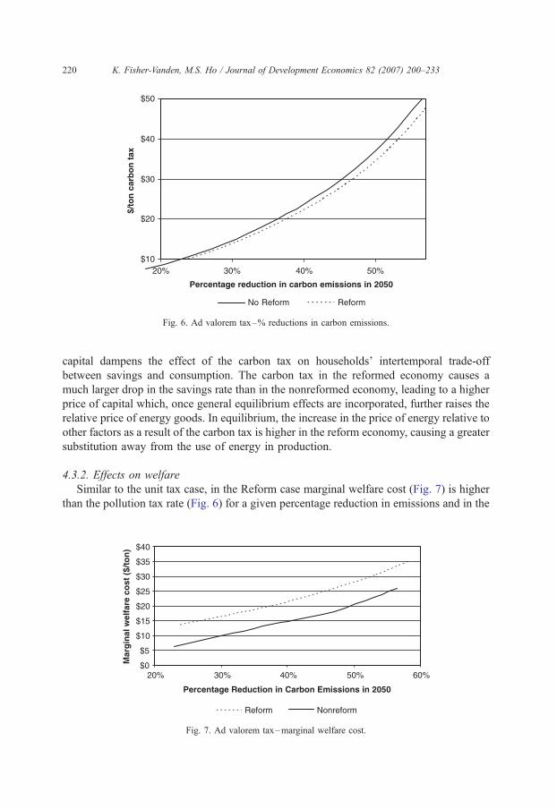
Fig. 6. Ad valorem tax–% reductions in carbon emissions.
K. Fisher-Vanden, M.S. Ho / Journal of Development Economics 82 (2007) 200–233220
capital dampens the effect of the carbon tax on households’ intertemporal trade-off
between savings and consumption. The carbon tax in the reformed economy causes a
much larger drop in the savings rate than in the nonreformed economy, leading to a higher
price of capital which, once general equilibrium effects are incorporated, further raises the
relative price of energy goods. In equilibrium, the increase in the price of energy relative to
other factors as a result of the carbon tax is higher in the reform economy, causing a greater
substitution away from the use of energy in production.
4.3.2. Effects on welfare
Similar to the unit tax case, in the Reform case marginal welfare cost (Fig. 7) is higher
than the pollution tax rate (Fig. 6) for a given percentage reduction in emissions and in the
$0
$5
$10
$15
$20
$25
$30
$35
$40
20% 30% 40% 50% 60%
Percentage Reduction in Carbon Emissions in 2050
Mar
gin
al w
elfa
re c
ost
($/
ton
)
Reform Nonreform
Fig. 7. Ad valorem tax–marginal welfare cost.
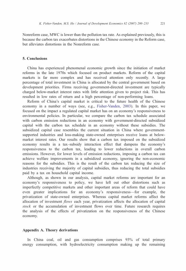
K. Fisher-Vanden, M.S. Ho / Journal of Development Economics 82 (2007) 200–233 221
Nonreform case, MWC is lower than the pollution tax rate. As explained previously, this is
because the carbon tax exacerbates distortions in the Chinese economy in the Reform case,
but alleviates distortions in the Nonreform case.
5. Conclusions
China has experienced phenomenal economic growth since the initiation of market
reforms in the late 1970s which focused on product markets. Reform of the capital
markets is far more complex and has received attention only recently. A large
percentage of total investment in China is allocated by the central government based on
development priorities. Firms receiving government-directed investment are typically
charged below-market interest rates with little attention given to project risk. This has
resulted in low rates of return and a high percentage of non-performing loans.
Reform of China’s capital market is critical to the future health of the Chinese
economy in a number of ways (see, e.g., Fisher-Vanden, 2003). In this paper, we
focused on the impact a regulated capital market has on an economy’s responsiveness to
environmental policies. In particular, we compare the carbon tax schedule associated
with carbon emission reductions in an economy with government-directed subsidized
capital with the carbon tax schedule in an economy without these subsidies. The
subsidized capital case resembles the current situation in China where government-
supported industries and loss-making state-owned enterprises receive loans at below-
market interest rates. Our results show that a carbon tax imposed on the subsidized
economy results in a tax–subsidy interaction effect that dampens the economy’s
responsiveness to the carbon tax, leading to lower reductions in overall carbon
emissions. However, for lower levels of emission reductions, imposing a carbon tax can
achieve welfare improvements in a subsidized economy, ignoring the non-economic
reasons for the subsidies. This is the result of the carbon tax reducing the size of
industries receiving the majority of capital subsidies, thus reducing the total subsidies
paid by a tax on household capital income.
Although, as shown in our analysis, capital market reforms are important for an
economy’s responsiveness to policy, we have left out other distortions such as
imperfectly competitive markets and other important areas of reform that could have
even greater implications for an economy’s responsiveness—for example, the
privatization of state-owned enterprises. Whereas capital market reforms affect the
allocation of investment flows each year, privatization affects the allocation of capital
stock or the accumulation of investment flows over time. Future research requires
the analysis of the effects of privatization on the responsiveness of the Chinese
economy.
Appendix A. Theory derivations
In China coal, oil and gas consumption comprises 93% of total primary
energy consumption, with hydroelectricity consumption making up the remaining
K. Fisher-Vanden, M.S. Ho / Journal of Development Economics 82 (2007) 200–233222
7%.25 As a result, and for the purpose of illustration, we therefore assume that carbon
emissions are the direct result of the amount of total energy consumed. In this theoretical
model, four factors of production—capital (K), energy (E), labor (L) and non-energy
materials (M)—are employed to produce two goods: an energy-intensive good (QE) and a
non-energy-intensive good (QN).26 In a nonreformed economy, certain protected
industries and firms receive capital at a lower than market rate of interest. These capital
subsidies are industry and firm specific, resulting in the following profit maximization
problem for firm i:
maxPi;t ¼ PQ;tQi;t � 1� si;t� �
PK;tKi;t � PL;tLi;t � PE;tEi;t � PM ;tMi;t ðA:1Þ
where Pi,tuprofit of firm i at time t; PQ,tuproducer price of good Q at time t;
Qi,tuamount of good Q (either QE or QN) produced by firm i at time t and of the form,
Qi,t=Q(Ki,t,Li,t,Ei,t,Mi,t); si,tucapital subsidy received by firm i at time t; Px,tumarket
price of input X at time t, X =K, L, E, M; Xi,tuamount of input X purchased by firm i at
time t, X =K, L, E, M.
Firm i’s demand for inputs other than capital are obtained from the following first-order
conditions for profit maximization:
PQ;tBQi;t
BXi;t¼ PX ;t where X ¼ L; E; M : ðA:2Þ
The existence of a capital subsidy modifies the firm’s demand for capital as follows:
PQ;tBQi;t
BKi;t¼ 1� si;t� �
PK;t: ðA:3Þ
The subsidy on capital is paid for by captive savings. As a result, households receive a
lower overall rate of return on capital compared to a deregulated capital market. In period
t, households save St and deposit this amount in the state bank, receiving a rate of return of
rt. The state bank collects these deposits and uses the funds to purchase investment goods
It that are accumulated into a stock of total capital assets; i.e.,
Kt ¼ 1� dð ÞKt�1 þ It: ðA:4Þ
The state bank rents these capital assets out to firms so no capital stock is wasted;
i.e.,
Kt�1 ¼Xi¼1...n
Ki;t�1: ðA:5Þ
25 Nuclear energy is a very recent addition, and biomass energy is not marketed and therefore not in the GDP
data, although separate data show a large contribution to total energy use.26 Capital and labor are supplied by households, and E and M are intermediate goods.
K. Fisher-Vanden, M.S. Ho / Journal of Development Economics 82 (2007) 200–233 223
In each period, the state bank receives a stream of income equal to the sum of the
subsidized rental income collected from each firm; i.e.,
P¯K;tKt�1 ¼Xi¼1...n
1� si;t� �
PK;tKi;t�1 ðA:6Þ
where PK,tu the non-subsidized (i.e., market) rental price of capital paid by firms at time t;
and P̄̄K,tu the average rental price of capital received by the state bank at time t.
The total value of capital assets held by the state bank at the end of t is the current value
of last period’s stock less depreciation plus investment:
PA;tKt ¼ 1� dð ÞPA;tKt�1 þ PA;tIt
PA,tuprice of capital assets at time t; ducapital depreciation rate.
The above wealth accumulation equation may also be written to make the capital gains
explicit:
PA;tKt ¼ PA;t�1Kt�1 þ PA;t � PA;t�1� �
Kt�1 � dPA;tKt�1 þ PA;tIt:
The value of new investment is the household saving deposits at time t, plus capital
income collected at time t (Eq. (A.6)), minus interest payments to households; i.e.,
PA;tIt ¼ St þ P¯K;tKt�1 � rtPA;t�1Kt�1 ðA:7Þ
where rtu rate of return on household deposits at time t.
The return on savings made at time t�1 is equal to the capital income generated plus
net capital appreciation; i.e.,
rtPA;t�1Kt�1 ¼ P¯K;tKt�1 þ PA;t � PA;t�1� �
Kt�1 � dPA;tKt�1: ðA:8Þ
Since the state bank controlled stock of capital assets is the only assumed vehicle for
household savings,27 households face rt in their decision of how much to consume and
save in each period. Dividing through by Kt� 1, we obtain the following cost-of-capital
equation:
ð1� s̄ÞPK;t þ PA;t�1 pt � d 1þ ptð Þð Þ ¼ rtPA;t�1 ðA:9Þ
27 This assumption is consistent with the situation in China where the only savings option available to
households historically has been to hold deposits in state banks. In 1994, the household savings rate was
estimated at 31% (World Bank, 1997). Factors contributing to the high rate of household savings include the lack
of consumer credit requiring households to save for big ticket items; uncertainty with respect to the future
availability of retirement, medical, and educational benefits; and firms requiring workers to invest a portion of
their earnings in the firm—a form of forced savings.
K. Fisher-Vanden, M.S. Ho / Journal of Development Economics 82 (2007) 200–233224
where
s̄u1�Xi
1� si;t� � Ki;t�1
Kt�1is the weighted average subsidy; and
ptuPA;t � PA;t�1
PA;t�1is the rate of asset inflation:
Dividing through by PA,t� 1 and rearranging, we get
ð1� s̄Þ PK;t
PA;t�1þ 1� dð Þ PA;t
PA;t�1¼ 1þ rtð Þ: ðA:10Þ
The household sector determines how much of the two goods to consume and how
much to save in each period by solving an intertemporal utility maximization problem.
We apply the Ramsey–Cass–Koopmans formulation (see, e.g. Barro and Sala-I-Martin,
1998) where households maximize the discounted sum of the log of aggregate
consumption:
MaxCt
Xlt¼1
1
1þ qð Þtlog Ctð Þ ðA:11Þ
subject to an intertemporal budget constraint:
Xlt¼1
1
Pts¼0 1þ rsð Þ Yt ¼
Xlt¼1
1
Pts¼0 1þ rsð Þ PC;tCt
� �ðA:12Þ
where Ctuaggregate consumption at time t; qu rate of time preference; Ytuhousehold
income at time t; rtumarket rate of interest at time t from Eq. (A.10); and PC,tuprice
of aggregate consumption at time t.
Maximizing Eq. (A.11) subject to Eq. (A.12) gives the familiar Euler equation:
PC;tCt
� �¼ 1þ qð Þ
1þ rtþ1ð Þ PC;tþ1Ctþ1� �
: ðA:13Þ
Household savings (St) is the residual of subtracting the value of aggregate
consumption in period t from after-tax household income in period t:
St ¼ Yt � PC;tCt: ðA:14ÞWe assume that the utility function is separable so that aggregate consumption is
divided between the two goods (energy-intensive and non-energy intensive) independent
of the rate of interest.28 Household consumption of the two goods is derived by
maximizing the intra-period utility function, U(CE,CN), subject to the following budget
constraint:
PC;tCt ¼ PCE;tCE;t þ PCN;t
CN;t ðA:15Þwhere CE,tuhousehold consumption of the energy-intensive good; and CN,tuhousehold
consumption of the non-energy-intensive good.
28 The inclusion of leisure in the utility function to allow for labor–leisure trade-offs may not be appropriate for
China, and therefore was not included in this formulation.
K. Fisher-Vanden, M.S. Ho / Journal of Development Economics 82 (2007) 200–233 225
The steady state of this economy is reached when all real quantities are constant relative
to effective labor supply. Consider, for simplicity, the case with no technical change and no
population growth. The steady state is then defined by:
Ct ¼ Ct�1 ¼ CSS and Kt ¼ Kt�1 ¼ KSS ðA:16Þ
where the SS subscript denotes steady state values. These imply that
ISS ¼ dKSS
rSS ¼ q: ðA:17Þ
Appendix B. Numerical model description
B.1 Model structure
B.1.1. Production sector
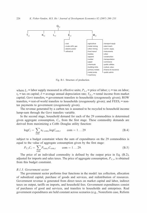
To simulate the effects of policy on structural change—e.g., the shift from heavy
industrial production to light—and thus on energy use and carbon emissions, the
producing sector is split into 29 sectors consisting of agriculture, 21 bindustrialQ sectors,construction, and six service sectors as listed in Table 1. The term industrial in the Chinese
data refers to mining, manufacturing and utilities. These 21 sectors include four energy
sectors (coal mining, crude oil/natural gas, refined oil and electricity) and 17 non-energy
sectors. Each sector chooses an input mix that maximizes profit in a manner similar to that
described in Appendix A. Instead of a simple production function like that given in Eq.
(A.1), output is produced from capital, labor, land and 19 intermediate inputs using a
nested production structure:
Qi;t ¼ f Ki;t; Li;t; Ti;t;E dð Þ;M dð Þ; t� �
ðB:1Þ
where Ti,tu land input; Ki,tucapital input; Li,tu labor input; Ei,tu intermediate energy
inputs; and Mi,tu intermediate non-energy materials inputs.
The nested structure of production in industry i at time t is depicted in Fig. B.1.
The zero profit condition of the producers is given by:
PQ;tQi;t ¼ 1� si;t� �
PK;tKi;t � PL;tLi;t � PE;tEi;t � PM ;tMi;t: ðB:2Þ
B.1.2. Household sector
The household sector is modeled in two stages. In the first stage, the household
determines its path of aggregate consumption and savings as described in Appendix A
(Eqs. A.11–A.14). Household income is defined as:
Yt ¼ 1� tlð Þ PL;tLt� �
þ 1� tk 1� dð Þð ÞYK;t þ Govt transferst
þ ROW transferst � FEESt ðB:3Þ
Qi,t
Ti,t Ki,t Li,t Ei,t Mi,t
--coal --agriculture --transport equip
--crude oil/N. gas --metal mining --elect mach.
--electric power --other mining --comm. equip.
--refined oil --food manuf --instruments
--textiles --other
--apparel --construction
--lumber --transportation
--paper --commerce
--chemicals --public utilities
--building mtrls --culture, educ.
--primary metals --finance & insurance
--metal prods --public admin
--machinery
Fig. B.1. Structure of production.
K. Fisher-Vanden, M.S. Ho / Journal of Development Economics 82 (2007) 200–233226
where Ltu labor supply measured in effective units; PL,tuprice of labor; tlu tax on labor;
tku tax on capital; duaverage annual depreciation rate; YK,tu rental income from market
capital; Govt transferstugovernment transfers to households (exogenously given); ROW
transferstu rest-of-world transfers to households (exogenously given); and FEEStunon-
tax payments to government (exogenously given).
The revenue generated by a carbon tax is assumed to be recycled to household income
lump-sum through the Govt transfers variable.
In the second stage, household demand for each of the 29 commodities is determined
given aggregate consumption, Ct, from the first stage. These commodity demands are
derived from maximizing a Cobb–Douglas utility function:
logCt ¼Xcom
aC;com;tlogCcom;t com ¼ 1 . . . 29 ðB:4Þ
subject to a budget constraint where the sum of expenditures on the 29 commodities is
equal to the value of aggregate consumption given by the first stage:
PC;tCt ¼Xcom
Pcom;tCcom;t com ¼ 1 . . . 29: ðB:5Þ
The price of an individual commodity is defined by the output price in Eq. (B.2),
adjusted for imports and sales taxes. The price of aggregate consumption, PC,t, is obtained
from this budget constraint.
B.1.3. Government sector
The government sector performs four functions in the model: tax collection, allocation
of subsidized capital, purchase of goods and services, and redistribution of resources.
Government revenue is generated from direct taxes on market capital and labor, indirect
taxes on output, tariffs on imports, and household fees. Government expenditures consist
of purchases of good and services, and transfers to households and enterprises. Real
government expenditures are held constant across scenarios (e.g., Nonreform case, Reform
K. Fisher-Vanden, M.S. Ho / Journal of Development Economics 82 (2007) 200–233 227
case, carbon tax case) through adjustments made to household income in the form of
lump-sum transfers.
B.1.4. Foreign sector
The foreign sector is modeled using the standard one-country approach where trade and
current account surpluses are set exogenously, and foreign-supplied goods are imperfect
substitutes for domestically-supplied goods (i.e., the Armington assumption). An
endogenous exchange rate is used to meet the exogenously set current account.
B.2 Model features and base case assumptions
The functional form assumed for the production technology is Cobb–Douglas, which
implies a unit elasticity of substitution between inputs. Currently, there are few estimates
of elasticities of substitution at this level of aggregation in China due to the lack of time
series input–output data. Given this, and the large and fairly rapid changes in energy use
observed (see, e.g. Fisher-Vanden, 2003 and Garbaccio et al., 1999), the assumption of an
elastic production function is reasonable at this level of aggregation, given that our focus is
on the long run. In the model, this Cobb–Douglas production function is defined as:
Q tð Þ ¼ A tð ÞKaK;t LaL;t TaT ;t EaE;tM aM ;t ðB:6Þ
where A(t) represents neutral productivity, and biased productivity change is represented by
the a coefficients that are indexed by time. By exogenously changing the aK,. . .aMcoefficients over time, we are allowing non-price induced changes in input demands to
occur in a way similar to past history. This is distinct from substitution as a result of relative
price changes which are also captured. Reform can have an endogenous effect on input
choices in this model through the effect of substitution towards the less expensive input.29
Lastly, neutral technological change—the change in total factor productivity, represented
by the A(t) term—is also allowed to occur.
The 1992 input–output table for China (State Statistical Bureau, 1996) was used to
estimate value shares for each factor input (intermediates and capital, labor, land) in the
base year. The future path of these aK,. . .aM share coefficients were projected by making
the simple assumption that the production structure will gradually resemble that of the
U.S. in 1992 by 2050, but with a higher share of coal use.30 This is a somewhat arbitrary
choice—any method of projecting so far ahead based on past data is subject to large
variance. We believe this procedure provides a plausible path for the near term. Sensitivity
analysis shows that changing the assumptions regarding the evolution of value shares in
production does little to change the results presented in Section 4. These assumptions are
important for setting the base case path of energy use; however, the percent difference
29 The Cobb–Douglas production function has fixed value shares of inputs, quantity shares thus change
endogenously in reaction to price changes.30 In particular, the relative value share of energy is assumed to fall and the relative value share of labor is
assumed to rise over time, mirroring what has occurred in the U.S. and other rich countries in the years leading up
to 1992. Details are provided in Ho and Jorgenson (2001).
K. Fisher-Vanden, M.S. Ho / Journal of Development Economics 82 (2007) 200–233228
between the base and counterfactual cases is not largely affected by these input share
coefficients.
The rate of technical progress, or total factor productivity growth (the rate at which
A(t) increases over time), is set at historical rates at the start of the projection path, and
rises in a way similar to that observed in advanced countries.31 Specifically, we
exogenously set A(t) to rise at a 3% annual rate at the beginning, declining gradually to
0.6% in 60 years. These rates of change achieve a growth rate of real GDP over time
consistent with other projections such as the World Economic Outlook (Standard and
Poor’s DRI, 1999). The sensitivity of the results in Section 4 to these growth assumptions
was examined. In general, different assumptions regarding the growth rates of neutral
technological change do not qualitatively change the results of comparing the base case
with the counterfactual case.
These assumptions regarding technical progress imply that improvements in production
efficiency will occur in the base case regardless of capital market reforms and
privatization. This reflects a broadly held belief that the significant productivity
improvements that have occurred over the last 20 years will likely continue for some
time. Further reforms may maintain, or even accelerate, these rates of change although our
model does not explicitly include an endogenous technical change feature.
Household demand for commodities is derived from a Cobb–Douglas utility
function as given in Eq. (B.4), which implies a unitary elasticity of substitution between
the 29 commodities. The value shares of demand for each of the commodities are
estimated based on the 1992 Chinese input–output table. Similar to the production
technology given in Eq. (B.6), these share coefficients are assumed to change over time,
reaching the consumption patterns observed in the U.S. in 1992—but with a higher share
of coal use—by 2050.32,33
The household’s rate of time preference, q, in Eq. (5) (the discount rate applied to
future consumption), was set to achieve a savings rate over time—defined as total
household savings as a percentage of income—consistent with estimated savings rates for
China from World Bank (1997).
31 Jefferson et al. (2000) estimates an average annual rate of TFP growth in China of 2.68% between the years
1988 and 1992. Ho and Jorgenson (2001) also provide estimates close to 3%. There is substantial variation in TFP
growth rates across industries but for simplicity we shall ignore them for the projections. Liang (2002) estimates
an average annual rate of TFP growth in the U.S. of 0.4% between 1960 and 1989.32 These assumptions imply, for instance, households will substitute away from energy (e.g., by purchasing
more fuel efficient automobiles) if the relative price of energy increases. The exogenously determined change
in household preferences (represented by the share coefficients) captures, for instance, an increase
consumption of automobiles over time since consumption patterns are assumed to reach those in the US
by 2050.33 A more carefully specified consumption function would recognize that demands are income elastic, e.g. as
in Jorgenson and Wilcoxen (1993). However, productivity growth in the Jorgenson–Wilcoxen model is forced
to converge to zero rapidly in order to avoid explosive demand shares. The recent rapid growth in incomes in
China is accompanied by rapid changes in demand patterns. However, we must worry whether historical
elasticities are appropriate if applied in a linear fashion, as is typically done in CGE models, to the high
projected income growth of China. To avoid these complications, we have opted to keep things simple by
allowing the parameters to change, generating a plausible change in the structure of the Chinese economy and
allowing for nonzero productivity growth.
K. Fisher-Vanden, M.S. Ho / Journal of Development Economics 82 (2007) 200–233 229
The labor market in China is undergoing fairly rapid changes; however, it is still
dominated by guaranteed employment and an abundance of surplus workers within state
enterprises, and low labor mobility. As a result, China lacks an efficiently functioning
labor market (see, e.g. World Bank, 1997), leading us to exclude labor–leisure choice in
the model.34 The inelastic labor supply (in effective hours per year) is a function of the
working-age population, average annual hours per work and an index of labor quality.
Working-age population is derived from projections of China’s population obtained from
World Bank (1990). The quality of labor is an index of the age and educational attainment
of the work force, calculated in Ho and Jorgenson (2001). We project this to grow at 0.7%
annually in the beginning, falling gradually over 60 years.35 The average annual hours per
worker is assumed to grow initially at 0.5% annually to represent a reduction in
underemployment over time, falling to 0% growth in 30 years.36
The government deficit, as a share of GDP, is set to 1992 levels (i.e., 3.5%) in the base
year. There are no official long-term projections of the government accounts and for
simplicity it is assumed that the deficit share will decline steadily to zero by 2025. These
exogenous values affect the base case path of the economy but have only trivial second
order effects on the items of interest which are the percentage differences between the base
and counterfactual cases. Although the short-run implications may be important, our
analysis focuses on the long run.
Since this is a one-country model, exogenous assumptions regarding international trade
are required. The current account balance (defined as the sum of net exports of goods,
services, factor income, and transfers) is set to 1992 levels in the base year. Forecasting
future current account deficits is similar to forecasting government deficits—important for
short-term considerations but not for the long-term responses that we are focusing on in
this analysis. It is simply assumed that the current account is balanced in 20 years. This is
consistent with International Monetary Fund projections which estimate a decline in
current account surplus over time (IMF, 2002). As with the assumption regarding the
government deficit, the results are not sensitive to different assumptions regarding the
current account balance.
Relative world prices are assumed to be constant over time except for the relative price
of crude oil which is based on U.S. Department of Energy’s Energy Information
Administration projections (U.S. DOE/EIA, 1999). In the base case path, the average
annual growth rate of each commodity exports is assumed to be 8% in the first year,
34 The female labor participation rate in China is high in comparison to other countries due to past Maoist
policies that encouraged female participation and provided child and health care to female workers. According to
the World Bank (1997), the female labor participation in China is 80% compared to an average rate of 50% in
East Asia. Therefore, the typical labor–leisure tradeoff we see prominently in countries like the US occurs
infrequently in China. Personal income and payroll taxes, other factors that could encourage a shift towards
leisure, are extremely low in China in order to encourage employment of China’s immense labor force (see, e.g.,
NBS, 2003). As a result, surplus labor has been a problem especially within state-owned enterprises which are the
providers of most social services.35 In comparison, the quality of labor index in the U. S. grew 0.5% annually in the 1950s (Jorgenson and Ho,
1994).36 Change in unemployment is considered a short-term disequilibrium which is not adequately captured in long-
term equilibrium models like the one used in this analysis. However, since the model is calibrated using actual
data on working-age population, hours worked and wage bill, unemployment in the base year is accounted for.
K. Fisher-Vanden, M.S. Ho / Journal of Development Economics 82 (2007) 200–233230
declining to 1% over 30 years. The exception is crude oil which has been exported in the
past; however, China is now a major importer of oil, leading us to assume a growth rate of
crude oil exports of 0%.
B.3 Derivation of industry-specific capital subsidy rates
As discussed in Section 2, the industry-specific capital subsidies have the effect of
lowering the rental price of capital paid by an industry; i.e.,
P¯K;i;t ¼ 1� si;t� �
PK;t: ðB:7Þ
Only a portion of each industry’s capital stock receives favorable loan terms;37
therefore, the average rental price of capital paid by each industry (P̄̄K,i,t) is equal to the
weighted average of the market rental price (PK,t) and the government-set (i.e., plan)
rental price (P̃K,i,t); i.e.,
P¯K;i;t ¼ P˜K;i;tdKplan;i;t
Kplan;i;t þ Kmkt;i;t
� � þ PK;tdKmkt;i;t
Kplan;i;t þ Kmkt;i;t
� � ðB:8Þ
where Kplan,i,tuamount of capital stock in firm i at time t receiving favorable loan terms;
and Kmkt,i,tuamount of capital stock in firm i at time t paying market interest rates.
Combining Eqs. (B.7) and (B.8) we obtain:
1� si;t� �
PK;t ¼ P˜K;i;tdKplan;i;t
Kplan;i;t þ Kmkt;i;t
� � þ PK;tdKmkt;i;t
Kplan;i;t þ Kmkt;i;t
� � : ðB:9Þ
Simplifying,
si;tPK;t ¼ PK;t � P˜K;i;t
� �d
Kplan;i;t
Kplan;i;t þ Kmkt;i;t
� � : ðB:90Þ
No data exists on the interest rate paid in the most favorable circumstances. Lardy
(1998), however, provides an average rate (i.e., a weighted average of both favorable and
market interest rates) paid on working capital loans in 1995 of 10.98% and estimates that
this rate would be approximately 21% if interest rates were deregulated. That is:
P¯K;1995
PK;1995¼ 10:98%
21%:
37 This model, similar to any CGE model, is unable to capture many real world details. For instance, constant
returns-to-scale and perfect competition are assumptions that are often made to ensure model tractability. We are
also limited by our ability to model at the firm level, and therefore are forced to adopt a certain industry
aggregation. Since our industry aggregation is at approximately the 2-digit SIC level, there will be industries
within one of our modeled industries that will receive preferential loans on their entire capital stock. In addition,
there may be certain firms within an industry (typically state-owned enterprises) that receive subsidies on their
entire capital stock. Eliminating these subsidies could have large discrete effects. As it is difficult to model this
reality in a tractable manner, our view of the industry as just one representative firm solving a profit maximization
problem implies that the economy responds to changes in subsidies in a smooth continuous manner.
K. Fisher-Vanden, M.S. Ho / Journal of Development Economics 82 (2007) 200–233 231
From the survey data described below, we estimate the share of plan capital stock in
total capital stock to be 53% in 1992. Therefore, from Eq. (B.8):
10:98% ¼ P̃K;i;t0:53þ 21% 1� 0:53ð Þ
or the return on plan capital (P̃K,i,t)=2.1%.
Thus,PK;t�P̃K;i;t
PK;t¼ 21%�2:1%
21%¼ 0:9. Plugging this into Eq. (B.9):
si;t ¼ 0:9dKplan;i;1995
Kplan;i;1995 þ Kmkt;i;1995
� � : ðB:10Þ
This implies that the industry-specific subsidy rate is 90% of the ratio of plan capital
stock to total capital stock in the base year.
To estimate the relative shares of plan and market capital stock, we use survey data from
two Chinese Academy of Social Sciences surveys—one of 769 state-owned enterprises,
covering the period 1980–1989, and another covering the period 1990–1994. These surveys
provide data on investment by source (i.e., central budget allocations, local budget
allocation, domestic loans, retained earnings, foreign investment, or other) and were used to
estimate the average share of an industry’s capital stock receiving favorable loan terms.
The amount of capital stock receiving below market interest rates by industry in 1992
was estimated as cumulative investment, less depreciation, of investment from the central
and local budget, policy loans and retained earning of SOEs from 1980 to 1992.38 The
amount of capital stock facing market interest rates by industry in 1992 was estimated as
the cumulative investment, less depreciation, from market and commercial loans, retained
earnings from non-SOEs, and foreign investment from 1980 to 1992. The share of total
capital stock receiving interest rate subsidies based on the survey data is therefore the ratio
of subsidized capital stock to total capital stock. Adjustments were made using data on the
sources of investment from World Bank (1995) and the China Investment Report for 1990
and 1992 (State Planning Commission and State Statistical Bureau, 1990, 1992)). Fixed
assets deflators are estimated based on data from Naughton (1992) and the Statistical
Yearbook of China (State Statistical Bureau, various issues).
The survey data described above only covers China’s industrial sector. We were unable
to calculate capital stocks for the estimation of subsidy rates in a similar way for the non-
industrial sectors (i.e., agriculture; construction; transportation; commerce; public utilities;
culture, education, and health; finance and insurance; and public administration).
However, data on investment by source for these sectors for one year is available in the
China Investment Report for 1992 (State Planning Commission and State Statistical
Bureau, 1992). Therefore, for the non-industrial sectors, investment flows in 1992 rather
than capital stocks were used to estimate the subsidy rate in Eq. (B.10).
The resulting subsidy rates from Eq. (B.10) are provided in Table 1. The national
average subsidy rate that enters into the cost-of-capital equation (Eq. (4)) is computed as a
38 According to Lardy (1998), policy lending from the four major banks in China was estimated at 42% of total
lending—an average across all industries receiving policy loans. To compute an estimate of policy loans as a
share of total domestic loans by industry for the model, we compare relative rates of return across industries and
assign higher shares to those industries with lower rates of return, achieving an average of 42%.
K. Fisher-Vanden, M.S. Ho / Journal of Development Economics 82 (2007) 200–233232
weighted-average of the industry-specific capital subsidy rates. The industries receiving
the highest subsidy on aggregate capital stock include the mining, food, electric power,
petroleum refining, chemicals, primary metals, and transport equipment sectors.
References
Ang, B.W., Zhang, F.W., 2000. A survey of index decomposition analysis in energy and environmental studies.
Energy 25, 1149–1176.
Barro, R., Sala-I-Martin, X., 1998. Economic Growth. MIT Press, Cambridge, MA.
Bovenberg, A. Lans, de Mooij, Ruud A., 1994. Environmental levies and distortionary taxation. American
Economic Review 84 (4), 1085–1089.
Bovenberg, A. Lans, Goulder, Lawrence H., 1996. Optimal environmental taxation in the presence of other taxes:
general equilibrium analyses. American Economic Review 86 (4), 985–1000.
Bovenberg, A. Lans, Goulder, Lawrence H., 1997. Costs of environmentally motivated taxes in the presence of
other taxes: general equilibrium analysis. National Tax Journal 50 (1), 59–87.
Bovenberg, A. Lans, van der Ploeg, F., 1994. Environmental policy, public finance and the labor market in a
second-best world. Journal of Public Economics 55 (3), 349–390.
de Mooij, R.A., Bovenberg, A.L., 1998. Environmental taxes, international capital mobility and inefficient tax
systems: tax burden vs. tax shifting. International Tax and Public Finance 5, 7–39.
Fisher-Vanden, K., 2003. The effects of market reforms on structural change: implications for energy use and
carbon emissions in China. Energy Journal 24 (3), 27–62.
Fisher-Vanden, K., Jefferson, G., Liu, H., Tao, Q., 2004. What is driving China’s decline in energy intensity?
Resource and Energy Economics 26, 77–97.
Garbaccio, R.F., Ho, M.S., Jorgenson, D.W., 1999. Why has the energy-output ratio fallen in China? Energy
Journal 20 (3), 63–91.
Garbaccio, R.F., Ho, M.S., Jorgenson, D.W., 2000. A Dynamic Economy-Energy-Environment Model of China.
Manuscript. Kennedy School of Government, Harvard University, Cambridge, MA.
Goulder, L.H., 1995. Effects of carbon taxes in an economy with prior tax distortions: an intertemporal general
equilibrium analysis. Journal of Environmental Economics and Management 29, 271–297.
Ho, Mun S., Jorgenson, Dale W., 2001. Productivity Growth in China, 1981–95. mimeo, Harvard University.
September.
International Monetary Fund (IMF), 2002. International Financial Statistics. International Monetary Fund,
Washington, D.C.
Jefferson, G.H., Rawski, T.G., Wang, L., Zheng, Y.X., 2000. Ownership, productivity change, and financial
performance in Chinese industry. Journal of Comparative Economics 28 (4), 786–813.
Jorgenson, D.W., Ho M.S., 1994. The Quality of the U.S. Work Force, 1948–1990. mimeo, Harvard University,
Cambridge, MA.
Jorgenson, D.W., Wilcoxen, P.J., 1993. Reducing US carbon dioxide emissions: an assessment of alternative
instruments. Journal of Policy Modeling 15 (5–6), 491–520.
Kruger, J.A., Pizer, W.A., 2004. Greenhouse gas trading in Europe. Environment 46 (8) (October).
Lardy, N., 1998. China’s Unfinished Economic Revolution. Brookings Institution Press, Washington, D.C.
Liang, C.-Y., 2002. An international comparison of total factor productivity changes, 1960–1993. World
Economy 25 (8), 1169–1195.
Lin, X., Polenske, K.R., 1995. Input–output anatomy of China’s energy use changes in the 1980’s. Economic
Systems Research 7 (1), 67–84.
National Bureau of Statistics (NBS), 2003. China Statistical Yearbook. China Statistical Press, Beijing,
P.R. China.
Naughton, B., 1992. The Capital Goods Deflator and the Growth of the Industrial Capital Stock. University of
California, San Diego.
Parry, Ian W.H., 1995. Pollution taxes and revenue recycling. Journal of Environmental Economics and
Management 29 (3), S64–S77.
Standard and Poor’s DRI, 1999. World Economic Outlook. Vol. 1 (Lexington, MA, 3rd Quarter 1999).

K. Fisher-Vanden, M.S. Ho / Journal of Development Economics 82 (2007) 200–233 233
State Planning Commission and State Statistical Bureau, 1990. Zhongguo Touzi Baogao 1990 [China Investment
Report 1990]. China Planning Press.
State Planning Commission and State Statistical Bureau, 1992. Zhongguo Touzi Baogao 1992 [China Investment
Report 1992]. China Planning Press.
State Statistical Bureau. 1996. Zhongguo touru chanchu biao 1992 nian du [Input–output table of China 1992
edition]. State Statistical Publishing House, Beijing.
State Statistical Bureau. Statistical Yearbook of China, various issues. State Statistical Publishing House,
Beijing.
U.S. Department of Energy/Energy Information Administration, 1999. Annual Energy Outlook: 1999. Report #
EIA/DOE- 0383 (99). Washington, DC.
U.S. Department of Energy/Energy Information Administration, 2004. International Energy Outlook: 2004.
Report # EIA/DOE- 0484(2004). Washington, DC.
Williams, R.C., 1999. Tax Interactions in a Dynamic Model with Capital Accumulation. Working paper,
University of Texas, Austin.
World Bank, 1990. World Population Projections 1989–90 Edition. Johns Hopkins University Press.
World Bank, 1995. China Public Investment and Finance. Report No. 14540-CHA. World Bank, Washington,
D.C.
World Bank, 1997. China 2020: Development Challenges in the New Century. World Bank, Washington, D.C.