1

Households and Economic Growthin Latin America and the Caribbean

by

Jere R. Behrman, Suzanne Duryea and Miguel Székely∗

February, 2000 ∗ Behrman is the William R. Kenan, Jr. Professor of Economics and Director of the Population Studies Center at theUniversity of Pennsylvania (McNeil 160, 3718 Locust Walk, University of Pennsylvania, Philadelphia, PA 19104-6297, USA, phone 215 8987704, fax 215 898 2124, e-mail jbehrman@econ.sas.upenn.edu). Duryea and Székelyare Economists in the Research Department, Inter-American Development Bank (1300 New York Ave. NW,Washington, DC 20577; phone 202 6233589 and 202 623 2907, fax 1 202 623 2481, e-mail suzanned@iadb.organd miguels@iadb.org). This paper was prepared for the Global Research Network Project on Explaining Growth.The paper draws extensively on Behrman (1999), Behrman, Duryea and Székely (1999a, b, c) and IDB (2000).

2

Introduction

The objective of this paper is to provide an overview and a framework for examining the relation between

households and economic growth in Latin America. We intend to explore the factors explaining growth

from the perspective of these microeconomic agents, and to point out the factors that shape these

decisions at the micro level.

We focus primarily on two kinds of household decisions that are crucial to economic growth: fertility and

investment in education. These two decisions determine the quantity and quality of the human resources

available to the economic system of a country and the age structure of the population. Another key input

in the growth process from the perspective of microeconomic agents is saving. Unfortunately, the lack of

information on household consumption at the micro level in the region prevents us from examining this

element here. We do not focus on household enterprises or rural production either, mainly because of data

limitations and because most countries in Latin America are already quite urbanized and the share of GDP

generated in the agricultural sector is relatively low.

The first section of the paper discusses the relevance of education and fertility decisions as inputs for

economic growth in Latin America and provides some examples of their importance. The second section

explores what determines the fertility and schooling investment behavior of households from a

macroeconomic and microeconomic perspective. Section three briefly discusses some data problems for

improving our understanding of the determinants of education and fertility decision in the region, and

section four concludes.

I. Why Focus on Fertility and Schooling Investment Decisions?

The household decisions that are crucial to economic growth can be divided into two broad categories. On

the one hand there are decisions that affect the current growth capacity of a country. Two of the most

important mechanisms are saving and investment decisions that have short gestation periods. If

households choose to have low saving rates, the resources needed to finance investment may be limited,

and this may become a restriction for growth. Additionally, if households choose to have low investment

rates in corporations or household enterprises, the private sector will tend to be relatively small, and the

dynamism of the economy will surely be quite limited. This will affect the overall demand for factors of

production including labor and therefore, their price structure in the market.

3

On the other hand, there are decisions that have an effect on growth in the longer run. This is the case of

fertility, and of investment in health and education. These decisions determine the size and quality of the

human resources at hand, but their effects become apparent long after they have been taken. In this

section we concentrate on these two types of decisions, mainly due to data availability in Latin America.

We start by explaining the connection between fertility and growth, and we then turn to education.

1.1 Fertility Decisions and Economic GrowthIn a similar manner to the way in which individuals change their needs, resources and behavior through

their life cycle, countries also change with shifts in the age structure of the population. When most of the

population is young, a country has relatively low capacity to generate resources but at the same time it has

considerable needs. Similarly to an individual’s life-cycle, the growth potential of a country will be

enhanced when larger shares of the population are of working age, while the needs to invest in human

resources will diminish. At some point, when the proportion of older adults with lower productivity and

labor force participation increases, the composition of demands for goods and services will change. So,

countries experience changes in needs and in their growth capacity depending on the relative sizes of the

age groups that are going through different stages of their life cycle.

What Determines the Differences in Age Structure?

The connection with household decisions is that the dynamics of the age structure of the population are

determined to a large extent by fertility decisions at the micro level. 1 Changes in the age structure also

respond to changes in mortality rates and migration, but at least since 1950 in developing countries,

fertility seems to have been the main driving force of the demographic transition. Since there is a lag

between declining mortality and total fertility rates, countries see a rapid growth in population with surges

1 The Malthusian emphasis traditionally has been on the negative impact of population growth rates by reducing percapita income growth because of diminishing returns to natural resources. From a theoretical perspective, however,the net impact of population growth on economic growth is ambiguous. In the simplest neoclassical growth models(e.g., Solow 1956, Phelps 1968), population growth affects the level of long-run per capita output, but not the long-run growth of per capita output. More complex models yield ambiguous results because the negative effects ofpopulation growth due to diminishing returns and pressures on common resources can be offset by positive effectsof scale, technological change, institutional change and market responses. There have been numerous efforts to useaggregate country data to see if there is empirical evidence of a significant relation between population growth andper capita income growth dating back at least to Kuznets (1958, 1967). Those based primarily on data before the1980s indicate no significant relation (for example, the World Bank's East Asian Miracle book), but several recentaggregate studies have found significantly negative correlations (Birdsall and Sinding (1999), Bloom andWilliamson (1998), Kelley and Schmidt (1994)). The debate about the effect of population growth on GDP growth

4

in young dependency ratios. At some point, fertility declines faster than mortality, population growth falls

and the young dependency ratio starts decreasing. The faster is the decrease in the young dependency

ratio caused by reductions in fertility, the greater the shift to a high working-age population share and low

dependency ratios. But as the population continues to age, the old dependency ratio increases with a

reduction in the working age share despite the continuing decline in the young dependency ratio.

Since fertility and mortality changes have taken place at a very different pace across regions, the young

and old dependency ratios over the past half-century vary widely. Figure 1 plots the young dependency

ratios of several regions, East Asia and the rest of Asia for 1950-1995. Africa has the highest young

dependency. Asia and Latin America & the Caribbean (LAC) have had young dependency ratios

throughout this half century that have been below those for Africa, but considerably higher than those for

North America and Europe. East Asian young dependency ratios have been lower than have been those

for the rest of Asia and LAC throughout this period, though they increased considerably between 1950

and 1960. They then peaked a little earlier in the 1960s and declined more sharply after the peak than in

the rest of Asia and in LAC so that by 1995 they were much closer to those in North America and Europe

than to those in the rest of Asia and LAC. The young dependency ratios for North America and even

more so for Europe have been below those for developing countries throughout the past half-century,

generally considerably below with the sole exception of East Asia recently. Over this past half century,

thus, the sharpest decline in young dependency ratios was for East Asia between 1970 and 1990. LAC has

had a substantial decline starting around 1970 that is ongoing, but not as steep as East Asia in 1970-1990

or North America in 1960-1980.

Figure 2 presents the regional total fertility rates for 1950-95.2 Africa is the developing country region

with the highest fertility and where fertility has declined most slowly. Europe also has had a slow fertility

decline because of the low levels already observed in the 1950s. The second highest fertility rates are

found in Asia (excluding East Asia) and LAC. In these two regions, fertility rates were somewhat lower

than in Africa in 1950, but they subsequently declined much faster, with the result that in 1995 their

fertility rates were about half of those observed in Africa. In 1950 fertility rates in East Asia were also

very similar to those in LAC but during the 1950s fertility in this region started to decline sharply and

is ongoing, but we argue here that age structures, rather than population growth per se, generate the greatestdemographic effects on growth (see IDB 2000).2 The total fertility rate is the number of children that would be born per woman if she were to live to the end of herchild-bearing years and bear children at each age in accordance with prevailing age-specific fertility rates.

5

faster than in any other region in the world. The difference between LAC and East Asia was 0.2 in 1950,

but had increased by a factor of over four to almost 1.0 in 1995.

The differences in mortality across regions between 1950 and 1995, presented in Figure 3, have been

much smaller than have been those for fertility. While fertility rates diverged significantly between East

Asia and LAC since 1950, crude mortality rates converged from 1960 on. Therefore, the differences that

we observe in age structures and dependency ratios across populations are due basically to differential

fertility rates.

Empirical Evidence on the Relation between Demographic Changes and Growth

Let’s start with a simple accounting exercise to illustrate the connections between fertility decisions taken

in the past and reflected in current age structures, and GDP. If there are two countries with identical

average productivity per worker and identical labor force participation rates, their GDP per capita would

differ if one had a larger share of its population in the working ages than did the other. For instance,

Figure 4 compares Hong Kong (one of the fastest growing economies with one of the oldest populations)

with Mexico (which has a relatively young population) and Argentina (which has one of the oldest

populations in LAC, but still a young population in comparison with developed countries).

The first panel plots GDP per capita for Mexico and Hong Kong. It shows that GDP per capita in Hong

Kong has been greater than that in Mexico since 1960. However, in Hong Kong a larger proportion of the

population has been of working age. Therefore if we plot the GDP per worker (which is similar to

extracting from the calculation the population that is not of working age) the differences narrow

considerably. According to Panel B, we would still conclude that Hong Kong has grown at a faster pace,

but it only seems to have surpassed Mexico in terms of GDP per worker in about 1990. So, our ranking of

these two countries for the period 1960-1990 changes after adjusting for differences in population. A

similar story applies for the difference between Argentina and Hong Kong in Panels C and D.

The differences in age structures also matter because key development indicators associated directly with

economic growth follow clear average-age patterns. For instance, the domestic saving rate is one of the

variables most closely related to the life cycle because people usually save little or dis-save at young ages

when their income-earning capacity is low. The same person has greater saving capacity in prime age. But

at retirement age there is lower income-earning capacity, and if available, past saving will be drawn down

to compensate for the mismatch between income and needs. In the same way, countries with large

6

proportions of children or elderly resulting from fertility declines in the past, will have reasons to save

less than when the same country has a larger share of its population in working age. Figure 5 plots

domestic saving rates over the past 45 years versus average country ages. As a country’s population

average age increases from values in the low 20s the savings rate increases sharply and reaches a peak at

around an average of 33 years of age and declines somewhat for higher country average ages. 3

The horizontal axis in Figure 5 shows where LAC and other regions stood in terms of population average

ages in 1995. The average for East Asia refers only to Hong Kong, Korea, Singapore and Taiwan, which

were the four fastest growing economies for 1965-1995 and which also have the fastest recent

demographic transition. Countries with high fertility and young populations, such as those in the African

and South Asian regions, have mean ages associated with relatively low saving rates.

LAC has populations that are five years older on average than Africa, which implies a larger proportion of

the population in the prime working ages and higher saving rates. LAC has a slightly older population on

average than all of Asia, but a much younger population on average than the four fast-growing East Asian

countries. It is well known that the East Asian economies have much larger domestic saving rates than the

average Latin American and Caribbean country. An important part of the difference is that since fertility

declined faster in these fast-growing East Asian economies, the average individual in these economies is

at a later stage of his/her life cycle, which is characterized by higher saving rates. Indeed at the averages

for the two regions in the figure the savings rate is twice as high for the average age of East Asia (about

28%) as for the average age for LAC (about 14%). Developed countries are the oldest group. They have

somewhat smaller average savings rates than East Asia. This is in part because their country average ages

are greater than the peak levels in the figure – due to the larger relative weights of older population

groups that are reaching or have reached retirement ages characterized by dissavings.

Within LAC there is considerably variability. Most of the countries in LAC, including the largest group

indicated in the figure (Ecuador, Venezuela, Mexico, Peru, Dominican Republic, Colombia and Costa

Rica all concentrated at around 26 years of age) have average ages associated with rapidly increasing

saving rates as the population ages further in the demographic transition.

3 The results are taken from Behrman, Duryea and Székely (1999a). In short, the average age patterns refer to theaverage trend shown in about 150 countries during the period 1950-1995, net of all country differences and year-specific events. The average age is negatively correlated with the share of population in the 0-15 group, and stronglypositively correlated with the share of working age population and with the 65-over group.

7

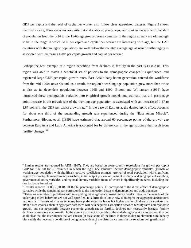
GDP per capita and the level of capita per worker also follow clear age-related patterns. Figure 5 shows

that historically, these variables are quite flat and stable at young ages, and start increasing with the shift

of population from the 0-14 to the 15-65 age groups. Some countries in the region already are old enough

to be in the range in which GDP per capita and capital per worker are increasing with age, but the LAC

countries with the youngest populations are well below the country average age at which further aging is

associated with increasing GDP per capita growth and capital per worker.

Perhaps the best example of a region benefiting from declines in fertility in the past is East Asia. This

region was able to match a beneficial set of policies to the demographic changes it experienced, and

registered large GDP per capita growth rates. East Asia’s baby-boom generation entered the workforce

from the mid-1960s onwards and, as a result, the region’s working-age population grew more than twice

as fast as its dependent population between 1965 and 1990. Bloom and Williamson (1998) have

introduced these demographic variables into empirical growth models and estimate that a 1 percentage

point increase in the growth rate of the working age population is associated with an increase of 1.37 to

1.87 points in the GDP per capita growth rate.4 In the case of East Asia, the demographic effect accounts

for about one third of the outstanding growth rate experienced during the “East Asian Miracle”.

Furthermore, Bloom, et al. (1999) have estimated that around 60 percentage points of the growth gap

between East Asia and Latin America is accounted for by differences in the age structure that result from

fertility changes.5,6

4 Similar results are reported in ADB (1997). They are based on cross-country regressions for growth per capitaGDP for 1965-90 for 78 countries in which the right side variables include demographic variables (growth ofworking age population with significant positive coefficient estimate, growth of total population with significantnegative estimate), human resource variables, initial output per worker, natural resource and geographical variables,governmental policy variables, and regional dummy variables (none of which is significantly nonzero, including theone for Latin America).5 Results reported in IDB (2000). Of the 60 percentage points, 11 correspond to the direct effect of demographicvariables while the remaining part corresponds to the interaction between demographics and trade openness.6 There are a number of problems with interpreting these aggregate cross-country results. Because the natures of theunderlying micro behaviors are not well-specified, it is difficult to know how to interpret the aggregate associationsin the data. If households in an economy have preferences for fewer but higher quality children or face prices thatinduce such choices, then in aggregate data there will be a negative association between fertility rates and economicgrowth, but not necessarily because economic growth causes fertility declines nor necessarily because fertilitydeclines cause economic growth. In the absence of specific models of the underlying behaviors, moreover, it is notat all clear that the instruments that are chosen (at least some of the time) in these studies to eliminate simultaneitybias satisfy the necessary condition of being independent of the disturbance terms in the relations being estimated.

8

1.2 Schooling Investments and Economic GrowthSchooling investments, the proximate determinants of which are households, are one of the most obvious

connections between household decisions at the micro level and economic growth. The economics

literature on growth often now includes some measure of human capital (proxied through schooling

indicators) in empirical and theoretical models. For instance, the "new neoclassical growth literature"

provides systematic aggregate theoretical models in which human resources generate positive

externalities to increase growth.7

Empirical Evidence on the Relation between Education Investments and Growth

The list of studies documenting the connection between schooling and GDP growth in Latin America is

quite large. Among the many studies, Barro (1991), IDB (1993), Benhabib and Spiegel (1994), Barro and

Sala-i-Martin (1995) and Behrman (1996) all find that initial measures of schooling are positively

correlated with the growth of GDP per capita in cross country regressions. Barro (1991) finds that higher

enrollment in 1960 is associated with higher growth of GDP per capita over 1960 to 1990. For Latin

America, IDB (1993) and Behrman (1996) explore whether the differences in 1965 in human resources in

the region from the levels predicted by real per capita income8 (hereafter "initial schooling" or “initial life

expectancies”) affect subsequent growth outcomes. Initial schooling is positively associated with

subsequent GNP per capita real growth, with an additional growth rate of about 0.35 percent for every

grade that initial schooling exceeded the level predicted by real per capita income. This means, for

example, that the difference between recent schooling controlling for per capita income of 3.8 grades for

Ecuador and -0.9 grades for Brazil all else equal would translate into a difference in future growth rates of

real GNP per capita of 1.6 percent per year. Thus this can be a considerable effect. Other estimates that

are presented and discussed in these sources indicate stronger relationships between more disaggregated

representations of initial schooling – such as the shares of primary or secondary -- and subsequent growth.

7 The origins of this literature are traced to Lucas (1988), who adapted the neoclassical growth model by addingexternalities, which permits permanent differences in per capita incomes across countries to be maintained. He alsoconsiders a model in which human capital only has external effects, with many commodities each with differentlearning-by-doing, and with international trade. He shows that such a model is consistent with very different levelsand rates of growth across countries, as well as sudden jumps in production patterns and growth rates in response tosmall changes in world prices. Azariadis and Drazen (1990) add technological externalities with a threshold propertyto Diamond's (1965) overlapping generations neoclassical growth model; within this model returns to scale canchange very rapidly and there can be multiple, locally-stable, balanced-growth equilibrium paths. Among theexternalities that they consider are labor-augmenting spillovers from human capital investments. For example, moreknowledge may make it easier to acquire still more knowledge, so that countries with high human resourceinvestments relative to their per capita income can experience subsequent periods of high sustained growth.8Note that controlling for the initial real per capita income means that the schooling indicators are not representinggeneral development to the extent that such development is associated with initial real per capita income.

9

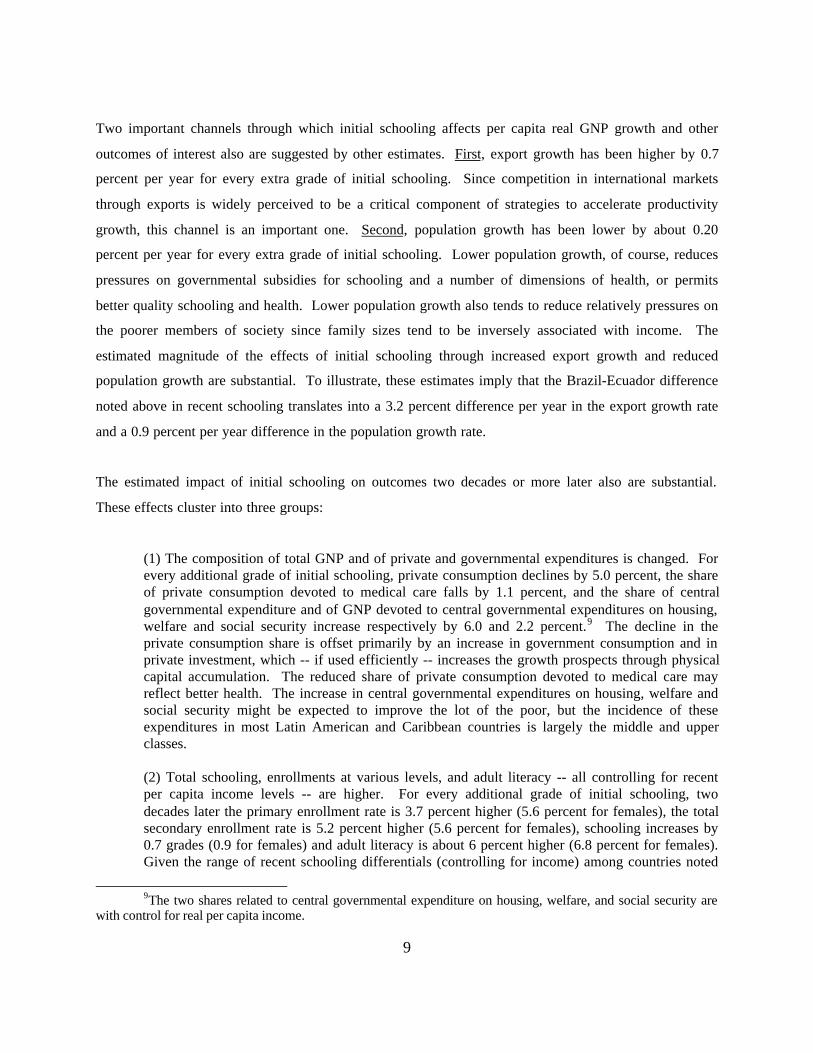
Two important channels through which initial schooling affects per capita real GNP growth and other

outcomes of interest also are suggested by other estimates. First, export growth has been higher by 0.7

percent per year for every extra grade of initial schooling. Since competition in international markets

through exports is widely perceived to be a critical component of strategies to accelerate productivity

growth, this channel is an important one. Second, population growth has been lower by about 0.20

percent per year for every extra grade of initial schooling. Lower population growth, of course, reduces

pressures on governmental subsidies for schooling and a number of dimensions of health, or permits

better quality schooling and health. Lower population growth also tends to reduce relatively pressures on

the poorer members of society since family sizes tend to be inversely associated with income. The

estimated magnitude of the effects of initial schooling through increased export growth and reduced

population growth are substantial. To illustrate, these estimates imply that the Brazil-Ecuador difference

noted above in recent schooling translates into a 3.2 percent difference per year in the export growth rate

and a 0.9 percent per year difference in the population growth rate.

The estimated impact of initial schooling on outcomes two decades or more later also are substantial.

These effects cluster into three groups:

(1) The composition of total GNP and of private and governmental expenditures is changed. Forevery additional grade of initial schooling, private consumption declines by 5.0 percent, the shareof private consumption devoted to medical care falls by 1.1 percent, and the share of centralgovernmental expenditure and of GNP devoted to central governmental expenditures on housing,welfare and social security increase respectively by 6.0 and 2.2 percent.9 The decline in theprivate consumption share is offset primarily by an increase in government consumption and inprivate investment, which -- if used efficiently -- increases the growth prospects through physicalcapital accumulation. The reduced share of private consumption devoted to medical care mayreflect better health. The increase in central governmental expenditures on housing, welfare andsocial security might be expected to improve the lot of the poor, but the incidence of theseexpenditures in most Latin American and Caribbean countries is largely the middle and upperclasses.

(2) Total schooling, enrollments at various levels, and adult literacy -- all controlling for recentper capita income levels -- are higher. For every additional grade of initial schooling, twodecades later the primary enrollment rate is 3.7 percent higher (5.6 percent for females), the totalsecondary enrollment rate is 5.2 percent higher (5.6 percent for females), schooling increases by0.7 grades (0.9 for females) and adult literacy is about 6 percent higher (6.8 percent for females).Given the range of recent schooling differentials (controlling for income) among countries noted

9The two shares related to central governmental expenditure on housing, welfare, and social security are

with control for real per capita income.

10

above with reference to the example of the difference between Ecuador and Brazil, thedifferences in schooling investments two decades later due to the differential initial schooling canbe considerable indeed. And these persistent positive schooling effects across the decades withtheir impact on economic growth and other factors mean that growth and human development candiverge among countries due to the initial schooling differentials.

(3) Fertility and mortality rates are lower, population is smaller with a smaller share of youngdependents, and life expectancies are higher.10 For every additional grade of initial schooling, 20-25 years later total fertility rates are 0.4 less, crude birth rates per 1000 are 2.4 less, infantmortality per 1000 live births falls by about 8, under-five mortality per 1000 live births falls from10 to 13 children (somewhat more for boys), the share of the population in the 0-14 age range is2.2 percent less and that in the 15-64 age range is 1.5 percent greater (so the dependency ratefalls), and life expectancy at birth increases by about 2 years. Given the range of recent schoolingdifferentials (controlling for income) among countries noted above with reference to the exampleof the difference between Ecuador and Brazil, once again the differences in demographicoutcomes and health 20-25 years later due to the differential initial schooling can be substantial.These induced demographic and health differentials are important in directly improving welfarein themselves, tend to be particularly important for those living in poverty, and -- similar to theschooling effects -- may have persistent ongoing positive impact on the development trajectory.

Not all econometric specifications show positive effects of schooling on growth. For example, Benhabib

and Spiegel (1994) and Pritchett (1996) present cross-country estimates in which the growth in GDP per

capita is regressed on growth in schooling attainment and report that the coefficient on education with

many specifications is negative (though often insignificant). While the data available on schooling

attainment are arguably of poor quality, measurement error probably is not the main source of the

specification error.11 This “perverse” result is likely the outcome of unobserved heterogeneity since

isolating the growth in schooling attainment from other conditions is extremely difficult. Countries in the

cross-section sample which have had much recent growth in schooling tend to be countries which had low

levels of schooling to begin with, a state that is correlated with other policies or conditions that are not

conducive to growth. These results, thus, are not inconsistent with the arguments and related micro

empirical evidence of those such as Welch (1970), Schultz (1975) and Rosenzweig (1995) who maintain

that returns to schooling are likely to be relatively high when there are new learning options due to

technological and market developments – conditions that have not been satisfied in much of the

developing world much of the time. Bils and Klenow (1998), finally, also question the large effects of

initial levels of schooling attainment on growth found in the standard regressions. They observe, as does

10Most of these effects occur whether or not there is control for per capita real income for the recent level variables.

11 Though Pritchett’s preferred measure of educational capital assumes the same constant rate of return for allschooling levels in all countries, which seems very peculiar in light of evidence presented by those such asRosenzweig (1995) that the returns to schooling are likely to be high where there are new technological or marketoptions, which hardly are uniform across school levels for all economies.

11

Pritchett, that while schooling attainment has increased nearly worldwide, growth rates have fallen in

most developing countries. Bils and Klenow use calibration to illustrate the possibility that the initial

level of schooling appears to have a positive effect on growth because the causality is at least halfway in

the reverse direction with anticipated GDP growth generating higher schooling.

With regards to studies at the micro level, there is a large literature that reports the impact of schooling

attainment on growth through its effects on wages and on economic productivity.12 Such estimates imply

that schooling, particularly at the primary level, is a very good investment both privately and socially in

Latin America and the Caribbean. However, the available estimates of the social returns to schooling in

the region do not incorporate externalities.13 If these are positive as often is claimed, the total returns to

schooling may be higher than the most careful present estimates suggest, perhaps with different effects for

different school levels. One possibly very important externality of higher levels of schooling, for

example, pertains to additions to knowledge. The impact of schooling quality on economic outcomes also

appears to be considerable, though available studies are few.

II. What Determines Fertility and Schooling Investment Decisions?

Now that we have established some of the connections between economic growth and fertility and

schooling investment decisions, we turn to the question of what factors influence the household decisions

underlying fertility and schooling investments. The factors that affect fertility and education also affect

growth indirectly through their effect on human resources, so they are also important for the growth

process. To simplify the discussion, we first draw on Behrman (1999) to discuss a simple framework for

the analysis. We then discuss findings from empirical investigations.

12 Behrman (1999) presents a thorough review of this literature. The available related empirical evidence of theeffects of schooling investments on growth at the micro level varies considerably in its coverage and in its quality.With respect to coverage, for instance, there are many studies that consider the impact of schooling, but relativelyfew consider other forms of education such as adult training programs. With respect to the quality of existingstudies, there are a number of estimation problems that are ignored in many existing studies. Therefore the existingempirical evidence has to be interpreted with care. Nevertheless, there seem to be some systematic patterns thatcome out of the analysis to date.

13 Very few studies do incorporate such externalities (at least effects that are external to families and households). Anotable exception is Foster and Rosenzweig’s (1995) study of agricultural technological diffusion in rural India, inwhich they present evidence that not only were there private benefits of more schooling through allowing farmers toadopt uncertain technologies at appropriate levels more quickly, but there were positive spillovers on otherneighboring farmers who learned more quickly because of the experience of the more-schooled farmers.

12

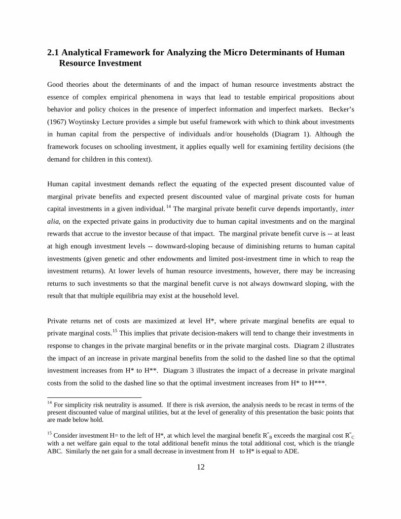
2.1 Analytical Framework for Analyzing the Micro Determinants of HumanResource Investment

Good theories about the determinants of and the impact of human resource investments abstract the

essence of complex empirical phenomena in ways that lead to testable empirical propositions about

behavior and policy choices in the presence of imperfect information and imperfect markets. Becker’s

(1967) Woytinsky Lecture provides a simple but useful framework with which to think about investments

in human capital from the perspective of individuals and/or households (Diagram 1). Although the

framework focuses on schooling investment, it applies equally well for examining fertility decisions (the

demand for children in this context).

Human capital investment demands reflect the equating of the expected present discounted value of

marginal private benefits and expected present discounted value of marginal private costs for human

capital investments in a given individual. 14 The marginal private benefit curve depends importantly, inter

alia, on the expected private gains in productivity due to human capital investments and on the marginal

rewards that accrue to the investor because of that impact. The marginal private benefit curve is -- at least

at high enough investment levels -- downward-sloping because of diminishing returns to human capital

investments (given genetic and other endowments and limited post-investment time in which to reap the

investment returns). At lower levels of human resource investments, however, there may be increasing

returns to such investments so that the marginal benefit curve is not always downward sloping, with the

result that that multiple equilibria may exist at the household level.

Private returns net of costs are maximized at level H*, where private marginal benefits are equal to

private marginal costs.15 This implies that private decision-makers will tend to change their investments in

response to changes in the private marginal benefits or in the private marginal costs. Diagram 2 illustrates

the impact of an increase in private marginal benefits from the solid to the dashed line so that the optimal

investment increases from H* to H**. Diagram 3 illustrates the impact of a decrease in private marginal

costs from the solid to the dashed line so that the optimal investment increases from H* to H***.

14 For simplicity risk neutrality is assumed. If there is risk aversion, the analysis needs to be recast in terms of thepresent discounted value of marginal utilities, but at the level of generality of this presentation the basic points thatare made below hold.

15 Consider investment H= to the left of H*, at which level the marginal benefit R=B exceeds the marginal cost R=

C

with a net welfare gain equal to the total additional benefit minus the total additional cost, which is the triangleABC. Similarly the net gain for a small decrease in investment from H≅ to H* is equal to ADE.

13

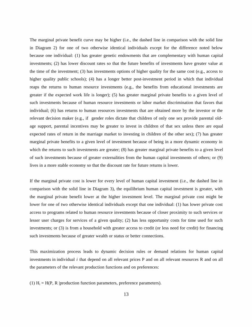
The marginal private benefit curve may be higher (i.e., the dashed line in comparison with the solid line

in Diagram 2) for one of two otherwise identical individuals except for the difference noted below

because one individual: (1) has greater genetic endowments that are complementary with human capital

investments; (2) has lower discount rates so that the future benefits of investments have greater value at

the time of the investment; (3) has investments options of higher quality for the same cost (e.g., access to

higher quality public schools); (4) has a longer better post-investment period in which that individual

reaps the returns to human resource investments (e.g., the benefits from educational investments are

greater if the expected work life is longer); (5) has greater marginal private benefits to a given level of

such investments because of human resource investments or labor market discrimination that favors that

individual; (6) has returns to human resources investments that are obtained more by the investor or the

relevant decision maker (e.g., if gender roles dictate that children of only one sex provide parental old-

age support, parental incentives may be greater to invest in children of that sex unless there are equal

expected rates of return in the marriage market to investing in children of the other sex); (7) has greater

marginal private benefits to a given level of investment because of being in a more dynamic economy in

which the returns to such investments are greater; (8) has greater marginal private benefits to a given level

of such investments because of greater externalities from the human capital investments of others; or (9)

lives in a more stable economy so that the discount rate for future returns is lower.

If the marginal private cost is lower for every level of human capital investment (i.e., the dashed line in

comparison with the solid line in Diagram 3), the equilibrium human capital investment is greater, with

the marginal private benefit lower at the higher investment level. The marginal private cost might be

lower for one of two otherwise identical individuals except that one individual: (1) has lower private cost

access to programs related to human resource investments because of closer proximity to such services or

lesser user charges for services of a given quality; (2) has less opportunity costs for time used for such

investments; or (3) is from a household with greater access to credit (or less need for credit) for financing

such investments because of greater wealth or status or better connections.

This maximization process leads to dynamic decision rules or demand relations for human capital

investments in individual i that depend on all relevant prices P and on all relevant resources R and on all

the parameters of the relevant production functions and on preferences:

(1) Hi = H(P, R |production function parameters, preference parameters).

14

The prices include all prices that enter into the investing household’s decision-making process, including

the prices paid by the household for human resource investments, other uses of household resources and

for transferring resources over time (i.e., the interest rate) and for insuring against uncertainty. At the

time that any human resource investment decision is made, these prices include all past and current prices

(perhaps embodied in current stocks of human capital), as well as expected future prices (including

expected future returns to human capital investments). The resources include all resources of the

individual, household (identified by ownership if there is intrahousehold bargaining), educational and

health/nutrition institutions, and community that affect any household decisions. These resources include

human resources that reflect past investments, financial resources, physical resources, genetic

endowments, and general learning environments.

This simple framework systematizes six critical, common sense, points for investigating dimensions of

the determinants and the effects of human capital investments.

First, the impacts of changes in policies may be hard to predict by policymakers and analysts. If

households face a policy or a market change, they can adjust all of their behaviors in response, with cross-

effects on other outcomes, not only on the outcome to which the policy is consciously directed.

Second, the marginal benefits and marginal costs of human capital investments in a particular individual

differ depending upon the point of view from which they are evaluated: (i) There may be externalities or

capital/insurance market imperfections so that the social returns differ from the private returns and (ii)

there may be a difference between who makes the investment decision (e.g. parents) and in whom the

investment is made (e.g. children) that raise intergenerational distributional issues.

Third, human capital investments are determined by a number of individual, family, community and

(actual or potential) employer characteristics, only a subset of which are observed in social science data

sets such as are available to analyze human resource investments determinants and effects. To identify the

impact of the observed characteristics on human capital investments, it is important to control for the

correlated unobserved characteristics).

15

Fourth, to identify the impact of human capital investments, it also is important to control for all

individual, family, and community characteristics that determine the human capital investments and also

have direct effects on outcomes of interest.

Fifth, empirically estimated determinants of and effects of human capital investments are for a given

macro economic, market, policy, and regulatory environment in which there may be feedbacks both at the

local and at a broader level. What is of interest from a policy perspective, at least from an efficiency

perspective, is the nature of markets and the policy environment. The nature of the policy environment, in

turn, may depend importantly on political economy considerations such as those that have been examined

in recent studies by Fernandez and Rogerson (1995a,b, 1996, 1997a,b, c), and Biswal (1998).

Sixth, for any individual the generic framework for human resource investments remains the same over

the life cycle, but the particular details and context are likely to vary over the lifecycle. For example,

investments in infants and small children are likely to be determined directly by parents, or other

household members, perhaps reflecting some bargaining within the household over resource allocations,

with the family or the household acting within a given market and policy environment and with a

relatively long time horizon for returns to such investments (though perhaps with substantial discounting

of the returns if the investors (e.g., parents) perceive that they will receive only a portion of the returns).

Initial investments in an individual are primarily in nutrition and health, with preschool education and

then formal schooling likely to become of increasing importance as the child ages. As the individual ages

further, s/he is likely to make ever more of the investment decisions and to expect to reap more of the

returns from such investments her/himself in light of the market and policy environment that s/he faces

directly, but the expected time horizon for such returns also declines with age at least eventually. At

some point in the life cycle the expected marginal benefits from further formal schooling are likely to

decline below the marginal costs, so education shifts from formal schooling to learning from experience

and training programs. As the individual ages further, the returns from earlier investments are realized in

labor and marriage and other markets, providing new information as well as further constraints that affect

further decisions. Many individuals enter into new familial arrangements and, with intrahousehold

bargaining over resources, make further human resource decisions some of which may result in children

and in investments in those children. As they age still further, the incentives for ongoing human resource

investments in themselves tend to decline because of the shortening remaining expected lives and their

children tend to become ever more independent. At the same time there may be increasing returns from

using resources for health problems related to aging, and individuals may have decreasing control over

16

decisions regarding their welfare and other family members and institutions may have increasing control.

Such considerations mean that the importance of different human resource investments in the aggregate

are likely to change substantially as the age structure of the population changes in the process of the

demographic transition.

Estimation Issues derived From the Framework

Estimation of the demands for human resource investments in relation (1) that are sensitive to these

considerations can be informative. For example, how responsive are human resource investment

decisions to the prices of resources or programs for human resource investments? How important are

incomplete markets, particularly for capital and insurance? Do limitations in such markets mean that

individuals from poorer backgrounds face relatively severe constraints on human resource investments

because their families have very limited resources for self-financing human resource investments and can

not readily finance human resource investments through capital markets? What role do information

imperfections play in the household human resource investment decisions? Are there important

interactions between household characteristics and program characteristics?

Embedded in the framework for human resource investments are a number of production functions. The

assessment of the direct impact on specific outcomes (as opposed to the total impact in relation 1) of some

important determinants including policies may be attained by estimating these relations. For example,

consider a production function for cognitive achievement CA i for the ith child depending on pre-school

human resource investments (PSi), ability (Ai), health (Hi), nutrition (Ni), school quality (Qi), time in

school (Si), family background characteristics (Fi) and other factors:

(2) CAi = CA(PSi, Ai, Hi, Ni, Qi, Si, Fi ...).

There are a number of important questions about this production process. For example, how much do

resources devoted to human resource investments and other educational programs improve cognitive

achievement? Are resources devoted to schools more effective in their impact on cognitive achievement

if a student has better health and nutrition? Greater abilities? Comes from a better family background?

The implied relations for investigating the determinants of family behaviors related to human resource

investments and the impact of such investments are (i) to estimate directly the underlying structural

relations that determine human resource investments or their impact (e.g., human resource and wage

17

production functions analogous to relation 2) and (ii) to estimate dynamic decision rules or demand

relations for human resource investments or for inputs used to produce human resource investments or for

their impact (e.g., expressions that are analogous to relation 1).

Structural Relations -- Production Functions: Structural relations are the basic underlying relations in the

models of family behaviors represented above. The most commonly-estimated structural relations are

production functions. A linear or log-linear approximation to a general production function of the type

discussed in relation (2) with, for example, cognitive achievement (CAi) produced by two categories of

variables relating to the ith individual and his/her household (XI) and to the sth school (XS) and by an

explicit stochastic disturbance term (Ui) is:16

(2A) CAi = aXIXI + aXSXS + Ui.

The stochastic term captures random events that are not correlated with any of the other predetermined

right-side variables. Generally each of the types of variables may be a vector that represents a whole set

of variables. It is useful for consideration of estimation issues to distinguish among four different

subgroups of variables: the superscripts “o“ and “u“ refer to “observed in the data used“ and “unobserved

in the data used“, the superscript “b“ refers to variables that are behaviorally-determined within the model

used, and the superscript “p“ refers to variables that are predetermined within the model used so that the

variable list in the general production function relation is XIob, XIub, XIop, XIup, XSob, XSub, XSop, XSup,

Ui. If these were substituted into (2A) each would have its own coefficient “a“ with an appropriate

superscript to indicate its impact on CAi. The distinctions among these different variables are important

because some of the most important and most pervasive estimation problems arise from unobserved

variables or behaviorally-determined variables.

The parameters (a’s) in the production function give the direct impact of the right-side variables, some of

which may reflect directly policies. With good estimates of the appropriate production functions the direct

16 Linear approximations are used here because they are the simplest forms but they still permit characterization ofvarious estimation issues. Log-linear forms in which all of the variables are replaced by the logarithms of theirvalues (which implies interactions among all the right-side variables) are identical in representation once thevariables are redefined. In empirical studies linear and log-linear specifications are very common, but otherfunctional forms also are used at times. For other functional forms the essence of the estimation issues is the same.If the functional form that is used is not a good approximation to the true functional form, there is misspecificationerror that is akin to omitted variable bias discussed below (with the unobserved variable being the variable thatwould have to be added to transform the assumed specification to the true functional form).

18

determinants of many outcomes determined by household behaviors and the direct impacts of many

human capital investments could be evaluated with considerable confidence to answer many of the

questions raised above. Good production function estimates may be difficult to obtain, however, because

of estimation problems that are noted briefly below.

19

Reduced-Form Dynamic Decision Rule or Demand Relations: A second set of relations that can be

estimated to explore the determinants of and the impact of family and firm behaviors and of policies

related to human resource investments are dynamic decision rules or “demand” relations. These relations

give some behavioral outcome in the current period as dependent on all predetermined (from the point of

view of the entity making the decisions) prices and resources and on the parameters in the underlying

production functions and preferences. These are the relations that most commonly are estimated. These

demand functions in principle are derived explicitly from the constrained maximization behavior of

families (or from the constrained maximization behavior of other entities such as the providers of services

related to human resources). As such they incorporate all of the underlying structural parameters that are

involved in that process. But all of the choice variables during the period of interest are substituted out,

so the demand functions are so-called reduced-form relations because the maximizing behavior that

determines such variables has been combined and “reduced” to the relations that give the behavioral

outcomes as a function of purely predetermined and expected prices and resources and of the underlying

preferences and technologies. In some empirical studies the underlying structural parameters can be

identified from estimation of the demand relations. In most cases, however, demand functions are just

posited to result from constrained maximization and the underlying structural parameters are not

identified in the estimates, though the demand parameters still are some combinations of these

parameters. In such cases demand functions permit the estimation of the total effects of predetermined

variables on the behavioral variables of concern, but not estimation of the exact mechanisms through

which preferences and production function parameters act.

On a general level demand functions can be written with a vector of behavioral outcomes (Z) dependent

on a vector of prices broadly-defined (P) and a vector of resources (R). If there are uncertainties

regarding relevant future prices, policies and shocks, then the characteristics known at the time of the

decision of interest regarding the distributions of those outcomes should be included. A linear

approximation for a family facing prices PF and with resources RFf and a vector of stochastic terms (Vf)

is:

(1A) Zf = bPFPF + bRFRFf + Vf.

The stochastic term in each relation includes all the effects of all the stochastic terms in all of the

production activities in which the family (or other investor) is engaged (i.e., all of the elements of the

vector Ui), plus perhaps other chance events. Both prices and resources may be observed or unobserved

20

in the data, so it is useful to indicate that distinction here as above in the discussion of production function

inputs (again, using superscripts “o” and “u”). There is one such demand relation (or one element in the

vector Zf) for every behavioral outcome of the family (and similarly for firms or other entities), including

all human resource investments and all behavioral inputs that affect human resource investments through

production relations such as (2A). Each of these demand relations conceptually includes the same

identical right-side predetermined variables so that any predetermined variable that affects any one

behavioral outcome may affect all other behavioral outcomes.

Conditional demand functions: Conditional demand functions, as contrasted with the unconditional ones

in relation (1A), include among the right-side variables some variable(s) that are determined by the

behavioral model for the decision-making unit under examination. If the included behavioral variable(s)

on the right side is determined at least in part by past behavior(s), its effect(s) may be estimated in such

relations by including its start-of-the current period value(s) instead of the past prices, resources and

stochastic terms that determine this value.17 In such a case, the start-of-the-period stocks of different

human resources are just other right-side variables that are predetermined with respect to current prices

and (other) resources in the demand relation in (1A). That relation also includes all of the current prices.

An unbiased estimate of the coefficients of the stocks of different human resource investments gives the

impact of the start-of-the-period stocks of ith’s human resources on, for example, the current-period

cognitive achievement. That the start-of-the-period stocks of human resources were determined by past

behavior poses some estimation problems discussed below, but the interpretation of unbiased coefficients

of these variables as reflecting their impact on current cognitive achievements is clear.

Estimation issues: There are a number of possible problems in obtaining good estimates of the

determinants of and the impact of human resource investments and the role of policies. Therefore what

are presented as estimates of relations such as those that are discussed above may be biased and therefore

difficult to interpret for understanding behaviors or for policy guidance. These estimation problems share

a common characteristic: the disturbance term in the relation actually estimated is not simply an element

in Ui or Vf that is distributed independently of all the right-side variables in the relation being estimated,

but instead is correlated with right-side variables (e.g., because it is a compound disturbance term that

17 It is not possible, however, to estimate persuasively the effect of one behavioral variable determined in

the current period on another with demand relations. The basic problem is that there is not, except through anarbitrary exclusion or functional form assumption, to identify in the statistical sense the current period behavioralvariable that appears on the right side of the relation because in general it depends on exactly the samepredetermined variables as does the dependent variable.

21

includes unobserved variables as well as Ui or Vf or because of the way that Ui or Vf is defined for the

sample used in the estimates). Perhaps the most important problems in these estimations are omitted

variable bias, simultaneity, selectivity and measurement error. These problems and possible resolutions

are not discussed here (Behrman 1999 provides a somewhat extensive discussion and reference to other

studies that are concerned with these issues). But it is important to recognize that how reliable is what we

think we know from estimation of relations such as are discussed in this section depends on how well

these estimation problems are dealt with in empirical studies.

2.2 Determinants of Schooling Decisions

This section reviews selected empirical studies from Latin America and the Caribbean that address the

macro and microeconomic determinants of household schooling investments.

Micro Determinants of Schooling Investments

Family background: There is general agreement that family background is important in determining

schooling, but perhaps with diminishing effects over time and with greater market liberalization. Studies

for Brazil, Nicaragua, Peru, and Panama report significantly positive effects of parental schooling on

child schooling (Birdsall 1985, Heckman and Hotz 1986, King and Bellew 1988, Wolfe and Behrman

1987). The estimated magnitudes range from an additional 0.1 to 1.1 grades of schooling attainment for

children for every additional grade of schooling of the parents. Generally these estimates suggest a

stronger association with maternal than with paternal schooling. The Nicaraguan estimates, moreover,

suggest that in such estimates parental schooling is representing in part unobserved dimensions of family

background rather than the effect of schooling itself; in standard estimates the coefficient of maternal

schooling is 0.45, but it drops to 0.11 with adult sibling control for unobserved childhood family

background characteristics that are shared by sisters growing up in the same household. Both the

estimates for Peru and for Panama indicate diminishing effects of parental schooling over time. For Peru,

for instance, the impact on females (males) of an additional year of mother's school was 0.33 years (0.29)

for the 1925-39 birth cohort and 0.12 (0.18) for the 1960-1966 birth cohort, and parallel estimates for

father's schooling are 0.13 (0.25) and 0.07 (and 0.10) years. These results suggest that the expansion of

public schooling weakened the intergenerational links over time.

Family income (or proxies therefore) generally has a significant positive effect on schooling of children in

studies for Brazil, Chile, Nicaragua and Peru (Behrman and Wolfe 1987a,b, Birdsall 1985, Farrell and

Schiefelbein 1985, and King and Bellew 1988). Estimates for Brazil, for example, imply that child

22

schooling attainment increases by about 5-8 percent for a 10 percent increase in income. Within the

above framework, income enters into human resource investment determination only if capital market

access is positively associated with income, or if household discount rates are negatively associated with

income (because the pressure of poverty means that immediate survival takes precedence over

investments), or if schooling is in part consumption rather than just investment. That income often is

significant in estimated schooling attainment relations suggests that at least one of these factors is

relevant. This is important since imperfect capital markets are one reason that policy interventions to

support human resource investments may be warranted on efficiency grounds. However in part income

appears to be representing other dimensions of family background or of the community, such as the

quality of local schools, since the estimated impact of income declines substantially with control for

unobserved family background using adult sibling data or with control for the quality of local schools.

The Peruvian estimates, the only ones for which separate estimates are given by birth cohorts, also

suggest a declining income effect over time, again probably because of the expansion of the schooling

system.

Behrman, Birdsall and Szekely (1999) explore some dimensions of the strength of the association of

family background with child schooling and whether the strength of this association is related to some

major macro and aggregate school policy variables. First, they present arguments about why family

background might be associated with schooling and how that association might depend on market reforms

and on public schooling policies within a framework for the determination of child schooling that is

parallel to that presented in Section 2.1 above, but with emphasis on how market liberalization and other

macro changes are likely to feed back on micro schooling decisions. Then the extent of child schooling

gaps overall and across parental schooling quintiles and child age groups are described and the empirical

associations of family background with schooling are estimated for children aged 10-21 in Latin America

based on micro data from 28 household surveys from 16 countries for the 1980-1996 time period for 559

subsamples. Based on these estimates two indices of intergenerational schooling mobility are constructed

and used to explore to what extent intergenerational schooling mobility is associated with basic macro

economic and aggregate schooling indicators. The empirical estimates have three important implications:

(1) They are consistent with family background having significant associations with schooling gaps

(defined with reference to how much schooling a child would have if s/he started at age six and advanced

one grade each year) accounting on the average for about a sixth of those gaps, though with differences

across countries, across time, across parental schooling quintiles (being more important for parents with

less schooling), and across child age groups (being more important for children in their late than in their

23

early teens). (2) They suggest that macro conditions “in particular those related to the extent of internal

market development” importantly shape intergenerational schooling mobility. (3) They suggest that

aggregate school policies that are directed towards increasing resources available for basic schooling in

general and for improving school quality in particular have important positive impact on intergenerational

schooling mobility, though other educational expenditures such as those on tertiary education may

reinforce the impact of family background and reduce intergenerational social mobility. Thus, even

though the immediate effects of macro market reforms and schooling policy reforms on current income

distribution may not have been that strong in the region, there may be important longer-run effects

through increasing intergenerational social mobility.

Capital markets: One channel through which family background may affect schooling and other human

resource investments within the above framework is through altering access to capital markets, or perhaps

the importance of such access because this depends on the extent to which the household can self-finance

such investments. While analysts often refer to capital market imperfections as reasons for policy

interventions to subsidize human resource investments, there are very few studies that address this

possibility in ways that identify the role of family background being because capital markets are

imperfect rather than a myriad of other possibilities such as through home learning environments and

through intergenerational genetic transmission of learning and preference endowments. Jacoby (1994)

investigates the effect of borrowing constraints on the timing of human capital investments in Peru by

considering how quickly children with different family backgrounds progress through the primary school

system using the 1985/6 Peruvian Living Standards Survey. He develops an explicit model of parental

investment in child schooling that is consistent with the framework described above. Within this model if

there is no credit rationing, children attend schooling full time until they quit with the optimal schooling

investment H*. If there is a binding credit constraint, however, consumption-investment decisions are not

separable because the borrowing constraint increases the cost of consuming today versus tomorrow, so

part-time school attendance may be optimal. Therefore, if the probability of a binding credit constraint is

inversely associated with family income, the probability of part-time rather than full-time school

attendance will be inversely associated with family income. For a given family income in a household

that is facing a binding credit constraint, moreover, the model predicts that children will start leaving

school when younger the smaller is the age gap between siblings -- a prediction that Jacoby maintains

would not come out of models that focused on other aspects of family background.18 His estimates

18 Though he does not incorporate explicitly endogenous fertility decisions and child quantity-quality tradeoffs intohis model. An extended model that incorporated such aspects of household behaviors might be consistent with hisestimates if there are market imperfections other than for capital, such as for innate abilities that are transferred

24

indicate that, indeed, children start withdrawing from school earlier, as indicated by grade repetition, in

households with lower income and lower durable assets and for children who are more closely spaced.

They also indicate that higher family income and durable good holdings do not significantly enhance

school progress in households that are predicted not to be constrained by capital markets (because they

have positive savings), but do so in households that are predicted to be constrained by capital markets.

This study thus presents an innovative systematic approach that is consistent with family background

reflecting capital market constraints in schooling investment decisions, thus leading to intergenerational

correlations in human resources, earnings and poverty and an important role of demographic outcomes in

other human resource determinants at the micro level.

School access and quality: Limited evidence suggests that households, rich and poor alike, value highly

schooling access and quality improvements: Gertler and Glewwe (1990) use the cost of travel time and of

time not working while in school to infer price elasticities for the demand for secondary schooling in rural

Peru. Their estimates indicate that price elasticities increase as prices rise and that the price elasticities do

not differ much by income except that they are lower for the top quarter by income than for the lower

three-quarters. Within the sample the price elasticities for the lower three quarters of the households

increase from about 0.1 to about 0.4 as prices increase, while those for the highest quarter of households

are about 0.1 for all prices. This means that if school costs to households increase ten percent, enrollers

from the bottom three quarters of households would decline by 1-4 percent (depending on how high was

the initial price) and those from the top quarter of households would decline by about 1 percent.

Therefore the enrollment declines induced by increased prices would be fairly limited (particularly

starting from initial low prices), but would be regressive in that they would be less for the top quarter of

households by income than for others. Note that this does not mean that poor households would be better

off if enrollment of their children were less affected by price changes. To the contrary their relatively

high price elasticities mean that they apparently can substitute more easily than would be indicated by

lower price elasticities between schooling and other resource uses.

Also the price elasticities alone do not tell if households are better or worse off with a policy that

increased schooling fees and used the fees to improve the quality of schools or to expand the number of

schools. Therefore the study estimates whether households living in areas without a local secondary

school would be willing to pay enough to cover the costs of having a local school. The estimates suggest

that households at all income levels are willing to pay more than the costs of operating a new school to

intergenerationally through genetics, that affect schooling investments and are associated with income.

25

reduce travel time from two hours to zero, though no households are willing to pay enough to cover the

costs of operating a new school to reduce travel time from one hour to zero. Though the analysis is crude,

it suggests that the welfare of residents in villages that are fairly remote (from secondary schools) would

improve with local secondary schools even if they had to pay the full costs of such schools.

Some specific measured inputs have limited impact on school achievement but considerable

improvements in the effectiveness of schools may be possible if appropriate incentives are instituted:

Some evidence exists that a few specific school characteristics affect schooling attainment (i.e., grades of

school) or school achievement (i.e., cognitive achievement scores) in Latin America and the Caribbean.

In Nicaragua, textbook availability has an important impact on learning mathematics, particularly in rural

areas (Jameson et al. 1981). In Peru, the number of grades offered in a school and secondarily the

availability of reading and/or math books increased significantly the years of schooling for most cohorts

of females and males (King and Bellew 1988). For Brazil, studies suggest that the quality of teachers

(measured by their schooling or salaries) positively affects school attainment as is suggested by the

framework (Birdsall 1985), and the availability of basic textbooks and instructional material and better

school facilities improves cognitive achievement (Armitage et al. 1986, Harbison and Hanushek 1992).

There also are important regional variations in Brazilian schooling quality that are associated with

regional variations in schooling attainment, though quality improvements may induce more -- or less --

schooling of children in poor households (Box 4.1 by Ricardo Paes de Barros, et al. in Behrman 1996).

For example, some quality improvement such as public provision of transport to school and of school

material are likely to induce more schooling in poor households because they release family resources,

but others such as those that demand complementary home inputs that are in short supply in most poor

households may place additional demands on poor households and reduce enrollments from poor families.

For Nicaragua, the extent of decentralization of schools significantly affects students’ test performance,

with better performance in schools in which more decisions are made locally (King and Özler 1998).

But what is striking about the currently available empirical evidence is how little really is known about

what specific characteristics of schools improve schooling achievement. A recent summary by Hanuschek

(1995) of 96 studies of educational production functions for developing countries highlights this point.

Macro Determinants of Schooling Investments

In a recent paper, Behrman, Duryea and Székely (1999c) use data for 18 LAC countries to assess the

effects of aggregate conditions on schooling attainment. Household survey data are used to construct a

26

quasi panel with information on attainment for birth cohorts born between 1930 (who were around 65

years of age in the mid 1990s) and 1970 (who were about 25 years old in the mid 1990s and generally

beyond school age), which was merged with aggregate data. This data set contains more detailed and

higher quality data on schooling than that published in international sources such as UNESCO that have

been widely used for aggregate studies of schooling. It permits combining cohort-specific data and time-

varying aggregate data for periods in which cohorts were making marginal schooling decisions.

The paper documents that on average, there was an increase of 4.6 grades of schooling in 18 LAC

countries between the cohort born in 1930 and their counterparts born in 1970. The largest increases were

in Mexico, Dominican Republic, Chile, Ecuador, Bolivia and Venezuela, for all of which there was a gain

of more than five grades during the period. The smallest changes were in Jamaica, Paraguay, Brazil and

Nicaragua, all with less than four grades. In contrast, the average grades of education increased by 6.8 and

6.5 grades in Korea and Taiwan, respectively, during the same period. Schooling progress in LAC was

considerably greater for the generations born between 1930 and 1950 -- a gain of 2.7 grades – than for

those born between 1950 and 1970 -- a gain of 1.9. The slowdown appears to be steeper in Honduras,

Dominican Republic, Venezuela, and Panama, where progress for cohorts born between 1930 and 1950

was more than 1.5 grades greater than for those born in the following two decades. Korea also had a much

greater apparent increase between the 1930 and 1950 birth cohorts (4.3 grades) than between the 1950

and 1970 birth cohorts (2.5 grades).

Figure 6 plots schooling attainment for Taiwan and the average LAC country, respectively, for all cohorts

born between 1930 and 1970.19 The figure shows that on average, LAC and Taiwan had very similar

levels of schooling among cohorts born before 1940, but from this year on, progress in Taiwan was much

faster. Thirty years later, cohorts in Taiwan were registering attainment levels almost 50% greater than

the average LAC country. The figures also show the slowdown in LAC for the 1960-1970 birth cohorts.

Cohorts born in these years were making marginal schooling decisions approximately between 1975 and

1986, which coincides with the early years of the debt crisis in the region. The figure also plots a line with

the trend in LAC from 1940 to 1960. Had the same trend continued for cohorts born after 1960, the

average grades of schooling for the last cohort would have been close to 10 grades, rather than around

8.5.

19 The LAC pattern was obtained by pooling all the information on the average grades of schooling by year of birth,for all 18 countries and estimating a country fixed-effects regression using the average schooling of each cohort asthe dependent variable and dummy variables for each year as the right-side variables. The Figure plots thecoefficients for the year dummies. For Taiwan, the same regression with OLS is estimated, and the year dummiesare plotted.

27

This paper tests whether aggregate conditions in a country affect schooling investment decisions by

shifting the marginal private benefit and marginal private cost curves for micro household decisions

relating to schooling investments. The main features of the aggregate economic environment that are

examined are:

• Macroeconomic shocks: In a world with perfect and costless credit and insurance markets,unexpected shocks are not likely to affect long-term investments such as schooling. However, in thepresence of liquidity constraints, uncertainty and lack of insurance or costly insurance, individualsfacing shocks have to reallocate their resources to absorb shocks. A negative shock in such a caseeffectively increases the private marginal costs of schooling by shifting the curve in Diagram 3 fromthe dashed line to the solid line, thus reducing the equilibrium level of schooling investments. Ifhouseholds are risk adverse and can not insure costlessly, moreover, greater uncertainty due to greatermacro fluctuations reduces their private marginal benefits in utility terms, which is equivalent to ashift from the dashed to the solid line in Diagram 2, again reducing the equilibrium level of schoolinginvestments. When physical capital assets can be used as a buffer stock, individuals may be able toprotect long-term investments in schooling. But in their absence, the reallocation of householdresources may lead to a reduction in schooling investment. If reductions or interruptions in schoolinghave effects on subsequent attainment, shocks can have long lasting effects even if they are onlytemporary phenomena. This may be the case because of the vital role of age in the schooling process.Generally, as a child ages the opportunity cost of not working increases. In addition, children whoare behind their peers in grade achievement may become discouraged and drop out. Also, the hightransaction costs of entering and exiting from schooling may preclude or delay re-entry of dropouts.Such factors frequently are alleged to be of considerable importance in LAC. There is some limitedevidence from a few mostly micro studies for developing countries that shocks to household incomeaffect schooling investment significantly precisely due to liquidity constraints and the absence ofinsurance mechanisms (Chiu 1998, Duryea 1998, Flug, et. al. 1996, and Jacoby and Skoufias 1997).

• Availability of resources to finance investment: In investment models of schooling if markets areperfect, parental income has no effect on schooling (Becker 1964, Ben-Porath 1967, and Heckman1976). However if access to credit is conditional on parents’ income then that income may affectinvestment in children’s schooling. Recent empirical estimates that incorporate a range of aspects ofschooling (e.g., age of starting schooling, rate of progress through grades, and cognitive achievementin addition to schooling attainment) and use representations of long-run income find strongerassociations between child schooling and parental income than in the previous literature (e.g.,Behrman and Knowles 1999). Consumption models of schooling also predict a positive correlationbetween permanent parental income and children’s schooling if child schooling is a “normal” good.If access to credit markets is conditional on parental income, higher household income due to bettermacro conditions lessens the capital market restrictions on schooling investments effectively byshifting the private marginal cost curve in Diagram 3 from the solid to the dashed line, thus increasingthe equilibrium level of schooling investment. If schooling is partly consumption and is a normalgood, higher household income due to better macro conditions shifts the marginal private benefitcurve up, as from the solid to the dashed line in Diagram 2, increasing the equilibrium level ofschooling investment. Public expenditures in education and public infrastructure also reduce theprivate marginal cost of acquiring education and increase the equilibrium level of attainment becausethey complement household resources.

28

• Factor endowments, trade openness and returns to schooling: Factor endowments determineproduction structures and therefore the demand for different kinds of skills, the returns to education,and the incentives to invest in education. Substantial natural resources, for example, are alleged tolead to production structures in which the returns to broad education are limited, though the returns tosome forms of specialized technical education (e.g., mining engineering) may be high. If so, thensubstantial natural resources lead to private marginal benefit curves more like the solid one inDiagram 2 than like the dashed one, thus in itself leading to a lower level of equilibrium schoolinginvestment than were the production structure are less based on natural resource riches. As noted bySpilimbergo, Londoño and Székely (1999), however, the demand and price paid for the income-earning assets owned by individuals (including education) are affected not only by the scarcity orabundance of factors of production in each country, but also by the extent to which the country isexposed to international trade. If a country opens up to trade, its production factors compete moredirectly with those of other countries, and the rewards paid to them change. In the case of schooling,we would expect that if a country opens up to trade there will be more incentives to acquire educationbecause trade openness generally involves more rapid changes in technology and in capital, whichhave positive effects on the returns to education (e.g. Rosenzweig 1995). Therefore trade opennessand other forms of deregulation in themselves are likely to lead to private marginal benefits such asthe dashed rather than the solid line in Diagram 2, implying a higher level of equilibrium schoolinginvestment than in a more closed and regulated economy ceteris paribus. However, if the returns toeducation increase and there are better labor market opportunities, the opportunity cost of spendingtime in school increases, with possible negative implications on attainment; in terms of Diagram 3 theprivate marginal costs are higher (e.g., the solid line rather than the dashed line) due to greateropportunity costs of time in a more open economy. Overall, the net effects of changes in factorendowments and trade openness, thus, are ambiguous.

• Age structure: As the demographic transition progresses, first the young dependency ratio increasesand then it falls. This changes the relative resources per child that are available for schooling thatmight be manifested in first decreasing and then increasing school quality as reflected, for example, instudent-teacher ratios. 20 The lower the young dependency rates and the smaller the cohort, therefore,the larger the expected attainment. A lower young dependency ratio, thus, may be reflected in higherschooling quality for given private costs (and thus the dashed rather than the solid private marginalbenefits curve in Diagram 2) or lower private marginal costs for a given level of schooling quality(and thus the dashed rather than the solid private marginal cost curve in Diagram 3), both of whichlead to higher equilibrium levels of private schooling investment.

• Urbanization, changing prices and child time use: With urbanization there typically are at least threeimportant price changes relevant to children’s time use. First, the value of child labor usually isrelatively high in predominantly agricultural activities on family farms but tends to decrease withshifts in production structure associated with urbanization, so the opportunity cost in terms offoregone labor activity to attend school declines. Second, the costs of providing schooling typicallyare lower in urban areas than in rural areas due to lower transportation costs and greater economies ofscale. Third, the expected returns to education are normally larger in urban areas, creating more

20 Behrman, Duryea and Szekely (1999a) present evidence of significant increases in public educationalexpenditures per school-age child as youth dependency ratios fall due to population aging based on aggregate datafrom 164 countries for 1950-1995. There is some controversy about how important are class sizes (e.g., Hanushek1995, Kremer 1995). But two recent papers with evidence on the negative effect of class size on attainment areAngrist and Lavy (1999) and Krueger (1999). Lazear (1999) also presents an interesting argument about why inequilibrium students may be selected so that true inverse effects of class size on student achievement are difficult todiscern.

29

incentives to acquire schooling in urban settings. For these reasons urbanization is expected to bepositively associated with higher enrollment and attainment. The first two effects are manifested inprivate marginal costs being lower in urban than in rural areas (i.e., the dashed rather than the solidline in Diagram 3). The third is manifested in the private marginal benefits being higher in urban thanin rural areas (i.e., the dashed rather than the solid line in Diagram 2).

• Health: Health can affect attainment through at least three channels. First, as health conditionsimprove and life expectancies increase, people will perceive increased probabilities of their childrensurviving to adulthood so they can achieve their desired family size with fewer births and allocatemore resources to each child.21 Second, better health permits children to learn more in school andthus increases the returns to time spent in school. Third, increases in life expectancies increase thepotential years of labor market participation, which in turn increases the returns to investments inschooling. Thus, improvements in health are expected to be associated with improvements inschooling attainment by effectively increasing the private marginal benefits through complementaryhousehold investments and through higher expected post-schooling returns, as in the dashed ratherthan the solid curve in Diagram 2.

• Cultural patterns, religious beliefs, and traditional values: Religious beliefs and cultural patternsinfluence time allocations between home and markets and within the household. Thereby they have alarge influence on schooling decisions, in some cases with large differences by gender. Within LAC,Catholicism has dominated since the European conquest and settlement, but Protestantism and non-Christian religions have grown relatively rapidly in recent decades. Cultural patterns, religious beliefsand values that allow, for example, for greater participation of females in labor markets are likely tobe associated with higher private marginal benefits of schooling investments in females (the dashedrather than the solid curve in Diagram 2) and lower private marginal costs at least in utility terms (thedashed rather than the solid curve in Diagram 2) and thus increase the equilibrium level of schoolinginvestment.

• Institutions: Differences in quality, emphasis among types of schooling, and in the organization ofschooling systems, all of which are related to the type of institutions that run the education system,can have strong effects on schooling enrollments and attainment. 22 Institutions that are moreresponsive to household demands for schooling, for example, can provide higher quality schooling(and thus private marginal benefit curves like the dashed rather than the solid lines in Diagram 2)and/or lower private marginal cost curves (i.e., the dashed rather than the solid private marginal costcurve in Diagram 2), thereby increasing the equilibrium level of schooling investments. Engerman,Haber and Sokoloff (1998) have argued that the geographic characteristics of countries determine thecomparative advantage, the types of goods and services produced in an economy, and different formsof organization and institutions that create incentives for schooling. Traditionally in LACgovernments have dominated the provision of schooling, though in recent years some countries suchas Chile and Colombia have been in the forefront of introducing new forms of delivering educationalservices.

21 Behrman, Duryea and Szekely (1999a) find that in aggregate data fertility declines over time are more associatedwith improved health and longer life expectancies than with any other variables, including women’s schooling thatoften has been claimed to have the strongest association with fertility declines based on cross-sectional comparisons.22 See for instance IDB (1996) and Behrman and King (2000).

30

The strategy for testing the relevance of these arguments is to exploit the time series dimension of the

cross sectional data to construct a quasi panel of schooling attainment for birth cohorts for 1930-1970 for

the 18 LAC countries under analysis. The panel is constructed by obtaining the average grades of

schooling attainment of each annual birth cohort, and then pooling the information for all countries. This

allows focusing on completed schooling and yet having variance in aggregate conditions.

To implement this procedure, it is necessary to link the aggregate variables with the critical time period of

marginal schooling decisions for each cohort because the data do not indicate exactly when individuals

completed their schooling. The authors define the relevant time period by first identifying in what year

the average individual in each cohort would have completed school if s/he had entered school at age six

and did not interrupt her/his schooling or repeat grades until s/he completed school. Then, these data are

linked to averages for aggregate data for a five-year period ending in this year. The independent variables

are averaged over several years under the assumption that the relevant time period during which marginal

school decisions were made covered several years near the end of this period.

The estimates from the fixed effects econometric estimations are then used to decompose the changes in

schooling progress in LAC in order to assess the economic impact of the right-side variables on the

patterns described in Figure 6. Table 1 summarizes the main conclusions from the simulation. The first

three columns in the first row in the table give the change in average grades of schooling for individuals

whose critical years for marginal schooling decisions were between 1950 and 1970. These individuals

where born during the late 1930s and late 1950s, and were going through the educational system in 1950-

1970. The last three columns give the change in average grades of schooling for all individuals going

through the school system after 1970. Most of these individuals were born between the early 1960s and

1970, and belong to the generations that experienced the slowdown in schooling accumulation. For all

columns the changes are normalized so to represent the change per 10-year period. The second row gives

the difference in the rate of schooling accumulation between the two periods. It shows that for the average

individual going through the school system during the 1980s the increase in grades of schooling were

0.72 grades less than individuals going through the system during the 1970s, with the declines somewhat

larger for males (-0.85) than for females (-0.58).

The following three rows give the differences in schooling that are predicted by the model, the differences

between the predicted and the real changes, and (for the 1970-1980s period) the slowdowns in schooling

that are predicted by the model. The first column indicates that the predicted change for the whole

31

population during the 1950-1970s decades is 1.91 grades, while the observed change was 1.89. The

difference is -0.02 grades, which is quite small (with similarly small differences for males and females

considered separately). The last three columns of the table show that the predictions are less accurate for

the 1970+ period, particularly for females. The third row presents the slowdown between the 1970s and

1980s that is predicted from our regressions. For females, a larger slowdown is predicted than actually

observed, but for males, the estimated slowdown is practically the same as that observed.

The next five rows decompose the effect of groups of right-side variables, which are net of country fixed

effects and the secular trend. The first column shows that most of the “explained” gain in average grades

of schooling for people going through the educational system during 1950-1970 is accounted for by

increasing shares of urban population and improving macroeconomic conditions. These two sets of

variables alone account for almost half of the increase in average grades of schooling per decade during

the period. The effects associated with urbanization were greater for males, while the favorable macro

conditions benefited females more. Health conditions provided an additional boost for female schooling

but only a small positive effect on males. The story for the 1970-1980s period, which is presented in the

last three columns, is quite different. The right-side variables actually predict a reduction in average

grades of schooling during this period for the whole population and for males, and only a marginal

improvement for females. The deterioration in the macroeconomic environment during the 1980s had a

strong negative effect, while the acceleration of urbanization (which may have been triggered in part by

the same adverse macroeconomic conditions) increased schooling. Factor endowment changes also had

negative implications for schooling. For males and females together, the effects of the aggregate variables

cancel out an increase of almost one third of a year of schooling from urbanization. For males, the

positive effect of urbanization was somewhat larger than the negative effect of the adverse

macroeconomic conditions, but factor endowments combined with the macro environment result in a

negative predicted gain. For females, the macro conditions of the 1980s were also the main cause of the

slowdown in schooling accumulation.

Figure 7 summarizes the results by showing the contribution of each group of variables to the slowdown

observed in the 1980s. The results suggest that the main cause for the slowdown was macroeconomic

conditions. Volatility was much higher in the 1980s than in preceding decades, growth was much lower

than during the 1970s and 1950s, and GDP per capita remained practically unchanged. These shifts had

important implications for schooling progress. Had there not been any other factors influencing

attainment, the model predicts that there would have been a negative change in average grades of

32

schooling for individuals going through the system during the 1980s crisis years. Figure 7 also shows that

the model predicts smaller negative effects for males than for females.

The last two rows in Table 1 show the final simulations. The penultimate row gives the predictions of the

change in attainment by using the mean values for the 1980s for factor endowments, health, urbanization

and demography, as in previous simulations. But the mean values of the 1970s for the terms of trade,

volatility, GDP per capita growth and GDP per capita level, rather than the 1980s values, are used. This

simulates the change that would have been observed had individuals going through the system in the

1980s faced the more favorable macroeconomic conditions of the 1970s rather than the adverse

conditions of the 1980s. According to these results, rather than a gain of 1.17 grades of schooling for the

whole population, the improvement would have been of 1.79 grades (more than half a grade more). In the

case of males and females, the simulated gains are 1.49 and 1.98, which are much higher than the actually

observed values of 0.84 and 1.50, respectively. The last row in the table gives the predictions of what

would the slowdown have been if rather than the conditions of the 1980s, individuals going to school

during these years faced the macro conditions of the 1970s. The result is that for the whole population, the

slowdown would have been 0.10 grades instead of 0.72. For males the slowdown would have been 0.19

rather than the observed 0.85, while for females the slowdown would have been 0.10 rather than the

observed 0.58 grades. Thus, the negative macroeconomic conditions of the 1980s are the most important

factor underlying the slowdown in schooling accumulation in LAC in that decade. This is an important

conclusion because it suggests that the macroeconomic crisis may have long-term negative effects

through lessening investments in human capital, which is likely to lower productivity long after the

recovery from the relatively short-term macro downturn.

2.3 Determinants of Fertility

A number of studies of demographic outcomes in the region focus on role of other human resources,

particularly schooling and particularly schooling of women, in determining fertility. In a recent book for

example, Jejeebhoy (1995) reviews the considerable recent literature on women’s education and fertility

in the developing world including Latin America and the Caribbean and aims to identify the pathways

through which education affects fertility and how education-fertility relations depend on cultural contexts.

In her words this book addresses three major questions:

33

First, is the relationship of women’s education to fertility always inverse...? If not, what are the conditions

under which non-inverse relationships are observed? Is there a threshold level ... of education that a

woman must achieve before the inverse relationship of education to fertility becomes apparent? Second,

what are the critical pathways influencing the relationship of women’s education to fertility? Is fertility

affected because education leads to changes in the duration of breast-feeding? Because it raises the age of

marriage? Because it increases the practice of contraception? Or because it reduces women’s preferences

for large numbers of children? Third, do improvements in education empower women in other areas of

life, such as enhancing their exposure to information, decision-making, control of resources, or

confidence in dealing with family and the outside worlds? And do these changes have consequences for

fertility and its proximate determinants?

Jejeebhoy summarizes a large number of studies, and the analysis permits her to come to some definite

insights about the associations in the data, their possible nonlinearities, and how those associations are

related to the contextual factors that she emphasizes -- the level of socioeconomic development and the

extent of male dominance. She concludes that the empirical evidence indicates that: (1) women’s

education tends to reduce fertility and increase women’s autonomy, (2) such effects are context-

dependent and may be less or even reversed if socioeconomic development is low enough, male

dominance great enough, and female education low enough (with a threshold effect for female education

that is inversely associated with the level of development), and (3) qualitatively similar contextual effects

hold for the pathways between women’s schooling and fertility, but with schooling thresholds that differ

among the pathways (e.g., low for child health improvements, medium for desired family size and

contraception, high for age of marriage). With regard to policy she argues that “above all, the results

argue strongly for sustained investment in women’s education, specifically for ensuring universal

primary-school enrolment and, more important, attendance -- a minimum of six or seven years -- for

girls....From a policy standpoint, the close association between female education and well-being,

including enhanced autonomy, improved family health and child survival, greater reproductive choices,

and lower fertility, are strong enough to warrant sustained government investment in female education.”

(p. 185, 188) Finally, she concludes that there are important research needs including better measurement

of dimensions of women’s autonomy, better identification of the relative role of various dimensions of

autonomy in affecting fertility, and more full empirical characterizations of the nature of education for

empirical research rather than using only years of formal schooling.

34

This book is an impressive summary of the vast empirical literature on associations between women’s

education and fertility, and possible intervening channels. An immense amount of information is

systematically organized, and nuanced patterns in these associations are observed -- many of which are

possible to observe only because Jejeebhoy has a broad empirical perspective with sufficient variation in

the contextual factors to be able to observe their relations to the fertility-education associations. The

delineation of such patterns and their complexities is a significant contribution that advances knowledge

on some dimensions of all three questions that Jejeebhoy poses.

But at the same time, this book and much of the literature in this area suffers from two major

shortcomings that are additional to those noted by the author in her characterization of research needs

related to better measurement. First, the difficult question of identifying causality rather than association

in behavioral data is not addressed persuasively -- and is hardly addressed at all. Basically no attention is

paid to the considerations regarding the determinants of schooling that are summarized in her

investigation of the impact of women’s schooling. The book is written as if schooling is distributed

randomly among women rather than differing systematically with unobserved tastes, productivities and

aspects of family background that are not likely to controlled by the crude indicators of family

background that are used (at best) in the studies that are surveyed. If women who have unobserved tastes

that are more child-oriented and less work-oriented are likely to have less schooling, for instance, the

effect of schooling on fertility is likely to be overstated in the studies reviewed because schooling is partly

representing the effects of such tastes. Or, for another example, if women who have greater unobserved

innate productivity in economic activities both invest more in their schooling and have higher costs of

foregoing such activities to care for children, again the effects of schooling are likely to be overestimated

in such studies. To interpret behavioral data as causal is conditional on the explicit or implicit

assumptions that are made regarding the model of behavior that generated the data -- and most of the

studies being reviewed make such strong assumptions (usually implicit) about what determines schooling

that it is hard to know how to interpret their estimates. Second, the bases for policy interventions, even

assuming that there are no problems with the interpretations of causality, are not spelled out. In

particular, there is no attention to the efficiency motive for policy. No evidence is presented, for example,

that people are privately choosing to have more children than would be socially desirable. Without such

evidence, it is not at all clear why it is desirable to reduce fertility. Further, even if it were desirable, there

is little discussion of whether women’s schooling is high in the hierarchy of policies ranked by

effectiveness (including distortionary costs) that would reduce fertility. If, for example, the reason that

reductions in fertility would have social benefits beyond the private ones in the present context is because

35

large numbers of children increase governmental budgetary deficits in order to finance schooling and

health, the most effective means of eliminating the difference between the private and the social costs of

fertility well might be to increase schooling and health prices now, not to increase schooling for girls so

that several decades later they have fewer children. To think clearly about such alternatives requires an

explicit recognition of exactly what is the problem that policy (perhaps) should address.

The U.S. National Academy of Science recently has released a book on Critical Perspectives on

Schooling and Fertility in the Developing World (Bledsoe, et al. 1999). The book notes the inverse

association between fertility and female schooling emphasized in the seminal study by Cochrane (1979)

and more recently by Jejeebhoy and others. But it also notes in the introduction that “the empirical record

does not support the idea that such a simple causal process [with female schooling reducing fertility]

operates everywhere. Understanding the nature and strength of the relationship between education and

fertility remains a central challenge both for scholars seeking to explain demographic and social change

and for policy makers who must decide on the allocation of scarce resources.” (p. 2).

Only one of the studies in the NAS volume presents new empirical estimates based on Latin American

and Caribbean experience. Montgomery and Lloyd (1999) examine excess fertility, unintended births and

children’s schooling using the Demographic Health Survey for the Dominican Republic (as well as for

Egypt, Kenya and the Philippines). They present a simple conceptual model in the spirit of the

framework in Section 2.1 in which parents choose their number of desired children and the schooling of

their children, but in which fertility has a stochastic component so that realized fertility may differ from

desired fertility so that there may be “unwanted fertility” that may affect the actual schooling of their

children. They then estimate relations for unintended and excess fertility (defined on the basis of births in

the past five years retrospectively characterized as unwanted and/or “badly mistimed” and as the

difference between women’s cumulative fertility and her retrospective ideal family size) and for child

schooling (either grades completed or whether the child has completed any secondary schooling) each as

dependent on a set of variables such as parental characteristics (e.g., women’s age and schooling, whether

she is in a union with a man, if so the man’s schooling, a standard of living index), community/cluster

characteristics (e.g., population size, travel time to primary and secondary schools), and, for the schooling

variables, child age and sex. They also include in the schooling relations a measure of unwanted or

unintended fertility. They recognize that this may pose a simultaneity bias problem, so they conduct

Hausman endogeneity tests based on the residuals from the fertility equations and conclude that there is

no evidence of endogeneity bias for the Dominican Republic (or Kenya, though possibly for the

36

Philippines and probably for Egypt). They interpret their estimates to support that there is an inverse

association between unwanted fertility and child schooling in the middle and later stages of the fertility

transition in countries such as the Dominican Republic (and the Philippines and probably in most of Latin

America and the Caribbean) so that the direct effects of mother’s schooling on child schooling are

amplified indirectly through lessening unwanted fertility. This interpretation, however, is conditional on

the validity of the endogeneity test which is conditional on identification assumptions that seem arbitrary

from the point of view of the model in Section 2.1 because only with an arbitrary exclusion or functional

form restriction are the residuals that are used for this test identified from a simple mis-specification of

the function form determining schooling. Thus, though this study has a number of strengths beyond

many previous studies in the literature -- including being guided in a general way by a behavioral

framework and being sensitive to alternative ways of specifying the critical variables, at the end it

illustrates the difficulties in undertaking such research and in implementing estimation procedures that are

consistent with the underlying model of behavior.

Fertility Decisions and Aggregate Conditions

Recently, Behrman, Duryea and Székely (1999b) have studied the factors that are associated with

differences in fertility across regions and differences in the rate at which fertility has declined over the

last half of the 20th, with a more detailed examination of Latin America and the Caribbean (LAC). They

specifically ask why did LAC and East Asia develop demographically along different paths after the

1950s, even though they appeared demographically similar in that decade? And why have some countries

within LAC experienced much sharper fertility reductions than others? Some of the factors highlighted in

the study are the role played by culture and religion, health and the epidemiological transition, the roles of

children in the family, income/wealth and children’s quality effects, and schooling and labor market

opportunities.

The study combines several international data sources with information for most of the countries in the

world for 1950-1995 to explore whether there are correlations in real world data that may be related to

some of the possibilities mentioned above. The coefficients from a series of regressions incorporating the

above variables are used to decompose the differences in fertility across regions and countries. The

dominant factors that are associated with the difference between fertility in the developed and the

developing countries in the simulations are female schooling and health conditions. Female schooling

differentials are consistent with about three-quarters of the difference (76%) with that for secondary

school most important (39%) and that for tertiary school next (22%). Better health in the developed than

37

in the developing world is consistent with about half of the difference (51%). These two sets of variables

alone, thus, are associated with more than the observed difference (127%), with partial offsets associated

somewhat with the total net effect of the other observed variables but primarily with differences in

unobserved variables. Among the other observed variables, religious differences have a relatively large

association (-17%), though, within the multivariate specification the associations with religion are

different from what frequently is assumed. In particular, developed countries have higher proportions of

Protestant populations than the average developing country, which are associated with a negative part of

the difference in fertility. Had the developing countries had smaller differences in the distribution of the

population by religion with respect to the developed countries, fertility rates would actually be higher.

The other four observed variables are associated on net with 15% of the difference between the

developing and developed countries’ fertilities: 9% for PPP GDP per capita, 5% for schooling of males,

3% for the percentage urban population, and –2% for latitude. Once there are controls for female

schooling, life expectancy at age one and religion, none of these other observed variables has a very large

association with regional fertility differentials. In sum, these decompositions indicate that the key

variables that are associated with differences in fertility rates in the developing and the developed world

are differences in female schooling, health and religion.

The analysis by LAC country reveals that the above conclusions apply to most individual cases in the

region. Nevertheless, there are some cases that deviate from the general pattern. For example, in

Argentina, Barbados, Costa Rica, Dominican Republic, Ecuador, Jamaica, Panama, Trinidad and Tobago

and Uruguay, there was a reduction in the proportion of females with primary schooling, and because

primary schooling is associated with lower fertility, this variable has a positive association with the TFR.

However, this reduction corresponds to a shift toward secondary schooling, which completely

compensates for the effect of reduced primary schooling. Two other cases that deviate from the general

pattern are Bolivia and Brazil, where the proportion of females with secondary schooling is associated

with an increase in fertility rather than a decline. The reason is that the share of females above 25 years of

age with secondary schooling decreased in these countries between 1960 and 1995, while the share with

primary and higher schooling increased. The increases in the latter two schooling levels fully offset the

positive association with changes in female secondary schooling.

The same basic procedure is used to decompose the changes in the total fertility rate (TFR) in each region

between 1960 and 1995. For all developing countries, the TFR declined by 2.09 between 1960 and 1995.

1.75 (84%) is associated with changes in the observed variables in the equation. Changes in health

38

(45%), female secondary schooling (22%) and female tertiary schooling (14%) are associated with most

of change in fertility rates. This general conclusion applies to the individual developing regions, albeit

with some differences in the details. In Africa, the expansion of primary schooling had a larger

association with fertility change than did changes in secondary or in tertiary schooling, and changes in

health were much more important in proportional terms (79%) than in other developing country regions.

In Asia (excluding East Asia), LAC and East Asia the associations with improvements in health -- while

less important in proportional terms than in Africa -- have had much larger absolute associations with

fertility changes – associated with reductions of 1.31, 1.06 and 1.36, respectively. In East Asia, further,

changes in female secondary schooling were associated with a larger part of the decomposition than in

any other developing country region.

The authors also present a decomposition of the difference in the change in TFR between LAC and East

Asia during the 1965-1995 period obtained by subtracting the predicted change in East Asia from the

predicted change in LAC for each independent variable. They find that the equation over-predicts the

differences in changes in the TFR between East Asia and Latin America by .30 (the actual difference is -

.68 and the predicted difference is -.98). Differences in changes in female schooling (76%) and in health

(43%) are associated with most of the difference in the speed at which the TFR declined, but differences

in changes in GDP per capita (20%) also has a fairly substantial association. After controlling for all

country-specific characteristics, differential changes in female secondary schooling are associated with a

larger share of the difference in fertility decline between East Asia and LAC and differential changes in

health have a somewhat more modest association with the differential fertility declines between East Asia

and LAC.

III. Data Limitations for the Analysis of the Relation Between HouseholdDecisions and Economic Growth

There are a number of possibly important data problems in making cross-country comparisons of patterns

in human resources -- that carry over, of course, to uses of such data for the analysis of the determinants

of household fertility and schooling investment decisions, as well as their connection to economic

growth:23

23 For more discussion of many of these issues see Ahmad (1994), Behrman (1996), Behrman and

Rosenzweig (1994), Chamie (1994), Heston (1994), Srinivasan (1994), and Summers and Heston (1991).

39

(1) Comparable cross-country time series data on some important human capital investments and

their determinants are not readily available (e.g., training programs, on-the-job learning, the quality of

human capital investments and related social services, morbidity). This leads to the risk that human

resources and human resource determinants for which data are available will be emphasized

disproportionately and others not emphasized enough.

(2) Even for human resource investments for which comparable data are relatively available for a

number of countries, there still are important measurement problems as can be illustrated by considering

the data for the most emphasized human resource indicators, schooling and mortality rates and life

expectancies.

The most used data for investigating schooling are the enrollment rates for primary, secondary

and tertiary schooling that are compiled by UNESCO primarily from annual reports of Ministries

of Education from various countries. Principal problems with these data include: (i) Enrollment

rates may reflect opening day enrollment rates, and not regular attendance. (ii) For many

countries until recently only gross enrollment rates (i.e., enrollments in a school level of

individuals of all ages relative to the census-estimated population for the age range appropriate

for that school level) have been available rather than net enrollment rates in which the age range

for the numerator is the same as for the denominator; for countries for which both the gross and

the net enrollment rates are available, the ratios of the two vary considerably because of

considerable differences across countries in late starting of school and in grade repetition. (iii)

Different starting ages for school and different durations of schooling levels further make cross-

country comparisons more difficult. (iv) Enrollment rates address only the quantitative, not the

qualitative, dimension of schooling investments.

Data on estimated life expectancies and on infant and child mortality rates, which are some of the

most important determinants of fertility decisions, have been used primarily for international

comparisons of health and nutrition. These data also are subject to problems of comparability. (i)

Definitions differ across countries. For example, an infant must survive at least 24 hours in some

countries before being counted as a live birth rather than a late fetal death, which causes a

reduction in the reported birth rate and a greater reduction in the reported infant mortality rate in

such cases than would occur if the 24-hour restriction were replaced by a zero hour restriction.

40

Since the use of the 24-hour restriction is more common for poorer countries, this difference in

definition tends to result in a less strong estimated inverse relation between per capita income and

fertility and between per capital income and mortality than would occur if all countries used

status at birth to define births and deaths. (ii) There are different degrees of completeness of

population data collection. For most more developed countries, death rates and life expectancies

are based on national registered deaths and official population estimates, which are believed to be

virtually complete in the sense that the information on deaths and on infant deaths in particular

represent at least 90 percent of the events occurring during the year. In the beginning of 1992, in

contrast, registered data on deaths and infant deaths were estimated to be complete in

approximately 70 percent of Latin American countries, 18 percent of African countries, and 21

percent of Asian countries. The countries with incomplete, defective or nonexistent vital

registration data generally are countries with higher mortality and lower per capita income. For

these countries mortality parameters are estimated by using estimation techniques with

incomplete vital registration data or with other mortality data collected in censuses or sample

surveys. Because censuses are held infrequently, most of the values cited for these countries in

the mid 1990s are in fact extrapolations from previous censuses rather than direct observations.

Such estimated and extrapolated data have obvious limitations that would be much greater for

efforts to characterize short-run changes for such variables than for use in representing longer-run

changes. But it is not clear, nevertheless, how such procedures for calculating such variables

affect estimates of how particular Latin American and Caribbean country values differ from

international values because such biases depend in part on what are the errors in the estimates for

those countries relative to those for other countries, particularly other developing countries. (iii)

A long life is not identical to a healthy life, finally, though micro studies indicate that in

developing country contexts there are fairly strong positive associations in many cases (e.g., see

surveys in Behrman and Deolalikar 1988 and Strauss and Thomas 1995).

If the errors that are introduced into the analysis by using such variables are independent of the right-side

per capita income variables in the regressions of these variables on per capita income or growth, they do

not cause any biases in the estimates of the regression coefficients. However it would seem likely that

these errors are likely to overestimate schooling and health for lower per capita income countries. If so,

then the cross-country estimates are likely to yield coefficients that understate the associations with per

capita real income. It is difficult to assess, nevertheless, whether this is likely to result in a bias of where

particular Latin American and Caribbean countries stand relative to international regressions.

41

(3) The human resource measures that are available generally are only averages, not variances or

other indicators of distribution. But the aggregate means do reflect some dimensions of the distributions.

For instance, almost universal schooling enrollment rates almost always imply that most of the students

from poor families are enrolling while lower enrollment rates imply that a proportionately larger number

of the students from poorer families are not enrolling. Moreover there are some data that have been used

in recent analysis, including IDB (1998), that explicitly measure distributional concerns based on

comparable household survey data across countries and over time, such as within-cohort schooling

variations.

Thus, though the available data of necessity shape our understanding of cross-country comparisons of

human resources and of their developments over time, care must be taken to interpret what the data

indicates with sensitivity to the limitations of the data.

IV. Concluding RemarksThis paper explores some of the key factors explaining economic growth from the perspective of

households. We focus on fertility decisions and schooling investment. While the connections between

schooling investments and growth are well established in the economics literature, the link with fertility

choices is not that obvious. Fertility affects economic growth because these decisions determine the size

of the human resources available to the economy, and most importantly because they are the major

determinants of changes in the age structure that become apparent long after fertility decisions were

made. In the same way that individuals have different income generation potential and needs through the

life cycle, countries vary their GDP growth capacity with changes in the share of population in different

age groups. According to recent studies, Latin America is at the verge of entering a period of a

demographic opportunity due to sharp increases in the proportion of population that is of working age

during the next two decades. This opportunity is given by fertility choices made in the 1960s and 1970s in

most countries, but there are others where fertility rates remain high, and where policy can influence this

household decision, which may generate a wider “ window of opportunity” for enhancing economic

growth.

We review the determinants of fertility and schooling investment decisions at the macro and micro level

that have been highlighted in the literature. In terms of schooling, the main microeconomic factors that

shape household decisions appear to be the functioning of financial markets, the restrictions imposed by

42

household resources, and in some cases the lack or low quality of public schooling services. At the

aggregate level, there is evidence that macroeconomic instability has had a strong negative effect over the

rate of schooling progress in the LAC region. Most of the slowdown in schooling progress for the

generations of school age during the 1980s decade can be attributed to the adverse macro environment.

This evidence points to the circularity between macro conditions, human capital investment and economic

growth. The generations subject to adverse macro conditions in LAC are the generations entering the

labor market during the 1990s. These generations will have lower income earning capacity and lower

productivity as compared with previous and subsequent generations, and this is likely to affect the growth

prospects of countries in the region.

With regards to fertility, most of the evidence at the micro level points to the inverse relation between

schooling and fertility. The role of health conditions has also been highlighted, as well as the influence of

cultural patterns and religion. Fertility choices are the outcome of a complex decision-making process that

also depends on the economic environment. Better market opportunities for women, given for instance by

economic growth, can have strong effects on fertility decisions at the micro level. These in turn influence

future growth prospects through their impact on the age structure of the population in subsequent years.

Finally, we briefly discuss some of the data limitations to carry out cross-country comparisons. Studying

these relations at the micro level in specific LAC countries imposes a great challenge due to data

limitations. However, the insights obtained from detailed analysis in each country will surely throw light

on the micro determinants of economic growth to complement what we have been able to review in this

paper.

43

Bibliography

Ahmad, Sultan 1994, "Improving Inter-Spatial and Inter-Temporal Comparability of National Accounts,"Journal of Development Economics 44:1 (June), 53-76.

Angrist, Joshua and Victor Lavy, 1999, Using Maimonides Rule to Estimate the Effect of Class Size onStochastic Achievement”, Quarterly Journal of Economics, May.

Armitage, J., B. Joao, R. Harbison, D. Holsinger, R. and Leite, 1986, "School Quality and Achievementin Rural Brazil.," EDT Discussion Paper No. 25, Washington, DC: World Bank.

Asian Development Bank (ADB), 1997, Emerging Asia: Changes and Challenges, Manila: AsianDevelopment Bank.

Azariadis, Costas and Allan Drazen, 1990, "Threshold Externalities in Economic Development,"Quarterly Journal of Economics 105:2 (May), 501-526.

Barro, Robert J., 1991, "Economic Growth in a Cross Section of Countries," Quarterly Journal ofEconomics 106 (May), 407-443.

Barro, Robert J. and Xavier Sali-I-Martin, 1995, Economic Growth, New York: McGraw-Hill.

Becker, Gary S., 1964, Schooling: A Theoretical and Empirical Analysis, with Special Reference toEducation, National Bureau of Economic Research, New York.

Becker, Gary S., 1967, "Human Capital and the Personal Distribution of Income: An AnalyticalApproach," Ann Arbor: University of Michigan, Woytinsky Lecture, republished in Gary S.Becker, Human Capital, New York: NBER, 2nd edition 1975, 94-117.

Behrman, Jere R., 1996, Human Resources in Latin America and the Caribbean, Baltimore: The JohnsHopkins University Press for the Inter-American Development Bank

Behrman, Jere R., 1999 “ Education, Health and Demography in Latin America Around the End of theCentury: What Do We Know?, What Questions Should be Explored?” Background Paper for theEconomic and Social Progress Report, 1999, Inter American Development Bank, Washington,1999.

Behrman, Jere R , Nancy Birdsall and Miguel Szekely, 1999, “Intergenerational Mobility in LatinAmerica: Deeper Markets and Better Schools Make a Difference” in Nancy Birdsall and CarolGraham, eds., New Markets, New Opportunities? Economic and Social Mobility in a ChangingWorld, Washington, DC: The Brookings Institution and the Carnegie Endowment forInternational Peace.

Behrman, Jere R. and Anil B. Deolalikar, 1988, "Health and Nutrition," in Hollis B. Chenery and T.N.Srinivasan, eds., Handbook on Economic Development, Vol. 1, Amsterdam: North HollandPublishing Co., 631-711.

44

Behrman, J., S. Duryea and M. Székely, 1999a “Aging and Economic Opportunities: Major WorldRegions at the Turn of the Century”, OCE Working Paper Series No. 405, Research Department,Inter American Development Bank, October.

Behrman, J., S. Duryea and M. Székely, 1999b “Decomposing Fertility Differences Across WorldRegions and Through Time”, OCE Working Paper Series No. 406, Research Department, InterAmerican Development Bank, October.

Behrman, J., S. Duryea and M. Székely, 1999c “Schooling Investments and Macroeconomic Conditions:A Micro-Macro Investigation for Latin America and the Caribbean”, OCE Working Paper SeriesNo., 407 Research Department, Inter American Development Bank, October.

Behrman, Jere R. and Elizabeth M. King, 2000, “Household Schooling Behaviors and Decentralization,”Economics of Education Review (forthcoming).

Behrman, Jere R. and James C. Knowles, 1999, “Household Income and Child Schooling in Vietnam”World Bank Economic Review 13:2 (May 1999), 211-256.

Behrman, Jere R. and Mark R. Rosenzweig, 1994, "Caveat Emptor: Cross-Country Data on Educationand the Labor Force," Journal of Development Economics 44:1 (June), 147-172.

Behrman, Jere R. and Barbara L. Wolfe, 1987a, "How Does Mother's Schooling Affect the Family'sHealth, Nutrition, Medical Care Usage, and Household Sanitation?" Journal of Econometrics 36,185-204.

Behrman, Jere R. and Barbara L. Wolfe, 1987b, "Investments in Schooling in Two Generations in Pre-Revolutionary Nicaragua: The Roles of Family Background and School Supply," Journal ofDevelopment Economics 27:1-2 (October), 395-420 (reprinted in International Trade, Investment,Macro Policies and History: Essays in Memory of Carlos F. Diaz-Alejandro (eds., PranabBardhan, Jere R. Behrman, and Albert Fishlow), Amsterdam: North-Holland, 1987), 395-420.

Benhabib, Jess and Mark Spiegel, 1994, “Role of Human Capital in Economic Development: Evidencefrom Aggregate Cross-Country Data,” Journal of Monetary Economics 34, 143-173.

Ben-Porath, Yoram, 1967, "The Production of Schooling and the Life Cycle of Earnings," Journal ofPolitical Economy 75, 352-365.

Bils, Mark, and Peter Klenow, 1998, “Does Schooling Cause Growth or the Other Way Around?”Rochester and Chicago: University of Rochester and University of Chicago, mimeo.

Birdsall, Nancy, 1985, "Public Inputs and Child Schooling in Brazil," Journal of Development Economics18:1 (May-June), 67-86.

Bloom, David E. and Jeffrey G. Williamson, 1998, ? Demographic Transitions and Economic Miracles inEmerging Asia,? The World Bank Economic Review 12:3 (September), 419-456.

Bloom, David E, David Canning, David K. Evans, Bryan S. Graham, Patrick Lynch, and Erin E. Murphy,1999 “Population Change and Human Development in Latin America”, Background studyprepared for the Inter-American Development Bank in connection with the 1999-2000 report onEconomic and Social Progress in Latin America. Harvard Institute for International Development.

45

Birdsall, Nancy and Steven Sinding, eds., 1999, Population Change and Economic Development (PapersPresented at a Conference Co-Sponsored by Rockefeller Foundation, Packard Foundation and theUnited Nations Population Fund UNFPA at the Rockefeller Foundation’s Bellagio Center, LakeComo, Italy, November 2-6, 1998) Oxford, UK: Oxford University Press.

Biswal, Bagala P. 1998, “The Implications of Private Tutoring on the School Education in LDCs,”Journal of Policy Reform.

Bledsoe, Caroline H., John B. Casterline, Jennifer A. Johnson-Kuhn and John G. Haaga, eds., 1999,Critical Perspectives on Schooling and Fertility in the Developing World, Washington, DC:National Academy Press

Chamie, Joseph, 1994, "Population Databases in Development Analysis," Journal of DevelopmentEconomics 44:1 (June), 131-146.

Chiu, Henry, 1998, “Income Inequality, Schooling Accumulation and Economic Performance”, TheEconomic Journal 108 (January), 44-59.

Cochrane, Susan H., 1979, Fertility and Education: What Do We Really Know?, World Bank StaffOccasional Paper No. 26, Baltimore, MD: Johns Hopkins.

Diamond, Peter, 1965, "National Debt in a Neoclassical Growth Model," American Economic Review 55,1026-50.

Duryea, Suzanne, 1998, “Children’s Advancement Through School in Brazil: The Role of TransitoryShocks to Household Income” Office of the Chief Economist, Working Paper Series 376, Inter-American Development Bank, Washington DC.

Engerman, Stanley, Stephen Haber and Kenneth Sokoloff, 1998, Inequality, Institutions and DifferentialPaths of Growth Among the New World Economies”, Mimeo, University of California at LosAngeles.

Farrell, J. and E. Schiefelbein, 1985, "Education and Status Attainment in Chile: A ComparativeChallenge to the Wisconsin Model of Status Attainment,” Comparative Education Review 29:4,490-506.

Fernandez, Raquel and Richard Rogerson, 1995a, ? On the Political Economy of Education Subsidies,?Review of Economic Studies 62, 249-262.

Fernandez, Raquel and Richard Rogerson, 1995b, ? Education Finance Reform and Investment in HumanCapital: Lessons from California,? Cambridge, MA: NBER Working Paper 5369.

Fernandez, Raquel and Richard Rogerson, 1996, ? Income Distribution, Communities, and the Quality ofPublic Education,? Quarterly Journal of Economics (February), 135-164.

Fernandez, Raquel and Richard Rogerson, 1997a, ? Keeping People Out: Income Distribution, Zoning,and the Quality of Public Education,? International Economic Review 38:1 (February), 23-42.

Fernandez, Raquel and Richard Rogerson, 1997b, ? Education Finance Reform: A DynamicPerspective,? Journal of Policy Analysis and Management 16:1, 67-84.

46

Fernandez, Raquel and Richard Rogerson, 1997c, ? The Determinants of Public Education Expenditures:Evidence from the States, 1950-1990,? Cambridge, MA: NBER Working Paper 5595.

Flug, Karnit, Antonio Spilimbergo and Erik Wachtenheim, 1997 “Investment In Education: Do EconomicVolatility and Credit Constraints Matter?” Journal of Development Economics.

Foster, Andrew and Mark R. Rosenzweig, 1995, "Learning by Doing and Learning from Others: HumanCapital and Technical Change in Agriculture," Journal of Political Economy 103:6(December),1176-1209.

Gertler, Paul and Paul Glewwe, 1990, "The Willingness to Pay for Education in Developing Countries:Evidence from Rural Peru," Journal of Public Economics, 251-275.

Hanushek, Eric A., 1995, "Interpreting Recent Research On Schooling in Developing Countries," TheWorld Bank Research Observer 10:2 (August), 227-246.

Hanushek, Eric A., Joao Batista Gomes-Neto, and Ralph W. Harbison, 1992, "Self-financing EducationalInvestments: The Quality Imperative in Developing Countries," Rochester, NY: University ofRochester, mimeo.

Harbison, Ralph W. and Eric A. Hanushek, 1992, Educational Performance of the Poor: Lessons fromRural Northeast Brazil, New York: Oxford University Press.

Heckman, James J., 1976, "A Life-Cycle Model of Earnings, Learning and Consumption," Journal ofPolitical Economy 84, 11-44.

Heckman, James J. and V. Joseph Hotz, 1986, "The Sources of Inequality for Males in Panama's LaborMarket," Journal of Human Resources 21:4 (Fall), 507-542.

Heston, Alan, 1994, "A Brief Review of Some Problems in Using National Accounts Data in LevelComparisons and Growth Studies," Journal of Development Economics 44:1 (June), 29-52.

Inter-American Development Bank (IDB), 1993, Economic and Social Progress in Latin America: 1993Report, Special Section - Human Resources, Baltimore, MD: Distributed by the Johns HopkinsUniversity Press for the Inter-American Development Bank.

Inter-American Development Bank (IDB), 1996, Economic and Social Progress in Latin America: 1996Report, Special Section - Making Social Services Work, Baltimore, MD: Distributed by the JohnsHopkins University Press for the Inter-American Development Bank.

Inter-American Development Bank (IDB), 1998, Economic and Social Progress in Latin America: 1998-1999 Report, Special Section - Facing Up to Inequality in Latin America, Baltimore, MD:Distributed by the Johns Hopkins University Press for the Inter-American Development Bank.

Inter-American Development Bank (IDB), 2000, Economic and Social Progress in Latin America: 2000Report, Special Section, Baltimore, MD: Distributed by the Johns Hopkins University Press forthe Inter-American Development Bank.

Jacoby, Hanan, 1994, "Borrowing Constraints and Progress Through School: Evidence from Peru,"Review of Economics and Statistics 76:1 (February), 151-160.

47

Jacoby, Hanan and Emmanuel Skoufias, 1997, "Risk, Financial Markets and Human Capital in aDeveloping Country," Review of Economic Studies 64:3 (July), 311-335.

Jamison, D., B. Searle, K. Galda, and S. Heyneman, 1981, "Improving Elementary MathematicsEducation in Nicaragua: An Experimental Study of the Impact of Textbooks and Radio onAchievement," Journal of Educational Psychology 74:4, 556-557.

Jejeebhoy, Shireen J., 1995, Women? s Education, Autonomy, and Reproductive Behavior: Experiencefrom Developing Countries, Oxford: Clarendon Press.

Kelley, Allen C. and Robert M. Schmidt, 1994, ? Population and Income Change: Recent Evidence,?Washington: World Bank Discussion Paper No. 249.

King, Elizabeth M. and R. Bellew, 1988, "Education Policy and Schooling Levels in Peru," Washington,D.C.: The World Bank, mimeo.

King, Elizabeth M. and Berk Özler, 1998, “What’s Decentralization Got to Do With Learning? The Caseof Nicaragua’s Education Reform,” Washington, DC: World Bank, Development ResearchGroup, Impact of Education Reform s Working Paper Np. 9.

Kremer, Michael R., 1995, “Research on Schooling: What We Know and What We Don t: A Commenton Hanushek,” World Bank Research Observer 10:2 (August), 247-254.

Krueger, Alan, 1999, “Experimental Estimates of Education Production Functions,” Quarterly Journal ofEconomics, May.

Kuznets, Simon, 1958, "Long Swings in the Growth of Population and in Related Economic Variables,"Proceedings of the American Philosophical Society 102 (February), 25-52.

Kuznets, Simon, 1967, "Population and Economic Growth," Proceedings of the American PhilosophicalSociety 111:3 (June), 170-193.

Lazear. Edward, 1999, “Educational Production,” Stanford, CA: Stanford University, mimeo.

Lucas, Robert E., 1988, "On the Mechanics of Economic Development," Journal of Monetary Economics21, 3-42.

Montgomery, Mark R. and Cynthia B. Lloyd, 1999, ? Excess Fertility, Unintended Births, andChildren? s Schooling? in Bledsoe, Caroline H., John B. Casterline, Jennifer A. Johnson-Kuhnand John G. Haaga, eds., Critical Perspectives on Schooling and Fertility in the DevelopingWorld, Washington, DC: National Academy Press, 216-266.

Phelps, Edmund S., 1968, "Population Increase," Canadian Journal of Economics 1:3 (August), 497-518.

Pritchett, Lant, 1996, “Where Has All the Education Gone?” Washington, DC: World, Bank mimeo.

Rosenzweig, Mark R., 1995, "Why Are There Returns in Schooling?" American Economic Review 85:2(May), 153-158.

Schultz, Theodore W., 1975, "The Value of the Ability to Deal with Disequilibria," Journal of EconomicLiterature 13:3, 827-846.

48

Solow, Robert M., 1956, "A Contribution to the Theory of Economic Growth," Quarterly Journal ofEconomics 70:1 (February), 65-94.

Spilimbergo, Antonio, Juan Luis, Londoño and Miguel Székely, 1999, “Income Distribution, FactorEndowments and Trade Openness”, Journal of Development Economics 59, 77-101.

Srinivasan, T. N., 1994, "Data Base for Development Analysis: An Overview," Journal of DevelopmentEconomics 44:1 (June), 3-26.

Strauss, John and Duncan Thomas, 1995, "Human Resources: Empirical Modeling of Household andFamily Decisions," in Jere R. Behrman and T.N. Srinivasan, eds., Handbook of DevelopmentEconomics, Volume 3A, Amsterdam: North-Holland Publishing Company, 1883-2024.

Summers, Robert and Alan Heston, 1991, "The Penn World Table (Mark 5): An Expanded Set ofInternational Comparisons, 1950-1988," Quarterly Journal of Economics 106:2 (May), 327-368.

Welch, Finis, 1970, "Education in Production," Journal of Political Economy 78:1 (January/February),35-59.

Wolfe, Barbara L. and Jere R. Behrman, 1987, "Women's Schooling and Children's Health: Are theEffects Robust with Adult Sibling Control for the Women's Childhood Background?" Journal ofHealth Economics 6:3, 239-254.

49

Figure 1

Figure 2

Figure 3

0.25

0.35

0.45

0.55

0.65

0.75

0.85

Pop

ulat

ion

0-14

/ P

opul

atio

n 15

-64

1950 1955 1960 1965 1970 1975 1980 1985 1990 1995 2000 Year

Young Dependency Ratios in the World

Africa

AsiaexcludingEast Asia

LAC

East Asia

N. America

Europe

Source: Behrman, Duryea and Székely (1999).

1

1.5

2

2.5

3

3.5

4

4.5

5

5.5

6

6.5

7

TFR

1950 1960 1970 1980 1990 1995Year

Total Fertility Rate by Region

Africa

AsiaexcludingEast Asia

LAC

East Asia

N. America

Europe

Source: Behrman, Duryea and Székely (1999).

50

Figure 4

Figure 5

6

8

10

12

14

16

18

20

22

24

26 C

MR

1950 1960 1970 1980 1990 1995Year

Crude Mortality Rate by Region

Africa

Asia excludingEast Asia

LAC

East Asia

N. America

Europe

Source: Behrman, Duryea and Székely (1999).

Panel A

pc

GDP per capita in Mexico and Hong Kongyear

1950 1955 1960 1965 1970 1975 1980 1985 19901991

7.37.5

8

8.5

9

9.5

10

Panel B

lpw

GDP per worker in Mexico and Hong Kongyear

1950 1955 1960 1965 1970 1975 1980 1985 19901991

7.37.5

8

8.5

9

9.5

10

Panel C

pc

GDP per capita in Argentina and Hong Kongyear

1950 1955 1960 1965 1970 1975 1980 1985 19901991

7.37.5

8

8.5

9

9.5

10

Panel D

lpw

GDP per worker in Argentina and Hong Kongyear

1950 1955 1960 1965 1970 1975 1980 1985 19901991

7.37.5

8

8.5

9

9.5

10

Hong Kong

Mexi

Hong Kong

Argenti

Argentin

Mexico

51

Figure 6

-10

0

10

20

30 C

oeffi

cien

t of d

umm

y fo

r ave

rage

age

-5000

0

5000

10000

15000

20000

25000

30000

20 21 22 23 24 25 26 27 28 29 30 31 32 33 34 35 36 37 38 39

Average Age Pattern of Macro Variables

Africa AsiaLAC East Asia Developed

GuaNicHonBel

HaiParBolElS

EcuVenMexPerDReColCri

PanJamBraBah

TTChlArg

BarUru

Savings

Capital per worker

GDP per capita

Tax revenue

Source: Behrman,Duryea andSzékely (1999)

4

5

6

7

8

9

10

11

12

Yea

r D

umm

y C

oeffi

cien

t, F

E r

egre

ssio

n

1930 1935 1940 1945 1950 1955 1960 1965 1970

Year of birth

Pattern of Schooling Progress inTaiwan and Latin America

Pattern forTaiwan

LAC pattern

LAC trend1940-1960

52

Figure 7

-1.3

-1.2

-1.1

-1 -0.9

-0.8

-0.7

-0.6 -0.5

-0.4

-0.3

-0.2 -0.1

0

0.1

0.2 0.3

0.4 C

ontri

butio

n in

sch

oolin

g ye

ars

Total Males Females

Unexplained

Demography

Macroeconomic variables

Urbanization

Health conditions

Factor endowments

Decomposition of the slowdown inschooling progress in LAC

53

Diagram 1. Private Marginal Benefits and Private Marginal Costs of an Investment for an Individual

Marginal Benefits,Marginal Costs

Investment

R*

PrivateMarginalBenefits

PrivateMarginalCosts

R’B

R’C

B

A

C

R”C

R”B

D

E

H’ H”H*

54

55

Diagram 2. Private Marginal Benefits and Private Marginal Costs of Investment for an Individual, with Increased Marginal Benefits (Dashed Line)

Marginal Benefits,Marginal Costs

Investment

R*

H*

PrivateMarginalBenefits (Solid)

Private MarginalCosts

R**

H**

Increased Marginal Benefits (Dashed)

56

Diagram 3. Private Marginal Benefits and PrivateMarginal Costs of Investment for an Individual, with Decreased Marginal Costs (Dashed Line)

Marginal Benefits,Marginal Costs

Investment

R*

H*

PrivateMarginalBenefits Private Marginal

Costs (Solid)

R***

H***

Decreased MarginalCosts (Dashed)

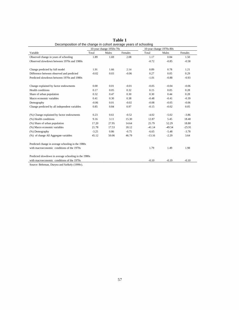
57

Table 1 Decomposition of the change in cohort average years of schooling

10-year change 1970s-80s 10-year change 1950s-70sFemalesMalesTotalFemalesMalesTotalVariable

1.500.841.172.081.691.89Observed change in years of schooling-0.58-0.85-0.72Observed slowdown between 1970s and 1980s

1.210.780.892.141.661.91Change predicted by full model0.290.050.27-0.060.03-0.02Difference between observed and predicted-0.93-0.88-1.01Predicted slowdown between 1970s and 1980s

-0.06-0.04-0.05-0.010.010.00Change explained by factor endowments0.280.050.150.320.050.17Health conditions0.280.440.300.300.470.32Share of urban population-0.39-0.41-0.480.380.300.41Macro economic variables-0.06-0.05-0.08-0.020.01-0.06Demography0.05-0.02-0.150.970.840.85Change predicted by all independent variables

-3.86-5.02-4.02-0.520.610.23(%) Change explained by factor endowments18.405.4512.8715.303.119.16(%) Health conditions18.8052.2925.7914.6427.9517.20(%) Share of urban population-25.91-49.54-41.1418.1217.5321.78(%) Macro economic variables-3.78-5.48-6.65-0.750.86-3.25(%) Demography3.64-2.29-13.1646.7950.0645.12(%) of change All Aggregate variables

Predicted change in average schooling in the 1980s1.981.491.79with macroeconomic conditions of the 1970s

Predicted slowdown in average schooling in the 1980s-0.10-0.19-0.10with macroeconomic conditions of the 1970s

Source: Behrman, Duryea and Székely (1999c).