House Value, Crime and Residential Location Choice

1

House Value, Crime and Residential Location Choice

Zhaohua Zhang

Auburn University

[email protected]

Diane Hite

Auburn University

[email protected]

Selected Paper prepared for presentation at the Southern Agricultural Economics Association’s 2015

Annual Meeting, Atlanta, Georgia, January 31-February 3, 2015

Copyright 2015 by Zhaohua Zhang and Diane Hite. All rights reserved. Readers may make verbatim

copies of this document for non-commercial purposes by any means, provided that this copyright notice

appears on all such copies.

2

Abstract

Households choose where to live by trading off wages, house prices and local amenities. In this

paper, I estimate the effect of crime on household location choice using a two-stage residential

sorting model which incorporates the effect of mobility cost. The choice set in this paper is

defined at the level of the metropolitan areas. The results from the second stage show that people

are willing to pay more to move to a location with lower violent crime occurrences and are

willing to pay more to move to a place with higher property crime; however, the effect of violent

crime is larger than property crime. When recovering the willingness to pay (WTP) for the two

types of crime using elasticities, the results show that people are willing to pay $651 and $977

for a one hundred unit decrease in violent crime and $23 and $27 for a one hundred unit increase

in property crime for 2005 and 2010 respectively. The difference in difference results for the

sorting model show that people are willing to pay less to move to a location in which the police

number increases, and pay more to move to a location where the crime rate decreases while

police force increases. The results of the difference in difference analysis, shows that the

elasticity of WTP for the increase in police number in the hedonic price model, is slightly lower

than that from the sorting model.

Key words: Location choice, Crime Rate, Residential Sorting Model

JEL Classification: R23, R21, C35

3

The study of residential location choice has captured the interest of researchers in a diverse range

of disciplines, including economists, geographers and sociologists. As a result, different methods

have been introduced to do the analysis. After Rosen’s (1974) seminal paper, the hedonic price

model became one of the most popular methods to analyze housing market issues. Charles

Tiebout’s (1956) introduced the Tiebout model and after that the Tiebout model was widely used

in analyzing the provision of public goods. The method used in this paper, which is developed by

Bayer (2009), is an extension of the traditional sorting model that introduces mobility cost.

People select the place where they live for different reasons, such as a new job opportunity

or to be together with their family. However, when making decisions, public goods and

amenities (e.g. clean air, school quality, and lower crime rates) are also characteristics that

people care about. As a result, the dwelling choice of households involves trade-offs among a

series of factors that affect the utility of households. For example, when people move from a

place with a higher crime rate to a place with a lower crime rate, it is true that it is a much safer

place for people to live but they may also experience a decrease in their wage and an increase in

housing prices. To maximize their utility, people must compare these trade-offs carefully.

Changes in housing prices and income reflect the willingness to pay for local amenities. Though

we can obtain the implicit price of the local amenities by using the hedonic price model, the

assumption of this model overlooks an important problem: the cost of migration and the effect of

income change. Moving to a new place not only costs money but also includes psychic cost due

to leaving behind our cultural roots. Thus, if we do not take these costs into account, the value of

an amenity will be overstated. While previous sorting models that analyze the impact of public

goods on household location choice ignore the cost of migration, in this paper I follow Bayer et

al. (2009) by including moving costs and modeling choices across MSAs to implement the

4

analysis. This paper concentrates on the effect of crime occurrences on household residential

location choice. As in previous papers, this paper analyzes the relationship between dwelling

location choice and public goods using observed behavior in the housing markets. What is

different is that this paper estimates both short and long-run migration impacts and adds a police

force variable to control for crime impacts using difference in difference methodology.

In this paper, I model the dwelling decision as a choice among different metropolitan

statistical areas (MSAs) taking potential income, house prices, moving cost, the number of crime

occurrences and other location-specific characteristics into account. The discrete choice model is

used to infer different utilities for household that live in different MSAs in 2005 and 2010. Then

I regress these utilities on the number of crime occurrences and local characteristics that varying

by MSA, in order to find the WTP for moving to a location with lower crime and compare the

results for 2005 and 2010. After that, I use a difference in difference model to estimate the

impact of changes of police and crime rates on individual’s WTP.

The remainder of the paper proceeds as follows. The next section provides the literature

review. The details of the analytical framework and methodology are shown in section 3. Section

4 describes the data and variables I use in the models and is followed by the analysis of

estimation results. The final part is the conclusions.

Literature Review

There is a vast body of literatures analyzing the relationship between house prices, crime

and household residential location choice. In this section I discuss some of the previous literature

addressing some of the same topics as in this paper.

Household location choices have been of continuing interest to economists for decades.

Rosen (1974) first introduced the basic theory for analyzing housing market prices using the

5

hedonic price model. However, the hedonic price model has methodological issues such as

identification and endogeneity problems. Chay and Greenstone (2005) showed problems with the

identification and consistent estimation of the hedonic price model. They were interested in

endogeneity of the pollution variable and introduced an instrumental variable approach to

estimate it consistently. They also showed that if there existed heterogeneity in preference

functions, endogeneity existed when sorting by house purchasers with different pollution levels.

Anselin and Gracia (2008) discussed spatial autocorrelation and heteroskedasticity in the error

terms when estimating hedonic models of house prices. This paper faced the problem of

mismatch between the spatial support of the explanatory variable, a pollution measure collected

at a finite set of monitoring stations, and the dependent variable, the price observed at the

location of the house sales transaction. To deal with this problem, the authors used a spatial

econometric approach and included a spatially lagged dependent variable in the hedonic

specification.

Since the hedonic price model has its shortcomings, a new method, the “discrete choice

model”, was introduced to study the residential location choice problem. The earliest attempt to

apply discrete choice theory to residential location analysis was McFadden (1978). He provided

a solution to the problem of modeling disaggregate choice of housing location when the number

of disaggregate alternatives was impractically large and when the presence of a structure of

similarities between alternatives invalidates the commonly used jointly multinomial Logit choice

model. Through the choice process of individuals, the population is sorted into optimum

communities according to the tastes of residents. Bayer et al. (2002) presented a new equilibrium

framework for analyzing economic and policy questions related to the sorting of households

within a large metropolitan area which incorporates choice-specific unobservables to identify

6

household preferences over choice characteristics. Bayer et al. (2007) developed a framework for

estimating household preferences for school and neighborhood attributes in the presence of

sorting, using restricted access Census data from a large metropolitan area. This paper introduced

a boundary discontinuity design to a heterogeneous residential choice model, addressing the

endogeneity of school and neighborhood characteristics. Yu et al. (2012) analyzed the

relationship between residential location choice and household energy consumption behavior,

using a joint mixed Multinomial Logit-Multiple Discrete-Continuous Extreme Value model by

controlling for self-selection. Recent research by Duijn and Rouwendal (2013) investigated the

impact of cultural heritage on the attractiveness of cities by analyzing the location choice of

households applying a residential sorting model. In this study, they also used spatial econometric

techniques to extend the residential sorting model to incorporate the effect of amenities of the

nearby locations. Kuminoff et al. (2013) built unemployment into a model of sorting across the

housing and labor markets to evaluate the welfare effect of a prospective regulation that would

improve environmental quality while simultaneously generating layoffs. The sorting model is

used to analyze the effect of different factors on house prices and residential location choice. The

method used in this paper follows Bayer’s (2009) model which extends McFadden’s (1978)

model by introducing mobility cost into the model.

Many researchers suggest that dwelling location decisions and house prices can be affected

by crime rates. Interestingly, different studies come to different conclusions. Cullen et al. (1999)

found negative relationships between them. The study of Lynch and Rasmussen (2001) estimates

the impact of crime on house prices using data on over 2800 house sales in Jacksonville, FL. But

the results showed that cost of crime had virtually no impact on house prices overall, but that

homes were highly discounted in high crime areas. Gibbons and Machin (2008) considered the

7

role of local amenities and disamenities in generating the variation of house prices within urban

areas, focusing on three highly policy-relevant urban issues--transport accessibility, school

quality, and crime. A recent study by Ihlanfeldt and Mayock (2009) studied the effect of

neighborhood crime on housing values, finding that a 10 percent increase in violent crime within

a neighborhood was found to reduce housing values by as much as 6 percent. Ihlanfeldt and

Mayock (2010) utilized a nine-year panel of crime for Miami-Dade County at the neighborhood

level to analyze the impact of crime on house prices. They found that house buyers were willing

to pay nontrivial premiums for housing located in neighborhoods with less aggravated assault

and robbery crime, with elasticities of house value with respect to aggravated assault crime and

robbery crime of -0.152 and -0.111, respectively. Frischtak and Mandel (2012) used a recent

policy experiment in Rio de Janeiro, the installation of permanent police stations in low-income

communities, to quantify the relationship between a reduction in crime and the change in the

prices of nearby residential real estate. Although these papers analyzed the impact of crime on

house prices, I did not find any paper that use sorting model to analyze the effect of crime on

household dwelling location choice. Thus, I apply a sorting model to analyze the effect of crime

on residential location choice in my study and also compare the results with the conventional

hedonic price model which has been commonly used in the literatures.

Methodology

Conceptual Model

In theoretical models of residential sorting, the residential location choice of households is

closely related to the demand for local public services, such as lower crime rate. In this

subsection, I start with individual choice behavior, and then introduce the model of residential

sorting. Individual choice behavior is modeled by postulating a utility function 𝑈 whose value is

8

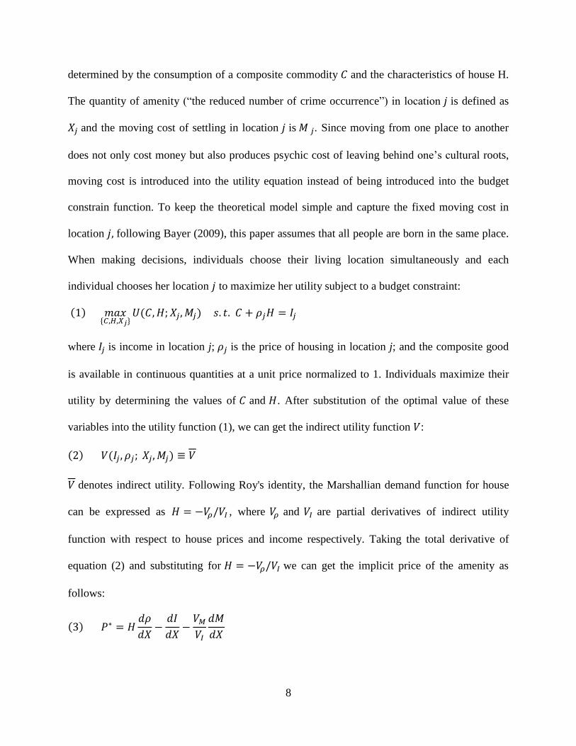
determined by the consumption of a composite commodity 𝐶 and the characteristics of house H.

The quantity of amenity (“the reduced number of crime occurrence”) in location 𝑗 is defined as

𝑋𝑗 and the moving cost of settling in location 𝑗 is 𝑀 𝑗. Since moving from one place to another

does not only cost money but also produces psychic cost of leaving behind one’s cultural roots,

moving cost is introduced into the utility equation instead of being introduced into the budget

constrain function. To keep the theoretical model simple and capture the fixed moving cost in

location 𝑗, following Bayer (2009), this paper assumes that all people are born in the same place.

When making decisions, individuals choose their living location simultaneously and each

individual chooses her location 𝑗 to maximize her utility subject to a budget constraint:

(1) 𝑚𝑎𝑥{𝐶,𝐻,𝑋𝑗}

𝑈(𝐶, 𝐻; 𝑋𝑗, 𝑀𝑗) 𝑠. 𝑡. 𝐶 + 𝜌𝑗𝐻 = 𝐼𝑗

where 𝐼𝑗 is income in location j; 𝜌𝑗 is the price of housing in location j; and the composite good

is available in continuous quantities at a unit price normalized to 1. Individuals maximize their

utility by determining the values of 𝐶 and 𝐻. After substitution of the optimal value of these

variables into the utility function (1), we can get the indirect utility function 𝑉:

(2) 𝑉(𝐼𝑗 , 𝜌𝑗; 𝑋𝑗, 𝑀𝑗) ≡ 𝑉

𝑉 denotes indirect utility. Following Roy's identity, the Marshallian demand function for house

can be expressed as 𝐻 = −𝑉𝜌/𝑉𝐼 , where 𝑉𝜌 and 𝑉𝐼 are partial derivatives of indirect utility

function with respect to house prices and income respectively. Taking the total derivative of

equation (2) and substituting for 𝐻 = −𝑉𝜌/𝑉𝐼 we can get the implicit price of the amenity as

follows:

(3) 𝑃∗ = 𝐻𝑑𝜌

𝑑𝑋−

𝑑𝐼

𝑑𝑋−

𝑉𝑀

𝑉𝐼

𝑑𝑀

𝑑𝑋

9

where 𝑉𝑀 represents the partial derivative of the indirect utility function with respect to mobility

cost. Thus, P∗ is the MWTP. From equation (3) we know that if mobility is costless (𝑉𝑀 = 0) or

mobility cost is constant under which condition 𝑑𝑀

𝑑𝑋= 0 , this equation is the same as the

traditional hedonic price model. If mobility is costless or mobility cost is constant, or we know

what 𝑀 really is, we can get the MWTP for amenities. However, in reality, we could not observe

𝑀 and if we want to get the MWTP for the amenity it is necessary to consider moving cost, and a

different method needs to be introduced. Following Bayer (2009), we start with the following

utility function assuming that individual 𝑖 lives in location 𝑗, and consumes quantities 𝐶𝑖 goods

and housing type 𝐻𝑖respectively:

(4) 𝑈𝑖,𝑗 = 𝐶𝑖𝛽𝐶𝐻𝑖

𝛽𝐻𝑋𝑗𝛽𝑋𝑒𝑀𝑖,𝑗+𝜉𝑗+𝜂𝑖,𝑗

where, 𝑋𝑗 denotes the amenity in location 𝑗; 𝑀𝑖,𝑗 measures the long-run and short-run (dis)utility

of migration associated with moving from person 𝑖’s birth location to destination 𝑗; 𝜉𝑗 contains

unobserved characteristics of location 𝑗 and 𝜂𝑖,𝑗 represents an individual-specific diosyncratic

component of utility which is assumed to be independent of mobility costs and location

characteristics. 𝛽𝐶, 𝛽𝐻, and 𝛽𝑋 are parameters associated with the consumption of goods, house

and the local amenity. Applying the budget constraint in equation (1), differentiating with respect

to 𝐻𝑖, and rearranging we can get the housing expenditure as follows:

(5) 𝐻𝑖,𝑗∗ =

𝛽𝐻

𝛽𝐻 + 𝛽𝐶∗

𝐼𝑖,𝑗

𝜌𝑗

“*” here represents the optimal result from utility maximization function. Since people do not

explicitly pay for consumption of the local amenity, 𝛽𝐻 (𝛽𝐻 + 𝛽𝐶⁄ ) represents the share of

income spent on housing. Substituting equation (5) into (4) and using the budget constrain, the

indirect utility function can be expressed as follows:

10

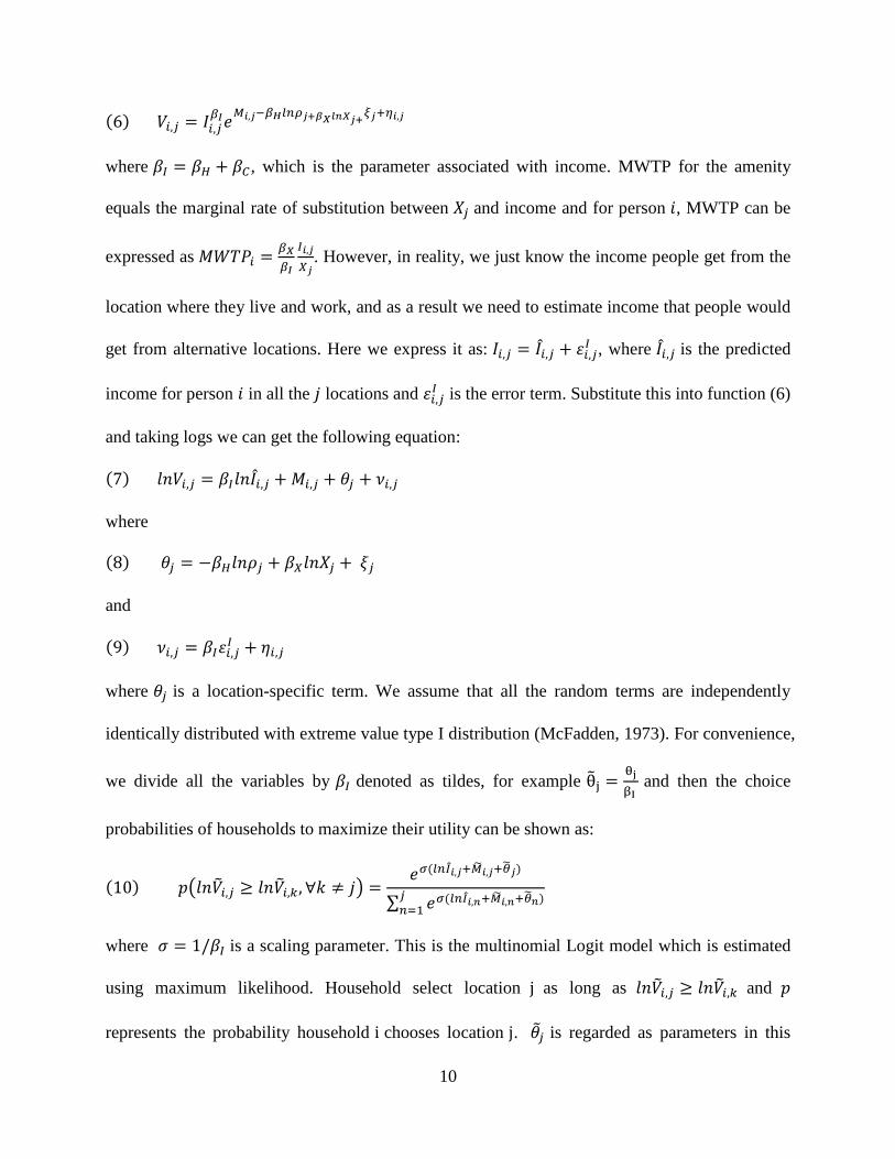
(6) 𝑉𝑖,𝑗 = 𝐼𝑖,𝑗𝛽𝐼𝑒

𝑀𝑖,𝑗−𝛽𝐻𝑙𝑛𝜌𝑗+𝛽𝑋𝑙𝑛𝑋𝑗+𝜉𝑗+𝜂𝑖,𝑗

where 𝛽𝐼 = 𝛽𝐻 + 𝛽𝐶, which is the parameter associated with income. MWTP for the amenity

equals the marginal rate of substitution between 𝑋𝑗 and income and for person 𝑖, MWTP can be

expressed as 𝑀𝑊𝑇𝑃𝑖 =𝛽𝑋

𝛽𝐼

𝐼𝑖,𝑗

𝑋𝑗. However, in reality, we just know the income people get from the

location where they live and work, and as a result we need to estimate income that people would

get from alternative locations. Here we express it as: 𝐼𝑖,𝑗 = 𝐼𝑖,𝑗 + 휀𝑖,𝑗𝐼 , where 𝐼𝑖,𝑗 is the predicted

income for person 𝑖 in all the 𝑗 locations and 휀𝑖,𝑗𝐼 is the error term. Substitute this into function (6)

and taking logs we can get the following equation:

(7) 𝑙𝑛𝑉𝑖,𝑗 = 𝛽𝐼𝑙𝑛𝐼𝑖,𝑗 + 𝑀𝑖,𝑗 + 𝜃𝑗 + 𝜈𝑖,𝑗

where

(8) 𝜃𝑗 = −𝛽𝐻𝑙𝑛𝜌𝑗 + 𝛽𝑋𝑙𝑛𝑋𝑗 + 𝜉𝑗

and

(9) 𝜈𝑖,𝑗 = 𝛽𝐼휀𝑖,𝑗𝐼 + 𝜂𝑖,𝑗

where 𝜃𝑗 is a location-specific term. We assume that all the random terms are independently

identically distributed with extreme value type I distribution (McFadden, 1973). For convenience,

we divide all the variables by 𝛽𝐼 denoted as tildes, for example θ̃j =θj

βI and then the choice

probabilities of households to maximize their utility can be shown as:

(10) 𝑝(𝑙𝑛�̃�𝑖,𝑗 ≥ 𝑙𝑛�̃�𝑖,𝑘, ∀𝑘 ≠ 𝑗) =𝑒𝜎(𝑙𝑛𝐼𝑖,𝑗+�̃�𝑖,𝑗+�̃�𝑗)

∑ 𝑒𝜎(𝑙𝑛𝐼𝑖,𝑛+�̃�𝑖,𝑛+�̃�𝑛)𝑗𝑛=1

where 𝜎 = 1/𝛽𝐼 is a scaling parameter. This is the multinomial Logit model which is estimated

using maximum likelihood. Household select location j as long as 𝑙𝑛�̃�𝑖,𝑗 ≥ 𝑙𝑛�̃�𝑖,𝑘 and 𝑝

represents the probability household i chooses location j. �̃�𝑗 is regarded as parameters in this

11

model. The focus of estimating equation (10) is to get �̃�𝑗 , which will be used in the second stage.

In the second stage, the estimated �̃�𝑗 is regressed on crime rate and other location characteristics.

From equation (8), the equation for the second stage can be written as follows:

(11) �̃�𝑗 = −𝛽𝐻𝑙𝑛𝜌𝑗 + 𝛽𝑋𝑙𝑛𝑋𝑗 + 𝜉𝑗

𝛽𝐻 =𝛽𝐻

𝛽𝐼 represents the share of income spent on house and 𝛽𝑋 =

𝛽𝑋

𝛽𝐼 represents the share of

income spent on other goods. As shown in previous part, for person 𝑖, 𝑀𝑊𝑇𝑃𝑖 =𝛽𝑋

𝛽𝐼

𝐼𝑖,𝑗

𝑋𝑗. Thus,

𝛽𝑋 = 𝑀𝑊𝑇𝑃𝑖 ×𝑋𝑗

𝐼𝑖,𝑗 from which the WTP for lower crime rate can be estimated.

Econometric implementation

The underlying assumption of the second-stage regression is that house prices are

uncorrelated with unobserved characteristics of residential locations. However, the observed

prices are often correlated with the unobservable attributes. For example, house prices may be

affected by the prices of the nearby houses and if we ignore the endogeneity of house prices, the

estimation results will be biased. Thus, to eliminate the correlation between house prices and

unobserved location characteristics and the correlation between amenity and unobserved local

attributes, this paper followed Chay and Greenstone estimating equation (11) by moving

−𝛽𝐻𝑙𝑛𝜌𝑗 to the left and then equation (11) can be written as:

(12) �̃�𝑗 + 𝛽𝐻𝑙𝑛𝜌𝑗 = 𝛽𝑋𝑙𝑛𝑋𝑗 + 𝜉𝑗

However, to implement the residential sorting model, the following problems still need to

be solved. The first problem is about how to get the “price of housing service”. The following

functions is used to estimate house prices taking the characteristics of individual house into

account:

(13) 𝑙𝑛𝑃𝑖,𝑗,𝑡 = 𝑙𝑛𝜌𝑗,𝑡 + 𝜔𝑡ℎ𝑖𝑡 + 휀𝑖,𝑗,𝑡

12

where 𝑃𝑖,𝑗,𝑡 is the value of the house 𝑖 in location 𝑗; ℎ𝑖𝑡 represents the characteristics of house 𝑖 in

time 𝑡; 𝜌𝑗,𝑡 is a scaling parameter; 𝜔𝑡 is the parameter that needs to be estimated and 휀𝑖,𝑗,𝑡 is the

error term. Since the index of "housing services" could be defined as 𝐻𝑖𝑡 = 𝑒𝜔𝑡ℎ𝑖𝑡 which can be

estimated using parameter 𝜔𝑡 , we can use 𝜌𝑗,𝑡 as the measurement of the effective "price of

housing service" which provides a consistent measure of the true prices of house. The house

characteristics in this analysis contain the number of rooms, the number of bedrooms, the

number of housing units, the age of the house, and the acres of the house.

The second problem relates to income. Since we can not observe the income of individuals

in every location, the following equation is used to estimate the MSA level income for each

individual (Bayer 2009):

(14) 𝑙𝑛𝐼𝑖,𝑗,𝑡 = 𝛼0,𝑗,𝑡 + 𝛼𝑤ℎ𝑖𝑡𝑒,𝑗,𝑡𝑤ℎ𝑖𝑡𝑒𝑖,𝑡 + 𝛼𝑚𝑎𝑙𝑒,𝑗,𝑡𝑚𝑎𝑙𝑒𝑖𝑡 + 𝛼𝑎𝑔𝑒>60,𝑗,𝑡𝑎𝑔𝑒 > 60𝑖,𝑡

+ 𝛼ℎ𝑠𝑑𝑟𝑜𝑝,𝑗,𝑡ℎ𝑠𝑑𝑟𝑜𝑝𝑖,𝑡 + 𝛼𝑠𝑜𝑚𝑒𝑐𝑜𝑙𝑙,𝑗,𝑡𝑠𝑜𝑚𝑒𝑐𝑜𝑙𝑙𝑖𝑡 + 𝛼𝑐𝑜𝑙𝑙𝑔𝑟𝑎𝑑,𝑗,𝑡𝑐𝑜𝑙𝑙𝑔𝑟𝑎𝑑𝑖,𝑡 + 휀𝑖,𝑗,𝑡𝐼

Where 𝑤ℎ𝑖𝑡𝑒𝑖,𝑡 is a dummy variable indicating whether the race of person 𝑖 is white; 𝑚𝑎𝑙𝑒𝑖𝑡 is a

dummy variable which equals 1 if the gender of person 𝑖 is male; 𝑎𝑔𝑒 > 60𝑖,𝑡 is a indicator

which equals 1 if a person is older than 60; ℎ𝑠𝑑𝑟𝑜𝑝𝑖,𝑡 is a dummy variable that equals 1 if person

𝑖 drop out in high school; 𝑠𝑜𝑚𝑒𝑐𝑜𝑙𝑙𝑖𝑡 denotes person 𝑖 get some college education that less than

four years and 𝑐𝑜𝑙𝑙𝑔𝑟𝑎𝑑𝑖,𝑡 equals 1 if person 𝑖 get college degree and higher. 휀𝑖,𝑗,𝑡𝐼 is the error

term and the 𝛼 are coefficients we need to be estimated. By estimating the above function, we

can generate the predicted value of income for each individual in all locations.

Then, it comes to mobility cost. The following function is used to measure the mobility

(Bayer et al. 2009):

(15) �̃�𝑖,𝑗,𝑡 = 𝜇𝑠𝑑𝑖,𝑗,𝑡𝑠 + 𝜇𝑟𝑑𝑖,𝑗,𝑡

𝑟 +𝜇𝑚𝑑𝑖,𝑗,𝑡𝑚

13

Where �̃�𝑖,𝑗,𝑡 represents the moving cost which is a function a series of dummy variables. 𝑑𝑖,𝑗,𝑡𝑠 is

a dummy variable which equals 1 if location 𝑗 is not in the state where individual 𝑖 was born (=0

otherwise); 𝑑𝑖,𝑗,𝑡𝑟 is an indicator whether a person lives in the same region as his/her birth region1;

and 𝑑𝑖,𝑗,𝑡𝑚 equals 1 if location 𝑗 is not in the macro-region2 where individual 𝑖 was born. In this

equation, 𝜇𝑠, 𝜇𝑟 and 𝜇𝑚are all parameters. Following Bayer, this equation represents long-run

utility cost and captures the psychic cost due to leaving behind one’s cultural roots. In order to

compare this long-run utility cost, I also estimate the mobility cost function which captures the

short-run utility. The short-run mobility cost function is defined as follows:

(16) �̃�𝑖,𝑗,𝑡 = �̃�𝑠𝑚𝑖,𝑗,𝑡𝑠 + �̃�𝑟𝑚𝑖,𝑗,𝑡

𝑟 +�̃�𝑚𝑚𝑖,𝑗,𝑡𝑚

In equation (16) �̃�𝑖,𝑗,𝑡 is still the mobility cost. 𝑚𝑖,𝑗,𝑡𝑠 is a dummy variable which equals 1 if

the current state that people is not the one they live one year before; 𝑚𝑖,𝑗,𝑡𝑟 indicates whether

people live in the same region as they lived one year before, and 𝑚𝑖,𝑗,𝑡𝑚 is also a dummy variable

which equals 1 if location j is not in the same macro region as people lived one year ago. All the

�̃� are parameters that need to be estimated. The difference between equation (15) and equation

(16) is that equation (16) represents the real moving cost in the short-run while equation (15)

captures both the long-run moving cost and the psychic cost of leaving behind the cultural root.

By investigating previous studies I find that researchers used either total crime or a single

type of crime to measure crime. In this paper, by adding up the number of crimes that occurred, I

estimate the effect of property and violent crime on people’s WTP separately. Violent crime here

1 Regional Definitions: (1) New England (CT, ME, MA, NH, RI, VT), (2)Middle Atlantic (NJ, NY, PA), (3) East North Central (IL, IN, MI, OH,

WI), (4) West North Central (IA, KS, MN, MO,NE, SD, ND), (5) South Atlantic (DE, DC, FL, GA, MD,NC, SC, VA, WV), (6) East South

Central (AL, KY, MS, TN), (7) West South Central (AR, LA, OK, TX), (8) Mountain (AZ, CO, ID, MT, NV, NM, UT,WY), and (9) Pacific

(AK,CA, HI, OR, WA). 2 There are four macro-regions defined by US census bureau: (1) Northeast (New England, Middle Atlantic), (2) Midwest()

East North Central, West North Central), (3) South(South Atlantic, East South Central, West South Central), (4) West(Mountain, Pacific).

14

includes murder and non-negligent manslaughter, forcible rape, robbery and aggravated assault.

Property crime sums up burglary, larceny-theft and motor vehicle theft.

For the first step, I estimate the parameters of 𝜇𝑠, 𝜇𝑟 , 𝜇𝑚, 𝜎 and �̃�𝑗 from the following likelihood

function in which we also assume that all the random terms are independently and identically

distributed with extreme value type I distribution3:

(17) 𝐿(𝜇𝑠, 𝜇𝑟 , 𝜇𝑚, 𝜎, �̃�𝑡) = ∏ ∏ ∏ [𝑒𝜎(𝑙𝑛𝐼𝑖,𝑗,𝑡+�̃�𝑠𝑑𝑖,𝑗,𝑡

𝑠 +�̃�𝑟𝑑𝑖,𝑗,𝑡𝑟 +�̃�𝑚𝑑𝑖,𝑗

𝑚+�̃�𝑗,𝑡)

∑ 𝑒𝜎(𝑙𝑛𝐼𝑖,𝑛,𝑡+�̃�𝑠𝑑𝑖,𝑗,𝑡𝑠 +�̃�𝑟𝑑𝑖,𝑗,𝑡

𝑟 +�̃�𝑚𝑑𝑖,𝑗𝑚+�̃�𝑛,𝑡)𝐽

𝑛=1

]

𝑥𝑖,𝑗,𝑡𝐽

𝑗=1𝑖𝑡

where 𝑥𝑖,𝑗,𝑡 is an indicator that equals one if household 𝑖 observed in year 𝑡 chooses to live at

location 𝑗. All the other symbols are the same as equations (10) and (15). Let 𝐶𝑗,𝑡 denote the

crime rate in location 𝑗 period 𝑡 and 𝑅𝑗,𝑡 represents other location characteristics, then equation

(12) can be rewritten as the following equation, which will be estimated in the second step:

(18) �̃�𝑗 + 𝛽𝐻𝑙𝑛𝜌𝑗 = 𝛽𝐶𝑙𝑛𝐶𝑗 + 𝛽𝑅𝑙𝑛𝑅𝑗 + 𝜉𝑗

In equation (18), the value of �̃�𝑗 is obtained from the first stage by using maximum

likelihood estimation, and 𝑙𝑛𝜌𝑗 is the “house service price” was obtained from the estimation of

equation (13). 𝐶𝑗 represents crime in location 𝑗 and 𝑅𝑗 represents other location characteristics.

𝛽𝐶 and 𝛽𝑅 are coefficients to estimate. 𝛽𝐻 in equation (18) is the share of income spent on

housing. To estimate the share, I use the annual average 30-year fixed mortgage rate of 2005 and

2010 which is 6.01% and 5.08% respectively4. Using this rate I can estimate the annual value for

each house using the following equation:

(19) 𝐴𝑉 =𝑇𝑉 ∗ 𝑅

1 − (1 + 𝑅)−𝑛

3 Here, I just show the likelihood function for long-run mobility cost for the sake of compact. The likelihood

function for short-run mobility cost can be get by replacing �̃�𝑠, �̃�𝑟 , �̃�𝑚 with �̃�𝑠, �̃�𝑟 , �̃�𝑚 and replacing 𝑑𝑖,𝑗,𝑡𝑠 , 𝑑𝑖,𝑗,𝑡

𝑟 , 𝑑𝑖,𝑗𝑚

with 𝑚𝑖,𝑗,𝑡𝑠 , 𝑚𝑖,𝑗,𝑡

𝑟 ,𝑚𝑖,𝑗,𝑡𝑚 .

4 These values can be get from HSH.com.

15

where 𝐴𝑉 represent the annual value of the house; 𝑇𝑉 is the total value of the house; 𝑅

represents the 30-year fixed mortgage rate and 𝑛 is the total period of installment which is 30

years in this case. When the annual value for each house is calculated, the share of income spent

on housing can be expressed by the ratio of annual house value to income. The median share of

income spent on housing is used in my study. 5

Difference in Difference Analysis

The innovation of this paper from other papers is that I introduce a difference in difference

analysis to analyze the effect of the change in crime rate and police numbers on individual’s

WTP. The estimation results of sorting model for 2005 and 2010 are obtained from the previous

analysis. However, comparing the two results, we could not decide whether the change of WTP

from 2005 to 2010 was a result of a change in crime incidence during this period, or if other

factors influenced WTP. The obvious evidence is that the occurrence of crimes is related closely

to the number of police in a location. Thus, by combining the data from 2005 and 2010, I use

both the change in crime occurrence and the change in police force size from 2005 and 2010 as

treatment to do a difference in difference analysis.

In reality, an increase in police number does not indicate a decrease in the crime rate, thus

in this paper I use two treatments. One is the increase in police numbers of per thousand people

and the other is the decrease in crime rate from 2005 to 2010. The crime rate is measured by the

ratio of the total number of crime (including both property crime and violent crime) to

population in each location. Difference in difference is measured with a minor change in the

second stage estimation as follows:

(19) �̃�𝑗 + 𝛽𝐻𝑙𝑛𝜌𝑗 = 𝛿1𝑇 + 𝛿2𝐷1𝑗 + 𝛿3𝐷2𝑗 + 𝛿4𝐷1𝑗 ∗ 𝑇 + 𝛿5𝐷2𝑗 ∗ 𝑇 + 𝛿6𝐷1𝑗 ∗ 𝐷2𝑗

5 The median share of income for the whole micro data sample is 0.36 and 0.29 for the year 2005 and 2010

respectively. Thus, β̃H in equation (18) equals to 0.36 for 2005and equals 0.29 for 2010.

16

+𝛿7𝐷1𝑗 ∗ 𝐷2𝑗 ∗ 𝑇 + 𝛽𝑅𝑙𝑛𝑅𝑗 + 𝜉𝑗

where �̃�𝑗 , 𝛽𝐻, 𝛽𝑅, 𝑙𝑛𝑅𝑗 and 𝑙𝑛𝜌𝑗 are defined as previously. 𝑇 is a dummy variable which equals

to 1 for 2010; 𝐷1𝑗 equals 1 if the police number in location 𝑗 increased from 2005 to 2010 and

𝐷2𝑗 indicates whether the crime rate in location 𝑗 decreases from 2005 to 2010. In equation (19),

the "𝛿 "s are the parameters to be estimated, with 𝛿1 capturing the time trend; 𝛿2 , 𝛿3 and 𝛿6

capture treatment group specific effects and 𝛿4, 𝛿5 and 𝛿7 represents the true treatment effect

which is the interest of the difference in difference analysis. To avoid endogeneity, I still move

house prices to the left hand side.

In equation (19), the left hand side variable is from the sorting model, in order to make

comparison, I also estimate the difference in difference effect using a traditional hedonic price

model in which the left hand side variable is the house value. The hedonic price model is defined

as follows:

(20) 𝑙𝑛𝑃𝑖,𝑗,𝑡 = 𝑙𝑛𝜌𝑗,𝑡 + 𝜔𝑡ℎ𝑖𝑡 + 𝛿1𝑇 + 𝛿2𝐷1𝑗 + 𝛿3𝐷2𝑗 + 𝛿4𝐷1𝑗 ∗ 𝑇 + 𝛿5𝐷2𝑗 ∗ 𝑇 + 𝛿6𝐷1𝑗 ∗ 𝐷2𝑗

+𝛿7𝐷1𝑗 ∗ 𝐷2𝑗 ∗ 𝑇 + 휀𝑖,𝑗,𝑡

Where 𝑙𝑛𝑃𝑖,𝑗,𝑡 is the logarithmic form of the house value in location 𝑗 of time period 𝑡; ℎ𝑖𝑡

represents the characteristics of the house 𝑖 in time 𝑡; 𝜌𝑗,𝑡 is a scaling parameter and 휀𝑖,𝑗,𝑡 is the

error term. Other variables are defined the same as those in equation (19).

Data sources

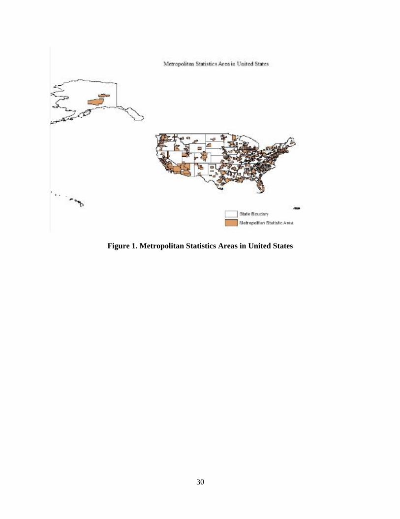
Date used in this study comes from several sources, all of which are publicly available. The

choice set used to analyze individuals' residential decisions in this paper is the metropolitan

statistical areas (MSAs) in the United States. The individual income prediction and the house

prices estimation are also at MSA level. A map of all the MSAs in the United States is shown in

figure 1. Though figure 1 shows that there are many MSAs that are not contiguous to each other,

17

most MSAs share the same border. Data used to estimate discrete choice model of residential

location choice, individual income and housing service price are obtained from the American

Community Survey (ACS) 2005 and 2010 sample. The ACS sample provides a variety of data at

MSA level including individual information as well as dwelling characteristics. In the estimation

of location specific incomes, I consider the household head as the decision maker, and during my

analysis, all householder attributes are relevant to household head. Variables used to estimate

housing service price include house value, the number of rooms, the number of bedrooms, the

age of the house, the units of the structure and the acres of the house. Variables used to predict

income include the sex, age, race, and education attainment of the household head. All these data

can be downloaded from Integrated Public Use Microdata Series (IPUMS) which is a project

dedicated to collecting and distributing United States census data. The data used to estimate

mobility cost are calculated from the data describing the birth state of household head and the

location where they live now, which can be also obtained from IPUMS. The crime data used in

my study are obtained from the Federal Bureau of Investigation's (FBI) annual report entitled

"Crime in the United States". These annual reports include the total reported numbers of violent

and property crime incidents. Police force data are also obtained from the FBI’s website. FBI

provides the employee data for all the metropolitan counties in each state and the MSA-level

employee data can be obtained by combining the county-level data. For the second stage analysis,

information about local employment, per capita personal income and population is needed. All

these data are obtained from the Bureau of Economic Analysis. After aggregating the data and

dropping the MSAs that are not included in any of the above datasets, there are 221 metropolitan

statistical areas left. Since the ACS sample is very large, I random select 20,000 observations

from the sample to do the analysis.

18

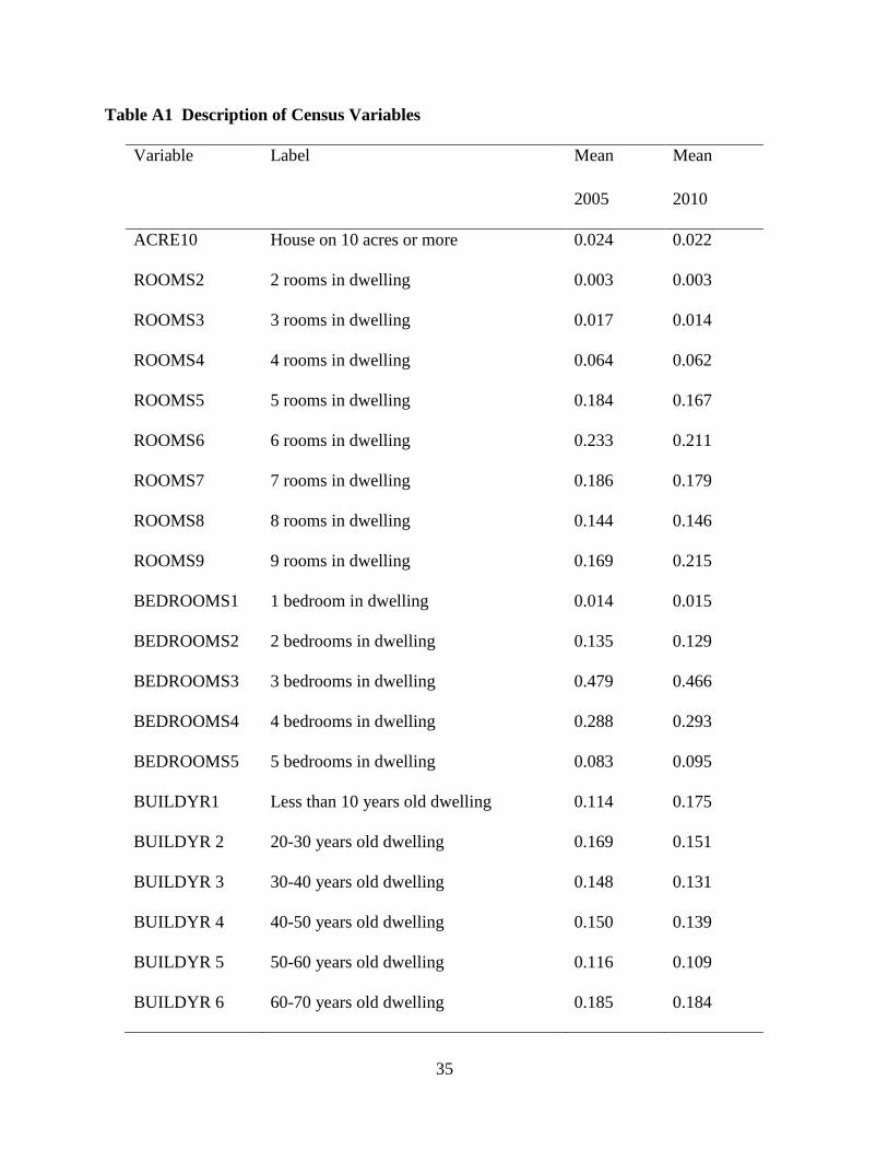
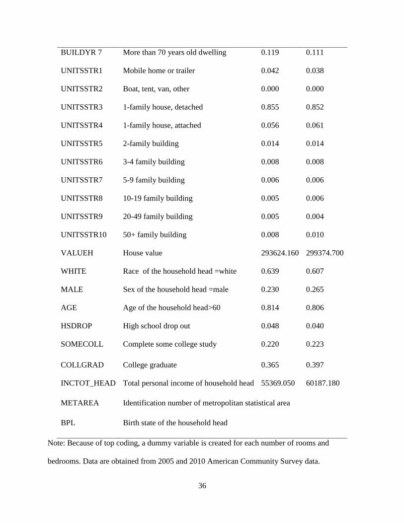
The list of all the variables used in my study and the summary statistics of all the variables

are given in Table A1. The summary statistics show that most of the houses in the sample are

smaller than 10 acres and a house with 6 rooms and 3 bedrooms is the most common type. For

individual variables, it shows that most household head in the sample are white female and aged

older than 60.

Estimation Results

Estimation Results of Incomes and House Prices

By using a two-step strategy, the effect of crime on household dwelling decision, taking

mobility cost into account, can be estimated easily. Before carrying out the first step-discrete

choice model, I must first estimate individual incomes and house service prices first. In the

sample data, we can only observe individual income in the location where he/she lives, thus we

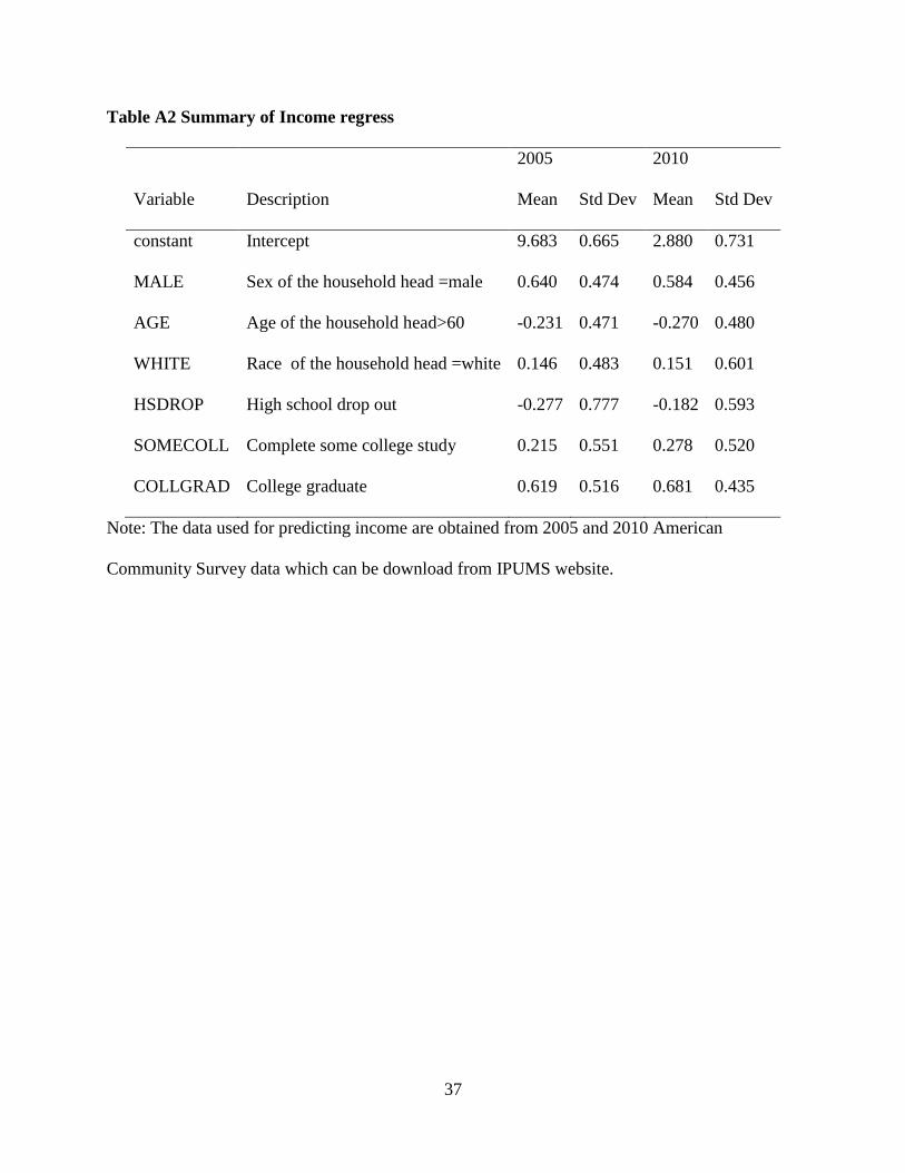
need to predict the individual incomes in every location. Using MSA-level population data in

2005 and 2010, the estimation results of location specific mean income described in equation (14)

for each year are shown in table A2. For educational attainment variables, the base group

includes the individuals with high school degree. For both years, the results show that males earn

more money than females after controlling for other variables, and white people earn more than

people of other races as expected. People over 60 years old earn less than people who are

younger than 60, which is consistent with the reality that many people are retired after age 60.

Individuals who dropped out of high school earn less than those with higher education attainment.

Table A3 shows the estimation results of housing service prices described in equation (13).

Because in the dataset, the number of rooms and bedrooms is top coded, I create a dummy

variable for each number of rooms and bedrooms and the description of the variables is shown in

table A1. For the year 2010, the more than 7 rooms does not affect house prices significantly and

19

the effect of the housing unit of boat, tent and van is not statistically significant for either years.

The other variables have significant effects on house value in both years. The estimation results

show that newer and larger houses yield more housing services. Comparing the housing service

price (in logs) in 2005 and 2010, it rose about 36.5% from 2005 to 2010. According to the results,

not all the room variables are signed correctly in 2010. I attribute this to the fact that we actually

have many correlated measures of size and counts of rooms of different types (total rooms and

bedrooms).

Estimation Results of Residential Sorting Model

When using a sorting model to analyze location choice, there are usually two stages. The

first stage is a multinomial Logit model for the personal choice and the second stage is an

ordinary least square estimation at the location level. In the first stage, specification of the choice

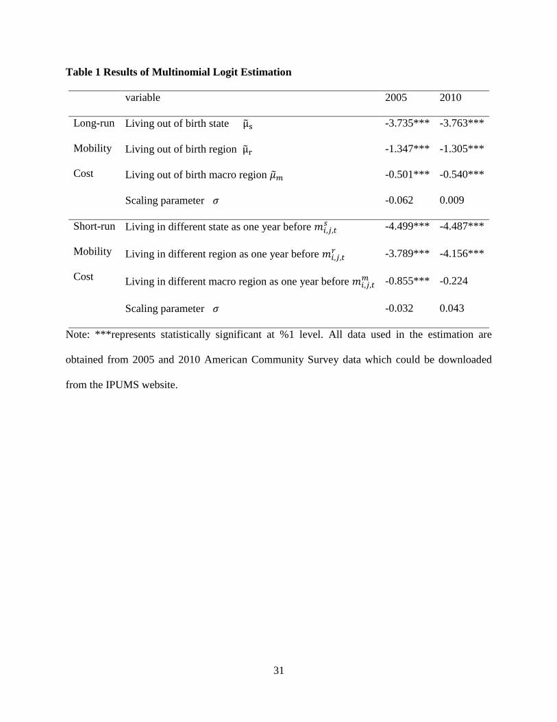
is very important for analyzing the Logit model. The estimation results of the discrete choice

equation (17) are shown in table 1. For the long-run mobility cost, all results are statistically

significant at the 1% level. As expected, living out of individuals' birth state and birth region has

negative effects on utility in both 2005 and 2010. Cost continues to increase with living out of

one's birth region and macro region. Leaving one’s birth state and birth region has almost the

same effect on residential location choice in 2005 and 2010. However the cost associated with

living out of one’s birth macro region increased in 2010. The results for short-run mobility cost

show that living in a different state from the one lived in a year before has a significant utility

cost in both 2005 and 2010, and the cost continues to increase with living in a different region

than one year before. What is different from the long-run mobility cost is that the cost associated

with living in a different region as one year before in 2010 is larger than that in 2005. The cost of

living in a different macro region as one year before is not statistically significant in 2010. This

20

may be explained by the fact that in the short-run there are less people who change the macro

region where they live because of the poor economy.

What needs to be mentioned here is that the most important thing in the first stage

estimation is to get the location fixed effect θ̃j which is not shown in table 16. However, when

the choice set is large like in this paper, the estimation of the Logit model to get θ̃j will become

difficult. One of the most commonly used methods is random selection, during which some

alternatives are randomly selected from the remaining nonchosen alternatives that the decision

maker faces. Using the random selection method, we can estimate parameters for all the

observations in the sample. However, as shown in equation (18), the focus of the first stage

estimation is to get the fixed effect parameter θ̃j for each location and the larger θ̃j is, the more

attractive the location is. In order to get the whole vector of θ̃j, Berry et al. (1994) introduced a

method to relate market shares to a scalar unobserved choice characteristic. In this paper, I apply

Berry’s method to estimate θ̃j 7 indirectly. Even though the location fixed effect θ̃j represents the

preference of people to live in this location, we cannot say that people prefer to live in the

location with higher θ̃j because the size of county also affects θ̃j. For large MSAs the share of

observations who live in these MSAs may be larger than the share of observations who live in

the MSAs with a small population. Without controlling for population, according to the rank of

θ̃j, the most attractive metropolitan area for people to live in both 2005 and 2010 is New York-

Northeastern, NJ. The least attractive metropolitan area is Iowa City, IA and Alexandria, LA for

2005 and 2010 respectively. However, we cannot make any conclusions without controlling for

population. Controlling for population gives us more precise conclusions and the results show

6 There are 221 fixed effects, which are not reported in table 1 for the sake of space. 7 We arbitrarily set θ̃j equal for zero for the Abilene, TX, MSA.

21

that even after controlling for population, New York-Northeastern is still the most attractive

location for both year, but Kokomo, IN became the least attractive location for both 2005 and

2010, which is different from the results without controlling the population. Thus, in the analysis,

population needs to be taken into account to control for city-size effects.

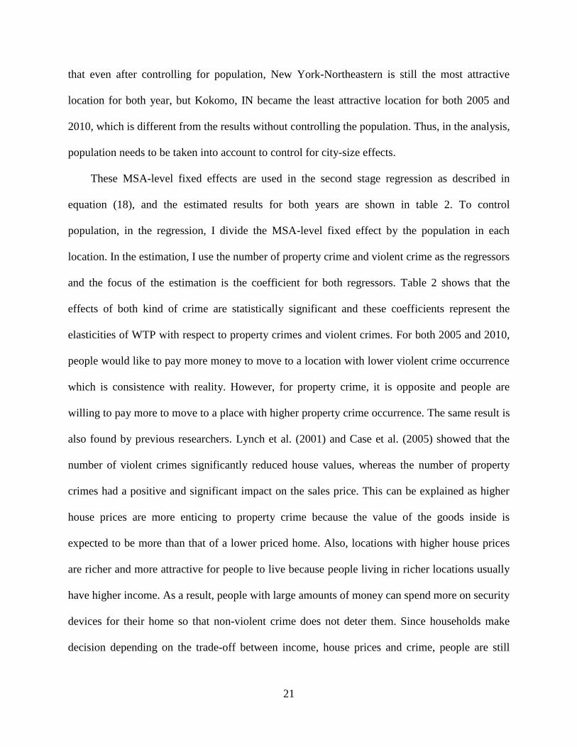
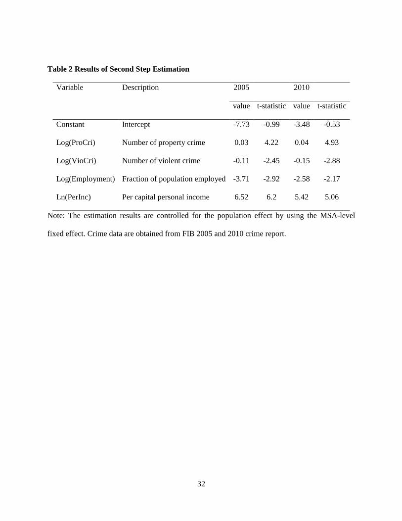
These MSA-level fixed effects are used in the second stage regression as described in

equation (18), and the estimated results for both years are shown in table 2. To control

population, in the regression, I divide the MSA-level fixed effect by the population in each

location. In the estimation, I use the number of property crime and violent crime as the regressors

and the focus of the estimation is the coefficient for both regressors. Table 2 shows that the

effects of both kind of crime are statistically significant and these coefficients represent the

elasticities of WTP with respect to property crimes and violent crimes. For both 2005 and 2010,

people would like to pay more money to move to a location with lower violent crime occurrence

which is consistence with reality. However, for property crime, it is opposite and people are

willing to pay more to move to a place with higher property crime occurrence. The same result is

also found by previous researchers. Lynch et al. (2001) and Case et al. (2005) showed that the

number of violent crimes significantly reduced house values, whereas the number of property

crimes had a positive and significant impact on the sales price. This can be explained as higher

house prices are more enticing to property crime because the value of the goods inside is

expected to be more than that of a lower priced home. Also, locations with higher house prices

are richer and more attractive for people to live because people living in richer locations usually

have higher income. As a result, people with large amounts of money can spend more on security

devices for their home so that non-violent crime does not deter them. Since households make

decision depending on the trade-off between income, house prices and crime, people are still

22

willing to pay to move to a place with higher house value even though it costs people more to

move to a location with high property crime occurrence. It should to be mentioned that the study

area in this paper is metropolitan statistics areas where more wealth in the U.S. is concentrated.

Thus, the results could only account for the phenomenon in wealthier locations. Also, simply

counting the number of crimes in this paper may provide a distorted picture of how public safety

varies over space because of spatial differences in the distribution of crimes and reporting

behavior. This may also explain the positive sign for property crime. Comparing the magnitude

of the coefficient for both types of crimes, we can find that violent crime has a larger effect than

property crime, which means that people care more about the number of violent crimes.

Comparing the results for 2005 and 2010 we find that the elasticity of WTP with respect to

property crime changes slightly, but the elasticity with respect to violent crime increases by 36%

which indicate that in 2010 people are willing to pay more to move to a location with lower

violent crime occurrence. To explain what the estimates implied with more detail, we can

consider the following example. In 2005, the number of violent crime in Abilene, TX is 640,

while in the same year the number of violent crimes\ in Albuquerque, NM is 6,630 which is

roughly ten times as big as Abilene. The estimated elasticity of WTP with respect to violent

crime in 2005 is -0.11 which implies that the decrease in violent crime by moving from

Albuquerque to Abilene would correspond to increase in WTP of 98%.

Now it comes to the analysis of MWTP for the decrease in crime occurrences. As

mentioned before in this paper, β̃C = MWTPi ×Cj

Ii,j , thus we can recover the MWTP for crime

rate using this formula. During the calculation, I used the median value of household income and

both kinds of crime in the full sample, which measured the median household's WTP for the

decrease in crime. In 2005, the median value of household income is $71,000 (in 2005 dollars)

23

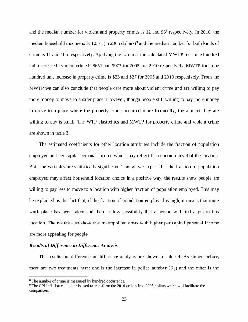
and the median number for violent and property crimes is 12 and 938 respectively. In 2010, the

median household income is $71,651 (in 2005 dollars)9 and the median number for both kinds of

crime is 11 and 105 respectively. Applying the formula, the calculated MWTP for a one hundred

unit decrease in violent crime is $651 and $977 for 2005 and 2010 respectively. MWTP for a one

hundred unit increase in property crime is $23 and $27 for 2005 and 2010 respectively. From the

MWTP we can also conclude that people care more about violent crime and are willing to pay

more money to move to a safer place. However, though people still willing to pay more money

to move to a place where the property crime occurred more frequently, the amount they are

willing to pay is small. The WTP elasticities and MWTP for property crime and violent crime

are shown in table 3.

The estimated coefficients for other location attributes include the fraction of population

employed and per capital personal income which may reflect the economic level of the location.

Both the variables are statistically significant. Though we expect that the fraction of population

employed may affect household location choice in a positive way, the results show people are

willing to pay less to move to a location with higher fraction of population employed. This may

be explained as the fact that, if the fraction of population employed is high, it means that more

work place has been taken and there is less possibility that a person will find a job in this

location. The results also show that metropolitan areas with higher per capital personal income

are more appealing for people.

Results of Difference in Difference Analysis

The results for difference in difference analysis are shown in table 4. As shown before,

there are two treatments here: one is the increase in police number (D1) and the other is the

8 The number of crime is measured by hundred occurrence. 9 The CPI inflation calculator is used to transform the 2010 dollars into 2005 dollars which will facilitate the

comparison.

24

decrease in crime rate (D2). The police variable is measured by the change of the total number of

police employed in each MSA. Our interest in this estimation is the coefficients for all the three

terms interacted with time period T (D1*T, D2*T and D1*D2*T). For the sorting model, the

coefficient for 𝐷1𝑡 is -0.39 and statistically significant at the 10% level. This means that people

are willing to pay 39% less to move to a location with higher numbers of police. This can be

explained by the fact that the increase in police number may be an indicator of high crime rate

and also people need to pay more by tax to cover the cost of additional police. The effect of the

crime rate decrease on WTP is not statistically significant in the sorting model. However, people

are willing to pay 41% more to move to a location in which the crime rate decreases and the

police number increases. Though there are maybe more police in bad areas generally, when

controlled by numbers of crimes then more police is a good thing. When comparing the

coefficients estimated from sorting model with those get from the hedonic price model, it should

be pointed out that the WTP elasticities are not directly comparable. The coefficients from the

hedonic price model represents the change of house prices associated with the decrease in crime

rate and increase in police force while the estimates from the sorting model not only reflect the

change in house prices but also the change in income and disutility from moving. Thus, the

estimates from hedonic price model may be misleading. The coefficients in the hedonic price

model represent house prices elassticities with respect to the two treatments. To translate the

house prices elassticities into MTP, we need to first multiply the coefficient from the hedonic

price model by the share of income spent on house, and here I use the average share of 2005 and

2010 which is 0.32 to calculate MTP. Thus, the elasticity of WTP for the police number increase

is 0.35 which is slightly lower than that from the sorting model. However, in the hedonic price

model, the true effect of the crime rate decrease and the effects from both treatments are not

25

statistically significant. For the other location characteristics, people are willingness to pay less

to move to a location where the employment rate is high and metropolitan areas with higher per

capital personal income is more appealing for people.

Conclusions

In this paper, I estimate the effect of crime on household location choice using a two stage

residential sorting model where the choice set is defined at the level of the metropolitan areas. In

the first stage a discrete choice model is estimated to get the MSA level fixed effect and in the

second stage, these fixed effects are estimated on the number of property and violent crime and

other location attritions. In this paper, the household head is regarded as the decision maker and

the characteristics of the household head are used to predict their income in each MAS. In order

to get the house prices, a linear function is used to regress house value on a set of dwelling

attributes. Finally, a difference in difference model is introduced to analyze the effects of crime

rate decrease and police force increase on households’ WTP.

The first stage estimation results show that living out of individuals' birth states and birth

regions have negative effect on their utility and cost continue to increase with living out of one's

birth region and macro region. Also, the results for short-run mobility cost show that living in a

different state than one year before has a significant utility cost in both 2005 and 2010 and the

cost continues to increase with living in a different region than one year before. However, the

cost of living in a different macro region than one year before is not statistically significant in

2010. This may be explained by the fact that in the short-run there are fewer people changing the

macro region where they live. The focus in the second stage analysis is the estimated coefficients

on the number of violent and property crime which represent the elasticities of WTP with respect

to these two kinds of crime. The results show that people are willing to pay more to move to a

26

location with lower violent crime occurrence and are also willing to pay more to move to a place

with higher property crime. This can be explained by the fact that higher house prices are more

enticing to property crime because the value of the goods inside is expected to be more than that

of a lower priced home. Also, people with large amounts of money can spend more on security

devices for their home so that non-violent crime does not deter them. When recovering the WTP

for the two types of crime using elasticities, it shows that people are willing to pay $651 and

$977 for a one hundred unit decrease in violent crime and $23 and $27 for a one hundred unit

increase in property crime for 2005 and 2010 respectively, which indicates that, though people

still willing to pay money to move to a place where the property crime occurred more frequently,

the amount they are willing to pay is small. The difference in difference results for the sorting

model show that people are willing to pay less to move to a location in which the police number

increases and pay more to move to a location where the crime rate decreases and police force

increased. This can be explained by the fact that the increase in police number may be an

indicator of high crime rate as well as higher tax payments to cover expenditures on additional

police. When comparing the difference in difference results for the sorting model with that for

the hedonic price model I find that the elasticity of WTP for the police number increase in the

hedonic price model are slightly lower than that from the sorting model.

27

References

Anselin L. and Gracia L. Nancy. 2008. “Errors in variables and spatial effects in hedonic house

price models of ambient air quality”. Empirical Economics.34:5–34.

Bayer P., Ferreira, F.V., and McMillan, R. 2005. “Tiebout Sorting, Social Multipliers and the

Demand for School Quality”. NBER Working Paper: No. 10871.

Bayer Patrick, Ferreira, Fernando, McMillan, Robert. 2007. “A unified framework for

measuring preferences for schools and neighborhoods.” Journal of Political Economy,

115[4]:588-638.

Bayer P., Keohane N. and Timmins C. 2009. “Migration and hedonic valuation: The case of air

quality”. Journal of Environmental Economics and management, 58(1):1-14.

Bayer P., Robert M. and Kim R. 2003. “An Equilibrium Model of Sorting in an Urban Housing

Market: The Causes and Consequences of Residential Segregation”. Economic Growth

Center, Yale University: Working Paper.

Berry, S. 1994. “Estimating Discrete-Choice Models of Product Differentiation,” RAND

Journal of Economics, 25: 242–62.

Biying Y., Junyi Z. and Akimasa F.2012. “Analysis of the Residential Location Choice and

Household Energy Consumption Behavior by Incorporating Multiple Self-selection

Effects.” Energy Policy 46: 319-334.

Brueckner, J. K., Thisse, J. F. and Zenou, Y. 1999. “Why is Central Paris rich and downtown

Detroit poor? An amenity-based theory”. European Economic Review, 43: 91–107.

Case, K. E. and Mayer, C. J. 1995. “Housing price dynamics within a metropolitan area”.

Federal Reserve Bank of Boston. Working Paper No. 95-3.

Chay K.Y. and Greenstone M. 2005. “Does air quality matter? Evidence form the housing

http://www.sciencedirect.com/science/article/pii/S0095069609000035

28

market”. Journal of Political Econonics. 113(2):376-424.

Claudio Frischtak and Benjamin R. Mandel. 2012. “Crime, House prices, and Inequality: The

Effect of UPPs in Rio.” Federal Reserve Bank of New York Staff Reports: No. 542

Cullen J.B. and Levitt S.D. 1999. “Crime, Urban Flight and the Consequences for Cities.”

Review of Economics and Statistics, 81:159-69.

Duijn M. and Rouwendal J.2013. “Cultural Heritage and the Location Choice of Dutch

Households in a Residential Sorting Model.” Journal of Economic Geography, 13:473–

500.

Gibbons S. and Machin S. 2008. “Valuing School Quality, Better Transport, and Lower Crime:

Evidence from House prices.” Oxford Review of Economic Policy, 24(1): 99-119.

Ihlanfeldt K. and Mayock T. 2010. “Panel Data Estimates of the Effects of Different Types of

Crime on

Housing prices.” Regional Science and Urban Economics, 40:161–172.

Kuminoff N., Schoellman T. and Timmins C. 2013. “Can Sorting Models Help Us Evaluate the

Employment Effects of Environmental Regulations? ” Association of Environmental and

Resource Economists 3nd Annual Summer Conference. Alberta, Canada.

Lynch A. and Rasmussen D. W. 2001. “Measuring the Impact of Crime on House prices.”

Applied Economics, 2001:1981-1989

McFadden, D. 1973. Conditional Logit Analysis of Qualitative Choice Behavior. New York, NY:

Academic Press.

McFadden D., 1978. “Modeling the choice of residential location, In Spatial Interaction Theory

and Planning Models”. North Holland Publishers: A. Karlqvist and Amsterdam.

Rosen, S. 1974. “Hedonic prices and implicit markets. Product differentiation in pure

29

competition”. Journal of Political Economy, 82: 34-55.

Sampson J.D. and Wooldredge. 1986. “Evidence that High Crime Rates Encourage Migration

Away from Central Cities.” Sociology and Social Research, 90:310-14

Tiebout, C. 1956. “A Pure Theory of Local Expenditures”. Journal of Political Economy, 64 (5):

416–424.

http://en.wikipedia.org/wiki/Journal_of_Political_Economy

30

Figure 1. Metropolitan Statistics Areas in United States

31

Table 1 Results of Multinomial Logit Estimation

variable 2005 2010

Long-run

Mobility

Cost

Living out of birth state μ̃s -3.735*** -3.763***

Living out of birth region μ̃r -1.347*** -1.305***

Living out of birth macro region 𝜇𝑚 -0.501*** -0.540***

Scaling parameter 𝜎 -0.062 0.009

Short-run

Mobility

Cost

Living in different state as one year before 𝑚𝑖,𝑗,𝑡𝑠 -4.499*** -4.487***

Living in different region as one year before 𝑚𝑖,𝑗,𝑡𝑟 -3.789*** -4.156***

Living in different macro region as one year before 𝑚𝑖,𝑗,𝑡𝑚 -0.855*** -0.224

Scaling parameter 𝜎 -0.032 0.043

Note: ***represents statistically significant at %1 level. All data used in the estimation are

obtained from 2005 and 2010 American Community Survey data which could be downloaded

from the IPUMS website.

32

Table 2 Results of Second Step Estimation

Variable Description

2005 2010

value t-statistic value t-statistic

Constant Intercept -7.73 -0.99 -3.48 -0.53

Log(ProCri) Number of property crime 0.03 4.22 0.04 4.93

Log(VioCri) Number of violent crime -0.11 -2.45 -0.15 -2.88

Log(Employment) Fraction of population employed -3.71 -2.92 -2.58 -2.17

Ln(PerInc) Per capital personal income 6.52 6.2 5.42 5.06

Note: The estimation results are controlled for the population effect by using the MSA-level

fixed effect. Crime data are obtained from FIB 2005 and 2010 crime report.

33

Table 3. Marginal Willingness to Pay for Property Crime and Violent Crime

2005 2010

Property Crime Violent Crime Property Crime Violent Crime

WTP elasticity 0.03 $23 0.04 $27

MWTP -0.11 $651 -0.15 $977

Note: MWTP is calculated by multiplying the WTP elasticity by the median household income

and dividing by the median number of each type of crime. The median household income is

71,000 and 71,651 (in 2005 dollars) for 2005 and 2010 respectively. The median number of

property crime and violent crime in 2005 is 93 and 12, and the median number of property crime

and violent crime in 2010 is 105 and 11. All the crimes are measured by hundred occurrence.

34

Table 4. Results for Difference in Difference Estimation

Variable Description Sorting

Model

Hedonic

Model

T Time period -0.78* 0.42

D1 =1 if police number increase 0.39** 1.09**

D2 =1 if crime rate decrease 0.05 0.13

D1*T The true effect of police number increase -0.39* -1.08*

D2*T The true effect of crime rate decrease -0.22 -0.72

D1*D2*T The true effect of both police number increase and

crime rate decrease

0.41* 1.15

Log(Employ-

ment)

Fraction of population employed -0.65* -1.63

Log(PerInc) Per capital personal income 0.46** 1.21**

Note: *** means statistically significant at 1% or above; ** means statistically significant at 5%

level and * means statistically significant at 10%. Crime data are obtained from FBI crime report

of 2005 and 2010. Income and employment data are obtained from Bureau of Economic

Analysis of 2005 and 2010.

35

Table A1 Description of Census Variables

Variable Label Mean Mean

2005 2010

ACRE10 House on 10 acres or more 0.024 0.022

ROOMS2 2 rooms in dwelling 0.003 0.003








BEDROOMS1 1 bedroom in dwelling 0.014 0.015

BEDROOMS2 2 bedrooms in dwelling 0.135 0.129




BUILDYR1 Less than 10 years old dwelling 0.114 0.175

BUILDYR 2 20-30 years old dwelling 0.169 0.151





36

BUILDYR 7 More than 70 years old dwelling 0.119 0.111

UNITSSTR1 Mobile home or trailer 0.042 0.038

UNITSSTR2 Boat, tent, van, other 0.000 0.000

UNITSSTR3 1-family house, detached 0.855 0.852

UNITSSTR4 1-family house, attached 0.056 0.061

UNITSSTR5 2-family building 0.014 0.014

UNITSSTR6 3-4 family building 0.008 0.008




UNITSSTR10 50+ family building 0.008 0.010

VALUEH House value 293624.160 299374.700

WHITE Race of the household head =white 0.639 0.607

MALE Sex of the household head =male 0.230 0.265

AGE Age of the household head>60 0.814 0.806

HSDROP High school drop out 0.048 0.040

SOMECOLL Complete some college study 0.220 0.223

COLLGRAD College graduate 0.365 0.397

INCTOT_HEAD Total personal income of household head 55369.050 60187.180

METAREA Identification number of metropolitan statistical area

BPL Birth state of the household head

Note: Because of top coding, a dummy variable is created for each number of rooms and

bedrooms. Data are obtained from 2005 and 2010 American Community Survey data.

37

Table A2 Summary of Income regress

Description

2005 2010

Variable Mean Std Dev Mean Std Dev

constant Intercept 9.683 0.665 2.880 0.731

MALE Sex of the household head =male 0.640 0.474 0.584 0.456

AGE Age of the household head>60 -0.231 0.471 -0.270 0.480

WHITE Race of the household head =white 0.146 0.483 0.151 0.601

HSDROP High school drop out -0.277 0.777 -0.182 0.593

SOMECOLL Complete some college study 0.215 0.551 0.278 0.520

COLLGRAD College graduate 0.619 0.516 0.681 0.435

Note: The data used for predicting income are obtained from 2005 and 2010 American

Community Survey data which can be download from IPUMS website.

38

Table A3 Housing Service Estimated Parameters

2005 2010

Variable Description Parameter t Value Parameter t Value

INTERCEPT Intercept 2.52 11.90 3.44 32.56

ROOMS2 2 rooms in dwelling 0.64 2.84 -0.34 -2.46







ROOMS9 9 rooms in dwelling 1.15 5.30 0.17 1.51

BEDROOMS2 2 bedrooms in dwelling 0.17 3.43 0.15 2.94




BUILDYR1 Less than 10 years old dwelling 0.38 19.97 0.19 9.58

BUILDYR r2 20-30 years old dwelling 0.32 17.91 0.15 7.63

BUILDYR 3 30-40 years old dwelling 0.22 12.48 0.08 4.01

BUILDYR 4 40-50 years old dwelling 0.08 4.58 -0.01 -0.67



ACRE10 House on 10 acres or more 0.23 7.66 0.16 4.70

39

UNITSSTR2 Boat, tent, van, other -0.21 -0.95 0.06 0.28

UNITSSTR3 1-family house, detached 1.56 65.66 1.59 58.90

UNITSSTR4 1-family house, attached 1.70 57.25 1.72 52.87

UNITSSTR5 2-family building 1.86 41.00 1.96 38.94

UNITSSTR6 3-4 family building 1.93 34.03 1.89 31.52




UNITSSTR10 50+ family building 2.14 38.80 2.12 37.54

Note: All the data used in this estimation are obtained form 2005 and 2010 American

Community Survey data.

House Value, Crime and Residential Location Choice

Documents

Transcript of House Value, Crime and Residential Location Choice