Hopf Bifurcation in Viscous Incompressible Flow Down an Inclined Plane: a Numerical Approach

J. math. fluid. mech. 99 (9999), 1–221422-6928/99000-0, DOI 10.1007/s00009-003-0000c© 2006 Birkhauser Verlag Basel/Switzerland

Journal of Mathematical

Fluid Mechanics

Hopf bifurcation in viscous incompressible flowdown an inclined plane: a numerical approach

Roland Glowinski and Giovanna Guidoboni

Abstract. In this article we investigate numerically a Hopf bifurcation phe-nomenon for a viscous incompressible flow down an inclined plane. This prob-lem has been discussed by Nishida et al. who proved the existence of periodicsolutions bifurcating from the steady flow. Using a computational method-ology based on finite elements for the space discretization and on operatorsplitting for the time discretization, we have been able to reproduce the re-sults predicted by Nishida et al.

Mathematics Subject Classification (2000). 70K50, 76B45, 76M10.

Keywords. free surface, surface tension, Hopf bifurcation, operator splitting,finite elements.

1. Introduction

In [15], Nishida, Teramoto and Yoshihara proved the existence of a Hopf bifurcationfor the flow of an incompressible viscous fluid down an inclined plane. The maingoal of this article is to investigate numerically the same flow problem in order toprecise at which value of the Reynolds number the Hopf bifurcation is occurring,and to visualize the shape of the past-bifurcation waves.

The computational methodology discussed in this article relies on the follow-ing components:

(i) As in [9] we map the two dimensional flow region Ω(t) on a rectangular one Ω(actually the main result in [15] is proved using a similar transformation, which isquite classical in this context).

(ii) We formulate the flow problem in Ω and we use a time discretization byoperator splitting to reduce the solution of the original flow problem to that ofsimpler sub-problems. Actually, it is easier to solve some of the sub-problems in

2 Roland Glowinski and Giovanna Guidoboni JMFM

the physical flow region, and we take advantage of this simplification each time itis possible.

(iii) We combine the time-splitting scheme with an isoparametric Bercoveir-Pironneaufinite element approximation of the Navier-Stokes equations (see e.g. [3], [8], [9],[10], [18]) to fully discretize the free surface problem.

(iv) The wave-like equation methodology discussed in, e.g., [8], [9], [10], and [17], isused to handle the pure advection problems resulting from the time-splitting andfrom the domain transformation. The resulting methodology is modular, relativelyeasy to implement, and it introduces very little numerical dissipation, an importantproperty if one wishes to identify accurately the critical Reynolds number at whichbifurcation occurs. We took advantage of this property in, e.g., [10] to study otherHopf bifurcation phenomena.

The computed results are in very good agreement with the experimental datareported in [13]. The flow problem in this article is a basic one. It is not surprisingtherefore that it has attracted the attention of many investigators. Let us mention,among many others, [1], [2], [5], [6], [11] and [16].

The content of the remainder of this article is as follows. In Section 2 wedescribe the mathematical formulation of the problem. In Section 3 we discuss thetime discretization by operator splitting. In Sections 4 and 5 the splitting scheme ofSection 3 is combined with the Bercovier-Pironneau finite element approximationof the Navier-Stokes equations to derive the full discretization of the problem. Theresults of the numerical experiments are presented in Section 6.

2. Mathematical formulation

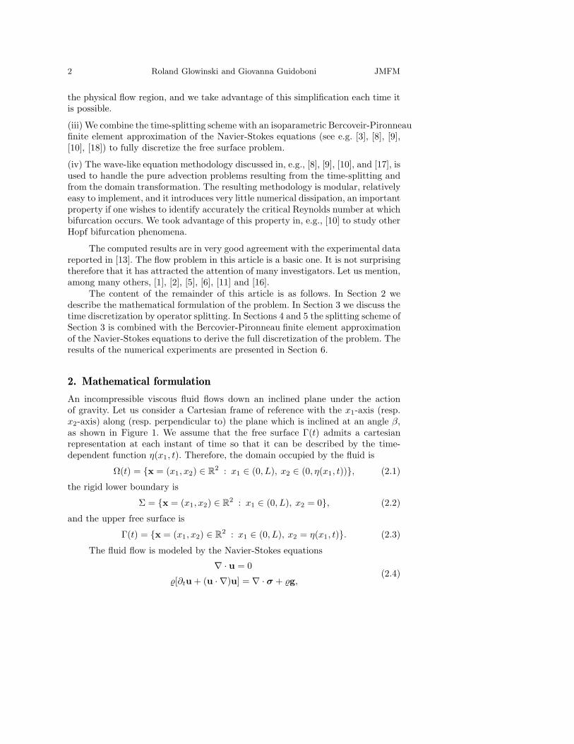
An incompressible viscous fluid flows down an inclined plane under the actionof gravity. Let us consider a Cartesian frame of reference with the x1-axis (resp.x2-axis) along (resp. perpendicular to) the plane which is inclined at an angle β,as shown in Figure 1. We assume that the free surface Γ(t) admits a cartesianrepresentation at each instant of time so that it can be described by the time-dependent function η(x1, t). Therefore, the domain occupied by the fluid is

Ω(t) = x = (x1, x2) ∈ R2 : x1 ∈ (0, L), x2 ∈ (0, η(x1, t)), (2.1)

the rigid lower boundary is

Σ = x = (x1, x2) ∈ R2 : x1 ∈ (0, L), x2 = 0, (2.2)

and the upper free surface is

Γ(t) = x = (x1, x2) ∈ R2 : x1 ∈ (0, L), x2 = η(x1, t). (2.3)

The fluid flow is modeled by the Navier-Stokes equations

∇ · u = 0

[∂tu + (u · ∇)u] = ∇ · σ + g,(2.4)

Vol. 99 (9999) Hopf bifurcation for a free surface flow 3

0

x2

L x1

η(x ,t)1

β

Γ(t)

Figure 1. Sketch of the geometry of the problem.

where u = (u1, u2) is the velocity of the fluid, is the fluid density, σ is the stresstensor defined as σ = −pI + 2µD(u), where p is the pressure, µ is the viscosityand D(u) = (∇u + (∇u)t)/2 is the rate-of-strain tensor, where the superscriptt means transpose. The external force is due to the gravity and it is given byg = g(sin β,− cosβ), where g is the acceleration of gravity. Here ∂t denotesthe partial derivative with respect to time, while ∇ = (∂1, ∂2) is the gradientwith respect to the spatial variables. Equations (2.4) hold in the time-dependentdomain Ω(t) defined in (2.1), and for 0 < t < T . No-slip condition is assumed forthe velocity at the rigid bottom, and therefore we have

u = 0 on Σ. (2.5)

The free boundary Γ(t) is a material surface, therefore we prescribe the followingkinematic condition

∂tη + u1∂1η − u2 = 0 on Γ(t), (2.6)

to ensure that the fluid particles do not cross the surface. An additional conditionis needed to establish the balance of stress

σn = sH(η(x1, t))n on Γ(t), (2.7)

where n = (−∂1η, 1)/√

1 + |∂1η|2 is the outward unit normal vector, s is thesurface tension (which is assumed to be positive and constant), and H(η(x1, t)) =∂21η/(1 + |∂1η|

2)3/2 is the curvature. We assume periodicity in the x1-directionof given period L. The incompressibility of the fluid and the periodic boundaryconditions imply that the area of the fluid domain must be conserved. Indeed wehave:

0 =

∫

Ω(t)

∇ · ud x =

∫

Γ(t)

u · n dΓ(t) =

∫ L

0

∂tη dx1 =d

dt

∫ L

0

η dx1 . (2.8)

This means that ∫ L

0

η(x1, t) dx1 = constant = HL, (2.9)


where H is the average height of the fluid layer. To complete the formulation ofthe problem, initial conditions should be prescribed for the velocity of the fluidand the shape of the domain:

u(x, 0) = u0(x) with ∇ · u0 = 0,

η(x1, 0) = η0(x1) with

∫ L

0

η0(x1) dx1 = HL.(2.10)

In order to write the variational formulation of the problem (2.4)-(2.10) weintroduce the following functional spaces:

V0(Ω(t)) = v | v ∈ (H1(Ω(t)))2,v = 0 on Σ, v|x1=0 = v|x1=L , (2.11)

L20(Ω(t)) = q | q ∈ L2(Ω(t)),

∫

Ω(t)

qdx = 0 , (2.12)

S = η | η ∈ H1(0, L), η|x1=0 = η|x1=L . (2.13)

Now, we multiply equations (2.4)1 and (2.4)2 by the test functions q ∈ L2(Ω(t))and v ∈ V0(Ω(t)), respectively, and we use the notation ϕ(t) to denote the func-tion x → ϕ(x, t). The resulting equations are integrated over Ω(t) to obtain thevariational formulation of (2.4)-(2.10):

For a.e. t > 0, find u(t) ∈ V0(Ω(t)), p(t) ∈ L20(Ω(t)), η(t) ∈ S such that

∫

Ω(t)

∂tu · v dx +

∫

Ω(t)

(u · ∇)u · v dx + 2µ

∫

Ω(t)

D(u) : D(v) dx

−

∫

Ω(t)

p∇ · v dx =

∫

Ω(t)

g · v dx

+s

∫

Γ(t)

H(η(x1, t))n · v dΓ(t), ∀v ∈ V0(Ω(t)),

∫

Ω(t)

q∇ · u dx = 0, ∀q ∈ L2(Ω(t)),

∫ L

0

∂tη φ dx1 +

∫ L

0

(u1|Γ(t)∂1η − u2|Γ(t)) φ dx1 = 0, ∀φ ∈ S,

u(x, 0) = u0(x), with ∇ · u0 = 0,

η(x1, 0) = η0(x1) with

∫ L

0

η0(x1) dx1 = HL.

(2.14)

Remark 1. There is no contradiction between the choice of S given by (2.13)and the fact that H(η) includes ∂2

1η. Indeed, by integration by parts we get

s

∫

Γ(t)

H(η)v1n1 dΓ(t) = −s

∫ L

0

(1 + |∂1η|2)−1/2∂1v1 dx1, (2.15)


L0 0 L

ΩΩ

At

(t)

H

At−1

Figure 2. At maps the the current domain Ω(t) into the refer-

ence domain Ω.

s

∫

Γ(t)

H(η)v2n2 dΓ(t) = −s

∫ L

0

∂1η(1 + |∂1η|2)−1/2∂1v2 dx1, (2.16)

where the x1-differentiation on η is transferred on the two components of the testfunction v.

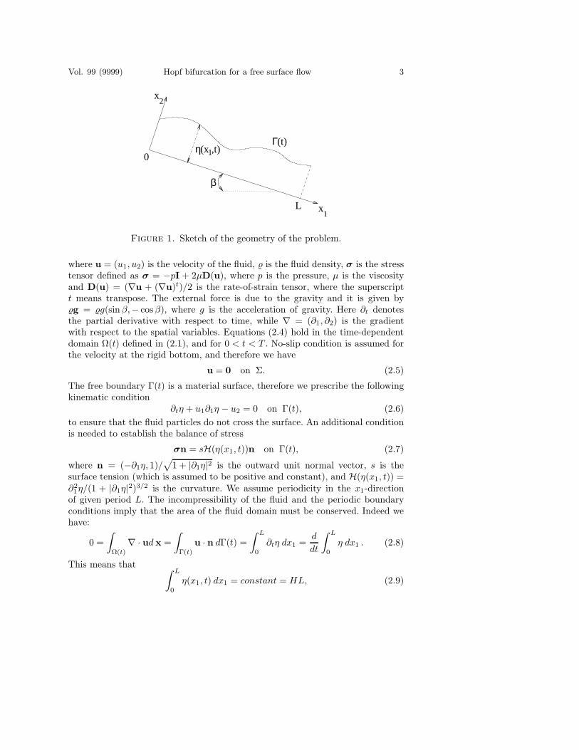
Problem (2.14) is defined on the domain Ω(t) which changes in time and itis not known a priori. Therefore we are going to reformulate problem (2.14) intoa fixed reference domain.

Let At be a family of mappings which at each time t ∈ (0, T ) maps the

current domain Ω(t) into the reference domain Ω = (0, L) × (0, H) defined by

At : Ω(t) ∈ R2 → Ω ∈ R

2

x = (x1, x2) → ξ = (ξ1, ξ2) = At(x) =

ξ1 = x1

ξ2 =H

η(x1, t)x2 ,

(2.17)

as sketched in Figure 2. We observe that the free surface Γ(t) is mapped into

Γ = ξ ∈ R2 | ξ1 ∈ (0, L), ξ2 = H. (2.18)

The Jacobian matrix J of this transformation and its determinant J are given by

J = J(η) =

1 0

−ξ2

η(ξ1, t)∂1η(ξ1, t)

H

η(ξ1, t)

, J = J(η) =

H

η(ξ1, t). (2.19)

It is clear that this transformation is well defined as long as η(ξ1, t) > 0 or, inother words, as long as the free surface does not touch the bottom. Let f = f(x, t)

be a function defined on Ω(t) and f = f(ξ, t) = f(A−1t (ξ), t) the correspondent


function defined on Ω. Due to the change of variables, we have∫

Ω(t)

f(x, t) dx =

∫

bΩ

f(ξ, t) Jdξ. (2.20)

Moreover, it follows from the chain rule that

∂tf = ∂tf − w · ∇f , (2.21)

where ∇ = J−t∇ and the domain velocity w is given by

w(ξ1, t) = ∂tx =ξ2

H∂tη(ξ1, t)e2

=ξ2

H

[u2(ξ1, η(ξ1, t), t) − u1(ξ1, η(ξ1, t), t)∂1η(ξ1, t)

]e2.

(2.22)

The last step is a consequence of the kinematic condition (2.6) and we used thenotation e2 = (0, 1).

Using (2.20) and (2.21) , problem (2.14) becomes:

For a.e. t > 0, find u(t) ∈ V0(Ω), p(t) ∈ L20(Ω), η(t) ∈ S, such that

∫

bΩ

∂tu · v J(η)dξ −

∫

bΩ

(w · ∇)u · v J(η)dξ +

∫

bΩ

(u · ∇)u · v J(η)dξ

+2µ

∫

bΩ

D(u) : D(v) J(η)dξ −

∫

bΩ

p∇ · v J(η)dξ =

∫

bΩ

g · v J(η)dξ

+s

∫ L

0

H(η)(v2(ξ1, H, t) − v1(ξ1, H, t)∂1η

)dξ1, ∀v ∈ V0(Ω),

∫

bΩ

q∇ · u J(η)dξ = 0, ∀q ∈ L2(Ω),

∫ L

0

∂tη φ dξ1 +

∫ L

0

(u1(ξ1, H, t)∂1η − u2(ξ1, H, t)) φ dξ1 = 0, ∀φ ∈ S,

u(ξ, 0) = u0(ξ), with ∇ · u0J(η0) = 0,

η(ξ1, 0) = η0(ξ1) with

∫ L

0

η0(ξ1) dξ1 = HL.

(2.23)

Here we used the notation D(u) = (∇u + (∇u)t)/2.

3. Time discretization

The numerical solution of problem (2.23) contains three main difficulties: (a) theincompressibility condition and the related unknown pressure, (b) an advectionterm associated to the velocity of the fluid, (c) an advection term associated tothe velocity of the domain. The difficulty associated with the unknown location ofthe free boundary has been removed through the transformation defined by (2.17).A time discretization by operator splitting allows to decouple the difficulties ofthe problem and to treat each of them with appropriate algorithms. Moreover it


makes possible to update the location of the free boundary as a sub-step, avoidingcostly sub-iterations between the location of the free surface and the solution ofthe Navier-Stokes equations. Among the many possible versions, we advocate avery simple operator splitting method which is first-order accurate [14]. The loworder accuracy is compensated, actually, by easy implementation and less cost incomputational time.

Let ∆t be the time discretization step and tn = n∆t, un = u(tn), pn = p(tn),ηn = η(tn). For n ≥ 0, un and ηn being known, the scheme consists of solving thefollowing problems.

1. Find un+1/5 ∈ V0(Ω) and pn+1/5 ∈ L20(Ω) such that

∫

bΩ

un+1/5 − un

∆t· vJ(ηn)dξ + µ

∫

bΩ

D(un+1/5) : D(v)J(ηn)dξ

−

∫

bΩ

pn+1/5∇ · vJ(ηn)dξ =

∫

bΩ

g · v J(ηn)dξ

+s

∫ L

0

H(ηn)(v2(ξ1, H, t) − v1(ξ1, H, t)∂1η

n)

dξ1, ∀v ∈ V0(Ω) ,

∫

bΩ

q∇ · un+1/5 J(ηn)dξ = 0, ∀q ∈ L2(Ω) .

(3.1)

2. Find un+2/5 ∈ V (Ω) via the solution of the following pure advection problem

in Ω × (tn, tn+1)

∫

bΩ

∂tu · v J(ηn)dξ +

∫

bΩ

(un+1/5 · ∇)u · v J(ηn)dξ = 0, ∀v ∈ V n+1/5,− ,

u(tn) = un+1/5 ,

u(t) = un+1/5 on Γn+1/5,− × (tn, tn+1) ,(3.2)

and then set un+2/5 = u(tn+1). The functional spaces introduced here aredefined as follows

V (Ω) = v | v ∈ (H1(Ω))2, v|x1=0 = v|x1=L ,

V n+1/5,− = v | v ∈ (H1(Ω))2, v = 0 on Γn+1/5,−, v|x1=0 = v|x1=L,

Γn+1/5,− = x | x ∈ Γ, un+1/5 · e2 < 0.


3. Find un+3/5 ∈ V0(Ω) and pn+3/5 ∈ L20(Ω) such that

∫

bΩ

un+3/5 − un+2/5

∆t· v J(ηn)dξ + µ

∫

bΩ

D(un+3/5) : D(v) J(ηn)dξ

−

∫

bΩ

pn+3/5∇ · v J(ηn)dξ = 0, ∀v ∈ V0(Ω) ,

∫

bΩ

q∇ · un+3/5 J(ηn)dξ = 0, ∀q ∈ L2(Ω) .

(3.3)

4. Find un+4/5 ∈ V (Ω) via the solution of the following pure advection problem

in Ω × (tn, tn+1)

∫

bΩ

∂tu · v J(ηn)dξ −

∫

bΩ

(wn+3/5 · ∇)u · v J(ηn)dξ = 0, ∀v ∈ Wn+3/5,+ ,

u(tn) = un+3/5 ,

u(t) = un+3/5 on Γn+3/5,+ × (tn, tn+1) ,(3.4)

and then set un+4/5 = u(tn+1) and pn+4/5 = pn+1/5 + pn+3/5. Here

wn+3/5(ξ1) =ξ2

H

[u

n+3/52 (ξ1, H) − u

n+3/51 (ξ1, H)∂1η

n(ξ1)]e2, (3.5)

and

Wn+3/5,+ = v | v ∈ (H1(Ω))2, v = 0 on Γn+3/5,+,

v periodic in x1 of period L,

Γn+3/5,+ = x | x ∈ Γ, wn+3/5 · e2 > 0.

5. Find the new position of the free surface ηn+1 ∈ S by solving the followingproblem in (0, L) × (tn, tn+1)

∫ L

0

∂tη φ dξ1 +

∫ L

0

(un+4/51 (ξ1, H)∂1η − u

n+4/52 (ξ1, H)) φdξ1 = 0, ∀φ ∈ S,

η(ξ1, tn) = ηn(ξ1).

(3.6)

The new physical domain Ωn+1 is obtained from the reference domain Ωthrough the mapping A−1

tn+1 defined as:

A−1tn+1 : Ω ∈ R

2 → Ωn+1 ∈ R2

ξ = (ξ1, ξ2) → x = (x1, x2) =

x1 = ξ1

x2 =ηn+1(ξ1)

Hξ2 .

(3.7)


The velocity un+1 and the pressure pn+1 defined on the new domain Ωn+1

are obtained as follows

un+1(x1, x2) = un+4/5(x1, Hx2/ηn+1(x1)),

pn+1(x1, x2) = pn+4/5(x1, Hx2/ηn+1(x1)),(3.8)

where (x1, x2) ∈ Ωn+1.

We remark that in (3.1)-(3.4) ∇ = J−t(ηn)∇ and that indeed it is much easierto solve the sub-problems (3.1)-(3.3) in their equivalent formulation in the physicaldomain Ωn (which is fixed from the way the problem was splitted). Moreover,problems (3.1) and (3.3) can be significantly simplified by noticing that

µ

∫

Ω(t)

D(u) : D(u) dx =µ

2

∫

Ω(t)

∇u : ∇v dx +µ

2

∫

Ω(t)

(∇u)t : ∇v dx, (3.9)

and then evaluating the last integral in (3.9) at the previous fractional step. Prob-lems (3.1)-(3.3) are then modified as follows.

1. Find un+1/5 ∈ V0(Ωn) and pn+1/5 ∈ L2

0(Ωn) such that

∫

Ωn

un+1/5 − un

∆t· vdx +

µ

2

∫

Ωn

∇un+1/5 : ∇vdx −

∫

Ωn

pn+1/5∇ · vdx

= s

∫

Γn

H(ηn)n · vdΓn +

∫

Ωn

g · vdx −µ

2

∫

Ωn

(∇un)t : ∇vdx, ∀v ∈ V0(Ωn) ,

∫

Ωn

q∇ · un+1/5dx = 0, ∀q ∈ L2(Ωn) .

(3.10)2. Find un+2/5 ∈ V (Ωn) via the solution of the following pure advection problem

in Ωn × (tn, tn+1)

∫

Ωn

∂tu · vdx +

∫

Ωn

(un+1/5 · ∇)u · vdx = 0, ∀v ∈ V n+1/5,− ,

u(tn) = un+1/5 ,

u(t) = un+1/5 on Γn+1/5,− × (tn, tn+1) ,

(3.11)

and then set un+2/5 = u(tn+1). The functional spaces introduced here aredefined as follows

V (Ωn) = v | v ∈ (H1(Ωn))2, v|x1=0 = v|x1=L ,

V n+1/5,− = v | v ∈ (H1(Ωn))2, v = 0 on Γn+1/5,−, v|x1=0 = v|x1=L,

Γn+1/5,− = x | x ∈ Γn, un+1/5 · n(x) < 0.


3. Find un+3/5 ∈ V0(Ωn) and pn+3/5 ∈ L2

0(Ωn) such that

∫

Ωn

un+3/5 − un

∆t· vdx +

µ

2

∫

Ωn

∇un+3/5 : ∇vdx −

∫

Ωn

pn+3/5∇ · vdx

= −µ

2

∫

Ωn

(∇un+2/5)t : ∇vdx, ∀v ∈ V0(Ωn) ,

∫

Ωn

q∇ · un+3/5dx = 0, ∀q ∈ L2(Ωn) .

(3.12)

Then we define un+3/5 by un+3/5(ξ1, ξ2) = un+3/5(ξ1, ηn(ξ1)ξ2/H); un+3/5

is needed to solve problem (3.4).

4. Space discretization

At each time step, the subproblems (3.10)-(3.12) are solved in the domain Ωn

which is clearly non-polygonal because of the curved portion Γn of the boundary.To approximate velocity and pressure we use here an isoparametric version (dis-cussed in, e.g., [8], Chapter 5) of the Bercovier-Pironneau finite elements methodalso known as the P1 − iso − P2 and P1 finite elements approximation. This ap-proximation was introduced in [3] and further discussed in, e.g., [18].

To describe the isoparametric finite element approximation of the problemlet us consider a bounded domain Ω(t) ∈ R

2 with a curved boundary Γ(t), like theone in Figure 1. We introduce a triangulation Th of Ω with discretization step hand we decompose it as Th = TRh

⋃T0h, where

TRh = T | T ∈ Th, the three edges of T are rectilinear , (4.1)

T0h = T | T ∈ Th, T has one curvilinear edge (4.2)

with the two extremities on Γ(t) . (4.3)

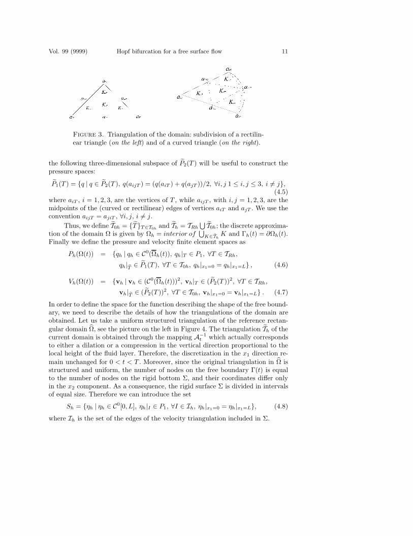
Every rectilinear triangle T ∈ TRh is divided into four sub-triangles KiT , i =1, 2, 3, 4 by joining the midpoints of its edges. On the other hand, every curved

triangle T ∈ T0h is approximated by the quadrilateral T obtained by joining themidpoints of the two rectilinear edges and the midpoint of the curved one. Then,

the quadrilateral T is divided into four sub-triangles KiT , i = 1, 2, 3, 4 as in theprevious case.

To construct the velocity spaces we introduce

P2(T ) =

q | q ∈ C0(T ), q|KiT ∈ P1, ∀i = 1, 2, 3, 4, if T ∈ TRh

q | q ∈ C0(T ), q|KiT ∈ P1, ∀i = 1, 2, 3, 4, if T ∈ T0h(4.4)

where C0(T ) (resp. C0(T )) is the space of the functions continuous over T (resp.

T ), and P1 is the space of polynomials with degree less or equal to one. Similarly,


Figure 3. Triangulation of the domain: subdivision of a rectilin-ear triangle (on the left) and of a curved triangle (on the right).

the following three-dimensional subspace of P2(T ) will be useful to construct thepressure spaces:

P1(T ) = q | q ∈ P2(T ), q(aijT ) = (q(aiT ) + q(ajT ))/2, ∀i, j 1 ≤ i, j ≤ 3, i 6= j,(4.5)

where aiT , i = 1, 2, 3, are the vertices of T , while aijT , with i, j = 1, 2, 3, are themidpoints of the (curved or rectilinear) edges of vertices aiT and ajT . We use theconvention aijT = ajiT , ∀i, j, i 6= j.

Thus, we define T0h = TT∈T0hand Th = TRh

⋃T0h; the discrete approxima-

tion of the domain Ω is given by Ωh = interior of⋃

K∈ThK and Γh(t) = ∂Ωh(t).

Finally we define the pressure and velocity finite element spaces as

Ph(Ω(t)) = qh | qh ∈ C0(Ωh(t)), qh|T ∈ P1, ∀T ∈ TRh,

qh|eT ∈ P1(T ), ∀T ∈ T0h, qh|x1=0 = qh|x1=L , (4.6)

Vh(Ω(t)) = vh | vh ∈ (C0(Ωh(t)))2, vh|T ∈ (P2(T ))2, ∀T ∈ TRh,

vh|eT ∈ (P2(T ))2, ∀T ∈ T0h, vh|x1=0 = vh|x1=L . (4.7)

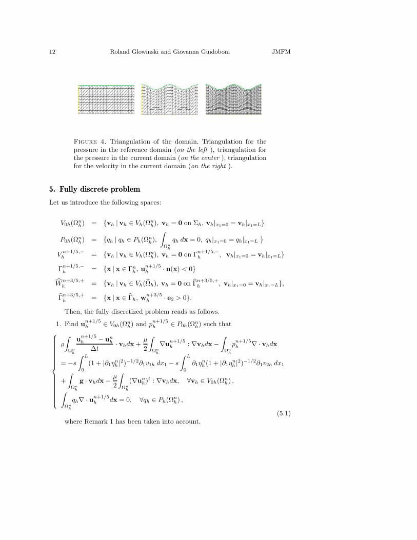
In order to define the space for the function describing the shape of the free bound-ary, we need to describe the details of how the triangulations of the domain areobtained. Let us take a uniform structured triangulation of the reference rectan-

gular domain Ω, see the picture on the left in Figure 4. The triangulation Th of thecurrent domain is obtained through the mapping A−1

t which actually correspondsto either a dilation or a compression in the vertical direction proportional to thelocal height of the fluid layer. Therefore, the discretization in the x1 direction re-

main unchanged for 0 < t < T . Moreover, since the original triangulation in Ω isstructured and uniform, the number of nodes on the free boundary Γ(t) is equalto the number of nodes on the rigid bottom Σ, and their coordinates differ onlyin the x2 component. As a consequence, the rigid surface Σ is divided in intervalsof equal size. Therefore we can introduce the set

Sh = ηh | ηh ∈ C0[0, L], ηh|I ∈ P1, ∀I ∈ Ih, ηh|x1=0 = ηh|x1=L, (4.8)

where Ih is the set of the edges of the velocity triangulation included in Σ.


Figure 4. Triangulation of the domain. Triangulation for thepressure in the reference domain (on the left ), triangulation forthe pressure in the current domain (on the center ), triangulationfor the velocity in the current domain (on the right ).

5. Fully discrete problem

Let us introduce the following spaces:

V0h(Ωnh) = vh | vh ∈ Vh(Ωn

h), vh = 0 on Σh, vh|x1=0 = vh|x1=L

P0h(Ωnh) = qh | qh ∈ Ph(Ωn

h),

∫

Ωnh

qh dx = 0, qh|x1=0 = qh|x1=L

Vn+1/5,−h = vh | vh ∈ Vh(Ωn

h), vh = 0 on Γn+1/5,−h , vh|x1=0 = vh|x1=L

Γn+1/5,−h = x | x ∈ Γn

h, un+1/5h · n(x) < 0

Wn+3/5,+h = vh | vh ∈ Vh(Ωh), vh = 0 on Γ

n+3/5,+h , vh|x1=0 = vh|x1=L,

Γn+3/5,+h = x | x ∈ Γh, w

n+3/5h · e2 > 0.

Then, the fully discretized problem reads as follows.

1. Find un+1/5h ∈ V0h(Ωn

h) and pn+1/5h ∈ P0h(Ωn

h) such that

∫

Ωnh

un+1/5h − un

h

∆t· vhdx +

µ

2

∫

Ωnh

∇un+1/5h : ∇vhdx −

∫

Ωnh

pn+1/5h ∇ · vhdx

= −s

∫ L

0

(1 + |∂1ηnh |

2)−1/2∂1v1h dx1 − s

∫ L

0

∂1ηnh (1 + |∂1η

nh |

2)−1/2∂1v2h dx1

+

∫

Ωnh

g · vhdx −µ

2

∫

Ωnh

(∇unh)t : ∇vhdx, ∀vh ∈ V0h(Ωn

h) ,

∫

Ωnh

qh∇ · un+1/5h dx = 0, ∀qh ∈ Ph(Ωn

h) ,

(5.1)where Remark 1 has been taken into account.


2. Find un+2/5h ∈ Vh(Ωn

h) via the solution of the following pure advection prob-lem in Ωn

h × (tn, tn+1)

∫

Ωnh

∂tuh · vhdx +

∫

Ωnh

(un+1/5h · ∇)uh · vhdx = 0, ∀vh ∈ V

n+1/5,−h ,

uh(tn) = un+1/5h ,

uh(t) = un+1/5h on Γ

n+1/5,−h × (tn, tn+1) ,

(5.2)

and then set un+2/5h = uh(tn+1).

3. Find un+3/5h ∈ V0h(Ωn

h) and pn+3/5h ∈ P0h(Ωn

h) such that

∫

Ωnh

un+3/5h − un

h

∆t· vhdx +

µ

2

∫

Ωnh

∇un+3/5h : ∇vhdx −

∫

Ωnh

pn+3/5h ∇ · vhdx

= −µ

2

∫

Ωnh

(∇un+2/5h )t : ∇vhdx, ∀vh ∈ V0h(Ωn

h) ,

∫

Ωnh

qh∇ · un+3/5h dx = 0, ∀q ∈ Ph(Ωn

h) .

(5.3)

4. Find un+4/5h ∈ Vh(Ωh) via the solution of the following pure advection prob-

lem in Ωh × (tn, tn+1)

∫

bΩh

∂tuh · vh J(η)dξ −

∫

bΩh

(wn+3/5h · ∇)uh · vh J(η)dξ = 0, ∀vh ∈ W

n+3/5,+h ,

uh(tn) = un+3/5h ,

uh(t) = un+3/5h on Γ

n+3/5,+h × (tn, tn+1) ,

(5.4)

and then set un+4/5h = uh(tn+1) and pn+4/5 = pn+1/5 + pn+1/3.

5. Find the new position of the free surface ηn+1h ∈ Sh by solving the following

problem in (0, L) × (tn, tn+1)

∫ L

0

∂tηh φh dξ1 +

∫ L

0

(un+4/51h (ξ1, H)∂1ηh − u

n+4/52h (ξ1, H)) φh dξ1 = 0, ∀φh ∈ Sh,

ηh(ξ1, tn) = ηn

h (ξ1),

(5.5)


The new domain Ωn+1h is obtained from the reference domain Ωh trough the

mapping A−1tn+1,h defined as:

A−1tn+1,h : Ωh ∈ R

2 → Ωn+1h ∈ R

2

ξ = (ξ1, ξ2) → x = (x1, x2) =

x1 = ξ1

x2 =ηn+1

h (ξ1)

Hξ2 .

(5.6)

The velocity un+1h and the pressure pn+1

h defined on the new domain Ωn+1h

are obtained as follows

un+1h (x1, x2) = u

n+4/5h (x1, η

nh(x1)x2/ηn+1(x1)), (5.7)

pn+1h (x1, x2) = p

n+4/5h (x1, η

nh(x1)x2/ηn+1

h ), (5.8)

where (x1, x2) ∈ Ωn+1h .

The backward Euler’s method has been used to derive the time discretizationin (5.1) and (5.3). These problem can be seen as a ”generalized” discrete Stokesproblem for which efficient solution methods already exist as shown in, e.g., [8].

The advection step (3.2) has been solved using a wave-like equation method[8, 10, 17]: this approach preserves the hyperbolic nature of advection, it does notintroduce numerical dissipation and it is easy to implement. It consists in replacingproblem (5.2) by the following wave-like equation one in Ωn

h × (tn, tn+1):

∫

Ωnh

∂2t uh · vhdx +

∫

Ωnh

(un+1/5h · ∇)uh · (u

n+1/5h · ∇)vhdx

+

∫

Γnh\Γ

n+1/5,−h

(un+1/5h · n)(∂tuh · vh)dΓn

h = 0, ∀vh ∈ Vn+1/5,−0h ,

uh(tn) = un+1/5h ,

∫

Ωnh

∂tuh(tn) · vhdx = −

∫

Ωnh

(un+1/5 · ∇)un+1/5h · vhdx, ∀vh ∈ V

n+1/5,−0h ,

∂tuh(tn) ∈ Vn+1/5,−0h , uh = u

n+1/5h on Γ

n+1/5,−h × (tn, tn+1).

(5.9)We have solved problem (5.9) using a second order accurate time discretizationscheme which is discussed in, e.g., [8], Chapter 6, and [17].

To solve the trasport problem (5.4) we use again the wave equation approach.We observe that (5.4) does not contain x1 differentiation of u and therefore theproblem reduces to the solution of a family (infinite for the continuous problem,finite for the discrete ones) of transport problems in one space dimension alongthe vertical direction. Then for ξ1 ∈ [0, L), each component of u is solution of a


transport problem of the following form:

∂ϕ

∂t− aξ2

∂ϕ

∂ξ2= 0 on (0, L) × (tn, tn+1),

ϕ(tn) = ϕ0,

ϕ(H, t) = b if a > 0, t ∈ (tn, tn+1),

(5.10)

with a and b constant with respect to ξ2 and t. We observe that any smoothsolution of (5.10) verifies:

∂2ϕ

∂t2− a2ξ2

∂

ξ2

(ξ2

∂ϕ

ξ2

)= 0 on (0, L) × (tn, tn+1),

ϕ(tn) = ϕ0,

∂ϕ

∂t(tn) = aξ2

∂ϕ0

∂ξ2,

ϕ(H, t) = b if a > 0, t ∈ (tn, tn+1),[aξ2

(∂ϕ

∂t− aξ2

∂ϕ

∂ξ2

)]

ξ2=H

= 0 if a ≤ 0, t ∈ (tn, tn+1).

(5.11)

From a practical point of view, we take advantage of the following variationalformulation of (5.10), better suited for finite element treatment.

1. Case a > 0.

∫ H

0

∂2ϕ

∂t2v

ξ2dξ2 + a2

∫ H

0

ξ2∂ϕ

∂ξ2

∂v

∂ξ2dξ2 = 0, ∀v ∈ D(0, H), a.e. on (t0, tf ),

ϕ(t0) = ϕ0,

∂ϕ

∂t(t0) = aξ2

∂ϕ0

∂ξ2,

ϕ(H, t) = f,(5.12)

with D(0, H) = v | v ∈ C∞[0, H ], v has compact support in (0, H) .2. Case a < 0.

∫ H

0

∂2ϕ

∂t2v

ξ2dξ2 + a2

∫ H

0

ξ2∂ϕ

∂ξ2

∂v

∂ξ2dξ2 − a

∂ϕ

∂t(H, t)v(H) = 0,

∀v ∈ D(0, H), a.e. on (t0, tf ),

ϕ(t0) = ϕ0,

∂ϕ

∂t(t0) = aξ2

∂ϕ0

∂ξ2,

(5.13)

with V0 = v | v ∈ C∞[0, H ], v has compact support in (0, H ] .


Finally, problem (5.5) is solved using a second order Taylor-Galerkin dis-cretization on (0, L) × (tn, tn+1), namely

∫ L

0

(ηn+1h − ηn

h) φh dx1 = ∆t

∫ L

0

(un+4/52h − u

n+4/51h ∂1η

nh) φh dx1

−(∆t)2

2

∫ L

0

un+4/51h ∂1u

n+4/52h φh dx1

−(∆t)2

2

∫ L

0

un+4/51h ∂1η

nh(∂1u

n+4/51h φh + u

n+4/51h ∂1φh) dx1 ,

(5.14)

where the velocity is computed at Γnh.

Remark 2. For a general approach concerning the approximation of free sur-face problems for incompressible viscous fluids with surface tension see, e.g., [4].

6. Numerical experiments

Problem (2.4)-(2.10) always admits a steady solution. Indeed, assuming that u =U(x2)e1, with e1 = (1, 0), p = P (x2) and η(x1, t) ≡ H , we get

U =g sin β

2µ(2Hx2 − x2

2), P = −g cosβ(x2 − H) in (0, L) × (0, H). (6.1)

Nishida et al. in [15] proved the existence of time periodic solutions bifurcatingfrom the basic flow (6.1) for Reynolds numbers large enough. The Reynolds numberRe is defined as Re = HUmax/µ, where H is the average height of the fluid layerand Umax is the velocity of the basic flow at the free surface, obtained from (6.1)with x2 = H , namely

Umax =H2g sinβ

2µ, (6.2)

implying that

Re =H32g sinβ

2µ2. (6.3)

Our goal is to explore the features of the bifurcating solutions using the numericalalgorithm described in the previous sections.

For the time discretization we have taken ∆t = 2.5 · 10−4. As mentioned inSection 5, we solve the advection steps (5.2) and (5.4) using a wave-like equationmethod which requires the specification of time substeps: here we have chosenboth of them equal to ∆t/5. In our numerical experiments, the dimensions of thereference rectangular domain are H = 0.15 and L = 3, the density of the fluid is = 1, and the angle of inclination is β = 45.

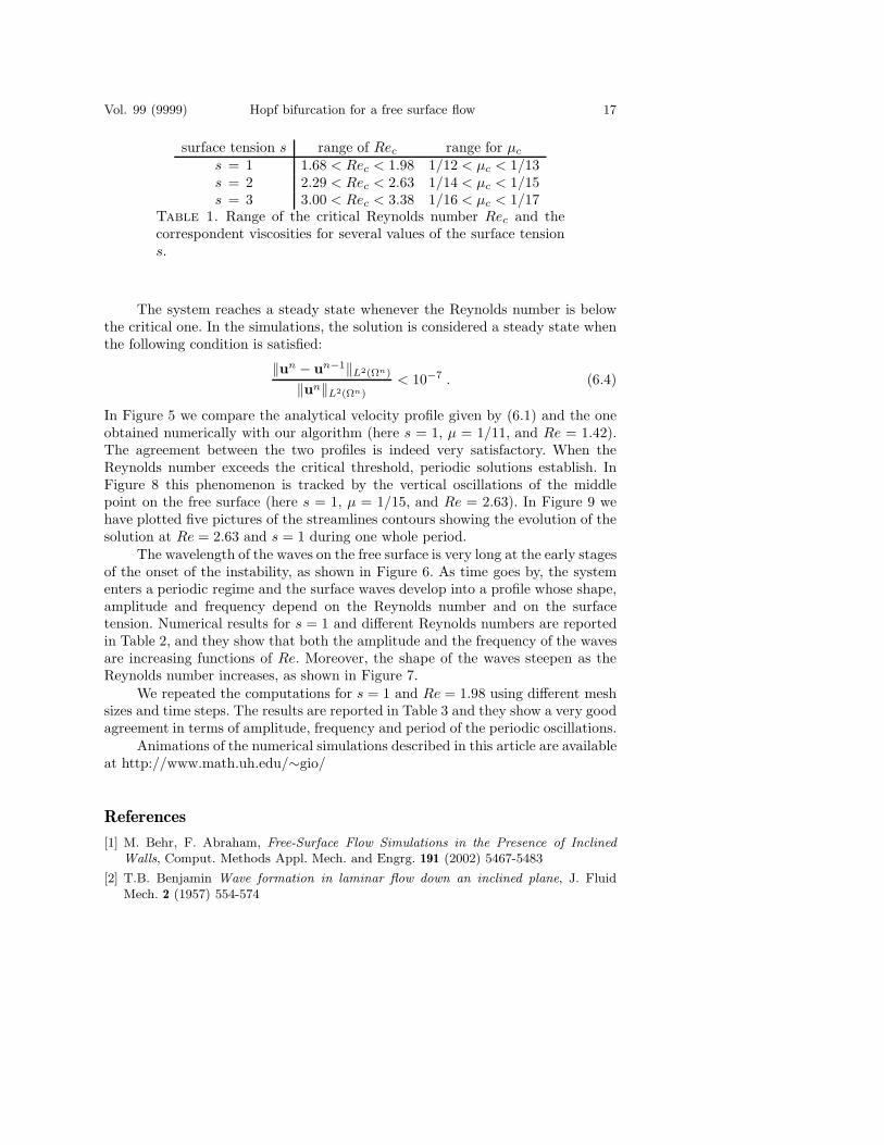
By direct simulation, we estimated the critical Reynolds number Rec as afunction of the surface tension. In particular, we considered s = 1, 2, 3. The resultsare reported in Table 1. It is clear that Rec is an increasing function of s, whichmeans that the surface tension has a stabilizing effect, as shown in [13].


surface tension s range of Rec range for µc

s = 1 1.68 < Rec < 1.98 1/12 < µc < 1/13s = 2 2.29 < Rec < 2.63 1/14 < µc < 1/15s = 3 3.00 < Rec < 3.38 1/16 < µc < 1/17

Table 1. Range of the critical Reynolds number Rec and thecorrespondent viscosities for several values of the surface tensions.

The system reaches a steady state whenever the Reynolds number is belowthe critical one. In the simulations, the solution is considered a steady state whenthe following condition is satisfied:

‖un − un−1‖L2(Ωn)

‖un‖L2(Ωn)< 10−7 . (6.4)

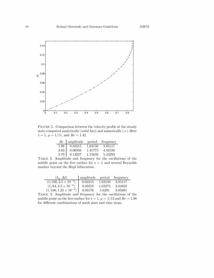
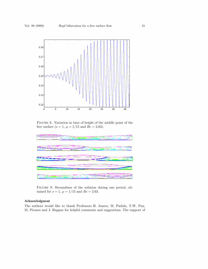
In Figure 5 we compare the analytical velocity profile given by (6.1) and the oneobtained numerically with our algorithm (here s = 1, µ = 1/11, and Re = 1.42).The agreement between the two profiles is indeed very satisfactory. When theReynolds number exceeds the critical threshold, periodic solutions establish. InFigure 8 this phenomenon is tracked by the vertical oscillations of the middlepoint on the free surface (here s = 1, µ = 1/15, and Re = 2.63). In Figure 9 wehave plotted five pictures of the streamlines contours showing the evolution of thesolution at Re = 2.63 and s = 1 during one whole period.

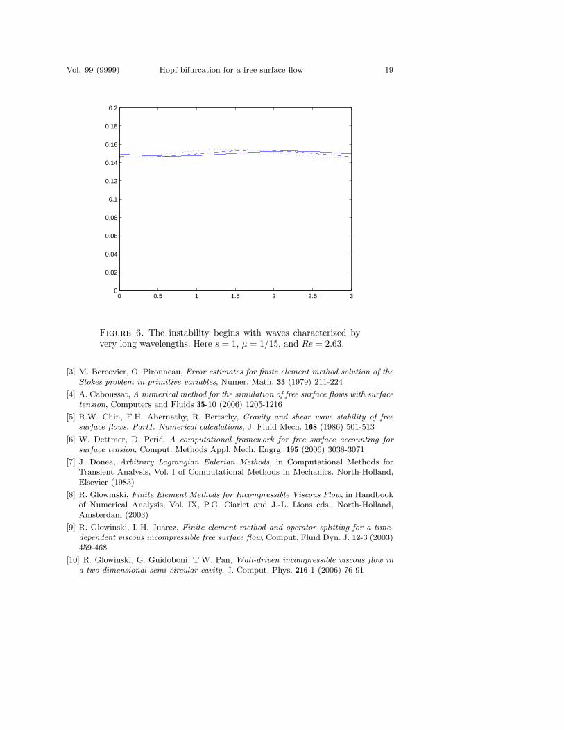
The wavelength of the waves on the free surface is very long at the early stagesof the onset of the instability, as shown in Figure 6. As time goes by, the systementers a periodic regime and the surface waves develop into a profile whose shape,amplitude and frequency depend on the Reynolds number and on the surfacetension. Numerical results for s = 1 and different Reynolds numbers are reportedin Table 2, and they show that both the amplitude and the frequency of the wavesare increasing functions of Re. Moreover, the shape of the waves steepen as theReynolds number increases, as shown in Figure 7.

We repeated the computations for s = 1 and Re = 1.98 using different meshsizes and time steps. The results are reported in Table 3 and they show a very goodagreement in terms of amplitude, frequency and period of the periodic oscillations.

Animations of the numerical simulations described in this article are availableat http://www.math.uh.edu/∼gio/

References

[1] M. Behr, F. Abraham, Free-Surface Flow Simulations in the Presence of InclinedWalls, Comput. Methods Appl. Mech. and Engrg. 191 (2002) 5467-5483

[2] T.B. Benjamin Wave formation in laminar flow down an inclined plane, J. FluidMech. 2 (1957) 554-574


0 0.1 0.2 0.3 0.4 0.5 0.6 0.7 0.80

0.02

0.04

0.06

0.08

0.1

0.12

0.14

x2

Figure 5. Comparison between the velocity profile at the steadystate computed analytically (solid line) and numerically (×). Heres = 1, µ = 1/11, and Re = 1.42.

Re amplitude period frequency1.98 0.03215 1.63150 3.851172.63 0.06956 1.41775 4.431803.79 0.13927 1.15650 5.43293

Table 2. Amplitude and frequency for the oscillations of themiddle point on the free surface for s = 1 and several Reynoldsnumber beyond the Hopf bifurcation.

(hp, ∆t) amplitude period frequency(1/100, 2.5× 10−4) 0.03215 1.63150 3.85117(1/64, 2.5× 10−4) 0.03210 1.63275 3.84822

(1/100, 1.25× 10−4) 0.03176 1.6291 3.85691Table 3. Amplitude and frequency for the oscillations of themiddle point on the free surface for s = 1, µ = 1/13 and Re = 1.98for different combinations of mesh sizes and time steps.


0 0.5 1 1.5 2 2.5 30

0.02

0.04

0.06

0.08

0.1

0.12

0.14

0.16

0.18

0.2

Figure 6. The instability begins with waves characterized byvery long wavelengths. Here s = 1, µ = 1/15, and Re = 2.63.

[3] M. Bercovier, O. Pironneau, Error estimates for finite element method solution of theStokes problem in primitive variables, Numer. Math. 33 (1979) 211-224

[4] A. Caboussat, A numerical method for the simulation of free surface flows with surfacetension, Computers and Fluids 35-10 (2006) 1205-1216

[5] R.W. Chin, F.H. Abernathy, R. Bertschy, Gravity and shear wave stability of freesurface flows. Part1. Numerical calculations, J. Fluid Mech. 168 (1986) 501-513

[6] W. Dettmer, D. Peric, A computational framework for free surface accounting forsurface tension, Comput. Methods Appl. Mech. Engrg. 195 (2006) 3038-3071

[7] J. Donea, Arbitrary Lagrangian Eulerian Methods, in Computational Methods forTransient Analysis, Vol. I of Computational Methods in Mechanics. North-Holland,Elsevier (1983)

[8] R. Glowinski, Finite Element Methods for Incompressible Viscous Flow, in Handbookof Numerical Analysis, Vol. IX, P.G. Ciarlet and J.-L. Lions eds., North-Holland,Amsterdam (2003)

[9] R. Glowinski, L.H. Juarez, Finite element method and operator splitting for a time-dependent viscous incompressible free surface flow, Comput. Fluid Dyn. J. 12-3 (2003)459-468

[10] R. Glowinski, G. Guidoboni, T.W. Pan, Wall-driven incompressible viscous flow ina two-dimensional semi-circular cavity, J. Comput. Phys. 216-1 (2006) 76-91


0 0.5 1 1.5 2 2.5 30.08

0.1

0.12

0.14

0.16

0.18

0.2

0.22

0.24

Figure 7. Shape of the waves on the free surface in the periodicregime for Re = 1.98 and µ = 1/13 (solid line), Re = 2.63 andµ = 1/15 (dashed line), Re = 3.79 and µ = 1/18 (dashed-dottedline), when s = 1.

[11] D.Rh. Gwynllyw, D.H. Peregrine, Numerical Simulation of Stokes flow down aninclined plane, Proc. R. Soc. Lond. A 452-1946 (1996) 543-565

[12] T.J. Hughes, W.K. Liu, T.K. Zimmermann, Lagrangian-eulerian finite element for-mulation for incompressible viscous flows, Comp. Meth. Appl. Mech. Engrg. 29 (1981)329-349

[13] J. Liu, J.D. Paul, J.P. Gollub, Measurements of the primary instabilites of film flows,J. Fluid Mech. 250 (1993) 69-101

[14] G.I. Marchuk, Splitting and alternate direction methods, in Handbook of NumericalAnalysis, Vol. I, P.G. Ciarlet and J.-L. Lions eds., North-Holland, Amsterdam (1990)

[15] T. Nishida, Y. Teramoto, H. Yoshihara, Hopf bifurcation in viscous incompressibleflow down an inclined plane, J. Math. Fluid Mech. 7 (2005) 29-71

[16] M. Padula, V.A. Solonnikov, On Rayleigh-Taylor stability, Ann. Univ. Ferrara Sez.VII (N.S.) 46 (2000), 307-336

[17] T.W. Pan and R. Glowinski, A projection/wave-like equation method for the nu-merical simulation of incompressible viscous fluid flow modeled by the Navier-Stokesequations , Comput. Fluid Dyn. J. 9-2 (2000) 28-42

[18] O. Pironneau, Finite Element Methods for Fluids, J. Wiley, Chichester (1989)


0 5 10 15 20 25 30 35

0.12

0.13

0.14

0.15

0.16

0.17

0.18

Figure 8. Variation in time of height of the middle point of thefree surface (s = 1, µ = 1/15 and Re = 2.63).

Figure 9. Streamlines of the solution during one period, ob-tained for s = 1, µ = 1/15 and Re = 2.63.

Acknowledgment

The authors would like to thank Professors H. Juarez, M. Padula, T.W. Pan,M. Picasso and J. Rappaz for helpful comments and suggestions. The support of


NSF (Grant DMS-9973318, 0209066, and CCR-9902035) and DOE/LACSI (GrantR71700K-292-000-99) is also acknowledged.

Roland GlowinskiDepartment of Mathematics,University of Houston,Houston, Texas 77204-3476, USAand Laboratoire Jacques-Louis Lions,Universite P. et M. Curie,4 Place Jussieu, 75005, Paris, Francee-mail: [email protected]

Giovanna GuidoboniDepartment of Mathematics,University of Houston,Houston, Texas 77204-3476, USAe-mail: [email protected]

Hopf Bifurcation in Viscous Incompressible Flow Down an Inclined Plane: a Numerical Approach

Documents

Transcript of Hopf Bifurcation in Viscous Incompressible Flow Down an Inclined Plane: a Numerical Approach