Higher Order Moreau’s Sweeping Process
317
NONSMOOTH MECHANICS AND ANALYSIS Theoretical and Numerical Advances
-
Upload
independent -
Category
Documents
-
view
5 -
download
0
Transcript of Higher Order Moreau’s Sweeping Process

NONSMOOTH MECHANICS AND ANALYSIS
Theoretical and Numerical Advances

Advances in Mechanics and Mathematics
VOLUME 12
Series Editors:
David Y. Gao Virginia Polytechnic Institute and State University, U.S.A.
Ray W. Ogden University of Glasgow, U.K.
Advisory Editors:
I. Ekeland University of British Columbia, Canada
S. Liao Shanghai Jiao Tung University, P.R. China
K.R. Rajagopal Texas A&M University, U.S.A.
T. Ratiu Ecole Polytechnique, Switzerland
W. Yang Tsinghua University, P.R. China

NONSMOOTH MECHANICS AND ANALYSIS
Theoretical and Numerical Advances
Edited by
P. ALART Université Montpellier II, Montpellier, France
O. MAISONNEUVE Université Montpellier II, Montpellier, France
R.T. ROCKAFELLAR University of Washington, Seattle, Washington, U.S.A.
1 3

Library of Congress Control Number: 2005932761
ISBN-10: 0-387-29196-2 e-ISBN 0-387-29195-4
ISBN-13: 978-0387-29196-3
Printed on acid-free paper.
2006 Springer Science+Business Media, Inc.
All rights reserved. This work may not be translated or copied in whole or in part without the written permission of the publisher (Springer Science+Business Media, Inc., 233 Spring Street, New York, NY 10013, USA), except for brief excerpts in connection with reviews or scholarly analysis. Use in connection with any form of information storage and retrieval, electronic adaptation, computer software, or by similar or dissimilar methodology now known or hereafter developed is forbidden.
The use in this publication of trade names, trademarks, service marks, and similar terms, even if they are not identified as such, is not to be taken as an expression of opinion as to whether or not they are subject to proprietary rights.
Printed in the United States of America.
9 8 7 6 5 4 3 2 1
springeronline.com

Contents
Preface ixA short biography of Jean Jacques Moreau xiii
Part I Convex and nonsmooth analysis
1Moreau’s proximal mappings and convexity in Hamilton-Jacobi theory 3R. T. Rockafellar
2Three optimization problems in mass transportation theory 13G. Buttazzo
3Geometrical and algebraic properties of various convex hulls 25B. Dacorogna
4Legendre-Fenchel transform of convex composite functions 35J.-B. Hiriart-Urruty
5What is to be a mean? 47M. Valadier
Part II Nonsmooth mechanics
6Thermoelastic contact with frictional heating 61L.-E. Andersson, A. Klarbring, J.R. Barber and M. Ciavarella
7A condition for statical admissibility in unilateral structural analysis 71G. Del Piero
8Min-max Duality and Shakedown Theorems in Plasticity 81

vi NONSMOOTH MECHANICS AND ANALYSIS
Q. S. Nguyen
9Friction and adhesion 93M. Raous
10The Clausius-Duhem inequality, an interesting and productive inequality 107M. Fremond
11Unilateral crack identification 119G. E. Stavroulakis, M. Engelhardt and H. Antes
12Penalty approximation of Painleve problem 129M. Schatzman
13Discrete contact problems with friction 145F. Maceri and P. Bisegna
Part III Fluid mechanics
14A brief history of drop formation 163J. Eggers
15Semiclassical approach of the “tetrad model” of turbulence 173A. Naso and A. Pumir
Part IV Multibody dynamics: numerical aspects
16The geometry of Newton’s cradle 185C. Glocker and U. Aeberhard
17Nonsmooth analysis for contact mechanics simulations 195P. Alart, D. Dureisseix and M. Renouf
18Numerical simulation of a multibody gas 209M. Jean
19Granular media and ballasted railway tracks 221
Contents vii
C. Cholet, G. Saussine, P.-E. Gautier and L.-M. Cleon
20Scaling behaviour of velocity fluctuations in slow granular flows 233F. Radjaı and S. Roux
Part V Topics in nonsmooth science
21Morphological equations and sweeping processes 249J.-P. Aubin and J. A. Murillo Hernandez
22Higher order Moreau’s sweeping process 261V. Acary and B. Brogliato
23An existence result in non-smooth dynamics 279M.D.P. Monteiro Marques and L. Paoli
24Finite time stabilization of nonlinear oscillators subject to dry friction 289S. Adly, H. Attouch and A. Cabot
25Canonical duality in nonsmooth, constrained concave minimization 305D. Y. Gao
Appendix: Theoretical and Numerical Nonsmooth Mechanics InternationalColloquium 315
Index 319

Preface
In the course of the last fifty years, developments in nonsmooth analy-sis and nonsmooth mechanics have often been closely linked. The presentbook acts as an illustration of this. Its objective is two-fold. It is ofcourse intended to help to diffuse the recent results obtained by variousrenowned specialists. But there is an equal desire to pay homage to JeanJacques Moreau, who is undoubtedly the most emblematic figure in thecorrelated, not to say dual, advances in these two fields.
Jean Jacques Moreau appears as a rightful heir to the founders ofdifferential calculus and mechanics through the depth of his thinkingin the field of nonsmooth mechanics and the size of his contribution tothe development of nonsmooth analysis. His interest in mechanics hasfocused on a wide variety of subjects: singularities in fluid flows, theinitiation of cavitation, plasticity, and the statics and dynamics of gran-ular media. The ‘Ariadne’s thread’ running throughout is the notion ofunilateral constraint. Allied to this is his investment in mathematics inthe fields of convex analysis, calculus of variations and differential mea-sures. When considering these contributions, regardless of their nature,one cannot fail to be struck by their clarity, discerning originality andelegance. Precision and rigor of thinking, clarity and elegance of styleare the distinctive features of his work.
In 2003, Jean Jacques Moreau’s colleagues decided to celebrate his80th birthday by organizing a symposium in Montpellier, the city inwhich he has spent the major part of his university life and where heis still very active scientifically in the Laboratoire de Mecanique et deGenie Civil. In the appendix, the reader will find a list of those who par-ticipated in the symposium, entitled “Theoretical and Numerical Nons-mooth Mechanics”. This book is one of the outcomes of the symposium.It does not represent the acts, stricto sensu, although it does reflect itsstructure in five parts. Each of these corresponds to a field of mathemat-ics or mechanics in which Jean Jacques Moreau has made remarkablecontributions. The works that follow are those of eminent specialists,

x NONSMOOTH MECHANICS AND ANALYSIS
united by the fact that they have all, at some time, appreciated andutilized these contributions.
The diversity of the topics presented in the following pages may comeas a surprise. In a way this reflects the open and mobile mind of theman they pay tribute to; it should allow the reader to appreciate, atleast in part, the importance of the scientific wake produced. Specialistsin one or a number of the subjects dealt with will enjoy discovering newresults in their own fields. But they will also discover subjects outsidetheir usual domain, linked through certain aspects and likely to openup new horizons. Not surprisingly, the first part is devoted to Con-vex and Nonsmooth Analysis, two modern and powerful approaches tothe study of theories like optimization, calculus of variations, optimalcontrol, differential inclusions, and Hamilton-Jacobi equations, in par-ticular. Some new aspects are presented regarding the evolution of thesetheories. When a convex function is propagated by a Hamilton-Jacobipartial differential equation involving a concave-convex hamiltonian, theassociated proximal mapping is shown to locally exhibit Lipschitz depen-dence on time. Models of transportation in a city are presented, whichin connection with Monge-Kantorovich, embrace optimal transportationnetworks, pricing policies and the design of the city. The following chap-ter deals with various types of convex hulls involving a differential inclu-sion with given boundary value. Next, we find proof of a formula givingthe Legendre-Fenchel transformation of a convex composite function interms of the transformation of its components. Last is a synthetic surveyof balayage involving bistochastic operators, using inequalities that goback to Hardy, Littlewood and Polya.
Some very different applications of nonsmooth analysis in mechanicsand thermomechanics are tackled in the second part. The existence anduniqueness of steady state solutions are investigated for thermoelasticcontact problems, where a variable contact heat flow resistance is con-sidered as well as frictional heating. A necessary and sufficient conditionis obtained, with a direct mechanical interpretation, for statical admissi-bility of loads in unilateral structural analysis. In the case of plasticity,an overall presentation of shakedown theorems in the framework of gen-eralized standard models is derived by min-max duality and some newresults are proposed for the kinematic safety coefficient. This is followedby a review of recent studies and applications carried out on the differentforms of a model coupling adhesion and friction, based on introducingthe adhesion intensity variable. From a general point of view, throughvarious examples in thermomechanics, it is shown how Clausius-Duheminequality may be productive, by identifying quantities that are relatedas constitutive laws and by suggesting useful experiments. The reader

PREFACE xi
will also find a thorough investigation, in two dimensions, of the unilat-eral crack identification problem in elastodynamics. This problem maybe quite complicated, nonsmooth and nonconvex. The last two papers inthis part concern, firstly, a penalty approximation of the Painleve prob-lem with convergence to a solution and, secondly, a block relaxationsolutions algorithm, in the case of a stress-based static formulation of adiscrete contact problem with friction.
Drop formation and turbulence are among the most fascinating topicsin fluid mechanics. In the third part a new approach of coarse-grainedapproximation of velocity during turbulence follows a history of dropformation focusing on the periodic rediscovery of non linear features.
The dynamics of a collection of rigid bodies interacting via contact,dry friction and multiple collisions is a vast subject, to which JeanJacques Moreau has devoted his attention over the last twenty years.The mathematical formulation of the equations of motion, in the senseof differential inclusions, within an implicit scheme, generates efficientalgorithms that are generically referred to as the “contact dynamicsmethod” in the field of granular media. The application of such algo-rithms, as an alternative to smoothing numerical strategies, has rapidlyasserted itself in very different applications. The fourth part deals bothwith new developments in the mathematical classification of numericalalgorithms and applications to the field of granular materials.
The last part, Topics in Nonsmooth Science, provides evidence of thewide possibilities of applying the concepts developed in convex and non-smooth analysis. Often used in mechanics, these have been applied andextended in other general frameworks. The sweeping process, useful forconstructive proofs and numerical solutions, may be applied to general-ized dynamical systems and to higher order differential equations. Theexistence may be proved of solutions for evolutionary dynamical sys-tems, involving differential measures, by constructive algorithms. Suchalgorithms are used to reach stationary solutions by taking advantage offriction. Finally, the duality theory, so pertinent in the convex context,is still useful in nonconvex programming.
The editors hope that, as a result, this book will attract a widepublic. They would like to thank the “Departement des Sciences del’Ingenieur”of the “Centre National de la Recherche Scientifique” for itsfinancial support, and David Dureisseix for his efficient help for finalizingthe layout of this book.
P. Alart, O. Maisonneuve and R. T. Rockfellar

A short biography ofJean Jacques MOREAU
Jean Jacques Moreau was born on 31 July 1923, in BLAYE (GIRON-DE). “Agrege” in Mathematics and Doctor of Mathematics (Universityof Paris), he began his career as a researcher at the Centre National dela Recherche Scientifique (CNRS) before being appointed as Professorof Mathematical Methods in Physics at Poitiers University, and thenProfessor of General Mechanics at Montpellier University II, where hehas spent most of his career. Today he is Emeritus Professor in the Lab-oratoire de Mecanique et Genie Civil, joint research unit at MontpellierUniversity II - CNRS.
The central theme of his research is nonsmooth mechanics, a fieldwhose applications concern for example contacts between rigid or de-formable bodies, friction, plastic deformation of materials, wakes in fluidflows, and cavitation... The helicity invariant in the dynamics of ideal

xiv NONSMOOTH MECHANICS AND ANALYSIS
fluids, discovered by Jean Jacques Moreau in 1962, provides a startingpoint for the consideration of certain problems arising in fluid dynamics.His mathematical knowledge equipped him to develop theoretical toolsadapted to these subjects and these have become standard practice innonsmooth mechanics. Since the sixties, this activity has led him toimportant contributions in the construction of nonsmooth analysis, amathematical field that is likewise of interest to specialists in optimisa-tion, operational research and economics. He thus founded the ConvexAnalysis Group in the 1970s, at the Mathematics Institute at Montpel-lier University II, which has continued, under a succession of titles, toproduce outstanding contributions.
Since the end of the 1980s, Jean Jacques Moreau has focused moreclosely on the numerical aspects of the subjects he has been studying.He notably devised novel calculation techniques for the statics or dy-namics of collections of very numerous bodies. The direct applicationsconcern, on one hand, the dynamics of masonry works subjected to seis-mic effects and, on the other, the largely interdisciplinary field of themechanics of granular media. His computer simulations have allowedhim to make substantial personal contributions to this mechanics, whilehis numerical techniques have found applications in seismic engineeringand rail engineering (TGV, train a grande vitesse, ballast behavior).
Jean Jacques Moreau has been awarded a number of prizes by theScience Academy, including the Grand Prix Joanides. He spent a yearas guest researcher at the Mathematics Research Centre at MontrealUniversity, and has been invited abroad on numerous occasions by thetop research teams in his field. He is author, co-author and editor ofseveral advanced works on contact mechanics and more generally, onnonsmooth mechanics, and has also published a two-volume course inmechanics that has greatly influenced the teaching of this discipline. Fornumerous academics Jean Jacques Moreau has been and truly remainsa Master of Mechanics.

I
CONVEX AND NONSMOOTHANALYSIS

Chapter 1
MOREAU’S PROXIMAL MAPPINGS ANDCONVEXITY IN HAMILTON-JACOBITHEORY
R. Tyrrell Rockafellar ∗
Department of Mathematics, box 352420, University of Washington, Seattle, WA 98195-4350, [email protected]
Abstract Proximal mappings, which generalize projection mappings, were intro-duced by Moreau and shown to be valuable in understanding the subgra-dient properties of convex functions. Proximal mappings subsequentlyturned out to be important also in numerical methods of optimizationand the solution of nonlinear partial differential equations and varia-tional inequalities. Here it is shown that, when a convex function ispropagated through time by a generalized Hamilton-Jacobi partial dif-ferential equation with a Hamiltonian that is concave in the state andconvex in the co-state, the associated proximal mapping exhibits locallyLipschitz dependence on time. Furthermore, the subgradient mappingassociated of the value function associated with this mapping is graph-ically Lipschitzian.
Keywords: Proximal mappings, Hamilton-Jacobi theory, convex analysis, subgra-dients, Lipschitz properties, graphically Lipschitzian mappings.
1. IntroductionIn some of his earliest work in convex analysis, J.J. Moreau introduced
in (Moreau, 1962, Moreau, 1965), the proximal mapping P associatedwith a lower semicontinuous, proper, convex function f on a Hilbert
∗Research supported by the U.S. National Science Foundation under grant DMS–104055

4 NONSMOOTH MECHANICS AND ANALYSIS
space H, namely
P (z) = argminx
{f(x) + 1
2 ||x− z||2}
. (1.1)
It has many remarkable properties. Moreau showed that P is everywheresingle-valued as a mapping from H into H, and moreover is nonexpan-sive:
||P (z′)− P (z)|| ≤ ||z′ − z|| for all z, z′. (1.2)
In this respect P resembles a projection mapping, and indeed when f isthe indicator of a convex set C, P is the projection mapping onto C. Healso discovered an interesting duality. The proximal mapping associatedwith the convex function f∗ conjugate to f , which we can denote by
Q(z) = argminx
{f∗(y) + 1
2 ||y − z||2}
, (1.3)
which likewise is nonexpansive of course, satisfies
Q = I − P, P = I −Q. (1.4)
In fact the mappings P and Q serve to parameterize the generally set-valued subgradient mapping ∂f associated with f :
y ∈ ∂f(x) ⇐⇒ (x, y) = (P (z), Q(z)) for some z, (1.5)
this z being determined uniquely through (1.4) by z = x + y. An-other important feature is that the envelope function associated with f ,namely
E(z) = minx
{f(x) + 1
2 ||x− z||2}
, (1.6)
is a finite convex function on H which is Frechet differentiable withgradient mapping
∇E(z) = Q(z). (1.7)
Our objective in this article is to tie Moreau’s proximal mappingsand envelopes into the Hamilton-Jacobi theory associated with convexoptimization over absolutely continuous arcs ξ : [0, t] → IRn; for thissetting we henceforth will have H = IRn. Let the space of such arcs bedenoted by A1
n[0, t].The optimization problems in question concern the functions ft on
IRn defined by f0 = f and
ft(x) = minξ∈A1
n[0,t],ξ(t)=x
{f(ξ(0)) +
∫ t
0L(ξ(τ), ξ(τ))dτ
}for t > 0, (1.8)

Proximal Mappings 5
which represent the propagation of f forward in time t under the “dy-namics” of a Lagrangian function L.
A pair of recent articles (Rockafellar and Wolenski, 2001, Rockafellarand Wolenski, 2001a), has explored this in the case where L satisfies thefollowing assumptions, which we also make here:
(A1) The function L is convex, proper and lsc on IRn × IRn.(A2) The set F (x) := domL(x, ·) is nonempty for all x, and there is
a constant ρ such that dist(0, F (x)) ≤ ρ(1 + ||x||
)for all x.
(A3) There are constants α and β and a coercive, proper, nondecreas-ing function θ on [0,∞) such that L(x, v) ≥ θ
(max
{0, ||v||−α||x||
})−
β||x|| for all x and v.The convexity of L(x, v) with respect to (x, v) in (A1), instead of just
with respect to v, is called full convexity . It opens the way to broaduse of the tools of convex analysis. The properties in (A2) and (A3) aredual to each other in a sense brought out in (Rockafellar and Wolenski,2001) and provide coercivity and other needed features of the integralfunctional.
It was shown in (Rockafellar and Wolenski, 2001, Theorem 2.1) that,under these assumptions, ft is, for every t, a lower semicontinuous,proper, convex function on IRn which depends epi-continuously on t(i.e., the set-valued mapping t → epi ft is continuous with respect tot ∈ [0,∞) in the sense of Kuratowsk-Painleve set convergence (Rock-afellar and Wets, 1997)). The topic we wish to address here is how, inthat case, the associated proximal mappings
Pt(z) = argminx
{ft(x) + 1
2 ||x− z||2}
, (1.9)
with P0 = P , and envelope functions
Et(z) = minx
{ft(x) + 1
2 ||x− z||2}
, (1.10)
with E0 = E, behave in their dependence on t. It will be useful for thatpurpose to employ the notation
P (t, z) = Pt(z), E(t, z) = Et(z). (1.11)
Some aspects of this dependence can be deduced readily from the epi-continuity of ft in t, for example the continuity of P (t, z) and E(t, z) withrespect to t ∈ [0,∞); cf. (Rockafellar and Wets, 1997, 7.37, 7.38). Fromthat, it follows through the nonexpansivity of P (t, z) in z and the finiteconvexity of E(t, z) in z, that both P (t, z) and E(t, z) are continuouswith respect to (t, z) ∈ [0,∞)× IRn.

6 NONSMOOTH MECHANICS AND ANALYSIS
At the end of our paper (Rockafellar, 2004) in an application of otherresults about variational problems with full convexity, we were able toshow more recently that E(t, z) is in fact continuously differentiable withrespect to (t, z), not just with respect to z, as would already be a con-sequence of the convexity and differentiability of Et, noted above. Butthis property does not, by itself, translate into any extra feature of thedependence of P (t, z) on t, beyond the continuity we already have at ourdisposal.
The following new result which we contribute here thus reaches a newlevel, moreover one where P and E are again on a par with each other.
Theorem 1. Under (A1), (A2) and (A3), both P (t, z) and ∇E(t, z) arelocally Lipschitz continuous with respect to (t, z). Thus, E is a functionof class C1+.
Our proof will rely on the Hamilton-Jacobi theory in (Rockafellar andWolenski, 2001a) for the forward propagation expressed by (1.8). Itconcerns the characterization of the function
f(t, x) = ft(x) for (t, x) ∈ [0,∞)× IRn (1.12)
in terms of a generalized “method of characteristics” in subgradient for-mat.
2. Hamilton-Jacobi frameworkThe Hamiltonian function H that corresponds to the Lagrangian func-
tion L is obtained by passing from the convex function L(x, ·) to itsconjugate:
H(x, y) := supv
{〈v, y〉 − L(x, v)
}. (2.1)
Because of the lower semicontinuity in (A1) and the properness of L(x, ·)implied by (A2), the reciprocal formula holds that
L(x, v) = supy
{〈v, y〉 −H(x, y)
}, (2.2)
so L and H are completely dual to each other. It was established in(Rockafellar and Wolenski, 2001) that a function H : IRn × IRn → IRis the Hamiltonian for a Lagrangian L fulfilling (A1), (A2) and (A3) ifand only if it satisfies
(H1) H(x, y) is concave in x, convex in y, and everywhere finite,(H2) There are constants α and β and a finite, convex function ϕ such
thatH(x, y) ≤ ϕ(y) + (α||y||+ β)||x|| for all x, y.

Proximal Mappings 7
(H3) There are constants γ and δ and a finite, concave function ψsuch that
H(x, y) ≥ ψ(x)− (γ||x||+ δ)||y|| for all x, y.
The convexity-concavity of H in (H1) is a well known counterpartto the full convexity of L under the “partial conjugacy” in (2.1) and(2.2), cf. (Rockafellar, 1970). It implies in particular that H is locallyLipschitz continuous; cf. (Rockafellar, 1970, §35). The growth condi-tions in (H2) and (H3) are dual to (A3) and (A2), respectively. Thisduality underscores the refined nature of (A2) and (A3); they are tightlyintertwined. They have also been singled out because of the role theycan play in control theory of fully convex type. For example, L satisfies(A1), (A2), (A3), when it has the form
L(x, v) = g(x) + minu
{h(u)
∣∣Ax + Bu = v}
(2.3)
for matrices A ∈ IRn×n, B ∈ IRn×m, a finite convex function g anda lower semicontinuous, proper convex function h that is coercive, orequivalently, has finite conjugate h∗. Then ft(x) is the minimum in theproblem of minimizing
f(ξ(0)) +∫ t
0
{g(ξ(τ)) + h(ω(τ))
}dt
over all summable control functions ω : [0, t]→ IRm such that
ξ(τ) = Aξ(τ) + Bω(τ) for a.e. τ, ξ(t) = x.
The corresponding Hamiltonian in this case is
H(x, y) = 〈Ax, y〉 − g(x) + h∗(y). (2.4)
In the control context, backward propagation from a terminal timewould be more natural than forward propagation from time 0, but it iselementary to reformulate from one to the other. Forward propagation ismore convenient mathematically for the formulas that can be developed.
For any finite, concave-convex function H on IRn × IRm, there is anassociated Hamiltonian dynamical system, which can be written as thedifferential inclusion
ξ(τ) ∈ ∂yH(ξ(τ), η(τ)), −η(τ) ∈ ∂xH(ξ(τ), η(τ)) for a.e. τ, (2.5)
where ∂y refers to subgradients in the convex sense in the y argument,and ∂x refers to subgradients in the concave sense in the x argument.

8 NONSMOOTH MECHANICS AND ANALYSIS
In principle, the candidates ξ and η for a solution over an interval [0, t]could just belong to A1
n[0, t], but the local Lipschitz continuity of H,and the local boundedness it entails for the subgradient mappings thatare involved (Rockafellar, 1970, §35), guarantee that ξ and η belong toA∞
n [0, t], i.e., that they are Lipschitz continuous.Dynamics of the kind in (2.5) were first introduced in (Rockafellar,
1970) for their role in capturing optimality in variational problems withfully convex Lagrangians. In the present circumstances where (A1), (A2)and (A3) hold, it has been established in (Rockafellar and Wolenski,2001) that
ξ solves (1.8) ⇐⇒{
ξ(t) = x and (ξ, η) solves (2.5)for some η with η(0) ∈ ∂f(ξ(0)) .
(2.6)
Again, ∂f refers to subgradients of the convex function f in the tradi-tions of convex analysis. Another powerful property obtained in (Rock-afellar and Wolenski, 2001), which helps in characterizing the functionsft and therefore f , is that
y ∈ ∂ft(x) ⇐⇒{
(ξ(t), η(t)) = (x, y) for some (ξ, η)satisfying (2.5) with η(0) ∈ ∂f(ξ(0)).
(2.7)
Yet another property from (Rockafellar and Wolenski, 2001), which wecan take advantage of here, is that, for any (x0, y0) ∈ IRn × IRn, theHamiltonian system has at least one trajectory pair (ξ, η) that startsfrom (x0, y0) and continues forever, i.e., for the entire time interval[0,∞). This implies further that any trajectory up to a certain timet can be continued indefinitely beyond t. Such trajectories need not beunique, however.
Subgradients of the value function f in (1.12) must be considered aswell. The complication there is that f(t, x) is only convex with respectto x, not (t, x). Subgradient theory beyond convex analysis is there-fore essential. In this respect, we use ∂f to denote subgradients withrespect to (t, x) in the broader sense of variational analysis laid out,for instance, in (Rockafellar and Wets, 1997). These avoid the convexhull operation in the definition utilized earlier by Clarke and are merely“limiting subgradients” in that context.
The key result from (Rockafellar and Wolenski, 2001) concerning sub-gradients ∂f , which we will need to utilize later, reveals that, for t > 0,
(s, y) ∈ ∂f(t, x) ⇐⇒ y ∈ ∂ft(x) and s = −H(x, y). (2.8)
Observe that the implication “⇒” in (2.8) says that f satisfies a sub-gradient version of Hamilton-Jacobi partial differential equation for H

Proximal Mappings 9
and the initial condition f(0, x) = f(x). It becomes the classical versionwhen f is continuously differentiable, so that ∂f(t, x) reduces to the sin-gleton ∇f(t, x). This subgradient version turns out, in consequence ofother developments in this setting, to agree with the “viscosity” versionof the Hamilton-Jacobi equation, but is not covered by the uniquenessresults that have so far been achieved in that setting. The uniqueness off as a solution, under our conditions (H1), (H2), (H3), and the initialfunction f follows, nonetheless, from independent arguments in varia-tional analysis; cf. (Galbraith, 1999, Galbraith).
By virtue of its implication “⇐” in our context of potential nons-moothness, (2.8) furnishes more than just a generalized Hamilton-Jacobiequation. Most importantly, it can be combined with (2.7) to see that
(s, y) ∈ ∂f(t, x) ⇐⇒
⎧⎪⎨⎪⎩∃(ξ, η) satisfying (2.6) over [0, t]such that (ξ(t), η(t)) = (x, y)and −H(ξ(t), η(t)) = s.
(2.9)
This constitutes a generalized “method of characteristics” of remark-able completeness, and in a global pattern not dreamed of in classicalHamilton-Jacobi theory, where everything depends essentially on theimplicit function theorem with its local character. Instead of relying onsuch classical underpinnings, the characterization in (2.9) is based onconvex analysis and extensive appeals to duality.
Proof of Theorem 1. We concentrate first on the claims about P ,which we already know to have the property that
||P (t, z′)− P (t, z)|| ≤ ||z′ − z|| for all z, z′ ∈ IRn, t ∈ [0,∞). (2.10)
To confirm the local Lipschitz continuity of P (t, z) with respect to (t, z),it will be enough, on this basis, to demonstrate local Lipschitz continuityin t with a constant that is locally uniform in z. Therefore, we fix anyt∗ ∈ [0,∞) and z∗ ∈ IRn, and take
x∗ = P (t∗, z∗), y∗ = Q(t∗, z∗), (2.11)
whereQ(t, z) = Qt(z) for Qt = I − Pt. (2.12)
Fix any (t∗, z∗) ∈ [0,∞) × IRn along with a compact neighborhoodT0 × Z0 of this pair. The mapping
M : (t, z)→(P (t, z), Q(t, z)
)∈ IR2n, (2.13)
which we already know is continuous, takes T0 × Z0 into a compactset M(T0, Z0) ⊂ IR2n. Utilizing the fact that H is locally Lipschitz

10 NONSMOOTH MECHANICS AND ANALYSIS
continuous on IR2n, we can select compact subsets U0 and U1 of IRn
such that M(T0, Z0) ⊂ U1 ⊂ intU0 and furthermore
(x, y) ∈ U0, u ∈ ∂xH(x, y), v ∈ ∂yH(x, y) =⇒{||u|| ≤ κ,
||v|| ≤ κ.
Trajectories (ξ, η) to the Hamiltonian system in (2.5) are then necessarilyLipschitz continuous with constant κ over time intervals during whichthey stay inside U0. It is possible next, therefore, to choose an intervalneighborhood T1 of t∗ within T0 such that any Hamiltonian trajectory(ξ, η) over T1 that touches U1 remains entirely in U0 (and thus has theindicated Lipschitz property). Finally, we can choose a neighborhoodT × Z of (t∗, z∗) within T1 × Z0, with T1 being an interval, such thatM(T,Z) ⊂ U1.
With these preparations completed, consider any z ∈ Z and any in-terval [t, t′] ⊂ T , with t < t′. Let (x, y) = M(t, z), so that
x = P (t, z) = Pt(z), y = Q(t, z) = Qt(z),
and consequentlyy ∈ ∂ft(x), x + y = z,
from the basic properties of proximal mappings. Also, (x, y) ∈ U1. By(2.7), there is a Hamiltonian trajectory (ξ, η) over [0, t] with (ξ(t), η(t)) =(x, y). It can be continued over [t, t′]. Our selection of [t, t′] ensures that,during that time interval, both ξ and η are Lipschitz continuous withconstant κ.
We also have η(τ) ∈ ∂ft(ξ(τ)); this follows by applying (2.7) to theinterval [0, τ ] in place of [0, t]. Let ζ(τ) = ξ(τ)+η(τ) for τ ∈ [t, t′]. Thenζ(t) = z and ζ is Lipschitz continuous with constant 2κ. Moreover
ξ(τ) = Pτ (ζ(τ)) = P (τ, ζ(τ)), η(τ) = Qτ (ζ(τ)) = Q(τ, ζ(τ)),
again according to Moreau’s theory of proximal mappings. Now, bywriting
P (t′, z)− P (t, z) = [P (t′, ζ(t))− P (t′, ζ(t′))] + [P (t′, ζ(t′))− P (t, ζ(t))],
where ||P (t′, ζ(t))−P (t′, ζ(t′))|| ≤ ||ζ(t))−ζ(t′)|| and, on the other hand,P (t, ζ(t)) = ξ(t) and P (t′, ζ(t′)) = ξ(t′), we are able to estimate that
||P (t, z)− P (t, z)|| ≤ ||ζ(t′)− ζ(t)||+ ||ξ(t′)− ξ(t)|| ≤ 3κ|t′ − t|.
Because this holds for all z ∈ Z and [t, t′] ⊂ T , we have the locallyuniform Lipschitz continuity property that was required for P in itstime argument.

Proximal Mappings 11
Note that the local Lipschitz continuity of P implies the same propertyfor Q, inasmuch as Q(t, z) = z − P (t, z).
Turning now to the claims about E, we observe, to begin with, thatsince ∇Et = Qt from proximal mapping theory, we have ∇zE(t, z) =Q(t, z). A complementary fact, coming from (Rockafellar, 2004, Theo-rem 4 and Corollary), is that
∂E
∂t(t, z) = −H(x, y) for (x, y) = (P (t, z), Q(t, z)).
In these terms we have
∇E(t, z) =(−H(P (t, z), Q(t, z)), Q(t, z)
).
Since H is locally Lipschitz continuous, and both P and Q are locallyLipschitz continuous, as just verified, we conclude that ∇E is locallyLipschitz continuous, as claimed, too.
3. Subgradient graphical Lipschitz propertyThe facts in Theorem 1 lead to a further insight into the subgradients
of the function f . To explain it, we recall the concept of a set-valuedmapping S : IRp → IRq being graphically Lipschitzian of dimension daround a point (u, v) in its graph. This means that there is some neigh-borhood of (u, v) in which, under a smooth change of coordinates, thegraph of S can be identified with that of a Lipschitz continuous mappingon a d-dimensional parameter space.
The subgradient mappings ∂f : IRn →→ IRn associated with lowersemicontinuous, proper, convex functions f on IRn, like here, are primeexamples of graphically Lipschitzian mappings. Indeed, this propertyis provided by Moreau’s theory of proximal mappings. In passing fromthe x, y, “coordinates” in which the relation y ∈ ∂f(x) is developed,to the z, w, “coordinates” specified by z = x + y and w = x − y, weget just the kind of representation demanded, since the graph of ∂f canbe viewed parameterically in terms of the pairs (P (z), Q(z)) as z rangesover IRn; cf. (1.5). Thus, ∂f is graphically Lipschitzian of dimension n,everywhere.
Is there an extension of this property to the mapping ∂f from (0,∞)×IRn to IR× IRn? The next theorem says yes.
Theorem 2. Under (A1), (A2) and (A3), the subgradient mapping ∂fis everywhere graphically Lipschitzian of dimension n + 1.
Proof. We get this out of (2.8) and the parameterization properties de-veloped in the proof of Theorem 1. These tell us that the representation(
−H(P (t, z), Q(t, z)), Q(t, z))∈ ∂f
(t, P (t, z)
)

12 NONSMOOTH MECHANICS AND ANALYSIS
fully covers the graph of ∂f in a one-to-one manner relative to (0,∞)×IRn as (t, z) ranges over (0,∞) × IRn. This is an n + 1-dimensionalparameterization in which the mappings are locally Lipschitz continuous,so the assertion of the theorem is fully justified.
ReferencesJ.J. Moreau, Fonctions convexes duales et points proximaux dans un es-
pace hilbertien. Comptes Rendus de l’Academie des Sciences de Paris255 (1962), 2897–2899.
J.J. Moreau, Proximite et dualite dans un espace hilbertien. Bulletin dela Societe Mathematique de France 93 (1965), 273–299.
R. T. Rockafellar, P. R. Wolenski, Convexity in Hamilton-Jacobi theoryI: dynamics and duality. SIAM Journal on Control and Optimization39 (2001), 1323–1350.
R. T. Rockafellar, P. R. Wolenski, Convexity in Hamilton-Jacobi theoryII: envelope representations. SIAM Journal on Control and Optimiza-tion 39 (2001), 1351–1372.
R. T. Rockafellar, Convex Analysis, Princeton University Press, 1970.R. T. Rockafellar, R. J-B Wets, Variational Analysis, Springer-Verlag,
Berlin, 1997.R. T. Rockafellar, Hamilton-Jacobi theory and parametric analysis in
fully convex problems of optimal control. Journal of Global Optimiza-tion, to appear.
R. T. Rockafellar, Generalized Hamiltonian equations for convex prob-lems of Lagrange. Pacific Journal of Mathematics 33 (1970), 411–428.
G. Galbraith, Applications of Variational Analysis to Optimal Trajecto-ries and Nonsmooth Hamilton-Jacobi Theory, Ph.D. thesis, Universityof Washington, Seattle (1999).
G. Galbraith, The role of cosmically Lipschitz mappings in nonsmoothHamilton-Jacobi theory (preprint).

Chapter 2
THREE OPTIMIZATION PROBLEMS INMASS TRANSPORTATION THEORY
Giuseppe ButtazzoDipartimento di Matematica, Universita di Pisa, Via Buonarroti 2, I-56127 Pisa, [email protected]
Abstract We give a model for the description of an urban transportation net-work and we consider the related optimization problem which consistsin finding the design of the network which has the best transportationperformances. This will be done by introducing, for every admissiblenetwork, a suitable metric space with a distance that inserted into theMonge-Kantorovich cost functional provides the criterion to be opti-mized. Together with the optimal design of an urban transportationnetwork, other kinds of optimization problems related to mass trans-portation can be considered. In particular we will illustrate some mod-els for the optimal design of a city, and for the optimal pricing policyon a given transportation network.
Keywords: Monge problem, transport map, optimal pricing policies
1. IntroductionIn this paper we present some models of optimization problems in
mass transportation theory; they are related to the optimal design ofurban structures or to the optimal management of structures that al-ready exist. The models we present are very simple and do not pretendto give a careful description of the urban realities; however, adding moreparameters to fit more realistic situations, will certainly increase thecomputational difficulties but does not seem to modify the theoreticalscheme in an essential way. Thus we remain in the simplest framework,since our goal is to stress the fact that mass transportation theory is theright tool to attack this kind of problems.

14 NONSMOOTH MECHANICS AND ANALYSIS
The problems we will present are of three kinds; all of them requirethe use of the Wasserstein distances Wp between two probabilities f+
and f−, that we will introduce in the next section. Let us illustrate hereshortly the problems that we are going to study later in more details.
Optimal transportation networks. In a given urban area Ω, withtwo given probabilities f+ and f−, which respectively represent the den-sity of residents and the density of services, a transportation network hasto be designed in an optimal way. A cost functional has to be introducedthrough a suitable Wasserstein distance between f+ and f−, which takesinto account the cost of residents to move outside the network (by theirown means) and on the network (for instance by paying a ticket). Theadmissible class of networks where the minimization will be performedconsists of all closed connected one-dimensional subsets of Ω with pre-scribed total length.
Optimal pricing policies. With the same framework as above (Ω,f+, f− given) we also consider the network as prescribed. The unknownis here the ticket pricing policy the manager of the network has to choose,and the goal is to maximize the total income. Of course, a too low ticketprice policy will not be optimal, but also a too high ticket price policywill push customers to use their own transportation means, decreasingin this way the total income of the company.
Optimal design of an urban area. In this case the urban area Ωis still considered as prescribed, whereas f+ and f− are the unknowns ofthe problem that have to be determined in an optimal way taking intoaccount the following facts:
• there is a transportation cost for moving from the residential areasto the services poles;
• people desire not to live in areas where the density of populationis too high;
• services need to be concentrated as much as possible, in order toincrease efficiency and decrease management costs.
2. The Wasserstein distancesMass transportation theory goes back to Gaspard Monge (1781) when
he presented a model in a paper on Academie des Sciences de Paris. Theelementary work to move a particle x into T (x), as in Figure 2.1, is givenby |x− T (x)|, so that the total work is∫
remblais|x− T (x)| dx .

Three optimization problems in mass transportation theory 15
remblais
déblais•
•
x
T(x)
gg
Figure 2.1. The Monge problem.
A map T is called admissible transport map if it maps “remblais” into“deblais”. The Monge problem is then
min{∫
remblais|x− T (x)| dx : T admissible
}.
It is convenient to consider the Monge problem in the framework ofmetric spaces:
• (X, d) is a metric space;
• f+, f− are two probabilities on X (f+ represents the “remblais”,f− the “deblais”);
• T is an admissible transport map if it maps f+ onto f−, that isT#f+ = f−.
The Monge problem is then
min{∫
Xd(x, T (x)
)df+(x) : T admissible
}.
The question about the existence of an optimal transport map Topt
for the Monge problem above is very delicate and does not belong to thepurposes of the present paper (we refer the interested reader to the sev-eral papers available in the literature). Since we want to consider f+ andf− as general probabilities, it is convenient to reformulate the problemin a relaxed form (due to Kantorovich (Kantorovich, 1942, Kantorovich,1948)): instead of transport maps we consider measures γ on X × X(called transport plans); γ is said an admissible transport plan if
π#1 γ = f+, π#
2 γ = f−

16 NONSMOOTH MECHANICS AND ANALYSIS
where π1 and π2 respectively denote the projections of X × X on thefirst and second factors. In this way, the Monge-Kantorovich problembecomes:
min{∫
X×Xd(x, y) dγ(x, y) : γ admissible
}.
Theorem 2.1 There exists an optimal transport plan γopt; in the Eu-clidean case γopt is actually a transport map Topt whenever f+ and f−
are in L1.
We denote by MK(f+, f−, d) the minimum value in the Monge-Kantorovich problem above. This defines the Wasserstein distance (ofexponent 1) by
W1(f+, f−, d) = MK(f+, f−, d)
where the metric space (X, d) is considered as fixed. The Wassersteindistances of exponent p > 1 are defined in a similar way:
Wp(f+, f−, d) = min{(∫
X×Xdp(x, y) dγ(x, y)
)1/p: γ admissible
}.
When X is a compact metric space all the distances Wp are topologicallyequivalent, and the topology generated by them coincides with the weak∗
topology on the probabilities on X.
3. Optimal transportation networksWe consider here a model for the optimal planning of an urban trans-
portation network, see (Brancolini and Buttazzo, 2003). Suppose thatthe following objects are given:
• a compact regular domain Ω of RN (N ≥ 2); it represents thegeographical region or urban area we are dealing with;
• a nonnegative measure f+ on Ω; it represents the density of resi-dents in the urban area Ω;
• a nonnegative measure f− on Ω; it represents the density of ser-vices in the urban area Ω.
We assume that f+ and f− have the same mass, that we normalizeto 1; so f+ and f− are supposed to be probability measures. The mainunknown of the problem is the transportation network Σ that has to

Three optimization problems in mass transportation theory 17
be designed in an optimal way to transport the residents f+ into theservices f−. The goal is to introduce a cost functional F (Σ) and tominimize it on a class of admissible choices. We assume that Σ variesamong all closed connected 1-dimensional subsets of Ω with total lengthbounded by a given constant L. Thus the admissible class where Σ variesis
AL ={Σ ⊂ Ω, closed, connected, H1(Σ) ≤ L
}. (2.1)
In order to introduce the optimization problem we associate to every“admissible urban network” Σ a suitable “point-to-point cost function”dΣ which takes into account the costs for residents to move by their ownmeans as well as by using the network. The cost functional will be then
F (Σ) = Wp(f+, f−, dΣ) (2.2)
for some fixed p ≥ 1, so that the optimization problem we deal with is
min{F (Σ) : Σ ∈ AL}. (2.3)
It remains to introduce the function dΣ (that in the realistic situationswill be a semi-distance on Ω). To do that, we consider:
• a continuous and nondecreasing function A : [0, +∞[→ [0,+∞[with A(0) = 0, which measures the cost for residents of travelingby their own means;
• a lower semicontinuous and nondecreasing function B : [0,+∞[→[0,+∞[ with B(0) = 0, which measures the cost for residents oftraveling by using the network.
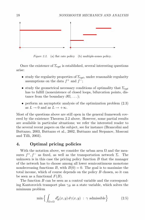
More precisely, A(t) represents the cost for a resident to cover a lengtht by his own means (walking, time consumption, car fuel, . . . ), whereasB(t) represents the cost to cover a length t by using the transportationnetwork (ticket, time consumption, . . . ). The assumptions made on thepricing policy function B allow us to consider the usual cases below: theflat rate policy of Figure 2.2 (a) as well as the multiple-zones policy ofFigure 2.2 (b).
Therefore, the function dΣ is defined by:
dΣ(x, y) = inf{A(H1(φ \ Σ)
)+ B
(H1(φ ∩ Σ)
): φ ∈ Cx,y
}, (2.4)
where Cx,y denotes the class of all curves in Ω connecting x to y.
Theorem 2.2 The optimization problem (2.3) admits at least a solutionΣopt.
18 NONSMOOTH MECHANICS AND ANALYSIS
• •
Figure 2.2. (a) flat rate policy (b) multiple-zones policy.
Once the existence of Σopt is established, several interesting questionsarise:
• study the regularity properties of Σopt, under reasonable regularityassumptions on the data f+ and f−;
• study the geometrical necessary conditions of optimality that Σopt
has to fulfill (nonexistence of closed loops, bifurcation points, dis-tance from the boundary ∂Ω, . . . );
• perform an asymptotic analysis of the optimization problem (2.3)as L→ 0 and as L→ +∞.
Most of the questions above are still open in the general framework cov-ered by the existence Theorem 2.2 above. However, some partial resultsare available in particular situations; we refer the interested reader tothe several recent papers on the subject, see for instance (Brancolini andButtazzo, 2003, Buttazzo et al., 2002, Buttazzo and Stepanov, Mosconiand Tilli, 2003).
4. Optimal pricing policiesWith the notation above, we consider the urban area Ω and the mea-
sures f+, f− as fixed, as well as the transportation network Σ. Theunknown is in this case the pricing policy function B that the managerof the network has to choose among all lower semicontinuous monotonenondecreasing functions B, with B(0) = 0. The goal is to maximize thetotal income, which of course depends on the policy B chosen, so it canbe seen as a functional F (B).
The function B can be seen as a control variable and the correspond-ing Kantorovich transport plan γB as a state variable, which solves theminimum problem
min{∫
Ω×Ωdp
B(x, y) dγ(x, y) : γ admissible}
(2.5)

Three optimization problems in mass transportation theory 19
where p is the Wasserstein exponent and dB is the cost function
dB(x, y) = inf{A(H1(φ \ Σ)
)+ B
(H1(φ ∩ Σ)
): φ ∈ Cx,y
}. (2.6)
The quantity dB(x, y) can be seen as the total minimal cost a customerhas to pay to go from a point x to a point y, using the best path φ. Thiscost is divided in two parts: a part A
(H1(φ \ Σ)
)due to the use of his
own means, and a part iB(x, y) = B(H1(φ ∩ Σ)
)due to the ticket to
pay for using the transportation network. The only condition we assumeto make the problem well posed is that, in case several paths φ realizethe minimum in (2.6), the customer chooses the one with minimal ownmeans cost (and so with maximal network cost). The total income isthen
F (B) =∫
Ω×ΩiB(x, y) dγB(x, y), (2.7)
so that the optimization problem we consider is:
max{F (B) : B l.s.c., nondecreasing, B(0) = 0
}. (2.8)
The following result has been proved in (Buttazzo et al.).
Theorem 2.3 There exists an optimal pricing policy Bopt solving themaximal income problem (2.8).
Also in this case some necessary conditions of optimality can be ob-tained. It may happen that several functions Bopt solve the maximalincome problem (2.8); in this case, as a canonical representative, wechoose the smallest one, with respect to the usual order between func-tions. It is possible to show that it is still a solution of problem (2.8).In particular, the function Bopt turns out to be continuous, and its Lip-schitz constant can be bounded by the one of A. We refer to (Buttazzoet al.) for all details as well as for the proofs above.
5. Optimal design of an urban areaWe consider the following model for the optimal planning of an urban
area, see (Buttazzo and Santambrogio, 2003).
• The domain Ω (the geographical region or urban area), a regularcompact subset of RN , is prescribed;
• the probability measure f+ on Ω (the density of residents) is un-known;
• the probability measure f− on Ω (the density of services) is un-known.

20 NONSMOOTH MECHANICS AND ANALYSIS
Here the distance d in Ω is taken for simplicity as the Euclidean one,but with a similar procedure one could also study the cases in which thedistance is induced by a transportation network Σ, as in the previoussections. The unknowns of the problem are f+ and f−, that have to bedetermined in an optimal way taking into account the following facts:
• residents have to pay a transportation cost for moving from theresidential areas to the services poles;
• residents like to live in areas where the density of population is nottoo high;
• services need to be concentrated as much as possible, in order toincrease efficiency and decrease management costs.
The transportation cost will be described through a Monge-Kantoro-vich mass transportation model; it is indeed given by a p-Wassersteindistance (p ≥ 1) Wp(f+, f−).
The total unhappiness of residents due to high density of populationwill be described by a penalization functional, of the form
H(f+) ={ ∫
Ω h(u) dx if f+ = u dx+∞ otherwise,
where h is assumed to be convex and superlinear (i.e. h(t)/t→ +∞ ast→ +∞). The increasing and diverging function h(t)/t then representsthe unhappiness to live in an area with population density t.
Finally, there is a third term G(f−) which penalizes sparse services.We force f− to be a sum of Dirac masses and we consider G(f−) as afunctional defined on measures, of the form studied by Bouchitte andButtazzo in (Bouchitte and Buttazzo, 1990, Bouchitte and Buttazzo,1992, Bouchitte and Buttazzo, 1992):
G(f−) ={ ∑
n g(an) if f− =∑
n anδxn
+∞ otherwise,
where g is concave and with infinite slope at the origin ((i.e. g(t)/t →+∞ as t→ 0+). Every single term g(an) in the sum above represents thecost for building and managing a service pole of dimension an, locatedat the point xn ∈ Ω.
We have then the optimization problem
min{Wp(f+, f−)+H(f+)+G(f−) : f+, f− probabilities on Ω
}. (2.9)
Theorem 2.4 There exists an optimal pair (f+, f−) solving the problemabove.

Three optimization problems in mass transportation theory 21
Also in this case we obtain some necessary conditions of optimality.In particular, if Ω is sufficiently large, the optimal structure of the cityconsists of a finite number of disjoint subcities: circular residential areaswith a service pole at their center.
AcknowledgmentsThis work is part of the European Research Training Network “Ho-
mogenization and Multiple Scales” (HMS2000) under contract HPRN-2000-00109.
ReferencesL. Ambrosio, Lecture notes on optimal transport problems. In “Mathe-
matical Aspects of Evolving Interfaces”, Madeira 2–9 June 2000, Lec-ture Notes in Mathematics 1812, Springer-Verlag, Berlin (2003), 1–52.
L. Ambrosio, A. Pratelli, Existence and stability results in the L1 the-ory of optimal transportation. In “Optimal Transportation and Ap-plications”, Martina Franca 2–8 September 2001, Lecture Notes inMathematics 1813, Springer-Verlag, Berlin (2003), 123–160.
G. Bouchitte, G. Buttazzo, New lower semicontinuity results for non-convex functionals defined on measures. Nonlinear Anal., 15 (1990),679–692.
G. Bouchitte, G. Buttazzo, Integral representation of nonconvex func-tionals defined on measures. Ann. Inst. H. Poincare Anal. Non Line-aire, 9 (1992), 101–117.
G. Bouchitte, G. Buttazzo, Relaxation for a class of nonconvex function-als defined on measures. Ann. Inst. H. Poincare Anal. Non Lineaire,10 (1993), 345–361.
G. Bouchitte, G. Buttazzo, Characterization of optimal shapes and mas-ses through Monge-Kantorovich equation. J. Eur. Math. Soc., 3 (2001),139–168.
G. Bouchitte, G. Buttazzo, P. Seppecher, Shape optimization solutionsvia Monge-Kantorovich equation. C. R. Acad. Sci. Paris, 324-I (1997),1185–1191.
A. Brancolini, G. Buttazzo, Optimal networks for mass transportationproblems. Preprint Dipartimento di Matematica Universita di Pisa,Pisa (2003).
G. Buttazzo, A. Davini, I. Fragala, F. Macia, Optimal Riemannian dis-tances preventing mass transfer. J. Reine Angew. Math., (to appear).
G. Buttazzo, L. De Pascale, Optimal shapes and masses, and optimaltransportation problems. In “Optimal Transportation and Applica-

22 NONSMOOTH MECHANICS AND ANALYSIS
tions”, Martina Franca 2–8 September 2001, Lecture Notes in Math-ematics 1813, Springer-Verlag, Berlin (2003), 11–52.
G. Buttazzo, E. Oudet, E. Stepanov, Optimal transportation problemswith free Dirichlet regions. In “Variational Methods for Discontinu-ous Structures”, Cernobbio 2001, Progress in Non-Linear DifferentialEquations 51, Birkhauser Verlag, Basel (2002), 41–65.
G. Buttazzo, A. Pratelli, E. Stepanov, Optimal pricing policies for publictransportation networks. Paper in preparation.
G. Buttazzo, F. Santambrogio, A model for the optimal planning of anurban area. Preprint Dipartimento di Matematica Universita di Pisa,Pisa (2003).
G. Buttazzo, E. Stepanov, On regularity of transport density in theMonge-Kantorovich problem. SIAM J. Control Optim., 42 (3) (2003),1044-1055.
G. Buttazzo, E. Stepanov, Transport density in Monge-Kantorovich pro-blems with Dirichlet conditions. Preprint Dipartimento di MatematicaUniversita di Pisa, Pisa (2001).
G. Buttazzo, E. Stepanov, Optimal transportation networks as free Diri-chlet regions for the Monge-Kantorovich problem. Ann. Scuola Norm.Sup. Pisa Cl. Sci., (to appear).
G. Carlier, I. Ekeland, Optimal transportation and the structure of cities.Preprint 2003, available at http://www.math.ubc.ca.
L. De Pascale, A. Pratelli, Regularity properties for Monge transportdensity and for solutions of some shape optimization problem. Calc.Var., 14 (2002), 249–274.
L. De Pascale, L. C. Evans, A. Pratelli, Integral estimates for transportdensities. Bull. London Math. Soc., (to appear).
L. C. Evans, Partial differential equations and Monge-Kantorovich masstransfer. Current Developments in Mathematics, Int. Press, Boston(1999), 65–126.
L. C. Evans, W. Gangbo, Differential Equations Methods for the Monge-Kantorovich Mass Transfer Problem. Mem. Amer. Math. Soc. 137,Providence (1999).
M. Feldman, R. J. McCann, Monge’s transport problem on a Rieman-nian manifold. Trans. Amer. Math. Soc., 354 (2002), 1667–1697.
W. Gangbo, R. J. McCann, The geometry of optimal transportation.Acta Math., 177 (1996), 113–161.
L. V. Kantorovich, On the transfer of masses. Dokl. Akad. Nauk. SSSR,37 (1942), 227–229.
L. V. Kantorovich, On a problem of Monge. Uspekhi Mat. Nauk., 3(1948), 225–226.

Three optimization problems in mass transportation theory 23
G. Monge, Memoire sur la Theorie des Deblais et des Remblais. Histoirede l’Academie Royale des Sciences de Paris, avec les Memoires deMathematique et de Physique pour la meme annee, (1781), 666–704.
S. J. N. Mosconi, P. Tilli, Γ-convergence for the irrigation problem.Preprint Scuola Normale Superiore, Pisa (2003), available athttp://cvgmt.sns.it.
S. T. Rachev, L. Ruschendorf, Mass transportation problems. Vol. I The-ory, Vol. II Applications. Probability and its Applications, Springer-Verlag, Berlin (1998).
C. Villani, Topics in Optimal Transportation. Graduate Studies in Math-ematics, Amer. Math. Soc. (2003).

Chapter 3
SOME GEOMETRICAL AND ALGEBRAICPROPERTIES OF VARIOUS TYPES OFCONVEX HULLS
Bernard DacorognaEPFL-DMA, CH 1015 Lausanne, [email protected]
Abstract This article is dedicated to Jean Jacques Moreau for his 80th birthday.He is a master of convex analysis.
When dealing with differential inclusions of the form
Du (x) ∈ E, a.e. in Ω
together with some boundary data u = ϕ on ∂Ω, one is lead to considerseveral types of convex hulls of sets. It is the aim of the present articleto discuss these matters.
Keywords: quasiconvexity, polyconvexity, rank one convexity, convex hulls
1. IntroductionWe start in this introduction with the analytical motivations for study-
ing some extensions of the notion of convex hull of a given set. In theremaining part of the article we will however only discuss geometricaland algebraic aspects of these notions. Therefore the reader only inter-ested on these aspects can completely skip the introduction, since wewill not use any of the notions discussed now.
We let Ω ⊂ Rn be a bounded open set, u : Ω ⊂ Rn → Rm andtherefore the gradient matrix Du belongs to Rm×n and finally we letE ⊂ Rm×n be a compact set.
We are interested in solving the following Dirichlet problem
(D){
Du (x) ∈ E, a.e. x ∈ Ωu (x) = ϕ (x) , x ∈ ∂Ω
26 NONSMOOTH MECHANICS AND ANALYSIS
where ϕ : Ω→ Rm is a given map.In the scalar case (n = 1 or m = 1) a sufficient condition for solving
the problem isDϕ (x) ∈ E ∪ int co E, a.e. in Ω (3.1)
where int co E stands for the interior of the convex hull of E. Thisfact was observed by several authors, with different proofs and dif-ferent levels of generality; notably in (Bressan and Flores, 1994, Cel-lina, 1993, Dacorogna and Marcellini, 1996, Dacorogna and Marcellini,1997, Dacorogna and Marcellini, 1999a, De Blasi and Pianigiani, 1999)or (Friesecke, 1994). It should be noted that this sufficient condition isvery close from the necessary one, which, when properly formulated, is
Dϕ (x) ∈ coE, a.e. in Ω, (3.2)
where coE denotes the closure of the convex hull of E.When turning to the vectorial case (n, m ≥ 2) the problem becomes
considerably harder and conditions (3.1) and (3.2) are not anymore ap-propriate. One needs to introduce several extensions of the notion ofconvex hull, namely the polyconvex, quasiconvex and rank one convexhulls. We will define these notions precisely in the next section, butlet us quote first an existence theorem involving the quasiconvex hull,QcoE.
We start with the following definition introduced by Dacorogna-Mar-cellini in (Dacorogna and Marcellini, 1999) (cf. also (Dacorogna andMarcellini, 1999a) and (Dacorogna and Pisante)), which is the key con-dition to get existence of solutions.
Definition 3.1 (Relaxation property) Let E ⊂ Rm×n. We saythat QcoE has the relaxation property if for every bounded open set Ω ⊂Rn, for every affine function uξ satisfying
Duξ (x) = ξ ∈ intQcoE,
there exists a sequence {uν} of piecewise affine functions in Ω, so that
uν ∈ uξ + W 1,∞0 (Ω; Rm) , Duν (x) ∈ intQcoE, a.e. in Ω
uν∗⇀ uξ in W 1,∞,
∫Ω
dist (Duν (x) ;E) dx→ 0 as ν →∞.
The main existence theorem is then
Theorem 3.2 Let Ω ⊂ Rn be open. Let E ⊂ Rm×n be such that Eis compact. Assume that QcoE has the relaxation property. Let ϕ be

Geometrical and algebraic properties of various convex hulls 27
piecewise C1(Ω; Rm
)and verifying
Dϕ (x) ∈ E ∪ intQcoE, a.e. in Ω.
Then there exists (a dense set of) u ∈ ϕ + W 1,∞0 (Ω; Rm) such that
Du (x) ∈ E, a.e. in Ω.
Remark 3.3 The theorem was first proved by Dacorogna-Marcellini in(Dacorogna and Marcellini, 1999) (cf. also Theorem 6.3 in (Dacorognaand Marcellini, 1999a)) under an extra further hypothesis. This hypoth-esis was later removed by Sychev in (Sychev, 2001) (see also Muller-Sychev (Muller and Sychev, 2001)), using the method of convex integra-tion of Gromov as revisited by Muller-Sverak (Muller and Sverak, 1996),and Kirchheim (Kirchheim, 2001). As stated it has been recently provedby Dacorogna-Pisante (Dacorogna and Pisante).
2. The different types of convex hullsWe now discuss the central notions of our article, for more background
we refer to Dacorogna-Marcellini (Dacorogna and Marcellini, 1999a).We will discuss the different notions of hulls by dual considerations
on functions; we therefore start with the following definitions.
Definition 3.4 (i) A function f : Rm×n → R = R ∪ {+∞} is said tobe polyconvex if
f
(τ+1∑i=1
tiξi
)≤
τ+1∑i=1
tif (ξi)
whenever ti ≥ 0 and
τ+1∑i=1
ti = 1, T
(τ+1∑i=1
tiξi
)=
τ+1∑i=1
tiT (ξi)
where for a matrix ξ ∈ Rm×n we let
T (ξ) = (ξ, adj2ξ, . . . , adjm∧nξ)
where adjsξ stands for the matrix of all s × s subdeterminants of thematrix ξ, 1 ≤ s ≤ m ∧ n = min {m,n} and where
τ = τ (m,n) =m∧n∑s=1
(ms
)(ns
)and
(ms
)=
m!s! (m− s)!
.

28 NONSMOOTH MECHANICS AND ANALYSIS
(ii) A Borel measurable function f : Rm×n → R is said to be quasi-convex if ∫
Uf (ξ + Dϕ (x)) dx ≥ f (ξ) meas(U)
for every bounded domain U ⊂ Rn, ξ ∈ Rm×n, and ϕ ∈W 1,∞0 (U ; Rm).
(iii) A function f : Rm×n → R = R ∪ {+∞} is said to be rank oneconvex if
f (tξ1 + (1− t)ξ2) ≤ t f (ξ1) + (1− t) f (ξ2)
for every ξ1, ξ2 with rank {ξ1 − ξ2} = 1 and every t ∈ [0, 1].(iv) The different envelopes of a given function f are defined as
Cf = sup {g ≤ f : g convex} ,
Pf = sup {g ≤ f : g polyconvex} ,
Qf = sup {g ≤ f : g quasiconvex} ,
Rf = sup {g ≤ f : g rank one convex} .
We are now in a position to define the main notions of the article.
Definition 3.5 We let, for E ⊂ Rm×n,
FE ={f : Rm×n → R = R∪{+∞} : f |E ≤ 0
}FE =
{f : Rm×n → R : f |E ≤ 0
}.
We then have respectively, the convex, polyconvex, rank one convex, rankone convex finite and (closure of the) quasiconvex hull defined by
co E ={ξ ∈ Rm×n : f (ξ) ≤ 0, for every convex f ∈ FE
}Pco E =
{ξ ∈ Rm×n : f (ξ) ≤ 0, for every polyconvex f ∈ FE
}Rco E =
{ξ ∈ Rm×n : f (ξ) ≤ 0, for every rank one convex f ∈ FE
}Rco fE =
{ξ ∈ Rm×n : f (ξ) ≤ 0, for every rank one convex f ∈ FE
}QcoE =
{ξ ∈ Rm×n : f (ξ) ≤ 0, for every quasiconvex f ∈ FE
}.
Remark 3.6 The definition of rank one convex hull Rco E that weadopted is called, by some authors, lamination convex hull of E; whilethe same authors call Rco fE the rank one convex hull of E.
We start by pointing out several important facts.
1) The definition of convex hull is equivalent to the classical one, i.e.the smallest convex set that contains E. In fact it is enough to consider

Geometrical and algebraic properties of various convex hulls 29
only one function: the convex envelope, CχE (= χco E), of the indicatorfunction of the set E, namely
χE (ξ) =
⎧⎨⎩0 if ξ ∈ E
+∞ if ξ /∈ E.
2) If we replace FE by FE in the definition of coE, we get coE theclosure of the convex hull.
3) Similar considerations apply to the polyconvex hull, in particular itis sufficient to consider the polyconvex envelope, PχE , of the indicatorfunction of the set E.
4) If the set E is compact then so are co E and PcoE.
5) We also have as a consequence of Caratheodory theorem
Proposition 3.7 Let E ⊂ Rm×n, then the following representationholds
co E =
{ξ ∈ Rm×n : ξ =
mn+1∑i=1
tiξi, ξi ∈ E, ti ≥ 0 withmn+1∑i=1
ti = 1
}
Pco E =
{ξ ∈ Rm×n : T (ξ) =
τ+1∑i=1
tiT (ξi), ξi ∈ E, ti ≥ 0withτ+1∑i=1
ti = 1
}
6) Matters are however very different with the other definitions, butlet us first start with some resemblances.
Proposition 3.8 Let E ⊂ Rm×n and set R0 co E = E, and let for i ∈ N
Ri+1 co E = {ξ ∈ Rm×n : ξ = tξ1 + (1− t)ξ2,
ξ1, ξ2 ∈ Ri co E, rank {ξ1 − ξ2} = 1, t ∈ [0, 1]}.
ThenRco E = ∪
i∈N
Ri co E.
7) The rank one convex hull is equivalently defined through the rankone convex envelope, RχE , of the indicator function of the set E and itis the smallest rank one convex set that contains E.
We now turn our attention to some differences of behavior amongthese notions.
8) Contrary to coE and PcoE, if the set E is compact then Rco E isnot necessarily compact as was pointed out by Kolar (Kolar, 2003).
30 NONSMOOTH MECHANICS AND ANALYSIS
9) Contrary to coE and PcoE, the set Rco fE is, in general (see belowfor an example), strictly larger than the closure of RcoE, i.e.,
RcoE � Rco fE.
10) There is no good definition of the quasiconvex hull if we replaceFE by FE , since quasiconvex functions with values in R = R∪{+∞}are not yet well understood. In particular if E = {ξ1, ξ2} ⊂ Rm×n, thenQχE = χE , independently of the fact that ξ1 − ξ2 is of rank one or not.
11) For any set E ⊂ Rm×n we have
E ⊂ Rco E ⊂ Pco E ⊂ co E
E ⊂ RcoE ⊂ Rco fE ⊂ QcoE ⊂ PcoE ⊂ coE.
We now discuss two examples that might shed some light on some dif-ferences between these new hulls and the convex one. In both exampleswe will consider the case m = n = 2 and denote by R2×2
d the set of 2× 2diagonal matrices, we will write any such matrix as a vector of R2.
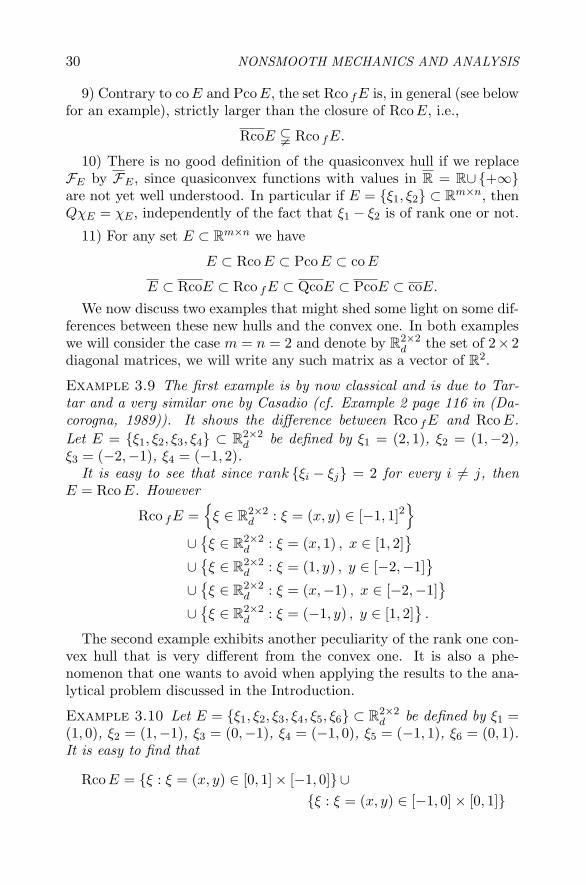
Example 3.9 The first example is by now classical and is due to Tar-tar and a very similar one by Casadio (cf. Example 2 page 116 in (Da-corogna, 1989)). It shows the difference between Rco fE and Rco E.Let E = {ξ1, ξ2, ξ3, ξ4} ⊂ R2×2
d be defined by ξ1 = (2, 1), ξ2 = (1,−2),ξ3 = (−2,−1), ξ4 = (−1, 2).
It is easy to see that since rank {ξi − ξj} = 2 for every i �= j, thenE = Rco E. However
Rco fE ={
ξ ∈ R2×2d : ξ = (x, y) ∈ [−1, 1]2
}∪
{ξ ∈ R2×2
d : ξ = (x, 1) , x ∈ [1, 2]}
∪{ξ ∈ R2×2
d : ξ = (1, y) , y ∈ [−2,−1]}
∪{ξ ∈ R2×2
d : ξ = (x,−1) , x ∈ [−2,−1]}
∪{ξ ∈ R2×2
d : ξ = (−1, y) , y ∈ [1, 2]}
.
The second example exhibits another peculiarity of the rank one con-vex hull that is very different from the convex one. It is also a phe-nomenon that one wants to avoid when applying the results to the ana-lytical problem discussed in the Introduction.
Example 3.10 Let E = {ξ1, ξ2, ξ3, ξ4, ξ5, ξ6} ⊂ R2×2d be defined by ξ1 =
(1, 0), ξ2 = (1,−1), ξ3 = (0,−1), ξ4 = (−1, 0), ξ5 = (−1, 1), ξ6 = (0, 1).It is easy to find that
Rco E = {ξ : ξ = (x, y) ∈ [0, 1]× [−1, 0]}∪{ξ : ξ = (x, y) ∈ [−1, 0]× [0, 1]}

Geometrical and algebraic properties of various convex hulls 31
and its interior (relative to R2×2d ) is given by
int Rco E = {ξ : ξ = (x, y) ∈ (0, 1)× (−1, 0)}∪{ξ : ξ = (x, y) ∈ (−1, 0)× (0, 1)} .
However there is no way of finding a set Eδ with the following “ap-proximation property” (cf. (Dacorogna and Marcellini, 1999a) and (Da-corogna and Pisante) for more details concerning the use of this prop-erty):
(1) Eδ ⊂ Rco Eδ ⊂ int Rco E for every δ > 0;(2) for every ε > 0 there exists δ0 = δ0 (ε) > 0 such that dist(η; E) ≤ ε
for every η ∈ Eδ and δ ∈ [0, δ0];(3) if η ∈ int Rco E then η ∈ Rco Eδ for every δ > 0 sufficiently small.In fact Rco Eδ will be reduced, at best, to four segments and will have
empty interior (and condition (3) will be violated).
3. The singular valuesOne of the most general example of such hulls concern sets that in-
volve singular values. Let us first recall that the singular values of agiven matrix ξ ∈ Rn×n, denoted by 0 ≤ λ1 (ξ) ≤ ... ≤ λn (ξ), are theeigenvalues of
(ξξt
)1/2.We will consider three types of sets, letting 0 < γ1 ≤ ... ≤ γn and
α ≤ β with α �= 0,
E ={ξ ∈ Rn×n : λi (ξ) = γi, i = 1, ..., n
}Eα =
{ξ ∈ Rn×n : λi (ξ) = γi, i = 1, ..., n, det ξ = α
}Eα,β =
{ξ ∈ Rn×n : λi (ξ) = γi, i = 2, ..., n, det ξ ∈ {α, β}
}where, since |det ξ| =
∏ni=1λi (ξ) and the singular values are ordered as
0 ≤ λ1 (ξ) ≤ ... ≤ λn (ξ), we should respectively impose in the secondand third cases that
n∏i=1
γi = |α|
γ2
n∏i=2
γi ≥ max {|α| , |β|} .
Note that the third case contains the other ones as particular cases.Indeed the first one is deduced from the last one by setting β = −α and
γ1 = β
[n∏
i=2
γi
]−1

32 NONSMOOTH MECHANICS AND ANALYSIS
while the second one is obtained by setting β = α and
γ1 = |α|[
n∏i=2
γi
]−1
in the third case.Our result (cf. (Dacorogna and Marcellini, 1999a, Dacorogna and
Tanteri, 2002) for the two first ones and for the third case: Dacorogna-Ribeiro (Dacorogna and Ribeiro)) is then
Theorem 3.11 Under the above conditions and notations the followingset of identities holds
co E =
{ξ ∈ Rn×n :
n∑i=ν
λi (ξ) ≤n∑
i=ν
γi, ν = 1, ..., n
}
Pco E = QcoE = Rco E =
{ξ ∈ Rn×n :
n∏i=ν
λi (ξ) ≤n∏
i=ν
γi, ν = 1, ..., n
}.
Pco Eα = Rco Eα ={ξ ∈ Rn×n :
n∏i=ν
λi (ξ) ≤n∏
i=ν
γi, ν = 2, ..., n, det ξ = α
}.
Pco Eα,β = Rco Eα,β ={ξ ∈ Rn×n :
n∏i=ν
λi (ξ) ≤n∏
i=ν
γi, ν = 2, ..., n, det ξ ∈ [α, β]
}.
As it was pointed out by Buliga (Buliga) there is a surprising for-mal connection, still not well understood, between the above theorem(with α = β) and some classical results of H. Weyl, A. Horn and C.J.Thompson (see (Horn and Johnson, 1985), (Horn and Johnson, 1991)page 171 or (Marshall and Olkin, 1979)). The result states that ifwe denote, as above, the singular values of a given matrix ξ ∈ Rn×n
by 0 ≤ λ1 (ξ) ≤ ... ≤ λn (ξ) and its eigenvalues, which are complexin general, by μ1 (ξ) , ..., μn (ξ) and if we order them by their modulus(0 ≤ |μ1 (ξ)| ≤ ... ≤ |μn (ξ)|) then the following result holds
n∏i=ν
|μi (ξ)| ≤n∏
i=ν
λi (ξ) , ν = 2, ..., n
n∏i=1
|μi (ξ)| =n∏
i=1
λi (ξ)

Geometrical and algebraic properties of various convex hulls 33
for any matrix ξ ∈ Rn×n.
AcknowledgmentsWe have benefitted from the financial support of the Fonds National
Suisse (grant 21-61390.00)
ReferencesBressan A. and Flores F., On total differential inclusions; Rend. Sem.
Mat. Univ. Padova, 92 (1994), 9-16.Buliga M., Majorisation with applications in elasticity; to appear.Cellina A., On minima of a functional of the gradient: sufficient condi-
tions, Nonlinear Anal. Theory Methods Appl., 20 (1993), 343-347.Croce G., A differential inclusion: the case of an isotropic set, to appear.Dacorogna B., Direct methods in the calculus of variations, Applied
Math. Sciences, 78, Springer, Berlin (1989).Dacorogna B. and Marcellini P., Theoremes d’existence dans le cas sca-
laire et vectoriel pour les equations de Hamilton-Jacobi, C.R. Acad.Sci. Paris, 322 (1996), 237-240.
Dacorogna B. and Marcellini P., General existence theorems for Hamil-ton-Jacobi equations in the scalar and vectorial case, Acta Mathemat-ica, 178 (1997), 1-37.
Dacorogna B. and Marcellini P., On the solvability of implicit nonlinearsystems in the vectorial case; in the AMS Series of ContemporaryMathematics, edited by G.Q. Chen and E. DiBenedetto, (1999), 89-113.
Dacorogna B. and Marcellini P., Implicit partial differential equations;Birkhauser, Boston, (1999).
Dacorogna B. and Pisante G., A general existence theorem for differen-tial inclusions in the vector valued case; to appear in Abstract andApplied Analysis.
Dacorogna B. and Ribeiro A.M., Existence of solutions for some im-plicit pdes and applications to variational integrals involving quasi-affine functions; to appear.
Dacorogna B. and Tanteri C., Implicit partial differential equations andthe constraints of nonlinear elasticity; J. Math. Pures Appl. 81 (2002),311-341.
De Blasi F.S. and Pianigiani G., On the Dirichlet problem for Hamilton-Jacobi equations. A Baire category approach; Nonlinear DifferentialEquations Appl. 6 (1999), 13–34.

34 NONSMOOTH MECHANICS AND ANALYSIS
Friesecke G., A necessary and sufficient condition for non attainment andformation of microstructure almost everywhere in scalar variationalproblems, Proc. Royal Soc. Edinburgh, 124A (1994), 437-471.
Horn R.A. and Johnson C.A.: Matrix Analysis; Cambridge UniversityPress (1985).
Horn R.A. and Johnson C.A.: Topics in Matrix Analysis; CambridgeUniversity Press (1991).
Kirchheim B., Deformations with finitely many gradients and stabilityof quasiconvex hulls; C. R. Acad. Sci. Paris, 332 (2001), 289–294.
Kolar J., Non compact lamination convex hulls; Ann. I. H. Poincare, AN20 (2003), 391-403.
Marshall A. W. and Olkin I., Inequalities: theory of majorisation and itsapplications; Academic Press (1979).
Muller S. and Sverak V., Attainment results for the two-well problem byconvex integration; ed. Jost J., International Press, (1996), 239-251.
Muller S. and Sychev M., Optimal existence theorems for nonhomoge-neous differential inclusions; J. Funct. Anal. 181 (2001), 447–475.
Sychev M., Comparing two methods of resolving homogeneous differ-ential inclusions; Calc. Var. Partial Differential Equations 13 (2001),213–229.

Chapter 4
A NOTE ON THE LEGENDRE-FENCHELTRANSFORM OF CONVEX COMPOSITEFUNCTIONS
Jean-Baptiste Hiriart-UrrutyUniversite Paul Sabatier, 118, route de Narbonne, 31062 Toulouse Cedex 4, [email protected]
Dedicated to J.J. Moreau on the occasion of his 80th birthday.
Abstract In this note we present a short and clear-cut proof of the formula giv-ing the Legendre-Fenchel transform of a convex composite functiong ◦ (f1, · · · , fm) in terms of the transform of g and those of the fi
′s.
Keywords: Convex functions; Composite functions; Legendre-Fenchel transform.
1. IntroductionThe Legendre-Fenchel transform (or conjugate) of a function ϕ : X →
R ∪ {+∞} is a function defined on the topological dual space X� of Xas
p ∈ X� −→ ϕ∗(p) := supx∈X
[〈p, x〉 − ϕ(x)] .
In Convex analysis, the transformation ϕ � ϕ∗ plays a role analogousto that of Fourier’s or Laplace’s transform in other places in Analysis.In particular, one cannot avoid it in analysing a variational problem,more specifically the so-called dual version of it. That explains why theLegendre-Fenchel transform occupies a key place in any work on Convexanalysis.
The purpose of the present note is to analyse the formula giving theLegendre-Fenchel transform of the convex composite function g ◦ (f1, · · ·, fm), with g and all the fi convex, in terms of g∗ and the fi
∗. Actually

36 NONSMOOTH MECHANICS AND ANALYSIS
such a formula is not new, even if it does not appear explicitly in booksbut only in some specialized research papers. We intend here to derivesuch a result in a short and clear-cut way, using only a “pocket theorem”from Convex analysis; in particular, we shall not appeal to any resulton convex mappings taking values in ordered vector spaces, as is usuallydone in the literature.
Before going further, some comments on the historical developmentof the convex analysis of g ◦ (f1, · · · , fm) are in order. First of all, thesetting: the fi’s are convex functions on some general vector space Xand g is an increasing convex function on Rm (increasing means herethat g(y) ≤ g(z) whenever yi ≤ zi for all i); the resulting compositefunction g ◦ (f1, · · · , fm) is convex on X. Then, how things evolved:
- Expressing the subdifferential of g◦(f1, · · · , fm) in terms of that of gand those of the fi
′s was the first work carried out in the convex analysisof g ◦ (f1, · · · , fm), as early as in the years 1965 − 1970. The goal wasmade easier to achieve by the fact that one knew the formula aimed at(by extending to subdifferentials the so-called chain rule in Differentialcalculus). The objective of obtaining the subdifferential of the convexcomposite function g ◦ F , with a vector-valued convex operator F, waspursued by several authors in various ways, see (Combari et al., 1994,Combari et al., 1996, Zalinescu, 2002) and references therein for recentcontributions.
- To our best knowledge, the first attempt to derive [g ◦ (f1, · · · , fm)]∗
in terms of g∗ and the fi∗′s is due to Kutateladze in his note (Kutate-
ladze, 1977) and full-fledged paper (Kutateladze, 1979). The workingcontext was that of convex operators taking values in ordered vectorspaces, and this was also the case in most of the subsequent papers onthe subject. Not only was the case of real-valued fi
′s somehow hidden inthe main results in these papers (Theorem 3.7.1 in (Kutateladze, 1979),Proposition 4.11 (ii) in (Combari et al., 1994), Theorem 3.4 (ii) in (Com-bari et al., 1996), Theorem 2.8.10 in (Zalinescu, 2002)), but more impor-tantly, the theorems were derived after some heavy preparatory work:on subdifferential calculus rules for vector-valued mappings in (Kutate-ladze, 1979), on perturbation functions in (Combari et al., 1996), onε-subdifferentials in (Zalinescu, 2002). All these aspects are summarizedin section 2.8 (especially bibliographical notes) of (Zalinescu, 2002).
In the setting we are considering in the present paper, the expectedformula for the Legendre-Fenchel conjugate of g ◦ (f1, · · · , fm) is as fol-

Legendre-Fenchel transform of convex composite functions 37
lows: for all p ∈ X�,
[g ◦ (f1, · · · , fm)]∗(p) = minαi≥0
[g∗(α1, · · · , αm) +
(m∑
i=1
αi fi
)∗
(p)
].
(4.1)This formula was proved in a simple way when m = 1 in (Hiriart-Urrutyand Lemarechal, 1993), Chapter X, Section 2.5; we shall follow here thesame approach as there, using only a standard result in Convex analy-sis, the one giving the Legendre-Fenchel conjugate of a sum of convexfunctions. However the formula (4.1) is not always informative, take
for example g(y1, · · · , ym) :=m∑
i=1
yi, a situation in which (4.1) does not
say anything new; we therefore shall go a step further in the expression
of [g ◦ (f1, · · · , fm)]∗(p) by developing
(m∑
i=1
αi fi
)∗
(p); hence the final
formula (4.7) below is obtained.We end with some illustrations enhancing the versatility of the proved
formula.
2. The Legendre-Fenchel transform ofg ◦ (f1, · · · , fm)
We begin by recalling some basic notations and results from Convexanalysis.
Let X be a real Banach space; by X� we denote the topological dualspace of X, and (p, x) ∈ X�×X −→ 〈p, x〉 stands for the duality pairing.The Legendre-Fenchel transform (or conjugate) of a function ϕ : X →R ∪ {+∞} is defined on X� as
p ∈ X� −→ ϕ∗(p) := supx∈X
[〈p, x〉 − ϕ(x)] . (4.2)
Clearly only those x in dom ϕ := {x ∈ X | ϕ(x) < +∞} are relevant inthe calculation of the supremum in (4.2).
As a particular example of ϕ, consider the indicator function of anonempty set C in X, that is
iC(x) := 0 if x ∈ C, +∞ if not; (4.3)
then i∗C is the so-called support function of C, that is
i∗C =: σC : p ∈ X� −→ σC(p) = supx∈C〈p, x〉. (4.4)

38 NONSMOOTH MECHANICS AND ANALYSIS
When α > 0, there is no ambiguity in defining αϕ and the resultingconjugacy result is: (αϕ)∗(p) = αϕ∗(
p
α). As for α = 0, one should be
more careful: we set (0ϕ)(x) = 0 if x ∈ dom ϕ, +∞ if not; in other words0ϕ = idomϕ. The corresponding conjugacy result is (0ϕ)∗ = σdom ϕ, afact coherent with the following result:
αϕ∗(p
α) −→α→0+ σdom ϕ(p)
(at least for convex lower-semicontinuous ϕ).We denote by Γ0(X) the set of functions ϕ : X −→ R ∪ {+∞} which
are convex, lower-semicontinuous and not identically equal to +∞ onX. The next theorem is the key result we shall rely on in our proofs;it is a classical one in Convex analysis (see (Laurent, 1972), Theoreme6.5.8 for example).
Theorem 1. Let f1, · · · , fk ∈ Γ0(X). Suppose there is a point ink⋂
i=1
dom fi at which f1, · · · , fk−1 are continuous. Then, for all p ∈ X�:
(f1 + · · ·+ fk)∗(p) = minp1+···+pk=p
[f∗1 (p1) + · · ·+ f∗
k (pk)] . (4.5)
The context of our work is the following one:
f1, · · · , fm ∈ Γ0(X);
g ∈ Γ0(Rm) and is increasing on Rm, i.e. g(y) ≤ g(z) wheneveryi ≤ zi for all i = 1, · · · ,m.
The composite function g ◦ (f1, · · · , fm) is defined on X as follows:
[g ◦ (f1, · · · , fm)](x) =
⎧⎨⎩ g[f1(x), · · · , fm(x)] if fi(x) < +∞for all i,
+∞ if not.
The resulting function g ◦ (f1, · · · , fm) is now convex on X. The mini-mal assumption to secure that g ◦ (f1, · · · , fm) does not identically equal
+∞ is: there is a point x0 ∈m⋂
i=1
dom fi such that (f1(x0), · · · , fm(x0)) ∈
dom g. We shall actually assume a little more to derive our main resultbelow.
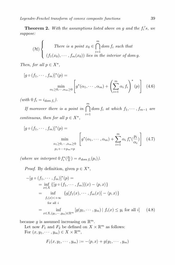
Legendre-Fenchel transform of convex composite functions 39
Theorem 2. With the assumptions listed above on g and the fi′s, we
suppose:
(H)
⎧⎪⎨⎪⎩ There is a point x0 ∈m⋂
i=1
dom fi such that
(f1(x0), · · · , fm(x0)) lies in the interior of dom g.
Then, for all p ∈ X�,
[g ◦ (f1, · · · , fm)]∗(p) =
minα1≥0,··· ,αm≥0
[g∗(α1, · · · , αm) +
(m∑
i=1
αi fi
)∗
(p)
](4.6)
(with 0 fi = idom fi).
If moreover there is a point inm⋂
i=1
dom fi at which f1, · · · , fm−1 are
continuous, then for all p ∈ X�,
[g ◦ (f1, · · · , fm)]∗(p) =
minα1≥0,··· ,αm≥0
p1+···+pm=p
[g∗(α1, · · · , αm) +
m∑i=1
αi f∗i (
pi
αi)
](4.7)
(where we interpret 0 f∗i (pi
0 ) = σdom fi(pi)).
Proof. By definition, given p ∈ X�,
−[g ◦ (f1, · · · , fm)]∗(p) == inf
x∈X{[g ◦ (f1, · · · , fm)](x)− 〈p, x〉}
= inffi(x)<+∞
for all i
{g[f1(x), · · · , fm(x)]− 〈p, x〉}
= infx∈X,(y1,··· ,ym)∈Rm
[g(y1, · · · , ym) | fi(x) ≤ yi for all i] (4.8)
because g is assumed increasing on Rm.Let now F1 and F2 be defined on X × Rm as follows:For (x, y1, · · · , ym) ∈ X × Rm,
F1(x, y1, · · · , ym) := −〈p, x〉+ g(y1, · · · , ym)

40 NONSMOOTH MECHANICS AND ANALYSIS
F2(x, y1, · · · , ym) := iepi f1(x, y1) + · · ·+ iepi fm(x, ym)
where epi fi denotes the epigraph of fi, that is the set of (x, yi) ∈ X×Rsuch that fi(x) ≤ yi.
Thus, (4.8) can be written as
− [g ◦ (f1, · · · , fm)]∗(p) =inf
(x,y1,··· ,ym)∈X×Rm[F1(x, y1, · · · , ym) + F2(x, y1, · · · , ym)] . (4.9)
We then have to compute the conjugate (at 0) of a sum of functions,however in a favorable context since:
F1 ∈ Γ0(X × R), F2 ∈ Γ0(X × R), dom F1 = X × dom g.According to the assumption (H) we made, there is a point (x0, f1(x0),
· · · , fm(x0)) ∈ dom F2 at which F1 is continuous (indeed g is continuousat (f1(x0), · · · , fm(x0)) whenever (f1(x0), · · · , fm(x0)) lies in the interiorof dom g). We therefore are in a situation where Theorem 1 applies:
[g ◦ (f1, · · · , fm)]∗(p) = (F1 + F2)∗(0) [from (4.9)]= min
s∈X�
(α1,··· ,αm)∈Rm
[F ∗1 (−s, α1, · · · , αm) + F ∗
2 (s,−α1, · · · ,−αm)] .
(4.10)
The computation of the above two conjugate functions (F ∗1 and F ∗
2 ) iseasy and gives:
F ∗1 (−s, α1, · · · , αm) =
{g∗(α1, · · · , αm) if s = p,
+∞ if not ;
F ∗2 (s, β1, · · · , βm) = sup
fi(x)≤yi
for all i
(〈s, x〉+m∑
i=1
βiyi)
= +∞ if at least one βi is > 0,
= supx∈dom fi
for all i
[〈s, x〉+m∑
i=1
βi fi(x)] if βi ≤ 0 for all i.
Consequently, the minimum in (4.10) is taken over s = p and those(α1, · · · , αm) ∈ Rm whose components are all nonnegative. Whence theformula (4.6) follows.

Legendre-Fenchel transform of convex composite functions 41
If there is a point x ∈m⋂
i=1
dom fi at which f1, · · · , fm−1 are continuous,
then x ∈m⋂
i=1
dom(αi fi) and α1 f1, · · · , αm−1 fm−1 are continuous at x (if
αi0 = 0, αi0 fi0 = idom fi0is indeed continuous at x, since x necessarily
lies in the interior of dom fi0). We apply Theorem 1 again:
(m∑
i=1
αi fi)∗(p) = minp1+···+pm=p
[m∑
i=1
αi fi∗(
p
αi)
].
Plugging this into (4.6) yields the formula (4.7).
3. By way of illustrationsSince g is assumed increasing in our setting, it is easy to prove that
dom g∗ is indeed included in (R+)m, thus the restriction in (4.6) or (4.7)to those αi which are positive is not surprising. However one may wonderif the optimal αi’s in these formulas are strictly positive or not. Theanswer is no, some of the α′
is may be null, possibly all of them. As ageneral rule, one can say more about the optimal α′
is only in particularinstances.
Consider for example p ∈ X� such that [g ◦ (f1, · · · , fm)]∗(p) < +∞;then, if σ⋂m
i=1 dom fi(p) = +∞ or if g∗(0, · · · , 0) = +∞, one is sure that
some of the optimal α′is in (6) or (7) are strictly positive (in either case,
having all the αi null leads to impossible equalities (4.6) and (4.7)). Insome other situations however, one is sure that all the optimal α′
is arestrictly positive; see some examples below.
3.1 The sum of the k largest valuesSuppose that the increasing g ∈ Γ0(Rm) is positively homogeneous; it
is then the support function of a closed convex set C ⊂ (R+)m (namelythe subdifferential of g at the origin). The Legendre-Fenchel transformg∗ of g is the indicator function of C so that (4.6) and (4.7) are simplifiedinto:
[g ◦ (f1, · · · , fm)]∗(p) = minα1,··· ,αm∈C
[(
m∑i=1
αi fi)∗(p)
](4.11)
= minα1,··· ,αm∈C
p1+···+pm=p
[m∑
i=1
αi f∗i (
pi
αi)
]. (4.12)

42 NONSMOOTH MECHANICS AND ANALYSIS
A first example, with a bounded C, is g(y1, · · · , ym) =m∑
i=1
y+i (where
y+i stands for the positive part of yi). Here g is the support function of
C = [0, 1]m and (11)-(12) give an expression of
(m∑
i=1
f+i
)∗
(p).
A more interesting example of g as the support function of C, stillwith a bounded C, is the following one: for an integer k ∈ {1, · · · ,m},let gk(y1, · · · , ym) := the sum of the k largest values among the yi’s.
It is not difficult to realize that gk is the support function of thecompact convex polyhedron
Ck := {(α1, · · · , αm) ∈ [0, 1]m | α1 + · · ·+ αm = k} . (4.13)
Since dom gk = Rm, the corollary below readily follows from Theorem 2.
Corollary 3. Let f1, · · · , fm ∈ Γ0(X), let ϕk be defined on X as
ϕk(x) := the sum of the k largest values among the fi(x)′s.
We suppose there is a point inm⋂
i=1
dom fi at which f1, · · · , fm−1 are con-
tinuous. Then, for all p ∈ X�
ϕ∗k(p) = min
α1,··· ,αm∈Ck
p1+···+pm=p
[m∑
i=1
αi f∗i (
pi
αi)
]. (4.14)
The two “extreme” cases, k = 1 or k = m, are interesting to consider.If k = 1, ϕ1(x) = max
i=1,··· ,mfi(x), C1 is the so-called unit-simplex in
Rm, and (4.14) reduces to a well-known formula on (maxi
fi)∗(p):
(maxi
fi)∗(p) = minα1≥0,··· ,αm≥0
α1+···+αm=1
p1+···+pm=p
[m∑
i=1
αi f∗i (
pi
αi)
]. (4.15)
If k = m, ϕm(x) =m∑
i=1
fi(x), Cm is the singleton {(1, · · · , 1)}, and
Corollary 3 takes us back to Theorem 1.

Legendre-Fenchel transform of convex composite functions 43
3.2 Smoothing the max functionA way of smoothing the nondifferentiable function max
i(y1, · · · , ym) is
via the so-called log-exponential function.Given ε > 0, let Θε : Rm −→ R be defined as following:
(y1, · · · , ym) ∈ Rm −→ Θε(y1, · · · , ym) := ε log (ey1ε + · · ·+ e
ymε ).
Such a function is studied in full detail in (Rockafellar and Wets, 1998)for example: Θε is a (finite-valued) increasing convex function on Rm,whose Legendre-Fenchel transform is given below (Rockafellar and Wets,1998), p. 482:
Θ∗ε(α1, · · · , αm) =
⎧⎪⎨⎪⎩ εm∑
i=1
αi log αiif α1 ≥ 0, · · · , αm ≥ 0
and α1 + · · ·+ αm = 1,
+∞ if not(4.16)
(the entropy function multiplied by ε).When f1, · · · , fm ∈ Γ0(X), the nonsmooth function max
i=1,··· ,mfi can be
approximated by the function Θε ◦ (f1, · · · , fm), smooth whenever allthe f ′
is are smooth.Here again dom Θε = Rm, so that the next corollary is an immediate
application of Theorem 2.
Corollary 4. Let f1, · · · , fm ∈ Γ0(X); we assume there is a point inm⋂
i=1
dom fi at which f1, · · · , fm−1 are continuous.
Then, for all p ∈ X�,
[Θε ◦ (f1, · · · , fm)]∗(p) =
minα1≥0,··· ,αm≥0
α1+···+αm=1
p1+···+pm=p
[ε
m∑i=1
αi log αi +m∑
i=1
αi f∗i (
pi
αi)
]. (4.17)
Compare (4.17) with (4.15): since the entropy function ε
m∑i=1
αi log αi is
negative and bounded from below by −ε log m (achieved at α1 = · · · =αm =
1m
), we have:
(maxi
fi)∗ − ε log m ≤ [Θε ◦ (f1, · · · , fm)]∗ ≤ (maxi
fi)∗. (4.18)

44 NONSMOOTH MECHANICS AND ANALYSIS
3.3 Optimality conditions in Convexminimization
Let K be a closed convex cone in Rm, let f1, · · · , fm be convex func-tions on X and
S := {x ∈ X | (f1(x), · · · , fm(x)) ∈ K} . (4.19)
As an example, suppose K = (R−)m: S is then a constraint set repre-sented by inequalities in Convex minimization.
The indicator function iS of S is nothing else than iK ◦ (f1, · · · , fm).We are again in the context considered in section 3.1 with g = iK thesupport function of the polar cone K◦ of K. We can thus express thesupport function of S, that is the Legendre-Fenchel transform of thecomposite function iK ◦ (f1, · · · , fm) in terms of the f∗
i′s.
Corollary 5. We assume the following on the f ′is and K:
All the fi: X −→ R are convex and continuous on X (as it isusually the case in applications);
There is a point x0 ∈ X such that (f1(x0), · · · , fm(x0)) lies in theinterior of K (this is Slater’s constraint qualification condition);
K is a closed convex cone of Rm containing (R−)m.
Then, for all 0 �= p ∈ X� such that σS(p) < +∞,
σS(p) = min0�=(α1,··· ,αm)∈K◦
p1+···+pm=p
[m∑
i=1
αi f∗i (
pi
αi)
]. (4.20)
Proof. The function iK ∈ Γ0(X) is increasing because of the assumption(R−)m ⊂ K. We have assumed there is a point x0 ∈ X such that(f1(x0), · · · , fm(x0)) lies in the interior of the domain of iK . Thus, byapplying Theorem 2, we obtain:
σS(p) = [iK ◦ (f1, · · · , fm)]∗(p) = min(α1,··· ,αm)∈K◦
p1+···+pm=p
[m∑
i=1
αi f∗i (
pi
αi)
].
Note that K◦ ⊂ (R+)m but, since σdom fi(pi) = +∞ for pi �= 0, all the
optimal αi are not null simultaneously.To pursue our illustration further, consider the following minimization
problem:(P) Minimize f0(x) over S,

Legendre-Fenchel transform of convex composite functions 45
where S is described as in (4.19).We suppose:
f0 ∈ Γ0(X) is continuous at some point of S;
vopt := infS
f0 > −∞ (f0 is bounded from below on S);
vopt > infX
f0 ((P) is genuinely a constrained problem);
Assumptions on the f ′is and K made in Corollary 5.
Corollary 6. Under the assumptions listed above, we have:
−vopt = min0�=(α1,··· ,αm)∈K◦
p1+···+pm=p�=0
[f∗0 (−p) +
m∑i=1
αi f∗i (
pi
αi)
]. (4.21)
This result is an alternate formulation, in the dual form (in the spiritof (Laurent, 1972), Chapter VII), of the existence of Lagrange-Karush-Kuhn-Tucker multipliers in (P): there exist positive α1, · · · , αm suchthat
vopt = minX
[f0(x) +
m∑i=1
αi fi(x)
].
Proof of Corollary 6. By definition,
vopt = −(f0 + iS)∗(0).
Applying Theorem 1, we transform the above into:
−vopt = minp∈X�
[f∗0 (−p) + σS(p))] . (4.22)
The optimal p cannot be null, as otherwise we would have −vopt =f∗0 (0) = − inf
Xf0, which is excluded by assumption.
It then remains to apply the result of Corollary 5 to develop σS(p) in(4.22).
AcknowledgmentsWe would like to thank Professors S. Robinson (University of Wiscon-
sin at Madison) and L. Thibault (Universite des sciences et techniquesdu Languedoc a Montpellier) for their remarks on the first version ofthis paper.
46 NONSMOOTH MECHANICS AND ANALYSIS
ReferencesC. Combari, M. Laghdir and L. Thibault, Sous-differentiel de fonctions
convexes composees, Ann. Sci. Math. Quebec 18, 119-148 (1994).C. Combari, M. Laghdir and L. Thibault, A note on subdifferentials of
convex composite functionals, Arch. Math. Vol. 67, 239-252 (1996).J.-B. Hiriart-Urruty and C. Lemarechal, Convex analysis and minimiza-
tion algorithms (2 volumes), Grundlehren der mathematischen wis-senschaften 305 & 306, Springer (1993). New printing in 1996.
S. S. Kutateladze, Changes of variables in the Young transformation,Soviet Math. Dokl. 18, 545-548 (1977).
S. S. Kutateladze, Convex operators, Russian Math. Surveys 34, 181-214(1979).
P.-J. Laurent, Approximation et optimisation, Hermann (1972).R. T. Rockafellar and R. J.-B. Wets, Variational analysis, Grundlehren
der mathematischen wissenschaften 317, Springer (1998).C. Zalinescu, Convex analysis in general vector spaces, World Scientific
(2002).

Chapter 5
WHAT IS TO BE A MEAN?
Michel ValadierLaboratoire ACSIOM, UMR CNRS 5149, Universite Montpellier II, Case courier 051,Place Eugene Bataillon, 34095 Montpellier Cedex, [email protected]
Abstract Bistochastic operators act on functions as bistochastic matrices act onn-vectors. They produce “means”. These means are closely connectedto inequalities of convexity (Jensen) and, as for the values, to “con-vex sweeping out” of Potential Theory. We present a synthetic survey,postponing the use of Probability language to the end of the paper.
Keywords: doubly stochastic (or bistochastic) operator, Hardy-Littlewood-Polya,ordering (or comparison) of measures, balayage, sweeping-out, condi-tional expectation, Cartier-Fell-Meyer, Ryff, Day, Strassen, Ruschendorf.
1. IntroductionThe results we present are essentially Convex Analysis. Convexity
is known to be a fundamental notion in Mathematics and Mechanics:see J.J. Moreau (Moreau, 1967). Inequalities relying on convexity wereintensively studied in the book of Hardy, Littlewood and Polya (Hardyet al., 1952).
Comparison of functions and of measures goes back to 1929 whenHardy, Littlewood and Polya published (Hardy et al., 1929). For twofinite sequences of n real numbers (a1, . . . , an) and (b1, . . . , bn), Hardy,Littlewood and Polya proved the equivalence of several properties amongwhich:
∀φ convex on R,
n∑i=1
φ(bi) ≤n∑
i=1
φ(ai)
and [ there exists a bistochastic matrix M such that, ∀i ∈ {1, . . . , n}, bi =

48 NONSMOOTH MECHANICS AND ANALYSIS∑nj=1 Mij aj ]. Note that b1 =
∑nj=1 M1j aj is a mean of the aj with some
weights (not necessarily 1n). Similarly b2 is a mean of the aj , but all the
weights are constrained by ∀j,∑n
i=1 Mij = 1 (bistochastic character ofM). The arithmetic means are the same:
∑ni=1
1n bi =
∑nj=1
1n aj . Using
rearrangements, Hardy, Littlewood and Polya gave another equivalentproperty which is very popular. Let (a∗i )i and (b∗i )i denote the increasingrearrangements. This third property is:
∀j ∈ {1, . . . , n}, b∗1 + · · ·+ b∗j ≥ a∗1 + · · ·+ a∗j
with equality for j = n.(5.1)
For functions, Hardy, Littlewood and Polya obtained some results, butnot as many equivalent properties.
A decisive progress was the famous Ryff theorem (Ryff, 1965) whichextends this to real integrable functions on [0, 1]. Then P.W. Day (Day,1973) treated arbitrary spaces, even different spaces for the two functionsf1 and f2. These works rely on rearrangements, so they need real valuedfunctions. In another direction, Cartier, Fell and Meyer (Cartier et al.,1964) proved an equivalence for comparison of measures on a vectorspace (sweeping-out or in French balayage). But compactness of thesupports is needed. Knowledge of these only papers is rather disturbing.Fortunately Theorem 8 of Strassen (Strassen, 1965) and an argument ofRuschendorf (Ruschendorf, 1981) permit getting a synthesis. Moreoverthe integral representation of bistochastic operators is not well known.It is possible and surely useful, gathering several scattered arguments,to get a clearer view: this is our aim.
2. PreliminariesLet (Ω1,F1, μ1) and (Ω2,F2, μ2) be two probability1 spaces, U a sep-
arable Banach space and B(U) its Borel tribe.
Definition. A linear continuous operator T : L1R(Ω1, μ1)→ L1
R(Ω2, μ2)
is bistochastic if it is positive (i.e. f1
μ1-a.e.
≥ 0 implies Tf1
μ2-a.e.
≥ 0), if moreoverT1Ω1
μ2-a.e.= 1Ω2 and if ∀A ∈ F1, ‖T1‖L1(Ω2) = ‖1A‖L1(Ω1) (variant for this
last property: tT1Ω2 = 1Ω1).
Bistochastic operators generalize bistochastic matrices. They havebeen studied particularly in (Ryff, 1963, Ryff, 1965, Luxemburg, 1967,Day, 1973, Chong, 1976); see especially (Day, 1973) (page 388).
1 This is only matter of normalization. One could assume only μ1(Ω1) = μ2(Ω2).

What is to be a mean? 49
We distinguish the “scalar” operator T from its vectorial extension−→T : L1
U (Ω1, μ1) → L1U (Ω2, μ2) (set
−→T (x1A) = xT (1A) and extend this
to simple functions by linearity).
Let projΩ1×Ω2i denote the projection from Ω1×Ω2 onto the i-th factor
or proji if no confusion may occur. The image measure of μ by a mapϕ, i.e. the set function B → μ(ϕ−1(B)), is denoted ϕ�(μ).
Proposition 5.1 Let T : L1R(Ω1, μ1) → L1
R(Ω2, μ2) be a bistochastic
operator. The set function Θ defined on the semi-ring S of all subsetsA×B of Ω1 × Ω2 where A ∈ F1 and B ∈ F2 by
Θ(A×B) :=∫
BT1A dμ2 =
∫Ω2
(T1A)1B dμ2 , (5.2)
has an extension into a probability measure on (Ω1 × Ω2,F1 ⊗ F2) withmarginals μ1 and μ2.
Proof. In (5.2), T1A is an equivalence class and 1B a true function;there is no difficulty. One can prove that Θ is σ-additive on S, henceextends in a probability measure on the σ-algebra F1⊗F2. The marginalΘ on Ω2 is μ2 since, as T1Ω1 = 1Ω2 ,[
(proj2)�(Θ)](B) = Θ(Ω1 ×B) =
∫B
T1Ω1 dμ2 = μ2(B) .
Since T is bistochastic, if A ∈ F1, Θ(A×Ω2) =∫Ω2
T1A dμ2 = ‖T1A‖L1
= ‖1A‖L1 = μ1(A), which shows that the marginal of Θ on Ω1 is μ1. �
3. Comparison relationsLet for fi ∈ L1
U (Ωi,Fi, μi), τi := (fi)�(μi) be the image measure (orin the language of Probability Theory, law of fi). The measures τi areof order 1. We are interested by the relation τ2 ≺ τ1 defined by: for anyreal convex function φ on U with linear growth (this implies continuity),∫
Uφ(y) dτ2(y) ≤
∫U
φ(x) dτ1(x) . (5.3)
Remark. This relation still holds if φ is an l.s.c. proper convex function.Indeed let φn(x) := inf{φ(y) + n‖x − y‖ ; y ∈ U}. Since φ admits acontinuous affine minorant, for n large enough, φn is real valued. Andφn is n-Lipschitz hence has linear growth, and converges increasingly toφ as n→∞. By Fatou lemma the inequality (5.3) holds at the limit.

50 NONSMOOTH MECHANICS AND ANALYSIS
For emphasizing the role of functions one writes f2 � f1, which isequivalent to
∀φ,
∫Ω2
φ(f2(ω2)) dμ2(ω2) ≤∫
Ω1
φ(f1(ω1)) dμ1(ω1) .
A kernel is a measurable family of probability measures.
Theorem 5.2 The following are equivalent
A) τ1 ≺ τ2 (or equivalently f2 � f1),
B) there exists a kernel (Ky)y∈U satisfying ∀y, bar(Ky) = y and
∀A ∈ B(U), τ1(A) =∫
UKy(A) dτ2(y) , (5.4)
C) there exists a bistochastic operator T such that f2 =−→T f1,
D) there exists a probability measure Θ on Ω1×Ω2 with marginals μ1
and μ2 such that
∀B ∈ F2,
∫B
f2 dμ2 =∫
Ω1×Bf1(ω1) dΘ(ω1, ω2) , (5.5)
E) there exists a probability measure P on U2 with marginals τ1 andτ2 such that
∀D ∈ B(U),∫
Dy dτ2 =
∫U×D
x dP (x, y) . (5.6)
Remarks. For another equivalent property see (5.9). The equivalencesA)⇔ B)⇔ E) do not concern the function f1 and f2 but only the mea-sures τ1 and τ2. The direct proof of B) ⇒ E) is easy when introducingP by2 P (C ×D) =
∫D Ky(C) dτ2 .
Proof. A)⇒ B) follows from Theorem 8 of Strassen (Strassen, 1965).
B) ⇒ C) is due to Ruschendorf (Ruschendorf, 1981, Theorem 7). Wereproduce3 his arguments. If h ∈ L1
U (U,B(U), τ1) we set
[−→T0(h)](ω2) =
∫U
h(x) dKf2(ω2)(x) .
2 More learnedly P =∫
U (Ky ⊗ δy) dτ2(y).3 With some more details.

What is to be a mean? 51
Observe that−→T0 is a linear contraction from L1
U (U, τ1) to L1U (Ω2, μ2).
Consider now for g ∈ L1U (Ω1, μ1), its conditional expectation4 E(g | f1)
as an element of L1U (U,B(U), τ1) (the map g → E(g | f1) is also a linear
contraction from L1U (Ω1, μ1) into L1
U (U, τ1)). Then, for g ∈ L1U (Ω1, μ1),
we set −→T (g) =
−→T0
(E(g | f1)
).
Firstly as E(f1 | f1) = idU ,−→T (f1)(ω2) =
∫U x dKf2(ω2)(x) = bar(Kf2(ω2))
= f2(ω2). Consider now the operator T acting on L1R(Ω1) (i.e. con-
sider h and g real valued) and check it is a bistochastic operator. Theproperties g ≥ 0 ⇒ T (g) ≥ 0 and T (1Ω1)(ω2) = 1 are easy. Check‖T1A‖L1(Ω2) = ‖1A‖L1(Ω1). Let A ∈ F1 and h := E(1A | f1). One has:
‖T1A‖L1(Ω2) =∫
Ω2
[∫U
h(x) dKf2(ω2)(x)]dμ2(ω2)
=∫
U
[∫U
h(x) dKy(x)]dτ2(y)
=∫
Uh dτ1
=∫
Ω1
(h ◦ f1) dμ1
=∫
Ω1
(E(1A | f1) ◦ f1
)dμ1
= μ1(A) .
C) ⇒ D) is easy with the measure Θ obtained from T by Proposition5.1. Observe that the definition (5.2) of Θ extends into: ∀h ∈ L1
U (Ω1),∫Ω2
(−→T h)1B dμ2 =
∫Ω1×Ω2
h(ω1)1B(ω2) dΘ(ω1, ω2) . (5.7)
Suppose C) and let B ∈ F2. The first term of (5.5) rewrites∫
Ω2
f2 1B dμ2
which by hypothesis and thanks to (5.7) equals∫Ω2
(−→T f1)1B dμ2 =
∫Ω1×Ω2
f1(ω1)1B(ω2) dΘ(ω1, ω2)
4 For conditional expectation see Section 4 below. The classical conditional expectation of gwith respect to the sub-tribe generated by f1 in the probability space (Ω1,F1, μ1), denoted
by Eσ(f1)(g), is nothing else but E(g | f1) ◦ f1.

52 NONSMOOTH MECHANICS AND ANALYSIS
hence equals the second term of (5.5).
D) ⇒ E) will be proved taking for P the image measure of Θ by(ω1, ω2) → (f1(ω1), f2(ω2)). Let D ∈ B(U). The first term of (5.6)rewrites∫
Ω2
f2 1D(f2) dμ2 =∫
f−12 (D)
f2 dμ2
=∫
Ω1×f−12 (D)
f1(ω1) dΘ(ω1, ω2) (thanks to D))
=∫
Ω1×Ω2
f1(ω1)1D(f2(ω2)) dΘ(ω1, ω2)
=∫
U2
x1D(y) dP (x, y)
which is nothing else but the second term of (5.6).
E) ⇒ A) follows from Jensen’s inequality for conditional expectation5.Firstly (5.6) rewrites proj2 = EP
(proj1
∣∣ proj2)
(we write proji insteadof projU
2
i ). Jensen’s inequality says (Meyer, 1966) ((47.3) page 50) or(Dudley, 1989) (10.2.7 page 274) that for φ convex with linear growth
φ(EP
(proj1 |σ(proj2)
))P -a.e.
≤ EP
(φ(proj1) |σ(proj2)
)hence integrating over U2∫
U2
φ(proj2) dP ≤∫
U2
φ(proj1) dP
that is ∫U
φ dτ2 ≤∫
Uφdτ1 . �
Remarks. A)⇔ C) in the vectorial case is Theorem 7 of (Ruschendorf,1981). Note that in his Theorem 6 he invokes Theorem 3 of (Strassen,1965) which does not work here: the set he denotes Kx is not closed;but he does refer to Strassen’s Theorem 8 in the remark which follows.
5 For this notion and the meaning of next formula see Section 4 below. In order to use onlyAnalysis arguments, one could prove E) ⇒ B) as explained in a remark below and then getA) by the ordinary Jensen inequality.

What is to be a mean? 53
Among all possible implications some ones could be difficult to beproved directly. Some of them were proved under stronger hypotheses.
A) ⇒ B) has been proved by Cartier, Fell and Meyer (Cartier etal., 1964, Theoreme 2) (see also (Meyer, 1966, Theoreme 36 page 288attributed to Cartier)) when the τi are carried by a convex compactmetrizable space (a subset of a locally convex linear topological space).
A) ⇒ C) has been proved by Ryff (Ryff, 1965) (Theorem 3) whenU = R and Ω1 = Ω2 = [0, 1]. Then Day (Day, 1973) (Theorem (4.9))extends6 the result to arbitrary measured spaces but still under thehypothesis U = R.
E) ⇒ B) can be proved taking the horizontal disintegration (Ky)y
of P . As the marginals of P are τ1 and τ2, (5.4) is obvious. As forbar(Ky) = y, using (5.6) one easily get
∫D bar(Ky) dτ2(y) =
∫D y dτ2(y).
Hence bar(Ky) = y τ2-a.e.D)⇒ C) (begin with U = R) follows from the Radon-Nikodym theo-
rem applied to B →∫Ω1×B g(ω1) dΘ(ω1, ω2): this gives Tg.
By Jensen’s inequality any of the conditions B) and C’) below implieseasily A).
4. Probability languageLet (Ω,F , P ) be a probability space, G a sub-tribe of F . Conditional
expectation of a random variable is a classical notion in Probability The-ory but is also an elementary notion of Analysis. The conditional expec-tation EG(X), or more precisely EG
P (X), of X ∈ L1R(Ω,F , P ) is charac-
terized by EG(X) ∈ L1R(Ω,G, P ) and ∀B ∈ G,
∫B EG(X) dP =
∫B X dP .
If X ∈ L2, EG(X) is the orthogonal projection of X on L2R(Ω,G, P ). Con-
ditional expectation admits a vectorial extension−→EG : L1
U (Ω,F , P ) →L1
U (Ω,G, P ). In the sequel the arrow above E will be forgotten.
Let fi ∈ L1U (Ωi,Fi, μi) be functions. The following notations will be
useful. Whereas f1 and f2 are defined on spaces which may be differentspaces, the following functions
f1 := f1 ◦ projΩ1×Ω21 (⇐⇒ f1(ω1, ω2) = f1(ω1))
f2 := f2 ◦ projΩ1×Ω22 (⇐⇒ f2(ω1, ω2) = f2(ω2))
are both defined on Ω1 × Ω2. We also write F2 := {∅, Ω1} ⊗ F2.
Now conditions D) and E) of Theorem 5.2 can be rewritten:
6 For [0, +∞[ see Theorem 5 of Sakamaki and Takahashi (Sakamaki and Takahashi, 1979).
54 NONSMOOTH MECHANICS AND ANALYSIS
D) there exists a probability measure Θ on Ω1×Ω2 with marginals μ1
and μ2 such thatf2 = EΘ(f1 | F2) ,
E) there exists a probability measure P on U2 with marginals τ1 andτ2 such that
projU2
2 = EP
(projU
2
1
∣∣ projU2
2
).
This means that there are two random variables with laws τ1 and τ2
such that the second is a conditional expectation of the first. If the prob-ability space is not specified this is a seemingly weaker property whichstill implies A) (by Jensen), hence is equivalent to the other conditions.For more than two indices (but with the compactness hypothesis) see(Doob, 1968).
5. Integral representation of T
We consider disintegration as a slicing of a measure on a product.For example let Q be a probability measure on the product space (Ξ1×Ξ2,S1⊗S2). If (Ξ2,S2) is abstract Suslin (Dellacherie and Meyer, 1983,III.16 page 72), there exists a kernel (Qξ1)ξ1∈Ξ1 such that for all mea-surable positive or Q-integrable real function ϕ,∫
Ξ1×Ξ2
ϕ dQ =∫
Ξ1
[ ∫Ξ2
ϕ(ξ1, ξ2) dQξ1(ξ2)]d[(proj1)�(Q)](ξ1) .
This is the vertical disintegration. If it exists, the horizontal disintegra-tion which is characterized similarly will be denoted (Qξ2)ξ2∈Ξ2 .
The following is due to Fakhoury (Fakhoury, 1979) (Theoreme 1), butthe disintegration technique was already in (Arveson, 1974) (Section 1.5pages 458–466, specially Lemma page 461). See also (Sourour, 1979)(second proof pages 345–346), (Sourour, 1982), and for disintegrationon a product (Valadier, 1973).
Proposition 5.3 Let (θω2)ω2∈Ω2 be a measurable family of probabil-ity measures on (Ω1,F1) such that μ1 =
∫Ω2
θω2 dμ2. Set for any g ∈L1
R(Ω1, μ1),
Tg = Cl(ω2 →∫
Ω1
g dθω2) , (5.8)
where Cl denotes the equivalence class. This defines correctly T as abistochastic operator. Assume that (Ω1,F1) is abstract Suslin. Thenany bistochastic operator T : L1
R(Ω1, μ1)→ L1
R(Ω2, μ2) has the foregoing
form.

What is to be a mean? 55
Proof. Deriving T from the kernel (θω2)ω2∈Ω2 relies on integration withrespect to kernels. We turn to the proof of the converse part. Let Θbe defined by Proposition 5.1. Now let (θω2)ω2∈Ω2 be an “horizontaldisintegration” of Θ. In particular for any A ∈ F1 and B ∈ F2,
Θ(A×B) =∫
Bθω2(A) dμ2(ω2)
hence comparing with (5.2), T1A = Cl(ω2 → θω2(A)). The operatorfrom L1(Ω1, μ1) to L1(Ω2, μ2) obtained from (θω2)ω2∈Ω2 by formula (5.8)coincides with T on the dense subspace of L1(Ω1, μ1) consisting of simplefunctions. So the two operators are the same. �
When (Ω1,F1) is abstract Suslin another equivalent property7 can beadded to those of Theorem 5.2:
C’) there exists a measurable family of probability measures (θω2)ω2∈Ω2
on (Ω1,F1) such that μ1 =∫Ω2
θω2 dμ2(ω2) and
f2(ω2) =∫
Ω1
f1 dθω2 μ2-a.e.
Remark. Proving C′)⇒ B) is possible with the formula
Ky(A) =∫
Ω2
θω2(f−11 (A)) dμy
2(ω2)
where μy2(ω2) is the conditional probability on Ω2 knowing f2 = y or
more precisely the horizontal disintegration of (idΩ2 , f2)�(μ2).
6. A strange propertyDenoting f∗
i the increasing rearrangements on [0, 1], f2 � f1 is alsoequivalent to
∀ξ ∈ [0, 1],∫ ξ
0f∗1 (r) dr ≤
∫ ξ
0f∗2 (r) dr, with equality for ξ = 1.
(5.9)
This formulation, analogous to (5.1), seems very popular: see for exam-ple (Toader, 2000). Here occurs in my opinion a strange coincidence:
7 For A) ⇒ C’) when the measures τ1 and τ2 are carried by a compact interval of R, seeLemma 4.4 of Toader (Toader, 2000).

56 NONSMOOTH MECHANICS AND ANALYSIS
the cone of real continuous increasing functions on [0, 1] gives an orderbetween probability measures νi on [0, 1] (this is still balayage), ν1 ismore on right than ν2 , which we note ν2 � ν1. Suppose further thatthe fi are positive and (after normalizing) have integrals 1. If f∗
i .L�[0,1]
denotes the probability measure having the density f∗i with respect to
Lebesgue measure, (5.9) means f∗2 .L�[0,1] � f∗
1 .L�[0,1], so one gets theequivalence f2 � f1 ⇐⇒ f∗
2 .L�[0,1] � f∗1 .L�[0,1] !
Late remark. The author has just discovered an integral rep-resentation theorem of bistochastic operators in the famous paper ofV.N. Sudakov Geometric problems in the theory of infinite-dimensionalprobability distributions, Proceed. of Steklov Institute 141 (1979), 1–178(firstly published in 1976 in Russian). This is Proposition 4.1 page 73.
ReferencesArveson, W. Operator algebras and invariant subspaces, Ann. of Math.
100 (1974), 433–532.Cartier, P., J.M.G. Fell & P.-A. Meyer, Comparaison des mesures portees
par un ensemble convexe compact, Bull. Soc. Math. France 92 (1964),435–445.
Chong, Kong Ming, Doubly stochastic operators and rearrangement the-orems, J. Math. Anal. Appl. 56 (1976), 309–316.
Day, P.W. Decreasing rearrangements and doubly stochastic operators,Trans. Amer. Math. Soc. 178 (1973), 383–392.
Dellacherie, C. & P.-A. Meyer, Probabilites et potentiel, Chapitres IX aXI, Theorie discrete du potentiel, Hermann, Paris, 1983.
Doob, J.L. Generalized sweeping-out and probability, J. Funct. Anal. 2(1968), 207–225.
Dudley, R.M. Real Analysis and Probability, Wadsworth & Brooks/Cole,Pacific Grove, California, 1989.
Fakhoury, H. Representations d’operateurs a valeurs dans L1(X, Σ, μ),Math. Ann. 240 (1979), 203–212.
Hardy, G.H., J.E. Littlewood & G. Polya, Some simple inequalities sat-isfied by convex functions, Messenger of Math. 58 (1929), 145–152.
Hardy, G.H., J.E. Littlewood & G. Polya, Inequalities, Cambridge Univ.Press, 1952 (first edition 1934).
Luxemburg, W.A.J. Rearrangement-invariant Banach function spaces,Queen’s Papers in Pure and Appl. Math. no10, Queen’s University,Kingston, Ont. (1967), 83–144.
Meyer, P.-A. Probabilites et potentiel, Hermann, Paris, 1966.

What is to be a mean? 57
Moreau, J.J. Fonctionnelles convexes, Lecture Notes, Seminaire sur lesequations aux derivees partielles, College de France, Paris 1967 (108pages) (second edition: Laboratoire Lagrange, Rome, 2003).
Ruschendorf, L. Ordering of distributions and rearrangement of func-tions, Ann. Probab. 9 (1981), 276–283.
Ryff, J.V. On the representation of doubly stochastic operators, PacificJ. Math. 13 (1963), 1379–1386.
Ryff, J.V. Orbits of L1-functions under doubly stochastic transforma-tions, Trans. Amer. Math. Soc. 117 (1965), 92–100.
Sakamaki, K. & W. Takahashi, Systems of convex inequalities and theirapplications, J. Math. Anal. Appl. 70 (1979), 445–459.
Sourour, A.R. Pseudo-integral operators, Trans. Amer. Math. Soc. 253(1979), 339–363.
Sourour, A.R. Characterization and order properties of pseudo-integraloperators, Pacific J. Math. 99 (1982), 145–158.
Strassen, V. The existence of probability measures with given marginals,Ann. Math. Statist. 36 (1965), 423–439.
Toader, A.-M. Links between Young measures associated to constrainedsequences, ESAIM: Control, Optimisation and Calculus of Variations5 (2000), 579–590.
Valadier, M. Desintegration d’une mesure sur un produit, C. R. Acad.Sci. Paris Ser. A 276 (1973), 33–35.

II
NONSMOOTH MECHANICS

Chapter 6
THERMOELASTIC CONTACT WITHFRICTIONAL HEATING
L.-E. AnderssonDepartment of Mathematics, University of Linkoping, SE-581 83 Linkoping, [email protected]
A. KlarbringDepartment of Mechanical Engineering, University of Linkoping, SE-581 83 Linkoping,[email protected]
J.R. BarberDepartment of Mechanical Engineering, University of Michigan, Ann Arbor, MI 48109-2125, [email protected]
M. CiavarellaCEMEC-PoliBA - Center of Excellence in Computational Mechanics, V.le Japigia 182,Politecnico di Bari, 70125 Bari, [email protected]
Abstract The paper treats thermoelastic contact problems, where a variable con-tact heat flow resistance as well as frictional heating are considered.Existence and uniqueness of steady state solutions, for both a one-dimensional and a three-dimensional system, are investigated. Exis-tence is guaranteed if the contact heat flow resistance goes to zero asthe pressure goes to infinity or if the frictional heating is sufficientlysmall. Uniqueness holds in the vicinity of zero frictional heating andthermally insulated contact.
Keywords: thermoelastic contact problems, frictional heating, existence and unique-ness, steady states

62 NONSMOOTH MECHANICS AND ANALYSIS
1. IntroductionIt is well known that contact and friction problems in thermoelas-
ticity may lack solutions or have multiple solutions. Previously, issuesrelated to thermal contact and to frictional heating have been discussedseparately. Here they are coupled. We treat both a one-dimensional rodproblem and a three-dimensional problem.
For the one-dimensional case we discuss existence and uniqueness ofsteady state solutions as well as stability of these solutions. The analy-sis is partly based on (Ciavarella et al. (2003)) and extends, to frictionalheating, previous results in (Barber (1978)) and (Barber et al. (1980)).These results, as most of the present ones, rely on the ingenious intro-duction of an auxiliary variable, which represents contact pressure whenthere is contact and contact gap when there is no contact and which“removes” the unilateral character of the problem. Such a variable wasused also in (Andrews et al. (1992)) and (Andrews et al. (1993)), and asimilar idea can be found in (Manners (1998)). Here it is shown how this“trick” relates to fundamentals of non-smooth mechanics, as developedby J.J. Moreau in (Moreau (1962)) and (Moreau (1966)).
For the three-dimensional case we give existence and uniqueness re-sults, the proofs of which are reported in (Andersson et al. (2003)).These results generalize to the case of frictional heating, results of (Du-vaut (1979)) and (Duvaut (1981)), which were built on Barber’s heatexchange conditions. Two qualitatively different existence results aregiven. The first one requires that the contact thermal resistance goesto zero at least as fast as the inverse of the contact pressure. The sec-ond existence theorem requires no such growth condition, but requiresinstead that the frictional heating, i.e., the sliding velocity times thefriction coefficient, is small enough. Finally, it is shown that a solutionis unique if the inverse of the contact thermal resistance is Lipschitzcontinuous and the Lipschitz constant, as well as the frictional heating,is small enough.
2. The rod modelIn this part of the paper we will treat a model of one-dimensional
thermoelastic frictional contact. A rod (a one-dimensional thermoelas-tic body) of length L that may come into contact with a rigid wall isshown in Figure 6.1. Neglecting mechanical inertia but including a timedependency in the thermal part of the problem, the governing equations

Thermoelastic contact with frictional heating 63
A C
L
x g
T A BT
Figure 6.1. The rod model.
are∂σ
∂x= 0
σ = E
(∂u
∂x− αT
)∂2T
∂x2=
1k
∂T
∂t
⎫⎪⎪⎪⎪⎪⎪⎬⎪⎪⎪⎪⎪⎪⎭on (0, L), (6.1)
u = 0 and T = TA at x = 0, (6.2)
p ≥ 0, u− g0 ≤ 0, p(u− g0) = 0
−K∂T
∂x=
TC − TB
R− μV p
⎫⎪⎬⎪⎭ at x = L. (6.3)
Equation (6.1)1 defines equilibrium for the stress field σ. Equation (6.1)2
is the constitutive equation, where E is Young’s modulus, α is the heatexpansion coefficient, u is the displacement field and T is the tempera-ture field. Equation (6.1)3 is the heat conduction equation, where k isthe thermal diffusivity. The right hand side of this equation is the timederivative of the temperature, which is zero in a steady state situation.Equations (6.2) are boundary conditions at the left end of the rod andTA is a fixed temperature. The inequalities (6.3)1 are Signorini’s uni-lateral contact conditions, where g0 is an initial contact gap and p isthe contact pressure defined by p = −σ(L). Equation (6.3)2 is the heatbalance of the contact interface. The term on the left hand side containsthe thermal conductivity coefficient K and represents the heat flow out

64 NONSMOOTH MECHANICS AND ANALYSIS
of the rod. Friction produces the heat μV p where μ is the friction coeffi-cient and V a velocity of the wall, with temperature TB, that is directedperpendicular to the rod surface. The heat flow term of the rod and thefrictionally produced heat leaves into the wall and then passes a thermalresistance, denoted R. The temperature TC is defined by TC = T (L).
2.1 Steady statesFor the steady state situation the right hand side of (6.1)3 vanishes
and the system (6.1) – (6.3) can be integrated. One then finds that thestress field is constant and equal to −p, and the temperature is lineargoing from TA to TC . In conclusion, it is easily shown that (6.1) – (6.3)reduce to the problem of finding p and u = u(L) such that
−pL
E= u−Δ, (6.4)
p ≥ 0, u− g0 ≤ 0, p(u− g0) = 0, (6.5)
where
Δ = αLTA −αL2(TA − TB)
2(KR + L)+
αL2μV pR
2(KR + L). (6.6)
To proceed further in discussing this problem, we need to say some-thing about how the thermal contact resistance R depends on p and u.Clearly, when the rod is in contact, i.e., when u = g0 and p > 0, theresistance to heat flow is smaller then when there is no contact, i.e.,when u < g0 and p = 0. However, to gain a first understanding of gen-eral properties of the problem we, anyway, start by assuming that R isconstant. Inserting (6.6) into (6.4) and the result into (6.5) gives
0 ≤ p ⊥ g0 − αLTA +αL2(TA − TB)
2(KR + L)︸ ︷︷ ︸q
+
+ p
(L
E− αL2μV R
2(KR + L)
)︸ ︷︷ ︸
M
≥ 0. (6.7)
That is, we have a problem with the structure 0 ≤ x⊥q+Mx ≥ 0, wherex⊥ y means xy = 0. This is a Linear Complementarity Problem (LCP),or, rather, a scalar version of an LCP. It is easily concluded, eitherdirectly or be referring to general results on LCPs, that this problemhas a unique solution if M is positive. Thus, without frictional heating,i.e., when μV is zero, the static thermal problem has a unique solution,but for large frictional heating we cannot expect such a property.

Thermoelastic contact with frictional heating 65
To treat a more general R than the constant one, we will make a fur-ther rewriting of the problem. Note that Signorini’s contact conditions(6.5) can equivalently be written as
g0 − u =(
g0 − u− pL
E
)+
or − pL
E=
(g0 − u− pL
E
)−
, (6.8)
where 2(x)+ = x + |x| and 2(x)− = x − |x|. That is, the augmentedvariable
r = g0 − u− pL
E,
is projected onto two mutually polar cones. This is an idea developedby J. J. Moreau [(Moreau (1962)) and (Moreau (1966))] as a generaliza-tion of the classical decomposition of a space into a direct sum of twoorthogonal complementary subspaces. Signorini’s contact condition nowbecomes
(r)− = −pL
E, (r)+ = g0 − u, (6.9)
so when r is negative it (essentially) represents the negative of the con-tact pressure and when it is positive it represents the contact gap.
Now, in terms of the augmented variable r, equation (6.4) becomes
r = g0 −Δ. (6.10)
Therefore, if Δ is a function of r, which follows from (6.6) if R is sucha function, then (6.10) represents a scalar equation for r. Solving thisequation, we next obtain the solution p and u for the system (6.4) – (6.6)by substituting into (6.9). Thus, remarkably, we have reduced the prob-lem essentially into one single equation in the the augmented variable rand Signorini’s contact conditions are simply treated as a post-processingingredient. This property of the one-dimensional thermoelastic systemwas first noticed by (Barber (1978)).
2.1.1 Existence and uniqueness of steady states. It willbe assumed that the contact resistance is a function of r, i.e., R = R(r),which from the physical point of view is very natural, since it will dependon the the contact pressure when there is contact and on the gap whenthere is no contact. Then, substituting (6.6) into (6.10) and using (6.9)1,we find
F(r) ≡ r − (g0 − αLTA) +V KR(r)(r)−(KR(r) + L)
−
− αL2(TA − TB)2(KR(r) + L)
= 0, (6.11)

66 NONSMOOTH MECHANICS AND ANALYSIS
whereV =
μV EαL
2K
is a dimensionless sliding speed. Note that F(r) is continuous if R(r) isso and this is assumed in the following.
One concludes thatlim
r→∞F(r) =∞.
Furthermore, let limr→−∞ R(r) = R∞, the resistance for large p. Then
limr→−∞
F(r) = −∞, (6.12)
ifV < V0 ≡ 1 +
L
KR∞. (6.13)
Thus, if (6.13) is satisfied, then F(r) is a continuous function extendingfrom +∞ to −∞, so it must have an odd number of roots (except inthe case of repeated roots) and in particular, at least one root, thusestablishing an existence theorem. Note that if R is constant, (6.13) isexactly the condition M > 0, which guaranties a unique solution of theLCP (6.7).
For V > V0, the limit (6.12) is replaced by
limr→−∞
F(r) =∞, (6.14)
and under some conditions, F may be positive for all r, giving no so-lutions to F(r) = 0. Under these conditions, (Ciavarella et al. (2003))showed by a numerical analysis of the transient system (6.1) – (6.3)that the contact pressure would grow without limit due to frictionalheating. This state of unbounded increase in pressure or “seizure” ismade possible by the interaction between thermal expansion and thezero-displacement boundary condition at the left end of the rod.
In general, we anticipate that R(r) will be a monotonically decreasingfunction of r and at arbitrarily large pressures it might tend either toa finite limit R∞, or to zero. In the latter case, (6.12) would hold forall values of μV , thus establishing an unconditional existence theoremin consistency with the results for the three-dimensional case shown inthe Section 3.
Turning now to the question of uniqueness, we note that for 1/R(r) =0 and μV = 0, F degenerates to the linear function F(r) = r − (g0 −αLTA), in which case F(r) = 0 has a unique solution. If we write1/R(r) = Ak1(r), where A is a constant and k1(r) a fixed function,the more general expression for F will be a continuous function of A

Thermoelastic contact with frictional heating 67
and μV and hence there will be a finite neighbourhood of the pointA = 0, μV = 0 within which the solution will be unique. This conclusionis also consistent with the general results given below for the three-dimensional case. Note that from the LCP formulation a slightly moreprecise statement can be given when R is constant.
2.1.2 Stability of steady states. The system (6.1) – (6.3) ispiecewise linear. Assuming that the steady state does not occur at theintermediate contact point (p = 0 and u = g0), a linear stability analysiscan be conducted. In (Ciavarella et al. (2003)) it was concluded that asmall temperature perturbation will not grow exponentially in time ata steady state solution point r∗ if
dF(r∗)dr
> 0.
From this result and the above discussion on existence and uniqueness,we conclude that when a steady state is unique it is also stable. Disre-garding situations with repeated roots, we can also conclude that when(6.12) holds, we have an odd number of roots that are alternately stableand unstable and the outermost ones are stable, and when (6.14) holdsand there are solutions, they are even in number with the rightmostbeing stable and the leftmost being unstable.
3. Three-dimensional steady state problemThe system (6.1) – (6.3) can be given a three-dimensional counterpart.
In the following we will state such a problem for the case of steady stateand give existence and uniqueness results. Proofs of these results aregiven in (Andersson et al. (2003)).
3.1 Variational formulationA thermoelastic body occupies a region Ω in Rd, (d = 2, 3). The
boundary of Ω contains three disjoint parts: Γ0, Γ1 and Γ2. On Γ0 thedisplacement vector u and the temperature T are prescribed to be zero.On Γ1 the traction vector t and the heat flow q are prescribed. In theinterior of Ω we have prescribed volume forces f and volume heat sourcesQ. Moreover, Γ2 is the potential contact surface.
Now let us introduce function spaces V1 and V2 of displacements andtemperatures, given by
V1 = {u ∈ (H1(Ω))d : u = 0 on Γ0},
V2 = {T ∈ H1(Ω) : T = 0 on Γ0}

68 NONSMOOTH MECHANICS AND ANALYSIS
and the closed, convex subset
K1 = {u ∈ V1 : uN ≤ 0 on Γ2}.then, using Green’s formula in the usual way, we may reformulate theclassical equations for equilibrium of forces and heat production into thefollowing coupled variational problems: Find (u, T ) ∈ K1×V2 such that
a1(u, v − u)−∫Ω
Tsij∂(vi − ui)
∂xjdx ≥ 〈L1, v − u〉 (6.16)
a2(T, ϕ) +∫∂Ω
[k(p∗)(T − T0)− μV p∗] ϕ dS = 〈L2, ϕ〉 (6.17)
for all (v, ϕ) ∈ K1 × V2.Here a1(·, ·) is the bilinear form of elastic energy, the second term
in (6.16) represents the thermoelastic coupling and the linear functionalL1 in the right hand side represents the external volume and tractionforces.
In equation (6.17), a2(·, ·) is the bilinear form of heat flow. L2 inthe right hand side represents the external heat sources. The contactpressure is p = −σijninj , and since this may only be expected to be apositive measure in the function space H−1/2(∂Ω) we have introduced aregularization operator
H−1/2(∂Ω) � p → p∗ ∈ L2(∂Ω) which is linear and bounded (6.18)
with norm C∗ so that
‖p∗‖L2(∂Ω) ≤ C∗‖p‖−1/2,∂Ω (6.19)
and thatp ≥ 0 =⇒ p∗ ≥ 0. (6.20)
In addition we require that if p is a measure on ∂Ω then
p ≥ 0 =⇒ ‖p∗‖L∞(∂Ω) ≤ c0‖p‖M(∂Ω) (6.21)
where c0 is independent of p and ‖ · ‖M(∂Ω) denotes the total variation-norm on the space M(∂Ω) of bounded measures on ∂Ω. The condi-tions (6.18) – (6.21) are certainly satisfied if for example the mapping∗ is given by a convolution (averaging) with a non-negative, piecewiseC1-function having compact support.
The heat balance of the contact interface is represented by the secondterm in (6.17). Frictional heating μV passes together with heat flowingfrom the bulk of the body through a thermal resistance
R = 1/k(p∗),
where k(p) is non-negative.

Thermoelastic contact with frictional heating 69
3.2 Two Theorems of ExistenceIn this section we will formulate two theorems of existence for the
frictional thermoelastic problem. Proofs can be found in (Andersson etal. (2003)). The first theorem deals with the case when the thermalconductance k(p) is at least linearly increasing as the contact pressurep tends to infinity.
Theorem 6.1 If k(p) = 0 for p ≤ 0, if mp ≤ k(p) with m > 0 and if kis continuous, then the problem defined by (6.16) and (6.17) has at leastone solution (u, T ). Moreover, for this solution we have
‖T‖H1(Ω) ≤ C(V ‖μ‖1/2,∂Ω, 1/m)
with C(·, ·) an increasing function of both arguments.
The idea of the growth condition in this theorem came from the factthat if equality is assumed, i.e., mp = k(p), one may define a modifiedtemperature T1 = T0 + μV/m ∈ H1(Ω), such that the integrand of theintegral reads k(p∗)(T − T1). This means that our problem takes theform already considered by (Duvaut (1979)) for the case of no frictionalheating and an existence result follows by analogy.
In the second theorem no growth condition is required for k. Insteadthere is a restriction on the size of frictional heating. On the other handthe regularity of μ is less restricted, only μ ∈ L2(∂Ω) or μ ∈ L∞(∂Ω) isneeded.
Theorem 6.2 If k(p) = 0 for p ≤ 0, if k(p) ≥ 0 for p ≥ 0, if k iscontinuous and if
V ‖μ‖L2(∂Ω) < c1c2/c0c4C21‖S‖‖E‖2 (6.22)
orV ‖μ‖L∞(∂Ω) < c1c2/C∗c4C1‖S‖‖E‖ (6.23)
then the problem defined by by (6.16) and (6.17) has at least one solution(u, T ).
Here the constants c1, c2, C1, C2 are related to the bilinear forms a1(·, ·)and a1(·, ·), c4 to a trace theorem and ‖E‖ is the norm of an extensionoperator from H1/2(∂Ω) to H1(Ω)-
3.3 UniquenessTo prove a theorem on uniqueness of solutions we make the additional
assumption that the function k is Lipschitz continuous. The followingresult can be found in (Andersson et al. (2003)).

70 NONSMOOTH MECHANICS AND ANALYSIS
Theorem 6.3 The solutions proven to exist in Theorems 6.1 and 6.2are unique if k is Lipschitz continuous with Lipschitz constant L, and ifL and the sliding velocity V are small enough
ReferencesAndersson, L.-E., Klarbring, A., Barber, J.R. & Ciavarella, M. (2003)
“On the existence and uniqueness of steady state solutions in ther-moelastic contact with frictional heating”, submitted.
Andrews, K.T., Mikelic, A, Shi, P., Shillor, M. & Wright, S. (1992) “One-dimensional thermoelastic contact with a stress-dependent radiationcondition”, SIAM J. Math. Anal., 23, 1393–1416.
Andrews, K.T., Shi, P., Shillor, M. & Wright, S. (1993) “Thermoelasticcontact with Barber’s heat exchange condition”, Appl. Math. Optim.,28, 11–48,
Barber, J.R. (1978) “Contact problems involving a cooled punch”, Jour-nal of Elasticity, 8(4), 409–423.
Barber, J.R., Dundurs, J. & Comninou, M. (1980) “Stability considera-tions in thermoelastic contact”, ASME J. Appl. Mech.,47, 871–874.
Ciavarella, M., Johansson, L., Afferrante, L., Klarbring, A. & Barber,J.R. (2003) “Interaction of thermal contact resistance and frictionalheating in thermoelastic instability”, Int. J. Solids Structures, 40,5583–5597.
Duvaut, G. (1979) “Free boundary problem connected with thermoe-lasticity and unilateral contact”, In Free boundary problems, Vol 11,Pavia.
Duvaut, G. (1981) “Non-Linear boundary value problem in thermoelas-ticity”, In Proceedings of the IUTAM symposium on Finite Elasticity.(Eds. D.E. Carlson and R.T. Shild), pp. 151-165. Martinus NijhoffPublishers.
Manners, W. (1998) “Partial contact between elastic surfaces with peri-odic profiles”, Proc. R. Soc. London. A, 454, 3203–3221.
Moreau, J.J. (1962) “Functions convexes duales et points proximauxdans un espace hilbertien”, C. R. Acad. Sci. Paris, 255, 2857–2899.
Moreau, J.J. (1966) “Quadratic programming in mechanics: dynamicsof one-sided constraints”, J. SIAM Control, 4(1), 153–158.

Chapter 7
A CONDITION FORSTATICAL ADMISSIBILITY INUNILATERAL STRUCTURAL ANALYSIS
Gianpietro Del PieroDipartimento di Ingegneria, Universita di Ferrara. Presently on leave at the CentroInterdipartimentale Linceo, Accademia Nazionale dei Lincei, Rome, [email protected]
Abstract In unilateral structural analysis, the equilibrium problem can be formu-lated as a minimum problem for a convex functional over a closed con-vex set. The functional may be either coercive or semi-coercive. In thesecond case, minimizers do exist only for some particular loads, calledstatically admissible. Sufficient conditions for statical admissibility areavailable in the literature; here, under some restrictive assumptions pe-culiar of linear structural analysis, I obtain a condition which is bothnecessary and sufficient, and has a direct mechanical interpretation.
Keywords: Convex analysis, Noncoercive variational problems, Unilateral struc-tural analysis.
1. IntroductionFor a linear elastic structure subject to unilateral constraints, the equi-librium problem can be formulated as the minimum problem for a func-tional of the form
F (v) = 12 a(v, v) + f(v) , (7.1)
defined over a Hilbert space H. Here a is a bilinear form on H, rep-resenting the strain energy of the structure, and f is a convex functionrepresenting the energy of the constraints and of the applied loads. Theeffective domain K of f is determined by the geometry of the constraints.
The problem was formulated independently by (Stampacchia, 1964)and by (Fichera, 1964). They proved the existence of global minimizers

72 NONSMOOTH MECHANICS AND ANALYSIS
for F in the two fundamental cases of a coercive and of K bounded.These cases cover all situations of interest in structural analysis, ex-cept that of constraints insufficient to prevent rigid-body motions. Thissemi-coercive case was studied intensively, and a number of sufficientconditions for the existence of solutions was found.1 Here I give a condi-tion which, under some supplementary restrictions on f and K, specificof linear structural analysis, is both necessary and sufficient for the exis-tence of minimizers. In Section 2 this condition is shown to be necessaryfor the existence of minimizers and sufficient for the boundedness frombelow of F . In Section 3 it is proved that the same condition is sufficientfor the existence of minimizers, when a suitable projection of K is closedand f is piecewise quadratic. In Section 4 these supplementary assump-tions are motivated within the context of linear structural analysis, andthe proposed condition is compared with other conditions available inthe literature.
2. An existence conditionLet H be a Hilbert space, with inner product u · v and norm ‖v‖ :=(v · v)1/2, and let a be a bilinear form over H, symmetric, continuous,and with finite-dimensional null-space nula. I recall that
r ∈ nul a ⇔ a(r, v) = 0 ∀v ∈ H, (7.2)
and that if nul a is finite-dimensional then every v in H admits a uniquedecomposition
v = v‖ + v⊥ (7.3)
into the sum of a v‖ in nul a and a v⊥ in the orthogonal complement(nul a)⊥. Assume, further, that a is coercive on (nul a)⊥, that is, thatthere is a positive constant c such that
a(v⊥, v⊥) ≥ c ‖v⊥‖2 ∀v⊥ ∈ (nul a)⊥ . (7.4)
A bilinear form a with a finite-dimensional null-space and coercive in(nul a)⊥ is called semi-coercive.
Let f be a convex function from H to R ∪ {+∞}. Denote by K theessential domain of f , that is, the set of all v in H such that f(v) < +∞,and assume that K is closed, convex, non-empty. For any u in K, the set
∂f(u) := { w ∈ H | f(v)− f(u) ≥ w · (v − u) ∀v ∈ H } (7.5)
1(Fichera, 1964; Fichera, 1972; Lions and Stampacchia, 1967; Schatzman, 1973; Baiocchi etal., 1986; Baiocchi et al., 1988; Goeleven 1996).

A condition for statical admissibility in unilateral structural analysis 73
is the subdifferential of f at u.In this paper I consider the following condition:
there is an uo in K such that the intersection of ∂f(uo) and(nul a)⊥ is not empty.
In other words, there exist a uo in K and wo in ∂f(uo) such that
wo · r = 0 ∀r ∈ nul a . (7.6)
I begin by showing that this is a necessary condition for the existence ofglobal minimizers for the functional F defined in (7.1).
Proposition 2.1 Let a, f and K be as above. If F has a global mini-mizer, then the condition (7.6) is satisfied.
Proof. Let uo be a global minimizer for F . Then, for all η in H and forall λ in (0,1),
0 ≤ F (uo + λη)−F (uo) = λa(uo, η) + 12λ2a(η, η) + f(uo + λη)− f(uo) ,
(7.7)and by the convexity of f ,
f(uo + λη)− f(uo) ≤ λ (f(uo + η)− f(uo)) . (7.8)
The two preceding inequalities imply
f(uo + η)− f(uo) ≥ −a(uo, η) ∀η ∈ H . (7.9)
By Lax-Milgram’s lemma,2 if a is continuous and semi-coercive there isa wo in (nul a)⊥ such that
−a(uo, η) = wo · η ∀η ∈ H . (7.10)
By (7.9), wo belongs to ∂f(uo). Then the intersection of ∂f(uo) and(nul a)⊥ is not empty. �
That (7.6) is not a general sufficient condition for the existence of globalminimizers is proved by the following two-dimensional counterexample.Let H = K = R2, and for any u = (u1, u2) and v = (v1, v2) in H define
a(u, v) = u1v1 , f(v) = max {v1, exp(v2)} . (7.11)
2See e.g. (Brezis, 1983, Corollary V.8.)

74 NONSMOOTH MECHANICS AND ANALYSIS
Then the vector wo = (1, 0) belongs to ∂f(u) for every u with u1 ≥ 1and u2 = 0, and satisfies the condition (7.6) because r1 = 0 for everyr = (r1, r2) in nul a. Nevertheless, the functional
F (v) = 12 v2
1 + max {v1 , exp(v2)} (7.12)
has no global minimizer. Indeed, the infimum of F is zero, and this valueis not attained.
Next, I show that (7.6) is a sufficient condition for the boundednessfrom below of F .
Proposition 2.2 Let a, f and K be as above. If there exist a uo in Kand a wo in ∂f(uo) which satisfy the condition (7.6), then F is boundedfrom below.
Proof. For wo in ∂f(uo), from (7.5) we have
F (v) = 12 a(v, v) + f(v) ≥ 1
2 a(v, v) + f(uo) + wo · (v − uo) . (7.13)
Consider the decomposition (7.3) of v. Since v‖ ∈ nul a, we have a(v, v) =a(v⊥, v⊥). Moreover, if wo satisfies the condition (7.6) we have wo · v‖ =0. Then the above inequality reduces to
F (v) ≥ 12 a(v⊥, v⊥) + f(uo)− wo · uo + wo · v⊥ , (7.14)
and by the semi-coerciveness assumption (7.4) we have
12 a(v⊥, v⊥)+wo ·v⊥ ≥ 1
2 c ‖v⊥‖2−‖wo‖ ‖v⊥‖ ≥ − 12 c−1‖wo‖2 . (7.15)
Then substitution into (7.14) shows that F is bounded from below. �
3. Affine constraintsConsider the special case of f affine: there are an h in H and a scalarγ such that
f(v) ={
h · v + γ if v ∈ K ,
+∞ if v ∈ H\K .(7.16)
Let h = h‖ + h⊥ be the decomposition (7.3) of h, and let sp h‖ be theset of all v in H parallel to h‖. Denote by P the orthogonal projectiononto ((nul a)⊥ × sp h‖):
Pv := v⊥ +h‖ · v‖h‖‖2
h‖ . (7.17)

A condition for statical admissibility in unilateral structural analysis 75
I prove below that for f as in (7.16) the condition (7.6) is sufficient forthe existence of global minimizers for F . Before this, I prove a propertyof weak convergence in the projected set PK.
Lemma 3.1 Let f be affine, and let the projection PK of K be closed. Ifthe condition (7.6) is satisfied, then for every sequence k → vk in K suchthat the numerical sequence k → F (vk) is bounded from above, there area subsequence k′ → vk′ and a vo ∈ K such that k′ → Pvk′ convergesweakly to Pvo.
Proof. For f as in (7.16), wo belongs to ∂f(uo) if
(h− wo) · (v − uo) ≥ 0 ∀v ∈ K , (7.18)
and satisfies (7.6) if wo · v = wo · v⊥ for all v in K. If this is the case, bythe semi-coerciveness of a we have
F (v) = 12 a(v⊥, v⊥) + h · v + γ ≥ 1
2 c ‖v⊥‖2 + wo · v⊥ + γ , (7.19)
with γ := h · uo − wo · u⊥o + γ. Thus, in a sequence k → vk with F (vk)
bounded from above the sequence k → v⊥k is bounded. Therefore, thereis a subsequence k′ → vk′ such that k′ → v⊥k′ is weakly convergent.
Its limit element v⊥o belongs to (nul a)⊥; indeed, weak convergenceimplies (v⊥k′ − v⊥o ) · r → 0 for all r in nula, and because v⊥k′ · r = 0 for allk′ we have v⊥o · r = 0 for all r in nul a. For each k′, consider the energy
F (vk′) = 12 a(v⊥k′ , v⊥k′) + h · vk′ + γ . (7.20)
In it, k′ → F (vk′) is bounded from above by assumption, and is boundedfrom below as a consequence of (7.6), as proved in Proposition 2.2.Moreover, k′ → a(v⊥k′ , v⊥k′) is bounded because k′ → v⊥k′ is boundedand a is continuous. Then we may extract a further subsequence, againdenoted by k′ → vk′ , such that all terms in (7.20) converge, except h·vk′ .Then this term must converge as well.
Denote the limit by δ. Then the numerical sequence h‖ ·vk′ = h ·v‖k′ =h · vk′ − h · v⊥k′ converges to δ − h · v⊥o , and from (7.17) we have
Pvk′ ⇀ v⊥o +δ − h · v⊥o‖h‖‖2
h‖ =: v1 , (7.21)
where the symbol ⇀ denotes weak convergence. But each Pvk′ belongsto PK, PK is closed by assumption, and PK closed and K convex implyPK weakly closed.3 Then v1 ∈ PK, that is, there is a vo in K such that
3See e.g. (Brezis, 1983, Theorem III.7).

76 NONSMOOTH MECHANICS AND ANALYSIS
Pvo = v1. �
Now I prove that condition (7.6) is necessary and sufficient for the exis-tence of global minimizers for F when f is affine.
Proposition 3.2 Let a be a bilinear form on H, symmetric, continu-ous, and semi-coercive. Let f be affine, with essential domain K closed,convex, non-empty, and let the projection PK be closed. Then there areglobal minimizers for F if and only if the condition (7.6) is satisfied.
Proof. The only if part has been proved in Proposition 2.1. Now assumethat (7.6) holds. Since F is bounded from below by Proposition 2.2,there is a minimizing sequence k → vk, and by Lemma 3.1 we mayextract a subsequence k′ → vk′ such that Pvk′ ⇀ Pvo for some vo in K.Moreover, the equality h · Pv = h · v which follows from (7.17) tells usthat k′ → h · vk′ converges to h · vo. Thus, from (7.20) in the limit fork′ → +∞ we get
inf {F (v), v ∈ H } = 12 lim
k′→+∞a(v⊥k′ , v⊥k′) + h · vo + γ . (7.22)
After recalling that the restriction of a to (nul a)⊥ is coercive, so that‖v‖ and (a(v, v))1/2 are equivalent norms in (nul a)⊥, and that by (7.17)Pvk′ ⇀ Pvo implies v⊥k′ ⇀ v⊥o , we have4
limk′→+∞
a(v⊥k′ , v⊥k′) ≥ a(v⊥o , v⊥o ) . (7.23)
Then, from (7.22),
inf {F (v), v ∈ H } ≥ 12 a(v⊥o , v⊥o ) + h · vo + γ = F (vo) , (7.24)
that is, vo is a global minimizer for F . �
That the assumption of PK closed is indeed necessary, is shown by thefollowing counterexample.5 Take H = R2 and
a(u, v) = u1v1 , f(v) ={
0 if v ∈ K ,+∞ if v ∈ R2\K ,
K = {(v1, v2) ∈ R2 | v1 > 0 , v1v2 ≥ 1} .
(7.25)
Then PK is the (open) half-line (0, +∞)× {0}, and the condition (7.6)is satisfied by wo = 0, which belongs to ∂f(xo) for all uo in K . However,the infimum in K of F (v) = v2
1/2 is zero, and is not attained.
4See e.g. (Dacorogna, 1989, Sect. 2.1.1.)5From (Fichera 1972), modified.

A condition for statical admissibility in unilateral structural analysis 77
The sufficient condition proved above can be extended to convex andpiecewise quadratic functions. These are functions f whose essentialdomain K is a finite union of n pairwise disjoint regions Ki, on each ofwhich f has the form
f(v) = fi(v) :=12
bi(v, v) + hi · v + γi , (7.26)
where γi are scalars, hi are elements of H, and bi are bilinear forms overH, symmetric and non-negative.
Proposition 3.3 Let a and K be as in Proposition 3.2, and let f beconvex and piecewise quadratic. If the condition (7.6) is satisfied, thenthere are global minimizers for F .
Proof. Consider first the case n = 1. For it, we have
F (v) = 12 (a + b)(v, v) + h · v + γ ∀v ∈ K , (7.27)
that is, F has the same form as in (7.1), with a replaced by (a + b).Because the semi-coerciveness of a implies that of (a + b),6 from Propo-sition 3.2 it follows that F has global minimizers if there is an uo in Ksuch that the intersection of (nul (a + b))⊥ and ∂f(uo) is not empty.
But nul (a + b) = nul a ∩ nul b is included in nul a, and therefore(nul a)⊥ is included in (nul (a + b))⊥. Then F has global minimizers ifthe intersection of (nul a)⊥ and ∂f(uo) is not empty.
Let now n > 1. Take a minimizing sequence k → vk. Because n isfinite, at least one of the Ki contains a subsequence. In the subsequence,f may be replaced by the corresponding fi all over K, and so we are backto the case n = 1. �
4. The case of structural analysisIn linear structural analysis the energy of the applied loads is linear,the energy of the constraints is convex and piecewise quadratic, andits effective domain is a polyhedral convex set.7 Accordingly, one maydecompose f into the sum of a linear part and of a piecewise quadraticpart
f(v) = −p · v + g(v) , (7.28)
6See e.g. (Del Piero and Smaoui, in preparation).7A polyhedral convex set is a finite union of closed half-spaces (Rockafellar, 1970, Sect. 2).The restriction on the energy of the constraints is dictated by consistency with the strainenergy a of the structure, which is assumed to be quadratic. For examples see (Del Pieroand Smaoui, in preparation).
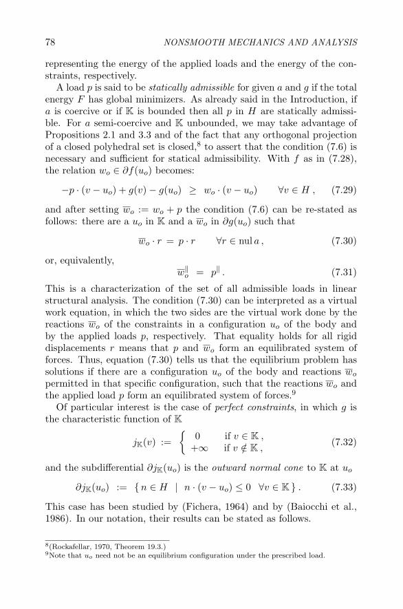
78 NONSMOOTH MECHANICS AND ANALYSIS
representing the energy of the applied loads and the energy of the con-straints, respectively.
A load p is said to be statically admissible for given a and g if the totalenergy F has global minimizers. As already said in the Introduction, ifa is coercive or if K is bounded then all p in H are statically admissi-ble. For a semi-coercive and K unbounded, we may take advantage ofPropositions 2.1 and 3.3 and of the fact that any orthogonal projectionof a closed polyhedral set is closed,8 to assert that the condition (7.6) isnecessary and sufficient for statical admissibility. With f as in (7.28),the relation wo ∈ ∂f(uo) becomes:
−p · (v − uo) + g(v)− g(uo) ≥ wo · (v − uo) ∀v ∈ H , (7.29)
and after setting wo := wo + p the condition (7.6) can be re-stated asfollows: there are a uo in K and a wo in ∂g(uo) such that
wo · r = p · r ∀r ∈ nul a , (7.30)
or, equivalently,w‖
o = p‖ . (7.31)
This is a characterization of the set of all admissible loads in linearstructural analysis. The condition (7.30) can be interpreted as a virtualwork equation, in which the two sides are the virtual work done by thereactions wo of the constraints in a configuration uo of the body andby the applied loads p, respectively. That equality holds for all rigiddisplacements r means that p and wo form an equilibrated system offorces. Thus, equation (7.30) tells us that the equilibrium problem hassolutions if there are a configuration uo of the body and reactions wo
permitted in that specific configuration, such that the reactions wo andthe applied load p form an equilibrated system of forces.9
Of particular interest is the case of perfect constraints, in which g isthe characteristic function of K
jK(v) :={
0 if v ∈ K ,+∞ if v /∈ K ,
(7.32)
and the subdifferential ∂jK(uo) is the outward normal cone to K at uo
∂jK(uo) := {n ∈ H | n · (v − uo) ≤ 0 ∀v ∈ K } . (7.33)
This case has been studied by (Fichera, 1964) and by (Baiocchi et al.,1986). In our notation, their results can be stated as follows.
8(Rockafellar, 1970, Theorem 19.3.)9Note that uo need not be an equilibrium configuration under the prescribed load.

A condition for statical admissibility in unilateral structural analysis 79
Theorem 4.1 (Fichera, 1972). Let H be a Hilbert space, let K be aclosed convex subset of H, let a be a bilinear form on H, symmetric,continuous and semicoercive, and let g be equal to jK. If a load p isstatically admissible, then
p · r ≤ 0 ∀r ∈ nul a ∩ rc K . (7.34)
Moreover, if PK is closed and if the above inequality holds, then p isstatically admissible.
Here P is the projection defined in (7.17) and rc K is the recession coneof K :
rc K := { η ∈ H | u + λη ∈ K ∀u ∈ K, ∀λ ≥ 0 } . (7.35)
In the next theorem, nul p denotes the set of all elements of H whichare orthogonal to p.
Theorem 4.2 (Baiocchi et al., 1986). Let H, K, a and g be as above.If a load p is statically admissible, then (7.34) holds. Moreover, p isstatically admissible if (7.34) holds and the set
nul a ∩ rc K ∩ nul p
is a subspace.
When compared with these two theorems, Proposition 3.3 shows somedistinctive properties: (i) there is no gap between necessary and suffi-cient condition for statical admissibility,10 (ii) no role is plaid by therecession cone, (iii) constraints more general than perfect constraintsare considered, (iv) the characterization (7.30), (7.31) of the set of alladmissible loads has a direct mechanical interpretation.
AcknowledgmentsThis research was supported by the Programma Cofinanziato 2002
Modelli Matematici per la Scienza dei Materiali of the Italian Ministryfor University and Scientific Research.
10In the case of structural analysis, in which K is a closed polyhedral set, this is also true forTheorem 4.1.

80 NONSMOOTH MECHANICS AND ANALYSIS
ReferencesBaiocchi C., Gastaldi F., Tomarelli F., Some existence results on nonco-
ercive variational inequalities, Annali Scuola Normale Superiore, Pisa,Serie IV, vol. XIII, pp. 617-659 (1986).
Baiocchi C., Buttazzo G., Gastaldi F., Tomarelli F., General existencetheorems for unilateral problems in continuum mechanics, Arch. Ra-tional Mech. Analysis, vol. 100, pp. 149-189 (1988).
Brezis H., Analyse Fonctionnelle. Theorie et Applications. Masson, Paris,1983.
Dacorogna B., Direct Methods in the Calculus of Variations, Springer1989.
Del Piero G., Smaoui H., Unilateral Problems in Structural Analysis.Theory and Applications. Springer-Verlag Heidelberg, in preparation.
Fichera G., Problemi elastostatici con vincoli unilaterali: il problema diSignorini con ambigue condizioni al contorno, Atti Accademia Naz.dei Lincei, sez. I, vol. 7, pp. 71-140 (1964).
Fichera G., Boundary value problems in elasticity with unilateral con-straints, in: Handbuch der Physik, vol VIa/2, Springer-Verlag, Berlin1972.
Goeleven D., Noncoercive Variational Problems and Related Results,Longman, Harlow 1996.
Lions J.-L., Stampacchia G., Variational Inequalities, Comm. Pure Appl.Mathematics, vol. XX, pp. 493-519 (1967).
Rockafellar R.T., Convex Analysis, Princeton University Press, Prince-ton, N.J. 1970.
Schatzman M., Problemes aux limites non lineaires, non coercifs, AnnaliScuola Normale Superiore, Pisa, Serie III, Vol. XXVII, pp. 641-686(1973).
Stampacchia G., Formes bilineaires coercitives sur les ensembles con-vexes, C. R. Acad. Sci. Paris vol. 258 pp. 4413-4416 (1964).

Chapter 8
MIN-MAX DUALITY AND SHAKEDOWNTHEOREMS IN PLASTICITY
Quoc-Son NguyenLaboratoire de Mecanique des Solides, CNRS-UMR7649, Ecole Polytechnique, Palaiseau,[email protected]
Abstract This paper gives an overall presentation of shakedown theorems in per-fect and in hardening plasticity. General results on shakedown theoremsare discussed in the framework of generalized standard materials. Thestarting point is a static shakedown theorem available for perfect andfor hardening plasticity. It leads by min-max duality to the dual staticand kinematic approaches to compute the safety coefficient with respectto shakedown. These approaches are discussed for common models ofisotropic and of kinematic hardening. In particular, the kinematic ap-proach leads to some new results on the expressions of the safety coef-ficient.
Keywords: Plasticity; shakedown analysis; min-max duality; kinematic/isotropichardening; static and kinematic approaches; safety coefficient.
IntroductionThe shakedown phenomenon is related to the long-term behavior of
an elastic-plastic solid under variable loads and expresses the fact thatthe mechanical response of the solid becomes purely elastic if the loadamplitude is small enough or if the hardening effect is strong enough,immaterial of the initial state of the evolution. Shakedown conditionshave been discussed in a large number of papers of the literature. Clas-sical shakedown theorems in a quasi-static deformation takes its defini-tive form from the pioneering works of Bleich (1932), Melan (1936) andKoiter (1960). Its generalization to dynamics has been discussed, cf.(Corradi and Maier, 1974). Further extensions to hardening plastic-

82 NONSMOOTH MECHANICS AND ANALYSIS
ity, to visco-plasticity or to damage mechanics and poro-plasticity canbe found in a large number of references, e.g. (Mandel, 1976, Konig,1987, Polizzotto et al., 1991, Debordes, 1976, Maier, 2001).
The objective of this paper is to give an overall presentation of shake-down theorems in elasto-plasticity, available for common models of strainhardening in the framework of generalized standard models of plasticity.This framework is a straightforward extension of perfect plasticity, withthe same ingredients of convexity and normality and has been shown tobe large enough to cover most common models of hardening plasticity,cf. (Halphen and Nguyen, 1975, Nguyen, 2000). As in perfect plasticity,e.g. (Koiter, 1960, Debordes, 1976), the method of min-max dualitycan be applied to obtain shakedown theorems. The starting point isan extended version of Melan’s static shakedown theorem, available inperfect plasticity and in hardening plasticity. This theorem leads tothe definition of the safety coefficient with respect to shakedown and,by a min-max duality, to dual safety coefficients obtained respectivelyfrom static and kinematic approaches. This method is then discussed inthe particular cases of strain hardening materials for which hardeningparameters are the plastic strain or equivalent plastic strain.
1. Perfect and hardening plasticityThis discussion is limited to the case of generalized standard models
of plasticity. A generalized standard material is defined by the followingconditions:
- State variables are (ε, α), which represents respectively the strain tensorand a set of internal parameters. Internal parameters α include theplastic strain and other hardening variables, α = (εp, β). There existsan energy potential W (ε, α) which leads to associated forces
σ = W,ε , A = −W,α (8.1)
and to a dissipation per unit volume din
din = A · α. (8.2)
- The force A must be plastically admissible, this means that physicallyadmissible forces A must remain inside a convex domain C, called theelastic domain.- Normality law is satisfied for α:
α ∈ ∂ΨC(A). (8.3)

Min-max Duality and Shakedown Theorems in Plasticity 83
Thus, the following maximum dissipation principle is satisfied:
A · α = D(α) = maxA∗∈C
A∗ · α (8.4)
in the spirit of Hill’s maximum principle in perfect plasticity. Finally,as in perfect plasticity, the notions of convexity, normality, energy andgeneralized forces are four principal ingredients of the generalized stan-dard models, cf. (Moreau, 1970, Halphen and Nguyen, 1975). Thedissipation potential D(α) is convex, positively homogeneous of degree1. This function is state-independent, i.e. independent of the presentvalue of state variables (ε, α), if the plastic criterion is assumed to bestate-independent.
In particular, the case of generalized standard models satisfying theassumption of linear stress/elastic-strain relationship is considered here.For such a model, the energy is{
W = WE(ε− εp) + WH(εp, β),where WE = 1
2(ε− εp) : L : (ε− εp) (8.5)
is a quadratic, positive function representing the stored energy by elasticdeformation, L denotes the elastic tensors. The second term WH(εp, β)is an arbitrary convex, differentiable function of the internal parametersand represents the energy stored by hardening effects. With the notationB = −WH,β, X = WH,εp , AH = −WH,α, the thermodynamic force A is:A = (σ −X, B) = (σ, 0) + AH .
2. Static shakedown theoremThe problem of elastic-plastic response of a solid of volume V in small
quasi-static deformation, starting from any given initial conditions of dis-placement and of the internal state under the action of a loading historyis considered. It is assumed as usual in shakedown analysis that an ad-missible loading history consists of a linear combination Pi(gi, Fi, u
di ) of
n load systems (of volume force gi and surface forces Fi on SF and ofgiven displacements ud
i on Su) where Pi(t), i = 1, n are n load parame-ters. These parameters may be considered as the components of a loadpoint P defined in the load parameter space Rn and the loading historyis described by a given curve P (t), 0 ≤ t ≤ +∞. It is assumed that P (t)takes its value arbitrarily in an allowable polyhedral and convex domainS of corners Sj , j = 1, J .
Let (u(t), σ(t), εp(t), β(t)) be the elastic-plastic response of the solidstarting from a given initial state on the interval t ≥ 0 under the actionof an admissible loading history.

84 NONSMOOTH MECHANICS AND ANALYSIS
By definition, this response shakes down if the existence of limt→∞ εp(t)is ensured. This property also ensures that limt→∞ u(t) − uel(t) andlimt→∞ σ(t)− σel(t) exist
where σel(t), uel(t)) denote the fictitious response to the same load-ing of the same solid, assumed to be purely elastic and admitting thesame elastic coefficients L. The proof of this statement is clear for dis-crete systems while for continua, some difficulties remain concerning thechoice of a relevent functional space in the case of perfect plasticity, cf.(Debordes, 1976, Nayroles, 1977, Suquet, 1981).
The following extension of Melan’s theorem is an enhanced version ofsome previous results given in the literature, cf. for example (Nguyen,1976, Polizzotto et al., 1991):
Theorem 8.1 (static shakedown theorem in perfect and in hard-ening plasticity)It is assumed that the plastic criterion is state-independent and that theassumption of linear stress/elastic-strain relationship is fulfilled. Thenthere is shakedown whatever be the initial state and the admissible load-ing history if there exists a self-stress field s∗, a constant internal pa-rameter field α∗ = (εp∗, β∗) and a coefficient m > 1 such that theforce field mA∗j is plastically admissible for all j = 1, J , where A∗j =(s ∗+σj
el −X(α∗), B(α∗)), and σjel denotes the elastic response in stress
of the solid, associated with the values of load parameters at corners Sj.
The proof of this theorem can be obtained in two steps. In the firststep, it is shown that under the introduced assumptions, the dissipatedenergy W d is necessarily bounded. In the second step, this propertyensures the existence of limt→∞ εp(t).
- first step:Under the assumptions of the theorem and from the convexity of the
elastic domain, it is clear that mA∗ is plastically admissible for all t ≥ τ ,where A∗(t) denotes
A∗(t) = (s∗ + σel(t)−X(α∗), B(α∗)) (8.6)
the following inequality holds∫V
(A−A∗) · α dV ≥ m− 1m
∫V
A · α dV.
More explicitly,
(A−A∗) · α = (σ − σ∗) : εp − (X −X∗) : εp + (B −B∗) : β,

Min-max Duality and Shakedown Theorems in Plasticity 85
where σ∗ = s∗+σel. Since σ−σ∗ is a self-stress field and since u−uel = 0on Su, one obtains
0 =∫
V(σ − σ∗) : (ε− εel) dV thus∫
V(σ − σ∗) : εp +
∫V
(σ − σ∗) : L−1 : (σ − σ∗) dV = 0.
It follows that{− d
dt
∫V {
12(σ(t)− σ∗(t)) : L−1 : (σ(t)− σ∗(t))+
WH(α)−WH(α∗)−WH,α(α∗) · (α− α∗) } dV ≥ m−1m
∫V din dV.
or that⎧⎨⎩ I(0)− I(t) ≥ m−1m W d with W d(t) =
∫ t0
∫V A · α dV dτ
I(t) =∫V {
12(σ(t)− σ∗(t)) : L : (σ(t)− σ∗(t))+
WH(α(t))−WH(α∗)−WH,α(α∗) · (α(t)− α∗) } dV.
(8.7)
Since I(t) is non-negative as a sum of two non-negative terms, it isconcluded that the dissipated energy W d(t) is bounded by I(0) for all t.
- second step:The second step consists of proving that α(t) = (εp(t), β(t)) tends to
a limit. The fact that the dissipated energy remains bounded alreadyensures the existence of a limit of α(t) for any appropriate functionalspace which is complete with respect to the norm associated with thedissipation, since there exists a constant c > 0 such that A · α ≥ c‖α‖.This inequality follows from the fact that the origin of forces is strictlyinside the elastic domain.
Theorem 8.1 gives a sufficient condition of shakedown. Melan’s the-orem in perfect plasticity is recovered when WH = 0. In this case, it iswell known that, since the stress solution σ(t) belongs to the convex setof plastically admissible fields PA and to the set of statically admissiblefields SA(t) for all t, the self-stress s(t) = σ(t)− σel(t) satisfies∫
V(s− s) : L−1 : sdV ≥ 0, ∀ s ∈ K(t) = {σel(t)}+ PA ∩ SA(t).
Thus, s(t) is a solution of the equation −s ∈ ∂ΨK(t)(s), a sweepingprocess by the variable convex K(t), cf. (Moreau, 1971, Moreau, 1974)in the stress space with energy norm.
3. Safety coefficient and min-max dualityMin-max duality is a well known method of Convex Analysis, cf. for
example (Rockafellar, 1970). It has been discussed in perfect plasticity

86 NONSMOOTH MECHANICS AND ANALYSIS
by (Debordes and Nayroles, 1976) for shakedown analysis. This methodis applied here following the same ideas. For this, the definition of astatic safety coefficient with respect to shakedown is first consideredand dual static and kinematic approaches are introduced.
3.1 Static safety coefficientA safety coefficient with respect to shakedown can be introduced from
the previous theorem.
Theorem 8.2 (static safety coefficient)Let ms be the safety coefficient defined by the maximum
ms = maxs∗,α∗,m
m (8.8)
among constant coefficient m, internal parameters α∗ and self-stressfields s∗ such that{
∀ j, mA∗j is plastically admissible,
with A∗j = (s∗ + σjel −X(α∗), B(α∗)).
(8.9)
Then there is shakedown if ms > 1.
Indeed, if ms > 1 then the assumptions of Theorem 8.1 are fulfilled andthe conclusion holds.
3.2 Min-max dualityThe minimization (8.8) is a convex optimization problem. The dual
approach consists of considering dual problems obtained by relaxingsome constraints. For this, the initial problem (8.8) is first written asthe search of maximum of m on the set of self-stress fields s∗, internalparameter fields α∗, coefficients m and of force fields Aj such that{
∀ j, Aj is plastically admissible,
Aj = m (s∗ + σjel −X(α∗), B(α∗)).
(8.10)
The last constraint is relaxed by the introduction of Lagrange multipliersaj = (dpj , bj) associated with the Lagrangian⎧⎪⎨⎪⎩
Λ = m +∫V (Aj −m (s∗ + σj
el −X(α∗), B(α∗))) · aj dV == m(1−
∫V σj
el : dpjdV )−m∫V s∗ : (
∑j dpj)dV +∫
V Aj · ajdV + m∫V (X∗ : (
∑j dpj)−B∗ · (
∑j bj))dV.
(8.11)
The max-min problem
maxs∗,α∗,A,m
mina
Λ(a,m, s∗, α∗, Aj) (8.12)

Min-max Duality and Shakedown Theorems in Plasticity 87
in the set of arbitrary rate fields aj and of self-stress fields s∗, internalparameter fields α∗, coefficients m and of plastically admissible fields Aj ,leads to the initial problem. Indeed, the result of the minimization withrespect to a gives mina Λ = m if Aj = m A∗j for all j and mina Λ = −∞otherwise.
3.3 Kinematic safety coefficientThe dual problem
mk = mina
maxs∗,α∗, A, m
Λ (8.13)
defines the dual approach to compute the safety coefficient. It is clearthat ms ≤ mk and that it is not possible to find a self-stress satisfyingthe condition of the previous propositions if mk < 1.
For a given rate aj = (dpj , bj), j = 1, J , the first operation consistsof searching for the maximum of Λ among coefficients m, self-stress fields∗, internal parameters α∗ and plastically admissible fields Aj . Thefollowing notation for the cycle residues is introduced
Δα =∑
j
aj = (Δεp, Δβ), Δεp =∑
j
dpj , Δβ =∑
j
bj , (8.14)
and let Q(Δα) denote the quantity
Q(Δα) = maxα∗ −AH∗ ·Δα = max
εp∗,β∗ X∗ : Δεp −B∗ ·Δβ. (8.15)
The result of the maximization is:
maxm,s∗,α∗,Aj
Λ =∑
j
∫V
D(aj)dV
where D(a) denotes the dissipation function, under the conditions:⎧⎨⎩Δεp must be a compatible strain field,Δεp and Δβ must ensure Q(Δα) < +∞,∫V (σj
el : dpj −Q(Δα)) = 1(8.16)
A compatible field means that there exists a displacement field up withup = 0 on Su such that Δεp = (∇up). The fact that (Δεp, Δβ) mustensure a finite value of Q leads to additional conditions as it will be shownlater in some examples. Finally, the following theorem is obtained
Theorem 8.3 (kinematic safety coefficient)Let mk be the kinematic safety coefficient, defined by the minimization

88 NONSMOOTH MECHANICS AND ANALYSIS
problem
mk = minaj
∑j
∫V
D(aj)dV (8.17)
among the fields aj = (dpj , bj), j = 1, J such that the conditions (8.16)are fulfilled. It is concluded that mk ≥ ms and the assumptions of The-orem 8.1 is impossible if mk < 1.
As usually established in min-max duality, equality ms = mk is gener-ically satisfied. In particular, this equality holds if the plastic domainis bounded in the stress space as it has been shown by (Debordes andNayroles, 1976) in perfect plasticity. It is expected that this equality al-ways holds although a general proof available for any standard model islacking for continuum solids. Under this equality, it is clear that mk > 1is then a sufficient condition of shakedown.
4. Kinematic approachIn the following sections, the kinematic approach is considered for
common models of plasticity.
4.1 Perfect plasticityThe elastic perfectly plastic model admits as internal parameter the
plastic strain εp and the hardening energy is WH = 0. Theorem 8.1 isreduced to Melan’s theorem and the kinematic approach leads to thefollowing result, cf. (Koiter, 1960, Debordes, 1976):
Statement 1 In perfect plasticity, the dual kinematic approach leadsto a coefficient mk ≥ ms, defined as the minimum
mk = mindp
∑j
∫V
D(dpj) dV (8.18)
among the plastic rates dp satisfying
Δεp =∑
j
dpj compatible,
∫V
σjel : dpj dV = 1. (8.19)
4.2 Isotropic hardeningFor the standard model with Mises criterion, the internal parameter
α = (εp, β) represents respectively the plastic strain and the equivalentplastic deformation β. By definition, β = ‖εp‖. It is assumed that thederivative of the hardening energy R = −B = W ′
H(β) is a positive,

Min-max Duality and Shakedown Theorems in Plasticity 89
increasing function admitting a finite limit Rmax. The plastic criterionis ‖σ′‖ + B − k ≤ 0. The normality law gives εp = λ σ′
‖σ′‖ , β = λ. The
dissipation is D = σ′ : εp + Bβ = k ‖εp‖. Since
Q = maxβ∗ −B∗Δβ = RmaxΔβ = Rmax
∑j
‖dpj‖ (8.20)
the min-max duality leads to a well known result
Statement 2 In isotropic hardening, the dual kinematic approach leadsto a coefficient mk ≥ ms, defined as the minimum
mk = mindp
∫V
k∑
j
‖dpj‖ dV (8.21)
among the plastic rates dp satisfying
Δεp =∑
j
dpj compatible,
∫V
(σjel : dpj −Rmax
∑j
‖dpj‖) dV = 1,
(8.22)
i.e. the shakedown behaviour of the solid is obtained as in perfect plas-ticity with the yield value Rmax + k.
4.3 Kinematic hardeningFor this model, the internal parameter is εp and the hardening energy
WH = V (y), with y = ‖εp‖ =√
εp : εp, is such that R(y) = V ′(y) isa monotone increasing function varying in [0, Rmax] when y ∈ R+. Ifεp is assumed to be incompressible (εp
kk = 0), the generalized force isA = −W,εp = σ′ − X with X = R(‖εp‖)εp/‖εp‖. With Mises criterion‖A‖ − k ≤ 0, the elastic domain is a sphere of radius k and with centerX in the force space. This center X remains near the origin since ‖X‖ ≤Rmax. Since
Q = maxεp∗j
R(‖εp∗‖) : (∑
j
dpj) = Rmax‖Δεp‖,
It follows that:
Statement 3 For this limited kinematic hardening model, the dual kine-matic approach leads to a coefficient mk ≥ ms, defined as the minimum
mk = mindpj
∑j
∫V
k‖dpj‖ dV (8.23)

90 NONSMOOTH MECHANICS AND ANALYSIS
σ
σ
1
2
’
’
Rmax
K
K
elastic domainsσ
O
C
ε
unidimensional curve
k
K
Figure 8.1. A model of limited kinematic hardening
among plastic rates dpj satisfying{dpj
kk = 0, and Δεp compatible,∫V (σj
el : dpj −Rmax‖Δεp‖) dV = 1.(8.24)
If Zieger-Prager’s model of linear kinematic hardening is considered, thenV = 1/2h‖εp‖2 and the kinematic hardening is unlimited. Since
Q = maxεp∗j
hεp∗ : (∑
j
dpj) = +∞ if Δεp �= 0,
It is concluded that
Statement 4 In linear kinematic hardening with Mises criterion, thedual kinematic approach leads to a coefficient mk ≥ ms, defined as theminimum
mk = mindpj
∑j
∫V
k‖dpj‖dV. (8.25)
among the plastic rates dpj satisfying
dpjkk = 0, Δεp = 0,
∫V
σjel : dpj dV = 1. (8.26)
Thus, closed cycles of plastic rates must be considered instead of com-patible plastic cycles as in perfect plasticity or in isotropic hardening.
In particular, if m0k, mukh
k and mlkhk denote respectively the kinematic
safety coefficients in perfect plasticity, in linear kinematic hardening andin limited kinematic hardening with the same yield stress k, it followsfrom their definition that
m0k ≤ mlkh
k ≤ mukhk . (8.27)

Min-max Duality and Shakedown Theorems in Plasticity 91
The case of limited hardening appears as the penalization of the unlim-ited case, Rmax is the penalty parameter associated with the constraint‖Δεp‖ = 0.
5. ConclusionIn this paper, an overall presentation of shakedown theorems is given
by min-max duality. In particular, new results concerning the expres-sions of kinematic safety coefficients, available for common models ofisotropic/kinematic hardening, are presented.
ReferencesCorradi, L., Maier, G., 1974. Dynamic non-shakedown theorem for elas-
tic perfectly-plastic continua. J. Mech. Phys. Solids 22, 401–413.Debordes, O., 1976. Dualite des theoremes statique et cinematique sur
la theorie de l’adaptation des milieux continus elasto-plastiques. C.R.Acad. Sc. 282, 535–537.
Debordes, O., Nayroles, B., 1976. Sur la theorie et le calcul a l’adaptationdes structures elasto-plastiques. J. Mecanique 20, 1–54.
Halphen, B., Nguyen, Q.-S., 1975. Sur les materiaux standard genera-lises. J. Mecanique 14, 1–37.
Koiter, W., 1960. General problems for elastic-plastic solids. In: Sned-don, J., Hill, R. (Eds.), Progress in Solid Mechanics. Vol. 4. NorthHolland, pp. 165–221.
Konig, J., 1987. Shakedown of elastic-plastic structures. Elsevier, Ams-terdam.
Maier, G., 2001. On some issues in shakedown analysis. J. Appl. Mech.68, 799–808.
Mandel, J., 1976. Adaptation d’une structure plastique ecrouissable.Mech. Res. Com 3, 251–256.
Moreau, J., 1970. Sur les lois de frottement, de plasticite et de viscosite.C. R. Acad. Sciences 271, 608–611.
Moreau, J., 1971. Rafle par un convexe variable. Seminaire d’AnalyseConvexe.
Moreau, J., 1974. On unilateral constraints, friction and plasticity. In:New variational techniques in Mathematical Physics. CIME Course,Springer-Verlag, pp. 173–322.
Nayroles, B., 1977. Tendances recentes et perspectives a moyen termeen elastoplasticite asymptotique des constructions. In: Proceedings,Congres Francais de Mecanique, Grenoble, France. Grenoble.
Nguyen, Q.-S., 1976. Extension des theoremes d’adaptation et d’uniciteen ecrouissage non lineaire. C.R. Acad. Sc. 282, 755–758.
92 NONSMOOTH MECHANICS AND ANALYSIS
Nguyen, Q.-S., 2000. Stability and Nonlinear Solid Mechanics. Wiley,Chichester.
Polizzotto, C., Borino, G., Cademi, S., Fuschi, P., 1991. Shakedown prob-lems for mechanical models with internal variables. Eur. J. Mech.A/Solids 10, 621–639.
Rockafellar, R., 1970. Convex analysis. Princeton University Press, Prince-ton.
Suquet, P., 1981. Sur les equations de la plasticite: existence et regularitedes solutions. J. Mecanique 20, 3–40.

Chapter 9
FRICTION AND ADHESION
Michel RaousLaboratoire de Mecanique et d’Acoustique, CNRS, 31, chemin Joseph Aiguier, 13402Marseille Cedex 20, [email protected]
Abstract The studies carried out on adhesion by the group “Modeling in ContactMechanics” at the LMA are reviewed in this paper and recent applica-tions are presented. Based on the introduction of the adhesion intensityvariable developed by M. Fremond, different forms of a model couplingadhesion to unilateral contact and friction have been developed. Theformulations are given either under the form of implicit variational in-equalities or the one of complementarity problems. Both quasi-staticand dynamic formulations are considered.
The model is non smooth because we do not use any regularizationfor the unilateral conditions and for the friction, i.e. Signorini conditionsand strict Coulomb law are written. In the thermodynamics analysis,the state and the complementarity laws are then written using sub-differentials and differential inclusions because of the non convexity andnon differentiability of the potentials. For the dynamics, the formulationis given in term of differential measures in order to deal with the noncontinuity of the velocities that may occur in the solutions.
This work therefore owes much to the theories and the numericalscheme developed by J. J. Moreau and M. Jean.
Keywords: Unilateral contact, friction, adhesion, non smooth dynamics
IntroductionIn order to describe the smooth transition from a completely adhesive
contact to a usual unilateral contact (Signorini conditions) with Coulombfriction, a model based on interface damage has been first developed forquasi-static problems in (Raous et al, 1997, Cangemi, 1997, Raous et al,1999, Raous, 1999). Using a dynamic formulation, the model was thenextended to account for the brittle behaviour occurring when a crack

94 NONSMOOTH MECHANICS AND ANALYSIS
interacts with fiber-matrix interfaces in composite materials in (Raous-Monerie, 2002, Monerie, 2000). More recently, the model has been usedto study metal/concrete interfaces in reinforced concrete in civil engi-neering (Karray et al, submitted), delamination of coated bodies (Raouset al, 2002), delamination of glued assembling in civil engineering (Raouset al, 2004), cohesive masonry (Jean et al, 2001, Acary, 2001) and pro-duction of wear particles in bio-engineering (Baudriller, 2003).
The quasi-static formulation was extended to deal with hyperelastic-ity in (Bretelle et al, 2001). Mathematical results about the existenceof the solutions were given in (Cocou-Rocca, 2000) without using anyregularization on the contact conditions.
1. The modelThe RCC model (Raous-Cangemi-Cocou) has been first given in (Ra-
ous et al, 1997, Cangemi, 1997) and then extensively presented in (Raouset al, 1999). It has been extended to the present form including progres-sive friction with the term (1 − β) in (Monerie, 2000, Raous-Monerie,2002). Adhesion is characterized in this model by the internal variable β,introduced by Fremond (Fremond, 1987, Fremond, 1988), which denotesthe intensity of adhesion. The introduction of a damageable stiffnessof the interface ensures a good continuity between the two models dur-ing the competition between friction and adhesion. The behaviour ofthe interface is described by the following relations, where (9.1) givesthe unilateral contact with adhesion, (9.2) gives the Coulomb frictionwith adhesion and (9.3) gives the evolution of the adhesion intensity β.Initially, when the adhesion is complete, the interface is elastic as longas the energy threshold w is not reached. After that, damage of theinterface occurs and consequently, on the one hand, the adhesion inten-sity β and the apparent stiffness β2CN and β2CT decrease, and on theother hand, friction begins to operate. When the adhesion is completelybroken (β = 0), we get the classical Signorini problem with Coulombfriction.
−RrN + β2CN uN ≥ 0 , uN ≥ 0 ,
(−Rr
N + β2CN uN
). uN = 0, (9.1)
RrT = β2CT uT , Rr
N = RN ,‖RT −Rr
T‖ ≤ μ(1− β)∣∣RN − β2CN uN
∣∣ , (9.2)
with
if ‖RT −RrT‖ < μ(1− β)
∣∣RN − β2CN uN
∣∣ ⇒ uT = 0,if ‖RT −Rr
T‖ = μ(1− β)∣∣RN − β2CN uN
∣∣ ⇒ ∃λ ≥ 0, uT = λ(RT −RrT),

Friction and adhesion 95
β = −[(
w − β (CN u2N + CT ‖uT‖2)− kΔβ
)−/b
]1/p
if β ∈ [0, 1[,
β ≤ −[(
w − β (CN u2N + CT ‖uT‖2)− kΔβ
)−/b
]1/p
if β = 1 .
(9.3)
RN and uN are the algebraic values of the normal components of the con-tact force and those of the relative displacement between the two bodies(occupying domains Ω1 and Ω2) defined on the contact boundary Γc,and RT and uT are the tangential components of this contact force andthose of this relative displacement. Subscript r denotes the reversibleparts. The constitutive parameters of this interface law are as follows:CN and CT are the initial stiffnesses of the interface (full adhesion), μ isthe friction coefficient, w is the decohesion energy, p is a power coefficient(p = 1 in what follows) and k = 0 in what follows.
0 1 2 3 4 50
0.4
0.8
1.2
Normal displacement
Nor
mal
forc
e
with unloadingwithout unloadingwithout viscosity, without unloading
Rn / Ro
un / uo
Figure 9.1. Normal behaviour of the interface
Fig. 9.1 and Fig. 9.2 give the normal and tangential behaviour ofthe interface during loading and unloading (CN = CT = C, u0 =
√ω/C
and R0 =√
ωC) . It should be noted that the Signorini conditions arestrictly imposed when compression occurs. References on other mod-els can be found in (Raous, 1999, Raous et al, 1999) and a comparisonbetween some of them is made in (Monerie et al, 1998) (models devel-oped by Tvergaard-Needleman, Girard-Feyel-Chaboche, Michel-Suquet,Allix-Ladeveze). Using penalization and augmented Lagrangian on asimilar model to the RCC one, Talon-Curnier have solved the quasi-static problem using generalized Newton method (Talon-Curnier, 2003).

96 NONSMOOTH MECHANICS AND ANALYSIS
0 2 4 6−0.4
0
0.4
0.8
1.2
Tangential displacement
Tan
gent
ial f
orce
with unloadingwithout unloadingwithout viscosity, without unloading
Rt / Ro
ut / uo
Figure 9.2. Tangential behaviour of the interface
2. The thermodynamicsIn the framework of continuum thermodynamics, the contact zone
is assumed to be a material surface and the local constitutive lawsare obtained by choosing two specific forms of the free energy and thedissipation potential associated to the surface. The following thermo-dynamic variables are introduced: the relative displacements (uN n,uT)and the adhesion intensity β are chosen as the state variables, and thecontact force R and a decohesion force G, as the associated thermody-namic forces. The thermodynamic analysis given for the RCC model in(Raous et al, 1999) has been extended to the present model in (Monerie,2000, Raous-Monerie, 2002) in order to obtain relations (9.1) to (9.3),where friction is progressively introduced in the form of the term (1−β)μinto (9.2).
Expressions (9.4) and (9.5) are adopted for the free energy Ψ(uN, uT, β)and the potential of dissipation Φ
(uT, β
). In (9.4), the indicator func-
tion IK
(where K = {v / v ≥ 0} ) imposes the unilateral conditionuN ≥ 0 and the indicator function IP (where P = {γ / 0 ≤ γ ≤ 1})imposes the condition β ∈ [0, 1]. In (9.5), the indicator function IC−(β)(where C− = {γ / γ ≤ 0}) imposes that β ≤ 0: the adhesion can onlydecrease and cannot be regenerated (it is irreversible) in the presentmodel.
Ψ(uN, uT, β) =12
β2 CN u2N +
12
β2 CT ‖uT‖2−w β +IK
(uN)+IP (β) (9.4)
Φ(uT, β
)= μ(1−β)
∣∣RN − β2 CN uN
∣∣ ‖uT‖+b
p + 1
∣∣∣β∣∣∣p+1+ IC−(β) (9.5)

Friction and adhesion 97
Ψ has a part which is convex but not differentiable and another partwhich is differentiable but not convex with respect to the pair (u, β). Φis convex but has a part which is not differentiable. The state laws andthe complementarity laws are then written as follows in order to obtainthe contact behaviour laws given in section 1 (Raous et al, 1999).⎧⎪⎨⎪⎩
RrT = ∂Ψd
∂[uT ] RrN − ∂Ψd
∂[uN ] ∈ ∂IK
([uN ])
−Gβ − ∂Ψd
∂β ∈ ∂I[0,1](β)(9.6)
RN = RrN (Rir
T , Gβ) ∈ ∂Φ( ˙[uT ], β) (9.7)
3. The quasi-static formulationThe formulation and the approximation of quasi-static frictional prob-
lems given in (Cocou et al, 1996) have been extended to adhesion prob-lems in (Raous et al, 1997, Raous et al, 1999, Raous, 1999). The problemcan be here set as the coupling between two variational inequalities (oneof which is implicit) and a differential equation.
Problem (P1): Find (u, β) ∈ W 1,2(0, T ; V ) ×W 1,2(0, T ; H) such thatu(0) = u0 ∈ K, β(0) = β0 ∈ H
⋂[0, 1[ and for ∀t ∈ [0, T ], u(t) ∈ K, and
∀v ∈ V a(u, v − ˙u) + j(β, uN, vT)− j(β, uN, uT) +∫ΓC
β2 CTuT . (vT − uT)ds ≥ (F , v − ˙u)− 〈RN, vN − uN〉, (9.8)
−〈RN, z − uN〉+∫
ΓC
β2 CNuN.(z − uN)ds ≥ 0 ∀z ∈ K, (9.9)
β = −1/b[w − (CN u2
N + CT ‖uT‖2)β]−
a.e. on ΓC , (9.10)
where:- u = (u1, u2) where u1 and u2 define the displacements in Ω1 and Ω2,- V = (V 1, V 2), V α =
{vα ∈
[H1(Ωα)
]3 ; vα = 0 a.e. on ΓαU
}, α = 1, 2,
- H = L∞(Γc),- K =
{v = (v1, v2) ∈ V 1 × V 2; vN ≥ 0 a.e. on Γc
}, where Γc is the
contact boundary between the two solids Ω1 and Ω2,- a(. , .) is the bilinear form associated to the elasticity mapping,
- j(β, uN, vT) =∫
ΓC
μ(1− β)∣∣∣RN − β2CNuN
∣∣∣ ‖vT‖ds ,
- F = (F 1, F 2) are the given force densities applied to solid 1 and tosolid 2 respectively.
98 NONSMOOTH MECHANICS AND ANALYSIS
By using an incremental approximation, it has been established in(Raous et al, 1997, Raous et al, 1999) that the numerical solutions canbe obtained by adapting the methods that we have developed for dealingwith classical frictional unilateral contacts (Raous, 1999). The solutionshave mainly been obtained as follows:
- either by taking a fixed point on the sliding threshold and solving asequence of minimization problems with the choice between a projectedGauss-Seidel method (accelerated by relaxation or Aitken processes) anda projected conjugate gradient method (Raous-Barbarin, 1992),- or by taking a complementarity formulation, using a mathematicalprogramming method (Lemke’s method).With the adhesion model, these solvers are coupled with the numericalintegration of the differential equation on β by using θ-methods (θ = 1is often chosen). Implementation of the algorithms has been conductedin our finite element code GYPTIS90 (Latil-Raous, 1991).
4. The dynamicsDepending on the characteristics of the interface, especially when b
tends towards zero (no viscosity for the evolution of the intensity of ad-hesion), brittle behaviour can be obtained and the inertia effects have tobe taken into account. A 3D dynamic formulation has been developed(Raous-Monerie, 2002, Monerie-Raous, 1999, Monerie-Acary, 2001). Be-cause of the non smooth character of these interface laws, the dynamicsis written in terms of differential measures as follows (where q denotesthe displacement and r the contact force):
M(q, t)dq = F (q, q, t)dt− rdν , (9.11)
where dq is a differential measure associated with q(t):∫ t2
t1
dq = q(t+2 )− q(t−1 ) ∀t2 > t1 , (9.12)
and hence: ∫ t2
t1
M(q, t)dq =∫ t2
t1
F (q, q, t)dt−∫
]t1, t2]rdν, (9.13)
q(t2) = q(t1) +∫ t2
t1
q(τ)dτ . (9.14)
The Non Smooth Contact Dynamics method developed by (Moreau,1998, Moreau, 1994, Moreau, 1999, Jean, 1999) has been extended to thetreatment of the RCC model. A solver for dealing with adhesion has been

Friction and adhesion 99
implemented in the finite element code LMGC (Jean, 1999, Monerie-Acary, 2001). Another solver based on complementarity formulation(Lemke’s method) dealing with non smooth dynamics problems has beenimplemented in the finite element code SIMEM3 at the LMA (Vola etal, 1998).
5. ApplicationsDelamination benchmarksVarious benchmarks for simulating delamination have been devel-oped in the framework of a joint project with the LaboratoireCentral des Ponts et Chaussees (Raous et al, 2004) focusing onadhesion and gluing in civil engineering.
(a) Deformation
0 5 10 15 20 25 30 35 40 45 50−12
−10
−8
−6
−4
−2
0
2
Interface (mm)
un (m
m)
(b) Normal displacement alongthe contact at various time steps
Figure 9.3. Delamination of two layers submitted to vertical traction
Micro-indentation of a single fiber in a composite materialThis model was first developed in order to describe the behaviour ofthe fiber-matrix interface of composite materials (Cangemi, 1997,Raous et al, 1999). The parameters of the model were identified onmicro-indentation experiments performed at the ONERA on sin-gle fibers. Physical and mechanical considerations are taken intoaccount in the identification procedure: for example, the values ofthe initial interface stiffness CN, CT are taken to be in the rangecorresponding to the elastic properties of the oxides located at theinterfaces. The viscosity parameter b is particularly difficult toidentify: experiments with different loading velocities are requiredfor this purpose. The validity of the model was then confirmedby taking various kinds of loadings (especially cyclic loadings) andcomparing experimental results with those obtained in the numer-

100 NONSMOOTH MECHANICS AND ANALYSIS
(a) Deformations
0 5 10 15 20 25 30 35 40 45 50−4
−3.5
−3
−2.5
−2
−1.5
−1
−0.5
0
Interface (mm)
ut (
mm
)
(b) Tangential displacement alongthe contact zone at various timesteps
Figure 9.4. Shear delamination of a block submitted to horizontal loading
ical simulation whith the same interface parameters. Details ofthese studies can be found in (Cangemi, 1997, Raous et al, 1999)and later in (Monerie, 2000).
Interaction between cracks and fiber/matrix interfaces incomposite materialsAgain in collaboration with ONERA, during the thesis (Monerie,2000), the RCC model has been used to investigate the differentways in which cracks propagate through a composite material andhow they depend on the interface properties. The adhesion modelhas been used to account both the crack propagation (decohesivecrack with no viscosity, i.e. b = 0) and the interface behaviour.Crack bridging, crack trapping and fiber breaking can be observeddepending on the interface characteristics (Raous-Monerie, 2002,Monerie, 2000). On Fig. 9.5 adhesion is broken in the black zones.
Metal/concrete interfaces in reinforced concreteIn civil engineering, we are now testing the RCC model for theadhesive contact between steel and concrete in reinforced concrete.Pull-out tests of a steel shaft are being simulated in the frameworkof a joint project between LMA and ENIT in Tunisia (Karray et al,submitted). In that case, a variable friction coefficient (dependingon the sliding displacement) has been used in order to take intoaccount the wear of the surface which occurs during the slidingwhich seems to be quite significant with concrete. Another versionof the way used to introduce friction has been used: (1−β2) instead

Friction and adhesion 101
0
D
H
0
Figure 9.5. Interaction of a crack and a fiber/matrix interface
of (1 − β). Results with CT = CN=16N/mm3 , μ varying from0.45 to 0.3 and f(β) = (1 - β2) are given in Fig. 9.6.
0.0 0.5 1.0 1.5 2.0 2.5 3.0 3.5 4.0 4.5 5.0 5.5 6.0Displacement (mm)
0
5
10
15
20
25
30
Forc
e(k
N)
0.0 0.5 1.0 1.5 2.0 2.5 3.0 3.5 4.0 4.5 5.0 5.5 6.0Euler implicite, f( )=1-
2, v=0.5mm/s, C=16N/mm
2, us=0.3 mm
0
5
10
15
20
25
30
Experimentalb=0J.s/m
2, =0.3, w=100J/m
2b=70J.s/m
2, 0.48->0.3, w=50J/m
2b=0J.s/m
2, 0.48->0.3, w=100J/m
2
Figure 9.6. Simulation of a pull-out test on reinforced concrete
Delamination of a coated bodyA simplified approach to the delamination of a coated body hasbeen conducted to simulate the indentation of a thin Chrome layeradhering to a metal body (Raous et al, 2002).
Cohesive masonryThe RCC model has been used in (Jean et al, 2001, Acary, 2001)to simulate the behaviour of a cohesive dome. In Fig. 9.8, thedeformation of a dome let on pillars and submitted to gravity isshown.

102 NONSMOOTH MECHANICS AND ANALYSIS
Figure 9.7. Indentation of a coated surface
+1.77E+04
+9.20E+04
+1.66E+05
+2.41E+05
+3.15E+05
+3.89E+05
+4.64E+05
+5.38E+05
+6.12E+05
+6.87E+05
+7.61E+05
+8.35E+05
+9.10E+05
+9.84E+05
Figure 9.8. Behaviour of a cohesive dome
Wear in biomechanicsIn order to simulate the wear occurring in biomaterials and espe-cially the production of wear particles, H. Baudriller (Baudriller,2003) has used the RCC model in a volumic sense. The adhesivemodel is used on all the interfaces between the finite elements. Fig9.9 gives an example of production of fragments.
Figure 9.9. Fragmentation of a block

Friction and adhesion 103
AcknowledgmentsM. Cocou, J.-C. Latil, I. Rosu, in the group MMC at the LMA,
L. Cangemi, Y. Monerie, during the preparation of their thesis, and M.A.Karray (ENIT) have contributed to the works presented here. Thanksto V. Acary and H. Baudrier for providing figures 9.8 and 9.9.
ReferencesAcary, V. (2001). Contribution la modelisation mecanique et numerique
des edifices maconnes . Thesis, Jean, M., supervisor, Universite de laMediterranee, Marseille.
Baudriller, H. (2003). Approche micro-mecanique et modelisation del’usure : application aux biomateriaux des protheses totales de hanche.Thesis, Chabrand, P., supervisor, Univ. de la Mediterranee, Marseille.
Alart, P., and Curnier, A. (1991). A generalised Newton method forcontact problems with friction. J. Mech. Theor. Appliq., (7): 67–82.
Bretelle, A.-S., Cocou, M., and Monerie, Y. (2001). Unilateral contactwith adhesion and friction between two hyperelastic bodies. Int. J.Eng. Sci., (39): 2015–2032.
Cangemi, L. (1997). Frottement et adherence : modele, traitement nume-rique et application a l’interface fibre/matrice, Thesis, Raous, M.,supervisor, Universite de la Mediterranee, Marseille.
Cocou, M., Pratt, E., and Raous, M. (1996). Formulation and approxi-mation of quasistatic frictional contact. Int. J. Eng. Sci., (34)7: 783–798.
Cocou, M., Cangemi, L., and Raous, M. (1997). Approximation resultsfor a class of quasistatic contact problem including adhesion and fric-tion. In Argoul, A., Fremond, M. and Nguyen, Q.S., editors, Variationof domains and free-boundary problems in solids mechanics, Solid Me-chanics and its Applications, Number 66, Kluwer, 211–218.
Cocou, M., and Rocca, R. (2000). Existence results for unilateral qua-sistatic contact problems with friction and adhesion. Math. Model.Num. Anal., (34)5: 981–1001.
Fremond, M. (1987). Adherence des solides. J. Mec. The. Appl. (6)3,383–407.
Fremond, M. (1988) Contact with adhesion. In Moreau, J. J. and Pana-giotopoulos, P.D., editors, Non Smooth Mechanics and Applications,CISM Courses and lectures, Number 302, Springer, 177–221.
Chaboche, J.-L., Feyel, F., and Monerie, Y. (2001). Interface debondingmodel: a viscous regularization with a limited rate dependency. Int.J. Solids Structures, (38)18: 3127–3160.
104 NONSMOOTH MECHANICS AND ANALYSIS
Jean, M. (1999). The Non Smooth Contact Dynamics method. ComputerMeth. Appl. Mech. and Engrg., (177)3-4: 235–257.
Jean, M., Acary, V. and Monerie, Y. (2001). Non-smooth contact dy-namics approach of cohesive materials. Phil. Trans. R. Soc. Lond. A,(359): 2497–2518.
Karray, M. A., Barbarin, S. and Raous, M. (submitted). Liaison beton-acier par un modele d’interface couplant adhesion et frottement.
Latil, J.-C. and Raous, M. (1991). Module GYPTIS 1.0 - Contact uni-lateral avec frottement en mecanique des structures. Note interneLMA, Number 132, CNRS.
Monerie, Y., Raous, M., Leroy, F.-H., Sudre, O., Feyel, F., and Chaboche,J.-L. (1998). Comparaison de lois d’interface fibre/matrice sur la based’un modele uni-axial d’experience de micro-indentation. In Lamon,J. and Baptiste D., XI J. Nat. Composites, AMAC publisher, 565–574.
Monerie, Y., and Raous, M. (2000). A model coupling adhesion to fric-tion for the interaction between a crack and a fibre-matrix interface.Zeitschrift fur Angewandte Mathematik und Mechanik, (80): 205–209.
Monerie, Y. (2000) Fissuration des materiaux composites : role de l’inter-face fibre-matrice, Thesis, Raous, M., supervisor, Universite de laMediterranee, Marseille.
Monerie, Y., and Acary, V. (2001). Formulation dynamique d’un modelede zone cohesive tridimensionnel couplant endommagement et frotte-ment. Rev. Eur. Elem. Finis, (10): 489–504.
Moreau J. J. (1994). Some numerical methods in multi-body dynamics:application to granular media. Eur. J. of Mechanics, (A13): 93–114.
Moreau, J. J. (1988). Unilateral contact and dry friction in finite free-dom dynamics. In Moreau, J. J. and Panagiotopoulos, P.D., editors,Non Smooth Mechanics and Applications, CISM Courses and lectures,Number 302, Springer, 1–82.
Moreau, J. J. (1999). Some basics of unilateral dynamics. In Pfeiffer,F. and Glocker, PH., editors, Unilateral Multibody Contacts, SolidMechanics and its applications, Number 72, Kluwer, 1–14.
Raous, M. and Barbarin, S. (1992). Preconditioned conjugate gradientmethod for a unilateral problem with friction. In Curnier, A. , Editor,Contact Mechanics, Presses Polytechn. et Univ. Romandes, 423–432.
Raous, M., Cangemi, L., and Cocou, M. (1997). Un modele couplantadherence et frottement pour le contact unilateral entre deux solidesdeformables. C. R. Acad. Sci. Paris, Serie II b (329): 503–509.
Raous, M. (1999). Quasistatic Signorini problem with Coulomb frictionand coupling to adhesion. In Wriggers, P. and Panagiotopoulos, P.D.,editors, New developments in contact problems, CISM Courses andlectures, Number 383, Springer, 101–178.

Friction and adhesion 105
Raous, M., Cangemi, L., and Cocou, M. (1999). Consistent model cou-pling adhesion, friction and unilateral contact. Comp. Meth. in Appl.Mech. and Engrg., (177)3-4: 383–399.
Raous, M. and Monerie, Y. (2002). Unilateral contact, friction and adhe-sion: 3D cracks in composite materials. In Martins, J.A.C. and Mon-teiro Marques M.D.P., eds, Contact mechanics, Kluwer, 333–346.
Raous, M., Monerie, Y. and Rosu, I. (2002). Dynamic formulation in con-tact mechanics: flutter instabilities and adhesion problems. Euromech434 Contact mechanics of coated bodies, Moscow, May 2002.
Raous, M., Belloeil, V. and Rosu, I. (2004). Modelisation de l’adhesionpar collage, LCPC contract report, LMA, 85 pages.
Talon, C. and Curnier, A. (2003) A model of adhesion coupled to contactand friction. European Journal of Mechanics A/Solids, (22): 545–565.
Vola, D., Pratt, E., Jean, M., and Raous, M. (1998). Consistent timediscretization for dynamical frictional contact problems and comple-mentarity techniques. Rev. Eur. Elements Finis (7): 149–162.

Chapter 10
THE CLAUSIUS-DUHEM INEQUALITY,AN INTERESTING AND PRODUCTIVEINEQUALITY
Michel FremondLaboratoire Lagrange, LCPC, 58 boulevard Lefebvre, 75732 Paris Cedex 15, [email protected]
Abstract The Clausius-Duhem inequality which appears in continuum mechan-ics when combining the momentum balance law and the two laws ofthermodynamics may be thought as an interesting inequality or as aproductive relation to derive constitutive laws. We recall that it gath-ers most of the quantities which intervene when deriving constitutivelaws. In some circumstances it may be much more than a summary:the duality pairings of the inequality give precious information on thequantities which are to be related in predictive theories and to be mea-sured in experiments. Examples are given in various problems of solidmechanics.
Keywords: Clausius-Duhem inequality, constitutive laws, damage, phase change,shape memory alloys, collisions, fracture.
1. IntroductionWhen building a predictive theory in the continuum mechanics frame-
work, an inequality, the Clausius-Duhem inequality, is derived. It sumsup in only one formula most of the elements which intervene in the the-ory. In this point of view, the list of the quantities which are involvegives a precise idea on the scope and sophistication of both thermal andmechanical aspects of the theory. In some cases, it may be more thaninteresting, it may be productive by identifying quantities which are tobe related in constitutive laws, and by suggesting useful experiments.

108 NONSMOOTH MECHANICS AND ANALYSIS
2. An interesting inequalityIn classical continuum mechanics, by combining the momentum bal-
ance law, the two laws of thermodynamics and using the free energy, onegets an inequality
σd : D(�U)− �Q · −−→gradT ≥ 0,
where σd is the dissipative stress, D(�U) is the strain rate, T is the tem-perature and T �Q is the heat flux vector, �Q being the entropy flux vector.This inequality is called the Clausius-Duhem inequality. Scientists donot agree on the status to be given to this inequality. Instead of focusingon the inequality which is the subject of some discussions, let us remarkthat its expression involves two quantities,
the mechanical dissipation
σd : D(�U),
which is the opposite of the power of the dissipative interior forces.This quantity results directly from the choice of the power of theinterior forces;
and the thermal dissipation
− �Q · −−→gradT,
which results from the first law of thermodynamics.
The inequality gathers quantities which are to be chosen by scientistsor engineers to build a predictive theory of some thermo-mechanicalphenomenon. It gives the quantities which are significant. Moreover itpoints out the ones which are to be related: it is wise to have experimentswhere the dissipative stress σd is plotted versus the strain rate D(�U), andto have experiments where the heat flux T �Q is plotted versus the gradientof temperature
−−→gradT . All the classical dissipative constitutive laws and
the classical thermal Fourier law are obtained in this framework.In terms of mathematics the various products are duality products
between linear spaces, namely products between quantities describingthe evolution D(�U), the thermal heterogeneity
−−→gradT and quantities
describing the interior forces σd and T �Q. But this duality structureis not the only one. There are cases where a product is not a dualityproduct between two linear spaces. We give an example down below.
We may remark that it is not the inequality which is the more impor-tant, but the expression of the two dissipations which are not fixed once

The Clausius-Duhem inequality, an interesting and productive inequality 109
for all, and contain information on the sophistication and properties ofthe predictive theories. In other words, the important elements of theClausius-Duhem inequality are: the power of the interior forces which ischosen when dealing with the principle of virtual power, and the ther-mal power which is chosen when dealing with the energy balance. In thesequel, we give various examples of such choices. We will see that thechoice of the quantities to be related when building predictive theoriesis not always obvious. In such a situation, the information gathered inthe Clausius-Duhem inequality is valuable for the development of theoryand experiments.
3. ExamplesWe give examples of the various form of the inequality:
inequalities of predictive theories for damage, phase change andshape memory alloys, contact with adhesion and friction, are ex-amples of situation where it is easy to know what are the quantitiesto appear in the inequality. They show how various it may be;
inequality for a shock in an adiabatic ideal fluid where the quantitywhich describes the evolution is unusual and is not an element ofa linear space;
inequality for collisions of two rigid balls, for collisions and frac-tures of solids where the quantity which describes the evolution isnot easy to choose.
3.1 DamageDamage of material results from microscopic motions creating mi-
crofractures and microcavities resulting in the decreasing of the mate-rial stiffness. In a predictive theory accounting for damage, the powerof these motions has to be taken into account. Thus we assume thatthe power of interior forces depends on the damage rate, which is clearlyrelated to microscopic motions, and on the gradient of damage rate ac-counting for local microscopic interactions. In this setting, the Clausius-Duhem inequality is
σd : D(�U) + Bd dβ
dt+ �Hd · −−→grad
dβ
dt− �Q · −−→gradT ≥ 0.
In this formula the quantity dβ/dt where β is the volume fraction of mi-crofractures and microcavities, accounts at the macroscopic level, for thevelocity of the microscopic motions responsible for the damage. Quan-tities B and �H are work and work flux vectors whose physical meaning

110 NONSMOOTH MECHANICS AND ANALYSIS
is given by an equation of motion in the same way the physical meaningof the stress σ is given by an equation of motion:
σ �N,
is the force applied by the exterior of a domain with outward normalvector �N onto this domain and, in the same way
�H. �N,
is the amount of work provided, without macroscopic motion, to thedomain by the exterior.
The constitutive laws relate the forces σd, Bd, �Hd and �Q to the quan-tities describing the evolution D(�U), dβ/dt,
−−→grad(dβ/dt) and
−−→gradT .
The numerical and theoretical results show that the theory describescorrectly the damage effects at the macroscopic level, (Fremond andNedjar, 1993), (Nedjar, 1995). Experiments on samples give propertiesof Bd and σd. Experiments on structures are needed for the properties of�Hd because they depend on the inhomogeneity of the damage. Of coursethe thermal effects may be coupled to the damage theory, (Huon et al.,2003). The theory which is based on the distinction between macro-scopic and microscopic motions, shows what occurs when a macroscopicmotions becomes microscopic: the motion vanishes but its damagingeffects remain, (Fremond, 2002), (Bonetti and Fremond, 2004).
3.2 Phase change. Shape memory alloysLiquid-solid phase change, for instance water-ice phase change, in-
volves microscopic motions. At the macroscopic level, the velocities ofthese motions may be represented by the liquid water volume fractionvelocity dβ/dt. The inequality is
Bd dβ
dt+ �Hd · −−→grad
dβ
dt− �Q · −−→gradT ≥ 0.
The elements of this theory allow to describe ice-water phase change, soilfreezing with many engineering applications in road and railway trackwinter maintenance, (Fremond, 2001).
The striking properties of shape memory alloys result from solid-solidphase change. Microscopic motions occur during those phase changes.At the macroscopic level, the volume fractions of the different phasesaccount for the microscopic evolution. Let �β be the vector of the volumefractions of the different phases, the inequality
σd : D(�U) + �Bd · d�β
dt+ Hd :
−−→grad
d�β
dt− �Q · −−→gradT ≥ 0,

The Clausius-Duhem inequality, an interesting and productive inequality 111
relates the interior forces to the quantities which characterize the evo-lution. Simple constitutive laws give the main physical properties ofshape memory alloys, (Fremond, 2001). By simple constitutive laws, wemean linear constitutive laws derived from quadratic pseudo-potentialsof dissipation introduced by Jean Jacques Moreau, (Moreau, 1970) and,reactions to internal constraints, if any, which cannot be avoided. Ex-ample of internal constraints are, (Fremond, 2001), (Fremond, 2001):volume fractions have values between 0 and 1, solids cannot interpene-trate, voids cannot appear,...
3.3 Contact with adhesionTwo solids in contact may have microscopic interactions, for instance
glue fibers may tighten the two solids. A predictive theory of the contacthas to take into account the power of these microscopic interactionsand motions. Let β be the active glue fibers surface fraction. Themicroscopic velocities may be schematized by the velocity dβ/dt. Apossible Clausius-Duhem inequality is
�Rd · (�U2 − �U1) + Bd dβ
dt+ �Hd · −−→grads
dβ
dt−Qs (T2 − T1) ≥ 0,
where the �Ui are the velocities of the two contacting solids and theTi are their temperatures, �Rd is the interaction force, Bd and �Hd arethe work and surface work vectors within the glue; Qs is the amountof entropy received by the contact surface, i.e., the difference betweenthe entropy received from side 2 and the entropy received from side 1;−−→grads is the surface gradient. The constitutive laws take into accountadhesion, Coulomb friction, and other sophisticated contact phenomenainvolving or not thermal effects, for instance in composite materials,(Point, 1988), (Ghidouche and Point, 1988), (Fremond, 2001), (Raouset al., 1999), (Bruneaux, 2004).
3.4 Shock in an adiabatic ideal fluid. A productwhich is not a duality pairing
For the sake of simplicity, let us consider a one dimensional adiabaticideal fluid flow with a shock (see for instance, (Germain, 1973)). Theequations of the shock are:
the mass balance
ρ1(U1 −W ) = ρ2(U2 −W ) = m,

112 NONSMOOTH MECHANICS AND ANALYSIS
where the ρi, i = 1, 2 are the densities of the fluid with velocitiesUi on the sides 1 and 2 of the discontinuity surface with velocityW . The mass balance defines the mass flow m;
the momentum balance
m[U ] = [−p],
where [A] = A2 −A1 denotes the discontinuity of quantity A, andp is the pressure given by the derivative of the fluid free energyΨ(ρ, T ) depending on the density ρ and the temperature T
p = − ∂Ψ∂(1/ρ)
,
or by using the mass balance
m2[1ρ] = [−p];
the first lawm([e] +
p1 + p2
2[1ρ]) = 0,
where e(ρ, T ) is the internal energy;
and the second lawm[s] ≥ 0,
where s(ρ, T ) is the entropy.
By an easy computation, the second law gives
m[s] = ξF d ≥ 0, (10.1)
with
F d = F d(ρ1, T1, ρ2, T2, |m|) =−2 |m|T1 + T2
([Ψ] +
s1 + s2
2[T ] +
p1 + p2
2[1ρ])
, (10.2)
and ξ is a selection of the graph S(m),
ξ ∈ S(m),
defined by
S(x) =
⎧⎨⎩if x > 1, S(x) = {1} ,
if x = 0, S(0) = [−1, 1] ,if x < 1, S(x) = {−1} .

The Clausius-Duhem inequality, an interesting and productive inequality 113
By abuse of notation, we denote ξ, the sign of m, by sg(m). The con-stitutive law is a relation between sg(m) and F d such that inequality(10.1) is satisfied. Let us remark that formula (10.2) gives
F d > 0 =⇒ |m| �= 0,
F d = 0 =⇒ |m| ∈ [0,∞) ,
F d < 0 =⇒ |m| �= 0.
Thus it is obvious that there is one and only one possible constitutivelaw
F d > 0 =⇒ sg(m) = 1,
F d = 0 =⇒ sg(m) ∈ [−1, 1] ,
F d < 0 =⇒ sg(m) = −1,
which may be written
F d ∈ ∂I(sg(m)), or sg(m) ∈ ∂I∗(F d), (10.3)
where ∂I(sg(m)) is the subdifferential set of the indicator function I ofthe segment [−1, 1] and, ∂I∗ is the subdifferential set of the dual functionI∗ of I. They are elements of convex functions theory developed by JeanJacques Moreau, (Moreau, 1966).
We conclude that the adequate quantity to describe the evolution isthe sign of m: sg(m). Clearly, being an element of a graph, it is notan element of a linear space. The effect of the constitutive law (10.3) isonly to discriminate between the two possible directions of the flow ona discontinuity line. Then the equations for a shock are
ρ1(U1 −W ) = ρ2(U2 −W ) = sg(m) |m| , (10.4)
|m|2 [1ρ] = [−p(ρ, T )], (10.5)
|m| ([e(ρ, T )] +p(ρ1, T1) + p(ρ2, T2)
2[1ρ]) = 0, (10.6)
sg(m) ∈ ∂I∗(F d(ρ1, T1, ρ2, T2, |m|)). (10.7)
A classical problem is to compute the quantities ρ2, T2, U2 on the side2 and the direction of the flow sg(m) depending on the quantities onthe other side ρ1, T1, U1 and on the mass outflow |m|. The solution isstraightforward:
when |m| �= 0, equations (10.5) and (10.6) give ρ2 and T2. Thenconstitutive law (10.7) gives sg(m), and the velocities U2 and Ware given by (10.4);

114 NONSMOOTH MECHANICS AND ANALYSIS
when |m| = 0, the discontinuity surface is a contact surface of twoidentical fluids with equal pressure (there is only equation (10.5)expressing that the pressures of the two fluids are equal).
This example is very specific but it shows that the theory exhibits thepertinent quantity, sg(m), to describe the evolution, (Fremond, 2001).
3.5 Collisions of solids and thermal effectsConsider two balls moving on a line. Both of them are schematized
by points with velocity Ui, i = 1, 2. The system made of the two balls isdeformable because the distance of the two balls may change, (Fremond,2001). The deformation of the system may be measured by the velocityof deformation
D (U) = U2 − U1,
where U = (U1, U2). We assume that the collisions are instantaneous.Thus there are velocities U− before a collision and U+ after. Becausethe system is deformable, there are interior forces: in this example, it isan interior percussion P int. We account also for the thermal phenomenadue to collisions with temperatures which are also discontinuous: T−
iare the temperatures before the collision and T+
i are the temperaturesafter. The ball 1 receives from ball 2, heat impulse T+
1 B+12 + T−
1 B−12
and entropy impulse B12 = B+12 + B−
12. Note that besides these interiorthermal impulses, the two balls may exchange thermal impulses with theexterior which appear in the energy balance of the system. Let us definethe difference of the average temperatures
δT =T−
2 + T+2
2− T−
1 + T+1
2,
which is the non-smooth equivalent of the gradient of temperature. TheClausius-Duhem inequality which results from the two laws of thermo-dynamics is
P intD
(U+ + U−
2
)− δT
B21 −B12
2≥ 0. (10.8)
To describe the collisions of the two balls we need constitutive laws forthe percussion P int and for the interior entropy impulse B21 − B12. Inthis perspective the inequality is useful: it is clear that the percussionis going to depend on the velocity of deformation but it is not easy toguess that it depends actually on the average relative velocities beforeand after the collision. Thus the inequality is a guide for theory andexperiments. The percussion P int is given by the equation of motion
m1
(U+
1 − U−1
)= P int,

The Clausius-Duhem inequality, an interesting and productive inequality 115
where m1 is the mass of ball 1. In experiments, velocities of the ballsU+ and U− are measured. Thus percussion P int may be plotted versusthe average velocity of deformation D ((U+ + U−)/2) in order to getconstitutive laws. For collisions of a small solid with a marble tablethis procedure gives excellent results: a Coulomb type constitutive lawis identified, (Cholet, 1998), (Dimnet, 2001). Plotting the percussionversus either the velocity of deformation before collision or the velocityof deformation after, gives actually very bad results: the plots showthat there is no functional dependence between these quantities. In thissituation the inequality is useful because it is not clear what are thequantities which are to be related and measured.
Notice that we do not infer that P int depends only on D (U+ + U−).It may also depend on other quantities χ but in any case it has to satisfyinequality (10.8). For instance, P int involves a reaction to the internalconstraint of impenetrability of the two balls
D(U+
)= U+
2 − U+1 ≥ 0. (10.9)
This percussion is
P reac ∈ ∂I+(D(U+), (10.10)
where ∂I+ is the subdifferential set of the indicator function of R+. Itdepends on D (U+) = D (U+ + U−) − D (U−). Thus P int depends onχ = D (U−) and
P int = P int(D
(U+ + U−)
, χ)
= P reac + P dis(D
(U+ + U−))
,(10.11)
where P dis (D (U+ + U−)) takes into account all the other dissipativeproperties of the colliding balls.
Concerning the thermal results one may think that it is rather difficultto measure the temperature discontinuities. But experimental resultsare now available: measurements of temperatures during collisions ofsteel balls with steel planes show jumps of temperature up to 7oC inless than a tenth of a second, (Pron, 2000). Thermal measurements areactually an experimental tool to improve the determination of collisionsconstitutive laws.
The idea that systems made of solids either rigid or deformable andthat systems made of solids and fluids, are deformable is productive,(Cholet, 1998), (Dimnet, 2001), (Fremond, 2001), (Fremond et al., 2003).The related inequalities contain different works involving different veloc-ities of deformations of the system and of the elements of the system.

116 NONSMOOTH MECHANICS AND ANALYSIS
3.6 Collisions and fractures of solidsWhen a plate falls on the floor, it breaks. Consider a rock avalanch-
ing a mountain slope and colliding a concrete protective wall: depend-ing on the circumstances, the rock and the wall break, or only one ofthem breaks or none of them breaks, (Fremond, 2002a), (Bonetti andFremond, 2004a), (Bonetti and Fremond, 2004b), (Bonetti and Fremond,2004c). Dealing with this problem at the macroscopic or engineeringlevel, we assume the collisions to be instantaneous: at collision time t,the velocity field is discontinuous with respect to time: �U−(�x, t) is thesmooth velocity field before collision and �U+(�x, t) is the velocity fieldafter collision. A fracture is characterized by a spatial discontinuity of�U+(�x, t). The predictive theory introduces new interior forces: percus-sion stresses Σ together with surface percussion �R on the fractures. Forthe sake of simplicity, we assume that a solid collides an indestructibleplane. At collision time, the solid occupies domain Ω and impacts theplane on part ∂Ω0 of its boundary. The fractures are unknown surfacesΓ. The inequalities are
Σ : D(�U+ + �U−
2) ≥ 0,
in the volume Ω\Γ;
−�R ·[
�U+ + �U−
2
]≥ 0, (10.12)
on the fractures Γ, where [A] is the spatial discontinuity of A on theoriented fracture;
�R ·�U+ + �U−
2≥ 0,
on the contact surface ∂Ω0.The three inequalities concern: the volume where the percussion stress
is related to the average strain rate, the fracture where the percussion isrelated to the average discontinuity of velocity and the contact surfacewith the plane obstacle where the percussion, the action of the solid onthe obstacle, is related to the average velocity. This average velocitybecomes a spatial discontinuity if the velocity of the obstacle, which iszero in this example, is taken into account. By introducing the obstaclein the system and taking into account its velocity �Uobs, the inequalityon the contact surfaces has the same structure that the inequality onfractures, for instance inequality (10.12)
−�R ·[
�U+ + �U−
2
]≥ 0,

The Clausius-Duhem inequality, an interesting and productive inequality 117
with [�U]
= �Uobs − �U.
This remark is useful both for choosing constitutive laws which involveimpenetrability condition on fractures, and for mathematics which dealeasily with discontinuities of velocity and not so easily with traces,(Bonetti and Fremond, 2004a), (Bonetti and Fremond, 2004b), (Bonettiand Fremond, 2004c).
4. ConclusionThe Clausius-Duhem inequality is interesting and useful because it
gathers physical information which has been introduced in the power ofthe interior forces and in the first law of thermodynamics. It is produc-tive in situations where it is not clear and precise what are the pertinentquantities to relate in constitutive laws.
Let us also recall that Clausius-Duhem is not very restricting and thatit leaves marvelous opportunities to fancy and invention of scientists andengineers to build constitutive laws.
ReferencesE. Bonetti, M. Fremond, 2004, Damage theory: microscopic effects of
vanishing macroscopic motions, Comp. Appl. Math., 22 (3), 1-21.E. Bonetti, M. Fremond, 2004a, Collisions and fractures, to appear in
the Vietnam Journal of Mathematics.E. Bonetti, M. Fremond, 2004b, Collisions and fractures: a model in
SBD, Rend. Mat. Acc. Lincei, 9 (15), 47-57.E. Bonetti and M. Fremond, 2004c, Collisions and fractures: a 1-D the-
ory. How to tear off a chandelier from the ceiling, Journal of Elasticity,74 (1), 47-66.
M. A. Bruneaux, 2004, Durabilite des assemblages colles : modelisationmecanique et physico-chimique, these, Ecole nationale des Ponts etChaussees, Paris.
C. Cholet, 1998, Chocs de solides rigides, these, Universite Pierre etMarie Curie, Paris.
E. Dimnet, 2001, Collisions de solides deformables, these, Ecole nationaledes Ponts et Chaussees, Paris.
M. Fremond, 2001, Non-smooth Thermomechanics, Springer-Verlag, Hei-delberg.
M. Fremond, 2001, Internal constraints in mechanics, Philosophical Tran-sactions of the Royal Society, vol 359, n◦ 1789, 2309-2326.
M. Fremond, 2002, Damage theory. A macroscopic motion vanishes butits effects remain, Comp. Appl. Math., 21 (2), 1-14.

118 NONSMOOTH MECHANICS AND ANALYSIS
M. Fremond, 2002a, Collisions and damage, Tendencias em MatematicaAplicada e Computacional, Vol 3, n◦1, SBMAC, Sao Carlos-SP, ISBN85-86883-06-9, Brazil.
M. Fremond, R. Gormaz, J. San martin, 2003, Collision of a solid with anincompressible fluid, Theoretical and Computational Fluid Dynamics,16, 405-420.
M. Fremond, B. Nedjar, 1993, Endommagement et principe des puis-sances virtuelles, C. R. Acad. Sci., Paris, 317, II, n◦7, 857-864.
P. Germain, 1973, Mecanique des milieux continus, Masson, Paris.H. Ghidouche, N. Point, 1988, Unilateral contact with adherence, in
Free boundary problems: Theory and application, K. H. Hoffmann, J.Spreckels, eds, Pittman, Longman, Harlow.
V. Huon, B. Cousin, O. Maisonneuve, 2003, Study of thermal and kine-matic phenomena associated with quasi-static deformation and dam-age process of some concretes, in Novel approaches in civil engineering,M. Fremond, F. Maceri, eds. Springer, Heidelberg, 187-201.
J. J. Moreau, 1966, Fonctionnelles convexes, Seminaire sur les equationsaux derivees partielles, College de France, and 2003, Dipartimento diIngegneria Civile, Tor Vergata University, Roma.
J. J. Moreau, 1970, Sur les lois de frottement, de viscosite et de plasticite,C. R. Acad. Sci., Paris, 271, 608-611.
B. Nedjar, 1995, Mecanique de l’endommagement. Theorie du premiergradient et application au beton, these, Ecole nationale des Ponts etChaussees, Paris.
N. Point, 1988, Unilateral contact with adhesion, Math. Methods Appl.Sci., 10, 367-381.
H. Pron, 2000, Application des effets photothermiques et thermome-caniques a l’analyse des contraintes appliquees et residuelles, these,Universite de Reims Champagne-Ardenne.
M. Raous, L. Cangemi, M. Cocu, 1999, A consistent model coupling ad-hesion, friction and unilateral contact, Computer Methods in AppliedMechanics and Engineering, 177, n◦3-4, 383-399.

Chapter 11
UNILATERAL CRACK IDENTIFICATION
Elastodynamic data, BEM and filter algorithm
Georgios E. StavroulakisUniversity of Ioannina, Dept. of Applied Mathematics and Mechanics, GR-73100 Ioan-nina, Greece∗
Marek Engelhardtand Heinz AntesTechnical University of Braunshweig, Department of Civil Engineering, Institute of Ap-plied Mechanics, Braunschweig, Germany†
Abstract Wave propagation and reflection from unilateral cracks in two-dimensio-nal elasticity can be numerically modeled by suitable boundary elementmethods and nonsmooth mechanics techniques. This tool is used, inconnection with Kalman-filter based optimization, for the study of theinverse crack identification problem.
Keywords: unilateral contact, cracks, boundary elements, inverse problems, Kalmanfilters
IntroductionCertain classes of inverse problems are related to optimal shape de-
sign of structures. This is the case of the crack identification problems
∗Partial funding provided by the Greek-German Cooperation program IKYDA.†Partial funding provided by the German Research Foundation DFG and the German-GreekCooperation program IKYDA.

120 NONSMOOTH MECHANICS AND ANALYSIS
discussed here. Unilateral and more general nonsmooth effects of themechanical problem, make the formulation and the solution of inverseproblems a considerably more complicated task. Nonsmooth effects arecaused by partial or total closure of cracks and related frictional effects,which are neglected in the majority of publications in fracture mechanicsand inverse analysis.
The problem of unilateral crack identification is studied numericallyin this paper. Previous publications of our group have been restrictedeither to static problems or to dynamic problems for relatively simplegeometries (the so-called impact-echo nondestructive evaluation test),see (Stavroulakis, 2000, Stavroulakis, 1999). The mechanical problemof wave propagation and reflection from unilaterally working cracks hasbeen solved numerically by means of boundary element techniques com-bined with a linear complementarity solver (we call it briefly BEM-LCPapproach, see (Antes and Panagiotopoulos, 1992, Stavroulakis, Antesand Panagiotopoulos, 1999)). The inverse problem is solved by a filter-driven optimization algorithm, analogously to our previous work in stat-ics presented in (Stavroulakis and Antes (2000)). Alternative methodsto solve the inverse problem include neural networks and other soft com-puting tools which have been presented elsewhere (Stavroulakis et al.,2004). It should be emphasized here that classical optimization is theless effective method to solve crack identification problems of this kindand often fails to provide results, cf. (Stavroulakis, 2000).
1. Mechanical ModelingLet us consider a two-dimensional elastodynamical problem for a lin-
early elastic medium. Using Betti’s reciprocal equation in statics, orit’s generalization in dynamics, the so-called Graffi’s lemma, and theexplicit solution of the mechanical problem for unitary boundary loads(impulses) in the form of the fundamental solutions, one formulates theboundary integral equation:
cij(ξ)uj(ξ, t) =∫Γ
ti(x, τ) ∗ u∗ij(x, ξ, t, τ)dΓ
−∫Γ
C t∗ij(x, ξ, t, τ) ∗ ui(x, τ)dΓ (11.1)
Here volumic forces and initial conditions are not considered, for simplic-ity. Furthermore cij is an integration constant, C in the second integraldenotes the Cauchy principal value, β∗(x, ξ, t, τ), β = uij , tij denotesthe fundamental solution which represents at point x and time-instantt the solution of the homogeneous equation due to an impulse at thesource point ξ applied at time τ and ∗ denotes the convolution operator.

Filter-driven crack identification in elastodynamics 121
This relation is the basis for the construction of the boundary elementmethod for the case of classical external and internal boundaries (holes).For cracks the equations (11.1) written for the points lying on the twoadjacent sides of the crack, Γ+ and Γ− of Figure 11.1, are linearly de-pendent.
Γ+
Γ−
Γ0
Figure 11.1. Discretization of a crack with similar discretization points
One possibility to overcome this problem is to use another boundaryequation at the second face of the crack. This leads to a hypersingularboundary integral equations, where instead of the displacements uj oneuses the boundary tractions tj as the basis of the calculations:
tj(ξ, t) =∫Γ
ti ∗ d∗ijdΓ−∫Γ
s∗ij ∗ uidΓ (11.2)
1.1 Boundary Element MethodAfter appropriate discretization of boundary values with boundary
elements and a suitable time-discretization, e.g. by point collocation,one gets for each time step n a procedure which leads to a recursiveformula for the discrete elastic boundary equations in time domain:
C1yn = D1yn + Rn (11.3)
Here vector yn denotes the unknowns and vector yn the given boundaryquantities, which are boundary displacements u and tractions t at thecorresponding part of the boundary Γ, for the time instant n:
yn =[
tΓu
uΓt
]n
, yn =[
uΓu
tΓt
]n
(11.4)

122 NONSMOOTH MECHANICS AND ANALYSIS
In the matrices C1 and D1 of equation (11.3) are included the stress anddisplacement fundamental solutions of the first (due to the translation)time step. In fact, the fundamental solutions are included in matricesU and T , which in turn are rearranged according to the boundary con-ditions of the studied problem in order to form the matrices of equation(11.3):
C1 =[−UΓu | TΓt
]1, D1 =
[−TΓu | UΓt
]1 (11.5)
Finally, the vector Rn introduces in the equation (11.3) the influence ofall previous time steps, up to the time step n, as follows:
Rn =n∑
k=2
(Uktn−k+1 −Tkun−k+1
)(11.6)
1.2 Unilateral Contact for CracksThe classical unilateral contact behavior describes, at each point of
a unilateral boundary, a highly nonlinear relation between a boundarytraction normal to the considered boundary tn and the correspondingdisplacement un: both quantities obey to certain inequalities, expressingthe inadmissibility of tension stresses and penetration, respectively, andare complementary quantities, which means that at most one of themmay attain a nonzero value. Schematically we have the complementarityrelations
Δun ≥ 0, tn ≥ 0, Δuntn = 0 (11.7)
This formulation, for the frictionless unilateral contact problem, andanalogous relations for frictional models, are coupled with the boundaryequations outlined in the previous section and lead to the formulation ofa linear complementarity problem within each time step. This is solvedhere, for example, by Lemke’s algorithm.
2. Inverse Problem
2.1 Least Output Error FormulationLet us assume that our mechanical model is suitably parametrized,
such that cracks, holes and other defects are described by the values ofthe parameters z. This model provides, for each value of the parametervector, an estimate of the solution. Obviously some of the boundaryvalues of this estimate, let us say displacements, will be compared withthe measurement. This leads to a least square formulation of the inverse

Filter-driven crack identification in elastodynamics 123
problem, which requires the solution of the following problem:
F :=m∑
i=1
(ui,measurement − ui,estimate(z))2 (11.8)
2.2 Filter AlgorithmLet us consider an extended Kalman filter algorithm for the estima-
tion of a nonlinear dynamical system. The variables to be estimatedzk correspond to the parameters of the unknown defect, which do notchange during the considered dynamical test loading. In other wordsone has a stationary, time-invariant process. Therefore the transitionsmatrix Φk, which describes the transition of the system from time steptk to time step tk+1, is the unity matrix I. Accordingly we set the errorin the system wk equal to zero. Finally the equation of the consideredprocess reads:
zk+1 = zk . (11.9)
The measurement vector uk corresponds to the displacements at theexternal boundary of the plate. They depend nonlinearly on the de-fect parameters through the mechanical model, which is done by thepreviously outlined boundary element model
uk = h(zk) + vk (11.10)
where, v is the measurement error. The application of Kalman filtertechnique for the solution of the defect identification problem requireswithin iteration step the minimization of the linear approximation ofrelation (11.10). The theory of extended Kalman filter is used, wherethe linearized measurement matrix Hk is defined within each iterationstep by means of a sensitivity analysis. The vector zk is covered withthe experimentally obtained (or calculated) displacements of each dis-cretization point of the external boundary for each considered time step.
The steps of the modified Kalman filter identification algorithm forthe solution of the inverse, defect identification problem, are:
Kalman filter identification0. Initialization (k = 0)
Φk = I, z−0 and P−0 take random initial values
1. Calculation of displacements uk with BEM2. Calculation of Hk with a sensitivity analysis of uk
3. Correction of the error covariance matrixP−1
k =(P−
k
)−1 + HTk R−1
k Hk
4. Calculation of Kalman gain matrix,

124 NONSMOOTH MECHANICS AND ANALYSIS
for the optimization of the defect parameter estimate zk
Kk = PkHTk R−1
k5. Update of estimated parameters zk
zk+1 = zk + Kk
(uk − u−
k
)6. Update of error covariance matrix
P−k+1 = Pk + Qk
7. Continue to next step, set k = k + 1 and continue withstep 1.
3. Numerical Examples
3.1 Crack identification in a quadrilateral plateLet us consider the quadrilateral example of Figure 11.2. Results for
more complicated, L− and U− shaped plates, are presented in (Engel-hardt, 2004). For the constitutive modeling of the elastic material, thefollowing data are used: elastic constant E = 1 · 106 and Poisson’s ratioν = 0.3. The steps of the algorithm for the calculation of the center
100
100
Figure 11.2. Discretization of boundary and defects
coordinates, the length and the direction of a rectilinear crack describedby z = [50 50 10 0], starting from the initial estimate z−0 = [70 20 20 1],are documented in Figure 11.3.
3.2 The Effect of Unilateral BehaviorUnilateral contact along the crack is activated if one considers a com-
pressive Heaviside loading at the upper boundary of the plate shown inFigure 11.2 As it is shown in Figure 11.4 the algorithm does not con-verge. This should be compared with the results of the same loadingin the opposite direction (tension), which is documented in Figure 11.5.Better results can be obtained if one considers a non-horizontal crack,

Filter-driven crack identification in elastodynamics 125
0 5 10 15 20
20
30
40
50
60
70
80
(a) Coordinates of crack’s center
0 5 10 15 202
6
10
14
18
22
26
30
0 5 10 15 20−1.5
−1
−0.5
0
0.5
1
1.5
2
0 5 10 15 20
−1
0
1
L θ
(b) Length L and direction θ
Figure 11.3. Convergence history, from starting point [70 20 20 1]
0 50 100 150
20
30
40
50
60
70
80
(a) Coordinates of crack’s center
0 50 100 1502
6
10
14
18
22
26
30
0 50 100 150−1.5
−1
−0.5
0
0.5
1
1.5
2
0 50 100 150
−1
0
1
L θ
(b) Length L and direction θ
Figure 11.4. Compressive loading, iterations from starting point [40 60 10 0]
where the activation of the contact mechanism by the incoming wave isless possible, or by using of different wave-type impulsive loadings.
3.3 The Effect of LoadingBeyond the Heaviside loading, we considered other types of impulsive
loadings: a modified Ricker-impulse
R∗(t) = e−(t+1)2
2((t + 1)2 − 1
)(11.11)
and sinusoidal loadings.The steps of the algorithm for a Ricker and a sinusoidal impulse areshown in Figures 11.6 and 11.7, respectively. Initial estimate of the solu-

126 NONSMOOTH MECHANICS AND ANALYSIS
0 5 10 15 20
20
30
40
50
60
70
80
(a) Coordinates of crack’s center
0 5 10 15 202
6
10
14
18
22
26
30
0 5 10 15 20−1.5
−1
−0.5
0
0.5
1
1.5
2
0 5 10 15 20
0
2
L θ
(b) Length L and direction θ
Figure 11.5. Convergence history, from starting point [40 60 10 0]
0 20 40 60 8010
20
30
40
50
60
70
80
(a) Coordinates of the crack’scenter
0 20 40 60 802
6
10
14
18
22
26
30
0 20 40 60 80−1.5
−1
−0.5
0
0.5
1
1.5
2
0 20 40 60 80
−1
0
1
L θ
(b) Length L and direction θ
Figure 11.6. Ricker-Impulse: Iterations from starting point [30 20 8 2]
tion vector is z−0 = [30 20 8 2], while the solution reads z = [50 50 10 0].In both cases the algorithm does not solve the problem satisfactorily.A thorough investigation has shown that the error function consideredhere for the inverse problem is a nonconvex function and that the al-gorithm stops in a local minimum of this error function. One shouldemphasize that in inverse analysis a local minimum provides no usefulinformation (Stavroulakis, 2000), while in classical optimal design onemay be satisfied with the calculation of some suboptimal solution.

Filter-driven crack identification in elastodynamics 127
0 20 40 60 8010
20
30
40
50
60
70
80
(a) Coordinates of the crack’scenter
0 20 40 60 802
6
10
14
18
22
26
30
0 20 40 60 80−1.5
−1
−0.5
0
0.5
1
1.5
2
0 20 40 60 80
−1
−0.5
0
0.5
1
L θ
(b) Length L and direction θ
Figure 11.7. Sinus-Function: Iterations from starting point [30 20 8 2]
4. ConclusionsA unilateral crack identification problem in elastodynamics may be
quite complicated. The problem may become nonsmooth and nonconvex(see also the discussion in (Stavroulakis, 2000)). A thorough investiga-tion has shown that the ability to solve this problem, by following a clas-sical output error minimization formulation, depends on the orientationof the crack, the loading, the starting point (for iterative algorithms) andthe shape of the structure. In some cases we may explain the inability ofa chosen algorithm to find a solution. Usually this happens if the errorfunction has local minima and the algorithm stops there. The proposedfilter-driven optimization algorithm is much more effective than classicaloptimization methods, but still may fail by stopping in local minima ofthe error function. An alternative method of comparable performancebut different advantages and disadvantages is the use of neural networks.Finally, the use of gradient-free, genetic optimization algorithms seemsto be the most powerful method for the numerical solution of the inverseproblem, able to avoid local minima. Nevertheless this last method, es-pecially in dynamics, is connected with enormous demans on computingtime.
ReferencesAntes, H. and Panagiotopoulos, P.D. (1992). The Boundary Integral Ap-
proach to Static and Dynamic Contact Problems. Equality and In-equality Methods. Basel, Boston: Birkhauser Verlag.

128 NONSMOOTH MECHANICS AND ANALYSIS
Engelhardt, M. (2004). Numerische Verfahren zur Identifizierung vonFehlstellen aus Randdaten. PhD Thesis, Department of Civil Engi-neering, Carolo Wilhelmina Technical University, Braunschweig, Ger-many, to appear.
Stavroulakis, G.E. (1999). Impact-echo from a unilateral interlayer crack.LCP-BEM modelling and neural identification. Engineering FractureMechanics, Vol. 62(2-3), pp. 165-184.
Stavroulakis, G.E., Antes, H. and Panagiotopoulos, P.D. (1999). Tran-sient elastodynamics around cracks including contact and friction.Computer Methods in Applied Mechanics and Engineering, Vol. 177(3-4), pp. 427-440.
Stavroulakis, G.E. and Antes, H. (2000). Unilateral crack identifica-tion. A filter-driven, iterative, boundary element approach. Journalof Global Optimization, Vol. 17(1-4), pp. 339-352.
Stavroulakis, G.E. (2000). Inverse and Crack Identification Problemsin Engineering Mechanics. Dordrecht, The Netherlands: Kluwer Aca-demic Publishers.
Stavroulakis, G.E., Engelhardt, M., Likas, A., Gallego, R., Antes, H.(2004). Neural network assisted crack and flaw identification in tran-sient dynamics. Journal of Theoretical and Applied Mechanics, PolishAcademy of Sciences in press.

Chapter 12
PENALTY APPROXIMATIONOF PAINLEVE PROBLEM
Michelle SchatzmanMAPLY (Laboratoire de Mathematiques Appliquees de Lyon), CNRS et UCBL, 69622Villeurbanne Cedex, [email protected]
Abstract An elongated solid bar drops onto a rigid foundation, and Coulombfriction acts at the contact. A penalty approximation is defined, and isproved to converge to a solution of the problem.
Keywords: Penalty, Coulomb friction, impact
1. IntroductionThe mathematical status of many problems in non-smooth mechanics
has been greatly advanced by the work of Jean Jacques Moreau.I have worked independently of Jean Jacques’ school and set up my
own techniques and approaches to problems of non-smooth mechanics;see for instance (Schatzman, 1977) and (Schatzman, 1978) for a first ap-pearance of vector-valued measures in the context of impact mechanics.It was a great honor to be present for the celebration of Jean JacquesMoreau’s eightieth birthday, and to have the opportunity to praise theimmense impact he had on non smooth mechanics.
Therefore, dear Jean Jacques, I hope that you will stay with us manymore years in good health and good spirits, with the sharpness of mindand the creativity that are your trademark, and may you reach yourhundred and twentieth birthday.
In this article, I will report on recent results on the penalty approachto combined friction and impact. I will concentrate on a very specificproblem, namely the case of a solid bar dropping onto a rigid foundation.This problem has been solved mathematically through a time-stepping

130 NONSMOOTH MECHANICS AND ANALYSIS
approach by David Stewart (Stewart, 1998), which is a very difficultpaper.
Here, I propose to use a penalty approach, which is applied only tothe non-interpenetration condition. I prove that as the stiffness in thepenalty approximation tends to infinity, the solution of the system ofdifferential equations tends to a solution of the limiting problem, in aslightly generalized sense. There is a substantial mathematical difficultyhere: the passage to the limit in the Coulomb condition seems to involvethe multiplication of a measure by a function which is discontinuousprecisely where the measure has a Dirac mass. There is a way aroundthis difficulty, since the details of the convergence are accessible, andtherefore a relation between the velocities after impact can be deducedfrom the velocities before impact.
The paper is organized as follows. In Section 2, the notations areintroduced, the system of differential equations and its approximationare described.
In Section 3, an auxiliary problem is stated: it is a multivalued equa-tion of first order, involving the multivalued sign function multiplied bya variable coefficient. Complete proofs will be given elsewhere.
Section 4 gives an existence result for the approximate problem; ituses a local existence theorem through the contraction principle and anenergy estimate in order to go global.
The convergence of the approximate solution is sketched in Section 5.Many interesting and intricate technical steps have been skipped, andwill be given in detail in a later publication.
Finally, an appendix contains the statement of some technical resultsrelative to the weak convergence of measures.
2. Notations and position of the problemLet 2� be the length of the bar, (X, Y ) the coordinates of the center
of mass, θ the angle of the bar with the horizontal; then the coordinatesof the possible contact points are (x, y) given by
x = X − � cos θ and y = Y − � sin θ (12.1)or
x = X + � cos θ and y = Y + � sin θ. (12.2)
We concentrate on the case (12.1); both cases can occur at the same timeonly if θ vanishes modulo π. This situation creates difficulties, which arenot yet solved, and we exclude it a priori.
Denote by m the mass of the bar and by μ the friction coefficient.Then, the moment of inertia of the bar about its center of mass is J =

Penalty approximation of Painleve problem 131
2
θ
(X,Y)
(x,y)
Figure 12.1. The geometry of the bar.
m�2/3. If RT and RN denote respectively the tangential and the normalreactions, and g denotes the gravity, the equations of motion can bewritten
mX = RT , (12.3)
mY = RN −mg, (12.4)
Jθ = −�RN cos θ + �RT sin θ. (12.5)
The condition of interpenetration is a Signorini condition:
0 ≤ RN ⊥ y ≥ 0, (12.6)
and friction is modeled through a Coulomb law:
−RT ∈ μRN Sign(x). (12.7)
The multivalued operator Sign is given by
Sign(r) =
⎧⎪⎨⎪⎩{−1} if t < 0,[−1,+1] if t = 0,{+1} if t > 0.
(12.8)
The purpose of this article is to show the existence of a solution ofthe system (12.3), (12.4), (12.5), (12.6), (12.7) in an appropriate sense.
We construct an approximate solution by a penalty method only onthe Signorini condition, that is, we replace (12.6) by
RN = −my−
τ2; (12.9)

132 NONSMOOTH MECHANICS AND ANALYSIS
here y−, the negative part of y is defined to be max(−y, 0) and τ is apositive parameter having the dimension of time, which will eventuallytend to 0.
We consider now the multivalued differential system
X + μσy−
τ2= 0, (12.10)
Y − y−
τ2+ g = 0, (12.11)
�
3θ +
y−
τ2cos θ + μσ
y−
τ2sin θ = 0, (12.12)
σ ∈ Sign(x). (12.13)
This system is supplemented by Cauchy conditions on X, Y , θ andtheir first derivatives at time 0:
X(0), Y (0), θ(0), X(0), Y (0), θ(0) are given. (12.14)
3. An auxiliary problemIn order to solve (12.10)–(12.14), we need to solve an auxiliary prob-
lem relative to a class of multivalued scalar equations:
Lemma 12.1 Let φ and ψ belong to L1(0, T ), and assume moreover thatφ is almost everywhere non negative. Then, there exists a unique abso-lutely continuous solution of
ξ + φ Sign(ξ) � ψ (12.15)
for all initial condition ξ(0) = ξ0. Moreover, given φ and ψ satisfying thesame conditions, we denote by ξ the solution of the analogous problem;then the following estimate holds:
|ξ(t)− ξ(t)| ≤ |ξ0 − ξ0| +∫ t
0
(|φ(s)− φ(s)| + |ψ(s)− ψ(s)|
)ds (12.16)
Principle of the proof. The existence is clear for piecewise constant func-tions φ and ψ; one obtains the existence in general by a density argu-ment. The uniqueness is a straightforward consequence of monotonicity,and relation (12.16) is also a consequence of monotonicity. Details willbe written elsewhere. �

Penalty approximation of Painleve problem 133
4. Existence for the approximate problemWe will now perform some algebraic manipulations on the system
(12.10)–(12.13); indeed, we infer from the definition x = X − � cos θ theidentity
X = x− �θ sin θ − �θ2 cos θ. (12.17)
We substitute now the value of �θ given by (12.12) into (12.17), and weobtain the following equation for x:
ddt
x +μ(1 + 3 sin2 θ)σy−
τ2= �θ2 cos θ − 3y− sin θ cos θ
τ2. (12.18)
Therefore, if we assume that Y , θ and θ are given continuous functions,according to Lemma 12.1 there exists a unique solution of Equ. (12.18),which satisfies the Cauchy data
x(0) = X0 + �θ0 sin θ0.
We denote this solution by
x(t) = X (Y, θ, θ)(t), (12.19)
the initial data being understated, for simplicity of notation.We are now able to prove an existence and uniqueness theorem for
the penalized problem:
Theorem 12.2 Given initial data (12.14), there exists a unique solutionon [0, T ] of (12.10)–(12.13), such that X, X, Y, Y , θ and θ are continu-ous, while the second derivatives X, y and θ are bounded.
Proof.
Step 1. Existence of a local solution. Assuming that thereexists a solution, we may rewrite Equ. (12.12) by expressing σy−/τ2 interms of x, θ and Y ; indeed, we infer from Equ. (12.18) the followingrelation:
μσy−
τ2=
(�θ2 cos θ − 3y−
τ2cos θ sin θ − x
)1
1 + 3 sin2 θ.
We substitute this expression into Equ. (12.12), and we obtain therelation
θ = −3y−
�τ2
cos θ
1 + 3 sin2 θ− 3θ2 cos θ sin θ
1 + 3 sin2 θ+
3�
sin θ
1 + 3 sin2 θx. (12.20)

134 NONSMOOTH MECHANICS AND ANALYSIS
We transform the differential system satisfied by U into an integralequation; we treat the term containing x through an integration by parts.
Let us define now
U =
⎛⎜⎜⎝YZθη
⎞⎟⎟⎠ , U0 =
⎛⎜⎜⎝Y0
Y0
θ0
θ0
⎞⎟⎟⎠ , e4 =
⎛⎜⎜⎝0001
⎞⎟⎟⎠ and F (U) =
⎛⎜⎜⎝F1(U)F2(U)F3(U)F4(U)
⎞⎟⎟⎠ ,
with Fi given as follows:
F1(U) = Z,
F2(U) =(Y − � sin θ)−
τ2− g,
F3(U) = η,
F4(U) = −3(Y − � sin θ)−
�τ2
cos θ
1 + 3 sin2 θ− 3η2 cos θ sin θ
1 + 3 sin2 θ.
When we integrate by parts oder [0, t] the x term in Equ. (12.20), weobtain the expression
x(t)3�
sin θ
1 + 3 sin2 θ(t)−x(0)
3�
sin θ
1 + 3 sin2 θ(0)−
∫ t
0x(s)
3�η(s)
ddθ
sin θ
1 + 3 sin2 θds.
Therefore, it is convenient to define the functions
χ0(r) =3�
sin r
1 + 3 sin2 r,
χ(U)(t) = χ0
(θ(0) +
∫ t
0η(s) ds
),
ω(U) = −χ′0(θ)η.
We also need the functions, which appear naturally in the definition ofX :
φ(U) = μ(1 + 3 sin2 θ)(Y − � sin θ)−
τ2,
ψ(U) = �η2 cos θ − 3(Y − � sin θ)− cos θ sin θ
τ2.
Observe that χ maps continuous functions to continuous functions, whileF maps R4 to itself and ω, φ and ψ map R4 to R.
Finally, it is convenient to write X (U) instead of X (Y, θ, η).

Penalty approximation of Painleve problem 135
Equ. (12.20) together with Cauchy data is equivalent to
η(t) = θ(0) +∫ t
0F4(U(s)) ds + χ(U)(t)X (U)(t)− χ0(θ(0))x(0)
+∫ t
0X (U)(s)ω(U(s)) ds,
provided that we let θ = η.At this point, we define
G(U)(t) = χ(U)(t)X (U)(t)− χ0(θ(0))x(0) +∫ t
0ω(U)X (U) ds.
It is equivalent to solve (12.10)–(12.13) with Cauchy data (12.14) andto find a fixed point of the operator T defined by
(T U)(t) = U0 +∫ t
0F (U(s)) ds + e4G(U)(t).
Let B be the closed ball of radius r > 0 about U0 in R4, and let B beB ×B deprived from its diagonal. Define for all r > 0 the quantities:
R1 = maxV ∈B
max(|F (V )|, |φ(V )| + |ψ(V )|, |ω(V )|
),
R2 = max|χ0|,
L1 = sup(V,V ′)∈B′
1|V − V ′|
(|F (V )− F (V ′)|, |φ(V )− φ(V ′)|
+ |ψ(V )− ψ(V ′)|, |ω(V )− ω(V ′)|),
L2 = max|χ′0|,
R = max(R1, R2), L = max(L1, L2).
The numbers R and L are finite, for all finite values of r.Equip the space C0([0, t0]; R4) with the maximum of the sup norm in
each component; the number t0 is a positive number that will be chosenlater; let the set B be the ball of radius r about the constant functionU0 in C0([0, t0]; R4). We show now that for small enough values of t0, Tis a strict contraction from B to itself.
If U belongs to B, we have the estimate
|(T U)(t)− U0| ≤ tR + |G(U)(t)|;
Decompose G into two pieces:
G1(U) = χ(U)X (U)− χ0(θ0)x0 and G2(U)(t) =∫ t
0ω(U)X (U)ds.
(12.21)

136 NONSMOOTH MECHANICS AND ANALYSIS
Thanks to Equ. (12.15), and by definition of R, we have
|X (U)(t)− x0| ≤ Rt, (12.22)
which implies|X (U)(t)| ≤ |x0| + Rt. (12.23)
We also have, thanks to Equ. (12.16) and the definition of L
|X (U∗)(t)−X (U)(t)| ≤ Lt‖U∗ − U‖. (12.24)
Let us estimate now χ(U)(t): by definition of R,
|χ(U)(t)| ≤ R (12.25)
and by definition of L:
|χ(U∗)(t)− χ(U)(t)| ≤ Lt‖U∗ − U‖ and |χ(U)(t)− χ0(θ0)| ≤ Ltr.(12.26)
We use the triangle inequality to obtain the estimates
|G1(U)(t)| ≤ |X (U)(t)− x0||χ(U)(t)| + |x0||χ(U)(t)− χ0(θ0)|≤ R2t + |x0|Ltr,
thanks to (12.22), (12.25), (12.26) and
|G2(U)(t)| ≤ R
∫ t
0(|x0| + Rs) ds = R
(|x0| + Rt2/2).
thanks to (12.23). Therefore, if
t0(R + R2 + |x0|Lr + R|x0|) + R2t20/2 ≤ r,
T maps B to itself.We move on to contractivity. It is plain that
|(T U∗ − T U)(t)| ≤ Lt‖U∗ − U‖ + |G(U∗)(t)−G(U)(t)|and we reuse estimates (12.22) to (12.26) to treat the G terms:
|G1(U∗)(t)−G1(U)(t)|≤ |X (U∗)||χ(U∗)(t)− χ(U)(t)| + |χ(U)(t)||X (U∗)−X (U)|≤ (|x0| + Rt)Lt‖U∗ − U‖ + RLt‖U∗ − U‖
and very similarly
|G2(U∗)(t)−G2(U)(t)| ≤∫ t
0
(RLs‖U∗ − U‖ + L(|x0| + Rs)
)ds.
Therefore, ifLt0
(2|x0| + 2Rt0 + R
)< 1,
T is a strict contraction, so that the system (12.10)–(12.14) possesses aunique solution.

Penalty approximation of Painleve problem 137
Step 2. Global solution. We obtain an energy identity: if wemultiply (12.10) by X, (12.11) by Y and (12.12) by �2θ, and we integrateover [0, t] for t ≤ t0, we get
12
(X2 + Y 2 +
�2θ2
3+
(y−)2
2τ2+ gY
)∣∣∣∣∣t
0
+∫ t
0μ|x| y
−
τ2ds = 0. (12.27)
A Gronwall inequality argument gives then
max[0,t0]
max(|X|, |Y |, |θ|, |y−/τ |) ≤ C, (12.28)
where the number C depends neither on t nor on τ , provided that Y0 −� sin θ0 = y(0) is non negative.
Therefore, the standard continuation argument shows that the solu-tion exists up to time T .
Moreover, if we integrate (12.10) over [0, T ], we obtain immediatelyfrom the identity
Y (T )− Y0 + gT =∫ T
0
y−
τ2dt
the bound
maxτ≥0
∫ T
0
y−
τ2dt ≤ C. (12.29)
�
5. Convergence of the approximate solutionIn this section, we put back the index τ on all the quantities, which
depend on τ .
Theorem 12.3 For all Cauchy data (12.14), and as long as the secondend of the bar does not hit the rigid foundation, there exist three func-tions X, Y and θ, whose derivatives are of bounded variation, and whichsatisfy the following equations:
X0 + μξ0 = 0, (12.30)
Y0 − η0 + g = 0, (12.31)�
3θ0 + η0 cos θ0 + μξ0 sin θ0 = 0, (12.32)
0 ≤ Y0 − � sin θ0 ⊥ η0 ≥ 0, (12.33)ξ0 = σ0η0. (12.34)

138 NONSMOOTH MECHANICS AND ANALYSIS
The function σ0 and the measures η0 and ξ0 satisfies the following con-ditions: η0 is non negative, according to (12.33), |σ0| ≤ 1, η0-almost ev-erywhere; moreover, if the decomposition of η0 and ξ0 into their atomicand continuous parts are respectively
η0 = ηa0 + ηc
0, ξ0 = ξa0 + ξc
0,
thenξc0 = σc
0ηc0, ξa
0 = σa0η
a0
and we have the relations
1 the continuous part σc0 of σ0 satisfies
σc0 ∈ Sign(x0), ηc
0-almost everywhere;
2 let ti be an atom of η0; if x0(ti + 0) and x0(ti − 0) have the samesign, then σa(ti) = sign(x0(ti ± 0));
3 if x0(ti − 0) does not vanish and x0(ti + 0) vanishes or has theopposite sign to x0(ti − 0) , then σa
0(ti) ∈ [−1, 1]; moreover, aprecise expression of σa
0(ti) can be given in terms of the values onthe left and on the right of all the derivatives of X0, Y0 and θ0 atti.
Proof. Let us write
ητ =y−ττ2
and ξτ = στy−ττ2
.
We may always extract subsequences, which will still be denoted byξτ and ητ , such that ξτ and ητ converge weakly ∗ in the space M1([0, T ])of Radon measures to their respective limits ξ0 and η0.
We will identify ητ with ητdt, and similarly for ξτ . Therefore, anyintegral that contains ητ or ξτ will contain its element of integration.This choice of notations makes life easier in the limit, when we have tointegrate with respect to more or less arbitrary Radon measures.
We have to characterize now the relation between η0 and ξ0. Thiscannot be a trivial matter since we expect that the limit of xτ willchange sign, and if it changes sign where ητ has an atom, then we haveto pass to the limit in relation (12.13), which amounts to multiplying anatom by a function, which is discontinuous at this atom.
Therefore, it is better to use the weak formulation of (12.13). Indeed,for any given τ > 0, Equ. (12.13) has an equivalent weak form
∀z ∈ C0([0, T ]),∫ T
0
(|z + xτ | − |xτ |
)ητ ≥
∫ T
0ξτz. (12.35)

Penalty approximation of Painleve problem 139
There will be an easy part in the passage to the limit and a difficultpart. Let η0 be decomposed into its atomic and continuous parts:
η0 = ηa0 + ηc
0.
Then, according to Theorem A.3, there exists a sequence of continuousfunctions Ψτ with values in [0, 1] such that
ητΨτ∗⇀ ηa
0, ητ (1−Ψτ )∗⇀ ηc
0.
Moreover, the support of Ψτ tends to the set of atoms of ξ0. If weconsider now ξτΨτ and ξτ (1 − Ψτ ), we may extract subsequences suchthat both measures converge weakly ∗ to their respective limits ξa
0 andξc0.Let us prove that these are precisely the atomic and continuous parts
of ξ0. The support of ξa0 is included in the set of atoms of η0; we also
have the inequality|ξc
0| ≤ |ηc0|; (12.36)
therefore, ξc0 is continuous and the support of ξc
0 is at most countable,which gives the desired conclusion.
We will write henceforth
ηcτ = (1−Ψτ )ητ , ηa
τ = Ψτητ ,
ξcτ = (1−Ψτ )ξτ , ξa
τ = Ψτξτ ;
the reader should beware: these four measures are identified with theproduct of an essentially bounded function by Lebesgue’s measure, andtherefore, they are continuous measures. It is plainly possible for asequence of continuous measures to converge to an atomic measure, andconversely.
The following inequality holds for all function φ with values in [0, 1]:
|xτ + zφ| − |xτ | ≤ φ(|xτ + z| − |xτ |
). (12.37)
Therefore, if we substitute z by 1 − Ψτ in (12.37), we can pass to thelimit; indeed, let us decompose xτ into two pieces:
xcτ (t) = x(0) +
∫ t
0
(�θ2
τ − 3ηcτ sin θτ cos θτ − μ
(1 + 3 sin2 θτ )ξc
τ
)dt,
xaτ = −
∫ t
0
(μ(1 + 3 sin2 θτ )ξa
τ + 3 sin θτ cos θτηaτ
).
Thanks to Lemma A.2, xcτ converges uniformly to its limit
xc0(t) = x(0) +
∫ t
0
(�θ2
0 dt− 3ηc0 sin θ0 cos θ0 − μ(1 + 3 sin2 θ0)ξc
0
).

140 NONSMOOTH MECHANICS AND ANALYSIS
This proves the following convergence:∫ T
0
(|xc
τ + z| − |xcτ |)ηc
τ →∫ T
0
(|xc
0 + z| − |xc0|)ηc0.
We have to estimate now∫ T
0
(|xτ + z| − |xτ | − |xc
τ | + |xcτ |)ηc
τ . (12.38)
But the expression inside parentheses in (12.38) vanishes wherever xcτ
is equal to xτ , that is outside of the support of Ψτ . Thus, we have theestimate∣∣∣∣∫ T
0
(|xτ + z| − |xτ | − |xc
τ | + |xcτ |)ηc
τ
∣∣∣∣ ≤ supt|xa
τ (t)|∫
1{Ψτ >0} ηaτ
(12.39)and by construction the integral factor in the right hand side of (12.39)tends to 0 as τ tends to 0. Also, the supremum of |xa
τ | is boundedindependently of τ . Therefore, we have in the limit the inequality∫ T
0
(|xc
0 + z| − |xc0|)ηc0 ≥
∫ T
0zξc
0, (12.40)
for all continuous function z on [0, T ]. This is the weak formulationof the multivalued relation (in the sense of measure-valued differentialinclusions)
ξc0 ∈ ηc
0 Sign(xc0). (12.41)
There is a slightly different way of writing things; as the measure ξc0 is
absolutely continuous with respect to the measure ξc0, there exists an
ηc0-measurable function σc, such that
ξc0 = σcηc
0.
In fact, σc is ηc0-essentially bounded, thanks to relation (12.36) Then
relation (12.41) is equivalent to
σc ∈ Sign(xc0), ηc
0–almost everywhere. (12.42)
Let us move on to the atomic part of the measure ξ0; of course thiswill be the difficult part of the proof. Since it is highly technical, it willbe only sketched.
We need more notations: define
κ = μ(1 + 3 sin2 θ), λ = 3 sin θ cos θ. (12.43)
Penalty approximation of Painleve problem 141
In order to emphasize the dependence of κ and λ over τ , we will affix anindex τ whenever necessary.
Then, close to an atom of η at ti, the equation for xτ is asymptoticto the equation
dxτ
dt+ (κ0(ti) Sign(xτ ) + λ0(ti))ητ � 0. (12.44)
The comparison between (12.44) and (12.17) can be performed with thehelp of Lemma 12.1. The nice feature of (12.44) is that the passage tothe limit is easy here, provided, of course, that we use Theorem A.3.
Then, we find the following relations between the velocity on the leftof ti and the velocity on the right of ti, where we have deonted by mi
the mass of the atom of η0 at ti:
if x0(ti−0) > 0 and v = x0(ti−0)−μmi(κ0(ti)+λ0(ti)) > 0, thenx0(ti + 0) = v;
if x0(ti − 0) > 0, x0(ti − 0) − μmi(κ0(ti) + λ0(ti), 0 and λ0(ti) −κ0(ti) > 0, then x0(ti + 0) > 0 and its value is given by
x0(ti + 0) =(κ0(ti)− λ0(ti))(mi + ni)(κ0(ti) + λ0(ti))(mi − ni)
x0(ti − 0),
where ni denotes the mass of ξ0 at ti;
if x0(ti − 0) > 0, x0(ti − 0) − μmi(κ0(ti) + λ0(ti), 0 and λ0(ti) −κ0(ti) ≤ 0, then x0(ti + 0) = 0.
For xo(ti − 0) there are analogous expressions, which are not given herefor simplicity.
The question now is to define mi and ni from the data of the problem.In the case when x does not change sign at ti, we pass to the limit inthe energy equality (12.27), and we find the formula
mi =2Y0(ti − 0)− 2�θ0(ti − 0)(cos θ(ti) + μ sin θ(ti))
1 + (cos θ(ti) + μ sin θ(ti))2.
There are analogous, but much more complicated formulas in the twoother cases. �
Appendix: Some results on the weak ∗ convergenceof measures
The construction of Radon measure is classical and is performed from two slightlydifferent points of view in Dieudonne’s treatise (Dieudonne, 1970) or the french origi-nal (Dieudonne, 1968) and in Malliavin’s superb course book (Malliavin, 1995), withfrench original (Malliavin and Airault, 1994).

142 NONSMOOTH MECHANICS AND ANALYSIS
I will assume that the reader if familiar with the weak convergence of measuresand the definition of the absolute value of a measure.
For a μ integrable set A, we use the standard notation∫A
fμ =
∫f1Aμ.
A measure μ has an atom at ξ iff 〈μ, 1{ξ}〉 does not vanish. We say that the massof this atom is 〈μ, 1{ξ}〉. Then |μ| also has an atom at x, and the mass of this atom is|〈μ, 1{ξ}〉|. The basic case of a measure, which has an atom is the Dirac mass δ(· − ξ)at ξ ∈ [0, T ], which is defined by
〈δ(· − ξ), φ〉 = φ(ξ).
It is a classical fact that every Radon measure can be decomposed into the sum ofits atomic part, of the form
μa =∑
α
mαδ(· − ξα).
and of its continuous part, which has no atoms and is defined as
μc = μ − μa.
Let us now recall Helly’s theorem:
Theorem A.1 Let(μj
)j≥1
be a weakly ∗ convergent sequence of Radon measures,
denote its limit by μ∞ and define
∀j = 1, 2, . . . ,∞, Fj(x) =
∫[0,x]
μj . (12.A.1)
Then, there exists an at most countable set D ∈ [0, T ] such that for all x ∈ [0, T ] \D,the sequence
(Fj(x)
)j∈N∗ converges to F∞(x).
There is a refinement of the above result when the limit μ∞ has no atomic part:
Lemma A.2 Let the sequence of Radon measures(μj
)jconverge weakly ∗ to a limit
μ∞ without atomic part. Let Fj be defined by (12.A.1); then the convergence of Fj toF∞ is uniform.
The proof of this result will be given in a later, developed version, of this article.Its statement makes sensible the main result of the present appendix:
Theorem A.3 Let(μj
)j∈N∗ be a sequence of measures over [0, T ], which converges
weakly ∗ to μ∞. Assume that μ decomposes into its atomic part μa and its continuouspart μc. There exists a sequence of continuous functions Ψj with values in [0, 1] suchthat the following assertions hold:
1 Ψjμj converges weakly ∗ to μa;
2 (1 − Ψj)μj converges weakly ∗ to μc, and in particular the integral∫[0,x]
(1 −Ψj)μj converges uniformly to the integral
∫[0,x]
μc∞;
3 the measure of the support of Ψj by |μj |(1−Ψj) tends to 0 as j tends to infinity.

Penalty approximation of Painleve problem 143
ReferencesH. Brezis. Operateurs maximaux monotones et semi-groupes de contrac-
tions dans les espaces de Hilbert. North-Holland Publishing Co., Am-sterdam, 1973. North-Holland Mathematics Studies, No. 5. Notas deMatematica (50).
J. Dieudonne. Elements d’analyse. Tome II: Chapitres XII a XV. CahiersScientifiques, Fasc. XXXI. Gauthier-Villars, Editeur, Paris, 1968.
J. Dieudonne. Treatise on analysis. Vol. II. Translated from the Frenchby I. G. Macdonald. Pure and Applied Mathematics, Vol. 10-II. Aca-demic Press, New York, 1970.
P. Malliavin and H. Airault. Integration et analyse de Fourier. Proba-bilites et analyse gaussienne. Collection Maıtrise de MathematiquesPures. [Collection of Pure Mathematics for the Master’s Degree]. Mas-son, Paris, second edition, 1994.
Paul Malliavin. Integration and probability, volume 157 of Graduate Textsin Mathematics. Springer-Verlag, New York, 1995. With the collab-oration of Helene Airault, Leslie Kay and Gerard Letac, Edited andtranslated from the French by Kay, With a foreword by Mark Pinsky.
Michelle Schatzman. Le systeme differentiel (d2u/dt2) + ∂ϕ(u) � f avecconditions initiales. C. R. Acad. Sci. Paris Ser. A-B, 284(11):A603–A606, 1977.
Michelle Schatzman. A class of nonlinear differential equations of secondorder in time. Nonlinear Anal., Theory, Methods and Applications,2:355–373, 1978.
David E. Stewart. Convergence of a time-stepping scheme for rigid-bodydynamics and resolution of Painleve’s problem. Arch. Ration. Mech.Anal., 145(3):215–260, 1998.
Chapter 13
DISCRETE CONTACT PROBLEMS WITHFRICTION: A STRESS-BASED APPROACH
Franco Maceri and Paolo BisegnaDepartment of Civil Engineering, University of Rome “Tor Vergata”, 00133 Rome, [email protected]
Abstract Many three-dimensional contact problems with friction between linearlyelastic bodies and rigid supports can be successfully modelled by us-ing Signorini’s law of unilateral contact and generalized Coulomb’s lawof anisotropic friction. The discrete stress-based static formulation ofsuch a class of nonlinear problems leads to quasi-variational inequalities,whose unknowns, after condensation on the initial contact area, are thenormal and tangential contact forces. In this paper a block-relaxationsolution algorithm of these inequalities is studied, at the typical step ofwhich two subproblems are solved one after the other. The former isa problem of friction with given normal forces, the latter is a problemof unilateral contact with prescribed tangential forces. For friction co-efficient values smaller than an explicitly-computable limit value, everystep of the iteration is shown to be a contraction. The contraction prin-ciple is used to establish the well-posedness of the discrete formulation,to prove the convergence of the algorithm, and to obtain an estimateof the convergence rate. An example shows the sub-optimality of theobtained limit value of the friction coefficient.
Keywords: Friction, unilateral contact, computational solid mechanics
1. IntroductionThe three-dimensional quasi-static problem of a deformable body mo-
notonically loaded, clamped along a part of its boundary and in recedingunilateral frictional contact with a rigid support along another part ofits boundary, is analyzed here in the linear elasticity framework. Thenonlinear constraint is modelled according to Signorini’s law of unilateral
146 NONSMOOTH MECHANICS AND ANALYSIS
contact and anisotropic Coulomb’s law of friction with associated sliprule.
In the isotropic case (i.e. if the classical Coulomb’s law prevails) thiscontact problem was extensively studied both in the dynamic context(Jean, 1999, Moreau, 1988) and in elastostatics (Kalker, 1983). Varia-tional (Duvaut and Lions, 1976, Panagiotopoulos, 1985, Panagiotopou-los, 1993) and mathematical-programming (Ciarlet, 1982, Cryer, 1971,Duvaut and Lions, 1976, Glowinski et al, 1975, Klarbring and Bjorkman,1988, Klarbring, 1986, Kikuchi and Oden, 1988, Panagiotopoulos, 1975)concepts were applied to investigate the well-posedness and computa-tional aspects. Recently some studies were devoted to simple models(Giambanco and Mroz, 2001, Hjiaj et al, 2002, Mroz, 2002, Zmitrow-icz, 1999) of anisotropic friction, introducing an elliptic Coulomb’s typecone.
The analysis of the isotropic problem is usually based on primal for-mulations (displacements) or mixed formulations (displacements-multi-pliers), and a large class of related numerical solution methods has beendeveloped (Alart and Curnier, 1991, Chabrand et al, 1998, Haslinger,1983, Haslinger et al, 1996, Lebon and Raous, 1992, Maceri and Bisegna,1998, Simo and Laursen, 1992, Wriggers, 1995). On the contrary, dual(stress-based) formulations have not been given such a quantity of strate-gies (Dostal and Vondrak, 1997, Haslinger and Panagiotopoulos, 1984,Panagiotopoulos and Haslinger, 1992, Telega, 1988, Telega, 1991), de-spite the importance of stress from a mechanical point of view. Indeed,the stress based approach gives directly, as a result, the directions of thetangential force on the contact area and of the slip, if present.
The aim of this paper is to present and to state the convergence of anew stress-based algorithm aimed at computing the contact forces, onthe basis of a discrete dual formulation of the contact problem, con-densed on the initial contact area in order to obtain a small-sized nu-merical problem.
The highly nonlinear problem arising from the simultaneous presenceof the Signorini and generalized Coulomb laws is split into two nestedsubproblems and solved by block-iteration. At each iteration step, firsta friction problem with given normal forces, resulting from the previousiteration step, is solved. This supplies new tangential forces which, inturn, are prescribed in the solution of a unilateral contact problem.
This algorithmic scheme is the dual version of the celebrated PANAalgorithm due to P. D. Panagiotopoulos (Panagiotopoulos, 1975), basedon the primal formulation of the contact problem.
In this paper the well-posedness of the discrete dual condensed formu-lation, the convergence of the proposed algorithm and an error estimate

Discrete contact problems with friction 147
of the k-th iterate are established for sufficiently small values of thefriction coefficients.
In very special cases the algorithm does not converge, for large enoughvalues of the friction coefficients, as it is shown by a counterexample.
2. Statement of the algorithmThe following discrete frictional three-dimensional contact problem,
in dual formulation, condensed on the contact area, is considered:
Find (N,T ) ∈ IRn− ×K−μN such that, for all (X, Y ) ∈ IRn
− ×K−μN ,
(X−N)t(ANNN +ANT T +DN )+(Y −T )t(ATNN +ATT T +DT ) ≥ 0(13.1)
where, for any Z ∈ IRn+
KZ ={
(Y1, Y2) ∈ A :[(Δ11Y1 +Δ12Y2)2 +(Δ21Y1 +Δ22Y2)2
]1/2≤ Z
}.
(13.2)Here the superscript t denotes transposition; IRn is the space of n-components real vectors; IRn
+ (respectively, IRn−) is the cone of IRn com-
posed by vectors with nonnegative (respectively, nonpositive) compo-nents; A = IRn × IRn; squares, square roots and inequalities involv-ing vectors are understood component-wise: e.g., (Y 2
1 + Y 22 )1/2 ≤ Z
means that the square root of the sum of the squares of the j-th com-ponents of Y1 and Y2 do not exceed the j-th component of Z, for eachj ∈ {1 . . . n}. The Euclidean vector norm is denoted by ‖ · ‖ and thesame symbol denotes the induced matrix norm. The vectors N ∈ IRn
and T = (T1, T2) ∈ A include the discrete normal and tangential Carte-sian components of the contact reactions. The linear operators ANN ,ATN = At
NT , and ATT , respectively mapping IRn into itself, IRn into A,and A into itself, are the block components of the condensed compliancematrix of the body, and satisfy the relation:
N tANNN + N tANT T + T tATNN + T tATT T > 0,
N ∈ IRn \ {0}, T ∈ A \ {(0, 0)}. (13.3)
The vectors DN ∈ IRn and DT ∈ A are the block components of thecondensed displacement. The symmetric positive-definite matrix Δ =(Δ11, Δ12//Δ21, Δ22) has diagonal blocks and maps A into itself. LetΓ = (Γ11, Γ12//Γ21, Γ22) be the inverse of Δ. The eigenvalues of thematrix (Γ11
jj , Γ12jj //Γ21
jj , Γ22jj ) are the multipliers of the friction coefficient
μ > 0 along the principal friction directions relevant to the anisotropicfriction law involving the j-th components of the contact reactions. In

148 NONSMOOTH MECHANICS AND ANALYSIS
the particular case of a homogeneous friction law, the blocks comprisingΔ and Γ are scalar matrices. In the isotropic case, Γ11
jj = Γ22jj = 1 and
Γ12jj = Γ21
jj = 0, for j ∈ {1 . . . n}.In order to solve the quasi-variational inequality (13.1), the following
block-relaxation algorithm is proposed. Let No ≤ 0 be given, the k-thiteration is
Tk is the solution of the friction problem with given normal contactforces
Tk = arg minT{12T tATT T + T t(DT + ATNNk−1), T ∈ K−μNk−1
};
(13.4)
Nk is the solution of the unilateral contact problem with giventangential forces
Nk = arg minN{12N tANNN +N t(DN +ANT Tk), N ∈ IRn
−}. (13.5)
Minimization problems (13.4) and (13.5) have unique solutions, sincethe involved functionals are strictly convex and the minimization setsare closed convex and not empty.
In a plane problem with homogeneous friction law, the tangentialreactions T belong to IRn × {0} and hence the convex KZ reduces to
KZ = {(Y1, 0) ∈ IRn × {0} : |Y1| ≤ Z}, (13.6)
where | · | operates component-wise. For such a problem, the block-relaxation algorithm was stated and discussed in (Bisegna et al, 2001),and relevant numerical results were discussed in (Bisegna et al, 2002,Bisegna et al). The isotropic three-dimensional case was analyzed in(Bisegna et al, 2002). In this paper, a convergence result for the algo-rithm in the anisotropic three-dimensional case, summarized by equa-tions (13.4) and (13.5), will be established, with a convergence rate for-mally identical to the one already established in the isotropic case.
3. Analysis of the algorithm
3.1 Diagonalized formulationBy introducing the following change of variables σ = (ANN )1/2N ,
τ = (ATT )1/2T , the discrete frictional contact problem (13.1) can berewritten as:
Find (σ, τ) ∈ H ×K−μQσσ such that, for all (ξ, θ) ∈ H ×K−μQσσ,
(ξ − σ)t(σ + Ctτ + dσ) + (θ − τ)t(Cσ + τ + dτ ) ≥ 0 (13.7)

Discrete contact problems with friction 149
where the following positions are understood
Qσ = (ANN )−1/2, Qτ = Δ(ATT )−1/2,
dσ = (ANN )−1/2DN , dτ = (ATT )−1/2DT ,
C = (ATT )−1/2ATN (ANN )−1/2, H = {x ∈ IRn : Qσx ≤ 0},Kz = {(x1, x2) ∈ A : ((Q11
τ x1 + Q12τ x2)2+
(Q21τ x1 + Q22
τ x2)2)1/2 ≤ z}, z ∈ IRn+.
(13.8)Both operators Qσ and Qτ are invertible. The latter is partitioned in fourblocks (Q11
τ , Q12τ //Q21
τ , Q22τ ), implied by the decomposition τ = (τ1, τ2).
Analogously, C is partitioned into two blocks (C1//C2), and has theproperty:
σtσ + σtCtτ + τ tCσ + τ tτ > 0, σ ∈ IRn \ {0}, τ ∈ A \ {(0, 0)}. (13.9)
Given σo ∈ H, the k-th iteration of the proposed algorithm is writtenas
τk = arg minτ{12τ tτ + τ t(dτ + Cσk−1), τ ∈ K−μQσσk−1
};(13.10)
σk = arg minσ{12σtσ + σt(dσ + Ctτk), σ ∈ H}. (13.11)
Equations (13.10) and (13.11) suggest to introduce the function f ,transforming H into itself, defined by:
f : σ ∈ H → q(−dσ − Ctp(−dτ − Cσ,−μQσσ)), (13.12)
whereq : b ∈ IRn → arg min
v{12vtv − vtb, v ∈ H} (13.13)
and
p : (b, c) ∈ A× IRn+ → arg min
v{12vtv − vtb, v ∈ Kc}. (13.14)
The functions p and q are well defined, since they are projection opera-tors onto nonempty closed convex sets.
For any fixed point σ ∈ H of the transformation f , the couple (σ, τ) ∈H×K−μQσσ, with τ = p(−dτ −Cσ,−μQσσ), is a solution of the quasi-variational inequality (13.7); conversely, the first component σ ∈ H of asolution (σ, τ) ∈ H ×K−μQσσ of (13.7) is a fixed point of f .
3.2 Preparatory resultsTwo elementary lemmas, simplifying the exposition of the convergence
proof, are gathered here and proved in the Appendix, for the sake ofcompleteness.

150 NONSMOOTH MECHANICS AND ANALYSIS
Lemma 13.1 Let C be a linear operator from IRn to A satisfying equa-tion (13.9). Then ‖C‖ < 1.
Lemma 13.2 Let Qτ = (Q11τ , Q12
τ //Q21τ , Q22
τ ) be an invertible linear op-erator from A into itself. The function p defined by equation (13.14) hasthe property:
‖p(b1, c1)− p(b2, c2)‖ ≤ ‖b1 − b2‖+ ‖Q−1τ ‖ ‖c1 − c2‖,
(b1, c1), (b2, c2) ∈ A× IRn+. (13.15)
3.3 Well-posedness and convergence resultTheorem 13.3 Under the hypotheses stated in section 2, there existsa positive constant M such that for 0 ≤ μ < M the transformationf : H → H defined by equation (13.12) is a contraction. As a con-sequence, for 0 ≤ μ < M the discrete dual condensed formulation(13.7) of the Signorini-Coulomb contact problem has a unique solution(σ, τ) ∈ H × K−μQσσ and the proposed algorithm converges to this so-lution for any initial vector σo ∈ H. Moreover, a constant 0 ≤ β < 1exists such that the following error estimates hold
‖σk − σ‖ ≤ ‖σo − σ1‖βk
1− β, ‖τk − τ‖ ≤ ‖σo − σ1‖βk
(1− β)‖C‖ , k ∈ N. (13.16)
The constants M and β are explicitly given in equations (13.19) and(13.18), respectively.
Proof. For any σ, σ ∈ H, by using the projection theorem (Ciarlet,1982) and Lemma 13.2, the following estimate is obtained:
‖f(σ)−f(σ)‖ ≤ ‖Ct(p(−dτ−Cσ,−μQσσ)−p(−dτ−Cσ,−μQσσ))‖ ≤‖C‖(‖ − Cσ + Cσ‖+ ‖Q−1
τ ‖ ‖ − μQσσ + μQσσ‖) ≤‖C‖(‖C‖+ μ‖Qσ‖ ‖Q−1
τ ‖)‖σ − σ‖. (13.17)
It follows that f is Lipschitz continuous with Lipschitz coefficient
β = ‖C‖(‖C‖+ μ‖Qσ‖ ‖Q−1τ ‖). (13.18)
From equation (13.9) and Lemma 13.1, it follows that ‖C‖ < 1. There-fore, setting
M =1− ‖C‖2
‖C‖ ‖Qσ‖ ‖Q−1τ ‖
> 0, (13.19)
for every 0 ≤ μ < M it turns out that 0 ≤ β < 1. Hence, the assertfollows from the Banach-Caccioppoli contraction principle, by observing

Discrete contact problems with friction 151
that equations (13.10) and (13.11) can be summarized by the equationσk = f(σk−1). The error estimate for τk easily follows from Lemma 13.2.
It is worth observing that the constantM depends on quantities rele-vant to the body and sharing a significant mechanical interest: they are‖C‖, which is a measure of the energetic coupling between σ and τ , and‖Qσ‖ ‖Q−1
τ ‖, related to the direct complementary energies associated toσ and τ .
3.4 Sub-optimality resultA large number of numerical investigations of case studies (Raous et
al, 1988) coming out from structural engineering applications showedthe effectiveness of the proposed algorithm, even for a friction coefficientμ largely exceeding the established limit value M. On the other hand,the convergence result obtained in the previous section is sub-optimal,since in very special cases the algorithm does not converge for μ >M,as it is shown by the following counterexample (Tosone, 2003).
Theorem 13.4 Let the hypotheses stated in section 2 be satisfied. More-over, it is assumed that
a) Qσ and Qτ are diagonal matrices;
b) C = (C1//C2) is such that C1 is diagonal and negative definite;
c) the diagonal matrix −μ(C1)t(Q11τ )−1Qσ has all its diagonal ele-
ments not smaller than one;
d) dσ ∈ IRn+;
e) dτ = (d1τ//d2
τ ) is such that −d2τ + C2dσ = 0 and −d1
τ + C1dσ >μ(Q11
τ )−1Qσdσ.
Under these assumptions, the algorithm defined in section 2 does notconverge when σo = 0.
Proof. Under the assumption a),
H = IRn−
Kz = {(x1, x2) ∈ A : ((Q11τ x1)2 + (Q22
τ x2)2)1/2 ≤ z}, z ∈ IRn+,(13.20)
where Q11τ and Q22
τ are diagonal matrices. Accordingly, for σo = 0, itturns out that
σ1 = f(σo) = q(−dσ − Ctp(−dτ , 0)) = q(−dσ) = −dσ, (13.21)
since −dσ ∈ IRn− by hypothesis d).

152 NONSMOOTH MECHANICS AND ANALYSIS
Now it remains to compute
σ2 = f(σ1) = q(−dσ − Ctp(−dτ + Cdσ, μQσdσ)). (13.22)
To this end, it is necessary to compute p(−dτ + Cdσ, μQσdσ), i.e., toproject −dτ + Cdσ onto the convex KμQσdσ . This projection is denotedby τ = (τ1//τ2). Moreover, the vector −dτ +Cdσ is partitioned into thetwo components (d1//d2) = (−d1
τ + C1dσ// − d2τ + C2dσ). Due to the
diagonal structure of Q11τ and Q22
τ , it is easily seen that (τ1i , τ2
i ) ∈ IR2 isthe projection of (d1
i , d2i ) over the ellipse
(x1,i, x2,i) ∈ IR2 : ((Q11τ,iix1,i)2 + (Q22
τ,iix2,i)2)1/2 ≤ μQσ,iidσ,i. (13.23)
On the other hand, by assumption e), it follows that
d1i > μ(Q11
τ,ii)−1Qσ,iidσ,i and d2
i = 0, (13.24)
so that (d1i , d
2i ) ∈ IR2 lies on the positive x1,i axis, outside the ellipse
(13.23). Thus,
τ1i = μ(Q11
τ,ii)−1Qσ,iidσ,i and τ2
i = 0, (13.25)
andp(−dτ + Cdσ, μQσdσ) = (μ(Q11
τ )−1Qσdσ, 0). (13.26)As a consequence, by (13.22) it turns out that
σ2 = q(−dσ − μ(C1)t(Q11τ )−1Qσdσ). (13.27)
Since, by hypotheses c) and d),
−dσ − μ(C1)t(Q11τ )−1Qσdσ ≥ 0, (13.28)
it follows that σ2 = 0. As a consequence, the sequence {σn} turns outto be {0,−dσ, 0,−dσ, . . .} and hence it is not regular.
In order to satisfy the hypothesis c), according to assumption b), itsuffices to take
μ ≥ maxi∈{1...n}
Q11τ,ii
−C1iiQσ,ii
. (13.29)
It appears that the right-hand side of equation (13.29) is greater thanor equal to 1/(‖C‖ ‖Qσ‖ ‖Q−1
τ ‖), which, in turn, is greater thanM.
AcknowledgmentsThe financial supports of CNR and MIUR are gratefully acknowl-
edged. This research was developed within the framework of LagrangeLaboratory, an European research group between CNRS, CNR, Univer-sity of Rome “Tor Vergata”, University of Montpellier II, ENPC andLCPC.

Discrete contact problems with friction 153
AppendixProof of Lemma 13.1. Choosing τ = −Cσ in equation (13.9), it follows that
σtσ−σtCtCσ > 0 for σ ∈ IRn \{0}, or, equivalently, ‖Cσ‖ < 1, for σ ∈ IRn : ‖σ‖ = 1.The compactness of the unit sphere of IRn then yields ‖C‖ = sup‖σ‖=1 ‖Cσ‖ =max‖σ‖=1 ‖Cσ‖ < 1.
Proof of Lemma 13.2. Let IN be the set of natural numbers. For any s ∈ IN ,s ≥ 3, the following function is considered:
ps : (b, c) ∈ A× IRn+ → arg min
v{1
2vtv − vtb, v ∈ Ks
c}, (13.A.1)
where, for αi = 2(i − 1)π/s,
Ksc = {(x1, x2) ∈ A : (Q11
τ x1 +Q12τ x2) cos αi +(Q21
τ x1 +Q22τ x2) sin αi ≤ c, i = 1 . . . s}.
(13.A.2)Clearly, ps projects b onto the closed convex nonempty polyhedron Ks
c which approx-imates Kc from outside when s tends to infinity.
As a matter of fact, it is easily seen that, for every fixed (b, c) ∈ A × IRn+, the
sequence {ps(b, c)}s∈IN converges to p(b, c). To this end, it is first observed that{ps(b, c)}s∈IN is bounded, since
Kc ⊆ Ksc ⊆ Kc/ cos(π/s) ⊆ K2c. (13.A.3)
Let {psm(b, c)}m∈IN any converging subsequence, whose limit is denoted by p. Byequation (13.A.3) it follows that
p ∈ Kc. (13.A.4)
On the other hand, since
‖psm(b, c) − b‖ ≤ ‖v − b‖, v ∈ Ksmc , (13.A.5)
it follows that‖p − b‖ ≤ ‖v − b‖, v ∈ Kc, (13.A.6)
which, together with (13.A.4), implies that p = p(b, c). Hence, ps(b, c) converges top(b, c).
As a consequence, the assert of Lemma 13.2 results from the following estimate,which holds for every (b1, c1) and (b2, c2) belonging to A× IRn
+:
‖ps(b1, c1) − ps(b2, c2)‖ ≤ ‖b1 − b2‖ + (cos(π/s))−1‖Q−1τ ‖ ‖c1 − c2‖, (13.A.7)
which, in turn, follows from the triangle inequality
‖ps(b1, c1)−ps(b2, c2)‖ ≤ ‖ps(b1, c1)−ps(b2, c1)‖+‖ps(b2, c1)−ps(b2, c2)‖. (13.A.8)
In fact, the estimate of the first term on the right-hand side of equation (13.A.8) by‖b1 − b2‖ is a classical result (Ciarlet, 1982), whereas the estimate of the second termby (cos(π/s))−1‖Q−1
τ ‖ ‖c1 − c2‖ is supplied by Lemma A.1.
Lemma A.1 Let Qτ = (Q11τ , Q12
τ //Q21τ , Q22
τ ) be an invertible linear operator fromA into itself. The function ps defined by equation (13.A.1) has the property:
‖ps(b, c1)− ps(b, c2)‖ ≤ (cos(π/s))−1‖Q−1τ ‖ ‖c1 − c2‖, c1, c2 ∈ IRn
+, b ∈ A. (13.A.9)

154 NONSMOOTH MECHANICS AND ANALYSIS
Proof of Lemma A.1. Let b ∈ A be fixed. The projection ps(b, c) of b onto Ksc
activates (i.e., satisfies with the equality sign) a certain subset, depending on c ∈ IRn+,
of the inequality constraints entering the definition of Ksc. The idea of the proof is
to quotient the set IRn+ according to the equivalence relation stating that two c’s are
equivalent if they activate the same subset of inequality constraints. Given c ∈ IRn+, let
ps(b, c) = (x1, x2), let cj , Aj and Bj denote the j-th components of c, Q11τ x1 + Q12
τ x2
and Q21τ x1 + Q22
τ x2, respectively, and let
Jo be the set of the indices j ∈ [1 . . . n] such that cj = 0;
Je be the set of the indices j ∈ [1 . . . n] such that Aj cos αi + Bj sin αi = cj forexactly one index i, say i(j); the function j ∈ Je �→ i(j) ∈ [1 . . . s] is denotedby ie;
Jv be the set of the indices j ∈ [1 . . . n] such that Aj cos αi + Bj sin αi = cj forexactly two consecutive indices i’s, say i(j) and i(j) + 1 (in particular, i(j) + 1is intended to be 1, if i(j) = s); the function j ∈ Jv �→ i(j) ∈ [1 . . . s] is denotedby iv;
It is readily verified that the quintet (Jo; Je, ie; Jv, iv) completely characterizes the setof active constraints, since Aj cos αi+Bj sin αi may result equal to cj for none, one, ortwo consecutive indices i’s, unless cj = 0. Two c’s are defined to be equivalent if thecorresponding quintets are the same. Accordingly, IRn
+ is partitioned into (2 + 2s)n
disjoint equivalence classes, the typical one being denoted by RJo;Je,ie;Jv,iv .Let an equivalence class RJo;Je,ie;Jv,iv be fixed. The estimate (13.A.9) holds true,
provided that c1, c2 ∈ RJo;Je,ie;Jv,iv , as a consequence of Lemma A.2.In order to prove the estimate (13.A.9) in the general case, let c1, c2 ∈ IRn
+ be given.The segment joining c1 and c2, which, of course, belongs to IRn
+, is decomposed intothe union of a finite number of segments, each having the interior in some equivalenceclass RJo;Je,ie;Jv,iv . Provided that c �→ ps(b, c) is continuous, the assert of Lemma A.1follows by writing the estimate (13.A.9) for the extremes of each of these segments,and then summing up the resulting inequalities.
It remains to prove that the function c �→ ps(b, c) is continuous. To this end, let{ck}k∈IN be any sequence in IRn
+ converging to some c belonging to some equivalenceclass RJo;Je,ie;Jv,iv . The assert follows by proving that ps(b, ck) converges to ps(b, c).Since only a finite number of equivalence classes exist, up to considering a finitenumber of subsequences, it may be assumed, without loss of generality, that all theck’s belong to the same equivalence class. Then, ps(b, ck) is a Cauchy sequence,according to Lemma A.2, and hence it converges to some p ∈ A. By construction,ps(b, ck) ∈ Ks
ck: hence, taking the limit for k → ∞, it results that:
p ∈ Ksc. (13.A.10)
On the other hand, for any sufficiently small ε > 0 there exists a natural number νsuch that, for k > ν, Π Jo
ck > ΠJo(c − ε), where Jo = [1 . . . n] \ Jo and the minus
operator acts component-wise. Then, setting
cε = Π tJo
ΠJo(c − ε), (13.A.11)
it follows thatk > ν ⇒ ‖ps(b, ck) − b‖ ≤ ‖v − b‖, v ∈ Ks
cε. (13.A.12)
Taking the limit for k → ∞ in equation (13.A.12) and exploiting the arbitrariness ofε and the continuity of the norm, it is obtained that
‖p − b‖ ≤ ‖v − b‖, v ∈ Ksc, (13.A.13)

Discrete contact problems with friction 155
which, together with (13.A.10), implies that p = ps(b, c) and hence the continuity ofc �→ ps(b, c) follows.
Lemma A.2 Let Qτ = (Q11τ , Q12
τ //Q21τ , Q22
τ ) be an invertible linear operator fromA into itself. Let c1, c2 ∈ IRn
+ belong to the same equivalence class RJo;Je,ie;Jv,iv
(defined in the proof of Lemma A.1). Then, the function ps defined by equation(13.A.1) has the property:
‖ps(b, c1) − ps(b, c2)‖ ≤ (cos(π/s))−1‖Q−1τ ‖ ‖c1 − c2‖, b ∈ A. (13.A.14)
Proof of Lemma A.2. Since c1 and c2 belong to the same equivalence classRJo;Je,ie;Jv,iv , the projection operations involved in the computation of ps(b, c1) andps(b, c2) activate the same constraints. In order to concisely describe these constraints,some definitions are introduced. Let J ⊆ [1 . . . n] and nJ denote its cardinality. LetΠJ be the projection operator from IRn onto IRnJ , associating to any v ∈ IRn thevector ΠJv ∈ IRnJ made of the components of v whose indices belong to J . Let Π∅be the projection operator on the zero-dimensional vector space. Then, the activeinequality constraints and the constraint manifold they define can be represented asfollows:
L = {x ∈ A : V PQτx = DΠ c}, (13.A.15)
where
Π =
⎛⎝ΠJo
ΠJe
ΠJv
⎞⎠, P =
(Π 00 Π
), V =
⎛⎜⎜⎜⎜⎝I 0 0 0 0 00 0 0 I 0 00 Ce 0 0 Se 00 0 Cv 0 0 Sv
0 0 C′v 0 0 S′
v
⎞⎟⎟⎟⎟⎠, D =
⎛⎜⎜⎜⎜⎝0 0 00 0 00 I 00 0 I0 0 I
⎞⎟⎟⎟⎟⎠.
(13.A.16)Here Ce and Se are diagonal matrices whose nonzero entries are respectively cos αi
and sin αi, for i spanning the image of ie; analogously, Cv and Sv [respectively, C′v
and S′v] are diagonal matrices whose nonzero entries are cos αi and sin αi [respectively,
cos αi+1 and sin αi+1], for i spanning the image of iv; moreover, I denotes appropriateidentity operators (e.g., I at position (1, 1) of V is ΠJoΠ
tJo
, whereas I at position (3, 2)of D is ΠJeΠ
tJe
); analogously, 0 denotes appropriate zero operators.It is observed that ps(b, c), c ∈ RJo;Je,ie;Jv,iv , can be regarded as the projection of
b onto the linear manifold L. Moreover, setting δ = sin(2π/s) and
W =
⎛⎜⎜⎜⎜⎜⎜⎝
I 0 0 0 00 0 Ce 0 00 0 0 S′
v/δ −Sv/δ0 I 0 0 00 0 Se 0 00 0 0 −C′
v/δ Cv/δ
⎞⎟⎟⎟⎟⎟⎟⎠ , (13.A.17)
it is readily verified that Q−1τ P tW is a right inverse of V PQτ . Then, according to
Lemma A.3, for every c1, c2 belonging to RJo;Je,ie;Jv,iv and every b belonging to A,it results that:
‖ps(b, c1) − ps(b, c2)‖ ≤ ‖Q−1τ ‖ ‖P t‖ ‖WD‖ ‖Π ‖ ‖c1 − c2‖. (13.A.18)

156 NONSMOOTH MECHANICS AND ANALYSIS
As a consequence, the estimate (13.A.14) follows by noting that P t and Π are pro-jection operators, and
WD =
⎛⎜⎜⎜⎜⎜⎜⎝
0 0 00 Ce 00 0 (S′
v − Sv)/δ0 0 00 Se 00 0 −(C′
v − Cv)/δ
⎞⎟⎟⎟⎟⎟⎟⎠ , (13.A.19)
has an Euclidean norm not greater than (cos(π/s))−1.
Lemma A.3 Let F be a linear operator from IRk onto IRm, b ∈ IRk and d ∈ IRm.Then the orthogonal projection of b onto the linear manifold {x ∈ IRk : Fx = d},defined by
x = arg minx
{1
2xtx − xtb, x ∈ IRk, Fx = d} (13.A.20)
is given byx = (I − P)b + PMd (13.A.21)
where I is the identity of IRk, P is the orthogonal projection operator onto the imageof F t and M is any linear operator from IRm to IRk such that FM is the identity ofIRm (i.e., M is a right inverse of F ).
Proof of Lemma A.3. It is well known (e.g., (Ciarlet, 1982)) that
x = b + F tλ, (13.A.22)
where λ ∈ IRm is the Lagrange multiplier of the constraint Fx = d, and satisfies theequation:
Fb + FF tλ = d. (13.A.23)
Since F is onto, FF t is invertible, and equation (13.A.23) provides a unique λ, which,after substitution into equation (13.A.22), yields equation (13.A.21). Indeed, P =F t(FF t)−1F is the orthogonal projection operator onto �F t, since it transformsker F into the null vector, and the orthogonal to ker F (i.e., �F t) into itself.
ReferencesAlart P., Curnier A., A mixed formulation for frictional contact problems
prone to Newton like solution methods, Computer Methods in AppliedMechanics and Engineering 92 (1991) 353–375.
Bisegna P., Lebon F., Maceri F., D-PANA: a convergent block-relaxationsolution method for the discretized dual formulation of the Signorini–Coulomb contact problem, C. R. Acad. Sci. Paris 333 (2001) 1053–1058.
Bisegna P., Lebon F., Maceri F., The frictional contact of a piezoelec-tric body with a rigid support, in: Martins J., Monteiro Marques M.(Eds.), Contact Mechanics, Kluwer, Dordrecht, 2002.
Bisegna P., Lebon F., Maceri F., Relaxation procedures for solving Signo-rini-Coulomb contact problems, Computers & Structures (to appear).

Discrete contact problems with friction 157
Bisegna P., Maceri F., Tocchetti, F., An algorithmic approach to the dis-cretized three-dimensional Signorini-Coulomb contact problem in dualformulation, in: Baniotopoulos, C.C. (Ed.), Nonsmooth/NonconvexMechanics with Applications in Engineering, Ziti Editions, Tessa-loniki, 2002.
Chabrand P., Dubois F., Raous M., Various numerical methods for solv-ing unilateral contact problems with friction, Mathematical and Com-puter Modelling 28 (1998) 97–108.
Ciarlet P. G., Introduction a l’analyse numerique matricielle et a l’opti-misation, Masson, Paris, 1982.
Cryer C. W., The solution of a quadratic programming problem usingsystematic overrelaxation, SIAM Journal of Control 9 (1971) 385–392.
Dostal Z., Vondrak V., Duality based solution of contact problems withCoulomb friction, Archives of Mechanics 49 (1997) 453–460.
Duvaut G., Lions J. L., Inequalities in mechanics and physics, SpringerVerlag, Berlin, 1976.
Giambanco, G., Mroz, Z., The interphase model for the analysis of jointsin rock masses and masonry structures, Meccanica 36 (2001) 111–130.
Glowinski R., Lions J. L., Tremolieres R., Analyse numerique des ine-quations variationnelles, Dunod, Paris, 1975.
Haslinger J., Approximation of the Signorini problem with friction obey-ing Coulomb law, Mathematical Methods in the Applied Science 5(1983) 422–437.
Haslinger J., Hlavacek I., Necas J., Numerical methods for unilateralproblems in solid mechanics, in: Ciarlet P. G., Lions J. L. (Eds.),Handbook of numerical analysis vol. IV, Elsevier, Amsterdam, 1996.
Haslinger J., Panagiotopoulos P. D., The reciprocal variational approachof the Signorini problem with friction. Approximation results, Pro-ceedings Royal Society Edinburgh 98 (1984) 365–383.
Hjiaj, M., de Saxce, G., Mroz, Z., A variational inequality-based formu-lation of the frictional contact law with a non-associated sliding rule,European Journal of Mechanics A/Solids 21 (2002) 49–59.
Jean M., The non smooth contact dynamics method, Computer Methodsin Applied Mechanics and Engineering 177 (1999) 235–257.
Kalker J. J., On the contact problem in elastostatics, in: Del Piero G.,Maceri F. (Eds.), Unilateral problems in structural analysis, SpringerVerlag, Berlin, 1983.
Kikuchi N., Oden J. T., Contact problems in elasticity: a study of vari-ational inequalities and finite element methods, SIAM, Philadelphia,1988.
Klarbring A., Quadratic programs in frictionless contact problems, In-ternational Journal of Engineering Science 24 (1986) 1207–1217.

158 NONSMOOTH MECHANICS AND ANALYSIS
Klarbring A., Bjorkman G., Solution of large displacement contact prob-lems with friction using Newton’s method for generalized equations,Internat. J. Numer. Methods Engrg. 34 (1992), 249–269.
Lebon F., Raous M., Friction modelling of a bolted junction under in-ternal pressure loading, Computers & Structures 43 (1992) 925–933.
Maceri F., Bisegna P., The unilateral frictionless contact of a piezoelec-tric body with a rigid support, Mathematical and Computer Mod-elling 28 (1998) 19–28.
Moreau J. J., Unilateral contact and dry friction in finite freedom dy-namics, in: Moreau J. J., Panagiotopoulos P. D. (Eds.), Nonsmoothmechanics and applications, Springer Verlag, Berlin, 1988.
Mroz, Z., Contact friction models and stability problems, in: MartinsJ.A.C., Raous M. (Eds.), Friction and instabilities, CISM Coursesand Lectures 457, Springer Verlag, Berlin, 2002.
Panagiotopoulos P. D., A nonlinear programming approach to the uni-lateral contact and friction boundary value problem in the theory ofelasticity, Ing.-Arch. 44 (1975) 421–432.
Panagiotopoulos P. D., Inequality problems in mechanics and applica-tions. Convex and nonconvex energy functions, Birkhauser, Boston,1985.
Panagiotopoulos P. D., Haslinger J., On the dual reciprocal variationalapproach to the Signorini-Fichera problem. Convex and nonconvexgeneralization, ZAMM Journal of Applied Mathematics and Mechan-ics 72 (1992) 497–506.
Panagiotopoulos P. D., Hemivariational inequalities. Applications in me-chanics and engineering, Springer Verlag, Berlin, 1993.
Raous M., Chabrand P., Lebon F., Numerical methods for frictionalcontact problem and applications, Journal of Theoretical and AppliedMechanics 7 (1988) 111–128.
Simo J., Laursen A., An augmented lagrangian treatment of contactproblems involving friction, Computers & Structures 42 (1992) 97–116.
Telega J. J., Topics on unilateral contact problems of elasticity and in-elasticity, in: Moreau J. J., Panagiotopoulos P. D. (Eds.), Nonsmoothmechanics and applications, Springer Verlag, Berlin, 1988.
Telega J. J., Quasi-static Signorini’s contact problem with friction andduality, Internat. Ser. Numer. Math. 101 (1991) 199–214.
Tosone C., Private communication, 2003.Wriggers P., Finite elements algorithms for contact problems, Archives
of Computational Methods in Engineering 2 (1995) 1–49.

Discrete contact problems with friction 159
Zmitrowicz, A., An equation of anisotropic friction with sliding pathcurvature effects, International Journal of Solids and Structures 36(1999) 2825–2848.

III
FLUID MECHANICS
Chapter 14
A BRIEF HISTORY OF DROP FORMATION
Jens EggersSchool of Mathematics, University of Bristol, University Walk, Bristol BS8 1TW, [email protected]
Abstract Surface-tension-related phenomena have fascinated researchers for a longtime, and the mathematical description pioneered by Young and Laplaceopened the door to their systematic study. The time scale on whichsurface-tension-driven motion takes place is usually quite short, makingexperimental investigation quite demanding. Accordingly, most theo-retical and experimental work has focused on static phenomena, and inparticular the measurement of surface tension, by physicists like Eotvos,Lenard, and Bohr. Here we will review some of the work that has even-tually lead to a closer scrutiny of time-dependent flows, highly non-linear in nature. Often this motion is self-similar in nature, such that itcan in fact be mapped onto a pseudo-stationary problem, amenable tomathematical analysis.
Keywords: drop formation, hydrodynamics, non-linear fluid mechanics, stroboscopicmethod
IntroductionFlows involving free surfaces lend themselves to observation, and thus
have been scrutinized for hundreds of years. The earliest theoreticalwork was concerned almost exclusively with the equilibrium shapes offluid bodies, and with the stability of the motion around those shapes.Experimentalists, always being confronted with physical reality, weremuch less able to ignore the strongly non-linear nature of hydrodynam-ics. Thus many of the non-linear phenomena, that are the focus of at-tention today, had already been reported 170 years ago. However, withno theory in place to put these observations into perspective, non-linearphenomena took the back seat to other issues, and were soon forgotten.

164 NONSMOOTH MECHANICS AND ANALYSIS
Figure 14.1. A figure from Savart’s original paper (Savart, 1833), showing thebreakup of a liquid jet 6 mm in diameter. It clearly shows the succession of main andsatellite drops as well as drop oscillations.
Here we report on the periodic rediscovery of certain non-linear featuresof drop formation, by retracing some of the history of experimental ob-servation of surface tension driven flow. Recently there has been someprogress on the theoretical side, which relies on the self-similar natureof the dynamics close to pinching.
1. Savart and PlateauModern research on drop formation begins with the seminal contri-
bution of (Savart, 1833). He was the first to recognize that the breakupof liquid jets is governed by laws independent of the circumstance underwhich the jet is produced, and concentrated on the simplest possiblecase of a circular jet. Without photography at one’s disposal, experi-mental observation of drop breakup is very difficult, since the timescaleon which it is taking place is very short.
Yet Savart was able to extract a remarkably accurate and completepicture of the actual breakup process using his naked eye alone. To thisend he used a black belt, interrupted by narrow white stripes, whichmoved in a direction parallel to the jet. This effectively permitted astroboscopic observation of the jet. To confirm beyond doubt the factthat the jet breaks up into drops and thus becomes discontinuous, Savartmoved a “slender object” swiftly across the jet, and found that it stayeddry most of the time. Being an experienced swordsman, he undoubtedlyused this weapon for his purpose (Clanet, 2003). Savart’s insight intothe dynamics of breakup is best summarized by Fig.14.1 taken from hispaper (Savart, 1833).
To the left one sees the continuous jet as it leaves the nozzle. Pertur-bations grow on the jet, until it breaks up into drops, at a point labeled“a”. Near a an elongated neck has formed between two bulges whichlater become drops. After breakup, in between two such drops, a muchsmaller “satellite” drop is always visible. Owing to perturbations re-ceived when they were formed, the drops continue to oscillate around aspherical shape. Only the very last moments leading to drop formationare not quite resolved in Fig.14.1.

A brief history of drop formation 165
Figure 14.2. Breakup of a liquid column of oil, suspended in a mixture of alcoholand water (Plateau, 1849). First small perturbations grow, leading to the formationof fine threads. The threads each break up leaving three satellites.
From a theoretical point of view, what is missing is the realization thatsurface tension is the driving force behind drop breakup, the groundworkfor the description of which was laid by (Young, 1804) and (Laplace,1805). Savart however makes reference to mutual attraction betweenmolecules, which make a sphere the preferred shape, around which oscil-lations take place. The crucial role of surface tension was recognized by(Plateau, 1849), who confined himself mostly to the study of equilibriumshapes. From this insight it follows as well whether a given perturbationimposed on a fluid cylinder will grow or not. Namely, any perturbationthat will lead to a reduction of surface area is favored by surface ten-sion, and will thus grow. This makes all sinusoidal perturbations withwavelength longer than 2π unstable. At the same time as Plateau, Ha-gen published very similar investigations, without quite mastering themathematics behind them (Hagen, 1849). The ensuing quarrel betweenthe two authors, published as letters to Annalen der Physik, is quitereminiscent of similar debates over priority today.
A little earlier Plateau had developed his own experimental techniqueto study drop breakup (Plateau, 1843), by suspending a liquid bridgein another liquid of the same density in a so-called “Plateau tank”,thus eliminating the effects of gravity. Yet this research was focusedon predicting whether a particular configuration would be stable or not.However Plateau also included some experimental sketches (cf. Fig.14.2)that offer interesting insight into the nonlinear dynamics of breakup for a

166 NONSMOOTH MECHANICS AND ANALYSIS
Figure 14.3. Two photographs of water jets taken by (Rayleigh, 1891), using a short-duration electrical spark.
viscous fluid: first a very thin and elongated thread forms, which has itsminimum in the middle. However, the observed final state of a satellitedrop in the center, with even smaller satellite drops to the right andleft indicates that the final stages of breakup are more complicated: thethread apparently broke at 4 different places, instead of in the middle.
Following up on Plateau’s insight, (Rayleigh, 1879) added the flowdynamics to the description of the breakup process. At low viscosities,the time scale τ of the motion is set by a balance of inertia and surfacetension:
τ =
√r3ρ
γ. (14.1)
Here r is the radius of the (water) jet, ρ the density, and γ the surfacetension. For the jet shown in Fig.14.1, this amounts to τ = 0.02 s, atime scale quite difficult to observe with the naked eye. Rayleigh’s linearstability calculation of a fluid cylinder only permits to describe the initialgrowth of instabilities as they initiate near the nozzle. It certainly failsto describe the details of drop breakup leading to, among others, theformation of satellite drops. Linear stability analysis is however quite agood predictor of important quantities like the continuous length of thejet.
2. PhotographyRayleigh was well aware of the intricacies of the last stages of breakup,
and published some experimental pictures himself (Rayleigh, 1891). Un-fortunately, these pictures were produced by a single short spark, so theyonly transmit a rough idea of the dynamics of the process. However, itis again clear that satellite drops, or entire sequences of them, are pro-

A brief history of drop formation 167
Figure 14.4. A sequence of pictures of a drop of water falling from a pipette (Lenard,1887). For the first time, the sequence of events leading to satellite formation can beappreciated.
duced by elongated necks between two main drops. Clearly, what isneeded for a more complete understanding is a sequence of photographsshowing one to evolve into the other.
The second half of the 19th century is an era that saw a great resur-gence of the interest in surface tension related phenomena, both from atheoretical and experimental point of view. The driving force was thecentral role it plays in the quest to understand the cohesive force be-tween fluid particles (Rowlinson, 2002), for example by making precisemeasurements of the surface tension of a liquid. Many of the most well-known physicists of the day contributed to this research effort, someof whom are known today for their later contributions to other fields(Eotvos, 1886, Quincke, 1877, Lenard, 1887, Bohr, 1909). A particularexample is the paper by (Lenard, 1887), who observed the drop oscilla-tions that remain after break-up, already noted by Savart. By measuringtheir frequency, the value of the surface tension can be deduced.
To record the drop oscillations, Lenard used a stroboscopic method,which enabled him to take an entire sequence with a time resolution thatwould otherwise be impossible to achieve. As more of an aside, Lenardalso records a sequence showing the dynamics close to breakup, leadingto the separation of a drop. It shows for the first time the origin of thesatellite drop: first the neck breaks close to the main drop, but before itis able to snap back, it also pinches on the side toward the nozzle. Thepresence of a slender neck is intimately linked to the profile near thepinch point being very asymmetric: on one side it is very steep, fittingwell to the shape of the drop. On the other side it is very flat, forcingthe neck to be flat and elongated.
However, as noted before, few people took note of the fascinatingdynamics close to breakup. From a theoretical point of view, tools werelimited to Rayleigh’s linear stability analysis, which does not include a

168 NONSMOOTH MECHANICS AND ANALYSIS
Figure 14.5. A drop of water (left) and a glycerol-alcohol mixture (right) falling froma pipette (Edgerton et al., 1937). The drop of viscous fluid pulls out long necks as itfalls.
mechanism for satellite formation. Many years later, the preoccupationwas still to find simple methods to measure surface tension, one of thembeing the “drop weight method” (Harkins and Brown, 1919). The ideaof the method is to measure surface tension by measuring the weight of adrop falling from a capillary tubes of defined diameter. Harold Edgertonand his colleagues looked at time sequences of a drop of fluid of differentviscosities falling from a faucet (Edgerton et al., 1937), rediscoveringsome of the features observed originally by Lenard, but adding somenew insight.
Fig.14.5 shows a water drop falling from a faucet, forming quite anelongated neck, which then decays into several satellite drops. The mea-sured quantity of water thus comes from the main drop as well as fromsome of the satellite drops; some of the satellite drops are projected up-ward, and thus do not contribute. The total weight thus depends ona very subtle dynamical balance, that can hardly be a reliable measureof surface tension. In addition, as Fig.14.5 demonstrates, a high viscos-ity fluid like glycerol forms extremely long threads, that break up intomyriads of satellite drops. In particular, the drop weight cannot be afunction of surface tension alone, but also depends on viscosity, makingthe furnishing of appropriate normalization curves unrealistically com-plicated.
3. Modern timesAfter Edgerton’s paper, the next paper that could report significant
progress in illuminating non-linear aspects of drop breakup was pub-lished in 1990 (Peregrine, 1990). Firstly, it contains a detailed sequenceof a drop of water falling from a pipette D = 5.2mm in diameter, re-newing efforts to understand the underlying dynamics. Secondly, it wasproposed that close to pinch-off the dynamics actually becomes quite

A brief history of drop formation 169
Figure 14.6. A high-resolution sequence showing the bifurcation of a drop of water(Peregrine, 1990).

170 NONSMOOTH MECHANICS AND ANALYSIS
Figure 14.7. A sequence of interface profiles of a jet of glycerol close to the pointof breakup (Kowalewski, 1996). The experimental images correspond to t0 − t =350μs, 298μs, and 46μs. Corresponding analytical solutions based on self-similarityof the entire profile are superimposed.
simple, since any external scale cannot play a role. Namely, if the mini-mum neck radius hmin is the only relevant length scale, and if viscositydoes not enter the description, than at a time t0 − t away from breakupon must have
hmin ∝(
γ
ρ
)2/3
(t0 − t)2/3 (14.2)
for dimensional reasons. At some very small scale, one expects viscosityto become important. The only length scale that can be formed fromfluid parameters alone is
�ν =ν2ρ
γ. (14.3)
Thus the validity of (14.2) is limited to the range D hmin �ν
between the external scale and this inner viscous scale.These simple similarity ideas can in fact be extended to obtain the
laws for the entire profile, not just the minimum radius (Eggers, 1993).Namely, one supposes that the profile around the pinch point remainsthe same throughout, while it is only its radial and axial length scaleswhich change. In accordance with (14.2), these length scales are them-selves power laws in the time distance from the singularity. In effect, bymaking this transformation one has reduced the extremely rapid dynam-

A brief history of drop formation 171
ics close to break-up to a static theory, and simple analytical solutionsare possible.
The experimental pictures in Fig.14.7 are again taken using a stro-boscopic technique, resulting in a time resolution of about 10μs (Kowa-lewski, 1996). Since for each of the pictures the temporal distance awayfrom breakup is known, the form of the profile can be predicted withoutadjustable parameters. The result of the theory is superimposed on theexperimental pictures of a glycerol jet breaking up as black lines. In eachpicture the drop about to form is seen on the right, a thin thread formson the left. The neighborhood of the pinch point is described quite well;in particular, theory reproduces the extreme asymmetry of the profile.We already singled out this asymmetry as responsible for the formationof satellite drops.
One of the conclusions of this brief overview is that research worksin a fashion that is far from straightforward. Times of considerableinterest in a subject are separated by relative lulls, and often knownresults, published in leading journals of the day, had to be rediscovered.However from a broader perspective one observes a development fromquestions of (linear) stability and the measurement of static quantities,to a focus that is more and more on the (non-linear) dynamics thatmakes fluid mechanics so fascinating.
AcknowledgmentsI have the pleasure to acknowledge very helpful input from Christophe
Clanet and David Quere.
ReferencesF. Savart, Ann. Chim. 53, 337; plates in vol. 54, (1833).C. Clanet (2003). I am relying on remarks by Christophe Clanet, a
scholar of Savart’s life and achievements.J. Plateau, Acad. Sci. Bruxelles Mem. XVI, 3 (1843).J. Plateau, Acad. Sci. Bruxelles Mem. XXIII, 5 (1849).G. Hagen, Verhandlungen Preuss. Akad. Wissenschaften, (Berlin), p.
281 (1849).T. Young, Philos. Trans. R. Soc. London 95, 65 (1804).P. S. de Laplace, Mechanique Celeste, Supplement au X Libre (Courier,
Paris, 1805)Lord Rayleigh, Proc. London Math. Soc. 10, 4 (1879). (appeared in the
volume of 1878)L. Eotvos, Wied. Ann. 27, 448 (1886).G.H. Quincke, Wied. Ann. 2, 145 (1877).

172 NONSMOOTH MECHANICS AND ANALYSIS
P. Lenard, Ann. Phys. 30, 209 (1887).Lord Rayleigh, Nature 44, 249 (1891).N. Bohr, Phil. Trans. Roy. Soc. A 209, 281 (1909).W.D. Harkins and F. E. Brown, J. Am. Chem. Soc. 41, 499 (1919).H.E. Edgerton, E. A. Hauser, and W. B. Tucker, J. Phys. Chem. 41,
1029 (1937).D.H. Peregrine, G. Shoker, and A. Symon, J. Fluid Mech. 212, 25 (1990).J. Eggers, Phys. Rev. Lett. 71, 3458 (1993).T.A. Kowalewski, Fluid Dyn. Res. 17, 121 (1996).J.S. Rowlinson, Cohesion, Cambridge (2002).

Chapter 15
SEMICLASSICAL APPROACH OF THE“TETRAD MODEL” OF TURBULENCE
Aurore Nasoand Alain PumirINLN, CNRS, 1361, route des Lucioles, F-06560, Valbonne, [email protected]
Abstract We consider the ‘tetrad model’ of turbulence, which describes the coarsegrained velocity derivative tensor as a function of scale with the helpof a mean field approach. The model is formulated in terms of a setof stochastic differential equations, and the fundamental object of thismodel is a tetrahedron (tetrad) of Lagrangian particles, whose char-acteristic size lies in the inertial range. We present the approximate‘semiclassical’ method of resolution of the model. Our first numericalresults show that the solution correctly reproduces the main featuresobtained in Direct Numerical Simulations, as well as in experiments(van der Bos et al., 2002).
Keywords: Hydrodynamic turbulence, Lagrangian tetrad, semiclassical approxima-tion
IntroductionTurbulence in fluids is a complex process, which involves subtle hy-
drodynamic effects (Moffatt, 1981). The existence of coherent vorticalstructures has a profound impact on turbulent motion. In this sense,the constraint discovered by Prof. Moreau (Moreau, 1961, see also Mof-fatt, 1969) to whom this article is dedicated, was a major reminder thatturbulent flows cannot be understood without properly addressing fluiddynamical issues.
Another fascinating aspect of turbulent flows comes from the existenceof a broad range of excited length scales. The successful prediction of a

174 NONSMOOTH MECHANICS AND ANALYSIS
k−5/3 spectrum of velocity fluctuations (Frisch, 1995) and the discoverythat simple scaling laws do not adequately describe turbulence has been amajor source of inspiration for theoretical work on turbulence. The moreso as the study of turbulence has relied for many years on measurementsand analysis of a signal (such as a velocity component) at one or twopoints. Much effort has been devoted to the investigation of the nth
order structure function and its scale dependence. However, althoughthese structure functions are very suitable for the study of scaling laws,they do not provide much information on dynamical processes such asthe vorticity stretching. Indeed, structure functions take into accountonly one of the eight independent components of the velocity gradienttensor.
This observation leads to the suggestion to describe the velocity fieldthrough the whole velocity gradient tensor, more particularly throughits average over a volume Γ whose characteristic scale lies in the inertialrange: Mab =
∫Γ d�r ∂bva (�r) (Chertkov et al., 1999), referred to in the
following as the coarse-grained velocity gradient tensor. Thus the flowis described with a mean field approach.
The first step for the construction of the model consists in param-eterizing these small volumes. As the minimal parametrization of atridimensional volume is a cluster of four points, we propose to followthe Lagrangian dynamics of a tetrad of Lagrangian particles, what givesaccess to the velocity finite difference. The phenomenological model in-troduced in (Chertkov et al., 1999) describes the M -dynamics, as wellas the geometrical deformation of the tetrahedron. In order to take intoaccount this geometry, the g-tensor is introduced: g = (ρρ+)−1, where ρis the reduced coordinates tensor of the tetrahedron vertices. In the orig-inal paper, an approximate solution was obtained in the classical limit.In a path integral formalism, the method consisted in constructing theGreen’s function by simply following the deterministic trajectory. Thisamounts to neglect the effect of the noise. Crude as this approximationwas, it led to numerical results in semiquantitative agreement with DNSresults.
In this short note, we propose to improve the solution by incorporatingthe effect of noise in a semiclassical approach.
Section 1 is devoted to the coarse-grained velocity gradient tensor Mand to its connection to the local topology of the flow. In Section 2we briefly remind the main aspects of the phenomenological stochasticmodel for M - and g- dynamics. In Section 3 we discuss the path integralrepresentation of the solution, as well as the classical approximation.In Section 4 we discuss the semiclassical approximation. We present

Semiclassical approach of the “tetrad model” of turbulence 175
numerical results which demonstrate that our analysis captures verywell the numerical results, as well as the experimental results.
1. The M-tensorBefore presenting the model, we insist on the advantages of the veloc-
ity gradient tensor M for the geometric description of the flow. Indeed,its eigenvalues permit to characterize the topology of the flow at a givenscale. In the incompressible case, the three eigenvalues can be completelycharacterized by the two invariants Q and R of the tensor M :{
Q = −12Tr M2
R = −13Tr M3
The local topology of the flow qualitatively depends on the sign of thediscriminant D = 27R2 + 4Q3. Thus, for D > 0, the M -tensor has twocomplex conjugate eigenvalues and a real one, hence the flow is elliptic,with locally swirling streamlines. For D < 0, the three eigenvalues of Mare real: physically strain dominates and the flow is locally hyperbolic.Hence the PDF of Q and R gives a geometric description of the flow. Itis also highly informative to represent the densities of quantities, such asthe entropy, the energy flux or the vortex stretching in the (R,Q) plane,as shown in Chertkov et al., 1999.
One of our main goals here is to compute the PDF of the Q, R invari-ants. We stress that this quantity can be computed in Direct NumericalSimulations of turbulence, and is now accessible in experiments (van derBos et al., 2002), suggesting challenging comparisons between theoryand experiments.
2. The phenomenological modelIn order to construct the coarse-grained approximation of the velocity
field over a finite size region of fluid comoving with the flow, we considera set of points. The minimal parametrization of a tridimensional volumeis a cluster of four points, hence we propose here to follow the dynamicsof four Lagrangian particles. The motion of the tetrad’s center of massresults from the overall advection of a parcel of fluid, of no interest forthe study of the small scale properties of turbulence. In the following, weconsider the reduced coordinates tensor ρ, and in particular, the momentof inertia tensor g, defined by:
g =(ρρ+
)−1 (15.1)
The evolution equation of this tensor is derived from the ρ one. Writ-ing the reduced velocities tensor v as the sum of a coherent component

176 NONSMOOTH MECHANICS AND ANALYSIS
and of a fluctuating one, and approximating the first one by the bestlinear fit (which defines the coarse-grained velocity gradient tensor M),we obtain the following equation:
dρ
dt= v = ρM + ζ (15.2)
Equations (15.1) and (15.2) imply:
dgdt
+ Mg + gM+ = ζ (15.3)
where ζ is a fluctuating term. We assume here that it is a Gaussiannoise, white in time.
The M evolution equation is reminiscent of the equation for the ve-locity gradient Aij ≡ ∂ivj :
dAij
dt+ A2
ij −13(Tr A2)δij = Hij
where Hij is the pressure hessian term, up to viscosity effects.The case where the right hand side of this equation is set to zero is the
Restricted Euler dynamics, derived from the Euler equation (Vieillefosse,1984) with the assumption that the pressure term is isotropic. Thisapproximation leads to a finite time singularity.
In the present model, the fundamental object is the averaged velocitygradient tensor, and the g-tensor is introduced in order to take intoaccount the shape of the tetrad, thus allowing an anisotropic model ofpressure. The postulated evolution equation for M is:
dMdt
+ (1− α)(M2 −Π TrM2
)= η (15.4)
where Π ≡ gTr g .
In (15.4), non local pressure effects are modeled as the sum of a co-herent component, which is chosen to renormalize the dynamics by anα factor (0 < α < 1), and a fluctuating term η. The coupling term be-tween M - and g- dynamics, Π, maintains incompressibility at any time.Its form was chosen to ensure that the pressure term does not contributeto the energy balance, as it should in an homogeneous isotropic flow. Thenoise term ζ is also assumed to be Gaussian, white in time.
Moreover, we assume that the ζ and η statistics obey the K41 scaling.Hence the expressions of their variances are:

Semiclassical approach of the “tetrad model” of turbulence 177
〈ζab (ρ; t) . ζcd (0; 0)〉 =12
(δacδbd + δbcδad)
× δ(t)
[a
ρ4
√Tr
(MM+
)+ b
ε1/3
ρ14/3
](15.5)
〈ηab (ρ; t) . ηcd (0; 0)〉 =(
δacδbd −13δabδcd
)ε
ρ2δ (t) (15.6)
where ε is the energy dissipation rate introduced in the Kolmogorovtheory, and α, a and b are constants of the model.
The equations (15.3), (15.4), (15.5) and (15.6) completely specify thestochastic model.
Details about the derivation can be found in Chertkov et al., 1999,2001.
3. Resolution of the model - Path integralrepresentation
The system (15.3,15.4,15.5,15.6) defines a well-posed stochastic prob-lem: it can be interpreted as the Langevin equation which governs theevolution of a Brownian particle in the (M , g) space. A Fokker-Planckequation for the Eulerian probability distribution function can thus bereadily derived:
∂tP (M, g, t) = LP (M, g, t)
We try to find the steady state solution of the problem. One also hasto impose the proper normalization for the PDF. The system is solvedsubject to the boundary condition that the velocity field is Gaussian atlarge (integral) scales. This latter constraint is consistent with manyexperimental observations. In order to satisfy these three constraints,we write the system:⎧⎪⎪⎨⎪⎪⎩
LP = 0∫dM P (M, g) = 1
P(M, g = L−2 Id
)∼ exp
[− c Tr(MM+)
(εL−2)2/3
]where c is a constant introduced in the model, and L is the integralscale.
Then the solutions can be expressed in terms of the Green’s functionof the system. This allows us to express the PDF of M and g as afunction of the corresponding PDF of M ′ and g′, at integral scales:

178 NONSMOOTH MECHANICS AND ANALYSIS
P (M,g) =∫
dM′∫
dT G−T
(M;g|M′;g′ = L−2 Id
)× P
(M′,g′ = L−2 Id
)(15.7)
The Green’s function can be written with the help of the followingpath integral representation, in which all the trajectories connecting(M, g) to (M ′, g′) must be considered:
G−T
(M;g|M′;g′) =
∫ M(0)=M
M(−T )=M ′[Dm′′]
×∫ g(0)=g
g(−T )=g′[Dg′′] exp
[−S
(m′′;g′′)](15.8)
where S is the usual action for each trajectory. The equations (15.7)and (15.8) lead to the following expression for the PDF:
P (M,g) =∫
dm′∫
dT
∫ m(0)=m
m(−T )=m′
[Dm′′]
×∫ g(0)=g
g(−T )=g′[Dg′′] exp−
[S
(m′′;g′′) + Tr
(m′.m′+
)](15.9)
Phenomenologically, one starts at a point (M ′, g′), at the integralscale, and integrates the system in time until a given scale in the inertialrange. In principle, it is necessary to take into account all the trajecto-ries, which could be possible numerically using a Monte-Carlo approach.However, due to the large number of degrees of freedom (large dimen-sion of the phase space), this is a daunting task. We thus resort to asimplifying approximation.
If one ignores for a moment the noise term, the dynamics becomesdeterministic. The unique trajectory governed by the deterministic partof the Lagrangian dynamics is the only considered in the calculation.Its action is equal to zero, which leads to a very simple form of thePDF expression. Indeed, the Green’s function is equal to the identity,and it is enough to integrate the deterministic equations backward intime. The results of this so called classical approximation are presentedin (Chertkov et al., 1999). In this paper, the authors compare resultsof the classical approximation and of direct numerical simulations forthe PDF of both invariants Q and R, as well as the densities of severaldynamically significant quantities. A semiquantitative agreement withthe DNS as well as with some experimental measurements (van der Boset al., 2002) was found.

Semiclassical approach of the “tetrad model” of turbulence 179
4. Semiclassical approximation
4.1 Theoretical approachTo go further, one uses the so called semiclassical approximation
which consists in considering small, but non-zero, noises. In that case,one can consider only the trajectory for which the action is minimal.At fixed initial and final conditions, this trajectory can be calculatedby integrating the Euler-Lagrange equations. However, by fixing Q, Rand a scale r0 in the inertial range, there remain seventeen free pa-rameters to define the initial conditions M , M , g, and g. Rigorously,it would be necessary to take into account all their possible values,which would be very costly in computer time. Instead, we use thesaddle approximation. Thereafter, we will keep only the initial con-ditions which contribute the most to the PDF, that is those for whichexp−
[S
(M ; g; M ; g
)+ Tr (MM+)
]is maximal. This maximization
over all possible initial conditions is realized numerically by using theamebsa algorithm (Press et al., 1992), a mixture of the amoeba algorithmand of the simulated annealing method.
4.2 ResultsIn Figure 15.1 are represented the isoprobability contours of the in-
variants Q and R, for two different scales. The values of Q (R) have beenscaled by 〈Tr(s2)〉 (〈Tr(s2)〉3/2). These contours are qualitatively muchcloser to the DNS pictures (Chertkov et al., 1999) than the isoprob-ability contours obtained in the classical approximation of the model.In particular, the low probability “gulf” along the R > 0 axis is verysignificantly smoothed. This is due to our better treatment of the fluc-tuations (ζ, η �= 0). Interestingly, the isoprobability contours do notchange much when r decreases from r = L/2 to r = L/4. This quasiself-similar behavior is consistent with the trend observed in DNS.
It is also interesting to investigate physical quantities such as strainvariance Tr(s2), where s = M+M+
2 . As a first step, we have representedthe average of this quantity 〈Tr(s2)〉 as a function of the normalizedscale r/L, L being the integral scale. The variance of strain is consistentwith the (Kolmogorov) scaling law 〈Tr(s2)〉 ∝ r−4/3 (Figure 15.2), whichresults from 〈(Δu)p〉 ∝ rp/3.
ConclusionWe have presented the semi-classical approximation, which allows us
to solve the stochastic equations governing the ‘tetrad model’ in the

180 NONSMOOTH MECHANICS AND ANALYSIS
(a)*
*
−2 −1 0 1 2−3
−2
−1
0
1
2
3
R
Q
(b)*
*
−1.5 −1 −0.5 0 0.5 1 1.5
−3
−2
−1
0
1
2
3
Q
R
Figure 15.1. PDF of Q∗, R∗, invariants normalized by the variance of strain 〈Tr(s2)〉:Q∗ = Q/〈Tr(s2)〉3/2, R∗ = R/〈Tr(s2)〉, calculated in the semiclassical resolution ofthe model, at: (a) r = L/2 and (b) r = L/4. The isoprobability contours arelogarithmically spaced, separated by factors of
√10. The dashed line is the separatrix:
27R2 + 4Q3 = 0.
limit where the noise term is weak. We have obtained numerical solu-tions which show much better agreement with the DNS results than the‘classical’ approximation.
The stochastic problem, formulated by Eq.(15.5,15.6) involves severalfree parameters. The precise behavior of the model is expected to dependon the chosen values of these parameters. A systematic parametric studyis under way.
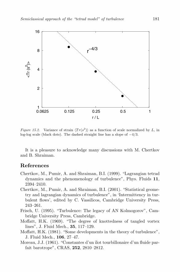
Semiclassical approach of the “tetrad model” of turbulence 181
1
2
4
8
16
0.0625 0.125 0.25 0.5 1
<T
r (s
2 )>
r / L
r−4/3
Figure 15.2. Variance of strain 〈Tr(s2)〉 as a function of scale normalized by L, inlog-log scale (black dots). The dashed straight line has a slope of −4/3.
It is a pleasure to acknowledge many discussions with M. Chertkovand B. Shraiman.
ReferencesChertkov, M., Pumir, A. and Shraiman, B.I. (1999). “Lagrangian tetrad
dynamics and the phenomenology of turbulence”, Phys. Fluids 11,2394–2410.
Chertkov, M., Pumir, A. and Shraiman, B.I. (2001). “Statistical geome-try and lagrangian dynamics of turbulence”, in ‘Intermittency in tur-bulent flows’, edited by C. Vassilicos, Cambridge University Press,243–261.
Frisch, U. (1995). “Turbulence: The legacy of AN Kolmogorov”, Cam-bridge University Press, Cambridge.
Moffatt, H.K. (1969). “The degree of knottedness of tangled vortexlines”, J. Fluid Mech., 35, 117–129.
Moffatt, H.K. (1981). “Some developments in the theory of turbulence”,J. Fluid Mech., 106, 27–47.
Moreau, J.J. (1961). “Constantes d’un ılot tourbillonaire d’un fluide par-fait barotrope”, CRAS, 252, 2810–2812.

182 NONSMOOTH MECHANICS AND ANALYSIS
Press, W.H., Teukolsky, S.A., Vetterling, W.T. and Flannery, B.P. (1992).“Numerical Recipes in C”, Cambridge University Press, 451–455.
Van der Bos, F., Tao, B., Meneveau, C. and Katz, J. (2002). “Effectsof small-scale turbulent motions on the filtered velocity gradient ten-sor as deduced from holographic particle image velocimetry measure-ments”, Phys. Fluids 14, 2456–2474.
Vieillefosse, P. (1984). “Internal motion of a small element of a fluid ininviscid flow”, Physica 125A, 150–162.

IV
MULTIBODY DYNAMICS:NUMERICAL ASPECTS
Chapter 16
THE GEOMETRY OFNEWTON’S CRADLE∗
Christoph Glockerand Ueli AeberhardIMES - Center of Mechanics, ETH Zentrum, Tannenstrasse 3, CH-8092 Zurich, [email protected]
Abstract A geometric approach to the multi-impact problem of perfect collisionsin finite freedom dynamics is presented. The set of all admissible post-impact velocities at an impact is derived from kinematic, kinetic andenergetic compatibility conditions. Impact events are classified withrespect to their topology, intensity and dissipation behavior. A quantityto characterize the influence of wave effects on the impacts, and thustheir deviation from the mechanical impact theory is introduced. Themethod is applied to Newton’s cradle with three balls.
Keywords: Newton’s cradle, unilateral constraint, impact, collision, rigid body
1. IntroductionThe paper is devoted to a geometric study of perfect collisions in
dynamics with the aim to find invariant characteristics of impacts. Insection 2 the concept of a breathing Riemannian manifold is chosen toembed impulsive behavior in the same mathematical setting as classicalmechanics. External impulsive excitation and time-dependent inequal-ity constraints are introduced, allowing the mechanical system to impactagainst perfect boundaries. This general approach is narrowed down tothe scleronomic case without excitations in section 3, in which the geo-metric picture of the impact in the tangent space is developed. A crucial
∗Parts of this research were conducted within the European project SICONOS IST-2001-37172 and supported by the Swiss Federal Office for Education and Science (BBW)

186 NONSMOOTH MECHANICS AND ANALYSIS
point in the entire analysis plays the impact with maximal dissipation asintroduced by J.J. Moreau, which is used as the reference for developingclassification concepts. This approach is illustrated by a discussion ofNewton’s cradle with three balls in section 4. To anticipate the conclu-sion, the present findings have already been extended to the rheonomiccase without and with external impulsive excitation, but still demandfurther investigations.
2. Collision ModelIn order to set up the kinematical and kinetical framework of our prob-
lem, we consider an f -dimensional breathing Riemannian configurationmanifold M(t) with t →M(t) “smooth”. We denote by q the f -tupleof local coordinates in use, and, for every fixed time t, by M(q, t) therepresentation with respect to q of the (kinetic) metric associated withM. The tangent cone to a set D at a point q ∈ D is denoted by TD(q)as defined in (Aubin and Ekeland, 1984). For D =M, the tangent conesimplifies to the classical tangent space with dual T �
M(q) = M TM(q).Inner products on TM(q) are denoted by a dot, a · b := aTMb fora, b ∈ TM(q), and the associated norm is written as ‖a‖ :=
√a · a.
We will first formulate the kinematics of the collision problem. Weassume n functions gi of class C1 defined by
gi : M× R→ R, (q, t)→ gi(q, t), (16.1)
which will be recognized as the gaps between bodies in a collision modelof a finite dimensional mechanical system. By this definition, there existn contact velocity mappings
γi : TM(q)→ R, u→ γi(u) := ∇gi · u + gi,t (16.2)
with gradient ∇gi := M−1 ∂gi/∂q and gi,t := ∂gi/∂t. The mappings
(16.2) are linearly affine in u, thus
γi(a + b) = γi(a) +∇gi · b. (16.3)
Consider now a curve onM which is absolutely continuous in time,
q : R→M(t), t→ q(t). (16.4)
Due to absolute continuity of q(t), the associated tangents u = q(t)exist almost everywhere and admit a left limit u− and a right limit u+
at every time t. In the same way behave the gaps (16.1) as functionsof time, gi(q(t), t), provided that the mapping (16.1) preserves absolutecontinuity. Thus, γi is related to gi thanks to (16.1) and (16.2) by
gi(q(t), t) = γi(u) (16.5)

The geometry of Newton’s Cradle 187
whenever u = q(t) exists. We further set
γi(u−) =: γi−, γi(u+) =: γi
+. (16.6)
For a discontinuity point of q(t) being caused by a collision, the valuesof γi
± provide the pre- and post-impact contact velocities. Using thegap functions (16.1), we introduce inequality constraints in the formgi(q, t) ≥ 0, which turnM into a manifold with boundary, characterizedby the set of admissible displacements C,
C(t) := {q | gi(q, t) ≥ 0, ∀i = 1, . . . , n}. (16.7)
Furthermore, let H denote the set of active constraints, i.e.
H(q) := {i | gi(q, t) = 0}. (16.8)
The tangent cone which characterizes the set C in some neighborhood ofa point q ∈ C, is then obtained by
TC(q) := {u ∈ TM(q) | ∇gi · u ≥ 0, ∀i ∈ H}. (16.9)
Note that this definition also includes the case that q is not a boundarypoint of C, for which H = ∅ and the tangent cone becomes identical tothe tangent space as a consequence. In general, one has TC(q) ⊂ TM(q).We further introduce the two polyhedral convex sets
P+C (q) := {u ∈ TM(q) | γi(u) ≥ 0, ∀i ∈ H}, (16.10)
P−C (q) := {u ∈ TM(q) | γi(u) ≤ 0, ∀i ∈ H}. (16.11)
Their definition is motivated by the fact that a necessary condition fora closed gap gi(q(t), t) = 0 not to leave the admissible region gi ≥ 0 insome adjoint time interval, is, that it has approached this value accordingto (16.5) and (16.6) by a left velocity γi
− ≤ 0, and it has to proceed intime by a right velocity γi
+ ≥ 0, respectively. Thus, P±C (q) describe the
set of admissible pre- and post-impact velocities u±.In the spirit of the virtual work approach in classical dynamics, kinet-
ics is treated in the framework of duality as an equality of measures onthe cotangent space T �
M(q). We denote by δq the virtual displacementsof the system, by du the measure accelerations related to the velocitiesu(t), see e.g. (Moreau, 1988a, Moreau, 1988b, Ballard, 2000), and by dFthe measure of external forces. The virtual action δdW has to vanish forarbitrary virtual displacements, when the system is to be in the dynamicequilibrium,
∀δq ∈ TM(q) : δdW := δqᵀ(Mdu− dF) = 0. (16.12)

188 NONSMOOTH MECHANICS AND ANALYSIS
The force measure dF can be split into the reactions dR due to theinequality constraints (16.7) and the remaining external forces dP,
dF = dR + dP. (16.13)
Following (Ballard, 2000, Glocker, 2001) we define a set of inequalityconstraints to be perfect if and only if the reactions satisfy
−δqᵀdR ≤ 0 ∀δq ∈ TC(q). (16.14)
In this case, the reactions are called constraint forces. The set of possiblereactions constitutes by (16.14) a cone in the cotangent space of M,
NC(q) := {ξ | δqᵀξ ≤ 0, ∀δq ∈ TC(q)}, (16.15)
which is the polar cone of TC(q), and which enables us to express theconstraint forces by the inclusion −dR ∈ NC(q). By combining thisrepresentation with (16.12)–(16.14), the dynamics is then stated as ameasure inclusion on the cotangent space,
Mdu− dP ∈ −NC(q). (16.16)
In order to allow for a geometric interpretation of this inclusion togetherwith the kinematical restrictions (16.7)–(16.11), we map (16.16) to thetangent space via the natural isomorphism available by the metric onM. We set dπ := M−1dP and T ⊥
C (q) := M−1NC(q) to arrive with
du− dπ ∈ −T ⊥C (q). (16.17)
Finally, this inclusion is integrated over a singleton {t} in time to obtainthe impact equations of the system,
u+ − u− − π ∈ −T ⊥C (q). (16.18)
Here, π represents any impulsive forces mapped to the tangent spacethat are externally applied on the system, −T ⊥
C (q) contains the impul-sive reactions due to the unilateral perfect constraints, and u+ − u− isthe instantaneous change in velocities with which the system dynami-cally reacts. Finally, it can be seen from (16.9) and (16.15) that −T ⊥
C (q)is positively generated by the gradients of gi,
T ⊥C (q) = {−∇gi Λi | Λi ≥ 0, ∀i ∈ H} (16.19)
with Lagrangian multipliers Λi ≥ 0 that act as compressive impulsivescalar forces in the associated contacts i ∈ H. As subsets of the tangentspace, we call TC(q) and T ⊥
C (q) a pair of cones that are orthogonal toeach other in the kinetic metric.

The geometry of Newton’s Cradle 189
3. Impacts without ExcitationIn this section we give a geometric characterization of impacts due to
collisions and confine ourselves to the special case of no external excita-tion. This assumption affects both the kinematic and kinetic excitation.Kinematic excitation acts on the system via the inhomogeneity terms gi
,t
in (16.2). If such an excitation is excluded for a certain impact configu-ration (gi
,t = 0 ∀i ∈ H), then the sets of admissible pre- and post-impactvelocities (16.10), (16.11) are directly related to the tangent cone (16.9)by P+
C (q) = −P−C (q) = TC(q). Thus, pre-impact velocities u− ∈ −TC(q)
have to be assumed. We understand by kinematic compatibility that thecollision ends up with feasible post-impact velocities
u+ ∈ TC(q). (16.20)
Kinetic excitation is excluded from the problem by setting the associatedexternal impulsive forces π in (16.18) equal to zero. This yields
u+ ∈ u− − T ⊥C (q), (16.21)
which we call kinetic compatibility. A third and independent propertythat we demand is energetic consistency. We do not allow for any activebehavior of the contacts as, for example, observed in pin ball machines,but assume a dissipative character only. This means that the kineticenergy T of the system must not increase during the collision, T+ −T− ≤ 0. From T = 1
2‖u‖2 for a scleronomic system, it follows that thedissipative character of the impact is assured if ‖u+‖ ≤ ‖u−‖. Thiscondition is expressed by the inclusion
u+ ∈ B‖u−‖(q), (16.22)
where B‖u−‖(q) denotes the energy ball with radius ‖u−‖ and midpointplaced at the origin. Thus, kinetic, kinematic and energetic consistencyrestricts the set of admissible post-impact velocities by (16.20)–(16.22)to
S := (u− − T ⊥C (q)) ∩ TC(q) ∩ B‖u−‖(q). (16.23)
This convex set is shown together with the orthogonal pair of conesTC(q), T ⊥
C (q) and the energy ball B‖u−‖(q) in figure 16.1. Note thespecial case that q is not a boundary point of C, i.e. q ∈ int C. Forthis situation, T ⊥
C (q) = 0, and S reduces to a single element S = {u−}.Thus, it holds that u+ = u− which means that there is no velocity jump.
The post-impact velocities u+ are restricted by equation (16.23) to theset S, but are still not uniquely defined. In order to pick a particularelement out of this set, one needs an impact law in the sense of an

190 NONSMOOTH MECHANICS AND ANALYSIS
�� ������� �����
�
� ����jj jj
�
���� ������� ���
�� ����
�� �� ���� �
� ����
�� �
0
Figure 16.1. Geometry of multi-contact collisions without excitation.
additional, independent equation. One possible approach is suggestedby J.J. Moreau in (Moreau, 1988a). It requires the (unique) orthogonaldecomposition of the pre-impact velocity u− into two parts z and z⊥ withrespect to the orthogonal pair of cones TC(q) and T ⊥
C (q) respectively,and can be stated as follows: For u− = z + z⊥ find u+ = z− εz⊥ suchthat
TC(q) � z ⊥ z⊥ ∈ T ⊥C (q). (16.24)
The tangential component z in this collision law is left unchanged by theimpact, whereas the normal component z⊥ is inverted and multiplied bya dissipation coefficient ε to give −εz⊥, see figure 16.2. From this figure,one recognizes also that z and z⊥ are the nearest points to u− in the setsTC(q) and T ⊥
C (q), respectively, which can be expressed in terms of prox-imations as z = proxTC(q)(u−) and z⊥ = proxT ⊥
C (q)(u−). For ε = 0, theimpact law yields u+ = z, which corresponds to the unique post-impactvelocity of minimal length under the restrictions (16.23). We call theassociated point in S the point of maximal dissipation. Thus, a uniquelydetermined half-line passing this point and emanating from the tip u−of the translated cone −T ⊥
C (q) is accessible through Moreau’s impactlaw by values ε ≥ −1. It is easily seen that ε = 0 addresses the point ofmaximal dissipation, whereas conservation of kinetic energy is assuredfor ε = 1. Values of ε in between correspond to different levels of dissi-pation, defining a family of concentric spheres in the tangent space. Asdiscussed in (Moreau, 1988a, Glocker, 2001a), Moreau’s half-line does

The geometry of Newton’s Cradle 191
���� ������� ���
�� ����
�� �� ���� �
� ������
� ����jj jj
�
impacttopology
impactintensity
point of maximaldissipation
Moreau's halfline (®=0)
®"=1
"=0
"
?z
z0
Figure 16.2. Geometric characterization of impacts without excitation.
not comprise events of collisions that benefit from impulse transfer be-tween non-neighboring bodies via traveling waves. This behavior is alsoexcluded in classical text books on single impacts by saying that waveeffects can be neglected. The framework achieved by this assumption isusually called the mechanical impact theory. However, a precise math-ematical formulation of this term has never been given. We thereforesuggest to define the mechanical impact theory as to consist precisely ofthose impact events that can be accessed through Moreau’s half-line.
Obviously, not every post-impact velocity in S can be reached byMoreau’s law. In view of a future parameterization of S we want to givealready here a characterization of general collisions based on geometricproperties. We define the impact topology as the entity connected to thedifferent half-lines of T ⊥
C (q). In other words, all post-impact velocitiespointing for some given Λi > 0 to the same half-line u− + R+
0 Λi∇gi
in u− − T ⊥C (q) are said to have the same impact topology. This clas-
sification corresponds to a constant impact impulse ratio, as called byother authors. We further propose to take the angle α between a certainhalf-line of T ⊥
C (q) and Moreau’s half-line as a measure of deviation fromthe mechanical impact theory, which also quantifies the wave effects atthe collision. We further take as impact intensity the distance of thepost-impact velocity u+ from the tip of the translated cone u−−T ⊥
C (q),which is nothing else than ‖u+ − u−‖. As soon as the post-impact ve-

192 NONSMOOTH MECHANICS AND ANALYSIS
��
���� ���
�� ��
���
��
Figure 16.3. Representation of Moreau’s impact law in contact coordinates.
locity u+ has been located in the set u− − T ⊥C (q), it can in addition be
characterized by the dissipation coefficient ε, associated with the sphereon which it is placed.
In (Glocker, 2002) a representation of Moreau’s impact law in localcontact coordinates has been derived, showing that
0 ≤ Λi ⊥ (γi+ + ε γi
−) ≥ 0 (16.25)
for each contact i in the active set H. The complementarity conditionsin (16.25) express that each contact that takes an impulsive force Λi > 0has to fulfill the classical Newtonian impact law γi
+ = −ε γi−. However,
if the contact point is to be regarded as not to participate in the impact(Λi = 0), then the post-impact relative velocity is allowed for havingvalues γi
+ > −εγi−. This impact behavior is said to have a global dissipa-
tion index, because the same restitution coefficient ε is taken in (16.25)for each individual contact. In order to extend this concept of local rep-resentation to general impacts in S, a matrix of impact coefficients εi
jhas to be introduced in the inequality impact law (16.25) as proposedin (Fremond, 1995),
0 ≤ Λi ⊥ (γi+ + εi
j γj−) ≥ 0. (16.26)
The matrix of impact coefficients allows to access impact topologies dif-ferent from Moreau’s half-line, such as spatially separated chain-likecontacts which directly interact with each other. Restrictions on thecoefficients εi
j such that u+ ∈ S is guaranteed have still to be workedout.
4. Newton’s CradleAs an example, we investigate the impact configuration in Newton’s
cradle with three balls of equal masses m1 = m2 = m3 =: m. The

The geometry of Newton’s Cradle 193
Moreau'shalfline
experiment
� ����
�� �� ���� �
� ���v
��
0
�
®
��� ���
���� ���1
u2
u
3u
m =m =m =:m1 2 3
1u
2u
3u
Figure 16.4. Impact geometry of Newton’s cradle with three balls.
horizontal absolute displacements of the three masses are denoted byq1, q2, q3, and the associated velocities by u1, u2, u3, respectively. Theinequality contact constraints are expressed by the two gap functionsg12 = q2 − q1 and g23 = q3 − q2. For the pre-impact state we assumethat balls two and three are at rest (u2
− = u3− = 0) by touching each other
(g23 = 0), and that ball one hits ball two (g12 = 0) with a velocity u1− =
v > 0. We therefore have a pre-impact velocity state u− = (v, 0, 0)ᵀ
with both contacts contained in the set of active constraints H from(16.8). The impact equations (16.18) for this configuration are⎛⎝u1
+ − u1−
u2+ − u2
−u3
+ − u3−
⎞⎠ =1m
⎛⎝−110
⎞⎠Λ12 +1m
⎛⎝ 0−11
⎞⎠Λ23, (16.27)
where Λ12 and Λ23 denote the impulsive forces between balls 1-2 and 2-3,respectively. From this equation one also identifies the gradients of thegap functions as ∇g12 = 1
m(−1, 1, 0) and ∇g23 = 1m(0, −1, 1), which
define by (16.19) the edges of T ⊥C (q). As shown in figure 16.4, kinetic
compatibility (16.21) yields a subset u−−T ⊥C (q) in the deviatoric plane
of the u1-u2-u3 trihedral, which is the plane that intersects the threeaxes by equal values v. The set S of admissible post-impact velocitiesu+ is obtained according to (16.23) by subsequent intersection with thetangent cone TC(q) and the energy ball Bv(q).
The point of maximal dissipation in S as the point in u− − T ⊥C (q)
with minimal distance from the origin, is recognized as the post-impactmotion, for which the three balls move together as one rigid body with

194 NONSMOOTH MECHANICS AND ANALYSIS
a common velocity u1,2,3+ = 1
3v. This point defines Moreau’s half-line,which emanates from the tip of u− − T ⊥
C (q) and carries the topologyof impacts with global dissipation index. On its intersection with theenergetic sphere that assures conservation of kinetic energy, balls twoand three remain in contact after the impact and move with a commonvelocity of u2,3
+ = 23v to the right, whereas ball one bounces back to
the left with a velocity of u1+ = −2
3v. In reality, balls one and twostand nearly idle (u12
+ = 0) after the impact, and ball three leaves withan approximate velocity u3
+ = v to the right. This behavior is on thesame energetic sphere, but takes place on the topological half-line thatdeviates by a maximal possible angle (α = 30◦) from Moreau’s impactlaw. Note that only one point of this half-line belongs to S. As aresult, Newton’s cradle can be seen as a device that shows experimentallya collision behavior that maximizes wave effects under all imaginableexperiments with three arbitrary bodies of equal mass.
ReferencesAubin, J., and Ekeland, I. (1984). Applied Nonlinear Analysis. New York:
John Wiley & Sons.Ballard, P. (2000). “The Dynamics of Discrete Mechanical Systems with
Perfect Unilateral Constraints,” Arch. Rational Mech. Anal. 154 3,pp. 199–274.
Fremond, M. (1995). “Rigid Bodies Collisions,” Physics Letters A 204,pp. 33–41.
Glocker, Ch. (2001). Set-Valued Force Laws: Dynamics of Non-SmoothSystems. Lecture Notes in Applied Mechanics 1. Berlin, Heidelberg:Springer.
Glocker, Ch. (2001a). “On Frictionless Impact Models in Rigid-BodySystems,” Phil. Trans. Royal. Soc. Lond. A 359, pp. 2385–2404.
Glocker, Ch. (2002). “The Geometry of Newtonian Impacts with GlobalDissipation Index for Moving Sets,” Proc. of the Int. Conf. on Non-smooth/Nonconvex Mechanics (ed. Baniotopoulos, C.C.), pp. 283 -290. Thessaloniki: Editions Ziti.
Moreau, J.J. (1988a). “Unilateral Contact and Dry Friction in FiniteFreedom Dynamics,” in Non-Smooth Mechanics and Applications,CISM Courses and Lectures Vol. 302 (eds. Moreau, J.J. and Pana-giotopoulos, P.D.), pp. 1–82. Wien: Springer.
Moreau, J.J. (1988b). “Bounded Variation in Time,” in Topics in Non-smooth Mechanics (eds. Moreau, J.J., Panagiotopoulos, P.D., andStrang, G.), pp. 1–74. Basel: Birkhauser Verlag.

Chapter 17
USING NONSMOOTH ANALYSIS FORNUMERICAL SIMULATION OFCONTACT MECHANICS
Pierre AlartDavid Dureisseixand Mathieu RenoufLMGC, University Montpellier 2, CNRS UMR5508, CC048, Place Eugene Bataillon,F-34095 Montpellier Cedex 5, [email protected]
Abstract Two different approaches for simulation of contact mechanics prob-lems are investigated. First, the equivalence of the Large Time INcre-ment (LATIN) method for unilateral contact problems, in terms of anaugmented Lagrangian approach dedicated to nonsmooth problems, isproved (with the non trivial introduction of two constraints: an equal-ity constraint and an inequality-type constraint). Second, the FiniteElement Tearing and Interconnecting method for Contact (FETI-C) isinterpreted as a projected gradient with projection, acting on the dualproblem. An extension to frictional contact is presented in the contextof granular media.
1. IntroductionIn nonsmooth analysis and mechanics, Jean Jacques Moreau pro-
claims to be firstly a mechanician and a mathematician who developsonly what is strictly necessary for mechanical modeling. He was notinitially a numerician even if his last works on granular material requireefficient computer resources and algorithms. His mathematical toolsproved to be very useful in physical / mechanical modeling (friction,plasticity...) and in applied mathematics related to the solution of partialdifferential equations and in optimization theory. The theory of duality

196 NONSMOOTH MECHANICS AND ANALYSIS
in Convex Analysis plays an important role in the mathematical mod-eling of the aforementioned fields and in the design of efficient solutionschemes based, for instance, on augmented Lagrangian functions. Buta lot of numerical developments in intensive computational mechanics,when limited to linear large scale problems, did not call for sophisticatednotions of Convex Analysis. This research field led to specific conceptsalready difficult to handle in a linear context (preconditioning, domaindecomposition methods...).
The motivation of this work is the re-engineering of algorithms arisingfrom ‘intuitive’ approaches of computational mechanics, using convexand nonsmooth analysis. This could be a guide for algorithm extensionsand development of new approaches.
1.1 Model problemTo simplify the presentation, let us consider the case of the friction-
less Signorini problem depicted in Figure 1.1: only one elastic body Ωpressed against a rigid plate, under small perturbations, with a quasi-static evolution process. The potential contact area Γ will be calledan interface. n designates the outward unitary normal vector on theboundary ∂Ω.
0 100 200 300 400 50010
10
10
10
10
10
10
-6
-5
-4
-3
-2
-1
10 0
1
GCP
GSNL
LATIN
error vs. iteration number
Figure 17.1. Left: vertical stress field solution on the model problem (cylindricalpunch); right: convergence results for different iterative algorithms
If F is the force applied to the body by the plate, and if V is thedisplacement of the body on the interface Γ, the interface behavior is:(i) no friction, i.e. (1−nnT )F = 0, and (ii) complementarity conditions(Karush-Khun-Tucker):
Nonsmooth analysis for contact mechanics simulations 197
no penetration: z = nT V ≥ 0, i.e. z ∈ C1 (the positive cone);
no adhesion: w = nT F ≥ 0, i.e. w ∈ C1;no dissipation: wz = 0.
The problem consists in finding a displacement field U(M), and astress field σ(M), such that:
U is sufficiently regular (the strain field is: ε = (gradU)sym), andequals some prescribed values on a first part of the boundary:U |∂1Ω = Ud, and on the interface: nT U |Γ = z; a couple (U, z)satisfying these conditions is said kinematically admissible (KA);
the stress field balances the external body force fd
and the pre-scribed forces on a second part of the boundary: div σ + f
d= 0 in
Ω, σn|∂2Ω = F d, and on the interface: σn|Γ = wn; a couple (σ, w)satisfying these conditions is said statically admissible (SA);
the constitutive relation of the body (linear elasticity with D asHooke tensor): σ = Dε, and of the interface (see above).
There are several ways to formulate this problem: minimization withinequality-like constraints, variational inequalities, linear complemen-tarity problems, differential inclusions... The formulations of the nextSections can be derived from the following: the problem is to find(U, z, σ, w) minimizing the so-called error in constitutive relation η forcontact problems (Coorevits et al., 1999):
η2(U, z, σ, w) =12
∫Ω
Tr[(σ −Dε(U))D−1(σ −Dε(U))]dΩ +∫
ΓwzdΓ
on the set of admissible fields (U, z) KA, (σ, w) SA, and z ∈ C1, w ∈C1 (on this set, η2 is obviously positive, and is zero if and only if theconstitutive relations are satisfied).
Using Stoke’s theorem, for admissible fields, the expression of η2 canbe split into two uncoupled terms: η2 = η2
1(U, z) + η22(σ, w) with:
η21(U, z) =
12
∫Ω
Tr[ε(U)Dε(U)]dΩ−∫
Ωf
d· UdΩ−
∫∂2Ω
F d · UdS
η22(σ, w) =
12
∫Ω
Tr[σD−1σ]dΩ−∫
∂1ΩUd · σndS
The minimization of the first part only leads to the primal formulationof the problem, while the minimization of the second one leads to thedual (in the Legendre-Fenchel way) formulation. Mixed formulationscan be obtained by dualizing each of them (in the Arrow-Hurwicz way)using a Lagrange multiplier (De Saxce, 1989).
198 NONSMOOTH MECHANICS AND ANALYSIS
1.2 Discretized formulationsThe discretized version of the primal formulation, once finite elements
are used, is:
minBu≥0
12uT Ku− uT f
where u is the set of finite element degrees of freedom (dof), K is thestiffness matrix, and f are the prescribed generalized forces. B is aBoolean operator that selects the dof on the interface; z = Bu. Bcan also change to the local basis on normal direction; for the sake ofsimplicity, we assume in all of the following that no such rotations arerequired. Therefore, the previous problem is easily condensed on thecontact dof z and leads to
minz≥0
φ(z) with φ(z) =12zT Mz + zT q (17.1)
where M is the condensed stiffness matrix, and q the opposite of thecondensed generalized forces.
Using the indicator function ψC1 of the discretized cone C1, this isequivalent to:
minz
φ(z) + ψC1(z) ⇔ 0 ∈ ∇φ(z) + ∂ψC1(z) (17.2)
The problem can therefore be re-stated as to find a ∈ ∂ψC1(z) such that∇φ(z) + a = 0. a must satisfy: ψ�
C1(a) + ψC1(z) − aT z ≤ 0, where
ψ�C1
is the Legendre-Fenchel transform of ψC1 . As the Legendre-Fenchelinequality should be satisfied, ψ�
C1(a) + ψC1(z)− aT z ≥ 0, the previous
inequality reduces to an equality. This equality is equivalent to: a ≤ 0,z ≥ 0 and aT z = 0. Using w = −a, the problem is then to find (z,w)such that
Mz −w = −q with 0 ≤ z ⊥ w ≥ 0 (17.3)
This is a classical linear complementarity problem (LCP), (Cottleet al., 1992). The unknown is the couple (z,w).
A dual formulation can be built from (17.2): with the indicator func-tion ψC1(z) = supw≥0(−z)T w, it is equivalent to: infz [supw≥0 φ(z) −zT w]. With sensible assumptions (convexity, semicontinuity) this isagain equivalent to: supw≥0[infz φ(z)− zT w]. The inner minimizationproblem leads to z = M−1(−q + w). Substituting this last value in theprevious problem leads to the dual problem:
supw≥0
−12wT M−1w + wT M−1q (17.4)

Nonsmooth analysis for contact mechanics simulations 199
2. The LATIN method for contact problemsThe LATIN method (Ladeveze, 1999) was originally designed for
time-dependent problems. However, it has been applied to differentsituations, and among them domain decomposition, contact problems(Champaney et al., 1995)... We are interested herein with the versiondealing with contact between substructures, for which the method canbe viewed as a mixed domain decomposition method, with nonlinear be-havior of interfaces. We will focus on frictionless contact. The principlesof the LATIN method will be briefly recalled, especially the splitting itintroduces for the problem unknowns and constraints, since the aug-mented Lagrangian approaches are often compared to operator splittingmethods (Fortin and Glowinski, 1982, Glowinski and Le Tallec, 1989).
2.1 The LATIN algorithmTo simplify the presentation, we will derive all the presentation for
the discretized problem (17.3), though the method is directly applicableto the continuum media problem. In each case, the unknowns are boththe displacement z and the forces w. The LATIN method is based onthree mechanical principles:
splitting the difficulties: the linear equations (possibly global) arecollected into the set Ad, while the local equations (possibly nonlinear) are collected into the second set Γ. The solution is theintersection of these sets.
For the problem (17.3), (w,z) belongs to Ad iff Mz − w = −q,and (w, z) belongs to Γ iff 0 ≤ z ⊥ w ≥ 0;
building a 2-stage iterative algorithm: the solution is searched withthe construction of two series of approximations belonging alter-natively to Ad and Γ.
At iteration n, the local stage consists in finding (w, z) ∈ Γ witha first search direction (w−wn, z− zn) ∈ E+. (wn,zn) is knownat this stage.
The linear stage consists in finding (wn+1,zn+1) ∈ Ad with asecond search direction (wn+1 − w,zn+1 − z) ∈ E−, while (w, z)is known from the previous stage;
using an ad hoc representation of the unknowns. This last principleis suited to time-dependent problems, and won’t be used herein.
The choice for the search direction is classically to use a parameterk homogeneous to an interface stiffness. For the local stage, the search

200 NONSMOOTH MECHANICS AND ANALYSIS
direction is: (w −wn)− k(z − zn) = 0. The local stage is a non-linearand local updating problem, but its solution (z, w) is explicit:
z = −k−1〈wn − kzn〉−w = 〈wn − kzn〉+
〈•〉− and 〈•〉+ designate respectively the negative part and the positivepart of their argument.
For the linear stage, the unknowns are (zn+1, w) and the conjugatesearch direction is used: (wn+1−w)+k(zn+1− z) = 0. The linear stageis a global and linear updating problem: zn+1 is obtained with
(M + k1)zn+1 = (w + kz)− q and wn+1 = (w + kz)− kzn+1
Here, k is a parameter of the method. The value of k has no influenceon the solution at convergence, but it modifies the convergence rate.Numerical simulations show that there is an optimal value, which isrelated to the interface operator obtained when condensing the problemon the interface. For the present model problem, this operator is M ,and k can be diagonal values of M , or an average of these.
Figure 1.1 reports convergence results (with an energy-norm error)for different iterative algorithms (CPG: conjugate gradient with projec-tion (Renouf and Alart, 2004), NLGS: non-linear Gauss-Seidel (Moreau,1999, Jean, 1999)). For this test case, the convergence rate comparisonis similar to the one that can be obtained in linear case, for which conju-gate gradient has usually a higher convergence rate than LATIN, itselfhigher than for Gauss-Seidel.
2.2 Interpretation as a nonsmooth augmentedLagrangian approach
For perfect interfaces, the LATIN algorithm has been proved to beequivalent to the augmented Lagrangian interpretation (Glowinski andLe Tallec, 1990) of the approach proposed in (Lions, 1990), and moreprecisely to the so-called ‘ALG3’ algorithm in (Fortin and Glowinski,1982), see (Champaney et al., 1995). We proposed herein to prove theequivalence to an augmented Lagrangian algorithm for the case of con-tact without friction.
Beginning with the minimization problem (17.1), the first step is tosplit the unknown z, using an intermediate unknown z, an to introducean equality constraint z = z, as well as an inequality-like on z:
minz=z, z≥0
φ(z) (17.5)

Nonsmooth analysis for contact mechanics simulations 201
The second step is to use two multipliers wc and wc and convexanalysis methodology for dualizing the previous constraints (Rockafel-lar, 1976). The augmented Lagrangian is obtained with a classical dual-ization and regularization of the equality constraint, while the Moreau-Yosida technique is applied to the inequality-like constraint, using apositive parameter k (Yosida, 1964, Moreau, 1965):
L(z, z; wc, wc) = φ(z)+
−12wT
c k−1wc +12[wc + k(z − z)]T k−1[wc + k(z − z)]+
−12wT
c k−1wTc +
12〈wc + kz〉T−k−1〈wc + kz〉− (17.6)
The stationary conditions for this augmented Lagrangian are
∂L∂z
=0 = Mz + q + wc + k(z − z)
∂L∂wc
=0 = −k−1 {wc − [wc + k(z − z)]}
∂L∂z
=0 = −wc − k(z − z) + 〈wc + kz〉−∂L∂wc
=0 = −k−1 {wc − 〈wc + kz〉−}
One can then remark that for the solution, z = z and wc = wc = −w.Designing an iterative Uzawa-like algorithm consists in expressing thesuccessive stationary conditions with the previous obtained values of theunknowns. With the previous remark, the latest values of z or z can besubstituted one to the other, and similarly for wc and wc. The successivesteps are the following:
step 1: assuming that the values w(n)c and z(n) are the latest ones,
the stationary with respect to z gives the next value of z(n+1):
Mz(n+1) + q + k(z(n+1) − z(n)) + w(n)c = 0
step 2: with this last updated value z(n+1), the stationary withrespect to wc gives the next value of w
(n+1)c :
w(n+1)c − [w(n)
c + k(z(n+1) − z(n))] = 0
step 3: with these last values z(n+1) and w(n+1)c , the stationary
with respect to both z and wc allows to update their values: first,
−w(n+1)c − k(z(n+1) − z(n+1)) + 〈w(n+1)
c + kz(n+1)〉− = 0

202 NONSMOOTH MECHANICS AND ANALYSIS
that leads to
z(n+1) = k−1{
(w(n+1)c + kz(n+1))− 〈w(n+1)
c + kz(n+1)〉−}
= k−1〈w(n+1)c + kz(n+1)〉+
and second, w(n+1)c − 〈w(n+1)
c + kz(n+1)〉− = 0
The steps 1 and 2 are the linear stage of the LATIN, while the step 3is the local stage.
Though other permutations may lead to other augmented Lagrangianversions for nonsmooth problems, the proposed one recovers the LATINmethod that appears to be efficient for the simulation of large scaleassemblies of deformable parts (Champaney et al., 1997).
3. Gradient methods for large scale contactproblems
We focuss herein on two kinds of large scale problems. Such largescale problems require sophisticated tools arising from the optimizationfield, traditionally relying on convex and nonsmooth analysis (Bonnanset al., 2003). The first one is related to finite element simulation ofassemblies with a dual domain decomposition method. This method iswell suited to problems with a large number of degrees of freedom and afew contact conditions between subdomains. The second one deals withsimulation of granular materials and structures: the contact conditionsare numerous in this case, between rigid bodies in a large collection.
3.1 Structural frictionless contact problemsThe FETI-C method has been built as an extension of the Finite El-
ement Tearing and Interconnecting (FETI) method (Farhat and Roux,1991) for the case of contact without friction between subdomains (Du-reisseix and Farhat, 2001). The numerical and parallel scalability (i.e.the ability to converge with a number of iterations depending weakly onthe number of subdomains) of the FETI method have been examplified,thanks to the presence of a ‘coarse’ problem acting on the rigid body dis-placement of the floating subdomains (subdomains without prescribeddisplacement). Nevertheless, for simplification, no floating subdomainwill be considered here, and only one subdomain is assumed to have aninterface with a rigid plate (as for the model problem of Figure 1.1).
The extension to interfaces that exhibit an unilateral contact behavioris performed with the following remarks:
the procedure should act on admissible reaction forces: w ≥ 0;

Nonsmooth analysis for contact mechanics simulations 203
the classical residual z, which is the displacement jump across theinterfaces, should be replaced by the contact residual z = 〈z〉− tomonitor the convergence;
the ‘gluing’ condition should act on the active contact interface(defined as the part Γa of Γ where w > 0), using an adapted
Boolean operator: Bwr =
{r on Γa
0 on Γ\Γa
With BTw as the transpose of the matrix Bw for a given w, one gets
the optimization problem (non quadratic due to the dependence of Bwon w):
minw≥0
12wT (BT
wM−1Bw)w −wT (BTwM−1q) (17.7)
The straightforward extension of FETI approach consists in applyingformally a conjugate gradient algorithm to the problem (17.7) as if thisproblem is quadratic, driving z to zero, and reusing classical precondi-tioners. It appears to be scalable for the case where there are floatingsubdomains, for which an additional projection is used (Dureisseix andFarhat, 2001). Of course, the conjugating property is not satisfied forall of the previous search directions because the Bw operator projectsthe iterate, and the BT
w operator projects the gradient.Therefore, this algorithm can be interpreted as a projected conjugate
gradient with projection, applied to the classical quadratic dual prob-lem as expressed in (17.4). Work is in progress on adapting FETI-DPversion (Farhat et al., 2001) to contact and friction. Such an adaptationwould take advantage of the aforementioned interpretation, and of thedevelopments presented in the next Section.
3.2 Granular frictional contact problemsIndependently, P. Alart and M. Renouf developed a conjugate gradient
type algorithm for granular media characterized with a large number ofbodies and consequently of contacts (Renouf and Alart, 2003).
A granular material is by essence a discrete medium, where each ‘sub-domain’ is a rigid body. The problem is therefore stated from the pointof view of interactions between these bodies. As an example, Figure 3.2illustrates the simulation of a sandbox experiment, useful in geomechan-ics for soil layer formation. About 40 000 grains in interaction (involving88 000 contact conditions) are modeled.
Each interaction, as an ‘interface’, deals with the relative velocitybetween bodies, z = Bv (where v stores the velocities of the bodies),as well as the contact impulsion w. This is of course a time-dependent

204 NONSMOOTH MECHANICS AND ANALYSIS
Figure 17.2. Sandbox simulation (40 000 grains)
problem, and for a given time step, the dynamic evolution of the bodiesis Mv = BT w−q where q stores external impulsions and contributionsof relative velocities at the end of the previous time step. M is in thiscase the block-diagonal mass matrix of all the bodies.
For the case of frictionless interaction, the constitutive relations aresimply 0 ≤ z ⊥ w ≥ 0. Expressing v from the dynamic evolution,one gets z = Ww − q, with W = BM−1BT and q = BM−1q. Theresulting problem is therefore similar to the previous ones.
For the case of frictional contact, normal and tangential componentsat each node have to be separated, and we will use lowerscript n and tto designate them. For simplicity, we will consider only bidimensionalanalysis. The constraints on impulsion w must belong to the Coulomb’sfriction cone, i.e. w ∈ C(μwn), with μ as the Coulomb’s friction coeffi-cient, wn the normal component of the impulsion, and
C(μwn) =nc∏
α=1
R+ × [−μwα,n, μwα,n]
where nc is the number of potential contact nodes. As for the friction-less contact, the matrix W = BM−1BT is semi definite positive andtherefore can be singular. The resulting quasi-optimization problem is:
w ∈ argminx∈C(μwn)
12xT Wx− xT q (17.8)
The solving procedure relies on a fixed point method for the Trescathreshold μwn and on an inner conjugate projected gradient. The pro-posed approach is a diagonalized version of this procedure (with a oneshot single loop). The projection operators are replaced by specific cor-rections which are not exactly projections, but may be derived from amathematical analyses in such a way that the converged solution satisfiesthe relation (17.8), (Renouf and Alart, 2004).

Nonsmooth analysis for contact mechanics simulations 205
Figure 17.2 is related to the first time step of the compaction undergravity of a box filled with 33 000 grains. The convergence of 3 differ-ent algorithms (CPG: conjugate projected gradient, NLGS: non-linearGauss-Seidel, and PCPG: preconditioned conjugate projected gradient)is compared for increasing values of Coulomb’s friction coefficient μ. Forall of them, the convergence requires more iterations when friction in-creases. The conjugate gradient methods are more efficient than theGauss-Seidel one, but the gain decreases as the friction increases.
0 1000 2000 3000 4000 5000
100
101
102
103
104
μ = 0.4
0 400 800 1200 160010
−1
100
101
102
103
104
105
μ = 0
0 1500 3000 4500 6000
μ = 0.8
0 900 1800 2700 3600 4500
μ = 0.1
NLGS NLGS
NLGS
NLGS
CPGCPG
CPGCPG
PCPG PCPG
PCPGPCPG
Figure 17.3. Influence of friction coefficient on convergence
4. Structural versus granularDifferent scientific communities usually develop different dedicated
tools that can sometimes be re-unified. Such a gap bridging is done inSection 2.2 where the LATIN algorithm for frictionless contact is reinter-preted as a Lagrangian approach for nonsmooth problems. Convergenceresults in this case can be transferred to Lagrangian approches as con-vergence is proved (Ladeveze, 1999) for 0 < k < ∞. The constructionof the equivalence can also lead to other versions of the method.
Moreover, between structural analysis and granular simulation com-munities, the approach used for frictional contact and gradient-basedsimulations of a large number of grains can guide the development of ex-tensions to frictional case for dual domain decomposition methods. The

206 NONSMOOTH MECHANICS AND ANALYSIS
primal domain decomposition method already got benefits from convexand nonsmooth analysis (Alart et al., 2004).
ReferencesAlart, P., Barboteu, M., and Renouf, M. (2004). Parallel computational
strategies for multicontact problems: Applications to cellular and gran-ular media. Int. J. for Multiscale Comput. Engng. to appear.
Bonnans, J.-F., Gilbert, J.-C., Lemarechal, C., and Sugastizabal, C.(2003). Numerical Optimization – Theoretical and Practical Aspect.Springer Verlag.
Champaney, L., Cognard, J.-Y., Dureisseix, D., and Ladeveze, P. (1995).Une approche modulaire pour l’analyse d’assemblages de structurestridimensionnelles. Application au contact avec frottement. In Pro-ceedings of StruCoMe 95, pages 295–306, Paris.
Champaney, L., Cognard, J.-Y., Dureisseix, D., and Ladeveze, P. (1997).Large scale applications on parallel computers of a mixed domaindecomposition method. Comput. Mech., (19):253–263.
Coorevits, P., Hild, P., and Pelle, J.-P. (1999). Controle des calculselements finis pour les problemes de contact unilateral. Revue Eu-ropeenne des Elements Finis, 8(1):7–29.
Cottle, R. W., Pang, J.-S., and Stone, R. E. (1992). The Linear Com-plementarity Problem. Academic Press, Boston.
De Saxce, G. (1989). Sur quelques problemes de mecanique des solidesconsideres comme materiaux a potentiel convexe. volume 118 of Pu-blications de la Faculte des Sciences appliquees. Universite de Liege.
Dureisseix, D. and Farhat, C. (2001). A numerically scalable domain de-composition method for the solution of frictionless contact problems.Int. J. for Numer. Meth. Engng., 50:2643–2666.
Farhat, C., Lesoinne, M., Le Tallec, P., Pierson, K., and Rixen, D. (2001).FETI-DP: a dual-primal unified FETI method - part I: a faster al-ternative to the two-level FETI method. Int. J. for Numer. Meth.Engng., 50(7):1523–1544.
Farhat, C. and Roux, F.-X. (1991). A method of finite element tearingand interconnecting and its parallel solution algorithm. Int. J. forNumer. Meth. Engng., 32:1205–1227.
Fortin, M. and Glowinski, R. (1982). Methodes de lagrangien augmente.In Lions, P.-L., editor, Methodes Mathematiques de l’informatique,volume 9.
Glowinski, R. and Le Tallec, P. (1989). Augmented lagrangian and ope-rator-splitting methods in nonlinear mechanics. volume 9 of SIAMStudies in Appl. Math. SIAM.

Nonsmooth analysis for contact mechanics simulations 207
Glowinski, R. and Le Tallec, P. (1990). Augmented lagrangian interpre-tation of the nonoverlapping Schwarz alternating method. In Chan,T. F., Glowinski, R., Periaux, J., and Widlund, O. B., editors, ThirdInt. Symp. on Domain Decomposition Methods for Part. Differ. Equa-tions, pages 224–231. SIAM.
Jean, M. (1999). The non-smooth contact dynamics method. Comput.Meth. Appl. Mech. Engng., 117(3-4):235–257.
Ladeveze, P. (1999). Nonlinear Computational Structural Mechanics —New Approaches and Non-Incremental Methods of Calculation. Sprin-ger Verlag.
Lions, P.-L. (1990). On the Schwarz alternating method III: a variant fornonoverlapping subdomains. In Chan, T. F., Glowinski, R., Periaux,J., and Widlund, O. B., editors, Third Int. Symp. on Domain Decom-position Methods for Partial Differential Equ., pages 202–223. SIAM.
Moreau, J. J. (1965). Proximite et dualite dans un espace hilbertien.Bulletin de la Societe Mathematique de France, 93:273–299.
Moreau, J. J. (1999). Numerical aspects of the sweeping process. Com-put. Meth. Appl. Mech. Engng., 117(3-4):329–349.
Renouf, M. and Alart, P. (2003). Un nouvel algorithme de quasi-opti-misation pour la resolution des problemes multicontacts et applica-tion aux milieux granulaires. In Proc. of the 16e Congres Francais deMecanique, Nice.
Renouf, M. and Alart, P. (2004). Conjugate gradient type algorithms forfrictional multicontact problems: applications to granular materials.Comput. Meth. Appl. Mech. Engng. submitted.
Rockafellar, R. T. (1976). Augmented lagrangians and applications ofthe proximal point algorithm in convex programming. Math. of Op-erations Research, 1(2):97–116.
Yosida, K. (1964). Functional analysis. Springer Verlag, Berlin.

Chapter 18
NUMERICAL SIMULATION OF AMULTIBODY GAS
Michel JeanLaboratoire de Mecanique et d’Acoustique, LMMA-CNRS, EGIM, 31 chemin JosephAiguier, 13402 Marseille, Cedex 20, [email protected]
Abstract Cet article traite du comportement d’une collection de disques rigides,enfermes dans un reservoir de forme circulaire, en collision avec une loide choc parfaitement elastique (et frottement nul). Des considerationssur les proprietes de similitude des solutions des equations de la dy-namique avec choc et plusieurs resultats de simulation numerique ob-tenus avec la methode NonSmooth Contact Dynamics permettent deconduire une discussion sur la notion de gaz parfait.
This paper deals with the behavior of a collection of rigid disks enclosedin a circular reservoir, colliding with a perfect elastic shock law (friction-less). Considerations concerning similarity properties of the solutionsof the dynamical equations of colliding bodies together with numericalresults using the NonSmooth Contact Dynamics method, allow for adiscussion about the notion of perfect gas.
1. IntroductionIs it possible to come to the idea of perfect gas, a basic concept in
classical thermodynamics, through multibody behavior introducing asreduced as possible statistical considerations? The following numericalexperiments are fine but cheap experiments, in the sense that the numberof grains used in the collection is rather small (2406 grains), and theduration of evolution is not really long enough to ensure the existence ofa steady regime. There would be so far no inconvenience in increasingthe number of grains and the duration of computation. Nevertheless,some encouraging prospects emerge. Similar simulations could be madeusing molecular dynamics or event driven methods with quite a large

210 NONSMOOTH MECHANICS AND ANALYSIS
number of grains. Actually, besides the question of perfect gas, is raisedalso the question of presumably other kinds of perfect gas, for instancerotating dipoles. The software LMGC90 is well equipped to deal withsuch collections, but they will not be considered in this paper.
The Contact Dynamics method was originated by J.J. Moreau around1984, see (Moreau, 1988), (Moreau, 1994), (Moreau, 1999). It was thenextended to deal with more general applications, such as finite elementmodelling, to which we refer as NonSmooth Contact Dynamics method,(Jean and Moreau, 1991), (Jean and Moreau, 1992), (Jean, 1995), (Jean,1999). For details about NSCD devoted to granular materials, see (Cam-bou and Jean, 2001). For details about the software LMGC90 see F.Dubois, M. Jean, http://www.lmgc.univ-montp2.fr.
2. The mechanical and mathematical frameworkSince similarity properties of the solutions of the dynamical problem
with perfect elastic shocks will be pointed out, here is a brief recall ofthe governing equations.
⎧⎪⎪⎪⎪⎪⎪⎪⎪⎪⎪⎪⎪⎪⎪⎨⎪⎪⎪⎪⎪⎪⎪⎪⎪⎪⎪⎪⎪⎪⎩
Mdq = rdθ ,
Uα = H∗α(q) q , r =∑α
rα =∑α
Hα(q) Rα ,
g+α = U+αN ,
if a shock occurs at time τ , Uα +N (τ) = −Uα −
N (τ) ,
initial conditions and boundary conditions.
(18.1)
where q is the Lagrange variable (the gravity centers coordinates and therotation vector of the rigid bodies), r is the generalized forces (impulses)representative of the local reaction forces (impulses) for the variable q;it is a density of measure with respect to a real positive measure dθ (insome circumstances, see assumption below, a sum of Dirac measures attimes where shocks occur). The mass matrix is noted M . The relativevelocity between contactors for the candidate to contact labelled α is Uα,Rα is the reaction force (impulse) between contactors, gα is the gap.The relative velocity and the local reaction have normal components(subscript N ) expressed in the local frame at the candidate contactingpoint (the tangential frame vector lies in the common tangent plane toboth contactors). Right values, superscript (+), represent values justafter the instant of a possible shock, and left values, superscript (−), are

Numerical simulation of a multibody gas 211
values just before the instant of a possible shock. The linear mappingsHα(q) and its transpose H∗α(q) allow to map the local reaction into itsgeneralized force (impulse) representative, and the time derivative of theLagrange variable to the relative velocity. The first equation in 18.1 isthe equation of dynamics written in the sense of measures. The secondset of equations is the kinematic relations. The third equation expressesthat the right derivative of the gap function is the right relative velocity.The fourth equation stands for perfect elastic shock law. The gravity isassumed to be zero, and no external loads are applied on the grains.
3. The numerical experimental setting
Figure 18.1. The packed sample of disks.
A reference sample of two-dimensional grains is composed of N = 2406rigid disks, packed between two cercles, see figures 18.1, 18.2. This sam-ple is polydisperse 1 Such a distribution of radii allows for a compactpacking avoiding the formation of crystal like clusters. We assume thatthe disks are actually cylinders of unit length, so that the “volume” of adisk is nothing but the area of the disk. All disks, labelled a = 1, N , havethe same specific mass 2 generating a distribution of masses ma, a = 1, N ,
142 grains of radius 0.75 10−2m, 311 grains of radius 0.65 10−2m, 845 grains of radius0.55 10−2m, 845 grains of radius 0.45 10−2m, 311 grains of radius 0.35 10−2m, 42 grains ofradius 0.2510−2m, and 2 grains of radius 0.8510−2m (what are you doing here poor grains?!).Furthermore, 8 extra grains of radius 0.2510−2m are used as projectiles to generate an initialkinetic energy.2The specific mass is 0.58 103Kg/m3.

212 NONSMOOTH MECHANICS AND ANALYSIS
Figure 18.2. A snapshot of a packed sample of disks; two projectiles can be seen.
Figure 18.3. Initial state, v/v0 = 10.

Numerical simulation of a multibody gas 213
Figure 18.4. State at time 150 s, v/v0 = 10.
Figure 18.5. Mean pressures and forces (average impulses over sub intervals 0.125 s)against time; pressure on the reservoir boundary [pressure on wall]; mean resultingforce on the reservoir boundary [resulting force]; an average of the pressure on thereservoir boundary between times 105s, 150s, is shown [mean value over time interval]:granular temperature T = 0.1893 10−4 J/mole, v/v0 = 10.
according to the distribution of the radii. The disks collide according toa perfect elastic frictionless shock law.

214 NONSMOOTH MECHANICS AND ANALYSIS
Replica of the reference packed sample of grains are enclosed succes-sively in different circular reservoirs with different radii; an example isshown in figure 18.2. The volume of the reservoir is equal to the area ofthe reservoir times a unit length. The reservoirs are labelled after theratio v/v0 where v is the volume of the reservoir and v0 is some refer-ence volume 3. As for the initial conditions, the packed sample is at restwhile the 8 enclosed projectile grains are given initial velocities directedoutward. The initial kinetic energy (the kinetic energy of projectiles),is the same for all simulations 4. When the projectiles reach the packedsample, simultaneous shocks occur within the sample and a kinematicwave propagates. After some time, grains reach the boundary and areflexive wave propagates backwards. The motion of grains degeneratesmore and more tending to a random motion, though some reminiscenceof the wave regime remains still visible, see figure 18.5, where mean pres-sures and forces (i.e. average impulses over time intervals of 0.125s) areplotted as a function of time, namely the mean pressure on the reservoirboundary (pressure on wall) and the mean force resultant on the reser-voir boundary. The mean value of this force is vanishing. In this figure,the volume of the reservoir is 10 times the reference volume v0. For amore precise definition of the mean pressure and of the temperature, seesubsection below 4.1. Figure 18.2 shows the initial state, and figure 18.4shows the state at time 150 s.
4. Inducing some macroscopic behavior lawIs it possible to come out with a behavior law between the pressure
acting on the cylindrical (circular) boundary of the reservoir and thevolume (cross section area) of the reservoir, in a steady state regime?The mean pressure is defined in the following way. Let t→ Rα(t) be thereaction density of impulse exerted by some grain in the neighborhoodof the reservoir boundary (expressed in the local frame); Rα(t) is zerounless a shock occurs. The mean pressure for a time interval [t1, t2] isdefined as the integral of the function Rα
N , the normal component of the
3The sum of the volumes of the grains belonging to the sample is about 0.1955 m3, thesmaller circular reservoir able to contain the whole packed collection of grains has a volumeabout 0.25 m3 with a radius 0.28 m ; the reference volume is chosen as 0.2827 m3. In fact,the volume of a reservoir with radius 0.3 m, is just large enough to enclose the sample.4The projectiles initial outward velocity is 1 m/s in the simulations v/v0 = 1.5, 2, 2.5, 3, 6;an initial outward velocity 0.75 m/s is applied to 4 projectiles and 1.1198957 m/s to theother 4 projectiles in the simulations v/v0 = 10, 18, such initial conditions generating lesswave propagation; the final state of experiment v/v0 = 18 at time 200 s, is used as initialconditions for the simulation v/v0 = 34. The time step is 0.5 10−3s in the simulationsv/v0 = 1.5, 2, 2.5, 3, 6, and 1 10−3 in other simulations
Numerical simulation of a multibody gas 215
density of impulse reaction, for the Dirac measure, with summation overall grains colliding the wall during the interval [t1, t2]. This is has thento be divided by t2− t1 and the boundary circumference of the reservoir.Similarly, the mean resultant force on the reservoir wall is the integral ofthe function r, the reaction forces exerted on each disk at its potentialcontacts (the components of which are expressed in the general frame)5.
4.1 An attempt to define a concept oftemperature
For a given sample, i.e. a given set of disks with its distribution of radiiand masses {mi}, the following property is true: Let X(t) be the vectorof the coordinates of disks centers at time t, and r(t) the generalizedimpulse vector;
If, X : t → X(t), is a motion solution of the multibody collisionproblem with initial conditions, X(0) = X0 , X(0) = X0,
together with the generalized impulse, r : t → r(t) ,
then, Xλ : t → Xλ(t) = X(λt) , is also a solution of the problemwith initial conditions, Xλ(0) = X0 , Xλ(0) = λX0 ,
together with the generalized impulse, rλ : t → rλ(t) = λr(t) .
Observe that the trajectories for motions X and Xλ are the same, butthe kinematics are different. In time intervals where no collision occurs,i.e. during a free flight, a grain is moving with a constant velocity vec-tor, while the velocity vector of the motion Xλ is λ times the velocity ofthe motion X during the same corresponding free flight. One observesalso that at some time τ where a shock occurs in the configurationX(τ), a homologue shock occurs at time τ/λ in the same configurationXλ(τ/λ) = X(τ), and the velocity vectors before and after the impacttime for the Xλ motion are respectively λ times the velocity vectors be-fore and after the impact time for the X motion, so that the reactionimpulse for the Xλ motion is λ times the reaction impulse for the X mo-tion. The above result is true thanks to peculiar circumstances inherentto this experiment; the gravity is assumed to be zero, and no externalloads are exerted.
5In fact the reservoir wall is a special contactor, a circle with a supplementary degree offreedom, a variable radius (set here to a constant value). The dual variable, the generalizedreaction for this supplementary degree of freedom, at time t, is the sum of the impulses be-tween all grains and the reservoir wall. Then a time-averaged value is recorded over specifiedtime intervals. In these simulations, we have t2 − t1 = 0.125 s.
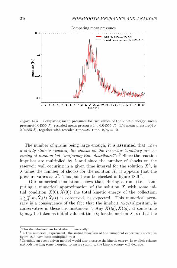
216 NONSMOOTH MECHANICS AND ANALYSIS
Figure 18.6. Comparing mean pressures for two values of the kinetic energy: meanpressure(0.04555 J); rescaled-mean-pressure(4 × 0.04555 J)=1/4 mean pressure(4 ×0.04555 J), together with rescaled-time=2× time. v/v0 = 10.
The number of grains being large enough, it is assumed that whena steady state is reached, the shocks on the reservoir boundary are oc-curing at random but “uniformly time distributed”. 6 Since the reactionimpulses are multiplied by λ and since the number of shocks on thereservoir wall occuring in a given time interval for the solution Xλ, isλ times the number of shocks for the solution X, it appears that thepressure varies as λ2. This point can be checked in figure 18.6 7.
Our numerical simulation shows that, during a run, (i.e. com-puting a numerical approximation of the solution X with some ini-tial condition X(0), X(0)) the total kinetic energy of the collection,12
∑Ni miXi(t).Xi(t) is conserved, as expected. This numerical accu-
racy is a consequence of the fact that the implicit NSCD algorithm, isconservative in these circumstances 8. Any X(t0), X(t0), at some timet0 may be taken as initial value at time t0 for the motion X, so that the
6This distribution can be studied numerically.7In this numerical experiment, the initial velocities of the numerical experiment shown infigure 18.5 have been multiplied by 28Certainly an event driven method would also preserve the kinetic energy. In explicit-schememethods needing some damping to ensure stability, the kinetic energy will degrade.

Numerical simulation of a multibody gas 217
λ scaling property holds. It may thus be inferred that the relevant pa-rameter is the kinetic energy, which will be noted 1
2
∑Ni miXi.Xi. This
parameter was already suggested in 1978 by S. Ogawa (Ogawa, 1978),and called granular temperature with extensive use in kinetic theoriesof granular gases. This parameter is not a new variable, though in thegranular case it emerges only through multibody dynamics considera-tions, with a touch of randomness and equidistribution properties.
Actually, more analysis is necessary before ending up with a relevantparameter. Indeed, let us now assume that the specific mass of the grainsis increased by a factor λ. The following proposition is true:
If, X : t → X(t), is a motion solution of the multibody collisionproblem with initial conditions, X0 , X0, for the distributionof masses {mi} , together with the generalized impulse,r : t → r(t) ,
then, X : t → X(t), is also a solution of the problem with initialconditions, X0 , X0, for the distribution of masses {λmi} ,
together with the generalized impulse, rλ : t → rλ(t) = λr(t) .
Although for a given multibody sample the distribution of masses is un-changed, it is worthwile to notice that, when the kinetic energy of thesample is increased by a factor λ2 by increasing X(0) by a factor λ orthe mass by a factor λ2, the pressure is increased by a factor λ2.
When a steady state regime is reached, it is expected that any sub-collection of the sample is governed by the same law as the one governingthe whole sample; a sub-reservoir containing a sub-collection of the sam-ple should bear the same pressure as the reservoir. If so, assuming thatthe kinetic energy is equally distributed in all parts of the reservoir, andthat the grains masses are also equally distributed, 9 the proper param-eter appears to be the average kinetic energy by grain,
T =12
∑Ni miXi.Xi
N .
The above expression will be called hereafter granular temperature. Onehas to notice that this definition is different, up to the number of grains,from definitions used in the literature, the whole kinetic energy, or thekinetic energy per unit of volume. Also, it should be noticed that thegranular temperature is a concept different from Kelvin temperature.The unit of granular temperature is T is J/mole, so that pv/NT is di-mensionless, wheseas that of the Kelvin temperature T is dimensionless,
9These distributions can be numerically studied.

218 NONSMOOTH MECHANICS AND ANALYSIS
so that the unit of pv/NT is J/mole K. In the case of a perfect gas,pv/NT = 8.3144 J/mole K.
4.2 Trying a lawpv = f(v)NT
The ratio pv/NT , with T = 0.189310−4 J/mole is plotted as a function
Figure 18.7. Evolution of pv/NT , T = 0.1893 10−4 J/mole
of v/v0 in figure 4.2. Though a steady regime is not really reached, aplausible steady mean pressure is evaluated as a mean value over a pe-riod of reminiscence of the wave regime, an interval of time from 40 to70 s, as shown in figure 18.5. One observes that the ratio is decreasingas the collection of disks gets more and more dilute, and this ratio tendsto 1.
5. Comments and conclusionAlhough the existence of a steady state of pressure is not proved,
and though properties of time equidistribution of shocks and of spatialhomogeneity may not be satisfactorily realized with such a small numberof grains, the graph plotted in figure 4.2 suggests the existence of aperfect gas behavior, with a physical constant 1. Deeper investigations

Numerical simulation of a multibody gas 219
are still necessary to ensure the relevance of the multibody perfect gasbehavior. Estimations may be obtained (a suggestion from J.J. Moreau)10 from the so called viriel equation,
x.mdu
dt= x.r .
One obtains the following relation, when a steady regime is reached,
NT = (p−Δp)v + [xr]bulk + [mxu] .
The term [mxu] (an average kinetic momentum) is vanishing at steadystate, and both terms Δp, (a boundary pressure grain size correctiveterm) and [xr]bulk, (an average internal reaction momentum term) arevanishing when the ratio lmean
L tends to zero (lmean is the grain meanradius, L is the radius of the reservoir). The perfect gas law,
pv = NT ,
is thus relevant for a dilute gas, as stated in statistical thermodynamics.
AcknowledgmentsA l’occasion de ce colloque, je tiens a dire a quel point cotoyer Jean
Jacques Moreau est pour moi (pour nous tous), scientifiquement en-richissant, stimulant, derangeant, etonnant et rassurant, tout cela a lafois.
ReferencesJ.J. Moreau. Unilateral contact and dry friction in finite freedom dy-
namics, volume 302 of International Centre for Mechanical Sciences,Courses and Lectures. pp.1–82, J.J. Moreau, P.D. Panagiotopoulos,Springer, Vienna, 1988.
J.J. Moreau. Some numerical methods in multybody dynamics: applica-tion to granular materials, Eur. J. Mech. , A/Solids, Vol. 13, n.4 -suppl., pp. 93–114, 1994.
J.J. Moreau. Some basics of unilateral dynamics, in F. Pfeiffer & C. Glocker(ed), Unilateral Multibody Dynamics, Kluwer, Dordrect, 1999.
M. Jean, J.J. Moreau. Dynamics of elastic or rigid bodies with frictionalcontact and numerical methods. In R. Blanc, P. Suquet, M. Raous,(ed), Publications du LMA, pp. 9–29, 1991.
10J.J. Moreau has also performed numerical “adiabatic compression” experiments of suchcollections of grains (private communication).
220 NONSMOOTH MECHANICS AND ANALYSIS
M. Jean, J.J. Moreau. Unilaterality and dry friction in the dynamics ofrigid bodies collections. In A. Curnier, (ed), Proc. of Contact Mech.Int. Symp., pp. 31–48, 1992.
M. Jean. Frictional contact in rigid or deformable bodies: numerical sim-ulation of geomaterials, pp. 463–486, A.P.S. Salvadurai J.M. Boulon,Elsevier Science Publisher, Amsterdam, 1995.
M. Jean. The NonSmooth Contact Dynamics Method, in ComputerMethods in Applied Mechanics and Engineering, special issue on com-putational modeling of contact and friction, J.A.C. Martins, A. Klar-bring (ed), 177, pp. 235 – 257, 1999.
B. Cambou, M. Jean. Micro Mecanique des Materiaux Granulaires. Her-mes, Paris, 2001.
S. Ogawa. Multitemperature theory of granular materials Proc. of US-Jpn Semin. Contin. Mech. and Stat. App. Mech. Granular Mat. Tokyo(1978) . 208-217.

Chapter 19
GRANULAR MEDIA AND BALLASTEDRAILWAY TRACKSMILIEUX GRANULAIRES ETVOIES BALLASTEES
Catherine CholetGilles SaussinePierre-Etienne Gautierand Louis-Marie CleonSNCF - Direction de la Recherche et de la Technologie, 45 rue de Londres, 75379 ParisCedex 08, [email protected]
AbstractSince the beginnings of the railway track, ballasted track is widely
employed because of its mechanical properties and its flexibility for con-struction and maintenance but also for their capacity to fulfil the me-chanical requirements fixed by the transport of heavy loads at a longdistance. The study of the track deterioration is one of the principle as-signments in railway engineering, specially for SNCF to preserve a goodquality of track and to ensure the comfort and the safety of circulation.
In spite of the experience on the railway track structure, the lifespanof a railway remains difficult to estimate and the mechanisms that leadto its deterioration remain insufficiently known. The answers come pri-marily from experiments or an empirical approach. A SNCF researchproject is to study the behaviour of the ballast so as to integrate thisunderstanding in a strategy of control of the costs for the design andthe maintenance, in particular the renewal of the railway.
In this context, it appears necessary to improve the understandingof the fundamental mechanisms that lead in the medium-to-long termto the appearance of the track defects. The simulation methods result-ing from research on the granular medium yielded significant results in

222 NONSMOOTH MECHANICS AND ANALYSIS
Civil Engineering which can be applied to railway problems and makeit possible to study the phenomena related to the microstructure of theballast. The interest of these methods was largely improved by work ofProfessor J.J. Moreau, in particular on the avalanches and old monu-ments (Moreau, 2000).
The work performed at SNCF in collaboration with LMGC concernsthe development of a two-dimensional and a three-dimensional discreteelement software using the platform LMGC90 to study the ballast be-haviour (Saussine et al, 2004). The first step is to provide validationsthrough comparisons with some existing experiments or developed forthis purpose. It is a prerequisite before an application to the industrialproblem. Next, we present some research orientations: on the one handthe behaviour of a granular media subjected to a great number of loadingcycles, which is strongly connected to the problems of the ballast set-tlement and its densification and on the other hand a three-dimensionalapplication of the software to the study of the lateral resistance of thetrack (Saussine et al, 2004).
Keywords: ballasted track, discrete element approach, cyclic loading, lateral resis-tance
1. Les enjeux des recherches sur l’infrastructureDepuis les debuts du ferroviaire, les voies ballastees sont tres large-
ment employees en raison de leur flexibilite a la fois pour la constructionet la maintenance mais egalement pour leur capacite a repondre auxexigences mecaniques fixees par le transport de lourdes charges sur unegrande distance. Le ballast est un des elements support de la voie. Ilest capital pour la SNCF et RFF de conserver une bonne qualite de voiepour assurer le confort et la securite des circulations.
En depit de l’experience acquise sur les infrastructures ferroviaires, laduree de vie d’une voie ferree reste difficile a estimer et les mecanismesa l’origine de sa degradation sont mal connus. Les reponses aux ques-tions posees proviennent essentiellement de l’experience terrain ou d’uneapproche empirique. Une des activites de recherche de la SNCF estd’etudier le comportement du ballast de maniere a integrer ces connais-sances dans une strategie de maıtrise des couts pour la conception et lamaintenance preventive, en particulier concernant le renouvellement dela voie ferree : les renouvellements sur ligne nouvelle (au bout de 15 anssur la ligne Paris Sud Est) ont pose de reelles difficultes d’exploitationet par voie de consequence des couts tres importants.
Dans ce contexte, il nous apparaıt necessaire de mieux comprendrele fonctionnement interne de la voie et des mecanismes qui conduisenta plus ou moins long terme a l’apparition des defauts de voie. Les per-

Granular media and ballasted railway tracks 223
spectives offertes par les approches granulaires permettent d’etudier lesphenomenes lies a la microstructure du ballast. L’interet de ces metho-des a ete largement demontre par les travaux du Professeur J.J. Moreau,notamment sur les avalanches et les monuments anciens (Moreau, 2000).
Dans cet article, nous nous interesserons specifiquement au comporte-ment du ballast mais des recherches prenant en compte une approcheplus globale de la voie sont egalement en cours (Quetin et al, 2003).
2. Construction et entretien d’une voie ferreeballastee
L’objectif de cette partie n’est pas de donner une description exhaus-tive de la voie mais de presenter les principes generaux qui gouvernentla construction, le fonctionnement et la maintenance de la voie ferreeballastee (Alias, 1984).
2.1 Structure de la voieLes principaux elements constitutifs de la voie ferree ballastee sont
presentes sur la figure 19.1. L’armement constitue la partie superieurede la voie : il est forme par le rail tenu par l’intermediaire d’attaches desemelles caoutchouc cannelees de 9 mm et enfin de traverses (en bois, enbeton, monobloc ou bibloc). La structure d’assise est constituee par lacouche de ballast, la sous-couche et repose sur la plate-forme de terrasse-ment dont la partie superieure est compactee en couche de forme. Les
Figure 19.1. Constitution d’une voie ferree ballastee — Constitution of the ballastedtrack.
regles de dimensionnement des structures d’assises ont ete reexaminees al’occasion des projets de lignes nouvelles et peuvent etre appliquees pour

224 NONSMOOTH MECHANICS AND ANALYSIS
la refection des lignes classiques. Elles consistent a choisir l’epaisseur descouches d’assise de facon a ce que les contraintes induites sur la plate-forme ne depassent pas une valeur limite. L’epaisseur varie en fonctionde la qualite des sols support en place.
L’epaisseur de la couche de ballast est d’au moins 30 cm sur Lignea Grande Vitesse (LGV). Sur voie classique, l’epaisseur sous traversebeton varie entre 15 et 25 cm selon le classement des lignes.
2.2 Le Ballast2.2.1 Origine. Le lit de ballast est compose d’une couche d’a-gregats mineraux grossiers concasses repondant a des criteres de qualiteportant essentiellement sur la petrographie, la morphologie des grainsainsi que la durete et les proprietes d’alterabilite. Par le passe, on apu utiliser d’autres materiaux beaucoup plus friables (comme le cal-caire ou des materiaux roules...) mais ces materiaux ont ete exclus detoute utilisation ferroviaire en raison de leurs mauvaises performances dupoint de vue mecanique et durabilite. Aux debuts de l’exploitation despremieres lignes a grande vitesse, les normes de durete et de resistancea la fragmentation ont ainsi ete ‘renforcees’ pour limiter la deteriorationdu ballast.
La granulometrie du ballast utilise en voie est fixee a 25/50 mm. Cefuseau est amene a evoluer (31.5/63 mm) depuis la mise en applicationd’une nouvelle norme europeenne sur les granulats.
2.2.2 Les fonctions du ballast. Le ballast assure un certainnombre de fonctions essentielles dans la voie :
l’ancrage lateral et longitudinal de la voie,
la transmission et la repartition des charges statiques et dynami-ques du rail vers la plate-forme,
le drainage des eaux pluviales,
et une fonction environnementale, de plus en plus reconnue, quiest de moindres emissions acoustiques qu’une voie sur dalle etl’amortissement des vibrations engendrees par les circulations.
Le ballast presente un avantage supplementaire en raison de sa flexibilitedu point de vue de sa mise en oeuvre et de la maintenance ainsi que sonfaible cout de construction par rapport a une voie sur dalle classique.

Granular media and ballasted railway tracks 225
2.3 Geometrie d’une voie ballasteeIl existe entre la voie et le vehicule des interactions tres etroites
en raison des efforts exerces par le vehicule sur la voie. Les imper-fections de cette derniere reagissent sur la stabilite du vehicule avecdes consequences importantes sur le confort des passagers voire sur lasecurite des circulations, d’ou la necessite de conserver une bonne qualitede voie.
Le suivi de la geometrie est un des criteres essentiel de qualite dela voie : au cours du temps des defauts de nivellement ou “defauts devoie” apparaissent dus a un tassement differentiel du ballast (voir partiesuivante). On distingue plusieurs types de defauts :
Les defauts de nivellement longitudinal qui mesurent (par file derail), la difference de hauteur entre un point et la moyenne d’alti-tude du rail calculee sur une base de 15 m,
les defauts de dressage qui mesurent (par file de rail) la variationde la position transversale par rapport a la moyenne calculee surune base de 10 m,
Les defauts de nivellement transversal. Le devers mesure la differenced’altitude entre les deux files de rail. On calcule les ecarts de deversen chaque point du rail en reference a une moyenne calculee sur10 m. Le gauche mesure la torsion de la voie (ecart de deversramene sur une base de 3 ou 9 m).
Les defauts de voie sont releves periodiquement grace a des voituresd’auscultation (de type voiture Mauzin). A titre indicatif, sur LGV,pour un defaut de nivellement (defaut isole) au dela de 15 mm, unerestriction des vitesses de circulation est imposee.
2.4 Maintenance d’une voie ferree ballasteeLa maintenance consiste essentiellement a agir sur le ballast ou sur
l’armement de la voie. Ces operations sont plus ou moins complexesselon la nature des defauts et peuvent aller jusqu’a un renouvellementpartiel ou complet d’une partie ou de la totalite de la voie.
Le bourrage-dressage mecanise est une des operations de nivellementles plus couramment pratiquees. Elle permet par un apport de materiauneuf et par une action de serrage et de vibration des grains situes sousla traverse (a une frequence d’environ 35 Hz) de redonner un niveaugeometrique satisfaisant a la voie et de reconstituer les “moules” c’est adire les zones unies et compactes situees sous les traverses (Alias, 1984).

226 NONSMOOTH MECHANICS AND ANALYSIS
Le renouvellement complet de la voie (ballast et armement) inter-vient lorsque les operations de maintenance deviennent inefficaces pourassurer une bonne qualite de voie et surtout garantir la durabilite decette geometrie dans le temps. C’est cette analyse qui a conduit aurenouvellement de troncons de la LGV Paris Sud Est apres 15 anneesd’exploitation.
Il est en revanche beaucoup plus delicat d’effectuer des operations surla sous-couche ou la plate-forme ferroviaire. Sur les LGV, il n’est en effetpas envisageable de deposer la voie en raison des tres fortes contraintesd’exploitation, d’ou l’importance du dimensionnement et de la receptionde la plate-forme ferroviaire lors de la construction d’une ligne nouvellepour limiter sa degradation.
3. Les problematiques rencontreesLe ballast est largement tributaire du trafic ecoule depuis sa mise en
place. La vie de la voie ferree est ponctuee par differentes operations demaintenance, de renouvellement partiel ou total de ses composants. Toutremaniement du ballast est le point de depart d’un nouveau cycle. Ladegradation de la qualite du ballast et/ou de ses interfaces peut cepen-dant conduire a accelerer considerablement le rythme des operations demaintenance.
Tassement et mise en place du ballast : le maintien de la geome-trie de la voie est lie pour une grande part au comportement du ballast.Lors de la construction ou apres une operation de relevage, on constateun tassement tres rapide de la voie caracteristique de sa mise en place.Lorsque la voie est dite “stabilisee”, le ballat continue de se tasser maisde maniere beaucoup plus lente. C’est un processus naturel pour toutgranulat mais la difficulte est que ce tassement n’est pas homogene d’unpoint a l’autre de la voie ce qui peut etre a l’origine de l’apparition desdefauts de voie. L’enjeu est donc de mieux comprendre les mecanismesa l’origine de l’apparition des tassements, d’etudier le role des interfaces(descentes de charge vers la sous-couche, traverse...) et d’identifier lesfacteurs aggravants.
L’augmentation des vitesses de circulation est un point importanten raison des enjeux economiques pour l’entreprise. En effet, depuisles debuts de l’exploitation des lignes TGV, la vitesse commerciale destrains est passee de 270 km/h a 300 km/h et bientot 320 km/h (sur laligne TGV Est en construction). Des experiences de laboratoire (Bodin,2001) ont mis en evidence que le tassement et la reponse elastique dela voie augmentent avec la vitesse de circulation. Au dela d’une cer-taine “frequence” critique, le phenomene s’accelere. D’autres facteurs

Granular media and ballasted railway tracks 227
ont egalement une incidence, comme la charge a l’essieu des materielsferroviaires en perspective d’une augmentation du tonnage a l’essieu destrains de fret sur les lignes classiques.
Resistance laterale : une des fonctions principales du ballast estd’assurer l’ancrage lateral et longitudinal de la voie. Cette proprieteest particulierement importante pour assurer la stabilite de la voie enlateral et ainsi controler les effets dus au flambement thermique du railen periode estivale. Il est donc souhaitable de bien comprendre quelssont les facteurs qui contribuent a la resistance laterale de la voie.
Bourrage : le bourrage est une operation complexe. Les parametresdu bourrage sont fixes par les constructeurs de machine (frequence desollicitation, serrage, descente des bourroirs dans la voie...). La qualitedu bourrage est egalement tres dependante du savoir faire technique desoperateurs de terrain.
Les performances du bourrage sont estimees a partir de la qualitegeometrique de la voie immediatement apres l’operation mais n’est pasevaluee en fonction de la tenue de la geometrie dans le temps. Il estdonc tres important de bien definir les specifications fonctionnelles dubourrage pour mieux maıtriser les contraintes operationnelles de la main-tenance.
Stabilisation : la stabilisation de la voie est etroitement liee a samise en place. La resistance du ballast est largement tributaire del’etat de stabilisation de la voie : tout remaniement de la voie entraıneune deconsolidation du milieu et particulierement une diminution de saresistance laterale. Une voie recemment posee ou remaniee n’acquiertque progressivement sa stabilite definitive : un ecoulement de trafic de100000 tonnes est considere comme necessaire. La stabilisation peut etreeffectuee au moyen d’un stabilisateur dynamique. La stabilisation dy-namique n’est cependant pas consideree comme suffisante pour restituercompletement le niveau de consolidation souhaite. Le couplage entrela stabilisation et le bourrage et sa repercussion sur la durabilite de latenue de la geometrie dans le temps est donc un sujet particulierementinteressant.
Usure du ballast : pour comprendre le comportement de la voie(tassement, mise en place, resistance laterale...) a ses differents stades,il est egalement necessaire de connaıtre les modes de degradation desgrains de ballast. La vie du ballast dans la voie entraıne des phenomenesplus ou moins lents d’attrition ou de fragmentation qui conduisent al’apparition d’elements fins. Ces elements fins vont peu a peu venir col-

228 NONSMOOTH MECHANICS AND ANALYSIS
mater les interstices entre les grains. Le ballast perd alors sa fonctiondrainante. Des facteurs exterieurs peuvent etre egalement a l’originedu colmatage de la voie comme des remontees de boue en provenancede la plate-forme, la deterioration des traverses... Ces effets accelerentencore les processus de degradation il est donc necessaire de les prendreen compte dans toute analyse du comportement de la voie.
4. Modelisation du ballast par l’approcheContact Dynamics
4.1 PrincipeLe travail realise a la SNCF en collaboration avec le LMGC porte sur
le developpement d’un code par elements discrets 2D et 3D dans la plate-forme logicielle LMGC90 en vue d’une application au ballast (Saussineet al, 2004). L’ensemble des simulations numeriques presentees ont eterealisees avec LMGC90.
Une premiere etude, appliquee au bourrage et realisee a la SNCF(Oviedo, 2001), a montre la pertinence d’une telle approche pour etudierle comportement du ballast. La methode Contact Dynamics a ete retenueen raison de ses performances numeriques : le principe de resolutionimplicite de la methode rend la resolution sur un pas de temps pluscouteuse mais ce meme pas de temps est beaucoup plus grand que dansles autres approches, d’ou un gain de temps significatif constate dansl’ensemble de nos applications. C’est un avantage d’un point de vuenumerique pour traiter un grand nombre de grains comme c’est le caspour des geometrie 3D ou pour simuler un grand nombre de cycles dechargement. Une description detaillee de l’approche Contact Dynamicsdeveloppee par Moreau et Jean pourra etre trouvee dans (Moreau etJean, 1992).
La demarche adoptee consiste a valider les simulations numeriques parconfrontation avec des resultats experimentaux, experiences existantes(tambours tournants...) ou developpees a cet effet. C’est un prealableavant de passer aux applications industrielles de la methode.
Nous presentons quelques axes de recherche : d’une part le comporte-ment d’un assemblage granulaire soumis a un grand nombre de cycles dechargement, ce qui rejoint la problematique du tassement du ballast etde sa mise en place et d’autre part une application du code 3D a l’etudede la resistance laterale du ballast (Saussine et al, 2004).

Granular media and ballasted railway tracks 229
4.2 Comportement de la voie sous un grandnombre de cycles de chargement
Un dispositif experimental bidimensionnel, inspire du principe desmateriaux de Schneebeli, a ete developpe avec pour objectif de valider lecode de calcul bidimensionnel sur un exemple simplifie mais representatifdu ferroviaire.
0 100 200 300 400 500 600 700 800 900 1000
Cycles de chargements.
0m
0,0002m
0,0004m
0,0006m
0,0008m
0,001m
0,0012m
0,0014m
0,0016m
0,0018m
0,002m
0,0022m
0,0024m
Expériencesimulation
Figure 19.2. Dispositif experimental bidimensionnel : Comparaison des tassementsexperimentaux et numeriques pour un echantillon — Two-dimensional experimentalset-up: Comparison of experimental and numerical settlement for one sample.
Le dispositif experimental 19.2, developpe au LCPC (Laboratoire Cen-tral des Ponts et Chaussees) represente une portion de voie ferroviaire(Cholet et al, 2003). Il est constitue d’un bloc en aluminium representantune portion de traverse, de prismes a sections polygonales modelisant lesgrains de ballast. Les prismes, en ciment haute performance et de troisdiametres differents (1 cm, 1.5 cm et 2 cm) reposent sur une couched’elastomere modelisant la couche sous-ballast. L’ensemble est disposedans un bati rectangulaire sur lequel est fixe un verin asservi en force.Celui-ci permet d’appliquer des chargements cycliques sur le blochet avecdifferentes inclinaisons. Des photos sont prises au cours du chargementpour suivre le deplacement de quelques grains. La position du blochetest enregistree.
Sur une experience, nous avons confronte les tassements mesures pourun echantillon numerise et les simulations numeriques. Une des diffi-cultes de cette operation a porte sur la modelisation de la sous-couchedeformable et le recalage dans l’echantillon numerique (la sous-couchen’est pas numerisee). On constate que le tassement evolue de manieresimilaire dans la simulation et l’experience et les memes phenomenes derecirculation des grains autour du blochet ont pu etre observes. Nousavons pu ainsi demontrer la faisabilite d’une telle etude. Les compara-isons realisees entre les simulations et les resultats experimentaux sont

230 NONSMOOTH MECHANICS AND ANALYSIS
encourageantes et donnent un bon indice de confiance quant a l’aptitudede la methode Contact Dynamics a reproduire les phenomenes observes.
La comprehension des phenomenes de tassement et de mise en placede la voie necessite de simuler un grand nombre de cycles de charge-ment : sur LGV, un mois d’exploitation correspond a environ 1 millionde passages d’essieu. Les simulations ont pu etre ‘poussees’ sur plusieursmilliers de cycles de chargement (35000 cycles) tout en concervant unebonne qualite de calcul : le cumul des erreurs d’interpenetration entreles grains reste controle. C’est peu en comparaison des situations reellesmais cette etude nous a permis de realiser des avancees significative dansce domaine qui reste largement ouvert.
4.3 Resistance laterale de la voieComme nous l’avons vu a la partie precedente, la resistance laterale
de la voie est un facteur important pour la securite des circulations.L’etude de la resistance laterale a l’aide de LMGC90 implique l’ela-
boration d’echantillons et d’un protocole d’experimentation : nous noussommes inspires d’essais existants realises a la SNCF.
Figure 19.3. Essai de resistance laterale sur un massif de ballast avec un blochet (agauche) - Profil de vitesse : seuls les grains de ballast ayant une vitesse entre 10% et50% de la vitesse maximale sont representes (a droite) — Lateral resistance test ona ballast bed with a half sleeper (on the left) - Profile speed: only the ballast grainshaving a speed between 10% and 50% maximum speed are represented (on the right)
Une petite portion de voie comportant un seul blochet (demi-traverse)a ete modelisee et en respectant la granulometrie reelle du ballast. Lesgrains utilises pour les simulations sont issus de la numerisation de 1000grains de ballast reel. Une fois l’echantillon depose (figure 1.3) il estpossible de realiser plusieurs types d’essais sur le meme echantillon, parexemple des essais de traction sur le blochet pour differentes chargesverticales, des cycles de chargement en nombres limites. Ces essais de

Granular media and ballasted railway tracks 231
traction peuvent etre exploites pour homologuer les traverses ou pouretablir les referentiels sur la resistance laterale de la voie.
Nous avons commence par etudier l’influence du coefficient de frot-tement entre le blochet et les grains de ballast sur le deripage du blo-chet soumis a une force incrementale transversale (figure 1.4) mais lesresultats obtenus demandent a etre calibres (Saussine et al, 2004).
0 0,005 0,01 0,015 0,02 0,025
Déplacement latéral du blochet (m)
0N
200N
400N
600N
800N
1000N
1200N
mu = 0.3mu = 0.4mu = 0.5mu = 0.6mu = 0.7
Figure 19.4. Champs de vitesse dans l’echantillon sous l’action de la force - Influ-ence des differents coefficients de frottement. — Fields speed in the loaded sample -Influence of the coefficient of friction.
D’autres applications sont envisagees comme l’etude de l’influence dupoids, de la forme de la traverse...
5. ConclusionLes problemes de conception ou d’exploitation de la voie ferree bal-
lastee sont nombreux et varies. Il est necessaire d’etudier le fonction-nement du ballast afin d’optimiser la conception de la voie mais egale-ment de comprendre les mecanismes de degradation pour mieux appre-hender la maintenance.
Les methodes par elements discrets nous permettent d’apprehender lacomplexite des phenomemes rencontres. La demarche adoptee consistea valider les simulations numeriques par confrontation avec des resultatsexperimentaux existants. C’est un prealable avant toute application in-dustrielle de ce type d’approche. Nous presentons les premiers resultatsissus des simulations numeriques : simulation d’un grand nombre decycles de chargement et resistance laterale de la voie.
ReferencesJ. Alias, La voie ballastee - Techniques de construction et d’entretien,
1984 (2eme edition).

232 NONSMOOTH MECHANICS AND ANALYSIS
V. Bodin, Comportement du ballast des voies ferrees soumises a unchargement vertical et lateral, These de doctorat de l’Ecole Nationaledes Ponts et Chaussees. 2001.
C. Cholet, G. Saussine, G. Combe, C. Bohatier, F. Dubois and K. Sab,Mechanical behaviour of the ballast using discrete element methodsdans Proceedings of The World Congress on the Railway Research.2003
M. Jean and J. J. Moreau, Unilaterality and dry friction in the dynamicsof rigid body collections dans Contact Mechanics. Presses Polytech-niques et Universitaires Romandes. 1992
J. J. Moreau, Contact et frottement en dynamique des systemes de corpsrigides dans Revue Europeenne des Elements Finis. Vol 9. 2000.
X. Oviedo. Etude du comportement du ballast par un modele micro-mecanique - Application aux operations de maintenance de la voieferree ballastee. These de doctorat de l’Ecole Nationale des Ponts etChaussees. 2001.
F. Quetin, L. Schmitt, K. Sab and D. Duhamel. Modelling of the dy-namical behaviour of railway ballasted track including its platformdansProceedings of the world congress on railway research. 2003.
G. Saussine, C. Cholet and P.E. Gautier. Modelling ballast under cyclicloading using discrete element method dans Proceedings of Interna-tional conference on cyclic behaviour of soils and liquefaction phenom-ena. 2004 (a paraitre).

Chapter 20
SCALING BEHAVIOUR OFVELOCITY FLUCTUATIONSIN SLOW GRANULAR FLOWS
Farhang RadjaıLMGC, CNRS-Universite Montpellier II, Place Eugene Bataillon, 34095 MontpellierCedex, [email protected]
Stephane RouxLaboratoire Surface du Verre et Interfaces, CNRS-Saint Gobain, 39 Quai Lucien Lefranc,93303 Aubervilliers Cedex, [email protected]
Abstract Steric exclusions among particles lead to strong velocity fluctuations ina granular flow. Modelling the effective behaviour of granular materi-als depends on the extent and scaling properties of these fluctuations.We consider here slow granular flows of rigid particles simulated bya discrete element method. Bi-periodic boundary conditions allow formacroscopically homogeneous shearing up to large strains. We obtainthus reliable statistics for an accurate analysis of particle velocity fluc-tuations. We find that the probability distribution function of velocitycomponents, evaluated from particle displacements, crucially dependson time resolution. It varies from stretched exponential to gaussian asthe integration time is increased. On the other hand, the spatial powerspectrum of the fluctuating velocity field is a power law, reflecting longrange correlations and the self-affine nature of the fluctuations. Finally,by considering individual particle displacements, we show that the par-ticles have a superdiffusive motion with respect to the mean backgroundflow. These scaling behaviours bear a close analogy with the known scal-ing properties of turbulent fluid flows although the underlying physicsis drastically different.

234 NONSMOOTH MECHANICS AND ANALYSIS
Keywords: granular media, discrete element method, plastic deformation, steric ex-clusions, probability density function, space correlations, superdiffusion,turbulence.
IntroductionGranular media have proved to be a rich source of intriguing phenom-
ena at all scales: from the anisotropic dilatant stress-strain behaviour(Hicher, 2000) to particle-scale phenomena such as inhomogeneous forcetransmission (Moreau, 1997, Radjai et al., 1996) or size segregation(Moreau, 1993, Moreau, 1994a). Generally, one has little intuition aboutwhat happens, and quite often theoretical understanding remains a chal-lenge (de Gennes, 1999, Jaeger et al., 1996, Roux and Radjai, 2001).
In analogy with molecular fluids, when a granular material flows, alarge number of degrees of freedom interact in a disordered way. Thecomplexity of granular flows arises from the dissipative nature of theseinteractions (friction, inelastic collisions) and geometrical frustrations in-duced by steric exclusions of particles (Moreau, 1988). These excluded-volume effects result in large force and velocity fluctuations in time. Thequasistatic behaviour is of elasto-plastic type with hardening variableswhich are not yet well appreciated from particle-scale arguments. Inthe conventional approach, it is assumed that the size of the representa-tive elementary volume is sufficiently small that the fluctuations in localvariables fully average out at scales of engineering interest.
Recently, several authors have reported on strong velocity fluctuationsin typical shear tests where it is often assumed that the velocity field ishomogeneous (Misra and Jiang, 1997, Kuhn, 1999, Miller et al., 1996).They also remarked that the fluctuations occur in a correlated fashion,but they did not analyze the length and time scales involved in thesefluctuations. An accurate evaluation of the statistics of fluctuations re-quires, indeed, long-time homogeneous and steady shearing, a conditionthat seems hardly accessible from experiments.
In this paper, we present a numerical investigation of velocity fields ina slow two-dimensional granular flow where the homogeneity of shearingis ensured by means of bi-periodic boundary conditions. We will brieflyintroduce the numerical procedures used for these simulations. Then, westudy the distribution functions of the velocities, calculated from particledisplacements, as a function of the integration time. In order to evaluatethe space correlations, we consider also the spatial power spectra of thevelocities. The temporal behaviour will be analyzed by considering thefluctuating trajectories of the particles in the bulk. Finally, we discussthe relevance of our findings to the macroscopic modelling of granular
Velocity fluctuations 235
media and we briefly depict the striking analogy suggested by thesefindings with the scaling features of fluid turbulence.
1. Numerical proceduresThe investigated granular system is a two-dimensional assembly of
4000 discs with diameters uniformly distributed between Dmin and Dmax
with Dmax = 3Dmin. The particles interact through a stiff linear repul-sive force as a function of mutual overlaps and the Coulomb frictionlaw. The coefficient of friction is 0.5. The equations of motion for parti-cle displacements and rotations are integrated by means of a predictor-corrector scheme (Allen and Tildesley, 1987).
In numerical simulations performed up to large cumulative deforma-tion, the boundary conditions tend to introduce spurious effects in thevicinity of the walls, and may even lead to a strongly inhomogeneousstrain field. The latter should, however, be as homogeneous as possibleto extract a meaningful statistics for intrinsic fluctuations. In order toreduce these edge effects, we have introduced bi-periodic boundary con-ditions: it consists in imposing such a periodicity along both directionsof the simulation cell for the stress and the strain fields. The displace-ment field, however, is not periodic if the mean strain is non-zero. Itcontains an affine part δri ≡ (δri
x, δriy) in addition to a bi-periodic (fluc-
tuating) field δsi ≡ (δsix, δsi
y) of zero mean (〈δs〉 = 0). This requires aspecial treatment of these two components with additional characteris-tics associated with the non-periodic part of the displacement, such asa fictive inertia (Parrinello and Rahman, 1980). However, the latter canbe shown to play a negligible role in the results. The origin of spacebeing now an arbitrary parameter, the stress-strain and more generallyany geometrical observable has to be translationally invariant, and hencethe strain remains spatially homogeneous on a large scale.
In our simulations, the gravity was set to zero and a confining pressurewas applied along the y direction. The width L of the simulation cell waskept constant. The system is driven by imposing the affine componentδrx
i = δtγriy, where γ is a constant shear rate and δt is the time step.
In other words, the Fourier mode k = 0 of the total strain is imposed,corresponding to a large scale forcing. This driving mode was appliedon a dense packing prepared by isotropic compaction. The height ofthe packing increases (dilation) in the initial stages of shearing beforea homogeneous steady state is reached where volume changes fluctuatearound zero, so that 〈δry
i〉 " 0. The solid fraction in the steady statefluctuates in the range [0.79, 0.81] and the average coordination number

236 NONSMOOTH MECHANICS AND ANALYSIS
is 3.8. Our focus here is on the fluctuating components (δsix, δsi
y) in thesteady state.
2. Time scalesAlthough our dynamic simulations involve the physical time, the in-
ertial effects are negligibly small and the contact network evolves qua-sistatically at time scales well below γ−1. We normalize all times by γ−1
so that the dimensionless time t in what follows will actually representthe cumulative shear strain. We will also use the mean particle diame-ter D to scale displacements. As a result, the velocities will be scaledby γD and the power spectra in space by (D2γ)2. In our simulationsthe time step is δt " 10−7, and more than 2.107 steps are simulated,corresponding to a total strain larger than 2.
We may distinguish two separate time scales involved in a quasistaticgranular flow: 1) contact time, corresponding to the elastic responsetime; and 2) shear time that corresponds to the time imposed by shear-ing. The latter is of the order of γ−1. The contact time for a multicontactassembly is of the same order of magnitude as the duration of a binarycollision. Up to a numerical time discretization, the particle motions be-low the contact time scale are smooth. We are interested here in timeslonger than the contact time scale. In other words, we consider the rigidrelative displacements of the particles that underly the plastic deforma-tions of the material. At such scales, the collisions can be consideredas instantaneous so that the particle velocities evolve discontinuously intime (Moreau, 1994b). In our simulations, the elastic response time isaround 10−5 in dimensionless units.
At contact time scales, it is physically plausible to rely on particlevelocities calculated for one time step since at those times the motionis smooth. But beyond the elastic time, the physically relevant particlevelocities should be evaluated from particle displacements. We considerhere the periodic part of the velocity field and we define the fluctuatingvelocities vi as a function of the integration time τ by
vi(t, t + τ) =1τ
∫ t+τ
tδsi(t′) dt′ (20.1)
Since we are concerned with steady flow, the statistical properties ofv are independent of t although, as shown below, they crucially dependon τ . Hence, accurate statistics can be obtained by cumulating the datafrom different time slices of a single simulation running for a long time.As we shall see below, the scaling of the fluctuations with τ reveals a

Velocity fluctuations 237
Figure 20.1. A snapshot of particle displacements δsi with respect to the meanbackground flow.
new characteristic time corresponding to a transition in the shape of theprobability density function of fluctuating velocities.
Fig. 20.1 shows a snapshot of fluctuating velocities vi for a shorttime lag τ = 10−5. We see that large-scale well-organized displacementscoexist with a strongly inhomogeneous distribution of amplitudes anddirections on different scales. Convection rolls appear quite frequently,but they survive typically for strains τ less than 10−3. After such shorttimes, large-scale rolls break down and new statistically uncorrelatedstructures appear. This behaviour is radically different from turbulenceeddies which survive long enough to undergo a significant distortion dueto fluid motion (Frisch, 1995).
3. Probability density functionsWe consider here the probability density functions (pdf’s) of the com-
ponents vix(t, t+τ) and vi
y(t, t+τ) as a function of time resolution τ . Thepdf’s of vi
y are shown in Fig.20.2 for a short integration time τ = 10−3,and for a long integration time τ = 10−1. The pdf has changed from anearly Gaussian shape at large τ to a non-Gaussian shape with broad
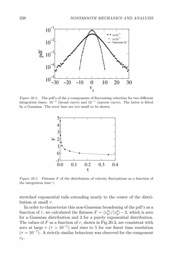
238 NONSMOOTH MECHANICS AND ANALYSIS
−30 −20 −10 0 10 20 30v
y
10−5
10−4
10−3
10−2
10−1
τ=10−3
τ=10−1
Gaussian fit
Figure 20.2. The pdf’s of the y-components of fluctuating velocities for two differentintegration times: 10−3 (broad curve) and 10−1 (narrow curve). The latter is fittedby a Gaussian. The error bars are too small to be shown.
0.0 0.1 0.2 0.3 0.4τ
-1
0
1
2
3
4
5
F
Figure 20.3. Flatness F of the distribution of velocity fluctuations as a function ofthe integration time τ .
stretched exponential tails extending nearly to the center of the distri-bution at small τ .
In order to characterize this non-Gaussian broadening of the pdf’s as afunction of τ , we calculated the flatness F = 〈v4
y〉/〈v2y〉−3, which is zero
for a Gaussian distribution and 3 for a purely exponential distribution.The values of F as a function of τ , shown in Fig.20.3, are consistent withzero at large τ (τ > 10−1) and rises to 5 for our finest time resolution(τ = 10−7). A strictly similar behaviour was observed for the componentvx.

Velocity fluctuations 239
10−2
10−1
100
101
k
10−1
100
101
102
103
104
E
vx
vy
E ~ k −β
Figure 20.4. Averaged power spectrum of the x and y components of the fluctuatingvelocity field with τ = 10−7 for one-dimensional cross sections along the mean flow.For the units, see text.
The basic physical mechanism underlying the fluctuations is the mis-match of the uniform strain field, applied here in the bulk, with mutualexclusions of the particles. As a result, the local strains deviate from themean (global) strain. The observation of a transition toward a Gaus-sian distribution for large time lags is a sign of partial loss of correlationand/or exhaustion of large fluctuations in the increment of displacementwhich occur at different times. Fig. 20.3 allows us to define a new timescale corresponding to the value of τ at transition to gaussian distribu-tion for which F = 0. This occurs for τ " 10−1. Beyond this point, aswe shall see below, the velocity fluctuations are basically reflected in thediffusive motions of individual particles.
4. Space correlationsIn order to quantify the extent of correlations in space, we estimated
the power spectrum E of velocity fluctuations both along and perpen-dicular to the flow and at different times. The Fourier transform wasperformed over the fluctuating velocity field defined on a fine grid byinterpolating the velocities from particle centers. The power spectrawere quite similar along and perpendicular to the flow, and for differentsnapshots of the flow.
The averaged spectrum on one-dimensional cross sections is shown inFig.20.4. It has a clear power-law shape k−β ranging from the smallestwavenumber k = D/L, corresponding to the system size L, up to acut-off around k = 0.5, corresponding to nearly two particle diameters.
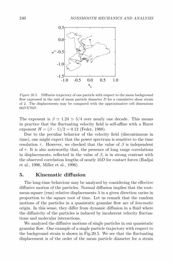
240 NONSMOOTH MECHANICS AND ANALYSIS
-1.0 -0.5 0.0 0.5 1.0s
x
-1.5
-1.0
-0.5
0.0
0.5
s y
Figure 20.5. Diffusive trajectory of one particle with respect to the mean backgroundflow expressed in the unit of mean particle diameter D for a cumulative shear strainof 2. The displacements may be compared with the approximative cell dimensions60DX70D.
The exponent is β " 1.24 " 5/4 over nearly one decade. This meansin practice that the fluctuating velocity field is self-affine with a Hurstexponent H = (β − 1)/2 = 0.12 (Feder, 1988).
Due to the peculiar behavior of the velocity field (discontinuous intime), one might expect that the power spectrum is sensitive to the timeresolution τ . However, we checked that the value of β is independentof τ . It is also noteworthy that, the presence of long range correlationsin displacements, reflected in the value of β, is in strong contrast withthe observed correlation lengths of nearly 10D for contact forces (Radjaiet al., 1996, Miller et al., 1996).
5. Kinematic diffusionThe long-time behaviour may be analyzed by considering the effective
diffusive motion of the particles. Normal diffusion implies that the root-mean-square (rms) relative displacements λ in a given direction varies inproportion to the square root of time. Let us remark that the randommotions of the particles in a quasistatic granular flow are of kinematicorigin. In this sense, they differ from dynamic diffusion in a fluid wherethe diffusivity of the particles is induced by incoherent velocity fluctua-tions and molecular interactions.
We analyzed the diffusive motions of single particles in our quasistaticgranular flow. One example of a single particle trajectory with respect tothe background strain is shown in Fig.20.5. We see that the fluctuatingdisplacement is of the order of the mean particle diameter for a strain
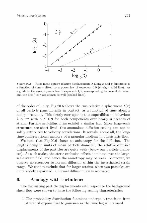
Velocity fluctuations 241
−4 −3 −2 −1 0 1log
10(τ)
−4
−3
−2
−1
0
log 10
(λ)
xy
λ ∼ τ1/2
λ ∼ τ
Figure 20.6. Root-mean-square relative displacements λ along x and y directions asa function of time τ fitted by a power law of exponent 0.9 (straight solid line). Asa guide to the eyes, a power law of exponent 1/2, corresponding to normal diffusion,and the line λ ∝ τ are shown as well (dashed lines).
of the order of unity. Fig.20.6 shows the rms relative displacement λ(τ)of all particle pairs initially in contact, as a function of time along xand y directions. This clearly corresponds to a superdiffusion behaviourλ ∝ τα with α " 0.9 for both components over nearly 3 decades ofstrain. Particle self-diffusivities exhibit a similar law. Since large-scalestructures are short lived, this anomalous diffusion scaling can not besolely attributed to velocity correlations. It reveals, above all, the long-time configurational memory of a granular medium in quasistatic flow.
We note that Fig.20.6 shows no anisotropy for the diffusion. Thelengths being in units of mean particle diameter, the relative diffusivedisplacements of the particles are quite weak (below one particle diame-ter). At such scales, the steric exclusion effects dominate over the large-scale strain field, and hence the anisotropy may be weak. Moreover, weobserve no crossover to normal diffusion within the investigated strainrange. We cannot exclude that for larger strains, when two particles aremore widely separated, a normal diffusion law is recovered.
6. Analogy with turbulenceThe fluctuating particle displacements with respect to the background
shear flow were shown to have the following scaling characteristics:
1 The probability distribution functions undergo a transition fromstretched exponential to gaussian as the time lag is increased.

242 NONSMOOTH MECHANICS AND ANALYSIS
2 The spatial power spectrum of the velocity field obeys a power law,reflecting long range correlations and the self-affine nature of thefluctuations.
3 The fluctuating displacements have a superdiffusive character.
There appears an evident analogy with the scaling features of fluidturbulence (Radjai and Roux, 2002). Turbulence studies focus mainlyon velocity differences δv measured at a fixed point of a fluid over a timeinterval τ or between two points separated by a distance r (Frisch, 1995).This is in contrast with granular flow which involves a discrete displace-ment field that is carried by individual particles. Up to this differencein framework, the scaling properties discussed above are shared by tur-bulent fluid flows. The broadening of the exponential tails of the pdf’sat increasingly smaller scales is a well-known property of fully developedturbulence (for velocity differences). It is attributed to the phenomenonof intermittency, i.e. strong localized energy transfers at small scales(Frisch, 1995). On the other hand, the power-law scaling k−β for thespectrum of velocity differences is a hallmark of 3D turbulence withβ " 5/3 (to be compared with β " 5/4 in our granular flow). Finally, in3D fluid turbulence at high Reynolds numbers, the long-time pair dif-fusivity of suspended particles is anomalous, following the Richardsonlaw λ ∝ τ3/2 which reflects the Kolmogorov-Obukhov velocity spectrum(Frisch, 1995).
A strict analogy with fluid turbulence makes certainly not much sensebecause of a drastically different physics that underlies granular fluctu-ations (hard-core interactions) as compared to turbulent fluctuations(Navier-Stokes equations, inertia regime). But, the observed analogyin terms of scaling characteristics is consistent enough to upgrade kine-matic fluctuations in quasistatic granular flows to the rank of a system-atic phenomenology which could be coined by the term “granulence” ascompared to “turbulence” in fluid dynamics!
Interestingly, this analogy works with three-dimensional turbulencealthough our data concern a two-dimensional granular flow. The en-ergy cascade in turbulence is governed by inertia, and two- and three-dimensional systems do differ significantly in this respect. In quasistaticgranular flow, the fluctuating velocity field is a consequence of the ge-ometrical compatibility of the strain with particle arrangements, anddissipation is mainly governed by friction at the particle scale. The dif-ference between two- and three-dimensional systems may thus be lesscrucial, but it was not investigated in the present work. Quite indepen-dently of its physical origins, this analogy is suggestive enough to be

Velocity fluctuations 243
used as a promising strategy towards a refined probabilistic descriptionof granular flow in the plastic regime.
The conventional approach disregards kinematic fluctuations in macro-scopic modelling of plastic flow in granular media. If the effective plasticproperties (yield surface, flow rule and hardening variables) are depen-dent only on the the mean strain, this approach is not in contradictionwith the above nontrivial scaling of fluctuating velocities. But, if theeffective properties involve higher-order moments of the velocities, thescaling should be taken into account. For example, the hardening be-haviour might involve higher order moments since the evolution of themicrostructure (typically, the contact network) is locally controlled bysteric exclusions (Troadec et al., 2002). Schematically, in larger systemsthe long-range correlations in particle motions induce stronger random-ness in local motions. As a result, we expect that longer shearing isrequired to reach the steady (critical) state which is characterized bya well-defined organization of the microstructure in terms of densityand anisotropy (Wood, 1990, Rothenburg and Bathurst, 1989). On theother hand, if some effective properties are indeed controlled by velocityfluctuations, and if a representative elementary volume exists (which ispossible if the power-law scaling in space breaks down for some reasonfor larger systems than ours), its dimension should be much larger than60 particle diameters (linear size of our system). In all cases, the veloc-ity fluctuations play a key role in modelling the effective bahaviour fromthe particle scale.
AcknowledgmentsPersonal note from F.R.: I met Jean Jacques Moreau for the first time
at the “Powders and Grains” meeting held in Birmingham in 1993. Usinghis laptop computer during a video presentation, Jean Jacques showed ushow his “contact dynamics method”, new then but widely used today,was able to simulate efficiently granular flows and reproduce puzzlingphenomena such as size segregation. He then explained, by means ofa rigourous analysis of the data, a physical mechanism at the origin ofsize segregation in a vibrated granular material. After such a delightfultheoretical demonstration, I was really impressed when he declared thatin his view the numerical results should be used “in interaction withexperiments”. Only rarely a mathematician talks of experiments! I hadthe priviledge to meet Jean Jacques quite often later in France and I en-joy discussing frequently with him since I joined the LMGC in 1997. Hislimitless enthusiasm for science, his ability to break through “cultural”walls between research fields and to associate rigourous reasoning with
244 NONSMOOTH MECHANICS AND ANALYSIS
experimental evidence have always been a source of lively research ongranular materials in the LMGC. I am greatly indebted to Jean Jacquesfor his encouraging attitude which has allowed me to initiate my researchwork on granular materials on solid grounds and to benefit in many waysfrom his vast competence during the last ten years.
ReferencesAllen, M. P. and Tildesley, D. J. (1987). Computer Simulation of Liquids.
Oxford University Press, Oxford.de Gennes, P.-G. (1999). Granular matter: a tentative review. Reviews
of Modern Physics, 71:S374–S382.Feder, J. (1988). Fractals. Plenum press, NewYork.Frisch, U. (1995). Turbulence, the Legacy of A. N. Kolmogorov. Cam-
bridge University Press, Cambridge, England.Hicher, P.-Y. (2000). Experimental behaviour of granular materials. In
Cambou, B., editor, Behaviour of Granular Materials, pages 1–98,Wien. Springer.
Jaeger, H. M., Nagel, S. R., and Behringer, R. P. (1996). Granular solids,liquids, and gases. Reviews of Modern Physics, 68(4):1259–1273.
Kuhn, M. (1999). Mechanics of Materials, 31:407.Miller, B., O’Hern, C., and Behringer, R. P. (1996). Stress fluctuations
for continously sheared granular materials. Phys. Rev. Lett., 77:3110–3113.
Misra, A. and Jiang, H. (1997). Measured kinematic fields in the biaxialshear of granular materials. Computers and Geotechnics, 20(3/4):267–285.
Moreau, J. J. (1988). Unilateral contact and dry friction in finite freedomdynamics, pages 1–82. Number 302.
Moreau, J. J. (1993). New computation methods in granular dynamics.In Powders & Grains 93, page 227, Rotterdam. A. A. Balkema.
Moreau, J. J. (1994a). Some numerical methods in multibody dynamics:Application to granular materials. European Journal of MechanicsA/Solids, supp.(4):93–114.
Moreau, J. J. (1994b). Some numerical methods in multibody dynamics:application to granular materials. Eur. J. Mech. A, 13:93.
Moreau, J. J. (1997). Numerical investigation of shear zones in granu-lar materials. In Wolf, D. E. and Grassberger, P., editors, Friction,Arching and Contact Dynamics, Singapore. World Scientific.
Parrinello, M. and Rahman, A. (1980). Phys. Rev. Lett., 45:1196.

Velocity fluctuations 245
Radjai, F., Jean, M., Moreau, J. J., and Roux, S. (1996). Force distri-bution in dense two-dimensional granular systems. Phys. Rev. Lett.,77(2):274.
Radjai, F. and Roux, S. (2002). Turbulentlike fluctuations in quasistaticflow of granular media. Phys. Rev. Lett., 89:064302.
Rothenburg, L. and Bathurst, R. J. (1989). Analytical study of inducedanisotropy in idealized granular materials. Geotechnique, 39:601–614.
Roux, S. and Radjai, F. (2001). Statistical approach to the mechanicalbehavior of granular media. In Aref, H. and Philips, J., editors, Me-chanics for a New Millennium, pages 181–196, Netherlands. KluwerAcad. Pub.
Troadec, H., Radjai, F., Roux, S., and Charmet, J.-C. (2002). Model forgranular texture with steric exclusions. Phys. Rev. E, 66:041305.
Wood, D. (1990). Soil behaviour and critical state soil mechanics. Cam-bridge University Press, Cambridge, England.

V
TOPICS IN NONSMOOTH SCIENCE
Chapter 21
MORPHOLOGICAL EQUATIONS ANDSWEEPING PROCESSES∗
Jean-Pierre AubinCentre de Recherche Viabilite, Jeux et Controle, Universite [email protected]
Jose Alberto Murillo Hernandez∗
Departamento de Matematica Aplicada y Estadıstica, Universidad Politecnica de [email protected]
This paper is dedicated to Jean Jacques Moreau, with respectfulfriendship.
Abstract In this paper the existence of viable evolutions governed by joint evolu-tionary-morphological systems is analyzed. For “nonviably” consistentevolutionary-morphological systems, it is shown that viable solutionscan be obtained correcting the dynamics by means of viability multipli-ers. Moreau’s sweeping processes arise in a natural way in the frameworkof correction of dynamical systems by viability multipliers for adaptingthe state to evolving constraints governed by morphological equations.
Keywords: Morphological equations, viability multipliers, sweeping process.
∗Work supported in part by the European Community’s Human Potential Programme undercontract HPRN-CT-2002-00281, Evolution Equations.∗Alberto Murillo Hernandez acknowledges the financial support provided through the Euro-pean Community’s Human Potential Programme under contract HPRNCT-2002-00281 (Evo-lution Equations for Deterministic and Stochastic Systems). This paper is also supportedby grant PI-53/00809/FS/01 (Nonlinear Differential Equations: Analysis, Simulation andControl) from the Fundacion Seneca (Gobierno Regional de Murcia, Spain).

250 NONSMOOTH MECHANICS AND ANALYSIS
1. IntroductionViability theory deals with evolutions t → x(t) which are viable in
“tubes” (time-dependent subsets of constraints) t � K(t), that is, whichsatisfy
∀ t ≥ 0, x(t) ∈ K(t)
This problem was first studied by Jean Jacques Moreau in some seminalpapers (Moreau, 1971, Moreau, 1972, Moreau, 1973) and (Moreau, 1977)where the sweeping process
x′(t) ∈ −NK(t)(x(t)) (21.1)
was introduced for governing such viable evolutions. This process andsome related evolution problems are still today the object of active math-ematical researches (see for instance (Castaing et al., 1993, Thibault,2003) or (Moreau, 2003) for recent references).
These tubes were first assumed to be given, and the characterizationof this viability property led to the introduction of a class of deriva-tives of set-valued maps, called graphical derivatives. Yet, biological andeconomical considerations led us not only to characterize and regulateviable evolutions of contingent (i.e., multivalued) dynamical systems togiven tubes K(·), but also to “endogenize” the evolution of tubes. Theissue quickly arose of having the evolution of tubes governed itself by akind of differential equation, called morphological equation. It enabledus to study the necessary and sufficient conditions linking the dynam-ics governing the evolution of the state x(·) and the dynamics rulingthe evolution of the closed subset K(·) in such a way that the aboveviability condition is satisfied. Unfortunately, the concepts of graphicalderivatives of tubes are no longer adequate for defining the velocities of atube, needed to design morphological equations governing the evolutionof subsets. This required the construction of another “differential cal-culus” in the metric space of nonempty compact sets in order to studythese morphological equations. The concept of mutation of a tube intro-duced in (Aubin, 1999) leads us to define tube velocities in an adequatemanner.
We shall revisit the viability problem when the evolution of both thestate and the tube is governed by a joint evolutionary-morphologicalsystem of the form{
(i) x′(t) ∈ F (t, x(t),K(t))
(ii)◦K (t) � Φ(t, x(t),K(t))(·)

Morphological equations and sweeping processes 251
required to be “viably consistent” in the sense that for all t ≥ 0, x(t) ∈K(t). The notations are explained later of the form (21.9)-(21.10) re-quired to be “viably consistent” in the sense that we shall define below.
2. Characterization of Viable TubesLet us denote by SF (T, x) ⊂ C(0,∞; X) the set of evolutions gov-
erned by differential inclusion x′(t) ∈ F (t, x(t)) starting at state x atinitial time T (the set-valued map SF is called the evolutionary systemassociated with F ).
We first consider the case when the tube K(·) is given a priori.
Definition 21.1 Let us consider two tubes t � K(t) and t � C(t),taking values in X := Rd. We shall say that the tube K(·) is viableoutside the tube C(·) under a time-dependent evolutionary system SF iffor any (T, x) ∈ Graph(K), there exist an evolution x(·) ∈ S(T, x) anda time t� := t�x(·) ≥ T such that{
i) if t� < +∞, x(t�) ∈ K(t�) ∩ C(t�)ii) ∀ t ∈ [T, t�[, x(t) ∈ K(t) (21.2)
In order to characterize viable tubes under time-dependent differentialinclusions, we introduce the (contingent) derivative at (t, x) ∈ Graph(K)of K(·) regarded as a set-valued map from R+ to X: Given τ ∈ R, thenv ∈ DK(t, x)(τ) if and only if (τ, v) belongs to the Bouligand-Severi tan-gent cone to the graph of K(·) at (t, x), TGraph(K)(t, x). We observe thatit is enough to know this contingent derivative only in the directions 1, 0and −1 because τ � DK(t, x)(τ) is positively homogeneous. MoreoverTK(t)(x) ⊂ DK(t, x)(0). We recall the observation:
Lemma 21.2 The forward derivative of K(·) at (t, x) ∈ Graph(K) isdefined by
DK(t, x)(1) ={
v ∈ X | lim infh→0+
d
(v,
K(t + h)− x
h
)= 0
}(21.3)
We deduce from Viability Theorem 11.1.3 in (Aubin, 1991) the fol-lowing characterization of viable tubes K(·) outside a target tube C(·):
Theorem 21.3 Assume that the set-valued map F : R+ × X � Xis Marchaud (i.e., upper semicontinuous with compact convex valuesand linear growth) and the tubes K(·), C(·) are closed (i.e., with closedgraph). Then K(·) is viable outside C(·) under the evolutionary systemSF if and only if
∀ t ≥ 0, ∀ x ∈ K(t) \ C(t), 0 ∈ F (t, x)−DK(t, x)(1) (21.4)

252 NONSMOOTH MECHANICS AND ANALYSIS
where SF (t, x) ⊂ C(0,∞; X) refers to the set of solutions of the Cauchyproblem x′(τ) ∈ F (τ, x(τ)), x(t) = x.
3. Mutations of TubesThe underlying idea behind the concept of mutation of a tube is to
regard the limit v of the usual differential quotientsu(t + h)− u(t)
hmea-
suring the variation of a differentiable map u : R→ X on half-lines t+has elements v satisfying
limh→0+
d(u(t) + hv,u(t + h))h
= 0. (21.5)
The half lines h → t + h and h → x + hv in vector spaces R and Xare regarded as transitions mapping each element to a neighboring onein a given “direction”, depicted by vectors 1 and v in the case of vectorspaces.
Since only the distance is involved in this reformulation of the di-rectional derivative, we can extend this concept to the case of tubest → K(t) ∈ K(X) regarded as maps from R to the metric space K(X) ofnonempty compact subsets of X supplied with the Pompeiu-Hausdorffdistance defined by
dl(L,M) := max
(supy∈L
dM (y), supz∈M
dL(z)
)where dM (y) := infz∈M ‖y − z‖ is the distance to M . We recall theclassical result:
Theorem 21.4 Let X be a complete metric space. Supplied with thisPompeiu-Hausdorff distance, the space K(X ) of nonempty compact sub-sets of X is a complete metric space.
We replace in (21.5) the half line h → u(t) + hv in the vector spaceX by the “half curve” h → ϑϕ(h, K(t)) where ϕ : X → X is a Lip-schitz map, ϑϕ(h, x) denotes the value at time h of the solution tothe differential equation z′ = ϕ(z) starting at z(0) = x at time h andϑϕ(h, M) := {ϑϕ(h, x)}x∈M is the reachable set from M ⊂ X at time hof ϕ.
It is then tempting to say that either ϕ(·) ∈ Lip(X, X) or its associatedtransition ϑϕ belongs to the mutation of K(·) at t in the forward direction1 if
limh→0+
dl(ϑϕ(h, K(t)),K(t + h))h
= 0 (21.6)

Morphological equations and sweeping processes 253
We can thus interpret definition (21.6) of the mutation◦K(t)(1) by
saying that the transition ϑϕ(h, K(t)) of the image K(t) and the imageK(t + h) of the transition t + h1 are “equivalent”.
Consequently, in the case of tubes t � K(t) with nonempty compactvalues, we define the velocity of the tube K(·) at time t as the mutation◦K(t) :=
◦K(t)(1) of K(·) at t in the forward direction 1.
In other words, the “half curve” h → ϑϕ(h, K(t)) plays the role ofthe half line h → x + hv in vector spaces. Both h → t + h and h →ϑϕ(h, K(t)) can be regarded as transitions mapping each element to aneighboring one in a given “direction”, depicted by a vector in the caseof vector spaces and by a Lipschitz map in the case of K(X). They shareenough common properties for allowing us to extend to metric spaces theclassical differential calculus on vector spaces, called mutational calculus.This is the idea used by Jean Cea and Jean-Paul Zolesio in 1976 fordefining shape derivatives and gradients of shape maps (mapping subsetsof a vector space to another vector space) in the framework of shapeoptimization or optimal design.
Here, this idea allows us to find the velocities of tubes among Lipschitzmaps ϕ ∈ Lip(X, X) (associated with the “transitions” h → ϑϕ(h, K)),which contain the usual vectors regarded as constant maps. They playthe role of directions when one defines directional derivatives of usualmaps.
4. Morphological Transitions on Compact SetsBy the way, we shall enrich this structure by associating transitions
not only with Lipschitz single-valued maps, but also with bounded Lips-chitz set-valued maps with closed convex values, that we call morpholog-ical maps, as candidates to be mutations of a tube. Enlarging the classof transitions increases the chances of a tube to have mutations.
We thus associate with any morphological map Φ ∈ LIP(X, X) thedifferential inclusion
x′(t) ∈ Φ(x(t)) (21.7)
and its reachable map defined by ϑΦ(h, x) := {x(h)}x(·)∈SΦ(x) and
ϑΦ(h, B) :=⋃x∈B
ϑΦ(h, x)
SΦ(x) being the set of solutions to (21.7) starting at x, with B ⊂ X anonempty set. The map ϑΦ defined by (h, B) → ϑΦ(h, B) is called themorphological transition (on the space K(X) of all the compact subsetsof X) associated with Φ.

254 NONSMOOTH MECHANICS AND ANALYSIS
Definition 21.5 Let K(·) be a tube. We shall say that the set-valuedmap Φ ∈ LIP(X, X) (or its associated transition ϑΦ) belongs to themutation of K(·) at t in the forward direction 1 if
limh→0+
dl(ϑΦ(h, K(t)),K(t + h))h
= 0
Then we shall write Φ ∈◦K(t)(1).
We shall regard this forward mutation◦K(t) :=
◦K(t)(1) as the velocity
of the tube K(·) at t for defining mutational equations governing theevolution of the tube.
Example 1. Dilations by Structuring ElementsFor instance, when we consider a constant map Φ ∈ LIP(X, X), equal
to a convex compact B, i.e., Φ(x) ≡ B, regarded as a structuring ele-ment, the associated structuring transition is equal to what is called inmathematical morphology the dilation ϑΦ(h, C) � C + hB of C by theconvex compact subset B.
Example 2. Mutations of Level Sets of Smooth Func-tions
When the tube t � K(t) := {x ∈ X | u(t, x) = λ} is given by thelevel sets of a smooth nondegenerate function u, we provide an analyticalformula of the mutation of the tube providing a link between mutationalequations and the “level set approach” describing the evolution of levelsets through the evolution of the functions governed by partial differen-tial equations:
Theorem 21.6 (Th. 3.6.1 in (Aubin, 1999)) Let us consider a dif-ferentiable function u : R+ ×X → R satisfying⎧⎪⎪⎪⎪⎨⎪⎪⎪⎪⎩
i) ∀ t ≥ 0, u′x(t, ·) and u′
t(t, ·) are Lipschitz on a neighborhoodN (t) of K(t)
ii) ∃ α > 0, M ≥ α such that ∀ (s, x) ∈ [t, t + 1]×N (t),α ≤ ‖u′
x(s, x)‖ ≤M and ‖u′t(t, x)‖ ≤M
iii) ∀ t ≥ 0, K(t) is compact
Then, if K(t) := {x ∈ X | u(t, x) = λ} is not empty, the Lipschitz mapϕ(t) defined by
ϕ(t)(x) := − u′t(t, x)
‖u′x(t, x)‖
u′x(t, x)
‖u′x(t, x)‖

Morphological equations and sweeping processes 255
belongs to the mutation◦K(t) of K(·) at t in the forward direction.
The map
x → a(t, x) := − u′t(t, x)
‖u′x(t, x)‖
is called the normal velocity of the level set of the function u(·). Sinceη(t, x) := u′
x(t, x)/‖u′x(t, x)‖ is the unit normal to K(t) at x ∈ K(t), the
restriction of the mutation ϕ(t) to K(t) can thus be written as
∀ x ∈ K(t), ϕ(t)(x) = − u′t(t, x)
‖u′x(t, x)‖ η(t, x)
So that the level set approach, when valid, relates naturally to the mu-tational approach.
5. Mutations and Derivatives of TubesTherefore, the question of comparing contingent derivatives and mu-
tations of tubes arises. “Graphical derivatives” are defined in a local wayat each point of the graph of a set-valued map. However “mutations” areglobal, in the sense that they are defined on the domain of the set-valuedmap. Furthermore, graphical derivatives are set-valued maps while mu-tations are bounded Lipschitz set-valued maps with compact convex im-ages (morphological maps). One can deduce from Frankowska’s formu-las of infinitesimal generators of set-valued semigroups a formula linkingthese two radically different concepts.
Theorem 21.7 (Corollary 5.4.3 in (Aubin, 1999)) Let K(·) be a
tube with closed values and let Φ ∈◦K(t) a forward mutation of K(·) at
t. Then:DK(t, x)(1) = Φ(x) + TK(t)(x) (21.8)
for any x ∈ K(t).
6. Viability of Tubes Governed byMorphological Equations
Let X be a finite dimensional vector space and K(X) be the metricspace of nonempty compact subsets of X. We assume that the evolutionsx(·) ∈ S(τ, x) are given by all the solutions to the differential inclusion
x′(t) ∈ F (t, x(t),K(t)) (21.9)

256 NONSMOOTH MECHANICS AND ANALYSIS
starting at time τ at point x, where F : R+ ×X × K(X) � X. Noticethat differential inclusion (21.9) includes control systems{
i) x′(t) = f(t, x(t), u(t),K(t))ii) u(t) ∈ U(t, x(t),K(t))
(by setting F (t, x,K) := f(t, x, U(t, x,K),K)) and also Moreau sweep-ing processes (21.1).
Given a map Φ : R+ × X × K(X) → LIP(X, X) and the associatedmorphological equation
◦K(t) � Φ(t, x(t),K(t))(·) (21.10)
we shall consider the evolutions governed by the joint evolutionary-morphological system (21.9)-(21.10), that is, (x(·),K(·)) ∈ S(T, x,K)will be a solution of (21.9)-(21.10) satisfying initial conditions x(T ) = xand K(T ) = K.
Definition 21.8 We set
V(X) := {(x, P ) ∈ X ×K(X) | x ∈ P}
and consider a tube C(·). The joint evolutionary-morphological system(21.9)-(21.10) is said to be viably consistent with respect to C(·) if forany (T, x,K) ∈ R+ × V(X), there exist a joint evolution (x(·),K(·)) inS(T, x,K) and a time t� := t�x(·) ≥ T such that (21.2) holds.
We deduce from Theorems 21.3 and 21.7 the following characterizationof viably consistent joint evolutionary-morphological systems:
Theorem 21.9 Let C(·) be a closed tube. Assume that the set-valuedmap F is Marchaud and that Φ is continuous and satisfies⎧⎪⎪⎪⎪⎨⎪⎪⎪⎪⎩
i) M := supt∈R+, (x,K)∈V(X) ‖Φ(t, x,K)‖Λ < +∞,
where ‖Φ(t, x,K)‖Λ denotes the Lipschitz constant associatedwith Φ(t, x,K) ∈ LIP(X, X)
ii) c := supt∈R+, (x,K)∈V(X) ‖Φ(t, x,K)‖∞ < +∞,
‖Φ(t, x,K)‖∞ := supz∈X supy∈Φ(t,x,K)(z) ‖y‖,
Then the joint evolutionary-morphological system (21.9)-(21.10) is vi-ably consistent if and only if for every t ≥ 0, every compact K ∈ K(X),for any t ≥ 0 and x ∈ K \ C(t)
0 ∈ F (t, x,K)− Φ(t, x,K)(x)− co(TK(x)) (21.11)

Morphological equations and sweeping processes 257
7. Viability Multipliers for JointEvolutionary-Morphological Systems
There is no reason why an arbitrary joint evolutionary-morphologicalsystem should be viably consistent. We can, therefore, introduce theviability kernel, as the largest closed subset of initial states from whichstarts at least one viable evolution, in the sense that (21.2) is satisfied,see (Aubin, 2001, Saint-Pierre, 2002). This does not, however, exhaustthe problem of restoring viability. One can imagine several methods forthis purpose:
1 Correct initial dynamics by introducing “viability multipliers” ascontrol variables.
2 Change the initial conditions by introducing a reset map R takingany pair (x,K) ∈ V(X) into a (possibly empty) subset R(x,K) ⊂V(X) of new “initialized states” (for more details about impulsiveevolution we refer to (Aubin et al., 2002)).
In this section we briefly sketch the first approach, that is, the use ofviability multipliers to correct the dynamics governing the evolution ofthe state in order to obtain a new viably consistent joint evolutionary-morphological system .
Definition 21.10 We call the function ϕ◦ : R+ × V(X)→ R+ definedby
ϕ◦(t, x,K) := miny∈F (t,x,K)
dΦ(t,x,K)(x)+co(TK(x))(y) (21.12)
viability discrepancy. Given a joint evolution t → (x(t),K(t)) ∈ V(X),every map p(·) satisfying
p(t) ∈ F (t, x(t),K(t))−Φ(t, x(t),K(t))(x(t))− co(TK(t)(x(t))) (21.13)
is said to be a viability multiplier for the system (21.9)-(21.10).
Under the assumptions made on F and Φ in Theorem 21.9, we deducethat ϕ0(·) has linear growth.
Theorem 21.11 Let ϕ : R+×V(X)→ R+ be an upper semicontinuousfunction with linear growth such that ϕ0(·) ≤ ϕ(·). Also assume that F ,Φ and C(·) satisfy the same assumptions as in Theorem 21.9. Then thecorrected joint evolutionary-morphological system⎧⎪⎨⎪⎩
i) x′(t) ∈ F (t, x(t),K(t))− p(t)
ii)◦K(t) � Φ(t, x(t),K(t))(·)
iii) ‖p(t)‖ ≤ ϕ(t, x(t),K(t))(21.14)

258 NONSMOOTH MECHANICS AND ANALYSIS
is viably consistent with respect to C(·).
Sketch of proof. Set G(t, x,K) := F (t, x,K) − c(t, x,K)BX , whereBX is the unit closed ball in X. Since ϕ(·) is an upper semicontinuous.function with linear growth, it is clear that G is Marchaud. Thus, byTheorem 21.9, it suffices to show that 0 ∈ G(t, x,K) − Φ(t, x,K)(x) −co (TK(x)), for every t ≥ 0, K ∈ K(X) and x ∈ K \C(t), but this claimfollows from the very definition of ϕ0(·). �
Remark 21.12 Given a solution (x(·),K(·)) to the corrected system(21.14), if t → p(t) ∈ ϕ(t, x(t),K(t))BX is the associated control, fromTheorem 21.7 we obtain that p(·) is a viability multiplier.
Remark 21.13 When the viability multiplier p0(·) is the projection ofzero onto F (·, x(·),K(·))−Φ(·, x(·),K(·))(x(·))−co
(TK(·)(x(·))
)or, equiv-
alently, ϕ0(t, x(t),K(t)) = ‖p0(t)‖, then the Moreau Projection Theoremonto closed convex cones applied to the set co
(TK(t)(x(t))
)implies that
p0(t) ∈ NK(t)(x(t)). Therefore, in such a case, the evolution x(·) gov-erned by the the perturbed sweeping process
x′(t) ∈ F (t, x(t),K(t))−NK(t)(x(t)) (21.15)
is viable. This happens, for instance, when ϕ0(·) is upper semicontinu-ous. In this case, we conclude that sweeping process (21.15) provides away to restore viability in the joint system (21.9)-(21.10).
ReferencesJ.-P. Aubin. Viability Theory, Birkhauser, 1991.J.-P. Aubin. Mutational and Morphological Analysis. Tools for Shape
Evolution and Morphogenesis, Birkhauser, 1999.J.-P. Aubin. Viability Kernels and Capture Basins of Sets under Differ-
ential Inclusions, SIAM J. Control, 40 (2001), 853–881.J.-P. Aubin, A. Bayen, N. Bonneuil and P. Saint-Pierre. Viability, Con-
trol and Games: Regulation of Complex Evolutionary Systems UnderUncertainty and Viability Constraints, Springer-Verlag, to appear.
J.-P. Aubin and H. Frankowska. Set-Valued Analysis, Birkhauser, 1990.J.-P. Aubin, J. Lygeros, M. Quincampoix, S. Sastry and N. Seube. Im-
pulse Differential Inclusions: A Viability Approach to Hybrid Systems,IEEE Trans. Automatic Control, 47 (2002), 2–20.
C. Castaing, T.X. Duc Ha, and M. Valadier. Evolution Equations Gov-erned by the Sweeping Process, Set-Valued Anal., 1 (1993), 109–139.
J.J. Moreau. Rafle par un convexe variable (Premiere partie), Sem. Anal.Convexe, (expose 15, 43 pages), (1971).

Morphological equations and sweeping processes 259
J.J. Moreau. Rafle par un convexe variable (Deuxieme partie), Sem.Anal. Convexe, (expose 3, 36 pages), (1972).
J.J. Moreau. Probleme d’evolution associe a un convexe mobile d’unespace hilbertien, C.R. Acad. Sci. Paris, 276 (1973), 791–794.
J.J. Moreau. Evolution problem associated with a moving set in a Hilbertspace, J. Differential Equations, 26 (1977), 347–374.
J.J. Moreau. An introduction to Unilateral Dynamics, in Novel ap-proaches in Civil Engineering, (M. Bremond and F. Maceri eds.),Sprinver-Verlag, 2003.
P. Saint-Pierre. Hybrid Kernels ans Capture Basins for Impulse Con-strained Systems, in Proceedings of Hybrid Systems: Computation andControl, HSCC 2002, (C. Tomlin and M. Greenstreet eds.), 2002.
L. Thibault. Sweeping process with regular and nonregular sets, J. Dif-ferential Equations, 193 (2003), 1–26.

Chapter 22
HIGHER ORDER MOREAU’S SWEEPINGPROCESS
Formulation and numerical simulation
Vincent Acaryand Bernard BrogliatoINRIA-BipOp project, ZIRST, 655 avenue de l’Europe, 38334 Saint-Ismier, [email protected]
Abstract In this chapter we present a mathematical formulation of complementar-ity dynamical systems with arbitrary dimension and arbitrary relativedegree between the complementary slackness variables. The proposedmodel incorporates the state jumps via high-order distributions throughthe extension of Moreau’s sweeping process, which is a special type ofdifferential inclusion. The time-discretization of these nonsmooth sys-tems, which is non-trivial, is also presented. Applications of such high-order sweeping processes can be found in dynamic optimization understate constraints and electrical circuits with ideal diodes, where it maybe helpful for a better understanding of the closed-loop dynamics in-duced by some feedback laws.
Keywords: Complementarity systems, Hybrid systems, Convex analysis, Differen-tial inclusions, Variational inequalities, Numerical simulation, Zero dy-namics, Relative degree.
IntroductionThe general objective of this chapter is the study of complementarity
dynamical systems with arbitrary relative degree. As we shall briefly seebelow, such systems possess complex dynamics and their well-posedness,numerical time integration, and analysis for control, have not yet beenunderstood except in some particular cases. It is proposed here to settle a

262 NONSMOOTH MECHANICS AND ANALYSIS
general dynamical framework for such higher relative degree complemen-tarity systems, using the concept of differential inclusions and Moreau’ssweeping process. Besides showing the coherence of the presented dy-namics and its usefulness in designing a numerical time-stepping scheme(which in particular paves the way for well-posedness studies), numer-ous problems like optimal control with state inequality constraints andfeedback control of circuits can benefit from the approach.
1. The ZD canonical representationIn this section several state space representations are derived, which
will prove to be useful to formalize the extended sweeping process.
1.1 Canonical state space representationsLet us consider the following linear complementarity system:
⎧⎨⎩x(t) = Ax(t) + Bλ(t), x(0−) = x0
0 ≤ λ(t) ⊥ w(t) = Cx(t) ≥ 0(22.1)
where x ∈ IRn, λ ∈ IR. If the pair (A,B) is controllable, then thesystem in (22.1) has a relative degree rwλ ≤ n (Sontag, 1998). Let usnote that it is implicitly assumed in (22.1) that the relative degree isstrictly larger than zero. Actually, the framework that is presented nextis essentially linked to systems with rwλ ≥ 1. As a consequence it isof little interest for so-called relay systems, whose relative degree rwλ isalways zero (Camlibel, 2001, Chapter 7). This allows one to perform astate space transformation, with new state vector z = Wx, W squarefull-rank, and zT = (w, w, w, ..., w(rwλ−1), ξT ) = (zT , ξT ), ξ ∈ IRn−rwλ
such that the new state space representation is (Sannuti, 1983)

Higher order Moreau’s sweeping process 263⎧⎪⎪⎪⎪⎪⎪⎪⎪⎪⎪⎪⎪⎪⎪⎪⎪⎪⎪⎪⎨⎪⎪⎪⎪⎪⎪⎪⎪⎪⎪⎪⎪⎪⎪⎪⎪⎪⎪⎪⎩
z1(t) = z2(t)z2(t) = z3(t)z3(t) = z4(t)
...
zrwλ−1(t) = zrwλ(t)zrwλ(t) = CArwλ
W−1z(t) + CArwλ−1Bλ(t)
ξ(t) = Aξξ(t) + Bξz1(t)
0 ≤ z1(t) ⊥ λ(t) ≥ 0, z(0−) = z0
(22.2)
In Systems and Control theory, the dynamics ξ = Aξξ is called thezero dynamics, so we shall denote the state space form in (22.2) the ZDrepresentation. The notion of relative degree is quite similar to that ofindex in DAE theory (Campbell and Gear, 1995), or to what is called thestate constraint order in optimal control (Hartl et al., 1995). We notethat the formalism in (22.2) continues to hold if λ, w ∈ IRm. The systemhas a uniform relative degree if all the Markov parameter CiA
rwλ−1Bj
are non zero for some rwλ and all integers i, j ∈ {1,m}, where Ci isthe ith row of C while Bj is the jth column of B. Then CArwλ−1Bis an m × m matrix. One has in the multivariable case zi
1(·) = wi(·),1 ≤ i ≤ m and⎧⎪⎪⎪⎪⎪⎪⎪⎪⎪⎪⎪⎨⎪⎪⎪⎪⎪⎪⎪⎪⎪⎪⎪⎩
zi1(t) = zi
2(t)zi2(t) = zi
3(t)...zirwλ(t) = CiA
rwλW−1z(t) + CiA
rwλ−1Bλ
ξi(t) = Aξiξi(t) + Bξi
zi1(t), 1 ≤ i ≤ m
0 ≤ z1(t) ⊥ λ(t) ≥ 0
(22.3)
Grouping terms together z1 = (z11 , ..., z
m1 )T , and so on, one gets the
same expression as in (22.2) but all zi, 1 ≤ i ≤ rwλ, are m−dimensional.One has also mrwλ ≤ n.
1.2 Distributional dynamicsUntil now possible state x(·) jumps have not been introduced. It is
of utmost importance to notice that in general, the solutions of (22.2)

264 NONSMOOTH MECHANICS AND ANALYSIS
(equivalently of (22.1)) will not be differentiable. Consider for instancethe initial data zi(0−) ≤ −δ for some δ > 0 and all 1 ≤ i ≤ rwλ. Thenobviously all the zi, 1 ≤ i ≤ rwλ, need to jump to some non-negativevalue so that the unilateral constraint z1(t) ≥ 0 is satisfied on (0, ε)for some ε > 0. At this stage we can just say that a jump mappingis needed. Its form will depend on the type of system one handles (inMechanics, this is the realm of impact mechanics (Brogliato, 1999)). Ifone considers (22.2) as an equality of distributions, then we can rewriteit as ⎧⎪⎪⎪⎪⎪⎪⎪⎪⎪⎪⎪⎪⎪⎪⎪⎨⎪⎪⎪⎪⎪⎪⎪⎪⎪⎪⎪⎪⎪⎪⎪⎩
Dz1 = z2
Dz2 = z3
Dz3 = z4
...
Dzrwλ−1 = zrwλ
Dzrwλ = CArwλW−1z + CArwλ−1Bλ
Dξ = Aξξ + Bξz1
(22.4)
where D denotes the distributional derivative (Ferreira (1997)). At areinitialization time one has z(t+k ) = F [z(t−k )], where F(·) is an operatorthat will be defined later. Let us denote the jump of a function f(·),with right and left limits at time t, as σf (t) = f(t+) − f(t−). Con-sider the above initial conditions on z(·). Then Dz1 is a distributionof degree 2 and we get Dz1 = {z1} + σz1(0)δ0 = z2. ConsequentlyDz2 is a distribution of degree 3 (Ferreira (1997), Theorem 1.1), andDz2 = D2z1 = D{z1} + σz1(0)δ0 = {z2} + σ{z1}(0)δ0 + σz1(0)δ0 = z3,and {z1} = {z2}. Then Dz3 is a distribution of degree 4, and we getDz3 = D{z2}+ σ{z1}(0)δ0 + σz1(0)δ0 = {z3}+ σ{z2}(0)δ0 + σ{z1}(0)δ0 +σz1(0)δ0 = z4, and {z2} = {z3}. Thus σ{z1}(0) = z2(0+) − z2(0−),and σ{z2}(0) = z3(0+) − z3(0−). And so on. Until now we have de-composed only the left hand side of the dynamics as distributions ofsome degrees. Now let us get back to the distributional dynamics in(22.4). Starting from Dz1 = z2, one deduces that the right hand sidehas to be of the same degree than the left hand side. This means thatthe right hand side is equal to {z2} + μ1, where μ1 is a distribution ofdegree 2, i.e. a measure. Similarly from Dz2 = z3 one deduces thatz3 = {z3} + μ′
2, where μ′2 has degree 3 and can therefore further be
decomposed as μ2 + μ′1, with deg(μ2) = 2 and deg(μ′
1) = 3. It is notdifficult to see that μ′
1 = μ1, using similar arguments as in (Brogliato,

Higher order Moreau’s sweeping process 265
1999, §1.1). Therefore Dz2 = {z3} + μ2 + μ1. The variables μ1 and μ2
are slack variables (or Lagrange multipliers), and are measures of theform μi = gi(t)dt + dμi, gi(·) being Lebesgue integrable function, anddμi an atomic measure. We will see later that one cannot merge gi(t)with {zi+1}, because supp(gi(t)dt) ⊂ {t| z1(t) = 0}, and the measureμi will obey specific sign conditions. It happens that when no externalinputs (functions of time) act on the system, the non-atomic part of μi,1 ≤ i ≤ rwλ − 1, will always be zero, see lemma 22.10. Continuing thereasoning until Dzrwλ , we obtain Dzrwλ = CArwλ
W−1{z}+CArwλ−1Bλwhere deg(λ) =deg(Dzrwλ) = rwλ+1. Consequently from (22.4) one gets⎧⎪⎪⎪⎪⎪⎪⎪⎪⎪⎪⎪⎪⎪⎪⎪⎨⎪⎪⎪⎪⎪⎪⎪⎪⎪⎪⎪⎪⎪⎪⎪⎩
Dz1 = {z2}+ μ1
Dz2 = {z3}+ μ1 + μ2
Dz3 = {z4}+ μ1 + μ2 + μ3
...Dzi = {zi+1}+ μ
(i−1)1 + μ
(i−2)2 + ... + μi−1 + μi
...Dzrwλ−1 = {zrwλ}+ μ
(rwλ−1)1 + ... + μrwλ−1
Dzrwλ = CArwλW−1{z}+ CArwλ−1Bλ
(22.5)
We keep the notation λ for the multiplier which appears in the lastline, and whose expression will be given in the next section. It is impor-tant at this stage to realize that λ is the unique source of higher degreedistributions in the system, which will allow the state to jump. Thereforethe measures μi have themselves to be considered as “sub-multipliers”.In (22.5) we have separated the regular (functions) parts denoted as {·}and the atomic distributional parts. Notice that {zi+1} = {zi}. AlsoD{zi} = {zi+1}+ μi. From this last fact it is convenient to extract the“measure” part of (22.5) as⎧⎪⎪⎪⎪⎪⎪⎪⎪⎪⎪⎪⎪⎪⎪⎨⎪⎪⎪⎪⎪⎪⎪⎪⎪⎪⎪⎪⎪⎪⎩
Dz1 = {z2}+ μ1
D{z2} = {z3}+ μ2
D{z3} = {z4}+ μ3
...D{zi} = {zi+1}+ μi...D{zrwλ−1} = {zrwλ}+ μrwλ−1
D{zrwλ} = CArwλW−1{z}+ CArwλ−1Bμrwλ
(22.6)

266 NONSMOOTH MECHANICS AND ANALYSIS
where the terms D{zi} can now be interpreted as the differential mea-sures of {zi} (Marques, 1993). It is noteworthy that (22.6) is not at allequivalent to (22.4). It will be quite useful, however, for the character-ization of the extended sweeping process and some of its properties, aswell as for time-discretization. Roughly speaking, (22.6) represents thesystem before and after a state reinitialization, whereas (22.4) intendsto also represent the dynamics at jump times.
The measures μi and the distribution λ in (22.5) play a similar roleto the Lagrange multiplier in Mechanics with unilateral contact. View-ing the dynamics as an equality of distributions as in (22.5) paves theway for time-discretization with time-stepping algorithms, i.e. numer-ical schemes working without event detection procedures and constanttime-step.
Positivity of λ: Only the Dirac measures μi and time functions aresigned. Consequently writing λ ≥ 0 is meaningless. The correct writingof the complementarity 0 ≤ z1 ⊥ λ ≥ 0 (see corollary 22.9 below)requires to reformulate the dynamics under a suitable representationand will be done through several steps. Another point of view is toassert that λ ≥ 0 implies that λ is a measure. However as we shall seethis is not sufficient to assure z1(t) ≥ 0. Consequently one has to resortto higher degree distributions to give a reasonably general meaning tothe dynamics in (22.2).
2. The extended Moreau’s sweeping processIn order to simplify the presentation we shall assume in many places
that m = 1. When the statements or results also obviously hold form ≥ 2 and uniform relative degree (see (22.3)) this will be pointed out.Starting from (22.4) (22.5) the extended sweeping process is written asfollows (in order to lighten the writing we will denote the non-singularpart of a distribution z as z(t))
μi ∈ −∂ψT i−1Φ (z1(t−),...,zi−1(t−))(zi(t+)) for all 1 ≤ i ≤ rwλ (22.7)
where T iΦ(z1, ..., zi) = TT i−1
Φ (z1,...,zi−1)(zi), T 1Φ(z1) = TΦ(z1), T 0
Φ(z1) =Φ and TΦ(x) = {v| v ≥ 0 if x ≤ 0, v ∈ IR if x > 0} is the tangent coneto Φ = IR+ at x (extended outside Φ), defined as in (Moreau, 1988)to take into account constraint violations. We shall keep the notationΦ noting that in general when one starts from the ZD dynamics, onegets Φ = (IR+)m. Moreover we also keep in mind the extension of thematerial that follows towards formalisms involving convex sets Φ(t) andnot necessarily being the ZD dynamics of a given system. The sets

Higher order Moreau’s sweeping process 267
∂ψT i−1Φ (z1(t−),...,zi−1(t−))(zi(t+)) are cones and therefore the inclusions in
(22.7) make sense: since μi = gi(t)dt + dμi, (22.7) means that eithergi(t) ∈ −∂ψT i−1
Φ (z1(t−),...,zi−1(t−))(zi(t+)) for all 1 ≤ i ≤ rwλ, or that
σμi(t) ∈ −∂ψT i−1Φ (z1(t−),...,zi−1(t−))(zi(t+)) for all 1 ≤ i ≤ rwλ, where
σμi(t) is the density of μi with respect to δt. Thus one sees that λ in(22.5) can be given a meaning as
λ = (CArwλ−1B)−1[μ(rwλ−1)1 + ... + μrwλ−1] + μrwλ (22.8)
provided CArwλ−1B is invertible. Then λ is uniquely defined as in(22.8). The positivity of λ is now understood as the positivity of μrwλ .It is then important to see that the distributional dynamics
Drwλz1 = Dzrwλ = CArwλ
W−1{z}+ CArwλ−1Bλ (22.9)
with λ in (22.7) (22.8), is equivalent to (22.5) (22.7). In (22.9) we usedthe standard notation for distributional derivatives (Ferreira (1997)).Notice that (22.9) (22.8) (22.7) is the same as (22.4) (22.8) (22.7).
Definition 22.1 The higher order (or extended) sweeping process isthe dynamical system represented in (22.4)-(22.5)-(22.7). This is a par-ticular measure differential inclusion.
Assumption 22.2 Let the test functions φ(·) be with compact supportand n times differentiable with continuous (n + 1)th derivative. Thesolutions of the higher order sweeping process in (22.4)-(22.5)-(22.7)are distributions T such that 〈T, φ〉 =
∑ni=0
∫supp(φ) φ(i)(t)dhi, where hi,
1 ≤ i ≤ n are RCLSBV (Right Continuous Locally Special BoundedVariation), and n ≤ rwλ + 1.
Thus dhi = hi(t)dt + μhia, where hi(·) is Lebesgue integrable andμhia is an atomic measure with countable set of atoms. Distributionsof the form f(t) +
∑li=0 aiδ
(i)tk
, l < +∞, belong to the above set, withgi(t) = aiHi(t), Hi(·) is the Heaviside function with jump at t = tk. Theproposed framework permits atomic distributions with support a set oftimes {tk}k≥0, 0 ≤ tk < +∞, with possible accumulations, and thatmay even not be orderable. We also note that assumption 22.2 impliesthat outside the state jump times, right and left limits exist so thatz(t+) = lims→t,s>t z(s) and z(t−) = lims→t,s<t z(s) have a meaning forall t in the interval of existence of solutions, which is a crucial property inthe developments which follow. This framework also allows us to recoverthe case of Mechanics which involves signed distributions of degree ≤ 2,i.e. measures (Ballard, 2000). The framework proposed in assumption
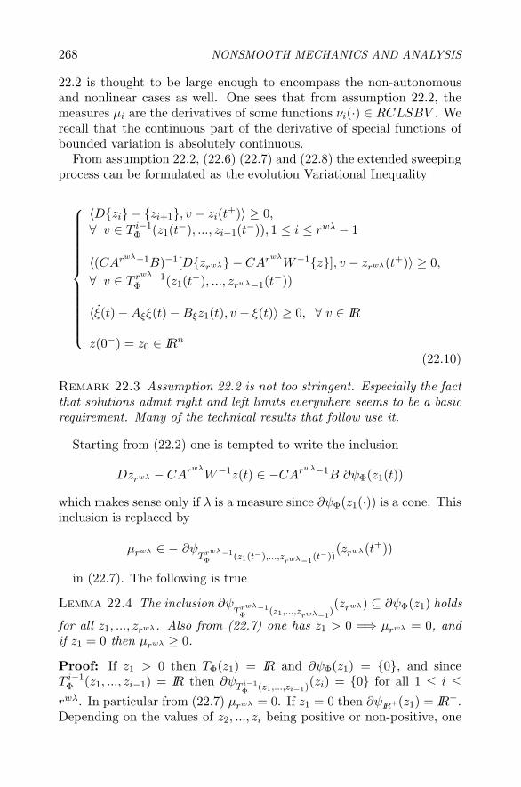
268 NONSMOOTH MECHANICS AND ANALYSIS
22.2 is thought to be large enough to encompass the non-autonomousand nonlinear cases as well. One sees that from assumption 22.2, themeasures μi are the derivatives of some functions νi(·) ∈ RCLSBV . Werecall that the continuous part of the derivative of special functions ofbounded variation is absolutely continuous.
From assumption 22.2, (22.6) (22.7) and (22.8) the extended sweepingprocess can be formulated as the evolution Variational Inequality
⎧⎪⎪⎪⎪⎪⎪⎪⎪⎪⎪⎪⎪⎨⎪⎪⎪⎪⎪⎪⎪⎪⎪⎪⎪⎪⎩
〈D{zi} − {zi+1}, v − zi(t+)〉 ≥ 0,
∀ v ∈ T i−1Φ (z1(t−), ..., zi−1(t−)), 1 ≤ i ≤ rwλ − 1
〈(CArwλ−1B)−1[D{zrwλ} − CArwλW−1{z}], v − zrwλ(t+)〉 ≥ 0,
∀ v ∈ T rwλ−1Φ (z1(t−), ..., zrwλ−1(t−))
〈ξ(t)−Aξξ(t)−Bξz1(t), v − ξ(t)〉 ≥ 0, ∀ v ∈ IR
z(0−) = z0 ∈ IRn
(22.10)
Remark 22.3 Assumption 22.2 is not too stringent. Especially the factthat solutions admit right and left limits everywhere seems to be a basicrequirement. Many of the technical results that follow use it.
Starting from (22.2) one is tempted to write the inclusion
Dzrwλ − CArwλW−1z(t) ∈ −CArwλ−1B ∂ψΦ(z1(t))
which makes sense only if λ is a measure since ∂ψΦ(z1(·)) is a cone. Thisinclusion is replaced by
μrwλ ∈ − ∂ψT rwλ−1Φ (z1(t−),...,z
rwλ−1(t−))
(zrwλ(t+))
in (22.7). The following is true
Lemma 22.4 The inclusion ∂ψT rwλ−1Φ (z1,...,z
rwλ−1)(zrwλ) ⊆ ∂ψΦ(z1) holds
for all z1, ..., zrwλ. Also from (22.7) one has z1 > 0 =⇒ μrwλ = 0, andif z1 = 0 then μrwλ ≥ 0.
Proof: If z1 > 0 then TΦ(z1) = IR and ∂ψΦ(z1) = {0}, and sinceT i−1
Φ (z1, ..., zi−1) = IR then ∂ψT i−1Φ (z1,...,zi−1)(zi) = {0} for all 1 ≤ i ≤
rwλ. In particular from (22.7) μrwλ = 0. If z1 = 0 then ∂ψIR+(z1) = IR−.Depending on the values of z2, ..., zi being positive or non-positive, one

Higher order Moreau’s sweeping process 269
may have ∂ψT iΦ(z1,...,zi)
(zi+1) = IR− or ∂ψT iΦ(z1,...,zi)
(zi+1) = {0} for all1 ≤ i ≤ rwλ−1. Indeed assume that z1 = z2 = ... = zj = 0 and zj+1 > 0(this implies that z $ 0). Then (Φ) = T 0
Φ(z1) = TΦ(z1) = T 2Φ(z1, z2) =
T 3Φ(z1, z2, z3) = ... = T j
Φ(z1, ..., zj) = IR+. And T j+1Φ (z1, ..., zj+1) =
T j+2Φ (z1, ..., zj+2) = ... = T rrλ−1
Φ (z1, ..., zrwλ−1) = IR. This can be seensince for instance T j+2
Φ (z1, ..., zj+2) = TT j+1Φ (z1,...,zj+1)
(zj+2) = TIR(zj+2) =
IR because also T j+1Φ (z1, ..., zj+1) = TIR+(zj+1) = IR. Consequently
∂ψT iΦ(z1,...,zi)
(zi+1) = IR− for all 0 ≤ i ≤ j, whereas ∂ψT iΦ(z1,...,zi)
(zi+1) ={0} for j + 1 ≤ i ≤ rwλ − 1. We conclude that under such conditionsμi ≥ 0 for all 1 ≤ i ≤ j + 1, and μi = 0 for all j + 2 ≤ i ≤ rwλ.Consequently μrwλ ≥ 0 when z1 = 0. The inclusion is also proved.
Lemma 22.5 The distribution Dz1 in (22.5) (22.7) is of degree ≤ 2, sothat z1(·) is a function of time and the zero-dynamics is an ODE (i.e.Dξ = dξ
dt (t)). Also λ has degree ≤ rwλ + 1.
Proof: From (22.7) μ1 has degree ≤ 2 so from (22.5) and (22.8) theresult follows.
The following lemmas prove that the extended sweeping process in-clusion defines a well-posed state jump mapping.
Lemma 22.6 From (22.4) (22.5) (22.7) we get for all 1 ≤ i ≤ rwλ − 1and all t ≥ 0,
zi+1(t+)− zi+1(t−) ∈ −∂ψT iΦ(z1(t−),...,zi(t−))(zi+1(t+))(a)
%
zi+1(t+) = prox[T i
Φ(z1(t−), ..., zi(t−)); zi+1(t−)]
(b)
(22.11)
Proof: The proof starts by noting that (22.5) is an equality of dis-tributions, and that at state jump times, Dzi is a distribution of degreestrictly larger than zi+1(·) which is a function (Ferreira (1997), Theo-rem 1.1). Equaling distributions of same degree results in (22.11) (a)(see (Brogliato, 1999, §1.1) for such a reasoning in the case of distribu-tions of degree ≤ 2). The rest of the proof is a direct consequence ofthe equivalence −x + y ∈ ∂ψK(x) ⇐⇒ x = prox[K; y] (Rockafellar andWets, 1998, Example 10.2) (Brezis, 1973, Example 2.8.2), where K is anonempty convex set, and prox[K; y] denotes the closest vector to y inK (i.e. the projection of y on K).

270 NONSMOOTH MECHANICS AND ANALYSIS
Remark 22.7 The proximation operation in (22.11) (b) is used here inthe sense of (Moreau, 1963), i.e. proxfz is the point where the functionu → 1
2 ||z − u||2 + f(u) attains its minimum value. When f(·) = ψK(·),then proxfz = prox[K; z].
This shows that jumps are automatically taken into account by thedynamics as it is written in (22.4)-(22.5)-(22.7). We notice also that thelower triangular structure of the tangent cones which appear in (22.7)merely reflects the way the measures μi appear in (22.5). We also have
Lemma 22.8 Let m ≥ 1.Let us assume that CArwλ−1B = (CArwλ−1B)T > 0. Then for all t ≥ 0,
−zrwλ(t+) + zrwλ(t−) ∈ CArwλ−1B ∂ψT rwλ−1Φ (z1(t−),...,z
rwλ−1(t−))
(zrwλ(t+))
%
zrwλ(t+) = prox(CArwλ−1B)−1
[T rwλ−1
Φ (z1(t−), ..., zrwλ−1(t−)); zrwλ(t−)]
(22.12)and these generalized equations possess the same unique solution zrwλ(t+)for any zrwλ(t−).
Corollary 22.9 Let the solution of (22.4) (22.5) (22.7) exist on a timeinterval [τ, τ+ε] and assumption 22.2 holds. Then zi(t+) ∈ T i−1
Φ (z1(t−), ..., zi−1(t−))for all 2 ≤ i ≤ rwλ, and 0 ≤ z1(t+) ⊥ μrwλ(t) ≥ 0 for all t ∈ [τ, τ + ε].
Proof: From lemmas 22.4, 22.6 and 22.8, and also from assumption22.2 which implies that solutions have right and left limits everywherein [τ, τ + ε]. Indeed from lemma 22.4 we have that z1 > 0 =⇒ μrwλ = 0,and if z1 = 0 then μrwλ ≥ 0. Let us assume now that μrwλ(t) > 0. Thisimplies that ∂ψ
T rwλ−1Φ (z1(t−),...,z
rwλ−1(t−))
(zrwλ(t+)) = IR+ which in turn
implies that z1(t−) ≤ 0 from the definition of the tangent cones (see alsothe developments in the proof of lemma 22.4). Now from lemma 22.6 itfollows that z1(t+) ≥ 0 for all t ∈ [τ, τ +ε] since z1(t+) = prox[Φ; z1(t−)].We deduce that in fact if μrwλ > 0 then z1(t+) = 0. Thus 0 ≤ z1(t+) ⊥μrwλ(t) ≥ 0. The assertion zi(t+) ∈ T i−1
Φ (z1(t−, ..., zi−1(t−)) is a conse-quence of (22.11) and (22.12): right limits, which by assumption exist,belong to the tangent cones.
This result (which is also a consequence of the inclusion in lemma22.4 and of (22.7) with i = rwλ) implies that on intervals [τ, τ + ε),ε > 0, on which z1(t) = 0, the inclusion (22.4)-(22.5)-(22.7) implies theexistence of a multiplier λ(t) = μrwλ(t) that belongs to−∂ψIR+(0) = IR+,

Higher order Moreau’s sweeping process 271
equivalently which satisfies 0 ≤ z1(t+) ⊥ λ(t) ≥ 0 and is the solution ofthe linear complementarity problem (LCP)
0 ≤ λ(t) ⊥ CArwλW−1z(t) + CArwλ−1Bλ(t) ≥ 0 (22.13)
Equivalently, μrwλ is the sum of an atomic measure dμrwλ , supp(dμrwλ) ⊂{t| z1(t) = 0}, that corresponds to jumps in zrwλ(·) and whose magni-tude is the solution of the LCP in (22.12), and of a Lebesgue measuregrwλ(t)dt where grwλ(t) is the solution of the LCP in (22.13). In corol-lary 22.9, the complementarity condition 0 ≤ z1(t+) ⊥ μrwλ(t) ≥ 0 canequivalently be written as 0 ≤ z1(t+) ⊥ grwλ(t) ≥ 0, since the comple-mentarity holds at the right limit z1(+). Similarly μi = gi(t)dt + dμi forall 1 ≤ i ≤ rwλ, with supp(dμi) ⊂ {t| z1(t) = 0}. On [τ, τ + ε) one hasgi(t) = 0 for all 1 ≤ i ≤ rwλ−1, as can easily be deduced from z1(t) ≡ 0.We thus have proved the following
Lemma 22.10 Consider the extended sweeping process dynamics (22.4)(22.5) (22.7) and let assumption 22.2 hold. Then gi(t) = 0 for all 1 ≤i ≤ rwλ − 1 and almost all t ≥ 0, whereas grwλ(t) is the solution of theLCP in (22.13).
Lemma 22.11 The following inclusion holds
∂ψT i−1Φ (z1,...,zi−1)(zi) ⊆ ∂ψT i−2
Φ (z1,...,zi−2)(zi−1) = NT i−2Φ (z1,...,zi−2)(zi−1)
(22.14)for all 1 ≤ i ≤ rwλ.
Proof: Let z1 = z2 = ... = zj = 0 and zj+1 > 0. Then as alreadyshown in the proof of lemma 22.4, one has ∂ψT i
Φ(z1,...,zi)(zi+1) = IR− for
all 0 ≤ i ≤ j, and ∂ψT iΦ(z1,...,zi)
(zi+1) = {0} for all j + 1 ≤ i ≤ rwλ − 1.So one sees that in particular it always holds that ∂ψT k
Φ(z1,...,zk)(zk+1) ⊆∂ψT k−1
Φ (z1,...,zk−1)(zk) for any 1 ≤ k ≤ rwλ − 1.
Corollary 22.12 The operators zi(t+) → −μi, 1 ≤ i ≤ rwλ, in (22.7)are maximal monotone.
Proof: These operators can be rewritten as the following cone CP
T i−1Φ (z1(t−), ..., zi−1(t−)) � zi(t+) ⊥
− μi ∈ ∂ψT i−1Φ (z1(t−),...,zi−1(t−))(zi(t+)) (22.15)
Since from lemma 22.11 we have
∂ψT i−1Φ (z1(t−),...,zi−1(t−))(zi(t+)) ⊆ NT i−2
Φ (z1(t−),...,zi−2(t−))(zi−1(t+)

272 NONSMOOTH MECHANICS AND ANALYSIS
the cones in both sides of (22.15) are closed polar convex cones. Con-sequently the operators that correspond to these cone CPs are maximalmonotone.
We notice that from (22.15) we get
TΦ(z1(t−)) � z2(t+) ⊥ −μ2 ∈ ∂ψTΦ(z1(t−))(z2(t+)) ⊆ NΦ(z1(t+))
It is also noteworthy that from corollary 22.9 one gets that the opera-tor −μrwλ → z1(t+) is also maximal monotone. Hence our frameworkcontains that of the sweeping process for Lagrangian systems (Moreau,1988).
3. Numerical time integration schemeThis section addresses the problem of the numerical time integration
of complementarity dynamical systems with arbitrary relative degree.Particularly, it is shown how one can take advantage of the formalismin (22.4)-(22.7) to design a time-stepping scheme, i.e, a time integrationscheme without explicit event handling procedure.
A naive way to design a time-stepping scheme for non smooth systemsis to apply a backward Euler method to the dynamical equation and todiscretize the complementarity condition in a fully implicit way. Oneobtains for the system (22.1) the following discretized system:⎧⎪⎨⎪⎩
xk+1 − xk
h= Axk+1 + Bλk+1
wk+1 = Cxk+1 + Dλk+1
0 ≤ λk+1 ⊥ wk+1 ≥ 0
(22.16)
where h is the constant time step of a subdivision {tk} of the time interval[0, T ] and the subscript k denotes the approximation of a value at timetk.
A straightforward substitution of wk+1 in the complementarity condi-tion leads to solve the following complementarity problem at each step:
0 ≤ λk+1 ⊥ C(I − hA)−1xk + hC(I − hA)−1Bλk+1 ≥ 0 (22.17)
For the linear complementarity systems, some sufficient conditions forconsistency and convergence of this backward Euler scheme have beengiven in (Camlibel, 2002). They also exhibit several examples for whichthe scheme does not work at all. Let us consider one of these examples,introduced in (Camlibel, 2001, Example 6.3.3), where the system (22.1)

Higher order Moreau’s sweeping process 273
is defined by
A =
⎡⎣ 0 1 00 0 10 0 0
⎤⎦ ; B =
⎡⎣ 001
⎤⎦ ; C =[
1 0 0]; x0 =
⎡⎣ 0−1
0
⎤⎦(22.18)
In this example, the relative degree rwλ is equal to 3 (D = 0, CB =0, CAB = 0, CA2B �= 0). Using the time discretization defined above,we can remark that:
limh−→0
hC(I − hA)−1B = 0 (22.19)
It is clear that if the time step h vanishes, which may be needed in manypractical cases or for the convergence analysis purpose, then the LCPmatrix in (22.17) has little chance to be well conditioned due to the factthat CB = 0. Furthermore, the numerical solution is given by
xk =
⎡⎣ k(k+1)hk1h
⎤⎦ ,∀k ≥ 1; λ1 =1h2
; λk = 0,∀k ≥ 2 (22.20)
which cannot converge towards a solution when h vanishes.In fact, the backward Euler scheme is only consistent for the systems of
relative degree, rwλ ≤ 1. Indeed, we can construct easily many examplesof inconsistency with systems of relative degree equal to two.
A similar time-stepping method has been introduced in (Moreau,1977) for a mathematical analysis purpose of the existence of solution forthe first order sweeping process. For systems of relative degree equal totwo, such as Lagrangian mechanical systems with unilateral constraints,Moreau (Moreau, 1988) introduces the Contact Dynamics method whichextends the simple Euler method when some discontinuities may be en-countered in the first time derivative of the state. Although the resultingscheme seems to be very close to a standard Euler scheme, there are sev-eral slight, but fundamental differences based on a sound mathematicalanalysis of Moreau about the nature of the solution. For the Lagrangiansystems, majors lessons of this seminal work may be stated as follows:
the use of a differential measure associated with a function ofbounded variation leads to a first order approximation given di-rectly by the integration of the differential measure,
the use of finite values, as primary unknowns, such as velocity andimpulse. This feature allows one to capture the discontinuitieswhen the time step vanishes,

274 NONSMOOTH MECHANICS AND ANALYSIS
the reformulation of constraints in terms of velocity associatedwith a viability lemma to ensure the satisfaction of the positionconstraint.
In the next section, we propose a time-stepping scheme based on theseremarks, which is able to integrate in time linear complementarity prob-lems of any relative degree.
3.1 The proposed numerical schemeThe proposed numerical scheme is based on the ZD dynamical form
written in terms of measures (22.6). Let us consider a subdivision {tk}of the interval [0, T ]. The time integration of the differential measure on]tk, tk+1] is given by∫
]tk,tk+1]D{zi} = zi(t+k+1)− zi(t+k ) (22.21)
and we pose as a primary unknown the right value of the non singularpart of zi such that zi,k = zi(t+k ) (recall that z(t) or {z} denote the nonsingular part of the distribution z). These remarks leads to the followingnumerical integration rule for a generic line of the system (22.6):∫
]tk,tk+1]D{zi} = zi,k+1 − zi,k =
∫]tk,tk+1]
{zi+1} dt +∫
]tk,tk+1]μi(22.22)
≈ hzi+1,k+1 +∫
]tk,tk+1]μi (22.23)
In order to manipulate only finite values, this second unknown, which isthe multiplier corresponding to μi, is defined as:
ri,k+1 =∫
]tk,tk+1]μi (22.24)
and we assume that:
ri,k+1 ∈ −∂ψT i−1Φ (z1,k,...,zi−1,k)(zi,k+1) for all 1 ≤ i ≤ rwλ (22.25)
The approximation of zi(t−) in the inclusion (22.7) by zi,k is a basicchoice. The operation can be viewed as a prediction of the state before adiscontinuity. More accurate prediction may be performed using higherorder derivatives, if exist, of zi(t−). Finally, the proposed discretization

Higher order Moreau’s sweeping process 275
scheme may be summarized as follows:⎧⎪⎪⎪⎪⎪⎪⎪⎪⎪⎪⎪⎪⎪⎪⎪⎪⎨⎪⎪⎪⎪⎪⎪⎪⎪⎪⎪⎪⎪⎪⎪⎪⎪⎩
z1,k+1 − z1,k = hz2,k+1 + r1,k+1
z2,k+1 − z2,k = hz3,k+1 + r2,k+1...zi,k+1 − zi,k = hzi+1,k+1 + ri,k+1...zrwλ,k+1 − zrwλ,k = hCArwλ
W−1zk+1 + CArwλ−1Brrwλ,k+1
ξk+1 − ξk = hAξξk+1 + hBξz1,k+1
ri,k+1 ∈ −∂ψT i−1Φ (z1,k,...,zi−1,k)(zi,k+1) for all 1 ≤ i ≤ rwλ
(22.26)If Φ = IR+, the inclusion (22.25) implies a sequence of unilateral con-
straints on zi,k to be satisfied. If the integer j is the first for which zj,k ispositive, then the system (22.26) is reduced to a linear complementarityproblem involving zi,k+1, ri,k+1 for all i, 1 ≤ i ≤ j.
3.2 Numerical examplesWe illustrate in this part the ability of the scheme to solve the prelim-
inary example. The numerical solution given by the scheme (22.26) forthe initial condition z0 = [0;−1; 0]T is given by zk = [0; 0; 0]T ,∀k ≥ 1and r2, 1 = 1, r2, k = 0, ∀k ≥ 2. The Figure 22.1 depicts a similar resultwith the initial condition zT
0 = (1,−1, 0).
-1.5
-1
-0.5
0
0.5
1
1.5
0 0.5 1 1.5 2
Val
ues
of x
Time t
z(1)z(2)z(3)
-1.5
-1
-0.5
0
0.5
1
1.5
0 0.5 1 1.5 2
Val
ues
of r
Time t
r(1)r(2)r(3)
Figure 22.1. EMSP scheme – Initial data z(0−)T = (1,−1, 0)
AcknowledgmentsThe authors wish to thank Daniel Goeleven (IREMIA, university of
La Reunion, France) for useful comments on their work. This work

276 NONSMOOTH MECHANICS AND ANALYSIS
was partially supported by the European project SICONOS IST-2001-37172.
ReferencesJ. Campos Ferreira, Introduction to the Theory of Distributions, Pit-
man Monographs and Surveys in Pure and Applied Mathematics, 87,Addison Wesley Longman Limited, 1997.
H. Brezis, 1973 Operateurs Maximaux Monotones et Semi-groupes deContraction dans les Espaces de Hilbert, North-Holland Publishing,Amsterdam.
J.J. Moreau, “Les liaisons unilaterales et le principe de Gauss”, CRASParis, t.256 (1963), pp.871-874.
J.J. Moreau, Evolution problem associated with a moving convex set ina Hilbert space, J. Differential Equations, 26 (1977), pp.347-374.
J.J. Moreau, “Unilateral contact and dry friction in finite freedom dy-namic”, CISM Courses and Lectures no 302 (1988), International Cen-ter for Mechanical Sciences, J.J. Moreau and P.D. Panagiotopoulos(Eds.), Springer-Verlag, pp.1-82.
M.D.P. Monteiro Marques, Differential Inclusions in Nonsmooth Me-chanical Problems, Shocks and Dry Friction, Birkhauser, Progress inNonlinear Differential Equations and Their Applications, 1993.
P. Sannuti, “Direct singular perturbation analysis of high-gain and cheapcontrol problems”, Automatica, vol.19 (1983), no 1, pp.41-51.
K. Camlibel, Complementarity Methods in the Analysis of Piecewise Lin-ear Dynamical Systems, PhD thesis, Katholieke Universiteit Brabant,ISBN: 90 5668 073X (2001).
K. Camlibel, W.P.M.H. Heemels, J.M. Schumacher, Consistency of atime-stepping method for a class of piecewise-linear networks, IEEETransactions on Circuits and Systems I, vol.49 (2002), pp.349-357.
S.L. Campbell and W. Gear. The index of general nonlinear DAEs. Nu-merische Mathematik, 72:173–196, 1995.
R.F. Hartl, S.P. Sethi, R.G. Vickson, A survey of the maximum princi-ples for optimal control problems with state constraints, SIAM Review,vol.37 (1995), no 2, pp.181-218.
E.D. Sontag, Mathematical Control Theory; Deterministic Finite Di-mensional Systems, Springer Texts in Applied Mathematics 6, secondedition, 1998.
R.T. Rockafellar, R.J.B. Wets, 1998 Variational Analysis, Springer, Grun-dlehren der mathematischen Wissenschaften, vol.317.

Higher order Moreau’s sweeping process 277
P. Ballard, “The dynamics of discrete mechanical systems with perfectunilateral constraints”, Arch. Rational Mech. Anal., vol.154 (2000),no 3, pp.199-274.
B. Brogliato, Nonsmooth Mechanics, Second edition, Springer VerlagLondon, 1999.

Chapter 23
AN EXISTENCE RESULT INNON-SMOOTH DYNAMICS
Manuel D.P. Monteiro MarquesCMAF and Faculdade de Ciencias, Universidade de Lisboa, 2, Av Prof. Gama Pinto,1649-003 Lisboa, [email protected]
Laetitia PaoliUniversite de Saint-Etienne, 23 rue Michelon, 42023 Saint Etienne Cedex 2, [email protected]
Abstract Starting in 1983, Jean Jacques Moreau gave remarkable new formula-tions of the dynamics of mechanical systems submitted to inelastic orfrictional contact as measure-differential inclusions. This paved the wayto proofs of existence of solutions, by the first author, in 1985 for thecase of standard inelastic shocks and in 1988 for frictional dynamics,both for one contact problems. These mathematical theoretical resultsleft out many other situations, that could be handled numerically byJ.J. Moreau and collaborators in a very effective way, as well as thePainleve example. Here we present a generalization of such existenceresults to variable mass matrices and non isotropic friction.
Keywords: Unilateral constraint, friction, non trivial mass matrix, measure differ-ential inclusion, velocities with bounded variation, time-discretizationscheme.
IntroductionWe consider a mechanical system with a finite number of degrees
of freedom subjected to a single unilateral constraint. Using generalizedcoordinates, the system is represented by a point q ∈ IRd and the motionis described by a function q : I → IRd with I = [0, T ], T > 0. The

280 NONSMOOTH MECHANICS AND ANALYSIS
unilateral constraint is expressed by an inequality f(q) ≤ 0 and thus
q(t) ∈ L = {q ∈ IRd; f(q) ≤ 0} ∀t ∈ I (23.1)
where f ∈ C1(IRd; IR) such that ∇f does not vanish in a neighbourhoodof the hypersurface S = {q ∈ IRd; f(q) = 0}.
Since we expect discontinuous velocities when f(q(t)
)= 0, an appro-
priate functional framework is to look for a motion q such that q is a func-tion of bounded variation, see (Schatzman, 1978, Moreau, 1983, Moreau,1985, Moreau, 1986, Moreau, 1988). It follows that q has right and leftlimits, q+ and q−, for all t ∈ (0, T ). Moreover, denoting u = q+, we canintroduce the Stieltjes measure du = dq and the dynamics is describedby
q(t) = q0 +∫ t
0u(s) ds ∀t ∈ I (23.2)
andM(q)du = g
(t, q,M(q)u
)dt + dr (23.3)
where M is the mass matrix of the system and dr is a measure describ-ing the reaction when the constraint is active. Using Radon-Nikodym’stheorem we can rewrite (23.3) as follows
M(q)u′μ = g
(t, q,M(q)u
)t′μ + r′μ dμ a.e.
where μ is a positive measure such that du, dt and dr are absolutelycontinuous with respect to dμ (we can choose dμ = |du|+dt for instance)and u′
μ, t′μ and r′μ are the densities of du, dt and dr with respect to dμ,see (Moreau, 1985) and (Moreau, 1988) for instance.
The reaction dr and the transmission of the velocities at impacts (i.ewhen f
(q(t)
)= 0) can be described more precisely if we know whether
the constraint is perfect or not. In both cases, there exists a subset R(q)of IRd such that
r′μ ∈ R(q(t)
)dμ a.e. (23.4)
and an impact law relating q+, q− and dr.In order to obtain existence results for this kind of problem, we study
the convergence of a sequence of approximants (qn, un)n≥0 of the form⎧⎨⎩ qn(t) = q0 +∫ t
0un(s) ds ∀t ∈ I
un(t) = uin ∀t ∈ [tin, ti+1
n [, 0 ≤ i ≤ 2n − 1(23.5)
with
tin = iT
2n0 ≤ i ≤ 2n, ∀n ≥ 0
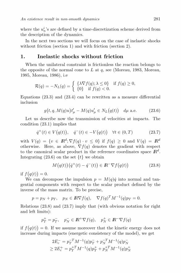
An existence result in non-smooth dynamics 281
where the uin’s are defined by a time-discretization scheme derived from
the description of the dynamics.In the next two sections we will focus on the case of inelastic shocks
without friction (section 1) and with friction (section 2).
1. Inelastic shocks without frictionWhen the unilateral constraint is frictionless the reaction belongs to
the opposite of the normal cone to L at q, see (Moreau, 1983, Moreau,1985, Moreau, 1986), i.e
R(q) = −NL(q) ={{λ∇f(q);λ ≤ 0} if f(q) ≥ 0,{0} if f(q) < 0.
Equations (23.3) and (23.4) can be rewritten as a measure differentialinclusion
g(t, q,M(q)u
)t′μ −M(q)u′
μ ∈ NL
(q(t)
)dμ a.e. (23.6)
Let us describe now the transmission of velocities at impacts. Thecondition (23.1) implies that
q+(t) ∈ V(q(t)
), q−(t) ∈ −V
(q(t)
)∀t ∈ (0, T ) (23.7)
with V (q) = {v ∈ IRd;∇f(q) · v ≤ 0} if f(q) ≥ 0 and V (q) = IRd
otherwise. Here, as above, ∇f(q) denotes the gradient with respectto the canonical scalar product in the reference coordinates space IRd.Integrating (23.6) on the set {t} we obtain
M(q(t)
)(q+(t)− q−(t)
)∈ IR−∇f
(q(t)
)(23.8)
if f(q(t)
)= 0.
We can decompose the impulsion p = M(q)q into normal and tan-gential components with respect to the scalar product defined by theinverse of the mass matrix. To be precise,
p = pN + pT , pN ∈ IR∇f(q), ∇f(q)T M−1(q)pT = 0.
Relations (23.8) and (23.7) imply that (with obvious notation for rightand left limits):
p+T = p−T , p−N ∈ IR+∇f(q), p+
N ∈ IR−∇f(q)
if f(q(t)
)= 0. If we assume moreover that the kinetic energy does not
increase during impacts (energetic consistency of the model), we get
2E−c = p−T
T M−1(q)p−T + p−TN M−1(q)p−N
≥ 2E+c = p+T
T M−1(q)p+T + p+T
N M−1(q)p+N

282 NONSMOOTH MECHANICS AND ANALYSIS
and thus the impact law is given by
p+N = −ep−N , p+
T = p−T
with a restitution coefficient e ∈ [0, 1], which is equivalent to
q+(t) = q−(t)−(1+e)∇f
(q(t)
)· q−(t)
∇f(q(t)
)TM−1
(q(t)
)∇f
(q(t)
)M−1(q(t)
)∇f
(q(t)
)(23.9)
if f(q(t)
)= 0.
Following J.J.Moreau (Moreau, 1983, Moreau, 1985), we consider nowthe case of inelastic shocks i.e e = 0. The impact law (23.9) can then berewritten as
q+(t) = proxq(t)
(q−(t), V
(q(t)
))if f
(q(t)
)= 0 (23.10)
where proxq
(v, V (q)
)denotes the projection (or “proximal point” of the
vector v on the convex set V , relatively to the kinetic metric at q de-fined by the mass matrix M(q). Observing that V
(q(t)
)is the set of
admissible right velocities for the system at time t, equation (23.10) canbe interpreted as a minimization principle.
Moreover, taking into account the impact law, we can rewrite equation(23.6) as follows
−r′μ = g(t, q,M(q)u
)t′μ −M(q)u′
μ ∈ ∂ψV(q(t)
)(u(t))
dμ a.e. (23.11)
where ψV (q) denotes the indicator function of V (q) and ∂ψV (q) is itssubdifferential.
Indeed, given the definition of V (q), we have ∂ψV(q(t)
)(u(t))⊂ NL
(q(t)
)for all t and, if the velocity is discontinuous at time t, we have q(t) ∈ ∂Land
−dr({t}
)= M
(q(t)
)(q+(t)− q−(t)
)∈ ∂ψ
V(q(t)
)(q+(t)),
hence
q+(t) = proxq(t)
(q−(t), V
(q(t)
)),
which gives again equations (23.6) and (23.9). For a more rigourousstudy of the equivalence of the two formulations see (Paoli, 2001).
Starting from (23.11) we propose the following time-discretizationscheme:
qi+1n = qi
n + huin, (23.12)

An existence result in non-smooth dynamics 283
ui+1n = proxqi+1
n
(ui
n + hM−1(qi+1n )g
(ti+1n , qi+1
n ,M(qi+1n )ui
n
), V (qi+1
n ))
(23.13)for all i ∈ {0, . . . , 2n − 1}, n ≥ 0, with an appropriate initialization forq0n and u0
n, see (Monteiro Marques, 1985, Monteiro Marques, 1993).The construction of this scheme is based on the following idea. With-
out constraint, the dynamics is described by the second order ODE
M(q)q = g(t, q,M(q)q
)and the velocity at ti+1
n can be approximated by
u′i+1n = ui
n + hM−1(qi+1n )g
(ti+1n , qi+1
n ,M(qi+1n )ui
n
).
This velocity can be considered as a left velocity at ti+1n for the con-
strained system and (23.13) is obtained by applying a discretized formu-lation of the impact law (23.10).
The convergence of the approximate motions (qn, un)n≥0 given by(23.5) and (23.12)-(23.13) has been proved in (Monteiro Marques, 1985),see also (Monteiro Marques, 1993), when the mass matrix is trivial (i.eM(q) = IdIRd for all q), ∇f is Lipschitz continuous and g is a continuousfunction of t and q, uniformly bounded on I × IRd. A generalization ofthis result to the case of partially or totally elastic shocks (i.e e �= 0)has been obtained by M.Mabrouk (Mabrouk, 1998). In this paper thefunction g may depend also on q but the assumption of a trivial massmatrix still holds.
2. Inelastic shocks with friction
2.1 Isotropic Coulomb frictionIn this subsection we assume for simplicity that the mass matrix of
the system is equal to IdIRd and that the classical Coulomb’s law offriction holds. When the constraint is active, the set of reactions R(q)is then a revolution cone C(q) revolving about the inward normal to Lat q, denoted n(q), with an angle α(q) ∈ (0, π/2) i.e
R(q) ={
C(q) ={v ∈ IRd; v · n(q) ≥ ‖v‖ cos α(q)
}if f(q) ≥ 0,
{0} if f(q) < 0.
Moreover, if f(q(t)
)= 0, we have the following alternative, see (Moreau,
1986, Moreau, 1988)• if u(t) · ∇f
(q(t)
)< 0 there is no reaction,
• if u(t)·∇f(q(t)
)= 0 then, if the reaction belongs to Int
(C(q(t)
))we
have u(t) = 0, otherwise u(t) is in the opposite direction of the tangentialpart of the reaction.

284 NONSMOOTH MECHANICS AND ANALYSIS
Using the density r′μ, we obtain dμ-a.e.
• if f(q(t)
)< 0 then r′μ = 0, (23.14)
• if f(q(t)
)= 0 and u(t) · ∇f
(q(t)
)< 0, then r′μ = 0, (23.15)
• if f(q(t)
)= 0 and u(t) · ∇f
(q(t)
)= 0, then
−u(t) ∈ projT(q(t)
)NC(q(t)
)(r′μ(t))
(23.16)
where T(q(t)
)= V
(q(t)
)∩
(−V
(q(t)
)). When the velocity is discontin-
uous at time t, the measure dr has a Dirac equal to(q+(t) − q−(t)
)δt
and (23.16) implies that
−u(t) ∈ projT(q(t)
)NC(q(t)
)(u(t)− q−(t)))
which is equivalent to
u(t) = prox(0,
(q−(t) + C
(q(t)
))∩ T
(q(t)
)). (23.17)
Using the same ideas as in the frictionless case, we propose the followingdiscretization:
qi+1n = qi
n + huin
u′i+1n = ui
n + hg(ti+1n , qi+1
n , uin
)ui+1
n = prox(0,
(u
′i+1n + C(qi+1
n ))∩ T (qi+1
n )),
for all i ∈ {0, . . . , 2n − 1}, n ≥ 0, with an appropriate initialization forq0n and u0
n, see (Monteiro Marques, 1993).The convergence of this discretization has been proved in (Monteiro
Marques, 1993) under the assumption that ∇f is Lipschitz continuous,g is a continuous function of t and q, uniformly bounded on I × IRd andα is a continuous function with values in (0, π/2).
2.2 GeneralizationWe consider now the case of a non trivial mass matrix and non
isotropic friction. The set of reactions R(q) is then a cone given by
R(q) ={
C(q) = IR+(n(q) + D1(q)
)if f(q) ≥ 0,
{0} if f(q) < 0,
where n(q) denotes once again the inward normal to L at q and D1(q) isa closed, bounded, convex subset of IRd such that n(q) �∈ span
(D1(q)
).
We assume moreover that
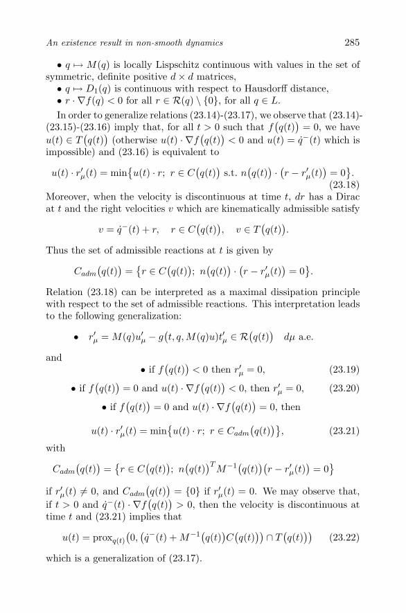
An existence result in non-smooth dynamics 285
• q → M(q) is locally Lispschitz continuous with values in the set ofsymmetric, definite positive d× d matrices,• q → D1(q) is continuous with respect to Hausdorff distance,• r · ∇f(q) < 0 for all r ∈ R(q) \ {0}, for all q ∈ L.In order to generalize relations (23.14)-(23.17), we observe that (23.14)-
(23.15)-(23.16) imply that, for all t > 0 such that f(q(t)
)= 0, we have
u(t) ∈ T(q(t)
)(otherwise u(t) · ∇f
(q(t)
)< 0 and u(t) = q−(t) which is
impossible) and (23.16) is equivalent to
u(t) · r′μ(t) = min{u(t) · r; r ∈ C
(q(t)
)s.t. n
(q(t)
)·(r − r′μ(t)
)= 0
}.
(23.18)Moreover, when the velocity is discontinuous at time t, dr has a Diracat t and the right velocities v which are kinematically admissible satisfy
v = q−(t) + r, r ∈ C(q(t)
), v ∈ T
(q(t)
).
Thus the set of admissible reactions at t is given by
Cadm
(q(t)
)=
{r ∈ C
(q(t)
); n
(q(t)
)·(r − r′μ(t)
)= 0
}.
Relation (23.18) can be interpreted as a maximal dissipation principlewith respect to the set of admissible reactions. This interpretation leadsto the following generalization:
• r′μ = M(q)u′μ − g
(t, q,M(q)u)t′μ ∈ R
(q(t)
)dμ a.e.
and• if f
(q(t)
)< 0 then r′μ = 0, (23.19)
• if f(q(t)
)= 0 and u(t) · ∇f
(q(t)
)< 0, then r′μ = 0, (23.20)
• if f(q(t)
)= 0 and u(t) · ∇f
(q(t)
)= 0, then
u(t) · r′μ(t) = min{u(t) · r; r ∈ Cadm
(q(t)
)}, (23.21)
with
Cadm
(q(t)
)=
{r ∈ C
(q(t)
); n
(q(t)
)TM−1
(q(t)
)(r − r′μ(t)
)= 0
}if r′μ(t) �= 0, and Cadm
(q(t)
)= {0} if r′μ(t) = 0. We may observe that,
if t > 0 and q−(t) · ∇f(q(t)
)> 0, then the velocity is discontinuous at
time t and (23.21) implies that
u(t) = proxq(t)
(0,
(q−(t) + M−1
(q(t)
)C(q(t)
))∩ T
(q(t)
))(23.22)
which is a generalization of (23.17).

286 NONSMOOTH MECHANICS AND ANALYSIS
For this problem we propose the following time-discretization:
qi+1n = qi
n + huin, (23.23)
u′i+1n = ui
n + hM−1(qi+1n )g
(ti+1n , qi+1
n ,M(qi+1n )ui
n
), (23.24)
ui+1n = proxqi+1
n
(0,
(u
′i+1n + M−1(qi+1
n )C(qi+1n )
)∩ T (qi+1
n )), (23.25)
for all i ∈ {0, . . . , 2n − 1}, n ≥ 0, with an appropriate initialization forq0n and u0
n.This scheme has already been implemented, see (Moreau, 1988, Jean
and Moreau, 1992). It is an alternative to and it allows more generalfriction cones than the scheme proposed by D.Stewart (Stewart, 1998).The study of the convergence of the approximate motions (qn, un)n≥0
defined by (23.5) and (23.23)-(23.25) is not yet finished but we can de-scribe here the main ideas. As in the previous cases, the proof is dividedin three main steps. First we establish a priori estimates for the discretevelocities and accelerations and using Ascoli-Arzela and Helly theoremswe pass to the limit. The ideas which yield these estimates are directlyinspired by (Monteiro Marques, 1993) and (Stewart, 1998) but, sincethe kinetic metric depends on the position q, a quadratic term appearsin the estimate of the discrete velocities and prevents us from directlyobtaining global estimates. Hence, we just get the convergence of asubsequence of (qn, un)n≥0 on [0, τ ], with τ ∈ (0, T ], i.e.
qn(t)→ q(t) uniformly on [0, τ ],un(t)→ v(t) for all t ∈ [0, τ ],
where v ∈ BV (0, τ ; IRd).Then we define u = v+ and, using the same techniques as in (Monteiro
Marques, 1993), we prove in the next step that
q(t) = q0 +∫ t
0u(s) ds ∈ L, u(t) ∈ V
(q(t)
)∀t ∈ [0, τ ]
and the measure dr = r′μdμ = u′μdμ− g
(t, q,M(q)u
)t′μdμ satisfies
r′μ(t) = 0 if f(q(t)
)< 0 or f
(q(t)
)= 0 and u(t) · n
(q(t)
)> 0, dμ a.e.
Moreover the classical properties of convex analysis combined with theweak-* convergence of measures lead to
r′μ ∈ R(q(t)
)dμ a.e.
and, by a global energy estimate, we can extend all these results to thewhole interval [0, T ].

An existence result in non-smooth dynamics 287
Finally, in the last step, we prove that the limit satisfies the frictionlaw (23.21) when f
(q(t)
)= 0. We consider separately several cases.
Case 1: q−(t) �∈ V(q(t)
).
Then the right velocity should be determined uniquely by (23.22).The main argument relies on a continuity property for the projectionoperator involved in relation (23.25) in a neighbourhood of q−(t).
Case 2: q−(t) ∈ T(q(t)
).
Then we can distinguish two subcases according to whether the ve-locity is continuous at time t or not.
Case 2.1: q−(t) = u(t).The idea is to prove that if r′μ(t) �= 0
−u(t) ∈ projT(q(t)
),q(t)
NC(q(t)
)(r′μ(t)),
(the orthogonal projection into T(q(t)
)being performed with respect
to the kinetic metric), which implies (23.21), by using the same “varia-tional” techniques as in (Monteiro Marques, 1993).
Case 2.2: q−(t) �= u(t).We observe first that this case can occur only if M−1
(q(t)
)C(q(t)
)∩
T(q(t)
)�= {0}, which corresponds to Painleve’s type cases, see (Painleve,
1905, Erdmann, 1994). Although the discretization is deterministic, itmay produce different solutions for this case, see (Moreau, 1988).
When span(D1
(q(t)
))is of dimension 1, which is the case studied in
(Stewart, 1998), we can prove that the limit satisfies Coulomb’s frictionlaw. If the dimension of span
(D1
(q(t)
))is greater than or equal to 2,
the question is still open.
AcknowledgmentsThis work has been partially supported by the European project
SICONOS IST-2001 37172 and M. M. Marques was partially supportedby FCT/POCTI/FEDER.
ReferencesErdmann M. On a representation of friction in configuration space, Int.
J. Robotics Research, 13(3):240–271, 1994.Mabrouk M. A unified variational model for the dynamics of perfect
unilateral constraints, Eur. J. Mechanics A/Solids, 17:819–842, 1998.Monteiro Marques M.D.P. Chocs inelastiques standards : un resultat
d’existence, Seminaire d’Analyse Convexe, Univ. Sci. Tech. Languedoc15, exp. 4, 1985.

288 NONSMOOTH MECHANICS AND ANALYSIS
Monteiro Marques M.D.P. Differential inclusions in non-smooth me-chanical problems: shocks and dry friction, Birkhauser, Boston PNLDE9, 1993.
Moreau J.J. Liaisons unilaterales sans frottement et chocs inelastiques,C.R. Acad. Sci. Paris, Serie II, 296:1473–1476, 1983.
Moreau J.J. Standard inelastic shocks and the dynamics of unilateralconstraints, In Unilateral problems in structural analysis, G.Del Piero& F.Maceri eds., pages 173–221, CISM courses and lectures 288, Sprin-ger-Verlag, New-York, 1985.
Moreau J.J. Dynamique de systemes a liaisons unilaterales avec frotte-ment sec eventuel, essais numeriques, preprint 85-1, LMGC Montpel-lier, 1986.
Moreau J.J. Unilateral contact and dry friction in finite freedom dy-namics, In Nonsmooth Mechanics and Applications, J.J.Moreau &P.D.Panagiotopoulos eds, pages 1–82, CISM courses and lectures 302,Springer-Verlag, New-York, 1988.
Jean M., and Moreau J.J. Unilaterality and dry friction in the dynamicsof rigid body collections, In Proceedings of Contact Mechanics Inter-national Symposium, A.Curnier ed., pages 31–48, PPUR, Lausanne,1992.
Painleve P. Sur les lois du frottement de glissement, C.R. Acad. Sci.Paris, 121:112–115, 1895 and 141:401–405 and 141:546–552, 1905.
Paoli L. Time-discretization of vibro-impact, Phil. Trans. Roy. Soc. Lon-don A, 359:2405–2428, 2001.
Schatzman M. A class of nonlinear differential equations of second orderin time, Nonlinear Anal.,Theory, Methods and Applications, 2:355–373, 1978.
Stewart D. Convergence of a time-stepping scheme for rigid body dy-namics and resolution of Painleve’s paradoxes, Arch. Rational Mech.Anal., 145:215–260, 1998.

Chapter 24
FINITE TIME STABILIZATIONOF NONLINEAR OSCILLATORS SUBJECTTO DRY FRICTION
Samir AdlyLaboratoire LACO, Universite de Limoges, 123 avenue Albert Thomas, 87060 LimogesCedex, [email protected]
Hedy AttouchLaboratoire ACSIOM, Universite Montpellier II, Place Eugene Bataillon, 34095 Mont-pellier Cedex 05, [email protected]
Alexandre CabotLaboratoire LACO, Universite de Limoges, 123 avenue Albert Thomas, 87060 LimogesCedex, [email protected]
Abstract Given a smooth function f : Rn → R and a convex function Φ : Rn → R,we consider the following differential inclusion:(S) x(t) + ∂Φ(x(t)) + ∇f(x(t)) � 0, t ≥ 0,where ∂Φ denotes the subdifferential of Φ. The term ∂Φ(x) is stronglyrelated with the notion of friction in unilateral mechanics. The trajec-tories of (S) are shown to converge toward a stationary solution of (S).Under the additional assumption that 0 ∈ int∂Φ(0) (case of a dry fric-tion), we prove that the limit is achieved in a finite time. This resultmay have interesting consequences in optimization.
Keywords: Dissipative dynamical system, differential inclusion, dry friction, finitetime convergence.

290 NONSMOOTH MECHANICS AND ANALYSIS
1. Introduction and notationThroughout the paper, H = Rn is equipped with the euclidean scalar
product 〈., .〉 and the corresponding norm | . |. Let f : Rn → R a functionof class C1 that we wish to minimize over Rn. A powerful method consistsin following the trajectories of a gradient-based dynamical system. If thedynamics is dissipative, the trajectories will hopefully converge toward acritical point of the potential f . In the past ten years, much attention hasbeen brought to the study of second-order in time dynamical systems.Because of the inertial aspects, the dynamics of such systems do notstop at each minimum point. These methods are endowed with betterexploration properties than first-order ones. Among them, let us quotethe “Heavy Ball with Friction” system:
(HBF ) x(t) + γ x(t) + ∇f(x(t)) = 0, t ≥ 0, γ > 0,
which has been initiated by Polyak (Polyack, 1964). Several authors haverecently studied the properties of the (HBF ) system (cf. Alvarez (Al-varez, 2000), Attouch-Goudou-Redont (Attouch et al., 2000)). The mainnumerical drawback of the (HBF ) method comes from the oscillatorybehaviour of the trajectory near the minimum. A first way to improvethe (HBF ) method consists in introducing a second-order informationon f via the hessian matrix. In mechanical terms, this amounts to re-placing the viscous friction −γ x by a hessian-driven one (and eventuallycombining both frictions). This approach has been studied by Attouch-Redont (Attouch and Redont, 2001) and Alvarez-Attouch-Bolte-Redont(Alvarez et al., 2002). Our point of view in this paper is quite dif-ferent and consists in strengthening the friction when the velocity xvanishes. This approach is inspired by mechanical models involving dryfriction. A very wide literature is devoted to the contact problems withCoulomb friction (see for example (Amassad and Fabre, 2003, Cadivelet al., 2000, Dumont et al., 2000, Eck and Jarusek, 2000, Han and So-fonea, 2002, Jean, 1988)). Let us recall that, in the one dimensionalsetting, the classical Coulomb friction is given by −α Sgn(x), whereα > 0 and Sgn is the set-valued sign function: Sgn(x) = 1 if x > 0,Sgn(x) = −1 if x < 0 and Sgn(0) = [−1, 1]. The multivalued func-tion Sgn coincides with the subdifferential of the function R � x→ |x|.These considerations lead us to study the following differential inclusion:
(S) x(t) + ∂Φ(x(t)) + ∇f(x(t)) � 0, t ≥ 0,
where ∂Φ denotes the subdifferential of the convex function Φ : Rn →R. Notice that in unilateral mechanics, the modelling by differentialinclusions has been initiated by Moreau (Moreau, 1977, Moreau, 1985)

Finite time stabilization of nonlinear oscillators 291
and has been intensively studied by many authors (Mabrouk, MonteiroMarques, 1993, Schatzman, 1978), to quote only some of them. Theformulation (S) allows to recover a large variety of friction models. Forexample, the function Φ = α | . | corresponds to the Coulomb frictionand on the other hand, Φ = γ | . |2/2 gives the viscous friction and theassociated (HBF ) system. Notice also that the function Φ = β | . |p/p(p ∈]1, 2[) generates an intermediate situation, which has been studiedby Amann-Dıaz (Amann and Dıaz, 2003) and Dıaz-Linan (Dıaz andLinan, 2001) under the terminology of “strong friction”.
The system (S) defined above may have interesting applications incognitive sciences and decision sciences (mathematical economy, gametheory,...). Indeed, the friction corresponds in this case to the cost ofchanging (cost of leaving a routine, cost of exploration by tests anderrors, cost of dissimilarity,...). The viscous friction is associated to aquadratic cost with respect to the distance to the rest position. Onthe other hand, the dry friction corresponds to a linear cost so that thechanges are relatively expensive. This last model may represent the iner-tial aspects of human behaviours. The introduction of costs of changingis an important characteristic of the theory of bounded rationality, cf.(Conlisk, 1996, Rubinstein, 1998, Sobel, 2000).
For any couple of initial conditions, the inclusion (S) is shown to ad-mit a unique solution x : [0, +∞[→ Rn of class C1 satisfying (S) almosteverywhere. The behaviour at infinity of the (S) trajectory essentiallydepends on the nature of the friction term Φ near the origin. When∂Φ(0) = {0}, the gradient ∇f(x(t)) tends to 0 when t tends to +∞;however the convergence of the trajectories may not hold without fur-ther assumptions on f (like convexity or analyticity). On the otherhand, when the friction is dry, i.e. 0 ∈ int∂Φ(0) the convergence of thetrajectories automatically holds. The main result of the paper consistsin showing that the limit is achieved in a finite time (see Theorem 24.8).Such a limit x∗ is a solution of the inclusion: −∇f(x∗) ∈ ∂Φ(0), i.e. x∗
is a stationary solution of (S). Since our goal is to minimize f , we mustchoose a function Φ having a “small” subdifferential set ∂Φ(0), so asto force the trajectories to converge close to the “exact” critical points.In the various contexts recalled above (mechanics, cognitive sciences,...),the finite time stabilization of the system is meaningful. Such a result infinite dimension opens interesting perspectives concerning similar resultsfor mechanical and physical systems with infinite degrees of freedom.
The paper is organized as follows. In section 2, we state the existenceand uniqueness of the solution satisfying the Cauchy problem associatedwith (S). For the sake of readability, the proof of this result is postponedto section 4. The technique consists in using the Moreau-Yosida approx-

292 NONSMOOTH MECHANICS AND ANALYSIS
imates of Φ, then establishing uniform estimates and finally passing tothe limit by means of compacity arguments. Section 3 is devoted to theasymptotic study of (S) in the case 0 ∈ int∂Φ(0).
2. The second order differential inclusion (S)
2.1 Mechanical example
Dry friction
A nonlinear spring
Figure 24.1. A nonlinear oscillator subject to dry friction.
Let us consider the nonlinear oscillator system whose dynamics equa-tion is given by:
mx + g(x) ∈ −∂Φ(x), (24.1)
Equation (24.1) describes the motion of a mass m sliding on a surfaceand attached to a nonlinear spring. The term −∂Φ(x) represents the dryfrictional contact of the mass on the surface and −g(x) corresponds tothe force exerted by the spring on the mass. In large displacement oper-ation springs are nonlinear: this is the case for example of the wool feltused for piano hammers which acts as a nonlinear hardening spring. Ex-perimental measurements show that the nonlinear relationship betweenapplied force and felt compression is of the form: g(x) = k xp (x ≥ 0),where k is a generalized stiffness coefficient and p is called the effectivenonlinearity exponent. Static measurements typically produce values ofp in the interval [2.2, 3.5]. For more details about the hardness of a pianohammer, we refer to (Russell, 1997). In general, for a nonlinear spring,the stiffness can be broken up into two parts: g(x) = k0x+k1|x|p sgn(x),where k0 and k1 are the constants for the linear and nonlinear parts re-

Finite time stabilization of nonlinear oscillators 293
spectively. Here sgn denotes the classical sign function. The function gderives from the potential f given by:
f(x) =k0
2|x|2 +
k1
p + 1|x|p+1.
The dry friction is usually modelled by the Coulomb one: Φ0(x) =γ0 |x|, where γ0 is a positive coefficient. The friction force is then givenby −∂Φ0(x) = −γ0Sgn(x) where Sgn is the multivalued operator definedby: Sgn(x) = 1 if x > 0, Sgn(x) = −1 if x < 0 and Sgn(0) = [−1, 1].In many situations, the dry friction is combined with a viscous friction−γ1 x, so that the total friction term equals:
Φ(x) = γ0 |x|+γ1
2|x|2.
For other examples of nonlinear oscillators involving dry friction, werefer the reader to (Adly and Goeleven, 2004, Cadivel et al., 2000, Du-mont et al., 2000).
2.2 Global existence and uniqueness resultConsider two functions Φ : Rn → R and f : Rn → R satisfying
respectively the following assumptions:(HΦ − i) Φ is convex;(HΦ − ii) minx∈Rn Φ(x) = Φ(0) = 0.
(Hf−i) f is of class C1 and∇f is Lipschitz continuous on the boundedsubsets of Rn.(Hf − ii) f is bounded from below.
Let us consider the problem of finding a continuous function x suchthat x ∈ L∞
loc([0,+∞[, Rn) and satisfying
(S) x(t) + ∂Φ(x(t)) + ∇f(x(t)) � 0, t ≥ 0.
We start with a general result of existence and uniqueness for the asso-ciated Cauchy problem.
Theorem 24.1 (Existence and uniqueness) Assume that hypothe-ses (Hf − i, ii) and (HΦ− i, ii) hold. Then, for every (x0, x0) ∈ Rn×Rn,there exists a unique solution x : [0,+∞[→ Rn of (S) in the followingsense:
(a) x ∈ C1([0,+∞[, Rn) and x ∈ W2,+∞([0, T ], Rn) for every T > 0.
(b) (S) is satisfied for almost every t ∈ [0,+∞[.
(c) x(0) = x0 and x(0) = x0.

294 NONSMOOTH MECHANICS AND ANALYSIS
The proof of the uniqueness in Theorem 24.1 is classical and left to thereader. The problem of the existence is postponed to section 4.
Remark 24.2 We note that the second-order system (S) can be writtenas a first-order one in Rn × Rn:
(S∗) X + ∂ϕ(X) + F (X) � 0,
with X(t) = (x(t), x(t)) = (x1, x2), ϕ(x1, x2) = Φ(x2) and F (x1, x2) =(−x2,∇f(x1)). The system (S∗) can be seen as a first-order dynamicalsystem governed by a perturbation of a maximal monotone operator ∂ϕwith a locally Lipschitz operator F . We can not apply general exis-tence and uniqueness results like Kato’s Theorem (see Brezis (Brezis,1972), Kato (Kato, 1970)) here since the perturbation function F is notLipschitz continuous on the whole space Rn × Rn.
3. Finite time convergence under dry friction
3.1 First asymptotical resultsOnce the global existence and uniqueness is acquired in the study of
(S), we wish to investigate the asymptotical properties of (S). The keytool is the existence of a Lyapounov function E emanating from themechanical interpretation of (S).
Proposition 24.3 Under the assumptions (Hf − i, ii) and (HΦ− i, ii),consider the unique solution of the (S) system and define the energyfunction by E(t) := 1
2 |x(t)|2 + f(x(t)). Then, the following holds:(i) For almost every t ∈ R+,
E(t) ≤ −Φ(x(t)) ≤ 0, (24.2)
and hence E is a Lyapounov function for the (S) system.(ii) x ∈ L∞([0,+∞[, Rn) and Φ(x) ∈ L1([0,+∞[, R).
Proof. (i) Let D be the subset of R+ on which the map x is derivableand the inclusion (S) is satisfied. Since the function x is absolutelycontinuous and taking into account Theorem 24.1 (b), it is clear that theset R+ \D is negligible. Let us prove that inequality (24.2) is satisfiedfor every t ∈ D. By differentiating the expression of E, we find:
∀t ∈ D, E(t) = 〈x(t), x(t)〉+ 〈∇f(x(t)), x(t)〉= −〈−x(t)−∇f(x(t)), x(t)〉.
From the fact that −x(t)−∇f(x(t)) ∈ ∂Φ(x(t)), we deduce that
E(t) ≤ −(Φ(x(t))− Φ(0)) = −Φ(x(t))

Finite time stabilization of nonlinear oscillators 295
and hence formula (24.2) holds for every t ∈ D.(ii) In view of (i), the function E is non increasing and hence
E(t) =12|x(t)|2 + f(x(t)) ≤ E(0).
We then deduce that 12 |x(t)|2 ≤ E(0)− inf f , i.e. x ∈ L∞([0,+∞[, Rn).
Now integrate inequality (24.2) between 0 and t; we obtain∫ t
0Φ(x(s)) ds ≤ E(0)− E(t) ≤ E(0)− inf f.
Taking the limit as t→ +∞, we obtain Φ(x) ∈ L1([0,+∞[, R). �From now on, we will assume that the term Φ strictly dissipates the
energy when the velocity |x| is positive, which amounts to suppose that:(HΦ − iii) argminΦ = {0}.
An essential step in the asymptotical study of (S) consists in provingthat the velocity x tends to 0 when t→ +∞.
Proposition 24.4 Under hypotheses (Hf − i, ii) and (HΦ − i, ii, iii),let x be the unique solution of the (S) system. If x ∈ L∞([0,+∞[, Rn),then we have limt→+∞ x(t) = 0.
Proof. Since ∇f is Lipschitz continuous on the bounded sets, it is clearthat
t → ∇f(x(t)) is bounded. (24.3)
From Proposition 24.3 (ii), the map x is bounded. In view of the bound-edness of ∂Φ on bounded sets, this implies the existence of a boundedset B ⊂ Rn such that for every t ∈ R+,
∂Φ(x(t)) ⊂ B. (24.4)
As a consequence, we deduce from (24.3), (24.4) and (S) that x ∈L∞([0,+∞[, Rn), i.e. x ∈ Lip([0, +∞[, Rn). Since the function Φ is Lips-chitz continuous on the bounded sets, it is clear that Φ(x) ∈ Lip([0, +∞[, R).This combined with the fact that Φ(x) ∈ L1([0,+∞[, R) classically im-plies that limt→+∞ Φ(x)(t) = 0.
Let u ∈ Rn be a cluster point of the bounded set {x(t), t ≥ 0}. Thereexists a sequence (tn) such that limn→+∞ x(tn) = u. From the continuityof Φ, we infer that Φ(u) = 0, i.e. u ∈ argminΦ = {0}. Consequently, 0 isthe unique limit point of {x(t), t ≥ 0} and therefore limt→+∞ x(t) = 0.�
To go further in the asymptotical results relative to (S), we have tospecify our assumptions on the function Φ. Indeed, the behaviour of

296 NONSMOOTH MECHANICS AND ANALYSIS
x at infinity depends on the nature of the friction near the origin. A“strong” friction can force the trajectories of (S) to converge fastly andeven in a finite time. These situations of “strong” friction are analyzedin the next section, where the adequate condition on Φ is shown to be0 ∈ int∂Φ(0).
3.2 Case of the dry friction: 0 ∈ int∂Φ(0)
Let us first remark that the condition 0 ∈ int∂Φ(0) amounts to sayingthat the function Φ is minorized by α | . |, for some α > 0. Indeed, wehave:
Lemma 24.5 Let Φ : Rn → R a convex function satisfying Φ(0) = 0.Then the following assertions are equivalent:(i) Φ ≥ α | . |, for some α > 0.(ii) 0 ∈ int∂Φ(0).
The proof of Lemma 24.5 is elementary and left to the reader. If 0 ∈int∂Φ(0), it is clear, in view of the previous lemma that assumption(HΦ − iii) is automatically satisfied. The following result shows theconvergence of the (S) trajectories under the condition 0 ∈ int ∂Φ(0).
Theorem 24.6 Under the hypotheses (HΦ − i, ii) and (Hf − i, ii), as-sume moreover that 0 ∈ int ∂Φ(0). Then the unique solution x of (S)satisfies the following assertions:(i) |x| ∈ L1([0,+∞[, R) and therefore x∞ := limt→+∞ x(t) exists.(ii) The limit point x∞ verifies
−∇f(x∞) ∈ ∂Φ(0), (24.5)
i.e. x∞ is an equilibrium point of (S).
Proof. (i) From Lemma 24.5, the condition 0 ∈ int ∂Φ(0) implies theexistence of α > 0 such that Φ ≥ α | . |. On the other hand, fromProposition 24.3 (ii), we have Φ(x) ∈ L1([0,+∞[, R) and it follows that|x| ∈ L1([0,+∞[, R). The convergence of the trajectory x(.) immediatelyresults from the equality x(t) = x(0) +
∫ t0 x(s) ds.
(ii) Let us argue by contradiction and assume that the set C :=∂Φ(0) +∇f(x∞) does not contain 0. It is then possible to strictly sep-arate the convex compact set {0} from the closed convex set C. Moreprecisely, there exist p ∈ Rn and m ∈ R∗
+ such that, for every x ∈ C,〈x, p〉 > m, which amounts to say that C is contained in the open half-space Hp,m defined by
Hp,m := {x ∈ Rn, 〈x, p〉 > m}.

Finite time stabilization of nonlinear oscillators 297
Let us prove that for t large enough, we have
∂Φ(x(t)) + ∇f(x(t)) ⊂ Hp,m. (24.6)
If this was not true, there would exist a sequence (tn) tending to +∞such that ∂Φ(x(tn)) + ∇f(x(tn)) �⊂ Hp,m. This means that, for everyn ∈ N, there exists un ∈ ∂Φ(x(tn)) such that
〈un +∇f(x(tn)), p〉 ≤ m. (24.7)
Since the operator ∂Φ is bounded on the bounded sets, the sequence(un) is bounded. Therefore, there exists u ∈ Rn and a converging subse-quence of (un), still denoted by (un) such that limn→+∞ un = u. On theother hand, we have limn→+∞ x(tn) = 0 and using the graph-closednessproperty of the operator ∂Φ in Rn × Rn, we conclude that u ∈ ∂Φ(0).Let us now take the limit in (24.7) when n→ +∞:
〈u +∇f(x∞), p〉 ≤ m,
i.e. u +∇f(x∞) �∈ Hp,m. Since u ∈ ∂Φ(0), we deduce that C = ∂Φ(0) +∇f(x∞) �⊂ Hp,m, a contradiction. Hence, we have proved that thereexists t0 ≥ 0 such that the inclusion (24.6) holds for t ≥ t0. Coming backto the (S) system, we infer that, for almost every t ≥ t0, 〈−x(t), p〉 > m.Integrating this inequality between t0 and t immediately yields
〈−x(t), p〉 > 〈−x(t0), p〉+ m (t− t0)
and we deduce that limt→+∞〈x(t), p〉 = −∞, a contradiction with thefact that x ∈ L∞([0,+∞[, Rn). As a consequence, the initial assumption0 �∈ ∂Φ(0) +∇f(x∞) is false, which ends the proof. �
Remark 24.7 We notice that in the case of a dry friction, the proof ofthe convergence of the trajectories x(.) in Theorem 24.6 is elementary.This contrasts with situations involving viscous friction, where the ve-locity x is in L2 but not in L1 in general. In the case of a linear dampeddynamics, convergence may not hold without further assumptions on flike convexity or analyticity (see for example (Alvarez, 2000, Attouchet al., 2000)). However the convergence of the (S) trajectories underdry friction has a counterpart: in view of (24.5), the limit is just an “ap-proximate” critical point of f . Since our goal is to minimize the functionf , we will have to choose a function Φ whose subdifferential set ∂Φ(0)is “relatively small”.
The most remarkable property of the dry friction is the convergencein finite time of the (S) trajectories. The following statement is quitegeneral and there are no further assumptions on the potential f .

298 NONSMOOTH MECHANICS AND ANALYSIS
Theorem 24.8 (Finite time convergence) Under the hypothesesof Theorem 24.6, let x be the unique solution of (S) and let x∞ ∈ Rn bedefined by x∞ := limt→+∞ x(t). If −∇f(x∞) �∈ bd(∂Φ(0)), then thereexists t1 ≥ 0 such that x(t) = x∞ for every t ≥ t1.
Proof. From Theorem 24.6, the limit point x∞ necessarily fulfils−∇f(x∞) ∈∂Φ(0), so that the assumption −∇f(x∞) �∈ bd(∂Φ(0)) is equivalent to−∇f(x∞) ∈ int (∂Φ(0)). This implies the existence of ε > 0 such that
−∇f(x∞) + B(0, 2 ε) ⊂ ∂Φ(0).
On the other hand, since limt→+∞∇f(x(t)) = ∇f(x∞), there existst0 ≥ 0 such that for every t ≥ t0, we have
∇f(x(t)) ∈ ∇f(x∞) + B(0, ε).
Hence,
−∇f(x(t)) + B(0, ε) ⊂ −∇f(x∞) + B(0, 2 ε) ⊂ ∂Φ(0).
This means that, for every t ≥ t0 and for every u ∈ B(0, 1), we have:
−∇f(x(t)) + ε u ∈ ∂Φ(0).
Thus, for every t ≥ t0, we deduce
∀u ∈ B(0, 1), Φ(x(t)) ≥ 〈−∇f(x(t)) + ε u, x(t)〉.
Taking the supremum over u ∈ B(0, 1), we obtain for every t ≥ t0,
Φ(x(t)) ≥ 〈−∇f(x(t)), x(t)〉 + ε |x(t)|. (24.8)
On the other hand, the inequality (24.2) of energy decay can be rewrittenas:
12
d
dt|x(t)|2 + 〈∇f(x(t)), x(t)〉+ Φ(x(t)) ≤ 0 a.e. on [0, +∞[. (24.9)
By combining (24.8) and (24.9), we get
12
d
dt|x(t)|2 + ε |x(t)| ≤ 0. (24.10)
By setting h(t) := |x(t)|2, it is clear that relation (24.10) can be rewrittenas the following differential inequality:
h(t) + 2 ε√
h(t) ≤ 0 a.e. on [0, +∞[. (24.11)

Finite time stabilization of nonlinear oscillators 299
Let us prove that there exists t1 ≥ t0 such that h(t1) = 0. Assume, onthe contrary that for every t ≥ t0, h(t) > 0. Dividing (24.11) by
√h(t)
and integrating on [t0, t], we obtain√h(t)−
√h(t0) ≤ −ε (t− t0).
Letting t → +∞, the previous inequality leads to limt→+∞√
h(t) =−∞, a contradiction, whence the existence of t1 ≥ t0 satisfying h(t1) = 0.
From (24.11), we deduce that h(t) ≤ 0 almost everywhere and henceh(t) ≤ h(t1) = 0, for every t ≥ t1. We conclude that |x(t)| = 0 for everyt ∈ [t1, +∞[, i.e. x(t) = x∞ for every t ∈ [t1, +∞[. �
We may notice that the conclusions of Theorem 24.8 hold under thekey assumption −∇f(x∞) �∈ bd(∂Φ(0)). Since the boundary of theconvex set ∂Φ(0) has an empty interior, it is reasonable to think thatthe circumstances leading to −∇f(x∞) ∈ bd(∂Φ(0)) are “exceptional”.More precisely, we conjecture that generically with respect to the initialdata (x0, x0) ∈ Rn × Rn, the point x∞ = limt→+∞ x(t) satisfies thecondition −∇f(x∞) �∈ bd(∂Φ(0)).
Let us now give a counterexample to finite time convergence when−∇f(x∞) ∈ bd(∂Φ(0)). For that purpose, take H = R, Φ := | . |+ | . |2(so that ∂Φ(0) = [−1, 1]) and f := | . |2/2. The differential inclusion (S)then reduces to
(S) x(t) + Sgn(x(t)) + 2 x(t) + x(t) � 0.
Let us choose as initial conditions x(0) = 2 and x(0) = −1. We let thereader check that the unique solution of (S) is given by x(t) = 1 + e−t,t ≥ 0. The trajectory tends toward the value x∞ = 1, which satisfies−f ′(x∞) = −1 ∈ bd(∂Φ(0)). However the convergence does not hold ina finite time.
4. Proof of the existence resultWe prove the existence of a function x : [0, +∞[→ Rn satisfying points
(a), (b) and (c) of Theorem 24.1. For that purpose, let us define for anypositive λ, the approximate equation
(Sλ) xλ(t) +∇Φλ(xλ(t)) +∇f(xλ(t)) = 0,
where Φλ denotes the Moreau-Yosida approximate of Φ. The generalfeatures relative to the Moreau-Yosida approximation can be found inBrezis (Brezis, 1972) or in Rockafellar-Wets (Rockafellar and Wets, 1998).Let us recall that, for any λ > 0, Φλ is a C1 function from Rn into R,whose gradient ∇Φλ is Lipschitz continuous. Equation (Sλ) falls into

300 NONSMOOTH MECHANICS AND ANALYSIS
the field of ordinary differential equations. We let the reader check thefollowing lemma.
Lemma 24.9 Assume (Hf − i, ii) and (HΦ − i, ii). Then, for every(x0, x0) ∈ Rn×Rn, there exists a unique maximal solution xλ : [0, +∞[→Rn of (Sλ) satisfying (xλ(0), xλ(0)) = (x0, x0). Moreover, setting Eλ(t) :=12 |xλ(t)|2 + f(xλ(t)), we have for every t ∈ R+,
Eλ(t) ≤ −Φλ(xλ(t)). (24.12)
The proof of the local existence and uniqueness of xλ relies on theCauchy-Lipschitz Theorem. Denoting by [0, Tmax[ the maximal inter-val on which xλ is defined, we use an estimate of xλ in L∞([0, Tmax[, Rn)to prove that Tmax = +∞. The decay property (24.12) is trivial.
Coming back to the existence problem in Theorem 24.1, we are goingto establish uniform estimates relying on the solutions of (Sλ). Thenarguing by compacity, we pass to the limit and exhibit a function xwhich is proved to fulfil (a), (b) and (c).
Estimations. Since minRn Φλ = minRn Φ = 0, we deduce from(24.12) that Eλ ≤ 0, i.e. Eλ is a non increasing function. Therefore, wehave
12|xλ(t)|2 + f(xλ(t)) = Eλ(t) ≤ Eλ(0) =
12|x0|2 + f(x0)
and since f is bounded from below, we immediately infer that
(xλ) is bounded in L∞([0,+∞[, Rn). (24.13)
Let us now fix some T > 0. From the formula xλ(t) = x0 +∫ t0 xλ(s) ds,
we deduce that
supλ > 0
t ∈ [0, T ]
|xλ(t)| ≤ |x0|+ T supλ>0||xλ||∞
and hence(xλ) is bounded in L∞([0, T ], Rn). (24.14)
From the last estimate (24.14), the boundedness of ∇f on the boundedsets implies that
(∇f(xλ)) is bounded in L∞([0, T ], Rn). (24.15)
On the other hand, denoting by ∂Φ0(y) the element of minimal norm,it is well-known that |∇Φλ(y)| ≤ |∂Φ0(y)| for every y ∈ Rn. As a conse-quence, we have |∇Φλ(xλ)| ≤ |∂Φ0(xλ)|, which combined with estimate(24.13) and the boundedness of ∂Φ on bounded sets, gives
(∇Φλ(xλ)) is bounded in L∞([0,+∞[, Rn). (24.16)

Finite time stabilization of nonlinear oscillators 301
By taking into account (24.15) and (24.16), we deduce in view of (Sλ)that
(xλ) is bounded in L∞([0, T ], Rn). (24.17)
Passing to the limit. From the inequality |xλ(t′) − xλ(t)| ≤(supλ>0 ||xλ||∞) |t′− t|, it ensues that (xλ) is an equicontinuous boundedsequence in C([0, T ], Rn) equipped with the supremum norm, and there-fore Ascoli Theorem shows the existence of a cluster point x ∈ C([0, T ], Rn)to the sequence (xλ). Then, there exists a subsequence of (xλ), still de-noted by (xλ) such that
xλ → x in C([0, T ], Rn).
In view of estimate (24.17), the same argument applied to the sequence(xλ) shows that there exist u ∈ Rn and a subsequence of (xλ), stilldenoted by (xλ) such that
xλ → u in C([0, T ], Rn).
Hence we have xλ → x and xλ → u in the sense of distributions in]0, T [. Identifying both limits, we infer that x ∈ C([0, T ], Rn), i.e. x ∈C1([0, T ], Rn). From (24.17), the sequence (xλ) is bounded in the spaceL∞([0, T ], Rn), which can be identified with the topological dual ofL1([0, T ], Rn). The Banach-Alaoglu Theorem then shows the existenceof v ∈ L∞([0, T ], Rn) and a subsequence of (xλ), still denoted by (xλ)such that
xλ → v for the topology σ(L∞([0, T ], Rn), L1([0, T ], Rn)).
Hence, we have xλ → x and xλ → v in the sense of distributions in]0, T [. The identification of the limits shows that x ∈ L∞([0, T ], Rn) orequivalently x ∈ W2,∞([0, T ], Rn).
Let us now prove that the map x satisfies (S) almost everywhere on[0, T ]. Fix θ ≥ 0 in Cc(]0, T [) (the set of continuous functions withcompact support included in ]0, T [). Since Φλ is convex, the followinginequality holds for every t ≥ 0:
∀ξ ∈ Rn, Φλ(ξ) ≥ Φλ(xλ(t)) + 〈∇Φλ(xλ(t)), ξ − xλ(t)〉≥ Φλ(xλ(t)) + 〈−xλ(t)−∇f(xλ(t)), ξ − xλ(t)〉.
Multiplying both members by θ and integrating on [0, T ], we obtain:∫ T
0θ(t) Φλ(ξ) dt ≥
∫ T
0θ(t) Φλ(xλ(t)) dt+∫ T
0θ(t) 〈−xλ(t)−∇f(xλ(t)), ξ − xλ(t)〉 dt.
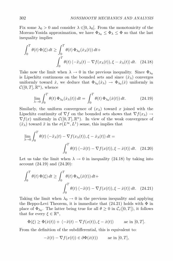
302 NONSMOOTH MECHANICS AND ANALYSIS
Fix some λ0 > 0 and consider λ ∈]0, λ0[. From the monotonicity of theMoreau-Yosida approximation, we have Φλ0 ≤ Φλ ≤ Φ so that the lastinequality implies∫ T
0θ(t) Φ(ξ) dt ≥
∫ T
0θ(t) Φλ0(xλ(t)) dt+∫ T
0θ(t) 〈−xλ(t)−∇f(xλ(t)), ξ − xλ(t)〉 dt. (24.18)
Take now the limit when λ → 0 in the previous inequality. Since Φλ0
is Lipschitz continuous on the bounded sets and since (xλ) convergesuniformly toward x, we deduce that Φλ0(xλ) → Φλ0(x) uniformly inC([0, T ], Rn), whence
limλ→0
∫ T
0θ(t) Φλ0(xλ(t)) dt =
∫ T
0θ(t) Φλ0(x(t)) dt. (24.19)
Similarly, the uniform convergence of (xλ) toward x joined with theLipschitz continuity of ∇f on the bounded sets shows that ∇f(xλ) →∇f(x) uniformly in C([0, T ], Rn). In view of the weak convergence of(xλ) toward x in the σ(L∞, L1) sense, this implies that
limλ→0
∫ T
0θ(t) 〈−xλ(t)−∇f(xλ(t)), ξ − xλ(t)〉 dt =∫ T
0θ(t) 〈−x(t)−∇f(x(t)), ξ − x(t)〉 dt. (24.20)
Let us take the limit when λ → 0 in inequality (24.18) by taking intoaccount (24.19) and (24.20):∫ T
0θ(t) Φ(ξ) dt ≥
∫ T
0θ(t) Φλ0(x(t)) dt+∫ T
0θ(t) 〈−x(t)−∇f(x(t)), ξ − x(t)〉 dt. (24.21)
Taking the limit when λ0 → 0 in the previous inequality and applyingthe Beppo-Levi Theorem, it is immediate that (24.21) holds with Φ inplace of Φλ0 . The latter being true for all θ ≥ 0 in Cc(]0, T [), it followsthat for every ξ ∈ Rn,
Φ(ξ) ≥ Φ(x(t)) + 〈−x(t)−∇f(x(t)), ξ − x(t)〉 ae in [0, T ].
From the definition of the subdifferential, this is equivalent to:
−x(t)−∇f(x(t)) ∈ ∂Φ(x(t)) ae in [0, T ],

Finite time stabilization of nonlinear oscillators 303
which means that inclusion (S) is satisfied almost everywhere in [0, T ].Let us now summarize our results. For every T > 0, we have proved
the existence of a function x ∈ C1([0, T ], Rn)∩W2,∞([0, T ], Rn) such that(S) is fulfilled for almost every t ∈ [0, T ]. Since (xλ(0), xλ(0)) = (x0, x0)for every λ > 0, it is immediate that the limit function x also satisfies(x(0), x(0)) = (x0, x0). To avoid confusion, we now denote by xT theprevious function defined on [0, T ]. For every T ′ > T , we obtain in thesame way a function xT ′
defined on [0, T ′]. From the uniqueness result,it is clear that xT ′
|[0,T ] = xT , so that we can define without any ambiguitya function x : [0, +∞[ in the following manner:
∀t ∈ [0,+∞[, x(t) = xT (t) as soon as T ≥ t.
It is then immediate that such a function x satisfies items (a), (b) and(c) of Theorem 24.1. �
ReferencesS. Adly, D. Goeleven, A stability theory for second order nonsmooth
dynamical systems with application to friction problems, Journal deMathematiques Pures et Appliquees, vol. 83, (2004), 17-51.
F. Alvarez, On the minimizing property of a second order dissipativesystem in Hilbert space, SIAM J. on Control and Optimization, vol.38, 4 (2000), 1102-1119.
F. Alvarez, H. Attouch, J. Bolte, P. Redont, A second-order gradient-likedissipative dynamical system with Hessian-driven damping. Applica-tion to optimization and mechanics, J. Math. Pures Appl., vol. 81, 8(2002), 747-779.
H. Amann, J. I. Dıaz, A note on the dynamics of an oscillator in thepresence of strong friction, Nonlinear Anal., vol. 55 (2003), 209-216.
A. Amassad, C. Fabre, Analysis of a viscoelastic unilateral contact prob-lem involving the Coulomb friction law, J. Optim. Theory Appl., vol.116, 3 (2003), 465-483.
H. Attouch, X. Goudou, P. Redont, The heavy ball with friction method.I The continuous dynamical system, Communications in Contempo-rary Math, vol. 2, 1 (2000), 1-34.
H. Attouch, P. Redont, The second-order in time continuous Newtonmethod. Approximation, optimization and mathematical economics(Pointe--Pitre, 1999), 25-36, Physica, Heidelberg, 2001.
H. Brezis, Operateurs maximaux monotones dans les espaces de Hilbertet equations d’evolution, Lecture Notes 5, North Holland, 1972.
M. Cadivel, D. Goeleven and M. Shillor, Study of a unilateral oscillatorwith friction, Math. Comput. Modelling, vol. 32, 2/3 (2000), 381-391.

304 NONSMOOTH MECHANICS AND ANALYSIS
J. Conlisk, Why bounded rationality, Journal of Economic Literature,vol. 34 (1996), 669-700.
J. I. Dıaz, A. Linan, On the asymptotic behavior of a damped oscillatorunder a sublinear friction term, Rev. R. Acad. Cien. Serie A. Mat.,vol. 95, 1 (2001), 155-160.
Y. Dumont, D. Goeleven, M. Rochdi and M. Shillor, Frictional contactof a nonlinear spring, Math. Comput. Modelling, vol. 31, 2/3 (2000),83-97.
C. Eck, J. Jarusek, A survey on dynamic contact problems with Coulombfriction, Multifield problems, (2000), 254-261, Springer, Berlin.
W. Han, M. Sofonea, Quasistatic contact problems in viscoelasticity andviscoplasticity, AMS and International Press, 2002.
M. Jean, Unilateral contact with dry friction: time and space discretevariables formulation, Arch. Mech., vol. 40, 5/6 (1988), 677–691.
T. Kato, Accretive operators and nonlinear evolution equations in Ba-nach spaces. Nonlinear functional analysis, Proc. Symp. Pure Math.,vol. 18, 1 (1970), 138-161.
M. Mabrouk, Sur un principe variationnel pour un probleme d’evolutionhyperbolique non lineaire, working paper, Laboratoire de MecaniqueAppliquee, Universite de Franche-Comte, Besancon.
M. D. P. Monteiro Marques, Differential inclusions in nonsmooth me-chanical problems, Progress in nonlinear differential equations andtheir applications, vol. 9, Birkhauser, 1993.
J. J. Moreau, Evolution problem associated with a moving convex set ina Hilbert space, J. Diff. Equ., (1977), 347-374.
J. J. Moreau, Standard inelastic shocks and the dynamics of unilateralconstraints. In: Unilateral Problems in Structural Analysis (ed. byG. Del Piero and F. Maceri), CISM Courses and Lectures, vol. 288,Springer Verlag, Wien, New York 1985, 173-221.
B.T. Polyack, Some methods of speeding up the convergence of iterativemethods, Z. Vylist Math. Fiz., vol. 4, (1964), 1-17.
R.T. Rockafellar and R. Wets, Variational analysis, Springer, Berlin,1998.
A. Rubinstein, Modeling bounded rationality, (1998), MIT Press.D. A. Russell, The piano hammer as a nonlinear spring, publications
of the Science and Mathematics Department, GMI Engineering &Management Institute, Kettering University, 1997.
M. Schatzman, A class of nonlinear differential equations of second orderin time, Nonlinear Analysis, vol. 2, (1978), 355-373.
J. Sobel, Economists’ models of learning, Journal of Economics Theory,vol. 94, (2000), 241-261.

Chapter 25
CANONICAL DUALITY IN NONSMOOTH,CONSTRAINED CONCAVEMINIMIZATION
David Y. GaoDepartment of Mathematics, Virginia Polytechnic Institute & State University, Blacks-burg, VA 24061, [email protected]
Abstract This paper presents a perfect duality theory for solving nonsmooth,concave minimization problems subjected to inequality constraints. Byuse of the canonical dual transformation developed recently, a canonicaldual problem is formulated, which is perfectly dual to the primal prob-lem with zero duality gap. It is shown that the global minimizer andlocal extrema of the nonconvex problem can be identified by the trialitytheory discovered recently (Gao, 2000). This canonical dual form andthe triality theory can be used to develop certain powerful algorithmsfor solving nonsmooth concave minimization problems.
Keywords: duality theory, concave minimization, canonical dual transformation,quadratic programming.
Dedicated to Professor Jean Jacques Moreau for his 80th birthday
1. Primal Problem and ParametrizationThe nonsmooth, concave minimization problem to be discussed in this
paper is denoted as the primal problem ((P) in short)
(P) : min P (x) ∀x ∈ Xf , (25.1)
where P (x) is a real-valued, nonsmooth, concave function defined on asuitable convex set Xa ⊂ Rn, and Xf ⊂ Rn is the feasible space, definedby
Xf = {x ∈ Xa ⊂ Rn| Bx ≤ b}, (25.2)

306 NONSMOOTH MECHANICS AND ANALYSIS
in which, B ∈ Rm×n is given matrix such that rankB = min{m,n}, andb ∈ Rm is a given vector. The goal in this problem is to find the (global)minimum value that P can achieve in the feasible space and, if this valueis not −∞, to find, if it exists, at least one vector x ∈ Xf that achievesthis value. The concave minimization problem (P) appears in manyapplications. Actually, even if P (x) is a quadratic function, the problem(P) is NP-hard (see, Horst et al, 2000; Floudas and Visweswaran, 1995).Methods and solutions to this very difficult problem are fundamentallyimportant in both mathematics and engineering science.
Mathematically speaking, if the nonconvex function P is continuouson its domain Xa and the feasible set Xf is compact, then by the well-known Weierstrass Theorem, the global minimum value is finite, and atleast one point in Xf exists which attains this value. From the pointof view of convex analysis, if the convex subset Xf ⊂ Rn is compact,it must be bounded and closed, i.e. the radius r0 of Xf , defined by|x| ≤ r0 ∀x ∈ Xf , is finite, thus, the problem (P) has at least onesolution. However, due to the concavity of the total cost P (x), theproblem (P) generally will possess many solutions that are local, butnot global, minimizers. The application of standard algorithms designedfor solving convex programming problems will generally fail to solvethis multi-extremal nonconvex global minimization problem. A detaileddiscussion and comprehensive review on this topic are given by Benson(1995).
Physically speaking, the primal problem (P) is called realizable if thereexists a vector x ∈ Xf such that P (x) = min{P (x)| ∀x ∈ Xf} > −∞.Thus, if (P) is realizable, the total cost P must be bounded below onXf , i.e. there exists a parameter μ > −∞ such that P (x) ≥ μ ∀x ∈ Xf .From point view of applications, if a problem is not realizable, then themathematical modeling of this problem might be not well proposed. Bythis philosophy, we consider only the realizable primal problem (P) sothat the primal problem can be written in the parametrization form (Pμ)
(Pμ) : minx∈Rn
P (x) (25.3)
s.t. Bx ≤ b, P (x) ≥ μ. (25.4)
Lemma 25.1 (Parametrization) Suppose that P : Xa → R is a con-cave function. For a given parameter μ ∈ R, the parametrized problem(Pμ) has at least one global minimizer x in the parametrical feasible setXμ ⊂ Rn defined by
Xμ = {x ∈ Rn| Bx ≤ b, P (x) ≥ μ}. (25.5)

Nonsmooth, constrained concave minimization 307
Moreover, if the problem (P) is realizable, then there exists a constantμ > −∞ such that the solution of the parametrized problem (Pμ) solvesalso the primal problem (P).
The main purpose of this paper is to find a canonical dual formulationof the parametric problem (Pμ) and extremality conditions for local andglobal extrema. Duality theory and methods in convex systems havebeen well established (cf. Moreau, 1966; Ekeland and Temam, 1976).However, many problems are still open in nonconvex systems. It isknown that due to the nonconvexity, the well developed Fenchel-Moreau-Rockafellar duality theory usually leads to a duality gap. It turns outthat the perfect duality theory and methods have been subjected toan extensively study during the recent years (see, Ekeland, 2003; Gohand Yang, 2002; Robinov and Yang, 2003). Based on the complemen-tary variational principle developed by Gao and Strang in nonconvexmechanics (Gao and Strang, 1989), a so-called canonical dual transfor-mation method and the associated triality theory have been establishedrecently (see Gao, 2000). This method and theory play an importantrole in global optimization (see Gao, 2003, 2004). In the present paper,a canonical dual problem has been formulated, which is perfectly dualto the parametric problem (Pμ) in the sense that they have the samesolution set. The global and local extrema are identified by the trialitytheory in the Section 3.
2. Canonical Dual Problem and CompleteSolutions
By the definition introduced in (Gao, 2000), a piecewise Gateauxdifferentiable function P : Xa → R is called a canonical function onXa ⊂ Rn if its Gateaux derivative x∗ = δP (x) is piecewise invertibleon the range X ∗
a ⊂ Rn, such that the Legendre conjugate of P can bedefined uniquely by
P ∗(x∗) = {xTx∗ − P (x)| x∗ = δP (x) ∀x ∈ Xa}. (25.6)
Thus, if P (x) is a canonical function on Xa, then the equivalent relations
x∗ = δP (x) ⇔ x = δP ∗(x∗) ⇔ P (x) + P ∗(x∗) = xTx∗ (25.7)
hold on Xa ×X ∗a . As it was shown by the author (Gao, 2000) that even
if P (x) may be a nonsmooth function, its Legendre conjugate is alwayssmooth (see Fig. 25.1). This simple fact plays an important role innonsmooth analysis.
Therefore, by the standard procedure of the canonical dual trans-formation, a dual problem ((Pμ
d) in short) can be formulated as the

308 NONSMOOTH MECHANICS AND ANALYSIS156 PROGRESSES IN NONSMOOTH MECHANICS AND ANALYSIS
P P ∗
(a) Graph of P (x).
x∗2
x∗1
(b) Graph of P ∗(x∗).
x1 xx∗
1 x∗2 x∗
Figure 14.1. Nonsmooth function P and its smooth Legendre conjugate P ∗
smooth (see Fig. 13.1). This simple fact plays an important role innonsmooth analysis.
Therefore, by the standard procedure of the canonical dual trans-formation, a dual problem ((Pμ
d) in short) can be formulated as thefollowing.
(Pμd) : max P d(ε∗, ρ∗) ∀(ε∗, ρ∗) ∈ Y∗
μ, (8)
where P d : Rm × R→ R is defined by
P d(ε∗, ρ∗) = (ρ∗ − 1)P ∗ (BT ε∗/(ρ∗ − 1))
+ μρ∗ − bT ε∗, (9)
in which, P ∗(x∗) is the Legendre conjugate function of P (x) on X ∗a , and
the dual feasible space Y∗μ is defined by
Y∗μ = {(ε∗, ρ∗) ∈ Rm×R| ε∗ ≥ 0 ∈ Rm, ρ∗ ≥ 0, BT ε∗/(ρ∗−1) ∈ X ∗
a }.(10)
Since P (x) is a canonical function over Xf , the canonical dual functionP d is well defined on Y∗
μ.
Theorem 1 (Perfect Duality Theorem) Suppose that the concavefunction P (x) is piecewise Gateaux differentiable on Xa such that itsLegendre conjugate P ∗(x∗) can be defined by (6), then for a given pa-rameter μ > −∞ and an m-vector b, the problem (Pd) is canoni-cally (or perfectly) dual to the primal problem (P) in the sense thatif y∗ = (ε∗, ρ∗) ∈ Y∗
μ is a KKT point of (Pμd), and x∗ = BT ε∗/(ρ∗ − 1),
then the vector x determined by
x = δP ∗(x∗) (11)
is a KKT point of (Pμ), and
P (x) = P d(y∗). (12)
Figure 25.1. Nonsmooth function P and its smooth Legendre conjugate P ∗
following.(Pμ
d) : maxP d(ε∗, ρ∗) ∀(ε∗, ρ∗) ∈ Y∗μ, (25.8)
where P d : Rm × R→ R is defined by
P d(ε∗, ρ∗) = (ρ∗ − 1)P ∗ (BT ε∗/(ρ∗ − 1))
+ μρ∗ − bT ε∗, (25.9)
in which, P ∗(x∗) is the Legendre conjugate function of P (x) on X ∗a , and
the dual feasible space Y∗μ is defined by
Y∗μ = {(ε∗, ρ∗) ∈ Rm×R| ε∗ ≥ 0 ∈ Rm, ρ∗ ≥ 0, BT ε∗/(ρ∗−1) ∈ X ∗
a }.(25.10)
Since P (x) is a canonical function over Xf , the canonical dual functionP d is well defined on Y∗
μ.
Theorem 25.2 (Perfect Duality Theorem) Suppose that the con-cave function P (x) is piecewise Gateaux differentiable on Xa such thatits Legendre conjugate P ∗(x∗) can be defined by (25.6), then for a givenparameter μ > −∞ and an m-vector b, the problem (Pd) is canoni-cally (or perfectly) dual to the primal problem (P) in the sense that ify∗ = (ε∗, ρ∗) ∈ Y∗
μ is a KKT point of (Pμd), and x∗ = BT ε∗/(ρ∗ − 1),
then the vector x determined by
x = δP ∗(x∗) (25.11)
is a KKT point of (Pμ), and
P (x) = P d(y∗). (25.12)
Moreover, if the primal problem (P) is realizable, then there exists afinite parameter μ > −∞ such that the vector x is also a KKT point ofthe problem (P).

Nonsmooth, constrained concave minimization 309
Proof. Suppose that y∗ = (ε∗, ρ∗) ∈ Y∗μ is a KKT point of (Pμ
d) andx∗ = BT ε∗/(ρ∗ − 1), then we have
0 ≤ ε∗ ⊥ BδP ∗(x∗)− b ≤ 0, (25.13)
0 ≤ ρ∗ ⊥ (δP ∗)T BT ε∗
ρ∗ − 1− P ∗ − μ ≥ 0. (25.14)
Since (x, x∗) is a canonical dual pair on Xa ×X ∗a , we have
x∗ =BT ε∗
(ρ∗ − 1)= δP (x) ⇔
x = δP ∗(x∗) ⇔P (x) = xT x∗ − P ∗(x∗).
Thus in term of x∗ = BT ε∗/(ρ∗ − 1) and x = δP ∗(x∗), the KKT condi-tions (25.13) and (25.14) can be written as
0 ≤ ε∗ ⊥ Bx− b ≤ 0, (25.15)0 ≤ ρ∗ ⊥ P (x)− μ ≥ 0. (25.16)
This shows that x = δP ∗ (BT ε∗/(ρ∗ − 1))
is indeed a KKT point of theparametric problem (Pμ).
By the complementarity conditions (25.15) and (25.16), we have bT ε∗ =(Bx)T ε∗ and ρ∗μ = ρ∗P (x), respectively. Thus, in term of
x∗ = BT ε∗/(ρ∗ − 1), and x = δP ∗(x∗),
we have
P d(ε∗, ρ∗) = (ρ∗ − 1)P ∗ (BT ε∗/(ρ∗ − 1))− xT BT ε∗ + ρ∗P (x) = P (x)
due to the fact that xT x∗ − P ∗(x∗) = P (x). �
Theorem 25.2 shows that there is no duality gap between the prob-lems (Pμ) and (Pμ
d). As we know that the KKT stationary conditionsare only necessary for the nonconvex optimization problem (Pμ). Thesufficient condition will be given by the triality theorem in the nextsection.
3. Triality Theory: Local and Global MinimizersLet
Y∗μ+ = {(ε∗, ρ∗) ∈ Y∗
μ| ρ∗ > 1}, (25.17)
Y∗μ− = {(ε∗, ρ∗) ∈ Y∗
μ| 0 ≤ ρ∗ < 1}, (25.18)

310 NONSMOOTH MECHANICS AND ANALYSIS
andXμb = {x ∈ Xf | P (x) = μ}. (25.19)
Theorem 25.3 (Triality Theorem) Suppose that for a given finiteparameter μ > −∞, the vector y∗ = (ε∗, ρ∗) is a KKT point of theproblem (Pd
μ), and x∗ = BT ε∗/(ρ∗ − 1).If ρ∗ > 1, then x = δP ∗(x∗) is a global minimizer of P (x) over Xμb,
and
P (x) = minx∈Xμb
P (x) = max(ε∗,ρ∗)∈Y∗
μ+
P d(ε∗, ρ∗) = P d(y∗). (25.20)
If 0 ≤ ρ∗ < 1, then x = δP ∗(x∗) is a global maximizer of P (x) overXμ if and only if y∗ = (ε∗, ρ∗) is a maximizer of P d over Y∗
μ− and
P (x) = maxx∈Xμ
P (x) = max(ε∗,ρ∗)∈Y∗
μ−P d(ε∗, ρ∗) = P d(y∗). (25.21)
If 0 < ρ∗ < 1, then x = δP ∗(x∗) is a global minimizer of P (x)over Xμb if and only if y∗ = (ε∗, ρ∗) is a global minimizer of P d overY∗
μ− ∩ {ρ∗ �= 0} and
P (x) = minx∈Xμb
P (x) = min(ε∗,ρ∗)∈Y∗
μ−P d(ε∗, ρ∗) = P d(y∗). (25.22)
Proof. Since P ∗(x∗) is concave on X ∗a , then for a given duality pair
(x, x∗), the inequality
P ∗(x∗) ≤ xT (x∗ − x∗) + P ∗(x∗) ∀x∗ ∈ X ∗a (25.23)
holds on X ∗a . In terms of y∗ = (ε∗, ρ∗), and y∗(ε∗, ρ∗) ∈ Y∗
μ, the inequal-ity (25.23) also holds for
x∗ =BT ε∗
ρ∗ − 1, x∗ =
BT ε∗
ρ∗ − 1.
Particularly, we let y∗ = (ε∗, ρ∗) ∈ Y∗μ be a KKT point of the problem
(Pμd) such that x∗ = BT ε∗/(ρ∗ − 1). By Theorem refthm:cavedual we
know that the vector x = δP ∗(x∗) is a KKT point of the problem (Pμ).Thus, if ρ∗ > 1, the inequality (25.23) leads to
(ρ∗ − 1)P ∗(
BT ε∗
ρ∗ − 1
)≤ xT BT ε∗ − xT BT ε∗
ρ∗ − 1(ρ∗ − 1)
+ (ρ∗ − 1)P ∗(
BT ε∗
ρ∗ − 1
)∀(ε∗, ρ∗) ∈ Y∗
μ.
Nonsmooth, constrained concave minimization 311
By the complementarity conditions xT BT ε∗ = xTb, and ρ∗(μ−P (x)) =0, as well as the equality P (x) = xT x∗ − P ∗(x∗), we have
P d(y∗) ≤ P d(y∗) + (Bx− b)T ε∗ + ρ∗(μ− P (x))≤ P d(y∗) ∀(ε∗, ρ∗) ∈ Y∗
μ, ρ∗ > 1.
This shows that if ρ∗ > 1, the KKT point y∗ = (ε∗, ρ∗) maximizes P d
on Y∗μ+.
We now need to prove that the vector x associated with the KKTpoint y∗ of (Pμ
d) minimizes P on Xμ. By the concavity of the canonicalfunction P on Xa, the Legendre conjugate
P ∗(x∗) = minx∈Xa
{xTx∗ − P (x)}
is uniquely defined on X ∗a . Particularly, for a given y∗ = (ε∗, ρ∗) ∈ Y∗
μ,we let x∗ = BT ε∗/(ρ∗ − 1). Thus, we have
P d(ε∗, ρ∗) = minx∈Xa
Ξ(x, ε∗, ρ∗) (25.24)
where
Ξ(x, ε∗, ρ∗) = xT BT ε∗ − (ρ∗ − 1)P (x) + μρ∗ − bT ε∗ (25.25)
is the so-called total complementary function, or the extended Lagrangian,which can be obtained by the standard canonical dual transformation(see (Gao, 2000)). Clearly, for any given ρ∗ > 1, Ξ(x, ε∗, ρ∗) is convexin x and concave (linear) in ε∗ and ρ∗. Thus, by the classical saddle-minimax theory, we have
P d(ε∗, ρ∗) = maxρ∗>1
maxε∗≥0
minx∈Xa
Ξ(x, ε∗, ρ∗)
= maxρ∗>1
minx∈Xa
maxε∗≥0
Ξ(x, ε∗, ρ∗)
= minx∈Xa
maxρ∗>1{(1− ρ∗)P (x) + μρ∗} s.t. Bx ≤ b
= minx∈Xf
{P (x)− min
ρ∗>1ρ∗(P (x)− μ)
}= min
x∈Xf
P (x) s.t. P (x) = μ,
since the linear programming
θ1 = minρ∗>1
ρ∗(P (x)− μ)
has a solution in the open domain (1, +∞) if and only if P (x) = μ. Thisshows that the KKT point y∗ = (ε∗, ρ∗) maximize P d on Y∗
μ+ if andonly if x is a global minimizer of P (x) on Xμb.

312 NONSMOOTH MECHANICS AND ANALYSIS
In the case that 0 < ρ∗ < 1, the total complementary functionΞ(x, ε∗, ρ∗) is concave in x ∈ Rn and concave in both ε∗ ∈ Rm
+ andρ∗ ∈ (0, 1). Thus, if (ε∗, ρ∗) is a global minimizer of P d on Y∗
μ−, then bythe so-called bi-duality theory developed in (Gao, 2000), we have either
maxx∈Rn
max(ε∗,ρ∗)∈Y∗
μ−Ξ(x, ε∗, ρ∗) = max
(ε∗,ρ∗)∈Y∗μ−
maxx∈Rn
Ξ(x, ε∗, ρ∗) (25.26)
or
minx∈Rn
max(ε∗,ρ∗)∈Y∗
μ−Ξ(x, ε∗, ρ∗) = min
(ε∗,ρ∗)∈Y∗μ−
maxx∈Rn
Ξ(x, ε∗, ρ∗). (25.27)
Thus, if y∗ = (ε∗, ρ∗) is a maximizer of P d over Y∗μ− then we have
P d(ε∗, ρ∗) = max(ε∗,ρ∗)∈Y∗
μ−P d(ε∗, ρ∗)
= maxε∗≥0, ρ∗∈[0,1)
maxx∈Rn
Ξ(x, ε∗, ρ∗)
= maxρ∗∈(0,1)
maxx∈Rn
maxε∗≥0
Ξ(x, ε∗, ρ∗)
= maxρ∗∈(0,1)
maxx∈Rn
{(1− ρ∗)P (x) + μρ∗ − xTb
}s.t. Bx ≤ b
= maxx∈Xf
{P (x)− min
ρ∗∈[0,1)ρ∗(P (x)− μ)
}= max
x∈Xf
P (x) s.t. P (x)− μ ≥ 0,
by the fact that the domain [0, 1) is closed on the lower bound and openon the upper bound, the problem
θ2 = minρ∗∈[0,1)
{ρ∗(P (x)− μ)} (25.28)
has a solution if and only if P (x) ≥ μ, and for this solution, θ2 = 0.On the other hand, if y∗ = (ε∗, ρ∗) is a minimizer of P d over Y∗
μ− ∩{ρ∗ �= 0} then we have
P d(ε∗, ρ∗) = min(ε∗,ρ∗)∈Y∗
μ−P d(ε∗, ρ∗)
= minε∗≥0
minρ∗∈(0,1)
maxx∈Rn
Ξ(x, ε∗, ρ∗)
= minρ∗∈(0,1)
minx∈Rn
maxε∗≥0
Ξ(x, ε∗, ρ∗)
= minρ∗∈(0,1)
minx∈Rn
{(1− ρ∗)P (x) + μρ∗} s.t. Bx ≤ b
= minx∈Xf
{P (x)− max
ρ∗∈(0,1)ρ∗(P (x)− μ)
}= min
x∈Xf
P (x) s.t. P (x) = μ,
Nonsmooth, constrained concave minimization 313
since the linear minimization
θ3 = maxρ∗∈(0,1)
ρ∗(P (x)− μ)
has a solution on the open domain (0, 1) if and only P (x) − μ = 0. Bythe fact that P d(ε∗, ρ∗) = P (x) for all KKT points of (Pμ), the theoremis proved. �
Theorem 25.3 shows that if the KKT point ρ∗ is in the open set (0, 1),then x is a minimizer of P only if x is located on the boundary of thefeasible set Xμ, i.e. P (x) = μ, which can not be located, generally speak-ing, by standard algorithms designed for convex minimization problems.This is the main reason that why the primal problem (P) is NP-hard.However, the dual problem in this case is a convex minimization over theopen set Y∗
μ−∩{ρ∗ �= 0}, which is much easier than the primal one. Thetriality theorem can be used to develop certain powerful algorithms forsolving this concave minimization problem with inequality constraints.
The canonical dual transformation method and triality theory wereoriginally developed from nonsmooth and nonconvex mechanics (seeGao, 2000). The key idea of this method is to choose certain geometri-cally admissible measure Λ : Xa → Ya such that the Legendre-Fenchel-Moreau transformation holds on the canonical dual spaces Ya ×Y∗
a (seeGao, 2000, 2003a,b). In the present paper, since the concave functionP is a canonical function, this geometrical measure is simply chosen tobe Λ(x) = P (x). In the case that P is a quadratic function, the con-straint P (x) ≤ μ can be simply replaced by the normality condition12 |x|2 ≤ μ, which has been studied very recently by the author (see Gao,2004). The results presented in this paper show again that the canonicaldual transformation and associated triality theory may possess impor-tant computational impacts on global optimization.
ReferencesBenson, H (1995), Concave minimization: theory, applications and al-
gorithms, in Handbook of Global Optimization, eds. R. Horst and P.Pardalos, Kluwer Academic Publishers, 43-148.
Ekeland, I. (2003). Nonconvex duality, in Proceedings of IUTAM Sym-posium on Duality, Complementarity and Symmetry in Nonlinear Me-chanics, D.Y. Gao (Edited), Kluwer Academic Publishers, Dordrecht /Boston / London, 13-22.
Ekeland, I. and Temam, R. (1976),Convex Analysis and VariationalProblems, North-Holland, and SIAM, Philadelphia, 1999, 402pp.

314 NONSMOOTH MECHANICS AND ANALYSIS
Floudas, C.A and Visweswaran, V. (1995). Quadratic optimization, inHandbook of Global Optimization, R. Horst and P.M. Pardalos (eds),Kluwer Academic Publ., Dordrecht / Boston / London, pp. 217-270.
Gao, D.Y. (2000). Duality Principles in Nonconvex Systems: Theory,Methods and Applications, Kluwer Academic Publishers, Dordrecht /Boston / London, xviii+454pp.
Gao, D.Y. (2003). Perfect duality theory and complete solutions to aclass of global optimization problems, Optimisation, Vol. 52, 4-5, 467-493.
Gao, D.Y. (2003). Nonconvex semi-linear problems and canonical du-ality solutions, in Advances in Mechanics and Mathematics, Vol. II,edited by D.Y. Gao and R.W. Ogden, Kluwer Academic Publishers,Dordrecht / Boston / London, pp. 261-312..
Gao, D.Y. (2004). Canonical duality theory and solutions to constrainednonconvex quadratic programming, J. Global Optimization, to appearin a special issue on duality edited by D.Y. Gao and KL Teo.
Gao, D.Y. and Strang, G. (1989), Geometric nonlinearity: Potentialenergy, complementary energy, and the gap function, Quart. Appl.Math., 47(3), 487-504, 1989.
Goh, C.J. and Yang, X.Q. (2002). Duality in Optimization and Varia-tional Inequalities, Taylor and Francis, 329pp.
Horst, R., Panos M. Pardalos, Nguyen Van Thoai (2000). Introductionto Global Optimization, Kluwer Academic Publishers.
Moreau, J.J. (1966). Fonctionelles Convexes, College de France, 1966,and Instituto Poligrafico E Zecca Dello Stato, S.p.A, Roma, 2003.
Rubinov, A.M. and Yang X.Q. (2003). Lagrange-Type Functions in Con-strained Non-Convex Optimization. Kluwer Academic Publishers, Bos-ton / Dordrecht / London, 285 pp.

APPENDIX 315
Appendix: Theoretical and Numerical NonsmoothMechanics International Colloquium

316 NONSMOOTH MECHANICS AND ANALYSIS
From 17 to 19 November 2003, the Laboratoire de Mecanique et Genie Civil inMontpellier, France, has organized an international colloquium in honour of the 80thbirthday of Jean Jacques Moreau, Emeritus Professor at University Montpellier II.The colloquium was devoted to the presentation of recent works in the fields wherethe contribution of Jean Jacques Moreau was original and significant.
Some of the participants were able to prepare the content of this book, in the samespirit, but all participate to the success of the event. Many thanks to all of them.They were:
Hedy Attouch, Universite Montpellier II, France,
Jean-Pierre Aubin, Universite Paris-Dauphine, France,
John Ball, University of Oxford, United Kingdom,
Bernard Brogliato, Institut National de Recherche en Informatique et en Au-tomatique, France,
Giuseppe Buttazzo, Universita di Pisa, Italy,
Francis Clarke, Universite Claude Bernard Lyon I, France,
Louis Marie Cleon, Societe Nationale des Chemins de Fer, France,
Bernard Dacoragna, Ecole Polytechnique Federale de Lausanne, Switzerland,
David Dureisseix, Universite Montpellier II, France,
Gianpietro Del Piero, University of Ferrara and Accademia Nazionale dei Lin-cei, Italy,
Michel Fremond, Laboratoire Central des Ponts et Chaussees, France,
David Gao, Virginia Polytechnic Institute & State University, USA,
Christoph Glocker, Swiss Federal Institute of Technology Zurich, Switzerland,
Jean-Baptiste Hiriart-Urruty, Universite Paul Sabatier, France,
Michel Jean, Laboratoire de Mecanique et d’Acoustique, CNRS, France,
Anders Klarbring, University of Linkoping, Sweden,
Franco Maceri, University of Roma II Tor Vergata, Italy,
Manuel Marques, Universidade de Lisboa, Portugal,
Henry Keith Moffatt, University of Cambridge, United Kingdom,
Bernard Nayroles, Institut National des Sciences Appliquees de Rouen, France,
Quoc Son Nguyen, Ecole Polytechnique, France,
Alain Pumir, Institut Non Lineaire de Nice, CNRS, France,
David Quere, Laboratoire de Physique de la Matiere Condensee, CNRS, France,
Farhang Radjaı, Laboratoire de Mecanique et Genie Civil, CNRS, France,
Michel Raous, Laboratoire de Mecanique et d’Acoustique, CNRS, France,
Renzo Ricca, Universita di Milano, Italy, and University College, United King-dom,
Ralph Tyrrell Rockafellar, University of Washington, USA,
Michelle Schatzman, Laboratoire de Mathematiques Appliquees de Lyon, CNRS,France,

APPENDIX 317
Georgios E. Stavroulakis, University of Ioannina, Greece,
Pierre Suquet, Laboratoire de Mecanique et d’Acoustique, CNRS, France,
Michel Valadier, Universite Montpellier II, France,
Jean-Pierre Vilotte, Institut de Physique du Globe de Paris, France.
This event was also made possible thanks to the sponsorship of:
Ministere de la Jeunesse, de l’Education Nationale et de la Recherche,
Centre National de la Recherche Scientifique,
Region Languedoc-Roussillon,
Conseil General de l’Herault,
Communaute d’Agglomeration de Montpellier,
Universite Montpellier II,
Association Francaise de Mecanique,
Societe de Mathematiques Appliquees et Industrielles,
Societe Nationale des Chemins de Fer.

Index
Aadmissible transport map . . . . . . . . . . . . . 15augmented Lagrangian . . . . . . . . . . . 95, 200
Bbalayage . . . . . . . . . . . . . . . . . . . . . . . . . . . . . . 48ballasted track . . . . . . . . . . . . . . . . . . . . . . 221bi-periodic boundary conditions .234, 235bistochastic operator . . . . . . . . . . . . . . . . . 48bounded variation . . . . . . . . . . . . . . . . . . . 267
Ccanonical dual transformation . . . . . . . 307coarse-grained approximation . . . . . . . . 175coarse-grained velocity gradient . . . . . . 174comparison relations between measures49complementarity dynamical systems . 261composite function . . . . . . . . . . . . . . . . . . . 38concave minimization . . . . . . . . . . . . . . . . 305conditional expectation . . . . . . . . . . . . . . . 53conjugate gradient with projection . . . 200conjugate projected gradient . . . . . . . . .205constraint forces . . . . . . . . . . . . . . . . . . . . . 188Contact Dynamics . . . . . . . . . 228, 243, 273contraction principle . . . . . . . . . . . . . . . . .150control systems . . . . . . . . . . . . . . . . . . . . . . 256
Ddifferential measures . . . . . . . . . . . . . . . . . 266diffusive motion . . . . . . . . . . . . . . . . . . . . . 240discrete element . . . . . . . . . . . . . . . . . . . . . 222disintegration . . . . . . . . . . . . . . . . . . . . . . . . . 54dissipation index . . . . . . . . . . . . . . . . . . . . 192domain decomposition . . . . . . . . . . . . . . . 199drop breakup . . . . . . . . . . . . . . . . . . . 165, 168drop formation . . . . . . . . . . . . . . . . . . . . . . 164drop oscillations . . . . . . . . . . . . . . . . . . . . . 167duality . . . . . . . . . . . . . . 7, 85, 108, 195, 307
Eenergy cascade . . . . . . . . . . . . . . . . . . . . . . 242envelope function . . . . . . . . . . . . . . . . . . . . . . 4extended Lagrangian . . . . . . . . . . . . . . . . 311extended sweeping process . . . . . . . . . . . 266
FFenchel . . . . . . . . . . . . . . . . . . . . . . . . . . . . . . 307FETI-C method . . . . . . . . . . . . . . . . . . . . . 202Finite Element Tearing and Interconnect-
ing . . . . . . . . . . . . . . . . . . . . . . . 202flatness . . . . . . . . . . . . . . . . . . . . . . . . . . . . . . 238fluid mechanics . . . . . . . . . . . . . . . . . . . . . . 171free surfaces . . . . . . . . . . . . . . . . . . . . . . . . . 163friction . . . . . . . . . . . . . . . . . . . . . . . . . . . . . . 283
GGaussian shape . . . . . . . . . . . . . . . . . . . . . . 237generalized Newton method. . . . . . . . . . .95granular media . . . . . . . . . . . . . . . . . 203, 234graphical derivates . . . . . . . . . . . . . . . . . . 250graphically Lipschitzian. . . . . . . . . . . . . . .11Green’s function . . . . . . . . . . . . . . . . . . . . . 177
HHamiltonian. . . . . . . . . . . . . . . . . . . . . . . . .6, 7Hausdorff distance . . . . . . . . . . . . . . 252, 285Heavy Ball with Friction. . . . . . . . . . . . .290Hurst exponent . . . . . . . . . . . . . . . . . . . . . . 240
Iimpact intensity . . . . . . . . . . . . . . . . . . . . . 191impact topology . . . . . . . . . . . . . . . . . . . . . 191inelastic shocks . . . . . . . . . . . . . . . . . . . . . . 281integral representation of a bistochastic
operator . . . . . . . . . . . . . . . . . . . 54
Kkinematically admissible . . . . . . . . . . . . . 197
LLagrange multiplier . . . . . . . . . . . . . . . . . .156Lagrangian . . . . . . . . . . 6, 86, 200, 272, 311lateral resistance . . . . . . . . . . . . . . . . . . . . 222LATIN method . . . . . . . . . . . . . . . . . . . . . . 199Legendre-Fenchel . . . . . . . . 35, 36, 198, 313linear complementarity problem . 64, 120,
198, 271–273LMGC90 . . . . . . . . . . . . . . . . . . . . . . . 222, 228
320 NONSMOOTH MECHANICS AND ANALYSIS
log-exponential function . . . . . . . . . . . . . . 43Lyapounov function . . . . . . . . . . . . . . . . . 294
Mmaximal dissipation principle . . . . . . . . 285maximal monotone . . . . . . . . . . . . . . . . . . 271measure differential inclusion . . . . . . . . 281measure inclusion. . . . . . . . . . . . . . . . . . . .188mechanical impact theory . . . . . . . . . . . 191Monge problem . . . . . . . . . . . . . . . . . . . . . . . 15Moreau’s impact law . . . . . . . . . . . . . . . . 190Moreau-Yosida . . . . . . . . . . . . . 201, 291, 299morphological equations . . . . . . . . . . . . . 250morphological maps . . . . . . . . . . . . . . . . . 253morphological transition . . . . . . . . . . . . . 253multipliers. . . . . . . . . . . . . . . . . . . . . . . . . . .147
NNewtonian impact law . . . . . . . . . . . . . . . 192non-linear Gauss-Seidel . . . . . . . . . 200, 205nonconvex mechanics . . . . . . . . . . . . . . . . 307
Pperfect collision. . . . . . . . . . . . . . . . . . . . . .185perfect constraints . . . . . . . . . . . . . . . . . . . 188plastic deformations . . . . . . . . . . . . . . . . . 236polyconvex . . . . . . . . . . . . . . . . . . . . . . . . . . . 28power spectrum. . . . . . . . . . . . . . . . .239, 242preconditioned conjugate projected gradi-
ent . . . . . . . . . . . . . . . . . . . . . . . 205pricing policy . . . . . . . . . . . . . . . . . . . . . . . . . 17probability density function. . . . . . . . . .237proximal mapping . . . . . . . . . . . . . . . . . . . . . 3proximal point . . . . . . . . . . . . . . . . . . . . . . 282proximation . . . . . . . . . . . . . . . . . . . . . . . . . 270
Qquasi-optimization . . . . . . . . . . . . . . . . . . . 204quasi-variational inequality . . . . . 148, 149
Rrank one convex . . . . . . . . . . . . . . . . . . . . . . 28rank one convex finite . . . . . . . . . . . . . . . . 28relative degree . . . . . . . . . . . . . . . . . . . . . . . 261
Sscaling laws . . . . . . . . . . . . . . . . . . . . . . . . . 174self-affine . . . . . . . . . . . . . . . . . . . . . . . 240, 242semi-classical approximation . . . . . . . . . 179size segregation. . . . . . . . . . . . . . . . . . . . . . 243slack variables . . . . . . . . . . . . . . . . . . . . . . . 265stability. . . . . . . . . . . . . . . . . . . . .67, 163, 171statically admissible . . . . . . . . . . . . . . . . . 197steric exclusions . . . . . . . . . . . . . . . . 234, 243stochastic equations . . . . . . . . . . . . . . . . . 179Strassen’s theorem. . . . . . . . . . . . . . . . . . . . 50stretched exponential . . . . . . . . . . . . . . . . 241superdiffusion . . . . . . . . . . . . . . . . . . . . . . . 241surface tension. . . . . . . . . . . . . . . . . .164, 167sweeping process . . . . . . . . . . . . . . . . . 85, 250sweeping-out . . . . . . . . . . . . . . . . . . . . . . . . . 48
Ttetrad of Lagrangian particles . . . . . . . 174time-stepping . . . . . . . . . . . . . . 129, 272–274total complementary function. . . . . . . .311transportation network . . . . . . . . . . . . . . . 16triality theory . . . . . . . . . . . . . . . . . . 307, 309turbulence . . . . . . . . . . . . . . . . . . . . . . 173, 242
UUzawa algorithm . . . . . . . . . . . . . . . . . . . . 201
Vvariational inequality . . . . . . . . . . . . . . . . 268velocity of the tube . . . . . . . . . . . . . . . . . . 253viability kernel . . . . . . . . . . . . . . . . . . . . . . 257viability lemma. . . . . . . . . . . . . . . . . . . . . . 274viability multipliers . . . . . . . . . . . . . . . . . . 257viable tubes . . . . . . . . . . . . . . . . . . . . . . . . . 251viably consistent. . . . . . . . . . . . . . . . . . . . .256virtual work . . . . . . . . . . . . . . . . . . . . . 78, 187viscosity . . . . . . . . . . . . . . . . . . . . 99, 166, 170
WWasserstein distance . . . . . . . . . . . . . . . . . . 16
Zzero dynamics . . . . . . . . . . . . . . . . . . . . . . . 263