No.190

High frequency sea level recording for tsunami warning and enhanced storm surge monitoring at UK sites

K.J. Horsburgh, L. Bradley, M. Angus, D.E. Smith, E.M.S. Wijeratne and P.L. Woodworth

12 February 2009

1. Summary • The risk to the UK of tsunami hazard is very small, but not zero (Kerridge et al.,

2005).

• Any tsunami warning system should have a high frequency sea level measuring component, capable of identifying tsunamis, to complement seismic and numerical modelling tools.

• The existing network of strategic UK tide gauges can contribute useful data for the

tsunami warning process, so long as they sample at suitable frequency (at least 1 min). A comprehensive network of sea level measurement for tsunami warning ought to also contain deep pressure sensors, capable of detecting tsunamis at the continental shelf-break.

• Any of the sensors deployed during this study could be used on land-based, or

structure-based sites. Pressure transducers coupled to the pneumatic lines of bubbler gauges exhibited less offset drift than those mounted directly underwater. Although radar gauges exhibited some time lags and damping, their amplitude response was adequate which makes them a reasonable alternative for tsunami detection.

• There is presently no requirement to install high frequency sea level monitoring at

any other sites, but were it requested then equipment costs are initially modest (approximately £1k per site). High quality broadband transmission (with a modem backup) costs approximately £1200 per site, per year. Obviously, any costs associated with an enlarged network of high frequency sensors, and the operational collection of data, would have to be covered by a fully funded program for tsunami warning. Whether such a project is necessary is the subject of ongoing discussion at Cabinet Office level.

• A simple, automated detection algorithm was developed. It is based on the variance

of the time-filtered sea level signal. Three alarm levels are currently included and these can be adjusted to prevent routine, local processes from initiating a warning whilst responding reliably to real tsunami signals.

• Exchange of real-time data from key European partners (and Portugal in particular)

has been established as a result of the parallel project, “Improved Access to European Near-Real Time Tide Gauge Data for Storm Surge Modelling and Tsunami Warning”. Data can be found at http://www.vliz.ioc

• The high-frequency sea level data from this project have already proven useful for

improved surge model validation within the operational forecasting service. The 1Hz signals give a better understanding of short-period (10-30 minutes) oscillations within harbours and channels. The correct specification of this seiching (which the numerical models do not simulate) helps to identify the correct sampling strategy for verification purposes. The new sensors will also allow a better analysis of swell wave data for coastal defence planning.

Page 2

2. Background The Sumatra-Andaman earthquake on 26 December 2004, off the west coast of northern Sumatra, and the resultant tsunami that swept across the Indian Ocean devastating parts of Indonesia, Thailand, Sri Lanka and other coastal areas of the Bay of Bengal, raised questions of the vulnerability of other areas of the world to tsunamis. There is some historical and geological evidence of tsunamis reaching the UK and so the possibility of future damaging events cannot be ignored. Investigations commissioned by Defra (Kerridge et al., 2005) considered there to be a very low probability of tsunami occurrence due to seismic events in UK coastal waters, with a low but not zero likelihood of tsunamis originating from more distant geological activity. Candidate areas are a passive margin earthquake in the western Celtic Sea, an earthquake off the coast of Portugal (akin to the 1755 Lisbon event), or a major landslide resulting from the collapse of La Cumbre Vieja volcano on the island of La Palma. Numerical modelling work within that study showed that in these cases the propagation time of any tsunami wave over the southwest continental shelf is approximately 4-8 hours, which makes detection and confirmation feasible if a suitable observational network is employed. Any warning network capable of detecting the sea level disturbance would be a valuable tool in the effective assessment of the threat, and would provide a crucial check on predictions from any operational computer model. Most European nations already make good use of sea level observations for the monitoring of storm surges and mean sea level. Therefore the framework for any tsunami warning system exists, subject to appropriate modification. Any complete instrumental network for tsunami warning around the UK would almost certainly employ deep pressure sensors (akin to the DART tsunameters used in the Pacific and, now, Indian oceans). Nevertheless, the existing network of strategic (Class A) tide gauges is sufficiently extensive that it has a useful role to play, particularly if complemented by real-time data exchange with other key European partners. However, the existing tide gauge hardware has not been evaluated for its suitability for higher frequency measurement. The sampling interval for the UK strategic tide gauge network is currently 15 minutes, which is incapable of resolving any tsunami; the 2004 Sumatra tsunami had a period of 40 minutes, and many tsunamis have much shorter periods than this. The objectives of this project were to install sub-surface differential transducer pressure sensors and new data acquisition systems at a small number of UK test sites. The new instruments sample at high frequency and their results may be compared with output from the existing pneumatic systems reconfigured to sample at similar high frequencies. Thus we compare the performance of the existing and new technologies for the detection of waves in the tsunami spectrum. This report focuses on the instrumentation and communications, evaluating their suitability for tsunami monitoring by analysis of the collected data. We also report on a tsunami signal-detection algorithm that will work in the presence of the ambient sea level variability (i.e. large tidal range and surface waves). This would be a necessary link in any semi-automated tsunami warning system (e.g. Allen and Greenslade, 2008).

Page 3

3. Equipment overview and test locations Prototype systems were installed at three sites; Holyhead, Lerwick and Newlyn. The systems comprised prototype data loggers incorporate a 56k PSTN modem, GPRS communications, and SensorTechnics pressure transducers. Kalesto and Vega radar units were installed and evaluated at Holyhead, whilst other hardware combinations were trialled the Liverpool tide gauge site to evaluate the data logger connected to ADSL broadband, GSM modem and a Hughes BGAN satellite-transmission unit. The three sites where these tests took place are shown in Figure 1. Site-specific equipment is detailed in Table 1. Laptop computers running the bespoke data capture and display software were installed at the three primary test sites, capturing one second averaged data transmitted by the data logger. The one second data is stored in a structured file system for future analysis, should the data transmitted over the internet not be available. Additional software captures and displays the real time data which are transmitted over the internet from the data logger. This data is stored on the POL network and is also uploaded to an ftp server for European data exchange.

Figure 1. Tsunami instrument test sites

Page 4

Table 1. Equipment installation summary at the three UK sites. Installed Communications Sensors Holyhead 13/01/07 GPRS 2 x Underwater mounted pressure transducers

1 x Surface mounted pressure transducer connected to the bubbler gauge pressure point line. 1 x Vega radar operating since Sept 07 A Kalesto radar was in operation for 9 months.

Lerwick 08/10/07 GPRS Changed to ADSL broadband on 15 Aug 08.

2 x Underwater mounted pressure transducers 2 x Surface mounted pressure transducers connected to the bubbler gauge pressure point lines.

Newlyn 10/07/08 GPRS 2 x Surface mounted pressure transducers connected to the bubbler gauge pressure point lines. One of the surface transducers will eventually be underwater mounted.

At Lerwick where was an ISP reliability issue on the GPRS link. This link was replaced by an ADSL broadband connection on 15 August 08, since when it has maintained a reliable connection without loss of data. The equipment package consists of five key modules which are the data logger, communications module, sensors, sensor interface and power supply. Each of these modules is now described in detail. 3.1 Sensors: pressure transducers and radar gauges These are relatively inexpensive transducers costing approx £250 each. The type used in this project are 2 bar differential with 0.1% accuracy and have been deployed in both underwater and surface-mounted configurations. The surface-mounted pressure transducer is connected to the bubbler gauge installed in the same building. The pressure sensors are sampled at 10Hz and averaged to produce both one second and integrated period heights. Calibration is carried out in the laboratory using a Druck pressure calibrator over a range appropriate for the site. In underwater deployments, the transducers proved to be resilient to seawater corrosion, with the original Holyhead transducers removed after 16 months underwater showing little sign of corrosion. However, previous experience suggested that transducers mounted underwater have exhibited varying degrees of corrosion depending upon the manufacturer, some becoming unusable after only several weeks immersion. For this reason the first pair of underwater transducers installed at Holyhead had one exposed to the seawater and the other placed inside a copper jacket as shown in Figure 2. The copper jacket was fitted with plastic spacers to insulate the transducers metal body from the copper, with silicone fluid filling the void. The top end cap was fitted with a drilled copper nozzle, allowing pressure to be transferred to the transducers stainless steel diaphragm via the silicone fluid. The transducer was recovered in pristine condition after 16 months underwater. The copper jacket is made from standard plumbing pipe and end fittings costing less than £10. This provides an inexpensive solution to the problem of mounting transducers underwater. In the surface-mounted arrangement, the transducers are located in the tide gauge building with a pneumatic connection into the strategic network bubbler system.

Page 5

Figure 2. Underwater transducer protection using a copper jacket The Vega radar gauge costs approx £1200 and has been operating at Holyhead tide gauge site since 25/09/07. It has proved to be a reliable and stable sensor, with the data producing an excellent fit to the bubbler system data. It does however exhibit a lag in the response of approx 10 seconds. The radar unit generates a signal which is converted to an averaged water depth by an interface board sampling at 10Hz. This requires calibration in the laboratory, but could be conducted at site using fixed distance reflectors, or by observations with a tide staff over a suitable integration period. Installation at Holyhead was inexpensive and straight forward using standard scaffolding tube and fittings fixed to the quay edge (see Figure 3).

Figure 3. Sensors evaluated at Holyhead were (left) Kalesto radar gauge, (middle) Vega radar gauge and (right) SensorTechnics pressure transducers. The Kalesto radar transmits a text string over a RS485 link, providing system status and height information, therefore the gauge does not require calibration. The unit consumes 600mA producing a height every 25 to 40 seconds. The developed interface board triggers the unit into a new height phase immediately a height is produced. All heights generated within the integration period are averaged and transferred to the data logger over the sensor interface. The Kalesto requires a substantial mounting structure due to the weight and wind drag profile (see Figure 3).

Page 6

3.2 Sensor interface The data logger incorporates a bespoke communications interface to the sensor interface boards. These interface boards synchronize with the data logger and generate various forms of information in engineering units derived from the raw sensor data. This allows virtually any sensor to be connected to the data logger. The sensor interface board provides a powerful method to interface virtually any sensor, without having to modify the data logger. The interface board is based around a microcontroller that communicates with the data logger via the interface bus, responding to commands and transferring requested data. A function of the interface is to provide calibration for sensors that are not internally calibrated. This is performed by communicating with the interface board via a terminal program, the microcontroller then provides the user with instructions for calibration. Coefficients are then calculated by the microcontroller, stored and used to provide data in engineering units. Figure 4 shows the interface board that has been installed at the three UK sites. It has been designed for the SensorTechnics analogue pressure transducers and the Vega radar gauge. It supports any two sensors providing 16 bit resolution fully calibrated. Similar boards have also been designed for the Kalesto radar gauge and the DigiQuartz pressure transducers used widely at strategic tide gauges. The DigiQuartz interface is currently being tested in the laboratory at POL.

Figure 4. Dual analogue interface board.

Page 7

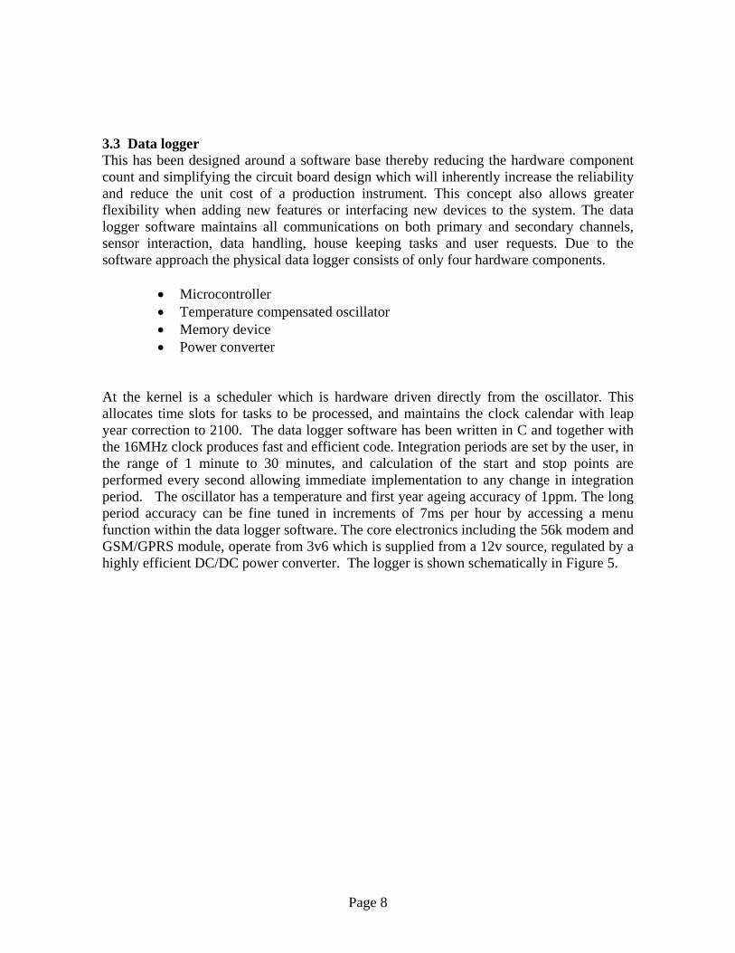
3.3 Data logger This has been designed around a software base thereby reducing the hardware component count and simplifying the circuit board design which will inherently increase the reliability and reduce the unit cost of a production instrument. This concept also allows greater flexibility when adding new features or interfacing new devices to the system. The data logger software maintains all communications on both primary and secondary channels, sensor interaction, data handling, house keeping tasks and user requests. Due to the software approach the physical data logger consists of only four hardware components.

• Microcontroller • Temperature compensated oscillator • Memory device • Power converter

At the kernel is a scheduler which is hardware driven directly from the oscillator. This allocates time slots for tasks to be processed, and maintains the clock calendar with leap year correction to 2100. The data logger software has been written in C and together with the 16MHz clock produces fast and efficient code. Integration periods are set by the user, in the range of 1 minute to 30 minutes, and calculation of the start and stop points are performed every second allowing immediate implementation to any change in integration period. The oscillator has a temperature and first year ageing accuracy of 1ppm. The long period accuracy can be fine tuned in increments of 7ms per hour by accessing a menu function within the data logger software. The core electronics including the 56k modem and GSM/GPRS module, operate from 3v6 which is supplied from a 12v source, regulated by a highly efficient DC/DC power converter. The logger is shown schematically in Figure 5.

Page 8

Data Logger

GSM / GPRS BGAN unit Regulator

Ethernet

Figure 5. Schematic configuration of the tsunami monitoring instrument 3.4 Communications Various methods of communications have been interfaced to the data logger, tested and evaluated, and summarized here. A PSTN modem interfaces directly to the microcontroller (i.e. there is no additional interface hardware). In this application it is used as a dial-in auto-answer modem but could be used to dial out if required. The GSM/GPRS module operates from 3v6; all communications and control lines interface directly to the microcontroller requiring no additional interface hardware. The antenna can be mounted directly from the module, or in poor reception areas a high-gain co-linear antenna can be installed. Running costs are typically less than £10 per month, with the GSM call originator bearing the cost of a call. GPRS costs increase dramatically once the monthly allocation is exceeded. The GSM has both data and voice channels which are used exclusively. The data channel functions similar to a standard modem but with a maximum data rate of 96kbaud. The GPRS functions exclusively with the GSM and provides a virtual point to point connection across the internet for data transfer. Duplex data transfer has a delay of less than 2 seconds and typically less than 1 second.

PSTN

Memory

Crystal

Modem

Micro controller

Broadband router

Filter

Laptop (Engineering connection)

Power

Optional

Laptop (Archiving one second data)

Dual channel interface board

SensorOther interface

board Sensor

Page 9

Broadband is provided via an ADSL line, micro filter and router providing both broadband and modem communications. Both can be utilised simultaneously; the broadband via the on-board Ethernet module and the phone line by the on board modem module described above. Running costs are likely to be less than £100 per month with no limit on the amount of data that can be transferred. The on-board Ethernet module has been successfully interfaced to a Hughes BGAN satellite transmission unit and tested at POL, transmitting 1 minute data over a period of 3 weeks with 1 loss of the link which was re-established automatically. 3.5 Power supply The main power supply for the instruments is derived from a regulated 12v supply which also maintains a rechargeable battery for use during power outages and low power source input, the latter being particularly noticeable from renewable sources such as solar panels and wind generators. All of the core electronics including the 56k modem and GSM/GPRS module operate from 3v6. The power for these devices is provided from the 12v regulated power source by a highly efficient (98%) DC/DC converter. This has the advantage over standard regulators of converting the power and not simply dropping the voltage, this minimises power wastage and still allows the use of a standard 12v source, thus providing easy integration to various charging options such as solar or wind power. 4. Data format and routing The data paths shown in Figure 6 illustrate a combination of 1 second, 10 second and integration period data; the latter being user selectable on the data logger between 1 and 30 minutes. Users are able to access the data files from either the POL internal network drive or externally from the ftp server. The three files created on the POL network drive are rolling records updated every 1 or 10 seconds depending upon the high frequency data rate, and contain:

• 120 records of 1 or 10 second data. • 96 records of integration period data. • 1200 records of 1 or 10 second data.

The last of these was set up to provide a real-time data feed for the tsunami detection algorithm described in Annex 1. The two files uploaded to the ftp server are rolling records updated every 1 or 10 seconds depending upon the high frequency data rate, and contain:

• 120 records of 1 or 10 second data. • 96 records of integration period data.

Page 10

Figure 6. Data routing from the Tsunami Monitoring Instrument to the end users

Data Logger

Users POL web page

SLEAC www.sleac.org

Flanders Institute

Data collection PC at POL

Network drive

ftp server

Site Holyhead Lerwick Newlyn

POL

External

1 second

Engineering and download path

Internet

PSTN

Optional

Laptop

Page 11

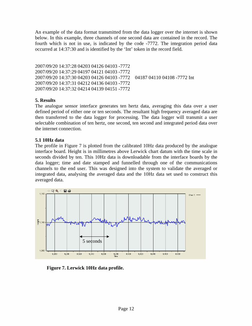
An example of the data format transmitted from the data logger over the internet is shown below. In this example, three channels of one second data are contained in the record. The fourth which is not in use, is indicated by the code -7772. The integration period data occurred at 14:37:30 and is identified by the ‘Int’ token in the record field. 2007/09/20 14:37:28 04203 04126 04103 -7772 2007/09/20 14:37:29 04197 04121 04103 -7772 2007/09/20 14:37:30 04203 04126 04103 -7772 04187 04110 04108 -7772 Int 2007/09/20 14:37:31 04212 04136 04103 -7772 2007/09/20 14:37:32 04214 04139 04151 -7772 5. Results The analogue sensor interface generates ten hertz data, averaging this data over a user defined period of either one or ten seconds. The resultant high frequency averaged data are then transferred to the data logger for processing. The data logger will transmit a user selectable combination of ten hertz, one second, ten second and integrated period data over the internet connection. 5.1 10Hz data The profile in Figure 7 is plotted from the calibrated 10Hz data produced by the analogue interface board. Height is in millimetres above Lerwick chart datum with the time scale in seconds divided by ten. This 10Hz data is downloadable from the interface boards by the data logger; time and date stamped and funnelled through one of the communications channels to the end user. This was designed into the system to validate the averaged or integrated data, analysing the averaged data and the 10Hz data set used to construct this averaged data.

5 seconds

Figure 7. Lerwick 10Hz data profile.

Page 12

(a)

20 seconds Blue Underwater direct reading pressure transducer. Red Transducer connected to the bubbler gauge.

Black Vega radar gauge.

(b)

50 seconds Blue Underwater direct reading pressure transducer. Red Underwater direct reading pressure transducer.

Black Kalesto radar gauge. Figure 8. One second sampling at Holyhead demonstrating radar lag from (a) Vega radar and (b) Kalesto radar.

Page 13

5.2 Radar comparison The plots in Figure 8 show the disturbance set up by the passing of the HSS high speed ferry leaving Holyhead on the 29/11/07 and 03/09/07 respectively. Figure 8a gives an indication to the frequency response of the sensors. The direct reading underwater transducer (blue) giving the best response with the transducer connected to the bubbler system (red) showing the characteristic lag as the air in the pressure point is unable to be replaced at the same rate it was lost. The Vega gauge (black) shows a smooth response with a lag of approx 10 seconds due to the internal damping and greater footprint being monitored. Figure 8b shows two underwater mounted transducers (blue and red) and the Kalesto (black). The plot indicates the step function produced by the Kalesto and the measurement interval delay. The time lines in the plots are in seconds from an arbitrary start point. Height values are in millimetres above chart datum. 5.3 Lerwick harbour event 29 May 2008 The plots shown in Figure 9 are of 1 second data transmitted in real time capturing an event in Lerwick harbour on the 29/05/08. This event was recorded at a number of locations including Peterhead some 200 miles away, and is thought to have been extreme seiching due to a local intense meteorological event, rather than a tsunami. The time axis is in seconds x 104 and the height in millimetres above chart datum. The plots demonstrate the ability to zoom into a specific point of interest using one second sampling without loss of detail due to averaging of data or spot sampling. In this case it can be seen that no sudden change took place on a sub minute scale, but a steady and rapid increase in level. The plots are made up of four profiles most noticeable in Figure 9d. Each profile colour maps to a physical transducer installed at Lerwick and detailed in the table below.

Table 2. Lerwick transducer profile mapping.

Profile colour

Physical channel

Transducer location / connection

Green Black

1 2

Underwater. Direct reading.

Blue Red

3 4

Tide gauge building. Connection to the bubbler system pressure point line.

Page 14

(a)

(b)

(c)

(d) . Figure 9. Event captured in Lerwick harbour with one second sampling. Time scales for (a) 14 hours, (b) 2 hours, (c) 12 minutes and (d) 2 minutes.

Page 15

6. Cost analysis The cost of the hardware evaluated during this project can vary between one thousand to several thousand pounds, depending upon the hardware configuration used and the number of sensors. The man hours required for an installation will vary greatly depending upon the sensors being installed and the location for the installation. Consequently this could become the dominant expense. Running costs are generally related to the communications and dependent on the volume of data being transferred. The general costs associated with providing a data logger, communications, additional equipment and setup charges, together with running costs experienced during this project are shown in Table 3.

Table 3. Equipment costs, standing and running charges (£) Data logger and sensors Hardware

cost Method of communications

Additional equipment costs

Standing charges. per month

Data charge

Basic data logger 150 PSTN modem 1. 50 Note 3. Call cost GSM/GPRS module 1. 100 GSM 6 Call cost GPRS 2. 10 1 / MB Ethernet module 1. 50 ADSL broadband 50 100 None BGAN 1500 50 5 / MB SensorTechnics transducer

250

Vega radar gauge 1200 1. Additional cost to the basic data logger. 2. Additional setup and standing charges apply for a VPN connection. 3. Basic line rental or a combined charge with the ADSL line. 7. Real-time detection algorithm Real-time tide gauge data, as measured by these new high frequency sensors, are a critical component of a complete warning system. They may be used to estimate tsunami wave heights along different coastal regions, predict exact arrival time, direction of propagation and harbours sensitive to resonant oscillations. The sea level data are thus crucial for early warning as well as cancelling any seismic warning when non-destructive tsunamis are generated. Any end-to-end tsunami warning system requires a level of automated detection of both seismic and sea level signals. As part of this project, we have developed codes to analyse the sea level data in real-time to identify tsunami or other abnormal sea level changes. Our code calculates the variance of non-tidal residual sea levels, the maximum and minimum water levels of high frequency (< 1hr) oscillations, and the periods of high frequency oscillations. The sea level data analysis provided by the algorithm in Annex 1

Page 16

consists of six objectives that are performed in chronological order: 1. Real time data retrieval. 2. Removing tide (and any seasonal cycle) from the sea level data. 3. Bandpass filtering of data to remove signals with periods larger than 1 hr and noise

with periods less 4 min. 4. Estimation of the variance distribution for 24 hr data. 5. Calculation of amplitude and periods of the remaining high frequency oscillations. 6. Set alarms based on variance changes, maximum and minimum residual sea levels.

These are site-specific: different tide gauge locations have different residual sea level oscillations, thus different reference levels need to be used for alarms.

We performed a number of trials to test the capability of the algorithm, the effectiveness of the filters and to produce a simple, user-friendly output. We tested the algorithm using sea level data from Holyhead (where a wave induced by a ferry may cause spurious alarms), data from a real tsunami affecting India, and a modelled signal from a simulation of the 1755 Lisbon earthquake (Horsburgh et al., 2008). 7.1 Holyhead data An initial test data test set, comprising 20 minutes of 1 second data (averaged from 10Hz) from the Holyhead sensors, produced the output shown in Figure 10.

Figure 10. 20 minutes of sea level data from Holyhead. Sea level (top), residual (middle), calculated variance (bottom).

Page 17

Three alarm settings are included in the algorithm: each can be set to a pre-determined threshold that is meaningful for the site under consideration. These could be, for example, (i) a primary alert based on unusual sea level variance, (ii) confirmation of a genuine wave within the tsunami spectrum and (iii) confirmation that wave amplitude is above a severe threshold. Of the three threshold alarms included in the algorithm, none were triggered by the time-series of normal tidal data. To further test the sensitivity of the algorithm, 1 second data from Holyhead was considered over a longer time period (Figure 11), when a significant bow wave from the Holyhead-Dublin high speed ferry was known to affect sea level. Two anomalies are evident, the first between 15:00-16:00 on 8 November 2007 and the second between 20:00-21:00 on the following day. It is important that the tsunami algorithm does not respond spuriously to these signals produced by the ferry passing.

Figure 11. Sea level data from Holyhead over the 8-9 November 2007. Channels 1 and 2 of the high frequency sensors are shown in green and blue respectively. The passage of the ferry is evident as the sharp spikes in the signal. The period between 15:00 and 16:00 on 8 November 2007 is analysed in Figure 12. The variance signal shown in the lower panel did, in this instance, falsely set off the tsunami alarms so a further Butterworth filter (e.g. Ifeachor and Jervis, 1993) was applied to the variance time series; after this modification only the first alarm was triggered by the ferry passage. Similar results were obtained when the algorithm was applied to the second ferry passage that can be seen in Figure 11.

Page 18

Figure 12. Sea level data from Holyhead 1500-1600 on 8 November 2007. Sea level (top), residual (middle), calculated variance (bottom). 7.2 2004 Boxing Day tsunami Having tuned the suite of filters to prevent rapid but erroneous changes in the sea surface height from triggering the tsunami warning system, it is important to demonstrate that the system responds correctly to an actual tsunami signal. In order to test this, data recorded at the port of Chennai during the 2004 Boxing day Tsunami has been taken from the National Institute of Oceanography, India (http://www.nio.org/jsp/tide_gauge.htm). 10 days of sea level measurements at 5 minute intervals have been analysed between 21-31 December 2004. The results are shown in Figure 13. Using the same filter settings as for Holyhead (in previous analysis), only the first and second threshold alarms were triggered. Although the variance of the real tsunami system had smaller magnitude than the Holyhead port data, the instantaneous change in residual height is much larger. In any real operational warning system, the third alarm setting could easily be modified to reflect some combination of variance and wave amplitude that represented a hazard.

Page 19

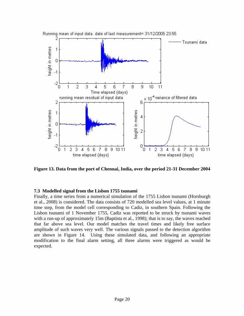
Figure 13. Data from the port of Chennai, India, over the period 21-31 December 2004 7.3 Modelled signal from the Lisbon 1755 tsunami Finally, a time series from a numerical simulation of the 1755 Lisbon tsunami (Horsburgh et al., 2008) is considered. The data consists of 720 modelled sea level values, at 1 minute time step, from the model cell corresponding to Cadiz, in southern Spain. Following the Lisbon tsunami of 1 November 1755, Cadiz was reported to be struck by tsunami waves with a run-up of approximately 15m (Baptista et al., 1998); that is to say, the waves reached that far above sea level. Our model matches the travel times and likely free surface amplitude of such waves very well. The various signals passed to the detection algorithm are shown in Figure 14. Using these simulated data, and following an appropriate modification to the final alarm setting, all three alarms were triggered as would be expected.

Page 20

Figure 14. Simulated data at a numerical model cell corresponding to Cadiz (6.30W, 36.5N) from the model of Horsburgh et al. (2008) 8. Conclusions Our examination of several months of collected data from both Holyhead and Lerwick demonstrated that the transducers mounted underwater had a tendency to develop offset drift, whereas those connected to the bubbler system (in the pneumatic line) within a tide gauge building exhibit superior stability, whilst the gain of the signal appeared to be unaffected. The main cause of drift for this type of transducer is temperature variation, yet the underwater transducers are in an environment inherently less prone to long-term temperature fluctuations than those inside the tide gauge building. Further inspection for biological growth, or other marine processes that might affect the transducer diaphragm, needs to be carried out. However, such pressure transducer drift would not be an important factor for a practical tsunami sensor whose only function is to detect large transient variations in sea level, not make an accurate absolute measurement. The installation of two underwater pressure transducers could provide a system at minimal cost and deliver a degree of redundancy in the event of transducer failure or contradictory data. The Vega radar gauge is also a suitable solution since it lends itself to quick and simple installation due to the small physical size, light weight and low power requirements.

Page 21

It can easily be mounted on quay edges, buildings or steel structures. The problem of unwanted reflections associated with radar gauges can be overcome with the supplied software, allowing changes to the internal parameters for site-specific anomalies. The trials showed that the difference in frequency response between an underwater pressure transducer, and one connected to the bubbler system pressure lines, is minimal in most cases. The radar gauges exhibited some lag and damping at high frequencies, but their ability to measure the correct amplitude – albeit with a small delay - was not impaired. To conclude, any of the evaluated sensors could be employed for tsunami monitoring. Signals from any of the sensor packages tested may be analysed by the detection algorithm described here, which can deliver an automated series of warning alarms. Further tuning of the alarm logic is required if it were ever needed as part of a national warning system, but the effort required would be modest. The use of GPRS communications should only be considered in locations with high levels of network data usage, because service providers would switch resources away from GPRS if demand were low; subsequently this would compromise the reliability of the system. Transmitting packets of data at short intervals would significantly increase the running cost. Maintaining a reasonable packet size with a 1 minute interval, as used in this project, resulted in a 1Mbyte per month allocation and incurred only modest costs. Glossary ADSL Asymmetric Digital Subscriber Line BGAN Broadband Global Area Network GPRS General Packet Radio Service GSM Global System for Mobile communications ISP Internet Service Provider MTBF Mean Time Between Failures POL Proudman Oceanographic Laboratory PSTN Private Switched Telephone Network VPN Virtual Private Network

Page 22

References Allen, S.C.R. and Greenslade, D.J.M. (2008). Developing tsunami warnings from numerical model output. Natural Hazards, 46, 35-52. Baptista, M. A., S. Heitor, J. M. Miranda, P. M. A. Miranda and L. Mendes Victor (1998). The 1755 Lisbon tsunami; evaluation of the tsunami parameters, J. Geodynamics, 25, 143-157. Horsburgh, K.J., Wilson, C., Baptie, B.J., Cooper, A., Cresswell, D., Musson, R.M.W., Ottemöller, L., Richardson, S., and Sargeant, S.L. (2008) Impact of a Lisbon-type tsunami on the UK coastline, and the implications for tsunami propagation over broad continental shelves. Journal of Geophysical Research, 113, C04007, doi:10.1029/2007JC004425. Ifeachor, E.C. and Jervis, B.W. (1993) Digital signal processing: a practical approach. Addison-Wesley Publishers Ltd, Wokingham, 760pp. Kerridge, D. et al. (2005). The threat posed by tsunami to the UK. Study commissioned by Defra Flood Management and produced by British Geological Survey, Proudman Oceanographic Laboratory, Met Office and HR Wallingford. 167pp.

Page 23

Annex 1. Matlab code for detection algorithm % Real time sea level data analysis % Matlab code for Holy Head: 1 sec data analysis for abnormal % sea level fluctuations %% Load Data hold on cd('N:\tsunami_progs'); load hlystr fid=fopen('holywv_data.txt'); % Read one second data file textfile=textscan(fid,'%19c %f %f %*f %f'); dt=textfile{1,1}; tm=datevec(dt,'yyyy/mm/dd HH:MM:SS'); %% Extract Channel Data and filter wvdata_ch1=textfile{1,2}; wvdata_ch2=textfile{1,3}; wvdata_ch3=textfile{1,4}; % Calculating mean values mean_wvdata_ch1=((wvdata_ch1-mean(wvdata_ch1))/1000); mean_wvdata_ch2=((wvdata_ch2-mean(wvdata_ch2))/1000); mean_wvdata_ch3=((wvdata_ch3-mean(wvdata_ch3))/1000); % Tide Prediction for Holy Head; varying every second over a given period prd_time=datenum(tm); pred_height=T_PREDIC(prd_time,TIDESTRUC); d_pred_height=pred_height-mean(pred_height); residual_mean_wvdata_ch1=mean_wvdata_ch1-d_pred_height; residual_mean_wvdata_ch2=mean_wvdata_ch2-d_pred_height; residual_mean_wvdata_ch3=mean_wvdata_ch3-d_pred_height; % Low pass butterworth filter SR = 60; %sample rate (number of samples per time period) nmin =20; %filter length (number of time periods) wn(1) = (1/nmin)/(SR/2); [B,A]=butter(1,wn,'low'); % Apply filter to coefficents filt_ch1=filtfilt(B,A,wvdata_ch1); filt_ch2=filtfilt(B,A,wvdata_ch2); filt_ch3=filtfilt(B,A,wvdata_ch3); % Calculating deviated values (value - overall mean) d_wvdata_ch1=((filt_ch1-mean(filt_ch1))/1000); d_wvdata_ch2=((filt_ch2-mean(filt_ch2))/1000); d_wvdata_ch3=((filt_ch3-mean(filt_ch3))/1000); % Residual of filtered data rs_mean_wvdata_ch1=d_wvdata_ch1-d_pred_height; rs_mean_wvdata_ch2=d_wvdata_ch2-d_pred_height; rs_mean_wvdata_ch3=d_wvdata_ch3-d_pred_height; %% Varience calculation vrc1=[]; vrc2=[]; vrc3=[];

Page 24

for jj=1:length(rs_mean_wvdata_ch1); ch1_hh=rs_mean_wvdata_ch1(1:jj); ch2_hh=rs_mean_wvdata_ch2(1:jj); ch3_hh=rs_mean_wvdata_ch3(1:jj); vrc1=[vrc1;var(ch1_hh)]; vrc2=[vrc2;var(ch2_hh)]; vrc3=[vrc3;var(ch3_hh)]; end % alarm programme dtanly %% Produce Timeseries lastdata=tm(length(tm),:); lst_dt_rc=num2str(lastdata); % Set time period for x-axis (minutes) t=(1:length(d_pred_height))/60; tmcal %% Plotting Data subplot(2,2,1:2) plot(t,d_pred_height+pred_height(1),'r',t,mean_wvdata_ch1+pred_height(1),... 'b',t,mean_wvdata_ch2+pred_height(1),'g',t,mean_wvdata_ch3+pred_height(1),'m') xlabel('Time elapsed (minutes)') ylabel('height in metres') title(['Running mean of input data. date of last measurement= ', lst_dt_rc]) set(gca,'Xtick',0:20) % Adjust x axis to suit time period set(gca,'XTickLabel',tmm1) leg=legend('Tidal prediction','Channel 1','Channel 2','Channel 3'); set(leg,'box','off'); set(leg,'location','BestOutside'); VV=axis; %% subplot(2,2,3) axis(VV) plot(t,residual_mean_wvdata_ch1,'b',t,residual_mean_wvdata_ch2,'g',t,... residual_mean_wvdata_ch3,'m') xlabel('time elapsed (minutes)') ylabel('height in metres') title('residual of running mean') set(gca,'Xtick',0:20) set(gca,'XTickLabel',tmm1) %% subplot(2,2,4) plot(t,vrc1,'b',t,vrc2,'g',t,vrc3,'m') set(gca,'Xtick',0:20) set(gca,'XTickLabel',tmm1) xlabel('time elapsed (minutes)') ylabel('height in metres') title('variance of filtered data')

Page 25