
Health and safety management and business economic ... - HSE
76
Health and Safety Executive Health and safety management and business economic performance An econometric study Prepared by Cambridge Econometrics for the Health and Safety Executive 2006 RR510 Research Report
-
Upload
khangminh22 -
Category
Documents
-
view
0 -
download
0
Transcript of Health and safety management and business economic ... - HSE

Health and Safety Executive
Health and safety management and business economic performance An econometric study
Prepared by Cambridge Econometrics for the Health and Safety Executive 2006
RR510 Research Report
Health and Safety Executive
Health and safety management and business economic performance An econometric study
Sadia Sheikh, Ben Gardiner & Saxon Brettell Cambridge Econometrics Covent Garden Cambridge CB1 2HS
This study explores the relationship between the scale of health and safety (H&S) activity undertaken by businesses and their economic performance. The objective is to measure whether increased H&S activity encourages investment in human and physical capital, thereby leading to an increase in productivity at both firm and industry levels. A gross output multiindustry approach has been adopted, in which growth in each industry's gross output is decomposed into the contributions from changes in capital services, labour and other inputs, with the residual defined as total factor productivity. The study then examines whether investment in health and safety explains some of the residual productivity.
This report and the work it describes were funded by the Health and Safety Executive (HSE). Its contents, including any opinions and/or conclusions expressed, are those of the authors alone and do not necessarily reflect HSE policy.
HSE Books

© Crown copyright 2006
First published 2006
All rights reserved. No part of this publication may bereproduced, stored in a retrieval system, or transmitted inany form or by any means (electronic, mechanical,photocopying, recording or otherwise) without the priorwritten permission of the copyright owner.
Applications for reproduction should be made in writing to:Licensing Division, Her Majesty’s Stationery Office,St Clements House, 216 Colegate, Norwich NR3 1BQor by email to hmsolicensing@cabinetoffice.x.gsi.gov.uk
ii

CONTENTS
Executive Summary............................................................................................................................ vGlossary .............................................................................................................................................vii1 Introduction................................................................................................................................. 1
1.1 Objectives and framework of analysis for the study ...................................................... 11.2 Context of study................................................................................................................ 1
2 Review of the Literature............................................................................................................. 32.1 Introduction....................................................................................................................... 32.2 Economic performance theories ...................................................................................... 42.3 Data measurement issues ................................................................................................. 82.4 Studies on the economic impact of health and safety activity....................................... 82.5 Conclusions..................................................................................................................... 12
3 Methodological Approach for the Study................................................................................. 133.1 Theoretical model ........................................................................................................... 13
APPENDIX to chap 3....................................................................................................................... 153.2 Formal specification of a growth accounting approach ............................................... 15
4 Data Review.............................................................................................................................. 184.1 Dependent Variable ........................................................................................................ 184.2 Primary Explanatory Variables...................................................................................... 194.3 Residual Component ...................................................................................................... 20
APPENDIX to chap 4....................................................................................................................... 324.4 Gross Output in Constant Basic Prices.......................................................................... 324.5 Quality-Adjusted Hours Worked ................................................................................... 32
5 Estimation and Results ............................................................................................................. 335.1 deriving a measure of productivity ................................................................................ 335.2 relationship between productivity and h&s activity ..................................................... 395.3 Using investment as the dependent variable ................................................................. 44
Appendix to Chapter 5...................................................................................................................... 45Estimation Results............................................................................................................... 45
5.4 .................................................................................................................................................. 455.5 Results of Cross Sectional Regression .......................................................................... 475.6 Results purged of zeros and outliers.............................................................................. 495.7 H&S VARiables Deflated by employment ................................................................... 505.8 Investment as the dependent variable............................................................................ 52
6 Conclusion ................................................................................................................................ 537 Methodology Review by Professor Gavin Cameron.............................................................. 55
7.1 Professor Cameron's comments on version 2.0 of the report....................................... 557.2 Professor Cameron's comments on version 3.0 of the report....................................... 56
8 References ................................................................................................................................. 588.1 Cited References ............................................................................................................. 588.2 Additional Readings ....................................................................................................... 60
iii

iv
EXECUTIVE SUMMARY
This study seeks to gather robust econometric evidence on the relationship between health and safety (H&S) activity undertaken by firms in a sector and sectoral economic performance in the UK. It presents a relevant literature review, a methodology for undertaking an empirical study, a review of H&S and other data used to inform the analysis, the empirical study itself and the comments of an independent peer reviewer.
The approach taken involved: • framing a model for understanding the manner in which H&S activity impinges on the
productivity of a sector of activity in the UK
• specifying a flexible empirical specification of the production process by sector using a gross output growth accounting framework capable of embracing a range of theoretical perspectives
• allowing for the empirical estimation of the major drivers of long-run industrial productivity growth in the UK by sector over the period 1970 to date as suggested by a literature review and utilising Cambridge Econometrics' annual time series of input-output consistent volume and value indices of change for 42 sectors of the UK economy from 1970 and the Bank of England Industry Dataset (2003)
• incorporating novel data sets on H&S activity by the HSE and LAs, specifically derived for this study in cooperation with the HSE, so as to look at the potential impact of health and safety activity on all components of factor productivity, while recognising that observed data on stringency measures of H&S activity are only available for the last ten years and are of mixed quality
The main conclusions of the study are: • The underlying process and linkage between H&S activity and sectoral performance is
quite complex.
• It is not clear a priori whether greater H&S stringency would lead to a fall in output and productivity as firms struggle to meet stricter regulatory requirements or whether, in conformance with the Porter hypothesis, higher H&S stringency will lead to the adoption of better technologies thereby enhancing productivity.
• It is possible that greater H&S stringency in some sectors may lead to a short-term fall in output but as newer technologies are adopted the long-term impact is an eventual increase in productivity. However, the lack of sufficient time-series data on H&S variables makes it difficult to identify any time trend in the impact of stringency data on productivity.
• The analysis done using the available (sectoral cross-sectional) data (while controlling for average firm size in a sector) yields statistically stable results although these show that the impact of H&S activity on sectoral productivity is not very strong. This may be because the impact of H&S activity on technology and production techniques is felt after a time lag which is difficult to capture given the lack of time-series data. Also, the impact of H&S activity could also be felt through secondary sources such as increased capital investment or better labour.
v

Despite these caveats, the results show that measures of H&S stringency that have a statistically significant, albeit small, effect on productivity are ‘notices issued’, ‘investigations’, ‘inspections’ and the ‘cost of regulation’.
The cost of regulation1 and the number of notices issued are positively associated with productivity. This indicates that sectors in which the cost of regulation is higher and those which receive a greater number of notices may have more incentive to invest in safer technologies that also positively impact productivity. These findings are consistent with the Porter hypothesis, although with limited possibilities for building time-adjustment into the analysis, this cannot be concluded with certainty. An alternative explanation could simply be that firms with low compliance, and therefore which have a greater number of notices, have higher productivity.
The number of investigations and inspections are both inversely related to productivity, indicating that greater operational activity (more inspections and investigations) is associated with lower productivity, although whether this is due to the simple fact that there is more HSE activity and monitoring in lower productivity sectors or whether a higher number of inspections initially lowers productivity as firms struggle to comply with regulation is difficult to ascertain with the available data. This negative association might imply that if H&S stringency measures were to be tightened, productivity would fall in these sectors, at least in the short-term. Generally, more regulated sectors have a higher number of inspections while investigations are higher in low-compliance sectors. If this is the case, then low compliance (higher notices) would be associated with low productivity.
While there are both positive and negative effects associated with different stringency measures, there is no over-riding positive or negative impact that can conclusively support Porter’s hypothesis for the overall UK economy.
It can be concluded that increased H&S activity has not been detrimental to sectoral performance. The evidence suggests that the investigations and inspections processes have a small, negative association with productivity. These are therefore the two regulatory procedures where the HSE may wish to ensure that the costs to businesses in terms of compliance are not higher than required to ‘catch up’ with achieving necessary compliance.
1 It should be borne in mind that the ‘cost of regulation’ variable does not take into account how much of the compliance cost a firm can pass on to consumers. The more firms are able to do this, the less incentive there will be for them to make cost-saving investments.
vi

GLOSSARY
CLEMS-TFP ‘Capital Labour Energy Materials Services’ TFP based on gross output Convex production an output space such that any averaged combination of inputs produce space an output that lies within the feasible output from the inputs taken
separately Efficiency technical efficiency is the degree to which engineering 'best practice' is
achieved; allocative efficiency measures the distance from an optimal (usually) profit-maximising solution
Endogenous causally determined factor in modelled change EPA Environmental Protection Agency Exogenous external factor driving modelled change Factor of production primary input into production such as labour or capital Factor Productivity output change related to specific input change at the margin FDI Foreign Direct Investment Gross output total measure of (physical) output GFCF Gross Fixed Capital Formation GLS Generalised Least Squares GVA Gross Value Added HAVS Hand Arm Vibration Syndrome H&S Health and Safety HSC Health and Safety Commission HSE Health and Safety Executive ICT Information and communication technology Intermediate outputs the factors of production that are produced and transformed or used up
by the production process within the accounting period IO Input-Output LA Local Authority MB Marginal Benefit MC Marginal Cost MDM Multisectoral Dynamic Model Net output value added measure of output Netput in a multi-product input-output inter-relationship; a netput is negative if
it defines an input level to a production activity, positive if it defines an output
OECD Organisation for Economic Co-operation and Development ONS Office for National Statistics OSHA Occupational Safety and Health Administration PIM Perpetual Inventory Method; a method for achieving stock asset
measures by cumulating flows over time and allowing for depreciation Primary inputs all forms of capital and labour PF Production Function; function linking maximum output to available
inputs: flexible forms satisfy some of the basic requirements of production theory while allowing parameters to be determined by data fit; a frontier production function defines the envelope of technically feasible outcomes
Profit function maximum value function relating profits to the price of inputs and outputs of the industry
RCI Risk Control Index Returns to scale ratio of the proportion of output change to a given proportional increase
vii

of inputs, constant returns is when a k-fold increase in output occurs as a consequence of a k-fold increase in inputs
RIA Regulatory Impact Assessment RIDDOR Reporting of Injuries, Diseases and Dangerous Occurrences Regulations RTD Research, Training and Development SNA 93 System of National Accounts, United Nations' standard for international
presentation of national accounts. This version was specified in 1993. Previous versions were 1953 and 1968. An important component of SNA '93 is the so-called SUT - Supply & Use Table - the system which forms the basis for the construction of input-output tables
SUTs Supply and Use Tables Technology currently known ways of converting resources into outputs.
Disembodied technology is costless general knowledge - 'blueprints'. Embodied technology - built in to the latest generation of a factor and not in previous 'vintages'
TFP Total Factor Productivity or multi-factor productivity, a measure of the rate of transformation of a total bundle of inputs into total output
Translog Transcendental Logarithmic (production function) - see Annex to chap 3 for details
Value added gross output less intermediate consumption (outputs - inputs)
viii

1 INTRODUCTION
1.1 OBJECTIVES AND FRAMEWORK OF ANALYSIS FOR THE STUDY
Health & Safety activity
Individuals’decisions
Firms’decisions
Quality of working
environment
Investment in human capital
Economic cycle
Investment (other than
human capital and quality of
working environment)
Total factor productivity
Other factors eg pollution controls
‘Returns to education
and training’
‘Growth theory and accounting’
‘Factors influencing the impact of Health & Safety’ and other
factors on decisions to invest
Figure 1.1 Relating health and safety activity to business performance
1.1.1 Objectives
This report seeks to gather robust econometric evidence on the relationship between health and safety (H&S) activity undertaken by businesses and business' economic performance in the UK economy. Figure 1.1 shows how this study has taken as its framework for analysis a production function approach that expresses the manner in which H&S activity is expected to impact on business performance. Both firm and individual employee decisions are seen as critical elements in economic performance of firm and industry, with H&S activity as one of the factors that affects costs but also drives up the quality of the working environment. This encourages the process of investment in both human and physical capital, and, in the context of economic change, allows a firm to change its competitive offer in its existing or prospective markets subject to regulation.
The study considers all H&S activities that firms carry out in compliance with legal/regulatory requirements.
1.2 CONTEXT OF STUDY
The HSE estimates that 40 million working days (about 0.6% of all working days) were lost to occupational injury and ill health in Britain in 2001/02 with 7 million days (about 0.1% of all working days) attributed to occupational injury.
1

While parts of preceding legislation remain in place2 and subsequent legislation has been added3, the 1974 Health and Safety at Work Act4 is the major legislative basis for current health and safety regulation. It places general duties on all employers to protect the health and safety of their employees and those affected by their work activities, and seeks to guide employers to strive to undertake better H&S practice. The Act led to the setting up of the Health and Safety Commission (HSC) and the Health and Safety Executive (HSE), and a provision for local authorities (LAs) to enforce health and safety law in certain premises.
The HSC and the HSE are responsible for the regulation of almost all the risks to health and safety arising from work activity in Britain by ensuring risks in the workplace are properly controlled. Their remit covers health and safety in nuclear installations and mines, factories, farms, hospitals and schools, offshore gas and oil installations, the safety of the gas grid and the movement of dangerous goods and substances, railway safety, and many other aspects of the protection both of workers and the public.
Local Authorities are responsible to the HSC for enforcement in offices, shops and other parts of the services sector, including leisure and catering sectors and residential care. Inspectors have substantial statutory powers and can enter any premises where work is carried on without notice. In the case of the inspector being dissatisfied, enforcement notices can be issued by the HSE and local authorities. These can range through advice and warnings, improvement notices, deferred prohibition notices or immediate prohibition notices, and, ultimately, prosecution. Each workplace is visited and rated for risk with such inspections generating close to 20,000 enforcement notices in 1999-2000.
The HSE employs close to 4,000 staff and spends close to £40m each year on its research and investigative activities5 while about 3,500 (1,100 full-time equivalent) H&S inspection staff are employed by the 400 or so local authorities in Britain. Development of the regulatory regime and approved codes of practice (ACOPs) is an evolving and ongoing process, with some 2,000 documents currently providing guidance to different sectors and activities and notifying employers on the current standards that inspectors expect to be achieved in the workplace. In addition, for the major hazards industries where 'permissioning regimes' require regulatory approval - gas transportation, offshore and onshore petrochemicals and the railway industry -charges are made for inspections, investigations and approvals.
The current national support strategy for workplace health and safety is set out in the February 2004 document Strategy for workplace health and safety Great Britain to 2010 and beyond6. The strategy sets out a clear direction for the health and safety system and defines the specific roles of the HSC, the HSE and the LAs. In terms of this study, one of the specific aims of this strategy is to develop closer strategic partnerships to improve the contribution to employment and productivity by keeping those at work healthy and in work.
2 These include the 1961 Factories Act, the 1964 Offices, Shops and Railways Premises Act and the 1965 Nuclear installations Act. 3 These include the 1992 Transport and Works Act, the 1993 Management and Administration of Safety and Health at Mines Regulations, and the 1993 (European Union Framework Directive 89/391/EEC) Management Regulations. 4 SI 1974/1439 5 Source: The Health and Safety System in great Britain, HSC, 2002,HSE Books 6 A strategy for workplace health and safety in Great Britain to 2010 and beyond, HSC, Feb 2004
2
2 REVIEW OF THE LITERATURE
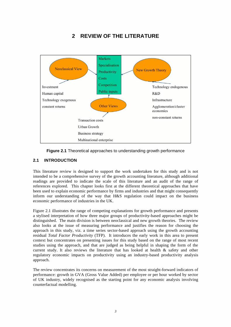
Figure 2.1 Theoretical approaches to understanding growth performance
2.1 INTRODUCTION
This literature review is designed to support the work undertaken for this study and is not intended to be a comprehensive survey of the growth accounting literature, although additional readings are provided to indicate the scale of this literature and an audit of the range of references explored. This chapter looks first at the different theoretical approaches that have been used to explain economic performance by firms and industries and that might consequently inform our understanding of the way that H&S regulation could impact on the business economic performance of industries in the UK.
Figure 2.1 illustrates the range of competing explanations for growth performance and presents a stylised interpretation of how three major groups of productivity-based approaches might be distinguished. The main division is between neoclassical and new growth theories. The review also looks at the issue of measuring performance and justifies the reason for choosing the approach in this study, viz. a time series sector-based approach using the growth accounting residual Total Factor Productivity (TFP). It introduces the early work in this area to present context but concentrates on presenting issues for this study based on the range of most recent studies using the approach, and that are judged as being helpful in shaping the form of the current study. It also reviews the literature that has looked at health & safety and other regulatory economic impacts on productivity using an industry-based productivity analysis approach.
The review concentrates its concerns on measurement of the most straight-forward indicators of performance: growth in GVA (Gross Value Added) per employee or per hour worked by sector of UK industry, widely recognised as the starting point for any economic analysis involving counterfactual modelling.
3

2.2 ECONOMIC PERFORMANCE THEORIES
2.2.1 Neoclassical theory perspectives
At the firm and industry level, or micro-economic, the level that is the interest of this study, there exists a reasonably clear and straightforward understanding of the notion of economic performance derived from traditional neoclassical theory. This is based on the capacity of firms and industries to compete, to grow, and to be profitable. At this level, competitiveness resides in the ability of firms to consistently and profitably produce products that meet the requirements of an open market in terms of price, quality, etc. Any firm must meet these requirements if it is to remain in business, and the more competitive a firm relative to its rivals the greater will be its ability to gain market share or grow profits, depending on industry conditions, and the firm's strategy.
It will consequently rate higher on the performance measures linked to this ability to compete -such as labour productivity, profitability and output growth rates. Conversely, less competitive firms will find their market shares decline, and ultimately any firm that remains uncompetitive -unless it is provided by some 'artificial' support or protection - will go out of business. Ability to compete in openly competitive economies is based on a superior productivity performance and, in a technologically changing world, on the ability of a firm to move to higher productivity activities, which in turn can generate higher levels of profits and wages. There are distinct theories of the competitive behaviour of firms and of the markets they operate. These provide starkly different perspectives on how firms compete and will perform depending on the market and technology assumptions. It is useful to distinguish the neo-classical and endogenous growth theoretical perspectives that underlie much of the literature discussions.
The core neo-classical assumptions
The core assumptions of neo-classical theory include perfect information and constant returns to scale (increasing inputs by any amount leads to an increase in output of exactly that amount). These assumptions provide the necessary conditions for a model in which firms and industries compete in a neo-classical world of perfect competition, where comparative advantage and relative performances exist due to differences in the relative abundance of factors of production (factor endowments). With technology assumed to be exogenous (fixed) for each firm and uniformly available this translates into a relatively straightforward productivity model, where performance is driven by the quantity of factor inputs, and therefore the ability to accumulate capital is a critical driver of a firm's performance in gaining market share. Neoclassical growth theory provides the foundation for much of the modern econometric analysis of productivity growth with the Solow (1956, 1957) growth model in particular the theoretical foundation for a large literature relating productivity to input factors and technological change.
Growth accounting
The most highly structured approach drawn from this Solow tradition has emerged as the aggregate growth accounting framework, with human capital added into traditional labour and capital as factors driving economic growth. There is also emphasis on multi-sectoral detail with total (or multi-) factor productivity (TFP) allocating the contribution to growth of output to inputs, and with the residual from this then related to knowledge and other variables. Such an
4
approach requires independent measures of capital and labour inputs, and is now captured in the internationally recommended approach of the OECD (2001a and 2001b).
Such a two-stage approach to productivity measurement is quite naturally associated with the suggestion that technology is exogenous (and therefore not embodied in particular factors) but this need not be the case. An influential model of this type that substitutes investment for capital and then derives an estimating equation on the basis of an aggregate Cobb-Douglas production function is provided by Mankiw, Romer and Weil (1992). This relates total factor productivity to knowledge factors, which in turn are related to institutional and other starting conditions. Where the approach has gone subsequently is in allowing for more flexible specification of the functional form, elaboration of sectoral effects, and more careful treatment of estimation issues.
Since this approach is the selected one for this study, a more detailed discussion of specification and estimation issues using this approach is undertaken in Chapter 3, with an additional technical annex providing a full formal derivation of results used in specification of the flexible functional specification - the transcendental logarithmic (translog) production function – that was the starting point for analysis in this study.
2.2.2 A national accounts-based perspective
The OECD (2001a) manual presents the most detailed practical specification of the TFP approach, with OECD (2001b) presenting associated capital measurement solutions, albeit from the perspective of an international statistical office and with a national accounts focus, rather than an econometric testing focus. They usefully distinguish capital-labour TFP from capital-labour-energy-materials-services (CLEMS) TFP, with the latter fully reflecting the role of intermediate inputs in production (and therefore providing the preferred method of choice in this study).
Gross and net output measures
The critical difference between gross and net measures of productivity reflects the role of intermediate inputs, viz. those factors that are produced and transformed or used up by the production process within a given accounting period. In a full multi-sector specification this will involve the use of inter-industry accounts. The SNA 93 standard for international (and UK national) accounts provides for such separation of the uses and resources within production units. This CLEMS-TFP approach would operate with gross output and consequently requires information on the time-series of prices and volumes of intermediate inputs bought by each sector. This would be achieved by using input-output tables for the whole period, the recommended approach in SNA 93, although requiring some data construction in the UK context, where full I-O structure and Use tables have been calculated only infrequently.
Lau and Vaze (2003) review the implementation of this approach in the UK by ONS but there is a strong US-based literature in this area with Jorgenson and Griliches (1967) providing the basis for many contributions. Jorgensen, Ho and Stiroh (2004) provide a particularly relevant example of a growth accounting empirical study of US industries, which demonstrates the importance in a US context of measuring intermediate inputs, when allocating productivity effects. In the UK, Oulton and Srinivasan (2004) provide a similar approach with a multi-industry contribution drawing on the output databases developed for the Bank of England by Cambridge Econometrics. Other interesting recent contributions are reviewed in O'Mahony and
5
van Ark (2003), which presents international EU/US comparisons using the approach. Cameron et al (2005) is an example of a recent application of the approach using time series panel estimation and that embraces both the choice of translog underlying flexible functional forms and empirical procedures for dealing with disequilibrium concerns.
Factor measurement issues
Measures of factor inputs are a crucial part of the TFP approach. Much of the recent work in this area has been directed at quality adjustment. Physical capital has always been problematic to conceptualise and measure. The modern treatment has been informed by the work of Erwin Diewert (see Diewert, 2004 for a review). Much of the practical work in this area has been based on simplifying assumptions about the depreciation rates of physical capital so that measured investment streams by industry can be translated to provide a measure of capital inventory. Thus in most countries, including the UK, capital stocks are estimated by the perpetual inventory method (PIM). For each type of asset, the stock figure is estimated by cumulating flows of gross investment over what is believed to be the service life, and allowing for depreciation.
Quality adjustment is of course a particular issue for labour input measures and quality-adjusted measures of labour inputs depend on some measures of labour quality, typically reflecting educational background or occupational mix. TFP can then better be associated with knowledge spillovers, increasing returns and those other interdependencies between factor inputs that are hypothesised in endogenous growth theory. This extra flexibility makes the approach much more potentially fruitful in application in this study where H&S is expected to generate labour quality effects. While steady-state growth is treated as exogenous in neoclassical approaches, endogenous growth theory suggests shifts in steady-state growth will be dependent on human capital accumulation, with human capital accumulation and technology diffusion in turn linked to trade. The theories include those derived by Nelson and Phelps (1966), Romer (1986) and Lucas (1988).
2.2.3 New economic growth theory - endogenous growth theory
Within the neoclassical tradition technological progress was assumed to be entirely exogenous. In this sense, shifts in a firm's performance are seen to be created in ways that lie outside the immediate control of individual firms. By contrast 'new' growth theories suggest that the accumulation of knowledge and human capital is more clearly the result of managerial actions in the past. The incorporation of 'technology' into economic models as an endogenous variable is the main contribution of endogenous (or new) growth theory, which has given rise to a large literature of applications. The key assumption of endogenous growth theory is that accumulation of knowledge generates increasing returns. Knowledge and know-how are not disseminated instantly - between nations, regions, sectors or companies - but need to be acquired. This means free and open markets do not necessarily yield an optimal result: companies have an incentive to keep knowledge to themselves and to protect intellectual property rights in order to keep investments in R&D profitable. Highly skilled workers are seen as more productive and innovative and are therefore of crucial importance to companies. Human capital is a critical productive factor. Drivers for this are R&D expenditure, innovativeness (eg patents), education and training and other forms of investment in human capital, and high quality dissemination routes for knowledge.
6
Endogenous growth theory essentially allows for shifts in steady state growth to be dependent on human capital accumulation, with human capital accumulation and technology diffusion linked to trade.
2.2.4 Other approaches
There are a number of other approaches that may be mentioned
New' institutional economics
The notion of 'transaction costs', lies at the heart of the theory put forward by Coase (1937, 1988) and elaborated by Williamson (1971,1981). Transaction costs include the costs connected to communication, coordination and decision-making. In principle, large organisations can realise significant savings in transaction costs by long-lasting contracts. Transaction costs also apply to the notion of vertical integration by long-term contractual arrangements. It suggests how the emergence of sustained industrial clusters can arise through outsourcing.
Cluster theories
Among the most influential of the approaches allied with business strategy economics theories is the cluster theory of Michael Porter. According to Porter, to be competitive, firms must continually improve operational effectiveness in their activities while simultaneously pursuing distinctive rather than imitative strategic positions. This encourages the formation of contiguous groupings of individuals firms that are of major benefit to their competitive performance. Fujita and Thisse (1997) correspondingly identify three major reasons for economic clustering: increasing returns under monopolistic competition; externalities under perfect competition; spatial competition under strategic interaction.
The observation that knowledge tends to flow freely between proximate firms operating within the same or related industries lies at the heart of the empirical literature investigating the link between innovation and location. A sizeable body of empirical studies have shown that knowledge spillovers not only increase productivity, but their effect also decays with geographic distance (Jaffe et al., 1993; Acs et al., 1994). In particular, Jaffe et al. (1993) point out that knowledge flows do sometimes leave a paper trail in the form of patented citations. Some types of knowledge are best transmitted via face-to-face interaction. In this case spatial proximity matters because tacit knowledge is non-rival in nature, in the sense that the use of a piece of information by a firm does not reduces its content for other firms and can easily spill over from firm to firm.
Along similar lines Glaeser et al. (1992) observe that the diffusion of technical knowledge may be highly localised and transfer is more likely to occur in places densely packed with organisations that share similar interests (local milieu). The attention devoted to the measurement and the effect of knowledge spillovers is also linked to the new growth theory (Romer, 1986; Lucas, 1988; Grossman and Helpman, 1991). Unlike neoclassical growth theory (Solow, 1956), endogenous growth models identify externalities, rather than scale economies, as the main engine of growth. Given that knowledge spillovers are an important source of externalities, regional differences in growth rates may result from increasing returns to knowledge.
Jacobs (1969) and Porter (1990) claim that local competition is superior to local monopoly, because it creates incentive to emulate best practice and boosts pressure to innovate. Among a
7

range of empirical studies, Armington and Acs (2002) look at the effect of new firm entry rates on local employment growth. Using data on nearly 400 labour market areas and six industrial sectors, they find that high rates of entry have a positive impact on the growth of local economies. The authors argue that their results are consistent with the theories of Porter and note how firms' incentive to cluster benefits from reciprocal technological spillovers.
2.3 DATA MEASUREMENT ISSUES
2.3.1 Industry versus firm issues
In addition to the distinction in the literature between gross and net outputs, that between the firm and the industry level of performance is important both theoretically and practically for this study. The data to be used in this study of H&S regulation and productivity is constrained to just the available industry level information, with little or no data as yet available from firms. The forthcoming WHASS survey on which the study team have advised is expected to be seeking to address this issue directly but will not produce information within the horizon of this study. This means that industry growth performance will be the essential concern of this study. Thus firm entry and exit processes remain an implicit part of industry adjustment processes to industry price changes. This is also better formally treated with a gross output rather than a net output approach to productivity measurement, since it makes no implicit assumption that industry behaves as a single optimising decision-maker with a single production function.
2.4 STUDIES ON THE ECONOMIC IMPACT OF HEALTH AND SAFETY ACTIVITY
2.4.1 Enforcement is a necessary basis for effectiveness
There is a body of literature dealing with the direct effectiveness of the enforcement process in the UK in encouraging H&S activity and H&S awareness by companies. Much of this is commissioned by the HSE itself. Greenstreet Berman (2004) provides a recent review of this literature. On the basis of their review they conclude that:
• The application of enforcement is an effective means of securing compliance, creating an incentive for self-compliance and a fear of adverse business impacts such as reputation damage in all sectors and sizes of organisations, including major hazard sectors.
• Fear of enforcement is a significant motivator for organisations, there may be value in exploring new types of penalties, charging regimes and enforcement strategies so as to maximise the deterrent effect of enforcement, such as court ordered publicity.
• There is evidence that enforcement and HSE leadership is an important element in prompting major hazard firms to manage health and safety, including major accident prevention.
• Enforcement supported by advice and guidance is considered to be of equal benefit to health hazards, such as noise, passive smoking, manual handling and stress, as it is to safety risks.
8

Ch
/ / / / / /
- j /j
-
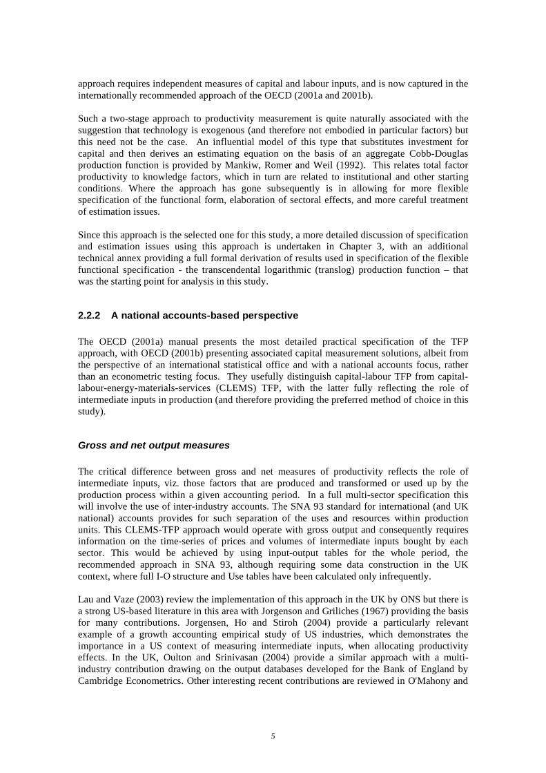
art 2.1 REPORTED MAJOR INJURIES IN UK CONSTRUCTION
1 000 2 000 3 000 4 000 5 000 6 000
91 92 93 94 95 96 97 98 99 00 01 02
Source: RIDDOR Note: Non fatal in ury statistics from 1996 97 cannot be compared directly with
earlier years due to revised in ury reporting requirements in 1996
Members of the public
Selfemployed
Employees
• There is some evidence that advice and information is less effective in the absence of the possibility of enforcement.
Greenstreet Berman includes the study by Davies and Elias (2000) who reported a long term (1986 -1997) downward trend in injuries in Great Britain. They attributed this to improved safety performance, having controlled for changes in industrial structures, the economic cycle and patterns of employment, albeit that they considered the improvements in the reporting of workplace injury under RIDDOR (reporting of injuries, diseases and dangerous occurrences regulations) in the 1990's obscured the level of improvement in workplace safety (see Chart 2.1 for evidence of this in the Construction sector).
2.4.2 Studies on the impact of regulation
2.4.2.1 Theoretical Arguments
There are a number of ways in which H&S activity is thought to influence productivity in the economy. First, H&S activity can be seen as indirectly raising the cost of certain types of activity which are associated with certain types of labour or capital (for example, manual work, and energy-intensive capital equipment). This will lead to a shift along the production function which will reduce measured TFP since the firm will no longer be choosing a measured cost-minimising input set. Consequently, H&S regulation will lead to a decline in sectoral performance and productivity.
On the other hand the hypothesis put forward by Michael Porter - and which is therefore known as the ‘Porter hypothesis’- suggests firms may then undertake certain investments to offset these higher costs which will shift the production function outwards. The proposition is that ‘properly designed’ regulation can induce innovation that can more than offset the costs of compliance. Allowing for a dynamic model structure, work by Porter (1991) and Porter and van der Linde (1995), suggests that regulations do not inevitably hinder competitive advantage against foreign rivals and that more severe regulation may actually have a positive effect on firms' performance by stimulating innovations.
9
The suggestion is that properly constructed regulatory standards, which aim at outcomes and not methods, will encourage companies to re-engineer their technology. The result in many cases will be a process that not is not only more efficient but which also lowers costs or improves quality. Thus, regulation may trigger innovation that offsets compliance costs. There is a sharp contrast with standard neoclassical economic models with perfect markets and no uncertainty. These cannot generate outcomes that satisfy the Porter hypothesis.
Lanoie et al (2001) argue that the Porter hypothesis can be extended in three directions. First, the Porter hypothesis is dynamic in that regulation adopted today will affect firms' productivity after a time lag; second, firms with a higher level of inefficiencies will have more opportunities to identify and eliminate these inefficiencies, so that the positive effect of regulation on performance is greater for firms that are initially more inefficient; third, firms in industries that are exposed to more competition are likely to have more of an incentive to innovate than less exposed firms.
Popp (2005) argues that the effects of uncertainty may be an explanation for the empirical finding of micro-level cases where complete innovation offsets occur and macro-level findings that such offsets do not occur. Using a simulation approach, Popp shows that complete offsets as hypothesized by Porter, while not occurring in a majority of cases, can occur frequently, even when the expected costs of regulation are on average positive.
The Porter hypothesis has been criticised on the grounds that profit-maximising firms would take advantage of existing investment opportunities even in the absence of regulation. However, it is possible that there may be positive externality effects that are gained through H&S regulation. In other words, there may be barriers to efficiency because of which firms, if left to the free market, may not reach their production frontier. Regulation may collectively allow all firms in the industry to operate at the most efficient (socially optimal) level.
There is also the possibility that, if barriers to entry and exit are low, then once regulation is in place, low productivity firms would leave the market thereby increasing overall productivity in the industry.
2.4.2.2 Empirical Evidence
There are several studies that have been carried out to analyse the impact of increased regulation on sectoral productivity, although most of these focus on environmental regulation rather than H&S activity and are relevant to the North American economy. Table 1 lists the main findings of some such studies.
It has been observed that regulation backed up by inspection or the threat of inspection improves direct injury rates in reported US studies. Gray and Mendeloff (2002) do, however, find declines in this measure of the impact of OSHA inspections since 1979. In comparing the impact of OSHA inspections on manufacturing industries using data from three time periods: 1979-85, 1987-91, they found a substantial decline in the impact of OSHA inspections – in 1979-85 period they estimate that having an OSHA inspection that imposed a penalty reduced injuries by about 15%; it fell to 8% in 1987-91 and to a (statistically insignificant) 1% effect in 1992-98.
Dufour, Lanoie and Patry (1998) and Lanoie et al (2001) have investigated the impact of occupational safety and health (OSH) and environmental regulation on the rate of growth of
10
total factor productivity (TFP) in the Quebec manufacturing sector during the 1985–88 period. Their results show that environmental regulation and OSH protective reassignments (a prevention policy with respect to OSH) have led to a reduction in productivity growth, while the presence of mandatory prevention programs (and of fines for infractions to OSH rules) have led to an increase in productivity growth. The stringency of environmental regulation was proxied by the change in the ratio of the value of investment in pollution-control equipment in an industry to the total cost in that industry. Variables to capture the stringency of occupational safety and health regulation, the fluctuations of quasi-fixed inputs and industry-specific effects were also included in the equation. The results show that when dynamic effects are allowed to occur, the impact of environmental regulation on productivity becomes less detrimental and even positive over a four-year horizon, confirming the Porter hypothesis (explored in the next chapter). The results also indicate that the level of external competition an industry faces is a key driving force inducing firms to turn environmental constraints into their advantage.
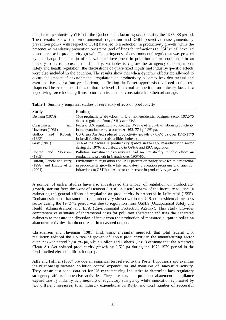
Table 1 Summary empirical studies of regulatory effects on productivity
Study Finding Denison (1978) 16% productivity slowdown in U.S. non-residential business sector 1972-75
due to regulation from OSHA and EPA. Christiansen and Haveman (1981)
Federal U.S. regulation reduced the US rate of growth of labour productivity in the manufacturing sector over 1958-77 by 0.3% pa.
Gollop and Roberts (1983)
US Clean Air Act reduced productivity growth by 0.6% pa over 1973-1979 in fossil-fuelled electric utilities industry.
Gray (1987) 30% of the decline in productivity growth in the U.S. manufacturing sector during the 1970s is attributable to OSHA and EPA regulation
Conrad and Morrison (1989)
Pollution investment expenditures had no statistically reliable effect on productivity growth in Canada over 1967-80.
Dufour, Lanoie and Patry (1998) and Lanoie et al (2001)
Environmental regulation and OSH prevention policy have led to a reduction in productivity growth, while mandatory prevention programs and fines for infractions to OSHA rules led to an increase in productivity growth.
A number of earlier studies have also investigated the impact of regulation on productivity growth, starting from the work of Denison (1978). A useful review of the literature to 1995 in estimating the general effects of regulation on productivity is presented in Jaffe et al (1995). Denison estimated that some of the productivity slowdown in the U.S. non-residential business sector during the 1972-75 period was due to regulation from OSHA (Occupational Safety and Health Administration) and EPA (Environmental Protection Agency). This study provides comprehensive estimates of incremental costs for pollution abatement and uses the generated estimates to measure the diversion of input from the production of measured output to pollution abatement activities that do not result in measured output.
Christiansen and Haveman (1981) find, using a similar approach that total federal U.S. regulation reduced the US rate of growth of labour productivity in the manufacturing sector over 1958-77 period by 0.3% pa, while Gollop and Roberts (1983) estimate that the American Clean Air Act reduced productivity growth by 0.6% pa during the 1973-1979 period in the fossil fuelled electric utilities industry.
Jaffe and Palmer (1997) provide an empirical test related to the Porter hypothesis and examine the relationship between pollution control expenditures and measures of innovative activity. They construct a panel data set for US manufacturing industries to determine how regulatory stringency affects innovative activities. They use data on pollutant abatement compliance expenditure by industry as a measure of regulatory stringency while innovation is proxied by two different measures: total industry expenditure on R&D, and total number of successful
11
patent applications by industry. They find that higher lagged compliance costs lead to higher levels of R&D. However, when they use patent applications as an indicator of innovation, they find little evidence that they are related to compliance costs.
Conrad and Morrison (1989), in a study of the manufacturing sectors of the U.S., Germany and Canada, find that pollution investment expenditures had virtually no effect on productivity growth in Canada during the 1967-80 period. Gray (1987) finds that about 30% of the decline in productivity growth in the U.S. manufacturing sector during the 1970s is attributable to OSHA and EPA regulation and Gray and Shadbegian (1998) show that regulation crowds out more productive investments in other areas.
2.5 CONCLUSIONS
2.5.1 Likely industry sector performance drivers
The conclusion of the literature review is that a number of drivers of economic growth performance are likely to be important for the H&S study: investment as measured by gross fixed capital formation over time (the accumulated stock of capital); investment in human capital (knowledge economy assets such as R&D, education and ICT, telecoms, internet access); level and quality of workforce such as qualifications and IT proficiencies; innovation and RTD (for instance RTD expenditure and patent applications). In addition there are important questions relating to spatial links for more or less globally tradable or non-tradable sectors, especially in relation to the direct role of trade in the former. Part of the interest is in terms of the setting of the industry-technology frontier by market boundaries, and how trickle-down effects of technology on productivity growth are determined.
Disaggregated micro-economic analysis using a gross output approach is both the recommended and likely to be the most productive way to explore the impact of H&S effects where regulation and H&S practice are seen to be associated with different stringencies of impact by a sector of industry but have knock on effects elsewhere that work through all sectors of the economy through intermediate inputs.
There is little micro-based work involving firm-based studies of H&S activity but there is strong evidence that industry aggregates are responsive to firm entry and exit effects in driving measured productivity change rather than endogenous forces within a firm. There is also evidence from a range of studies to suggest that economic scale is an important factor in industrial productivity change. While data availability precludes all but industry-based analysis in this study, the literature review at least suggests that there are important market conditions that should be taken into account.
12

3 METHODOLOGICAL APPROACH FOR THE STUDY
3.1 THEORETICAL MODEL
In the light of the literature review, the form considered most useful for framing the H&S impact analysis is a gross output multi-industry approach. This requires the use of UK input-output tables to generate an explicit gross output measure, and to derive indices of primary and intermediate inputs for each of the designated sectors. This is drawn from CE's comprehensive volume and price databanks of the UK economy and developed for 42 sectors for use in its MDM work. Estimation is focused around the use of a flexible functional form, the translog function, which has a number of theoretical advantages in aggregation, but for this study is especially recommended as having a form that allows for consistent and plausible volume and value indices to be calculated across industries. The approach is a CLEM-TFP approach that thereby isolates the effect of a range of inputs in a consistent and comprehensive way across the economy
3.1.1 Supporting analyses
The proposed approach responds directly to the conclusions of Jorgensen, Ho and Stiroh (2004), the work undertaken by CE for, and the findings of, Oulton and Srinivasan (2004) and follows the recommendations of the OECD (2001a) Manual on productivity. Human and ICT-capital and non-ICT capital variables, and labour headcount and labour hours measures of productivity are modelled in accordance with the recommendations of the OECD productivity manual and reflect the recent literature in this area on the treatment of vintage effects. In particular the approach updates that part of the work of Oulton and Srinivasan that was based on an earlier version of CE's industry IO databank. The study is set at the most detailed industry level of results, appropriate for assessing important H&S impacts, which are firm and industry focussed, but which through intermediation are in principle going to affect value added in all sectors of the economy. Micro to macro consistency in aggregation is thereby captured in a manner of especial suitability for this study.
Because of the need for a systematic treatment of intermediate inputs, the study benefits from a methodology that establishes consistent empirical results across all industries in the UK. Also, because the effects are likely to be slow acting and short-term 'noise' is substantial, the study concentrates on establishing longer duration comparisons, across suitable periods. The outcome will be established long-run drivers of industry productivity, and a common baseline decomposition of the experience of TFP change between 1970 and 2002. This analysis is the starting point for understanding the manner in which the H&S contribution is to be fully assessed in any one industry. The H&S specific industry analysis will come from using a range of novel variables to measure H&S 'stringency', reflecting the available data from 1992 and established from HSE in-house and other HSE-provided or facilitated activity figures.
Measured productivity is likely, on the basis of previous studies reviewed, to be significantly differentially affected by changes in primary and intermediate inputs, as well as by the external effects driving the transformation of total inputs into total output. Among the most important of these last effects will be technology transfers from higher productivity locations, reflected for example in the 'productivity gap' notably with the US, emphasised by Cameron et al (2005), and evidenced in a wide range of recent empirical studies at both aggregate and micro levels in the wide-ranging international literature. In the full approach of this study, H&S activity is allowed
13

to shape both the location of the industry technology frontier and the allocative decisions taken by industry. The latter will come as a response to factor price changes as initial cost shifts force firms and factors to react. As factor prices respond then optimal inputs will be changed to achieve a particular output. Since this is likely to take more than a single year, the most suitable empirical framework for such a study, and the basis of our empirical analysis, is a cumulative multi-annual measure of productivity change. The work can be expressed therefore as the search for an equilibrium factor productivity effect where a flexible production function and variable factor costs must be accommodated. It therefore does not use a panel approach.
More formally, the estimated efficiency frontier will need to reflect: scale of industry effects, the likely force coming from the best practice technology that is available internationally to produce the outputs of the industry in question, the incentives otherwise given to firms to adopt industry standard H&S or other technologies, or to pursue research and development to generate such new technologies, the role prices of primary inputs, direct and indirect effects via intermediate inputs from other (perhaps not proximate to UK) industries7 , the quality of the primary factors of production that can be employed directly within the industry - essentially measuring the changing effectiveness of the services of labour of particular types, and similarly for capital services, and finally proxies for organisational variables that are likely to relate to transaction costs for these industries.
The study approach embraces an econometric TFP approach (as categorised by the OECD Manual) by allowing for the role of technology to be embodied as a factor-based driver of the position of the industry efficiency frontier - the maximum output that can be achieved for a given combination of factor resources. It accommodates the possibility that there is a transition mechanism in the UK of faster technology adoption by any industry not at the current global technological frontier by proxies for openness to trade. The productivity gap literature suggests inefficiency in these terms may be because of poor quality industry inputs but also because of barriers to removal of less efficient firms. The latter may be receiving relative protection from competitive effects of innovations by those leading industries/firms external to that sector in the UK economy, especially other industries in external economies, for example the US. Export orientation is likely to be a suitable proxy. Health and safety activity and other forms of regulation are seen as levering on efficiency by influencing both cost and output through compliance and efficiency effects.
7 The effect of intermediates inputs that do not enter into external trade is a special case but potentially influential if the sector is protected from international trade. The Balassa-Samuelson effect is concerned with changes in the relative productivity of tradable versus non-tradable inputs of one country. An increase for example raises relative wages, thus increasing the relative price of non-tradables and relative average prices, impacting on the exchange rate.
14

APPENDIX TO CHAP 3
3.2 FORMAL SPECIFICATION OF A GROWTH ACCOUNTING APPROACH The methodology for measuring total factor productivity requires a definition of the industry production function. This is:
),,;,,(ƒit !"#XMNYit =
Where N is primary inputs, M is intermediate inputs, X is exogenous factors, and α, β, δ are associated parameters defining the links. H&S inputs would impact potentially on any one of these components.
As an example this could be specified in a constant share, constant returns to scale format for primary capital and labour inputs as:
rtijt
jititit eMLKY MjLK !!!
! "= 0
Where subscript i references sector and t a time index.
3.2.1 The TFP approach based on a simple functional specification
This simplest of specifications is the 'Cobb-Douglas' growth accounting specification that is in line with the Solow balanced growth path model. This special case underpins the TFP growth accounting calculation using the conventional net output approach in the OECD (2001a) Manual, where Y is net output and M is explicitly dropped. Thus a strong justification for this would be hypothesising that all production flows taken together satisfy the Cobb-Douglas aggregate production function, to display constant returns to scale in aggregate and with exogenous technical improvement that augments labour viz:
!"!" ##=
1)( ttttt LZHKY
Where Y t is a value-added measure of output, K t is physical capital services, H t is human capital services, L t is labour service and Z t is exogenous technological improvement enhancing the productivity of labour. Z t is assumed to accumulate as a by-product of economic activity but, unlike consumption, investment and capital depreciation, does not use up current output. Using lower case letters to indicate per labour input quantities gives the productivity measure, output per labour input, as
!"!"
tttt hkZy ##=
1
Output is allocated to the following uses:
tHttKttt HHKKCY !! ++++= &&
15
Where Ct is consumption, and δ K and δ H are rates of depreciation for physical, Kt, and human, Ht, capital respectively. If L t grows at rate n in the long run, then the balanced growth path for physical capital, and human capital output per labour input are derived respectively as
tktkttk knyskkg )(/ +!== "&thhtth hnyshhg )(/ +!== "&and
Where s k is the share of output allocated to physical capital and s h is the share of output allocated to human capital. At balanced growth
hytt ggyy =!&
giving a final estimated form of particular simplicity. Clearly the growth accounting approach is based on a strong set of underlying assumptions (see OECD 2001, Annex 3, pp 124-127 for a fuller derivation). The outcome is a log difference form where productivity change may be decomposed as the contributions from the weighted rates of change of physical and human capital, with the residual defining exogenous technical improvement, viz:
)log(log)log(log)log(logloglog 0000 hhkkyyZZ tttt !!!!!=! "#
Under perfect competition assumptions, parameters α and β would be the monetary shares of returns to the primary factors, physical and human capital in the accounts and using these factor shares as the weighting system in industry input analysis gives statisticians a suitable combined index of inputs and thereby delivers the OECD recommended statistical measure of TFP as the residual from this specified calculated net output.
More generally this TFP specification can be represented as the difference in logs:
!"N
N NdsYd lnln
Where N is the input indicator, s N the payment share of input.
It should also be noted that an alternative dual approach could be used based on constructing a maximum profit value or minimum unit cost function. The solution to this dual model would, logically, be exactly the same as that obtained using the production function approach. There are some useful benefits in terms of tractability for the empirical approaches from using the dual, with residual decomposition of factor price to value added ratios the equivalents in the dual of obtaining the primal TFP residual.
3.2.2 The translog specification
The chosen flexible functional form is the transcendental logarithmic (or translog) function. As an illustrative three factor input case determining gross output, this would give a quadratic form in logarithms of primary inputs, K and L, and intermediate input, M, viz:
! !++++=ƒ g ƒi
iƒg0 loglogloglogloglog gii
iMi
iLi
iK
ii FFMLKY "####
where F is K, L or M in the summation.
16

The translog function is a desirable approximation to any functional form that is 'well behaved' in economic space (i.e. with uniquely defined first and second order derivatives for the function corresponding to a convex production space). If Tornqvist 8 indices are used for calculating input and output prices and volumes, then these are superlative indices as defined by Diewert (Diewert, 1976, and OECD 2001a, p88), in that using such indices would exactly conform to an underlying translog function.
*pYCFpF =!"The maximisation of this function subject to each sector's satisfying a cost constraint at the sector optimum, can see the expression of choices of optimal industry factor inputs determined by the prices of achieved output and factor input prices.
Thus, dropping the i'th industry subscript, for each industry sector the following optimal(*) factor demand matrix equilibrium condition holds, expressed here in an illustrative way to give four equations determining the three inputs, and the shadow price (λ) on the cost constraint:
!!!!
"
#
$$$$
%
&
'(
)*+
,=
!!!!
"
#
$$$$
%
&
!!!!!
"
#
$$$$$
%
&
---- CmMwLrK
YMLK
MMMLMKM
LMLLLKL
kMkLkkK
***
*log*log*log
1
222222222222
ƒMƒLƒKƒ
.
///0
///0
///0
///0
This linear form in the parameters is readily generalised to many inputs, and also indicates a linear form in parameters that can be used to estimate empirically the parameters of the base translog production function for each sector, given the observations over time on output volumes, total intermediate costs, factor inputs, and factor prices or factor shares.
8 A Tornqvist index is an exponential average of the product of price or volume relatives using weights that are the average of the base and current expenditures on each component. By comparison a Fisher Ideal index is a geometric average of the summed relatives using base and current expenditure weights respectively and would be a superlative index for a Cobb-Douglas PF.
17
4 DATA REVIEW
This section reviews and analyses the data that are to be used in the final estimation. The industry-level (i) production function to be estimated takes the form
),,(ƒi iiii MLKY =
where Y is gross output, K is capital services, L is labour services and M is intermediate input (an aggregate of purchases from all the industries). The residual would then typically capture any other effects arising from technological progress including the possible effects of increased health & safety activity.
4.1 DEPENDENT VARIABLE
4.1.1 Gross output in constant basic prices
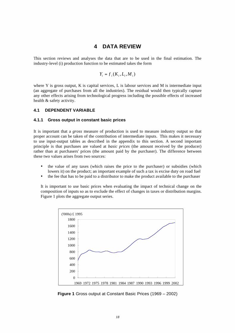
It is important that a gross measure of production is used to measure industry output so that proper account can be taken of the contribution of intermediate inputs. This makes it necessary to use input-output tables as described in the appendix to this section. A second important principle is that purchases are valued at basic prices (the amount received by the producer) rather than at purchasers' prices (the amount paid by the purchaser). The difference between these two values arises from two sources:
• the value of any taxes (which raises the price to the purchaser) or subsidies (which lowers it) on the product; an important example of such a tax is excise duty on road fuel
• the fee that has to be paid to a distributor to make the product available to the purchaser
It is important to use basic prices when evaluating the impact of technical change on the composition of inputs so as to exclude the effect of changes in taxes or distribution margins. Figure 1 plots the aggregate output series.
0
200
400
600
800
1000
1200
1400
1600
1800
1969 1972 1975 1978 1981 1984 1987 1990 1993 1996 1999 2002
('000s) £ 1995
Figure 1 Gross output at Constant Basic Prices (1969 – 2002)
18
4.2 PRIMARY EXPLANATORY VARIABLES
The main explanatory variables are labour services, capital services and intermediate demand.
4.2.1 Labour Services Labour services can be measured in two ways
• Compensation of employees • The quality-adjusted hours worked
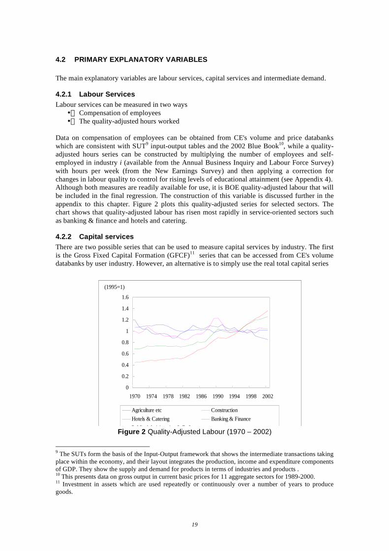
Data on compensation of employees can be obtained from CE's volume and price databanks which are consistent with SUT9 input-output tables and the 2002 Blue Book10, while a quality-adjusted hours series can be constructed by multiplying the number of employees and self-employed in industry i (available from the Annual Business Inquiry and Labour Force Survey) with hours per week (from the New Earnings Survey) and then applying a correction for changes in labour quality to control for rising levels of educational attainment (see Appendix 4). Although both measures are readily available for use, it is BOE quality-adjusted labour that will be included in the final regression. The construction of this variable is discussed further in the appendix to this chapter. Figure 2 plots this quality-adjusted series for selected sectors. The chart shows that quality-adjusted labour has risen most rapidly in service-oriented sectors such as banking & finance and hotels and catering.
4.2.2 Capital services There are two possible series that can be used to measure capital services by industry. The first is the Gross Fixed Capital Formation (GFCF)11 series that can be accessed from CE's volume databanks by user industry. However, an alternative is to simply use the real total capital series
0
0.2
0.4
0.6
0.8
1
1.2
1.4
1.6
1970 1974 1978 1982 1986 1990 1994 1998 2002
(1995=1)
Agriculture etc ConstructionHotels & Catering Banking & FinancePublic Administration & DefenceFigure 2 Quality-Adjusted Labour (1970 – 2002)
9 The SUTs form the basis of the Input-Output framework that shows the intermediate transactions taking place within the economy, and their layout integrates the production, income and expenditure components of GDP. They show the supply and demand for products in terms of industries and products . 10 This presents data on gross output in current basic prices for 11 aggregate sectors for 1989-2000. 11 Investment in assets which are used repeatedly or continuously over a number of years to produce goods.
19
0
200
400
600
800
1000
1200
1969 1972 1975 1978 1981 1984 1987 1990 1993 1996 1999 2002
(£ '000)
0
50
100
150
200
250
300
350
400
1969 1972 1975 1978 1981 1984 1987 1990 1993 1996 1999 2002
(£ '000)
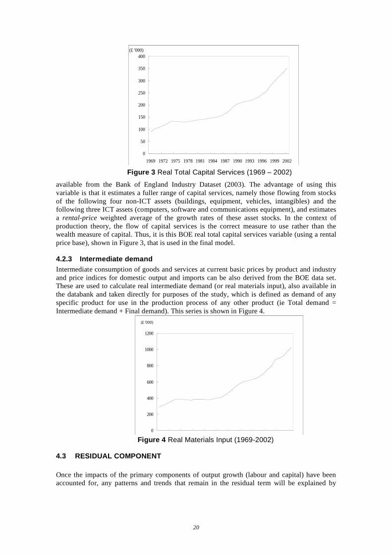
Figure 3 Real Total Capital Services (1969 – 2002)
available from the Bank of England Industry Dataset (2003). The advantage of using this variable is that it estimates a fuller range of capital services, namely those flowing from stocks of the following four non-ICT assets (buildings, equipment, vehicles, intangibles) and the following three ICT assets (computers, software and communications equipment), and estimates a rental-price weighted average of the growth rates of these asset stocks. In the context of production theory, the flow of capital services is the correct measure to use rather than the wealth measure of capital. Thus, it is this BOE real total capital services variable (using a rental price base), shown in Figure 3, that is used in the final model.
4.2.3 Intermediate demand Intermediate consumption of goods and services at current basic prices by product and industry and price indices for domestic output and imports can be also derived from the BOE data set. These are used to calculate real intermediate demand (or real materials input), also available in the databank and taken directly for purposes of the study, which is defined as demand of any specific product for use in the production process of any other product (ie Total demand = Intermediate demand + Final demand). This series is shown in Figure 4.
Figure 4 Real Materials Input (1969-2002)
4.3 RESIDUAL COMPONENT
Once the impacts of the primary components of output growth (labour and capital) have been accounted for, any patterns and trends that remain in the residual term will be explained by
20

other possible sources of output growth. In particular, the additional variables that are explored in the study include health & safety activity and stringency.
4.3.1 Health & Safety Activity
The health & safety variables that have been considered for the final model are described below. Information on all these variables has been provided by the HSE.
4.3.1.1 RIDDOR data
The Reporting of Injuries, Diseases and Dangerous Occurrences Regulations 1985 (RIDDOR 85) were introduced in April 1986, and have now been replaced by RIDDOR 95 (effective from 1 April 1996). The Regulations require employers to report all cases of a defined list of diseases occurring among their employees where they receive a doctor's written diagnosis and the affected employee's current job involves the work activity specifically associated with the disease. Comparison of RIDDOR data with those for disablement benefit for the corresponding DWP prescribed diseases suggests that there is still substantial under-reporting under RIDDOR, particularly for diseases with long induction periods.
RIDDOR data (under RIDDOR 95 regulations) are available for the period 1996/97-2003/04 and are organised by three types of incidents: fatalities, major accidents and incidents that last more than three days. The relevant times series that can be extracted from this data is the ‘total number of accidents’ by type of accident for each industrial sector. There are 16 possible kinds of injuries reported under RIDDOR: superficial, strains, natural causes, multiple, loss of sight, laceration, fracture, electricity, dislocation, contusion, concussion internal, burn, asphyxiation, amputation, other known, other not known. It is then possible to ‘deflate’ the time series on the total number of accidents by type and industry by dividing them by some measure of employment in that sector for that year to obtain a approximation for the incidence or injury rate of accidents in each industry.
The Warwick Institute of Employment Research (IER) have prepared an injury rate series by aggregate sector for an HSE study ‘Trends and Context to Rates of Workplace Injury’. In the construction of this injury rate series, IER have make several necessary adjustments to the employment variable used to deflate the number of injuries by sector. ONS estimates of seasonally adjusted employment derived from the Labour Force Survey were used as a starting point for the employment base.
It was, however, recognised that a simple count of the number of people in employment did not account for the fact that an increasing number of people are opting for part-time employment which leads to an increase in the employment base, while the exposure to risk in terms of work done may remain unchanged (e.g. a full time job may be replaced by two part time jobs). IER, thus, use an alternative adjusted employment denominator based on a rescaling of total employment to a full time equivalent level based on a full time employee working 40 hours per week. The injury rates, referred to as a ‘full-time equivalent’, are then expressed per 100,000 employees. The structural break in the series due to changes in RIDDOR definitions in April 1996 is also removed from the data using a one off step-shift dummy derived from a time series model of injury rates.
Finally, IER adjust the data to account for the fact that non-fatal injuries are substantially under-reported within the RIDDOR data, particularly among the self-employed. Also reporting rates vary over time, particularly during periods surrounding the introduction of new health and safety campaigns, initiatives or regulations. Increased reporting levels may therefore disguise
21
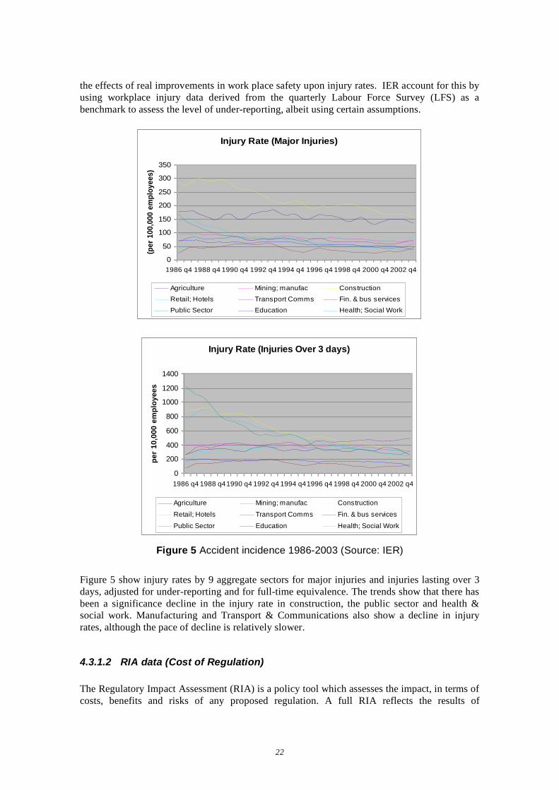
the effects of real improvements in work place safety upon injury rates. IER account for this by using workplace injury data derived from the quarterly Labour Force Survey (LFS) as a benchmark to assess the level of under-reporting, albeit using certain assumptions.
Injury Rate (Major Injuries)
0
50
100
150
200
250
300
350
1986 q4 1988 q4 1990 q4 1992 q4 1994 q4 1996 q4 1998 q4 2000 q4 2002 q4
(per
100
,000
em
ploy
ees)
Agriculture Mining; manufac Construction
Retail; Hotels Transport Comms Fin. & bus services
Public Sector Education Health; Social Work
Injury Rate (Injuries Over 3 days)
0
200
400
600
800
1000
1200
1400
1986 q4 1988 q41990 q4 1992 q4 1994 q41996 q4 1998 q4 2000 q4 2002 q4
per
10,0
00 e
mpl
oyee
s
Agriculture Mining; manufac Construction
Retail; Hotels Transport Comms Fin. & bus services
Public Sector Education Health; Social Work
Figure 5 Accident incidence 1986-2003 (Source: IER)
Figure 5 show injury rates by 9 aggregate sectors for major injuries and injuries lasting over 3 days, adjusted for under-reporting and for full-time equivalence. The trends show that there has been a significance decline in the injury rate in construction, the public sector and health & social work. Manufacturing and Transport & Communications also show a decline in injury rates, although the pace of decline is relatively slower.
4.3.1.2 RIA data (Cost of Regulation)
The Regulatory Impact Assessment (RIA) is a policy tool which assesses the impact, in terms of costs, benefits and risks of any proposed regulation. A full RIA reflects the results of
22
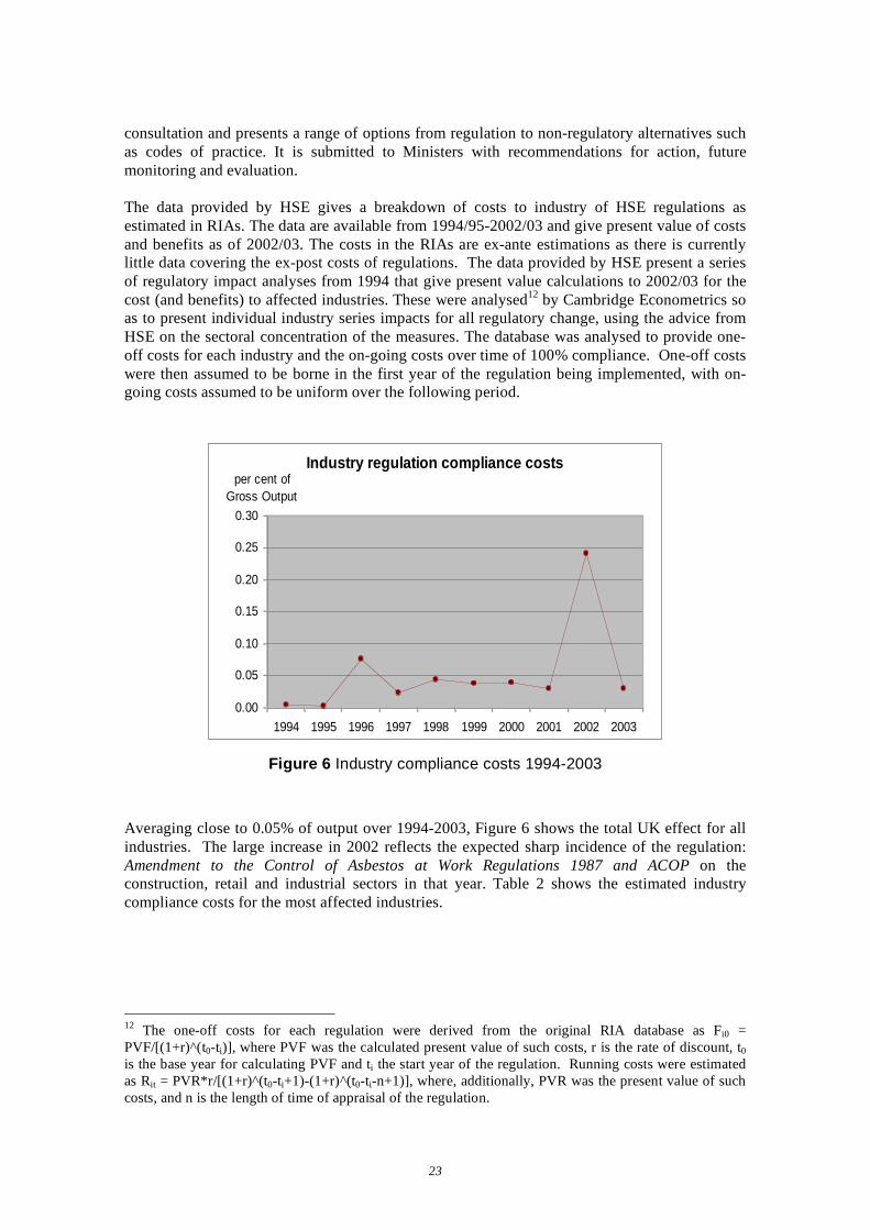
consultation and presents a range of options from regulation to non-regulatory alternatives such as codes of practice. It is submitted to Ministers with recommendations for action, future monitoring and evaluation.
The data provided by HSE gives a breakdown of costs to industry of HSE regulations as estimated in RIAs. The data are available from 1994/95-2002/03 and give present value of costs and benefits as of 2002/03. The costs in the RIAs are ex-ante estimations as there is currently little data covering the ex-post costs of regulations. The data provided by HSE present a series of regulatory impact analyses from 1994 that give present value calculations to 2002/03 for the cost (and benefits) to affected industries. These were analysed12 by Cambridge Econometrics so as to present individual industry series impacts for all regulatory change, using the advice from HSE on the sectoral concentration of the measures. The database was analysed to provide one-off costs for each industry and the on-going costs over time of 100% compliance. One-off costs were then assumed to be borne in the first year of the regulation being implemented, with on-going costs assumed to be uniform over the following period.
Industry regulation compliance costs
0.00
0.05
0.10
0.15
0.20
0.25
0.30
1994 1995 1996 1997 1998 1999 2000 2001 2002 2003
per cent of Gross Output
Figure 6 Industry compliance costs 1994-2003
Averaging close to 0.05% of output over 1994-2003, Figure 6 shows the total UK effect for all industries. The large increase in 2002 reflects the expected sharp incidence of the regulation: Amendment to the Control of Asbestos at Work Regulations 1987 and ACOP on the construction, retail and industrial sectors in that year. Table 2 shows the estimated industry compliance costs for the most affected industries.
The one-off costs for each regulation were derived from the original RIA database as Fi0 = PVF/[(1+r)^(t0-ti)], where PVF was the calculated present value of such costs, r is the rate of discount, t0 is the base year for calculating PVF and ti the start year of the regulation. Running costs were estimated as Rit = PVR*r/[(1+r)^(t0-ti+1)-(1+r)^(t0-ti-n+1)], where, additionally, PVR was the present value of such costs, and n is the length of time of appraisal of the regulation.
23
12
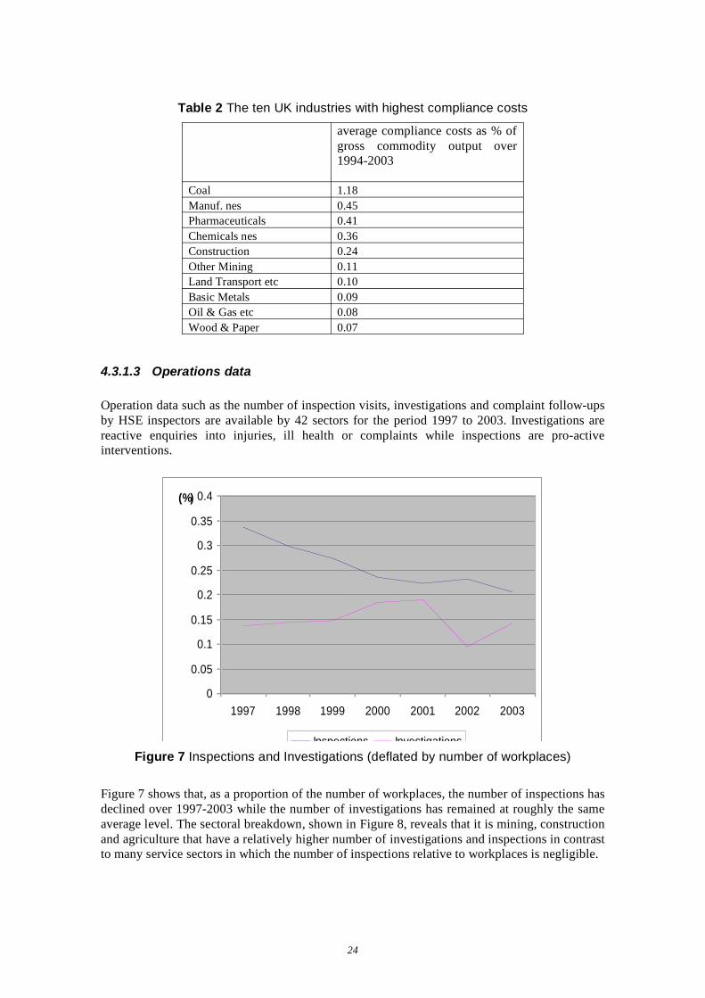
Table 2 The ten UK industries with highest compliance costs
average compliance costs as % of gross commodity output over 1994-2003
Coal 1.18 Manuf. nes 0.45 Pharmaceuticals 0.41 Chemicals nes 0.36 Construction 0.24 Other Mining 0.11 Land Transport etc 0.10 Basic Metals 0.09 Oil & Gas etc 0.08 Wood & Paper 0.07
4.3.1.3 Operations data
Operation data such as the number of inspection visits, investigations and complaint follow-ups by HSE inspectors are available by 42 sectors for the period 1997 to 2003. Investigations are reactive enquiries into injuries, ill health or complaints while inspections are pro-active interventions.
0
0.05
0.1
0.15
0.2
0.25
0.3
0.35
0.4
1997 1998 1999 2000 2001 2002 2003
(%)
Inspections InvestigationsFigure 7 Inspections and Investigations (deflated by number of workplaces)
Figure 7 shows that, as a proportion of the number of workplaces, the number of inspections has declined over 1997-2003 while the number of investigations has remained at roughly the same average level. The sectoral breakdown, shown in Figure 8, reveals that it is mining, construction and agriculture that have a relatively higher number of investigations and inspections in contrast to many service sectors in which the number of inspections relative to workplaces is negligible.
24
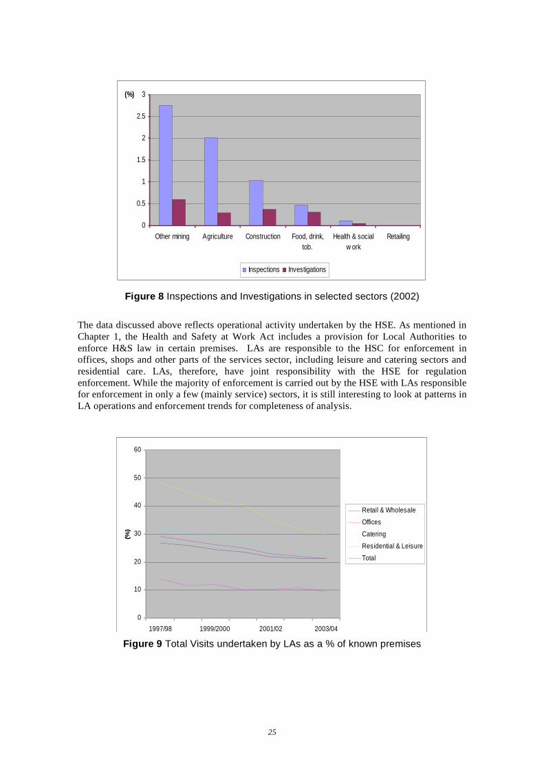
0
0.5
1
1.5
2
2.5
3
Other mining Agriculture Construction Food, drink,tob.
Health & socialw ork
Retailing
(%)
Inspections Investigations
Figure 8 Inspections and Investigations in selected sectors (2002)
The data discussed above reflects operational activity undertaken by the HSE. As mentioned in Chapter 1, the Health and Safety at Work Act includes a provision for Local Authorities to enforce H&S law in certain premises. LAs are responsible to the HSC for enforcement in offices, shops and other parts of the services sector, including leisure and catering sectors and residential care. LAs, therefore, have joint responsibility with the HSE for regulation enforcement. While the majority of enforcement is carried out by the HSE with LAs responsible for enforcement in only a few (mainly service) sectors, it is still interesting to look at patterns in LA operations and enforcement trends for completeness of analysis.
0
10
20
30
40
50
60
1997/98 1999/2000 2001/02 2003/04
(%)
Retail & Wholesale
Offices
Catering
Residential & Leisure
Total
Figure 9 Total Visits undertaken by LAs as a % of known premises
25
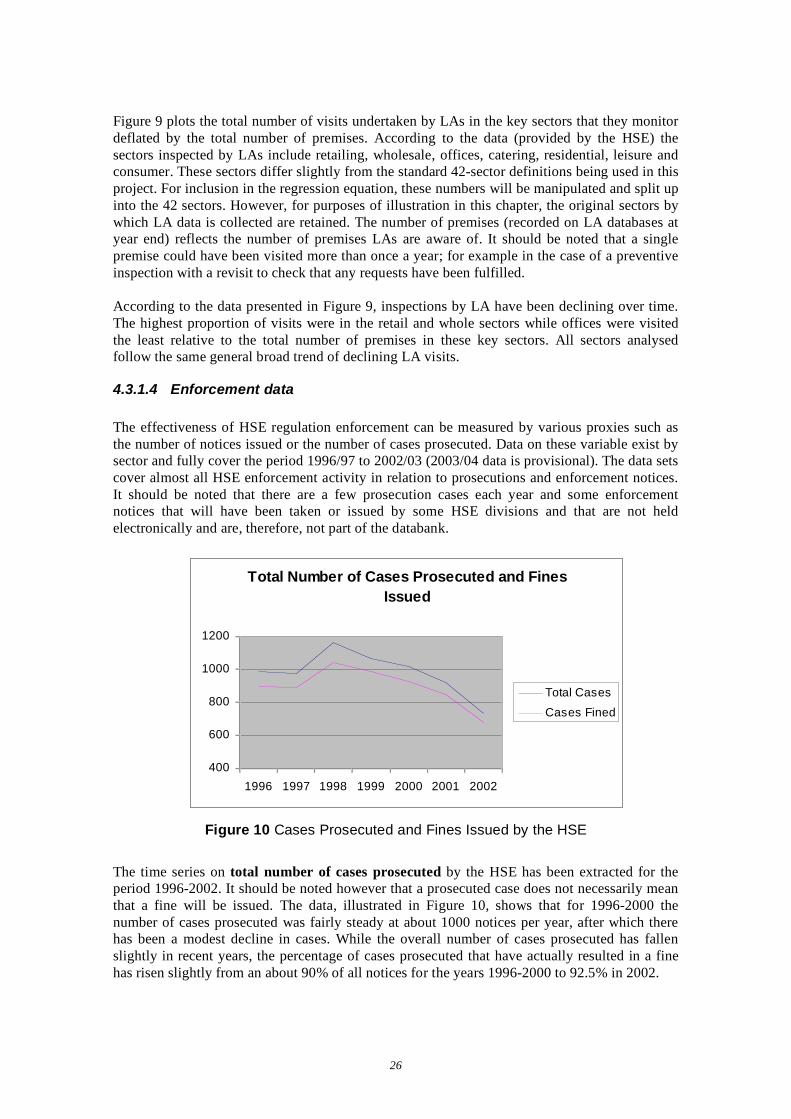
Figure 9 plots the total number of visits undertaken by LAs in the key sectors that they monitor deflated by the total number of premises. According to the data (provided by the HSE) the sectors inspected by LAs include retailing, wholesale, offices, catering, residential, leisure and consumer. These sectors differ slightly from the standard 42-sector definitions being used in this project. For inclusion in the regression equation, these numbers will be manipulated and split up into the 42 sectors. However, for purposes of illustration in this chapter, the original sectors by which LA data is collected are retained. The number of premises (recorded on LA databases at year end) reflects the number of premises LAs are aware of. It should be noted that a single premise could have been visited more than once a year; for example in the case of a preventive inspection with a revisit to check that any requests have been fulfilled.
According to the data presented in Figure 9, inspections by LA have been declining over time. The highest proportion of visits were in the retail and whole sectors while offices were visited the least relative to the total number of premises in these key sectors. All sectors analysed follow the same general broad trend of declining LA visits.
4.3.1.4 Enforcement data
The effectiveness of HSE regulation enforcement can be measured by various proxies such as the number of notices issued or the number of cases prosecuted. Data on these variable exist by sector and fully cover the period 1996/97 to 2002/03 (2003/04 data is provisional). The data sets cover almost all HSE enforcement activity in relation to prosecutions and enforcement notices. It should be noted that there are a few prosecution cases each year and some enforcement notices that will have been taken or issued by some HSE divisions and that are not held electronically and are, therefore, not part of the databank.
Total Number of Cases Prosecuted and Fines Issued
400
600
800
1000
1200
1996 1997 1998 1999 2000 2001 2002
Total Cases
Cases Fined
Figure 10 Cases Prosecuted and Fines Issued by the HSE
The time series on total number of cases prosecuted by the HSE has been extracted for the period 1996-2002. It should be noted however that a prosecuted case does not necessarily mean that a fine will be issued. The data, illustrated in Figure 10, shows that for 1996-2000 the number of cases prosecuted was fairly steady at about 1000 notices per year, after which there has been a modest decline in cases. While the overall number of cases prosecuted has fallen slightly in recent years, the percentage of cases prosecuted that have actually resulted in a fine has risen slightly from an about 90% of all notices for the years 1996-2000 to 92.5% in 2002.
26
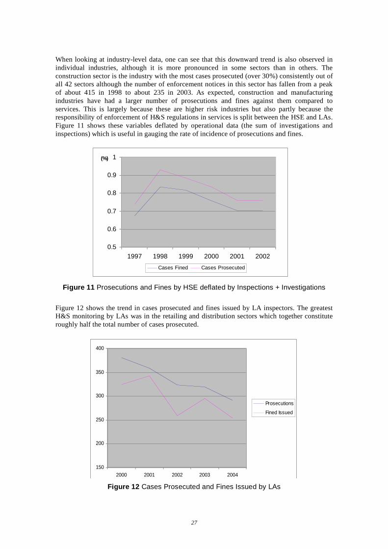
When looking at industry-level data, one can see that this downward trend is also observed in individual industries, although it is more pronounced in some sectors than in others. The construction sector is the industry with the most cases prosecuted (over 30%) consistently out of all 42 sectors although the number of enforcement notices in this sector has fallen from a peak of about 415 in 1998 to about 235 in 2003. As expected, construction and manufacturing industries have had a larger number of prosecutions and fines against them compared to services. This is largely because these are higher risk industries but also partly because the responsibility of enforcement of H&S regulations in services is split between the HSE and LAs. Figure 11 shows these variables deflated by operational data (the sum of investigations and inspections) which is useful in gauging the rate of incidence of prosecutions and fines.
0.5
0.6
0.7
0.8
0.9
1
1997 1998 1999 2000 2001 2002
(%)
Cases Fined Cases Prosecuted
Figure 11 Prosecutions and Fines by HSE deflated by Inspections + Investigations
Figure 12 shows the trend in cases prosecuted and fines issued by LA inspectors. The greatest H&S monitoring by LAs was in the retailing and distribution sectors which together constitute roughly half the total number of cases prosecuted.
150
200
250
300
350
400
2000 2001 2002 2003 2004
Prosecutions
Fined Issued
Figure 12 Cases Prosecuted and Fines Issued by LAs
27
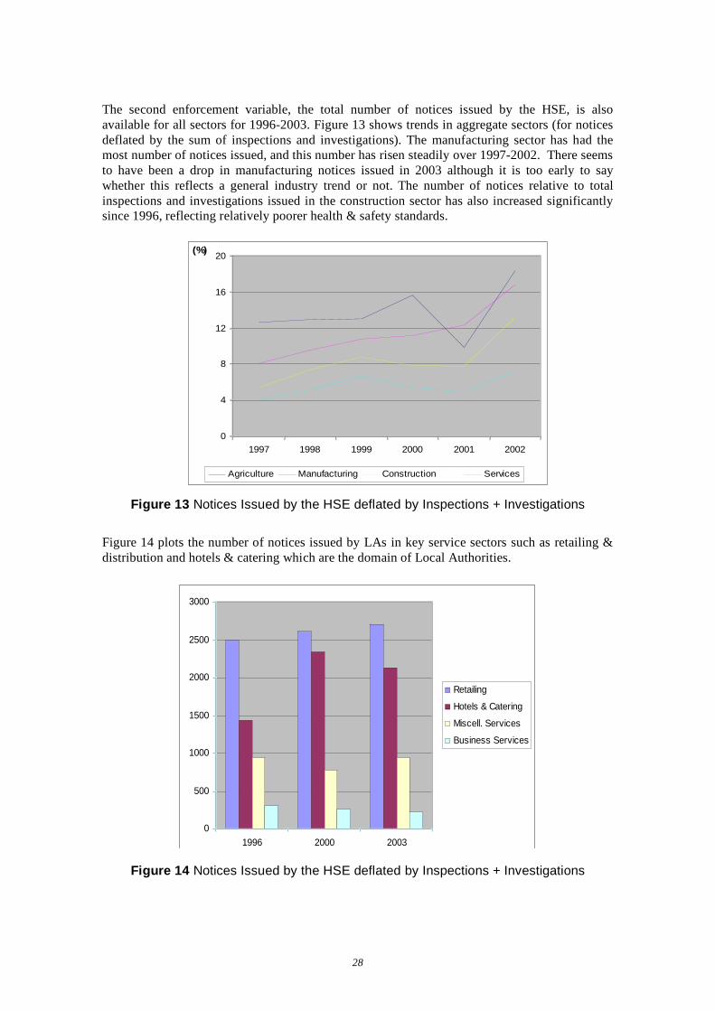
The second enforcement variable, the total number of notices issued by the HSE, is also available for all sectors for 1996-2003. Figure 13 shows trends in aggregate sectors (for notices deflated by the sum of inspections and investigations). The manufacturing sector has had the most number of notices issued, and this number has risen steadily over 1997-2002. There seems to have been a drop in manufacturing notices issued in 2003 although it is too early to say whether this reflects a general industry trend or not. The number of notices relative to total inspections and investigations issued in the construction sector has also increased significantly since 1996, reflecting relatively poorer health & safety standards.
0
4
8
12
16
20
1997 1998 1999 2000 2001 2002
(%)
Agriculture Manufacturing Construction Services
Figure 13 Notices Issued by the HSE deflated by Inspections + Investigations
Figure 14 plots the number of notices issued by LAs in key service sectors such as retailing & distribution and hotels & catering which are the domain of Local Authorities.
0
500
1000
1500
2000
2500
3000
1996 2000 2003
Retailing
Hotels & Catering
Miscell. Services
Business Services
Figure 14 Notices Issued by the HSE deflated by Inspections + Investigations
28
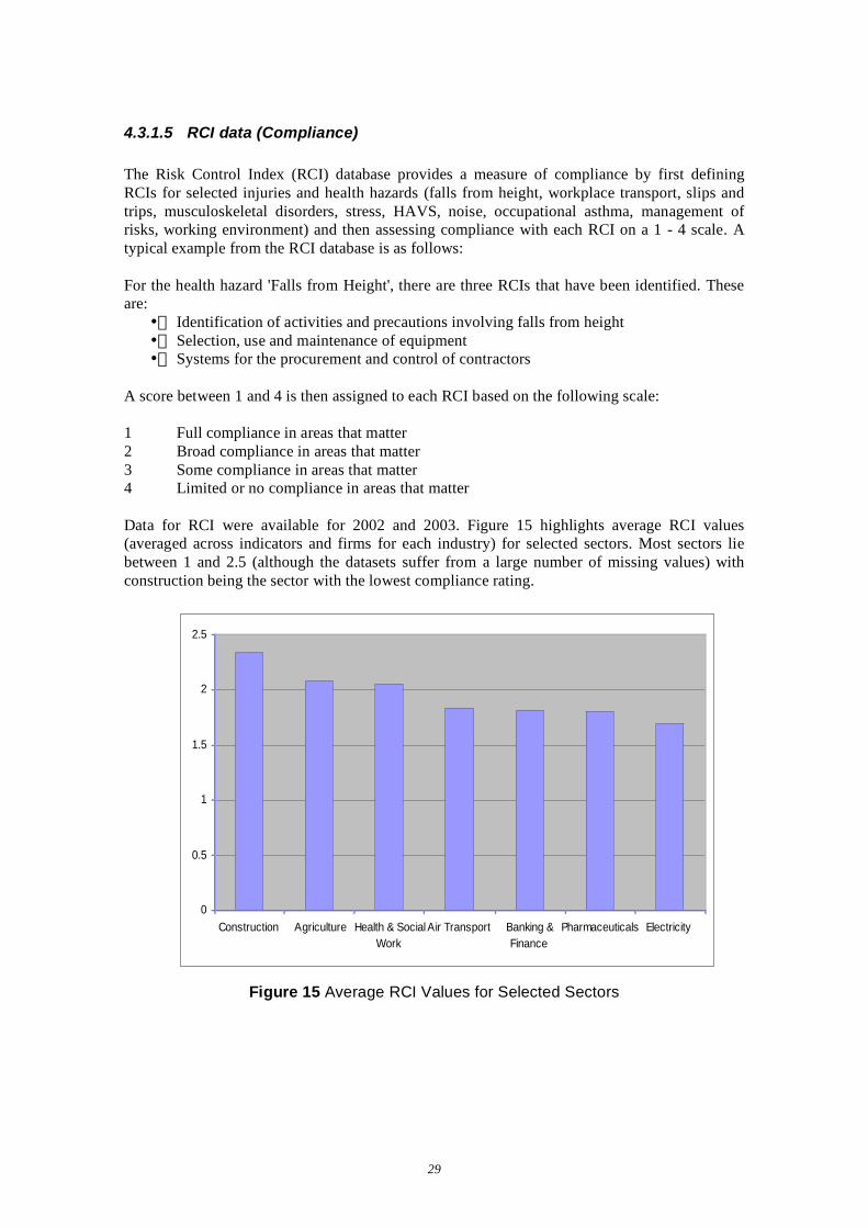
4.3.1.5 RCI data (Compliance)
The Risk Control Index (RCI) database provides a measure of compliance by first defining RCIs for selected injuries and health hazards (falls from height, workplace transport, slips and trips, musculoskeletal disorders, stress, HAVS, noise, occupational asthma, management of risks, working environment) and then assessing compliance with each RCI on a 1 - 4 scale. A typical example from the RCI database is as follows:
For the health hazard 'Falls from Height', there are three RCIs that have been identified. These are:
• Identification of activities and precautions involving falls from height • Selection, use and maintenance of equipment • Systems for the procurement and control of contractors
A score between 1 and 4 is then assigned to each RCI based on the following scale:
1 Full compliance in areas that matter 2 Broad compliance in areas that matter 3 Some compliance in areas that matter 4 Limited or no compliance in areas that matter
Data for RCI were available for 2002 and 2003. Figure 15 highlights average RCI values (averaged across indicators and firms for each industry) for selected sectors. Most sectors lie between 1 and 2.5 (although the datasets suffer from a large number of missing values) with construction being the sector with the lowest compliance rating.
0
0.5
1
1.5
2
2.5
Construction Agriculture Health & SocialWork
Air Transport Banking &Finance
Pharmaceuticals Electricity
Figure 15 Average RCI Values for Selected Sectors
29

4.3.1.6 Relationship between RIDDOR and other H&S variables
It is important to make the distinction between high RIDDOR rates (which simply measure the rate of accidents and injuries) and the other H&S measure such as notices issues and inspections that measure H&S activity and stringency.
The sectors with the highest rates of accidents and injuries RIDDOR are, as expected, mainly manufacturing industries although some service sectors such as public administration & defence and communications also rank highly. Basic Metals, Food, Drink & Tobacco and Communications are the top three industries; with Other Mining and Rubber & Plastics behind them, all of which are heavily manufacturing-based.
It is logical that sectors in which the incidence rate of accidents and injuries is higher should have greater H&S activity and regulatory mechanisms in place. Table 3 lists the correlation coefficients between RIDDOR and the other H&S stringency measures.
Table 3 Correlation coefficients between Incidence rate of accidents and injuries (RIDDOR) and other HSE variables13
Cases Prosecuted
Cases Fined
Notices Issued Inspect. Investig.
Cost Of Reg
Agriculture etc -0.61 -0.37 -0.10 -0.49 0.04 0.38 Coal 0.23 0.23 0.74 0.77* 0.21 -0.52 Oil & Gas etc 0.41 0.41 0.20 0.27 0.61 -0.46 Other Mining 0.60 0.65 -0.65 0.86* 0.53 -0.01 Food, Drink & Tobacco 0.25 0.31 -0.69 0.69 -0.11 -0.80 Textiles, Clothing & Leather -0.24 -0.24 0.10 -0.05 -0.07 0.00 Wood & Paper 0.17 0.17 -0.19 0.44 0.35 -0.55 Printing & Publishing 0.01 -0.05 0.22 0.05 0.44 -0.01 Manufactured Fuels 0.47 0.47 0.51 0.88* 0.56 0.11 Chemicals nes 0.95* 0.91* 0.88* 0.95* 0.98* -0.57 Rubber & Plastics 0.37 0.44 -0.15 0.53 0.18 -0.57 Non-Metallic Mineral Products 0.19 0.38 -0.68 0.37 0.12 -0.63 Basic Metals -0.19 -0.04 -0.67 0.46 -0.17 -0.69 Metal Goods 0.30 0.22 0.17 0.00 0.88* -0.62 Mechanical Engineering -0.28 -0.42 -0.73 0.48 0.13 -0.39 Electronics 0.12 0.26 -0.08 0.88* 0.18 -0.38 Electrical Engineering & Instruments 0.49 0.46 -0.09 -0.48 0.85* -0.81 Motor Vehicles 0.17 0.16 -0.83 0.43 -0.07 -0.83 Other Transport Equipment 0.65 0.65 -0.81 0.79* 0.22 -0.35 Manufacturing nes -0.03 0.07 0.57 -0.77 -0.55 0.77* Electricity -0.52 -0.55 -0.50 0.91* 0.05 -0.35 Gas Supply 0.26 0.47 0.59 0.94* 0.84* -0.14 Water Supply -0.62 -0.62 -0.60 0.47 -0.04 0.09 Construction 0.92* 0.93* -0.62 0.53 0.31 -0.73 Distribution -0.53 -0.46 -0.67 0.57 -0.09 -0.27 Retailing 0.26 0.26 0.59 0.36 0.32 -0.24 Hotels & Catering -0.79 -0.79 0.08 0.01 -0.15 0.15
13 The RIDDOR rates used in this table are not the IER rates adjusted for under-reporting and full-time equivalent as these are available for 12 aggregate sectors.
30
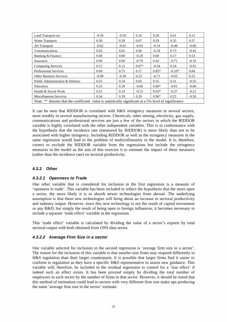
Land Transport etc -0.59 -0.50 0.16 0.28 0.61 0.11 Water Transport 0.30 0.30 0.67 0.29 0.35 0.57 Air Transport -0.62 -0.62 -0.03 -0.14 -0.48 -0.06 Communications 0.65 0.65 0.60 -0.18 0.73 -0.45 Banking & Finance 0.00 0.00 -0.29 0.00 0.17 0.53 Insurance 0.00 0.00 -0.79 0.42 -0.71 -0.10 Computing Services 0.12 0.12 0.87* -0.24 0.24 -0.41 Professional Services 0.69 0.75 0.17 0.85* -0.10* 0.84 Other Business Services -0.09 -0.36 0.23 -0.71 -0.02 0.23 Public Administration & Defence 0.55 0.54 0.05 0.55 0.31 -0.55 Education 0.25 0.18 -0.66 0.96* -0.01 -0.06 Health & Social Work 0.31 0.19 -0.15 0.93* -0.37 -0.21 Miscellaneous Services 0.34 0.39 0.20 0.96* 0.25 -0.50 Note: ‘*’ denotes that the coefficient value is statistically significant at a 5% level of significance
It can be seen that RIDDOR is correlated with H&S stringency measures in several sectors, most notably in several manufacturing sectors. Chemicals, other mining, electricity, gas supply, communications and professional services are just a few of the sectors in which the RIDDOR variable is highly correlated with the other independent variables. This is in conformance with the hypothesis that the incidence rate (measured by RIDDOR) is more likely than not to be associated with higher stringency. Including RIDDOR as well as the stringency measures in the same regression would lead to the problem of multicollinearity in the model. It is, therefore, correct to exclude the RIDDOR variable from the regressions but include the stringency measures in the model as the aim of this exercise it to estimate the impact of these measures (rather than the incidence rate) on sectoral productivity.
4.3.2 Other
4.3.2.1 Openness to Trade One other variable that is considered for inclusion in the first regression is a measure of ‘openness to trade’. This variable has been included to reflect the hypothesis that the more open a sector, the more likely it is to absorb newer technologies from abroad. The underlying assumption is that these new technologies will bring about an increase in sectoral productivity and industry output. However, since this new technology is not the result of capital investment or any R&D, but simply the result of being open to foreign influences, it becomes necessary to include a separate ‘trade effect’ variable in the regression.
This ‘trade effect’ variable is calculated by dividing the value of a sector’s exports by total sectoral output with both obtained from ONS data series.
4.3.2.2 Average Firm Size in a sector
One variable selected for inclusion in the second regression is ‘average firm size in a sector’. The reason for the inclusion of this variable is that smaller-size firms may respond differently to H&S regulation than their larger counterparts. It is possible that larger firms find it easier to conform to regulation as they have a specific H&S representative to assess new guidance. This variable will, therefore, be included in the residual regression to control for a ‘size effect’ if indeed such an effect exists. It has been proxied simply by dividing the total number of employees in each sector by the number of firms in that sector. However, it should be noted that this method of estimation could lead to sectors with very different firm size make ups producing the same ‘average firm size in the sector’ estimate.
31
APPENDIX TO CHAP 4
4.4 GROSS OUTPUT IN CONSTANT BASIC PRICES
The required data has been obtained from CE's volume and price databanks which make use of UK input-output tables to derive indices of primary and intermediate inputs for each of the 42 designated sectors. The tables in the final data set are disaggregated by 42 industries and products in a manner consistent with the 2002 Blue Book and the 1992-2000 Supply and Use Tables (SUTs) that are consistent with the 2002 Blue Book. For 1992-2000, data from SUTs was used by aggregating across industries and products while prior to 1992 the Use tables were made consistent with the 2002 Blue Book by imposing appropriate constraints on row and column sums. This process yielded a gross output series in current basic prices. To construct an industrially disaggregated gross output series in constant basic prices from the current price series, the current price data for the selected years was deflated by a composite deflator which takes into account domestic and export prices. This is calculated as:
!"
#$%
&'(
)*+
,-''(
)**+
,+
./0
123
!"
#$%
&'(
)*+
,4-=
VYVQX
QXVQX
VYVQXPQHHPY AAA
0
1
where PQHH = domestic producer prices VQXA = current price exports VY = current price gross output QX0 = constant price exports
Data for the missing years (1980-83, 1985-88) are interpolated by taking estimates of the change in real value-added (consistent with the indices published in the 2002 Blue Book) for each industry, and adding an adjustment calculated so that the required change in gross output over the whole period of interpolation is achieved. The result is the annual change in gross output for each industry in the interpolated years.
4.5 QUALITY-ADJUSTED HOURS WORKED
A time series for quality-adjusted hours can be constructed by multiplying the number of employees and self-employed in industry i (available from the Annual Business Inquiry and Labour Force Survey) with hours per week (from New Earnings Survey). First, growth in this estimate of total hours worked has to be constrained to conform to the official index of aggregate hours worked (available from ONS). The second adjustment is to apply a correction for changes in labour quality to control for rising levels of educational attainment. This data series is available from the Bank of England Industry Dataset (2003) and was updated by the Bank of England (BOE) for use in this project. A formal description of this variable is discussed in Oulton, N and Srinivasan, S (2005),. The basic principle behind the construction of this variable is to break down as many different types of labour as possible – distinguished by age, gender and qualifications – and to measure aggregate labour input as a weighted average of the hours worked by each group. The weights are the shares of each type of labour in the aggregate wage bill.
32

5 ESTIMATION AND RESULTS
This chapter describes how the data available was applied to the methodology discussed in Section 3, the problems that arose in applying this model and how the model was adapted to overcome any data limitations and estimation problems. It also discusses the results obtained from the final models chosen and implications for H&S activity.
5.1 DERIVING A MEASURE OF PRODUCTIVITY
As discussed in Chapter 3, the first step in measuring the impact of H&S activity on sectoral productivity is to derive a meaningful measure of productivity using the growth accounting system. There are a number of approaches that can be taken:
the most general version of a production function, the translog production function, can be estimated and the estimation residuals can be taken as a proxy for productivity the more specific and often-used Cobb-Douglas production function can be estimated and the estimation residuals can be taken as a proxy for productivity a TFP growth accounting calculation, following the OECD manual, can be used to generate productivity using information on output, inputs and shares derived from the Bank of England dataset
5.1.1 Estimating the Translog Production Function
As described in Section 3, the translog production function is a desirable approximation to any functional form and is a more general version of the often-used Cobb-Douglas production function. It is this form that will be starting point for the estimation. This general trans-log function was estimated for all the industries. This function took the form
LnTLnMLnMLnKLnTLnKLnMLnKLnKLnKTLnLLnMLnLLnKLnLLnKLnLTLnM
LnKLnKLnLTLnMLnKLnKLnLLnY
*********)()(
)()()(
192181171162115
14132121112
102
9
228
217
2654231210
!!!!!
!!!!!!
!!!!!!!!!
+++++
++++++
++++++++=
where Y is Gross Output, L is quality-adjusted labour, K1 is ICT capital, K2 is non-ICT capital, M is intermediate inputs and T is the share of exports in total output (measuring how open an industry is).
The results of this first regression for all sectors show that, despite very high R2 values (indicating a good model fit), individual coefficients for the inputs and their interaction terms are statistically insignificant, the classic signs of multicollinearity. To formally check for evidence of multicollinearity, we look at the correlation coefficients between the dependent variables of the regression. The results are illustrated for three important sectors (as information for all sectors is difficult to present). The three sectors selected for purposes of discussion are construction, mechanical engineering and hotels & catering. These may also be considered to represent the three aggregate sectors (construction, manufacturing and services, respectively). Below are the correlation coefficients for these three sectors.
33
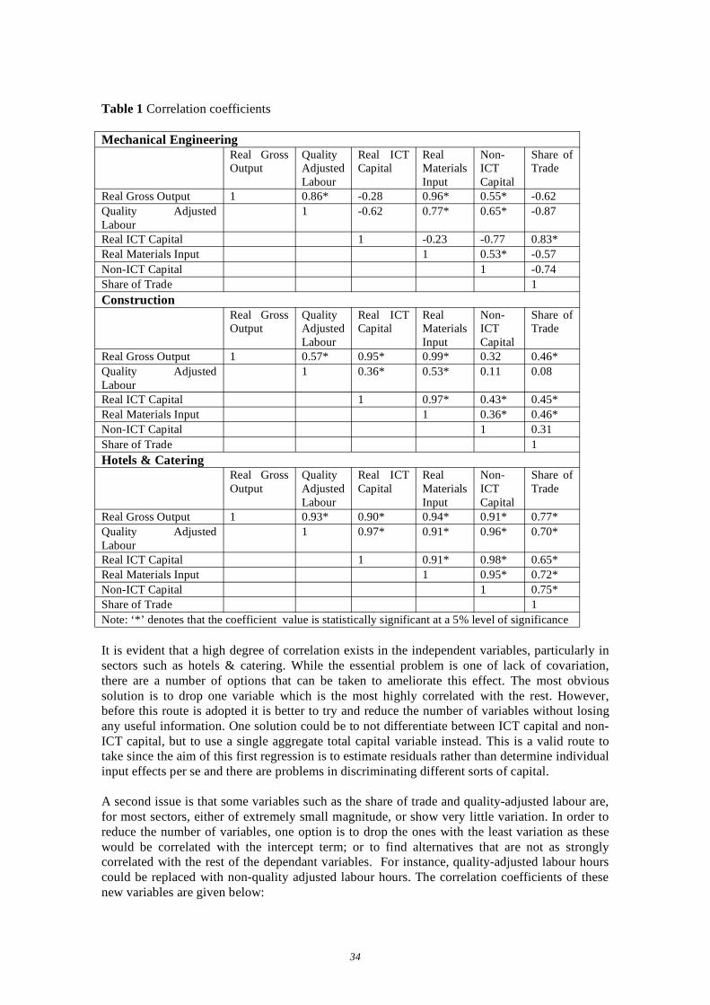
Table 1 Correlation coefficients
Mechanical Engineering Real Gross Output
Quality Adjusted Labour
Real ICT Capital
Real Materials Input
Non-ICT Capital
Share of Trade
Real Gross Output 1 0.86* -0.28 0.96* 0.55* -0.62 Quality Adjusted Labour
1 -0.62 0.77* 0.65* -0.87
Real ICT Capital 1 -0.23 -0.77 0.83* Real Materials Input 1 0.53* -0.57 Non-ICT Capital 1 -0.74 Share of Trade 1 Construction
Real Gross Output
Quality Adjusted Labour
Real ICT Capital
Real Materials Input
Non-ICT Capital
Share of Trade
Real Gross Output 1 0.57* 0.95* 0.99* 0.32 0.46* Quality Adjusted Labour
1 0.36* 0.53* 0.11 0.08
Real ICT Capital 1 0.97* 0.43* 0.45* Real Materials Input 1 0.36* 0.46* Non-ICT Capital 1 0.31 Share of Trade 1 Hotels & Catering
Real Gross Output
Quality Adjusted Labour
Real ICT Capital
Real Materials Input
Non-ICT Capital
Share of Trade
Real Gross Output 1 0.93* 0.90* 0.94* 0.91* 0.77* Quality Adjusted Labour
1 0.97* 0.91* 0.96* 0.70*
Real ICT Capital 1 0.91* 0.98* 0.65* Real Materials Input 1 0.95* 0.72* Non-ICT Capital 1 0.75* Share of Trade 1 Note: ‘*’ denotes that the coefficient value is statistically significant at a 5% level of significance
It is evident that a high degree of correlation exists in the independent variables, particularly in sectors such as hotels & catering. While the essential problem is one of lack of covariation, there are a number of options that can be taken to ameliorate this effect. The most obvious solution is to drop one variable which is the most highly correlated with the rest. However, before this route is adopted it is better to try and reduce the number of variables without losing any useful information. One solution could be to not differentiate between ICT capital and non-ICT capital, but to use a single aggregate total capital variable instead. This is a valid route to take since the aim of this first regression is to estimate residuals rather than determine individual input effects per se and there are problems in discriminating different sorts of capital.
A second issue is that some variables such as the share of trade and quality-adjusted labour are, for most sectors, either of extremely small magnitude, or show very little variation. In order to reduce the number of variables, one option is to drop the ones with the least variation as these would be correlated with the intercept term; or to find alternatives that are not as strongly correlated with the rest of the dependant variables. For instance, quality-adjusted labour hours could be replaced with non-quality adjusted labour hours. The correlation coefficients of these new variables are given below:
34
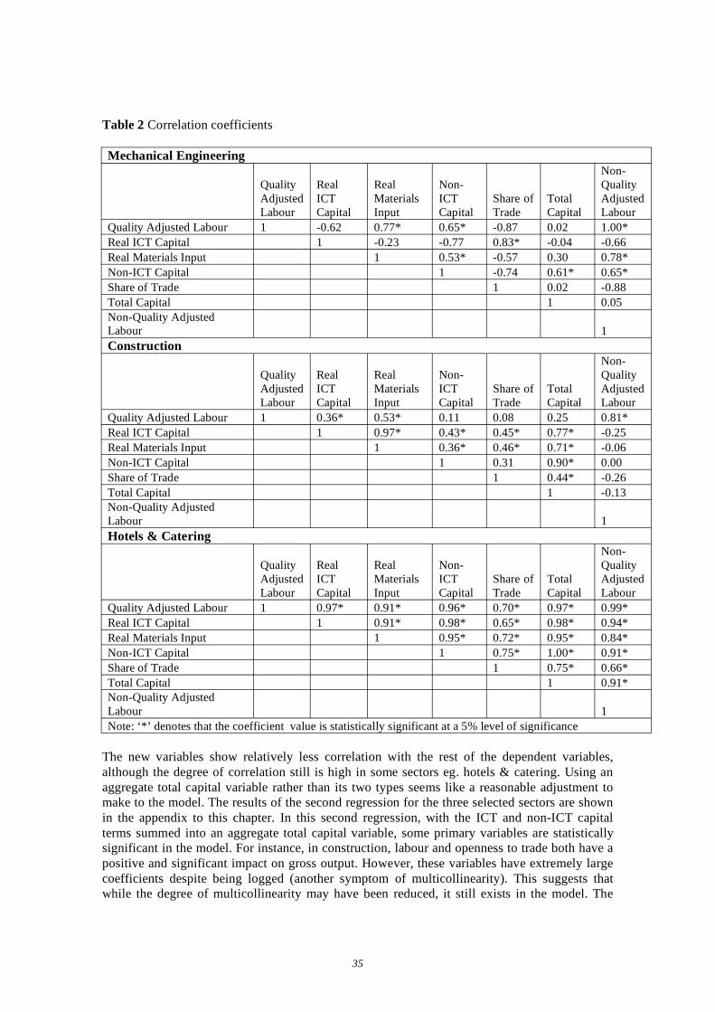
Table 2 Correlation coefficients
Mechanical Engineering Non-
Quality Adjusted Labour
Real ICT Capital
Real Materials Input
Non-ICT Capital
Share of Trade
Total Capital
Quality Adjusted Labour
Quality Adjusted Labour 1 -0.62 0.77* 0.65* -0.87 0.02 1.00* Real ICT Capital 1 -0.23 -0.77 0.83* -0.04 -0.66 Real Materials Input 1 0.53* -0.57 0.30 0.78* Non-ICT Capital 1 -0.74 0.61* 0.65* Share of Trade 1 0.02 -0.88 Total Capital 1 0.05 Non-Quality Adjusted Labour 1 Construction
Non-Quality Real Real Non- Quality Adjusted ICT Materials ICT Share of Total Adjusted Labour Capital Input Capital Trade Capital Labour
Quality Adjusted Labour 1 0.36* 0.53* 0.11 0.08 0.25 0.81* Real ICT Capital 1 0.97* 0.43* 0.45* 0.77* -0.25 Real Materials Input 1 0.36* 0.46* 0.71* -0.06 Non-ICT Capital 1 0.31 0.90* 0.00 Share of Trade 1 0.44* -0.26 Total Capital 1 -0.13 Non-Quality Adjusted Labour 1 Hotels & Catering
Non-Quality Adjusted Labour
Real ICT Capital
Real Materials Input
Non-ICT Capital
Share of Trade
Total Capital
Quality Adjusted Labour
Quality Adjusted Labour 1 0.97* 0.91* 0.96* 0.70* 0.97* 0.99* Real ICT Capital 1 0.91* 0.98* 0.65* 0.98* 0.94* Real Materials Input 1 0.95* 0.72* 0.95* 0.84* Non-ICT Capital 1 0.75* 1.00* 0.91* Share of Trade 1 0.75* 0.66* Total Capital 1 0.91* Non-Quality Adjusted Labour 1 Note: ‘*’ denotes that the coefficient value is statistically significant at a 5% level of significance
The new variables show relatively less correlation with the rest of the dependent variables, although the degree of correlation still is high in some sectors eg. hotels & catering. Using an aggregate total capital variable rather than its two types seems like a reasonable adjustment to make to the model. The results of the second regression for the three selected sectors are shown in the appendix to this chapter. In this second regression, with the ICT and non-ICT capital terms summed into an aggregate total capital variable, some primary variables are statistically significant in the model. For instance, in construction, labour and openness to trade both have a positive and significant impact on gross output. However, these variables have extremely large coefficients despite being logged (another symptom of multicollinearity). This suggests that while the degree of multicollinearity may have been reduced, it still exists in the model. The
35

remaining two sectors still clearly suffer from a high degree of multicollinearity with generally insignificant explanatory variables, very high R2 values, and generally high coefficient magnitudes.
These findings suggest that though it is correct to start off with the most general translog function, in this particular case, due to generally highly correlated input variables and high degree of multicollinearity in the model, it may be better to drop the interaction terms and instead use a simpler Cobb-Douglas function to estimate the residual series. This is justified statistically on the general-to-specific testing criterion as there are no particular interaction terms that are consistently significant in the regression results.
5.1.2 Estimating the Cobb-Douglas functional form
An alternative model that can be run is the simpler Cobb-Douglas production function, which is a simplified version of the more general translog functional form, in which the coefficients on the squared and cross-product terms are constrained to zero. Given that no cross product or squared term was consistently significant in the translog regression, this is not an unreasonable assumption to make, particularly since it eliminates a large number of explanatory variables that potentially suffer from multicollinearity.
In this particular case, the Cobb-Douglas function would simply take the form
LnTLnMLnKLnKLnLLnY 54231210 !!!!!! +++++=
or LnTLnMLnKLnLLnY 54210 !!!!! ++++=
if ICT and non-ICT capital are aggregated into a single variable. The results of the OLS regression on this Cobb-Douglas equation (using an aggregate capital term to eliminate possible multicollinearity between ICT and non-ICT capital investments) are shown in the appendix to this chapter.
The results of this estimation are in general statistically more robust. Most of the coefficients are significant and, generally, are of the right sign and magnitude. Quality-adjusted labour, for example, is positive and statistically significant in all three selected sectors. In construction and mechanical engineering, it has a coefficient of about 0.36, while in hotels & catering, it is much higher (0.8%), implying that a 1% increase in quality-adjusted labour leads to a 0.4% increase in output in construction and mechanical engineering but to a 0.8% output increase in hotels & catering.
The variable for ‘intermediate materials inputs’, too, is reassuringly positive in all three sectors and is statistically highly significant. The magnitudes reflect that an increase in this variable has a larger impact on output in construction and mechanical engineering (a 1% increase in intermediate inputs leads to a 0.8% increase in output) compared to hotels & catering (where a 1% increase in intermediate inputs leads to a 0.5% increase in output). This is not surprising considering that sectors like construction and manufacturing are more reliant on raw materials and intermediate inputs than service-oriented sectors.
The total capital variable, on the other hand, has a negative coefficient in all three sectors although it is not statistically significant in mechanical engineering. The results for all the sectors are summarised in Table 3. A ‘*’ denotes that the coefficient value is statistically significant at a 5% level of significance.
36

Table 3 Cobb Douglas Regression Results
Labour Capital Interm. Inp. Trade
Agriculture etc 0.280* 0.758* -0.889* 0.0442 Coal 0.596* -0.270 0.874* -0.228 Oil & Gas etc 4.20* 0.364 1.37 -0.896* Other Mining 0.0817 -1.41 2.03* -0.164 Food, Drink & Tobacco -0.319* 0.698* 0.271 -0.181 Textiles, Clothing & Leather 0.127 -0.231* 0.789* -0.109 Wood & Paper 0.0180 -0.148 0.924* 0.00253 Printing & Publishing 0.0123 0.342 0.706* -0.0438 Manufactured Fuels 0.963* 0.131 1.09* 0.745* Pharmaceuticals -0.427* -0.0190 0.780* 0.279* Chemicals nes 0.0489 -0.342 0.754* 0.435* Rubber & Plastics -0.367* 0.499 0.847* -0.213 Non-Metallic Mineral Products 0.558* 0.00211* 0.403* -0.187* Basic Metals 0.254 -0.591* 0.955* -0.252* Metal Goods -0.922* -0.782* 1.02* 0.130 Mechanical Engineering 0.362* -0.197 0.894* -0.233* Electronics -0.726 1.302* 0.0763 0.305 Electrical Engineering & Instruments -0.231 0.269 0.627* -0.210 Motor Vehicles 0.108 0.0426 0.836* -0.0869* Other Transport Equipment 0.277* 0.146 0.685* -0.00897 Manufacturing nes -1.17* -1.37* 2.06* -0.167 Electricity -0.854* 0.911* 0.557* -0.172 Gas Supply -0.0427 0.922* 0.889* -0.311 Water Supply 0.175 -0.134 0.679* -0.108 Construction 0.370* -0.464* 0.802* 0.0809 Distribution 1.20* 0.0130 0.269* 0.185* Retailing 0.365 0.700* 0.282 0.0104 Hotels & Catering 0.836* -0.336* 0.485* -0.172* Land Transport etc 0.0509 -0.139 0.773* 0.0421 Water Transport -0.268* 0.106 1.72* -0.106 Air Transport 0.0957 -0.0869 0.869* -0.0664 Communications 1.60* -0.473 1.14* -0.113 Banking & Finance 0.156 0.0802 0.663* 0.0702 Insurance 0.256 0.189 0.611* -0.0148 Computing Services 0.122* -0.0966 1.13* 0.336* Professional Services 0.0409 0.854* -0.331 0.0734 Other Business Services 0.0192 0.597* -0.202 0.279 Public Administration & Defence 0.894 0.135 0.463* -0.0430 Education 0.825* -1.04* 0.406* -0.354* Health & Social Work 0.331 0.364 0.312* 0.246* Miscellaneous Services -0.474* -0.815* 1.53* 0.161 Note: ‘*’ denotes that the coefficient value is statistically significant at a 5% level of significance
The results show that intermediate inputs is one of most important determinants of gross output in this context. Quality-adjusted labour, too, is generally positive and statistically significant in
37

MSLSKSYTFP MLk !!!=
most sectors. The capital and openess to trade variables show a mixed trend; capital, for instance, is generally positive in services sectors and in higher-end manufacturing.
Although Cobb-Douglas model has eliminated the problems caused by multicollinearity in the translog production function, there are still some unresolved issues in the data. For instance, the capital variable is negative and significant in several important sectors such as education, manufacturing nes and hotels & catering, suggesting that capital could be picking up the influence of some other variable not included in the model. Also, in several sectors both labour and capital are insignificant in determining output which, again, undermines the conventional economic logic and makes it necessary to consider alternative measures of productivity.
5.1.3 OECD Total Factor Productivity calculation
A third measure of productivity can be computed from the available data by using gross ouput, labour, capital and intermediate input measures and the shares of these inputs as given in the Bank of England database to compute the OECD recommended statistical measure of total factor productivity (TFP) using the following equation:
where all variables are defined as before and Sk, SL, SM are shares of capital, labour and intermediate inputs in gross nominal output. This approach is based on a widely-accepted standard calculation using consistent input, output and share variables from a single databank. Also, since this is simply a calculation, any estimation issues such as those arising from multicollinearity or model misspecification are by-passed. In effect the approach imposes a Cobb-Douglas form but allows the coefficients (shares) to move over time for each sector.
Table 3 Change in Total Factor Productivity over 1970-2002 Computing Services 5.53 Manufactured Fuels -0.11 Oil & Gas etc 4.37 Printing & Publishing -0.12 Land Transport etc 2.50 Wood & Paper -0.27 Other Mining 1.84 Non-Metallic Mineral Products -0.54 Metal Goods 1.64 Air Transport -0.59 Water Transport 1.29 Water Supply -0.64 Pharmaceuticals 1.01 Construction -0.67 Basic Metals 0.86 Motor Vehicles -0.81 Agriculture etc 0.67 Miscellaneous Services -0.88 Textiles, Clothing & Leather 0.57 Coal -0.89 Banking & Finance 0.51 Other Transport Equipment -0.99 Electronics 0.47 Electrical Engineering & Instruments -1.06 Chemicals nes 0.43 Public Administration & Defence -1.24 Professional Services 0.37 Electricity -1.25 Food, Drink & Tobacco 0.22 Communications -1.32 Other Business Services 0.21 Mechanical Engineering -1.42 Gas Supply 0.18 Distribution -1.76 Rubber & Plastics 0.11 Insurance -1.93 Hotels & Catering 0.09 Education -1.96 Manufacturing nes 0.01 Retailing -2.18
Health & Social Work -4.28
Table 3 shows the change in TFP over 1970-2002 for all 41 sectors. The computing services sector has enjoyed the strong growth in productivity while health & social work seems to have
38
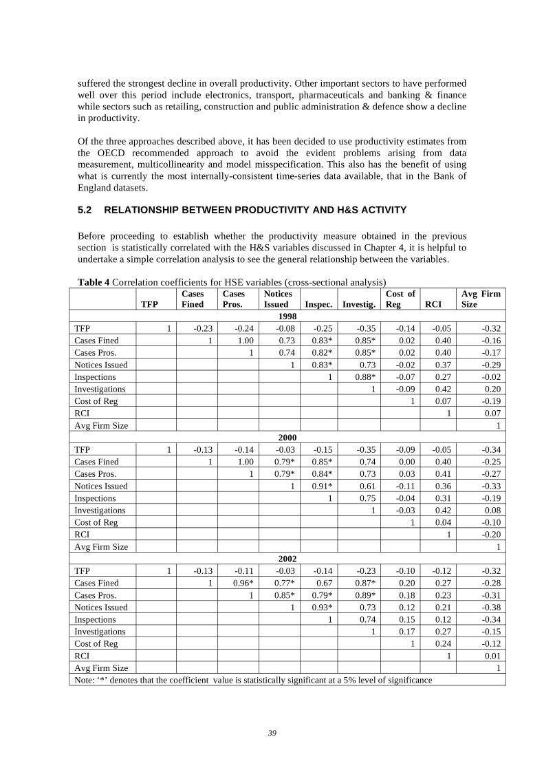
suffered the strongest decline in overall productivity. Other important sectors to have performed well over this period include electronics, transport, pharmaceuticals and banking & finance while sectors such as retailing, construction and public administration & defence show a decline in productivity.
Of the three approaches described above, it has been decided to use productivity estimates from the OECD recommended approach to avoid the evident problems arising from data measurement, multicollinearity and model misspecification. This also has the benefit of using what is currently the most internally-consistent time-series data available, that in the Bank of England datasets.
5.2 RELATIONSHIP BETWEEN PRODUCTIVITY AND H&S ACTIVITY
Before proceeding to establish whether the productivity measure obtained in the previous section is statistically correlated with the H&S variables discussed in Chapter 4, it is helpful to undertake a simple correlation analysis to see the general relationship between the variables.
Table 4 Correlation coefficients for HSE variables (cross-sectional analysis)
TFP Cases Fined
Cases Pros.
Notices Issued Inspec. Investig.
Cost of Reg RCI
Avg Firm Size
1998 TFP 1 -0.23 -0.24 -0.08 -0.25 -0.35 -0.14 -0.05 -0.32 Cases Fined 1 1.00 0.73 0.83* 0.85* 0.02 0.40 -0.16 Cases Pros. 1 0.74 0.82* 0.85* 0.02 0.40 -0.17 Notices Issued 1 0.83* 0.73 -0.02 0.37 -0.29 Inspections 1 0.88* -0.07 0.27 -0.02 Investigations 1 -0.09 0.42 0.20 Cost of Reg 1 0.07 -0.19 RCI 1 0.07 Avg Firm Size 1
2000 TFP 1 -0.13 -0.14 -0.03 -0.15 -0.35 -0.09 -0.05 -0.34 Cases Fined 1 1.00 0.79* 0.85* 0.74 0.00 0.40 -0.25 Cases Pros. 1 0.79* 0.84* 0.73 0.03 0.41 -0.27 Notices Issued 1 0.91* 0.61 -0.11 0.36 -0.33 Inspections 1 0.75 -0.04 0.31 -0.19 Investigations 1 -0.03 0.42 0.08 Cost of Reg 1 0.04 -0.10 RCI 1 -0.20 Avg Firm Size 1
2002 TFP 1 -0.13 -0.11 -0.03 -0.14 -0.23 -0.10 -0.12 -0.32 Cases Fined 1 0.96* 0.77* 0.67 0.87* 0.20 0.27 -0.28 Cases Pros. 1 0.85* 0.79* 0.89* 0.18 0.23 -0.31 Notices Issued 1 0.93* 0.73 0.12 0.21 -0.38 Inspections 1 0.74 0.15 0.12 -0.34 Investigations 1 0.17 0.27 -0.15 Cost of Reg 1 0.24 -0.12 RCI 1 0.01 Avg Firm Size 1 Note: ‘*’ denotes that the coefficient value is statistically significant at a 5% level of significance
39
In this table the variables for cases fined, cases prosecuted and notices issued include both HSE and LA data while inspections and investigations are available only for HSE operations. All these variables have been deflated by total sectoral employment14 while the cost of regulation variable has been weighted by the compliance indicator as discussed in Chapter 4. The table shows that H&S variables show a consistent (negative) pattern of correlation with the productivity term and also a high degree of correlation among themselves; operational and enforcement data, for instance, seem to be fairly highly correlated with each other in all three years analysed. This strong correlation is important to account for in the second regression to avoid any issues of multicollinearity.
H&S activity seems to be generally negatively associated with TFP, suggesting that higher regulation costs and greater H&S enforcement activity is associated with lower sectoral productivity. There is, however, no way of establishing a causal ordering between productivity and H&S variables based on the information available ie it cannot be established whether, if a relationship exists between regulation and productivity, lower productivity necessitates higher regulatory costs or whether it is regulation that lowers productivity in the sector. The H&S variables are also consistently negatively correlated with average firm size in a sector.
For a fuller analysis, several OLS regression were run with the total factor productivity variable on the left-hand side and the H&S variables on the right as explanatory variables. The aim of this exercise is to statistically establish a link between productivity and H&S variables (if it exists) and to isolate their individual impacts.
5.2.1 Pooled Estimation
The first set of regressions was run on data pooled for all sectors and years (1997-2002).
The first model included the H&S variables (cases prosecuted, notices issued, cost of regulation, RCI) as well as the proxy for average firm size in a sector on the right-hand side of the equation as the explanatory variables. The ‘cases fined’ variable was dropped due to high correlation with ‘cases prosecuted’. The ‘cost of regulation’ was deflated by RCI data while ‘cases prosecuted’ and ‘notices issued’ were deflated by operational data (ie the sum of investigations and inspections by the HSE and the total number of visits by LA inspectors). The results of this estimation, given in Appendix 5, show that for this regression only the ‘cases prosecuted’ variable and the ‘average firm size in a sector’ variable were statistically significant and inversely related to productivity.
The second pooled model included the H&S variables (cases prosecuted, notices issued, inspections, investigations, cost of regulation) now deflated by sectoral employment. The cost of regulation, however, was still deflated by the RCI data. The results of this second estimation, given in Appendix 5, show that the number of investigations, the number of inspections and the cost of regulation are negatively associated with sectoral productivity. Although the number of prosecutions is also inversely associated with productivity, it is not statistically significant. In contrast, average firm size in a sector has a statistically significant negative relationship with sectoral productivity.
14 Some H&S variables have been deflated by sectoral employment to control for the size of each sector while assessing risk. For example, a large sector that may have been issued a large absolute number of notices (by virtue of its size) may actually have a lower number of notices per employee and would therefore be rated ‘safer’ than smaller sectors that have a lower absolute number of notices issued.
40
However, both these stacked regressions have very low R2 values and insignificant coefficients on most H&S variables, implying that these variables do not have much explanatory power when it comes to explaining sectoral productivity. It is possible there may be some information in sectoral behaviour when controlling for time. One way of doing this is to run a cross-sectional regression on TFP and H&S variables for each of the years for which full data is available (1997-2002), eliminating the problems that may arise from pooling the data over time.
5.2.2 Cross-sectional Estimation
5.2.2.1 H&S variables deflated by operational data
The second set of regressions was run on cross-sectional data for 1997-2002. A general-to-specific modelling approach was taken in which all insignificant variables are dropped from the model with only the more significant ones remaining in the final model.
The first model to be estimated for all years is of the form:
SIZERCICORNICPTFP 543210 !!!!!! +++++=
where:
CP is the number of cases prosecuted (deflated by the sum of inspections, investigations andvisits by LA inspectors)NI is the number of notices issued (deflated by the sum of inspections, investigations and visitsby LA inspectors)COR is the cost of regulation (adjusted for compliance)RCI is the measure of compliance in each industrySIZE is the measure of average firm size in a sector
The results for all years, given in Appendix 5, show that the two variables to demonstrate aconsistent trend in the 6 years analysed are average firm size in a sector and the number ofcases prosecuted. The cost of regulation, though statistically significant in two of the years,shows a positive coefficient in the first year but a negative coefficient in the second. Thenumber of notices issued is also statistically significant in one of the six years and has apositive impact on productivity.
The results of this set of regressions imply that a high number of cases prosecuted (indicatingpoor H&S performance) is associated with lower sectoral productivity. This suggests that better H&S performance (ie a lower number of cases prosecuted) could have a positive impact onsectoral productivity.
Although there are some consistent trends that can be identified in the data, the changingcoefficient sign for the cost of regulation variable suggests that there may be some outlierobservation in the data distorting the coefficient value. Figures 16 and 17 show the cross plotsbetween TFP and cases prosecuted (deflated by operations data) and between TFP and the costof regulation (deflated by compliance data) respectively.
41

Cross Plot between TFP and Cases Prosecuted
-2
-1
0
1
2
3
4
0 1 2 3 4 5 6 7 8
Total Factor Productivity
Cas
es P
rose
cute
d/O
pera
tions
Education
Figure 16 Total Factor Productivity and Cases Prosecuted (2000)
Cross Plot between TFP and Cost of Regulation
-20
0
20
40
60
80
100
120
0 1 2 3 4 5 6 7 8
Total Factor Productivity
Cos
t of
Reg
/RC
I
Chemicals
Land Transport
Figure 17 Total Factor Productivity and Cost of Regulation (2000)
The charts show that there are indeed some outliers that may be distorting the coefficient value. A few – Education, in the case of prosecutions; and Chemicals and Land Transport in the case of regulation - stand out in particular. For certain sectors, such as computing services, insurance and banking & finance, there are zeros in the data that may also be distorting the coefficient values of the variables.
The above regressions were re-run after purging the data of any distorting influences. The outlier sectors (Education, Land Transport and Chemicals) were removed from the data sets. Those sectors which had zeros in the data for all years (Insurance, Computing Services, Banking & Finance) were also removed prior to the estimation.
42
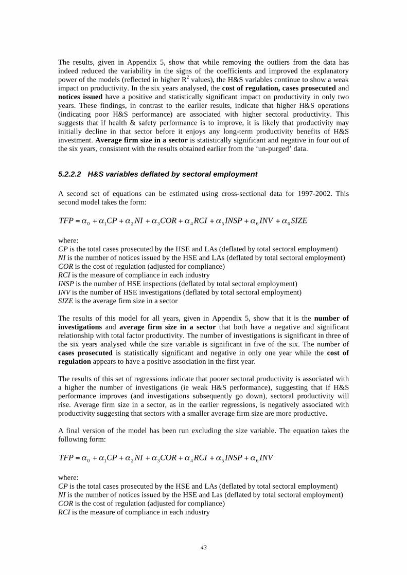
The results, given in Appendix 5, show that while removing the outliers from the data has indeed reduced the variability in the signs of the coefficients and improved the explanatory power of the models (reflected in higher R2 values), the H&S variables continue to show a weak impact on productivity. In the six years analysed, the cost of regulation, cases prosecuted and notices issued have a positive and statistically significant impact on productivity in only two years. These findings, in contrast to the earlier results, indicate that higher H&S operations (indicating poor H&S performance) are associated with higher sectoral productivity. This suggests that if health & safety performance is to improve, it is likely that productivity may initially decline in that sector before it enjoys any long-term productivity benefits of H&S investment. Average firm size in a sector is statistically significant and negative in four out of the six years, consistent with the results obtained earlier from the ‘un-purged’ data.
5.2.2.2 H&S variables deflated by sectoral employment
A second set of equations can be estimated using cross-sectional data for 1997-2002. This second model takes the form:
SIZEINVINSPRCICORNICPTFP 66543210 !!!!!!!! +++++++=
where:CP is the total cases prosecuted by the HSE and LAs (deflated by total sectoral employment)NI is the number of notices issued by the HSE and LAs (deflated by total sectoral employment)COR is the cost of regulation (adjusted for compliance)RCI is the measure of compliance in each industryINSP is the number of HSE inspections (deflated by total sectoral employment)INV is the number of HSE investigations (deflated by total sectoral employment)SIZE is the average firm size in a sector
The results of this model for all years, given in Appendix 5, show that it is the number ofinvestigations and average firm size in a sector that both have a negative and significantrelationship with total factor productivity. The number of investigations is significant in three ofthe six years analysed while the size variable is significant in five of the six. The number ofcases prosecuted is statistically significant and negative in only one year while the cost ofregulation appears to have a positive association in the first year.
The results of this set of regressions indicate that poorer sectoral productivity is associated witha higher the number of investigations (ie weak H&S performance), suggesting that if H&Sperformance improves (and investigations subsequently go down), sectoral productivity willrise. Average firm size in a sector, as in the earlier regressions, is negatively associated withproductivity suggesting that sectors with a smaller average firm size are more productive.
A final version of the model has been run excluding the size variable. The equation takes thefollowing form:
INVINSPRCICORNICPTFP 6543210 !!!!!!! ++++++=
where:CP is the total cases prosecuted by the HSE and LAs (deflated by total sectoral employment)NI is the number of notices issued by the HSE and Las (deflated by total sectoral employment)COR is the cost of regulation (adjusted for compliance)RCI is the measure of compliance in each industry
43
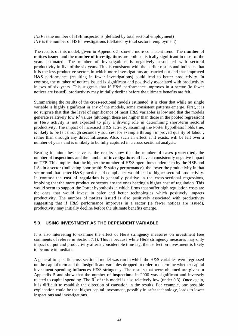
INSP is the number of HSE inspections (deflated by total sectoral employment) INV is the number of HSE investigations (deflated by total sectoral employment)
The results of this model, given in Appendix 5, show a more consistent trend. The number of notices issued and the number of investigations are both statistically significant in most of the years estimated. The number of investigations is negatively associated with sectoral productivity in five of the six years. This is consistent with the earlier results and indicates that it is the less productive sectors in which more investigations are carried out and that improved H&S performance (resulting in fewer investigations) could lead to better productivity. In contrast, the number of notices issued is significant and positively associated with productivity in two of six years. This suggests that if H&S performance improves in a sector (ie fewer notices are issued), productivity may initially decline before the ultimate benefits are felt.
Summarising the results of the cross-sectional models estimated, it is clear that while no single variable is highly significant in any of the models, some consistent patterns emerge. First, it is no surprise that that the level of significance of most H&S variables is low and that the models generate relatively low R2 values (although these are higher than those in the pooled regression) as H&S activity is not expected to play a driving role in determining short-term sectoral productivity. The impact of increased H&S activity, assuming the Porter hypothesis holds true, is likely to be felt through secondary sources, for example through improved quality of labour, rather than through any direct influence. Also, such an effect, if it exists, will be felt over a number of years and is unlikely to be fully captured in a cross-sectional analysis.
Bearing in mind these caveats, the results show that the number of cases prosecuted, the number of inspections and the number of investigations all have a consistently negative impact on TFP. This implies that the higher the number of H&S operations undertaken by the HSE and LAs in a sector (indicating poor health & safety performance), the lower the productivity in that sector and that better H&S practice and compliance would lead to higher sectoral productivity. In contrast the cost of regulation is generally positive in the cross-sectional regressions, implying that the more productive sectors are the ones bearing a higher cost of regulation. This would seem to support the Porter hypothesis in which firms that suffer high regulation costs are the ones that would invest in safer and better technologies which positively impacts productivity. The number of notices issued is also positively associated with productivity suggesting that if H&S performance improves in a sector (ie fewer notices are issued), productivity may initially decline before the ultimate benefits emerge.
5.3 USING INVESTMENT AS THE DEPENDENT VARIABLE
It is also interesting to examine the effect of H&S stringency measures on investment (see comments of referee in Section 7.1). This is because while H&S stringency measures may only impact output and productivity after a considerable time lag, their effect on investment is likely to be more immediate.
A general-to-specific cross-sectional model was run in which the H&S variables were regressed on the capital term and the insignificant variables dropped in order to determine whether capital investment spending influences H&S stringency. The results that were obtained are given in Appendix 5 and show that the number of inspections in 2000 was significant and inversely related to capital spending. The R2 of this model is also relatively low (under 0.3). Once again, it is difficult to establish the direction of causation in the results. For example, one possible explanation could be that higher capital investment, possibly in safer technology, leads to lower inspections and investigations.
44

APPENDIX TO CHAPTER 5
5.4 ESTIMATION RESULTS
5.4.1 Variable Names and Nomenclature • IN is the intercept • L is Quality-Adjusted Labour • K is Real Capital • M is Real Material Inputs • T is Trade • L preceeding any variable indicated the log of that variable • Till Section 5.4.3, two variables alongside each other indicated they have been
multiplied (eg LLLL is the Log of Labour multiplied by the Log of Labour). • CPIIV is Cases Prosecuted divided by Inspections and Investigations • NIIIV is Notices Issued divided by Inspections and Investigations • CORC is Cost of Regulation divided by compliance • RCI is Risk Compliance Index • SIZE is Average Firm Size in a sector • CPE is Cases Prosecuted divided by sectoral employment • NE is Notices Issued divided by sectoral employment • INSE is Inspections divided by sectoral employment • INVE is Investigations divided by sectoral employment
5.4.2 IN The Translog Production Function
Ordinary Least Squares Estimation for Construction
****************************************************************Dependent variable is LY
***************************************************************Regressor Coefficient Standard Error T-Ratio[Prob]IN 377.3554 166.6523 2.2643[.036]LL 103.7141 47.6694 2.1757[.043]LK -44.8877 28.2517 -1.5889[.130]LM -15.1377 8.7092 -1.7381[.099]LT 65.5284 29.7055 2.2059[.041]LLLL 3.5649 2.5530 1.3964[.180]LKLK 1.9797 1.9657 1.0071[.327]LMLM -.87550 .51084 -1.7138[.104]LTLT .12401 .19185 .64639[.526]LLLM .65715 1.3892 .47304[.642]LKLM 1.4427 1.2687 1.1372[.270]LTLM -10.2543 4.8332 -2.1216[.048]LLLK -10.0045 4.4709 -2.2377[.038]LLLT 6.7727 3.8015 1.7816[.092]LKLT 4.8109 2.7049 1.7786[.092]
**************************************************************R-Squared .98188 R-Bar-Squared .96778DW-statistic 1.5038
***************************************************************
Ordinary Least Squares Estimation for Mechanical Engineering
45
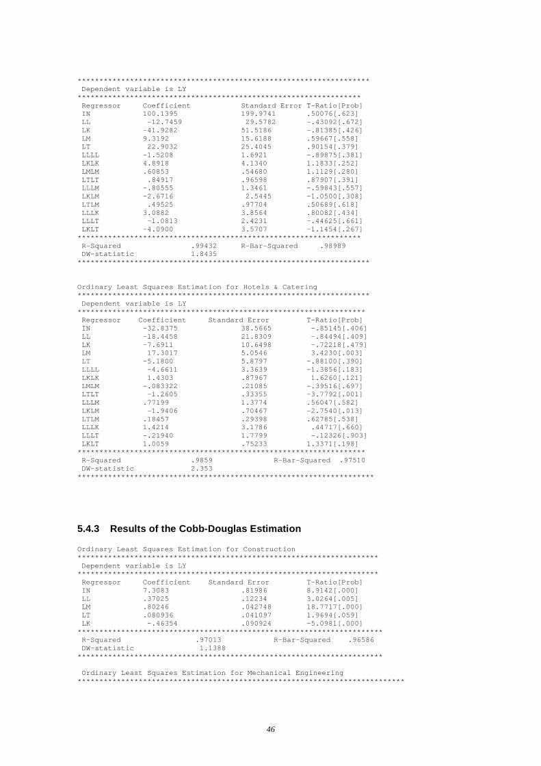
*******************************************************************Dependent variable is LY
*****************************************************************Regressor Coefficient Standard Error T-Ratio[Prob] IN 100.1395 199.9741 .50076[.623] LL -12.7459 29.5782 -.43092[.672] LK -41.9282 51.5186 -.81385[.426] LM 9.3192 15.6188 .59667[.558] LT 22.9032 25.4045 .90154[.379] LLLL -1.5208 1.6921 -.89875[.381] LKLK 4.8918 4.1340 1.1833[.252] LMLM .60853 .54680 1.1129[.280] LTLT .84917 .96598 .87907[.391] LLLM -.80555 1.3461 -.59843[.557] LKLM -2.6716 2.5445 -1.0500[.308] LTLM .49525 .97704 .50689[.618] LLLK 3.0882 3.8564 .80082[.434] LLLT -1.0813 2.4231 -.44625[.661] LKLT -4.0900 3.5707 -1.1454[.267]
*****************************************************************R-Squared .99432 R-Bar-Squared .98989DW-statistic 1.8435
*******************************************************************
Ordinary Least Squares Estimation for Hotels & Catering*******************************************************************Dependent variable is LY
******************************************************************Regressor Coefficient Standard Error T-Ratio[Prob]IN -32.8375 38.5665 -.85145[.406]LL -18.4458 21.8309 -.84494[.409]LK -7.6911 10.6498 -.72218[.479]LM 17.3017 5.0546 3.4230[.003]LT -5.1800 5.8797 -.88100[.390]LLLL -4.6611 3.3639 -1.3856[.183]LKLK 1.4303 .87967 1.6260[.121]LMLM -.083322 .21085 -.39516[.697]LTLT -1.2605 .33355 -3.7792[.001]LLLM .77199 1.3774 .56047[.582]LKLM -1.9406 .70467 -2.7540[.013]LTLM .18457 .29398 .62785[.538]LLLK 1.4214 3.1786 .44717[.660]LLLT -.21940 1.7799 -.12326[.903]LKLT 1.0059 .75233 1.3371[.198]
******************************************************************R-Squared .9859 R-Bar-Squared .97510DW-statistic 2.353
********************************************************************
5.4.3 Results of the Cobb-Douglas Estimation
Ordinary Least Squares Estimation for Construction*********************************************************************Dependent variable is LY
*********************************************************************Regressor Coefficient Standard Error T-Ratio[Prob]IN 7.3083 .81986 8.9142[.000]LL .37025 .12234 3.0264[.005]LM .80246 .042748 18.7717[.000]LT .080936 .041097 1.9694[.059]LK -.46354 .090924 -5.0981[.000]
**********************************************************************R-Squared .97013 R-Bar-Squared .96586DW-statistic 1.1388
**********************************************************************
Ordinary Least Squares Estimation for Mechanical Engineering***************************************************************************
46
Dependent variable is LY***************************************************************************Regressor Coefficient Standard Error T-Ratio[Prob] IN 4.0310 1.1587 3.4789[.002] LL .36207 .11186 3.2368[.003] LM .89379 .055241 16.1800[.000] LT -.23293 .088365 -2.6360[.014] LK -.19743 .14289 -1.3817[.178]
****************************************************************************R-Squared .98327 R-Bar-Squared .98088DW-statistic .81147
****************************************************************************
Ordinary Least Squares Estimation for Hotels & Catering****************************************************************************Dependent variable is LY
****************************************************************************Regressor Coefficient Standard Error T-Ratio[Prob]IN 9.1761 .96429 9.5159[.000]LL .83648 .27200 3.0753[.005]LM .48508 .055463 8.7461[.000]LT -.17209 .081030 -2.1237[.043]LK -.33605 .12428 -2.7039[.012]
****************************************************************************R-Squared .90041 R-Bar-Squared .88618
DW-statistic .44588****************************************************************************
5.4.4 Results of Pooled Regression
Ordinary Least Squares Estimation*******************************************************************************Dependent variable is TFP
*******************************************************************************Regressor Coefficient Standard Error T-Ratio[Prob]INT 5.3141 1.0592 5.0170[.000]CPIIV -.33803 .16580 -2.0388[.043]NIIIV .028312 .020255 1.3977[.163]CORC -.9541E-3 .8315E-3 -1.1474[.252]RCI -.59159 .52835 -1.1197[.264]SIZE -.013700 .0028638 -4.7840[.000]
*******************************************************************************R-Squared .12699 R-Bar-Squared .10881DW-statistic 1.1872
*******************************************************************************
Ordinary Least Squares Estimation*******************************************************************************Dependent variable is TFP
*******************************************************************************Regressor Coefficient Standard Error T-Ratio[Prob]INT 4.0793 1.0677 3.8205[.000]CPE -.068486 1.7750 -.038584[.969]NE .28958 .16408 1.7649[.079]INSE -.039441 .027803 -1.4186[.157]INVE -.15176 .056576 -2.6824[.008]CORC -.0010788 .8044E-3 -1.3411[.181]RCI .14922 .53400 .27945[.780]SIZE -.012076 .0030196 -3.9992[.000]
*******************************************************************************R-Squared .19292 R-Bar-Squared .16918******************************************************************************
5.5 RESULTS OF CROSS SECTIONAL REGRESSION
47
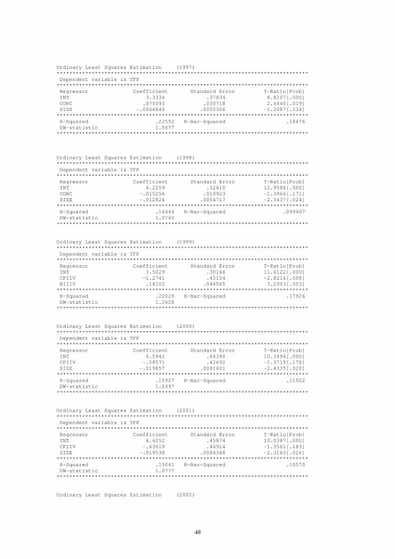
Ordinary Least Squares Estimation (1997)*******************************************************************************Dependent variable is TFP
*******************************************************************************Regressor Coefficient Standard Error T-Ratio[Prob] INT 3.3334 .37834 8.8107[.000] CORC .075093 .030718 2.4446[.019] SIZE -.0066846 .0055306 -1.2087[.234]
*******************************************************************************R-Squared .22552 R-Bar-Squared .18476DW-statistic 1.5677
*******************************************************************************
Ordinary Least Squares Estimation (1998)*******************************************************************************Dependent variable is TFP
*******************************************************************************Regressor Coefficient Standard Error T-Ratio[Prob]INT 4.2259 .32610 12.9588[.000]CORC -.015256 .010923 -1.3966[.171]SIZE -.012824 .0054717 -2.3437[.024]
*******************************************************************************R-Squared .14444 R-Bar-Squared .099407DW-statistic 1.0760
*******************************************************************************
Ordinary Least Squares Estimation (1999)*******************************************************************************Dependent variable is TFP
*******************************************************************************Regressor Coefficient Standard Error T-Ratio[Prob]INT 3.5029 .30166 11.6122[.000]CPIIV -1.2741 .45154 -2.8216[.008]NIIIV .14102 .044065 3.2003[.003]
*******************************************************************************R-Squared .22029 R-Bar-Squared .17926DW-statistic 1.2628
*******************************************************************************
Ordinary Least Squares Estimation (2000)*******************************************************************************Dependent variable is TFP
*******************************************************************************Regressor Coefficient Standard Error T-Ratio[Prob]INT 4.5942 .44390 10.3496[.000]CPIIV -.58571 .42692 -1.3719[.178]SIZE -.019857 .0081601 -2.4335[.020]
*******************************************************************************R-Squared .15927 R-Bar-Squared .11502DW-statistic 1.2497
*******************************************************************************
Ordinary Least Squares Estimation (2001)*******************************************************************************Dependent variable is TFP
*******************************************************************************Regressor Coefficient Standard Error T-Ratio[Prob]INT 4.6052 .45874 10.0387[.000]CPIIV -.63619 .46914 -1.3561[.183]SIZE -.019538 .0084348 -2.3163[.026]
*******************************************************************************R-Squared .15041 R-Bar-Squared .10570DW-statistic 1.0777
*******************************************************************************
Ordinary Least Squares Estimation (2002)
48
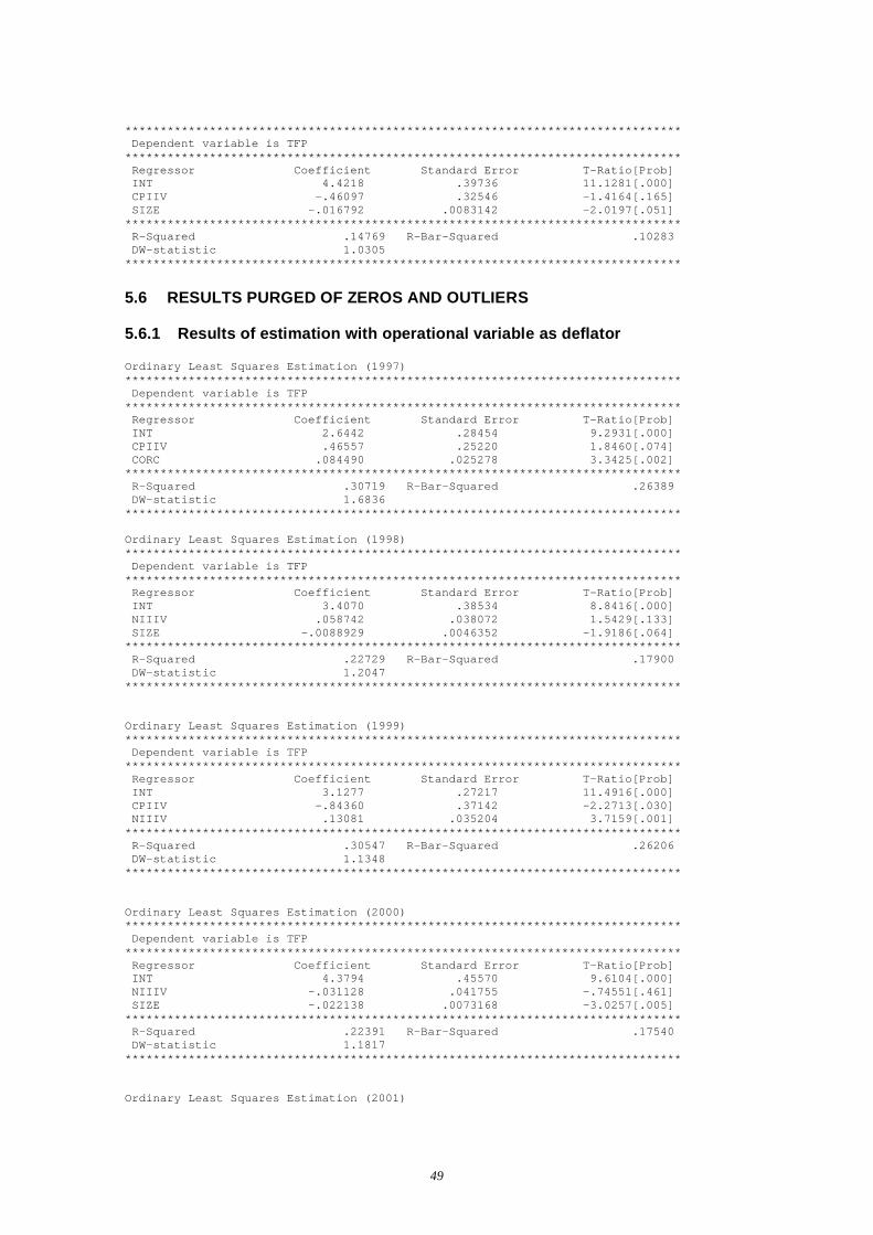
*******************************************************************************Dependent variable is TFP
*******************************************************************************Regressor Coefficient Standard Error T-Ratio[Prob] INT 4.4218 .39736 11.1281[.000] CPIIV -.46097 .32546 -1.4164[.165] SIZE -.016792 .0083142 -2.0197[.051]
*******************************************************************************R-Squared .14769 R-Bar-Squared .10283DW-statistic 1.0305
*******************************************************************************
5.6 RESULTS PURGED OF ZEROS AND OUTLIERS
5.6.1 Results of estimation with operational variable as deflator
Ordinary Least Squares Estimation (1997)*******************************************************************************Dependent variable is TFP
*******************************************************************************Regressor Coefficient Standard Error T-Ratio[Prob]INT 2.6442 .28454 9.2931[.000]CPIIV .46557 .25220 1.8460[.074]CORC .084490 .025278 3.3425[.002]
*******************************************************************************R-Squared .30719 R-Bar-Squared .26389DW-statistic 1.6836
*******************************************************************************
Ordinary Least Squares Estimation (1998)*******************************************************************************Dependent variable is TFP
*******************************************************************************Regressor Coefficient Standard Error T-Ratio[Prob]INT 3.4070 .38534 8.8416[.000]NIIIV .058742 .038072 1.5429[.133]SIZE -.0088929 .0046352 -1.9186[.064]
*******************************************************************************R-Squared .22729 R-Bar-Squared .17900DW-statistic 1.2047
*******************************************************************************
Ordinary Least Squares Estimation (1999)*******************************************************************************Dependent variable is TFP
*******************************************************************************Regressor Coefficient Standard Error T-Ratio[Prob]INT 3.1277 .27217 11.4916[.000]CPIIV -.84360 .37142 -2.2713[.030]NIIIV .13081 .035204 3.7159[.001]
*******************************************************************************R-Squared .30547 R-Bar-Squared .26206DW-statistic 1.1348
*******************************************************************************
Ordinary Least Squares Estimation (2000)*******************************************************************************Dependent variable is TFP
*******************************************************************************Regressor Coefficient Standard Error T-Ratio[Prob]INT 4.3794 .45570 9.6104[.000]NIIIV -.031128 .041755 -.74551[.461]SIZE -.022138 .0073168 -3.0257[.005]
*******************************************************************************R-Squared .22391 R-Bar-Squared .17540DW-statistic 1.1817
*******************************************************************************
Ordinary Least Squares Estimation (2001)
49
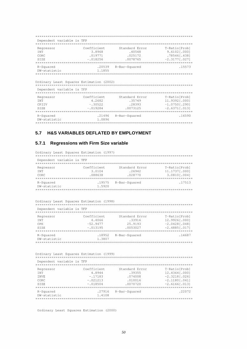
*******************************************************************************Dependent variable is TFP
*******************************************************************************Regressor Coefficient Standard Error T-Ratio[Prob] INT 3.8968 .40548 9.6102[.000] CORC .019771 .025172 .78546[.438] SIZE -.018256 .0078765 -2.3177[.027]
*******************************************************************************R-Squared .20539 R-Bar-Squared .15573DW-statistic 1.1855
*******************************************************************************
Ordinary Least Squares Estimation (2002)*******************************************************************************Dependent variable is TFP
*******************************************************************************Regressor Coefficient Standard Error T-Ratio[Prob]INT 4.2682 .35749 11.9392[.000]CPIIV -.30522 .28393 -1.0750[.290]SIZE -.019284 .0073125 -2.6371[.013]
*******************************************************************************R-Squared .21496 R-Bar-Squared .16590DW-statistic 1.0896
*******************************************************************************
5.7 H&S VARIABLES DEFLATED BY EMPLOYMENT
5.7.1 Regressions with Firm Size variable
Ordinary Least Squares Estimation (1997)*******************************************************************************Dependent variable is TFP
*******************************************************************************Regressor Coefficient Standard Error T-Ratio[Prob]INT 3.0104 .26942 11.1737[.000]CORC .088638 .028770 3.0810[.004]
*******************************************************************************R-Squared .19575 R-Bar-Squared .17513DW-statistic 1.5920
*******************************************************************************
Ordinary Least Squares Estimation (1998)*******************************************************************************Dependent variable is TFP
*******************************************************************************Regressor Coefficient Standard Error T-Ratio[Prob]INT 4.4066 .33916 12.9926[.000]CPE -52.9477 25.9193 -2.0428[.048]SIZE -.013195 .0053027 -2.4885[.017]
*******************************************************************************R-Squared .18952 R-Bar-Squared .14687DW-statistic 1.3807
*******************************************************************************
Ordinary Least Squares Estimation (1999)*******************************************************************************Dependent variable is TFP
*******************************************************************************Regressor Coefficient Standard Error T-Ratio[Prob]INT 4.8944 .39355 12.4364[.000]INVE -.17183 .074008 -2.3218[.026]CORC -.021213 .010016 -2.1180[.041]SIZE -.018504 .0070720 -2.6166[.013]
*******************************************************************************R-Squared .27916 R-Bar-Squared .22072DW-statistic 1.4108
*******************************************************************************
Ordinary Least Squares Estimation (2000)
50
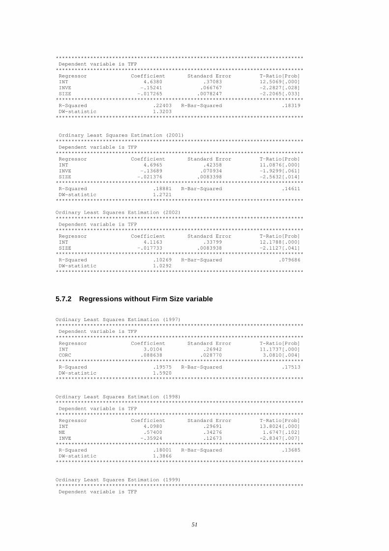
*******************************************************************************Dependent variable is TFP
*******************************************************************************Regressor Coefficient Standard Error T-Ratio[Prob] INT 4.6380 .37083 12.5069[.000] INVE -.15241 .066767 -2.2827[.028] SIZE -.017265 .0078247 -2.2065[.033]
*******************************************************************************R-Squared .22403 R-Bar-Squared .18319DW-statistic 1.3203
*******************************************************************************
Ordinary Least Squares Estimation (2001)*******************************************************************************Dependent variable is TFP
*******************************************************************************Regressor Coefficient Standard Error T-Ratio[Prob]INT 4.6965 .42358 11.0876[.000]INVE -.13689 .070934 -1.9299[.061]SIZE -.021376 .0083398 -2.5632[.014]
*******************************************************************************R-Squared .18881 R-Bar-Squared .14611DW-statistic 1.2721
*******************************************************************************
Ordinary Least Squares Estimation (2002)*******************************************************************************Dependent variable is TFP
*******************************************************************************Regressor Coefficient Standard Error T-Ratio[Prob]INT 4.1163 .33799 12.1788[.000]SIZE -.017733 .0083938 -2.1127[.041]
*******************************************************************************R-Squared .10269 R-Bar-Squared .079686DW-statistic 1.0292
*******************************************************************************
5.7.2 Regressions without Firm Size variable
Ordinary Least Squares Estimation (1997)*******************************************************************************Dependent variable is TFP
*******************************************************************************Regressor Coefficient Standard Error T-Ratio[Prob]INT 3.0104 .26942 11.1737[.000]CORC .088638 .028770 3.0810[.004]
*******************************************************************************R-Squared .19575 R-Bar-Squared .17513DW-statistic 1.5920
*******************************************************************************
Ordinary Least Squares Estimation (1998)*******************************************************************************Dependent variable is TFP
*******************************************************************************Regressor Coefficient Standard Error T-Ratio[Prob]INT 4.0980 .29691 13.8024[.000]NE .57400 .34276 1.6747[.102]INVE -.35924 .12673 -2.8347[.007]
*******************************************************************************R-Squared .18001 R-Bar-Squared .13685DW-statistic 1.3866
*******************************************************************************
Ordinary Least Squares Estimation (1999)*******************************************************************************Dependent variable is TFP
51

*******************************************************************************Regressor Coefficient Standard Error T-Ratio[Prob] INT 4.3010 .32077 13.4085[.000] NE .67172 .31718 2.1178[.041] INVE -.37780 .11890 -3.1773[.003] CORC -.016786 .010034 -1.6729[.103]
*******************************************************************************R-Squared .23813 R-Bar-Squared .17636DW-statistic 1.4645
*******************************************************************************
Ordinary Least Squares Estimation (2000)*******************************************************************************Dependent variable is TFP
*******************************************************************************Regressor Coefficient Standard Error T-Ratio[Prob]INT 4.1386 .30799 13.4373[.000]INVE -.16439 .069769 -2.3562[.024]
*******************************************************************************R-Squared .12461 R-Bar-Squared .10216DW-statistic 1.4609
*******************************************************************************
Ordinary Least Squares Estimation (2001)*******************************************************************************Dependent variable is TFP
*******************************************************************************Regressor Coefficient Standard Error T-Ratio[Prob]INT 3.9866 .30845 12.9249[.000]NE .69891 .33154 2.1081[.042]INVE -.29232 .11398 -2.5648[.014]
*******************************************************************************R-Squared .14817 R-Bar-Squared .10334DW-statistic 1.2214
*******************************************************************************
Ordinary Least Squares Estimation (2002)*******************************************************************************Dependent variable is TFP
*******************************************************************************Regressor Coefficient Standard Error T-Ratio[Prob]INT 3.8939 .31300 12.4404[.000]INVE -.19183 .12962 -1.4799[.147]
*******************************************************************************R-Squared .053171 R-Bar-Squared .028893DW-statistic 1.2878
*******************************************************************************
5.8 INVESTMENT AS THE DEPENDENT VARIABLE
Ordinary Least Squares Estimation*******************************************************************************Dependent variable is K
*******************************************************************************Regressor Coefficient Standard Error T-Ratio[Prob]INT 15668.2 2543.2 6.1607[.000]INSE -667.7939 245.4253 -2.7210[.010]SIZE -157.1158 53.4441 -2.9398[.006]
*******************************************************************************R-Squared .26146 R-Bar-Squared .22258
DW-statistic 2.1246*******************************************************************************
52

6 CONCLUSION
The econometric modelling has highlighted the difficulties in disentangling the possible impact of H&S stringency on sectoral productivity.
First, the underlying process and linkage between H&S activity and sectoral performance is quite complex and interdependent, making it difficult to put an expected sign on the coefficients a priori. For instance, it is not clear whether greater H&S stringency would lead to a fall in output and productivity (a negative coefficient) or whether, in conformance with the Porter hypothesis, higher H&S stringency will lead to the adoption of better technologies thereby enhancing productivity (leading to a positive coefficient).
Second, it is possible that, in conformance with the Porter hypothesis, greater H&S stringency in some sectors may lead to a short-term fall in output but as newer and safer technologies are adopted the long-term impact is an eventual increase in productivity. Again, the direction of the relationship between H&S activity and productivity is not obvious and may vary from sector to sector, depending on how quickly the industry adapts to new technology.
Third, the lack of data on H&S variables makes it difficult to conduct a time-series analysis which would allow identification of the process through which H&S stringency affects output and, ultimately, productivity. This is important as there is a there is likely to be a time lag between a change in H&S stringency and productivity.
Fourth, this lack of time-series data led to the choice of a cross-sectional final model. This forced pooling across industries to estimate a single parameter determining responses for all sectors. This is a simplifying assumption made at the risk of losing information contained in sectoral behaviour; it is possible that some sectors behave differently to others, yet this is not captured in the analysis when the condition of parameter homogeneity is imposed.
Nonetheless, the analysis done using the available data has, to a large extent, addressed any statistical issues such as model misspecification, multicollinearity and data measurement as effectively as possible, yielding results that are statistically stable. For a complete analysis, data on LA operations were included (where possible) and a proxy was included to control for firm size. A number of models were run using different combinations of H&S variables to determine which ones had the most consistent impact on total factor productivity in each sector.
The results show that the impact of H&S activity on sectoral productivity is not very strong. There are a number of reasons for this: first, as mentioned above, if H&S activity is to impact technology and production techniques positively, it will do so after a time lag which is difficult to capture given the limited data available. Second, it is also likely that the impact of H&S activity is felt through secondary sources such as increased capital investment or better labour.
However, despite these caveats, the results show that measures of H&S stringency that have some significant effects on productivity are ‘notices issued’, ‘investigations’, ‘inspections’ and the ‘cost of regulation’. The cost of regulation and the number of notices issued are positively associated with productivity. This indicates that sectors in which the cost of regulation is higher and those which receive a greater number of notices may have more incentive to invest in safer technologies that also positively impact productivity. These findings are consistent with the Porter hypothesis, although with limited possibilities for building time-adjustment into the analysis, this cannot be concluded with certainty. An alternative explanation
53

could simply be that firms with low compliance, and therefore which have a greater number of notices, have higher productivity. Also, it should be kept in mind that the ‘cost of regulation’ variable does not take into account how much of the compliance cost a firm can pass on to consumers. The more firms are able to do this, the less incentive there will be for them to make cost-saving investments.
The number of investigations and inspections are both inversely related to productivity, indicating that greater operational activity (more inspections and investigations) is associated with lower productivity, although whether this is due to the simple fact that there is more HSE activity and monitoring in lower productivity sectors or whether a higher number of inspections initially lowers productivity as firms struggle to comply with regulation is difficult to ascertain with the available data. Generally, more regulated sectors have a higher number of inspections while investigations are higher in low-compliance sectors. The negative association may imply that if H&S stringency measures were to be tightened, productivity would fall in these sectors, at least in the short-term. Since the regressions did not include a time element, it cannot be determined whether or not the long-term impact of these variables would be negative or positive (as suggested by Porter).
It can be concluded that while increased H&S activity may not have had a large impact on productivity, there is also no evidence to suggest that the impact of increased regulation or higher stringency has been detrimental to sectoral performance. In other words, there is no evidence to suggest that H&S regulation has been bad for businesses. The evidence suggests that the investigations and inspections processes have a small, negative association with productivity. These are therefore the two regulatory procedures where the HSE may wish to ensure that the costs to businesses in terms of compliance are not higher than required to ‘catch up’ with achieving necessary compliance.
Porter’s hypothesis, too, does not seem to be supported by the data: his conclusion was that increased stringency would lead to a decline in productivity in the early stages of regulation as firms struggle to meet tighter H&S requirements but over time firms would become more efficient and would invest in safer and better technology raising overall sectoral productivity. However, the results obtained from the UK data do not conclusively support this. While there are both positive and negative effects associated with different stringency measures, there is no over-riding positive or negative impact that can conclusively support the theory for the overall UK economy.
54
7 METHODOLOGY REVIEW BY PROFESSOR GAVIN CAMERON
7.1 PROFESSOR CAMERON'S COMMENTS ON VERSION 2.0 OF THE REPORT
Comments on 'Health and Safety Management and Business Economic Performance' by Gavin Cameron, University of Oxford, 2 June 2005
Taken together, the literature review and proposed methodology present a coherent and sensible approach to the issue. It is proposed to use the existing CE database on 42 sectors of the UK economy to examine the performance of TFP between 1970 and 1992 using a translog gross output growth accounting methodology. Given that measures of H&S stringency are only available from 1992, the paper proposes essentially a three-step procedure. First, growth accounting to derive measures of TFP. Second, modelling of TFP to establish the long-run drivers of TFP. Third, to look at the covariance of residual TFP growth since 1992 with H&S measures.
Clearly, the success of the entire project depends upon the success of each of these individual steps, but it seems to me that the movement from step 2 to step 3 is particularly fraught empirically. This is both because the H&S measures are only available for a short period and also because the modelling in stage 2 requires that there is only a very low covariance of H&S measures with the right hand side variables in order that the 'common baseline decomposition' is consistently estimated.
Turning now to the detailed issues that arise in the paper, I have a number of points to make.
First, although I think figure 1.1 provides a good description of the processes at work as does the general discussion, there is some scope for a clearer statement of the issues, perhaps at the point of the discussion of the Porter hypothesis which I thought was a little muddled. As I see it, H&S activity can be seen as indirectly raising the cost of certain types of activity which are associated with certain types of labour or capital (for example, manual work, and energy-intensive capital equipment). This will lead to a shift along the production function which will reduce measured TFP since the firm will no longer be choosing a measured cost-minimising input set. Furthermore, monitoring and other H&S activity will also involve hiring new workers which will further reduce measured TFP. Now, Porter and figure 1.1 then essentially go on to say that firms may undertake certain investments to offset these higher costs which may shift the production function outwards. To take the Porter argument seriously is to say that the outward shift leads to a rise in measured TFP, which is quite a big step! After all, if there were all these investment possibilities out there, surely firms would already be undertaking them!
Second, following figure 1.1 I wonder whether it might be interesting to look at the effect of H&S stringency on investment separately from TFP (i.e. model investment growth separately from TFP growth). After all, if the social excess rate of return to investment is low, then little of the effect will show up in TFP (note this is related to my earlier point that it is useful to consider shifts in, and shifts along, the production function). The TFP equations that you are proposing are measures of the social excess rate of return.
Third, H&S measures have both a marginal cost and marginal benefit. Therefore it is possible that H&S stringency is endogenous... clearly one would expect the HSE to be undertaking interventions in industries where the MB of intervention is high relative to MC. This means
55

both that the effect of H&S stringency may not be constant across industries and over time, and also that H&S stringency itself may be endogenous.
Fourth, since industry responses are likely to be different, it is not clear how you intend to address parameter heterogeneity in a parsimonious way. I would certainly think that it is worth moving a little way beyond parameter homogeneity, although since you plan to use a translog form I appreciate that you have a lot of parameters to estimate!
Fifth, it seems to me that H&S stringency may also have an effect on bargaining within industries. It often seems to me that unions use H&S issues to enhance their bargaining power (eg the tube drivers during the central line shutdown), so it might be worth investigating whether unionisation matters too.
Sixth, there are also a couple of issues that arise about the changes within a given industry in response to H&S activity. For example, it could be that the change in productivity is partly due to shifts within a sector towards higher productivity firms that are better able to afford H&S measures (a survivor effect) or equally, towards those 3 or 4 digit sectors within the industry that are relatively non-injurious (a batting average effect). It is unclear how the methodology would treat these changes.
Lastly, in section 1.2 (context of study) it would be helpful to have some long-run comparative data. For example, how many working days were lost in 1974? Perhaps some of the data from chart 2.1 would be appropriate here? No doubt, the extent of industrial change since 1974 has affected the overall figures since services are no doubt less injurious than mining etc. It would be very interesting to see the industry breakdowns of working days lost and to do a shift-share analysis of how much of the fall is due to changes in sectoral size and how much to falling injury-intensity within sectors, but that might be a separate project.
7.1.1 CE response to Professor Cameron's review
We broadly agree with these interesting and insightful comments and will seek to address Professor Cameron's suggestions in the next stage of the work. We have also responded with a modest revision of part of the literature review in the light of his comments. He will, of course, have the opportunity to assess how successful we have been in dealing with the empirical estimation matters in his subsequent peer review of our empirical work.
7.2 PROFESSOR CAMERON'S COMMENTS ON VERSION 3.0 OF THE REPORT
There are two key steps to the modelling undertaken in the report. The first takes raw data on output and inputs in 41 UK industries and uses an econometric approach to estimate the underlying production functions and total factor productivity levels for those industries under either translog or Cobb-Douglas assumptions. The second takes the total factor productivity (TFP) residuals and attempts to correlate them with various measures of H&S stringency.
Naturally, many technical issues arise in the course of these two steps, not least because while fairly long time-series are available for the first step (33 years from 1970 to 2002 for the 41 industries), the second step can only be undertaken for the six years from 1997 to 2002.
56
My overall judgment is that the report takes a sensible approach to the data and econometric issues that arise. Given the difficult nature of both the hypothesis and the modeling, the report produces as coherent and robust a set of conclusions as is possible. In short, there is little evidence that there is any economically significant impact at the industry level of H&S stringency. However, there is some evidence of statistically significant impacts – generally speaking, total notices issued and the cost of regulation appear to be associated with lower productivity, while the number of inspections tends to be associated with higher productivity.
However, there are a number of wrinkles in the analysis that should be pointed out.
First, as is clear from the discussion in §5.1, the report finds considerable difficulty in obtaining sensible and significant parameters for the production functions in step 1. This is a familiar situation to me – I’ve encountered this problem many times myself! However, given that table 3 does produce some quite odd results (for example, negative coefficients on capital and/or labour) it would be worth doing some further investigation. If the report were to present some estimates of TFP growth rates alongside growth rates of inputs then it would be possible to judge whether the final specifications used were producing sensible results that were similar to those found by other authors such as O’Mahony. If the results are not sensible it would have been better to switch to imposing reasonable parameter values as in the growth-accounting approach used by the OECD.
Second, the report moves quickly from the panel data approach to using cross-section data. The justification given on pp. 56 is not entirely clear and it would be interesting to see this explained in more detail. For example, since it is clear that the time-series dimension of the data provides many difficulties for the report, there is the question of stationarity. It seems plausible that the TFP residual data are I(1) while the H&S stringency data are I(0). Attempting to estimate models combining different orders of integration is difficult, so it would be useful to report some unit-root tests for the TFP residual data and to discuss the issue for the H&S stringency data (clearly a unit root test based on 6 observations is worthless).
Third, in the correlation data in tables 5 and 6 it would be interesting to see some summary data. For example, the tables could report the mean correlations for all the industries and particular sub-sets (manufacturing for example). This would help the discussion on pp. 55.
Last, the report also estimates some investment equations, finding that inspections and investigations are negatively correlated with investment, while notices are positively correlated. This suggests a number of possible paths by which H&S stringency may affect economic performance. One possibility is that increases in investment spending is associated with a broader excess social return, and consequently, changes in investment spending lead to consequent changes in TFP. It would be therefore be interesting to see more discussion in the conclusion of how the TFP and investment results can be reconciled.
7.2.1 CE response to Professor Cameron's review
Again, these comments are very helpful. We have taken on board most of the referees suggestions such as using Total Factor Productivity derived using the OECD manual methodology as well as looking at the relationship between investment and H&S activity.
57

8 REFERENCES
8.1 CITED REFERENCES
Acs, Z. J., Fitzroy, F. R. and Smith, I. (1994), High Technology Employment, Wages and University R&D Spillovers: Evidence from US Cities. Economics of Innovation and New Technology, 8 (1-2), 57-78.
Armington C. and Acs, Z. (2002), The determinants of regional variation in new form formation. Regional Studies, 36 (1), 33-45.
Cameron G., Proudman J., Redding, S. (2005), Technological convergence, R&D, trade and productivity growth. European Economic Review 49, 775 - 807.
Christiansen, G.B. and Haveman, R.H. (1981), Public Regulations and the Slowdown in Productivity Growth. American Economic Review Proceedings, 77, 320-325.
Coase, R. H. (1937), The Nature of the Firm. Economica, 4(n.s.), 1937, 386-405. Reprinted in R.H. Coase, (1988) The Firm, the Market, and the Law, Chicago: University of Chicago Press, 33-55.
Conrad and Morrison (1989), The Impact of Pollution Abatement Investment on Productivity Change: An Empirical Comparison of the U.S., Germany, and Canada. NBER Working Paper No. 1763
Davies, R. and Elias, P. (2000), An Analysis of Temporal and National Variations in Reported Workplace Injury Rates, IER.
Denison, E. (1978), Effects of Selected Changes in the Institutional and Human Environment Upon Output per Unit of Input. Survey of Current Business, 58 (1), 21-44.
Diewert, W.E. (2004), Measuring Capital. Department Of Economics, University Of British Columbia Discussion Paper No.: 04-10, July
Dufour, C., Lanoie, P. and Patry, M. (1998), Regulation and Productivity. Journal of Productivity Analysis, 9 (3), 233-247.
Fujita, M. and Thisse, J. F. (1997), Economie Géographique. Problèmes Anciens et Nouvelles Perspectives. Annales d'Economie et Statistiques, 45, 37-87.
Glaeser et al. (1992), Growth in Cities. Journal of Political Economy, 100, 1126-1152.
Gollop, F.M. and Roberts, M.J. (1983), Environmental Regulations and Productivity Growth: the Case of Fossil-Fuelled Electric Power Generation. Journal of Political Economy, 91, 654-674.
Gray, W.B. (1987), The Cost of Regulation: OSHA, EPA and the Productivity Slowdown. American Economic Review, 77 (5), 998-1006.
Gray, W.B. and Mendeloff, J. (2002), The Declining Effects of OSHA Inspections on Manufacturing Injuries: 1979 to 1998. NBER Working Papers from National Bureau of Economic Research, Inc, 9119.
58

Gray, W.B. and Shadbegian, R.J. (1998), Environmental Regulation, Investment Timing and Technology Choice. The Journal of Industrial Economics, 46, 235-256.
Greenstreet Berman Ltd, (2004). (Wright, M., Marsden, S., and Antonelli, A.) Building an evidence base for the Health and Safety Commission Strategy to 2010 and beyond: A literature review of interventions to improve health and safety compliance. HSE Books
Grossman, G. and Helpman, E. (1991), Innovation and Growth in the Global Economy. MIT Press, Cambridge, MA.
Jacobs, J. (1969), The Economy of Cities. Random House, New York.
Jaffe, A. B., Trajtenberg, M., et al. (1993), Geographic Localisation of Knowledge Spillovers as Evidenced by Patent Citations. Quarterly Journal of Economics, 108 (3), 577-598.
Jaffe, A. B. and Palmer, K. (1997), Environmental Regulation and Innovation : A Panel Data Study. Review of Economics and Statistics, 79 (4), 610-619.
Jorgensen, D. and Griliches, Z. (1967), The Explanation of Productivity Changes. Review of Economic Studies, 34, 249-283.
Jorgensen, D., Dale, W., Man, S., Ho, S. and Stiroh, K.J. (2004), Growth of U.S. Industries and Investments in Information Technology and Higher Education. In ‘Measuring Capital in a New Economy’, eds. C. Corrado, C. Hulten, and D. Sichel. Chicago: University of Chicago Press.
Lanoie, P., Patry, M. and Lajeunesse, R. (2001), Environmental Regulation and Productivity: New Findings on the Porter Hypothesis. CIRANO research series, Montreal.
Lau, E. and Vaze, P. (2003), Accounting growth: capital, skills and output, ONS.
Lucas, R. (1988), On The Mechanics of Economic Development. Journal of Monetary Economics, 22, 3-42.
Mankiw, N. G., Romer, D. and Weil, D.N. (1992), A contribution to the empirics of economic growth. Quarterly Journal of Economics, 407-437.
Nelson, R. and Phelps, E. (1966), Investment in humans, technological diffusion, and economic growth. American Economic Review 56, 69-75.
O'Mahony, M. and van Ark B. (ed.) (2003), EU Productivity and Competitiveness: An Industry Perspective: Can Europe Resume the Catching-up Process? Luxembourg: Office for Official Publications of the European Communities.
Oulton, N. and Srinivasan, S. (2004), Productivity Growth in the UK industries, 1970-2000, structural change and the role of ICT. October, paper presented at the "Information technology, productivity and growth" conference NIESR, 28-29 October 2004.
OECD (2001a), Paul Schreyer, Measuring Productivity, Measurement of Aggregate and Industry-level Productivity. OECD Manual.
OECD (2001b), Measuring capital, measurement of capital stocks, composition of fixed capital and capital services. OECD Manual.
59

Popp, D. (2005), Uncertain R&D and the Porter Hypothesis. Contributions to Economic Analysis & Policy, 4 (1).
Porter, M. (1990), The Competitive Advantage of Nations. Free Press, New York.
Porter, M. (1991), America's Green Strategy. Scientific American, April, p. 168.
Porter, M. and van der Linde, C. (1995), Toward a New Conception of the Environment-Competitiveness Relationship. Journal of Economic Perspective, 9 (4), 97-118.
Romer, P. M. (1986), Increasing Returns and Long-run Growth. Journal of Political Economy, 94 (5), 1002-1037.
Solow, R.M. (1956), A Contribution to the Theory of Economic Growth. Quarterly Journal of Economics, 70 (1), 65-94.
Solow R.M. (1957), Technical Change and the Aggregate Production Function. Review of Economics and Statistics, 39, 312-320.
Williamson, O. (1971), The Vertical Integration of Production: Market Failure Considerations. American Economic Review, 61, 112-123.
Williamson, O. (1981), The Economics of Organization: The Transaction Cost Approach. American Journal of Sociology, 87 (3), 548-577.
8.2 ADDITIONAL READINGS
Abramovitz, M. (1986), Catching up, forging ahead, and falling behind. Journal of Economic History 46, 386 - 406.
Acemoglu, D. (1996), A micro foundation for social increasing returns in human capital accumulation. Quarterly Journal of Economics 111 (3), 779 - 804.
Acs, Z.J. and Audretsch, D.B. eds.,(1990), The Economics of Small Firms, A European Challenge., Studies in Industrial Organization, Volume 11, Kluwer Academic Publishers, Dordrecht.
Aghion, P. and Howitt, P. (1992), A model of growth through creative destruction. Econometrica 60 (2), 323 - 351.
Aghion, P. and Howitt, P. (1998), Endogenous Growth Theory. MIT Press, Cambridge, MA.
Bahk, Byong-Hyong., Gort, M., (1993), Decomposing learning by doing in new plants. Journal of Political Economy 101 (4), 561 - 583.
Barro, R. and Lee, J. (1993), International comparisons of educational attainment. Journal of Monetary Economics 32 (3), 363 - 394.
Barro, R. and Lee, J. (2000), International data on educational attainment: Updates and implications. CID Working Paper, 42.
Barro, R. and Sala-i-Martin, X. (1992), Convergence. Journal of Political Economy. 100 (2), 223-251.
60

Barro, R. and Sala-i-Martin, X., (1995). Economic Growth. McGraw-Hill, New York.
Benhabib, J. and Spiegel, M. (1994), The role of human capital in economic development: Evidence from aggregate cross-country data. Journal of Monetary Economics 34, 143-173.
Berman, E., Bound, J. and Machin, S. (1998), Implications of skill biased technological change: International evidence. Quarterly Journal of Economics 113, 1245-1279.
Berman, E. and Bui L.T.M. (2001), Envirionmental regulation and productivity: Evidence from oil refineries, Review of Economics and Statistics, 83(3), 498-510.
Bernard, A. and Durlauf, S. (1995), Convergence in international output. Journal of Applied Econometrics 10, 97-108.
Bernard, A. and Jones, C. (1996a), Productivity across industries and countries: Time series theory and evidence. Review of Economics and Statistics 78 (1), 135-146.
Bernard, A. and Jones, C. (1996b), Comparing apples to oranges: Productivity convergence and measurement across industries and countries. American Economic Review 1, 216-238.
Bernstein, J. and Mohnen, P. (1998), International R&D spillovers between US and Japanese R&D intensive sectors. Journal of International Economics 44, 315-338.
Branstetter, L. (2000), Are knowledge spillovers international or intranational in scope?: Microeconometric evidence from the United States and Japan. Journal of International Economics 53 (1), 53-79.
Caves, D., Christensen, L. and Diewert, E. (1982), Multilateral comparisons of output, input and productivity using superlative index numbers. Economic Journal 92, 73-86.
Coe, D. and Helpman, E. (1995), International R&D spillovers. European Economic Review 39 (5), 859-887.
Coe, D., Helpman, E. and Hoffmaister, A. (1997), North-South R&D spillovers. Economic Journal 107, 134-149.
Cohen, W. and Levinthal, D. (1989), Innovation and learning: Two faces of R&D. Economic Journal 99, 569-596.
Diewert, W.E. (1976), Exact and Superlative Index Numbers, Journal of Econometrics, 4, 115-146.
Diewert, W.E. (1992), Fisher's Ideal Output, Input and Productivity Indexes Revisited, The Journal of Productivity Analysis, 3, 211-248.
Dufour, C. and Lanoie, P., (1995), Regulation And Productivity In The Quebec Manufacturing Sector, Nº 95s-12 CIRANO research series, Montreal.
Dunning, J. (1993), Multinational Enterprises and the Global Economy, Addison-Wesley, Wokingham.
Easterly, W. and Levine, R. (2001), It's not factor accumulation: stylized facts and growth models, World Bank Economic Review, 15 (2), 177-219.
61

Eaton, J. and Kortum, S. (1999), International patenting and technology diffusion: theory and evidence. International Economic Review 40 (3), 537 - 570.
Edwards, S. (1998), Openness, productivity and growth: What do we really know? Economic Journal 108, 383-398.
Feenstra, R. and Hanson, G. (1999), The impact of outsourcing and high-technology capital on wages: Estimates for the United States, 1979-1990. Quarterly Journal of Economics 144 (3), 907- 940.
Felipe, J. and McCombie, J.S.L. (2001), Biased Technical Change, Growth Acounting, and the Conundrum of the East Asian Miracle. Journal of Comparative Economics, 29, 542-565
Florida, R. (2000), The Economic Geography of Talent, SWIC Working Papers, September.
Frankel, J. and Romer, D. (1999), Does trade cause growth? American Economic Review 89 (3), 379-399.
Gibrat, R. (1931), Les inégalités économiques, Librairie du Receuil Sirey, Paris.
Glaeser, E. and Sheifer, A. (1995), Economic Growth in a Cross-Section of Cities, Journal of Monetary Economics, 36, 117-143.
Griliches, Z. (1970), Notes on the role of education in production functions and growth accounting. In: Hansen, L. (Ed.), Education, Income and Human Capital, NBER Studies in Income and Wealth. Columbia University Press, New York, pp.71 - 115.
Griliches, Z. (1992), The search for R&D spillovers. Scandinavian Journal of Economics 94 (Suppl.), S29 - S47.
Griliches, Z. and Lichtenberg, F. (1984), R&D and productivity growth at the industry level: Is there still a relationship? In: Griliches, Z. (Ed.), R&D, Patents and Productivity. NBER and Chicago University Press, Chicago, IL.
Griliches, Z. (1990), Patent Statistics as Economic Indicators: A Survey, Journal of Economic Literature, 28, 1661-1707.
Griliches, Z. and Regev, H. (1995), Firm productivity in Israeli industry, 1979-88. Journal of Econometrics 65, 175-203.
Grossman, G. M. and Helpman, E. (1994), Endogenous Innovation in the Theory of Growth, Journal of Economic Perspectives, Winter 1994, 23-44.
Hall, R. and Jones, C. (1999), Why do some countries produce so much more output per worker than others? Quarterly Journal of Economics 114 (1), 83-116.
Hall,B. and Mairesse, J. (1995), Exploring the relationship between R&D and productivity in French manufacturing firms. Journal of Econometrics 65, 263-294.
Hansson, P. and Henrekson, M. (1994), Catching up in industrialized countries: A disaggregated study. The Journal of International Trade and Economic Development, 3 (2), 129-145.
Harrigan, J. (1997), Technology, factor supplies and international specialisation. American Economic Review, 87, 475-494.
62

Harrigan,J. (1999), Estimation of cross-country differences in industry production functions. Journal of International Economics 47, 267-293.
Hsieh, C. (2000), Measuring Biased Technological Change. Working paper available at http://www.wws.princeton.edu/~chsieh
Jaffe,A. (1986), Technological opportunity and spillover of R&D: Evidence from firms patents, profits and market value. American Economic Review 76, 984-1001.
Jaffe, A.B., Peterson, S., Portney, P. and Stavins, R. (1995), Environmental Regulation and the Competitiveness of U.S. Manufacturing: What Does the Evidence Tell Us? Journal of Economic Literature Vol. XXXIII, 132–163.
Jaffe,A. and Trajtenberg, M. (1998). International knowledge flows: Evidence from patent citations. NBER Working Paper, 6507.
James Jr, H.S. (1998), Estimating OSHA compliance costs, Policy Sciences 31, 321-341.
Jones,C. and Williams,J. (1998), Measuring the social return to R&D. Quarterly Journal of Economics 113, 1119-1135.
Keller,W. (2000), How trade patterns and technology flows affect productivity growth. World Bank Economic Review 17-47.
Keller,W. (2001), International technology diffusion. NBER Working Paper, 8573.
Keller,W. (2002), Geographic localization of international technology diffusion. American Economic Review 92, 120-142.
Kenny, C. and Williams, D. (2001), What Do Economists Know About Economic Growth? Or Why Don't They Know Very Much? World Development, 29 (1).
Klepper, S. and Simons, K. (1997), Technological extinctions of industrial firms: an inquiry into their nature and causes, Industrial and Corporate Change, 6 (2), 379-460.
Krueger, A. and Lindahl, M. (2001), Education and growth: Why and for whom? Journal of Economic Literature 39 (4), 1101-1136.
Lucas, R.E. (1978), On the size distribution of business firms, Bell Journal of Economics, 9, 508-523.
Machin,S. and Van Reenen,J. (1998), Technology and changes in skill structure: Evidence from seven OECD countries. Quarterly Journal of Economics 113, 1215-1244.
Mansfield, E. (1980), Basic research and productivity increase in manufacturing. American Economic Review 70, 863-873.
McKinsey Global Institute (1998), Driving productivity and growth in the UK economy http://www.mckinsey. com/mgi.html.
Mohnen, P. (1996), R&D externalities and productivity growth. Science, Technology and Innovation 18, 39-66.
63

Muellbauer, J. (1991), Productivity and competitiveness. Oxford Review of Economic Policy7 (3), 99-117.
Nadhiri, M. (1993), Innovation and technological spillovers. NBER Working Paper, 4423.
Nelson, R (1982), Government and technical progress. Oxford: Pergamon Press.
Nelson, R.R. and Winter, S.G. (1982), An Evolutionary Theory of Economic Change. BelknapPress, Cambridge (Mass.).
Nickell, S., Redding, S. and Swaffield, J. (2001), Educational attainment, labour marketinstitutions, and the structure of production. CEPR Discussion Paper, 3068.
Organisation for Economic Cooperation and Development (OECD). (2001), The NewEconomy: Beyond the Hype.
Oulton, N. (2004), A Statistical Framework for the Analysis of Productivity and Sustainable Development, CEP Discussion Paper No 629, April.
Oulton, N. and Srinivasan, S. (2005), ‘Productivity Growth in UK Industries, 1970-2000:structural change and the role of ICT’; Bank of England Working paper no. 259.
Parente, S. and Prescott, E. (1994), Barriers to technology adoption and development. Journal of Political Economy 102 (2), 298-321.
Pesaran, H. and Smith, R. (1995), Estimating long-run relationships from dynamicheterogeneous panels. Journal of Econometrics 68, 79-113.
Pilat, D. (1996), Competition, productivity and efficiency. OECD Economic Studies 27,107-146.
Porter, M. (1998a), On Competition. Boston: Harvard Business School Press.
Porter, M. (1998b), Competitive Strategy: Techniques for Analyzing Industries andCompetitors. Boston: 1st Free Press Ed.
Prescott, E. (1998), Needed: A theory of total factor productivity. International EconomicReview 39 (3), 525.
Redding, S. (1996), The low-skill, low-quality trap: Strategic complementarities betweenhuman capital and R&D. Economic Journal 106, 458-470.
Romer, P. M. (1990), Endogenous Technological Change, Journal of Political Economy, 98,71-102.
Scarpetta, S., Hemmings, P., Tressel, T. and Woo, J. (2002), The role of policy andinstitutions for productivity and firm dynamics: evidence from micro and industry data.OECD Economics Department Working Papers No. 329, 2002.
Sveikauskas, L. (1981), Technology inputs and multifactor productivity growth. Review of Economics and Statistics 63, 275-282.
Temple, J. (1999), A positive effect of human capital on growth. Economics Letters, 65, 131-134.
64

van Ark, B. (1992), Comparative productivity in British and American manufacturing. National Institute Economic Review (November), 63-74.
van Ark, B. (1996), Productivity and competitiveness in manufacturing: A comparison of Europe, Japan and the United States. In: Wagner, K., van Ark, B. (Eds.), International Productivity Differences: Measurement and Explanations.
Williamson, O. and Winters S.G. (eds.) (1993), The Nature of the Firm: Origins, Evolution, and Development. New York: Oxford University Press.
65

Published by the Health and Safety Executive 11/06

Health and Safety Executive
Health and safety management and business economic performance An econometric study
This study explores the relationship between the scale of health and safety (H&S) activity undertaken by businesses and their economic performance. The objective is to measure whether increased H&S activity encourages investment in human and physical capital, thereby leading to an increase in productivity at both firm and industry levels. A gross output multiindustry approach has been adopted, in which growth in each industry's gross output is decomposed into the contributions from changes in capital services, labour and other inputs, with the residual defined as total factor productivity. The study then examines whether investment in health and safety explains some of the residual productivity.
This report and the work it describes were funded by the Health and Safety Executive (HSE). Its contents, including any opinions and/or conclusions expressed, are those of the authors alone and do not necessarily reflect HSE policy.
RR510
www.hse.gov.uk