HEAL HBCSE

Health and Environment: Action-based Learning

(HEAL)

Programme co-ordinators:

Dr. (Ms) Bakhtaver S. Mahajan Ms. Suma Nair

Homi Bhabha Centre for Science Education V.N. Purav Marg, Mumbai 400 088

Authors: Dr. (Ms) Bakhtaver S. Mahajan Ms. Suma Nair

Cover design by: Mr. Manoj Nair

2004 Homi Bhabha Centre for Science Education (HBCSE)

Homi Bhabha Centre for Science Education V.N Purav Marg, Opposite Anushakti Nagar Bus Depot Mankhurd Mumbai

HEAL HBCSE

Acknowledgements: Students represent a large body of workforce, which can perform many useful

tasks. In the international educational project, GLOBE, students from all over the

world are collecting data about different environmental parameters. These data are

being sent to a large team of American scientists in different disciplines, which

analyse and use these data to predict climatic changes and other related issues.

We have been guided and inspired by several Globe experiments and

methodology.

The Centre for Science and Environment, New Delhi, with its fortnightly publication,

Down to Earth, is playing an important role in raising environment-based issues in

the country. We have greatly benefited by the different issues raised in the

publication.

The different resource persons, teachers, scientists associated with BARC and

other scientific Institutions, medical doctors with Brihan Mumbai Municipal Hospital

and BARC hospital, retired scientists and Navi Mumbai Municipal Corporation

(NMMC) have provided us complete support at all stages. The public health

department and other departments of NMMC have co-operated with great

enthusiasm.

ICLE’s Motilal Jhunjhuwala College and Rayat Shikshan Sanstha’s Modern

College, both at Vashi, were active partners in the pilot study. In the extended

mode, HEAL has active support from NSS unit of the University of Mumbai.

The Centre Director, Dean and colleagues in the scientific and administrative

streams, have all encouraged us in this new initiative.

We are grateful to all.

BSM

SN

i

HEAL HBCSE

CONTENTS

Page Nos.

Introduction I, ii Text (T) and worksheets (WS) of environmental parameters

‘Air’ watch…for good health AT: 1-23 AWS: 24-35

‘Water’ watch…for good health WT: 36-81 WWS: 82-98 ‘Soil’ watch…for good health ST: 99-128 SWS: 129-140 ‘Green’ watch…for good health GCT: 141-151 GCWS: 152-159 ‘Waste’ watch…for good health WMT: 160-166 WMWS: 167-170

Text (T) and worksheets (WS) of health surveys HT: 171-184 HWS: 185-194 Appendixes

App. 1: Preparation of solutions 195-203

App. 2: Materials and apparatus 204

App. 3: Conversion chart of SDT to NTU 205

App. 4: Most Probable Number (MPN) 206

App. 5: Tan sheet 207

App. 6: DALY loss 208

App. 7: Abbreviations 209-210

HEAL HBCSE

INTRODUCTION

Health and environment are intricately linked, but few among us seem to realize

this. Rapid urbanization and industrialization has deteriorated our environment

considerably, leading to a heavy burden of environment-related diseases. These

range from the fatal cancers to chronic problems of cough, asthma and cold to a

variety of gastro-intestinal problems and vector-borne diseases, to eye and skin

irritations. Our burden of diseases is going to increase in the next decade or two, as

more and more people from villages with shrinking agriculture and new world trade

norms, migrate to towns and cities.

In a new initiative, Health and Environment: Action-based Learning of Homi Bhabha

Centre for Science Education (TIFR) attempts to bring health and environment on a

common platform. Students, under the supervision of oriented and trained

teachers, will be carrying out surveys, collecting data and performing experiments

to bring out the quality of the environment and health (in selected site areas).

Besides leading to a culture of scientific data collection and analysis, this

methodology has the potential of creating mass awareness and sensitizing our

young students (and adults) about these important issues.

Both environment and health are complex concepts with many dimensions.

Environment of an individual includes: (a) internal environment, incorporating the

indoor environment of home and work places, and (b) external environment,

consisting of air, water and soil and related dimensions in public domain. In the first

part of this program, the external environment -- air, water and soil --- will be

studied. Several physical and chemical parameters under each head, in addition to

solid waste management, green cover, and noise and traffic pollution are included.

These combined, could give information about the quality of our environment.

In the second part of the program, environment related diseases, largely

communicable diseases caused by pathogens, would be monitored in terms of

morbidity and mortality caused by them. These include, diseases of the upper,

middle and lower respiratory tract, gastro intestinal diseases, vector-borne

diseases, noise induced hearing loss, and others like skin and eye irritations. For

i

HEAL HBCSE

ii

establishing correlations between diseases and pollution, the exposure time and

dose of the pollutants received by individuals needs to be considered.

This will be a long-term, open-ended programme, involving HBCSE and other

resource persons, teachers and students of schools and colleges. In this three-tier

program, teachers will be oriented at HBCSE, who, in turn, will train/motivate their

students in carrying out experiments and data-collection about different parameters

of environment and health. Students will be collecting and filling in data according

to protocols prepared by HBCSE. Simple activities are included so that later school

students also could monitor their environment and health.

The protocol developed by HBCSE and tested in the pilot study has given us

confidence to launch the programme on a larger scale, when in this academic year,

more students, especially those associated with the National Social Service of the

University of Mumbai, will participate. The methodology of the programme will

remain the same and we expect to cover additional nodes of Navi Mumbai in this

phase. All studies and surveys will be carried out during vacations (April-May;

October-Nov.; Dec.-Jan), or seasonally, or even on a monthly basis if there is

enough motivation among students and their teachers.

The Health Department of Navi Mumbai Municipal Corporation has offered its co-

operation in this programme: An electronic air monitor is already installed at Vashi,

health-related and water quality data will be provided to teachers and HBCSE for

validation. High volume air samplers will be made available to students/teachers.

This programme provides a platform to students and teachers to introduce novel

experiments/projects. Other elements of the programme are:

• Association with prestigious scientific institutions in the city.

• Interactions with scientists from India and abroad.

• The project will help participants to explore their organizational skills and

creativity in this scientific endeavour of vital importance to the nation. Suma Nair

Bakhtaver S. Mahajan

(Programme co-coordinators)

HEAL HBCSE

‘Air’ watch… for good health

INTRODUCTION: The surrounding -- ambient -- air, generally termed as atmosphere, has been

taken for granted by humans. Breathing in and out, billions of time from birth

till our death, the quality of air has a direct impact on our health, and on other

life forms on this planet. The air quality keeps on changing on a daily and

even on an hourly basis. The �development� process and increasing

industrialization has led to considerable damage and pollution of the

atmospheric layer. To improve air quality, it is important that we have a

scientific understanding about the atmosphere and take steps to prevent its

further deterioration.

Earth�s atmosphere is composed of many layers, based on the changes in the

vertical temperatures as follows:

Troposphere - It is the lowest layer (up to 10 km) of the atmosphere

nearest to earth. It is the storehouse of all major air pollutants, in

particular the mixing layer, 1-2 kms height from the earth�s surface.

•

•

•

•

Stratosphere - It �extends� from the troposphere to about 50 km. Being

less dense than the troposphere, there is less mixing of molecules

here. Pollutants in this layer reside for extended periods, leading to

long-term global hazards. Stratosphere also contains the ozone layer,

which absorbs the UV radiation, thus protecting life on the earth.

Exposure to UV is known to cause skin cancer in humans.

Mesosphere - It occurs above the stratosphere extending to a height

of 80 km. Low temperatures (often as low as �100 0C) are observed

here.

Thermosphere � It occurs above the mesosphere. Here temperature

increases with height. The atomic oxygen present in the upper part of

this layer filters ultraviolet (UV) radiation. This is important as the

harmful UV rays could otherwise enter into the inner layers of the

atmosphere.

AT 1

HEAL HBCSE

The atmosphere comprises of a mixture of, gases held to the earth by gravity. A sample of dry air from any region at ground level shows the following major

constituent gases: about 79% nitrogen, 20% oxygen and 1% of other gases,

including water vapour and carbon dioxide.

Besides these gases, the natural atmosphere also contains gases (water

vapour, carbon dioxide and ozone) whose concentrations keep on varying

due to various processes, both natural and due to human activities

(anthropogenic). In addition, non-gaseous constituents like smoke, dust and

sea salt particles are also present.

Atmosphere is a finite, non-renewable resource that has to be conserved and

treated with care. Unfortunately, today it is being used as a dumping place for

several gases, endangering our health and existence on this earth.

WHAT IS AIR POLLUTION? Atmosphere is a dynamic system that continuously absorbs a wide range of

solids, liquids and gases from both natural and various anthropogenic

sources. These substances are often dispersed and transported over long

distances through air. They react with one another and with other substances

at both physical and chemical levels. Most of these substances eventually find

their way into a sink, such as oceans and soil, or to a receptor, such as man,

other life forms and vegetation, depending on their residence time.

Air pollution is the presence of foreign substances in air. Contaminants, which

interact with the environment to cause toxicity, disease, physiological defects

and environmental degradation, are labeled as pollutants. In fact, some

scientists consider any phenomenon (even fog) or substance causing

inconvenience to humans as a pollutant. The various sources of pollutants

can be broadly classified as:

Natural sources: forest fires, sea spray, volcanic eruptions, and from

the earth crust. Here the pollutants are: fog, mist, pollens and bacteria.

•

AT 2

HEAL HBCSE

Anthropogenic sources: emissions from industry, automobiles, power

stations and smelters, waste incineration, biomass burning, etc.

•

o Combustion sources: stationary (industry) or mobile (vehicle).

Here the pollutants are: aerosols (particulates), dust, smoke, and

fumes and gases and vapors of sulphur dioxide, carbon monoxide,

nitrogen oxide and volatile organic compounds (VOC).

ANALYSIS OF AIR: Attempts will be made here to find out the quality of air in specific locations by

studying some physical and chemical properties. Analysis of the chemical

composition of air requires sophisticated instruments, not easily available in

schools and colleges. Hence, the students may have to approach the

appropriate authorities of their local municipalities or study air monitoring

indicators/stations to obtain relevant data. Alternatively, they can obtain

information from some TV telecasts on pollution status.

Wind speed (zero, low, medium or high) and wind direction are known to

affect the dispersion of different pollutants. Liquid or solid precipitation, like

rain or snow, is known to wash off pollutants from the air and also dilute their

concentrations. Cloud colour, especially grey, brown-black, and orange clouds

and the presence of smog and odour are strong indicators of air pollution.

Hence, these factors should be considered while performing the experiments.

• The physical properties of air to be examined in this programme are:

temperature, odour, and particulate matter. The chemical properties to be examined are: pH of precipitation,

different air pollutants--carbon monoxide, sulphur dioxide and nitrogen

dioxide.

•

Vehicular pollution is also highlighted via activities, such as, vehicle

density in a given area.

•

The noise levels will also be monitored. Data will be collected

preferably by using a noise meter.

•

AT 3

HEAL HBCSE

Sampling details: Choose a convenient site, preferably the same site for water bodies and soil

analysis. The site should be a native, undisturbed open plot, with minimum

structural obstacles and dumping. Air sampling can be done either by using a

mobile high volume air sampling pump, or from the digital display board in the

area, if available. Both these devises give information about the air quality of

the immediate surrounding area only.

Guidelines for monitoring air quality:

1. Site selection: The big picture should be clear. In other words,

participants of the study should know what they are looking for and

why, i. e., whether one is studying the air (environment) quality of a

road, node, sector or city. Accordingly, the sampling sites should be

representative of the area and give a whole picture of the study area.

The study is classified at different levels-scales--depending on the area

of the site:

Micro -----a few metres to about 100 metres •

•

•

•

•

•

Middle----100 mts to 500 mts

Neighbourhood---0.5 km to 4 kms

Urban---4-50 kms

Regional---The geography should be of homogenous nature

National/Global---Trans-boundary issues and global status.

(Depending on the objective of the monitoring, one chooses the

appropriate scale. For instance, if the objective of the study is to

monitor the effect �source impact--of air pollutants on a population,

then the appropriate site-scale could be: neighbourhood, urban, or

even micro or middle levels measurements, according to

convenience. )

2. Air monitoring devises are sensitive and site specific.

3. Continuous monitoring system: Electronic air monitoring indicators,

which record the concentrations of major pollutants in the air on a

continuous basis, are the best option.

AT 4

HEAL HBCSE

4. Alternatively, approach an environmental consultancy company or

monitor using a high volume air-sampling pump (details given later).

Here the analysis of gaseous pollutants is based on absorption

techniques.

5. Averaging period: Ideally, air monitoring and keeping its record should

be done on a daily basis, at different times of the day (early morning,

morning peak hour, mid afternoon, late evening and at late night),

depending on the standards set (24 hrs standard. etc).

6. Monitoring the air quality with change of seasons is imperative. This is

more so, before and after the monsoons, and in winters when

dispersion is minimum.

7. Monitoring the air before, during and after certain festivals (like Diwali),

and at different sites (traffic junctions, green parks, etc) could give

interesting results for source identification.

Depending on the availability of the number of air sampling units, different

strategies for air sampling is to be adopted. The points to keep in mind

are:

Wind data (location specific for previous years). •

•

•

The location and contours of the sites.

If air monitoring is to be done at many different sites, then group

them according to their location, wind direction and contours.

All samples for gaseous pollutants should be refrigerated and analysed within

48 hours.

STANDARDS: Every country has its own set of standards or limiting concentrations for air

and water pollutant. Any increase or rise of the pollutants above these limits is

considered harmful to human health. These standards are based on the

severity of the health effects (on humans, vegetation and other materials)

caused by each of the pollutants.

AT 5

HEAL HBCSE

The Ministry of Environment and Forests under the Environment Protection

Act 1986 has formulated standards in India for different air (and water)

pollutants. Standards have been set for vehicle emissions and day and night

noise levels, too. (Standards are given separately under relevant heads in the

worksheets.) The Central Pollution Control Board (CPCB), New Delhi, a

statutory body constituted in 1974, is entrusted with the powers and functions

to enforce the statutes (laws, etc) to control, prevent and decrease pollution in

the country. This is carried out through the State Pollution Control Boards. In

Maharashtra, the competent authority is Maharashtra Pollution Control Board

(MPCB).

The standard values for different pollutants vary with the nature of sites, such

as sensitive areas (national forests, hospitals zones and sensitive

ecosystems), and industrial, residential and other areas, like commercial

zones. The standards for different pollutants are checked at different

durations depending on their dispersion rate, volatility and settling time.

The concentration of the chemical components in air is expressed in

micrograms per cubic metre of air (µg\m3).

Physical Properties: Activity 1 TEMPERATURE: Activity 1

The temperature of a place shows day/night and seasonal variations. It also

differs with the altitude of the place. Temperature has influence on the

precipitation and chemical cycles occurring in the atmosphere. Temperatures

above 27ºC speeds up different chemical reactions in the atmosphere. Low

temperatures, below 15ºC lead to condensation of fine particles.

A U-shaped maximum-minimum thermometer is used to measure the air

temperature. On one side of the thermometer, the temperature increases as

you read from the bottom to the top: this is the maximum side. On the other

AT 6

HEAL HBCSE

side, the temperature decreases from the bottom to the top. The thermometer

should be calibrated before taking the reading. Read the manual of

instructions of the manufacturer and then set up the thermometer.

Materials required: A maximum-minimum thermometer, pole or a wooden vertical post to nail/hold

it. Avoid rooftops and concrete\paved surfaces as these can become hotter

than a grassy surface and alter temperature readings.

Experimental procedure: 1. Mount the thermometer on a pole allowing air to circulate around it. It

should be placed, in shade, 1.5 meters above the ground. The location

should eliminate all vibrations.

2. Students should read the thermometer daily around 8.00 am, 12 noon,

4.00 pm and 8.00 pm, and note both the maximum and minimum

temperatures. To avoid errors, do not touch or breathe hard near the

thermometer bulb.

3. Students should read the thermometer with the eye and the top of the

mercury column at the same level. Note the temperatures and report

the average readings in Air Worksheet: Activity 1 (AWS: Activity 1).

4. Reset the thermometer by dragging the mercury column to the zero

levels with a magnet and take the next set of readings.

ODOUR: Activity 1 This characteristic (along with certain visible characteristics like dark clouds,

haziness or smog) is the first indicator of polluted air. Odour is defined as the

sense of smell. Garbage dumps, sewage works, agricultural practices,

exhaust from motor vehicles are some sources of odours. Industrial and food

processing units, oil refining, paper and tanneries are other major odour

producers.

AT 7

HEAL HBCSE

Every chemical or pollutant has a distinct odour. For instance, the sulphide

compounds in the air produce a distinct foul odour of rotten eggs. Foul smells

may not cause direct damage, but may become a nuisance, causing

discomfort, nausea, insomnia and headaches.

Experimental procedure: This is a subjective experiment. The observer will sniff the air and note for

specific smells. The smell may be defined as: odourless, foul, fishy, smell like

rotten eggs, sweet, pungent, marshy or stale (Air worksheet: AWS: Activity 1).

To familiarize with the different smells, try out the following chemical

reactions. Take care with strong acids (nitric and sulphuric acids) and the final

product chlorine released in the second reaction. Cu(NO3)2 +2H2O + 2NO2 Cu + 4HNO3

(This produces reddish-brown fumes, with smell of NOX.)

FeS + H2SO4 FeSO4 +H2S

MnO2 + 4HCl MnCl2 +Cl2+2H2O

or 2NH3 + Cl2 + 2H2NH4Cl

∆

(The release of chlorine gas produces a distinct odour.)

(This reaction gives a distinct odour of sulphide compounds.)

PARTICULATE MATTER: Activity 2, 3 The term �particulate matter� also termed as aerosols are small aggregates of

solid and liquid particles in the air. These particles are composed of a

carbonaceous fraction (sooty carbon), water-soluble inorganic fraction (ions of

chloride, sulfate, nitrate and ammonium), and water insoluble inorganic

fraction of elements and oxides. Their size approximately ranges from

0.0002µm to 500µm. They are generally categorized as Total Suspended

AT 8

HEAL HBCSE

Particulate Matter (TSPM) and Respirable Suspended Particulate Matter

(RSPM). The particulate size of less than or equal to (≤) 10 µm falls in the

category of RSPM.

Depending on their size, different particles have varying settling velocities: for

instance, smaller particles between 0.1-1µm settle easily in still air, while

particles larger than 1µm have small but significant settling velocities.

Aerosols of 20µm sizes have large settling velocities. The different classes of

particulate matter are as follows:

Particulate matter Size (of diameter) Fine dust less than 1µm

Coarse dust above 100µm

Fumes 0.001 to 1.0µm

Mist 0.01 to 10.0µm

RSPM ≤ 10 µm

Fine (inhalation risks) ≤ 20 µmCourtesy: Env. Biology, B. Mukherjee 1µm = 1 micron

Aerosols, such as mist and pollen dust, are produced naturally. Various

human activities, such as industrial emissions, mining and quarrying,

automobile exhaust and burning of fossil fuels also contribute to the aerosol

load. Smoke consists of carbon or soot particles or tarry droplets. These are

less than 0.1 µm in size and suspended in air. This smoke results from

incomplete combustion of carbonaceous materials such as coal, oil and wood.

High concentration of aerosols in the air causes reduction of visibility with the

sky appearing grey and hazy. The resultant haze, which is the most common

indicator of particulate pollution, is due to the absorption and scattering of light

by air particulates.

These aerosols have an adverse effect on health. They can easily enter and

pass the filtering mechanism of the respiratory system and get deposited

either in the trachea, walls of the air sacs, and the lung tissue. This results in

AT 9

HEAL HBCSE

various respiratory disorders of upper, middle and lower lung infections.

Variety of cardiac problems and even lung cancers are attributed to air

pollutants. Recent research reveals that fumes and smoke from chullahs in

homes, especially when wood is used as fuel, causes severe damage to the

inmates. Women are the easy targets. This problem is multiplied in ill-

ventilated homes.

Aerosols also have a killing effect on plants and other materials, like metals

and buildings. Dust from cement kilns and other construction works including

roads, combines with mist or rain and settles as a crust on the leaves of

plants. Particles containing fluorides also cause damage to plants.

Materials required: A vacuum pump of known flow rate, tubing, filter holder and glass fibre filter

papers of appropriate size, or Whatman 1 or 41 papers.

Note: The collection efficiency will vary depending on the type of paper used.

(This expt. does not use the high volume air sampler.) As the results of

particulates are expressed as µg\m3, the flow rate of the pump should be

known. This information is available in the booklet of the manufacturer or

displayed on the machine.

Experimental procedure: Activity 2a:

1. Fix one end of the pipe to the pump and to the other end attach a filter

holder with the fitted filter paper. Weigh the fresh filter paper before the

experiment. (As Whatman paper made of cellulose acetate absorbs

moisture, hence use a desiccator before and after weighing.)

2. Place the instrument in an open area in the site. Start the pump for a

fixed time (two hours with regular breaks for the pump to cool).

3. Observe the deposition of particles on the filter. Weigh the filter and

note (AWS: Activity 2).

4. The difference between the two weights gives a value of the amount of

the particulates present in the sucked air.

AT 10

HEAL HBCSE

5. Repeat the same process with other filters. The volume of the air

sucked in a given time is fixed and mentioned on the pump.

6. For accurate results, contact the local municipality. Many municipalities

give the particulate concentrations in terms of Total Suspended

Particulate Matter (TSPM) and Respirable Suspended Particulate

Matter (RSPM). Fill out the details in the data sheet (AWS: Activity 2a)

Activity 2b: Repeat the above at different sites: residential, industrial, commercial,

sensitive and traffic junctions. Try to perform this expt. at different times.

Activity 3: Depending on their sizes, particulate matter deposit in different sites in the

respiratory tract. (Note that inhaled particles of about 20 µm deposit in the

nose and upper air ways; 7 to 20 µm in bronchioles and still smaller aerosols

are of about 0.5 to 7 µm.) This activity, assign the site of deposition for

particulates of different sizes.

Internal design of high volume air samplerA high volume air sampler

AT 11

HEAL HBCSE

Courtesy: Environmental Assessment Division, BARC Air particulate matter at Anushakti Nagar, Mumbai:

Wt. of particulate matter= 8.8 mg Volume of air =144 m3

TSPM concentration =200 µg m-3

Details of Sample Collection Sampling duration = 24 hours Flow rate of pump = 100 litres / min Total volume of air collected = 144,000 litres

= 144 m3 Wt. of blank filter paper = 0.5211 g Wt of filter paper + sample (TPM) = 0.5499 g Wt. of TPM = 0.0288 g Concentration of TPM = 0.0288 g/ 144 m3

= 200 µg m-3

AT 12

HEAL HBCSE

Chemical Properties: Activity 4, 5

The common sources of air pollution in our country are: vehicular exhausts,

industrial emissions and domestic combustion, such as burning of fuels, like

kerosene and wood, and burning of garbage. These sources give out large

amounts of chemical gases. Here a few chemical parameters of air will be

studied. All the gaseous pollutants can be monitored from media, municipality-

display boards or high volume air sampler (HVAS).

pH OF PRECIPITATION: Activity 4

Natural rain from the least polluted place on the earth is slightly acidic (pH

between 5 and 6). This acidity is due to the presence of carbon dioxide in the

air, which dissolves in the rainwater to form carbonic acid. Rainwater of

greater acidity includes traces of strong acids, such as sulphuric acid and

nitric acid. These strong acids have their origin in the gaseous sulphur oxides

(SOx) and nitrogen oxides (NOx) present in the air.

The acid load in the atmosphere originates from fossil fuel combustion,

contributed by industrialization and vehicular emissions. The resultant acid

rain has a pH of 4.0-4.2 and is potentially damaging to the environment. It

affects freshwater fishes, material surfaces and vegetation. The growth of

vegetation is greatly affected leading to its reduced growth and inhibition of

seed germination. Acid rains also cause a significant damage to material

surfaces, especially metals due to its corrosive property.

Materials required: pH paper and a 100ml beaker/glass container.

Alternatively, one can use a pH meter too, if available. Before use, its

calibration and being familiar with its principles and working is important.

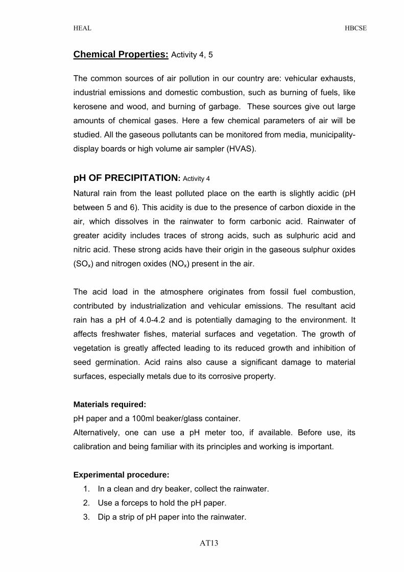
Experimental procedure: 1. In a clean and dry beaker, collect the rainwater.

2. Use a forceps to hold the pH paper.

3. Dip a strip of pH paper into the rainwater.

AT 13

HEAL HBCSE

AT 14

4. Hold the pH paper in the water for 20 sec.

5. Make sure all sides of the pH paper are well immersed in water.

6. Remove the paper from the beaker and read the colour developed

against the colour chart provided with the pH booklet.

7. Note down the corresponding value of the pH in the Air Worksheet

(AWS-Activity 4).

pH paper held

CARBON MONOXIDE: Activity 5 Carbon monoxide (CO) is formed when carbonaceous fuel is burnt, under

conditions of insufficient oxygen. The main contributors of CO are: automobile

exhausts, petroleum refining operations, electric and blast furnaces, gas

manufacturing plants and coalmines. The average rate of increase of CO is

about 0.03 ppm\year (0.03 mg\l). The national ambient quality standard is 4

mg\m3 and 10 mg\m3 (1 hour) for residential and industrial areas, respectively.

Above this concentration, CO acts as a pollutant.

High concentrations of carbon monoxide cause physiological and pathological

changes in humans, ultimately leading to death. It binds 250 times more

strongly than oxygen to hemoglobin in the blood. It inhibits many haeme �

containing enzymes and interferes with oxygen transport by blood leading to

physiological problems, brain damage and finally death.

HEAL HBCSE

As a pollutant, carbon monoxide does not have any damaging effects on

material surfaces. At concentrations, below 100 ppm it does not show any

drastic effect on the plant life. However, long exposures of even minute

amounts of this gas leads to chronic injury of plants. Most instruments have a

detection limit of 2 ppm (2 mg/l), making monitoring of low concentrations of

CO difficult.

Experimental procedure: Data for this gas should be collected from your local municipality, from public

displayed air monitors or from TV channels. Alternatively, use a standard high

volume air sampler pump. (Enter the result in Air worksheet (AWS: Activity 5).

Principle: This gas is analysed using the non-dispersive infrared absorption

method. (The amount of CO in air is proportional to the distension of

diaphragm, this distension being proportional to the intensity of radiation

passing through the sample and reference cells.)

SULPHUR DIOXIDE: Activity 5

It is the most prevalent gaseous air pollutant in India. Burning of fossil fuels,

such as coal and petroleum and domestic garbage are the major producers of

this pollutant. Coal and petroleum contain varied amounts of sulphur

compounds. Good quality coal, technically known as anthracite, is identified

with less (less than 1%) sulphur. Bituminous coal, plenty in India, on the other

hand, contains 4% of sulphur. Petroleum products contain 1 to 5% sulphur.

Sulphur dioxide (SO2) is also released during metallurgical processes. Clean

fuel and efficient vehicular engines contribute a lot in reducing the SO2

emissions. The national standard for ambient concentration of SO2 in the air

is 80 µg/m3 (0.028 ppm), averaged over 24 hours for residential areas.

SOX is also one of the contributory factors for poor visibility. Sulphur oxides

(SOX!SO2 and SO3) are strong respiratory irritants. At 25-ppm concentration,

the irritation is seen in the upper respiratory tract. SOx�containing smoke

AT 15

HEAL HBCSE

produced from bituminous coal, causes chronic and acute bronchitis, pleurisy

and emphysema, common lung disorders. SOx also cause eye irritation, tears

and redness. In high concentrations, sulphur dioxide may also be fatal.

Experimental procedure: Data to be entered as for other pollutants (AWS-Activity 5).

Principle: SO2 present in the sample air is bubbled through a dilute aq.

solution of Sodium tetra chloro mercurate, which quantitatively converts SO2

to sodium dichloro sulfito mecurate. This reacts with p-rosaniline dye to form a

red-violet coloured complex (p rosaniline methyl sulfonic acid). This is

colorimetrically estimated at 560 nm.

OXIDES OF NITROGEN: Activity 5

The major sources of nitrogen oxides (NOX) in the air are: fuel combustion as

in different industries and vehicles and garbage burning. The quality of the

engines in vehicles, such as spark ignition and compression ignition, also

affect the emission amount \ quality of this gas.

The ambient air quality standard for nitrogen oxides is 80 µg\m3 (0.028 ppm.)

for 24 hours in residential areas. Above this concentration, the gas acts as a

pollutant with serious effects, both on humans and on material surfaces.

Among the different nitrogen oxides, nitric oxide (NO) and nitrogen dioxide

(NO2) are the main pollutants. At 0.25ppm, NO2 absorbs visible light and

causes reduced visibility. At these low concentrations, NO2 causes acute eye

irritation. At higher concentrations it leads to pulmonary fibrosis, with serious

respiratory problems. NO reacts with moisture in the atmosphere to form nitric

acid, causing corrosion of metal surfaces.

AT 16

HEAL HBCSE

Experimental procedure: Using a HVAS, air is collected in a solvent of NaOH solution. This is then

analysed in the lab.

Principle: NO2 in the sample is converted into a stable solution of NaNO2.

This is converted into an azo dye with sulphanilamide, which then couples

with the reagent N (1-naphthyl ) ethylenediamine dihydrochloride to form a

colour complex. The latter is determined colorimetrically at 540 nm. (AWS-

Activity 5).

LEAD: Activity 5

Lead occurs naturally in small quantities in the air, water and soil. It is a heavy

metal, which can exist as an air pollutant in the form of vapours and as

particles.

Often called as a �silent killer and crippler of humans�, automobile exhaust and

lead-based paint are the most common sources of lead pollution in the air.

This paint is dangerous when it is peeling, chipping, chalking or cracking.

Improper renovation of homes with lead-based paint can generate lead dust in

the air, and soil, and in and around homes. Industries, such as lead ore

mining, lead ore milling, smelting, municipal solid waste incinerators, and

lead-acid battery recycling facilities are other sources of lead in soil and air.

Soil contaminated with lead is a potential source of lead exposure. As floor

dust, it can become a source of lead contamination in the air. Other sources

of air borne lead include, emissions from gasoline combustion (now

eliminated by unleaded gasoline), smelters and battery manufacturers. In

recent decades, the dominant source of lead exposure to humans is from

emissions of motor vehicles operating on leaded petrol.

Humans can inhale lead particles or ingest lead via the consumed food and

water. Although lead can enter the body in a number of ways, people living in

urban areas are exposed to lead via inhaling airborne particles containing

lead. Lead can be found in all tissues of the body and tends to accumulate in

AT 17

HEAL HBCSE

the bones, where it is immobilized and hence stored. The liver and kidneys

eliminate ingested lead slowly (over years) by excretion.

Lead affects practically all systems within the body, mainly the human central

nervous system. Lower levels of lead can adversely affect the brain, central

nervous system, blood cells, and kidneys. In young children, lead can cause

learning difficulties. In adults, it leads to heart problems. At high exposures,

lead can cause kidney disorders, anemia, convulsions, coma, and even

death. The effects of lead exposure on fetuses and young children can be

severe. They include delays in physical and mental development, lower IQ

levels, shortened attention spans, and increased behavioral problems.

Fetuses, infants, and children are more vulnerable to lead exposure than

adults since lead is more easily absorbed into growing bodies, and the tissues

of small children are more sensitive to the damaging effects of lead. Children

may have higher exposures since they are more likely to get lead dust on their

hands and then put their fingers or other lead contaminated objects into their

mouths.

Symptoms of lead exposure have not been observed in blood lead

concentrations below 0.2 µg/ml. For the protection of human health, the

national ambient air quality standards for airborne lead range from 0.5 to 1.5

µg/m3 for sensitive, residential and industrial areas.

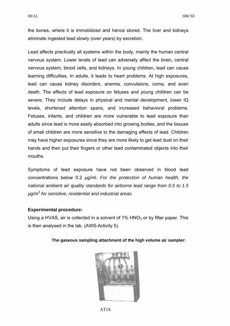
Experimental procedure: Using a HVAS, air is collected in a solvent of 1% HNO3 or by filter paper. This

is then analysed in the lab. (AWS-Activity 5).

The gaseous sampling attachment of the high volume air sampler:

AT 18

HEAL HBCSE

AUTOMOBILE POLLUTION: Activity 6 to 9 In recent years, emissions from automobiles form one of the major

components of air pollution in the country, especially in metropolitan cities.

The main reason for this rise in air pollution is the increasing number of

vehicles and the poor quality of fuel.

Exhaust of automobiles is highly complex, giving out a host of air pollutants.

These include carbon monoxide, volatile oxides of carbon (VOC), particulates,

nitrogen oxides (NOX), unburnt hydrocarbons, sulphur dioxide, lead, and, of

course, smoke. Smog formation primarily composed of ozone and particulate

matter, is another outcome of traffic pollution. According to the World Health

Organization, air pollution due to traffic threatens the health of billions of

people in the country. The three main types of automobiles largely used in the

country are:

Passenger cars powered by four stroke engines •

•

•

Two wheelers powered by two /four stroke engines.

Buses and trucks powered by four stroke diesel engines.

The vehicle exhaust depends on the fuel type and its contents. The amount

and volume of pollutants emitted by a vehicle depends on a number of

factors, including the engine type\design, the type of fuel, emission control

device and the engine�s mechanical operations, such as idle \accelerated

engine and the road conditions.

The harmful effects of vehicular pollutants are many. To give one instance,

the NOx leading to the formation of ground level ozone, can aggravate

breathing problems, including asthma and reduce lung functions. Exposure to

carbon monoxide due to its competing nature with oxygen slows down

reflexes with increasing drowsiness; ozone and particulates, even in very

minute quantities, lead to lung malfunctioning, which shows up initially as

breathing problems. In short, all the pollutants released in exhausts have

synergistic and additive effects on human health, leading to early ageing of

lungs in the long run.

AT 19

HEAL HBCSE

Lead pollution in air, both due to vehicles and soldering industry in the country

has attracted attention of many scientists, due to the detection of lead in the

blood.

Experimental procedure: A few survey-based exercises are designed to bring out the threat of vehicular

air pollution in an area. This will be supported by the data of various pollutants

like NOx, particulate matter, and carbon monoxide collected from the nearest

air monitoring station/pump, or municipality done on a regular basis and

accordingly entered in the work sheet.

Activity 6: 1. The number of different types of vehicles at a particular site (residential

area or a traffic junction), at specific times �for 1 hour at peak and non-

peak times�has to be recorded. Repeat this exercise at the same time

on three different days. Record the average number of vehicles in the

air worksheet {AWS-Activity 6(i)}. Ideally, repeat this exercise at

different times of the year/during different seasons.

2. Simultaneously, obtain and enter the pollution data {Activity 6(ii)} from

the municipality for the above sites. Avail of the facility of the mobile air

monitoring van from the municipality/HBCSE for this purpose.

Remember to match the dates and time of the two.

3. Pollution data for the two sites�residential and traffic�{Activity 6(ii)}

should be done with the same type of monitoring instrument.

Activity 7:

1. At a traffic junction, record the number of any one type of vehicle (e.g.

cars) on an hourly basis, for any one day of the month (preferably on a

working day).

2. Represent the vehicle numbers on a graph sheet. (The graph sheet

consists of one cm squares, with each one cm. square further divided

into 100 squares.) For every vehicle counted, darken (shade) one small

square in one cm. square. For each hour (represented on X axis), use

a different centimeter square.

AT 20

HEAL HBCSE

3. Plot hours (at least 12 hours) on the x axis;

4. Simultaneously, monitor TPM, NOx or CO levels for the same day and

at corresponding time intervals.

5. Keep a separate record of the pollutants. Graphically represent

different pollutants as different graphs.

6. Match/superimpose/layer the pollution data on the vehicle number

data. Use colours to bring out different pollutants.

7. The y-axis could represent the pollutant concentrations.

8. This entire procedure should be repeated at least three times to get an

understanding about air pollution and traffic.

9. Repeat the entire Activity in a residential area/ or near a green park.

10. Remember to use the same monitoring devise throughout the expt.

Activity 8: This activity brings out the role of public transport in reducing air pollution.

1. For one week or one month, record the number of students coming to

college/school in various vehicles: cars, school bus or BEST (public

buses), 2-wheelers or by cycle. Also keep a record of those walking

down to school / college.

2. Also, note the average number of students traveling per vehicle type.

3. A table of emission factor derived based on particle size analysis

carried out by NEERI (National Environment Engineering Research

Institute, Nagpur) is provided in the Worksheets (AWS: Activity 8).

4. If all the vehicle types are traveling at a fixed speed and cover a fix

distance of 10 km from home to college, calculate the total PM 2.5

(particulate matter size less than 2.5µ) emitted per vehicle type.

5. Calculate the total emissions of PM 2.5µ for the recorded number of

vehicles. Calculate the PM 2.5µ emission per one transported

individual and enter the values in the Air Worksheet (AWS-Activity 8).

Activity 9:

1. In the next step, assume there is an increase in the number of vehicles

in your area (at the approximate rate of about 2,000 cars per year).

AT 21

HEAL HBCSE

2. Try to model this increase over a period of five years and the

subsequent increase in the different types of air pollutants. Plot the

standard for each pollutant also on these graphs.

3. Visualize a scenario for air pollution when more stringent air pollution

norms are implemented in the country. This could include: advanced

Euro norms for engine designs, or improving fuel quality by drastically

reducing sulphur content, or using alternative fuels, such as CNG or

with battery-powered vehicles.

4. Combined with several of the above steps, air pollution could be

drastically reduced with strong administrative measures, including

improved infrastructure and more disciplined traffic.

NOISE POLLUTION: Activity 10

Noise is any unwanted or unpleasant sounds around us. It is a reality of

today�s fast moving life. The increasing noise levels are mostly due to

industrialization and ever increasing traffic.

Appliances used in homes, such as mixers, air coolers, water-pumps and loud

music and in vehicles (locking, unlocking and reverse alarms) all add to the

noise load. Use of loud speakers and loud musical instruments during

different religious practices, festivals and marriages, also contribute to the

decibel levels, both in rural and urban areas. In India, most of us are

insensitive to noise pollution and disregard its existence.

Noise is recorded in decibel (db) units, which combines both sound pressure

and intensity. The Central Pollution Control Board (CPCB) of India has laid

down permissible sound levels for cities for four different zones, viz, industrial,

commercial, residential and sensitive areas (extending about 100 m around

educational institutes, courts and hospitals). Levels exceeding these

constitute noise pollution. According to experts, the decibel levels of normal

conversation ranges between 45-65 db, passenger cars and trucks generate

decibel levels of 75 and 110 db respectively.

AT 22

HEAL HBCSE

Noise pollution causes gen

invisible but direct effect on

for prolonged periods suffer f

to cardiac problems, high blo

Activity 10 (I, ii, iii):

1. Obtain the decibel lev

areas traffic junctions,

municipality. Alternativ

levels in selected are

(AWS�Activity 10 (i))

Activity 10 (ii) 1. To monitor the noise

site so that the noise m

2. Note the values in Air

Activity 10 (iii): 1. In your municipal war

halls and religious pla

of surrounding trees

worksheet.

2. Try to collect data ab

these places, especi

should be at least 30 m

Areas

Sensitiv

Residen

Commer

Industria

Average permissible soun

AT 23

eral degradation of environment and has an

our health. People exposed to high noise levels

rom a variety of ailments, ranging from deafness,

od pressure to disturbances in sleep.

els at different sites: sensitive areas, residential

commercial and industrial areas, from the local

ely, use a noise meter to measure the decibel

as. Record the observations in Air Worksheet

.

pollution caused by traffic, select an appropriate

eter is exposed to the moving traffic.

worksheet (AWS�Activity 10 (ii).

d, or street, note down the number of marriage

ces. Also fill in the their location details, number

(they act as sound absorbers), etc. in the

out noise levels using the noise meter outside

ally during festivities. The measurement time

inutes.

Day

Night

e 50dB 40dB

tial 50dB 45dB

cial 65dB 55dB

l 75dB 65dB

d levels for Indian cities (prescribed by CPCB).

HEAL HBCSE

Air Worksheets Name Of The Observer: Date:

College Name/Address:

General Observations Of The Site:

Site Name: Location:

Site description: Parks\gardens___, Open area___, Beach\ any water

body___, Others______

Type of vegetation: NIL___, Scanty___, Grassy___, Specify others___

Observation of the sky : Clear___, Cloudy___, Scattered clouds ___

If cloudy: Colour of the clouds: Grey___, Brown/black___, Orange___,

Other___

Air movement: Windy___, Light winds___, Breezy___, No winds___

Wind direction: East\West\North\South___

Extent of visibility: Clear______, Hazy___;

If hazy: Due to: Smog: ____, Mist: ____, Fog: ____ , Other____

Activity 1: Study Of Physical Properties Of Air Day temperature:

Maximum: Result 1_____, Result 2: _____, Result 3: _____ ,

Average: _______oC

Minimum : Result 1_____, Result 2: _____, Result 3: _____

Average: _______ oC

Smell (0dour): No smell ____, Smell _____

If smell is present, then : Pleasant___, Marshy___, Foul___, Fishy ___, Smell

of rotten eggs___, Others: ________

AW S 24

HEAL HBCSE

Activity 2a: Total Particulate Matter (TPM)

Flow rate of the pump: ______litres\min; Time duration of pumping: ____

Total volume of air collected: _______m3

Type of

filter

Wt. of

clean filter (gms) (X)

Wt. of

filter+particulates gms (Y)

Wt. of the

particulates (Y-X gms)

Amount/conc. of

particulates in vol. of air collected (gms/m3)

Whatman I Whatman A

Glass fiber filter

If electronic monitoring station is present in the area, record the concentration

of particulates (TPM and RPM) below.

TPM: ______mg/m3 ; RPM: _______mg/m3

Actity 2b: Particulate Matter At Different Sites Repeat the procedure of Activity 2a at different sites: commercial, residential,

industrial, sensitive (hospitals) and traffic junctions. Note the weights of

particulate matter calculated in the table below: If possible, repeat the expt. at

different times of the day.

Amount of particulate matter at different sites (gms/m3) Type\Size of filter Residential Commercial Industrial Sensitive Traffic

junctions

Whatman1

Whatman A

Glass fiber filter

AW S 25

HEAL HBCSE

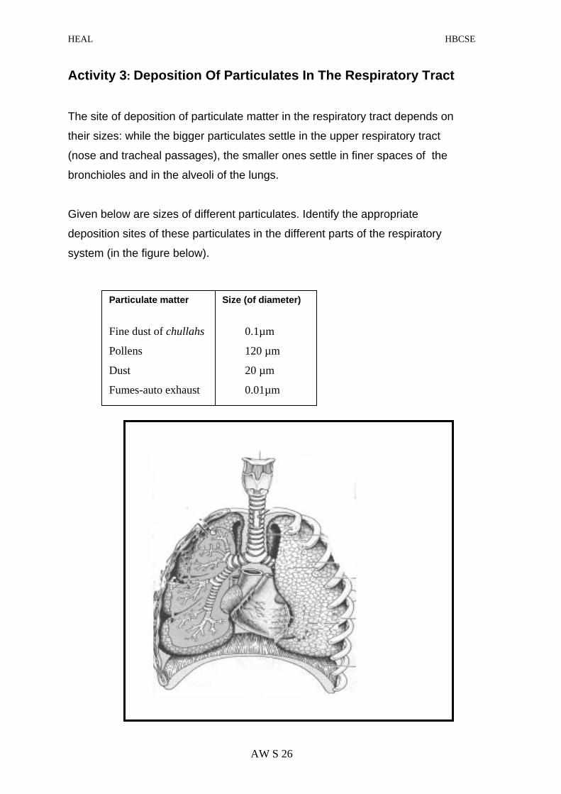
Activity 3: Deposition Of Particulates In The Respiratory Tract The site of deposition of particulate matter in the respiratory tract depends on

their sizes: while the bigger particulates settle in the upper respiratory tract

(nose and tracheal passages), the smaller ones settle in finer spaces of the

bronchioles and in the alveoli of the lungs.

Given below are sizes of different particulates. Identify the appropriate

deposition sites of these particulates in the different parts of the respiratory

system (in the figure below).

Particulate matter Size (of diameter)

Fine dust of chullahs 0.1µm

Pollens 120 µm

Dust 20 µm

Fumes-auto exhaust 0.01µm

AW S 26

HEAL HBCSE

Activity 4: pH Of Precipitation Last recorded rainfall in: _____months/days/hour;

pH measured using _________

pH of precipitation: observer 1____; observer 2_____; observer 3______

Average pH of precipitation:_______ Activity 5: Concentration Of Different Air Pollutants Date:

Source of pollution data: Air monitoring station____, sampling

pump______,TV____ or press____

If the data refers to a specific site, then identify the site as: Industrial ___,

Residential ____, Sensitive ___

Data for different pollutants

Pollutants Time weighted average

Concentration in air

Carbon monoxide (CO)

1hr 8 hrs

Sulphur dioxide (SO2) 24 hrs

Nitrogen dioxides (NO2)

24 hrs

Total particulate matter (TPM> 10 µm)

24 hrs

Respirable particulate matter (RPM<10 µm)

24 hrs

Lead (Pb) 24 hrs

AW S 27

HEAL HBCSE

Activity 6 (I): Automobile Pollution: Average number of vehicles passing in a fixed time, say, in one hour. Site / Location:_________ Date:________, Time:_______

Residential area (R) Traffic junction (T) Type of vehicles

Nos. at (PT)

Nos. at (NPT)

Nos. at (PT)

Nos. at (NPT)

Cars

Auto rickshaws

Two wheelers

Buses

Trucks

R: residential area; T: traffic junction; PT: Peak time; NPT: Non peak time

Activity 6 (Ii) Pollution Data For The Above Site

Pollutant data obtained CO NOx SOx Particulate

matter R T R T R T R T

Dat

e of

obs

.

PT

NPT

PT

NPT

PT

NPT

PT

NPT

PT

NPT

PT

NPT

PT

NPT

PT

NPT

AW S 28

HEAL HBCSE

Activity 7 : Match The Number Of Vehicles And Air Pollutants. Make separate graphs for different pollutants.

AW S 29

HEAL HBCSE

Activity 8: Carbon Monoxide Emission Per Transported Individual For Different Vehicle-Types. Emission factor derived on the basis of particle size analysis carried out by NEERI.

Type of vehicles PM 2.5 emission (gm\km)

Cars 0.046 Taxis 0.046 LDDV* 0.840 HDDV** 2.180 3-wheelers 0.399 2-wheelers 0.0399

LDDV*-Low density diesel vehicle (diesel cars); HDDV**-high density diesel vehicles

(buses and trucks)

In this activity, (i) survey of different types of vehicles—petrol or diesel driven

cars (LDDV), buses etc, used by students to come to college/school is to be

noted. (ii) Note the average number of students /vehicle.

One has to assume here that ALL vehicles have traveled a fixed distance of

10 kms at a fixed speed.

Type of vehicle/ Nos.

No. of Vehicles

(A)

Average number of

students per car (B)

PM 2.5 * emission

per vehicle type for 10

kms (gm/km) (C)*

Total PM 2.5

emission (gm\km)

(CxA) (D)

PM 2.5 emission

per transported individual

(D/A) Cars (petrol driven)

Cars (diesel driven)

School buses

Two wheelers

Auto rickshaws

Cycle

* NOTE: To get the correct value of C, calculate the emission for 10 kms.

AW S 30

HEAL HBCSE

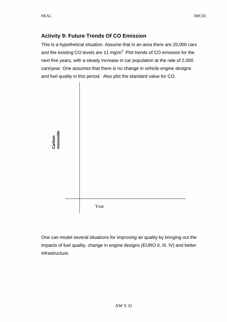
Activity 9: Future Trends Of CO Emission This is a hypothetical situation. Assume that in an area there are 20,000 cars

and the existing CO levels are 11 mg\m3. Plot trends of CO emission for the

next five years, with a steady increase in car population at the rate of 2,000

cars\year. One assumes that there is no change in vehicle engine designs

and fuel quality in this period. Also plot the standard value for CO.

One can model several situations for improving air quality by bringing out the

impacts of fuel quality, change in engine designs (EURO II, III, IV) and better

infrastructure.

Car

bon

mon

oxid

e

Year

AW S 31

HEAL HBCSE

Activity 10 (I): Noise Pollution

Decibel levels at different sites, obtained from a monitoring station and with a

noise meter.

Average decibel levels obtained from:

Area\site chosen

Monitoring station

Noise meter

Residential

Sensitive

Commercial

Traffic junction

Activity 10 (Ii): Decibel Levels Recorded For Noise Pollution.

Decibels Name of the site.

Max. Min.

AW S 32

HEAL HBCSE

Activity 10 (Iii): Decibel Levels Recorded At Different Points Of The Study Site.

Decibel levels at:

Marriage halls

Religious places

Parks Schools Hospitals

Characterize area as: R: residential

S: sensitive

C: commercial

I: industrial

Name of site

Num

ber

+\ --

Dci

bel l

evel

at e

ach

hall

Num

ber +

\--

Dci

bel l

evel

at e

ach

plac

e

Num

ber +

\--

Dci

bel l

evel

at e

ach

park

Num

ber +

\--

Dci

bel l

evel

at e

ach

scho

ol

Num

ber +

\--

Dci

bel l

evel

at e

ach

hosp

ital

AW S 33

HEAL HBCSE

National Ambient Air Quality Standards: Concentration in ambient air Pollutants Time weighted

average Sensitive area

Industrial area

Residential area

8 hrs

1.0mg\m3

5.0mg\m3

2. 0mg\m3

Carbon monoxide

1 hr 2.0mg\m3 10.0mg\m3 4. 0mg\m3

Annual

15µg\m3

80 µg/m3

60 µg\m3

Oxides of nitrogen

24 hours 30 µg\m3 120 µg\m3 80 µg\m3

Annual

15 µg/m3

80 µg/m3

60 µg/m3

Sulphur dioxide

24 hours 30 µg/m3 120 µg/m3 80 µg/m3

Annual

50 µg/m3

120 µg/m3

60 µg/m3

Respirable particulate matter(<10 um)

24 hours 70 µg/m3 150 µg/m3 100 µg/m3

Annual

70 µg/m3

360 µg/m3

140 µg/m3

Suspended particulate matter 24 hours 100 µg/m3 500 µg/m3 200 µg/m3

Annual 0.50 µg/m3 1.0 µg/m3 0.75 µg/m3 Lead

24 hours 0.75 µg/m3 1.5 µg/m3 1.0 µg/m3

* Annual Arithmetic Mean of minimum 104 measurements in a year taken twice a week, 24-hourly, at uniform interval.

** 24-hourly/8-hourly values should be met 98% of the time in a year.

However, 2% of the time, it may exceed but not on two consecutive days.

AW S 34

HEAL HBCSE

AW S 35

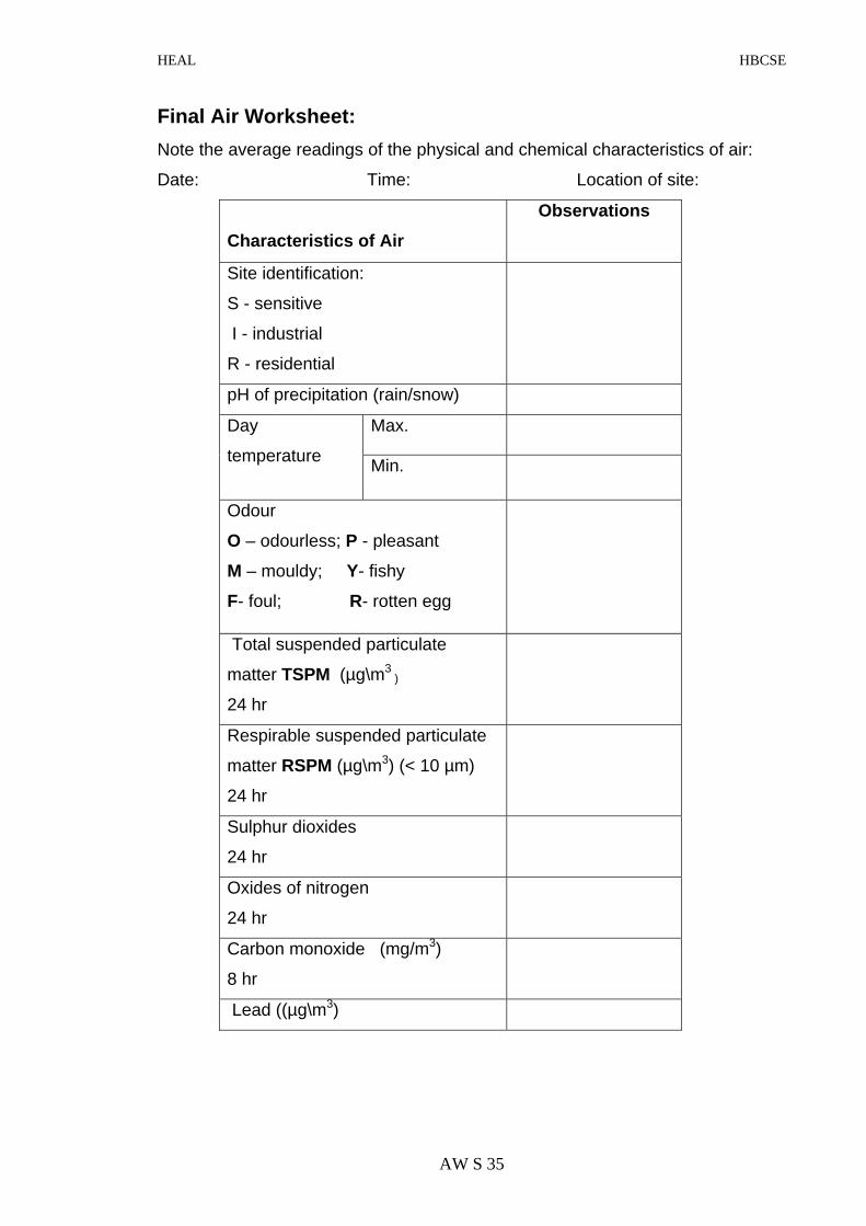
Final Air Worksheet: Note the average readings of the physical and chemical characteristics of air:

Date: Time: Location of site:

Characteristics of Air Observations

Site identification:

S - sensitive

I - industrial

R - residential

pH of precipitation (rain/snow)

Max. Day

temperature Min.

Odour

O – odourless; P - pleasant

M – mouldy; Y- fishy

F- foul; R- rotten egg

Total suspended particulate

matter TSPM (µg\m3 )

24 hr

Respirable suspended particulate

matter RSPM (µg\m3) (< 10 µm)

24 hr

Sulphur dioxides

24 hr

Oxides of nitrogen

24 hr

Carbon monoxide (mg/m3)

8 hr

Lead ((µg\m3)

HEAL HBCSE

‘Water’ watch… for good health

INTRODUCTION: All aspects of water, its quality, quantity, its uses and sources, are at the

center stage of discussions (academic, social and political) today in the

country. On one hand, water quality is steadily deteriorating, and, on the other

hand, there are increasing demands on this natural resource. Balanced

development demands a scientific understanding of this valuable resource, as

water quality and quantity has a direct impact on our health.

Water is an important and the most abundant resource in the biosphere. The

water molecule is represented as H2O, with an oxygen atom in the central

position, bound by two hydrogen atoms.

The biological importance of water in supporting life is due to its unique

physical and chemical properties. It is a universal solvent with high melting

and boiling points, high heat capacity and maximum density as a liquid at 40

C, These properties are attributed to the structure of the water molecule. To

give one instance, the last property allows organisms to live below the ice

cover in denser and warmer waters.

The world�s water can be classified as fresh and saline water. It exists in three

different states: liquid (salt and fresh), solid (fresh) and vapour (fresh). Fresh

water constitutes only about 3% of the total water, and a large part of this is

locked up as ice caps and glaciers. The remaining fresh water is found in

rivers, streams, lakes and ponds and as sub-surface ground water aquifers.

This freshwater balance is greatly dependent on the monsoon system in each

region. The marine (salt) environment constitutes the large oceans and seas.

The salt waters are equally important as they support an entire marine water

ecosystem. Pollution of water sources/bodies could be hazardous for our very

survival. This finite resource, which is so vital to all life on this earth, must be

protected, conserved and treated with care.

WT 36

HEAL HBCSE

WHAT IS WATER POLLUTION? Rapid urbanization, industrialization and certain agricultural practices have led

to pollution and deterioration of natural water bodies. These water bodies are

constantly being abused by activities, such as, washing and domestic /

industrial waste loads. Indiscriminate use of pesticides and fertilizers,

combined with inadequate training of farmers and workers, has led to highly

contaminated agricultural runoffs being released in water bodies. The highly

toxic chemicals (malathoin, lindane, DDT and chlorphyrophos) used as

pesticides in India, pollute our water bodies, or find their way in the ground

water. Several of these chemicals, especially DDT, are banned in most of the

countries in the world.

In urban areas, the situation is worsened often by the direct discharge into the

natural water bodies of untreated or partially treated sewage and industrial

wastes. Water pollution can also result from natural processes, such as,

surface runoffs due to rains or presence of dead organic matter, but these are

slow processes, giving enough time for the water body to rejuvenate.

Drinking water, which has been treated by municipalities, often is

contaminated with sewage (and other waste) in transit from the storage

reservoirs to residential units.

Some of the noticeable signs of water pollution are: dark, dirty colour of the

water body, reduction in transparency, unpleasant smells, unchecked growth

of weeds, decrease in the number of fish, oil and grease floating on the

surface of the water body and bad taste of drinking water.

ANALYSIS OF WATER: There are several physical, chemical and microbiological properties of water,

which can be monitored to find out its overall quality. Among the many

chemical properties are: pH, dissolved oxygen (DO), biological oxygen

demand (BOD), chemical oxygen demand (COD), residual chlorine, alkalinity,

WT 37

HEAL HBCSE

nitrates, nitrites, total Kjeldhal nitrogen (TKN), phosphate, sulphate, zinc,

chromium, lead, copper, etc. For the initial phase of this program, a few

chemical properties will be monitored.

Before starting with water analysis, participants should be certain about the

source of the water and the purpose for which the water is being used, and

accordingly carry out the tests.

Physical properties examined are: smell (odour), colour, turbidity, temperature,

suspended solids.

Chemical properties studied here are: pH, conductivity, alkalinity, dissolved

oxygen (DO), biochemical oxygen demand, chemical oxygen demand,

chlorides, fluorides, ammonia, phosphates and heavy metals like iron, copper

and chromium.

Microbial parameter checked is: presence of the bacteria, Escherichia coli

(E.coli—coliforms) and their numbers expressed as MPN (most probable

number), will be checked in drinking water.

SAMPLING SITE DETAILS:

1. Site selection should be made with care, keeping in mind the purpose

of the water body, i.e., the water is used for drinking, recreational use,

or whether it is a dumpsite, like a nullah.

2. Any water source like rivers, streams and lakes is a good site for

sampling. Beaches, ponds, or creeks and water tanks can be

alternative sites for water sampling. Preferably, select a water source

nearest to the school /college.

3. For monitoring drinking water, samples can be collected from taps,

storage tanks (overhead and underground).

4. While collecting samples from the tank, consider the state of water

level �nearly empty, half filled or full. The results will vary depending on

these conditions.

WT 38

HEAL HBCSE

5. Water sample should also be obtained directly during the supply hours.

This would give a fair idea of the quality of municipal supply.

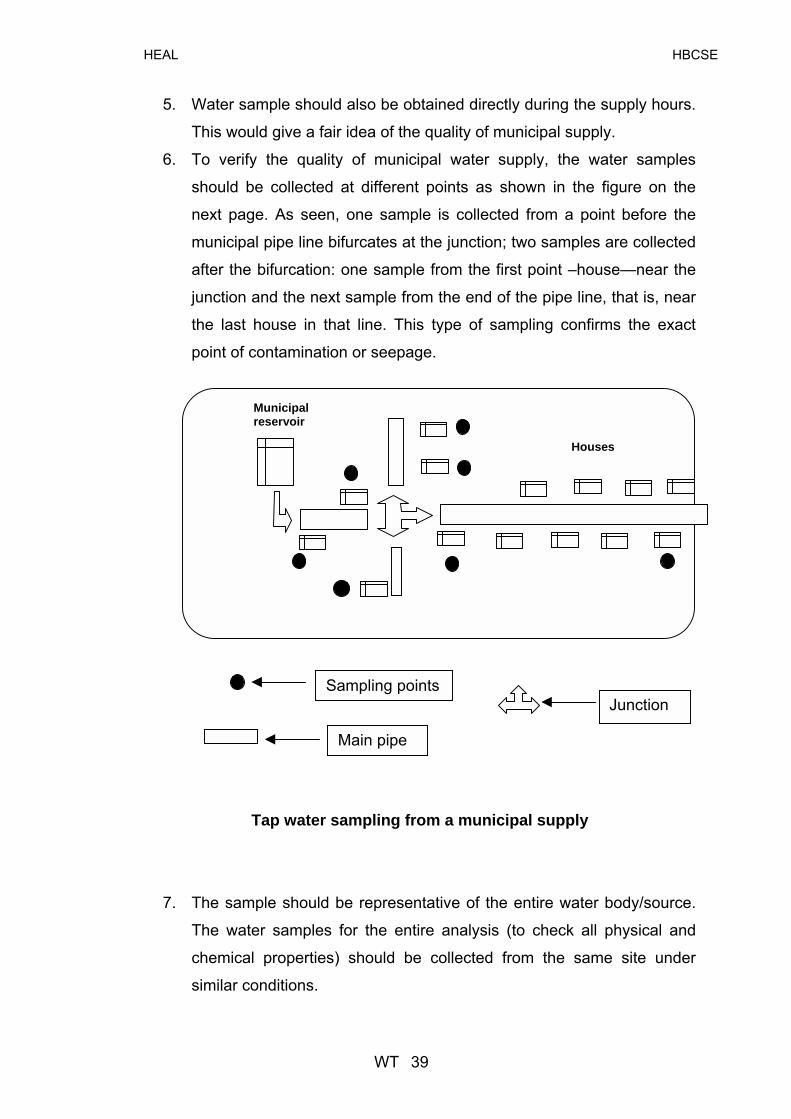
6. To verify the quality of municipal water supply, the water samples

should be collected at different points as shown in the figure on the

next page. As seen, one sample is collected from a point before the

municipal pipe line bifurcates at the junction; two samples are collected

after the bifurcation: one sample from the first point �house�near the

junction and the next sample from the end of the pipe line, that is, near

the last house in that line. This type of sampling confirms the exact

point of contamination or seepage.

Houses

Municipal reservoir

Sampling points Junction

Main pipe

Tap water sampling from a municipal supply

7. The sample should be representative of the entire water body/source.

The water samples for the entire analysis (to check all physical and

chemical properties) should be collected from the same site under

similar conditions.

WT 39

HEAL HBCSE

8. Ideally, water samples should be collected and monitored two to three

times every month. It is important that water is monitored during late

summers, when the water levels dip in lakes and other reservoirs.

Pathogens, such as protozoa, Cryptosporidium parvum, which settles

in the sediments, and are resistant to chlorination, are then pumped

into the water flow.

SAMPLING: All sampling procedures should be performed under supervision. Care should

be taken to avoid any accidents: never enter any water body without inquiring

about its depth, currents and tides from a local person. Look out for

informational signposts regarding the water body.

Materials required: A small bucket with a strong rope and heavy stone attached to the handle,

500 ml polythene bottles with wide mouth, screw caps and sealing tape.

Experimental procedure: 1. If the sampling site is a well, holding on to a rope, lower the bucket into

the water. To get the sample from a certain depth, use a bucket with an

attached heavy stone.

2. Fill it partially with water. Pull out the bucket with water and thoroughly

rinse the bucket. Discard this water.

3. Repeat the procedure and now use the water sample for analysis.

4. If the sampling site is an open water body like stream, lake, creek, or a

sea, study its location and different points of entry and exit of water.

5. Ideally, surface water samples are collected by averaging grab

sampling method:

! All samples to be collected 300 cms (10 feet) away from

the shoreline. Use a boat to collect all these samples.

WT 40

HEAL HBCSE

! Starting from a point (A), collect ~50 ml water in a

container. Repeat this at regular intervals, till a distance

of about 5 m (pt. B) is reached. This will make one

sample.

! From (B) continue sampling similarly for the next 5 m (pt.

C). This will be the second sample.

! Repeat this procedure until you make a complete circle to

come back to pt. A.

! If possible, try to obtain another sample from the center of

the water body.

Sample 2

Sample 1

G

DFE

H

C

BA

Water body

! Alternatively, with a boat, collect samples along the

diameter so that opposite ends could be considered for

sampling.

6. Depending on the accessibility of the water and to get the true picture

of the quality of water of open water bodies, choose appropriate

sampling points. For instance: (i) A point where there is an inlet of

wastewater or other streams. (ii) A point from where water is pumped

out. (iii) A sample collected from the center of the water body will give a

fair idea of the level of pollution. (iv) A bottom water sample at a depth

of about 5-10 mts will determine the extent of mixing and the presence

of debris and other pollutants settling at the bottom.

WT 41

HEAL HBCSE

7. Take a minimum of five samples from each water body, to represent

the entire body.

8. First, rinse the bucket with water from the shore and then throw the

bucket out as far as possible.

9. Take a sample from the top surface of water. Do not allow the bucket

to fill up and sink. Avoid stirring the bottom sediment.

10. To obtain the sample, allow the bucket to fill to two-thirds or three-

fourths levels. Then pull the bucket out of the water.

11. Avoid taking samples from shores where the water is stagnant.

12. Use a float with a rope, which could be a light object like an empty

plastic bottle or a wooden block, to check the direction of the flow of

water.

13. For drinking water, if the sampling point is a tap: Using a sterile

container (use an autoclave or a pressure cooker), first rinse the bottle

with tap water and then collect the water sample. (Check the earlier

details on page 4.)

Bottling technique: It is preferred to do all the water analysis, especially, the physical properties,

at the site itself. Only certain experiments are performed in the laboratory.

This requires that the sample be carefully bottled so that its original properties

and chemistry are not altered.

1. Label a 500 ml polythene bottle giving the site and sampling details.

Rinse the bottle and cap with the sample water.

2. Fill the bottle up to the top rim with sample water, so that when the cap

is put on, no air is trapped inside. Seal the cap of the bottle with a

sealing tape.

3. Store these samples in a refrigerator at about 40C until they can be

tested.

4. Once the seal is broken, do the pH test first; then proceed with

alkalinity and nitrites, followed by other tests.

WT 42

HEAL HBCSE

5. Ideally, once the seal is broken, all the tests should be performed in a

single laboratory session. Hence, prior planning is important.

6. The sampling for DO, BOD and COD requires a special bottle and

technique, mentioned under the topic of DO.

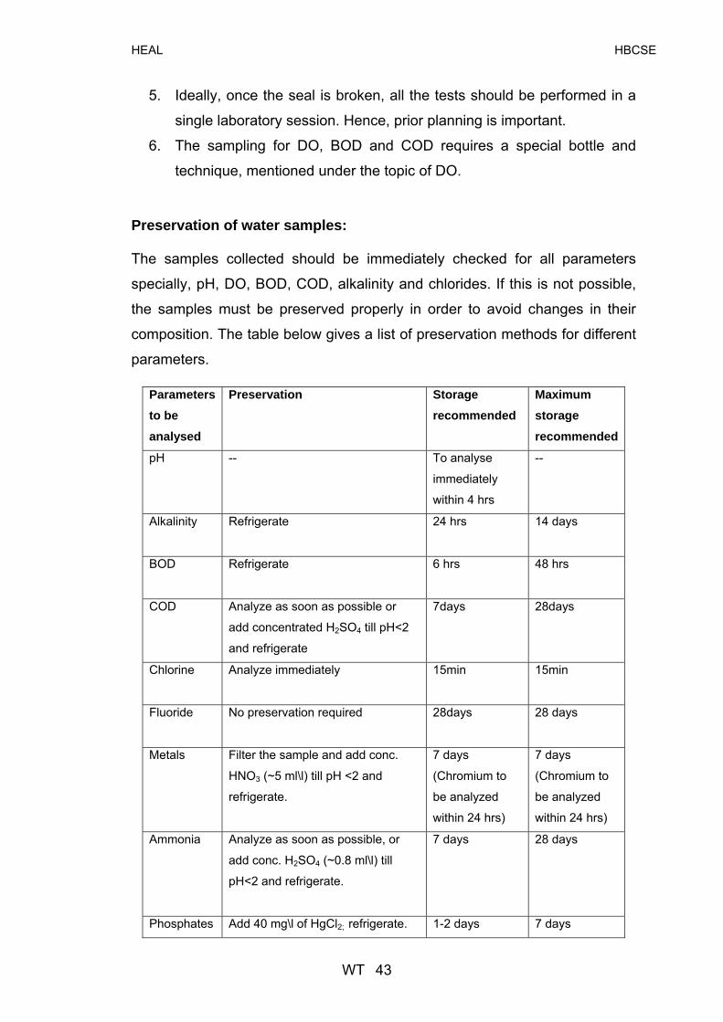
Preservation of water samples: The samples collected should be immediately checked for all parameters

specially, pH, DO, BOD, COD, alkalinity and chlorides. If this is not possible,

the samples must be preserved properly in order to avoid changes in their

composition. The table below gives a list of preservation methods for different

parameters.

Parameters to be analysed

Preservation Storage recommended

Maximum storage recommended

pH -- To analyse

immediately

within 4 hrs

--

Alkalinity Refrigerate

24 hrs 14 days

BOD Refrigerate

6 hrs 48 hrs

COD Analyze as soon as possible or

add concentrated H2SO4 till pH<2

and refrigerate

7days 28days

Chlorine Analyze immediately

15min 15min

Fluoride No preservation required

28days 28 days

Metals Filter the sample and add conc.

HNO3 (~5 ml\l) till pH <2 and

refrigerate.

7 days

(Chromium to

be analyzed

within 24 hrs)

7 days

(Chromium to

be analyzed

within 24 hrs)

Ammonia Analyze as soon as possible, or

add conc. H2SO4 (~0.8 ml\l) till

pH<2 and refrigerate.

7 days 28 days

Phosphates Add 40 mg\l of HgCl2; refrigerate. 1-2 days 7 days

WT 43

HEAL HBCSE

Physical Properties: Activity 1

COLOUR: Activity 1

Clean water is colourless. However, natural water bodies often show colours

due to the presence of dissolved or suspended solids and variety of water

plants and organisms. Decaying organic matter, including weeds too, impart

colour to water. Other sources that contribute dark undesirable colours are:

effluents from industries, domestic sewage discharges and spillages from

ships and boats, and other washing activities. Normally, the coastal areas are

maximally affected, except the oil spills in mid-oceans.

Materials required: Clean glass container, source of white light (if sunlight is not bright), a white

cardboard or plain white sheet of paper for background.

Experimental procedure: 1. Transfer 50 ml of water sample in a clean and clear glass

tube/container.

2. Observe the colour of the water by looking through (down) the tube,

against a white background in bright\white light (sunlight preferred).

3. Compare the colour of the sample with clear distilled water under

similar conditions.

4. Repeat with three different observers and note the observations with

intensities of colours in the water worksheet (WWS: Activity 1).

5. At a later stage, measure the colour intensity quantitatively in colour

units using potassium chloroplatinate and cobaltous chloride (Platinum-

cobalt method) for accurate colour measurement.

ODOUR: Activity 1

Unpolluted clean water has no odour. However, water in natural bodies could

acquire some odours ranging from mild to excessive. These odours could be

due to certain treatment procedures such as chlorination, or due to natural

WT 44

HEAL HBCSE

processes, like, decaying of vegetable matter (ammonia and hydrogen

sulphide is given out with decaying vegetable matter). Human activities, such

as sewage disposal or industrial discharges may also produce foul odours.

Industrial effluents give out a variety of compounds like, halogens, sulphides,

phosphates and volatile organic compounds, contributing to smells.

Materials required: Two clean glass containers or test tubes. Experimental procedure: The experiment should be performed with a fresh sample, preferably at the

site itself.

1. Take a clean glass container, and rinse it with the sample water.

2. Fill the container up to three-fourths volume with water sample and

smell it.

3. Check for the following odours: sweetish, unpleasant or marshy, rotten

eggs (sulphide), organic chemicals (volatile organic compounds),

others (specify), no odour. Also, note the intensity of odours. Note

down your observations in the water worksheet (WWS: Activity 1). Repeat the procedure with three different students.

TEMPERATURE: Activity 1

Water temperature varies with climate, season and the time of the day. The

temperature of a water body is normally lower than the surrounding air, unless

thermal effluents are released in the water body. A gradual decrease in the

temperature is observed with the increase in depth of the water body.

Temperature affects aquatic life and alters the physico-chemical processes

occurring in water. For instance, high temperatures result in the decrease in

concentration of dissolved oxygen. Water temperatures are altered both due

to natural (direct sunlight) and human activities. Discharges of hot industrial

effluents, from nuclear reactors and thermal power plants affects the water

WT 45

HEAL HBCSE

temperatures. These processes can raise the temperatures considerably.

Turbid waters absorb more sunlight hence record high temperatures.

Materials required: Clean glass container and alcohol thermometer.

Experimental procedure: Temperature is measured with an alcohol thermometer, preferably at the site.

1. Hold the end of the thermometer (opposite to the bulb) and shake it to

remove any trapped air. Note the temperature reading.

2. Immerse the thermometer into the water to a depth of about 12 cms,

and hold it for 3-5 minutes. Take care not to drop the thermometer in

the water (tie the thermometer to a strong string to avoid losing it).

3. Raise the thermometer and quickly note the reading. Remember to

raise the thermometer (with the bulb within water) only as much is

needed to read the temperature.

4. If temperature alters, lower the thermometer again in water, allow it to

stabilize for one minute and then take the reading. Record the

temperature along with date and time.

5. Repeat three to four times and note down the average reading in the

worksheet (WWW: Activity 1).

6. Alternatively, take 100 ml of the sample in a 250 ml clean glass

container. Place the thermometer upright and immerse the bulb in

water, without touching the walls of the container.

7. Read the thermometer at the eye level and record the average reading

after three repeats in the work sheet (WWS: Activity 1).

Thermometer

WT 46

HEAL HBCSE

TRANSPARENCY: Activity 1

Clean water is relatively transparent and less turbid. Transparency or clarity is

an expression of the optical property that allows light to scatter. It is also

described in terms of turbidity, which is a result of the suspended solid matter

present in water. These particles can be in the form of sand, clay, silt, organic

matter and plankton.

Increased turbidity prevents light penetration, which, in turn, disturbs the

natural ecology of the water body. Water bodies get turbid during monsoon

due to increased surface runoffs, which carry the topsoil. Turbidity also

increases the water temperature. Turbidity also changes with the land use

pattern and by activities such as washing, dumping and wading of cattle.

Natural waters have a transparency ranging from one meter to a few meters.

A value of less than one meter, can be expected in a water body with many

weeds. A low value may also result due to the high concentration of

suspended solids and pollution. Very clear lakes and streams without many

weeds may record a transparency value of about 40 meters.

Materials required:

A clean glass container, test-tube, a wooden disc\cardboard disc to make a

Secchi disc, brushes, black and white paint, hook screws, 6 mt. long rope,

small piece (3-4�) metal pipe to act as a counterweight, meter stick, marker

and glue.

Experimental procedure: Transparency of water in natural waters as in rivers, lakes and creeks is

measured using a Secchi disc:

1. Secchi disc is a slim wooden disc. Divide the area of the disk into four

quadrants. Paint the two opposite quadrants in black and white.

2. Screw a hook screw on the top center and bottom center of the disk.

3. Tie a long rope, about five meters long, through the top hook screw.

WT 47

HEAL HBCSE

4. Tie a short piece of rope on the bottom hook and string it through the

pipe. Tie a large knot at the bottom of the pipe so that the pipe does

not fall off when the disc is held in a vertical position.

5. Using a measuring tape or a meter stick, make markings (graduations)

at every 10 cms with a dark colured marker on the rope starting from

the point of attachment of the disc. Highlight every 50 cm with another

colour marker and every meter (100 cms) with a red marker. Now the

Secchi disc is ready for measurement.

Alternatively, the transparency protocol can be performed in the laboratory,

too. For this, the tube turbidometer is used. To construct the tube

turbidometer:

1.

2.

3.

4.

Take a clear glass tube, about 20-30 cms in length and a diameter of

about 7 cms. Alternatively, use a 500 ml measuring cylinder.

Put a PVC cap on one end of the tube. The cap should firmly fit it.

Cut a disc of plastic or a cardboard, the same size as the tube diameter

and prepare the disc with four quadrants, same as for Secchi disc

method. Waterproof the disc by lamination or varnish.

Glue the disc to the PVC cap (or at the inner base of cylinder), with the

painted side facing up. Use a marker and a meter stick to make a scale

on the side of the tube.

90 80 70 60 50 40 20 10

Mark in cm Clear tube 4.5 x 120 cm

Painted disc to fit bottom of the tube

PVC cap

Courtesy:GLOBE

WT 48

HEAL HBCSE

Transparency measurement with the Secchi disc:

1. Lower the disc gradually into water until the disc just disappears.

2. Grab the rope at this point at the surface of water and mark this point

as (B) with a marker.

3. Raise the disc until it reappears to view; grab the rope and mark that

point as (A).

4. The rope will now have two points, which are a few cms apart.

5. Record both these depths and calculate the average depths (A+B/2).

6. Repeat the procedure three times and calculate the cumulative

average.

7. Note this value as SDT (Secchi disc transparency) in the water

worksheet (WWS: Activity 1).

8. Turbidity is usually measured in NTU (Nephelometric Turbidity Units).

To convert the SDT value into NTU, multiply SDT with 1.5, which is a

constant. (This constant �euphotic--will take care of the light factors

involved while taking readings). This will give the SDT value.

9. To convert the SDT into NTU (turbidity), plot the SDT value obtained

on the calibrated conversion graph provided {in Appendix (3)} and read

the corresponding NTU units.

Tranparency measurement with the tube method:

This is a slight variation of the above method. Pour the water sample into the

tube until the disc disappears. In other words, the center point of the disc

should disappear, even though the black quadrants are visible. Look directly

from the top of the water column.

Rotate the tube to confirm the view. Record this depth in the water work sheet

(WWS: Activity 1).

Note: The Secchi disc method gives a rough estimation of transparency of

water. For both the methods, light intensity and angular viewing will affect the

readings. Hence, bright light of the sun should be behind the observer, i.e.,

observations should be made in a shadow, to avoid errors. If the

shadow/shade is not present, use an umbrella.

WT 49

HEAL HBCSE

For accurate measurements, a turbidimeter or nephelometer is used. This

method is based on a comparison of intensity of light scattered by the water

sample and a standard reference (solution of hydrazine sulphate and

hexamethylene tetramine) under similar conditions.

CONDUCTIVITY: This property is a measure of the ability of an aqueous solution to carry an

electric current. It depends on the concentration and mobility of ions and

temperature of the solution at the time of measurement. Solutions containing

inorganic compounds show greater conductivity than solutions containing

organic compounds. Hence, this property is an indirect method to measure

the presence of salts of different ions. Greater the amount of ions (Ca+, Mg+,

Cl-, SO42-, HCO3, CO3 2-) in water, higher is the conductivity.

Conductance (G) is defined as the reciprocal of resistance (R): {G= 1/R}.

Conductivity is measured with an instrument �conductometer--containing a

conductivity cell, which could either be of platinum electrode type or non-

platinum type. Conductance of a solution is measured using two chemically

inert electrodes. These electrodes are fixed at two ends with the solution in

between. The conductance of a solution is directly proportional to surface

area of electrodes (A cm2) and inversely proportional to the distance between

two electrodes (L cms); k is the constant of proportionality.

Hence G ∞ k ( A/L) µmho/cm, where k= 1/ohm-cm.

To convert in SI system, conductance is measured as: milli siemens per

meter, ie, mS/m.

1 mS/m = 10 µmho/cm.

Note: All conductivity measurements should be carried out at 250 C.

WT 50

HEAL HBCSE

Conductivity of distilled water produced in a laboratory is in the range of 0.5 to

3 µmho/cm, while that of potable water ranges between 50 to 1500 µmho/cm.

According to the Central Pollution Control Board, the permissible limits of

conductivity for fresh water are in the range of 50 to 500 µmho/cm; ground

waters have more conductivity than surface water. Conductivity of polluted

waters is high, e.g., industrial waste is 10,000 µmho/cm.

Materials required: Distilled water, conductivity meter, thermometer, flask, beakers.

0.01 M anhydrous potassium chloride solution (appendix 1, preparation of

solutions).

Experimental procedure: 1. Rinse the conductivity cell with 0.01M KCl three times. Dip the probe in

a beaker containing standard solution of 0.01 M KCl. Adjust the reading

of the instrument to 1412 µmho/cm at 250 C. The instrument is ready

for use.

2. Thoroughly rinse the cell two to three times with the water sample.

3. Note the temp. of the water sample and read the conductivity.

Calculations:

1+ 0.019 (t-25)

k m

Conductivity µmho/cm = Where km = measured conductivity at t0 C

t = temp. of the water sample

SUSPENDED SOLIDS: Activity 2

Suspended solids are small and can easily be trapped on an ordinary filter

paper. They are light and hence do not sediment down in a container. In water

bodies, these solids are contributed by a variety of agriculture, municipal and

WT 51

HEAL HBCSE

industrial activities. They make the water turbid and block the passage of light

and thus they degrade the quality of water.

Materials required: Two clean glass beakers (100 ml), a glass funnel, filter papers, oven and a

weighing balance.

Procedure: Thoroughly mix the water sample by stirring or shaking vigorously before

proceeding with the experiment.

1. Filter 100 ml of sample water through a funnel layered with filter paper

of known weight. Collect the filtrate in another clean container.

(Fold the filter paper into half; again fold into half; make a cone by

pulling one layer on one side and three layers on the other side).

2. Stir the water sample and then pour through the filter-layered funnel,

and slowly allow the water to filter. After all the water has filtered, allow

the filter paper to dry at 1050 C for about 30 mins. in an oven.

3. Weigh it with residue. The difference between the two weights

represents the suspended matter present in the water sample.

4. Note both the weights and their difference in the water worksheet. 5. Repeat the procedure three times and report the average reading in the

water work sheet (WWS: Activity 2).

WT 52

HEAL HBCSE

Chemical Properties: Activity 3 to 14

pH: Activity 3

This is an indicator of acidity or alkalinity of water. Its value ranges from 0 to

14, with pH between 6 and 7 indicating a neutral state. Values above 7

indicate alkaline state and that below 7 indicates acidic condition. Natural

water bodies are slightly alkaline in nature.

Different human activities such as mining, agriculture run offs and discharge

of industrial and domestic effluents into water bodies can cause considerable

pH fluctuation.

pH has a strong influence on the types of living organisms in a water body.

Amphibians like frogs and salamanders are particularly sensitive to low pH.

Acidic pH of water is corrosive in action for metal and concrete structures.

Extreme pH on either side of the pH scale can lead to several skin and gastro-

intestinal problems in humans.

Materials required: A clean glass container, pH paper

Experimental procedure:

1. Rinse a 50 ml beaker at least twice with the sample water.

2. Fill the beaker about half way with the sample to be tested.

3. Hold the pH paper with a forceps and dip it into the sample for at least

a minute.

4. Make sure that all the four sides of the paper are immersed in the

water.

5. Remove the paper and compare the colour developed with the colour

chart on the pH booklet.

6. Repeat the procedure three times and note the average pH in the

water worksheet (WWS: Activity 3).

WT 53

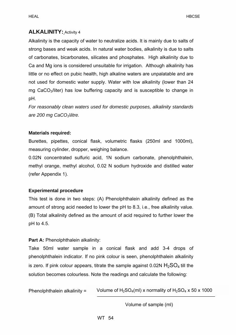
HEAL HBCSE

ALKALINITY: Activity 4

Alkalinity is the capacity of water to neutralize acids. It is mainly due to salts of

strong bases and weak acids. In natural water bodies, alkalinity is due to salts

of carbonates, bicarbonates, silicates and phosphates. High alkalinity due to

Ca and Mg ions is considered unsuitable for irrigation. Although alkalinity has

little or no effect on pubic health, high alkaline waters are unpalatable and are

not used for domestic water supply. Water with low alkalinity (lower than 24

mg CaCO3/liter) has low buffering capacity and is susceptible to change in

pH.

For reasonably clean waters used for domestic purposes, alkalinity standards

are 200 mg CaCO3\litre.

Materials required: Burettes, pipettes, conical flask, volumetric flasks (250ml and 1000ml),

measuring cylinder, dropper, weighing balance.

0.02N concentrated sulfuric acid, 1N sodium carbonate, phenolphthalein,

methyl orange, methyl alcohol, 0.02 N sodium hydroxide and distilled water

(refer Appendix 1).

Experimental procedure This test is done in two steps: (A) Phenolphthalein alkalinity defined as the

amount of strong acid needed to lower the pH to 8.3, i.e., free alkalinity value.

(B) Total alkalinity defined as the amount of acid required to further lower the

pH to 4.5.

Part A: Phenolphthalein alkalinity:

Take 50ml water sample in a conical flask and add 3-4 drops of

phenolphthalein indicator. If no pink colour is seen, phenolphthalein alkalinity

is zero. If pink colour appears, titrate the sample against 0.02N H2SO4 till the

solution becomes colourless. Note the readings and calculate the following:

Phenolphthalein alkalinity =

Volume of sample (ml)

Volume of H2SO4(ml) x normality of H2SO4 x 50 x 1000

WT 54

HEAL HBCSE

Part (B): Total alkalinity

In the above same beaker, add 3-4 drops of methyl orange. Titrate the yellow

solution against sulfuric acid till the colour changes from yellow to orange.

Total alkalinity = Volume of sample (ml)

Volume of H2SO4 (ml) x normality of H2SO4 x 50 x 1000

{In the above formula, 50 represents: 1ml of NaOH = 50 mg of CaCO3,

calculated from standardization procedure of H2SO4 (Appendix 1)}

Once we know the total alkalinity, determine if the alkalinity is due to

hydroxide, carbonate or bicarbonate, from the table given below.

*P = Phenolphthalein alkalinity and T = Total alkalinity

Values of P* and T*

Hydroxide alkalinity (as CaCO3)

Carbonate alkalinity (as

CaCO3)

Bicarbonate alkalinity (as

CaCO3) P =0 0 0 T

P <1/2 T 0 2P T-2P P =1/2 T 0 2P 0 P >1/2 T 2P-T 2 (T-P) 0

P = T T 0 0

Principle: Alkalinity of surface waters is due to presence of carbonates,

bicarbonates and hydroxides. Alkalinity thus indicates the sum of

concentration of all these ions. Borates, phosphates, silicates and other bases

may also contribute to alkalinity values. Hydroxyl ions produced due to

dissociation/hydrolysis of solutes react with acids (H2SO4, HCl); titrations to

end point pH 8.3 (Phenolphthalein alkalinity) and then to pH 4.3 (total

alkalinity) are done using indicators. These two alkalinities help to determine

the specific ions that contribute to alkalinity in the water sample.

WT 55

HEAL HBCSE

DISSOLVED OXYGEN: Activity 5

Dissolved oxygen (DO) is the amount of oxygen present in water. It is an

important characteristic of any water body and is essential for maintaining its

natural ecology. DO also reflects the physical, chemical and biological

processes occurring in a water body, and is an indirect measure of

photosynthetic activity in water eco-systems. Less oxygen means reduced

number of life forms in the water body and is an indirect indicator of water

pollution. DO is mostly contributed by atmosphere; algae and rooted plants

also give out oxygen during photosynthesis. It is expressed as mg of oxygen

in one litre (mg/l) of water. The DO of unpolluted natural waters is usually in

the range of 4 to 8 mg/l.

Oxygen content of waters varies with salinity, turbulence, photosynthetic

activity and temperature. Since it is a poorly soluble gas, its solubility directly

varies with atmospheric pressure at any given temperature. The range of

solubility of atmospheric oxygen, in fresh waters is, 14.6 mg\l at 00 C to about

7.0 mg\l at 350 C under one atmospheric pressure. Warm water holds less

oxygen as compared to cold water. Therefore, water fauna and flora

experience stress during the hot summer months. Build up of organic wastes

of dead plants and animals, discharges of domestic waste and industrial

effluents containing oxidizing chemicals are the major factors that cause

depletion of DO in a water body. Eutrophication (increase in algae numbers)

also causes DO depletion.

Materials required: 250 ml DO bottle (any glass bottle with a air-tight stopper), 2 nos. of 2 ml

syringes (glass or plastic), 1 no. of 10 ml. syringe, conical flasks, an ink

dropper. Manganese sulphate (Mn(II)SO4) solution , alkaline potassium iodide

(KI) solution, sulphamic acid (NH2SO3H), 1% starch solution and 0.025 N

sodium thiosulphate (Na2 S2O3) (refer Appendix�Preparation of solutions 1).

WT 56

HEAL HBCSE

Experimental procedure: DO is measured by Winkler test. Before proceeding with the expt, the water

sample has to be fixed (removal of oxidizing chemicals by chelation) for DO

immediately at the site itself.

DO fixing:

1. The 250 ml DO bottle is filled completely with water sample.

2. The bottle is immediately corked up to ensure that no air bubble is

trapped. To the sample water, add 2ml of MnSO4 solution with a

pipette or a syringe. The solution should be added well below the

surface of the water. Mix the contents by inverting the bottle 3-4 times.

3. Next, add the same amount of alkaline potassium iodide (KOH\KI)

solution to the sample water. Mix well until a brown precipitate forms.

4. A brown precipitate is formed and will soon settle down. Place the

stopper tightly and shake the bottle vigorously.

5. Allow the sample to stand for at least 20 minutes.

Measurement of DO

1. To the above fixed water sample, add 2 gms of sulphamic acid.

2. Replace the stopper and mix the solution to dissolve the precipitate.

3. Pour out 50 ml of this sample into the conical flask.

4. Holding the conical flask in one hand, gently add thiosulphate solution

drop by drop, with simultaneous mixing of the contents. Care must be

taken not to spill the contents of the flask.

5. When the colour of the contents in the flask changes to pale yellow,

stop adding thiosulphate. Note the volume of thiosulphate added.

6. Drop wise add the indicator (1 % starch solution, about 15-20 drops)

with a dropper to the conical flask.

7. Shake the flask and observe the colour change to blue.

8. Now again add the thiosulphate solution drop wise until the blue color

disappears. This is the endpoint of the titration. Note the volume of

thiosulphate added.

9. Note the total volume of thiosulphate added (A ml). This will be the sum

of the amount of thiosulphate added before and after adding starch.

WT 57

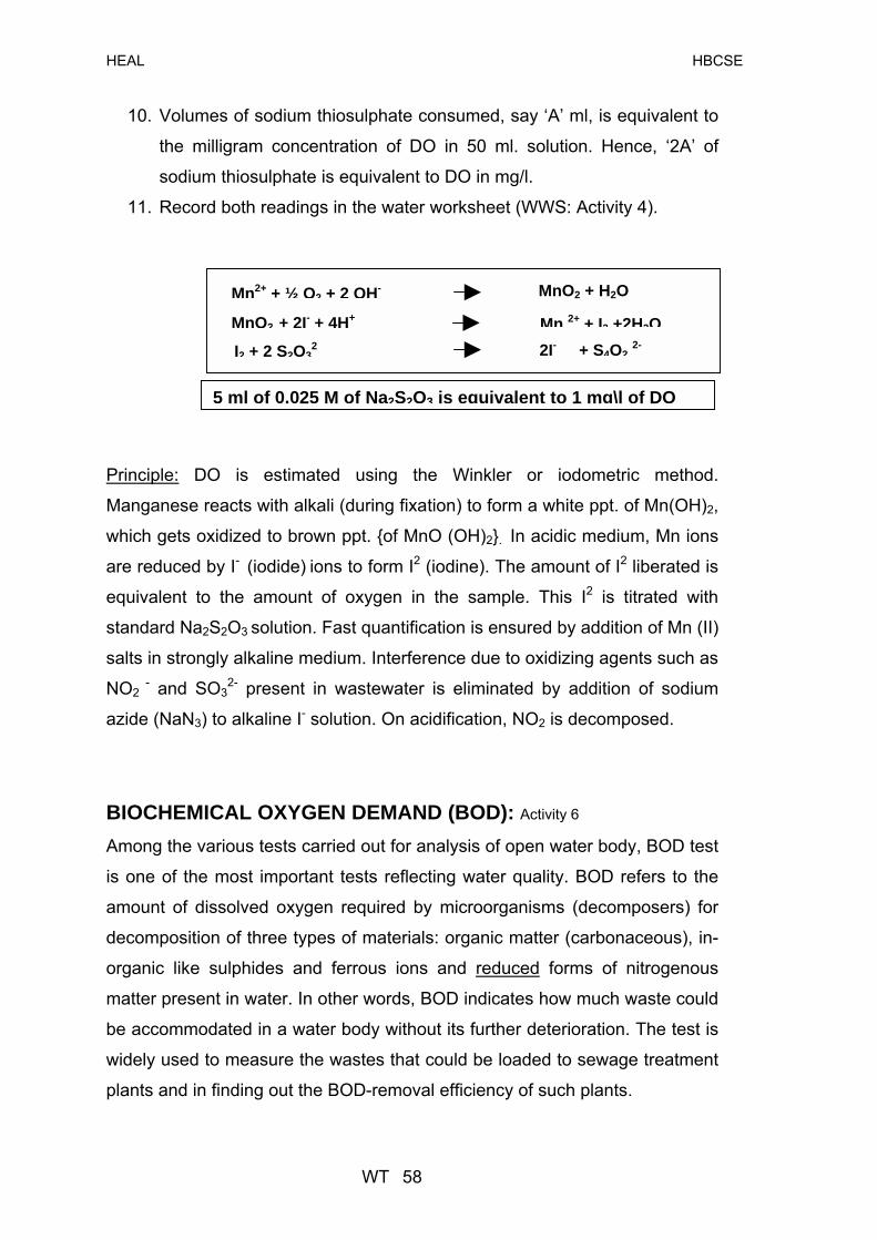
HEAL HBCSE

10. Volumes of sodium thiosulphate consumed, say �A� ml, is equivalent to

the milligram concentration of DO in 50 ml. solution. Hence, �2A� of

sodium thiosulphate is equivalent to DO in mg/l.

11. Record both readings in the water worksheet (WWS: Activity 4).

5 ml of 0.025 M of Na2S2O3 is equivalent to 1 mg\l of DO

I2 + 2 S2O32

MnO2 + 2I- + 4H+

Mn2+ + ½ O2 + 2 OH- MnO2 + H2O

2I- + S4O2 2- Mn 2+ + I2 +2H2O

Principle: DO is estimated using the Winkler or iodometric method.

Manganese reacts with alkali (during fixation) to form a white ppt. of Mn(OH)2,

which gets oxidized to brown ppt. {of MnO (OH)2}. In acidic medium, Mn ions

are reduced by I- (iodide) ions to form I2 (iodine). The amount of I2 liberated is

equivalent to the amount of oxygen in the sample. This I2 is titrated with

standard Na2S2O3 solution. Fast quantification is ensured by addition of Mn (II)

salts in strongly alkaline medium. Interference due to oxidizing agents such as

NO2 - and SO3

2- present in wastewater is eliminated by addition of sodium

azide (NaN3) to alkaline I- solution. On acidification, NO2 is decomposed.

BIOCHEMICAL OXYGEN DEMAND (BOD): Activity 6

Among the various tests carried out for analysis of open water body, BOD test

is one of the most important tests reflecting water quality. BOD refers to the

amount of dissolved oxygen required by microorganisms (decomposers) for

decomposition of three types of materials: organic matter (carbonaceous), in-

organic like sulphides and ferrous ions and reduced forms of nitrogenous

matter present in water. In other words, BOD indicates how much waste could

be accommodated in a water body without its further deterioration. The test is

widely used to measure the wastes that could be loaded to sewage treatment

plants and in finding out the BOD-removal efficiency of such plants.

WT 58

HEAL HBCSE

A large amount of organic matter in water leads to increased growth of

decomposers. These demand a high amount of oxygen for their respiration. If

the growth of the decomposers is unchecked, the oxygen demand by them

leads to deficiency of dissolved oxygen in water creating anaerobic

conditions. Such anaerobic conditions deprive water plants, animals and

microorganism (aerobic) of enough oxygen for respiration, leading to their

death. This causes eutrophication of water body, where it is completely

covered with a layer of algae and other water plants. However, dissolved

oxygen is always found in the upper layers of waters being in direct contact

with air. Thus, all forms of life, especially water plants, crowd on the surface,

further reducing entry of sunlight into the water body.

BOD measurements give variable results depending on the water body. For

standardization, BOD is taken at different times of incubation of microbes and

hence there is 5-Day BOD test (5-d BOD, BOD5), 60-90 incubation test called

as ultimate BOD or (UBOD) and continuous oxygen uptake by Respirometric

method. Here the 5-d BOD method is used. To mimic the original water body

quality in the water sample collected, seeding and dilution of the water sample

is carried out. These also maintain the pH at 6.5 to 7.5 for BOD estimation.

According to the standards laid out by the CPCB, BOD limits for: (i) drinking

water (DW) without conventional treatment but after disinfection, (ii) DW after

conventional treatment and disinfection, (iii) organized outdoor bathing source

and (iv) industrial effluents discharged in inland surface waters should not

exceed 2, 3, 3, and 30 mg/l resp. (5-d at 200 C). (See BOD under liquid waste

for further details.)

. Materials required: Reagent bottles of 250-300 ml, volumetric flasks, beakers, pipettes, burette,

measuring cylinder, weighing balance, incubator and aerator (for vigorous

shaking).

Double distilled water (BOD free), ammonium chloride (NH4Cl), disodium

phosphate hydrogen heptahydrate (Na2HPO4 .7H2O), dipotassium hydrogen

phosphate (K2HPO4), potassium dihydrogen phosphate (KH2PO4),

WT 59

HEAL HBCSE

magnesium sulfate heptahydrate (MgSO4 .7H2O), calcium chloride (CaCl2 ),

ferric chloride hexahydrate (Fe Cl3 .6H2O), concentrated sulfuric acid and

distilled water, dilution water and seeding mixture (See Appendix 1).

Experimental procedure: Conventionally, a 5-d BOD test is done wherein the amounts of oxygen

required for biochemical degradation of organic matter in five days is

measured. This requires that samples be incubated at 200 C for five days.

Then DO is measured initially (Day 1) and after incubation (Day 5); the BOD

is calculated as the difference between the two DOs (D1-D2).

The amount of BOD in wastewaters often exceeds the concentration of DO.

Therefore, it is necessary to dilute the sample (with dilution water) for

estimation of the BOD. This dilution water contains all the nutrients and

appropriate pH suitable for bacterial growth. It could be distilled, tap or any

stream water free of biodegradable organics and other bio-inhibitory

substances, such as chlorine and heavy metals. If the sample is highly

polluted (such as, industrial effluents, high temperature and extreme pH

wastes) and if it does not support any microbial growth, then these samples

are seeded with a microbial population obtained from supernatant of domestic

wastewater.

1. Collect the water samples and fix the sample as mentioned for DO.

Next, dilute these samples with dilution water (see appendix 1). The

dilution ratio for various water samples is given below. Dilution is not

necessary for unpolluted/potable water.

Sample Percentage dilution

Dilution mixture (sample + water)

Total volume

Sample

Water 1000 ml 50 % 500ml 500ml 1000 ml 25 % 250ml 750ml 1000 ml 20 % 200ml 800ml 1000 ml

Polluted water

10 % 100ml 900ml 1000 ml

WT 60

HEAL HBCSE

If the waters are polluted/dirty, use 25% and 50% dilutions for analysis. If

water is from industrial effluents/excessively treated not allowing any

microbes to survive, then seed the dilution water with a culture/domestic

waste. Adjust the pH of the sample to7.0 using an acid or a base.

2. Fill the BOD bottles with the sample and immediately estimate DO.

3. Make two sets of bottles for each dilution. Immediately estimate the DO

of one sample of each dilution. Label these as D1. Keep the other set

for incubation at 20-250C for five days. The airtight bottles are

incubated in dark to prevent photosynthesis.

4. Determine the DO of incubated samples after 5 days (D2).

5. Carry out blank readings for the above two sets before and after

incubation (B1 and B2). The blank does not contain the sample water

(only contains dilution water).

Calculation: (i) (If sample is not seeded)

BOD (mg/l) = D1-D2

P

Where: D1 and D2 are the DO content of the samples on days 1 and 5

P is the volume of sample used for titration

(ii) (If sample is seeded)

BOD (mg/l) = (D1-D2)- (B1-B2) x F

Where: D1 and D2 are the D

B1 and B2 are the DO

F is the total volume

P is the volume of the

W

P

O content of samples on days 1 and 5

content of samples on days 1 and 5

of solution in the DO bottle

sample used for titration.

T 61

HEAL HBCSE

The quality of water in terms of BOD values can be interpreted as :

BOD (mg\l)

0-1 2 3 5 >10

Water quality

Very clean Clean Fairly clean

Doubtful Bad

CHEMICAL OXYGEN DEMAND (COD): Activity 7

COD reflects the degree of organic and inorganic pollution in a water body. It

is a good measure of pollutants in waste and natural waters. It is defined as

the amount of oxygen required for complete oxidation of all substances

present in the water. The COD values are always higher than BOD values

because all pollutants are not mineralized in the biochemical processes. COD

is a preferred to BOD in determining the quality of industrial effluents

containing non-biodegradable organic pollutants. Such effluents record very

low values of BOD. Besides, determination of COD is faster as it does not

require any incubation period.

According to Central Pollution Control Board, COD standards for clean water

bodies lie between 4-10 mg/l. Standards for discharge of effluents in different

waters is: 250 mg/l. These waters include: inland surface water, land for

irrigation and marine coastal areas.

Materials required: Conical flask, burette, pipette, bunsen burner, tripod stand, wire gauze,

beaker, measuring cylinder and weighing balance.

0.25N Potassium dichromate, 0.25 N ferrous ammonium sulfate (FAS

solution), concentrated sulfuric acid, 1,10 phenanthroline monohydrate,

ferrous sulfate (FeSO4. 7H2O), mercuric sulfate and distilled water (see

appendix 1).

WT 62

HEAL HBCSE

Experimental procedure: 1) Take 20 ml of water sample in a conical flask and add 0.1 gm (pinch) of

mercuric sulfate

2) Slowly add 5ml of concentrated sulfuric acid (an ice bath must be used

to avoid spurting) and add 10ml of 0.25 N potassium dichromate

solution. Cool the flask and again add 30 ml of sulphuric acid, taking

the above-mentioned precautions. Add few porcelain pieces to prevent

jumping during boiling (reflux) in the next stage.

3) Cover the flask with a watch glass/small petri plate and allow it to stand

in boiling water bath for 30 mins. If the colour of the solution changes to

green (indicating high COD), dilute the sample water appropriately with

distilled water and repeat steps 1 to 3. If the colour after boiling

remains orange, proceed with step 4.

4) After boiling (solution colour is orange), double the volume of the

sample with distilled water.

5) Add 5 drops of ferroin indicator (see appendix 1) and titrate against

0.25N FAS solution. The end point of the titration is reddish brown

colour.

6) Similarly, carry out the titration for distilled water blank.

Calculation:

COD (mg/l) =

(Y-X) x (N) x 8 x 1000

Volume of water sample taken for digestion

Where:

Y is the volume of ferrous ammonium sulfate (FAS) for the

X is the volume of FAS used in titration for the sample

N is the normality of FAS

8 is the equivalent wt of oxygen

1000, to determine COD value in 1 liter of water sample.

Dilution factor (DF): is 1, if 20 ml sample is diluted with 20 m

2, if 20 ml sample is diluted with 40 ml DW.

WT 63

(if sample is diluted)

X dilution factor

blank

l of DW. Or, DF=

HEAL HBCSE

Principle: Boiling a mixture of chromic and sulphuric acids oxidizes most types

of organic matter. Potassium dichromate in the presence of sulphuric acid is

the commonly used oxidizing agent. The sample is refluxed with the acidic

oxidant in the presence of mercuric sulphate to neutralize the effect of

chlorides and catalyst (silver sulphate). The excess of potassium dichromate

is titrated against ferrous ammonium sulphate with ferroin as an indicator. The

amount of chromate used is proportional to the oxidizable organic matter

present in the sample.

CHLORIDES: Activity 8

Chlorides are one of the major constituents of water and wastewater. The

presence of chlorides in drinking water in concentrations below 250 mg\l

causes no harm to the human body. At concentrations greater than 250 mg\l

chlorides impart a salty taste to water. The degree of salty taste depends on

the cation associated with the chloride and on the concentration of the salt in

water. Chloride salts of sodium produce more saltiness than those of

magnesium and calcium. The concentration of chlorides is higher in

wastewater (domestic sewage) than in fresh natural waters. As sodium

chloride is an important constituent of human diet, it passes unchanged

through the digestive system and expelled out of the human system.

The natural sources of chlorides in open water bodies are contributed by

washing of mineral rocks containing salts of potassium, magnesium, etc.

Excessive amounts of chloride suggest water contamination due to seepage

of sea water into surface and ground water, human faecal contamination (as

sewage contains high amount of salt content), and industrial discharge of

effluents.

Chlorides are essential for plants and animals and are stored as sodium

chloride in their body. Chlorides are not considered to be harmful to human

health. However, high concentrations are harmful to plants and damage may

WT 64

HEAL HBCSE

occur at 70-250 mg\l. Drinking water standard for chloride lies between 200-

250 mg\l.

Materials required: Volumetric flasks, conical flask, measuring cylinder, burettes, pipettes,

weighing balance, potassium chromate (K2CrO4), silver nitrate (AgNO3), NaCl

and aluminum hydroxide suspension (see Appendix 1).

Experimental procedure:

1. If the sample is highly coloured, add 3 ml of the aluminum hydroxide

suspension; mix and allow it to settle and then filter.

2. Take 1ml of the water sample and adjust the pH between 7.0-8.0 (use

either NaOH or conc. H2SO4).

3. To this sample and add 1ml of potassium chromate.

4. Titrate against standard silver nitrate solution until a brick red

precipitate is formed. The first drop of AgNO3 that turns the precipitate

to brick red in colour shows the endpoint.

5. Note the colour of the precipitate and not the solution to get the

accurate endpoint. Repeat the procedure with blank containing distilled

water. This method is termed as Argentometric titration. Calculation:

Chloride (mg/l) = Volume of sample (ml)

(X-Y) x Normality of AgNO3 x 35.45 x 1000

Where:

X is the volume of AgNO3 required for sample;

Y is the volume of AgNO3 required for blank.

35.45 is equivalent weight of chlorine; 1000 is factor for conversion to liter.

Principle: Chloride is determined by Argentometric titration in which potassium

chromate acts as an indicator in alkaline conditions. On titrating with AgNO3

solution using K2CrO4 as a self-indicator, silver nitrate is precipitated as silver

WT 65

HEAL HBCSE

chloride and further converted to silver chromate (brick red ppt) thereby

indicating the end point.

FLUORIDES: Activity 9

The natural source of fluorides in water is the weathered material from rocks.

The concentration of fluorides in ground waters is higher than in surface

waters. Effluent from fertilizer, glass and chemical manufacturing industries

are major anthropogenic sources of fluorides in water.

Detection of fluorides in drinking water is important as high concentration of

fluoride consumption causes discolouration of teeth and abnormalities in

skeletal system called fluorosis, the incidence of which is high when fluoride

levels are greater than 1.5 mg/l in drinking water. At concentrations of 1 mg/l

in drinking water, fluorides prevent dental caries, with no harmful effects on

overall health. The acceptable limit for fluorides in drinking water is 1.5 mg/l.

Materials required: Colorimeter/spectrophotometer, test tubes, pipettes, 1000 ml volumetric

flasks, measuring cylinder and a weighing balance.

3-alizarin sulfuric sodium salt, zirconyl chloride octahydrate, concentrated

sulfuric acid, sodium fluoride and distilled water (see Appendix 1).

Experimental procedure:

1. Take 10 ml of the sample in a clean 50 ml flask.

2. Add 1.0 ml of acid zirconium-alizarin solution (mixed reagent) to the

sample. Make the volume to 50 ml.

3. Mix well immediately and allow it to stand for 20 minutes at room

temperature.

4. Repeat the procedure with reagent blank

5. Read the colour developed at 540 nm and determine the concentration

of fluoride in sample using the standard graph. Alternatively, compare

the colour developed against the colour grid provided and note the

WT 66

HEAL HBCSE

observation as low (L), permissible (P), high (H) or critical (C) in the

water work sheet (WWS: Activity 9). Note: Higher fluoride conc. gives

yellow colour. (The intensity of this yellow colour decreases with

increase in fluoride conc.) Lower concentrations of fluoride give a

reddish brown colour (the intensity of this red colour increases with

decrease in the fluoride concentration).

Preparation of standard graph: Stock sodium fluoride (NaF) solution: Prepare a stock solution of 100-ppm

NaF. From this, prepare a working stock solution of 10 ppm. Use this working

stock to prepare a range of standards of 1-5 ppm Measure the colour

obtained at 690nm. Plot a graph of absorbance vs. concentration.

Principle: Fluoride reacts with the zirconyl alizarin reagent to form colourless

Zr F62- and the dye. The colour of the dye lightens with the increase in amount

of fluoride.

AMMONIA: Activity 10

Ammonia is a natural component in surface water, ground water and domestic

sewage. It is produced largely due to deamination (removal of amino groups)

of organic nitrogen-containing compounds and hydrolysis of urea. In water

bodies, ammonia is some times produced by the reduction of nitrates under

anaerobic conditions. The maximum permissible limit for ammonia is 0.5

mg/litre. Concentrations of ammonia higher than this value indicate pollution,

and it becomes harmful for humans, fish and other water life forms.

Materials required: 100 ml beakers or test tubes, ink dropper, 5ml and 1ml syringes or pipettes,

Nessler�s reagent (*Nessler�s reagent is poisonous and utmost care has to be

practiced while handling it), 6N sodium hydroxide (NaOH) solution, 10 % zinc

sulphate (ZnSO4) solution, standard ammonia solution (100 ppm), EDTA

solution (refer Appendix�Preparation of solutions (1)).

WT 67

HEAL HBCSE

Experimental procedure:

1. Take 10 ml of the sample in a clean beaker. Add 10 drops of NaOH

with a pipette or ink dropper (to neutralize the acid used for storage).

2. To the above mixture, add 0.1ml 10% ZnSO4.7H2O followed by 0.1ml

6N NaOH.

3. Stir and filter the mixture. This process will remove all interfering ions of

Ca, Fe, Mg, S2+ precipitate.

4. Slowly tilt the beaker and collect the colorless fraction in a fresh

beaker. Add 1 drop of 50% EDTA. Mix the contents well.

5. Add 0.6 ml Nessler�s reagent. Shake well to mix the contents.

6. Compare the colour developed against the colour grid provided and

note the observation as low (L), high (H), critical (C) or permissible (P)

in the water work sheet (WWS: Activity 10).

7. If a colorimeter is available, measuring the resulting yellow color at 420

nm gives quantitative estimation of ammonia content in the sample.

Plot this value against a standard graph.

Preparation of standard graph: Stock ammonium chloride solution: Prepare a 100-ppm (refer Appendix (1)

solution of ammonium chloride (NH4Cl). From this solution, prepare a working

stock of 10 ppm. Prepare a range of concentrations from the working stock

(0.1 to 5 ppm). With these solutions (10 ml), proceed as for the sample

solution. Measure the colour obtained at 420 nm. Plot these values against

the concentrations to obtain a standard graph.

Principle: The presence of ammonia in higher concentrations (above 5 ppm)

is indicated as a brown precipitate with Nessler�s reagent, where the actual

amount is calculated by reading on a spectrophotometer or colorimeter.

Orange brown ppt

NH2 Hg2IO + 7I-- + 2H2ONH3 + 2HgI4 2- + 3OH

WT 68

HEAL HBCSE

PHOSPHATES: Activity 11

Natural waters contain phosphates either in the organic or inorganically bound

form. Run-offs from agricultural fields, detergent industries, biological sludge

from sugar and canning industries and domestic sewage add phosphates into

the water body. In natural waters, phosphate concentrations range from 0.005

to 0.020 mg\l. According to US Public Health Department, the maximum

permissible concentration of phosphates in drinking water is 0.1 mg\l.

Higher concentration of phosphates is a clear indicator of pollution.

Phosphates in water bodies indicate high levels of nutrients, which lead to

undesirable growth of algae and other water flora (eutrophication), decreasing

the DO content of the water body. Besides giving a distinct odour to the water

body, high levels of phosphates lead to skin and eye allergies and colouration

of teeth.

Materials required: Conical flasks, beakers, test tubes, 10 ml and 1 ml syringes or pipettes,

colorimeter, concentrated sulphuric acid (H2SO4), conc. nitric acid (HNO3),

10% ammonium molybdate, stannous chloride solution, standard phosphate

solution (100 ppm) {refer Appendix (1): Preparation of solutions}.

Experimental procedure

1. Take 10 ml of the sample in a clean test tube.

2. Add 0.4 ml of ammonium molybdate solution in the test tube.

3. Add 1 drop of stannous chloride solution with an ink dropper.

4. Read the colour developed against the colour grid and report the

observation as C, H, P or L in the water work sheet (WWS: Activity 11). 5. To quantify the amount of phosphates present in the sample, measure

the absorbance of the colour developed at 690 nm between 10 � 12

minutes after the development of colour.

6. Plot the absorbance value of the unknown sample against the standard

graph to estimate the concentration of phosphate in the sample.

WT 69

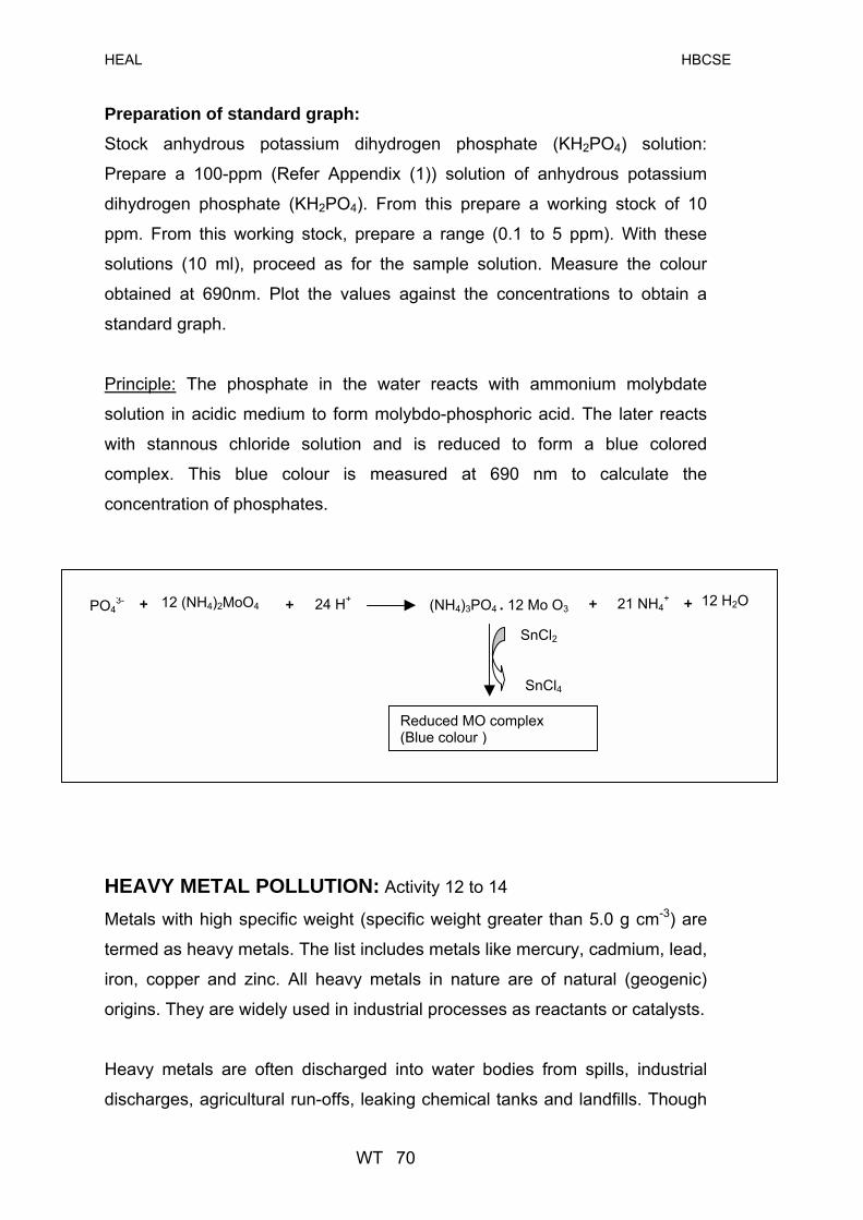
HEAL HBCSE

Preparation of standard graph: Stock anhydrous potassium dihydrogen phosphate (KH2PO4) solution:

Prepare a 100-ppm (Refer Appendix (1)) solution of anhydrous potassium

dihydrogen phosphate (KH2PO4). From this prepare a working stock of 10

ppm. From this working stock, prepare a range (0.1 to 5 ppm). With these

solutions (10 ml), proceed as for the sample solution. Measure the colour

obtained at 690nm. Plot the values against the concentrations to obtain a

standard graph.

Principle: The phosphate in the water reacts with ammonium molybdate

solution in acidic medium to form molybdo-phosphoric acid. The later reacts

with stannous chloride solution and is reduced to form a blue colored

complex. This blue colour is measured at 690 nm to calculate the

concentration of phosphates.

12 (NH4)2MoO4 +

Reduced MO complex (Blue colour )

21 NH4+ +

SnCl4

SnCl2

12 H2O + (NH4)3PO4 . 12 Mo O3 24 H+ + PO43-

HEAVY METAL POLLUTION: Activity 12 to 14

Metals with high specific weight (specific weight greater than 5.0 g cm-3) are

termed as heavy metals. The list includes metals like mercury, cadmium, lead,

iron, copper and zinc. All heavy metals in nature are of natural (geogenic)

origins. They are widely used in industrial processes as reactants or catalysts.

Heavy metals are often discharged into water bodies from spills, industrial

discharges, agricultural run-offs, leaking chemical tanks and landfills. Though

WT 70

HEAL HBCSE

found in low concentrations in natural waters, they tend to concentrate in

certain components, such as, clay sediments and in living organisms, such as

mollusks, mussels and shellfish. Since these metals are non-degradable, they

persist in the environment and cause long-term pollution.

Heavy metals in water can cause several skin and gastro-intestinal problems.

Long-term exposure may affect many enzymatic activities and disturb the

development of an organism, including humans.

IRON: Activity 12

Iron may either be in the Fe 2+ or Fe3+ state, dissolved or suspended in water.

Surface water contains less than 1 ppm of Fe. Some ground waters and acid

surface drainage may contain higher levels. Waters containing more than

2ppm iron cause staining of clothes and gives a bitter astringent taste. The

maximum permissible limit by USPHS for filterable Fe in drinking water is 0.3

mg/l (ppm).

Materials required: 5 and 10 ml syringes/pipettes, 50/100ml conical flasks, colorimeter, water

bath; conc. hydrochloric acid (HCl), 1ml of 10 % hydroxyl amine hydrochloride

(NH2OH.HCl), 10 ml ammonium acetate buffer, 2ml phenanthroline, standard

iron stock solution {refer Appendix (1)}.

Experimental procedure: Iron in the sample is detected by the Phenanthroline method: Total dissolved

Fe(II) conc. between 0.01 and 5ppm can be determined by this method.

Detection limit is 50 µg of Fe. in solution.

1. Take 10 ml sample in a clean and clear container.

2. Add 0.5ml conc. HCl and 0.2ml NH2OH.HCl (10%).

3. Boil the mixture in a water bath for 15 minutes.

4. Cool the solution to room temperature and then transfer it to 50/100ml

conical flask.

WT 71

HEAL HBCSE

5. Add 2 ml ammonium acetate buffer.

6. Then add 0.4 ml phenanthroline.

7. Shake well.

8. Wait for 10- 15 min for maximum colour development.

9. Compare the colour developed against the colour grid provided and

note the observations as L, P, H or C. Note your observation in the

water work sheet (WWS: Activity 12).

10. Alternatively, measure absorbance at 510 nm against reagent blank.

Plot the absorbance value of the unknown sample against the standard

graph to estimate the concentration of iron in the sample.

Preparation of standard graph: Stock ferrous ammonium sulphate [(NH4)2 Fe (SO4)2 . 6H2O] solution: Prepare

a 50-ppm solution of ferrous ammonium sulphate [ (NH4)2 Fe (SO4)2 . 6H2O]

{refer Appendix (1)}. From this, prepare a range (0.1 to 5 ppm). With these

solutions (10 ml), proceed as for the sample solution. Measure the colour

obtained at 510nm. Plot these values against the concentrations to obtain a

standard graph.

Principle: Fe (III) is reduced to Fe(II) by NH2OH adjusted to pH 3.2/3.3. Next,

it is treated with 1,10 phenanthroline. Resulting orange red solution is

measured at 510 nm.

COPPER: Activity 13

Copper is one of the essential elements required in human diet, the adult daily

requirement being about 2.0 mg of copper. Copper salts are used in municipal

water supply systems for controlling biological growth in reservoirs and in

distribution pipes and as catalyzers in various chemical reactions. Copper in

combination with sulphate is also used as a pesticide. High concentration of

copper in natural waters is due to pollution from agricultural run offs or

corrosion of copper� containing alloys in pipes and fittings. Presence of

WT 72

HEAL HBCSE

copper causes undesirable flavouring of drinking water. The permissible

levels of copper in drinking water are in the range of 0.05-1.5 mg\ml.

Materials required: 100 ml beakers, test tubes, pipettes, water bath and a colorimeter.

Liquid ammonia (NH3), 15% citric acid, 1% sodium diethyl dithio carbamate,

1% iso-amyl acetate, distilled water and standard copper solution (10 µg \ml),

{refer Appendix (1)}.

Experimental procedure: Take 5ml of sample in a clean beaker. Add 5ml of citric acid and with a

dropper add 4 drops of liquid ammonia.

1. Add 1 ml of carbamate solution + 39 ml of distilled water + 10 ml of iso

amyl acetate.

2. Shake the beaker vigorously for 15 min and allow it to stand until the

two layers are clearly demarcated.

3. Slowly decant\pipette the upper organic layer and compare the colour

developed with the colour grid provided and note your observations as

L, P, H or C in water work sheet (WWS: Activity 13).

4. Alternatively, collect the upper organic phase carefully in a test tube.

Measure the absorbance of the organic layer at 440 nm against

reagent blank. Plot the absorbance value of the unknown sample

against the standard graph to estimate the concentration of copper in

the sample.

5. Note the value in the work sheet. Plot a standard graph with

concentration on the X axis and absorbance on the Y-axis.

Preparation of standard graph: Stock copper (Cu) solution: Prepare a 200-ppm {refer appendix (1)} solution

of copper. From this prepare a working stock of 10 ppm. With this working

stock prepare a range (0.1 to 5 ppm). With these solutions (5 ml), proceed as

for the sample solution. Measure the colour obtained at 440 nm. Plot these

values against the concentrations to obtain a standard graph.

WT 73

HEAL HBCSE

Principle: Copper present in the water sample interacts with sodium diethyl

dithio carbamate in an alkaline medium to form the copper salt of carbamate.

This complex is golden yellow in colour. Adding a few drops of liquor

ammonia creates alkaline conditions. The golden yellow colour is extracted in

the organic phase of iso-amyl acetate and is then estimated colorimetrically.

Citric acid is added to prevent precipitation of other metal ions due to change

in pH. It also acts as a chelating agent.

CHROMIUM: Activity14

In natural waters chromium exists as trivalent (Cr3+, Cr (OH)2+ and Cr(OH)4- )

or in the hexavalent form (Cr O42- and as Cr2O7

2-. Cr 3+). However, in potable

waters hexavelent chromium alone is prevalent. The hexavalent chromium

forms strong complexes with amines and are adsorbed by clay particles. The

amount of chromium ions in the water is dependent on the hardness and

alkalinity of the water. The main contributors of chromium pollution are

washes from chrome iron ore; chromium is also released in the discharges of

alloy, electroplating and pigment industry.

Chromium is non-essential for plants, but is an essential trace element for

animals. High loads of hexavalent chromium are known to have carcinogenic

effects and are harmful to tissues of humans. The permissible level for

chromium (VI) in drinking water is 0.05mg/l.

Materials required: Test-tubes, pipettes, conical flask, beakers, flask, measuring cylinder, watch

glass, rubber bulb, weighing balance, hot-plate, colorimeter.

Potassium dichromate, concentrated nitric acid, concentrated sulfuric acid,

concentrated ammonium hydroxide, potassium permanganate, sodium azide,

concentrated phosphoric acid and diphenylcarbazide.

WT 74

HEAL HBCSE

Experimental procedure: To determine the concentration of total chromium in the sample, it is first

necessary to treat the sample by acid digestion to concentrate the chromium

present in the sample. For total chromium estimation, convert all the

chromium into the hexavalent state. This is done by oxidation with potassium

permanganate.

Treatment of sample (acid digestion):

To determine the total chromium content in the sample, digest the

sample as follows:

1. Transfer 50 ml of well-mixed sample in a beaker or flask. Add 5ml

conc nitric acid and cover with a watch glass. Slowly boil and

evaporate the solution till only half of the initial amount remains (this

takes about 3 to 4 hours). Cool the flask.

2. Again add 5ml conc nitric acid and 10 ml of conc sulfuric acid and

observe for brown fumes. Next, evaporate by boiling until brown

fumes disappear and the solution becomes clear. Some white

fumes of SO3 also might appear. (This takes about 90 mins.)

3. If the solution does not become clear, repeat step no. 2 (add 5 ml

conc HNO3 and 10 ml H2SO4 and boil until white fumes appear.)

4. Cool and dilute to 50 ml with distilled water and boil for 5 minutes to

dissolve any salts.

Oxidation of trivalent chromium:

1. Carefully with a rubber bulb, pipette out the treated sample in a

conical flask and add 10 drops of methyl orange.

2. Add concentrated ammonium hydroxide until the solution begins to

turn yellow.

3. Check the pH of the solution. Add sulphuric acid drop wise (~20

drops) until the solution is acidic. Add excess of 1ml of sulphuric

acid drop wise.

4. Adjust the volume to about 40 ml with DW and add a few glass

beads. Heat to boiling. Add few drops of potassium permanganate

solution till persistent red colour appears.

WT 75

HEAL HBCSE

5. Continue to boil for 2 mins (the solution may become turbid). Add

1ml sodium azide and boil gently, till the red colour fades. In turbid

solution, a ppt. may be formed.

6. If red colour does not fade after boiling for few minutes, then add

another 1 ml of sodium azide.

7. Boil till red colour has faded completely and then cool the solution.

If ppt is formed, filter the solution and proceed for colour

development.

Colour development and measurement:

1. Add 2 ml. of phosphoric acid to the above sample and check the

pH. Adjust the pH to 1.0.

2. Take 10 ml of this sample in a clean flask.

3. Add 0.5 ml of diphenylcarbazide solution, mix and let it stand for 5-

10 mins. A violet colour is formed if chromium is present.

4. Determine the OD at 540 nm using reagent water as reference

(diphenylcarbazide + distilled water to make the volume 100 ml).

Alternatively, compare the colour developed against the colour grid

provided and note the observations as L, P, H or C. Note your

observation in the water work sheet (WWS: Activity 14).

5. Correct the absorbance of sample by subtracting the OD of blank

from sample reading. Calculate the concentration of chromium

using the standard graph (calibration curve).

Preparation of calibration curve

Prepare a stock solution of 100 ppm followed by a working stock solution

of 10ppm. Using this working stock, prepare a range of 0.1-5ppm. Add 2ml

phosphoric acid and 0.5 ml diphenyl carbazide. A dark violet colour is

formed. Determine the OD at 540nm. Determine the concentration of

sample using this standard curve.

Principle: The total chromium is converted to hexavalent chromium before

colour development. The hexavalent chromium present in the sample

reacts with diphenylcarbazide in acid condition to form a red-violet

WT 76

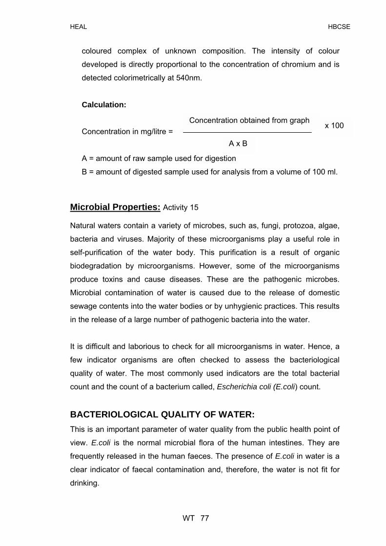
HEAL HBCSE

WT 77

coloured complex of unknown composition. The intensity of colour

developed is directly proportional to the concentration of chromium and is

detected colorimetrically at 540nm.

Calculation: Concentration in mg/litre =

A = amount of raw sample used for digestion

A x B

x 100 Concentration obtained from graph

B = amount of digested sample used for analysis from a volume of 100 ml.

Microbial Properties: Activity 15 Natural waters contain a variety of microbes, such as, fungi, protozoa, algae,

bacteria and viruses. Majority of these microorganisms play a useful role in

self-purification of the water body. This purification is a result of organic

biodegradation by microorganisms. However, some of the microorganisms

produce toxins and cause diseases. These are the pathogenic microbes.

Microbial contamination of water is caused due to the release of domestic

sewage contents into the water bodies or by unhygienic practices. This results

in the release of a large number of pathogenic bacteria into the water.

It is difficult and laborious to check for all microorganisms in water. Hence, a

few indicator organisms are often checked to assess the bacteriological

quality of water. The most commonly used indicators are the total bacterial

count and the count of a bacterium called, Escherichia coli (E.coli) count.

BACTERIOLOGICAL QUALITY OF WATER: This is an important parameter of water quality from the public health point of

view. E.coli is the normal microbial flora of the human intestines. They are

frequently released in the human faeces. The presence of E.coli in water is a

clear indicator of faecal contamination and, therefore, the water is not fit for

drinking.

HEAL HBCSE

The presence and numbers of E.coli is estimated by the presumptive coliform

test and is expressed as Most Probable Number (MPN) of E.coli in water. This

number is derived based on certain probability functions. The number

indicates the approximate mean density of coliforms in the sample.

For the presumptive coliform test, a known volume of the sample water is

added to tubes containing culture media (i.e., fermentation tubes). The tubes

are then incubated for a fixed time, and later checked for the production of

acid and gas. The presence of both the gas and acid production is a positive

indicator for coliform bacteria.

The number of tubes showing positive is recorded and matched with the MPN

table provided {Appendix (4): MPN chart}, and the corresponding number is

reported as the MPN for the water sample. The result is expressed as the

most probable number (MPN)/100 ml of organisms present. The MPN for the

quality of water is interpreted as follows:

MPN result Water quality

<1 Excellent

1-2 Satisfactory

3-10 Suspected

>10 Not suitable for drinking

Materials required: Normal microbiological materials: sterile cotton, test tubes or culture tubes,

conical flasks pressure cooker, incubator or hot case, pipettes, newspaper,

measuring cylinders, physical balance, cooking stove, Bunsen burners or

spirit lamps and Durham tubes (small tubes of about 2.5 cm long with one end

closed and the other end open. The gas produced accumulates in this tube.)

Culture medium: A culture medium provides the necessary nutrients for growing

microorganisms. The MacConkey broth is the most commonly used medium

WT 78

HEAL HBCSE

for the isolation of coliforms. The coliforms present in the water sample

ferment the lactose in the culture media leading to the production of acid and

gas. A pH indicator is also added to this medium for the detection of acid.

Readymade double strength (ds) MacConkeys broth nutrient medium is

available in the market. If not available, the media can be prepared as follows:

Ingredients required: 40 gm peptone, 20 gm lactose, 10 gm bile salt (sodium

thaurocholate), 10 gm sodium chloride, 0.15 gm neutral red and 1000ml

distilled water.

1. Dissolve all ingredients except the neutral red dye in 800 ml of distilled

water in a conical flask. Some of the nutrients may not dissolve easily.

In such case, the mixture is heated slightly to dissolve all nutrients and

allowed to cool.

2. Adjust the pH of the solution to 7.4 by adding acid or base accordingly.

Add the neutral red dye after adjusting the pH. Finally, make up the

volume to 1000 ml. The culture broth is ready now.

3. Prepare single strength broth by dissolving half the amounts of the

ingredients used in the double strength in 1000 ml distilled water.

Adjust the pH of the broth to 7.4 similarly as for (ds) broth.

Experimental procedure: This is a technical microbiological experiment and requires skill and practice

of handling culture media and maintaining sterile conditions. It is necessary to

perform the experiment under proper supervision. Collect the water samples

for MPN test in sterile bottles.

1. Take 9 test tubes; add 10 ml of single strength (ss) MacConkey broth

to 6 test tubes and 10 ml of double strength broth to 3 tubes.

2. Place a Durham tube in each test tube in an inverted position using

forceps. Plug each test tube with cotton plugs. These are the

fermentation tubes.

WT 79

HEAL HBCSE

3. Wrap the tubes containing the medium separately in newspapers.

Keep the tubes in a container on a stand inside the pressure cooker.

Add sufficient water to fill a quarter of the tub.

4. Heat the pressure cooker. Place the weight on the cooker just after the

steam starts escaping the nozzle. Continue heating for 20 minutes. Put

off the flame. Allow the pressure to come down.

5. Open the lid and remove the tubes. Allow the tubes to cool.

6. Place two lit bunsen burners or spirit lamps about 15-20 cms apart or

at a workable distance. This provides a sterile working platform.

7. Pipette out 1 ml of the broth carefully in the center of the two burners to

avoid contamination. Replace the cotton plugs immediately.

8. Add 10 ml of water sample to each of the three double strength tubes

using a sterile 10 ml pipette and label as 10 ml.

9. Similarly, add 1 ml of the water sample to each of the three single

strength tubes using a sterile 1 ml pipette and label the tube as 1 ml.

10. Add 0.1 ml of the water sample in the remaining 3 single strength tubes

using a fresh sterile 1 ml pipette and label the tube as 0.1ml.

11. Incubate all the tubes in a incubator at 37 0C for 24 to 48 hours. If an

incubator is not available, a hot case used in the kitchen can be used.

This can keep the warmth up to 6 hours after which the temperature in

the hot case drops to the ambient temperature.

# During summers, place the tubes in a small beaker in the hot

case. Close the lid tightly. Remove the lid every 6 hours and

observe.

# In order to maintain the temperatures during winter and rainy

seasons place a 50 ml beaker with boiling water in the hot case.

Close the lid tightly and incubate. Replace the hot water every 6

hours and at this point check for any changes in the tube.

12. After the incubation, observe all the test tubes.

13. Examine all the tubes for the production of acid as indicated by the

change of the broth colour from orange to yellow. Also, check for the

production of gas, indicated by bubbles in the Durham tube.

14. Count the number of tubes showing positive results. Also, note the

volume of the water sample.

WT 80

HEAL HBCSE

WT 81

15. If the tubes do not show a positive result at the end of 24 hours, they

should again be incubated until 48 hours and examined similarly.

16. The absence of gas and acid production is recorded as a negative

result.

17. If the presumptive test is positive, determine the MPN of coliforms

present in 100 ml of the water sample using the MPN table.

(For example, if gas appears in all three tubes labeled 10 ml and

two tubes labeled 1 ml the MPN table indicates that there are

approximately 93 coli forms in 100 ml of the water sample).

18. Absence of gas and acid production constitutes a negative presumptive

test indicating that the water sample is devoid of any coliforms.

19. Since the presumptive test is sometimes positive for non-coliforms, a

confirmatory test has to be performed to confirm the presence of

coliforms.

Confirmatory test: Streak a loop full of the culture from a positive test tube

onto a deferential\selective media like Eosin methylene blue agar plate and

incubate the plate up side down for 24-48 hours in a incubator and check for

the growth of colonies. The eosin methylene blue in the medium allows

selective growth of gram-negative bacteria.

The presence of E.coli in the sample is indicated by a pink-red colony with a

shiny surface. Count the number of E.coli colonies and express it as colony

counts per 100 ml. Note this number in water work sheet (WWS Activity 15).

A few points to think about: ! Check the microbial, plant and animal population in the water body.

! Check the presence or absence of mosquito larvae in the water body. ! Compare the quality of water (physical, chemical and biological

parameters) in stretches where mangroves are present and absent.

HEAL HBCSE

Water Worksheets

Name Of The Investigator: Date:

College Name/Address:

Site Name: Location:

General Observations Of The Site: Monitoring of: Drinking water source______, Open water body___

If monitoring drinking water: Source of drinking water: Wells____, Bore wells____,

Municipal supply____, Other____

Position of storage tank: Underground___, Overhead____

Type of storage tank: Plastic___, Metal___, Concrete____, Other____

Sampling point: Tap____; Other____

Sampling point for overhead tank: At inlet of water supply____

When: Full tank____, Tank half empty____, Tank nearly empty_____

Sampling point for underground tank: At inlet of water supply____

When: Full tank____, Tank half empty____, Tank nearly empty____

If monitoring open water body: Water type: Salt____, Fresh ____,

Moving water: River____, Stream ____, Creek___, Other ____

Standing water: Pond ___, Lake ____, Reservoir____, Well_____ , Other____

Sample collection point for moving and standing water: Shoreline ____,

Bridge_____, Boat____, Other____

Clarity of water body: Clear ____, Turbid ____

WWS 82

HEAL HBCSE

Activity1: Study Of Physical Properties Of The Water Sample

Colour

Smell/Odour Turbidity Depth of sechi disc when: (cms)*

Serial no.

Type C-colourless B-blue G-green R-red B-brown Others (specify)

Intensity D-dark L-light

Type O-Odourless F-fishy S-sweetish E-faecal U-unpleasant Others (specify)

Intensity St-strong F-faint M-moderate Te

mpe

ratu

re o C

Visi

ble

(A)

Invi

sibl

e

(B)

Diff

eren

ce (B

-A)

Average

Report the transparency as NTU by referring to the graph in the appendix (3) �

SDT-NTU conversion chart. (Note: Greater the NTU->-> smaller the transparency)

(Report the average readings/observations in final water data sheet) * Tube method observations: Pour sample water till the disc pattern disappears. Black quadrants will be

somewhat visible, but mark that depth at which the center point of the disc blurs or

disappears. Often, for potable water, the pattern is visible even after filling of the

entire tube; enter the length of the tube in cms.

Observations:

____ cms: (depth at which the center point of the disc gets invisible/blurred)

OR ____ cms: if pattern/center point is visible with the entire tube full of water. (Repeat three times and report the average readings in final water data sheet.)

WWS 83

HEAL HBCSE

Activity 2: Suspended Solids: Date of sampling: Date of performing the experiment:

Drying temperature:

Observations for the wet weight-dry weight experiment

Sr.no Weight of

clean filter paper in

gms

(A)

Weight of

paper + residue in

gms

(B)

Weight of

residue in

gms

(B-A)

Average

Average weight of the residue: _____

(Report average reading of residue weight in the final water data sheet.)

Chemical Properties Activity 3: pH Date of sampling: Date of performing expt:

pH measured with: _____

pH value of distilled water: _____

pH value of sample water: _____

Observer 1: ___, Observer 2: ____, Observer 3: ____,

Average pH: _____

(Report average reading in the final water data sheet)

WWS 84

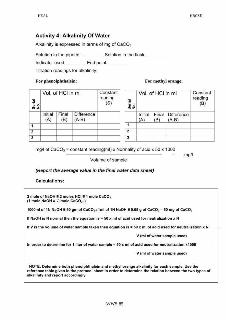
HEAL HBCSE

Activity 4: Alkalinity Of Water Alkalinity is expressed in terms of mg of CaCO3

Solution in the pipette: ________ Solution in the flask: _______

Indicator used: ________End point: _______

Titration readings for alkalinity: For phenolphthalein: For methyl orange:

mg/l of CaCO3 = constant reading(ml) x Normality of acid x 50 x 1000

= mg/l Volume of sample (Report the average value in the final water data sheet) Calculations:

Seria

l N

o.

Vol. of HCl in ml Constant reading

(B)

Initial (A)

Final (B)

Difference(A-B)

1 2 3

Seria

l N

o.

Vol. of HCl in ml Constant reading

(S)

Initial (A)

Final (B)

Difference(A-B)

1 2 3

2 mole of NaOH ≡ 2 moles HCl ≡ 1 mole CaCO3; (1 mole NaOH ≡ ½ mole CaCO3)-) 1000ml of 1N NaOH ≡ 50 gm of CaCO3-: 1ml of 1N NaOH ≡ 0.05 g of CaCO3 = 50 mg of CaCO3 If NaOH is N normal then the equation is = 50 x ml of acid used for neutralization x N If V is the volume of water sample taken then equation is = 50 x ml of acid used for neutralization x N V (ml of water sample used) In order to determine for 1 liter of water sample = 50 x ml of acid used for neutralization x1000 V (ml of water sample used) NOTE: Determine both phenolphthalein and methyl orange alkalinity for each sample. Use the reference table given in the protocol sheet in order to determine the relation between the two types of alkalinity and report accordingly.

WWS 85

HEAL HBCSE

Activity 5: Dissolved Oxygen Date of sampling: Date of performing the experiment:

Solution in burette/syringe: Solution in flask\beaker:

Indicator: End-point colour:

Observations of titration

Reading for sodium thiosulphate Sr.no.

Initial Final Difference

Constant burette

reading

�A�

1

2

3

A ml = ______

Calculation: 2Na2S2O3 = I2 = (O)

i.e., 2 moles of Na2S2O3 = 1 mole of nascent oxygen

1000ml of 1N Na2S2O3 = 8gm of oxygen

1ml of 1N Na2S2O3 = 8mg of oxygen (equivalent wt. of oxygen)

1 ml of 0.025 N Na2S2O3 = 8 Χ 0.025 mg of oxygen

A ml of 0.025N Na2S2O3 = 8 Χ 0.025 Χ �A� mg of oxygen

This is for 50 ml sample

For 1000 ml of sample = 8×0.025× A ×1000 = 0.2×A×1000 mg oxygen \L 50 50

Average Dissolved Oxygen: __________ mg\l

(Report average reading of DO in the final water data sheet)

WWS 86

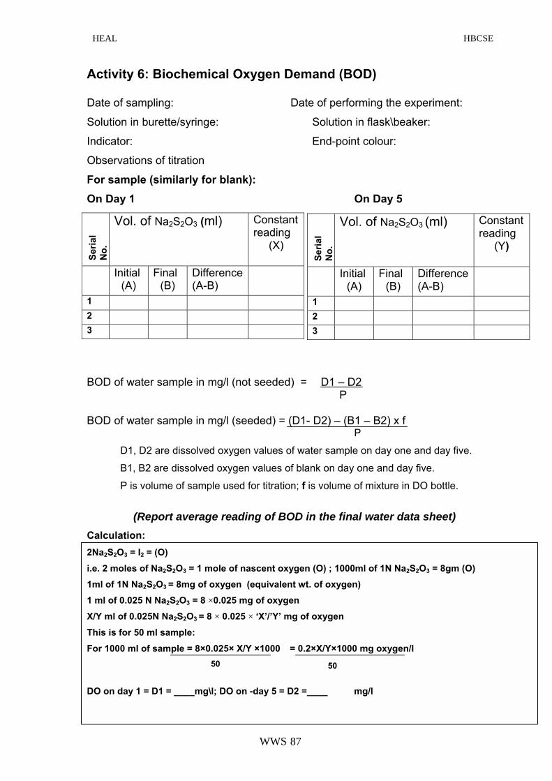
HEAL HBCSE

Activity 6: Biochemical Oxygen Demand (BOD) Date of sampling: Date of performing the experiment:

Solution in burette/syringe: Solution in flask\beaker:

Indicator: End-point colour:

Observations of titration

For sample (similarly for blank): On Day 1 On Day 5

Seria

l N

o.

Vol. of Na2S2O3 (ml) Constant reading

(X)

Initial (A)

Final (B)

Difference(A-B)

1 2 3

Seria

l N

o.

Vol. of Na2S2O3 (ml) Constant reading

(Y)

Initial (A)

Final (B)

Difference(A-B)

1 2 3

BOD of water sample in mg/l (not seeded) = D1 � D2 P BOD of water sample in mg/l (seeded) = (D1- D2) � (B1 � B2) x f P

D1, D2 are dissolved oxygen values of water sample on day one and day five.

B1, B2 are dissolved oxygen values of blank on day one and day five.

P is volume of sample used for titration; f is volume of mixture in DO bottle.

(Report average reading of BOD in the final water data sheet)

Calculation: 2Na2S2O3 = I2 = (O) i.e. 2 moles of Na2S2O3 = 1 mole of nascent oxygen (O) ; 1000ml of 1N Na2S2O3 = 8gm (O) 1ml of 1N Na2S2O3 = 8mg of oxygen (equivalent wt. of oxygen) 1 ml of 0.025 N Na2S2O3 = 8 ×0.025 mg of oxygen X/Y ml of 0.025N Na2S2O3 = 8 × 0.025 × �X�/�Y� mg of oxygen This is for 50 ml sample: For 1000 ml of sample = 8×0.025× X/Y ×1000 = 0.2×X/Y×1000 mg oxygen/l 50 50 DO on day 1 = D1 = ____mg\l; DO on -day 5 = D2 =____ mg/l

WWS 87

HEAL HBCSE

Activity 7: Chemical Oxygen Demand (COD) Activity 7: Chemical Oxygen Demand (COD) Date of sampling: Date of performing the experiment: Date of sampling: Date of performing the experiment:

Solution in burette/syringe: Solution in flask\beaker: Solution in burette/syringe: Solution in flask\beaker:

Indicator: End-point colour: Indicator: End-point colour:

Observations of titration: Observations of titration:

For sample For blank For sample For blank

Seria

l No.

Vol. of FAS (ml) (burette reading)

Constant reading

(Y)

Initial (A)

Final (B)

Difference (A-B)

1 2 3

COD of sample in mg/l = COD of sample in mg/l =

Where:Where:

Y= burette reading for blank; X= burette reading for sample

N = normality of FAS

8 = gm equivalent of nascent oxygen

1000 = factor for liter conversion (Report average reading of COD in the final water data sheet) Calculation: K2Cr2O7+ 4H2SO4 K2SO4 + Cr2(SO4)3 + 4H2O +3(O)

14 H+ +Cr2O7-2 + 6e- + 6 Fe+2 2Cr+3 +7H2O + 6Fe+3 +6e-

1 mole of K2Cr2O7= 3(O) i.e., 1 moles of K2Cr2O7 = 3 mole of nascent oxygen 1000ml of 1N K2Cr2O7 = 8gm of oxygen 1 Fe = 8 g (O) 1000 ml of 1N Fe = 8g (O); therefore 1 ml of n N Fe = 8mg x n Volume (Y-X) of n N Fe = (Y-X) x n x 8 mg If volume of sample is V; then (Y-X) x n x 8 mg / V For 1000 ml =

1/6K2Cr2O7 1/6 Cr2O7

- 2/6 Cr2 +3 = 6/6 Fe+2

Seria

l N

o.

Vol. of ferrous ammonium sulphate (FAS) (ml) (burette reading)

Constant reading

(X)

Initial (A)

Final (B)

Difference (A-B)

1 2 3

Volume of sample

(Y-X) x N x 8 x 1000

(Y-X) x N x 8 x 1000

Volume of sample

WWS 88

HEAL HBCSE

Activity 8:Chlorides Date of sampling: Date of performing the experiment:

Solution in burette: Solution in flask\beaker:

Indicator: End-point colour:

Observation of titration For sample: For blank:

mg/l of chloride = (X-Y) x Normality of AgNO3 x 35.45 x 1000

= mg/l Volume of sample Where, X = ml of AgNO3 required by water sample Y = ml of AgNO3 required by blank 35.45 is equivalent weight of chlorine 1000 is liter conversion factor (Report the average value in the final soil data sheet)

Seria

l N

o.

Vol. of AgNO3 in ml Constant reading

(X)

Initial (A)

Final (B)

Difference(A-B)

1 2 3

Seria

l N

o.

Vol. of AgNO3 in ml Constant reading

(Y)

Initial (A)

Final (B)

Difference(A-B)

1 2 3

Normality of AgNO3 = Normality of NaCl x Volume of NaCl Volume of AgNO3 Use this normality for the main formula in order to determine chloride content in mg/liter

WWS 89

HEAL HBCSE

Activity 9: Fluorides Date and time of sampling: Date of performing the experiment:

Observations: Concentration of fluoride in the sample observed by comparing the colour

developed against the colour grid, as L, P, H, C: ________

Plot and read the concentration of the sample from the standard graph.

Readings: Observer 1=______ Observer2 =_______ Observer 3 =________

Average value of fluoride in the sample =________ppm

(Report average readings of fluorides in the final water data sheet)

WWS 90

HEAL HBCSE

Activity 10: Ammonia Date and time of sampling: Date of performing the experiment:

Observations: Concentration of ammonia in the sample observed by comparing the colour

developed against the colour grid, as L, P, H, C: ________

Plot and read the concentration of the sample from the standard graph.

Readings: Observer 1=______ Observer2 =_______ Observer 3 =________

Average value of ammonia in the sample =________ppm

(Report average readings of ammonia in the final water data sheet)

WWS 91

HEAL HBCSE

Activity 11: Phosphates Date of sampling: Date of performing the experiment:

Observations Concentration of phosphates in the sample observed by comparing the colour

developed against the colour grid as L, P, H, C: ________

Plot and read the concentration of the sample from the standard graph.

Observer 1=______ mg\l; Observer 2 =______ mg\l; Observer 3 =______ mg\l

Average phosphate concentration in the sample = _______ mg\l

(Report average readings of phosphates in the final water data sheet.)

WWS 92

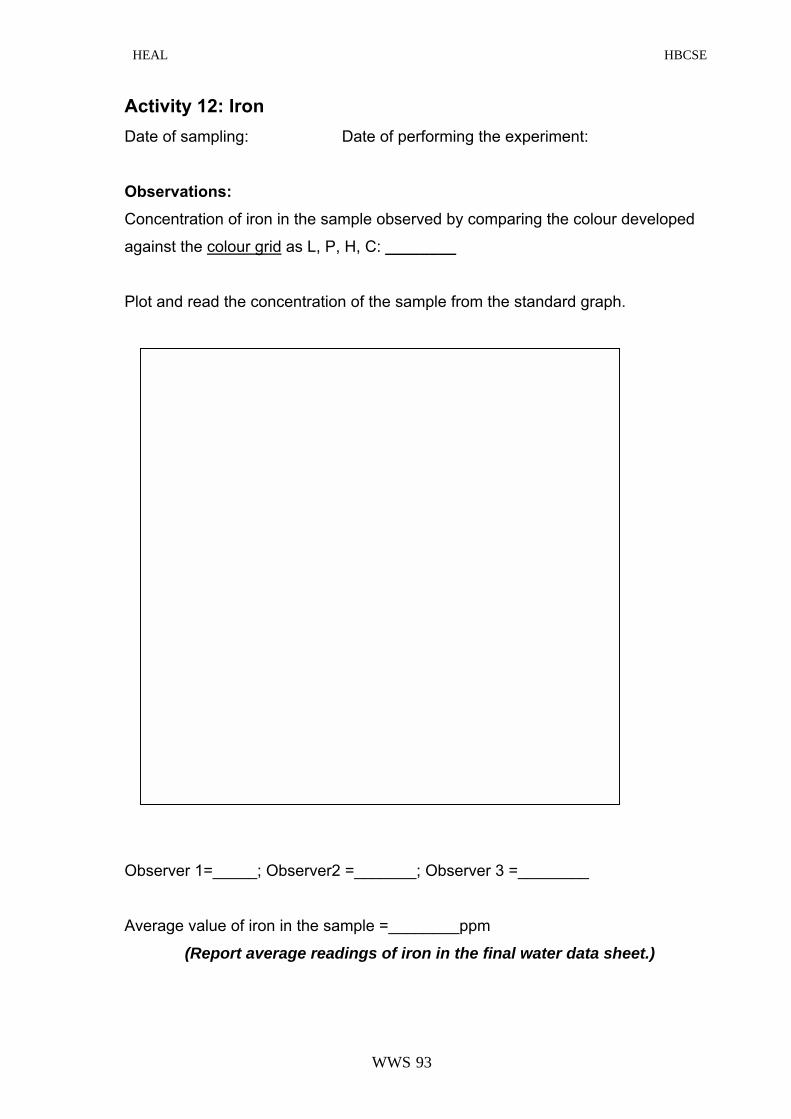
HEAL HBCSE

Activity 12: Iron Date of sampling: Date of performing the experiment:

Observations: Concentration of iron in the sample observed by comparing the colour developed

against the colour grid as L, P, H, C: ________

Plot and read the concentration of the sample from the standard graph.

Observer 1=_____; Observer2 =_______; Observer 3 =________

Average value of iron in the sample =________ppm

(Report average readings of iron in the final water data sheet.)

WWS 93

HEAL HBCSE

Activity 13: Copper Date of sampling: Date of performing the experiment:

Observations: Concentration of copper in the sample observed by comparing the colour

developed against the colour grid as L, P, H, C: ________

Plot and read the concentration of the sample from the standard graph.

Observer 1=______Observer2 =_______ Observer 3 =________

Average value of copper in the sample =________mg\l of copper

(Report average readings of copper in the final water data sheet.)

WWS 94

HEAL HBCSE

Activity 14: Chromium Date and time of sampling: Date of performing the experiment:

Observations: Concentration of ammonia in the sample observed by comparing the colour

developed against the colour grid, as L, P, H, C: ________

Plot and read the concentration of the sample from the standard graph.

Readings: Observer 1=______ Observer2 =_______ Observer 3 =________

Average value of chromium in the sample =________ppm

(Report average readings of chromium in the final water data sheet)

WWS 95

HEAL HBCSE

Activity 15: MPN count of water sample: Date of sampling: Date of performing the experiment:

Observations

MPN count Confirmatory test

No. of positive tubes of: No. of colonies

observed after:

Site name Sample source

10 ml 1 ml 0.1 ml MPN 24 hrs 48 hrs

Most probable number of E.coli in the water sample is: ____

Confirmatory test:

24-hour colony count: ______

48-hour colony count: ______

(Report average MPN of the sample in the final water data sheet.)

WWS 96

HEAL HBCSE

Final data sheet: Note the average values of your observations to give a comprehensive view of the

water quality

Site details: identify the site as: residential ___, industrial___, commercial____

Observations Grid reading

Water Characteristics Average readings

L, P, H, C Sample source: G: ground water S: surface water

Identify source as: W: wells H: hand pumps B: bore wells L: lakes T: tanks (E: elevated\ U: underground) O: other

D: Dark L: light

Colour:

NC: colourless B: blue G: green R: red Others specify

St: Strong Ft: Faint M: Moderate

Odour:

O-Odourless F-fishy S-sweetish U-unpleasant Others (specify)

Temperature o C Turbidity: By seechi disc By tube method

Non- filterable solids pH Alkalinity Dissolved oxygen (DO) Biochemical oxygen demand (BOD) Chemical oxygen demand (COD) Chlorides Fluorides Ammonia Phosphates Iron Copper Chromium E.coli MPN Standards for quality of drinking water (including all fresh water bodies) according to IS-10500-1991

WWS 97

HEAL HBCSE

WWS 98

Standards for physical properties of drinking water

Physical property Standards Colour Colourless Odour Odourless Temperature Varies with air temp. Transparency No turbidity Non filterable solids (suspended matter) 1000 mg/litre Standards for chemical properties of drinking water

Chemical property

Standard values

pH 6.5-8.5

Alkalinity 200 mg CaCO3\l

DO 4-6 mg\ l

BOD 3 mg\l (with treatment)

COD 4-10 mg\l (for clean water bodies)

Chlorides 200-250 mg\l

Fluorides 1.5 mg\l

Ammonia 0.5 mg \l

Nitrites 50 mg\ l

Phosphates 0.1 mg\ l

Iron 0.3 mg\l

Copper 0.05-1.5 mg \ l

Chromium 0.05 mg\l

HEAL HBCSE

‘Soil’ watch…

for good health

INTRODUCTION: Soil, or the shallow upper layers of the earth, is an important natural resource.

Highly abused in recent decades, it is often used as a dumping ground for

both, wastewater and domestic/urban solids waste. Several air pollutants,

especially heavy metals, also settle in soil to find their way into the food chain.

Few realize that the health of soil is intricately related to human health.

Soil has a strong influence on the entire ecosystem. Hence it is often called

the ‘great integrator’.

Soil allows water, energy and heat to flow through it. It helps in percolation of

water into confined and unconfined groundwater aquifers. It holds nutrients

and water, and functions as a filter that cleans the water as it flows through it.

The soil cover is essential for the production of food crops and forests. It has

an intimate association with plants, animals and microorganisms. Soil

moisture and temperature has a great influence on the climate of the place.

Soil is a decomposition product formed by weathering of a parent rock. It has

two main components, namely the mineral inorganic matter derived from the

weathering of a rock, and an organic component provided by colonization of

plants and animals in the soil. The close integration of these two components

characterizes the mature soil. Soil is dynamic—it keeps on changing with

time, especially soil moisture and temperature. However, the mineral

composition changes slowly, over a period of hundreds of years.

SOIL PROFILE: A soil profile represents the way the soil looks if one cuts a longitudinal

section of it out of the ground. Soil profile is made up of layers called horizons.

These horizons could be as thin as a few millimeters or thicker than a meter.

ST 99

HEAL HBCSE

Clear well-demarcated horizons are often found in undisturbed areas. In city

areas, the horizons may not be that distinct. Not all soils have the same

horizons. The type and number of horizons in a profile often depend on how

the soil is formed.

Different horizons are identified based on slight differences in their colours,

sizes of particles and distinct textures of soil particles. Conventionally, the

different horizons are labeled as O, A, B, C, D, E and R.

Details of the various horizons in a soil profile (Courtesy: GLOBE)

Horizon Location Composition

Found in:

O Soil surface

Rich in organic materials (vegetation, remains of dead animals and insects)

Forested areas

A First mineral layer/top soil

Rich in mineral matter; may include completely decomposed organic matter and hence dark in colour; can show two textures: granular and platy.

Agricultural areas/tilled layer

B Second layer or sub-soil

Reflects the weathered parent material; also called the accumulation horizon due to accumulation of leached out materials from A and E; rich in iron, aluminum, clay and organic matter. Also saturated with water and hence shows red, yellow and brown colours.

Found in all soil profiles

C Third major layer

The composition (colour and structure) is similar to the parent material.

-do-

E Optional, between A and B

Mainly composed of the alluvial material, i.e., clay, iron, aluminum and organic matter, which have been leached from it; the horizon appears white or light in colour; it shows two textures: platy or single grained.

Found in wet conditions, as in forests, with dominance of coniferous trees

R Lowest of the soil profile

Reflects the bedrock on which the soil is formed indicating the parent material of the soil, such as glacial, alluvial or volcanic material.

In all soil profiles

ST 100

HEAL HBCSE

The horizons ‘O’ and ‘E’ are found only in forested areas. Agricultural, dessert

or grassy areas show a profile starting with ‘A’ horizon and do not have the ‘E’

horizon. An eroded area will show a profile that may start with ‘B’ horizon.

Shallow soils or soils that are not extensively weathered may go from ‘A’ to ‘C’

with no ‘B’ horizon.

B -horizon

E- horizon

A- horizon

O- horizon

B -horizon

C- horizon

R- horizon

A typical soil profile (Courtesy:GLOBE)

WHAT IS SOIL POLLUTION? Soil pollution is defined as the presence of one or more contaminants in

quantities and for durations, which are injurious to animals, plants and for

human health. It is caused due to various human (anthropogenic) activities.

The rapid growth of industries and agricultural units, along with urbanization

has resulted in the production of large amounts of wastes, from sources such

as, municipalities, agriculture, industry and commercial establishments. The

improper disposal of these wastes in degraded landfill areas and the un-

regulated use of pesticides and chemicals in agriculture, industry and

households add a heavy dose of contaminants into the soil. The load of these

ST 101

HEAL HBCSE

contaminants cannot be absorbed by the normal soil nutrient cycle. These

pollutants then contribute directly or indirectly to soil pollution.

These pollutants have the potential to disturb the entire ecological balance in

nature. They can disturb the normal metabolic and physiological cycles of

different life forms living in the soil, and tend to collect in large amounts in

plants and animals (bioaccumulation and biomagnification—gradual increase

in pollutant concentration from the primary producer to the final consumer).

Over a period, these pollutants concentrate in the tissues of plants and

animals and get into the human food chain. This leads to harmful effects and

a variety of diseases in the humans.

Pollutants are also easily trapped in the air spaces between soil particles. The

capacity of soil to exchange cations and anions also decides how best a

retainer of pollutant the soil is. Subsequently, the water table and aquifers,

which are known to carry pure, clean water for generations, are also polluted.

ANALYSIS OF SOIL Useful information about the suitability of the soil for different purposes--

agriculture, industrialization and urbanization--is obtained by analysing the

soil. Monitoring the different parameters of soil gives an idea about the extent

of soil pollution and hence the health of soil. This then helps to develop new

regulatory norms for a clean environment.

Here a few physical and chemical properties that give indications about the

quality or the health of the soil will be analysed. Study of land (green) cover

will also be carried out.

The soil samples will be analyzed for the following physical properties: Soil

profile, structure and consistence, colour, texture, temperature, moisture,

infiltration capacity and presence of wastes like plastics, paper, glass, metal.

ST 102

HEAL HBCSE

The following chemical properties will be checked up: Soil pH, conductivity,

calcium carbonates and heavy metal pollutants like iron and copper.

Soil will also be monitored for the following biological indicators: Land (green)

cover study which involves calculation of percentages of canopy and grass

cover and identification of dominant and co-dominant species and common

plants.

SAMPLING: Sampling site could be local open fields, school play grounds (not manured

gardens) or beaches. Ideally, the site area should be natural (not paved), flat,

open with natural vegetation, away from any buildings. The number of

sampling points chosen should represent the entire area under survey.

A detailed sampling procedure is given below with dimensions. However,

depending on the size of the site area, one could reduce the corresponding

dimensions.

Soil sampling procedure: Ideally, the sampling is done in a star pattern, where the samples are

collected each time from a different location on the star along a single

transect. Alternatively, sampling can be done in a circle or a quadrangle, with

samples collected along the diameter or diagonals.

Before starting, take an overview of the sampling site, its total area and

sampling points. These points should be representative of the entire sampling

site.

1. Choose any reference—centre--point in the site. From this reference

point, locate four points approximately one meter north, south, east and

west with a compass.

ST 103

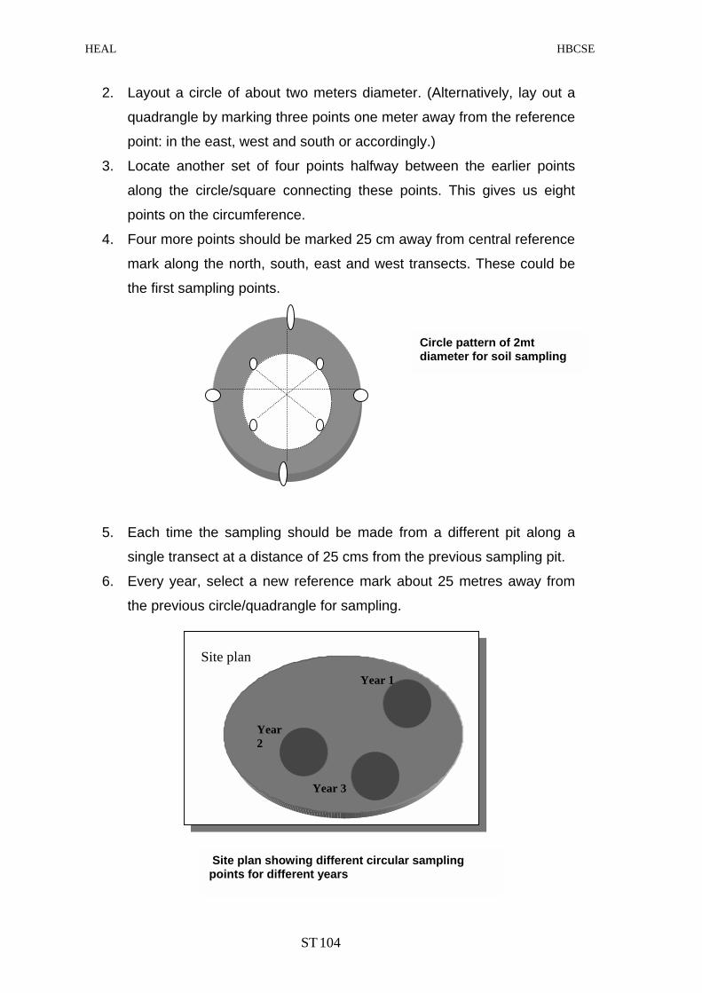
HEAL HBCSE

2. Layout a circle of about two meters diameter. (Alternatively, lay out a

quadrangle by marking three points one meter away from the reference

point: in the east, west and south or accordingly.)

3. Locate another set of four points halfway between the earlier points

along the circle/square connecting these points. This gives us eight

points on the circumference.

4. Four more points should be marked 25 cm away from central reference

mark along the north, south, east and west transects. These could be

the first sampling points.

Circle pattern of 2mt diameter for soil sampling

5. Each time the sampling should be made from a different pit along a

single transect at a distance of 25 cms from the previous sampling pit.

6. Every year, select a new reference mark about 25 metres away from

the previous circle/quadrangle for sampling.

Site plan showing different circular sampling points for different years

Year 3

Year 1

Year 2

Site plan

ST 104

HEAL HBCSE

Alternatively,

7. To collect soil samples, in the chosen site, make square grids of about

5 x 5 meters at various reference points. Divide the square into four

quadrants. From each quarter, scoop out some topsoil at about 5 to 10

cms depth with a non-metallic shovel, collecting the soil as cone in the

centre. Mix the soil from four quadrants and this will be the sample

used for analysis. This method is known as ‘Quartering and Coning’,

1 + 1 = 1a 2 + 2 = 2a 1a + 2a = soil sample

1

1

2 2

8. Pass the soil through a sieve (25 mesh) to separate stones and other

debris. The soil sample should then be placed either in airtight

containers or in zip plastic bags. These samples can then be analyzed

in the laboratory.

SOIL PROFILE: Activity 1 and 2

Soil profile indicates many things: its geological and archaeological history

and the climate changes experienced over years. It can also give an

indication of about some physical and chemical soil properties and hence can

predict the best uses of the land.

Materials required: Garden tools like shovels and small spades, water bottle with squirt top (as in

plastic sauce bottles), plastic sheet or sheets of news paper on which you can

lay out the soil layers, meter stick or measuring tape, 20 nails or coloured

board pins to mark the horizons, plastic bags or sealable containers of one

liter size to carry the soil sample, water proof markers and buckets for

removing soil.

ST 105

HEAL HBCSE

Experimental procedure: 1. Select a relatively flat, undisturbed and safe site with natural vegetation

to dig for studying the soil profile. Alternatively, an already dug pit (road

construction site, etc) close to your sampling site will also do for

analysis of the soil profile.

2. Check with the local authorities so that different utility cables, water or

sewer pipelines are left undisturbed.

3. With a spade, dig a pit one meter deep and as round as is necessary to

easily observe all horizons of the soil. This may require a person to get

into the pit.

4. At this stage, think of ‘soil as a great integrator’ and represent the idea

as a concept map (SWS: Activity 1).

5. Spread a plastic or newspaper sheet and lay the soil from each layer

as a separate pile. Use a shovel or a big garden spoon, if necessary, to

dig out some soil from the layers. A bucket can be used to carry the

soil to the plastic sheet.

6. Transfer a small portion of the soil samples dug out from each horizon

in separate plastic containers or plastic bags, and label them

appropriately.

7. Use these samples for further characterization and analysis to be

performed in the classroom.

8. Look at the side of the soil pit where the sun shines directly so that the

soil profile and its properties are clearly visible.

9. Starting from the top of the profile and moving down to the bottom,

observe the soil profile closely for changes in soil colour and structure.

If the soil is dry, spray a little water to help in distinguishing the colours

of the various zones.

10. Mark the locations of each of these changes or boundaries by fixing a

nail or board pins.

11. It is sometimes difficult to demarcate and identify the various horizons

clearly. Often, there may be only a few very thick horizons present. Do

your best to record exactly what you observe in the field.

12. Measure the width of each horizon to the nearest cm. and record the

observation in the soil worksheets [SWS: Activity 2 (i)].

ST 106

HEAL HBCSE

13. If the horizons are very thin (less than 3 cm), do not report them as a

separate layer. Combine the thin horizon with the one above or below

and record.

14. If possible, using the profile characteristic data provided in the

introduction, try to draw a schematic representation of the soil profile

with appropriate names for the various horizons observed [SWS:

Activity 2 (ii)]. Consider the profile from all sides of the pit.

15. Once the protocol is completed, students should remember to refill the

pit with the original soil.

SOIL STRUCTURE AND CONSISTENCE: Activity 2

Soil structure refers to the arrangement of soil particles in natural aggregates.

These aggregates are called as peds. The different types of soil structures

are: granular, rocky, massive, platy, columnar and prismatic or even

structureless. The soil structure has an influence on its properties, like

infiltration rate and moisture holding capacity. These soil structures/peds

breakup in varied ways. This breakup determines the soil consistence.

Mixed structure

Nst

r

Platy Blocky

Granular

Single grains

ST 107

Prismatic

Columna

o ru

Massive

Various soil structures

well-defined cture

(Courtesy: LOBE)

HEAL HBCSE

Materials required: Same as materials used for soil profile experiments.

Experimental procedure: 1. Take a sample of the soil from the pit; alternatively observe for the soil

structure in the pit itself, using a lighted torch (battery operated).

2. Observe the various patterns of soil structure and fill out the soil

worksheet [SWS: Activity 2 (i)].

3. To study the soil consistence: Take a moist ped of soil.

4. Spray (put) water and mix the soil well, if it is dry.

5. With a bit of pressure with your fingers, try to crumble the ped. It will

crumble differently depending on the soil type. Hence, they are

classified as:

• Loose ---if there is trouble picking out a single ped and the

structure falls apart before handling it;

• Friable—the ped breaks with small amount of pressure;

• Firm---the ped breaks with a good amount of pressure leaving

an impression on the fingers before breakage;

• Extremely firm—the ped cannot be broken with the fingers. A

hammer may be needed.

Note your observations in the soil worksheets [SWS: Activity 2 (i)].

SOIL COLOUR: Activity 2

Different soils show a variety of colours. It could be red, brown, black, yellow

and occasionally white. Soil colour is determined by the percentage

composition of silicon, iron and humus. Red colour indicates the presence of

oxidized iron in the soil, while yellow colour indicates the presence of hydrated

forms of ions.

Usually, the upper layers of the soil appear darker due to the presence of

organic matter. At lower depths, it becomes pale to yellow indicating high

ST 108

HEAL HBCSE

moisture content. Black soils develop in waterlogged and anaerobic

conditions.

Materials required: Materials are same as mentioned in the soil profile experiment.

Experimental procedure: 1. Dig out a portion of the topsoil. Clear the soil of all debris like roots and

wastes (such as plastics and paper).

2. Alternatively, take the soil sample earlier collected in soil profile

experiment for this observation.

3. Check if the soil is wet or dry. If the soil is dry, moisten it by squirting

some water and then observe for its colour.

4. Note down the observations in the soil worksheets [SWS: Activity 2(i)]

5. Observe for any variations in colour of the different soil horizons.

SOIL TEXTURE: Activity 2

Soil is a mixture of particles of various sizes. Based on their sizes, the

particles are graded as: sand, silt and clay

Clay - < 0.002mm

Silt - 0.002 to 0.02mm

Sand - 0.02 to 2mm

Gradation of different soil particles according to size (Courtesy:GLOBE)

ST 109

HEAL HBCSE

Soil texture is defined as the proportion of sand, silt and clay in the soil.

Hence, the different types of soils are sandy, clayey, silty and loamy. Loamy

soils have equal proportions of clay and sand particles.

Texture influences many soil properties, such as, its moisture, mineral

storage, its water retention capacity and root penetration. The smaller the size

of the soil particle, the greater is its surface area in relation to its volume.

Sandy soil allows easy water percolation and has very low metal ion and

water retention capacity. Clayey soils, on the other hand, exhibit high water

retention capacity, and are poorly aerated with low water infiltration capacity.

Clay particles have large surface area and the surface molecules tend to have

negative charges. These negative charges give the clay their cation exchange

properties, which make it a good concentrator of all heavy metals in cationic

state.

Materials required: Materials are same as mentioned in the soil profile experiment.

Experimental procedure: The soil sample is collected as stated earlier.

1. Take a small amount of soil sample and add enough water to moisten it

(the way in which we make our atta for chappatis).

2. Work on this mixture with your forefinger and thumb to form ribbons. If

the soil feels hard and sticky, and you are unable to form a ribbon, it is

clayey in nature. 3. If it feels less hard and sticky, and is soft and relatively easy to

squeeze, then it is clay-loam. 4. If the soil is soft, smooth and easy to squeeze and is only slightly

sticky, it is classified as loam. 5. If the soil feels very smooth, with no sandy grittiness/coarse, then it is

silt. One can also get silty clay or silty loam. 6. If the soil feels very gritty, then it is sandy. There could be

combinations of sandy clay, sandy loam or sandy clay-loam.

ST 110

HEAL HBCSE

7. If the soil feels neither very gritty nor very smooth, it has same amounts

of silt and sand particles, it is sandy-silty in nature; clay particles may

be absent or in small amounts.

8. Note the observations in the soil worksheets [SWS:Activity 2 (i)]

One can also represent the soil profile as a pyramid or triangle of proportions

of different soil textures. This pyramid is obtained if each horizon in a profile is

classified based on the soil texture. One can come across combination of

textures in a horizon, too. Note your observations in the soil work sheet [SWS:

Activity 2 (iii)].

PRESENCE OF ROOTS, ROCKS AND ANTHROPOGENIC MATERIALS: Activity 2

Presence or absence of roots, rocks and materials generated by human

activity (anthropogenic) give hints about the origins and the overall health of

the soil. Presence of roots often in the upper two horizons indicate the type of

vegetation growing in a certain area. In contrast, absence or fewer roots could

be due to either no vegetation at the chosen site, or give indications that the

site is a disturbed area and it does not reflect the original situation. Soils with

good root presence indicate fertility of the soil. Rocks, often found in deeper

horizons, indicate the origin of soils and its parent material. Man-made

materials, especially waste materials, like plastic, glass, metals and polythene

bags are often found buried in the soil. Long-term deposition of these wastes

degrades the soil by release of harmful chemicals.

Materials required: Materials are same as mentioned in the soil profile experiment.

Experimental procedure: 1. Visually inspect the soil profile and check for roots, rocks and other

materials in different horizons.

2. Ideally, collect soil samples from each horizon in a container.

ST 111

HEAL HBCSE

3. Soil will have to be sifted through a mesh. Alternatively, feel the soil

with your fingers. Any stony or a hard rocky fragment of 2 mm and

more in size is categorized as rock.

4. Record your observations in soil worksheet as present (+) or absent (-),

along with their proportions as few, or many [SWS: Activity 2 (i)].

SOIL TEMPERATURE: Activity 3

Soil temperature has important influence on the climate of a place. Over a

long period, soil temperature influences the water cycle (i.e., the overall

precipitation in a place and cloud formation) and has an important role in land

and sea breeze formation.

The temperature of the soil is dependent on a variety of factors like the

moisture content of the soil and surface vegetation. The moisture content of

the soil is closely related to its heat absorbing capacity. One calorie of heat

energy is needed to raise the temperature of one gram of water through one

degree Celsius, while, only 0.2 calories is sufficient to raise the temperature of

one gram of soil to the same level. The thermal conductivity of the wet soil is

higher than that of dry soil. The heat propagated to the lower layers is greatly

dampened due to poor conductivity of the soil. As the daytime temperature

varies, one can observe variations in the soil temperatures too at different

depths (though there might not be much variation in the wet garden soil). In

the morning hours, the deeper layers of the soil are cooler and temperatures

of the upper exposed layer are high. The reverse is seen in the evening, when

surface heat has been conducted to the deeper layers.

Surface vegetation also has a considerable effect on lowering soil

temperature due to moisture trapping by roots. Hence it is important to take

soil temperature at at least two hours interval and at different times of the day

and at different depths.

ST 112

HEAL HBCSE

Materials required: Garden shovels or other digging tools, digital probe thermometer or any

thermometer, 12 cm long nail, long rod (about 20 cm), hammer, and a

wooden block with 6 mm diameter hole drilled through it.

Experimental procedure: 1. Select a relatively flat sunny area; the ground should not be compacted

but can be covered with light vegetation.

2. Make a hole in the soil of about 5 cm. deep, insert the nail through a

wooden block and push it so that only two cm of the nail is above the

top of the block. If the ground is hard, use a hammer.

3. Remove the nail with a twisting motion. If the ground cracks or bulges

up as you remove the nail, repeat the process again at a distance of 25

cm.

4. Carefully insert the thermometer through the block. Gently push the

thermometer so that the bulb is at the depth of 5 cm in the ground.

5. Wait for two minutes; read the thermometer. Wait for another minute

and reread the thermometer. Remove the thermometer and the block

without disturbing the soil.

6. Repeat the steps two to five without the wooden block, but use depths

of 12 and 20 cms. Keep a temperature record and represent the

observations as a graph [SWS: Activity 3 (i, ii)].

7. Ideally, the temperatures should be monitored at an interval of two

hours, at different times of the day. However, you can monitor at two

hours intervals in the early morning, in the afternoon and in the late

evening on two consecutive days.

Activity 3 (iii) in the soil worksheet will further bring out the temperature

variability under different situations.

ST 113

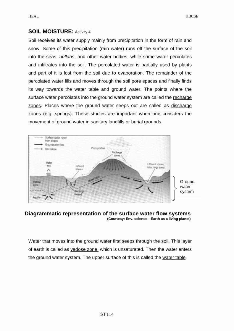
HEAL HBCSE

SOIL MOISTURE: Activity 4

Soil receives its water supply mainly from precipitation in the form of rain and

snow. Some of this precipitation (rain water) runs off the surface of the soil

into the seas, nullahs, and other water bodies, while some water percolates

and infiltrates into the soil. The percolated water is partially used by plants

and part of it is lost from the soil due to evaporation. The remainder of the

percolated water fills and moves through the soil pore spaces and finally finds

its way towards the water table and ground water. The points where the

surface water percolates into the ground water system are called the recharge

zones. Places where the ground water seeps out are called as discharge

zones (e.g. springs). These studies are important when one considers the

movement of ground water in sanitary landfills or burial grounds.

Ground water system

Diagrammatic representation of the surface water flow systems(Courtesy: Env. science—Earth as a living planet)

Water that moves into the ground water first seeps through the soil. This layer

of earth is called as vadose zone, which is unsaturated. Then the water enters

the ground water system. The upper surface of this is called the water table.

ST 114

HEAL HBCSE

Microscopic view of the soil Courtesy: Environmental Biology

T

w

e

r

W

p

t

m

d

w

a

t

w

Microscopic view of soil particlesshowing the flow of water into the soilthrough the air spaces.

here are points in the ground water zone from which adequate quantities of

ater can be obtained. These points are called aquifers. Certain soil types or

arth materials, such as loose gravel and sand particles with air spaces, or

ocks with open fractures, make ideal aquifers.

ater in the soil flows through the pores or spaces found around the soil

articles. This movement of water is not straight and smooth, but is jerky, as

he water molecules have to move around the soil particles. This jerky

ovement is termed as mechanical mixing. This mechanical mixing allows

issolution of the pollutants trapped in the soil particles to finally reach the

ater table. This should alert us to the easy movement of pollutants from one

rea of the soil to the ground water at a far away distance. Molecular and

urbulent dispersions are important parameters for water transport to ground

ater.

ST 115

HEAL HBCSE

Materials required: Tools to dig and remove soil samples, oven for drying the samples, weighing

balance and clean, dry, heat resistant containers.

Experimental procedure:

The dry and wet weight technique is used here.

Dig out soil samples from different depths, i.e., 0-5 cm, 10, 30, 60, 90 cm. The

samples collected from the different horizons are transferred to clean, dry

containers of known weight.

1. Weigh the soil samples along with the containers. This is the wet

weight of the sample soils. Record the value as (A gms).

2. Dry the samples in an oven at 95° C for 10 hours/overnight.

3. Remove the containers from the oven and allow them to cool. Weigh

the dried soil samples and record the value as (B gms).

4. Record the drying time and the dry weight to the nearest 0.1gm in the

soil work sheet (SWS: Activity 4).

5. Calculate the water weight (C) by calculating A-B.

6. Empty the soil samples from the containers and clean them.

7. Weigh and record the weights of empty containers (D gms).

8. Calculate the weight of dry soils by subtracting the container weight

from the dry weight (B-D). Calculate the soil water content by dividing

the water weight by the dry soil weight [SWS:Activity 4 (i)].

9. Represent the values as a graph [SWS: Activity 4 (ii)].

SOIL INFILTRATION CAPACITY: Activity 5

Another important property of soil is its infiltration capacity, which is defined as

the flow rate of water through the soil into the ground. The infiltration rate

depends on several structural properties of the soil, such as, its texture and

structure, bulk-density, water content and organic matter present in it. The

infiltration rates vary widely, ranging from 20 mm/hr for clay and compacted

soils (with low as 0.1 to 0.01 cm/day), to 60 mm/min for loose dry sand.

ST 116

HEAL HBCSE

Infiltration capacity of different soils will be studied here. In turn, this could

reflect how different pollutants in the soil also can infiltrate, often finding their

way into the ground water or aquifers. (Think: how do pesticides find their way

into the food chain?) To confirm this point, chemical analysis of soil should

bring out the absence or presence of different pollutants.

Further, one could plan a series of advanced activities and study water

infiltration with respect to different soil characteristics, such as shape, size

and compaction of soil. What do you think would happen in case of a heavy

downpour on a large compacted surface area versus in a natural open field?

In simulated laboratory set ups, one could also add different types of

chemicals {soda bicarb —highly alkaline, sodium bicarbonate (Na2HCO3), or

vinegar (acetic acid), or citric acid crystals} to the water sample. Check for the

changes in pH, if any, in the infiltrated water. Repeat this experiment for

different types of soils, or with the entire soil profile.

Materials required:

Two metal cans (10-20 cm diameter and 5-10 cms diameter), buckets, ruler,

waterproof marker and stopwatch or a watch with a second hand, hammer, a

block of wood, funnel.

Experimental procedure: First, make the two - canned infiltrometer. Cut the bottom of the cans.

Using a marker, shade a ring on the inside of the smaller can, at a

distance of about 9 cms from the bottom of the can. The width of this

ring should be 20 to 40 mm. Use this ring as your reference mark (R).

1.

2. Insert the smaller can into the bigger one. Measure the distance

between the two rims of the cans at their open mouth regions.

Procedure for measuring the infiltration rate:

1. Cut the vegetation, if any, to the ground surface.

2. Twist the cans into the soil and fix them at 2- 5 cms deep into the soil. 3. Measure the heights of the lower and upper edges of the reference

band (R) from the ground level.

ST 117

HEAL HBCSE

4. Pour water into both the cans so that the water level is slightly above

the inner reference mark. Match this level in the outer can too.

5. Start your watch as the water level reaches the upper reference mark.

6. This is the start time (A). Observe how the water level slowly/rapidly

falls down—in other words, water is infiltrating into the soil.

7. Keep a check of the water level in the outer can: it should be

maintained at the same level as in the inner can. You may have to pour

water with a funnel in the outer can. Avoid spilling into the inner can.

8. As the water level reaches the lower edge of the reference band (R),

note this time as your end time (B).

9. Calculate the time interval (C) {which is B-A} and note it.

10. Repeat the above steps at least nine times or for 45 minutes, till you

get two consecutive constant readings. Note in [SWS: Activity 5 (i)].

11. Calculate the time interval for each reading (C).

12. Note the water level change, which is the same as the width of the

reference band (R).

13. Calculate the mid point of the time interval, i.e., A+C\2

14. The flow rate is calculated as R\C in mm\min.

15. Plot a graph with the C values on the X-axis and the flow rate values

on the Y- axis [SWS: Activity 5 (i)].

Typical infiltrometer (Courtesy: GLOBE)

ST 118

HEAL HBCSE

(ii) This activity is to demonstrate the relationship between water infiltration

and different types of soils and bring out the role of soil characteristics

(particle size distribution) on infiltration rate and water holding capacity.

Materials required: 5 nos. clear 2-liter bottles, a stopwatch, 6 nos. 500ml beakers, soil samples,

mesh/nylon cloth, tape, 5-liter water, pH paper and scissors.

Experimental procedure: 1. Collect at least five different types of soil samples.

2. Note the soil characteristics such as, soil types, structure,

consistencies, and colour.

3. Take five nos. of 1.5 to 2 liter plastic bottles and cut the bottom and top

ends of the bottle.

4. Fix a nylon net/ mesh piece at the mouth end of the bottle with a string/

tape.

5. Place the bottle with the mesh side down, over a catchments beaker.

Fill each bottle with a different soil sample.

6. Collect 5 liters of water, check its pH and clarity, and note it.

7. Start the stopwatch and using a clean beaker pour approximately 300

ml of water into the first soil filled bottle.

8. Observe the water flow through the soil and collect in the catchments

beaker.

9. Stop the watch when the water stops dripping into the beaker. Record

the time duration for the water flow.

10. Check the pH and clarity of the collected water and observe for any

changes.

11. Repeat the same procedure for the remaining soil samples.

12. Record the different time durations for each type of soil, and changes

in pH and water clarity, if any.

13. Record the observations in soil worksheet [SWS: Activity 5 (ii)].

ST 119

HEAL HBCSE

Soil

Beaker

Water

Beaker/container to hold water

Mesh

Bottle

Filtered water

(iii) Perform the wet /dry weight protocol for the above soil samples after the

experiment. This test will tell about the water holding capacity of the soil

[SWS: Activity 5 (iii)].

Materials required: A clean and dry container of known weight, oven for drying and a weighing

balance.

Experimental procedure: 1. After the infiltration experiment, transfer some soil into a dry container

of known weight. Note the weight of the soil and container.

2. Subtract the weight of empty container from this to get the weight of

wet soil.

3. Dry the soil in an oven at 95˚C, and at hourly intervals, regularly weigh

the soil. Avoid spilling.

4. Stop the drying when a same value for two consecutive readings is

obtained. Note this weight. Subtract the weight of empty container

from this to get the weight of dry soil.

5. Difference between the dry and wet weights gives the water content of

the soil

6. Record this in the soil work sheet [SWS: Activity 5 (iii)].

7. Repeat this protocol for all the soil types used in the activity described

earlier.

ST 120

HEAL HBCSE

Chemical Parameters: Activity 6 to 9

SOIL pH: Activity 6

The measure of the hydrogen ion concentration of soil gives its pH. This

depends largely on relative amounts of the adsorbed hydrogen and metallic

ions. Hence pH is a good measure of the acidity and alkalinity of the soil.

Normally, the pH values of the soil lie in the range of 4.5 and 8.5. Soil is often

considered as an amphoteric buffer showing the properties of both acids and

bases. A well-buffered soil is less subjected to climatic and environmental

fluctuations. pH is also a strong indicator of soil fertility.

Several factors determine soil pH including the concentrations of different

salts and carbon dioxide, the exchangeable cations, the parent material, land

management practices and the activities of organisms living in the soil.

The chemical composition of rain and all other waters entering into the soil

also has a strong influence on the soil pH. In the wet tropics, soils are slightly

acidic due to constant leaching of the salts (replacement of calcium,

magnesium, potassium and sodium ions by hydrogen ions) from the soil. In

contrast, soil from dry areas is frequently alkaline. Places rich in calcium as in

limestone areas are distinctly alkaline. In the soil profile, the upper layers with

humus are generally acidic, while the deeper ones are alkaline. Solubility of

different ions in the soil is highly dependent on the soil pH. Certain

ions/substances are more soluble in acidic soil and may easily leach out

causing nutrient deficiencies. The pH of the soil also influences the activities

and relative abundance of the different groups of soil organisms. Acidic soils

have few species of soil organisms and favor development of fungi; basaltic

(intermediate pH) have a richer fauna and lime stone (alkaline) soils have the

greatest number of soil organisms. Knowledge of the pH of the soil helps

farmers to take decisions for improving soil fertility. Soil pH may also affect the

pH of the ground water or near by surface water, like streams or even lakes.

ST 121

HEAL HBCSE

Materials required: pH meter or pH paper, distilled water, spoon, conical flask.

Experimental procedure:

1. Use the soil sample collected in the profile experiment for this purpose.

2. In a clean container, mix sun-dried, sieved soil with distilled water in

the ratio of 1:1 (100 gms/100ml). Handle the soil with a spoon/spatula

to avoid soil contamination with oils and other materials on your hand.

Mix enough soil and water so that the pH reading can be made in the

supernatant.

3. Stir the soil-water mixture every 3-minutes for 15 minutes. After 15

minutes, allow the mixture to settle until a supernatant forms.

4. Measure the pH of the supernatant formed by dipping the pH paper

held with a forceps into the clear supernatant. 5. Hold the pH paper in the supernatant for a minute until the colour of the

pH paper changes on both the sides. Remove the paper from the

container, read the colour developed against the colour chart on the pH

paper booklet and note the pH in the soil work sheet (SWS: Activity 6). pH-dependent soil characteristics pH dependent soil types Characteristics

Acidic soils •

•

•

•

•

Found in humid regions with high rainfall.

Formed due to continued leaching of salts.

Lime application neutralizes the acidity.

Crops like millets and peas tolerate acidic soils.

Trees, such as, tamarind, Gliricidia and Deris indica can grow here.

Saline soils or white alkali soils

•

•

•

•

Found in regions where: water logging and water table are high as in several regions of the Punjab.

Formation of surface white encrustations, due to excess soluble salts like: chlorine, sulphate and sodium.

Ridge-trench, sub-surface and furrow irrigation planting reduces toxicity of soil.

Trees like Azadiracta indica (neem), Prosopis sps., Albizia sps. can grow here.

Alkaline or sodic soils •

•

•

•

•

Found in places rich in limestone.

The soil appears black due to presence of sodium carbonate.

It has low infiltration rate.

Treatment: Addition of gypsum (hydrous calcium sulphate), silt and rice husk improves texture.

Trees: neem, Alibizia sps. Derris sps. and Subabul grow here.

ST 122

HEAL HBCSE

CALCIUM CARBONATES : Activity 7

The presence of calcium carbonates in the soil leads to alkaline conditions of

the soil. Hence, alkalinity is an indirect indicator of this salt. In fact, high pH

exceeding pH 9 is a good indicator of calcium carbonates in the soil. The main

sources of calcium carbonates are limestone and degraded organic matter,

like bones. High alkalinity reduces crop yield and affects flora and fauna. High

concentrations of calcium carbonates may lead to hardness of water.

Materials required: Conical flask, pipettes, aluminum foil and filter paper, 1N hydrochloric acid

(HCL), 1N sodium hydroxide (NaOH), indicator--bromothymol blue.

Experimental procedure: 1. Transfer 5 g of soil sample to a dry conical flask. Add 100 ml of 1N

HCL. Cover the flask and allow the mixture to stand for 1 hr with

regular mixing at every 15 mins.

2. Decant the supernatant through a filter paper. Take 5 ml filterate, add

0.4 ml of bromothymol blue and titrate it against 1 N NaOH till the

colour changes from yellow to orange. Note the pipette reading as ‘S’ (sample).

3. Repeat the procedure for a blank using 5 ml 1N HCl; note the reading

as ‘B’ (blank). Using the formula in the soil work sheet calculate the %

of calcium carbonate [SWS: Activity 7].

Calcium carbonate in the sample neutralizes HCl. The excess of HCl is

titrated against NaOH using bromothymol blue, which changes colour from

yellow to orange at a pH of 3.7.

2HCl+CaCO3

NaOH+HCl

ST 123

CaCl2+H2O+CO2

NaCl+H2O

HEAL HBCSE

HEAVY METAL POLLUTION: Activity 8 and 9

Certain concentrations of heavy metals are present in the soils as natural

mineral constituents. But often soils can collect large quantities of heavy

metals and other waste products from various activities. These metals are

introduced into the soil from spills, industrial discharges, agricultural practices,

leaking tanks and landfills. In other words, unscientific management of all

wastes, both liquid and solids, contribute largely to pollution or degradation of

soil. Dumps of junk automobiles, electronic appliances and containers also

add to this problem.

Vehicular emissions and fuel combustion result in heavy loads of metal

residues in the soil. Among these, mercury, cadmium, lead, iron and zinc are

the frequent contaminants. They tend to concentrate in certain components of

the soil, such as, clay sediments and in organisms, such as mollusks,

mussels and shellfish. Since metals are non-degradable, they persist in the

environment and cause long-term pollution. Heavy metals can cause several

problems to humans, including skin and gastro-intestinal problems. Long-term

exposure may affect many enzymatic activities and disturb the development

of an organism, including humans.

For detection of heavy metals, the clear supernatant of the soil mixture will be

used. The protocol (A) of this step is as follows:

1. In a clean, dry beaker, mix the sample with DW in a 1: 2 ratio.

2. Stir the mixture well by shaking the flask every 3 minutes for 15

minutes. Heat the mixture till the volume of water reduces to half.

3. Allow the mixture to stand for 20 minutes or so, till the soil sediments

and a clear liquid appears on the top. Use this supernatant liquid for

the analysis of heavy metals as instructed.

ST 124

HEAL HBCSE

Effects of heavy metals on human health

Heavy metal Source Effects due to bio-accumulation

Arsenic Occurs naturally Chronic poisoning, loss of weight, diarrhoea alternating with constipation, conjunctivitis and sometimes skin cancer.

Cadmium Mining, chemical and

metallurgy industry.

Chronic poisoning, kidney malfunctions and formation

of kidney stones.

Lead Lead smelters, storage

batteries

Mental retardation and death.

Mercury

Industrial wastes Neurological problems, renal damage

Cyanides

Waste from metal treatment

with heat, electroplating.

Rapid death due to inhibition of cellular respiration

Note : Since the standards for heavy metals in soils were not available, use

the colour grid provided for water for determining the heavy metal levels

present in the soil. But, remember that these levels are not the cut off limits

for these pollutants. Also, the colour of the soil may add to the colour

developed.

IRON (Fe): Activity 8

Iron may be present in the soil in dissolved or suspended state. It may be in

the Fe 2+, Fe3+ or Fe(OH)3 state, suspended or filterable. When the ground

water is acidic, iron is present as Fe3; when the ground water is alkaline or

neutral, iron is present as Fe(OH)3. It gets easily transferred to the ground

waters. Some ground waters naturally contain high levels of iron. Though Fe

is an essential element of our diet, its accumulation in humans causes a

variety of problems, including those of liver, kidneys and muscles.

Materials required: Conc. HCl, 1ml hydroxyl amine hydrochloride (NH2OH.HCl (10%), 50/100ml

volumetric flask, 10 ml ammonium acetate buffer, 2 ml phenanthroline (refer

appendix 1), 5 and 10 ml syringes.

Experimental procedure:

1. Take 10 ml sample supernatant (protocol A) in a clean and clear

container.

ST 125

HEAL HBCSE

2. Add 0.5ml conc. HCl and 0.2ml NH2OH.HCl (10%).

3. Boil the mixture in a water bath for 15 minutes.

4. Cool the solution to room temp. and transfer it to 100ml flask.

5. Add 2 ml ammonium acetate buffer, followed by addition of 0.4 ml

phenanthroline.

6. Shake well. Wait for 10- 15 min for colour development (colour is stable

for 30 minutes).

7. Compare the colour developed against the grid provided. Note the

observations as L, P, H or C {SWS: Activity 8}.

8. Alternatively, measure absorbance at 510 nm against reagent blank.

Plot the absorbance value of the unknown sample against the standard

graph to estimate the concentration of iron in the sample.

Preparation of standard graph: Stock ferrous ammonium sulphate [(NH4)2Fe(SO4)2.6H2O] solution: Prepare a

50-ppm (Refer appendix 1) solution of ferrous ammonium sulphate [ (NH4)2 Fe

(SO4)2 . 6H2O].

From this prepare a range of concentrations including 0.01, 0.1, 0.3, 1 and 5

ppm. Using 10 ml of each of these solutions, proceed as for the sample

solution. Measure the colour obtained at 510 nm. Plot these values against

the concentrations to obtain a standard graph.

Total dissolved Fe(II) conc. between 0.01 and 5 ppm can be detected by this

method. Detection limit is 50 µg of Fe. in solution. Fe+3 is reduced to Fe+2 by

NH2OH adjusted to pH 3.2-3.3. It is then treated with 1,10 phenanthroline.

Resulting orange red solution is measured at 510 nm.

COPPER (Cu): Activity 9

High concentration of copper in the soil is due to pollution from agricultural run

offs or corrosion of copper–containing alloys in pipe-fittings and industrial

effluents. Salts of copper are often used in water reservoirs and in distribution

pipes as it prevents growth of weeds. It binds strongly with the organic

components of the soil and is found as metalo-organic complexes. It exhibits

ST 126

HEAL HBCSE

very slow mobility. The concentration of copper in the soil determines its

uptake rate in the plants: concentrations less than 100 ppm show low uptake

and at higher levels there is a significant increase in the uptake.

The normal background concentration of copper in the soil is 1-20 ppm.

Increasing concentrations and values exceeding the threshold limit of 100

ppm is an indicator of serious pollution.

Copper is easily accumulated in plants and at concentrations of 20 ppm it is

toxic to the plant. It is an essential micronutrient in the human diet, the

recommended daily allowance (RDA) being 2.0 mg. It plays a significant role

in enzyme catalysis and the electron transport processes. Copper gets

accumulated in the blood, bones and muscles.

Materials required: Separating funnel, test tubes, pipettes, standard copper solution (10 µg \ml),

liquid NH3, 15% citric acid, 1% sodium diethyl dithio carbamate, 1% iso amyl

acetate (refer Appendix 1), distilled water. Experimental procedure:

1. Take 5 ml of sample supernatant (protocol A) in a clean beaker.

2. To the above add 5ml of citric acid and with a dropper add 4 drops of

liquid ammonia.

3. Add 1 ml of carbamate solution + 39 ml of distilled water + 10 ml of iso

amyl acetate.

4. Shake the beaker vigorously for 15 min and allow it to stand till the two

layers are clearly demarcated.

5. Compare the colour developed with the colour grid provided and note

your observations as L, P, H or C.

6. Alternatively, drain off the lower aqueous layer and collect the upper

organic phase carefully in a test tube. Measure the absorbance of the

organic layer at 440 nm. against reagent blank. Plot the absorbance

value of the unknown sample against the standard graph to estimate

the concentration of copper in the sample.

ST 127

HEAL HBCSE

ST 128

7. Note the value in the soil work sheet [SW: Activity 9]. Plot a standard

graph with concentration on the X axis and absorbance on the Y-axis.

Preparation of standard graph: Stock copper (Cu) solution: Prepare a 200-ppm (Refer appendix 1) solution of

copper solution.

From this prepare a range of concentrations including 0.01, 0.05, 0.1, 1, 10,

20 and 100 ppm. Using 10 ml of these solutions, proceed as for the sample

solution. Measure the colour obtained at 440 nm. Plot these values against

the concentrations to obtain a standard graph.

Copper present in the sample reacts with sodium-diethyl-dithio -carbamate in

an alkaline medium to form the Cu salt of the carbamate. This complex is

golden yellow in colour. A few drops of liquid ammonia generate the alkalinity.

The golden yellow colour is extracted into the organic phase of iso -amyl

acetate and is then estimated colorimetrically. Citric acid is added to prevent

the precipitation of any metal ions due to change in pH. Citrate also acts as a

chelating agent.

Note: One can carry out soil analysis for other chemical constituents as in

water.

HEAL HBCSE

Soil Worksheets

Name Of The Investigator: Date: College Name/ Address:

Site name: Location:

General observation of the site: Vegetation: Present______, Absent_______

If present, then type of vegetation: Natural ___, Cultivated____,

Garden ____, Others_____

Type of surface cover: Short grass (<10 cm) ____, Long grass (>10

cm) ____, Shrubs_______, Herbs____, Others______

Type of canopy cover: Umbrella (overarching) canopy ____, Conical

vertical canopy ______, Other______

If vegetation is absent, then describe the site in brief: _____________

Rain within last 24 hours: Yes___, No____; Last rain: _________

Activity 1: Soil Concept Map Draw a concept map/flow chart with minimum 20 fields or concepts to justify

the statement: ‘Soil is a great integrator’.

(Field)

SWS 129

HEAL HBCSE

Activity 2: Soil Profile (i) General characteristics of each horizon of the soil profile.

Presence (+) or

Absence (-) of:

Rt-Roots Ro-Rocks

Anthropogenic material

Hor

izon

Hor

izon

hei

ght

(cm

s)

Moisture W-wet M-moist D- dry

Structure R-regular B-blocky P-platy C-columnar Cy-cylindrical G-grainy C

olou

r

Soil

cons

iste

nce*

Soil Texture C- clay S- silt Sa- sand L- loam Combinations

+/-

Few Many

Nil

+/- Type* Few Many

Nil

*Soil consistence: Loose, friable, firm, extremely firm.

*Type of anthropogenic material: plastic, glass, metal, rubber, etc.

SWS 130

HEAL HBCSE

(ii) Draw a labeled diagram (appropriately scaled) of the different

layers/horizons of the soil profile.

(iii) Represent the soil texture data of the different horizons as a pyramid. This

representation will be based on the rough distribution of different soil textures

in the entire soil profile. The most frequent soil texture will be at the bottom of

the pyramid, and the least frequent at the top.

SWS 131

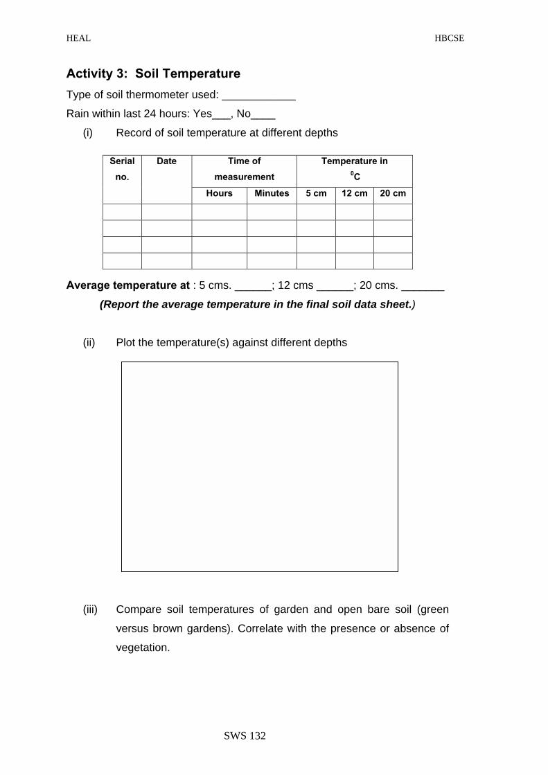
HEAL HBCSE

Activity 3: Soil Temperature Type of soil thermometer used: ____________

Rain within last 24 hours: Yes___, No____ (i)

(ii)

(iii)

Record of soil temperature at different depths

Time of

measurement Temperature in

0C

Serial no.

Date

Hours Minutes 5 cm 12 cm 20 cm

Average temperature at : 5 cms. ______; 12 cms ______; 20 cms. _______

(Report the average temperature in the final soil data sheet.)

Plot the temperature(s) against different depths

Compare soil temperatures of garden and open bare soil (green

versus brown gardens). Correlate with the presence or absence of

vegetation.

SWS 132

HEAL HBCSE

Activity 4: Soil Moisture Date of sampling: Date of performing the experiment: Current condition: Wet_____; Dry_________ Drying temperature: ______; Average drying time: _____ hours or minutes

(i) Record of the moisture content of the soil

Sam

ple

no.

Sample depth

A Wet-

weight in gms

B Dry-

weight in gms

C Water weight in gms (A-B)

D Container weight in

gms

E Dry soil weight in gms (B-D)

F Soil water content (C\E)×100

0-5 cm 1

20 cm

0-5 cm 2

20 cm

0-5 cm 3

20 cm

Average soil moisture content at : 5 cms ________, 20 cms ______ (Report the average soil moisture in the final soil data sheet)

(ii) Graphically represent the above data.

SWS 133

HEAL HBCSE

Activity 5: Soil Infiltration Capacity Date of sampling: Date of performing the experiment:

Distance from the soil moisture study site: _______metres Width of the reference band (R):_____ (i) Observations for soil infiltration capacity

Sr no.

A Start time (min)(sec)

B End time (min)(sec)

C Time

interval(B-A)

D Mid-point

(mins) (A+C/2)

R Water level

change (mm)

F Flow rate mm/min (R/C)

1. 2. 3. 4. 5. 6. 7. 8. 9.

Repeat the experiment three times, until consecutive readings are obtained.

Average flow rate: _______ (Report the average flow rate in the final soil data sheet .)

Plot the flow rate against the time interval.

SWS 134

HEAL HBCSE

Activity 5 (Ii): Flow Rates Of The Different Types Of Soil

Soil characteristics Infiltration time

Characteristics of water

Clarity C-clear M-muddy

pH

Sr. no.

Nature M-Moist D-Dry

Colour

Type C-clay S-sandy S-silt L-loam O-others

Start time (min)

End time (min)

Before expt.

After expt.

Before expt.

After expt.

Plot a bar graph to illustrate the flow rates of different types of soil.

SWS 135

HEAL HBCSE

Activity 5 (Iii): Water Holding Capacity Of The Soil Samples.

Drying temperature: _____˚ C; Time of drying: _____hours

Wt. of empty container (X gms): _____

Wt. of wet soil + container (Y gm): ____; Wt. of wet soil A (Y-X gm): _____ Wt. of dry soil + container (Z gm): ____; Wt. of dry soil B (Z-X gm): _____

(iii) Record of soil moisture Soil

type Weight of wet

soil (A in gm)

Weight of dry soil

(B in gm)

Water content of the soil (A-B gms)

Represent the results of (iii) graphically.

ThthePoInv

SWS 136

Combine both the infiltration time and the water content of all soil types in ONE graph.

e correlation noticed between the two properties of soil? sitive____; Negative____; Partial____; erse____; Others___

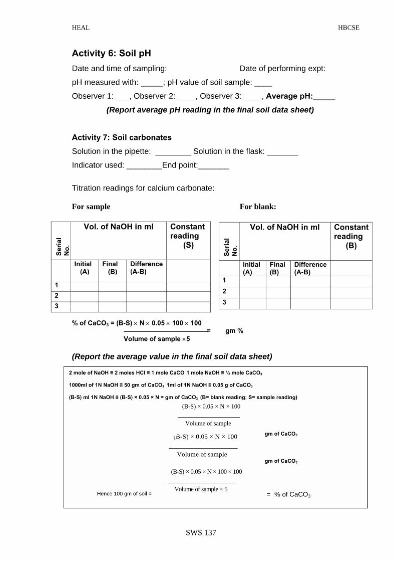
HEAL HBCSE

Activity 6: Soil pH Date and time of sampling: Date of performing expt:

pH measured with: _____; pH value of soil sample: ____

Observer 1: ___, Observer 2: ____, Observer 3: ____, Average pH:_____

(Report average pH reading in the final soil data sheet) Activity 7: Soil carbonates Solution in the pipette: ________ Solution in the flask: _______

Indicator used: ________End point:_______

Titration readings for calcium carbonate: For sample For blank:

Seria

l N

o.

Vol. of NaOH in ml Constant reading

(S)

Initial (A)

Final (B)

Difference (A-B)

1 2 3

Seria

l N

o.

Vol. of NaOH in ml Constant reading

(B)

Initial (A)

Final (B)

Difference (A-B)

1 2 3

% of CaCO3 = (B-S) × N × 0.05 × 100 × 100 = gm %

Volume of sample ×5 (Report the average value in the final soil data sheet)

2 mole of NaOH ≡ 2 moles HCl ≡ 1 mole CaCO; 1 mole NaOH ≡ ½ mole CaCO3

1000ml of 1N NaOH ≡ 50 gm of CaCO3 1ml of 1N NaOH ≡ 0.05 g of CaCO3 (B-S) ml 1N NaOH ≡ (B-S) × 0.05 × N = gm of CaCO3

(B= blank reading; S= sample reading)

Volume of sample

(B-S) × 0.05 × N × 100

Volume of sample

(B-S) × 0.05 × N × 100

(B-S) × 0.05 × N × 100 × 100

gm of CaCO3

gm of CaCO3

5 gm of soil =

hence 100 ml of soil sample =

Volume of sample × 5 Hence 100 gm of soil =

SWS 137

= % of CaCO3

HEAL HBCSE

Activity 8: Iron Date and time of sampling: Date of performing the experiment: Observations: Concentration of iron in the sample observed by comparing the colour

developed against the colour grid: (C, H, P, L) ________

Plot and read the concentration of the sample from the standard graph.

Observer 1=_____; Observer 2 =_______; Observer 3 =________

Average value of iron in the sample =________ppm

(Report the average value for iron in the final soil data sheet.)

SWS 138

HEAL HBCSE

Activity 9: Copper Date and time of sampling: Date of performing the experiment:

Observations: Concentration of copper in the sample observed by comparing the colour

developed against the colour grid: (C, H, P, L) ________

Plot and read the concentration of the sample from the standard graph.

Observer 1=______Observer2 =_______ Observer 3 =________

Average value of copper in the sample =________mg\l of Cu

(Report the average value for copper in the final soil data sheet.)

SWS 139

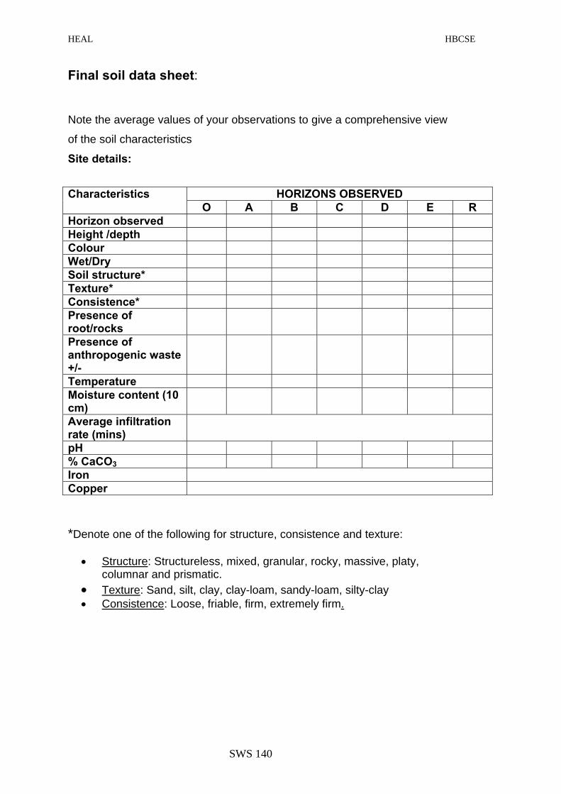
HEAL HBCSE

SWS 140

Final soil data sheet: Note the average values of your observations to give a comprehensive view

of the soil characteristics

Site details:

HORIZONS OBSERVED Characteristics

O A B C D E R Horizon observed Height /depth Colour Wet/Dry Soil structure* Texture* Consistence* Presence of root/rocks

Presence of anthropogenic waste +/-

Temperature Moisture content (10 cm)

Average infiltration rate (mins)

pH % CaCO3 Iron Copper *Denote one of the following for structure, consistence and texture:

• Structure: Structureless, mixed, granular, rocky, massive, platy,

columnar and prismatic. • Texture: Sand, silt, clay, clay-loam, sandy-loam, silty-clay • Consistence: Loose, friable, firm, extremely firm.

HEAL HBCSE

‘Green’ watch…

for good health

INTRODUCTION: Natural vegetation in any area is often referred to as land or green cover. The

quality and quantity of this vegetation is a good indicator of the changes in the

environment. This is especially true with respect to climate, which can vary

greatly and most noticeably with increasing pollution. Human induced

changes in the land cover (such as, deforestation and increased concrete

surfaces and constructions vis-a-vis green cover), affect not just the plants but

also the different ecological and energy cycles.

Tracking changes in the quality, quantity and type of the land cover can give

valuable information about the state of our environment and pollution, and

indirectly about health. For instance, the diminishing canopy cover, the

reduced tree growth, failure of flowering and changes in the leaf colour are all

indicators of poor quality of the environment.

For detailed study of the land cover, scientists often make use of the modified

UNESCO classification system, often called the MUC system, to identify the

type or class of land cover. This classification makes use of ecological

principles and the different vegetation types found in different climatic zones.

Under this MUC system, every land cover type is classified as a separate

class, with each class being further sub -classified into three or four levels.

For instance, in the original MUC system, �Cultivated Land�, at MUC Class 8,

at Level 1, is further divided into Agriculture (81) and Non agriculture (82) at

Level 2. The sub-class 81�Agriculture-- is further classified as: �row crop or

pasture� (811), orchard or horticulture (812), confined livestock feeding (813)

and other agriculture category (814), at level 3. Similarly, non agriculture (82)

at level 2 has four sub categories at level 3: parks and athletic fields (821),

golf courses (822), cemeteries (823) and other non agriculture (824). The

following table gives ten major MUC classes with their characteristics.

GCT141

HEAL HBCSE

Perhaps at a later stage, this MUC system could be used to classify the area

under study.

The MUC levels for green cover identification

Class no

MUC class Characteristics of the class

0 Forest > 40% trees, 5 mt tall, crowns interlocking

1 Woodland > 40% trees, 5 mt tall, crowns not inter locking

2 Shrub land > 40% shrubs, 0.5-5 mt tall

3 Dwarf shrub land > 40% shrubs under 0.5 mt tall

4 Herbaceous

vegetation

> 60 % herbaceous or broad leaved plants,

grasses

5 Barren < 40% vegetative cover

6 Wet land > 40% vegetative cover, includes marshes,

swamps and bogs

7 Open water > 60% open water

8 Cultivated land > 60% non-native cultivated species

9 Urban > 40% urban land cover (buildings, paved

surfaces) (Courtesy: GLOBE)

The recommended green cover for an urban site is 3 acres of green cover for

every thousand people living in that site.

Ideally, the investigation of land cover involves, calculating percentages of

ground and canopy cover, and identification of the type of vegetation and the

dominant and less dominant species of an area. Mangrove stretches, if

present, could also be monitored.

Interested students/teachers can monitor the same site on a continuous basis.

Green cover, tree numbers, heights and circumferences could also be

monitored over time; for this it is imperative to tag/label the trees and keep a

GCT142

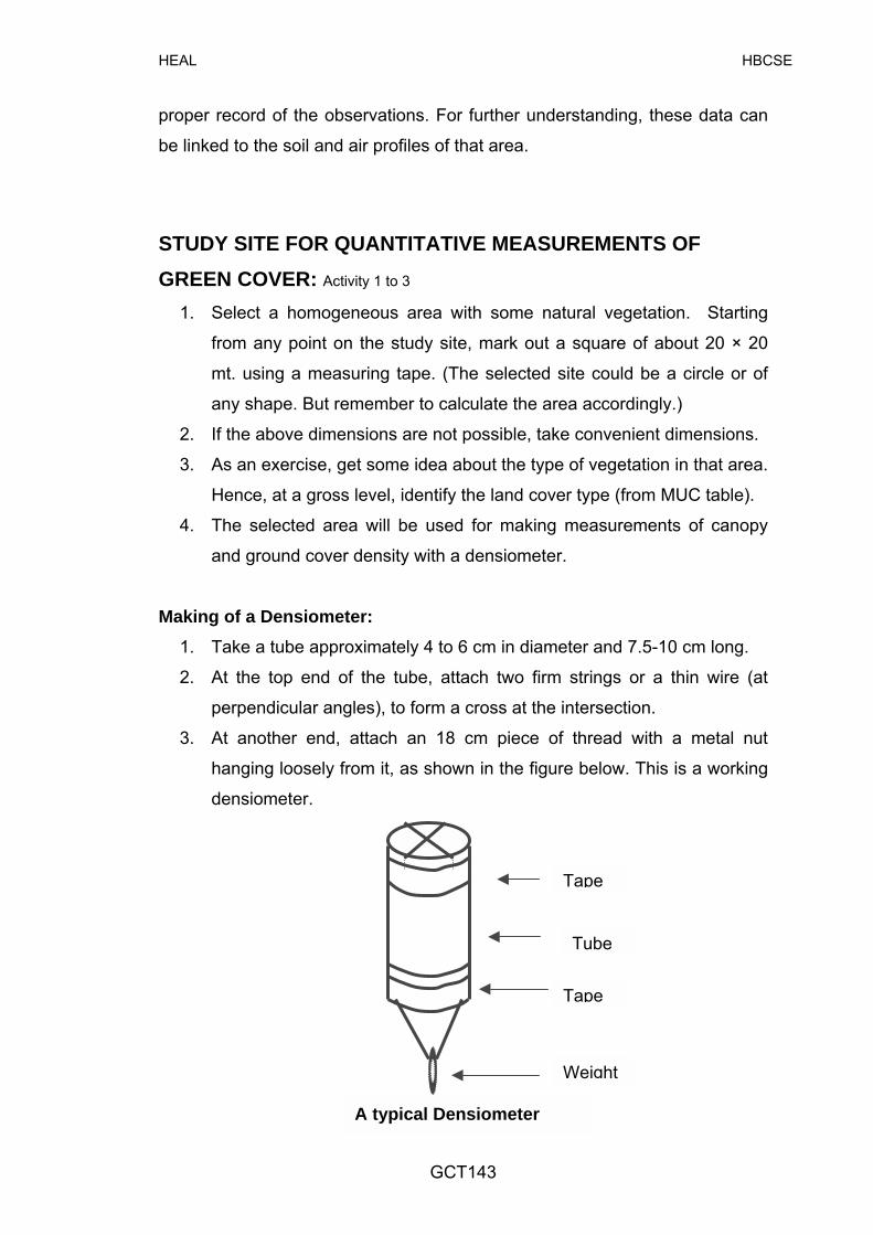
HEAL HBCSE

proper record of the observations. For further understanding, these data can

be linked to the soil and air profiles of that area.

STUDY SITE FOR QUANTITATIVE MEASUREMENTS OF GREEN COVER: Activity 1 to 3

1. Select a homogeneous area with some natural vegetation. Starting

from any point on the study site, mark out a square of about 20 × 20

mt. using a measuring tape. (The selected site could be a circle or of

any shape. But remember to calculate the area accordingly.)

2. If the above dimensions are not possible, take convenient dimensions.

3. As an exercise, get some idea about the type of vegetation in that area.

Hence, at a gross level, identify the land cover type (from MUC table). 4. The selected area will be used for making measurements of canopy

and ground cover density with a densiometer. Making of a Densiometer:

1. Take a tube approximately 4 to 6 cm in diameter and 7.5-10 cm long.

2. At the top end of the tube, attach two firm strings or a thin wire (at

perpendicular angles), to form a cross at the intersection.

3. At another end, attach an 18 cm piece of thread with a metal nut

hanging loosely from it, as shown in the figure below. This is a working

densiometer.

Weight

Tube

Tape

Tape

A typical Densiometer

GCT143

HEAL HBCSE

OBSERVATIONS AND MEASUREMENTS OF CANOPY COVER: Activity 1 (i)

One or more students walk along the diagonals of the square (circle) with the

densiometer in the hand. After every two steps, the student looks up at the

canopy through the densiometer.

Make sure that the metal weight (ring) is in line with the intersection point of

the cross.

1. Presence of vegetation, twigs or branches touching the cross hair

intersection, is recorded as �+�. If no vegetation is seen, record as �-� in

the �Green cover� work sheet [GCWS: Activity 1(i)].

2. For accuracy, repeat the readings twice with different students at the

same site.

3. Enter average values in the worksheet.

4. Calculate the percentages of canopy cover for the selected area.

(All +�s/ total observations) × 100

OBSERVATIONS AND MEASUREMENTS OF GROUND COVER: Activity 1(ii)

Take two steps along the diagonals, as in Activity 1 (i), but here the student

should look down on the ground.

1. If the vegetation is underfoot or touches the foot or leg below the knee,

record it as +G for GREEN vegetation; and +B if the vegetation is

BROWN.

2. If there is no vegetation observed, note it as �-�.

3. For accuracy, repeat the readings twice with different students at the

same site. Enter average values in worksheet {GCWS: Activity 1 (ii)}.

4. Calculate the percentage of ground cover for the selected site.

(All +�s/ total observations) × 100

5. Similarly, calculate the percentage of green and brown ground cover.

Note: Think of ways of extending this method to find out the green cover for

built up and other areas. Interesting results can be observed by recording and

GCT144

HEAL HBCSE

monitoring the extent of green cover of the same site on a regular and

continuous basis. If interested, adopt the selected site, build up the green

cover and keep meticulous record of the green cover.

Qualitative And Quantitative Observations Of Green Cover: Activity 1 (iii, iv) Canopy cover measurements include trees that have a canopy (umbrella).

However, this eliminates trees without overarching canopies. To take care of

such situations, counting of individual trees along bisects \diagonals of the

chosen study site area is carried out.

(III): QUALITATIVE AND QUANTITATIVE OBSERVATIONS OF GREEN COVER (TREES AND SHRUBS) AT GROUND LEVEL

1. Extend 1meter area (total 2 mts wide bisects) on either side of the

diagonals (now called bisects). Now the tree and ground cover

measurements will be made along these bisects.

Bisect 2

Bisect 11 mt

2 mt

Study site

2. First, take an overall view of the study site and note down the type of

trees and shrubs in your rough book.

3. Walk along the two bisects, one after the other, and identify the

different types of trees\shrubs.

4. Count the number of individual tree types in each bisect.

5. Enter the observations in green cover worksheet {GCW: Activity 1 (iii)}. 6. Calculate the percentage of each tree and shrub type. (No. of individual

tree type\ total no. of trees counted χ by hundred.)

GCT145

HEAL HBCSE

Note: Different tree types could be considered along different families

(mimosae, ficus, palms, etc) or along leaf morphology (broad, narrow or

simple and compound leaves, etc). Shrubs can be grouped based on their

heights.

(IV): QUALITATIVE AND QUANTITATIVE OBSERVATIONS OF GREEN COVER (HERBS : GRASSES)

1. The above method can also be extended for the ground (grass ) cover.

2. The spread of grass along the entire bisect is difficult to count. Hence

bisects will be divided into small samples/quadrants of 1mt X 1 mt.

(Mark the four corners of the quadrants with big nails or sticks. Pass a

string around the nails to demarcate the quadrant.)

3. Count the grass cover in alternate quadrants; add them up to give the

grass cover for the bisect. (For this, grass tufts are counted : lift a

bunch of leafy blades and observe: if they have a common root \origin,

it is counted as one tuft. This is continued for the entire quadrant.)

4. The grass cover could be of many types; try to identify each type and

count how many of each type is present in a quadrant.

5. If the identification is not possible, report the observation as grass type

1, grass type 2�

6. Calculate the percentage of each type of grass as for the tree cover.

7. If the place is well maintained, the growth of grass will be well spread

out and luxuriant. This type of growth could be reported as 100% cover

with Type 1=__%; Type 2=__%, etc.

IDENTIFICATION OF SPECIES TYPE: Activity 1 (v)

1. Identify the different plant species in the study area as dominant and

co-dominant species.

2. While the most frequently occurring species (most common) in an area

is termed as the dominant, the next dominant species (second most

common) is recognized as the co-dominant.

3. Identify the origin of plant species as endogenous (originating in an

area) or exogenous (brought from outside).

GCT146

HEAL HBCSE

4. Identify the species by using both common and botanical names.

5. It is an interesting exercise to find out the common names of plants in

different Indian languages.

6. For the ground cover, identify the cover as shrubs, herbs with broad or

narrow leaves and narrow leaved grass.

7. Note the observations in GCWS: Activity 1 (i and ii) respectively.

8. Help of experts in botany can be sought for precise identification.

MEASUREMENTS OF THE TREE CIRCUMFERENCE: Activity 2 (i)

1. Use a bendable tape to measure the circumference of the tree.

2. The circumference of the tree trunk is usually measured at 1.35 m

above the ground level.

3. Repeat the process with different students twice for all the dominant

and co-dominant trees of the study site.

4. Record the circumference in cms.in worksheet (GCWS: Activity 2(i) (ii).

5. Remember to tag the trees in the area, if interested in monitoring the

green cover over time.

MEASUREMENT OF TREE HEIGHT: Activity 2 (ii)

1. A clinometer is used to measure the height of a tree.

2. Making of a clinometer is as follows:

! Stick the clinometer sheet to a cardboard of the same size.

! Make a hole at the encircled mark on the clinometer and pass a

15 cm string through it, with a knot at one end to avoid slippage.

! Tie a metal bolt at the other end of the string.

! At the demarcated area of the sheet, paste a broad drinking

straw or any narrow tube/pipe. This is the working clinomenter.

GCT147

HEAL HBCSE

Distance between tree andobserver

Weight

String

Drinking straw

ZX

3. To measure the tree height

at a fixed distance from the

4. Note the distance of the o

known quantity (height of th

5. Before making measurem

clinometer. For this allow th

the vertical (y-axis) line on t

6. To measure tree height, loo

7. Another student or partner

string on the clinometer (an

string during the observatio

calculate the height of the tr

8. Repeat the procedure twice

average readings in the GC

A clinometer

, hold the clinometer at eye level and stand

selected tree. Note this distance (XZ in fig). bserver�s eye from the ground, which is a

e observer). ents make the zero adjustment for the

e string to hang loosely and set it parallel to

he clinometer chart. k through the straw and view the tree tip. should then note the angle made by the

gle X); take care not to move or shake the

ns. Using the tan sheet and the formula,

ee. with different students and record the

WS: Activity 2 (i) and (ii).

GCT148

HEAL HBCSE

ZX

Y

X

Measuring tree height with a clinometer

Y

ZX

Tan angle X= YZ/XZ; YZ =(XZ) Х ( tan < X)

Hence, actual tree height = YZ + distance of the observer�s eye from the

ground.

Remember to tag the trees in the area, if interested in monitoring the green

cover over time.

GCT149

HEAL HBCSE

MEASUREMENTS OF GRASS BIOMASS: Activity 3

1. In the study site, mark a square of about 1 meter, where there is

natural vegetation.

2. Using a garden scissor cut all the grass vegetation in that square.

3. Collect the grass in bags; do not collect any other loose material/

leaves.

4. Sort the grass clippings into green and brown.

5. Place the two portions in separate labeled paper bags.

6. Weigh the grass in both the bags. Note the weights.

7. Next, dry the bags containing grass over a period of days in an oven

at a temperature not higher than 50-70o C.

8. Weigh each bag once a day.

9. The grass in the bags is completely dry when two consecutive

weights are similar.

10. Next, empty the contents and weigh the empty bags.

11. Subtract the weight of the empty bags from the weight of the filled

ones. This will give the weight of the grass clippings.

12. Repeat this procedure in more patches such that the grass cover in

the entire study site is represented.

13. Report the weights for both green and brown grass in the green

cover work sheet [GCWS: Activity 3].

QUALITATIVE CHARACTERISTICS OF CANOPY AND GROUND COVER: Activity 4

To determine the quality of the land cover, certain characteristics are checked

for both canopy and ground cover.

1. Identify the type of canopy cover (trees: deciduous or evergreen) and

ground cover (grass, weeds, shrubs or herbs).

2. Check for the colour of the leaves of the canopy cover. Observe for any

insect or fungal infections, too.

GCT150

HEAL HBCSE

GCT151

3. Note the tree\ grass growth). Check if the green cover is well

maintained.

4. Check if tree\ ground cover exhibits regular flowering and fruiting.

5. Finally, identify the green cover of the study site as healthy or

diseased.

6. Record your observations in land cover data sheet [GCWS: Activity 4].

A FEW QUESTIONS TO THINK ABOUT: • Recall the total area of your study site: Is the observed and recorded

percentage of green cover adequate for that area?

• Calculate the percentage of green cover for the defined area/garden.

Report the results considering the foll: (i) measure the total area of the

garden using a tape; (ii) measure the areas covered with: trees with

canopy + trees without canopy + shrubs + grass.

• To measure the area covered by canopy e.g., canopy of banyan

tree, consider the area covered by the entire canopy; multiply

this area by the no. of banyan trees (look out for young and old

trees). Similarly, carry out this measurement for other tree types.

And calculate the total green cover in an area.

•

•

•

•

•

From the Town Planning department of your municipality/district, find

out the ideal / adequate green cover percentage for urban areas?

Check out the diversity of the tree cover.

On similar lines, mangrove cover could also be monitored. Find out if

there is an increase or decrease in the mangrove cover, say over a

period of three to four years.

Find out the absence/presence of green cover along the roads and at

the road dividers.

In the final analysis, try to link up the pollution data obtained to the

green cover study.

HEAL HBCSE

Green cover Worksheets Date And Time Of Experiment: Name Of The Site: Location:

Activity 1: Observations And Measurements Of Canopy Cover (i) Canopy cover--qualitative and quantitative observations

Canopy type is:

Origin of species

Densiometer observations + = tree - = nil

Canopy type E=evergreen S=seasonal

Botanical name of the trees

Common name of the trees

D=dominant C= co-dominant

E=exogenous N=endogenous

% Canopy cover:________

(Report the average value for canopy cover in final green cover data sheet. )

Determining canopy cover: Total observations= total no. of (+) and (-)_______

% Canopy cover: (All +�s\total observations) ×100 =______

GCWS 152

HEAL HBCSE

Activity 1(Ii): Observations And Measurements Of Ground Cover

(ii) Ground cover---qualitative and quantitative observations

% Ground cover: _________ (Report the percent ground cover in final land cover data sheet.)

Densiometer observations of ground cover: + = grass -- = no grass

Colour of ground cover B= brown cover G = green cover

Ground cover type Grass/ herbs/ shrubs

Determining ground cover: Total observations = Total no. of (G) + (B) + (-) = _______

% Ground cover = (All G+ All B \ total observations) × 100 =________

GCWS 153

HEAL HBCSE

Activity 1 (Iii): Qualitative And Quantitative Observations Of Green Cover (Trees And Shrubs) At Ground Level

Name of plants

Nos. in

Bisect 1

Nos. in

Bisect 2

Total Nos. % of each plant type

GCWS 154

HEAL HBCSE

Activity 1 (Iv): Qualitative And Quantitative Observations Of Green Cover (Herbs = Grasses)

Name/type of herbs

Nos. in

Bisect 1

Nos. in

Bisect 2

Total Nos. % of each herb type

GCWS 155

HEAL HBCSE

Activity 2 (I) And (Ii): Measurements Of Tree Circumference And Height Date: Name of the site: Location:

(i) and (ii) Tree circumference and height Height of tree in metres (m)

Average readings of:

Dominant species

Co-dominant species

Name of the plant

Endo

geno

us

Exog

enou

s.

Endo

geno

us

Exog

enou

s

Tree

girt

h (c

ms)

Dis

t. of

obs

erve

r

from

tree

(XZ)

Ang

le o

n

clin

omet

er (

X)

Tan

angl

e <

X

Tree

hei

ght

(cm

s)

Tree

girt

h (c

ms)

Tree

hei

ght (

cms)

Tan angle X= YZ/XZ;

YZ = (XZ) Х ( tan < X)

Hence, actual tree height = YZ + distance of the observer�s eye from the ground

(Report average tree girth and height for at least two dominant or co-dominant species in the final data sheet. )

GCWS 156

HEAL HBCSE

Activity 3: Measurements Of Grass Biomass Date:

Name of the site: Location:

Sr.no.

Wt o

f bag

+

drie

d gr

een

lgra

ss.

(X g

m)

Wt.

of e

mpt

y ba

g

(Y g

m)

Wt.

of b

ag +

drie

d br

own

gras

s

(A g

m)

Wt.

of e

mpt

y ba

g

(B g

m)

Wt.

of d

ried

gree

n

gras

s (X-Y

= Z

gm)

Wt.

of d

ried

brow

n

gras

s (A-B

= C

gm

)

Tota

l gra

ss b

iom

ass

(Z+C

gm

s)

Total grass biomass: ______ (Report the total value for grass biomass in final green cover data sheet)

GCWS 157

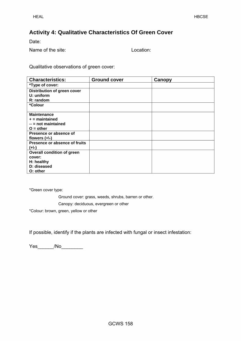
HEAL HBCSE

Activity 4: Qualitative Characteristics Of Green Cover Date:

Name of the site: Location: Qualitative observations of green cover:

Characteristics: Ground cover Canopy *Type of cover: Distribution of green cover U: uniform R: random

*Colour

Maintenance + = maintained -- = not maintained O = other

Presence or absence of flowers (+\-)

Presence or absence of fruits (+\-)

Overall condition of green cover: H: healthy D: diseased O: other

*Green cover type:

Ground cover: grass, weeds, shrubs, barren or other.

Canopy: deciduous, evergreen or other

*Colour: brown, green, yellow or other

If possible, identify if the plants are infected with fungal or insect infestation:

Yes______/No________

GCWS 158

HEAL HBCSE

GCWS 159

Final Green - Cover Data Sheet: Date: Site details:

Green cover characteristics

Observations

MUC class

Dominant species

Co-dominant species

% Canopy cover

% Ground cover

Average tree circumference (cms) (of at least two dominant/co-dominant species) (i) (ii)

Average tree height (cms) (of at least two dominant/ co-dominant species)(i) (ii)

Grass biomass

HEAL HBCSE

‘Waste’ watch…

for good health

INTRODUCTION: Rapid urbanization and industrialization, combined with increasing population,

has resulted in generation of large volumes of waste, both liquid and solid.

The situation is further aggravated by our consumerist lifestyles, scarcity of

dumping grounds and fast filling up of these dumping sites in urban areas.

These sites with limited land area cannot accommodate the increasing

volumes of waste. Further, unscientific management of waste poses threats to

health and environment. All developing societies need regulations and strict

implementation for scientific disposal of their wastes. Practicing the concept,

‘Reduce, reuse and recycle’ will go a long way in managing our waste, without

compromising on the development process.

Manufacturing practices, in all fields, demand that the inventors /

manufacturers are made ‘liable’ / responsible for their products. This would

include: chemicals of all types, including cosmetics, textiles, electronics,

automobiles, paper and food industry. The final products should not be solely

judged by their uses or profits earned. Attempts should also be made to

check out the waste generated by the manufacturing process of this product

or its byproducts/ residues. In turn, these should not pose any threat to the

environment in their destruction /degradation. There is an urgent need to

introduce and implement the concept of “Polluters Pay” in the country.

There are a variety of industries (metals, chemical and dyes, cement,

fertilisers, leather, distilleries, sugar, pharmaceuticals, paper pulp, etc), with

each having a specific type of waste, and requiring special treatment and

disposal methods. This topic is complex and requires detailed study in the

country. An effective watchdog body is the need of the hour. There is also an

urgent need for different groups – government, industries, scientists,

engineers and consumers-- to work together to minimize pollution without

affecting development in the country. In one such move, the ‘Ecomark’

WMT 160

HEAL HBCSE

scheme of the Government of India formulated in 1991, classifies different

consumer items according to their impact on environment. The different

criteria for obtaining an ecomark rests on the basic concept of cradle-to-grave

approach, i.e., the environmental impact of the product, right from raw

material extraction, its manufacturing to its final disposal. In recent years,

many more schemes have evolved to keep a check on industries, but much

more needs to be done. Unfortunately, sufficient attention has not been given

to the scientific management of waste, both in urban and rural areas. We are

ignoring this problem at a great risk to our health.

Liquid waste: Large volumes of liquid waste are primarily contributed by untreated sewage,

agricultural run-off and industrial liquid discharges. Often these are released

directly into rivers, creeks or nallahs, or even in storm water drains meant for

carrying rain water, which finally empty into seas or bigger rivers or lakes,

causing serious problems of water pollution. This also causes serious

degradation of water bodies thereby changing the water or shore ecology.

These effluents may also gain entry into the drinking water supply pipes

leading to health hazards. Along with a heavy load of disease causing

microorganisms (pathogens), these liquid wastes often contain high

concentrations of nitrogen and phosphates causing excessive growth of algae

and weeds. These produce characteristic bad odours. These wastes\effluents

also contain harmful toxins, which can permeate into the soil and the air

causing pollution.

Solid waste: Solid waste is commonly classified as dry, wet and medical. Materials like

paper, plastics, glass, rubber, metals, packing materials, cloth and polythene

bags form a large proportion of dry waste. These are not easily degraded in

the soil. In fact, the time taken for degeneration\breakdown of each type of

waste varies from a few days to several years.

WMT 161

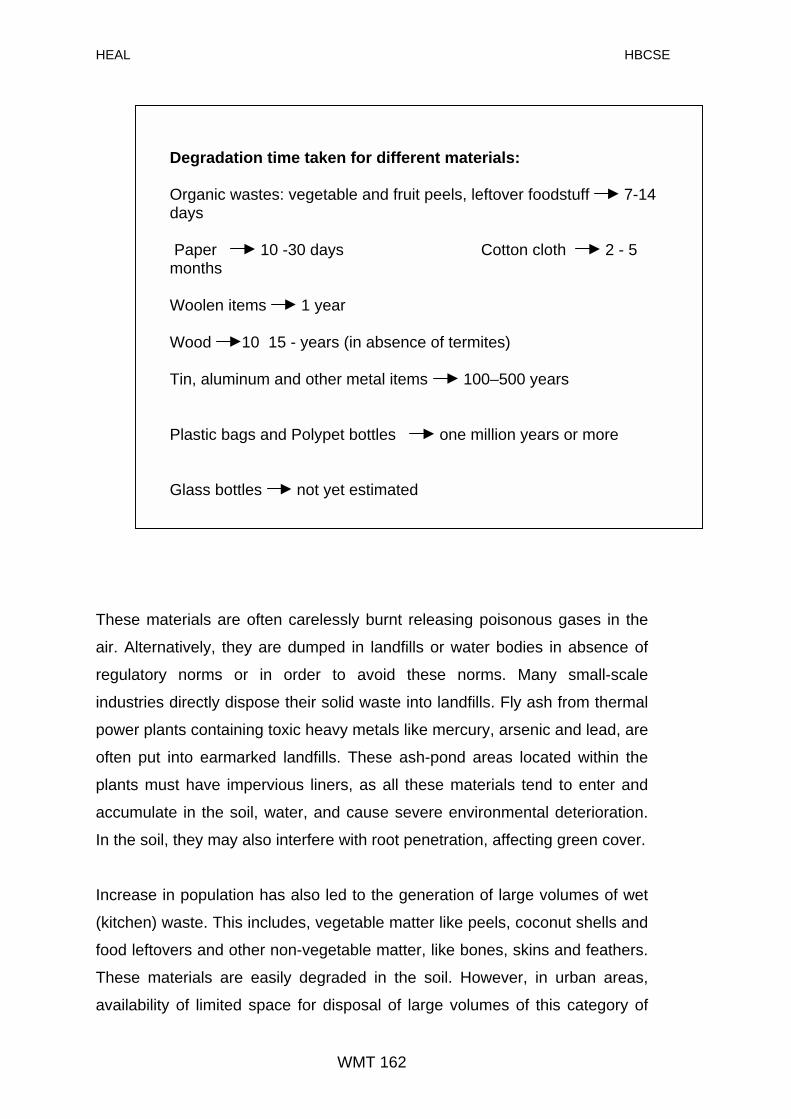
HEAL HBCSE

Degradation time taken for different materials:

Organic wastes: vegetable and fruit peels, leftover foodstuff 7-14 days

Paper 10 -30 days Cotton cloth 2 - 5 months

Woolen items 1 year

Wood 10 15 - years (in absence of termites)

Tin, aluminum and other metal items 100–500 years

Plastic bags and Polypet bottles one million years or more

Glass bottles not yet estimated

These materials are often carelessly burnt releasing poisonous gases in the

air. Alternatively, they are dumped in landfills or water bodies in absence of

regulatory norms or in order to avoid these norms. Many small-scale

industries directly dispose their solid waste into landfills. Fly ash from thermal

power plants containing toxic heavy metals like mercury, arsenic and lead, are

often put into earmarked landfills. These ash-pond areas located within the

plants must have impervious liners, as all these materials tend to enter and

accumulate in the soil, water, and cause severe environmental deterioration.

In the soil, they may also interfere with root penetration, affecting green cover.

Increase in population has also led to the generation of large volumes of wet

(kitchen) waste. This includes, vegetable matter like peels, coconut shells and

food leftovers and other non-vegetable matter, like bones, skins and feathers.

These materials are easily degraded in the soil. However, in urban areas,

availability of limited space for disposal of large volumes of this category of

WMT 162

HEAL HBCSE

waste poses problems. In turn, it raises new problem of pests (like

mosquitoes, rats, pigs and stray dogs) in our society. People will have to

come up with ingenious solutions for managing wet waste too. Among other

options, those of vermiculture or production of fuel from wet waste are also

being explored.

Another option being recommended for easing the problem of waste from

plants and animals (like animal dung, wet and agriculture waste) in the

country to some extent is conversion of solid waste into energy. This would

require examining the different materials for their energy potential (calorific

values).

Medical wastes like cotton, bandages, syringes, needles, invasive instruments

like those used by dentists and surgeons and biological materials (organs,

tissues, etc) need careful handling and disposal. Medical waste should not be

mixed with other categories of waste; each of the above wastes needs special

treatment before disposal. Sanitary napkins and the so-called disposable

diapers pose a new set of problems, since they are not biodegradable. In this

program, only certain aspects of solid waste disposal will be taken up via

activities. With proper understanding of issues involved, one can design a

series of activities for better understanding of waste management.

Dirty environment around spots of collected garbage and stagnant/still pools

of water provide an excellent breeding ground for a host of pathogens, insects

(mosquitoes) and animals like rats and stray dogs. These are vectors for

spread of communicable diseases. For example, rats are vectors for

leptospirosis, typhus and plague; infected stray dogs carry the rabies virus in

their saliva; malaria and dengue are caused by parasites spread by

mosquitoes.

In our battle against diseases, it is important to have a scientific

understanding of different causative agents of diseases, their vectors and the

places where they live and multiply. For instance, a single female mosquito

WMT 163

HEAL HBCSE

lays about 100 eggs in a stagnant pool of water, which, in turn, develop into

100 adult mosquitoes, which may spread malaria.

Hence, the best way to prevent the spread of communicable diseases,

including insect-borne diseases, is by keeping the environment clean and

reducing the number of breeding places. Insecticides and other pesticides are

short-term remedies. A few activities are planned to bring out the linkages

between dirty environment and these diseases.

Experimental Procedures: TYPE OF SOLID WASTE GENERATED (+ PRESENT /-- ABSENT): Activity 1

1. Identify different types of waste generated in your home.

2. Suggest methods for their disposal.

3. Note the observations in Waste Management Worksheet--Activity 1.

4. Based on this survey, extend these observations to what must be

happening at a larger scale in the entire sector/node/city.

5. Fill out the observations in Waste Management Worksheet--Activity 1.

WASTE SEGREGATION IN MEDICAL SET UPS: Activity 2

1. In the selected area/sector, count the number of health care centers.

Or, the number of dispensaries/ hospitals, both private and public.

2. Check out if the waste is being segregated or not in these places. Fill

out the details in waste management worksheet [WMW: Activity 2 ].

WASTE COLLECTION AT DIFFERENT SITES: Activity 3 (i)

1. Roughly estimate the area in square metres of the study site.

2. Check for the presence or absence of waste collection bins.

3. Count the number of bins in the area.

WMT 164

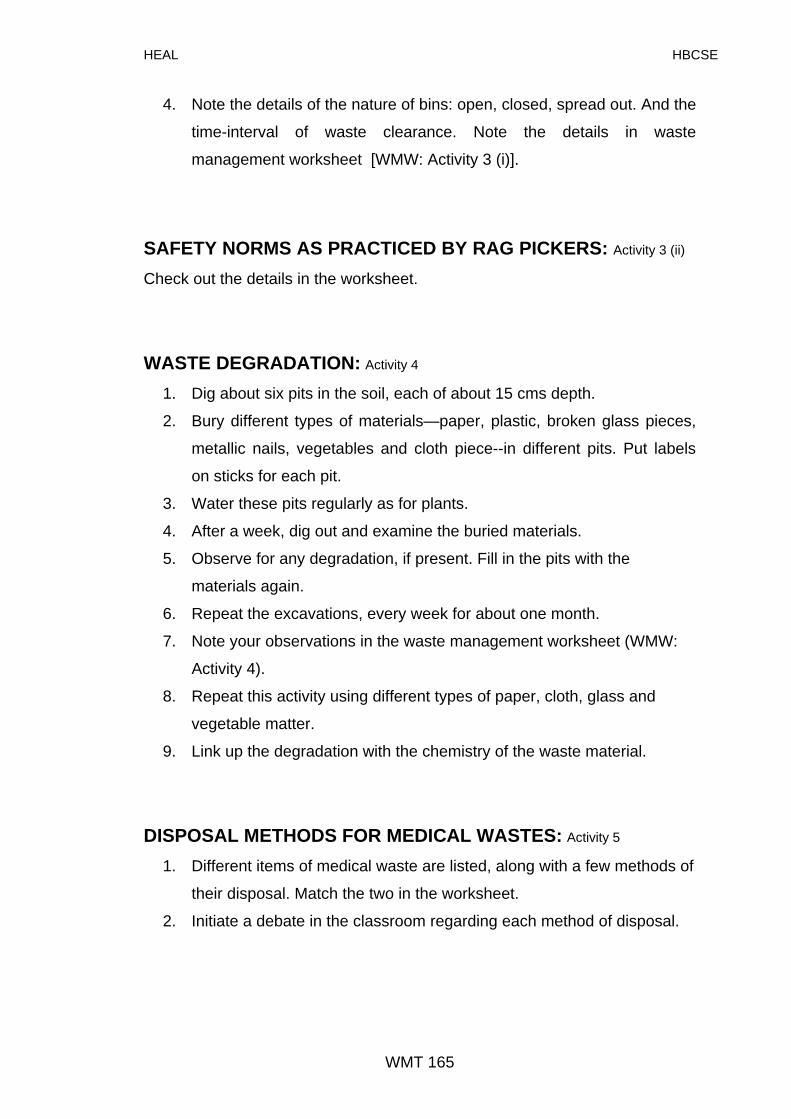
HEAL HBCSE

4. Note the details of the nature of bins: open, closed, spread out. And the

time-interval of waste clearance. Note the details in waste

management worksheet [WMW: Activity 3 (i)].

SAFETY NORMS AS PRACTICED BY RAG PICKERS: Activity 3 (ii)

Check out the details in the worksheet.

WASTE DEGRADATION: Activity 4

1. Dig about six pits in the soil, each of about 15 cms depth. 2. Bury different types of materials—paper, plastic, broken glass pieces,

metallic nails, vegetables and cloth piece--in different pits. Put labels

on sticks for each pit. 3. Water these pits regularly as for plants. 4. After a week, dig out and examine the buried materials. 5. Observe for any degradation, if present. Fill in the pits with the

materials again. 6. Repeat the excavations, every week for about one month. 7. Note your observations in the waste management worksheet (WMW:

Activity 4). 8. Repeat this activity using different types of paper, cloth, glass and

vegetable matter. 9. Link up the degradation with the chemistry of the waste material.

DISPOSAL METHODS FOR MEDICAL WASTES: Activity 5

1. Different items of medical waste are listed, along with a few methods of

their disposal. Match the two in the worksheet.

2. Initiate a debate in the classroom regarding each method of disposal.

WMT 165

HEAL HBCSE

WMT 166

SITE OBSERVATION FOR WASTE DUMPS AND PESTS: Activity 6

1. In the selected site, observe for open nallahs, sewers, stray dogs, rats

and garbage collection points and dumping sites.

2. Try to trace the entire chain of garbage—right from the point of

generation to its final disposal, including segregation, if practiced.

Note: The experiments and observations outlined here mostly refer to solid

waste generated by citizens. At a later stage, students can also try to find out

the following:

(i) Trace the path of liquid and solid domestic waste right from

the point of its origins\generation (at homes, etc) to the final

disposal points.

(ii) Map the sewerage system in the area.

(iii) Map the storm-water drainage system in the area.

(iv) Find out the variety of solid and liquid wastes generated by

different industries in your area. (Do not miss out on small

/unorganized industries.)

(v) If possible, find out if proper pollution control measures—for

air, water and solid are being adopted by these industries.

(vi) Based on the type of population in an area, the amount and

the kind of waste vary. Consider that per capita waste

generated per day is: 0.1 kg in slums, 0.5 kg in middle class

areas, and 1 to 1.5 kg in elitist areas. Survey some sites and

verify the above amounts.

(vii) Have you heard about the Advanced Locality Management

(ALM) in Mumbai? Work towards the formation of ALM in

Navi Mumbai.

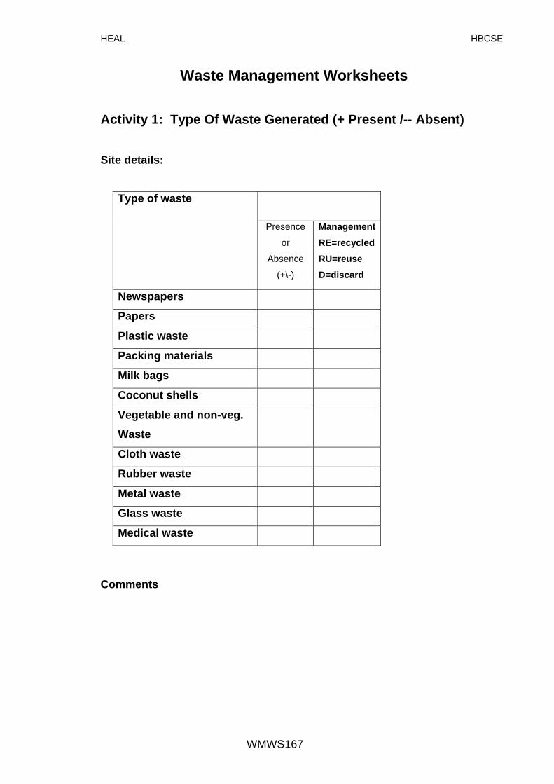
HEAL HBCSE

Waste Management Worksheets

Activity 1: Type Of Waste Generated (+ Present /-- Absent) Site details:

Type of waste

Presence

or

Absence

(+\-)

ManagementRE=recycled RU=reuse D=discard

Newspapers

Papers

Plastic waste

Packing materials

Milk bags

Coconut shells

Vegetable and non-veg. Waste

Cloth waste

Rubber waste

Metal waste

Glass waste

Medical waste

Comments

WMWS 167

HEAL HBCSE

Activity 2: Waste Segregation In Medical Set-Ups Total number of:

Public Private

Name of site

Hos

pita

ls

Dis

pens

arie

s

Hos

pita

ls

Dis

pens

arie

s

Name of dispensary/hospital

Was

te s

egre

gatio

n

(+/_

)

Activity 3 (I): Waste Collection At Different Sites Site details:

Description of site area Characteristics Residential Industrial Commercial

Approximate area in sq. mts.

Presence or absence of waste bins (+/-) No. of bins

Nature of the bins: open/closed/spread out

Time interval of waste clearance

Type of waste: Wet/Dry/Medical/Mixed

Waste management: Segregated/ non-segregated

WMWS 168

HEAL HBCSE

Activity 3 (Ii): Safety Norms As Practiced By Rag Pickers

No. of

rag pickers

Type of

protective gear

Working

with:

Site details

Adult Child

Mal

e

Fem

ale

Mal

e

Fem

ale

Glo

ves

Mas

ks

Shoe

s

Han

ds

Tool

s

Activity 4: Waste Degradation

Degree of degradation Initiation—(+); Intermediate — (++); Complete — (+++); Absent — (--)

Type of materials

Week 1 Week 2 Week 3 Week 4Paper

Plastic bags

Metal nails

Glass pieces

Cloth

Vegetable matter

WMWS 169

HEAL HBCSE

WMWS 170

Activity 5: Disposal Methods For Medical Wastes. Match the different waste materials to the methods of disposal listed below

the table.

Different materials

Method of disposal

Invasive surgical instruments Syringes: plastic and glass Used cotton and bandages Biological materials Needles Plastic saline and blood bags Expired medicines

Methods of disposal: Incineration, autoclave, dumping, exposure to low temperatures, dismantling, brushing and disinfection, boiling, breaking. *In some cases, more than one method may be used. Activity 6: Site Observation For Waste Dumps And Pests Numbers of: Presence

or Absence

(+/-)

Sr. No.

Site name

Ope

n ga

rbag

e co

llect

ion

poin

ts

Ope

n nu

llahs

Ope

n se

wer

s

Dum

ping

site

s

Stra

y do

gs

Rat

s

HEAL HBCSE

‘Health’ watch…

for good health

INTRODUCTION: The subject of "health" is of concern to all. Several strategies are adopted from

time to time, both at the global and national levels, to promote health. Advances

in sciences, especially biological sciences, have created a new awareness

about health at the global level, and the focus has clearly shifted from clinical

and curative approach to one encompassing preventive and sociological

aspects.

An important aspect of our education at the college and school level is to make

students aware of the various scientific concepts concerning health and the

close linkages between our environment and health. This is particularly

important in India since our record in the control of diseases (especially

communicable and environment related diseases, and in improving nutrition)

has been unimpressive. In indices like child-mortality, we rank with the least

developed countries. The DALY loss (DALY=Disability-Adjusted Life Years is a

global unit which measures productivity losses due to morbidity, including

injuries and illnesses, and mortality due to premature deaths) in India caused by

communicable diseases is high even among the developing countries of the

world. Variety of gastro-intestinal infections, respiratory diseases, including

tuberculosis and pneumonia, malaria, dengue and several other insect-borne

diseases continue to claim millions of lives every year. Globally, our health

status, especially with respect to the incidence of the above-mentioned

diseases, ranks next only to sub-Saharan African countries. China, which has a

greater population than that of India, and nearly comparable incomes (GNP),

has achieved a remarkable degree of progress in the control of communicable

diseases. (Refer DALY chart– Appendix 6).

A major factor for this seems to be insufficient awareness among our masses,

including the educated, as to how the policies and practices based on relevant

scientific knowledge have been used by other countries to improve their health

HT 171

HEAL HBCSE

standards during the last century. Sensitising the next generation to important

health and environment issues is essential to improve our standards of hygiene

and public health measures. This would include improving the quality of our air,

water and soil, including, sanitation and scientific management of waste,

housing for the poor and other related aspects.

In recent years, contrary to adopting a holistic and preventive approach to

health, there has been a heavy reliance on curative aspects of health. The

preventive approach to environmental health becomes more relevant, since

the health and urban planners and policy makers have recognised that health

cannot be divorced from environmental and social factors. J.M. Last (1983), a

pioneering epidemiologist, in the Oxford Dictionary of Epidemiology, describes

three distinct levels of prevention: (i) Primary prevention is defined as the

promotion of health by personal and community efforts; (ii) Secondary

prevention is defined as measures available to individuals and populations for

the early detection and prompt effective intervention to correct treatment; (iii)

Tertiary prevention consists of measures available to reduce impairments and

disabilities, minimize suffering caused by existing departures from health.

With this background information, it is apparent that health of a population or

society, as influenced by environment, is a complex concept to monitor.

Besides causing deaths, the different environmental agents can cause

sickness and variety of diseases. These diseases may occur immediately on

exposure to these agents, within a few minutes, hours or a few days, as in the

case of several gastro-intestinal problems and some respiratory infections.

Alternatively, diseases due to polluted environment may show up only after a

long time, as in several cardio-vascular problems and cancers of skin, blood

and lungs.

Incidence of only certain environment-related diseases and their

accompanying symptoms occurring over short time periods will be considered

in this programme. There will be survey-based activities, wherein students

will be approaching medical set ups, both in private and public sectors, to

collect data about the presence or absence of specific diseases. This is a

HT 172

HEAL HBCSE

‘passive’ approach of data collection. Students will also be conducting ‘active’

door-to-door surveys about the symptoms (diseases). To further validate their

findings, students will also collect data of the above plus the mortality (deaths)

due to these diseases from their local municipalities. Besides the absence or

presence of diseases, and their symptoms, the data will include mortality

caused by these diseases.

Malaria remains one of the biggest killers in our country, perhaps next only to

tuberculosis. This disease also causes great economic loss in the country as

millions, especially the young and employed, get affected. The parasite,

Plasmodium, causes the disease, and these parasites complete their

complicated life cycles in two hosts: the mosquitoes and a mammal, which

can be humans or cattle. Female mosquitoes of the genus, Anopheles,

transmit the parasite (disease) by biting the mammal when sucking the blood

meal. Simultaneously, the parasites are released in the blood stream.

Malaria, among other vector-borne diseases, has been singled out here for

three reasons: its origins lie in wet tropics (often unhygienic environment), the

disease has staged a comeback in recent years in several parts of the country

and its spread is accelerated by continuing migrations of peoples from

endemic to non endemic areas. The incidence of malaria will increase greatly

in the future as more and more people from villages migrate to urban areas

and then again travel to rural areas, and also due to disturbed ecology.

However, the disease has been nearly wiped out in several tropical countries

by adoption of stringent water management techniques, including removal of

all potential breeding places of the mosquito. This has been done with active

co-operation of the people and educational advisories.

Let us prevent mosquito-borne diseases, like malaria. Let us be active partnrs

in the “Roll back malaria” project of the World Health Organisation, which

aims by 2010 to reduce the number of malaria cases. On one hand, scientists

all over the world are working on different strategies, including several

molecular approaches, to kill the parasites in the blood stream; on the other

HT 173

HEAL HBCSE

hand, public health experts advocate tracking of mosquitoes, and other

methods for eradicating mosquitoes.

Malaria Research Centre, Delhi, has categorized malaria into five types, all

due to human activities: (i) disturbed ecology in forest areas leads to tribal

malaria; (ii) irrigation malaria strikes in areas with irrigation projects; (iii) urban

malaria occurs due to presence of stagnant pools of water providing breeding

places for mosquitoes; (iv) industrial malaria has rendered areas of the

Punjab and Harayana endemic to the disease; (v) migration malaria occurs

when there is large scale migration of people from endemic to non endemic

areas. In reality, there may be a combination of factors leading to the spread

of this disease. For instance, both migration and breeding places in urban

areas (like Mumbai and Navi Mumbai) may lead to endemicity of the disease.

This understanding should help in working out the few activities for malaria.

Equipped with two data sets, one of environment indicators and the other

about health, students can search for correlations between the two, if

possible. In addition, urban and rural profiles, both for environment and

health, could also be prepared.

Focused programs on health and environment education are an important

intervention, with student body playing a pivotal role in imparting and

promoting scientific understanding about close linkages between health and

environment.

SITE SELECTION: The area for study could be a municipal ward, city, city-nodes or even a group

of streets. In addition, health surveys need to be also carried out in rural

areas. However, the chosen area for survey of health indicators should be the

same as the one studied for different environmental indicators. The sampling

should be representative of the entire study area, as shown in the figure.

HT 174

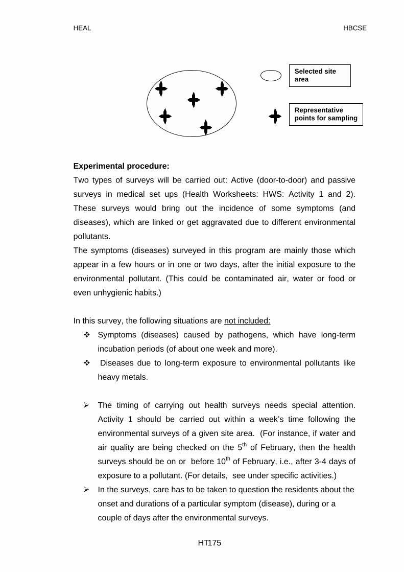
HEAL HBCSE

Representative points for sampling

Selected site area

Experimental procedure: Two types of surveys will be carried out: Active (door-to-door) and passive

surveys in medical set ups (Health Worksheets: HWS: Activity 1 and 2).

These surveys would bring out the incidence of some symptoms (and

diseases), which are linked or get aggravated due to different environmental

pollutants.

The symptoms (diseases) surveyed in this program are mainly those which

appear in a few hours or in one or two days, after the initial exposure to the

environmental pollutant. (This could be contaminated air, water or food or

even unhygienic habits.)

In this survey, the following situations are not included:

! Symptoms (diseases) caused by pathogens, which have long-term

incubation periods (of about one week and more).

! Diseases due to long-term exposure to environmental pollutants like

heavy metals.

# The timing of carrying out health surveys needs special attention.

Activity 1 should be carried out within a week’s time following the

environmental surveys of a given site area. (For instance, if water and

air quality are being checked on the 5th of February, then the health

surveys should be on or before 10th of February, i.e., after 3-4 days of

exposure to a pollutant. (For details, see under specific activities.)

# In the surveys, care has to be taken to question the residents about the

onset and durations of a particular symptom (disease), during or a

couple of days after the environmental surveys.

HT 175

HEAL HBCSE

# Some preplanning would be needed for selection of medical set-ups for

Activity 2. The set ups should be those frequented by the participating

residents of Active survey (1). This information is also obtained from

the Active survey itself. (The Health Dept. of Municipality will be

requesting the doctors for cooperation in this study.) # A copy of the data sheet (HWS: Activity 2) will also be filled out by the

doctors, to validate the findings of the students. This data sheet is

identical to the one used in Activity 1. # Another level of validation will be made from the data obtained from the

Health Dept. of the local municipality.

ACTIVE SURVEY: Activity 1

1.

2.

3.

4.

5.

6.

7.

For this survey, students will have to work in groups of two’s or three’s.

Study well the survey sheets, before approaching any household.

The methodology of active survey involves visiting representative

individual households in the study area (figure1).

In the worksheet, first enter the details of the address of the house.

This will be the key no. to identify the surveyed resident. The key

number should include: sector details, building number, flat number,

and the number of family members. (Sec\Bldg no.\Flat no.\No. of

members---9\JN1\42\4. ) Alternatively, make your own key for correct

identification of residence.

Briefly, explain the purpose of the survey to the householder.

Obtain the no. of family members and their approximate ages.

Find out how many are/were affected with any of the listed

symptoms\diseases since the week before the house visit.

8.

9.

Next, note the symptoms and other related information, such as the

date of onset, duration, treatment (yes/no) and outcome of treatment

(recovered, still sick, etc) in the health work sheet (HWS: 1).

Make a provisional diagnosis, if possible, from the symptoms. An

educated householder could also make this diagnosis.

HT 176

HEAL HBCSE

10.

11.

1.

Information about the doctor visited by the affected is essential. This

entry should guide the students correctly to the doctors\medical set ups

to be approached for carrying out the passive survey.

The same work sheet as used in active survey is issued to the doctors

for entry. Fill out the details in the HWS: Activity 1.

This active door-to-door survey can provide accurate information about the

health profile of individuals surveyed. This has to be carried out both in urban

and rural areas.

PASSIVE SURVEY: Activity 2

The door-to-door survey is further supported / validated by Activity 2, taken

from medical set ups. The data worksheet (activity 2) should be given to the doctors right on

the first day of the survey when the env. study is started. Groups of two

to three students will visit the out-patient departments (OPDs) of public

hospitals and spend 1-2 days with the concerned doctors. Alternatively,

private doctors may also be contacted.

2.

3.

4.

5.

Students may also have to visit the doctors on the last two days of the

survey, after identifying the different medical set ups frequented by the

people of the study site {obtained from Activity 1 (i)}.

Care should be exercised when choosing the medical set ups. These

set ups should be frequented by those people in the area, where the

environmental data has been simultaneously collected. In other words,

the people covered in the Active Survey—Activity 1 (i) —should have

visited these medical set-ups.

Accordingly, decide on the public and private medical setups from

where the health data will be obtained. This may require some prior

planning, preparation and permission of the Dean/Doctors by your

teachers/ Municipalities.

With the help of the doctor, students will be filling out the work sheet.

This worksheet is the same one as used in Activity 1 (i).

HT 177

HEAL HBCSE

(HWS: Activity 2 ).

6.

7.

8.

Along with patient details (key no), age and sex, symptoms, provisional

diagnosis of different diseases, under the category of gastro intestinal

(GI), respiratory diseases (RD) and vector borne diseases (VBD) will

be entered by the doctor as per visits of patients.

Collect data of any deaths (mortality) for the listed diseases for the

survey period (check the dates).

Local municipal public health department or ward office may also be

approached for this.

MALARIA AND INSECT BORNE DISEASES: Activity 3 to 7

In recent years, malaria (and other vector-borne diseases, such as dengue)

has staged a comeback in the country, including in Navi Mumbai and Mumbai,

due to a variety of reasons. Some of these are: the resistance developed by

the parasites against various anti-malarial drugs, emergence of insecticide-

resistant mosquitoes, reduction in the use of DDT, and a casual attitude of the

populace to dirty environment. The disease spread is further accelerated by

continuing migrations (movements) of peoples from endemic to non endemic

areas and vice versa.

A few activities are included to give a scientific understanding about the

spread of the disease: how the mosquitoes multiply, i.e., their life cycle, their

potential breeding places, and mapping these places.

It is important to remember that mosquito breeding is seasonal, with increase

in numbers observed during the winter months. This point is to be

remembered when checking for the potential breeding places. The same

place may give varied results at different times so the year. The real solution

to the problem is removal of these potential breeding places.

HT 178

HEAL HBCSE

LIFE CYCLE OF MOSQUITOES: Activity 3

Experimental procedure:

1.

2.

3.

4.

5.

6.

7.

8.

9.

10.

Get blood fed female mosquitoes (when you see a mosquito, catch it

with a test tube). Turgid and dark abdomen is an indication of blood fed

females (gravid).

Once a gravid female is caught with the test-tube, transfer it to a bottle

containing dilute yeast solution, preferably 100 ml of 0.1% yeast

solution (about two to three yeast granules in 100 ml of water). Yeast

serves as a source of food for emerging larval stages.

Cover the bottle with a net or thin muslin cloth.

Within two to three days, the females will lay eggs in the form of a raft.

One female can lay more than one egg raft. (The time taken by

females to lay eggs is variable, depending on seasons and salinity of

water. In winter months, egg-laying may be after four to six days after

capture in the bottle. Factors like humidity and temperature affect the

ovi-position and the survival of larvae and pupae.) Eggs may be very

tiny if the females are not well fed.

Each egg raft contains about 50 to 400 eggs. Transfer the egg rafts in

a shallow tray of water + yeast. Keep the tray open.

Four different larval stages will emerge. This development period takes

about 10-12 days. First instar larvae: 24-28 hrs; second instar larvae:

26- 32 hrs; third instar larvae: 28-35 hrs and the fourth instar larvae:

52-68 hrs.

In this above period, change the tray water by carefully transferring the

larvae back and forth (with a dropper, pick up the larvae and transfer

them into a bottle containing little water.) Remember to add the yeast in

proper concentration in the fresh water.

Transfer the larvae back into the tray.

Pupal stage will emerge from the moulting of the fourth larval instar.

Pupae are comma shaped. (One pupa from one larvae)

Pupae are non feeding and this is a short transient phase of about 1-3

days. (Males emerge in one day and females later.)

HT 179

HEAL HBCSE

11.

12.

13.

Once the pupae emerge in the tray, transfer them with a dropper in a

bottle containing water and cover the bottle.

Mosquitoes will emerge from the pupae after about 30—35 hours.

Generally, one female gives rise to an egg raft of about 100 eggs, 100

larvae, 100 pupae, and 100 adults.

Based on your observations, draw the complete life cycle of a

mosquito, with figures and appropriate labels (HWS: Activity 3).

In our region, there are three major types of mosquitoes: Anopheles causing

malaria, Aedes (aegypti) causing dengue and Culex forms, which are mostly

nuisance mosquitoes. The accompanying figure brings out the major

differences between anopheline and culicine life cycles.

Life cycles of mosquitoes

HT 180

HEAL HBCSE

POTENTIAL BREEDING PLACES OF MOSQUITOES: Activity 4

Mosquitoes live and multiply (breed) in a variety of places, especially places,

which hold water. These range from still—stagnant-- pools of clean water,

slow (sluggish) moving streams and edges of water holding places, water

drums, old tyres or any containers which could hold some water, even tree

holes. The rate of multiplication of mosquitoes differs in different seasons,

depending on temperatures and the availability of breeding places. Hence, the

breeding potential, active breeding and density of larvae is constantly

fluctuating. But it is important that one becomes aware about these breeding

places. Elimination of these places could go a long way in our fight against

malaria and other vector-borne diseases, including dengue. Mosquitoes travel

long distances and travel in lifts, too!

Experimental protocol: 1.

2.

3.

4.

5.

This survey too, has to be conducted during Activity 1.

Take a rough survey of the study site.

Try to identify the potential breeding places of mosquitoes in and

around houses in the selected site. Check out different items and

places, howsoever insignificant they might appear.

These data could be obtained when students are checking up for

symptom surveillance {Activity 1 (i)}. Residents could be specifically

asked for the absence or presence of different items, as listed in

Activity 4 (i).

Try to cursorily check for at least one or two potential breeding places

in homes. Students could request to see vases, tanks, pots, etc, as

listed in HWS: Activity sheet 4 (i).

6.

7.

Check for the presence of mosquito larvae.

Next, check around the homes for potential mosquito breeding places

as listed in Activity 4 (ii).

8.

9.

Make your observations in Activity 4 (ii).

Note the action suggested /taken on identification of a breeding

place—HWS: Activity 4 (I and ii).

HT 181

HEAL HBCSE

MOSQUITO LARVAL SURVEY: Activity 5

Different breeding places of mosquitoes have already been identified. For

mosquito larval surveys, there is a method for collecting water samples.

Collect the larvae with a pipette (fixed to a teat/ rubber bulb). Transfer the

larvae to clear bottles and observe them.

Alternatively, use a dipper, which is like a saucepan with a long handle.

Hold the dipper at an angle of 450 and gently lower it just below the water

surface. Allow water to flow into the dipper along with larvae/pupae.

When one is collecting the water sample from a place with dense

vegetation or floating debris, first disturb the water surface with the dipper.

This causes the larvae and pupae to slightly sink below the surface. Clear

all the debris\ vegetation with the dipper. Slowly the larvae will resurface. At

that time, collect these larvae along with the water sample with a smooth

long sweep of your hand.

HT 182

HEAL HBCSE

Experimental procedure: Collect water samples from some of the potential breeding places, identified in

Activity 4 (i) and (ii). Fill out the worksheet (HWS: Activity 5).

MAPPING THE BREEDING PLACES OF MOSQUITOES: Activity 6

It is important to know and have a pictorial representation of the areas where

mosquitoes breed. This can lead to elimination of these breeding places by

public health officials and by citizens’ involvement, too. At some places,

remote sensing techniques are employed to track the breeding sites. Later

computers interpret these images as maps with colours.

Here an attempt will be made to ‘map’ the study site and locate the breeding

sites.

Experimental procedure:

1.

2.

3.

4.

5.

6.

7.

8.

Get a rough estimate about the dimensions (length, overall area) of the

study site in metres. Refer to the maps of your city/node/district.

Say, a street , circular or linear, of about 30 square metres is the study

site.

Locate a few landmarks, and the four directions (N, S, E, W). Map the

study site by using an appropriate scale (say, 1 cm square = 1 metre).

Indicate the scale on the face of the map as a line –scale.

Draw the study site with reference marks and directions.

Locate (at least ten) larvae breeding points on the scaled up map. Use

appropriate symbols for the landmarks, breeding places and other

relevant details.

Label and indicate the symbols on the face of the map.

These breeding points could be shallow pits, old tires in a side street,

or construction sites (HWS: Activity 4).

Use fresh worksheets if uncomfortable with the small boxes (Activity 6).

HT 183

HEAL HBCSE

HT 184

SUPERIMPOSING THE DATA OF MOSQUITO BREEDING PLACES AND DISEASE INCIDENCE: Activity 7 Here an attempt is made to establish the burden of one communicable vector-

borne disease, i.e., malaria, in a given area. This involves: (i) identifying and

plotting the distribution of vector breeding points and (ii) confirmed (incidence)

cases of malaria in a given area, and superimposing these two sets of data.

This should bring out the correlation, if any, between disease incidence and

the prevailing environment (mosquito breeding spots).

Experimental procedure:

1. Refer to the number of people affected with malaria (positive cases)

and the location of their residences (Activity 6).

2. Data about mosquito breeding places are also obtained (Activity 4 (i

and ii).

3. Plot the data about malaria incidence on a map of the area.

4. Superimpose (overlay) the two maps –breeding sites and disease

incidence—over each other. Check for correlation between the two.

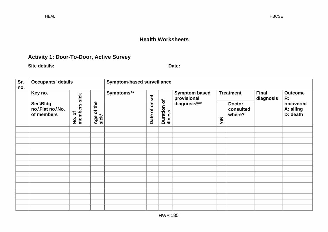
HEAL HBCSE

Health Worksheets

Activity 1: Door-To-Door, Active Survey Site details: Date:

Sr. no.

Occupants’ details Symptom-based surveillance

Treatment Key no. Sec\Bldg no.\Flat no.\No. of members

No.

of

mem

bers

sic

k

Age

of t

he

sick

* Symptoms**

Dat

e of

ons

et

Dur

atio

n of

ill

ness

Symptom based provisional diagnosis***

Y\N

Doctor consulted where?

Final diagnosis

Outcome R: recovered A: ailing D: death

HWS 185

HEAL HBCSE

Symptoms** Fever Head ache Vomiting Loose motions Stomach ache \ cramps Watery stools Mild diarrhoea Black stools with mucous Nausea Yellowish discolouration of urine\sclera Head ache Skin rash/ itching Watering/irritation/redness of eyes Loss of sleep Cough and cold Breathlessness Giddiness

2&3

1

Provisional diagnosis:*** 1

Acute diarrhoea Acute gastro enteritis (including cholera) Hepatitis A\E Entric fever (typhoid)

2 Upper respiratory tract infections (URTI) Acute tonsillitis Acute pharyngitis Rhinitis

3 Lower respiratory tract infections (LRTI) Pneumonia

Code* Age (in years) A At birth

B 0-5

C 5-14

D 14-30

E 30-60

F 60-80

G 80+

Chest pain

Fever Fatigue/malaise Chills/shivering Body pains Loss of weight/appetite

Dog/Rat bites Talking loudly, ringing in the ears, unable to hear specific sounds like S, Ch /Others

4

Pulmonary tuberculosis Environmental asthma Allergic dermatitis

4 Malaria, Dengue Insect/Rabies/Dog bites

Noise induced hearing loss Others

HWS 186

HEAL HBCSE

Activity 2: Passive Survey At Medical Set Ups Site details: Date:

Sr. no.

Occupants’ details Symptom-based surveillance

Treatment Key no. Sec\Bldg no.\Flat no.\No. of members

No.

of

mem

bers

sic

k

Age

of t

he

sick

*

Symptoms**

Dat

e of

ons

et

Dur

atio

n of

ill

ness

Symptom based provisional diagnosis***

Y\N

Doctor consulted where?

Final diagnosis

Outcome R: recovered A: ailing D: death

HWS 187

HEAL HBCSE

Symptoms** Fever Head ache Vomiting Loose motions Stomach ache \ cramps Watery stools Mild diarrhoea Black stools with mucous Nausea Yellowish discolouration of urine\sclera Head ache Skin rash/ itching Watering/irritation/redness of eyes Loss of sleep Cough and cold Breathlessness Giddiness Chest pain

Fever Fatigue/malaise Chills/shivering Body pains Loss of weight/appetite

Dog/Rat bites Talking loudly, ringing in the ears, unable to hesounds like S, Ch /Others

1

2

Provisional diagnosis:*** 1

Acute diarrhoea Acute gastro enteritis (including cholera) Hepatitis A\E Entric fever (typhoid)

2 Upper respiratory tract infections (URTI) Acute tonsillitis Acute pharyngitis Rhinitis

3

Code* Age (in years) A At birth

B 0-5

C 5-14

D 14-30

E 30-60

F 60-80

G 80+

ar specific

&3

4

Lower respiratory tract infections (LRTI) Pneumonia Pulmonary tuberculosis Environmental asthma Allergic dermatitis

4 Malaria, Dengue Insect/Rabies/Dog bites

Noise induced hearing loss

Others

HWS 188

HEAL HBCSE

HWS 189

HEAL HBCSE

Activity 3: Life Cycle Of Mosquitoes Plan the experiment in advance by following the experimental protocol. Observe the life cycle of mosquitoes and draw the different stages with labels.

HWS 189

HEAL HBCSE

Activity 4: Potential Breeding Places Of Mosquitoes

Identify different potential breeding points/places in the selected area. Note

the type of breeding points: permanent : ponds, nallahs, water tanks

(overhead and underground); transitory: water-drum; flower pots, stagnant

pools, etc. Date: Details of the study site: Mark the area of study as: residence: ____, industrial:____, public space:____, other______. (i) Potential mosquito breeding places inside homes (in your societies)

Type of breeding points in (and around) residential premises

Water tank Loft Overhead Under-ground

Water drum

Flower pots Potted plants (with plates)

Key No.

Nos

.

Pres

ence

of

larv

ae

(+\-)

*A

ctio

n su

gges

ted

\take

n N

os.

Pres

ence

of

larv

ae

(+\-)

*A

ctio

n su

gges

ted\

take

n N

os.

Pres

ence

of

larv

ae

(+\-)

*A

ctio

n su

gges

ted\

take

n N

os.

Pres

ence

of

larv

ae

(+\)

*Act

ion

take

n

*Action suggested/ taken: E=emptied; C=cleaned; El= eliminated

HWS 190

HEAL HBCSE

(Ii) Potential mosquito breeding places in open public spaces

Type of breeding point

Puddles (B-*Big S-Small)

Construction sites

Nullahs Tyres Water bodies

Stud

y-si

te n

ame

Nos

. Pr

esen

ce o

f lar

vae

(+\-)

Act

ion

sugg

este

d \

take

n**

Nos

. Pr

esen

ce o

f lar

vae

(+\-)

Act

ion

sugg

este

d\

take

n**

Nos

. Pr

esen

ce o

f lar

vae

(+\-)

Act

ion

sugg

este

d\

take

n**

Nos

. Pr

esen

ce o

f lar

vae

(+\-)

Act

ion

sugg

este

d\

Nos

.

Pres

ence

of l

arva

e (+

\-)

Act

ion

sugg

este

d\

take

n**

Oth

ers

*Big – Puddle area larger than 30 cm2 **Action suggested / taken: E=emptied; C=cleaned; El= eliminated

HWS 191

HEAL HBCSE

Activity 5: Mosquito Larval Survey Date: Site details

Location Type of breeding places

No. of places checked

Larvae observed per dip/sweep

Action suggested/taken

Comment:

HWS 192

HEAL HBCSE

Activity 6: Mapping The Breeding Places Of Mosquitoes Locate at least ten potential breeding points on a map of the study site.

Out line map of the study area

Map of the study site showing potential breeding places.

HWS 193

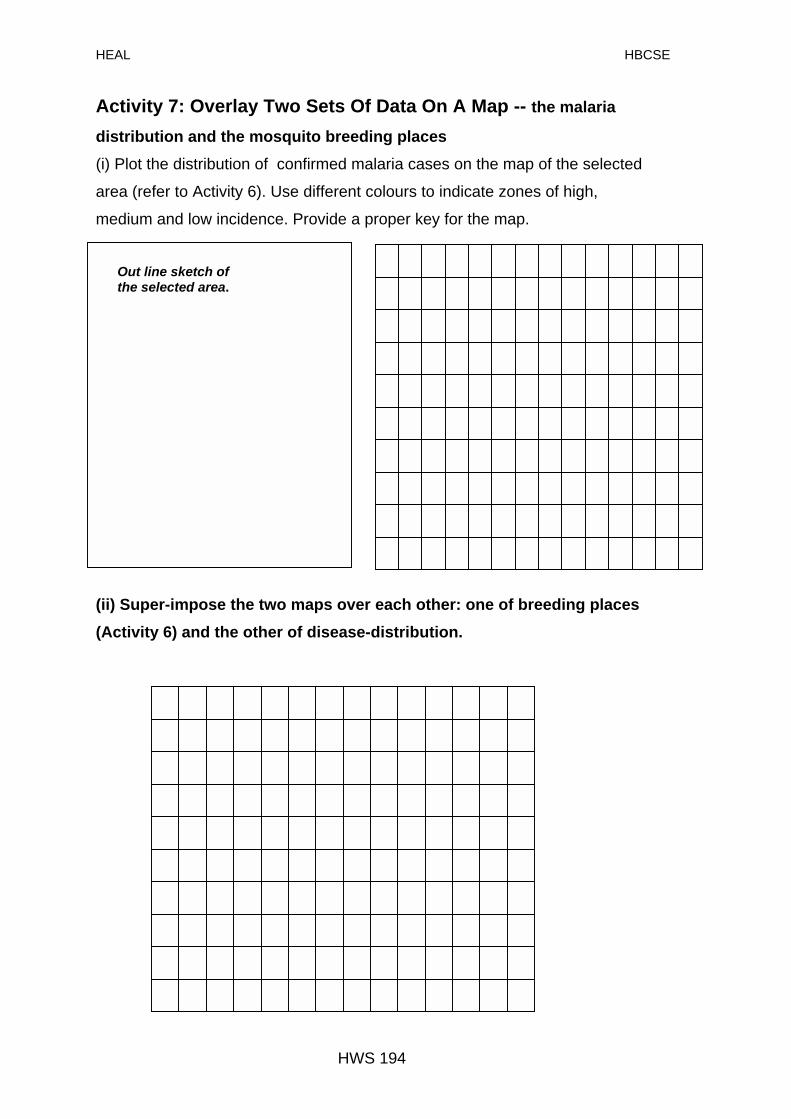
HEAL HBCSE

HWS 194

Activity 7: Overlay Two Sets Of Data On A Map -- the malaria

distribution and the mosquito breeding places (i) Plot the distribution of confirmed malaria cases on the map of the selected

area (refer to Activity 6). Use different colours to indicate zones of high,

medium and low incidence. Provide a proper key for the map.

Out line sketch of the selected area.

(ii) Super-impose the two maps over each other: one of breeding places (Activity 6) and the other of disease-distribution.

HEAL HBCSE

Appendix 1 PREPARATION OF SOLUTIONS CONDUCTIVITY: 0.01M standard potassium chloride solution: Dissolve 74.56 mg of anhydrous potassium chloride in 10 ml distilled water.

Make the volume to 100 ml. store the solution at 250C.

ALKALINITY: 0.02 N standard H2SO4: Dilute 2.8ml of conc. sulfuric acid to 1 liter of distilled water to form 0.1N

sulfuric acid. Standardise this solution against 0.1N sodium carbonate.

For standardization of 0.1N H2SO4, take 50ml of 0.1N sodium carbonate

in a conical flask and add 2-3 drops of methyl orange. Titrate against

the 0.1N sulfuric acid solution taken in a burette. The end point is the

colour change from yellow to orange.

Use appropriate volume of 0.1N sulfuric acid and dilute to 100 ml using distilled

water to prepare 0.02 N sulfuric acid.

1N sodium carbonate solution: Weigh accurately 13.25 gm of anhydrous sodium carbonate and dissolve it in

distilled water. Make up the volume to 250 ml in a volumetric flask.

0.02N sodium hydroxide solution: Dissolve 0.08gm of sodium hydroxide in 100ml of distilled water.

Phenolphthalein indicator: pH 8.3 indicator solution. If the solution is not available, dissolve 0.5 gms of

phenolphthalein in 50 ml of 95% methyl alcohol. Add 50 ml DW, 0.02 N NaOH

dropwise till faint pink colour appears. Store in a dark bottle.

Methyl orange indicator: Dissolve 0.1gm of methyl orange in 50ml-distilled water and dilute to 200ml

with distilled water.

195

HEAL HBCSE

DISSOLVED OXYGEN: Manganese (II) sulphate solution: Dissolve 100 gm of MnSO4.4 H2O in 200 ml of freshly boiled distilled water,

filter if necessary after cooling. Akaline potassium iodide- azide reagent:

Dissolve 50 gm of sodium hydroxide pellets and 15 gm of potassium

iodide salt in distilled water.

•

•

•

Dissolve 2.5 gm of sodium azide salt in 10 ml of distilled water.

Mix the above two solutions and dilute it to 100 ml. Sulphamic acid: This is a solid salt and is used in that form. Starch solution: Prepare a paste of 2.0 gm of soluble starch powder and 0.2 gm salicylic acid

(preservative) in distilled water. Pour this paste to 100 ml boiling water. Heat

the solution to boil. Cool and then use.

Sodium thiosulphate solution : Dissolve 6.21 gm of Na2S2O3 . 5H2O in freshly boiled and cooled distilled

water. Make up the volume to one litre. Keep the solution in a dark coloured

bottle after adding a pellet of sodium hydroxide as a stabilizer.

BIOCHEMICAL OXYGEN DEMAND:

All reagents used in determination of dissolved oxygen as discussed earlier.

BOD-free water:

Pass water through a column of activated carbon and redistill it. If this is not

available, use double distilled water.

Phosphate buffer solution:

Dissolve 33.4 gm of disodium hydrogen phosphate and 1.7 gm of ammonium

chloride in 500 ml distilled water. Adjust the pH to 7.2 and dilute to 1000 ml.

Magnesium phosphate:

196

HEAL HBCSE

Dissolve 22.5 gm of magnesium sulphate in 100 ml distilled water and dilute to

1000ml

Calcium chloride:

Dissolve 27.5 gm of anhydrous CaCl2 in 100 ml distilled water and dilute to

1000ml.

Ferric chloride:

Dissolve 0.75 gm of ferric chloride in 50 ml distilled water and dilute to 1000

ml.

Preparation of dilution water:

First aerate BOD free distilled water in a glass container for about half an hour

using an aerator. Add 1ml each of phosphate buffer, magnesium sulphate,

calcium chloride and ferric chloride solutions to 1000 ml of aerated distilled

water.

Seeding mixture:

Supernatant from domestic wastewater after settling for at least one hour at

room temperature. Add a fixed volume of 0.3 ml of this mixture per 300ml of

sample

CHEMICAL OXYGEN DEMAND: 1N Potassium dichromate (K2Cr2O7) stock solution:

Dissolve 24.5 gm of K2Cr2O7 in distilled water and make the volume to 500 ml

with distilled water.

0.25N Potassium dichromate solution: Dissolve 250 ml of 1N K2Cr2O7 in distilled water to make up to 1L .

1N Ferrous ammonium sulfate solution: Dissolve 322.9 gm of Fe(NH4)2 (SO4). 6H2O in distilled water and then add 20

ml of concentrated H2SO4 to it. Cool the solution, dilute to 1000 ml with DW,

and store it in dark.

197

HEAL HBCSE

0.25N Ferrous ammonium sulfate solution: 250 ml of 1N FAS and make up the volume to 1000ml in volumetric flask.

Standardize this against 0.25N potassium dichromate as described below.

Standardization 0.25 N FAS solution Pipette 2.5 ml of 0.25N potassium dichromate solution into 250ml

conical flask. Dilute to 25 ml with DW and add 7.5 ml of

concentrated sulfuric acid. Cool to room temperature. Add 5

drops of Ferroin indicator and titrate against FAS solution. The

end point is reddish brown.

N1(FAS) = V1(FAS)

V2(K2Cr2O7) x N2(K2 Cr2 O7)

Ferroin indicator: Dissolve 1.485gm of 1,10 phenanthroline monohydrate in 5-10 ml water; if the

crystals do not dissolve add a few drops of concentrated hydrochloric acid.

Next add 0.695 gm of ferrous sulfate and make the volume to 100ml with

distilled water.

Mercuric sulfate

Crystals or powder of HgSO4

Concentrated sulfuric acid.

CHLORIDES: Potassium chromate indicator:

Dissolve 25 gm of potassium chromate in 100ml of distilled water and add

silver nitrate solution till a definite red colour ppt is formed. Allow standing for

12 hours and filtering the solution. Dilute to 500ml with DW.

0.0282N Silver nitrate solution:

Dissolve 4.791 gm of silver nitrate in distilled water and dilute to 1000 ml.

Standardize against 0.0282 N sodium chloride.

198

HEAL HBCSE

Standardization of silver nitrate:

Take 10 ml of sodium chloride solution in a conical flask and adjust the pH

between 7.0 to 8.0 (either with NaOH or conc. H2SO4). Add 1ml of

potassium chromate. Titrate this against silver nitrate until a brown ppt is

formed. Find the normality of silver nitrate.

0.0282 N sodium chloride:

Dissolve 1.648 mg sodium chloride and dilute to 1000 ml.

Aluminum hydroxide suspension:

Dissolve 125 gm aluminum potassium sulfate or aluminum ammonium sulfate

in 1 L distilled water. Warm to 600C and add 55 ml concentrated ammonium

hydroxide slowly with stirring. Allow to stand for about one hour and transfer to

a large bottle. Wash the precipitate by successive additions, thorough mixing

and decanting with distilled water, until free from chloride ppt. Freshly prepared

suspension occupies a volume of 1L.

AMMONIA: Stock ammonium chloride (NH4 Cl) solution (100 ppm): Weigh 38.2 mg of NH4 Cl salt and dissolve it in 100 ml distilled water.

10% solution of ZnSo4. 7 H2O: Dissolve 10 gm of ZnSo4. 7 H2O in distilled water and dilute it to 100 ml.

6N solution of NaOH: Dissolve 24 gm NaOH in distilled water and dilute it to 100 ml.

50 % solution of EDTA: Dissolve 10 gm of NaOH in 60 ml of distilled water. Weigh 50 gm of EDTA and

dissolve it in the 60 ml of NaOH. Cool and dilute the solution to 100 ml. (* if the

EDTA does not dissolve keep adding NaOH pellets few at a time till the EDTA

salt completely dissolves. This is because EDTA dissolves in water only at a

particular pH of 8.5).

199

HEAL HBCSE

Nessler’s reagent: Dissolve 70 gm KI + 160 gm HgI2 in distilled water. Add this mixture to cooled

solution of 160 gm NaOH in 500 ml distilled water. Dilute to 1 liter. Keep the

solution overnight. Store the supernatant in amber\ dark coloured bottle. Use

the supernatant for the experiment.

FLUORIDES:

Stock sodium fluoride solution (100 ppm):

Dissolve 22.1gm of anhydrous sodium fluoride in 100 ml distilled water.

Fluoride standard solution:

Dilute 100 ml of stock solution to 1000ml in a volumetric flask, with distilled

water.

Alizarin red solution:

Dissolve 0.7 gm of alizarin red S in 100 ml of DW.

Zirconyl acid solution:

Dissolve 0.45 gm of zirconyl chloride in 100 ml of distilled water

Sulfuric acid solution:

Add 70 ml of conc sulfuric acid to 700 ml of water in a beaker and cool the

solution.

Mixed reagent:

Pour slowly alizarin red S to zirconyl acid solution and then add sulfuric acid.

Make the volume up to 1000ml. Store in dark and use after 24 hours.

PHOSPHATES:

Preparation of standard phosphate solution (100 ppm):

Dissolve 14.3 gm of dried anhydrous KH2PO4 in distilled water and make up

the volume to 100 ml.

200

HEAL HBCSE

Preparation of ammonium molybdate solution:

Dissolve 31.4 gm of (NH4)2Mo4 in 200 ml of distilled water. •

•

•

Add carefully 252 ml of concentrated H2SO4 to 400 ml of distilled water

and cool. Add 3.4 ml conc. HNO3

Mix the above two solutions and dilute it to one litre with distilled water.

Preparation of stanous chloride solution:

Dissolve 2.5 gm of SnCl2.2H2O in 100 ml glycerol by heating on water bath for

rapid disolution.

IRON:

Preparation of stock iron solution (50 ppm):

Dissolve 35 mg of [ (NH4)2 Fe (SO4)2 . 6H2O] in distilled water and make up the

volume to 100 ml.

10% solution of hydroxylamine HCl (NH2OH):

Dissolve 10 gm of (NH2OH) in distilled water and dilute to 100 ml.

Ammonium acetate buffer (NH2C2H3O2):

Dissolve 25 gm NH2C2H3O2 in 15 ml distilled water. Add 70 ml glacial acetic

acid. The final volume will be slightly more than 100 ml.

Phenanthroline solution:

Dissolve 100mg of phenanthroline monohydrate in 100 ml distil water. Warm

slightly or add 2 drops of concentrated HCL if necessary for complete

dissolution.

201

HEAL HBCSE

COPPER:

Preparation of stock iron solution (200 ppm):

Dissolve 20 mg of copper metal salt in 10 ml distilled water. To this add 5 ml of

concentrated HNO3. (Exercise caution while handling acids.) The reaction is

slow, wait for 10 minutes for completion of the reaction. Warm the solution

gently for complete dissolution. Cool the solution in a water bath and add 50 ml

water. Finally, dilute to 100 ml.

15% solution of citric acid:

Dissolve 15 gm of citric acid salt in 100ml of distilled water.

1% solution of sodium diethyl dithio carbamate:

Dissolve1 gm of sodium diethyl dithio carbamate salt in 100 ml distilled water.

1% solution of isoamyl acetate:

Mix one ml of isoamyl acetate solution in 99 ml of distilled water.

CHROMIUM:

Stock potassium dichromate solution (100 ppm):

Dissolve 28.26 mg K2Cr2O7 in water and dilute to 100 ml with distilled water.

Standard Chromium solution :

Dilute 1 ml of stock chromium solution to 100 ml.

0.2N sulfuric acid:

Dilute 17 ml of 6 N H2 SO4 to 500 ml of distilled water.

Potassium permanganate solution:

Dissolve 4 grams ofKMnO4 in 100 ml distilled water.

Sodium azide solution:

Dissolve 0.5 grams NaN3 in 100 ml distilled water.

Diphenylcarbazide solution:

202

HEAL HBCSE

Dissolve 250 mg of 1,5-diphenylcarbazide in 50 ml acetone. Store in a brown

bottle. Discard when solution becomes discoloured.

CALCIUM CARBONATES:

1N HCL:

Dilute 3.6 ml oh concentrated HCL in 100 ml of fresh diatilled water.

1N NaOH:

Dissolve 4 gm of sodium hydroxide pellets in 1000 ml fresh distilled water.

Bromothymol blue indicator:

Dissolve 0.1 gm of Bromothymol blue in 16 ml of 0.1 N NaOH and make up the

volume with 250 ml distilled water.

203

HEAL HBCSE

Appendix 2: MATERIALS AND APPARATUS

Others: A block of wood

Hammer

Wooden

stick

Water:

Buckets

Rope

Sealing tape

Filter papers

Syringes Swabs

Garde trowels

Small spade

Water bottle

Glass ware: 500 ml bottles with screw caps

Glass beakers

Glass funnels

Conical flask

Do bottle

Pipette

Dropper

Testtubes

Petriplates

Glass rods

Apparatus: U-shaped thermometer

Air suction pump

Whatman filters 0,1,2,4

pH paper

Alcohol thermometer

Sechi disc

Oven

Weighing balance

Colorimeter

Burners\UV hood

Digital probe

thermometer

Infiltrometer

Plastic sheets

Nails\board pins

Measuring tapeWater

proof markers

Garden clippers\tools

Bags

204

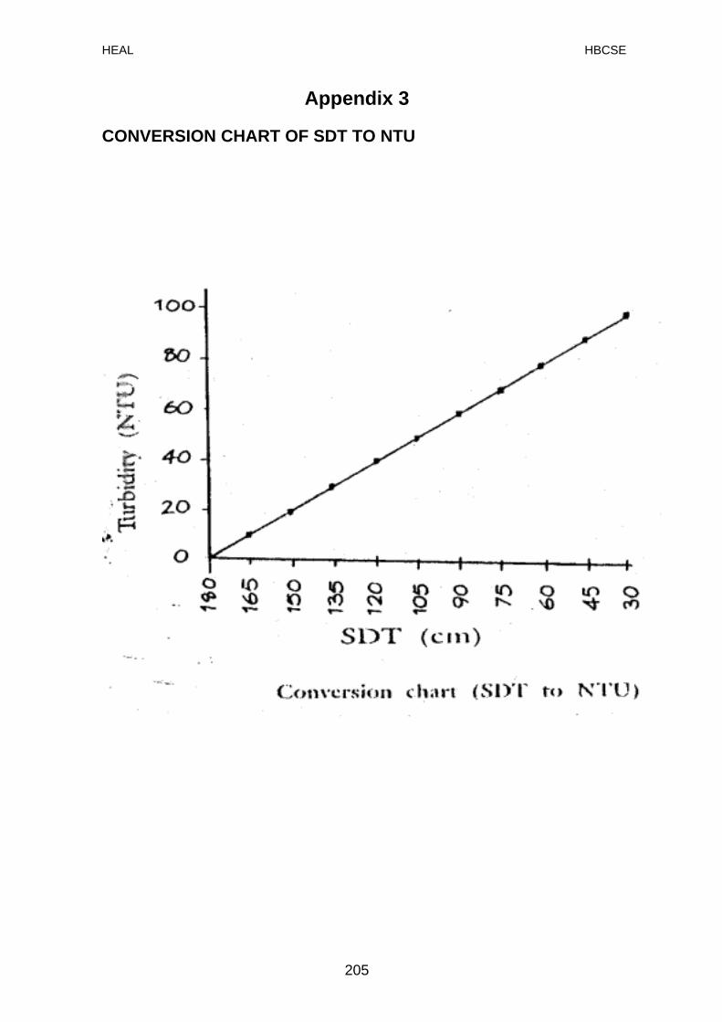
HEAL HBCSE

Appendix 3 CONVERSION CHART OF SDT TO NTU

205

HEAL HBCSE

Appendix 4

MOST PROBABLE NUMBER (MPN): MPN of coliform bacteria present in 100 ml of water for different positive combinations. Number of tubes giving a positive reaction out of: 3 of 10 ml each 3 of 1 ml each 3 of 0.1 ml each

MPN index per 100 ml

0 0 1 3 0 1 0 3 1 0 0 4 1 0 1 7 1 1 0 7 1 1 1 11 1 2 0 11 2 0 0 9 2 0 1 14 2 1 0 15 2 1 1 20 2 2 0 21 2 2 1 28 3 0 0 23 3 0 1 39 3 0 2 64 3 1 0 43 3 1 1 75 3 1 2 120 3 2 0 93 3 2 1 150 3 2 2 210 3 3 0 240 3 3 1 460 3 3 2 1100 3 3 3 2400

206

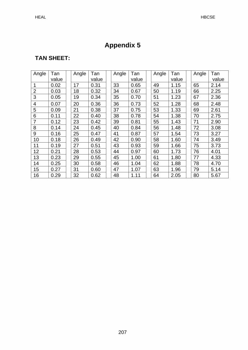
HEAL HBCSE

Appendix 5 TAN SHEET:

Angle Tan value

Angle Tan value

Angle Tan value

Angle Tan value

Angle Tan value

1 0.02 17 0.31 33 0.65 49 1.15 65 2.14 2 0.03 18 0.32 34 0.67 50 1.19 66 2.25 3 0.05 19 0.34 35 0.70 51 1.23 67 2.36 4 0.07 20 0.36 36 0.73 52 1.28 68 2.48 5 0.09 21 0.38 37 0.75 53 1.33 69 2.61 6 0.11 22 0.40 38 0.78 54 1.38 70 2.75 7 0.12 23 0.42 39 0.81 55 1.43 71 2.90 8 0.14 24 0.45 40 0.84 56 1.48 72 3.08 9 0.16 25 0.47 41 0.87 57 1.54 73 3.27 10 0.18 26 0.49 42 0.90 58 1.60 74 3.49 11 0.19 27 0.51 43 0.93 59 1.66 75 3.73 12 0.21 28 0.53 44 0.97 60 1.73 76 4.01 13 0.23 29 0.55 45 1.00 61 1.80 77 4.33 14 0.25 30 0.58 46 1.04 62 1.88 78 4.70 15 0.27 31 0.60 47 1.07 63 1.96 79 5.14 16 0.29

32 0.62 48 1.11 64 2.05

80 5.67

207

HEAL HBCSE

Appendix 6

A table showing distribution of DALY loss in some regions of the world, with emphasis on per capita health and public sector health expenditure

208

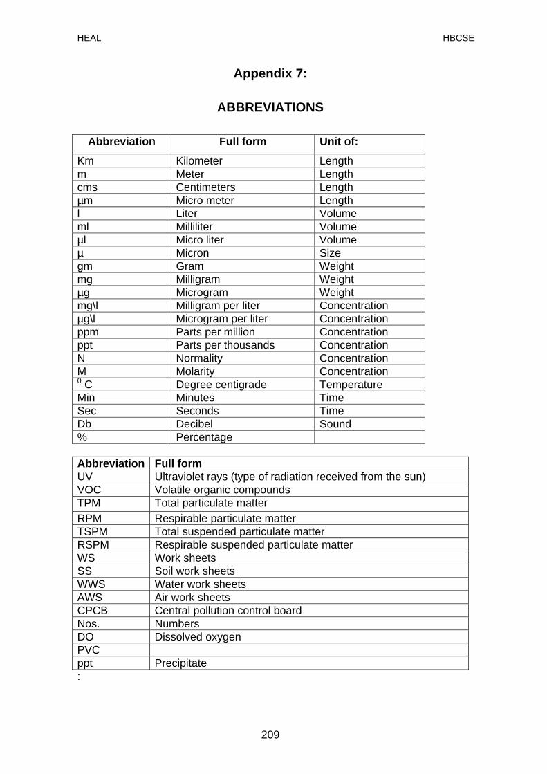
HEAL HBCSE

Appendix 7:

ABBREVIATIONS

Abbreviation Full form Unit of:

Km Kilometer Length m Meter Length cms Centimeters Length µm Micro meter Length l Liter Volume ml Milliliter Volume µl Micro liter Volume µ Micron Size gm Gram Weight mg Milligram Weight µg Microgram Weight mg\l Milligram per liter Concentration µg\l Microgram per liter Concentration ppm Parts per million Concentration ppt Parts per thousands Concentration N Normality Concentration M Molarity Concentration 0 C Degree centigrade Temperature Min Minutes Time Sec Seconds Time Db Decibel Sound % Percentage Abbreviation Full form UV Ultraviolet rays (type of radiation received from the sun) VOC Volatile organic compounds TPM Total particulate matter RPM Respirable particulate matter TSPM Total suspended particulate matter RSPM Respirable suspended particulate matter WS Work sheets SS Soil work sheets WWS Water work sheets AWS Air work sheets CPCB Central pollution control board Nos. Numbers DO Dissolved oxygen PVC ppt Precipitate :

209

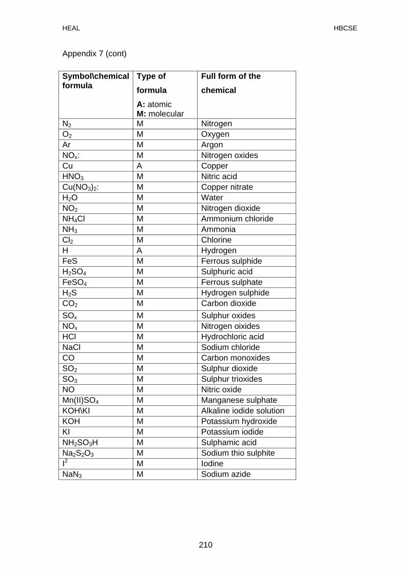
HEAL HBCSE

210

Appendix 7 (cont)

Symbol\chemical formula

Type of formula A: atomic M: molecular

Full form of the chemical

N2 M Nitrogen O2 M Oxygen Ar M Argon NOx: M Nitrogen oxides Cu A Copper HNO3 M Nitric acid Cu(NO3)2: M Copper nitrate H2O M Water NO2 M Nitrogen dioxide NH4Cl M Ammonium chloride NH3 M Ammonia Cl2 M Chlorine H A Hydrogen FeS M Ferrous sulphide H2SO4 M Sulphuric acid FeSO4 M Ferrous sulphate H2S M Hydrogen sulphide CO2 M Carbon dioxide SOx M Sulphur oxides NOx M Nitrogen oixides HCl M Hydrochloric acid NaCl M Sodium chloride CO M Carbon monoxides SO2 M Sulphur dioxide SO3 M Sulphur trioxides NO M Nitric oxide Mn(II)SO4 M Manganese sulphate KOH\KI M Alkaline iodide solution KOH M Potassium hydroxide KI M Potassium iodide NH2SO3H M Sulphamic acid Na2S2O3 M Sodium thio sulphite I2 M Iodine NaN3 M Sodium azide

HEAL HBCSE

Air watch…

HEAL HBCSE

Water watch…

HEAL HBCSE

Soil watch…

HEAL HBCSE

Green watch…

HEAL HBCSE

Waste watch…

HEAL HBCSE

Health watch…

HEAL HBCSE

APPENDIXES

HEAL HBCSE

Wor

Air ksheets

HEAL HBCSE

Water Worksheets

HEAL HBCSE

Soil Worksheets

HEAL HBCSE

Green cover Worksheets

HEAL HBCSE

Waste -management Worksheets

HEAL HBCSE

Health Worksheets