Guide to financial statement analysis : basis for management ...

University of Mississippi University of Mississippi

eGrove eGrove

Guides, Handbooks and Manuals American Institute of Certified Public Accountants (AICPA) Historical Collection

2006

Guide to financial statement analysis : basis for management Guide to financial statement analysis : basis for management

advice advice

Wallace N. Davidson

James L. McDonald

Follow this and additional works at: https://egrove.olemiss.edu/aicpa_guides

Part of the Accounting Commons, and the Taxation Commons

Recommended Citation Recommended Citation Davidson, Wallace N. and McDonald, James L., "Guide to financial statement analysis : basis for management advice" (2006). Guides, Handbooks and Manuals. 460. https://egrove.olemiss.edu/aicpa_guides/460

This Book is brought to you for free and open access by the American Institute of Certified Public Accountants (AICPA) Historical Collection at eGrove. It has been accepted for inclusion in Guides, Handbooks and Manuals by an authorized administrator of eGrove. For more information, please contact [email protected].

https://egrove.olemiss.edu/

https://egrove.olemiss.edu/aicpa_guides

https://egrove.olemiss.edu/aicpa_pubs

https://egrove.olemiss.edu/aicpa_pubs

https://egrove.olemiss.edu/aicpa_guides?utm_source=egrove.olemiss.edu%2Faicpa_guides%2F460&utm_medium=PDF&utm_campaign=PDFCoverPages

http://network.bepress.com/hgg/discipline/625?utm_source=egrove.olemiss.edu%2Faicpa_guides%2F460&utm_medium=PDF&utm_campaign=PDFCoverPages

http://network.bepress.com/hgg/discipline/643?utm_source=egrove.olemiss.edu%2Faicpa_guides%2F460&utm_medium=PDF&utm_campaign=PDFCoverPages

https://egrove.olemiss.edu/aicpa_guides/460?utm_source=egrove.olemiss.edu%2Faicpa_guides%2F460&utm_medium=PDF&utm_campaign=PDFCoverPages

mailto:[email protected]

Guide to Financial Statement Analysis: Basis for Management Advice

Wallace N. “Dave" Davidson, III, Ph.D. James L. McDonald, Ph.D.

[AICPA]


Wallace N. “Dave" Davidson, III, Ph.D. James L. McDonald, Ph.D.

Notice to Readers

Guide to Financial Statement Analysis: Basis for Management Advice does not represent an official position of the American Institute of Certified Public Accountants, and is distributed with the understanding that the author(s), editor(s), and publisher are not rendering legal, accounting, or other professional services in this publication. The views expressed are those of the author(s) and not the publisher. If legal advice or other expert assistance is required, the services of a competent professional should be sought.

Copyright © 2006 byAmerican Institute of Certified Public Accountants, Inc.New York, NY 10036-8775

All rights reserved. Checklists and sample documents contained herein may be reproduced and distributed as part of professional services or within the context of professional practice, provided that reproduced materials are not in any way directly offered for sale or profit. For information about the procedure for requesting permission to make copies of any part of this work, please visit www.copyright.com or call (978) 750-8400.

1 2 3 4 5 6 7 8 9 0 PP 0 9 8 7 6

ISBN 0-87051-652-3

http://www.copyright.com


Table of Contents

Chapter 1—Firm Valuation.................................................................................................................... 1-1Overview.......................................................................................................................................1-1Introduction...................................................................................................................................1-1

Why Use a Valuation Technique?..................................................................................................... 1-1Who Uses Valuation Techniques?.................................................................................................... 1-2

Owners..........................................................................................................................................1-2Potential Owners.......................................................................................................................... 1-2Bankers........................................................................................................................................ 1-2Security Analysts..........................................................................................................................1-2

Wells Fargo “Dividend Capitalization” Model................................................................................. 1-2Dividend Computation for Privately-Held Corporation.................................................................... 1-3

Chapter 2—The Effect Ratios................................................................................................................. 2-1Overview...................................................................................................................................... 2-1Introduction.................................................................................................................................. 2-1

Effect Ratios...................................................................................................................................... 2-1Liquidity Measures...................................................................................................................... 2-1Leverage Measures ..................................................................................................................... 2-2Profitability Measures................................................................................................................. 2-2

Liquidity............................................................................................................................................ 2-2Inventory to Working Capital............................................................................................................ 2-4Trade Receivables to Working Capital Ratio.................................................................................... 2-5Net Sales to Working Capital............................................................................................................ 2-6Debt Ratios........................................................................................................................................ 2-7

Tangible Debt Ratios................................................................................................................... 2-7Current Liabilities to Net Worth....................................................................................................... 2-8Times Interest Earned........................................................................................................................ 2-8Net Profit to Net Worth (Return on Equity)...................................................................................... 2-9Effect Ratio Summary..................................................................................................................... 2-10

iii

Chapter 3—Analysis of Profitability...................................................................................................... 3-1Overview...................................................................................................................................... 3-1Introduction.................................................................................................................................. 3-1

DuPont® System ROE....................................................................................................................... 3-1DuPont® System ROA.......................................................................................................................3-2Total DuPont® System....................................................................................................................... 3-3EBITDA Analysis.............................................................................................................................3-4Earnings Quality................................................................................................................................ 3-4

Continuation of Earnings............................................................................................................. 3-5Relationship of Earnings to Cash Flow.......................................................................................3-6

Chapter 4—Causal Ratios.......................................................................................................................4-1Overview......................................................................................................................................4-1Introduction..................................................................................................................................4-1

Causal Ratios.....................................................................................................................................4-1Fixed Assets to Net Worth................................................................................................................4-2How Fixed Assets Affect Profit........................................................................................................4-4Correction Procedures.......................................................................................................................4-4Collection Period...............................................................................................................................4-5Collection Period—Example.............................................................................................................4-6Impact of Collection Period on Profits..............................................................................................4-6Correction Procedures.......................................................................................................................4-7

How to Correct an Abnormal Collection Period Ratio................................................................4-7Net Sales to Inventory (Inventory Turnover)....................................................................................4-7Net Sales to Inventory—Example.....................................................................................................4-8Correction Procedures.......................................................................................................................4-9

Sluggish Movement of Stock.......................................................................................................4-9Net Sales to Net Worth......................................................................................................................4-9

The Trading Ratio........................................................................................................................4-9Trading Ratio—Example................................................................................................................4-10Trading Ratio—Example ...............................................................................................................4-12Overtrading Characteristics.............................................................................................................4-12Correction Procedures ....................................................................................................................4-13

Overtrading................................................................................................................................4-13The Profit Margin............................................................................................................................4-13The Profit Margin—Example..........................................................................................................4-14Correction Procedures for a Low or Negative Profit Margin..........................................................4-14Miscellaneous Assets to Net Worth................................................................................................4-15Correction Procedures.....................................................................................................................4-15

Investment in Miscellaneous Assets..........................................................................................4-15Causal Ratio Summary....................................................................................................................4-16

iv

Chapter 5—How to Conduct a Financial Statement Analysis............................................................ 5-1Overview...................................................................................................................................... 5-1Introduction.................................................................................................................................. 5-1

How to Conduct an Analysis of Financial Statements...................................................................... 5-1Industry and Time Series Analysis.................................................................................................... 5-2Sources of Industry Averages............................................................................................................ 5-2

Primary Sources........................................................................................................................... 5-2Other Sources............................................................................................................................... 5-3

Problems With Using Industry Data............... ..................................................................................5-3An Example of Computing Industry Statistics, a Common-Sized Balance Sheet............................5-4An Example of Computing Industry Statistics From Dun and Bradstreet® Data..............................5-5Guidelines to Use in Applying Ratio Analysis.................................................................................5-5

Chapter 6—Case Studies......................................................................................................................... 6-1Case Study 1—Manufacturer of Boxes............................................................................................. 6-1

Effect Ratio Summary.................................................................................................................. 6-2Causal Ratio Summary................................................................................................................ 6-2Recommendation......................................................................................................................... 6-3

Case Study 2—National West Airline............................................................................................... 6-3National West Airline.................................................................................................................. 6-4Analysis—Causal Ratios............................................................................................................. 6-5Year 20Y9—External Shock.......................................................................................................6-5

Case Study 3—Firm A...................................................................................................................... 6-5Analysis—Effect Ratios.............................................................................................................. 6-6Analysis—Causal Ratios............................................................................................................. 6-6Summary...................................................................................................................................... 6-7

Case Study 4—Store Container Corporation.................................................................................... 6-7Analysis—Effect Ratios.............................................................................................................. 6-9Analysis—Causal Ratios............................................................................................................. 6-9

Case Study 5—Biscayne Apparel................................................................................................... 6-10Analysis—Effect Ratios............................................................................................................ 6-11Analysis—Causal Ratios........................................................................................................... 6-12

Chapter 7—Users of Financial Statements........................................................................................... 7-1Overview...................................................................................................................................... 7-1Introduction.................................................................................................................................. 7-1

Ratios Examined by Banks for Short-Term Loans............................................................................ 7-1Ratios Examined by Banks for Long-Term Loans............................................................................ 7-2Commercial Loan Departments’ Most Significant Ratios and Their Primary

Measures—Gibson’s Study.......................................................................................................................7-2Commercial Loan Departments’ Ratios Appearing Most Frequently in Loan Agreements.............7-3Corporate Controllers’ Most Significant Ratios and Their Primary Measures.................................7-4Ratios Appearing in Corporate Objectives and Their Primary Measures.........................................7-4

V

Chapter 8—Forecasting Sustainable Growth.......................................................................................8-1Overview...................................................................................................................................... 8-1Introduction.................................................................................................................................. 8-1

Definitions......................................................................................................................................... 8-1Derivation of the Sustainable Growth Model.................................................................................... 8-1The Alabama Door Company Sustainable Growth—Example.........................................................8-3

Assumptions................................................................................................................................. 8-3Class Exercise.............................................................................................................................. 8-3

Calculation of Alabama Door Growth Rate...................................................................................... 8-4Improving Sustainable Growth......................................................................................................... 8-4Sustainable Growth—Available External Equity..............................................................................8-5

Chapter 9—Case Problem...................................................................................................................... 9-1Overview...................................................................................................................................... 9-1Introduction.................................................................................................................................. 9-1

Marine Supply Company Balance Sheet........................................................................................... 9-2Marine Supply Company Selected Income Figures..........................................................................9-2Marine Supply Company Selected Financial Ratios.........................................................................9-3

Solution to Case........................................................................................................................... 9-3

Chapter 10—Forecasting Bankruptcy................................................................................................. 10-1Overview.................................................................................................................................... 10-1Introduction.................................................................................................................................10-1

Altman’s® Bankruptcy Prediction Formula..................................................................................... 10-1Altman’s® Suggested Z-Score Cutoff........................................................................................ 10-2Computational Note................................................................................................................... 10-2Usage Notes............................................................................................................................... 10-2

Bankruptcy Prediction Example...................................................................................................... 10-2Altman’s® Second Model................................................................................................................ 10-3

Critical Values........................................................................................................................... 10-3

vi

Chapter 1

Firm Valuation

OverviewUpon completion of this chapter you will be able to:

• Value a firm utilizing a basic valuation formula.• Understand who uses firm valuations.

IntroductionThis section shows the correct method for determining the value of a firm using the constant growth dividend capitalization model. Explanations are presented of (1) the variables defined in the model and (2) the valuation techniques and who uses them.

Why Use a Valuation Technique?

Profitability

Growth

Risk

Financial information is an important determinant of firm value. We need to know how the financial statements affect firm value.

• How does increased profitability affect firm value?— Profitability is positively related to firm value. That is, as a firm becomes more prof

itable its value increases.• How does increased growth affect firm value?

— Growth is defined as the firm’s increasing ability to produce cash flows or profits. Growth is positively related to firm value.

• How does increased risk affect firm value? Liquidity risk? Financial risk?— All types of risk reduce firm value. Liquidity and financial risk can be measured from

financial statements. As they increase, firm value declines.

1-1

FIRM VALUE


A valuation technique is particularly important for small- and medium-sized companies. Large- company values are found in the security markets. Smaller companies do not have this luxury.

The value of a firm is determined largely by its ability to earn. We want to know how the interpretation of the firm’s financial statements affects the value of the firm. The value of a firm is, after all, a reflection of the owner’s wealth.

Who Uses Valuation Techniques?OwnersThe owner of a firm needs to know the firm’s value if he/she (1) is expecting to sell the firm or (2) is determining borrowing capacity.

Potential OwnersThe potential owner of a firm must understand the concept of firm value to determine how much to pay for the firm.

BankersA banker must understand firm value when determining a firm’s borrowing capacity or collateral value.

Security AnalystsFor large companies, security analysts spend considerable time with valuation techniques. This is not important for our purposes. We want to understand how financial statement information affects firm value.

Our purpose in examining valuation is to give us a gauge by which we can determine the effect of the ratios on the firm’s value.

Wells Fargo “Dividend Capitalization” ModelThe value of a firm’s equity is the present value of cash flows (dividends) that can be taken out of the firm. Value is affected by the firm’s cash earnings, the expected growth rate of cash earnings and the firm’s risk. Cash earnings and growth are positively related to firm value, whereas risk is negatively related to firm value.

Mathematically this expression can be reduced to:

Value =

FCF = Funds that can be withdrawn from the business—called free cash flow R = Risk adjusted rate of returnG = Expected growth rate

1-2

Value of a firm’s equity =FCF1 FCF2 FCF21 + R + (1 + R)2 +(1 + R)3 + ...

FCF1R-G

Firm Valuation

In the numerator, the expression FCF represents the company’s free cash flow. Free cash flow is the cash left over after all necessary investments have been made and expenses paid. Whenever we examine a ratio or other financial data that relates to a firm’s earning power, valuation can be referred to. Specifically, if a company’s earning power increases (FCF goes up), then the value of the firm will go up.

In the denominator, the expression R represents a company’s cost of equity capital. As a company’s risk increases, its cost of equity increases. It is important to note that if a firm’s risk is increasing (liquidity or financial risk), then its value is declining. As R rises, the firm’s equity value declines.

R is the rate of return required by equity holders. Since equity is riskier than debt to investors, R is greater than a company’s cost of debt. In large firms, it has been estimated that R is roughly 3% greater than the company’s cost of debt.

The second term in the denominator, G, represents the firm’s ability to grow in terms of earning power. As G rises, the value of the firm will rise.

Dividend Computation for Privately-Held CorporationWhat is the dividend capacity of a privately held firm? This example will clarify the issue. Suppose that the owner of a company (C-corporation) pays a $150,000 salary to him/herself for a job that he/she could hire an outside manager to do for $50,000. The owner’s added salary is $100,000. This practice eliminates the double taxation of dividends.

ExampleDividend paid.................................................................. $ 75,000Owner’s salary................................................................. 150,000Equivalent manager’s salary............................................ 50,000

The added salary of $100,000 was tax deductible as a salary, but it would not be tax deductible as a dividend. At a 50% tax rate, it would be worth only $50,000 as a dividend.

Real Dividend ComputationDividend paidAdjustment for salaryFree cash flow

$ 75,000 50,000*

$125,000

* $100,000 (1 - .5) with an assumed 50% tax rate

Therefore, free cash flow represents the earning power of the company in terms of cash flows that the owner(s) may withdraw from the firm. If a decision is made that increases the firm’s cash flows, then the firm’s value is increased. If a decision is made that increases the firm’s risk, then the value is decreased. Financial statement analysis is used to measure both the risk and return of the firm.

Note also that in valuing a business one should look for other inefficiencies that may reduce FCF and the value of the business.

1-3

Chapter 2

The Effect Ratios


• Understand why these ratios are “effect” ratios and not causal ratios;• Know why you should not focus on the effect but on the cause;• Determine what each of these ratios measures;• Calculate each ratio; and• Determine how a change in any one of the causal ratios will affect each ratio.

IntroductionThe effect ratios are used to determine the extent of a company’s problems. Liquidity, leverage, and profitability measures are included.

The purpose of this chapter is to introduce you to the effect ratios. These ratios do not show the reason for a change; they only show that a change has occurred and the magnitude of a change. We call them effect ratios because that is what they are. These ratios are really symptoms of problems. Something else has caused them, and we will identify causes later. An analogy may be useful here. When you get a cold, the symptoms may include a sore throat and the sniffles. The actual cause is the underlying cold virus. The effect ratios are like the symptoms. They show results but do not show the cause.

It is important to know whether there are liquidity, leverage or profit problems. However, to fix these problems we must both identify the cause and fix it.

Effect RatiosThere are three groups of effect ratios. The first are ratios that measure liquidity. Liquidity is important for a company to monitor. When liquidity is too low, a company will experience problems paying its bills. When liquidity is too high, the company’s profits will likely be hurt.

Liquidity Measures• Current Ratio• Quick Ratio• Defensive Interval

2-1


• Inventory/Working Capital• Receivables/Working Capital• Net Sales/Working Capital

The second set of effect ratios are those that measure leverage. Leverage ratios are ratios that show the amount of debt a company carries and its ability to afford its debt. Debt increases the variability of profits across business cycles. A company with large debt ratios will have greater up-swings in profits in good years but will have greater down-swings in profits in bad years.

Leverage Measures• Debt-to-Net Worth• Debt to Assets• Tangible Debt Ratios• Short-Term Debt to Net Worth• Times Interest Earned• Cash Times Interest Earned• Fixed-Charge Coverage

Profitability measures the results of the company’s activities. Without profits a company cannot survive and inadequate profits can prevent a company from reaching its potential. In this chapter we will discuss only one profitability measure, but will return to the topic and discuss it in more depth in later chapters.

Profitability Measures• Return on Equity—Net Income/Net Worth

To summarize, there are three areas of concern for a business that are measured by financial statement characteristics: The first is liquidity. Liquidity is the measurement of how well the firm can meet its obligations in the short run. The second area is leverage. Leverage ratios measure the firm’s debt usage and how well it can afford its debt. The third area is profitability. Profitability ratios are a measure of how profitable a firm is relative to its size.

LiquidityThe concept of liquidity can be easily explained as the ease with which a company can pay its bills. Companies that do not struggle to pay bills have adequate liquidity. Companies can have excessive liquidity since liquid assets tend to earn a low rate of return. Excessive liquidity can hurt profitability. Inadequate liquidity increases the risk of default and financial embarrassment.

There are four different aspects to liquidity. These are: quantity, timing, quality, and early warning. The quantity of liquidity measures how much liquidity the company carries relative to its size. Timing aspects of liquidity measure how long the liquidity will last. Quality of liquidity is concerned with the make up of the liquidity. Finally, there is an early warning ratio that measures liquidity in rapidly growing companies. As you can see below, there are several ratios that measure these aspects of liquidity.

2-2

The Effect Ratios

Liquidity Category RatiosQuantity of Liquidity Current Ratio

Quick RatioTiming of LiquidityQuality of Liquidity

Defensive IntervalInventory/Working Capital Receivable/Working Capital

Early Warning Net Sales/ Net Worth

The most commonly used liquidity ratio is the current ratio. It can be computed as:

Current Ratio = Current AssetsCurrent Liabilities

Current assets are those assets that are either cash or will be converted to cash within one year. Current liabilities are those liabilities that are due within one year. So the current ratio shows how many times the liquid (current) assets can cover the liabilities that are due soon. The current ratio is a measure of the quantity of liquidity. When the ratio is large, the quantity of liquidity is large. When the ratio is too small the quantity of liquidity is insufficient and the company may experience problems paying its bills. How large this ratio or any other ratio should be depends on the industry. Some industries, those with very steady cash inflows, can get by with very small current ratios. Others, whose cash inflow is less predictable and less steady may require a greater current ratio.

The current ratio only tells you how much liquidity you have. It does not let you know the makeup of the liquidity. A company can have a “sound” current ratio and still have a liquidity problem if its current assets, for example, are composed largely of inventory that cannot be sold or receivables that cannot be collected.

There used to be a common statement that current ratios need to be at least 2 to 1. Do not be overly concerned with the 2 to 1 standard (unless your banker uses this standard in loan covenants).

The second quantity measure of liquidity is the quick ratio. It is computed as:

Quick Ratio = Quick Assets Current Liabilities

We compute this ratio by dividing quick assets by current liabilities. Quick assets are those assets that can be converted to cash without additional sales. They include cash, marketable securities, and accounts receivables. The quick ratio measures the liquidity of the company assuming that no additional sales of inventory can be made. This ratio increases in importance as inventory’s proportion of total assets is large, when inventory becomes obsolete or spoils quickly, and in any circumstances in which the real value of the inventory is questionable.

The second aspect of liquidity is timing. The ratio we use to measure the timing of liquidity is the defensive interval. It can be computed as:

Defensive Interval = _______ Quick Assets_______ Daily Cash Operating Expenses

2-3


The defensive interval measures the length of time a company can continue to operate on its liquid assets without any new sales. To compute this ratio, divide quick assets by daily cash operating expenses. Daily cash operating expenses include all expenses listed above operating income on the income statement except for non-cash items such as depreciation and amortization. So it includes cost of goods sold as well as all selling and administrative expenses. It focuses on the need for liquidity.

If the ratio is, say 50 days, then the company can survive 50 days without future sales if it continues to spend cash at the existing rate. A longer defensive interval implies greater liquidity. This ratio, however, ignores the possibility of future cash inflows.

Inventory to Working CapitalWorking capital is the margin of protection a company provides for the payment of current obligations. It is measured in terms of “quantity” by the current ratio. This ratio, inventory to working capital, is a measure of the quality of working capital. The quality of liquidity is important because not all liquid assets are equally as liquid. The ratio of inventory to working capital measures the dependency of the company’s working capital on inventory, and, therefore, the quality of liquidity.

Working capital can be defined as current assets, less current liabilities. Generally, if a firm has positive working capital, its liquid assets exceed its near term liabilities. In this ratio, one may use current assets in the denominator when net working capital is negative.

What makes this ratio important is that inventory is the least liquid of the major categories of current assets. When inventory is large, the quantity of liquidity may be large, but we would argue that the quality is low. It is low because if there is a problem selling the inventory, the company is not as liquid as its quantity ratios would suggest. Historically, inventory problems have caused a lot of firms to go under. When the inventory to working capital ratio becomes large, then the firm becomes more susceptible to problems caused by inventory that will not sell.

We show an example using this ratio below. There are two companies in the example and both of these companies operate in the same industry. Company A’s inventory to working capital ratio is below average, and Company B’s ratio is way above average. We would argue that company A has good quality of liquidity while company B has poor quality since inventory is such a large part of working capital.

CompanyA B

Cash $ 2,000 $ 10,000Accounts receivable 16,000 40,000Inventory 10,000 60,000

Total 28,000 110,000Current liabilities 10,000 80,000Working capital $18,000 $ 30,000

Inventory to working capital 56% 200%Industry average 60% 60%

2-4

The Effect Ratios

To show why a large inventory to working capital ratio is a problem, suppose that the inventory values of both companies are cut by one-half. This reduction in inventory value could be caused by a competitor developing a new and better product or for other reasons. Regardless of the reason for the drop in inventory value, both companies would be hurt, but Company B would be hurt worse. Company A would lose $5,000 but would still have $13,000 of working capital. The current ratio would drop from 2.8 to 2.3.

Company B, on the other hand, would lose $30,000 and its working capital would drop to zero. Its current ratio would be 1. Clearly, Company B is more vulnerable to problems caused by inventory troubles. Unless the receivables and other current assets were in excellent shape, an inventory problem could put company B out of business.

This ratio is a measure of the quality of working capital and is affected by all six of the causal ratios. However, it is particularly sensitive to the inventory turnover ratio.

Trade Receivables to Working Capital RatioThis ratio is a measure of working capital quality; that is, the extent of the company’s reliance on receivables for its working capital. When this ratio becomes large, the quality of the company’s liquidity is said to be poor. The interpretation of this ratio is very similar to that of inventory to working capital.

This is a very important ratio for small firms. They generally do not subscribe to credit reporting or credit interchange services. Often these small firms do not have anyone special to handle their receivables. A build-up of receivables can be a signal of collection problems.

We have presented an example below. Suppose that Companies H and J are in the same industry whose average receivables to working capital ratio is 75%. Company H has a ratio of 60%, and we would argue that its quality of liquidity is good. Company J has a ratio of 166.7%, and because it is so large relative to the industry norm, we would argue that it has poor quality of liquidity. Company J would be more susceptible to anything affecting the paying behavior of its customers than would Company H.

CompanyH J

Cash $ 1,000 $ 5,000Trade receivables 6,000 50,000Inventory 7,000 30,000Total current assets 14,000 85,000Total current liabilities 4,000 55,000Working capital $10,000 $30,000

Trade receivables to working capital 60.0% 166.7%Industry average 75.0% 75.0%

If these companies lost all of their receivables to default, Company H would still have positive working capital. Hence this company has some ability to withstand such a problem.

2-5


Company J is in serious straits. Receivables are greater than working capital by $20,000, leaving a very low margin for error. If customers slowed down their payments, Company J would be in a bind.

The trade receivables to working capital ratio is affected by all of the causal ratios. However, it is particularly affected by the collection period.

Suppose that Company J’s collection period increased by 50%. Receivables would rise by 50% to $75,000. If this rise were financed by current liabilities (which would rise to $80,000), working capital would remain at $30,000, but the current ratio would drop to 1.375 from 1.545. Receivables to working capital would rise to 250%.

Net Sales to Working CapitalAnother liquidity ratio is the Net Sales to Working Capital Ratio. This ratio is often redundant with the other liquidity ratios in that when there are liquidity problems demonstrated by the other liquidity ratios, this ratio will generally be large as well. However, this ratio is particularly useful when sales have grown rapidly.

When a company’s sales increase, to maintain liquidity, working capital must increase. So when a sales increase is not met with a proportionate increase in working capital, the ratio of sales to working capital increases. In the example, below, Company V has a sales to working capital ratio of 150%. A ratio that is this large in an industry where the norm is 15 suggests inadequate liquidity. However, Company W has a sales to working capital ratio of 10.7. This is below the industry norm indicating adequate liquidity.

CompanyV W

Current assets $ 25,000 $ 25,000Current liabilities 24,000 11,000Working capital 1,000 14,000Sales $150,000 $150,000

Sales to working capital 150 times 10.7 timesIndustry average 15.0 times 15.0 times

This ratio indicates the demands made upon working capital in support of the sales volume. The higher the sales in comparison to working capital, the greater the strain a company encounters in satisfying creditors while meeting payroll and taxes.

This ratio is particularly useful when a company is experiencing rapid sales growth. It may signal a working capital problem before the other liquidity ratios do.

In the example Firm V has insufficient working capital to support its sales, and would be more susceptible to an external shock.

2-6

The Effect Ratios

Debt RatiosDebt ratios are often called leverage ratios. Like a lever in the physical world, financial leverage magnifies. A physical lever magnifies a person’s strength, and a financial lever magnifies the bottom line. What this means is that in good years, debt increases income. In bad years, debt worsens income. The more debt a company carries the greater the variability of its income over business cycles.

There are two basic ratios that measure debt usage. The first is the debt-to-asset ratio. It is computed by dividing total debt (all liabilities) by total assets. The second is the debt-to-equity ratio. It is found by dividing total debt by net worth. These two ratios are perfectly redundant. That is, they measure the same thing, but use a different scale of measurement (just like inches and centimeters measure the same thing). The formulas for these two ratios appear below:

Debt to Asset Ratio = Total DebtTotal Assets

Debt to Equity Ratio = Total DebtTotal Net Worth

When either of these ratios grows, debt usage has increased. Since this increases the variability of income, we would argue that the leverage risks have increased as well.

Both ratios are measures of financial risk. When a firm’s debt ratios increase, its financial risk increases. In fact, these ratios are generally one of the major determinants of a company’s eligibility for a “new” loan and a determinant of borrowing rates.

With these ratios it is particularly important to know what limits our lenders have placed on us. This limit becomes our debt capacity. Furthermore, it is useful to monitor industry averages to be sure that we do not deviate from the norm.

Tangible Debt RatiosLenders often use tangible debt ratios. Lenders are concerned about the safety of the dollars they lend to companies. So it is common in the loan application for the lender to subtract intangible assets from the total assets of the loan applicant. Since the balance sheet must balance, the lender will also subtract the intangible assets from net worth. What remains is the tangible balance sheet. From this revised statement, the lender then computes tangible debt to assets or tangible debt to equity as in the formulas below:

Tangible Debt to Asset Ratio =

The tangible debt ratios will be larger than the normal debt ratios if the company has intangible assets. The lender’s formulas for debt ratios are more conservative and make the company appear to be more levered.

2-7

Tangible Debt to Equity Ratio =

____ Total DebtTotal Tangible Assets

__________ Total Debt__________ Total Net Worth - Intangible Assets


Tangible debt ratios are particularly useful when the market value of the intangible assets is questionable. Lenders want the debt ratios based upon assets that they can actually sell or receive value. In particular, lenders are concerned about “goodwill”, an account that occurs in mergers. If the company has financial trouble, goodwill has no real value. Hence, with the concern for safety of the principal, lenders simply assume it is not there.

Current Liabilities to Net WorthSmall businesses must often rely upon short-term financing. This ratio is a measure of the extent to which the small firm uses short-term financing rather than net worth. Companies use shortterm debt as temporary financing for seasonal and other temporary needs. However, some companies use short-term debt as permanent financing by continually rolling-over the short-term loan into a new short-term loan or by constantly keeping an outstanding balance on their line of credit. The benefits of using short-term debt in this manner are lower interest rates (assuming a normal yield curve), fewer restrictions in the loan agreement, and the relative ease of obtaining short-term debt versus long-term debt for small businesses.

There is, however, no free lunch. The benefits of using short-term debt as permanent financing are at least partially offset by increased risks for borrowers that use short-term debt in this way. Short-term debt not only increases leverage risk as does long-term debt, it also lowers liquidity and increases liquidity risks. In addition, short-term debt, when used as “permanent” financing can increase a company’s risks beyond the risks of long-term debt. The increased risks include rollover risks (bank saying “no” to the rollover) and interest rate risks (taking a potentially higher rate when the debt is rolled-over). Rollover risk is the chance that a firm cannot renew a loan. Short-term debt usage increases this risk because rollover occurs more frequently. Short-term debt has more volatile interest rates than long-term debt and the rate must be renegotiated more often. This reduces the predictability of interest costs and increases risk.

A company with a low current liabilities to net worth ratio is generally free from creditor demands. If this ratio is high, the management must spend excessive amounts of time dealing with creditors. This excessive time robs the company of initiative. We can illustrate this in the example below:

2-8

Company ratio Industry ratio

In the example, Company D and Company F are in the same industry and have current liabilities to net worth ratios of 40% and 145%, respectively. Company D has ample coverage to permit prompt payment. Creditors will have few restrictions. Company F is nearly twice the industry average. This company has excessive short-term borrowing. Generally, this company would have very severe restrictions from its creditors: Restricted current ratio, salaries, and operations.

Times Interest EarnedThe times interest earned ratio measures the ability of a company to afford its debt. As a result, it is often called a “solvency” ratio. When the ratio is large, the company can easily afford its debt obligations. However, when the ratio is small, the ability to afford debt, solvency, is impaired.

D F40% 145%75% 75%

The Effect Ratios

To compute the ratio we divide earnings before interest and taxes (operating income) by interest expense, as shown below:

Times Interest Earned - Earnings Before Interest and Taxes Interest Expense

If this ratio is adequate, then there is little danger of default. Companies with a large and stable times interest earned ratio have no trouble when it is time to “roll over” their debt.

Since causal ratios directly influence profit and debt usage, the times interest earned ratio is directly related to, and affected by, all of the ratios. A manager must be able to look beyond this ratio. The times interest earned ratio is affected by the amount of debt carried by the company, the level of interest rates in the economy and by profits.

Since this ratio is a measure of risk, its influence on value should be apparent.

There is another version of this ratio. This second version is based on the idea that interest is actually paid with cash and not income. The formula below shows the computation formula. The interpretation is the same as the income-based version; the larger the ratio, the greater the solvency:

Cash Times Interest Earned = Cash Flow From Operations Before Interest and Taxes Cash Interest Payments

This ratio measures the same thing as the times interest earned, however it bases the computation on cash flow. Here, we are measuring how many times cash flow covers cash interest payments. Lenders often use the cash flow approach.

A third version of this ratio includes financial obligations other than interest expense. For example, some companies lease assets with operating leases. Leasing can be considered to be a fixed financial obligation. We can include the effect of leasing by including it in the formula as shown below:

Fixed Charge Coverage = Earnings Before Interest, Taxes, and Lease Payments Interest Expense + Lease Payments

This ratio measures the number of times that earnings cover all financial obligations. The denominator can also include preferred stock dividends (Preferred Stock Dividend/1 - Tax Rate) on a before-tax basis, as well as sinking fund payments (principal payments) (Sinking Fund Payment/1 - Tax Rate).

Net Profit to Net Worth (Return on Equity)The return on equity, ROE, is a measure of the return on the equity investment in the firm. If this ratio is too low, then profits are insufficient. If this ratio is excessively high, then the firm is using too much debt and too little equity. Many analysts consider it to be the most important of the profitability ratios because it shows the income return to shareholders. All else constant, a larger ROE is better.

2-9


CompanyA B

Net sales $2,000,000 $2,000,000Net profit 20,000 100,000Net worth 80,000 1,000,000

Net profit to net sales 1% 5%Industry average 3.3% 3.3%Net profit to net worth (ROE) 25% 10%Industry average 8.8% 8.8%

In the example, both companies have above average ROEs. While we indicated that a larger ROE is better “all else constant”, all else is rarely constant. Company A has a substandard profit margin indicating that the large ROE is due to high leverage. Company B, on the other hand, has an above average profit margin and ROE ratios. Company B is a profitable company even though its ROE is below that of Company A. Its large ROE did not result from the excessive use of debt. We will explore how debt and other factors influence the ROE in the next chapter.

Effect Ratio Summary1. Current ratio—if small, indicates inadequate liquidity2. Quick ratio—if small, indicates inadequate liquidity3. Defensive interval—if small, implies the company could not survive very long in a finan

cial crisis4. Inventory to working capital—if large, indicates poor quality of liquidity5. Receivables to working capital—if large, indicates poor quality of liquidity6. Net sales to working capital—if large, indicates inadequate liquidity to support sales7. Debt to net worth—if large, indicates increased financial risk8. Debt to assets—if large, indicates increased financial risk9. Tangible debt ratio—measures debt usage proportionate to tangible assets

10. Short-term debt to net worth—if large, implies extremely high risk situation11. Times interest earned—if small, indicates insufficient financial solvency and high finan

cial risk. May also be computed as a cash flow ratio.12. Fixed charge coverage—measures how many times earnings cover all financial obliga

tions13. Return on equity—the key profitability ratio is a measure of the return on owners’ in

vestment in the firm

2-10

Chapter 3

Analysis of Profitability

OverviewUpon completion of this section you will:

• Understand what a “DuPont® Analysis” is, and

• Know how the ROE is simultaneously affected by cost control, sales, and leverage.

IntroductionThe purpose of this section is to discuss how the DuPont® system enables one to examine a firm’s financial statements to determine what, if anything, is causing its Return on Investment or Return on Equity to fall short of expectations. This is accomplished by breaking these returns into three component parts: Profit margin, asset turnover, and return on assets. Only when that area of weakness is identified can management take appropriate steps towards improvement.

DuPont® System ROEWe start with the return on equity or ROE. By dissecting this ratio we can obtain more information than we would have by only examining it. The formula for the ROE appears below:

Net IncomeROE = ——————Equity

We can split the numerator from the denominator. Simple algebra allows this as long as we replace the question marks in both places with the same number:

ROE =

We will replace the question marks with “total assets”. By doing so, we now have two ratios. The first is the return on assets, or “ROA,” and the second is the equity multiplier. By multiplying the ROA times the equity multiplier we would obtain the original ROE that we could have obtained directly. So, why would we compute the ROE the long way instead of the direct way? The answer is that we obtain more information if we look at the two component ratios. We can then determine why the ROE is not large enough or conversely why it is large:

ROE =

3-1

Net Income ?? X Equity

Net Income Total Assets Total Assets X Equity


The ROA shows the rate of profitability from the investment in assets. Suppose two companies in the same industry have the same dollar amount of net income. We would argue that the company with fewer assets had performed better since the income was produced with fewer assets. We will shortly dissect the ROA even further.

The other ratio is the equity multiplier and it shows how debt usage can “lever up” the ROE. The more debt a company has, the larger its equity multiplier will be. The equity multiplier is perfectly redundant with the debt to asset ratio. That is, they measure the same thing but use a different scale of measurement. The equity multiplier is “1” for an all-equity firm. As leverage increases, the equity multiplier decreases. For example, a company with a debt to asset ratio of 50% would have an equity multiplier of 2. When debt usage increases and a larger equity multiplier occurs, this can increase the ROE.

If a firm’s ROA is 10%, an increase in debt usage that causes the equity multiplier to rise from 2 to 3 will cause the ROE to rise from 20% to 30%. The reverse is also true. When a company is losing money, the equity multiplier “levers down” the ROE.

By breaking down the ROE into these two ratios, we can see how much of the reported ROE is due to the profitability of assets and how much to leverage.

DuPont® System ROAThe DuPont® System allows us to further dissect the ratios. Here, we start with the return on assets, or ROA. We compute it as follows:

_ Net IncomeTotal Assets

As before, we can split the numerator from the denominator:

We then replace the question mark with “Sales” (revenues). This produces two ratios, the profit margin and the asset turnover. The asset turnover is sometimes called the asset utilization ratio:

For a company to make a profit, it must do two things. First, it must bring in revenues by selling its product or services. Second, it must control costs so that they are less than the revenues. By breaking down the ROA we can address these two issues.

The profit margin shows the number of pennies of profit from each dollar of revenue. When sales are stable or increasing, the profit margin determines the company’s ability to control costs. So a declining profit margin generally signals a cost control problem. Of course, one could conceivably increase a profit margin by increasing prices. However, price increases may be unrealistic in a competitive environment. A low or declining profit margin when sales are stable or increasing signals the need to control costs.

3-2

ROA = Net Income ____ ?? X Total Assets

ROA = Net Income Sales Sales X Total Assets


The asset turnover ratio shows how well the company is using its asset base to produce sales. A low asset turnover implies insufficient sales or excessive assets, while a large turnover suggests that assets are being sufficiently used to produce sales. When the asset turnover is too small or is declining, the company should focus on producing sales.

Note that this system does not answer all of our questions about profitability. By identifying whether the problem is sales or cost-related, it does allow us to ask the correct questions.

From this breakdown, we can see that a low ROA (or ROE) can be caused by inadequate cost control or inadequate sales. We can observe this in the example below:

Profit Margin Asset Turnover ROACompany A 6% 2 12%Company B 2% 6 12%Industry Average 4% 4 16%

Both Company A and B have positive profits, but both have below average ROAs. To improve their profitability, we would recommend two different strategies. Company A is already above average at cost control. There would be little room for improvement here. However, Company A is below average in producing sales. It should increase its marketing efforts.

Company B also has a below average ROA. Its problems are not sales-related as it has an above average asset turnover. Company B has considerable room for improvement in cost control. Alternately, if the industry is not too competitive, it could improve the profit margin with a price increase.

Total DuPont® SystemWe can see the entire system below. The product of the profit margin, asset turnover and equity multiplier is the ROE. We can now see that the ROE depends on cost control, the ability of the assets to produce sales and leverage:

ROE =

The following example highlights the use of the DuPont® System:

AProfit Margin 4.5%Asset Turnover 1.8Return on Assets 8.0%

CompaniesB C Industry

6.0% 3.0% 5.0%1.5 3.0 2.09.0% 9.0% 10.0%

What does this tell us about the profitability of the three companies? Company A is below average in both cost control and ability to generate sales. Clearly, company B is controlling its costs better than the others. However, Company B has a low asset turnover. Its focus should be on

3-3

Net Income Sales AssetsSales Assets Equity

Cost Control Sales Leverage


producing sales. Company C has a large asset turnover but a low profit margin. Its focus should be on cost control:

Return on AssetsEquity MultiplierReturn on Equity

8%4

32%

B9%2

18%

C9%

1.3312%

Industry10%2

20%

What has happened to the relative rankings? Company A has moved to the top because of its use of debt. Company C is run very conservatively, so it is penalized. Which company is best? From the use of debt point of view, there is no one answer; it is a risk/retum trade-off. From the point of view of running the company well, Company C is the best-run company. What would happen to Company C’s ROE if C used an average amount of debt? It would rise to 18%.

EBITDA AnalysisEBITDA refers to “earnings before deduction of interest expense income taxes, depreciation and amortization” (depletion). This number is often used in ratio analyses prepared by stock analysts. By using this number the analyst attempts to reduce the effect of outside influences (such as interest expense), the impact of timing (depreciation), and the impact of authorities on profit.

For these ratios we also use operating assets. Operating assets are total assets less investments and other assets; and they therefore, include most current assets and property plant and equipment:

Operating ROA =

This ratio provides a measure of profitability that focuses on operations without the outside influences discussed above.

As in the DuPont® System, we can identify the two components that make up the operating ROA. They are:

Operating Assets ROA = Operating Margin x Operating Asset Turnover

Operating margin measures the efficiency of operations in producing operating profits. That is, it measures the number of pennies of EBITDA per dollar of sales.

Operating asset turnover measures management efficiency in utilizing operating assets to generate revenues.

Earnings QualityThe quality of a company’s earnings depend upon two things. The first is its perceived ability to continue earning profits at this level or better. When we believe that it can continue at this rate, then we argue that earnings quality is good. If we doubt that it can continue earning at this rate,

3-4

EBITDAOperating Assets

EBITDA EBITDA Sales ---------------------- = ----------- X ---------------------- Operating Assets Sales Operating Assets


then we argue that earnings quality is poor. The key word here is “perception” because the measurement of earnings quality is judgmental and the analyst must rely on several things to form an opinion. The second aspect of earnings quality is the relation of earnings to cash flow. While earnings and cash flow are not the same thing, if they have no relation with each other then we argue that earnings quality is poor.

Continuation of EarningsContinuation of earnings can be measured by examining five things. These include:

• Strength of the balance sheet,• Presence of one-time transactions,• Age of the assets,• Adequacy of research and development, and• Age and incentive of key managers.

If a company has a weak balance sheet, they may not be able to maintain earnings. Recall that a weak balance sheet would mean a company has excessive debt and/or inadequate liquidity. In either case the company’s earnings will suffer more when there is an inevitable downturn in the business cycle. Excessive debt will lever-down the earnings when economic times become tough. A weak balance sheet makes it less likely that a company can survive a severe external shock and it is, therefore, less likely to continue earning at the current rate.

Second, a company that has increased its earnings through one-time transactions will not be able to maintain their earnings. For example, suppose a company has a gain because it sold fixed assets at a profit, or because it sold its investment in financial securities. These transactions cannot be repeated year after year. The presence of one-time transactions reduces the quality of earnings. You might consider removing the effect of one-time transactions from profit and profitability ratios when you examine the company.

Third, you should examine the age of the company’s assets. If a company does not replace its assets, some time in the future it will potentially be faced with considerable investment. Thus, with aging assets it will not be able to maintain its profits over the long run. To estimate the age of assets you can divide the accumulated depreciation by the year’s depreciation expense.

Estimated Age of Assets =

Fourth, you should examine a company’s research and development expenditures across time and relative to its industry. If a company stops research and development, even temporarily, future profits will suffer. This is especially true in industries with rapid technological changes, such as the computer or electronics industries. However, it may be relatively less important in other industries. To examine this concept, you should compute the research and development expenses relative to sales across time and, if available, to an industry average:

Relative R&D Expenses =

3-5

Accumulated DepreciationDepreciation Expense

R&D Expense Sales


Finally, you should examine the age of the key managers and the incentive systems within the company, especially when the managers have a defined benefit retirement system. As managers move closer to retirement age, and if their pay is closely tied to corporate earnings, there are incentives created to inflate current corporate earnings, their pay, and therefore their retirement benefits. Please note that we are not arguing that older managers are less effective or dishonest. However, as analysts, we need to be aware that the possibility exists for these misaligned incentives.

Relationship of Earnings to Cash FlowThere are four things for you to examine when determining the relationship of earnings to cash flow: The first is fraud. Fraud can take many forms, and unless a company has discovered the fraud, the effect of it on earnings quality cannot be determined. Second, you should look at the company’s accounting policies in relationship with the industry, and determine the effect of any recent accounting changes. There is considerable latitude given companies in the selection of accounting principles. The selection of one type of procedure versus others can affect earnings. It may be difficult to determine the exact effect of one procedure versus the others, but you can look for several of the following:

• Look at the accounting policies of the company in relationship to those of two or three other companies in the same industry. Are they the same, different?

• Has the company recently changed (reduced) the amount of expenses that they allocate for bad debts, warranties, or other reserve and contingency accounts? If so, this may overstate earnings.

• Has the company changed auditors recently? If so, it may be the result of a disagreement over accounting principles. However, some companies change auditors for more legitimate reasons, so a change does not always indicate an earnings quality problem.

• Do the footnotes indicate a recent change in accounting practices? If so, does the company show the effect on earnings?

• If deferred taxes are growing rapidly, more rapidly than in previous years, this indicates a big difference between financial reporting income and tax income. This may mean that the company has used aggressive accounting practices for financial reporting but conservative practices for taxes.

• Does the auditor’s report contain any qualifications? If so, the auditor may have a disagreement with management over the presentation of the financial results. You would need to estimate the effect of this disagreement on earnings.

Third, you need to look into the possibility that a company accelerated sales at year’s end. If a company has run a promotion at year-end with excessive discounts or with overly-liberal credit terms, the sales for the current year may be overstated. This would tend to boost the current year’s earnings at the expense of the future, and would make the earnings less related to cash flow. One thing to watch for would be dramatic increases in accounts receivable. While this often occurs because of other problems or policies, it may occur when a company has attempted to accelerate its sales.

3-6


Finally, you should compare the various earnings ratios with those that use cash flow instead of earnings. The cash return on equity is a good example. You compute this ratio by dividing net cash from operations by stockholders’ equity:

Cash Return on Equity = Net Cash Provided by OperationsStockholders Equity

The interpretation of this ratio is the same as for the ROE, but you are examining cash flow instead of income. Similarly, you can compute a cash return on assets or a cash margin. Thus, a complete DuPont® analysis is possible with cash instead of income.

Why would you want to examine cash flow in addition to income? It is cash flow that keeps a company afloat. A company pays its creditors and employees in cash. Shareholders that expect dividends are generally paid in cash. Cash is the basis for most transactions and is necessary for a business to survive. It is possible for a company to have positive income, but negative cash flow from operations. So, monitoring cash along with income is appropriate.

3-7

Chapter 4

Causal Ratios

OverviewUpon completion of this section you should be able to:

• Determine which ratios are causal and which are not,• Explain why each ratio is a causal ratio,• Evaluate how each ratio affects profits, net worth, working capital and debt, and• Advise your client about each ratio.

IntroductionThe purpose of this chapter is to be able to determine the causes of a company’s financial problems. The procedure to be used is the analysis of a set of financial ratios. These ratios focus on why the statements are changing and not just on the change, itself. The chapter covers the ratios and shows why they are causal in nature. The ratios covered are fixed assets to net worth, the collection period, net sales to inventory, net sales to net worth, the profit margin and miscellaneous assets to net worth. Each of these ratios measures an action (or lack of action) that causes financial problems.

Causal RatiosRatio analysis helps to set limits on the firm’s liquidity, capital structure and profitability. By observing the ratios that we discussed earlier, we can identify financial problems. Knowing that a company has financial problems is one thing. Being able to determine the cause is just as important and may be even more important when finding a solution.

What happens when you do the ratio analysis of any firm, XYZ?

The analyst will very likely find XYZ company deficient in several areas, but above average in others. What can we conclude about XYZ? The causal ratios help to provide an answer. By viewing the effect of these six ratios on the firm, we will understand why the firm is in the situation (good or bad) that it is.

An analogy may help at this point. A boy is running down the street. He steps into a pothole and falls. Stepping in the pothole caused him to fall. The fall did not cause him to step in the pothole. Identifying and measuring the financial problems is akin to the observing the fall of the boy. However, it is the pothole that caused the fall. To prevent future falls, we would fix the pothole. Similarly, to fix financial problems, we should focus on their cause. After all companies do not decide to have financial problems; yet they do have them. Something causes them.

4-1


Causes can be external or internal. External causes are things that negatively impact a company’s financial problem but it is not under the company’s control. For example, an increase in fuel prices may hurt a company that relies on fuel as a major input. The company has limited control over fuel prices. This would be an example of an external cause. Identifying external causes and potential causes is important because it allows a company to perhaps engage in hedging or purchasing insurance.

Some causes are internal. These are things that a company does to itself—often with good motivation. We measure these internal causes with the six causal ratios. They are:

• Fixed Assets to Net Worth—measures over-investment in fixed assets• Collection Period—measures a rise in accounts receivable• Net Sales to Inventory—measures a rise in inventory• Net Sales to Net Worth—measures overtrading or unrestrained growth• Net Profit to Net Sales—measures profitability• Miscellaneous Assets to Net Worth—measures the rise in “other” assets

Each of the causal ratios will be examined individually.

Fixed Assets to Net WorthThe fixed assets to net worth ratio is a measure of the extent to which the owner’s capital (equity) is tied up in non-liquid, permanent, depreciable property. It is a measure of the amount of capital that remains for investment in other more liquid assets. When this ratio increases due to an increase in fixed assets, it may cause some short-term problems. To observe these problems, think of a balance sheet. The increase in fixed assets must be financed. If the company does not increase external equity (stock sale) then the ratio increases. If the company does not use equity financing, it must finance the fixed assets with a reduction in current assets, an increase in shortterm debt or an increase in long-term debt. What has just happened? The debt ratios have increased and/or the liquidity ratios have decreased. If the change in these ratios is large enough, then liquidity and leverage problems are the result. Note that the cause is the increase in fixed assets.

You should understand that this is a short-run problem. Over time, if the new assets are productive, the company will increase its income. If the company retains the earnings, then equity increases. The firm can retire the debt and replenish the working capital. Reaching this long-run solution does assume that the new assets are productive; if not, then the long-run solution will not be likely to occur.

The fixed assets to net worth ratio may be high as a result of a management decision to acquire fixed assets. The important thing to understand is the effects that this ratio has elsewhere in the company if it is too high (or low).

Why is this ratio an important causal ratio? If too much net worth is tied up in fixed assets:• The firm will have too little working capital,

• The firm will over-utilize debt, and• Profitability will suffer.

4-2

Causal Ratios

An example may help to illustrate the changes. Compare two companies, A and B. The two companies are identical in the beginning. Examine the effect of a large increase in fixed assets on working capital:

Companies A and BCurrent Assets $6,000,000Current Liabilities $3,000,000Current Ratio 2 to 1

Now Company B expands its fixed assets by $2,000,000 without an increase in net worth. One way to accomplish this expansion is to use up working capital or increase leverage in one of the following ways:

• Decrease current assets to $5,000,000,• Increase current liabilities to $4,000,000, or• Use long-term debt by $2,000,000.• Combination of the above.

If the B Company chooses short-term debt to finance the growth in fixed assets, then its liquidity and leverage risks are increased. We will assume both companies are identical otherwise:

Companies A and BNet Sales $30,000,000Inventory 2,000,000Receivables 2,400,000Net Worth $ 5,500,000

Company B, after expanding its fixed assets, now has $6,000,000 in current assets and $5,000,000 (not $3,000,000) in current liabilities. The current ratio of Company B drops to 1.2, compared to 2.0 before the change.

Both companies are identical with respect to sales, inventory, receivables, and long-term debt. But Company B only has $500,000 in working capital. Further effect of the increase in the fixed assets to net worth ratio can be seen in the following ratios:

Inventory to working capital Receivables to working capital Current debt to net worth Current ratio

A66.67%80.00%54.50%

2 to 1

B200.0%240.0%

90.9%1.2 to 1

We can see the direct impact of the fixed asset to net worth ratio on the firm’s working capital. Both the quantity and quality of liquidity have dropped. Traditionally, an analyst would see only the working capital problems. More importantly, we can now see the cause. The cause was not the company’s desire to have a shortage of working capital. The cause was an over-investment in fixed assets and/or an under-utilization of net worth financing. You should also note that leverage has increased.

4-3


If long-term debt had been used, then a much larger debt to asset ratio would have resulted. Instead of liquidity problems, the firm would have used up its debt capacity. Therefore, this ratio can affect the firm’s capital structure.

How Fixed Assets Affect ProfitIn the example above, we demonstrated how an increase in fixed assets impacts the balance sheet ratios. It will also have an effect on income in the short-run. The fixed assets to net worth ratio also affects profits through:

• Interest expense,• Increased depreciation, (This may put a firm in violation of its debt covenants.)• Increased property taxes and insurance costs,• Reduced working capital (to the point that cash discounts are lost),• Late charges,• Inventory stock-outs, or• Reduced bank balances (to the point that service charges are incurred).

We would see the effect on profit in any profitability ratios (ROA, ROE, profit margin, etc.). If long-term debt had been used to finance the assets, then increased interest charges would have resulted.

Recall that to reach the long-run, profits are required. However, in the short-run, until the assets are productive, profits may actually decrease.

Correction ProceduresSuppose that we identify a company with financial problems and the cause seems to be an increase in the fixed assets to net worth ratio. To correct the problem, focus on the cause not the effects of the increase. Following is a list of things to consider when faced with this problem:

• Raising additional equity capital from existing owners or through attracting outside investors. This is not always possible or practical, but it provides an immediate influx of capital that can correct the balance sheet.

• Selling idle machinery and parts, unused vehicles, and unnecessary equipment. That is, raise capital from these sources to pay for the new fixed assets.

• Arranging sale and lease-back of plant and equipment. There are numerous disadvantages to leasing. However, a company that is truly starved for capital may find this to be a way to alleviate the problem.

• Restricting further investment in fixed assets. The idea here is to slow the rate of growth to a level that the company can sustain, a level of growth that does not hurt the balance sheet.

• Developing compensating advantages. A compensating advantage is to do other things really well to offset the problems created by the rapid expansion of fixed assets. WalMart

4-4

Causal Ratios

grew at a rapid rate and regularly added fixed assets. Yet WalMart did not suffer from these problems because it did other things very well.

• Securing long-term loans from banks, finance companies, or factors.• Resorting to Small Business Administration (SBA) loans or Small Business Investment

Company (SBIC) financing.• Seeking longer terms from key suppliers.

Collection PeriodThe collection period is a ratio that has been used historically to measure credit and collection efficiency:

Collection Period = Accounts ReceivableSales per Day

This ratio is a measure of the credit and collection efficiency of the firm, the probability of bad debt write-off, and the company’s receivable position over time and as compared to the industry standard. It is computed by dividing trade receivables by credit sales per day.

If this ratio is too high, it can indicate credit inefficiency or a decision to allow loose credit terms. In either event, it affects many other things in the company, and that is why we categorize it as a causal ratio. So, whether it is too high as a result of inefficiency or as a result of a decision, its causal nature must be understood. When the collection period increases, the increased receivables must be financed. Generally, a company will finance the increased receivables with cash (cash decreases because collections take longer) or with short-term debt. With less cash the company draws on its line of credit, increasing its short-term debt.

Why is this ratio an important causal ratio?• Borrowing—To finance the increases in receivables, debt may be used. Higher interest

costs will result, reducing the firm’s capacity for future debt financing.• Working capital—The decreased cash and/or increased short-term debt causes liquidity

ratios to decrease.• Sales attainment—If you find a firm with terms of 2/10, net 30 and a 12-day collection

period, the firm may be passing up sales. An excessively short collection period may be unprofitable.

• Profitability—A long collection period may cause receivables write-off, collection costs (collection agencies), and increased interest costs.

4-5


Collection Period—ExampleWe can see how an increase in the collection period impacts the balance sheet with an example. Suppose that two firms are virtually identical except that firm X has an 80-day collection period and firm Y has a 40-day collection period. This difference in collection periods is the cause of X’s problems. The effect can be seen in the following ratios:

Company X Company YCashAccounts ReceivableInventoryTotal Current Assets

$ 300,0004,000,0002,300,000

$ 6,600,000

$ 300,0002,000,0002,300,000

$ 4,600,000

Total Current Liabilities Long-term Liabilities Total Liabilities

$ 3,500,000 2,500,000

$ 6,000,000

$ 1,500,000 2,500,000

$ 4,000,000

Net Worth Sales

$ 600,00018,240,000

$ 600,00018,240,000

Trade receivables to working capital 129.0% 64.5%Current liabilities to net worth 58.3% 25.0%Debt to equity 100.0% 66.7%

Company X has a reduced quantity and quality of working capital, as evident in the receivables to working capital ratio. Each company has the same dollar amount of working capital, $3,100,000, but X is really less liquid:

Working capital: X ($6,600,000 - $3,500,000) = $3,100,000Y ($4,600,000-$1,500,000) = $3,100,000

The collection period alone has caused these changes; hence, it is a causal ratio. Its effect goes beyond collections efficiency. Traditional ratio analysis would only have seen these effects without tracing them back to the collection period.

Impact of the Collection Period on ProfitsWhen a company has a large collection period, profits can suffer. There are a number of ways this can occur. First, if collections period has increased, then it is likely that bad debt expense may increase as well. Second, if a company has collection problems, then more resources are typically devoted to the problem. Finally, if receivables have increased, the company must finance the receivables, which increases interest expense. Profits, therefore, generally decline when the collection period increases.

4-6

Causal Ratios

Correction ProceduresWhen a company is having financial problems, one of the causes can be an abnormally large collection period. Once again, it is best to focus on the cause, the collection period, than on the symptoms.

How to Correct an Abnormal Collection Period Ratio• Selling terms can be either shortened (or lengthened) to improve sales. However, a com

pany must be alert to competition. In a competitive environment, reducing credit terms can have the same effect as an increase in price.

• Cash discount can be injected into selling terms, or existing cash discount can be increased, or cash discount can be eliminated entirely, thus restricting all sales to a net basis. Cash discounts allow a company to effectively charge interest without the restrictions that come with interest charging finance companies.

• Greater selectivity in accepting accounts can be imposed, or liberalization of credit policy can be instituted. This is perhaps the most important and most effective tool in combating a large collection period.

• A more systematic collection follow-up can be established, or a relaxing of arbitrary payment demands can be inaugurated.

• A professional credit manager can be hired, or the training of the employee now handling credit functions can be initiated.

• Slow receivables can be factored or discounted with a finance company or bank. The cost of this can be quite high, so be careful here.

• Compensating advantages can, perhaps, be developed (i.e., the other financial characteristics of the company can be improved to offset the collection problems).

Net Sales to Inventory (Inventory Turnover)There are two alternate computations for the inventory turnover ratio:

Net Sales Cost of Goods SoldInventory Inventory

The inventory turnover ratio traditionally is used as a measure of the firm’s inventory turnover and its “merchandising efficiency.” A high ratio generally signals that management is able to move the inventory sufficiently. If the ratio is too high, however, it can signal stockouts. While we generally want this ratio large, stockouts can be very costly.

A low ratio often signals inventory problems. That is, when the ratio is large, it generally means a buildup of inventory. Stated differently, it means that inventory is not moving. However, its effect goes beyond the measurement of inventory problems; therefore, it is our third causal ratio.

A low ratio can signal the following:• Physical deterioration of inventory,• Softening of prices,

4-7


• Obsolescence,• Seasonal variations,• Overvaluation, or• Unsalable inventory.

Through the audit process the auditor is in the best position to see these problems. A slow turnover can cause other problems. It effects the balance sheet because the increased inventory must be financed. If the company finances the inventory with cash, liquidity suffers. If the company finances the inventory with short-term debt, liquidity suffers and leverage increases. Cash and short-term debt are the two most likely sources of financing for the build-up of inventory or a slow-down in the inventory turnover. This is shown in the following example:

Net Sales to Inventory—ExampleCompany X Company ¥

Cash $ 2,000 $ 2,000Accounts Receivable 24,000 24,000Inventory 25,000 50,000Total Current Assets $ 51,000 $ 76,000

Current Liabilities $ 26,000 $ 51,000Long-term Liabilities 6,000 6,000Total Liabilities $ 32,000 $ 57,000

Net Worth $ 70,000 $ 70,000Sales 200,000 200,000

Current ratio 2.0x 1.5xCurrent liabilities to net worth 37% 73%Total debt to equity 46% 81%Inventory to working capital 100.0% 200.0%Net sales to inventory 8x 4x

Company X and Y are virtually identical, except that Company Y has double the inventory. Its turnover is four while Company X has a turnover of eight. This inventory must be financed. Notice that the extra $25,000 is financed with short-term debt.

The result of the slow turnover is a lower current ratio, larger debt ratios and a larger inventory to working capital ratio. We can see that slow moving inventory hurts both the quantity and quality of liquidity, increases debt, and causes over-investment in the least liquid of the current assets (inventory). If inventory had to be written off, profits would fall at the same time that the firm had a liquidity crunch.

4-8

Causal Ratios

Correction ProceduresWhen financial problems are the result of a slow inventory turnover, you should focus your attention on the slow turnover.

Sluggish Movement of Stock• Study of inventory records to detect items no longer used in the present manufacturing or

marketing program. It may not be the entire inventory that is a problem;• Review of the turnover rate of the various inventory components (e.g., raw material,

work in progress or finished goods);• Establishment of perpetual inventory records to insure that articles are not purchased in

excessive quantity or in advance of need;• Purchase of merchandise on consignment;• Delegation of the purchasing and inventory control function to a single responsible per

son. Here it is also wise to establish a compensation system that rewards them for inventory management;

• Study of the physical layout of the warehouse and storage areas. As a company grows, its warehouse may need to be reorganized and expanded;

• Promotion of increased sales while holding inventory levels constant; and• Development of compensating advantages to offset the competitive disadvantage of slow

inventory turnover.

Net Sales to Net WorthThe Trading RatioThe trading ratio is a measure of the extent to which a company’s sales volume is supported by invested capital (net worth). We compute the ratio as:

Trading Ratio = Net SalesNet Worth

The undertrader has a low trading ratio. Undertrading occurs when sales have stopped growing or the growth rate has become very slow. In the short-run, the company is generally making money and improving its balance sheet. The problem is more of a long-run problem. If sales growth have stopped, then a sales reduction may be right around the comer. This company’s most pressing problem is to increase sales. One solution is to expand into new areas or markets to increase growth while simultaneously reducing investment in the non-growing areas.

The overtrader has a substantially higher trading ratio than average. This company is stretching its invested dollars to the maximum. Generally, it is burdened by excessive debt, and insufficient working capital, and its survival hinges on the long-term continuation of optimum conditions. The overtrader may actually look like a healthy company on the surface. As sales grow, the company must continually invest in new assets. If sales grow faster than net worth, then the new assets are typically financed with debt and/or working capital.

4-9


If the trading ratio is too high, the company may be very profitable, but it is in a very risky position because of its weak balance sheet. It could easily be forced out of business. In fact, overtrading may be responsible for the demise of many businesses. Growth is good, but excessive growth can be counter-productive.

Why is this ratio important? Sales and capital are correlated. Only so much turnover can be obtained from each dollar of invested capital. An overtrader generally has expanded its business without putting new equity capital into the firm. It generally has borrowed a lot of money and/or has under-invested in working capital.

Trading Ratio—ExampleCompany X

200W 200X 200Y 200ZCash $ 200,000 $ 200,000 $ 200,000 $ 200,000Receivables 600,000 1,200,000 2,400,000 4,800,000Inventory 1,200,000 2,400,000 4,800,000 9,600,000Total current assets 2,000,000 3,800,000 7,400,000 14,600,000Fixed assets 900,000 900,000 2,900,000 4,900,000Miscellaneous assets 100,000 100,000 100,000 100,000Total assets $3,000,000 $ 4,800,000 $10,400,000 $19,600,000

Due banks $ 0 $ 0 $ 1,800,000 $ 1,800,000Due trade 600,000 2,000,000 3,000,000 9,100,000Total current liabilities 600,000 2,000,000 4,800,000 10,900,000Long-term liabilities 0 0 2,000,000 3,500,000Total liabilities 600,000 2,000,000 6,800,000 14,400,000Net worth 2,400,000 2,800,000 3,600,000 3,200,000Total liabilities and net worth $3,000,000 $ 4,800,000 $10,400,000 $ 9,800,000

Net sales $7,200,000 $14,400,000 $28,800,000 $57,600,000Net profit 200,000 400,000 800,000 1,600,000Working capital 1,400,000 1,800,000 2,600,000 3,700,000

Company X is an example of an overtrader:• Sales double each year 200W-200Z. On the surface, this sounds good. However, as we

will see shortly, the balance sheet has become very weak. The company has poor liquidity and high debt ratios.

• Profit margin is held constant for the example (2.78%). In practice, it may actually decline because of sales concessions, extensions into unprofitable territories, etc.

• All profits are retained in the business. So equity is growing as fast as possible from internal sources.

• Inventory turnover is held to 6 times.

4-10

Causal Ratios

• Collection period is held to 30 days—when in fact it will generally increase for an overtrader.

• All taxes have been paid.

How is the firm doing?

Despite retaining all of the earnings, the company has increased its trading ratio from 3 times in 200W to 11.1 times in 200Z.

There is a sharp increase in debt, and particularly in current debt. The debt is rising almost geometrically. This is a common overtrading problem.

The company did find long-term debt sources, but many small- and medium-sized companies would be forced to rely on short-term debt. So this company’s problems would be worse if it had used only short-term debt.

In 200Y and 200Z, the growth in sales caused further investments in fixed assets. Despite the new assets, the net sales to fixed assets climbed to 11.76%. Overtraders often have additional problems because FA/NW increases.

Unless sales growth is curtailed or new equity sources are found, additional working capital will have to be diverted to fixed assets.

Some of the major symptoms of overtrading are discussed below. Current ratio has declined from 3.33 to 1.34. Without the long-term loans it would be around 1.01. The strain on working capital can be seen several ways:

• Net sales to working capital—5.14x to 15.57x.• Inventory to working capital—85.7% to 259.5%.• Receivables to working capital—42.9% to 129.7%, despite a constant collection period.

The ratio of net profit to net worth grew from 8.33% to 30.77%. Remember that the company appears to be very profitable. Profits doubled every year. This makes overtrading a difficult concept to explain to a client who may only be interested in profits.

4-11


Trading Ratio—Example200W 200X 200Y 200Z

Causal RatiosNet sales to net worth 3.0x 5.1x 8.0x 11.lxFixed assets to net worth 37.5% 32.1% 80.6% 94.2%Collection period 30 days 30 days 30 days 30 daysNet sales to inventory 6.0x 6.0x 6.0x 6.0xNet profit to net sales 2.8% 2.8% 2.8% 2.8%Miscellaneous assets to net worth 4.2% 3.6% 2.8% 1.9%

Liquidity MeasuresInventory to working capital 85.7% 133.3% 184.6% 259.5%Trade receivables to working capital 42.9% 66.7% 92.3% 129.7%Current ratio 3.3x 1.9x 1.5x 1.3x

Leverage MeasuresCurrent liabilities to net worth 25.0% 71.4% 133.3% 209.6%Total liabilities to net worth 25.0% 71.4% 188.9% 276.9%

Profit MeasuresNet profit to net worth 8.3% 14.3% 22.2% 30.8%

Overtrading Characteristics• Firm maximizes sales;• Owners are reluctant to assume risk (no new equity);• Firm is vulnerable to unexpected problem;• Overtrading may overextend supply lines; and• Growth is unrestrained.

If a company seems overly preoccupied with sales growth and is unwilling to put new equity into the firm, the firm may be an overtrading candidate. Overtraders usually have numerous problems with finances, employees and other matters. An overtrader’s business will have the appearance of a CPA firm at tax time. That is, there is not enough time to do everything that needs to be done.

Growth at the micro and macro level is essential for a capitalistic system. However, unrestrained growth (overtrading) can very quickly put a firm out of business.

Excessive growth will be a misleading problem because the overtrader often looks extremely profitable. However, it is the weak balance sheet that harms the company.

4-12

Causal Ratios

Correction ProceduresOvertradingThere are three things to think about when correcting an overtrader’s problems.First, the overtrader could consider doing nothing. For this to be successful, the overtrader needs luck. That is, the overtrader must hope that there will be no external shocks.Second, the overtrader could focus on sales growth. Here, the overtrader could consider slowing the rate of expansion to a more sustainable level. The overtrader could also consider a price increase. A price increase serves two purposes; it slows sales growth and increases profit. Similarly, the overtrader could shorten collection terms, which effectively raises prices.Third, the overtrader could consider sources of equity. Raising dollars through a stock sale or other forms of external equity will provide a quick fix to the balance sheet. Or, the overtrader could focus attention on cost control. This can improve profitability and earnings retention. Finally, the overtrader could consider reducing the payout to owners to increase earnings retention.

The Profit MarginEvery company has profit as its goal. The profit margin ratio is a measure of the percentage of sales kept as profits (the number of pennies kept per dollar of sales). We discussed this ratio earlier as part of the chapter on profitability. This ratio is also a causal ratio.Why is this ratio a causal ratio? The difference between sales and profit is the company’s expenses. This ratio is a measure of how well a company is controlling its expenses. The company must be able to reinvest profits back into the firm. If profits are not available to increase net worth, then working capital and/or debt problems often result. In the example that follows, a company had positive profits the first year, but negative profits the second year. Notice that the problem is not just a profit problem. The balance sheet also suffers:

Company Q200X 200Y

Cash $ 600,000 $ 300,000Receivables 1,500,000 1,500,000Inventory 7,000,000 7,000,000

Total Current Assets 9,100,000 8,800,000Fixed assets 3,200,000 3,000,000Other assets 600,000 600,000

Total assets $12,900,000 $12,400,000Notes payable $ 1,500,000 $ 1,700,000Accounts payable 2,000,000 1,900,000

Total current liabilities 3,500,000 3,600,000Long-term liabilities 2,300,000 2,200,000Net worth 7,100,000 6,600,000

Total liabilities and net worth $12,900,000 $12,400,000

Sales $24,000,000 $24,000,000Working capital 5,600,000 5,200,000Net profit 800,000 (500,000)

4-13


The Profit Margin—ExampleIn the example, for 200X and 200Y the inventory turnover and collection period have been held constant. But in 200Y the company has a loss, bringing a direct reduction in net worth:

200X 200YProfit Margin 3.3% (2.1)%Current liabilities to net worth 49.3% 54.6%Inventory to working capital 125.0% 134.6%

Net sales to net worth 3.4x 3.6xInventory Turnover 3.4x 3.4xCollection period 23 days 23 days

The negative profit margin is a problem by itself. Negative income is never good. However, it causes this firm’s reduction in liquidity and increase in leverage. These problems will continue and worsen until the firm can increase its profitability. The actual changes to the ratios is listed below:

• The current ratio declined; reduction of liquidity.• Current liabilities to net worth has risen; risk has increased.• Inventory to working capital has increased; reduced quality of working capital so risk

has increased.• The trading ratio has risen, even with a constant sales amount.

The profit margin affects virtually all other ratios; therefore, it is a causal ratio. Traditional ratio analysis would only have examined the changes in liquidity and debt without ever revealing their cause. Since we now know their cause, a solution is possible.

Be sure that your client understands the full impact of continual losses, particularly if your client wants to make large withdrawals from the firm while the firm is losing money.

Correction Procedures for a Low or Negative Profit MarginOne way to determine what to do when there is a profit margin problem is to first examine the company’s recent sales trend. If sales are going down, then one course of action would be appropriate, but if sales are stable or increasing, a different set of actions would be necessary:

• If sales are declining, then a low or negative profit margin may be the result. Correcting this problem means either generating more sales (sometimes easier said than done) or downsizing; that is, reducing the size of the firm and selling off assets. This would allow the company to be profitable at the lower level of sales.

• If sales are increasing or stable, a low or negative profit margin is a cost control problem. Compute a common size income statement with all expenses listed as a percent of sales. Compare this to the industry’s “Robert Morris®” size income statement to determine

4-14

Causal Ratios

which expenses are out of line. Alternately, if the industry is not overly competitive, a price increase may be warranted.

Miscellaneous Assets to Net WorthThe final causal ratio is the miscellaneous assets to net worth ratio. When this ratio grows, it can cause liquidity, leverage and profit problems.

Miscellaneous assets include:• Loans to officers,• Advances to subsidiaries,• Prepaid expenses,• Investments in other than marketable securities,• Mortgage receivables,• Cash value of life insurance,• Office supplies, and• Other assets.

This ratio should not be too large. Miscellaneous assets generally earn less than a market rate of return so they cost the firm potential profits. This ratio is often a problem in small companies where the owner lends money to employees—the “one big happy family” syndrome.

This ratio can affect working capital and debt, since the miscellaneous assets have to be financed by something. As with other causal ratios if working capital or debt increases as a result of the growth in miscellaneous assets, the balance sheet will be weaker and the company’s risks will be greater.

Although each miscellaneous asset may be immaterial, when added together, their effect can be large. The miscellaneous assets to net worth ratio can cause all of the problems that the other causal ratios can.

Correction ProceduresInvestment in Miscellaneous Assets

• Collect loans to officers;• Call in advances to subsidiaries;• Charge interest on these loans; and• Use term-life insurance or market-rate paying whole-life.

4-15


Causal Ratio SummaryCausal Ratios

Problems

Reduced Liquidity

Increased Leverage

Reduced Profits...caused by

Large Fixed Assets/Net Worth

Large Collection Period

Low Inventory Turnover

Large Net Sales/Net Worth

Low or Negative Profit Margin

Large Misc. Assets/Net Worth

4-16

Chapter 5

How to Conduct a Financial Statement Analysis


• Conduct a financial statement analysis;

• Understand importance of time series and industry comparisons;

• Recognize the various sources of industry data; and

• Understand the problems inherent in using industry data.

IntroductionThe purpose of this section is to provide general guidance on how to conduct a financial statement analysis and to discuss the importance of both time series and industry comparisons as critical components of that analysis. The success of that analysis is also dependent on the analyst’s awareness of the various sources of industry data as well as the problems inherent in the use of that data.

How to Conduct an Analysis of Financial StatementsWhen conducting a financial statement analysis, it is good to approach it with a plan of action. One such plan is to follow the four steps listed below:

1. Determine what problems exist by comparing the company’s effect ratios to similar ratios for the company’s industry and to the same ratios for previous years. With most companies you will find some strengths and some weaknesses. Here, we are focused on liquidity, leverage and profitability.

2. Take a cursory look at the causal ratios, comparing them to previous years and to industry averages. In this step, we simply examine the causal ratios. If the causal ratio has been stable and is near or better than the industry average, we can conclude that this ratio is not the cause of the financial problems. For any of the causal ratios that appear to have changed in a bad direction or that are considerably different from the industry norm, it is a good idea to take a further look. This brings us to step 3.

3. Determine which of the causal ratios are at fault by looking back at the balance sheet and income statement. Remember, the causal ratios can affect each other, so try to determine

5-1


which one(s) is (are) at fault. For example, a company could appear to be an overtrader because it has a large and growing trading ratio. However, overtrading may not be the problem if the company has negative net income. In this case, the large trading ratio has not resulted from growth, it has resulted from shrinking net worth. We can only conclude this by comparing the out-of-line causal ratios to the values on the financial statements.

4. Take corrective action by attacking the cause of the problem, not the symptom.

Industry and Time Series AnalysisThere are two ways to compare ratios. The first is an industry comparison. Different industries behave differently and have different financial characteristics. To compare a ratio to some preconceived notion of what it should be does not make good economic sense. The analyst should compare a company’s ratios to similar companies. This task can be done two ways. The first is comparing the company ratios to an industry average. This lets the analyst know how the company’s financial condition compares to the average company in the industry. The second type of industry analysis is the comparison of company ratios to those of an industry leader. The company can then try to emulate the leader whenever possible.

A time series analysis of financial ratios compares the company’s current ratios to those of previous years. The purpose is to understand how the company’s financial condition is changing over time.

A complete analysis of a company should include both an industry and a time series comparison. By knowing that a company’s ratios are different from average (industry comparison) and are changing in the wrong direction (time series analysis), we can then argue with some certainty that the company has a problem.

Sources of Industry AveragesPrimary Sources

• Industry Norms and Key Business Ratios. This source covers approximately 1000 lines of business. It provides 14 ratios by industry. The averages are given in quartile format. The middle quartile is the median and is, therefore the industry average. It also provides common-sized financial statements. A common-sized financial statement is a balance sheet with all accounts listed as a percent of assets and an income statement with all accounts listed as a percent of sales. Contact information: Dun’s Analytical Service, Dun & Bradstreet, One Diamond Hill Road, Murray Hill, NJ 07974-0027, 1-800-223-0141.

• Risk Management Associates Annual Statement Studies (Formerly called Robert Morris and Associates). This source covers nearly 400 lines of business. RMA provides 16 ratios for each industry. It also provides common-sized financial statements. Not only can you obtain industry averages, but RMA provides a size breakdown within each industry. Contact information: Robert Morris Associates, One Liberty Place, Philadelphia, PA 19103-7398.

• Financial Studies of the Small Business. This source is useful for companies with total capitalization less than $1,000,000. The data is provided by 1500 CPA firms and covers

5-2


69 industries. It provides 16 ratios and common-sized income statement. Contact information: Financial Research Associates, 510 Avenue J, S.E. Winterhaven, FL 33880.

• The Almanac of Business and Industrial Financial Ratios. This data source provides 10 ratios by industry and asset size as well as 12 items as a percent of sales. This data source also divides the industry averages by firm size. In addition, the Almanac gives the averages for all companies in the industry and again for those that had positive profits. Contact information: Prentice-Hall, Business and Professional Division, Englewood Cliffs, NJ 07632.

Other Sources• Business Week Quarterly Corporate Scoreboard—Provides numerous sales and stock

market data by industry.

• Value Line Investment Surveys—Provides numerous detail on large industries.

• Various publications of Moody’s and Standard and Poor’s.

• Trade journals—Your clients may subscribe. There is a fairly comprehensive list of these in the back of Risk Management Associates’ source material.

Problems With Using Industry DataWhile it is very important to use industry ratios, there are many problems associated with the practice. They are listed below:

1. Averages are not goals; they are just averages. So if your client matches all of the averages, it is not in great shape, it is in average shape.

2. Conglomerates—Which industry should you use? If you have a client in two or three industries, you can average the averages for the different industries.

3. Accounting differences within industry. If your client uses different methods than most companies, the averages will not always be relevant.

4. Small sample of firms in industry. Sometimes there are only one or two firms in the industry. If this is the case, there may not be averages available. Or, your client might represent a large portion of the average. This makes using the average suspect.

5. Size differences in the industry. Some of the data sources adjust for firm size and some do not. When there are a variety of firm sizes in the industry, it is better to use one of the sources that adjusts for size.

6. Alternate calculations of ratios. Some ratios can be computed in multiple ways. Be sure you use the same procedure as the industry average source or your data will not be comparable.

7. Delay (at least eight months) in publication of industry ratios. Industry ratios generally are not published for several months after the end of the year. So you may be doing an analysis with out-of-date averages. Be mindful of possible industry changes that likely occurred.

5-3


8. Not all of the ratios you need are provided. The industry sources do not provide all of the numbers you need. The solution is to take the data they do provide and convert it to what you need. On the next two pages, we show how you can manipulate the industry data to provide ratios not provided. Most of the sources do not provide receivables to working capital. So in both examples we will find this information. In the first example, we find the receivables to working capital ratio from the common-sized financial statements. In the second example, we find the ratio with algebra from the other ratios that have been provided.

An Example of Computing Industry Statistics, a Common-Sized Balance Sheet

Assets PercentCash 5.7Marketable securities 1.1Receivables, net 38.9Inventory, net 19.0All other current assets 2.7Total current assets 67.5Fixed assets, net 26.5All other noncurrent assets 6.0

100.0

LiabilitiesDue to banks, short-term 13.5Due to trade 17.9Income taxes 1.1Current maturities, long-term debt 2.6All other current liabilities 8.8Total current liabilities 43.9Noncurrent debt, unsubordinated 11.0Total unsubordinated debt 54.9Subordinated debt 1.7Tangible net worth 43.4

100.0

With a common-sized financial statement, we can use the percentages as if they are dollars. So in this case, we divide accounts receivables (38.9%) by the difference between current assets and current liabilities (67.5% - 43.9%). The result is an industry average of receivables to working capital of 165.5%.

5-4


An Example of Computing IndustryStatistics From Dun and Bradstreet Data

Net sales to net worth 3.65 timesCurrent debt to net worth 75.0%Current assets to current liabilities 2.00 timesCollection period 30 days

Compute receivables to working capital from the four ratios provided by Dun & Bradstreet® by following these eight simple steps:

1. Assume that net worth is $1,000,000;2. Sales then are $3,650,000, since net worth turns 3.65 times per year;3. Dividing $3,650,000 annual sales by 365, we find average daily sales to be $10,000;4. Multiplying $10,000 by the 30-day collection period, we arrive at a receivables figure of

$300,000;5. Current debt is 75.0% of net worth ($1,000,000) or $750,000;6. Current assets are 2.00 times current debt (as shown by the current ratio) or $1,500,000;7. Subtracting $750,000 current debt from $1,500,000 current assets, we can establish that

working capital is $750,000;8. Dividing $300,000 receivables by $750,000 working capital, we find that the ratio of

trade receivables to working capital is 40.0%.

Guidelines to Use in Applying Ratio Analysis1. Ignore isolated figures; financial balance is relative.2. Compare likes; ratios of a company under study must be related to averages for the line

of business in which the particular concern is engaged.3. Study any substantial deviation from normal, either high or low.4. Avoid concentration on astronomically high percentages or spectacular variances; the

significant ratios may be less sensational in appearance.5. Remember that a ratio measures both components, the numerator and denominator.6. Recognize the seasonal factor and make appropriate allowance for it.7. Watch for trends.8. Be alert to compensating advantages—offsetting strengths in other financial areas.

5-5

Chapter 6

Case Studies

Case Study 1—Manufacturer of BoxesThis company is a manufacturing company from Michigan. Notice on this page, that the company has had negative profits for the past three years.

20X0 20X1 20X2 20X3Cash $ 300,000 $ 250,000 $ 100,000 $ 50,000Receivables 400,000 375,000 325,000 350,000Inventory 450,000 425,000 425,000 400,000All other 100,000 100,000 100,000 100,000Total current 1,250,000 1,150,000 1,000,000 900,000Fixed 750,000 725,000 700,000 650,000All other 250,000 250,000 200,000 150,000Total assets $2,250,000 $2,125,000 $1,900,000 $1,700,000

Due banks $ -0- $ -0- $ -0- $ -0-Due trade 400,000 450,000 550,000 725,000Taxes 50,000 -0- -0- -0-All other -0- -0- -0- -0-Total current 450,000 450,000 550,000 725,000Long-term liabilities 300,000 275,000 250,000 225,000Total liabilities 750,000 725,000 800,000 950,000Net worth 1,500,000 1,400,000 1,100,000 750,000Total $2,250,000 $2,125,000 $1,900,000 $1,700,000

Net sales $4,500,000 $4,250,000 $4,000,000 $3,750,000Net profit 150,000 (100,000) (300,000) (350,000)Working capital 800,000 700,000 450,000 175,000

6-1


20X0Liquidity MeasuresCurrent ratio 2.8xInventory to working capital 56.3%Receivables to working capital 50.0%Net sales to working capital 5.6x

Leverage and Profitability MeasuresCurrent liabilities to net worth 30.0%Debt to Equity 50.0%Return on Equity 10.0%

Causal RatiosFixed assets to net worth 50.0%Net sales to net worth 3.0xNet profit to net sales 3.3%Net sales to inventory 10.0XCollection period 32 daysMiscellaneous assets to net worth 16.7%

Industry20X1 20X2 20X3 Average

2.6x 1.8x 1.2x 2.8x60.7% 94.4% 228.6% 67.6%53.6% 83.3% 200.0% 39.4%

6.1x 8.9x 21.4x 5.9x

32.1% 50.0% 96.7% 27.6%51.8% 72.7% 126.7% 59.3%(7.1%) (27.3%) (46.7%) 7.6%

51.8% 63.6% 86.7% 50.9%3.0x 3.6x 5.0x 2.4x

(2.4%) (7.5%) (9.3%) 3.2%lO.Ox 9.4x 9.4x 9.2x

32 days 34 days 34 days 32 days17.9% 18.2% 20.0% 10.7%

Effect Ratio Summary• The liquidity ratios all show deterioration. The current ratio has fallen from 2.8 to 1.2 in

an industry with an average of 2.8. We can conclude that the quantity of liquidity has decreased and is well below the norm. Inventory to working capital has increased from 56 to 228% and is well above the industry average of 67%. The receivables to working capital ratio shows a similar deterioration. We can conclude that the quality of liquidity is below standard and is getting worse.

• The current liability to net worth ratio has increased from 30 to 97% in an industry in which the average is 27%. The debt to equity ratio has increased from 50% to 126% and is considerably higher than the industry average of 59%. This company has excessive leverage and the problem is getting worse.

• The ROE is negative in the past three years and it is becoming more negative.

Causal Ratio Summary• Fixed assets to net worth—With 86.7% against industry average of 50.9% the Company

appears to have excess investment in fixed assets relative to capital. This ratio is “bad” or at best “doubtful.” However, this ratio is not the cause of the problem. It is growing because net worth is shrinking; it is not growing due to fixed asset growth.

• Net sales to net worth—With a trading ratio of 5 times per year in contrast to the industry average of 2.4, this measure points to an overtrading situation and should prompt the analyst to mark this ratio, too, as “bad.” This ratio is not the cause either. It has also grown because net worth has shrunk due to the company’s net loss.

• Miscellaneous assets to net worth—The present investment of 20% in this area is twice as great as the industry average of 10.7%. Any such major variance requires investigation; thus a preliminary assessment of this ratio shows it as “bad.” As before, this ratio

6-2

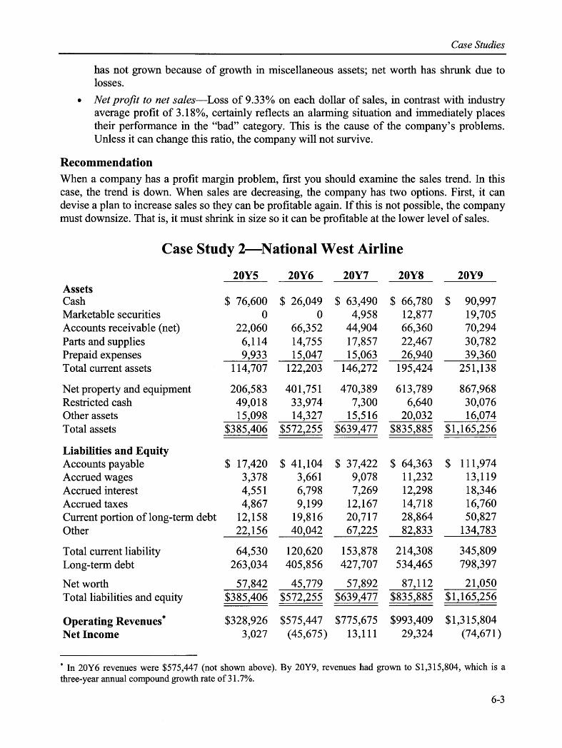
Case Studies

has not grown because of growth in miscellaneous assets; net worth has shrunk due to losses.

• Net profit to net sales—Loss of 9.33% on each dollar of sales, in contrast with industry average profit of 3.18%, certainly reflects an alarming situation and immediately places their performance in the “bad” category. This is the cause of the company’s problems. Unless it can change this ratio, the company will not survive.

RecommendationWhen a company has a profit margin problem, first you should examine the sales trend. In this case, the trend is down. When sales are decreasing, the company has two options. First, it can devise a plan to increase sales so they can be profitable again. If this is not possible, the company must downsize. That is, it must shrink in size so it can be profitable at the lower level of sales.

Case Study 2—National West Airline

* In 20Y6 revenues were $575,447 (not shown above). By 20Y9, revenues had grown to $1,315,804, which is a three-year annual compound growth rate of 31.7%.

20Y5 20Y6 20Y7 20Y8 20Y9AssetsCash $ 76,600 $ 26,049 $ 63,490 $ 66,780 $ 90,997Marketable securities 0 0 4,958 12,877 19,705Accounts receivable (net) 22,060 66,352 44,904 66,360 70,294Parts and supplies 6,114 14,755 17,857 22,467 30,782Prepaid expenses 9,933 15,047 15,063 26,940 39,360Total current assets 114,707 122,203 146,272 195,424 251,138

Net property and equipment 206,583 401,751 470,389 613,789 867,968Restricted cash 49,018 33,974 7,300 6,640 30,076Other assets 15,098 14,327 15,516 20,032 16,074Total assets $385,406 $572,255 $639,477 $835,885 $1,165,256

Liabilities and EquityAccounts payable $ 17,420 $ 41,104 $ 37,422 $ 64,363 $ 111,974Accrued wages 3,378 3,661 9,078 11,232 13,119Accrued interest 4,551 6,798 7,269 12,298 18,346Accrued taxes 4,867 9,199 12,167 14,718 16,760Current portion of long-term debt 12,158 19,816 20,717 28,864 50,827Other 22,156 40,042 67,225 82,833 134,783

Total current liability 64,530 120,620 153,878 214,308 345,809Long-term debt 263,034 405,856 427,707 534,465 798,397

Net worth 57,842 45,779 57,892 87,112 21,050Total liabilities and equity $385,406 $572,255 $639,477 $835,885 $1,165,256

Operating Revenues* $328,926 $575,447 $775,675 $993,409 $1,315,804Net Income 3,027 (45,675) 13,111 29,324 (74,671)

6-3


* For these three ratios, receivables, inventory, and sales are generally divided by the working capital. However, working capital is negative, so we use current assets in the denominator. The interpretation is very similar.

Per Dun & Bradstreet®.

20Y5 20Y6 20Y7 20Y8 20Y9 Ind.LiquidityCurrent ratio 1.78 1.01 0.95 0.91 0.73 1.36Receivables/current assets 19.2% 54.3% 30.7% 33.9% 28.0% 40.7%Inventory/current assets 5.3% 12.1% 12.2% 11.5% 12.3% 1.8%Sales/current assets 286.8% 470.9% 530.3% 508.3% 523.9% 235.6%

DebtDebt to net worth 566.3% 1,150.0% 1,004.6% 859.6% 5,435.7% 172.3%Current debt/net worth 111.6% 263.5% 265.8% 246.0% 1,642.7% 91.9%

ProfitsROE 5.2% (99.8%) 22.6% 33.7% (354.7%) 9.1%

CausalFixed assets/net worth 357.2% 877.6% 812.5% 704.6% 4,123.4% 92.9%Collection period 24.1 days 41.5 days 20.8 days 24.0 days 19.2 days 62.2 daysInventory turnover 53.8x 39.0x 43.4x 44.2x 42.7x 26.3xNet sales/net worth 5.68x 12.57X 13.4x 11.4x 62.5x 2.95xProfit margin 0.9% (7.9%) 1.7% 3.0% (5.7%) 3.1%Misc. assets/net worth 43.3% 64.2% 52.8% 53.9% 263.3% N/A

National West AirlineIn analyzing this company, it is best to examine the first four years, 20Y5 to 20Y8. This is where the causes of the problems occur. In year 20Y9, the company is hit by a large external shock. It is the shock that puts them into bankruptcy, but their actions in the earlier years really set them up for the fall.

Analysis—Effect Ratios

• Liquidity—The company’s quantity of liquidity, as measured by the current ratio, has declined over this four-year period from 1.78 to 0.91 and is well below the industry average of 1.36. The quantity of liquidity is inadequate. The ratio of receivables to current assets has grown but is still below average. The sales to the current asset ratio has also grown over this time period and is considerably above the industry average.

• Debt—The company’s debt ratios each year are very large and considerably above average. The debt to net worth ratio has grown from 5.66% to 859% over the four years. The current debt to net worth ratio has grown from 111% to 246%.

• Profits—The return on equity is very high in 20Y7 and 20Y8. These years are before the external shocks hit. The company appears very profitable in 20Y8.

• Causes—This is a classic case of a company that has grown too quickly. The fixed assets to net worth ratio and the trading ratio are considerably larger than the industry averages.

6-4

Case Studies

Analysis—Causal RatiosThis company is a classic overtrader. Its trading ratio has grown from 5.68 to 11.4. Its fixed assets to net worth ratio has grown from 357% to 704%. When we examine the financial statements we see that both sales and fixed assets have grown rapidly. This company has grown.

Year 20Y9—External ShockIn the year 20Y9, the company is beset with external problems. First, a recession hits. Second, the company uses jet fuel for its airplanes. Due to problems in the mid-East, oil prices rise through the roof. The company is unable to withstand the shock because of its weak balance sheet. They declare bankruptcy in 20Y9. By 20Y9, it is too late to correct the problems. Had they focused on solutions for overtraders in the preceding two years, the bankruptcy might have been averted.

Case Study 3—Firm ACase study 3 is based on International Harvester. IH was a producer of the tractor portion of large trucks as well as large farm equipment such as tractors. In our analysis, we will focus on the first three years; this is where the foundation for their financial problems begin. In the final two years, the IH is beset with numerous external financial problems.

Firm A (in 000s)—Selected Figures

200V 200W 200X 200Y 200ZCash $ 27,256 $ 25,205 $ 137,106 $ 185,561 $ 40,691Trade receivables (net) 682,641 895,542 768,756 555,394 305,467Inventory 1,892,830 2,342,941 2,331,676 1,634,425 646,842Current assets 2,648,711 3,265,769 3,427,419 2,672,003 1,656,178Fixed assets (net) 889,723 1,039,147 1,277,239 1,360,792 965,638Other assets 68,000 124,400 231,400 146,062 131,673

Current liabilities 1,438,891 1,873,371 2,480,230 1,846,039 1,135,247Long-term liabilities 932,541 948,170 1,327,068 1,984,981 2,015,346Total liabilities 2,439,957 3,098,402 4,147,003 3,842,348 3,666,155Net worth 1,876,148 2,149,073 1,696,455 1,501,880 32,629

Net sales 6,664,347 8,392,042 6,311,804 6,297,915 4,292,304Net profit 186,680 369,562 397,328 (393,128) (1,638,193)Working capital (CA-CL) 1,209,820 1,392,398 947,189 825,964 520,931

6-5


Firm A

200V 200W 200X 200Y 200ZCausal RatiosFixed assets to net worth .47x .48x .75x .91x 29.6xCollection period 37 days 38 days 44 days 32 days 26 days

Net sales to inventory 3.52x 3.58x 2.7x 3.85x 6.6xNet sales to net worth 3.55x 3.90x 3.72x 4.19x 131.5xNet profits to net sales 2.8% 4.4% 6.3% (6.24%) (38.2%)Misc. assets to net worth 3.6% 5.8% 13.6% 9.7% 403.5%

Effect RatiosCurrent Ratio 1.84x 1.74x 1.38x 1.45x 1.46xInventory to working capital 156.5% 168.3% 246.2% 197.9% 124.2%Receivables to working capital 56.4% 64.3% 81.16% 67.2% 58.6%Net sales to working capital 5.51x 6.03x 6.66x 7.62x 8.24x

Current liability to net worth 76.7% 87.2% 146.2% 122.9% 3,479.3%Total liability to net worth 130.1% 144.2% 244.5% 255.8% 11,235.9%

Return on Equity 9.9% 17.2% 23.4% (26.2%) (5,020.6%)

Analysis—Effect RatiosFrom 200V to S00X, the company’s current ratio falls from 1.84 to 1.38. Inventory to working capital increases 156% to 246%, and receivables to working capital increases from 56% to 81%. Both the quantity and quality of liquidity have decreased. Leverage has increased. The company’s current liability to net worth ratio has increased from 76% to 146% and the debt to equity ratio has increased from 130% to 244%. Over this time period, the company’s balance sheet has become weaker. Remember, a weak balance sheet makes it harder for a company to survive external shocks.

Offsetting the balance sheet problems is the return on equity (ROE). The ROE has increased from 9.9% to 23.4%.

Analysis—Causal RatiosThe company’s fixed asset to net worth ratio increased from .47 to .75 between 200V and 200X. This reflects an expansion undertaken by the company.

The company’s collection period has increased from 37 days to 44 days. While this is not a large increase, it compounds the impact of the fixed asset expansion. When expanding, a company needs to pay attention to other details, like the collection period, to make sure that the expansion is successful.

The company’s inventory turnover has fallen from 3.5 to 2.7. As with the collection period, this drop in the inventory turnover exacerbates the problems caused by the fixed asset expansion.

Finally, the miscellaneous assets to net worth ratio increases from 3.6 to 13.6.

6-6

Case Studies

SummaryDue to the expansion of fixed assets combined with the problems with the collection period, inventory turnover and miscellaneous assets, the balance sheet has become weaker. In the final two years, IH is hit with a considerable number of external problems. These include a recession, an increase in interest rates, trucking deregulation and problems in the farming industry. IH was forced into bankruptcy.

Could bankruptcy have been averted? Had IH paid more attention to receivables and inventory during the expansion and/or expanded their fixed assets at a slower rate, they may have survived the external shocks.

Case Study 4—Store Container CorporationBalance Sheet

As of December 31 200X 200Y 200ZAssets: (Millions of dollars)Cash and equivalent $ 8,290 $ 3,880 $ 15,400Receivables 123,860 127,950 243,140Inventories 152,660 148,350 238,210Other current 38,440 40,000 33,710

Total current 323,250 320,180 530,460

Net property, plant and equipment 657,660 642,560 924,360Other assets 25,750 47,580 68,780

Total assets $1,006,660 $1,010,320 $1,523,600

Liabilities and Stockholders’ Equity:Notes payable $ 62,200 $ 57,630 $ 7,330Accounts payable 53,000 57,970 105,250Income taxes payable 3,740 4,120 5,880Other current 45,440 45,410 84,950

Total current 164,380 165,130 203,410

Long-term debt 491,330 501,250 768,490Deferred taxes 55,800 49,210 69,900

Total long-term debt 547,130 550,460 838,390Total liabilities 711,510 715,590 1,041,800

Common stock 147,390 152,170 222,360

Retained earnings 147,760 142,560 163,250Total common equity 295,150 294,730 385,610

Preferred stock — — 96,190

Total liabilities and equity $1,006,660 $1,010,320 $1,523,600

6-7


Income Statement

200X 200Y 200ZSales: (Millions of dollars)Net sales $1,244,390 $1,229,150 $2,032,320Other income 7,110 4,600 10,850

Total 1,251,500 1,233,750 2,043,170Costs and expenses:Cost of sales 925,870 944,150 1,564,610Selling and administrative expenses 147,640 156,990 241,180Depreciation and amortization 63,380 67,810 92,310Interest expense 59,280 63,310 85,340

Total 1,196,170 1,232,260 1,983,440Income (loss) before taxes 55,330 1,490 59,730Provision (credit) for income taxes 21,670 (2,290) 24,320Net income $ 33,660 $ 3,780 $ 35,410

Key Ratios 200X-200Z

Ratio 200X 200Y 200Z Industry

LiquidityCurrent Ratio 1.97x 1.94x 2.61x 1.80xQuick Ratio .80x 0.80x 1.27x 0.90xReceivables/Working capital 78.00% 83.00% 74.00% 69.00%Inventory/Working capital 96.00% 96.00% 73.00% 72.00%

DebtDebt to Equity 241.07% 242.80% 270.17% 129.10%Current Liabilities to Equity 55.69% 56.03% 52.75% 50.90%Times Interest Earned 1.93x 1.02x 1.70x 5.76x

ProfitabilityProfit Margin 2.71% 0.31% 1.74% 2.50%Asset Turnover 1.24x 1.22x 1.33x 1.68xEquity Multiplier 3.41x 3.43x 3.95x 3.26xReturn on Equity 11.400% 1.280% 9.180% 13.70%

CausalFixed assets/Equity 222.82% 218.01% 239.71% 110.00%Collection period 36.33 days 38.00 days 43.67 days 38.90 daysSales/Inventory 8.15x 8.29x 8.53x 12.30xSales/Equity 4.22x 4.17x 5.27x 2.63xNet income/Sales 2.71% 0.30% 1.74% 5.20%Miscellaneous assets/Equity 8.72% 16.14% 17.83% 7.95%

6-8

Case Studies

Analysis—Effect RatiosStore Container’s current ratio has increased from 1.97 to 2.61 from 200X to 200Z. It is also above the industry average. The quick ratio increased from .8 to 1.27 and is also above the industry average of 0.9. The quantity of liquidity is certainly adequate. However, when liquidity is high, profits can suffer. The quality of liquidity ratios (inventory and receivables to working capital) are both near average and in good shape.

The leverage ratios, however, are not in great shape. Debt to equity has grown from 241% to 270% in an industry with an average of 129%. Times interest earned has fallen from 1.93 to 1.70 in an industry with an average of 5.76. Debt has increased and is above average while solvency, the ability to afford debt, has decreased.

The company’s ROE has fallen from 11.4 to 9.18 and is below the industry average of 13.7. Remember, the ROE is the product of the profit margin, asset turnover and equity multiplier. Of these ratios, the profit margin seems to be the problem. It has fallen from 2.715 to 1.74%. Since the company’s sales have grown from $1,244,390 to $2,032,320, the problem seems to rest with cost control. A falling profit margin during a period with a sales increase generally means that expenses have grown proportionately faster than sales.

Analysis—Causal RatiosThe company’s fixed assets to net worth ratio is well above average (239% compared to 110%). It has also grown over this time period. The collection period has grown from 36 days to 44 days in an industry with an average of 39 days. The inventory turnover is also below average (8.5 compared to 12.3). The trading ratio has grown from 4.2 to 5.3 in an industry with an average of 2.6. Recall sales and fixed assets have increased. This company is in the beginning stages of overtrading. Overtraders often have problems with their collection periods, inventory turnover and profit margins. Overtraders become so fixated on sales increases that other aspects of the business do not receive the appropriate attention.

6-9


Case Study 5—Biscayne ApparelBalance Sheet

200X 200Y 200ZAssetsCash $ 1,568 $ 4,178 $ 312Receivables 14,401 21,009 18,271Inventory 8,419 22,584 25,890Other 337 1,573 3,941

Total current assets 24,725 49,344 48,414Property, Plant, and Equipment 2,098 2,984 3,652Other assets 7,968 8,250 9,676

Total assets $34,791 $60,578 $ 61,742

LiabilitiesAccounts payable $ 2,343 $ 6,060 $ 3,841Accruals 3,384 6,841 5,914Notes payableCurrent portion of long-term debt

2,850 8,500 17,8501,250

Bridge note — 4,776 —Total current liabilities 8,577 26,177 28,855

Notes payable 6,444 7,944 6,444Long-term debt — — 6,250Other 210 576 358Net worth 19,560

$34,79125,881

$60,57819,835

$ 61,742

Revenue $65,258 $72,350 $100,294Net income 3,895 2,048 (6,127)

6-10

Case Studies

Ratios

Industry200X 200Y 200Z Average

LiquidityDefensive interval 95.70 137.00 76.20 57.50Current ratio 2.88 1.89 1.68 2.02Quick ratio 1.90 1.02 0.78 1.18Receivables to working capital 0.89 0.91 0.93 0.70Inventory to working capital 0.52 0.97 1.32 0.83

DebtDebt to equity 0.78 1.34 2.11 1.00Current debt to equity 0.44 1.01 1.45 0.77Times interest earned 5.74 3.19 (1.39) N/A

DuPont®Profit margin 6.00% 3.00% (6.00%) 4.00%Asset turnover 1.88x 1.19x 1.62x 2.98xROA 11.28% 3.57% (9.72%) 11.92%Equity multiplex 1.78x 2.34x 3.11x 2.00xROE 20.08% 8.35% (30.23%) 23.84%

CausalFixed assets to net worth 10.70% 11.50% 18.40% 34.00%Collection period (days) 79.40 104.50 65.60 33.50Net sales to inventory 7.75x 3.20x 3.87x 9.10xNet sales to net worth 3.34x 2.80x 5.06x 5.94xNet profit to net sales 6.00% 3.00% (6.00%) 4.00%Miscellaneous assets to net worth 0.00% 6.00% 8.00% 10.00%

Analysis—Effect RatiosBiscayne’s defensive interval has fallen from 95 days to 76 days but is above the industry average of 57 days. However, its current ratio has fallen from 2.8 to 1.6 in an industry with an average of about 2. Similarly, the quick ratio has fallen from 1.9 to 0.8 in an industry with an average of 1.18. The quantity of liquidity is somewhat below average. Receivables and inventory to working capital have both increased and are above average. We can conclude that both the quantity and quality of liquidity are below average.

The company’s debt to equity ratio has risen from 0.78 to 2.11. The industry average is 1.0. Leverage is excessive. The times interest earned ratio has fallen and is now negative.

The profit margin has fallen from positive 6 to negative 6%. This occurred in a period with a sales (revenue) increase. With the increased equity multiplier, this has caused the ROE to fall from 20% to negative 30%.

6-11


Analysis—Causal RatiosWhile the company’s collection period has decreased from 79 days to 65 days, it is still considerably above the industry average of 33 days. The inventory turnover has fallen from 7.7 times to 3.8 times. This is also below average (nine times). We have already mentioned the profit margin and cost control problems. To correct its problems the company should improve its inventory management and determine how to get its cost structure back in line.

6-12

Chapter 7

Users of Financial Statements


• Understand the ratios creditors use to analyze a set of financial statements,• Anticipate how lenders will view financial statements, and• Know how creditors analyze specific asset and liability accounts.

IntroductionIn this section, we examine the different ways in which creditors and owners look at a set of financial statements. Creditors are more balance sheet-oriented. Owners and managers are more income-statement oriented.

Ratios Examined by Banks for Short-Term LoansCreditors must be concerned for the safety of the funds that they lend. That is why they focus considerable attention on the balance sheet. A credit analyst or loan officer at a bank will evaluate a company’s financial statements. Short-term creditors are primarily interested in the balance sheet, which shows the firm’s current financial condition. These six ratios are commonly used for this purpose:

• The current ratio,• Cash and receivables to current debt,• Receivables to average day’s sales,• Inventory supply in days,• Total debt to tangible net worth, and• Fixed assets to tangible net worth.

Lenders and creditors are concerned with two things: The borrower’s ability to repay and the security in case the borrower cannot repay.

Given these facts, how does a creditor view financial information? The answer depends upon whether we are dealing with short-term or long-term debt.

7-1


Ratios Examined by Banks for Long-Term LoansThe importance of the income statement increases with the length of the loan. Bankers place more emphasis on liquidity for short-term loans. Note that the first six ratios are the same as for short-term credit; with long-term credit notice, now income statement ratios become more important:

• The current ratio• Cash and receivables to current debt• Receivables to average day’s sales• Inventory supply in days• Total debt to tangible net worth• Fixed assets to tangible net worth

As the duration of a loan increases, the importance of the income statement grows:• Net profit to sales• Net profit to net worth• Net sales to net worth• Accounts payable turnover in days• Debt ratio• Debt to equity• Times interest earned• Fixed-charge coverage

Commercial Loan Departments’ Most Significant Ratios and Their Primary Measures—Gibson’s Study

For his Financial Statement Analysis: Using Accounting Information (1989, pp. 508-510), Dr. Charles Gibson of Stanford University conducted a survey of loan officers at large banks. Gibson asked bankers to rank over 50 ratios based upon their importance when examining loan applications. The ratios listed above were deemed to be the most important ones. Notice that liquidity and debt ratios are heavily emphasized.

7-2

Users of Financial Statements

Results of the StudyPrimary

_________________Ratio_________________ Measure Debt/equity___________________________________ DebtCurrent ratio LiquidityCash flow/current maturities of long-term debt DebtFixed charge coverage DebtNet profit margin after tax ProfitabilityTimes interest earned DebtNet profit margin before tax ProfitabilityDegree of financial leverage DebtInventory turnover in days LiquidityAccounts receivable turnover in days Liquidity

Note: Not all sentences are double-spaced.

In addition to the above ratios, many bankers will require more detailed information about specific accounts.

Commercial Loan Departments' Ratios Appearing Most Frequently in Loan Agreements

Creditors generally place certain restrictions on borrowers. Quite often these restrictions are in the form of ratios. Gibson’s study points out the most common ratios that appear in loan agreements. The following table shows, once again, the importance that lenders place on the balance sheet.

* A measure of payout that may include owner/officer salaries.

RatioPrimary Measure

Debt/equity DebtCurrent ratio LiquidityDivided payout ratio *

Cash flow/current maturities of long-term debt DebtFixed charge coverage DebtTimes interest earned DebtDegree of financial leverage DebtEquity/assets DebtCash flow/total debt DebtQuick ratio Liquidity

7-3


Corporate Controllers’ Most Significant Ratios and Their Primary Measures

Gibson also surveyed controllers of large corporations. He asked them to rank ratios based upon their importance to their company. The following table shows that managers are most concerned about income:

* Primary measure indicated to be other than liquidity, debt, or profitability. These ratios are usually related to stock analysis.


Earnings per share ProfitabilityReturn on equity after tax ProfitabilityNet profit margin after tax ProfitabilityDebt/equity ratio DebtNet profit margin before tax ProfitabilityReturn on total invested capital after tax ProfitabilityReturn on assets after tax ProfitabilityDividend payout ratio Other*Price/eamings ratio Other*Current ratio Liquidity

These ratios show that managers are concerned with profitability first and liquidity and debt second. This contrasts with the view taken by creditors. Corporate controllers were asked to rank the usefulness of ratios.

Ratios Appearing in Corporate Objectives and Their Primary Measures

Finally, Gibson examined ratios that appeared in corporate objectives. These are the most common ratios. The table again shows that managers are most concerned about income:


Earnings per share ProfitabilityDebt/equity ratio DebtReturn on equity after tax ProfitabilityCurrent ratio LiquidityNet profit margin after tax ProfitabilityDividend payout ratio OtherReturn on total invested capital after tax ProfitabilityNet profit margin before tax ProfitabilityAccounts receivable turnover in days LiquidityReturn on assets after tax Profitability

7-4

Chapter 8

Forecasting Sustainable Growth

OverviewUpon completion of this section you will be able to:

• See how growth can put a firm’s balance sheet out of order; and• Determine how fast a company can grow without weakening its balance sheet.

IntroductionThis section develops a simple forecasting model that permits the analyst to determine how fast a growth pattern a company can sustain. This approach can be a valuable planning tool.

DefinitionsSA Spontaneous assets—These are assets that generally need to increase as sales increase.

They include most of the current assets.

▲FA Change in net fixed assets—This includes new, fixed asset acquisitions, less depreciation expenses.

PO Payout ratio—This is the proposition of earnings paid out as a dividend. The retention ratio is (1 - PO).

PM Profit margin—This is often called the net profit margin and is net income divided by net sales revenue.

EFN External financing needed—This is the amount of additional long-term financing needed from external debt and equity sources.

Derivation of the Sustainable Growth ModelThe model comes from the equation used in the sales method forecasting model. This model shows that a company’s external financing needs, EFN, are a function of the growth in spontaneous assets. We measure this using the historical percentage of spontaneous assets to sales (SA/S) multiplied times the expected change to sale (AS). In addition, the company must add fixed assets as it grows. This amount is the cost of new assets less the expected depreciation on the new and existing assets (▲FA). Internal sources of funds come from spontaneous liabilities and the addition to retained earnings. We estimate spontaneous liabilities as the historical ratio of spontaneous liabilities to sales, SL/S multiplied times the expected change to sales (AS). We estimate the addition to retained earnings as the sum of historical sales, S and the expected change (AS),

8-1


multiplied times the expected profit margin and the retention ratio, measured as 1 minus the payout ratio:

(1)

An expression for new debt and new assets can be set up that equals our target debt to asset ratio for the increased business. We assume that the EFN will be entirely debt financed. That is, the company does not want to add external equity dollars at this time. So the new debt is the sum of the EFN and the new spontaneous liabilities. The new assets include the new spontaneous assets and new fixed assets:

(2)

By substituting the value of EFN from (1) into (2) and solving for AS, we can obtain the solution:

This is the sustainable growth model when there are no available sources of external equity dollars. By plugging in the values that we know, we can determine the maximum AS with our desired D/A ratio as a constraint.

Most companies place some limit on the amount of debt they are willing to assume. In addition, raising new equity capital is difficult and may be virtually impossible for most small businesses. Thus, as long as a target debt to asset ratio is not to be exceeded, growth is limited.

In order to determine the maximum growth potential for a given time period, one must begin with a determination of the amount of equity that can be raised internally. This amount depends upon the new sales level (which depends on the amount of internally generated equity). This joint dependence between the new sales level and new equity can be solved only with simultaneous equations:

• The model is derived from the EFN equation;• Assumes that the company wants to limit its debt to asset ratio; and• Finds the maximum amount of sustainable sales growth:

— Sales growth requires assets;— Assets require debt and/or equity;— Limited equity and desire to limit the debt to assets ratio limits the amount of new as

sets; and— The limit on assets in turn limits sales.

8-2

SA SLEFN =—ΔS + ΔFA -—ΔS - (s + ΔS)(pm)(1 - PO) s s

SLEFN+—-AS S—ΔS+ΔFA S

(3) AS = ΔF(1 - d/a) - S(PM)(1 - po) SA—(D/A -1) + (pm)(1 - PO) s

D/A New DebtNew Assets


The Alabama Door Company Sustainable Growth—Example

20X7 Balance Sheet

Cash $ 5,000 Accounts Payable $ 3,000Marketable Securities 5,000 Taxes Payable 12,000Accounts Receivable 10,000 Accruals 3,500Inventory 35,000

Total 18,500Total 55,000

Notes Payable (8%) 15,000Building 100,000 Bonds Payable (12%) 30,000Equipment 15,000 Common Stock 48,000

Retained Earnings 58,500

Total Assets $170,000 Total Debt and Equity $170,000

Selected Income Statement Figures 20X7Sales $245,000Net Income 19,008Dividends 15,000

Assumptions• Assume that $5,000 of new fixed assets is required.• The Alabama Door Company wants to maintain its 37.4% debt to asset ratio.

Class Exercise• Compute the Alabama Door Company’s maximum growth rate for 20X8 if no new

externally-generated equity is available.• Recompute the Alabama Door Company’s maximum growth rate for 20X8, assuming

that $20,000 of new fixed assets is required.

8-3


Calculation of Alabama Door Growth Rate

ΔS =

• The Alabama Door Company can have a sustainable sales increase of $7,891 with the $5,000 increase in fixed assets and the debt to asset ratio remaining at 37.4%. Growth beyond $7,891 will require new equity or a relaxation of the debt to asset constraint.

• If fixed assets must increase by $20,000, AS becomes negative, implying that assets cannot increase by the specified amount without new equity or a relaxation of the debt to asset constraint.

Improving Sustainable GrowthAnything that improves the amount of earnings retention will increase a company’s sustainable growth rate. Companies that grow rapidly and do so successfully have this in common; they are highly profitable and they retain earnings in the company.

1. What would happen to AS if the profit margin increased to, say, 10%? As you can see, if we improve the company’s rate of profitability, sustainable growth can increase:

2. What would happen to AS if the payout ratio dropped to 50% as well as the change in (1) above. By improving earnings retention, sustainable growth can increase:

8-4

ΔFA(1 - D / A)- S(P.M.)(1 - PO)

(D / A -1)+(P.M.)(1 - PO)

5,000(1 - .374)- (245,000)(.07758)(l - .7891) 50,000 (.374 -1)+(.07758)(1 - .7891)

245,000

----- —— = $7,891-.1113935

5,000(1 - .374)- (245,000)(.10)(l -.7891)

(.374- 1)+(.10)(1-.7891)

3,130-5,167 _ -2037-0.12776 + .02109 =-.10667

5,000(1 - .374) - (245,000)(. 10)(1 - .5) 50,000(.374-l)+(.10)(1-.5) 245,000

3,130-12,250-.12776+ .05

ΔS =

AS =

ΔS =

ΔS = - = $19,096

ΔS =

ΔS = -9,120 -.07776 = $117,284

50,000245,000


Sustainable Growth—Available External EquityIn some instances external equity is available to finance growth. Existing stockholders or new stockholders (partners) may have a fixed sum of equity to invest in the company.

If we define the amount of externally generated equity to be EE, then the growth formula becomes:

If we return to the example of the Alabama Door Company, part 1, the growth in sales can be computed for the case in which $10,000 of external equity is available:

The change in sales for this example is considerably larger than that which could be afforded when no external equity was available. The increased equity allows for more debt financing while still keeping the debt to asset ratio at 37.4%. The increased debt and equity permits assets to grow sufficiently to support the larger sales volume.

8-5

ΔFA(1 - D /A) - S(P.M.)(1 - PO) - EE

(D/A-1)+(P.M.)(1-PO)

5,000(1 -.374)- (245,000)(.07758)(1 -.7891)-10,000

(.374 -1)+(.07758)(1 - .7891)

ΔS =

ΔS = 50,000

245,000

ΔS = $97,663

SAS

Chapter 9

Case Problem

OverviewUpon completion of this section you will be able to:

• Analyze the financial position of a company utilizing both the cause-and-effect and DuPont® systems.

• Compare the information gained by the two systems of analysis.

IntroductionThe purpose of this section is to allow you to pull the information together and work with the systems explained previously in the text. The problem allows you to use the causal ratios and the DuPont® System of ratio analysis and to compare the results from the two systems. You must also use the percent of sales method to forecast the external financial needs of the company. Last, you must prepare pro forma statements under different financing alternatives to see the effect that this type of external financing has on the causal ratios and the DuPont® System.

9-1


Marine Supply Company Balance Sheet

Year 1 Year 2 Year 3 Year 4Cash $ 12,100 $ 17,400 $ 19,500 $ 17,480Receivables 31,400 35,600 46,500 53,700Inventories 64,700 79,000 100,800 97,320Total current assets 108,200 132,000 166,800 168,500Net plant 46,200 58,600 68,900 72,020Miscellaneous assets 10,700 11,900 12,700 15,440Total assets $165,100 $202,500 $248,400 $255,960

Liabilities and CapitalAccounts payable $ 7,000 $ 15,200 $ 24,600 $ 24,530Other current liabilities 23,500 26,900 35,000 36,750Total current liabilities 30,500 42,100 59,600 61,280Long-term debt 12,400 28,700 45,700 46,040Deferred taxes 2,570 4,580 5,380 7,140Other liabilities 2,030 1,520 2,570 1,050Total liabilities 47,500 76,900 113,250 115,510Net worth 117,600 125,600 135,150 140,450Total $165,100 $202,500 $248,400 $255,960

Marine Supply Company Selected Income Figures

Year 1 Year 2 Year 3 Year 4Net sales $233,400 $280,200 $327,100 $304,480Gross profit 83,970 95,290 111,999 107,840Earnings before interest & taxes 29,930 33,300 40,550 34,850Interest 1,230 2,100 4,730 6,600

Net income $ 15,230 $ 15,660 $ 17,080 $ 13,390Dividend 6,070 7,660 7,530 8,090Addition to net worth $ 9,160 $ 8,000 $ 9,550 $ 5,300

9-2

Case Problem

Marine Supply Company Selected Financial Ratios

Assume all sales are credit sales. Industry ratio unavailable.

Causal Ratios Year 1 Year 2 Year 3 Year 4 IndustryFixed assets to net worth 39.2% 46.7% 51.0% 51.3% 45.5%Collection period* * 49.1 days 46.4 days 51.9 days 64.4 days 44.0 daysNet sales to inventory 3.61X 3.55x 3.25x 3.13x 4.1xNet sales to net worth 1.98x 2.23x 2.42x 2.17x 2.10xNet profit to net sales 6.5% 5.6% 5.2% 4.4% 6.2%Misc. assets to net worth 9.1% 9.5% 9.3% 10.9% t

DuPont® AnalysisProfit margin 6.5% 5.6% 5.2% 4.4% 6.2%Asset turnover 1.41X 1.38x 1.32x 1.18x 1.5xReturn on assets 9.2% 7.7% 6.9% 5.2% 9.3%Equity Multiplier 1.402x 1.610X 1.841X 1.827X 1.376XReturn on equity 12.9% 12.4% 12.7% 9.5% 12.8%

Other RatiosCurrent ratio 3.55x 3.14x 2.80x 2.74x 2.40xCurrent liability to net worth 25.94% 33.52% 44.10% 46.63% 20.10%Debt to asset ratio 28.8% 37.9% 45.6% 45.1% 27.3%Times interest earned 24.3x 15.8x 8.6x 5.3x 8.6xInventory to working capital 83.3% 87.8% 94.0% 90.7% 91.07%Receivables to working capital 40.4% 39.6% 43.4% 50.1% 44.9%Net sales to fixed assets 5.1x 4.8x 4.7x 4.2x 6.4xNet sales to working capital 3.0x 3.1x 3.1x 2.8x 4.0x

Solution to CaseQuestion 1—Marine Supply Company Causal Ratio Analysis

• Fixed asset to net worth—This ratio has risen sharply. Remember that when this ratio rises, working capital and leverage problems can result. Marine Supply’s debt ratio has risen and its current ratio has fallen.

• Collection period—This ratio has risen consistently and is above the industry average. A large collection period can cause debt and liquidity problems, both of which are present for Marine Supply. The receivables to working capital ratio has increased substantially, indicating a reduction in the quality of Marine Supply’s liquidity.

• Net sales to inventory—This ratio has fallen consistently and is below industry average. This build-up of inventory can cause debt and liquidity problems. In addition, the inventory to working capital ratio has risen, indicating a reduction in the quality of Marine Supply’s working capital.

9-3


• Net sales to net worth—Has remained fairly stable and is close to the industry average.• Net profit to net sales—Measures the company’s ability to keep profits from its sales

dollars. This ratio has fallen over the whole time period. Insufficient profits can harm the liquidity ratios and cause a company to use substantial amounts of debt.

• Miscellaneous assets to net worth—The jump in this ratio needs to be explained. There is no industry average to compare this to. However, the magnitude of the jump requires study.

Question 2—Marine Supply Company DuPont Analysis

• Return on equity—Until Year 4 the ROE remained fairly stable, but only because of increased use of debt. Once the company stopped increasing its debt, the ROE dropped. The use of debt magnified Marine Supply’s profitability (ROE), but only at the expense of increasing its financial risks.

• Return on assets—The ROA declined steadily throughout the whole time period. Its two components, profit margin and asset turnover, declined as well. These ratios demonstrate that Marine Supply is having difficulty controlling its costs and producing sales.

9-4

Chapter 10

Forecasting Bankruptcy


• Determine the ratios to be used in a Z-score;• Calculate a Z-score; and• Know how a Z-score determines the likelihood of bankruptcy.

IntroductionThe purpose of this section is to provide you with a way to forecast bankruptcy using five simple ratios to determine a Z-score for any firm. The ratios used to determine the Z-score are working capital to total assets, retained earnings to total assets, earnings before interest and tax “EBIT” to total assets, the market value of the firm’s equity to the book value of its debt, and sales to total assets. The Z-score is a measure of overall financial health.

©Altman’s Bankruptcy Prediction FormulaThe Z-score was developed by Dr. Edward I. Altman of New York University. Altman developed this model to use as a bankruptcy predictor. The model is based on a statistical technique called discriminant analysis. This type of statistical model allows the user to determine differences between groups. In this case we are trying to determine differences between bankrupt and non-bankrupt companies.

Using a sample of bankrupt companies plus an industry and sized-matched control sample of non-bankrupt companies, Altman developed the following model. The model has five independent (X) variables. The numbers in front of each X variable is its coefficient. These coefficients came from the statistical technique and are the same for each company.

To use the model, all you need to do is compute each of the five X variables. Then multiply the X variable times its coefficient. The sum of these products provides the Z -score:

10-1

Z = .012X1 + .014X2 + .033X3 + .006X4 + .999X5

X1 = working capital/total assetsX2 = retained eamings/total assetsX3 = earnings before interest and taxes/total assetsX4 = total market value of equity/total debtX5 = sales/total assetsZ = Overall index


Altman’s Suggested Z-Score Cutoff

If Z is:____________Less than 1.81Between 1.81 and 2.99Greater than 2.99

This indicates:A problemConcernNo problem

Computational NoteVariables X1 to X4 are to be computed as a percent, not as a decimal. For example, if X1 is 21.8%, put it in the model as 21.8 not as 0.218.

Usage NotesThe Z-score is a good measure of overall health. Do not become too concerned with Altman’s 1.81 cutoff. Observe how the Z-score varies across time. One should be less worried about a company who’s Z-score remains between 1.70 and 1.85 for the last ten years than about a firm that dropped from 2.8 to 1.95 in one year. Use your judgment regarding this ratio.

Bankruptcy Prediction Example

Crystal Brands, Inc. Selected Financial Data

(in 000s)

20X5 20X6 20X7 20X8 20X9Net sales $857,241 $868,465 $826,876 $486,893 $444,302EBIT 84,758 84,393 (19,345) 1,103 (87,379)Current assets 351,726 363,880 350,048 245,744 155,245Current liabilities 167,558 172,179 199,761 77,165 313,392Total assets 682,528 688,138 659,437 486,309 248,437Total debt 444,779 421,963 465,946 362,128 340,556Retained earnings 47,161 74,235 1,019 (66,801) (282,917)Number of shares 9,078 9,098 9,116 9,117 9,117Market Price/Share 33.03 21.06 14.00 4.03 1.07

X1 26.98% 27.86% 22.79% 34.66% (63.66%)x2 6.91% 10.79% 0.15% (13.74%) (113.88%)X3 12.4% 12.2% (2.9%) (0.2%) (35.17%)X4 67.41% 45.41% 27.39% 10.15% 2.86%X5 1.26 1.26 1.25 1.00 1.79

z 2.49 2.42 1.59 1.29 (1.71)

10-2

Forecasting Bankruptcy

Altman’s Second ModelIn 1983, Dr. Altman developed a second model that is, perhaps, more useful for small companies (service companies and manufacturers). Each variable is computed as a percent, not as a decimal.

10-3

Z = 0.0656Y1 +0.0326Y2 +0.0672Y3 +0.0105Y4

Y1 = working capital to total assetsY2 = retained earnings to total assetsY3 = earnings before interest and taxes to total assetsY4 = net worth to total liabilities

Z'<1.1 Concern1.1<Z'<2.6 Grey Area2.6 < Z' Strong Company

Where:

Critical Values

There are several other bankruptcy prediction models that have been proposed. Altman’s models may work as well as most others. However, if you would like an additional model to choose from, we recommend the following:

• Fulmer, J.G, J.E. Moon, T.A. Gavin, and J.M. Erwin, “A Bankruptcy Classification Model for Small Firms.” The Journal of Commercial Bank Lending, July 1984, pp. 25- 37.

• Altman, E.I, R.G. Haldeman, and P. Narayanan, “Zeta Analysis: A New Model to Identify Bankruptcy Risk of Corporations.” Journal of Banking and Finance, June 1977, pp. 29-54.

Guide to Financial Statem

ent Analysis: B

asis for Managem

ent AdviceAICPA Member and

Public Information: www.aicpa.org

AICPA Online Store:www.cpa2biz.com

ISO Certified091022

http://www.aicpa.org

http://www.cpa2biz.com

Guide to financial statement analysis : basis for management ...

Documents

Transcript of Guide to financial statement analysis : basis for management ...