Electronic copy available at: http://ssrn.com/abstract=1259333

1

Growth, poverty and chronic poverty in rural Ethiopia:

Evidence from 15 Communities 1994-2004

Stefan Dercon

John Hoddinott

Tassew Woldehanna

May 2008

This paper examines growth, poverty and chronic poverty in 15 Ethiopian villages between 1994 and 2004. Growth and poverty reduction in these communities was substantial; headcount poverty fell from 48 to 35 percent. However, there is also movement in and out of poverty over this period and a significant proportion of the sample was chronically poor. Chronic poverty is associated with several characteristics: lack of physical assets, education, and ‘remoteness’ in terms of distance to towns or poor roads. The chronically poor appear to be benefit from roads or extension services in much the same way that the non-chronically poor benefit. However, their ‘initial’ conditions, as captured in estimated latent growth related to time-invariant characteristics suggests that they face a considerable growth handicap. This ‘fixed’ growth effect is correlated with the characteristics of the chronic poor during the sample period. Chronic poverty, as reflected in poor initial assets and remoteness, appears to be correlated with a divergence in living standards over the sample period. Acknowledgements: Paper prepared for the CPRC. The data and some of the research on which this review is based has been funded by SIDA, ESRC, USAID, The World Bank and the World Food Programme. We are grateful to our co-authors on much of the work quoted in this paper, most notably Pramila Krishnan and Dan Gilligan. Addresses for correspondence: Stefan Dercon, Department of Economics, University of Oxford. Email: Stefan.Dercon@economics.oxford.ac.uk John Hoddinott, International Food Policy Research Institute, Washington DC. J.Hoddinott@cgiar.org. Tassew Woldehanna, Department of Economics, Addis Ababa University, wtassew@econ.aau.edu.et.

Electronic copy available at: http://ssrn.com/abstract=1259333

2

1. Introduction

In 1991, after decades of civil war in Ethiopia, the military Marxist-inspired regime of the

Dergue came to end with its defeat to a coalition of opposition forces, led by a rebel movement

from Tigray. Then, as now, Ethiopia was one of the poorest countries in the world. It has few

natural resources, is highly drought-prone and has poor economic and political relations with

most of its neighbours. But it would be wrong to argue that nothing has changed. The economy

has gone through a relevant and significant reform programme, reversing some of the extensive

but counterproductive control regime in the economy established during the Dergue. Aid

increased dramatically, albeit from extremely low levels, but resulting in significant investment

in health and education infrastructure, and not least, in new roads. A series of initiatives to

stimulate agricultural productivity growth were taken, including a technology transfer based on

extension, fertilizer and HYV seeds. But serious instability remained. Political reform has been

slow. After granting Eritrea independence in 1993, relations broke down and by 1998, a bloody,

costly war broke out ending with a cease fire in 2000. A serious drought hit the country in 2002,

and large scale relief operations unseen since the 1984-85 famine took place. Despite these

adverse events, real per capita GDP grew by 2.1 percent per year between 1994 and 2004, albeit

with high variability and recent analysis of nationally representative data indicates that

consumption poverty fell over this period (Woldehanna et al, 2008).

While there is an understanding of levels of consumption and poverty, as in much of sub-

Saharan Africa, little is known about poverty dynamics in Ethiopia This paper seeks to redress

this, examining poverty dynamics, and chronic poverty in 15 Ethiopian villages between 1994

and 2004. Growth and poverty reduction in these communities was substantial; headcount

poverty fell from 48 to 35 percent. However, there is also movement in and out of poverty over

3

this period and a significant proportion of the sample was chronically poor. Given these results,

the paper focuses on the magnitude and correlates of chronic poverty. We find that it is

associated with several characteristics: lack of physical assets, education, and ‘remoteness’ in

terms of distance to towns or poor roads. The chronically poor appear to be benefit from roads or

extension services in much the same way that the non-chronically poor benefit. However, their

‘initial’ conditions, as captured in estimated latent growth related to time-invariant characteristics

suggests that they face a considerable growth handicap. This ‘fixed’ growth effect is correlated

with the characteristics of the chronic poor during the sample period. Chronic poverty, as

reflected in poor initial assets and remoteness, appears to be correlated with a divergence in

living standards over the sample period.

Earlier work on poverty dynamics in poor contexts, such as the contributions in Baulch

and Hoddinott (2000), has tended to focus on poverty transitions: the frequency of people

moving in and out of poverty. This counting approach provides helpful insights in describing the

nature of poverty over a period of time, and is presented in this paper as well. However, a

weakness is that it does not take account of the depth and severity of poverty in each period.

Jalan and Ravallion (2000) present an approach to chronic poverty, in which chronic poverty

over a particular period of time is defined as the Foster-Greer-Thorbecke (FGT) index of

poverty, defined using average consumption over this period of time. A person is then chronic

poor if her average consumption is below the poverty line; the depth and severity of chronic

poverty is then be defined using the gap with the poverty line based on average consumption.

Calvo and Dercon (2007) pointed out a weakness of this approach as it allows for full

compensation between years of low consumption and high consumption, and present a number

of approaches that could . An intuitively appealing approach is to use all information on gaps

4

between consumption and the poverty line, and the average value of the FGT index can then be

seen as an index of chronic poverty, or more precisely, an index of intertemporal poverty. Foster

(2007) offers a hybrid version of the counting approach and this approach, by limiting those

counted as chronically poor to those poor for more than a threshold number of periods, and then

offering the average FGT based on the gap between consumption and the poverty line for these

households only. In this paper, we use the intertemporal poverty measure as in Calvo and Dercon

(2007).

In the next section, we describe the household level longitudinal data we use. In section

3, we present the basic evidence on poverty and its dynamics, as well discussing how this may fit

in with other evidence, including perceptions of poverty. We focus on standard period-by-period

overall living standards, as well as persistent poverty. In section 4, we take up a discussion of

likely causal factors in explaining this evolution. We present a simple model and a regression

analysis that nests a few of the key likely factors that may have mattered. We then extend this

analysis to include a discussion of whether the growth or the lack of it for the poor and the

persistently poor has similar explanatory factors. Section 5 concludes.

2. Data and setting

Ethiopia is a federal country divided into 11 regions. Each region is sub-divided into zones and

the zones into woredas which are roughly equivalent to a county in the US or UK. Woredas, in

turn, are divided into Peasant Associations (PA), or kebeles, an administrative unit consisting of

a number of villages. Peasant Associations were set up in the aftermath of the 1974 revolution.1

1 The PA was responsible for the implementation of land reform following 1974 and held wide ranging powers as a local authority. All land is owned by the government. To obtain land, households have to register with the PA and, thus, lists are maintained of the households who have been allocated land. These household lists were a good source of information for the construction of a sampling frame.

5

Our data are taken from the Ethiopia Rural Household Survey (ERHS), a unique longitudinal

household data set. The ERHS began in 1989, when a survey team visited 6 Peasant Associations

in Central and Southern Ethiopia. The survey was expanded in 1994 to include an additional nine

Peasant Associations, yielding a sample of 1477 households. As part of the survey re-design and

extension that took place in 1994, the samples in the original six villages were adjusted so as to

representative at the village level. The nine additional PAs were selected to better account for the

diversity in the farming systems found in Ethiopia. The sample was stratified within each village

to ensure that a representative number of landless households were also included. Similarly, an

exact proportion of female headed households were included via stratification, see Dercon and

Hoddinott (2004) for further details. Table 1 gives the details of the sampling frame and the

actual proportions in the total sample. Using Westphal (1976) and Getahun (1978)

classifications, Table 1 also shows that population shares within the sample are broadly

consistent with the population shares in the three main sedentary farming systems – the plough

based cereals farming systems of the Northern and Central Highlands, mixed plough/hoe cereals

farming systems, and farming systems based around enset (a root crop also called false banana)

that is grown in southern parts of the country. In fact, the sample sizes in each village were

chosen so as to approximate a self-weighting sample, when considered in terms of farming

system: each person (approximately) represents the same number of persons found in the main

farming systems as of 1994. However, results should not be regarded as nationally

representative. The sample does not include pastoral households or urban areas.2 Also, the

practical aspects associated with running a longitudinal household survey when the sampled

localities are as much as 1000km apart in a country where top speeds on the best roads rarely

2 Pastoral areas were excluded, in part, because of the practical difficulties in finding and resurveying such highly mobile households over long periods of time.

6

exceed 50km/hour constrained sampling to only 15 communities in a country of thousands of

villages. Therefore, extrapolation from these results should be done with care.

An additional round was conducted in late 1994, with further rounds in 1995, 1997, 1999

and 2004. These surveys were conducted, either individually or collectively, by the Economics

Department at Addis Ababa University, the Centre for the Study of African Economies,

University of Oxford or the International Food Policy Research Institute. Sample attrition

between 1994 and 2004 is low, with a loss of only 12.4 percent (or 1.3 percent per year) of the

sample over this ten year period, in part because of this institutional continuity.3 This continuity

also helped ensure that questions asked in each round were identical, or very similar, to those

asked in previous rounds and that the data were processed in comparable ways.

3. Poverty and welfare

We focus on poverty defined in terms of consumption. More than any other dimensions of

poverty, such as education or child mortality, it tends to be most closely related to changing

economic opportunities. Consumption is defined as the sum of values of all food items, including

purchased meals and non-investment non-food items. The latter are interpreted in a limited way,

so that contributions for durables and spending with some investment connotation, such as health

and education expenditures, are not included (Hentschel and Lanjouw, 1996). Although there are

good conceptual reasons for including use values for durables or housing (Deaton and Zaidi,

2002), we do not do so here; the heterogeneity in terms of age and quality of durables owned by

3 We examined whether this sample attrition is non-random. Over the period 1994-2004, there are no significant differences between attriters and non-attriters in terms of initial levels of characteristics of the head (age, sex), assets (fertile land, all land holdings, cattle), or consumption. However, attriting households were, at baseline, smaller than non-attriting households. Between 1999 and 2004, there are some significant differences by village with one village, Shumsha, having a higher attrition rate than others in the sample. Our survey supervisors recorded the reason why a household could not be traced. Using these data, we examined attrition in Shumsha on a case-by-case basis, but could not find any dominant reason why households attrited.

7

our respondents, together with the near complete absence of a rental market for housing would

make the calculation of use values highly arbitrary. Because comparisons of productive and

consumer durable holdings between 1994 and 2004 show rising holdings of these durables and

comparisons of school enrollment data show significant increases in enrollment (see Table 2

below), ceteris paribus, our consumption estimates may understate the actual increases in

household welfare. These values are expressed in monthly per capita terms and deflated using

the food price index with base year 1994.

Mean consumption per capita in 1994 was 71.1 birr per capita per month. By 2004, this

had risen to 91.5 birr per capita in real (1994) terms. Over this ten year period, consumption

growth of the mean was on average 2.6 percent per year. This is broadly comparable to the

average annual rate of growth of real GDP per capita (2.1 per cent) and the increases reported

using nationally representative household consumption data found in Woldehanna et al (2008).

These figures suggest a significant improvement in material wellbeing. However, they do not tell

us anything about the distribution of these gains and it would be instructive to see if these gains

are corroborated by other data collected in these surveys.

Figure 1 shows how the distribution of consumption has evolved since 1994. The striking

feature of this figure is the uniform shift of the distribution to the right, indicating that gains in

consumption appear to have been widely shared. Table 2 corroborates this, showing the Gini

coefficient for consumption inequality to be essentially unchanged over this period. It also

provides descriptive statistics on selected forms of asset ownership, schooling and access to

public services. There are improvements in all of these measures, although certain outcomes

(such as schooling and access to public services) remain low. In 2004, we asked people to rank

themselves (in a scale of 7 steps) how poor or rich they were. We asked the same question in

8

1995 and Table 2 also reports these findings. These self-reports also speak to improvements in

well-being, with the proportions of households reporting themselves to be in the poorest two

categories dropping markedly.

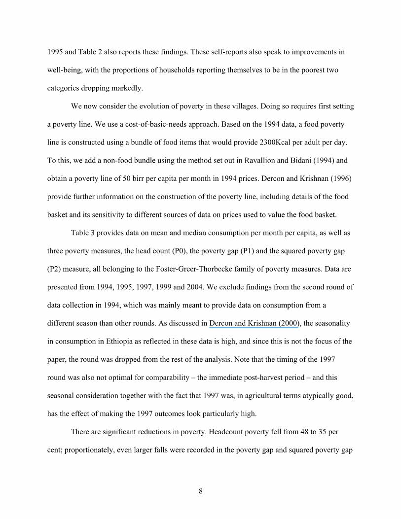
We now consider the evolution of poverty in these villages. Doing so requires first setting

a poverty line. We use a cost-of-basic-needs approach. Based on the 1994 data, a food poverty

line is constructed using a bundle of food items that would provide 2300Kcal per adult per day.

To this, we add a non-food bundle using the method set out in Ravallion and Bidani (1994) and

obtain a poverty line of 50 birr per capita per month in 1994 prices. Dercon and Krishnan (1996)

provide further information on the construction of the poverty line, including details of the food

basket and its sensitivity to different sources of data on prices used to value the food basket.

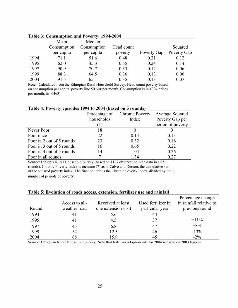
Table 3 provides data on mean and median consumption per month per capita, as well as

three poverty measures, the head count (P0), the poverty gap (P1) and the squared poverty gap

(P2) measure, all belonging to the Foster-Greer-Thorbecke family of poverty measures. Data are

presented from 1994, 1995, 1997, 1999 and 2004. We exclude findings from the second round of

data collection in 1994, which was mainly meant to provide data on consumption from a

different season than other rounds. As discussed in Dercon and Krishnan (2000), the seasonality

in consumption in Ethiopia as reflected in these data is high, and since this is not the focus of the

paper, the round was dropped from the rest of the analysis. Note that the timing of the 1997

round was also not optimal for comparability – the immediate post-harvest period – and this

seasonal consideration together with the fact that 1997 was, in agricultural terms atypically good,

has the effect of making the 1997 outcomes look particularly high.

There are significant reductions in poverty. Headcount poverty fell from 48 to 35 per

cent; proportionately, even larger falls were recorded in the poverty gap and squared poverty gap

9

indices. When we asked these households in 1995 to describe their circumstances (see Table 2),

about 49 percent reported to have never quite enough, poor or destitute. This figure fell to about

35 percent by 2004. This ‘panel’ of perceptions also suggests a substantial reduction in poverty,

in fact surprisingly close to our estimated consumption poverty reduction. However, these results

should not be taken as implying that all households benefitted from the growth observed here.

About 20 percent of households were poor in both 1994 and 2004, and 35 percent not poor in

both periods; 27 percent moved out of poverty, and 13 percent moved into poverty. While some

of this movement may reflect measurement error, results shown below suggest that there is

genuine movement behind these changes.

Table 4 provides further evidence on the persistence of poverty. Since food consumption

accounts for more than 75 per cent of total consumption, and since as is customary, food

consumption is measured using a short recall period, it should not come as a surprise that many

households were identified at least once above the poverty line. But about 21 percent remained

poor throughout or had only once a consumption level above the poverty line, while 18 percent

was never poor and 22 percent poor once.

One definition of ‘chronic’ poverty is ‘three or more times below the poverty line’

(Foster, 2007). Using this definition, about 27 percent of our sample are chronically poor. Calvo

and Dercon (2007) describe an alternative set of measures of chronic or intertemporal poverty.

One such set is the sum of the Foster-Greer-Thorbecke poverty measures. Column (2) gives this

based on the within period P2 (severity) of poverty, so the measure is simply the sum of the P2

measures over five periods, giving a sense of how bad this ten-year period (5 observations) has

been. It offers a more comprehensive way of quantifying poverty over time, taking into account

the severity of poverty in each period, which simple counting approaches ignore. The final

10

column takes the average of the Chronic Poverty Index, per period of poverty. In other words, it

gives a sense of the depth of poverty experienced in each poverty episode by particular groups.

The results are very suggestive. Unsurprisingly, those with more periods in poverty

experience more ‘chronic’ poverty, as measured by the cumulative Chronic Poverty index in

column (2). However, the increase in not linear: more episodes do not add to chronic poverty to

the same extent. The last column, which gives the average FGT squared poverty gap index,

shows that those experiencing more periods of poverty also had the highest severity of poverty

on average in their periods of poverty. In other words, these people are not just poor more often

over these 10 years, their poverty is more severe.

4. Conceptual framework and econometric results

The descriptive statistics provided above suggest that: a) income growth, as proxied by changes

in consumption, is associated with reductions in poverty; b) despite this impressive growth, a

significant proportion of households remain mired in chronic poverty. This suggests that the

determinants of growth may differ significantly across households depending on their initial

conditions. To explore this hypothesis further, we use a standard empirical growth model,

allowing for transitional dynamics (Temple, 1999). We observe i households (i = 1, …, N) across

periods t (t = 1, …, T).4 Growth rates for household i (ln yit – ln yit-1) are negatively related to

initial levels of income (ln yit-1). Let δ represent sources of growth common to all households and

X reflect fixed characteristics of the household, such as location, that also affect growth. Other

sources of growth from t to t-1 are exogenous levels of capital stocks and access to technologies

(kit-1) observed at t-1 both of which are time varying. Lastly, while standard growth models do

4 Earlier work using these data and this framework include Dercon (2004) and Dercon, Gilligan, Hoddinott and Woldehanna (2008). This work differs from those earlier papers by explicitly focusing on growth in chronically poor households.

11

not allow for transitory shocks such as changes in rainfall (ln Rt – ln Rt-1), we know from

previous work with our data (Dercon, 2004; Dercon, Hoddinott and Woldehanna, 2005) that such

events do have growth effects. Mindful of the numerous reasons why one should be careful in

applying this framework to any context, given the theoretical and empirical assumptions implied

by this model (Temple, 1999) and dropping the i subscripts, our basic model is:

ln yt – ln yt-1 = δ + αln yt-1 + βln kt-1 + γ(ln Rt – ln Rt-1) + λX

(1)

We focus on three factors that, a priori, we believe may have affected consumption

growth in this sample: the expansion in road infrastructure, the extension programme aiming to

increase productivity and the role played by the recurrent drought, not least the 2002 drought.

We will treat roads and extension as a form of kt-1 with possible subsequent growth effects, and

rainfall and other shocks as a source of ln Rt – ln Rt-1.

All households in this sample have access to some sort of road or path. However, the

quality of this road varies significantly from all-weather roads suitable for vehicular traffic to

mud tracks that at best can support foot traffic. The benefits to roads are perceived to operate

through four channels: reducing the costs of acquiring inputs; increasing output prices; reducing

the impact of shocks and permitting entry into new, more profitable activities. Given this, and

given the data available to us in the survey, we define road access as a dummy variable equaling

one if the household has access to a road capable of supporting truck (and therefore trade) and

bus (and therefore facilitating the movement of people) traffic in both the rainy and dry seasons.

Capturing the role played by the agricultural productivity programme is more

complicated. The household survey instrument asked households how many times they had been

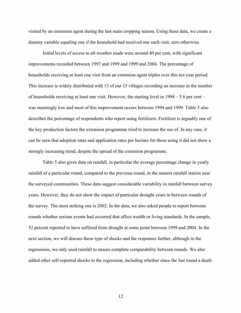
12

visited by an extension agent during the last main cropping season. Using these data, we create a

dummy variable equaling one if the household had received one such visit, zero otherwise.

Initial levels of access to all-weather roads were around 40 per cent, with significant

improvements recorded between 1997 and 1999 and 1999 and 2004. The percentage of

households receiving at least one visit from an extension agent triples over this ten year period.

This increase is widely distributed with 13 of our 15 villages recording an increase in the number

of households receiving at least one visit. However, the starting level in 1994 – 5.6 per cent –

was stunningly low and most of this improvement occurs between 1994 and 1999. Table 5 also

describes the percentage of respondents who report using fertilizers. Fertilizer is arguably one of

the key production factors the extension programme tried to increase the use of. In any case, it

can be seen that adoption rates and application rates per hectare for those using it did not show a

strongly increasing trend, despite the spread of the extension programme.

Table 5 also gives data on rainfall, in particular the average percentage change in yearly

rainfall of a particular round, compared to the previous round, in the nearest rainfall station near

the surveyed communities. These data suggest considerable variability in rainfall between survey

years. However, they do not show the impact of particular drought years in between rounds of

the survey. The most striking one is 2002. In the data, we also asked people to report between

rounds whether serious events had occurred that affect wealth or living standards. In the sample,

52 percent reported to have suffered from drought at some point between 1999 and 2004. In the

next section, we will discuss these type of shocks and the responses further, although in the

regressions, we only used rainfall to ensure complete comparability between rounds. We also

added other self-reported shocks to the regression, including whether since the last round a death

13

or a serious illness was experienced, as well as whether input price declines or output price

increases had been affected the household seriously.

The first column of Table 6 shows the results of estimating (1) using an instrumental

variables model with household fixed effects. This regression suggests that 10 percent more

rainfall increases consumption by 1.7 percent. Rainfall is therefore one crucial source of

variability. Of the other shocks, only death shocks appear to be significant – suggesting that it

contributes to 15 percentage point losses in growth. Roads appear to have mattered a lot in terms

of explaining differential growth. Those with access to a road appear to have almost 16 percent

higher growth per year than those without. Given the nature of the overall growth (a few percent

per year in per capita terms), this is clearly a crucial factor explaining divergence between

communities. Another way to look at the evidence is that the data in table 5 suggests about 27

percent more households experiencing good roads since 1994, leading to a growth acceleration

of about 4 percent in our sample. Finally, we find positive growth and negative poverty impacts

from extension services. Of course, by 2004, we are still talking only about 16 percent of the

households but for them it appears to have contributed to consumption growth and poverty

declines. Between 1994 and 2004, it contributed to about 0.7 percent higher growth, relatively

small but significant.5

Do the chronically poor obtain similar growth effects from these changes? Columns (2)

to (4) explore this. We begin with households that are chronically poor, defined in terms of

experiencing at least 3 periods of poverty. Did they experience a different growth trajectory

because they could not benefit from roads or extension services and other factors in the same

5 Care should be taken in interpreting these results. A typical objection is that roads are built in rich areas, or extension services are provided in areas with good agricultural potential. This is not a problem for our analysis: by using household fixed effects, we control for time-invariant placement effects. However, time varying heterogeneity may still be a problem: roads may be built in areas with high growth potential; extension targeted to areas with growth potential. Finally, risk may have longer term effects not captured in the regression.

14

way, or was their growth trajectory different for example because they simply had fewer roads or

extension services (or more negative shocks)? To explore this, we interact these independent

variables (and the shocks) with whether the household was ‘chronic poor’ in this period. The

results found in column (2) suggest that the chronically poor have not been following a different

growth trajectory in nature: the only significant effect that we could find when using the

interaction terms is that the ‘chronic’ poor had somewhat lower sensitivity to rainfall.6 But for

the core variables used to capture the growth process – the role of infrastructure and extension –

we find no significant differences between the chronic poor and the rest. However, as the

interaction variable uses information that is the outcome of the growth process (consumption

levels at t+1, t+2, etc), the results need to be treated with caution.

Results found in columns (3) and (4) in Table 6 side step this problem of simultaneity.

Before considering these, consider Table 7. We regress initial (1994) household and community

characteristics on whether a household was chronically poor. Household characteristics include

levels of land per capita (in natural logarithms of hectares per capita)7, education of the head

(whether primary or more had been completed, and whether at least some primary education had

been completed)8, household composition (the number of adults above 15 years of age, the

number elderly above 65, children below 5 and children between 5 and 15, all disaggregated by

6 One possible explanation is that because their level of consumption is lower, they can bear less downside risk, and they are engaged in activities that are low risk at the cost of lower returns, limiting the fluctuations ex-post in consumption. 7 Less than two percent of our sample reported to have no land at baseline. To account for this, while allowing logarithms to be taken, we added 0.01 to everybody’s land holdings, as if they have a small garden plot of 10 by 10 square meter, which in practice most people have around their house, although farmers usually do not count these when reporting their land. 8 Education levels are extremely low in this sample (and in Ethiopia by the early 1990s): 9 percent of the household heads completed at least primary education, while 15 percent had some incomplete primary school education. The rest had never attended school.

15

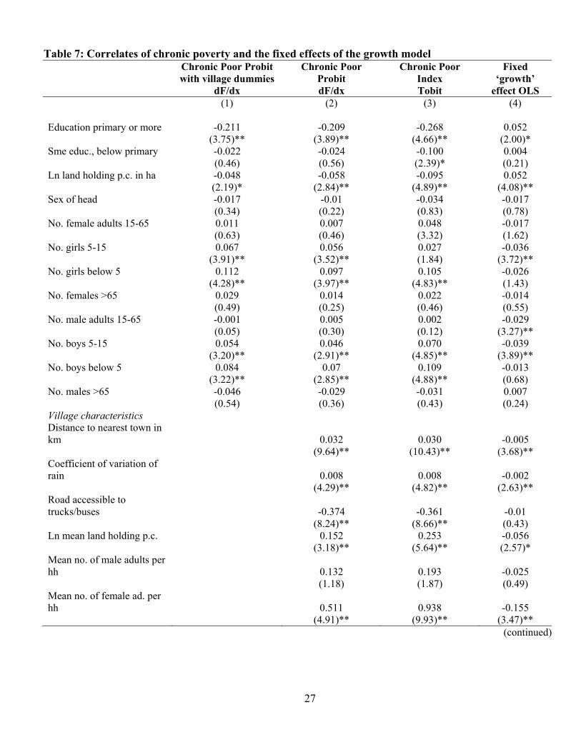
sex), and the sex of the head (male equals one).9 Table 7 reports the marginal effects of probit

regressions of being observed chronically poor in our villages, defined as three or more episodes

of poverty between 1994 and 2004. The first column controls for village dummies, i.e. fixed

effects, absorbing any factors contributing to village-wide chronic poverty. The second column

controls for these factors explicitly, thereby unpacking the community-wide determinants of

chronic poverty. As it is a cross-section regression based on 15 communities, the degrees of

freedom to identify the community-wide variables are limited. We experimented with different

possible characteristics, and the factors that were both stable across specifications and left the

household characteristics unaffected are included in table 7: distance in kilometres to the nearest

town, whether the road was capable to handling trucks and buses, the coefficient of variation of

yearly rainfall and number of village-wide averages of endowments in terms of mean land

holdings per capita, and mean number of male and female adults per household in the village.10

As a cross-section regression, this does not control for other unobserved heterogeneity, so the

interpretation has to be done cautiously.

With or without village fixed effects, the marginal effects of the household characteristics

are similar. However, the village fixed effects (not reported) are suggestive in themselves.

Taking a striking example, a household residing in Gara Godo (an enset growing village in the

south) with household characteristics identical to a household in Sirbana Godeti (not far from the

large trading town Debre Zeit and the survey site closest to Addis Ababa) is 80 percent more

likely to be chronically poor. Education matters: with primary education complete in 1994, the

probability to be found chronic poor in 1994-2004 was more than a fifth lower. Land matters as

9 Livestock is not included, not because it did not matter, but because in these regressions it appeared highly collinear with land (per capita livestock and ln land per capita have a correlation coefficient of 0.76). If either was included without the other, the effects were virtually identical, while including both gave insignificant estimates. 10 The village-wide mean values of land per capita and adults per household were relevant for the stability of the results on other village-wide variables, probably reflecting relative land and labour scarcity.

16

well, although in percentage terms not as much: doubling land (which implies increasing land by

just under one standard deviation in the land distribution) would reduce the probability of being

chronic poor by about 5 percent. There are surprisingly strong effects on having children: they

increase the likelihood of being found chronic poor in this period, with children below 5 and

especially girls adding most. We explored whether this effect is due to the use of a poverty

definition based on consumption per capita, which would ‘penalize’ families with children

relatively more by understating their likely consumption, as children have lower basic food

needs. However, even using consumption per adult as the basis for poverty showed the same

effect, even if all children and not just younger children were similarly costly in terms of

increasing the likelihood of being chronic poor. As economies of scale are also possible, we have

to be careful to attach too much importance to this result, but the sheer size makes scale

economies not a very plausible: ceteris paribus, another child appears to increase the probability

of being found ‘chronic poor’ by up to 8.4 percent.

Turning to the community characteristics in column (2), the role of road access and distance

to towns is striking: having a good road reduces the likelihood being found chronic poor by 37

percent, while a reduced distance to the nearest small town by about 12 kilometres (which is

moving from a distance as in the 75 percentile to the 25th percentile) also brings down the

probability of being chronic poor by about 38 percent. Rainfall variability, the simplest measure

of ‘risk’ faced by different communities, is also found to be highly significant, but its impact is

actually relatively small: moving from the 75th to 25th percentile would reduce the probability of

being chronic poor by about 1 percent. Finally, it should be noted that the land result reported

earlier is relative, as villages in the sample with more land per capita (possibly a sign of poor

land quality or agro-climatic conditions, sustaining low population densities) are more likely to

17

have high chronic poverty. Also, villages with relatively speaking many female adults (in the

sample a sign of high past involvement in conflict resulting in a high male death rate, e.g. in the

Tigrayan villages found in the northern Highlands) are more likely to be chronically poor. As

mentioned before, with only 15 communities, we have to be cautious with attaching to strong an

interpretation to these results. Column (3) reports an alternative way of exploring the correlates

of chronic poverty, using the index that takes into account the severity of poverty in each period.

In terms of the factors that matter, the results are similar adding credence that these factors

matter for different ways of looking at poverty persistence.

In short, we find that chronic poverty is correlated to a number of household and community

endowments (including education, productive assets such as land, as well as factors affecting

‘remoteness’ such as distance to towns and road access). Besides being interesting in itself, it

allows us to revisit Table 6, and the question whether the growth relationship estimated is really

not different for the chronic poor and the rest? If we divide the sample on the basis of 1994

characteristics, that we know are subsequently correlated with chronic poverty, can we detect

different trajectories? This is done in columns (3) and (4) of Table 6. Even though there is some

element of arbitrariness in dividing the sample, the results are remarkably robust across

specifications. Column (3) defined ‘chronic poor’ as those with relatively low productive assets

(below the median in both land and livestock per capita). This would consider about half the

sample as ‘chronic poor’ (compared to 37 percent using the definition of three or more times

poor). Column (4) restricts this further by excluding from those below the mean in both land and

livestock, also those with at least primary education, and by restricting the chronic poor to those

that are also either not having access to a good road for trucks and buses, or those who are living

far from a town (in the highest quartile in terms of distance to town in the sample). These

18

restrictions result in approximately 38 percent chronic poor. These are not necessarily the same

as those included in our earlier definition of the chronic poor, but there is a significant

correlation between these indicators and the chronic poor definition used earlier. The results are

remarkably stable across the three specifications: roads and extension appear to have mattered

significantly in this period, but not different between the ‘chronic poor’ and the ‘non-chronic

poor’.

On the basis of the evidence, are the chronic poor then just like the others, only poorer? Will

growth, for example via the expansion of roads and extension services then lift them up as fast as

the non-poor? Table 8 shows poverty, road access and extension access for the chronic poor

versus the rest of the sample. Head count poverty among the chronic poor has been falling

gradually, from peaks in early year where most of the ‘chronic poor’ where also observed to be

below the poverty line. Poverty among the other groups had falling to low levels by 1997,

although has increased since, even though to still considerably lower levels than in 1994. The

(slow) expansion of extension is correlated with this, while for the non-poor road access

improved gradually. Strikingly, by 2004, both access to roads and to extension are not different

between the chronic poor and non-chronic poor. As the statistical exercise in Table 6 linked the

importance of initial levels of roads to their subsequent impact on growth, then, according to the

models in table 6 and 7, the recent expansion (between 1999 and 2004) of roads for the chronic

poor is likely to result in a further considerable improvement in living standards for the chronic

poor post 2004.

But this is not the whole story. The models in Table 6 and 7 are fixed effects models,

implying that they control for household heterogeneity in the underlying growth rate. In other

words, beyond the factors modeled, each household has its own ‘unexplained’, latent part of

19

growth. Using model (2) in Table 6, we find that the average fixed effects for the chronic poor is

-15.4 percent per year, while for the non-chronic poor it is 9.2 percent per year; these means are

significantly different from each other at 1 percent and less. In other words, for the same values

of shocks, or roads or extension visits, the growth difference between these two groups is

estimated to be almost 25 percent. Further, the correlation between the household fixed effect

and whether one is chronic poor or not, or with the chronic poverty index that allows for the

severity of chronic poverty is very high (respectively -0.47 and -0.50). In other words, the

chronic poor face a serious growth deficit, making catching up with the rest very difficult – in

terms of time-varying characteristics, they need much ‘better’ values to obtain the same level of

growth as the non-chronic poor.

What determines this fixed effect? By retrieving the fixed growth effect from the

regressions, it is possible to study its correlates. However, as this is a cross-section, one should

be careful not to overinterpret these regressions, reported in the fourth column in Table 7.11 The

most striking result is that the main correlates for lower chronic poverty are the correlates for a

higher fixed effect. For example, moving from the 25th to the 75th percentile in terms of distance

to town, would cost 6 percent in latent growth. Strikingly, unlike remoteness, access to roads is

not a significant part the latent growth effect.

In sum, the evidence suggests that the chronic poor tend to have the same return from

growth stimulating factors, such as improved infrastructure or extension. Overall, however, the

chronic poor appear to start from a serious growth handicap, linked to physical assets, education

and remoteness, contributing to poverty persistence, and being left behind in relative terms. This

11 As the ‘fixed effect’ estimator is obtained by subtracting all time invariant information from time variant information, the fixed effect itself contains all this time-invariant information, including the mean levels of all time variant variables in the sample period. As a result, it is closer to the spirit of the fixed effect estimator to correlate the fixed effect with household and community level means across the entire sample period, rather than just the initial period. This is done in Table 7.

20

fixed growth handicap is the microeconometric equivalent of showing ‘club’ convergence,

whereby the initial characteristics matter permanently for long-term outcomes.

5. Conclusion

This paper has examined growth, poverty and chronic poverty in 15 Ethiopian villages. While

the communities were chosen to broadly represent socio-economic diversity across regions and

the country, it is not a nationally representative survey. Nevertheless, the dearth of alternative

data makes the ERHS unique in its ability to analyze the broad patterns of growth and poverty,

and its determining factors. Growth and poverty reduction in these communities was substantial.

Headcount poverty fell from 48 to 35 percent. However, there is also movement in and out of

poverty over this period and a significant proportion of the sample was chronically poor.

Chronic poverty is associated with several characteristics: lack of physical assets,

education, and ‘remoteness’ in terms of distance to towns or poor roads. The chronically poor

appear to be benefit from roads or extension services in much the same way that the non-

chronically poor benefit. However, their ‘fixed’ or ‘initial’ conditions, as reflected in the

estimated latent growth related to time-invariant characteristics, suggest that they face a

considerable growth handicap compared to the rest. This ‘fixed’ growth effect correlates also

well with the characteristics of the chronic poor during the sample period. Chronic poverty, as

reflected in poor initial assets and remoteness, appears to be correlated with a divergence in

living standards over the sample period.

Despite the economic growth observed in these communities and elsewhere in Ethiopia,

one cannot but be reminded that GDP per capita in real terms is currently only just about back at

the levels of the early 1970s, before the 1973 drought and the long period of political turmoil and

21

economic stagnation that set in soon after. Further, the growth we are observing is not a period of

rural transformation ready to accelerate into Asia-style large scale growth and poverty reduction.

There is little evidence of movement out of agriculture into more productive and high return non-

agricultural activities. Even within agriculture, there is little change over time in the relative

importance of crops in most areas as well, and there has been no systematic shift towards more

profitable and possible new growth crops. This will have to change to allow a further

acceleration of growth and poverty reduction to take place.

22

References

Baulch. B. and J. Hoddinott, 2000, “Economic Mobility and Poverty Dynamics in Developing

Countries”, introduction to special issue, Journal of Development Studies.

Calvo, C. and S.Dercon (2007), “Chronic Poverty and All That: The Measurement of Poverty over Time” The Centre for the Study of African Economies Working Paper Series. Working Paper 263.

Deaton, A. and S. Zaidi, 2002. Guidelines for constructing consumption aggregates for welfare

analysis. Living Standards Measurement Study Working Paper: 135, Washington, D.C.: The World Bank.

Dercon, S. 2004. Growth and shocks: Evidence from rural Ethiopia. Journal of Development

Economics 74 (2): 309-329. Dercon, S., D.Gilligan, J.Hoddinott and T. Woldehanna. 2006, The impact of roads and

agricultural extension on crop income, consumption and poverty in fifteen Ethiopian villages, mimeo.

Dercon, S., and J. Hoddinott, 2004. The Ethiopian Rural Household Surveys: Introduction.

International Food Policy Research Institute, mimeo. Dercon, S., J. Hoddinott and T. Woldehanna, 2005. Consumption and shocks in 15 Ethiopian

Villages, 1999-2004. Journal of African Economies, 14: 559-585. Dercon, S., and P. Krishnan, 1996. A consumption based measure of poverty in Ethiopia: 1989-

1994 in, M. Taddesse and B. Kebede, Poverty and economic reform in Ethiopia, Proceedings Annual Conference of the Ethiopian Economics Association.

Dercon, S., and P. Krishnan. 2000. Vulnerability, poverty and seasonality in Ethiopia. Journal

of Development Studies 36 (6): 25-53. Dercon S., and P. Krishnan. 2003. Changes in poverty in rural Ethiopia 1989-1995: in A.Booth

and P.Mosley, (eds.) The New Poverty Strategies, Palgrave MacMillan, London. Foster, J., 2007. A Class of Chronic Poverty Measures, mimeo.

Getahun. 1978. Report on framing systems in Ethiopia. Ministry of Agriculture, Government of Ethiopia, Addis Ababa.

Hentschel, J. and P. Lanjouw, 1996. Constructing an indicator of consumption for the analysis of

poverty: Principles and illustrations with reference to Ecuador. Living Standards Measurement Study Working Paper: 124, Washington, D.C.: The World Bank.

23

Jalan, J. and M. Ravallion, 2000, ‘Is Transient Poverty Different? Evidence from Rural China’, Journal of Development Studies, Vol.36, No.6.

Mani, S. 2008. Essays on human capital accumulation – Health and education. Unpublished PhD. Thesis, Department of Economics, University of Southern California.

Temple, J., 1999. The new growth evidence. Journal of Economic Literature, 37(1): 112-156. Westphal, E. 1976. Farming Systems in Ethiopia. Food and Agriculture Organization of the

United Nations. Woldehanna, T., J. Hoddinott, F. Ellis and S. Dercon, 2008. Dynamics of growth and poverty in

Ethiopia: 1995/96-2004/05. Report submitted to Ministry of Finance and Economic Development, Addis Ababa.

24

Table 1: The distribution of households in the Ethiopian Rural Household Survey, by agroecological zone

Population

share in 1994 Sample share

in 1994 Number

of villages (percent) (percent) Grain plough complex: Northern Highlands 21.2% 20.2% 3 Grain plough complex: Central Highlands 27.7 29.0 4 Grain plough: Arsi/Bale 9.3 14.3 2 Sorghum plough/hoe: Hararghe 9.9 6.6 1 Enset (with or without coffee/cereals) 31.9 29.9 5

Total 100 100 15 Source: Dercon and Hoddinott (2004). Note: Percentages of population share relate to the rural sedentary population; they exclude pastoralists who

account for about 10 percent of total rural population. Table 2: Inequality, assets, school enrollment and perceptions of wellbeing: 1994-2004 1994 2004 Inequality Gini coefficient 0.45 0.44 Livestock: Percentage of households owning:

Oxen 13 49

Any livestock 81 90 Livestock Real (1994) value of per capita

holdings 342 421

Ownership of other assets. Percentage of households with:

Hoes 59 79 Ploughs 79 87 Beds 49 58

School Enrollment. Percentage of:

Boys age 11, enrolled 21 60 Girls age 11, enrolled 13 58 Children, aged 7-14 enrolled 13 45

Public services. Percentage of households with access to:

Electricity 0 13

Piped water 11 31 Public services. Distance (km) to:

Nearest telephone 14.8 9.3

Perceptions of wellbeing. How would you describe your household circumstances? (Percentages)*

Very rich 0.5 0.4 Rich 5.4 5.9 Comfortable 19.9 30.4 Can manage to get by 25.4 29.2 Never have quite enough 7.9 13.0 Poor 33.4 19.9 Destitute 7.6 1.1

Source: Ethiopia Rural Household Survey. Enrollment data are from Mani (2008). Perceptions questions were asked in 1995.

25

Table 3: Consumption and Poverty: 1994-2004

Mean Consumption

per capita

Median Consumption

per capita Head count

poverty Poverty Gap Squared

Poverty Gap 1994 71.1 51.6 0.48 0.21 0.12 1995 62.0 45.3 0.55 0.24 0.14 1997 90.9 70.7 0.33 0.12 0.06 1999 88.3 64.5 0.36 0.13 0.06 2004 91.5 65.1 0.35 0.13 0.07

Note: Calculated from the Ethiopian Rural Household Survey. Head count poverty based on consumption per capita, poverty line 50 birr per month. Consumption is in 1994 prices per month. (n=6463) Table 4: Poverty episodes 1994 to 2004 (based on 5 rounds) Percentage of

households (1)

Chronic Poverty Index

Average Squared Poverty Gap per period of poverty

Never Poor 18 0 0 Poor once 22 0.13 0.13 Poor in 2 out of 5 rounds 23 0.32 0.16 Poor in 3 out of 5 rounds 16 0.65 0.22 Poor in 4 out of 5 rounds 14 1.04 0.26 Poor in all rounds 7 1.34 0.27 Source: Ethiopia Rural Household Survey (based on 1187 observation with data in all 5 rounds). Chronic Poverty Index is measure (7) as in Calvo and Dercon, the cumulative sum of the squared poverty index. The final column is the Chronic Poverty Index, divided by the number of periods of poverty. Table 5: Evolution of roads access, extension, fertilizer use and rainfall

Round Access to all-weather road

Received at least one extension visit

Used fertilizer in particular year

Percentage change in rainfall relative to

previous round 1994 41 5.6 44 1995 41 4.5 37 +11% 1997 43 6.8 47 +8% 1999 52 12.3 46 -13% 2004 68 15.9 45 -2%

Source: Ethiopian Rural Household Survey. Note that fertilizer adoption rate for 2004 is based on 2003 figures

26

Table 6: Do the chronic poor face different determinants of consumption growth? Annualized Growth

in Consumption per capita

Annualized Growth in Consumption per capita with chronic poverty interaction

effects

Annual Annualized Growth in

Consumption per capita with ‘low

endowments’ interactions

Annual Annualized Growth in

Consumption per capita with ‘low endowments and

remoteness’ interactions

(1) (1) (2) (3) Log consumption (IV) -0.365 -0.353

(8.55)** -0.359 -0.355

(9.03)** (8.81)** (8.53)** Access to all-weather road 0.159 0.162

(4.60)** 0.188 0.200

(5.14)** (4.18)** (4.89)** Received visit from extension officer

0.071 0.094 (1.81)*

0.073 0.087 (1.91)* (1.29) (1.84)*

Rainfall shocks 0.173 0.239 (4.06)**

0.433 0.361 (4.37)** (6.03)** (6.03)**

Input price shocks -0.116 -0.245 (1.43)

-0.185 -0.199 (0.89) (0.92) (1.05)

Output price shocks 0.069 -0.148 (0.70)

-0.029 -0.01 (0.41) (0.06) (0.03)

Death shocks -0.149 -0.060 (0.53)

-0.161 -0.059 (1.80)* (1.54) (0.54)

Illness shocks -0.108 -0.159 (1.23)

-0.141 -0.132 (1.14) (1.05) (1.06)

Interaction terms Access to all-weather road -0.012

(0.17) -0.015 -0.036

(0.26) (0.63) Received visit from extension officer

-0.042 (0.55)

0.008 -0.015 (0.10) (0.20)

Rainfall shocks -0.143 (1.71)*

-0.341 -0.297 (3.95)** (3.57)**

Input price shocks 0.189 (0.68)

0.118 0.129 (0.42) (0.46)

Output price shocks 0.470 (1.21)

-0.007 -0.01 (0.01) (0.03)

Death shocks -0.193 (1.15)

0.03 -0.198 (0.18) (1.15)

Illness shocks 0.117 (0.58)

0.122 0.088 (0.62) (0.44)

Sample size 4578 4578 4578 Notes: (1) Interactions are whether the household is chronic poor, defined as three or more times poor in the sample.

(2) Interactions are whether the household is below the median for livestock per capita and for land holdings per capita. (3) below median for livestock per capita and for land holdings per capita, and below primary or no education, and ‘remote’: either far from town (highest quartile in terms of furthest distance to town) or no access to road for trucks/bus. Lagged endogenous variables are expressed in real per adult equivalent terms. Instruments for lagged endogenous variables are lagged log livestock units per adult equivalent, lagged log number of adult equivalents and lagged log cultivable land per adult equivalent. F statistic on first stage instruments is 87.64 and Cragg-Donald F statistic is 103.00. Both are significant at the 5% level. Hansen J test is 4.59. Household fixed effects and a dummy variable if survey conducted in post harvest period is included but not reported. Absolute values of z stats in parentheses; * significant at 10% level; ** significant at 5% level.

27

Table 7: Correlates of chronic poverty and the fixed effects of the growth model Chronic Poor Probit

with village dummies dF/dx

Chronic Poor Probit dF/dx

Chronic Poor Index Tobit

Fixed ‘growth’

effect OLS (1) (2) (3) (4) Education primary or more -0.211 -0.209 -0.268 0.052 (3.75)** (3.89)** (4.66)** (2.00)* Sme educ., below primary -0.022 -0.024 -0.100 0.004 (0.46) (0.56) (2.39)* (0.21) Ln land holding p.c. in ha -0.048 -0.058 -0.095 0.052 (2.19)* (2.84)** (4.89)** (4.08)** Sex of head -0.017 -0.01 -0.034 -0.017 (0.34) (0.22) (0.83) (0.78) No. female adults 15-65 0.011 0.007 0.048 -0.017 (0.63) (0.46) (3.32) (1.62) No. girls 5-15 0.067 0.056 0.027 -0.036 (3.91)** (3.52)** (1.84) (3.72)** No. girls below 5 0.112 0.097 0.105 -0.026 (4.28)** (3.97)** (4.83)** (1.43) No. females >65 0.029 0.014 0.022 -0.014 (0.49) (0.25) (0.46) (0.55) No. male adults 15-65 -0.001 0.005 0.002 -0.029 (0.05) (0.30) (0.12) (3.27)** No. boys 5-15 0.054 0.046 0.070 -0.039 (3.20)** (2.91)** (4.85)** (3.89)** No. boys below 5 0.084 0.07 0.109 -0.013 (3.22)** (2.85)** (4.88)** (0.68) No. males >65 -0.046 -0.029 -0.031 0.007 (0.54) (0.36) (0.43) (0.24) Village characteristics Distance to nearest town in km

0.032 0.030 -0.005

(9.64)** (10.43)** (3.68)** Coefficient of variation of rain 0.008 0.008 -0.002 (4.29)** (4.82)** (2.63)** Road accessible to trucks/buses -0.374 -0.361 -0.01 (8.24)** (8.66)** (0.43) Ln mean land holding p.c. 0.152 0.253 -0.056 (3.18)** (5.64)** (2.57)* Mean no. of male adults per hh 0.132 0.193 -0.025 (1.18) (1.87) (0.49) Mean no. of female ad. per hh 0.511 0.938 -0.155 (4.91)** (9.93)** (3.47)**

(continued)

28

Constant -1.058 0.532 (9.14)** (9.81)** Village dummies included but not reported

x

Diagnostic statistics R2 or Pseudo R2 0.359 0.284 0.277 0.202 Sample size 1102 1125 1125 1125

Notes: Absolute values of z stats in parentheses; * significant at 10% level; ** significant at 5% level. (1) +(2) marginal effects from probit regression with dependent variable whether chronic poor defined as three or more times poor in the sample 1994-2004. Marginal effects for discrete variables are changes from zero to one); for continuous variables they are changes by one. (3) Tobit regression unconditional marginal effects base on chronic poverty index, column (2) in table 5. (4) OLS regression of fixed effect from table 6, column (1), retrieved using xtivreg command in STATA, given the household specific constant growth rate between 1994 and 2004. Sample restricted to households for which chronic poverty is fully defined. (1), (2) and (3) use characteristics in first year of the data, 1994. (4), in keeping with logic of fixed effects model gives mean values across the sample period.

Table 8: Evolution of head count poverty, roads access and for chronically and non-chronically poor households

Round Head count

Poverty Received at least one

extension visit Access to all-weather road (trucks/buses)

Chronic

poor

Non-chronic

poor Chronic

poor

Non-chronic

poor Chronic

poor

Non-chronic

poor 1994 0.83 0.27 0.05 0.07 0.26 0.54 1995 0.93 0.33 0.02 0.06 0.26 0.54 1997 0.70 0.12 0.06 0.08 0.23 0.59 1999 0.68 0.17 0.16 0.11 0.25 0.72 2004 0.62 0.19 0.15 0.15 0.68 0.70 Source: Ethiopian Rural Household Survey

29

0.2

.4.6

Den

sity

0 2 4 6 8Log p.c. consumption

Log p.c. consumption, 1994 Log p.c. consumption, 2004

Figure 1