General rights Copyright and moral rights for the publications made accessible in the public portal are retained by the authors and/or other copyright owners and it is a condition of accessing publications that users recognise and abide by the legal requirements associated with these rights.

• Users may download and print one copy of any publication from the public portal for the purpose of private study or research. • You may not further distribute the material or use it for any profit-making activity or commercial gain • You may freely distribute the URL identifying the publication in the public portal

If you believe that this document breaches copyright please contact us providing details, and we will remove access to the work immediately and investigate your claim.

Downloaded from orbit.dtu.dk on: Dec 18, 2017

Group Contribution sPC-SAFT Equation of State

Tihic, Amra; Kontogeorgis, Georgios; Michelsen, Michael Locht; von Solms, Nicolas; Constantinou,Leonidas

Publication date:2008

Document VersionPublisher's PDF, also known as Version of record

Link back to DTU Orbit

Citation (APA):Tihic, A., Kontogeorgis, G., Michelsen, M. L., von Solms, N., & Constantinou, L. (2008). Group Contribution sPC-SAFT Equation of State.

Group Contribution sPC-SAFT Equation of State

2008

Group Contribution sPC-SAFTEquation of State

Ph.D. Thesis

Amra Tihic

May 13, 2008

Supervisors: Georgios M. KontogeorgisMichael L. MichelsenNicolas von Solms

Leonidas Constantinou

IVC-SEP

Department of Chemical and Biochemical Engineering

Technical University of Denmark

Summary

Modelling of thermodynamic properties and phase equilibria with equations of state (EoS)remains an important issue in chemical and related industries. The simplified Perturbed Chain-Statistical Associating Fluid Theory (sPC-SAFT) EoS is widely used for various industrial appli-cations. The model requires three parameters: the segment number (m), the hard-core segmentdiameter (σ), and the segment-segment interaction energy parameter (ε/k) for each pure non-associating fluid. They are typically fitted to experimental vapour pressure and liquid densitydata. Since high-molecular-weight compounds, like polymers, do not have a detectable vapourpressure, there is a need for a predictive calculation method for parameters of polymers and othercomplex compounds. This thesis suggests a solution to this problem.

The main objective of this project is to develop a group-contribution (GC) version of the sPC-SAFT EoS where the parameters of the model are calculated from a predefined GC scheme. In thisway, the PC-SAFT parameters for complex compounds can still be estimated when experimentaldata are unavailable. The applied GC methodology includes two levels of contributions; bothfirst-order groups (FOG) and second-order groups (SOG). The latter can, to some extent, captureproximity effects and distinguish among structural isomers.

Initially, the PC-SAFT parameter table is extended with over 500 newly estimated parametersets for pure non-associating compounds from different chemical families using mainly experi-mental data from the DIPPR database. The chemical families include alkanes, branched alkanes,alkenes, alkynes, benzene derivatives, gases, ethers, esters, ketones, cyclo- and fluorinated hydro-carbons, polynuclear aromatics, nitroalkanes, sulphides, and plasticizers. Several important typesof experimental thermodynamic data, such as vapour-liquid and liquid-liquid equilibria, are col-lected from the literature and used to systematically evaluate the performance of the sPC-SAFTmodel when using these new PC-SAFT parameters.

The experimentally derived PC-SAFT parameters display clear linear trends, which are uti-lized to fit parameter sets (m, σ, and ε/k) for distinct chemical groups contained in the compoundsfrom this database using an optimization routine. At present, the table includes 45 FOG and 26SOG, but can be further extended using the outlined methodology. The parameters of new com-pounds can now be calculated by summing up the contributions of these well-defined groups ofatoms after being multiplied by their number of occurrences within the molecule.

The fluid phase equilibria of some larger and complex compounds not included in the optimi-sation database are examined to confirm the predictive capability of the proposed GC sPC-SAFTEoS. Good agreement between predictions and experimental data is demonstrated. For many bi-nary mixtures investigated, a small binary interaction parameter, kij , is needed before the modelaccurately correlates the experimental data. As a possibility, a more predictive way to calcu-late the required kij values has been investigated using an additional physical parameter (theionization energy of involved compounds), and it shows some promising initial results.

Further testing, on e.g. multicomponent and solid-liquid equilibria modelling, is needed toestablish the real potential of the GC sPC-SAFT EoS. It is expected that optimization and exten-sion of the proposed GC scheme can lead to further improvements within the general limitationsof the PC-SAFT and sPC-SAFT models. However, the current work has already shown that withthe newly developed GC scheme in hand to calculate parameters for complex compounds, thesPC-SAFT model has become a relevant and useful engineering tool for the design and develop-ment of complex products. These include e.g. detergents or food ingredients, pharmaceuticals,and specialty chemicals, where predictions of thermodynamic and phase equilibria properties arerequired, but for which required vapour pressure and/or liquid density data may not be available.

i

Resumé (Summary in Danish)

Modellering af termodynamiske egenskaber og faseligevægte er en udfordring for den kemiskeindustri. Forenklet Perturbed Chains-Statistical Associating Fluid Theory (sPC-SAFT) er en til-standsligning med udbredt anvendelse i en række industrielle sammenhænge. Modellen benyttertre parametre: segment antal (m), hård-kugle segment diameter (σ) og segment-segment interak-tionsenergi (ε/k) for hver enkelt ikke-associerende stof som indgår i beregningen. Disse parametrekan typisk fittes til eksperimentelle værdier for damptryk og væskefasedensitet. Stoffer med megethøj molekylevægt, som fx. polymere, har så lave damptryk, at det i praksis er umuligt at måle.Dermed opstår et behov for en beregningsmetode til at forudsige modelparametre for polymereog andre komplekse stoffer. Denne afhandling præsenterer en løsning på dette problem.

Formålet med dette projekt er at udvikle en gruppebidragsbaseret (GC) udgave af sPC-SAFTtilstandsligningen, hvor modelparametrene beregnes udfra veldefinerede funktionelle grupper ogderes individuelle bidrag, uden at der gøres brug af eksperimentelle data. Gruppebidragsmetodeninkluderer bidrag fra både første ordens (FOG) og anden ordens funktionelle grupper (SOG),hvor tilstedeværelsen af sidstnævnte gør det muligt at korrigere for gensidige påvirkninger mellemnærliggende grupper samt skelne mellem isomere strukturer.

Som udgangspunkt for projektet er den eksisterende tabel med PC-SAFT parametre udvidetmed parametersæt for over 500 nye ikke-associerende stoffer. Hertil er anvendt eksperimentelledata fra DIPPR databasen. De kemiske stofgrupper som er repræsenteret i denne database omfat-ter alkaner, forgrenede alkaner, alkener, alkyner, benzenderivater, gasser, ethere, estere, ketoner,cyklo- and fluorerede kulbrinter, polyaromatiske kulbrinter, nitroalkaner, sulfider og blødgørere.En række vigtige eksperimentelle datatyper er desuden indsamlet fra litteraturen; heriblandt gas-væske (VLE) og væske-væske (LLE) ligevægtsdata, som er anvendt til systematisk evaluering afsPC-SAFT modellens funktionalitet ved brug af disse nye parametersæt.

De eksperimentelt baserede PC-SAFT parametre udviser tydelig lineær opførsel. Dette erudnyttet ved den efterfølgende optimering og udledning af parametersæt (m, σ og ε/k) for speci-fikke funktionelle gruppe, der optræder i stoffer inkluderet i databasen. Den fremkomne grup-pebidragstabel indeholder 45 FOG og 26 SOG. Tabellen kan yderligere udvides ved at følge denbeskrevne fremgangsmåde. Udfra denne tabel kan modelparametre beregnes for nye stoffer ved atsummere bidrag fra de enkelte funktionelle grupper multipliceret med antallet af deres forekomsteri molekylstrukturen.

For at bekræfte GC sPC-SAFT tilstandsligningens forudsigende evner er faseligevægtsdatamodelleret for en række komplekse stoffer, som ikke er inkluderet i optimeringsdatabasen. Derer opnået god overensstemmelse mellem modelforudsigelser og eksperimentelle data. For flerebinære systemer er det nødvendigt at anvende en binær interaktionsparameter (kij) med lav nu-merisk værdi for at opnå nøjagtig korrelation med de eksperimentelle data. I den forbindelse eren teoretisk fremgangsmåde til beregning af kij blevet undersøgt. Metoden gør brug af ioniser-ingsenergien for individuelle stoffer som en ekstra parameter og har vist lovende resultater.

Yderligere karakterisering af modellens evner til at forudsige fx. multikomponent-blandingerog faststof-væske ligevægte er nødvendig for at bestemme det reelle potential af GC sPC-SAFTtilstandsligningen. Det forventes, at videre optimering og udvidelse af gruppebidragsskemaetkan forbedre modellens nøjagtighed og anvendelsesområde indenfor de generelle begrænsninger iPC-SAFT og sPC-SAFT modellerne.

Med den anvendte gruppebidragsmetode til beregning af parametersæt for komplekse stofferer sPC-SAFT tilstandsligningen blevet et attraktivt ingeniørværktøj til brug ifm. design og ud-vikling af komplicerede produkter, som fx. ingredienser til vaskemidler og fødevarer, farmaceutiskestoffer og specialkemikalier, hvor det er vigtigt at kunne forudsige termodynamiske egenskaber ogfaseligevægte, og hvor mulighederne tidligere har været begrænset af mangel på relevante eksper-imentelle data.

iii

Preface

This thesis is submitted in partial fulfillment of the requirements to obtain the Doctorof Philosophy degree at the Technical University of Denmark (DTU). The work has beencarried out at the IVC-SEP (Centre of Phase Equlibria and Separation Processes) at theDepartment of Chemical and Biochemical Engineering, DTU, under the supervision ofProfessors Georgios M. Kontogeorgis and Michael L. Michelsen, Asc. Prof. Nicolas vonSolms and Dr. Leonidas Constantinou.

The project was financially supported by the Danish Technical Research Council(Statens Forskningsråd for Teknologi og Produktion, FTP) in the framework of a grantentitled Computer-Aided Product Design Using the PC-SAFT Equation of State. Theauthor gratefully acknowledges their support.

I would like to express my gratitude to my adviser Prof. Georgios M. Kontogeorgis forhis support over the last many years since my graduate student studies. An extra thanksfor his endless passion and enthusiasm for this work from the beginning.

I am very thankful to Professor Michael L. Michelsen and Asc. Prof. Nicolas vonSolms for their help. Your ideas and comments through this work have always beenhighly appreciated.

Also, I would like to thank Prof. Leonidas Constantinou for giving me the opportunityto visit the Research Center of Cyprus and always being ready to answer any questions Imight have.

To the colleagues that I have worked with in the past three years at KT: I have enjoyedbeing a part of the IVC-SEP research group benefiting from the expertise available withinthe group. Thanks to you all.

At last but no least to my dear families, Tihic and Segal, for supporting me in all thedecisions I have made and always been by my side. Vasa ljubav i podrska su uvijek bili iostali za mene svjetlost u mracnim tunelima.

Finally to Christian... You mean everything to me. Without your understanding andsupport the accomplishment of this work would not have been possible.

Amra TihicKgs. Lyngby, DenmarkMay 13, 2008

v

Table of Contents

Summary i

Summary in Danish iii

Preface v

Table of Contents vii

List of Figures xi

List of Tables xv

List of Symbols xix

1 Introduction 11.1 Introduction . . . . . . . . . . . . . . . . . . . . . . . . . . . . . . . . . . . 11.2 Industrial Applications of Polymers . . . . . . . . . . . . . . . . . . . . . . 2

1.2.1 High-Priority Research Topics . . . . . . . . . . . . . . . . . . . . . 31.3 The Role of Thermodynamics . . . . . . . . . . . . . . . . . . . . . . . . . 41.4 Project Objectives . . . . . . . . . . . . . . . . . . . . . . . . . . . . . . . 5References . . . . . . . . . . . . . . . . . . . . . . . . . . . . . . . . . . . . . . . 8

2 The SAFT Model 112.1 Introduction . . . . . . . . . . . . . . . . . . . . . . . . . . . . . . . . . . . 112.2 The SAFT Equation of State . . . . . . . . . . . . . . . . . . . . . . . . . 12

2.2.1 Original SAFT Equation of State . . . . . . . . . . . . . . . . . . . 132.2.1.1 Pure Component Parameters . . . . . . . . . . . . . . . . 152.2.1.2 Polymer Parameters . . . . . . . . . . . . . . . . . . . . . 162.2.1.3 Binary Mixtures and Mixing Rules . . . . . . . . . . . . . 162.2.1.4 Binary Interaction Parameter . . . . . . . . . . . . . . . . 18

2.2.2 PC-SAFT Equation of State . . . . . . . . . . . . . . . . . . . . . . 182.2.2.1 Model Description . . . . . . . . . . . . . . . . . . . . . . 18

2.2.3 Simplified PC-SAFT Equation of State . . . . . . . . . . . . . . . . 222.2.3.1 Pure Component Parameters . . . . . . . . . . . . . . . . 23

vii

TABLE OF CONTENTS

2.2.3.2 Polymer Parameters . . . . . . . . . . . . . . . . . . . . . 232.3 Final Comments . . . . . . . . . . . . . . . . . . . . . . . . . . . . . . . . 25References . . . . . . . . . . . . . . . . . . . . . . . . . . . . . . . . . . . . . . . 25

3 Group Contribution Approach 293.1 Introduction . . . . . . . . . . . . . . . . . . . . . . . . . . . . . . . . . . . 293.2 Overview of GC Approaches Applied to SAFT . . . . . . . . . . . . . . . 303.3 The Constantinou-Gani GC Method . . . . . . . . . . . . . . . . . . . . . 32

3.3.1 Constantinou-Gani Method into an EoS . . . . . . . . . . . . . . . 343.4 The Tamouza et al. GC Approach . . . . . . . . . . . . . . . . . . . . . . 353.5 Final Comments . . . . . . . . . . . . . . . . . . . . . . . . . . . . . . . . 37References . . . . . . . . . . . . . . . . . . . . . . . . . . . . . . . . . . . . . . . 37

4 Extension of the PC-SAFT Parameter Table 414.1 Introduction . . . . . . . . . . . . . . . . . . . . . . . . . . . . . . . . . . . 414.2 Complete Parameter Table . . . . . . . . . . . . . . . . . . . . . . . . . . . 424.3 Heavy Alkanes . . . . . . . . . . . . . . . . . . . . . . . . . . . . . . . . . 61

4.3.1 Sensitivity Analysis . . . . . . . . . . . . . . . . . . . . . . . . . . . 644.3.1.1 VLE with Light Alkanes . . . . . . . . . . . . . . . . . . . 644.3.1.2 VLE with Light Gases . . . . . . . . . . . . . . . . . . . . 65

4.3.2 Evaluation of γ∞ . . . . . . . . . . . . . . . . . . . . . . . . . . . . 704.4 Correlations of Parameters for Other Families . . . . . . . . . . . . . . . . 72

4.4.1 Various Binary Mixtures . . . . . . . . . . . . . . . . . . . . . . . . 744.4.2 Fluorocarbon Mixtures . . . . . . . . . . . . . . . . . . . . . . . . . 764.4.3 Hexane–Acetone System . . . . . . . . . . . . . . . . . . . . . . . . 78

4.5 Prediction of Binary Interaction Parameters (kij) . . . . . . . . . . . . . . 804.6 Final Comments . . . . . . . . . . . . . . . . . . . . . . . . . . . . . . . . 84References . . . . . . . . . . . . . . . . . . . . . . . . . . . . . . . . . . . . . . . 85

5 Validation of sPC-SAFT in Novel Polymer Applications 915.1 Introduction . . . . . . . . . . . . . . . . . . . . . . . . . . . . . . . . . . . 915.2 Binary PVC Mixtures . . . . . . . . . . . . . . . . . . . . . . . . . . . . . 92

5.2.1 The ”Rule of Thumb” . . . . . . . . . . . . . . . . . . . . . . . . . 935.2.2 PVC–Solvent Systems . . . . . . . . . . . . . . . . . . . . . . . . . 94

5.2.2.1 Evaluation of VLE . . . . . . . . . . . . . . . . . . . . . . 945.2.2.2 Evaluation of Ω∞ . . . . . . . . . . . . . . . . . . . . . . 97

5.2.3 PVC–Plasticizer Systems . . . . . . . . . . . . . . . . . . . . . . . 1015.2.3.1 Evaluation of Ω∞ . . . . . . . . . . . . . . . . . . . . . . 101

5.3 Silicone Polymers . . . . . . . . . . . . . . . . . . . . . . . . . . . . . . . . 1025.3.1 Poly(dimethylsiloxane) (PDMS) . . . . . . . . . . . . . . . . . . . . 103

5.3.1.1 Evaluation of PDMS Parameters . . . . . . . . . . . . . . 1035.3.1.2 Evaluation of VLE . . . . . . . . . . . . . . . . . . . . . . 1055.3.1.3 Evaluation of Ω∞ . . . . . . . . . . . . . . . . . . . . . . 106

5.3.2 Poly(dimethylsilamethylene) (PDMSM) . . . . . . . . . . . . . . . 108

viii

TABLE OF CONTENTS

5.3.2.1 Evaluation of PDMSM Parameters . . . . . . . . . . . . . 1085.3.2.2 Evaluation of VLE . . . . . . . . . . . . . . . . . . . . . . 110

5.3.3 Calculation of So with sPC-SAFT . . . . . . . . . . . . . . . . . . 1155.4 High T, P Polymer–Solvent VLE . . . . . . . . . . . . . . . . . . . . . . . 1175.5 Polymer Blends . . . . . . . . . . . . . . . . . . . . . . . . . . . . . . . . . 1205.6 Final Comments . . . . . . . . . . . . . . . . . . . . . . . . . . . . . . . . 125References . . . . . . . . . . . . . . . . . . . . . . . . . . . . . . . . . . . . . . . 126

6 The GC sPC-SAFT model 1296.1 Introduction . . . . . . . . . . . . . . . . . . . . . . . . . . . . . . . . . . . 1296.2 Parameter Trends . . . . . . . . . . . . . . . . . . . . . . . . . . . . . . . . 1306.3 Program for GC Estimation . . . . . . . . . . . . . . . . . . . . . . . . . . 1316.4 Development of GC sPC-SAFT . . . . . . . . . . . . . . . . . . . . . . . . 132

6.4.1 Predictions of P sat and ρ . . . . . . . . . . . . . . . . . . . . . . . 1436.4.1.1 n-Alkanes . . . . . . . . . . . . . . . . . . . . . . . . . . . 1456.4.1.2 1-Alkenes . . . . . . . . . . . . . . . . . . . . . . . . . . . 1476.4.1.3 1-Alkynes . . . . . . . . . . . . . . . . . . . . . . . . . . . 1486.4.1.4 2-Methyl Alkanes . . . . . . . . . . . . . . . . . . . . . . 1496.4.1.5 n-Alkyl Benzenes . . . . . . . . . . . . . . . . . . . . . . . 1496.4.1.6 Alkyl Acetate Esters . . . . . . . . . . . . . . . . . . . . . 151

6.4.2 Inspiration from the Tamouza et al. Approach . . . . . . . . . . . 1526.5 Ongoing Attempts to Improve the GC Scheme . . . . . . . . . . . . . . . . 1556.6 Final Comments . . . . . . . . . . . . . . . . . . . . . . . . . . . . . . . . 155References . . . . . . . . . . . . . . . . . . . . . . . . . . . . . . . . . . . . . . . 156

7 Analysis and Applications of GC sPC-SAFT 1577.1 Introduction . . . . . . . . . . . . . . . . . . . . . . . . . . . . . . . . . . . 1577.2 Complex Binary Systems . . . . . . . . . . . . . . . . . . . . . . . . . . . . 157

7.2.1 Aromatic Esters . . . . . . . . . . . . . . . . . . . . . . . . . . . . 1587.2.2 Phytochemicals (Cineole and Limonene) . . . . . . . . . . . . . . . 1597.2.3 Sulfur Containing Compounds . . . . . . . . . . . . . . . . . . . . 160

7.2.3.1 Alkyl and Aryl Sulfides . . . . . . . . . . . . . . . . . . . 1607.2.3.2 Thiols . . . . . . . . . . . . . . . . . . . . . . . . . . . . . 161

7.2.4 Polynuclear Aromatic Hydrocarbons . . . . . . . . . . . . . . . . . 1647.3 Biodiesel . . . . . . . . . . . . . . . . . . . . . . . . . . . . . . . . . . . . . 166

7.3.1 Vapour Pressure Predictions . . . . . . . . . . . . . . . . . . . . . . 1687.3.2 Phase Equilibria . . . . . . . . . . . . . . . . . . . . . . . . . . . . 1697.3.3 Evaluation of γ∞ . . . . . . . . . . . . . . . . . . . . . . . . . . . . 172

7.4 Predicting γ∞ for Athermal Systems . . . . . . . . . . . . . . . . . . . . . 1747.5 Applications to Polymer Systems . . . . . . . . . . . . . . . . . . . . . . . 177

7.5.1 Density Predictions . . . . . . . . . . . . . . . . . . . . . . . . . . . 1777.5.2 Evaluation of VLE . . . . . . . . . . . . . . . . . . . . . . . . . . . 180

7.5.2.1 Polar Systems . . . . . . . . . . . . . . . . . . . . . . . . 1837.5.3 Evaluation of LLE . . . . . . . . . . . . . . . . . . . . . . . . . . . 189

ix

TABLE OF CONTENTS

7.5.4 PVC–Solvent Systems . . . . . . . . . . . . . . . . . . . . . . . . . 1907.6 Final Comments . . . . . . . . . . . . . . . . . . . . . . . . . . . . . . . . 194References . . . . . . . . . . . . . . . . . . . . . . . . . . . . . . . . . . . . . . . 194

8 Conclusion and Future Work 1998.1 Conclusions . . . . . . . . . . . . . . . . . . . . . . . . . . . . . . . . . . . 1998.2 Suggestions for Future Work . . . . . . . . . . . . . . . . . . . . . . . . . . 202

8.2.1 Extension of the Parameter Table . . . . . . . . . . . . . . . . . . . 2028.2.2 Multicomponent Modelling . . . . . . . . . . . . . . . . . . . . . . 2028.2.3 SLE Modelling . . . . . . . . . . . . . . . . . . . . . . . . . . . . . 2028.2.4 Applications to Complex Polymer Mixtures . . . . . . . . . . . . . 202

Appendices 204

A Ω∞1 for PVC–Solvents Systems using Different Models 205

References . . . . . . . . . . . . . . . . . . . . . . . . . . . . . . . . . . . . . . . 207

B The Tamouza et al. Approach 209References . . . . . . . . . . . . . . . . . . . . . . . . . . . . . . . . . . . . . . . 217

C Improvements of the FOG and SOG Schemes 219C.1 Extension of the GC Scheme . . . . . . . . . . . . . . . . . . . . . . . . . 219

C.1.1 Recalculation of ε/k . . . . . . . . . . . . . . . . . . . . . . . . . . 220C.2 Updated FOG and SOG Schemes . . . . . . . . . . . . . . . . . . . . . . . 220

C.2.1 Comparisons of ε/k and Predicted P sat and ρ . . . . . . . . . . . . 232C.2.1.1 n-Alkanes . . . . . . . . . . . . . . . . . . . . . . . . . . . 232C.2.1.2 1-Alkenes . . . . . . . . . . . . . . . . . . . . . . . . . . . 235C.2.1.3 1-Alkynes . . . . . . . . . . . . . . . . . . . . . . . . . . . 236C.2.1.4 Acetates . . . . . . . . . . . . . . . . . . . . . . . . . . . . 239C.2.1.5 Mercaptans . . . . . . . . . . . . . . . . . . . . . . . . . . 241

C.2.2 Summary of Observations . . . . . . . . . . . . . . . . . . . . . . . 243References . . . . . . . . . . . . . . . . . . . . . . . . . . . . . . . . . . . . . . . 243

D Molecular Structures of Complex Compounds 245

E Application of the GC Method 251E.1 Example 1: Poly(methyl methacrylate) (PMMA) . . . . . . . . . . . . . . 251E.2 Example 2: Poly(isopropyl methacrylate) (PIPMA) . . . . . . . . . . . . . 252

x

List of Figures

2.1 Schematic illustration of the physical basis of the PC-SAFT model . . . . 19

3.1 Schematic illustration of various molecular models . . . . . . . . . . . . . 313.2 A dominant conjugate, its generated recessive conjugate, and the corre-

sponding conjugate operator of n-propane . . . . . . . . . . . . . . . . . . 33

4.1 Parameters m, mσ3, and mε/k vs. Mw for n-alkanes up to C36 . . . . . . 614.2 VLE of CO2–C18 and CO2–C36 mixtures . . . . . . . . . . . . . . . . . . . 664.3 Isothermal VLE of propane–H2S . . . . . . . . . . . . . . . . . . . . . . . 694.4 Experimental and predicted γ∞

2 for heavy n-alkanes in n-hexane . . . . . 714.5 Experimental and predicted γ∞

2 for heavy n-alkanes in cyclohexane . . . . 714.6 Experimental and predicted γ∞

2 for heavy n-alkanes in n-heptane . . . . . 714.7 Experimental and predicted γ∞

1 for light alkanes in n-C30 . . . . . . . . . 724.8 Experimental and predicted γ∞

1 for light alkanes in n-C36 . . . . . . . . . 724.9 Segment number m vs. Mw for different families of compounds . . . . . . 734.10 Segment number mσ3 vs. Mw for different families of compounds . . . . . 734.11 Segment number mε/k vs. Mw for different families of compounds . . . . 744.12 VLE of perfluorohexane–n-pentane and perfluorohexane–n-hexane . . . . 764.13 Solubility of Xe in perfluoroalkanes at 101.3 kPa . . . . . . . . . . . . . . 774.14 Solubility of O2 in perfluoroalkanes at 101.3 kPa . . . . . . . . . . . . . . 774.15 LLE of perfluorohexane–n-alkanes . . . . . . . . . . . . . . . . . . . . . . . 784.16 VLE of acetone–n-hexane . . . . . . . . . . . . . . . . . . . . . . . . . . . 794.17 VLE of acetone–n-hexane . . . . . . . . . . . . . . . . . . . . . . . . . . . 794.18 LLE of acetone–n-hexane . . . . . . . . . . . . . . . . . . . . . . . . . . . 804.19 LLE of acetone–n-heptane . . . . . . . . . . . . . . . . . . . . . . . . . . . 804.20 LLE of acetone–n-octane . . . . . . . . . . . . . . . . . . . . . . . . . . . . 804.21 LLE of acetone–n-nonane . . . . . . . . . . . . . . . . . . . . . . . . . . . 804.22 VLE of methane–n-octane . . . . . . . . . . . . . . . . . . . . . . . . . . . 824.23 Fitted and predicted kij values for H2S and CO2 systems . . . . . . . . . . 83

5.1 Schematic illustration of the UCST–LCST diagram . . . . . . . . . . . . . 945.2 PVC(34000)–toluene at 316.15 K . . . . . . . . . . . . . . . . . . . . . . . 955.3 PVC(34000)–di-n-propylether at 315.35 K . . . . . . . . . . . . . . . . . . 955.4 PVC(34000)–di-n-butylether at 315.35 K . . . . . . . . . . . . . . . . . . . 95

xi

LIST OF FIGURES

5.5 Optimum kij for PVC–solvent systems vs. Mw . . . . . . . . . . . . . . . 965.6 Dependency of the plasticizers’ Ω∞

1 on their Mw . . . . . . . . . . . . . . . 1025.7 Repeating monomer units of PDMS and PDMSM . . . . . . . . . . . . . . 1035.8 VLE of PDMS–n-octane at 313 K . . . . . . . . . . . . . . . . . . . . . . . 1055.9 VLE of PDMS–benzene at 298, 303, and 313 K . . . . . . . . . . . . . . . 1065.10 VLE of PDMS–toluene at 316.35 K . . . . . . . . . . . . . . . . . . . . . . 1065.11 Density predictions for PDMSM . . . . . . . . . . . . . . . . . . . . . . . . 1095.12 Solubility of n-hexane in PDMSM. Parameters from Case 1 . . . . . . . . 1115.13 Solubility of n-hexane in PDMSM. Parameters from Case 2 . . . . . . . . 1115.14 Solubility of n-hexane in PDMSM. Parameters from Case 3 . . . . . . . . 1115.15 Solubility of n-hexane in PDMSM. Parameters from Case 4 . . . . . . . . 1115.16 Solubility of n-butane in PDMSM. Parameters from Case 1 . . . . . . . . 1125.17 Solubility of n-butane in PDMSM. Parameters from Case 2 . . . . . . . . 1125.18 Solubility of n-butane in PDMSM. Parameters from Case 3 . . . . . . . . 1125.19 Solubility of n-butane in PDMSM. Parameters from Case 4 . . . . . . . . 1125.20 Solubility of n-propane in PDMSM. Parameters from Case 1 . . . . . . . . 1135.21 Solubility of n-propane in PDMSM. Parameters from Case 2 . . . . . . . . 1135.22 Solubility of n-propane in PDMSM. Parameters from Case 3 . . . . . . . . 1135.23 Solubility of n-propane in PDMSM. Parameters from Case 4 . . . . . . . . 1135.24 Solubility of methane in PDMSM. Parameters from Case 1 . . . . . . . . . 1145.25 Solubility of methane in PDMSM. Parameters from Case 2 . . . . . . . . . 1145.26 Solubility of methane in PDMSM. Parameters from Case 3 . . . . . . . . . 1145.27 Solubility of methane in PDMSM. Parameters from Case 4 . . . . . . . . . 1145.28 Predicted So of n-alkanes in PDMS and PDMSM . . . . . . . . . . . . . . 1155.29 Predicted So of gases in PDMS vs. their Tc at 300 K . . . . . . . . . . . . 1165.30 Predicted So of gases in PDMS . . . . . . . . . . . . . . . . . . . . . . . . 1165.31 VLE of LDPE–ethylene at 399.15, 413.15, and 428.15 K . . . . . . . . . . 1185.32 VLE of LDPE–n-pentane at 423.65 and 474.15 K . . . . . . . . . . . . . . 1185.33 VLE of LDPE–cyclopentane at 425.15 and 474.15 K . . . . . . . . . . . . 1195.34 VLE of LDPE–3-pentanone at 425.15 and 474.15 K . . . . . . . . . . . . . 1195.35 VLE of LDPE–propyl acetate 426.15 and 474.15 K . . . . . . . . . . . . . 1195.36 VLE of LDPE–isopropyl amine 427.15 and 474.15 K . . . . . . . . . . . . 1205.37 T − w of PS–PBD(1100) . . . . . . . . . . . . . . . . . . . . . . . . . . . . 1225.38 Optimum kij for PS–PBD blend . . . . . . . . . . . . . . . . . . . . . . . 1235.39 T − w of PS(2780)–PBD(1000) . . . . . . . . . . . . . . . . . . . . . . . . 1235.40 T − w of PS–P-αMS . . . . . . . . . . . . . . . . . . . . . . . . . . . . . . 1245.41 T − w of PS(1250)–PMMA(6350) . . . . . . . . . . . . . . . . . . . . . . . 1245.42 T − w of iPP(152000)–LDPE(100400) . . . . . . . . . . . . . . . . . . . . 125

6.1 Schematic illustration of the GC methodology in flow chart form . . . . . 1336.2 Scatter plots and % deviations of GC- vs. DIPPR-estimated PC-SAFT

parameters using the proposed GC method . . . . . . . . . . . . . . . . . 1446.3 Predictions of P sat and ρ of light n-alkanes . . . . . . . . . . . . . . . . . 1466.4 Predictions of P sat and ρ of heavy n-alkanes . . . . . . . . . . . . . . . . . 146

xii

LIST OF FIGURES

6.5 Predictions of P sat and ρ of 1-alkenes . . . . . . . . . . . . . . . . . . . . . 1476.6 Predictions of P sat and ρ of alkynes . . . . . . . . . . . . . . . . . . . . . 1486.7 Predictions of P sat and ρ of 2-methyl alkanes . . . . . . . . . . . . . . . . 1496.8 Predictions of P sat and ρ of n-alkyl benzenes . . . . . . . . . . . . . . . . 1506.9 Predictions of P sat and ρ of acetates . . . . . . . . . . . . . . . . . . . . . 1516.10 Scatter plots and % deviations of GC- vs. DIPPR-estimated PC-SAFT

parameters using the approach of Tamouza et al. . . . . . . . . . . . . . . 154

7.1 VLE of limonene with CO2/ethylene at different temperatures . . . . . . . 1597.2 VLE of cineole with CO2/ethylene at different temperatures . . . . . . . . 1607.3 Experimental and predicted P sat for sulfides . . . . . . . . . . . . . . . . . 1617.4 Methanethiol–n-hexane at 253.15, 263.15, and 273.15 K . . . . . . . . . . 1627.5 Ethanethiol–1-propylene at 253.15 and 323.15 K . . . . . . . . . . . . . . . 1637.6 Propanethiol–n-butane at 343.15 and 383.15 K . . . . . . . . . . . . . . . 1637.7 VLE of tetralin–biphenyl at 423.15 K . . . . . . . . . . . . . . . . . . . . . 1657.8 VLE of tetralin–dibenzofuran at 423.15 K . . . . . . . . . . . . . . . . . . 1657.9 Predictions of P sat for methyl oleate and methyl stearate . . . . . . . . . . 1697.10 VLE of methyl myristate–methyl palmitate at different pressures . . . . . 1717.11 VLE of CO2–methyl myristate . . . . . . . . . . . . . . . . . . . . . . . . 1717.12 VLE of CO2–methyl stearate . . . . . . . . . . . . . . . . . . . . . . . . . 1717.13 VLE of CO2–methyl palmitate . . . . . . . . . . . . . . . . . . . . . . . . 1727.14 VLE of CO2–methyl oleate . . . . . . . . . . . . . . . . . . . . . . . . . . 1727.15 Prediction of γ∞

i vs. T of 1,2-dichloromethane in ethyl oleate . . . . . . . 1737.16 Prediction of γ∞ of n-pentane in long chain n-alkanes . . . . . . . . . . . 1757.17 Polymer density predictions with GC sPC-SAFT . . . . . . . . . . . . . . 1797.18 PMA density predictions with GC sPC-SAFT . . . . . . . . . . . . . . . . 1797.19 VLE of the PP–CCl4 and PP–CH2Cl2 systems. . . . . . . . . . . . . . . . 1807.20 VLE of the PS–cyclohexane system . . . . . . . . . . . . . . . . . . . . . . 1807.21 VLE of the PS–acetone system . . . . . . . . . . . . . . . . . . . . . . . . 1807.22 VLE of the PMMA–toluene and PMMA–MEK systems . . . . . . . . . . . 1817.23 VLE of the PVAc–methyl acetate system . . . . . . . . . . . . . . . . . . . 1817.24 PBMA–MEK at 313.2, 333.2, and 353.2 K . . . . . . . . . . . . . . . . . . 1867.25 PBMA–1-propanol at 313.2, 333.2, and 353.2 K . . . . . . . . . . . . . . . 1867.26 PBMA–2-methyl-1-propanol at 313.2, 333.2, and 353.2 K . . . . . . . . . . 1877.27 PIB–methyl acetate at 313.2, 333.2, and 353.2 K . . . . . . . . . . . . . . 1877.28 Various alcohols in PIB at 333.2 K . . . . . . . . . . . . . . . . . . . . . . 1887.29 Various solvents in PIB at 333.2 K . . . . . . . . . . . . . . . . . . . . . . 1897.30 Various solvents in PBMA at 333.2 K . . . . . . . . . . . . . . . . . . . . 1897.31 VLE of the PVAc–1-propanol system . . . . . . . . . . . . . . . . . . . . . 1907.32 LLE of the PMMA–4-heptanone and PMMA–chlorobutane systems . . . . 1907.33 LLE of the PBMA–octane system . . . . . . . . . . . . . . . . . . . . . . . 1917.34 AAD % between experimental and predicted P of PVC–solvent mixtures . 1927.35 Linear trends of optimized kij values for selected PVC–solvent systems . . 193

xiii

LIST OF FIGURES

C.1 Schematic illustration of the GC methodology of Approach (II) in flowchart form for recalculation of ε/k . . . . . . . . . . . . . . . . . . . . . . 221

C.2 Scatter plots and % deviations of GC- vs. DIPPR-estimated m and σparameters using additional compounds . . . . . . . . . . . . . . . . . . . 231

C.3 Scatter plots and % deviations of GC- vs. DIPPR-estimated ε/k parametersusing additional compounds and updated methodology . . . . . . . . . . . 232

C.4 Comparison of ε/k from Approaches (I) and (II) with DIPPR fitted valuesfor n-alkanes . . . . . . . . . . . . . . . . . . . . . . . . . . . . . . . . . . 234

C.5 AAD % of P sat and ρ for n-alkanes using parameters from DIPPR, andApproaches (I) and (II) . . . . . . . . . . . . . . . . . . . . . . . . . . . . 234

C.6 Comparison of ε/k from Approaches (I) and (II) with DIPPR fitted valuesfor 1-alkenes . . . . . . . . . . . . . . . . . . . . . . . . . . . . . . . . . . . 236

C.7 AAD % of P sat and ρ for 1-alkenes using parameters from DIPPR, andApproaches (I) and (II) . . . . . . . . . . . . . . . . . . . . . . . . . . . . 237

C.8 Comparison of ε/k from Approaches (I) and (II) with DIPPR fitted valuesfor 1-alkynes . . . . . . . . . . . . . . . . . . . . . . . . . . . . . . . . . . 238

C.9 AAD % of P sat and ρ for 1-alkynes using parameters from DIPPR, andApproaches (I) and (II) . . . . . . . . . . . . . . . . . . . . . . . . . . . . 238

C.10 Comparison of ε/k from Approaches (I) and (II) with DIPPR fitted valuesfor alkyl acetates . . . . . . . . . . . . . . . . . . . . . . . . . . . . . . . . 240

C.11 AAD % of P sat and ρ for acetates using parameters from DIPPR, andApproaches (I) and (II) . . . . . . . . . . . . . . . . . . . . . . . . . . . . 240

C.12 Comparison of ε/k from Approaches (I) and (II) with DIPPR fitted valuesfor mercaptans . . . . . . . . . . . . . . . . . . . . . . . . . . . . . . . . . 242

C.13 AAD % of P sat and ρ for mercaptans using parameters from DIPPR, andApproaches (I) and (II) . . . . . . . . . . . . . . . . . . . . . . . . . . . . 242

xiv

List of Tables

2.1 Modifications of sPC-SAFT compared to PC-SAFT . . . . . . . . . . . . . 222.2 PC-SAFT parameters and AAD % between calculated and experimental ρ

of PVC using different methods . . . . . . . . . . . . . . . . . . . . . . . . 24

4.1 Pure component parameters for the PC-SAFT EoS . . . . . . . . . . . . . 434.2 PC-SAFT parameters for some heavy n-alkanes . . . . . . . . . . . . . . . 624.3 Comparison of calculated P sat of heavy n-alkanes using different PC-SAFT

parameter sets with experimental data from Morgan and Kobayashi, 1994 634.4 VLE of propane–n-alkane systems with sPC-SAFT . . . . . . . . . . . . . 644.5 PC-SAFT parameters’ sensitivity analysis for asymmetric systems . . . . 654.6 VLE of light alkane–heavy alkanes binary systems with sPC-SAFT . . . . 654.7 VLE of light gases–heavy alkanes binary systems with sPC-SAFT . . . . . 664.8 VLE of binary H2S systems with sPC-SAFT . . . . . . . . . . . . . . . . . 694.9 AAD % between experimental and predicted γ∞

i with PC-SAFT and sPC-SAFT . . . . . . . . . . . . . . . . . . . . . . . . . . . . . . . . . . . . . . 71

4.10 Linear correlations for PC-SAFT parameters for different families of com-pounds . . . . . . . . . . . . . . . . . . . . . . . . . . . . . . . . . . . . . . 74

4.11 Correlation results for binary VLE of different systems with sPC-SAFT . 754.12 Predicted kij for binary mixtures of n-alkanes from C1 to C8 . . . . . . . . 824.13 Comparison of experimental and calculated VLE data for n-alkane mixtures

using predicted kij . . . . . . . . . . . . . . . . . . . . . . . . . . . . . . . 83

5.1 Schematic overview of purely predictive models used in this work . . . . . 925.2 Optimised kij for PVC–solvent systems . . . . . . . . . . . . . . . . . . . . 965.3 Ω∞

1 for PVC–solvent systems . . . . . . . . . . . . . . . . . . . . . . . . . 985.4 Comparison of predicted Ω∞

1 values with experimental solvent activity data 995.5 Ω∞

1 and aw-indications for PVC–solvent systems at 298 K . . . . . . . . . 1005.6 Ω∞

1 values for PVC(50000)–plasticizer systems at 298 K . . . . . . . . . . 1015.7 PC-SAFT parameters and AAD % between calculated and experimental ρ

of PDMS using different methods . . . . . . . . . . . . . . . . . . . . . . . 1045.8 VLE of PDMS–solvent systems . . . . . . . . . . . . . . . . . . . . . . . . 1065.9 Ω∞

1 values for PDMS–solvent systems . . . . . . . . . . . . . . . . . . . . 107

xv

LIST OF TABLES

5.10 Experimental and correlated Ω∞1 for PDMS–solvent systems using sPC-

SAFT with kij from finite VLE . . . . . . . . . . . . . . . . . . . . . . . . 1075.11 PC-SAFT parameters and AAD % between calculated and experimental ρ

of PDMSM using different methods . . . . . . . . . . . . . . . . . . . . . . 1085.12 Comparison of PDMSM density data predictions from MS . . . . . . . . . 1095.13 Optimised kij and AAD % for PDMSM–alkane mixtures for Case 1–4 . . 1105.14 Pure polymer parameters for PC-SAFT EoS . . . . . . . . . . . . . . . . . 121

6.1 Ranges of dipole moments for families of polar compounds . . . . . . . . . 1316.2 Statistical results with the proposed GC method . . . . . . . . . . . . . . 1346.3 FOG contributions from the parameters m, mσ3, and mε/k . . . . . . . . 1356.4 SOG contributions from the parameters m, mσ3, and mε/k . . . . . . . . 1396.5 GC estimated PC-SAFT parameters for n-alkanes and AAD % of P sat and

ρ predictions . . . . . . . . . . . . . . . . . . . . . . . . . . . . . . . . . . 1456.6 GC estimated PC-SAFT parameters for 1-alkenes and AAD % of P sat and

ρ predictions . . . . . . . . . . . . . . . . . . . . . . . . . . . . . . . . . . 1476.7 GC estimated PC-SAFT parameters for 1-alkynes and AAD % of P sat and

ρ predictions . . . . . . . . . . . . . . . . . . . . . . . . . . . . . . . . . . 1486.8 GC estimated PC-SAFT parameters for 2-methyl alkanes and AAD % of

P sat and ρ predictions . . . . . . . . . . . . . . . . . . . . . . . . . . . . . 1496.9 GC estimated PC-SAFT parameters for n-alkyl benzenes and AAD % of

P sat and ρ predictions . . . . . . . . . . . . . . . . . . . . . . . . . . . . . 1506.10 GC estimated PC-SAFT parameters for alkyl acetates and AAD % of P sat

and ρ predictions . . . . . . . . . . . . . . . . . . . . . . . . . . . . . . . . 151

7.1 PC-SAFT parameters for some aromatic esters using different methods . . 1587.2 Binary VLE of different thiol-systems using GC sPC-SAFT . . . . . . . . 1627.3 PC-SAFT parameters for some PAHs using different methods . . . . . . . 1647.4 GC sPC-SAFT pure component parameters for investigated FAMEs . . . 1697.5 Comparison of PC-SAFT parameters for methyl oleate . . . . . . . . . . . 1697.6 GC sPC-SAFT predictions of VLE mixtures of FAMEs . . . . . . . . . . . 1707.7 Comparisons of γ∞

i for VOCs in methyl oleate . . . . . . . . . . . . . . . . 1737.8 AAD % of exp. and calc. γ∞

1 for short-chain alkane solutes in long-chainalkane solvents . . . . . . . . . . . . . . . . . . . . . . . . . . . . . . . . . 176

7.9 AAD % of exp. and calc. γ∞2 for long-chain alkane solutes in short-chain

alkane solvents . . . . . . . . . . . . . . . . . . . . . . . . . . . . . . . . . 1767.10 Pure polymer parameters for PC-SAFT by GC . . . . . . . . . . . . . . . 1777.11 Pure polymer parameters for PC-SAFT by GC and other sources, and AAD

% from experimental ρ . . . . . . . . . . . . . . . . . . . . . . . . . . . . . 1787.12 Overview of AAD % of predicted ρ . . . . . . . . . . . . . . . . . . . . . . 1797.13 Comparison of P sat of binary mixtures with PS, PIB, and PMMA and

various solvents . . . . . . . . . . . . . . . . . . . . . . . . . . . . . . . . . 1827.14 VLE results for PIB–, PBMA–, and PVAc–solvent systems . . . . . . . . . 184

xvi

LIST OF TABLES

7.15 PC-SAFT parameters and AAD % between calculated and experimental ρof PVC using different methods . . . . . . . . . . . . . . . . . . . . . . . . 191

7.16 AAD % between experimental and predicted P of PVC–solvent mixtures . 1927.17 AAD % between experimental and correlated P of PVC–solvent mixtures 193

A.1 Experimental and calculated Ω∞1 values for PVC–solvent systems using

different models. . . . . . . . . . . . . . . . . . . . . . . . . . . . . . . . . 206

B.1 FOG contributions from the parameters m, σ, and ε/k using the Tamouzaet al. approach . . . . . . . . . . . . . . . . . . . . . . . . . . . . . . . . . 210

B.2 SOG contributions from the parameters m, σ, and ε/k using the Tamouzaet al. approach . . . . . . . . . . . . . . . . . . . . . . . . . . . . . . . . . 214

B.3 Statistical results with the Tamouza et al. approach . . . . . . . . . . . . 217

C.1 Updated FOG contributions from the parameters m, mσ3, and mε/k . . . 222C.2 Updated SOG contributions from the parameters m, mσ3, and mε/k . . . 227C.3 Statistical results with the updated GC method . . . . . . . . . . . . . . . 230C.4 GC estimated PC-SAFT parameters for n-alkanes using Approaches (I)

and (II), and AAD % of P sat and ρ predictions . . . . . . . . . . . . . . . 233C.5 GC estimated PC-SAFT parameters for 1-alkenes using Approaches (I) and

(II), and AAD % of P sat and ρ predictions . . . . . . . . . . . . . . . . . . 235C.6 GC estimated PC-SAFT parameters for 1-alkynes using Approaches (I)

and (II), and AAD % of P sat and ρ predictions . . . . . . . . . . . . . . . 237C.7 GC estimated PC-SAFT parameters for acetates using Approaches (I) and

(II), and AAD % of P sat and ρ predictions . . . . . . . . . . . . . . . . . . 239C.8 GC estimated PC-SAFT parameters for alkyl mercaptans using Approaches

(I) and (II), and AAD % of P sat and ρ predictions . . . . . . . . . . . . . 241

D.1 Molecular structures of investigated complex compounds . . . . . . . . . . 245D.2 Molecular structures of monomer units of investigated polymers . . . . . . 249

xvii

List of Symbols

Abbreviations

AAD Average Absolute Deviation

AAE Average Absolute Error

ABC Atoms and Bonds in the properties of Conjugate forms

BR Butadiene rubber (polybutadiene)

CPA Cubic Plus Association EoS

DIPPR Design Institute for Physical Properties

EoS Equation of State

ESD Elliott-Suresh-Donohue

FAME Fatty Acid Methyl Ester

FC Fluorocarbons

FOG First-Order Groups

FV Free-Volume

GC Group Contribution

GC EoS Group Contribution EoS

GCLF Group Contribution Lattice-Fluid

HC Hydrocarbons

IGC Inverse Gas Chromatography

iPP iso-Polypropylene

LBY -UNI Lyngby modified group interaction parameters

LCST Lower Critical Solution Temperature

xix

LIST OF SYMBOLS

LCV M Linear Combination of Vidal and Michelsen mixing rule

LLE Liquid-liquid equilibrium

MD Molecular Dynamics

MEK Methyl Ethyl Ketone

MHV 2 Modified Huron-Vidal second order

NRHB Non-Random Hydrogen Bonding

NRTL Non-Random Two-Liquid

P -αMS Poly(α-methyl styrene)

PAH Polynuclear Aromatic Hydrocarbons

PBD Poly(butylene)

PBMA Poly(butyl methacrylate)

PC-SAFT Perturbed Chain Statistical Associating Fluid Theory

PDMS Poly(dimethyl siloxane)

PDMSM Poly(dimethyl silamethylene)

PE Polyethylene

PHSC Perturbed Hard Sphere Chain

PIB Polyisobutylene

PIPMA Poly(isopropyl methylacrylate)

PMA Poly(methyl acrylate)

PMMA Poly(methyl methacrylate)

PP Polypropylene

PRISM Polymer Reference Interaction Site Model

PS Polystyrene

PV Ac Poly(vinyl acetate)

PV Ac Poly(vinyl chloride)

PV T Pressure, Volume, Temperature

sPC-SAFT Simplified PC-SAFT

xx

LIST OF SYMBOLS

PSRK Predictive Soave-Redlich-Kwong

SAFT Statistical Associating Fluid Theory

SAFT -HR Statistical Associating Fluid Theory - Hard Sphere

SAFT -LJ Statistical Associating Fluid Theory - Lennard Jones

SAFT -V R Statistical Associating Fluid Theory - Varial Range

SL Sanchez-Lacombe

SLE Solid-Liquid Equilibria

SOG Second-Order Groups

SRK Soave-Redlich-Kwong EoS

SSAFT Simplified Statistical Associating Fluid Theory

STP Standard Temperature Pressure

THF Tetrahydrofuran

TPT Thermodynamic Perturbation Theory

UCST Upper Critical Solution Temperature

UNIFAC Universal Functional Group Activity Coefficients

UNIQUAC Universal Quasichemical Group Activity Coefficients

V F Volume Fraction

V LE Vapour-Liquid Equilibrium

V OC Volatile Organic Compounds

Symbols

a Reduced Helmholtz energy

A Helmholtz energy [J]

a Parameter in the energy term [bar L2/mol2]

aA/B Permselectivity

aw Activity-Weight

B Second virial coefficient [cm3 mol/g2]

b Co-volume parameter [L/mol]

xxi

LIST OF SYMBOLS

D Diffusion coefficient [cm2/s or m2/s]

d Temperature-dependent segment diameter[Å]

Dij Universal constants

g Radial distribution function

GE Excess Gibbs energy

H Henry’s constant [L atm/mol or Pa m3/mol]

I Ionisation potential [eV]

k Boltzmann’s constant[1.38066 × 10−23 J/K

]kij Binary interaction parameter

m Mean segment number per molecule

M Number of association sites per molecule

m Segment number per molecule

Mn Number average polymer molecular weight

Mw Molecular weight [g/mol]

N Number of molecules

n Number of moles

NA Avogadros’ constant[6.022 × 1023 1/mol

]Nc Number of carbon atoms

NDP Number of data points

ni Occurence of the type i first-order group in a compound

nj Occurence of the type j second-order group in a compound

NC Number of compounds

P Permeability coefficient [cm3(STP) cm/cm2 s Pa]

P Pressure [Pa or atm]

P exp Experimental vapour pressure [Pa or atm]

P sat Saturated vapour pressure [Pa or atm]

Q Quadrupolar moment term

xxii

LIST OF SYMBOLS

R Ideal gas constant [8.3145 J/mol K]

R2 Coefficient of determination of a linear regression

S Shape factor

S Sorption coefficient [cm3(STP)/cm3 Pa]

T Temperature [K or ◦C]

Tb Boiling point temperature [K or ◦C]

Tr Reduced temperature

u Intermolecular potential

V Total volume [cm3 or L]

VL Liquid volume [cm3/mol]

w Weight fraction

x, y Mole fraction

XA Mole fraction of molecules NOT bonded at site A

Z Compressibility factor (= PV/nRT)

Greek letters

χ Flory-Huggins interaction parameter

ΔAB Association strength

ε (Energy parameter) depth of the dispersion potential [J]

η Packing fraction, reduced segment density

γ∞ Mole fraction activity coefficient at infinite dilution

κAB Volume of association

μ Dipole moment [D]

ν0 Closed packed hard-core volume

ν00 Segment volume

Ω∞ Weight fraction activity coefficient at infinite dilution

ρ Total number density of molecules [Å−3]

Σ Summation

xxiii

LIST OF SYMBOLS

σ Segment diameter[Å]

(temperature-independent)

ζ Partial volume fraction XXXXXXXXXXXXXXXXXXXXXXXXXXXXXXXXXXXXXXXXXXXXXXXXXXXXXXXXXXXXXXXXXXXXXXXXXXXXXXXXX

Superscripts

assoc Association

calc Calculated

chain Chain

disp Dispersion

est Estimated

exp Experimental

hc Hard chain

hs Hard sphere

id Ideal

∝ Infinite dilution

sat Saturated

seg Segment

Subscripts

1 Component index for the solvent/short chain alkane

2 Component index for the polymer/long chain alkane

AB Alkyl benzene

BR Benzene ring

i, j Component i, j

PA Polyaromatic

xxiv

Chapter 1

Introduction

”Applied thermodynamics today is ’primarily a tool for stretching’ experimental data: givensome data for limited conditions, thermodynamics provides procedures for generating dataat other conditions.” by Prof. J.M. Prausnitz

1.1 Introduction

The chemical industry is involved in the development of high-value products, e.g. in theareas of specialty chemicals, functional materials, paints, detergents, pharmaceuticals, andfood ingredients. Development of these complex ”soft” products requires the ability to findmolecular structures with the required functionality and without undesirable side effectsfor health or the environment. Such characteristics are related to the physical properties(thermodynamics) of the molecules and the mixtures involved. Predicting the productproperties based on molecular structure is often referred to as Computer-Aided ProductDesign. This type of modelling requires special considerations due to

• the complexity of molecules which are normally composed of several interlinkedaromatic cores and multiple substituents containing heteroatoms [N, P, O, X (= F,Cl, etc.)]

• the presence of various types of intermolecular forces (polarity, hydrogen bonding,etc.) where some of them are due to the aromatic delocalized π-electrons and theelectronegative heteroatoms, and

• the frequent coexistence of many phases at equilibrium e.g. vapour-liquid-liquid orsolid-liquid-liquid.

In order to facilitate modelling of chemical systems of various complexities, it is ben-eficial to have predictive thermodynamic models.

1

1 Introduction

1.2 Industrial Applications of Polymers

By definition, polymers (or synonymous ”macromolecules”) are very large molecules thatcontain more than 100 atoms (up to millions). The production, modification, and process-ing of polymers are very important to world industry. The world production of polymershas now by far exceeded the production of steel (by weight) and is close to 250 milliontons in the year 2007. The initial problem of plastics waste disposal seems to be solvedby a combination of legal actions and economically viable collection and redistributionsystems.

Most polymers produced as structural materials, ”standard plastics”, are based onpolyolefins such as PE, PP, and similar hydrocarbon polymers and copolymers. The ap-plication of plastics to substitute more conventional materials, e.g. metals, glass, ceramics,in the packaging industry, or to develop new technologies, e.g. optical devices, is innova-tive and a constant source of industrial evolution. More expensive ”specialty” polymers,those made from different, complicated starting monomers or from complex mixtures, areincreasingly substituted by new generations of inexpensive ”commodity” polymers; thoseproduced from a few simple starting compounds. This relates to the constant improve-ment of the processing properties and physical characteristics of polyolefins by inventionand adaptation of novel catalysts in the polymerization processes. The new structuralvariations at the level of the molecular architecture lead to a constant evolution of theproperties in application [1].

Polymers produced as functional materials serve in a multitude of applications; asadditives, processing aids, adhesives, coatings, viscosity regulators, lubricants, and manymore. They are found in cosmetics and pharmaceuticals, semi-prepared foods, in printinginks and paints; they are used as super absorbers in hygienic products and in the processingof ceramics and concrete, as flocculants in waste-water treatments, and as adhesive in thehardware production of various electro-optical equipments. This is just to mention afew. Recent developments of functional polymers have had revolutionary effects on theindustry in which they found applications. The widespread use of polymers in biomedicalapplications plays an increasing role as implants, in dentistry, in the surgery of connectivetissue and arteries, artificial lenses, as well as general medical technology [1, 2].

The truth is that plastics and other polymers, e.g. elastomers and fibers, have takenover many roles in the world we live in today, to a point where it is impossible to escapethem; from the containers of the food we eat to the trash we produce. Plastics are un-avoidable! That is why various challenges of establishing a model-based understanding ofchemical products and processes inspire thermodynamic researchers. Solutions to thesechallenges may arrive from the developments and further improvements in statistical the-ories, molecular simulations, and other similar computational tools. Moreover, advancedequipment and extended experimental databases are needed to assist in the assessment ofthese challenges without which no models can ever be developed and tested.

2

1.2 Industrial Applications of Polymers

1.2.1 High-Priority Research Topics

A brief Internet survey among the largest leading industries in polymer production, suchas DuPont, BASF, DSM, etc., gave the following high-priority targets for research devotedto polymers:

• ”Solvent free” polymerization processes to reduce environmental hazards and reducethe costs of polymer production.

• A development of analytical and quantitative predictive methods of characterizationof structure and performance of polymers. Among these, the analytical characteri-zation of particulate systems and of dispersions needs to be improved.

• Polymerization in aqueous media. Water born polymers and water based coatingswill reduce environmental hazards of present technologies. To achieve this it isimportant to develop fast and precise methods to determine phase equilibrium ofaqueous polymer mixtures.

• Enhanced efforts in the finding and evolution of better catalysts for olefins polymer-ization, with emphasis on metallocene based catalysts, to improve already existinglarge-scale polymer productions.

• Understanding and improving the mechanisms of adhesion and failure of adhesives,being possibly prevented by various surface modifications, adhesion between livingsystems (cells) and polymers, the co-called bioadhesives.

• Improved availability of computational techniques to understand the behaviour ofpolymer materials and phase equilibrium in order to relate details of the molecularstructure and changes during processing and applications. Recent modified com-putational techniques used by academia need to be transferred to industries, and,at the same time improving the methods of simulations with regards to the broadspectrum of applications and properties of polymers in practice.

• Understanding how and why weak- and long-range interactions among the molecularconstituents in various polymeric materials lead to hierarchical structures and inmost cases time-dependent physical and engineering properties.

3

1 Introduction

1.3 The Role of Thermodynamics

During industrial applications, polymers are usually subjected to various conditions oftemperatures and pressures. Furthermore, they are also very often in contact with gassesand fluids, either as on-duty materials (as containers, pipes) or as process intermediates(in foaming, moulding). Therefore, careful characterization and investigation must bedone not only at the early stages of their development, but also throughout their lifecycle. Their properties as function of temperature and pressure must be well established,including phase transitions, phase diagrams, and chemical reactivity. Knowledge of gassolubility and gas diffusion in polymers, as well as swelling capacity is quite essential inmany areas and requires information on the type and extent of the interactions betweenthe polymer and the gas.

When engineers first attempted to model polymerization chemistries, they either hadto limit their efforts to modelling single-phase properties or use polymer thermodynamicmodels with composition-dependent interaction parameters that offered little extrapo-lation capability [3]. The lack of experimental data and engineering models for polymerthermodynamics further limited the value of these polymer modelling efforts. The progresswithin computer-based simulation and modelling of various properties of polymers of in-terest have speeded up the process of research and development in polymer science. The-oretical treatment of polymer solutions was initiated independently and simultaneouslyby Flory [4] and Huggins [5] in 1942. The Flory-Huggins theory is based on the latticemodel. The limitations of the Flory-Huggins theory have been recognized for a long timeand there has been considerable subsequent work done to correct the deficiencies and ex-tend lattice-type theory [3]. Today, proven polymer thermodynamic models, such as thepolymer NRTL activity coefficient models of Chen from 1993 [6], and the Perturbed-ChainStatistical Associating Fluid Theory (PC-SAFT) Equation of State (EoS) of Gross andSadowski from 2002 [7], with composition-independent model parameters, are availableto allow interpolation and extrapolation of phase behaviours. For example, an engineercan ask how the phase behaviour of a mixture changes when the number of carbons in asolvent molecule is increased or decreased or when a hydrogen bonding group is added toone of the components [8].

Nevertheless, existing relevant software is often unable to serve the purpose adequatelyand needs further improvements. As an example, let us take the computation of phaseequilibrium for polymer systems where no distribution of polymer molecular weight andchemical compositions of various phases are taken into account. Industrial polymer(s)is(are) polydisperse. After the feed polymer phase separates, the molecular weight distri-bution of polymers in the light phase is different from that in the heavy phase. Researchis still on-going to enhance robustness of the existing algorithms for solving this kindof problem. Recently, Jog and Chapman [9] and Gosh et al. [10] have developed andimplemented robust algorithms for polydisperse polymers. Further discussion on calcu-

4

1.4 Project Objectives

lation methods for polydisperse polymer solutions can be found in the work of Hu andothers [11–13].

Another example to be mentioned is the pharmaceutical process design where thechoice of solvents and solvent mixtures, from among hundreds of common candidates,for reaction, separation, and purification is very important. Phase behaviour, such assolubility, of the new molecules in solvents depends on the choice of solvents in the initialrecipe developments [14]. Often little or no experimental data are available for the newmolecules. Predictive models that allow for computation of phase behaviour are needed.Existing solubility parameter models, such as that of Hansen [15], offer limited predictivepower, and group contribution models, such as UNIFAC by Fredenslund et al. [16], maypossibly fail due to inadequacy of functional group additivity rule with large, complexmolecules and various limitations for complex types of phase equilibria and mixtures.

Indeed many articles have been written on the development of applied thermodynamicsin the chemical industry and the practical challenges that remain. For example, Prausnitz[17–20] has reviewed many years of progress in developing and applying phase equilibriamodels to various processes and presented how molecular thermodynamics and chemicalengineering with a variety of novel, powerful concepts, and experimental tools are makinga liberating impact on the subject concerned in this thesis. Additionally, Abildskov andKontogeorgis [21] discussed the challenges of applied thermodynamics. Several otherrelevant investigations have been published, such as by Zeck [22], Villadsen [23], Arltet al. [24], Mathias [25], etc.

1.4 Project Objectives

The prediction or correlation of the thermodynamic properties and phase equilibria withequations of state remains an important goal in chemical and related industries. Sincethe early 1980’s, when the theory of Wertheim [26–29] emerged from statistical ther-modynamics, the method has been implemented into a new generation of engineeringequations of state called Statistical Associating Fluid Theory (SAFT). Numerous modifi-cations and improvements of different versions of SAFT have been proposed and applied tovarious mixtures over the last years, such as SAFT hard-sphere (SAFT-HS) [30–32], sim-plified SAFT [33], SAFT Lennard-Jones (SAFT-LJ) [34,35], perturbed-chain SAFT (PC-SAFT) [7], simplified PC-SAFT (sPC-SAFT) [36], polar SAFT [37], soft-SAFT [38, 39],SAFT variable range (SAFT-VR) [40, 41] to mention only a few. Two reviews [42, 43]provide more detailed discussions of recent developments and applications of the varioustypes of SAFT.

Both versions of the PC-SAFT model, the original and simplified, are able to predictthe effects of molecular weight, copolymerization, and hydrogen bonding on the thermo-dynamic properties and phase behaviour of complex fluids including solvents, monomers,and polymer solutions and blends. Complete description of these systems requires three

5

1 Introduction

physically meaningful temperature-independent parameters: the segment number (m),the hard-core segment diameter (σ), and the segment-segment interaction energy param-eter (ε/k) for each pure non-associating fluid. They are typically fitted to vapour pressureand liquid density data. Associating fluids require two additional compound parameters,the association energy (εAB), and the association volume (κAB).

Since high-molecular-weight compounds, like polymers, do not have a detectable vapourpressure and commonly undergo thermal degradation before exhibiting a critical point, de-termination of EoS parameters is sometimes based solely on experimental density data [44].Unfortunately, derivation of polymer parameters based only on density data usually re-sults in poor prediction of phase equilibria with the SAFT EoS. Alternatively, densitydata for the pure polymer together with mixture phase equilibria data can be used. Thismethod is not practical and moreover the parameters may depend on the type of mixturedata used. Hence, there is a need for a predictive calculation method for polymers andcomplex compounds EoS parameters.

One suggested solution to this problem is to develop a group contribution scheme forestimating the parameters of these EoS based on low molecular weight compounds, forwhich data is available, and then extrapolate to complex molecules.

The main objective of this project is to develop a theoretically based engineering toolthat can be used for complex mixtures of importance to polymer and pharmaceuticalindustries. The thermodynamic model to be developed is a group-contribution (GC)version of the sPC-SAFT [36] EoS where the parameters of the model are estimated viathe group contribution method developed by Constantinou and Gani in 1994 [45].

Several practically important types of experimental thermodynamic data, such as VLEand LLE, will be collected from the literature and used to evaluate the performance of thepredictive GC sPC-SAFT model. The only data required for calculating these propertiesare the molecular structure of the compounds of interest in terms of functional groups,and a single binary interaction parameter for accurate mixture calculations.

The thesis is, accordingly, divided into the following chapters. Details regarding chem-ical structures of complex compounds investigated in this work and supplementary mate-rials are provided in the appendices.

6

1.4 Project Objectives

Chap. 1: IntroductionCurrent chapter. Provides an introduction to the subject of the thesis andproblem objectives.

Chap. 2: The SAFT ModelProvides a brief description of the models that are used throughout this thesis.

Chap. 3: Group Contribution ApproachGives a short overview of the use of the group contribution formalism withinthe SAFT formalism, and explains the group-contribution concept based on theso-called ”conjugation principle” applied in this work.

Chap. 4: Extension of the PC-SAFT Parameter TablePresents applications of the sPC-SAFT model using an extended parametertable for predicting VLE and LLE for non-associating systems. Parts of thiswork are published in Ref. [46]. A more predictive way to calculate the requiredkij values is investigated using an additional physical parameter (ionizationenergy of involved compounds).

Chap. 5: Validation of sPC-SAFT in Novel Polymer ApplicationsThe sPC-SAFT description of the phase equilibria of binary mixtures of poly-mers with non-associating and associating solvents, as well as some polymerblends with available polymer parameters is presented. Ability of the model tocorrelate the solubility of plasticizers in poly(vinyl chloride) (PVC) is investi-gated, and the results are compared with free-volume activity coefficient models,such as UNIFAC, ENTROPIC-FV, etc. Prediction of the infinite dilution activ-ity coefficients in athermal and nearly athermal systems is tested as well. Partsof this work are published in Ref. [47].

Chap. 6: The GC sPC-SAFT ModelOutlines the important steps in the development of the model including a GCscheme for first-order and second-order groups, as well as various approachesconsidered during the work.

Chap. 7: Analysis and Application of GC sPC-SAFTThe predictive capability of the GC approach is tested. Additionally, VLEand LLE modeling of mixtures of some industrially important polymers areinvestigated. Numerous other chemical systems, e.g. biofuels, phytochemicals,alkyl and aryl sulfides, thiols and aromatic compounds including various benzenederivatives, etc, are investigated with the proposed approach. A part of thiswork considering polymer systems is published in Ref. [48].

Chap. 8: Conclusion and Future WorkSummarizing important conclusions and rounding off the thesis with proposalsof subjects for future work.

7

REFERENCES

References[1] N. J. Mills, Plastics: Microstructure and Engineering Applications. Arnold, London, UK,

1993.

[2] S. L. Rose, Fundamental Principles of Polymeric Materials. John Wiley and Sons, USA,1993.

[3] J. M. Prausnitz, R. N. Lichtenthaler, and E. Gomes de Azevedo, Molecular Thermodynamicsof Fluid Phase Equilibria. Prantice-Hall, Englewood Cliffs, NJ, 1999.

[4] P. J. Flory, “Thermodynamics of High Polymer Solutions,” J. Chem. Phys., vol. 10, pp. 51–61,1942.

[5] M. L. Huggins, “Some Properties of Solutions of Long-Chain Compounds,” J. Phys. Chem.,vol. 46, pp. 151–158, 1942.

[6] C.-C. Chen, “A Segment-Based Local Composition Model for the Gibbs Energy of PolymerSolutions,” Fluid Phase Equilibria, vol. 83, pp. 301–312, 1993.

[7] J. Gross and G. Sadowski, “Modeling Polymer Systems Using the Perturbed-Chain StatisticalAssociating Fluid Theory Equation of State,” Ind. Eng. Chem. Res., vol. 41, pp. 1084–1093,2002.

[8] D. Ghonasgi and W. G. Chapman, “Prediction of the Properties of Model Polymer Solutionsand Blends,” AIChE J., vol. 40, pp. 878–887, 1994.

[9] P. K. Jog and W. G. Chapman, “An Algorithm for Calculation of Phase Equilibria in Poly-disperse Polymer Solutions Using the SAFT Equation of State,” Macromolecules, vol. 35,pp. 1002–1011, 2002.

[10] A. Ghosh, P. D. Ting, and W. G. Chapman, “Thermodynamic Stability Analysis andPressure-Temperature Flash for Polydisperse Polymer Solutions,” Ind. Eng. Chem. Res.,vol. 43, pp. 6222–6230, 2004.

[11] J. Cai, H. Liu, and J. M. Prausnitz, “Critical Properties of Polydisperse Fluid Mixtures froman Equation of State,” Fluid Phase Equlibria, vol. 168, pp. 91–106, 2000.

[12] Y. Hu, X. Ying, D. T. Wu, and J. M. Prausnitz, “Liquid-Liquid Equilibria for Solutions ofPolydisperse Polymers. Continuous Thermodynamics for the Close-Packed Lattice Model,”Macromolecules, vol. 26, pp. 6817–6823, 1993.

[13] Y. Hu and J. M. Prausnitz, “Stability Theory for Polydisperse Fluid Mixtures,” Fluid PhaseEqulibria, vol. 130, pp. 1–18, 1997.

[14] K. A. Connors, Thermodynamics of Pharmaceutical Systems: An Introduction for Studentsof Pharmacy. John Wiley and Sons, USA, 2002.

[15] C. M. Hansen, Hansens Solubility Parameters: A User’s Handbook. CRC Press LLC, BocaRaton, Florida, 1999.

[16] A. Fredenslund, R. L. Jones, and J. M. Prauznitz, “Group-Contribution Estimation of Ac-tivity Coefficients in Nonideal Liquid Mixtures,” AIChE J., vol. 21, pp. 1086–1099, 1975.

[17] J. M. Prausnitz, “Biotechnology: A New Frontier for Molecular Thermodynamics,” FluidPhase Equilibria, vol. 53, pp. 439–451, 1989.

[18] J. M. Prausnitz, “Some New Frontiers in Chemical Engineering Thermodynamics,” FluidPhase Equilibria, vol. 104, pp. 1–20, 1995.

8

REFERENCES

[19] J. M. Prausnitz, “Thermodynamics and the Other Chemical Engineering Sciences: Old Mod-els for New Chemical Products and Processes,” Fluid Phase Equilibria, vol. 158–160, pp. 95–111, 1999.

[20] J. M. Prausnitz, “Chemical Engineering and the Post-Modern World,” Chem. Eng. Sci.,vol. 56, pp. 3627–3639, 2001.

[21] J. Abildskov and G. Kontogeorgis, “Chemical Product Design: A New Challenge of AppliedThermodynamics,” Chem. Eng. Res. Dev., vol. 82, pp. 1505–1510, 2004.

[22] S. Zeck, “Thermodynamics in Process Development in the Chemical Industry - Importance,Benefits, Current State and Future Development,” Fluid Phase Equilibria, vol. 70, pp. 125–140, 1991.

[23] J. Villadsen, “Putting Structure into Chemical Engineering: Proceedings of an Industry/U-niversity Conference,” Chem. Eng. Sci., vol. 52, pp. 2857–2864, 1997.

[24] W. Arlt, O. Spuhl, and A. Klamt, “Challenges in Thermodynamics,” Chem. Eng. Process,vol. 43, pp. 221–238, 2004.

[25] P. M. Mathias, “Applied Thermodynamics in Chemical Technology: Current Practice andFuture Challenges,” Fluid Phase Equilibria, vol. 228–229, pp. 49–57, 2002.

[26] M. S. Wertheim, “Fluid with Highly Directional Attractive Forces. I. Statistical Thermody-namics,” J. Stat. Phys., vol. 35, pp. 19–34, 1984.

[27] M. S. Wertheim, “Fluid with Highly Directional Attractive Forces. II. Thermodynamic Per-turbation Theory and Integral Equations,” J. Stat. Phys., vol. 35, pp. 35–47, 1984.

[28] M. S. Wertheim, “Fluid with Highly Directional Attractive Forces. III. Multiple AttractionSites,” J. Stat. Phys., vol. 42, pp. 459–476, 1986.

[29] M. S. Wertheim, “Fluid with Highly Directional Attractive Forces. IV. Equilibrium Polymer-ization,” J. Stat. Phys., vol. 42, pp. 477–492, 1986.

[30] W. G. Chapman, K. E. Gubbins, G. Jackson, and M. Radosz, “New Reference Equation ofState for Associating Liquids,” Ind. Eng. Chem. Res., vol. 29, pp. 1709–1721, 1990.

[31] A. Galindo, P. J. Whitehead, and G. Jackson, “Predicting the High-Pressure Phase Equilib-ria of Water+n-Alkanes Using a Simplified SAFT Theory with Transferable IntermolecularInteraction Parameters,” J. Phys. Chem., vol. 100, pp. 6781–6792, 1996.

[32] A. Galindo, P. J. Whitehead, G. Jackson, and A. N. Burgess, “Predicting the Phase Equi-libria of Mixtures of Hydrogen Fluoride with Water, Difluromethane (HFC-32), and 1,1,1,2-Tetrafluoroethane (HFC-134a) Using a Simplified SAFT Approach,” J. Phys. Chem. B.,vol. 101, pp. 2082–2091, 1997.

[33] Y. H. Fu and S. I. Sandler, “A Simplified SAFT Equation of State for Associating Compoundsand Mixtures,” Ind. Eng. Chem. Res., vol. 34, pp. 1897–1909, 1995.

[34] T. Kraska and K. E. Gubbins, “Phase Equilibria Calculations with a Modified SAFT Equa-tion of State, Fluid Phase Equilibria,” Ind. Eng. Chem. Res., vol. 35, pp. 4727–4737, 1996.

[35] T. Kraska and K. E. Gubbins, “Phase Equilibria Calculations with a Modified SAFT Equa-tion of State. 1. Pure Alkanes, Alkanols, and Water,” Ind. Eng. Chem. Res., vol. 35, pp. 4738–4746, 1996.

9

REFERENCES

[36] N. von Solms, M. L. Michelsen, and G. M. Kontogeorgis, “Computational and Physical Per-formance of a Modified PC-SAFT Equation of State for Highly Asymmetric and AssociatingMixtures,” Ind. Eng. Chem. Res., vol. 42, pp. 1098–1105, 2003.

[37] E. K. Karakatsani, T. Spyriouni, and I. G. Economou, “Extended SAFT Equations of Statefor Dipolar Fluids,” AIChE. J., vol. 51, pp. 2328–2342, 2005.

[38] F. J. Blas and L. F. Vega, “Thermodynamic Behaviour of Homonuclear and HeteronuclearLennard-Jones Chains with Association Sites from Simulation and Theory,” Mol. Phys.,vol. 92, pp. 135–150, 1997.

[39] F. J. Blas and L. F. Vega, “Prediction of Binary and Ternary Diagrams Using the StatisticalAssociating Fluid Theory (SAFT) Equation of State,” Ind. Eng. Chem. Res., vol. 37, pp. 660–674, 1998.

[40] A. Gil-Villegas, A. Galindo, P. J. Whitehead, S. J. Mills, G. Jackson, and A. N. Burgess, “Sta-tistical Associating Fluid Theory for Chain Molecules with Attractive Potentials of VariableRange,” J. Chem. Phys., vol. 106, pp. 4168–4186, 1997.

[41] A. Galindo, L. A. Davies, A. Gil-Villegas, and G. Jackson, “The Thermodynamics of Mixturesand the Corresponding Mixing Rules in the SAFT-VR Approach for Potentials of VariableRange,” Mol. Phys., vol. 93, pp. 241–252, 1998.

[42] E. A. Müller and K. E. Gubbins, “Molecular-Based Equations of State for Associating Fluids:A Review of SAFT and Related Approaches,” Ind. Eng. Chem. Res., vol. 40, pp. 2193–2211,2001.

[43] I. G. Economou, “Statistical Associating Fluid Theory: A Successful Model for Calculationof Thermodynamic and Phase Equilibrium Properties of Complex Fluid Mixtures,” Ind. Eng.Chem. Res., vol. 41, pp. 953–962, 2002.

[44] O. Pfohl, C. Riebesell, and R. Z. Dohrn, “Measurement and Calculation of Phase Equilibria inthe System n-Pentane + Poly(dimethylsiloxane) at 308.15–423.15 K,” Fluid Phase Equilibria,vol. 202, pp. 289–306, 2002.

[45] L. Constantinou and R. Gani, “New Group Contribution Method for Estimating Propertiesof Pure Compounds,” AIChE J., vol. 40, pp. 1697–1710, 1994.

[46] A. Tihic, G. M. Kontogeorgis, N. von Solms, and M. L. Michelsen, “Application of theSimplified Perturbed-Chain SAFT Equation of State Using an Extended Parameter Table,”Fluid Phase Equilibria, vol. 248, pp. 29–43, 2007.

[47] I. G. Economou, Z. A. Makrodimitri, G. M. Kontogeorgis, and A. Tihic, “Solubility of Gasesand Solvents in Silicon Polymers: Molecular Simulation and Equation of State Modeling,”Molecular Simulation, vol. 33, pp. 851–860, 2007.

[48] A. Tihic, G. M. Kontogeorgis, N. von Solms, M. L. Michelsen, and L. Constantinou, “A Pre-dictive Group-Contribution Simplified PC-SAFT Equation of State: Application to PolymerSystems,” Ind. Eng. Chem. Res., vol. 47, pp. 5092–5101, 2008.

10

Chapter 2

The SAFT Model

”A theory is the more impressive the greater the simplicity of its premises, the more dif-ferent kinds of things it relates, and the more extended its area of applicability. Therefore,the deep impression which thermodynamics made upon me. It is the only physical theoryof universal content which I am convinced will never be overthrown, within the frameworkof applicability of its basic concepts.” by Albert Einstein

2.1 Introduction

Accurate and, preferably, simple equations of state (EoS) are needed for the study of small-molecules/solvent or macromolecules/solvent mixtures and simulation of different processscenarios. Models should be able to predict the changes in phase behaviour as a functionof solvent quality or as a function of the solute nature, e.g. polymer, with a minimumnumber of fitted parameters [1]. Most conventional engineering EoS are variations ofthe van der Waals equations. These equations are based on the idea of a hard-spherereference term to represent the repulsive interactions, and a mean-field term to accountfor the dispersion and other long-range forces. Some commonly used EoS, such as cubic,involve improvements to either the treatment of the hard-sphere contribution or the mean-field terms. Such models are found to be very flexible in fitting phase equilibrium data forsimple, nearly spherical molecules such as low molecular mass hydrocarbons, and simpleinorganic compounds, e.g. nitrogen or carbon monoxide.

During the last decade cubic EoS have been employed in the oil and chemical indus-try with extensions to polymer applications [2, 3]. The extensions of these equations topolymers possess some theoretical limitations and weaknesses and are, therefore, mainlyaccomplished in an empirical way. Chain formation, which is of utmost importance inpolymer solutions, is not explicitly taken into account. The a and b parameters, which inthe case of low molecular compounds are obtained via the critical pressure and tempera-ture, now have to be calculated either through empirical correlations or from some fixedvalues of ”critical” polymer properties that are the same for all polymers. As a result,

11

2 The SAFT Model

extra parameters are usually needed in the correlation equations, which are adjusted toa specific set of experimental data depending on the desired application of the EoS and,thus, cannot be considered universal. Additionally, cubic EoS with conventional mixingrules are not adequate for systems with polar or associating compounds (e.g. water) thatpresent high deviations from ideality in the liquid phase. This is because in the cubic EoSonly the dispersive interactions are explicitly taken into account.

A better predictive capability can generally be expected with an equation such as theStatistical Associating Fluid Theory (SAFT) [4,5] or the Sanchez-Lacombe (SL) [6] EoS.Both of these non-cubic EoS are derived from statistical mechanics. The SL equationis a lattice-gas expression that accounts for dispersion and repulsive interactions. Chainformation for short chains can be considered but association is not accounted for. TheSAFT EoS has been developed by Chapman et al. [7] and is based on the perturbationtheory of Wertheim [8–11]. Perturbation theories divide the interactions of molecules intoa repulsive part and a contribution due to the attractive part of the potential. To calculatethe repulsive contribution, a reference fluid is defined in which no attractions are present.Each perturbation is a correction that results in the model resembling more closely theactual mixture.

The development of segment-based non-cubic EoS obtained from statistical mechanicsis performed in a quite rigorous and systematic way. As one of the few approaches thathas, in practice, been able to migrate from ”small molecules” to macromolecules, theability of the SAFT approach to perform calculations of the phase equilibria of mixturesof compounds with wide disparities in molecular size, such a polymer/solvent mixtures,is very successful.

It is worth mentioning that in the various SAFT modifications, different attractiveterms are proposed, i.e. different terms for the dispersion term of the EoS, while thechain and association terms remain essentially unchanged. Several reviews of EoS thatinclude comparisons of some of the SAFT models are available [12, 13]. In the past 18years (since SAFT appeared), more than 450 published articles dealing directly with theSAFT approach and its application, and more than 5400 cross-references have proved thatthe SAFT framework indeed provides a state-of-art thermodynamic description of multi-compound mixtures of varying complexity. (Based on ISI Web of Science survey [14].)

2.2 The SAFT Equation of State

In SAFT, molecules are modelled as chains of covalently bounded spheres. Homologousseries, such as n-alkanes and polymers, can be modelled as chains of identical sphereswhere the number of spheres in the chain is proportional to the molecular weight. InSAFT, the reduced residual Helmholtz energy is of the form:

12

2.2 The SAFT Equation of State

a ≡ A

NkT= aseg + achain + aassoc (2.1)

where aseg is the part of the Helmholtz energy due to segment-segment interactions,achain is the term due to chain formation, and aassoc represents the contribution due toassociation between different molecules, e.g. hydrogen bonding.

A detailed discussion of the mathematical form of the SAFT equations can be foundelsewhere [12,13] and is not provided here. However, in the following subsections, a briefdescription is given of the SAFT model used in this work.

2.2.1 Original SAFT Equation of State

As mentioned before, Wertheim [8–11] developed a statistical thermodynamic theory forfluids with a repulsive core and one or more highly directional short-range attractivesites. Wertheim [15] extended his theory to non-associating chain fluids and developedthe first- and second-order thermodynamic perturbation theories (TPT1 and TPT2) for apolydisperse mixture of chains of varying lengths with mean length m. Following the workof Wertheim [15], Chapman and co-workers [4, 7, 16] developed an EoS for spherical andchain molecules of fixed length m with one or more hydrogen-bonded sites. Their model ledto an EoS for associating chain molecules called the Statistical Associating Fluid Theory(SAFT) and therefore it is often referred to as original SAFT in the literature. In fact,there are relatively small differences between the SAFT model of Chapman et al. [4] andthe SAFT model of Huang and Radosz [5], which has also gained considerable popularitymaybe due to the numerous parameters available for real fluids. In the implementationof Chapman et al., for the hard-sphere term, the Carnahan-Starling equation [17] is used,while the dispersion term is expressed by Cotterman et al. [18]. Huang and Radosz [5]applied a different dispersion term proposed by Chen and Kreglewski [19] in their SAFTframework. The difference will be shown later on. In this study, when referred to theoriginal SAFT, the Chapman model is implied.

As with any theory, SAFT is based on the following assumptions [20]:

1. Only one bond can form at any associating site [10].

2. Only single bonds are formed between molecules.

3. The property of the fluid is independent of the angles between association sites onthe molecule [21].

4. When solved by thermodynamic perturbation theory, the theory includes the effectof chain-like and three-like associated clusters, but not ring clusters.

13

2 The SAFT Model

One of the possible ways of writing the original SAFT EoS for pure fluids [4] is interms of the compressibility factors:

Z = 1 − Zhs + Zchain + Zassoc + Zdisp (2.2)

where

Zhs =4η − 3η2

(1 − η)2(2.3)

Zchain = (1 − m) ln

[1 − 1

2η

(1 − η)3

](2.4)

Zassoc =M∑

A=1

[ln XA − XA

2

]+

12M (2.5)

Zdisp = mu0

kT

(adisp

1 +u0

kTadisp

2

)(Chapman et al. [4]) (2.6)

where adisp1 = −11.604η − 6.132η2 − 2.871η3 + 13.885η4

where adisp2 = −2.575η + 13.463η2 − 29.992η3 + 21.470η4

Zdisp = m

4∑i=1

9∑j=1

Dij

( u

kT

)i ( η

0.74048

)j(Huang & Radosz [5]) (2.7)

whereu

k=(

u0

k

)(1 +

ε

kT

)and ε/k = 10K

except for a few small molecules (for details, see [5])

with the auxiliary definitions

η = 0.74048ρmν0 (2.8)

ν0 = ν00

[1 + 0.2977

(u0

kT

)−1]/[

1 + 0.33163(

u0

kT

)−1]

+[0.00140477 + 0.025337

m − 1m

]/[u0

kT

]2

(Chapman et al. [4])

(2.9)

ν0 = ν00

[1 + C exp

(−3

u0

kT

)]3

(Huang & Radosz [5]) (2.10)

where C = 0.12 (except for hydrogen, which is 0.241)

14

2.2 The SAFT Equation of State

XA =

(1 +

M∑B=1

ρXBΔAB

)−1

(2.11)

ΔAB =√

2ν0 1 − 12η

(1 − η)3

[exp

(εAB

kT

)− 1]

κAB (2.12)

(Chapman et al. [4])

ΔAB =√

2ν00 1 − 12η

(1 − η)3

[exp

(εAB

kT

)− 1]

κAB (2.13)

(Huang & Radosz [5])

Chapman et al. [4] reported that the agreement with molecular simulation data wasgood at all stages of the model development, for associating spheres, mixtures of associ-ating spheres, and non-associating chains up to m = 8.

2.2.1.1 Pure Component Parameters

The first step in the application of the SAFT EoS to multicompound mixtures, or generallyin any EoS, is to determine the pure compound parameters. There are five pure compoundparameters in the equation. The first parameter is the number of hard spheres, m, thatform a molecule. The second parameter is the volume of a mole of these spheres whenthey are closely packed, ν00 (in cm3/mol); this variable sets their size. The third purecompound parameter is the segment energy, u0 (in K), which determines segment-segmentinteractions. In addition to these three parameters for non-associating compounds, theequation has two associating parameters, εAA and κAA. The parameter εAA characterizesthe association energy and the parameter κAA characterizes the associating volume forthe associating site A.

These parameters are normally determined by fitting experimental vapor pressure andliquid density data. The fitted parameters were found to be well-behaved and physicallyreasonable, following a simple relationship with molar mass within a given homologousseries, so that extrapolation could be made to fluids not included in the fit.

It is known that the resulting predictions around the critical point are not good unlessan additional term is explicitly considered taking into account the density (and composi-tion) fluctuations appearing in this region. This approach has been considered by someresearch groups [22–27]. In order to provide a better description of the critical region,the crossover formalism has been applied within the SAFT approach. Unfortunately, thisformalism cannot be applied to mixtures in a straightforward way. Its application to evenpure fluids is complex enough to avoid its use for practical applications. As an alternative

15

2 The SAFT Model

solution, the pure compound parameters of the SAFT equation can be rescaled to thecritical point of each pure fluid and then used to predict the mixture behaviour [28–30].This approach leads to two different sets of molecular parameters; those used for subcrit-ical calculations and those rescaled to the critical point for near-critical calculations. It isworth mentioning that although the critical region is more accurately represented with thescaled parameters, the problems affect the accuracy at lower temperatures. In particular,the saturated liquid densities are under predicted with these parameters. However, allmixtures modeled in this work have been far away from the critical region, and thereforethere has been no need to consider these improvements.

2.2.1.2 Polymer Parameters

Since high molecular weight polymers have no detectible vapour pressure and thermallydegrade before reaching the critical point, EoS parameters for polymers are generallydetermined using measured data for pure liquid molar volumes. Unfortunately, withoriginal SAFT, it is seen that a regression over polymer parameters from this type of datagenerally leads to incorrect phase equilibrium calculations.

For example, in their original work, Huang and Radosz [5] proposed ν00 = 12 mL/mol

and u0/k = 210K for polymers, and to estimate segment number parameters from then-alkanes corollary: m = 0.05096Mn, where Mn stands for the number average polymermolecular weight, which is the sum of the molecular weights of the individual moleculespresent in a sample divided by their total number; that is Mn =

∑NiMi∑

Ni. An alternative

approach to obtain the polymer parameters is to regress a pure compound parameter fromthe polymer binary phase equilibrium data. A third alternative based on a combinationof these two approaches was proposed by Lora et al. [31]. They extended the groupcontribution approach of Huang and Radosz for calculating m and ν00 to acrylate polymersas a function of the value for a repeating unit, with m being corrected for the size of thepolymer according to Mn.

The polymers are polydisperse in all of these approaches, but the calculations areperformed by taking a monodisperse molecular weight equal to Mn, because of the oth-erwise large amount of work required to model and characterize polydisperse polymers.However, it has been possible to model the polymers as a mixture of pseudo-compounds,as the data for the molecular weight fractions of the polymers are available [5].

2.2.1.3 Binary Mixtures and Mixing Rules

The great utility of EoS is for phase equilibrium calculations involving mixtures. Theassumption in such calculations is that the same EoS used for pure fluids can be used formixtures. This is commonly achieved by using mixing rules and combining rules, whichrelate the properties of the pure compounds to that of the mixtures. Mixing rules are

16

2.2 The SAFT Equation of State

commonly used in various mixture models ranging from cubic EoS to theoretically-basedmolecular models.

The mixing rule based on the van der Waals one-fluid theory, referred to as the vdW1mixing rule, is applied in the original SAFT EoS. Mixing rules are only required for thedispersion term in the SAFT EoS, in fact only for two parameters, u/k and m.

A mixing rule is needed for the average segment number, m, which is given from theexpression:

m =∑

i

∑j

xixjmij (2.14)

where mij = 12 (mi + mj).

A second mixing rule is needed for the energy of attraction between segments, u/k.Chapman et al. [4] used:

ν0 =

∑i

∑j xixjmimj

(ν0)ij(∑

i

∑j xixjmij

)2 (2.15)

u0

kν0 =

∑i

∑j xixjmimj

u0ij

k

(ν0)ij(∑

i

∑j xixjmij

)2 (2.16)

where u0ij =

(u0

iiu0jj

)1/2(1 − kij) and

(ν0)ij

=(

12

[(ν0)1/3i

+(ν0)1/3j

])3.

Huang and Radosz [5] used:

u

k=

∑i

∑j xixjmimj

uij

k

(ν0)ij∑

i

∑j xixjmij (ν0)ij

(2.17)

where uij = (uiiujj)1/2 (1 − kij) and

(ν0)ij

=(

12

[(ν0)1/3i

+(ν0)1/3j

])3. In addition, they

proposed an alternative mixing rule based on volume fraction (VF ) expressed with:

u

k=

∑i

∑j xixjmimj

uij

k

(ν0)ii

(ν0)jj∑

i

∑j xixjmij (ν0)ii (ν0)jj

(2.18)

Both mixing rules assume that the local composition of the fluid is similar to the bulkcomposition (one-fluid theory) and therefore the parameters of the mixture fluid can becalculated as an average of the parameters of pure compounds using a weighting factor(mole fraction of volume fraction). Huang and Radosz [5] concluded that the two mixingrules provide similar results for VLE calculations except when close to the critical regionwhere the VF mixing rule is more accurate, and so it is to be preferred if the investigatedsystem contains a compound near its critical point.

17

2 The SAFT Model

2.2.1.4 Binary Interaction Parameter

The binary interaction parameter kij is a fitted, binary mixture parameter that correctsthe mean-field energy contribution of SAFT. This parameter is determined by fitting toexperimental mixture phase equilibrium data.

It is essential to keep in mind that binary interaction parameters are used to ”correct” atheory, in a way that real systems can be represented with higher accuracy. Larger valuesof the binary interaction parameter would indicate that the applied model (or combiningrule) is not the most adequate to represent the system of interest and that modificationsor different models should be utilized instead.

2.2.2 PC-SAFT Equation of State

One of the successful SAFT modifications is the PC-SAFT EoS [32]. The main differencebetween SAFT and PC-SAFT is the perturbation sequence: PC-SAFT takes the refer-ence system to be the mixture of hard-sphere chains and then introduces the dispersiveattractions. In Figure 2.1, the physical basis underlying PC-SAFT is shown schematically.

The PC-SAFT equation of state is an attempt to model asymmetric and highlynon-ideal systems. PC-SAFT has previously been applied to high-pressure liquid-liquidequilibria of mixtures of polymers and polymer blends with various hydrocarbon sol-vents [32,34,35], where it has shown improved performance over the original SAFT [4,5].It has also recently been applied to associating mixtures of alcohols in short-chain hydro-carbons [36], where both vapour-liquid and liquid-liquid equilibrium were simultaneouslydescribed with a single binary interaction parameter. Most recently it has been extendedto copolymer systems [37], systems with polar and quadrupolar components [38–42], etc.

2.2.2.1 Model Description

In the framework of PC-SAFT, molecules are assumed to be chains of freely jointedspherical segments and can be expressed in terms of the reduced residual Helmholtz energy,which is made up of the following contributions:

a ≡ A

NkT= aid + ahc + adisp + aassoc (2.19)

The hard-sphere chain contribution accounting for the repulsion of the chain-likemolecules is made up by the hard-sphere and the chain formation contributions:

ahc = mahs + achain = mahs −∑

i

xi(mi − 1)ρ∂ ln ghs

ii

∂ρ(2.20)

where m is the average number of segments per chain:

m =NC∑i=1

ximi (2.21)

18

2.2 The SAFT Equation of State

Chainformation

Hard-sphere fluid

Introductionof dispersion

forces

Hard-sphere (reference) fluid

Formation ofassociationcomplexes

Figure 2.1: Schematic illustration of the physical basis of the PC-SAFT model. The illustration isfreely adopted from [33].

The hard-sphere term is given by the mixture version of the Carnahan-Starling [17]EoS for hard-spheres.

ahs =1ζ0

[3ζ1ζ2

1 − ζ3+

ζ32

ζ3 (1 − ζ3)2 +

(ζ32

ζ23 − ζ0

)ln (1 − ζ3)

](2.22)

where ζn are the partial volume fractions defined by:

ζn =πρ

6

∑i

ximidni , n ∈ {0, 1, 2, 3} (2.23)

and di is the Chen and Kreglewski [19] temperature-dependent segment diameter of com-ponent i:

di = σi

[1 − 0.12 exp

(−3εi

kT

)](2.24)

19

2 The SAFT Model

The temperature-dependent segment diameter of component i is the outcome of theintegration of the equation for the effective hard-collision diameter of the chain segments:

d(T ) =∫ σ

0

[1 − exp

(−u(r)

kT

)]dr (2.25)

which is based on the modified square well potential for segment-segment interactions.The chain term in Equation (2.20) depends also on the radial distribution function atcontact, which is given by:

ghsij (dij) =

11 − ζ3

+(

didj

di + dj

)3ζ2

(1 − ζ3)2 +

(didj

di + dj

)2 2ζ22

(1 − ζ3)2 (2.26)

The radial distribution function denotes the probability density for finding a hard-sphere belonging to a j-molecule at a distance d from a hard sphere belonging to ani-molecule.

In most versions of the SAFT equation the dispersion term contribution to the molec-ular Helmholtz energy is proportional to the number of segments. However, in PC-SAFT,the dispersion term is written for chains of segments based on second order perturbationtheory, i.e. the attractive part of the chain interactions is calculated from a first and asecond order perturbation, according to Barker and Henderson [43]. Basically, these arecalculated by integrating the intermolecular interactions over the entire mixture volume,which leads to:

adisp = −2πρI1m2εσ3 − πρm

(1 + ahc + ρ

∂ahc

∂ρ

)−1

I2m2ε2σ3 (2.27)

The required integrals are approximated by power-series in density, where the coeffi-cients of the power series are functions of the chain length:

I1 =6∑

i=0

ai (m) ηi (2.28)

I2 =6∑

i=0

bi (m) ηi (2.29)

The dependency of the coefficients ai(m) and bi(m) upon segment number is describedby the equations:

ai(m) = a01 +m − 1

ma1i +

m − 1m

m − 2m

a2i (2.30)

bi(m) = b01 +m − 1

mb1i +

m − 1m

m − 2m

b2i (2.31)

20

2.2 The SAFT Equation of State

and

m2εyσ3 =NC∑i=1

NC∑i=j

xixjmimj

( εij

kT

)yσ3

ij , y ∈ {1, 2} (2.32)

The cross-parameters are obtained from the combining rules:

σij =σi + σj

2(2.33)

εij =√

εiiεjj (1 − kij) (2.34)

The constants in Equations (2.30) and (2.31) are considered to be universal, and areobtained by an indirect regression to experimental pure compound vapour pressures for aseries of n-alkanes. The fitting procedure and the values of fitting constants can be foundin Ref. [32] based on results of Chiew [44].

The association contribution is only included for systems containing components ca-pable of self-associating and cross-associating (e.g. alcohols and acids). The associationcontribution is:

aassoc =∑

i

xi

∑Ai

(ln XAi − 1

2XAi +

12

)(2.35)

where XAi is the fraction of A-sites on molecule i that does not form associating bondswith other active sites. This number is found through the solution of the non-linear systemof equations:

XAi =

⎛⎝1 + NA

∑j

ρj

∑Bj

XBj ΔAiBj

⎞⎠

−1

(2.36)

where ρj is the molar density of component j, and ΔAiBj is a measure of the associationstrength between site A on molecule i and site B on molecule j. This parameter in turnis a function of the association volume κAiBj , the association energy εAiBj , and the radialdistribution function as follows:

ΔAiBj = σ3ijg

hs(d+)κAiBj

[exp

(εAiBj

kT

)− 1]

(2.37)

where ΔAiBj is the so-called association strength. Note that the temperature independentdiameter σ is used in Equation (2.37).

21

2 The SAFT Model

2.2.3 Simplified PC-SAFT Equation of State

In the simplified PC-SAFT (sPC-SAFT) EoS [45], the expression for the contributionsfrom dispersion (adisp) is identical to Equations (2.27)–(2.34) of the original PC-SAFTpresented in the previous paragraph.

The targets of the modification are Equations (2.22) and (2.26) and the motivation isthat since the segment diameters of the species in the mixture are frequently very similarto each other, Equations (2.22) and (2.26) will reduce to the much simpler pure componentversions. This, in turn, makes the computation of the derivatives in phase equilibriumcalculations simpler and less computational intensive, both for the hard-sphere chain term,Equation (2.20), and for the association term, Equation (2.35).

Therefore, by assuming that all the segments in the mixture have the same meandiameter d, that gives a mixture volume fraction identical to that of the actual mixture,the volume fraction ζ3 = πρ

6

∑i ximid

3i is now based on the diameter of a one-component

mixture having a volume corresponding to the fraction ζ3:

ζ3 ≡ η =πρ

6d3∑

i

ximi (2.38)

This average diameter is then given by the following expression:

d =(∑

i ximid3i∑

i ximi

)1/3

(2.39)

When this modification is applied to Equations (2.22) and (2.26), they are reduced to:

ahs =4ζ − 3ζ2

(1 − ζ)2(2.40)

ghs =1 − 1

2ζ

(1 − ζ)3(2.41)

Modifications of the sPC-SAFT EoS compared to the original PC-SAFT are given inTable 2.1.

Table 2.1: Modifications of the sPC-SAFT EoS compared to the original PC-SAFT.

PC-SAFT [32] XXX sPC-SAFT [45] XXX

ghsij = 1

1−ζ3+(

didj

di+dj

)23ζ2

(1−ζ3)2+(

didj

di+dj

)22ζ2

2(1−ζ3)3

ghs(η) = 1−η/2

(1−η)3

ahs = 1ζ0

[3ζ1ζ21−ζ3

+ζ32

ζ3(1−ζ3)2+(

ζ32

ζ23− ζ0

)ln (1 − ζ3)

]ahs = 4η−3η2

(1−η)2

When it comes to the association term, the modification yields a composition-independentexpression for the radial distribution function used in Equation (2.37), which means thatthis complex contribution to ΔAiBj is factored out of the component summation of Equa-tion (2.36).

22

2.2 The SAFT Equation of State

2.2.3.1 Pure Component Parameters

The sPC-SAFT requires, like the original PC-SAFT, three pure component parametersfor a non-associating compound: the segment number, m, the interaction energy, ε/k,expressed in K, and the hard core segment radius, σ, expressed in Å. For associatingcompounds, sPC-SAFT needs two additional parameters: the association energy (well-depth) εAB and the dimensionless association co-volume (well-width) κAB . For volatilesubstances, the values for these parameters can be obtained by fitting experimental data,e.g. vapour pressures and liquid densities.

2.2.3.2 Polymer Parameters

For polymers, the current practice is to estimate the pure component parameters fromvolumetric (PVT) data and experimental binary data. Alternatively, for polyolefins, theparameters can be estimated by extrapolating the n-alkane parameters. As a result, theeffect of chemical structure, chain architecture, branching, and morphology of the polymeron the phase behaviour of a mixture is calculated implicitly through the binary interactionparameter(s).

von Solms et al. [45] have observed that for n-alkanes (from ethane to eicosane), thefollowing equations show linearity of pure component parameters as a function of Mw:

m = 0.02537Mw + 0.9081 (2.42)

mε/k = 6.918Mw + 127.3 (2.43)

Inspired by similar linear trends, an alternative approach to estimate polymer param-eters has been proposed by Kouskoumvekaki et al. [46] based on analysis from n-alkaneseries. By assuming that the functional form of Equations (2.42) and (2.43) holds for allpolymers, these two equations can be rewritten in a more generalized form:

m = AmMw + Bm (2.44)

mε/k = AεMw + Bε (2.45)

In order to find the four constants in Equations (2.44) and (2.45), Kouskoumvekakiet al. made the assumption that polymers become indistinguishable in the limit of zeroMw; hence Bm = 0.9081 and Bε = 127.3. The two remaining constants Am and Aε

can be obtained by using Equations (2.44) and (2.45), and the values of the parametersm and ε/k for the monomer unit of the polymer under study. Meaning that by dividingEquations (2.44) and (2.45) by Mw and considering the limit of high Mw, Equations (2.46)and (2.47) are obtained:

m/Mw = Am (2.46)

ε/k = Aε/Am (2.47)

23

2 The SAFT Model

The parameters m and ε/k of the polymer are afterwards calculated with Equations(2.46) and (2.47). The value of the last missing parameter σ is obtained by fitting thevalue to the pure polymer PVT data over a wide range of temperatures and pressures.Following this procedure, Kouskoumvekaki et al. [46] obtained results including valuesof the constants Am and Aε for investigated monomers, and PC-SAFT parameters for anumber of polymers.

However, it has been observed earlier [46] that pure component polymer parametersfor PC-SAFT obtained by methods, which use binary phase equilibrium, are not uniquefor each polymer, but rather dependent on the binary system chosen for the regression.This is demonstrated by results in Table 2.2 when comparing the pure component pa-rameters of PVC regressed from pure polymer PVT data and binary phase equilibriumdata in five different ways. The PVC parameter estimation methods are listed as following:

Case 1: The method developed by Kouskoumvekaki et al. [46].

Case 2: Using PVT and a single binary VLE data set for the system PVC–1,4-dioxane.

Case 3: Using PVT and the same binary VLE data sets as Case 2, excluding the binaryinteraction parameter.

Case 4: Using PVT and six binary VLE data sets for PVC with di(1-butyl)ether, 1,4-dioxane, tetrachloromethane, toluene, tetrahydrofuran (THF), and vinyl chloride.

Case 5: Using PVT and the same number of binary VLE data sets as Case 4, excludingthe binary interaction parameter.

Table 2.2: Values of PC-SAFT parameters and average deviations between calculated and experimentalliquid densities of poly(vinyl chloride) (PVC) using different methods.

Case Data set m/Mw σ ε/k T range P range AAD ρ

[mol/g] [Å] [K] [K] [bar] [%]

1. Kouskoumvekaki et al. 0.0210 3.724 315.93 373–423 1–1000 0.5[46] approach

2. PVT + single binary 0.0121 4.726 541.56 373–423 1–1000 1.6VLE incl. kij

3. PVT + single binary 0.0298 3.213 221.19 373–423 1–1000 1.2VLE excl. kij

4. PVT + all binary 0.0097 5.030 495.86 373–423 1–1000 1.4VLE incl. kij

5. PVT + all binary 0.0142 4.298 360.92 373–423 1–1000 0.8VLE excl. kij

The results summarized in Table 2.2 show that the values of all parameters dependto a great extent on the number of the binary data sets used in combination with the

24

2.3 Final Comments

pure polymer PVT data, as well as the presence of a binary interaction parameter. Howthese different parameter sets effect phase equilibria calculations for PVC will be furtheranalysed in Chapters 5 and 7.

Good initial values are important in the optimization of the parameters based onexperimental data, because the dispersive and associating forces are intercorrelated. Forexample, the estimated value of the liquid density can be increased by increasing theassociation energy, but also by decreasing the hard-core radius. Thus, the five parametersare largely intercorrelated and multiple solutions can be obtained [47].

2.3 Final Comments

Past efforts have mainly concentrated on developing SAFT equations suitable for phaseequilibrium calculations. Numerous published works have demonstrated that the SAFTequations are particularly useful for complex phase equilibrium problems, including poly-mers and their mixtures, surfactants and micellar systems, water and electrolytes, and flu-ids with strong intermolecular bonding. Even though SAFT-based models have receivedan acceptance in academia and in industry, more work remains before these models canbecome standard tools for process simulations. In terms of polymer applications, one ofthe most important limitations of SAFT models is the currently used methods to estimatepolymer model parameters. For example, derivation of polymer parameters based only ondensity data usually results in poor predictions of phase equilibria with the SAFT EoS.Recent publications have demonstrated that this shortcoming remains even in the newestversions of the SAFT EoS, such as PC-SAFT and sPC-SAFT. Hence, there is a need fora predictive calculation method for polymer EoS parameters.

The study of strength and limitations of sPC-SAFT model to present mixtures withsmall molecules and those with small molecules and macromolecules will be carried outin the following chapters. Most of the work is performed using sPC-SAFT version of EoS,while some comparisons are performed with the original PC-SAFT model.

References[1] C. F. Kirkby and M. A. McHugh, “Phase Behaviour of Polymers in Supercritical Fluid

Solvents,” Chem. Rev., vol. 99, pp. 565–602, 1999.

[2] G. M. Kontogeorgis, V. I. Harismiadis, A. Fredenslund, and D. P. Tassios, “Application ofthe van der Waals Equation of State to Polymers. I. Correlation,” Fluid Phase Equilibria,vol. 96, pp. 65–92, 1994.

[3] T. Sako, A. H. Wu, and J. M. Prausnitz, “A Cubic Equation of State for High-PressurePhase Equilibria of Mixtures Containing Polymers and Volatile Fluids,” J. Appl. Chem. Sci.,vol. 38, pp. 1839–1858, 1989.

[4] W. G. Chapman, K. E. Gubbins, G. Jackson, and M. Radosz, “New Reference Equation ofState for Associating Liquids,” Ind. Eng. Chem. Res., vol. 29, pp. 1709–1721, 1990.

25

REFERENCES

[5] S. H. Huang and M. Radosz, “Equation of State for Small, Large, Polydisperse, and Associ-ating Molecules,” Ind. Eng. Chem. Res., vol. 29, pp. 2284–2294, 1990.

[6] I. C. Sanchez and R. H. Lacombe, “Statistical Thermodynamics of Polymer Solutions,”Macromolecules, vol. 11, pp. 1145–1156, 1978.

[7] W. G. Chapman, G. Jackson, and K. E. Gubbins, “Phase Equilibria of Associating Fluids:Chain Molecules with Multiple Bonding Sites,” Mol. Phys., vol. 65, pp. 1057–1079, 1988.

[8] M. S. Wertheim, “Fluid with Highly Directional Attractive Forces. I. Statistical Thermody-namics,” J. Stat. Phys., vol. 35, pp. 19–34, 1984.

[9] M. S. Wertheim, “Fluid with Highly Directional Attractive Forces. II. Thermodynamic Per-turbation Theory and Integral Equations,” J. Stat. Phys., vol. 35, pp. 35–47, 1984.

[10] M. S. Wertheim, “Fluid with Highly Directional Attractive Forces. III. Multiple AttractionSites,” J. Stat. Phys., vol. 42, pp. 459–476, 1986.

[11] M. S. Wertheim, “Fluid with Highly Directional Attractive Forces. IV. Equilibrium Polymer-ization,” J. Stat. Phys., vol. 42, pp. 477–492, 1986.

[12] E. A. Müller and K. E. Gubbins, “Molecular-Based Equations of State for Associating Fluids:A Review of SAFT and Related Approaches,” Ind. Eng. Chem. Res., vol. 40, pp. 2193–2211,2001.

[13] I. G. Economou, “Statistical Associating Fluid Theory: A Successful Model for Calculationof Thermodynamic and Phase Equilibrium Properties of Complex Fluid Mixtures,” Ind. Eng.Chem. Res., vol. 41, pp. 953–962, 2002.

[14] “ISI Web of Science.” http://isiwebofknowledge.com. ISI Web of Knowledge, ThomsonScientific, January 2008.

[15] M. S. Wertheim, “Thermodynamic Perturbation Theory of Polymerisation,” J. Chem. Phys.,vol. 87, pp. 7323–7330, 1987.

[16] G. Jackson, W. G. Chapman, and K. E. Gubbins, “Phase Equilibria of Associating FluidsSpherical Molecules with Multiple Bonding Sites,” Mol. Phys., vol. 65, pp. 1–31, 1988.

[17] N. F. Charnahan and K. E. Starling, “Equation of State for Nonattracting Rigid Spheres,”J. Chem. Phys., vol. 51, pp. 635–636, 1969.

[18] R. L. Cotterman, B. J. Schwarz, and J. M. Prausnitz, “Molecular Thermodynamics for Fluidat Low and High Densities. Part 1: Pure Fluid Containing Small and Large Molecules,”AIChE J., vol. 32, pp. 1787–1798, 1986.

[19] S. S. Chen and A. Kreglewski, “Applications of Augmented van der Waals Theory of Fluids.I. Pure Fluids,” Ber. Bunsen. Phys. Chem., vol. 81, pp. 1048–1052, 1977.

[20] D. Ghonasgi and W. G. Chapman, “Prediction of the Properties of Model Polymer Solutionsand Blends,” AIChE J., vol. 40, pp. 878–887, 1994.

[21] D. Ghonasgi and W. G. Chapman, “Theory and Simulation for Associating Chain Fluids,”Molec. Phys., vol. 80, pp. 161–175, 1993.

[22] A. K. Wyscalkowska, J. V. Senger, and M. A. Anisimov, “Critical Fluctuations and theEquation of State of van der Waals,” Physica A, vol. 334, pp. 482–512, 2004.

[23] S. B. Kiselev, “Cubic Crossover Equation of State,” Fluid Phase Equilibria, vol. 147, pp. 7–23,1998.

26

REFERENCES

[24] S. B. Kiselev and D. Friend, “Cubic Crossover Equation of State for Mixtures,” Fluid PhaseEquilibria, vol. 162, pp. 51–82, 1999.

[25] L. Lue and J. M. Prausnitz, “Renormalization Group Corrections to an Approximate Free-Energy Model for Simple Fluids Near to and Far From the Critical Region,” J. Chem. Phys.,vol. 108, pp. 5529–5536, 1998.

[26] J. Jiang and J. M. Prausnitz, “Equation of State for Thermodynamic Properties of ChainFluids Near-To and Far-From the Vapour-Liquid Critical Region,” J. Chem. Phys., vol. 111,pp. 5964–5974, 1999.

[27] J. Cai and J. M. Prausnitz, “Thermodynamics for Fluid Mixtures near to and far from theVapour-Liquid Critical Region,” Fluid Phase Equlibria, vol. 219, pp. 205–217, 2004.

[28] F. Llovell, J. C. Pàmies, and L. F. Vega, “Thermodynamic Properties of Lennard-Jones ChainMolecules: Renormalization-Group Corrections to a Modified Statistical Associating FluidTheory,” J. Chem. Phys., vol. 121, pp. 10715–10724, 2004.

[29] F. J. Blas and L. F. Vega, “Critical Behaviour and Partial Miscibility Phenomena in BinaryMixtures of Hydrocarbons by the Statistical Associating Fluid Theory,” J. Chem. Phys.,vol. 109, pp. 7405–7413, 1998.

[30] C. McCabe, A. Gil-Villegas, and G. Jackson, “Predicting the High Pressure Phase Equilibriaof Methane+n-Hexane Using the SAFT-VR Approach,” J. Phys. Chem. B, vol. 102, pp. 4183–4188, 1998.

[31] M. Lora, F. Rindfleisch, and M. A. McHugh, “Influence of the Alkyl Tail on the Solubility ofPoly(alkyl acrylates) in Ethylene and CO2 at High Pressures: Experiments and Modeling,”J. Appl. Poly. Sci., vol. 73, pp. 1979–1991, 1999.

[32] J. Gross and G. Sadowski, “Perturbed-Chain SAFT: An Equation of State Based on Pertur-bation Theory for Chain Molecules,” Ind. Eng. Chem. Res., vol. 40, pp. 1244–1260, 2001.

[33] J. M. Prausnitz, R. N. Lichtenthaler, and E. Gomes de Azevedo, Molecular Thermodynamicsof Fluid Phase Equilibria. Prantice-Hall, Englewood Cliffs, NJ, 1999.

[34] J. Gross and G. Sadowski, “Modeling Polymer Systems Using the Perturbed-Chain StatisticalAssociating Fluid Theory Equation of State,” Ind. Eng. Chem. Res., vol. 41, pp. 1084–1093,2002.

[35] F. Tumakaka, J. Gross, and G. Sadowski, “Modeling of Polymer Phase Equilibria usingPerturbed-Chain SAFT,” Fluid Phase Equilibria, vol. 194, pp. 541–551, 2002.

[36] J. Gross and G. Sadowski, “Application of the Perturbed-Chain SAFT Equation of State toAssociating Systems,” Ind. Eng. Chem. Res., vol. 41, pp. 5510–5515, 2002.

[37] J. Gross, O. Spuhl, F. Tumakaka, and G. Sadowski, “Modeling Copolymer Systems Using thePerturbed-Chain SAFT Equation of State,” Ind. Eng. Chem. Res., vol. 42, pp. 1266–1274,2003.

[38] E. K. Karakatsani, T. Spyriouni, and I. G. Economou, “Extended SAFT Equations of Statefor Dipolar Fluids,” AIChE. J., vol. 51, pp. 2328–2342, 2005.

[39] E. K. Karakatsani and I. G. Economou, “Perturbed Chain-Statistical Associating Fluid The-ory Extended to Dipolar and Quadrupolar Molecular Fluids,” J. Phys. Chem. B, vol. 110,pp. 9252–9261, 2006.

27

REFERENCES

[40] M. Kleiner and J. Gross, “An Equation of State Contribution for Polar Components: Polar-izable Dipoles,” AIChE J., vol. 52, pp. 1951–1961, 2006.

[41] J. Gross and J. Vrabec, “An Equation of State Contribution for Polar Components: DipolarMolecules,” AIChE J., vol. 52, pp. 1194–1204, 2006.

[42] J. Gross, “An Equation of State Contribution for Polar Components: QuadrupolarMolecules,” AIChE J., vol. 51, pp. 2556–2568, 2005.

[43] J. A. Barker and D. Henderson, “Perturbation Theory and Equation of State for fluids. II.A Successful Theory of Liquids,” J. Chem. Phys., vol. 47, pp. 4714–4721, 1967.

[44] Y. Chiew, “Percus-Yevich Integral Equation Theory for Athermal Hard-Sphere Chains: II.Average Intermolecular Correlation Function,” Mol. Phys., vol. 73, pp. 359–373, 1991.

[45] N. von Solms, M. L. Michelsen, and G. M. Kontogeorgis, “Computational and Physical Per-formance of a Modified PC-SAFT Equation of State for Highly Asymmetric and AssociatingMixtures,” Ind. Eng. Chem. Res., vol. 42, pp. 1098–1105, 2003.

[46] I. A. Kouskoumvekaki, N. von Solms, T. Lindvig, M. L. Michelsen, and G. M. Kontogeorgis,“Novel Method for Estimating Pure-Component Parameters for Polymers: Application tothe PC-SAFT Equation of State,” Ind. Chem. Eng. Res., vol. 43, pp. 2830–2838, 2004.

[47] I. A. Kouskoumvekaki, N. von Solms, M. L. Michelsen, and G. M. Kontogeorgis, “Applicationof a Simplified Perturbed Chain SAFT Equation of State to Complex Polymer Systems UsingSimplified Mixing Rules,” Fluid Phase Equilibria, vol. 215, pp. 71–78, 2004.

28

Chapter 3

Group Contribution Approach

”Scientists discover the world that exists; engineers create the world that never was.”by Thedore Von Karman

3.1 Introduction

The experimental data needed to develop thermodynamic models are often scarce for com-plex and large molecules. Moreover, experimental measurements can be extremely costlyand time consuming. Therefore, predictive thermodynamic models play an importantrole in process design and development of complex products. Accurate prediction of thephysical properties of candidate molecular structures is an integral part of computer aidedmolecular design, in which optimal molecules with a desired set of properties are designed.Group contribution (GC) methods are widely used predictive tools in both process andmolecular design. The framework of each group contribution approach is that a system,which can be a pure component or mixture, is treated at the level of representative func-tional groups, and the properties of the system are obtained by considering the separatecontributions that the involved groups make to the overall molecular properties.

GC methods are the most widely used techniques for estimating and predicting thermo-physical properties of pure compounds and mixtures [1]. Use of the GC principle in modelsfor phase equilibrium calculations can greatly enhance their predictive capabilities.

29

3 Group Contribution Approach

3.2 Overview of GC Approaches Applied to SAFT

Throughout the last decades, different GC concepts have been applied directly withinthe framework of an EoS to develop a predictive thermodynamic theory. Various pop-ular methods have been proposed in which a GC activity coefficient approach (such asUNIFAC) is used to obtain a mixing rule for the calculation of the mixture parameterswithin a given EoS. The resulting theories, so-called EoS-GE methods, become predictiveas no fitting binary interaction parameter is needed. Nevertheless, knowledge of the purecompound parameter is necessary for the application of these methods, which limits theirapplicability. One popular EoS-GE model is the predictive Soave-Redlich-Kwong (PSRK)approach [2], in which the SRK EoS [3] is combined with UNIFAC for the calculation ofthe attractive mixture parameter. Other EoS-GE model include MHV2 [4,5], LCVM [6],and the method of Orbey et al. [7]. Among the first attempts, one may find the GC-EoSby Skjold-Jorgensen [8]; later modified by Gros et al. [9], who added an additional associ-ating term. 35 different chemical groups are treated within the GC EoS and various otherextensions have been presented [10, 11]. The model covers wide temperature ranges andpressures below 25MPa.

Implementation of GC concepts within an EoS where a group contribution scheme isapplied directly to the calculation of the molecular parameters of the theory, enhances thepredictive capability of the EoS. High and Danner [12,13] developed a group contributionlattice-fluid (GCLF) EoS for polymer solutions. A number of modifications followed theiroriginal article in order to apply the method to VLE of polymer–solvents [14,15]. Coniglioet al. [16,17] examined the popular cubic Peng-Robinson (PR) [18] EoS. Another approachproposed by Elvassore et al. [19] combines a GC method with the perturbed-hard-sphere-chain (PHSC) EoS developed by Song et al. [20]. The characteristic molecular EoS pa-rameters were obtained by fitting both vapour pressures and saturated liquid densitiesfrom which the GC values were determined. This approach provided satisfactory resultsand improved the PHSC theory allowing modelling of VLE and LLE of mixtures of highMw compounds. Elliott and Natarajan [21] developed a GC form of the Elliott-Suresh-Donohue (ESD) EoS and applied it to various polymer solutions. 88 group contributionswere presented to estimate the ESD shape parameter complementing in this way existingGC methods for the solubility parameters and molar volume. This GC EoS has beenapplied primarily to polymer solutions (mostly VLE).

One of the first applications of a GC formalism within a SAFT EoS is the work ofLora et al. [22] in the context of a study of the fluid properties of poly(alkylacrylates) inethylene and CO2. The contributions of CH3, CH2, CH, and the acrylate AC groups weredetermined to make the overall molecular chain-length (m), and the segment size (ν00) pa-rameters for investigated hydrocarbon systems. However, because the energy parameterswere not treated at the GC level, this method lacked full predictive capability. Vijande etal. [23] described in this work all three model parameters within a complete GC context

30

3.2 Overview of GC Approaches Applied to SAFT

by using the PC-SAFT EoS for the pure compound VLE modeling of hydrofluoroethersincluding CH3, CH2, CF3, CF2, and the ether–O group.

In 2004, a GC method presented by Tamouza et al. [24] was coupled with two versionsof SAFT: the original SAFT [25], and SAFT-VR [26]. During recent years, this GC SAFTapproach has been extended to binary mixtures [27], esters [28], and aromatic compounds[29], and also applied to various polar compounds with the PC-SAFT model [29–32].Despite the fact that this method yields good results for several classes of compounds,the method has not yet been tested for polymer systems. The relevant equations of thisapproach will be addressed in Section 3.4.

All the existing GC approaches are based on a homonuclear version of the theory.Here, all of the segments making up the chain are identical (homonuclear) each with thesame ”average” parameter. Lymperiadis et al. [33] developed a predictive GC SAFT-γby extending the SAFT-VR [26] to treat heteronuclear molecules which are formed fromtangentially fused segments of different types. See Figure 3.1.

(a)

(b)

(c)

(d)

Figure 3.1: Schematic illustration of various molecular models. (a) Homonuclear chain of united-atom segments. (b) Tangent heteronuclear united-atom representation of propane. (c)Tangent heteronuclear all-atom representation of propane where the box indicates theCH2 group. (d) Fused heteronuclear united-atom representation of propane. Illustrationfreely adopted from [33].

31

3 Group Contribution Approach

The use of the SAFT-γ formalism introduces an extra shape parameter Sk per groupk, which denotes the extent to which each group contributes to the overall molecularproperties. This approach is the first of its kind. Functional groups described in thisapproach are CH3, CH2, CH3CH, ACH, ACCH2, CH2=, CH=, and OH, together with thedifferent energy parameters between groups of different types. In the case of associatinggroups, additional hydrogen bonding energy and range parameters have to be specified.The approach is found to describe accurately the VLE for the n-alkanes, branched alkanes,n-alkylbenzenes, mono- and di-unsaturated hydrocarbons, 2-ketones, carboxylic acids,primary amines, and 1-alcohols.

Before ending this short overview of the implementation of the GC concept withinthe SAFT formalism, it is important to recall that the use of transferable atom groupparameters is well suited to a SAFT description of the thermodynamic properties ofhomologous series. These transferable SAFT parameters have also been used in the samemanner to describe not only the thermodynamic properties of n-alkanes [34], siloxane,and their mixtures [35,36], but more complex fluid phase behaviour of polymer solutions,copolymers, and blends [37–39].

3.3 The Constantinou-Gani GC Method

In this work, the Constantinou-Gani GC method [40] is used in combination with sPC-SAFT to determine the three characteristic molecular PC-SAFT parameters. This choiceis made because, unlike other approaches found in the literature, this GC methodol-ogy includes two levels of contributions; both first-order groups (FOG) and second-ordergroups (SOG) that can, to some extent, capture proximity effects1 and distinguish amongstructural isomers.In general, group contribution methods can be divided into two classes:

1. Methods in the first class are those that estimate the property of a compound as asummation of the contributions of simple first-order groups (FOG) that may occurin the molecular structure, such as CH2 and OH. This approach is necessary whenthere is no theoretical basis for group’s identification and the groups are not able tocapture proximity effects or isomer differences.

2. The second class includes methods that attempt to capture fine structural differ-ences by additionally introducing, in a consistent manner, the so-called second-ordergroups (SOG).

A method that belongs to this second class of models was developed by Constantinouand Gani in 1994 [40]. Only the basic principle of this method is presented in the follow-ing. The method is applicable when predicting physical and thermodynamic properties

1The fact that two or more strong functional groups situated on two neighbouring carbon atoms willhave different properties than if the groups are spaced far apart.

32

3.3 The Constantinou-Gani GC Method

of simple compounds. This is done at two levels. The basic level has contributions fromfirst-order functional groups. The next level has a set of SOG, which have the FOG asbuilding blocks. The SOG should be as small and simple as possible. The definitionand identification of SOG are theoretically based on the concept of conjugation opera-tors according to the ABC theory [41], whose basic property is the standard enthalpy offormation at 298K.

According to the method of Constantinou and Gani [40], the molecular structure of acompound is viewed as a hybrid of a number of conjugate (also known as resonance, alter-native formal arrangement of valence electrons) forms. It may therefore contain fractionalcharges and bonds which are delocalized, and stronger or weaker than ideal integer-orderbonds. The property of such a compound is a linear combination of these conjugate formcontributions. Each conjugate form is an idealized structure with integer-order localizedbonds and integer charges on the atoms. The purely covalent conjugate form is the domi-nant conjugate form that is defined as the arrangement of electron pairs, which results inthe maximum number of bonds. The ionic forms are the recessive conjugates, which canbe obtained from the dominant form by a rearrangement of electron pairs. A conjugateoperator defines a particular pattern of electron rearrangements and, when applied to adominant conjugate, yields an entire class of recessive conjugates. As an example, Figure3.2 illustratively presents identification of a dominant conjugate, its generated recessiveconjugate and the corresponding conjugate operator of n-propane.

H C

H

H

C

H

H

C

H

H

H

Dominant Conjugate(purely covalent form)

⇐⇒ H C⊕H

H

C

H

H

C

H

H

H

Recessive Conjugate(ionic form)

C C C H ⇐⇒Conjugation Operator

(pattern of electron rearrangement)

C⊕ C C H

Figure 3.2: Illustration of a dominant conjugate, its generated recessive conjugate, and the corre-sponding conjugate operator of n-propane. The figure is freely adopted from [40].

The group identification follows precise principles and focuses on the operators withsignificantly higher contributions than the other operators. The structure of the SOGshould incorporate the distinct subchain of at least one important conjugation operator;for example, the CH3COCH2 SOG incorporates the O=C–C, the O=C–C–H, and theC–C–C–H operators.

33

3 Group Contribution Approach

The methodology for the definition of SOG is:

1. Identification of all FOG present in the syntactic type of a given compound.

2. Definition of all possible substructures of two or three adjacent FOG.

3. Identification of all two-bond and three-bond conjugation operators in the substruc-tures.

4. Estimation of the conjugation operator energy of all substructures by addition ofthe energies of all of the conjugation operators.

5. Identification of substructures with much higher conjugation energy than the othersubstructures. These substructures then become the SOG.

On the basis of this method, Constantinou and Gani [40] have presented extensivelists of FOG and SOG. One molecule has definitely FOG but may or may not have SOG.However, it is worth mentioning that because of the physical background of this approach,the group parameters can easily be transferred, which means that the contribution of e.g.a CH2 group in an alkane, has the same contribution to the EoS parameter values as inan alcohol or in an olefin.

The main advantage of this method is the ability to determine the SOG contributionsindependently of any FOG. Therefore, the method is applicable to existing GC approaches.In general, this method gives sufficiently good results when used to predict temperature-dependent properties of pure organic compounds, such as vapour pressure, liquid density,heat of vapourisation, etc.

Another thing to emphasize at this point is the need for consistent group tables.An important contribution of Constantinou and Gani [40] was the consistent use of theUNIFAC group table [42]. Consistent, in the sense that the same description in terms ofgroups is applied to the same molecules, regardless of whether it is one or another propertythat is considered. This approach eliminates the need for accommodating separate grouptables and for translation of the one group structure into the other.

3.3.1 Constantinou-Gani Method into an EoS

The Constantinou-Gani [40] GC method has been combined with the novel Non-RandomHydrogen-Bonding (NRHB) [43] EoS from Stefanis et al. [44]. In this EoS model, the char-acteristic constants of pure fluids are ε∗, ν∗∗, and ν∗

sp, which are related to the equivalentset of T ∗, P ∗, and ρ∗ with the following equations:

34

3.4 The Tamouza et al. GC Approach

ε∗ = RT ∗ (3.1)

ν∗ =ε∗

P ∗ (3.2)

ν∗sp =

1ρ∗

(3.3)

where ε∗ is the average interaction energy per molecular segment, ν∗ is the average segmentvolume, ν∗

sp is the hard-core specific volume, T ∗ is the scaling temperature, P ∗ is thescaling pressure, ρ∗ is the scaling density, and R is the universal constant.

The scaling constants for 334 organic compounds (of carbon number between 5 and15) belonging to 14 different families of compounds are calculated through regressionusing data from the DIPPR database [45] following the methodology given in the originalpaper [40]. These scaling constants are then used in the group contribution regression forobtaining FOG and SOG contributions to the ε∗, ν∗, and ν∗

sp scaling constants. Using thelinear least-square analysis, the equations that give the characteristic scaling constantsare obtained to be:

ε∗ =∑

i

niFi + Φ∑

j

mjFj + 4438 J/mol (3.4)

ν∗ =∑

i

niFi + Φ∑

j

mjFj + 8.8303 cm3/mol (3.5)

ν∗sp =

∑i

niFi + Φ∑

j

mjFj + 1.19155 cm3/g (3.6)

where Φ = 0 when SOG are not present, or Φ = 1 when SOG are present. Fi is thecontribution of the FOG of type i that appears ni times, and Fj is the contributionof the SOG of type j that appears mj times. The relevant group contributions andall other equations are reported in the paper. The method is applied to estimate thescaling constants used by the NRHB theory to predict temperature-dependent propertiesof pure organic compounds such as vapour pressure, liquid density, surface tension, heatof vapourisation in a wide range of temperatures.

3.4 The Tamouza et al. GC Approach

In the Group Contribution method proposed by Tamouza et al. [24], the three molecularparameters for the PC-SAFT model are calculated through averages using the Lorentz-Berthelot combining rules, where energy parameters are averaged geometrically and sizeparameters are averaged arithmetically.

35

3 Group Contribution Approach

εmolecule = C√√√√ngroups∏

i=1

εnii where C =

ngroups∑i=1

ni (3.7)

σmolecule =∑ngroups

i=1 niσi∑ngroups

i=1 ni(3.8)

where the subscript i refers to a specific chemical group, so that ni is the number ofchemical groups of type i, while ngroups is the total number of chemical groups in themolecule.

The chain parameter, m, fits neither the carbon atom nor generally an integer value.It is assumed to be computed linearly with the number of considered chemical groups inthe following way:

mmolecule =ngroups∑

i=1

niRi (3.9)

where Ri is the contribution of group i to the chain length of the molecular model. Theassociating parameters (εAB and κAB) are taken to be identical for all the 1-alkanols, whichare treated with an association model denoted as 3B by Huang and Radosz [46]. Here,any effects that the carbon chain may have on the chemical group –O–H are neglected.Additionally, when polar compounds are treated with this approach, such as esters [28]and polyaromatic hydrocarbons [29], an additional polar term is introduced accounting formulti-polar interactions, resulting with some additional adjustable parameters. The dipolemoment, which was correlated to the COO chemical group position in the ester chain, isintroduced for light and heavy esters, while the quadrupolar moment term of alkylbenzene(QAB), benzene ring (QBR), and polyaromatic (QPA) is introduced for polyaromatichydrocarbons.

Each group is characterized by three parameters. The separate contributions thatthe various groups make to the overall model’s parameters are obtained by optimising thedescription of the vapour pressure and liquid density of pure compounds. For example, theCH2 and CH3 groups contribution were determined by experimental VLE data regressionof the n-alkane family and so on.

36

3.5 Final Comments

3.5 Final Comments

The literature review presented in this chapter demonstrates the large amount of researchthat has been devoted to the development of GC methods. By incorporating the GCconcept within EoS, one avoids the limitations of the GC activity coefficient models,such as problematic application at high pressures or in the critical region, while adding apredictive and convenient character to the EoS.

While the combination of the Constantinou-Gani method with the NRHB theory [44]predicts scaling constants that are temperature-independent as input to the NRHB model,which in turn evaluates the desired thermo physical properties, the other analogous meth-ods presented in this chapter predict those temperature-dependent thermophysical prop-erties directly. Therefore, no direct comparison can be made between the GC methods.Hence, the main goal of this work is the implementation of the Constantinou-Gani methodinto sPC-SAFT EoS which would be applicable to a wide array of compounds and thiswill be further elaborated in the next chapters.

References

[1] D. Boudouris, L. Constantinou, and C. Panayiotou, “A Group Contribution Estimation ofthe Thermodynamic Properties of Polymer,” Ind. Eng. Chem. Res., vol. 36, pp. 3968–3973,1997.

[2] T. Holderbaum and J. Gmehling, “PSRK: A Group Contribution Equation of State Basedon UNIFAC,” Fluid Phase Equilibria, vol. 70, pp. 251–265, 1991.

[3] G. Soave, “Equilibrium Constant from a Modified Redlich-Kwong Equation of State,” Chem.Eng. Sci., vol. 27, pp. 1197–1203, 1972.

[4] S. Dahl and M. L. Michelsen, “High-Pressure Vapor-Liquid Equilibrium with a UNIFAC-Based Equation of State,” AIChE J., vol. 36, pp. 1829–1836, 1990.

[5] S. Dahl, A. Fredenslund, and P. Rasmussen, “MHV2 model. A UNIFAC-Based Equation ofState Model for Prediction of Gas Solubility and Vapor-Liquid Equilibria at Low and HighPressures,” Ind. Eng. Chem. Res., vol. 30, pp. 1936–1945, 1991.

[6] C. Boukouvalas, N. Spiliotis, P. Coutsikos, N. Tzouvaras, and D. Tassios, “Prediction ofVapor-Liquid Equilibrium with the LCVM Model: A Linear Combination of the Vidal andMichelsen Mixing Rules Coupled with the Original UNIFAC and t-mPR Equation of State,”Fluid Phase Equlibria, vol. 92, pp. 75–106, 1994.

[7] N. Orbey, S. Sandler, and D. S. H. Wong, “Accurate Equation of State Predictions at HighTemperatures and Pressures Using the Existing UNIFAC Model,” Fluid Phase Equilibria,vol. 85, pp. 41–54, 1993.

[8] S. Skjold-Jorgensen, “Gas Solubility Calculations. II. Application of a New Group-Contribution Equation of State,” Fluid Phase Equilibria, vol. 16, pp. 317–353, 1984.

[9] H. P. Gros, S. Bottini, and E. Brignole, “A Group Contribution Equation of State for Asso-ciating Mixtures,” Fluid Phase Equilibria, vol. 116, pp. 537–544, 1996.

37

REFERENCES

[10] S. Espinosa, G. M. Foco, A. Bermudez, and T. Fornari, “Revision and Extension of theGroup Contribution Equation of State to New Solvent Groups and Higher Molecular WeightAlkanes,” Fluid Phase Equilibria, vol. 172, pp. 129–143, 2000.

[11] S. Espinosa, T. Fornari, S. B. Bottini, and E. A. Brignole, “Phase Equilibria in Mixtures ofFatty Oils and Derivatives with near Critical Fluids Using the GC-EOS Model,” SupercriticalFluids, vol. 23, pp. 91–102, 2002.

[12] M. S. High and R. P. Danner, “A Group Contribution Equation of State for Polymer Sys-tems,” Fluid Phase Equilibria, vol. 53, pp. 323–330, 1989.

[13] M. S. High and R. P. Danner, “Application of the Group Contribution Lattice-Fluid EoS forPolymer Solution,” AIChE J., vol. 36, pp. 1625–1632, 1990.

[14] B. C. Lee and R. P. Danner, “Predictions of Polymer-Solvent Phase Equilibria by a ModifiedGroup-Contribution Lattice-Fluid Equation of State,” AIChE J., vol. 42, pp. 837–849, 1996.

[15] B. C. Lee and R. P. Danner, “Group-Contribution Lattice-Fluid EoS: Prediction of LLE inPolymer Solutions,” AIChE J., vol. 42, pp. 3223–3230, 1996.

[16] L. Coniglio, E. Rauzy, and C. Berro, “Representation and Prediction of ThermophysicalProperties of Heavy Hydrocarbons,” Fluid Phase Equilibria, vol. 87, pp. 53–88, 1993.

[17] L. Coniglio, L. Trassy, and E. Rauzy, “GENERAL RESEARCH – Estimation of Thermo-physical Properties of Heavy Hydrocarbons through a Group Contribution Based Equationof State,” Ind. Chem. Eng. Res., vol. 39, pp. 5037–5048, 2000.

[18] D. Y. Peng and D. B. Robinson, “New Two-Constant Equation of State,” Ind. Eng. Chem.Fundam., vol. 15, pp. 59–64, 1976.

[19] N. Elvassore, A. Bertucco, and M. Fermeglis, “Phase-Equilibria Calculations by Group-Contribution Perturbed-Hard-Sphere-Chain Equation of State,” AIChE J., vol. 48, pp. 359–368, 2002.

[20] Y. Song, S. M. Lambert, and J. M. Prausnitz, “A Perturbed-Hard-Sphere-Chain Equation ofState for Normal Fluids and Polymers,” Ind. Eng. Chem. Res., vol. 33, pp. 1047–1057, 1994.

[21] J. R. Elliott and R. N. Natarajan, “Extension of the Elliott-Suresh-Donohue Equation ofState to Polymer Solutions,” Ind. Eng. Chem. Res., vol. 41, pp. 1043–1050, 2002.

[22] M. Lora, F. Rindfleisch, and M. A. McHugh, “Influence of the Alkyl Tail on the Solubility ofPoly(alkyl acrylates) in Ethylene and CO2 at High Pressures: Experiments and Modeling,”J. Appl. Poly. Sci., vol. 73, pp. 1979–1991, 1999.

[23] J. Vijande, M. M. Pineiro, D. Bessieres, H. Saint-Guirons, and J. L. Legido, “Description ofPVT Behaviour of Hydrofluoroethers Using the PC-SAFT EoS,” Phys. Chem. Chem. Phys.,vol. 6, pp. 766–770, 2004.

[24] S. Tamouza, J.-P. Passarello, P. Tobaly, and J.-C. de Hemptinne, “Group ContributionMethod with SAFT EoS Applied to Vapor Liquid Equilibria of Various Hydrocarbon Se-ries,” Fluid Phase Equilibria, vol. 222-223, pp. 67–76, 2004.

[25] W. G. Chapman, K. E. Gubbins, G. Jackson, and M. Radosz, “New Reference Equation ofState for Associating Liquids,” Ind. Eng. Chem. Res., vol. 29, pp. 1709–1721, 1990.

[26] A. Gil-Villegas, A. Galindo, P. J. Whitehead, S. J. Mills, G. Jackson, and A. N. Burgess, “Sta-tistical Associating Fluid Theory for Chain Molecules with Attractive Potentials of VariableRange,” J. Chem. Phys., vol. 106, pp. 4168–4186, 1997.

38

REFERENCES

[27] S. Tamouza, J.-P. Passarello, P. Tobaly, and J.-C. de Hemptinne, “Application to BinaryMixtures of a Group Contribution SAFT EoS (GC-SAFT),” Fluid Phase Equilibria, vol. 228-229, pp. 409–419, 2005.

[28] T. X. Nguyen Thi, S. Tamouza, J.-P. Passarello, P. Tobaly, and J.-C. de Hemptinne, “Applica-tion of Group Contribution SAFT Equation of State (GC-SAFT) to Model Phase Behaviourof Light and Heavy Esters,” Fluid Phase Equilibria, vol. 238, pp. 254–261, 2005.

[29] D. N. Huynh, M. Benamira, J.-P. Passarello, P. Tobaly, and J.-C. de Hemptinne, “Applicationof GC-SAFT EOS to Polycyclic Aromatic Hydrocarbons,” Fluid Phase Equilibria, vol. 254,pp. 60–66, 2007.

[30] C. Le Thi, S. Tamouza, J.-P. Passarello, P. Tobaly, and J.-C. de Hemptinne, “ModelingPhase Equilibrium of H2+n-Alkane and CO2+n-Alkane Binary Mixtures Using a GroupContribution Statistical Association Fluid Theory Equation of State GC-SAFT-EoS with akij Group Contribution Method,” Ind. Eng. Chem. Res., vol. 45, pp. 6803–6810, 2006.

[31] D. N. Huynh, J.-P. Passarello, P. Tobaly, and J.-C. de Hemptinne, “Application of GC-SAFT EOS to Polar Systems Using a Segment Approach,” Fluid Phase Equilibria, vol. 264,pp. 62–75, 2008.

[32] D. N. Huynh, A. Falaix, J.-P. Passarello, P. Tobaly, and J.-C. de Hemptinne, “PredictingVLE of Heavy Esters and Their Mixtures Using GC-SAFT,” Fluid Phase Equilibria, vol. 264,pp. 184–200, 2008.

[33] A. Lymperiadis, C. S. Adjiman, A. Galindo, and G. Jackson, “A Group Contribution Methodfor Associating Chain Molecules Based on the Statistical Associating Fluid Theory (SAFT-γ),” J. Chem. Phys., vol. 127, pp. 234903–2349032, 2007.

[34] A. Galindo, P. J. Whitehead, and G. Jackson, “Predicting the High-Pressure Phase Equilib-ria of Water+n-Alkanes Using a Simplified SAFT Theory with Transferable IntermolecularInteraction Parameters,” J. Phys. Chem., vol. 100, pp. 6781–6792, 1996.

[35] A. L. Archer, M. D. Amos, G. Jackson, and I. A. McLure, “The Theoretical Prediction of theCricital Points of Alkanes, Perfluoroalkanes, and Their Mixtures Using Bonded Hard-Sphere(BHS) Theory,” Int. J. Thermophys., vol. 17, pp. 201–211, 1996.

[36] P. J. Clements, S. Zafar, A. Galindo, G. Jackson, and I. M. McLure, “Thermo-dynamics of Ternary Mixtures Exhibiting Tunnel Phase Behaviour Part 3. Hexane–Hexamethyldisiloxane– Perfluorohexane,” J. Chem. Soc. Faraday Trans., vol. 93, pp. 1331–1339, 1997.

[37] M. Banaszak, C. K. Chen, and M. Radosz, “Copolymer SAFT Equation of State. Thermo-dynamic Perturbation Theory Extended to Heterobonded Chains,” Macromolecules, vol. 29,pp. 6481–6486, 1996.

[38] C. K. Chen, M. Banaszak, and M. Radosz, “Statistical Associating Fluid Theory Equationof State with Lennard-Jones Reference Applied to Pure and Binary n-Alkane Systems,” J.Phys. Chem. B, vol. 102, pp. 2427–2431, 1998.

[39] H. Adidharma and M. Radosz, “Prototype of an Engineering Equation of State for Heteroseg-mented Polymers,” Ind. Eng. Chem. Rev., vol. 37, pp. 4453–4462, 1998.

[40] L. Constantinou and R. Gani, “New Group Contribution Method for Estimating Propertiesof Pure Compounds,” AIChE J., vol. 40, pp. 1697–1710, 1994.

39

REFERENCES

[41] M. L. Mavrovouniotis, “Estimation of Properties of Conjugate Forms of Molecular Struc-tures,” Ind. Eng. Chem. Res., vol. 32, pp. 1734–1746, 1990.

[42] A. Fredenslund, R. L. Jones, and J. M. Prauznitz, “Group-Contribution Estimation of Ac-tivity Coefficients in Nonideal Liquid Mixtures,” AIChE J., vol. 21, pp. 1086–1099, 1975.

[43] P. Paricaud, A. Galindo, and G. Jackson, “Nonrandom Hydrogen-Bonding Model of Fluidsand Their Mixtures. 1. Pure Fluid,” Ind. Eng. Chem. Res., vol. 43, pp. 6592–6606, 2004.

[44] E. Stefanis, L. Constantinou, I. Tsivintzelis, and C. Panayiotou, “New Group-ContributionMethod for Predicting Temperature-Dependent Properties of Pure Organic Compounds,”Int. J. Thermophys., vol. 26, pp. 1369–1388, 2005.

[45] AIChE J., DIPPR Table of Physical and Thermodynamic Properties of Pure Compounds.New York, USA, 1998.

[46] S. H. Huang and M. Radosz, “Equation of State for Small, Large, Polydisperse, and Associ-ating Molecules,” Ind. Eng. Chem. Res., vol. 29, pp. 2284–2294, 1990.

40

Chapter 4

Extension of the PC-SAFTParameter Table

”But although, as a matter of history, statistical mechanics owes its origin to investigationsin thermodynamics, it seems eminently worthy of an independent development, both onaccount of the elegance and simplicity of its principles, and because it yields new resultsand places old truths in a new light in departments quite outside of thermodynamics.” byJ.W. Gibbs

4.1 Introduction

Equation of state parameters for pure compounds are generally determined from availablevapour pressure and liquid density data as mentioned in the previous chapters. One of thereasons why the version of SAFT with the implementation of Huang and Radosz [1] hasgained substantial popularity is the extended list of parameters covering 100 real fluidswhich is available in one single article. Similarly, the first articles about PC-SAFT containparameters for around 120 compounds.

Hydrocarbons are the major components of petroleum. Recent developments in drillingtechnology allow the extraction of petroleum reservoirs at greater depths up to 10 km.These new reservoirs present specific characteristics regarding temperature, pressure andcompositions. It is possible to encounter reservoir temperatures up to 473K, pressuresup to 200MPa, and asymmetric fluid compositions, with mole fractions of methane up to0.60 and the presence of long chain n-alkanes reaching up to C60. These reservoirs areknown as hyperbaric reservoirs [2]. Therefore, it can be of major industrial importanceto be able to correctly model the phase behaviour of such asymmetric fluids at elevatedconditions in order to be able to extrapolate work toward more extreme conditions oftemperature and pressure.

An important point to this investigation is that long-chain alkanes are oligomers thatbridge the gap between simple molecules and polymers. Unlike polymer systems, mix-

41

4 Extension of the PC-SAFT Parameter Table

tures of long-chain alkanes and solvents are well-defined, and have quantifiable liquid andvapour compositions. However, unlike mixtures of simple molecules, these systems exhibitconsiderable solvent-solute size asymmetry.

The purpose of the work presented in this chapter is to extend the existing PC-SAFT parameter table with numerous compounds so that in a subsequent step, a group-contribution scheme for parameter estimation can be developed. The aim is not to analyzeand enhance the performance of the model, but to give an idea of the performance of themodel when necessary parameters are calculated by different approaches. This will makecomparisons with the new proposed GC sPC-SAFT model easier at a later stage andprovide a foundation of an evaluation of what the new method has to offer.

4.2 Complete Parameter Table

Parameter estimations for new non-associating compounds and corresponding modellingresults for phase equilibria of binary systems obtained with sPC-SAFT are presented inthe following sections. The PC-SAFT pure component parameters for numerous non-associating compounds have been obtained by fitting vapour-pressure and liquid-densitiesextracted mainly from the DIPPR correlations [3] in a reduced temperature range of0.5 ≤ Tr ≤ 0.9. These parameters are listed in Table 4.1 including molecular weight(Mw), temperature range covered by the experimental data, and correlation errors inthe vapour pressure and liquid density. The complete PC-SAFT table currently consistsof about 500 newly estimated parameters for different families of non-associating com-pounds: n-alkanes, branched alkanes, alkenes, alkynes, benzene derivatives, gases, ethers,esters, ketones, cyclo- and fluorinated hydrocarbons, polynuclear aromatics, nitroalkanes,sulphides, and plasticizers.

42

4.2 Complete Parameter Table

Tab

le4.

1:P

ure

com

pone

ntpa

ram

eter

sfo

rth

eP

C-S

AFT

Equ

atio

nof

Stat

e.t.w

.=

this

wor

k.

CA

S-nr

.D

IPP

Rnr

.C

ompo

und

Mw

mσ

ε/k

Tra

nge

AA

D( V

L/P

sa

t)

Ref

.[g/m

ol]

[−]

[ Å]

[K]

[K]

[%]

n-al

kane

s74

–82–

81

met

hane

16.0

41.

0000

3.70

3915

0.03

97–3

000.

67/0

.36

[4]

74–8

4–0

2et

hane

30.0

71.

6069

3.52

0619

1.42

90–3

050.

57/0

.30

[4]

74–9

8–6

3pr

opan

e44

.10

2.00

23.

6184

208.

1185

–523

0.77

/1.2

9[4

]10

6–97

–85

buta

ne58

.12

2.33

163.

7086

222.

8813

5–57

31.

59/0

.75

[4]

109–

66–0

7pe

ntan

e72

.15

2.68

963.

7729

231.

214

3–46

90.

78/1

.45

[4]

110–

54–3

11he

xane

86.1

83.

0576

3.79

8323

6.77

177–

503

0.76

/0.3

1[4

]14

2–82

–517

hept

ane

100.

203.

4831

3.80

4923

8.4

182–

623

2.10

/0.3

4[4

]11

1–65

–927

octa

ne11

4.23

3.81

763.

8373

242.

7821

6–56

91.

59/0

.77

[4]

111–

84–2

46no

nane

128.

254.

2079

3.84

4824

4.51

219–

595

0.32

/0.8

9[4

]12

4–18

–556

deca

ne14

2.29

4.66

273.

8384

243.

8724

3–61

71.

18/0

.24

[4]

1120

–21–

463

unde

cane

156.

314.

9082

3.88

9324

8.82

247–

639

0.69

/2.0

2[4

]11

2–40

–364

dode

cane

170.

345.

306

3.89

5924

9.21

263–

658

0.93

/2.1

0[4

]62

9–50

–565

trid

ecan

e18

4.37

5.68

773.

9143

249.

7826

7–67

51.

77/3

.15

[4]

629–

59–4

66te

trad

ecan

e19

8.39

5.90

023.

9396

254.

2127

9–69

31.

28/4

.80

[4]

629–

62–9

67pe

ntad

ecan

e21

2.42

6.28

553.

9531

254.

1428

3–70

85.

35/1

.04

[4]

544–

76–3

68he

xade

cane

226.

456.

6485

3.95

5225

4.7

291–

723

0.75

/4.8

8[4

]62

9–78

–769

hept

adec

ane

240.

476.

9809

3.96

7525

5.65

295–

736

0.69

/5.3

5[4

]59

3–45

–370

octa

deca

ne25

4.40

7.32

713.

9668

256.

230

1–74

71.

19/4

.99

[4]

629–

92–5

71no

nade

cane

268.

537.

7175

3.97

2125

6.00

305–

758

0.64

/5.0

8[4

]11

2–95

–874

eico

sane

282.

557.

9849

3.98

6925

7.75

309–

775

1.13

/7.6

5[4

]64

6–31

–177

tetr

acos

ane

338.

659.

822

3.93

725

3.18

325–

804

0.47

/0.6

5[5

]63

0–06

–820

86he

xatr

iaco

ntan

e50

6.97

13.8

64.

014

256.

3735

0–87

42.

10/1

4.70

[5]

bran

ched

alka

nes

75–2

8–5

4isob

utan

e58

.12

2.26

163.

7574

216.

5311

3–40

71.

47/0

.55

[4]

78–7

8–4

8isop

enta

ne72

.15

2.56

23.

8296

230.

7511

3–46

01.

53/0

.40

[4]

463–

82–1

9ne

open

tane

72.1

52.

3543

3.95

522

5.69

256–

433

0.38

/0.0

4[4

]75

–83–

214

2,2-

dim

ethy

lbut

ane

86.1

82.

6008

4.00

4224

3.51

174–

488

0.21

/0.3

2[4

]79

–29–

815

2,3-

dim

ethy

lbut

ane

86.1

82.

6853

3.95

4524

6.07

145–

500

0.46

/0.3

8[4

]

Con

tinu

eson

next

page

43

4 Extension of the PC-SAFT Parameter TableC

AS-

nr.

DIP

PR

nr.

Com

poun

dM

wm

σε/

kT

rang

eA

AD( V

L/P

sa

t)

Ref

.[g/m

ol]

[−]

[ Å]

[K]

[K]

[%]

107–

83–5

122-

met

hylp

enta

ne86

.18

2.93

173.

8535

235.

5811

9–49

80.

59/0

.61

[4]

96–1

4–0

133-

met

hylp

enta

ne86

.18

2.88

523.

8605

240.

4811

0–50

40.

65/0

.33

[4]

565–

59–3

222,

3-di

met

hylp

enta

ne10

0.20

3.06

433.

9278

249.

8328

0–50

00.

52/0

.22

t.w

.46

4–06

–225

2,2,

3-tr

imet

hylb

utan

e10

0.20

2.73

734.

0914

258.

6517

0–56

00.

17/0

.08

t.w

.61

7–78

–720

3-et

hylp

enta

ne10

0.20

3.13

963.

9068

249.

1721

0–57

00.

63/2

.56

t.w

.58

9–34

–419

3-m

ethy

lhex

ane

100.

203.

2570

3.85

4324

3.02

280–

480

0.57

/0.1

8t.w

.59

0–35

–221

2,2-

dim

ethy

lpen

tane

100.

202.

9552

4.00

9424

6.30

260–

465

0.16

/0.5

6t.w

.10

8–08

–723

2,4-

dim

ethy

lpen

tane

100.

203.

1426

3.92

5023

8.91

260–

465

0.32

/0.2

1t.w

.56

2–49

–224

3,3-

dim

ethy

lpen

tane

100.

202.

8915

4.03

5525

4.43

275–

475

0.70

/0.2

1t.w

.59

1–76

–418

2-m

ethy

lhex

ane

100.

203.

3478

3.86

1223

7.42

154–

530

1.44

/0.7

4[4

]56

4–02

–340

2,2,

3-tr

imet

hylp

enta

ne11

4.23

3.09

544.

0670

260.

5928

0–50

00.

63/0

.18

t.w

.58

4–94

–133

2,3-

dim

ethy

lhex

ane

114.

233.

4634

3.92

9824

9.02

160–

500

0.14

/0.1

2t.w

.58

3–48

–237

3,4-

dim

ethy

lhex

ane

114.

233.

4026

3.94

3125

3.13

280–

560

0.13

/0.1

5t.w

.56

5–75

–343

2,3,

4-tr

imet

hylp

enta

ne11

4.23

3.21

544.

0164

257.

8228

0–56

00.

25/0

.20

t.w

.56

0–21

–442

2,3,

3-tr

imet

hylp

enta

ne11

4.23

3.01

704.

1001

268.

0025

0–53

00.

19/0

.13

t.w

.59

0–73

–832

2,2-

dim

ethy

lhex

ane

114.

233.

4476

3.96

0324

3.00

230–

490

0.23

/1.0

4t.w

.54

0–84

–141

2,2,

4-tr

imet

hylp

enta

ne11

4.23

3.14

134.

0862

249.

7723

0–49

00.

21/1

.76

t.w

.59

2–27

–828

2-m

ethy

lhep

tane

114.

233.

7035

3.86

7624

1.21

280–

500

0.15

/0.2

0t.w

.58

9–81

–129

3-m

ethy

lhep

tane

114.

233.

6225

3.88

1024

5.39

280–

505

0.23

/0.1

7t.w

.58

9–53

–730

4-m

ethy

lhep

tane

114.

233.

6536

3.87

0324

3.36

280–

505

0.09

/0.2

8t.w

.59

2–13

–235

2,5-

dim

ethy

lhex

ane

114.

233.

5480

3.92

8024

0.85

280–

490

0.25

/0.2

4t.w

.60

9–26

–738

2-m

ethy

l-3-e

thyl

pent

ane

114.

233.

3320

3.96

1025

4.65

285–

505

0.67

/0.2

0t.w

.10

67–0

8–9

393-

met

hyl-3

-eth

ylpe

ntan

e11

4.23

3.09

834.

0683

266.

6628

5–51

50.

13/0

.13

t.w

.59

4–82

–144

2,2,

3,3-

tetr

amet

hylb

utan

e11

4.23

2.92

414.

1423

266.

4828

0–51

00.

51/0

.96

t.w

.61

9–99

–831

3-et

hylh

exan

e11

4.23

3.56

583.

8849

247.

4529

0–50

50.

40/0

.23

t.w

.58

9–43

–534

2,4-

dim

ethy

lhex

ane

114.

233.

4949

3.94

4724

2.99

280–

498

0.31

/0.2

2t.w

.56

3–16

–636

3,3-

dim

ethy

lhex

ane

114.

233.

2197

4.01

7725

6.55

280–

505

0.90

/0.1

9t.w

.54

0–84

–141

2,2,

4-tr

imet

hylp

enta

ne11

4.23

3.13

664.

0875

249.

987

270–

510

0.10

/0.1

0[6

]10

70–8

7–7

532,

2,4,

4-te

tram

ethy

lpen

tane

128.

263.

1746

4.20

8626

2.92

180–

570

0.21

/0.6

5t.w

.35

22–9

4–9

472,

2,5-

trim

ethy

lhex

ane

128.

263.

7620

3.98

4124

1.10

230–

510

0.29

/3.5

7t.w

.10

71–2

6–7

962,

2-di

met

hylh

epta

ne12

8.26

3.87

063.

9496

243.

3023

0–51

50.

27/1

.76

t.w

.16

747–

32–3

190

2,2-

dim

ethy

l-3-

ethy

lpen

tane

128.

263.

4503

4.06

9825

9.84

250–

530

0.21

/2.1

4t.w

.

Con

tinu

eson

next

page

44

4.2 Complete Parameter TableC

AS-

nr.

DIP

PR

nr.

Com

poun

dM

wm

σε/

kT

rang

eA

AD( V

L/P

sa

t)

Ref

.[g/m

ol]

[−]

[ Å]

[K]

[K]

[%]

3221

–61–

291

2-m

ethy

loct

ane

128.

264.

0707

3.88

8924

3.85

295–

525

0.35

/0.8

0t.w

.22

16–3

3–3

923-

met

hylo

ctan

e12

8.26

3.97

483.

9126

247.

5729

5–52

50.

45/0

.86

t.w

.22

16–3

4–4

934-

met

hylo

ctan

e12

8.26

3.95

383.

9162

247.

1329

5–52

00.

33/0

.65

t.w

.10

72–0

5–5

176

2,6-

dim

ethy

lhep

tane

128.

264.

0443

3.88

8823

9.47

290–

520

0.12

/0.3

9t.w

.10

68–8

7–7

192

2,4-

dim

ethy

l-3-e

thyl

pent

ane

128.

263.

5106

4.04

5625

9.44

295–

530

0.31

/0.4

0t.w

.15

869–

80–4

943-

ethy

lhep

tane

128.

263.

9113

3.92

5424

8.56

295–

530

0.15

/0.4

3t.w

.71

54–7

9–2

512,

2,3,

3-te

tram

ethy

lpen

tane

128.

263.

1245

4.17

8927

9.57

310–

540

0.16

/0.4

3t.w

.11

86–5

3–4

522,

2,3,

4-te

tram

ethy

lpen

tane

128.

263.

2491

4.14

5926

7.81

305–

530

0.10

/0.1

0t.w

.16

747–

38–9

542,

3,3,

4-te

tram

ethy

lpen

tane

128.

263.

1835

4.16

0627

7.47

305–

540

0.16

/0.3

4t.w

.16

747–

30–1

492,

4,4-

trim

ethy

lhex

ane

128.

263.

4059

4.10

9125

8.97

295–

520

0.37

/0.3

1t.w

.15

869–

87–1

722,

2-di

met

hylo

ctan

e14

2.28

4.04

614.

0217

251.

0125

5–54

00.

36/2

.83

t.w

.87

1–83

–086

2-m

ethy

lnon

ane

142.

284.

5569

3.86

6424

2.57

310–

545

0.42

/1.1

8t.w

.59

11–0

4–6

853-

met

hyln

onan

e14

2.28

4.44

073.

8840

246.

3031

5–54

00.

14/0

.10

t.w

.17

301–

94–9

874-

met

hyln

onan

e14

2.28

4.38

103.

9151

246.

4231

5–54

00.

65/0

.36

t.w

.15

869–

85–9

885-

met

hyln

onan

e14

2.28

4.32

723.

9261

247.

9431

5–54

00.

43/1

.01

t.w

.71

46–6

0–3

2095

2,3-

dim

ethy

loct

ane

142.

284.

1480

3.97

7925

2.62

310–

550

0.54

/0.2

6t.w

.40

32–9

4–4

2096

2,4-

dim

ethy

loct

ane

142.

284.

3750

3.92

2024

0.62

310–

540

0.74

/0.8

4t.w

.15

869–

89–3

2097

2,5-

dim

ethy

loct

ane

142.

284.

1938

3.96

8124

7.67

310–

540

0.46

/0.7

8t.w

.20

51–3

0–1

2098

2,6-

dim

ethy

loct

ane

142.

284.

3242

3.94

0324

4.67

310–

540

0.77

/0.4

6t.w

.10

72–1

6–8

2099

2,7-

dim

ethy

loct

ane

142.

284.

2935

3.94

3924

5.33

310–

540

0.28

/0.2

0t.w

.10

67–2

0–5

503,

3-di

ethy

lpen

tane

156.

313.

2334

4.14

0327

8.43

310–

545

0.05

/0.1

8t.w

.

cycloa

lkan

es75

–19–

410

1cy

clop

ropa

ne42

.02

1.82

583.

5084

234.

4514

5–39

50.

36/0

.10

t.w

.28

7–23

–010

2cy

clob

utan

e56

.11

2.09

883.

6189

254.

4518

5–49

00.

96/.

073

t.w

.28

7–92

–310

4cy

clop

enta

ne70

.13

2.36

553.

7114

265.

8319

3–50

30.

20/0

.69

[4]

110–

82–7

137

cycl

ohex

ane

84.1

52.

5303

3.84

9927

8.11

279–

533

3.12

/0.5

3[4

]96

–37–

710

5m

ethy

lcyc

lope

ntan

e84

.16

2.61

33.

8253

265.

1218

3–53

20.

37/0

.88

[4]

1640

–89–

710

7et

hylc

yclo

pent

ane

98.1

82.

9062

3.88

7327

0.5

134–

569

0.75

/2.5

5[4

]10

8–87

–213

8m

ethy

lcyc

lohe

xane

98.1

82.

6637

3.99

9328

2.33

203–

572

0.31

/1.9

1[4

]29

1–64

–515

9cy

cloh

epta

ne98

.19

2.69

753.

9336

296.

0918

0–51

00.

24/0

.46

t.w

.16

38–2

6–2

108

1,1-

dim

ethy

lcyc

lope

ntan

e98

.19

2.78

633.

9460

264.

1228

0–49

00.

38/0

.38

t.w

.

Con

tinu

eson

next

page

45

4 Extension of the PC-SAFT Parameter TableC

AS-

nr.

DIP

PR

nr.

Com

poun

dM

wm

σε/

kT

rang

eA

AD( V

L/P

sa

t)

Ref

.[g/m

ol]

[−]

[ Å]

[K]

[K]

[%]

1192

–18–

310

9ci

s-1,

2-di

met

hylc

yclo

pent

ane

98.1

92.

8090

3.91

8027

2.78

285–

505

0.39

/0.2

1t.w

.82

2–50

–411

0tr

ans-

1,2-

dim

ethy

lcyc

lope

ntan

e98

.19

2.86

073.

9202

263.

2728

5–50

00.

46/0

.16

t.w

.59

0–66

–914

11,

1-di

met

hylc

yclo

hexa

ne11

2.21

2.71

964.

1593

290.

0624

0–59

00.

85/0

.72

t.w

.29

2–64

–816

0cy

cloo

ctan

e11

2.21

2.88

564.

0117

307.

0329

0–64

00.

86/0

.72

t.w

.38

75–5

1–2

115

isop

ropy

lcyc

lope

ntan

e11

2.21

3.03

204.

0022

278.

1516

5–59

00.

26/0

.26

t.w

.20

40–9

6–2

114

prop

ylcy

clop

enta

ne11

2.21

3.26

393.

9042

270.

4820

0–59

00.

27/0

.09

t.w

.22

07–0

1–4

142

cis-

1,2-

dim

ethy

lcyc

lohe

xane

112.

212.

7880

4.10

6529

4.75

305–

545

1.00

/1.0

0t.w

.68

76–2

3–9

143

trans-

1,2-

dim

ethy

lcyc

lohe

xane

112.

212.

7483

4.14

8729

1.38

305–

535

0.66

/0.6

4t.w

.22

07–0

3–6

145

trans-

1,3-

dim

ethy

lcyc

lohe

xane

112.

212.

8762

4.07

5328

5.17

305–

530

0.95

/1.0

1t.w

.63

8–04

–014

4ci

s-1,

3-di

met

hylc

yclo

hexa

ne11

2.21

2.86

864.

1003

281.

5630

0–53

00.

57/0

.80

t.w

.62

4–29

–314

6ci

s-1,

4-di

met

hylc

yclo

hexa

ne11

2.21

2.86

454.

0814

285.

6130

0–53

00.

76/0

.89

t.w

.22

07–0

4–7

147

trans-

1,4-

dim

ethy

lcyc

lohe

xane

112.

212.

7970

4.13

8728

4.87

300–

530

0.44

/0.6

4t.w

.16

78–9

1–7

140

ethy

lcyc

lohe

xane

112.

222.

8256

4.10

3929

4.04

263–

609

1.04

/2.3

8[4

]20

40–9

5–1

122

buty

lcyc

lope

ntan

e12

6.24

3.64

423.

9149

269.

6617

0–62

00.

42/0

.83

t.w

.69

6–29

–715

0isop

ropy

lcyc

lohe

xane

126.

243.

2678

4.04

1828

4.66

185–

625

0.63

/0.1

5t.w

.16

78–9

2–8

149

prop

ylcy

cloh

exan

e12

6.24

3.27

794.

0499

285.

9118

0–63

00.

37/1

.18

t.w

.49

3–01

–615

3ci

s-de

cahy

dron

apht

hale

ne13

8.25

2.98

504.

1803

331.

1823

0–70

00.

65/0

.81

t.w

.49

3–02

–715

4tr

ans-

deca

hydr

onap

htha

lene

138.

252.

9477

4.23

6532

5.91

245–

685

0.70

/0.8

5t.w

.16

78–9

3–9

152

buty

lcyc

lohe

xane

140.

273.

6023

4.06

3728

5.97

200–

660

0.26

/1.0

8t.w

.17

95–1

6–0

158

decy

lcyc

lohe

xane

224.

436.

0329

4.00

8327

2.23

280–

750

0.65

/0.9

3t.w

.

alke

nes

74–8

5–1

201

1-et

hyle

ne28

.05

1.59

33.

445

176.

4710

4–40

02.

61/1

.16

[4]

513–

81–5

319

2,3-

dim

ethy

l-1,3

-but

adie

ne28

.14

2.70

053.

7841

257.

7022

0–47

00.

32/0

.96

t.w

.46

3–49

–030

1pr

opad

iene

40.0

61.

5506

3.70

8225

7.73

140–

390

1.77

/2.1

5t.w

.11

5–07

–120

2pr

opyl

ene

42.0

81.

9597

3.53

5620

7.19

87–3

641.

41/0

.66

[4]

590–

19–2

302

1,2-

buta

dien

e54

.09

2.29

793.

5395

239.

0123

0–40

01.

20/0

.52

t.w

.10

6–99

–030

31,

3-bu

tadi

ene

54.0

92.

2309

3.58

9222

8.60

170–

420

0.58

/0.1

7t.w

.10

6–98

–920

41-

bute

ne56

.11

2.28

643.

6431

222.

87–4

190.

52/0

.69

[4]

107–

01–7

206

2-bu

tene

56.1

12.

3842

3.56

422

6.29

615

0–39

00.

40/0

.70

[6]

115–

11–7

207

isob

uten

e56

.11

2.28

263.

6442

221.

5821

0–37

50.

30/0

.13

t.w

.78

–79–

530

92-

met

hyl-1

,3-b

utad

iene

68.1

22.

3837

3.75

0124

9.88

245–

430

0.38

/0.9

7t.w

.

Con

tinu

eson

next

page

46

4.2 Complete Parameter TableC

AS-

nr.

DIP

PR

nr.

Com

poun

dM

wm

σε/

kT

rang

eA

AD( V

L/P

sa

t)

Ref

.[g/m

ol]

[−]

[ Å]

[K]

[K]

[%]

1574

–41–

030

5ci

s-1,

3-pe

ntad

iene

68.1

22.

4704

3.70

7025

3.73

255–

445

0.68

/1.7

7t.w

.20

04–7

0–8

306

trans-

1,3-

pent

adie

ne68

.12

2.35

913.

7913

258.

2625

5–45

00.

57/2

.18

t.w

.59

1–93

–530

71,

4-pe

ntad

iene

68.1

22.

3128

3.83

5724

6.23

245–

430

2.17

/2.6

1t.w

.59

1–95

–730

41,

2-pe

ntad

iene

68.1

22.

4867

3.69

4925

3.50

260–

450

0.47

/1.8

2t.w

.59

1–96

–830

82,

3-pe

ntad

iene

68.1

22.

7682

3.55

8124

1.21

250–

445

0.72

/1.0

6t.w

.59

8–25

–431

13-

met

hyl-1,

2-bu

tadi

ene

68.1

22.

6171

3.63

8924

2.43

250–

440

1.01

/1.1

7t.w

.56

3–45

–121

33-

met

hyl-1-

bute

ne70

.13

2.45

413.

8146

231.

1511

0–45

00.

37/0

.25

t.w

.56

3–46

–221

22-

met

hyl-1-

bute

ne70

.13

2.64

853.

6924

231.

1324

0–41

50.

50/0

.13

t.w

.51

3–35

–921

42-

met

hyl-2-

bute

ne70

.13

2.64

313.

6916

237.

5524

0–41

50.

27/0

.15

t.w

.10

9–67

–120

91-

pent

ene

70.1

32.

6006

3.73

9923

1.99

108–

464

1.04

/0.3

1[4

]59

2–45

–031

31,

4-he

xadi

ene

82.1

42.

8076

3.77

3924

7.98

260–

455

0.83

/0.1

6t.w

.59

2–42

–731

01,

5-he

xadi

ene

82.1

42.

6060

3.87

6425

3.78

260–

455

0.21

/0.5

2t.w

.51

94–5

0–3

320

cis,

trans-

2,4-

hexa

dien

e82

.14

2.89

203.

7275

259.

0927

0–48

00.

98/0

.49

t.w

.51

94–5

1–4

314

trans,

trans-

2,4-

hexa

dien

e82

.14

2.92

563.

7198

256.

1627

0–48

00.

64/0

.79

t.w

.76

0–20

–322

23-

met

hyl-1-

pent

ene

84.1

62.

6583

3.91

7524

5.25

140–

440

0.30

/0.2

3t.w

.56

3–78

–023

02,

3-di

met

hyl-1-

bute

ne84

.16

2.95

293.

7347

247.

1512

0–50

00.

62/1

.09

t.w

.76

3–29

–122

12-

met

hyl-1-

pent

ene

84.1

62.

8761

3.80

1124

1.33

255–

450

0.40

/0.7

8t.w

.62

5–27

–422

42-

met

hyl-2-

pent

ene

84.1

62.

9916

3.74

4624

0.24

260–

460

0.42

/0.8

6t.w

.69

1–37

–222

34-

met

hyl-1-

pent

ene

84.1

62.

7316

3.88

4124

1.15

250–

440

0.18

/0.1

0t.w

.56

3–79

–123

22,

3-di

met

hyl-2-

bute

ne84

.16

2.95

463.

7334

247.

0326

5–47

00.

56/1

.03

t.w

.76

0–21

–422

92-

ethy

l-1-b

uten

e84

.16

2.93

983.

7577

240.

6326

0–46

00.

40/0

.84

t.w

.76

88–2

1–3

217

cis-

2-he

xene

84.1

63.

0051

3.74

0724

0.53

260–

460

0.59

/0.5

3t.w

.40

50–4

5–7

218

trans-

2-he

xene

84.1

62.

9747

3.76

9324

1.09

260–

460

0.50

/0.6

6t.w

.69

1–38

–322

74-

met

hyl-c

is-2

-pen

tene

84.1

62.

8277

3.83

1123

8.83

255–

445

0.19

/0.5

4t.w

.67

4–76

–022

84-

met

hyl-t

rans-

2-pe

nten

e84

.16

2.90

173.

8003

237.

1425

5–45

00.

19/0

.46

t.w

.59

2–41

–621

61-

hexe

ne84

.62

2.98

533.

7753

236.

8113

3–50

41.

23/0

.42

[4]

592–

76–7

234

1-he

pten

e98

.00

3.36

373.

7898

240.

6217

4–53

40.

99/0

.95

[7]

3404

–61–

324

03-

met

hyl-1

-hex

ene

98.1

93.

3079

3.80

1723

6.03

150–

525

0.23

/0.5

9t.w

.60

94–0

2–6

238

2-m

ethy

l-1-h

exen

e98

.19

3.23

383.

8321

244.

6927

0–48

00.

48/0

.28

t.w

.37

69–2

3–1

226

4-m

ethy

l-1-h

exen

e98

.19

3.29

653.

7985

238.

6027

0–48

00.

19/0

.47

t.w

.34

04–7

1–5

233

2-et

hyl-1-

pent

ene

98.1

93.

0561

3.89

5825

4.37

275–

480

0.10

/0.8

2t.w

.81

6–79

–523

93-

ethy

l-2-p

ente

ne98

.19

3.30

653.

7784

236.

5727

0–47

00.

38/0

.32

t.w

.

Con

tinu

eson

next

page

47

4 Extension of the PC-SAFT Parameter TableC

AS-

nr.

DIP

PR

nr.

Com

poun

dM

wm

σε/

kT

rang

eA

AD( V

L/P

sa

t)

Ref

.[g/m

ol]

[−]

[ Å]

[K]

[K]

[%]

1468

6–13

–623

6tr

ans-

2-he

pten

e98

.19

3.20

733.

8565

249.

7927

5–48

00.

67/0

.41

t.w

.64

43–9

2–1

235

cis-

2-he

pten

e98

.19

3.06

793.

9183

256.

4928

0–49

31.

25/0

.51

t.w

.14

686–

14–7

237

trans-

3-he

pten

e98

.19

3.83

593.

2596

246.

0827

5–48

50.

58/0

.26

t.w

.76

42–1

0–6

249

cis-

3-he

pten

e98

.19

3.13

063.

8852

251.

8127

5–48

50.

68/0

.39

t.w

.62

7–58

–732

92,

5-di

met

hyl-1,

5-he

xadi

ene

110.

203.

3690

3.88

2225

3.76

285–

510

0.60

/0.4

8t.w

.76

4–13

–633

02,

5-di

met

hyl-2,

4-he

xadi

ene

110.

203.

4490

3.82

7726

5.66

300–

530

0.14

/1.4

0t.w

.10

7–39

–125

62,

4,4-

trim

ethy

l-1-p

ente

ne11

2.21

3.06

504.

0683

256.

3223

0–49

00.

38/1

.82

t.w

.15

870–

10–7

2252

2-m

ethy

l-1-h

epte

ne11

2.21

3.40

813.

9348

253.

9628

5–51

00.

88/0

.71

t.w

.10

7–40

–425

72,

4,4-

trim

ethy

l-2-p

ente

ne11

2.21

3.34

013.

9343

247.

3528

5–49

00.

16/0

.22

t.w

.16

32–1

6–2

258

2-et

hyl-1-

hexe

ne11

2.21

3.42

363.

9141

254.

1829

0–51

50.

45/0

.46

t.w

.13

389–

42–9

251

trans-

2-oc

tene

112.

213.

3323

3.97

5726

1.12

290–

515

0.91

/0.3

8t.w

.76

42–0

4–8

276

cis-

2-oc

tene

112.

213.

4103

3.94

2725

8.10

290–

510

1.35

/1.1

1t.w

.14

919–

01–8

277

trans-

3-oc

tene

112.

213.

3614

3.96

9025

8.69

290–

515

0.87

/0.4

7t.w

.14

850–

22–7

280

cis-

3-oc

tene

112.

213.

4131

3.93

2125

6.24

290–

510

0.67

/0.8

4t.w

.14

850–

23–8

279

trans-

4-oc

tene

112.

213.

3646

3.96

8325

7.89

290–

515

0.83

/0.9

7t.w

.76

42–1

5–1

278

cis-

4-oc

tene

112.

213.

4444

3.91

8425

4.85

290–

510

0.64

/1.1

5t.w

.11

1–66

–025

01-

octe

ne11

2.22

3.74

243.

8133

243.

0217

1–56

70.

75/0

.79

[4]

124–

11–8

259

1-no

nene

126.

003.

993.

8746

249.

2723

2–59

20.

60/1

.04

[7]

872–

05–9

259

1-de

cene

140.

004.

373.

8908

250.

3520

7–60

70.

85/1

.83

[7]

821–

95–4

261

1-un

dece

ne15

4.29

4.85

723.

8615

248.

6832

5–57

00.

45/0

.87

t.w

.11

2–41

–426

21-

dode

cene

168.

004.

988

3.94

725

5.14

278–

638

0.84

/1.5

3[7

]24

37–5

6–1

263

1-tr

idec

ene

182.

355.

6086

3.88

6125

0.46

340–

600

0.66

/0.8

6t.w

.11

20–3

6–1

264

1-te

trad

ecen

e19

6.00

5.74

373.

9625

6.66

280–

680

1.44

/3.2

3[7

]13

360–

61–7

265

1-pe

ntad

ecen

e21

0.40

6.39

453.

8951

251.

1636

0–63

00.

59/2

.04

t.w

.62

9–73

–226

61-

hexa

dece

ne22

4.00

6.5

3.97

4825

6.7

277–

702

1.40

/2.3

1[7

]67

65–3

9–5

281

1-he

ptad

ecen

e23

8.45

6.96

203.

9523

254.

6739

0–66

00.

76/1

.96

t.w

.11

2–88

–926

71-

octa

dece

ne25

2.48

7.29

013.

9687

255.

5841

0–66

00.

79/2

.44

t.w

.18

435–

45–5

283

1-no

nade

cene

266.

517.

8402

3.93

5925

3.51

380–

680

0.76

/2.2

7t.w

.34

52–0

7–1

284

1-ei

cose

ne28

0.53

8.20

123.

9425

253.

7439

0–68

00.

67/2

.21

t.w

.

cycloa

lken

es54

2–92

–731

5cy

clop

enta

dien

e66

.10

1.93

273.

8126

294.

2919

0–50

50.

51/2

.07

t.w

.

Con

tinu

eson

next

page

48

4.2 Complete Parameter TableC

AS-

nr.

DIP

PR

nr.

Com

poun

dM

wm

σε/

kT

rang

eA

AD( V

L/P

sa

t)

Ref

.[g/m

ol]

[−]

[ Å]

[K]

[K]

[%]

142–

29–0

257

cycl

open

tene

68.1

12.

2934

3.66

6826

7.76

223–

393

0.07

/0.1

4[4

]59

2–57

–433

11,

3-cy

cloh

exad

iene

80.1

32.

5354

3.69

4628

0.68

165–

550

1.34

/0.2

6t.w

.26

519–

91–5

312

met

hylc

yclo

pent

adie

ne80

.13

2.77

273.

5933

260.

5515

0–54

00.

14/0

.48

t.w

.62

8–41

–133

21,

4-cy

cloh

exad

iene

80.1

33.

1349

3.39

2225

5.23

290–

510

0.48

/1.0

0t.w

.11

0–83

–827

0cy

cloh

exen

e82

.14

2.44

753.

8085

287.

4417

0–56

00.

52/0

.43

t.w

.69

3–89

–028

6m

ethy

lcyc

lope

nten

e82

.14

2.70

283.

7044

264.

5027

5–48

50.

10/0

.47

t.w

.62

8–92

–227

3cy

cloh

epte

ne96

.17

2.94

383.

7689

279.

2322

0–59

00.

66/0

.77

t.w

.10

0–40

–328

5vi

nylc

yclo

hexe

ne10

8.18

2.84

613.

9732

291.

4117

0–59

01.

00/1

.05

t.w

.11

1–78

–433

31,

5-cy

cloo

ctad

iene

108.

183.

2217

3.76

4729

0.33

325–

570

1.52

/0.9

6t.w

.93

1–88

–427

4cy

cloo

cten

e11

0.20

3.01

103.

8277

296.

2421

5–63

02.

76/0

.86

t.w

.

alky

nes

74–8

6–2

401

ethy

ne26

.04

2.48

702.

7578

156.

1719

5–30

00.

16/2

.08

t.w

.74

–99–

740

21-

prop

yne

40.0

62.

4826

3.10

2420

5.18

170–

400

0.41

/0.5

1t.w

.64

6–05

–942

11-

pent

ene-

3-yn

e66

.10

2.13

953.

8483

291.

3115

0–52

03.

80/0

.88

t.w

.69

1–37

–242

01-

pent

ene-

4-yn

e66

.10

1.99

143.

8972

288.

0015

5–50

00.

92/0

.28

t.w

.59

8–23

–241

43-

met

hyl-1

-but

yne

66.1

02.

7145

3.61

4122

7.51

185–

460

1.04

/0.6

1t.w

.62

7–19

–040

51-

pent

yne

68.1

32.

8902

3.51

0522

8.48

170–

480

2.77

/0.8

1t.w

.62

7–21

–441

22-

pent

yne

68.1

32.

3963

3.74

7226

9.25

165–

510

1.52

/1.8

7t.w

.69

3–02

–741

31-

hexy

ne82

.14

3.15

553.

5961

237.

5614

5–51

50.

12/0

.75

t.w

.76

4–35

–240

72-

hexy

ne82

.14

2.86

043.

7368

261.

6618

5–54

51.

34/1

.38

t.w

.92

8–49

–440

63-

hexy

ne82

.14

2.92

953.

7000

255.

4317

5–54

00.

32/0

.68

t.w

.62

8–71

–724

141-

hept

yne

96.1

73.

2242

3.77

4425

2.76

200–

550

0.68

/1.6

3t.w

.62

9–05

–041

61-

octy

ne11

0.20

3.76

473.

7327

247.

3419

5–58

50.

23/1

.05

t.w

.

benz

ene

deri

vative

s71

–43–

250

1be

nzen

e78

.11

2.46

533.

6478

287.

3527

8–56

21.

42/0

.64

[4]

108–

88–3

502

tolu

ene

92.1

42.

8149

3.71

6928

5.69

178–

594

1.35

/2.4

1[4

]10

0–41

–450

4et

hylb

enze

ne10

6.17

3.07

993.

7974

287.

3517

8–61

71.

05/0

.41

[4]

108–

38–3

506

m-x

ylen

e10

6.17

3.18

613.

7563

283.

9822

5–61

91.

05/1

.08

[4]

95–4

7–6

505

o-xy

lene

106.

173.

1362

3.76

291.

0524

8–63

01.

15/0

.64

[4]

106–

42–3

507

p-x

ylen

e10

6.17

3.17

233.

7781

283.

7728

6–61

60.

58/2

.09

[4]

Con

tinu

eson

next

page

49

4 Extension of the PC-SAFT Parameter TableC

AS-

nr.

DIP

PR

nr.

Com

poun

dM

wm

σε/

kT

rang

eA

AD( V

L/P

sa

t)

Ref

.[g/m

ol]

[−]

[ Å]

[K]

[K]

[%]

108–

67–8

516

1,3,

5-tr

imet

hylbe

nzen

e12

0.19

3.75

473.

7032

274.

2134

0–57

00.

70/1

.26

t.w

.52

6–73

–851

41,

2,3-

trim

ethy

lbe

nzen

e12

0.19

3.46

883.

7574

295.

3734

0–59

00.

21/1

.00

t.w

.95

–63–

651

51,

2,4-

trim

ethy

lbe

nzen

e12

0.19

3.52

043.

7770

287.

4533

0–58

00.

76/0

.56

t.w

.98

–82–

851

0cu

men

e12

0.19

3.31

983.

8675

284.

0932

0–56

50.

96/0

.59

t.w

.62

0–14

–451

21-

met

hyl-3-

ethy

lben

zene

120.

193.

4593

3.81

9828

4.20

325–

570

1.19

/0.8

7t.w

.61

1–14

–351

11-

ethy

l-2-

met

hylb

enze

ne12

0.19

3.34

083.

8426

293.

0732

5–58

00.

89/1

.08

t.w

.62

2–96

–851

31-

ethy

l-4-

met

hylb

enze

ne12

0.19

3.33

643.

8708

290.

2332

5–57

50.

92/0

.63

t.w

.10

3–65

–150

9n-p

ropy

lben

zene

120.

193.

3438

3.84

3828

8.13

173–

638

1.19

/1.2

9[4

]11

9–64

–270

1te

tral

in13

2.21

3.31

313.

875

325.

0723

7–72

00.

54/1

.06

[4]

98–0

6–6

521

tert

-but

ylbe

nzen

e13

4.22

3.44

613.

9669

287.

7927

0–59

00.

86/2

.24

t.w

.99

–87–

652

4p-c

ymen

e13

4.22

3.60

223.

9247

285.

5933

0–58

00.

87/0

.59

t.w

.53

5–77

–352

3m

-cym

ene

134.

223.

4623

3.97

3029

0.71

335–

590

0.92

/0.8

9t.w

.52

7–84

–452

2o-

cym

ene

134.

223.

4251

3.96

9629

5.04

335–

590

1.08

/0.9

9t.w

.14

1–93

–552

5m

-die

thyl

benz

ene

134.

223.

6407

3.90

4928

7.43

335–

590

0.96

/0.9

3t.w

.13

5–01

–352

6o-

diet

hylb

enze

ne13

4.22

3.62

173.

6876

290.

3234

0–59

00.

81/1

.28

t.w

.10

5–05

–552

7p-d

ieth

ylbe

nzen

e13

4.22

3.74

943.

8741

284.

2734

0–59

01.

20/0

.52

t.w

.11

0–57

–657

62-

ethy

l-m-x

ylen

e13

4.22

3.82

603.

8033

286.

2833

0–60

00.

94/0

.21

t.w

.17

58–8

8–9

577

2-et

hyl-p

-xyl

ene

134.

223.

9306

3.78

4527

9.78

335–

590

0.94

/1.1

2t.w

.87

4–41

–957

84-

ethy

l-m-x

ylen

e13

4.22

3.86

263.

8134

283.

3033

5–59

01.

11/0

.97

t.w

.93

4–80

–557

94-

ethy

l-o-x

ylen

e13

4.22

3.80

073.

8949

282.

9133

5–59

50.

89/0

.39

t.w

.93

4–74

–757

55-

ethy

l-m-x

ylen

e13

4.22

3.82

933.

8383

281.

0133

0–58

51.

20/0

.46

t.w

.13

5–98

–852

0se

c-bu

tylb

enze

ne13

4.22

3.18

004.

0867

303.

5835

5–59

00.

62/1

.68

t.w

.95

–93–

253

21,

2,4,

5-te

tram

ethy

lbe

nzen

e13

4.22

3.94

803.

7777

285.

7735

0–60

01.

20/0

.45

t.w

.93

3–98

–258

01-

ethy

l-2,

3-di

met

hylb

enze

ne13

4.22

3.78

263.

8250

290.

7434

5–61

01.

14/0

.65

t.w

.53

8–93

–251

92-

met

hylp

ropy

lben

zene

134.

223.

6917

3.89

0027

8.86

330–

580

0.62

/0.8

5t.w

.10

4–51

–851

8n-b

utyl

benz

ene

134.

223.

7662

3.87

2728

3.07

185–

660

1.32

/0.6

0[4

]53

8–68

–156

7n-p

enty

lben

zene

148.

243.

9635

3.93

5028

8.02

340–

610

0.78

/1.3

7t.w

.92

–52–

455

8bi

phen

yl15

4.21

3.88

773.

8151

327.

4234

2–77

31.

14/0

.94

[4]

1746

–23–

262

1p-t

ert-

buty

lsty

rene

160.

263.

8619

4.04

8730

3.56

300–

600

0.98

/3.9

7t.w

.10

77–1

6–3

568

n-h

exyl

benz

ene

162.

274.

3760

3.92

9828

4.07

355–

625

0.78

/1.1

6t.w

.10

78–7

1–3

549

n-h

epty

lben

zene

176.

304.

5241

4.01

4928

9.08

360–

540

1.26

/1.8

9t.w

.21

89–6

0–8

569

n-o

ctyl

benz

ene

190.

325.

0295

3.97

5228

2.80

370–

650

1.00

/1.9

5t.w

.

Con

tinu

eson

next

page

50

4.2 Complete Parameter TableC

AS-

nr.

DIP

PR

nr.

Com

poun

dM

wm

σε/

kT

rang

eA

AD( V

L/P

sa

t)

Ref

.[g/m

ol]

[−]

[ Å]

[K]

[K]

[%]

1081

–77–

257

0n-n

onyl

benz

ene

204.

355.

4290

3.97

1828

0.64

390–

630

0.84

/2.0

0t.w

.10

4–72

–355

4n-d

ecyl

benz

ene

218.

385.

9324

3.94

4827

6.10

380–

675

1.00

/1.8

8t.w

.67

42–5

4–7

571

n-u

ndec

ylbe

nzen

e23

2.40

6.44

193.

9192

272.

3138

5–68

00.

81/1

.87

t.w

.12

3–01

–357

4n-d

odec

ylbe

nzen

e24

6.43

6.74

753.

9410

272.

5339

5–70

00.

91/1

.09

t.w

.12

3–02

–457

2n-t

ride

cylb

enze

ne26

0.46

7.08

333.

9538

272.

3839

5–71

00.

91/1

.56

t.w

.14

59–1

0–5

573

n-t

etra

decy

lben

zene

274.

487.

4567

3.95

7027

1.19

405–

720

0.90

/1.3

6t.w

.21

31–1

8–2

2575

n-p

enta

decy

lben

zene

288.

517.

8646

3.95

5026

9.89

410–

710

0.85

/1.9

0t.w

.14

59–0

9–2

2576

n-h

exad

ecyl

benz

ene

302.

548.

3513

3.94

1626

7.76

430–

735

0.54

/1.0

0t.w

.14

752–

75–1

2577

n-h

epta

decy

lben

zene

316.

568.

3475

3.99

8927

1.69

440–

742

0.46

/0.9

6t.w

.44

45–0

7–2

2578

n-o

ctad

ecyl

benz

ene

330.

598.

5544

4.01

6327

2.99

450–

750

0.41

/0.8

9t.w

.

poly

nucl

ear

arom

atic

s95

–13–

680

3in

dene

116.

162.

8969

3.88

0033

4.88

272–

687

2.19

/1.2

3t.w

.49

6–11

–782

0in

dane

118.

183.

1093

3.82

3331

6.99

220–

680

1.05

/0.1

7t.w

.91

–20–

370

1na

phth

alen

e12

8.17

3.00

473.

9133

353.

6335

4–74

80.

74/0

.51

t.w

.28

1–23

–281

0ad

aman

tane

136.

231.

8837

4.79

7945

2.13

545–

740

3.31

/0.8

0t.w

.79

–92–

583

9ca

mph

ene

136.

233.

0322

4.14

7030

0.83

325–

635

0.57

/0.2

3t.w

.90

–12–

070

21-

met

hyln

apht

hale

ne14

2.20

3.59

753.

8173

335.

5739

0–69

00.

54/0

.59

t.w

.91

–57–

670

32-

met

hyln

apht

hale

ne14

2.20

3.32

343.

9533

347.

5531

0–76

01.

08/1

.02

t.w

.83

–32–

980

8ac

enap

hthe

ne15

4.21

3.63

873.

8560

355.

5040

0–72

01.

28/0

.55

t.w

.11

27–7

6–0

704

1-et

hyln

apht

hale

ne15

6.22

3.78

653.

8809

333.

5526

0–77

60.

33/1

.50

t.w

.13

2–64

–914

80di

benz

ofur

an16

8.19

2.38

294.

5718

452.

2142

0–75

03.

23/2

.05

t.w

.27

65–1

8–6

718

1-pr

opyl

naph

thal

ene

170.

253.

8084

4.03

0733

8.48

270–

780

0.83

/0.9

6t.w

.12

0–12

–780

4an

thra

cene

178.

233.

3811

4.14

2341

1.47

490–

870

0.83

/1.5

0t.w

.16

34–0

9–9

713

1-bu

tyln

apht

hale

ne18

4.28

4.69

503.

8582

311.

6625

5–79

00.

35/0

.34

t.w

.12

9–00

–071

7py

rene

202.

253.

7597

4.15

7442

1.04

290–

935

3.67

/0.7

7t.w

.60

5–02

–771

01-

phen

ylna

phth

alen

e20

4.27

4.91

703.

8225

331.

0632

0–84

51.

08/0

.53

t.w

.28

76–5

3–1

714

1-he

xyln

apht

hale

ne21

2.33

5.57

953.

8581

300.

4026

0–81

00.

39/0

.48

t.w

.26

438–

26–6

711

1-no

nyln

apht

hale

ne25

4.41

5.52

744.

1881

319.

5228

5–84

02.

03/0

.75

t.w

.26

438–

27–7

712

1-de

cyln

apht

hale

ne26

8.44

5.76

714.

2172

318.

5129

0–86

02.

16/0

.84

t.w

.

Con

tinu

eson

next

page

51

4 Extension of the PC-SAFT Parameter TableC

AS-

nr.

DIP

PR

nr.

Com

poun

dM

wm

σε/

kT

rang

eA

AD( V

L/P

sa

t)

Ref

.[g/m

ol]

[−]

[ Å]

[K]

[K]

[%]

haloge

nate

dhy

droc

arbo

ns74

–87–

315

02m

ethy

lchl

orid

e50

.49

1.92

973.

2293

240.

5617

5–41

61.

55/0

.48

[4]

75–0

0–3

1503

chlo

roet

hane

64.5

12.

2638

3.41

624

5.43

134–

460

1.77

/1.6

3[4

]75

–29–

615

302-

chlo

ropr

opan

e78

.54

2.41

513.

6184

251.

4715

6–48

90.

61/2

.89

[4]

75–0

9–2

1511

dich

loro

met

hane

84.9

32.

2632

3.33

8027

4.20

180–

510

1.53

/1.1

8t.w

.12

6–99

–815

832-

chlo

ro-1

,3-b

utad

iene

88.5

42.

1489

3.84

3229

0.65

265–

460

0.91

/0.1

6t.w

.10

9–69

–315

861-

chlo

robu

tane

92.5

72.

8585

3.64

2425

8.66

150–

537

1.14

/0.9

9[4

]78

–86–

415

872-

chlo

robu

tane

92.5

72.

6874

3.71

3825

8.80

265–

450

0.52

/1.1

7t.w

.50

7–20

–015

352-

chlo

ro-2

-met

hylp

ropa

ne92

.57

2.42

503.

8665

259.

2726

5–45

00.

14/0

.33

t.w

.10

7–06

–215

231,

2-di

chlo

roet

hane

98.9

62.

5964

3.44

6328

5.01

300–

500

0.89

/0.3

4t.w

.54

3–59

–915

881-

chlo

rope

ntan

e10

6.59

2.75

133.

9027

284.

3129

0–50

01.

07/0

.53

t.w

.10

8–90

–715

71ch

loro

benz

ene

112.

562.

6929

3.73

6731

2.11

230–

630

0.46

/0.2

9t.w

.10

8–90

–715

71ch

loro

benz

ene

112.

562.

6485

3.75

3331

5.04

228–

632

0.66

/2.5

9[4

]67

–66–

315

21ch

loro

form

119.

382.

5038

3.47

0927

1.62

525

0–49

00.

38/0

.78

[8]

7415

–31–

815

981,

3-di

chlo

ro-t

-2-b

uten

e12

5.00

2.83

163.

7365

300.

0431

5–53

00.

49/2

.61

t.w

.14

76–1

1–5

1593

1,4-

dich

loro

-c-2

-but

ene

125.

003.

2115

3.57

7529

7.27

320–

570

1.73

/0.5

0t.w

.11

0–57

–615

051,

4-di

chlo

ro-t

-2-b

uten

e12

5.00

3.17

523.

5967

302.

2632

5–57

01.

77/0

.45

t.w

.76

0–23

–615

973,

4-di

chlo

ro-1

-but

ene

125.

003.

1083

3.61

1427

3.60

300–

530

0.84

/0.4

1t.w

.61

6–21

–715

361,

2-di

chlo

robu

tane

127.

012.

9616

3.72

3928

6.55

300–

530

0.14

/0.1

5t.w

.11

0–56

–515

081,

4-di

chlo

robu

tane

127.

013.

1317

3.67

9130

0.85

330–

560

1.37

/0.3

8t.w

.75

81–9

7–7

1537

2,3-

dich

loro

buta

ne12

7.01

2.92

403.

7730

284.

2832

5–53

51.

40/0

.33

t.w

.71

–55–

615

271,

1,1-

tric

hlor

oeth

ane

133.

402.

4646

3.75

5827

9.13

270–

540

0.52

/0.3

2t.w

.10

9–65

–916

551-

brom

obut

ane

137.

022.

7452

3.74

9128

2.47

290–

510

0.76

/1.0

4t.w

.78

–76–

226

382-

brom

obut

ane

137.

023.

1836

3.52

3425

3.14

290–

490

1.50

/0.4

3t.w

.62

8–76

–215

091,

5-di

chlo

rope

ntan

e14

1.04

3.65

363.

6703

291.

0433

5–60

01.

09/0

.43

t.w

.95

–50–

115

72o-

dich

loro

benz

ene

147.

012.

8409

3.84

7033

8.40

260–

705

1.23

/1.4

8t.w

.56

–23–

515

01ca

rbon

tetr

achl

orid

e15

3.82

2.32

521

3.80

5529

2.13

426

0–51

00.

32/0

.48

[8]

108–

86–1

1680

brom

oben

zene

157.

012.

6456

3.83

633

4.37

242–

670

1.44

/1.2

7[4

]10

8–86

–116

80br

omob

enze

ne15

7.01

2.58

993.

8534

338.

5534

0–60

00.

78/0

.96

t.w

.10

6–38

–726

61p-b

rom

otol

uene

171.

033.

3482

3.70

8230

8.97

350–

625

0.39

/2.1

5t.w

.62

9–04

–916

671-

brom

ohep

tane

179.

103.

9421

3.79

0727

3.68

325–

580

0.15

/1.0

2t.w

.59

1–50

–416

91io

dobe

nzen

e20

4.01

2.73

263.

8793

352.

8536

5–64

50.

75/0

.23

t.w

.

Con

tinu

eson

next

page

52

4.2 Complete Parameter TableC

AS-

nr.

DIP

PR

nr.

Com

poun

dM

wm

σε/

kT

rang

eA

AD( V

L/P

sa

t)

Ref

.[g/m

ol]

[−]

[ Å]

[K]

[K]

[%]

90–1

1–9

1697

1-br

omon

apht

hale

ne20

7.07

3.65

493.

8328

358.

2042

0–74

01.

06/0

.55

t.w

.10

8–36

–116

78m

-dib

rom

oben

zene

235.

902.

8807

3.91

3836

3.31

385–

680

0.23

/0.7

7t.w

.

ethe

rs11

5–10

–614

01di

met

hyle

ther

46.0

72.

3071

3.25

2821

1.06

200–

400

0.8/

0.25

[4]

107–

25–5

1470

viny

lmet

hyle

ther

58.0

82.

7079

3.24

3121

5.05

220–

390

0.08

/0.5

1t.w

.60

–29–

714

02di

ethy

leth

er74

.12

2.96

863.

5147

220.

0924

0–46

70.

94/0

.46

[4]

557–

17–5

1415

met

hyl-n

-pro

pyle

ther

74.1

23.

0087

3.45

6922

2.73

220–

476

1.99

/1.0

4[4

]55

7–17

–514

15m

ethy

l-n-p

ropy

leth

er74

.12

3.19

343.

3897

215.

4322

0–47

60.

97/0

.63

t.w

.12

3–91

–114

21p-d

ioxa

ne88

.11

2.97

243.

3762

275.

8830

5–52

50.

34/0

.80

t.w

.11

1–43

–314

46di

prop

ylet

her

102.

173.

4930

3.69

2823

4.16

150–

530

0.00

8/0.

18t.w

.10

8–20

–314

03di

isop

ropy

leth

er10

2.17

3.71

023.

4577

219.

6318

8–50

00.

07/1

.99

[4]

628–

80–8

1429

met

hyl-n

-pen

tyle

ther

102.

173.

8886

3.54

7822

7.85

150–

540

0.34

/0.4

8t.w

.14

2–96

–114

04di

buty

leth

er13

0.23

4.62

003.

6404

228.

4818

0–58

00.

16/0

.77

t.w

.53

9–30

–014

60be

nzyl

ethy

leth

er13

6.19

4.01

453.

6513

277.

7528

0–66

00.

27/1

.61

t.w

.10

1–84

–814

65di

phen

ylet

her

170.

213.

5961

4.02

0534

0.40

300–

760

1.60

/1.4

7t.w

.10

3–50

–414

63di

benz

ylet

her

198.

267.

0830

3.30

9825

8.77

280–

770

1.96

/2.7

7t.w

.

fluor

inat

edhy

droc

arbo

ns75

–10–

516

14di

fluor

omet

hane

52.0

22.

5229

2.78

5216

8.40

1—

0.46

/0.2

8[9

]75

–37–

616

40di

fluor

oeth

ane

66.0

52.

1772

3.35

5421

6.17

0–37

02.

24/2

.80

[10]

75–4

6–7

1615

trifl

uoro

met

hane

70.0

12.

9404

2.72

1314

1.13

—0.

40/0

.22

[9]

75–4

5–6

1601

diflu

oroc

hlor

omet

hane

86.4

72.

1012

3.31

0420

3.32

15—

0.41

/0.4

0[9

]75

–73–

016

16ca

rbon

tetr

aflu

orid

e88

.00

2.17

793.

1383

122.

6511

5–20

50.

16/0

.18

t.w

.42

1–14

–7—

trifl

uoro

met

hylm

ethy

leth

er10

0.40

2.88

083.

2403

181.

6919

7–35

3-/

[11]

116–

14–3

1630

tetr

afluo

roet

hane

102.

031.

9793

3.14

1818

9.14

—0.

58/0

.31

[9]

76–1

6–4

2693

hexa

fluor

oeth

ane

138.

012.

7543

3.34

5914

1.69

160–

260

0.54

/1.2

3t.w

.22

410–

44–2

—pe

ntafl

uoro

ethy

lmet

hyle

ther

150.

053.

565

3.33

4217

7.02

—0.

15/0

.10

[11]

392–

56–3

1864

perfl

uoro

benz

ene

186.

053.

2897

3.56

0123

9.92

288–

313

0.00

/0.3

9t.w

.76

–19–

726

52oc

taflu

orop

ropa

ne18

8.02

3.45

473.

3031

154.

2018

0–30

50.

20/1

.48

t.w

.11

5–25

–326

54oc

taflu

oroc

yclo

buta

ne20

0.03

3.73

543.

3674

164.

6620

0–34

50.

24/0

.45

t.w

.37

5–03

–1—

hept

afluo

ropr

opyl

met

hyle

ther

200.

064.

7413

3.26

2217

1.44

—/0

.05

[11]

Con

tinu

eson

next

page

53

4 Extension of the PC-SAFT Parameter TableC

AS-

nr.

DIP

PR

nr.

Com

poun

dM

wm

σε/

kT

rang

eA

AD( V

L/P

sa

t)

Ref

.[g/m

ol]

[−]

[ Å]

[K]

[K]

[%]

434–

64–0

—pe

rfluo

roto

luen

e23

6.06

4.40

793.

4490

215.

9528

8–31

30.

13/0

.86

t.w

.35

5–25

–916

22de

caflu

orob

utan

e23

8.03

3.83

263.

5361

162.

2819

5–34

00.

70/0

.38

t.w

.16

3702

–07–

6—

nona

fluor

obut

ylm

ethy

leth

er25

0.07

6.98

923.

036

163.

98—

—[1

1]35

5–42

–0—

perfl

uoro

-n-h

exan

e33

8.04

4.96

693.

6172

171.

4528

8–31

30.

09/1

.40

t.w

.16

3702

–07–

6—

nona

fluor

obut

ylet

hyle

ther

364.

107.

1779

3.14

6716

8.62

283–

350

0.04

/0.0

4[1

1]33

5–65

–9—

1H-p

erflu

oro-

n-o

ctan

e42

0.07

5.35

043.

8249

195.

4128

8–31

30.

22/0

.62

t.w

.30

6–94

–5—

perfl

uoro

deca

lin46

2.08

2.25

273.

4135

341.

3528

8–31

30.

17/2

.77

t.w

.37

5–96

–2—

perfl

uoro

-n-n

onan

e48

8.06

5.98

463.

8425

188.

6228

8–31

30.

01/0

.70

t.w

.30

7–43

–7—

1Br-

perfl

uoro

-n-o

ctan

e49

8.96

4.42

724.

2492

229.

9728

8–31

30.

07/2

.12

t.w

.

nitroa

lkan

es75

–05–

817

72ac

eton

itrile

41.0

51.

6092

3.61

6219

0.21

230–

545

0.89

/0.4

1[1

2]75

–05–

817

72ac

eton

itrile

41.0

51.

9693

3.36

4834

4.90

275–

470

0.39

/1.8

9t.w

.75

–52–

517

60ni

trom

etha

ne61

.04

2.53

253.

1174

314.

1924

5–59

03.

44/1

.63

t.w

.79

–24–

317

61ni

troe

than

e75

.07

2.95

563.

2322

290.

5518

5–59

02.

21/0

.76

t.w

.10

8–03

–217

621-

nitr

opro

pane

89.0

93.

1377

3.40

6628

9.01

170–

605

0.85

/1.9

3t.w

.79

–46–

917

632-

nitr

opro

pane

89.0

93.

1019

3.42

4328

1.65

171–

590

1.69

/1.1

3t.w

.98

–95–

318

86ni

trob

enze

ne12

3.11

3.14

423.

6415

344.

8828

0–71

52.

72/1

.09

t.w

.99

–08–

117

80m

-nitro

tolu

ene

137.

143.

5459

3.67

1933

1.95

290–

730

2.64

/5.1

4t.w

.88

–72–

217

78o-

nitr

otol

uene

137.

143.

9917

3.50

1430

6.03

270–

720

2.16

/2.5

1t.w

.50

9–14

–817

68te

tran

itro

met

hane

151.

044.

0979

3.22

9429

0.53

184–

593

2.13

/0.7

8t.w

.99

–65–

027

40m

-din

itro

benz

ene

168.

116.

0678

3.00

2529

3.97

364–

805

0.75

/0.7

9t.w

.52

8–29

–027

41o-

dini

trob

enze

ne16

8.11

6.28

373.

0511

297.

6139

0–83

10.

50/0

.65

t.w

.10

0–25

–427

42p-d

initro

benz

ene

168.

116.

4161

3.04

3328

3.69

450–

800

0.23

/0.6

6t.w

.

este

rs10

7–31

–313

01m

ethy

lmet

hano

ate

60.0

52.

6784

3.08

7524

2.63

174–

487

1.48

/1.1

7[4

]10

9–94

–413

02et

hylm

etha

noat

e74

.08

2.88

763.

3109

246.

4719

3–50

81.

80/0

.92

[4]

79–2

0–9

1312

met

hyla

ceta

te74

.08

3.14

213.

1888

235.

7520

0–50

00.

95/1

.10

[6]

108–

05–4

1321

viny

lace

tate

86.0

93.

4674

3.24

8223

1.45

180–

515

0.52

/0.5

3t.w

.96

–33–

313

41m

ethy

lacr

ylat

e86

.09

3.13

653.

3462

250.

6527

0–48

00.

23/1

.04

t.w

.14

1–78

–613

13et

hyla

ceta

te88

.11

3.60

003.

2719

228.

9219

0–52

00.

54/0

.68

t.w

.

Con

tinu

eson

next

page

54

4.2 Complete Parameter TableC

AS-

nr.

DIP

PR

nr.

Com

poun

dM

wm

σε/

kT

rang

eA

AD( V

L/P

sa

t)

Ref

.[g/m

ol]

[−]

[ Å]

[K]

[K]

[%]

141–

78–6

1313

ethy

lace

tate

88.1

13.

5375

3.30

7923

0.8

180–

533

2.24

/1.3

0[4

]55

4–12

–113

22m

ethy

lpro

pano

ate

88.1

13.

4793

3.31

4223

4.96

185.

53–1

.87

1.26

/[4]

110–

74–7

1322

prop

ylm

etha

noat

e88

.11

3.20

883.

4168

246.

4627

0–53

81.

01/0

.95

[4]

110–

74–7

1303

n-p

ropy

lfor

mat

e88

.11

3.28

583.

3803

243.

4227

0–48

00.

45/1

.12

t.w

.59

1–87

–713

18al

lylac

etat

e10

0.12

3.33

403.

5146

254.

6414

0–55

51.

22/2

.11

t.w

.10

5–38

–413

31vi

nylp

ropi

onat

e10

0.12

3.80

513.

3433

232.

1328

0–49

00.

47/0

.51

t.w

.80

–62–

613

51m

ethy

lmet

hacr

ylat

e10

0.12

3.23

853.

5269

257.

0631

5–48

00.

92/1

.17

t.w

.10

9–60

–413

14pr

opyl

acet

ate

102.

133.

7861

3.42

2723

5.76

290–

543

1.07

/1.2

2[4

]10

8–21

–413

19isop

ropy

lace

tate

102.

133.

6084

3.48

1823

1.91

199–

532

1.09

/4.8

2t.w

.10

5–37

–313

23et

hylp

ropa

noat

e10

2.13

3.38

373.

4031

232.

7819

9–54

61.

07/2

.18

[4]

623–

42–7

1332

met

hylb

utan

oate

102.

133.

6758

3.44

3724

0.62

187–

554

0.94

/1.3

6[4

]54

7–63

–723

32m

ethy

liso

buty

rate

102.

133.

6605

3.44

423

4.10

920

–510

0.60

/0.8

0[6

]59

2–84

–713

04n-b

utyl

form

ate

102.

133.

6969

3.43

8824

1.79

270–

500

0.26

/0.8

6t.w

.58

9–40

–223

05se

c-bu

tylf

orm

ate

102.

133.

7042

3.42

7423

3.07

270–

490

0.24

/0.7

8t.w

.76

2–75

–423

06te

rt-b

utyl

form

ate

102.

133.

2023

3.63

4124

3.32

290–

485

1.31

/0.5

5t.w

.92

5–60

–013

43n-p

ropy

lacr

ylat

e11

4.14

4.28

643.

3799

230.

5328

5–51

00.

19/0

.57

t.w

.12

3–86

–413

15n-b

utyl

acet

ate

116.

163.

9808

3.54

2724

2.52

199–

579

1.26

/2.0

3[4

]11

0–19

–013

16isob

utyl

acet

ate

116.

164.

2012

3.45

1922

9.69

175–

560

0.21

/1.2

2t.w

.10

5–46

–413

20se

c-bu

tyla

ceta

te11

6.16

4.14

243.

4735

228.

3117

5–56

00.

20/1

.10

t.w

.10

6–36

–513

24n-p

ropy

lpro

pano

ate

116.

164.

1155

3.48

7523

5.6

220–

568

0.73

/3.5

3[4

]63

8–49

–313

06n-p

enty

lfor

mat

e11

6.16

4.00

483.

5391

245.

5730

0–51

01.

46/0

.58

t.w

.54

0–88

–523

21te

rt-b

utyl

acet

ate

116.

163.

9416

3.50

6422

5.11

300–

485

0.86

/1.1

6t.w

.97

–62–

123

37et

hyli

sobu

tyra

te11

6.16

3.96

603.

5351

232.

1029

0–49

50.

41/1

.09

t.w

.43

51–5

4–6

2311

cycl

ohex

ylfo

rmat

e12

8.17

3.49

493.

7095

285.

2632

5–58

00.

83/0

.32

t.w

.14

1–32

–213

44n-b

utyl

acry

late

128.

173.

9771

3.66

4525

3.90

330–

510

1.39

/1.3

6t.w

.10

6–63

–823

84isob

utyl

acry

late

128.

174.

3238

3.53

3423

7.54

300–

520

0.18

/0.4

3t.w

.22

10–2

8–8

1353

n-p

ropy

lmet

hacr

ylat

e12

8.17

3.94

013.

6466

252.

0430

5–53

00.

54/0

.45

t.w

.12

3–92

–213

17isop

enty

lace

tate

130.

184.

1790

3.63

0324

4.76

200–

595

0.37

/0.5

2t.w

.62

8–63

–713

57pe

ntyl

acet

ate

130.

184.

7077

3.47

2923

4.57

205–

595

0.15

/0.5

7t.w

.62

9–33

–423

07n-h

exyl

form

ate

130.

184.

6713

3.47

4723

9.13

310–

540

0.32

/0.5

7t.w

.10

5–66

–813

27n-p

ropy

ln-b

utyr

ate

130.

184.

1319

3.64

7424

5.90

305–

525

0.59

/0.4

9t.w

.64

4–49

–513

36n-p

ropy

ln-iso

buty

rate

130.

184.

0428

3.68

0024

3.56

310–

530

0.48

/0.6

1t.w

.

Con

tinu

eson

next

page

55

4 Extension of the PC-SAFT Parameter TableC

AS-

nr.

DIP

PR

nr.

Com

poun

dM

wm

σε/

kT

rang

eA

AD( V

L/P

sa

t)

Ref

.[g/m

ol]

[−]

[ Å]

[K]

[K]

[%]

108–

64–5

1347

ethy

liso

vale

rate

130.

184.

4745

3.55

2623

0.77

305–

525

1.01

/0.9

6t.w

.10

4–57

–423

50be

nzyl

form

ate

136.

154.

0732

3.52

3729

0.32

355–

620

1.05

/0.4

1t.w

.93

–58–

313

90m

ethy

lben

zoat

e13

6.15

3.69

223.

6377

303.

4635

5–62

01.

32/1

.07

t.w

.62

2–45

–723

64cy

cloh

exyl

acet

ate

142.

204.

2248

3.61

5126

3.35

195–

645

0.13

/0.5

6t.w

.97

–88–

113

89n-b

utyl

met

hacr

ylat

e14

2.20

4.55

253.

6067

244.

6831

0–55

00.

33/0

.55

t.w

.97

–86–

913

88isob

utyl

met

hacr

ylat

e14

2.20

4.03

773.

7721

254.

8131

0–54

00.

39/0

.34

t.w

.62

4–48

–623

87di

met

hylm

alea

te14

4.13

5.01

013.

2679

262.

8325

5–67

51.

02/0

.30

t.w

.97

–85–

813

60isob

utyl

isob

utyr

ate

144.

214.

3798

3.73

2123

9.13

525

0–56

01.

10/1

.60

[6]

142–

92–7

1363

n-h

exyl

acet

ate

144.

214.

8447

3.58

3424

1.42

195–

615

0.43

/0.7

5t.w

.11

2–23

–223

08n-h

epty

lfor

mat

e14

4.21

4.14

883.

7096

256.

3934

5–56

00.

90/1

.70

t.w

.10

9–21

–713

85n-b

utyl

n-b

utyr

ate

144.

214.

4071

3.70

0624

9.14

315–

550

0.24

/0.4

1t.w

.14

0–11

–413

59be

nzyl

acet

ate

150.

174.

3419

3.61

6528

3.70

225–

700

1.73

/0.5

0t.w

.11

2–06

–113

67n-h

epty

lace

tate

158.

245.

3796

3.58

7423

9.08

225–

635

0.87

/1.4

7t.w

.11

2–32

–313

08n-o

ctyl

form

ate

158.

244.

1067

3.98

5327

9.89

350–

510

1.01

/1.1

5t.w

.59

1–68

–413

46n-b

utyl

vale

rate

158.

245.

4038

3.56

4323

5.66

325–

540

0.08

/1.5

7t.w

.10

5–53

–313

94di

ethy

lmal

onat

e16

0.17

5.30

903.

4069

247.

8034

0–56

00.

83/1

.36

t.w

.23

15–6

8–6

2392

n-p

ropy

lben

zoat

e16

4.20

4.66

553.

6530

281.

5622

5–71

01.

00/0

.30

t.w

.14

1–05

–923

86di

ethy

lmal

eate

172.

185.

3643

3.58

7725

7.45

265–

680

0.57

/4.3

9t.w

.10

3–09

–313

58et

hylh

exyl

acet

ate

172.

265.

9074

3.53

1323

1.85

185–

635

0.97

/0.7

2t.w

.11

2–14

–113

68n-o

ctyl

acet

ate

172.

265.

9596

3.56

0323

6.43

235–

650

0.25

/0.9

1t.w

.65

9–70

–113

61isop

enty

liso

vale

rate

172.

264.

7649

3.81

7925

2.55

380–

570

0.72

/2.0

1t.w

.54

51–9

2–3

1309

n-n

onyl

form

ate

172.

275.

6297

3.63

7824

3.93

365–

570

0.35

/2.0

2t.w

.12

3–25

–123

78di

ethy

lsuc

cina

te17

4.19

6.22

333.

3197

238.

2125

5–66

50.

17/0

.99

t.w

.13

6–60

–713

65bu

tylb

enzo

ate

178.

234.

9127

3.70

7328

3.08

255–

720

0.63

/2.2

9t.w

.10

3–11

–713

862-

ethy

lhex

ylac

ryla

te18

4.28

5.73

553.

6697

242.

0838

0–58

00.

29/2

.20

t.w

.14

3–13

–513

69n-n

onyl

acet

ate

186.

296.

8356

3.49

5022

7.63

250–

660

0.34

/1.2

1t.w

.11

0–42

–913

95m

ethy

ldec

anoa

te18

6.29

6.03

823.

6480

244.

1734

5–59

00.

41/0

.60

t.w

.54

51–5

2–5

1310

n-d

ecyl

form

ate

186.

306.

2919

3.58

9724

0.31

395–

600

0.18

/1.6

7t.w

.13

1–11

–323

77di

met

hylp

htha

late

194.

185.

6798

3.44

9628

4.56

275–

765

0.85

/1.9

6t.w

.14

59–9

3–4

1377

dim

ethy

liso

phth

alat

e19

4.18

3.77

293.

9445

347.

7540

0–67

02.

58/1

.66

t.w

.12

0–61

–613

81di

met

hylt

erep

htha

late

194.

184.

4909

3.74

9132

0.95

435–

660

0.43

/2.6

4t.w

.99

9–21

–323

81di

ally

lm

alea

te19

6.20

7.32

893.

2317

235.

2923

0–69

30.

27/0

.62

t.w

.

Con

tinu

eson

next

page

56

4.2 Complete Parameter TableC

AS-

nr.

DIP

PR

nr.

Com

poun

dM

wm

σε/

kT

rang

eA

AD( V

L/P

sa

t)

Ref

.[g/m

ol]

[−]

[ Å]

[K]

[K]

[%]

2432

–63–

523

88di

prop

ylm

alea

te20

0.23

7.26

283.

1371

235.

2225

0–69

10.

45/1

.68

t.w

.11

2–17

–413

70n-d

ecyl

acet

ate

200.

326.

8956

3.57

4523

4.94

260–

675

0.17

/3.6

2t.w

.12

0–51

–413

64be

nzyl

benz

oate

212.

245.

7986

3.66

0929

9.33

295–

820

2.14

/0.7

7t.w

.50

623–

57–9

1345

n-b

utyl

nona

noat

e21

4.34

7.83

553.

4778

215.

5034

0–58

00.

88/0

.72

t.w

.11

1–82

–023

85m

ethy

ldod

ecan

oate

214.

346.

1495

3.64

2226

0.31

370–

630

1.41

/0.9

3t.w

.11

0–27

–013

96isop

ropy

lmyr

ista

te21

4.34

8.06

693.

8004

245.

6940

0–64

00.

28/1

.07

t.w

.84

–66–

223

75di

ethy

lpht

hala

te22

2.24

6.83

893.

4744

262.

7227

0–75

51.

25/0

.36

t.w

.10

5–76

–023

82di

buty

lmal

eate

228.

288.

2638

3.35

5223

4.78

280–

715

0.69

/3.5

t.w

.13

1–16

–813

75di

prop

ylph

thal

ate

250.

296.

9781

3.60

9526

8.80

245–

765

0.48

/1.4

0t.w

.84

–74–

223

76di

buty

lpht

hala

te27

8.34

7.72

833.

6571

265.

3723

8–78

10.

45/3

.84

t.w

.11

2–62

–913

62m

ethy

lole

ate

296.

499.

6659

3.65

0724

0.45

295–

760

0.69

/7.9

8t.w

.10

9–43

–313

84di

buty

lseb

acat

e31

4.46

10.2

719

3.59

0823

7.05

265–

765

1.70

/8.7

7t.w

.11

0–33

–823

79di

hexy

ladi

pate

314.

4610

.532

23.

5584

234.

0925

5–76

51.

05/5

.46

t.w

.12

3–95

–513

83n-b

utyl

stea

rate

340.

589.

7890

3.85

5423

8.32

425–

685

0.49

/1.1

2t.w

.10

3–23

–133

79di

(2-e

thyl

hexy

l)ad

ipat

e37

0.57

9.87

443.

9007

264.

1216

5–84

50.

46/6

.89

t.w

.

keto

nes

67–6

4–1

1051

acet

one

58.0

82.

7740

93.

2557

253.

406

250–

480

1.95

/0.9

9[8

]57

–57–

810

91be

ta-p

ropi

olac

tone

72.0

62.

9031

3.15

3833

6.84

240–

680

2.04

/0.4

5t.w

.78

–93–

310

522-

buta

none

72.1

12.

9093

3.44

7326

0.07

200–

490

1.86

/1.4

7[8

]78

–84–

210

062-

met

hylp

ropa

nal

72.1

13.

5582

3.20

0322

2.71

210–

505

0.83

/0.4

9t.w

.67

4–82

–810

99di

kete

ne84

.07

3.83

313.

0270

258.

6027

0–61

20.

42/2

.32

t.w

.12

0–92

–310

79cy

clop

enta

none

84.1

22.

8092

3.53

4430

7.24

225–

630

1.25

/0.3

2t.w

.96

–22–

010

533-

pent

anon

e86

.13

3.35

652

3.47

7825

2.72

628

0–53

01.

39/1

.28

[8]

108–

10–1

1054

met

hyli

sobu

tylk

eton

e10

0.16

3.36

283.

6799

259.

8919

0–57

00.

97/1

.50

t.w

.10

8–24

–712

91ac

etic

anhy

drid

e10

2.09

4.21

753.

1329

250.

9320

0–60

01.

63/0

.36

t.w

.10

0–52

–710

41be

nzal

dehy

de10

6.12

3.14

743.

5760

321.

1935

0–62

00.

91/0

.28

t.w

.10

5–60

–218

80ca

prol

acta

m11

3.16

4.30

008

3.30

1433

0.11

240

0–74

00.

77/0

.76

[13]

108–

55–4

1296

glut

aric

anhy

drid

e11

4.10

4.12

653.

1949

353.

5933

0–83

01.

83/2

.63

t.w

.11

0–43

–010

632-

hept

anon

e11

4.19

3.79

653.

6415

259.

346

300–

550

0.10

/0.1

0[6

]56

5–80

–010

69di

isop

ropy

lket

one

114.

193.

7063

83.

5532

251.

843

250–

540

1.36

/0.4

8[8

]92

5–54

–210

162-

met

hylh

exan

al11

4.19

4.42

903.

4976

238.

1523

0–59

00.

54/0

.51

t.w

.

Con

tinu

eson

next

page

57

4 Extension of the PC-SAFT Parameter TableC

AS-

nr.

DIP

PR

nr.

Com

poun

dM

wm

σε/

kT

rang

eA

AD( V

L/P

sa

t)

Ref

.[g/m

ol]

[−]

[ Å]

[K]

[K]

[%]

104–

87–0

1040

p-t

olua

ldeh

yde

120.

154.

1695

3.42

6128

9.34

290–

680

1.09

/0.5

4t.w

.12

3–05

–710

132-

ethy

lhex

anal

128.

214.

8693

3.50

3723

6.37

200–

600

0.57

/0.5

5t.w

.12

3–62

–612

92pr

opio

nic

anhy

drid

e13

0.14

4.81

383.

3220

244.

8023

0–62

01.

30/1

.38

t.w

.62

3–27

–810

44te

reph

thal

dehy

de13

4.13

5.15

703.

1091

286.

9139

0–73

51.

80/0

.63

t.w

.78

–59–

110

77isop

horo

ne13

8.21

3.26

354.

0318

328.

8627

0–71

01.

00/3

.22

t.w

.10

8–83

–810

68di

isob

utyl

keto

ne14

2.24

4.61

793.

7032

243.

7226

0–60

00.

64/1

.03

[14]

76–2

2–2

2850

cam

phor

152.

233.

7441

3.88

6630

1.73

460–

705

0.37

/4.6

2t.w

.10

6–31

–012

93bu

tyric

anhy

drid

e15

8.19

5.24

973.

5274

246.

8820

0–64

01.

36/0

.83

t.w

.

sulfi

des

7783

–06–

419

22hy

drog

ensu

lfide

34.0

81.

6941

3.02

1422

6.79

190–

373

0.31

/0.3

6t.w

.46

3–58

–118

93ca

rbon

sulfi

de44

.08

1.57

993.

4631

240.

3313

5–38

00.

37/0

.32

t.w

.75

–18–

318

20di

met

hyls

ulfid

e62

.14

2.19

853.

4975

273.

2517

5–50

30.

14/0

.44

t.w

.75

–15–

019

38ca

rbon

disu

lfide

76.1

41.

7072

3.61

7133

3.44

165–

550

0.52

/0.8

7t.w

.62

4–89

–518

13m

ethy

leth

ylsu

lfide

76.1

62.

5289

3.61

0927

1.40

168–

533

0.80

/0.9

1t.w

.35

2–93

–218

18di

ethy

lsul

fide

90.1

92.

9078

3.65

9926

6.25

170–

555

0.42

/0.3

3t.w

.38

77–1

5–4

1814

met

hyl-n

-pro

pyls

ulfid

e90

.19

2.92

833.

6524

267.

8316

0–56

50.

72/0

.19

t.w

.62

4–92

–018

28di

met

hyld

isul

fide

94.2

02.

6430

3.58

3630

0.67

190–

605

0.85

/0.6

1t.w

.62

8–29

–528

15m

ethy

l-n-b

utyl

sulfi

de10

4.21

3.24

293.

7186

270.

1117

5–59

00.

46/0

.31

t.w

.61

63–6

4–0

1815

met

hyl-t

-but

ylsu

lfide

104.

212.

8002

3.90

9027

3.18

190–

570

0.14

/0.7

1t.w

.11

1–47

–718

17di

prop

ylsu

lfide

118.

243.

5494

3.77

6626

7.42

170–

608

0.45

/0.3

8t.w

.63

8–46

–028

16et

hyl-t

-but

ylsu

lfide

118.

243.

1483

3.93

3526

8.45

185–

588

0.16

/0.4

3t.w

.17

41–8

3–9

1816

met

hyl-t

-pen

tyls

ulfid

e11

8.24

2.96

504.

0306

299.

8115

5–63

20.

79/0

.38

t.w

.11

0–81

–618

24di

ethy

ldisul

fide

122.

253.

1372

3.79

0529

7.77

175–

640

0.70

/0.4

9t.w

.62

9–19

–618

29di

prop

yldi

sulfi

de15

0.31

3.91

453.

8224

285.

7818

8–67

50.

75/0

.48

t.w

.

Si-c

ompo

unds

7803

–62–

519

82sila

ne32

.12

1.23

563.

8939

191.

9989

–265

2.32

/1.1

4t.w

.99

2–94

–939

84m

ethy

lsila

ne46

.14

1.91

493.

6541

198.

3612

0–35

00.

49/0

.60

t.w

.11

11–7

4–6

3985

dim

ethy

lsila

ne60

.17

1.78

214.

0532

241.

9512

5–40

00.

91/1

.52

t.w

.15

90–8

7–0

1980

disila

ne62

.22

1.47

514.

0212

284.

0014

5–43

00.

72/0

.66

t.w

.99

3–07

–739

86tr

imet

hyls

ilane

74.2

02.

2372

3.99

5523

0.66

140–

430

0.73

/0.4

4t.w

.

Con

tinu

eson

next

page

58

4.2 Complete Parameter TableC

AS-

nr.

DIP

PR

nr.

Com

poun

dM

wm

σε/

kT

rang

eA

AD( V

L/P

sa

t)

Ref

.[g/m

ol]

[−]

[ Å]

[K]

[K]

[%]

993–

00–0

3935

met

hylc

hlor

osila

ne80

.60

2.04

433.

7866

251.

9714

0–44

00.

88/0

.66

t.w

.75

–76–

319

84te

tram

ethy

lsila

ne88

.22

2.74

403.

9150

217.

8917

5–45

00.

30/0

.36

t.w

.10

66–3

5–9

3987

dim

ethy

lchl

oros

ilane

94.6

22.

5167

3.77

7124

0.78

165–

470

0.11

/1.2

9t.w

.41

09–9

6–0

1935

dich

loro

sila

ne10

1.01

2.08

053.

6551

251.

4915

5–45

51.

31/1

.63

t.w

.75

–77–

439

88tr

imet

hylc

hlor

osila

ne10

8.64

2.90

763.

8116

235.

7722

0–49

51.

23/0

.27

t.w

.75

–54–

739

36m

ethy

ldic

hlor

osila

ne11

5.03

2.43

903.

7565

251.

7318

5–48

01.

0/1.

44t.w

.75

–78–

539

89di

met

hyld

ichl

oros

ilane

129.

063.

0756

3.69

2323

8.85

200–

520

0.57

/0.3

2t.w

.10

025–

78–2

1936

tric

hlor

osila

ne13

5.45

2.48

853.

6894

241.

6514

5–47

50.

43/0

.67

t.w

.63

1–36

–729

94te

trae

thyl

sila

ne14

4.33

3.74

274.

0716

259.

0419

0–60

00.

17/2

.04

t.w

.75

–79–

639

37m

ethy

ltrich

loro

sila

ne14

9.48

2.60

343.

8815

259.

2620

0–51

50.

7/1.

83t.w

.99

9–97

–319

64he

xam

ethy

ldisila

zane

161.

394.

4767

3.91

7321

9.01

295–

540

0.43

/0.6

3t.w

.10

7–46

–019

65he

xam

ethy

ldisilo

xane

162.

384.

0530

4.04

6621

4.19

205–

515

0.08

/2.0

9t.w

.10

026–

04–7

1937

tetr

achl

oro

sila

ne16

9.90

2.72

983.

7680

246.

2720

5–50

50.

13/0

.19

t.w

.

S-co

mpo

unds

110–

02–1

1821

thio

phen

e84

.14

2.40

133.

5401

299.

0129

0–52

00.

46/0

.93

t.w

.11

0–01

–018

43te

trah

ydro

thio

phen

e88

.17

2.35

543.

6959

333.

1832

0–56

80.

94/0

.72

t.w

.61

6–44

–428

453-

met

hylt

hiop

hene

98.1

72.

7257

3.63

1429

8.37

307–

550

0.17

/0.4

6t.w

.55

4–14

–328

442-

met

hylt

hiop

hene

98.1

72.

7094

3.65

2029

6.78

305–

648

0.78

/0.7

3t.w

.12

6–33

–018

45su

lfola

ne12

0.17

3.33

063.

5058

393.

8843

0–76

71.

87/0

.43

t.w

.87

2–93

–518

473-

met

hyls

ulfo

lane

134.

23.

9202

3.48

9634

8.53

410–

730

1.35

/0.5

5t.w

.95

–15–

818

22be

nzo

thio

phen

e13

4.2

2.93

133.

8360

363.

2838

0–67

82.

35/0

.57

t.w

.59

8–03

–818

48di

-n-p

ropy

lsul

fone

150.

245.

3670

3.36

7228

8.28

385–

685

0.82

/0.4

8t.w

.59

8–04

–918

49di

-n-b

utyl

sulfo

ne17

8.29

6.32

003.

4062

273.

9338

5–69

00.

35/0

.69

t.w

.13

2–65

–028

23di

benz

oth

ioph

ene

184.

263.

7015

3.95

9638

6.77

450–

807

0.39

/0.8

7t.w

.60

12–9

7–1

4877

tetr

achl

oro

thio

phen

e22

1.92

4.11

363.

5422

308.

4338

0–67

70.

35/1

.08

t.w

.

mer

capt

ans/

thio

ls75

–33–

218

10isop

ropy

lmer

capt

an76

.16

2.43

023.

6762

264.

8226

0–46

50.

31/1

.05

t.w

.10

7–03

–918

03n-p

ropy

lmer

capt

an76

.16

2.45

643.

6540

276.

8228

5–48

20.

85/0

.95

t.w

.10

9–79

–518

41n-b

utyl

mer

capt

an90

.19

2.72

533.

7499

281.

4128

5–51

30.

56/1

.04

t.w

.51

3–44

–018

05isob

utyl

mer

capt

an90

.19

2.68

463.

7706

275.

5128

0–50

30.

59/0

.86

t.w

.

Con

tinu

eson

next

page

59

4 Extension of the PC-SAFT Parameter TableC

AS-

nr.

DIP

PR

nr.

Com

poun

dM

wm

σε/

kT

rang

eA

AD( V

L/P

sa

t)

Ref

.[g/m

ol]

[−]

[ Å]

[K]

[K]

[%]

110–

66–7

1827

n-p

enty

lmer

capt

an10

4.21

3.17

883.

7578

275.

2630

0–53

80.

92/0

.77

t.w

.10

8–98

–518

42ph

enyl

mer

capt

an11

0.18

3.29

333.

5183

307.

0334

5–62

00.

55/2

.75

t.w

.15

69–6

9–3

1811

cycl

ohex

ylm

erca

ptan

116.

232.

7597

3.96

1032

3.53

340–

597

0.71

/0.1

5t.w

.11

1–31

–918

07n-h

exyl

mer

capt

an11

8.24

3.44

713.

8209

278.

9031

5–56

00.

62/0

.44

t.w

.10

0–53

–818

12be

nzyl

mer

capt

an12

4.20

3.55

573.

6078

307.

9335

6–64

00.

83/0

.95

t.w

.16

39–0

9–4

1839

n-h

epty

lmer

capt

an13

2.27

3.83

303.

8372

276.

7533

0–58

00.

68/0

.91

t.w

.11

1–88

–618

09n-o

ctyl

mer

capt

an14

6.29

4.14

323.

8728

277.

2233

5–60

00.

57/0

.63

t.w

.14

55–2

1–6

1808

n-n

onyl

mer

capt

an16

0.32

4.62

573.

8494

272.

3734

0–61

00.

64/0

.87

t.w

.14

3–10

–218

26n-d

ecyl

mer

capt

an17

4.35

5.00

163.

8442

271.

7035

0–62

60.

16/0

.51

t.w

.

gase

s13

33–7

4–0

902

hydr

ogen

2.02

1.00

002.

986

19.2

775

462–

583

—[7

]63

0–08

–090

8ca

rbon

mon

oxid

e28

.01

1.30

973.

2507

92.1

580

–133

1.38

/2.2

1[4

]77

27–3

7–9

905

nitr

ogen

28.0

11.

2053

3.31

390

.96

63–1

261.

5/0.

34[4

]77

82–4

4–7

901

oxyg

en32

.00

1.12

173.

2098

114.

9655

–154

0.32

/0.1

8t.w

.74

40–3

7–1

914

argo

n39

.95

0.92

853.

4784

122.

2384

–151

0.68

/0.3

2[4

]12

4–38

–990

9ca

rbon

diox

ide

44.0

12.

0729

2.78

5216

9.21

216–

304

2.73

/2.7

8[4

]74

46–0

9–5

910

sulfu

rdi

oxid

e64

.07

2.86

112.

6826

205.

3519

8–43

11.

33/1

.82

[4]

7782

–50–

591

8ch

lorine

70.9

11.

5514

3.36

7226

5.67

172–

417

0.57

/0.9

9[4

]75

–15–

019

38ca

rbon

disu

lfide

76.1

41.

7173

3.61

0733

2.23

150–

550

0.47

/0.8

7t.w

.75

–15–

019

38ca

rbon

disu

lfide

76.1

41.

6919

3.61

7233

4.82

200–

552

0.77

/2.2

6[4

]74

39–9

0–9

920

kryp

ton

83.8

00.

9610

3.66

3416

7.26

110–

185

0.52

/0.4

0t.w

.74

40–6

3–3

959

xeno

n13

1.29

0.90

254.

0892

239.

6914

8–26

00.

97/0

.56

t.w

.

60

4.3 Heavy Alkanes

4.3 Heavy Alkanes

Accurate experimental results of the thermodynamic properties, e.g. vapour pressures andliquid densities, of light/medium Mw alkanes are available. Properties of heavier alkanesare more irregular and less reliable due to their thermal instability at temperatures above650K making experimental investigations difficult [15]. For this reason, in order to obtaina complete picture of the thermodynamic properties of not only alkanes, but other familiesof compounds, various theoretical approaches have been developed for extrapolating theexisting experimental data. As mentioned earlier, the suggested solution to this problemis to develop a group contribution scheme for estimating the model parameters from lowMw compounds for which data is available and then extrapolate to complex molecules.

The scope of the original work of von Solms et al. [16] on n-alkanes up to n-eicosaneis here extended to n-hexatriacontane. Correlations of the PC-SAFT parameters arefirst obtained to enable extrapolation to longer members of the homologous series. Theparameters for all n-alkanes (excluding methane exhibiting anomalous behaviour) up tohexatriacontane are shown graphically as a function of Mw in Figure 4.1.

0 100 200 300 400 5000

500

1000

1500

2000

2500

3000

3500

4000

Molecular weight [g/mol]

C36

C32

C28

C24

C20

m × 100mε/kmσ3

Figure 4.1: Parameters m, mσ3, and mε/k vs. Mw for n-alkanes up to C36. Symbols arePC-SAFT parameters obtained from various studies and the lines are linear fitsdescribed by Equations (4.1)–(4.3).

The three parameters are all shown to vary linearly with Mw of the n-alkane molecules:

m = 0.0249Mw + 0.9711 (4.1)

mε/k = 6.5446Mw + 177.92 (4.2)

mσ3 = 1.6947Mw + 23.27 (4.3)

61

4 Extension of the PC-SAFT Parameter Table

Units of σ and ε/k are in Å and K, respectively. Equations (4.1)–(4.3) provide astandard way to obtain parameters for SAFT-type models for higher members of n-alkaneseries for which no experimental data exist. Similar expressions were obtained for n-alkanes by Gross and Sadowski [4], though only selected n-alkanes from ethane to n-eicosane were studied. It is noticed that this trend of linearity has also been observed forother SAFT-family models, for example SAFT-VR [17].

Several investigations have previously been reported on the estimation of pure compo-nent PC-SAFT parameters for heavy alkanes. The parameters estimated by these differentinvestigations are summarized in Table 4.2.

Table 4.2: Pure component PC-SAFT parameters for heavy n-alkanes estimated with various methods.

Compound m σ ε/k XT rangeX AADRef.XP sat/VL

aX[–] [Å] [K] [K] [%]

Eicosane 7.9850 3.9870 257.75 318–768 5.6/1.6 [18]C20H42 7.9849 3.9869 257.75 309–775 7.7/1.1 [4]

8.4092 3.9120 251.92 400–690 2.3/0.2 b

8.0765 3.9764 257.78 309–775 8.9/0.7 [16]8.0316 3.9688 252.39 — 7.4/0.6 [5]

Docosane 8.9601 3.9511 254.31 400–700 2.6/0.9 b

C22H46 8.7880 3.9856 258.9924 400–700 15.9/1.0 [16]8.7067 3.9820 225.390 400–700 10.4/0.7 c

Tetracosane 9.8820 3.8890 252.8 450–600 1.0/1.5 [18]C24H50 9.8220 3.9370 253.18 — 0.7/0.5 [5]

9.6836 3.9709 254.69 450–720 0.8/0.4 b

9.4997 3.9934 260.018 450–720 18.4/2.0 [16]9.4034 3.9896 254.61 450–720 20.7/1.1 c

Octacosane 11.0830 3.9789 255.62 460–720 1.9/0.2 b

C28H58 10.9230 4.0059 261.6 460–710 27.6/1.4 [16]10.8004 4.0019 255.67 460–710 20.4/0.9 c

10.3620 4.0217 252.0 — 23.3/1.7 [19]Hexatriacontane 13.4880 4.015 259.35 500–600 2.5/0.8 [18]C36H74 14.3320 3.8836 252.89 510–720 10.8/4.9 b

13.7699 4.0229 263.946 510–770 35.7/2.1 [16]13.5946 4.0189 257.15 510–770 6.0/1.3 c

13.8600 4.014 256.37 — 14.7/2.1 [5]

a AAD [%] P sat = 100 ×∑data

(∣∣P satexp − P sat

calc

∣∣)/P satexp and similar for AAD [%] VL.

b Estimated in present work by direct fitting of vapour-pressure and saturated liquid-density data using DIPPR [3].

c Estimated in present work using Equations (4.1)–(4.3).

It is not unusual for SAFT-type models that more than one set of parameters mayprovide equally accurate correlation of experimental data [8]. Due to the existence ofdifferent sets of parameters proposed for heavy alkanes, an investigation is made in orderto select the best set of parameters. Thus, vapour pressure predictions with sPC-SAFT

62

4.3 Heavy Alkanes

for a few heavy alkanes are performed for which reliable experimental vapour pressuredata are available [20]. Table 4.3 shows the result of the comparison.

Table 4.3: Comparison of calculated vapour pressure of heavy n-alkanes using different PC-SAFTparameter sets with the experimental data from Morgan and Kobayashi [20].

Alkane Mw T range AAD P Ref.[g/mol] [K] [%]

Eicosane C20H42 282.55 433–583

2.5 [18]1.3 [3]3.2 a

11.1 [16]22.3 b

Docosane C22H46 310.60 453–573

2.3 [3]1.5 a

16.2 [16]42.7 b

Tetracosane C24H50 338.65 453–588

1.7 [18]1.0 [3]2.2 a

21.0 [16]29.6 b

Octacosane C28H58 394.76 483–588

2.0 [3]3.0 a

32.7 [16]24.3 b

a Estimated in present work by direct fitting of vapour-pres-sure and saturated liquid-density data using DIPPR [3].

b Estimated in present work using Equations (4.1)–(4.3).

The differences in the reported AAD values among various parameter sets may indi-cate use of different sources of experimental data for their estimation. At the same time,the results show that the sensitivity of pure alkanes’ saturation pressure to the parametersof PC-SAFT is rather high. Results are generally good when the parameters have beenobtained from direct fitting to experimental data, while they are less satisfactory whenthese have been obtained from various extrapolation methods, i.e. correlations similarto Equations (4.1)–(4.3). Nevertheless, it is of interest to test the validity of PC-SAFTparameters obtained by the extrapolation, as in many other cases, these parameters couldnot be obtained from direct fitting to experimental data. The implications of this sen-sitivity is further evaluated in the following Section 4.3.1 through a comparison betweensPC-SAFT predictions obtained with the parameters from the linear correlation, Equa-tions (4.1)–(4.3), and the parameters obtained from direct fitting of vapour-pressure andsaturated liquid density data.

63

4 Extension of the PC-SAFT Parameter Table

4.3.1 Sensitivity Analysis

This section presents results on how the PC-SAFT parameter sets from Table 4.2 affectthe modelling of the phase behaviour of heavy alkanes. More specifically, the abilityof sPC-SAFT to predict the phase behaviour of asymmetric systems, such as the lightalkanes–heavy alkanes and gases–heavy alkanes mixtures is investigated.

4.3.1.1 VLE with Light Alkanes

The performance of sPC-SAFT is tested when modelling systems containing propane witha series of alkanes and hexane with two heavy alkanes, tetratriacontane and hexacontane.Binary VLE correlations for n-propane systems are presented in Table 4.4, where theoverall average deviation is 1.5%.

Table 4.4: VLE predictions of propane–n-alkane binary systems.

n-Alkane x (n-Alkane) T range AAD P Ref.[K] [%]

Eicosane 0.2448 293–350 2.7 [21]0.3445 304–357 2.4

Tetratriacontane 0.0112 320–366 0.1 [22]0.3969 336–427 1.2

Hexacontane 0.2405 365–419 1.7 [23]0.3902 368–413 1.0

Table 4.5 shows the AAD % between sPC-SAFT predictions using different pure com-ponent parameters and the experimental data reported by Joyce et al. [24]. The resultsshow that sPC-SAFT reproduces the experimental data equally well when using differentparameter sets for heavy alkanes. The deviations are slightly higher when using the pa-rameters fitted directly to experimental data; especially at high temperatures and higherasymmetries. Therefore, it has been decided to use the parameters based on Equations(4.1)–(4.3) for further modelling of mixtures with heavy alkanes, since focus is less on thequality of the fit of pure components but more on the parameter behaviour and trendswhen used by sPC-SAFT for mixture phase behaviour.

Table 4.6 shows the optimised binary interaction parameters and the AAD % betweenexperimental and calculated vapour pressure for mixtures with short alkanes and heavyalkanes. The overall AAD % for vapour pressure is 3.8% when using a temperature-independent interaction parameter, which emphasizes the success of sPC-SAFT to repro-duce the experimental data. Furthermore, the optimised kij values slightly decrease withincreasing system asymmetry and they are closer to zero than kij’s reported by otherauthors [18]. The excellent agreement obtained in many of the cases between the experi-mental data and the sPC-SAFT predictions is encouraging. The same sets of parametersare used in the subsequent calculations.

64

4.3 Heavy Alkanes

Table 4.5: PC-SAFT parameters’ sensitivity analysis for asymmetric systems. CX repre-sents a n-alkane with X number of carbon atoms.

Sources of C6–C24 C6–C36

parameters AAD P [%] AAD P [%] AAD P [%] AAD P [%](473.7 K) (524.1 K) (521.7 K) (573.1 K)

[18] 1.1 6.3 2.0 3.0[5] 1.5 5.1 1.8 3.0[16] 1.1 6.1 4.2 6.2t.w., direct fittinga 1.7 5.0 3.5 4.4t.w., interpolationb 1.7 4.7 1.9 2.7

a Estimated in present work by direct fitting of vapour-pressure and saturatedliquid-density data using DIPPR [3].

b Estimated in present work using Equations (4.1)–(4.3).

Table 4.6: VLE results for different light alkane–heavy alkanes binary systems.CX represents a n-alkane with X number of carbon atoms.

System T kij AAD P Ref.[K] [–] [%]

C1–C16 623.15 0.130 4.0 [25]

C1–C20323.15 0.025 4.9 [26]353.15 5.0

C1–C30 374.15 0.035 4.2 [2]C2–C10 377.16 0.000 4.9 [27]

C6–C16

472.3

0.000

1.1

[28]524.4 0.8572.3 2.1623.0 2.2

C6–C24

473.0

0.000

1.7

[24]524.4 4.7573.0 8.4622.9 8.7

C6–C36521.7 0.000 1.9 [24]573.1 2.7

AAD [%] overall 3.8

4.3.1.2 VLE with Light Gases

It has been shown earlier [4] that mixtures with carbon dioxide, which is a strong quadrupo-lar compound, could be well described with PC-SAFT, even when the specific quadrupolarinteractions are not explicitly taken into account. Mixture data of carbon dioxide withtwo heavy alkanes, octacosane and hexatriacontane, are used for further testing of thereliability of pure component parameters for heavy alkanes and are presented in Figure4.2.

65

4 Extension of the PC-SAFT Parameter Table

0 0.2 0.4 0.60

1

2

3

4

5

6

7

8

9

10

CO2 mole fraction

Pre

ssur

e [M

Pa]

(a)

373.2 K423.2 K

0 0.2 0.4 0.60

1

2

3

4

5

6

7

8

9

10

CO2 mole fraction

Pre

ssur

e [M

Pa]

(b)

373.2 K423.2 K

Figure 4.2: VLE of (a) CO2–octacosane and (b) CO2–hexatriacontane mixtures. Symbols are ex-perimental data [29] and lines are sPC-SAFT correlations with kij = 0.055 and 0.04,respectively.

A further illustration of the predictive capability of the heavy alkanes’ parameters isshown in Table 4.7 that contains results for other light gases–heavy alkane systems. Thelight gases include hydrogen, hydrogen sulphide, carbon monoxide, nitrogen, methane,ethane, and ethylene.

Table 4.7: VLE results of light gases–heavy alkanes binary systems with sPC-SAFT.

Heavy alkane Light gas Tkij

AAD P Ref.[K] [%]

Eicosane

H2

323.2 0.9[30]373.2 –0.43 0.9

423.2 2.9

H2S322.9 0.035 2.8

[31]361.3 0.02 5.9423.2 0.015 4.8

N2

323.3 0.8[32]373.2 0.095 1.9

423.2 1.6

CO323.3 0.01 1.2

[33]373.2 0.04 1.4423.2 0.095 1.0

CO2323.2 0.00 1.5 [29]373.2 0.055 2.2

CH4

323.3 0.02 2.1[34]373.2 0.03 1.7

423.2 0.035 0.5

Continues on next page

66

4.3 Heavy Alkanes

Heavy alkane Light gas Tkij

AAD P Ref.[K] [%]

Eicosane

C2H4

373.3 2.2[35]473.2 0.00 2.2

573.2 3.8

C2H6

373.3 3.2[36]473.2 0.00 4.2

573.2 1.7

Octacosane

H2

323.2 2.9[30]373.2 –0.45 0.8

423.2 0.7

N2

348.3 0.6[32]373.2 0.095 0.9

423.2 1.5

CO348.3 0.01 3.6

[33]373.2 0.035 1.4423.2 0.075 1.0

CO2

348.2 5.1[29]373.2 0.055 1.0

423.2 2.8

CH4

348.3 3.1[34]373.2 0.025 1.5

423.2 2.5

C2H4

373.3 1.6[35]473.2 0.005 4.0

573.2 2.7

C2H6

348.2 5.8[36]373.2 0.00 2.2

423.2 0.7

Hexatriacontane

H2373.3 –0.45 1.5 [30]423.2 2.5

N2373.3 0.095 0.9 [32]423.2 1.0

CO 373.3 0.01 1.5 [33]423.2 0.065 0.5

CO2373.2 0.04 4.1 [29]423.2 3.0

CH4373.3 0.025 1.9 [34]423.2 0.030 1.7

C2H4

373.3 1.9[35]473.2 0.00 1.1

573.2 1.1

C2H6373.2 0.00 2.4 [36]423.2 2.9

AAD [%] overall 2.1

The following points summarize observations from Table 4.7:

• The behaviour of nitrogen–alkanes and ethane– and ethylene–alkanes are interestingas the same values of kij can be used at higher asymmetries and/or temperatures.A temperature-independent kij = 0.095 accurately predicts nitrogen solubility with

67

4 Extension of the PC-SAFT Parameter Table

increasing carbon number of the alkane solvent, and kij = 0 (pure prediction) forethane and ethylene mixtures.

• For CO–alkanes, kij values slightly increase with increasing temperature.

• A comment should be made for the rather peculiar behaviour of hydrogen–alkanes.A very high negative kij value is needed to correlate hydrogen containing mixtures.This could be attributed to hydrogen’s special features compared to other gases. Atthe same time, the vapour-liquid coexistence for pure hydrogen occurs at very lowtemperatures (4–15K). The PC-SAFT parameters for hydrogen are fitted to thesedata, and such parameters may not be equally successful at higher temperatures.The hydrogen parameters used in these calculations are m = 1, σ = 2.986Å, and ε/k

= 19.2775K, taken from Ghosh et al. [7]. Considering the extremely low solubilityof hydrogen at the tested conditions (close to 10−4 mole fraction), the obtainedresults are quite good. Similar results have been obtained applying another versionof SAFT to mixtures of hydrogen with heavy n-alkanes [7, 37].

• The overall AAD % for vapour pressure is only 2.0%, which shows the success ofsPC-SAFT to represent the experimental data for light gas–heavy alkanes.

• From those results, it is clear that the weak light gases–alkane interactions togetherwith the very different properties of the involved molecules require use of compound-dependent binary interaction parameter to obtain accurate correlations.

Hydrogen sulphide is found in substantial amounts in many natural gases and crudeoils. It is an undesirable compound that makes the gas sour. Hydrogen sulphide, beinghighly toxic and corrosive, affects the economical proportions of the hydrocarbons inthe reservoir. Therefore, it should be eliminated or removed. The procedures for gassweetening require accurate knowledge of mixture phase behaviour [38], which is affectedby the hydrogen-bonding ability of hydrogen sulphide. Thus, VLE of hydrogen sulphide–alkanes is of interest.

PC-SAFT parameters for pure hydrogen sulphide are not taken from the literature,where normally hydrogen sulphide is assumed to be a self-associating compound [39], butinstead estimated in this work as a non-associating compound. The predictive capabilitiesof sPC-SAFT to predict VLE of these systems are considered as well as the ability to obtainsuccessful correlations. The obtained results presented in Table 4.8 are satisfactory. Theyinclude hydrogen sulphide–pentadecane and hydrogen sulphide–eicosane, which are highlyasymmetric systems.

Figure 4.3 compares experimental [42] and sPC-SAFT VLE of the propane–hydrogensulphide binary system at different temperatures. sPC-SAFT correlates well the complexazeotropic behaviour of this mixture with a single binary interaction parameter (kij =0.055) over a wide temperature range. The model can accurately calculate the location

68

4.3 Heavy Alkanes

Table 4.8: VLE predictions and correlations of binary H2S systems with sPC-SAFT.

System T NDP

kij = 0kij

AAD AAD Ref.AAD P AAD y P y

[K] [%] [–] [%] [–]

H2S–eicosane 323 8 10.3 0.004 0.035 2.8 0.001 [31]H2S–butane 366 13 11.8 0.027 0.045 3.5 0.053 [40]H2S–isobutane 363 12 6.1 0.087 0.026 3.7 0.059 [40]H2S–hexane 323 8 20.1 0.015 0.048 2.6 0.002 [41]H2S–cyclohexane 323 7 32.1 0.011 0.061 2.2 0.006 [41]H2S–benzene 323 8 4.3 0.002 0.010 0.7 0.003 [41]H2S–pentadecane 422 8 9.6 0.004 0.030 2.8 0.001 [41]

AAD [%] overall 13.5 2.6

0 0.2 0.4 0.6 0.8 10

400

800

1200

1600

H2S mole fraction

Pre

ssur

e [k

Pa]

243.15 K273.15 K288.15 K

Figure 4.3: Isothermal VLE of propane–H2S. Symbols represent experimental data [42], where thedotted lines are predictions (kij = 0.0) and the solid lines are correlations (kij = 0.055)with sPC-SAFT.

of the azeotrope at the different temperatures studied even when hydrogen sulphide ismodelled as a non-associating compound. For n-alkanes larger than propane, sPC-SAFTdoes not predict an azeotrope which is in agreement with available experimental data[31,40,41].

Mixtures such as n-alkanes with carbon dioxide, nitrogen, or hydrogen sulphide con-sidered in this work are rather difficult tests for the predictive capability of the sPC-SAFTmodel because of the complex intermolecular effects rising from the quadrupolar characterof the molecules, the existance of hydrogen bonding, as well as size and shape effects. Tosummarize, sPC-SAFT can rather accurately predict VLE for most of the asymmetricsystems studied. This acts in favour of the reliability of PC-SAFT parameters for heavyalkanes estimated from Equations (4.1)–(4.3). It is evident that the fitted interactionparameters are relatively small and approach a constant value as the chains of the alkanes

69

4 Extension of the PC-SAFT Parameter Table

are increased. Whether this holds to higher carbon numbers can only be answered oncethe experimental data for longer chain alkanes systems have been studied.

4.3.2 Evaluation of γ∞

The aim of this section is to evaluate the ability of sPC-SAFT to describe the activityof a long-chain molecule using the newly estimated parameters for heavy alkanes. Asexperimental polymer activities are not available, the mole fraction activity coefficient atinfinite dilution (γ∞

2 ) can provide a way to test the model in the ”polymer” end, whichis of importance when performing e.g. LLE calculations in polymer mixtures where theactivities of all the components in the mixture are involved. Moreover, γ∞ is importantfor:

• Characterizing the behaviour of liquid mixtures.

• Fitting GE-model parameters (e.g. Margules, van Laar, Wilson, NRTL, and UNI-QUAC).

• Predicting the existence of an azeotrope.

• Estimation of mutual solubilities.

• Providing incisive information for the statistical thermodynamics.

• Analytical chromatographers.

• Screening solvents for extraction and extractive distillation processes.

• Calculation of limiting separation factors necessary for the reliable design of distil-lation processes.

• Calculation of Henry constants and partition coefficients.

• Development of predictive methods, as was the case with UNIFAC.

Calculations of γ∞2 have been performed with the sPC-SAFT model for mixtures

of heavy hydrocarbons (C12–C36). Calculations using newly estimated and previouslyobtained parameters are compared with those results obtained when using the originalPC-SAFT EoS. Additionally, calculation of γ∞

1 of light alkanes (C4–C10) in heavy ones(C30 and C36) are also performed. The extended database of experimental γ∞

2 availablein the literature is used in this study [43, 44]. The extensive literature data [43, 45] forγ∞

1 , obtained from gas-liquid chromatography measurements, are used as well.Table 4.9 summarizes the results, while the results of the individual systems are pre-

sented in Figures 4.4–4.8 where only new parameters are used. Notice that all calculations

70

4.3 Heavy Alkanes

Table 4.9: AAD % between experimental data and predicted (kij = 0) γ∞i with two versions of PC-

SAFT [4, 16] using newly estimated pure compound parameters and old parameters. CX

indicates an alkane with X carbon atoms.

AAD [%] Fig.original original

sPC-SAFT PC-SAFT sPC-SAFT PC-SAFTnew new old old

C12–C36 in hexane 4.4 10 11 16 8C16–C32 in cyclohexane 4.5 30 16 30 15C18–C36 in heptane 4.6 8 11 15 6C4–C10 in C30 4.7 2 5 5 3C4–C10 in C36 4.8 3 5 6 2

150 200 250 300 350 400 450 500 550

0.4

0.6

0.8

1.0

1.2

Molecular weight [g/mol]

γ i∞

C12−C36 in Hexane Exp. datasPC−SAFTPC−SAFT

Figure 4.4: Experimental and predicted γ∞2 for

heavy n-alkanes in n-hexane as a func-tion of the Mw of the heavy alkanes.

250 275 300 325 350 375 400

0.4

0.6

0.8

1.0

Molecular weight [g/mol]

γ i∞C16−C32 in Cyclohexane Exp. data

sPC−SAFTPC−SAFT

Figure 4.5: Experimental and predicted γ∞2 for

heavy n-alkanes in cyclohexane as afunction of Mw of the heavy alkanes.

200 250 300 350 400 450 500 550

0.4

0.6

0.8

1.0

1.2

Molecular weight [g/mol]

γ i∞

C18−C36 in Heptane Exp. datasPC−SAFTPC−SAFT

Figure 4.6: Experimental and predicted γ∞2 for heavy n-alkanes in n-

heptane as a function of the Mw of the heavy alkanes.

71

4 Extension of the PC-SAFT Parameter Table

50 70 90 110 130 150

0.6

0.7

0.8

0.9

Molecular weight [g/mol]

γ i∞

C4−C10 in C30Exp. datasPC−SAFTPC−SAFT

Figure 4.7: Experimental and predicted γ∞1 for

light alkanes in n-C30 as a function ofthe Mw of the light alkane.

50 70 90 110 130 150

0.5

0.6

0.7

0.8

0.9

Molecular weight [g/mol]

γ i∞

C4−C10 in C36Exp. datasPC−SAFTPC−SAFT

Figure 4.8: Experimental and predicted γ∞1 for

light alkanes in n-C36 as a function ofthe Mw of the light alkane.

have been performed with kij = 0. ”Old parameters” refer to those taken from von Solmset al. [16], while ”new parameters” are calculated from Equations (4.1)–(4.3).

From Table 4.9 and Figures 4.4–4.8 it is observed that it is difficult to representexperimental data for these asymmetric systems with the same accuracy. The sPC-SAFTmodel predicts γ∞

2 values that are close to the experimental values, with the exceptionsof the cases where very low values of γ∞

2 have been measured, like C24 in hexane, C16

and C30 in cyclohexane, and C32 in heptane. There is also a tendency that the modeloverestimates the experimental data.

The deviation of sPC-SAFT from original PC-SAFT is more obvious when Mw ofthe heavy n-alkanes increases; in other words, when the size-difference between the twocomponents is greater. Table 4.9 shows that the best performance in the majority ofthe studied systems is by sPC-SAFT when using newly estimated parameters for heavyn-alkanes. It is noted that the experimental points that deviate from the general trend ofthe rest are excluded when calculating AAD %.

This investigation provides a preliminary study of the activity coefficient values thatwill later be encountered in relation to polymer–solvent LLE calculations. Furthermore,a detailed evaluation of sPC-SAFT to predict activity coefficient values to numerousasymmetric systems will be addressed in Chapter 7, as well as in polymer mixtures whenusing the pure compound parameters calculated from the GC scheme.

4.4 Correlations of Parameters for Other Families

In order to continue the extent of the parameter database, it has been investigated whetherother compounds belonging to the same chemical family can be analysed in the same wayas n-alkanes. The results are presented graphically in Figures 4.9–4.11 and the linear

72

4.4 Correlations of Parameters for Other Families

equations of estimated PC-SAFT parameters of all the tested families of compounds aresummarized in Table 4.10.

0 50 100 150 200 250 3000

1

2

3

4

5

6

7

8

9

Molecular weight [g/mol]

mAlkanesAlkenesAlkynesCycloalkanesKetonesEstersSulfidesPolynuclearFluorinated

Figure 4.9: The segment number m vs. Mw for different families of compounds.

0 50 100 150 200 250 3000

50

100

150

200

250

300

350

400

450

500

Molecular weight [g/mol]

mσ3

AlkanesAlkenesAlkynesCycloalkanesKetonesEstersSulfidesPolynuclearFluorinated

Figure 4.10: The segment number mσ3 vs. Mw for different families of compounds.

Although there is some scatter, it can be concluded that linear relationships of sPC-SAFT parameters can be employed for many classes of compounds. Fluorinated com-pounds exhibit significantly different slopes, which may be related to the substitution ofhydrogen with fluorine on the carbon backbone. The success of this extrapolation furtherunderlines the sound physical basis of the EoS.

73

4 Extension of the PC-SAFT Parameter Table

0 50 100 150 200 250 3000

300

600

900

1200

1500

1800

2100

Molecular weight [g/mol]

mε/

k

AlkanesAlkenesAlkynesCycloalkanesKetonesEstersSulfidesPolynuclearFluorinated

Figure 4.11: The segment number mε/k, vs. Mw for different families of compounds.

Table 4.10: Linear correlations for PC-SAFT parameters for different families of compounds.

Family ofNDP m mσ3 mε/kcompounds

Alkanes 23 0.0249Mw+0.9711 1.6947Mw+23.27 6.5446Mw+177.92Alkenes 13 0.0247Mw+0.9173 1.7575Mw+11.983 6.9348Mw+119.25Alkynes 8 0.0170Mw+1.7585 1.7223Mw+6.5264 6.1464Mw+242.59Cycloalkanes 10 0.0223Mw+0.6646 1.7092Mw+2.1664 6.4676Mw+147.52Ketones 9 0.0282Mw+0.6646 1.6774Mw–0.8076 6.9060Mw+176.09Esters 13 0.0309Mw+0.6355 1.6799Mw–21.492 7.1101Mw+167.66Sulfides 10 0.0204Mw+0.9247 1.4849Mw+1.4107 6.5816Mw+162.94Fluorinated 9 0.0121Mw+1.634 0.6888Mw+22.895 2.9412Mw+230.1Polynuclear 11 0.0203Mw+0.607 1.7024Mw–39.059 5.8932Mw+325.34aromatic

4.4.1 Various Binary Mixtures

Phase equilibrium calculations are performed for several families of compounds such asethers, ketones, aromatic compounds, nitroalkanes, fluorinated compounds, siloxanes, andplasticizers, in order to further investigate the reliability of the newly estimated param-eters. Results obtained for some representative mixtures are shown in Table 4.11. Theoverall AAD % for vapour pressure is 1.8% and 0.1% for mole fractions. These resultsare considered to be satisfactory.

The ability of sPC-SAFT EoS to model other families of compounds will be discussedin more detail in the proceeding sections.

74

4.4 Correlations of Parameters for Other Families

Table 4.11: Correlation results for binary VLE of different systems with sPC-SAFT.

System T NDP kijAAD AAD

Ref.P y[K] [–] [%] [–]

EthersDipropyl ether–benzene 323 20 –0.004 0.9 0.0 [46]Dipropyl ether–toluene 343 19 –0.002 0.4 0.0 [46]Dipropyl ether–ethyl benzene 323 10 0.00 0.7 0.1 [46]Dipropyl ether–octane 363 11 0.008 3.7 0.1 [46]Dipropyl ether–nonane 363 11 0.00 4.7 0.0 [46]Diisopropyl ether–benzene 323 17 0.00 0.6 0.0 [46]Diisopropyl ether–toluene 333 13 –0.002 1.2 0.0 [46]

KetonesMethyl isobutyl ketone–benzene 353 14 0.00 2.3 0.1 [46]Methyl isobutyl ketone–toluene 323 28 –0.0075 1.4 0.1 [46]Methyl isobutyl ketone 353 13 0.0038 2.1 0.1 [46]–cyclohexane

Aromatic compounds1-Methylnaphthalene 463 10 0.01 0.4 0.0 [47]–naphthalene1-Methylnaphthalene–biphenyl 463 10 0.008 0.3 0.0 [47]Tetralin–1-methylnaphthalene 463 11 0.003 0.6 0.0 [47]Tetralin–naphthalene 443 11 0.003 0.5 0.0 [48]Tetralin–acenaphthene 443 10 0.00 0.6 0.0 [48]Tetralin–dibenzofuran 443 10 0.01 1.0 0.0 [48]

NitroalkanesNitrobenzene–chlorobenzene 353 12 0.01 4.4 0.0 [49]Acetonitrile–toluene 343 19 0.02 3.2 0.1 [50]Acetonitrile–1,4-dioxane 313 16 0.003 2.1 0.1 [51]

Fluorinated compoundsPerfluorohexane–pentane 293 15 0.077 3.3 0.0 [52]Perfluorohexane–hexane 298 18 0.077 3.3 0.1 [52]

Si-compoundsTetraethyl silane–acetone 308 9 0.04 2.9 0.4 [53]Tetrachloro silane–hexane 308 14 0.01 1.0 — [54]Hexamethyl disiloxane–hexane 308 8 –0.005 0.2 0.0 [55]

PlasticizersBenzyl benzoate–benzene 453 13 0.00 1.6 — [56]Benzyl benzoate–toluene 453 13 0.004 2.0 — [56]Benzyl benzoate–benzaldehyde 453 13 0.004 3.6 — [56]

AAD [%] overall 1.8 0.1

75

4 Extension of the PC-SAFT Parameter Table

4.4.2 Fluorocarbon Mixtures

The present section extends the study toward a specific family of compounds, namely n-fluorocarbons. Despite their similar formulas, fluorocarbons and hydrocarbons posses to-tally different structures and properties and express their reciprocal phobicity and incom-patibility in a number of interesting phenomena because of the existing intrinsic atomicproperties of fluorine and carbon [57]. Fluorocarbons are used in different fields, e.g. inbiomedical applications as artificial blood and synthetic oxygen carriers, due to their highintramolecular (covalent) and low intermolecular (van der Waals) forces that characterizethem. They are much more stable than their corresponding hydrocarbons, with low sur-face tension, low dielectric constants and refractive indexes, high vapour pressures, highcompressibility, and high respiratory gas solubilities [57–59].

The modelling of fluorocarbons’ thermodynamic properties is of great importance, be-cause there are features of these compounds that are still not completely understood, andtheir thermodynamic modelling is quite difficult. Recently, highly fluorinated compoundshave been modelled using different versions of SAFT [60–63], but not sPC-SAFT. Thereliability of sPC-SAFT parameters for perfluorohexane estimated from recent publisheddata [64] has been tested by predicting VLE of its mixtures with different alkanes. Forthese calculations, the kij value is optimised so that the difference between experimentaland calculated azeotrope pressure is minimised. Figure 4.12 shows the good agreementachieved between experimental data [52] and sPC-SAFT estimations. The occurrence andlocation of the azeotropes are well captured by the model.

0 0.2 0.4 0.6 0.8 10

10

20

30

40

50

60

70

80

Perfluorohexane mole fraction

Pre

ssur

e [k

Pa]

Figure 4.12: VLE of perfluorohexane–C5 at 293.15 K and perfluorohexane–C6 at 298.65 K[52]. Lines are sPC-SAFT correlations (kij = 0.077).

Moreover, calculations of the solubility of two gases, xenon and oxygen, in three per-fluoroalkanes are shown in Figures 4.13 and 4.14. Binary interaction parameters areused in the modelling of all mixtures. sPC-SAFT provides satisfactory results for xenon–

76

4.4 Correlations of Parameters for Other Families

270 280 290 300 310 320 330

0.010

0.012

0.014

0.016

0.018

0.020

0.022

0.024

Temperature [K]

Xen

on m

ole

fract

ion

Figure 4.13: Solubility of Xe in perfluo-rohexane (circles), perfluoroheptane(squares) and perfluoroctane (trian-gles) at 101.3 kPa [65]. Lines are sPC-SAFT correlations using kij = 0.098,0.085, and 0.07, respectively.

285 290 295 300 305 310 3150.001

0.002

0.003

0.004

0.005

0.006

Temperature [K]

Oxy

gen

mol

e fra

ctio

nFigure 4.14: Solubility of O2 in perfluo-

rohexane (circles), perfluoroheptane(squares) and perfluoroctane (trian-gles) at 101.3 kPa [62]. Lines are sPC-SAFT correlations using kij = 0.12,0.085, and 0.06, respectively.

perfluoroalkanes, as well as for alkanes–perfluorohexane mixtures (see Figure 4.12). Thisis possibly because xenon is considered as the first member of the n-alkane series, methane,in terms of its phase equilibria properties [66], and behaves like one. Further examples ofthe similarity between xenon and methane in terms of phase equilibria can be found inmixtures with alcohols [67], namely methanol. This similarity is observed in other micro-scopic properties. The diameter of the xenon atom measured in terms of van der Waalsradii agrees well with that of the cross-sectional diameter of the n-alkanes. Also, the di-electric polarisability of xenon (the relation between the dipole moment and the incidentelectric field) fits well with the linear dependency on n exhibited by the n-alkanes.

For the oxygen–perfluoroalkanes mixtures, sPC-SAFT does not provide satisfactoryresults regardless of the value of the binary interaction parameter, as shown in Figure4.14. The modelling of these systems is done without including cross-association effects.It turns out that for these particular systems such effects need to be included in order tocapture the strong interactions present between molecular oxygen and the carbon atomsof the perfluorocarbon chains [62].

Furthermore, calculations of LLE are performed for the three perfluorohexane–n-alkane systems and presented in Figure 4.15. sPC-SAFT overpredicts the upper criticalsolution temperature (UCST), and although many experimental points are located in thecritical region, it is observed that the shape of the curve is correct and the correlationscan be considered satisfactory; at least in the low-temperature region.

77

4 Extension of the PC-SAFT Parameter Table

0 0.2 0.4 0.6 0.8 1270

280

290

300

310

320

330

340

Perfluorohexane mole fraction

Tem

pera

ture

[K]

Figure 4.15: LLE of perfluorohexane–n-alkanes [52]; n-hexane (circles), n-heptane (squares)and n-octane (triangles). Lines are sPC-SAFT correlations (kij = 0.073).

4.4.3 Hexane–Acetone System

Acetone contains a carbonyl group which has a dipole moment particular to the molecularaxis and is therefore a self-associating compound [68]. In this work, acetone is assumedto be a non-associating compound and PC-SAFT parameters are taken from [8]. Thebinary system of acetone with n-hexane exhibits large deviations from ideality resultingfrom dipole-dipole interactions of acetone molecules. The phase equilibria for this binarysystem has been measured in the range of 20–120 kPa and 253–323K. Fourteen phaseequlibrium datasets for this system can be collected covering both the VLE and LLEbehaviour. In fact, there are 110 experimental VLE data [69–72] and a few LLE data [73].

Thus, various possibilities exist in terms of how the data may best be fitted. In theprocedure which is found to yield good results, the optimisation proceeds in two steps.First, VLE data are treated to determine the optimum kij . With this kij value, sPC-SAFT correlates the LLE data, while in the other step, LLE data are treated to determinethe optimum kij and with this kij sPC-SAFT correlates the VLE data. Examples thatillustrate the effective reproduction of experimental results are given in Figure 4.16.

78

4.4 Correlations of Parameters for Other Families

320

330

340

350Experimentskij = 0kij = 0.034

0 0.2 0.4 0.6 0.8 1180

200

220

240

Acetone mole fraction

Tem

pera

ture

[K]

320

330

340

350Experimentskij = 0kij = 0.048

0 0.2 0.4 0.6 0.8 1180

220

260

300

Acetone mole fractionTe

mpe

ratu

re [K

]Figure 4.16: sPC-SAFT correlations of phase behaviour of acetone in n-hexane with kij = 0.034 optimised

from LLE data [71] (left), and kij = 0.048 optimised from VLE data [73] (right).

As shown in Figure 4.17, very good accuracy is obtained when representing experi-mental pressure–mole fraction of acetone–n-hexane at 268.15 and 293.15K [70] with thetemperature independent kij = 0.048. Even when using kij = 0.034 optimised from LLEdata, the location of the azeotrope is well captured by the model.

0 0.2 0.4 0.6 0.8 10

5

10

15

20

25

30

35

Acetone mole fraction

Pre

ssur

e [k

Pa]

293.15 K268.15 Kkij = 0.034

0 0.2 0.4 0.6 0.8 10

5

10

15

20

25

30

35

Acetone mole fraction

Pre

ssur

e [k

Pa]

293.15 K268.15 Kkij = 0.048

Figure 4.17: sPC-SAFT correlations of VLE of acetone–n-hexane with kij = 0.034 optimised from LLEdata [71] (left) and kij = 0.048 optimised from VLE data [70] (right).

Additionally, calculations of LLE are performed for the four acetone–n-alkane systemsand presented in Figures 4.18–4.21. sPC-SAFT satisfactorily represents experimentaldata [73] with a single kij = 0.034. The overall AAD for the temperature is 3.5% for allfour systems.

79

4 Extension of the PC-SAFT Parameter Table

0 0.2 0.4 0.6 0.8 1

200

250

300

350

400

450

Acetone mole fraction

Tem

pera

ture

[K]

Experimentskij = 0kij = 0.034

Figure 4.18: LLE of acetone–n-hexane [73].

0 0.2 0.4 0.6 0.8 1

200

250

300

350

400

450

Acetone mole fraction

Tem

pera

ture

[K]

Experimentskij = 0kij = 0.034

Figure 4.19: LLE of acetone–n-heptane [73].

0 0.2 0.4 0.6 0.8 1

200

250

300

350

400

450

Acetone mole fraction

Tem

pera

ture

[K]

Experimentskij = 0kij = 0.034

Figure 4.20: LLE of acetone–n-octane [73].

0 0.2 0.4 0.6 0.8 1

200

250

300

350

400

450

Acetone mole fraction

Tem

pera

ture

[K]

Experimentskij = 0kij = 0.034

Figure 4.21: LLE of acetone–n-nonane [73].

The overall study of acetone–n-alkane systems indicates that the sPC-SAFT model re-quires a fitted kij to model both VLE and LLE. The temperature and system independentkij optimised to LLE data can be used to VLE providing satisfactory correlations overa wide temperature and pressure range, and vise versa. Furthermore, the optimised kij

values for these mixtures are closer to zero than kij = 0.063 reported by other authors [68].

4.5 Prediction of Binary Interaction Parameters (kij)

It has been demonstrated that the Lorentz-Berthelot combining rules; see Equations (4.4)–(4.5), provide a good representation of the phase equilibria of binary mixtures whenstudied with the sPC-SAFT EoS. As discussed in Section 2.2.1.4, the binary interactionparameter kij determined by fitting to experimental mixture phase equilibrium data isoften introduced to improve their applicability by correcting the mean-field energy contri-

80

4.5 Prediction of Binary Interaction Parameters (kij)

bution of the SAFT EoS. However, as experimental data are not available for all mixturesof interest, constructing a more predictive way to calculate these kij values is required.There are several empirical correlations for kij presented in the literature. A detaileddiscussion of these correlations can be found elsewhere [74,75] and is not provided here.

σij =σi + σj

2(4.4)

εij =√

εiiεjj (1 − kij) (4.5)

In the recent work of Haslam et al. [76], a method where the Hudson-McCoubreycombining rules [77] are used in the framework of the SAFT-VR EoS [78] for modellingfluid mixtures is presented. At first, a derivation of the Hudson-McCoubrey combiningrules to the intermolecular potentials that are not of Lennard-Jones form is provided asthese combining rules are originally determined assuming the Lennard-Jones potential.Secondly, various improvements in their predictions for mixtures compared with thosemade when using the most applied Lorentz-Berthelot rules are given.

Additionally, Haslam and coworkers [76] have looked at the possibility of applying thenew method to sPC-SAFT as well. Assuming that although the potential model in sPC-SAFT is not exactly of Lennard-Jones form, it is defined by the two analogous parameters,ε/k and σ, and therefore the original Hudson-McCoubrey rules provide means of predictingkij for sPC-SAFT. The following Equation (4.6) is used to calculate a predictive binaryinteraction parameter, kij , for sPC-SAFT:

kij = 1 −{

27

((IiIj)

1/2

Ii + Ij

)(σ3

iiσ3jj

(σii + σjj)6

)}(4.6)

where σi is a molecular-size parameter in Å, and Ii is the ionisation potential of compoundi expressed in eV.

For a more detailed explanation of the applied Hudson-McCoubrey combining rulesand the derivation of Equation (4.6), please see references [76, 77].

Continuing their observations [76] when looking at the modelling results with sPC-SAFT, the original Hudson-McCoubrey rules’ applicability to sPC-SAFT is further testedhere by comparison with available binary interaction parameters from the studies pre-sented in this chapter and with new calculations for some binary mixtures.

Table 4.12 presents predicted binary-interaction parameters for n-alkane mixtures cal-culated using Equation (4.6), which seem to be close to zero when alkanes are near neigh-bours in the homologous series as expected according to the theory. For these calculations,values of ionisation potential are taken from Reference [79].

New VLE calculations for the methane–n-octane systems at three temperatures areperformed in order to illustrate the sensitivity of calculated phase equilibria to kij valuesof such small magnitude. Figure 4.22 shows the predictions with sPC-SAFT using kij = 0,

81

4 Extension of the PC-SAFT Parameter Table

Table 4.12: Predicted kij for binary mixtures of n-alkanes from C1 to C8.

n-Alkane Methane Ethane Propane n-Butane n-Pentane n-Hexane n-Heptane

Ethane 0.00287Propane 0.00289 0.00093n-Butane 0.00405 0.00311 0.00065n-Pentane 0.00545 0.00530 0.00181 0.00029n-Hexane 0.00644 0.00648 0.00252 0.00062 0.00006n-Heptane 0.00763 0.00738 0.00308 0.00092 0.00020 0.00005n-Octane 0.00882 0.00893 0.00412 0.00152 0.00050 0.00022 0.00008

as well as the correlations using the predictive kij = 0.00882. The results of this systemshow that the correlations using the predicted kij provide an overall better description ofthe experimental data.

0 0.2 0.4 0.6 0.8 1.00

5

10

15

20

25

30

Methane mole fraction

Pre

ssur

e [M

Pa]

423.15 K 333.15 K273.15 Kkij = 0kij = 0.00882

Figure 4.22: Pressure-composition isotherms for the methane–n-octane system. Symbols areexperimental data, while lines are sPC-SAFT modelling results.

Based on this evidence, the following calculations are performed for several otheralkane systems. The results are summarized in Table 4.13.

Calculations for these mixtures using fitted kij are expected to provide correct rep-resentations of phase equilibria, as previously demonstrated in this chapter for differentn-alkane mixtures. It is not expected that the predicted kij values will match exactly thoseobtained by fitting, but they should improve the correlations with sPC-SAFT rather thanusing kij = 0 in accordance with the smaller AAD values listed in Table 4.13.

Another test is performed on the binary mixtures of H2S with various hydrocarbons.Calculations of VLE of these mixtures with sPC-SAFT are previously presented in Table4.8 listing the fitted kij values. The fitted and predicted kij values of these systems aregraphically compared in Figure 4.23 showing that the kij values do not match but followthe same trends.

82

4.5 Prediction of Binary Interaction Parameters (kij)

Table 4.13: Comparison of experimental [46] and calculated VLE data for binary mixtures ofn-alkanes from C1 to C8 using the predicted kij values from Table 4.12.

System AAD [%]

XX kij = 0 XX kij from Table 4.12

C1–C2 0.9 0.3C1–C3 2.7 2.1C1–C4 4.4 3.5C1–C5 7.4 5.2C1–C6 11.3 8.3C1–C7 7.7 5.2C1–C8 7.8 5.1C2–C3 1.6 1.6C2–C4 2.8 2.1C2–C5 2.6 1.3C2–C6 6.6 4.7C2–C7 3.7 1.9C2–C8 6.2 1.5C3–C4 1.4 1.2C3–C5 4.5 4.2C3–C6 2.0 0.8C4–C5 3.9 3.0AAD [%] overall 4.6 3.1

0 0.02 0.04 0.06 0.08

n−Butane

i−Butane

n−Hexane

Cyclohexane

Benzene

kij

Fitted kijPredicted kij

0 0.05 0.10 0.15

Methane

Propane

n−Butane

n−Pentane

n−Heptane

kij

Fitted kijPredicted kij

Figure 4.23: Fitted and predicted kij values for H2S (left) and CO2 (right) systems.

Particularly, the investigated theory suggests an increasing kij for increasing asymmet-ric CO2–n-alkane mixtures except for methane that exhibit higher ionisation potential of12.61 eV than the other alkanes. This is due to the steady increase in ionisation potential

83

4 Extension of the PC-SAFT Parameter Table

of n-alkanes with chain length, whereas CO2 has a relatively large ionisation potential of13.78 eV [79]. The same trend is observed with the fitted kij values as presented in Figure4.23.

As the potential model in sPC-SAFT is not exactly of Lennard-Jones form, one cannotdraw a firm conclusion from this study. However, the study presents a possibility to predictkij values using the information on the properties of pure compounds alone. Furtherwork and some improvements of the present theory are required for reliable prediction ofbinary interaction parameters in fluid mixtures. Unfortunately, this approach is limitedto available ionisation potential energy values for compounds under consideration. Theknown ionisation potentials for most heavy hydrocarbons are not very accurate, andthey are found to vary proportionally with 1/σ3, as discussed in [74]. In order to beapplicable, for example, for polymer–solvent mixtures, it is necessary that these valuesare extrapolated from the values for non-polymer compounds. This possibility is brieflyinvestigated on the binary PE mixtures both with SAFT-VR and sPC-SAFT [76]. Thekij values for binary PE–gas mixtures obtained by adjusting to experimental data [8, 16]and the predicted kij values calculated by Equation (4.6) are compared, and the trendsare qualitatively captured using the Hudson-McCoubrey rules.

4.6 Final Comments

sPC-SAFT has been applied to phase equilibria modelling, especially VLE, of numer-ous non-associating compounds. Special attention has been given to the estimation ofthe models’ pure compound parameters. The pure compound parameters of 500 non-associating compounds are determined by simultaneously fitting vapour pressure and liq-uid density data. Good agreement is obtained for light gases–heavy alkanes systems usinga constant value of the binary interaction parameters. Using those new estimated PC-SAFT parameters, the results justify the capability of sPC-SAFT in describing asymmetricsystems.

It is shown that sPC-SAFT can correlate binary mixtures of alkanes and perfluoroalka-nes by adjusting a temperature-independent interaction parameter. The same is true withbinary mixtures of xenon and perfluoroalkanes. Even when modelling phase equilibria ofpolar low Mw compounds, such as acetone–n-alkanes, sPC-SAFT generally performs wellusing a fitted kij value. The application of the model to mixtures with more than onepolar compound is troublesome, and requires higher values of kij for the optimal descrip-tion. Implementing an additional polar term to account for dipole-dipole interactions, asdiscussed by other authors [68, 80–82], may improve these results and provide more pre-dictive capability of the model. Moreover, as the focus of engineers in the near future ismoved to more complex biological processes with polar and aqueous solutions, the furtherextension of the model toward these systems is quite essential.

Generally satisfactory estimations are obtained for the tested binary systems using

84

REFERENCES

the newly estimated parameters (with or without kij). Moreover, a suitable predictiveform of the kij parameter based on the Hudson-McCoubrey rules is presented. Furtherwork and some improvements of the present theory are required for reliable prediction ofbinary interaction parameters in fluid mixtures.

References[1] S. H. Huang and M. Radosz, “Equation of State for Small, Large, Polydisperse, and Associ-

ating Molecules,” Ind. Eng. Chem. Res., vol. 29, pp. 2284–2294, 1990.

[2] J. J. B. Machado and T. W. de Loos, “Liquid-Vapour and Solid-Fluid Equilibria for theSystem of Methane + Triacontane at High Temperature and High Pressure,” Fluid PhaseEquilibria, vol. 222–223, pp. 261–267, 2004.

[3] AIChE J., DIPPR Table of Physical and Thermodynamic Properties of Pure Compounds.New York, USA, 1998.

[4] J. Gross and G. Sadowski, “Perturbed-Chain SAFT: An Equation of State Based on Pertur-bation Theory for Chain Molecules,” Ind. Eng. Chem. Res., vol. 40, pp. 1244–1260, 2001.

[5] P. D. Ting, C. P. Joyce, P. K. Jog, W. G. Chapman, and M. C. Thies, “Phase EquilibriumModeling of Mixtures of Long-Chain and Short-Chain Alkanes Using Peng-Robinson andSAFT,” Fluid Phase Equilibria, vol. 206, pp. 267–286, 2003.

[6] I. A. Kouskoumvekaki, N. von Solms, T. Lindvig, M. L. Michelsen, and G. M. Kontogeorgis,“Novel Method for Estimating Pure-Component Parameters for Polymers: Application tothe PC-SAFT Equation of State,” Ind. Chem. Eng. Res., vol. 43, pp. 2830–2838, 2004.

[7] A. Ghosh, W. G. Chapman, and R. N. French, “Gas solubility in Hydrocarbons – A SAFT-based Approach,” Fluid Phase Equlibria, vol. 209, pp. 229–243, 2003.

[8] I. A. Kouskoumvekaki, N. von Solms, M. L. Michelsen, and G. M. Kontogeorgis, “Applicationof a Simplified Perturbed Chain SAFT Equation of State to Complex Polymer Systems UsingSimplified Mixing Rules,” Fluid Phase Equilibria, vol. 215, pp. 71–78, 2004.

[9] P. Arce and M. Aznar, “Modeling the Phase Behavior of Commercial Biodegradable Polymersand Copolymer in Supercritical Fluids,” Fluid Phase Equilibria, vol. 238, pp. 242–253, 2005.

[10] N. von Solms, M. L. Michelsen, and G. M. Kontogeorgis, “Prediction and Correlation ofHigh-Pressure Gas Solubility in Polymers with Simplified PC-SAFT,” Ind. Eng. Chem. Res.,vol. 44, pp. 3330–3335, 2005.

[11] J. Vijande, M. M. Pineiro, D. Bessieres, H. Saint-Guirons, and J. L. Legido, “Description ofPVT Behaviour of Hydrofluoroethers Using the PC-SAFT EoS,” Phys. Chem. Chem. Phys.,vol. 6, pp. 766–770, 2004.

[12] O. Spuhl, S. Herzog, J. Gross, I. Smirnova, and W. Arlt, “Reactive Phase Equilibria in SilicaAerogel Synthesis: Experimental Study and Prediction of the Complex Phase Behavior Usingthe PC-SAFT Equation of State,” Ind. Eng. Chem. Res., vol. 43, pp. 4457–4464, 2004.

[13] I. A. Kouskoumvekaki, G. J. P. Krooshof, M. L. Michelsen, and G. M. Kontogeorgis, “Ap-plication of the Simplified PC-SAFT Equation of State to the Vapor-Liquid Equilibria ofBinary and Ternary Mixtures of Polyamide 6 with Several Solvents,” Ind. Chem. Eng. Res.,vol. 43, pp. 826–834, 2004.

85

REFERENCES

[14] N. von Solms, I. A. Kouskomvekaki, T. Lindvig, M. L. Michelsen, and G. M. Kontogeorgis,“A Novel Approach to Liquid-Liquid in Polymer Systems with Application to SimplifiedPC-SAFT,” Fluid Phase Equlibria, vol. 222–223, pp. 87–93, 2004.

[15] M. J. Anselme, M. Gude, and A. S. Teja, “The Critical Temperatures and Densities of then-Alkanes from Pentane to Octadecane,” Fluid Phase Equlibria, vol. 57, pp. 317–326, 1990.

[16] N. von Solms, M. L. Michelsen, and G. M. Kontogeorgis, “Computational and Physical Per-formance of a Modified PC-SAFT Equation of State for Highly Asymmetric and AssociatingMixtures,” Ind. Eng. Chem. Res., vol. 42, pp. 1098–1105, 2003.

[17] C. McCabe and G. Jackson, “SAFT-VR Modelling of the Phase Equlibria of Long-Chainn-Alkanes,” Phys. Chem. Chem. Phys, vol. 1, pp. 2057–2064, 1999.

[18] E. C. Voutsas, G. D. Pappa, K. Magoulas, and D. P. Tassios, “Vapor Liquid EquilibriumModeling of Alkane Systems with Equations of State: ”Simplicity versus Complexity”,” FluidPhase Equilibria, vol. 240, pp. 127–139, 2006.

[19] R. Agarwal, D. Prasad, S. Maity, K. Gayen, and S. Ganguly, “Experimental Measurmentsand Model Based Inferencing of Solubility of Polyethylene in Xylene,” J. Chem. Eng. Jpn.,vol. 37, pp. 1427–1435, 2004.

[20] D. L. Morgan and R. Kobayashi, “Direct Vapor Pressure Measurements of Ten n-Alkanes inthe C10–C28 Range,” Fluid Phase Equilibria, vol. 97, pp. 211–242, 1994.

[21] J. Gregorowicz, T. W. de Loos, and J. de Swaan Arons, “System Propane + Eicosane. P, T,and x Measurements in the Temperature Range 288–358 K,” J. Chem. Eng. Data., vol. 37,pp. 356–358, 1992.

[22] C. J. Peters, T. W. de Loos, and J. de Swaan Arons, “Measurements and Calculations ofPhase Equilibria in Binary Mixtures of Propane + Tetratriacontane,” Fluid Phase Equilibria,vol. 72, pp. 251–266, 1992.

[23] C. J. Peters, T. W. de Loos, and J. de Swaan Arons, “Phase Equilibria in Binary Mixturesof Propane and Hexacontane,” Fluid Phase Equilibria, vol. 85, pp. 301–312, 1993.

[24] P. C. Joyce, J. Gordon, and M. C. Thies, “Vapor-Liquid Equilibria for the Hexane + Tetra-cosane and Hexane + Hexatriacontane Systems at Elevated Temperatures and Pressures,”J. Chem. Eng. Data, vol. 45, pp. 424–427, 2000.

[25] H. M. Lin, H. M. Sebastian, and K. C. Chao, “Gas-Liquid Equilibrium in Hydrogen + n-Hexadecane and Methane + n-Hexadecane at Elevated Temperatures and Pressures,” J.Chem. Eng. Data., vol. 25, pp. 252–254, 1980.

[26] H. J. van der Kooi, E. Flöter, and T. W. de Loos, “High-Pressure Phase Equilibria of (1 −x)CH4+xCH3(CH2)18CH3,” J. Chem. Thermodyn., vol. 27, pp. 847–861, 1995.

[27] H. H. Reamer and B. H. Sage, “Phase Equilibria in Hydrocarbon Systems. Volumetric andPhase Behaviour of the Ethane–n-Decane System,” Phase Equilib. Mol. Transp. Thermodyn.,vol. 7, pp. 161–168, 1962.

[28] P. C. Joyce and M. C. Thies, “Vapor-Liquid Equilibria for the Hexane + Hexadecane andHexane + 1-Hexadecanol Systems at Elevated Temperatures and Pressures,” J. Chem. Eng.Data, vol. 4, pp. 819–822, 1998.

[29] K. A. M. Gasem and R. L. Robinson, “Solubilities of Carbon Dioxide in Heavy NormalParaffins (C20–C44) at Pressures to 9.6 MPa and Temperatures from 323 to 423 K,” J.Chem. Eng. Data., vol. 30, pp. 53–56, 1985.

86

REFERENCES

[30] J. Park, R. L. Robinson, and K. A. M. Gasem, “Solubilities of Hydrogen in Heavy NormalParaffins at Temperatures from 323.2 to 423.2 K and Pressures to 17.4 MPa,” J. Chem. Eng.Data., vol. 40, pp. 241–244, 1995.

[31] G.-X. Feng and A. E. Mather, “Solubility of Hydrogen Sulfide in n-Eicosane at ElevatedPressure,” J. Chem. Eng. Data., vol. 37, pp. 412–413, 1992.

[32] J. Tong, W. Gao, R. L. Robinson, and K. A. M. Gasem, “Solubilities of Nitrogen in HeavyNormal Paraffins from 323 to 423 K at Pressures to 18.0 MPa,” J. Chem. Eng. Data., vol. 44,pp. 784–787, 1999.

[33] S. Strivatsan, X. Yi, R. L. Robinson, and K. A. M. Gasem, “Solubilities of Carbon Monoxidein Heavy Normal Paraffins at Temperatures from 311 to 423 K and Pressures to 10.2 MPa,”J. Chem. Eng. Data., vol. 40, pp. 237–240, 1995.

[34] N. A. Darwish, J. Fathikalajski, K. A. M. Gasem, and R. L. Robinson, “Solubility of Methanein Heavy Normal Paraffins at Temperature from 323 to 423 K and Pressure to 10.7 MPa,”J. Chem. Eng. Data., vol. 38, pp. 44–48, 1993.

[35] J. S. Chou and K. Chao, “Solubility of Ethylene in n-Eicosane, n-Octacosane, and n-Hexatriacontane,” J. Chem. Eng. Data., vol. 34, pp. 68–70, 1989.

[36] K. A. M. Gasem, B. A. Bufkin, A. M. Raff, and R. L. Robinson, “Solubilities of Ethane inHeavy Normal Paraffins at Pressures to 7.8 MPa and Temperatures from 348 to 423 K,” J.Chem. Eng. Data., vol. 34, pp. 187–191, 1989.

[37] L. F. Vega, L. J. Florusse, C. J. Peters, J. C. Pámies, and H. Meijer, “Solubility of Hydrogenin Heavy n-Alkanes: Experiments and SAFT Modeling,” AIChE J., vol. 49, pp. 3260–3269,2003.

[38] H. H. Reamer, B. H. Sage, and B. H. Lacey, “Phase Equilibria in Hydrocarbon Systems,”Ind. Eng. Chem., vol. 43, pp. 976–989, 1951.

[39] S. Apparicio-Martinez and K. R. Hall, “Use of PC-SAFT for Global Phase Diagrams inBinary Mixtures Relevant to Natural Gases. 3. Alkane + Non-Hydrocarbons,” Ind. Eng.Chem. Res., vol. 46, pp. 291–296, 2007.

[40] A. Leu and D. B. Robinson, “Equilibrium Phase Properties of the n-Butane–Hydrogen Sulfideand Isobutane–Hydrogen Sulfide Binary Systems,” J. Chem. Eng. Data., vol. 34, pp. 315–319,1989.

[41] S. Laugier and D. Richon, “Vapor-Liquid Equilibria for Hydrogen Sulfide + Hexane, + Cy-clohexane, + Benzene, + Pentadecane, and + (Hexane + Pentadecane),” J. Chem. Eng.Data., vol. 40, pp. 153–159, 1995.

[42] J. J. Carroll and A. E. Mather, “An Examination of the Vapor-Liquid Equilibrium in theSystem Propane–Hydrogen Sulfide,” Fluid Phase Equlibria, vol. 81, pp. 187–204, 1992.

[43] K. Kniaz, “Influence of the Size and Shape Effect on the Solubility of Hydrocarbons: TheRole of the Combinatorial Entropy,” Fluid Phase Equilibria, vol. 68, pp. 35–46, 1991.

[44] K. Kniaz, “Solubility of n-Docosane in n-Hexane and Cyclohexane,” J. Chem. Eng. Data,vol. 36, pp. 471–482, 1991.

[45] J. F. Parcher, P. H. Weiner, C. L. Hussey, and T. N. Westlake, “Specific Retention Volumesand Limited Activity Coefficients of C4–C8 Alkane Solutes in C22–C36 n-Alkane Solvents,”J. Chem. Eng. Data, vol. 20, pp. 145–151, 1975.

87

REFERENCES

[46] J. Gmehling, U. Onken, and W. Arlt, Vapor-Liquid Equilibrium Data Collection. DECHEMAChemistry data serie, vol. I–IV, Frankfurt: DECHEMA, 1979.

[47] A. Gupta, F. R. Groves, and E. McLaughlin, “Isothermal Vapor-Liquid Equilibrium of Binaryand Ternary Systems Composed of Heavy Aromatic Compounds,” J. Chem. Eng. Data.,vol. 37, pp. 32–36, 1992.

[48] A. Gupta, S. Gupta, F. R. Groves, and E. McLaughlin, “Measurement of Vapor-LiquidEquilibrium for Binary Systems Containing Polynuclear Aromatic Compounds,” Fluid PhaseEquilibria, vol. 65, pp. 305–326, 1991.

[49] B. Varughese and J. T. Sommerfeld, “Vapor-Liquid Equilibria for the Chlorobenzene–Nitrobenzene System at 80.0 and 95.0◦C,” J. Chem. Eng. Data., vol. 34, pp. 21–25, 1989.

[50] J. P. Monfort, “Vapor-Liquid Equilibriums for Benzene–Acetonitrile and Toluene–Acetonitrile Mixtures at 343.15 K,” J. Chem. Eng. Data., vol. 28, pp. 24–27, 1983.

[51] R. Francesconi and F. Comelli, “Excess Thermodynamic Properties for the Binary System1,4-Dioxane–Acetonitrile at 40◦C,” J. Chem. Eng. Data., vol. 33, pp. 80–83, 1988.

[52] C. Duce, M. R. Tinè, L. Lepori, and E. Matteoli, “VLE and LLE of Perfluoroalkane + Alkanemixtures,” Fluid Phase Equilibria, vol. 199, pp. 197–212, 2002.

[53] N. Bjerrum and E. Jozefowicz, “Studies on Ionic Separation Coefficients. II. Solubilitiesof Tetraethylsilane and Tetraethylammonium Halogenides in Different Means of Solution,”Phys. Chem. (Leipzig), vol. 159, pp. 194–222, 1932.

[54] D. V. S. Jain and O. P. Yadav, “Thermodynamics of n-Alkane Solutions: Part VIII – VapourPressures and Excess Free Energies for the SiCl4/n-Hexane System,” Indian J. Chem., vol. 11,pp. 28–30, 1973.

[55] E. Dickinson, I. A. McLure, and B. H. Powell, “Thermodynamics of Alkane–Dimethyl Silox-ane Mixtures. 2. Vapor Pressures and Enthalpies of Mixing,” J. Chem. Soc., Faraday Trans.1, vol. 70, pp. 2321–2333, 1974.

[56] B. Nienhaus, R. Witting, R. Bölts, S. H. Niemann, A. B. de Haan, and J. Gmehling, “Vapor-Liquid Equilibria at 453.25 K and Excess Enthalpies at 363.15 K and 413.15 K for Mixturesof Benzene, Toluene, Phenol, Benzaldehyde, and Benzyl Alcohol with Benzyl Benzoate,” J.Chem. Eng. Data., vol. 3, pp. 303–308, 1999.

[57] P. Lo Nostro, “Aggregates from Semifluorinated n-Alkanes: How Incompatibility DeterminesSelf-Assembly,” Curr. Opin. Colloid Interface Sci., vol. 8, pp. 223–226, 2003.

[58] P. Lo Nostro, “Phase Separation Properties of Fluorocarbons, Hydrocarbons and TheirCopolymers,” Adv. Colloid Interface Sci., vol. 56, pp. 245–287, 1995.

[59] M. P. Krafft, “Fluorocarbons and Fluorinated Amphiphiles in Drug Delivery and BiomedicalResearch,” Adv. Drug Delivery Rev., vol. 47, pp. 209–228, 2001.

[60] F. J. Blas and L. F. Vega, “Thermodynamic Behaviour of Homonuclear and HeteronuclearLennard-Jones Chains with Association Sites from Simulation and Theory,” Mol. Phys.,vol. 92, pp. 135–150, 1997.

[61] F. J. Blas and L. F. Vega, “Prediction of Binary and Ternary Diagrams Using the StatisticalAssociating Fluid Theory (SAFT) Equation of State,” Ind. Eng. Chem. Res., vol. 37, pp. 660–674, 1998.

88

REFERENCES

[62] A. M. A. Dias, M. Freire, J. A. P. Coutinho, and I. M. Marrucho, “Solubility of Oxygen inLiquid Perfluorocarbons,” Fluid Phase Equlibria, vol. 222/223, pp. 325–330, 2004.

[63] A. M. A. Dias, J. C. Pámies, J. A. P. Coutinho, I. M. Marrucho, and L. Vega, “SAFTModeling of the Solubility of Gases in Perfluoroalkanes,” J. Phys. Chem. B, vol. 108, pp. 1450–1457, 2004.

[64] A. M. A. Dias, C. M. B. Gancalves, A. I. Caco, L. M. N. B. F. Santos, M. M. Pineiro, L. F.Vega, J. A. P. Coutinho, and I. M. Marrucho, “Densities and Vapor Pressures of HighlyFluorinated Compounds,” J. Chem. Eng. Data, vol. 50, pp. 1328–1333, 2005.

[65] R. P. Kennan and G. L. Pollack, “Solubility of Xenon in Perfluoroalkanes: TemperatureDependence and Thermodynamics,” J. Chem. Phys., vol. 89, pp. 517–521, 1988.

[66] E. J. M. Filipe, L. M. B. Dias, J. C. G. Calado, C. McCabe, and G. Jackson, “Is Xenon an”Ennobled” Alkane?,” Phys. Chem. Chem. Phys., vol. 4, pp. 1618–1621, 2002.

[67] T. A. Gricus, K. D. Luks, and C. L. Patton, “Liquid-Liquid-Vapor Phase Equilibrium Behav-ior of Binary Xenon + 1-Alkanol Mixtures,” Fluid Phase Equilibria, vol. 108, pp. 219–229,1995.

[68] F. Tumakaka and G. Sadowski, “Application of the Perturbed-Chain SAFT Equation of Stateto Polar Systems,” Fluid Phase Equilibria, vol. 217, pp. 233–239, 2004.

[69] K. Schafer and W. Rall, “Dampfdruckuntersuchungen und Aktivitaetskoeffizienten des Sys-tems Aceton–n-Hexan,” Z. Elektrochem., vol. 62, pp. 1090–1092, 1958.

[70] W. Rall and K. Schafer, “Thermodynamische Untersuchungen an fluessigen Mischsyste-men von Aceton und n-Pentan sowie von. Aceton und n-Hexan,” Z. Electrochem., vol. 63,pp. 1019–1024, 1959.

[71] L. S. Kudryavtseva and M. P. Susarev, “Liquid-Vapor Equilibrium in the Systems Acetone–Hexane and Hexane–Ethyl Alcohol at 35, 45 and 55 deg. and 760 mmHg,” Zh. Prikl. Khim.,vol. 36, pp. 1471–1477, 1963.

[72] S. K. Ogorodnikov, V. B. Kogan, and M. S. Nemtsov, “Separation of C5 Hydrocarbons byAzeotropic and Extractive Fractionation. III. Liquid Equilibrium in Binary Systems Formedby Hydrocarbons with Acetone,” Zh. Prikl. Khim, vol. 34, pp. 323–331, 1961.

[73] G. Spinolo and R. Riccardi, “Liquid-Liquid Equilibria in Propanone and n-Alkane Mixtures,”International DATA Series, Selected Data on Mixtures, vol. A, pp. 91–94, 1977.

[74] J. A. P. Coutinho, G. Kontogeorgis, and E. H. Stenby, “Binary Interaction parame-ters for Nonpolar Systems with Cubic Equation of State: A Theoretical Approach 1.CO2/Hydrocarbons using SRK Equation of State,” Fluid Phase Equilibria, vol. 102, pp. 31–60, 1994.

[75] J. A. P. Coutinho, P. M. Vlamos, and G. Kontogeorgis, “General Form of the Cross-EnergyParameter of Equations of State,” Ind. Eng. Chem. Res., vol. 39, pp. 3076–3082, 2000.

[76] A. J. Haslam, A. Galindo, and G. Jackson, “Prediction of Binary Intermolecular PotentialParameters for Use in Modelling Fluid Mixtures,” Fluid Phase Equilibria, vol. 266, pp. 105–128, 2008.

[77] G. H. Hudson and J. C. McCoubrey, “Intermolecular Forces Between Unlike Molecules. AMore Complete Form of the Combining Rules,” Trans. Faraday Soc., vol. 56, pp. 761–766,1960.

89

REFERENCES

[78] A. Gil-Villegas, A. Galindo, P. J. Whitehead, S. J. Mills, G. Jackson, and A. N. Burgess, “Sta-tistical Associating Fluid Theory for Chain Molecules with Attractive Potentials of VariableRange,” J. Chem. Phys., vol. 106, pp. 4168–4186, 1997.

[79] D. R. Lide, CRC Handbook of Chemistry and Physics. Taylor and Francis, Boca Raton,Florida, USA, 2005.

[80] N. von Solms, M. L. Michelsen, and G. M. Kontogeorgis, “Applying Association Theories toPolar Fluids,” Ind. Eng. Chem. Res., vol. 43, pp. 1803–1806, 2004.

[81] A. Dominik, W. G. Chapman, M. Kleiner, and G. Sadowski, “Modeling of Polar Systemswith the Perturbed-Chain SAFT Equation of State. Investigation of the Performance of TwoPolar Terms,” Ind. Eng. Chem. Res., vol. 44, pp. 6928–6938, 2005.

[82] E. K. Karakatsani and I. G. Economou, “Perturbed Chain-Statistical Associating Fluid The-ory Extended to Dipolar and Quadrupolar Molecular Fluids,” J. Phys. Chem. B, vol. 110,pp. 9252–9261, 2006.

90

Chapter 5

Validation of sPC-SAFT in NovelPolymer Applications

”To dissolve or not to dissolve. That is the question.” by Anonymous(with apologies to William Shakespeare)

5.1 Introduction

The knowledge of the solubility of solvents in polymers is essential for many processes inpolymer production and purification. The removal of solvents and unconverted monomersfrom the polymer at the end of these processes is typically done by vapourization. Im-portant thermodynamic parameters for the design of these processes are the solvent molefraction activity coefficient, γ∞

1 , and the solvent weight fraction activity coefficient at in-finite dilution, Ω∞

1 , in the polymer. Generally, for highly asymmetric systems like these,Ω∞ is much better scaled than γ∞ because of very low mole fractions of dissolved high-molecular-weight compounds, e.g. polymer, in solvents. Additionally, Ω∞ is independentof polymer Mw.

Often the vapour pressure of a solvent above a polymer solution (solvent activity)is calculated using the Flory-Huggins Equation, an activity coefficient model, in whichthe thermodynamic quantities of the solution are derived from a simple concept of thecombinatorial entropy of mixing and a Gibbs energy parameter, the χ-parameter [1].

There are several different EoS that can be used to calculate polymer–solvent phasebehaviour but only one is used in this work, the sPC-SAFT EoS. Being widely used in thepolymer solution thermodynamics community, it is at the same time a good representativeexample of the perturbation models used to describe polymer solution behaviour.

Generally, EoS have certain predictive limitations for polymer solutions, and are thusin a state of continuous development. These equations can be used to correlate data, and,with caution, they can be used to simulate other experimental conditions not explicitly

91

5 Validation of sPC-SAFT in Novel Polymer Applications

measured. The strength and limitations of the sPC-SAFT EoS modeling of some polymermixtures are presented in this chapter.

5.2 Binary PVC Mixtures

The first task is to evaluate how well the sPC-SAFT EoS represents the data for PVC–solvent and PVC–plasticizer systems and to see if the model can be used to assess mis-cibility of these systems. For this purpose, results are compared to those of more purelypredictive models, such as Group Contribution Lattice-Fluid (GCLF) [2], UNIversal qua-sichemical Functional group Activity Coefficients–Free Volume (UNIFAC-FV) [3], andEntropic-FV [4], which are based on the group contribution principle and for which cal-culations can be made without parameter regressions.

The basic characteristics of the molecular and predictive models used for the compar-ison are summarized in Table 5.1. For more details on the theory behind these thermo-dynamic models, their different versions and applications, the reader is referred to theoriginal publications [2–4].

Table 5.1: Schematic overview of purely predictive models used in this work, including the presentationof various physical effects and the parameters used in each model.

Combina- Free- Energetic Group GroupModel torial volume effect parameters interaction

effect effect parameters

Entropic- Derived from theUNIFAC Volume (Rk)

amn from low

FV generalized van der Waals Surf. area (Qk)Mw binary

partition function VLE data

UNIFAC- UNIFACObtained

UNIFAC Volume (Rk)amn from low

FV from Surf. area (Qk)Mw binary

Flory’s EoS VLE data

GCLFDerived from Guggenheim’s Quasi- Volume (v∗

k) amn from lowstatistical combinatorial chemical Interaction Mw binaryformula theory energy (εkk) VLE data

Combina- Free- Energetic Pure- InteractionModel torial volume effect component parameterseffect effect parameters

sPC- 1st and 2nd order perturbation theoryOne per

SAFT mi, σi, (ε/k)i binary ij-pair(kij = kji)

92

5.2 Binary PVC Mixtures

The original form of the UNIFAC model [5] may be applied within the temperaturerange 275–425K, and the model uses a parameter table with temperature-independentgroup interaction parameters. The parameter table has been revised and extended byHansen et al. in 1991 [6], where a few new groups have been added. In 1992, Hansen et al.[7] introduced changes in the residual term using a linear temperature dependency in thegroup-interaction parameters. UNIFAC-FV [3] and Entropic-FV [4] use these parametertables. In this work, when the parameter table of Hansen et al. from 1991 [6] is used, thisis referred to as ”1 coefficient”. When the parameter table of Hansen et al. from 1992 [7]is used, this is referred to as ”2 coefficient”. In cases where the original parameter tableof Fredenslund et al. [5] is used, this is stated as ”Fred’75”.

5.2.1 The ”Rule of Thumb”

This summary of the ”rule of thumb” [1] briefly discusses the way to assess the miscibilityof polymers and solvents. A chemical (1) is often a good solvent for a specific polymer(2), or the two components have a tendency to be miscible if one or more of the followingstatements are fulfilled:

• Flory-Huggins parameter χ12 ≤ 0.5 indicates good miscibility.

• The value of the Ω∞1 :

Ω∞1 ≤ 6 : Good solvency

6 < Ω∞1 < 8 : Uncertainty

Ω∞1 ≥ 8 : Non-solvency

• Theta temperatures1 can be found for many liquid-liquid equilibria (LLE) systemsand define the ultimate limit of solubility. For LLE, according to thermodynamics,complete miscibility is achieved if

(∂2ΔG∂ϕ2

1

)T,P

≥ 0 at all concentrations. The higher

the polymer molecular weight (Mw), the less miscible are polymer and solvent, or inother words the greater the LLE region (the area below the UCST-curve and abovethe LCST-curve; see Figure 5.1).

• A plot of the activity which is calculated by thermodynamic models, as a functionof the solvent weight fraction, can give us indications of miscibility. If the activityvalue exceeds one, the system is immiscible according to the thermodynamic model.

1With respect to molecular interactions in dilute polymer solutions, theta temperature is the tem-perature at which the second virial coefficient disappears. That is, the temperature at which the coiledpolymer molecules expand to their full contour lengths and become rod-shaped. Also known as the Florytemperature.

2For conditions of constant pressure, or when pressure effects are negligible, binary LLE is convenientlydisplayed on a solubility diagram, a plot of T vs. x1. Various types of these diagrams are observedfor LLE, which are strongly dependent on the type of specific interactions that are determined in the

93

5 Validation of sPC-SAFT in Novel Polymer Applications

immiscible

immiscible

miscible metastable

LCST

UCSTTemperature

Figure 5.1: Schematic illustration of the UCST–LCST diagram2.

5.2.2 PVC–Solvent Systems

The pure component parameters for PVC are obtained using the method developed byKouskoumvekaki et al. [8]. The basic principle behind the method is explained in Section2.2.3.2, which at the same time discusses the problematic issues when calculating polymerparameters. The corresponding monomer for PVC is chloroethane. Pure componentsparameters for PVC used in the following calculations are m/Mw = 0.02101 mol/g, σ =3.724Å, and ε/k = 315.93K, while the model’s parameters for different solvents can befound in Table 4.1 in Section 4.2.

5.2.2.1 Evaluation of VLE

sPC-SAFT EoS has been applied to VLE for several different PVC–solvent systems. Atemperature independent kij value is used to obtain better correlations of experimentaldata.

Figure 5.2 shows VLE for the system PVC–toluene where the sPC-SAFT model pro-vides a good correlation with kij = −0.016. Similar modelling results are obtained for thePVC–CCl4 system with the same kij .

system considered. Endothermic systems demix below the binodal (the borderline between the one-phaseregion and the two-phase region) into two liquid phases. The maximum of the binodal is the uppercritical solution temperature (UCST). This temperature exists because the thermal motion increases withtemperature and thus overcomes any potential energy advantage in molecules of any type being closetogether. Exothermic systems demix with increasing temperature, and the minimum of the binodal is thelower critical solution temperature (LCST). LCST correspond to entropically induced phase separationsand UCST to enthalpically induced ones.

94

5.2 Binary PVC Mixtures

0 0.2 0.4 0.6 0.8 10

2

4

6

8

10

Toluene weight fraction

Pre

ssur

e [k

Pa]

PVC (34000), T = 316.35 Kkij = 0kij = −0.016

Figure 5.2: Pressure-weight fraction of the PVC–toluene system. Symbols represent experi-mental data [9], while lines are sPC-SAFT modelling results.

The aim of Figures 5.3 and 5.4 is to evaluate sPC-SAFT for two different PVC–ethersystems. The PVC–di-n-propyl ether mixture in Figure 5.3 is well correlated by a smallnegative kij . However, this is not the case with the binary mixture of PVC and di-n-butyl ether in Figure 5.4. Even though the underestimation of the prediction is somewhatcorrected by a small positive kij , the correlation is still not satisfactory. The kij value isknown to be sensitive to temperature and solvents used, and even small changes in kij

lead to differences as seen in Figure 5.3 for the PVC–di-n-propyl ether system.

0 0.1 0.2 0.3 0.4 0.50

4

8

12

16

20

Di−n−propyl ether weight fraction

Pre

ssur

e [k

Pa]

PVC (34000), T = 315.35 Kkij = 0kij = −0.005kij = −0.007

Figure 5.3: Pressure-weight fraction of PVC–di-n-propyl ether. Symbols represent exper-imental data [9], while lines are sPC-SAFT modelling results.

0 0.2 0.4 0.6 0.8 10

4

8

12

16

20

Di−n−butylether weight fraction

Pre

ssur

e [k

Pa]

PVC (34000), T = 315.35 Kkij = 0kij = 0.04

Figure 5.4: Pressure-weight fraction of PVC–di-n-butyl ether. Symbols represent exper-imental data [9], while lines are sPC-SAFT modelling results.

95

5 Validation of sPC-SAFT in Novel Polymer Applications

The optimised kij values for the investigated PVC–solvent systems are listed in Table5.2. Figure 5.5 shows the linear trend of kij for PVC–solvent systems with increasing sol-vent Mw. The binary interaction parameter can be calculated using Equation (5.1), wherethe values for PVC–toluene and PVC–di(1-propyl) ether systems are removed assumed tobe outsiders. Furthermore, it is not possible to investigate the temperature dependencyof the kij values, due to unavailable experimental data.

kij = 8.85 × 10−4Mw − 7.83 × 10−2 (5.1)

Table 5.2: Optimised kij for PVC–solvent systems.

Solvent Optimized kij

Toluene –0.016Tetrachloromethane 0.016Vinyl chloride –0.0251,4-Dioxane 0.002Tetrahydrofuran –0.015Di(1-propyl) ether –0.007Di(1-butyl) ether 0.040

60 80 100 120 140 160−0.04

−0.02

0.00

0.02

0.04

0.06

Solvent molecular weight [g/mol]

kij

Figure 5.5: Optimized binary interaction parameter (kij) values for PVC–solvent systems as function ofsolvents’ Mw. The line represents a linear regression and is described by Equation (5.1).

Now that the optimum kij is identified by fitting to PVC–solvents mixture data, thesame kij can be used to predict (Ω∞

1 ) for other members of the homologous series and atdifferent temperatures. This assumption is further investigated in the following sectionwhere the Ω∞ values for the binary PVC–solvent systems are evaluated.

96

5.2 Binary PVC Mixtures

5.2.2.2 Evaluation of Ω∞

The solvent weight fraction activity coefficient at infinite dilution (Ω∞1 ) is a useful quantity

for selection of good solvents, where values below six typically indicate a good solvent, andvalues above eight indicate a poor solvent (see Section 5.2.1). On the other hand, thereis a problem with this kind of approach. The objection stems from the observation thatthe Ω∞ values determined by inverse gas chromatography (IGC) are usually obtainedat temperatures which may easily be 373.15K or above the temperature at which onetypically wishes the polymer solubility to be assessed [10].

The experimental data [11,12] for solvents’ Ω∞1 in 19 PVC–solvent systems are listed

in Table 5.3. The values of Ω∞1 estimated by the sPC-SAFT model with different kij

values are included as well. The results in Table 5.3 clearly show the significant influenceof kij on the estimation of solvent’ Ω∞

1 of binary PVC–solvent systems. Unfortunately, thecorrelated results with the optimum kij calculated using Equation (5.1) provides higherdeviations than pure predictions of the model, and thus cannot be used for this type ofcalculations. While, with temperature and system dependent values of kij , sPC-SAFTsuccessfully correlate experimental data resulting in a total average deviation of 0.5%contrary to the higher deviations obtained when predicting the Ω∞

1 values or using kij

from Equation (5.1). In most cases, the optimum kij assumes a very small negative value,and is rather system specific.

For additional comparison purposes, Table A.1 is presented in Appendix A with val-ues of Ω∞

1 for various PVC–solvent systems using different thermodynamic models anddeviations from the experimental data for each investigated system. The table is adaptedfrom Tihic [13].

97

5 Validation of sPC-SAFT in Novel Polymer Applications

Tab

le5.

3:E

xper

imen

tal[1

1,12

]an

dca

lcul

ated

Ω∞ 1

valu

esfo

rP

VC

–sol

vent

syst

ems

with

the

sPC

-SA

FT

EoS

.V

alue

sw

ritt

enin

ital

icar

ere

gard

edas

outl

iers

.

No.

Syst

emE

xp.

sPC

-SA

FT

AA

Dk

ijsP

C-S

AFT

AA

Dk

ijsP

C-S

AFT

AA

DΩ

∞ 1(k

ij=

0)

[%]

from

(kij

Eq.

(5.1

))[%

]fit

ted

to(fi

tted

kij

)[%

]Ω

∞ 1E

q.(5

.1)

Ω∞ 1

exp.

data

Ω∞ 1

1P

VC

(400

00)–

mon

ochl

orob

enze

ne6.

197

3.7

39.8

0.05

416

.516

5.0

0.01

836.

180.

32

PV

C(1

7000

0)–c

hlor

ofor

m6.

0519

.222

5.0

0.02

9135

.849

1.0

–0.0

576.

070.

33

PV

C(1

7000

0)–d

ichl

orom

etha

ne8.

1623

.719

0.0

–0.0

019

22.9

181.

0–0

.06

8.19

0.4

4P

VC

(970

00)–

nitr

oeth

ane

7.56

16.1

113.

0–0

.010

712

.767

.7–0

.034

7.52

0.5

5P

VC

(340

00)–

1,4-

diox

ane

9.61

6.79

29.3

0.00

096.

9927

.30.

011

9.64

0.3

6P

VC

(970

00)–

tetr

ahyd

rofu

rane

7.33

18.3

150.

0–0

.013

413

.989

.4–0

.044

7.39

0.8

7P

VC

(340

00)–

tetr

ahyd

rofu

rane

7.44

8.43

13.3

–0.0

134

5.77

22.4

–0.0

477.

40.

58

PV

C(9

7000

)–te

trah

ydro

fura

ne6.

8917

.916

0.0

–0.0

134

13.8

99.6

–0.0

496.

840.

79

PV

C(1

7000

0)–t

etra

hydr

ofur

ane

12.8

732

.435

.2–0

.013

424

.489

.9–0

.044

12.8

60.

110

PV

C(9

7000

)–to

luen

e7.

4717

.413

3.0

0.00

4619

.616

2.0

–0.0

337.

410.

811

PV

C(3

4000

0)–t

olue

ne12

.22

79.8

553.

00.

0046

93.9

669.

0–0

.052

812

.25

0.3

12P

VC

(970

00)–

benz

ene

7.36

317

.513

8.0

–0.0

0814

.799

.2–0

.039

37.

340.

313

PV

C(9

7000

)–ac

eton

e10

.82

27.7

156.

0–0

.026

916

.855

.6–0

.050

510

.84

0.2

14P

VC

(410

00)–

acet

one

11.8

111

.80.

0–0

.026

916

.035

.60.

011

.81

0.0

15P

VC

(340

00)–

di-n

-pro

pylet

her

26.4

619

.526

.20.

0137

33.3

26.0

0.00

7826

.50.

216

PV

C(9

7000

)–n-n

onan

e34

.44

45.2

31.3

0.03

7119

5.46

7.0

–0.0

0734

.33

0.3

17P

VC

(970

00)–

n-o

ctan

e34

.32

45.5

32.6

0.02

4510

8.5

216.

0–0

.007

135

.39

0.1

18P

VC

(970

00)–

n-p

enta

ne38

.65

50.9

31.7

–0.0

133

37.5

2.9

–0.0

012

38.6

70.

119

PV

C(9

7000

)–n-h

epta

ne31

.89

21.3

33.2

0.01

1931

.51.

20.

0122

31.8

90.

0

Ave

rage

AA

D[%

]11

0.0

156.

20.

5Ave

rage

AA

D[%

]witho

utou

tlier

s77

.283

.80.

5

98

5.2 Binary PVC Mixtures

Furthermore, the results in Table 5.4 show that the solubilities between PVC and seventested solvents predicted by Ω∞

1 values are in good agreement with the predictions fromthe experimental solvent(s)/non-solvent(ns) data [11, 12]. One out of seven miscibilityindications is incorrect for sPC-SAFT, and sPC-SAFT compares favorably with the otherthree thermodynamic models.

Table 5.4: Comparison of results from the assessment of miscibility by predicted Ω∞1 values with experi-

mental solvent activity data [11,12]. Green colour indicates agreement with experiments, whilered numbers disagree. ’s’ means miscible system, while ’ns’ indicates immiscible system.

System Temp. Exp. E-FV U-VF GCLF sPC-SAFT[K] data Ω∞

1 Ω∞1 Ω∞

1 Ω∞1

PVC(34000)–toluene 316.15 ns 5.12 4.09 8.90 7.97PVC(39600)–CCl4 338.15 ns 1.82 1.69 9.12 5.04PVC(62500)–vinyl chloride 340.15 ns 1.89 1.75 9.95 18.96PVC(34000)–1,4-dioxane 315.15 ns 10.25 18.32 5.61 6.79PVC(34000)–THF 315.15 s 9.26 16.51 6.65 8.43PVC(34000)–di-n-propyl ether 315.15 ns 8.62 7.47 20.03 19.52PVC(34000)–di-n-butyl ether 315.15 ns 7.89 8.50 22.06 21.44

Additionally, it is investigated whether solvent selection for PVC at 298K can be basedon the Ω∞

1 -”rule of thumb” together with aw-diagrams, where the activity coefficients areplotted as function of the solvent weight fraction [13]. The Ω∞

1 values are predicted byfour activity coefficient models, Entropic-FV (E-FV), UNIFAC-FV (U-FV), UNIFAC, andGCLF, which are among the best models for such calculations [13], and compared withpredicted values by sPC-SAFT. In these calculations the PVC Mw is set to 50000 g/mol asthe value of Ω∞

1 varies only slightly with the polymer Mw. In Table 5.5, the results fromthe five models are compared with the experimental solvent(s)/non-solvent(ns) data thatare available in the literature [11,12,14].

The GCLF and sPC-SAFT (kij = 0) models have most wrong answers for solvent/non-solvent assessment for the PVC systems at 298K. For an isolated group of compounds,which is n-alkanes, sPC-SAFT performs well, as seen in Table 5.5. As expected [13],the two free-volume based activity coefficient models, Entropic-FV and UNIFAC-FV,predict solubility assessments with quite good results with the smallest number of wrongcalculations.

99

5 Validation of sPC-SAFT in Novel Polymer ApplicationsTab

le5.

5:O

bser

ved

and

pred

icte

dΩ

∞ 1an

daw

-indi

cation

sfo

rP

VC

(500

00)–

solv

ent

syst

ems

at29

8K

.C

olou

rin

dica

tion

s:G

reen

agre

esw

ith

expe

rim

enta

lass

essm

ents

.R

eddi

sagr

ees

wit

hex

perim

enta

lass

essm

ents

.B

lue

mea

nsno

avai

labl

ean

swer

or6

<Ω

∞ 1<

8.

Reg

ardi

ngaw

-indi

cati

ons:

’s’i

ndic

ates

solu

ble

chem

ical

s.T

hesy

stem

isim

mis

cibl

eif

the

activi

tyva

lue

>1.

Num

eric

valu

esar

eth

em

axim

umon

solv

ent

acti

vity

over

solv

ent

wei

ght

frac

tion

curv

es(m

eani

ngin

solu

ble

chem

ical

s).

Solv

ent

Exp

.E

-FV

U-F

VG

CLF

UN

IFA

CsP

C-S

AFT

2co

effici

ent

[7]

Fred

’75

[5]

1co

effici

ent

[6]

kij

=0

s/ns

Ω∞ 1

a1(w

)Ω

∞ 1a1(w

)Ω

∞ 1Ω

∞ 1a1(w

)Ω

∞ 1

1

Mon

ochl

orob

enze

nes

5.08

s3.

08s

4.54

2.45

s8.

08C

hlor

ofor

mns

2.98

s4.

44s

4.54

2.11

s8.

41D

ichl

orom

etha

nes

3.79

s4.

12s

4.5

2.64

s10

.28

1,2-

Dic

hlor

oben

zene

s2.

06s

1.58

s6.

222.

01s

5.48

Vin

ylch

loride

ns2.

17s

3.93

s3.

8—

—19

.57

2

But

ylac

ryla

tens

3.67

s8.

651.

0212

.78

4.08

s18

.25

1,4-

Dio

xane

s12

.2s

19.0

81.

345.

7614

.51.

2211

.05

Tet

rahy

drof

uran

es

——

——

6.67

7.32

1.01

13.8

Di-n

-pro

pyle

ther

ns13

.58

1.03

17.1

1.13

23.4

99.

521.

0133

.75

3

n-N

onan

ens

18.8

91.

2416

.27

1.08

29.8

911

.57

1.02

44.7

9n-O

ctan

ens

17.7

21.

215

.72

1.06

27.3

410

.72

1.01

44.2

8n-P

enta

nens

15.9

81.

215

.88

1.02

22.5

68.

71s

48.2

2n-H

epta

nens

16.7

21.

1615

.31

1.05

25.2

49.

96s

16.3

8

4Tol

uene

s2.

54s

19.9

1.72

9.16

2.87

s7.

06B

enze

nes

4.64

s4.

47s

8.23

3s

13.1

1o-

Xyl

ene

s11

.26

1.17

5.16

s10

.23.

85s

11.8

7

5A

ceto

nens

6.44

s9.

5s

8.45

6.02

s21

.96

Met

hyle

thyl

keto

nes

5.09

s6.

63s

9.35

——

16.3

2

6N

itro

etha

nens

——

——

—5.

67s

9.9

Car

bon

disu

lfide

ns—

——

—4.

67.

14s

8.21

Num

ber

ofw

rong

calc

ulat

ions

45

24

74

99

Tot

alnu

mbe

rof

calc

ulat

ions

1817

1717

1918

1820

100

5.2 Binary PVC Mixtures

5.2.3 PVC–Plasticizer Systems

5.2.3.1 Evaluation of Ω∞

Similar calculations as in Section 5.2.2 are performed in this section. It is investigatedhow sPC-SAFT performs in predicting plasticizer Ω∞

1 in PVC, and how these resultscan be used to predict the miscibility of PVC in plasticizers based on the ”rule of thumb”(presented in Section 5.2.1). As seen in Section 5.2.2, only limited amounts of experimentaldata for PVC containing systems are available in the literature. In fact, there are nodirect phase equilibrium data, e.g. activity coefficients, VLE data, etc., available forPVC–plasticizer systems. Therefore, no direct comparison with the results of sPC-SAFTmodelling is possible.

To start with, PC-SAFT parameters for various plasticizers are estimated and pre-sented in Table 4.1. Even though sPC-SAFT correlates experimental vapour pressure dataaccurately for most of the pure plasticizers studied, higher deviations are obtained in afew cases, such as diethyl maleate, dihexyl adipate, methyl oleate, and dibutyl sebacate.This may however be related to experimental uncertainties of the available data [15].

Table 5.6: Predicted Ω∞1 values for different PVC(50000)–

plasticizer systems at 298 K by sPC-SAFT.

No. Plasticizer XXX Ω∞1 XX

1Benzyl benzoate 6.47Butyl benzoate 9.52Propyl benzoate 9.26

2

Diethyl maleate 13.42Dimethyl maleate 10.17Dipropyl maleate 13.27Dibutyl maleate 15.86

3

Dimethyl phthalate 7.14Diethyl phthalate 9.32Dipropyl phthalate 9.62Dibutyl phthalate 11.92

4 Dihexyl adipate 34.20Di(2-ethyl hexyl) adipate 53.77

5 Diethyl succinate 13.666 Methyl oleate 38.267 Dibutyl sebacate 33.82

Table 5.6 lists predicted Ω∞1 for different PVC–plasticizer systems at 298K. The plas-

ticizers are classified into seven families according to their structure. The results showthat sPC-SAFT predicts immiscibility with almost all plasticizers as the values of Ω∞

1 arelarger than 8, except for benzyl benzoate and dimethyl phthalate that lie in the uncer-tainty range (see Section 5.2.1). Again, there are no direct experimental data availablefor these systems in order to analyse the performance of sPC-SAFT.

101

5 Validation of sPC-SAFT in Novel Polymer Applications

Figure 5.6 shows the connection between the predicted plasticizer Ω∞1 and the size of

the plasticizer.

150 200 250 300 350 4000

10

20

30

40

50

60

Molecular weight [g/mol]

Ω1∞

Figure 5.6: Dependency of the plasticizers’ Ω∞1 on their Mw.

Figure 5.6 shows that the values of Ω∞1 predicted by sPC-SAFT range between 8 and

16 up to the Mw of 280 g/mol. Above this Mw, the values of Ω∞1 begin to differ and increase

significantly.In order to arrive at more definite conclusions about the performance of sPC-SAFT

in binary PVC systems, it is necessary to have more and better experimental data atdifferent temperatures. Although the models provide highly uncertain activity coefficientpredictions, they can be used roughly for pointing out solvents and non-solvents for PVC,either by plotting the entire aw-diagram or by using the models in a combination withthe semi-empirical ”rule of thumb”.

5.3 Silicone Polymers

The practical applications of selectivity of gas permeation through polymer membraneshave generated substantial interest in theoretical methods of studying the underlyingmolecular mechanisms. Quantitative predictions of permeability and selectivity open theprospect of developing tools for the design of membranes with predefined properties. Theproperties that determine whether a given polymer is, in practice, suitable for a specificmixture separation are the sorption coefficient, S, and the diffusion coefficient, D, foreach of the mixture components in the polymer. These properties depend strongly on themolecular structure of the polymer and penetrants, and related microscopic properties (i.e.free-volume change, intra- and intermolecular interactions, etc.). The permeability coeffi-cient, P = DS, is further used for the calculation of permselectivity3, aA/B, which, for a

3The permeation of certain ions in preference to other ions through an ion-exchange membrane deter-mined by difference in the transport rate of various components in the membrane matrix.

102

5.3 Silicone Polymers

specific binary mixture of components A and B, is equal to the ratio of the permeabilitycoefficients of each. For industrial applications, Pi must be as high as possible, whereas, atthe same time, aA/B should differ significantly from unity to facilitate separation [16–18].

In most industrial applications, glassy polymers are preferred as permeability is con-trolled by the diffusivity of the penetrants so that these polymers normally operate byfavoring passage of the lighter compound(s) of the mixture. While on the other hand,permeability of rubber polymers is solubility driven and so suitable for separation of heavycomponent(s).

Poly(dimethylsiloxane) (PDMS) is a widely used rubber polymer for industrial mem-brane applications. Its derivatives contain the Si–O backbone bonds, which are vulner-able to sulfuric compounds found in natural gases. Another type of polymers containthe Si(CH3)2 groups attached to the main chains and are distinguished by great gas per-meability and diffusion coefficients. These polymers, e.g. poly(dimethyl silamethylene)(PDMSM) are identified as potential membrane materials for the separation of heavy hy-drocarbons in natural gas. Figure 5.7 shows the repeating monomer units of PDMS andPDMSM.

Si

CH3

CH3

On

PDMS

Si

CH3

CH3

CH2n

PDMSM

Figure 5.7: Repeating monomer units of PDMS and PDMSM.

The sPC-SAFT model is used to correlate the low pressure phase equilibria of variousPDMS–solvent and PDMSM–solvent mixtures. Calculations are compared to experimen-tal data from the literature. Furthermore, the infinite dilution solubility coefficients ofvarious n-alkanes, C3–C6, noble gases, and light gases in the two silicone-containing rubberpolymers, PDMS and PDMSM, are investigated with sPC-SAFT and compared againstavailable experimental and molecular simulation data.

5.3.1 Poly(dimethylsiloxane) (PDMS)

5.3.1.1 Evaluation of PDMS Parameters

As observed in earlier publications [8], and discussed in Section 2.2.3.2 for PVC, pure com-ponent polymer parameters for PC-SAFT obtained by methods which use binary phaseequilibrium, are not unique for each polymer, but rather depend on the binary systemchosen for the regression. The same is demonstrated in Table 5.7 when comparing the

103

5 Validation of sPC-SAFT in Novel Polymer Applications

pure component parameters of PDMS obtained from regression over pure polymer PVTdata and binary phase equilibrium data in five different ways. The parameter estimationmethods are listed in the following:

Case 1: Using only PVT data.

Case 2: Using PVT data and a single binary VLE data set for the system PDMS–n-octane.

Case 3: Using PVT data and the same binary VLE data sets as Case 2, with the binaryinteraction parameter excluded.

Case 4: Using PVT data and ten binary VLE data sets for PDMS with pentane, hex-ane, heptane, octane, cyclohexane, benzene, and toluene, excluding the binaryinteraction parameter.

Case 5: Using PVT data and seven binary VLE data are used (with heptane, octane,benzene, and toluene), excluding the binary interaction parameter.

Table 5.7: Values of PC-SAFT parameters and AAD % between calculated and experimental ρ [19]of poly(dimethylsiloxane) (PDMS) using five different data sets for the parameter estimationmethods.

Case Data set m/Mw σ ε/k T range P range AAD ρ

[mol/g] [Å] [K] [K] [MPa] [%]

1. PVT only 0.03245 3.531 204.95 325–385 0.1–100 0.1

2. PVT + single binary 0.02240 4.070 248.77 325–385 0.1–100 0.2VLE incl. kij

3. PVT + single binary 0.02229 4.076 248.49 325–385 0.1–100 0.2VLE excl. kij

4. PVT + 10 binary 0.03998 3.225 159.65 325–385 0.1–100 2.7VLE excl. kij

5. PVT + 7 binary 0.02264 4.055 248.36 325–385 0.1–100 0.2VLE excl. kij

The most commonly used correlation for polymeric PVT data is the Tait equation [19].The Tait equation is able to represent the experimental data for the melt state withinthe limits of experimental errors, i.e. the maximum deviations between measured andcalculated specific volumes are about 0.001–0.002 cm3/g. As the volumes calculated by theTait equation do not differ so much from the actual experimental data, the Tait calculatedvolumes can be considered as equivalent to the experimental values for applications in thepresent work.

As shown in Table 5.7, the AAD % between sPC-SAFT calculated and experimentalliquid density is the lowest when PDMS pure components parameters are based on PVT

104

5.3 Silicone Polymers

data. When using only PVT data for estimation of the parameters, the PDMS parametersare not dependent on any VLE data sets. This gives an opportunity to evaluate the perfor-mance of sPC-SAFT on the VLE modeling of PDMS systems with all available solvents.Therefore, the parameter set from Case 1 will be used in the following calculations.

5.3.1.2 Evaluation of VLE

The sPC-SAFT model has been used to calculate the entire composition-pressure diagramfor various PDMS–solvent mixtures and results are compared to experimental data. Inthis case, a binary interaction parameter, kij , has been introduced in order to obtain anaccurate correlation with the experimental data.

In Figure 5.8, a representative calculation is shown for the PDMS–n-octane mixture at313K. Model predictions are in fair agreement with the experiments [20], while kij = 0.01results in a very accurate correlation of the data over the entire pressure range.

0 0.2 0.4 0.6 0.8 10

1

2

3

4

Octane weight fraction

Pre

ssur

e [k

Pa]

PDMS(4170), T = 313.15 Kkij = 0kij = 0.01

Figure 5.8: Pressure-weight fraction of PDMS–n-Octane. Symbols represent experimentaldata [20], while lines are sPC-SAFT modelling results.

As shown in Figure 5.9, good accuracy is obtained for PDMS–benzene systems at 298,303, and 313K with the temperature-independent kij = 0.015. In Figure 5.10, experimen-tal data [20] and sPC-SAFT calculations are shown for PDMS–toluene at 298 and 313K.The same temperature-independent kij = 0.015 provides a very good correlation of thedata.

Modeling results of VLE for all the PDMS–solvent systems with sPC-SAFT are pre-sented in tabulated form in Table 5.8 including optimum kij values. The overall AAD %for vapour pressure is 32.6% for predictions and 4.2% for correlations emphasizing theneed to include kij when modelling PDMS binary systems.

105

5 Validation of sPC-SAFT in Novel Polymer Applications

0 0.2 0.4 0.6 0.8 10

5

10

15

20

25

Benzene weight fraction

Pre

ssur

e [k

Pa]

PDMS(1540), T = 298.15 KPDMS(6650), T = 303.15 KPDMS(1540), T = 313.15 Kkij = 0kij = 0.015

Figure 5.9: Pressure-weight fraction of PDMS–benzene. Symbols represent experi-mental data [20], while lines are sPC-SAFT modelling results.

0 0.2 0.4 0.6 0.8 10

2

4

6

8

Toluene weight fractionP

ress

ure

[kP

a]

PDMS(1540), T = 298.15 KPDMS(1540), T = 313.15 Kkij = 0kij = 0.015

Figure 5.10: Pressure-weight fraction of PDMS–toluene. Symbols represent experi-mental data [20], while lines are sPC-SAFT modelling results.

Table 5.8: Prediction and correlation of VLE of PDMS–solvent systems with sPC-SAFT.

System Temp. AAD Pkij

AAD P Ref.[K] [%] (kij = 0) [%]

PDMS(1540)–benzene298 19.2 1.5

[20]303 30.0 0.015 6.2313 26.6 6.7

PDMS(1540)–toluene 298 24.9 0.015 3.3 [20]313 27.0 2.6PDMS(89000)–pentane 303 56.3 –0.045 8.9 [21]PDMS(4170)–octane 313 29.1 0.010 2.1 [20]PDMS(89000)–cyclohexane 303 48.1 –0.030 1.9 [22]

AAD [%] overall 32.6 4.2

5.3.1.3 Evaluation of Ω∞

The sPC-SAFT modelling of full isotherms, from zero up to high solvent concentrationsin PDMS mixtures, has been presented in Section 5.3.1.2. In this section, a comparisonof sPC-SAFT modelling is conducted against relevant experimental data [11, 12] for thecase of infinite dilution.

Solvent weight fraction activity coefficients at infinite dilution (Ω∞1 ) for several PDMS–

solvent systems at different temperatures and polymer Mw have been predicted by sPC-SAFT. The results are presented in Table 5.9. It can be observed that the model canpredict the Ω∞

1 within 26% overall deviation. There is a tendency that sPC-SAFT un-derestimates the solvent activity for all investigated systems. As the experimental errorsof activity coefficint are often rather large for polymer solutions, it is not possible to drawany final conclusions on this matter.

106

5.3 Silicone Polymers

Table 5.9: Experimental [11,12] and predicted Ω∞1 values for PDMS–solvent systems with sPC-SAFT.

Solvent PDMS characteristics Exp. sPC-SAFT (kij = 0)Mn Mw T Ω∞

1 Ω∞1 AAD Ω∞

1 [%]

Pentane 20700 95300 303.2 5.937 5.376 9.5208000 580000 303.2 5.964 5.418 9.1

Benzene 89000 — 303.0 6.404 4.066 36.5

Cyclohexane20700 95300 303.2 5.227 3.799 27.389000 — 303.0 5.378 3.820 29.0

208000 580000 303.2 5.208 3.823 26.6

Hexane20700 95300 303.2 5.854 4.727 19.289000 — 303.0 6.023 4.761 21.0

208000 580000 303.2 5.863 4.766 18.7Toluene 89000 — 303.0 6.457 3.721 42.4Methylcyclohexane 89000 — 303.0 4.712 3.522 25.2

Heptane 20700 95300 303.2 5.927 4.358 26.520800 580000 303.2 5.92 4.396 25.7

Octane 20700 95300 303.2 6.169 4.041 34.520800 580000 303.2 6.14 4.041 34.2

AAD [%] overall 25.7

The results in Table 5.10 show the estimation of Ω∞1 for PDMS–solvent systems when

using kij from finite VLE (see Table 5.8). In fact, this investigation shows that introducingkij from VLE calculations does not improve the Ω∞

1 calculations. As in the case for thePVC binary mixtures, the values of kij are specific with regards to system and type ofcalculation.

Table 5.10: Experimental [11, 12] and correlated Ω∞1 values for PDMS–solvent systems using

sPC-SAFT with kij from finite VLE.

Solvent PDMS characteristics Exp. sPC-SAFT (kij �= 0)Mn Mw T Ω∞

1 kij Ω∞1 AAD Ω∞

1 [%]

Pentane 20700 95300 303.2 5.937 –0.045 1.781 70.0208000 580000 303.2 5.964 1.784 70.2

Benzene 89000 — 303.0 6.404 0.015 5.852 8.6

Cyclohexane20700 95300 303.2 5.227 1.725 67.189000 — 303.0 5.378 –0.030 1.723 67.8

208000 580000 303.2 5.208 1.727 66.8Toluene 89000 — 303.0 6.457 0.015 5.699 11.9

Octane 20700 95300 303.2 6.169 0.010 5.880 4.520800 580000 303.2 6.14 5.910 3.9

AAD [%] overall 38.0

107

5 Validation of sPC-SAFT in Novel Polymer Applications

5.3.2 Poly(dimethylsilamethylene) (PDMSM)

5.3.2.1 Evaluation of PDMSM Parameters

PDMSM is not a polymer as widely studied as PDMS and therefore only limited meltdensity data are available. There are no PC-SAFT parameters available for PDMSM inthe literature, so the starting point is to obtain these parameters. The analysed estima-tion methods for obtaining PDMSM parameters are:

Case 1: Two parameters, m/Mw and ε/k, are calculated with the Kouskomvekaki et al. [8]method using dimethyl silazane as the corresponding monomer. The remainingparameter, σ, is obtained by fitting to relatively few melt density data availableover a narrow temperature and pressure range [17].

Case 2: PDMDM is a non-polar elastomer whose chemical structure closely resemblesthe structure of polyolefins. Consequently, the energetic interactions betweenPDMSM segments are expected to be close to those between polyolefin segments.For this reason, previously published PC-SAFT parameters for polyethylene(PE)[8] are used for PDMSM.

Case 3: The m/Mw from Case 1 and ε/k from Case 2 are used as fixed variables, and theremaining σ parameter is fitted to the density data.

Case 4: The ε/k from Case 2 is used as a fixed variable, and the other two parameters,m/Mw and σ, are fitted to the density data.

As shown in Table 5.11, the lowest AAD % between accurate molecular simulationdensity results [17] in the temperature range 300–400K and pressures up to 160MPa, andsPC-SAFT correlation is obtained with the parameters from Case 4.

Table 5.11: Values of PC-SAFT parameters and AAD % between calculated and simulated ρ [17] ofpoly(dimethylsilamethylene) (PDMSM) using four different approaches for the regression.

Case Approach m/Mw σ ε/k AAD ρ

[mol/g] [Å] [K] [%]

1 Kouskomvekaki et al. [8] 0.0145 4.971 347.7 3.3

2 Parameters equivalent to PE 0.0254 4.107 272.4 6.0

3 Fixed m/Mw and ε/k 0.0145 4.893 272.4 4.2

4 Fixed ε/k 0.0563 3.8054 272.4 1.0

The following calculations are performed in order to check the accuracy of used densitydata obtained by MS simulations [17] and to compare the values with the values obtainedusing predictive density approaches, such as the Group-Contribution VOLume (GC-VOL)[23] and the van Krevelen [24] methods. For both of these latter methods, PDMSM is

108

5.3 Silicone Polymers

divided into the following groups: 2×CH3, 1×CH2, and 1×Si per repeating unit as thechemical structure of the polymer is [(CH3)2Si(CH2)]n (see Figure 5.7).

Table 5.12: Comparison of PDMSM density data predictions from molecular dynamics (MD) with otherpredictive approaches.

Temperature MD GC-VOL AAD ρ van Krevelen AAD ρ

[K] [g/cm3] [g/cm3] [%] [g/cm3] [%]

300.1 0.918 0.803 14.3 0.844 8.8350.1 0.893 0.728 22.6 0.818 9.1400.1 0.871 0.637 36.7 0.794 9.7

AAD [%] overall 24.5 9.2

Table 5.12 shows deviations between densities estimated by the GC-VOL and the vanKrevelen models, and densities determined by molecular simulation. The overall AAD %for the prediction of PDMSM density is 24.5% for GC-VOL and 9.2% for van Krevelenin the tested temperature range. Data are also plotted in Figure 5.11.

300 320 340 360 380 4000

0.2

0.4

0.6

0.8

1.0

Temperature [K]

Den

sity

of P

DM

SM

[g/c

m3 ]

MD simulationsvan KrevelenGC−VOL

Figure 5.11: Density predictions for PDMSM with different models. Data fromTable 5.12.

In this calculation, the GC-VOL method is used to predict densities for amorphouspolymers, as the glass transition temperature for PDMSM is 187K, and as it most closelyresembles the liquid density of a solvent at the temperatures between the glass transitiontemperature and the degradation temperature.

The performance of each parameter set for PDMSM in VLE calculations with sPC-SAFT is further evaluated in the following section.

109

5 Validation of sPC-SAFT in Novel Polymer Applications

5.3.2.2 Evaluation of VLE

The sPC-SAFT model is applied to a few binary systems of PDMSM with several n-alkanes (methane, propane, butane, and hexane). The four sets of PDMSM parametersfrom Table 5.11 are used to obtain the following VLE modelling results, which are thencompared to the experimental data.

Modeling results of VLE for all the PDMSM–n-alkane systems with sPC-SAFT aresummarized in Table 5.13 including optimum kij values and the average deviations forvapour pressure.

Table 5.13: Optimised kij and AAD % for PDMSM–alkane binary mixtures for Case 1–4.

System Parameterskij

AAD P Figurefrom Case no. [%]

PDMSM–hexane

1 0.035 19.2 (5.12)2 –0.01 3.5 (5.13)3 –0.03 6.9 (5.14)4 –0.07 10.5 (5.15)

PDMSM–butane

1 –0.05 24.2 (5.16)2 –0.014 17.0 (5.17)3 –0.045 10.6 (5.18)4 –0.065 18.7 (5.19)

PDMSM–propane

1 –0.03 to –0.07 72.5, 43.8, 17.2 (5.20)2 –0.019 16.7, 7.2, 6.5 (5.21)3 –0.035 24.7, 12.1, 9.9 (5.22)4 –0.085 3.9, 4.7, 3.5 (5.23)

PDMSM–methane

1 –0.22 to –0.15 9.8, 7.1, 13.0 (5.24)2 –0.065 12.2, 2.3, 27.6 (5.25)3 –0.08 to –0.04 2.3, 4.5, 9.6 (5.26)4 –0.19 to –0.15 2.1, 1.0, 11.2 (5.27)

110

5.3 Silicone Polymers

0 5 10 15 200

0.1

0.2

0.3

0.4

Pressure [kPa]

Wei

ght f

ract

ion

of n

−hex

ane

298.15 Kkij = 0kij = −0.035

Figure 5.12: Solubility of n-hexane in PDMSM.Experiments (symbols) and sPC-SAFT (lines) using parameters fromCase 1.

0 5 10 15 200

0.1

0.2

0.3

0.4

Pressure [kPa]W

eigh

t fra

ctio

n of

n−h

exan

e

298.15 Kkij = 0kij = −0.01

Figure 5.13: Solubility of n-hexane in PDMSM.Experiments (symbols) and sPC-SAFT (lines) using parameters fromCase 2.

0 5 10 15 200

0.1

0.2

0.3

0.4

Pressure [kPa]

Wei

ght f

ract

ion

of n

−hex

ane

298.15 Kkij = 0kij = −0.03

Figure 5.14: Solubility of n-hexane in PDMSM.Experiments (symbols) and sPC-SAFT (lines) using parameters fromCase 3.

0 5 10 15 200

0.1

0.2

0.3

0.4

Pressure [kPa]

Wei

ght f

ract

ion

of n

−hex

ane

298.15 Kkij = 0kij = −0.07

Figure 5.15: Solubility of n-hexane in PDMSM.Experiments (symbols) and sPC-SAFT (lines) using parameters fromCase 4.

For the PDMSM–n-hexane mixture in Figures 5.12–5.15, sPC-SAFT correlation andprediction are in good agreement with the experimental data over the low-pressure rangein all four cases, but fails in Case 1 and 4 when the pressure is increased. This is observedin Figures 5.12 and 5.15 requiring rather high kij values to correlate data.

111

5 Validation of sPC-SAFT in Novel Polymer Applications

0 50 100 150 2000

0.02

0.04

0.06

0.08

0.10

Pressure [kPa]

Wei

ght f

ract

ion

of n

−but

ane

295.15 Kkij = 0kij = −0.05

Figure 5.16: Solubility of n-butane in PDMSM.Experiments (symbols) and sPC-SAFT (lines) using parameters fromCase 1.

0 50 100 1500

0.02

0.04

0.06

0.08

0.10

Pressure [kPa]

Wei

ght f

ract

ion

of n

−but

ane

295.15 Kkij = 0kij = −0.014

Figure 5.17: Solubility of n-butane in PDMSM.Experiments (symbols) and sPC-SAFT (lines) using parameters fromCase 2.

0 50 100 1500

0.02

0.04

0.06

0.08

0.10

Pressure [kPa]

Wei

ght f

ract

ion

of n

−but

ane

295.15 Kkij = 0kij = −0.045

Figure 5.18: Solubility of n-butane in PDMSM.Experiments (symbols) and sPC-SAFT (lines) using parameters fromCase 3.

0 50 100 1500

0.02

0.04

0.06

0.08

0.10

Pressure [kPa]

Wei

ght f

ract

ion

of n

−but

ane

295.15 Kkij = 0kij = −0.065

Figure 5.19: Solubility of n-butane in PDMSM.Experiments (symbols) and sPC-SAFT (lines) using parameters fromCase 4.

For the n-butane–PDMSM mixtures in Figures 5.16–5.19, some scatter is observed inthe experimental data at higher pressures, which makes the comparison difficult. However,sPC-SAFT can predict the data well over the low-pressure range; especially when usingthe parameters from Case 2.

112

5.3 Silicone Polymers

0 200 400 600 8000

0.05

0.10

0.15

0.20

Pressure [kPa]

Wei

ght f

ract

ion

of p

ropa

ne

283.15 K303.15 K323.15 Kkij = 0kij = −0.03kij = −0.05kij = −0.07

Figure 5.20: Solubility of n-propane in PDMSM.Experiments (symbols) and sPC-SAFT (lines) using parameters fromCase 1.

0 200 400 600 8000

0.05

0.10

0.15

0.20

Pressure [kPa]

Wei

ght f

ract

ion

of p

ropa

ne

283.15 K303.15 K323.15 Kkij = 0kij = −0.019

Figure 5.21: Solubility of n-propane in PDMSM.Experiments (symbols) and sPC-SAFT (lines) using parameters fromCase 2.

0 200 400 600 8000

0.05

0.10

0.15

0.20

Pressure [kPa]

Wei

ght f

ract

ion

of p

ropa

ne

283.15 K303.15 K323.15 Kkij = 0kij = −0.035

Figure 5.22: Solubility of n-propane in PDMSM.Experiments (symbols) and sPC-SAFT (lines) using parameters fromCase 3.

0 200 400 600 8000

0.05

0.10

0.15

0.20

Pressure [kPa]

Wei

ght f

ract

ion

of p

ropa

ne

283.15 K303.15 K323.15 Kkij = 0kij = −0.085

Figure 5.23: Solubility of n-propane in PDMSM.Experiments (symbols) and sPC-SAFT (lines) using parameters fromCase 4.

The existing experimental data of n-propane in PDMSM (Figures 5.20 to 5.23) covera broader temperature and pressure range than the data of heavier alkanes. sPC-SAFTcorrelates particularly well the experimental data in Figure 5.23 for Case 4 using a tem-perature independent binary interaction parameter kij .

113

5 Validation of sPC-SAFT in Novel Polymer Applications

0 0.5 1.0 1.5 2.0 2.5 3.0 3.50

0.002

0.004

0.006

0.008

0.010

Pressure [MPa]

Wei

ght f

ract

ion

of m

etha

ne

283.15 K303.15 K323.15 Kkij = 0kij = −0.22kij = −0.195kij = −0.15

Figure 5.24: Solubility of methane in PDMSM. Ex-periments (symbols) and sPC-SAFT(lines) using parameters from Case 1.

0 0.5 1.0 1.5 2.0 2.5 3.0 3.50

0.002

0.004

0.006

0.008

0.010

Pressure [MPa]

Wei

ght f

ract

ion

of m

etha

ne

283.15 K303.15 K323.15 Kkij = 0kij = −0.08kij = −0.065kij = −0.02

Figure 5.25: Solubility of methane in PDMSM. Ex-periments (symbols) and sPC-SAFT(lines) using parameters from Case 2.

0 0.5 1.0 1.5 2.0 2.5 3.0 3.50

0.002

0.004

0.006

0.008

0.010

Pressure [MPa]

Wei

ght f

ract

ion

of m

etha

ne

283.15 K303.15 K323.15 Kkij = 0kij = −0.08kij = −0.06kij = −0.04

Figure 5.26: Solubility of methane in PDMSM. Ex-periments (symbols) and sPC-SAFT(lines) using parameters from Case 3.

0 0.5 1.0 1.5 2.0 2.5 3.0 3.50

0.002

0.004

0.006

0.008

0.010

Pressure [MPa]

Wei

ght f

ract

ion

of m

etha

ne

283.15 K303.15 K323.15 Kkij = 0kij = −0.19kij = −0.18kij = −0.15

Figure 5.27: Solubility of methane in PDMSM. Ex-periments (symbols) and sPC-SAFT(lines) using parameters from Case 4.

Solubility values of methane in PDMSM are more than one order of magnitude lowerthan the solubility values of other higher weight alkanes. sPC-SAFT fails to correlate theexperimental data well with a temperature independent kij . Therefore, different valuesof binary interaction parameters have been used as presented in Figures 5.24 to 5.27.Additionally, sPC-SAFT underpredicts the experimental data in Case 1 and 4.

In this investigation involving Figures 5.12–5.27, the most satisfying modelling resultsof VLE data with sPC-SAFT are obtained using the parameter sets of Case 4 for PDMSM.Therefore, this parameter set is used in further calculations with PDMSM.

114

5.3 Silicone Polymers

5.3.3 Calculation of So with sPC-SAFT

In this section, the solubilities of various n-alkanes and gases in PDMS and PDMSMare calculated by sPC-SAFT. Pure components parameters for PDMS used in the fol-lowing calculations are m/Mw = 0.03245 mol/g, σ = 3.5310Å, and ε/k = 204.95K, whilefor PDMSM m/Mw = 0.0563 mol/g, σ = 3.8054Å, and ε/k = 272.40K. Results arecompared with results obtained from molecular simulation performed at the isobaric-isothermal (NPT) ensemble [18], and experimental data [25] when available.

Molecular dynamic (MD) simulation results for So for all the systems examined aretaken from Economou et al. [26]. Calculations for PDMSM are reported at 300, 350, and400K, while calculations for PDMS are provided over a wider temperature range up to450K. Calculations and limited experimental data for So of n-alkanes in PDMSM andPDMS at 0.1MPa are shown in Figure 5.28.

0 1 2 3 4 5 6 70.1

1

10

100

1000

Carbon number

S0 [c

m3 (S

TP)/c

m3 p

ol a

tm] 300 K

450 K

ExperimentalMD SimulationssPC−SAFT

0 1 2 3 4 5 6 70.1

1

10

100

1000

Carbon number

S0 [c

m3 (S

TP)/c

m3 p

ol a

tm]

ExperimentalMD SimulationssPC−SAFT

Figure 5.28: The infinite dilution solubility coefficient of n-alkanes in PDMS (left) and PDMSM(right) at 0.1 MPa.

The solubility investigation from this work depicts several interesting features. In allcases, solubility increases with n-alkane carbon number. The obtained results are in goodagreement with available experiment data. Furthermore, for a given n-alkane, So valuesare very similar for the two investigated polymers. In other words, the chemical structureof the polymer for these two polymers has very little effect on the solubility of the solvents.

So of various solvents in a polymer correlate nicely with the solvent experimentalcritical temperature (Tc) [25]. In Figure 5.29, experimental data [25], molecular simulationcalculations, and sPC-SAFT predictions are shown for eight different gases in PDMS.Predictions from sPC-SAFT are in good agreement with the experimental data and MDresults in all cases showing that the solubility correlates strongly with the Tc of thesolvent. Additionally, from this data, it is observed that the dependency of solubility onTc diminishes as the temperature of the system increases.

115

5 Validation of sPC-SAFT in Novel Polymer Applications

0 50 100 150 200 250 3000.01

0.1

1

10

Tc [K]

S0 [c

m3 (S

TP)/c

m3 p

ol a

tm]

HeNe

N2

O2

Ar

CH4

Kr

Xe

ExperimentsMD SimulationssPC−SAFT

Figure 5.29: Predicted infinite dilution solubility coefficient of gases in PDMS versustheir experimental critical temperature at 300 K. The solid line is alinear fit to experimental data.

In Figure 5.30, an interesting temperature dependence on So is observed for differentsolvents. For the lighter gas He solubility increases with temperature. For the intermediategases, including Ar, N2, and O2, solubility is fairly independent of temperature, while forthe heavier ones, such as CH4, Kr, Xe, and beyond, solubility decreases as temperatureincreases.

200 250 300 350 400 450 5000.01

0.1

1

10

Temperature [K]

S0 [c

m3 (S

TP)/c

m3 p

ol a

tm]

HeNeArKrXeO2N2CH4

200 250 300 350 400 450 5000.01

0.1

1

10

Temperature [K]

S0 [c

m3 (S

TP)/c

m3 p

ol a

tm]

NeArKrXeO2N2CH4

Figure 5.30: The predicted infinite dilution solubility coefficient of gases in PDMS by MD (left) andsPC-SAFT (right) at 300, 375, and 450 K.

In the present investigation, a systematic crossover is observed for both polymers,where the solubility crosses at the single value of the Tc of the solvent. For PDMSM,the crossover temperature is estimated from a least square fit to the data and is around150–160K, while for PDMS it is a little lower at around 125–135K. This behaviour hasbeen observed experimentally by van Amerongen [27] for various gases in natural rubber

116

5.4 High T, P Polymer–Solvent VLE

where the crossover is estimated to occur between N2 and O2 in the critical temperaturerange of Tc = 126 − 154K. Furthermore, the same phenomenon is predicted by Curro etal. [28] for noble gases in PE using an accurate integral equation theory known as polymerreference interaction site (PRISM). PRISM has predicted a crossover value of Tc = 165K,which is in good agreement with experiments and predictions shown in their work. Withthe exceptions of the prediction from PRISM, all sets of data and calculations agree inthe temperature range of crossover. The crossover temperature seems to be independentof the nature of the polymer (at least for the two polymers examined) and depends onlyon the solvent.

A phenomenological explanation for this behaviour can be based on combined energeticand entropic effects. A temperature increase results in a decrease of the polymer density orincrease of the free volume accessible to small molecules and so light gases become moresoluble. On the other hand, the temperature increase makes heavier solvent moleculesbehave more like gas molecules with a significant decrease in their density and a substantialdecrease in their solubility in polymer [26].

5.4 High T, P Polymer–Solvent VLE

Even though high-pressure VLE data for polymer–solvent systems are essential for the de-sign and optimization of various processes such as polymer synthesis and devolatilization,at present, only limited data at high pressures are available in the literature. In addi-tion, only a few publications deal with modelling of this type of systems using the modelsbased on the SAFT EoS. Pure components parameters for LDPE used in the followingcalculations are m/Mw = 0.0263 mol/g, σ = 4.0217Å, and ε/k = 249.5K taken from [29]with the reported AAD % for density of 1.1%.

VLE data of low density polyethylene (LDPE) with ethylene is presented in Figure5.31 together with the sPC-SAFT calculations. Model predictions are in fair agreementwith the experimental data [30] at all three temperatures. Deviations increase as the tem-perature of the system increases when the optimum temperature-independent kij = 0.013is used. Using a temperature dependent kij does not improve the sPC-SAFT correlationssignificantly.

Experimental VLE data of LDPE with n-pentane, cyclopentane, 3-pentanone, propylacetate, and isopropyl acetate at temperatures of 423.15 and 473.15K, and solvent con-centration up to 50% by weight reported by Surana et al. [31] are used in the followingcalculations with sPC-SAFT.

Figure 5.32 shows the VLE data and the modeling results for LDPE with n-pentane.For this particular case, sPC-SAFT gives rather good results within lower pressures, butshows considerable underprediction at pressures higher than 1MPa. At 473.15K, wheren-pentane is above its critical temperature, the modeling is not successful.

117

5 Validation of sPC-SAFT in Novel Polymer Applications

0 0.01 0.02 0.03 0.04 0.050

2.0

4.0

6.0

8.0

Ethylene weight fraction

Pre

ssur

e [M

Pa]

428.15 K413.15 K399.15 Kkij = 0kij = 0.013

0 0.01 0.02 0.03 0.04 0.050

2.0

4.0

6.0

8.0

Ethylene weight fraction

Pre

ssur

e [M

Pa]

kij = 0428.15 Kkij = 0.035413.15 Kkij = 0.025399.15 Kkij = 0.0125

Figure 5.31: Pressure-weight fraction of LDPE and ethylene. Symbols represent experimen-tal data [30], while lines are sPC-SAFT modelling results with temperature-independent kij (left) and temperature-dependent kij (right).

0 0.1 0.2 0.3 0.4 0.5 0.60

1.0

2.0

3.0

n−Pentane weight fraction

Pre

ssur

e [M

Pa]

474.15 K423.65 Kkij = 0kij = 0.013kij = 0.5

0 0.1 0.2 0.3 0.4 0.5 0.60

0.5

1.0

1.5

n−Pentane weight fraction

Pre

ssur

e [M

Pa]

423.65 Kkij = 0kij = 0.013

Figure 5.32: Pressure-weight fraction of LDPE and n-pentane. Left figure only shows results at423.65 K. Symbols represent experimental data [31], while lines are sPC-SAFT modellingresults.

For cyclopentane, however, sPC-SAFT provides good predictions of experimental dataat 425.15K with the AAD % in the pressure of 9% over the entire concentration range, aspresented in Figure 5.33. More accurate correlations of the data at 473.15K are obtainedby introducting kij = 0.015, which gives the AAD % of 15% in the pressure.

118

5.4 High T, P Polymer–Solvent VLE

0 0.1 0.2 0.3 0.4 0.5 0.60

0.5

1.0

1.5

2.0

2.5

Cyclopentane weight fraction

Pre

ssur

e [M

Pa]

474.15 K425.15 Kkij = 0kij = 0.015

Figure 5.33: Pressure-weight fraction of LDPE and cyclopentane. Symbols represent experi-mental data [31], while lines are sPC-SAFT modelling results.

Figures 5.34 and 5.35 represent the VLE data and the corresponding sPC-SAFT pre-dictions and correlations for binary mixtures of LDPE with two moderately polar com-pounds: 3-pentanone and propyl acetate. Despite the polar nature of these compounds,the model performs well for these two systems with the temperature independent kij of0.015.

0 0.1 0.2 0.3 0.4 0.5 0.60

0.2

0.4

0.6

0.8

1.0

3−Pentanone weight fraction

Pre

ssur

e [M

Pa]

477.15 K425.15 Kkij = 0kij = 0.015

Figure 5.34: Pressure-weight fraction of LDPE and3-pentanone. Symbols represent ex-perimental data [31], while lines aresPC-SAFT modelling results.

0 0.1 0.2 0.3 0.4 0.5 0.60

0.2

0.4

0.6

0.8

1.0

1.2

Propyl acetate weight fraction

Pre

ssur

e [M

Pa]

474.15 K426.15 Kkij = 0kij = 0.015

Figure 5.35: Pressure-weight fraction of LDPE andpropyl acetate. Symbols represent ex-perimental data [31], while lines aresPC-SAFT modelling results.

119

5 Validation of sPC-SAFT in Novel Polymer Applications

In Figure 5.36, experimental VLE and sPC-SAFT calculations are shown for theLDPE–isopropyl amine system. The model cannot represent the data at 473.15K as theamine here is above its critical temperature of 471.9K, but the agreement is reasonableat 427.15K.

0 0.1 0.2 0.3 0.4 0.5 0.60

1.0

2.0

3.0

4.0

Isopropyl amine weight fraction

Pre

ssur

e [M

Pa]

475.15 K427.15 Kkij = 0kij = 0.015

Figure 5.36: Pressure-weight fraction of LDPE and isopropyl amine. Symbols represent exper-imental data [31], while lines are sPC-SAFT modelling results.

The evaluation of the VLE data of LDPE for a variety of solvents; both nonpolar andpolar, at high pressure and temperatures with sPC-SAFT shows that the model is capableof representing the experimental data. The AAD % in pressure are 14.5 and 25.1% at423.15 and 473.15K respectively in the case of the predictions of the model, and 7.5 and18.3% for the correlations. It is advisable to use a temperature independent kij of 0.015for all binary LDPE systems in order to obtain quantitatively better results. However, itseems that the model cannot represent the experimental results for temperatures abovethe critical point of the solvents.

5.5 Polymer Blends

Polymer blends, by definition, are physical mixtures of structurally different homopoly-mers or copolymers. In polymer blends or polymer alloys, the mixing of two or morepolymers provides a new material with a modified array of properties. Within the pastyears, the use of polymer blends is constantly increasing due to the numerous chemicaland mechanical properties that they exhibit making them suitable for various applications.The study of the blend miscibility is of major importance as it affects the physical proper-ties of the final blend and, at the same time, determines the fields of applications. Polymerblends exhibit very complex phase behaviour due to free-volume, dispersion forces, com-pressibility effects and specific interactions between the consistent compounds. At lowtemperatures and in the absence of specific interactions, polymer blends are not miscible

120

5.5 Polymer Blends

due to dispersion forces. As the temperature increases, these effects diminish and mixingoccurs as a result of the entropy of mixing until free-volume effects become importantand immiscibility starts to occur. It is not always possible to reach those temperaturesexperimentally. In typical cases, phase separation should be expected and the major-ity of the binary polymer blends are hence incompatible over much of the concentrationrange [32–34].

The study of phase behaviour of polymer blends is hampered by the scarcity of accurateexperimental data because experimental measurements of polymer blend miscibility arefar more difficult than that of polymer–solvent solutions. Particularly troublesome isthe attainment of the equilibrium state after the phase separations, because the highviscosity of polymer blends leads to very slow diffusion. Moreover, traditional methodsfor measuring phase boundaries, free energy, etc. are not applicable to polymer blends.As a consequence, only few results are available in the literature and limited work hasbeen done from modification of the original Flory-Huggins expression, to cubic and morecomplex EoS for the prediction and correlation of blend miscibility [35–39]. The resultspresented in these articles show that it is rather difficult to correlate simultaneously thevariation of the binodal curves with respect to Mw and the concentration.

The purpose of this study is to apply sPC-SAFT to LLE calculations of polymer blendswhich do not exhibit strong specific interactions, and hence investigate the suitabilityof the model for similar phase equilibria calculations and identify strong points as wellas limitations. Only a small number of polymer blends are considered as preliminaryexamples of the applicability of sPC-SAFT for this kind of mixtures. One should alsonote that all applied experimental data correspond to nearly monodispersive polymers,having polydispersity indices <1.1, which is not expected to have a significant influenceon blend miscibility.

Pure components parameters for polymers used in the calculations are listed in Table5.14.

Table 5.14: Pure polymer parameters for PC-SAFT EoS.

Polymer m/Mw σ ε/k T range AAD ρ Ref.[mol/g] [Å] [K] [K] [%]

PS 0.0205 4.152 348.2 390–470 0.6 [8]PBD 0.0245 4.097 288.84 320–380 1.0 t.w.P-αMS 0.0204 4.204 354.055 320–380 1.0 t.w.PMMA 0.027 3.553 264.6 390–430 1.0 [8]

The experimental data for the PS–PBD system are rather numerous compared to otherpolymer blends, and therefore a more detailed investigation of the description of the phasebehaviour with sPC-SAFT is performed for this mixture. Additionally, the effect of Mw

and the sensitivity of kij values on the modelling results with sPC-SAFT are investigated.

121

5 Validation of sPC-SAFT in Novel Polymer Applications

The effect of Mw on the phase behaviour for the PS–PBD blend is shown in Figure 5.37where the Mw of PBD is kept constant while varying Mw of PS from 1340 to 4370 g/mol.As Mw increases, mobility of polymer chains and the entropy of the system decreases sothat higher temperatures are needed to overcome the enthalpy of mixing and obtain onephase region. Therefore, as presented in Figure 5.37, higher Mw of PS gives higher CSTvalues for the related system.

0 0.2 0.4 0.6 0.8 1150

200

250

300

350

400

PS weight fraction

Tem

pera

ture

[K]

PS(4370)−PBD(1100)kij = 0.00399PS(1670)−PBD(1100)kij = 0.00497PS(1340)−PBD(1100)kij = 0.00539

Figure 5.37: Temperature–weight fraction of PS–PBD(1100). Symbols represent experimentaldata [37], while lines are sPC-SAFT modelling results.

The optimum kij values determined from UCST data for the PS–PBD blends areplotted versus Mw of the polymer in Figure 5.38. The obtained plot indicates that kij

decreases with increasing Mw of PS but there is some scatter observed. The kij valuescan be roughly represented by the linear Equation (5.2) and can consequently be used topredict the UCST for the PS blends with PBD. The predicted versus the experimentalUCST values for the systems included in the analysis are plotted in Figure 5.38 wheresatisfactory correlations can be observed.

kij = −9.07 × 10−7Mw + 1.61 × 10−3 (5.2)

A case where sPC-SAFT has difficulties representing qualitatively the shape of thephase diagram for the PS–PBD blend is presented in Figure 5.39. As this is the onlyexperimental data available, it is not possible to check if the reason for this deviation isdue to experimental uncertainties or lack of suitability of the model.

122

5.5 Polymer Blends

0 1000 2000 3000 4000 5000−0.0025

−0.0020

−0.0015

−0.0010

−0.0005

0

0.0005

0.0010

0.0015

PS molecular weight [g/mol]

kij

250 350 450 550250

350

450

550

Experimental UCST [K]C

orre

late

d U

CS

T [K

]

Figure 5.38: Correlated UCTS versus optimum kij and versus experimental UCST for PS–PBD blends.

0 0.2 0.4 0.6 0.8 1250

300

350

400

PS weight fraction

Tem

pera

ture

[K]

PS(2780)−PBD(1000)kij = 0.00532

Figure 5.39: Temperature–weight fraction of PS–PBD. Symbols represent experimental data[40], while lines are sPC-SAFT modelling results.

Another blend of PS which exhibits no polarity, hydrogen bonding, or other specificinteractions, is with poly(α-methyl styrene) (P-αMS). Figure 5.40 shows that sPC-SAFTmodels the phase behaviour of this blend quite well and is moreover able to capture thechange in Mw.

As shown in Figure 5.41 for the blend of PS(1250) with PMMA(6350), sPC-SAFTdescribes rather accurately the UCST using a single kij = −0.0095.

123

5 Validation of sPC-SAFT in Novel Polymer Applications

0 0.2 0.4 0.6 0.8 1250

300

350

400

450

500

550

600

PS weight fraction

Tem

pera

ture

[K]

PS(58000) − P−αMS(62000)kij = 0.000171PS(49000) − P−αMS(56000)kij = 0.000179

Figure 5.40: Temperature–weight fraction of PS–P-αMS. Symbols represent experimental data[41], while lines are sPC-SAFT modelling results.

0 0.2 0.4 0.6 0.8 10

200

400

600

800

PMMA weight fraction

Tem

pera

ture

[K]

PMMA(6350)−PS(1250)kij = 0kij = −0.0095

Figure 5.41: Temperature–weight fraction of PS–PMMA. Symbols represent experimental data[35], while lines are sPC-SAFT modelling results.

The phase behavior of the semicrystalline polymer blend composed of isotactic polypropy-lene (iPP) and linear low density polyethylene (LDPE) is studied where polymers haverather high Mw of 100440 and 152000 g/mol, respectively. Sensitivity of the model onthe kij value is considerably high. Figure 5.42 illustrates the binary phase diagram ofthis blend showing that the model can correlate UCST well, but the shape of the phasediagram is not in good agreement with the experimental data.

124

5.6 Final Comments

0 0.2 0.4 0.6 0.8 1250

300

350

400

450

iPP weight fraction

Tem

pera

ture

[K]

iPP(152000)−LDPE(100440)kij = −0.0001890

Figure 5.42: Temperature–weight fraction of iPP–LDPE. Symbols represent experimental data[42], while lines are sPC-SAFT modelling results.

Generally, for ordinary non-polar systems, such as PS–P-αMS and PS–PBD blends,very satisfactory results are obtained with the sPC-SAFT model. For the iPP–LDPEblend the results are less satisfactory. It seems that monomer structural effects, inac-curate polymer parameters estimation (side branches have been neglected) or even highpolydispersity of experimental cloud points can have an effect on the modeling resultson polymer blends. It is observed that for blends exhibiting both UCST and LCST, thesPC-SAFT model is highly sensitive with respect to the binary interaction parameter(kij). In all investigated cases, pure predictions give large deviations when representingthe experimental data.

5.6 Final Comments

Describing the complex phase behaviour of polymer solutions and polymer blends is arather difficult task. The Flory-Huggins theory has been the primary theoretical tool forthe past years, although it is known to have deficiencies, which limits its usefulness as apredictive tool.

In this chapter, the sPC-SAFT EoS is used to explain the behaviour of polymer so-lutions. Despite the complexity and the varying nature of the mixtures considered, thesPC-SAFT model with an adjustable binary interaction parameter generally yields sat-isfactory results. Additionally, it is observed that the phase diagrams of sPC-SAFT arerather sensitive to small kij deviations. The model is capable of describing the qualitativeaspects of the phase diagram of polymer blends, meaning upper or lower critical solu-tion behaviour, but the exact critical solution temperatures predicted by the model differsignificantly from the experimental data.

125

REFERENCES

References[1] K. S. Birdi, Handbook of Surface and Colloidal Chemistry. 2nd edition, CRC Press Inc.,

USA, 2003.

[2] B. C. Lee and R. P. Danner, “Predictions of Polymer-Solvent Phase Equilibria by a ModifiedGroup-Contribution Lattice-Fluid Equation of State,” AIChE J., vol. 42, pp. 837–849, 1996.

[3] T. Oishi and M. Prausnitz, “Estimation of Solvent Activities in Polymer Solutions Usinga Group-Contribution Method,” Ind. Eng. Chem. Process Des. Dev., vol. 17, pp. 333–339,1978.

[4] G. M. Kontogeorgis, A. Fredenslund, and D. P. Tassios, “Simple Activity Coefficient Modelfor the Prediction of Solvent Activities in Polymer Solutions,” Ind. Eng. Chem. Res., vol. 32,pp. 362–372, 1993.

[5] A. Fredenslund, J. Gmehling, and P. Rasmussen, “Group Contribution Estimation of ActivityCoefficients in Non-Ideal Liquid Mixtures,” AIChE J., vol. 25, pp. 1089–1096, 1975.

[6] H. K. Hansen, P. Rasmussen, A. Fredenslund, M. Schiller, and J. Gmehling, “Vapor-LiquidEquilibria by UNIFAC Group Contribution. 5. Revision and Extension,” Ind. Eng. Chem.Res., vol. 30, pp. 2352–2355, 1991.

[7] H. K. Hansen, B. Coto, and B. Kuhlmann, UNIFAC with Linearly Temperature-DependentGroup-Interaction Parameters. Internal Report SEP 9212, Department of Chemical Engi-neering, Technical University of Denmark, DK-2800 Kgs. Lyngby, 1992.

[8] I. A. Kouskoumvekaki, N. von Solms, T. Lindvig, M. L. Michelsen, and G. M. Kontogeorgis,“Novel Method for Estimating Pure-Component Parameters for Polymers: Application tothe PC-SAFT Equation of State,” Ind. Chem. Eng. Res., vol. 43, pp. 2830–2838, 2004.

[9] P. J. T. Tait and A. M. Abushihada, “Comparative Studies on the Use of Gas Chromato-graphic and Vapour Pressure Techniques for the Determination of the Interaction EnergyParameter,” Polymer, vol. 18, pp. 810–816, 1977.

[10] H. S. Elbro, Phase Equilibria of Polymer Solutions – with Special Emphasis on Free Volume.Ph. D. Thesis, Department of Chemical Engineering, Technical University of Denmark, DK-2800 Kgs. Lyngby, 1992.

[11] W. Hao, H. S. Elbro, and P. Alessi, Polymer Solution Data Collection: Vapor Liquid Equi-librium (Dechema Chemistry Data Series : Volume 14, Part 1 and 2). Scholium Intl.,DECHAMA, Germany, 1992.

[12] C. Wohlfarth, Vapour-Liquid Equilibrium Data for Binary Polymer Solutions (Physical Sci-ences Data 44). Elsevier Science, Amsterdam, The Netherlands, 1994.

[13] A. Tihic, Investigation of the Miscibility of Plasticizers in PVC. Bachelor Thesis, Departmentof Chemical Engineering, Technical University of Denmark, DK-2800 Kgs. Lyngby, 2003.

[14] A. M. F. Barton, Handbook of Solubility Parameters and Other Cohesion Parameters. CRCPress Inc., Florida, USA, 1983.

[15] AIChE J., DIPPR Table of Physical and Thermodynamic Properties of Pure Compounds.New York, USA, 1998.

[16] M. Mulder, Basic Principle of Membrane Technology. Kluwer Academic Publichers, London,UK, 1996.

126

REFERENCES

[17] V. E. Raptis, I. G. Economou, D. N. Theodorou, J. Petrou, and J. H. Petropou-los, “Molecular Dynamics Simulation of Structure and Thermodynamic Properties ofPoly(dimethylsilamethylene) and Hydrocarbon Solubility Therein: Toward the Develop-ment of Novel Membrane Materials for Hydrocarbon Separation,” Macromolecules, vol. 37,pp. 1102–1112, 2004.

[18] Z. A. Makrodimitri, V. E. Raptis, and I. G. Economou, “Molecular Dynamics Simulationof Structure, Thermodynamic, and Dynamic Properties of Poly(dimethylsilamethylene),Poly(dimethylsilatrimethylene) and Their Alternating Copolymer,” J. Phys. Chem. B.,vol. 110, pp. 16047–16058, 2006.

[19] P. A. Rodgers, “Pressure Volume Temperature relationships for Polymeric Liquids – A Reviewof Equations of State and Their Characteristic Parameters for 56 Polymers,” J. Appl. Polym.Sci., vol. 48, pp. 1061–1980, 1993.

[20] E. M. Dolch, M. Glaser, A. Heintz, H. Wagner, and R. N. Lichtenthaler, “Thermodynamicsof Polydimethylsiloxane Solutions. III. Experimental Results and Theoretical Calculations ofSolvent Activities,” Ber Bunsen–Ges. Phys. Chem., vol. 88, pp. 479–484, 1984.

[21] O. Pfohl, C. Riebesell, and R. Z. Dohrn, “Measurement and Calculation of Phase Equilibria inthe System n-Pentane + Poly(dimethylsiloxane) at 308.15–423.15 K,” Fluid Phase Equilibria,vol. 202, pp. 289–306, 2002.

[22] A. J. Ashworth, C. F. Chien, D. L. Furio, D. Hooker, M. M. Kopecnik, R. J. Laub, and G. J.Price, “Comparison of Static with Gas–Chromatographic Solute Infinite Dilution ActivityCoefficients with Poly(Dimethylsiloxane)Solvent,” Macromolecules, vol. 17, pp. 1090–1094,1984.

[23] H. S. Elbro, A. Fredenslund, and P. Rasmussen, “Group Contribution Method for the Predic-tion of Liquid Densities as a Function of Temperature for Solvents, Oligomers, and Polymers,”Ind. Eng. Chem. Res., vol. 30, pp. 2576–2582, 1991.

[24] D. W. van Krevelen and P. J. Hoftyzer, Properties of Polymers. Their Correlation withChemical Structure. Elsevier Science, Amsterdam, The Netherlands, 1972.

[25] Y. Kamiya, Y. Naito, K. Terada, K. Mizoguchi, and A. Tsuboi, “Volumetric Propertiesand Interaction Parameters of Dissolved Gases in Poly(dimethylsiloxane) and Polyethylene,”Macromolecules, vol. 33, pp. 3111–3119, 2000.

[26] I. G. Economou, Z. A. Makrodimitri, G. M. Kontogeorgis, and A. Tihic, “Solubility of Gasesand Solvents in Silicon Polymers: Molecular Simulation and Equation of State Modeling,”Molecular Simulation, vol. 33, pp. 851–860, 2007.

[27] G. J. van Amerongen, “Diffusion in Elastomers,” Rub. Chem. Technol., vol. 37, pp. 1065–1152, 1964.

[28] J. G. Curro, K. G. Honnell, and J. D. McCoy, “Theory of Gases in Polymers: Application toMonatomic Solutes,” Macromolecules, vol. 30, pp. 145–152, 1997.

[29] J. Gross and G. Sadowski, “Modeling Polymer Systems Using the Perturbed-Chain StatisticalAssociating Fluid Theory Equation of State,” Ind. Eng. Chem. Res., vol. 41, pp. 1084–1093,2002.

[30] Y. L. Cheng and D. C. Bonner, “Solubility of Ethylene in Liquid, Low-Density Polyethyleneto 69 Atmospheres,” J. Polym. Sci., Polym. Phys. Ed., vol. 15, pp. 593–600, 1977.

127

REFERENCES

[31] R. K. Surana, R. D. Danner, A. B. de Haan, and N. Bechers, “New Technique to MeasureHigh-Pressure and High-Temperature Polymer–Solvent Vapor-Liquid Equilibrium,” FluidPhase Equilibria, vol. 139, pp. 361–370, 1997.

[32] M. M. Coleman, J. F. Graf, and P. C. Painter, Specific Interactions and the Miscibility ofPolymer Blends: Practical Guides for Predicting and Designing Miscible Polymer Mixtures.Technomic Publishing Company, Inc., USA, 1991.

[33] A. Wakker and M. A. van Dijk, “Predicting Polymer Blend Miscibility: Dispersive VersusSpecific Interactions,” Polym. Networks Blends, vol. 2, pp. 123–133, 1992.

[34] E. C. Voutsas, G. D. Pappa, C. J. Boukouvalas, K. Magoulas, and D. P. Tassios, “Miscibilityin Binary Polymer Blends: Correlation and Prediction,” Ind. Eng. Chem. Res., vol. 43,pp. 1312–1321, 2004.

[35] V. I. Harismiadis, A. R. D. van Bergen, A. Saraiva, G. M. Kontogeorgis, A. Fredenslund, andD. P. Tassios, “Miscibility of Polymer Blends with Engineering Models,” AIChE J., vol. 42,pp. 3170–3180, 1996.

[36] J. Kressler, N. Higashida, K. Shimomai, T. Inoue, and T. Ougizawa, “Temperature Depen-dence of the Interaction Parameter Between Polystyrene and Poly(methyl methacrylate),”Macromolecules, vol. 27, pp. 2448–2453, 1994.

[37] B. H. Chang and Y. C. Bae, “Molecular thermodynamics approach for Liquid-Liquid Equi-libria of the Symmetrical Polymer Blend Systems,” Chem. Eng. Sci., vol. 58, pp. 2931–2936,2003.

[38] X. Chen, Z. Sun, J. Yin, and L. An, “Thermodynamics of Blends of PEO with PVAc:Application of the Sanchez-Lacombe Lattice Fluid Theory,” Polymer, vol. 41, pp. 5669–5674,2000.

[39] I. G. Economou, “Lattice-Fluid Theory Prediction of High-Density Polyethylene-BranchedPolyolefin Blend Miscibility,” Macromolecules, vol. 33, pp. 4954–4960, 2000.

[40] J. T. Cabral and A. Karim, “Discrete Combinatorial Investigation of Polymer Mixture PhaseBoundaries,” Measurement Science and Technology, vol. 16, pp. 191–198, 2005.

[41] Y. Song, T. Hino, and S. M. Lambert, “Liquid-liquid Equilibria for Polymer Solutions andBlends, including Copolymers,” Fluid Phase Equilibria, vol. 117, pp. 69–76, 1996.

[42] C. T. Lo, S. Seifert, P. Thiyagarajan, and B. Narasimhan, “Phase Behavior of SemicrystallinePolymer Blends,” Polymer, vol. 45, pp. 3671–3679, 2004.

128

Chapter 6

The GC sPC-SAFT model

”If we knew what we were doing, it would not be called research, would it?” by AlbertEinstein

6.1 Introduction

In this work, the Constantinou-Gani Group Contribution (GC) approach [1] in com-bination with the sPC-SAFT EoS [2] is applied in order to determine the three char-acteristic molecular PC-SAFT parameters that are required in the model to describe anon-associating compound. These parameters are the segment number, m, the interactionenergy, ε/k, and the hard-core segment diameter, σ.

As mentioned in Section 3.3, the choice is made because, unlike other approachesfound in the literature, this GC methodology includes two levels of contributions. Theseare first-order groups (FOG) and second-order groups (SOG) that can, to some extent,capture proximity effects and distinguish among structural isomers.

The objective of this chapter is twofold: first, to generate a parameter table, whoseextent ultimately determines the range of applicability of the model, and second, to evalu-ate the capability of the GC approach in accurately describing important thermodynamicproperties. The methodology behind the GC approach will be presented in this chap-ter outlining the important steps in the development of the model. Moreover, otherapproaches which are considered during this work are discussed.

Correlations of experimental data are drawn from DIPPR [3]. These data are referredto as ”experimental” even though they may include compilations of real experiments andcomputational results, and are therefore, in fact, only pseudo-experimental in naturewith some uncertainties. Sometimes, measurements are rather difficult to obtain, e.g.vapour pressures of heavy compounds, so they might not be as accurate as desired. Thismust be kept in mind when interpreting the performance of the current method and thedeviations from the so-called ”experimental values”. Hence, deviations of the order ofseveral percentages should not automatically be considered as a failure of the method.

129

6 The GC sPC-SAFT model

6.2 Parameter Trends

Chapter 4 presented a thorough parameterization of various compounds in the frameworkof the sPC-SAFT EoS (cf. Table 4.1). The quality of the fit for both vapour pressure (P sat)and liquid density (ρ) is satisfactory for a three-parameter EoS. However, the focus in thiswork is not as much on the quality of the fit as on the overall parameter behaviour. Thisis important because a future challenge lies in estimating the EoS parameters for complexcompounds, like polymers, and compounds that are poorly experimentally defined ingeneral, rather than fine-tuning precise values for well-defined pure components. Apartfrom an unavoidable level of scatter due to inaccuracies in experimental data and fittingitself, the parameter values reported in Table 4.1 are well-behaved and suggest predictabletrends for similar compounds with increasing molecular weight, Mw.

Numerous sets of PC-SAFT parameters for various polar and non-polar non-associatingcompounds have been analyzed in order to study possible trends and parameter depen-dencies on various physical properties such as Mw, dipole moment, van der Waals volume,etc.

It has already been shown that the increase of segment number m with increasing Mw

is practically linear within each homologous series, cf. Chapter 4. This linear relationshipholds for many other investigated chemical families. The parameter groupings mσ3 andmε/k are essentially linear functions of Mw as well. This is an expected finding since σ

and ε/k do not vary much with chain length and remain almost constant for long chains,and m is a linear function of Mw. This means that if there are no accurate PVT dataavailable, which is sometimes the case, the three PC-SAFT parameters can be estimatedfrom Mw alone.

It is well known that dipole interactions have a significant effect on the phase behaviorof various chemical systems of industrial importance, such as mixtures containing ketones,esters, ethers, and aldehydes, as well as many polar polymers, copolymers, and differentbiochemicals. Non-ideal behaviour of a polar compound in a mixture with non-polarcompounds is very common due to differences in the intermolecular interactions. Thisissue will be addressed in Chapter 7. Generally, the deviation from ideal solution can bemodelled by various EoS by fitting a binary interaction parameter. To improve existingmodels for applications with these kinds of mixtures, various types of the SAFT EoS havebeen developed. One example is the polar version of SAFT [4–6].

In the present study, dipole moments have been collected from the literature to de-termine if possible parameter dependencies could be observed and, perhaps, applied forextrapolation purposes. The ranges of dipole moments of various polar compounds takenfrom DIPPR [3] are given in Table 6.1.

Unfortunately, it has not been possible to observe any usable trends as function ofMw or individual or grouped PC-SAFT parameters. However, as presented by Grossand Vrabec [6], the polar PC-SAFT correlation results with compounds that exhibit high

130

6.3 Program for GC Estimation

Table 6.1: Ranges of dipole moments (μ) for families of polar compounds.

Chemical family Range of μ [D]a

Esters 1.7–3.0Ethers 1.1–1.4Ketones 2.4–4.8Halogenated:Fluoro 1.4–3.0Bromo 1.0–2.3Iodo 1.6–2.1

a) 1D = 3.33564 × 10−30 C.m

dipole moments above 3D are improved when dipole interactions are taken into accountcompared to results with original PC-SAFT. For ethers with weak dipoles, only slightimprovement is found.

It is noted that a more comprehensive investigation will not be presented in this thesis,but further progress in the same line can be helpful if the proposed GC methodology isto be extended to polar compounds and their corresponding mixtures.

6.3 Program for GC Estimation

The GC parameters are determined using an optimisation program developed by Con-stantinou [7] and modified by Constantinou and Gani in 1994 [1]. For the current ap-plication, the program is adjusted with updated equations. A brief summary of theoptimisation method is given in the following.

The objective function is a sum of squares of residuals between the experimental andcalculated property Ψ, which in this case can be one of the three pure compound PC-SAFT parameters or a grouping of these, e.g. m or mσ3. The objective function F forthe optimisation then becomes:

F =∑

i

[ΨGC

i − ΨDIPPRi

]2 (6.1)

where i represents individual compounds included in the optimisation. The routine appliesa Levenberg-Marquard algorithm [8] for the minimization of F . The specific program hasearlier proven to be a stable and fast tool for calculations of required parameters for groupcontributions [1, 9].

The parameter estimation is facilitated by Table 4.1 with the extensive list of purecompound PC-SAFT parameters estimated from data (P sat and ρ) that are mainly drawnfrom the DIPPR [3] data bank.

The final outcome of the group contribution scheme depends on the selection andweighting of input data for the optimisation. For the determination of group contribution

131

6 The GC sPC-SAFT model

parameters, it is not only required to include reliable and consistent data, where estimatedpure compounds parameters exhibit minimum errors, but the included compounds mustalso be represented correctly and in a consistent manner within the same chemical family.Thus, when the database is ready and all molecular structures included are broken downinto well-defined chemical groups, the regression will rely on a large number of data pointsthat will ensure dilution of noise from outliers and inter-family variations.

6.4 Development of GC sPC-SAFT

The specific methodology applied in this work is as follows:

• Identification and occurrences of FOG and SOG in each compound in the databaseare defined. In order to obtain a list covering various functional groups, severaldifferent families of chemical compounds are included.

• An extensive parameter table for PC-SAFT for numerous non-associating com-pounds are developed by fitting P sat and ρ data obtained from DIPPR correla-tions [3] in a reduced temperature range of 0.5 ≤ Tr ≤ 0.9. In this way, the vicinityof the critical point is not included because this would deteriorate the quality of thedescription of temperatures removed from the critical region (cf. Section 2.2.1.1).Here, only experimental data of relatively low Mw compounds (C≥5) are used thatexhibit <5% experimental uncertainty for P sat and <3% for ρ. The values obtainedare found to have a linear relation with their molecular parameters, as discussed inChapter 4. The linear relationship of the parameter groupings is used as the basisfor developing the present GC method.

• Fitting the three GC based parameters to the corresponding DIPPR fitted param-eters using linear regression with the sum of squares of residuals between DIPPRfitted and GC-based values as the objective function.

Assuming that a given molecule contains ni groups of type i, the following linearrelations for the three parameter groupings: m, mσ3, and mε/k, are applied as modelsfor the linear regression:

mmolecule =∑

i

(nimi)FOG + Φ∑

j

(njmj)SOG (6.2)

(mσ3

)molecule

=∑

i

(nimiσ

3i

)FOG

+ Φ∑

j

(njmjσ

3j

)SOG

(6.3)

(mε/k)molecule =∑

i

(nimiεi/k)FOG + Φ∑

j

(njmjεj/k)SOG (6.4)

where Φ = 0 when no SOG are present, and Φ = 1 when SOG are present.

132

6.4 Development of GC sPC-SAFT

The parameters mi, σi, and εi/k represent contributions of the FOG of type i thatappears ni times, and mj, σj , and εj/k are the contributions of the SOG of type j thatappears nj times. The multiplication of σ and ε/k by m (scaling) is introduced to avoidnumerical instabilities during the linear least square analysis.

Figure 6.1 is a schematic illustration of the method in a flow chart form.

DIPPR

P sat, ρ

DIPPR basedm

DIPPR basedσ

DIPPR based

ε/k

Linear leastsquare analysis

m =∑

i

(nimi)FOG

+∑

j

(njmj)SOG

Linear leastsquare analysismσ3 =

∑i

(nimiσ

3i

)FOG

+∑

j

(njmjσ

3j

)SOG

Linear leastsquare analysismε/k =

∑i

(nimiεi/k)FOG

+∑

j

(njmjεj/k)SOG

GC basedm

GC based

mσ3

GC based

mε/k

GC basedPC-SAFT parameter set

Molecule

Group

Figure 6.1: Schematic illustration of the GC method in flow chart form used for GC sPC-SAFT.

133

6 The GC sPC-SAFT model

The first- and second-order group contributions for each of the PC-SAFT parametersare shown in Tables 6.3 and 6.4 respectively. The same FOG have been proposed byFredenslund et al. [10] in the UNIFAC model, and therefore, the group notation fromUNIFAC is also provided in the tables as supplementary to the reader who is familiar withthe UNIFAC GC approach. Following the interpretation of the GC scheme by Fredenslundet al. [10], a group appearing in an aliphatic ring is considered equivalent to its identicalnon-ring one. So each group has a single contribution independent of the type of thecompound involved, acyclic or cyclic. In other words, the contribution of e.g. a –CH2

group in an alkane has the same contribution to the pure parameter of an alcohol as anolefin. This justifies the use of all families of compounds for the fitting of a specific grouprather than selecting a single family as representative of that specific group, e.g. usingonly alkanes to fit –CH3 and –CH2 groups.

Screening through Tables 6.3 and 6.4, it is observed that the resulting GC parametervalues follow physically meaningful trends. The values of the three parameter groupings,m, mσ3, and mε/k, of a group i decrease with decreasing size of groups such as –CH3,–CH2, –CH<, and >C<. Moreover, it is noted as well that a few FOG contributionsexhibit negative values. Similar behaviour has been observed by Elbro et al. [11] andStefanis et al. [9].

Table 6.2 gives the standard deviations, the average errors, and the average absolutedeviations for the FOG and SOG approximations. These results indicate an overall im-provement of the estimation of groups’ approximations achieved after the introduction ofSOG in the estimation method. Therefore, it can be argued that the contribution of theSOG serves as a correction to the FOG approximation.

Table 6.2: Statistical results with the GC method implemented in the sPC-SAFT EoS.

Parameter NDPStd. dev.a AAEa AADa [%]

. FOG . FOG+SOG . FOG. FOG+SOG . FOG . FOG+SOG

m 399 0.27 0.26 0.19 0.18 5.11 4.54mσ3 399 4.11 3.94 2.77 2.55 1.38 1.25mε/k 399 41.7 36.6 31.1 27.8 3.26 2.87

a Std. dev. =√∑

(Xest − Xexp) / (NDP − 1); AAE = (1/NDP )∑∣∣Xest − Xexp

∣∣; AAD =a(1/NDP )

∑(∣∣Xest − Xexp∣∣ /Xexp

)100 %. NDP is the number of experimental data points;

aXest is the estimated value of the property X, and Xexp is the experimental value of theaproperty X.

134

6.4 Development of GC sPC-SAFT

Tab

le6.

3:First

-Ord

erG

roup

(FO

G)

cont

ribu

tion

sfr

omth

epa

ram

eter

sm

,mσ

3,a

ndm

ε/k.

First

-ord

ergr

oup

Con

trib

utio

nU

NIF

AC

Sam

ple

grou

pas

sign

men

t(F

OG

)m

[–]

mσ

3[Å

3]

mε/

k[K

]no

tation

[10]

(occ

urre

nces

)

CH H

H0.

6443

6234

.169

5512

9.38

66”–

CH

3”

prop

ane

(2)

CH H

0.38

4329

24.3

3981

102.

3238

”–C

H2”

n-b

utan

e(2

)

CH

0.04

3834

13.9

5391

68.2

084

”–C

H<

”i-

bute

ne(1

)

C–0

.492

080

2.32

5415

–10.

9830

”>C

<”

neop

enta

ne(1

)

C����

HC

��H

��H

1.03

1502

52.0

8640

240.

7577

”CH

2=

CH

–”pr

opyl

ene

(1)

C����

HC

����H

0.90

0577

39.6

8639

257.

6914

”–C

H=

CH

–”ci

s-2-

buta

ne(1

)

C����

C��

H

��H

0.73

9720

40.8

5726

214.

9811

”CH

2=

C<

”i-

bute

ne(1

)

C����

C����

H0.

5136

2129

.695

8920

8.65

38”–

CH

=C

<”

2-m

ethy

l-2-b

uten

e(1

)

C����

C����

0.37

7151

17.0

7079

212.

3236

”>C

=C

<”

2,3-

dim

ethy

l-2-b

uten

e(1

)

C����

HC

C��

H

��H

1.58

8361

67.4

6085

412.

7788

”CH

2=

C=

CH

–”1,

2-bu

tadi

ene

(1)

Con

tinu

eson

next

page

135

6 The GC sPC-SAFT modelFirst

-ord

ergr

oup

Con

trib

utio

nU

NIF

AC

Sam

ple

grou

pas

sign

men

t(F

OG

)m

[–]

mσ

3[Å

3]

mε/

k[K

]no

tation

[10]

(occ

urre

nces

)

C����

CC

��H

��H

1.32

8356

57.7

6490

375.

6868

”CH

2=

C=

C<

”3-

met

hyl-1

,2-b

utad

iene

(1)

C����

HC

C����

H1.

4794

8656

.356

9040

8.94

68”C

H=

C=

CH

–”2,

3-pe

ntad

iene

(1)

CC

H1.

1723

4241

.800

5428

7.83

96”C

HE

C–”

prop

yne

(1)

CC

0.71

5504

33.1

7167

276.

7768

”CE

C”

2-bu

tyne

(1)

���� � �

� �� �

� �C

H0.

3663

3019

.817

5310

6.94

81”A

CH

”be

nzen

e(6

)

���� � �

� �� �

� �C

0.01

0721

10.5

1468

87.9

3008

”AC

”na

ptha

lene

(2)

���� � �

� �� �

� �C

CH H

H0.

8368

6143

.574

9723

5.06

36”A

CC

H3”

tolu

ene

(1)

���� � �

� �� �

� �C

CH H0.

3897

6034

.498

2317

1.38

98”A

CC

H2–”

m-e

thyl

tolu

ene

(1)

���� � �

� �� �

� �C

CH

–0.0

3617

027

.226

1710

9.92

70”A

CC

H<

”se

c-bu

tylb

enze

ne(1

)

CO

CH H

H1.

7938

2161

.903

4749

6.60

67”C

H3C

O”

met

hyle

thyl

keto

ne(1

)

CO

CH H1.

5520

6752

.185

2144

4.98

88”C

H2C

O”

cycl

open

tano

ne(1

)

Con

tinu

eson

next

page

136

6.4 Development of GC sPC-SAFTFirst

-ord

ergr

oup

Con

trib

utio

nU

NIF

AC

Sam

ple

grou

pas

sign

men

t(F

OG

)m

[–]

mσ

3[Å

3]

mε/

k[K

]no

tation

[10]

(occ

urre

nces

)

CO

CH

1.08

5097

15.6

3589

347.

6752

”CH

CO

”di

isop

ropy

lket

one

(1)

CO

H1.

8896

3031

.066

9343

6.21

65”C

HO

”1-

buta

nal(

1)

OCO

CH H

H2.

3625

5765

.594

4253

8.04

40”C

H3C

OO

”et

hyla

ceta

te(1

)

OCO

CH H1.

9527

9654

.809

9046

2.79

27”C

H2C

OO

”m

ethy

lpro

pion

ate

(1)

OCO

H1.

7458

4143

.392

0942

6.27

67”H

CO

O”

n-p

ropy

lfor

mat

e(1

)

OCO

1.43

9110

32.5

1328

351.

1344

”CO

O”

ethy

lace

tate

(1)

OCH H

H1.

5270

0338

.226

0233

0.73

21”C

H3O

”m

ethy

leth

ylet

her

(1)

OCH H

1.22

6298

28.9

7937

277.

2849

”CH

2O

”et

hylv

inyl

ethe

r(1

)

OCH H

(cyc

lic)

1.10

1871

32.8

5569

307.

6912

”CH

2O

(cyc

lic)”

1,4-

diox

ane

(2)

OC

H1.

5441

7116

.263

3232

1.89

93”C

HO

”di

isop

ropy

leth

er(1

)

O(e

xcep

tas

abov

e)–0

.088

640

14.5

0239

–21.

2312

”O(e

xcep

tas

abov

e)”

divi

nyle

ther

(1)

Con

tinu

eson

next

page

137

6 The GC sPC-SAFT modelFirst

-ord

ergr

oup

Con

trib

utio

nU

NIF

AC

Sam

ple

grou

pas

sign

men

t(F

OG

)m

[–]

mσ

3[Å

3]

mε/

k[K

]no

tation

[10]

(occ

urre

nces

)

SCH H

H1.

3919

7961

.468

3142

8.33

81”C

H3S”

met

hyle

thyl

sulfi

de(1

)

SCH H

0.97

0886

51.0

7098

341.

3012

”CH

2S”

diet

hyls

ulfid

e(1

)

SC

H0.

9281

1740

.554

8936

3.42

52”C

HS”

diisop

ropy

lsul

fide

(1)

I0.

8901

7949

.922

7034

1.50

94”I

”isop

ropy

liod

ide

(1)

Br

0.88

8904

35.9

4299

276.

4405

”Br”

2-br

omop

ropa

ne(1

)

CH H

Cl

1.20

9673

53.6

5876

368.

3897

”CH

2C

l”n-b

utyl

chlo

ride

(1)

CH

Cl

0.81

0132

43.1

4092

272.

4527

”CH

Cl”

isop

ropy

lchl

orid

e(1

)

���� � �

� �� �

� �C

Cl

0.71

3602

41.1

7843

273.

3549

”AC

Cl”

m-d

ichl

orob

enze

ne(2

)

���� � �

� �� �

� �C

F1.

4580

5049

.349

3725

4.51

59”A

CF”

fluor

oben

zene

(1)

CF F

F0.

6157

5046

.220

0011

8.25

50”C

F3”

n-p

erflu

oroh

exan

e(2

)

CF F0.

9338

5035

.658

2515

3.76

75”C

F2”

perfl

uoro

met

hylc

yclo

hexa

ne(5

)

Con

tinu

eson

next

page

138

6.4 Development of GC sPC-SAFTFirst

-ord

ergr

oup

Con

trib

utio

nU

NIF

AC

Sam

ple

grou

pas

sign

men

t(F

OG

)m

[–]

mσ

3[Å

3]

mε/

k[K

]no

tation

[10]

(occ

urre

nces

)

CH H

N����

O

�� ��O

2.21

0123

65.5

8354

702.

2415

”CH

2N

O2”

1-ni

trop

ropa

ne(1

)

���� � �

� �� �

� �C

N����

O

�� ��O

2.34

0985

48.0

5376

687.

6930

”AC

NO

2”

nitr

oben

zene

(1)

Tab

le6.

4:Se

cond

-Ord

erG

roup

(SO

G)

cont

ribu

tion

sfr

omth

epa

ram

eter

sm

,mσ

3,a

ndm

ε/k.

Seco

nd-o

rder

grou

pC

ontr

ibut

ion

UN

IFA

CSa

mpl

egr

oup

assign

men

t(S

OG

)m

[–]

mσ

3[Å

3]

mε/

k[K

]no

tation

[10]

(occ

urre

nces

)

H3C

CH

CH

30.

0162

630.

2808

72–9

.836

15”(

CH

3) 2

–CH

–”i-

buta

ne(1

)

H3C

CCH

3

CH

30.

0414

371.

4722

96–6

.895

16”(

CH

3) 3

–C–”

neop

enta

ne(1

)

CCH

3

H

C HCH

3

–0.0

4634

0–2

.464

521

–6.8

1456

”–C

H(C

H3)–

CH

(CH

3)–

”2,

3-di

met

hylb

utan

e(1

)

CCH

3

H

C CH

3

CH

3

–0.1

0148

0–1

.913

722

–4.6

8034

”–C

H(C

H3)–

C(C

H3) 2

–”2,

2,3-

trim

ethy

lpen

tane

(1)

CCH

3

CH

3

C CH

3

CH

3

–0.1

8329

0–7

.464

243

23.7

2792

”–C

(CH

3) 2

–C(C

H3) 2

–”2,

2,3,

3-te

tram

ethy

lpen

tane

(1)

Con

tinu

eson

next

page

139

6 The GC sPC-SAFT modelSe

cond

-ord

ergr

oup

Con

trib

utio

nU

NIF

AC

Sam

ple

grou

pas

sign

men

t(S

OG

)m

[–]

mσ

3[Å

3]

mε/

k[K

]no

tation

[10]

(occ

urre

nces

)

����C

CC

����

����

0.67

2813

5.82

6574

121.

0887

0”r

ing

of3

carb

ons”

cycl

opro

pane

(1)

CC

CC

� ���

� ���

0.50

6911

2.64

3507

101.

7898

0”r

ing

of4

carb

ons”

cycl

obut

ane

(1)

����

CC C

CC��

���� ��

����

0.30

9498

1.01

5915

61.4

0257

”rin

gof

5ca

rbon

s”cy

clop

enta

ne(1

)

���� � �

� �C

CC

C

CC

����

����

����

����

0.06

4237

–0.6

3691

229

.246

76”r

ing

of6

carb

ons”

cycl

ohex

ane

(1)

CC

CC

CC

C0.

1215

77–4

.990

554

52.6

8976

”rin

gof

7ca

rbon

s”cy

cloh

epta

ne(1

)

C����

C����

CC

������

–0.1

1220

0-0

.955

843

–19.

7539

0”–

C=

CC

=C

–”1,

3-bu

tadi

ene

(1)

C��

H

��H

��C

����H

0.01

3538

0.34

2635

1.52

891

”CH

3–C

=”

i-bu

tene

(2)

C��

H

����

C����

H

–0.0

4350

00.

6589

82–5

.937

27”–

CH

2–C

=”

1-bu

tene

(1)

C�� ��

��C

����X

(X=

Hor

C)

0.08

7414

–0.8

0659

1–0

.989

85”–

C{H

orC

}–C

=”

3-m

ethy

l-1-b

uten

e(1

)

Con

tinu

eson

next

page

140

6.4 Development of GC sPC-SAFTSe

cond

-ord

ergr

oup

Con

trib

utio

nU

NIF

AC

Sam

ple

grou

pas

sign

men

t(S

OG

)m

[–]

mσ

3[Å

3]

mε/

k[K

]no

tation

[10]

(occ

urre

nces

)

H3C(

C����

(cyc

licca

rbon

))

Cn

X’

X”

(X=

Hor

C)

–0.1

4510

–0.2

2010

0–5

.719

82”s

trin

gin

cycl

ic”

ethy

lcyc

lohe

xane

(1)

CH

C��

H

�� ��O

0.25

4933

4.32

2626

24.8

3824

”>C

HC

HO

”2-

met

hylb

utyr

alde

hyde

(1)

CH H

CO

CH H

H–0

.038

69–1

.234

490

–6.9

0654

”CH

3(C

O)C

H2–”

2-pe

ntan

one

(1)

CO

����(c

yclic

carb

on)

–0.0

3092

0–0

.169

280

32.2

9944

”C(c

yclic

)==

O”

cycl

open

tano

ne(1

)

CX

CO

OCH H

H (X=

Hor

C)

0.08

8960

–1.2

1804

0–1

8.93

980

”CH

3(C

O)O

C{H

orC

}<”

i-bu

tyric

acid

(1)

OCO

CH H

CO

–0.0

1091

03.

5539

1847

.566

69”(

CO

)C{H

2}C

OO

”et

hyla

ceto

acet

ate

(1)

CO

OCO

–0.0

7707

03.

2420

18–1

3.21

250

”(C

O)O

(CO

)”pr

opan

oic

anhy

drid

e(1

)

���� � �

� �� �

� �C

C��

H

�� ��O

–0.2

4222

0–0

.313

420

–8.3

5346

”AC

HO

”be

nzal

dehy

de(1

)

���� � �

� �� �

� �C

Br

–0.1

2326

10.

4247

62–3

7.97

600

”AC

Br”

brom

otol

uene

(1)

���� � �

� �� �

� �C

CO

O–0

.080

001

1.30

3279

–23.

8303

0”A

CC

OO

”be

nzoi

cac

idet

hyle

ster

(1)

Con

tinu

eson

next

page

141

6 The GC sPC-SAFT modelSe

cond

-ord

ergr

oup

Con

trib

utio

nU

NIF

AC

Sam

ple

grou

pas

sign

men

t(S

OG

)m

[–]

mσ

3[Å

3]

mε/

k[K

]no

tation

[10]

(occ

urre

nces

)

��

��

��� �� � ��

��

��

� � ����� �

CC–0

.000

133

0.66

5582

5.95

001

”AC

(AC

Hm

) 2A

C(A

CH

n) 2

”be

nzoi

cac

idet

hyle

ster

(1)

CO

����O (c

yclic

stru

ctur

e)0.

3635

293.

4239

97–0

.922

22”O

(cyc

lic)–

C(c

yclic

)=O

”di

kete

ne(1

)

142

6.4 Development of GC sPC-SAFT

Using the above linear relations in Equation (6.3) and (6.4), the σ and ε/k parametersfor each investigated compound can then be calculated. Calculated average errors for theσ and ε/k parameters, when compared to DIPPR fitted values, are about 0.5 and 3.3%,respectively, when only FOG are included, and 0.4 and 2.8% when both FOG and SOGcontributions are taken into account. The observed improvement of ∼10% when usingSOG is typical for the Constantinou-Gani GC method [1]. It is important to say that theperformance of SOG is directly related to the extent that the database contains molecularstructures with SOG. The smaller the number of compounds with SOG, the lower theaccuracy of the SOG contributions.

Figure 6.2 presents comparisons with corresponding experimental reference values fromDIPPR [3] in terms of linear correlations and % deviations of GC estimated parametersfor the almost 400 different molecules that have been included in the derivation of the GCschemes in Tables 6.3 and 6.4.

Linear correlations between the GC estimated parameters and the reference valuesfrom DIPPR are clearly obtained; especially for m and σ with coefficient of determina-tion values (R2)1 of 0.9740 and 0.9878 respectively. The linear correlation of ε/k is lesspronounced, but even so, R2 > 0.9 is considered to be satisfactory. The scatter plots tothe right in Figure 6.2 show % deviations of individual datapoints. Dashed lines markranges that are considered to embrase low deviations and provide a mean of comparisonwith alternative GC approaches considered later in this work.

The number of datapoints that exhibit low deviations, i.e. datapoints lying within thedashed lines in Figure 6.2 (right), includes 90.2% of the GC estimated m parameters that,hence, deviate <10% from their corresponding experimental reference values. Similarly,98.2% of the GC estimated σ parameters deviate <2% from their reference values, while83.9% of the GC estimated ε/k parameters yield <5% deviation.

A higher accuracy of the GC estimated ε/k parameters would be desired. However,since the current accuracy is considered to be acceptable, rigorous testing and evaluationof the current GC scheme is given higher priority than attempts to further improve the GCscheme. Nevertheless, Section 6.5 addresses ongoing attempts to improve the accuracy ofε/k using different updated approaches.

6.4.1 Predictions of P sat and ρ

In the previous section, it was described how the GC scheme in Tables 6.3 and 6.4 iscombined with the sPC-SAFT EoS in order to yield the ”GC sPC-SAFT EoS”. Beforeconsidering the description of binary mixtures with the model, the attention is focusedon pure component properties in terms of P sat and ρ, and trends within some selectedchemical families.

1The coefficient of determination is a measure of how well the regression line represents the data.

143

6 The GC sPC-SAFT model

2 4 6 8 10

2

4

6

8

10

DIPPR estimated m

GC

est

imat

ed m

R2 = 0.9740

2 4 6 8 10−30

−20

−10

0

10

20

30

DIPPR estimated m

Dev

iatio

n [%

]

3.0 3.5 4.0 4.5

3.0

3.5

4.0

4.5

DIPPR estimated σ

GC

est

imat

ed σ

R2 = 0.9878

3.0 3.5 4.0 4.5−4

−2

0

2

4

DIPPR estimated σ

Dev

iatio

n [%

]

150 200 250 300 350 400 450150

200

250

300

350

400

450

DIPPR estimated ε/k

GC

est

imat

ed ε

/k

R2 = 0.9152

150 200 250 300 350 400 450−15

−10

−5

0

5

10

15

DIPPR estimated ε/k

Dev

iatio

n [%

]

Figure 6.2: Scatter plots showing linear correlations (left) and % deviations (right) of GC- vs.DIPPR-estimated PC-SAFT parameters m (top), σ (middle), and ε/k (bottom)using the proposed GC method. Dashed lines (right) mark ranges of deviatingdatapoints; see text.

In the following, predictions of experimental P sat and ρ for several families of chemicalcompounds are investigated, including n-alkanes, n-alkenes, n-alkynes, branched alkanes,2-alkyl benzenes, and alkyl acetate esters. Results from each chemical family will bediscussed separately.

144

6.4 Development of GC sPC-SAFT

6.4.1.1 n-Alkanes

The agreement of the GC sPC-SAFT description of the fluid phase equilibria with theexperimental data obtained for the n-alkanes is summarised in Table 6.5. The overallAAD %, obtained as an average of the AADs for individual compounds, is found to be24% for P sat and 0.9% for ρ of n-pentane to n-eicosane. The presented results indicatethat representation of experimental data is improving with increasing n-alkane carbonnumber.

Table 6.5: GC estimated PC-SAFT parameters for various n-alkanes and the resulting AAD % of P sat

and ρ predictions when compared to values from DIPPR [3].

n-Alkane NDP

GC estimated parametersT range AAD [%] AAD [%]

m σ ε/k[K] P sat ρ[–] [Å] [K]

n-Pentane 20 2.4417 3.8685 231.70 235–422 66.7 2.0n-Hexane 20 2.8260 3.8849 236.39 260–450 56.2 1.9n-Heptane 21 3.2104 3.8973 239.97 280–480 46.9 1.7n-Octane 23 3.5947 3.9070 242.78 290–510 40.7 1.4n-Nonane 24 3.9790 3.9147 245.04 300–530 34.7 1.2n-Decane 25 4.3634 3.9211 246.91 310–550 30.5 0.8n-Undecane 26 4.7477 3.9264 248.48 320–570 25.2 0.7n-Dodecane 25 5.1320 3.9310 249.81 350–590 18.2 0.5n-Tridecane 25 5.5163 3.9349 250.95 340–580 16.2 0.6n-Tetradecane 27 5.9007 3.9382 251.95 350–610 11.5 0.4n-Pentadecane 26 6.2850 3.9412 252.82 360–610 9.2 0.4n-Hexadecane 27 6.6693 3.9438 253.59 370–630 3.4 0.5n-Heptadecane 27 7.0537 3.9461 254.28 370–630 1.8 0.4n-Octadecane 28 7.4380 3.9482 254.90 380–660 3.5 0.5n-Nonadecane 30 7.8223 3.9501 255.46 390–680 9.7 0.6n-Eicosane 30 8.2066 3.9518 255.96 390–680 8.9 0.6

AAD [%] overall 23.9 0.9

The satisfactory description of P sat and ρ for n-alkanes is also evident from Figure6.3.

Heavier n-alkanes (C>10) are also included in the estimation of the –CH3 and –CH2

group parameters, but one may be concerned that these compounds will introduce a biasin the objective function owing to their larger relative deviations in experimental dataarising from limited or older measurements and from the fact that these compounds havevery low vapour pressures. A more detailed analysis on this matter has been presentedin Section 4.3. The agreement with experimental data may be improved by not includingthese compounds, but as the GC approach aims to be applied to heavier compounds, onlyheavy n-alkanes with accurately reported experimental data are included.

Calculations of heavier compounds using the GC approach are a pertinent test ofthe predictive capability of the proposed method. With the PC-SAFT parameters for

145

6 The GC sPC-SAFT model

200 300 400 500 600

10−2

10−1

100

101

102

Temperature [K]

Pre

ssur

e [b

ar]

n−Pentanen−Hexanen−Heptanen−Octanen−Nonanen−Decane

200 300 400 500 6003

4

5

6

7

8

9

10

Temperature [K]

ρ [1

0−3 m

ol/c

m3 ]

n−Pentanen−Hexanen−Heptanen−Octanen−Nonanen−Decane

Figure 6.3: Vapour pressures (left) and liquid densities (right) of light n-alkanes. The symbolsrepresent the experimental data [3], while the solid curves correspond to the GCsPC-SAFT description with the parameters estimated in this work.

heavy alkanes, listed in Table 6.5, the P sat and ρ are calculated for heavy n-alkanesup to n-eicosane. The calculation results, graphically shown in Figure 6.4, indicate thatrepresentation of experimental data is improving with increasing n-alkanes carbon number.The same trend is observed for light n-alkanes as well.

300 400 500 600 700

10−3

10−2

10−1

100

101

Temperature [K]

Psa

t [bar

]

n−Undecanen−Dodecanen−Tridecanen−Tetradecanen−Pentadecanen−Hexadecanen−Heptadecanen−Octadecanen−Nonadecane

300 400 500 600 700

2

3

4

5

Temperature [K]

ρ [1

0−3 m

ol/c

m3 ]

n−Undecanen−Dodecanen−Tridecanen−Tetradecanen−Pentadecanen−Hexadecanen−Heptadecanen−Octadecanen−Nonadecane

Figure 6.4: Vapour pressures (left) and liquid densities (right) of heavy n-alkanes. The symbolsrepresent the experimental data [3], while the solid curves correspond to the GCsPC-SAFT description with the parameters estimated in this work.

Examination of the results obtained for n-alkanes shows that the deviations remainrelatively stable when the chain length increases, making the first indications that theGC method can be applied successfully to polymers, as presented in Section 7.5 of thefollowing chapter. As a matter of fact, the GC deviations decrease slightly with chainlength for the other families as well. This is also observed in the following calculations.

146

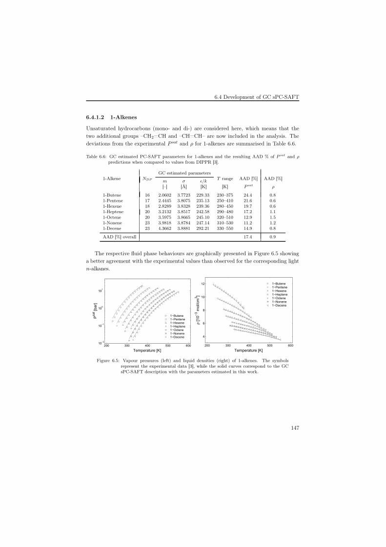
6.4 Development of GC sPC-SAFT

6.4.1.2 1-Alkenes

Unsaturated hydrocarbons (mono- and di-) are considered here, which means that thetwo additional groups –CH2=CH and –CH=CH– are now included in the analysis. Thedeviations from the experimental P sat and ρ for 1-alkenes are summarised in Table 6.6.

Table 6.6: GC estimated PC-SAFT parameters for 1-alkenes and the resulting AAD % of P sat and ρpredictions when compared to values from DIPPR [3].

1-Alkene NDP

GC estimated parametersT range AAD [%] AAD [%]

m σ ε/k[K] P sat ρ[–] [Å] [K]

1-Butene 16 2.0602 3.7723 229.33 230–375 24.4 0.81-Pentene 17 2.4445 3.8075 235.13 250–410 21.6 0.61-Hexene 18 2.8289 3.8328 239.36 280–450 19.7 0.61-Heptene 20 3.2132 3.8517 242.58 290–480 17.2 1.11-Octene 20 3.5975 3.8665 245.10 320–510 12.9 1.51-Nonene 23 3.9818 3.8784 247.14 310–530 11.2 1.21-Decene 23 4.3662 3.8881 292.21 330–550 14.9 0.8

AAD [%] overall 17.4 0.9

The respective fluid phase behaviours are graphically presented in Figure 6.5 showinga better agreement with the experimental values than observed for the corresponding lightn-alkanes.

200 300 400 500 60010−2

10−1

100

101

Temperature [K]

Psa

t [bar

]

1−Butene1−Pentene1−Hexene1−Heptene1−Octene1−Nonene1−Decene

200 300 400 500 600

4

6

8

10

12

Temperature [K]

ρ [1

0−3 m

ol/c

m3 ]

1−Butene1−Pentene1−Hexene1−Heptene1−Octene1−Nonene1−Decene

Figure 6.5: Vapour pressures (left) and liquid densities (right) of 1-alkenes. The symbolsrepresent the experimental data [3], while the solid curves correspond to the GCsPC-SAFT description with the parameters estimated in this work.

147

6 The GC sPC-SAFT model

6.4.1.3 1-Alkynes

With the GC estimated parameters of a few alkynes listed in Table 6.7, sPC-SAFT cal-culates their P sat and ρ with good accuracy, as shown in Figure 6.6.

Table 6.7: GC estimated PC-SAFT parameters for 1-alkynes and the resulting AAD % of P sat and ρpredictions when compared to values from DIPPR [3].

1-Alkyne NDP

GC estimated parametersT range AAD [%] AAD [%]

m σ ε/k[K] P sat ρ[–] [Å] [K]

1-Pentyne 19 2.5854 3.6396 229.33 250–430 11.1 2.71-Hexyne 16 2.9697 3.6882 235.13 310–460 4.3 1.21-Heptyne 18 2.3540 3.7248 239.36 350–500 4.2 0.61-Octyne 20 3.7383 3.7534 242.58 350–520 2.2 1.72-Hexyne 17 2.7729 3.7836 266.94 290–490 2.8 1.5

AAD [%] overall 4.9 1.5

200 300 400 500 60010−2

10−1

100

101

Temperature [K]

Psa

t [bar

]

1−Pentyne1−Hexyne2−Hexyne1−Heptyne1−Octyne

200 300 400 500 6004

6

8

10

12

Temperature [K]

ρ [1

0−3 m

ol/c

m3 ]

1−Pentyne1−Hexyne2−Hexyne1−Heptyne1−Octyne

Figure 6.6: Vapour pressures (left) and liquid densities (right) of 1-alkynes. The symbolsrepresent the experimental data [3], while the solid curves correspond to the GCsPC-SAFT description with the parameters estimated in this work.

Predictions of P sat and ρ of the five investigated 1-alkynes in Table 6.7 generallyexhibit low deviations from experimental data; especially when compared to the corre-sponding predictions of n-alkanes and 1-alkenes as presented in Sections 6.4.1.1 and 6.4.1.2respectively.

148

6.4 Development of GC sPC-SAFT

6.4.1.4 2-Methyl Alkanes

In the case of the 2-methyl alkanes, the new group –CH3CH is included in the parametercalculations. GC estimated parameters for these compounds, as well as the deviationsfrom the experimental P sat and ρ are summarised in Table 6.8. The overall AAD % forall investigated compounds of this family is 12% for P sat and 0.7% for ρ. Moreover,accurate representations of both properties are seen in Figure 6.7.

Table 6.8: GC estimated PC-SAFT parameters for 2-methyl alkanes and the resulting AAD % of P sat

and ρ predictions when compared to values from DIPPR [3].

2-Methyl Alkane NDP

GC estimated parametersT range AAD [%] AAD [%]

m σ ε/k[K] P sat ρ[–] [Å] [K]

2-Methyl butane 19 2.3612 3.9068 236.61 230–410 24.5 0.52-Methyl pentane 21 2.7456 3.9181 240.76 250–447 17.2 0.92-Methyl hexane 22 3.1299 3.9266 243.89 270–477 11.8 0.72-Methyl heptane 23 3.5142 3.9331 246.33 280–500 8.3 0.42-Methyl octane 24 3.8986 3.9384 248.29 290–520 6.3 0.82-Methyl decane 24 4.2829 3.9427 249.90 310–545 3.1 1.1

AAD [%] overall 11.9 0.7

200 300 400 500 60010−3

10−2

10−1

100

101

Temperature [K]

Psa

t [bar

]

2−Methyl butane2−Methyl pentane2−Methyl hexane2−Methyl heptane2−Methyl octane2−Methyl nonane

200 300 400 500 6003

4

5

6

7

8

9

10

Temperature [K]

ρ [1

0−1 m

ol/c

m3 ]

2−Methyl butane2−Methyl pentane2−Methyl hexane2−Methyl heptane2−Methyl octane2−Methyl nonane

Figure 6.7: Vapour pressures (left) and liquid densities (right) of 2-methyl alkanes. The symbolsrepresent the experimental data [3], while the solid curves correspond to the GCsPC-SAFT description with the parameters estimated in this work.

6.4.1.5 n-Alkyl Benzenes

Description of the vapour-liquid coexistence of aromatic compounds is a more rigoroustest for the GC method as these compounds have very distinct chemical properties, such

149

6 The GC sPC-SAFT model

as more significant quadropole moments and the possibility of interactions between π-electrons. In this case, two new groups, ACH and ACH2, are required for calculating purecompound parameters of some n-alkyl benzenes (from ethyl benzene to n-decyl benzene).PC-SAFT parameters calculated using the proposed GC scheme are listed in Table 6.9.

Results presented in Table 6.9 indicate rather good adequacy of the model in describingP sat and ρ of this chemical family. This can also be seen in Figure 6.8.

Table 6.9: GC estimated PC-SAFT parameters for n-alkyl benzenes and the resulting AAD % of P sat

and ρ predictions when compared to values from DIPPR [3].

n-alkyl benzene NDP

GC estimated parametersT range AAD [%] AAD [%]

m σ ε/k[K] P sat ρ[–] [Å] [K]

Ethyl benzene 25 2.8658 3.8828 291.55 310–550 28.9 1.2n-Propyl benzene 25 3.2501 3.8953 288.56 320–570 14.5 0.7n-Butyl benzene 25 3.6344 3.9051 286.20 340–590 10.5 0.7n-Pentyl benzene 26 4.0188 3.9130 284.29 345–610 6.9 0.5n-Hexyl benzene 26 4.4031 3.9195 282.71 350–628 2.0 0.6n-Heptyl benzene 26 4.7874 3.9249 281.39 360–640 4.3 0.9n-Octyl benzene 26 5.1717 3.9295 280.27 365–656 6.2 0.8n-Nonyl benzene 27 5.5561 3.9334 279.29 370–665 7.6 1.0n-Decyl benzene 25 5.9404 3.9369 278.45 380–677 11.9 1.1

AAD [%] overall 10.3 0.8

300 400 500 600 700

10−3

10−2

10−1

100

101

Temperature [K]

Psa

t [bar

]

Ethyl benzenePropyl benzeneButyl benzenePentyl benzeneHexyl benzeneHeptyl benzeneOctyl benzeneNonyl benzeneDecyl benzene

300 400 500 600 7002

3

4

5

6

7

8

9

Temperature [K]

ρ [1

0−3 m

ol/c

m3 ]

Ethyl benzenePropyl benzeneButyl benzenePentyl benzeneHexyl benzeneHeptyl benzeneOctyl benzeneNonyl benzeneDecyl benzene

Figure 6.8: Vapour pressures (left) and liquid densities (right) of n-alkyl benzenes. The symbolsrepresent the experimental data [3], while the solid curves correspond to the GCsPC-SAFT description with the parameters estimated in this work.

Predictions of P sat and ρ of the nine investigated n-alkyl benzenes generally exhibit lowdeviations from experiments, with the overall deviations of 10.3% and 0.8% respectively.

150

6.4 Development of GC sPC-SAFT

6.4.1.6 Alkyl Acetate Esters

The final class of compounds examined in this part of the work is acetate esters withvarying alkyl chain length. For this family, an extra group –CH3COO is considered.

Table 6.10 lists GC estimated parameters and AAD % of P sat and ρ predictions forthe investigated acetates. The results in Figure 6.9 show decreasing predicted values ofP sat with increasing alkyl carbon number going from 2 to 6, but the deviation begins toincrease again at alkyl carbon numbers >7. This is similarly observed for n-alkyl benzenesin Section 6.4.1.5. Predictions of ρ seem to be more accurate when the alkyl chain containsfewer carbon atoms, but deviations are very low in the first place.

Table 6.10: GC estimated PC-SAFT parameters for alkyl acetates and the resulting AAD % of P sat andρ predictions when compared to values from DIPPR [3].

Alkyl Acetates NDP

GC estimated parametersT range AAD [%] AAD [%]

m σ ε/k[K] P sat ρ[–] [Å] [K]

Ethyl acetate 20 3.3912 3.3200 226.98 280–470 42.6 0.4Propyl acetate 23 3.7756 3.4004 230.98 270–490 29.9 0.0Butyl acetate 24 4.1599 3.4632 234.24 290–520 16.5 0.5Pentyl acetate 21 4.5442 3.5137 236.94 330–530 8.7 1.1Hexyl acetate 21 4.9286 3.5552 239.23 350–550 1.7 0.3Heptyl acetate 24 5.3129 3.5899 241.18 320–550 1.8 1.3Octyl acetate 26 5.6972 3.6195 242.87 330–580 6.9 0.8Nonyl acetate 27 6.0816 3.6449 244.35 340–590 19.7 2.5Decyl acetate 27 6.4659 3.6670 245.65 350–600 18.8 1.1

AAD [%] overall 16.3 0.8

300 400 500 600 70010−3

10−2

10−1

100

101

Temperature [K]

Psa

t [bar

]

Ethyl acetatePropyl acetateButyl acetatePentyl acetateHexyl acetateHeptyl acetateOctyl acetateNonyl acetateDecyl acetate

300 400 500 600 7000.2

0.4

0.6

0.8

1.0

1.2

Temperature [K]

ρ [1

0−3 m

ol/c

m3 ]

Ethyl acetatePropyl acetateButyl acetatePentyl acetateHexyl acetateHeptyl acetateOctyl acetateNonyl acetateDecyl acetate

Figure 6.9: Vapour pressures (left) and liquid densities (right) of alkyl acetates. The symbolsrepresent the experimental data [3], while the solid curves correspond to the GCsPC-SAFT description with the parameters estimated in this work.

151

6 The GC sPC-SAFT model

In the work presented by Nguyen Huynh et al. [12], several heavy esters and theirmixtures are treated with their version of the GC PC-SAFT EoS, and the resulting pre-dictions of P sat and ρ are in the same range as the ones from this work. The overalldeviations are reported to be around 6% for P sat and 3% for ρ. However, in additionto the usual terms of the EoS, they use a multi polar term as well, which improves thepredictive capability of their GC approach. This does not come unexpected when thenumber of model parameters is increased. Moreover, they have also reported significantlyhigher deviations for nonyl acetate and decyl acetate compared to other alkyl acetates,which is similar to this work (cf. Table 6.10). This might indicate an inconsistency of theexperimental results for these two compounds rather than shortcomings by the models.

The description of the fluid phase behaviour with the currently proposed GC schemeis not comparable with the calculations reported by Tamouza et al. [13] (see Section 3.4)using their GC version of the PC-SAFT EoS, where the reported overall deviations for theP sat and ρ are somewhat lower than deviations reported in this work. A more detailedcomparison at this stage is not provided because of the use of different experimental datasets and temperature ranges.

6.4.2 Inspiration from the Tamouza et al. Approach

One of the most complete GC treatments within the SAFT formalism is that of Tamouzaet al. (see Section 3.4). In this case, separate contributions from various groups tothe overall chain length, segment size, dispersive energy, and association parameters areobtained by optimising the description of P sat and ρ of pure components. Numerouschemical families are considered with their approach. An excellent description of the fluidphase behaviour of the pure components and representative mixtures of these systems isobtained.

Therefore, inspired by the approach presented by Tamouza et al. [13] (see Section 3.4),the three PC-SAFT parameters are calculated through averages by the Lorentz-Berthelotcombining rules. In these rules, energy parameters are averaged geometrically, whereassize parameters are averaged arithmetically.

Applying their method using FOG and SOG defined in this work, the relations forthe calculation of pure compound GC parameters become as follows. The chain-lengthparameter m is calculated as a sum of group contributions as presented in Equation (6.5).The energy parameter ε/k of a molecule is obtained from Equation (6.6) by a geometricaverage of FOGs present in the molecule, whereas the segment diameter σ is calculatedas an arithmetic average in Equation (6.7) including both FOG and SOG.

152

6.4 Development of GC sPC-SAFT

mmolecule =∑

i

(nimi)FOG + Φ∑

j

(njmj)SOG (6.5)

(ε/k)molecule =

⎛⎝ C√∏

i

(εi/k)ni

⎞⎠

FOG

where C =∑

i

ni (6.6)

σmolecule =

∑i

(niσi)FOG + Φ∑

j

(njσj)SOG∑i,j

(ni + nj)(6.7)

where Φ = 0 when no SOG are present, and Φ = 1 when SOG are present.The parameters mi, σi, and εi/k represent the contributions of the FOG of type i that

appears ni times, and mj and σj are the contributions of the SOG of type j that appearsnj times. Equation (6.6) does not contain a contribution from SOG, because this lead tonumerical instabilities during the linear least square analysis. A solution to this problemhas not been sought, since it is not expected that contributions from SOG will lead tosignificant improvements of the resulting GC scheme.

GC parameters for FOG and SOG are now calculated using the correlations in Equa-tions (6.5)–(6.7) with the methodology explained in Section 6.4. The resulting GC schemewith values of m, σ, and ε/k is found in Tables B.1 and B.2 in Appendix B together withstatistical results in Table B.3. Since values of σ and ε/k are directly fitted in the currentapproach instead of the parameter groupings mσ3 and mε/k, the statistical results inTable B.3 are not directly comparable with statistical results from the original approachin Table 6.2.

Figure 6.10 shows linear correlations and % deviations of GC estimated parametersfor about 400 different molecules, obtained from the GC scheme in Tables B.1 and B.2,with corresponding experimental reference values from DIPPR [3].

The results in Figure 6.10 should be compared to the scatter plots presented in Figure6.2 on page 144 for the GC approach based on the linear equations in (6.2)–(6.4) proposedin this work. The linear correlation of m and corresponding % deviations in Figure 6.10(top) are more or less identical to the result obtained in Figure 6.2 (top). This does notcome as a surprise since the underlying equations for m, i.e. Equations (6.2) and (6.5),are identical, so the small differences observed can only arise from slight deviations in theset of experimental data used for the linear regression.

However, for the σ and ε/k parameters in Figure 6.10, the linear correlations withexperimental reference values have deteriorated compared to the results in Figure 6.2;especially for ε/k, where the value of R2 = 0.7116 is considered unacceptable for furtherapplication of this approach. In addition, only 71.7 and 70.2% of the σ and ε/k datapoints,

153

6 The GC sPC-SAFT model

2 4 6 8 10

2

4

6

8

10

DIPPR estimated m

GC

est

imat

ed m

R2 = 0.9740

2 4 6 8 10−30

−20

−10

0

10

20

30

DIPPR estimated m

Dev

iatio

n [%

]

3.0 3.5 4.0 4.5

3.0

3.5

4.0

4.5

DIPPR estimated σ

GC

est

imat

ed σ

R2 = 0.9023

3.0 3.5 4.0 4.5−6

−4

−2

0

2

4

6

DIPPR estimated σ

Dev

iatio

n [%

]

150 200 250 300 350 400 450150

200

250

300

350

400

450

DIPPR estimated ε/k

GC

est

imat

ed ε

/k

R2 = 0.7116

150 200 250 300 350 400 450

−30

−20

−10

0

10

20

30

DIPPR estimated ε/k

Dev

iatio

n [%

]

Figure 6.10: Scatter plots showing linear correlations (left) and % deviations (right) of GC- vs.DIPPR-estimated PC-SAFT parameters m (top), σ (middle), and ε/k (bottom),using the Tamouza et al. approach [13]. Dashed lines (right) mark ranges ofdeviating datapoints and are used to compare different GC approaches; see text.

respectively, lie within the ranges of the dashed lines that are considered to mark the limitsof low devations; as discussed previously in Section 6.4. This is in contrast to 98.2 and83.9% for the GC estimated σ and ε/k parameters from Figure 6.2.

154

6.5 Ongoing Attempts to Improve the GC Scheme

Considering the poor linear correlation between the GC estimated ε/k parametersand reference values from DIPPR, it is concluded that Equations (6.5)–(6.7), based onproposals from Tamouza et al. [13], do not perform as well as the equations proposed inthis work, i.e. Equations (6.2)–(6.4), when applied to the current GC methodology; atleast when numerous groups are regressed at the same time.

6.5 Ongoing Attempts to Improve the GC Scheme

There have been some difficulties obtaining a solid linear correlation between GC esti-mated ε/k parameters and reference values from DIPPR. This can be observed in thescatter plots in Figure 6.2 (bottom) for the currently proposed GC approach, and in Fig-ure 6.10 (bottom) for the application of the GC approach proposed by Tamouza et al. [13].Moreover, it is the experience of the author that GC sPC-SAFT model predictions aregenerally more sensitive to the value of ε/k than the m and σ parameters, and hence, alsosensitive to deviations of the ε/k parameter. Therefore, attempts to improve the currentGC scheme have been focused on the accuracy of ε/k.

This part of the work has been carried out after finishing detailed testing and analysisof the proposed GC scheme in Tables 6.3 and 6.4; the results of which will be the subjectof the proceeding Chapter 7. It has resulted in what appears to be a further improvementof the existing GC scheme, but within the time limitations of the project it has not beenpossible to complete testing of this potential improvement of the GC scheme in a moreconsistent way. Therefore, it is regarded as supplementary to this thesis, and is, hence,presented in Appendix C from where it can serve as a springboard for future work withinthe subject.

6.6 Final Comments

The first-order group and second-order group contributions have been estimated followingthe procedure described in this chapter, and the accuracy of the fluid phase behaviourdescription of the compounds included in the fitting database has been examined. Twotables have been compiled including the contributions of 45 FOG and 26 SOG for each ofthe three parameter groupings, m, mσ3, and mε/k.

The quality of the GC sPC-SAFT description of the pure compound data has beenassessed for selected chemical families. It has been demonstrated that the GC approachprovides a good representation of the fluid phase equilibria of the various compoundsexamined, and, particularly, for heavier members of the investigated families with observedlow overall deviations from the experimental data. For almost all investigated compounds,AAD of P sat decreases with increasing carbon number. Predictions of ρ are very accurateand in range of the AAD obtained when predicting ρ using DIPPR estimated parametersets (reported in Table 4.1).

155

REFERENCES

In this chapter, the accuracy of the fluid phase behaviour of the compounds includedin the optimisation database has been examined. In the next chapter, the predictivecapability of the GC sPC-SAFT EoS is tested. The estimated parameters are used in amore predictive manner for the treatment of compounds not included in the database andfor some selected binary mixtures.

References[1] L. Constantinou and R. Gani, “New Group Contribution Method for Estimating Properties

of Pure Compounds,” AIChE J., vol. 40, pp. 1697–1710, 1994.

[2] N. von Solms, M. L. Michelsen, and G. M. Kontogeorgis, “Computational and Physical Per-formance of a Modified PC-SAFT Equation of State for Highly Asymmetric and AssociatingMixtures,” Ind. Eng. Chem. Res., vol. 42, pp. 1098–1105, 2003.

[3] AIChE J., DIPPR Table of Physical and Thermodynamic Properties of Pure Compounds.New York, USA, 1998.

[4] E. K. Karakatsani, T. Spyriouni, and I. G. Economou, “Extended SAFT Equations of Statefor Dipolar Fluids,” AIChE. J., vol. 51, pp. 2328–2342, 2005.

[5] E. K. Karakatsani and I. G. Economou, “Perturbed Chain-Statistical Associating Fluid The-ory Extended to Dipolar and Quadrupolar Molecular Fluids,” J. Phys. Chem. B, vol. 110,pp. 9252–9261, 2006.

[6] J. Gross and J. Vrabec, “An Equation of State Contribution for Polar Components: DipolarMolecules,” AIChE J., vol. 52, pp. 1194–1204, 2006.

[7] L. A. Constantinou, Estimation of Properties of Acyclic Organic Compounds Through Con-jugation. PhD Thesis, Institute for Systems Research, University of Maryland, USA, 1993.

[8] D. Marquardt, “An Algorithm for Least Squares Estimation on Nonlinear Parameters,” SIAM(Soc. Ind. Appl. Math.) J. Appl. Math., vol. 11, pp. 431–441, 1936.

[9] E. Stefanis, L. Constantinou, I. Tsivintzelis, and C. Panayiotou, “New Group-ContributionMethod for Predicting Temperature-Dependent Properties of Pure Organic Compounds,”Int. J. Thermophys., vol. 26, pp. 1369–1388, 2005.

[10] A. Fredenslund, R. L. Jones, and J. M. Prauznitz, “Group-Contribution Estimation of Ac-tivity Coefficients in Nonideal Liquid Mixtures,” AIChE J., vol. 21, pp. 1086–1099, 1975.

[11] H. S. Elbro, A. Fredenslund, and P. Rasmussen, “Group Contribution Method for the Predic-tion of Liquid Densities as a Function of Temperature for Solvents, Oligomers, and Polymers,”Ind. Eng. Chem. Res., vol. 30, pp. 2576–2582, 1991.

[12] D. N. Huynh, J.-P. Passarello, P. Tobaly, and J.-C. de Hemptinne, “Application of GC-SAFT EOS to Polar Systems Using a Segment Approach,” Fluid Phase Equilibria, vol. 264,pp. 62–75, 2008.

[13] S. Tamouza, J.-P. Passarello, P. Tobaly, and J.-C. de Hemptinne, “Group ContributionMethod with SAFT EoS Applied to Vapor Liquid Equilibria of Various Hydrocarbon Se-ries,” Fluid Phase Equilibria, vol. 222-223, pp. 67–76, 2004.

156

Chapter 7

Analysis and Applications of GCsPC-SAFT

”When you come to the end of all the light you know, and it’s time to step into the darknessof the unknown, faith is knowing that one of two things shall happen: Either you will begiven something solid to stand on or you will be taught to fly.” by Edward Teller

7.1 Introduction

The GC method presented in Chapter 6 is now used for the treatment of binary mixtureswhere the quality of the phase behaviour modeling with the sPC-SAFT model is assessedthrough comparison with experimental data. For this final assessment, selected systemswill be investigated representing a broad range of classes of industrially important mix-tures. Even though the list of investigated compounds is far from exhaustive it shouldprovide the reader with a good impression of the applicability of the method for binarysystems.

7.2 Complex Binary Systems

In the previous chapter the correlative capability of the GC sPC-SAFT EoS has been in-vestigated demonstrating satisfactory description of the fluid behaviour of the compoundsused in the regression. However, the main objective of the GC approach is to functionas a predictive tool for complex compounds or mixtures not necessarily included in thedatabase but which can be formed from the various functional groups. Thus, emphasisis given to the predictive capability of the GC sPC-SAFT EoS without use of any binaryinteraction parameters. As supplementary help to the reader Table D.1 in Appendix Dshows chemical structures of the complex compounds and monomer units of polymersinvestigated in this chapter together with their FOG and SOG descriptions.

157

7 Analysis and Applications of GC sPC-SAFT

7.2.1 Aromatic Esters

Aromatic esters belong to a family of valuable compounds with a number of importanttechnological applications. The presence of the polarizable aromatic group (electron sys-tems in the vicinity of the dipolar ester group) together with their hydrophobic character,confers to these compounds a highly selective solvent ability that is used for applicationsin fields such as cosmetic formulations, polymer science, and several synthesis processesamong others [1, 2]. Aromatic esters with various chemical structures are tested in orderto observe the effects of the alkylic chain length or the presence of the aromatic ringand its influence on the pure compounds’ properties. Ester compounds investigated inthis work are: methyl, ethyl, propyl, butyl benzoate, and phenyl acetate (See Table D.1in Appendix D for their molecular structures). The experimental PVT behavior of theinvestigated aromatic esters reported by Aparicio et al. [3] is used for comparison withmodelling results.

Table 7.1: Pure component PC-SAFT parameters for investigated aromatic esters and AAD % of P sat

and ρ for aromatic esters with various metods.

Compound m σ ε/k AAD [%] Method[–] [Å] [K] XP sat/ρX

Methyl benzoate

3.9654 3.5674 279.67 24.5/1.8 FOG3.8751 3.5934 281.62 26.0/1.6 FOG+SOG3.657 3.6412 304.91 2.8/0.5 fitted to [3]3.6922 3.6377 303.46 1.3/1.1 fitted to [4]

Ethyl benzoate4.3488 3.6073 278.30 22.6/2.0 FOG4.2586 3.313 280.05 25.3/1.9 FOG+SOG4.636 3.5045 274.08 5.4/0.2 [3]

Propyl benzoate

4.7323 3.6401 277.16 17.7/1.4 FOG4.6421 3.6624 278.74 29.0/1.4 FOG+SOG3.587 4.0173 322.70 2.8/1.3 fitted to [3]4.6655 3.653 281.56 0.9/1.0 fitted to [4]

Butyl benzoate

5.1158 3.6675 276.19 11.5/1.8 FOG5.0256 3.6883 277.63 12.4/1.7 FOG+SOG4.0960 3.9644 312.50 5.4/0.9 fitted to [3]4.9127 3.7073 283.08 0.6/2.3 fitted to [4]

Phenyl acetate 4.2470 3.4773 275.03 29.4/3.0 FOG4.446 3.4136 273.38 3.5/0.9 fitted to [3]

The results in Table 7.1 indicate that the SOG contribution, which in this case isthe ACCOO group, in the pure parameter estimations does not improve the predictionsof vapour pressures nor the liquid densities of the investigated aromatic esters. On thecontrary, indications of larger deviations from the experimental data are observed whenintroducing the contributions from SOG as well. However, due to the small number of in-vestigated aromatic esters and their internal similarities (all belonging to alkyl benzoates),care should be taken when drawing final conclusions regarding the application of SOG forthis family of compounds.

158

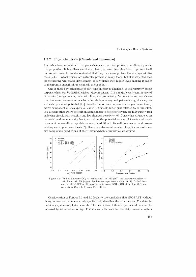
7.2 Complex Binary Systems

7.2.2 Phytochemicals (Cineole and Limonene)

Phytochemicals are non-nutritive plant chemicals that have protective or disease preven-tive properties. It is well-known that a plant produces these chemicals to protect itselfbut recent research has demonstrated that they can even protect humans against dis-eases [5, 6]. Phytochemicals are naturally present in many foods, but it is expected thatbioengineering will enable development of new plants with higher levels making it easierto incorporate enough phytochemicals in our food [7].

One of these phytochemicals of particular interest is limonene. It is a relatively stableterpene, which can be distilled without decomposition. It is a major constituent in severalcitrus oils (orange, lemon, mandarin, lime, and grapefruit). Various studies have shownthat limonene has anti-cancer effects, anti-inflammatory and pain-relieving efficiency, aswell as large market potential [8,9]. Another important compound is the pharmaceuticallyactive component of eucalyptus oil called 1,8-cineole (often just referred to as ’cineole’).It is a cyclic ether where the carbon atoms linked to the ether oxygen are fully substitutedendowing cineole with stability and low chemical reactivity [6]. Cineole has a future as anindustrial and commercial solvent, as well as the potential to control insects and weedsin an environmentally acceptable manner, in addition to its well documented and provenexisting use in pharmaceuticals [7]. Due to a substantial number of applications of thesetwo compounds, predictions of their thermodynamic properties are desired.

0.70 0.75 0.80 0.85 0.90 0.95 1.00

7.0

7.5

8.0

8.5

9.0

9.5

10.0

CO2 mole fraction

Pre

ssur

e [M

Pa]

323.15 K318.15 Kkij = 0 (FOG+SOG)kij = 0.03 (FOG+SOG)

0.5 0.6 0.7 0.8 0.9 1.0

4.0

4.5

5.0

5.5

6.0

6.5

7.0

Ethylene mole fraction

Pre

ssur

e [M

Pa]

298.15 K288.15 Kkij = 0 (FOG+SOG)

Figure 7.1: VLE of limonene–CO2 at 318.15 and 323.15 K (left) and limonene–ethylene at288.15 and 298.15 K (right). Symbols are experimental data [10, 11]. Dashed linesare GC sPC-SAFT predictions (kij = 0) using FOG+SOG. Solid lines (left) arecorrelations (kij = 0.03) using FOG+SOG.

Consideration of Figures 7.1 and 7.2 leads to the conclusion that sPC-SAFT withoutbinary interaction parameters only qualitatively describes the experimental P, x data forthe binary systems of phytochemicals. The description of these experimental data can beimproved by introduction of kij . This is clearly the case for the CO2–limonene system

159

7 Analysis and Applications of GC sPC-SAFT

0.70 0.75 0.80 0.85 0.90 0.95 1.006.0

7.0

8.0

9.0

10.0

CO2 mole fraction

Pre

ssur

e [M

Pa]

323.15 K318.15 Kkij = 0 (FOG+SOG)kij = 0.05 (FOG+SOG)

0.6 0.7 0.8 0.9 1.0

3.0

4.0

5.0

6.0

7.0

Ethylene mole fraction

Pre

ssur

e [M

Pa]

298.15 K288.15 Kkij = 0 (FOG+SOG)

Figure 7.2: VLE of cineole–CO2 at 318.15 and 323.15 K (left) and cineole–ethylene at 288.15and 298.15 K (right). Symbols are experimental data [10, 11], dashed lines areGC sPC-SAFT predictions (kij = 0) using FOG+SOG, and solid lines (left) arecorrelations (kij = 0.05) using FOG+SOG.

where the optimum temperature independent kij is 0.03; and for the CO2–cineole systemthe value of kij is 0.05. For the other two systems where the solvent is ethylene, thepredictions of sPC-SAFT give good results. Unfortunately, due to limited experimentaldata for binary systems with phytochemicals, it is not possible to perform a more detailedanalysis and therefore no final conclusion is given on the performance of the model.

7.2.3 Sulfur Containing Compounds

The content of sulfur in petroleum products has to be reduced in accordance with theenvironmental protection legislation. Petroleum refiners and natural gas processors facethe various challenges of removing the increased sulfur content and doing it cost-effectively.This can be done either by improving desulfurization processes or by employing betterthermodynamic characterization of sulfur compounds in different petroleum cuts [12].Sulfur compounds are generally grouped into three classes: sulfides, thiols, and thiophenes.

This section aims at calculating PC-SAFT parameters for some sulfur containing com-pounds; investigating at the same time how well the model can predict their individualvapour pressures.

7.2.3.1 Alkyl and Aryl Sulfides

The GC sPC-SAFT EoS is applied to predict vapour pressures for various alkyl andaryl sulfide compounds, which are compared to experimental data reported by Sawayaet al. [13]. There are no experimental PVT data available for these compounds in theDIPPR database [4]. Therefore no comparison is included.

The presented GC method is able to reproduce the experimental P sat of sulfides over

160

7.2 Complex Binary Systems

a wide range of temperatures. The results are graphically presented in Figure 7.3. For apurely predictive method the current accuracy is considered reasonably good and possiblysufficient for first-hand engineering calculations.

200 250 300 350 400 450100

101

102

103

104

105

Temperature [K]

Psa

t [Pa]

t−Butyl methyl sulfideDibutyl sulfideEthyl phenyl sulfideDihexyl sulfideBenzyl phenyl sulfideDioctyl sulfide

Figure 7.3: Vapor pressure of alkyl and aryl sulfides. Symbols are experimental data [13] anddashed lines are predictions with GC sPC-SAFT with sulfides parameters obtainedfrom the proposed GC method.

7.2.3.2 Thiols

If a sulfur distribution is carried out on a petroleum distillate, the majority of the sulfur-containing fractions appear at boiling points, which do not correlate with known sulfurcompounds. This indicates that azeotropes are formed between sulfur compounds andhydrocarbons, which is perhaps to be expected, as the different types of hydrocarbons areknown to form azeotropes among themselves [14]. When looking through the availableliterature, it is apparent that the information available on the occurrence and propertiesof these azeotropes is quite limited, which is surprising since hydrocarbons are foundassociated with sulfur compounds not only in petroleum products but also in coal tarsand shale oils. Therefore, the study of thiols, often referred to as mercaptans, with sPC-SAFT is initiated to possibly increase knowledge of the chemical and physical propertiesof the sulfur compounds present in petroleum distillates.

Results obtained for some representative mixtures are shown in Table 7.2, where theoverall average deviation for vapour pressure is 8.8% of predictions and 2.4% of correla-tions using a temperature-independent kij .

161

7 Analysis and Applications of GC sPC-SAFT

Table 7.2: Comparison of predicted and correlated results for binary VLE of different thiol-systems usingGC sPC-SAFT.

System Temp. AAD P [%] kij AAD P [%] AAD P [%] Ref.[K] kij = 0 optimal kij = 0.03

Methanethiol+n-hexane 253.15 17.1 5.1 5.1263.15 16.7 0.03 4.2 4.2 [15]273.13 15.4 3.3 3.3

Methanethiol+n-decane 315.15 10.5 0.03 1.9 1.9 [15]

Ethanethiol+1-propylene 253.15 7.1 0.01 1.7 12.4 [16]323.15 4.2 0.9 20.1

Propanethiol+n-butane 343.15 6.0 0.02 0.8 3.5 [17]383.15 4.2 1.1 3.8

Butanethiol+n-hexane323.15 5.7 3.8 3.6353.15 3.3 0.025 1.5 1.6 [18]372.66 2.3 1.3 1.7

Butanethiol+toluene323.05 16.6 2.7 2.7353.15 6.8 0.03 2.8 2.8 [18]371.53 7.1 2.7 2.7

AAD [%] overall 8.8 2.4 5.0

Figures 7.4–7.6 show the total system pressure as a function of liquid and vapourcomposition to illustrate the performance of the model for this type of compounds.

0 0.2 0.4 0.6 0.8 10

20

40

60

80

Methanethiol mole fraction

Pre

ssur

e [k

PA

]

273.15 K263.15 K253.15 Kkij = 0kij = 0.03

Figure 7.4: P,x-diagram of methanethiol–n-hexane at 253.15, 263.15, and 273.15 K. Symbolsrepresent experimental data [15], where lines are GC sPC-SAFT modelling results.

In Figure 7.5, for the ethanethiol–1-propylene system, the 253.15K isotherm showspositive deviations from Raoult’s law, while at 323.15K there is significant non-ideality inthe liquid phase causing the total pressure to lie below Raoult’s law in the propylene-richregion of the system. In both cases, GC sPC-SAFT is well capable of predicting theobserved behaviour.

Results of the propanethiol–n-butane system at 343.15 and 383.15K are plotted in

162

7.2 Complex Binary Systems

0 0.2 0.4 0.6 0.8 10

500

1000

1500

2000

Ethanethiol mole fraction

Pre

ssur

e [k

PA

]

253.15 K323.15 Kkij = 0kij = 0.01

Figure 7.5: P,x,y-diagram of ethanethiol–1-propylene at 253.15 and 323.15 K. Symbols representexperimental data [16], where lines are GC sPC-SAFT modelling results.

Figure 7.6. The figure shows that a single kij = 0.02 correlates the results quite sat-isfactorily, but even so pure predictions (kij = 0) are able to follow the trends in theexperimental data.

0 0.2 0.4 0.6 0.8 10

500

1000

1500

2000

Propanethiol mole fraction

Pre

ssur

e [k

PA

]

343.15 K383.15 Kkij = 0kij = 0.02

Figure 7.6: P,x,y-diagram of propanethiol–n-butane at 343.15 and 383.15 K. Symbols representexperimental data [17], where lines are GC sPC-SAFT modelling results.

As observed in Table 7.2, the optimum kij values for the thiol systems tend to liebetween 0.01 and 0.03. Additionally, Table 7.2 includes AAD for correlations using a fixedkij = 0.03, which performs well for all the investigated systems except for ethanethiol–1-propylene. Therefore, from a practical point of view, it can be expected that transferablebinary parameters in this range allow straightforward extension of the model to otherthiol-containing binary mixtures without any additional fitting.

163

7 Analysis and Applications of GC sPC-SAFT

7.2.4 Polynuclear Aromatic Hydrocarbons

Polynuclear aromatic hydrocarbons (PAHs) comprise a group of more than 100 differentchemical compounds that result from incomplete combustion of organic materials suchas coal, oil, wood, etc. They have a wide range of potential commercial applications infields ranging from use as pharmaceuticals and cosmetic additives to use as additives inelectron- and photo-resists, proton-conducting membranes for fuel cells, optical limitingmaterials and devices, lithium battery anodes, active elements in organic transistors, andas pigments [19–21]. Due to the presence of ring structures, they are quite good testcompounds for the effect of SOG on the overall calculations.

The relative deviations obtained on vapour pressures for some investigated PAHs aregiven in Table 7.3.

Table 7.3: Pure component PC-SAFT parameters for some investigated PAHs and AAD % from theexperimental P sat [4, 22].

Compound m σ ε/k AAD P sat

Method[–] [Å] [K] [%]

Phenanthrene 3.7431 4.0130 375.67 60.3 FOG3.7313 4.0283 379.84 36.5 FOG+SOG

Benzo[a]pyrene 4.4474 4.1485 432.24 101.7 FOG4.4177 4.1795 441.43 33.2 FOG+SOG

Tetralin3.0256 4.0204 329.54 58.6 FOG3.0681 3.9996 330.47 39.3 FOG+SOG3.2987 3.8755 325.73 0.4 fitted to [4]

Biphenyl 3.7703 3.9069 333.97 6.5 FOG

Dibenzofuran2.8087 4.2072 408.82 15.9 FOG3.1176 4.0714 388.66 11.6 FOG+SOG2.3829 4.5718 452.21 2.1 fitted to [4]

Acenaphthene2.9906 4.1058 389.14 44.6 FOG3.2936 3.9901 374.30 8.3 FOG+SOG3.6387 3.8560 355.5 2.3 fitted to [4]

From Table 7.3, it appears that the accuracy of the predictions with the GC sPC-SAFT EoS is not always convincing. E.g., when comparing the predicted P sat of tetralinwith the experimental data from Ruuzicka et al. [22], absolute deviations of 58.6 and39.3% are obtained with FOG and FOG+SOG contributions respectively. A comparisonof the same predicted parameter sets to experimental data from the DIPPR database [4]yields absolute deviations of 39.7 and 26.2% for FOG and FOG+SOG contributionsrespectively. These differences suggest some uncertainty in the available experimentaldata, but still the present GC approach seems to have some difficulties in capturing thenature of these complex aromatic compounds. Nonetheless, it is observed that applicationof SOG provides substantial improvements of the modeling results.

In the work presented by Nguyen Huynh et al. [23], several more PAHs are treated withtheir version of the GC PC-SAFT EoS, and the predictions of P sat and ρ are somewhat

164

7.2 Complex Binary Systems

lower (generally within 3 % on both properties) than the ones from this work. However,in addition to the usual terms, a quadrupolar-quadrupolar contribution is used as well,which seems to improve the predictive capability of the approach.

Figures 7.7 and 7.8 show attempts to model VLE of binary mixtures of tetralin withbiphenyl/dibenzofuran as measured by Coon et al. [24]. The figures reveal substantialdeviations from the experimental values; especially the prediction of the bubble pointcurves. However, when considering the already observed deviations in the predicted P sat

values in Table 7.3 above, the observed deviations in Figures 7.7 and 7.8 do not comeunexpected.

0 0.2 0.4 0.6 0.8 1.00

10

20

30

40

Tetralin mole fraction

Pre

ssur

e [k

Pa]

423.15 Kkij = 0 (FOG)kij = 0 (FOG+SOG)kij = −0.08 (FOG+SOG)

Figure 7.7: VLE of tetralin–biphenyl at 423.15 K. Symbols represent experimental data [24]. Dashedand dotted lines are predictions with GC sPC-SAFT with and without SOG, respectively.

0 0.2 0.4 0.6 0.8 1.00

10

20

30

40

Tetralin mole fraction

Pre

ssur

e [k

Pa]

423.15 Kkij = 0 (FOG)kij = 0 (FOG+SOG)kij = −0.05 (FOG+SOG)

Figure 7.8: VLE of tetralin–dibenzofuran at 423.15 K. Symbols represent experimental data [24].Dashed and dotted lines are predictions with GC sPC-SAFT with and without SOG,respectively.

165

7 Analysis and Applications of GC sPC-SAFT

Both Figures 7.7 and 7.8 show that the modeling results approach the experimentaldata when the tetralin mole fraction becomes low. This is most pronounced when kij = 0.It indicates that the model is able to capture the pure component properties of biphenyland dihydrofuran, which is also consistent with the somewhat lower deviations of purecompound P sat for these compounds, as listed above in Table 7.3. The main difficulty inthe validation of the proposed method is the lack of sufficient experimental data, especiallyfor binary mixtures containing at least one PAH compound.

7.3 Biodiesel

The use of vegetable oils as fuel for diesel engines goes back to the 1900s, when Dr.Rudolph Diesel, the inventor of the engine that bears his name, used peanut oil to fuelone of his engines at the Paris Exposition. He declared that ’the diesel engine can befed with vegetable oil and will help considerably in the development of the agriculture ofthe countries which use it’ [25]. At that time, the vegetable oil fuels were not acceptablebecause they were more expensive than petroleum fuels. However, with recent increasesin petroleum prices and uncertainties concerning petroleum availability, there is renewedinterest in this area. The earliest known use of alkyl esters for fuel is documented in aBelgian patent granted in 1937 to G. Chavanne [26].

Biodiesel, defined as the mono-alkyl esters of vegetable oils or animal fats, is an al-ternative diesel fuel that is accepted in a steady growing number of countries around theworld. It contains no petroleum but it can be blended at any level with petroleum dieselto create a biodiesel blend. Application of this kind of fuel contributes to the mitigationof our environmental issues such as global warming and air pollution since its feedstockof biomass is carbon neutral and has a low content of sulfur and aromatic carcinogeniccompounds. It is considered a renewable resource, due to the fact that it is derived fromproducts that can be grown and produced domestically [27].

The transesterification of an oil or fat with a monohydric alcohol; in most casesmethanol due to its low price and least reactivity, and an alkaline catalyst such as potas-sium or sodium hydroxide, yields the corresponding mono-alkyl esters, which are definedas biodiesel. As this is a reversible reaction, 60 to 200% excess methanol is typicallyadded during the reaction in order to force the equilibrium in the direction of the desiredproducts [28–30].

The final biodiesel product is dominated by methyl ester with a hydrocarbon chainof 18 carbon atoms and 1, 2, or 3 unsaturated bonds representing more than 90% of thematerial. The residuals are the methyl esters with hydrocarbon chains from 12 to 22 andsmall amounts of un-reacted oil, glycerol, etc. [31].

Temperature-independent vapour pressures of i.e. methyl esters of fatty acids thatare commonly present in biodiesel fuel are usually predicted by the Antoine equationand in some cases group contributions. These esters have the general molecular formula

166

7.3 Biodiesel

CH3(CH2)nCOOCH3 (see Appendix D). Boiling point, Tb, is a key fuel property forbiodiesel [32] in relation to quality control. Besides its importance for quality control,boiling point at atmospheric pressure, called normal boiling point, is also the basis forthe prediction of the critical properties, and temperature-dependent properties such asvapour pressure, density, latent heat of vapourization, viscosity, and surface tension ofbiodiesel. Determination of these properties requires measurements over a wide range oftemperatures, which can, in practice, be a substantial obstacle. Therefore, accurate Tb ofpure fatty acid esters and their biodiesel mixtures are useful for predicting fuel properties.Although the normal boiling points of some fatty acid esters have been published, thoseof real world biodiesel fuels are scarce. For example, most of the reported data focuson the short chain saturated fatty acid methyl esters (FAMEs) (C8–C14), while data forC16 and C18 are very limited and not available; especially those with carbon atoms 20 ormore [32].

In 2004, Ceriani and Meirelles [33] proposed a GC method for the estimation of thevapour pressure of fatty compounds. The method seems to be accurate when used togetherwith the UNIFAC model for estimating VLE of binary and multicomponent fatty acid estermixtures.

Another important property that is of interest to the biodiesel industry is predictinginfinite dilution activity coefficients. Biodiesel is a high boiling solvent well-suited forvolatile organic compounds (VOC) absorption due to its beneficial physical propertiesand low market prices. In addition, the high-boiling solvent used, once spent, must betreated as hazardous waste with great expenses, while biodiesel is a readily biodegradablematter. However, this last advantage requires particular attention regarding the stabilityof the fuel. If exposed to a specific ’oxidation stress’, i.e., high temperatures and frequentcontact with atmospheric oxygen, it ages faster than normal mineral diesel. For thispurpose, environmentally friendly additives, so-called antioxidants, are added during theproduction of biodiesel [34].

In order to use biodiesel effectively as an absorption solvent for a specific waste gasproblem, it is important to determine the activity coefficients at infinite dilution of theVOCs to be separated with biodiesel. The affinity of the solvent towards a VOC [34] canbe expressed using Henry’s law in terms of partial pressure Pi of the VOC and its molefraction xi in the solvent phase at infinite dilution. Here, the activity coefficient of theVOC in the solvent at infinite dilution (γ∞

1 ) is determined by taking into account thevapour pressure of the VOC at the same temperature, P sat

i :

γ∞i =

H

P sati

where H = limxi→0

Pi

xi(7.1)

In this case, both H and γ∞i allow the assessment of the mutual affinity of the com-

pounds under consideration. The vapour pressures of biodiesels are almost zero at lowtemperatures. This is a desired property as it prevents secondary emissions or loss of

167

7 Analysis and Applications of GC sPC-SAFT

solvent by evapouration. Additionally, biodiesel must be suitable for use during winter attemperatures around –20 ◦C. Additives are typically applied to ensure this. Hence, theantioxidants, winter additives, and methanol remaining from the production, representthe volatile fraction of the biodiesel [34].

The next sections will cover:

• Prediction of vapour pressure for the most common FAMEs (i.e. methyl caprylate,methyl caprate, methyl laurate, methyl myristate, methyl palmitate, etc.) andmodeling VLE of numerous systems with these esters investigated in the literature.

• Modeling of VLE for binary mixtures of carbon dioxide and fatty acid methyl esters,particularly, methyl stearate, methyl palmitate, methyl myristate, and methyl oleateat four different temperatures. Investigation of mixtures of these compounds thatexhibit nearly, but not entirely, ideal VLE behaviour. The non-ideality is a negativedeviation from Raoult’s law.

• Existing experimental data of the infinite dilution activity coefficients for VOCs(1,2-chloroethane, benzene, and toluene) in methyl oleate are available at threetemperatures, and these will be compared with the predicted values from GC sPC-SAFT and two versions of the UNIFAC model.

7.3.1 Vapour Pressure Predictions

Experimental vapour pressure-temperature data for numerous FAMEs are reported byRose and Supina [35]. Table 7.4 presents the vapour pressure descriptions of saturatedfatty acid methyl esters using the GC sPC-SAFT model including a comparison withexperiments. The absolute deviations seem to decrease with the size of the saturatedFAMEs. Figure 7.9 shows comparisons of the experimental and predicted vapour pressuresspecifically for methyl oleate and methyl stearate using the parameters listed in Table7.5. The prediction of P sat using GC sPC-SAFT in the right graph in Figure 7.9 showsexcellent correlation with both sets of experimental data [35, 36], while some deviationsare observed in the left graph, when using the GC sPC-SAFT parameter sets (dashedlines). The molecular structures of methyl oleate and methyl stearate differ by a singledouble bond, which may suggest that the GC method has difficulties accounting for thisparticular structural phenomenon.

In an article by van Genderen et al. [37], experimental vapour pressures have beenreported for a number of fatty acid methyl and ethyl esters, and these values are comparedagainst data available from other sources. However, even in this article, the databasesonly go up to methyl stearate with carbon number 19. Predictions of vapour pressure isan important issue when no data for desired FAMEs are available. There are numerouscorrelations proposed in the literature based on various theoretical approaches, but onlya few can deal with heavier fatty acid esters with carbon atom of 20 or more.

168

7.3 Biodiesel

Table 7.4: Pure component parameters for investigated FAMEs calculated using the GC scheme for usewith the sPC-SAFT EoS. Cn:m indicates n total number og carbon atoms and m number ofdouble bonds.

FAMEs m σ ε/k T range AAD P

[−] [Å] [K] [K] [%]

Methyl caprylate C9:0 5.0277 3.6592 241.82 374–419 46.7Methyl caprate C11:0 5.7947 3.7044 244.78 381–462 29.3Methyl laurate C13:0 6.5616 3.7383 247.04 430–486 17.1Methyl myristate C15:0 7.3286 3.7647 248.84 440–511 9.4Methyl palmitate C17:0 8.0956 3.7858 250.29 467–506 3.4Methyl stearate C19:0 8.8625 3.8031 251.49 477–513 3.8Methyl oleate C19:1 8.9962 3.7639 253.79 430–212 41.5

Table 7.5: Comparison of sPC-SAFT parameters for methyl oleate.

FAMEs m σ ε/k T range AAD P Method[−] [Å] [K] [K] [%]

Methyl oleate 9.3898 3.6881 243.32 430–212 5.59 DIPPR fitted8.9962 3.7639 253.79 41.5 GC

400 420 440 460 480 5000

0.5

1.0

1.5

2.0

2.5

Temperature [K]

Pre

ssur

e [k

Pa]

Rose & Schrodt, 1964DIPPR fittedGC

400 420 440 460 480 500 5200

1.0

2.0

3.0

4.0

5.0

6.0

Temperature [K]

Pre

ssur

e [k

Pa]

Rose & Supina, 1961Rose & Schrodt, 1964GC

Figure 7.9: Predicting P sat for methyl oleate (left) and methyl stearate (right) with sPC-SAFTusing parameters fitted to DIPPR and calculated from the GC scheme as shown inTables 7.4 and 7.5. Experimental data are taken from ref. [35,36].

7.3.2 Phase Equilibria

There are very few experimental data on VLE of the fatty ester systems. Rose andSupina [35] are some of the few researches who have conducted intensive experimentalmeasurements of the VLE for various binary systems involving FAMEs under isobaricconditions. Table 7.6 shows overall results of the predictions with the GC sPC-SAFTEoS. Moreover, a comparison of experimental and predicted values at isobaric conditions

169

7 Analysis and Applications of GC sPC-SAFT

is given in Figure 7.10 in terms of x− y diagrams for methyl myristate–methyl palmitatemixtures. The results are considered to be satisfactory.

Table 7.6: GC sPC-SAFT predictions (kij = 0) of VLE mixtures of FAMEs.

Mixture T or P AAD T or P AAD y Ref.[K] or [kPa] [%] [%]

Methyl oleate + 470 K 21.39 — [36]methyl sterate 480 K 30.65 —

Methyl laurate +4.0 kPa 14.96 1.94

[35]methyl myristate5.3 kPa 14.17 2.426.7 kPa 14.79 3.62

13.3 kPa 14.92 2.63

Methyl caprate +4.0 kPa 27.53 2.01

[35]methyl laurate5.3 kPa 17.89 1.596.7 kPa 26.36 3.28

13.3 kPa 25.87 2.13

Methyl myristate +4.0 kPa 6.16 1.72

[35]methyl palmitate5.3 kPa 5.01 1.936.7 kPa 5.34 2.53

13.3 kPa 5.32 1.72

The ability of the GC sPC-SAFT EoS to predict isothermal VLE data from four binarymixtures of CO2 and FAMEs at four temperatures is further evaluated in Figures 7.11–7.14. The experimental data are reported by Inomata et al. [38]. Figure 7.14 also containsresults for CO2–methyl oleate when applying PC-SAFT parameters obtained from fittingdata from DIPPR [4].

170

7.3 Biodiesel

0 0.2 0.4 0.6 0.8 10

0.2

0.4

0.6

0.8

1

x (methyl myristate)

y (m

ethy

l myr

ista

te)

at 4.0 kPakij = 0

0 0.2 0.4 0.6 0.8 10

0.2

0.4

0.6

0.8

1

x (methyl myristate)

y (m

ethy

l myr

ista

te)

at 5.3 kPakij = 0

0 0.2 0.4 0.6 0.8 10

0.2

0.4

0.6

0.8

1

x (methyl myristate)

y (m

ethy

l myr

ista

te)

at 6.7 kPakij = 0

0 0.2 0.4 0.6 0.8 10

0.2

0.4

0.6

0.8

1

x (methyl myristate)

y (m

ethy

l myr

ista

te)

at 13.3 kPakij = 0

Figure 7.10: VLE of methyl myristate–methyl palmitate at pressures from 4.0 to 13.3 kPa. Symbolsrepresent experimental data [35], and lines are predictions with GC sPC-SAFT.

0.2 0.4 0.6 0.8 10

5

10

15

20

CO2 mole fraction

Pre

ssur

e [M

Pa]

333.15 K323.15 K313.15 Kkij = 0kij = 0.04

Figure 7.11: VLE of CO2–methyl myristate[38]with GC sPC-SAFT.

0.4 0.5 0.6 0.7 0.8 0.9 10

5

10

15

20

CO2 mole fraction

Pre

ssur

e [M

Pa]

343.15 K333.15 K323.15 K313.15 Kkij = 0kij = 0.04

Figure 7.12: VLE of CO2–methyl stearate [38]with GC sPC-SAFT.

Figures 7.11–7.14 show that the solubility of saturated methyl esters increases with thepressure and decrease with the carbon number of the esters. In most cases, satisfactorycorrelations of the solubility’s are obtained using a temperature independent kij = 0.04. It

171

7 Analysis and Applications of GC sPC-SAFT

0.2 0.4 0.6 0.8 10

5

10

15

20

CO2 mole fraction

Pre

ssur

e [M

Pa]

343.15 K333.15 K323.15 K313.15 Kkij = 0kij = 0.04

Figure 7.13: VLE of CO2–methyl palmitate [38]with GC sPC-SAFT.

0.2 0.4 0.6 0.8 10

5

10

15

20

CO2 mole fraction

Pre

ssur

e [M

Pa]

with DIPPR343.15 K333.15 K323.15 K313.15 Kkij = 0kij = 0.038

0.2 0.4 0.6 0.8 10

5

10

15

20

CO2 mole fraction

Pre

ssur

e [M

Pa]

with GC343.15 K333.15 K323.15 K313.15 Kkij = 0kij = 0.0335

Figure 7.14: VLE of CO2–methyl oleate [38] using sPC-SAFT with parameters fitted to DIPPR(left) and calculated using the GC scheme (right).

is observed that the solubility with lower mole fraction of CO2 is more difficult to captureby the model. Furthermore, Figure 7.14 shows that there is little difference between theperformance of parameter sets based on data from DIPPR and the GC scheme.

7.3.3 Evaluation of γ∞

Group contribution methods like UNIFAC are commonly used for the estimation of γ∞ fordifferent substances. Therefore, the values of γ∞ of the three VOCs (1,2-dichloroethane,toluene, and benzene) in methyl oleate reported experimentally and calculated with twodifferent UNIFAC methods, original UNIFAC and Lyngby Modified UNIFAC, by Bay etal. [34] are compared with predictions of GC sPC-SAFT. Tabulated values are given inTable 7.7, while a graphical illustration is provided in Figure 7.15. The results show

172

7.3 Biodiesel

that the methodology used in this work performs equally well as other well-establishedpredictive tools (for activity coefficients and vapour pressure).

Table 7.7: Comparison of experimental and calculated γ∞i values for VOCs in methyl oleate. Results for

original UNIFAC and Lyngby Modified UNIFAC are reported by Bay et al. [34].

Component Temp. Exp. Predicted γ∞i (kij = 0)

[K] γ∞i UNIFAC LBY-UNI GC sPC-SAFT

303.15 0.647 0.740 1.252 0.7071,2-Dichloroethane 308.15 0.668 0.735 1.228 0.700

313.15 0.699 0.732 1.203 0.694303.15 0.628 0.580 0.855 0.712

Benzene 308.15 0.636 0.579 0.850 0.708313.15 0.647 0.579 0.846 0.704303.15 0.651 0.649 0.838 0.752

Toluene 308.15 0.672 0.651 0.835 0.749313.15 0.718 0.652 0.833 0.746

AAD [%] overall 7.80 46.6 8.81

302 304 306 308 310 312 3140.2

0.4

0.6

0.8

1.0

1.2

1.4

Temperature [K]

γ i∞

ExperimentsUNIFACLBY−UNIGC sPC−SAFT

Figure 7.15: Comparison of predictivity of γ∞i as a function of temperature with various

models using the system 1,2-dichloromethane in methyl oleate.

In general, the LBY-UNI yields higher values for all investigated compounds with largedeviations (46.6%) from the experimental values. With the GC sPC-SAFT model, thisoverall absolute deviation is reduced to 8.81%.

173

7 Analysis and Applications of GC sPC-SAFT

7.4 Predicting γ∞ for Athermal Systems

In athermal systems, the enthalpy of mixing is approximately zero. This is almost thecase for hydrocarbon mixtures containing short- and long-chain alkanes, and also somepolymers. Although entirely athermal mixtures are very rare, it is assumed that anydeviations from ideality in the liquid phase (Raoult’s law) are due to size, shape, andfree-volume differences between the involved compounds. It has been shown that it isgenerally difficult to simultaneously predict the activity coefficients of both a short-chainsolute and a long-chain solvent (γ∞

1 ), and a long-chain solute in a short-chain solvent(γ∞

2 ) with the same model.The purpose of this section is to carry out a comparison of the results obtained from

existing activity coefficient models, such as Entropic-FV [39,40] and Modified UNIFAC [41]previously mentioned in Section 5.2, with results obtained from original PC-SAFT [42]and sPC-SAFT. The applied pure compound parameters in the two versions of the PC-SAFT model are obtained from both the proposed GC scheme and from fitting to vapourpressure and liquid density data from DIPPR [4].

Experimental results of mixtures of short-chain alkanes in long-chain solvents revealnegative deviations from ideality, which become more pronounced as the difference be-tween chain lengths of the compounds increases. Negative deviations are particularly largefor mixtures of hydrocarbons with cycloalkanes. It is γ∞ that describes these deviationsfrom ideality. For higher Mw systems at higher temperatures, the activity coefficient isgenerally independent of temperature because of low partial excess enthalpies (hE

i ) ofthese systems, as presented with Equation (7.2). However, at lower temperatures, theactivity coefficients generally decrease with increasing temperatures. Therefore, it is notadvisable to compare data sets at different temperatures for low Mw systems. Addition-ally, several data sets of experimental γ∞ for alkane mixtures show a small variation withtemperature indicating that these systems, including both low and high Mw compounds,may not behave completely athermally.[

∂ (ln γi)∂T

]P,x

= − hEi

RT 2(7.2)

Results of γ∞ predictions for short-chain alkanes in long-chain alkanes, and long-chain alkanes in short-chain alkanes are presented in Tables 7.8 and 7.9 respectively, andrepresentative results are shown graphically in Figure 7.16 for γ∞ of n-pentane and 2,3-dimethyl butane in long chain n-alkanes.

The performance of the different models is evaluated using AAD % in the activitycoefficient predictions. Based on the evaluation of the predictions of γ∞

1 of short-chainalkanes in long-chain alkanes, the four models perform satisfactorily with the Entropic-FV model providing the largest deviations. When γ∞

2 of long-chain alkanes in short-chainalkanes are considered, the Entropic-FV model also provides the poorest correlation with

174

7.4 Predicting γ∞ for Athermal Systems

15 20 25 30 35 400.5

0.6

0.7

0.8

0.9

1.0

Carbon atoms in long chain n−alkanes

γ 1∞ o

f n−p

enta

ne

ExperimentssPC−SAFT DIPPRsPC−SAFT GCPC−SAFT DIPPRPC−SAFT GC

15 20 25 30 35 400.5

0.6

0.7

0.8

0.9

1.0

Carbon atoms in long chain n−alkanes

γ 1∞ o

f 2,4

−dim

ethy

l but

ane

ExperimentssPC−SAFT DIPPRsPC−SAFT GCPC−SAFT DIPPRPC−SAFT GC

Figure 7.16: Experimental [43,44] and predicted γ∞ of n-pentane (left) and 2,3-dimethyl butane(right) in long chain n-alkanes.

the experimental data resulting in an overall deviation of 33%. The results from the GCsPC-SAFT EoS are satisfactory and comparable to those obtained by those from ModifiedUNIFAC and original PC-SAFT; especially for short-chain alkanes in long-chain alkanes(Table 7.8).

The γ∞ calculations provide a convenient way of testing the performance of the modelin the region where the maximum degree of non-ideality is encountered, and such eval-uations are useful for solvent–polymer mixtures. Note that in the VLE calculations forsolvent–polymer mixtures, the key property is usually the solvent activity, while in LLEthe dominating factor is the polymer activity coefficient. In fact, the analysis of these γ∞

calculations provides indications of the suitability of the GC sPC-SAFT model for LLEcalculations for polymer solutions.

175

7 Analysis and Applications of GC sPC-SAFTTab

le7.

8:A

AD

%be

twee

nex

perim

enta

l[4

3–45

]an

dpr

edic

ted

(wit

hk

ij=

0)

γ∞ 1

for

shor

t-ch

ain

alka

neso

lute

sin

long

-cha

inal

kane

solv

ents

.C

nin

dica

tes

nnu

mbe

rof

carb

onat

oms.

Solu

te/S

olve

ntT

rang

eP

C-S

AFT

sPC

-SA

FT

Ent

ropi

c-FV

bM

odifi

ed[K

]D

IPP

Ra

GC

DIP

PR

aG

CU

NIF

AC

b

n-P

enta

ne/n

-C16,2

0,2

2,2

8X

313–

343

X4.

82.

21.

72.

612

.49.

4n-H

exan

e/n-C

16,1

8,2

0,2

2,2

830

3–34

33.

81.

61.

72.

19.

75.

0n-H

epta

ne/n

-C16,1

8,2

0,2

2,2

4,2

8,3

0,3

2,3

4,3

630

3–39

36.

13.

41.

91.

69.

63.

6n-O

ctan

e/n-C

18,2

0,2

2,2

4,2

8,3

0,3

2,3

4,3

630

8–39

36.

84.

22.

92.

09.

63.

0n-D

ecan

e/n-C

20,2

2,2

4,2

8,3

0,3

2,3

4,3

635

3–39

37.

34.

52.

42.

18.

82.

4C

yclo

hexa

ne/n

-C16,1

8,2

0,2

4,2

8,3

229

8–34

35.

85.

98.

57.

59.

13.

52,

3-D

imet

hylb

utan

e/n-C

18,2

0,2

2,2

4,2

8,3

0,3

2,3

4,3

630

8–39

31.

52.

91.

62.

98.

53.

82,

2,4-

Trim

ethy

lpen

tane

/n-C

20,2

2,2

4,2

8,3

0,3

2,3

4,3

635

3–39

32.

92.

33.

12.

211

.86.

8

AA

D[%

]ov

eral

l4.

93.

43.

02.

99.

74.

9a)

For

n-C

>20,p

aram

eter

sar

eca

lcul

ated

usin

gE

q.(4

.1)–

(4.3

)fr

omSe

ctio

n4.

3.b)R

esul

tsre

port

edby

Vou

tsas

etal

.[4

6].

Tab

le7.

9:A

AD

%be

twee

nex

perim

enta

l[4

3,44

]an

dpr

edic

ted

(wit

hk

ij=

0)

γ∞ 2

for

long

-cha

inal

kane

solu

tes

insh

ort-

chai

nal

kane

solv

ents

.C

nin

dica

tes

nnu

mbe

rof

carb

onat

oms.

Solu

te/S

olve

ntT

rang

eP

C-S

AFT

sPC

-SA

FT

Ent

ropi

c-FV

bM

odifi

ed[K

]D

IPP

Ra

GC

DIP

PR

aG

CU

NIF

AC

b

n-C

12,1

6,2

0,2

2,3

2,3

6/n

-hex

ane

X28

8–29

3X

13.6

8.4

11.1

14.5

25.4

11.7

n-C

16,1

8,2

0,2

4,3

2,3

6/n

-hep

tane

262–

293

14.3

9.2

8.7

12.8

25.7

9.5

n-C

16,2

2,2

8/c

yclo

pent

ane

218–

274

46.2

49.9

86.5

75.8

48.0

20.1

n-C

16,1

8,1

9,2

0,2

2,2

4,2

6,2

8,3

2/c

yclo

hexa

ne25

7–30

516

.216

.730

.924

.339

.97.

7n-C

16,1

8,2

0,2

2,2

8/2

,2-d

imet

hylb

utan

e25

6–28

517

.629

.017

.027

.136

.729

.2n-C

16,2

2,2

8/2

,3-d

imet

hylb

utan

e25

4–28

211

.125

.712

.925

.235

.020

.3n-C

16,2

2,2

8/2

-met

hylp

enta

ne25

0–28

316

.76.

99.

36.

032

.825

.7n-C

16,1

8,2

0,2

2,2

8/3

-met

hylp

enta

ne25

9–27

812

.111

.314

.115

.022

.310

.4

AA

D[%

]ove

rall

18.5

19.6

23.8

25.1

32.8

15.0

a)

For

n-C

>20,p

aram

eter

sar

eca

lcul

ated

usin

gE

q.(4

.1)–

(4.3

)fr

omSe

ctio

n4.

3.b)R

esul

tsre

port

edby

Vou

tsas

etal

.[4

6].

176

7.5 Applications to Polymer Systems

7.5 Applications to Polymer Systems

With the availability of Tables 6.3 and 6.4, it is now possible to calculate the pure poly-mer parameters for sPC-SAFT using only the molecular structure in terms of presentfunctional groups and the Mw as necessary inputs. Detailed examples of the applica-tion of the GC method to calculate PC-SAFT parameters for PMMA and PIPMA aregiven in Appendix E. Using this approach, Table 7.10 presents PC-SAFT parameters fortwelve commonly used polymers and the resulting average absolute deviations of exper-imental liquid densities from Rodgers [47]. As supplementary, Table 7.11 compares thepredicted parameters from Table 7.10 with other previously published PC-SAFT param-eters for polymers that have been estimated using various methods, none of which arepurely predictive methods. Table 7.11 also shows absolute deviations from experimentalliquid densities when all parameter sets are applied to sPC-SAFT revealing similar perfor-mance of the present GC method compared to other methods. The subsequent Table 7.12gives an overview of the AAD % from experimental liquid densities presented in Table7.11. It shows similar performance of the different methods including the proposed GCmethodology.

Table 7.10: PC-SAFT parameters for polymers and AAD % between calculated and experimental ρ of thestudied polymers. These polymer parameters are calculated from the GC schemes in Tables6.3 and 6.4. Molecular structures of the monomer units are shown in Table D.2 in AppendixD.

Polymer m/Mw σ ε/k AAD ρ

[mol/g] [Å] [K] [%]

PMMA 0.0262 3.6511 267.64 4.1PBMA 0.0269 3.7599 267.21 1.9PIPMA 0.0259 3.7543 267.41 2.1PVAc 0.0292 3.3372 227.68 2.0PS 0.0202 4.1482 367.17 2.9PP 0.0255 4.0729 279.64 2.7PIB 0.0210 4.3169 296.46 3.4PMA 0.0292 3.4704 259.21 1.3BR 0.0293 3.8413 284.70 1.1PBA 0.0286 3.6486 261.43 2.2PEA 0.0289 3.5478 260.15 1.9PB 0.0297 3.7548 276.98 2.0PVC 0.0191 3.8358 314.56 0.8PPA 0.0287 3.6048 260.86 1.5AAD [%] overall 2.24

7.5.1 Density Predictions

As observed in Table 7.10, the GC method is able to represent the experimental densitiesover a wide range of temperatures and pressures with an average deviation of 2.24%.

177

7 Analysis and Applications of GC sPC-SAFT

Table 7.11: PC-SAFT parameters for polymers obtained using the GC scheme and from other methods.Comparison of AAD % between predicted and experimental [47] ρ. The approach in Ref. [48]is discussed in Section 2.2.3.2, while in Ref. [49–52] corresponding VLE or LLE data are usedfor the regression.

Polymer m/Mw σ ε/k AAD ρ T range Ref.[mol/g] [Å] [K] [%] [K]

PMMA0.0262 3.6511 267.64 4.1 305–385 t.w.0.027 3.5530 264.60 1.0 – [48]0.0262 3.60 245.00 1.8 – [49]

PBMA0.0269 3.7598 267.21 1.9 390–470 t.w.0.0241 3.8840 264.70 1.0 – [48]0.0268 3.75 233.80 3.4 – [49]

PVAc0.0292 3.3372 227.68 2.0 305–385 t.w.0.0299 3.4630 261.60 0.4 – [48]0.0321 3.3970 204.60 1.9 – [50]

PS0.0202 4.1482 367.17 2.9 390–470 t.w.0.0205 4.1520 348.20 0.6 – [48]0.0190 4.1071 267.00 1.2 – [51]

PP

0.0255 4.0729 279.64 2.7 390–470 t.w.0.0248 4.1320 264.60 1.1 – [48]0.0321 4.1 217.00 5.5 – [51]0.0270 4.0215 289.33 1.4 – [52]

PIB0.0210 4.3169 296.46 3.4 390–470 t.w.0.0233 4.1170 267.60 1.4 – [48]0.0235 4.1000 265.50 1.0 – [51]

PMA

0.0292 3.4704 259.21 1.3 390–470 t.w.0.0292 3.5110 268.30 0.5 – [48]0.0292 3.5 243.00 5.2 – [49]0.0309 3.5000 275.00 3.3 – [50]

BR0.0293 3.8413 284.70 4.9 390–470 t.w.0.0245 4.1440 275.50 0.9 – [48]0.0140 4.2000 230.00 7.0 – [50]

PBA 0.0286 3.6486 261.43 2.2 390–470 t.w.0.0259 3.9500 224.00 4.5 – [49]

PEA 0.0289 3.5478 260.15 1.9 390–470 t.w.0.0271 3.6500 229.00 3.1 – [49]

PPA 0.0287 3.6048 260.86 1.5 390–470 t.w.0.0262 3.8000 225.00 2.4 – [49]

Figure 7.17 reports predictions of densities of all the investigated polymers at the pressureof 0.1MPa. In the particular case of poly(methyl acrylate) (PMA), the overall averagedeviation in liquid density predictions is only about 1% over a wide pressure range, asshown in Figure 7.18.

For a purely predictive method the accuracy of the density predictions is considered tobe satisfactory. The accuracy is similar and, in some cases, even better than the accuracyobtained when using parameters from other methods reported in the literature (referencesin Table 7.11).

178

7.5 Applications to Polymer Systems

Table 7.12: Overview of AAD % of predicted ρ from Table 7.11 using GC parameters from this work(t.w.) as well as methods proposed in different literature sources.

Ref. PMMA PBMA PVAc PS PP PIB PMA BR PBA PEA PPA NDP Overall

t.w. 4.1 1.9 2.0 2.9 2.7 3.4 1.3 4.9 2.2 1.9 1.5 11 3.3[48] 1.0 1.0 0.4 0.6 1.1 1.4 0.5 0.9 — — — 8 0.9[49] 1.8 3.4 — — — — 5.2 — 4.5 3.1 2.4 6 3.4[50] — — 1.9 — — — 3.2 7.0 — — — 3 4.1[51] — — — 1.2 5.5 1.0 — — — — — 3 2.6[52] — — — — 1.4 — — — — — — 1 1.4

300 350 400 450 5000.7

0.8

0.9

1.0

1.1

1.2

1.3

Temperature [K]

Den

sity

[g/c

m3 ]

PMMAPVAcPMAPEAPSPBMAPIBBRPP

Figure 7.17: Polymer density predictions (lines) with GC sPC-SAFT as a function of temperatureat P = 0.1 MPa. Symbols indicate experimental data [47].

380 400 420 440 460 480

1.05

1.10

1.15

1.20

1.25

Temperature [K]

Den

sity

[g/c

m3 ]

100 MPa 50 MPa 10 MPa 0.1 MPa

Figure 7.18: GC sPC-SAFT density predictions (lines) for PMA as a function of temperature atvarious pressures. Experimental data [47] are indicated with points.

In the following sections, the new polymer parameters obtained by the GC methodwill be evaluated for a variety of polymer–solvent systems exhibiting both VLE and LLE.Pure compound parameters for the solvents are taken from Table 4.1.

179

7 Analysis and Applications of GC sPC-SAFT

7.5.2 Evaluation of VLE

VLE calculations are performed for some binary polymer–solvent systems. Figure 7.19shows VLE for the system PP with carbon tetrachloride (CCl4) and methylene chloride(CH2Cl2). A single system specific binary interaction parameter is needed in order toobtain accurate correlations of these two systems.

0 0.2 0.4 0.6 0.8 10

1

2

3

4

5

6

7

CCl4 weight fraction

Pre

ssur

e [k

PA

]

278.68 K, PP(2050)kij = 0kij = −0.02

0 0.02 0.04 0.06 0.08 0.100

10

20

30

40

50

60

70

CH2Cl2 weight fraction

Pre

ssur

e [k

PA

]

298.15 K, PP(15600)kij = 0kij = 0.09

Figure 7.19: VLE of the PP–CCl4 and PP–CH2Cl2 systems. Experiments [53] and GC sPC-SAFTcorrelations using PP parameters from Table 7.10.

As shown in Figures 7.20–7.22, promising results can also be obtained when the GC-predicted polymer parameters are used for polymer systems with PS and PMMA. In allcases, the interaction parameters have reasonably low values.

0 0.1 0.2 0.3 0.4 0.5 0.6 0.70

5

10

15

20

25

30

35

Cyclohexane weight fraction

Pre

ssur

e [k

PA

]

307.15 K, PS(44000)317.15 K, PS(44000)kij = 0kij = −0.012

Figure 7.20: VLE of the PS–cyclohexane sys-tem. Experiments [54] and GCsPC-SAFT correlations using PSparameters from Table 7.10.

0 0.1 0.2 0.3 0.4 0.50

5

10

15

20

25

30

35

Acetone weight fraction

Pre

ssur

e [k

PA

]

298.15 K, PS(15700)kij = 0kij = 0.03

Figure 7.21: VLE of the PS–acetone system.Experiments [55] and GC sPC-SAFT correlations using PS pa-rameters from Table 7.10.

180

7.5 Applications to Polymer Systems

For the PMMA–methyl ethyl ketone system in Figure 7.22 (right), pure predictions(kij = 0) with sPC-SAFT give excellent results with an average deviation for vapourpressure within 1%.

0 0.1 0.2 0.3 0.4 0.5 0.60

2

4

6

8

10

12

Toluene weight fraction

Pre

ssur

e [k

PA

]

321.65 K, PMMA(19700)kij = 0kij = 0.0035

0 0.1 0.2 0.3 0.4 0.5 0.60

10

20

30

40

Methyl ethyl ketone weight fraction

Pre

ssur

e [k

PA

]

321.65 K, PMMA(19700)kij = 0

Figure 7.22: VLE of the PMMA–toluene (left) and PMMA–MEK (right) systems. Experiments [56]and GC sPC-SAFT correlations using PMMA parameters from Table 7.10.

VLE calculations for PVAc–methyl acetate at three temperatures are presented inFigure 7.23. The pure predictions (kij = 0) are in good agreement with the experiments,and excellent correlations are achieved using a small negative temperature-independentbinary interaction parameter (kij = −0.005).

0 0.05 0.10 0.15 0.20 0.25 0.300

25

50

75

100

125

150

Methyl acetate weight fraction

Pre

ssur

e [k

PA

]

353.2 K, PVAc(167000)333.2 K, PVAc(167000)312.2 K, PVAc(167000)kij = 0kij = −0.005

Figure 7.23: VLE of the PVAc–methyl acetate system. Experiments [57] and GC sPC-SAFTcorrelations using PVAc parameters from Table 7.10.

Not all studied binary polymer–solvent mixtures are presented graphically in this sec-tion. Instead, Table 7.13 summarizes the results by showing AAD % between experimentalVLE data and predicted and correlated modelling results.

181

7 Analysis and Applications of GC sPC-SAFT

Tab

le7.

13:

AA

D%

ofpr

edic

ted

(kij

=0)

and

corr

elat

ed(k

ij�=

0)

bubb

lepo

int

pres

sure

sof

bina

rym

ixtu

res

with

PS,

PIB

,an

dP

MM

Aan

dva

riou

sso

lven

tsus

ing

poly

mer

para

met

ers

from

Tab

le7.

10.

Solv

ent

PS

PIB

PM

MA

kij

=0

kij

AA

DP

[%]

kij

=0

kij

AA

DP

[%]

kij

=0

kij

AA

DP

[%]

AA

DP

[%]

AA

DP

[%]

AA

DP

[%]

Ace

tone

15.3

–0.0

1485

8.6

——

—4.

80.

0026

82.

9B

enze

ne26

.4–0

.029

496.

85.

2–0

.006

014.

1—

——

n-B

utan

e—

——

36.3

–0.0

2194

4.7

——

—C

hlor

ofor

m32

.5–0

.040

4813

.0—

——

39.7

–0.0

4189

5.3

Cyc

lohe

xane

6.9

–0.0

1731

0.7

5.6

–0.0

0907

2.5

——

—M

EK

21.5

–0.0

1872

7.8

——

—5.

30.

0043

34.

4E

thyl

benz

ene

——

—13

.4–0

.006

464.

9—

——

n-H

exan

e—

——

24.1

–0.0

1806

6.6

——

—i-

But

ane

——

—37

.4–0

.021

21.

9—

——

i-Pen

tane

——

—35

.8–0

.018

513.

6—

——

n-N

onan

e50

.1–0

.016

342.

5—

——

——

—n-O

ctan

e—

——

0.3

–0.0

013

0.2

——

—n-P

enta

ne—

——

12.2

–0.0

1268

6.0

——

—P

ropy

lace

tate

28.2

–0.0

2277

9.8

——

——

——

Tet

rach

loro

met

hane

46.6

–0.0

3263

4.8

——

——

——

Tol

uene

10.0

–0.0

2653

3.1

12.1

–0.0

0282

6.5

3.7

0.00

199

2.4

AA

D[%

]ov

eral

l26

.46.

318

.24.

113

.43.

8

182

7.5 Applications to Polymer Systems

7.5.2.1 Polar Systems

The proposed GC methodology is primarily targeted at solutions that do not form hy-drogen bonds with other molecules, i.g. non–associating compounds where m, σ, andε/k are the only required PC-SAFT parameters. Regardless hereof, this section presentsmodelling results of the phase behaviour of polar and non-polar polymers with a vari-ety of polar solvents using sPC-SAFT with the current GC scheme both with hydrogenbonding, i.e. alcohols, and non–hydrogen bonding compounds, i.e. ketones. PC-SAFTparameters for polar solvents are taken from Reference [58], which are assigned with thetwo association sites, often referred to as the 2B model in the terminology of Huang andRadosz [59]. The polymer parameters are taken from Table 7.10.

As mentioned earlier, knowledge of the solubility of vapours of low Mw solvents inpolymers is required for the design and operation of polymer plants so that residualmonomers, oligomers, and polymerization solvents can be removed from polymer products.VLE and solubility data for systems containing polar solvents are rather scarce, and oftenonly available at infinite-dilution conditions. Experimental solubilities of many polarorganic solvents in polymers at 313, 333, and 353K reported by Wibawa et al. [57] areused in this work. PBMA and PVAc are polar polymers, and PIB is a non-polar polymer.

The effect of solvent self-association is considered in this work, while the effects ofpolarity are not considered explicitly. Therefore, it is expected that modelling polarsystems using only three pure compound parameters might not be as successful as fornon-polar polymer mixtures, especially for polymers that contain polar groups. This is,in fact, observed in Table 7.14 where the AAD % between experimental and calculatedvapour pressures for the studied polymer–solvent mixtures with GC sPC-SAFT are shown.High deviations of the predictions with GC sPC-SAFT are corrected with a small value ofthe binary interaction parameter. One may argue that a three-site model could provide abetter physical description of pure alcohols used in the calculations, and with that improvethe obtained VLE predictions of the binary mixtures. However, the extra complexityrequired in using a three-site model is not justified in this case because of the complexityof the polar polymer systems.

183

7 Analysis and Applications of GC sPC-SAFT

Tab

le7.

14:

VLE

resu

lts

for

PIB

–,P

BM

A–,

and

PVA

c–so

lven

tsy

stem

sw

ith

GC

sPC

-SA

FT

.

Syst

emT

=313.2

KT

=333.2

KT

=353.2

K

kij

=0

kij

AA

DP

[%]

kij

=0

kij

AA

DP

[%]

kij

=0

kij

AA

DP

[%]

AA

DP

[%]

AA

DP

[%]

AA

DP

[%]

PIB

with

solv

ents

1-P

ropa

nol

152.

0–0

.035

28.0

109.

1–0

.035

21.3

52.3

–0.0

255.

12-

Pro

pano

l13

4.0

–0.0

47.

812

0.3

–0.0

412

.791

.0–0

.04

9.5

1-B

utan

ol99

.1–0

.03

16.4

69.4

–0.0

2514

.159

.4–0

.02

18.2

2-B

utan

ol64

.1–0

.02

5.5

43.8

–0.0

156.

437

.9–0

.01

12.9

2-M

ethy

l-1-p

ropa

nol

57.6

–0.0

1510

.934

.4–0

.010

14.2

17.6

–0.0

058.

8M

ethy

lace

tate

24.1

0.02

2.5

29.1

0.02

02.

231

.20.

024.

0P

ropy

lace

tate

9.3

0.00

54.

59.

20.

005

4.8

11.9

0.00

54.

8M

ethy

leth

ylet

her

25.2

0.01

53.

223

.80.

015

2.7

9.5

——

AA

D[%

]ove

rall

80.8

9.9

54.9

9.8

38.9

9.1

PB

MA

with

solv

ents

Eth

anol

—–0

.20

18.1

—–0

.215

.3—

–0.2

20.2

1-P

ropa

nol

130.

0–0

.035

26.7

141.

0–0

.035

32.6

176.

0–0

.06

13.7

2-P

ropa

nol

172.

0–0

.04

33.8

144.

0–0

.04

30.6

148.

0–0

.04

38.7

1-B

utan

ol16

3.0

–0.0

339

.212

9.0

–0.0

332

.959

.4–0

.03

18.2

2-B

utan

ol93

.3–0

.03

9.7

90.9

–0.0

313

.781

.1–0

.03

14.7

2-M

ethy

l-1-p

ropa

nol

98.5

–0.0

2524

.281

.8–0

.02

27.8

77.3

–0.0

2516

.7M

ethy

lace

tate

21.5

–0.0

13.

414

.2–0

.01

3.2

11.4

–0.0

19.

6P

ropy

lace

tate

17.6

–0.0

083.

419

.3–0

.008

4.3

17.4

–0.0

085.

8M

ethy

leth

ylet

her

12.3

–0.0

053.

715

.2–0

.005

7.0

18.9

–0.0

0511

.7A

AD

[%]o

vera

ll85

.518

.079

.418

.673

.716

.6

PVA

cwith

solv

ents

1-P

ropa

nol

103.

0–0

.025

17.3

106.

0–0

.035

25.4

105.

0–0

.04

14.6

2-P

ropa

nol

172.

0–0

.025

52.1

108.

0–0

.035

39.9

143.

0–0

.045

26.0

Con

tinu

eson

next

page

184

7.5 Applications to Polymer Systems

Syst

emT

=313.2

KT

=333.2

KT

=353.2

K

kij

=0

kij

AA

DP

[%]

kij

=0

kij

AA

DP

[%]

kij

=0

kij

AA

DP

[%]

AA

DP

[%]

AA

DP

[%]

AA

DP

[%]

1-B

utan

ol71

.7–0

.02

17.2

101.

0–0

.02

38.1

101.

0–0

.03

21.4

2-B

utan

ol30

.8–0

.01

4.9

60.6

–0.0

213

.052

.4–0

.03

13.4

2-M

ethy

l-1-p

ropa

nol

43.1

–0.0

1511

.737

.0–0

.015

13.2

64.4

–0.0

1524

.4M

ethy

lace

tate

11.4

–0.0

053.

314

.3–0

.005

4.9

5.6

–0.0

053.

5P

ropy

lace

tate

9.9

——

1.4

——

2.7

——

Met

hyle

thyl

ethe

r3.

1—

—5.

9—

—6.

0—

—A

ceto

ne19

1.2

–0.0

824

.115

9.–0

.06

16.8

144.

1–0

.06

8.0

Pro

pyla

min

e27

.3–0

.01

4.0

——

——

——

Isop

ropy

lam

ine

10.2

–0.0

072.

8—

——

——

—A

AD

[%]o

vera

ll61

.215

.365

.921

.669

.415

.9

185

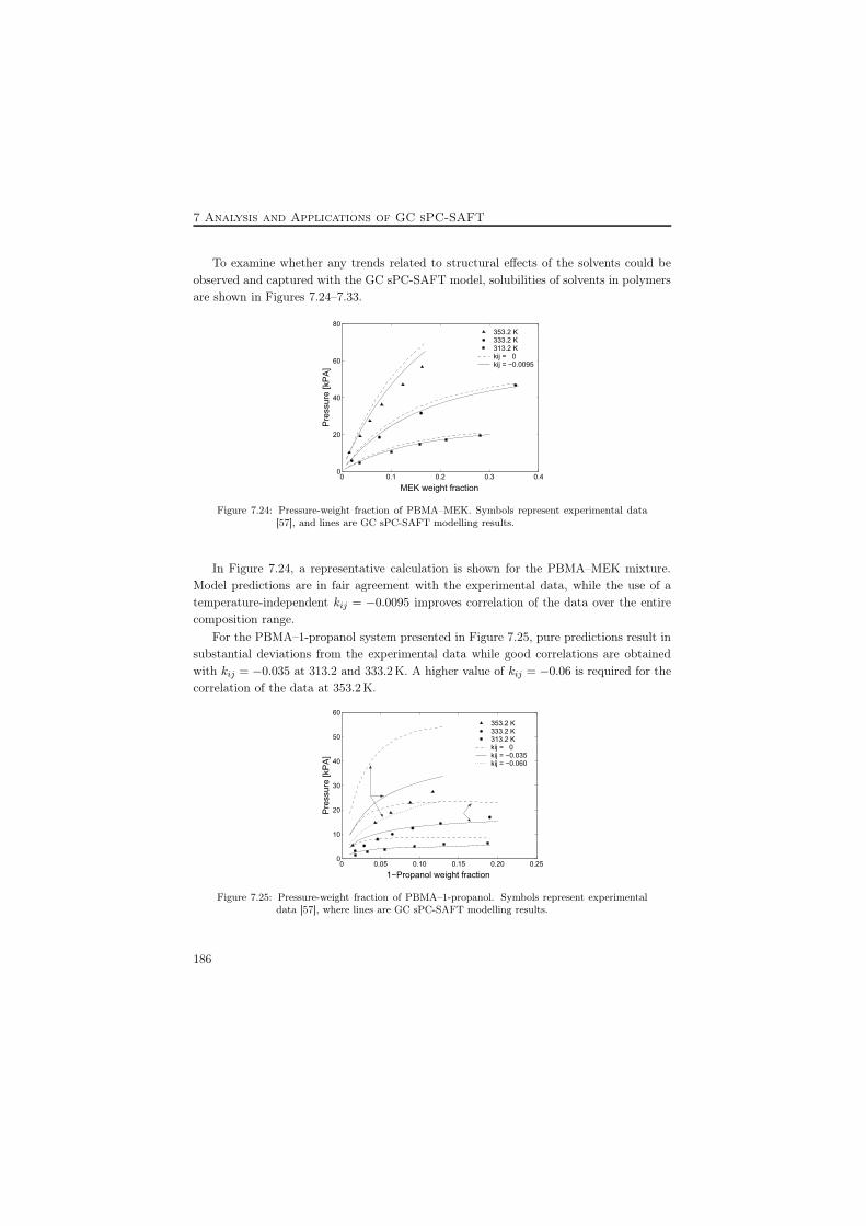
7 Analysis and Applications of GC sPC-SAFT

To examine whether any trends related to structural effects of the solvents could beobserved and captured with the GC sPC-SAFT model, solubilities of solvents in polymersare shown in Figures 7.24–7.33.

0 0.1 0.2 0.3 0.40

20

40

60

80

MEK weight fraction

Pre

ssur

e [k

PA

]353.2 K333.2 K313.2 Kkij = 0kij = −0.0095

Figure 7.24: Pressure-weight fraction of PBMA–MEK. Symbols represent experimental data[57], and lines are GC sPC-SAFT modelling results.

In Figure 7.24, a representative calculation is shown for the PBMA–MEK mixture.Model predictions are in fair agreement with the experimental data, while the use of atemperature-independent kij = −0.0095 improves correlation of the data over the entirecomposition range.

For the PBMA–1-propanol system presented in Figure 7.25, pure predictions result insubstantial deviations from the experimental data while good correlations are obtainedwith kij = −0.035 at 313.2 and 333.2K. A higher value of kij = −0.06 is required for thecorrelation of the data at 353.2K.

0 0.05 0.10 0.15 0.20 0.250

10

20

30

40

50

60

1−Propanol weight fraction

Pre

ssur

e [k

PA

]

353.2 K333.2 K313.2 Kkij = 0kij = −0.035kij = −0.060

Figure 7.25: Pressure-weight fraction of PBMA–1-propanol. Symbols represent experimentaldata [57], where lines are GC sPC-SAFT modelling results.

186

7.5 Applications to Polymer Systems

Solubilities of 2-methyl-1-propanol in both PBMA and PIB are graphically presentedin Figure 7.26. The kij value required to accurately correlate the PBMA system (left) ishigher than kij for the PIB system (right), which may be attributed to the more polarnature of the PBMA system.

0 0.05 0.10 0.15 0.20 0.25 0.300

5

10

15

20

25

30

35

2−Methyl−1−propanol weight fraction

Pre

ssur

e [k

PA

]

353.2 K333.2 K313.2 Kkij = −0.02kij = 0

0 0.02 0.04 0.06 0.08 0.100

5

10

15

20

25

30

35

2−Methyl−1−propanol weight fraction

Pre

ssur

e [k

PA

]kij = 0353.2 Kkij = −0.005333.2 Kkij = −0.010313.2 Kkij = −0.015

Figure 7.26: Pressure-weight fraction of PBMA–2-methyl-1-propanol (left) and PIB–2-methyl-1-propanol (right). Symbols represent experimental data [57], while lines are GCsPC-SAFT modelling results.

In Figure 7.27, very good agreement is obtained for the PIB–methyl acetate systemat 313.2, 333.2, and 353.2K using the temperature-independent kij = 0.02. For thisparticular system, the overall average deviation at 313.2K is improved from 24.1% forpredictions to 2.5% for correlations, as shown in Table 7.14, where the deviations for allother investigated binary PIB systems are also given.

0 0.05 0.10 0.150

50

100

150

200

Methyl acetate weight fraction

Pre

ssur

e [k

PA

]

353.2 K333.2 K313.2 Kkij = 0kij = 0.02

Figure 7.27: Pressure-weight fraction of PIB–methyl acetate. Symbols represent experimentaldata [57], while lines are GC sPC-SAFT modelling results.

The two graphs in Figure 7.28 show that the polar solvents are more soluble in polarPBMA than in non-polar PIB at the same temperature. In general, the lowest solubilities

187

7 Analysis and Applications of GC sPC-SAFT

of all investigated solvents are obtained in PIB, which is shown by the experimental dataand reproduced with GC sPC-SAFT with accurate correlations.

0 0.02 0.04 0.060

10

20

30

40

50

Solvent weight fraction

Pre

ssur

e [k

PA

]

GC sPC−SAFT (kij ≠ 0)2−Methyl−1−propanol1−Propanol2−Propanol1−Butanol2−Butanol

0 0.05 0.10 0.15 0.20 0.25 0.300

10

20

30

40

50

Solvent weight fraction

Pre

ssur

e [k

PA

]

GC sPC−SAFT (kij ≠ 0)2−Methyl−1−propanol1−Propanol2−Propanol1−Butanol2−Butanol

Figure 7.28: Pressure-weight fraction of various alcohols in PBMA (left) and PIB (right) at333.2 K. Symbols represent experimental data [57], while lines are correlationswith GC sPC-SAFT.

The more alcoholic nature the solvent is in polar polymer mixtures, the more prob-lematic is the modelling with the sPC-SAFT model. This is observed in Figures 7.29and 7.30, where both predictions and correlations of solubilities of various solvents inPIB and PBMA are presented. Even with inaccurate predictions, as shown for examplein Figure 7.29, the solubility of polar solvents with hydrogen bonding, e.g. alcohols, islower than that of polar solvents without hydrogen bonding, e.g. MEK and ketone, ininvestigated polymers. While for polar solvents without hydrogen bonding, the effect ofsolvent compounds on solubility is not significant in polar polymers such as PBMA.

The VLE phase diagram of PVAc–propanol [60] is shown in Figure 7.31 where the threedifferent PVAc parameter sets from Table 7.11 are used including those obtained from theGC scheme. A comparison of the obtained correlations with kij = −0.025 is chosen for theevaluation of the PVAc parameters. The performance is not satisfactory. The absoluteaverage deviations are 16.6, 15.9, and 15.5 % for parameters of Ref. [48], [50], and thiswork, respecively. Similar accuracy for correlating the phase behaviour of this system isobtained by Elliott and Natarajan [61] using a GC form of the ESD EoS discussed inSection 3.2.

Generally, results presented in Section 7.5.2.1 show that the presented GC method isapplicable to polymer systems involving self-associating solvents, but requires a binaryinteraction parameter to improve accuracy in most of the investigated systems.

Often, comparisons of modelling results with experimental LLE data provide a morerigorous test and challenge for a model and its parameters than comparison with experi-mental VLE data. Some LLE results are presented in the next section.

188

7.5 Applications to Polymer Systems

0 0.02 0.04 0.06 0.08 0.10 0.120

20

40

60

80

100

120

Solvent weight fraction

Pre

ssur

e [k

PA

]

GC sPC−SAFT (kij = 0)Methyl acetateMEK2−Butanol2−Methyl−1−propanol

0 0.02 0.04 0.06 0.08 0.10 0.120

20

40

60

80

100

120

Solvent weight fraction

Pre

ssur

e [k

PA

]

GC sPC−SAFT (kij ≠ 0)Methyl acetateMEK2−Butanol2−Methyl−1−propanol

Figure 7.29: Pressure-weight fraction of various solvents in PIB at 333.2 K. Symbols representexperimental data [57], while lines are predictions (left) and correlations (right)with GC sPC-SAFT.

0 0.1 0.2 0.3 0.40

20

40

60

80

100

120

Solvent weight fraction

Pre

ssur

e [k

PA

]

GC sPC−SAFT (kij = 0)Methyl acetateMEK2−Butanol2−Methyl−1−propanol

0 0.1 0.2 0.3 0.40

20

40

60

80

100

120

Solvent weight fraction

Pre

ssur

e [k

PA

]

GC sPC−SAFT (kij ≠ 0)Methyl acetateMEK2−Butanol2−Methyl−1−propanol

Figure 7.30: Pressure-weight fraction of various solvents in PBMA at 333.2 K. Symbols rep-resent experimental data [57], while lines are predictions (left) and correlations(right) with GC sPC-SAFT.

7.5.3 Evaluation of LLE

Liquid-liquid equilibria (LLE) calculations of a few polymer–solvent systems have beenperformed. Mixtures with PMMA and PBMA have been considered. Figure 7.32 showsdifferent PMMA solutions with 4-heptanone and chlorobutane, respectively. Both systemsdisplay UCST behaviour and are well correlated using small positive binary interactionparameters. However, the flatness of the curve towards increased polymer weight fractionscannot be accurately described. This is expected to be a weakness of the model rather thanof the polymer parameters [62]. Very similar behaviour is observed for the PBMA–octanesystem in Figure 7.33 using a small negative value of kij = −0.0038.

189

7 Analysis and Applications of GC sPC-SAFT

0 0.05 0.10 0.15 0.20 0.25 0

1

2

3

4

5

6

7

1−Propanol weight fraction

Pre

ssur

e [k

PA

]

313.2 K, PVAc(167000)Ref. [48]Ref. [50]This work

Figure 7.31: VLE of the PVAc–1-propanol system. Symbols are experimental data [60] and linesare GC sPC-SAFT correlations (kij=-0.025) with PVAc parameters from Table 7.11.

0 0.05 0.1 0.15 0.2 0.25 0.3 0.35 0.4255

260

265

270

275

PMMA weight fraction

Tem

pera

ture

[K]

PMMA(36500)kij = 0.00179

0 0.1 0.2 0.3 0.4 0.5250

260

270

280

290

PMMA weight fraction

Tem

pera

ture

[K]

PMMA(36500)kij = 0kij = 0.0002

Figure 7.32: LLE of the PMMA–4-heptanone (left) and PMMA–chlorobutane (right) systems.Symbols are experimental data [63] and lines are GC sPC-SAFT correlations withPMMA parameters from Table 7.10.

7.5.4 PVC–Solvent Systems

Table 2.2 from Section 5.2.2 is slightly modified to include an additional set of PVCpure parameters calculated from the proposed GC scheme. Different sets of PC-SAFTparameters for PVC are summarised in Table 7.15.

With the GC estimated PVC parameters sPC-SAFT predicts the liquid density with0.8% deviation in the investigated temperature and pressure range. The accuracy issimilar to the other aproaches which are based on experimental data. In the following,sPC-SAFT EoS using different parameter sets is applied to VLE for selected PVC–solventsystems.

First, the predictive capabilities of the approach are tested by predicting the vapour

190

7.5 Applications to Polymer Systems

0 0.2 0.4 0.6 0.8200

220

240

260

280

300

320

PBMA weight fraction

Tem

pera

ture

[K]

PBMA(11600)kij = −0.0038

Figure 7.33: LLE of the PBMA–octane system. Symbols are experimental data [64] and lines areGC sPC-SAFT correlations with PBMA parameters from Table 7.10.

Table 7.15: Values of PC-SAFT parameters and AAD % between calculated and experimental ρ ofpoly(vinyl chloride) (PVC) using different methods.

Case Data set m/Mw σ ε/k T range P range AAD ρ

[mol/g] [Å] [K] [K] [bar] [%]

1. Kouskoumvekaki et al. 0.0210 3.724 315.93 373–423 1–1000 0.5[48] approach

2. PVT + single binary 0.0121 4.726 541.56 373–423 1–1000 1.6VLE incl. kij

3. PVT + single binary 0.0298 3.213 221.19 373–423 1–1000 1.2VLE excl. kij

4. PVT + all binary 0.0097 5.030 495.86 373–423 1–1000 1.4VLE incl. kij

5. PVT + all binary 0.0142 4.298 360.92 373–423 1–1000 0.8VLE excl. kij

6. from Table 7.10 0.0191 3.8358 314.56 373–423 1–1000 0.8

7. from 0.02136 3.7486 370.42 373–423 1–1000 0.2[52]

pressures of different PVC systems with each set of parameters after imposing a value ofkij = 0. The deviations are reported in Table 7.16 and are graphically presented in Figure7.34. It is observed that parameters based on Cases 1, 5, and 6 (this work) result in thelowest overall AAD %.

Second, to evaluate the effect of a non-zero value of kij , optimised values of kij havebeen determined for each binary system. Both the values of kij and the resulting absoluteaverage deviations are reported in Table 7.17. The values of kij are generally low, but

191

7 Analysis and Applications of GC sPC-SAFT

Table 7.16: AAD % between experimental and predicted (kij = 0) bubble pressures of investigated binaryPVC–solvent mixtures.

System AAD P [%] with Case no.

1 2 3 4 5 6 7

1. Toluene 31.9 123.7 10.6 88.9 42.8 27.0 85.12. Tetrachloromethane 19.0 120.3 72.2 76.2 5.2 15.9 46.13. Vinyl chloride 21.2 61.9 12.6 36.1 20.9 25.5 57.34. 1,4-Dioxane 7.5 31.1 16.4 24.5 14.4 7.8 24.95. Tetrahydrofuran 26.8 63.5 6.7 49.9 33.0 25.2 48.96. Di(1-butyl) ether 29.6 150.1 87.1 114.7 15.9 27.2 21.8

AAD [%] overall 19.6 79.0 29.8 56.3 19.6 19.2 41.6

1 2 3 4 5 60

20

40

60

80

100

120

140

160

System no.

AA

D %

pre

ssur

e

Case 1Case 2Case 3Case 4Case 5Case 6Case 7

Figure 7.34: AAD % between experimental and predicted (kij = 0) bubble pressures of inves-tigated binary PVC–solvent mixtures. Data, case and system no. refer to Table7.16.

they still vary and can even be negative. Analyzing the correlated results in terms ofAAD %, a significant improvement in the accuracy is obtained, this time highlighting theperformance of parameters from Cases 1, 3, 6 (this work), and 7. However, the approach isno longer predictive. A more consistent approach would have been to determine a uniquevalue of kij , but this has not been done because it is unlikely, in view of the variations ofkij in Table 7.17, that the predictions would be much improved.

The optimised kij values for the investigated PVC–solvent systems listed in Table 7.17are plotted as a function of solvents’ Mw and of van der Waals volume of solvents in orderto test if any significant trends are obtained.

Figure 7.35 shows linear trends of the optimized kij values for selected PVC–solvent

192

7.5 Applications to Polymer Systems

Table 7.17: Average absolute deviations (AAD %) between experimental and correlated (kij �= 0) bubblepoint pressures of investigated binary PVC–solvent mixtures.

System AAD P [%] with Case no.

1 2 3 4 5 6 7

1. Toluene 6.9 40.6 4.5 37.2 13.4 7.7 8.52. Tetrachloromethane 0.8 29.6 2.2 29.2 5.0 0.5 0.53. Vinyl chloride 3.9 17.6 1.7 16.2 7.9 4.6 5.04. 1,4-Dioxane 6.9 29.2 3.3 25.9 11.9 7.5 9.45. Tetrahydrofuran 5.5 38.4 1.3 33.9 12.8 6.3 8.36. Di(1-butyl) ether 4.0 54.2 2.8 47.9 11.5 4.7 6.8

AAD [%] overall 4.6 34.9 2.6 31.7 10.4 5.2 6.4

Solvent Optimized kij with Case no.

1 2 3 4 5 6 7

1. Toluene –0.01750 –0.06702 0.00478 –0.05611 –0.02689 0.01571 –0.039612. Tetrachloromethane 0.00916 0.05729 0.03729 –0.04261 0.00112 0.01290 –0.019423. Vinyl chloride –0.02219 –0.06299 0.01334 –0.04373 –0.02571 –0.01804 –0.051514. 1,4-Dioxane –0.00592 –0.02990 0.01271 –0.02543 –0.01634 –0.00634 –0.020075. Tetrahydrofuran –0.03210 –0.08273 –0.00806 –0.07625 –0.04751 –0.03255 –0.050666. Di(1-butyl) ether 0.01166 –0.06046 0.03733 –0.05285 –0.00693 0.01121 –0.00801

systems listed in Table 7.17 when plotted as a function of Mw and van der Waals volumeof solvents. The data reveal substantial scatter; especially for the van der Waals volumesin the right graph of Figure 7.35. Hence, care should be taken to extrapolate these trendlines for use in practical applications.

60 80 100 120 140 160−0.06

−0.04

−0.02

0.00

0.02

0.04

Solvent molecular weight [g/mol]

k ij

R2 = 0.8018

R2 = 0.7003

R2 = 0.8093

R2 = 0.6428

Case 1Case 5Case 6Case 7

30 40 50 60 70 80 90 100−0.06

−0.04

−0.02

0.00

0.02

0.04

Solvent van der Waals volume [cm3/mol]

k ij

R2 = 0.4524

R2 = 0.2114

R2 = 0.3746

R2 = 0.5430

Case 1Case 5Case 6Case 7

Figure 7.35: Linear trends of optimized kij values for selected PVC–solvent systems. Case no. referto the systems listed in Table 7.17.

Most of the VLE and LLE results presented for various polymer–solvent systems inChapter 7 have already been subjected to tests with the sPC-SAFT EoS using another set

193

REFERENCES

of polymer parameters estimated by Kouskoumvekaki et al. [48]. The results are rathersimilar. The overall results demonstrate that properly calculated pure predictive GCestimated polymer parameter values can result in quite accurate modelling of mixturephase equilibria. For many systems investigated, a small kij value is needed before themodel accurately correlates the experimental data.

7.6 Final Comments

Not only has it been shown that the presented GC methodology provides a good represen-tation of the phase equilibria of heavy members of the investigated chemical families, butit also exhibits a good agreement with the experimental data of various classes of binarymixtures. Generally, the approach has proven to be a fairly reliable predictive tool forpure compounds and binary mixtures comprising the functional groups in the GC schemeof Tables 6.3 and 6.4.

With the newly developed GC scheme in hand to calculate parameters for complexcompounds, the sPC-SAFT model has become a relevant and useful tool in the design anddevelopment of complex products, e.g. detergents or food ingredients, pharmaceuticalsand other speciality chemicals, where predictions of various thermodynamic and phaseequilibrium properties are required, but for which expected vapour pressure and/or liquiddensity data may not be available.

References[1] K. A. Connors, Thermodynamics of Pharmaceutical Systems: An Introduction for Students

of Pharmacy. John Wiley and Sons, USA, 2002.

[2] S. L. Rose, Fundamental Principles of Polymeric Materials. John Wiley and Sons, USA,1993.

[3] S. Aparicio, R. Alcalde, M. J. Dávila, B. García, and J. M. Leal, “Properties and Structureof Aromatic Ester Solvents,” J. Phys. Chem. B., vol. 111, pp. 4417–4431, 2007.

[4] AIChE J., DIPPR Table of Physical and Thermodynamic Properties of Pure Compounds.New York, USA, 1998.

[5] K. Kevin, “Phascinating Phytochemicals,” Food Processing, USA, vol. 56, pp. 79–81, 1995.

[6] S. O. Duke, F. E. Dayan, J. G. Romagni, and A. M. Rimando, “Natural Products as Sourcesof Herbicides: Current Status and Future Trends,” Weed Research, vol. 40, pp. 99–111, 2000.

[7] “Phytochemicals.” http://www.phytochemicals.info/. General about phytochemicals,April 2008.

[8] H. Schmandke, “D-Limonene in Citrus Fruit with Anticarcinogenic Action,” Ernaehrungs-Umschau, vol. 50, pp. 264–266, 2003.

[9] B. Arizaga, A. de Leon, N. Burgueno, A. Lopez, D. Paz, N. Martinez, D. Lorenzo, E. Della-cassa, and J. Bussi, “A Clean Process for the Production of Oxygenated Limonene DerivativesStarting from Orange Oil,” J. Chem. Tech. Biotechnol., vol. 82, pp. 532–538, 2007.

194

REFERENCES

[10] H. A. Matos, E. Gomes De Azevedo, P. C. Simoes, M. T. Carrondo, and M. Nunes Da Ponte,“Phase Equilibria of Natural Flavours and Supercritical Solvents,” Fluid Phase Equilibria,vol. 52, pp. 357–364, 1989.

[11] E. Gomes de Azevedo, H. A. Matos, and M. Nunes de Ponte, “Phase Equilibria ofEthene+Limonene and Ethene+Cineole from 285 K to 308 K and Pressures to 8 MPa,”Fluid Phase Equilibria, vol. 83, pp. 193–202, 1993.

[12] J. G. Speight, The Desulfurization of Heavy Oils and Residua. CRC Press, USA, 1999.

[13] T. Sawaya, I. Mokbel, E. Rauzy, J. Saab, C. Berro, and J. Jose, “Experimental VapourPressure of Alkyl and Aryl sulfides. Prediction by a Group Contribution Method,” FluidPhase Equilibria, vol. 226, pp. 283–288, 2004.

[14] C. H. Twu, V. Tassone, and W. D. Sim, “Accurately Predict the VLE of Thiol–HydrocarbonMixtures,” Chem. Eng. Progress, vol. 100, pp. 39–45, 2004.

[15] H. Wolff, J. Szydlowski, and L. Dill-Staffenberger, “Vapor-Liquid Equilibria of Deuteroiso-meric Methanethiols and Their Mixtures with n-Hexane,” J. Chem. Thermodyn., vol. 12,pp. 641–652, 1980.

[16] N. F. Giles, H. L. Wilson, and W. V. Wilding, “Phase Equilibrium Measurements on TwelveBinary Mixtures,” J. Chem. Eng. Data, vol. 41, pp. 1223–1238, 1996.

[17] N. F. Giles, H. L. Wilson, and W. V. Wilding, “Phase Equilibrium on Eight Binary Mixtures,”J. Chem. Eng. Data, vol. 42, pp. 1067–1074, 1997.

[18] J. Kilner, S. E. McBain, and M. G. Roffey, “(Vapour+ Liquid) Equilibria of (Methanthiolor Ethanethiol or Propane-1-thiol or Butan-1-thiol + n-Hexane or n-Decane or Toluene orWater) for Mole Fractions X=0 to 0.2 of Thiol at Temperatures Between 323 and 373 K,” J.Chem. Thermody., vol. 22, pp. 203–210, 1990.

[19] S. Monarca, “Polycyclic Aromatic Hydrocarbons in Petroleum Products for Medicinal andCosmetic Uses-Analytical Procedure,” Sci. Total Environ, vol. 14, pp. 233–243, 1980.

[20] S. Monarca, F. Fagioli, and G. Morozzi, “Evaluation of the Potential Carcinogenicity ofParaffins for Medical and Cosmetic Uses-Dash Determination of Polycyclic Aromatic Hydro-carbons,” Sci. Total Environ, vol. 17, pp. 83–93, 1981.

[21] R. S. Hamir, Handbook of Chromatography: Liquid Chromatography of Polycyclic AromaticHydrocarbons. CRC Press, USA, 1993.

[22] K. Ruuzicka, I. Mokbel, V. Majer, V. Ruuzicka, J. Jose, and M. Zábranský, “Descriptionof Vapor-Liquid and Vapor-Solid Equilibria for a Group of Polycondensed Compounds ofPetroleum Interest,” Fluid Phase Equilibria, vol. 148, pp. 107–137, 1998.

[23] D. N. Huynh, M. Benamira, J.-P. Passarello, P. Tobaly, and J.-C. de Hemptinne, “Applicationof GC-SAFT EOS to Polycyclic Aromatic Hydrocarbons,” Fluid Phase Equilibria, vol. 254,pp. 60–66, 2007.

[24] E. J. Coon, J. E. Auwaerter, and E. McLaughlin, “A Comparison of Solid-Liquid Equilibriumwith Vapour-Liquid Equilibrium for Prediction of Activity Coefficients in Systems ContainingPolynuclear Aromatics,” Fluid Phase Equilibria, vol. 44, pp. 305–345, 1989.

[25] G. Morton, Diesel: The Man and The Engine. Atheneum, NY, USA, 1978.

195

REFERENCES

[26] C. E. Goering, A. W. Schwab, M. J. Daugherty, E. H. Pryde, and A. J. Heakin, “FuelProperties of Eleven Vegetable Oils,” Transactions of the ASAE, vol. 25, pp. 1472–1477,1982.

[27] L. G. Schumacher, J. van Gerpen, and B. Adams, “Biodiesel Fuels,” Encyclopedia of Energy,vol. 1, pp. 151–162, 2004.

[28] A. Demirbas, “Recent Developments in Biodiesel Fuels,” Int. J. Green Energy, vol. 4, pp. 15–26, 2007.

[29] M. A. Dubé, A. Y. Tremblay, and J. Liu, “Biodiesel Production Using a Membrane Reactor,”Bioresource Technology, vol. 98, pp. 639–647, 2007.

[30] H. Fukuda, A. Kondo, and H. Noda, “Review: Biodiesel Fuel Production by Transesterifica-tion of Oils,” Journal of Bioscience and Bioengineering, vol. 92, pp. 405–416, 2001.

[31] G. Knothe, “Dependence of Biodiesel Fuel Properties on the Structure of Fatty Acid AlkylEsters,” Fuel Processing Technology, vol. 86, pp. 1059–1070, 2005.

[32] W. Yuan, A. C. Hansen, and Q. Zhang, “Vapor Pressure and Normal Boiling Point Predic-tions for Pure Methyl Esters and Biodiesel Fuels,” Fluid, vol. 84, pp. 943–950, 2005.

[33] R. Ceriani and A. J. A. Meirelles, “Predicting Vapour-Liquid Equilibria of Fatty Acids,”Fluid Phase Equlibria, vol. 215, pp. 227–236, 2004.

[34] K. Bay, H. Wanko, and J. Ulrich, “Absorption of Volatile Organic Compounds in Biodiesel.Determination of Infinite Dilution Activity Coefficients by Headspace Gas Chromatography,”Chem. Eng. Res. Des., vol. 84, pp. 22–28, 2006.

[35] A. Rose and W. R. Supina, “Vapor Pressure and Vapor-Liquid Equilibrium Data for MethylEsters and the Common Saturated Normal Fatty Acids,” Ind. Eng. Chem. Data, vol. 6,pp. 173–179, 1961.

[36] A. Rose and V. N. Schrodt, “Vapor-Liquid Equilibria for the Methyl Oleate and MethylStearate Binary Mixtures,” Ind. Eng. Chem. Data, vol. 9, pp. 12–16, 1964.

[37] A. C. G. van Genderen, J. C. van Miltenburg, G. B. Jacobus, M. J. van Bommel, P. J. vanEkeren, G. J. K. van den Berg, and H. A. J. Oonk, “Liquid-Vapour Equilibria of the MethylEsters of Alkanoic Acids: Vapour Pressures as a Function of Temperature and StandardThermodynamic Function Changes,” Fluid Phase Equlibria, vol. 202, pp. 109–120, 2002.

[38] H. Inomata, T. Kondo, S. Hirohama, K. Arai, Y. Suzuki, and M. Konno, “Vapour-LiquidEquilibria for Binary Mixtures of Carbon Dioxide and Fatty Acid Methyl Esters,” FluidPhase Equlibria, vol. 46, pp. 41–52, 1989.

[39] H. S. Elbro, A. Fredenslund, and P. Rasmussen, “A New Simple Equation for the Predictionof Solvent Activities in Polymer Solutions,” Macromolecules, vol. 23, pp. 4707–4713, 1990.

[40] G. M. Kontogeorgis, P. Coutsikos, D. P. Tassios, and A. Fredenslund, “Improved Models forthe Prediction of activity Coefficients in Nearly Athermal Mixtures,” Fluid Phase Equilibria,vol. 92, pp. 35–66, 1994.

[41] B. L. Larsen, P. Rasmussen, and A. Fredensund, “A Modified UNIFAC Group-ContributionModel for Prediction of Phase Equilibria and Heats of Mixing,” Ind. Eng. Chem. Res., vol. 26,pp. 2274–2286, 1987.

[42] J. Gross and G. Sadowski, “Perturbed-Chain SAFT: An Equation of State Based on Pertur-bation Theory for Chain Molecules,” Ind. Eng. Chem. Res., vol. 40, pp. 1244–1260, 2001.

196

REFERENCES

[43] K. Kniaz, “Influence of the Size and Shape Effect on the Solubility of Hydrocarbons: TheRole of the Combinatorial Entropy,” Fluid Phase Equilibria, vol. 68, pp. 35–46, 1991.

[44] K. Kniaz, “Solubility of n-Docosane in n-Hexane and Cyclohexane,” J. Chem. Eng. Data,vol. 36, pp. 471–482, 1991.

[45] J. F. Parcher, P. H. Weiner, C. L. Hussey, and T. N. Westlake, “Specific Retention Volumesand Limited Activity Coefficients of C4–C8 Alkane Solutes in C22–C36 n-Alkane Solvents,”J. Chem. Eng. Data, vol. 20, pp. 145–151, 1975.

[46] E. C. Voutsas, N. S. Kalospiros, and D. P. Tassios, “A Combinatorial Activity CoefficientModel for Symmetric and Asymmetric Mixtures,” Fluid Phase Equilibria, vol. 109, pp. 1–15,1995.

[47] P. A. Rodgers, “Pressure Volume Temperature relationships for Polymeric Liquids – A Reviewof Equations of State and Their Characteristic Parameters for 56 Polymers,” J. Appl. Polym.Sci., vol. 48, pp. 1061–1980, 1993.

[48] I. A. Kouskoumvekaki, N. von Solms, T. Lindvig, M. L. Michelsen, and G. M. Kontogeorgis,“Novel Method for Estimating Pure-Component Parameters for Polymers: Application tothe PC-SAFT Equation of State,” Ind. Chem. Eng. Res., vol. 43, pp. 2830–2838, 2004.

[49] F. Becher, M. Buback, H. Latz, G. Sadowski, and F. Tumakaka, “Cloud-Point Curves ofEthylene–(meth)acrylate Copolymers in Fluid Ethene up to High Pressures and Temperature.Experimental Study and PC-SAFT Modeling,” Fluid Phase Equilibria, vol. 215, pp. 263–282,2004.

[50] J. Gross, O. Spuhl, F. Tumakaka, and G. Sadowski, “Modeling Copolymer Systems Using thePerturbed-Chain SAFT Equation of State,” Ind. Eng. Chem. Res., vol. 42, pp. 1266–1274,2003.

[51] J. Gross and G. Sadowski, “Modeling Polymer Systems Using the Perturbed-Chain StatisticalAssociating Fluid Theory Equation of State,” Ind. Eng. Chem. Res., vol. 41, pp. 1084–1093,2002.

[52] P. Arce and M. Aznar, “Modeling the Phase Behavior of Commercial Biodegradable Polymersand Copolymer in Supercritical Fluids,” Fluid Phase Equilibria, vol. 238, pp. 242–253, 2005.

[53] R. W. Kershaw and G. N. Malcolm, “Thermodynamics of Solutions of Polypropylene Oxidein Chloroform and in Carbon Tetrachloride,” Trans. Faraday Soc., vol. 64, pp. 323–336, 1968.

[54] W. R. Kriegbaum and D. O. Geymer, “Thermodynamics of Polymer Solutions. ThePolystyrene–Cyclohexane System Near the Flory Theta Temperature,” J. Am. Chem. Soc.,vol. 81, pp. 1859–1868, 1959.

[55] C. E. H. Bawn and M. A. Wajid, “High Polymer Solutions. Part 7: Vapor Pressure ofPolystyrene Solutions with Acetone, Chloroform and Propyl Acetate,” Trans. Faraday Soc.,vol. 52, pp. 1658–1664, 1956.

[56] P. J. T. Tait and A. M. Abushihada, “Comparative Studies on the Use of Gas Chromato-graphic and Vapour Pressure Techniques for the Determination of the Interaction EnergyParameter,” Polymer, vol. 18, pp. 810–816, 1977.

[57] G. Wibawa, R. Hatano, Y. Sato, S. Takishima, and H. Masuoko, “Solubilities of 11 PolarOrganic Solvents in Four Polymers Using the Piezoelectric-Quartz Sorption Method,” J.Chem. Eng. Data, vol. 47, pp. 1022–1029, 2002.

197

REFERENCES

[58] I. A. Kouskoumvekaki, N. von Solms, M. L. Michelsen, and G. M. Kontogeorgis, “Applicationof a Simplified Perturbed Chain SAFT Equation of State to Complex Polymer Systems UsingSimplified Mixing Rules,” Fluid Phase Equilibria, vol. 215, pp. 71–78, 2004.

[59] S. H. Huang and M. Radosz, “Equation of State for Small, Large, Polydisperse, and Associ-ating Molecules,” Ind. Eng. Chem. Res., vol. 29, pp. 2284–2294, 1990.

[60] R. J. Kokes, A. R. Dipietro, and F. A. Long, “Equilibrium Sorption of Several OrganicDiluents in Polyvinyl Acetate,” J. Am. Chem. Soc., vol. 75, pp. 6319–6325, 1953.

[61] J. R. Elliott and R. N. Natarajan, “Extension of the Elliott-Suresh-Donohue Equation ofState to Polymer Solutions,” Ind. Eng. Chem. Res., vol. 41, pp. 1043–1050, 2002.

[62] N. von Solms, I. A. Kouskomvekaki, T. Lindvig, M. L. Michelsen, and G. M. Kontogeorgis,“A Novel Approach to Liquid-Liquid in Polymer Systems with Application to SimplifiedPC-SAFT,” Fluid Phase Equlibria, vol. 222–223, pp. 87–93, 2004.

[63] B. A. Wolf and G. Blaum, “Measured and Calculated Solubility of Polymers in Mixed Sol-vents: Monotony and Consolvency,” J. Polym. Sci., vol. 13, pp. 1115–1132, 1975.

[64] A. Saraiva, M. Pleuss, O. Persson, and A. Fredenslund, A Study of the Miscibility/Immisci-bility of Low Molecular Weight Poly(n-butyl methylate)/ Single Solvent Systems by ThermoOptical Analysis by Microscopy. Internal Report SEP9412, Department of Chemical Engi-neering, Technical University of Denmark, DK-2800 Kgs. Lyngby, 1994.

198

Chapter 8

Conclusion and Future Work

”Learn from yesterday, live for today, hope for tomorrow. The important thing is not tostop questioning.” by Albert Einstein

8.1 Conclusions

In this thesis a predictive group contribution (GC) simplified perturbed chain-statisticalassociating fluid theory (sPC-SAFT) has been developed to extend the applicability ofthe sPC-SAFT equation of state (EoS) to treat molecules of different types. Within theGC formalism, a system (that can be both a pure component or a mixture) is treatedat the level of representative functional groups, and the properties of the system areobtained by considering the contributions of each individual group. By incorporatingthe GC approach within a molecular and statistical mechanical theory such as SAFT,it is possible to develop a predictive thermodynamic model that can accurately describecomplex chain-like systems.

A detailed review of the literature shows that a large amount of work has been devotedto the development of GC methods and that the various available GC thermodynamicmodels are based on fundamentally different theories. Although the GC activity coefficientmodels, like UNIFAC, etc., are a popular and rather convenient choice for the prediction ofmixture phase behaviour, they also have serious limitations. These limitations are mainlyassociated with the fact that such models are based on lattice (quasi-chemical) theories,which do not provide a good representation of the structure of the fluid. As a result,they are mainly suitable for liquid phase description and have difficulties capturing e.g.pressure effects. In particular, the lower critical solution behaviour of a polymer solutionis highly sensitive to pressure variations due to the fact that the volumetric expansionof the solvent that induces phase separation upon heating is partially governed by thepressure of the system. These deficiencies are overcome by using GC EoS.

In time, a number of EoS, including SAFT, have been modified in order to use the GCformalism to obtain a more predictive EoS. The existing GC approaches that are based on

199

8 Conclusion and Future Work

the SAFT EoS have been developed at the level of the molecular parameters, which arethen introduced as average values into the standard homonuclear versions of the theory.Moreover, the adjustment of binary interaction parameters (kij) when considering thephase equilibria of mixtures plays an important role.

In this work and in the same manner, the development of a GC approach within thesPC-SAFT formalism is presented, where a predictive GC approach by Constantinou-Gani from 1994 with an extended parameter table is implemented. This choice is madebecause, unlike other approaches found in the literature, this GC methodology includestwo levels of contributions: both first-order groups (FOG) and second-order groups (SOG)that, to some extent, allow capture of proximity effects and distinguish among structuralisomers.

Traditionally, parameters for molecular based EoS are obtained by fitting experimen-tal vapour pressures and liquid densities. A drawback of this technique is the requirementof extensive experimental data on pure compounds to obtain reliable parameters. Addi-tionally, a fast computational routine (e.g. a Marquardt algorithm) is required to performthe multivariable search for the parameters, as well as, in many cases, the critical regionis overpredicted. It generally requires more time and effort than the average user of theEoS may be willing to invest. Therefore, the unavailability of fluid-specific parameters isstill a major obstacle in the application of EoS. With that in mind, the most importantfuture efforts in improving SAFT, and in fact any molecular based EoS, should explorethe possibility and consequences of parameterizing them. As a preliminary work in thisline, a way to estimate molecular based EoS parameters for a wide variety of fluids isexplored.

The main achievements of the work presented in this thesis are the following:

• A detailed review of the available GC methods in order to get an overview of ad-vantages and deficiencies of various models is given in Chapter 1.

• A brief description of the models that are used throughout this thesis are providedin Chapter 2, and a short overview of the use of the GC formalism within the SAFTformalism explaining the GC concept based on the so-called conjugation principlein Chapter 3.

• Pure component parameters for the PC-SAFT model (m, σ, and ε/k) are obtainedthrough a regression method for approximately 500 non-associating compounds. In-vestigations of trends and the physical significance of the numerous models’ param-eters are performed indicating an existing trend of linearity in the specific groupingsof the parameters as presented in Chapter 4.

• An extensive evaluation of the sPC-SAFT description of fluid phase equilibria ofseveral chemical families obtaining satisfactory estimations with or without kij . Fur-

200

8.1 Conclusions

thermore, the application of sPC-SAFT in modelling both VLE and LLE of a varietyof binary polymer mixtures with either non-associating or associating solvents is suc-cessfully tested. Considering the complexity of molecules and the presence of varioustypes of intermolecular interactions within these mixtures, satisfactory results areobtained. Typical results of VLE, LLE, activity coefficients at infinite dilution, andazeotropic data for various binary systems are shown in Chapter 5.

• Generation of the parameter table for the PC-SAFT EoS from newly estimatedcompound parameters in a sequential procedure that includes 45 FOG and 26 SOGis given in Chapter 6. The parameters of a new compound can then be calculatedby summing up the contributions of certain defined groups of atoms, at the sametime considering the number of occurrences of each group within the molecule.

• An investigation of the predictive capability of the GC sPC-SAFT EoS throughcomparison of the method’s predictions for compounds with high Mw, and severalselected binary mixtures of high industrial performance with experimental data,such as benzene derivatives, sulfur containing compounds, biodiesel, and variouspolymer–solvent mixtures and blends. The results are summarised in Chapter 7.The model is slightly more accurate in the case of mixtures modelling than in thecase of pure compounds, but the quality of the predictions still remains satisfactory,especially when one keeps in mind that no direct experimental data were used inthe parameter estimation.

The work presented in this thesis demonstrates the capability of sPC-SAFT to modelbinary systems of different chemical natures, and to use it in order to obtain a betterunderstanding of the thermodynamics and phase equilibria of these systems. This islargely facilitated by the extensive table covering newly estimated PC-SAFT parametersfor numerous pure non-associating compounds.

Due to a present need for the adjustment of kij when considering the phase equilibriaof mixtures, special emphasis is made on their characteristics, e.g. specific values, temper-ature dependency, and range of applicability (temperature, pressure, composition). As apossibility, a more predictive way to calculate kij values has been investigated in Chapter4 based on the recent work of Haslam et al. The methodology makes use of an additionalphysical parameter (ionization energy of involved compounds) and shows some promisingresults, which can be useful in situations where no experimental data are available.

The variety of functional groups in the presented GC schemes ensure broad applica-tions of the GC sPC-SAFT EoS. Moreover, the quality of results obtained in this thesisis generally comparable to those of previous significant works from the literature when ithas been possible to perform direct comparisons. This is considered as a strength of theproposed GC sPC-SAFT EoS.

201

8 Conclusion and Future Work

8.2 Suggestions for Future Work

In the following, a number of suggestions for future work are given that may improvefurther applicability of the GC sPS-SAFT EoS for modelling of the phase behavior offluids.

8.2.1 Extension of the Parameter Table

The applicability range and thus the engineering utility of any GC method are primarilydetermined by the extent of the available parameter table. Therefore, in order to enhancethe utility of the GC sPC-SAFT approach, the current parameter table (now including 45FOG and 26 SOG) should be extended with other important functional groups in a waysimilar to the one presented in Appendix C. This will allow the investigation of e.g. morehighly branched hydrocarbons and halogenated hydrocarbons, among others. Moreover,extending the table to treat associating molecules will be another advantage, as this typeof compounds are of significant importance in the chemical, biochemical, pharmaceutical,and food industries, as well as for environmental protection.

8.2.2 Multicomponent Modelling

The phase equilibria for binary mixtures as a function of temperature, pressure, andcomposition can generally be measured experimentally and modelled with various existingthermodynamic models, such as sPC-SAFT. However, measurements of multicomponentsystems are very complex, time consuming, and costly. Therefore, the treatment of thesemulticomponent systems with sPC-SAFT is particularly appealing.

8.2.3 SLE Modelling

The solubility of solid solutes in common organic solvents is a key property of concern forthe pharmaceutical industry because pharmaceutical product purification is often carriedout through crystallisation at low temperatures. However, solubility data for new drugmolecules are often scarce, and solubility experiments are costly and time consuming.Hence, the ability of the proposed GC method to be successfully applied in a predictivemanner for solid-liquid equilibria (SLE) should also be investigated. Additionally, sol-ubility of steroids in polymers is of importance in the design of controlled drug releasedevices.

8.2.4 Applications to Complex Polymer Mixtures

The study of polymer systems comprised of compounds that exhibit wide disparities inmolecular size would benefit from availability of an accurate EoS. Of more significantimportance to the polymeric scientific community would be:

202

8.2 Suggestions for Future Work

• The study of Flory-Huggins’ parameters.

• Modelling of second order properties of pure polymer and polymer mixtures, e.g.specific heats at constant pressure and volume, or the speed of sound.

• A detailed study of copolymers, not only for the prediction of phase equilibria, butalso for studying the formation of aggregates. For the copolymer concept of the sPC-SAFT, pure compound parameters of the respective homopolymers composing thecopolymer chain and an additional parameter to correct the dispersive interactionsbetween unlike segment types in chains are additionally required.

• Adequate modelling of associating polymers.

It is evident from the investigations carried out in this work that existing thermody-namic methods may provide only a rough estimation of the phase behaviour of systems forwhich experimental data are unavailable. This is specially the case for complex mixtureand polymer containing systems. When at least some experimental data are available fora given system, it may be possible to interpolate and extrapolate to other conditions, butthe scarcity of experimental data for many important types of phase equilibria results in aneed of additional experimental data and more reliable predictive thermodynamic models.

Information obtained from computational chemistry and modelling will probably neverbe a complete replacement for the data obtained from experiments, but can definitelysupplement experimental work, with the result that each approach feeds off informationderived by the other. Thus, any effort in directing this work in product design and discov-ery processes is worthwhile, because, once established, the empirical approach togetherwith the information derived from computational modelling can be used to derive therequired thermodynamic properties.

203

Appendix A

Ω∞1 for PVC–Solvents Systems using

Different Models

Table A.1 presents comparisons of calculated values of Ω∞1 for PVC-solvents systems with

experimental values using different thermodynamic models. The table is a supplement toTable 5.3 in Section 5.2.2.2. It is adopted from the Bachelor Thesis of the author [1].

205

A Ω∞1 for PVC–Solvents Systems using Different Models

Tab

leA

.1:

Exp

erim

enta

lan

dca

lcul

ated

Ω∞ 1

valu

esfo

rP

VC

–sol

vent

syst

ems

usin

gdi

ffere

ntm

odel

s.Per

cent

age

valu

essh

owA

AD

%fr

omex

perim

ents

a.

See

Sect

ion

5.2

for

expl

anat

ions

ofab

brev

iati

ons.

No.

Syst

emTem

p.E

xp.

EN

TR

OP

IC-F

VU

NIF

AC

-FV

UN

IFA

CG

CLF

PC

-SA

FT

[K]

Ω∞ 1

Ω∞ 1

Ω∞ 1

Ω∞ 1

Ω∞ 1

Ω∞ 1

2co

eff.

1co

eff.

Fred

’75

2co

eff.

1co

eff.

1co

eff.

2co

eff.

kij

=0

kij

Eq.

(5.1

)

1P

VC

(400

00)–

383.

156.

197

4.85

2.45

3.03

3.43

4.47

3.72

3.19

6.15

3.73

16.5

mon

ochl

orob

enze

ne21

.7%

60.5

%51

.1%

44.7

%27

.9%

40.0

%48

.2%

0.8%

39.8

%16

5.%

2P

VC

(170

000)

–39

3.15

6.05

5.46

4.21

4.17

3.92

4.01

2.35

2.40

4.54

19.6

635

.8ch

loro

form

9.8%

30.4

%31

.1%

35.2

%33

.7%

61.2

%60

.3%

25.3

%22

5.%

491.

%

3P

VC

(170

000)

–39

3.15

8.16

2.74

4.96

4.78

4.77

2.62

2.65

2.65

4.72

23.7

22.9

dich

loro

met

hane

66.4

%39

.2%

41.4

%41

.5%

67.9

%67

.5%

67.5

%42

.6%

190.

%18

1.%

4P

VC

(970

00)–

398.

157.

565.

927.

517.

437.

546.

035.

114.

08b

16.1

112

.7ni

troe

than

e21

.7%

0.7%

1.7%

0.3%

20.2

%32

.8%

46.0

%11

3.%

67.7

%

5P

VC

(340

00)–

315.

159.

6110

.24

18.8

918

.32

18.3

29.

9813

.47

7.33

5.65

6.79

6.99

1,4-

diox

ane

6.6%

96.6

%90

.6%

90.6

%3.

9%40

.2%

23.7

%41

.2%

29.3

%27

.3%

6P

VC

(970

00)–

398.

157.

335.

0811

.26

15.0

210

.21

4.96

6.25

3.03

6.05

18.3

13.9

tetr

ahyd

rofu

rane

30.7

%53

.6%

105.

%39

.3%

32.3

%14

.7%

58.7

%17

.5%

150.

%89

.4%

7P

VC

(340

00)–

315.

657.

449.

2610

.94

16.5

110

.69

7.99

7.0

5.32

6.55

8.43

5.77

tetr

ahyd

rofu

rane

24.5

%47

.0%

121.

9%43

.7%

7.4%

5.9%

28.5

%12

.0%

13.3

%22

.4%

8P

VC

(970

00)–

413.

156.

894.

5511

.38

14.6

610

.03

4.49

6.14

2.75

6.00

17.9

13.8

tetr

ahyd

rofu

rane

34.0

%65

.2%

112.

8%45

.6%

34.8

%10

.9%

60.1

%13

.0%

160.

%99

.6%

9P

VC

(175

000)

–39

3.15

12.8

75.

2611

.23

15.1

310

.27

5.12

6.29

3.14

6.08

32.4

24.4

tetr

ahyd

rofu

rane

59.1

%12

.7%

17.6

%20

.2%

60.2

%51

.1%

75.6

%52

.8%

35.2

%89

.9%

10P

VC

(970

00)–

398.

157.

473.

425.

133.

124.

635.

333.

103.

588.

4417

.40

19.6

tolu

ene

53.6

%31

.3%

58.2

%38

.0%

28.7

%58

.5%

52.1

%13

.0%

133.

%16

2.%

11P

VC

(340

000)

–31

6.35

12.2

25.

124.

284.

094.

104.

922.

933.

518.

9179

.893

.9to

luen

e58

.1%

65.0

%66

.5%

66.5

%59

.7%

76.0

%71

.3%

27.1

%55

3.%

669.

%

12P

VC

(970

00)–

398.

157.

363

6.10

45.

725.

167

5.17

5.55

3.18

3.39

7.94

17.5

14.7

benz

ene

17.1

%22

.3%

29.8

%29

.8%

24.6

%56

.8%

54.0

%7.

8%13

8.%

99.2

%

13P

VC

(970

00)–

398.

1510

.82

9.52

10.3

210

.39

10.3

99.

595.

715.

279.

1227

.7c

acet

one

12.0

%4.

6%4.

0%4.

0%11

.4%

47.2

%51

.3%

15.7

%15

6.%

14P

VC

(410

00)–

393.

1511

.81

9.33

10.1

910

.39

10.3

99.

525.

725.

249.

0111

.82

cac

eton

e21

.0%

13.7

%12

.0%

12.0

%19

.4%

51.6

%55

.6%

23.7

%0.

0%C

onti

nues

onne

xtpa

ge

206

REFERENCESN

o.Sy

stem

Tem

p.E

xp.

EN

TR

OP

IC-F

VU

NIF

AC

-FV

UN

IFA

CG

CLF

PC

-SA

FT

[K]

Ω∞ 1

Ω∞ 1

Ω∞ 1

Ω∞ 1

Ω∞ 1

Ω∞ 1

2co

eff.

1co

eff.

Fred

’75

2co

eff.

1co

eff.

1co

eff.

2co

eff.

kij

=0

kij

Eq.

(5.1

)

15P

VC

(340

00)–

315.

3526

.46

12.2

03d

16.9

8d

dd

d22

.06

19.5

33.3

di-n

-pro

pyle

ther

53.9

%35

.8%

16.6

%26

.2%

26.0

%

16P

VC

(970

00)–

383.

1534

.44

15.1

114

.97

14.7

614

.80

14.9

39.

6514

.97

22.9

345

.219

5.n-n

onan

e56

.1%

56.5

%57

.1%

57.0

%56

.7%

72.2

%56

.5%

33.4

%31

.3%

467.

%

17P

VC

(970

00)–

383.

1534

.32

14.8

814

.76

14.6

214

.65

14.7

79.

119.

1821

.78

45.5

108.

5n-o

ctan

e56

.6%

57.0

%57

.4%

57.3

%57

.0%

73.5

%73

.3%

36.5

%32

.6%

216.

%

18P

VC

(970

00)–

393.

1538

.65

16.5

716

.66

15.8

415

.86

15.7

87.

737.

6920

.66

50.9

37.5

n-p

enta

ne57

.1%

56.9

%59

.0%

59.0

%59

.2%

80.0

%80

.0%

46.6

%31

.7%

2.90

%

19P

VC

(970

00)–

398.

1531

.89

14.7

314

.93

14.4

314

.43

14.2

38.

468.

3520

.67

21.3

31.5

n-h

epta

ne53

.8%

53.2

%54

.8%

54.8

%55

.4%

73.5

%73

.8%

35.2

%33

.2%

1.16

%

a:A

AD

%is

calc

ulat

edfr

omA

AD

%=

1N

da

ta

∑∣ ∣Ω

ex

p−

Ωca

lc∣ ∣/ Ω

ex

p×

100.

b:Ω

∞ 1ca

nnot

beca

lcul

ated

byG

CLF,sinc

eth

egr

oup

para

met

erta

ble

does

not

incl

ude

CH

2N

O2.

c:Ω

∞ 1ca

nnot

beca

lcul

ated

asM

wof

acet

one

isou

tof

rang

e.d:

Ω∞ 1

cann

otbe

calc

ulat

eddu

eto

unav

aila

ble

para

met

ers.

Ref

eren

ces

[1]

A.

Tih

ic,In

vest

igat

ion

ofth

eM

isci

bilit

yof

Pla

stic

izer

sin

PV

C.

Bac

helo

rT

hesi

s,D

epar

tmen

tof

Che

mic

alE

ngin

eeri

ng,Tec

hnic

alU

nive

rsity

ofD

enm

ark,

DK

-280

0K

gs.L

yngb

y,20

03.

207

Appendix B

The Tamouza et al. Approach

With reference to Section 6.4.2 in Chapter 6, this appendix presents the GC scheme withthe contributions of FOG and SOG for each of the three PC-SAFT parameters, m, σ, andε/k, when using the Tamouza et al. [1] approach.

Tables B.1 and B.2 list the contributions of FOG and SOG that have been defined forthe new GC scheme. Statistical results with this scheme and the number of compoundsused in the regressions are provided in Table B.3.

Since the GC scheme for PC-SAFT parameters proposed in this appendix is not testedexhaustively, this work should merely be considered as supplementary material to the workpresented in Chapter 6.

209

B The Tamouza et al. Approach

Tab

leB

.1:

First

-Ord

erG

roup

(FO

G)

cont

ribu

tion

sfr

omth

epa

ram

eter

sm

,σ,a

ndε/

kus

ing

the

Tam

ouza

etal

.[1

]ap

proa

ch.

First

-ord

ergr

oup

Con

trib

utio

nU

NIF

AC

Sam

ple

grou

pas

sign

men

t(F

OG

)m

[–]

σ[Å

]ε/

k[K

]no

tation

[2]

(occ

urre

nces

)

CH H

H0.

6444

3.70

9219

7.27

”–C

H3”

prop

ane

(2)

CH H

0.38

433.

9114

264.

07”–

CH

2”

n-b

utan

e(2

)

CH

0.04

383

4.37

8937

2.17

”–C

H<

”i-

bute

ne(1

)

C–0

.492

15.

5162

595.

14”>

C<

”ne

open

tane

(1)

C����

HC

��H

��H

1.03

153.

6808

238.

51”C

H2=

CH

–”pr

opyl

ene

(1)

C����

HC

����H

0.90

063.

6030

323.

81”–

CH

=C

H–”

cis-

2-bu

tane

(1)

C����

C��

H

��H

0.73

973.

7830

312.

55”C

H2=

C<

”i-

bute

ne(1

)

C����

C����

H0.

5136

3.60

3040

1.78

”–C

H=

C<

”2-

met

hyl-2

-but

ene

(1)

C����

C����

0.37

723.

8300

607.

38”>

C=

C<

”2,

3-di

met

hyl-2

-but

ene

(1)

C����

HC

C��

H

��H

1.58

843.

3869

293.

65”C

H2=

C=

CH

–”1,

2-bu

tadi

ene

(1)

Con

tinu

eson

next

page

210

First

-ord

ergr

oup

Con

trib

utio

nU

NIF

AC

Sam

ple

grou

pas

sign

men

t(F

OG

)m

[–]

σ[Å

]ε/

k[K

]no

tation

[2]

(occ

urre

nces

)

C����

CC

��H

��H

1.32

843.

4982

366.

11”C

H2=

C=

C<

”3-

met

hyl-1

,2-b

utad

iene

(1)

C����

HC

C����

H1.

4795

3.25

5836

0.61

”CH

=C

=C

H–”

2,3-

pent

adie

ne(1

)

CC

H1.

1723

3.11

425

4.42

”CH

EC

–”pr

opyn

e(1

)

CC

0.71

553.

6996

488.

34”C

EC

”2-

buty

ne(1

)

���� � �

� �� �

� �C

H0.

3663

3.78

1129

2.25

”AC

H”

benz

ene

(6)

���� � �

� �� �

� �C

0.01

074.

2387

571.

41”A

C”

napt

hale

ne(2

)

���� � �

� �� �

� �C

CH H

H0.

8369

3.72

7227

9.54

”AC

CH

3”

tolu

ene

(1)

���� � �

� �� �

� �C

CH H

0.38

984.

3414

398.

83”A

CC

H2–”

m-e

thyl

tolu

ene

(1)

���� � �

� �� �

� �C

CH

–0.0

362

5.36

1263

7.74

”AC

CH

<”

sec-

buty

lben

zene

(1)

CO

CH H

H1.

7938

3.47

3230

1.00

”CH

3C

O”

met

hyle

thyl

keto

ne(1

)

CO

CH H1.

5521

2.89

9347

2.20

”CH

2C

O”

cycl

open

tano

ne(1

)

Con

tinu

eson

next

page

211

B The Tamouza et al. ApproachFirst

-ord

ergr

oup

Con

trib

utio

nU

NIF

AC

Sam

ple

grou

pas

sign

men

t(F

OG

)m

[–]

σ[Å

]ε/

k[K

]no

tation

[2]

(occ

urre

nces

)

CO

CH

1.08

510.

9303

452.

64”C

HC

O”

diisop

ropy

lket

one

(1)

CO

H1.

8896

1.19

0617

4.66

”CH

O”

1-bu

tana

l(1)

OCO

CH H

H2.

3626

2.33

3122

1.19

”CH

3C

OO

”et

hyla

ceta

te(1

)

OCO

CH H1.

9527

2.41

6424

9.00

”CH

2C

OO

”m

ethy

lpro

pion

ate

(1)

OCO

H1.

7458

1.76

0722

4.27

”HC

OO

”n-p

ropy

lfor

mat

e(1

)

OCO

1.43

912.

2379

250.

95”C

OO

”et

hyla

ceta

te(1

)

OCH H

H1.

5270

1.99

7615

3.20

”CH

3O

”m

ethy

leth

ylet

her

(1)

OCH H

1.22

632.

6560

214.

26”C

H2O

”et

hylv

inyl

ethe

r(1

)

OCH H

(cyc

lic)

1.10

192.

8410

288.

22”C

H2O

(cyc

lic)”

1,4-

diox

ane

(2)

OC

H1.

5442

1.19

0617

4.66

”CH

O”

diisop

ropy

leth

er(1

)

O(e

xcep

tas

abov

e)–0

.088

65.

9777

555.

20”O

(exc

ept

asab

ove)

”di

viny

leth

er(1

)

Con

tinu

eson

next

page

212

First

-ord

ergr

oup

Con

trib

utio

nU

NIF

AC

Sam

ple

grou

pas

sign

men

t(F

OG

)m

[–]

σ[Å

]ε/

k[K

]no

tation

[2]

(occ

urre

nces

)

SCH H

H1.

3920

3.17

0239

2.66

”CH

3S”

met

hyle

thyl

sulfi

de(1

)

SCH H

0.97

093.

7494

452.

17”C

H2S”

diet

hyls

ulfid

e(1

)

SC

H0.

9281

3.44

3864

8.84

”CH

S”di

isop

ropy

lsul

fide

(1)

I0.

8902

4.01

0755

9.02

”I”

isop

ropy

liod

ide

(1)

Br

0.88

893.

2222

376.

51”B

r”2-

brom

opro

pane

(1)

CH H

Cl

1.20

973.

3761

328.

93”C

H2C

l”n-b

utyl

chlo

ride

(1)

CH

Cl

0.81

013.

7828

361.

84”C

HC

l”isop

ropy

lchl

orid

e(1

)

���� � �

� �� �

� �C

Cl

0.71

363.

9058

454.

69”A

CC

l”m

-dic

hlor

oben

zene

(2)

���� � �

� �� �

� �C

F1.

4581

2.45

4989

.46

”AC

F”

fluor

oben

zene

(1)

CF F

F0.

6158

4.11

6818

5.88

”CF

3”

n-p

erflu

oroh

exan

e(2

)

CF F0.

9338

3.36

7416

4.66

”CF

2”

perfl

uoro

met

hylc

yclo

hexa

ne(5

)

Con

tinu

eson

next

page

213

B The Tamouza et al. ApproachFirst

-ord

ergr

oup

Con

trib

utio

nU

NIF

AC

Sam

ple

grou

pas

sign

men

t(F

OG

)m

[–]

σ[Å

]ε/

k[K

]no

tation

[2]

(occ

urre

nces

)

CH H

N����

O

�� ��O

2.21

012.

7072

438.

54”C

H2N

O2”

1-ni

trop

ropa

ne(1

)

���� � �

� �� �

� �C

N����

O

�� ��O

2.34

101.

6797

297.

99”A

CN

O2”

nitr

oben

zene

(1)

Tab

leB

.2:

Seco

nd-O

rder

Gro

up(S

OG

)co

ntri

bution

sfr

omth

epa

ram

eter

sm

,σ,a

ndε/

kus

ing

the

Tam

ouza

etal

.[1

]ap

proa

ch.

Seco

nd-o

rder

grou

pC

ontr

ibut

ion

UN

IFA

CSa

mpl

egr

oup

assign

men

t(S

OG

)m

[–]

σ[Å

]no

tation

[2]

(occ

urre

nces

)

H3C

CH

CH

30.

0162

3.64

62”(

CH

3) 2

–CH

–”i-

buta

ne(1

)

H3C

CCH

3

CH

30.

0414

3.93

89”(

CH

3) 3

–C–”

neop

enta

ne(1

)

CCH

3

H

C HCH

3

–0.0

463

4.17

48”–

CH

(CH

3)–

CH

(CH

3)–

”2,

3-di

met

hylb

utan

e(1

)

CCH

3

H

C CH

3

CH

3

–0.1

015

4.44

95”–

CH

(CH

3)–

C(C

H3) 2

–”2,

2,3-

trim

ethy

lpen

tane

(1)

CCH

3

CH

3

C CH

3

CH

3

–0.1

833

4.82

99”–

C(C

H3) 2

–C(C

H3) 2

–”2,

2,3,

3-te

tram

ethy

lpen

tane

(1)

Con

tinu

eson

next

page

214

Seco

nd-o

rder

grou

pC

ontr

ibut

ion

UN

IFA

CSa

mpl

egr

oup

assign

men

t(S

OG

)m

[–]

σ[Å

]no

tation

[2]

(occ

urre

nces

)

����C

CC

����

����

0.67

283.

8793

”rin

gof

3ca

rbon

s”cy

clop

ropa

ne(1

)

CC

CC

� ���

� ���

0.50

692.

9877

”rin

gof

4ca

rbon

s”cy

clob

utan

e(1

)

����

CC C

CC��

���� ��

����

0.30

953.

1221

”rin

gof

5ca

rbon

s”cy

clop

enta

ne(1

)

���� � �

� �C

CC

C

CC

����

����

����

����

0.06

423.

7952

”rin

gof

6ca

rbon

s”cy

cloh

exan

e(1

)

CC

CC

CC

C0.

1216

3.55

40”r

ing

of7

carb

ons”

cycl

ohep

tane

(1)

C����

C����

CC

������

–0.1

122

3.88

06”–

C=

CC

=C

–”1,

3-bu

tadi

ene

(1)

C��

H

��H

��C

����H

0.01

353.

7139

”CH

3–C

=”

i-bu

tene

(2)

C��

H

����

C����

H

–0.0

435

3.99

96”–

CH

2–C

=”

1-bu

tene

(1)

C�� ��

��C

����X

(X=

Hor

C)

0.08

413.

4806

”–C

{Hor

C}–

C=

”3-

met

hyl-1

-but

ene

(1)

Con

tinu

eson

next

page

215

B The Tamouza et al. ApproachSe

cond

-ord

ergr

oup

Con

trib

utio

nU

NIF

AC

Sam

ple

grou

pas

sign

men

t(S

OG

)m

[–]

σ[Å

]no

tation

[2]

(occ

urre

nces

)

H3C(

C����

(cyc

licca

rbon

))

Cn

X’

X”

(X=

Hor

C)

–0.1

455

5.11

13”s

trin

gin

cycl

ic”

ethy

lcyc

lohe

xane

(1)

CH

C��

H

�� ��O

0.25

493.

0597

”>C

HC

HO

”2-

met

hylb

utyr

alde

hyde

(1)

CH H

CO

CH H

H–0

.038

72.

7533

”CH

3(C

O)C

H2–”

2-pe

ntan

one

(1)

CO

����(c

yclic

carb

on)

–0.0

309

2.75

18”C

(cyc

lic)=

=O

”cy

clop

enta

none

(1)

CX

CO

OCH H

H (X=

Hor

C)

0.08

902.

8948

”CH

3(C

O)O

C{H

orC

}<”

i-bu

tyric

acid

(1)

OCO

CH H

CO

–0.0

109

3.62

68”(

CO

)C{H

2}C

OO

”et

hyla

ceto

acet

ate

(1)

CO

OCO

–0.0

771

3.72

30”(

CO

)O(C

O)”

prop

anoi

can

hydr

ide

(3)

���� � �

� �� �

� �C

C��

H

�� ��O

–0.2

422

3.55

25”A

CH

O”

benz

alde

hyde

(1)

���� � �

� �� �

� �C

Br

–0.1

236

2.91

99”A

CB

r”br

omot

olue

ne(1

)

���� � �

� �� �

� �C

CO

O–0

.080

03.

1588

”AC

CO

O”

benz

oic

acid

ethy

lest

er(1

)

Con

tinu

eson

next

page

216

REFERENCESSe

cond

-ord

ergr

oup

Con

trib

utio

nU

NIF

AC

Sam

ple

grou

pas

sign

men

t(S

OG

)m

[–]

σ[Å

]no

tation

[2]

(occ

urre

nces

)

��

��

��� �� � ��

��

��

� � ����� �

CC–0

.000

14.

5000

”AC

(AC

Hm

) 2A

C(A

CH

n) 2

”be

nzoi

cac

idet

hyle

ster

(1)

CO

����O (c

yclic

stru

ctur

e)0.

3635

3.16

08”O

(cyc

lic)–

C(c

yclic

)=O

”di

kete

ne(3

)

Tab

leB

.3:

Stat

istica

lre

sults

with

the

Tam

ouza

etal

.[1

]app

roac

him

plem

ente

din

the

sPC

-SA

FT

EoS

.

Par

amet

erN

DP

Std.

dev.

aA

AE

aA

AD

a[%

]

.FO

G.

FO

G+

SOG

.FO

G.

FO

G+

SOG

.FO

G.

FO

G+

SOG

m39

90.

270.

260.

190.

175.

114.

54σ

381

0.08

0.07

0.06

0.06

1.68

1.51

ε/k

393

21.4

—12

.6—

4.79

—

aSt

d.de

v.=√ ∑

(Xest−

Xex

p)/(N

DP−

1);

AA

E=

(1/N

DP

)∑∣ ∣

Xest−

Xex

p∣ ∣ ;A

AD

=a(1

/ND

P)∑(

∣ ∣ Xest−

Xex

p∣ ∣ /X

ex

p) 1

00

%.

ND

Pis

the

num

ber

ofex

perim

enta

ldat

apo

ints

;aX

est

isth

ees

tim

ated

valu

eof

the

prop

erty

X,a

ndX

ex

pis

the

expe

rim

enta

lval

ueof

the

apr

oper

tyX

.

Ref

eren

ces

[1]

S.Tam

ouza

,J.

-P.Pas

sare

llo,P.

Tob

aly,

and

J.-C

.de

Hem

ptin

ne,

“Gro

upC

ontr

ibut

ion

Met

hod

wit

hSA

FT

EoS

App

lied

toVap

orLi

quid

Equ

ilibr

iaof

Var

ious

Hyd

roca

rbon

Seri

es,”

Flu

idPha

seEqu

ilibr

ia,vo

l.22

2-22

3,pp

.67–

76,2

004.

[2]

A.

Fred

ensl

und,

R.

L.Jo

nes,

and

J.M

.P

rauz

nitz

,“G

roup

-Con

trib

utio

nE

stim

atio

nof

Act

ivity

Coe

ffici

ents

inN

onid

eal

Liqu

idM

ixtu

res,

”A

IChE

J.,v

ol.2

1,pp

.108

6–10

99,1

975.

217

Appendix C

Improvements of the FOG and SOGSchemes

With reference to Section 6.5 in Chapter 6, this appendix presents the results of the latestefforts to further improve the current GC methodology in terms of the FOG and SOGschemes.

Since the GC PC-SAFT parameters proposed in this appendix are not tested exhaus-tively, this work should merely be considered as supplementary material to the completedwork presented in Chapter 6 and 7, and serve as inspiration for future work in the field.

C.1 Extension of the GC Scheme

The GC schemes in Tables 6.3 and 6.4 (Chapter 6) are based on a regression approach thatincludes 399 compounds; each with PC-SAFT parameters fitted to DIPPR correlations [1]or similar. From this, FOG and SOG are extracted with separate parameter sets. Thedetailed approach is described in Section 6.4 and illustrated in Figure 6.1 on page 133.

The substantial number of compounds on which this approach relies is important forthe achievement of an acceptable accuracy. Extending the number of compounds willeventually dilute outliers and inter-family variations of the chemical compounds providedthe underlying experimental data exhibit low uncertainties. It will also likely result inappearances of new FOG and SOG embedded within the molecular structures of theadditional compounds, which can then be added to the existing FOG and SOG schemes.

The first attempt to improve the existing GC scheme consists of first removing a fewof the 399 compounds from the database that produce the most significant deviations andthen add several new compounds. It is unknown whether the removed outliers arise fromexperimental uncertainties or limitations in the GC approach, but there is a trend thatsmall compounds, like C3−4, produce significant deviations. This emphasizes the enhancedapplicability of the GC sPC-SAFT EoS for larger compounds, as it has previously beenobserved during the parameter testing in Chapter 6. For this reason, the new compounds

219

C Improvements of the FOG and SOG Schemes

added to the database are all C≥5. In total, the compound database is subjected to a netincrease of 35 compounds from different families as part of the current update.

After the adjustment of the experimental compound database, all parameter sets arerecalculated using the same approach as described in Section 6.4 and illustrated in Figure6.1. As previously, pure component PC-SAFT parameters for the additional compoundsare obtained by fitting vapour pressure and liquid density data extracted mainly from theDIPPR correlations [1]. This approach is hereafter denoted ”Approach (I)”.

C.1.1 Recalculation of ε/k

Experiences with the GC sPC-SAFT EoS and the impact of deviations in m, σ, and ε/k

on model predictions show that the accuracy of ε/k is of particular importance in orderto obtain accurate results. This is consistent with previous observations from the scatterplots in Figure 6.2 on page 144, which displayed a less linear relationship between GCestimated ε/k parameters of ∼400 different molecules with experimental reference valuesfrom DIPPR than the trends observed for m and σ.

In the pursuit of higher accuracies of ε/k, a second approach is proposed where mε/k

is recalculated using already fitted GC parameters of m and mσ3 from Approach (I).By fitting values of mε/k to values of P sat and ρ from DIPPR, while fixing the othertwo parameters m and mσ3, the resulting values of mε/k will ensure an overall exactmatch to P sat and ρ from DIPPR where uncertainties to the individual parameters canbe attributed solely to m and σ besides, of course, the experimental uncertainties. In thefollowing, this approach is called ”Approach (II)”.

The methodology behind Approach (II) is illustrated in Figure C.1.

C.2 Updated FOG and SOG Schemes

The extended GC scheme with updated values of m, σ, and ε/k of both FOG and SOGusing Approach (I) and Approach (II) are shown in Tables C.1 and C.2 respectively.Statistical results with the updated schemes are provided in Table C.3.

220

C.2 Updated FOG and SOG Schemes

DIPPR

P sat, ρ

DIPPR basedm

DIPPR basedσ

DIPPR/GC based

ε/k

Linear leastsquare analysis

m =∑

i

(nimi)FOG

+∑

j

(njmj)SOG

Linear leastsquare analysismσ3 =

∑i

(nimiσ

3i

)FOG

+∑

j

(njmjσ

3j

)SOG

Linear leastsquare analysismε/k =

∑i

(nimiεi/k)FOG

+∑

j

(njmjεj/k)SOG

GC basedm

GC based

mσ3

GC based

mε/k

GC basedPC-SAFT parameter set

Molecule

Group

Figure C.1: Schematic illustration of the GC methodology for recalculation of ε/k using alreadycalculated GC values for m and mσ3, i.e. Approach (II).

221

C Improvements of the FOG and SOG Schemes

Tab

leC

.1:

Upd

ated

Fir

st-O

rder

Gro

up(F

OG

)co

ntri

bution

sfr

omth

epa

ram

eter

sm

,mσ

3,a

ndm

ε/k.

(I)

and

(II)

refe

rto

the

new

appr

oach

es.

First

-ord

ergr

oup

Con

trib

utio

nU

NIF

AC

Sam

ple

grou

pas

sign

men

t(F

OG

)m

[–]

mσ

3[Å

3]

mε/

k(I

)[K

]m

ε/k

(II)

[K]

nota

tion

[2]

(occ

urre

nces

)

CH H

H0.

6406

34.1

710

126.

028

122.

837

”–C

H3”

prop

ane

(2)

CH H

0.38

3223

.905

110

1.53

910

1.45

9”–

CH

2”

n-b

utan

e(2

)

CH

0.06

4314

.654

472

.938

081

.358

”–C

H<

”i-

bute

ne(1

)

C–0

.484

22.

6700

–2.9

216.

489

”>C

<”

neop

enta

ne(1

)

C����

HC

��H

��H

1.03

8253

.054

924

1.87

224

3.14

4”C

H2=

CH

–”pr

opyl

ene

(1)

C����

HC

����H

0.89

1140

.692

725

7.49

625

8.90

3”–

CH

=C

H–”

cis-

2-bu

tane

(1)

C����

C��

H

��H

0.74

3541

.243

622

9.66

823

3.08

8”C

H2=

C<

”i-

bute

ne(1

)

C����

C����

H0.

5259

29.8

519

217.

432

224.

739

”–C

H=

C<

”2-

met

hyl-2

-but

ene

(1)

C����

C����

0.39

2317

.064

825

0.54

726

5.87

3”>

C=

C<

”2,

3-di

met

hyl-2

-but

ene

(1)

C����

HC

C��

H

��H

1.59

2567

.603

641

6.74

941

9.96

4”C

H2=

C=

CH

–”1,

2-bu

tadi

ene

(1)

Con

tinu

eson

next

page

222

C.2 Updated FOG and SOG SchemesFirst

-ord

ergr

oup

Con

trib

utio

nU

NIF

AC

Sam

ple

grou

pas

sign

men

t(F

OG

)m

[–]

mσ

3[Å

3]

mε/

k(I

)[K

]m

ε/k(I

I)[K

]no

tation

[2]

(occ

urre

nces

)

C����

CC

��H

��H

1.33

5957

.761

938

2.38

329

4.35

6”C

H2=

C=

C<

”3-

met

hyl-1

,2-b

utad

iene

(1)

C����

HC

C����

H1.

4870

56.3

539

415.

663

422.

047

”CH

=C

=C

H–”

2,3-

pent

adie

ne(1

)

CC

H1.

1743

42.6

077

292.

951

294.

356

”CH

EC

–”pr

opyn

e(1

)

CC

0.72

1833

.470

328

3.45

128

8.80

8”C

EC

”2-

buty

ne(1

)

���� � �

� �� �

� �C

H0.

3831

20.8

141

111.

198

111.

758

”AC

H”

benz

ene

(6)

���� � �

� �� �

� �C

–0.0

159

8.44

5174

.339

73.1

30”A

C”

napt

hale

ne(2

)

���� � �

� �� �

� �C

CH H

H0.

8233

42.6

528

233.

803

233.

858

”AC

CH

3”

tolu

ene

(1)

���� � �

� �� �

� �C

CH H0.

3330

31.5

584

155.

137

155.

697

”AC

CH

2–”

m-e

thyl

tolu

ene

(1)

���� � �

� �� �

� �C

CH

–0.0

919

21.7

108

93.6

7297

.180

”AC

CH

<”

sec-

buty

lben

zene

(1)

CO

CH H

H1.

7917

61.6

920

489.

820

508.

249

”CH

3C

O”

met

hyle

thyl

keto

ne(1

)

CO

CH H1.

5061

52.1

167

500.

118

484.

951

”CH

2C

O”

cycl

open

tano

ne(1

)

Con

tinu

eson

next

page

223

C Improvements of the FOG and SOG SchemesFirst

-ord

ergr

oup

Con

trib

utio

nU

NIF

AC

Sam

ple

grou

pas

sign

men

t(F

OG

)m

[–]

mσ

3[Å

3]

mε/

k(I

)[K

]m

ε/k(I

I)[K

]no

tation

[2]

(occ

urre

nces

)

CO

CH

1.07

9714

.929

435

6.37

536

0.72

1”C

HC

O”

diisop

ropy

lket

one

(1)

CO

H1.

8611

30.7

200

438.

229

438.

985

”CH

O”

1-bu

tana

l(1)

OCO

CH H

H2.

3621

66.3

943

539.

966

538.

376

”CH

3C

OO

”et

hyla

ceta

te(1

)

OCO

CH H2.

0670

55.4

808

497.

570

526.

708

”CH

2C

OO

”m

ethy

lpro

pion

ate

(1)

OCO

H1.

7485

44.8

107

433.

891

436.

028

”HC

OO

”n-p

ropy

lfor

mat

e(1

)

OCO

1.40

9633

.497

135

1.73

134

9.81

4”C

OO

”et

hyla

ceta

te(1

)

OCH H

H2.

6712

42.0

130

375.

570

470.

720

”CH

3O

”m

ethy

leth

ylet

her

(1)

OCH H

1.22

8733

.282

028

5.83

129

0.89

3”C

H2O

”et

hylv

inyl

ethe

r(1

)

OCH H

(cyc

lic)

1.10

3033

.290

430

8.46

130

8.54

1”C

H2O

(cyc

lic)”

1,4-

diox

ane

(2)

OC

H1.

5372

16.4

277

334.

034

328.

008

”CH

O”

diisop

ropy

leth

er(1

)

O(e

xcep

tas

abov

e)–0

.202

78.

6761

–36.

757

–39.

939

”O(e

xcep

tas

abov

e)”

divi

nyle

ther

(1)

Con

tinu

eson

next

page

224

C.2 Updated FOG and SOG SchemesFirst

-ord

ergr

oup

Con

trib

utio

nU

NIF

AC

Sam

ple

grou

pas

sign

men

t(F

OG

)m

[–]

mσ

3[Å

3]

mε/

k(I

)[K

]m

ε/k(I

I)[K

]no

tation

[2]

(occ

urre

nces

)

SCH H

H1.

3972

61.9

364

433.

125

435.

259

”CH

3S”

met

hyle

thyl

sulfi

de(1

)

SCH H

0.99

6850

.883

235

8.50

736

7.22

1”C

H2S”

diet

hyls

ulfid

e(1

)

SC

H0.

9227

39.8

484

372.

129

376.

475

”CH

S”di

isop

ropy

lsul

fide

(1)

SH

CH H1.

3103

58.7

256

422.

558

424.

425

”CH

2SH

”n-b

utyl

mer

capt

ane

(1)

SH

CH

0.62

8331

.354

323

3.63

723

5.10

7”C

HSH

”cy

cloh

exyl

mer

capt

ane

(1)

� �� �

S��

2.07

7097

.076

068

2.64

768

8.96

3”C

4H

3S”

2-m

ethy

lthi

ophe

ne(1

)

SH2.

9261

114.

1668

825.

603

826.

252

”SH

(exc

ept

asab

ove)

”2-

mer

capt

oben

zoth

iazo

le(1

)

S����

O

�� ��O

2.28

8943

.214

988

1.83

988

9.97

7”S

O2”

sulfo

lene

(1)

S(e

xcep

tas

abov

e)0.

6198

27.0

604

220.

548

218.

362

”S(e

xcep

tas

abov

e)”

thio

phen

e(1

)

I0.

8331

47.0

096

333.

812

332.

220

”I”

isop

ropy

liod

ide

(1)

Br

0.80

0836

.644

626

4.67

127

1.15

6”B

r”2-

brom

opro

pane

(1)

CH H

Cl

1.21

1254

.202

637

0.08

737

0.32

8”C

H2C

l”n-b

utyl

chlo

ride

(1)

Con

tinu

eson

next

page

225

C Improvements of the FOG and SOG SchemesFirst

-ord

ergr

oup

Con

trib

utio

nU

NIF

AC

Sam

ple

grou

pas

sign

men

t(F

OG

)m

[–]

mσ

3[Å

3]

mε/

k(I

)[K

]m

ε/k(I

I)[K

]no

tation

[2]

(occ

urre

nces

)

CH

Cl

0.81

1842

.869

527

5.41

127

7.26

6”C

HC

l”isop

ropy

lchl

orid

e(1

)

���� � �

� �� �

� �C

Cl

0.67

0138

.680

826

2.51

226

1.02

9”A

CC

l”m

-dic

hlor

oben

zene

(2)

���� � �

� �� �

� �C

F0.

5608

26.0

483

142.

374

143.

636

”AC

F”

fluor

oben

zene

(1)

CF F

F1.

7826

45.8

243

181.

806

173.

358

”CF

3”

n-p

erflu

oroh

exan

e(2

)

CF F0.

3601

36.0

467

114.

201

112.

940

”CF

2”

perfl

uoro

met

hylc

yclo

hexa

ne(5

)

F(e

xcep

tas

abov

e)0.

6714

11.3

185

52.7

8656

.583

”F(e

xcep

tas

abov

e)”

2-flo

ropr

opan

e(1

)

CH H

N����

O

�� ��O

2.21

4565

.799

570

6.13

770

9.36

9”C

H2N

O2”

1-ni

trop

ropa

ne(1

)

���� � �

� �� �

� �C

N����

O

�� ��O

2.30

6045

.617

467

9.14

767

7.93

4”A

CN

O2”

nitr

oben

zene

(1)

226

C.2 Updated FOG and SOG Schemes

Tab

leC

.2:

Upd

ated

Seco

nd-O

rder

Gro

up(S

OG

)co

ntribu

tion

sfr

omth

epa

ram

eter

sm

,mσ

3,a

ndm

ε/k.

(I)

and

(II)

refe

rto

the

new

appr

oach

es.

Seco

nd-o

rder

grou

pC

ontr

ibut

ion

UN

IFA

CSa

mpl

egr

oup

assign

men

t(S

OG

)m

[–]

mσ

3[Å

3]

mε/

k(I

)[K

]m

ε/k(I

I)[K

]no

tation

[2]

(occ

urre

nces

)

H3C

CH

CH

30.

0057

–0.0

443

–9.3

93–9

.779

”(C

H3) 2

–CH

–”i-

buta

ne(1

)

H3C

CCH

3

CH

30.

0402

1.67

01–2

.547

–2.3

58”(

CH

3) 3

–C–”

neop

enta

ne(1

)

CCH

3

H

C HCH

3

–0.0

688

–3.2

665

–3.3

57–7

.650

”–C

H(C

H3)–

CH

(CH

3)–

”2,

3-di

met

hylb

utan

e(1

)

CCH

3

H

C CH

3

CH

3

–0.1

090

–2.7

240

–1.3

32–3

.400

”–C

H(C

H3)–

C(C

H3) 2

–”2,

2,3-

trim

ethy

lpen

tane

(1)

CCH

3

CH

3

C CH

3

CH

3

–0.1

740

–7.9

255

24.2

0124

.421

”–C

(CH

3) 2

–C(C

H3) 2

–”2,

2,3,

3-te

tram

ethy

lpen

tane

(1)

����C

CC

����

����

0.67

285.

8265

121.

088

113.

201

”rin

gof

3ca

rbon

s”cy

clop

ropa

ne(1

)

CC

CC

� ���

� ���

0.51

124.

2086

104.

566

103.

366

”rin

gof

4ca

rbon

s”cy

clob

utan

e(1

)

����

CC C

CC��

���� ��

����

0.30

831.

7362

61.5

6148

.719

”rin

gof

5ca

rbon

s”cy

clop

enta

ne(1

)

���� � �

� �C

CC

C

CC

����

����

����

����

0.04

340.

0310

15.2

47–5

9.33

8”r

ing

of6

carb

ons”

cycl

ohex

ane

(1)

Con

tinu

eson

next

page

227

C Improvements of the FOG and SOG SchemesSe

cond

-ord

ergr

oup

Con

trib

utio

nU

NIF

AC

Sam

ple

grou

pas

sign

men

t(S

OG

)m

[–]

mσ

3[Å

3]

mε/

k(I

)[K

]m

ε/k(I

I)[K

]no

tation

[2]

(occ

urre

nces

)

CC

CC

CC

C0.

1366

–2.8

849

77.7

4256

.390

”rin

gof

7ca

rbon

s”cy

cloh

epta

ne(1

)

C����

C����

CC

������

–0.1

106

-1.9

186

–23.

002

–14.

845

”–C

=C

C=

C–”

1,3-

buta

dien

e(1

)

C��

H

��H

��C

����H

0.01

510.

2645

5.07

95.

411

”CH

3–C

=”

i-bu

tene

(2)

C��

H

����

C����

H

–0.0

363

1.14

23–4

.439

–2.4

54”–

CH

2–C

=”

1-bu

tene

(1)

C�� ��

��C

����X

(X=

Hor

C)

0.07

33–1

.859

5–4

.958

–7.8

26”–

C{H

orC

}–C

=”

3-m

ethy

l-1-b

uten

e(1

)

H3C(

C����

(cyc

licca

rbon

))

Cn

X’

X”

(X=

Hor

C)

–0.1

372

1.67

1311

.267

69.0

87”s

trin

gin

cycl

ic”

ethy

lcyc

lohe

xane

(1)

CH

C��

H

�� ��O

0.30

606.

0822

36.4

9029

.676

”>C

HC

HO

”2-

met

hylb

utyr

alde

hyde

(1)

CH H

CO

CH H

H–0

.034

7–0

.778

3–1

.975

12.9

85”C

H3(C

O)C

H2–”

2-pe

ntan

one

(1)

CO

����(c

yclic

carb

on)

0.00

600.

1356

–26.

275

–19.

128

”C(c

yclic

)==

O”

cycl

open

tano

ne(1

)

Con

tinu

eson

next

page

228

C.2 Updated FOG and SOG SchemesSe

cond

-ord

ergr

oup

Con

trib

utio

nU

NIF

AC

Sam

ple

grou

pas

sign

men

t(S

OG

)m

[–]

mσ

3[Å

3]

mε/

k(I

)[K

]m

ε/k(I

I)[K

]no

tation

[2]

(occ

urre

nces

)

CX

CO

OCH H

H (X=

Hor

C)

0.07

87–1

.852

0–1

2.88

0–8

.497

”CH

3(C

O)O

C{H

orC

}<”

i-bu

tyric

acid

(1)

OCO

CH H

CO

0.05

902.

8874

55.4

3465

.891

”(C

O)C

{H2}C

OO

”et

hyla

ceto

acet

ate

(1)

CO

OCO

–0.1

159

2.93

21–6

6.56

8–7

7.33

0”(

CO

)O(C

O)”

prop

anoi

can

hydr

ide

(3)

���� � �

� �� �

� �C

C��

H

�� ��O

–0.2

367

–1.0

993

–11.

176

–12.

973

”AC

HO

”be

nzal

dehy

de(1

)

���� � �

� �� �

� �C

Br

–0.0

532

0.68

48–2

2.54

4–2

9.33

5”A

CB

r”br

omot

olue

ne(1

)

���� � �

� �� �

� �C

CO

O–0

.064

5–0

.021

5–1

7.37

6–1

2.15

2”A

CC

OO

”be

nzoi

cac

idet

hyle

ster

(1)

��

��

��� �� � ��

��

��

� � ����� �

CC–0

.013

70.

9180

4.16

14.

377

”AC

(AC

Hm

) 2A

C(A

CH

n) 2

”be

nzoi

cac

idet

hyle

ster

(1)

CO

����O (c

yclic

stru

ctur

e)0.

3026

4.56

8220

7.80

721

8.90

8”O

(cyc

lic)–

C(c

yclic

)=O

”di

kete

ne(3

)

S����

(cyc

licst

ruct

ure)

0.20

89–3

.685

512

1.64

511

3.20

1”–

S–(c

yclic

)”te

trah

ydro

thio

phen

e(1

)

229

C Improvements of the FOG and SOG Schemes

Table C.3: Statistical results with the updated GC method implemented in the sPC-SAFT EoS andcomparison with the proposed GC schemes in Tables 6.3 and 6.4 (this work = t.w.).

Parameter NDPStd. dev.a AAEa AADa [%]

. FOG . FOG+SOG . FOG. FOG+SOG . FOG . FOG+SOG

m 423 0.28 0.27 0.19 0.18 5.20 4.72m (t.w.) 399 0.27 0.26 0.19 0.18 5.11 4.54

mσ3 422 6.46 6.30 3.67 3.42 1.68 1.55mσ3 (t.w.) 399 4.11 3.94 2.77 2.55 1.38 1.25

mε/k (I) 423 40.9 29.5 24.5 20.4 2.52 2.10mε/k (II) 424 46.2 38.6 26.9 24.4 2.76 2.52mε/k (t.w.) 399 41.7 36.6 31.1 27.8 3.26 2.87

a Std. dev. =√∑

(Xest − Xexp) / (NDP − 1); AAE = (1/NDP )∑∣∣Xest − Xexp

∣∣; AAD =a(1/NDP )

∑(∣∣Xest − Xexp∣∣ /Xexp

)100 %. NDP is the number of experimental data points;

aXest is the estimated value of the property X, and Xexp is the experimental value of theaproperty X.

The comparison of statistical results from the updated and proposed GC schemes inTable C.3 reveals small deteriorations of the three overall statistical indicators of m andmσ3 when using the extended compound database for the linear regression. On the otherhand, the statistical indicators for mε/k have generally improved; especially for Approach(I). As discussed in Section C.1.1, the accuracy of ε/k is of particular importance tothe performance of the GC sPC-SAFT EoS, and the obtained results, hence, encouragefurther testing of the model using the currently updated GC schemes.

Figures C.2 and C.3 show scatter plots of the updated GC estimated parameters ofmolecules from the extended database in terms of linear correlations and % deviations fromcorresponding experimental reference values from DIPPR [1]. The reader is reminded thatApproaches (I) and (II) share the values of m and σ in Figure C.2, while different valuesof ε/k are obtained, as shown in Figure C.3.

The linear correlations and % deviations of m and σ are similar to those obtained forthe original approach outlined in Section 6.4 (see the scatter plots in Figure 6.2 on page144). The ranges marked by dashed lines in Figure C.2 (right) contain 89.6 and 97.6%of the datapoints for m and mσ3 respectively, which is comparable to the correspondingvalues of 90.2 and 98.2% obtained with the original approach in Figure 6.2, and consistentwith the results in Tabel C.3 above.

230

C.2 Updated FOG and SOG Schemes

2 4 6 8 10 12 14

2

4

6

8

10

12

14

DIPPR estimated m

GC

est

imat

ed m

R2 = 0.9714

2 4 6 8 10 12 14−30

−20

−10

0

10

20

30

DIPPR estimated m

Dev

iatio

n [%

]

3.0 3.5 4.0 4.5

3.0

3.5

4.0

4.5

DIPPR estimated σ

GC

est

imat

ed σ

R2 = 0.9884

3.0 3.5 4.0 4.5−4

−2

0

2

4

DIPPR estimated σ

Dev

iatio

n [%

]

Figure C.2: Scatter plots showing linear correlations (left) and % deviations (right) of GC- vs. DIPPR-estimated parameters: m (top) and σ (bottom) using an extended compound database.Dashed lines (right) mark ranges of deviating datapoints and are used to compare differentGC approaches; see text.

The revision and extension of the compound database has lead to an improvement ofthe linear correlation of ε/k and % deviation from DIPPR estimated parameters comparedto the original approach in Figure 6.2. This can be seen from the values of R2, which yield0.9686 and 0.9578 for Approach (I) and (II) respectively, compared to R2 = 0.9152 withthe original approach. Moreover, 93.3 and 90.2% of the datapoints applied in Approach(I) and (II) respectively, lie within the ranges of the dashed horisontal lines. Only 83.9%of the datapoints used with the original approach revealed the same low deviation of <5%.

Based on these observations, the newly proposed approaches are expected to performsomewhat better than the original approach.

231

C Improvements of the FOG and SOG Schemes

150 200 250 300 350 400 450150

200

250

300

350

400

450

DIPPR estimated ε/k

GC

est

imat

ed ε

/k

R2 = 0.9686

150 200 250 300 350 400 450−15

−10

−5

0

5

10

15

DIPPR estimated ε/k

Dev

iatio

n [%

]

150 200 250 300 350 400 450150

200

250

300

350

400

450

DIPPR estimated ε/k

GC

est

imat

ed ε

/k

R2 = 0.9578

150 200 250 300 350 400 450−15

−10

−5

0

5

10

15

DIPPR estimated ε/k

Dev

iatio

n [%

]

Figure C.3: Scatter plots showing linear correlations (left) and % deviations (right) of GC- vs. DIPPR-estimated PC-SAFT parameters ε/k using an extended compound database (Approach I,top), and an extended compound database with the updated methodology from Figure C.1(Approach II, bottom). Dashed lines (right) mark ranges of deviating datapoints and areused to compare different GC approaches; see text.

C.2.1 Comparisons of ε/k and Predicted P sat and ρ

C.2.1.1 n-Alkanes

Table C.4 shows estimated PC-SAFT parameters for various n-alkanes obtained from bothdirectly fitting to data from DIPPR [1] and by using Approaches (I) and (II). Moreover,model predictions are compared in terms of AAD % to values of P sat and ρ also drawnfrom DIPPR. Figure C.4 contains a graphical comparison of ε/k of Approaches (I) and (II),while Figure C.5 shows AAD % of P sat and ρ for n-alkanes with lower carbon numbers.

232

C.2 Updated FOG and SOG Schemes

Table C.4: GC estimated PC-SAFT parameters for various n-alkanes using Approaches (I) and (II), andthe resulting AAD % of P sat and ρ predictions when compared to values from DIPPR [1].

n-AlkaneGC estimated parameters

T range AAD [%] AAD [%]m σ ε/k

[K] P sat ρ[–] [Å] [K]

DIPPR fitted

n-Pentane 2.6896 3.7729 231.2 143–469 1.5 0.8n-Hexane 3.0576 3.7983 236.77 177–503 0.3 0.7n-Heptane 3.4831 3.8049 238.4 182–623 0.3 2.1n-Octane 3.8176 3.8373 242.78 216–569 0.8 1.6n-Nonane 4.2079 3.8448 244.51 219–595 0.9 0.3n-Decane 4.6627 3.8384 243.87 243–617 0.2 1.2

Approach (I)

n-Pentane 2.4309 3.8623 229.00 240–380 107.8 1.2n-Hexane 2.8141 3.8766 233.90 260–450 77.8 1.9n-Heptane 3.1973 3.8877 237.62 280–480 67.0 1.5n-Octane 3.5805 3.8962 240.55 290–510 60.0 1.0n-Nonane 3.9638 3.9030 242.91 300–530 53.5 0.8n-Decane 4.347 3.9087 244.85 310–550 49.0 0.3n-Undecane 4.7302 3.9134 246.48 320–570 42.9 0.3n-Dodecane 5.1134 3.9174 247.87 350–590 34.3 0.4n-Tridecane 5.4967 3.9208 249.06 340–580 33.4 1.1n-Tetradecane 5.8799 3.9238 250.09 350–610 27.8 0.8n-Pentadecane 6.2631 3.9264 251.00 360–610 23.6 1.0n-Hexadecane 6.6463 3.9287 251.81 370–630 18.9 1.0n-Heptadecane 7.0296 3.9307 252.52 370–630 17.6 0.9n-Octadecane 7.4128 3.9326 253.17 380–660 11.5 1.0n-Nonadecane 7.796 3.9342 253.75 390–680 7.2 1.2n-Eicosane 8.1793 3.9357 254.27 390–680 5.3 1.2n-Docosane 8.9457 3.9383 255.19 410–690 4.0 1.1n-Tricosane 9.3289 3.9395 255.60 410–690 4.5 1.9n-Tetracosane 9.7122 3.9405 255.96 410–690 8.6 2.3Approach (II)

n-Pentane 2.4309 3.8623 226.27 240–420 133.6 1.9n-Hexane 2.8141 3.8766 231.52 260–450 95.3 2.8n-Heptane 3.1973 3.8877 235.50 275–480 82.0 2.2n-Octane 3.5805 3.8962 238.63 290–500 73.6 1.7n-Nonane 3.9638 3.9030 241.15 310–520 66.1 1.3n-Decane 4.347 3.9087 243.24 310–540 60.6 0.7n-Undecane 4.7302 3.9134 244.98 320–570 53.7 0.5n-Dodecane 5.1134 3.9174 246.46 350–590 43.7 0.3n-Tridecane 5.4967 3.9208 247.74 340–580 43.3 0.7n-Tetradecane 5.8799 3.9238 248.85 350–610 36.7 0.4n-Pentadecane 6.2631 3.9264 249.82 360–610 32.0 0.6n-Hexadecane 6.6463 3.9287 250.68 370–630 26.7 0.7n-Heptadecane 7.0296 3.9307 251.45 370–630 25.4 0.6

Continues on next page

233

C Improvements of the FOG and SOG Schemes

n-AlkaneGC estimated parameters

T range AAD [%] AAD [%]m σ ε/k

[K] P sat ρ[–] [Å] [K]

n-Octadecane 7.4128 3.9326 252.13 380–660 18.6 0.6n-Nonadecane 7.796 3.9342 252.76 390–680 13.8 0.8n-Eicosane 8.1793 3.9357 253.32 390–680 11.8 0.9n-Docosane 8.9457 3.9383 254.27 410–690 2.3 0.9n-Tricosane 9.3289 3.9395 254.73 410–690 1.4 1.5n-Tetracosane 9.7122 3.9405 255.12 410–690 3.0 2.1

5 6 7 8 9 100

1

2

3

4

5

6

Alkane carbon no.

Abs

. diff

eren

ce in

ε/k

Approach (I)Approach (II)

Figure C.4: Comparison of ε/k from Approaches (I) and (II) with DIPPR fitted values forn-alkanes with lower carbon numbers. Data are from Table C.4.

5 6 7 8 9 100

20

40

60

80

100

120

140

Alkane carbon no.

AA

D P

sat [%

]

DIPPRApproach (I)Approach (II)

5 6 7 8 9 100

1

2

3

Alkane carbon no.

AA

Dρ

[%]

DIPPRApproach (I)Approach (II)

Figure C.5: AAD % of experimental [1] and calculated P sat and ρ for n-alkanes with lowercarbon numbers using DIPPR fitted parameters and parameters from Approaches(I) and (II). Data are from Table C.4.

234

C.2 Updated FOG and SOG Schemes

The general trend is observed that deviations from DIPPR based values are reducedwith increasing n-alkane carbon number. This trend is particularly pronounced for P sat

predictions, as shown in Figure C.5 (left), where AAD >100% is obtained for n-pentane,but falling to approximately half the value for n-decane. It is expected that this trend willcontinue with carbon numbers >10. Figure C.4 shows that ε/k values are more accuratelydetermined with Approach (I) when the alkane carbon number is low. At higher numbers,similar values of ε/k are typically obtained with the two approaches, as can be observedin Table C.4. Predictions of ρ by Approaches (I) and (II) yield similar AAD % as theDIPPR based parameters, which indicates that these values are probably accurate to thelimit of the underlying experimental uncertainties.

Based on the investigated data, it is concluded that for n-alkane predictions, Approach(I) displays more promising performance than Approach (II).

C.2.1.2 1-Alkenes

Table C.5 shows estimated PC-SAFT parameters for 1-alkenes of increasing carbon num-ber obtained from directly fitting to data from DIPPR [1] and by using Approaches (I)and (II). Model predictions are compared in terms of AAD % to values of P sat and ρ alsodrawn from DIPPR. Figure C.6 compares ε/k from Approaches (I) and (II), while FigureC.7 shows AAD % of P sat and ρ for the investigated 1-alkanes.

Table C.5: GC estimated PC-SAFT parameters for 1-alkenes using Approaches (I) and (II), and theresulting AAD % of P sat and ρ predictions when compared to values from DIPPR [1].

1-AlkeneGC estimated parameters

T range AAD [%] AAD [%]m σ ε/k

[K] P sat ρ[–] [Å] [K]

DIPPR fitted

1-Butene 2.2864 3.6431 222. 87–419 0.7 0.51-Pentene 2.6006 3.7399 231.99 108–464 0.3 1.01-Hexene 2.9853 3.7753 236.81 133–504 0.4 1.21-Heptene 3.3637 3.7898 240.62 174–534 1.0 1.01-Octene 3.7424 3.8133 243.02 171–567 0.8 0.81-Nonene 3.99 3.8746 249.27 232–592 1.0 0.61-Decene 4.37 3.8908 250.35 207–607 1.8 0.9

Approach (I)

1-Butene 2.0257 3.8127 229.55 230–375 28.2 2.81-Pentene 2.409 3.8379 235.17 250–410 26.9 1.91-Hexene 2.7922 3.8560 239.26 280–450 27.2 1.61-Heptene 3.1754 3.8696 242.37 290–480 25.2 1.71-Octene 3.5587 3.8801 244.79 320–510 20.5 1.91-Nonene 3.9419 3.8887 246.76 310–530 17.9 1.4

Continues on next page

235

C Improvements of the FOG and SOG Schemes

1-AlkeneGC estimated parameters

T range AAD [%] AAD [%]m σ ε/k

[K] P sat ρ[–] [Å] [K]

1-Decene 4.3251 3.8957 248.37 330–550 14.7 0.7Approach (II)

1-Butene 2.0257 3.8127 229.54 230–375 31.2 2.81-Pentene 2.409 3.8379 235.14 250–410 29.3 1.91-Hexene 2.7922 3.8560 239.20 280–450 27.5 1.61-Heptene 3.1754 3.8696 242.29 290–480 25.6 1.81-Octene 3.5587 3.8801 244.70 320–510 21.0 1.91-Nonene 3.9419 3.8887 246.65 310–530 20.4 1.51-Decene 4.3251 3.8957 248.26 330–550 17.3 0.8

4 5 6 7 8 9 100

1

2

3

4

5

6

7

8

Alkene carbon no.

Abs

. diff

eren

ce in

ε/k

Approach (I)Approach (II)

Figure C.6: Comparison of ε/k from Approaches (I) and (II) with DIPPR fitted values forseveral 1-alkenes. Data are from Table C.5.

Figures C.6 and C.7 display very similar performance of Approaches (I) and (II).There is a substantial absolute difference in ε/k for the smallest 1-alkene (1-butene), but,otherwise, the absolute differences are fairly constant with increasing carbon numbers inFigure C.6. For P sat predictions in Figure C.7 (left), the investigated 1-alkenes show thesame trend of increasing accuracy of the two approaches with increasing carbon numberas observed for n-alkanes in Section C.2.1.1. Predictions of ρ by Approaches (I) and (II)yield slightly higher AAD % than the DIPPR based parameters, but are still within asatisfactory accuracy.

C.2.1.3 1-Alkynes

Table C.6 presents estimated PC-SAFT parameters of four 1-alkynes with increasing car-bon number obtained from direct fitting to data from DIPPR [1] and by using Approaches(I) and (II). Model predictions are compared in terms of AAD % to values of P sat andρ also drawn from DIPPR. Predicted values of ε/k from Approaches (I) and (II) are

236

C.2 Updated FOG and SOG Schemes

4 5 6 7 8 9 100

10

20

30

40

Alkene carbon no.

AA

D P

sat [%

]

DIPPRApproach (I)Approach (II)

4 5 6 7 8 9 100

1

2

3

Alkene carbon no.

AA

Dρ

[%]

DIPPRApproach (I)Approach (II)

Figure C.7: AAD % of experimental [1] and calculated P sat and ρ for 1-alkenes with increasingcarbon number using DIPPR fitted parameters and parameters from Approaches(I) and (II). Data are from Table C.5.

compared in Figure C.8, while Figure C.9 presents AAD % of P sat and ρ for the four1-alkynes.

Table C.6: GC estimated PC-SAFT parameters for 1-alkynes using Approaches (I) and (II), and theresulting AAD % of P sat and ρ predictions when compared to values from DIPPR [1].

1-AlkyneGC estimated parameters

T range AAD [%] AAD [%]m σ ε/k

[K] P sat ρ[–] [Å] [K]

DIPPR fitted

1-Pentyne 2.8902 3.5105 228.48 245–430 0.8 2.81-Hexyne 3.1555 3.5961 237.56 260–465 0.8 0.11-Heptyne 3.2242 3.7744 252.76 280–490 1.6 0.71-Octyne 3.7647 3.7327 247.34 290–510 1.1 0.2

Approach (I)

1-Pentyne 2.5814 3.6409 240.98 255–430 10.4 2.81-Hexyne 2.9646 3.6862 244.08 260–460 4.6 0.91-Heptyne 3.3478 3.7204 246.47 280–500 5.4 0.21-Octyne 3.7311 3.7471 248.37 300–500 0.8 0.2Approach (II)

1-Pentyne 2.5814 3.6409 240.22 255–430 13.5 2.61-Hexyne 2.9646 3.6862 243.36 260–460 3.7 0.81-Heptyne 3.3478 3.7204 245.84 280–500 4.1 0.21-Octyne 3.7311 3.7471 247.78 300–500 2.0 0.3

237

C Improvements of the FOG and SOG Schemes

5 6 7 80

5

10

15

Alkyne carbon no.

Abs

. diff

eren

ce in

ε/k

Approach (I)Approach (II)

Figure C.8: Comparison of ε/k from Approaches (I) and (II) with DIPPR fitted values for four1-alkynes. Data are from Table C.6.

5 6 7 80

5

10

15

Alkyne carbon no.

AA

D P

sat [%

]

DIPPRApproach (I)Approach (II)

5 6 7 80

1

2

3

Alkyne carbon no.

AA

Dρ

[%]

DIPPRApproach (I)Approach (II)

Figure C.9: AAD % of experimental [1] and calculated P sat and ρ for four 1-alkynes withincreasing carbon number using DIPPR fitted parameters and parameters fromApproaches (I) and (II). Data are from Table C.6.

Predictions of P sat and ρ of the four investigated 1-alkynes generally exhibit lowdeviations from experiments; especially when compared to the corresponding predictionsof n-alkanes and 1-alkenes in Section C.2.1.1 and C.2.1.2, respectively. Like for n-alkanes,AAD % of ρ with Approaches (I) and (II) are within the same range as predictions basedon the DIPPR fitted parameters. Approach (II) yields values of ε/k that are slightlycloser to the DIPPR-fitted values than Approach (I), which is opposite n-alkanes and1-alkenes (see Figures C.4 and C.6). Again, there is a clear trend that deviations declinewith increasing carbon number.

238

C.2 Updated FOG and SOG Schemes

C.2.1.4 Acetates

Table C.7 provides estimated PC-SAFT parameters of several alkyl acetates with increas-ing carbon number obtained from direct fitting to data from DIPPR [1] and by usingApproaches (I) and (II). Model predictions are compared in terms of AAD % to values ofP sat and ρ also drawn from DIPPR. Figure C.10 compares predicted ε/k from Approaches(I) and (II). Figure C.11 shows AAD % of P sat and ρ for the investigated acetates.

Table C.7: GC estimated PC-SAFT parameters for alkyl acetates using Approaches (I) and (II), and theresulting AAD % of P sat and ρ predictions when compared to values from DIPPR [1].

AcetateGC estimated parameters

T range AAD [%] AAD [%]m σ ε/k

[K] P sat ρ[–] [Å] [K]

DIPPR fitted

Propyl acetate 3.7861 3.4227 235.76 290–543 1.1 1.2Butyl acetate 3.9808 3.5427 242.52 290–510 2.0 1.3Pentyl acetate 4.7077 3.4729 243.49 205–595 0.6 0.2Hexyl acetate 4.8447 3.5834 241.42 195–615 0.8 0.4Heptyl acetate 5.3796 3.5874 239.08 225–635 1.5 0.9Octyl acetate 5.9596 3.5603 236.43 235–650 0.9 0.3Nonyl acetate 6.8356 3.495 235.63 250–660 1.2 0.3Decyl acetate 6.8956 3.5745 234.94 260–675 3.6 0.2

Approach (I)

Propyl acetate 3.7691 3.4018 230.58 280–495 33.9 0.2Butyl acetate 4.1524 3.4619 233.75 280–500 20.8 0.6Pentyl acetate 4.5356 3.5103 236.39 300–540 13.2 0.3Hexyl acetate 4.9188 3.5502 238.61 310–550 6.5 0.7Heptyl acetate 5.302 3.5836 240.52 320–570 3.8 1.8Octyl acetate 5.6853 3.6119 242.16 326–580 2.4 1.3Nonyl acetate 6.0685 3.6364 243.60 335–590 14.2 3.2Decyl acetate 6.4517 3.6577 244.87 340–610 14.2 1.8Approach (II)

Propyl acetate 3.7691 3.4018 229.27 280–495 42.4 0.6Butyl acetate 4.1524 3.4619 232.54 280–500 27.8 0.4Pentyl acetate 4.5356 3.5103 235.26 300–540 19.1 0.2Hexyl acetate 4.9188 3.5502 237.56 310–550 11.8 0.3Heptyl acetate 5.302 3.5836 239.53 320–570 9.5 1.6Octyl acetate 5.6853 3.6119 241.22 326–580 4.2 1.0Nonyl acetate 6.0685 3.6364 242.71 335–590 9.8 2.8Decyl acetate 6.4517 3.6577 244.02 340–610 9.9 1.3

The acetates display a somewhat different behavior from the n-alkanes, 1-alkenes,and 1-alkynes. Figure C.10 shows a decreasing absolute difference of predicted ε/k ofApproaches (I) and (II) with increasing alkyl carbon numbers going from 3 to 7, butthe absolute differences begin to increase again at alkyl carbon numbers >7. Moreover,

239

C Improvements of the FOG and SOG Schemes

Approach (I) yields slightly lower differences for the lower carbon numbers (3 to 6), whileApproach (II) provides the smallest differences above carbon number 6. A similar behavioris observed for predicted values of P sat in Figure C.11 (left). Here, the lowest deviationis observed at carbon number 8 above which, Approach (I) begins to yield more accuratepredictions than Approach (II). Predictions of ρ are more accurate when the alkyl chaincontains fewer carbon atoms. From carbon numbers >7 significant differences from DIPPRbased predictions are observed with Approach (I) yielding the largest AAD.

3 4 5 6 7 8 9 100

5

10

15

Acetate alkyl carbon no.

Abs

. diff

eren

ce in

ε/k

Approach (I)Approach (II)

Figure C.10: Comparison of ε/k from Approaches (I) and (II) with DIPPR fitted values forseveral alkyl acetates. Data are from Table C.7.

3 4 5 6 7 8 9 100

10

20

30

40

50

Acetate alkyl carbon no.

AA

D P

sat [%

]

DIPPRApproach (I)Approach (II)

3 4 5 6 7 8 9 100

1

2

3

Acetate alkyl carbon no.

AA

Dρ

[%]

DIPPRApproach (I)Approach (II)

Figure C.11: AAD % of experimental [1] and calculated P sat and ρ for several alkyl acetates ofincreasing alkyl carbon number using DIPPR fitted parameters and parametersfrom Approaches (I) and (II). Data are from Table C.7.

In general, the alkyl acetate predictions indicate that some proximity effects oper-ates within the generic molecular structure that is most accurately captured by the GCmethodology when the alkyl chain contains 6–8 carbon atoms.

240

C.2 Updated FOG and SOG Schemes

C.2.1.5 Mercaptans

Estimated PC-SAFT parameters of some alkyl mercaptans, also known as thiols, withincreasing carbon numbers are presented in Table C.8. The parameter sets are obtainedfrom direct fitting to data from DIPPR [1] and by using Approaches (I) and (II). Modelpredictions are compared in terms of AAD % to values of P sat and ρ also drawn fromDIPPR. Predicted values of ε/k from Approaches (I) and (II) are compared in FigureC.12, while Figure C.13 provides AAD % of P sat and ρ.

Table C.8: GC estimated PC-SAFT parameters for alkyl mercaptans using Approaches (I) and (II), andthe resulting AAD % of P sat and ρ predictions when compared to values from DIPPR [1].

MercaptanGC estimated parameters

T range AAD [%] AAD [%]m σ ε/k

[K] P sat ρ[–] [Å] [K]

DIPPR fitted

Propyl mercaptan 2.4564 3.654 276.82 285–482 0.9 1.0Butyl mercaptan 2.7253 3.7499 281.41 285–513 0.6 1.0Pentyl mercaptan 3.1788 3.7578 275.26 300–538 0.9 0.8Hexyl mercaptan 3.4471 3.8209 278.9 315–560 0.6 0.4Heptyl mercaptan 3.8330 3.8372 276.75 330–580 0.7 0.9Octyl mercaptan 4.1432 3.8728 277.22 335–600 0.6 0.6Nonyl mercaptan 4.6257 3.8494 272.37 340–610 0.6 0.9Decyl mercaptan 5.0016 3.8442 271.7 350–626 0.2 0.5

Approach (I)

Propyl mercaptan 2.3341 3.6850 278.53 285–482 26.8 1.4Butyl mercaptan 2.7173 3.7273 276.62 285–513 22.1 0.8Pentyl mercaptan 3.1005 3.7585 275.18 300–538 18.5 1.7Hexyl mercaptan 3.4837 3.7825 274.06 315–560 13.8 0.9Heptyl mercaptan 3.8670 3.8014 273.15 330–580 11.6 1.2Octyl mercaptan 4.2502 3.8168 272.42 335–600 6.9 1.3Nonyl mercaptan 4.6334 3.8296 271.80 340–610 2.9 1.4Decyl mercaptan 5.0167 3.8403 271.27 350–626 0.4 0.2Approach (II)

Propyl mercaptan 2.3341 3.6850 277.93 285–482 29.2 1.2Butyl mercaptan 2.7173 3.7273 276.08 285–513 24.4 0.7Pentyl mercaptan 3.1005 3.7585 274.68 300–538 20.8 1.6Hexyl mercaptan 3.4837 3.7825 273.59 315–560 15.9 0.8Heptyl mercaptan 3.8670 3.8014 272.70 330–580 13.7 1.1Octyl mercaptan 4.2502 3.8168 271.99 335–600 4.4 1.4Nonyl mercaptan 4.6334 3.8296 271.39 340–610 4.7 1.3Decyl mercaptan 5.0167 3.8403 270.88 350–626 1.9 0.2

It is not possible to deduce a general trend in the behavior of the absolute differencesin ε/k with varying carbon numbers based on Figure C.12. Approach (I) yields marginallylower differences from the DIPPR fitted values than Approach (II) though, with propyl

241

C Improvements of the FOG and SOG Schemes

3 4 5 6 7 8 9 100

1

2

3

4

5

6

7

Mercaptan carbon no.

Abs

. diff

eren

ce in

ε/k

Approach (I)Approach (II)

Figure C.12: Comparison of ε/k from Approaches (I) and (II) with DIPPR fitted values forsome mercaptans. Data are from Table C.8.

3 4 5 6 7 8 9 100

5

10

15

20

25

30

Mercaptan carbon no.

AA

D P

sat [%

]

DIPPRApproach (I)Approach (II)

3 4 5 6 7 8 9 100

0.5

1.0

1.5

2.0

Mercaptan carbon no.

AA

Dρ

[%]

DIPPRApproach (I)Approach (II)

Figure C.13: AAD % of experimental [1] and calculated P sat and ρ for some mercaptans ofincreasing carbon number using DIPPR fitted parameters and parameters fromApproaches (I) and (II). Data are from Table C.8.

mercaptan as the only exception among the investigated mercaptans.In contrast, a pronounced decrease in AAD of P sat predictions is observed in Figure

C.13 with decreasing carbon number. Approach (I) generally yields the highest accuracy.Predictions of ρ exhibit similar low AAD as predictions based on DIPPR fitted parameters.

Based on the current observations, it is recommended to apply Approach (I) to yieldthe most accurate predictions for alkyl mercaptans.

242

REFERENCES

C.2.2 Summary of Observations

Approaches (I) and (II) have resulted in improvements of the linear correlations betweenthe GC estimated ε/k parameters and experimental reference values from DIPPR as wellas deviations of individual datapoints.

For almost all investigated compounds, AAD of P sat predictions decrease with increas-ing carbon numbers. The same trend is observed for the absolute differences in ε/k. Alkylacetates are the only exception from this trend, since AAD of P sat and abs. differences ofε/k here begin to increase again with carbon numbers >7–8. Predictions of ρ are typicallyvery accurate and in range of the AAD obtained when predicting ρ using parameter setsobtained from direct fitting to data from DIPPR.

Based on an overall evaluation of the performance of Approaches (I) and (II), theformer is generally recommended for more accurate predictions. Since the GC scheme ofApproach (I) is based on a slightly larger database of compounds, it is also expected toexhibit similar, or even better, accuracy than the GC scheme proposed in Chapter 6, eventhough more rigorous testing is required to confirm this.

References[1] AIChE J., DIPPR Table of Physical and Thermodynamic Properties of Pure Compounds. New

York, USA, 1998.

[2] A. Fredenslund, R. L. Jones, and J. M. Prauznitz, “Group-Contribution Estimation of ActivityCoefficients in Nonideal Liquid Mixtures,” AIChE J., vol. 21, pp. 1086–1099, 1975.

243

Appendix D

Molecular Structures of ComplexCompounds

As supplementary information and help to the reader, this appendix presents molecularstructures of complex compounds (Table D.1) as well as monomer unit of polymers (TableD.2) investigated in this work.

Table D.1: Molecular structures of investigated complex compounds.

Compound Molecular structure Contained groups (UNIFAC notation)

Limonene

��

����

�� ��

��

FOG: 2×CH3, 3×CH2, 1×CH,1×CH2=C<, 1×–CH=C<

SOG: 1×ring of 6 carbons,1×CH3–C=

Cineole ��

��

��

��

��

��O

FOG: 3×CH3, 4×CH2, 1×CH,2×C, 1×O (except as above)

SOG: 1×ring of 6 carbons

Methyl benzoate ��

����

��

�������� O

O

��

FOG: 1×CH3, 5×ACH, 1×AC,1×COO,

SOG: 1×ACCOO

Ethyl benzoate ��

����

��

�������� O

O

����

FOG: 1×CH3, 1×CH2, 5×ACH,1×AC, 1×COO

SOG: 1×ACCOO

Propyl benzoate ��

����

��

�������� O

O

���� ��

FOG: 1×CH3, 2×CH2, 5×ACH,1×AC, 1×COO

SOG: 1×ACCOO

Continues on next page

245

D Molecular Structures of Complex Compounds

Compound Molecular structure Contained groups (UNIFAC notation)

Butyl benzoate ��

����

��

�������� O

O

���� ����

FOG: 1×CH3, 3×CH2, 5×ACH,1×AC, 1×COO

SOG: 1×ACCOO

Phenyl acetate ���� O

O

��

��

��

������

FOG: 5×ACH, 1×AC,1×CH3COO

Methyl caprylate ����O

O

���� ���� ����

FOG: 2×CH3, 5×CH2,1×CH2COO

Methyl caprate ����O

O

���� ���� ���� ����

FOG: 2×CH3, 7×CH2,1×CH2COO

Methyl laurate ����O

O

���� ���� ���� ��

��

��

FOG: 2×CH3, 9×CH2,1×CH2COO

Methyl myristate ����O

O

���� ���� ��

��

�� ��

����

��

FOG: 2×CH3, 11×CH2,1×CH2COO

Methyl palmitate ����O

O

���� ��

��

�� ��

����

�� ��

����

��

FOG: 2×CH3, 13×CH2,1×CH2COO

Methyl stearate ����O

O

��

��

�� ��

����

�� ��

����

�� ��

����

��

FOG: 2×CH3, 15×CH2,1×CH2COO

Methyl oleate ����O

O

��

��

�� ��

����

�� ��

����

�� ��

����

�� ��

FOG: 2×CH3, 13×CH2,1×–CH=CH–, 1×CH2COO

SOG: 1×–CH2–C=

Dibutyl sulfide ���� S ���� ��������

FOG: 2×CH3, 5×CH2,1×CH2S

Di-sec-butyl sulfide���� S ��������

FOG: 4×CH3, 2×CH2, 1×CH,1×CHS

Continues on next page

246

Compound Molecular structure Contained groups (UNIFAC notation)

tert-butyl methyl sulfide��

S

FOG: 3×CH3, 1×C, 1×CH3S

SOG: 1×(CH3)3–C–

Dihexyl sulfide ���� S ���� ���� ���� ���� ����

FOG: 2×CH3, 9×CH2,1×CH2S

Dioctyl sulfide���� S ���� ��

����

����

����

�� ����

FOG: 2×CH3, 13×CH2,1×CH2S

Ethyl phenyl sulfide��S �

��

�

��

������ FOG: 2×CH3, 5×ACH, 1×AC,

1×CH2S

Benzyl phenyl sulfide ��S �

��

�

��

�������

��

�

��

������ FOG: 10×ACH, 2×AC,

1×CH2S

Dibenzyl sulfide��S

��

��

��

��

������

��

��

��

������

FOG: 10×ACH, 2×AC,1×ACCH2, 1×CH2S

Methyl cyclopentane sulfide���� S ����

FOG: 4×CH2, 1×CH, 1×CH3S,

SOG: 1×ring of 5 carbons

Methyl phenyl sulfide���� S ��

����

��

���� FOG: 5×ACH, 1×AC,

1×CH3S

Tetralin��

����

�� ��

����

��

���� FOG: 4×CH2, 4×ACH, 2×AC

SOG: 1×ring of 6 carbons

Biphenyl ��

��

��

������

��

��

��

������ FOG: 10×ACH, 2×AC

Dibenzofuran��

����

��

���� ���� O ��

����

��

���� FOG: 8×ACH, 4×AC,

1×O (except as above)SOG: 1×ring of 5 carbons

Continues on next page

247

D Molecular Structures of Complex Compounds

Compound Molecular structure Contained groups (UNIFAC notation)

Phenanthrene ��

����

��

������

����

��

����

��

����

��

���� FOG: 10×ACH, 4×AC

SOG: 2×AC(ACHm)2AC(ACHn)2

Acenapthene��

����

��

������

����

��

��������

FOG: 2×CH2, 6×ACH, 4×AC

SOG: 1×ring of 5 carbons1×AC(ACHm)2AC(ACHn)2

Benzo[a]pyrene ��

����

��

������

����

��

������

����

��

����

��

����

��

������

����

��

���� FOG: 12×ACH, 8×AC

SOG: 6×AC(ACHm)2AC(ACHn)2

248

Table D.2: Molecular structures of monomer units of investigated polymers.

Molecular structures

PMMA PBMA PIPMA PVAc PS

CH2 C

CH3

C

O

CH3

On

CH2 C

CH3

C

O

(CH2)3

CH3

On

CH2 C

CH3

C

O

CHH3C

CH3

On

CH2 CH

O

C

CH3

O

nCH2 CH

��

����

��

����n

PP PIB PMA PBA PEA

CH2 CH

CH3n

CH2 C

CH3

CH3n

CH2 CH

C

O

CH3

On

CH2 CH

C

O

(CH2)3

CH3

On

CH2 CH

C

O

CH2

CH3

On

PVC PPA PE P-αMS PDMS

CH2 CH

Cln

CH2 CH

C

O

(CH2)2

CH3

On

CH2 CH2

n

C

CH3

��

����

��

����

CH2

n Si

CH3

CH3

On

BR PB PDMSM

CH2 CH CH CH2

n

CH2 CH2 CH CHn

Si

CH3

CH3

CH2

n

249

Appendix E

Application of the GC Method

This appendix presents typical examples of the application of the proposed GC methodfor calculating the PC-SAFT parameters (m, σ, and ε/k) for two polymers.

E.1 Example 1: Poly(methyl methacrylate) (PMMA)

The repeating polymer unit of PMMA is:

CH2 C

CH3

C

O

CH3

On

The molecular weight of the repeating unit is 100.12 g/mol. There are only first-ordergroups (FOG) present. Using the values of the FOG contributions from Table 6.3, thefollowing results are obtained:FOG(i) ni mi miσ

3i miεi/k

CH3 2 1.288724 68.3391 258.7732CH2 1 0.384329 24.33981 102.3238C 1 −0.49208 2.325415 −10.983COO 1 1.43911 32.51328 351.1344∑

nimi = 2.62008∑

nimiσ3i = 127.5176

∑nimiεi/k = 701.2483

From those values, the following PC-SAFT parameters are calculated:m

MW=

2.62008100.12

= 0.0262 mol/g

σ = 3

√mσ3

m= 3

√127.51762.62008

= 3.6511Å

ε/k =mε/k

m=

701.24832.62008

= 267.64K

251

E Application of the GC Method

With this parameter set calculated from the group-contribution scheme, the AAD% between sPC-SAFT calculations and the experimental liquid density is 4.1%, in thetemperature range 300–400K and pressures up to 1000 bar.

E.2 Example 2: Poly(isopropyl methacrylate) (PIPMA)

The repeating polymer unit of PIPMA is:

CH2 C

CH3

C

O

CHH3C

CH3

On

The molecular weight of the repeating unit is 128.17 g/mol. There are both FOG andSOG present. Using the values of the FOG and SOG contributions from Table 6.3 and6.4, the following results are obtained:FOG(i) ni mi miσ

3i miεi/k

CH3 3 1.93309 102.5086 388.1598CH2 1 0.384329 24.33981 102.3238CH 1 0.043834 13.95391 68.20842C 1 −0.49208 2.325415 −10.983COO 1 1.43911 32.51328 351.1344∑

nimi = 3.30828∑

nimiσ3i = 175.64107

∑nimiεi/k = 898.8434

SOG(j) nj mj mjσ3j mjεj/k

(CH3)2CH 1 0.01626 0.28087 −9.83615∑njmj = 0.01626

∑njmjσ

3j = 0.28087

∑njmjεj/k = −9.83615

From those values, the following PC-SAFT parameters are calculated:

m

MW=

3.30828 + 0.01626128.17

= 0.02594 mol/g

σ = 3

√mσ3

m= 3

√175.9223.3245

= 3.7543Å

ε/k =mε/k

m=

889.00733.3245

= 267.41K

With this parameter set calculated from the group-contribution scheme, the AAD% between sPC-SAFT calculations and the experimental liquid density is 2.1%, in thetemperature range 300–400K and pressures up to 1000 bar.

252

Department of Chemical and Biochemical EngineeringDTU Building 229Søltofts PladsDK-2800 Kgs. Lyngbywww.kt.dtu.dk