Grey-­box Methods in Forecasting Financial Markets

J.A.Sørlie, Ph.D.

Caixa Cinzenta SA

Lisbon, Portugal

James.A.Sorlie@Gmail.com

Abstract—We first present methods of data analysis in defining stochastic mathematical models suitable for use in forecasting financial markets. With the purpose of multi-­period portfolio selection via model predictive control, we focus on input-­output model structures. By capturing cause-­and-­effect dynamic behaviors these models exhibit improved fidelity in simulation. Second we present a probabilistic approach for augmenting the identified models with auxiliary speculative/subjective information derived from analyst and regulatory reports. The technique is an application of the Kalman filter and can be interpreted as a logical extension—to a multi-­period framework—of the well-­known single-­period Black-­Litterman approach from portfolio optimization.

Keywords—Grey-­box methods;; forecasting;; systemic interactions;; Kalman;; Black-­Litterman;; multi-­period portfolio selection.

Introduction

Modeling and forecasting of financial markets is both implicit and integral in today's world of quantitative

finance. Given the blizzard/tsunami of data and analyses available, the challenge is to find efficient and

scalable methods to harness and integrate the many disparate forms and sources of information. The grey-­box

metaphor is suggestive of the conjectural, partial or uncertain nature of information. Figuratively speaking, grey

(or translucent) is between black (opaque) and white (transparent). These two extremes correspond to, in

essence, the two approaches that exist in mathematical model building: first-­principles and empirical. A

grey-­box method is a pragmatic hybrid approach that blends a priori auxiliary information with empirical data

to yield a more objective a posteriori conditional result [1].

The outline of this expository paper is as follows: First we survey the available information, classify it

according how we intend to use it and review the necessary pretreatments. Then guided by our purpose we

outline the construction of our mathematical model [2]. We restrict our attention to discrete-­time systems and,

for reasons of parametric parsimony, we adopt a dynamic factor model structure [3]. We discuss how

data-­driven methods of system identification [4-­6] guide us in developing a taxonomy of the available data

with regard to systemic interactions [7-­11]. The motivation for this work is our desire to attack the problem of

multi-­period portfolio selection using control theoretic methods, specifically model predictive control [12-­14].

Next we explore the connection between the Black-­Litterman approach in asset allocation [15-­16] and the

discrete-­time Kalman filter [17]. Given the algorithmic structure of the Kalman filter, we propose a grey-­box

approach to incorporate uncertain analyst views into a multi-­period forecasting framework. While similar in

spirit to the recent work [18], our discrete-­time approach differs both in purpose and in that it enables use of

either filtered or smoothed estimates in forecasting. Finally we end the paper with some concluding remarks as

to how these grey-­box methods can be exploited in the context of the multi-­period portfolio selection problem.

Preliminaries

Narrowing the Focus from Big to Lean Data To begin we should enunciate what is given and what we seek from it. We presume to have a basket or

ensemble of assets in which we would like to invest and we would like to do this as intelligently as possible, or

as Markowitz elucidated, by taking a minimum of risk for a given expected return [19]. Given the practical

commoditization and virtually unlimited online availability of raw data and information, the challenge becomes

a question of how we can best leverage this big data in the context of forecasting financial markets. Our

proposition is that, instead of big data we need lean data;; moreover, grey-­box methods provide techniques for

winnowing the chaff from the big data, to discriminate the lean data from which we can actually profit.

Classification of Information An essential first step in avoiding the diseconomies of scale with big data is to demarcate the types of information available, what they mean to us and define strategies of how to exploit the information. We indicated already one category: the investable basket of assets. Prices of these assets are what define the market that we aim to model. Cast into a systems theoretic framework, these variables logically correspond to the outputs of our mathematical model. For most investable assets price information varies in frequency from real-­time trading book values to daily net-­asset-­values. The purpose of our model and desired prediction horizons dictate that we are principally interested in daily, weekly and monthly frequencies.

A second source of information is the econometric data assembled and analyzed by academic and government agencies. Sites like the U.S. Federal Reserve aggregate this data and make it freely available. Business media bombards us with reports of how the markets anticipate and respond to the latest releases of this information. It is in these databases that we can look for risk drivers and leading indicators. Cast into a systems theoretic framework, these time series serve logically as exogenous input signals for our mathematical model;; moreover, given their typical schedule of weekly, monthly, and quarterly releases, the available frequencies of these time series match well with our modeling objectives.

A third source of information is the regulatory environment within which publicly traded markets operate together with the financial services industry itself. Although some regulatory phenomena generate monthly events, the frequency of this information is predominantly quarterly. Additionally, because of the financial engineering involved and also the vested interests of its buy/sell-­side creators, the nature of this auxiliary information is inherently speculative. Though not immediately obvious how one might assimilate such data into a model, we present an intuitive strategy to exploit this third type of information.

Exposition of the Data Outwardly the investable assets may appear to behave as random variables;; rather, their prices tend to fluctuate seemingly in a random manner. Accordingly our aim is to develop a stochastic description of the data. From statistics we know by the law of large numbers that, if we observe things long enough, these assets will behave asymptotically according to some statistical distribution. In reality financial markets are not stationary;; literally, we are chasing a moving target. Matters are further complicated by the scope of investable assets. For example, with fixed-­income the underlying stochastic behavior is nonlinearly masked by the term structure. Structured derivative products present further complexities;; cf. [16].

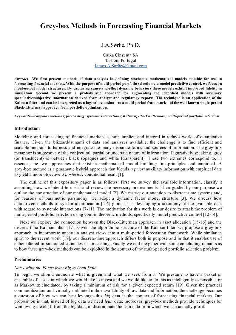
An essential first technical step is thus dimensional analysis to identify transformations of the raw data, which yield time series that are in some sense—at least weakly—homogeneous [3]. Effectively the task is to distill from the raw data an invariant probabilistic behavior that we can model stochastically as independent and identically distributed random variables. These transformed data are the market invariants [16]. Examples of transformations include but are not limited to detrending and removing cyclical or seasonal components. For equities and other tradable assets like commodities and currencies, the most important transformation is the compounded total return (CTR), defined as the logarithm of the ratio of two sequential prices:

n yk = l (P P )k / k 1

For equities the salient feature of this transformation is that tends to have approximately symmetrical y k sample distributions. As demonstration, consider the comparison shown in Figure 1 of the two invariance analyses of the Russell 3000 index representing approximately 98% of the investable U.S. equity market.

Regarding the econometric data that we intend to use as exogenous input to our model, some similar technical treatment of the raw data is typically necessary. Rather than for statistical requirements, this is motivated by the hunt for the most informative driving-­form of the exogenous signal. Indeed this is where the model building process becomes grey;; discovery of what transformation works best is necessarily a data-­driven process of trial and error. Examples of transformations include detrending, seasonal adjustments, smoothed moving averages. As demonstration, consider the weekly jobs data reported by the U.S. Department of Labor. To reduce the variance, these data are generally analyzed using a four-­week moving average. Figure 2 shows the raw data alongside the dimensionless year-­on-­year change. An important feature of the transformed series is that it now indicates perturbations about zero and ranges between Here the maximal absolute value of . 1 the data was used in normalization;; other metrics for normalization exist, eg. using signal spectra [4].

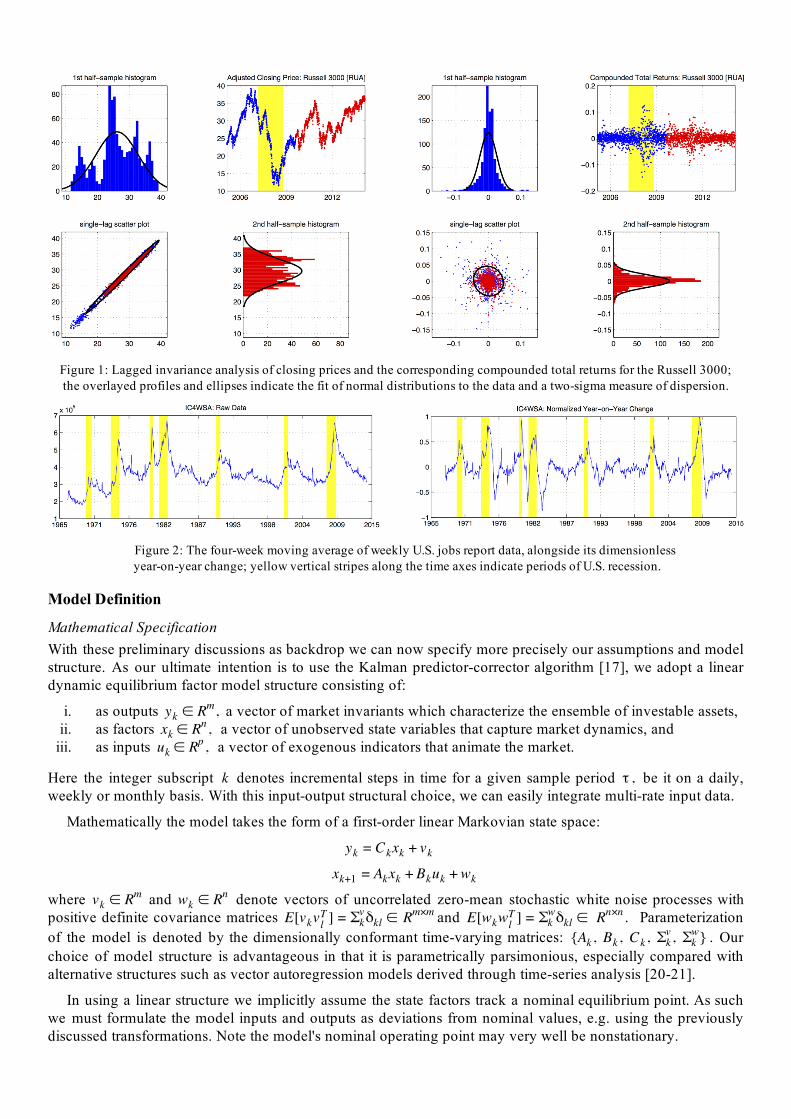
Figure 1: Lagged invariance analysis of closing prices and the corresponding compounded total returns for the Russell 3000;; the overlayed profiles and ellipses indicate the fit of normal distributions to the data and a two-­sigma measure of dispersion.

Figure 2: The four-­week moving average of weekly U.S. jobs report data, alongside its dimensionless year-­on-­year change;; yellow vertical stripes along the time axes indicate periods of U.S. recession.

Model Definition

Mathematical Specification With these preliminary discussions as backdrop we can now specify more precisely our assumptions and model structure. As our ultimate intention is to use the Kalman predictor-­corrector algorithm [17], we adopt a linear dynamic equilibrium factor model structure consisting of:

i. as outputs a vector of market invariants which characterize the ensemble of investable assets,y ∈ R , km

ii. as factors a vector of unobserved state variables that capture market dynamics, andx ∈ R , k n

iii. as inputs a vector of exogenous indicators that animate the market.u ∈ R , k p

Here the integer subscript denotes incremental steps in time for a given sample period be it on a daily, k ,τ weekly or monthly basis. With this input-­output structural choice, we can easily integrate multi-­rate input data.

Mathematically the model takes the form of a first-­order linear Markovian state space:

x yk = Ck k + vk

x uxk+1 = Ak k + Bk k +wk

where and denote vectors of uncorrelated zero-­mean stochastic white noise processes withv ∈ R km w ∈ R k

n positive definite covariance matrices and Parameterization E[v v ] k l

T = δ ∈Σvk kl Rm×m E[w w ] k lT = δ ∈ Σk

wkl . Rn×n

of the model is denoted by the dimensionally conformant time-­varying matrices: Our A , B , C , Σ , Σ k k k vk k

w . choice of model structure is advantageous in that it is parametrically parsimonious, especially compared with alternative structures such as vector autoregression models derived through time-­series analysis [20-­21].

In using a linear structure we implicitly assume the state factors track a nominal equilibrium point. As such we must formulate the model inputs and outputs as deviations from nominal values, e.g. using the previously discussed transformations. Note the model's nominal operating point may very well be nonstationary.

As mentioned in the introduction the purpose of our model is forecasting in portfolio selection. Hence at any point in time we seek to forecast future values, with sample period being k, y , y , y , ...︿k+1 k/ ︿k+2 k/ ︿k+3 k/ τ weekly or monthly. Mathematically the single-­step forecast as given by the predictor equations of y , ︿k+1 k/ Kalman's seminal algorithm [17], takes the form:

x y︿k+1 k/ = Ck︿k+1 k/

x u x︿k+1 k/ = Ak︿k k 1/ + Bk k +Kk y x[ k Ck

︿k k 1/ ] .

Here the Kalman gain matrix is given asK k

Σ C C Σ C Kk = Akxk k 1/ k

T [ kxk k 1/ k

T + Σvk]1

Σ A Σ C C Σ C C Σ A Σxk+1 k/ = Akxk k 1/ k

T + Σkw Ak

xk k 1/ k

T [ kxk k 1/ k

T + Σvk]1

kxk k 1/ k

T

and represents the conditional covariance matrix of the estimated error in the dynamic factors. Based onΣ xk k 1/

estimates of future exogenous inputs and the conditional state estimate a u , u , ..., u k+1 k+2 k+m x , ︿k+1 k/ general m-­step forecast is derived using the state model to recurse ahead in time to the desired horizon.

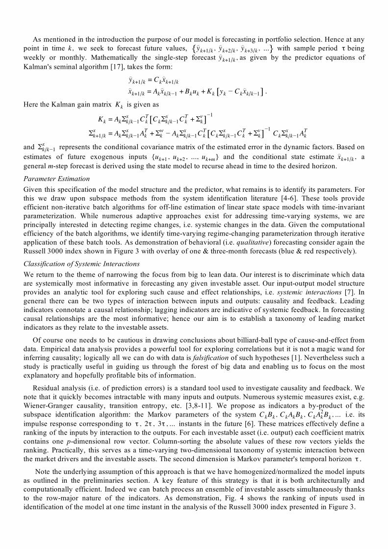
Parameter Estimation Given this specification of the model structure and the predictor, what remains is to identify its parameters. For this we draw upon subspace methods from the system identification literature [4-­6]. These tools provide efficient non-­iterative batch algorithms for off-­line estimation of linear state space models with time-­invariant parameterization. While numerous adaptive approaches exist for addressing time-­varying systems, we are principally interested in detecting regime changes, i.e. systemic changes in the data. Given the computational efficiency of the batch algorithms, we identify time-­varying regime-­changing parameterization through iterative application of these batch tools. As demonstration of behavioral (i.e. qualitative) forecasting consider again the Russell 3000 index shown in Figure 3 with overlay of one & three-­month forecasts (blue & red respectively).

Classification of Systemic Interactions We return to the theme of narrowing the focus from big to lean data. Our interest is to discriminate which data are systemically most informative in forecasting any given investable asset. Our input-­output model structure provides an analytic tool for exploring such cause and effect relationships, i.e. systemic interactions [7]. In general there can be two types of interaction between inputs and outputs: causality and feedback. Leading indicators connotate a causal relationship;; lagging indicators are indicative of systemic feedback. In forecasting causal relationships are the most informative;; hence our aim is to establish a taxonomy of leading market indicators as they relate to the investable assets.

Of course one needs to be cautious in drawing conclusions about billiard-­ball type of cause-­and-­effect from data. Empirical data analysis provides a powerful tool for exploring correlations but it is not a magic wand for inferring causality;; logically all we can do with data is falsification of such hypotheses [1]. Nevertheless such a study is practically useful in guiding us through the forest of big data and enabling us to focus on the most explanatory and hopefully profitable bits of information.

Residual analysis (i.e. of prediction errors) is a standard tool used to investigate causality and feedback. We note that it quickly becomes intractable with many inputs and outputs. Numerous systemic measures exist, e.g. Wiener-­Granger causality, transition entropy, etc. [3,8-­11]. We propose as indicators a by-­product of the subspace identification algorithm: the Markov parameters of the system i.e. its B , Ck k A B ,Ck k k A B , ..Ck k

2k .

impulse response corresponding to instants in the future [6]. These matrices effectively define a , 2τ , 3τ , ..τ . ranking of the inputs by interaction to the outputs. For each investable asset (i.e. output) each coefficient matrix contains one p-­dimensional row vector. Column-­sorting the absolute values of these row vectors yields the ranking. Practically, this serves as a time-­varying two-­dimensional taxonomy of systemic interaction between the market drivers and the investable assets. The second dimension is Markov parameter's temporal horizon .τ

Note the underlying assumption of this approach is that we have homogenized/normalized the model inputs as outlined in the preliminaries section. A key feature of this strategy is that it is both architecturally and computationally efficient. Indeed we can batch process an ensemble of investable assets simultaneously thanks to the row-­major nature of the indicators. As demonstration, Fig. 4 shows the ranking of inputs used in identification of the model at one time instant in the analysis of the Russell 3000 index presented in Figure 3.

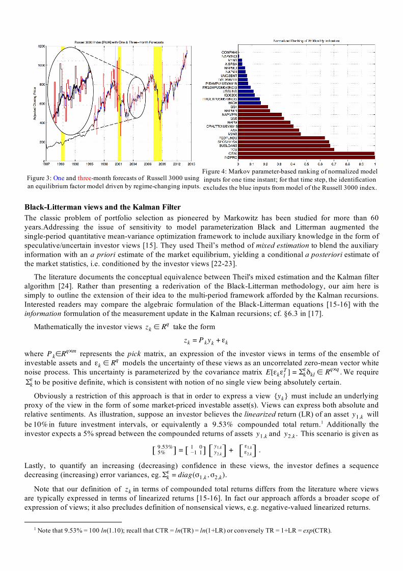
Figure 3: One and three-­month forecasts of Russell 3000 using

an equilibrium factor model driven by regime-­changing inputs.

Figure 4: Markov parameter-­based ranking of normalized model

inputs for one time instant;; for that time step, the identification

excludes the blue inputs from model of the Russell 3000 index.

Black-­Litterman views and the Kalman Filter The classic problem of portfolio selection as pioneered by Markowitz has been studied for more than 60

years.Addressing the issue of sensitivity to model parameterization Black and Litterman augmented the

single-­period quantitative mean-­variance optimization framework to include auxiliary knowledge in the form of

speculative/uncertain investor views [15]. They used Theil’s method of mixed estimation to blend the auxiliary

information with an a priori estimate of the market equilibrium, yielding a conditional a posteriori estimate of

the market statistics, i.e. conditioned by the investor views [22-­23].

The literature documents the conceptual equivalence between Theil's mixed estimation and the Kalman filter

algorithm [24]. Rather than presenting a rederivation of the Black-­Litterman methodology, our aim here is

simply to outline the extension of their idea to the multi-­period framework afforded by the Kalman recursions.

Interested readers may compare the algebraic formulation of the Black-­Litterman equations [15-­16] with the

information formulation of the measurement update in the Kalman recursions;; cf. §6.3 in [17].

Mathematically the investor views take the formz ∈ R kq

zk = P yk k + εk

where represents the pick matrix, an expression of the investor views in terms of the ensemble of∈R Pkq×m

investable assets and models the uncertainty of these views as an uncorrelated zero-­mean vector white ε ∈ R kq

noise process. This uncertainty is parameterized by the covariance matrix We require E[ε ε ] k lT = δ ∈Σε

k kl .Rq×q

to be positive definite, which is consistent with notion of no single view being absolutely certain.Σεk

Obviously a restriction of this approach is that in order to express a view must include an underlying y k

proxy of the view in the form of some market-­priced investable asset(s). Views can express both absolute and

relative sentiments. As illustration, suppose an investor believes the linearized return (LR) of an asset will y1,k

be in future investment intervals, or equivalently a compounded total return. Additionally the0%1 .53%9 1

investor expects a 5% spread between the compounded returns of assets and This scenario is given asy1,k .y2,k

[ 5%9.53%] = [ 1

101] [ y1,k

y2,k] + [ ε1,kε2,k] .

Lastly, to quantify an increasing (decreasing) confidence in these views, the investor defines a sequence

decreasing (increasing) error variances, eg. iag(σ , ).Σεk = d 1,k σ2,k

Note that our definition of in terms of compounded total returns differs from the literature where views zk

are typically expressed in terms of linearized returns [15-­16]. In fact our approach affords a broader scope of

expression of views;; it also precludes definition of nonsensical views, e.g. negative-­valued linearized returns.

1 Note that 9.53% = 100 ln(1.10);; recall that CTR = ln(TR) = ln(1+LR) or conversely TR = 1+LR = exp(CTR).

Augmentation of Auxiliary Information With the preceding discussion as preface, it is not difficult to imagine how one might incorporate auxiliary investor views into the formulation of our dynamic factor model. Note that views are equivalently expressed as

zk = P C xk k k + εk

we simply redefine the output model

x . ykBL = Ck

BLk + vk

BL

Here we have defined:

i. as outputs y kBL = y ,[ k

T zkT ]T , Rm+q

ii. as parameterization and CkBL = C , P[ k

T CkT

kT ]T , R(m+q) n

iii. as error with covariance vkBL = v ,[ k

T εkT ]T Rm+q Σ iag k

BL = d (Σ , )vk Σε

k . R(m+q) (m+q)

Given this augmented output model and the investor's estimated sequences of views and uncertainty, it is straightforward to apply the previously specified Kalman predictor.

Conceptually the Kalman filter tracks the first and second central moments of a time-­varying conditional probability density whose distribution need not be Gaussian/normal. Inclusion of Black-­Litterman views effectively provides a mechanism to massage these results. Arguably such auxiliary information could instead be mapped as constraints in the objective function of the portfolio optimization process. The counter argument to this position is that Black-­Litterman views provide an intuitive interface to map the investor sentiments. Investigation of this question remains a topic of ongoing study.

Conclusion

Grey-­box methods refer to hybrid analytic techniques that draw upon disparate sources of information, attempt to blend insights and yield purpose-­driven solutions. Figuratively grey-­box methods enable us to peek inside the black-­boxes of the financial markets, narrow the focus on the key systemic interactions and presumably develop better mathematical models for use in forecasting. Motivating our interest in financial forecasting is the need of a market model in the portfolio selection problem. Our ongoing research is focused on use of these input-­output equilibrium models in multi-­period model predictive control applied via convex optimization.

We conclude with a brief paraphrasing of the key results:

i. Using a linear equilibrium input-­output factor model structure, we presented a scalable data-­driven technique for classification of systemic interactions between risk drivers and investable assets. Column-­sorting absolute values of the Markov coefficients yields a ranking the inputs. The Markov coefficients are an interim result of the computationally efficient non-­iterative subspace identification algorithm used for parameter estimation of the factor model. For each investable asset this ranking yields a time-­varying two-­dimensional taxonomy of the systemic interactions in terms of the risk drivers. The second dimension corresponds to the temporal horizon of the Markov coefficients. Practically the taxonomy serves to narrow the focus from big to lean data. A quantitative demonstration was presented verifying the potential of both the input-­output structure and the utility of the taxonomy in identifying regime-­changing models dependent on the ranking of the prevailing systemic interactions.

ii. We presented a conceptual extension of the Black-­Litterman technique for integrating uncertain investor views into a multi-­period market model. The extension is based on the equivalence of Theil's method of mixed estimation with the measurement update of the Kalman filter recursions. This framework enables exploration of auxiliary quantitative information derived from subjective/speculative sources such as equity analyst and regulatory reports. The technique is novel in that such information typically defies assimilation into quantitative financial market models.

References [1] T. Bohlin, “Practical grey-­box process identification: Theory and applications,” Springer-­Verlag, 2006. [2] J. Sørlie, “On grey-­box model definition and symbolic derivation of extended Kalman filters,” Ph.D. dissertation, Reglerteknik, Kungl

Tekniska Högskolan, Stockholm, 1996. [3] A.C. Harvey, “Forecasting, structural time series models and the Kalman filter,” Cambridge University Press. [4] L. Ljung, “System identification: Theory for the user,” Prentice-­Hall, 1999. [5] P. Van Overschee and B. De Moor, “Subspace Identification for Linear Systems: Theory, Implementation, Applications,” Kluwer, 1996. [6] N. Chui and J. Maciejowski, “Subspace identification: a Markov parameter approach,” Intl. Journal of Control, vol. 78, pp. 1412-­1436, 2005. [7] T. Sowell, “Basic Economics,” Basic Books, 2011. [8] G.R. Skoog, “Causality characterizations: bivariate, trivariate, and multivariate propositions,” No. 14. Fed. Res. Bank of Minneapolis, 1976. [9] S.L. Bressler and A.K. Seth, “Wiener-­Granger causality: a well established methodology,” NeuroImage, vol. 58:2, pp. 323-­329, 2011. [10] M. Billio, M. Getmansky, A.W. Lo and L. Pelizzon, “Econometric measures of connectedness and systemic risk in the finance and insurance

sectors,” Journal of Financial Economics, vol.104:3, pp. 535-­559, 2012. [11] A. Zaremba and T. Aste, “Measures of causality in complex datasets with application to financial data,” Entropy, vol.16:4, pp.2309-­49, 2014. [12] M.E. Morari, “Model Predictive Control,” Prentice-­Hall, 1993. [13] F. Herzog, “Strategic Portfolio Management for Long-­Term Investments: an Optimal Control Approach,” Ph.D. dissertation, Swiss Federal

Institute of Technology, Zurich, 2005. [14] J. Skaf and S. Boyd, “Multi-­period portfolio optimization with constraints and transaction costs,” unpublished, April 2009. [15] F. Black and R. Litterman, “Global asset allocation with equities, bonds and currencies,” Goldman, Sachs & Co., Oct. 1991. [16] A. Meucci, “Risk and asset allocation,” Springer, 2005. [17] B.D.O. Anderson and J.B. Moore, “Optimal filtering,” Prentice-­Hall, 1979. [18] M. Davis and S. Lleo, “Black-­Litterman in continuous time: the case for filtering,” Quantitative Finance Letters, vol. 1, pp. 30-­35, 2013. [19] H. Markowitz, “Portfolio Selection,” Journal of Finance, vol. 7:1, pp. 77-­91, 1952. [20] M. Forni, M. Hallin, M. Lippi, and L Reichlin, “The generalized dynamic factor model: Identification and estimation,” Rev. Economic Stud.,

vol. 65, pp. 453-­473, 2000. [21] M. Deistler, B.D.O. Anderson, A. Filler, Ch. Zinner, and W. Chen, “Generalized linear dynamic factor models: An approach via singular

autoregressions,” European Journal of Control, vol. 16:3, pp. 211-­224, 2010. [22] H. Theil and A.S. Goldberger, “On pure and mixed statistical estimation in economics,” Int. Economic Review, vol. 2:1, pp. 65-­78, 1961. [23] H. Toutenberg, “Prior information in linear models,” Wiley, 1982. [24] G.T. Diderrich, “The Kalman filter from the perspective of Goldberger-­Theil estimators,” The Amer. Statistician, vol. 39:3, pp. 193-­198, 1985.