Greedy randomized adaptive search and variableneighbourhood search for the minimum labelling

spanning tree problemS. Consoli a,∗, K. Darby-Dowman a, N. Mladenovic a, J. A. Moreno Perez b

aCARISMA and NET-ACE, School of Information Systems, Computing and Mathematics, BrunelUniversity, Uxbridge, Middlesex, UB8 3PH, United Kingdom

bDEIOC, IUDR, Universidad de La Laguna, Facultad de Matematicas, 4a planta Astrofisico FranciscoSanchez s/n, 38271, Santa Cruz de Tenerife, Spain

Abstract

This paper studies heuristics for the minimum labelling spanning tree (MLST) problem. Thepurpose is to find a spanning tree using edges that are as similar as possible. Given an undi-rected labelled connected graph, the minimum labelling spanning tree problem seeks a spanningtree whose edges have the smallest number of distinct labels. This problem has been shownto be NP-hard. A Greedy Randomized Adaptive Search Procedure (GRASP) and a VariableNeighbourhood Search (VNS) are proposed in this paper. They are compared with other algo-rithms recommended in the literature: the Modified Genetic Algorithm and the Pilot Method.Nonparametric statistical tests show that the heuristics based on GRASP and VNS outperformthe other algorithms tested. Furthermore, a comparison with the results provided by an exactapproach shows that we may quickly obtain optimal or near-optimal solutions with the proposedheuristics.

Key words: Metaheuristics, Combinatorial optimisation, Minimum labelling spanning tree, VariableNeighbourhood Search, Greedy Randomized Adaptive Search Procedure.

1. Introduction

Many combinatorial optimisation problems can be formulated on a graph where thepossible solutions are spanning trees. These problems consist of finding spanning trees

∗ Corresponding author.( +44 (0)1895 266820; fax: +44 (0)1895 269732� sergio.consoli@brunel.ac.uk

Preprint submitted to EJOR April 11, 2008

that are optimal with respect to some measure and have been extensively studied in graphtheory (Avis et al., 2005). Typical measures include the total length or the diameter of thetree. Many real-life combinatorial optimisation problems belong to this class of problemsand consequently there is a large and growing interest in both theoretical and practicalaspects. For some of these problems there are polynomial-time algorithms, while mostare NP-hard. Thus, it is not possible to guarantee that an exact solution to the problemcan be found within an acceptable timeframe and one has to settle for heuristics andapproximate solution approaches with performance guarantees.

The minimum labelling spanning tree (MLST) problem is an NP-hard problem inwhich, given a graph with labelled edges, one seeks a spanning tree with the least numberof labels. Such a model can represent many real-world problems in telecommunicationsnetworks, power networks, and multimodal transportation networks. For example, intelecommunications networks, there are many different types of communications media,such as optical fibre, coaxial cable, microwave, and telephone line (Tanenbaum, 2003). Acommunications node may communicate with different nodes by choosing different typesof communications media. Given a set of communications network nodes, the problem isto find a spanning tree (a connected communications network) that uses as few commu-nications types as possible. This spanning tree will reduce the construction cost and thecomplexity of the network.

The MLST problem can be formulated as a network or graph problem. We are given alabelled connected undirected graph G = (V, E, L), where V is the set of n nodes, E is theset of m edges, and L is the set of ` labels. In the telecommunications example (Tanen-baum, 2003), the vertices represent communications nodes, the edges communicationslinks, and the labels communications types. Each edge in E has a label in a finite setL that identifies the communications type. The objective is to find a spanning tree thatuses the smallest number of different types of edges. Define LT to be the set of differentlabels of the edges in a spanning tree T . The labelling can be represented by a functionfL : E → L for all edges e ∈ E or by a partition PL of the edge set; the sets of thepartitions are those consisting of the edges with the same label.

Another example is given by multimodal transportation networks (Van-Nes, 2002). Insuch problems, it is desirable to provide a complete service using the minimum numberof companies. The multimodal transportation network is represented by a graph whereeach edge is assigned a label, denoting a different company managing that edge. Theaim is to find a spanning tree of the graph using the minimum number of labels. Theinterpretation is that all terminal nodes are connected without cycles, using the minimumnumber of companies.

The minimum labelling spanning tree problem is formally defined as follows:

MLST problem: Given a labelled graph G = (V, E, L), where V is the set of nnodes, E is the set of m edges, and L is the set of ` labels, find a spanning tree T ofG such that |LT | is minimized, where LT is the set of labels used in T .

Although a solution to the MLST problem is a spanning tree, we first consider con-nected subgraphs. A feasible solution is defined as a set of labels C ⊆ L, such that all theedges with labels in C represent a connected subgraph of G and span all the nodes in G.If C is a feasible solution, then any spanning tree of C has at most |C| labels. Moreover,if C is an optimal solution, then any spanning tree of C is a minimum labelling spanning

2

tree. Thus, in order to solve the MLST problem we seek a feasible solution with the leastnumber of labels (Xiong et al., 2005a).

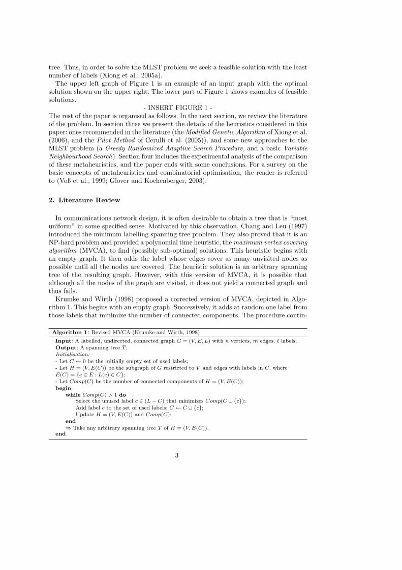
The upper left graph of Figure 1 is an example of an input graph with the optimalsolution shown on the upper right. The lower part of Figure 1 shows examples of feasiblesolutions.

- INSERT FIGURE 1 -The rest of the paper is organised as follows. In the next section, we review the literatureof the problem. In section three we present the details of the heuristics considered in thispaper: ones recommended in the literature (the Modified Genetic Algorithm of Xiong et al.(2006), and the Pilot Method of Cerulli et al. (2005)), and some new approaches to theMLST problem (a Greedy Randomized Adaptive Search Procedure, and a basic VariableNeighbourhood Search). Section four includes the experimental analysis of the comparisonof these metaheuristics, and the paper ends with some conclusions. For a survey on thebasic concepts of metaheuristics and combinatorial optimisation, the reader is referredto (Voß et al., 1999; Glover and Kochenberger, 2003).

2. Literature Review

In communications network design, it is often desirable to obtain a tree that is “mostuniform” in some specified sense. Motivated by this observation, Chang and Leu (1997)introduced the minimum labelling spanning tree problem. They also proved that it is anNP-hard problem and provided a polynomial time heuristic, the maximum vertex coveringalgorithm (MVCA), to find (possibly sub-optimal) solutions. This heuristic begins withan empty graph. It then adds the label whose edges cover as many unvisited nodes aspossible until all the nodes are covered. The heuristic solution is an arbitrary spanningtree of the resulting graph. However, with this version of MVCA, it is possible thatalthough all the nodes of the graph are visited, it does not yield a connected graph andthus fails.

Krumke and Wirth (1998) proposed a corrected version of MVCA, depicted in Algo-rithm 1. This begins with an empty graph. Successively, it adds at random one label fromthose labels that minimize the number of connected components. The procedure contin-

Algorithm 1: Revised MVCA (Krumke and Wirth, 1998)

Input: A labelled, undirected, connected graph G = (V, E, L) with n vertices, m edges, ` labels;Output: A spanning tree T ;Initialisation:- Let C ← 0 be the initially empty set of used labels;- Let H = (V, E(C)) be the subgraph of G restricted to V and edges with labels in C, whereE(C) = {e ∈ E : L(e) ∈ C};- Let Comp(C) be the number of connected components of H = (V, E(C));begin

while Comp(C) > 1 doSelect the unused label c ∈ (L− C) that minimizes Comp(C ∪ {c});Add label c to the set of used labels: C ← C ∪ {c};Update H = (V, E(C)) and Comp(C);

end⇒ Take any arbitrary spanning tree T of H = (V, E(C)).

end

3

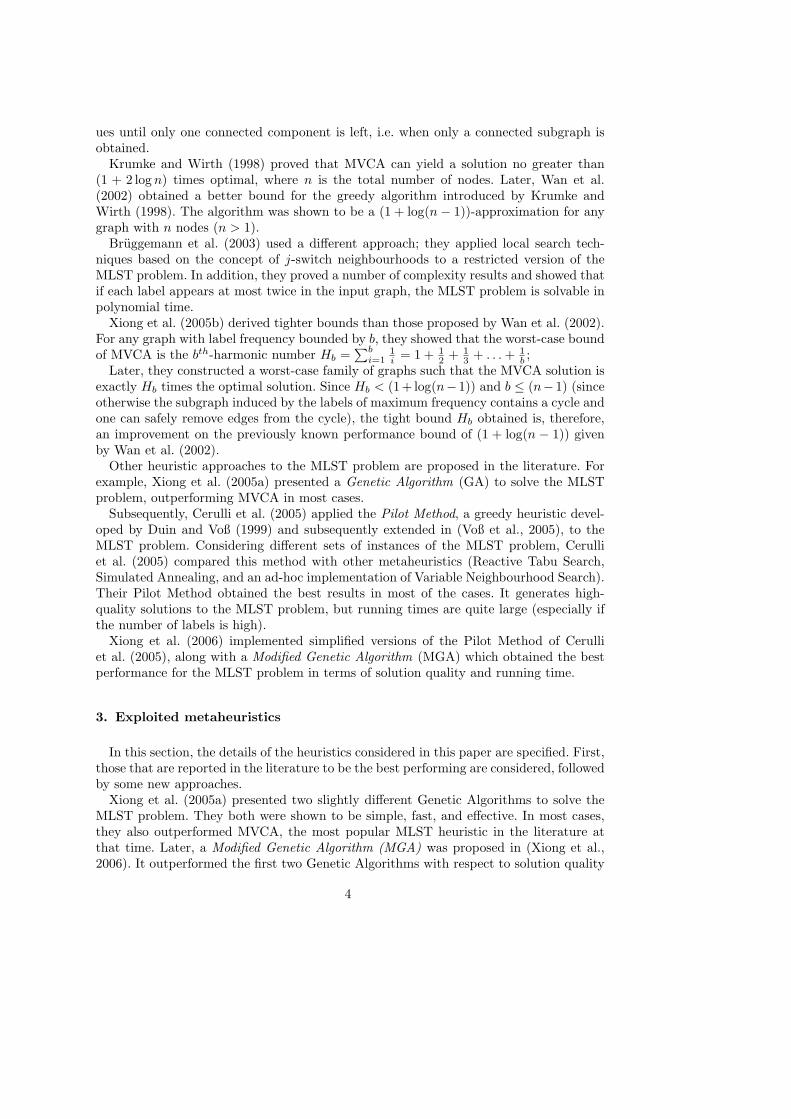
ues until only one connected component is left, i.e. when only a connected subgraph isobtained.

Krumke and Wirth (1998) proved that MVCA can yield a solution no greater than(1 + 2 log n) times optimal, where n is the total number of nodes. Later, Wan et al.(2002) obtained a better bound for the greedy algorithm introduced by Krumke andWirth (1998). The algorithm was shown to be a (1 + log(n− 1))-approximation for anygraph with n nodes (n > 1).

Bruggemann et al. (2003) used a different approach; they applied local search tech-niques based on the concept of j-switch neighbourhoods to a restricted version of theMLST problem. In addition, they proved a number of complexity results and showed thatif each label appears at most twice in the input graph, the MLST problem is solvable inpolynomial time.

Xiong et al. (2005b) derived tighter bounds than those proposed by Wan et al. (2002).For any graph with label frequency bounded by b, they showed that the worst-case boundof MVCA is the bth-harmonic number Hb =

∑bi=1

1i = 1 + 1

2 + 13 + . . . + 1

b ;Later, they constructed a worst-case family of graphs such that the MVCA solution is

exactly Hb times the optimal solution. Since Hb < (1+ log(n− 1)) and b ≤ (n− 1) (sinceotherwise the subgraph induced by the labels of maximum frequency contains a cycle andone can safely remove edges from the cycle), the tight bound Hb obtained is, therefore,an improvement on the previously known performance bound of (1 + log(n − 1)) givenby Wan et al. (2002).

Other heuristic approaches to the MLST problem are proposed in the literature. Forexample, Xiong et al. (2005a) presented a Genetic Algorithm (GA) to solve the MLSTproblem, outperforming MVCA in most cases.

Subsequently, Cerulli et al. (2005) applied the Pilot Method, a greedy heuristic devel-oped by Duin and Voß (1999) and subsequently extended in (Voß et al., 2005), to theMLST problem. Considering different sets of instances of the MLST problem, Cerulliet al. (2005) compared this method with other metaheuristics (Reactive Tabu Search,Simulated Annealing, and an ad-hoc implementation of Variable Neighbourhood Search).Their Pilot Method obtained the best results in most of the cases. It generates high-quality solutions to the MLST problem, but running times are quite large (especially ifthe number of labels is high).

Xiong et al. (2006) implemented simplified versions of the Pilot Method of Cerulliet al. (2005), along with a Modified Genetic Algorithm (MGA) which obtained the bestperformance for the MLST problem in terms of solution quality and running time.

3. Exploited metaheuristics

In this section, the details of the heuristics considered in this paper are specified. First,those that are reported in the literature to be the best performing are considered, followedby some new approaches.

Xiong et al. (2005a) presented two slightly different Genetic Algorithms to solve theMLST problem. They both were shown to be simple, fast, and effective. In most cases,they also outperformed MVCA, the most popular MLST heuristic in the literature atthat time. Later, a Modified Genetic Algorithm (MGA) was proposed in (Xiong et al.,2006). It outperformed the first two Genetic Algorithms with respect to solution quality

4

and running time. MGA is the first metaheuristic that we consider.Cerulli et al. (2005) applied the Pilot Method to the MLST problem. Comparing it

with some other metaheuristic implementations (Reactive Tabu Search, Simulated An-nealing, and an ad-hoc implementation of Variable Neighbourhood Search), it was thebest performing in most of the test problems. The Pilot Method of Cerulli et al. (2005)is the second metaheuristic considered in this paper.

We then present some new approaches to the problem. We propose a new heuristic forthe problem based on GRASP: Greedy Randomized Adaptive Search Procedure. Basically,GRASP is a metaheuristic combining the power of greedy local search with randomisa-tion. For a survey on GRASP, the reader is referred to (Feo and Resende, 1995; Resendeand Ribeiro, 2003).

The other algorithm that we propose is a basic Variable Neighbourhood Search (VNS).Variable Neighbourhood Search is a recently exploited metaheuristic based on dynam-ically changing neighbourhood structures during the search process. For more detailssee (Mladenovic and Hansen, 1997; Hansen and Mladenovic, 2001, 2003).

3.1. Modified Genetic Algorithm (Xiong et al., 2006)

Genetic Algorithms are based on the principle of evolution, operations such as crossoverand mutation, and the concept of fitness (Goldberg et al., 1991).

In the MLST problem, fitness is defined as the number of distinct labels in the can-didate solution. After a number of generations, the algorithm converges and the bestindividual, hopefully, represents a near-optimal solution.

An individual (or a chromosome) in a population is a feasible solution. Each labelin a feasible solution can be viewed as a gene. The initial population is generated byadding labels randomly to empty sets, until feasible solutions emerge. Crossover andmutation operations are then applied in order to build one generation from the previousone. Crossover and mutation probability values are set to 100%. The overall number ofgenerations is chosen to be half of the initial population value. Therefore, in the GeneticAlgorithm of Xiong et al. (2006) the only parameter to tune is the population size.

The crossover operation builds one offspring from two parents, which are feasible solu-tions. Given the parents P1 ⊂ L and P2 ⊂ L, it begins by forming their union P = P1∪P2.Then it adds labels from the subgraph P to the initially empty offspring until a feasiblesolution is obtained, by applying the revised MVCA of Krumke and Wirth (1998) to thesubgraph with labels in P , node set V , and the edge set associated with P . On the otherhand, the mutation operation consists of adding a new label at random, and next tryingto remove the labels (i.e., the associated edges), from the least frequently occurring labelto the most frequently occurring one, whilst retaining feasibility.

3.2. Pilot Method (Cerulli et al., 2005)

The Pilot Method is a metaheuristic proposed by Duin and Voß (1999) and Voß et al.(2005). It uses a basic heuristic as a building block or application process, and thenit tentatively performs iterations of the application process with respect to a so-calledmaster solution. The iterations of the basic heuristic are performed until all the possiblelocal choices (or moves) with respect to the master solution are evaluated. At the end of

5

all the iterations, the new master solution is obtained by extending the current mastersolution with the move that corresponds to the best result produced.

Considering a master solution M , for each element i /∈ M , the Pilot Method is toextend tentatively a copy of M to a (fully grown) solution including i, built throughthe application of the basic heuristic. Let f(i) denote the objective function value of thesolution obtained by including each element i /∈ M , and let i∗ be a most promising ofsuch elements, i.e. f(i∗) ≤ f(i), ∀i /∈ M . The element i∗, representing the best localmove with respect to M , is included in the master solution by changing it in a minimalfashion, leading to a new master solution M = M ∪ {i∗}. On the basis of this newmaster solution M , new iterations of the Pilot Method are started ∀i /∈ M , providing anew solution element i∗, and so on. This look-ahead mechanism is repeated for all thesuccessive stages of the Pilot Method, until no further moves need to be added to themaster solution. Alternatively, some user termination conditions, such as the maximumallowed CPU time or the maximum number of iterations, may be imposed in order to stopthe algorithm when these conditions are satisfied. The last master solution correspondsto the best solution to date and it is produced as the output of the procedure.

For the MLST problem, the Pilot Method proposed by Cerulli et al. (2005) starts fromthe null solution (an empty set of labels) as master solution, uses the revised MVCAof Krumke and Wirth (1998) as the application process, and evaluates the quality of afeasible solution by choosing the number of labels included in the solution as the objec-tive function. It then computes all the possible local choices from the master solution,performing a series of iterations of the application process to the master solution. Thismeans that, at each step, it alternatively tries to add to the master solution each la-bel not yet included, and then applies MVCA in a greedy fashion from then on (i.e. byadding at each successive step the label that minimizes the total number of connectedcomponents), stopping when the resulting subgraph is connected (note that, when theMVCA heuristic is applied to complete a partial solution, in case of ties in the minimumnumber of connected components, a label is selected at random within the set of labelsproducing the minimum number of components).

The Pilot Method successively chooses the best local move, that is the label that, ifincluded to the current master solution, produces the feasible solution with the minimumobjective function value (number of labels). In case of ties, it selects one label at randomwithin the set of labels with the minimum objective function value. This label is thenincluded in the master solution, leading to a new master solution. If the new mastersolution is still infeasible, the Pilot Method proceeds with the same strategy in this newstep, by alternatively adding to the master solution each label not yet included, and thenapplying the MVCA heuristic to produce feasible solutions for each of these candidatelabels. Again, the best move is selected to be added to the master solution, producing anew master solution, and so on. The procedure continues with the same mechanism untila feasible master solution is produced, that is one representing a connected subgraph, oruntil the user termination conditions are satisfied. At the end of the computation it maybe beneficial to greedily drop labels from the master solution while retaining feasibility.The last master solution represents the output of the method.

Since up to ` master solutions can be considered by this procedure, and up to ` localchoices can be evaluated for each master solution, the overall computational running timeof the Pilot Method is O(`2) times the computational time of the application process (i.e.the MVCA heuristic), leading to an overall complexity O(`3).

6

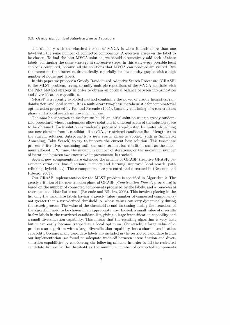
3.3. Greedy Randomized Adaptive Search Procedure

The difficulty with the classical version of MVCA is when it finds more than onelabel with the same number of connected components. A question arises on the label tobe chosen. To find the best MVCA solution, we should alternatively add each of theselabels, continuing the same strategy in successive steps. In this way, every possible localchoice is computed, because all the solutions that MVCA can produce are visited. Butthe execution time increases dramatically, especially for low-density graphs with a highnumber of nodes and labels.

In this paper we propose a Greedy Randomized Adaptive Search Procedure (GRASP)to the MLST problem, trying to unify multiple repetitions of the MVCA heuristic withthe Pilot Method strategy in order to obtain an optimal balance between intensificationand diversification capabilities.

GRASP is a recently exploited method combining the power of greedy heuristics, ran-domisation, and local search. It is a multi-start two-phase metaheuristic for combinatorialoptimisation proposed by Feo and Resende (1995), basically consisting of a constructionphase and a local search improvement phase.

The solution construction mechanism builds an initial solution using a greedy random-ized procedure, whose randomness allows solutions in different areas of the solution spaceto be obtained. Each solution is randomly produced step-by-step by uniformly addingone new element from a candidate list (RCLα: restricted candidate list of length α) tothe current solution. Subsequently, a local search phase is applied (such as SimulatedAnnealing, Tabu Search) to try to improve the current best solution. This two-phaseprocess is iterative, continuing until the user termination condition such as the maxi-mum allowed CPU time, the maximum number of iterations, or the maximum numberof iterations between two successive improvements, is reached.

Several new components have extended the scheme of GRASP (reactive GRASP, pa-rameter variations, bias functions, memory and learning, improved local search, pathrelinking, hybrids,. . .). These components are presented and discussed in (Resende andRibeiro, 2003).

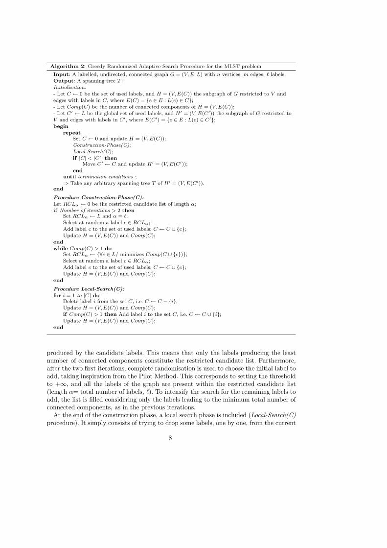
Our GRASP implementation for the MLST problem is specified in Algorithm 2. Thegreedy criterion of the construction phase of GRASP (Construction-Phase() procedure) isbased on the number of connected components produced by the labels, and a value-basedrestricted candidate list is used (Resende and Ribeiro, 2003). This involves placing in thelist only the candidate labels having a greedy value (number of connected components)not greater than a user-defined threshold, α, whose values can vary dynamically duringthe search process. The value of the threshold α and its tuning during the iterations ofthe algorithm need to be chosen in an appropriate way. Indeed, a small value of α resultsin few labels in the restricted candidate list, giving a large intensification capability anda small diversification capability. This means that the resulting algorithm is very fast,but it can easily become trapped at a local optimum. Conversely, a large value of αproduces an algorithm with a large diversification capability, but a short intensificationcapability, because many candidate labels are included in the restricted candidate list. Inour implementation, we found an adequate trade-off between intensification and diver-sification capabilities by considering the following scheme. In order to fill the restrictedcandidate list we fix the threshold as the minimum number of connected components

7

Algorithm 2: Greedy Randomized Adaptive Search Procedure for the MLST problem

Input: A labelled, undirected, connected graph G = (V, E, L) with n vertices, m edges, ` labels;Output: A spanning tree T ;Initialisation:- Let C ← 0 be the set of used labels, and H = (V, E(C)) the subgraph of G restricted to V andedges with labels in C, where E(C) = {e ∈ E : L(e) ∈ C};- Let Comp(C) be the number of connected components of H = (V, E(C));- Let C′ ← L be the global set of used labels, and H′ = (V, E(C′)) the subgraph of G restricted toV and edges with labels in C′, where E(C′) = {e ∈ E : L(e) ∈ C′};begin

repeatSet C ← 0 and update H = (V, E(C));Construction-Phase(C);Local-Search(C);if |C| < |C′| then

Move C′ ← C and update H′ = (V, E(C′));end

until termination conditions ;⇒ Take any arbitrary spanning tree T of H′ = (V, E(C′)).

end

Procedure Construction-Phase(C):Let RCLα ← 0 be the restricted candidate list of length α;if Number of iterations > 2 then

Set RCLα ← L and α = `;Select at random a label c ∈ RCLα;Add label c to the set of used labels: C ← C ∪ {c};Update H = (V, E(C)) and Comp(C);

endwhile Comp(C) > 1 do

Set RCLα ← {∀c ∈ L/ minimizes Comp(C ∪ {c})};Select at random a label c ∈ RCLα;Add label c to the set of used labels: C ← C ∪ {c};Update H = (V, E(C)) and Comp(C);

end

Procedure Local-Search(C):for i = 1 to |C| do

Delete label i from the set C, i.e. C ← C − {i};Update H = (V, E(C)) and Comp(C);if Comp(C) > 1 then Add label i to the set C, i.e. C ← C ∪ {i};Update H = (V, E(C)) and Comp(C);

end

produced by the candidate labels. This means that only the labels producing the leastnumber of connected components constitute the restricted candidate list. Furthermore,after the two first iterations, complete randomisation is used to choose the initial label toadd, taking inspiration from the Pilot Method. This corresponds to setting the thresholdto +∞, and all the labels of the graph are present within the restricted candidate list(length α= total number of labels, `). To intensify the search for the remaining labels toadd, the list is filled considering only the labels leading to the minimum total number ofconnected components, as in the previous iterations.

At the end of the construction phase, a local search phase is included (Local-Search(C)procedure). It simply consists of trying to drop some labels, one by one, from the current

8

solution C while retaining feasibility. Local search gives a further improvement to theintensification phase of the algorithm.

The entire algorithm proceeds until the user termination conditions are satisfied.

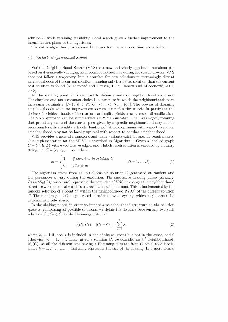
3.4. Variable Neighbourhood Search

Variable Neighbourhood Search (VNS) is a new and widely applicable metaheuristicbased on dynamically changing neighbourhood structures during the search process. VNSdoes not follow a trajectory, but it searches for new solutions in increasingly distantneighbourhoods of the current solution, jumping only if a better solution than the currentbest solution is found (Mladenovic and Hansen, 1997; Hansen and Mladenovic, 2001,2003).

At the starting point, it is required to define a suitable neighbourhood structure.The simplest and most common choice is a structure in which the neighbourhoods haveincreasing cardinality: |N1(C)| < |N2(C)| < ... < |Nkmax

(C)|. The process of changingneighbourhoods when no improvement occurs diversifies the search. In particular thechoice of neighbourhoods of increasing cardinality yields a progressive diversification.The VNS approach can be summarized as: “One Operator, One Landscape”, meaningthat promising zones of the search space given by a specific neighbourhood may not bepromising for other neighbourhoods (landscape). A local optimum with respect to a givenneighbourhood may not be locally optimal with respect to another neighbourhood.

VNS provides a general framework and many variants exist for specific requirements.Our implementation for the MLST is described in Algorithm 3. Given a labelled graphG = (V, E,L) with n vertices, m edges, and ` labels, each solution is encoded by a binarystring, i.e. C = (c1, c2, . . . , c`) where

ci =

1 if label i is in solution C

0 otherwise(∀i = 1, . . . , `). (1)

The algorithm starts from an initial feasible solution C generated at random andlets parameter k vary during the execution. The successive shaking phase (Shaking-Phase(Nk(C)) procedure) represents the core idea of VNS: it changes the neighbourhoodstructure when the local search is trapped at a local minimum. This is implemented by therandom selection of a point C ′ within the neighbourhood Nk(C) of the current solutionC. The random point C ′ is generated in order to avoid cycling, which might occur if adeterministic rule is used.

In the shaking phase, in order to impose a neighbourhood structure on the solutionspace S, comprising all possible solutions, we define the distance between any two suchsolutions C1, C2 ∈ S, as the Hamming distance:

ρ(C1, C2) = |C1 − C2| =∑

i=1

λi (2)

where λi = 1 if label i is included in one of the solutions but not in the other, and 0otherwise, ∀i = 1, ..., `. Then, given a solution C, we consider its kth neighbourhood,Nk(C), as all the different sets having a Hamming distance from C equal to k labels,where k = 1, 2, . . . , kmax, and kmax represents the size of the shaking. In a more formal

9

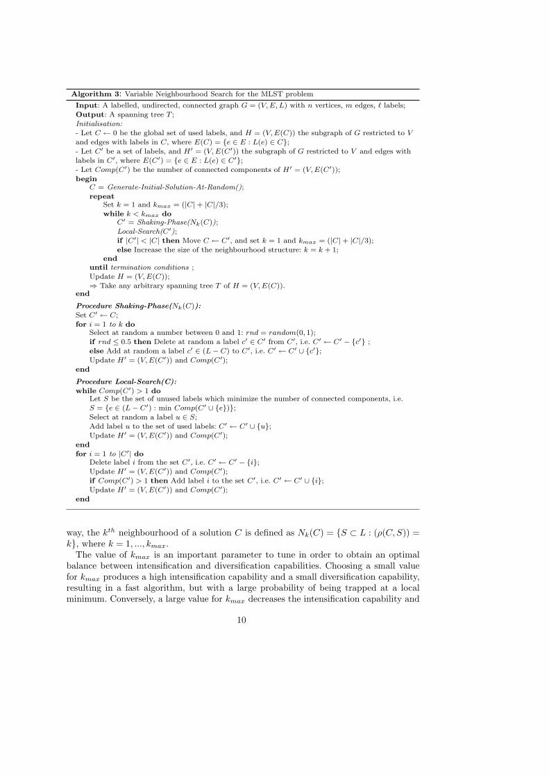
Algorithm 3: Variable Neighbourhood Search for the MLST problem

Input: A labelled, undirected, connected graph G = (V, E, L) with n vertices, m edges, ` labels;Output: A spanning tree T ;Initialisation:- Let C ← 0 be the global set of used labels, and H = (V, E(C)) the subgraph of G restricted to Vand edges with labels in C, where E(C) = {e ∈ E : L(e) ∈ C};- Let C′ be a set of labels, and H′ = (V, E(C′)) the subgraph of G restricted to V and edges withlabels in C′, where E(C′) = {e ∈ E : L(e) ∈ C′};- Let Comp(C′) be the number of connected components of H′ = (V, E(C′));begin

C = Generate-Initial-Solution-At-Random();repeat

Set k = 1 and kmax = (|C|+ |C|/3);while k < kmax do

C′ = Shaking-Phase(Nk(C));Local-Search(C′);if |C′| < |C| then Move C ← C′, and set k = 1 and kmax = (|C|+ |C|/3);else Increase the size of the neighbourhood structure: k = k + 1;

enduntil termination conditions ;Update H = (V, E(C));⇒ Take any arbitrary spanning tree T of H = (V, E(C)).

end

Procedure Shaking-Phase(Nk(C)):Set C′ ← C;for i = 1 to k do

Select at random a number between 0 and 1: rnd = random(0, 1);if rnd ≤ 0.5 then Delete at random a label c′ ∈ C′ from C′, i.e. C′ ← C′ − {c′} ;else Add at random a label c′ ∈ (L− C) to C′, i.e. C′ ← C′ ∪ {c′};Update H′ = (V, E(C′)) and Comp(C′);

end

Procedure Local-Search(C):while Comp(C′) > 1 do

Let S be the set of unused labels which minimize the number of connected components, i.e.S = {e ∈ (L− C′) : min Comp(C′ ∪ {e})};Select at random a label u ∈ S;Add label u to the set of used labels: C′ ← C′ ∪ {u};Update H′ = (V, E(C′)) and Comp(C′);

endfor i = 1 to |C′| do

Delete label i from the set C′, i.e. C′ ← C′ − {i};Update H′ = (V, E(C′)) and Comp(C′);if Comp(C′) > 1 then Add label i to the set C′, i.e. C′ ← C′ ∪ {i};Update H′ = (V, E(C′)) and Comp(C′);

end

way, the kth neighbourhood of a solution C is defined as Nk(C) = {S ⊂ L : (ρ(C, S)) =k}, where k = 1, ..., kmax.

The value of kmax is an important parameter to tune in order to obtain an optimalbalance between intensification and diversification capabilities. Choosing a small valuefor kmax produces a high intensification capability and a small diversification capability,resulting in a fast algorithm, but with a large probability of being trapped at a localminimum. Conversely, a large value for kmax decreases the intensification capability and

10

increases the diversification capability, resulting in a slower algorithm, but able to escapefrom local minima. According to our experience, the value kmax = (|C|+ |C|/3) gives agood trade-off between these two factors.

In our implementation, in order to select a solution in the k-th neighbourhood of asolution C, the algorithm randomly adds further labels to C, or remove labels fromC, until the resulting solution has a Hamming distance equal to k with respect to C.Addition and deletion of labels at this stage have the same probability of being chosen.For this purpose, a random number is selected between 0 and 1 (rnd = random(0, 1)). Ifthis number is smaller than 0.5, the algorithm proceeds with the deletion of a label fromC. Otherwise, an additional label is included at random in C from the set of unused labels(L − C). The procedure is repeated until the number of addition/deletion operations isexactly equal to k.

The successive local search (Local-Search(C’) procedure) consists of two steps. In thefirst step, since deletion of labels often gives an infeasible incomplete solution, additionallabels may be added in order to restore feasibility. In this case, addition of labels followsthe MVCA criterion of adding the label with the minimum number of connected com-ponents. Note that in case of ties in the minimum number of connected components, alabel not yet included in the partial solution is chosen at random within the set of labelsproducing the minimum number of components (i.e. u ∈ S where S = {e ∈ (L − C ′) :min Comp(C ′ ∪ {e})}). Then, the second step of the local search tries to delete labelsone by one from the specific solution, whilst maintaining feasibility.

After the local search phase, if no improvements are obtained (|C ′| ≥ |C|), the neigh-bourhood structure is increased (k = k+1) giving a progressive diversification (|N1(C)| <|N2(C)| < ... < |Nkmax(C)|). Otherwise, the algorithm moves to the improved solution(C ← C ′) and sets the first neighbourhood structure (k = 1). Then the procedure restartswith the shaking and the local search phases, continuing iteratively until the user ter-mination conditions (maximum allowed CPU time, maximum number of iterations, ormaximum number of iterations between two successive improvements) are satisfied.

4. Computational results

In this section, the metaheuristics are compared in terms of solution quality and compu-tational running time. We identify the metaheuristics with the abbreviations: PILOT (Pi-lot Method), MGA (Modified Genetic Algorithm), GRASP (Greedy Randomized Adap-tive Search Procedure), VNS (Variable Neighbourhood Search).

Different sets of instances of the problem have been generated in order to evaluatehow the algorithms are influenced by the parameters, the structure of the network andthe distribution of the labels on the edges. The parameters considered are the number ofedges of the graph (m), the number of nodes of the graph (n), and the number of labelsassigned to the edges (`).

We thank the authors of (Cerulli et al., 2005), who kindly provided data for use in ourexperiments. In our computations, run on a Pentium Centrino microprocessor at 2.0 GHzwith 512 MB RAM, we consider different datasets, each one containing 10 instances ofthe problem with the same set of values for the parameters n, `, and m. For each dataset,solution quality is evaluated as the average objective value for the 10 problem instances. Amaximum allowed CPU time (max-CPU-time), determined with respect to the dimension

11

of the problem instance, is chosen as the stopping condition for all the metaheuristics.For MGA, we use a variable number of iterations for each instance, determined such thatthe computations take approximately max-CPU-time for the specific dataset. Selectionof the maximum allowed CPU time as the stopping criterion is made in order to have adirect comparison of all the metaheuristics with respect to the quality of their solutions.

All the heuristic methods run for max-CPU-time and, in each case, the best solutionis recorded. The computational times reported in the tables are the times at which thebest solutions are obtained. The reported times have precision of ±5 ms. Where possible,the results of the metaheuristics are compared with the exact solution, identified withthe label EXACT.

The Exact Method is an A* or backtracking procedure to test the subsets of L. Thissearch method performs a branch and prune procedure in the partial solution space basedon a recursive procedure Test that attempts to find a better solution from the currentincomplete solution. The main program that solves the MLST problem calls the Testprocedure with an empty set of labels. The details are specified in Algorithm 4.

In order to reduce the number of test sets, it is more convenient to use a good approx-imate solution for C∗ in the initial step, instead of considering all the labels. Anotherimprovement that avoids the examination of a large number of incomplete solutions con-sists of rejecting every incomplete solution that cannot be completed to get only oneconnected component. Note that if we are evaluating an incomplete solution C ′ with anumber of labels |C ′| = |C∗|−2, we should try to add the labels one by one to check if it ispossible to find a better solution for C∗ with a smaller dimension, that is |C ′| = |C∗|−1.To complete this solution C ′, we need to add a label with a frequency at least equal to

Algorithm 4: Exact Method for the MLST problem

Input: A labelled, undirected, connected graph G = (V, E, L) with n vertices, m edges, ` labels;Output: A spanning tree T ;Initialisation:- Let C ← 0 be the initially empty set of used labels;- Let H = (V, E(C)) be the subgraph of G restricted to V and edges with labels in C, whereE(C) = {e ∈ E : L(e) ∈ C};- Let C∗ ← L be the global set of used labels;- Let H∗ = (V, E(C∗)) be the subgraph of G restricted to V and edges with labels in C∗, whereE(C∗) = {e ∈ E : L(e) ∈ C∗};- Let Comp(C) be the number of connected components of H = (V, E(C));begin

Call Test(C);⇒ Take any arbitrary spanning tree T of H∗ = (V, E(C∗)).

end

Procedure Test(C):if |C| < |C∗| then

Update Comp(C);if Comp(C) = 1 then

Move C∗ ← C;else if |C| < |C∗| − 1 then

foreach c ∈ (L− C) doTry to add label c : Test(C ∪ {c});

end

end

end

12

the actual number of connected components minus 1. If this requirement is not satisfied,the incomplete solution can be rejected, speeding up the search process.

The running time of this Exact Method grows exponentially, but if either the prob-lem size is small or the optimal objective function value is small, the running time isreasonable and the method obtains the exact solution. The complexity of the instancesincreases with the dimension of the graph (number of nodes and labels), and the reduc-tion in the density of the graph. In our tests, the optimal solution is reported unless asingle instance requires more than 3 hours of CPU time. In such a case, we report notfound (NF).

4.1. Experimental analysis

In our computations we have considered two different groups of datasets, includinginstances with a number of vertices, n, and a number of labels, `, from 20 up to 500.All these instances are available from the authors (Consoli, 2007). The number of edges,m, is obtained indirectly from the density d of edges whose values are chosen to be0.8, 0.5, and 0.2. Analysing the performance of the considered algorithms, for a singledataset a metaheuristic should be considered worse than another one if either it obtainsa larger average objective value, or an equal average objective value but in a greatercomputational time.

Group 1 examines small instances with the number of vertices equal to the numberof labels. These values are chosen to be between 20 and 50 in steps of 10. Thus, theconsidered datasets are n = ` = 20, 30, 40, 50, and d = 0.8, 0.5, 0.2, for a total of 12datasets (120 instances). Computational results are presented in Table 1, which reportsthe average objective function values found by the heuristics for the datasets of Group 1,and the corresponding average computational times, with a max-CPU-time of 1 second.

- INSERT TABLE 1 -Looking at this table, all the heuristics performed well and faster than the Exact Methodfor the Group 1 instances. However, MGA is considerably slower than the other meta-heuristics, as a result of a poor intensification capability and an excessive diversificationcapability for these instances. PILOT is faster than MGA but it produces slightly worsesolutions with respect to solution quality. It exhibits an opposite behaviour to that ofMGA, being characterised by a limited diversification capability which sometimes doesnot allow the search process to escape from local optima. The performance of GRASPand VNS are both comparable for these trivial instances of the problem. They are ableto obtain all the exact solutions in very short running times and are the best performingheuristics for the Group 1 in terms of solution quality and computational running time.

Group 2 considers larger instances of the MLST problem with a fixed number ofvertices, and a number of labels ` = 0.25 · n, 0.5 · n, n, 1.25 · n. Thus, the datasets ofGroup 2 are n = 100, 200, 500 vertices, ` = 0.25 · n, 0.5 · n, n, 1.25 · n, and d = 0.8,0.5, 0.2, for a total of 36 datasets (360 instances). Furthermore, we have considered amax-CPU-time of 20 seconds for Group 2 with n = 100; of 60 seconds for Group 2 withn = 200; and of 300 seconds for Group 2 with n = 500. Average objective functionvalues and the corresponding average computational times are reported in Tables 2 - 3- 4 respectively.

- INSERT TABLE 2, TABLE 3, TABLE 4-

13

For all the Group 2 instances with n = 100, looking at Table 2, the best performanceis obtained by VNS which produces the solutions with the best solution quality and theshortest running times. GRASP also performs well, obtaining the same solutions as VNS,with the exception of the instance [n = ` = 100, d = 0.2]. As in Group 1, PILOT andMGA obtain the worse solutions and they confirm their defects: excessive diversificationand poor intensification capabilities for MGA and, conversely, excessive intensificationand poor diversification capabilities for PILOT.

Table 3 and Table 4 with larger instances of the problem (Group2 with n = 200,and Group 2 with n = 500) show the same relative behaviour for all the consideredmetaheuristics. VNS and GRASP are always the best performing methods, indicating anoptimal tuning between intensification and diversification of the search process, whichevidently is not obtained by PILOT and MGA that obtain the worse solution in termsof solution quality and computational running time. VNS always obtains the solutionswith the best quality, but it loses a lot, sometimes, in terms of computational runningtime (see for example the instances [n = ` = 200, d = 0.2], [n = ` = 500, d = 0.2],and [n = 500, ` = 625, d = 0.2]). From this analysis, perhaps GRASP slightly defects interms of exploration of the search space with respect to the VNS approach.

Considering only solution quality, the average values of the objective function of themetaheuristics among all the considered datasets are: PILOT = 5.66, MGA = 5.68,GRASP = 5.61, VNS = 5.59. Thus, the best ranking with respect to the solution quality(from the best to the worst) is: VNS, GRASP, PILOT, MGA.

4.2. Statistical analysis of the results

Computing only the average objective values of the metaheuristics over multiple datadoes not provide a full comparison between them. Averages are susceptible to outliers:they can allow excellent performance on some datasets to compensate for an overall badperformance. There may be situations in which such behaviour is desired. However, ingeneral we prefer algorithms that behave well on as many problems as possible.

We have carried out tests to determine the statistical significance of differences be-tween the performances of the metaheuristics (Hollander and Wolfe, 1999). The issueof statistical tests for comparison of algorithms on multiple datasets was theoreticallyand empirically reviewed by Demsar (2006). The null-hypothesis being tested is that themetaheuristics have equal mean performance and the observed differences are merely ran-dom. The alternative hypothesis is that the algorithms have different mean performancesof statistical significance.

The most common statistical method for testing differences between more than twoalgorithms is Analysis of Variance (ANOVA) (see (Hollander and Wolfe, 1999; Demsar,2006) for more details). Since ANOVA is based on assumptions that are violated in thiscontext, we make use of the Friedman Test (Friedman, 1940), that is the non-parametricequivalent of ANOVA, and its corresponding Nemenyi Post-hoc Test (Nemenyi, 1963).

According to the Friedman test, the statistical significance of differences between themetaheuristics is examined by testing whether the measured average ranks are signif-icantly different from the overall mean rank. In particular, we use the version of theFriedman test developed by Iman and Davenport (1980), which considers a powerful teststatistic FF (Appendix A). If the equivalence of the algorithms is rejected, the Nemenyi

14

post-hoc test is applied in order to perform pairwise comparisons.To perform the Friedman and Nemenyi tests, the ranks of the algorithms for each

dataset are evaluated, with a rank of 1 assigned to the best performing algorithm, rank2 to the second best one, and so on. The average ranks for each metaheuristic among the48 datasets are: PILOT = 3.30, MGA = 3.48, GRASP = 1.76, VNS = 1.46. Accordingto the ranking, VNS is the best performing algorithm, immediately followed by GRASP,then PILOT and MGA achieving the worst results.

Now, we analyse the statistical significance of differences between these ranks. Considerthe Iman and Davenport (1980) version of the Friedman test for k = 4 algorithms andN = 48 datasets. The value of the FF test statistic, which is distributed according to theF -distribution with (k − 1, (k − 1)(N − 1)) = (3, 141) degrees of freedom, is computed.This value is 124.2, which is greater than the critical value (3.92 for α = 1%, where α isthe significance level of the test expressed as percentage). Thus, a significant differencebetween the performance of the metaheuristics exists, according to the Friedman test.

As the equivalence of the algorithms is rejected, we proceed with the Nemenyi post-hoc test. Considering a significance level α = 1%, the critical value is q0.01

∼= 3.11. Thecritical difference (CD) for the Nemenyi test is

CD = 3.11 ·√

4 · 56 · 48

∼= 0.82; (3)

The differences between the average ranks of the metaheuristics are reported in Table 5.- INSERT TABLE 5 -

From this table, we can identify two groups of metaheuristics. The first group includesVNS and GRASP, while the second group includes PILOT and MGA. Considering asignificance level α = 1%, the algorithms within each group have comparable performanceaccording to the Nemenyi test since, in each case, the value of the test statistic is lessthan the critical difference. Conversely, two algorithms belonging to different groups havesignificantly different performance according to the Nemenyi test.

Summarizing, from the Friedman and Nemenyi statistical tests, VNS and GRASPhave comparable performance, and they are the best performing algorithms. On theother hand, PILOT and MGA have comparable performance, but worse than VNS andGRASP.

Another way to compare the performance of the algorithms is to count the numberof times they generate the optimal solution. In particular, counting the overall numberof exact solutions obtained is a good approach to estimate the diversification capabilityof each metaheuristic. The Exact Method obtains the exact solution for all probleminstances of 32 datasets, among the overall 48 datasets; for the remaining sets NF isreported. Therefore, the total number of instances having the exact solution is: 32×10 =320.

The percentages of the number of optimal solutions obtained by the metaheuristicsamong the 320 instances are (ranking from the best to the worst algorithm): VNS = 100,GRASP = 99.7, MGA = 99.7, PILOT = 97.5.

VNS obtains all the optimal solutions, underlying a high exploration capability even forcomplex instances. In the same way, GRASP and MGA offer very good results, missingonly 1 solution out of 320, although MGA is extremely time consuming. With 8 cases(out of 320), PILOT fails to find the global optimum and becomes trapped at a localoptimum.

15

Furthermore, some optima reached by the metaheuristics require a greater computa-tional time than required by the Exact Method, thus nullifying the purpose of the meta-heuristics. In this sense the best performances are obtained by VNS and GRASP, all ofwhich require less computational time than the Exact Method among the 32 datasets. Incontrast, PILOT and MGA obtain the optimal solution but in a time that exceeds thatof the Exact Method in 11 and 18 datasets, respectively. Although MGA reaches moreexact solutions than PILOT, it is computationally more burdensome.

From this further analysis, the results reinforce the conclusion that VNS and GRASPare effective metaheuristics for the MLST problem. They are particularly recommendedfor the proposed problem thanks to the following features: ease of implementations, user-friendly codes, high quality of the solutions, and shorter computational running times.

5. Conclusions and further research

In this paper, we have studied metaheuristics for the minimum labelling spanning tree(MLST) problem. In particular, we have examined and implemented the metaheuristicsrecommended in the literature: the Modified Genetic Algorithm (MGA) of Xiong et al.(2006) and the Pilot Method (PILOT) of Cerulli et al. (2005). Furthermore, some newimplementations for the MLST problem have been proposed: a Greedy RandomizedAdaptive Search Procedure (GRASP) and a basic Variable Neighbourhood Search (VNS).

Computational experiments were performed using different instances of the MLSTproblem to evaluate how the algorithms are influenced by the parameters, the structure ofthe network, and the distribution of the labels on the edges. Applying the nonparametricstatistical tests of Friedman (1940) and Nemenyi (1963), we concluded that VNS andGRASP have significantly better performance than the other methods recommended inthe literature with respect to solution quality and running time. Furthermore, this resulthas been reinforced by comparing the metaheuristics with an exact approach. VNS andGRASP obtain a large number of optimal or near-optimal solutions, showing an enhanceddiversification capability.

All the results allow us to state that VNS and GRASP are fast and extremely ef-fective metaheuristics for the MLST problem. They are particularly recommended forthe proposed problem because of their simplicity and their ability to obtain high-qualitysolutions in short computational running times.

Future research will consist of trying to further improve the performance of these pro-cedures (for example through hybridization with other metaheuristics) particularly forlarge instances of the problem. For this purpose, an algorithm based on Ant ColonyOptimisation (ACO) is currently under study in order to try to obtain a larger diversifi-cation capability by extending the current greedy MVCA local search. Indeed, a properACO implementation may allow moves to worse solutions by providing an alternativeprobabilistic solution construction mechanism.

Appendix A. Statistical tests

Friedman Test (Friedman, 1940): The Friedman test is a non-parametric statisticaltest that examines the existence of significant differences between the performances ofmultiple algorithms over different datasets. Given k algorithms and N datasets, it ranks

16

the algorithms for each dataset separately, and tests whether the measured average ranksare significantly different from the mean rank. The statistic used by Friedman (1940) is

χ2F =

12 ·Nk · (k + 1)

·∑

j

R2j −

k · (k + 1)4

, (4)

which follows a Chi-Square distribution with (k − 1) degrees of freedom.Iman and Davenport (1980) developed a more powerful version of the Friedman test

by considering the following statistic:

F 2F =

(N − 1) · χ2F

N · (k − 1)− χ2F

, (5)

which is distributed according to the F -distribution with (k − 1) and (k − 1) · (N − 1)degrees of freedom. For more details, see (Demsar, 2006).

Nemenyi Test (Nemenyi, 1963): The Nemenyi test is used to perform pairwise compar-isons of multiple algorithms over different datasets (Nemenyi, 1963). The performanceof two algorithms is considered significantly different if the corresponding average ranksdiffer by at least the critical difference (CD):

CD = qα ·√

k · (k + 1)6 ·N , (6)

where k is the number of the metaheuristics, N the number of datasets, qα the criticalvalue, and α the significance level of the statistical test. For more details, see (Demsar,2006).

Acknowledgments

Sergio Consoli was supported by an E.U. Marie Curie Fellowship for Early Stage Re-searcher Training (EST-FP6) under grant number MEST-CT-2004-006724 at BrunelUniversity (project NET-ACE).

Jose Andres Moreno Perez was supported by the projects TIN2005-08404-C04-03 ofthe Spanish Government (with financial support from the European Union under theFEDER project) and PI042005/044 of the Canary Government.

We gratefully acknowledge this support.

References

Avis, D., Hertz, A., Marcotte, O., 2005. Graph theory and combinatorial optimization.Springer-Verlag, New York.

Bruggemann, T., Monnot, J., Woeginger, G. J., 2003. Local search for the minimum labelspanning tree problem with bounded colour classes. Operations Research Letters 31,195–201.

Cerulli, R., Fink, A., Gentili, M., Voß, S., 2005. Metaheuristics comparison for the mini-mum labelling spanning tree problem. In: Golden, B., Raghavan, S., Wasil, E. (Eds.),The next wave in computing, optimization, and decision technologies. Springer-Verlag,Berlin, pp. 93–106.

17

Chang, R. S., Leu, S. J., 1997. The minimum labeling spanning trees. Information Pro-cessing Letters 63 (5), 277–282.

Consoli, S., March 2007. Test datasets for the minimum labelling spanning tree problem.[online], http://people.brunel.ac.uk/˜mapgssc/MLSTP.htm.

Demsar, J., 2006. Statistical comparison of classifiers over multiple data sets. Journal ofMachine Learning Research 7, 1–30.

Duin, C., Voß, S., 1999. The pilot method: A strategy for heuristic repetition with ap-plications to the Steiner problem in graphs. Networks 34 (3), 181–191.

Feo, T. A., Resende, M. G. C., 1995. Greedy randomized adaptive search procedures.Journal of Global Optimization 6 (2), 109–133.

Friedman, M., 1940. A comparison of alternative tests of significance for the problem ofm rankings. The Annals of Mathematical Statistics 11 (1), 86–92.

Glover, F., Kochenberger, G. A., 2003. Handbook of metaheuristics (International se-ries in Operations Research & Management Science). Kluwer Academic Publishers,Norwell, MA.

Goldberg, D. E., Deb, K., Korb, B., 1991. Don’t worry, be messy. In: Proceedings ofthe 4th International Conference on Genetic Algorithms. Morgan-Kaufmann, La Jolla,CA, pp. 24–30.

Hansen, P., Mladenovic, N., 2001. Variable neighbourhood search: Principles and appli-cations. European Journal of Operational Research 130, 449–467.

Hansen, P., Mladenovic, N., 2003. Variable neighbourhood search. In: Glover, F., Kochen-berger, G. A. (Eds.), Handbook of metaheuristics. Kluwer Academic Publishers, Nor-well, MA, Ch. 6, pp. 145–184.

Hollander, M., Wolfe, D. A., 1999. Nonparametric statistical methods, 2nd Edition. JohnWiley & Sons, New York.

Iman, R. L., Davenport, J. M., 1980. Approximations of the critical region of the Fried-man statistic. Communications in Statistics - Theory and Methods 9, 571–595.

Krumke, S. O., Wirth, H. C., 1998. On the minimum label spanning tree problem. Infor-mation Processing Letters 66 (2), 81–85.

Mladenovic, N., Hansen, P., 1997. Variable neighbourhood search. Computers & Opera-tions Research 24, 1097–1100.

Nemenyi, P. B., 1963. Distribution-free multiple comparisons. Ph.D. thesis, PrincetonUniversity, New Jersey.

Resende, M. G. C., Ribeiro, C. C., 2003. Greedy randomized adaptive search proce-dure. In: Glover, F., Kochenberger, G. A. (Eds.), Handbook of metaheuristics. KluwerAcademic Publishers, Norwell, MA, pp. 219–249.

Tanenbaum, A. S., 2003. Computer networks, 4th Edition. Prentice Hall, EnglewoodCliffs, New Jersey.

Van-Nes, R., 2002. Design of multimodal transport networks: A hierarchical approach.Delft University Press, Delft.

Voß, S., Fink, A., Duin, C., 2005. Looking ahead with the pilot method. Annals ofOperations Research 136, 285–302.

Voß, S., Martello, S., Osman, I. H., Roucairol, C., 1999. Meta-heuristics: Advances andtrends in local search paradigms for optimization. Kluwer Academic Publishers, Nor-well, MA.

Wan, Y., Chen, G., Xu, Y., 2002. A note on the minimum label spanning tree. InformationProcessing Letters 84, 99–101.

18

Xiong, Y., Golden, B., Wasil, E., 2005a. A one-parameter genetic algorithm for theminimum labeling spanning tree problem. IEEE Transactions on Evolutionary Com-putation 9 (1), 55–60.

Xiong, Y., Golden, B., Wasil, E., 2005b. Worst-case behavior of the MVCA heuristicfor the minimum labeling spanning tree problem. Operations Research Letters 33 (1),77–80.

Xiong, Y., Golden, B., Wasil, E., 2006. Improved heuristics for the minimum label span-ning tree problem. IEEE Transactions on Evolutionary Computation 10 (6), 700–703.

19

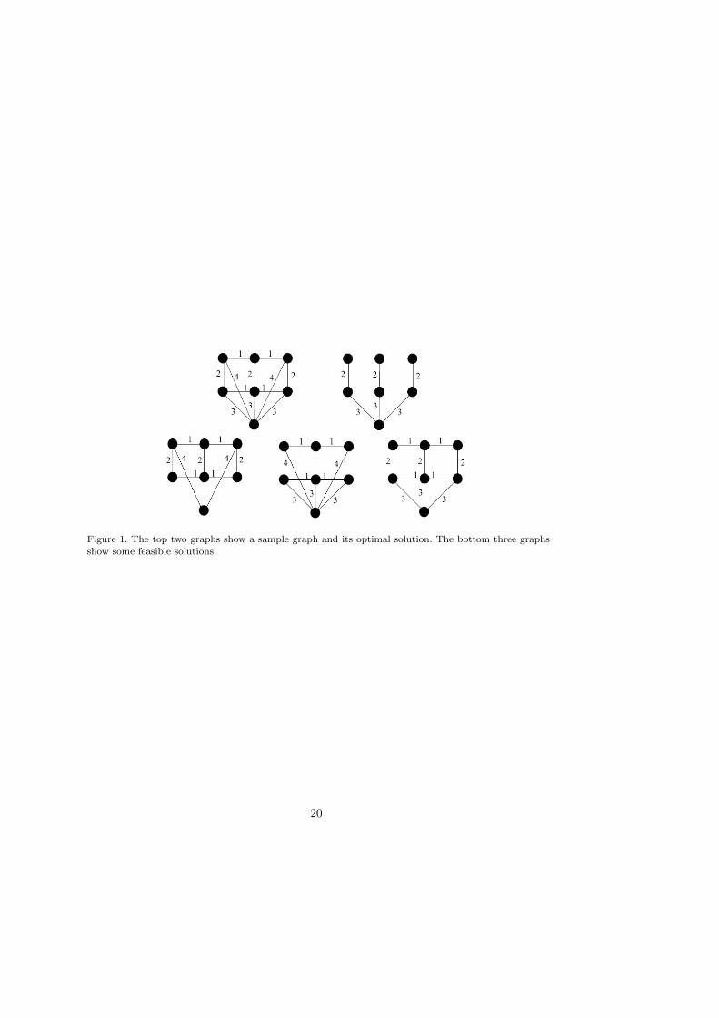
Figure 1. The top two graphs show a sample graph and its optimal solution. The bottom three graphsshow some feasible solutions.

20

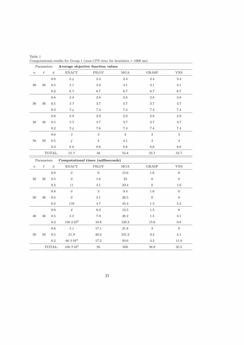
Table 1Computational results for Group 1 (max-CPU-time for heuristics = 1000 ms)

Parameters Average objective function values

n ` d EXACT PILOT MGA GRASP VNS

0.8 2.4 2.4 2.4 2.4 2.4

20 20 0.5 3.1 3.2 3.1 3.1 3.1

0.2 6.7 6.7 6.7 6.7 6.7

0.8 2.8 2.8 2.8 2.8 2.8

30 30 0.5 3.7 3.7 3.7 3.7 3.7

0.2 7.4 7.4 7.4 7.4 7.4

0.8 2.9 2.9 2.9 2.9 2.9

40 40 0.5 3.7 3.7 3.7 3.7 3.7

0.2 7.4 7.6 7.4 7.4 7.4

0.8 3 3 3 3 3

50 50 0.5 4 4 4.1 4 4

0.2 8.6 8.6 8.6 8.6 8.6

TOTAL: 55.7 56 55.8 55.7 55.7

Parameters Computational times (milliseconds)

n ` d EXACT PILOT MGA GRASP VNS

0.8 0 0 15.6 1.6 0

20 20 0.5 0 1.6 22 0 0

0.2 11 3.1 23.4 0 1.6

0.8 0 3 9.4 1.6 0

30 30 0.5 0 3.1 26.5 0 0

0.2 138 4.7 45.4 1.5 5.2

0.8 2 6.3 12.5 1.5 0

40 40 0.5 3.2 7.9 28.2 1.5 3.1

0.2 100.2·103 10.8 120.3 15.6 9.6

0.8 3.1 17.1 21.8 3 0

50 50 0.5 21.9 20.2 531.3 9.4 4.1

0.2 66.3·103 17.2 93.6 3.2 11.9

TOTAL: 166.7·103 95 950 38.9 35.5

21

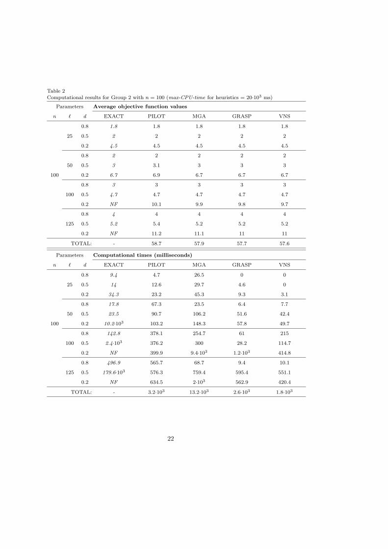
Table 2Computational results for Group 2 with n = 100 (max-CPU-time for heuristics = 20·103 ms)

Parameters Average objective function values

n ` d EXACT PILOT MGA GRASP VNS

0.8 1.8 1.8 1.8 1.8 1.8

25 0.5 2 2 2 2 2

0.2 4.5 4.5 4.5 4.5 4.5

0.8 2 2 2 2 2

50 0.5 3 3.1 3 3 3

100 0.2 6.7 6.9 6.7 6.7 6.7

0.8 3 3 3 3 3

100 0.5 4.7 4.7 4.7 4.7 4.7

0.2 NF 10.1 9.9 9.8 9.7

0.8 4 4 4 4 4

125 0.5 5.2 5.4 5.2 5.2 5.2

0.2 NF 11.2 11.1 11 11

TOTAL: - 58.7 57.9 57.7 57.6

Parameters Computational times (milliseconds)

n ` d EXACT PILOT MGA GRASP VNS

0.8 9.4 4.7 26.5 0 0

25 0.5 14 12.6 29.7 4.6 0

0.2 34.3 23.2 45.3 9.3 3.1

0.8 17.8 67.3 23.5 6.4 7.7

50 0.5 23.5 90.7 106.2 51.6 42.4

100 0.2 10.2·103 103.2 148.3 57.8 49.7

0.8 142.8 378.1 254.7 61 215

100 0.5 2.4·103 376.2 300 28.2 114.7

0.2 NF 399.9 9.4·103 1.2·103 414.8

0.8 496.9 565.7 68.7 9.4 10.1

125 0.5 179.6·103 576.3 759.4 595.4 551.1

0.2 NF 634.5 2·103 562.9 420.4

TOTAL: - 3.2·103 13.2·103 2.6·103 1.8·103

22

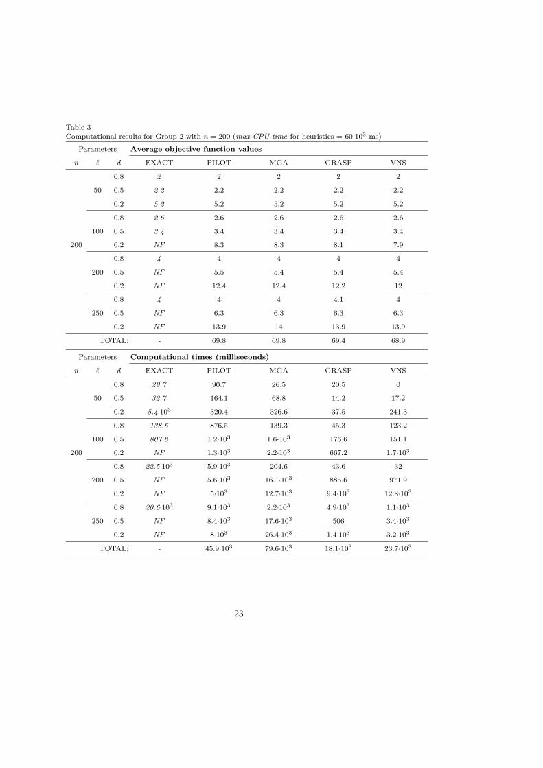
Table 3Computational results for Group 2 with n = 200 (max-CPU-time for heuristics = 60·103 ms)

Parameters Average objective function values

n ` d EXACT PILOT MGA GRASP VNS

0.8 2 2 2 2 2

50 0.5 2.2 2.2 2.2 2.2 2.2

0.2 5.2 5.2 5.2 5.2 5.2

0.8 2.6 2.6 2.6 2.6 2.6

100 0.5 3.4 3.4 3.4 3.4 3.4

200 0.2 NF 8.3 8.3 8.1 7.9

0.8 4 4 4 4 4

200 0.5 NF 5.5 5.4 5.4 5.4

0.2 NF 12.4 12.4 12.2 12

0.8 4 4 4 4.1 4

250 0.5 NF 6.3 6.3 6.3 6.3

0.2 NF 13.9 14 13.9 13.9

TOTAL: - 69.8 69.8 69.4 68.9

Parameters Computational times (milliseconds)

n ` d EXACT PILOT MGA GRASP VNS

0.8 29.7 90.7 26.5 20.5 0

50 0.5 32.7 164.1 68.8 14.2 17.2

0.2 5.4·103 320.4 326.6 37.5 241.3

0.8 138.6 876.5 139.3 45.3 123.2

100 0.5 807.8 1.2·103 1.6·103 176.6 151.1

200 0.2 NF 1.3·103 2.2·103 667.2 1.7·103

0.8 22.5·103 5.9·103 204.6 43.6 32

200 0.5 NF 5.6·103 16.1·103 885.6 971.9

0.2 NF 5·103 12.7·103 9.4·103 12.8·103

0.8 20.6·103 9.1·103 2.2·103 4.9·103 1.1·103

250 0.5 NF 8.4·103 17.6·103 506 3.4·103

0.2 NF 8·103 26.4·103 1.4·103 3.2·103

TOTAL: - 45.9·103 79.6·103 18.1·103 23.7·103

23

Table 4Computational results for Group 2 with n = 500 (max-CPU-time for heuristics = 300·103 ms)

Parameters Average objective function values

n ` d EXACT PILOT MGA GRASP VNS

0.8 2 2 2 2 2

125 0.5 2.6 2.6 2.6 2.6 2.6

0.2 NF 6.3 6.2 6.2 6.2

0.8 3 3 3 3 3

250 0.5 NF 4.2 4.3 4.2 4.1

500 0.2 NF 9.9 10.1 9.9 9.9

0.8 NF 4.8 4.7 4.7 4.7

500 0.5 NF 6.7 7.1 6.5 6.5

0.2 NF 15.9 16.6 15.9 15.8

0.8 NF 5.1 5.4 5.1 5.1

625 0.5 NF 8.1 8.3 7.9 7.9

0.2 NF 18.5 19.1 18.4 18.3

TOTAL: - 87.1 89.4 86.4 86.1

Parameters Computational times (milliseconds)

n ` d EXACT PILOT MGA GRASP VNS

0.8 370 3.4·103 18 152 17.1

125 0.5 597 6.6·103 2.6·103 455 1.1·103

0.2 NF 11.9·103 57.1·103 4·103 3.9·103

0.8 5.3·103 35.49·103 516 248 142.3

250 0.5 NF 65.3·103 28·103 583 84·103

500 0.2 NF 156.4·103 181.2·103 3.3·103 5.1·103

0.8 NF 200.5·103 117.5·103 28.1·103 22.3·103

500 0.5 NF 190.1·103 170.9·103 90.9·103 32.3·103

0.2 NF 300.6·103 241.8·103 20.2·103 139.7·103

0.8 NF 184.3·103 51.9·103 4.9·103 16.1·103

625 0.5 NF 200.9·103 222.2·103 35.7·103 44.7·103

0.2 NF 289.9·103 297.8·103 53.1·103 155.5·103

TOTAL: - 1645.3·103 1371.5·103 213.8·103 504.9·103

24

Table 5Pairwise differences of the average ranks of the algorithms (Critical difference = 0.82 for a significancelevel of 1% for the Nemenyi test)

ALGORITHM (average rank) VNS (1.46) GRASP (1.76) PILOT (3.30) MGA (3.48)

VNS (1.46) - 0.3 1.84 2.02

GRASP (1.76) - - 1.54 1.72

PILOT (3.30) - - - 0.18

MGA (3.48) - - - -

25