Global Warming, Climate Policies and their Consequences on ...
418
HAL Id: tel-03337175 https://tel.archives-ouvertes.fr/tel-03337175 Submitted on 7 Sep 2021 HAL is a multi-disciplinary open access archive for the deposit and dissemination of sci- entific research documents, whether they are pub- lished or not. The documents may come from teaching and research institutions in France or abroad, or from public or private research centers. L’archive ouverte pluridisciplinaire HAL, est destinée au dépôt et à la diffusion de documents scientifiques de niveau recherche, publiés ou non, émanant des établissements d’enseignement et de recherche français ou étrangers, des laboratoires publics ou privés. Global Warming, Climate Policies and their Consequences on the Business Cycle : a general equilibrium Approah Maxime Alexandre Bouter To cite this version: Maxime Alexandre Bouter. Global Warming, Climate Policies and their Consequences on the Business Cycle: a general equilibrium Approah. Economics and Finance. Université de Pau et des Pays de l’Adour, 2021. English. NNT: 2021PAUU2089. tel-03337175
-
Upload
khangminh22 -
Category
Documents
-
view
1 -
download
0
Transcript of Global Warming, Climate Policies and their Consequences on ...

HAL Id: tel-03337175https://tel.archives-ouvertes.fr/tel-03337175
Submitted on 7 Sep 2021
HAL is a multi-disciplinary open accessarchive for the deposit and dissemination of sci-entific research documents, whether they are pub-lished or not. The documents may come fromteaching and research institutions in France orabroad, or from public or private research centers.
L’archive ouverte pluridisciplinaire HAL, estdestinée au dépôt et à la diffusion de documentsscientifiques de niveau recherche, publiés ou non,émanant des établissements d’enseignement et derecherche français ou étrangers, des laboratoirespublics ou privés.
Global Warming, Climate Policies and theirConsequences on the Business Cycle : a general
equilibrium ApproahMaxime Alexandre Bouter
To cite this version:Maxime Alexandre Bouter. Global Warming, Climate Policies and their Consequences on the BusinessCycle : a general equilibrium Approah. Economics and Finance. Université de Pau et des Pays del’Adour, 2021. English. NNT : 2021PAUU2089. tel-03337175

THÈSE UNIVERSITE DE PAU ET DES PAYS DE L’ADOUR École doctorale Sciences Sociales et Humanités
ED - 481
Présentée et soutenue publiquement le 12 mars 2021 par Maxime BOUTER
pour obtenir le grade de docteur
de l’Université de Pau et des Pays de l’Adour Spécialité : Sciences Économiques
Global Warming, Climate Policies and their Consequences on the Business Cycle:
a General Equilibrium Approah
MEMBRES DU JURY RAPPORTEURS • M. Thierry Brechet Professeur des Universités – Université Catholique de Louvain (UCL). • M. Patrick Villieu Professeur des Universités – Université d’Orléans. EXAMINATEURS • M. Christian de Perthuis Professeur des Universités – Université Paris Dauphine. • Mme Katheline Schubert Professeure des Universités – Université Paris 1 Panthéon-Sorbonne. Président du Jury • M. Serge Rey Professeur des Universités – Université de Pau et des Pays de l’Adour. DIRECTEUR • M. Jacques Le Cacheux Professeur des Universités – Université de Pau et des Pays de l’Adour.

II
Contents
Remerciements XXIX
Abstract XXXIII
1 A public policy, for a public good 1
1.1 Introduction . . . . . . . . . . . . . . . . . . . . . . . . . . . . . . . . . . . 1
1.2 The climate change issue . . . . . . . . . . . . . . . . . . . . . . . . . . . . 3
1.2.1 Greenhouse Gases and their Effect on Global Atmospheric Warming: 4
1.2.2 Consequences and feedback effects of climate change . . . . . . . . 5
1.3 The GHG externality and climate as public good . . . . . . . . . . . . . . 7
1.3.1 Greenhouse gases and externalities . . . . . . . . . . . . . . . . . . 7
1.3.2 Possible solutions to climate change . . . . . . . . . . . . . . . . . 9
1.4 Energy and pollution in the business cycle: . . . . . . . . . . . . . . . . . . 13
1.4.1 The role of energy in the business cycle: . . . . . . . . . . . . . . . 13
1.4.2 Pollution and climate policy in the business cycle: . . . . . . . . . 18
2 Irreversibility and global warming 25
2.1 Introduction: . . . . . . . . . . . . . . . . . . . . . . . . . . . . . . . . . . 25
2.2 State of the art and contribution: . . . . . . . . . . . . . . . . . . . . . . . 28
2.3 General assumptions . . . . . . . . . . . . . . . . . . . . . . . . . . . . . . 32
2.4 Planning problem . . . . . . . . . . . . . . . . . . . . . . . . . . . . . . . . 35
2.5 Decentralized competitive equilibrium: . . . . . . . . . . . . . . . . . . . . 39
III
IV CONTENTS
2.5.1 Representative household: . . . . . . . . . . . . . . . . . . . . . . . 39
2.5.2 Firms: . . . . . . . . . . . . . . . . . . . . . . . . . . . . . . . . . . 40
2.5.3 Closing the model: . . . . . . . . . . . . . . . . . . . . . . . . . . . 42
2.6 Calibration: . . . . . . . . . . . . . . . . . . . . . . . . . . . . . . . . . . . 42
2.6.1 Carbon cycle: . . . . . . . . . . . . . . . . . . . . . . . . . . . . . . 43
2.6.2 Preferences and technology parameters: . . . . . . . . . . . . . . . 47
2.7 Simulations: . . . . . . . . . . . . . . . . . . . . . . . . . . . . . . . . . . . 50
2.7.1 General methodology: . . . . . . . . . . . . . . . . . . . . . . . . . 50
2.7.2 Results: . . . . . . . . . . . . . . . . . . . . . . . . . . . . . . . . . 53
2.7.3 Rise in renewable energy productivity: . . . . . . . . . . . . . . . . 60
2.7.4 Robustness: . . . . . . . . . . . . . . . . . . . . . . . . . . . . . . . 70
2.8 Conclusion: . . . . . . . . . . . . . . . . . . . . . . . . . . . . . . . . . . . 75
3 Energy price shock 77
3.1 Introduction: . . . . . . . . . . . . . . . . . . . . . . . . . . . . . . . . . . 77
3.2 Research context: . . . . . . . . . . . . . . . . . . . . . . . . . . . . . . . . 79
3.2.1 The European carbon market subject to failures in the wake of the
2008 financial crisis: . . . . . . . . . . . . . . . . . . . . . . . . . . 79
3.2.2 Carbon tax, Yellow Vests and and fossil fuel price changes: . . . . 82
3.3 State of the art and contribution to the literature: . . . . . . . . . . . . . 86
3.4 The model: . . . . . . . . . . . . . . . . . . . . . . . . . . . . . . . . . . . 88
3.4.1 Households: . . . . . . . . . . . . . . . . . . . . . . . . . . . . . . . 88
3.4.2 Firms: . . . . . . . . . . . . . . . . . . . . . . . . . . . . . . . . . . 90
3.4.3 Climate policy and overall resource constraint: . . . . . . . . . . . 91
3.4.4 Competitive equilibrium . . . . . . . . . . . . . . . . . . . . . . . . 92
3.5 Calibration: . . . . . . . . . . . . . . . . . . . . . . . . . . . . . . . . . . . 94
3.6 Simulations: . . . . . . . . . . . . . . . . . . . . . . . . . . . . . . . . . . . 98
3.6.1 General Methodology: . . . . . . . . . . . . . . . . . . . . . . . . . 98
3.6.2 Technology shock: . . . . . . . . . . . . . . . . . . . . . . . . . . . 99

CONTENTS V
3.6.3 Energy price shock: . . . . . . . . . . . . . . . . . . . . . . . . . . . 102
3.6.4 Sensitivity analysis: . . . . . . . . . . . . . . . . . . . . . . . . . . 106
3.7 Conclusion: . . . . . . . . . . . . . . . . . . . . . . . . . . . . . . . . . . . 114
4 Energy and Monetary policy analysis 117
4.1 Introduction . . . . . . . . . . . . . . . . . . . . . . . . . . . . . . . . . . . 117
4.2 Carbon cycle. General assumptions . . . . . . . . . . . . . . . . . . . . . . 119
4.3 The model . . . . . . . . . . . . . . . . . . . . . . . . . . . . . . . . . . . . 124
4.3.1 Households . . . . . . . . . . . . . . . . . . . . . . . . . . . . . . . 124
4.3.2 Firms . . . . . . . . . . . . . . . . . . . . . . . . . . . . . . . . . . 126
4.3.3 Public policies and environmental taxation . . . . . . . . . . . . . 131
4.3.4 Aggregation and market-clearing conditions . . . . . . . . . . . . . 132
4.4 Calibration: . . . . . . . . . . . . . . . . . . . . . . . . . . . . . . . . . . . 132
4.5 Simulations: . . . . . . . . . . . . . . . . . . . . . . . . . . . . . . . . . . . 136
4.5.1 Simulations for various shocks: . . . . . . . . . . . . . . . . . . . . 137
4.5.2 Robustness: . . . . . . . . . . . . . . . . . . . . . . . . . . . . . . . 146
4.6 Monetary policy analysis . . . . . . . . . . . . . . . . . . . . . . . . . . . . 159
4.6.1 Optimized instrument rules . . . . . . . . . . . . . . . . . . . . . . 160
4.7 Conclusion: . . . . . . . . . . . . . . . . . . . . . . . . . . . . . . . . . . . 171
5 General conclusion: 175
A Chapter 2 technical appendix: 193
A.1 Appendix: rise in renewable energy productivity . . . . . . . . . . . . . . 193
A.2 Technical appendix . . . . . . . . . . . . . . . . . . . . . . . . . . . . . . . 197
A.2.1 Planning problem: . . . . . . . . . . . . . . . . . . . . . . . . . . . 197
A.2.2 Decentralized Competitive Equilibrium: . . . . . . . . . . . . . . . 198
A.2.3 Steady state model: . . . . . . . . . . . . . . . . . . . . . . . . . . 200
A.2.4 Carbon Cycle: . . . . . . . . . . . . . . . . . . . . . . . . . . . . . 203

VI CONTENTS
B Chapter 3 technical appendix: 205
B.1 Appendix: model equilibrium . . . . . . . . . . . . . . . . . . . . . . . . . 205
B.2 Appendix: solving the steady state equilibrium . . . . . . . . . . . . . . . 207
B.3 Simulation results: . . . . . . . . . . . . . . . . . . . . . . . . . . . . . . . 211
B.3.1 Business As Usual: . . . . . . . . . . . . . . . . . . . . . . . . . . . 211
B.3.2 Models with a carbon tax: . . . . . . . . . . . . . . . . . . . . . . . 217
B.3.3 Models with an emissions cap: . . . . . . . . . . . . . . . . . . . . 222
B.3.4 Models with an intensity target: . . . . . . . . . . . . . . . . . . . 228
B.4 Simulations: . . . . . . . . . . . . . . . . . . . . . . . . . . . . . . . . . . . 234
B.5 Sensitivity analysis . . . . . . . . . . . . . . . . . . . . . . . . . . . . . . . 236
C Chapter 4 technical appendix: 239
C.1 Decentralized Competitive Equilibrium: . . . . . . . . . . . . . . . . . . . 239
C.2 Log-Linearized model . . . . . . . . . . . . . . . . . . . . . . . . . . . . . . 258
C.3 Optimal monetary policy: . . . . . . . . . . . . . . . . . . . . . . . . . . . 267
C.3.1 Second-order approximation of instantaneous utility . . . . . . . . 267
C.3.2 Ramsey optimal monetary policy . . . . . . . . . . . . . . . . . . . 271
C.4 Simulations . . . . . . . . . . . . . . . . . . . . . . . . . . . . . . . . . . . 277
C.4.1 IRF to stochastic exogenous shocks: . . . . . . . . . . . . . . . . . 277
C.4.2 Simulations results . . . . . . . . . . . . . . . . . . . . . . . . . . . 291
CONTENTS VII
Abbreviations
AR5 fith Assesment Report
BAU Business As Usual
BTU Britsh Thermal Unit
CDM Clean development mechanism
CSP concentrating solar power
DICE dynamic integrated climate-economy
DSGE Dynamic Stochastic General Equilibrium
EKC environmental Kuznet curve
eq. equivalent
ETS Emissions trading system
FOC first order conditions
GHG greenhouse gas
Gt Gigaton
GW Giga Watt
GWP Global warming potential
IPCC Intergovernmental Panel on Climate Change
kW kilo Watt
kWh kilo Watt hour
LCOE Levelized cost of energy
LHS left-hand side
VIII CONTENTS
LULCF Land Use Land Use and Change and Forestry
Mbd Million barrels per day
Mtoe Million ton of oil equivalent
MW Mega Watt
OECD Organisation for economic co-operation and development
ppm parts per million
RHS right-hand side
RICE regional integrated climate-economy
TWh Terawatt-hour

CONTENTS IX
Nomenclature
CO2 carbon dioxyde
CH4 methane
N2O nitrous oxyde

X CONTENTS
List of Figures
1.1 Monthly crude oil price index 2016 = 100 . . . . . . . . . . . . . . . . . . 15
1.2 Oil production cost curve - Source: Rystad Energy Research . . . . . . . 17
2.1 Kaya’s identity for the world - Source: IEA . . . . . . . . . . . . . . . . . 32
2.2 Emissions intensity per fossil fuel unit . . . . . . . . . . . . . . . . . . . . 46
2.3 GHG emissions flow and atmospheric stock. . . . . . . . . . . . . . . . . . 54
2.4 Rise in temperature above the pre-industrial levels . . . . . . . . . . . . . 55
2.5 GHG atmospheric stock and its consequences in terms of temperature and
damages. . . . . . . . . . . . . . . . . . . . . . . . . . . . . . . . . . . . . . 57
2.6 Main economic variables of the stationary model: . . . . . . . . . . . . . . 58
2.7 Energy block: . . . . . . . . . . . . . . . . . . . . . . . . . . . . . . . . . . 60
2.8 Rise in clean energy productivity . . . . . . . . . . . . . . . . . . . . . . . 63
2.9 BAU scenarios and consequences on emission flow and atmospheric stock . 64
2.10 GHG emission flow and GHG atmospheric stock with carbon tax . . . . . 65
2.11 Consumption . . . . . . . . . . . . . . . . . . . . . . . . . . . . . . . . . . 67
2.12 Production . . . . . . . . . . . . . . . . . . . . . . . . . . . . . . . . . . . 68
2.13 Fossil fuel uses . . . . . . . . . . . . . . . . . . . . . . . . . . . . . . . . . 69
2.14 Robustness for different values of n99 . . . . . . . . . . . . . . . . . . . . . 72
2.15 Robustness for different values of n50 . . . . . . . . . . . . . . . . . . . . . 72
3.1 EU ETS allowance price (e/ton) . . . . . . . . . . . . . . . . . . . . . . . 80
XI
XII LIST OF FIGURES
3.2 French retail fuel price (e/l), panel A: with taxes, panel B : without tax.
Source: European Commission . . . . . . . . . . . . . . . . . . . . . . . . 84
3.3 Share of global oil production per country - Source: BP . . . . . . . . . . 86
3.4 Impulse response functions to a TFP shock (1/2) . . . . . . . . . . . . . . 101
3.5 Impulse response functions to a TFP shock (2/2) . . . . . . . . . . . . . . 102
3.6 IRF to an energy price shock (1/2) . . . . . . . . . . . . . . . . . . . . . . 105
3.7 IRF to an energy price shock (2/2) . . . . . . . . . . . . . . . . . . . . . . 105
3.8 IRF to a TFP shock in the BAU (1/2) . . . . . . . . . . . . . . . . . . . . 108
3.9 IRF to a TFP shock in the BAU (2/2) . . . . . . . . . . . . . . . . . . . . 109
3.10 IRF to an energy price shock in the BAU (1/2) . . . . . . . . . . . . . . . 109
3.11 IRF to an energy price shock in the BAU (2/2) . . . . . . . . . . . . . . . 110
3.12 IRF to a TFP shock in the carbon tax scenario (1/2) . . . . . . . . . . . . 110
3.13 IRF to a TFP shock in the carbon tax scenario (2/2) . . . . . . . . . . . . 111
3.14 IRF to an energy price shock in the carbon tax scenario (1/2) . . . . . . . 111
3.15 IRF to an energy price shock in the carbon tax scenario (2/2) . . . . . . . 112
3.16 The role of utilisation rate of capital(1/2) . . . . . . . . . . . . . . . . . . 112
3.17 The role of utilisation rate of capital (2/2) . . . . . . . . . . . . . . . . . . 113
3.18 IRF to a TFP shock shock in the intensity target scenario (1/2) . . . . . . 113
3.19 IRF to a TFP shock shock in the intensity target scenario (2/2) . . . . . . 114
4.1 Impulse responses functions (IRF) to a total factor productivity (TFP)
shock (1/3) - red dotted line: cap-and-trade market; black dotted line:
carbon tax . . . . . . . . . . . . . . . . . . . . . . . . . . . . . . . . . . . . 139
4.2 IRF to a TFP shock (2/3) - red dotted line: cap-and-trade market; black
dotted line: carbon tax . . . . . . . . . . . . . . . . . . . . . . . . . . . . . 139
4.3 IRF to a TFP shock (3/3) - red dotted line: cap-and-trade market; black
dotted line: carbon tax . . . . . . . . . . . . . . . . . . . . . . . . . . . . . 140
4.4 IRF to a productivity shock in the polluting sector (1/3) - red dotted line:
cap-and-trade market; black dotted line: carbon tax . . . . . . . . . . . . 143
LIST OF FIGURES XIII
4.5 IRF to a productivity shock in the polluting sector (2/3) - red dotted line:
cap-and-trade market; black dotted line: carbon tax . . . . . . . . . . . . 143
4.6 IRF to a productivity shock in the polluting sector (3/3) - red dotted line:
cap-and-trade market; black dotted line: carbon tax . . . . . . . . . . . . 144
4.7 IRF to a productivity shock in the non-polluting sector (1/3) - red dotted
line: cap-and-trade market; black dotted line: carbon tax . . . . . . . . . 145
4.8 IRF to a productivity shock in the non-polluting sector (2/3) - red dotted
line: cap-and-trade market; black dotted line: carbon tax . . . . . . . . . 145
4.9 IRF to a productivity shock in the non-polluting sector (3/3) - red dotted
line: cap-and-trade market; black dotted line: carbon tax . . . . . . . . . 146
4.10 IRF to a productivity shock in the polluting sector in a carbon tax regime
(1/3) - black dotted line : ε = 0.51; red dashed line ε = 1.22; blue dashed
line ε = 1.85 . . . . . . . . . . . . . . . . . . . . . . . . . . . . . . . . . . . 149
4.11 IRF to a productivity shock in the polluting sector in a carbon tax regime
(2/3) - black dotted line : ε = 0.51; red dashed line ε = 1.22; blue dashed
line ε = 1.85 . . . . . . . . . . . . . . . . . . . . . . . . . . . . . . . . . . . 149
4.12 IRF to a productivity shock in the polluting sector in a carbon tax regime
(3/3) - black dotted line : ε = 0.51; red dashed line ε = 1.22; blue dashed
line ε = 1.85 . . . . . . . . . . . . . . . . . . . . . . . . . . . . . . . . . . . 150
4.13 IRF to a productivity shock in the non-polluting sector in a carbon tax
regime (1/3) - black dotted line : ε = 0.51; red dashed line ε = 1.22; blue
dashed line ε = 1.85 . . . . . . . . . . . . . . . . . . . . . . . . . . . . . . 151
4.14 IRF to a productivity shock in the non-polluting sector in a carbon tax
regime (2/3) - black dotted line : ε = 0.51; red dashed line ε = 1.22; blue
dashed line ε = 1.85 . . . . . . . . . . . . . . . . . . . . . . . . . . . . . . 152
4.15 IRF to a productivity shock in the non-polluting sector in a carbon tax
regime (3/3) - black dotted line : ε = 0.51; red dashed line ε = 1.22; blue
dashed line ε = 1.85 . . . . . . . . . . . . . . . . . . . . . . . . . . . . . . 153
XIV LIST OF FIGURES
4.16 IRF to a productivity shock in the polluting sector in an emission cap
regime (1/3) - black dotted line : ε = 0.51; red dashed line ε = 1.22; blue
dashed line ε = 1.85 . . . . . . . . . . . . . . . . . . . . . . . . . . . . . . 154
4.17 IRF to a productivity shock in the polluting sector in an emission cap
regime (2/3) - black dotted line : ε = 0.51; red dashed line ε = 1.22; blue
dashed line ε = 1.85 . . . . . . . . . . . . . . . . . . . . . . . . . . . . . . 155
4.18 IRF to a productivity shock in the polluting sector in an emission cap
regime (3/3) - black dotted line : ε = 0.51; red dashed line ε = 1.22; blue
dashed line ε = 1.85 . . . . . . . . . . . . . . . . . . . . . . . . . . . . . . 156
4.19 IRF to a productivity shock in the non-polluting sector in an emission cap
regime (1/3) - black dotted line : ε = 0.51; red dashed line ε = 1.22; blue
dashed line ε = 1.85 . . . . . . . . . . . . . . . . . . . . . . . . . . . . . . 157
4.20 IRF to a productivity shock in the non-polluting sector in an emission cap
regime (2/3) - black dotted line : ε = 0.51; red dashed line ε = 1.22; blue
dashed line ε = 1.85 . . . . . . . . . . . . . . . . . . . . . . . . . . . . . . 158
4.21 IRF to a productivity shock in the non-polluting sector in an emission cap
regime (3/3) - black dotted line : ε = 0.51; red dashed line ε = 1.22; blue
dashed line ε = 1.85 . . . . . . . . . . . . . . . . . . . . . . . . . . . . . . 159
4.22 Monetary policy optimized coefficients and household welfare . . . . . . . 165
4.23 Standard deviations for different monetary policies . . . . . . . . . . . . . 165
4.24 Contributions of variables to household’s welfare . . . . . . . . . . . . . . 166
4.25 Monetary policy optimized coefficients and household welfare . . . . . . . 170
4.26 Standard deviations for different monetary policies . . . . . . . . . . . . . 170
4.27 Contributions of variables to household’s welfare . . . . . . . . . . . . . . 171
A.1 Stock of capital . . . . . . . . . . . . . . . . . . . . . . . . . . . . . . . . . 193
A.2 Stationnarized model: . . . . . . . . . . . . . . . . . . . . . . . . . . . . . 194
A.3 Labor in the global sector: . . . . . . . . . . . . . . . . . . . . . . . . . . . 194
A.4 Fossil fuel price: . . . . . . . . . . . . . . . . . . . . . . . . . . . . . . . . . 195
LIST OF FIGURES XV
A.5 Green energy price: . . . . . . . . . . . . . . . . . . . . . . . . . . . . . . . 195
A.6 Labor in the fossil fuel sector: . . . . . . . . . . . . . . . . . . . . . . . . . 196
A.7 Labor in the ren. energy sector: . . . . . . . . . . . . . . . . . . . . . . . . 196
B.1 Variables simulated for a total factor productivity shock . . . . . . . . . . 235
C.1 IRF to a risk premium shock in a carbon tax regime (1/3) - black dotted
line : ε = 0.51; red dashed line ε = 1.22; blue dashed line ε = 1.85 . . . . . 277
C.2 IRF to a risk premium shock in a carbon tax regime (2/3) - black dotted
line : ε = 0.51; red dashed line ε = 1.22; blue dashed line ε = 1.85 . . . . . 278
C.3 IRF to a risk premium shock in a carbon tax regime (3/3) - black dotted
line : ε = 0.51; red dashed line ε = 1.22; blue dashed line ε = 1.85 . . . . . 278
C.4 IRF to a risk premium shock in a carbon tax regime (1/3) - black dotted
line : ε = 0.51; red dashed line ε = 1.22; blue dashed line ε = 1.85 . . . . . 279
C.5 IRF to a risk premium shock in a carbon tax regime (2/3) - black dotted
line : ε = 0.51; red dashed line ε = 1.22; blue dashed line ε = 1.85 . . . . . 279
C.6 IRF to a risk premium shock in a carbon tax regime (3/3) - black dotted
line : ε = 0.51; red dashed line ε = 1.22; blue dashed line ε = 1.85 . . . . . 280
C.7 IRF to an investment shock in a carbon tax regime (1/3) - black dotted
line : ε = 0.51; red dashed line ε = 1.22; blue dashed line ε = 1.85 . . . . . 280
C.8 IRF to an investment shock in a carbon tax regime (2/3) - black dotted
line : ε = 0.51; red dashed line ε = 1.22; blue dashed line ε = 1.85 . . . . . 281
C.9 IRF to an investment shock in a carbon tax regime (3/3) - black dotted
line : ε = 0.51; red dashed line ε = 1.22; blue dashed line ε = 1.85 . . . . . 281
C.10 IRF to an investment shock in a carbon tax regime (1/3) - black dotted
line : ε = 0.51; red dashed line ε = 1.22; blue dashed line ε = 1.85 . . . . . 282
C.11 IRF to an investment shock in a carbon tax regime (2/3) - black dotted
line : ε = 0.51; red dashed line ε = 1.22; blue dashed line ε = 1.85 . . . . . 282
C.12 IRF to an investment shock in a carbon tax regime (3/3) - black dotted
line : ε = 0.51; red dashed line ε = 1.22; blue dashed line ε = 1.85 . . . . . 283
XVI LIST OF FIGURES
C.13 IRF to an inflation shock in a carbon tax regime (1/3) - black dotted line
: ε = 0.51; red dashed line ε = 1.22; blue dashed line ε = 1.85 . . . . . . . 283
C.14 IRF to an inflation shock in a carbon tax regime (2/3) - black dotted line
: ε = 0.51; red dashed line ε = 1.22; blue dashed line ε = 1.85 . . . . . . . 284
C.15 IRF to an inflation shock in a carbon tax regime (3/3) - black dotted line
: ε = 0.51; red dashed line ε = 1.22; blue dashed line ε = 1.85 . . . . . . . 284
C.16 IRF to an inflation shock in a carbon tax regime (1/3) - black dotted line
: ε = 0.51; red dashed line ε = 1.22; blue dashed line ε = 1.85 . . . . . . . 285
C.17 IRF to an inflation shock in a carbon tax regime (2/3) - black dotted line
: ε = 0.51; red dashed line ε = 1.22; blue dashed line ε = 1.85 . . . . . . . 285
C.18 IRF to an inflation shock in a carbon tax regime (3/3) - black dotted line
: ε = 0.51; red dashed line ε = 1.22; blue dashed line ε = 1.85 . . . . . . . 286
C.19 IRF to a government spending shock in a carbon tax regime (1/3) - black
dotted line : ε = 0.51; red dashed line ε = 1.22; blue dashed line ε = 1.85 . 286
C.20 IRF to a government spending shock in a carbon tax regime (2/3) - black
dotted line : ε = 0.51; red dashed line ε = 1.22; blue dashed line ε = 1.85 . 287
C.21 IRF to a government spending shock in a carbon tax regime (3/3) - black
dotted line : ε = 0.51; red dashed line ε = 1.22; blue dashed line ε = 1.85 . 287
C.22 IRF to a government spending shock in a carbon tax regime (1/3) - black
dotted line : ε = 0.51; red dashed line ε = 1.22; blue dashed line ε = 1.85 . 288
C.23 IRF to a government spending shock in a carbon tax regime (2/3) - black
dotted line : ε = 0.51; red dashed line ε = 1.22; blue dashed line ε = 1.85 . 288
C.24 IRF to a government spending shock in a carbon tax regime (3/3) - black
dotted line : ε = 0.51; red dashed line ε = 1.22; blue dashed line ε = 1.85 . 289
C.25 IRF to a carbon tax shock in a carbon tax regime (1/3) - black dotted line
: ε = 0.51; red dashed line ε = 1.22; blue dashed line ε = 1.85 . . . . . . . 289
C.26 IRF to a carbon tax shock in a carbon tax regime (2/3) - black dotted line
: ε = 0.51; red dashed line ε = 1.22; blue dashed line ε = 1.85 . . . . . . . 290

LIST OF FIGURES XVII
C.27 IRF to a carbon tax shock in a carbon tax regime (3/3) - black dotted line
: ε = 0.51; red dashed line ε = 1.22; blue dashed line ε = 1.85 . . . . . . . 290

XVIII LIST OF FIGURES
List of Tables
2.1 Global warming potential (GWP) . . . . . . . . . . . . . . . . . . . . . . . 43
2.2 Global GHG emissions by gas (Gt-CO2 eq.) . . . . . . . . . . . . . . . . . 44
2.3 Elasticity of substitution . . . . . . . . . . . . . . . . . . . . . . . . . . . . 50
2.4 US average depth of oil and natural gas wells drilled (feet per well) . . . . 61
3.1 Level of the French carbon tax, before the Yellow Vests movements . . . . 82
3.2 Carbon tax per product: . . . . . . . . . . . . . . . . . . . . . . . . . . . . 84
3.3 OPEC’s oil production (thousand barrels per day) . . . . . . . . . . . . . 85
3.4 Variables and parameters calibration . . . . . . . . . . . . . . . . . . . . . 96
3.5 Steady state ratios . . . . . . . . . . . . . . . . . . . . . . . . . . . . . . . 97
3.6 Variables mean and standard deviation . . . . . . . . . . . . . . . . . . . 99
3.7 Variables mean and standard deviation when utilisation rate is constant . 108
4.1 Elasticity of substitution between polluting and non-polluting energies . . 147
4.2 Optimized coefficients for monetary policy rules . . . . . . . . . . . . . . . 164
4.3 Optimized coefficients for monetary policy rules . . . . . . . . . . . . . . . 169
B.1 Moments of simulated variables with variable depreciation rate of capital
- BAU . . . . . . . . . . . . . . . . . . . . . . . . . . . . . . . . . . . . . . 211
B.2 Autocorrelation of simulated variables with variable depreciation of capital
- BAU . . . . . . . . . . . . . . . . . . . . . . . . . . . . . . . . . . . . . . 212
B.3 Variance decomposition simulating one shock at a time (in percent) - BAU 212
XIX
XX LIST OF TABLES
B.3 (continued) . . . . . . . . . . . . . . . . . . . . . . . . . . . . . . . . . . . 213
B.4 Moments of simulated variables with constant depreciation rate of capital-
BAU . . . . . . . . . . . . . . . . . . . . . . . . . . . . . . . . . . . . . . 213
B.4 (continued) . . . . . . . . . . . . . . . . . . . . . . . . . . . . . . . . . . . 214
B.5 Autocorrelation of simulated variables with constant depreciation rate of
capital - BAU . . . . . . . . . . . . . . . . . . . . . . . . . . . . . . . . . 214
B.5 (continued) . . . . . . . . . . . . . . . . . . . . . . . . . . . . . . . . . . . 215
B.6 Variance decomposition simulating one shock at a time with constant de-
preciation rate of capital (in percent)- BAU . . . . . . . . . . . . . . . . . 215
B.6 (continued) . . . . . . . . . . . . . . . . . . . . . . . . . . . . . . . . . . . 216
B.7 Matrix of covariance of exogenous shocks . . . . . . . . . . . . . . . . . . . 216
B.8 Moments of simulated variables with variable depreciation rate of capital
- carbon tax . . . . . . . . . . . . . . . . . . . . . . . . . . . . . . . . . . 217
B.9 Autocorrelation of simulated variables with variable depreciation rate of
capital - carbon tax . . . . . . . . . . . . . . . . . . . . . . . . . . . . . . . 218
B.10 Variance decomposition simulating one shock at a time with variable de-
preciation rate of capital (in percent)- carbon tax . . . . . . . . . . . . . . 219
B.11 Moments of simulated variables with constant depreciation rate of capital-
carbon tax . . . . . . . . . . . . . . . . . . . . . . . . . . . . . . . . . . . . 220
B.12 Autocorrelation of simulated variables with constant depreciation rate of
capital - carbon tax . . . . . . . . . . . . . . . . . . . . . . . . . . . . . . . 220
B.12 (continued) . . . . . . . . . . . . . . . . . . . . . . . . . . . . . . . . . . . 221
B.13 Variance decomposition simulating one shock at a time with constant de-
preciation rate of capital (in percent)- carbon tax . . . . . . . . . . . . . . 221
B.13 (continued) . . . . . . . . . . . . . . . . . . . . . . . . . . . . . . . . . . . 222
B.14 Moments of simulated variables with variable depreciation rate of capital
- cap-and-trade . . . . . . . . . . . . . . . . . . . . . . . . . . . . . . . . . 222
B.14 (continued) . . . . . . . . . . . . . . . . . . . . . . . . . . . . . . . . . . . 223
LIST OF TABLES XXI
B.15 Autocorrelation of simulated variables with variable depreciation rate of
capital - cap-and-trade . . . . . . . . . . . . . . . . . . . . . . . . . . . . . 223
B.15 (continued) . . . . . . . . . . . . . . . . . . . . . . . . . . . . . . . . . . . 224
B.16 Variance decomposition simulating one shock at a time with variable de-
preciation rate of capital(in percent) - cap-and-trade . . . . . . . . . . . . 224
B.16 (continued) . . . . . . . . . . . . . . . . . . . . . . . . . . . . . . . . . . . 225
B.17 Moments of simulated variables with constant depreciation rate of capital
- cap-and-trade . . . . . . . . . . . . . . . . . . . . . . . . . . . . . . . . . 225
B.17 (continued) . . . . . . . . . . . . . . . . . . . . . . . . . . . . . . . . . . . 226
B.18 Autocorrelation of simulated variables with constant depreciation rate of
capital - cap-and-trade . . . . . . . . . . . . . . . . . . . . . . . . . . . . . 226
B.18 (continued) . . . . . . . . . . . . . . . . . . . . . . . . . . . . . . . . . . . 227
B.19 Variance decomposition simulating one shock at a time with constant de-
preciation rate of capital(in percent) - cap-and-trade . . . . . . . . . . . . 227
B.19 (continued) . . . . . . . . . . . . . . . . . . . . . . . . . . . . . . . . . . . 228
B.20 Moments of simulated variables with variable depreciation rate of capital
- intensity target . . . . . . . . . . . . . . . . . . . . . . . . . . . . . . . . 228
B.20 (continued) . . . . . . . . . . . . . . . . . . . . . . . . . . . . . . . . . . . 229
B.21 Autocorrelation of simulated variables with variable depreciation rate of
capital - intensity target . . . . . . . . . . . . . . . . . . . . . . . . . . . . 229
B.21 (continued) . . . . . . . . . . . . . . . . . . . . . . . . . . . . . . . . . . . 230
B.22 Variance decomposition simulating one shock at a time with variable de-
preciation rate of capital (in percent) - intensity target . . . . . . . . . . . 230
B.22 (continued) . . . . . . . . . . . . . . . . . . . . . . . . . . . . . . . . . . . 231
B.23 Moments of simulated variables with constant depreciation rate of capital
- intensity target . . . . . . . . . . . . . . . . . . . . . . . . . . . . . . . . 231
B.23 (continued) . . . . . . . . . . . . . . . . . . . . . . . . . . . . . . . . . . . 232
B.24 Autocorrelation of simulated variables with constant depreciation rate of
capital - intensity target . . . . . . . . . . . . . . . . . . . . . . . . . . . . 232
XXII LIST OF TABLES
B.24 (continued) . . . . . . . . . . . . . . . . . . . . . . . . . . . . . . . . . . . 233
B.25 Variance decomposition simulating one shock at a time with constant de-
preciation rate of capital - intensity target . . . . . . . . . . . . . . . . . . 233
B.26 steady state value for different discount factor . . . . . . . . . . . . . . . . 236
B.27 steady state value for different depreciation rate of capital . . . . . . . . . 237
C.1 Theoretical moments for an elasticity of substitution of ε = 0.51 with a
carbon tax . . . . . . . . . . . . . . . . . . . . . . . . . . . . . . . . . . . . 291
C.1 (continued) . . . . . . . . . . . . . . . . . . . . . . . . . . . . . . . . . . . 292
C.1 (continued) . . . . . . . . . . . . . . . . . . . . . . . . . . . . . . . . . . . 293
C.2 Variance decomposition (in percent) for an elasticity of substitution of
ε = 0.51 with a carbon tax . . . . . . . . . . . . . . . . . . . . . . . . . . . 294
C.2 (continued) . . . . . . . . . . . . . . . . . . . . . . . . . . . . . . . . . . . 295
C.2 (continued) . . . . . . . . . . . . . . . . . . . . . . . . . . . . . . . . . . . 296
C.3 Coefficients of autocorrelation for an elasticity of substitution of ε = 0.51
with a carbon tax . . . . . . . . . . . . . . . . . . . . . . . . . . . . . . . . 297
C.3 (continued) . . . . . . . . . . . . . . . . . . . . . . . . . . . . . . . . . . . 298
C.3 (continued) . . . . . . . . . . . . . . . . . . . . . . . . . . . . . . . . . . . 299
C.4 Theoretical moments for an elasticity of substitution of ε = 0.95 with a
carbon tax . . . . . . . . . . . . . . . . . . . . . . . . . . . . . . . . . . . . 300
C.4 (continued) . . . . . . . . . . . . . . . . . . . . . . . . . . . . . . . . . . . 301
C.4 (continued) . . . . . . . . . . . . . . . . . . . . . . . . . . . . . . . . . . . 302
C.5 Variance decomposition (in percent) for an elasticity of substitution of
ε = 0.95 with a carbon tax . . . . . . . . . . . . . . . . . . . . . . . . . . . 303
C.5 (continued) . . . . . . . . . . . . . . . . . . . . . . . . . . . . . . . . . . . 304
C.5 (continued) . . . . . . . . . . . . . . . . . . . . . . . . . . . . . . . . . . . 305
C.6 Coefficients of autocorrelation for an elasticity of substitution of ε = 0.95
with a carbon tax . . . . . . . . . . . . . . . . . . . . . . . . . . . . . . . . 306
C.6 (continued) . . . . . . . . . . . . . . . . . . . . . . . . . . . . . . . . . . . 307
LIST OF TABLES XXIII
C.6 (continued) . . . . . . . . . . . . . . . . . . . . . . . . . . . . . . . . . . . 308
C.7 Theoretical moments for an elasticity of substitution of ε = 1.008 with a
carbon tax . . . . . . . . . . . . . . . . . . . . . . . . . . . . . . . . . . . . 309
C.7 (continued) . . . . . . . . . . . . . . . . . . . . . . . . . . . . . . . . . . . 310
C.7 (continued) . . . . . . . . . . . . . . . . . . . . . . . . . . . . . . . . . . . 311
C.8 Variance decomposition (in percent) for an elasticity of substitution of
ε = 1.008 with a carbon tax . . . . . . . . . . . . . . . . . . . . . . . . . . 312
C.8 (continued) . . . . . . . . . . . . . . . . . . . . . . . . . . . . . . . . . . . 313
C.8 (continued) . . . . . . . . . . . . . . . . . . . . . . . . . . . . . . . . . . . 314
C.9 Coefficients of autocorrelation for an elasticity of substitution of ε = 1.008
with a carbon tax . . . . . . . . . . . . . . . . . . . . . . . . . . . . . . . . 315
C.9 (continued) . . . . . . . . . . . . . . . . . . . . . . . . . . . . . . . . . . . 316
C.9 (continued) . . . . . . . . . . . . . . . . . . . . . . . . . . . . . . . . . . . 317
C.10 Theoretical moments for an elasticity of substitution of ε = 1.22 with a
carbon tax . . . . . . . . . . . . . . . . . . . . . . . . . . . . . . . . . . . . 318
C.10 (continued) . . . . . . . . . . . . . . . . . . . . . . . . . . . . . . . . . . . 319
C.10 (continued) . . . . . . . . . . . . . . . . . . . . . . . . . . . . . . . . . . . 320
C.11 Variance decomposition (in percent) for an elasticity of substitution of
ε = 1.22 with a carbon tax . . . . . . . . . . . . . . . . . . . . . . . . . . . 321
C.11 (continued) . . . . . . . . . . . . . . . . . . . . . . . . . . . . . . . . . . . 322
C.11 (continued) . . . . . . . . . . . . . . . . . . . . . . . . . . . . . . . . . . . 323
C.12 Coefficients of autocorrelation for an elasticity of substitution of ε = 1.22
with a carbon tax . . . . . . . . . . . . . . . . . . . . . . . . . . . . . . . . 324
C.12 (continued) . . . . . . . . . . . . . . . . . . . . . . . . . . . . . . . . . . . 325
C.12 (continued) . . . . . . . . . . . . . . . . . . . . . . . . . . . . . . . . . . . 326
C.13 Theoretical moments for an elasticity of substitution of ε = 1.85 with a
carbon tax . . . . . . . . . . . . . . . . . . . . . . . . . . . . . . . . . . . . 327
C.13 (continued) . . . . . . . . . . . . . . . . . . . . . . . . . . . . . . . . . . . 328
C.13 (continued) . . . . . . . . . . . . . . . . . . . . . . . . . . . . . . . . . . . 329
XXIV LIST OF TABLES
C.14 Variance decomposition (in percent) for an elasticity of substitution of
ε = 1.85 with a carbon tax . . . . . . . . . . . . . . . . . . . . . . . . . . . 330
C.14 (continued) . . . . . . . . . . . . . . . . . . . . . . . . . . . . . . . . . . . 331
C.14 (continued) . . . . . . . . . . . . . . . . . . . . . . . . . . . . . . . . . . . 332
C.15 Coefficients of autocorrelation for an elasticity of substitution of ε = 1.85
with a carbon tax . . . . . . . . . . . . . . . . . . . . . . . . . . . . . . . . 333
C.15 (continued) . . . . . . . . . . . . . . . . . . . . . . . . . . . . . . . . . . . 334
C.15 (continued) . . . . . . . . . . . . . . . . . . . . . . . . . . . . . . . . . . . 335
C.16 Matrix of covariance of exogenous shocks - models with a carbon tax . . . 336
C.17 Theoretical moments for an elasticity of substitution of ε = 0.51 with an
emission cap . . . . . . . . . . . . . . . . . . . . . . . . . . . . . . . . . . . 337
C.17 (continued) . . . . . . . . . . . . . . . . . . . . . . . . . . . . . . . . . . . 338
C.17 (continued) . . . . . . . . . . . . . . . . . . . . . . . . . . . . . . . . . . . 339
C.18 Coefficients of autocorrelation for an elasticity of substitution of ε = 0.51
with an emission cap . . . . . . . . . . . . . . . . . . . . . . . . . . . . . . 340
C.18 (continued) . . . . . . . . . . . . . . . . . . . . . . . . . . . . . . . . . . . 341
C.18 (continued) . . . . . . . . . . . . . . . . . . . . . . . . . . . . . . . . . . . 342
C.19 Variance decomposition (in percent) for an elasticity of substitution of
ε = 0.51 with an emission cap . . . . . . . . . . . . . . . . . . . . . . . . . 343
C.19 (continued) . . . . . . . . . . . . . . . . . . . . . . . . . . . . . . . . . . . 344
C.19 (continued) . . . . . . . . . . . . . . . . . . . . . . . . . . . . . . . . . . . 345
C.20 Theoretical moments for an elasticity of substitution of ε = 0.95 with an
emission cap . . . . . . . . . . . . . . . . . . . . . . . . . . . . . . . . . . . 346
C.20 (continued) . . . . . . . . . . . . . . . . . . . . . . . . . . . . . . . . . . . 347
C.20 (continued) . . . . . . . . . . . . . . . . . . . . . . . . . . . . . . . . . . . 348
C.21 Coefficients of autocorrelation for an elasticity of substitution of ε = 0.95
with an emission cap . . . . . . . . . . . . . . . . . . . . . . . . . . . . . . 349
C.21 (continued) . . . . . . . . . . . . . . . . . . . . . . . . . . . . . . . . . . . 350
C.21 (continued) . . . . . . . . . . . . . . . . . . . . . . . . . . . . . . . . . . . 351
LIST OF TABLES XXV
C.22 Variance decomposition (in percent) for an elasticity of substitution of
ε = 0.95 with an emission cap . . . . . . . . . . . . . . . . . . . . . . . . . 352
C.22 (continued) . . . . . . . . . . . . . . . . . . . . . . . . . . . . . . . . . . . 353
C.22 (continued) . . . . . . . . . . . . . . . . . . . . . . . . . . . . . . . . . . . 354
C.23 Theoretical moments for an elasticity of substitution of ε = 1.008 with an
emission cap . . . . . . . . . . . . . . . . . . . . . . . . . . . . . . . . . . . 355
C.23 (continued) . . . . . . . . . . . . . . . . . . . . . . . . . . . . . . . . . . . 356
C.23 (continued) . . . . . . . . . . . . . . . . . . . . . . . . . . . . . . . . . . . 357
C.24 Coefficients of autocorrelation for an elasticity of substitution of ε = 1.008
with an emission cap . . . . . . . . . . . . . . . . . . . . . . . . . . . . . . 358
C.24 (continued) . . . . . . . . . . . . . . . . . . . . . . . . . . . . . . . . . . . 359
C.24 (continued) . . . . . . . . . . . . . . . . . . . . . . . . . . . . . . . . . . . 360
C.25 Variance decomposition (in percent) for an elasticity of substitution of
ε = 1.008 with an emission cap . . . . . . . . . . . . . . . . . . . . . . . . 361
C.25 (continued) . . . . . . . . . . . . . . . . . . . . . . . . . . . . . . . . . . . 362
C.25 (continued) . . . . . . . . . . . . . . . . . . . . . . . . . . . . . . . . . . . 363
C.26 Theoretical moments for an elasticity of substitution of ε = 1.22 with an
emission cap . . . . . . . . . . . . . . . . . . . . . . . . . . . . . . . . . . . 364
C.26 (continued) . . . . . . . . . . . . . . . . . . . . . . . . . . . . . . . . . . . 365
C.26 (continued) . . . . . . . . . . . . . . . . . . . . . . . . . . . . . . . . . . . 366
C.27 Coefficients of autocorrelation for an elasticity of substitution of ε = 1.22
with an emission cap . . . . . . . . . . . . . . . . . . . . . . . . . . . . . . 367
C.27 (continued) . . . . . . . . . . . . . . . . . . . . . . . . . . . . . . . . . . . 368
C.27 (continued) . . . . . . . . . . . . . . . . . . . . . . . . . . . . . . . . . . . 369
C.28 Variance decomposition (in percent) for an elasticity of substitution of
ε = 1.22 with an emission cap . . . . . . . . . . . . . . . . . . . . . . . . . 370
C.28 (continued) . . . . . . . . . . . . . . . . . . . . . . . . . . . . . . . . . . . 371
C.28 (continued) . . . . . . . . . . . . . . . . . . . . . . . . . . . . . . . . . . . 372
XXVI LIST OF TABLES
C.29 Theoretical moments for an elasticity of substitution of ε = 1.85 with an
emission cap . . . . . . . . . . . . . . . . . . . . . . . . . . . . . . . . . . . 373
C.29 (continued) . . . . . . . . . . . . . . . . . . . . . . . . . . . . . . . . . . . 374
C.29 (continued) . . . . . . . . . . . . . . . . . . . . . . . . . . . . . . . . . . . 375
C.30 Coefficients of autocorrelation for an elasticity of substitution of ε = 1.85
with an emission cap . . . . . . . . . . . . . . . . . . . . . . . . . . . . . . 376
C.30 (continued) . . . . . . . . . . . . . . . . . . . . . . . . . . . . . . . . . . . 377
C.30 (continued) . . . . . . . . . . . . . . . . . . . . . . . . . . . . . . . . . . . 378
C.31 Variance decomposition (in percent) for an elasticity of substitution of
ε = 1.85 with an emission cap . . . . . . . . . . . . . . . . . . . . . . . . . 379
C.31 (continued) . . . . . . . . . . . . . . . . . . . . . . . . . . . . . . . . . . . 380
C.31 (continued) . . . . . . . . . . . . . . . . . . . . . . . . . . . . . . . . . . . 381
C.32 Matrix of covariance of exogenous shocks with an emission cap . . . . . . 382

À mes parents.

XXVIII LIST OF TABLES
Remerciements
Comme le disait si bien ce cher Edouard Baer, à qui je rends hommage en lui empruntant
ces quelques mots, si je devais résumer ma thèse aujourd’hui avec vous, je dirais c’est
d’abord des rencontres, des gens qui m’ont tendu la main, peut-être à un moment où je
ne pouvais pas, où j’étais seul chez moi. Et c’est assez curieux de se dire que les hasards,
les rencontres forgent une destinée. Parce que quand on a le goût de la recherche bien
faite, le beau geste, parfois on ne trouve pas l’interlocuteur en face, je dirai le miroir qui
vous aide à avancer. Alors ce n’est pas mon cas, comme je le disais là, puisque moi au
contraire, j’ai pu. Et je dis merci à la vie, je lui dis merci, je chante la vie, je danse
la vie... Je ne suis qu’amour. Et finalement, quand beaucoup de gens aujourd’hui me
disent "Mais comment as-tu fait cette thèse?" Eh bien, je leur réponds très simplement,
je leur dis que c’est le goût de la recherche, ce goût qui m’a poussé aujourd’hui à finaliser
une thèse. Mais demain, qui sait, peut être simplement à me mettre au service de la
communauté, à faire le don de soi. Je tiens donc à prendre le temps de remercier toutes
les personnes qui m’ont aidé dans cette entreprise longue.
Je remercie tout d’abord Jacques Le Cacheux, mon directeur de recherche, sans qui
cette thèse n’aurait pu aboutir. Je tiens à le remercier pour son soutien incondtion-
nel durant ces quatres années, pour ses précieux conseils et pour son aide inéstimable.
Jacques a été plus qu’un directeur de thèse, il m’a insuflé sa passion pour les Sciences
Économiques et m’a donné goût pour la recherche en me permettant de travailler à
l’OFCE avec Jérôme Creel. Je me souviens entre autres de ces longues discussions dans
le bureau de Jacques à discuter de l’actualité économique et politique, de ses dernières
XXX LIST OF TABLES
découvertes littéraires et philosophiques. C’est grâce au Professeur Gérard Denis que
je dois d’avoir étudié l’économie. Bien avant que je ne sois un de ses étudiants, il a
cru en mon potentiel. Je tiens à le remercier, ainsi que l’ensemble de la famille Denis,
pour toutes ces longues soirées passées à descendre les premiers crus de sa cave ainsi
que sa réserve d’Armagnac en refaisant le monde. En tant que Professeur, bien que ses
remarques pouvaient être, à juste escient, caustiques, je garde un souvenir impérrissable
de tous ses cours de macroéconomie auxquels j’ai pu assister. Dur, mais juste dans sa
notation, il recquierait de ses étudiants exigence et rigueur. J’ose espérer que cela m’a
servi dans la réalisation de cette thèse, et que cela continuera à être le cas dans mes
futurs projets. Je ne peux dissocier mes souvenirs pour Gérard de ceux que j’éprouve
pour Claude Émonnot. La dissertation est un art noble, complexe à maitriser. Sujet,
problème, à ne pas confondre avec "LA" problématique, plan, argumentation, autant de
notions sur lesquelles je me suis cassé les dents mais qui demeurent indispensables quand
on s’engage dans l’écritutre d’une thèse. Je ne les maîtrise certainement pas, mais il ne
fait aucun doute que Claude a joué un rôle non négligeable dans ma progression. Je
veux lui dire en outre merci pour son cours de croissance économique qui fût l’un des
plus passionnants à suivre. Il me vient ensuite à l’esprit Olivier Peron. De la même
trempe que Gérard, ce fût un plaisir d’assister à l’ensemble de ses cours (Mathématiques,
probabilités, économétrie, dynamique économique), et de me prendre des bâches avant
d’éxceller à force de travail et de ténacité. Il m’a donné l’envie d’approfondir, lors de ma
thèse, la modélisation économique et la dynamique. Pour m’épauler dans l’utilisation
de ces outils, j’ai fait appel à des "matheux": Isabelle Greff et Daniel Delabre, que je
tiens à remercier pour l’assitance qu’ils m’ont apportée, ne rechignant à aucun moment
pour m’aider à débrouissailler certaines démonstrations. J’ai eu la chance, de m’exporter
durant la thèse, pour travailler avec des chercheurs d’une grande qualité, ce qui m’a
permis de mûrir considérablement mon travail de recherche. Je remercie E2S d’avoir
financé mon séjour à Stockholm, tout comme les Professeurs Per Krussel et John Hassler
ainsi que l’IIES pour leur accueil au sein de la Stockholm Universitet, leur aide et gen-
tillesse. Après la Suède, j’ai eu l’opportunité de me rendre en Espagne, à l’Universidad
LIST OF TABLES XXXI
Pública de Navarra, où le Professeur Mikel Casares m’a donné les clés des voies, qui me
semblaient impénetrables, de la recherche en politique monétaire. Sans les chercheurs
de la "team" DYNARE du CEPREMAP, cette thèse n’aurait pu voir le jour. Je les
remercie, et je pense notamment à Michel Juillard, pour avoir créé ce logiciel incroyable,
en open source. Je partage cette vision de la recherche accessible à tous, sans condition
de ressources financières. Je tiens aussi à exprimer ma reconnaissance au travail réalisé
par Sci-Hub qui rend accessible les articles de recherche à l’ensemble de la communauté
scientifique mondiale. Pour sa gentillesse, pour sa disponibilité permanente, je remercie
chaleureusement Marie-Hélène Henry, la documentaliste du CATT. Merci au Professeur
Serge Rey, aux autres enseignants-chercheurs de l’UPPA et à Sciences Po Toulouse de
m’avoir fait confiance pour enseigner. Je tiens enfin à dire à quel point je suis fier d’avoir
étudié et réalisé mon docotorat à l’Université de Pau, qui a su tirer le meilleur de moi
même.
Comme a pu me le dire un jour Maryse Raffestin, "la thèse est un exercice solitaire",
auquel j’ajouterai, qui se réalise à plusieurs. Je remercie mes collègues, mes compères
et amis de m’avoir accompagné ces années durant. Pour cette entraide, pour ces fous
rires entre doctorants du CATT et du CREG, pour ces découvertes cullinaires de la
gastronomie internationale le samedi midi, pour cette bonne humeur et pour avoir fait
du laboratoire un lieu agréable à vivre et à travailler je vous remercie. Oussama, Yas-
sine, Asmaa, Nafaa, Jean-Claude, Setembrino, Bruno, Anne-Soline, Ilyes, Ayaz, George,
Stephane, merci, mille fois.
Issu de la diversité et du métissage, je ne crois ni en l’ostracisme, ni au corporatisme.
Les rencontres extérieures, souvent innopinées nous forgent, et bien que parfois, elle
puissent s’avérer décevantes, elles sont pour la plupart enrichissantes. Commercants,
éducateurs spécialisés, avocats, chercheurs, médecins, passionnés, épircuriens, artisans,
artistes, ongeurs, barmans, entrepreneurs, instituteurs, cuisiniers, juristes, saurisseurs,
jardiniers, pompiers, vieux amis ou amis récents, merci pour ce que vous m’avez donné.
J’éprouve une reconnaissance infinie envers Audrey pour son soutien moral indéfectible,
pour son accompagnement pendant les moments de doute et de joie durant l’essentiel
XXXII LIST OF TABLES
de cette aventure. Adrien, Amandine (10.148 fois merci), Anaïs, Arthur, Ben, Brice,
Chakib, Dario, Delphine, Emilia, Emilie, Eurélie, La Faya, La Grimpette d’Escampette,
Ismael, Jérôme, Juliette, Matias, Max, La Negro Corp., Nico, Les Panamas Papers, Popo,
RKK, Salma, Sud étudiant-e-s, Valérie, pour vos choix, pour les épreuves que vous avez
endurées, pour celles que vous traversez, pour les valeurs que vous représentez et que vous
défendez, pour ce que vous Êtes, et ce que vous incarnez, je vous remercie d’avoir un jour
croisé ma route. Bien évidemment, je remercie Les Papilles Insolites, L’Imparfait, et La
Cave de Max, pour ces nuits d’ivresse qui sans nul doute ont ralenti l’évolution de cette
thèse, mais qui sont surtout les foyers de ces si belles rencontres.
Last, but definitely not least je souhaite écrire quelque mots pour remercier ma famille,
union des Barouti & des Bouter. A mes soeurs tout d’abord, Aurore et Coralie, j’aimerai
leur dire à quel point je suis fier d’elles, pour ce qu’elles font de leurs vies. Pour avoir
pleinement assumé leurs choix. Vous m’inspirez par vos déterminations sans faille. A mes
parents, mes héros, je n’aurai jamais assez de mots pour exprimer toute ma gratitude.
Merci, merci pour tout. A ma mère, Micheline, cette femme exceptionnelle, pour tout ce
que tu as su me donner, pour ce que tu m’as appris, pour ton parcours, pour ta résilience,
pour cette leçon de vie permanente. A mon père, Jean-Pierre, parti trop tôt, sans qui je
n’aurai jamais pu en arriver là où j’en suis aujourd’hui. Tu restes une personne unique à
mes yeux pour tout ce que tu as réalisé, tant dans ta vie professionnelle que personnelle,
et qui force mon admiration. J’espère être à la hauteur de tes attentes. On ne se le dit
jamais assez :
je Vous aime,
Maxime.
Abstract:
Recognised by the United Nations as one of the eight Millennium Development Goals, the
preservation of the environment and consequently of the climate, requires strong interven-
tion by public authorities in order to limit the negative consequences of climate change.
This thesis proposes to study some aspects of climate policies and the consequences they
have on the economic cycle. We first address the issue of climate reversibility. One of
the particularities of greenhouse gases is their particularly long lifetime. While on a
geological scale, carbon sinks could in theory absorb a major part of anthropogenic emis-
sions, on a human scale global warming appears irreversible without a transformation of
the world economy towards a decarbonised model. In the absence of the discovery of a
technology capable of reducing the carbon intensity of energy, public policy seems to be
the solution most likely to meet the 2C limit by the end of the 21st century. Secondly,
we compare the consequences of introducing different climate policy instruments (carbon
tax, allowances market, intensity target) in an economy that is subject to different exoge-
nous shocks (productivity shock, shock on the price of fossil fuels). To this end, we use
an RBC DSGE model to assess the economic consequences of these different measures.
The implementation of one of these instruments can indeed have a contractionary effect,
or on the contrary be inefficient from a climate point of view in periods of expansion. We
therefore recommend the joint use of an allowance market, with the establishment of a
floor price for carbon in order to achieve the emission reduction target. Finally, we look
at the links between climate policy and monetary policy. We optimise the Taylor rule in
the presence of either an allowance market or a carbon tax in order to make monetary
XXXIII

XXXIV LIST OF TABLES
policy recommendations. We show that the Taylor rule coefficients that maximise con-
sumer welfare are significantly different with the introduction of climate policy. These
effects should therefore be taken into account in order to conduct the most effective
environmental policy.
Chapter 1
A public policy, for a public good
1.1 Introduction
Global warming has been officially and internationally recognized as an issue in 1972
during the United Nations Conferences on the Human Environment which was held
in Stockholm. It resulted in the creation of the United Nation Environment Program
(UNEP). In December 1997 the Kyoto Protocol was adopted, and it forced developed
countries to stabilize at least or to reduce their greenhouse gases (GHG) emissions. Im-
plemented in 2005 for seven years, it could be seen as the first binding agreement whose
objective was to reduce our environmental impact and to switch towards a mode of devel-
opment more respectful of the current and future generations. Among the goals to aim
at, the 2009 Copenhagen Summit has included "limiting global temperature increase to 2C relative to the pre-industrial levels". Nonetheless, it has been disappointing because
no agreement has been found to include the United States and China, without which
it seems impossible to find a solution to climate change (Colombier and Ribera, 2015).
In 2015, 175 countries signed the Paris agreement which also recognizes the necessity to
limit the temperature rise to an average of 2 C. Nevertheless, current countries commit-
ments to reduce GHG emissions do not allow to stay under this limit (Waisman et al.,
2016).
To meet the target of either 2 or 1.5C of global warming on average, developed
1
2 CHAPTER 1. A PUBLIC POLICY, FOR A PUBLIC GOOD
countries must drastically cut their GHG emissions. According to the fifth Assessment
Report (AR5) of the Intergovernmental Panel on Climate Change (IPCC) carbon dioxide
atmospheric concentration should not exceed 430 parts per million (ppm) to limit global
warming to 1.5 C and stay under 450 to 480 ppm for the 2 C limit (Pachauri et al.,
2014) . That corresponds to a cut in global emissions by 41 to 72% in 2050 compared with
the 2010 level and of 78 to 118% at the end of the century for the latter scenario. The
pathway that keeps global warming under 1.5 C requires an annual emission flow below
35 Gigaton (Gt) CO2 equivalent (eq.) per year by 2030, which corresponds to a 45%
decline of global anthropogenic emissions compared to the 2010 level (25% for the 2C
target) and the world should reach zero net emissions by 2070 (IPCC, 2018). According
to the last Emissions Gap Report (UNEP, 2019) anthropogenic GHG emissions continue
to rise in spite of scientific warning. Over the last decade GHG emissions have risen
annually by 1.5 %, and emissions from fossil fuels consumption rose by 2% in 2018.
Worse, there is currently no evidence of reaching a peak in the next years that would
allow to reach the objective of either 1.5 or 2C by the end of the century.
Almost 50 years after the Stockholm conference, almost 30 years after the signing of
the Kyoto Protocol, the climate issue has still not been resolved. Introducing an effective
climate policy is not easy. Climate and the negative externalities of emissions are global
issues, and the consequences are unequally distributed geographically. Some countries
will benefit from global warming while other countries will lose out. Some countries
therefore have an interest in implementing climate policies, while others have no incentive
to do so - especially fossil fuel producing countries (Sinn, 2012). Moreover, as climate is
a global public good, it is subject to the free-rider behaviour. Some countries are shifting
the effort to reduce emissions to other countries, thereby reducing the effectiveness of
existing climate policies and introducing distortions that can lead to the relocation of
polluting industries to these pollution havens. For these various reasons, since the Kyoto
Protocol, no international agreement has really forced the various Parties to reduce their
GHG emissions. The longer we wait, the greater the effort required to limit global
warming to socially acceptable levels and the greater the risk that global warming will
1.2. THE CLIMATE CHANGE ISSUE 3
become irreversible (Stern and Stern, 2007).
To be efficient, these climate policies must be properly designed, at the risk of being
ineffective, or worse, counterproductive (Sinn, 2008, 2012). The economic crisis of 2008
has spilled over into the European carbon market, and due to a variety of mechanisms,
the price of carbon has stagnated at an abnormally low level to allow the European
Union to make the low-carbon investments necessary to achieve a sustainable reduction
in GHG emissions (Laurent and Le Cacheux, 2009). In France, the continuous increase
of the carbon tax has led to the protest movement of the Yellow Vests, as this tax has
not adapted to international fluctuations in the price per barrel. Poorly designed, the
consequences could be deplorable in the long term, if the population challenges this
instrument. The current COVID health crisis may also have significant consequences for
existing climate policy instruments if they have been poorly designed.
In the present thesis we contribute to the macroeconomics literature on climate poli-
cies. We first address the issue of climate irreversibility in Chapter 2. Chapters 3 and
4 compare the different climate policy instruments available to public authorities, when
the economy is subject to different exogenous shocks, in general equilibrium models. The
models of chapters 2 and 3 assumed a neoclassical analytical framework, where prices
are perfectly flexible. The short-term consequences in an economy with nominal rigidi-
ties are considered in Chapter 4. The purpose of the current chapter is to describe the
various concepts that will be of particular interest to us. Namely, the past causes of
global warming, the future consequences, but also climate as a public good and possible
solutions. Finally, we propose a review of the literature, and summarize our contribution
to it.
1.2 The climate change issue
In this section, we briefly introduce the nature of GHG emissions, its implications on
climate change, and the options currently available to manage it and diminish risks.

4 CHAPTER 1. A PUBLIC POLICY, FOR A PUBLIC GOOD
1.2.1 Greenhouse Gases and their Effect on Global Atmospheric
Warming:
The earth’s atmosphere is composed by several gases (78% of dinitrogen, 21% of dioxygen,
and less than 1% of methane, water vapor, carbon dioxyde, argon, helium), and one of its
role is to regulate the temperature. Thanks to the presence of GHG1 in the atmosphere
(and obviously to a distance neither too near nor too far from the sun), the average
temperature on the earth’s surface is around 15C which ensures conditions for life to
exist, to compare with Venus 450 C (due to the presence of an atmosphere) and Mars
-50 C (due to the lack of an atmosphere). The mechanism linking the presence of GHG
and the earth temperature is the following: gases trap a part of the heat from sun rays,
while another part is reflected and escaped into space.
In 1824, the French mathematician J. Fourrier published "On the Temperature of
the Terrestrial Sphere and Interplanetary Space" in which he described the greenhouse
effect. In 1859, John Tyndall reproduces by experimentation the greenhouse gas effect in
his laboratory, and identifies molecules responsible for it. In 1896, the Swedish chemist
Svante August Arrhenius quantified the greenhouse effect and estimated that doubling
the amount of GHG in the atmosphere would increase the temperature at the earth’s
surface by 5 C on average. Thus, by increasing the quantity of GHG in the atmosphere,
the greenhouse gas effect increases, more energy remains at the earth’s surface and finally
temperature mechanically rises, which could at last disturb life.
Since the Industrial Revolution, human activities have used fossil fuels (coal, oil,
natural gas) that had for consequences to increase the concentration of CO2 and others
GHG in the atmosphere. The GHG concentration present in the atmosphere depends on
the difference between annual emissions flows, and the natural earth absorption capacities1GHG are gases that trap heat. The main GHG emitted from economic activities are carbon dioxyde
(or CO2), methane (or CH4) nitrous oxide (or N2O), and fluorinated gases (ex: hydrofluocarbons,
perfluorocarbons, sulfur hexafluoride). They differ from each other by their lifespan - each of these gases
remain in the atmosphere for different amounts of time from years to thousands of years, and by their
warming potential - GHG affected more or less climate. Each GHG lifespan and warming impact are
detailed in Chapter 2, in table 2.2, p.44.
1.2. THE CLIMATE CHANGE ISSUE 5
(oceans, forests, and other sinks). When the former exceed absorptions capacity, GHG
stock increases. According to Pachauri et al. (2014), in 2011 the CO2 stock in the
atmosphere around was 390 parts-per millions or ppm, i.e. 40% higher than in 1750.
Global temperature is increasing, and the last three decades have been the warmest over
a period of 1400 years. On average, between 1880 and 2012, average temperature has
risen between 0.65 and 1.06C in the Northern hemisphere (Pachauri et al., 2014).
Consequences of climate change in the medium and long run highly depend on the
future pathway of GHG concentration in the atmosphere. The IPCC considers four
different scenarios, depending on the use of fossil fuels in the next decades. In the first
case (RCP 2.6), climate change is limited thanks to a radical change in human behaviour
corresponding to a decrease in the GHG emission flow by at least 41% in 2050. In the
worst case, GHG stock will be multiplied by a factor 4 relatively to the current levels if
we still continue to use coal and oil in the future, in that case it would yield an increase
of at least 8C of the earth’s surface temperature. Two intermediates scenarios can lead
to an increase of the temperature in between 3 and 4C at the end of the 21st century.
1.2.2 Consequences and feedback effects of climate change
The effects of global warming are numerous, complex and uncertain (see Pachauri et al.
(2014), Stern and Stern (2007) and Wagner and Weitzman (2015)). Forecasting the
effects of climate change in medium and long run is not obvious because it depends both
on a large number of parameters and also on exogenous stochastic phenomenons - volcanic
eruptions, meteorite falls, variable solar activity. For example, in 1991, Mont Pinatubo
erupted and emitted over 20 million tons of sulphur dioxide into the atmosphere, which
had the effect of lowering the temperature on the earth’s surface for a few months to
pre-industrial levels (Wagner and Weitzman, 2015). However assuming no exogenous
stochastic shocks, depending on the trend of GHG stock, it is possible to anticipate the
main consequences of climate change.
The first visible effect of the rise in temperature is the polar ice melting, but also the
permafrost, and Greenland ice sheet. Glaciers volume, from all around the world tends
6 CHAPTER 1. A PUBLIC POLICY, FOR A PUBLIC GOOD
to decrease, because of a diminishing number of snowfall days and ice melting. As a
consequence, sea level is rising, but also affecting both pH and salinity, which eventually
modify ecosystems affecting a large number of species. One purpose of ice is to reflect a
part of sun rays. If a too large amount of ice disappear, one consequence is to increase the
temperature because of the absence of the ice reflection capacity due to its white surface
or albedo effect. In that sense, it is possible to reach a GHG stock threshold above which
a feedback effect is self-sustaining. In other words, if the atmospheric GHG stock reaches
this threshold, even if human activities stop using fossil fuels, rising in temperature will
be self-sustained.
In Chapter 2 we look at this question of the irreversibility of climate. An exogenous
reduction in GHG emissions is assumed and various scenarios (intervention versus no
climate policy) are compared in a Real Business Cycle Integrated Assessment Model to
see whether or not climate is reversible. We base our analysis on the Golosov et al.
(2014) Real Business Cycle Integrated Assessment Model, in particular we use their
climate module which reproduces the dynamics of the atmosphere and the carbon cycle.
According to the results we obtain, climate change is irreversible and a climate policy
must be put in place as soon as possible to achieve the IPCC objectives. In the absence
of rapid intervention, adaptation to climate change would be the only option left, with
potentially high costs.
The consequences are unevenly distributed among the different regions of the world
(Change, 2014). Some, in cold or temperate climates, would be winners, while others
would be more or less losers, but overall the negative consequences outweigh the positive
ones. In the best case, a limited increase in temperature will affect essentially the Artic
Region, Africa, and the tropics. In this scenario, global ice surface would decrease by
20% (IPCC, 2014). In the worst case, a large part of arable land could become barren
soils in Africa, South America, and in the south of the USA. Due to the sea level rise,
archipelagos, coastal regions and low altitude areas could be flooded. Extremes events
such as floods, droughts, hurricanes, storms would become more frequent and increase
the costs for all societies (IPCC, 2014). Animal survival depends on their ability to move
1.3. THE GHG EXTERNALITY AND CLIMATE AS PUBLIC GOOD 7
to another territories in order to adapt to climate change. The faster climate change
is, the higher the likelihood of species loss is. According to the United Nation Refugee
Agency, in 2008 22.5 million people were displaced by climate, most of the concerned
people are concentrated in the most vulnerable areas of the world, and the number of
climate refugees will unfortunately increase in the next decades. In addition, climate
change consequences on human life are various and would lead to an increase in poverty,
conflicts and would affect health negatively .
1.3 The greenhouse gases externality and the climate as a
public good
Climate change is inseparable from public goods and GHG emissions are negative exter-
nalities. A public good is characterized in economy by two properties: non-exclusion and
non-rivalry. Samuelson (1954) defines a public good as having the property that "one
man’s consumption does not reduce some other man’s consumption". The principle of
externalities in economics is based on the market failure and miss-allocated properties
rights. In the case of climate change, those who pollute do not take into account the
negative consequences of their use of fossil resources.
1.3.1 Greenhouse gases and externalities
The concept of externalities has been first introduced by Sidgwick (1901) and Pigou
(1920). According to Pigou (1920) some times it exists a difference between the "marginal
social net product" and the "marginal private net product" which he called the external
effect2. Many economists tried after him to define the concepts of externalities. Among
2Pigou (1920) defines the "marginal net product of resources [or factor]" as the "result of the marginal
increment of resources [or factor] employed there". However, he distinguishes "the marginal social net
product" from "the marginal private net product". He defines the former as "the total net product of
physical things or objective services due to the marginal increment of resources in any given use or place,
no matter to whom any part of this product may accrue". On the other hand, he defines the latter as
"the part of the total net product of physical things or objective services due to the marginal increment

8 CHAPTER 1. A PUBLIC POLICY, FOR A PUBLIC GOOD
others, we can successively cite Meade (1952), Scitovsky (1954), Buchanan and Stub-
blebine (1962), Mishan (1971), Baumol and Oates (1988). However we will retain the
Baumol and Oates (1988) definition of externality :
"Condition 1. An externality is present whenever some individual’s (say A’s) utility
or production relationships include real (that is nonmonetary) variables, whose values are
chosen by others (persons corporations governments) without particular attention to the
effects on A’s welfare. [...] It has also been suggested that for a relationship to qualify as
an externality it must satisfy a second requirement: Condition 2. The decision maker,
whose activity affects others’ utility levels or enters their production functions, does not
receive (pay) in compensation for this activity an amount equal in value to the resulting
benefits (or costs) to others" (Baumol and Oates, 1988, p. 17).
Following Bator (1958), Baumol and Oates (1988) make the distinction between "pub-
lic" and "private" externalities. Indeed, many externalities affect not only one but several
agents, and have the characteristics of a public good. For example, if a firm is respon-
sible for polluting air, one person breathing the pollution will obviously not reduce the
amount of pollution available to the rest of the population. In that case, the presence
of the public externality results from a suboptimal system of price, because "agents take
into account only the direct effects upon themselves, not the effect on others, the decisions
they make are likely not to be "efficient". Air and water pollution are perhaps the most
notable examples" (Atkinson and Stiglitz, 2015, p. 7).
GHG emissions belong to the concept of negative externalities, but they also have
specific characteristics that distinguish them from other externalities. Climate change is
of resources in any given use or place which accrues in the first instance to the person responsible
for investing resources there". When the marginal private net product exceeds the marginal social net
product, costs are not supported by the right people. In the specific case of climate change, GHG emitters
do not support the consequences of using fossil fuels. Climate change damage such as floods drought or
diseases, will be supported by the entire society. It is the social cost, or the negative externality of GHG
emissions. In order to achieve the social optimum again such that the "the marginal social net product"
is equal to "the marginal private net product", Pigou’s idea is to introduce a tax for the resource user
responsible for emissions, which reflects the marginal social cost following the use of the resource.
1.3. THE GHG EXTERNALITY AND CLIMATE AS PUBLIC GOOD 9
global. When an agent emits GHG in one part of the world, the effect is not localized, it
dissipates. It is also timeless, GHG have a relatively long lifespan3, so today’s pollution
will affect future generations. Finally, because of delayed and very long-term effects, they
are also characterized by a high degree of uncertainty (Stern and Stern, 2007). Generally
when a household or a firm uses fossils fuels, its price does not reflect the negative effects
of GHG emissions. Marginal damages exceed marginal benefits because of a market
failure, the price does not internalize the externality of fossil fuel consumption.
1.3.2 Possible solutions to climate change
A distinction has to be made between technological solutions and regulatory or policy
solutions. Geoengineering is one possible technological solution. According to Wagner
and Weitzman (2015) the 1991 eruption of the Mount Pinatubo volcano released 20
million tons of sulfur dioxide, a very small amount compared to anthropogenic GHG
emissions since the beginning of the industrial era (585 billion tons). However, this
small quantity of sulfur dioxide has reduced the global temperature by 0.5C and has
temporary totally compensated for the rise in temperature due to the greenhouse effect.
However, using this kind of geoengineering solution is not viable for at least two reasons.
On the one hand, the long-term consequences linked to the emission of such particles are
not known. According to Wagner and Weitzman (2015), these emissions of sulfur dioxide
following the eruption may have been responsible for a rise of droughts and floods. On
the other hand, the use of these particles does not solve the problem in the long term.
Indeed, as long as fossil fuel consumption behaviour remains the same, GHG will continue
to accumulate in the atmosphere. Consequently, the problem is postponed in time, and
the consequences will be all the more important in the long term as the GHG stock
in the atmosphere will be higher. Other technical solutions, such as renewable energy
production, would make it possible to substitute the use of fossil fuels with non-polluting
energy sources. As long as the production cost of these energies exceeds that of fossil
3See table 2.2, p.44
10 CHAPTER 1. A PUBLIC POLICY, FOR A PUBLIC GOOD
fuels, substitution cannot take place4. Thus, in order to use relatively more non-polluting
energies in the energy mix, the relative price of energies must be changed. In the absence
of an increase in productivity, or a reduction in production costs, public authorities can
use environmental policy instruments, which leads us to the second category of solutions
that can limit global warming: policy regulations. Instruments available to policy-makers
to avoid externalities of production or consumption may be divided into two groups. The
first group contains prices instruments while the second uses quantity instruments. The
next two sub-sections develop these two types of instruments: if well designed they are
able to restore the social optimum through a better definition of property rights, or
to reduce the cost of GHG abatement and consequently a greater use of low-carbon
technologies.
1.3.2.1 Prices instruments
Pigou (1920) was the first to propose an instrument able to equalize marginal social cost
to marginal social benefit of pollution (situation defined as the optimum). According to
the polluter-payer principle, the implementation of a Pigouvian tax per unit of emissions,
permits to equalize the marginal damage of pollution to the marginal benefit. Never-
theless, policy-makers need to exactly know the marginal damage function in order to
implement the optimal tax rate: a lack of information on the real damage function would
lead to a suboptimal situation. If the tax rate is lower than the optimum, polluters will
emit more than the desired amount of GHG, and in contrast a higher tax will lead to
the opposite result a suboptimal quantity of pollution. In order for the tax to be eas-
ily accepted by the population, some economists have argued in favor of recycling tax
revenues by reducing another tax level such as capital income tax or labour taxes. The
idea underlying is to attain a "double dividend": obviously the first goal is to increase
4Another crucial element is the elasticity of substitution between polluting and non-polluting energies.
In the presence of complementary energies, the use of renewable energies cannot be dissociated from fossil
fuels. On the other hand, if they are substitutable, it is possible to replace the use of one energy source
by another.
1.3. THE GHG EXTERNALITY AND CLIMATE AS PUBLIC GOOD 11
the environmental quality, the second one is to reduce the tax distorsion thanks to the
recycling revenue. This theory has been initially developed by Goulder (1995), Boven-
berg (1999) and it has been challenged by Fullerton and Metcalf (1997). More recently,
McKibbin and Wilcoxen (2013) have also discussed this subject.
The second price instrument is a subsidy to clean up production or consumption.
Theoretically, a subsidy or a tax are equivalent in the short run, in their ability to reach
the optimum. However if firms prefer the former instrument to the latter, they are
not equivalent in the long run. Indeed the subsidy could permit to some projects to
be profitable, while in the absence of this policy they certainly would not have existed.
Therefore, at a micro level, it permits to reduce GHG emissions thanks to more efficient
technology, nevertheless at a macro level, aggregate pollution can exceed initial level
because of a larger number of emitter (see Spulber (1985)).
1.3.2.2 Quantity instruments
Instead of a price instrument, a policy-maker can use an instrument which have an effect
on quantity, such as technical standards or quotas. Tietenberg and Lewis (2018) defined
a standard as "a legal limit on the amount of the pollutant an individual source is allowed
to emit"(Tietenberg and Lewis, 2018, p. 370). It consists in a ceiling or a bound not to
be exceeded. This kind of instruments is not optimal from an economic point of view
because it sets the same limit to all polluters. For some this standard would be too low
while for others it would be too high. Moreover, it could also lead to a Jevons paradox5.
5Think of a policy implementing a standard in order to increase the fuel efficiency of cars and therefore
reducing oil consumption per kilometer. Apparently it seems equivalent to introduce a fuel consumption
tax. However they are not the same. Indeed, on the one hand the fuel tax increases the marginal cost
per kilometer driven so that drivers will tend to reduce their car utilisation or to substitute it to others
means of transport (like bus, bicycle, train). On the other hand, a fuel-economy standard implies a
reduction in the marginal cost of using cars. Because each kilometer driven costs less than before, car
owners may use their cars more due to a more efficient engine. For this reason, there is no incentive to
substitute their car utilization for others more environmental friendly means of transport. Eventually, a
standard may have a positive, a negative or no effect. In the first case, the reduction of oil consumption
12 CHAPTER 1. A PUBLIC POLICY, FOR A PUBLIC GOOD
The last quantity instrument available to policy-makers is quotas market or cap-
and-trade market. They are directly inspired by the analysis of Coase (1960). Often
externalities result from the absence of market or from improperly designed property
rights. A well defined property right must have the following three characteristics: 1.
Exclusivity - benefits and costs are attributable to the owner ; 2. Transferability - a
property right must be transferable (free of charge or not) ; 3. Enforceability - property
right should be secured by law. Obviously, property right may not only be private, but
also co-ownership or state-ownership (for example national parks). The global warming
issue can be explained by a lack of property right because of an open-access to climate
(nobody owns the atmosphere). This phenomenon has become famous with the "Tragedy
of commons" developed by Lloyd (1833) and Hardin (2016). Coase’s (1960) intuition to
solve this market failure, was to argue that the policy-maker is not obliged to imple-
ment a Pigouvian tax, but on the contrary if government is able to establish adequate
property rights, the market will by adjustment between supply and demand go towards
equilibrium. Theoretically this solution seems to be easier to implement compared to a
tax. As explained above, the policy-maker needs to know exactly the marginal damage
function in order to introduce an efficient tax. In the case of a quota market, authorities
first defined a target for emissions, and then distribute the quotas or Rights to Pollute to
emitters. In a second step the latter may exchange these rights on a market. Those who
have too many quotas will sell them, while those who have not enough will buy them on
the market. If the number of quotas is well defined, a price will emerge and will be equal
to the optimal price able to reduce the pollution to the desired level. However, if the
number of marketable permits is initially over-evaluated the emission reduction will be
lower than the optimal reduction in emissions. Because authorities do not know ex ante
with certainty the marginal damage function, in order to reveal it ex post, it is necessary
to adjust step by step the number of negotiable permits in a first phase.
effect is larger than the increase of car utilization, in the second case the two effects are equivalent while
in the last case the policy effect is lower than the income effect.
1.4. ENERGY AND POLLUTION IN THE BUSINESS CYCLE: 13
1.4 Energy and pollution in the business cycle:
Although macroeconomics has largely studied the role of energy in the economic cycle,
little work has focused on the macroeconomic consequences of pollution from fossil fuel
use, and by extension the consequences of environmental policies in the economic cycle.
We contribute to this literature, which is still under-explored.
1.4.1 The role of energy in the business cycle:
The first models to include energy in DSGE models looked at the role of this production
factor in the business cycle and in particular the consequences of exogenous oil price
shocks on the economic cycle. Kim and Loungani (1992) are among the first to contribute
to the RBC model literature in this regard. They integrate energy into the production
function, and consider the price of energy as exogenous. The basic idea is to stress
that the cycle cannot be explained exclusively by technology shocks as in Kydland and
Prescott (1982) or Hansen (1985) models. Thus, they want to take into account the role
played by the oil shocks of the 1970s and 1980s and their economic consequences on the
United States, particularly their consequences in terms of unemployment. Rotemberg and
Woodford (1996) start from the same empirical finding on the significant impact of energy
prices on economic activity and on the negative relationship between higher intermediate
costs and lower production levels. They examine energy price shocks by considering either
a perfect competition or imperfect competition model. They show that the imperfectly
competitive model is better able to reproduce the consequences of energy shocks in terms
of lower output and lower wages. They find that nominal rigidities play a key role in the
transmission of energy shocks to the rest of the economy. Finn (1991, 2000) also studied
the role of energy shocks on economic activity. She introduces an endogenous capital
utilization variable, and assumes that the energy shock will dissipate to the economy
through a variation in capital utilization and consequently by capital services (Finn,
1991). Finn (2000) in a more recent article, she assumes a pure and perfect competition
model, and still demonstrates that even in that case energy shocks have recessionary
14 CHAPTER 1. A PUBLIC POLICY, FOR A PUBLIC GOOD
effects. For this purpose, she assumes a variable capital utilisation rate. In addition, she
also considers energy as essential to use capital and to produce goods. Capital without
energy is unusable, so there is a complementary relationship between these two inputs.
She thus shows that, even in a context of pure and perfect competition, and contrary to
Rotemberg and Woodford (1996) conclusion, the negative consequences of energy shocks
can be explained also in the absence of nominal rigidities. More recently Dhawan and
Jeske (2008) investigated the issue of energy shocks in the presence of durable goods. In
their DSGE model, they introduce two goods that they distinguish according to their
lifetime: a consumable good and a durable good. They also introduce energy into the
utility function of the consumer. According to their results, output volatility is lower in
this context, following a shock on energy prices. The household has to make a trade-off
between investment in capital, or consumption of durable goods. Because the shock will
have a greater impact on the consumption of durable goods, the capital stock will fall,
but relatively less than in the other DSGE models like Kim and Loungani (1992). The
authors find that energy does not play a significant role in explaining the volatility of
output.
These studies have so far considered the price of energy to be exogenous. However,
recent empirical studies tend to show that the price of energy is not purely exogenous.
It is determined both by the supply of fossil fuel producing countries and by global
demand (see Kilian (2009), Kilian and Murphy (2012, 2014) and Baumeister and Peers-
man (2013a,b)). Thereafter, other studies made the effort to endogenize the price of
oil. Among this literature are the work of Backus and Crucini (2000), who developed a
three-country model. Bodenstein et al. (2011a,b), also developed an international trade
model to analyse the issues of energy price shocks. Nakov and Pescatori (2010), and
Bodenstein et al. (2012) looked at the issue of optimal monetary policy in response to
energy-price shocks.
The importance of the role of oil as a factor of production and the consequences of oil
prices shocks in the economic cycle no longer needs to be demonstrated. More broadly,
we can extend this observation to various energies inputs like others fossil fuel, or non-
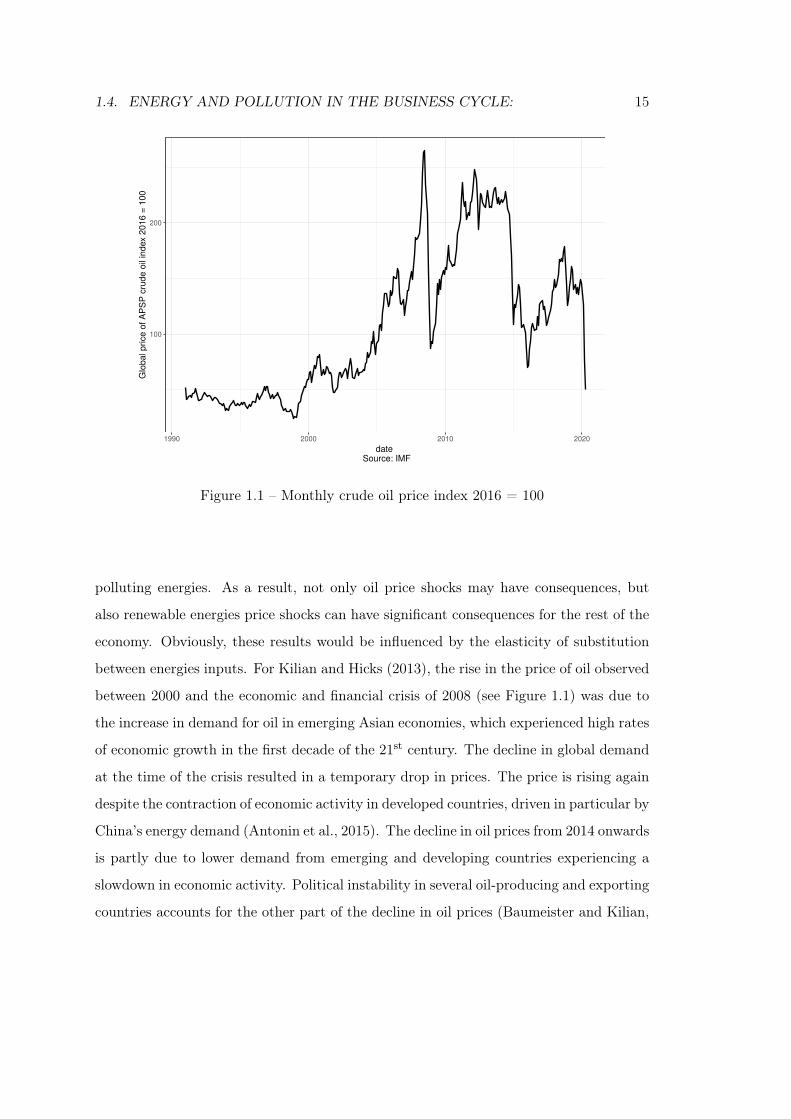
1.4. ENERGY AND POLLUTION IN THE BUSINESS CYCLE: 15
100
200
1990 2000 2010 2020
date Source: IMF
Glo
bal pri
ce o
f A
PS
P c
rude o
il in
dex 2
016 =
100
Figure 1.1 – Monthly crude oil price index 2016 = 100
polluting energies. As a result, not only oil price shocks may have consequences, but
also renewable energies price shocks can have significant consequences for the rest of the
economy. Obviously, these results would be influenced by the elasticity of substitution
between energies inputs. For Kilian and Hicks (2013), the rise in the price of oil observed
between 2000 and the economic and financial crisis of 2008 (see Figure 1.1) was due to
the increase in demand for oil in emerging Asian economies, which experienced high rates
of economic growth in the first decade of the 21st century. The decline in global demand
at the time of the crisis resulted in a temporary drop in prices. The price is rising again
despite the contraction of economic activity in developed countries, driven in particular by
China’s energy demand (Antonin et al., 2015). The decline in oil prices from 2014 onwards
is partly due to lower demand from emerging and developing countries experiencing a
slowdown in economic activity. Political instability in several oil-producing and exporting
countries accounts for the other part of the decline in oil prices (Baumeister and Kilian,

16 CHAPTER 1. A PUBLIC POLICY, FOR A PUBLIC GOOD
2016). The exploitation of shale gas in the United States through hydraulic fracturing
has reduced the demand for imported oil. As a result, the supply of available oil on
world markets has increased, explaining the downward trend in oil prices (Kilian, 2017).
On the other hand, as the break-even point for onshore oil production is lower in Saudi
Arabia (see Figure 1.2), the latter has tried to exclude this new player from the market
by increasing its production, thus further lowering the oil price. This strategy did not
work since in 2015, the US Congress authorized oil exports, a first since the oil shocks of
the 1970s, and the United States became the leading oil producer from 2017. Facing this
failure, Saudi Arabia and the other members of OPEC decided to lower their production.
The resulting increase in the world barrel price was reflected in France by the Yellow Vests
movement, which saw the price of gasoline at the pump rise adding to the increase in
the carbon tax. The global coronavirus health crisis, which has forced governments to
lock-down more than a third of the world’s population, has reduced the demand for oil.
Saudi Arabia and Russia took advantage of this situation to try once again to exclude
the United States from world markets. The imbalance between supply and demand
was such that the West Texas intermediate crude oil price became negative on Monday
April 20th 2020. These variations in the world price of oil, and more broadly in fossil fuel
prices in general, play a determinant role in the demand for oil and consequently in GHG
emissions. Including the possibility of exogenous shocks on polluting energies is therefore
essential to understand the mechanisms of environmental policies in the business cycle.
These exogenous variations in energy prices are taken into account in Chapters 3 and 4.
Two DSGE models are developed in which energy is included as a factor of production
and also as a source of GHG emissions. In Chapter 3, the DSGE model is based on the
one developed by Fischer and Springborn (2011) (see next section), in which the price of
energy is considered as an exogenous source of uncertainty. In the manner of Finn (1991)
and Finn (2000), climate policies are evaluated by assuming a variable rate of capital
utilization. Chapter 4 develops an NK DSGE model with nominal rigidities à la Calvo.
The model uses the assumptions of Smets and Wouters (2003, 2007). The energy block
is disaggregated in two parts and we assume on the one hand, polluting energies and,
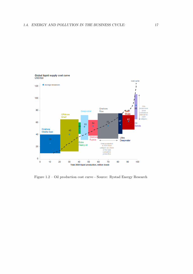
1.4. ENERGY AND POLLUTION IN THE BUSINESS CYCLE: 17
Figure 1.2 – Oil production cost curve - Source: Rystad Energy Research
18 CHAPTER 1. A PUBLIC POLICY, FOR A PUBLIC GOOD
on the other hand, non-polluting energies. It is assumed that the two sources of energy
can be the cause of exogenous shocks. The literature on the business cycle and climate
policies is developed in more detail, as is our contribution in the next section.
1.4.2 Pollution and climate policy in the business cycle:
The evolution of the carbon price on the European cap-and-trade market shows the
importance of studying the effectiveness of climate policies in the business cycle. Set up
in 2005 to meet the binding GHG emission reduction targets of the Kyoto Protocol, after
15 years this market covers 12,000 production plants of the most polluting industries
accounting for almost half of EU emissions. The EU ETS market has been established
and extended over three successive phases: the first one or "pilot phase" (2005 - 2007)
aimed to be on the one hand a learning phase, and on the other hand to determine
correctly the volume of allowances for the next phases. The second phase from 2008 to
2012 was essentially the same as the first one. The third phase includes civil aviation, and
allowances are no longer allocated entirely free of charge, but a fraction being auctioned.
The third phase, which began in 2013 and runs until 2020, aims to achieve the emission
reduction targets in accordance with the commitments of the Kyoto Protocol. During the
first phase, allowance prices have been characterized by a high volatility from a range
of e0.7 to 25. According to the market feature there was no restriction on banking
or borrowing allowances. In fact they were issued annually, but the firms could used
them whenever they wanted within the trading period. However, banking or borrowing
allowances were not allowed between between the first and second period. This is the
reason why allowance price fell to approximatively e0 well before the end of the trial
period (Ellerman and Joskow, 2008). According to Ellerman and Joskow (2008) carbon
price was higher than expected in 2005 and 2006 because of the weather: a cold winter
during 2005 and a hot summer in 2006; and also due to a high price for oil and natural
gas which made coal relatively more affordable, as coal emits more GHG than oil and
natural gas, as a consequence the demand for allowances increased.
Carbon price forecasts was about e35 for 2012, but EUA carbon price fell below
1.4. ENERGY AND POLLUTION IN THE BUSINESS CYCLE: 19
e10 during the third phase. Among the various weaknesses, Laurent and Le Cacheux
(2011) and de Perthuis and Trotignon (2014), identify the global financial crisis, which
has been followed by an economic downturn and a decline in industrial activity. Indeed,
industrial sectors such as steel and cement reduced their production, and GHG emissions
decreased. Obviously, it had a strong effect on diminishing demand for allowances and
therefore it led to a fall in carbon price. Because the number of quotas was stable,
allowances prices fell below the price that had been forecasted to a new equilibrium in a
context of a sluggish growth. At the end of the 2nd phase, another crisis hit the European
economy known as the "debt crisis". It has also impacted the EU ETS market. Laurent
and Le Cacheux (2011) also identify structural reasons such as the use of the Clean
Development Mechanism allowed by the Kyoto protocol. Thanks to this mechanism, a
firm that implement a emission-reduction project in developing countries gains access to
an emission credit. Therefore it also reduces demand for emission permits.
From 2012 and until 2018, the third phase has been characterized by a stable and low
carbon price. It is the result from the previous dysfunctional period, on the one hand
the economic conjuncture (global financial crisis, and European sovereign debt crisis),
and on the other hand by structural issues such as international credits due to the Clean
Development Mechanism. Unlike the transition from the first to the second phase, where
banking or borrowing allowances was not possible, the European Commission allowed it
between the second and third period. Because of a low demand for allowances during the
second phase, a surplus of allowances remain in the third period implying a low carbon
price. Unfortunately, this situation could affect the functioning of the carbon market and
in the long run make difficult or impossible to meet the GHG emissions reduction goal.
To increase the carbon price, the European Commission decided for the forth phase to
accelerate the annual rate of allowances decline to 1.74% to 2.2% and to implement the
Market Stability Reserve, to limit carbon price volatility. Because this market is subject
to exogenous shocks such as the 2008 financial crisis and the 2020 global COVID-19
pandemic, it is important to understand the consequences of the business cycle, and
exogenous shocks on the effectiveness of climate policies.
20 CHAPTER 1. A PUBLIC POLICY, FOR A PUBLIC GOOD
The literature of macroeconomics business cycle addressing climate policies is recent.
Among the first papers we can site Angelopoulos et al. (2010), Fischer and Springborn
(2011), and Heutel (2012). The main extension of these environmental DSGE models
has been to include pollution, but they differ from each other by the way they model it.
Fischer and Springborn (2011) include energy as a factor of production and assume that
pollution is proportional to the quantity of energy used in the production process. In
Angelopoulos et al. (2010) and Heutel (2012), there is no energy input in the production
function, and emissions are proportional to output. In these last two articles, environ-
mental damages linked to pollution are explicitly modelled, whereas there is no explicit
damage function in Fischer and Springborn (2011). They also differ in the research
questions they address. Fischer and Springborn (2011) are interested in understanding
how the economy will react using different environmental policies - a carbon tax, a cap-
and-trade market or an intensity target - faced with a total factor productivity shock.
Angelopoulos et al. (2010) also compare different environmental policies, but they as-
sume in addition to a TFP shock, an exogenous variation of emissions per output ratio
or "environmental uncertainty". They find that the cap-and-trade policy is the worst
policy because the utility level will be the lowest in that case. But they are not able
to identify which policy is better between a carbon tax a cap-and-trade market and a
numerical target (an example of a numerical target is the Kyoto Protocol, which imposes
a 25-40% reduction in emissions in 2020 compared to 1990 levels). Results will depend
on which uncertainty dominate between the total factor productivity shock and the "en-
vironmental uncertainty". For Fischer and Springborn (2011), the intensity target is the
best policy that can achieve the reduction in emissions at the lowest economic cost. Un-
der a cap-and-trade regime, macroeconomic variables volatility will be lower, and carbon
price volatility will increase, while under a carbon tax scenario, variables volatility will
be higher because of the constant carbon price. Heutel (2012) is not interested in a com-
parison of environmental policies, but cares about how environmental policy variables
(tax or an emission cap), may adapt to the cycle in order to maximize social welfare.
For him, both of these instruments must vary in time and adapt to the business cycle.
1.4. ENERGY AND POLLUTION IN THE BUSINESS CYCLE: 21
The optimal tax must be procyclical, increasing during expansion and decreasing during
recession. The same is true for the cap-and-trade market, if it is well designed it must
react procyclically.
Annicchiarico and Di Dio (2015, 2017) are the first to develop a NK DSGE models
to analyse the link between environmental policies and monetary policies. There is no
energy in their model, they assume as in Heutel (2012) that emissions are proportional
to output. In their first paper Annicchiarico and Di Dio (2015) focus on environmental
policies comparison but with two other sources of uncertainty in addition to the common
TFP shock: public consumption shock and monetary shock. Their results suggest that
the cap-and-trade market will decrease the volatility of usual macroeconomic variables,
while the carbon price will instead adapt to the shocks by a greater volatility, and this
result is confirmed in the presence of nominal rigidities. They also find that with strong
nominal rigidities, an intensity target will increase the volatility of macroeconomic vari-
ables. According to their results, the degree of price stickiness will play an important role
for welfare analysis. In a pure competitive model, when prices adjusts immediately, they
found no difference between the tax and the intensity target, and only minor differences
with the emission cap. When prices adjust quickly, welfare tend to be higher in the
intensity or tax scenarios and lower in the cap scenario, whereas it is the contrary when
prices adjust slowly. They also conduct a Ramsey analysis, and solve a Ramsey problem
to derive the optimal environmental policy. In this model, the planner is able to control
both the emission level and the environmental policy. Their results are consistent with
the one obtained by Heutel (2012) and suggest that the carbon tax must be procyclical.
Finally they consider different monetary policy regimes, and they conclude that the car-
bon tax response must be more aggressive when the monetary policy is less concerned
by inflation. In their second paper Annicchiarico and Di Dio (2017) are more interested
in the link between optimal monetary policy and optimal environmental policy. When
the planner can control both monetary policy and environmental policy, it must fight
against price distortion due nominal rigidities on the one hand and also fight against
emission damages that affect negatively production. When the planner only controls
22 CHAPTER 1. A PUBLIC POLICY, FOR A PUBLIC GOOD
emissions and in the presence of an accommodative monetary policy, emissions must be
countercyclical. When the planner only controls monetary policy, the inflation target
rules only hold for the carbon tax case, if there is no environmental damage. Otherwise,
in the presence of an emission cap or a carbon tax with environmental damage, prices
must adapt in order to fight inflation or the negative consequences of emissions.
More recently, Argentiero et al. (2017) and Xiao et al. (2018) developed environ-
mental DSGE models including energy in the production function. Xiao et al. (2018)
assume energy as one factor of production, while Argentiero et al. (2017) disaggregate
energy between polluting and non-polluting energies using a CES function. Argentiero
et al. (2017) estimated a Bayesian DSGE models for China, the US and the EU 15 to
understand how a carbon tax can result in incentives to use more renewable energies
Because their results suggest that the elasticity of substitution between the two energies
inputs is higher in the EU, they find that a carbon tax generates a quicker reallocation of
factors in the renewable energy sector. They also find that a carbon tax will diminish the
use of fossil fuel, and consequently emissions in the case of a positive productivity shock
in the fossil fuel sector. Xiao et al. (2018) developed a NK DSGE model following the
approach of the Annicchiarico and Di Dio (2015) model and calibrate it for China. They
also contribute to the literature by assuming different sources of uncertainty: technology
shock, energy efficiency shock, government expenditures shocks, but also environmental
tax rate shocks, emission cap shock or emission intensity shock. As expected, following
a positive shock on the volume of allowances, the economy will react by increasing pol-
lution because of the decrease in pollution price. The macro variables responses will be
higher in the case of intensity target or in a carbon tax shock.
In Chapters 3 and 4, we contribute to this burgeoning literature by considering energy
as a necessary production factor. Thus, in the third chapter, we make a comparison
of the different climate policy instruments available to public authorities in a model
with perfect price flexibility. We extend the model of Fischer and Springborn (2011) by
considering, as in Finn (1991, 2000), that capital is not always fully utilized. The variable
rate of capital utilization is then an important variable, since it allows the economy to
1.4. ENERGY AND POLLUTION IN THE BUSINESS CYCLE: 23
adapt to shocks more quickly. We also differ from Fischer and Springborn (2011) by
considering in addition to the usual technology shocks, a new source of uncertainty: the
price of energy. Our main results are as follows. In the case of a positive productivity
shock, the volatility of the macro variables differs little or not at all from the base-line
scenario when the government implements a tax or an intensity target. On the other
hand, the volatility of the usual economic variables decreases in the case of an emission
cap because the price of carbon rises sharply during a productivity shock to ensure the
emission reduction target. On the other hand, in the case of an energy price shock, in
the presence of a tax, the dynamic responses of the variables will follow the reference
scenario (no policy). While the emission cap and intensity target will see the price of
carbon decrease, which will further reduce the volatility of the model. The implications
in terms of policy are important, since it suggests adapting the carbon tax in particular
according to the volatility of the energy price to avoid the risk of Yellow Vests. Thus a flat
tax would make it possible to reduce this risk. In the fourth chapter, we develop a DSGE
model with nominal rigidities in the manner of Annicchiarico and Di Dio (2015). We
add the energy factor like Xiao et al. (2018), but we differ from them by disaggregating
the energy into two factors: the polluting energy source and the non-polluting energy
using a CES. It allows us to consider these two sources of energies as complementary
or substitutable. We further assume that emissions affect the utility of the consumer,
not the level of production as it is usually the case in the literature. We compare two
instruments of climate policy: a carbon tax and a cap-and-trade market. We consider
8 different exogenous shocks: TFP shock, shock in the polluting energy sector, in the
non-polluting energy sector... According to our results, there is no significant difference
between the two instruments in the event of a shock to the TFP. These results suggest the
introduction of a floor price for carbon on the European allowance market, which would
prevent the price from falling below a certain threshold, as was the case after the economic
crisis of 2008. In the case of a shock in the fossil fuel sector, in the presence of a tax,
emissions will increase because the marginal cost of pollution is constant. Consequently,
emissions will reduce the consumer’s utility. On the other hand, in the presence of an

24 CHAPTER 1. A PUBLIC POLICY, FOR A PUBLIC GOOD
emission cap, the price will adjust so as to limit emissions according to the cap. However,
there is no significant difference between the instruments during a productivity shock in
renewable production. When we optimize the monetary policy rule, we find that in the
carbon tax case, the Central Bank must be more sensitive to inflation and less sensitive
to the output gap compare to the usual coefficient of the Taylor rule. Whereas in the
case of an emission cap it must be more responsive to both inflation and output gap.

Chapter 2
Irreversibility of emitting
greenhouse gas and the cost of
delaying climate policy
2.1 Introduction:
It has been ten years since the Copenhagen conference, ten years in which global demand
for fossil energy has increased. This rise, due to the absence of an environmental policy
instrument or to an excessively low carbon price, has resulted in a rise in emissions, which
reduces the odds of limiting climate change.
The consequences of this increase in the GHG atmospheric stock are various. On the
one hand, the current rise in emissions will result in even greater efforts if the objectives
of the Paris agreement are to be met. On the other hand, this increase accentuates the
feedback effects. The change in cloud formation, the concentration of water vapour in
the atmosphere and the reflection effects of ice (albedo) modify the radiative forces and
amplifying global warming (see IPCC (2014, 2018) and Stern and Stern (2007)). A higher
stock of GHG in the atmosphere would also decrease the GHG absorption capacity of
oceans and land. Thus, above a certain GHG threshold, climate change could be self-
25
26 CHAPTER 2. IRREVERSIBILITY AND GLOBAL WARMING
sustaining, even if emissions were totally cut off. The possibility of such a threshold effect
could then lead to a form of irreversibility of climate change. However, little work has
been done on this notion of irreversibility. Economic theory is essentially based on the
notion of reversibility of pollution. According to Grossman and Krueger (1995), pollution
is a necessary stage, and it would suffice to continue to develop in order to return to the
initial equilibrium where the environment is cleaned up.
We are interested in this question of irreversibility of climate change in absence of
public intervention. To do so, we make the hypothesis, as in the Brock and Taylor (2010)
model, that without public policy, the economy will be able to reduce its GHG emissions
through an exogenous technological process per unit of fossil fuel energy consumed. We
compare the long-term equilibrium - in terms of the stock of GHG in the atmosphere and
their economic consequences - in the absence of intervention, to the results obtained with
a public intervention. We show that climate dynamics is an irreversible phenomenon in
the long term and consequently intervention is needed in the short term. We also show
that the elasticity of substitution between the two sources of energy is a key parameter
that also determines the long-term equilibrium. In order to limit global warming as much
as possible, in addition to the fastest possible public intervention, a strong elasticity of
substitution between polluting and non-polluting energies should be promoted. The aim
of this chapter is not to reproduce IPCC projections or to calculate the optimal value
of the carbon tax. The model is too simplistic to claim to make a recommendation on
the optimal level of CO2 in the atmosphere, or on the level of the tax to be put in
place. All the more so as we do not know with certainty the true functional form of
the damage function(see Pindyck (2017). Instead, the aim is to focus on the question
of climate reversibility, and the carbon cycle. The interest is therefore to make relative
comparisons between the status quo and public intervention.
To explore this question of irreversibility, we use a real business cycle integrated
assessment model (RBC IAM) initially developed by Golosov et al. (2014) which is based
on Nordhaus’s ones. Nordhaus (1977, 1994) acted as a precursors by including carbon
cycle and the consequences of the GHG atmospheric stock on economic activity in its
2.1. INTRODUCTION: 27
DICE model. His RICE model (see Nordhaus and Yang (1996)) is a disaggregated version
of its world-region model and includes 12 regions in its latest version. More recently,
Hope (2006), and Waldhoff et al. (2011) developed respectively the PAGE and FUND
models, but Nordhaus’ model still remains the reference. Golosov et al. (2014) (GHKT
hereafter) proposed a model based on Nordhauss’ work. GHKT’s and Nordhaus’s work
mainly differ in how they model the carbon cycle and the consequences of GHG damages.
Unlike Nordhaus, GHKT admit that a significant proportion of emissions remain in the
atmosphere for several thousand years. Moreover, according to them, the temperature
response to the GHG atmospheric is immediate and not delayed over time. We use the
same analytical framework as GHKT, including the same carbon cycle and the damage
function of GHG emissions, but we differ from them in several ways. Their time reference
is the decade and they assume a full depreciation of capital over this period (so that their
capital depreciation rate equals 10% per year). On the contrary, we consider the year as
a time unit, so we calibrate the capital depreciation rate to under 10% per year, more
consistently with data. In addition we take into account the capital adjustment cost
while GHKT consider this cost to be zero. Finally the structure of the energy sector
differs from that of GHKT. They separate fossil energy intro two regimes: a regime for
exhaustible resources, and a regime for non-exhaustible resources such as coal. We only
consider the non-depleting fossil fuels regime of coal regime. To see whether climate
change is reversible (Grossman and Krueger (1995) model hypothesis), an exogenous
variable, representing a form of technical progress, which reduces the carbon intensity of
energy, is incorporated into the model.
Section 2 develops the concept of irreversibility, and its application in economics ac-
cording to the 2nd principle of thermodynamics introduced by Georgescu-Roegen (1971).
Section 3 summarises the different hypotheses of the model, section 4 presents the plan-
ner’s problem in order to obtain the marginal cost of pollution. The decentralized com-
petitive equilibrium is solved in section 5, the different parameters of the model are
calibrated in section 6 and the results of the simulations are discussed in section 7 before
concluding.
28 CHAPTER 2. IRREVERSIBILITY AND GLOBAL WARMING
2.2 State of the art and contribution:
Much of the economic literature on growth and pollution is based on the Grossman
and Krueger (1995) model. According to them, the relationship between demand for
environmental quality and income would be an inverted U-shape, also known as the
Environmental Kuznet Curve (EKC). It states that pollution diminishes as soon as an
income threshold has been reached. There are three stages. In the early stage of de-
velopment environmental quality is high, then as production increases (and therefore
income), pollution increases, adversely affecting environmental quality. In a second step,
pollution reaches a peak before falling while income is increasing. The other explanation
of the EKC, given by Brock and Taylor (2010) would be related to technical progress.
In time, a technological way would be found to reduce pollution. Here too, an inverted
U-curve would be observed. It would then be necessary to degrade one’s environment
before cleaning it up. This theory is well suited for some pollutants that have the follow-
ing characteristics: ideally, their lifespan should be short, and pollution remain locally
concentrated. Indeed, if the pollution does not diffuse and if the pollutant can degrade
quickly, then it is possible to reduce pollution over time. On the other hand, if pollution
spreads, and/or if it lasts a long time, then public intervention becomes necessary to face
the risk of inflicting irreversible damage.
The 1986 Chernobyl disaster is an example of irreversible environmental damage.
The half-life of nuclear fuel ranges from ten to several tens of millions of years, so that if
no technology is found to clean up the site, it will remain unusable for an infinite period
of time (at the human life scale). The positive aspect is that nuclear pollution is (partly)
geographically contained. Another example of irreversible damage is plastic waste found
in the oceans. This time again the lifetime of plastic exceeds 100 years. It kills many
species that ingest it before it degrades, and even when it decomposes as microplastics,
marine wildlife ingests it and contaminates the entire food chain. The lack of technology
to address this issue makes such pollution appear irreversible.
The same is true for global warming. Greenhouse gases have two characteristics that
2.2. STATE OF THE ART AND CONTRIBUTION: 29
make global warming irreversible if nothing is done to reduce our emissions in the short
run. On the one hand, once emitted, GHG diffuse to the entire atmosphere. Thus, in the
absence of a coordinated response, the efforts made by some may be less effective due to
the free rider behaviour of other countries (see Stern and Stern (2007)). This well-known
concept of public goods, is the consequence of market failure ans misallocated property
rights. The Trump administration’s decision to leave in 2017 the Paris Agreement, while
the US is the world’s largest emitter of GHG in terms of CO2 eq. per capita illustrates
this situation. On the other hand, several factors influence climate, whose laws of motion
are very slow. In other words, once the initial equilibrium has been modified, it will be
difficult to return to this equilibrium. The radiative forcing effect (or warming effect)
is currently contained by the oceans, which act as a buffer and regulate temperature.
However, once the ocean temperature have increased, due to this buffer effect, the time
required to reverse the trend once emissions have sufficiently decreased is also very long.
The phenomenon of global warming can also be self-sustaining once a certain threshold
has been reached. For example, glaciers, sea ice and icecaps also acts as climate regula-
tors. They do not only play the role of the planet’s air conditioner. Indeed, ice’s white
surface reflects sunbeams and keeps our global climate mild. If ice melts, darker surfaces
will absorb heat and increase temperature. For those different, albeit non-exhaustive
reasons, in the absence of a technological solution that would allow us to absorb the
stock of GHG currently present in the atmosphere, without a carbon price high enough
to limit the use of fossil fuels climate change could have irreversible effects. Thus, even
if income increases, we would not have the ability to avoid global warming as predicted
by the EKC. In its report on green growth, the World Bank puts forward the idea,
without developing it, of a possible irreversibility of the climate p.33:"Climate change
itself may be irreversible. This irreversibility is a clear incentive for early action, as the
consequences of warming exceeding 2C are highly uncertain and potentially severe[...].
The 2C objective, for example is achievable only if significant emission reductions can
be made before 2030" (Bank, 2012)
In this chapter, we propose to investigate this concept of irreversibility of global
30 CHAPTER 2. IRREVERSIBILITY AND GLOBAL WARMING
warming. Irreversibility is derived from the 2nd principle of thermodynamics (entropy
law), and it has been introduced in economics by Georgescu-Roegen (1971). In his work,
Georgescu criticizes the economic reasoning based on the classical laws of mechanics or
Newtonian laws that are by nature reversible. He therefore recalls the origin of thermody-
namics. This branch of physics, which appeared at the time of the industrial revolution,
was intended to explain phenomena that the law of classical physics could no longer
explain. Steam trains used the energy stored in the form of coal to convert it into me-
chanical work. This fuel allows the train locomotive to move forward. Once the fuel
has been consumed, it decelerates before stopping. Hence, the mechanical movement is
reversible. But another phenomenon has occurred, which is irreversible. Indeed, coal
has not only been transformed into mechanical work, a share of energy has vanished in
the form of heat, and ashes are the residue. This process is irreversible, it is unidirec-
tional and irreversible. Just as birth always precedes death, life is unidirectional and
irreversible.
This concept of irreversibility is a definition in the strict sense of the term. Irreversibil-
ity in the broad sense can be defined as a very low process of return to equilibrium on
the scale of human life, as in the case of plastic or nuclear pollution. Thus, the dynamics
governing climate change is slow. As a result, in the absence of technological innova-
tion that can reduce emissions intensity, the damage caused is irreversible at least in the
medium to long term on the scale of human life. Similarly if the implementation of a
sufficiently high carbon price is delayed in the short term, consequence could also be non
reversible in the distant future.
According to the Kaya’s identity (see Kaya et al. (1997) and Waggoner and Ausubel
(2002)) GHG emission are driven by four different factors: total population, GDP per
capita, GDP energy intensity and carbon intensity of energy. It can be express as follows:
CO2,t = POPt ×GDPtPOPt
× ENEtGDPt
× CO2,tENEt
Taking logs on both sides of previous equation and differentiating gives:
gCO2 = gPOP + gGDP/POP + gENE/GDP + gCO2/ENE
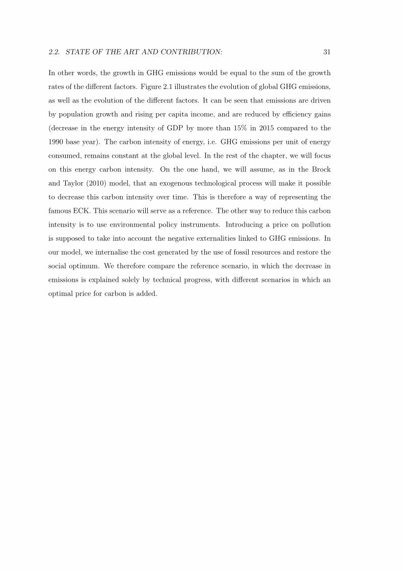
2.2. STATE OF THE ART AND CONTRIBUTION: 31
In other words, the growth in GHG emissions would be equal to the sum of the growth
rates of the different factors. Figure 2.1 illustrates the evolution of global GHG emissions,
as well as the evolution of the different factors. It can be seen that emissions are driven
by population growth and rising per capita income, and are reduced by efficiency gains
(decrease in the energy intensity of GDP by more than 15% in 2015 compared to the
1990 base year). The carbon intensity of energy, i.e. GHG emissions per unit of energy
consumed, remains constant at the global level. In the rest of the chapter, we will focus
on this energy carbon intensity. On the one hand, we will assume, as in the Brock
and Taylor (2010) model, that an exogenous technological process will make it possible
to decrease this carbon intensity over time. This is therefore a way of representing the
famous ECK. This scenario will serve as a reference. The other way to reduce this carbon
intensity is to use environmental policy instruments. Introducing a price on pollution
is supposed to take into account the negative externalities linked to GHG emissions. In
our model, we internalise the cost generated by the use of fossil resources and restore the
social optimum. We therefore compare the reference scenario, in which the decrease in
emissions is explained solely by technical progress, with different scenarios in which an
optimal price for carbon is added.
32 CHAPTER 2. IRREVERSIBILITY AND GLOBAL WARMING
90
120
150
1990 1995 2000 2005 2010 2015year
Inde
x 10
0=19
90
drivers carbon intensity co2 emissions Energy intensity GDP per capita population
Source: International Energy Agency
Figure 2.1 – Kaya’s identity for the world - Source: IEA
2.3 General assumptions:
In this section, we describe the main assumptions of the model, on the one hand the
construction of the environmental block and the carbon cycle, and on the other hand the
economic block, energy use and environmental damage related to the use of fossil energy.
GHG atmospheric stock evolves as follows:
St − S =t+T∑
s=0
(1− ds)ΦΩt−sec,t−s (2.3.1)
1− ds = ψ1 + (1− ψ1)ψ2(1− ψ3)s, ds ∈ [0, 1] (2.3.2)
Where S is the pre-industrial stock of GHG in the atmosphere, Φ is the conversion factor
that transforms one unit of fossil fuel ec,t consumed (or polluting energy) into Φec,t units
of GHG emitted in the atmosphere. According to GHKT, in each period the carbon
cycle can be summarized by this mechanism. For each unit of emitted GHG, a share
2.3. GENERAL ASSUMPTIONS 33
ψ1 ∈ [0, 1] remains in the atmosphere forever. For the remaining share (1 − ψ1), one
part (1 − ψ2) ∈ [0, 1] is immediately absorbed, while the last part ψ2 slowly degrades
at a rate ψ3 ∈ [0, 1] in each period. Finally, we assume that exogenous technological
progress Ωt ∈ [0, 1] will reduce the quantity of emissions per unit of burnt fossil fuel in
the future. This is the central assumption in our model, it is a way to assume an EKC,
its functional form is discussed more at length in the calibration section. This variable
has the following properties, in t = 0, Ω0 = 1, and its limits tends towards ε, when t
tends to infinity. The current stock of GHG depends on past uses of fossil fuels:
St = L(etc)
with et = ec,−T , ec,−T+1, ..., ec,t
Another useful way to describe the evolution of the GHG atmospheric stock is to trans-
form the previous sum of past emissions, into a recursive representation as the sum of
two state variables S1t and S2
t . In this representation, the accumulation of GHG can be
broken down into two reservoirs whose dynamics are independent of each other, where S1t
represents the first reservoir where the flow of emissions accumulates in the atmosphere
forever, and S2t , on the other hand, represents the second reservoir in which the stock
depreciates at a geometric rate ψ3. This formulation can be represented by the three
following equations:
St = S1t + S2
t
S1t = ψ1ΩtΦec,t + S1
t−1
S2t = (1− ψ1)ψ2ΩtΦec,t + (1− ψ3)S2
t−1
(2.3.3)
The infinitely lived representative household has the following logarithmic utility func-
tion:
U(Ct) = logCt (2.3.4)
Output Yt in the final goods sector is given by a Cobb-Douglas function and it requires
three inputs capital Kg,t, labor Lg, t and energy Eg,t:
Yt =(
1−D(St))Kαg,t−1
(AgLg,t
)1−α−γEγg,t (2.3.5)
34 CHAPTER 2. IRREVERSIBILITY AND GLOBAL WARMING
D(St(ec,t)) is the global damage equation of the atmospheric GHG stock. We follow
GHKT and assume that:
D(St) = 1− exp(κ(S − St)
)(2.3.6)
where S is the pre-industrial atmospheric GHG concentration, and κ is a scale parameter
to be calibrated.
It is assumed that energy production comes from several sources. We simplify re-
ality by assuming that we can distinguish these two sources into non-polluting er,t and
polluting sources ec,t. Unlike the polluting source, the non-polluting source does not
emit greenhouse gases. We assume that there is no Hotelling rent, in other words there
is no rent linked to the exploitation of the exhaustible resource, we thus assume a coal
regime. Indeed, coal is a finite, yet not a scarce resource, and the disposable quantity of
coal is large enough to be used for several centuries, so that we do not consider it as a
depletable resource. Energy is aggregated using a CES production function, where ω is
a share parameter, and σ = 11−ϕ is the elasticity of substitution between polluting and
non-polluting energies.
Eg,t =(ωeϕr,t + (1− ω)eϕc,t
) 1ϕ (2.3.7)
The aggregate accounting identity of the economy is:
Ct + It +φ
2
( ItKg,t−1
− δ)2Kg,t−1 + Tt = Yt (2.3.8)
It, includes investment adjustment costs: C (It,Kg,t) =φ
2
( ItKg,t−1
− δ)2Kg,t−1, with
φ ≥ 0, and where the cost function has the following properties: it is homogeneous of
degree one, it is equal to zero in the steady state (C(δKg,Kg) = 0) and the marginal
cost of investment increases with It, and decreases with the stock of capital Kg,t. This
adjustment cost specification has been initially suggested by Hayashi (1982). Assuming
first that φ = 0, one obtains the usual capital accumulation equation. On the contrary,
if φ > 0, then outside the steady state ( ItKg,t6= δ) increasing It makes capital depreciate
faster. This functional form has been widely used in the literature (see Abel and Blan-
chard (1983), Blanchard et al. (1989), Obstfeld et al. (1996) or Jermann (1998) among
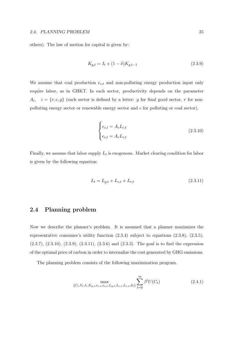
2.4. PLANNING PROBLEM 35
others). The law of motion for capital is given by:
Kg,t = It + (1− δ)Kg,t−1 (2.3.9)
We assume that coal production ec,t and non-polluting energy production input only
require labor, as in GHKT. In each sector, productivity depends on the parameter
Ai, i = r, c, g (each sector is defined by a letter: g for final good sector, r for non-
polluting energy sector or renewable energy sector and c for polluting or coal sector),
ec,t = AcLc,t
er,t = ArLr,t
(2.3.10)
Finally, we assume that labor supply Lt is exogenous. Market clearing condition for labor
is given by the following equation:
Lt = Lg,t + Lc,t + Lr,t (2.3.11)
2.4 Planning problem
Now we describe the planner’s problem. It is assumed that a planner maximizes the
representative consumer’s utility function (2.3.4) subject to equations (2.3.8), (2.3.5),
(2.3.7), (2.3.10), (2.3.9), (2.3.11), (2.3.6) and (2.3.3). The goal is to find the expression
of the optimal price of carbon in order to internalize the cost generated by GHG emissions.
The planning problem consists of the following maximization program.
maxCt,Yt,It,Kg,t,er,t,ec,t,Lg,t,Lc,t,Lr,t,St
∞∑
t=0
βtU(Ct) (2.4.1)
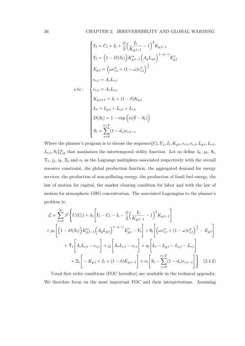
36 CHAPTER 2. IRREVERSIBILITY AND GLOBAL WARMING
s.to :
Yt = Ct + It +φ
2
( ItKg,t−1
− 1)2Kg,t−1
Yt =(
1−D(St))Kαg,t−1
(AgLg,t
)1−α−γEγg,t
Eg,t =(ωeϕr,t + (1− ω)eϕc,t
) 1ϕ
ec,t = AcLc,t
er,t = ArLr,t
Kg,t+1 = It + (1− δ)Kg,t
Lt = Lg,t + Lc,t + Lr,t
D(St) = 1− exp(κ(S − St)
)
St =
t+T∑
s=0
(1− ds)ec,t−s
Where the planner’s program is to choose the sequenceCt, Y,t, It,Kg,t, er,t, ec,t, Lg,t, Lc,t,
Lr,t, St∞t=0 that maximizes the intertemporal utility function. Let us define λt, µt, θt,
Υt, ζt, ηt, Ξt and νt as the Lagrange multipliers associated respectively with the overall
resource constraint, the global production function, the aggregated demand for energy
services, the production of non-polluting energy, the production of fossil fuel energy, the
law of motion for capital, the market clearing condition for labor and with the law of
motion for atmospheric GHG concentration. The associated Lagrangian to the planner’s
problem is:
L =
∞∑
t=0
βt
U(Ct) + λt
[Yt − Ct − It −
φ
2
( ItKg,t−1
− 1)2Kg,t−1
]
+ µt
[(1−D(St)
)Kαg,t−1
(AgLg,t
)1−α−γEγg,t − Yt
]+ θt
[(ωeϕr,t + (1− ω)eϕc,t
) 1ϕ − Eg,t
]
+ Υt
[AcLc,t − ec,t
]+ ζt
[ArLr,t − er,t
]+ ηt
[Lt − Lg,t − Lc,t − Lr,t
]
+ Ξt
[−Kg,t + It + (1− δ)Kg,t−1
]+ νt
[St −
t+T∑
s=0
(1− ds)ec,t−s]
(2.4.2)
Usual first order conditions (FOC hereafter) are available in the technical appendix.
We therefore focus on the most important FOC and their interpretations. Assuming
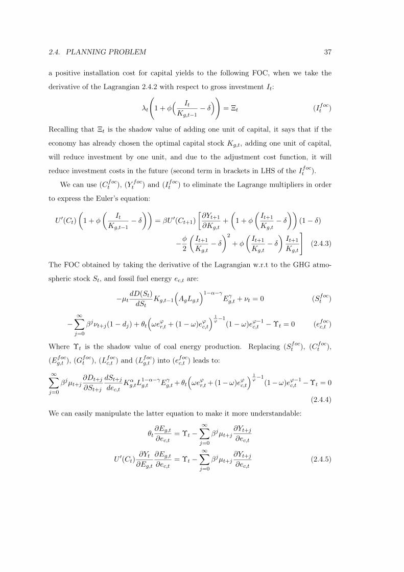
2.4. PLANNING PROBLEM 37
a positive installation cost for capital yields to the following FOC, when we take the
derivative of the Lagrangian 2.4.2 with respect to gross investment It:
λt
(1 + φ
( ItKg,t−1
− δ))
= Ξt (Ifoct )
Recalling that Ξt is the shadow value of adding one unit of capital, it says that if the
economy has already chosen the optimal capital stock Kg,t, adding one unit of capital,
will reduce investment by one unit, and due to the adjustment cost function, it will
reduce investment costs in the future (second term in brackets in LHS of the Ifoct ).
We can use (Cfoct ), (Y foct ) and (Ifoct ) to eliminate the Lagrange multipliers in order
to express the Euler’s equation:
U ′(Ct)(
1 + φ
(It
Kg,t−1− δ))
= βU ′(Ct+1)
[∂Yt+1
∂Kg,t+
(1 + φ
(It+1
Kg,t− δ))
(1− δ)
−φ2
(It+1
Kg,t− δ)2
+ φ
(It+1
Kg,t− δ)It+1
Kg,t
](2.4.3)
The FOC obtained by taking the derivative of the Lagrangian w.r.t to the GHG atmo-
spheric stock St, and fossil fuel energy ec,t are:
−µtdD(St)
dStKg,t−1
(AgLg,t
)1−α−γEγg,t + νt = 0 (Sfoct )
−∞∑
j=0
βjνt+j(1− dj) + θt
(ωeϕr,t + (1− ω)eϕc,t
) 1ϕ−1
(1− ω)eϕ−1c,t −Υt = 0 (efocc,t )
Where Υt is the shadow value of coal energy production. Replacing (Sfoct ), (Cfoct ),
(Efocg,t ), (Gfoct ), (Lfocc,t ) and (Lfocg,t ) into (efocc,t ) leads to:
∞∑
j=0
βjµt+j∂Dt+j
∂St+j
dSt+jdec,t
Kαg,tL
1−α−γg,t Eγg,t + θt
(ωeϕr,t + (1−ω)eϕc,t
) 1ϕ−1
(1−ω)eϕ−1c,t −Υt = 0
(2.4.4)
We can easily manipulate the latter equation to make it more understandable:
θt∂Eg,t∂ec,t
= Υt −∞∑
j=0
βjµt+j∂Yt+j∂ec,t
U ′(Ct)∂Yt∂Eg,t
∂Eg,t∂ec,t
= Υt −∞∑
j=0
βjµt+j∂Yt+j∂ec,t
(2.4.5)
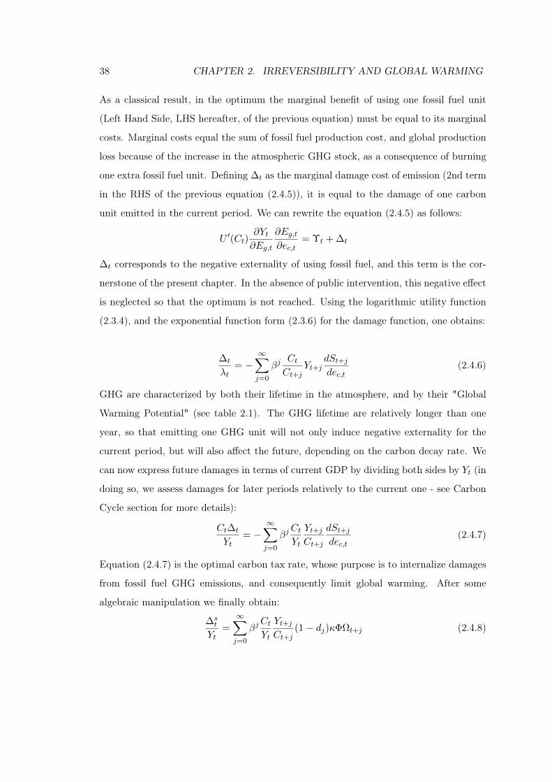
38 CHAPTER 2. IRREVERSIBILITY AND GLOBAL WARMING
As a classical result, in the optimum the marginal benefit of using one fossil fuel unit
(Left Hand Side, LHS hereafter, of the previous equation) must be equal to its marginal
costs. Marginal costs equal the sum of fossil fuel production cost, and global production
loss because of the increase in the atmospheric GHG stock, as a consequence of burning
one extra fossil fuel unit. Defining ∆t as the marginal damage cost of emission (2nd term
in the RHS of the previous equation (2.4.5)), it is equal to the damage of one carbon
unit emitted in the current period. We can rewrite the equation (2.4.5) as follows:
U ′(Ct)∂Yt∂Eg,t
∂Eg,t∂ec,t
= Υt + ∆t
∆t corresponds to the negative externality of using fossil fuel, and this term is the cor-
nerstone of the present chapter. In the absence of public intervention, this negative effect
is neglected so that the optimum is not reached. Using the logarithmic utility function
(2.3.4), and the exponential function form (2.3.6) for the damage function, one obtains:
∆t
λt= −
∞∑
j=0
βjCtCt+j
Yt+jdSt+jdec,t
(2.4.6)
GHG are characterized by both their lifetime in the atmosphere, and by their "Global
Warming Potential" (see table 2.1). The GHG lifetime are relatively longer than one
year, so that emitting one GHG unit will not only induce negative externality for the
current period, but will also affect the future, depending on the carbon decay rate. We
can now express future damages in terms of current GDP by dividing both sides by Yt (in
doing so, we assess damages for later periods relatively to the current one - see Carbon
Cycle section for more details):
Ct∆t
Yt= −
∞∑
j=0
βjCtYt
Yt+jCt+j
dSt+jdec,t
(2.4.7)
Equation (2.4.7) is the optimal carbon tax rate, whose purpose is to internalize damages
from fossil fuel GHG emissions, and consequently limit global warming. After some
algebraic manipulation we finally obtain:
∆st
Yt=
∞∑
j=0
βjCtYt
Yt+jCt+j
(1− dj)κΦΩt+j (2.4.8)
2.5. DECENTRALIZED COMPETITIVE EQUILIBRIUM: 39
This carbon tax depends on β, ψ3 and κ parameters and the exogenous technological
process that diminishes energy carbon intensity Ωt. Everything remaining equal, the
higher discount rate, the lower the preference rate for the present time, the more future
well-being is taken into account, the higher tax will be. The carbon tax depends nega-
tively on the rate of carbon decay (ψ3). The higher this absorption rate, the lower the
tax will be. Similarly, all other things being equal, the more the exogenous variable Ωt
tends towards 0, the lower GHG intensity of consuming one unit of fossil fuel, the lower
tax will be (environmental damage being low).
According to the (Lfocc,t ),(Lfocr,t ), (L
focg,t ), marginal benefit of labor is equal across sec-
tors:
ΥtAc = ζtAr = (1− α− γ)µt
(1−D(St)
)Kαg,t
(AgLg,t
)1−α−γL−1g,tE
γg,t = ηt
Υt∂ec,t∂Lc,t
= ζt∂er,t∂Lr,t
= µt∂Yt∂Lg,t
= ηt
2.5 Decentralized competitive equilibrium:
2.5.1 Representative household:
We assume that the representative household owns capital Kg,t, makes investment de-
cisions It, and supplies its labor force Lt. The representative household gets its income
from the supply of its labor force Lt (because we assume a purely competitive market the
household is a price-taker and consequently the wage wt is given) and from renting capital
Kg,t to the firm (rt, which takes also as given). All its income is consumed or invested.
We assume that government implements a tax on GHG emissions, and redistributes its
revenue as a lump-sum subsidy Tt. The household gets utility only from consumption,
so that leisure does not enter the utility function. Utility from future consumption is
discounted according to β ∈]0, 1[. Given the sequence wt, Lt, rt∞t=0, the representative
household chooses the sequence Ct, It,Kg,t∞t=0 that maximizes its intertemporal utility
function:
maxCt,It,kg,t
∞∑
t=0
βtU(Ct) (2.5.1)
40 CHAPTER 2. IRREVERSIBILITY AND GLOBAL WARMING
subject to its budget constraint:
Ct + It +φ
2
( ItKg,t−1
− δ)2Kg,t−1 = rtKg,t−1 + wtLt + Tt (2.5.2)
Investment is given by the following equation:
Kg,t = It + (1− δ)Kg,t−1 (2.5.3)
By assuming the logarithmic utility function, and combining the FOC1 for consumption
and investment with the FOC for capital stock we obtain the Euler equation:
1Ct
(1 + φ
(It
Kg,t−1− δ))
= β 1Ct+1
[rt+1 − φ
2
(It+1
Kg,t− δ)2
+φ(It+1
Kg,t− δ)It+1
Kg,t+
(1 + φ
(It+1
Kg,t− δ))(
1− δ)]
(2.5.4)
If the Euler equation (2.5.4) is satisfied, the household is indifferent between consuming
today and consuming in the future. On the other hand, depending on the inequality
that holds, household prefers either to save more in the current period and to postpone
its consumption in the future, or on the contrary to increase its consumption level in
the current period. This Euler equation is the same as the one obtained in the planning
problem (equation (2.4.3)).
2.5.2 Firms:
We assume that all markets are competitive, so that firms are price takers in both final
goods and intermediate goods sectors.
2.5.2.1 Final goods sector:
We first consider the firm in the final-good, it does not take into account the externalities
linked to the use of polluting energy. In that case, in each period t, the representative firm
chooses the sequence of inputs Kg,t−1, Lg,tEg,t, that maximizes its profit Πg,t taking
1See Technical appendix for more details
2.5. DECENTRALIZED COMPETITIVE EQUILIBRIUM: 41
the sequence rt, wt, pc,t, pr,t, τc,t as given:
maxKg,t−1,Lg,t,ec,t,er,t
Πg,t = Yt − wtLg,t − rtkg,t−1 − pc,t(1 + τc,t)ec,t − pr,ter,t
s.to
Yt =(
1−D(St))Kαg,t−1
(AgLg,t
)1−α−γEγg,t
Eg,t =(ωeϕr,t + (1− ω)eϕc,t
) 1ϕ
Demand for energy services from the final goods sector is given by the aggregated CES
function Eg,t, and energy services are provided by intermediate goods firms. On these
markets, the program is to choose the amounts of fossil fuel ec,t and non-polluting energy
er,t that minimize its costs pr,t and (1+τc,t)pc,t. From the FOC we find the demand from
the representative firm for each energy input:
er,t =
[γωYt
pr,t(ωeϕr,t + (1− ω)eϕc,t
)] 1
1−ϕ
ec,t =
[γ(1− ω)Yt
pc,t(1 + τc,t)(ωeϕr,t + (1− ω)eϕc,t
)] 1
1−ϕ
In the absence of public intervention (when τc = 0), the representative firm in the final
goods sector does not take into account the damage caused by its use of fossil fuel.
The demand for fossil fuel is greater than the optimum. Consequently, GHG emissions
accumulate into the atmosphere, and increase long run damage.
When the firm is not myopic and takes into account the negative externalities of GHG
emissions on the economy, it solves the following intertemporal maximisation program:
max∑∞
t=0 βt λtλ0
exp
(κ(S −∑t+T
s=0 (1− ds)ec,t−s))
Kαg,t−1
(AgLg,t
)1−α−γEγg,t
−wtLg,t − rtkg,t−1 − p∗c,tec,t − pr,ter,t
The FOC for the optimal use of fossil fuel is therefore:
γ(
1−D(St))Kαg,t−1
(AgLg,t
)1−α−γ(ωeϕr,t + (1− ω)eϕc,t
) γϕ−1
(1− ω)eϕ−1c,t
−∑∞j=0 βj λt+jλt
(1− dj)Yt+j = p∗c,t (2.5.5)
42 CHAPTER 2. IRREVERSIBILITY AND GLOBAL WARMING
By moving the second term of the LHS to the RHS of the latter equation, we obtain the
same result as in the planning problem (equation(2.4.7)). By setting the emissions tax
at this level, public policy makes it possible to reach the social optimum.
2.5.2.2 Production of intermediate goods:
A typical firm in the energy sector uses only labor as input in its production function
ei,t = AiLi,t i = c, r. Energy prices pc,t, pr,t are given so that a representative firm in
each of these sectors maximizes its profit:
maxLi,t
Πi,t = Pi,tei,t − wtLi,t i = c, r
2.5.3 Closing the model:
Consolidating the household budget constraint with the necessary conditions on each
market yields the aggregate accounting identity:
Yt = Ct + It +φ
2
( ItKg,t−1
− δ)2Kg,t−1 (2.5.6)
At each period, depending on the quantity of fossil fuel consumed, the atmospheric GHG
stock evolves according to the carbon cycle, and generates damages on the economy.
D(St) = 1− exp(κ(S − St)
)
St = S1t + S2
t
S1t = ψ1ΩtΦec,t + S1
t−1
S2t = (1− ψ1)ψ2ΩtΦec,t + (1− ψ3)S2
t−1
2.6 Calibration:
In this section we attribute numerical values to the model parameters. The unit of time
is the year, and we take 2010 as the initial period. For the Kyoto Protocol’s first binding
agreement in terms of emissions, the historical base year is 1990, but in the last IPCC
report (IPCC, 2014) the different scenarios are calculated relatively to 2010 so that we
use this year as a benchmark.
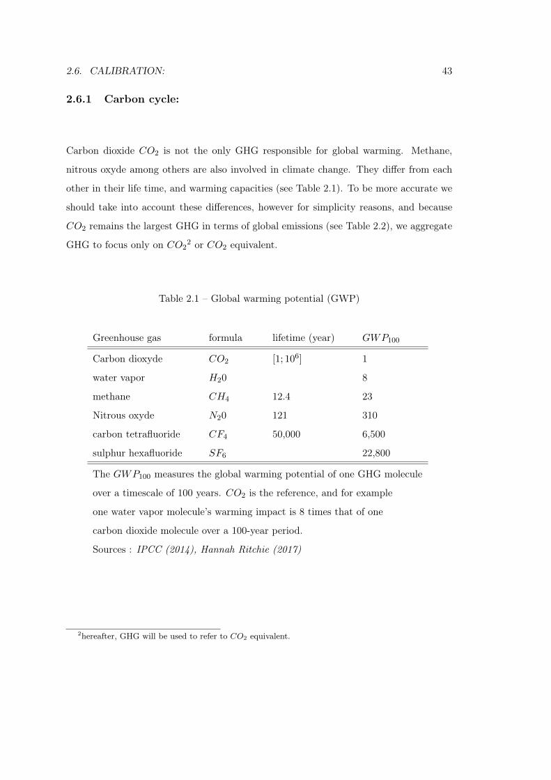
2.6. CALIBRATION: 43
2.6.1 Carbon cycle:
Carbon dioxide CO2 is not the only GHG responsible for global warming. Methane,
nitrous oxyde among others are also involved in climate change. They differ from each
other in their life time, and warming capacities (see Table 2.1). To be more accurate we
should take into account these differences, however for simplicity reasons, and because
CO2 remains the largest GHG in terms of global emissions (see Table 2.2), we aggregate
GHG to focus only on CO22 or CO2 equivalent.
Table 2.1 – Global warming potential (GWP)
Greenhouse gas formula lifetime (year) GWP100
Carbon dioxyde CO2 [1; 106] 1
water vapor H20 8
methane CH4 12.4 23
Nitrous oxyde N20 121 310
carbon tetrafluoride CF4 50,000 6,500
sulphur hexafluoride SF6 22,800
The GWP100 measures the global warming potential of one GHG molecule
over a timescale of 100 years. CO2 is the reference, and for example
one water vapor molecule’s warming impact is 8 times that of one
carbon dioxide molecule over a 100-year period.
Sources : IPCC (2014), Hannah Ritchie (2017)
2hereafter, GHG will be used to refer to CO2 equivalent.
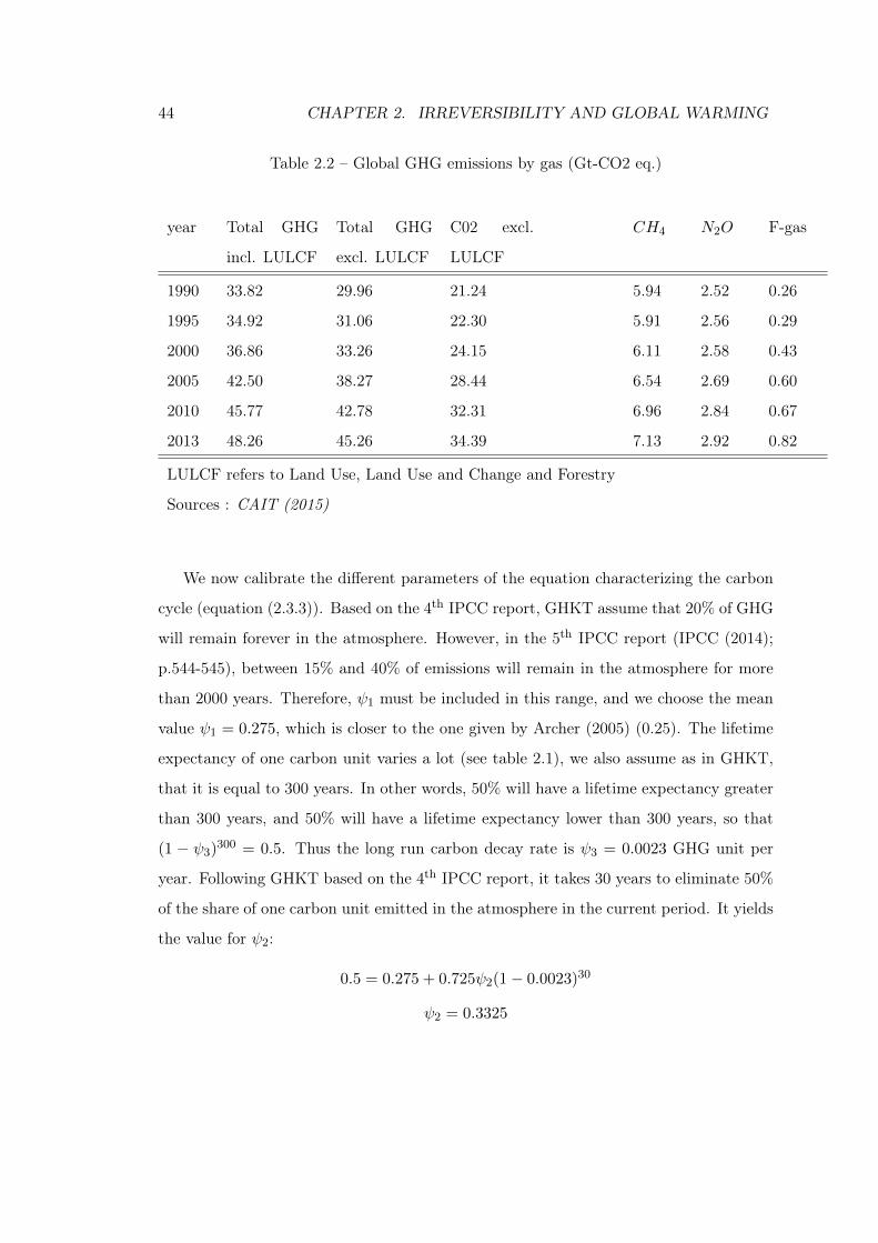
44 CHAPTER 2. IRREVERSIBILITY AND GLOBAL WARMING
Table 2.2 – Global GHG emissions by gas (Gt-CO2 eq.)
year Total GHG
incl. LULCF
Total GHG
excl. LULCF
C02 excl.
LULCF
CH4 N2O F-gas
1990 33.82 29.96 21.24 5.94 2.52 0.26
1995 34.92 31.06 22.30 5.91 2.56 0.29
2000 36.86 33.26 24.15 6.11 2.58 0.43
2005 42.50 38.27 28.44 6.54 2.69 0.60
2010 45.77 42.78 32.31 6.96 2.84 0.67
2013 48.26 45.26 34.39 7.13 2.92 0.82
LULCF refers to Land Use, Land Use and Change and Forestry
Sources : CAIT (2015)
We now calibrate the different parameters of the equation characterizing the carbon
cycle (equation (2.3.3)). Based on the 4th IPCC report, GHKT assume that 20% of GHG
will remain forever in the atmosphere. However, in the 5th IPCC report (IPCC (2014);
p.544-545), between 15% and 40% of emissions will remain in the atmosphere for more
than 2000 years. Therefore, ψ1 must be included in this range, and we choose the mean
value ψ1 = 0.275, which is closer to the one given by Archer (2005) (0.25). The lifetime
expectancy of one carbon unit varies a lot (see table 2.1), we also assume as in GHKT,
that it is equal to 300 years. In other words, 50% will have a lifetime expectancy greater
than 300 years, and 50% will have a lifetime expectancy lower than 300 years, so that
(1 − ψ3)300 = 0.5. Thus the long run carbon decay rate is ψ3 = 0.0023 GHG unit per
year. Following GHKT based on the 4th IPCC report, it takes 30 years to eliminate 50%
of the share of one carbon unit emitted in the atmosphere in the current period. It yields
the value for ψ2:
0.5 = 0.275 + 0.725ψ2(1− 0.0023)30
ψ2 = 0.3325
2.6. CALIBRATION: 45
Each time one GHG unit is emitted in the atmosphere, 27.5% of it will remain forever in
the atmosphere. This means that 72.5% will be absorbed: two thirds will be immediately
removed from the atmosphere and the remaining third will be degraded at an annual rate
of 0.23% per year.
GHKT used 2000 as a reference year and assume that the total GHG stock in the
atmosphere was S2000 = 802 Gt, which was distributed as follows: 684 Gt were stocked
in the first tank S1, and 118 Gt in the second tank S2. According to the NOAA annual
GHG index, in 2010, the GHG atmospheric concentration was 448 ppm CO2 eq., using
the conversion factor 1 ppm ↔ 2.13 Gt C (see Clark (1982)), the corresponding amount
of GHG was 996 GT C. To find the corresponding initial GHG stock in each reservoir
from 2000 to the 2010 year reference, we need to calibrate the conversion factor Φ, and
to assume a functional form for Ωt to match 996 GT C in 2010. In 2010, 2,879 of gas
(Mtoe) were consumed, 3,636 Mtoe of coal and 4,085 Mt of oil were consumed, a total
of 10.6 Gt of oil eq (see Dudley et al. (2015)).
The exogenous variable Ωt ∈ [0, 1] stands for the exogenous technology progress that
reduces emission intensity per fossil fuel unit burned. It is the way we model the EKC
supposed in the Grossman and Krueger (1995) model. According to Nordhaus (2010),
we already have observed a reduction in emission intensity without implementing an
environmental policy, he assumes that this decrease is the consequence of technological
progress. This function is assumed to be decreasing over time, equals to 1 in t = 0, and
tends towards 0 when t tends to infinity. We assume that Ωt follows a sigmoid-function as
in Barrage (2014) and Krusell and Smith (2015), of parameters Θ = log(
0.010.99
). Moreover,
it is estimated that after 10 years (n99 = 10), the emission intensity per unit of fossil fuel
consumed will be reduced by 1%, and that it will take approximately 125 years to divide
them by a factor 2. This means that after 298 years, emissions intensity will be reduced
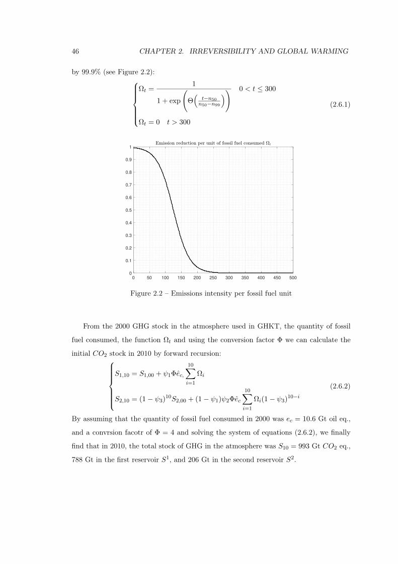
46 CHAPTER 2. IRREVERSIBILITY AND GLOBAL WARMING
by 99.9% (see Figure 2.2):
Ωt =1
1 + exp
(Θ(
t−n50n50−n99
)) 0 < t ≤ 300
Ωt = 0 t > 300
(2.6.1)
0 50 100 150 200 250 300 350 400 450 500
0
0.1
0.2
0.3
0.4
0.5
0.6
0.7
0.8
0.9
1
Figure 2.2 – Emissions intensity per fossil fuel unit
From the 2000 GHG stock in the atmosphere used in GHKT, the quantity of fossil
fuel consumed, the function Ωt and using the conversion factor Φ we can calculate the
initial CO2 stock in 2010 by forward recursion:
S1,10 = S1,00 + ψ1Φec,
10∑
i=1
Ωi
S2,10 = (1− ψ3)10S2,00 + (1− ψ1)ψ2Φec
10∑
i=1
Ωi(1− ψ3)10−i(2.6.2)
By assuming that the quantity of fossil fuel consumed in 2000 was ec = 10.6 Gt oil eq.,
and a convrsion facotr of Φ = 4 and solving the system of equations (2.6.2), we finally
find that in 2010, the total stock of GHG in the atmosphere was S10 = 993 Gt CO2 eq.,
788 Gt in the first reservoir S1, and 206 Gt in the second reservoir S2.
2.6. CALIBRATION: 47
We calibrate the scale parameter κ = 5.3 ·10−5 of the damage function, as in GHKT,
and we assume that the pre-industrial GHG atmospheric stock was S = 581 Gt C02 eq.
To find the corresponding rise in temperature to the GHG atmospheric stock, we use the
following equation as in GHKT:
Tt =3
log(2)log
(StS
)(2.6.3)
Using the initial GHG stock in 2000 S = 802 of GHKT, the corresponding temperature
increase was assumed to be 1.4 C above pre-industrial levels. Assuming now an atmo-
spheric stock of S = 993 Gt CO2 eq. in 2010, we should see a temperature increase of 2.3C. Both of these values overestimate what we observe in reality. According to GHKT,
Schwartz et al. (2010), and Stern and Stern (2007) (p.15), the warming observed is lower
than the warming expected, because other pollutants in the atmosphere such as aerosols,
cool down the temperature, and mask a share of warming effects of GHG.
2.6.2 Preferences and technology parameters:
We use the Penn World Table (Feenstra et al., 2015), to calibrate some parameters to
reach steady state ratios. Out of 185 observations for the 2010 reference year, 47 countries
are removed for which data are missing, resulting in a total of 135 countries. To calculate
the KgY steady state ratio, we aggregate the capital stock at 2011 constant price, and we
divide it by the "gross world product", calculated as the sum of the GDP of each of the
135 countries. We find a capital to gross world product ratio of 3.83 in 2010. The global
capital stock represents nearly 4 years of global production.
The average global depreciation rate is calculated in two steps. First, the depreciation
rate of each country of the Penn World Table are used to calculate the share of capital
that has depreciated, which gives us the global depreciated capital in 2010. Then, this
share is divided by the global capital stock for the same year to calculate the average
annual depreciation rate of capital:
δ =
∑j δjKg,j
Kg= 0.0441
48 CHAPTER 2. IRREVERSIBILITY AND GLOBAL WARMING
We use each country’s real internal rate of capital, and the above capital stock to produc-
tion ratio to find α = 0.325, and an aggregated steady state interest rate of r = 0.074.
With an annual depreciation rate of capital δ = 4.4%, we find a gross investment to
capital stock steady state ratio of IKg
= 4.42%, and an investment rate of IG = 16.9%.
Consequently the income share consumed is equal to CG = 83.1%. We choose the discount
factor β = 0.971, so that the rate of return of capital is r = 7.4%.
The relative price PrPc
of non-polluting energy input in terms of polluting energy input
is equal to the productivity ratio AcAr
. To calculate this ratio, we aggregate the amount of
coal, gas and oil consumed into one polluting energy input and we calculate an aggregate
price. The same technique is used to determine the amount of non-polluting energy
(solar panel, wind, nuclear, hydro-energy, and biomass) consumed and its aggregated
price. According to Dudley et al. (2015), in 2010 4,085 Mtoe of oil were produced, 2,879
Mtoe of gas and 3636 Mtoe of coal. The aggregated fossil fuel price pc is calculated
as a coal average price, natural gas average price and crude oil average price, weighted
by the quantity of each fossil fuel consumed. According to the US Energy Information
Administration, between 2000 and 2017, the annual WTI crude oil price was in average
$ 64.72 per barrel. The conversion factor of 1 barrel is 0.1364 metric ton, so on average
one metric ton of oil cost $ 474.46. For the same period, the Henry Hub Natural Gas
Spot Price averaged $ 5.2 per million Britsh Thermal Unit (BTU). One million BTU is
equal to 0.18 barrel of oil equivalent, so that the natural gas price averaged $ 211.81 per
metric ton. The global price of coal amounted to $ 69.99 per metric ton. The aggregate
price of fossil fuel is therefore:
Pc =211.81 · 2879.7 + 69.99 · 3635.6 + 474.46 · 4085.42
2879.7 + 3635.6 + 4085.42= 264.39 $/toe
The aggregate price of non-polluting energy is calculated in the same way. In 2010, nearly
15% of primary energy consumed did not emit GHG: 2,767.3 TWh (626.2 Mtoe) was of
nuclear3 origin, 3,463.3 TWh (783.9 Mtoe) came from hydroelectricity, 31.4 TWh (7.1
Mtoe) from solar energy, 343.4 TWh (77.7 Mtoe) from wind energy and 367.6 TWh (83.3Nulcear energy is by definition not a renewable energy, but since it does not emit GHG it is opposed
to fossil fuels and consequently we include it into non-polluting energies in the sense of climate change.
2.6. CALIBRATION: 49
Mtoe) from biomass (Dudley et al., 2015). The world price per MWh of nuclear energy
is based on the costs of generating electricity calculated by the US Energy Information
Administration 4. The cost price is an average of operation, maintenance and fuel cost;
its annual average between 2007 and 2017 amounted $26.89 per MWh. According to
IRENA5, the 2010-2017 average Levelised Cost6 of hydropower is $45 per MWh, $230
per MWh for solar photovoltaic, $ 140 per MWh for offshore wind, and $ 70 per MWh
for onshore wind. Using the conversion factor between MWh and ton of oil equivalent
(1MWh ↔ 0.085 toe), we find an aggregate price of Pr = 484.65 $/toe. Consequently,
the we assume that erec
= 0.142, and we calibrate the productivity ratio as equal to:ArAc
= 0.544
We simulate the model for different values of the elasticity of substitution between
polluting and non-polluting energy. Pelli (2012) estimates the world elasticity of sub-
stitution between polluting and non-polluting inputs in the production of electricity to
σ = 0.53 using a sample of 20 countries, so that we calibrate ϕ = −0.88. The relative
price of renewable in terms of fossil fuel is PrPc
= 1.84, using the relative energy demanderec
= 0.142, with the elasticity of substitution σ = 0.53 we finally find ω = 0.0442. Stern
(2012), used 47 studies to conduct his meta-analysis on the elasticity of substitution of
energies. The weighted mean of oil-electricity (1.06), coal-electricity (0.866) and gas-
electricity (1.099) elasticities is greater than unity: σ = 1.004. GHKT used the same
study to calibrate their elasticity of substitution but they only focused on oil and coal so
that their elasticity of substitution is slightly less than unity (0.95). Finally, we consider
two extreme cases where the elasticity of substitution is either equal to 2 or 5 (see table
2.3).
4https : //www.eia.gov/electricity/annual/html/epa_08_04.html5http : //resourceirena.irena.org/gateway/dashboard/?topic = 3&subTopic = 10656The Levelised Cost of electricity is a measure of the overall costs necessary (investment and mainte-
nance over time) to produce one unit of electricity over the lifetime of the system considered (25 years
for wind power, solar PV, 30 years for hydropower and 20 years for biomass power).
50 CHAPTER 2. IRREVERSIBILITY AND GLOBAL WARMING
Table 2.3 – Elasticity of substitution
σ ϕ Ar/Ac er/ec ω ref.
0.53 -0.887 0.544 0.142 0.044 Pelli (2012)
1.004 3.98 · 10−3 0.544 0.142 0.208 Stern (2012)
2 0.5 0.544 0.142 0.408
5 0.8 0.544 0.142 0.554
According to Dudley et al. (2015), the world’s primary energy consumption amounted
to 12,110.765 Mtoe in 2010. This gives an energy intensity of the 2010 gross world product
of EgG = 0.138 kt oil eq. (ktoe) per million of 2011 US dollar constant, hence we calibrate
γ = 0.0434, which is very close to the value of Golosov et al. (2014) (γ = 0.04).
According to our sample of 135 countries from the Penn table, the corresponding
population that of 5.9 billions in 2010. To determine the corresponding wage and labor
demand across sectors we first assume that in 2010, the carbon tax was equal to zero,
and consequently the household lump sump subsidy was also zero. Using the different
parameter values for our calibration we find that in the final good sector, demand for
labor is: Lg = 5.52. Labor demand for non-polluting energy is Lr = 0.0783, labor
demand for the fossil fuel sector is Lc = 0.301, corresponding to a productivity in each
sector respectively of Ar = 19.22 and Ac = 35.22. Productivity in the final good sector
is calibrated to Ag = 1.5 · 104.
2.7 Simulations:
2.7.1 General methodology:
We use the Dynare software (Adjemian et al., 2011) to perform our simulations. This
software, which is a set of MatLab routines, was developed to solve both stochastic and
deterministic macroeconomic models. Dynare is able to solve deterministic non linear
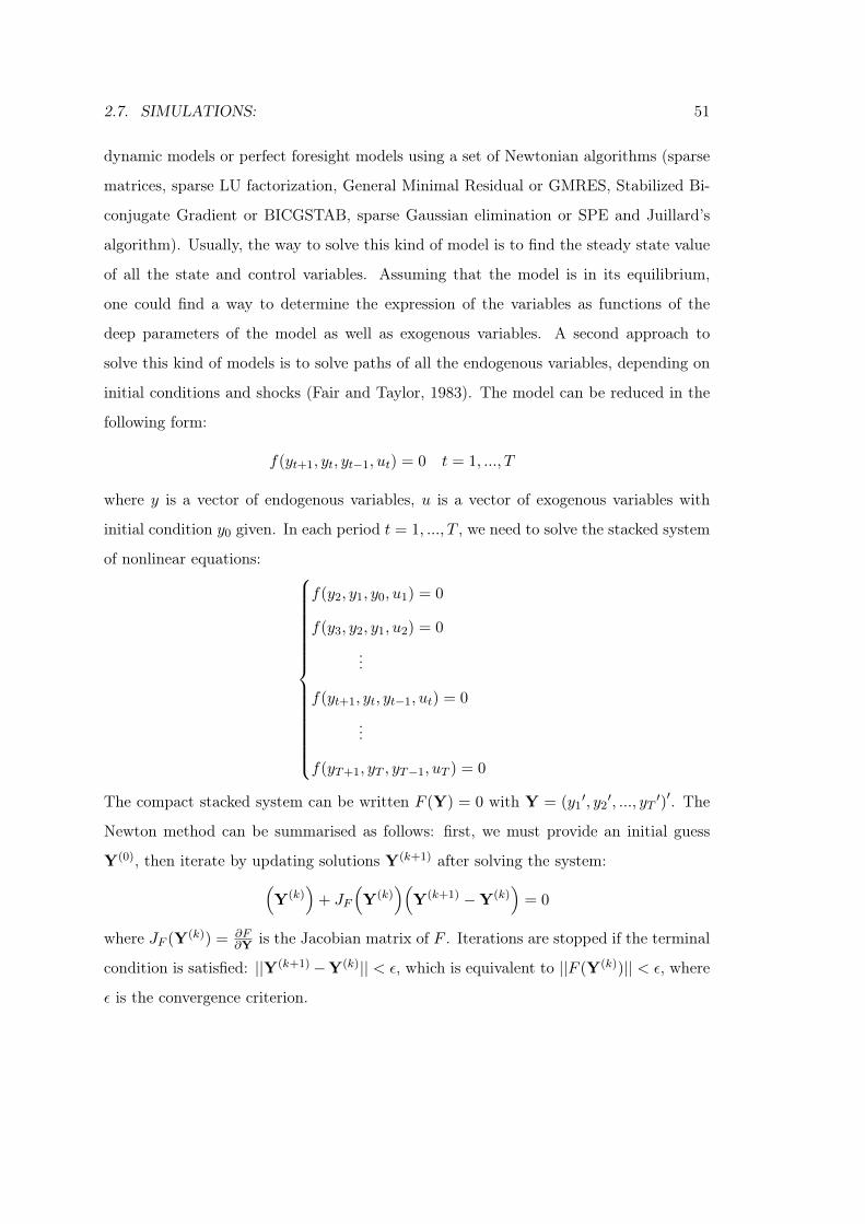
2.7. SIMULATIONS: 51
dynamic models or perfect foresight models using a set of Newtonian algorithms (sparse
matrices, sparse LU factorization, General Minimal Residual or GMRES, Stabilized Bi-
conjugate Gradient or BICGSTAB, sparse Gaussian elimination or SPE and Juillard’s
algorithm). Usually, the way to solve this kind of model is to find the steady state value
of all the state and control variables. Assuming that the model is in its equilibrium,
one could find a way to determine the expression of the variables as functions of the
deep parameters of the model as well as exogenous variables. A second approach to
solve this kind of models is to solve paths of all the endogenous variables, depending on
initial conditions and shocks (Fair and Taylor, 1983). The model can be reduced in the
following form:
f(yt+1, yt, yt−1, ut) = 0 t = 1, ..., T
where y is a vector of endogenous variables, u is a vector of exogenous variables with
initial condition y0 given. In each period t = 1, ..., T , we need to solve the stacked system
of nonlinear equations:
f(y2, y1, y0, u1) = 0
f(y3, y2, y1, u2) = 0
...
f(yt+1, yt, yt−1, ut) = 0
...
f(yT+1, yT , yT−1, uT ) = 0
The compact stacked system can be written F (Y) = 0 with Y = (y1′, y2
′, ..., yT ′)′. The
Newton method can be summarised as follows: first, we must provide an initial guess
Y(0), then iterate by updating solutions Y(k+1) after solving the system:(Y(k)
)+ JF
(Y(k)
)(Y(k+1) −Y(k)
)= 0
where JF (Y(k)) = ∂F∂Y is the Jacobian matrix of F . Iterations are stopped if the terminal
condition is satisfied: ||Y(k+1)−Y(k)|| < ε, which is equivalent to ||F (Y(k))|| < ε, where
ε is the convergence criterion.
52 CHAPTER 2. IRREVERSIBILITY AND GLOBAL WARMING
In order to solve our system of non-linear equations, we must provide a boundary
condition y0. Usually this condition is the steady state value of the system. However this
solution is irrelevant in our case. Indeed, by definition this implies that all variables are
invariant, including the law of motion for the accumulation of GHG in the atmosphere.
Yet, this assumption is incompatible with the current increase in GHG concentration
in the atmosphere. Another solution would be to use the long-term equilibrium and
by backward recursion calculate the trajectories from now that lead to this equilibrium.
Once again, this solution is difficult to implement, since there is an infinite number of
long-term steady states, that depend on the different possible fossil fuel energy con-
sumption paths and so on emission trajectories. According to the model’s assumptions,
we know that even if the economy continues to use fossil fuels, emission intensity per
unit of fossil energy consumed will tend towards 0, thanks to the exogenous variable
Ωt. As a result, the GHG stock in the atmosphere will reach a maximum and then
decrease over time towards its long-term equilibrium, and this equilibrium will define
the equilibrium of the model. But the dynamics vary and the long-run equilibriums are
determined from past GHG accumulations. In the second reservoir, the one in which
CO2 is gradually eliminated, the very long term quantity of GHG in this reservoir will
be equal to zero since it is assumed that the rate of carbon decay will be higher than the
emissions rate, so that limt−>∞ S2,t = 0. In contrast, since GHG are not removed from
the other reservoir S1, the long term equilibrium of the overall stock of CO2 in the atmo-
sphere will be determined by the amount of CO2 that has accumulated in this reservoir:
limt−>∞ St = limt−>∞(S1,t + S2,t) = limt−>∞ S1,t. Once we have this equilibrium, we
would be able to determine environmental damages as well as the steady state of the
entire model. There are as many possible trajectories as there are S1 limits.
Recalling the recursive representation of the carbon cycle (equation (2.3.3)):
S1t = ψ1ΩtΦec,t + S1
t−1
S2t = (1− ψ1)ψ2ΩtΦec,t + (1− ψ3)S2
t−1
2.7. SIMULATIONS: 53
After 300 years, Ωt = 0, thus:
⇔
ψ1ΩtΦec,t = 0
(1− ψ1)ψ2ΩtΦec,t = 0
Consequently,
limt→+∞
S1t = S1
0 +300∑
j=1
ψ1ΩjΦec,j
limt→+∞
S2t = 0
limt→+∞
St = S1t
The solution we have chosen for the initial guess is the following: it is assumed that
all economic variables of the system are determined at their steady state, but not the
carbon stock. Thus in the baseline scenario (the business as usual one) where externalities
are not taken into account, the dynamics of the system will be induced by the carbon
cycle. We thus simulated the model over a sufficiently large numbers of periods (t > 300)
to allow carbon dynamics to converge, but our analysis will focus on a shorter period.
We choose T = 1000, the number of periods simulated. This strategy is reused for the
different simulations environmental policy .
2.7.2 Results:
2.7.2.1 Environmental impacts:
In this section the 4 Business As Usual (BAU) scenarios (for the 4 different elasticities
assumed see Table 2.3) are summarised in a single scenario. Since the productivity ratio
of energies remains constant, the same results are obtained. The next section explores the
case where the energy productivity ratio evolves in time, and then considers the 8 different
scenarios. We thus consider one BAU scenario as the benchmark scenario (without an
environmental policy), and 4 different scenarios with an optimal environmental policy for
the different elasticities of substitution considered. Under the assumption of exogenous
emission reduction, according to the results of the model, in all the different relevant
scenarios we observe a decrease in emissions, yet in different proportions.
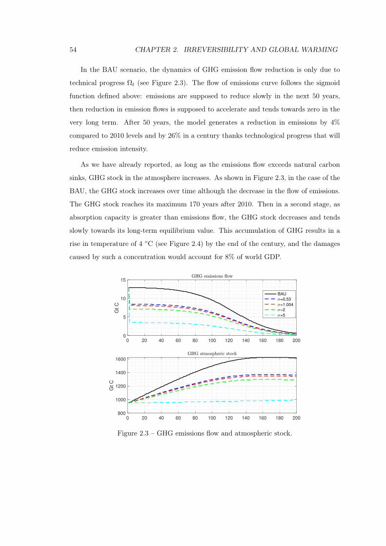
54 CHAPTER 2. IRREVERSIBILITY AND GLOBAL WARMING
In the BAU scenario, the dynamics of GHG emission flow reduction is only due to
technical progress Ωt (see Figure 2.3). The flow of emissions curve follows the sigmoid
function defined above: emissions are supposed to reduce slowly in the next 50 years,
then reduction in emission flows is supposed to accelerate and tends towards zero in the
very long term. After 50 years, the model generates a reduction in emissions by 4%
compared to 2010 levels and by 26% in a century thanks technological progress that will
reduce emission intensity.
As we have already reported, as long as the emissions flow exceeds natural carbon
sinks, GHG stock in the atmosphere increases. As shown in Figure 2.3, in the case of the
BAU, the GHG stock increases over time although the decrease in the flow of emissions.
The GHG stock reaches its maximum 170 years after 2010. Then in a second stage, as
absorption capacity is greater than emissions flow, the GHG stock decreases and tends
slowly towards its long-term equilibrium value. This accumulation of GHG results in a
rise in temperature of 4 C (see Figure 2.4) by the end of the century, and the damages
caused by such a concentration would account for 8% of world GDP.
0 20 40 60 80 100 120 140 160 180 200
0
5
10
15
Gt C
BAU
=0.53
=1.004
=2
=5
0 20 40 60 80 100 120 140 160 180 200
800
1000
1200
1400
1600
Gt C
Figure 2.3 – GHG emissions flow and atmospheric stock.
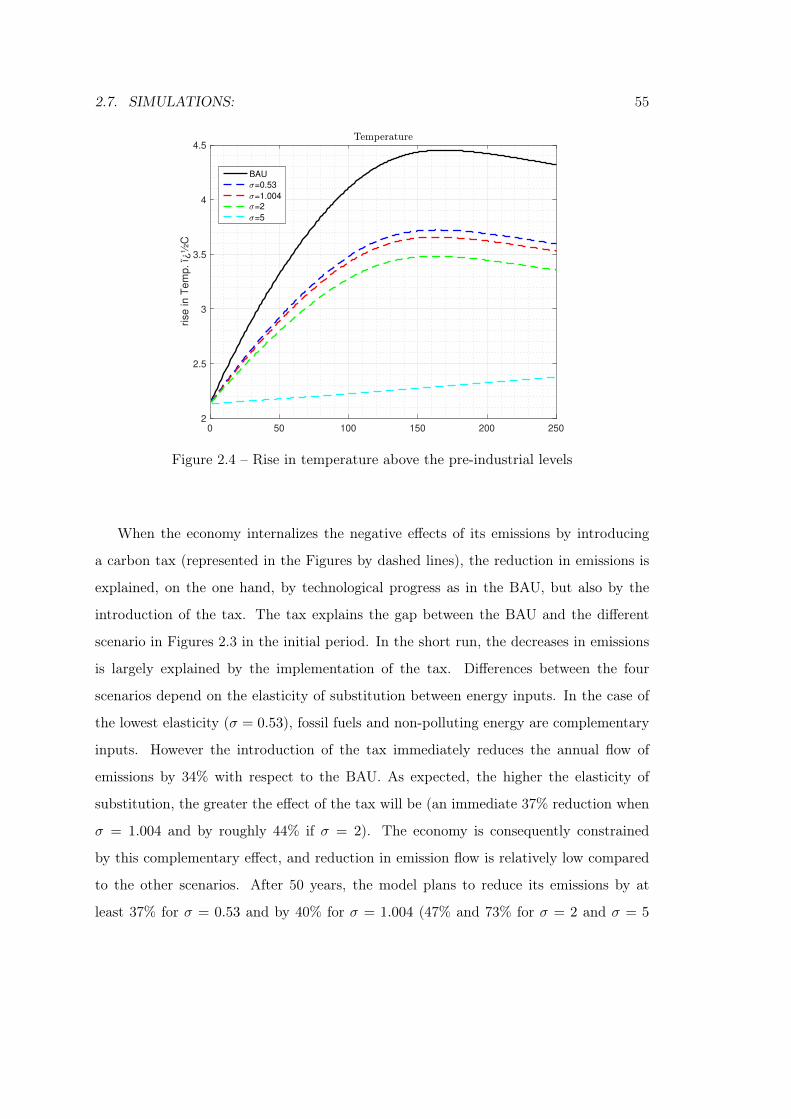
2.7. SIMULATIONS: 55
0 50 100 150 200 2502
2.5
3
3.5
4
4.5
rise in T
em
p. ï¿
½C
BAU
=0.53
=1.004
=2
=5
Figure 2.4 – Rise in temperature above the pre-industrial levels
When the economy internalizes the negative effects of its emissions by introducing
a carbon tax (represented in the Figures by dashed lines), the reduction in emissions is
explained, on the one hand, by technological progress as in the BAU, but also by the
introduction of the tax. The tax explains the gap between the BAU and the different
scenario in Figures 2.3 in the initial period. In the short run, the decreases in emissions
is largely explained by the implementation of the tax. Differences between the four
scenarios depend on the elasticity of substitution between energy inputs. In the case of
the lowest elasticity (σ = 0.53), fossil fuels and non-polluting energy are complementary
inputs. However the introduction of the tax immediately reduces the annual flow of
emissions by 34% with respect to the BAU. As expected, the higher the elasticity of
substitution, the greater the effect of the tax will be (an immediate 37% reduction when
σ = 1.004 and by roughly 44% if σ = 2). The economy is consequently constrained
by this complementary effect, and reduction in emission flow is relatively low compared
to the other scenarios. After 50 years, the model plans to reduce its emissions by at
least 37% for σ = 0.53 and by 40% for σ = 1.004 (47% and 73% for σ = 2 and σ = 5
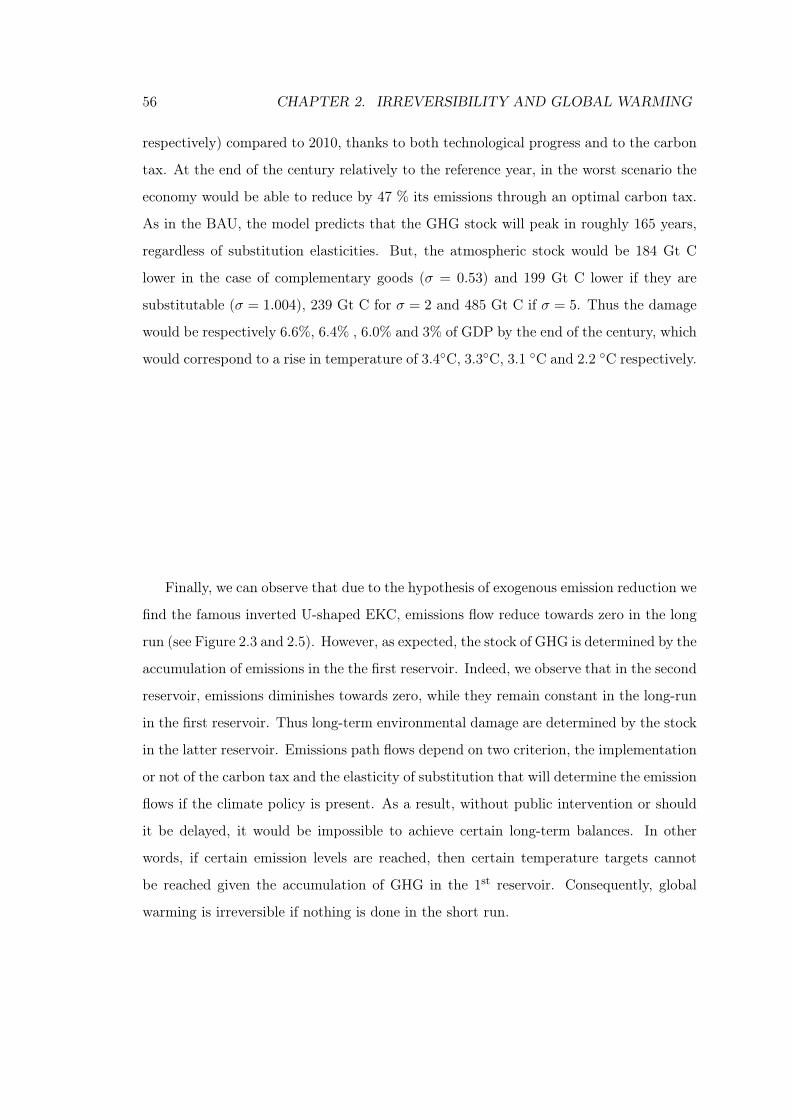
56 CHAPTER 2. IRREVERSIBILITY AND GLOBAL WARMING
respectively) compared to 2010, thanks to both technological progress and to the carbon
tax. At the end of the century relatively to the reference year, in the worst scenario the
economy would be able to reduce by 47 % its emissions through an optimal carbon tax.
As in the BAU, the model predicts that the GHG stock will peak in roughly 165 years,
regardless of substitution elasticities. But, the atmospheric stock would be 184 Gt C
lower in the case of complementary goods (σ = 0.53) and 199 Gt C lower if they are
substitutable (σ = 1.004), 239 Gt C for σ = 2 and 485 Gt C if σ = 5. Thus the damage
would be respectively 6.6%, 6.4% , 6.0% and 3% of GDP by the end of the century, which
would correspond to a rise in temperature of 3.4C, 3.3C, 3.1 C and 2.2 C respectively.
Finally, we can observe that due to the hypothesis of exogenous emission reduction we
find the famous inverted U-shaped EKC, emissions flow reduce towards zero in the long
run (see Figure 2.3 and 2.5). However, as expected, the stock of GHG is determined by the
accumulation of emissions in the the first reservoir. Indeed, we observe that in the second
reservoir, emissions diminishes towards zero, while they remain constant in the long-run
in the first reservoir. Thus long-term environmental damage are determined by the stock
in the latter reservoir. Emissions path flows depend on two criterion, the implementation
or not of the carbon tax and the elasticity of substitution that will determine the emission
flows if the climate policy is present. As a result, without public intervention or should
it be delayed, it would be impossible to achieve certain long-term balances. In other
words, if certain emission levels are reached, then certain temperature targets cannot
be reached given the accumulation of GHG in the 1st reservoir. Consequently, global
warming is irreversible if nothing is done in the short run.
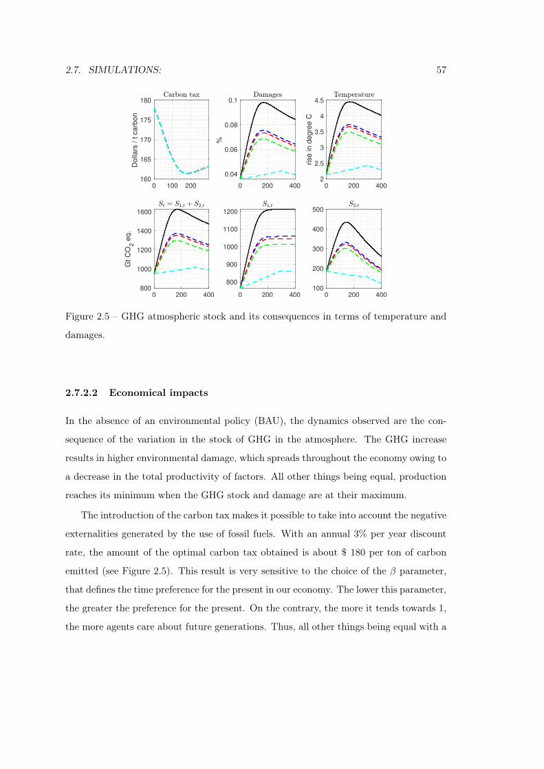
2.7. SIMULATIONS: 57
0 100 200160
165
170
175
180
Dolla
rs / t c
arb
on
0 200 400
0.04
0.06
0.08
0.1
%
0 200 4002
2.5
3
3.5
4
4.5
rise in d
egre
e C
0 200 400800
1000
1200
1400
1600
Gt C
O2 e
q.
0 200 400
800
900
1000
1100
1200
0 200 400100
200
300
400
500
Figure 2.5 – GHG atmospheric stock and its consequences in terms of temperature and
damages.
2.7.2.2 Economical impacts
In the absence of an environmental policy (BAU), the dynamics observed are the con-
sequence of the variation in the stock of GHG in the atmosphere. The GHG increase
results in higher environmental damage, which spreads throughout the economy owing to
a decrease in the total productivity of factors. All other things being equal, production
reaches its minimum when the GHG stock and damage are at their maximum.
The introduction of the carbon tax makes it possible to take into account the negative
externalities generated by the use of fossil fuels. With an annual 3% per year discount
rate, the amount of the optimal carbon tax obtained is about $ 180 per ton of carbon
emitted (see Figure 2.5). This result is very sensitive to the choice of the β parameter,
that defines the time preference for the present in our economy. The lower this parameter,
the greater the preference for the present. On the contrary, the more it tends towards 1,
the more agents care about future generations. Thus, all other things being equal with a
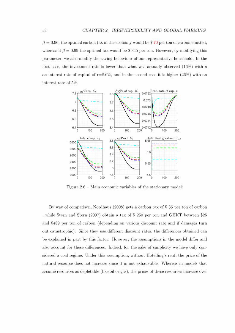
58 CHAPTER 2. IRREVERSIBILITY AND GLOBAL WARMING
β = 0.96, the optimal carbon tax in the economy would be $ 70 per ton of carbon emitted,
whereas if β = 0.99 the optimal tax would be $ 345 per ton. However, by modifying this
parameter, we also modify the saving behaviour of our representative household. In the
first case, the investment rate is lower than what was actually observed (16%) with a
an interest rate of capital of r=8.6%, and in the second case it is higher (26%) with an
interest rate of 5%.
0 100 200
6.4
6.6
6.8
7
7.210
4
0 100 200
3.4
3.5
3.6
3.7
3.810
5
0 100 200
0.0742
0.0744
0.0746
0.0748
0.075
0.0752
0 100 200
9000
9200
9400
9600
9800
10000
0 100 200
7.8
8
8.2
8.4
8.6
8.810
4
0 100 200
5.5
5.55
5.6
5.65
Figure 2.6 – Main economic variables of the stationary model:
By way of comparison, Nordhaus (2008) gets a carbon tax of $ 35 per ton of carbon
, while Stern and Stern (2007) obtain a tax of $ 250 per ton and GHKT between $25
and $489 per ton of carbon (depending on various discount rate and if damages turn
out catastrophic). Since they use different discount rates, the differences obtained can
be explained in part by this factor. However, the assumptions in the model differ and
also account for these differences. Indeed, for the sake of simplicity we have only con-
sidered a coal regime. Under this assumption, without Hotelling’s rent, the price of the
natural resource does not increase since it is not exhaustible. Whereas in models that
assume resources as depletable (like oil or gas), the prices of these resources increase over
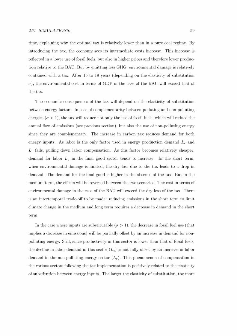
2.7. SIMULATIONS: 59
time, explaining why the optimal tax is relatively lower than in a pure coal regime. By
introducing the tax, the economy sees its intermediate costs increase. This increase is
reflected in a lower use of fossil fuels, but also in higher prices and therefore lower produc-
tion relative to the BAU. But by emitting less GHG, environmental damage is relatively
contained with a tax. After 15 to 19 years (depending on the elasticity of substitution
σ), the environmental cost in terms of GDP in the case of the BAU will exceed that of
the tax.
The economic consequences of the tax will depend on the elasticity of substitution
between energy factors. In case of complementarity between polluting and non-polluting
energies (σ < 1), the tax will reduce not only the use of fossil fuels, which will reduce the
annual flow of emissions (see previous section), but also the use of non-polluting energy
since they are complementary. The increase in carbon tax reduces demand for both
energy inputs. As labor is the only factor used in energy production demand Lc and
Lr falls, pulling down labor compensation. As this factor becomes relatively cheaper,
demand for labor Lg in the final good sector tends to increase. In the short term,
when environmental damage is limited, the dry loss due to the tax leads to a drop in
demand. The demand for the final good is higher in the absence of the tax. But in the
medium term, the effects will be reversed between the two scenarios. The cost in terms of
environmental damage in the case of the BAU will exceed the dry loss of the tax. There
is an intertemporal trade-off to be made: reducing emissions in the short term to limit
climate change in the medium and long term requires a decrease in demand in the short
term.
In the case where inputs are substitutable (σ > 1), the decrease in fossil fuel use (that
implies a decrease in emissions) will be partially offset by an increase in demand for non-
polluting energy. Still, since productivity in this sector is lower than that of fossil fuels,
the decline in labor demand in this sector (Lc) is not fully offset by an increase in labor
demand in the non-polluting energy sector (Lr). This phenomenon of compensation in
the various sectors following the tax implementation is positively related to the elasticity
of substitution between energy inputs. The larger the elasticity of substitution, the more
60 CHAPTER 2. IRREVERSIBILITY AND GLOBAL WARMING
the economy will use non-polluting energy, the greater the demand for labor in this
sector. As in the previous case where energies were supposed to be complementary, the
tax has a recessionary effect but this is offset by the use of the tax revenues in the form of
subsidies which prevents consumption from collapsing. Nevertheless the negative effect
of the tax is lessened by the ability of the economy to use non-polluting energy. In the
case where energies are close substitute, the economy can reduce these GHG emissions
in a larger proportion, the effect of the tax is then much more effective and thus limits
the negative consequences related to environmental damage. With a larger production
level, long-term consumption and utility are therefore higher than in the previous case.
0 100 2001
2
3
4
5
Gt oil
eq.
0 100 200
480
490
500
510
520
$ t o
il eq.
0 100 2000.05
0.1
0.15
0.2
0.25
0 100 2002
4
6
8
10
12
Gt oil
eq.
0 100 200
260
270
280
290
$ t o
il eq.
0 100 200
0.1
0.15
0.2
0.25
0.3
Figure 2.7 – Energy block:
2.7.3 Rise in renewable energy productivity:
We now consider the possibility of increased productivity in the non-polluting energy
sector. Until now we have assumed that the productivity ratio (Ar/Ac) remains constant
over time. However over the past decade, there has been a decline in the global weighted-
average levelized cost of electricity from non-polluting energies (bioenergy, geothermal,
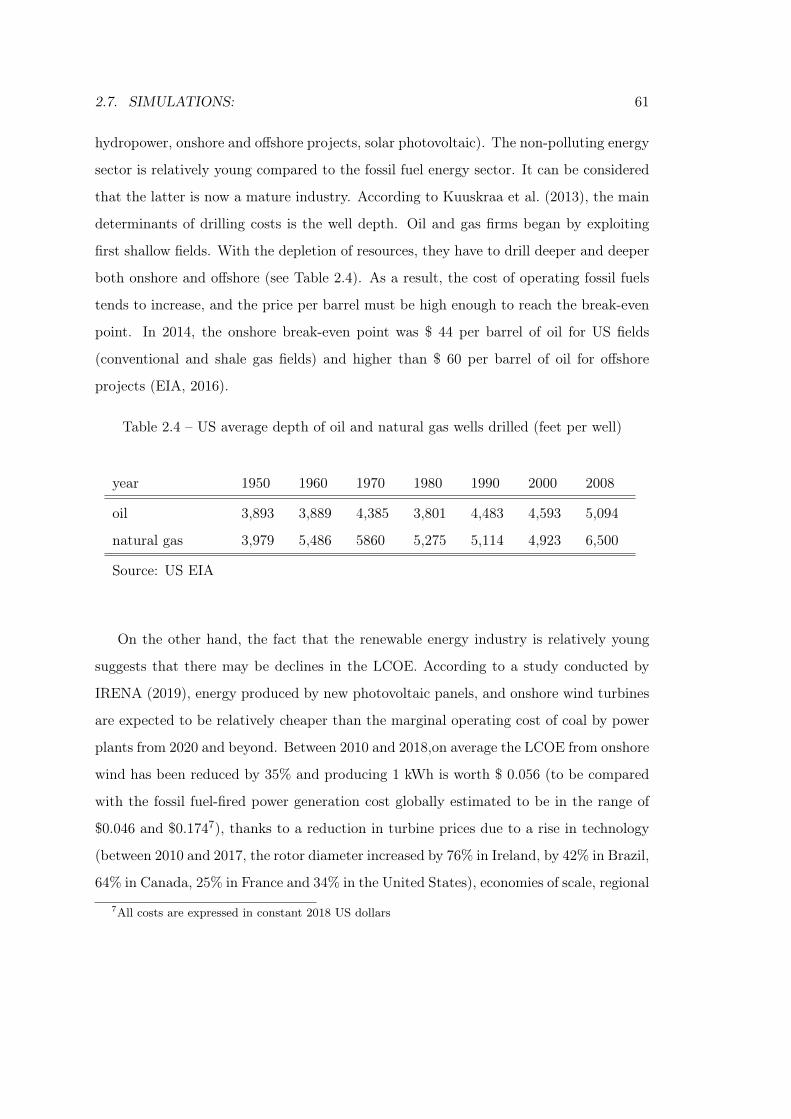
2.7. SIMULATIONS: 61
hydropower, onshore and offshore projects, solar photovoltaic). The non-polluting energy
sector is relatively young compared to the fossil fuel energy sector. It can be considered
that the latter is now a mature industry. According to Kuuskraa et al. (2013), the main
determinants of drilling costs is the well depth. Oil and gas firms began by exploiting
first shallow fields. With the depletion of resources, they have to drill deeper and deeper
both onshore and offshore (see Table 2.4). As a result, the cost of operating fossil fuels
tends to increase, and the price per barrel must be high enough to reach the break-even
point. In 2014, the onshore break-even point was $ 44 per barrel of oil for US fields
(conventional and shale gas fields) and higher than $ 60 per barrel of oil for offshore
projects (EIA, 2016).
Table 2.4 – US average depth of oil and natural gas wells drilled (feet per well)
year 1950 1960 1970 1980 1990 2000 2008
oil 3,893 3,889 4,385 3,801 4,483 4,593 5,094
natural gas 3,979 5,486 5860 5,275 5,114 4,923 6,500
Source: US EIA
On the other hand, the fact that the renewable energy industry is relatively young
suggests that there may be declines in the LCOE. According to a study conducted by
IRENA (2019), energy produced by new photovoltaic panels, and onshore wind turbines
are expected to be relatively cheaper than the marginal operating cost of coal by power
plants from 2020 and beyond. Between 2010 and 2018,on average the LCOE from onshore
wind has been reduced by 35% and producing 1 kWh is worth $ 0.056 (to be compared
with the fossil fuel-fired power generation cost globally estimated to be in the range of
$0.046 and $0.1747), thanks to a reduction in turbine prices due to a rise in technology
(between 2010 and 2017, the rotor diameter increased by 76% in Ireland, by 42% in Brazil,
64% in Canada, 25% in France and 34% in the United States), economies of scale, regional
7All costs are expressed in constant 2018 US dollars
62 CHAPTER 2. IRREVERSIBILITY AND GLOBAL WARMING
production etc. On the global weighted average, LCOE of solar photovoltaic was worth
about $ 0.085 in 2018, 77% lower than in 2010. This decrease is the result of a much
lower raw material price (crystalline silicon module price fell by nearly 30% between 2017
and 2018). The total installed cost per kW was divided by a factor 4 between 2010 and
2018 ($ 4,621 in 2010 and $ 1,210 in 2018 global weighted average).
According to the same study, the LCOE from offshore wind power was worth $0.127
per kWh in 2018, corresponding to a 20% reduction in costs between 2010 and 2018. The
main drivers explaining that decrease in costs are innovations (larger rotor), economies
of scales (installation and logistics). Larger turbines imply lower installation costs for
a given power capacity. While the total installed cost remained constant because farms
were installed in deeper ocean ($ 4,572 in 2010 against $4,353 in 2018). Setting up
offshore wind turbines in deeper waters is more expensive, but the field covered is wider,
wind is less volatile which increases the capacity factor. The rise in the capacity factor
from 38% to 43% explained the decrease in LCOE for the same period.
Concentrating solar power (CSP) and bioenergy has also seen their LCOE fall over
the past decade. A decrease of 46% per KWh for CSP and 15% for bioenergy compared
to 2010. Energy production from CSP is in its early stages, global capacity was 5.5 GW,
to be compared with 95 GW of new solar panel capacity installed the same year. China
is developing several CSP projects, which should lower the LCOE in the near future.
The total cost of installing a kW roughly amounted $ 5,200 in 2018, against $ 8,800 in
2010.
For geothermal power generation and hydropower, LCOE have increased between
2010 and 2018, by 40% for geothermal energies, and by 29% for hydropower. However, the
LCOE for geothermal are very low $ 0.07 per kWh, and $ 0.047 per kWh for hydropower.
The very small capacity (500 MW of new capacity in 2018) and specificities of each
project (geography, country) explain this rise for geothermal energy. On the contrary,
hydropower is a mature energy industry, and explains why new capacities increased its
costs. Indeed, the best sites are already exploited, and developing this energy requires
to overcome difficulties linked to geography like bigger rivers.
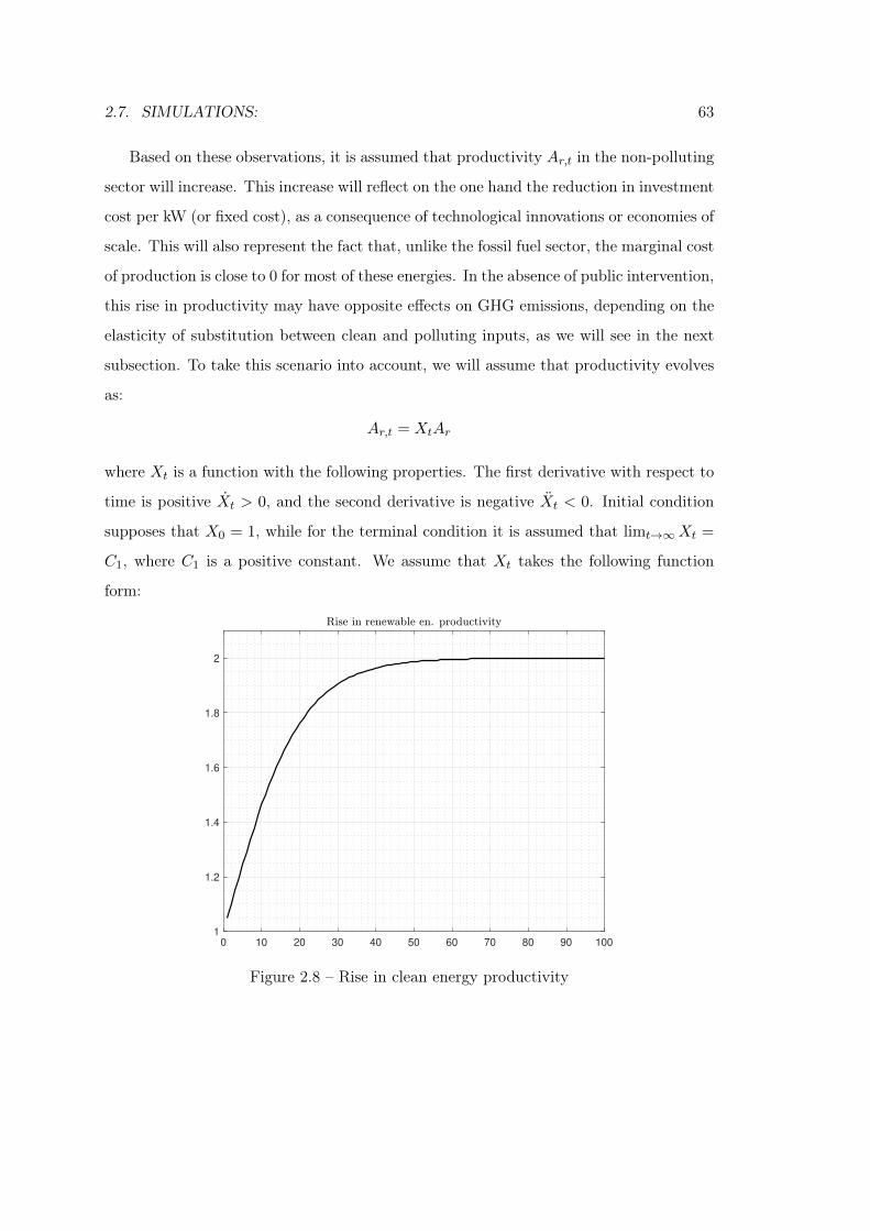
2.7. SIMULATIONS: 63
Based on these observations, it is assumed that productivity Ar,t in the non-polluting
sector will increase. This increase will reflect on the one hand the reduction in investment
cost per kW (or fixed cost), as a consequence of technological innovations or economies of
scale. This will also represent the fact that, unlike the fossil fuel sector, the marginal cost
of production is close to 0 for most of these energies. In the absence of public intervention,
this rise in productivity may have opposite effects on GHG emissions, depending on the
elasticity of substitution between clean and polluting inputs, as we will see in the next
subsection. To take this scenario into account, we will assume that productivity evolves
as:
Ar,t = XtAr
where Xt is a function with the following properties. The first derivative with respect to
time is positive Xt > 0, and the second derivative is negative Xt < 0. Initial condition
supposes that X0 = 1, while for the terminal condition it is assumed that limt→∞Xt =
C1, where C1 is a positive constant. We assume that Xt takes the following function
form:
0 10 20 30 40 50 60 70 80 90 100
1
1.2
1.4
1.6
1.8
2
Figure 2.8 – Rise in clean energy productivity
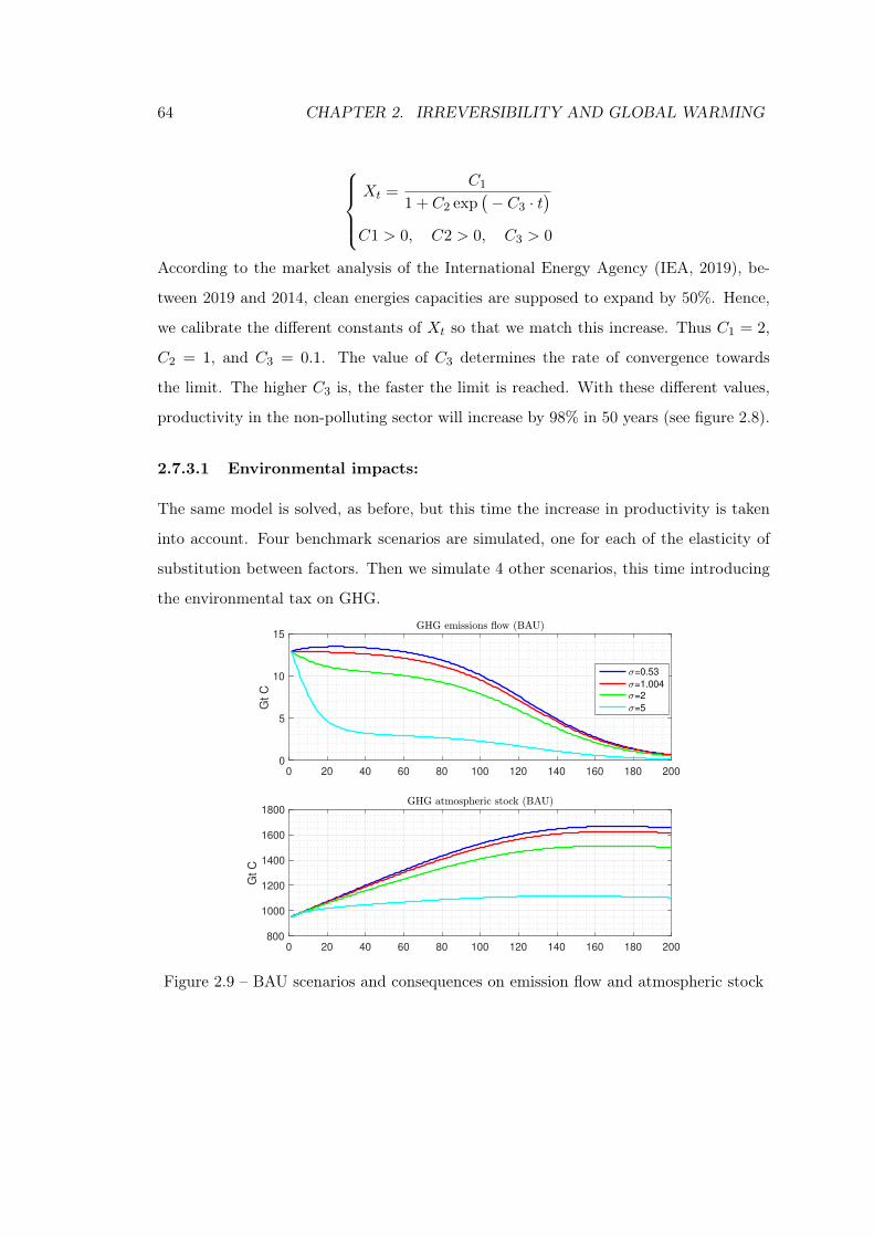
64 CHAPTER 2. IRREVERSIBILITY AND GLOBAL WARMING
Xt =C1
1 + C2 exp(− C3 · t
)
C1 > 0, C2 > 0, C3 > 0
According to the market analysis of the International Energy Agency (IEA, 2019), be-
tween 2019 and 2014, clean energies capacities are supposed to expand by 50%. Hence,
we calibrate the different constants of Xt so that we match this increase. Thus C1 = 2,
C2 = 1, and C3 = 0.1. The value of C3 determines the rate of convergence towards
the limit. The higher C3 is, the faster the limit is reached. With these different values,
productivity in the non-polluting sector will increase by 98% in 50 years (see figure 2.8).
2.7.3.1 Environmental impacts:
The same model is solved, as before, but this time the increase in productivity is taken
into account. Four benchmark scenarios are simulated, one for each of the elasticity of
substitution between factors. Then we simulate 4 other scenarios, this time introducing
the environmental tax on GHG.
0 20 40 60 80 100 120 140 160 180 200
0
5
10
15
Gt C
=0.53
=1.004
=2
=5
0 20 40 60 80 100 120 140 160 180 200
800
1000
1200
1400
1600
1800
Gt C
Figure 2.9 – BAU scenarios and consequences on emission flow and atmospheric stock
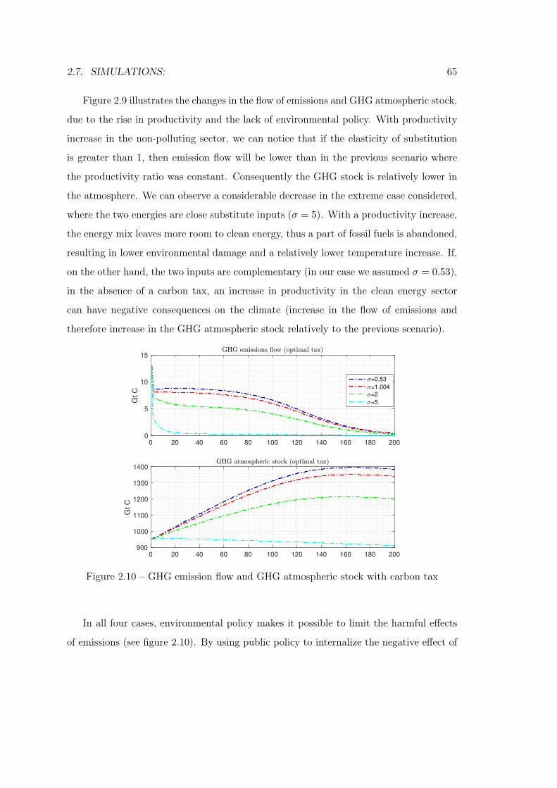
2.7. SIMULATIONS: 65
Figure 2.9 illustrates the changes in the flow of emissions and GHG atmospheric stock,
due to the rise in productivity and the lack of environmental policy. With productivity
increase in the non-polluting sector, we can notice that if the elasticity of substitution
is greater than 1, then emission flow will be lower than in the previous scenario where
the productivity ratio was constant. Consequently the GHG stock is relatively lower in
the atmosphere. We can observe a considerable decrease in the extreme case considered,
where the two energies are close substitute inputs (σ = 5). With a productivity increase,
the energy mix leaves more room to clean energy, thus a part of fossil fuels is abandoned,
resulting in lower environmental damage and a relatively lower temperature increase. If,
on the other hand, the two inputs are complementary (in our case we assumed σ = 0.53),
in the absence of a carbon tax, an increase in productivity in the clean energy sector
can have negative consequences on the climate (increase in the flow of emissions and
therefore increase in the GHG atmospheric stock relatively to the previous scenario).
0 20 40 60 80 100 120 140 160 180 200
0
5
10
15
Gt C
=0.53
=1.004
=2
=5
0 20 40 60 80 100 120 140 160 180 200
900
1000
1100
1200
1300
1400
Gt C
Figure 2.10 – GHG emission flow and GHG atmospheric stock with carbon tax
In all four cases, environmental policy makes it possible to limit the harmful effects
of emissions (see figure 2.10). By using public policy to internalize the negative effect of
66 CHAPTER 2. IRREVERSIBILITY AND GLOBAL WARMING
fossil fuels, annual emissions initially decrease by at least 34% in the case where energies
are assumed to be complementary. The higher the elasticity of substitution, the less fossil
fuels the economy uses, the more the climate is preserved in the long term. After 50 years,
emissions would decrease by 34% when σ = 0.53, and by 59% when σ = 2. According
to the simulations, the GHG stock reaches its maximum after 159 to 170 years (Figures
2.9 and 2.10) depending on the policy regime and the elasticity of substitution. In the
extreme case where σ = 5, the maximum is reached 13 years after the tax. However the
consequences are more significant in the absence of a policy. At the end of the century,
the loss of global GDP is about 8.5%, 8.2% and 7.5% for elasticity of substitution or
0.53, 1.004 and 2 respectively for the BAU, while they are limited to 6.7%, 6.4% and
5.5% in case of public intervention. With a very high elasticity of substitution between
factors (σ = 5), annual emissions decrease sufficiently for the GHG stock to decrease
monotonously. The absorption capacity of natural sinks is greater than the emission
flow. In this case global warming is avoided.
2.7.3.2 Economic impacts:
As already explained, in the absence of environmental policy, if productivity increases
in the non-polluting sector, the quantity of fossil fuels used will be more or less signifi-
cant, depending on the elasticity of substitution between energy inputs. If energies are
complementary (σ < 1), increased productivity Ar,t increases demand for polluting en-
ergy (Figure 2.13), the annual emissions flow increases (Figure 2.9) and environmental
damage increases (Figure 2.12). Environmental policy is in then essential to limit the
consequences of global warming. In the absence of intervention, emissions will increase
by almost 1% after 50 years and then decrease, thanks to technical progress, by almost
15% by the end of the century. With the tax, emissions will decrease by 34% after 50
years and by 44% in 2100.
In the event of weak substitutability between factors (σ = 1.004), fossil energy use
remains constant over time despite the increase in relative productivity Ar,t/Ac, if the
tax is not introduced (Figure 2.13). The carbon tax thus permits to limit the harmful
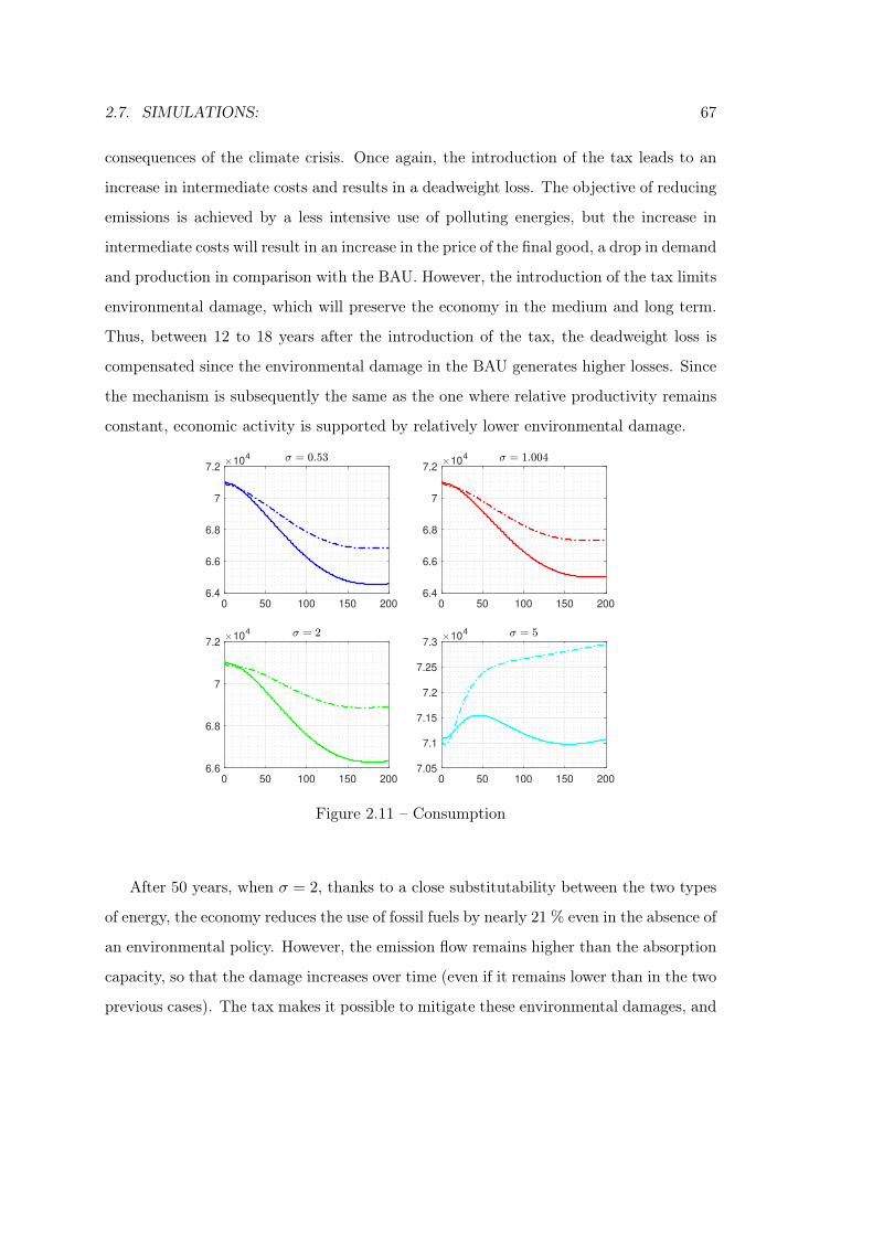
2.7. SIMULATIONS: 67
consequences of the climate crisis. Once again, the introduction of the tax leads to an
increase in intermediate costs and results in a deadweight loss. The objective of reducing
emissions is achieved by a less intensive use of polluting energies, but the increase in
intermediate costs will result in an increase in the price of the final good, a drop in demand
and production in comparison with the BAU. However, the introduction of the tax limits
environmental damage, which will preserve the economy in the medium and long term.
Thus, between 12 to 18 years after the introduction of the tax, the deadweight loss is
compensated since the environmental damage in the BAU generates higher losses. Since
the mechanism is subsequently the same as the one where relative productivity remains
constant, economic activity is supported by relatively lower environmental damage.
0 50 100 150 200
6.4
6.6
6.8
7
7.210
4
0 50 100 150 200
6.4
6.6
6.8
7
7.210
4
0 50 100 150 200
6.6
6.8
7
7.210
4
0 50 100 150 200
7.05
7.1
7.15
7.2
7.25
7.310
4
Figure 2.11 – Consumption
After 50 years, when σ = 2, thanks to a close substitutability between the two types
of energy, the economy reduces the use of fossil fuels by nearly 21 % even in the absence of
an environmental policy. However, the emission flow remains higher than the absorption
capacity, so that the damage increases over time (even if it remains lower than in the two
previous cases). The tax makes it possible to mitigate these environmental damages, and
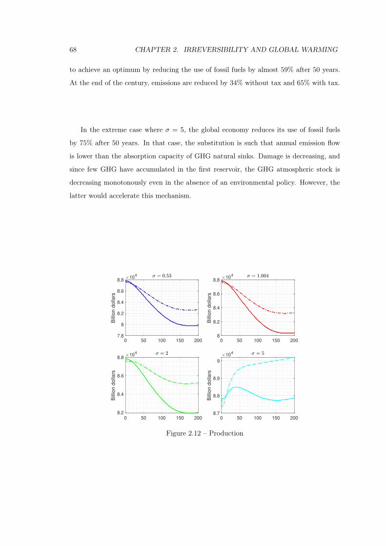
68 CHAPTER 2. IRREVERSIBILITY AND GLOBAL WARMING
to achieve an optimum by reducing the use of fossil fuels by almost 59% after 50 years.
At the end of the century, emissions are reduced by 34% without tax and 65% with tax.
In the extreme case where σ = 5, the global economy reduces its use of fossil fuels
by 75% after 50 years. In that case, the substitution is such that annual emission flow
is lower than the absorption capacity of GHG natural sinks. Damage is decreasing, and
since few GHG have accumulated in the first reservoir, the GHG atmospheric stock is
decreasing monotonously even in the absence of an environmental policy. However, the
latter would accelerate this mechanism.
0 50 100 150 200
7.8
8
8.2
8.4
8.6
8.8
Billion d
ollars
104
0 50 100 150 200
8
8.2
8.4
8.6
8.8
Billion d
ollars
104
0 50 100 150 200
8.2
8.4
8.6
8.8
Billion d
ollars
104
0 50 100 150 200
8.7
8.8
8.9
9
Billion d
ollars
104
Figure 2.12 – Production
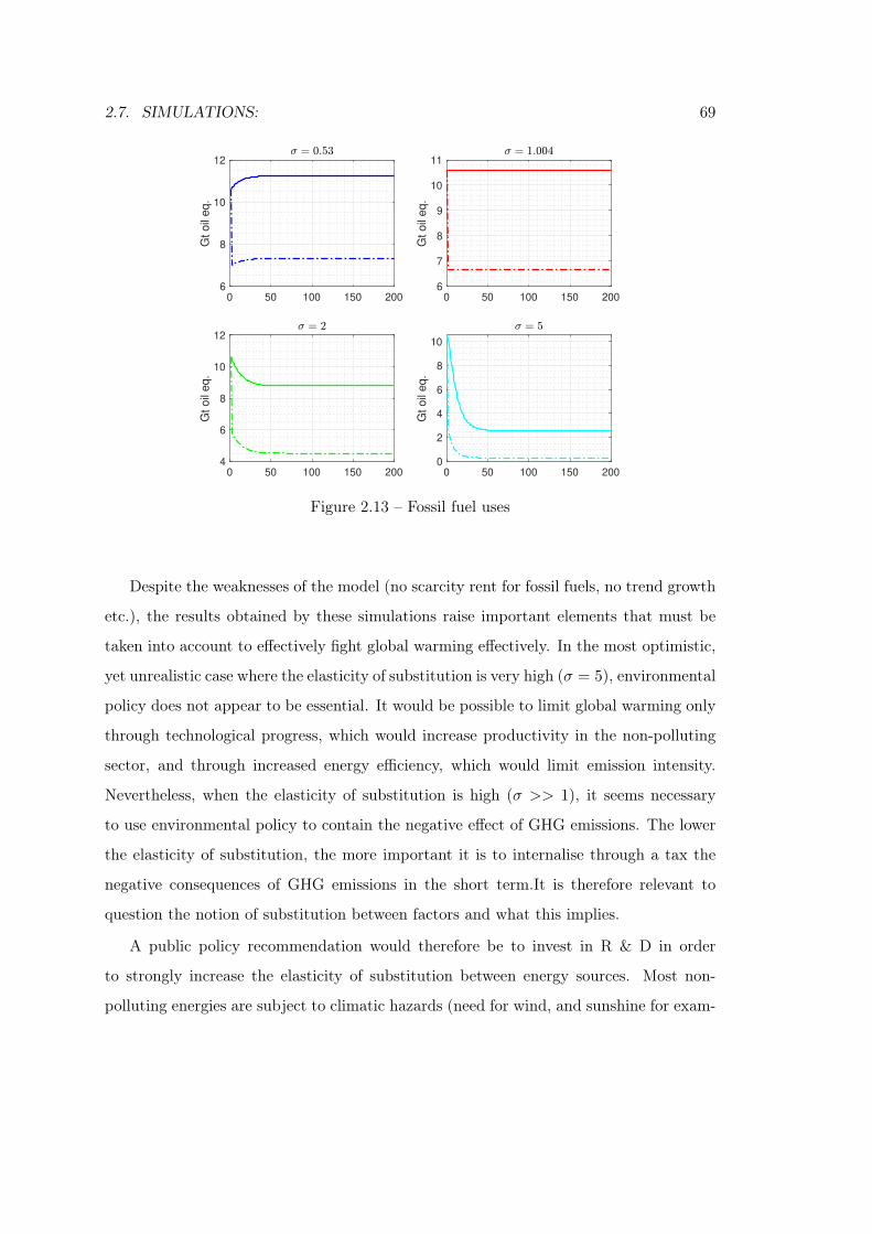
2.7. SIMULATIONS: 69
0 50 100 150 2006
8
10
12
Gt oil
eq.
0 50 100 150 2006
7
8
9
10
11
Gt oil
eq.
0 50 100 150 2004
6
8
10
12
Gt oil
eq.
0 50 100 150 2000
2
4
6
8
10
Gt oil
eq.
Figure 2.13 – Fossil fuel uses
Despite the weaknesses of the model (no scarcity rent for fossil fuels, no trend growth
etc.), the results obtained by these simulations raise important elements that must be
taken into account to effectively fight global warming effectively. In the most optimistic,
yet unrealistic case where the elasticity of substitution is very high (σ = 5), environmental
policy does not appear to be essential. It would be possible to limit global warming only
through technological progress, which would increase productivity in the non-polluting
sector, and through increased energy efficiency, which would limit emission intensity.
Nevertheless, when the elasticity of substitution is high (σ >> 1), it seems necessary
to use environmental policy to contain the negative effect of GHG emissions. The lower
the elasticity of substitution, the more important it is to internalise through a tax the
negative consequences of GHG emissions in the short term.It is therefore relevant to
question the notion of substitution between factors and what this implies.
A public policy recommendation would therefore be to invest in R & D in order
to strongly increase the elasticity of substitution between energy sources. Most non-
polluting energies are subject to climatic hazards (need for wind, and sunshine for exam-
70 CHAPTER 2. IRREVERSIBILITY AND GLOBAL WARMING
ple). However, the time when energy is produced does not necessarily coincide with the
time when its is consumed. The substitution between non-polluting energies and fossil fu-
els raises the question of energy storage. In the absence of a storage solution, it is difficult
to have a strong elasticity of substitution between energies. Increasing storage capac-
ity as a result of clean energy production would increase this elasticity of substitution.
Nevertheless, the production of clean energy faces other challenges. The development
of non-polluting energies is constrained by physical limitations. For MacKay (2008), it
would be necessary to cover Britain entirely with wind turbines to meet its energy de-
mand. Using agricultural land to produce biofuels would only provide 12% of the energy
required, without taking into account the consequences on quantities and prices of food
commodities. Moreover, several non-polluting energies are in fact not recent, and will be
confronted with physical limitations. We have already pointed out that hydropower has
existed for centuries, and increasing the production capacity of this energy is technically
challenging as it requires the building of new dams, as the most easily controllable rivers
are already producing electricity. It is therefore difficult to imagine a reduction in the
production cost of this energy. Wind energy is also quite old, and it will not be possible
to increase the size of rotors or blades indefinitely.
2.7.4 Robustness:
We now discuss how our results are affected by changes in the parameter of the sigmoid
function (equation 2.6.1). Indeed to model an EKC, we have assumed that an exogenous
technological progress will reduce emissions over time. The two parameters of interest
are n99 and n50, representing the number of year after the reference year when emissions
will be exogenously reduced by 1% and 50% respectively. In the benchmark scenario, we
have chosen n99 = 10 and n50 = 125 as in Barrage (2014) and Krusell and Smith (2015).
One may argues that the choice of these parameters are uncertain and changing these
values can affect significatively the results of our model previously obtained. We thus
simulate the same model with a constant productivity ratio Ar/Ac, with an elasticity
of substitution between the two energy inputs of σ = 1.004, by assuming first different
2.7. SIMULATIONS: 71
values for n99, then focusing on the consequences of the choice of the second parameter
by varying the values of n50 (and keeping n99 = 10).
In the first series of simulations, n99 is chosen in the next 10-tuple: n99 =
[2, 4, 6, 8, 10, 12, 14, 16, 18, 20]. In other words we run 10 different simulations, assum-
ing for n99 = 2 that emissions will be reduced by 1% after 2 years, for n99 = 4 emissions
will be reduced by 1% after 4 years etc. We also assume that the year in which emis-
sions are divided by 2 will also change linearly. For example, if emissions are reduced
by 1% after 2 years instead of 10, it is assumed that halving emissions will take 117
years instead of 125. Similarly, if it takes 4 years to reduce them by 1%, then it will
take 119 years to reduce them by 50%, etc. So the associated 10-tuple for n50 is :
n50 = [117, 119, 121, 123, 125, 127, 129, 131, 133, 135]. In the second series of simulations,
it is assumed that it will take 10 years (n99 = 10) to reduce GHG emissions by 1% per
unit of polluting energy consumed. Different values are chosen for the n50 parameter,
we estimate that in the best case it will take 75 years to halve emissions exogenously,
and in the worst scenario 165 years. The values taken by n50 are therefore as follows:
n50 = [75, 85, 95, 105, 115, 125, 135, 145, 155, 165]. Figures 2.14 and 2.15 plots the sigmoid
function used for each simulation as well as the responses of the variables consumption,
production and the total stock of GHG in the atmosphere. The black lines correspond to
all the scenarios considered that are different from our benchmark scenario, while the red
curve represents the initial sigmoid function used and calibrated in the previous sections.
The black dashed lines for the three variables represent the ratio between the simulated
variable considered value of the two parameters n99 and n50 for this robustness study
over the simulated variable for the standard values of the benchmark scenario. By doing
so, the benchmark scenario is normalized to 1, and for each of the 9 other scenarios
considered, we observe the percentage deviation from the reference scenario.
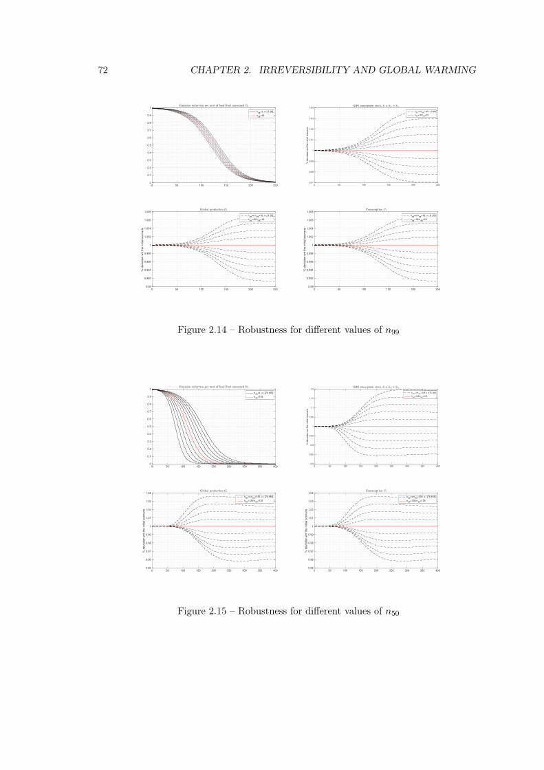
72 CHAPTER 2. IRREVERSIBILITY AND GLOBAL WARMING
0 50 100 150 200 2500
0.1
0.2
0.3
0.4
0.5
0.6
0.7
0.8
0.9
1
n99
=x, x [1,20]
n99
=10
0 50 100 150 200 2500.97
0.98
0.99
1
1.01
1.02
1.03
1.04
% d
evia
tion w
rt the initia
l scenario
n99
=x/n99
=10, x [1,20]
n99
=10/n99
=10
0 50 100 150 200 2500.99
0.992
0.994
0.996
0.998
1
1.002
1.004
1.006
1.008
% d
evia
tio
n w
rt t
he
in
itia
l sce
na
rio
n99
=x/n99
=10, x [1,20]
n99
=10/n99
=10
0 50 100 150 200 2500.99
0.992
0.994
0.996
0.998
1
1.002
1.004
1.006
1.008
% d
evia
tio
n w
rt t
he
in
itia
l sce
na
rio
n99
=x/n99
=10, x [1,20]
n99
=10/n99
=10
Figure 2.14 – Robustness for different values of n99
0 50 100 150 200 250 300 350 4000
0.1
0.2
0.3
0.4
0.5
0.6
0.7
0.8
0.9
1
n50
=x, x [75,165]
n50
=125
0 50 100 150 200 250 300 350 4000.8
0.85
0.9
0.95
1
1.05
1.1
1.15
1.2
% d
evia
tion w
rt the initia
l scenario
n50
=x/n50
=125, x [75,165]
n50
=125/n50
=125
0 50 100 150 200 250 300 350 4000.95
0.96
0.97
0.98
0.99
1
1.01
1.02
1.03
1.04
% d
evia
tio
n w
rt t
he
in
itia
l sce
na
rio
n50
=x/n50
=125, x [75,165]
n50
=125/n50
=125
0 50 100 150 200 250 300 350 4000.95
0.96
0.97
0.98
0.99
1
1.01
1.02
1.03
1.04
% d
evia
tio
n w
rt t
he
in
itia
l sce
na
rio
n50
=x/n50
=125, x [75,165]
n50
=125/n50
=125
Figure 2.15 – Robustness for different values of n50
2.7. SIMULATIONS: 73
We first describe the results obtained by the first series of simulations (Figure 2.14).
By modifying the parameter n99, the GHG stock will vary by more or less 1% after a
century. The environmental damage linked to this variation in pollution emitted is in
between -2% and +2% compared to the initial calibration. The repercussions on the
economic block (production, consumption, investment or capital stock) are of the order
of 2%. The model becomes stable after two centuries, the GHG stock varies by more
or less 4% and the deviations of the economic variables are less than 1% in absolute
value. By modifying in a second step the parameter n50, the response of the model is
similar compared to the first series of simulations. Only the time needed to to return
to equilibrium and the level of deviation of the variables differ. As could be expected,
the faster the economy halves the carbon intensity of polluting energy consumed, the
lower the GHG stock is, relatively to the benchmarck scenario (and vice versa). For
the second series of simulations (Figure 2.15), when n50 = 75, after 100 years the GHG
atmospheric stock is 7.5 % lower than in the initial scenario, and stabilises at a 15% lower
level after two centuries. When on the contrary, n50 = 165, the GHG stock increases by
2.5% after 100 years, reaching a maximum of nearly 20 % more after 250 years before
stabilising at this level. When emissions are reduced to their minimum (n50 = 75)
thanks to the exogenous technology world production increases by 4%, in the opposite
case (n50 = 165), world production decreases by 4%. The decrease or increase of other
great economic variables (consumption, investment and stock of capital) are within more
or less 4% with respect to the initial scenario.
Several important points emerge from this robustness study. First of all, the param-
eter n99 corresponding to the year when the economy will be able to reduce its GHG
emissions by 1%, has relatively little influence on the GHG atmospheric stock, and there-
fore has little effect on the economy. This result is easily explained by the functional form
chosen for the technological process, which exogenously reduces the carbon intensity of
the polluting energy input used in the production of the final good. In fact, the sigmoid
form can be broken down into three distinct phases. The first one is characterised by a
fairly low slope, reflecting a relatively limited decrease in emissions. This phase illustrates
74 CHAPTER 2. IRREVERSIBILITY AND GLOBAL WARMING
the fact that the probability of finding, in the near future, a technology capable of quickly
reducing emissions is low. The second phase, where the slope is steeper, assumes that
technical progress to limit emissions will occur more rapidly. Finally in the third phase,
technical progress admits an asymptote in the long run, reflecting the fact that, beyond a
certain threshold, reducing emissions becomes more and more difficult, in other words, it
illustrates the fact that the marginal technological progress is decreasing. Thus, reducing
emissions by 1% after 1, 10 or 20 years has relatively small influence on the whole model
compared to the second parameter, which corresponds to the year when emissions will
decrease by 50%. A substantial effect could therefore be expected when we assume that
the economy will be able to reduce its emissions more or less rapidly over time by a factor
of two. The results obtained are consistent for the GHG atmospheric stock, which varies
significantly downwards if n50 is low, or upwards when n50 is high. Consequently, the
variations in damage related to the level of GHG stock are also significant. They reach
a maximum of 7.5% after 100 years when n50 = 75, and almost 12% when n50 = 165
after more than 200 years. Nevertheless, it may be surprising that the consequences of
such variations in terms of GHG stock and by extension environmental damage have
a relatively small impact on the economic block. The small increase, or decrease, in
all economic variables could be explained by the model’s assumptions. We have indeed
assumed that the GHG stock generates damage exclusively on the production supply.
However, this assumption may be too simplistic. Indeed, we have overlooked the fact
that the stock of GHG and thus global warming also has repercussions on the well-being
of the representative household. To be more accurate, the variable St should have been
included in the household utility function. Because climate change can be a source of
illness, or if the the representative household has an environmental awareness, then the
increase in the GHG stock generates disutility. The household thus makes a trade-off
between consumption and environmental quality. Either it continues to consume, which
would generate more pollution, or it reduces its consumption in order to preserve the
climate. Thus, by taking into account both the environmental damage into the produc-
tion function and the disutility due to the GHG atmospheric stock, the model results
2.8. CONCLUSION: 75
could better illustrate the negative consequences of climate change on the economy. In
chapter 4, we integrate pollution into the household utility function in the manner of
Heutel (2012) and Khan et al. (2019).
2.8 Conclusion:
Climate dynamics is a slow phenomenon with delayed consequences. Even if emissions
flow are completely reduced to zero, the inertia is such that it would take several decades
to find a new balance. To be fully effective, environmental policies must take into ac-
count the irreversibility of global warming. The irreversibility of climate change raises
important questions, particularly about the efforts that current generations are prepared
to make in the short term to preserve the climate in the long term, especially for future
generations. While the problem of global warming has been highlighted by the scientific
community since the 1970s, concluding that a strong policy response is needed, the lack
of a drastic decision to reduce the use of fossil fuels shows that some countries are not
ready to make the necessary efforts. The USA withdrawal from the Paris Agreement
in 2017, the Yellow Vests movement in France in 2018, low share of emissions taxed
worldwide, etc.
Policies to limit global warming are unpopular policies. The cost to current genera-
tions is substantial, while the positive effects will only be felt in the distant future. This
chapter also shows that public intervention remains essential to internalize emissions,
especially if productivity in the renewable energy sector increases and if energies are
complementaries. Indeed, in the absence of a short-term solution to store non-polluting
energy production, the use of fossil fuels remains essential to cope with the discontinuity
of renewable energy production (lack of wind, sunshine, etc.). In the absence of a carbon
tax, the effect could be counter-productive and the risk would be that emissions would
increase rather than decrease (as demonstrated by the German experience following the
closure of nuclear power plants after the Fukushima nuclear accident in 2011).
The simple model can be extended in many ways to refine the results obtained. First,

76 CHAPTER 2. IRREVERSIBILITY AND GLOBAL WARMING
the model considers exclusively a coal regime. However, the results could differ taking
into account Hotelling’s rent related to the exploitation of exhaustible energy for gas
and oil. Sinn (2008, 2012), through his concept of the green paradox, showed how the
behaviour of the owners of these exhaustible resources could be changed as a result of
environmental policies, leading to an increase in emissions in the short term. However,
we have seen how short-term emissions can affect the long-term balance. The results
obtained could then be modified by the reaction of polluting energy suppliers, whose
Hotelling rent would be modified by the introduction of the tax.
Disaggregating the world economy into a multi-region economy in the Nordhaus way
would make it possible to simulate several scenarios of cooperation or not in the fight
against global warming. This would have the consequences of scenarios that consider
free-riding behaviour at the national level in relation to global warming.
Chapter 3
Fossil fuel price shocks and climate
policies in the business cycle
3.1 Introduction:
Reducing annual anthropogenic GHG emissions flow is one of the major challenges of
the 21st century to limit global warming. The AR5 report and more recently the "world
scientists warning to humanity" manifesto signed by more than 15,000 scientists high-
light the urgency of the situation, as well as the need to change our production and
consumption behaviour. The European Union (EU), which signed the Kyoto Protocol,
has been committed to cut its emissions since the mid-1990s. In this sense, it adopted
in 2008 the climate energy package whose objective was to achieve the "3×20" by 2020
(20% cut in GHG emissions, compared to its 1990 level, a rise of 20% of renewable in
the EU energy mix, a 20% improvement in energy efficiency). This package has been
revised in 2014 and set new targets for 2030: a 40% reduction in CO2 emissions, a 27%
increase in renewable energies and a 27% increase in energy efficiency. To reduce its GHG
emissions, the EU set up in 2005 the world’s first carbon market where emissions rights
are traded: the European Union Emissions Trading Scheme or EU ETS. The principle
is first to set an emissions cap, then to distribute allowances to the 12,000 heavy energy-
77
78 CHAPTER 3. ENERGY PRICE SHOCK
using installations concerned and let them trade between those for which the demand
for pollution exceed the number of allowances they have, and the others for which the
demand for pollution is lower than the number of allowances distributed, so that the
confrontation of supply and demand generates a carbon price. However, over the past
decade, the price of carbon has remained at an abnormally low level, too low to hope
to limit warming to 2C by the end of the century. This low carbon price is explained
on the one hand by the economic situation and recessions that have hit the EU over the
past decade and on the other hand by structural reasons which have led to the reform
of the carbon market in order to limit the volatility of the carbon price. Recent devel-
opments in the price of pollution rights show that the measure is starting to take effect.
However, other instruments such as the carbon tax are subject to shocks, which can also
have negative effects on the objective of containing climate change. Indeed, according
to ECOFYS (2018), among the 57 existing environmental policy instruments worldwide,
only 4 are at sufficiently high levels to limit our GHG emissions in line with the 2 or 1.5C
objective. The French carbon tax was one of these instruments at sufficiently high levels.
However, the recent exogenous rise in the price of oil on the world markets and carbon
taxes was reflected in a rise in the price of gasoline, which was one of the causes Yellow
Vests movement. Following these demonstrations, the increase in the carbon tax was
frozen in France, which could have harmful long-term effects for limiting global warming.
Thus, in order to limit these dysfunctions, it is necessary to better understand the effect
that can be caused not only by technological shocks, usually studied in the literature of
DSGE models focusing on environmental policies, but also by the role of energy prices
when the economy depends on the price of this exogenous factor.
The aim of this chapter is therefore to compare different environmental policies sub-
ject to various shocks. We use a Real Business Cycle (RBC) model based on the model
developed by Fischer and Springborn (2011) to compare the economic consequences of
several environmental policies whose objective is to reduce the anthropogenic impact on
global climate subject to two exogenous shocks: a technology shock and an oil price
shock. We consider four different scenarios: the first one corresponds to our benchmark
3.2. RESEARCH CONTEXT: 79
scenario without environmental policy, the second one reproduces the EU ETS carbon
market and more generally a cap-and-trade market, the third one is the carbon tax case,
and the last scenario considers the implementation of an intensity target. Our results
are as follows. Like Annicchiarico and Di Dio (2015), for a technology shock, we find no
significant difference over the business cycle between the BAU, the tax and the intensity
target. However, setting an emissions cap reduces the positive effect of the shock by
increasing the cost of carbon. In the case of a positive exogenous shock on the price of
energy, the intensity target and the emissions cap will absorb the shock and limit the
consequences on the business cycle, whereas the tax will have a significant pro-cyclical ef-
fect. Thus, if such an instrument is implemented, it should be accompanied by a floating
tax to limit the rise in energy prices, which would contain both GHG emissions without
penalising consumption or long-term climate policy.
The goal of section 2 is to present the research context, while section 3 shows both the
state of the art and our contribution. The model is developed in section 4, we calibrate
it in section 5, and we present our results in section 6 before concluding.
3.2 Research context:
3.2.1 The European carbon market subject to failures in the wake of
the 2008 financial crisis:
Many studies have tried to calculate the optimal carbon price (see Quinet (2009) and
Maibach (2008) for a literature review). According to the OECD, in 2008 the price per
ton of CO2 was expected to be $ 25 and would have increased by 2.4% per year (OECD,
2008) and a more recent OECD study evaluated that $ 325 per ton of CO2 is needed in
2050 to limit global warming to 2C (Marchal et al., 2011). The Stiglitz Stern commission
estimated that the price should be between $ 40 and $ 80 per ton of CO2 in 2020 to
be consistent with the 2C target (Stern and Stiglitz, 2017). However between January
2013 (date of implementation of the 3rd phase of the EU ETS market) and June 2018,
the average monthly carbon price was $ 11 per ton, which is far from being enough to
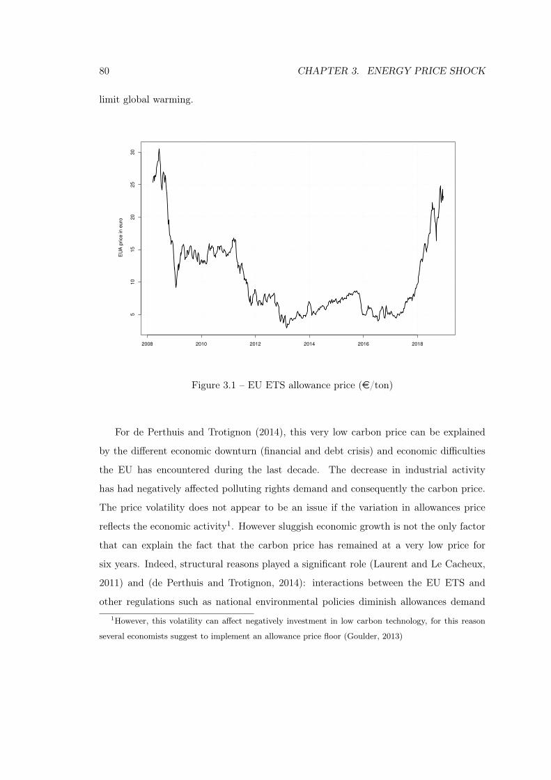
80 CHAPTER 3. ENERGY PRICE SHOCK
limit global warming.
EU
A p
rice in e
uro
2008 2010 2012 2014 2016 2018
510
15
20
25
30
Figure 3.1 – EU ETS allowance price (e/ton)
For de Perthuis and Trotignon (2014), this very low carbon price can be explained
by the different economic downturn (financial and debt crisis) and economic difficulties
the EU has encountered during the last decade. The decrease in industrial activity
has had negatively affected polluting rights demand and consequently the carbon price.
The price volatility does not appear to be an issue if the variation in allowances price
reflects the economic activity1. However sluggish economic growth is not the only factor
that can explain the fact that the carbon price has remained at a very low price for
six years. Indeed, structural reasons played a significant role (Laurent and Le Cacheux,
2011) and (de Perthuis and Trotignon, 2014): interactions between the EU ETS and
other regulations such as national environmental policies diminish allowances demand1However, this volatility can affect negatively investment in low carbon technology, for this reason
several economists suggest to implement an allowance price floor (Goulder, 2013)
3.2. RESEARCH CONTEXT: 81
and reduce the carbon market efficiency. Similarly, according to Laurent and Le Cacheux
(2009) the clean development mechanism (CDM) which has been first introduced in order
to allow European firms to take into account projects they carried out in developing
countries, has in fact introduced an additional weakness on the EU ETS market. It has
reduced firstly the demand for allowances, and secondly this mechanism seems to be
inefficient because between one and two thirds of the projects would not actually result
in real emission reductions (see Wara and Victor (2008) for concrete examples). Lastly
because it was possible to bank and transfer allowances that were not used from the
2nd to the 3rd phase, this rule played a role in the low carbon price observed during the
current phase2. For these structural reasons, the carbon price was relatively too low to
reduce GHG emissions in the long run.
Thus, to eliminate its dysfunctions and to strengthen its climate policy, the EU has
undertaken a reform for the EU ETS market at the end of 3rd phase. On July 2015, the
European Parliament adopted the proposal of the European Commission to implement
the Market Stability Reserve (MSR) which has been started in January 2019. Its first
objective is to diminish the number of allowances currently available. The second goal is
to control carbon price volatility by creating a mechanism that can protect the system
from an economic shock likely to unbalance the EU ETS, between supply and demand
allowances. By doing so, legislators send a strong signal to investors and firms about
the EU’s commitment to meet its GHG emission reduction target. If the number of
allowances available exceeds 833 Mega ton (Mt), then the authorities will remove 12%
of them per year. On the contrary, they will reintroduce 100 Mt of allowances if their
number is lower than 400 Mt. Between the two thresholds, their is no intervention.
Moreover, the European Parliament decided for the 4th phase to accelerate the annual
rate of decline of allowances number from 1.74% to 2.2% per year to reach the energy
package targets. These policies should cause the carbon price to slowly increase during2This market failure should disappear with the suppression of the free allocation system. Indeed, in
the auctioning system, firms must now buy every year the required quantity of allowances and no longer
receive too many allowances and they are no longer supposed to bank them (de Perthuis and Trotignon,
2014).
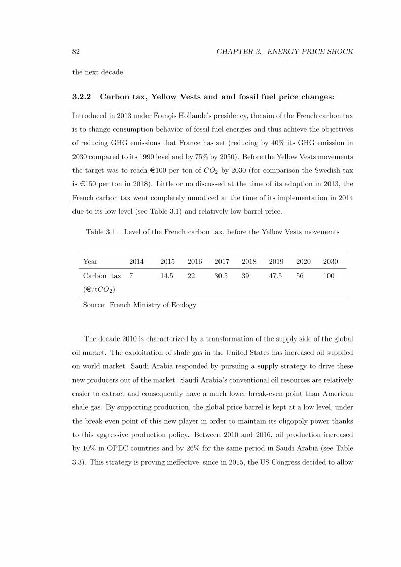
82 CHAPTER 3. ENERGY PRICE SHOCK
the next decade.
3.2.2 Carbon tax, Yellow Vests and and fossil fuel price changes:
Introduced in 2013 under Franois Hollande’s presidency, the aim of the French carbon tax
is to change consumption behavior of fossil fuel energies and thus achieve the objectives
of reducing GHG emissions that France has set (reducing by 40% its GHG emission in
2030 compared to its 1990 level and by 75% by 2050). Before the Yellow Vests movements
the target was to reach e100 per ton of CO2 by 2030 (for comparison the Swedish tax
is e150 per ton in 2018). Little or no discussed at the time of its adoption in 2013, the
French carbon tax went completely unnoticed at the time of its implementation in 2014
due to its low level (see Table 3.1) and relatively low barrel price.
Table 3.1 – Level of the French carbon tax, before the Yellow Vests movements
Year 2014 2015 2016 2017 2018 2019 2020 2030
Carbon tax
(e/tCO2)
7 14.5 22 30.5 39 47.5 56 100
Source: French Ministry of Ecology
The decade 2010 is characterized by a transformation of the supply side of the global
oil market. The exploitation of shale gas in the United States has increased oil supplied
on world market. Saudi Arabia responded by pursuing a supply strategy to drive these
new producers out of the market. Saudi Arabia’s conventional oil resources are relatively
easier to extract and consequently have a much lower break-even point than American
shale gas. By supporting production, the global price barrel is kept at a low level, under
the break-even point of this new player in order to maintain its oligopoly power thanks
to this aggressive production policy. Between 2010 and 2016, oil production increased
by 10% in OPEC countries and by 26% for the same period in Saudi Arabia (see Table
3.3). This strategy is proving ineffective, since in 2015, the US Congress decided to allow
3.2. RESEARCH CONTEXT: 83
oil exports that had been banned after the oil shocks of the 1970s (production was then
exclusively reserved for the US market) and in 2017 the United States has became the
leading oil producing country. As a result of the failure of Saudi Arabia’s strategy and
to a low barrel price, OPEC countries are emerging weakened, since their economies are
mainly based on the rent provided by the exploitation of fossil fuels. Consequently they
decided to reduce their production from 2017 onward (see Table 3.3). Trade tensions
between the US and Iran, as well as the rise in global oil demand (1.4 Million barrels
per day - Mbd) - two thirds of this increase comes from China (0.7 Mbd) and India
(0.3 Mbd) while the remaining share comes from the rise of the US demand) drove oil
prices up in 2018. In the same year, the French carbon tax increased by 27% compared
to 2017 (see Table 3.1). Diesel which until recently benefited from lower taxation than
regular gas, saw its taxes increase by 11% between 2017 and 2018, and by almost 40%
between 2013 and 2018. While for regular gasoline, the tax increased by 5% between
2017 and 2018 and by 11% between 2013 and 2018 (see Table 3.2). As shown in Figure
3.2, the difference in gas price (including taxes) between diesel and gasoline decreased
significantly in 2018. As a result of this exogenous increase on the global markets in the
oil price per barrel, combined with the increase in the French carbon tax on fossil fuel
products, the Yellow Vests movement began in France in November 2018. On December
5 2018, President Emmanuel Macron decided to freeze the initially planned increases in
this tax. The interest of this research is therefore to better understand the consequences
that an exogenous shock on fossil fuels price can have depending on the environmental
policy in place.
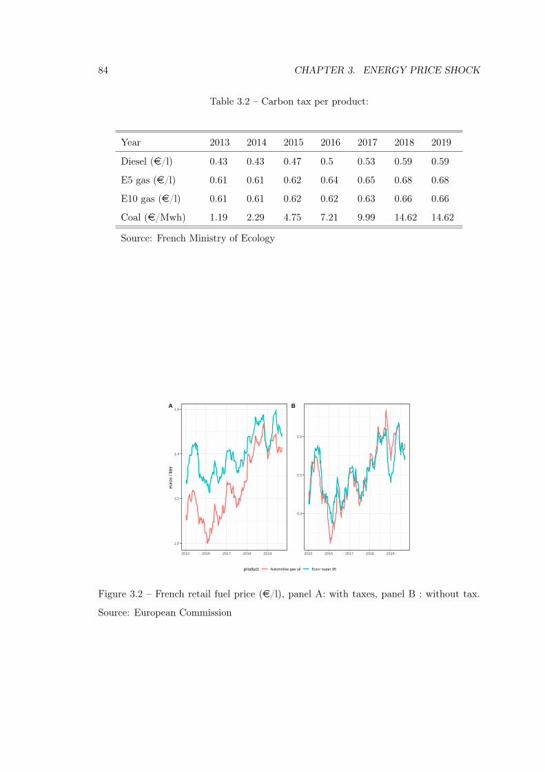
84 CHAPTER 3. ENERGY PRICE SHOCK
Table 3.2 – Carbon tax per product:
Year 2013 2014 2015 2016 2017 2018 2019
Diesel (e/l) 0.43 0.43 0.47 0.5 0.53 0.59 0.59
E5 gas (e/l) 0.61 0.61 0.62 0.64 0.65 0.68 0.68
E10 gas (e/l) 0.61 0.61 0.62 0.62 0.63 0.66 0.66
Coal (e/Mwh) 1.19 2.29 4.75 7.21 9.99 14.62 14.62
Source: French Ministry of Ecology
1.0
1.2
1.4
1.6
2015 2016 2017 2018 2019
euro
s / l
iter
A
0.4
0.5
0.6
2015 2016 2017 2018 2019
B
product Automotive gas oil Euro−super 95
Figure 3.2 – French retail fuel price (e/l), panel A: with taxes, panel B : without tax.
Source: European Commission
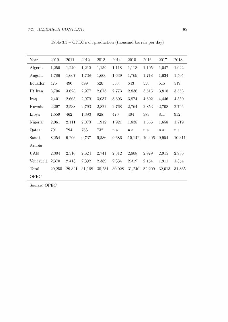
3.2. RESEARCH CONTEXT: 85
Table 3.3 – OPEC’s oil production (thousand barrels per day)
Year 2010 2011 2012 2013 2014 2015 2016 2017 2018
Algeria 1,250 1,240 1,210 1,159 1,118 1,113 1,105 1,047 1,042
Angola 1,786 1,667 1,738 1,600 1,639 1,769 1,718 1,634 1,505
Ecuador 475 490 499 526 553 543 530 515 519
IR Iran 3,706 3,628 2,977 2,673 2,773 2,836 3,515 3,818 3,553
Iraq 2,401 2,665 2,979 3,037 3,303 3,974 4,392 4,446 4,550
Kuwait 2,297 2,538 2,793 2,822 2,768 2,764 2,853 2,708 2,746
Libya 1,559 462 1,393 928 470 404 389 811 952
Nigeria 2,061 2,111 2,073 1,912 1,921 1,838 1,556 1,658 1,719
Qatar 791 794 753 732 n.a. n.a n.a n.a n.a.
Saudi
Arabia
8,254 9,296 9,737 9,586 9,686 10,142 10,406 9,954 10,311
UAE 2,304 2,516 2,624 2,741 2,812 2,908 2,979 2,915 2,986
Venezuela 2,370 2,413 2,392 2,389 2,334 2,319 2,154 1,911 1,354
Total
OPEC
29,255 29,821 31,168 30,231 30,028 31,240 32,209 32,013 31,865
Source: OPEC
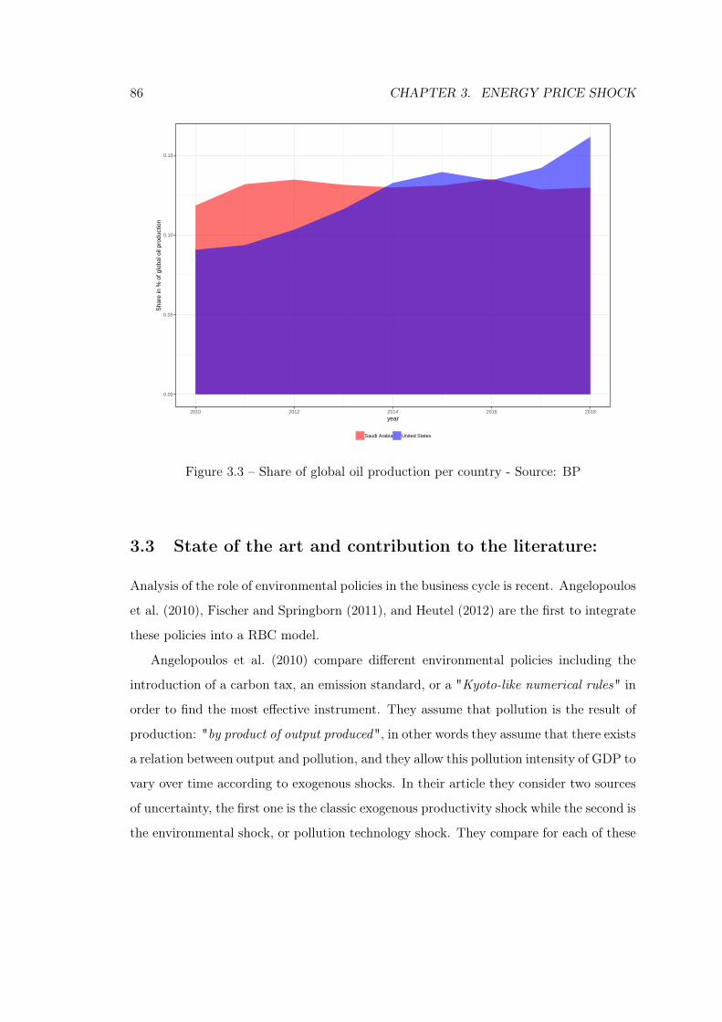
86 CHAPTER 3. ENERGY PRICE SHOCK
0.00
0.05
0.10
0.15
2010 2012 2014 2016 2018
year
Sha
re in
% o
f glo
bal o
il pr
oduc
tion
Saudi Arabia United States
Figure 3.3 – Share of global oil production per country - Source: BP
3.3 State of the art and contribution to the literature:
Analysis of the role of environmental policies in the business cycle is recent. Angelopoulos
et al. (2010), Fischer and Springborn (2011), and Heutel (2012) are the first to integrate
these policies into a RBC model.
Angelopoulos et al. (2010) compare different environmental policies including the
introduction of a carbon tax, an emission standard, or a "Kyoto-like numerical rules" in
order to find the most effective instrument. They assume that pollution is the result of
production: "by product of output produced", in other words they assume that there exists
a relation between output and pollution, and they allow this pollution intensity of GDP to
vary over time according to exogenous shocks. In their article they consider two sources
of uncertainty, the first one is the classic exogenous productivity shock while the second is
the environmental shock, or pollution technology shock. They compare for each of these
3.3. STATE OF THE ART AND CONTRIBUTION TO THE LITERATURE: 87
two shocks which instrument is best suited to reduce emissions and consequently which
instrument has the greatest effect on welfare (in their model environmental quality enters
the household utility function and the stock of pollution affects negatively its utility).
They find that when volatility comes from productivity shock, introducing a tax is the
best instrument, whereas when volatility comes from environmental technology shock,
the introduction of a rule is more appropriate for pollution abatement. Finally, they find
that in all cases the establishment of pollution permits is the least effective policy.
Fischer and Springborn (2011) also compare three different policies (a tax, an emission
cap, and an output to pollution intensity target) but they differ from Angelopoulos
et al. (2010) for several reasons. First, in their model it is the energy used as input in
production which is source of pollution emissions. Secondly and contrary to Angelopoulos
et al. (2010) who model the pollution stock as being the cause of pollution damage,
Fischer and Springborn (2011) do not clearly explain the underlying relation between
emissions and environmental damage, and lastly the only source of uncertainty comes
from technological progress. They differ mainly from Angelopoulos et al. (2010) in the
way they study the cost of each policy. Angelopoulos et al. (2010) evaluate the policy
effects by comparing the gain in terms of welfare, on the contrary Fischer and Springborn
(2011) compare the loss from the economic point of view. By doing so, they find that the
intensity target achieves its goal in terms of reduction in pollution at the lowest economic
cost.
Heutel (2012) is interested in the capacity of a tax or a cap to adapt to the cycle in
order to maximize the welfare. The idea behind this proposal is that an environmental
policy should adapt to the business cycle and consequently be stronger during economic
expansion (when emissions tend to rise), and less restrictive during recession for the
opposite reason (a lower growth means less emissions). For the two policies studied
Heutel (2012) finds that it would be optimal to adapt them to the economic cycle: by
increasing the tax rate and reducing the number of quotas during expansions periods and
the opposite in the case of recession.
88 CHAPTER 3. ENERGY PRICE SHOCK
Annicchiarico and Di Dio (2015) are the first to develop a new keynesian model in
this context by including in their model nominal price rigidities and monetary policy.
They compare several environmental policies, and they care about the role play by these
rigidities when we implement such a policy on the business cycle. They first find that a
cap-and-trade system will diminish economic fluctuations, and will behave as an auto-
matic stabilizer. As expected nominal price rigidities play an important role in terms of
welfare variation as a response to environmental policy. The higher the price rigidities
are, the higher the welfare loss is.
We contribute to the existing literature on environmental policy assessment in the
context of a RBC model by analysing the consequences of energy price shock in the
business cycle when the economy implements a climate policy. We use Fischer and
Springborn (2011) model that includes energy as an input to conduct our research. We
consider as in Kim and Loungani (1992) that one source of uncertainty comes from energy
prices that are exogenously determined. Moreover and to our knowledge, it is the first
article that takes into account the variation in the utilisation rate of capital in order to
evaluate environmental policy. This assumption plays an important role in order to not
over or under-estimate the impact of policy.
3.4 The model:
3.4.1 Households:
It is assumed that households are similar, they all adopt the same behaviour, so we
can aggregate them such that that there is one infinitely lived representative agent. We
suppose the following CRRA utility function
Ut (ct, lt) =
(cϕt (1− lt)1−ϕ)1−σ − 1
1− σ (3.4.1)
σ > 1, ϕ ∈ [0, 1]
where ct is the final good consumption level in period t, lt is labor supply in period
3.4. THE MODEL: 89
t, and where ϕ and σ are preferences parameter. We normalize to unity, household’s
time disposable in each period, such as 1 − lt corresponds to leisure time. Household
maximises its intertemporal utility function subject to its budget constraint:
ct + it = wtlt + rtktut + Tt (3.4.2)
The left hand side (LHS) of (3.4.2) corresponds to the household’s demand, while
right hand side (RHS) is household earnings from the labor force it supplies to the firm
and as the owner of capital it also rents capital services to the firm. ut is the rate of
utilisation of capital (we suppose that the entire stock of capital is variable), therefore
utkt corresponds to the services derived from the utilisation of capital. The government
redistributes tax revenues in the form of a lump-sum subsidy Tt. During each period,
household divides a share of its income into capital investment, while the remaining goes
to consumption of final goods. The law of motion for investment in capital is:
it = kt+1 −(
1− δ(ut))kt +
B
2
(kt+1 − ktkt
)2(3.4.3)
δ(ut) =ω0
ω1utω1 , (3.4.4)
δ(.) ∈]0, 1[, ω0 > 0, ω1 > 1, B > 0
where the last term in the RHS of (3.4.3) is the adjustment costs in capital invest-
ment, B is a positive parameter of the quadratic cost functions (to be calibrated). This
assumption implies that increasing the capital stock is costly for the firm. Augmenting
its investment could require for example formation of workers, such they are no longer
working, so it could have a direct cost and an indirect cost by lowering labor productivity
in the short run.
We assume that the depreciation rate of capital (3.4.4) and as the following properties:∂δ(ut)
∂ut> 0 and
∂2δ(ut)
∂u2t
> 0. Therefore the depreciation rate of capital is a convex and
increasing function of ut, as in Taubman and Wilkinson (1970), Greenwood et al. (1988)
and Finn (2000). By doing so this formulation takes into account Keynes’ definition
90 CHAPTER 3. ENERGY PRICE SHOCK
of usage cost of capital: in other words an increase in utilisation rate of capital will
accelerate capital depreciation.
The household intertemporal program is to choose the sequence ct, lt, ut, kt+1 thatmaximises its utility function 3.4.1 subject to its resource constraint 3.4.2 and the law of
motion for capital accumulation (3.4.3).
maxct,lt,ut,kt+1
Ut (ct, lt)
s.to
ct + it = wtlt + rtktut + Tt
it = kt+1 −(
1− δ(ut))kt +
B
2
(kt+1 − ktkt
)2
δ(ut) =ω0
ω1utω1
The Lagrangian associated with this maximisation program is:
L = E∞∑
j=0
βt+j
(cϕt+j(1− lt+j)ϕ
)1−α− 1
1− α + λ1,t+j
(wt+jlt+j + rt+jkt+jut+j + Tt+j
− ct+j − kt+j+1 +(
1− δ(ut+j))kt+j −
B
2
(kt+j+1 − kt+jkt+j
)2)
where λ1,t is the co-state variable associated with the budget constraint. FOC are detailed
in the technical appendix.
3.4.2 Firms:
The final good is produced using three different inputs : labor, capital and energy. The
production function of the final good is supposed to be a Cobb-Douglas form, where at
is technological progress:
yt = at (ktut)α eγt l
1−α−γt (3.4.5)
et is the energy input used in production, and we assume that GHG emissions are pro-
portional to its use, as in Fischer and Springborn (2011). It is assumed that each unit
consumed of et generates Ξ units of GHG.
3.4. THE MODEL: 91
When the government decides to implement a climate policy, the firm faces another
cost that modifies its optimizing program. Assuming that et is exogenously decided
by the public authorities, and represents one of the four policy at its disposable. In
every period, the firm’s objective is therefore to choose the sequence lt, ktut, et that
maximizes its profits:
maxlt,ktut,et
at (ktut)α eγt l
1−α−γt − wtlt − rtktut − pe,tet − pCt et
Where pCt is the price of carbon that the company has to pay for each GHG unity emitted
into the atmosphere. FOC are detailed in the technical appendix.
3.4.3 Climate policy and overall resource constraint:
We assume four different scenarios. In the first case nothing is done, the public authorities
do not intervene, this is the benchmark, or Business As Usual scenario. In the other
cases, they set up either a cap-and-trade market (or an emission cap), a carbon tax or
an intensity target. When they decide to internalize GHG emissions externalities with a
cap-and-trade market, in every period, they decide the quantity of emissions not to be
exceed, and to supply the corresponding quantity of allowances to the firms. Defining
by qet , the number of allowances supplied on the market in order to achieve the emission
target, the emissions policy constraint is consequently:
et ≡ qet > Ξet (3.4.6)
According to the Kuhn and Tucker optimality conditions, if the emissions cap is not
binding, i.e. if the firm emitted less than the upper bound qet , then the carbon price will
be zero. On the other hand, if the constraint binds, then the carbon price pCt will be
positive. Next, we suppose that public authorities decide to implement a carbon tax. In
that case, they decide exogenously the carbon price pCt = pe,tτCt for each unit of GHG
emitted. Finally, in the case of an intensity target, GHG emissions must not exceed a
threshold At for each unit of GDP as in Fischer and Springborn (2011). The constraint
is in this case:
et ≡ At =Ξetyt
(3.4.7)
92 CHAPTER 3. ENERGY PRICE SHOCK
We follow Annicchiarico and Di Dio (2015) and assume that, the shadow value pCt of
emissions associated with the intensity constraint (3.4.7) represents carbon price. In-
deed, in this case the government sells also permits to the firm, and pCt corresponds to
the market price of emissions, that satisfies the exogenous constraint defined by the au-
thorities. To close the model we need to find the overall resource constraint. We assume
that the government implement the climate policy to contain GHG emissions flow, as
described. It redistributes the tax revenues by a lump-sum subsidy to the household, so
that government resource constraint is:
Tt = pCt et
Combining the government budget constraint with the household budget constraint an
using optimality conditions of the firms, one obtains the overall resource constraint in
the economy:
yt = ct + it + pe,tet (3.4.8)
3.4.4 Competitive equilibrium
Competitive equilibrium is obtained when the representative household and the rep-
resentative firm optimize their program. In the case of a cap-and-trade market, it is
determined by equations (3.4.3), (3.4.4), (3.4.5), (3.4.6), (3.4.8), and by the following set
of equations3:
3see appendix for more details.
3.4. THE MODEL: 93
ϕwt(1− lt) = (1− ϕ)ct (3.4.9a)
rtkt = δ′(ut)kt (3.4.9b)(cϕt (1− lt)1−ϕ)1−σ
ct
(1 +B
(kt+1 − ktkt
) 1
kt
)
= βEt
(cϕt+1(1− lt+1)1−ϕ)1−σ
ct+1
(rt+1ut+1 + 1− δ(ut+1) +B
(kt+2 + kt+1
kt+1
) kt+2
(kt+1)2
)
(3.4.9c)
wt = (1− α− γ)ytlt
(3.4.9d)
rt = αytktut
(3.4.9e)
pe,t + ΞpCt = γytet
(3.4.9f)
Combining FOC for consumption and labor supply gives (3.4.9a), it equates the marginal
rate of substitution between leisure and consumption ∂U∂lt× 1
∂U∂lt
to the wage. Equation
(3.4.9b) gives the optimal utilisation rate of capital. It equates the marginal benefit of
increasing by 1% the utilisation rate of capital (LHS of equation (3.4.9b)) to its costs,
that corresponds to an increase in capital depreciation due to a more intensive use of
capital. Using FOC for consumption to eliminate the Lagrange multiplier λ1 into FOC
for capital gives equation (3.4.9c). It is the well known Euler’s equation and equates the
marginal rate of substitution between consumption level in period t and consumption
level in period t + 1 to the relative price of today consumption. It states that the
representative household is indifferent between consuming one unit today or postponing
its consumption to the next period if this equation is satisfied. The terms in brackets
corresponds to the gross return on capital (rt+1ut+1) which is corrected from depreciation
rate of capital. The last terms in the RHS of the Euler’s equation is the reduction in
capital adjustment cost in period t+ 2, if capital as increased in period t+ 1. Equations
(3.4.9d) and (3.4.9e) equalise the marginal productivities of labor and capital to their
respective costs. Equation (3.4.9f) equalises marginal productivity of oil to its cost as
the sum of oil price plus carbon price. In the absence of climate policy, carbon price
94 CHAPTER 3. ENERGY PRICE SHOCK
pCt = 0, and the use of fossil fuel is not high enough to limit GHG emissions in the aim
of limiting global warming.
In the case of a carbon tax, equation (3.4.6) is not any more necessary in the opti-
mizing program, and equation (3.4.9f) is replaced by pe,t(1+τCt Ξ) = γytet. Finally for the
intensity target scenario, the constraint (3.4.6) is replaced by (3.4.7) and the optimality
condition for the use of energy is modified: pe,t + ΞpCt et = γytet.
3.5 Calibration:
We now calibrate the different parameters of the model using either 1st moment of ob-
served variables (assuming that in the absence of stochastic shocks, the model is in its
steady state), or past studies. The value for the rate of time preference β, for the utility
function parameters σ, are the same as those used by Finn (2000). Labor supply (l) is
calculated as the average of weekly hours worked in the EU (Eurostat) divided by the
total number of hours in a week (168 hours). Share of labor compensation into GDP
(1 − α − γ) is measured as the annual average in the European Union for the period
1995-2017 from AMECO’s database. It corresponds to the compensation of employees
(wage and salaries plus employer’s social contribution) divided by gross domestic prod-
uct. Energy income share in the EU is calculated as follows: total primary energy in
million tonne of oil equivalent (Mtoe) used in the EU is obtained thanks to Eurostat
database. In a second step it is transformed into barrels by multiplying this quantity by
the oil metric tonnes per barrel approximate conversion factor (BP, 2017). It is therefore
multiplied by the WTI crude oil Brent price and expressed in Euros using the Euro-
Dollar exchange rate4 and we divide this value by the EU GDP (Eurostat) to finally
obtain γ = 0.04. This value is consistent with the one used in Golosov et al. (2014) and
Fischer and Springborn (2011). The utilization rate of capital comes from the Eurostat
database, and it corresponds to the quarterly average of the current level of capacity
utilization in the manufacturing industry. The Penn World Table is used to calculate
4The Euro-Dollar exchange rate can be found on: https://fred.stlouisfed.org/series/CCUSMA02EZQ618N
3.5. CALIBRATION: 95
the capital depreciation rate in the EU 28 for the years 2010-2017. The total stock of
capital that depreciates in the EU is calculated as follows. We sum the share of the
capital stock that depreciates annually in each of the 28 EU countries, weighted by the
annual depreciation rates in each of the 28 EU countries: δK =∑
i δiKi. We divide this
share of capital that has depreciated by the total stock of capital, it gives us the annual
depreciation rate of capital. Finally we divide this result by 4 to obtain the quarterly
depreciation rate. Assuming a capital interest rate of 2.7%, a capital depreciation rate
of 1.25% and a capital utilization rate of 81% in steady state, equations (3.4.4) and
(3.4.9b) can be used to determine ω0 = 0.033 and ω1 = 1.80. We normalize to unity
the conversion factor Ξ between energy use and GHG emissions. Finally, we have to
calibrate the exogenous process of each climate policy. According to the Global Carbon
Project, between 2005, our reference year when the EU ETS market was introduced,
and 2017, GHG emissions from fossil fuel consumption have been reduced by 20% in
the EU 28. Hence, Assuming a 20% reduction in GHG emissions, with an initial level
of energy used at a stationary equilibrium of 0.026 in the absence of an environmental
policy, the number of allowances offered on the market is therefore qe = 0.021. In order
to be comparable, the other environmental policy instruments are calibrated so that we
can observe this 20% reduction in emissions. Thus, if we set the initial intensity target
at A = 0.0313, this allows us to observe this 20% reduction in GHG emissions. The
rate of the carbon tax that allows a 20% reduction in GHG emissions is τC = 0.278.
In the absence of an environmental policy, by calibrating the parameters of the model
accordingly to the previously values (see table 3.4), in the steady state, the investment
rate is 18%, the share of income consumed is 78% and the share allocated to energy is
4%. Finally, the capital stock represents roughly 15 times the quarterly GDP, which
corresponds to 3.75 years of production. Assigned values, data sources, and calculation
methods are summarized in table 3.4, and great steady state ratios in Table 3.5.
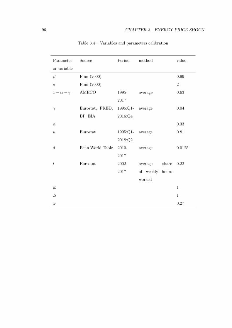
96 CHAPTER 3. ENERGY PRICE SHOCK
Table 3.4 – Variables and parameters calibration
Parameter
or variable
Source Period method value
β Finn (2000) 0.99
σ Finn (2000) 2
1− α− γ AMECO 1995-
2017
average 0.63
γ Eurostat, FRED,
BP, EIA
1995:Q1-
2016:Q4
average 0.04
α 0.33
u Eurostat 1995:Q1-
2018:Q2
average 0.81
δ Penn World Table 2010-
2017
average 0.0125
l Eurostat 2002-
2017
average share
of weekly hours
worked
0.22
Ξ 1
B 1
ϕ 0.27
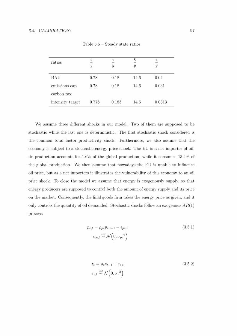
3.5. CALIBRATION: 97
Table 3.5 – Steady state ratios
ratiosc
y
i
y
k
y
e
y
BAU 0.78 0.18 14.6 0.04
emissions cap 0.78 0.18 14.6 0.031
carbon tax
intensity target 0.778 0.183 14.6 0.0313
We assume three different shocks in our model. Two of them are supposed to be
stochastic while the last one is deterministic. The first stochastic shock considered is
the common total factor productivity shock. Furthermore, we also assume that the
economy is subject to a stochastic energy price shock. The EU is a net importer of oil,
its production accounts for 1.6% of the global production, while it consumes 13.4% of
the global production. We then assume that nowadays the EU is unable to influence
oil price, but as a net importers it illustrates the vulnerability of this economy to an oil
price shock. To close the model we assume that energy is exogenously supply, so that
energy producers are supposed to control both the amount of energy supply and its price
on the market. Consequently, the final goods firm takes the energy price as given, and it
only controls the quantity of oil demanded. Stochastic shocks follow an exogenous AR(1)
process:
pe,t = ρpepe,t−1 + εpe,t (3.5.1)
εpe,tiid∼ N
(0, σpe
2)
zt = ρzzt−1 + εz,t (3.5.2)
εz,tiid∼ N
(0, σz
2)
98 CHAPTER 3. ENERGY PRICE SHOCK
We estimate the parameters of equation (3.5.1) using global price of Crude oil5 from
1995:Q1 to 2017:Q2. To detrend the series we use a one-sided HP filter. The resulting
estimation is ρpe = 0.725 and σpe = 0.0536. The parameters of the Solow residual
are estimated using the AMECO database for the capital stock and for labor used in
production. The capital utilisation rate is taken from Eurostat, while the energy demand
comes from the IEA database. Annual data are transformed into quarterly data using
the Denton Cholette method. Finally, estimating the AR(1) process of equation (3.5.2)
yields to the autocorrelation parameter ρz = 0.896 and the standard deviation of the
white noise is σz = 0.0353.
3.6 Simulations:
3.6.1 General Methodology:
We use Dynare software (Adjemian et al., 2011) to compute our stochastic model, in this
subsection we briefly describe the underlying methodology used to solve and simulate
DSGE models. We assume that the non-linear rational expectation model developed in
this chapter can be represented in the following reduced form:
Et [f (yt+1, yt, yt−1, εt)] = 0
where y is an ny×1 vector of endogenous variables and ε is an nε×1 vector of exogenous
stochastic shocks, with the following properties Et(εt) = 0, Et(εtε′t) = Σε and Et(εtεt+j) =
0, ∀j 6= 0. In period t, the only stochastic variables is yt+1. To solve this problem, we use
the perturbation approach (see Jin and Judd (2002)). It consists in linearizing the model
by taking a first order Taylor expansion around the steady state, then in a second stage
solving the linearized model using the generalized Schur decomposition, and assuming
that the steady state is stable, the covariance matrix is solved using an algorithm for
discrete time Lyapunov equations that allows us to find the impulse response function.
5Nominal prices are available on fred website, and they are transformed into real prices:
https://fred.stlouisfed.org/series/POILWTIUSDQ
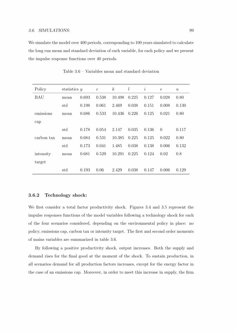
3.6. SIMULATIONS: 99
We simulate the model over 400 periods, corresponding to 100 years simulated to calculate
the long run mean and standard deviation of each variable, for each policy and we present
the impulse response functions over 40 periods.
Table 3.6 – Variables mean and standard deviation
Policy statistics y c k l i e u
BAU mean 0.693 0.538 10.498 0.225 0.127 0.028 0.80
std 0.198 0.061 2.469 0.038 0.151 0.008 0.130
emissions
cap
mean 0.686 0.533 10.436 0.226 0.125 0.021 0.80
std 0.178 0.054 2.147 0.035 0.136 0 0.117
carbon tax mean 0.684 0.531 10.385 0.225 0.125 0.022 0.80
std 0.173 0.041 1.485 0.038 0.138 0.006 0.132
intensity
target
mean 0.681 0.529 10.291 0.225 0.124 0.02 0.8
std 0.193 0.06 2.429 0.038 0.147 0.006 0.129
3.6.2 Technology shock:
We first consider a total factor productivity shock. Figures 3.4 and 3.5 represent the
impulse responses functions of the model variables following a technology shock for each
of the four scenarios considered, depending on the environmental policy in place: no
policy, emissions cap, carbon tax or intensity target. The first and second order moments
of mains variables are summarized in table 3.6.
By following a positive productivity shock, output increases. Both the supply and
demand rises for the final good at the moment of the shock. To sustain production, in
all scenarios demand for all production factors increases, except for the energy factor in
the case of an emissions cap. Moreover, in order to meet this increase in supply, the firm
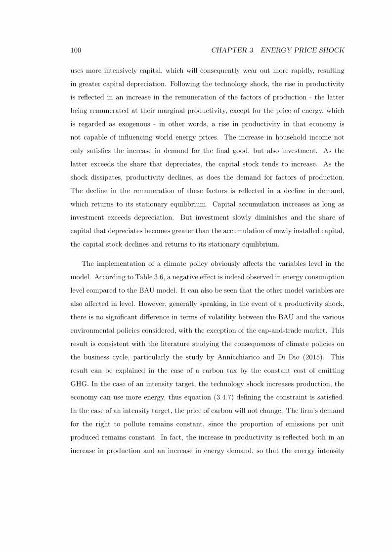
100 CHAPTER 3. ENERGY PRICE SHOCK
uses more intensively capital, which will consequently wear out more rapidly, resulting
in greater capital depreciation. Following the technology shock, the rise in productivity
is reflected in an increase in the remuneration of the factors of production - the latter
being remunerated at their marginal productivity, except for the price of energy, which
is regarded as exogenous - in other words, a rise in productivity in that economy is
not capable of influencing world energy prices. The increase in household income not
only satisfies the increase in demand for the final good, but also investment. As the
latter exceeds the share that depreciates, the capital stock tends to increase. As the
shock dissipates, productivity declines, as does the demand for factors of production.
The decline in the remuneration of these factors is reflected in a decline in demand,
which returns to its stationary equilibrium. Capital accumulation increases as long as
investment exceeds depreciation. But investment slowly diminishes and the share of
capital that depreciates becomes greater than the accumulation of newly installed capital,
the capital stock declines and returns to its stationary equilibrium.
The implementation of a climate policy obviously affects the variables level in the
model. According to Table 3.6, a negative effect is indeed observed in energy consumption
level compared to the BAU model. It can also be seen that the other model variables are
also affected in level. However, generally speaking, in the event of a productivity shock,
there is no significant difference in terms of volatility between the BAU and the various
environmental policies considered, with the exception of the cap-and-trade market. This
result is consistent with the literature studying the consequences of climate policies on
the business cycle, particularly the study by Annicchiarico and Di Dio (2015). This
result can be explained in the case of a carbon tax by the constant cost of emitting
GHG. In the case of an intensity target, the technology shock increases production, the
economy can use more energy, thus equation (3.4.7) defining the constraint is satisfied.
In the case of an intensity target, the price of carbon will not change. The firm’s demand
for the right to pollute remains constant, since the proportion of emissions per unit
produced remains constant. In fact, the increase in productivity is reflected both in an
increase in production and an increase in energy demand, so that the energy intensity
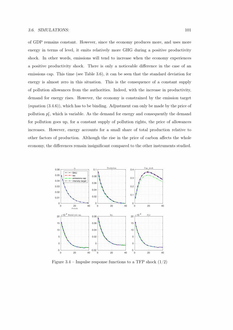
3.6. SIMULATIONS: 101
of GDP remains constant. However, since the economy produces more, and uses more
energy in terms of level, it emits relatively more GHG during a positive productivity
shock. In other words, emissions will tend to increase when the economy experiences
a positive productivity shock. There is only a noticeable difference in the case of an
emissions cap. This time (see Table 3.6), it can be seen that the standard deviation for
energy is almost zero in this situation. This is the consequence of a constant supply
of pollution allowances from the authorities. Indeed, with the increase in productivity,
demand for energy rises. However, the economy is constrained by the emission target
(equation (3.4.6)), which has to be binding. Adjustment can only be made by the price of
pollution pct , which is variable. As the demand for energy and consequently the demand
for pollution goes up, for a constant supply of pollution rights, the price of allowances
increases. However, energy accounts for a small share of total production relative to
other factors of production. Although the rise in the price of carbon affects the whole
economy, the differences remain insignificant compared to the other instruments studied.
0 20 400
0.01
0.02
0.03
0.04
0.05
0.06
BAU
tax
emissions cap
intensity target
0 20 400
0.02
0.04
0.06
0.08
0.1
0 20 400
0.1
0.2
0.3
0.4
0 20 40-5
0
5
10
15
2010
-4
0 20 40-0.02
0
0.02
0.04
0.06
0.08
0 20 40-5
0
5
10
15
2010
-4
Figure 3.4 – Impulse response functions to a TFP shock (1/2)
102 CHAPTER 3. ENERGY PRICE SHOCK
0 20 40
-0.02
0
0.02
0.04
0.06
0 20 40
0
1
2
3
410
-3
0 20 40
-5
0
5
10
15
2010
-3
0 20 40
0.004
0.006
0.008
0.01
0.012
0.014
0.016
0 20 40
0
0.02
0.04
0.06
0.08
0.1
0 20 40
0
0.05
0.1
0.15
0.2
Figure 3.5 – Impulse response functions to a TFP shock (2/2)
3.6.3 Energy price shock:
According to Kilian (2009), we can distinguish three different oil shocks. An oil supply
shock caused by the physical amount of oil disposable on the market6, and two demand
shocks. The first demand shock is driven by the business cycle, in period of expansion
the demand effect increase oil price - and the opposite during recession, while the second
demand shock can be called "Precautionary or speculative demand shock". This last
shock can be seen as the response to an anticipation of a price increase. Indeed oil
consumers behave rationally and if they are expecting an increase in oil price, they
would buy more oil in order to use it later, which eventually accelerate price inflation.
In our case the economy takes the price as given so that, the second stochastic shock
considered corresponds to Kilian’s oil supply shock. Figures 3.16 and 3.17 represent
impulses responses function to an energy price shock for the different environmental
policies assumed.
6OPEC control 42% of the global oil production and 72% of the proved reserved.
3.6. SIMULATIONS: 103
Following a positive shock on the price of energy, two different reactions can be
observed depending on the environmental policies implemented. On the one hand, the
variables will react in the same way in the case of the BAU or a carbon tax. On the
other hand, the variables will have a similar reaction in the case of an emission cap or
an intensity target.
In the absence of an environmental policy, the exogenous rise in energy price results
in a drop in demand for this factor of production. All other things being equal, the
increase in this intermediate cost is reflected in a fall in demand for the final good, and
thus a fall in consumption. Indeed, the price of the good reflects the marginal cost
of production. Since the latter is now higher as a result of the rise in energy prices,
the price of the final good also rises. Output production adapts to the fall in demand,
which also decreases, leading at the same time to a fall in demand for the other inputs.
The economy contracts at the time of the shock, and the firm remunerates its production
factors at a relatively lower level compared to the stationary equilibrium. Physical capital
is used less intensively, the depreciation rate of capital reacts pro-cyclically, and wears
out less rapidly. However, the decrease in wear and tear on capital, linked to its less
intensive use, does not compensate for the decrease in investment, but limits the share
of capital that depreciates. The capital stock declines immediately. and tends to decline
further over time. Then, as the shock dissipates, the price of energy converges towards
its initial value. The firm has a relatively greater recourse to all factors of production.
As the price of the good declines, consumption rises again, supported by an increase in
household income. Investment also tends to return to its initial level, but still does not
compensate for the loss of capital. However, the capital stock is decreasing at a slower
and slower pace, reaching its minimum 10 quarters after the shock before increasing
again. In order to be able to satisfy its level of production, the firm will therefore use
capital more intensively, which will increase its wear and tear, and this as long as the
capital stock has not returned to its initial level.
In the case of a carbon tax, the impulse responses of the variables to an energy price
shock are similar to the BAU scenario. A carbon tax corresponds to a constant marginal
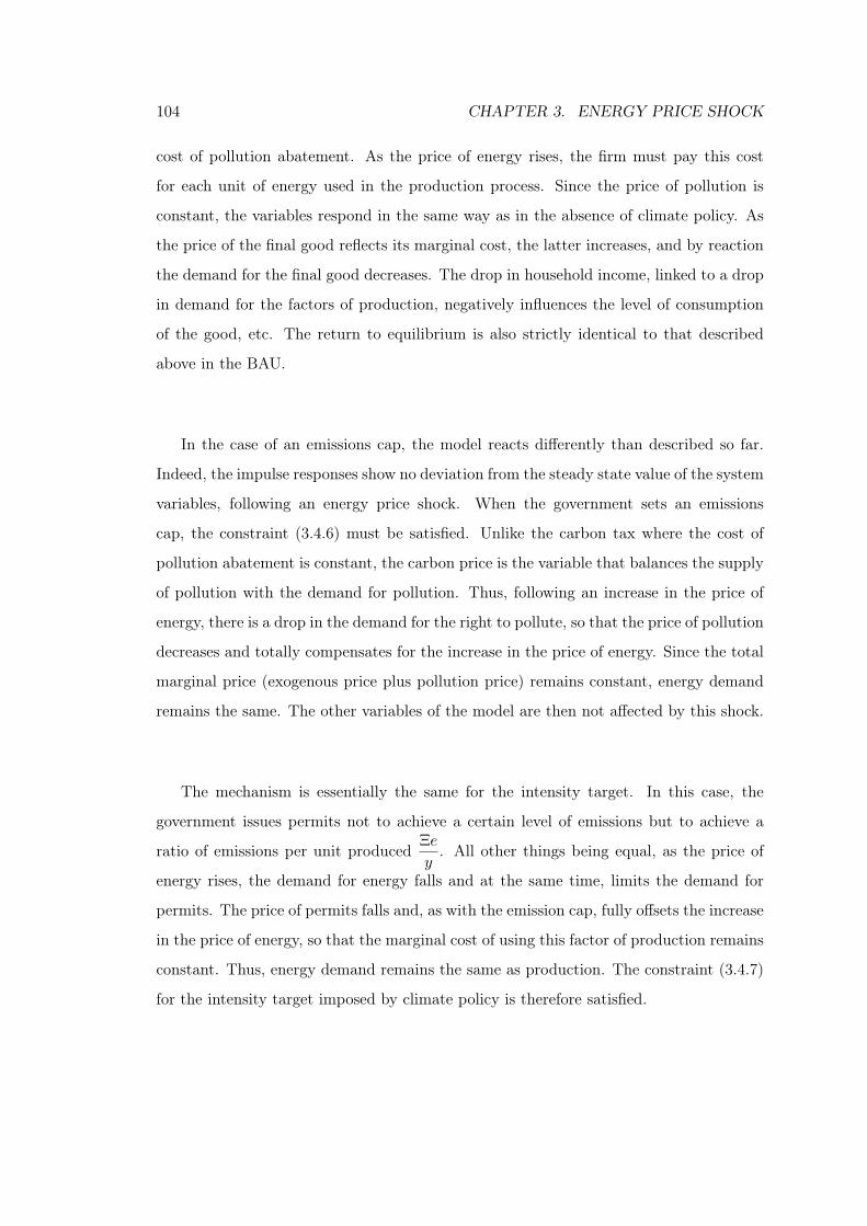
104 CHAPTER 3. ENERGY PRICE SHOCK
cost of pollution abatement. As the price of energy rises, the firm must pay this cost
for each unit of energy used in the production process. Since the price of pollution is
constant, the variables respond in the same way as in the absence of climate policy. As
the price of the final good reflects its marginal cost, the latter increases, and by reaction
the demand for the final good decreases. The drop in household income, linked to a drop
in demand for the factors of production, negatively influences the level of consumption
of the good, etc. The return to equilibrium is also strictly identical to that described
above in the BAU.
In the case of an emissions cap, the model reacts differently than described so far.
Indeed, the impulse responses show no deviation from the steady state value of the system
variables, following an energy price shock. When the government sets an emissions
cap, the constraint (3.4.6) must be satisfied. Unlike the carbon tax where the cost of
pollution abatement is constant, the carbon price is the variable that balances the supply
of pollution with the demand for pollution. Thus, following an increase in the price of
energy, there is a drop in the demand for the right to pollute, so that the price of pollution
decreases and totally compensates for the increase in the price of energy. Since the total
marginal price (exogenous price plus pollution price) remains constant, energy demand
remains the same. The other variables of the model are then not affected by this shock.
The mechanism is essentially the same for the intensity target. In this case, the
government issues permits not to achieve a certain level of emissions but to achieve a
ratio of emissions per unit producedΞe
y. All other things being equal, as the price of
energy rises, the demand for energy falls and at the same time, limits the demand for
permits. The price of permits falls and, as with the emission cap, fully offsets the increase
in the price of energy, so that the marginal cost of using this factor of production remains
constant. Thus, energy demand remains the same as production. The constraint (3.4.7)
for the intensity target imposed by climate policy is therefore satisfied.
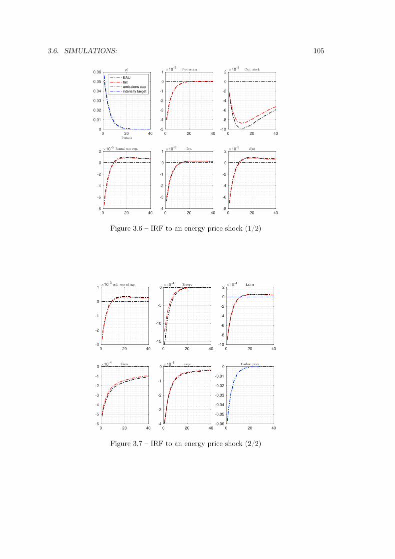
3.6. SIMULATIONS: 105
0 20 400
0.01
0.02
0.03
0.04
0.05
0.06
BAU
tax
emissions cap
intensity target
0 20 40-5
-4
-3
-2
-1
0
110
-3
0 20 40-10
-8
-6
-4
-2
0
210
-3
0 20 40-8
-6
-4
-2
0
210
-5
0 20 40-4
-3
-2
-1
0
110
-3
0 20 40-8
-6
-4
-2
0
210
-5
Figure 3.6 – IRF to an energy price shock (1/2)
0 20 40
-3
-2
-1
0
110
-3
0 20 40
-15
-10
-5
010
-4
0 20 40
-10
-8
-6
-4
-2
0
210
-4
0 20 40
-6
-5
-4
-3
-2
-1
010
-4
0 20 40
-4
-3
-2
-1
010
-3
0 20 40
-0.06
-0.05
-0.04
-0.03
-0.02
-0.01
0
Figure 3.7 – IRF to an energy price shock (2/2)
106 CHAPTER 3. ENERGY PRICE SHOCK
3.6.4 Sensitivity analysis:
As Solow (1999) emphasizes, even if capital depreciation is considered constant in the
literature, this assumption is "empirically inaccurate". Despite the fact that capital
depreciation plays an important role, notably in Jorgenson’s theory of investment and
more particularly in the notion of user cost of capital that he developed (see Jorgenson
(1963, 1967, 1971)), we can highlight that among the literature that seeks to assess
the economic impact of environmental policies in a DSGE model (see Angelopoulos et al.
(2010), Fischer and Springborn (2011), Heutel (2012), Angelopoulos et al. (2013) Golosov
et al. (2014), Argentiero et al. (2017)), to our knowledge this article is the first to analyze
the effects of environmental policy when the depreciation rate of capital is endogenous.
This can be explained by the fact that several empirical studies have shown that geometric
form is the function that best summarizes the depreciation of capital (see Hulten and
Wykoff (1981) and more recently Pilat and Schreyer (2002), and Schreyer (2009)) and this
geometric form implies a constant rate of depreciation. Consequently, if the depreciation
rate of capital is constant, it will not be central in evaluating the economic impact of
carbon pricing. However a recent study conducted by Albonico et al. (2014) using a
Bayesian DSGE model leads to totally different results. On the contrary these authors
show that the depreciation rate of capital in Canada and the US, is on the one hand
not constant over time but volatile and responds with a highly procyclical pattern. Thus,
if we assume as we previously did that the depreciation rate of capital is not constant
but endogenous and responds to the cycle notably via the capital utilisation rate, then
it is an important function in the model that need to be taken into account. Assuming
that the depreciation rate of capital is constant when it is not, may lead to an over-
or underestimation of the environmental policy impact. Indeed, in the analysis of the
impulse responses of the variables following the two stochastic shocks, we were able to see
that when the capital stock varies, as a result of an increase or decrease in investment, the
utilization rate of capital moves pro-cyclically and is reflected in the rate of depreciation of
capital, which also reacts pro-cyclically. To understand the role played by the utilization
rate of capital in the model, we compare the previous results with a model where the
3.6. SIMULATIONS: 107
capital stock is fully utilized (assuming that ut = u = 1). For this purpose, equation
(3.4.4) is replaced by a constant:
δ(ut) ≡ δ = 0.0125 ∀t (3.6.1)
Hence, the law of motion for capital (3.4.3), and the Euler’s equation (3.4.9c) are slightly
modified while the marginal productivity of capital rate utilisation (3.4.9b) is removed
from set of dynamic equations. The entire model with constant depreciation rate of
capital is developed in the appendix.
Figures 3.7 to 3.19 illustrate for each of the four environmental policy scenarios the
results with, on the one hand, where utilisation rate and capital depreciation are variables
and, on the other hand, a model where they are considered as constant. The standard
deviations that assume a full utilisation of the capital stock are summarised in Table
3.7. First, we note that the variables adopt the same response to shocks, depending on
whether or not firms are allowed to use physical capital more or less intensively. On the
other hand, it can be seen that, for the four scenarios considered, the magnitude of the
reactions differs. In fact, it can be seen that when the firm uses the entire capital stock,
the model reacts relatively less to the business cycles. Firms are unable to raise capital
in response to periods of economic expansion or contraction. As well, the speed at which
variables return to their stationary equilibrium is slower than when variable capital use is
taken into account. Investment is a process that comes at a cost, there is an adjustment
lag between the time when the decision to invest is made and the time when capital is
productive. Adjustment to the cycle is therefore slower than in the case of variable capital
use. Indeed, in this latter case, when capital is used more or less intensively, the firm
has the capacity to mobilise immediately or, on the contrary, to reduce the proportion
of capital used. The implementation of a climate policy will change the relative cost of
energy compared to that of capital. By not taking account of this possible adaptation
by the firm when substituting these two factors, because of the variation in relative cost,
the reaction may be underestimated.
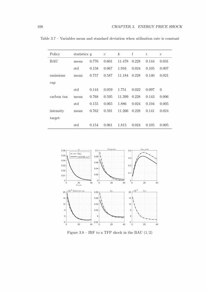
108 CHAPTER 3. ENERGY PRICE SHOCK
Table 3.7 – Variables mean and standard deviation when utilisation rate is constant
Policy statistics y c k l i e
BAU mean 0.776 0.601 11.478 0.228 0.144 0.031
std 0.158 0.067 1.916 0.024 0.105 0.007
emissions
cap
mean 0.757 0.587 11.184 0.228 0.140 0.021
std 0.144 0.059 1.751 0.022 0.097 0
carbon tax mean 0.768 0.595 11.399 0.228 0.143 0.006
std 0.155 0.065 1.886 0.024 0.104 0.005
intensity
target
mean 0.762 0.591 11.266 0.228 0.141 0.024
std 0.154 0.061 1.815 0.024 0.105 0.005
0 20 400
0.01
0.02
0.03
0.04
0.05
0.06
(ut)
=0.0125, u=1
0 20 400
0.02
0.04
0.06
0.08
0.1
0 20 400
0.1
0.2
0.3
0.4
0 20 40-5
0
5
10
15
2010
-4
0 20 40-0.02
0
0.02
0.04
0.06
0.08
0 20 40-5
0
5
10
15
2010
-4
Figure 3.8 – IRF to a TFP shock in the BAU (1/2)
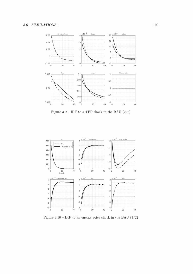
3.6. SIMULATIONS: 109
0 20 40
-0.02
0
0.02
0.04
0.06
0 20 40
0
1
2
3
410
-3
0 20 40
-5
0
5
10
15
2010
-3
0 20 40
0.005
0.01
0.015
0 20 40
0
0.02
0.04
0.06
0.08
0.1
0 20 40
-1
-0.5
0
0.5
1
Figure 3.9 – IRF to a TFP shock in the BAU (2/2)
0 20 400
0.01
0.02
0.03
0.04
0.05
0.06
(ut)
=0.0125, u=1
0 20 40-5
-4
-3
-2
-1
0
110
-3
0 20 40-10
-8
-6
-4
-210
-3
0 20 40-10
-8
-6
-4
-2
0
210
-5
0 20 40-4
-3
-2
-1
0
110
-3
0 20 40-8
-6
-4
-2
0
210
-5
Figure 3.10 – IRF to an energy price shock in the BAU (1/2)
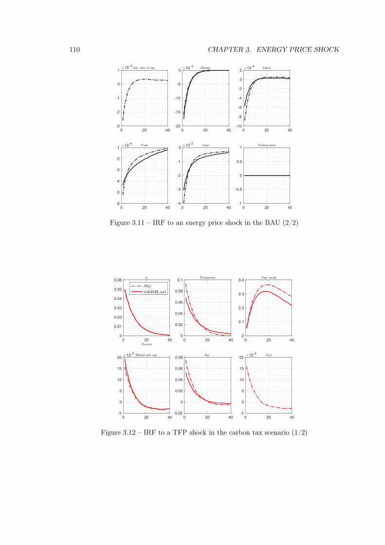
110 CHAPTER 3. ENERGY PRICE SHOCK
0 20 40
-3
-2
-1
0
110
-3
0 20 40
-20
-15
-10
-5
010
-4
0 20 40
-10
-8
-6
-4
-2
0
210
-4
0 20 40
-6
-5
-4
-3
-2
-110
-4
0 20 40
-4
-3
-2
-1
010
-3
0 20 40
-1
-0.5
0
0.5
1
Figure 3.11 – IRF to an energy price shock in the BAU (2/2)
0 20 400
0.01
0.02
0.03
0.04
0.05
0.06
(ut)
=0.0125, u=1
0 20 400
0.02
0.04
0.06
0.08
0.1
0 20 400
0.1
0.2
0.3
0.4
0 20 40-5
0
5
10
15
2010
-4
0 20 40-0.02
0
0.02
0.04
0.06
0.08
0 20 40-5
0
5
10
15
2010
-4
Figure 3.12 – IRF to a TFP shock in the carbon tax scenario (1/2)
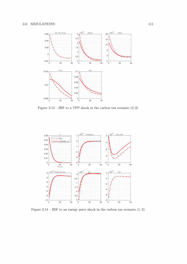
3.6. SIMULATIONS: 111
0 20 40
-0.02
0
0.02
0.04
0.06
0 20 40
0
0.5
1
1.5
2
2.5
310
-3
0 20 40
-5
0
5
10
15
2010
-3
0 20 40
0.005
0.01
0.015
0 20 40
0
0.02
0.04
0.06
0.08
0.1
Figure 3.13 – IRF to a TFP shock in the carbon tax scenario (2/2)
0 20 400
0.01
0.02
0.03
0.04
0.05
0.06
(ut)
=0.0125, u=1
0 20 40-4
-3
-2
-1
0
110
-3
0 20 40-10
-8
-6
-4
-210
-3
0 20 40-10
-8
-6
-4
-2
0
210
-5
0 20 40
-3
-2.5
-2
-1.5
-1
-0.5
0
10-3
0 20 40-8
-6
-4
-2
0
210
-5
Figure 3.14 – IRF to an energy price shock in the carbon tax scenario (1/2)
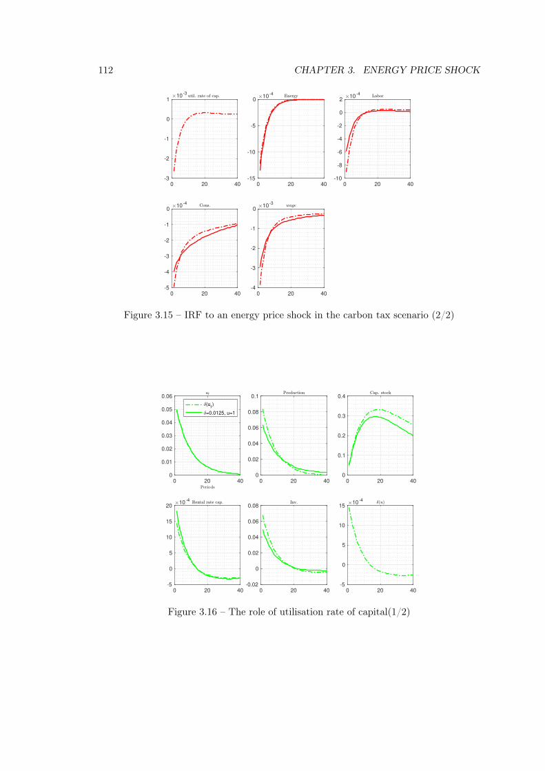
112 CHAPTER 3. ENERGY PRICE SHOCK
0 20 40
-3
-2
-1
0
110
-3
0 20 40
-15
-10
-5
010
-4
0 20 40
-10
-8
-6
-4
-2
0
210
-4
0 20 40
-5
-4
-3
-2
-1
010
-4
0 20 40
-4
-3
-2
-1
010
-3
Figure 3.15 – IRF to an energy price shock in the carbon tax scenario (2/2)
0 20 400
0.01
0.02
0.03
0.04
0.05
0.06
(ut)
=0.0125, u=1
0 20 400
0.02
0.04
0.06
0.08
0.1
0 20 400
0.1
0.2
0.3
0.4
0 20 40-5
0
5
10
15
2010
-4
0 20 40-0.02
0
0.02
0.04
0.06
0.08
0 20 40-5
0
5
10
1510
-4
Figure 3.16 – The role of utilisation rate of capital(1/2)
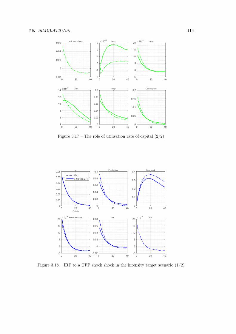
3.6. SIMULATIONS: 113
0 20 40
-0.02
0
0.02
0.04
0.06
0 20 40
-2
-1
0
1
2
310
-17
0 20 40
-5
0
5
10
15
2010
-3
0 20 40
4
6
8
10
12
1410
-3
0 20 40
0
0.02
0.04
0.06
0.08
0.1
0 20 40
0
0.05
0.1
0.15
0.2
Figure 3.17 – The role of utilisation rate of capital (2/2)
0 20 400
0.01
0.02
0.03
0.04
0.05
0.06
(ut)
=0.0125, u=1
0 20 400
0.02
0.04
0.06
0.08
0.1
0 20 400
0.1
0.2
0.3
0.4
0 20 40-5
0
5
10
15
2010
-4
0 20 40-0.02
0
0.02
0.04
0.06
0.08
0 20 40-5
0
5
10
15
2010
-4
Figure 3.18 – IRF to a TFP shock shock in the intensity target scenario (1/2)
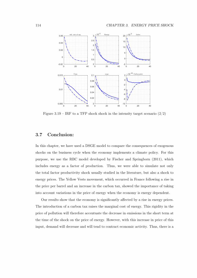
114 CHAPTER 3. ENERGY PRICE SHOCK
0 20 40
-0.02
0
0.02
0.04
0.06
0 20 40
0
0.5
1
1.5
2
2.5
310
-3
0 20 40
-5
0
5
10
15
2010
-3
0 20 40
0.005
0.01
0.015
0 20 40
0
0.02
0.04
0.06
0.08
0.1
0 20 40
-10
-8
-6
-4
-2
0
210
-16
Figure 3.19 – IRF to a TFP shock shock in the intensity target scenario (2/2)
3.7 Conclusion:
In this chapter, we have used a DSGE model to compare the consequences of exogenous
shocks on the business cycle when the economy implements a climate policy. For this
purpose, we use the RBC model developed by Fischer and Springborn (2011), which
includes energy as a factor of production. Thus, we were able to simulate not only
the total factor productivity shock usually studied in the literature, but also a shock to
energy prices. The Yellow Vests movement, which occurred in France following a rise in
the price per barrel and an increase in the carbon tax, showed the importance of taking
into account variations in the price of energy when the economy is energy dependent.
Our results show that the economy is significantly affected by a rise in energy prices.
The introduction of a carbon tax raises the marginal cost of energy. This rigidity in the
price of pollution will therefore accentuate the decrease in emissions in the short term at
the time of the shock on the price of energy. However, with this increase in price of this
input, demand will decrease and will tend to contract economic activity. Thus, there is a
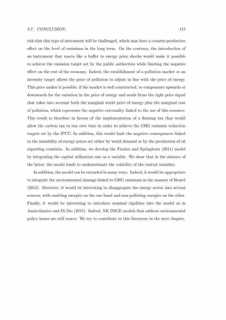
3.7. CONCLUSION: 115
risk that this type of instrument will be challenged, which may have a counter-productive
effect on the level of emissions in the long term. On the contrary, the introduction of
an instrument that reacts like a buffer to energy price shocks would make it possible
to achieve the emission target set by the public authorities while limiting the negative
effect on the rest of the economy. Indeed, the establishment of a pollution market or an
intensity target allows the price of pollution to adjust in line with the price of energy.
This price makes it possible, if the market is well constructed, to compensate upwards or
downwards for the variation in the price of energy and sends firms the right price signal
that takes into account both the marginal world price of energy plus the marginal cost
of pollution, which represents the negative externality linked to the use of this resource.
This result is therefore in favour of the implementation of a floating tax that would
allow the carbon tax to rise over time in order to achieve the GHG emission reduction
targets set by the IPCC. In addition, this would limit the negative consequences linked
to the instability of energy prices set either by world demand or by the production of oil
exporting countries. In addition, we develop the Fischer and Springborn (2011) model
by integrating the capital utilization rate as a variable. We show that in the absence of
the latter, the model tends to underestimate the volatility of the central variables.
In addition, the model can be extended in many ways. Indeed, it would be appropriate
to integrate the environmental damage linked to GHG emissions in the manner of Heutel
(2012). Moreover, it would be interesting to disaggregate the energy sector into several
sources, with emitting energies on the one hand and non-polluting energies on the other.
Finally, it would be interesting to introduce nominal rigidities into the model as in
Annicchiarico and Di Dio (2015). Indeed, NK DSGE models that address environmental
policy issues are still scarce. We try to contribute to this literature in the next chapter.

116 CHAPTER 3. ENERGY PRICE SHOCK
Chapter 4
The role of energy and greenhouse
gas emissions for monetary policy
design.
4.1 Introduction
The literature in macroeconomics that focuses on climate issues is still an under-explored
field of research Schubert (2017), and this is especially true for the neo-Keynesian macroe-
conomics. Among the articles that have integrated environmental damage due to climate
change, or studied the consequences of environmental policies on the economic cycle, are
the work of Angelopoulos et al. (2013), Fischer and Springborn (2011), Heutel (2012)
and more recently Annicchiarico and Di Dio (2015), Argentiero et al. (2017) and Xiao
et al. (2018). Angelopoulos et al. (2013), Fischer and Springborn (2011), Heutel (2012)
and Argentiero et al. (2017) use RBC models in their articles to analyse various climate
policies. Annicchiarico and Di Dio (2015) are the first to develop a NK DSGE model with
nominal rigidities á la Calvo. This model uses only two factors of production: capital
and labor. Emissions is proportional to the quantity of final good produced. They com-
pare different environmental policies instrument, and consider various shocks including
117
118 CHAPTER 4. ENERGY AND MONETARY POLICY ANALYSIS
monetary policy shock. Xiao et al. (2018), use this model and estimate a Bayesian model
for the Chinese economy, but incorporate a third factor of production, energy. Therefore,
emissions depend on the quantity of energy used in production.
We contribute to the literature on environmental NK DSGE models in the following
ways. We integrate as Xiao et al. (2018) energy into the model, but we disaggregate this
factor into polluting and non-polluting energy using a CES function, which allows us
to consider energies as complementary or substitutable. We use the introduce nominal
rigidities in the model as in Annicchiarico and Di Dio (2015) and compare two environ-
mental policy instruments: a carbon tax with an emission cap. Our results show that
a total factor productivity shock does not generate significant differences depending on
the instrument used, as suggested by Annicchiarico and Di Dio (2015) results. On the
other hand, this result is similar to those obtained by Xiao et al. (2018). Only GHG
emissions in the case of the tax will vary significantly. Thus, to be fully effective, the
European carbon market could integrate a floor price, or a tax that would replace the
allowance market if the price is too low. This would avoid a drop in the carbon price in
the event of a major recession. On the other hand, responses of macroeconomic variables
differ, depending on the instrument implemented in the event of a productivity shock in
the polluting energy sector. Indeed, a positive productivity shock in this sector (such as
fracking) will reduce the price of this energy source. In the case of a tax where the price
of pollution remains constant, emissions will tend to increase relatively more than in the
case of an emission cap. The combined use of these two instruments therefore appears
to be the best solution to economic fluctuations. Finally, we contribute to the literature
by optimizing the coefficients of the monetary policy rule used. In this sense, we show
that when negative externalities related to GHG emissions are taken into account, it is
optimal for the central bank to be more averse to inflation and output gap.
4.2. CARBON CYCLE. GENERAL ASSUMPTIONS 119
4.2 Carbon cycle. General assumptions
Since the industrial revolution, economic activity has generated a flow of GHG emissions
by using fossil fuels in the production processes. Some of these emissions are naturally
dissipated: either absorbed in the air through photosynthesis or diluted in oceans. When
GHG is not assimilated by this degradation processes, it accumulates in the atmosphere.
According to the AR5 (Pachauri et al., 2014), there exists a positive relationship between
the rise in the stock of GHG that stays in the atmosphere and the damage caused by
climate change and warmer temperatures (e.g., storms, sea level rise, coastal flooding,
inland flooding, extreme heat etc.).1
The environmental damage associated with the increase in atmospheric GHG stock
affects the production process. Negative consequences of GHG are usually modelled in
such a way as to decrease total factors productivity. The DICE and RICE computable
general equilibrium models developed by Nordhaus (1991, 1994, 2013) and Nordhaus and
Yang (1996) integrate environmental damage into the production function. The Golosov
et al. (2014) model derived from the DICE model also uses an exponential loss function
that affects GDP. In the PAGE model(see Hope (2006)), damage is also accounted for
as a loss as a percentage of GDP.
For the purposes of this chapter, we instead assume that negative externalities asso-
ciated with emissions do not affect productivity but rather the household utility. Rising
emissions generate disutility for the representative household. Incorporating the nega-
tive externalities of emissions into the household utility function allows us to optimize
the coefficients of monetary policy rule. Moreover, the flow rather than the stock of
GHG is considered responsible for these externalities. This approximation is made for a
methodological reason. Resolution of DSGE models is based on Taylor’s expansion, or
perturbation method in the neighbourhood of steady state. The starting point is a deter-
ministic stationary equilibrium that can be solved. This equilibrium is then perturbed
by stochastic shocks, and in a second step, we observe the return of the variables to their
1A systemic risk of a breakdown of infrastructure network can also be potentially connected to extreme
weather. This could materialize in food insecurity, water stress or losses of ecosystem and biodiversity.
120 CHAPTER 4. ENERGY AND MONETARY POLICY ANALYSIS
initial equilibrium as the shocks dissipate. This methodology assumes that all variables
are stationary at equilibrium. In other words, in order to incorporate the stock instead of
the flow, the stock would have to be invariant. However, this stock continues to grow as
the annual flow of emissions exceeds the earth capacity to absorb GHG. Thus, assuming
the stock to be invariant would be inconsistent with reality. Therefore, we consider the
emissions flow and not the stock as a source of externalities. Thus, it is assumed that an
increase in this flow will reduce household utility.
In the RBC model developed by Heutel (2012), and that of Annicchiarico and Di Dio
(2015, 2017), there is no energy, but emissions are proportional to the level of production.
In Fischer and Springborn (2011) and Xiao et al. (2018), production requires three factors
of production : capital, labor and energy. But energy is an aggregate factor, so emissions
are proportional to the use of this factor. Argentiero et al. (2017) also use three factors of
production in their RBC model, including energy, which they disaggregate into polluting
energy and renewable energy, in this case, emissions are proportional to the use of fossil
energies and not to the aggregate energy as it is the case in Fischer and Springborn (2011)
or Xiao et al. (2018). In our model, we assume as Argentiero et al. (2017) that emissions
arise from the use of fossil fuels in the production process. Energy factor is similarly
disaggregated into polluting energy and clean energy. Both energy inputs are aggregated
using a CES production function. Emissions are then proportional to the quantity of
polluting energy used in production. To the best of our knowledge, this is the first article
to disaggregate energy use in a NK DSGE model. This approach allows for finer results,
since the results will depend also on the elasticity of substitution between energy factors.
Without public intervention, fossil fuel users do not take into account negative ex-
ternalities generated by the combustion of oil, gas or coal. Due to a lack of definition
of property rights, costs of using these energies do not reflect real cost of pollution. In
the absence of technological innovation that could increase energy efficiency and would
result in a reduction in emissions per unit of fossil fuels consumed, the only way to reduce
emissions is to implement a public policy instrument. Public authorities have different
instruments at their disposal to internalize the cost of pollution: emission standard, a tax
4.2. CARBON CYCLE. GENERAL ASSUMPTIONS 121
or a cap-and-trade market. In our model we compare two instruments: a carbon tax and
a cap-and-trade market. We assume that public policy decides in each period both the
tax rate for emissions, τt, and how to use tax revenues. In the second case, it is assumed
that public authority set an emission cap not to be exceeded. They then offer a number
of emission allowances on the market. The demand for allowances comes from firms that
use fossil fuels in the production process, and let the market determine the pollution
equilibrium price. Because we work at an aggregate level, we do not model allowances
trade between firms. We focus on comparing a price instrument - a carbon tax - with an
instrument acting on quantities, and variables responses for different exogenous shocks.
In the latter case, the price of pollution will adapt to market fluctuations. This article
expands the recent but dynamic literature between business cycle and climate policies.
Fischer and Springborn (2011) compare a carbon tax,with an emission cap and an inten-
sity target in a RBC model. The only source of exogenous variability comes from total
factor productivity. Their results indicate that an intensity target instrument has least
effect on economic growth compare to the two others instruments considered, and an
emission cap leads to less volatility than a carbon tax. Thus, production and utility vary
less in the case of an emissions cap. Heutel (2012) considers a tax and an emission cap,
but is more interested in how these instruments should be adapted to maximise welfare.
According to these results, both instruments should vary pro-cyclically. Annicchiarico
and Di Dio (2015) will extend this literature by developing the first NK DSGE model in
which they will consider various sources of uncertainty other than TFP, including public
consumption and monetary policy shocks. Among other instruments they also compare
a tax to an emission cap. They find that the cap reduces the volatility of the main
macroeconomic variables of their model. Consequently, a climate policy instrument acts
as an economic stabiliser. More recently Annicchiarico and Di Dio (2017) developed their
model to analyse the optimal policy mix between environmental and monetary policy.
They studied Ramsey’s planner problem, where alternatively can control both environ-
mental and monetary policy or monetary policy, and takes as given the environmental
policy (carbon tax or cap-and-trade market), or in the last case it optimizes environ-
122 CHAPTER 4. ENERGY AND MONETARY POLICY ANALYSIS
mental policy and takes as given monetary policy. When the planner can optimize both
environmental and monetary policies, they find optimal to diminish the procicycality of
emissions (the planner is making a trade-off between the three imperfections present in
the models: negative externalities of emissions, imperfect competitions and costly price
adjustment). When the planner only has access to monetary policy, GHG emissions mit-
igation is not neutral for monetary policy, and depends on the climate policy instrument
implemented. Under a carbon tax regime with no environmental damage, inflation tar-
geting seems to be optimal while it is not under a cap-and-trade market or when damage
occur with a carbon tax. In such cases, it appears to be optimal to allow changes in price
in order "to address feedback of pollution on productivity". For Xiao et al. (2018), who
add the energy factor in an NK DSGE into a model similar to the one develop by Annic-
chiarico and Di Dio (2015, 2017), they compare four environmental policy instruments
to the BAU, which corresponds to a situation without policy. As expected, in the case
of a total factor productivity shock, the model is more volatile in the absence of public
intervention. The instruments will also act as stabilizers. They find that there is no
significant difference between instruments of environmental policies. Only the volatilities
of carbon prices or emissions will increase. Emissions are more volatile with a tax than
with an emissions cap.
We contribute to this literature by comparing a carbon tax regime to an emission
cap. We limit our analysis to these two instruments because they represent the major
part of the instruments implemented to fight climate change ECOFYS (2018). The
major contribution consists in the disaggregation of the energy sector in a NK DSGE
model. This makes it possible to study various shocks, standard in recent macroeconomic
literature, but we mainly focus on productivity shocks in the polluting energy sector, or
in the clean energy sector. The model also allows us to assume that the two sources of
energies are substitutable or complementary inputs. Our main findings are as follows.
Our results are consistent with Xiao et al. (2018) who find that there are no significant
differences between the two instruments used when a total factor productivity shock
occurs in the economy. However, the tax generate more volatility in GHG emissions,
4.2. CARBON CYCLE. GENERAL ASSUMPTIONS 123
and an emissions cap generate more volatility in carbon price. Similarly, after a shock in
the non-polluting energy sector, there is no significant difference between a tax and an
emission cap. On the other hand, a tax generates more volatility than an emission cap in
the case of a productivity shock in the polluting energy sector. Because polluting price
remains constant, emissions will vary accordingly to the quantity of fossil fuel burnt,
while in an emission cap regime, carbon price will adapt more or less to the situation
and it lowers emissions flows. The elasticity of substitution between energies will play
an essential role in variables responses following a productivity shock in the polluting
energy sector in a carbon tax regime. There is indeed a significant difference if the
energies are considered as complementary or substitutable. On the other hand, elasticity
does not influence the response of variables in the case of a productivity shock in the non-
polluting energy sector in the presence of a tax. In the presence of an instrument acting
on quantities, the elasticity of substitution will essentially play a role on the carbon price.
Depending on whether or not energy is substitutable, during a shock in the non-polluting
energy sector, the price of allowances will either increase or decrease. But in the end,
the rest of the economy is not affected by differences in elasticity.
Thus, based on these results, it seems appropriate to recommend the joint use of
these two instruments in order to minimize GHG emissions as much as possible. Indeed,
the 2008 financial crisis highlighted the shortcomings of using an allowance market alone.
The European experience and its EU ETS market has shown that in the event of a crisis,
the price of carbon tends to collapse. In line with IPCC recommendations, a carbon
market alone seems insufficient to achieve the targets set. By remaining at a low level a
carbon price does not sent the right signal to investors. If the price is too low, it does
not seem profitable to invest in low carbon technologies. So when the economy starts to
recover, the economy starts using again more fossil fuels and emissions rise. The reform
of the EU ETS market for the next period has put in place a mechanism to limit this
phenomenon but does not totally prevent it Trotignon et al. (2015). The Californian
carbon market, for its part, has a floor price below which carbon price cannot fall. In
order to avoid a further sharp drop in the price of carbon in the event of an economic
124 CHAPTER 4. ENERGY AND MONETARY POLICY ANALYSIS
recession, it seems wise to adopt the same system. Consequences are limited since we
find no significant differences between both instruments in case of a TFP shock, as our
results show.
4.3 The model
This section describes the way the behavioral equations of the model are obtained from
the optimizing (rational) behavior of both households and firms.
4.3.1 Households
There is a representative household in the economy whose welfare depends positively
on consumption (shaped by habits from lagged consumption, 0 < χ < 1) and nega-
tively on labor supplied to firms.2 Moreover, toxic (GHG) emissions reduce household
welfare measured through a damage function d (Gt) which is increasing in the level of
gas emissions Gt. At a given period t, this representative household seeks to maximize
the intertemporal constant relative risk aversion (CRRA) utility function with constant
discount factor β < 1 at infinite time horizon:
Et∞∑
j=0
βj
(1− d (Gt+j))
(ct+j − χcAt−1+j
)1−σ
1− σ − ψ(nst+j)
1+γ
1 + γ
(4.3.1)
where ct is current household-level consumption, cAt−1 is lagged aggregate consumption, nst
is the current labor supply and Gt denotes the amount of economy-wide GHG emissions
in period t. For the same current period t, the budget constraint in real terms is
ct + it + a(zt)kt−1 +(
exp(εbt
)(1 + rt)
)−1bt+1 − bt +mt − (1 + πt)
−1mt−1 + h(ct,mt)
= wtnst + rkt ztkt−1 + divt − taxt (4.3.2)
where wt is the real wage, rkt is real rental rate of capital, kt is the stock of capital,
zt is the capital utilization rate and a(zt) is its associated adjustment cost (with the2Consumption habits may be assumed with respect to lagged household-level consumption (internal
habits) or lagged aggregate consumption (external habits).
4.3. THE MODEL 125
steady-state properties z = 1, a′(z) > 0 and a′′(z) = σa > 0 as in Smets and Wouters,
2007), bt+1 is the amount of government bonds purchased in period t to be redeemed
in period t+ 1 with a gross real return of exp(εbt)
(1 + rt) which can be decomposed in
the contributions of the risk-free real interest rate rt and the AR(1) risk-premium shock
εbt , the amount of real money holdings available for purchases in the current t period is
mt, there is a lump sum taxt from the government, h(ct,mt) is a function that delivers
the transaction costs depending positively on consumption and negatively on real money
holdings, and divt is the amount of real dividends collected from firm ownership.
Capital accumulation is costly as in Smets and Wouters (2007). Thus, the equation
of motion for capital is,
kt = (1− δ) kt−1 + exp(εit) [
1− S(
itit−1
)]it, (4.3.3)
where δ is the constant rate of capital depreciation rate, S(it/it−1) is the investment
adjustment cost function with the steady-state properties S (1) = S′ (1) = 0 and S′′ (1) =
ϕk > 0, and εit is an stochastic AR(1) shock to the price of investment relative to
consumption goods. Regarding the transactions technology, we follow Casares (2007)
and the amount of income required to cover the transaction costs is determined by this
function
h(ct,mt) =
0 if ct = 0
φ0 + ctφ1
(ctmt
)φ2/(1−φ2)if ct > 0
where φ0, and φ1 > 0, and 0 < φ2 < 1, so that the transaction costs increases with
consumption, but falls with the stock of real money. The damage function that captures
the gas emissions externality is quadratic as in Heutel (2012) and Khan et al. (2019)
d (Gt) = d0 + d1Gt + d2G2t
The representative household chooses the sequence ct, nst , zt, kt, it, bt, and mt. to
maximize (4.3.1) subject to budget constraints and capital accumulation constraints such
as (4.3.2) and (4.3.3), respectively for period t and analogous expected constraints for
future periods.
126 CHAPTER 4. ENERGY AND MONETARY POLICY ANALYSIS
4.3.2 Firms
The production sector is composed of both final-good firms (competitive packers) and
intermediate-good firms that operate in monopolistic competition as in Dixit and Stiglitz
(1977).
4.3.2.1 Final-good firms
A continuum of intermediate goods is used in the production of the final good:
yt =
[∫ 1
0yθ−1θ
t (i)di
] θθ−1
where yt is the output of final good produced using yt(i) quantity of intermediate goods of
type i, θ > 1 represents the elasticity of substitution between intermediates goods. The
production of final goods is assumed to be under perfect competition. The representative
firm chooses the quantity of intermediate goods yt(i) that maximises its profit:
Ptyt −∫ 1
0Pt(i)yt(i)di
where Pt(i) is the nominal price of the intermediate good i, and Pt is the final good price.
4.3.2.2 Intermediate-good firms
Intermediate goods are produced by monopolistically competitive firms using labor, n,
capital, k, and energy, e, as inputs. The production technology of the representative i
firm is given by:
yt(i) = atkt(i)αnt(i)
1−α−υet(i)υ (4.3.4)
The intermediate goods firm determines the demand for inputs by solving the cost-
minimization program
Min wtnt(i) + rkt kt(i) + petet(i)
subject to technological constraint (4.3.4) . We also assume that prices are set with
nominal rigidities à la Calvo (1983). In each period a firm has the probability 1 − ηto adjust its price, and consequently has the remaining probability η to not adjust its
4.3. THE MODEL 127
price. If the firm is not able to adjust its price optimally, the following indexation rule
is appliedPt(i)
Pt−1(i)= (1 + πt−1)κ (1 + π + νt)
1−κ
where κ ∈ [0, 1] is the indexation share parameter of lagged inflation πt−1, and its com-
plementary 1− κ is the indexation share for the steady-state rate of inflation π modified
as determined by the νt price-push shock generated from an exogenous AR(1) process.
Between period t when firm has the market signal to set its price optimally and t + j,
the price indexation factor is:
ΠPt,t+j =
j∏
k=1
[(1 + πt+k−1)κ (1 + π + νt+k)
1−κ]
Intermediate-good firms face a Dixit-Stiglitz demand constraint which for the represen-
tative i firms reads as follows
yt(i) =
(Pt(i)
Pt
)−θyt (4.3.5)
Since Pt(i) is the price chosen by firm i when it has the ability to choose its price
optimally, it is set at the value that maximizes the discounted present value of real
profits conditional to the lack of future optimal price setting:
MaxPt(i)
Et∞∑
j=0
(βη)j
(Pt(i)Π
Pt,t+j
Pt+jyt+j(i)−mct+jyt+j(i)
)
where mct+j is the real marginal cost in period t+ j.
When the firm is able to set its price optimally in period t, using the demand con-
straint (4.3.5) in current and future periods gives this alternative way of writing the
intertemporal profit function conditional to Calvo-type rigidity,
MaxPt(i)
Et∞∑
j=0
(βη)j
(Pt(i)Π
Pt,t+j
Pt+j
)1−θ
yt+j −mct+j(Pt(i)Π
Pt,t+j
Pt+j
)−θyt+j
Defining λt(i) as the Lagrange multiplier associated with the technological constraint of
the representative firm. It is the shadow price of increasing the production of intermediate
output, or the marginal cost of inputs (capital, labor and energy) necessary to produce
128 CHAPTER 4. ENERGY AND MONETARY POLICY ANALYSIS
one extra unit of output. From the solution of the minimizing cost optimisation program,
it is easy to show that all the firms will have both same capital-labor ratio and energy-
labor ratio. Consequently, real marginal cost mct is the same across firms, and it is equal
to:3
mct =1
ααυυ(1− α− υ)(1−α−υ)
1
at(rkt )α(pet )
υw(1−α−υ)t (4.3.6)
Considering now the above price setting problem, if the intermediate good firm i has the
opportunity to choose its price, then from the first order condition associated with this
program the firm will impose the following price:
Pt(i) =θ
θ − 1
Et∑∞
j=0(βη)jmct+jΠPt,t+j
−θP θt+jyt+j
Et∑∞
j=0(βη)jΠpt,t+j
1−θP θ−1t+j yt+j
(4.3.7)
Since in the right hand side of the optimal price condition (4.3.7), no term depends on i,
all firms able to set their price will do it at this level so we can remove the i index, and
call this common optimal price Pt(i) = P ∗t .Bearing in mind that inflation rate between
two successive periods is πt = PtPt−1
− 1, the rate of inflation between t and t + j is
therefore:Pt+1(i)Pt(i)
Pt+2(i)Pt+1(i) · · ·
Pt+jPt+j−1
=Pt+jPt−1(i) = Πj
k=1(1 + πt+k). Using this formulation into
the optimal price gives us the optimal relative price:
P ∗tPt
=θ
θ − 1
Et∑∞
j=0(βη)jmct+jΠPt,t+j
−θΠjk=1(1 + πt+k)
θyt+j
Et∑∞
j=0(βη)jΠpt,t+j
1−θΠjk=1(1 + πt+k)θ−1yt+j
In the extreme case when all the firms are able to adjust their price optimally in every
period η = 0, we find the common result that firms will set their price to a fixed mark-up
over its marginal cost:P ∗tPt
=θ
θ − 1mct
The aggregated price index is an average between prices set by firms that have the capac-
ity to do so (1−η), and other prices that could not be set optimally by the remaining firms
and they are adjusted through the indexation rule. With the Dixit-Stiglitz aggregation
scheme, it gives
Pt =
[(1− η)P ∗t
1−θ + ηP 1−θt−1
[(1 + πt−1)κ (1 + π + νt)
1−κ]1−θ] 1
1−θ(4.3.8)
3Proof available upon request.
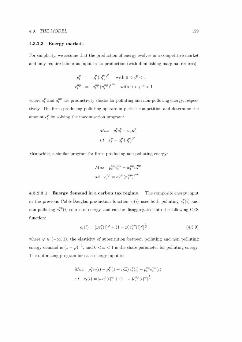
4.3. THE MODEL 129
4.3.2.3 Energy markets
For simplicity, we assume that the production of energy evolves in a competitive market
and only require labour as input in its production (with diminishing marginal returns):
ept = apt (npt )ςp with 0 < ςp < 1
enpt = anpt (nnpt )ςnp with 0 < ςnp < 1
where apt and anpt are productivity shocks for polluting and non-polluting energy, respec-
tively. The firms producing polluting operate in perfect competition and determine the
amount ept by solving the maximisation program:
Max ppt ept − wtnpt
s.t ept = apt (npt )ςp
Meanwhile, a similar program for firms producing non polluting energy:
Max pnpt enpt − wnpt nnpt
s.t enpt = anpt (nnpt )ςnp
4.3.2.3.1 Energy demand in a carbon tax regime. The composite energy input
in the previous Cobb-Douglas production function et(i) uses both polluting ept (i) and
non polluting enpt (i) source of energy, and can be disaggregated into the following CES
function:
et(i) = [ωept (i)ϕ + (1− ω)enpt (i)ϕ]
1ϕ (4.3.9)
where ϕ ∈ (−∞, 1), the elasticity of substitution between polluting and non polluting
energy demand is (1− ϕ)−1, and 0 < ω < 1 is the share parameter for polluting energy.
The optimizing program for each energy input is:
Max petet(i)− ppt (1 + τtΞ) ept (i)− pnpt enpt (i)
s.t et(i) = [ωept (i)ϕ + (1− ω)enpt (i)ϕ]
1ϕ
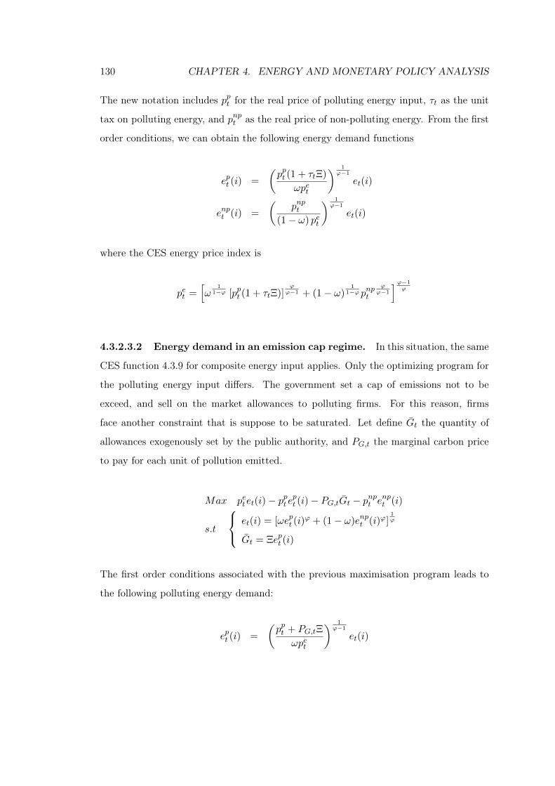
130 CHAPTER 4. ENERGY AND MONETARY POLICY ANALYSIS
The new notation includes ppt for the real price of polluting energy input, τt as the unit
tax on polluting energy, and pnpt as the real price of non-polluting energy. From the first
order conditions, we can obtain the following energy demand functions
ept (i) =
(ppt (1 + τtΞ)
ωpet
) 1ϕ−1
et(i)
enpt (i) =
(pnpt
(1− ω) pet
) 1ϕ−1
et(i)
where the CES energy price index is
pet =[ω
11−ϕ [ppt (1 + τtΞ)]
ϕϕ−1 + (1− ω)
11−ϕ pnpt
ϕϕ−1
]ϕ−1ϕ
4.3.2.3.2 Energy demand in an emission cap regime. In this situation, the same
CES function 4.3.9 for composite energy input applies. Only the optimizing program for
the polluting energy input differs. The government set a cap of emissions not to be
exceed, and sell on the market allowances to polluting firms. For this reason, firms
face another constraint that is suppose to be saturated. Let define Gt the quantity of
allowances exogenously set by the public authority, and PG,t the marginal carbon price
to pay for each unit of pollution emitted.
Max petet(i)− ppt ept (i)− PG,tGt − pnpt enpt (i)
s.t
et(i) = [ωept (i)ϕ + (1− ω)enpt (i)ϕ]
1ϕ
Gt = Ξept (i)
The first order conditions associated with the previous maximisation program leads to
the following polluting energy demand:
ept (i) =
(ppt + PG,tΞ
ωpet
) 1ϕ−1
et(i)
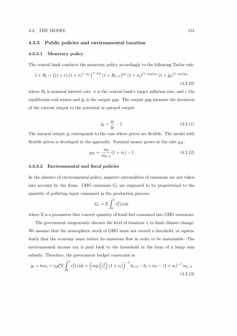
4.3. THE MODEL 131
4.3.3 Public policies and environmental taxation
4.3.3.1 Monetary policy
The central bank conducts the monetary policy accordingly to the following Taylor rule:
1 +Rt =((1 + r) (1 + π)1−µπ)1−µR (1 +Rt−1)µR (1 + πt)
(1−µR)µπ (1 + yt)(1−µR)µy
(4.3.10)
where Rt is nominal interest rate, π is the central bank’s target inflation rate, and r the
equilibrium real return and yt is the output gap. The output gap measure the deviation
of the current output to the potential or natural output:
yt =ytyt− 1 (4.3.11)
The natural output yt corresponds to the case where prices are flexible. The model with
flexible prices is developed in the appendix. Nominal money grows at the rate gM :
gM =mt
mt−1(1 + πt)− 1 (4.3.12)
4.3.3.2 Environmental and fiscal policies
In the absence of environmental policy, negative externalities of emissions are not taken
into account by the firms. GHG emissions Gt are supposed to be proportional to the
quantity of polluting input consumed in the production process:
Gt = Ξ
∫ 1
0ept (i)di
where Ξ is a parameter that convert quantity of fossil fuel consumed into GHG emissions.
The government exogenously chooses the level of taxation τt to limit climate change.
We assume that the atmospheric stock of GHG must not exceed a threshold, or equiva-
lently that the economy must reduce its emissions flow in order to be sustainable. The
environmental income tax is paid back to the household in the form of a lump sum
subsidy. Therefore, the government budget constraint is:
gt = taxt + τtpptΞ
∫ 1
0ept (i)di+
(exp
(εbt
)(1 + rt)
)−1bt+1 − bt +mt − (1 + πt)
−1mt−1
(4.3.13)
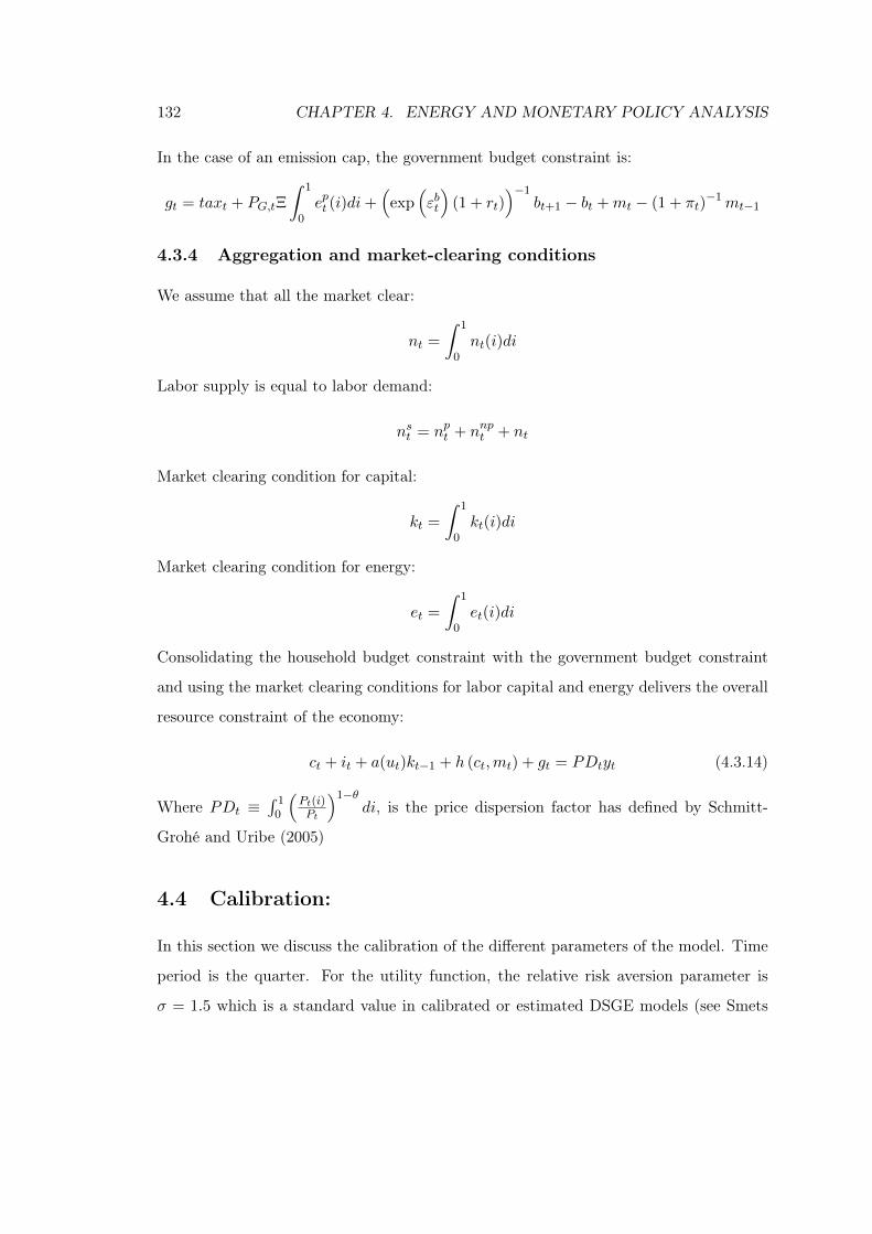
132 CHAPTER 4. ENERGY AND MONETARY POLICY ANALYSIS
In the case of an emission cap, the government budget constraint is:
gt = taxt + PG,tΞ
∫ 1
0ept (i)di+
(exp
(εbt
)(1 + rt)
)−1bt+1 − bt +mt − (1 + πt)
−1mt−1
4.3.4 Aggregation and market-clearing conditions
We assume that all the market clear:
nt =
∫ 1
0nt(i)di
Labor supply is equal to labor demand:
nst = npt + nnpt + nt
Market clearing condition for capital:
kt =
∫ 1
0kt(i)di
Market clearing condition for energy:
et =
∫ 1
0et(i)di
Consolidating the household budget constraint with the government budget constraint
and using the market clearing conditions for labor capital and energy delivers the overall
resource constraint of the economy:
ct + it + a(ut)kt−1 + h (ct,mt) + gt = PDtyt (4.3.14)
Where PDt ≡∫ 1
0
(Pt(i)Pt
)1−θdi, is the price dispersion factor has defined by Schmitt-
Grohé and Uribe (2005)
4.4 Calibration:
In this section we discuss the calibration of the different parameters of the model. Time
period is the quarter. For the utility function, the relative risk aversion parameter is
σ = 1.5 which is a standard value in calibrated or estimated DSGE models (see Smets
4.4. CALIBRATION: 133
and Wouters (2003, 2007) and Casares et al., (2019)). Empirical evidence (Altonji (1986),
Pencavel (1986), Domeij and Floden (2006)) show that Frisch’s labor supply elasticity
must be low. We calibrate γ = 4, so that the labor elasticity with respect to wage
turn out to be 0.25. We follow Smets and Wouters (2007), who estimated the habit
formation parameter to 0.71 very close to the prior 0.7 using a Bayesian DSGE model.
We consequently set χ = 0.7. The inter-temporal discount factor for the household is set,
as in Smets and Wouters (2007), to β = 0.9975 so that the risk-free real interest rate is
2% in the steady state. The parameters of the transaction costs function are set as follow:
the transaction cost parameter φ0 = 0.007 implying a total transaction costs of about 1%
of GDP in steady state, the scale parameter is φ1 = 0.05 in order to reach a ratio of real
money over consumption close to 1 (as considered a realistic average value for OECD
countries), and the elasticity parameter is calibrated to have an nominal elasticity of
nominal interest rest in money demand function as in the Baumol-Tobin model φ2 = 0.5.
Finally we calibrate the parameters of the damage function d0 = 0, d1 = 0.0278 and
d2 = 0.3898, with a double criteria: i) the damage is null with zero emissions (d(G) = 0
if G = 0), the augmenting effect of pollution on consumption disutility is 5% in steady
state, i.e 1− d(G) = 0.95.
According to Smets and Wouters (2003, 2007), they obtain a value of 6.77 for their
adjusment cost parameter for investment in their Bayesian estimated model for the Euro
area, while they obtain a value of 5.44 for their estimated Bayesian model on US data.
The posteriors value are also close to the prior 4. Therefore, we use the average value for
ϕk = 6.12. The depreciation rate of capital is supposed to be δ = 0.025, corresponding
to a 10% annual depreciation rate, which is a standard calibration in both RBC and NK
literature. The value for the price mark-up parameter is θ = 6, as in Casares (2010),
Gali and Monacelli (2005) and Erceg et al. (2000).
The parameters of the Cobb-Douglas production function in the consumption good
sector are calibrated as follow. Argentiero et al. (2017) estimate the energy share pa-
rameter at 0.06 in a Bayesian DSGE model for the EU-15 and 0.12 for the US. We use
the mean value ν = 0.09 as a representative value for the OECD countries. We choose
134 CHAPTER 4. ENERGY AND MONETARY POLICY ANALYSIS
α = 0.3, a standard value also assumed by Golosov et al. (2014), so that capital income
share is 25%, labor income share is 55% and dividends income share is 20% in the steady
state. Golosov et al. (2014) used Stern (2012) meta-study to calibrate the elasticity of
substitution between energy inputs. In their article they used three different inputs (coal,
oil and electricity) while we only distinguish polluting and non polluting energies. They
calibrated the elasticity of substitution as an average between coal-oil, coal-electricity and
oil-electricity, and finally set ϕ = −0.0584. Using the same methodology as in Golosov
et al. (2014), we find that our benchmark elasticity of substitution between clean and
dirty energies is ϕ = 0.008 assuming Stern (2012) estimations for elasticities of coal-
electricity (0.866), oil-electricity (1.06) and gas-electricity (1.099). The share parameter
for the CES energy function is set to ω = 0.815, in order to match the average ratio of
non-polluting energy over polluting energy in steady state suggested by Acemoglu and
Rafey (2018) enp/ep = 0.23. The parameters of the two energy production functions are
set ςp = ςnp = 0.35 so that employment share in the energy sector over total employment
(4 to 5%) is consistent with US data (US Energy and Employment Report).
We use data from the BP statistical database (Dudley et al., 2018) to calculate energy
demand. We aggregate energy inputs as follow. Between 2008 and 2018, for the OECD
countries, the average annual quantity of oil consumed was 2111 million tons (million
tons of oil equivalent or Mtoe henceforth), 1363 Mtoe of natural gas and 1004 Mtoe of
coal. Corresponding to an average aggregate demand for fossil fuel of about ep = 4478
Mtoe. For the same period considered, the demand for non-polluting energy was in
average enp = 984 Mtoe per year, which can be broken down as follows: 469 Mtoe of
non-polluting energy consumed was of nuclear origin, 312 Mtoe from hydroelectric power
plants, 32 Mtoe from solar energy, 102 Mtoe from wind and 70 Mtoe from biomass energy.
According to the same database, CO2 emissions in OECD countries for the period 2008-
2018 are on average 12636Mt CO2 per year. The intensity of CO2 emissions per unit of
fossil energy is therefore 2.82 t CO2/toe. One ton of CO2 contains 0.27 ton of carbon.
4If we define ε as the elasticity of substitution between the polluting and non-polluting energy inputs,
then ε−1ε
= ϕ and ε = (1 − ϕ)−1.
4.4. CALIBRATION: 135
Thus the conversion factor in terms of carbon is Ξ = 0.76 tC/toe. The demand for
non-polluting energy thus represents 18% of the total energy demand, and the ratio of
clean energy demand over polluting energy is ep
enp = 0.22.
The aggregate price of each energy input is calculated as a weighted average of the
prices of each energy source:
pp =
∑i piei∑
i ei
i = oil, gas, coal
According to the Crude oil Price time series for Europe from the U.S. Energy Information
Administration database (US EIA), in average between 2008 and 2018 the price of oil
per barrel was $ 83 (2015 dollars constant). A barrel of oil corresponds to 0.1364 metric
ton. Thus, the price of oil is $ 610 per ton. We find an average price of $ 99 per ton of
coal, and an average price of $ 9 per million of British Thermal Unit (Btu). One million
of Btu is equivalent to 0.172 barrel of oil equivalent. So the average price of gas is $ 54
per barrel of oil equivalent, and we finally find that the price of gas is pp = 398$/toe.
The weighted average price of the polluting energy input is therefore $326 pet ton of oil
equivalent. The carbon price on the EU Emissions Trading Scheme is used to calculate
the carbon tax rate. Between 2019 and 2020, the average allowance price was e25/tCO2,
corresponding to e92/tC or $ 102/tC using the euro-dollar exchange rate for the same
year (EUR 1←→ USD 1.11 according to the ECB euro reference exchange rate). Finally,
by using the aggregate price pp, the conversion factor Ξ, and the carbon price, we obtain
a carbon tax rate of τ = 0.24.
In their model, Smets and Wouters (2003) calibrate government expenditures to GDP
ratio as 0.18. However, this value is well below the OECD data. Indeed the average is
0.41 for years 2007, 2009, 2014 and 2015. We thus calibrate Φgy = 0.41. We assume, as
it is standard in the literature that the Calvo probability is η = 0.75, so that the firm is
able to set the optimal price once a year. The indexation share parameter of inflation is
κ = 0.35. The value is calculated as the average value between Smets and Wouters (2003)
Bayesian estimation for the Euro area (0.47) and their estimation for the US (0.24). We
assume that the elasticity of the marginal cost of adjusting capital utilization rate with
136 CHAPTER 4. ENERGY AND MONETARY POLICY ANALYSIS
respect to the capital utilisation rate is σa = 1.17, which is consistent with Smets and
Wouters (2003, 2007) estimations.
We choose the same parameters for the monetary policy rule as in Taylor (1993),
thus the coefficient for responses of the interest rate to inflation deviations is µπ = 1.5,
the response of the interest to output gap µy = 0.125 (we divide the initial value by 4,
because we consider quarter time period), and the interest rate smoothing µR = 0.85.
Next, we calibrate the exogenous processes of the model. We assume that the
autoregressive parameter of the Solow residual is ρa = 0.9, and its standard devia-
tion is ea = 0.007, a standard value in the literature. Autocorrelation parameters of
the stochastic processes in both energies sectors are also supposed to be equal, we set
ρap = ρanp = 0.9, and their white noise have for standard deviation eap = eanp
= 0.014.
Stochastic parameters of the three demand shocks - risk premium shock, investment cost
shock, and government spending shock - are calibrated so that they explain around 50%
of total output growth variance, a realistic value of business fluctuations. Consequently,
we take ρb = ρi = ρg = 0.8 and the standard deviations of white noises are respectively
eb = 0.0039, ei = 0.0024,and eg = 0.0045. The price-push shock parameters are ρP = 0.6
and eP = 0.01, so that this shock explain 40% of inflation variance.
4.5 Simulations:
The following section uses the model to analyse the economy’s response to various exoge-
nous shocks considered under two environmental policy regimes. We analyse shocks under
a carbon tax regime and under a cap-and-trade market (or emission cap). The model is
computed using a perturbation approach after a first order approximation (or Taylor’s
expansion) around the steady state with Dynare software (Adjemian et al., 2011). The
log-linearised model is developed in the technical appendix. We have considered seven
exogenous shocks, among which five are standard in the NK DSGE literature (total fac-
tor productivity shock, investment cost shock, risk premium shock, inflation shock and
government spending shock) plus two productivities shocks in each energy sectors. We
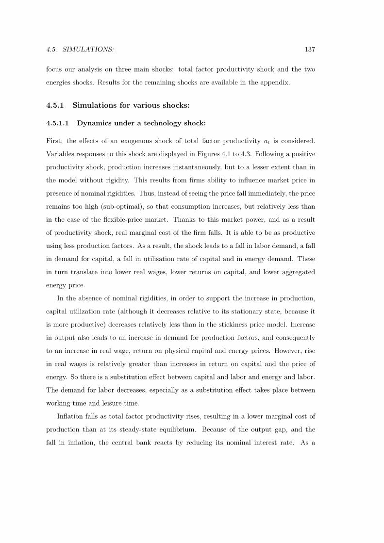
4.5. SIMULATIONS: 137
focus our analysis on three main shocks: total factor productivity shock and the two
energies shocks. Results for the remaining shocks are available in the appendix.
4.5.1 Simulations for various shocks:
4.5.1.1 Dynamics under a technology shock:
First, the effects of an exogenous shock of total factor productivity at is considered.
Variables responses to this shock are displayed in Figures 4.1 to 4.3. Following a positive
productivity shock, production increases instantaneously, but to a lesser extent than in
the model without rigidity. This results from firms ability to influence market price in
presence of nominal rigidities. Thus, instead of seeing the price fall immediately, the price
remains too high (sub-optimal), so that consumption increases, but relatively less than
in the case of the flexible-price market. Thanks to this market power, and as a result
of productivity shock, real marginal cost of the firm falls. It is able to be as productive
using less production factors. As a result, the shock leads to a fall in labor demand, a fall
in demand for capital, a fall in utilisation rate of capital and in energy demand. These
in turn translate into lower real wages, lower returns on capital, and lower aggregated
energy price.
In the absence of nominal rigidities, in order to support the increase in production,
capital utilization rate (although it decreases relative to its stationary state, because it
is more productive) decreases relatively less than in the stickiness price model. Increase
in output also leads to an increase in demand for production factors, and consequently
to an increase in real wage, return on physical capital and energy prices. However, rise
in real wages is relatively greater than increases in return on capital and the price of
energy. So there is a substitution effect between capital and labor and energy and labor.
The demand for labor decreases, especially as a substitution effect takes place between
working time and leisure time.
Inflation falls as total factor productivity rises, resulting in a lower marginal cost of
production than at its steady-state equilibrium. Because of the output gap, and the
fall in inflation, the central bank reacts by reducing its nominal interest rate. As a
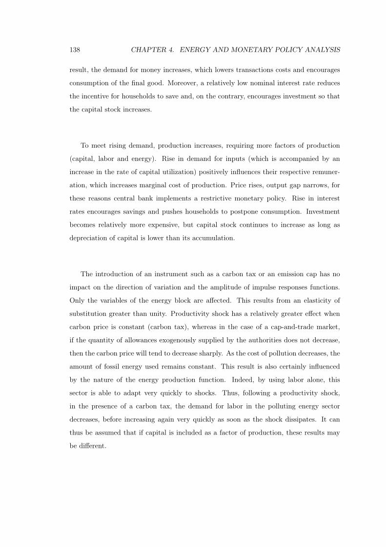
138 CHAPTER 4. ENERGY AND MONETARY POLICY ANALYSIS
result, the demand for money increases, which lowers transactions costs and encourages
consumption of the final good. Moreover, a relatively low nominal interest rate reduces
the incentive for households to save and, on the contrary, encourages investment so that
the capital stock increases.
To meet rising demand, production increases, requiring more factors of production
(capital, labor and energy). Rise in demand for inputs (which is accompanied by an
increase in the rate of capital utilization) positively influences their respective remuner-
ation, which increases marginal cost of production. Price rises, output gap narrows, for
these reasons central bank implements a restrictive monetary policy. Rise in interest
rates encourages savings and pushes households to postpone consumption. Investment
becomes relatively more expensive, but capital stock continues to increase as long as
depreciation of capital is lower than its accumulation.
The introduction of an instrument such as a carbon tax or an emission cap has no
impact on the direction of variation and the amplitude of impulse responses functions.
Only the variables of the energy block are affected. This results from an elasticity of
substitution greater than unity. Productivity shock has a relatively greater effect when
carbon price is constant (carbon tax), whereas in the case of a cap-and-trade market,
if the quantity of allowances exogenously supplied by the authorities does not decrease,
then the carbon price will tend to decrease sharply. As the cost of pollution decreases, the
amount of fossil energy used remains constant. This result is also certainly influenced
by the nature of the energy production function. Indeed, by using labor alone, this
sector is able to adapt very quickly to shocks. Thus, following a productivity shock,
in the presence of a carbon tax, the demand for labor in the polluting energy sector
decreases, before increasing again very quickly as soon as the shock dissipates. It can
thus be assumed that if capital is included as a factor of production, these results may
be different.
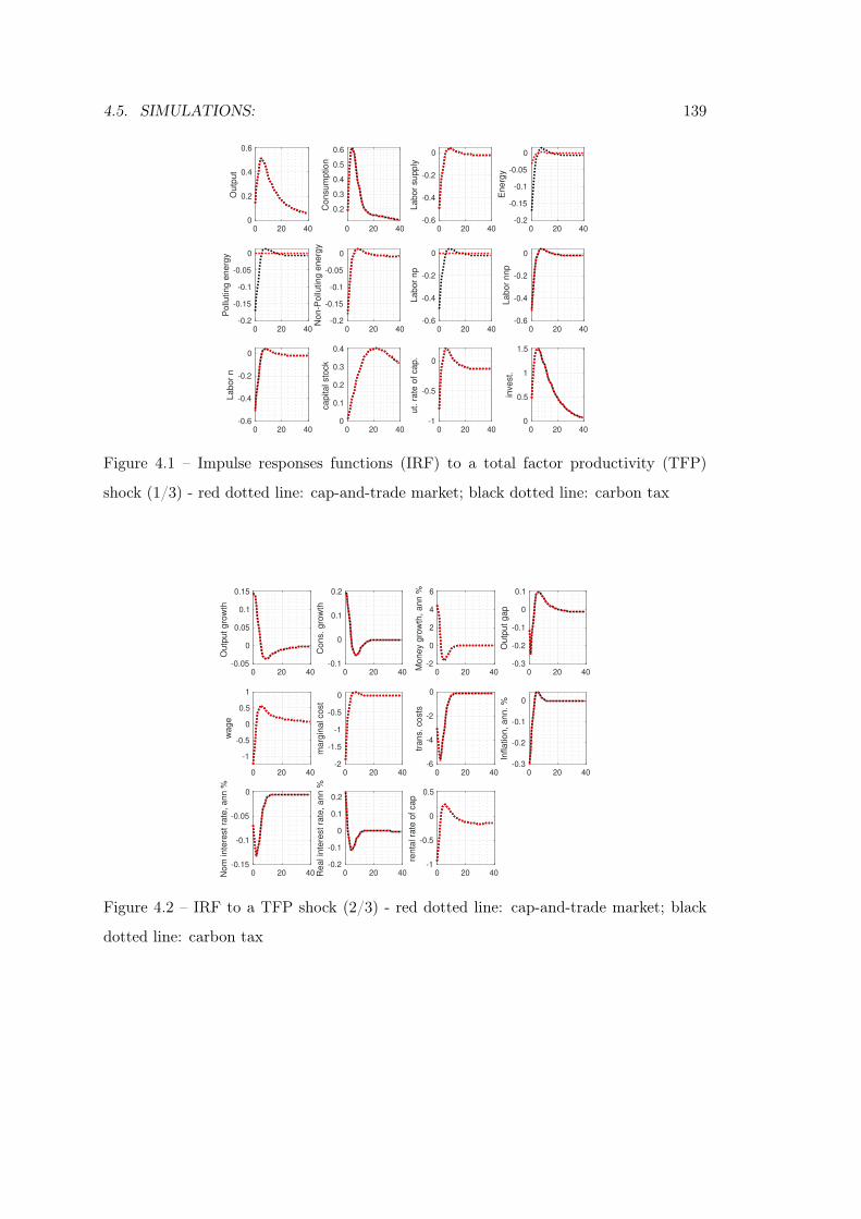
4.5. SIMULATIONS: 139
0 20 400
0.2
0.4
0.6
Outp
ut
0 20 40
0.2
0.3
0.4
0.5
0.6
Consu
mption
0 20 40-0.6
-0.4
-0.2
0
La
bor
supply
0 20 40-0.2
-0.15
-0.1
-0.05
0
En
erg
y
0 20 40-0.2
-0.15
-0.1
-0.05
0
Po
lluting e
ne
rgy
0 20 40-0.2
-0.15
-0.1
-0.05
0
Non-P
ollu
ting e
nerg
y
0 20 40-0.6
-0.4
-0.2
0
Lab
or
np
0 20 40-0.6
-0.4
-0.2
0
Labo
r nnp
0 20 40-0.6
-0.4
-0.2
0
Labo
r n
0 20 400
0.1
0.2
0.3
0.4
capital sto
ck
0 20 40-1
-0.5
0
ut. r
ate
of cap.
0 20 400
0.5
1
1.5
inve
st.
Figure 4.1 – Impulse responses functions (IRF) to a total factor productivity (TFP)
shock (1/3) - red dotted line: cap-and-trade market; black dotted line: carbon tax
0 20 40-0.05
0
0.05
0.1
0.15
Outp
ut gro
wth
0 20 40-0.1
0
0.1
0.2
Cons. gro
wth
0 20 40-2
0
2
4
6
Money g
row
th, ann %
0 20 40-0.3
-0.2
-0.1
0
0.1
Outp
ut gap
0 20 40
-1
-0.5
0
0.5
1
wage
0 20 40-2
-1.5
-1
-0.5
0
marg
inal cost
0 20 40-6
-4
-2
0
trans. costs
0 20 40-0.3
-0.2
-0.1
0
Inflation, ann. %
0 20 40-0.15
-0.1
-0.05
0
Nom
inte
rest ra
te, ann %
0 20 40-0.2
-0.1
0
0.1
0.2
Real in
tere
st ra
te, ann %
0 20 40-1
-0.5
0
0.5
renta
l ra
te o
f cap
Figure 4.2 – IRF to a TFP shock (2/3) - red dotted line: cap-and-trade market; black
dotted line: carbon tax
140 CHAPTER 4. ENERGY AND MONETARY POLICY ANALYSIS
0 20 40-2
-1.5
-1
-0.5
0
0.5
1
Net e
nerg
y p
rice p
p0 20 40
-6
-4
-2
0
2
Gro
ss e
ne
rgy p
rice
0 20 40-5
-4
-3
-2
-1
0
1
Carb
on p
rice
0 20 40-2
-1.5
-1
-0.5
0
0.5
1
Energ
y p
rice
pn
p
0 20 40-2
-1.5
-1
-0.5
0
0.5
1
Energ
y p
rice
pe
Figure 4.3 – IRF to a TFP shock (3/3) - red dotted line: cap-and-trade market; black
dotted line: carbon tax
4.5.1.2 Technology shock in the polluting sector:
In the case of a positive productivity shock in the polluting energy sector, the con-
sequences will differ depending on the environmental policy instrument implemented.
Figures 4.4 to 4.6 illustrate this case. With a carbon tax, the price to be paid for each
ton of pollution emitted remains constant. Therefore, all other things being equal, the
increase in productivity results in a decrease in gross price for fossil fuels. Relative
price of energies changes in favour of polluting energies. Demand for polluting energy
increases, and because of possible substitution between the two energy sources, demand
for non-polluting energy tends to decrease at the time of the shock. Aggregate price of
energy falls sharply, which reduces demand for other factors of production, capital and
labor. Energy intensity of final good increases. As production costs fall, real marginal
cost also falls, but since firms have market power, the price they set is above the optimal
price relatively to the one in absence of nominal rigidities. This results in a negative
output gap. Fall in prices and this output gap encourages the central bank to react by
lowering its nominal interest rate. As the cost of investment is lower, investment rises,
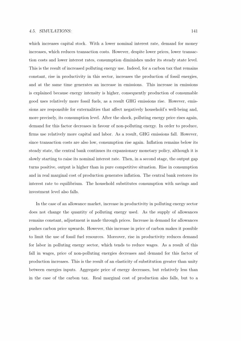
4.5. SIMULATIONS: 141
which increases capital stock. With a lower nominal interest rate, demand for money
increases, which reduces transaction costs. However, despite lower prices, lower transac-
tion costs and lower interest rates, consumption diminishes under its steady state level.
This is the result of increased polluting energy use. Indeed, for a carbon tax that remains
constant, rise in productivity in this sector, increases the production of fossil energies,
and at the same time generates an increase in emissions. This increase in emissions
is explained because energy intensity is higher, consequently production of consumable
good uses relatively more fossil fuels, as a result GHG emissions rise. However, emis-
sions are responsible for externalities that affect negatively household’s well-being and,
more precisely, its consumption level. After the shock, polluting energy price rises again,
demand for this factor decreases in favour of non-polluting energy. In order to produce,
firms use relatively more capital and labor. As a result, GHG emissions fall. However,
since transaction costs are also low, consumption rise again. Inflation remains below its
steady state, the central bank continues its expansionary monetary policy, although it is
slowly starting to raise its nominal interest rate. Then, in a second stage, the output gap
turns positive, output is higher than in pure competitive situation. Rise in consumption
and in real marginal cost of production generates inflation. The central bank restores its
interest rate to equilibrium. The household substitutes consumption with savings and
investment level also falls.
In the case of an allowance market, increase in productivity in polluting energy sector
does not change the quantity of polluting energy used. As the supply of allowances
remains constant, adjustment is made through prices. Increase in demand for allowances
pushes carbon price upwards. However, this increase in price of carbon makes it possible
to limit the use of fossil fuel resources. Moreover, rise in productivity reduces demand
for labor in polluting energy sector, which tends to reduce wages. As a result of this
fall in wages, price of non-polluting energies decreases and demand for this factor of
production increases. This is the result of an elasticity of substitution greater than unity
between energies inputs. Aggregate price of energy decreases, but relatively less than
in the case of the carbon tax. Real marginal cost of production also falls, but to a
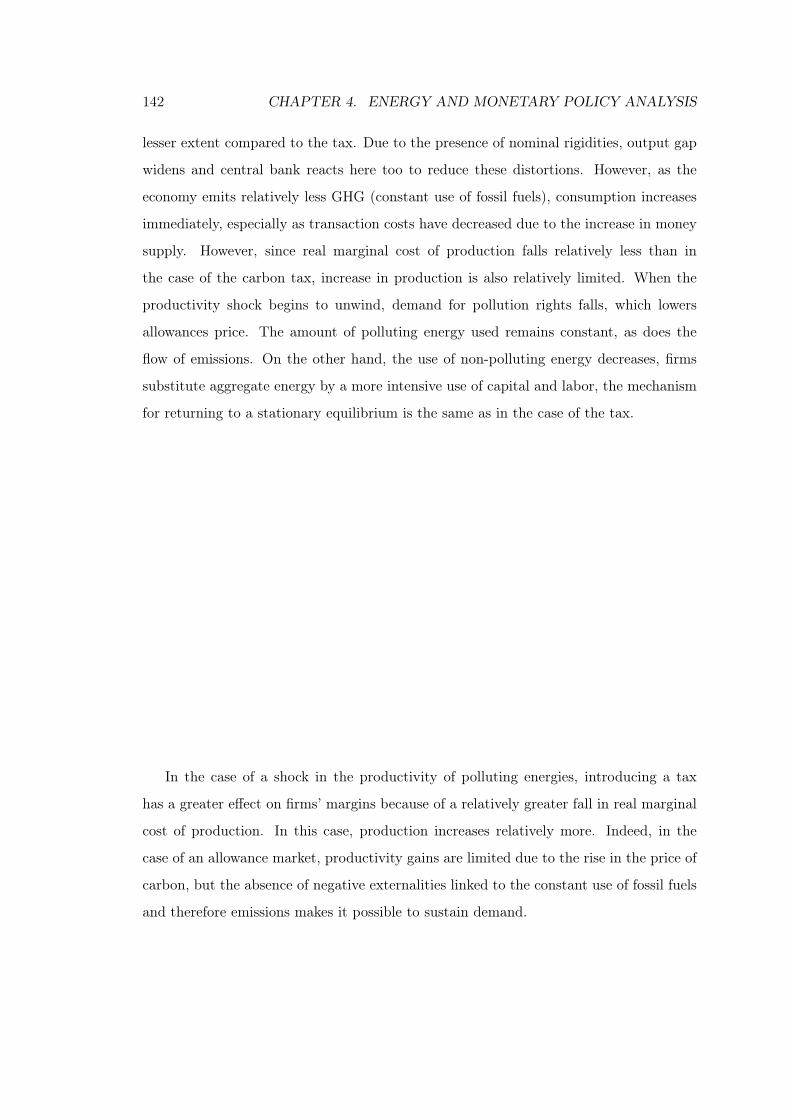
142 CHAPTER 4. ENERGY AND MONETARY POLICY ANALYSIS
lesser extent compared to the tax. Due to the presence of nominal rigidities, output gap
widens and central bank reacts here too to reduce these distortions. However, as the
economy emits relatively less GHG (constant use of fossil fuels), consumption increases
immediately, especially as transaction costs have decreased due to the increase in money
supply. However, since real marginal cost of production falls relatively less than in
the case of the carbon tax, increase in production is also relatively limited. When the
productivity shock begins to unwind, demand for pollution rights falls, which lowers
allowances price. The amount of polluting energy used remains constant, as does the
flow of emissions. On the other hand, the use of non-polluting energy decreases, firms
substitute aggregate energy by a more intensive use of capital and labor, the mechanism
for returning to a stationary equilibrium is the same as in the case of the tax.
In the case of a shock in the productivity of polluting energies, introducing a tax
has a greater effect on firms’ margins because of a relatively greater fall in real marginal
cost of production. In this case, production increases relatively more. Indeed, in the
case of an allowance market, productivity gains are limited due to the rise in the price of
carbon, but the absence of negative externalities linked to the constant use of fossil fuels
and therefore emissions makes it possible to sustain demand.
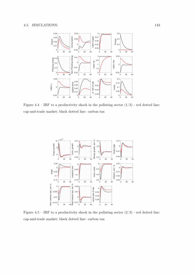
4.5. SIMULATIONS: 143
0 20 400
0.01
0.02
0.03
0.04
Outp
ut
0 20 40-0.02
0
0.02
0.04
Consu
mption
0 20 40
-0.04
-0.03
-0.02
-0.01
0
La
bor
supply
0 20 400
0.2
0.4
0.6
En
erg
y
0 20 400
0.2
0.4
0.6
Po
lluting e
ne
rgy
0 20 40-0.02
-0.01
0
0.01
Non-P
ollu
ting e
nerg
y
0 20 40-2
-1.5
-1
-0.5
0
Lab
or
np
0 20 40-0.05
0
0.05
Labo
r nnp
0 20 40-0.05
0
0.05
Labo
r n
0 20 400
0.01
0.02
0.03
0.04
capital sto
ck
0 20 40
-0.06
-0.04
-0.02
0
ut. r
ate
of cap.
0 20 400
0.05
0.1
0.15
0.2
inve
st.
Figure 4.4 – IRF to a productivity shock in the polluting sector (1/3) - red dotted line:
cap-and-trade market; black dotted line: carbon tax
0 20 40
0
5
10
Outp
ut gro
wth
10-3
0 20 40-0.02
-0.01
0
0.01
Cons. gro
wth
0 20 40-0.2
0
0.2
0.4
Money g
row
th, ann %
0 20 40
-0.02
-0.01
0
0.01
Outp
ut gap
0 20 40-0.15
-0.1
-0.05
0
0.05
wage
0 20 40-0.15
-0.1
-0.05
0
marg
inal cost
0 20 40-0.6
-0.4
-0.2
0
trans. costs
0 20 40-0.03
-0.02
-0.01
0
0.01
Inflation, ann. %
0 20 40-0.015
-0.01
-0.005
0
Nom
inte
rest ra
te, ann %
0 20 40
-0.01
0
0.01
0.02
Real in
tere
st ra
te, ann %
0 20 40
-0.06
-0.04
-0.02
0
renta
l ra
te o
f cap
Figure 4.5 – IRF to a productivity shock in the polluting sector (2/3) - red dotted line:
cap-and-trade market; black dotted line: carbon tax
144 CHAPTER 4. ENERGY AND MONETARY POLICY ANALYSIS
0 20 40-2.5
-2
-1.5
-1
-0.5
0
Net e
nerg
y p
rice p
p0 20 40
-2
0
2
4
6
8
Gro
ss e
ne
rgy p
rice
0 20 400
2
4
6
8
10
12
Carb
on p
rice
0 20 40-0.15
-0.1
-0.05
0
0.05
Energ
y p
rice
pn
p
0 20 40-0.8
-0.6
-0.4
-0.2
0
0.2
Energ
y p
rice
pe
Figure 4.6 – IRF to a productivity shock in the polluting sector (3/3) - red dotted line:
cap-and-trade market; black dotted line: carbon tax
4.5.1.3 Technology shock in the non-polluting sector:
The use of a price, or quantity instrument has little, or no impact on the economy
in the case of a technology shock in the non-polluting energy sector (see figures 4.7
to 4.9. Rising productivity immediately increases the use of non-polluting energy. In
the presence of a carbon tax, demand for polluting energy decreases, due to changes
in relative prices. In the case of an emission cap, if the supply of allowances remains
constant, demand for pollution decreases, carbon price falls and demand for polluting
energy remains constant. Aggregate energy demand increases at the expense of other
factors of production. This increase in productivity is reflected in a fall in real marginal
cost of production, the output gap widens and a fall in inflation is observed. The central
bank then implements its expansionary monetary policy, which supports demand. This
favours economic activity, inflation rises again and output gap becomes positive. The
return to a stationary equilibrium is achieved by a further substitution of energy by a
more intensive use of capital and labor. The central bank raises its nominal interest rate
again, which favours savings, and households reduce their consumption.
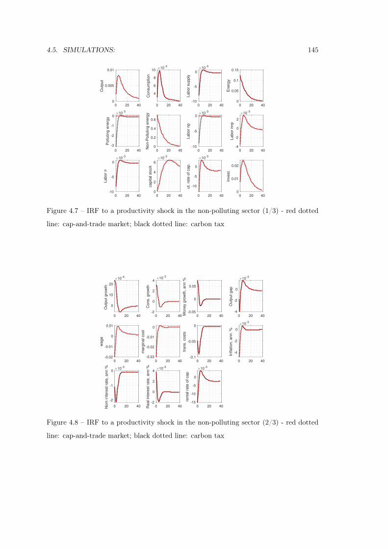
4.5. SIMULATIONS: 145
0 20 400
0.005
0.01
Outp
ut
0 20 40
4
6
8
10
Consum
ptio
n
10-3
0 20 40-10
-5
0
Labo
r sup
ply
10-3
0 20 400
0.05
0.1
0.15
Energ
y
0 20 40
-3
-2
-1
0
Pollu
tin
g e
nerg
y
10-3
0 20 400
0.2
0.4
0.6
Non
-Pollu
ting
energ
y0 20 40
-10
-5
0
La
bor
np
10-3
0 20 40-4
-2
0
2
Labor
nnp
10-3
0 20 40-10
-5
0
La
bor
n
10-3
0 20 400
2
4
6
ca
pital sto
ck
10-3
0 20 40
-10
-5
0
ut. r
ate
of cap
.
10-3
0 20 400
0.01
0.02
invest.
Figure 4.7 – IRF to a productivity shock in the non-polluting sector (1/3) - red dotted
line: cap-and-trade market; black dotted line: carbon tax
0 20 40
0
10
20
Outp
ut gro
wth
10-4
0 20 40-2
0
2
4
Cons.
gro
wth
10-3
0 20 40-0.05
0
0.05
Money g
row
th,
ann %
0 20 40-4
-2
0
Outp
ut gap
10-3
0 20 40-0.02
-0.01
0
0.01
wage
0 20 40-0.03
-0.02
-0.01
0
marg
inal cost
0 20 40-0.1
-0.05
0
trans. costs
0 20 40
-4
-2
0
Inflation, ann. %
10-3
0 20 40
-2
-1
0
Nom
inte
rest ra
te, ann % 10
-3
0 20 40-2
0
2
4
Real in
tere
st ra
te, ann % 10
-3
0 20 40-15
-10
-5
0
renta
l ra
te o
f cap
10-3
Figure 4.8 – IRF to a productivity shock in the non-polluting sector (2/3) - red dotted
line: cap-and-trade market; black dotted line: carbon tax
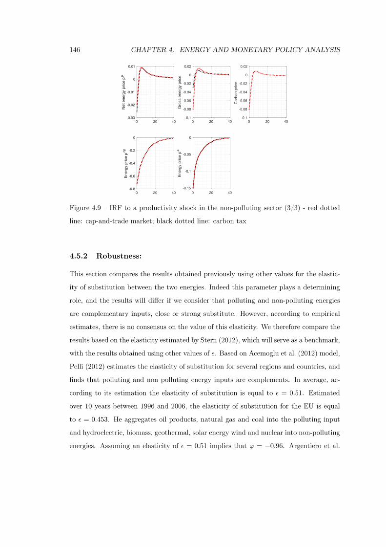
146 CHAPTER 4. ENERGY AND MONETARY POLICY ANALYSIS
0 20 40-0.03
-0.02
-0.01
0
0.01
Net e
nerg
y p
rice p
p0 20 40
-0.1
-0.08
-0.06
-0.04
-0.02
0
0.02
Gro
ss e
ne
rgy p
rice
0 20 40-0.1
-0.08
-0.06
-0.04
-0.02
0
0.02
Carb
on p
rice
0 20 40-0.8
-0.6
-0.4
-0.2
0
Energ
y p
rice
pn
p
0 20 40
-0.15
-0.1
-0.05
0
Energ
y p
rice
pe
Figure 4.9 – IRF to a productivity shock in the non-polluting sector (3/3) - red dotted
line: cap-and-trade market; black dotted line: carbon tax
4.5.2 Robustness:
This section compares the results obtained previously using other values for the elastic-
ity of substitution between the two energies. Indeed this parameter plays a determining
role, and the results will differ if we consider that polluting and non-polluting energies
are complementary inputs, close or strong substitute. However, according to empirical
estimates, there is no consensus on the value of this elasticity. We therefore compare the
results based on the elasticity estimated by Stern (2012), which will serve as a benchmark,
with the results obtained using other values of ε. Based on Acemoglu et al. (2012) model,
Pelli (2012) estimates the elasticity of substitution for several regions and countries, and
finds that polluting and non polluting energy inputs are complements. In average, ac-
cording to its estimation the elasticity of substitution is equal to ε = 0.51. Estimated
over 10 years between 1996 and 2006, the elasticity of substitution for the EU is equal
to ε = 0.453. He aggregates oil products, natural gas and coal into the polluting input
and hydroelectric, biomass, geothermal, solar energy wind and nuclear into non-polluting
energies. Assuming an elasticity of ε = 0.51 implies that ϕ = −0.96. Argentiero et al.
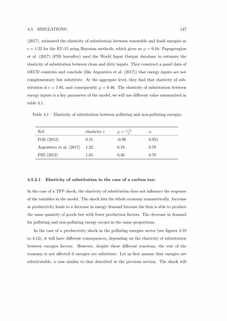
4.5. SIMULATIONS: 147
(2017), estimated the elasticity of substitution between renewable and fossil energies at
ε = 1.22 for the EU-15 using Bayesian methods, which gives us ϕ = 0.18. Papageorgiou
et al. (2017) (PSS hereafter) used the World Input Output database to estimate the
elasticity of substitution between clean and dirty inputs. They construct a panel data of
OECD countries and conclude (like Argentiero et al. (2017)) that energy inputs are not
complementary but substitute. At the aggregate level, they find that elasticity of sub-
stitution is ε = 1.85, and consequently ϕ = 0.46. The elasticity of substitution between
energy inputs is a key parameter of the model, we will use different value summarized in
table 4.1.
Table 4.1 – Elasticity of substitution between polluting and non-polluting energies
Ref. elasticity ε ϕ = ε−1ε ω
Pelli (2012) 0.51 -0.96 0.951
Argentiero et al. (2017) 1.22 0.18 0.78
PSS (2012) 1.85 0.46 0.70
4.5.2.1 Elasticity of substitution in the case of a carbon tax:
In the case of a TFP shock, the elasticity of substitution does not influence the response
of the variables in the model. The shock hits the whole economy symmetrically. Increase
in productivity leads to a decrease in energy demand because the firm is able to produce
the same quantity of goods but with fewer production factors. The decrease in demand
for polluting and non-polluting energy occurs in the same proportions.
In the case of a productivity shock in the polluting energies sector (see figures 4.10
to 4.12), it will have different consequences, depending on the elasticity of substitution
between energies factors. However, despite these different reactions, the rest of the
economy is not affected if energies are substitute. Let us first assume that energies are
substitutable, a case similar to that described in the previous section. The shock will
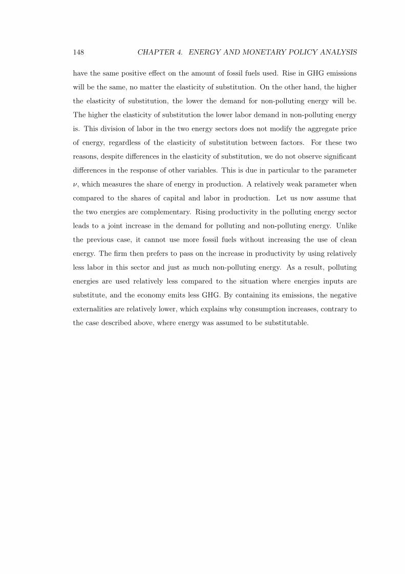
148 CHAPTER 4. ENERGY AND MONETARY POLICY ANALYSIS
have the same positive effect on the amount of fossil fuels used. Rise in GHG emissions
will be the same, no matter the elasticity of substitution. On the other hand, the higher
the elasticity of substitution, the lower the demand for non-polluting energy will be.
The higher the elasticity of substitution the lower labor demand in non-polluting energy
is. This division of labor in the two energy sectors does not modify the aggregate price
of energy, regardless of the elasticity of substitution between factors. For these two
reasons, despite differences in the elasticity of substitution, we do not observe significant
differences in the response of other variables. This is due in particular to the parameter
ν, which measures the share of energy in production. A relatively weak parameter when
compared to the shares of capital and labor in production. Let us now assume that
the two energies are complementary. Rising productivity in the polluting energy sector
leads to a joint increase in the demand for polluting and non-polluting energy. Unlike
the previous case, it cannot use more fossil fuels without increasing the use of clean
energy. The firm then prefers to pass on the increase in productivity by using relatively
less labor in this sector and just as much non-polluting energy. As a result, polluting
energies are used relatively less compared to the situation where energies inputs are
substitute, and the economy emits less GHG. By containing its emissions, the negative
externalities are relatively lower, which explains why consumption increases, contrary to
the case described above, where energy was assumed to be substitutable.

4.5. SIMULATIONS: 149
0 20 400
0.01
0.02
0.03
0.04
Outp
ut
0 20 40-0.02
0
0.02
0.04
Consu
mption
0 20 40
-0.04
-0.03
-0.02
-0.01
0
La
bor
supply
0 20 400
0.2
0.4
0.6
En
erg
y
0 20 400
0.2
0.4
0.6
Po
lluting e
ne
rgy
0 20 40-0.15
-0.1
-0.05
0
Non-P
ollu
ting e
nerg
y
0 20 40-2
-1.5
-1
-0.5
0
Lab
or
np
0 20 40-0.4
-0.3
-0.2
-0.1
0
Labo
r nnp
0 20 40-0.05
0
0.05
Labo
r n
0 20 400
0.01
0.02
0.03
0.04
capital sto
ck
0 20 40
-0.06
-0.04
-0.02
0
ut. r
ate
of cap.
0 20 400
0.05
0.1
0.15
0.2
inve
st.
Figure 4.10 – IRF to a productivity shock in the polluting sector in a carbon tax regime
(1/3) - black dotted line : ε = 0.51; red dashed line ε = 1.22; blue dashed line ε = 1.85
0 20 40
0
5
10
Outp
ut gro
wth
10-3
0 20 40-0.02
-0.01
0
0.01
Cons. gro
wth
0 20 40-0.2
0
0.2
0.4
Money g
row
th, ann %
0 20 40
-0.02
-0.01
0
0.01
Outp
ut gap
0 20 40-0.15
-0.1
-0.05
0
0.05
wage
0 20 40-0.15
-0.1
-0.05
0
marg
inal cost
0 20 40-0.6
-0.4
-0.2
0
trans. costs
0 20 40-0.03
-0.02
-0.01
0
0.01
Inflation, ann. %
0 20 40-0.015
-0.01
-0.005
0
Nom
inte
rest ra
te, ann %
0 20 40
-0.01
0
0.01
0.02
Real in
tere
st ra
te, ann %
0 20 40
-0.06
-0.04
-0.02
0
renta
l ra
te o
f cap
Figure 4.11 – IRF to a productivity shock in the polluting sector in a carbon tax regime
(2/3) - black dotted line : ε = 0.51; red dashed line ε = 1.22; blue dashed line ε = 1.85
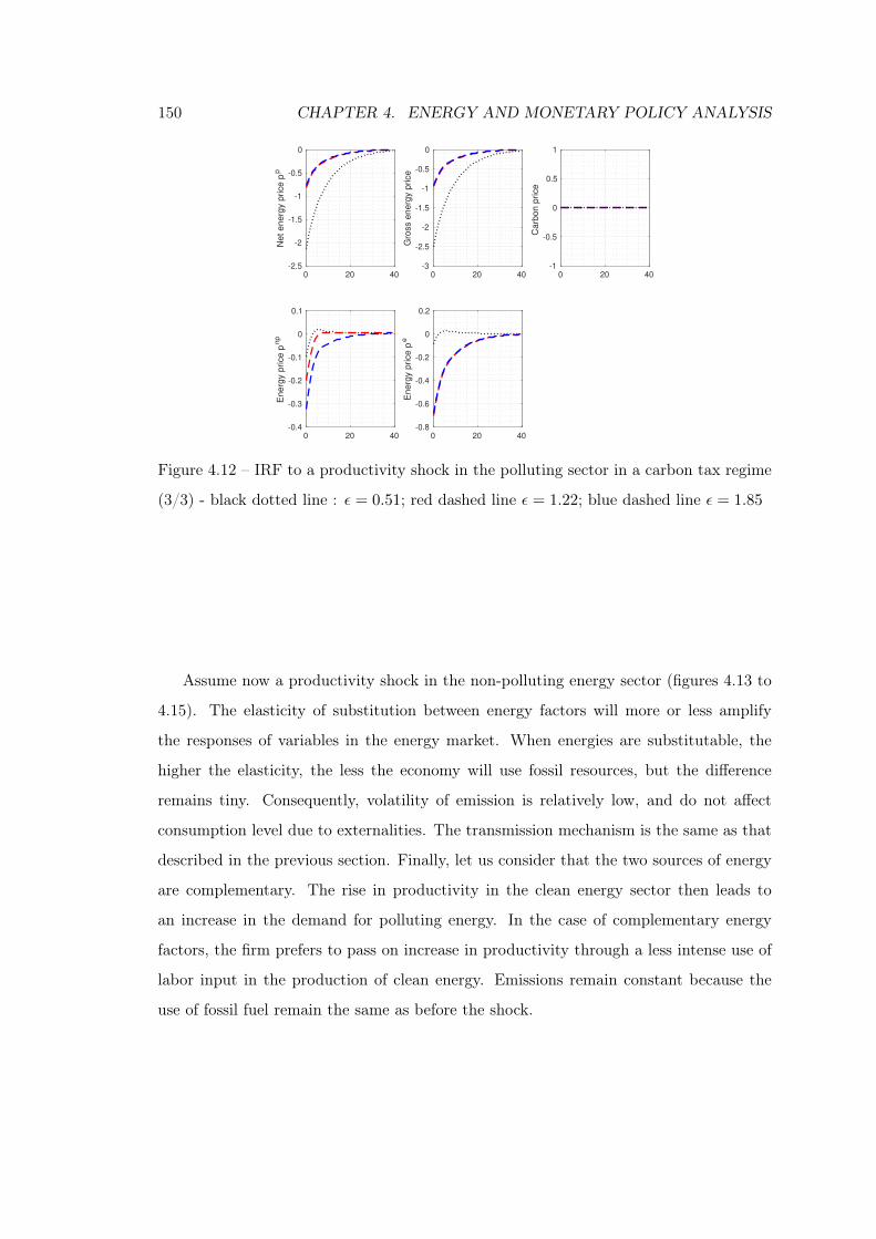
150 CHAPTER 4. ENERGY AND MONETARY POLICY ANALYSIS
0 20 40-2.5
-2
-1.5
-1
-0.5
0
Net e
nerg
y p
rice p
p0 20 40
-3
-2.5
-2
-1.5
-1
-0.5
0
Gro
ss e
ne
rgy p
rice
0 20 40-1
-0.5
0
0.5
1
Carb
on p
rice
0 20 40-0.4
-0.3
-0.2
-0.1
0
0.1
Energ
y p
rice
pn
p
0 20 40-0.8
-0.6
-0.4
-0.2
0
0.2
Energ
y p
rice
pe
Figure 4.12 – IRF to a productivity shock in the polluting sector in a carbon tax regime
(3/3) - black dotted line : ε = 0.51; red dashed line ε = 1.22; blue dashed line ε = 1.85
Assume now a productivity shock in the non-polluting energy sector (figures 4.13 to
4.15). The elasticity of substitution between energy factors will more or less amplify
the responses of variables in the energy market. When energies are substitutable, the
higher the elasticity, the less the economy will use fossil resources, but the difference
remains tiny. Consequently, volatility of emission is relatively low, and do not affect
consumption level due to externalities. The transmission mechanism is the same as that
described in the previous section. Finally, let us consider that the two sources of energy
are complementary. The rise in productivity in the clean energy sector then leads to
an increase in the demand for polluting energy. In the case of complementary energy
factors, the firm prefers to pass on increase in productivity through a less intense use of
labor input in the production of clean energy. Emissions remain constant because the
use of fossil fuel remain the same as before the shock.
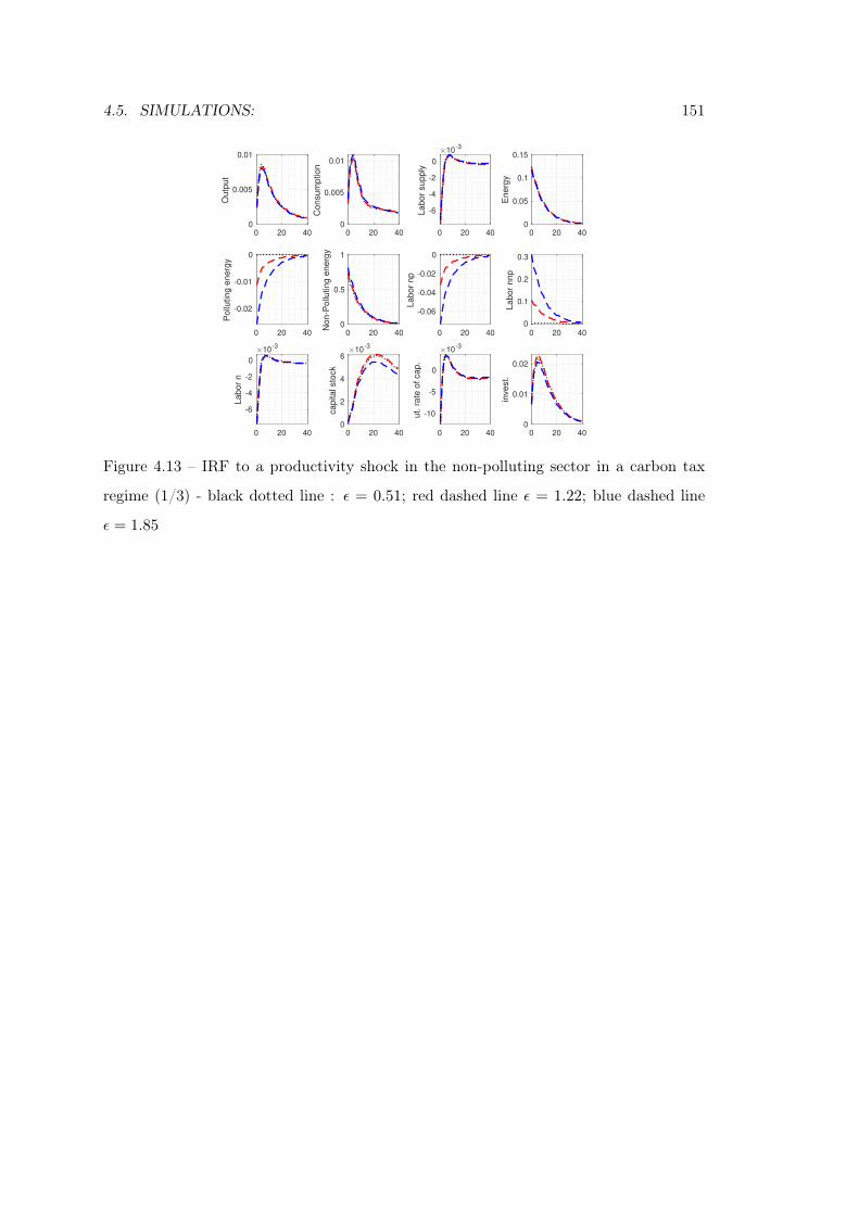
4.5. SIMULATIONS: 151
0 20 400
0.005
0.01
Outp
ut
0 20 400
0.005
0.01
Consum
ptio
n
0 20 40
-6
-4
-2
0
Labo
r sup
ply
10-3
0 20 400
0.05
0.1
0.15
Energ
y
0 20 40
-0.02
-0.01
0
Pollu
tin
g e
nerg
y
0 20 400
0.5
1
Non
-Pollu
ting
energ
y0 20 40
-0.06
-0.04
-0.02
0
La
bor
np
0 20 400
0.1
0.2
0.3
Labor
nnp
0 20 40
-6
-4
-2
0
La
bor
n
10-3
0 20 400
2
4
6
ca
pital sto
ck
10-3
0 20 40
-10
-5
0
ut. r
ate
of cap
.
10-3
0 20 400
0.01
0.02
invest.
Figure 4.13 – IRF to a productivity shock in the non-polluting sector in a carbon tax
regime (1/3) - black dotted line : ε = 0.51; red dashed line ε = 1.22; blue dashed line
ε = 1.85
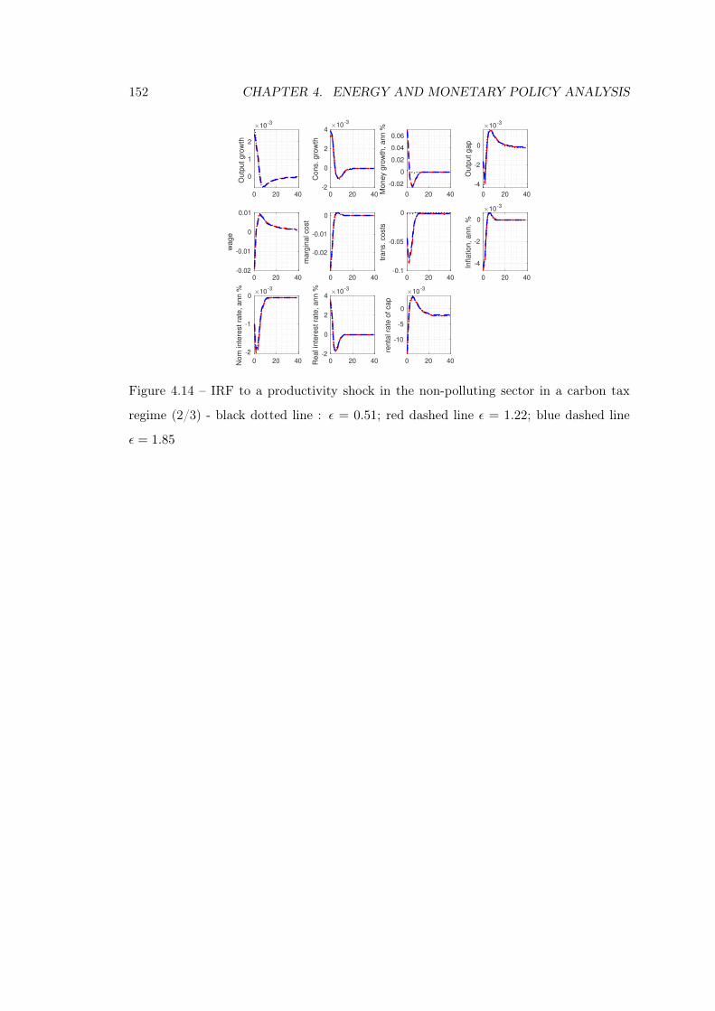
152 CHAPTER 4. ENERGY AND MONETARY POLICY ANALYSIS
0 20 40
0
1
2
Ou
tpu
t gro
wth
10-3
0 20 40-2
0
2
4
Cons.
gro
wth
10-3
0 20 40
-0.02
0
0.02
0.04
0.06
Mone
y g
row
th, a
nn %
0 20 40
-4
-2
0
Outp
ut
gap
10-3
0 20 40-0.02
-0.01
0
0.01
wage
0 20 40
-0.02
-0.01
0
marg
ina
l cost
0 20 40-0.1
-0.05
0
trans. costs
0 20 40
-4
-2
0
Infla
tion, a
nn. %
10-3
0 20 40
-2
-1
0
Nom
inte
rest ra
te, an
n % 10
-3
0 20 40-2
0
2
4
Rea
l in
tere
st
rate
, ann % 10
-3
0 20 40
-10
-5
0
renta
l ra
te o
f cap
10-3
Figure 4.14 – IRF to a productivity shock in the non-polluting sector in a carbon tax
regime (2/3) - black dotted line : ε = 0.51; red dashed line ε = 1.22; blue dashed line
ε = 1.85
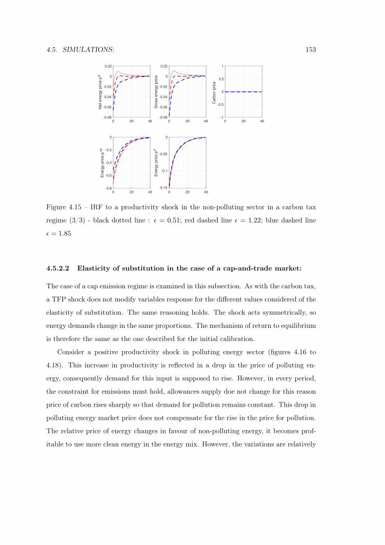
4.5. SIMULATIONS: 153
0 20 40-0.08
-0.06
-0.04
-0.02
0
0.02
Net e
nerg
y p
rice p
p
0 20 40-0.08
-0.06
-0.04
-0.02
0
0.02
Gro
ss e
ne
rgy p
rice
0 20 40-1
-0.5
0
0.5
1
Carb
on p
rice
0 20 40-0.8
-0.6
-0.4
-0.2
0
Energ
y p
rice
pn
p
0 20 40-0.15
-0.1
-0.05
0
Energ
y p
rice
pe
Figure 4.15 – IRF to a productivity shock in the non-polluting sector in a carbon tax
regime (3/3) - black dotted line : ε = 0.51; red dashed line ε = 1.22; blue dashed line
ε = 1.85
4.5.2.2 Elasticity of substitution in the case of a cap-and-trade market:
The case of a cap emission regime is examined in this subsection. As with the carbon tax,
a TFP shock does not modify variables response for the different values considered of the
elasticity of substitution. The same reasoning holds. The shock acts symmetrically, so
energy demands change in the same proportions. The mechanism of return to equilibrium
is therefore the same as the one described for the initial calibration.
Consider a positive productivity shock in polluting energy sector (figures 4.16 to
4.18). This increase in productivity is reflected in a drop in the price of polluting en-
ergy, consequently demand for this input is supposed to rise. However, in every period,
the constraint for emissions must hold, allowances supply doe not change for this reason
price of carbon rises sharply so that demand for pollution remains constant. This drop in
polluting energy market price does not compensate for the rise in the price for pollution.
The relative price of energy changes in favour of non-polluting energy, it becomes prof-
itable to use more clean energy in the energy mix. However, the variations are relatively
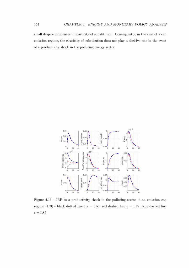
154 CHAPTER 4. ENERGY AND MONETARY POLICY ANALYSIS
small despite differences in elasticity of substitution. Consequently, in the case of a cap
emission regime, the elasticity of substitution does not play a decisive role in the event
of a productivity shock in the polluting energy sector
0 20 400
0.01
0.02
0.03
Outp
ut
0 20 40
0.01
0.02
0.03
Consum
ption
0 20 40-0.04
-0.02
0
Labor
supply
0 20 400
1
2
Energ
y
10-3
0 20 40
-5
0
5
10
Pollu
ting e
nerg
y
10-17
0 20 400
5
10
Non-P
ollu
ting e
nerg
y 10-3
0 20 40-2
-1
0
Labor
np
0 20 400
0.02
0.04
Labor
nnp
0 20 400
0.02
0.04
Labor
n
0 20 400
0.01
0.02
capital sto
ck
0 20 40-0.04
-0.02
0
0.02
ut. r
ate
of cap.
0 20 400
0.02
0.04
0.06
invest.
Figure 4.16 – IRF to a productivity shock in the polluting sector in an emission cap
regime (1/3) - black dotted line : ε = 0.51; red dashed line ε = 1.22; blue dashed line
ε = 1.85
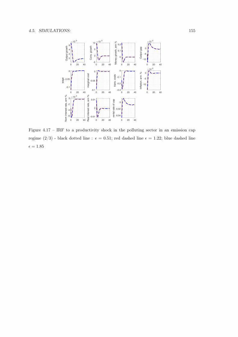
4.5. SIMULATIONS: 155
0 20 40
0
2
4
6
Outp
ut g
row
th
10-3
0 20 40-5
0
5
10
Co
ns. g
row
th
10-3
0 20 40
0
0.1
0.2
Mon
ey g
row
th,
ann %
0 20 40
-10
-5
0
Outp
ut
gap
10-3
0 20 40
-0.1
-0.05
0
wage
0 20 40-0.1
-0.05
0
marg
inal cost
0 20 40-0.3
-0.2
-0.1
0
trans.
costs
0 20 40
-10
-5
0
Inflation, a
nn. %
10-3
0 20 40
-6
-4
-2
0
Nom
inte
rest ra
te, ann
% 10-3
0 20 40
-0.01
0
0.01
Rea
l in
tere
st
rate
, ann %
0 20 40
-0.04
-0.02
0
renta
l ra
te o
f cap
Figure 4.17 – IRF to a productivity shock in the polluting sector in an emission cap
regime (2/3) - black dotted line : ε = 0.51; red dashed line ε = 1.22; blue dashed line
ε = 1.85
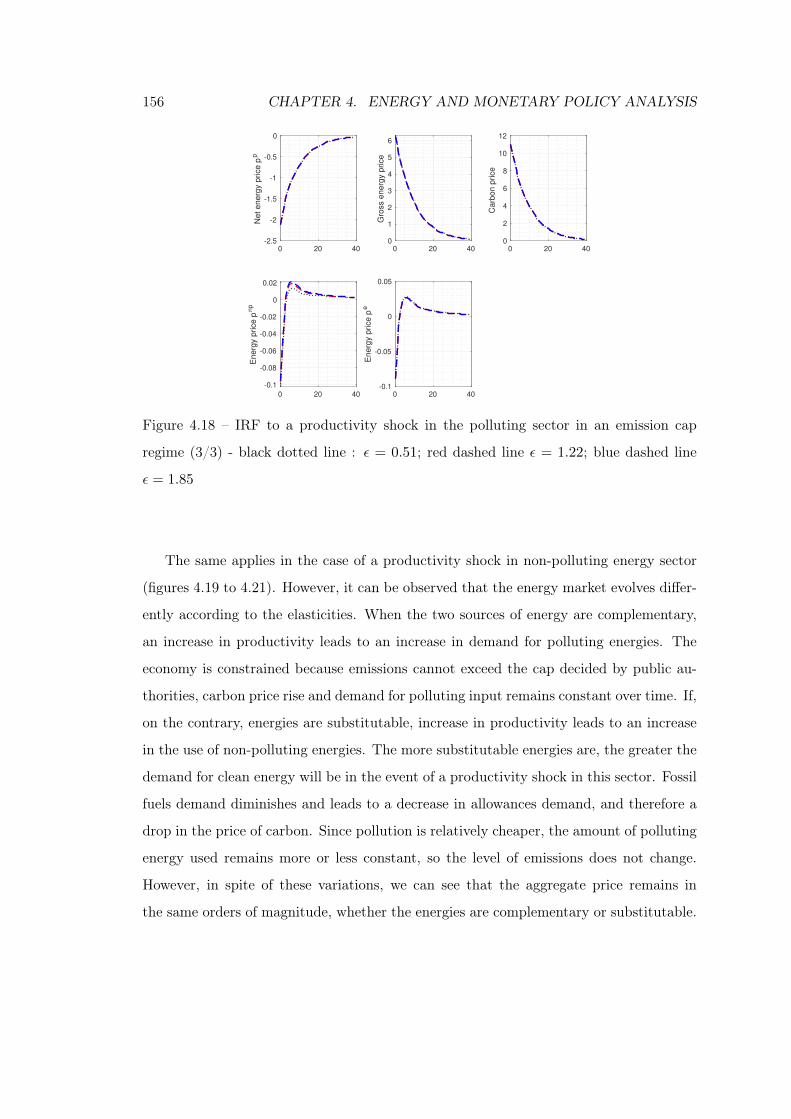
156 CHAPTER 4. ENERGY AND MONETARY POLICY ANALYSIS
0 20 40-2.5
-2
-1.5
-1
-0.5
0
Net e
nerg
y p
rice p
p0 20 40
0
1
2
3
4
5
6
Gro
ss e
ne
rgy p
rice
0 20 400
2
4
6
8
10
12
Carb
on p
rice
0 20 40
-0.1
-0.08
-0.06
-0.04
-0.02
0
0.02
Energ
y p
rice
pn
p
0 20 40-0.1
-0.05
0
0.05
Energ
y p
rice
pe
Figure 4.18 – IRF to a productivity shock in the polluting sector in an emission cap
regime (3/3) - black dotted line : ε = 0.51; red dashed line ε = 1.22; blue dashed line
ε = 1.85
The same applies in the case of a productivity shock in non-polluting energy sector
(figures 4.19 to 4.21). However, it can be observed that the energy market evolves differ-
ently according to the elasticities. When the two sources of energy are complementary,
an increase in productivity leads to an increase in demand for polluting energies. The
economy is constrained because emissions cannot exceed the cap decided by public au-
thorities, carbon price rise and demand for polluting input remains constant over time. If,
on the contrary, energies are substitutable, increase in productivity leads to an increase
in the use of non-polluting energies. The more substitutable energies are, the greater the
demand for clean energy will be in the event of a productivity shock in this sector. Fossil
fuels demand diminishes and leads to a decrease in allowances demand, and therefore a
drop in the price of carbon. Since pollution is relatively cheaper, the amount of polluting
energy used remains more or less constant, so the level of emissions does not change.
However, in spite of these variations, we can see that the aggregate price remains in
the same orders of magnitude, whether the energies are complementary or substitutable.
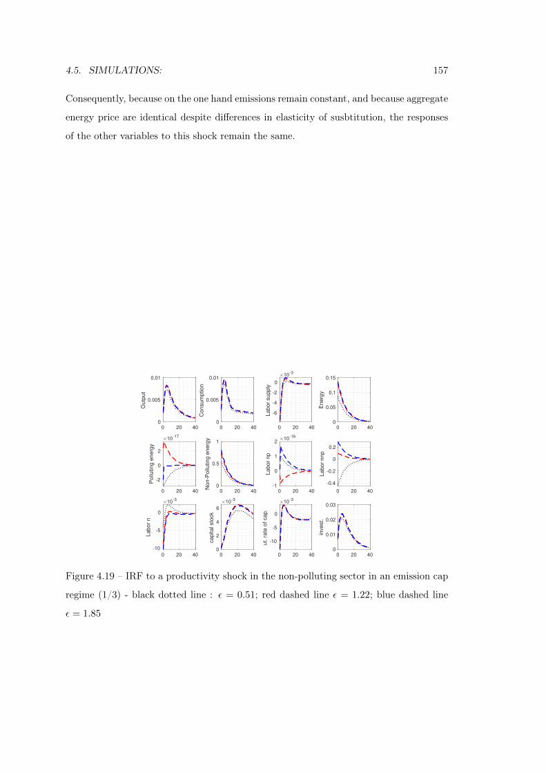
4.5. SIMULATIONS: 157
Consequently, because on the one hand emissions remain constant, and because aggregate
energy price are identical despite differences in elasticity of susbtitution, the responses
of the other variables to this shock remain the same.
0 20 400
0.005
0.01
Outp
ut
0 20 400
0.005
0.01
Consum
ption
0 20 40
-6
-4
-2
0
Labor
supply
10-3
0 20 400
0.05
0.1
0.15
Energ
y
0 20 40
-2
0
2
Pollu
ting e
nerg
y
10-17
0 20 400
0.5
1
Non-P
ollu
ting e
nerg
y
0 20 40-1
0
1
2
Labor
np
10-16
0 20 40
-0.4
-0.2
0
0.2
Labor
nnp
0 20 40
-10
-5
0
Labor
n
10-3
0 20 400
2
4
6
capital sto
ck
10-3
0 20 40
-10
-5
0
ut. r
ate
of cap.
10-3
0 20 400
0.01
0.02
0.03
invest.
Figure 4.19 – IRF to a productivity shock in the non-polluting sector in an emission cap
regime (1/3) - black dotted line : ε = 0.51; red dashed line ε = 1.22; blue dashed line
ε = 1.85
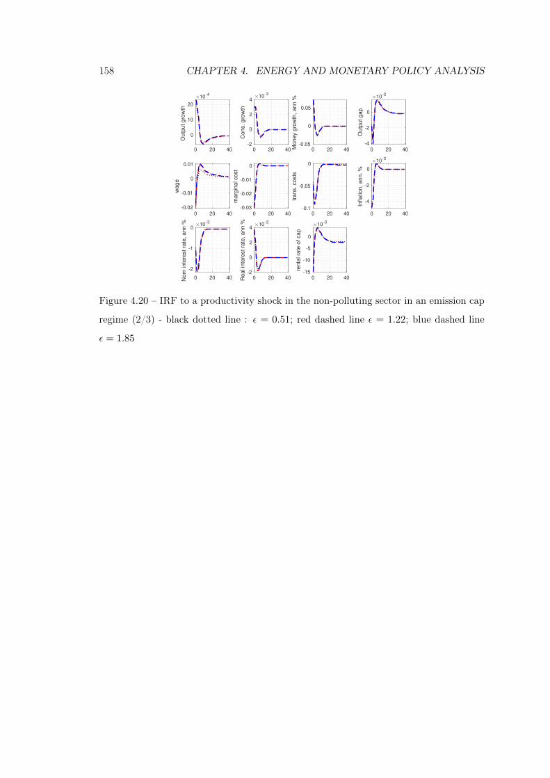
158 CHAPTER 4. ENERGY AND MONETARY POLICY ANALYSIS
0 20 40
0
10
20
Ou
tpu
t gro
wth
10-4
0 20 40-2
0
2
4
Cons.
gro
wth
10-3
0 20 40-0.05
0
0.05
Mone
y g
row
th, a
nn %
0 20 40-4
-2
0
Outp
ut
gap
10-3
0 20 40
-0.02
-0.01
0
0.01
wage
0 20 40-0.03
-0.02
-0.01
0
marg
ina
l cost
0 20 40-0.1
-0.05
0
trans. costs
0 20 40
-4
-2
0
Infla
tion, a
nn. %
10-3
0 20 40
-2
-1
0
Nom
inte
rest ra
te, an
n % 10
-3
0 20 40-2
0
2
4
Rea
l in
tere
st
rate
, ann % 10
-3
0 20 40-15
-10
-5
0
renta
l ra
te o
f cap
10-3
Figure 4.20 – IRF to a productivity shock in the non-polluting sector in an emission cap
regime (2/3) - black dotted line : ε = 0.51; red dashed line ε = 1.22; blue dashed line
ε = 1.85

4.6. MONETARY POLICY ANALYSIS 159
0 20 40
-0.02
-0.015
-0.01
-0.005
0
0.005
0.01
Net e
nerg
y p
rice p
p
0 20 40-0.4
-0.2
0
0.2
0.4
Gro
ss e
ne
rgy p
rice
0 20 40-0.5
0
0.5
Carb
on p
rice
0 20 40-1.2
-1
-0.8
-0.6
-0.4
-0.2
0
Energ
y p
rice
pn
p
0 20 40-0.2
-0.15
-0.1
-0.05
0
Energ
y p
rice
pe
Figure 4.21 – IRF to a productivity shock in the non-polluting sector in an emission cap
regime (3/3) - black dotted line : ε = 0.51; red dashed line ε = 1.22; blue dashed line
ε = 1.85
4.6 Monetary policy analysis
In this section, we assume that the central bank behaves as a social planner that seeks
to maximise household’s utility subject to the set of equation that characterizes the
competitive equilibrium of the economy. As described in the technical appendix, the
quadratic approximation to the instantaneous household utility function is
U(ct, Gt)− V (nst )∼= (1− d(G))
1− σ c1−σ − ψ
1 + γ− (1− d(G)) (σ − 1) c1−σ
2 (1− χ)2 (ct − χct−1)2
+ (1− d(G)) c1−σ (ct − χct−1)
1− χ − c1−σ
1− σG(d1
(Gt +
G2t
2
)+ 2d2GGt
)
− (d1 + 2d2G)
1− χ c1−σ (ct − χct−1)GGt − ψnst −ψ(1 + γ)
2(nst )
2
160 CHAPTER 4. ENERGY AND MONETARY POLICY ANALYSIS
The unconditional expectation of the second-order approximation to U(U(ct, Gt)−V (nst )
is
E [U(ct, Gt)− V (nst )] =(1− d(G))
1− σ c1−σ − ψ
1 + γ− (1− d(G)) (σ − 1)
2var(ˆc)
− ψ(1 + γ)
2var (ns)− c1−σG
1− σd1
2var(G)− (d1 + 2d2G)c1−σG cov
(ˆc, G
)
We can define W1, W2, W3, W4 and W5 to rewrite the last expression into a more
compact form:
W1 ≡(1− d(G))
1− σ c1−σ − ψ
1 + γ
W2 ≡ −(1− d(G)) (σ − 1)
2var(ˆc)
W3 ≡ −ψ(1 + γ)
2var (ns)
W4 ≡ −c1−σG1− σ
d1
2var(G)
W5 ≡ −(d1 + 2d2G)c1−σG cov(
ˆc, G)
so that:
E [U(ct, Gt)− V (nst )] = W1 + W2 + W3 + W4 + W5
4.6.1 Optimized instrument rules
Household’s welfare loss depends on consumption, labor supply, and greenhouse gas emis-
sions variances, but also on the covariance between gas emissions and consumption. It is
the consequence of variables deviations from their steady state, due to various exogenous
shocks considered in our model. The central bank strategy is to choose coefficients val-
ues µπ and µy, that minimizes the household’s welfare loss for fixed values of smoothing
coefficients µR = 0.85. The optimized coefficients depend upon specific calibrations. The
larger the value of µπ, the more aggressively the central bank reacts to inflation (and vice
versa). Similarly, the greater the value of µy, the more the central bank is concerned with
stabilizing the output gap. To find the combination that maximizes household welfare,
4.6. MONETARY POLICY ANALYSIS 161
we proceed in two steps. First, we replicate the model for different configurations of the
coefficients on the monetary policy instrument. Thus, we assume that µπ(i), can take
its values between 1.1 and 4.5, and we increase its initial value by 0.01 at each iteration.
Similarly, the second coefficient µy(j) is assumed to take its values in the interval [0, 1],
and is iterated in steps of 0.01. Consequently, we replicate 34,000 times the model. Then,
defining by W the household welfare, we are looking for the combination of µπ(i)?, and
µy(j)?, that maximizes W. More formally it can be expressed as follows:
argmaxµ?π ,µ?y W(Gt, n
st , ˆct, µπ, µy
)
4.6.1.1 Optimal monetary policy in the carbon tax case:
For different calibration, including the optimal value for monetary policy instrument
considered, table 4.2 shows standard deviations of fluctuations of habit-adjusted con-
sumption, employment, gas emissions, nominal interest rate and nominal money growth
as well as the contribution to household welfare. Table 4.2 reports also results for the
benchmark Taylor rule, when µπ = 1.5, µy = 0.125, and µR = 0.85.
The values that maximize consumer welfare are µ?π = 3.44 and µ?y = 0.08, which are
different from the standard values in every respect. Compared to the initial calibration
for the Taylor rule, according to the optimal values obtained that maximize household’s
welfare, the central bank must be more aggressive against inflation and less sensitive
to output gap. Figure 4.22 shows welfare as a function of the two coefficients of the
Taylor rule. Welfare is an inverted U-shape function of µy, and reaches its maximum
in µ?y < 0.125. In other words, the central bank must give less consideration to output
gap when authorities introduce a carbon tax. The existence of this output gap is the
consequence of a lack of competition and to the markup. Although this is a sub-optimal
situation that central bank must normally avoid, when it acts to reduce the gap between
optimal output and real production, the flow of emissions will vary depending on the more
or less accommodative monetary policy implemented. Indeed, the carbon tax is constant
over time. In the presence of nominal rigidities, when a productivity shock occurs, firm
uses fewer factors of production to produce as much. By fighting this production gap,
162 CHAPTER 4. ENERGY AND MONETARY POLICY ANALYSIS
monetary policy will generate an increase in the use of fossil fuels and in GHG emissions.
Consequently, since emissions generate disutility, central bank, by fighting output gap,
also generates a loss of well-being for the household. In the same way, well-being is an
increasing function of µπ < µ?π and decreasing beyond this threshold. On the contrary,
by placing greater emphasis on inflation control, the central bank will allow market
imperfections to substitute. Indeed, by stabilising prices during a productivity shock, the
central bank will not encourage companies to change their behaviour, so that this will
limit the flow of emissions and, at the same time, the negative externalities of greenhouse
gases. Thus, with such a monetary policy, in a carbon tax regime, it is desirable for the
central bank to focus on price stability and not on the lack of competition.
Figure 4.23 shows the standard deviation for each of the variables on which household
well-being depends, as a function of the parameters used for the monetary policy instru-
ment. The standard deviation of consumption increases with µπ and µy, for µπ > 1.3.
Beyond this threshold (µπ > 1.3), when µπ increases, the central bank attaches relatively
more importance to inflation. All other things being equal, beyond this threshold, the
more µy increases, the more the central bank will take the output gap into account.
However, nominal interest rate volatility will increase if central bank is more reactive to
these variations. Consequently, money supply and consumption transaction costs will
vary relatively more.Indeed, household observes a greater volatility of the nominal inter-
est. It thus makes more trade-offs between consumption and savings. Thus, the higher
µπ is, the more the household will adapt its consumption or savings levels.
Standard deviation of emissions depends positively on µy. By tackling output gap
more aggressively, the central bank will increase output volatility, and thus GHG emis-
sions in order to be closer to the level of production in perfect competition. The standard
deviation of emissions decreases with µπ < µ′π, and increases with µπ > µ′π, however its
variation remains weak. For low values of µπ, the central bank has little control over
inflation. The standard deviation of emissions is relatively high because they depend
on consumption, which in turn depends on prices. If prices are subject to variations,
emissions will tend to have a relatively high variance.Then this volatility will decrease as
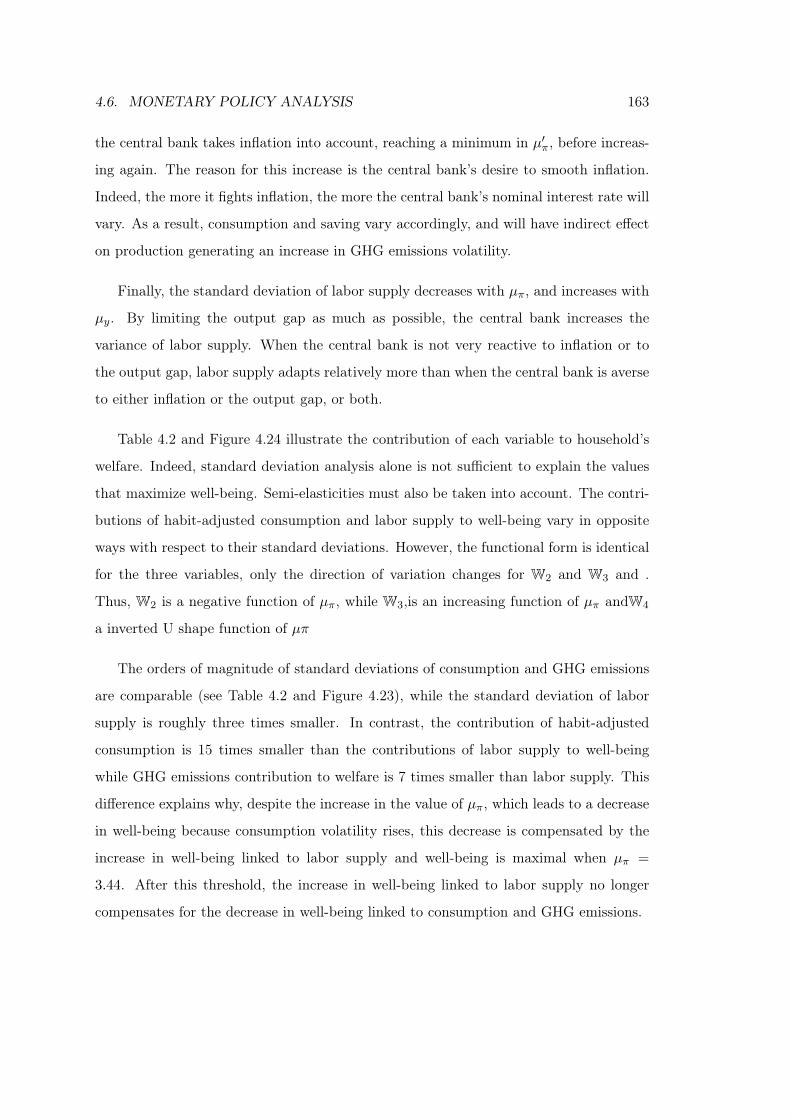
4.6. MONETARY POLICY ANALYSIS 163
the central bank takes inflation into account, reaching a minimum in µ′π, before increas-
ing again. The reason for this increase is the central bank’s desire to smooth inflation.
Indeed, the more it fights inflation, the more the central bank’s nominal interest rate will
vary. As a result, consumption and saving vary accordingly, and will have indirect effect
on production generating an increase in GHG emissions volatility.
Finally, the standard deviation of labor supply decreases with µπ, and increases with
µy. By limiting the output gap as much as possible, the central bank increases the
variance of labor supply. When the central bank is not very reactive to inflation or to
the output gap, labor supply adapts relatively more than when the central bank is averse
to either inflation or the output gap, or both.
Table 4.2 and Figure 4.24 illustrate the contribution of each variable to household’s
welfare. Indeed, standard deviation analysis alone is not sufficient to explain the values
that maximize well-being. Semi-elasticities must also be taken into account. The contri-
butions of habit-adjusted consumption and labor supply to well-being vary in opposite
ways with respect to their standard deviations. However, the functional form is identical
for the three variables, only the direction of variation changes for W2 and W3 and .
Thus, W2 is a negative function of µπ, while W3,is an increasing function of µπ andW4
a inverted U shape function of µπ
The orders of magnitude of standard deviations of consumption and GHG emissions
are comparable (see Table 4.2 and Figure 4.23), while the standard deviation of labor
supply is roughly three times smaller. In contrast, the contribution of habit-adjusted
consumption is 15 times smaller than the contributions of labor supply to well-being
while GHG emissions contribution to welfare is 7 times smaller than labor supply. This
difference explains why, despite the increase in the value of µπ, which leads to a decrease
in well-being because consumption volatility rises, this decrease is compensated by the
increase in well-being linked to labor supply and well-being is maximal when µπ =
3.44. After this threshold, the increase in well-being linked to labor supply no longer
compensates for the decrease in well-being linked to consumption and GHG emissions.
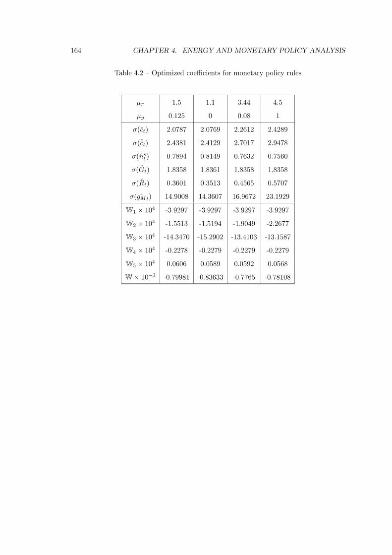
164 CHAPTER 4. ENERGY AND MONETARY POLICY ANALYSIS
Table 4.2 – Optimized coefficients for monetary policy rules
µπ 1.5 1.1 3.44 4.5
µy 0.125 0 0.08 1
σ(ct) 2.0787 2.0769 2.2612 2.4289
σ(ˆct) 2.4381 2.4129 2.7017 2.9478
σ(nst ) 0.7894 0.8149 0.7632 0.7560
σ(Gt) 1.8358 1.8361 1.8358 1.8358
σ(Rt) 0.3601 0.3513 0.4565 0.5707
σ( ˆgMt) 14.9008 14.3607 16.9672 23.1929
W1 × 104 -3.9297 -3.9297 -3.9297 -3.9297
W2 × 104 -1.5513 -1.5194 -1.9049 -2.2677
W3 × 104 -14.3470 -15.2902 -13.4103 -13.1587
W4 × 104 -0.2278 -0.2279 -0.2279 -0.2279
W5 × 104 0.0606 0.0589 0.0592 0.0568
W× 10−3 -0.79981 -0.83633 -0.7765 -0.78108
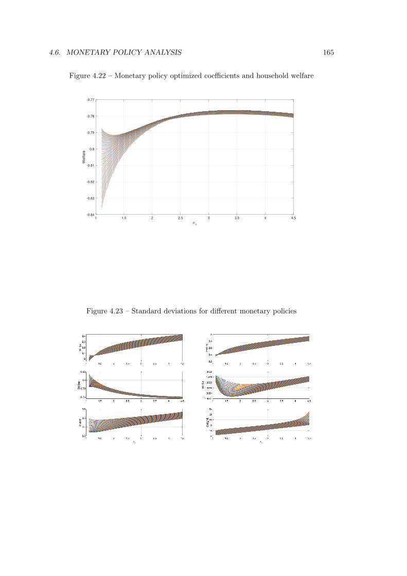
4.6. MONETARY POLICY ANALYSIS 165
Figure 4.22 – Monetary policy optimized coefficients and household welfare
1 1.5 2 2.5 3 3.5 4 4.5
-0.84
-0.83
-0.82
-0.81
-0.8
-0.79
-0.78
-0.77
We
lfare
Figure 4.23 – Standard deviations for different monetary policies

166 CHAPTER 4. ENERGY AND MONETARY POLICY ANALYSIS
Figure 4.24 – Contributions of variables to household’s welfare
4.6.1.2 Optimal monetary policy in a cap-an-trade market:
We simulate the model 34,000 times in the same way, but this time replacing the carbon
tax with an emissions cap. Table 4.3 summarizes the results of these simulations, includ-
ing the values for each of the bounds considered (lower and upper bounds), as well as
the results for the standard calibration of the Taylor rule, and finally the results for the
optimized values of the monetary policy coefficients. Figure 4.25 illustrates the relation-
ship between household welfare as a function of the monetary policy coefficients, Figure
4.26 details the standard deviations for the different variables of interest, and Figure 4.27
shows the contribution of W2 to W5 to household’s welfare.
First, it can be noted that when coefficients of the monetary policy instrument are
optimized, household welfare in the case of an emissions cap is higher than in the case of
a carbon tax. We also find that the values µ?π and µ?y that maximize household welfare
are higher than those optimized in the presence of a carbon tax, but also higher than the
usual values of the Taylor rule. Thus, in this case, the central bank is more responsive
to both the output gap and inflation. When the government sets the emissions cap and
distributes allowances, price of pollution adjusts according to demand in order to ensure
4.6. MONETARY POLICY ANALYSIS 167
a balance between supply and demand for pollution. Thus, by setting up an allowance
market, standard deviation of emissions is zero (see table 4.3 figure 4.26 and 4.27). On
the other hand, as the price of allowances adapts to the economic cycle and to various
shocks, standard deviation of price of pollution increases (whereas it was zero in the case
of the carbon tax). This significant difference in the effects of the two environmental
policy instruments explains why such differences in the optimized coefficients of monetary
policy are observed.
Indeed, in the case of the carbon tax, the weight that the central bank gives to
the output gap when setting its nominal interest rate is close to zero (µ?y = 0.08). On
the other hand, it will give much greater importance to the output gap when setting an
emissions cap (µ?y = 0.29). With a carbon tax, as the price of pollution remains constant.
The higher the value of µy, the more the central bank is concerned by the output gap. It
fights the lack of competitiveness at the source of this gap between optimal production
and real production, by adapting its nominal interest rate and generates variations in
the use of production factors, and in particular in demand for polluting energy. This
variation in demand for fossil energy increases household disutility and promotes a loss
of welfare. On the contrary, a cap-and-trade market will prevent an increase in the use of
these energies. Demand for polluting energy will then remain constant and at the same
time limit the negative consequences of GHG emissions. From then on, the central bank
can take the output gap into account and use its instrument to compensate for the lack
of competition by a more aggressive monetary policy.
By varying the price of pollution, with an emissions market, aggregate cost of energy
is modified according to variation in demand for allowances. At the same time, this leads
to variation in intermediate costs and affects the price level. This environmental policy
instrument generates a greater source of price variability. Here again, central bank needs
to be more reactive regarding inflation, in comparison with the carbon tax.
Except for the standard deviation for emissions, which in this case is zero (see Table
4.3 and Figures 4.26 and 4.27), other variables reactions is identical to that obtained
with the carbon tax. The same analysis is therefore applied in case of an emission
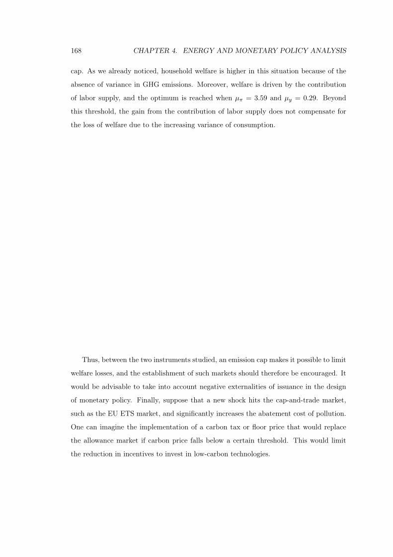
168 CHAPTER 4. ENERGY AND MONETARY POLICY ANALYSIS
cap. As we already noticed, household welfare is higher in this situation because of the
absence of variance in GHG emissions. Moreover, welfare is driven by the contribution
of labor supply, and the optimum is reached when µπ = 3.59 and µy = 0.29. Beyond
this threshold, the gain from the contribution of labor supply does not compensate for
the loss of welfare due to the increasing variance of consumption.
Thus, between the two instruments studied, an emission cap makes it possible to limit
welfare losses, and the establishment of such markets should therefore be encouraged. It
would be advisable to take into account negative externalities of issuance in the design
of monetary policy. Finally, suppose that a new shock hits the cap-and-trade market,
such as the EU ETS market, and significantly increases the abatement cost of pollution.
One can imagine the implementation of a carbon tax or floor price that would replace
the allowance market if carbon price falls below a certain threshold. This would limit
the reduction in incentives to invest in low-carbon technologies.
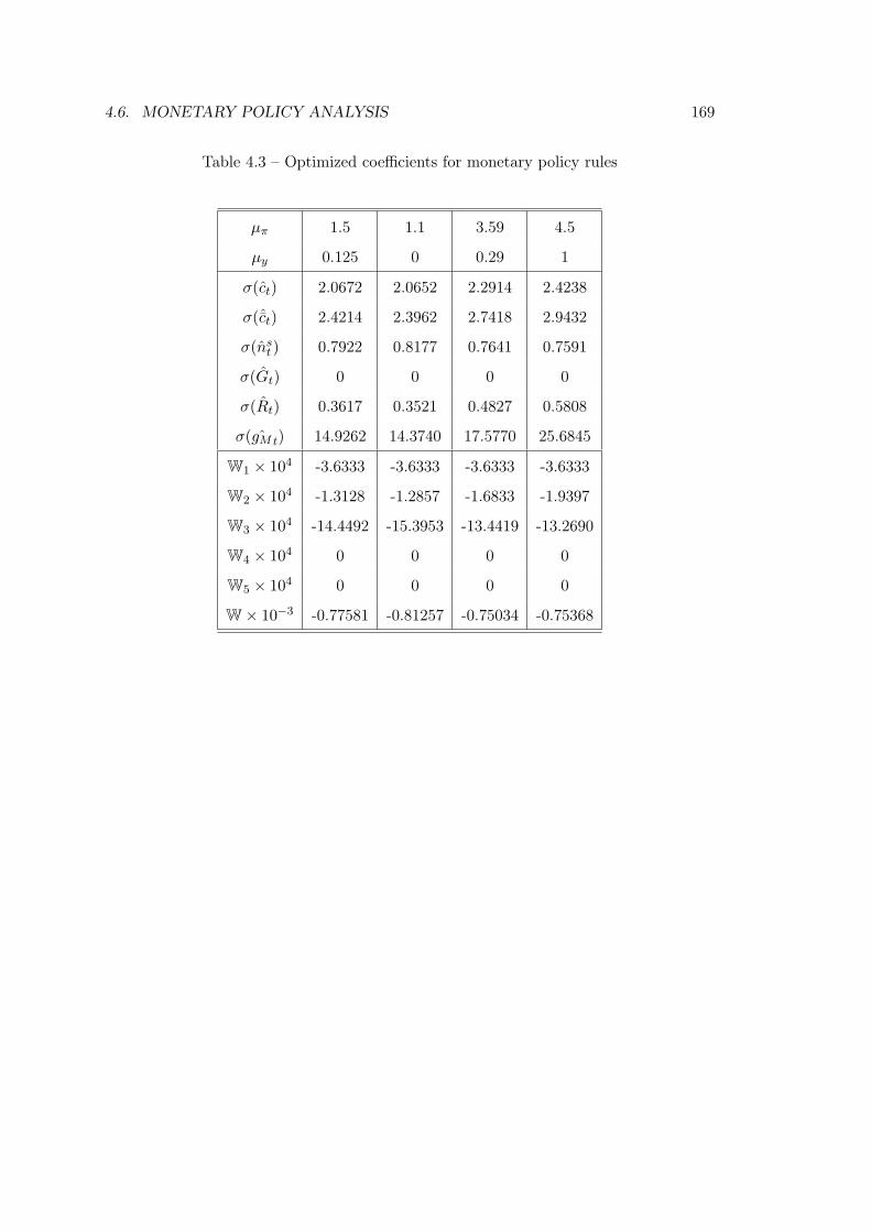
4.6. MONETARY POLICY ANALYSIS 169
Table 4.3 – Optimized coefficients for monetary policy rules
µπ 1.5 1.1 3.59 4.5
µy 0.125 0 0.29 1
σ(ct) 2.0672 2.0652 2.2914 2.4238
σ(ˆct) 2.4214 2.3962 2.7418 2.9432
σ(nst ) 0.7922 0.8177 0.7641 0.7591
σ(Gt) 0 0 0 0
σ(Rt) 0.3617 0.3521 0.4827 0.5808
σ( ˆgMt) 14.9262 14.3740 17.5770 25.6845
W1 × 104 -3.6333 -3.6333 -3.6333 -3.6333
W2 × 104 -1.3128 -1.2857 -1.6833 -1.9397
W3 × 104 -14.4492 -15.3953 -13.4419 -13.2690
W4 × 104 0 0 0 0
W5 × 104 0 0 0 0
W× 10−3 -0.77581 -0.81257 -0.75034 -0.75368
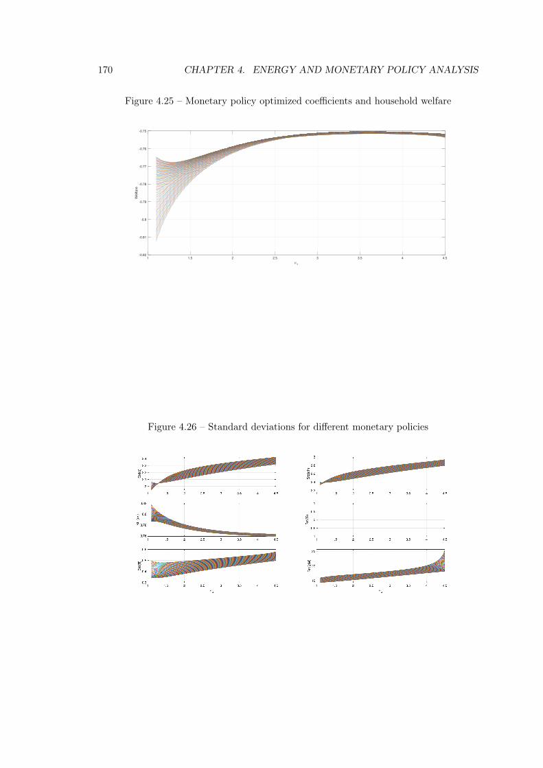
170 CHAPTER 4. ENERGY AND MONETARY POLICY ANALYSIS
Figure 4.25 – Monetary policy optimized coefficients and household welfare
1 1.5 2 2.5 3 3.5 4 4.5
-0.82
-0.81
-0.8
-0.79
-0.78
-0.77
-0.76
-0.75
Welfare
Figure 4.26 – Standard deviations for different monetary policies
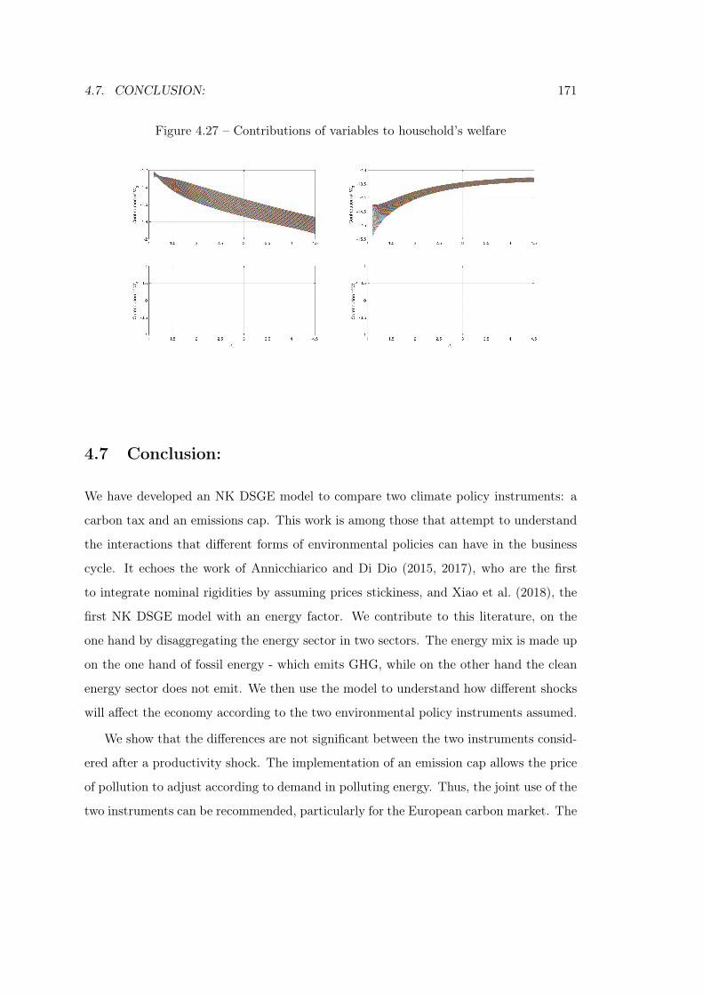
4.7. CONCLUSION: 171
Figure 4.27 – Contributions of variables to household’s welfare
4.7 Conclusion:
We have developed an NK DSGE model to compare two climate policy instruments: a
carbon tax and an emissions cap. This work is among those that attempt to understand
the interactions that different forms of environmental policies can have in the business
cycle. It echoes the work of Annicchiarico and Di Dio (2015, 2017), who are the first
to integrate nominal rigidities by assuming prices stickiness, and Xiao et al. (2018), the
first NK DSGE model with an energy factor. We contribute to this literature, on the
one hand by disaggregating the energy sector in two sectors. The energy mix is made up
on the one hand of fossil energy - which emits GHG, while on the other hand the clean
energy sector does not emit. We then use the model to understand how different shocks
will affect the economy according to the two environmental policy instruments assumed.
We show that the differences are not significant between the two instruments consid-
ered after a productivity shock. The implementation of an emission cap allows the price
of pollution to adjust according to demand in polluting energy. Thus, the joint use of the
two instruments can be recommended, particularly for the European carbon market. The
172 CHAPTER 4. ENERGY AND MONETARY POLICY ANALYSIS
establishment of a floor price for pollution below which pollution allowances could not
be traded would avoid the situation encountered after the economic and financial crisis
of 2008. On the other hand, in the event of a productivity shock in the polluting energy
sector - such as new extracting method for non-convential fossil fuels, the emission cap
is preferable to the carbon tax, as it allows the price adjustment mechanism to reduce
emissions. We obtain the same results for different values of the elasticity of substitution
between energy factors. On the contrary, in the case of a carbon tax, when a productivity
shock in the fossil fuel sector occurs, increase in emissions is linked to a more intensive
use of this factor and therefore more negative externalities, due to a constant pollution
price. In this case, the elasticity of substitution can more or less amplify this result. The
increase in emissions will be all the more important as the factors are substitutable. In
the case of a productivity shock in the renewable energy sector, the use of a tax or an
emission cap does not change the response of the variables, either in their direction of
variation or in the amplitude of the responses. Following such a shock, the elasticity of
substitution will play a role in the level of emissions in presence of a carbon tax. Rise
in productivity in this sector will result in a relatively greater drop of GHG emissions
the higher the elasticity of substitution. While the variables of the energy market will
be affected by changes in energy demand, responses of the other variables in the model
are essentially the same. In the case of an emissions cap, the model responds in exactly
the same way, no matter the elasticity of substitution considered. This can be explained
by the variation in the carbon price that will adapt to pollution demand.
Finally, we seek to optimize the Taylor rule in order to make a recommendation
for the monetary policy. Negative externalities related to the use of polluting energies
will modify household behaviour. Using the initial values of the Taylor rule parameters,
welfare losses are not optimized. Indeed, by fighting inflation or the output gap, the
central bank influences the flow of emissions. Depending on the central bank’s aversion
to the output gap or to inflation, GHG emissions will vary more or less, which will affect
the household’s utility. We show that, in the presence of an emissions cap, although the
volatility of emissions is reduced by the nature of the instrument, central bank must be
4.7. CONCLUSION: 173
more aggressive towards inflation and output gap. Similarly, if the public authorities
introduce a carbon tax, the use of this instrument will generate more or less volatility
in emissions, as the price of pollution remains constant. In this case, the coefficients
that make it possible to minimise welfare losses are even higher than in the case of an
emissions cap.
This work contributes to expand the literature on business cycle and climate policies.
Like all research work, it has its own limitations. On the one hand, we considered that
only work was needed to produce polluting or non-polluting energy. It can be assumed
that by integrating physical capital, the results obtained may thus differ. Adaptation
to shocks may thus be more or less long. Furthermore, it can be assumed that negative
externalities do not affect the demand for goods but rather labor supply. Another exten-
sion would be to incorporate another source of rigidities such as wage stickiness. Finally,
the monetary policy analysis should take account of the current situation of very low
nominal interest rates, and consequently analyse the special situation of the zero lower
bound.

174 CHAPTER 4. ENERGY AND MONETARY POLICY ANALYSIS
Chapter 5
General conclusion:
In this thesis, we analyzed the consequences of climate change and the different envi-
ronmental policy instruments from a number of different perspectives. First, we looked
at the reversibility of climate change. The model developed by Grossman and Krueger
(1995) suggests that environmental degradation is a necessary evil that we have to go
through. Applied to the climate, this means that we must observe a rise in the global av-
erage temperature before returning to an equilibrium where temperatures will be lower,
and this without public intervention. To study this question of reversibility, we have
assumed, in accordance with the theory, that an exogenous process would make it pos-
sible to reduce GHG emissions over time. We applied this assumption in a RBC model
with a climate module capable of reproducing the dynamics of the atmosphere and the
damage caused by climate change. We have thus shown that climate change is not re-
versible in the long term. Therefore, in order to achieve the objectives defined by the
IPCC and included in the Paris agreement, climate policy instruments must be used to
internalise the negative consequences of GHG emissions and also to reduce our emissions
in the short term, which is a necessary condition for combating climate change in the
long term. Indeed, beyond the uncertainty as to the discovery of a process capable of
reducing GHG emissions, once they are released into the atmosphere or the oceans, the
emissions persist and have a lasting effect on the climate. Thus, in the absence of rapid
intervention, it would become impossible to limit the rise in temperature to 2 degrees,
175
176 CHAPTER 5. GENERAL CONCLUSION:
and it would then be more relevant to adapt to this new situation rather than try to fight
against it. Finally, by increasing the elasticity of substitution between energy factors we
show that it is possible to achieve a relatively lower temperature increase than when the
elasticity is low. A third line of thought in terms of policy implications would there-
fore be to favour this elasticity. There would be at least two tracks. On the one hand,
favouring the storage of energy produced from renewable resources. Indeed, the produc-
tion of renewable energy is subject to the hazards of the weather. Consequently, there
can be imbalances between energy supply and demand. By supporting the storage of
energy produced from renewable resources, this would limit these imbalances and there-
fore reduce the use of power plants using fossil fuels. Secondly, there is necessarily the
question of the use of nuclear power in the energy mix. Indeed, nuclear energy, although
it produces waste, is not polluting in the sense of the climate. Moreover, the production
of energy from nuclear power is flexible and adaptable. However, it is also subject to
external stochastic processes (sunshine, wind, swell, etc.) like renewable energy sources.
Indeed, when temperatures are too high, nuclear power plants cannot produce energy
because the discharge of water into rivers endangers the eco-systems because of too high
water temperatures.
In the 3rd chapter, we compared different climate policy instruments in a closed
economy model with energy as a factor of production. In this model we assume two
sources of uncertainty, TFP and energy prices. We distinguished ourselves from the rest of
the literature by assuming that capital was not fully mobilized in the production process.
We show that the volatility of the model is roughly the same in the case of a productivity
shock for the carbon tax and for the intensity target. For these two instruments during
a productivity shock, emissions increase. First, with an emissions cap, the volatility of
the economic variables will decrease because of the increased volatility of the carbon
price, which adjusts to guarantee the emissions target. Nevertheless, during an energy
price shock, intensity target and emissions cap are equivalent instruments, they will fully
absorb the shock by lowering the carbon price. Whereas, in the presence of a tax, as the
marginal cost of pollution remains constant, this instrument has a recessive effect. Thus,
177
in the case of exogenous energy price shocks, in order to limit the risk of behaviour that
calls into question environmental policy, such as the movement of yellow jackets, it may
be wise to introduce a floating tax that would adapt according to the price per barrel.
Since the aim is to reduce emissions, if the price of energy rises exogenously, this increase
will reduce demand and can replace the tax. The objective of reducing emissions is then
met, and the cost of using energy remains constant over time.
In the fourth chapter, we analysed different climate policy instruments in the presence
of nominal rigidities. Energy as a factor of production has been integrated and disaggre-
gated into two sources: polluting and non-polluting energy sources. With a TFP shock,
there is no significant difference between the two instruments. After a productivity shock
in the fossil fuel sector, in the presence of a tax, because of the constant marginal cost
of pollution, as the price of polluting energies falls, the economy sees these production
costs fall, which will have an expansionary effect. As a result, emissions will tend to in-
crease. Consumption will tend to decrease due to the disutility generated by the increase
in emissions. Consequently, investment will replace consumption. In the presence of an
emissions cap, the fall in the price of fossil energy will be offset by a rise in the price of
carbon, which will limit GHG emissions. As intermediate production costs remain more
or less the same, the effect in terms of production is limited. On the other hand, not
using fossil fuels does not lead to disutility, and the household consumes relatively more.
In terms of policy recommendations, the lack of difference between the two instruments
during a productivity shock suggests that it would be wise to introduce floor prices in the
allowance markets. Below this threshold, a carbon tax-type instrument would replace
the allowance market. By doing so, this would send the message that the carbon price
cannot fall below a certain level. The use of an instrument combining a carbon tax with
an allowance market would avoid the phenomenon that was observed on the European
carbon market after the 2008 financial crisis, which resulted in a price below e10 per
tonne for almost 10 years. We do not currently know the consequences of the COVID-19
crisis on this market, the MSR may not be sufficient to limit the shock, and in this case
the floor price would be more effective. Finally, we have also shown that climate policy
178 CHAPTER 5. GENERAL CONCLUSION:
is not neutral for monetary policy.
This work deserves to be deepened and further developed. We have indeed reasoned
exclusively in a closed economy. But it is important to understand what could happen
in an open economy, when different countries adopt asymmetrical climate policies, in
order to see how we can limit the possible behaviour of pollution havens, which could be
done with a carbon tax at the borders. Moreover, by imagining a country importing and
exporting fossil fuels, we could analyse the risk of the green paradox, a concept developed
by Sinclair (1992) and later taken up by Sinn (2008, 2012). According to them, when a
country exploits an exhaustible resource, if a climate policy is put in place, its Hotelling
rent will be modified, and it will be led to over-exploit its resource in the short term,
which would induce more pollution and reduce the effectiveness of the climate policy.
BIBLIOGRAPHY 179
Bibliography
Abel, A. and Blanchard, O. J. (1983). An intertemporal equilibrium mo-del of saving
and investment. Econometrica, 51:675–692.
Acemoglu, D., Aghion, P., Bursztyn, L., and Hemous, D. (2012). The environment and
directed technical change. American economic review, 102(1):131–66.
Acemoglu, D. and Rafey, W. (2018). Mirage on the horizon: Geoengineering and car-
bon taxation without commitment. Technical report, National Bureau of Economic
Research.
Adjemian, S., Bastani, H., Juillard, M., Mihoubi, F., Perendia, G., Ratto, M., and
Villemot, S. (2011). Dynare: Reference manual, version 4.
Albonico, A., Kalyvitis, S., and Pappa, E. (2014). Capital maintenance and depreciation
over the business cycle. Journal of Economic Dynamics and Control, 39:273–286.
Altonji, J. G. (1986). Intertemporal substitution in labor supply: Evidence from micro
data. Journal of Political Economy, 94(3, Part 2):S176–S215.
Angelopoulos, K., Economides, G., and Philippopoulos, A. (2010). What is the best
environmental policy? taxes, permits and rules under economic and environmental
uncertainty.
Angelopoulos, K., Economides, G., and Philippopoulos, A. (2013). First-and second-
best allocations under economic and environmental uncertainty. International Tax
and Public Finance, 20(3):360–380.
Annicchiarico, B. and Di Dio, F. (2015). Environmental policy and macroeconomic
dynamics in a new keynesian model. Journal of Environmental Economics and Man-
agement, 69:1–21.
Annicchiarico, B. and Di Dio, F. (2017). Ghg emissions control and monetary policy.
Environmental and Resource Economics, 67(4):823–851.
180 CHAPTER 5. GENERAL CONCLUSION:
Antonin, C., Ducoudré, B., Péléraux, H., Rifflart, C., and Saussay, A. (2015). Pétrole:
du carbone pour la croissance. Revue de l’OFCE, (2):169–204.
Archer, D. (2005). Fate of fossil fuel co2 in geologic time. Journal of Geophysical Research:
Oceans, 110(C9).
Argentiero, A., Atalla, T., Bigerna, S., Micheli, S., and Polinori, P. (2017). Comparing
renewable energy policies in eu 15, us and china: A bayesian dsge model. Energy
Journal, 38.
Atkinson, A. B. and Stiglitz, J. E. (2015). Lectures on Public Economics: Updated
Edition. Princeton University Press.
Backus, D. K. and Crucini, M. J. (2000). Oil prices and the terms of trade. Journal of
international Economics, 50(1):185–213.
Bank, W. (2012). Inclusive green growth: The pathway to sustainable development. World
Bank Publications.
Barrage, L. (2014). Sensitivity analysis for golosov, hassler, krusell, and tsyvinski
(2014): Optimal taxes on fossil fuel in general equilibrium, econometrica supple-
mental materia. Technical report, Tech Rep 82. http://www. econometricsociety.
org/ecta/supmat/10217_extensions.
Bator, F. M. (1958). The anatomy of market failure. The quarterly journal of economics,
72(3):351–379.
Baumeister, C. and Kilian, L. (2016). Understanding the decline in the price of oil
since june 2014. Journal of the Association of Environmental and resource economists,
3(1):131–158.
Baumeister, C. and Peersman, G. (2013a). The role of time-varying price elasticities in
accounting for volatility changes in the crude oil market. Journal of Applied Econo-
metrics, 28(7):1087–1109.
BIBLIOGRAPHY 181
Baumeister, C. and Peersman, G. (2013b). Time-varying effects of oil supply shocks on
the us economy. American Economic Journal: Macroeconomics, 5(4):1–28.
Baumol, W. J. and Oates, W. E. (1988). The theory of environmental policy. Cambridge
university press.
Blanchard, O. J., Fischer, S., BLANCHARD, O. A., et al. (1989). Lectures on macroe-
conomics. MIT press.
Bodenstein, M., Erceg, C. J., and Guerrieri, L. (2011a). Oil shocks and external adjust-
ment. Journal of International Economics, 83(2):168–184.
Bodenstein, M., Guerrieri, L., et al. (2011b). Oil efficiency, demand, and prices: a tale
of ups and downs. Federal Reserve Board.
Bodenstein, M., Guerrieri, L., and Kilian, L. (2012). Monetary policy responses to oil
price fluctuations. IMF Economic Review, 60(4):470–504.
Bovenberg, A. L. (1999). Green tax reforms and the double dividend: an updated reader’s
guide. International tax and public finance, 6(3):421–443.
BP (2017). Bp statistical review of world energy.
Brock, W. A. and Taylor, M. S. (2010). The green solow model. Journal of Economic
Growth, 15(2):127–153.
Buchanan, J. M. and Stubblebine, W. C. (1962). Externality. In Classic papers in natural
resource economics, pages 138–154. Springer.
CAIT (2015). Cait climate data explorer. World Resources Institute, CAIT Climate Data
Explorer, Washington, DC. Available online at: cait.wri.org.
Calvo, G. A. (1983). Staggered prices in a utility-maximizing framework. Journal of
monetary Economics, 12(3):383–398.
Casares, M. (2007). The new keynesian model and the euro area business cycle. Oxford
Bulletin of Economics and Statistics, 69(2):209–244.
182 CHAPTER 5. GENERAL CONCLUSION:
Change, I. C. (2014). Synthesis report (eds core writing team, pachauri, rk & meyer
la)(ipcc, 2014).
Clark, W. C. (1982). Carbon dioxide review: 1982. Technical report, Oxford Univ. Press,
New York, NY.
Coase, R. H. (1960). The problem of social cost. In Classic papers in natural resource
economics, pages 87–137. Springer.
Colombier, M. and Ribera, T. (2015). Quel accord à paris en 2015? In Annales des
Mines-Responsabilite et environnement, number 1, pages 10–13. FFE.
de Perthuis, C. and Trotignon, R. (2014). Governance of co2 markets: lessons from the
eu ets. Energy Policy, 75:100–106.
Dhawan, R. and Jeske, K. (2008). Energy price shocks and the macroeconomy: the role
of consumer durables. Journal of Money, Credit and Banking, 40(7):1357–1377.
Dixit, A. K. and Stiglitz, J. E. (1977). Monopolistic competition and optimum product
diversity. The American economic review, 67(3):297–308.
Domeij, D. and Floden, M. (2006). The labor-supply elasticity and borrowing constraints:
Why estimates are biased. Review of Economic dynamics, 9(2):242–262.
Dudley, B. et al. (2015). Bp statistical review of world energy 2016. London, UK.
Dudley, B. et al. (2018). Bp statistical review of world energy. BP Statistical Review,
London, UK, accessed Aug, 6:2018.
ECOFYS, W.-B. (2018). State and trends of carbon pricing 2018.Washington, DC: World
Bank. https://openknowledge.worldbank.org/handle/10986/29687. World Bank Publi-
cations.
EIA, U. (2016). Trends in us oil and natural gas upstream costs. US Energy Information
Administration.
BIBLIOGRAPHY 183
Ellerman, A. D. and Joskow, P. L. (2008). The European Union’s emissions trading
system in perspective. Pew Center on Global Climate Change Arlington, VA.
Erceg, C. J., Henderson, D. W., and Levin, A. T. (2000). Optimal monetary policy with
staggered wage and price contracts. Journal of monetary Economics, 46(2):281–313.
Fair, R. C. and Taylor, J. B. (1983). Solution and maximum likelihood estimation
of dynamic nonlinear rational expectations models. Econometrica: Journal of the
Econometric Society, 51(4):1169–1185.
Feenstra, R. C., Inklaar, R., and Timmer, M. P. (2015). The next generation of the penn
world table. American economic review, 105(10):3150–82.
Finn, M. G. (1991). Energy price shocks, capacity utilization and business cycle fluctu-
ations. Technical report, Federal Reserve Bank of Minneapolis.
Finn, M. G. (2000). Perfect competition and the effects of energy price increases on
economic activity. Journal of Money, Credit and banking, pages 400–416.
Fischer, C. and Springborn, M. (2011). Emissions targets and the real business cycle:
Intensity targets versus caps or taxes. Journal of Environmental Economics and Man-
agement, 62(3):352–366.
Fullerton, D. and Metcalf, G. E. (1997). Environmental taxes and the double-dividend
hypothesis: did you really expect something for nothing? Technical report, National
bureau of economic research.
Gali, J. and Monacelli, T. (2005). Monetary policy and exchange rate volatility in a
small open economy. The Review of Economic Studies, 72(3):707–734.
Georgescu-Roegen, N. (1971). The Entropy Law and the Economic Process. Harvard
University Press.
Golosov, M., Hassler, J., Krusell, P., and Tsyvinski, A. (2014). Optimal taxes on fossil
fuel in general equilibrium. Econometrica, 82(1):41–88.
184 CHAPTER 5. GENERAL CONCLUSION:
Goulder, L. H. (1995). Environmental taxation and the double dividend: a reader’s
guide. International tax and public finance, 2(2):157–183.
Goulder, L. H. (2013). Markets for pollution allowances: what are the (new) lessons?
Journal of Economic Perspectives, 27(1):87–102.
Greenwood, J., Hercowitz, Z., and Huffman, G. W. (1988). Investment, capacity utiliza-
tion, and the real business cycle. The American Economic Review, pages 402–417.
Grossman, G. M. and Krueger, A. B. (1995). Economic growth and the environment.
The quarterly journal of economics, 110(2):353–377.
Hannah Ritchie, M. R. (2017). Co2 and other greenhouse gas emissions. Published online
at OurWorldinData.org.
Hansen, G. D. (1985). Indivisible labor and the business cycle. Journal of monetary
Economics, 16(3):309–327.
Hardin, G. (2016). The tragedy of the commons. Food Ethics, page 54.
Hayashi, F. (1982). Tobin’s marginal q and average q: A neoclassical interpretation.
Econometrica: Journal of the Econometric Society, pages 213–224.
Heutel, G. (2012). How should environmental policy respond to business cycles? optimal
policy under persistent productivity shocks. Review of Economic Dynamics, 15(2):244–
264.
Hope, C. (2006). The marginal impact of co2 from page2002: an integrated assessment
model incorporating the ipcc’s five reasons for concern. Integrated assessment, 6(1).
Hulten, C. R. and Wykoff, F. C. (1981). The estimation of economic depreciation using
vintage asset prices: An application of the box-cox power transformation. Journal of
Econometrics, 15(3):367–396.
IEA (2019). Renewables 2019. Technical report, IEA, Paris
https://www.iea.org/reports/renewables-2019.
BIBLIOGRAPHY 185
IPCC (2014). Climate Change 2014: Synthesis Report. Contribution of Working Groups
I, II and III to the Fifth Assessment Report of the Intergovernmental Panel on Climate
Change [Core Writing Team, R.K. Pachauri and L.A. Meyer (eds.)]. IPCC, Geneva,
Switzerland.
IPCC (2018). Summary for Policymakers. In: Global Warming of 1.5C. An IPCC
Special Report on the impacts of global warming of 1.5C above pre-industrial levels
and related global greenhouse gas emission pathways, in the context of strengthening
the global response to the threat of climate change, sustainable development, and efforts
to eradicate poverty. IPCC.
IRENA (2019). Renewable power generation costs in 2018. Abu Dhabi.
Jermann, U. J. (1998). Asset pricing in production economies. Journal of monetary
Economics, 41(2):257–275.
Jin, H. and Judd, K. L. (2002). Perturbation methods for general dynamic stochastic
models. Technical report, Citeseer.
Jorgenson, D. W. (1963). Capital theory and investment behavior. The American Eco-
nomic Review, 53(2):247–259.
Jorgenson, D. W. (1967). The theory of investment behavior. In Determinants of invest-
ment behavior, pages 129–175. NBER.
Jorgenson, D. W. (1971). Econometric studies of investment behavior: a survey. Journal
of Economic literature, 9(4):1111–1147.
Kaya, Y., Yokobori, K., et al. (1997). Environment, energy, and economy: strategies for
sustainability. United Nations University Press Tokyo.
Khan, H., Metaxoglou, K., Knittel, C. R., and Papineau, M. (2019). Carbon emissions
and business cycles. Journal of Macroeconomics, 60:1–19.
186 CHAPTER 5. GENERAL CONCLUSION:
Kilian, L. (2009). Not all oil price shocks are alike: Disentangling demand and supply
shocks in the crude oil market. American Economic Review, 99(3):1053–69.
Kilian, L. (2017). The impact of the fracking boom on arab oil producers. The Energy
Journal, 38(6).
Kilian, L. and Hicks, B. (2013). Did unexpectedly strong economic growth cause the oil
price shock of 2003–2008? Journal of Forecasting, 32(5):385–394.
Kilian, L. and Murphy, D. P. (2012). Why agnostic sign restrictions are not enough: un-
derstanding the dynamics of oil market var models. Journal of the European Economic
Association, 10(5):1166–1188.
Kilian, L. and Murphy, D. P. (2014). The role of inventories and speculative trading in
the global market for crude oil. Journal of Applied Econometrics, 29(3):454–478.
Kim, I.-M. and Loungani, P. (1992). The role of energy in real business cycle models.
Journal of Monetary Economics, 29(2):173–189.
Krusell, P. and Smith, A. (2015). Climate change around the world. In Work in progress,
Walras-Bowley Lecture. Econometric Society 2015 World Congress, Montréal.
Kuuskraa, V., Stevens, S. H., and Moodhe, K. D. (2013). Technically recoverable shale oil
and shale gas resources: an assessment of 137 shale formations in 41 countries outside
the United States. US Energy Information Administration, US Department of Energy.
Kydland, F. E. and Prescott, E. C. (1982). Time to build and aggregate fluctuations.
Econometrica: Journal of the Econometric Society, pages 1345–1370.
Laurent, E. and Le Cacheux, J. (2009). Le grand bluff: l’union europeenne et les etats-
unis a six mois de copenhague. Lettre de l’OFCE, (310):1–5.
Laurent, E. and Le Cacheux, J. (2011). Reforme de la fiscalite du carbone dans l’union
europeenne. Revue de l’OFCE, (1):393–408.
Lloyd, W. F. (1833). Two lectures on the checks to population.
BIBLIOGRAPHY 187
MacKay, D. (2008). Sustainable Energy-without the hot air. UIT Cambridge.
Maibach, Markus, S. C. S. D. e. a. (2008). Handbook on estimation of external costs in
the stransport sector. CE Delft.
Marchal, V., Dellink, R., and Van Vuuren, e. a. (2011). Oecd environmental outlook to
2050. Organization for Economic Co-operation and Development, 8:397–413.
McKibbin, W. J. and Wilcoxen, P. J. (2013). A global approach to energy and the
environment: The g-cubed model. In Handbook of computable general equilibrium
modeling, volume 1, pages 995–1068. Elsevier.
Meade, J. E. (1952). External economies and diseconomies in a competitive situation.
The economic journal, 62(245):54–67.
Mishan, E. J. (1971). The postwar literature on externalities: an interpretative essay.
Journal of economic literature, 9(1):1–28.
Nakov, A. and Pescatori, A. (2010). Monetary policy trade-offs with a dominant oil
producer. Journal of Money, Credit and Banking, 42(1):1–32.
Nordhaus, W. (2013). Integrated economic and climate modeling. In Handbook of com-
putable general equilibrium modeling, volume 1, pages 1069–1131. Elsevier.
Nordhaus, W. D. (1977). Economic growth and climate: the carbon dioxide problem.
The American Economic Review, 67(1):341–346.
Nordhaus, W. D. (1991). A sketch of the economics of the greenhouse effect. The
American Economic Review, 81(2):146–150.
Nordhaus, W. D. (1994). Managing the global commons: the economics of climate change,
volume 31. MIT press Cambridge, MA.
Nordhaus, W. D. (2008). A question of balance: Weighing the options on global warming
policies. Yale University Press.
188 CHAPTER 5. GENERAL CONCLUSION:
Nordhaus, W. D. (2010). Dice-2010 model. Yale University, New Haven, CT, USA.
Nordhaus, W. D. and Yang, Z. (1996). A regional dynamic general-equilibrium model of
alternative climate-change strategies. The American Economic Review, pages 741–765.
Obstfeld, M., Rogoff, K. S., and Wren-Lewis, S. (1996). Foundations of international
macroeconomics, volume 30. MIT press Cambridge, MA.
OECD (2008). Oecd environmental outlook to 2030 and research agenda.
Pachauri, R. K., Allen, M. R., Barros, V. R., Broome, J., Cramer, W., Christ, R.,
Church, J. A., Clarke, L., Dahe, Q., Dasgupta, P., et al. (2014). Climate change 2014:
synthesis report. Contribution of Working Groups I, II and III to the fifth assessment
report of the Intergovernmental Panel on Climate Change. IPCC.
Papageorgiou, C., Saam, M., and Schulte, P. (2017). Substitution between clean and dirty
energy inputs: A macroeconomic perspective. Review of Economics and Statistics,
99(2):281–290.
Pelli, M. (2012). The elasticity of substitution between clean and dirty inputs in the
production of electricity. In Proceedings of the Conference on Sustainable Resource
Use and Economic Dynamics (SURED 2012), Ascona, Switzerland, pages 4–7.
Pencavel, J. (1986). Labor supply of men: a survey. Handbook of labor economics,
1:3–102.
Pigou, A. C. (1920). The economics of welfare. Palgrave Macmillan.
Pilat, D. and Schreyer, P. (2002). Measuring productivity. OECD Economic studies,
2001(2):127–170.
Pindyck, R. S. (2017). The use and misuse of models for climate policy. Review of
Environmental Economics and Policy, 11(1):100–114.
Quinet, A. (2009). La valeur tutelaire du carbone, rapport du centre d’analyse strate-
gique. La documentation francaise.
BIBLIOGRAPHY 189
Rotemberg, J. J. and Woodford, M. (1996). Imperfect competition and the effects of
energy price increases on economic activity. Technical report, National Bureau of
Economic Research.
Samuelson, P. A. (1954). The pure theory of public expenditure. The review of economics
and statistics, pages 387–389.
Schmitt-Grohé, S. and Uribe, M. (2005). Optimal fiscal and monetary policy in a medium-
scale macroeconomic model. NBER Macroeconomics Annual, 20:383–425.
Schreyer, P. (2009). Oecd manual: Measuring capital. Organisation for Economic De-
velopment and Cooperation, Paris.
Schubert, K. (2017). Macroéconomie et environnement. Revue de l’OFCE, (4):133–150.
Schwartz, S. E., Charlson, R. J., Kahn, R. A., Ogren, J. A., and Rodhe, H. (2010). Why
hasn’t earth warmed as much as expected? Journal of Climate, 23(10):2453–2464.
Scitovsky, T. (1954). Two concepts of external economies. Journal of political Economy,
62(2):143–151.
Sidgwick, H. (1901). The principles of political economy, volume 132. Kraus reprint.
Sinclair, P. (1992). High does nothing and rising is worse: carbon taxes should keep
declining to cut harmful emissions. The Manchester School, 60(1):41–52.
Sinn, H.-W. (2008). Public policies against global warming: a supply side approach.
International Tax and Public Finance, 15(4):360–394.
Sinn, H.-W. (2012). The green paradox: a supply-side approach to global warming. MIT
press.
Smets, F. and Wouters, R. (2003). An estimated dynamic stochastic general equilibrium
model of the euro area. Journal of the European economic association, 1(5):1123–1175.
Smets, F. and Wouters, R. (2007). Shocks and frictions in us business cycles: A bayesian
dsge approach. American economic review, 97(3):586–606.
190 CHAPTER 5. GENERAL CONCLUSION:
Solow, R. M. (1999). Neoclassical growth theory. Handbook of macroeconomics, 1:637–
667.
Spulber, D. F. (1985). Effluent regulation and long-run optimality. Journal of Environ-
mental Economics and Management, 12(2):103–116.
Stern, D. I. (2012). Interfuel substitution: a meta-analysis. Journal of Economic Surveys,
26(2):307–331.
Stern, N. and Stern, N. H. (2007). The economics of climate change: the Stern review.
cambridge University press.
Stern, N. and Stiglitz, J. E. (2017). Report of the high-level commission on carbon prices.
Taubman, P. and Wilkinson, M. (1970). User cost, capital utilization and investment
theory. International Economic Review, 11(2):209–215.
Taylor, J. B. (1993). Discretion versus policy rules in practice. In Carnegie-Rochester
conference series on public policy, volume 39, pages 195–214. Elsevier.
Tietenberg, T. H. and Lewis, L. (2018). Environmental and natural resource economics.
Routledge.
Trotignon, R., Jouvet, P.-A., Solier, B., Quemin, S., Elbeze, J., et al. (2015). European
carbon market: lessons on the impact of a market stability reserve using the zephyr
model. Technical report.
UNEP (2019). Emissions gap report 2019. Technical report, United Nations Environment
Programme.
Waggoner, P. E. and Ausubel, J. H. (2002). A framework for sustainability science: A
renovated ipat identity. Proceedings of the National Academy of Sciences, 99(12):7860–
7865.
Wagner, G. and Weitzman, M. L. (2015). Climate shock: the economic consequences of
a hotter planet. Princeton University Press.
BIBLIOGRAPHY 191
Waisman, H., Spencer, T., Torres, G., Marquard, A., et al. (2016). Emerging from paris:
Post-2015 process, action and research agenda.
Waldhoff, S. T., Anthoff, D., Rose, S., and Tol, R. S. (2011). The marginal damage costs
of different greenhouse gases: An application of fund. Economics Discussion Paper,
(2011-43).
Wara, M. W. and Victor, D. G. (2008). A realistic policy on international carbon offsets.
Program on Energy and Sustainable Development Working Paper, 74:1–24.
Xiao, B., Fan, Y., and Guo, X. (2018). Exploring the macroeconomic fluctuations under
different environmental policies in china: A dsge approach. Energy Economics, 76:439–
456.

192 CHAPTER 5. GENERAL CONCLUSION:
ulber
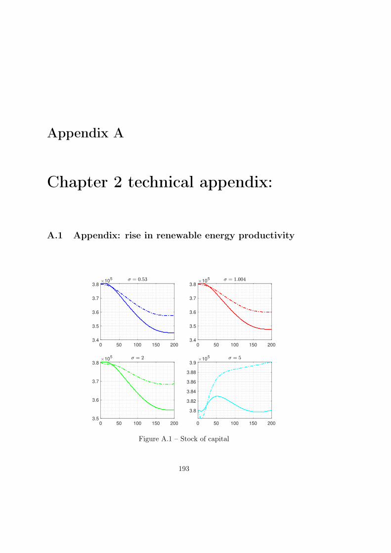
Appendix A
Chapter 2 technical appendix:
A.1 Appendix: rise in renewable energy productivity
0 50 100 150 200
3.4
3.5
3.6
3.7
3.810
5
0 50 100 150 200
3.4
3.5
3.6
3.7
3.810
5
0 50 100 150 200
3.5
3.6
3.7
3.810
5
0 50 100 150 200
3.8
3.82
3.84
3.86
3.88
3.910
5
Figure A.1 – Stock of capital
193
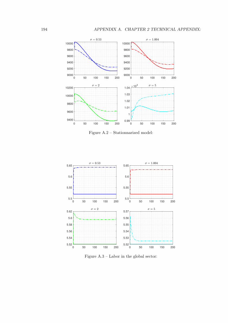
194 APPENDIX A. CHAPTER 2 TECHNICAL APPENDIX:
0 50 100 150 200
9000
9200
9400
9600
9800
10000
0 50 100 150 200
9000
9200
9400
9600
9800
10000
0 50 100 150 200
9400
9600
9800
10000
10200
0 50 100 150 200
0.99
1
1.01
1.02
1.03
1.0410
4
Figure A.2 – Stationnarized model:
0 50 100 150 200
5.5
5.55
5.6
5.65
0 50 100 150 200
5.5
5.55
5.6
5.65
0 50 100 150 200
5.52
5.54
5.56
5.58
5.6
5.62
0 50 100 150 200
5.52
5.53
5.54
5.55
5.56
5.57
Figure A.3 – Labor in the global sector:
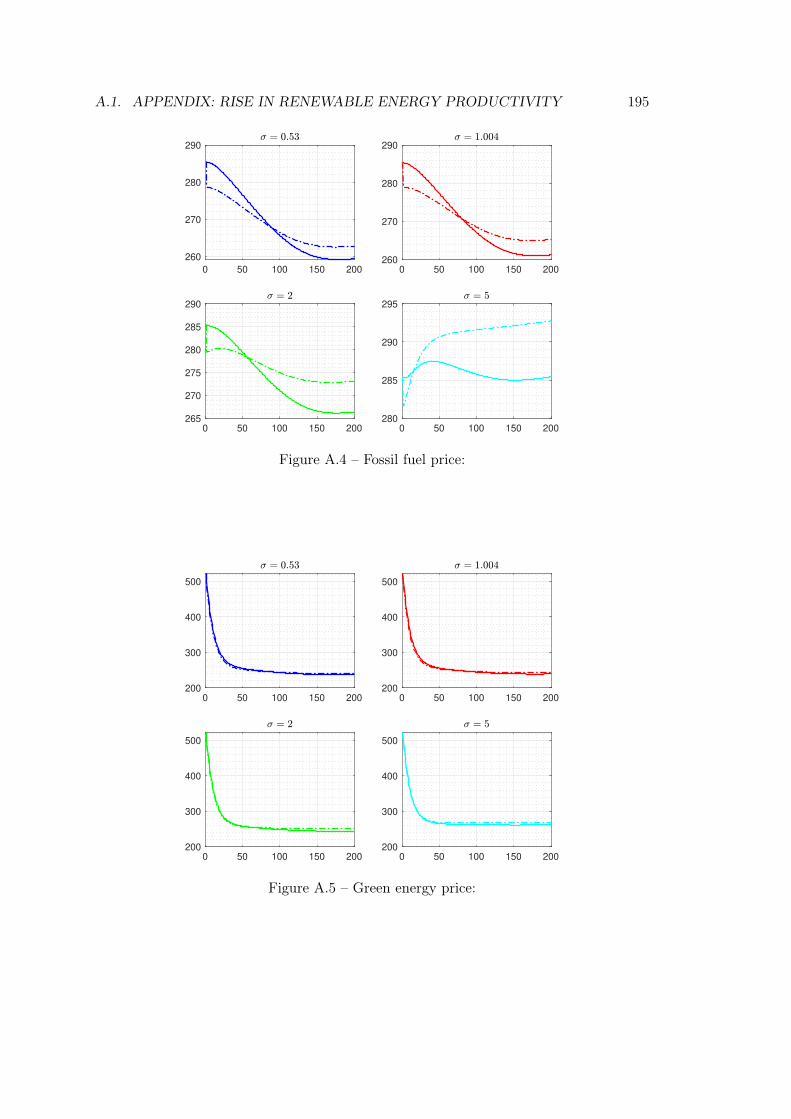
A.1. APPENDIX: RISE IN RENEWABLE ENERGY PRODUCTIVITY 195
0 50 100 150 200
260
270
280
290
0 50 100 150 200
260
270
280
290
0 50 100 150 200
265
270
275
280
285
290
0 50 100 150 200
280
285
290
295
Figure A.4 – Fossil fuel price:
0 50 100 150 200
200
300
400
500
0 50 100 150 200
200
300
400
500
0 50 100 150 200
200
300
400
500
0 50 100 150 200
200
300
400
500
Figure A.5 – Green energy price:
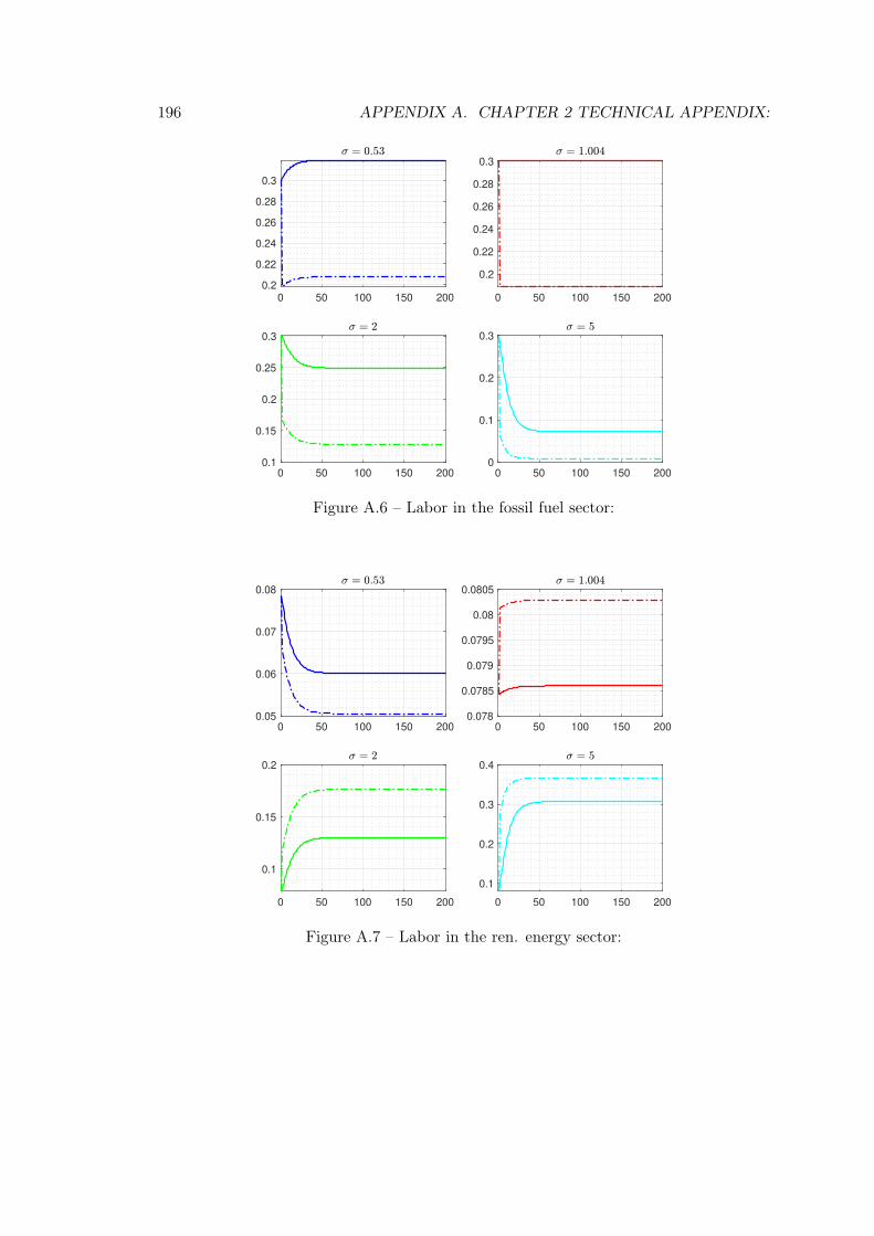
196 APPENDIX A. CHAPTER 2 TECHNICAL APPENDIX:
0 50 100 150 200
0.2
0.22
0.24
0.26
0.28
0.3
0 50 100 150 200
0.2
0.22
0.24
0.26
0.28
0.3
0 50 100 150 200
0.1
0.15
0.2
0.25
0.3
0 50 100 150 200
0
0.1
0.2
0.3
Figure A.6 – Labor in the fossil fuel sector:
0 50 100 150 200
0.05
0.06
0.07
0.08
0 50 100 150 200
0.078
0.0785
0.079
0.0795
0.08
0.0805
0 50 100 150 200
0.1
0.15
0.2
0 50 100 150 200
0.1
0.2
0.3
0.4
Figure A.7 – Labor in the ren. energy sector:
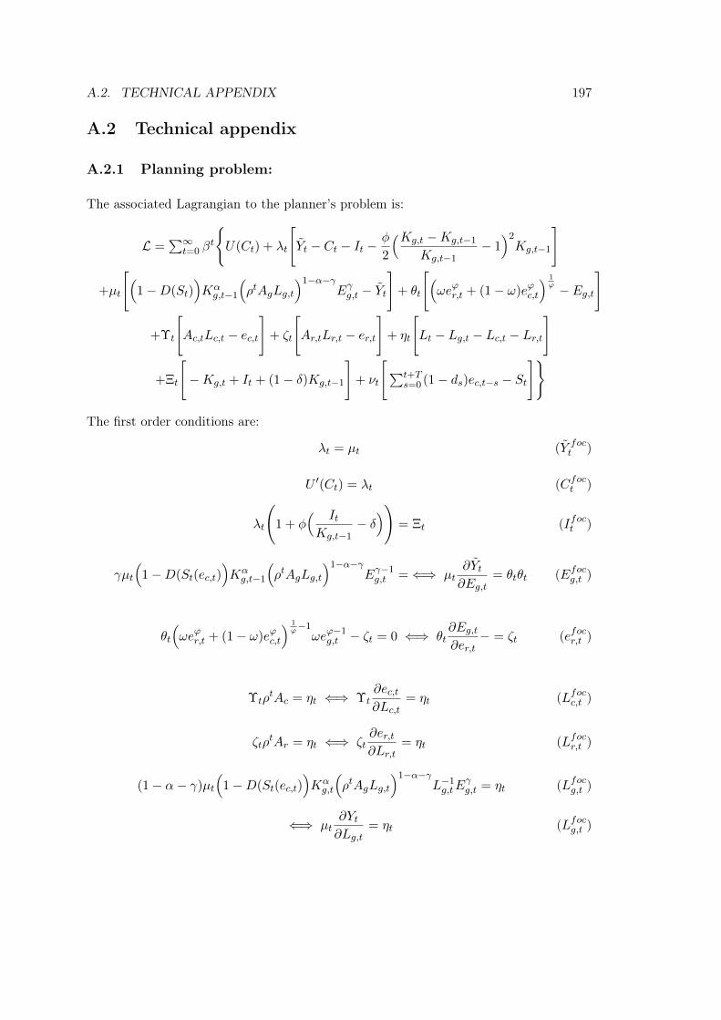
A.2. TECHNICAL APPENDIX 197
A.2 Technical appendix
A.2.1 Planning problem:
The associated Lagrangian to the planner’s problem is:
L =∑∞
t=0 βt
U(Ct) + λt
[Yt − Ct − It −
φ
2
(Kg,t −Kg,t−1
Kg,t−1− 1)2Kg,t−1
]
+µt
[(1−D(St)
)Kαg,t−1
(ρtAgLg,t
)1−α−γEγg,t − Yt
]+ θt
[(ωeϕr,t + (1− ω)eϕc,t
) 1ϕ − Eg,t
]
+Υt
[Ac,tLc,t − ec,t
]+ ζt
[Ar,tLr,t − er,t
]+ ηt
[Lt − Lg,t − Lc,t − Lr,t
]
+Ξt
[−Kg,t + It + (1− δ)Kg,t−1
]+ νt
[∑t+T
s=0 (1− ds)ec,t−s − St]
The first order conditions are:
λt = µt (Y foct )
U ′(Ct) = λt (Cfoct )
λt
(1 + φ
( ItKg,t−1
− δ))
= Ξt (Ifoct )
γµt
(1−D(St(ec,t)
)Kαg,t−1
(ρtAgLg,t
)1−α−γEγ−1g,t =⇐⇒ µt
∂Yt∂Eg,t
= θtθt (Efocg,t )
θt
(ωeϕr,t + (1− ω)eϕc,t
) 1ϕ−1ωeϕ−1
g,t − ζt = 0 ⇐⇒ θt∂Eg,t∂er,t
− = ζt (efocr,t )
ΥtρtAc = ηt ⇐⇒ Υt
∂ec,t∂Lc,t
= ηt (Lfocc,t )
ζtρtAr = ηt ⇐⇒ ζt
∂er,t∂Lr,t
= ηt (Lfocr,t )
(1− α− γ)µt
(1−D(St(ec,t)
)Kαg,t
(ρtAgLg,t
)1−α−γL−1g,tE
γg,t = ηt (Lfocg,t )
⇐⇒ µt∂Yt∂Lg,t
= ηt (Lfocg,t )
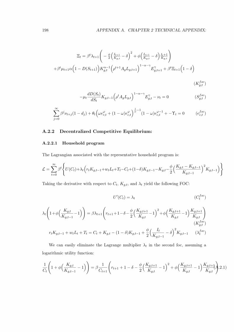
198 APPENDIX A. CHAPTER 2 TECHNICAL APPENDIX:
Ξt = βtλt+1
(− φ
2
(It+1
Kg,t− δ)2
+ φ(It+1
Kg,t− δ)It+1Kg,t
)
+βtµt+1α(
1−D(St+1))Kα−1g,t
(ρt+1AgLg,t+1
)1−α−γEγg,t+1 + βtΞt+1
(1− δ
)
(Kfocg,t )
−µtdD(St)
dStKg,t−1
(ρtAgLg,t
)1−α−γEγg,t − νt = 0 (Sfocg,t )
∞∑
j=0
βjνt+j(1− dj) + θt
(ωeϕr,t + (1− ω)eϕc,t
) 1ϕ−1
(1− ω)eϕ−1c,t +−Υt = 0 (efocc,t )
A.2.2 Decentralized Competitive Equilibrium:
A.2.2.1 Household program
The Lagrangian associated with the representative household program is:
L =
∞∑
t=0
βt
U(Ct)+λt
(rtKg,t−1+wtLt+Tt−Ct+(1−δ)Kg,t−1−Kg,t−
φ
2
(Kg,t −Kg,t−1
Kg,t−1
)2Kg,t−1
)
Taking the derivative with respect to Ct, Kg,t, and λt yield the following FOC:
U ′(Ct) = λt (Cfoct )
λt
(1+φ
( Kg,t
Kg,t−1−1))
= βλt+1
(rt+1 +1−δ− φ
2
(Kg,t+1
Kg,t−1)2
+φ(Kg,t+1
Kg,t−1)Kg,t+1
Kg,t
)
(Kfocg,t )
rtKg,t−1 + wtLt + Tt = Ct +Kg,t − (1− δ)Kg,t−1 +φ
2
( ItKg,t−1
− δ)2Kg,t−1 (λfoct )
We can easily eliminate the Lagrange multiplier λt in the second foc, assuming a
logarithmic utility function:
1
Ct
(1 + φ
( Kg,t
Kg,t−1− 1))
= β1
Ct+1
(rt+1 + 1− δ − φ
2
(Kg,t+1
Kg,t− 1)2
+ φ(Kg,t+1
Kg,t− 1)Kg,t+1
Kg,t
)(A.2.1)
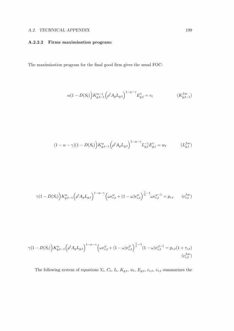
A.2. TECHNICAL APPENDIX 199
A.2.2.2 Firms maximisation program:
The maximization program for the final good firm gives the usual FOC:
α(1−D(St))Kα−1g,t−1
(ρtAgLg,t
)1−α−γEγg,t = rt (Kfoc
g,t−1)
(1− α− γ)(1−D(St))Kαg,t−1
(ρtAgLg,t
)1−α−γL−1g,tE
γg,t = wt (Lfocg,t )
γ(1−D(St))Kαg,t−1
(ρtAgLg,t
)1−α−γ(ωeϕr,t + (1− ω)eϕc,t
) γϕ−1ωeϕ−1
r,t = pr,t (efocr,t )
γ(1−D(St))Kαg,t−1
(ρtAgLg,t
)1−α−γ(ωeϕr,t + (1− ω)eϕc,t
) γϕ−1
(1− ω)eϕ−1c,t = pc,t(1 + τc,t)
(efocc,t )
The following system of equations Yt, Ct, It, Kg,t, wt, Eg,t, ec,t, er,t summarizes the
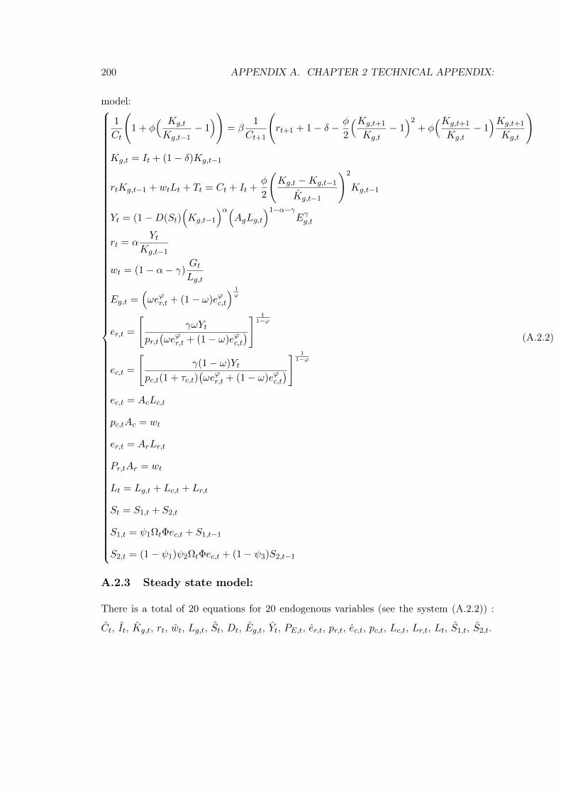
200 APPENDIX A. CHAPTER 2 TECHNICAL APPENDIX:
model:
1
Ct
(1 + φ
( Kg,t
Kg,t−1− 1))
= β1
Ct+1
(rt+1 + 1− δ − φ
2
(Kg,t+1
Kg,t− 1)2
+ φ(Kg,t+1
Kg,t− 1)Kg,t+1
Kg,t
)
Kg,t = It + (1− δ)Kg,t−1
rtKg,t−1 + wtLt + Tt = Ct + It +φ
2
(Kg,t −Kg,t−1
Kg,t−1
)2
Kg,t−1
Yt = (1−D(St)(Kg,t−1
)α(AgLg,t
)1−α−γEγg,t
rt = αYt
Kg,t−1
wt = (1− α− γ)GtLg,t
Eg,t =(ωeϕr,t + (1− ω)eϕc,t
) 1ϕ
er,t =
[γωYt
pr,t(ωeϕr,t + (1− ω)eϕc,t
)] 1
1−ϕ
ec,t =
[γ(1− ω)Yt
pc,t(1 + τc,t)(ωeϕr,t + (1− ω)eϕc,t
)] 1
1−ϕ
ec,t = AcLc,t
pc,tAc = wt
er,t = ArLr,t
Pr,tAr = wt
Lt = Lg,t + Lc,t + Lr,t
St = S1,t + S2,t
S1,t = ψ1ΩtΦec,t + S1,t−1
S2,t = (1− ψ1)ψ2ΩtΦec,t + (1− ψ3)S2,t−1
(A.2.2)
A.2.3 Steady state model:
There is a total of 20 equations for 20 endogenous variables (see the system (A.2.2)) :
Ct, It, Kg,t, rt, wt, Lg,t, St, Dt, Eg,t, Yt, PE,t, er,t, pr,t, ec,t, pc,t, Lc,t, Lr,t, Lt, S1,t, S2,t.
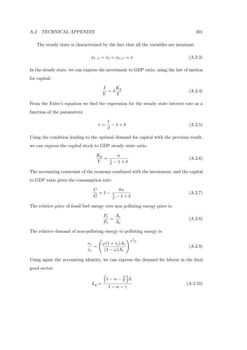
A.2. TECHNICAL APPENDIX 201
The steady state is characterized by the fact that all the variables are invariant:
xt−1 = xt = xt+1 = x (A.2.3)
In the steady state, we can express the investment to GDP ratio, using the law of motion
for capital:
I
Y= δ
Kg
Y(A.2.4)
From the Euler’s equation we find the expression for the steady state interest rate as a
function of the parameters:
r =1
β− 1 + δ (A.2.5)
Using the condition leading to the optimal demand for capital with the previous result,
we can express the capital stock to GDP steady state ratio:
Kg
Y=
α1β − 1 + δ
(A.2.6)
The accounting constraint of the economy combined with the investment, and the capital
to GDP ratio gives the consumption rate:
C
G= 1− δα
1β − 1 + δ
(A.2.7)
The relative price of fossil fuel energy over non polluting energy price is:
PcPr
=ArAc
(A.2.8)
The relative demand of non-polluting energy to polluting energy is:
erec
=
(ω(1 + τc)Ar(1− ω)Ac
) 11−ϕ
(A.2.9)
Using again the accounting identity, we can express the demand for labour in the final
good sector:
Lg =
(1− α− T
Y
)L
1− α− γ (A.2.10)
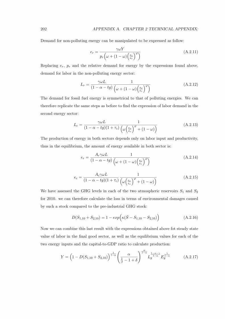
202 APPENDIX A. CHAPTER 2 TECHNICAL APPENDIX:
Demand for non-polluting energy can be manipulated to be expressed as follow:
er =γωY
pr
(ω + (1− ω)
(ecer
)ϕ) (A.2.11)
Replacing er, pr and the relative demand for energy by the expressions found above,
demand for labor in the non-polluting energy sector:
Lr =γωL
(1− α− tg)
1(ω + (1− ω)
(ecer
)ϕ) (A.2.12)
The demand for fossil fuel energy is symmetrical to that of polluting energies. We can
therefore replicate the same steps as before to find the expression of labor demand in the
second energy sector:
Lc =γωL
(1− α− tg)(1 + τc)
1(ω(erec
)ϕ+ (1− ω)
) (A.2.13)
The production of energy in both sectors depends only on labor input and productivity,
thus in the equilibrium, the amount of energy available in both sector is:
er =ArγωL
(1− α− tg)
1(ω + (1− ω)
(ecer
)ϕ) (A.2.14)
ec =AcγωL
(1− α− tg)(1 + τc)
1(ω(erec
)ϕ+ (1− ω)
) (A.2.15)
We have assessed the GHG levels in each of the two atmospheric reservoirs S1 and S2
for 2010. we can therefore calculate the loss in terms of environmental damages caused
by such a stock compared to the pre-industrial GHG stock:
D(S1,10 + S2,10) = 1− exp(κ(S − S1,10 − S2,10)
)(A.2.16)
Now we can combine this last result with the expressions obtained above fot steady state
value of labor in the final good sector, as well as the equilibrium values for each of the
two energy inputs and the capital-to-GDP ratio to calculate production:
Y =(
1−D(S1,10 + S2,10)) 1
1−α
(α
1β − 1 + δ
) α1−α
L1−α−γ1−α
g Eγ
1−αg (A.2.17)
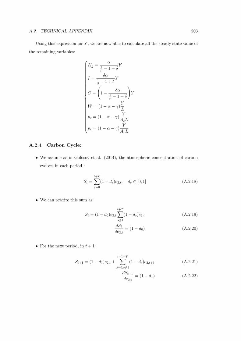
A.2. TECHNICAL APPENDIX 203
Using this expression for Y , we are now able to calculate all the steady state value of
the remaining variables:
Kg =α
1β − 1 + δ
Y
I =δα
1β − 1 + δ
Y
C =
(1− δα
1β − 1 + δ
)Y
W = (1− α− γ)Y
L
pc = (1− α− γ)Y
AcL
pr = (1− α− γ)Y
ArL
A.2.4 Carbon Cycle:
• We assume as in Golosov et al. (2014), the atmospheric concentration of carbon
evolves in each period :
St =
t+T∑
s=0
(1− ds)e2,t, ds ∈ [0, 1] (A.2.18)
• We can rewrite this sum as:
St = (1− d0)e2,t
t+T∑
s≥1
(1− ds)e2,t (A.2.19)
dStde2,t
= (1− d0) (A.2.20)
• For the next period, in t+ 1:
St+1 = (1− d1)e2,t +t+1+T∑
s=0,s 6=1
(1− ds)e2,t+1 (A.2.21)
dSt+1
de2,t= (1− d1) (A.2.22)
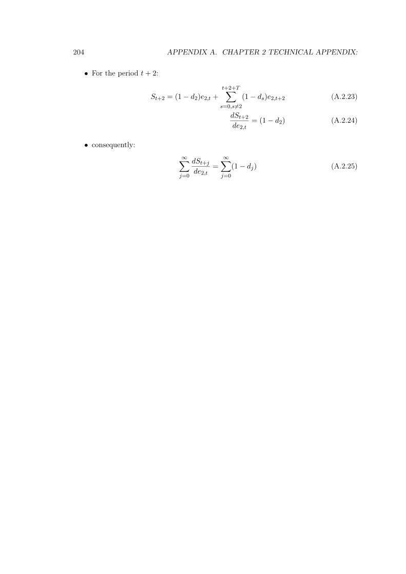
204 APPENDIX A. CHAPTER 2 TECHNICAL APPENDIX:
• For the period t+ 2:
St+2 = (1− d2)e2,t +t+2+T∑
s=0,s 6=2
(1− ds)e2,t+2 (A.2.23)
dSt+2
de2,t= (1− d2) (A.2.24)
• consequently:
∞∑
j=0
dSt+jde2,t
=
∞∑
j=0
(1− dj) (A.2.25)
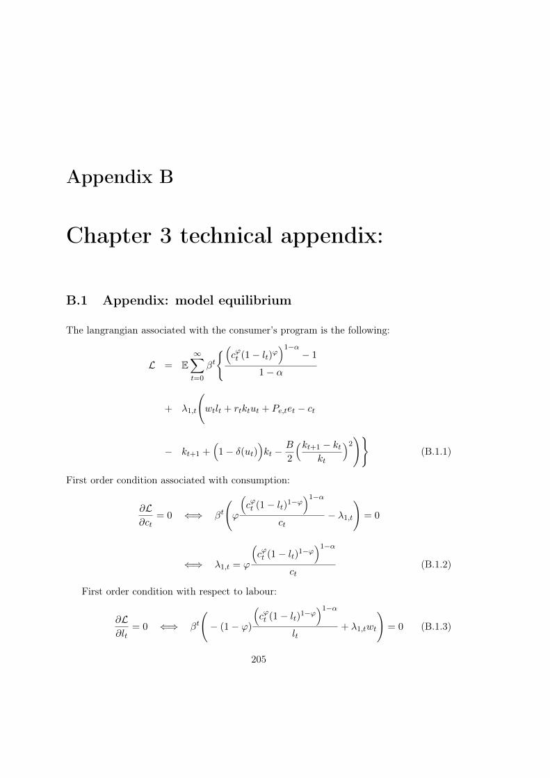
Appendix B
Chapter 3 technical appendix:
B.1 Appendix: model equilibrium
The langrangian associated with the consumer’s program is the following:
L = E∞∑
t=0
βt
(cϕt (1− lt)ϕ
)1−α− 1
1− α
+ λ1,t
(wtlt + rtktut + Pe,tet − ct
− kt+1 +(
1− δ(ut))kt −
B
2
(kt+1 − ktkt
)2)
(B.1.1)
First order condition associated with consumption:
∂L∂ct
= 0 ⇐⇒ βt
(ϕ
(cϕt (1− lt)1−ϕ
)1−α
ct− λ1,t
)= 0
⇐⇒ λ1,t = ϕ
(cϕt (1− lt)1−ϕ
)1−α
ct(B.1.2)
First order condition with respect to labour:
∂L∂lt
= 0 ⇐⇒ βt
(− (1− ϕ)
(cϕt (1− lt)1−ϕ
)1−α
lt+ λ1,twt
)= 0 (B.1.3)
205
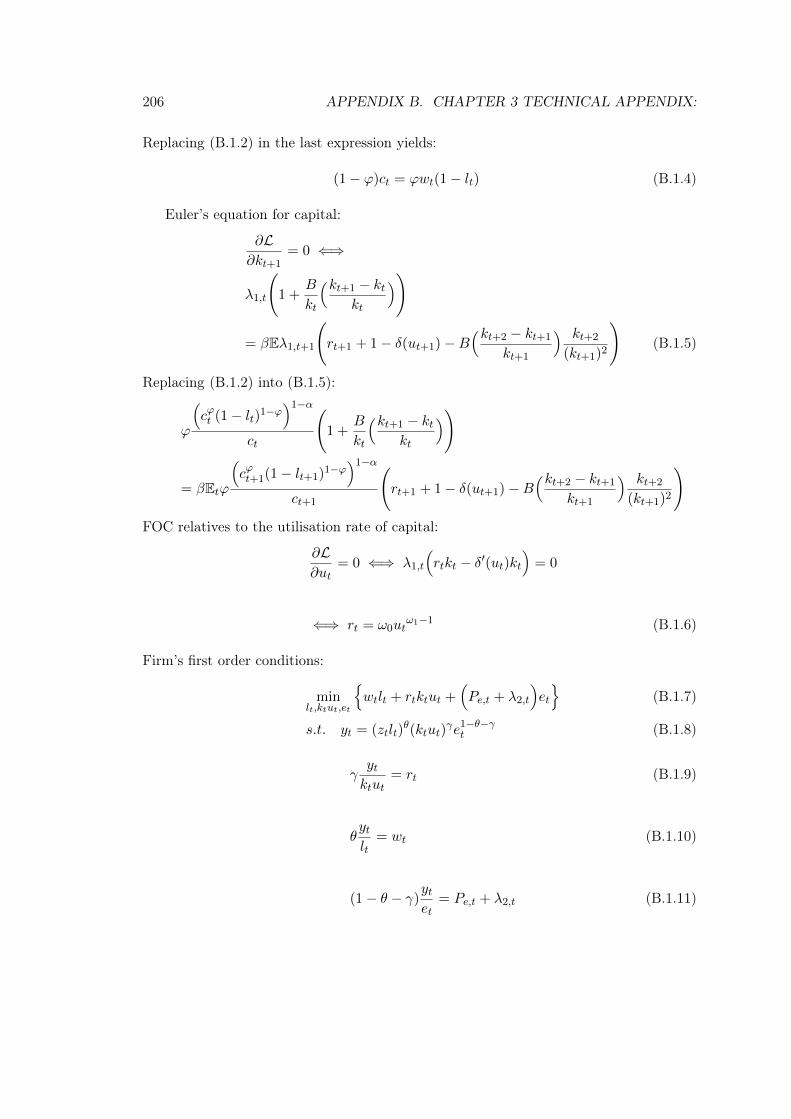
206 APPENDIX B. CHAPTER 3 TECHNICAL APPENDIX:
Replacing (B.1.2) in the last expression yields:
(1− ϕ)ct = ϕwt(1− lt) (B.1.4)
Euler’s equation for capital:
∂L∂kt+1
= 0 ⇐⇒
λ1,t
(1 +
B
kt
(kt+1 − ktkt
))
= βEλ1,t+1
(rt+1 + 1− δ(ut+1)−B
(kt+2 − kt+1
kt+1
) kt+2
(kt+1)2
)(B.1.5)
Replacing (B.1.2) into (B.1.5):
ϕ
(cϕt (1− lt)1−ϕ
)1−α
ct
(1 +
B
kt
(kt+1 − ktkt
))
= βEtϕ
(cϕt+1(1− lt+1)1−ϕ
)1−α
ct+1
(rt+1 + 1− δ(ut+1)−B
(kt+2 − kt+1
kt+1
) kt+2
(kt+1)2
)
FOC relatives to the utilisation rate of capital:
∂L∂ut
= 0 ⇐⇒ λ1,t
(rtkt − δ′(ut)kt
)= 0
⇐⇒ rt = ω0utω1−1 (B.1.6)
Firm’s first order conditions:
minlt,ktut,et
wtlt + rtktut +
(Pe,t + λ2,t
)et
(B.1.7)
s.t. yt = (ztlt)θ(ktut)
γe1−θ−γt (B.1.8)
γytktut
= rt (B.1.9)
θytlt
= wt (B.1.10)
(1− θ − γ)ytet
= Pe,t + λ2,t (B.1.11)
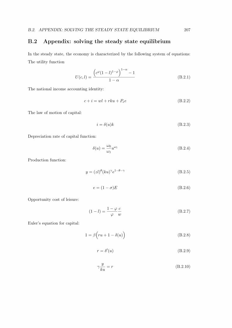
B.2. APPENDIX: SOLVING THE STEADY STATE EQUILIBRIUM 207
B.2 Appendix: solving the steady state equilibrium
In the steady state, the economy is characterized by the following system of equations:
The utility function
U(c, l) =
(cϕ(1− l)1−ϕ
)1−α− 1
1− α (B.2.1)
The national income accounting identity:
c+ i = wl + rku+ Pee (B.2.2)
The law of motion of capital:
i = δ(u)k (B.2.3)
Depreciation rate of capital function:
δ(u) =ω0
ω1uω1 (B.2.4)
Production function:
y = (zl)θ(ku)γe1−θ−γ (B.2.5)
e = (1− σ)E (B.2.6)
Opportunity cost of leisure:
(1− l) =1− ϕϕ
c
w(B.2.7)
Euler’s equation for capital:
1 = β(ru+ 1− δ(u)
)(B.2.8)
r = δ′(u) (B.2.9)
γy
ku= r (B.2.10)
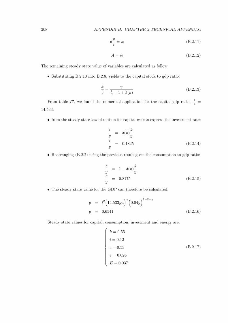
208 APPENDIX B. CHAPTER 3 TECHNICAL APPENDIX:
θy
l= w (B.2.11)
A = ιe (B.2.12)
The remaining steady state value of variables are calculated as follow:
• Substituting B.2.10 into B.2.8, yields to the capital stock to gdp ratio:
k
y=
γ1β − 1 + δ(u)
(B.2.13)
From table ??, we found the numerical application for the capital gdp ratio: ky =
14.533.
• from the steady state law of motion for capital we can express the investment rate:
i
y= δ(u)
k
yi
y= 0.1825 (B.2.14)
• Rearranging (B.2.2) using the previous result gives the consumption to gdp ratio:
c
y= 1− δ(u)
k
yc
y= 0.8175 (B.2.15)
• The steady state value for the GDP can therefore be calculated:
y = lθ(
14.533yu)γ(
0.04y)1−θ−γ
y = 0.6541 (B.2.16)
Steady state values for capital, consumption, investment and energy are:
k = 9.55
i = 0.12
c = 0.53
e = 0.026
E = 0.037
(B.2.17)
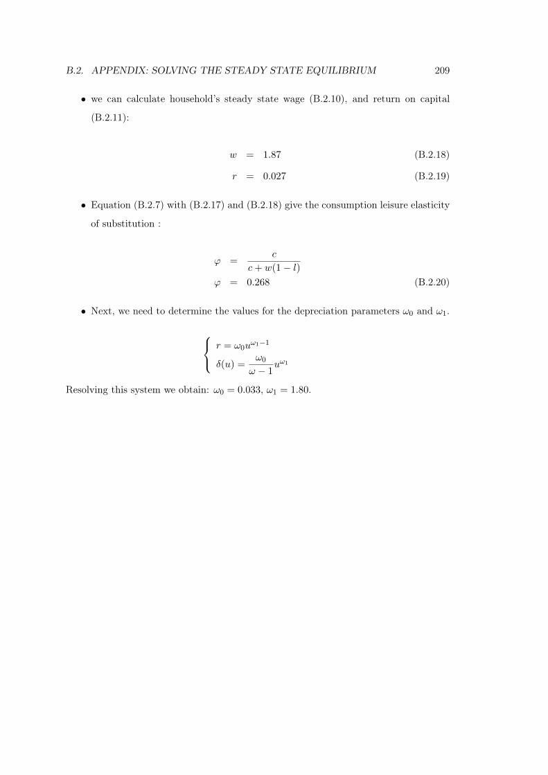
B.2. APPENDIX: SOLVING THE STEADY STATE EQUILIBRIUM 209
• we can calculate household’s steady state wage (B.2.10), and return on capital
(B.2.11):
w = 1.87 (B.2.18)
r = 0.027 (B.2.19)
• Equation (B.2.7) with (B.2.17) and (B.2.18) give the consumption leisure elasticity
of substitution :
ϕ =c
c+ w(1− l)ϕ = 0.268 (B.2.20)
• Next, we need to determine the values for the depreciation parameters ω0 and ω1.
r = ω0uω1−1
δ(u) =ω0
ω − 1uω1
Resolving this system we obtain: ω0 = 0.033, ω1 = 1.80.
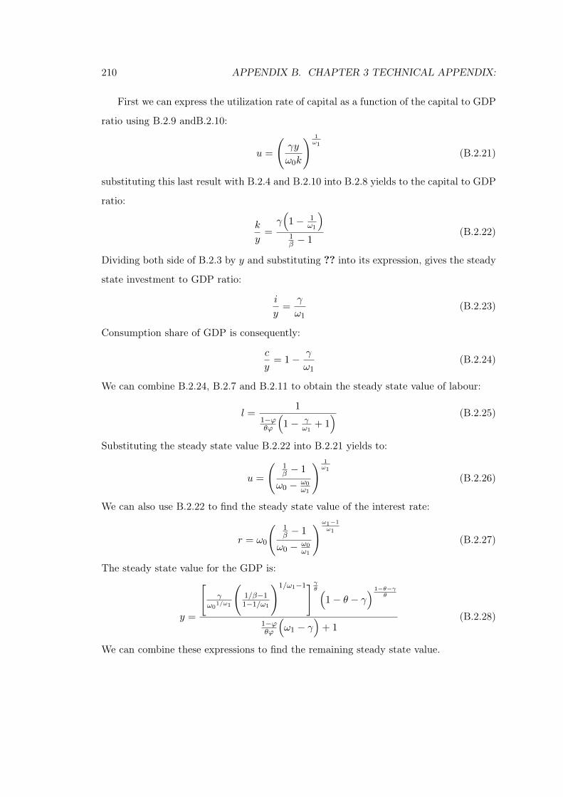
210 APPENDIX B. CHAPTER 3 TECHNICAL APPENDIX:
First we can express the utilization rate of capital as a function of the capital to GDP
ratio using B.2.9 andB.2.10:
u =
(γy
ω0k
) 1ω1
(B.2.21)
substituting this last result with B.2.4 and B.2.10 into B.2.8 yields to the capital to GDP
ratio:
k
y=γ(
1− 1ω1
)
1β − 1
(B.2.22)
Dividing both side of B.2.3 by y and substituting ?? into its expression, gives the steady
state investment to GDP ratio:
i
y=
γ
ω1(B.2.23)
Consumption share of GDP is consequently:
c
y= 1− γ
ω1(B.2.24)
We can combine B.2.24, B.2.7 and B.2.11 to obtain the steady state value of labour:
l =1
1−ϕθϕ
(1− γ
ω1+ 1) (B.2.25)
Substituting the steady state value B.2.22 into B.2.21 yields to:
u =
(1β − 1
ω0 − ω0ω1
) 1ω1
(B.2.26)
We can also use B.2.22 to find the steady state value of the interest rate:
r = ω0
(1β − 1
ω0 − ω0ω1
)ω1−1ω1
(B.2.27)
The steady state value for the GDP is:
y =
[γ
ω01/ω1
(1/β−11−1/ω1
)1/ω1−1] γθ (
1− θ − γ) 1−θ−γ
θ
1−ϕθϕ
(ω1 − γ
)+ 1
(B.2.28)
We can combine these expressions to find the remaining steady state value.
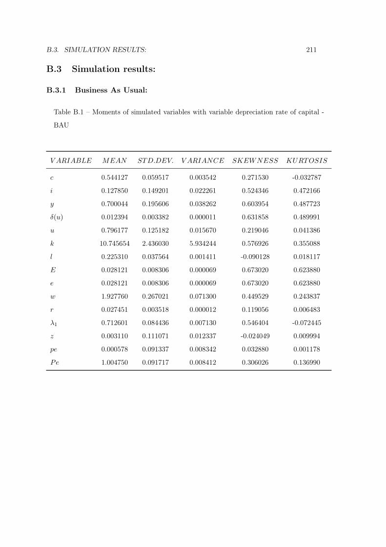
B.3. SIMULATION RESULTS: 211
B.3 Simulation results:
B.3.1 Business As Usual:
Table B.1 – Moments of simulated variables with variable depreciation rate of capital -
BAU
V ARIABLE MEAN STD.DEV. V ARIANCE SKEWNESS KURTOSIS
c 0.544127 0.059517 0.003542 0.271530 -0.032787
i 0.127850 0.149201 0.022261 0.524346 0.472166
y 0.700044 0.195606 0.038262 0.603954 0.487723
δ(u) 0.012394 0.003382 0.000011 0.631858 0.489991
u 0.796177 0.125182 0.015670 0.219046 0.041386
k 10.745654 2.436030 5.934244 0.576926 0.355088
l 0.225310 0.037564 0.001411 -0.090128 0.018117
E 0.028121 0.008306 0.000069 0.673020 0.623880
e 0.028121 0.008306 0.000069 0.673020 0.623880
w 1.927760 0.267021 0.071300 0.449529 0.243837
r 0.027451 0.003518 0.000012 0.119056 0.006483
λ1 0.712601 0.084436 0.007130 0.546404 -0.072445
z 0.003110 0.111071 0.012337 -0.024049 0.009994
pe 0.000578 0.091337 0.008342 0.032880 0.001178
Pe 1.004750 0.091717 0.008412 0.306026 0.136990
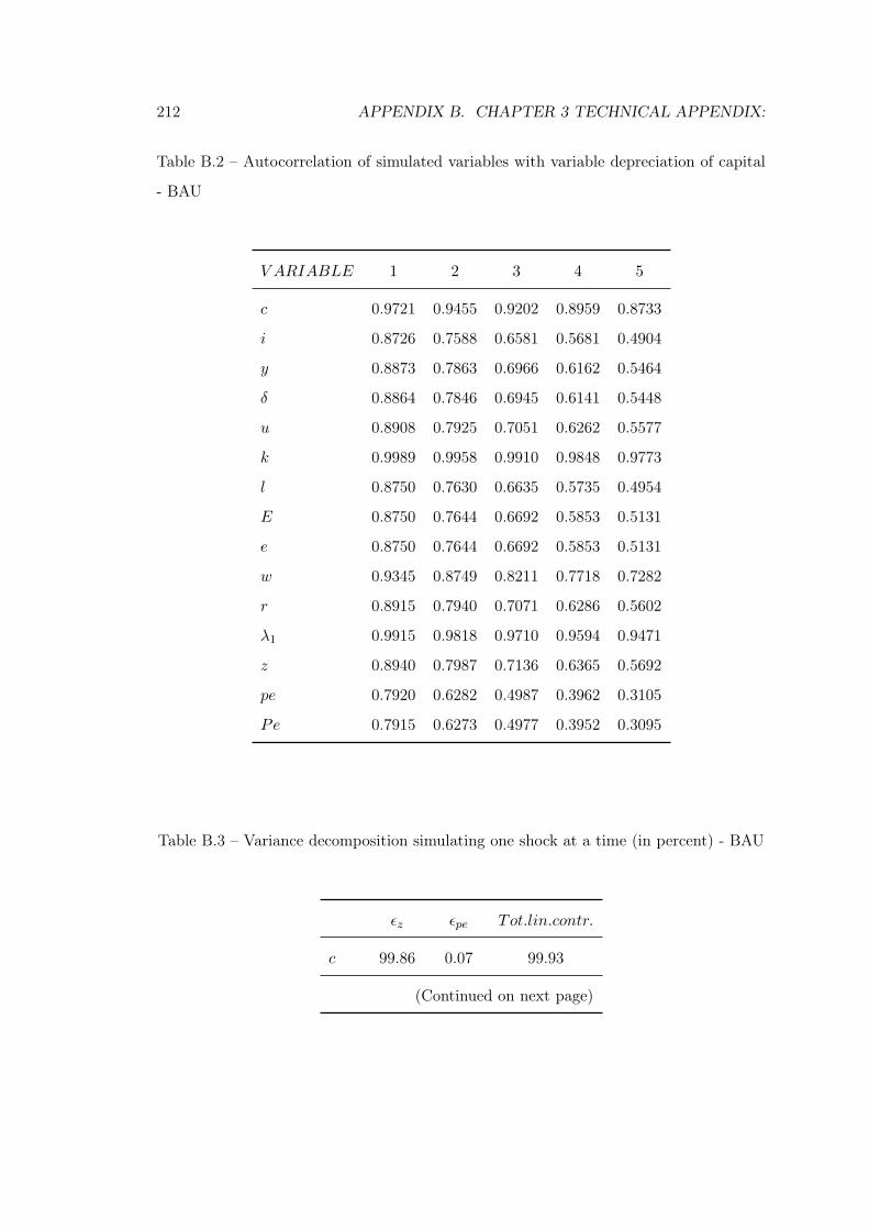
212 APPENDIX B. CHAPTER 3 TECHNICAL APPENDIX:
Table B.2 – Autocorrelation of simulated variables with variable depreciation of capital
- BAU
V ARIABLE 1 2 3 4 5
c 0.9721 0.9455 0.9202 0.8959 0.8733
i 0.8726 0.7588 0.6581 0.5681 0.4904
y 0.8873 0.7863 0.6966 0.6162 0.5464
δ 0.8864 0.7846 0.6945 0.6141 0.5448
u 0.8908 0.7925 0.7051 0.6262 0.5577
k 0.9989 0.9958 0.9910 0.9848 0.9773
l 0.8750 0.7630 0.6635 0.5735 0.4954
E 0.8750 0.7644 0.6692 0.5853 0.5131
e 0.8750 0.7644 0.6692 0.5853 0.5131
w 0.9345 0.8749 0.8211 0.7718 0.7282
r 0.8915 0.7940 0.7071 0.6286 0.5602
λ1 0.9915 0.9818 0.9710 0.9594 0.9471
z 0.8940 0.7987 0.7136 0.6365 0.5692
pe 0.7920 0.6282 0.4987 0.3962 0.3105
Pe 0.7915 0.6273 0.4977 0.3952 0.3095
Table B.3 – Variance decomposition simulating one shock at a time (in percent) - BAU
εz εpe Tot.lin.contr.
c 99.86 0.07 99.93
(Continued on next page)
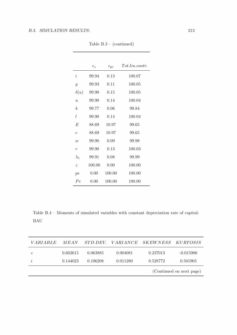
B.3. SIMULATION RESULTS: 213
Table B.3 – (continued)
εz εpe Tot.lin.contr.
i 99.94 0.13 100.07
y 99.93 0.11 100.05
δ(u) 99.90 0.15 100.05
u 99.90 0.14 100.04
k 99.77 0.06 99.84
l 99.90 0.14 100.04
E 88.69 10.97 99.65
e 88.69 10.97 99.65
w 99.90 0.09 99.98
r 99.90 0.13 100.03
λ1 99.91 0.08 99.99
z 100.00 0.00 100.00
pe 0.00 100.00 100.00
Pe 0.00 100.00 100.00
Table B.4 – Moments of simulated variables with constant depreciation rate of capital-
BAU
V ARIABLE MEAN STD.DEV. V ARIANCE SKEWNESS KURTOSIS
c 0.602615 0.063885 0.004081 0.237013 -0.015986
i 0.144023 0.106208 0.011280 0.528772 0.501903
(Continued on next page)
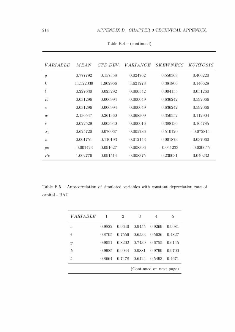
214 APPENDIX B. CHAPTER 3 TECHNICAL APPENDIX:
Table B.4 – (continued)
V ARIABLE MEAN STD.DEV. V ARIANCE SKEWNESS KURTOSIS
y 0.777792 0.157358 0.024762 0.550368 0.406220
k 11.522039 1.902966 3.621278 0.381806 0.146628
l 0.227630 0.023292 0.000542 0.004155 0.051260
E 0.031296 0.006994 0.000049 0.636242 0.592066
e 0.031296 0.006994 0.000049 0.636242 0.592066
w 2.136547 0.261360 0.068309 0.350552 0.112904
r 0.022529 0.003940 0.000016 0.388136 0.164785
λ1 0.625720 0.076067 0.005786 0.510120 -0.072814
z 0.001751 0.110193 0.012143 0.001873 0.037060
pe -0.001423 0.091627 0.008396 -0.041233 -0.020655
Pe 1.002776 0.091514 0.008375 0.230031 0.040232
Table B.5 – Autocorrelation of simulated variables with constant depreciation rate of
capital - BAU
V ARIABLE 1 2 3 4 5
c 0.9822 0.9640 0.9455 0.9269 0.9081
i 0.8705 0.7556 0.6533 0.5626 0.4827
y 0.9051 0.8202 0.7439 0.6755 0.6145
k 0.9985 0.9944 0.9881 0.9799 0.9700
l 0.8664 0.7478 0.6424 0.5493 0.4671
(Continued on next page)
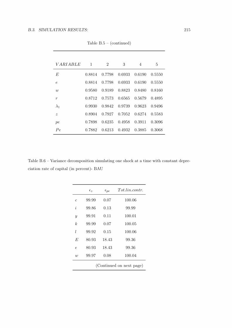
B.3. SIMULATION RESULTS: 215
Table B.5 – (continued)
V ARIABLE 1 2 3 4 5
E 0.8814 0.7798 0.6933 0.6190 0.5550
e 0.8814 0.7798 0.6933 0.6190 0.5550
w 0.9580 0.9189 0.8823 0.8480 0.8160
r 0.8712 0.7573 0.6565 0.5679 0.4895
λ1 0.9930 0.9842 0.9739 0.9623 0.9496
z 0.8904 0.7927 0.7052 0.6274 0.5583
pe 0.7898 0.6235 0.4958 0.3911 0.3096
Pe 0.7882 0.6213 0.4932 0.3885 0.3068
Table B.6 – Variance decomposition simulating one shock at a time with constant depre-
ciation rate of capital (in percent)- BAU
εz εpe Tot.lin.contr.
c 99.99 0.07 100.06
i 99.86 0.13 99.99
y 99.91 0.11 100.01
k 99.99 0.07 100.05
l 99.92 0.15 100.06
E 80.93 18.43 99.36
e 80.93 18.43 99.36
w 99.97 0.08 100.04
(Continued on next page)
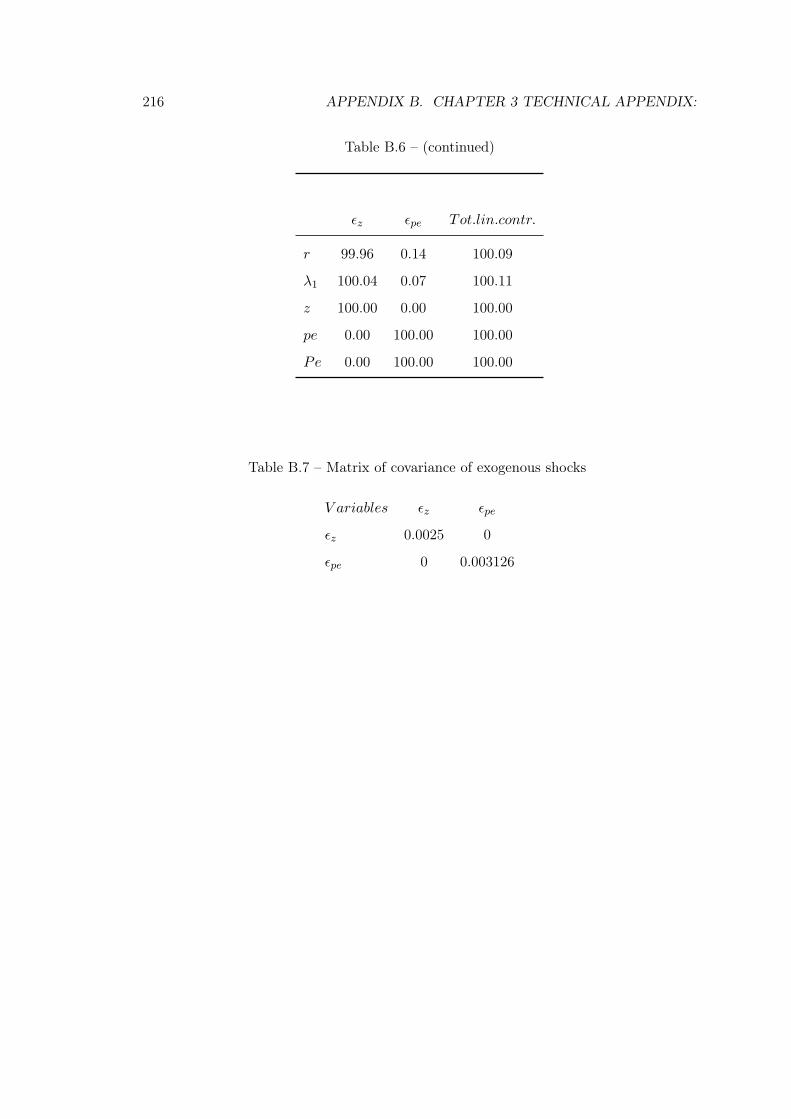
216 APPENDIX B. CHAPTER 3 TECHNICAL APPENDIX:
Table B.6 – (continued)
εz εpe Tot.lin.contr.
r 99.96 0.14 100.09
λ1 100.04 0.07 100.11
z 100.00 0.00 100.00
pe 0.00 100.00 100.00
Pe 0.00 100.00 100.00
Table B.7 – Matrix of covariance of exogenous shocks
V ariables εz εpe
εz 0.0025 0
εpe 0 0.003126
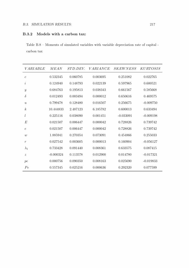
B.3. SIMULATION RESULTS: 217
B.3.2 Models with a carbon tax:
Table B.8 – Moments of simulated variables with variable depreciation rate of capital -
carbon tax
V ARIABLE MEAN STD.DEV. V ARIANCE SKEWNESS KURTOSIS
c 0.532345 0.060785 0.003695 0.251082 0.022765
i 0.124940 0.148793 0.022139 0.597965 0.600521
y 0.684763 0.195813 0.038343 0.661567 0.585668
δ 0.012493 0.003494 0.000012 0.650616 0.469575
u 0.799478 0.128480 0.016507 0.256675 -0.009750
k 10.444833 2.487123 6.185782 0.600013 0.633494
l 0.225116 0.038090 0.001451 -0.033091 -0.009198
E 0.021507 0.006447 0.000042 0.728826 0.739742
e 0.021507 0.006447 0.000042 0.728826 0.739742
w 1.885941 0.270354 0.073091 0.454866 0.255033
r 0.027542 0.003605 0.000013 0.160904 -0.056127
λ1 0.733428 0.091440 0.008361 0.633575 0.087415
z -0.000324 0.113578 0.012900 0.014780 -0.017321
pe 0.000756 0.090350 0.008163 0.025690 -0.019833
Pe 0.557345 0.025216 0.000636 0.292320 0.077599
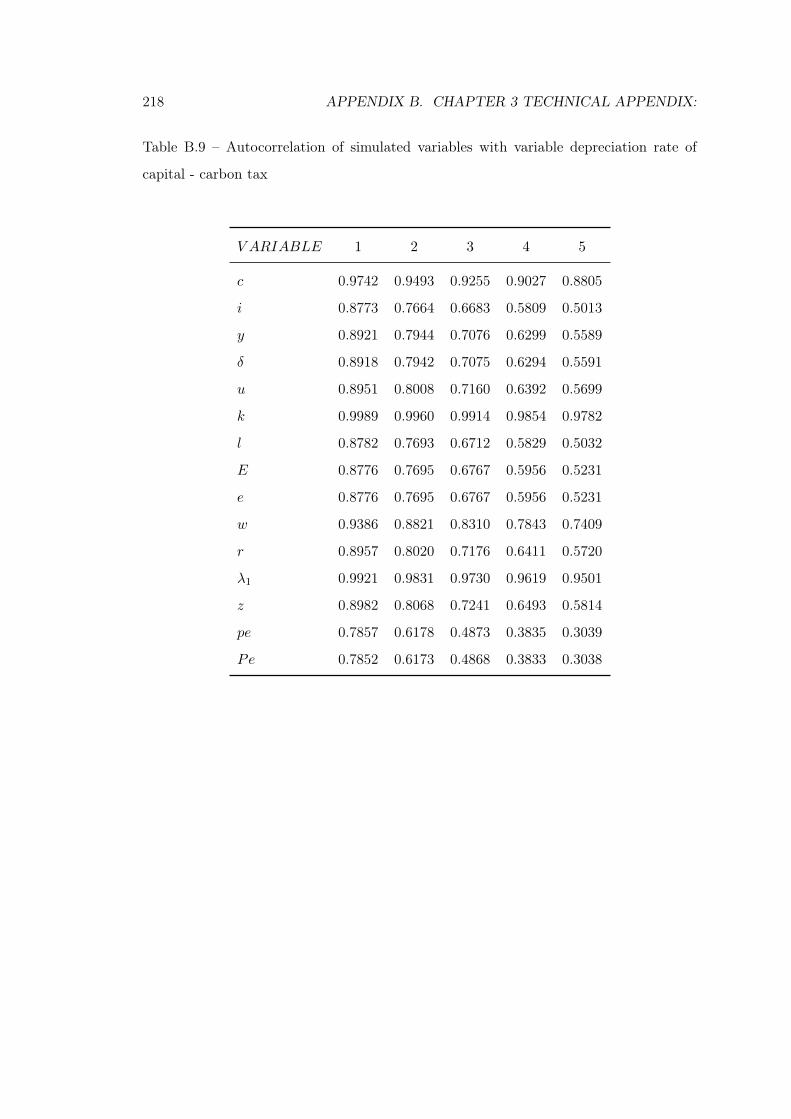
218 APPENDIX B. CHAPTER 3 TECHNICAL APPENDIX:
Table B.9 – Autocorrelation of simulated variables with variable depreciation rate of
capital - carbon tax
V ARIABLE 1 2 3 4 5
c 0.9742 0.9493 0.9255 0.9027 0.8805
i 0.8773 0.7664 0.6683 0.5809 0.5013
y 0.8921 0.7944 0.7076 0.6299 0.5589
δ 0.8918 0.7942 0.7075 0.6294 0.5591
u 0.8951 0.8008 0.7160 0.6392 0.5699
k 0.9989 0.9960 0.9914 0.9854 0.9782
l 0.8782 0.7693 0.6712 0.5829 0.5032
E 0.8776 0.7695 0.6767 0.5956 0.5231
e 0.8776 0.7695 0.6767 0.5956 0.5231
w 0.9386 0.8821 0.8310 0.7843 0.7409
r 0.8957 0.8020 0.7176 0.6411 0.5720
λ1 0.9921 0.9831 0.9730 0.9619 0.9501
z 0.8982 0.8068 0.7241 0.6493 0.5814
pe 0.7857 0.6178 0.4873 0.3835 0.3039
Pe 0.7852 0.6173 0.4868 0.3833 0.3038
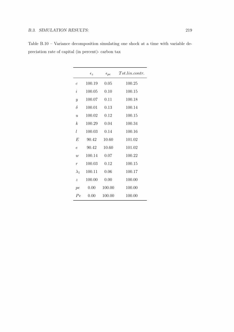
B.3. SIMULATION RESULTS: 219
Table B.10 – Variance decomposition simulating one shock at a time with variable de-
preciation rate of capital (in percent)- carbon tax
εz εpe Tot.lin.contr.
c 100.19 0.05 100.25
i 100.05 0.10 100.15
y 100.07 0.11 100.18
δ 100.01 0.13 100.14
u 100.02 0.12 100.15
k 100.29 0.04 100.34
l 100.03 0.14 100.16
E 90.42 10.60 101.02
e 90.42 10.60 101.02
w 100.14 0.07 100.22
r 100.03 0.12 100.15
λ1 100.11 0.06 100.17
z 100.00 0.00 100.00
pe 0.00 100.00 100.00
Pe 0.00 100.00 100.00
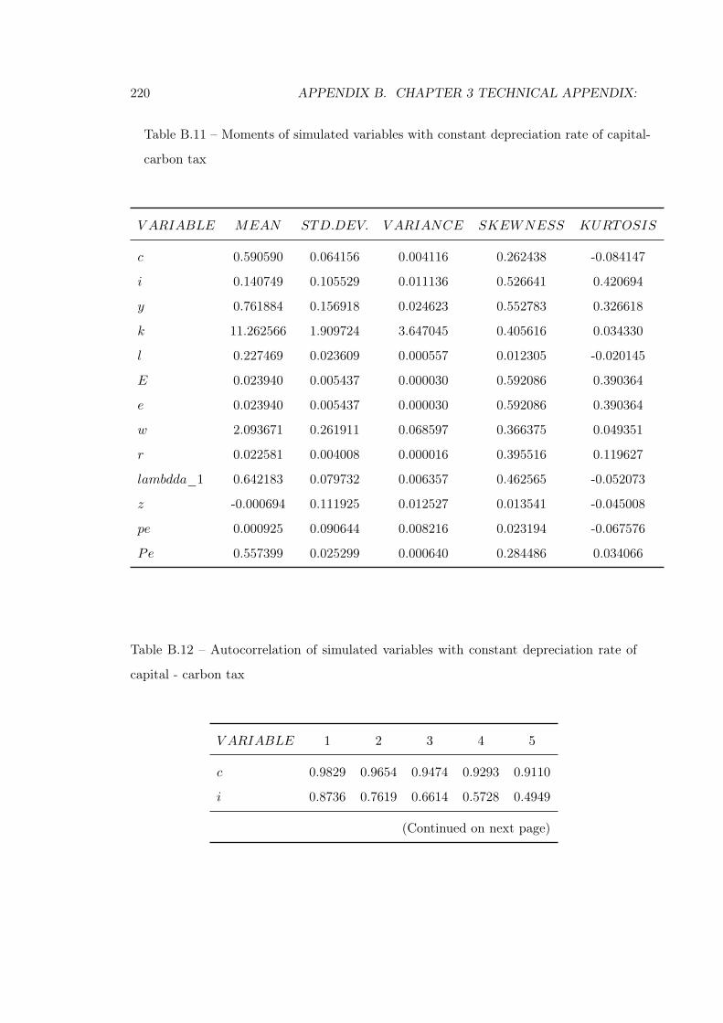
220 APPENDIX B. CHAPTER 3 TECHNICAL APPENDIX:
Table B.11 – Moments of simulated variables with constant depreciation rate of capital-
carbon tax
V ARIABLE MEAN STD.DEV. V ARIANCE SKEWNESS KURTOSIS
c 0.590590 0.064156 0.004116 0.262438 -0.084147
i 0.140749 0.105529 0.011136 0.526641 0.420694
y 0.761884 0.156918 0.024623 0.552783 0.326618
k 11.262566 1.909724 3.647045 0.405616 0.034330
l 0.227469 0.023609 0.000557 0.012305 -0.020145
E 0.023940 0.005437 0.000030 0.592086 0.390364
e 0.023940 0.005437 0.000030 0.592086 0.390364
w 2.093671 0.261911 0.068597 0.366375 0.049351
r 0.022581 0.004008 0.000016 0.395516 0.119627
lambdda_1 0.642183 0.079732 0.006357 0.462565 -0.052073
z -0.000694 0.111925 0.012527 0.013541 -0.045008
pe 0.000925 0.090644 0.008216 0.023194 -0.067576
Pe 0.557399 0.025299 0.000640 0.284486 0.034066
Table B.12 – Autocorrelation of simulated variables with constant depreciation rate of
capital - carbon tax
V ARIABLE 1 2 3 4 5
c 0.9829 0.9654 0.9474 0.9293 0.9110
i 0.8736 0.7619 0.6614 0.5728 0.4949
(Continued on next page)
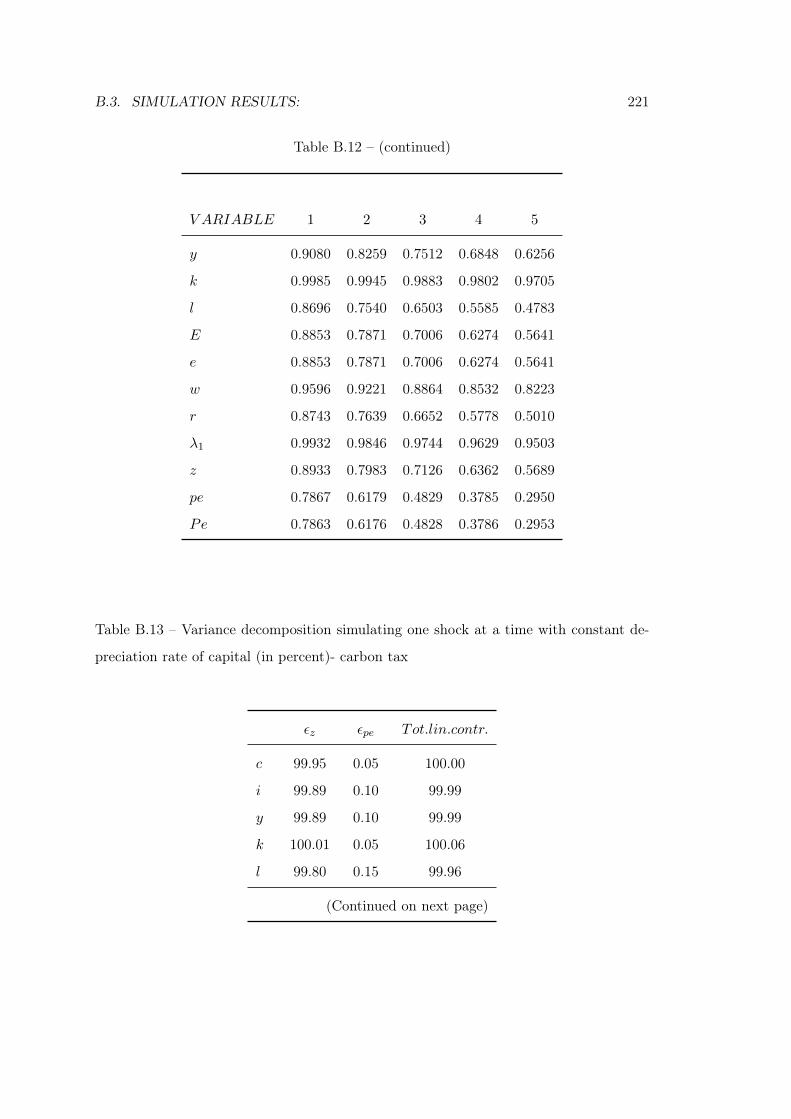
B.3. SIMULATION RESULTS: 221
Table B.12 – (continued)
V ARIABLE 1 2 3 4 5
y 0.9080 0.8259 0.7512 0.6848 0.6256
k 0.9985 0.9945 0.9883 0.9802 0.9705
l 0.8696 0.7540 0.6503 0.5585 0.4783
E 0.8853 0.7871 0.7006 0.6274 0.5641
e 0.8853 0.7871 0.7006 0.6274 0.5641
w 0.9596 0.9221 0.8864 0.8532 0.8223
r 0.8743 0.7639 0.6652 0.5778 0.5010
λ1 0.9932 0.9846 0.9744 0.9629 0.9503
z 0.8933 0.7983 0.7126 0.6362 0.5689
pe 0.7867 0.6179 0.4829 0.3785 0.2950
Pe 0.7863 0.6176 0.4828 0.3786 0.2953
Table B.13 – Variance decomposition simulating one shock at a time with constant de-
preciation rate of capital (in percent)- carbon tax
εz εpe Tot.lin.contr.
c 99.95 0.05 100.00
i 99.89 0.10 99.99
y 99.89 0.10 99.99
k 100.01 0.05 100.06
l 99.80 0.15 99.96
(Continued on next page)
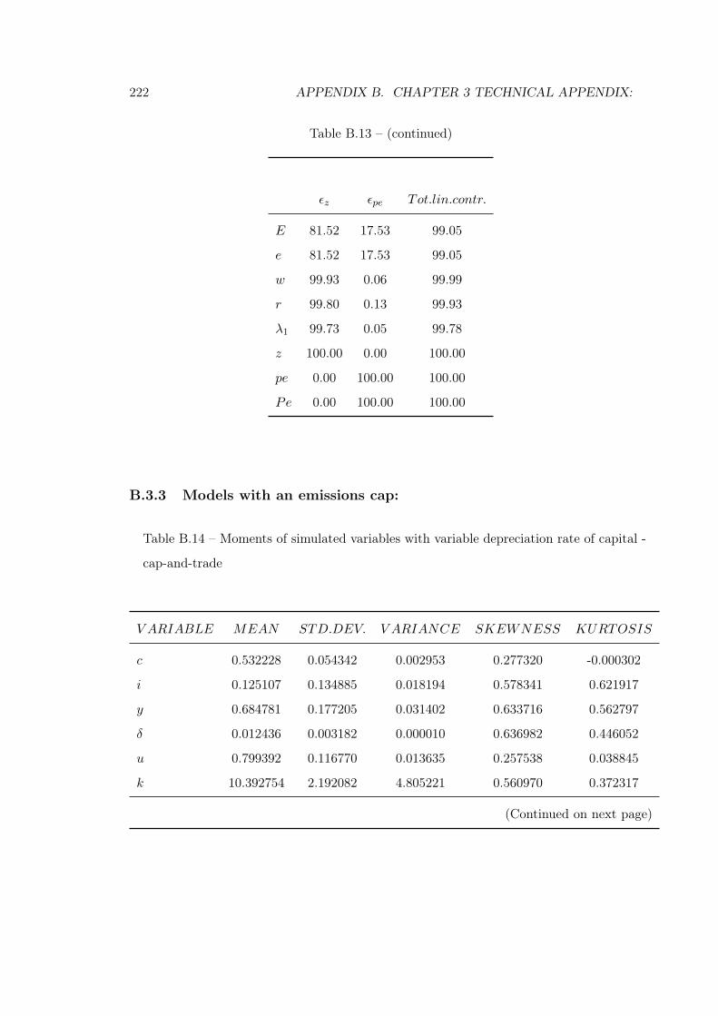
222 APPENDIX B. CHAPTER 3 TECHNICAL APPENDIX:
Table B.13 – (continued)
εz εpe Tot.lin.contr.
E 81.52 17.53 99.05
e 81.52 17.53 99.05
w 99.93 0.06 99.99
r 99.80 0.13 99.93
λ1 99.73 0.05 99.78
z 100.00 0.00 100.00
pe 0.00 100.00 100.00
Pe 0.00 100.00 100.00
B.3.3 Models with an emissions cap:
Table B.14 – Moments of simulated variables with variable depreciation rate of capital -
cap-and-trade
V ARIABLE MEAN STD.DEV. V ARIANCE SKEWNESS KURTOSIS
c 0.532228 0.054342 0.002953 0.277320 -0.000302
i 0.125107 0.134885 0.018194 0.578341 0.621917
y 0.684781 0.177205 0.031402 0.633716 0.562797
δ 0.012436 0.003182 0.000010 0.636982 0.446052
u 0.799392 0.116770 0.013635 0.257538 0.038845
k 10.392754 2.192082 4.805221 0.560970 0.372317
(Continued on next page)
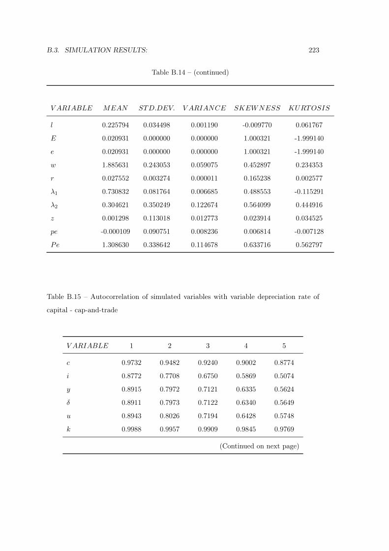
B.3. SIMULATION RESULTS: 223
Table B.14 – (continued)
V ARIABLE MEAN STD.DEV. V ARIANCE SKEWNESS KURTOSIS
l 0.225794 0.034498 0.001190 -0.009770 0.061767
E 0.020931 0.000000 0.000000 1.000321 -1.999140
e 0.020931 0.000000 0.000000 1.000321 -1.999140
w 1.885631 0.243053 0.059075 0.452897 0.234353
r 0.027552 0.003274 0.000011 0.165238 0.002577
λ1 0.730832 0.081764 0.006685 0.488553 -0.115291
λ2 0.304621 0.350249 0.122674 0.564099 0.444916
z 0.001298 0.113018 0.012773 0.023914 0.034525
pe -0.000109 0.090751 0.008236 0.006814 -0.007128
Pe 1.308630 0.338642 0.114678 0.633716 0.562797
Table B.15 – Autocorrelation of simulated variables with variable depreciation rate of
capital - cap-and-trade
V ARIABLE 1 2 3 4 5
c 0.9732 0.9482 0.9240 0.9002 0.8774
i 0.8772 0.7708 0.6750 0.5869 0.5074
y 0.8915 0.7972 0.7121 0.6335 0.5624
δ 0.8911 0.7973 0.7122 0.6340 0.5649
u 0.8943 0.8026 0.7194 0.6428 0.5748
k 0.9988 0.9957 0.9909 0.9845 0.9769
(Continued on next page)
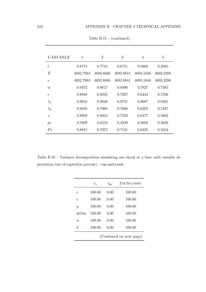
224 APPENDIX B. CHAPTER 3 TECHNICAL APPENDIX:
Table B.15 – (continued)
V ARIABLE 1 2 3 4 5
l 0.8774 0.7710 0.6751 0.5869 0.5085
E 4692.7983 4692.8886 4692.9841 4693.1048 4693.2288
e 4692.7983 4692.8886 4692.9841 4693.1048 4693.2288
w 0.9372 0.8817 0.8306 0.7827 0.7385
r 0.8948 0.8035 0.7207 0.6444 0.5766
λ1 0.9918 0.9826 0.9721 0.9607 0.9485
λ2 0.8850 0.7868 0.7000 0.6203 0.5487
z 0.8959 0.8054 0.7233 0.6477 0.5802
pe 0.7898 0.6233 0.4939 0.3882 0.3049
Pe 0.8915 0.7972 0.7121 0.6335 0.5624
Table B.16 – Variance decomposition simulating one shock at a time with variable de-
preciation rate of capital(in percent) - cap-and-trade
εz εpe Tot.lin.contr.
c 100.00 0.00 100.00
i 100.00 0.00 100.00
y 100.00 0.00 100.00
deltta 100.00 0.00 100.00
u 100.00 0.00 100.00
k 100.00 0.00 100.00
(Continued on next page)
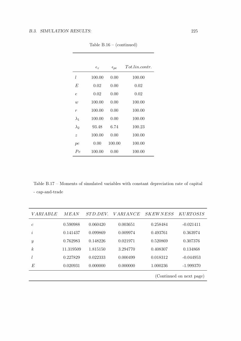
B.3. SIMULATION RESULTS: 225
Table B.16 – (continued)
εz εpe Tot.lin.contr.
l 100.00 0.00 100.00
E 0.02 0.00 0.02
e 0.02 0.00 0.02
w 100.00 0.00 100.00
r 100.00 0.00 100.00
λ1 100.00 0.00 100.00
λ2 93.48 6.74 100.23
z 100.00 0.00 100.00
pe 0.00 100.00 100.00
Pe 100.00 0.00 100.00
Table B.17 – Moments of simulated variables with constant depreciation rate of capital
- cap-and-trade
V ARIABLE MEAN STD.DEV. V ARIANCE SKEWNESS KURTOSIS
c 0.590988 0.060420 0.003651 0.258484 -0.021411
i 0.141437 0.099869 0.009974 0.493761 0.363974
y 0.762983 0.148226 0.021971 0.520869 0.307376
k 11.319509 1.815150 3.294770 0.408307 0.134868
l 0.227829 0.022333 0.000499 0.018312 -0.044953
E 0.020931 0.000000 0.000000 1.000236 -1.999370
(Continued on next page)
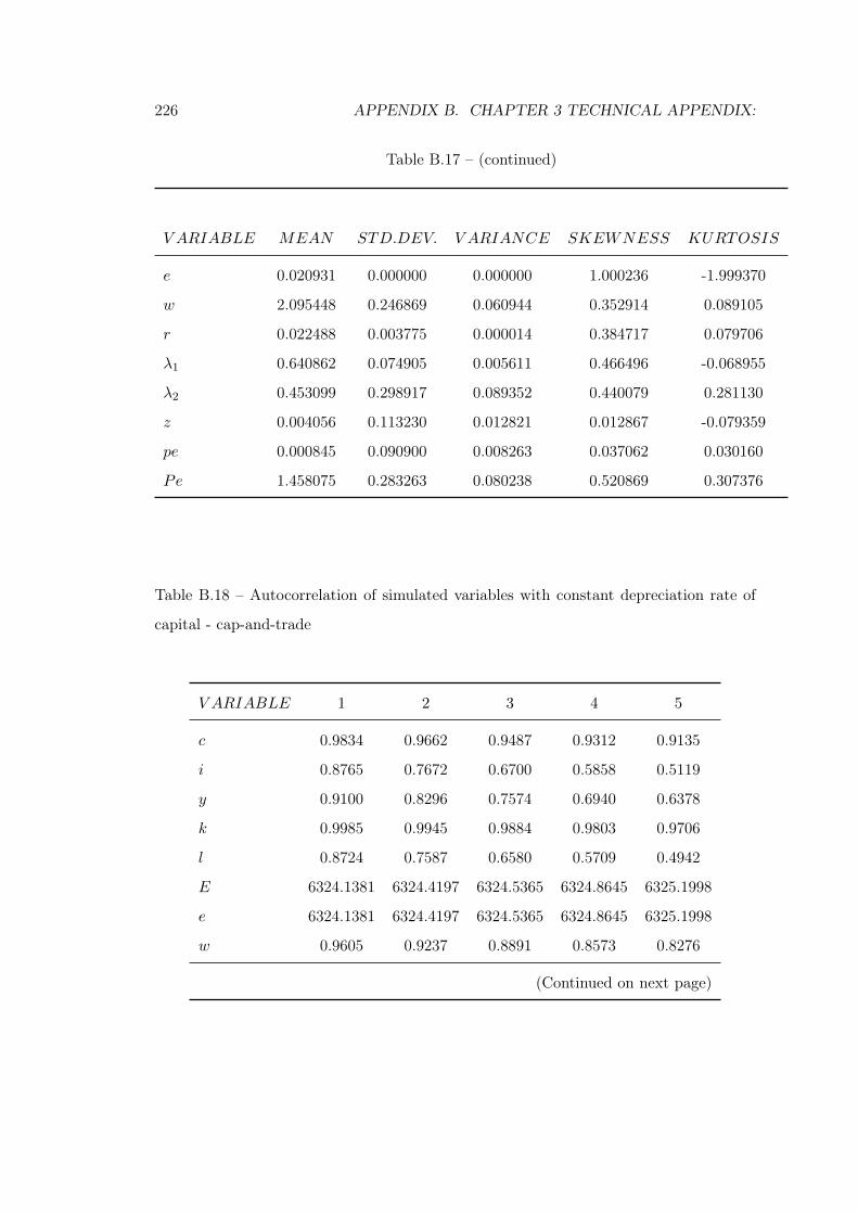
226 APPENDIX B. CHAPTER 3 TECHNICAL APPENDIX:
Table B.17 – (continued)
V ARIABLE MEAN STD.DEV. V ARIANCE SKEWNESS KURTOSIS
e 0.020931 0.000000 0.000000 1.000236 -1.999370
w 2.095448 0.246869 0.060944 0.352914 0.089105
r 0.022488 0.003775 0.000014 0.384717 0.079706
λ1 0.640862 0.074905 0.005611 0.466496 -0.068955
λ2 0.453099 0.298917 0.089352 0.440079 0.281130
z 0.004056 0.113230 0.012821 0.012867 -0.079359
pe 0.000845 0.090900 0.008263 0.037062 0.030160
Pe 1.458075 0.283263 0.080238 0.520869 0.307376
Table B.18 – Autocorrelation of simulated variables with constant depreciation rate of
capital - cap-and-trade
V ARIABLE 1 2 3 4 5
c 0.9834 0.9662 0.9487 0.9312 0.9135
i 0.8765 0.7672 0.6700 0.5858 0.5119
y 0.9100 0.8296 0.7574 0.6940 0.6378
k 0.9985 0.9945 0.9884 0.9803 0.9706
l 0.8724 0.7587 0.6580 0.5709 0.4942
E 6324.1381 6324.4197 6324.5365 6324.8645 6325.1998
e 6324.1381 6324.4197 6324.5365 6324.8645 6325.1998
w 0.9605 0.9237 0.8891 0.8573 0.8276
(Continued on next page)
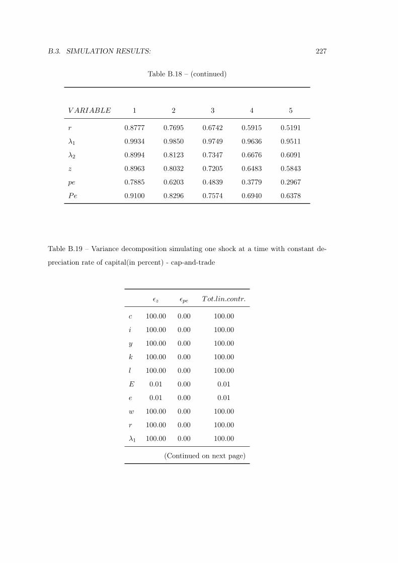
B.3. SIMULATION RESULTS: 227
Table B.18 – (continued)
V ARIABLE 1 2 3 4 5
r 0.8777 0.7695 0.6742 0.5915 0.5191
λ1 0.9934 0.9850 0.9749 0.9636 0.9511
λ2 0.8994 0.8123 0.7347 0.6676 0.6091
z 0.8963 0.8032 0.7205 0.6483 0.5843
pe 0.7885 0.6203 0.4839 0.3779 0.2967
Pe 0.9100 0.8296 0.7574 0.6940 0.6378
Table B.19 – Variance decomposition simulating one shock at a time with constant de-
preciation rate of capital(in percent) - cap-and-trade
εz εpe Tot.lin.contr.
c 100.00 0.00 100.00
i 100.00 0.00 100.00
y 100.00 0.00 100.00
k 100.00 0.00 100.00
l 100.00 0.00 100.00
E 0.01 0.00 0.01
e 0.01 0.00 0.01
w 100.00 0.00 100.00
r 100.00 0.00 100.00
λ1 100.00 0.00 100.00
(Continued on next page)
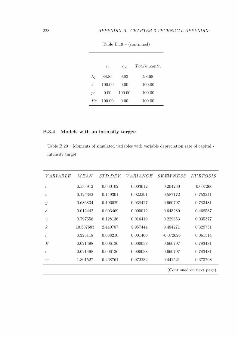
228 APPENDIX B. CHAPTER 3 TECHNICAL APPENDIX:
Table B.19 – (continued)
εz εpe Tot.lin.contr.
λ2 88.85 9.83 98.68
z 100.00 0.00 100.00
pe 0.00 100.00 100.00
Pe 100.00 0.00 100.00
B.3.4 Models with an intensity target:
Table B.20 – Moments of simulated variables with variable depreciation rate of capital -
intensity target
V ARIABLE MEAN STD.DEV. V ARIANCE SKEWNESS KURTOSIS
c 0.533912 0.060102 0.003612 0.204230 -0.007266
i 0.125382 0.149301 0.022291 0.587172 0.753241
y 0.686834 0.196029 0.038427 0.660797 0.783481
δ 0.012442 0.003469 0.000012 0.643280 0.468587
u 0.797656 0.128136 0.016419 0.229853 0.035377
k 10.507683 2.440787 5.957444 0.484271 0.329751
l 0.225118 0.038210 0.001460 -0.072626 0.061514
E 0.021498 0.006136 0.000038 0.660797 0.783481
e 0.021498 0.006136 0.000038 0.660797 0.783481
w 1.891527 0.268761 0.072232 0.442521 0.373798
(Continued on next page)
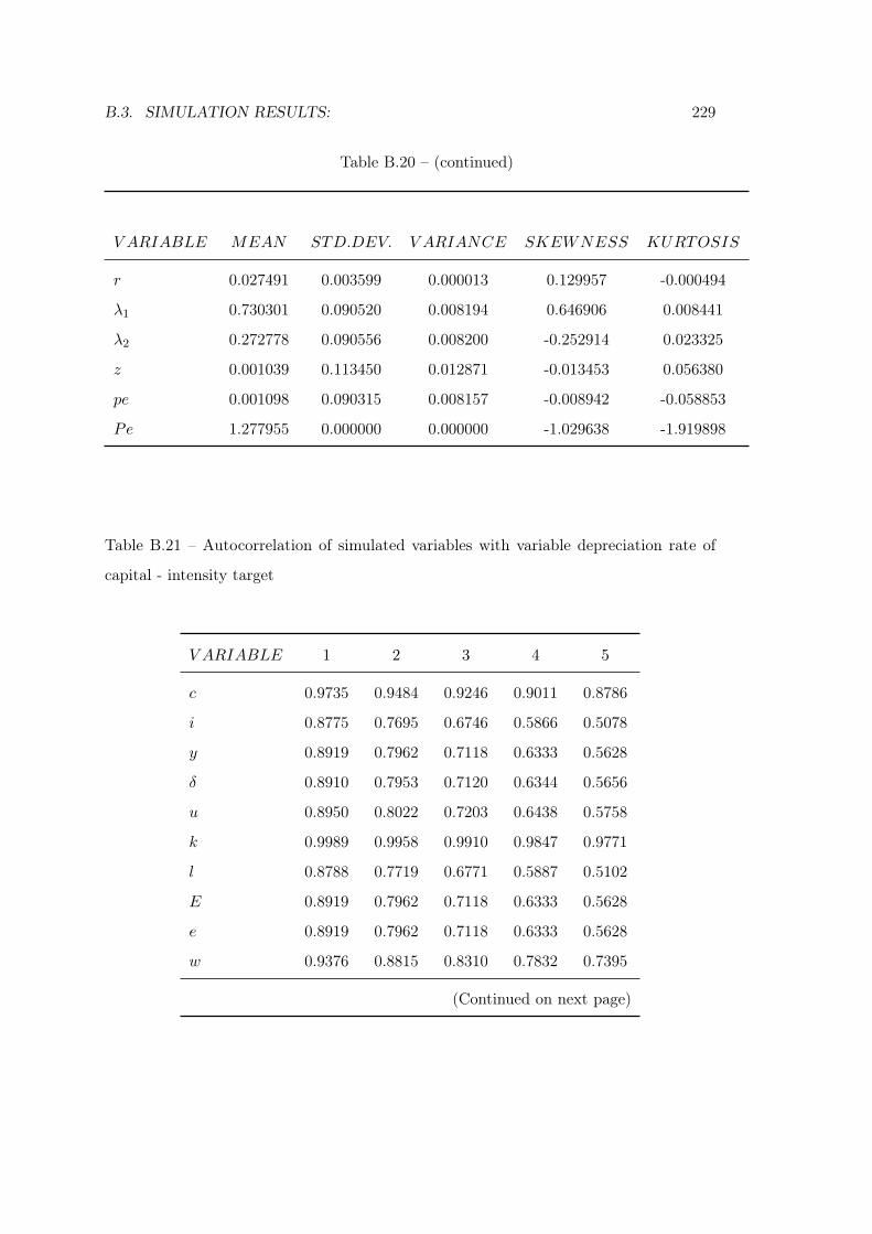
B.3. SIMULATION RESULTS: 229
Table B.20 – (continued)
V ARIABLE MEAN STD.DEV. V ARIANCE SKEWNESS KURTOSIS
r 0.027491 0.003599 0.000013 0.129957 -0.000494
λ1 0.730301 0.090520 0.008194 0.646906 0.008441
λ2 0.272778 0.090556 0.008200 -0.252914 0.023325
z 0.001039 0.113450 0.012871 -0.013453 0.056380
pe 0.001098 0.090315 0.008157 -0.008942 -0.058853
Pe 1.277955 0.000000 0.000000 -1.029638 -1.919898
Table B.21 – Autocorrelation of simulated variables with variable depreciation rate of
capital - intensity target
V ARIABLE 1 2 3 4 5
c 0.9735 0.9484 0.9246 0.9011 0.8786
i 0.8775 0.7695 0.6746 0.5866 0.5078
y 0.8919 0.7962 0.7118 0.6333 0.5628
δ 0.8910 0.7953 0.7120 0.6344 0.5656
u 0.8950 0.8022 0.7203 0.6438 0.5758
k 0.9989 0.9958 0.9910 0.9847 0.9771
l 0.8788 0.7719 0.6771 0.5887 0.5102
E 0.8919 0.7962 0.7118 0.6333 0.5628
e 0.8919 0.7962 0.7118 0.6333 0.5628
w 0.9376 0.8815 0.8310 0.7832 0.7395
(Continued on next page)
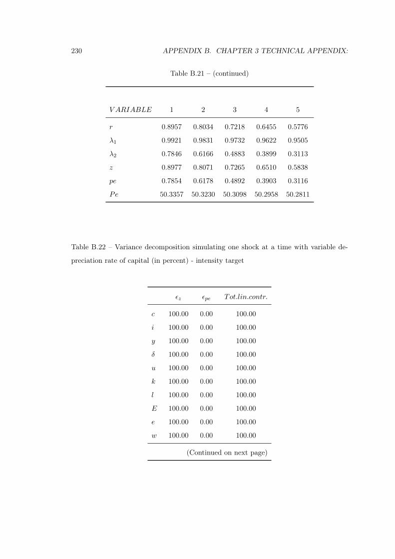
230 APPENDIX B. CHAPTER 3 TECHNICAL APPENDIX:
Table B.21 – (continued)
V ARIABLE 1 2 3 4 5
r 0.8957 0.8034 0.7218 0.6455 0.5776
λ1 0.9921 0.9831 0.9732 0.9622 0.9505
λ2 0.7846 0.6166 0.4883 0.3899 0.3113
z 0.8977 0.8071 0.7265 0.6510 0.5838
pe 0.7854 0.6178 0.4892 0.3903 0.3116
Pe 50.3357 50.3230 50.3098 50.2958 50.2811
Table B.22 – Variance decomposition simulating one shock at a time with variable de-
preciation rate of capital (in percent) - intensity target
εz εpe Tot.lin.contr.
c 100.00 0.00 100.00
i 100.00 0.00 100.00
y 100.00 0.00 100.00
δ 100.00 0.00 100.00
u 100.00 0.00 100.00
k 100.00 0.00 100.00
l 100.00 0.00 100.00
E 100.00 0.00 100.00
e 100.00 0.00 100.00
w 100.00 0.00 100.00
(Continued on next page)
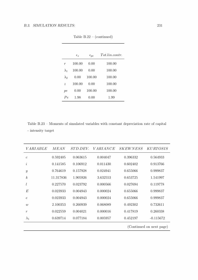
B.3. SIMULATION RESULTS: 231
Table B.22 – (continued)
εz εpe Tot.lin.contr.
r 100.00 0.00 100.00
λ1 100.00 0.00 100.00
λ2 0.00 100.00 100.00
z 100.00 0.00 100.00
pe 0.00 100.00 100.00
Pe 1.98 0.00 1.99
Table B.23 – Moments of simulated variables with constant depreciation rate of capital
- intensity target
V ARIABLE MEAN STD.DEV. V ARIANCE SKEWNESS KURTOSIS
c 0.592405 0.063615 0.004047 0.396332 0.564933
i 0.141585 0.106912 0.011430 0.602402 0.913766
y 0.764619 0.157928 0.024941 0.655066 0.999837
k 11.317836 1.905926 3.632553 0.653725 1.541997
l 0.227570 0.023792 0.000566 0.027694 0.119778
E 0.023933 0.004943 0.000024 0.655066 0.999837
e 0.023933 0.004943 0.000024 0.655066 0.999837
w 2.100353 0.260939 0.068089 0.492302 0.732611
r 0.022559 0.004021 0.000016 0.417819 0.260338
λ1 0.639714 0.077184 0.005957 0.452197 -0.115672
(Continued on next page)
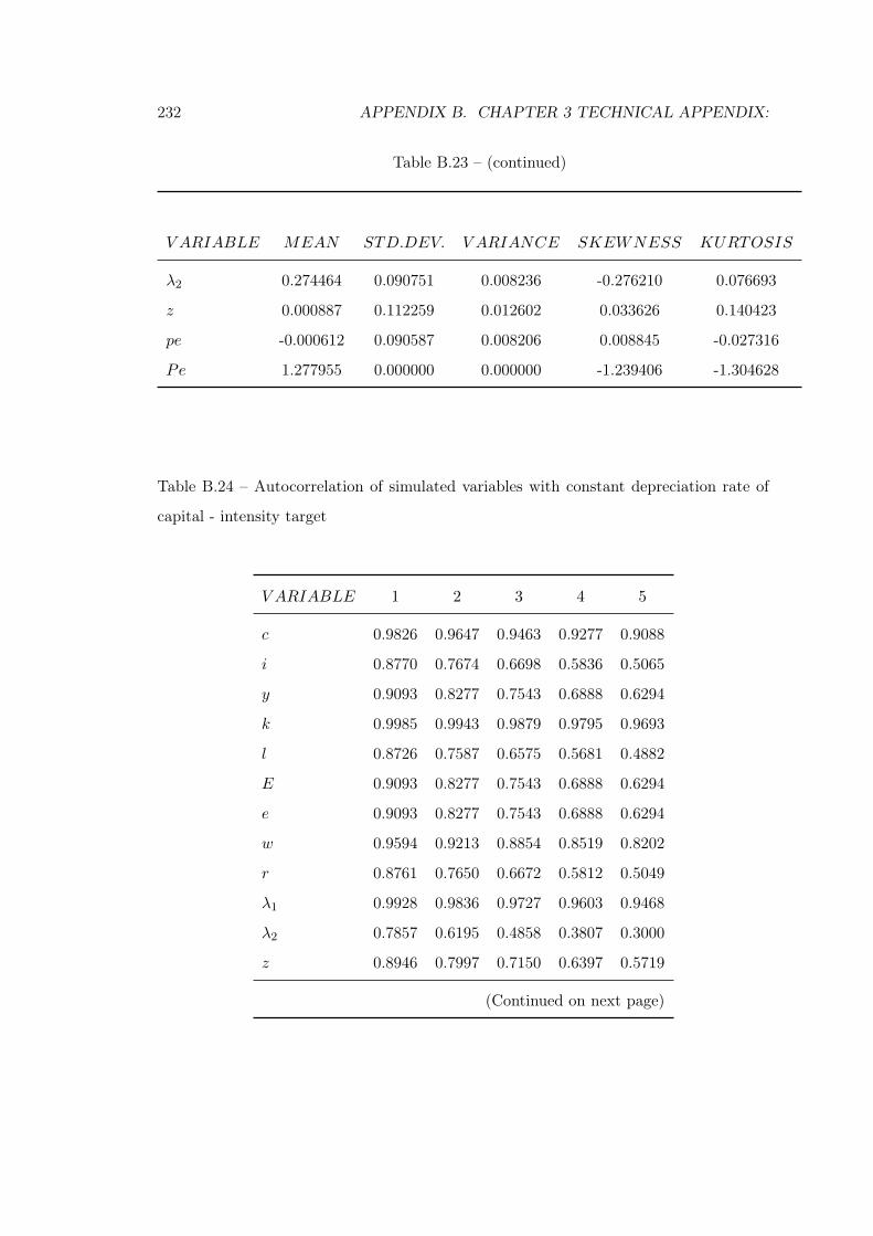
232 APPENDIX B. CHAPTER 3 TECHNICAL APPENDIX:
Table B.23 – (continued)
V ARIABLE MEAN STD.DEV. V ARIANCE SKEWNESS KURTOSIS
λ2 0.274464 0.090751 0.008236 -0.276210 0.076693
z 0.000887 0.112259 0.012602 0.033626 0.140423
pe -0.000612 0.090587 0.008206 0.008845 -0.027316
Pe 1.277955 0.000000 0.000000 -1.239406 -1.304628
Table B.24 – Autocorrelation of simulated variables with constant depreciation rate of
capital - intensity target
V ARIABLE 1 2 3 4 5
c 0.9826 0.9647 0.9463 0.9277 0.9088
i 0.8770 0.7674 0.6698 0.5836 0.5065
y 0.9093 0.8277 0.7543 0.6888 0.6294
k 0.9985 0.9943 0.9879 0.9795 0.9693
l 0.8726 0.7587 0.6575 0.5681 0.4882
E 0.9093 0.8277 0.7543 0.6888 0.6294
e 0.9093 0.8277 0.7543 0.6888 0.6294
w 0.9594 0.9213 0.8854 0.8519 0.8202
r 0.8761 0.7650 0.6672 0.5812 0.5049
λ1 0.9928 0.9836 0.9727 0.9603 0.9468
λ2 0.7857 0.6195 0.4858 0.3807 0.3000
z 0.8946 0.7997 0.7150 0.6397 0.5719
(Continued on next page)
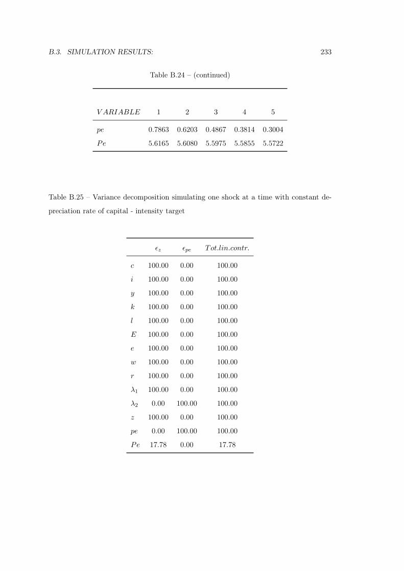
B.3. SIMULATION RESULTS: 233
Table B.24 – (continued)
V ARIABLE 1 2 3 4 5
pe 0.7863 0.6203 0.4867 0.3814 0.3004
Pe 5.6165 5.6080 5.5975 5.5855 5.5722
Table B.25 – Variance decomposition simulating one shock at a time with constant de-
preciation rate of capital - intensity target
εz εpe Tot.lin.contr.
c 100.00 0.00 100.00
i 100.00 0.00 100.00
y 100.00 0.00 100.00
k 100.00 0.00 100.00
l 100.00 0.00 100.00
E 100.00 0.00 100.00
e 100.00 0.00 100.00
w 100.00 0.00 100.00
r 100.00 0.00 100.00
λ1 100.00 0.00 100.00
λ2 0.00 100.00 100.00
z 100.00 0.00 100.00
pe 0.00 100.00 100.00
Pe 17.78 0.00 17.78

234 APPENDIX B. CHAPTER 3 TECHNICAL APPENDIX:
B.4 Simulations:
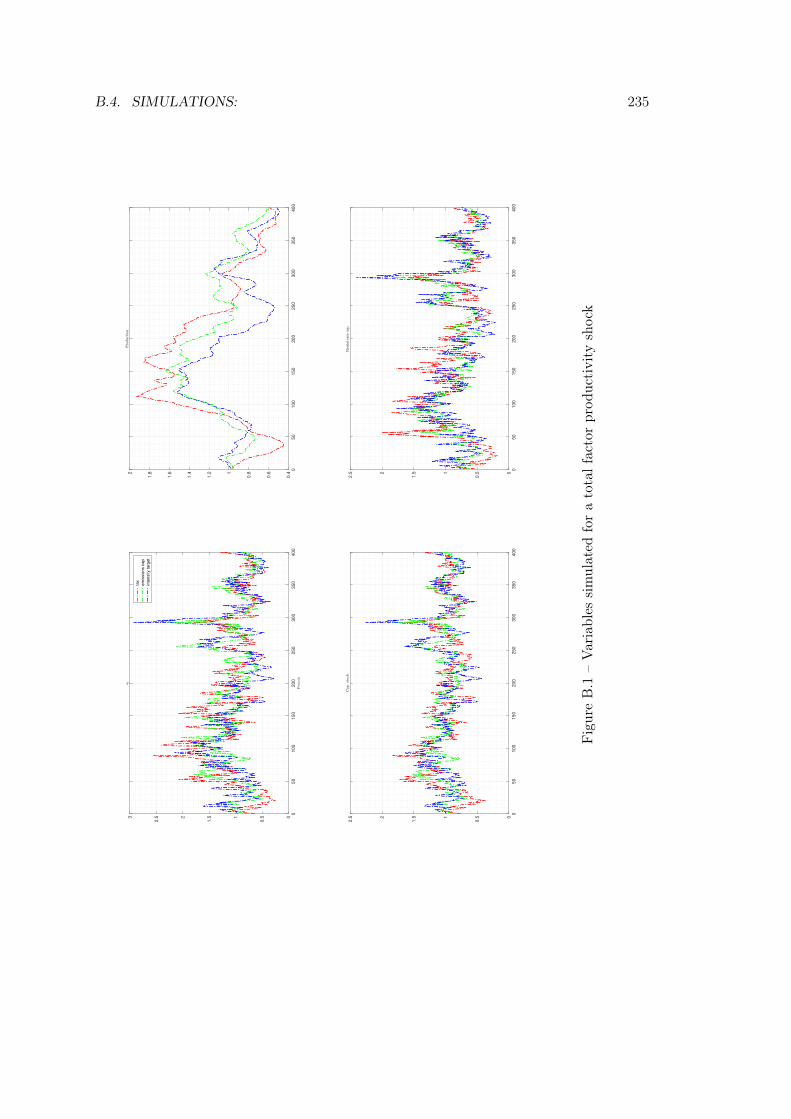
B.4. SIMULATIONS: 235
05
01
00
15
02
00
25
03
00
35
04
00
0
0.51
1.52
2.53
tax
em
issio
ns c
ap
inte
nsity t
arg
et
05
01
00
15
02
00
25
03
00
35
04
00
0.4
0.6
0.81
1.2
1.4
1.6
1.82
05
01
00
15
02
00
25
03
00
35
04
00
0
0.51
1.52
2.5
05
01
00
15
02
00
25
03
00
35
04
00
0
0.51
1.52
2.5
FigureB.1
–Variables
simulated
foratotalfactorprod
uctivity
shock
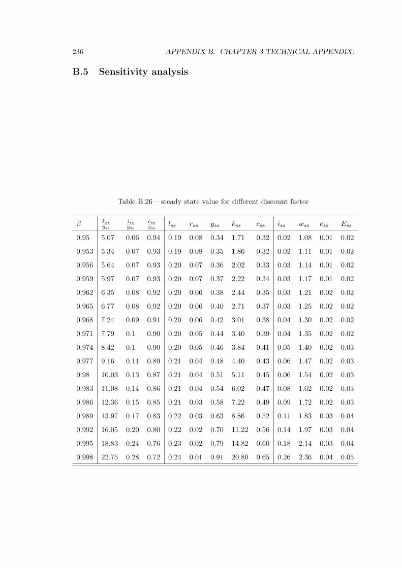
236 APPENDIX B. CHAPTER 3 TECHNICAL APPENDIX:
B.5 Sensitivity analysis
Table B.26 – steady state value for different discount factor
β kssyss
issyss
cssyss
lss rss yss kss css iss wss ess Ess
0.95 5.07 0.06 0.94 0.19 0.08 0.34 1.71 0.32 0.02 1.08 0.01 0.02
0.953 5.34 0.07 0.93 0.19 0.08 0.35 1.86 0.32 0.02 1.11 0.01 0.02
0.956 5.64 0.07 0.93 0.20 0.07 0.36 2.02 0.33 0.03 1.14 0.01 0.02
0.959 5.97 0.07 0.93 0.20 0.07 0.37 2.22 0.34 0.03 1.17 0.01 0.02
0.962 6.35 0.08 0.92 0.20 0.06 0.38 2.44 0.35 0.03 1.21 0.02 0.02
0.965 6.77 0.08 0.92 0.20 0.06 0.40 2.71 0.37 0.03 1.25 0.02 0.02
0.968 7.24 0.09 0.91 0.20 0.06 0.42 3.01 0.38 0.04 1.30 0.02 0.02
0.971 7.79 0.1 0.90 0.20 0.05 0.44 3.40 0.39 0.04 1.35 0.02 0.02
0.974 8.42 0.1 0.90 0.20 0.05 0.46 3.84 0.41 0.05 1.40 0.02 0.03
0.977 9.16 0.11 0.89 0.21 0.04 0.48 4.40 0.43 0.06 1.47 0.02 0.03
0.98 10.03 0.13 0.87 0.21 0.04 0.51 5.11 0.45 0.06 1.54 0.02 0.03
0.983 11.08 0.14 0.86 0.21 0.04 0.54 6.02 0.47 0.08 1.62 0.02 0.03
0.986 12.36 0.15 0.85 0.21 0.03 0.58 7.22 0.49 0.09 1.72 0.02 0.03
0.989 13.97 0.17 0.83 0.22 0.03 0.63 8.86 0.52 0.11 1.83 0.03 0.04
0.992 16.05 0.20 0.80 0.22 0.02 0.70 11.22 0.56 0.14 1.97 0.03 0.04
0.995 18.83 0.24 0.76 0.23 0.02 0.79 14.82 0.60 0.18 2.14 0.03 0.04
0.998 22.75 0.28 0.72 0.24 0.01 0.91 20.80 0.65 0.26 2.36 0.04 0.05
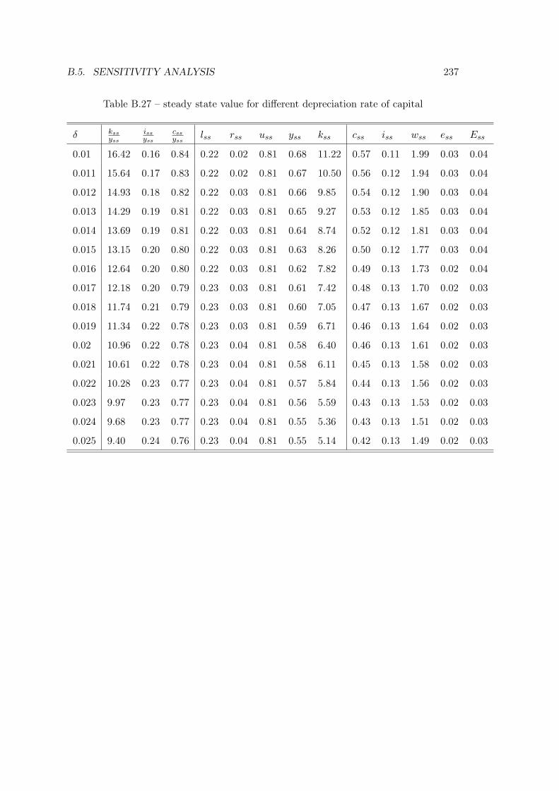
B.5. SENSITIVITY ANALYSIS 237
Table B.27 – steady state value for different depreciation rate of capital
δ kssyss
issyss
cssyss
lss rss uss yss kss css iss wss ess Ess
0.01 16.42 0.16 0.84 0.22 0.02 0.81 0.68 11.22 0.57 0.11 1.99 0.03 0.04
0.011 15.64 0.17 0.83 0.22 0.02 0.81 0.67 10.50 0.56 0.12 1.94 0.03 0.04
0.012 14.93 0.18 0.82 0.22 0.03 0.81 0.66 9.85 0.54 0.12 1.90 0.03 0.04
0.013 14.29 0.19 0.81 0.22 0.03 0.81 0.65 9.27 0.53 0.12 1.85 0.03 0.04
0.014 13.69 0.19 0.81 0.22 0.03 0.81 0.64 8.74 0.52 0.12 1.81 0.03 0.04
0.015 13.15 0.20 0.80 0.22 0.03 0.81 0.63 8.26 0.50 0.12 1.77 0.03 0.04
0.016 12.64 0.20 0.80 0.22 0.03 0.81 0.62 7.82 0.49 0.13 1.73 0.02 0.04
0.017 12.18 0.20 0.79 0.23 0.03 0.81 0.61 7.42 0.48 0.13 1.70 0.02 0.03
0.018 11.74 0.21 0.79 0.23 0.03 0.81 0.60 7.05 0.47 0.13 1.67 0.02 0.03
0.019 11.34 0.22 0.78 0.23 0.03 0.81 0.59 6.71 0.46 0.13 1.64 0.02 0.03
0.02 10.96 0.22 0.78 0.23 0.04 0.81 0.58 6.40 0.46 0.13 1.61 0.02 0.03
0.021 10.61 0.22 0.78 0.23 0.04 0.81 0.58 6.11 0.45 0.13 1.58 0.02 0.03
0.022 10.28 0.23 0.77 0.23 0.04 0.81 0.57 5.84 0.44 0.13 1.56 0.02 0.03
0.023 9.97 0.23 0.77 0.23 0.04 0.81 0.56 5.59 0.43 0.13 1.53 0.02 0.03
0.024 9.68 0.23 0.77 0.23 0.04 0.81 0.55 5.36 0.43 0.13 1.51 0.02 0.03
0.025 9.40 0.24 0.76 0.23 0.04 0.81 0.55 5.14 0.42 0.13 1.49 0.02 0.03

238 APPENDIX B. CHAPTER 3 TECHNICAL APPENDIX:
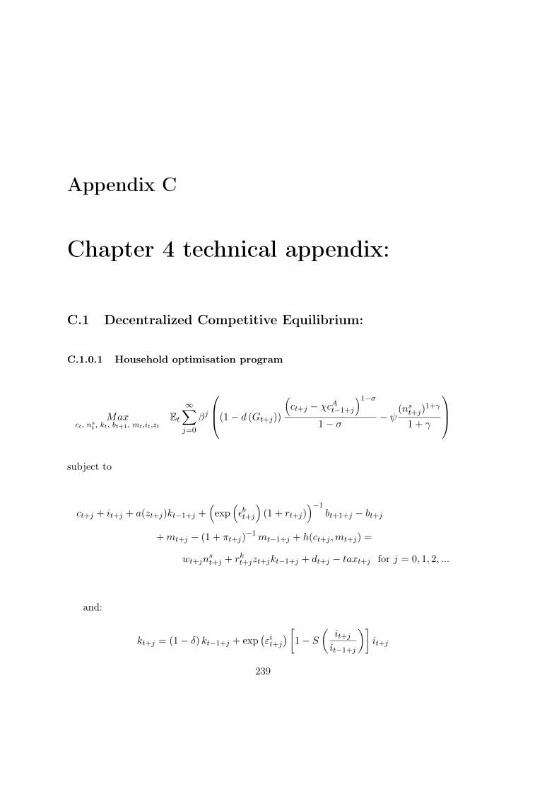
Appendix C
Chapter 4 technical appendix:
C.1 Decentralized Competitive Equilibrium:
C.1.0.1 Household optimisation program
Maxct, nst , kt, bt+1, mt,it,zt
Et∞∑
j=0
βj
(1− d (Gt+j))
(ct+j − χcAt−1+j
)1−σ
1− σ − ψ(nst+j)
1+γ
1 + γ
subject to
ct+j + it+j + a(zt+j)kt−1+j +(
exp(εbt+j
)(1 + rt+j)
)−1bt+1+j − bt+j
+mt+j − (1 + πt+j)−1mt−1+j + h(ct+j ,mt+j) =
wt+jnst+j + rkt+jzt+jkt−1+j + dt+j − taxt+j for j = 0, 1, 2, ...
and:
kt+j = (1− δ) kt−1+j + exp(εit+j
) [1− S
(it+jit−1+j
)]it+j
239
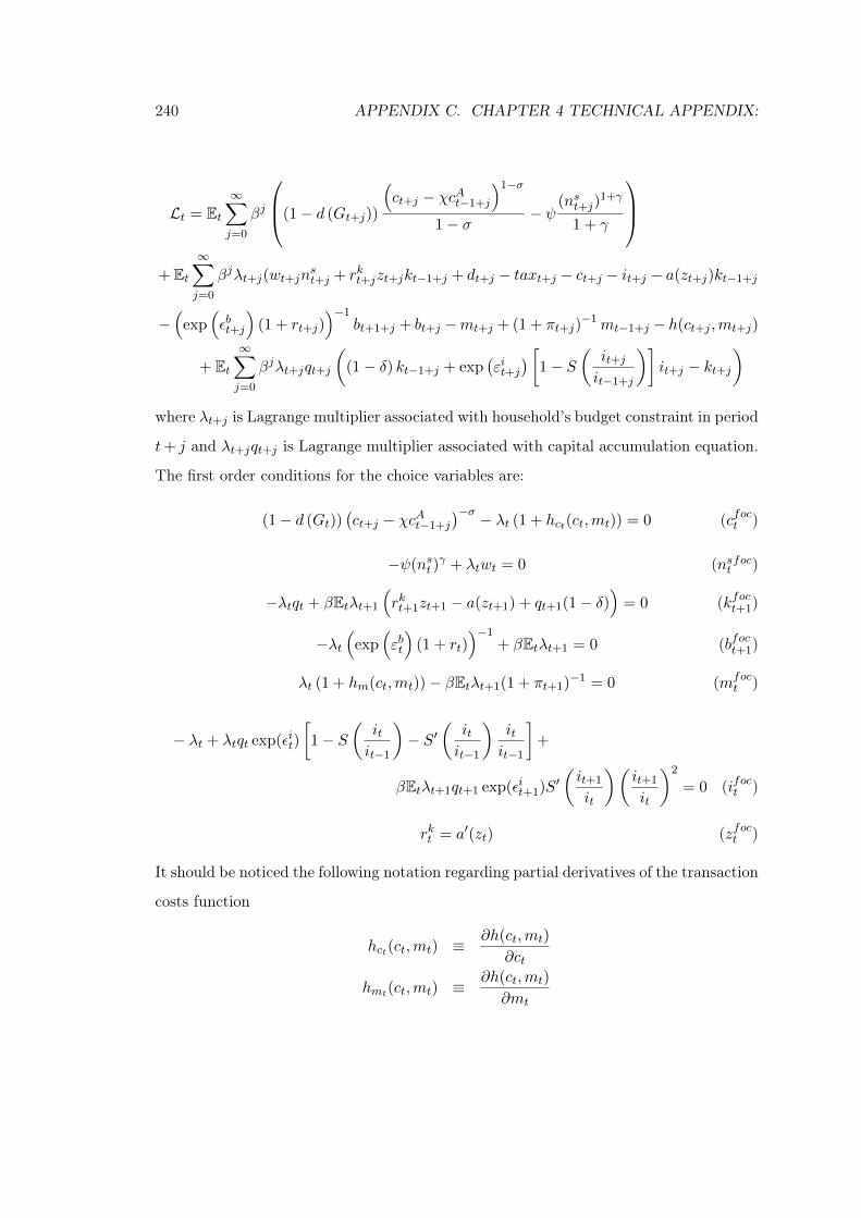
240 APPENDIX C. CHAPTER 4 TECHNICAL APPENDIX:
Lt = Et∞∑
j=0
βj
(1− d (Gt+j))
(ct+j − χcAt−1+j
)1−σ
1− σ − ψ(nst+j)
1+γ
1 + γ
+ Et∞∑
j=0
βjλt+j(wt+jnst+j + rkt+jzt+jkt−1+j + dt+j − taxt+j − ct+j − it+j − a(zt+j)kt−1+j
−(
exp(εbt+j
)(1 + rt+j)
)−1bt+1+j + bt+j −mt+j + (1 + πt+j)
−1mt−1+j − h(ct+j ,mt+j)
+ Et∞∑
j=0
βjλt+jqt+j
((1− δ) kt−1+j + exp
(εit+j
) [1− S
(it+jit−1+j
)]it+j − kt+j
)
where λt+j is Lagrange multiplier associated with household’s budget constraint in period
t+ j and λt+jqt+j is Lagrange multiplier associated with capital accumulation equation.
The first order conditions for the choice variables are:
(1− d (Gt))(ct+j − χcAt−1+j
)−σ − λt (1 + hct(ct,mt)) = 0 (cfoct )
−ψ(nst )γ + λtwt = 0 (nst foc)
−λtqt + βEtλt+1
(rkt+1zt+1 − a(zt+1) + qt+1(1− δ)
)= 0 (kfoct+1)
−λt(
exp(εbt
)(1 + rt)
)−1+ βEtλt+1 = 0 (bfoct+1)
λt (1 + hm(ct,mt))− βEtλt+1(1 + πt+1)−1 = 0 (mfoct )
− λt + λtqt exp(εit)
[1− S
(itit−1
)− S′
(itit−1
)itit−1
]+
βEtλt+1qt+1 exp(εit+1)S′(it+1
it
)(it+1
it
)2
= 0 (ifoct )
rkt = a′(zt) (zfoct )
It should be noticed the following notation regarding partial derivatives of the transaction
costs function
hct(ct,mt) ≡∂h(ct,mt)
∂ct
hmt(ct,mt) ≡∂h(ct,mt)
∂mt
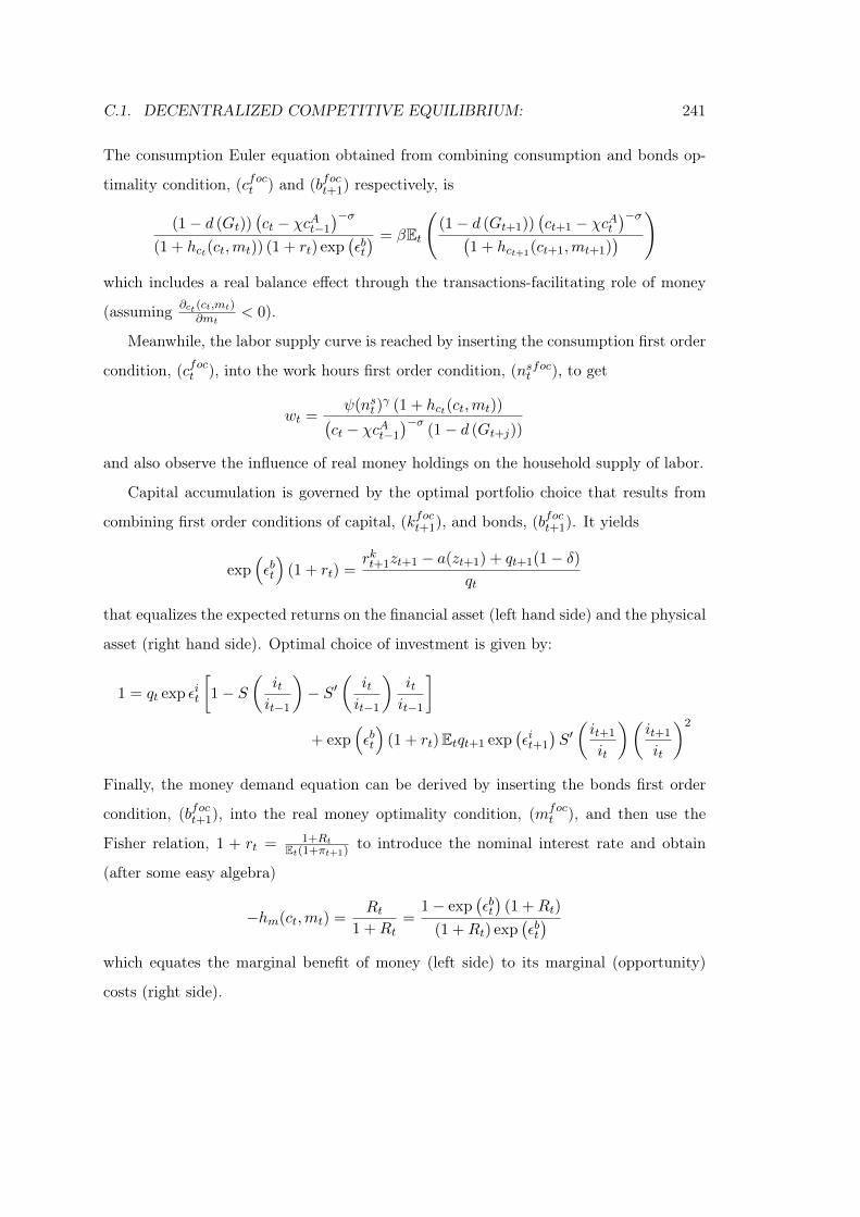
C.1. DECENTRALIZED COMPETITIVE EQUILIBRIUM: 241
The consumption Euler equation obtained from combining consumption and bonds op-
timality condition, (cfoct ) and (bfoct+1) respectively, is
(1− d (Gt))(ct − χcAt−1
)−σ
(1 + hct(ct,mt)) (1 + rt) exp(εbt) = βEt
((1− d (Gt+1))
(ct+1 − χcAt
)−σ(1 + hct+1(ct+1,mt+1)
))
which includes a real balance effect through the transactions-facilitating role of money
(assuming ∂ct (ct,mt)∂mt
< 0).
Meanwhile, the labor supply curve is reached by inserting the consumption first order
condition, (cfoct ), into the work hours first order condition, (nstfoc), to get
wt =ψ(nst )
γ (1 + hct(ct,mt))(ct − χcAt−1
)−σ(1− d (Gt+j))
and also observe the influence of real money holdings on the household supply of labor.
Capital accumulation is governed by the optimal portfolio choice that results from
combining first order conditions of capital, (kfoct+1), and bonds, (bfoct+1). It yields
exp(εbt
)(1 + rt) =
rkt+1zt+1 − a(zt+1) + qt+1(1− δ)qt
that equalizes the expected returns on the financial asset (left hand side) and the physical
asset (right hand side). Optimal choice of investment is given by:
1 = qt exp εit
[1− S
(itit−1
)− S′
(itit−1
)itit−1
]
+ exp(εbt
)(1 + rt)Etqt+1 exp
(εit+1
)S′(it+1
it
)(it+1
it
)2
Finally, the money demand equation can be derived by inserting the bonds first order
condition, (bfoct+1), into the real money optimality condition, (mfoct ), and then use the
Fisher relation, 1 + rt = 1+RtEt(1+πt+1) to introduce the nominal interest rate and obtain
(after some easy algebra)
−hm(ct,mt) =Rt
1 +Rt=
1− exp(εbt)
(1 +Rt)
(1 +Rt) exp(εbt)
which equates the marginal benefit of money (left side) to its marginal (opportunity)
costs (right side).
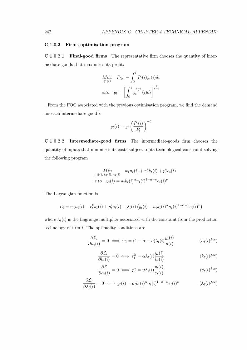
242 APPENDIX C. CHAPTER 4 TECHNICAL APPENDIX:
C.1.0.2 Firms optimisation program
C.1.0.2.1 Final-good firms The representative firm chooses the quantity of inter-
mediate goods that maximises its profit:
Maxyt(i)
Ptyt −∫ 1
0Pt(i)yt(i)di
s.to yt =
[∫ 1
0yθ−1θ
t (i)di
] θθ−1
. From the FOC associated with the previous optimisation program, we find the demand
for each intermediate good i:
yt(i) = yt
(Pt(i)
Pt
)−θ
C.1.0.2.2 Intermediate-good firms The intermediate-goods firm chooses the
quantity of inputs that minimises its costs subject to its technological constraint solving
the following program
Minnt(i), kt(i), et(i)
wtnt(i) + rkt kt(i) + petet(i)
s.to yt(i) = atkt(i)αnt(i)
1−α−υet(i)υ
The Lagrangian function is
Lt = wtnt(i) + rkt kt(i) + petet(i) + λt(i)(yt(i)− atkt(i)αnt(i)1−α−υet(i)υ
)
where λt(i) is the Lagrange multiplier associated with the constaint from the production
technology of firm i. The optimality conditions are
∂Lt∂nt(i)
= 0 ⇐⇒ wt = (1− α− υ)λt(i)yt(i)
n(i)(nt(i)foc)
∂Lt∂kt(i)
= 0 ⇐⇒ rkt = αλt(i)yt(i)
kt(i)(kt(i)foc)
∂L∂et(i)
= 0 ⇐⇒ pet = υλt(i)yt(i)
et(i)(et(i)foc)
∂Lt∂λt(i)
= 0 ⇐⇒ yt(i) = atkt(i)αnt(i)
1−α−υet(i)υ (λt(i)foc)
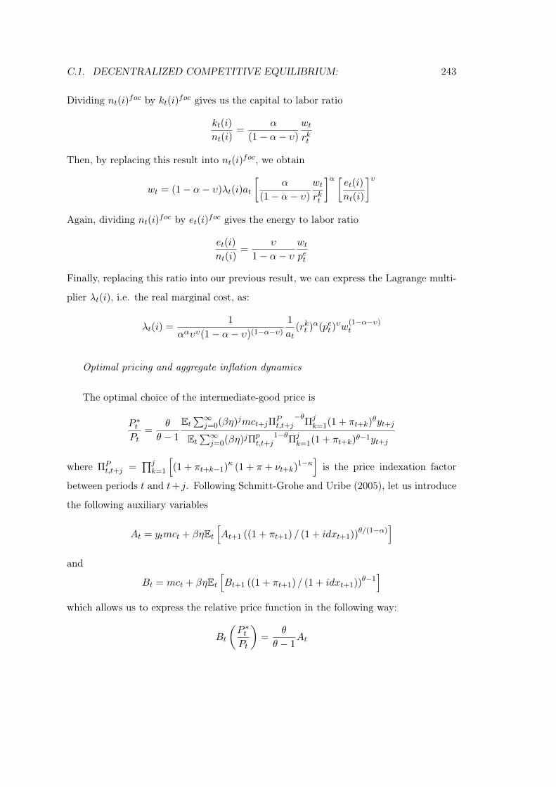
C.1. DECENTRALIZED COMPETITIVE EQUILIBRIUM: 243
Dividing nt(i)foc by kt(i)foc gives us the capital to labor ratio
kt(i)
nt(i)=
α
(1− α− υ)
wt
rkt
Then, by replacing this result into nt(i)foc, we obtain
wt = (1− α− υ)λt(i)at
[α
(1− α− υ)
wt
rkt
]α [ et(i)nt(i)
]υ
Again, dividing nt(i)foc by et(i)foc gives the energy to labor ratio
et(i)
nt(i)=
υ
1− α− υwtpet
Finally, replacing this ratio into our previous result, we can express the Lagrange multi-
plier λt(i), i.e. the real marginal cost, as:
λt(i) =1
ααυυ(1− α− υ)(1−α−υ)
1
at(rkt )α(pet )
υw(1−α−υ)t
Optimal pricing and aggregate inflation dynamics
The optimal choice of the intermediate-good price is
P ∗tPt
=θ
θ − 1
Et∑∞
j=0(βη)jmct+jΠPt,t+j
−θΠjk=1(1 + πt+k)
θyt+j
Et∑∞
j=0(βη)jΠpt,t+j
1−θΠjk=1(1 + πt+k)θ−1yt+j
where ΠPt,t+j =
∏jk=1
[(1 + πt+k−1)κ (1 + π + νt+k)
1−κ]is the price indexation factor
between periods t and t+ j. Following Schmitt-Grohe and Uribe (2005), let us introduce
the following auxiliary variables
At = ytmct + βηEt[At+1 ((1 + πt+1) / (1 + idxt+1))θ/(1−α)
]
and
Bt = mct + βηEt[Bt+1 ((1 + πt+1) / (1 + idxt+1))θ−1
]
which allows us to express the relative price function in the following way:
Bt
(P ∗tPt
)=
θ
θ − 1At
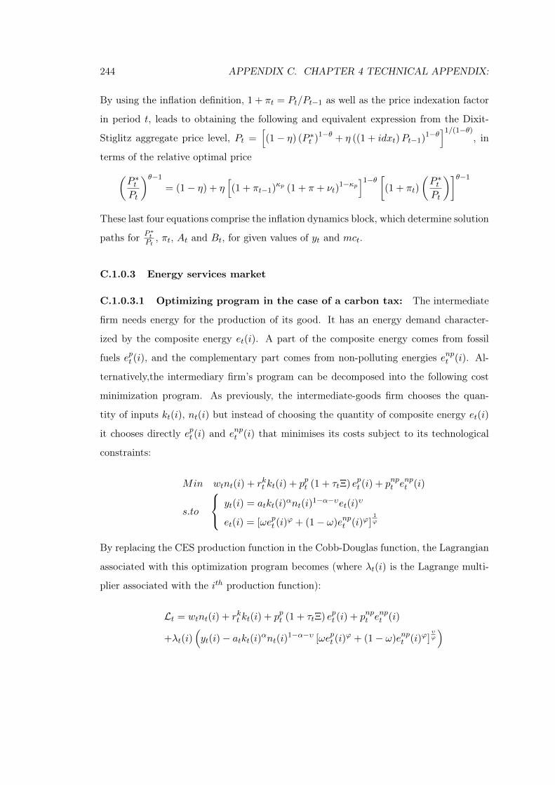
244 APPENDIX C. CHAPTER 4 TECHNICAL APPENDIX:
By using the inflation definition, 1 + πt = Pt/Pt−1 as well as the price indexation factor
in period t, leads to obtaining the following and equivalent expression from the Dixit-
Stiglitz aggregate price level, Pt =[(1− η) (P ∗t )1−θ + η ((1 + idxt)Pt−1)1−θ
]1/(1−θ), in
terms of the relative optimal price
(P ∗tPt
)θ−1
= (1− η) + η[(1 + πt−1)κp (1 + π + νt)
1−κp]1−θ [
(1 + πt)
(P ∗tPt
)]θ−1
These last four equations comprise the inflation dynamics block, which determine solution
paths for P ∗tPt
, πt, At and Bt, for given values of yt and mct.
C.1.0.3 Energy services market
C.1.0.3.1 Optimizing program in the case of a carbon tax: The intermediate
firm needs energy for the production of its good. It has an energy demand character-
ized by the composite energy et(i). A part of the composite energy comes from fossil
fuels ept (i), and the complementary part comes from non-polluting energies enpt (i). Al-
ternatively,the intermediary firm’s program can be decomposed into the following cost
minimization program. As previously, the intermediate-goods firm chooses the quan-
tity of inputs kt(i), nt(i) but instead of choosing the quantity of composite energy et(i)
it chooses directly ept (i) and enpt (i) that minimises its costs subject to its technological
constraints:
Min wtnt(i) + rkt kt(i) + ppt (1 + τtΞ) ept (i) + pnpt enpt (i)
s.to
yt(i) = atkt(i)αnt(i)
1−α−υet(i)υ
et(i) = [ωept (i)ϕ + (1− ω)enpt (i)ϕ]
1ϕ
By replacing the CES production function in the Cobb-Douglas function, the Lagrangian
associated with this optimization program becomes (where λt(i) is the Lagrange multi-
plier associated with the ith production function):
Lt = wtnt(i) + rkt kt(i) + ppt (1 + τtΞ) ept (i) + pnpt enpt (i)
+λt(i)(yt(i)− atkt(i)αnt(i)1−α−υ [ωept (i)
ϕ + (1− ω)enpt (i)ϕ]υϕ
)
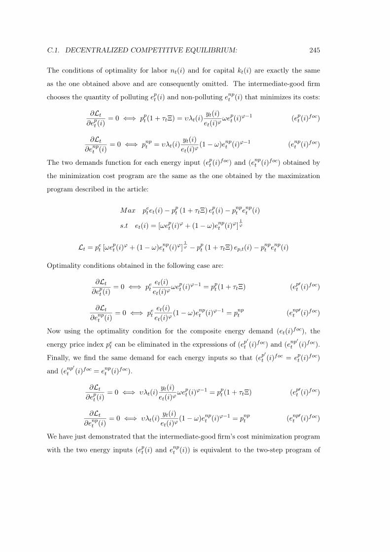
C.1. DECENTRALIZED COMPETITIVE EQUILIBRIUM: 245
The conditions of optimality for labor nt(i) and for capital kt(i) are exactly the same
as the one obtained above and are consequently omitted. The intermediate-good firm
chooses the quantity of polluting ept (i) and non-polluting enpt (i) that minimizes its costs:
∂Lt∂ept (i)
= 0 ⇐⇒ ppt (1 + τtΞ) = υλt(i)yt(i)
et(i)ϕωept (i)
ϕ−1 (ept (i)foc)
∂Lt∂enpt (i)
= 0 ⇐⇒ pnpt = υλt(i)yt(i)
et(i)ϕ(1− ω)enpt (i)ϕ−1 (enpt (i)foc)
The two demands function for each energy input (ept (i)foc) and (enpt (i)foc) obtained by
the minimization cost program are the same as the one obtained by the maximization
program described in the article:
Max petet(i)− ppt (1 + τtΞ) ept (i)− pnpt enpt (i)
s.t et(i) = [ωept (i)ϕ + (1− ω)enpt (i)ϕ]
1ϕ
Lt = pet [ωept (i)ϕ + (1− ω)enpt (i)ϕ]
1ϕ − ppt (1 + τtΞ) ep,t(i)− pnpt enpt (i)
Optimality conditions obtained in the following case are:
∂Lt∂ept (i)
= 0 ⇐⇒ petet(i)
et(i)ϕωept (i)
ϕ−1 = ppt (1 + τtΞ) (ep′t (i)foc)
∂Lt∂enpt (i)
= 0 ⇐⇒ petet(i)
et(i)ϕ(1− ω)enpt (i)ϕ−1 = pnpt (enp′t (i)foc)
Now using the optimality condition for the composite energy demand (et(i)foc), the
energy price index pet can be eliminated in the expressions of (ep′t (i)foc) and (enp
′t (i)foc).
Finally, we find the same demand for each energy inputs so that (ep′t (i)foc = ept (i)
foc)
and (enp′
t (i)foc = enpt (i)foc).
∂Lt∂ept (i)
= 0 ⇐⇒ υλt(i)yt(i)
et(i)ϕωept (i)
ϕ−1 = ppt (1 + τtΞ) (ep′t (i)foc)
∂Lt∂enpt (i)
= 0 ⇐⇒ υλt(i)yt(i)
et(i)ϕ(1− ω)enpt (i)ϕ−1 = pnpt (enp′t (i)foc)
We have just demonstrated that the intermediate-good firm’s cost minimization program
with the two energy inputs (ept (i) and enpt (i)) is equivalent to the two-step program of
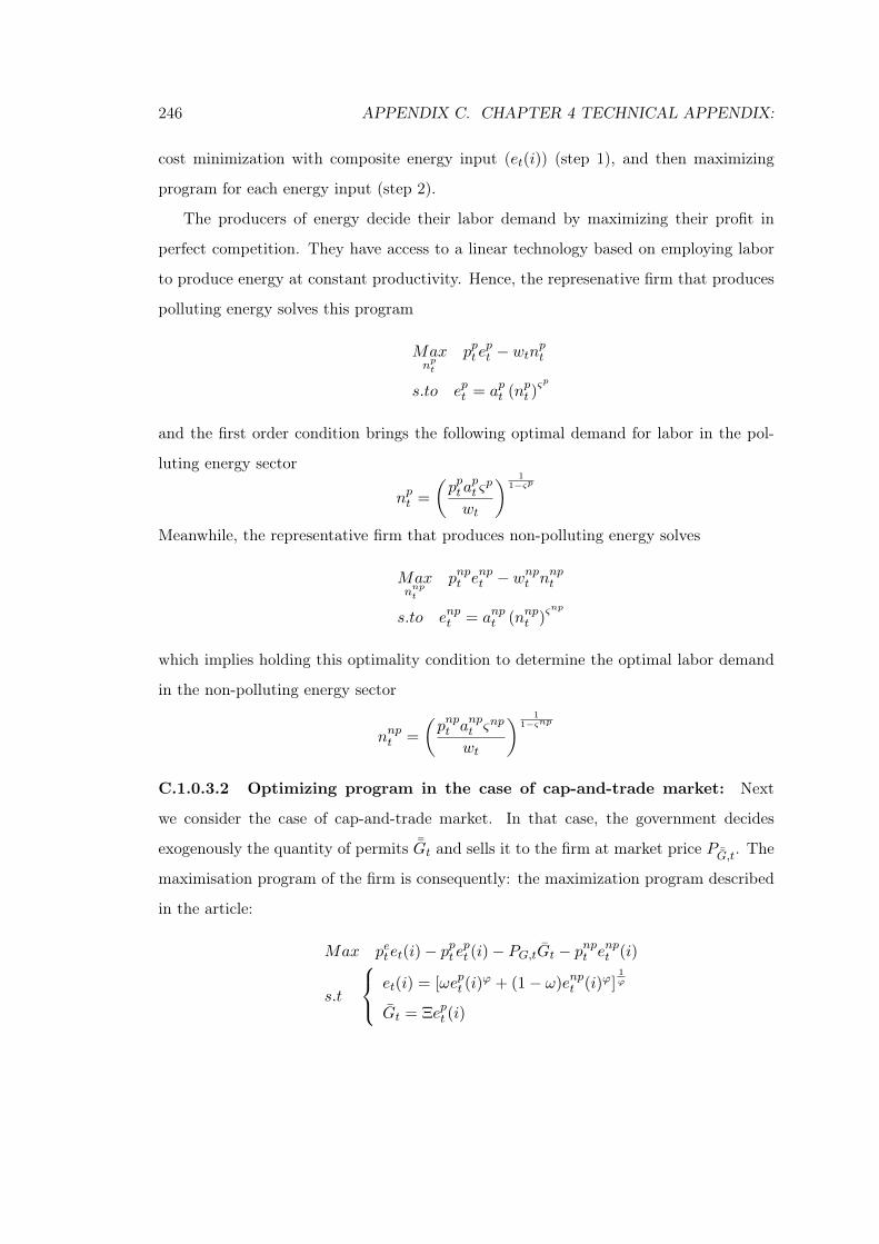
246 APPENDIX C. CHAPTER 4 TECHNICAL APPENDIX:
cost minimization with composite energy input (et(i)) (step 1), and then maximizing
program for each energy input (step 2).
The producers of energy decide their labor demand by maximizing their profit in
perfect competition. They have access to a linear technology based on employing labor
to produce energy at constant productivity. Hence, the represenative firm that produces
polluting energy solves this program
Maxnpt
ppt ept − wtnpt
s.to ept = apt (npt )ςp
and the first order condition brings the following optimal demand for labor in the pol-
luting energy sector
npt =
(ppta
pt ςp
wt
) 11−ςp
Meanwhile, the representative firm that produces non-polluting energy solves
Maxnnpt
pnpt enpt − wnpt nnpt
s.to enpt = anpt (nnpt )ςnp
which implies holding this optimality condition to determine the optimal labor demand
in the non-polluting energy sector
nnpt =
(pnpt a
npt ς
np
wt
) 11−ςnp
C.1.0.3.2 Optimizing program in the case of cap-and-trade market: Next
we consider the case of cap-and-trade market. In that case, the government decides
exogenously the quantity of permits ¯Gt and sells it to the firm at market price P ¯G,t. The
maximisation program of the firm is consequently: the maximization program described
in the article:
Max petet(i)− ppt ept (i)− PG,tGt − pnpt enpt (i)
s.t
et(i) = [ωept (i)ϕ + (1− ω)enpt (i)ϕ]
1ϕ
Gt = Ξept (i)
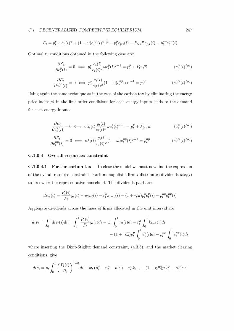
C.1. DECENTRALIZED COMPETITIVE EQUILIBRIUM: 247
Lt = pet [ωept (i)ϕ + (1− ω)enpt (i)ϕ]
1ϕ − ppt ep,t(i)− PG,tΞep,t(i)− pnpt enpt (i)
Optimality conditions obtained in the following case are:
∂Lt∂ept (i)
= 0 ⇐⇒ petet(i)
et(i)ϕωept (i)
ϕ−1 = ppt + PG,tΞ (ep′t (i)foc)
∂Lt∂enpt (i)
= 0 ⇐⇒ petet(i)
et(i)ϕ(1− ω)enpt (i)ϕ−1 = pnpt (enp′t (i)foc)
Using again the same technique as in the case of the carbon tax by eliminating the energy
price index pet in the first order conditions for each energy inputs leads to the demand
for each energy inputs:
∂Lt∂ept (i)
= 0 ⇐⇒ υλt(i)yt(i)
et(i)ϕωept (i)
ϕ−1 = ppt + PG,tΞ (ep′t (i)foc)
∂Lt∂enpt (i)
= 0 ⇐⇒ υλt(i)yt(i)
et(i)ϕ(1− ω)enpt (i)ϕ−1 = pnpt (enp′t (i)foc)
C.1.0.4 Overall resources constraint
C.1.0.4.1 For the carbon tax: To close the model we must now find the expression
of the overall resource constraint. Each monopolistic firm i distributes dividends divt(i)
to its owner the representative household. The dividends paid are:
divt(i) =Pt(i)
Ptyt(i)− wtnt(i)− rkt kt−1(i)− (1 + τtΞ)ppt e
pt (i)− pnpt enpt (i)
Aggregate dividends across the mass of firms allocated in the unit interval are
divt =
∫ 1
0divt(i)di =
∫ 1
0
Pt(i)
Ptyt(i)di− wt
∫ 1
0nt(i)di− rkt
∫ 1
0kt−1(i)di
− (1 + τtΞ)ppt
∫ 1
0ept (i)di− pnpt
∫ 1
0enpt (i)di
where inserting the Dixit-Stiglitz demand constraint, (4.3.5), and the market clearing
conditions, give
divt = yt
∫ 1
0
(Pt(i)
Pt
)1−θdi− wt (nst − npt − nnpt )− rkt kt−1 − (1 + τtΞ)ppt e
pt − pnpt enpt
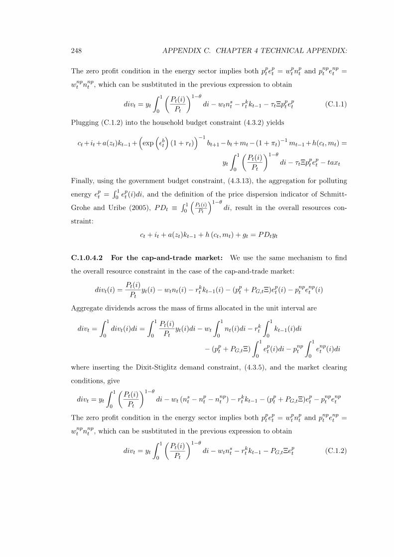
248 APPENDIX C. CHAPTER 4 TECHNICAL APPENDIX:
The zero profit condition in the energy sector implies both ppt ept = wpt n
pt and pnpt e
npt =
wnpt nnpt , which can be susbtituted in the previous expression to obtain
divt = yt
∫ 1
0
(Pt(i)
Pt
)1−θdi− wtnst − rkt kt−1 − τtΞppt ept (C.1.1)
Plugging (C.1.2) into the household budget constraint (4.3.2) yields
ct+ it+a(zt)kt−1 +(
exp(εbt
)(1 + rt)
)−1bt+1−bt+mt− (1 + πt)
−1mt−1 +h(ct,mt) =
yt
∫ 1
0
(Pt(i)
Pt
)1−θdi− τtΞppt ept − taxt
Finally, using the government budget constraint, (4.3.13), the aggregation for polluting
energy ept =∫ 1
0 ept (i)di, and the definition of the price dispersion indicator of Schmitt-
Grohe and Uribe (2005), PDt ≡∫ 1
0
(Pt(i)Pt
)1−θdi, result in the overall resources con-
straint:
ct + it + a(zt)kt−1 + h (ct,mt) + gt = PDtyt
C.1.0.4.2 For the cap-and-trade market: We use the same mechanism to find
the overall resource constraint in the case of the cap-and-trade market:
divt(i) =Pt(i)
Ptyt(i)− wtnt(i)− rkt kt−1(i)− (ppt + PG,tΞ)ept (i)− pnpt enpt (i)
Aggregate dividends across the mass of firms allocated in the unit interval are
divt =
∫ 1
0divt(i)di =
∫ 1
0
Pt(i)
Ptyt(i)di− wt
∫ 1
0nt(i)di− rkt
∫ 1
0kt−1(i)di
− (ppt + PG,tΞ)
∫ 1
0ept (i)di− pnpt
∫ 1
0enpt (i)di
where inserting the Dixit-Stiglitz demand constraint, (4.3.5), and the market clearing
conditions, give
divt = yt
∫ 1
0
(Pt(i)
Pt
)1−θdi− wt (nst − npt − nnpt )− rkt kt−1 − (ppt + PG,tΞ)ept − pnpt enpt
The zero profit condition in the energy sector implies both ppt ept = wpt n
pt and pnpt e
npt =
wnpt nnpt , which can be susbtituted in the previous expression to obtain
divt = yt
∫ 1
0
(Pt(i)
Pt
)1−θdi− wtnst − rkt kt−1 − PG,tΞept (C.1.2)
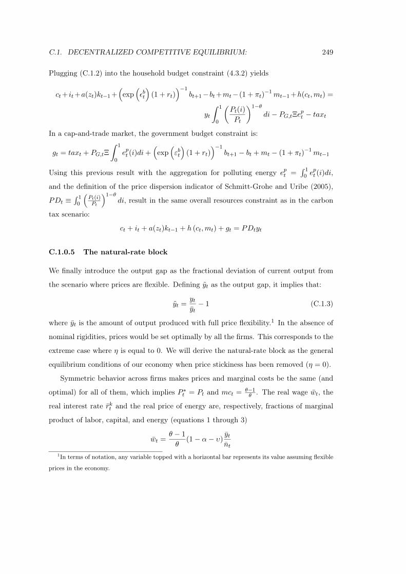
C.1. DECENTRALIZED COMPETITIVE EQUILIBRIUM: 249
Plugging (C.1.2) into the household budget constraint (4.3.2) yields
ct+ it+a(zt)kt−1 +(
exp(εbt
)(1 + rt)
)−1bt+1−bt+mt− (1 + πt)
−1mt−1 +h(ct,mt) =
yt
∫ 1
0
(Pt(i)
Pt
)1−θdi− PG,tΞept − taxt
In a cap-and-trade market, the government budget constraint is:
gt = taxt + PG,tΞ
∫ 1
0ept (i)di+
(exp
(εbt
)(1 + rt)
)−1bt+1 − bt +mt − (1 + πt)
−1mt−1
Using this previous result with the aggregation for polluting energy ept =∫ 1
0 ept (i)di,
and the definition of the price dispersion indicator of Schmitt-Grohe and Uribe (2005),
PDt ≡∫ 1
0
(Pt(i)Pt
)1−θdi, result in the same overall resources constraint as in the carbon
tax scenario:
ct + it + a(zt)kt−1 + h (ct,mt) + gt = PDtyt
C.1.0.5 The natural-rate block
We finally introduce the output gap as the fractional deviation of current output from
the scenario where prices are flexible. Defining yt as the output gap, it implies that:
yt =ytyt− 1 (C.1.3)
where yt is the amount of output produced with full price flexibility.1 In the absence of
nominal rigidities, prices would be set optimally by all the firms. This corresponds to the
extreme case where η is equal to 0. We will derive the natural-rate block as the general
equilibrium conditions of our economy when price stickiness has been removed (η = 0).
Symmetric behavior across firms makes prices and marginal costs be the same (and
optimal) for all of them, which implies P ∗t = Pt and mct = θ−1θ . The real wage wt, the
real interest rate rkt and the real price of energy are, respectively, fractions of marginal
product of labor, capital, and energy (equations 1 through 3)
wt =θ − 1
θ(1− α− υ)
ytnt
1In terms of notation, any variable topped with a horizontal bar represents its value assuming flexible
prices in the economy.
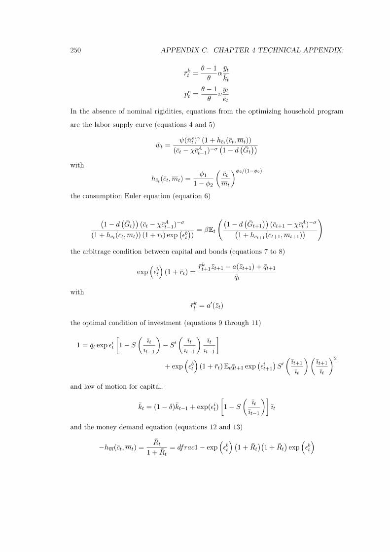
250 APPENDIX C. CHAPTER 4 TECHNICAL APPENDIX:
rkt =θ − 1
θαytkt
pet =θ − 1
θυytet
In the absence of nominal rigidities, equations from the optimizing household program
are the labor supply curve (equations 4 and 5)
wt =ψ(nst )
γ (1 + hct(ct,mt))
(ct − χcAt−1)−σ(1− d
(Gt))
with
hct(ct,mt) =φ1
1− φ2
(ctmt
)φ2/(1−φ2)
the consumption Euler equation (equation 6)
(1− d
(Gt))
(ct − χcAt−1)−σ
(1 + hct(ct,mt)) (1 + rt) exp(εbt))
= βEt
((1− d
(Gt+1
))(ct+1 − χcAt )−σ(
1 + hct+1(ct+1,mt+1))
)
the arbitrage condition between capital and bonds (equations 7 to 8)
exp(εbt
)(1 + rt) =
rkt+1zt+1 − a(zt+1) + qt+1
qt
with
rkt = a′(zt)
the optimal condition of investment (equations 9 through 11)
1 = qt exp εit
[1− S
(ıtıt−1
)− S′
(ıtıt−1
)ıtıt−1
]
+ exp(εbt
)(1 + rt)Etqt+1 exp
(εit+1
)S′(ıt+1
ıt
)(ıt+1
ıt
)2
and law of motion for capital:
kt = (1− δ)kt−1 + exp(εit)
[1− S
(ıtıt−1
)]ıt
and the money demand equation (equations 12 and 13)
−hm(ct,mt) =Rt
1 + Rt= dfrac1− exp
(εbt
) (1 + Rt
)(1 + Rt
)exp
(εbt
)
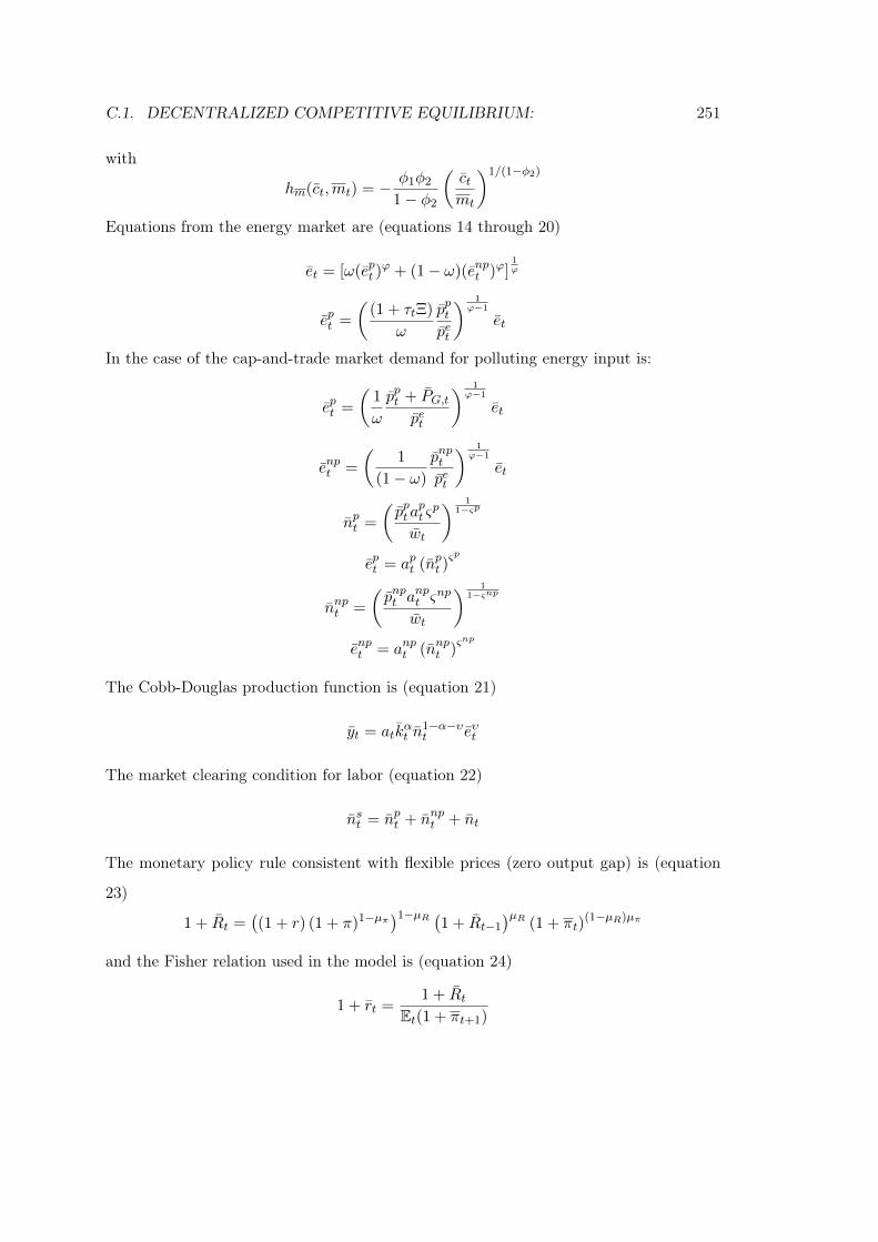
C.1. DECENTRALIZED COMPETITIVE EQUILIBRIUM: 251
with
hm(ct,mt) = − φ1φ2
1− φ2
(ctmt
)1/(1−φ2)
Equations from the energy market are (equations 14 through 20)
et = [ω(ept )ϕ + (1− ω)(enpt )ϕ]
1ϕ
ept =
((1 + τtΞ)
ω
pptpet
) 1ϕ−1
et
In the case of the cap-and-trade market demand for polluting energy input is:
ept =
(1
ω
ppt + PG,tpet
) 1ϕ−1
et
enpt =
(1
(1− ω)
pnptpet
) 1ϕ−1
et
npt =
(ppta
pt ςp
wt
) 11−ςp
ept = apt (npt )ςp
nnpt =
(pnpt a
npt ς
np
wt
) 11−ςnp
enpt = anpt (nnpt )ςnp
The Cobb-Douglas production function is (equation 21)
yt = atkαt n
1−α−υt eυt
The market clearing condition for labor (equation 22)
nst = npt + nnpt + nt
The monetary policy rule consistent with flexible prices (zero output gap) is (equation
23)
1 + Rt =((1 + r) (1 + π)1−µπ)1−µR (1 + Rt−1
)µR (1 + πt)(1−µR)µπ
and the Fisher relation used in the model is (equation 24)
1 + rt =1 + Rt
Et(1 + πt+1)
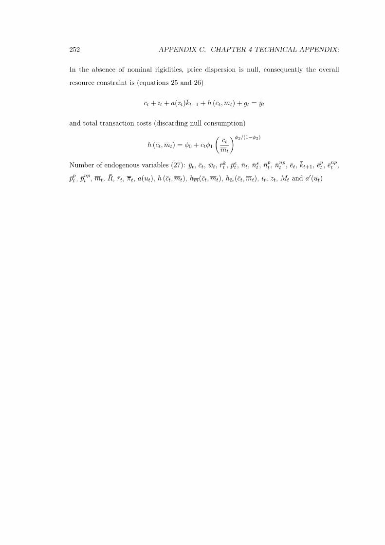
252 APPENDIX C. CHAPTER 4 TECHNICAL APPENDIX:
In the absence of nominal rigidities, price dispersion is null, consequently the overall
resource constraint is (equations 25 and 26)
ct + ıt + a(zt)kt−1 + h (ct,mt) + gt = yt
and total transaction costs (discarding null consumption)
h (ct,mt) = φ0 + ctφ1
(ctmt
)φ2/(1−φ2)
Number of endogenous variables (27): yt, ct, wt, rkt , pet , nt, nst , npt , n
npt , et, kt+1, e
pt , e
npt ,
ppt , pnpt , mt, R, rt, πt, a(ut), h (ct,mt), hm(ct,mt), hct(ct,mt), it, zt, Mt and a′(ut)
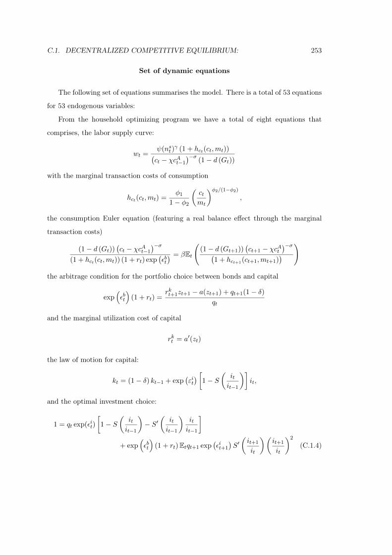
C.1. DECENTRALIZED COMPETITIVE EQUILIBRIUM: 253
Set of dynamic equations
The following set of equations summarises the model. There is a total of 53 equations
for 53 endogenous variables:
From the household optimizing program we have a total of eight equations that
comprises, the labor supply curve:
wt =ψ(nst )
γ (1 + hct(ct,mt))(ct − χcAt−1
)−σ(1− d (Gt))
with the marginal transaction costs of consumption
hct(ct,mt) =φ1
1− φ2
(ctmt
)φ2/(1−φ2)
,
the consumption Euler equation (featuring a real balance effect through the marginal
transaction costs)
(1− d (Gt))(ct − χcAt−1
)−σ
(1 + hct(ct,mt)) (1 + rt) exp(εbt) = βEt
((1− d (Gt+1))
(ct+1 − χcAt
)−σ(1 + hct+1(ct+1,mt+1)
))
the arbitrage condition for the portfolio choice between bonds and capital
exp(εbt
)(1 + rt) =
rkt+1zt+1 − a(zt+1) + qt+1(1− δ)qt
and the marginal utilization cost of capital
rkt = a′(zt)
the law of motion for capital:
kt = (1− δ) kt−1 + exp(εit) [
1− S(
itit−1
)]it,
and the optimal investment choice:
1 = qt exp(εit)
[1− S
(itit−1
)− S′
(itit−1
)itit−1
]
+ exp(εbt
)(1 + rt)Etqt+1 exp
(εit+1
)S′(it+1
it
)(it+1
it
)2
(C.1.4)
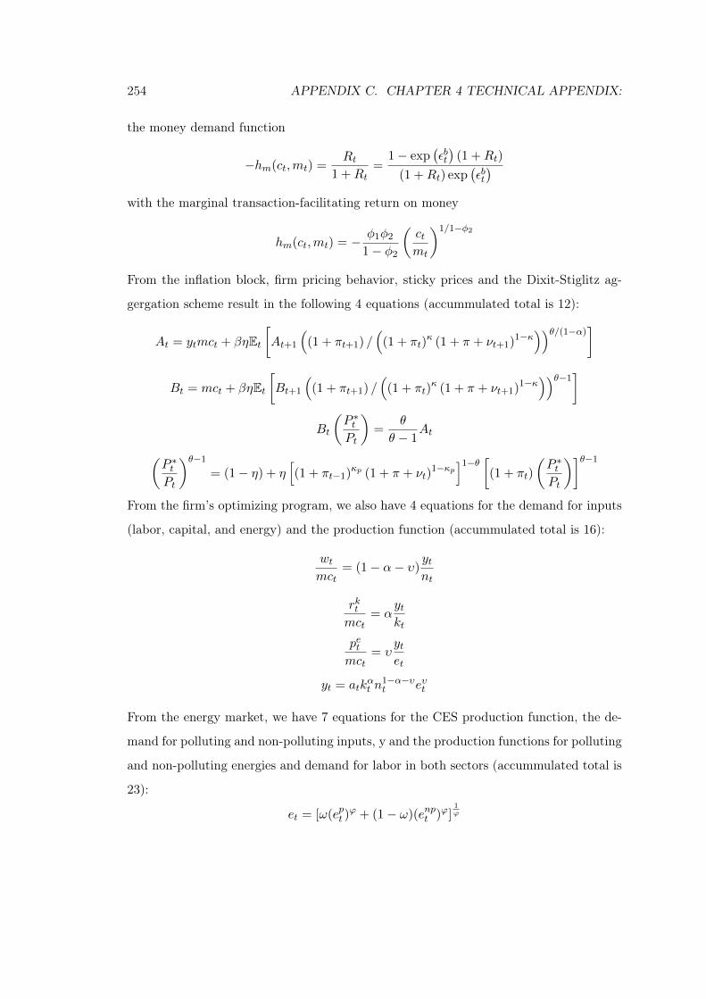
254 APPENDIX C. CHAPTER 4 TECHNICAL APPENDIX:
the money demand function
−hm(ct,mt) =Rt
1 +Rt=
1− exp(εbt)
(1 +Rt)
(1 +Rt) exp(εbt)
with the marginal transaction-facilitating return on money
hm(ct,mt) = − φ1φ2
1− φ2
(ctmt
)1/1−φ2
From the inflation block, firm pricing behavior, sticky prices and the Dixit-Stiglitz ag-
gergation scheme result in the following 4 equations (accummulated total is 12):
At = ytmct + βηEt[At+1
((1 + πt+1) /
((1 + πt)
κ (1 + π + νt+1)1−κ))θ/(1−α)
]
Bt = mct + βηEt[Bt+1
((1 + πt+1) /
((1 + πt)
κ (1 + π + νt+1)1−κ))θ−1
]
Bt
(P ∗tPt
)=
θ
θ − 1At
(P ∗tPt
)θ−1
= (1− η) + η[(1 + πt−1)κp (1 + π + νt)
1−κp]1−θ [
(1 + πt)
(P ∗tPt
)]θ−1
From the firm’s optimizing program, we also have 4 equations for the demand for inputs
(labor, capital, and energy) and the production function (accummulated total is 16):
wtmct
= (1− α− υ)ytnt
rktmct
= αytkt
petmct
= υytet
yt = atkαt n
1−α−υt eυt
From the energy market, we have 7 equations for the CES production function, the de-
mand for polluting and non-polluting inputs, y and the production functions for polluting
and non-polluting energies and demand for labor in both sectors (accummulated total is
23):
et = [ω(ept )ϕ + (1− ω)(enpt )ϕ]
1ϕ
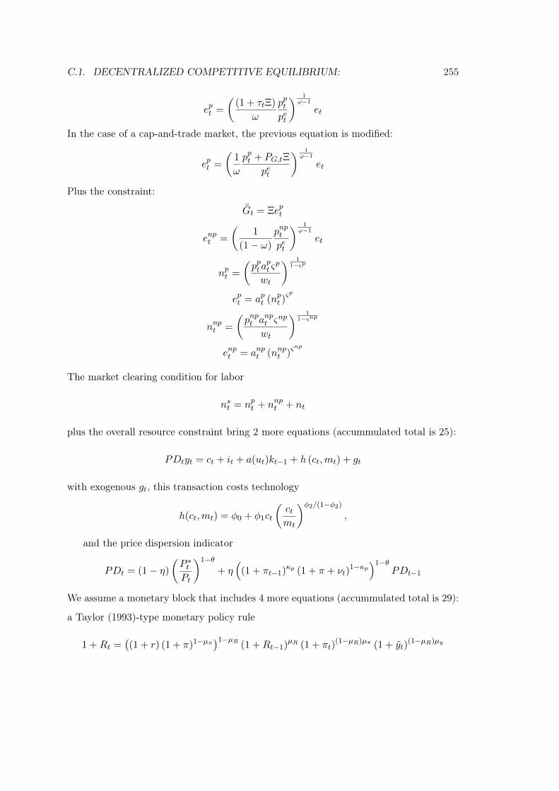
C.1. DECENTRALIZED COMPETITIVE EQUILIBRIUM: 255
ept =
((1 + τtΞ)
ω
pptpet
) 1ϕ−1
et
In the case of a cap-and-trade market, the previous equation is modified:
ept =
(1
ω
ppt + PG,tΞ
pet
) 1ϕ−1
et
Plus the constraint:¯Gt = Ξept
enpt =
(1
(1− ω)
pnptpet
) 1ϕ−1
et
npt =
(ppta
pt ςp
wt
) 11−ςp
ept = apt (npt )ςp
nnpt =
(pnpt a
npt ς
np
wt
) 11−ςnp
enpt = anpt (nnpt )ςnp
The market clearing condition for labor
nst = npt + nnpt + nt
plus the overall resource constraint bring 2 more equations (accummulated total is 25):
PDtyt = ct + it + a(ut)kt−1 + h (ct,mt) + gt
with exogenous gt, this transaction costs technology
h(ct,mt) = φ0 + φ1ct
(ctmt
)φ2/(1−φ2)
,
and the price dispersion indicator
PDt = (1− η)
(P ∗tPt
)1−θ+ η
((1 + πt−1)κp (1 + π + νt)
1−κp)1−θ
PDt−1
We assume a monetary block that includes 4 more equations (accummulated total is 29):
a Taylor (1993)-type monetary policy rule
1 +Rt =((1 + r) (1 + π)1−µπ)1−µR (1 +Rt−1)µR (1 + πt)
(1−µR)µπ (1 + yt)(1−µR)µy
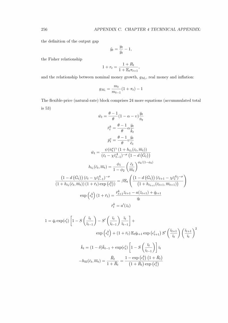
256 APPENDIX C. CHAPTER 4 TECHNICAL APPENDIX:
the definition of the output gap
yt =ytyt− 1,
the Fisher relationship
1 + rt =1 +Rt
1 + Etπt+1,
and the relationship between nominal money growth, gMt , real money and inflation:
gMt =mt
mt−1(1 + πt)− 1
The flexible-price (natural-rate) block comprises 24 more equations (accummulated total
is 53)
wt =θ − 1
θ(1− α− υ)
ytnt
rkt =θ − 1
θαytkt
pet =θ − 1
θυytet
wt =ψ(nst )
γ (1 + hct(ct,mt))
(ct − χcAt−1)−σ(1− d
(Gt))
hct(ct,mt) =φ1
1− φ2
(ctmt
)φ2/(1−φ2)
(1− d
(Gt))
(ct − χcAt−1)−σ
(1 + hct(ct,mt)) (1 + rt) exp(εbt))
= βEt
((1− d
(Gt))
(ct+1 − χcAt )−σ(1 + hct+1(ct+1,mt+1)
))
exp(εbt
)(1 + rt) =
rkt+1zt+1 − a(zt+1) + qt+1
qt
rkt = a′(zt)
1 = qt exp(εit)
[1− S
(ıtıt−1
)− S′
(ıtıt−1
)ıtıt−1
]+
exp(εbt
)+ (1 + rt)Etqt+1 exp
(εit+1
)S′(ıt+1
ıt
)(ıt+1
ıt
)2
kt = (1− δ)kt−1 + exp(εit)
[1− S
(ıtıt−1
)]ıt
−hm(ct,mt) =Rt
1 + Rt=
1− exp(εbt) (
1 + Rt)
(1 + Rt
)exp
(εbt)
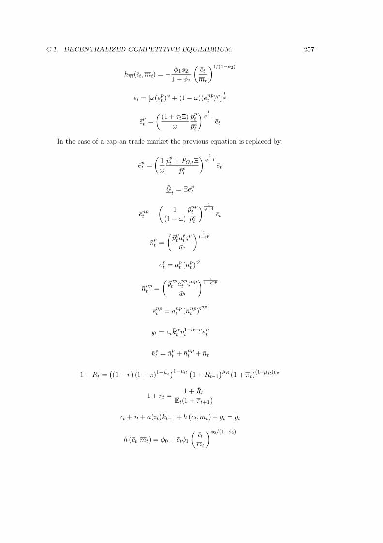
C.1. DECENTRALIZED COMPETITIVE EQUILIBRIUM: 257
hm(ct,mt) = − φ1φ2
1− φ2
(ctmt
)1/(1−φ2)
et = [ω(ept )ϕ + (1− ω)(enpt )ϕ]
1ϕ
ept =
((1 + τtΞ)
ω
pptpet
) 1ϕ−1
et
In the case of a cap-an-trade market the previous equation is replaced by:
ept =
(1
ω
ppt + PG,tΞ
pet
) 1ϕ−1
et
Gt
= Ξept
enpt =
(1
(1− ω)
pnptpet
) 1ϕ−1
et
npt =
(ppta
pt ςp
wt
) 11−ςp
ept = apt (npt )ςp
nnpt =
(pnpt a
npt ς
np
wt
) 11−ςnp
enpt = anpt (nnpt )ςnp
yt = atkαt n
1−α−υt eυt
nst = npt + nnpt + nt
1 + Rt =((1 + r) (1 + π)1−µπ)1−µR (1 + Rt−1
)µR (1 + πt)(1−µR)µπ
1 + rt =1 + Rt
Et(1 + πt+1)
ct + ıt + a(zt)kt−1 + h (ct,mt) + gt = yt
h (ct,mt) = φ0 + ctφ1
(ctmt
)φ2/(1−φ2)
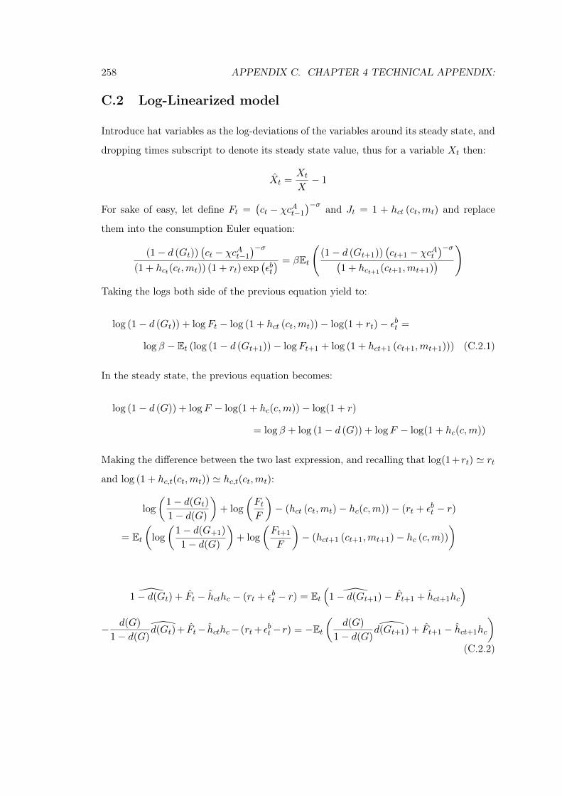
258 APPENDIX C. CHAPTER 4 TECHNICAL APPENDIX:
C.2 Log-Linearized model
Introduce hat variables as the log-deviations of the variables around its steady state, and
dropping times subscript to denote its steady state value, thus for a variable Xt then:
Xt =Xt
X− 1
For sake of easy, let define Ft =(ct − χcAt−1
)−σ and Jt = 1 + hct (ct,mt) and replace
them into the consumption Euler equation:
(1− d (Gt))(ct − χcAt−1
)−σ
(1 + hct(ct,mt)) (1 + rt) exp(εbt) = βEt
((1− d (Gt+1))
(ct+1 − χcAt
)−σ(1 + hct+1(ct+1,mt+1)
))
Taking the logs both side of the previous equation yield to:
log (1− d (Gt)) + logFt − log (1 + hct (ct,mt))− log(1 + rt)− εbt =
log β − Et (log (1− d (Gt+1))− logFt+1 + log (1 + hct+1 (ct+1,mt+1))) (C.2.1)
In the steady state, the previous equation becomes:
log (1− d (G)) + logF − log(1 + hc(c,m))− log(1 + r)
= log β + log (1− d (G)) + logF − log(1 + hc(c,m))
Making the difference between the two last expression, and recalling that log(1+rt) ' rtand log (1 + hc,t(ct,mt)) ' hc,t(ct,mt):
log
(1− d(Gt)
1− d(G)
)+ log
(FtF
)− (hct (ct,mt)− hc(c,m))− (rt + εbt − r)
= Et(
log
(1− d(G+1)
1− d(G)
)+ log
(Ft+1
F
)− (hct+1 (ct+1,mt+1)− hc (c,m))
)
1− d(Gt) + Ft − hcthc − (rt + εbt − r) = Et(
1− d(Gt+1)− Ft+1 + hct+1hc
)
− d(G)
1− d(G)d(Gt)+ Ft− hcthc− (rt+ εbt−r) = −Et
(d(G)
1− d(G)d(Gt+1) + Ft+1 − hct+1hc
)
(C.2.2)
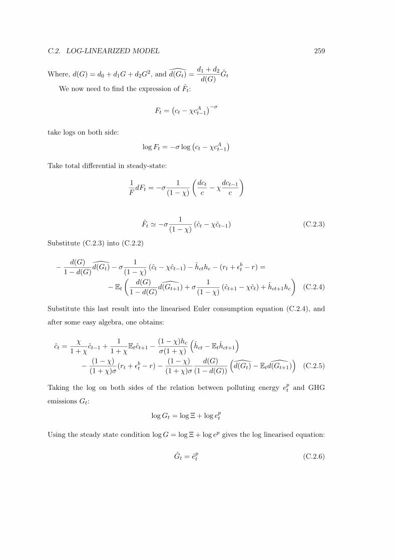
C.2. LOG-LINEARIZED MODEL 259
Where, d(G) = d0 + d1G+ d2G2, and d(Gt) =
d1 + d2
d(G)Gt
We now need to find the expression of Ft:
Ft =(ct − χcAt−1
)−σ
take logs on both side:
logFt = −σ log(ct − χcAt−1
)
Take total differential in steady-state:
1
FdFt = −σ 1
(1− χ)
(dctc− χdct−1
c
)
Ft ' −σ1
(1− χ)(ct − χct−1) (C.2.3)
Substitute (C.2.3) into (C.2.2)
− d(G)
1− d(G)d(Gt)− σ
1
(1− χ)(ct − χct−1)− hcthc − (rt + εbt − r) =
− Et(
d(G)
1− d(G)d(Gt+1) + σ
1
(1− χ)(ct+1 − χct) + hct+1hc
)(C.2.4)
Substitute this last result into the linearised Euler consumption equation (C.2.4), and
after some easy algebra, one obtains:
ct =χ
1 + χct−1 +
1
1 + χEtct+1 −
(1− χ)hcσ(1 + χ)
(hct − Ethct+1
)
− (1− χ)
(1 + χ)σ(rt + εbt − r)−
(1− χ)
(1 + χ)σ
d(G)
(1− d(G))
(d(Gt)− Et d(Gt+1)
)(C.2.5)
Taking the log on both sides of the relation between polluting energy ept and GHG
emissions Gt:
logGt = log Ξ + log ept
Using the steady state condition logG = log Ξ + log ep gives the log linearised equation:
Gt = ept (C.2.6)
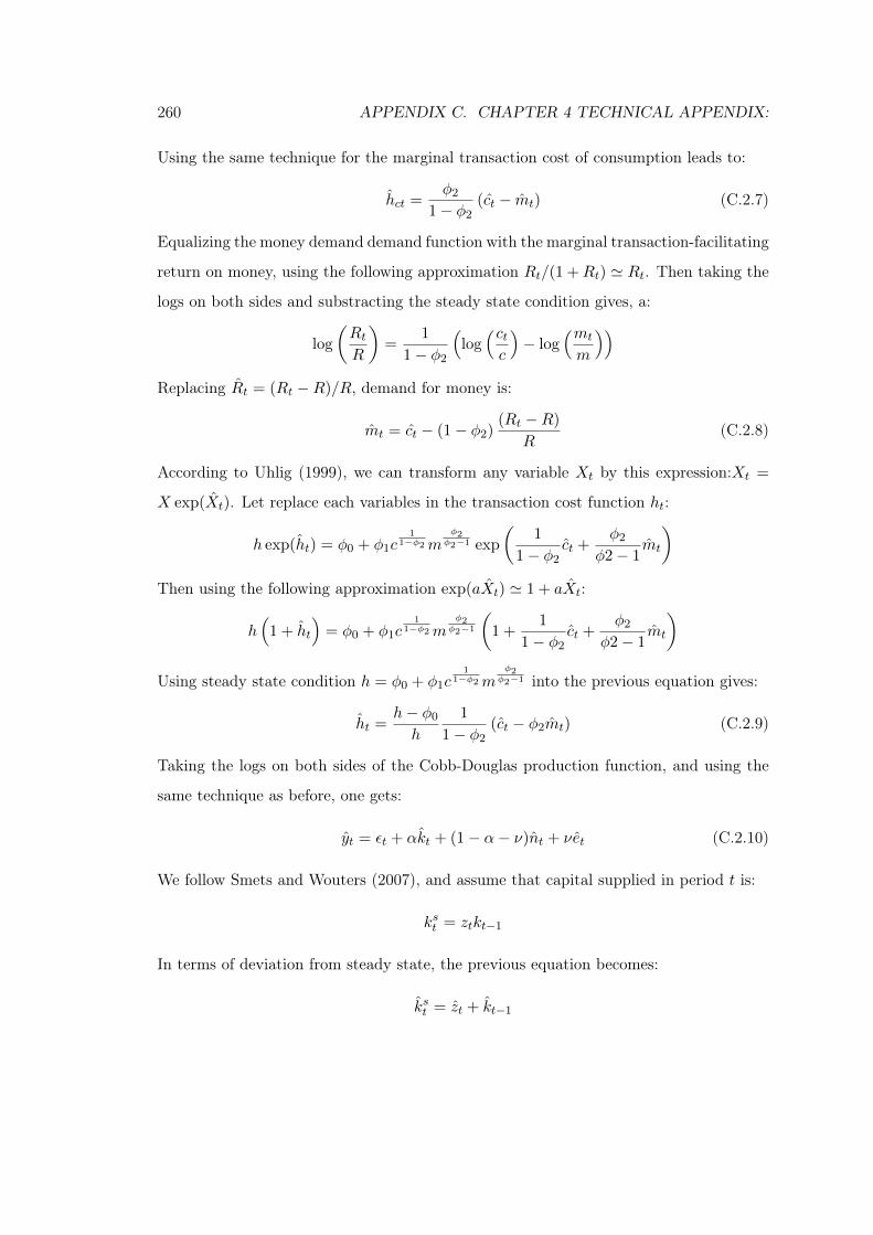
260 APPENDIX C. CHAPTER 4 TECHNICAL APPENDIX:
Using the same technique for the marginal transaction cost of consumption leads to:
hct =φ2
1− φ2(ct − mt) (C.2.7)
Equalizing the money demand demand function with the marginal transaction-facilitating
return on money, using the following approximation Rt/(1 +Rt) ' Rt. Then taking the
logs on both sides and substracting the steady state condition gives, a:
log
(RtR
)=
1
1− φ2
(log(ctc
)− log
(mt
m
))
Replacing Rt = (Rt −R)/R, demand for money is:
mt = ct − (1− φ2)(Rt −R)
R(C.2.8)
According to Uhlig (1999), we can transform any variable Xt by this expression:Xt =
X exp(Xt). Let replace each variables in the transaction cost function ht:
h exp(ht) = φ0 + φ1c1
1−φ2mφ2φ2−1 exp
(1
1− φ2ct +
φ2
φ2− 1mt
)
Then using the following approximation exp(aXt) ' 1 + aXt:
h(
1 + ht
)= φ0 + φ1c
11−φ2m
φ2φ2−1
(1 +
1
1− φ2ct +
φ2
φ2− 1mt
)
Using steady state condition h = φ0 + φ1c1
1−φ2mφ2φ2−1 into the previous equation gives:
ht =h− φ0
h
1
1− φ2(ct − φ2mt) (C.2.9)
Taking the logs on both sides of the Cobb-Douglas production function, and using the
same technique as before, one gets:
yt = εt + αkt + (1− α− ν)nt + νet (C.2.10)
We follow Smets and Wouters (2007), and assume that capital supplied in period t is:
kst = ztkt−1
In terms of deviation from steady state, the previous equation becomes:
kst = zt + kt−1
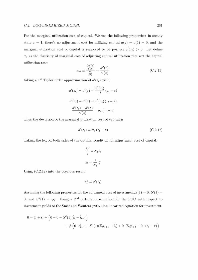
C.2. LOG-LINEARIZED MODEL 261
For the marginal utilization cost of capital. We use the following properties: in steady
state z = 1, there’s no adjustment cost for utilizing capital a(z) = a(1) = 0, and the
marginal utilization cost of capital is supposed to be positive a′(zt) > 0. Let define
σa as the elasticity of marginal cost of adjusting capital utilization rate wrt the capital
utilization rate:
σa ≡∂a′(z)a′(z)∂z∂z
=a′′(z)a′(z)
(C.2.11)
taking a 1st Taylor order approximation of a′(zt) yield:
a′(zt) = a′(z) +a′′(zt)
1!(zt − z)
a′(zt)− a′(z) = a′′(zt) (zt − z)a′(zt)− a′(z)
a′(z)= σa (zt − z)
Thus the deviation of the marginal utilization cost of capital is:
a′(zt) = σa (zt − z) (C.2.12)
Taking the log on both sides of the optimal condition for adjustment cost of capital:
rktz
= σazt
zt =1
σarkt
Using (C.2.12) into the previous result:
rkt = a′(zt)
Assuming the following properties for the adjusment cost of investment,S(1) = 0, S′(1) =
0, and S′′(1) = φk. Using a 2nd order approximation for the FOC with respect to
investment yields to the Smet and Wouters (2007) log-linearized equation for investment:
0 = qt + εit +(
0− 0− S′′(1)(it − it−1
)
+ β(
0 · εit+1 + S′′(1)(Etit+1 − it) + 0 · Etqt+1 − 0 · (rt − r))
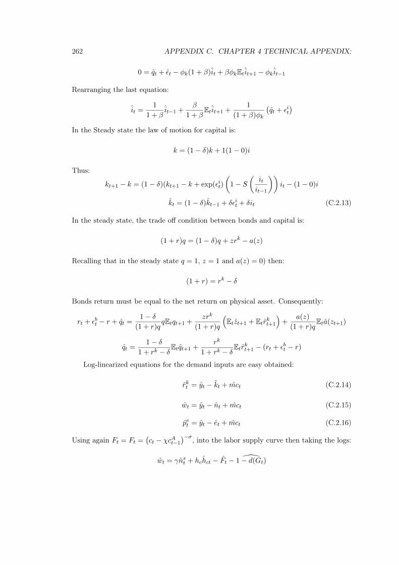
262 APPENDIX C. CHAPTER 4 TECHNICAL APPENDIX:
0 = qt + εt − φk(1 + β)it + βφkEtit+1 − φk it−1
Rearranging the last equation:
it =1
1 + βit−1 +
β
1 + βEtit+1 +
1
(1 + β)φk
(qt + εit
)
In the Steady state the law of motion for capital is:
k = (1− δ)k + 1(1− 0)i
Thus:
kt+1 − k = (1− δ)(kt+1 − k + exp(εit)
(1− S
(itit−1
))it − (1− 0)i
kt = (1− δ)kt−1 + δεit + δit (C.2.13)
In the steady state, the trade off condition between bonds and capital is:
(1 + r)q = (1− δ)q + zrk − a(z)
Recalling that in the steady state q = 1, z = 1 and a(z) = 0) then:
(1 + r) = rk − δ
Bonds return must be equal to the net return on physical asset. Consequently:
rt + εbt − r + qt =1− δ
(1 + r)qqEtqt+1 +
zrk
(1 + r)q
(Etzt+1 + Etrkt+1
)+
a(z)
(1 + r)qEta(zt+1)
qt =1− δ
1 + rk − δEtqt+1 +rk
1 + rk − δEtrkt+1 − (rt + εbt − r)
Log-linearized equations for the demand inputs are easy obtained:
rkt = yt − kt + mct (C.2.14)
wt = yt − nt + mct (C.2.15)
pet = yt − et + mct (C.2.16)
Using again Ft = Ft =(ct − χcAt−1
)−σ, into the labor supply curve then taking the logs:
wt = γnst + hchct − Ft − 1− d(Gt)
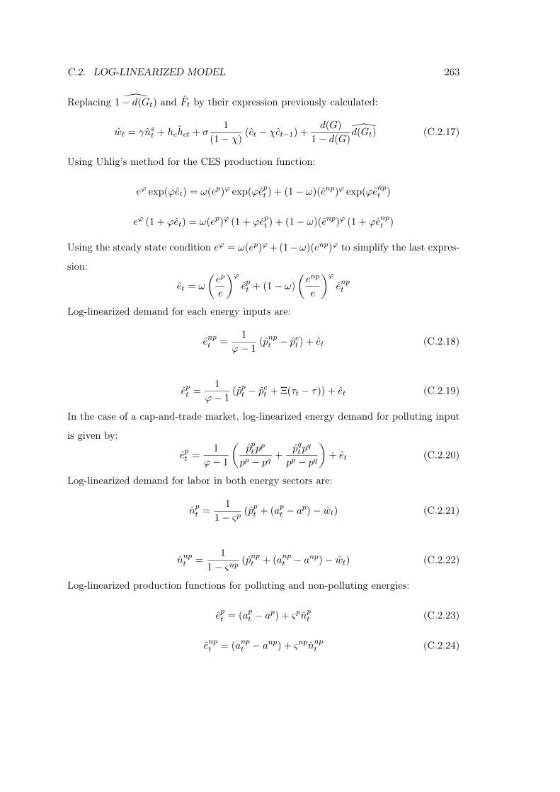
C.2. LOG-LINEARIZED MODEL 263
Replacing 1− d(Gt) and Ft by their expression previously calculated:
wt = γnst + hchct + σ1
(1− χ)(ct − χct−1) +
d(G)
1− d(G)d(Gt) (C.2.17)
Using Uhlig’s method for the CES production function:
eϕ exp(ϕet) = ω(ep)ϕ exp(ϕept ) + (1− ω)(enp)ϕ exp(ϕenpt )
eϕ (1 + ϕet) = ω(ep)ϕ (1 + ϕept ) + (1− ω)(enp)ϕ (1 + ϕenpt )
Using the steady state condition eϕ = ω(ep)ϕ + (1−ω)(enp)ϕ to simplify the last expres-
sion:
et = ω
(ep
e
)ϕept + (1− ω)
(enp
e
)ϕenpt
Log-linearized demand for each energy inputs are:
enpt =1
ϕ− 1(pnpt − pet ) + et (C.2.18)
ept =1
ϕ− 1(ppt − pet + Ξ(τt − τ)) + et (C.2.19)
In the case of a cap-and-trade market, log-linearized energy demand for polluting input
is given by:
ept =1
ϕ− 1
(ppt p
p
pp − pq +pqtp
q
pp − pq)
+ et (C.2.20)
Log-linearized demand for labor in both energy sectors are:
npt =1
1− ςp (ppt + (apt − ap)− wt) (C.2.21)
nnpt =1
1− ςnp (pnpt + (anpt − anp)− wt) (C.2.22)
Log-linearized production functions for polluting and non-polluting energies:
ept = (apt − ap) + ςpnpt (C.2.23)
enpt = (anpt − anp) + ςnpnnpt (C.2.24)
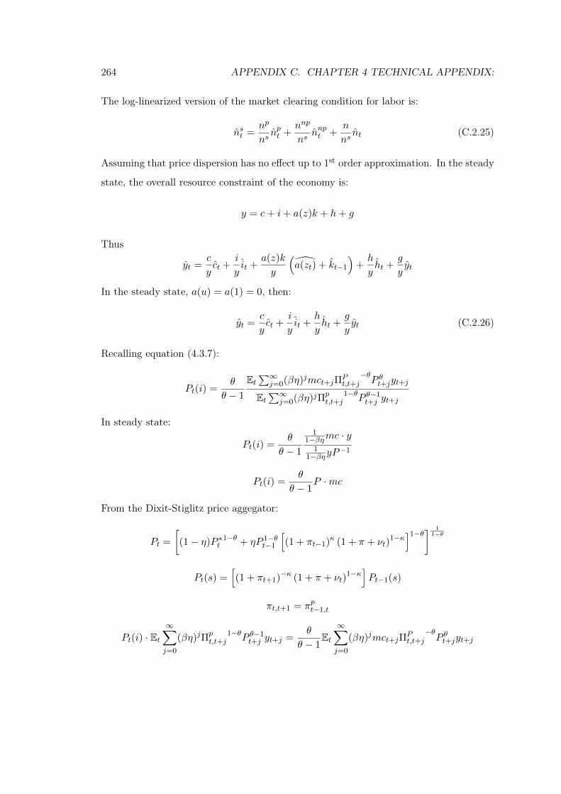
264 APPENDIX C. CHAPTER 4 TECHNICAL APPENDIX:
The log-linearized version of the market clearing condition for labor is:
nst =np
nsnpt +
nnp
nsnnpt +
n
nsnt (C.2.25)
Assuming that price dispersion has no effect up to 1st order approximation. In the steady
state, the overall resource constraint of the economy is:
y = c+ i+ a(z)k + h+ g
Thus
yt =c
yct +
i
yit +
a(z)k
y
(a(zt) + kt−1
)+h
yht +
g
yyt
In the steady state, a(u) = a(1) = 0, then:
yt =c
yct +
i
yit +
h
yht +
g
yyt (C.2.26)
Recalling equation (4.3.7):
Pt(i) =θ
θ − 1
Et∑∞
j=0(βη)jmct+jΠPt,t+j
−θP θt+jyt+j
Et∑∞
j=0(βη)jΠpt,t+j
1−θP θ−1t+j yt+j
In steady state:
Pt(i) =θ
θ − 1
11−βηmc · y
11−βηyP
−1
Pt(i) =θ
θ − 1P ·mc
From the Dixit-Stiglitz price aggegator:
Pt =
[(1− η)P ∗t
1−θ + ηP 1−θt−1
[(1 + πt−1)κ (1 + π + νt)
1−κ]1−θ] 1
1−θ
Pt(s) =[(1 + πt+1)−κ (1 + π + νt)
1−κ]Pt−1(s)
πt,t+1 = πpt−1,t
Pt(i) · Et∞∑
j=0
(βη)jΠpt,t+j
1−θP θ−1t+j yt+j =
θ
θ − 1Et∞∑
j=0
(βη)jmct+jΠPt,t+j
−θP θt+jyt+j
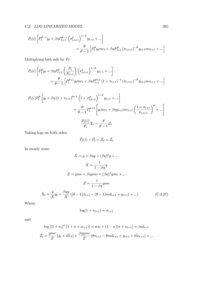
C.2. LOG-LINEARIZED MODEL 265
Pt(i)
[P θ−1t yt + βηP θ−1
t+1
(πpt,t+1
)1−θyt+1 + ...
]
=θ
θ − 1
[P θt ytmct + βηP θt+1 (πt,t+1)−θ yt+1mct+1 + ...
]
Multiplying bith side by Pt:
Pt(i)
[P θt yt + βηP θt+1
(PtPt+1
)(πpt,t+1
)1−θyt+1 + ...
]
=θ
θ − 1
[P θ+1t ytmct + βηP θ+1
t+1 (1 + πt+1)−1 (πt,t+1)−θ yt+1mct+1 + ...]
Pt(i)Pθt
[yt + βη (1 + πt+1)θ−1
(1 + πpt,t+1
)1−θyt+1 + ...
]
=θ
θ − 1P θ+1t
[ytmct + βηyt+1mct+1
(1 + πt+1
πt,t+1
)θ+ ...
]
Pt(i)
PtXt =
θ
θ − 1Zt
Taking logs on both sides:
Pt(i)− Pt + Xt = Zt
In steady state:
X = y + βηy + (βη)2y + ...
X =1
1− βηy
Z = ymc+ βηymc+ (βη)2ymc+ ...
Z =1
1− βηymc
Xt =y
Xyt +
βηy
X((θ − 1)πt+1 − (θ − 1)indt+1 + yt+1) + ...) (C.2.27)
Where
log(1 + πt+1) = πt+1
and
log [(1 + πt)κ (1 + π + νt+1)] = κπt + (1− κ)(π + νt+1) = indt+1
Zt =ymc
Z(yt + mct) +
βηymc
Z(θπt+1 − θindt+1 + yt+1 + mct+1) + ...
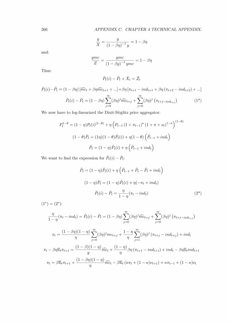
266 APPENDIX C. CHAPTER 4 TECHNICAL APPENDIX:
y
X=
y
(1− βη)−1 y= 1− βη
and:ymc
Z=
ymc
(1− βy)−1 ymc= 1− βη
Thus:
Pt(i)− Pt + Xt = Zt
Pt(i)−Pt = (1− βη) [mct + βηmct+1 + ...]+βη [πt+1 − indt+1 + βη (πt+2 − indt+2) + ...]
Pt(i)− Pt = (1− βη)∞∑
j=0
(βη)jmct+j +∞∑
j=0
(βη)j(πt+j−indt+j
)(1*)
We now have to log-linearized the Dixit-Stiglitz price aggregator:
P 1−θt = (1− η)Pt(i)
(1−θ) + η(Pt−1 (1 + πt−1)κ (1 + π + νt)
1−κ)(1−θ)
(1− θ)Pt = (1η)(1− θ)Pt(i) + η(1− θ)(Pt−1 + indt
)
Pt = (1− η)Pt(i) + η(Pt−1 + indt
)
We want to find the expression for Pt(i)− Pt:
Pt = (1− η)Pt(i) + η(Pt−1 + Pt − Pt + indt
)
(1− η)Pt = (1− η)Pt(i) + η(−πt + indt)
Pt(i)− Pt =η
1− η (πt − indt) (2*)
(1∗) = (2∗):
η
1− η (πt − indt) = Pt(i)− Pt = (1− βη)
∞∑
j=0
(βη)jmct+j +
∞∑
j=0
(βη)j(πt+j−indt+j
)
πt =(1− βη)(1− η)
η
∞∑
j=0
(βη)jmct+j +1− ηη
∞∑
j=1
(βη)j (πt+j − indt+j) + indt
πt − βηEtπt+1 =(1− β)(1− η)
ymct +
(1− η)
ηβη (πt+1 − indt+1) + indt − βηEtindt+1
πt = βEtπt+1 +(1− βη)(1− η)
ηmct − βEt (κπt + (1− κ)νt+1) + κπt−1 + (1− κ)νt
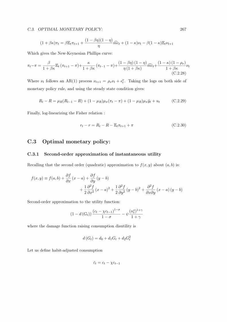
C.3. OPTIMAL MONETARY POLICY: 267
(1 + βκ)πt = βEtπt+1 +(1− βη)(1− η)
ηmct + (1− κ)νt − β(1− κ)Etνt+1
Which gives the New-Keynesian Phillips curve:
πt−π =β
1 + βκEt (πt+1 − π)+
κ
1 + βκ(πt−1 − π)+
(1− βη) (1− η)
η (1 + βκ)mct+
(1− κ) (1− ρν)
1 + βκνt
(C.2.28)
Where νt follows an AR(1) process νt+1 = ρννt + ενt . Taking the logs on both side of
monetary policy rule, and using the steady state condition gives:
Rt −R = µR(Rt−1 −R) + (1− µR)µπ(πt − π) + (1− µR)µπyt + ut (C.2.29)
Finally, log-linearizing the Fisher relation :
rt − r = Rt −R− Etπt+1 + π (C.2.30)
C.3 Optimal monetary policy:
C.3.1 Second-order approximation of instantaneous utility
Recalling that the second order (quadratic) approximation to f(x, y) about (a, b) is:
f(x, y) ≡ f(a, b) +∂f
∂x(x− a) +
∂f
∂y(y − b)
+1
2
∂2f
∂x2(x− a)2 +
1
2
∂2f
∂y2(y − b)2 +
∂2f
∂x∂y(x− a) (y − b)
Second-order approximation to the utility function:
(1− d (Gt))(ct − χct−1)1−σ
1− σ − ψ (nst )1+γ
1 + γ
where the damage function raising consumption disutility is
d (Gt) = d0 + d1Gt + d2G2t
Let us define habit-adjusted consumption
ct = ct − χct−1
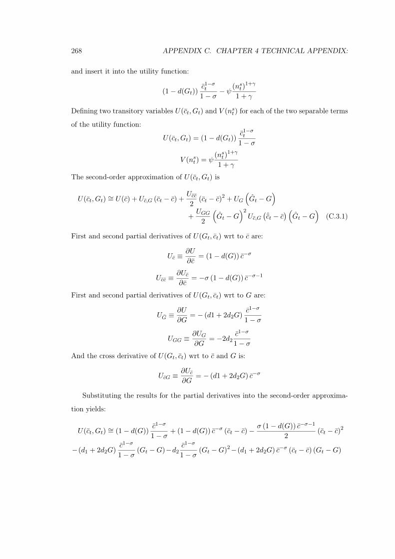
268 APPENDIX C. CHAPTER 4 TECHNICAL APPENDIX:
and insert it into the utility function:
(1− d(Gt))c1−σt
1− σ − ψ(nst )
1+γ
1 + γ
Defining two transitory variables U(ct, Gt) and V (nst ) for each of the two separable terms
of the utility function:
U(ct, Gt) = (1− d(Gt))c1−σt
1− σ
V (nst ) = ψ(nst )
1+γ
1 + γ
The second-order approximation of U(ct, Gt) is
U(ct, Gt) ∼= U(c) + Uc,G (ct − c) +Ucc2
(ct − c)2 + UG
(Gt −G
)
+UGG
2
(Gt −G
)2Uc,G
(ˆct − c
) (Gt −G
)(C.3.1)
First and second partial derivatives of U(Gt, ct) wrt to c are:
Uc ≡∂U
∂c= (1− d(G)) c−σ
Ucc ≡∂Uc∂c
= −σ (1− d(G)) c−σ−1
First and second partial derivatives of U(Gt, ct) wrt to G are:
UG ≡∂U
∂G= − (d1 + 2d2G)
c1−σ
1− σ
UGG ≡∂UG∂G
= −2d2c1−σ
1− σAnd the cross derivative of U(Gt, ct) wrt to c and G is:
UcG ≡∂Uc∂G
= − (d1 + 2d2G) c−σ
Substituting the results for the partial derivatives into the second-order approxima-
tion yields:
U(ct, Gt) ∼= (1− d(G))c1−σ
1− σ + (1− d(G)) c−σ (ct − c)−σ (1− d(G)) c−σ−1
2(ct − c)2
−(d1 + 2d2G)c1−σ
1− σ (Gt −G)−d2c1−σ
1− σ (Gt −G)2−(d1 + 2d2G) c−σ (ct − c) (Gt −G)
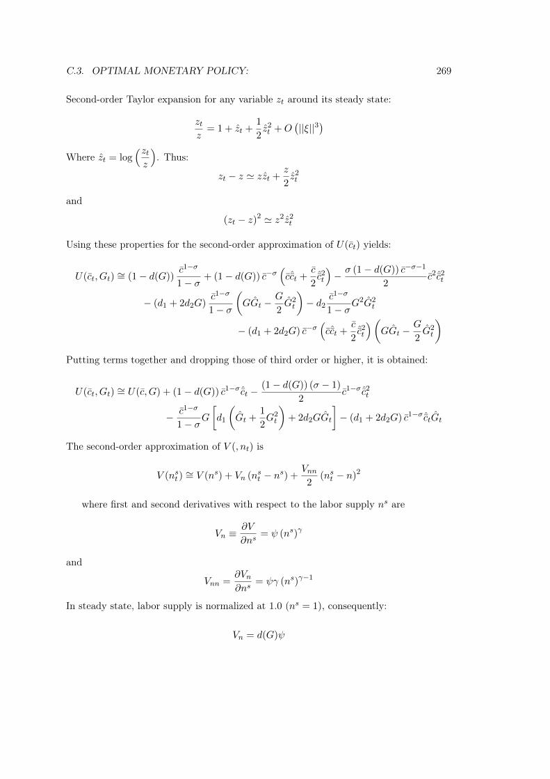
C.3. OPTIMAL MONETARY POLICY: 269
Second-order Taylor expansion for any variable zt around its steady state:
ztz
= 1 + zt +1
2z2t +O
(||ξ||3
)
Where zt = log(ztz
). Thus:
zt − z ' zzt +z
2z2t
and
(zt − z)2 ' z2z2t
Using these properties for the second-order approximation of U(ct) yields:
U(ct, Gt) ∼= (1− d(G))c1−σ
1− σ + (1− d(G)) c−σ(cˆct +
c
2ˆc2t
)− σ (1− d(G)) c−σ−1
2c2ˆc2
t
− (d1 + 2d2G)c1−σ
1− σ
(GGt −
G
2G2t
)− d2
c1−σ
1− σG2G2
t
− (d1 + 2d2G) c−σ(cˆct +
c
2ˆc2t
)(GGt −
G
2G2t
)
Putting terms together and dropping those of third order or higher, it is obtained:
U(ct, Gt) ∼= U(c, G) + (1− d(G)) c1−σ ˆct −(1− d(G)) (σ − 1)
2c1−σ ˆc2
t
− c1−σ
1− σG[d1
(Gt +
1
2G2t
)+ 2d2GGt
]− (d1 + 2d2G) c1−σ ˆctGt
The second-order approximation of V (, nt) is
V (nst )∼= V (ns) + Vn (nst − ns) +
Vnn2
(nst − n)2
where first and second derivatives with respect to the labor supply ns are
Vn ≡∂V
∂ns= ψ (ns)γ
and
Vnn =∂Vn∂ns
= ψγ (ns)γ−1
In steady state, labor supply is normalized at 1.0 (ns = 1), consequently:
Vn = d(G)ψ
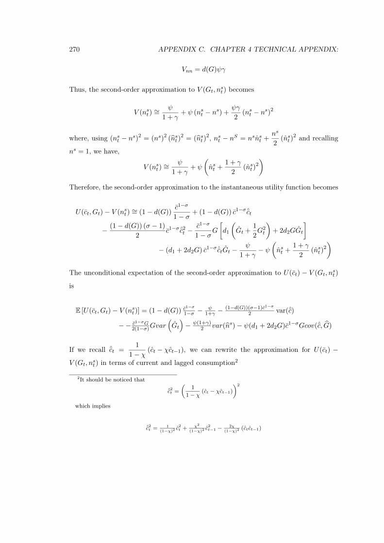
270 APPENDIX C. CHAPTER 4 TECHNICAL APPENDIX:
Vnn = d(G)ψγ
Thus, the second-order approximation to V (Gt, nst ) becomes
V (nst )∼= ψ
1 + γ+ ψ (nst − ns) +
ψγ
2(nst − ns)2
where, using (nst − ns)2 = (ns)2 (nst )2 = (nst )
2, nst − nS = nsnst +ns
2(nst )
2 and recalling
ns = 1, we have,
V (nst )∼= ψ
1 + γ+ ψ
(nst +
1 + γ
2(nst )
2
)
Therefore, the second-order approximation to the instantaneous utility function becomes
U(ct, Gt)− V (nst )∼= (1− d(G))
c1−σ
1− σ + (1− d(G)) c1−σ ˆct
− (1− d(G)) (σ − 1)
2c1−σ ˆc2
t −c1−σ
1− σG[d1
(Gt +
1
2G2t
)+ 2d2GGt
]
− (d1 + 2d2G) c1−σ ˆctGt −ψ
1 + γ− ψ
(nst +
1 + γ
2(nst )
2
)
The unconditional expectation of the second-order approximation to U(ct) − V (Gt, nst )
is
E [U(ct, Gt)− V (nst )] = (1− d(G)) c1−σ
1−σ −ψ
1+γ −(1−d(G))(σ−1)c1−σ
2 var(ˆc)
−− c1−σG2(1−σ)Gvar
(Gt
)− ψ(1+γ)
2 var(ns)− ψ(d1 + 2d2G)c1−σGcov(ˆc, G)
If we recall ˆct =1
1− χ (ct − χct−1), we can rewrite the approximation for U(ct) −V (Gt, n
st ) in terms of current and lagged consumption2
2It should be noticed that
ˆc2t =
(1
1 − χ(ct − χct−1)
)2
which implies
ˆc2t = 1(1−χ)2 c
2t + χ2
(1−χ)2 c2t−1 − 2χ
(1−χ)2 (ctct−1)
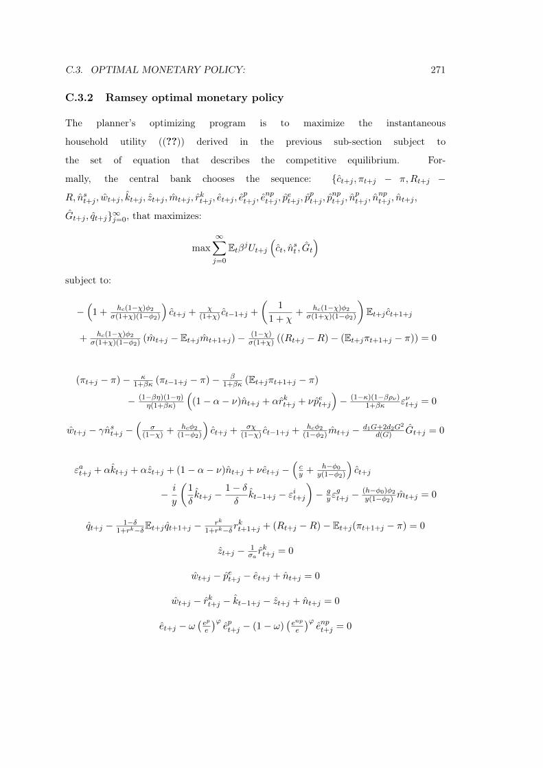
C.3. OPTIMAL MONETARY POLICY: 271
C.3.2 Ramsey optimal monetary policy
The planner’s optimizing program is to maximize the instantaneous
household utility ((??)) derived in the previous sub-section subject to
the set of equation that describes the competitive equilibrium. For-
mally, the central bank chooses the sequence: ct+j , πt+j − π,Rt+j −R, nst+j , wt+j , kt+j , zt+j , mt+j , r
kt+j , et+j , e
pt+j , e
npt+j , p
et+j , p
pt+j , p
npt+j , n
pt+j , n
npt+j , nt+j ,
Gt+j , qt+j∞j=0, that maximizes:
max
∞∑
j=0
EtβjUt+j(ct, n
st , Gt
)
subject to:
−(
1 + hc(1−χ)φ2σ(1+χ)(1−φ2)
)ct+j + χ
(1+χ) ct−1+j +
(1
1 + χ+ hc(1−χ)φ2
σ(1+χ)(1−φ2)
)Et+j ct+1+j
+ hc(1−χ)φ2σ(1+χ)(1−φ2) (mt+j − Et+jmt+1+j)− (1−χ)
σ(1+χ) ((Rt+j −R)− (Et+jπt+1+j − π)) = 0
(πt+j − π)− κ1+βκ (πt−1+j − π)− β
1+βκ (Et+jπt+1+j − π)
− (1−βη)(1−η)η(1+βκ)
((1− α− ν)nt+j + αrkt+j + νpet+j
)− (1−κ)(1−βρν)
1+βκ ενt+j = 0
wt+j − γnst+j −(
σ(1−χ) + hcφ2
(1−φ2)
)ct+j + σχ
(1−χ) ct−1+j + hcφ2(1−φ2)mt+j − d1G+2d2G2
d(G) Gt+j = 0
εat+j + αkt+j + αzt+j + (1− α− ν)nt+j + νet+j −(cy + h−φ0
y(1−φ2)
)ct+j
− i
y
(1
δkt+j −
1− δδ
kt−1+j − εit+j)− g
yεgt+j −
(h−φ0)φ2y(1−φ2) mt+j = 0
qt+j − 1−δ1+rk−δEt+j qt+1+j − rk
1+rk−δ rkt+1+j + (Rt+j −R)− Et+j(πt+1+j − π) = 0
zt+j − 1σarkt+j = 0
wt+j − pet+j − et+j + nt+j = 0
wt+j − rkt+j − kt−1+j − zt+j + nt+j = 0
et+j − ω(ep
e
)ϕept+j − (1− ω)
(enp
e
)ϕenpt+j = 0

272 APPENDIX C. CHAPTER 4 TECHNICAL APPENDIX:
enpt+j − 1ϕ−1
(pnpt+j + pet+j
)− et+j = 0
ept+j − 1ϕ−1
(ppt+j + pet − Ξετt+j
)− et+j = 0
npt+j −1
1− ςp(ppt+j + εa
p
t+j − wt+j)
= 0
nnpt+j − 11−ςnp
(pnpt+j + εa
np
t+j − wt+j)
= 0
ept+j − εap
t+j − ςpnpt+j = 0
enpt+j − εanp
t+j − ςnpnnpt+j = 0
nst+j − np
ns npt+j − nnp
ns nnpt+j − n
ns nt+j = 0
mt+j − ct+j + 1−φ2R (Rt+j −R) = 0
Gt+j − ept+j = 0
(1
δkt+j −
1− δδ
kt−1+j − εit+j)− 1
1+β
(1
δkt−1+j −
1− δδ
kt−2+j − εit−1+j
)
− β1+β
(1
δEt+j kt+1+j −
1− δδ
kt+j − εit+1+j
)− 1
(1+β)φkqt+j − εit+j = 0
Defining λi,t+j with i = 1 · · · 19 the Lagrange multipliers respectively associated with the
19 constraints of the central bank optimizing program, the set of first order conditions
comprises the 19 equations above and the following equations from the central-bank
choice variables (we set j = 0 in order to obtain expressions for period t):
c1−σ(
1−βχ1−χ
)− (σ−1)c1−σ(1+βχ2)
(1−χ)2ct + β(σ−1)c1−σχ
(1−χ)2Etct+1 + (σ−1)c1−σχ
(1−χ)2ct−1
+ β−1(
11+χ + hc(1−χ)φ2
σ(1+χ)(1−φ2)
)λ1,t−1 −
(1 + hc(1−χ)φ2
σ(1+χ)(1−φ2)
)λ1,t + βχ
1+χEtλ1,t+1
−(
σ1−χ + hcφ2
1−φ2
)λ3,t + βσχ
1−χEtλ3,t+1 −(cy + h−φ0
y(1−φ2)
)λ4,t − λ17,t = 0 (cfoct )
(1−χ)βσ(1+χ)λ1,t−1 + λ2,t − 1
1+βκλ2,t−1 − βκ1+βκEtλ2,t+1 − λ5,t−1 = 0 ((πt − π)foc)
− (1−χ)σ(1+χ)λ1,t + λ5,t + (1−φ2)
R λ17,t = 0 ((Rt −R)foc)
−d(G)ψ − d(G)ψ(1 + γ)nst − ψ(d1 + 2d2G)GGt − λ3,tγ + λ16,t = 0 ((nst )foc)
− (1−βη)(1−η)(1−α−ν)η(1+βκ) λ2,t + λ3,t + λ7,t + λ8,t + 1
1−ςpλ12,t + 11−ςnpλ13,t = 0 (wfoct )
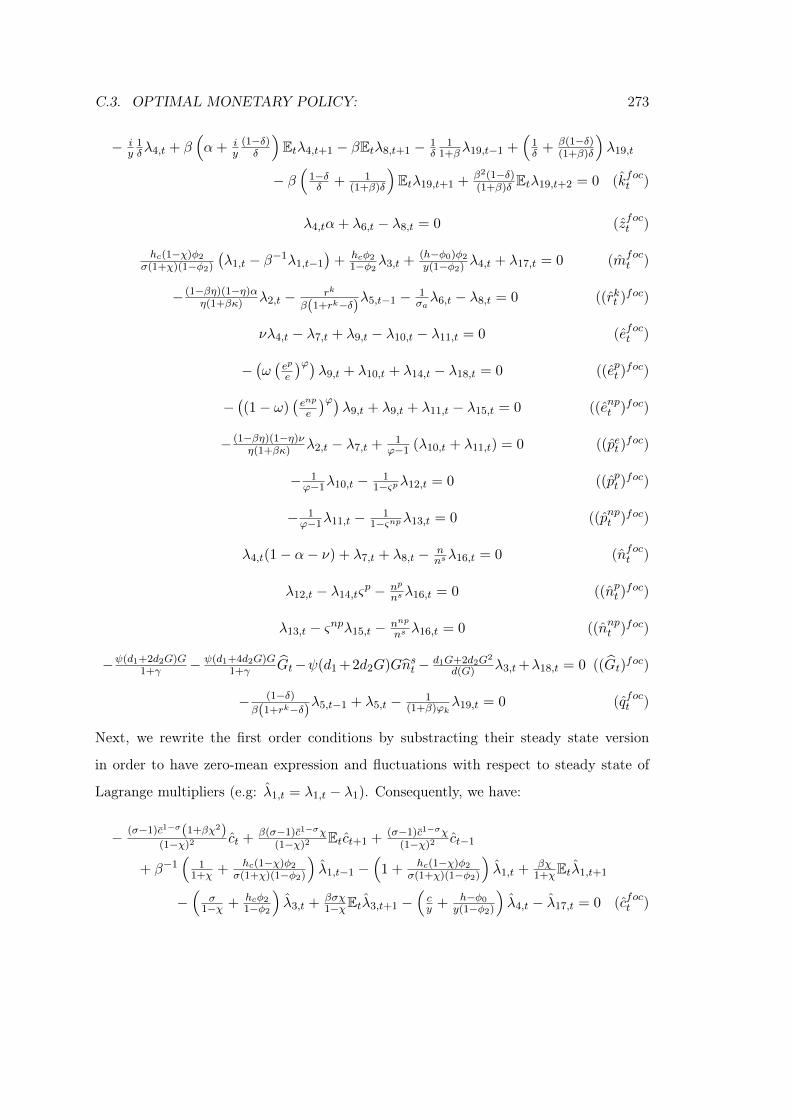
C.3. OPTIMAL MONETARY POLICY: 273
− iy
1δλ4,t + β
(α+ i
y(1−δ)δ
)Etλ4,t+1 − βEtλ8,t+1 − 1
δ1
1+βλ19,t−1 +(
1δ + β(1−δ)
(1+β)δ
)λ19,t
− β(
1−δδ + 1
(1+β)δ
)Etλ19,t+1 + β2(1−δ)
(1+β)δ Etλ19,t+2 = 0 (kfoct )
λ4,tα+ λ6,t − λ8,t = 0 (zfoct )
hc(1−χ)φ2σ(1+χ)(1−φ2)
(λ1,t − β−1λ1,t−1
)+ hcφ2
1−φ2λ3,t + (h−φ0)φ2y(1−φ2) λ4,t + λ17,t = 0 (mfoc
t )
− (1−βη)(1−η)αη(1+βκ) λ2,t − rk
β(1+rk−δ)λ5,t−1 − 1σaλ6,t − λ8,t = 0 ((rkt )foc)
νλ4,t − λ7,t + λ9,t − λ10,t − λ11,t = 0 (efoct )
−(ω(ep
e
)ϕ)λ9,t + λ10,t + λ14,t − λ18,t = 0 ((ept )foc)
−((1− ω)
(enp
e
)ϕ)λ9,t + λ9,t + λ11,t − λ15,t = 0 ((enpt )foc)
− (1−βη)(1−η)νη(1+βκ) λ2,t − λ7,t + 1
ϕ−1 (λ10,t + λ11,t) = 0 ((pet )foc)
− 1ϕ−1λ10,t − 1
1−ςpλ12,t = 0 ((ppt )foc)
− 1ϕ−1λ11,t − 1
1−ςnpλ13,t = 0 ((pnpt )foc)
λ4,t(1− α− ν) + λ7,t + λ8,t − nnsλ16,t = 0 (nfoct )
λ12,t − λ14,tςp − np
nsλ16,t = 0 ((npt )foc)
λ13,t − ςnpλ15,t − nnp
ns λ16,t = 0 ((nnpt )foc)
−ψ(d1+2d2G)G1+γ − ψ(d1+4d2G)G
1+γ Gt−ψ(d1 +2d2G)Gnst − d1G+2d2G2
d(G) λ3,t+λ18,t = 0 ((Gt)foc)
− (1−δ)β(1+rk−δ)λ5,t−1 + λ5,t − 1
(1+β)ϕkλ19,t = 0 (qfoct )
Next, we rewrite the first order conditions by substracting their steady state version
in order to have zero-mean expression and fluctuations with respect to steady state of
Lagrange multipliers (e.g: λ1,t = λ1,t − λ1). Consequently, we have:
− (σ−1)c1−σ(1+βχ2)(1−χ)2
ct + β(σ−1)c1−σχ(1−χ)2
Etct+1 + (σ−1)c1−σχ(1−χ)2
ct−1
+ β−1(
11+χ + hc(1−χ)φ2
σ(1+χ)(1−φ2)
)λ1,t−1 −
(1 + hc(1−χ)φ2
σ(1+χ)(1−φ2)
)λ1,t + βχ
1+χEtλ1,t+1
−(
σ1−χ + hcφ2
1−φ2
)λ3,t + βσχ
1−χEtλ3,t+1 −(cy + h−φ0
y(1−φ2)
)λ4,t − λ17,t = 0 (cfoct )
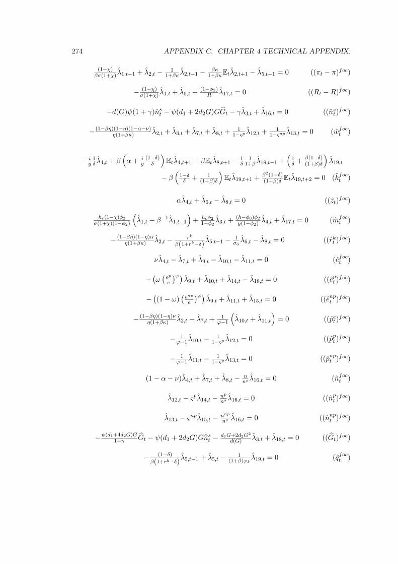
274 APPENDIX C. CHAPTER 4 TECHNICAL APPENDIX:
(1−χ)βσ(1+χ) λ1,t−1 + λ2,t − 1
1+βκ λ2,t−1 − βκ1+βκEtλ2,t+1 − λ5,t−1 = 0 ((πt − π)foc)
− (1−χ)σ(1+χ) λ1,t + λ5,t + (1−φ2)
R λ17,t = 0 ((Rt −R)foc)
−d(G)ψ(1 + γ)nst − ψ(d1 + 2d2G)GGt − γλ3,t + λ16,t = 0 ((nst )foc)
− (1−βη)(1−η)(1−α−ν)η(1+βκ) λ2,t + λ3,t + λ7,t + λ8,t + 1
1−ςp λ12,t + 11−ςnp λ13,t = 0 (wfoct )
− iy
1δ λ4,t + β
(α+ i
y(1−δ)δ
)Etλ4,t+1 − βEtλ8,t+1 − 1
δ1
1+β λ19,t−1 +(
1δ + β(1−δ)
(1+β)δ
)λ19,t
− β(
1−δδ + 1
(1+β)δ
)Etλ19,t+1 + β2(1−δ)
(1+β)δ Etλ19,t+2 = 0 (kfoct )
αλ4,t + λ6,t − λ8,t = 0 ((zt)foc)
hc(1−χ)φ2σ(1+χ)(1−φ2)
(λ1,t − β−1λ1,t−1
)+ hcφ2
1−φ2 λ3,t + (h−φ0)φ2y(1−φ2) λ4,t + λ17,t = 0 (mfoc
t )
− (1−βη)(1−η)αη(1+βκ) λ2,t − rk
β(1+rk−δ) λ5,t−1 − 1σaλ6,t − λ8,t = 0 ((rkt )foc)
νλ4,t − λ7,t + λ9,t − λ10,t − λ11,t = 0 (efoct )
−(ω(ep
e
)ϕ)λ9,t + λ10,t + λ14,t − λ18,t = 0 ((ept )foc)
−((1− ω)
(enp
e
)ϕ)λ9,t + λ11,t + λ15,t = 0 ((enpt )foc)
− (1−βη)(1−η)νη(1+βκ) λ2,t − λ7,t + 1
ϕ−1
(λ10,t + λ11,t
)= 0 ((pet )foc)
− 1ϕ−1 λ10,t − 1
1−ςp λ12,t = 0 ((ppt )foc)
− 1ϕ−1 λ11,t − 1
1−ςp λ13,t = 0 ((pnpt )foc)
(1− α− ν)λ4,t + λ7,t + λ8,t − nns λ16,t = 0 (nfoct )
λ12,t − ςpλ14,t − np
ns λ16,t = 0 ((npt )foc)
λ13,t − ςnpλ15,t − nnp
ns λ16,t = 0 ((nnpt )foc)
−ψ(d1+4d2G)G1+γ Gt − ψ(d1 + 2d2G)Gnst − d1G+2d2G2
d(G) λ3,t + λ18,t = 0 ((Gt)foc)
− (1−δ)β(1+rk−δ) λ5,t−1 + λ5,t − 1
(1+β)ϕkλ19,t = 0 (qfoct )
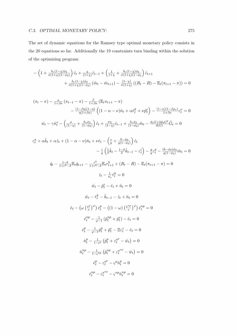
C.3. OPTIMAL MONETARY POLICY: 275
The set of dynamic equations for the Ramsey type optimal monetary policy consists in
the 20 equations so far. Additionally the 19 constraints turn binding within the solution
of the optimizing program:
−(
1 + hc(1−χ)φ2σ(1+χ)(1−φ2)
)ct + χ
(1+χ) ct−1 +(
11+χ + hc(1−χ)φ2
σ(1+χ)(1−φ2
)ct+1
+ hc(1−χ)φ2σ(1+χ)(1−φ2) (mt − mt+1)− (1−χ)
σ(1+χ) ((Rt −R)− Et(πt+1 − π)) = 0
(πt − π)− κ1+βκ (πt−1 − π)− β
1+βκ (Etπt+1 − π)
− (1−βη)(1−η)η(1+βκ)
((1− α− ν)nt + αrkt + νpet
)− (1−κ)(1−βρν)
1+βκ ενt = 0
wt − γnst −(
σ(1−χ) + hcφ2
(1−φ2)
)ct + σχ
(1−χ) ct−1 + hcφ2(1−φ2)mt − d1G+2d2G2
d(G) Gt = 0
εat + αkt + αzt + (1− α− ν)nt + νet −(cy + h−φ0
y(1−φ2)
)ct
− iy
(1δ kt − 1−δ
δ kt−1 − εit)− g
yεgt − (h−φ0)φ2
y(1−φ2) mt = 0
qt − 1−δ1+rk−δEtqt+1 − rk
1+rk−δEtrkt+1 + (Rt −R)− Et(πt+1 − π) = 0
zt − 1σarkt = 0
wt − pet − et + nt = 0
wt − rkt − kt−1 − zt + nt = 0
et −(ω(ep
e
)ϕ)ept −
((1− ω)
(enp
e
)ϕ)enpt = 0
enpt − 1ϕ−1 (pnpt + pet )− et = 0
ept − 1ϕ−1 p
pt + pet − Ξετt − et = 0
npt − 11−ςp
(ppt + εa
p
t − wt)
= 0
nnpt − 11−ςnp
(pnpt + εa
np
t − wt)
= 0
ept − εap
t − ςpnpt = 0
enpt − εanp
t − ςnpnnpt = 0
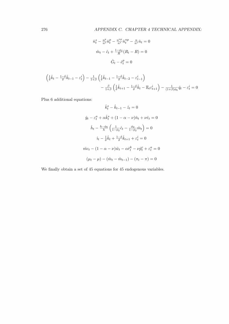
276 APPENDIX C. CHAPTER 4 TECHNICAL APPENDIX:
nst − np
ns npt − nnp
ns nnpt − n
ns nt = 0
mt − ct + 1−φ2R (Rt −R) = 0
Gt − ept = 0
(1δ kt − 1−δ
δ kt−1 − εit)− 1
1+β
(1δ kt−1 − 1−δ
δ kt−2 − εit−1
)
− β1+β
(1δ kt+1 − 1−δ
δ kt − Etεit+1
)− 1
(1+β)φkqt − εit = 0
Plus 6 additional equations:
kst − kt−1 − zt = 0
yt − εat + αkst + (1− α− ν)nt + νet = 0
ht − h−φ0h
(1
1−φ2 ct −φ2
1−φ2 mt
)= 0
ıt − 1δ kt + 1−δ
δ kt+1 + εit = 0
mct − (1− α− ν)wt − αrkt − νpet + εat = 0
(µt − µ)− (mt − mt−1)− (πt − π) = 0
We finally obtain a set of 45 equations for 45 endogenous variables.
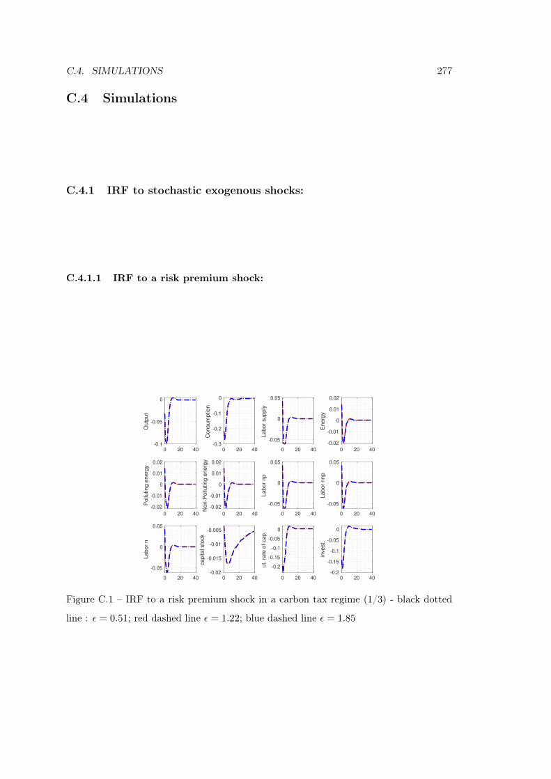
C.4. SIMULATIONS 277
C.4 Simulations
C.4.1 IRF to stochastic exogenous shocks:
C.4.1.1 IRF to a risk premium shock:
0 20 40-0.1
-0.05
0
Outp
ut
0 20 40-0.3
-0.2
-0.1
0
Consum
ption
0 20 40
-0.05
0
0.05
Labor
supply
0 20 40
-0.02
-0.01
0
0.01
0.02
Energ
y
0 20 40
-0.02
-0.01
0
0.01
0.02
Pollu
ting e
nerg
y
0 20 40
-0.02
-0.01
0
0.01
0.02
Non-P
ollu
ting e
nerg
y
0 20 40
-0.05
0
0.05
Labor
np
0 20 40
-0.05
0
0.05
Labor
nnp
0 20 40
-0.05
0
0.05
Labor
n
0 20 40-0.02
-0.015
-0.01
-0.005
capital sto
ck
0 20 40
-0.2
-0.15
-0.1
-0.05
0
ut. r
ate
of cap.
0 20 40-0.2
-0.15
-0.1
-0.05
0
invest.
Figure C.1 – IRF to a risk premium shock in a carbon tax regime (1/3) - black dotted
line : ε = 0.51; red dashed line ε = 1.22; blue dashed line ε = 1.85
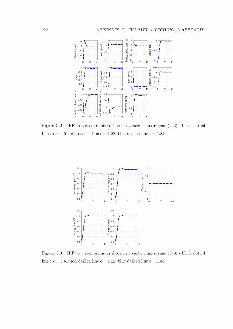
278 APPENDIX C. CHAPTER 4 TECHNICAL APPENDIX:
0 20 40
-0.04
-0.02
0
0.02
Ou
tput gro
wth
0 20 40
-0.2
-0.1
0
Cons.
gro
wth
0 20 40-15
-10
-5
0
5
Mo
ney g
row
th,
ann %
0 20 40-0.1
-0.05
0
Outp
ut
gap
0 20 40
-0.4
-0.3
-0.2
-0.1
0
wage
0 20 40
-0.4
-0.3
-0.2
-0.1
0
marg
inal cost
0 20 400
2
4
6
trans. costs
0 20 40-0.15
-0.1
-0.05
0
0.05
Inflation,
ann. %
0 20 40
-0.06
-0.04
-0.02
0
Nom
inte
rest ra
te, an
n %
0 20 40
-0.05
0
0.05
0.1
Re
al in
tere
st ra
te, ann %
0 20 40-0.3
-0.2
-0.1
0
renta
l ra
te o
f ca
pFigure C.2 – IRF to a risk premium shock in a carbon tax regime (2/3) - black dotted
line : ε = 0.51; red dashed line ε = 1.22; blue dashed line ε = 1.85
0 20 40-0.5
-0.4
-0.3
-0.2
-0.1
0
0.1
Net energ
y p
rice p
p
0 20 40-0.6
-0.5
-0.4
-0.3
-0.2
-0.1
0
Gro
ss e
nerg
y p
rice
0 20 40-1
-0.5
0
0.5
1
Carb
on p
rice
0 20 40-0.5
-0.4
-0.3
-0.2
-0.1
0
0.1
Energ
y p
rice p
np
0 20 40-0.5
-0.4
-0.3
-0.2
-0.1
0
0.1
Energ
y p
rice p
e
Figure C.3 – IRF to a risk premium shock in a carbon tax regime (3/3) - black dotted
line : ε = 0.51; red dashed line ε = 1.22; blue dashed line ε = 1.85
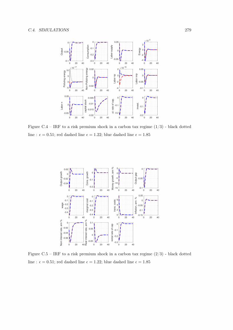
C.4. SIMULATIONS 279
0 20 40-0.1
-0.05
0
Outp
ut
0 20 40-0.3
-0.2
-0.1
0
Consum
ptio
n
0 20 40
-0.05
0
0.05
Labo
r sup
ply
0 20 40
-4
-2
0
2
Energ
y
10-3
0 20 40
-5
0
5
10
Pollu
tin
g e
nerg
y
10-17
0 20 40
-0.02
0
0.02
Non
-Pollu
ting
energ
y
0 20 40-4
-2
0
2
La
bor
np
10-16
0 20 40-0.1
-0.05
0
0.05
Labor
nnp
0 20 40
-0.05
0
0.05
La
bor
n
0 20 40-0.02
-0.015
-0.01
-0.005
ca
pital sto
ck
0 20 40
-0.2
-0.1
0
ut. r
ate
of cap
.
0 20 40-0.2
-0.1
0
invest.
Figure C.4 – IRF to a risk premium shock in a carbon tax regime (1/3) - black dotted
line : ε = 0.51; red dashed line ε = 1.22; blue dashed line ε = 1.85
0 20 40
-0.04
-0.02
0
0.02
Outp
ut gro
wth
0 20 40
-0.2
-0.1
0
Cons. gro
wth
0 20 40-15
-10
-5
0
5
Money g
row
th, ann %
0 20 40-0.1
-0.05
0
Outp
ut gap
0 20 40
-0.4
-0.3
-0.2
-0.1
0
wage
0 20 40
-0.4
-0.3
-0.2
-0.1
0
marg
inal cost
0 20 400
2
4
6
trans. costs
0 20 40-0.15
-0.1
-0.05
0
0.05
Inflation, ann. %
0 20 40
-0.06
-0.04
-0.02
0
Nom
inte
rest ra
te, ann %
0 20 40
-0.05
0
0.05
0.1
Real in
tere
st ra
te, ann %
0 20 40-0.3
-0.2
-0.1
0
renta
l ra
te o
f cap
Figure C.5 – IRF to a risk premium shock in a carbon tax regime (2/3) - black dotted
line : ε = 0.51; red dashed line ε = 1.22; blue dashed line ε = 1.85
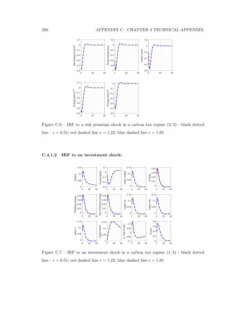
280 APPENDIX C. CHAPTER 4 TECHNICAL APPENDIX:
0 20 40-0.5
-0.4
-0.3
-0.2
-0.1
0
0.1
Net e
nerg
y p
rice p
p0 20 40
-1
-0.8
-0.6
-0.4
-0.2
0
0.2
Gro
ss e
ne
rgy p
rice
0 20 40-0.8
-0.6
-0.4
-0.2
0
0.2
Carb
on p
rice
0 20 40-0.5
-0.4
-0.3
-0.2
-0.1
0
0.1
Energ
y p
rice
pn
p
0 20 40-0.6
-0.5
-0.4
-0.3
-0.2
-0.1
0
Energ
y p
rice
pe
Figure C.6 – IRF to a risk premium shock in a carbon tax regime (3/3) - black dotted
line : ε = 0.51; red dashed line ε = 1.22; blue dashed line ε = 1.85
C.4.1.2 IRF to an investment shock:
0 20 400
0.05
0.1
0.15
Outp
ut
0 20 40-0.3
-0.2
-0.1
0
0.1
Consum
ption
0 20 40
0
0.05
0.1
0.15
Labor
supply
0 20 40
0
0.01
0.02
0.03
0.04
Energ
y
0 20 40
0
0.01
0.02
0.03
0.04
Pollu
ting e
nerg
y
0 20 40
0
0.01
0.02
0.03
0.04
Non-P
ollu
ting e
nerg
y
0 20 40
0
0.05
0.1
0.15
Labor
np
0 20 40
0
0.05
0.1
0.15
Labor
nnp
0 20 40
0
0.05
0.1
0.15
Labor
n
0 20 400
0.05
0.1
0.15
capital sto
ck
0 20 40-0.1
-0.05
0
0.05
0.1
ut. r
ate
of cap.
0 20 400
0.2
0.4
0.6
0.8
invest.
Figure C.7 – IRF to an investment shock in a carbon tax regime (1/3) - black dotted
line : ε = 0.51; red dashed line ε = 1.22; blue dashed line ε = 1.85
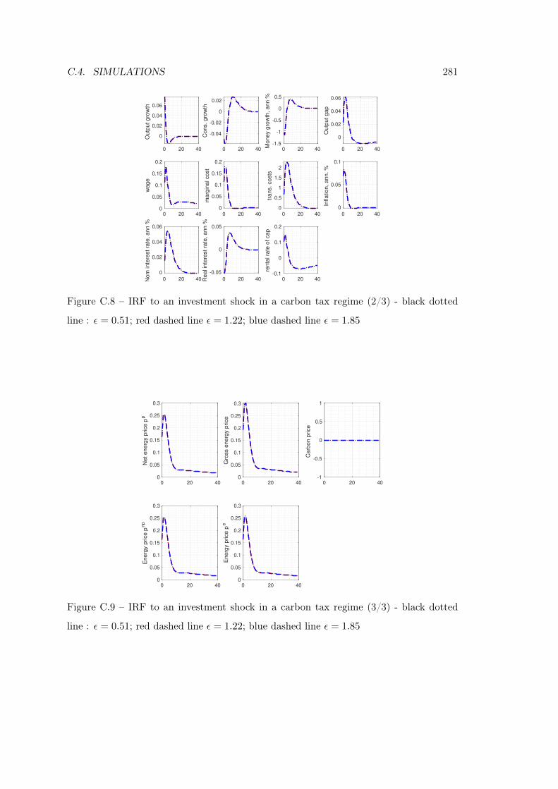
C.4. SIMULATIONS 281
0 20 40
0
0.02
0.04
0.06
Ou
tput gro
wth
0 20 40
-0.04
-0.02
0
0.02
Cons.
gro
wth
0 20 40-1.5
-1
-0.5
0
0.5
Mo
ney g
row
th,
ann %
0 20 40
0
0.02
0.04
0.06
Outp
ut
gap
0 20 400
0.05
0.1
0.15
0.2
wage
0 20 400
0.05
0.1
0.15
0.2
marg
inal cost
0 20 40
0
0.5
1
1.5
2
trans. costs
0 20 40
0
0.05
0.1
Inflation,
ann. %
0 20 40
0
0.02
0.04
0.06
Nom
inte
rest ra
te, an
n %
0 20 40
-0.05
0
0.05
Re
al in
tere
st ra
te, ann %
0 20 40-0.1
0
0.1
0.2
renta
l ra
te o
f ca
p
Figure C.8 – IRF to an investment shock in a carbon tax regime (2/3) - black dotted
line : ε = 0.51; red dashed line ε = 1.22; blue dashed line ε = 1.85
0 20 400
0.05
0.1
0.15
0.2
0.25
0.3
Net energ
y p
rice p
p
0 20 400
0.05
0.1
0.15
0.2
0.25
0.3
Gro
ss e
nerg
y p
rice
0 20 40-1
-0.5
0
0.5
1
Carb
on p
rice
0 20 400
0.05
0.1
0.15
0.2
0.25
0.3
Energ
y p
rice p
np
0 20 400
0.05
0.1
0.15
0.2
0.25
0.3
Energ
y p
rice p
e
Figure C.9 – IRF to an investment shock in a carbon tax regime (3/3) - black dotted
line : ε = 0.51; red dashed line ε = 1.22; blue dashed line ε = 1.85
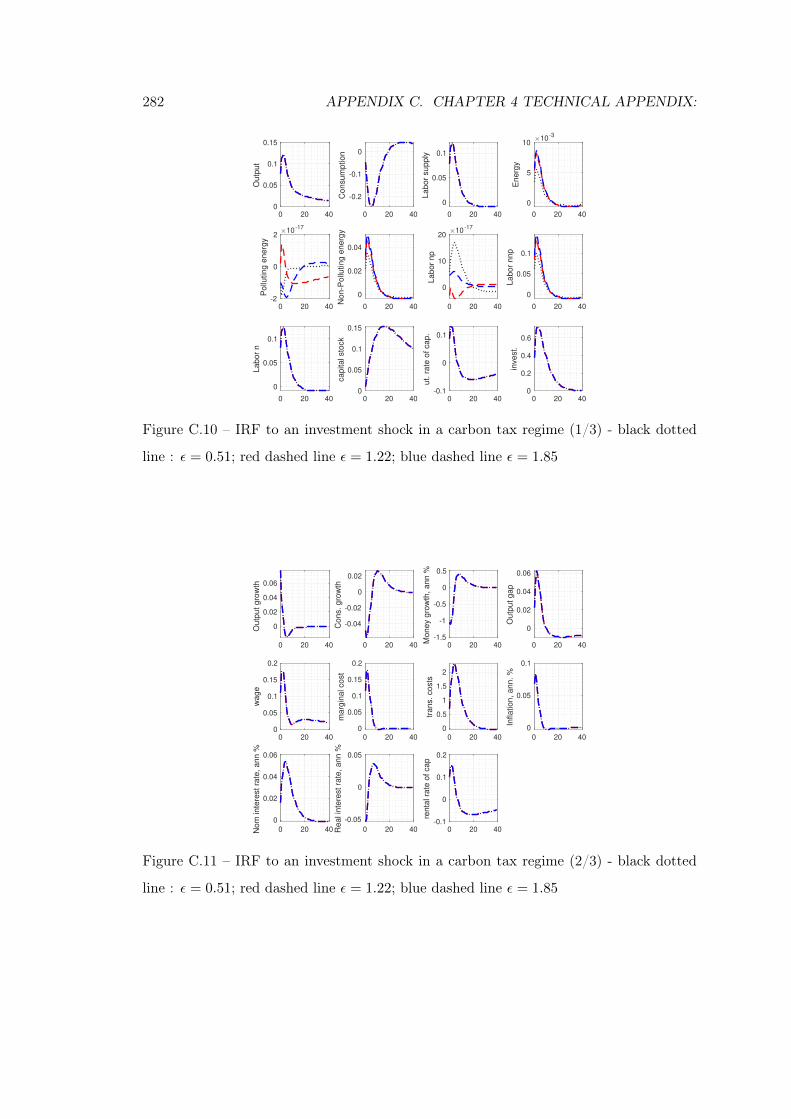
282 APPENDIX C. CHAPTER 4 TECHNICAL APPENDIX:
0 20 400
0.05
0.1
0.15
Outp
ut
0 20 40
-0.2
-0.1
0
Consum
ptio
n
0 20 40
0
0.05
0.1
Labo
r sup
ply
0 20 40
0
5
10
Energ
y
10-3
0 20 40-2
0
2
Pollu
tin
g e
nerg
y
10-17
0 20 40
0
0.02
0.04
Non
-Pollu
ting
energ
y
0 20 40
0
10
20
La
bor
np
10-17
0 20 40
0
0.05
0.1
Labor
nnp
0 20 40
0
0.05
0.1
La
bor
n
0 20 400
0.05
0.1
0.15
ca
pital sto
ck
0 20 40-0.1
0
0.1
ut. r
ate
of cap
.
0 20 400
0.2
0.4
0.6
invest.
Figure C.10 – IRF to an investment shock in a carbon tax regime (1/3) - black dotted
line : ε = 0.51; red dashed line ε = 1.22; blue dashed line ε = 1.85
0 20 40
0
0.02
0.04
0.06
Outp
ut gro
wth
0 20 40
-0.04
-0.02
0
0.02
Cons. gro
wth
0 20 40-1.5
-1
-0.5
0
0.5
Money g
row
th, ann %
0 20 40
0
0.02
0.04
0.06
Outp
ut gap
0 20 400
0.05
0.1
0.15
0.2
wage
0 20 400
0.05
0.1
0.15
0.2
marg
inal cost
0 20 400
0.5
1
1.5
2
trans. costs
0 20 40
0
0.05
0.1
Inflation, ann. %
0 20 40
0
0.02
0.04
0.06
Nom
inte
rest ra
te, ann %
0 20 40
-0.05
0
0.05
Real in
tere
st ra
te, ann %
0 20 40-0.1
0
0.1
0.2
renta
l ra
te o
f cap
Figure C.11 – IRF to an investment shock in a carbon tax regime (2/3) - black dotted
line : ε = 0.51; red dashed line ε = 1.22; blue dashed line ε = 1.85
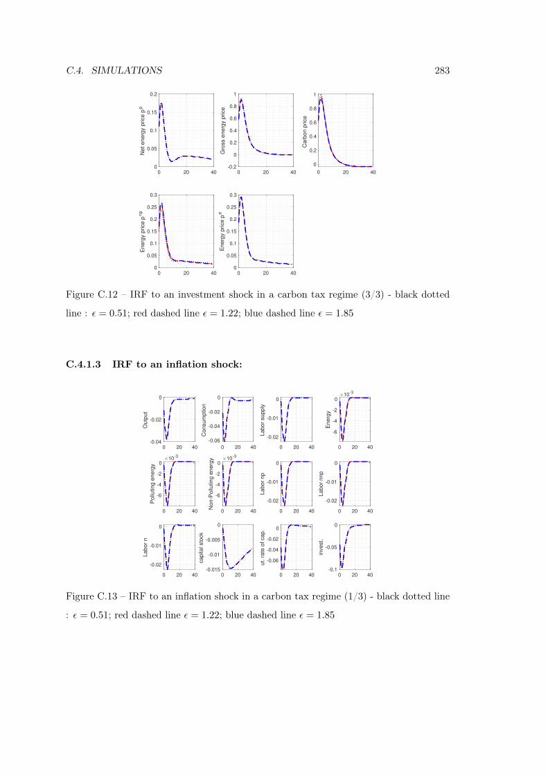
C.4. SIMULATIONS 283
0 20 400
0.05
0.1
0.15
0.2
Net e
nerg
y p
rice p
p
0 20 40-0.2
0
0.2
0.4
0.6
0.8
1
Gro
ss e
ne
rgy p
rice
0 20 40
0
0.2
0.4
0.6
0.8
1
Carb
on p
rice
0 20 400
0.05
0.1
0.15
0.2
0.25
0.3
Energ
y p
rice
pn
p
0 20 400
0.05
0.1
0.15
0.2
0.25
0.3
Energ
y p
rice
pe
Figure C.12 – IRF to an investment shock in a carbon tax regime (3/3) - black dotted
line : ε = 0.51; red dashed line ε = 1.22; blue dashed line ε = 1.85
C.4.1.3 IRF to an inflation shock:
0 20 40-0.04
-0.02
0
Outp
ut
0 20 40
-0.06
-0.04
-0.02
0
Consum
ption
0 20 40
-0.02
-0.01
0
Labor
supply
0 20 40
-6
-4
-2
0
Energ
y
10-3
0 20 40
-6
-4
-2
0
Pollu
ting e
nerg
y
10-3
0 20 40
-6
-4
-2
0
Non-P
ollu
ting e
nerg
y 10-3
0 20 40
-0.02
-0.01
0
Labor
np
0 20 40
-0.02
-0.01
0
Labor
nnp
0 20 40
-0.02
-0.01
0
Labor
n
0 20 40-0.015
-0.01
-0.005
0
capital sto
ck
0 20 40
-0.06
-0.04
-0.02
0
ut. r
ate
of cap.
0 20 40-0.1
-0.05
0
invest.
Figure C.13 – IRF to an inflation shock in a carbon tax regime (1/3) - black dotted line
: ε = 0.51; red dashed line ε = 1.22; blue dashed line ε = 1.85
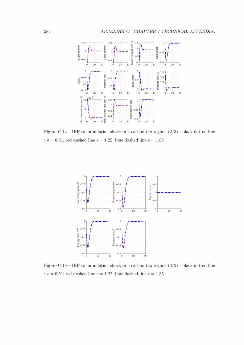
284 APPENDIX C. CHAPTER 4 TECHNICAL APPENDIX:
0 20 40
-0.01
0
0.01
Ou
tpu
t gro
wth
0 20 40
-0.02
0
0.02
Cons.
gro
wth
0 20 40-1
-0.5
0
0.5
Mone
y g
row
th, a
nn %
0 20 40-0.04
-0.02
0
Outp
ut
gap
0 20 40
-0.15
-0.1
-0.05
0
wage
0 20 40
-0.1
-0.05
0
marg
ina
l cost
0 20 40
0
0.5
1
trans. costs
0 20 40
0
0.02
0.04
0.06
Infla
tion, a
nn. %
0 20 40
0
10
20
Nom
inte
rest ra
te, an
n % 10
-3
0 20 40
-0.04
-0.02
0
0.02
Rea
l in
tere
st
rate
, ann %
0 20 40-0.1
-0.05
0
renta
l ra
te o
f cap
Figure C.14 – IRF to an inflation shock in a carbon tax regime (2/3) - black dotted line
: ε = 0.51; red dashed line ε = 1.22; blue dashed line ε = 1.85
0 20 40-0.2
-0.15
-0.1
-0.05
0
Net energ
y p
rice p
p
0 20 40-0.2
-0.15
-0.1
-0.05
0
Gro
ss e
nerg
y p
rice
0 20 40-1
-0.5
0
0.5
1
Carb
on p
rice
0 20 40-0.2
-0.15
-0.1
-0.05
0
Energ
y p
rice p
np
0 20 40-0.2
-0.15
-0.1
-0.05
0
Energ
y p
rice p
e
Figure C.15 – IRF to an inflation shock in a carbon tax regime (3/3) - black dotted line
: ε = 0.51; red dashed line ε = 1.22; blue dashed line ε = 1.85
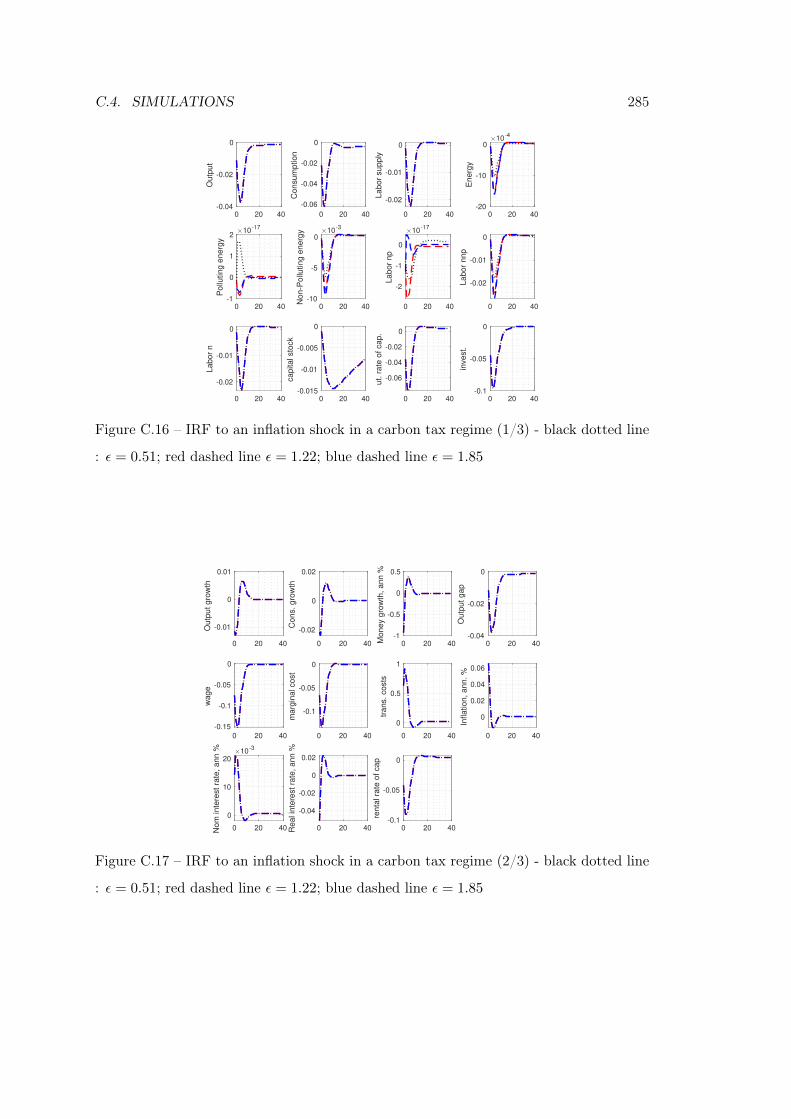
C.4. SIMULATIONS 285
0 20 40-0.04
-0.02
0
Outp
ut
0 20 40
-0.06
-0.04
-0.02
0
Consum
ptio
n
0 20 40
-0.02
-0.01
0
Labo
r sup
ply
0 20 40-20
-10
0
Energ
y
10-4
0 20 40-1
0
1
2
Pollu
tin
g e
nerg
y
10-17
0 20 40-10
-5
0
Non
-Pollu
ting
energ
y 10-3
0 20 40
-2
-1
0
La
bor
np
10-17
0 20 40
-0.02
-0.01
0
Labor
nnp
0 20 40
-0.02
-0.01
0
La
bor
n
0 20 40-0.015
-0.01
-0.005
0
ca
pital sto
ck
0 20 40
-0.06
-0.04
-0.02
0
ut. r
ate
of cap
.
0 20 40-0.1
-0.05
0
invest.
Figure C.16 – IRF to an inflation shock in a carbon tax regime (1/3) - black dotted line
: ε = 0.51; red dashed line ε = 1.22; blue dashed line ε = 1.85
0 20 40
-0.01
0
0.01
Outp
ut gro
wth
0 20 40
-0.02
0
0.02
Cons.
gro
wth
0 20 40-1
-0.5
0
0.5
Money g
row
th,
ann %
0 20 40-0.04
-0.02
0
Outp
ut gap
0 20 40
-0.15
-0.1
-0.05
0
wage
0 20 40
-0.1
-0.05
0
marg
inal cost
0 20 40
0
0.5
1
trans. costs
0 20 40
0
0.02
0.04
0.06
Inflation, ann. %
0 20 40
0
10
20
Nom
inte
rest ra
te, ann % 10
-3
0 20 40
-0.04
-0.02
0
0.02
Real in
tere
st ra
te, ann %
0 20 40-0.1
-0.05
0
renta
l ra
te o
f cap
Figure C.17 – IRF to an inflation shock in a carbon tax regime (2/3) - black dotted line
: ε = 0.51; red dashed line ε = 1.22; blue dashed line ε = 1.85
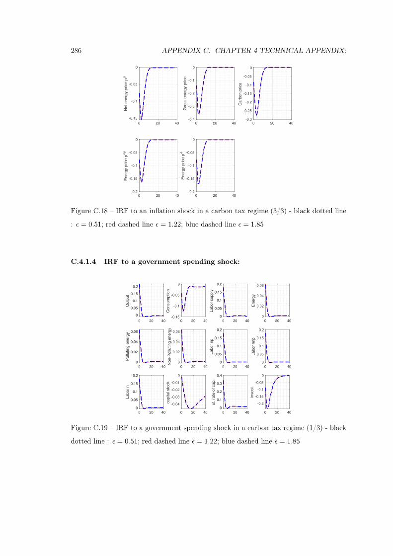
286 APPENDIX C. CHAPTER 4 TECHNICAL APPENDIX:
0 20 40
-0.15
-0.1
-0.05
0
Net e
nerg
y p
rice p
p0 20 40
-0.4
-0.3
-0.2
-0.1
0
Gro
ss e
ne
rgy p
rice
0 20 40-0.3
-0.25
-0.2
-0.15
-0.1
-0.05
0
Carb
on p
rice
0 20 40-0.2
-0.15
-0.1
-0.05
0
Energ
y p
rice
pn
p
0 20 40-0.2
-0.15
-0.1
-0.05
0
Energ
y p
rice
pe
Figure C.18 – IRF to an inflation shock in a carbon tax regime (3/3) - black dotted line
: ε = 0.51; red dashed line ε = 1.22; blue dashed line ε = 1.85
C.4.1.4 IRF to a government spending shock:
0 20 40
0
0.05
0.1
0.15
0.2
Outp
ut
0 20 40-0.15
-0.1
-0.05
0
Consum
ption
0 20 40
0
0.05
0.1
0.15
0.2
Labor
supply
0 20 40
0
0.02
0.04
0.06
Energ
y
0 20 40
0
0.02
0.04
0.06
Pollu
ting e
nerg
y
0 20 40
0
0.02
0.04
0.06
Non-P
ollu
ting e
nerg
y
0 20 40
0
0.05
0.1
0.15
0.2
Labor
np
0 20 40
0
0.05
0.1
0.15
0.2
Labor
nnp
0 20 40
0
0.05
0.1
0.15
0.2
Labor
n
0 20 40
-0.04
-0.03
-0.02
-0.01
0
capital sto
ck
0 20 40
0
0.1
0.2
0.3
0.4
ut. r
ate
of cap.
0 20 40
-0.2
-0.15
-0.1
-0.05
0
invest.
Figure C.19 – IRF to a government spending shock in a carbon tax regime (1/3) - black
dotted line : ε = 0.51; red dashed line ε = 1.22; blue dashed line ε = 1.85
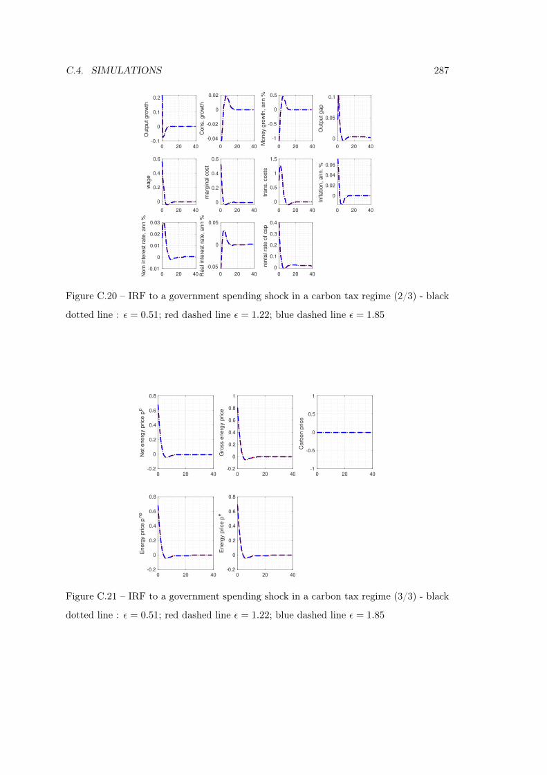
C.4. SIMULATIONS 287
0 20 40-0.1
0
0.1
0.2
Ou
tput gro
wth
0 20 40
-0.04
-0.02
0
0.02
Cons.
gro
wth
0 20 40
-1
-0.5
0
0.5
Mo
ney g
row
th,
ann %
0 20 40
0
0.05
0.1
Outp
ut
gap
0 20 40
0
0.2
0.4
0.6
wage
0 20 40
0
0.2
0.4
0.6
marg
inal cost
0 20 40
0
0.5
1
1.5
trans. costs
0 20 40
0
0.02
0.04
0.06
Inflation,
ann. %
0 20 40-0.01
0
0.01
0.02
0.03
Nom
inte
rest ra
te, an
n %
0 20 40
-0.05
0
0.05
Re
al in
tere
st ra
te, ann %
0 20 40
0
0.1
0.2
0.3
0.4
renta
l ra
te o
f ca
p
Figure C.20 – IRF to a government spending shock in a carbon tax regime (2/3) - black
dotted line : ε = 0.51; red dashed line ε = 1.22; blue dashed line ε = 1.85
0 20 40-0.2
0
0.2
0.4
0.6
0.8
Net energ
y p
rice p
p
0 20 40-0.2
0
0.2
0.4
0.6
0.8
1
Gro
ss e
nerg
y p
rice
0 20 40-1
-0.5
0
0.5
1
Carb
on p
rice
0 20 40-0.2
0
0.2
0.4
0.6
0.8
Energ
y p
rice p
np
0 20 40-0.2
0
0.2
0.4
0.6
0.8
Energ
y p
rice p
e
Figure C.21 – IRF to a government spending shock in a carbon tax regime (3/3) - black
dotted line : ε = 0.51; red dashed line ε = 1.22; blue dashed line ε = 1.85
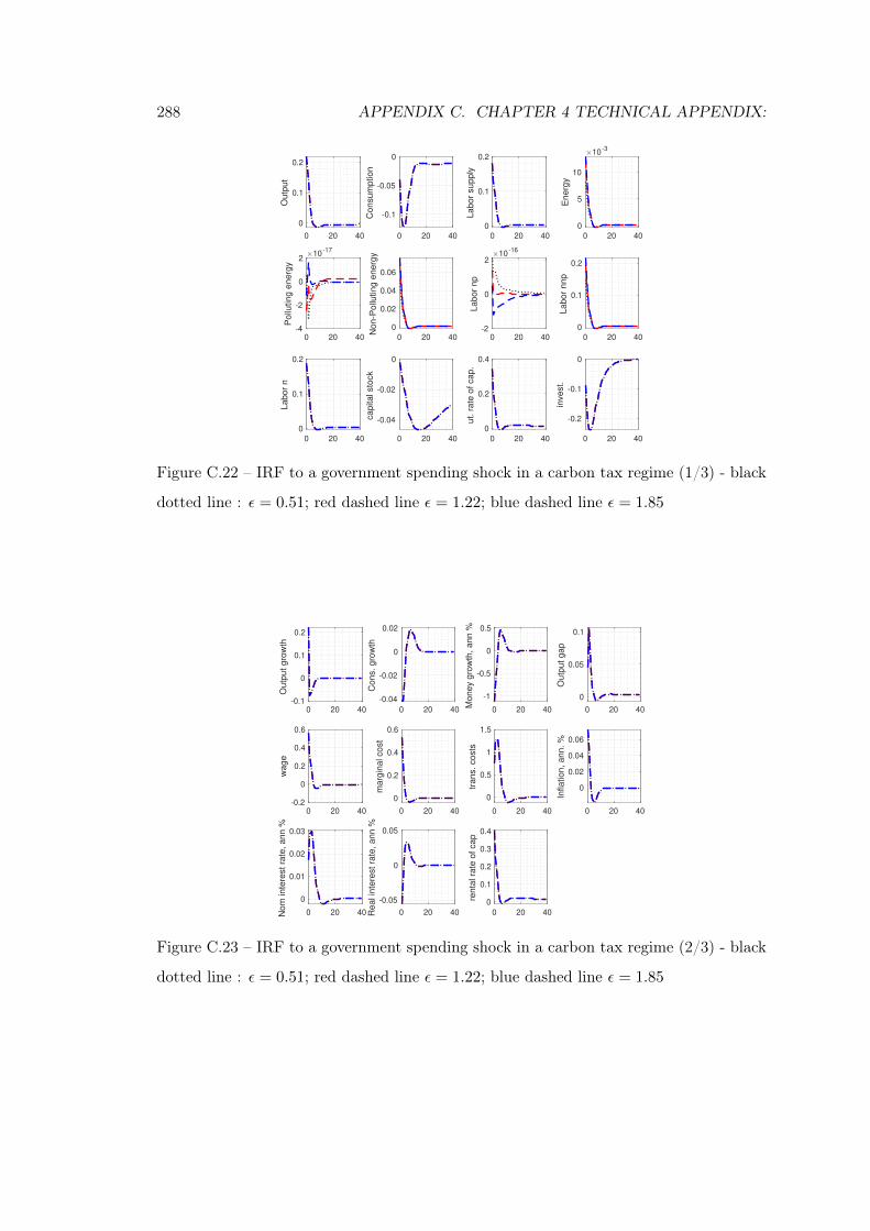
288 APPENDIX C. CHAPTER 4 TECHNICAL APPENDIX:
0 20 40
0
0.1
0.2
Outp
ut
0 20 40
-0.1
-0.05
0
Consum
ptio
n
0 20 40
0
0.1
0.2
Labo
r sup
ply
0 20 40
0
5
10
Energ
y
10-3
0 20 40-4
-2
0
2
Pollu
tin
g e
nerg
y
10-17
0 20 40
0
0.02
0.04
0.06
Non
-Pollu
ting
energ
y
0 20 40-2
0
2
La
bor
np
10-16
0 20 40
0
0.1
0.2
Labor
nnp
0 20 40
0
0.1
0.2
La
bor
n
0 20 40
-0.04
-0.02
0ca
pital sto
ck
0 20 40
0
0.2
0.4
ut. r
ate
of cap
.
0 20 40
-0.2
-0.1
0
invest.
Figure C.22 – IRF to a government spending shock in a carbon tax regime (1/3) - black
dotted line : ε = 0.51; red dashed line ε = 1.22; blue dashed line ε = 1.85
0 20 40-0.1
0
0.1
0.2
Outp
ut gro
wth
0 20 40
-0.04
-0.02
0
0.02
Cons. gro
wth
0 20 40
-1
-0.5
0
0.5
Money g
row
th, ann %
0 20 40
0
0.05
0.1
Outp
ut gap
0 20 40-0.2
0
0.2
0.4
0.6
wage
0 20 40
0
0.2
0.4
0.6
marg
inal cost
0 20 40
0
0.5
1
1.5
trans. costs
0 20 40
0
0.02
0.04
0.06
Inflation, ann. %
0 20 40
0
0.01
0.02
0.03
Nom
inte
rest ra
te, ann %
0 20 40
-0.05
0
0.05
Real in
tere
st ra
te, ann %
0 20 40
0
0.1
0.2
0.3
0.4
renta
l ra
te o
f cap
Figure C.23 – IRF to a government spending shock in a carbon tax regime (2/3) - black
dotted line : ε = 0.51; red dashed line ε = 1.22; blue dashed line ε = 1.85
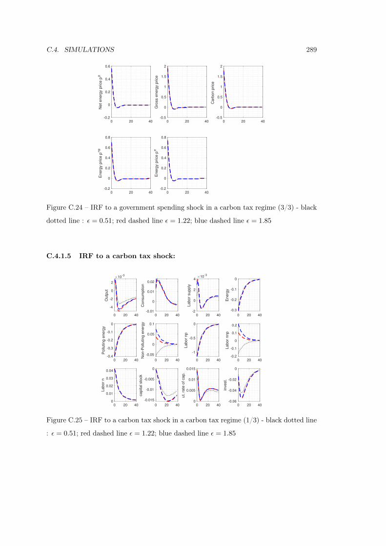
C.4. SIMULATIONS 289
0 20 40-0.2
0
0.2
0.4
0.6
Net e
nerg
y p
rice p
p
0 20 40-0.5
0
0.5
1
1.5
2
Gro
ss e
ne
rgy p
rice
0 20 40-0.5
0
0.5
1
1.5
2
Carb
on p
rice
0 20 40-0.2
0
0.2
0.4
0.6
0.8
Energ
y p
rice
pn
p
0 20 40-0.2
0
0.2
0.4
0.6
0.8
Energ
y p
rice
pe
Figure C.24 – IRF to a government spending shock in a carbon tax regime (3/3) - black
dotted line : ε = 0.51; red dashed line ε = 1.22; blue dashed line ε = 1.85
C.4.1.5 IRF to a carbon tax shock:
0 20 40
-4
-2
0
2
Outp
ut
10-3
0 20 40-0.01
0
0.01
0.02
Consum
ption
0 20 40-2
0
2
4
Labor
supply
10-3
0 20 40
-0.3
-0.2
-0.1
0
Energ
y
0 20 40-0.4
-0.3
-0.2
-0.1
0
Pollu
ting e
nerg
y
0 20 40
-0.05
0
0.05
0.1
Non-P
ollu
ting e
nerg
y
0 20 40
-1
-0.5
0
Labor
np
0 20 40-0.2
-0.1
0
0.1
0.2
Labor
nnp
0 20 400
0.01
0.02
0.03
0.04
Labor
n
0 20 40
-0.015
-0.01
-0.005
0
capital sto
ck
0 20 400
0.005
0.01
0.015
ut. r
ate
of cap.
0 20 40-0.06
-0.04
-0.02
0
invest.
Figure C.25 – IRF to a carbon tax shock in a carbon tax regime (1/3) - black dotted line
: ε = 0.51; red dashed line ε = 1.22; blue dashed line ε = 1.85
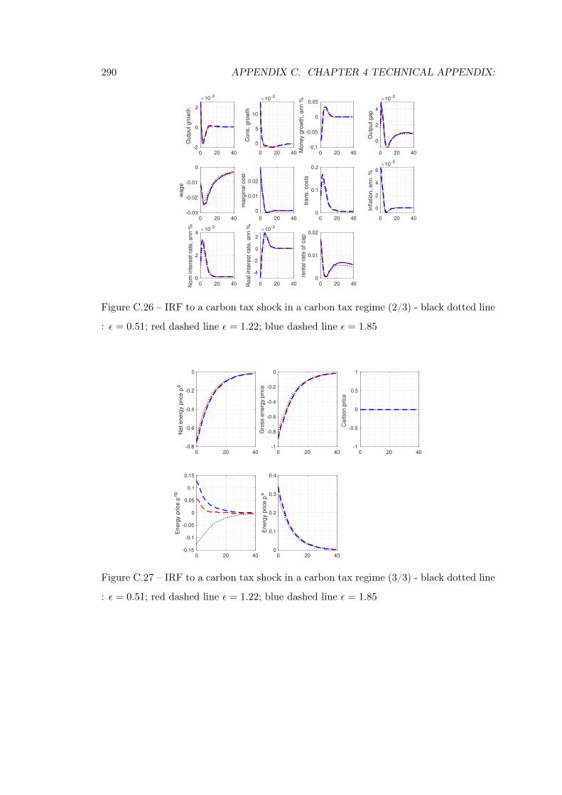
290 APPENDIX C. CHAPTER 4 TECHNICAL APPENDIX:
0 20 40-2
0
2
Ou
tpu
t gro
wth
10-3
0 20 40
0
5
10
Cons.
gro
wth
10-3
0 20 40-0.1
-0.05
0
0.05
Mone
y g
row
th, a
nn %
0 20 40
0
2
4
Outp
ut
gap
10-3
0 20 40-0.03
-0.02
-0.01
0
wage
0 20 40
0
0.01
0.02
marg
ina
l cost
0 20 400
0.1
0.2
trans. costs
0 20 40
0
2
4
6
Infla
tion, a
nn. %
10-3
0 20 400
2
4
Nom
inte
rest ra
te, an
n % 10
-3
0 20 40
-4
-2
0
2
Rea
l in
tere
st
rate
, ann % 10
-3
0 20 400
0.01
0.02
renta
l ra
te o
f cap
Figure C.26 – IRF to a carbon tax shock in a carbon tax regime (2/3) - black dotted line
: ε = 0.51; red dashed line ε = 1.22; blue dashed line ε = 1.85
0 20 40-0.8
-0.6
-0.4
-0.2
0
Net energ
y p
rice p
p
0 20 40-1
-0.8
-0.6
-0.4
-0.2
0
Gro
ss e
nerg
y p
rice
0 20 40-1
-0.5
0
0.5
1
Carb
on p
rice
0 20 40-0.15
-0.1
-0.05
0
0.05
0.1
0.15
Energ
y p
rice p
np
0 20 400
0.1
0.2
0.3
0.4
Energ
y p
rice p
e
Figure C.27 – IRF to a carbon tax shock in a carbon tax regime (3/3) - black dotted line
: ε = 0.51; red dashed line ε = 1.22; blue dashed line ε = 1.85
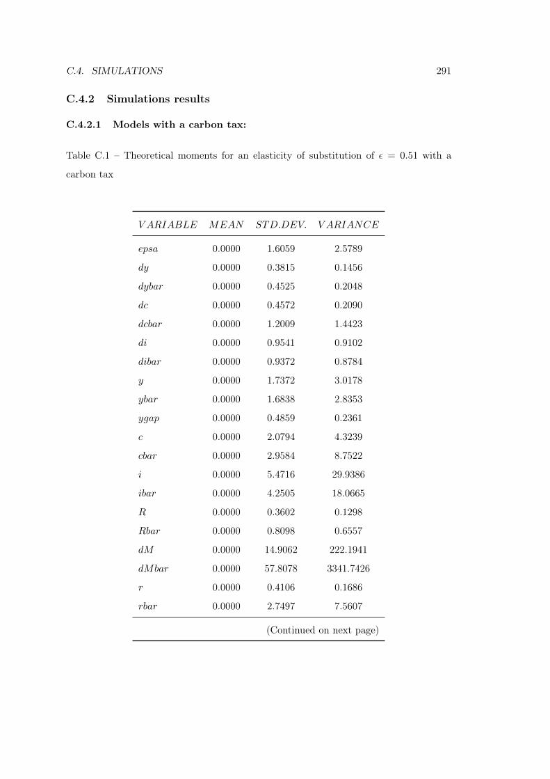
C.4. SIMULATIONS 291
C.4.2 Simulations results
C.4.2.1 Models with a carbon tax:
Table C.1 – Theoretical moments for an elasticity of substitution of ε = 0.51 with a
carbon tax
V ARIABLE MEAN STD.DEV. V ARIANCE
epsa 0.0000 1.6059 2.5789
dy 0.0000 0.3815 0.1456
dybar 0.0000 0.4525 0.2048
dc 0.0000 0.4572 0.2090
dcbar 0.0000 1.2009 1.4423
di 0.0000 0.9541 0.9102
dibar 0.0000 0.9372 0.8784
y 0.0000 1.7372 3.0178
ybar 0.0000 1.6838 2.8353
ygap 0.0000 0.4859 0.2361
c 0.0000 2.0794 4.3239
cbar 0.0000 2.9584 8.7522
i 0.0000 5.4716 29.9386
ibar 0.0000 4.2505 18.0665
R 0.0000 0.3602 0.1298
Rbar 0.0000 0.8098 0.6557
dM 0.0000 14.9062 222.1941
dMbar 0.0000 57.8078 3341.7426
r 0.0000 0.4106 0.1686
rbar 0.0000 2.7497 7.5607
(Continued on next page)

292 APPENDIX C. CHAPTER 4 TECHNICAL APPENDIX:
Table C.1 – (continued)
V ARIABLE MEAN STD.DEV. V ARIANCE
pi 0.0000 0.5100 0.2601
pibar 0.0000 3.8178 14.5756
mc 0.0000 2.5382 6.4426
nbar 0.0000 0.8179 0.6689
n 0.0000 0.7961 0.6338
np 0.0000 2.4963 6.2315
npbar 0.0000 2.5012 6.2559
nnp 0.0000 1.5103 2.2809
nnpbar 0.0000 1.5200 2.3105
m 0.0000 26.7339 714.6991
mbar 0.0000 52.9325 2801.8532
h 0.0000 16.0896 258.8753
hbar 0.0000 33.6494 1132.2788
ks 0.0000 2.3267 5.4134
ksbar 0.0000 2.3199 5.3821
k 0.0000 2.7459 7.5402
kbar 0.0000 2.1252 4.5165
z 0.0000 1.5023 2.2569
zbar 0.0000 0.2903 0.0843
q 0.0000 1.8208 3.3151
qbar 0.0000 3.8270 14.6462
rk 0.0000 1.7577 3.0894
rkbar 0.0000 1.9977 3.9908
(Continued on next page)
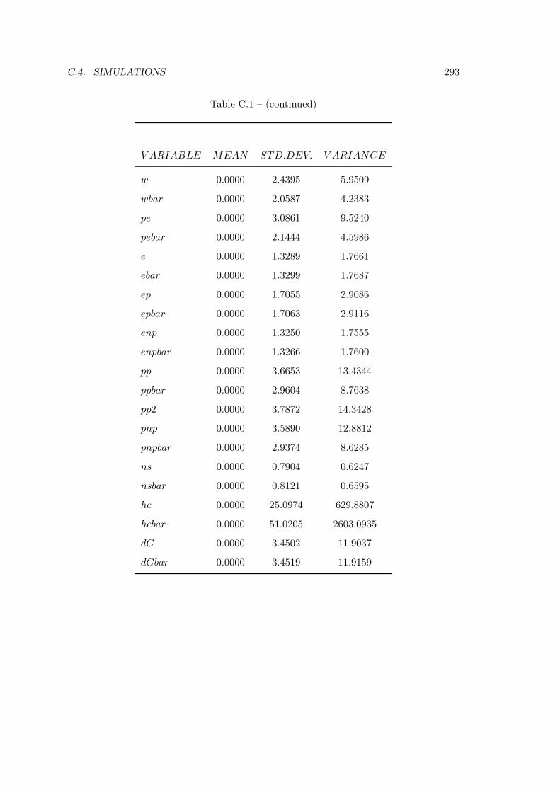
C.4. SIMULATIONS 293
Table C.1 – (continued)
V ARIABLE MEAN STD.DEV. V ARIANCE
w 0.0000 2.4395 5.9509
wbar 0.0000 2.0587 4.2383
pe 0.0000 3.0861 9.5240
pebar 0.0000 2.1444 4.5986
e 0.0000 1.3289 1.7661
ebar 0.0000 1.3299 1.7687
ep 0.0000 1.7055 2.9086
epbar 0.0000 1.7063 2.9116
enp 0.0000 1.3250 1.7555
enpbar 0.0000 1.3266 1.7600
pp 0.0000 3.6653 13.4344
ppbar 0.0000 2.9604 8.7638
pp2 0.0000 3.7872 14.3428
pnp 0.0000 3.5890 12.8812
pnpbar 0.0000 2.9374 8.6285
ns 0.0000 0.7904 0.6247
nsbar 0.0000 0.8121 0.6595
hc 0.0000 25.0974 629.8807
hcbar 0.0000 51.0205 2603.0935
dG 0.0000 3.4502 11.9037
dGbar 0.0000 3.4519 11.9159

294 APPENDIX C. CHAPTER 4 TECHNICAL APPENDIX:
Table C.2 – Variance decomposition (in percent) for an elasticity of substitution of ε =
0.51 with a carbon tax
e_a e_ap e_anp e_b e_i e_g e_P e_tao
epsa 100.00 0.00 0.00 0.00 0.00 0.00 0.00 0.00
dy 48.39 0.13 0.01 4.46 5.68 40.93 0.40 0.01
dybar 74.72 0.21 0.02 0.07 1.52 23.47 0.00 0.00
dc 57.94 0.13 0.01 29.77 8.21 2.95 0.88 0.11
dcbar 86.26 0.20 0.02 0.10 2.34 11.08 0.00 0.01
di 67.45 0.65 0.02 3.14 26.05 2.16 0.48 0.05
dibar 77.67 0.68 0.02 0.01 15.55 6.02 0.00 0.05
y 92.37 0.36 0.02 1.05 3.38 2.59 0.23 0.01
ybar 95.94 0.43 0.02 0.00 2.36 1.23 0.00 0.01
ygap 67.01 0.42 0.02 13.24 7.71 8.65 2.93 0.03
c 79.70 0.17 0.01 5.57 12.03 2.02 0.39 0.12
cbar 85.95 0.25 0.02 0.09 8.16 5.50 0.00 0.04
i 82.78 0.93 0.02 0.35 14.32 1.35 0.17 0.08
ibar 81.31 1.04 0.02 0.01 15.37 2.16 0.00 0.10
R 56.40 0.46 0.01 24.39 15.20 2.45 1.06 0.03
Rbar 74.10 0.42 0.02 10.92 4.82 9.70 0.00 0.02
dM 18.74 0.11 0.00 77.43 1.94 1.12 0.65 0.00
dMbar 86.35 0.38 0.02 0.55 0.60 12.09 0.00 0.01
r 61.45 0.46 0.01 22.07 10.25 3.94 1.79 0.03
rbar 85.68 0.33 0.02 1.18 0.33 12.46 0.00 0.00
pi 66.20 0.46 0.02 18.63 8.53 3.60 2.54 0.02
pibar 84.08 0.37 0.02 3.09 0.66 11.77 0.00 0.01
(Continued on next page)
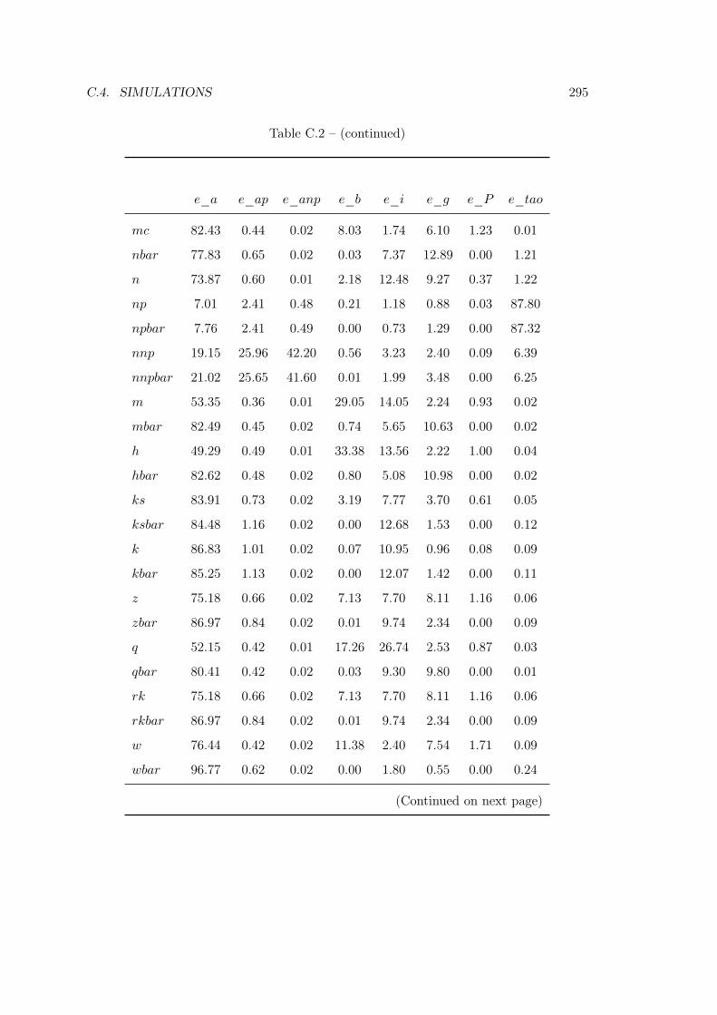
C.4. SIMULATIONS 295
Table C.2 – (continued)
e_a e_ap e_anp e_b e_i e_g e_P e_tao
mc 82.43 0.44 0.02 8.03 1.74 6.10 1.23 0.01
nbar 77.83 0.65 0.02 0.03 7.37 12.89 0.00 1.21
n 73.87 0.60 0.01 2.18 12.48 9.27 0.37 1.22
np 7.01 2.41 0.48 0.21 1.18 0.88 0.03 87.80
npbar 7.76 2.41 0.49 0.00 0.73 1.29 0.00 87.32
nnp 19.15 25.96 42.20 0.56 3.23 2.40 0.09 6.39
nnpbar 21.02 25.65 41.60 0.01 1.99 3.48 0.00 6.25
m 53.35 0.36 0.01 29.05 14.05 2.24 0.93 0.02
mbar 82.49 0.45 0.02 0.74 5.65 10.63 0.00 0.02
h 49.29 0.49 0.01 33.38 13.56 2.22 1.00 0.04
hbar 82.62 0.48 0.02 0.80 5.08 10.98 0.00 0.02
ks 83.91 0.73 0.02 3.19 7.77 3.70 0.61 0.05
ksbar 84.48 1.16 0.02 0.00 12.68 1.53 0.00 0.12
k 86.83 1.01 0.02 0.07 10.95 0.96 0.08 0.09
kbar 85.25 1.13 0.02 0.00 12.07 1.42 0.00 0.11
z 75.18 0.66 0.02 7.13 7.70 8.11 1.16 0.06
zbar 86.97 0.84 0.02 0.01 9.74 2.34 0.00 0.09
q 52.15 0.42 0.01 17.26 26.74 2.53 0.87 0.03
qbar 80.41 0.42 0.02 0.03 9.30 9.80 0.00 0.01
rk 75.18 0.66 0.02 7.13 7.70 8.11 1.16 0.06
rkbar 86.97 0.84 0.02 0.01 9.74 2.34 0.00 0.09
w 76.44 0.42 0.02 11.38 2.40 7.54 1.71 0.09
wbar 96.77 0.62 0.02 0.00 1.80 0.55 0.00 0.24
(Continued on next page)
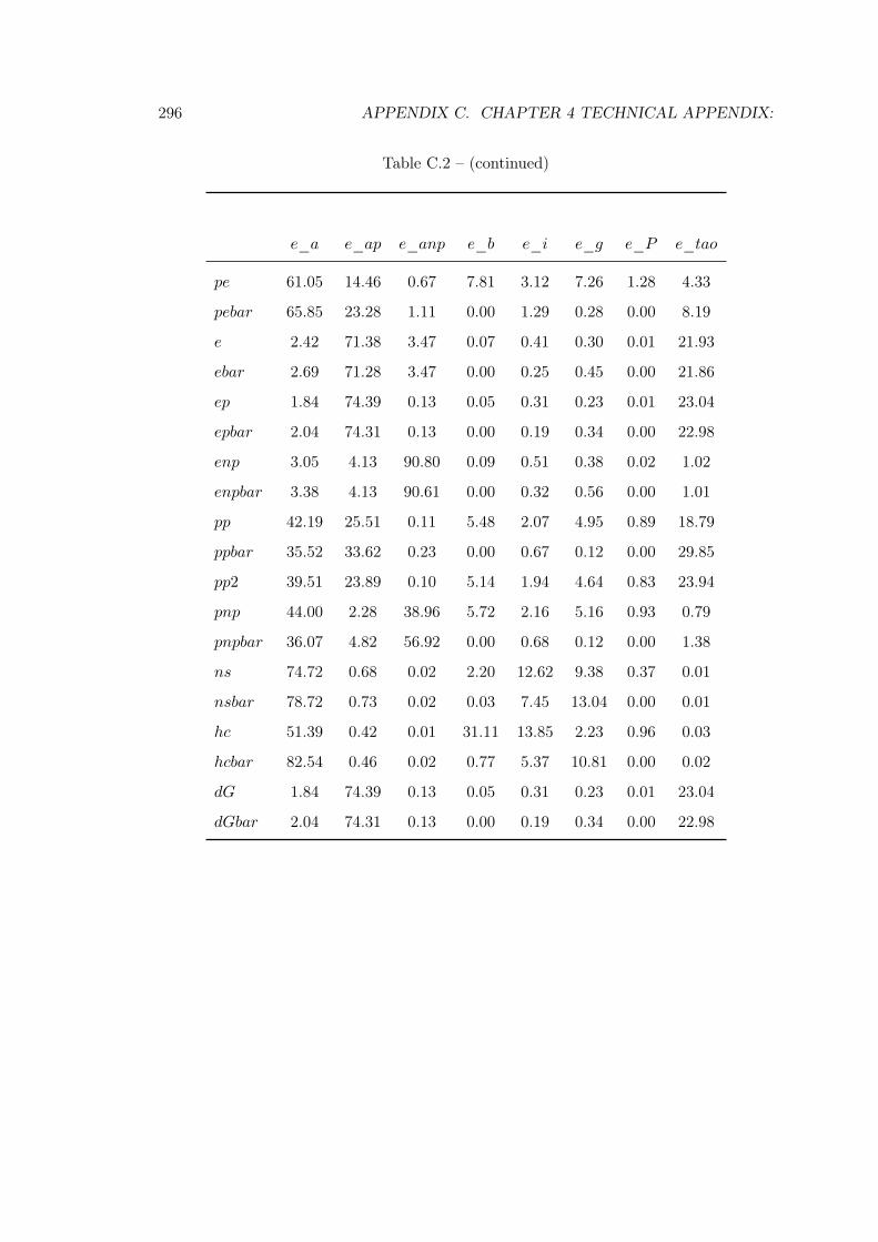
296 APPENDIX C. CHAPTER 4 TECHNICAL APPENDIX:
Table C.2 – (continued)
e_a e_ap e_anp e_b e_i e_g e_P e_tao
pe 61.05 14.46 0.67 7.81 3.12 7.26 1.28 4.33
pebar 65.85 23.28 1.11 0.00 1.29 0.28 0.00 8.19
e 2.42 71.38 3.47 0.07 0.41 0.30 0.01 21.93
ebar 2.69 71.28 3.47 0.00 0.25 0.45 0.00 21.86
ep 1.84 74.39 0.13 0.05 0.31 0.23 0.01 23.04
epbar 2.04 74.31 0.13 0.00 0.19 0.34 0.00 22.98
enp 3.05 4.13 90.80 0.09 0.51 0.38 0.02 1.02
enpbar 3.38 4.13 90.61 0.00 0.32 0.56 0.00 1.01
pp 42.19 25.51 0.11 5.48 2.07 4.95 0.89 18.79
ppbar 35.52 33.62 0.23 0.00 0.67 0.12 0.00 29.85
pp2 39.51 23.89 0.10 5.14 1.94 4.64 0.83 23.94
pnp 44.00 2.28 38.96 5.72 2.16 5.16 0.93 0.79
pnpbar 36.07 4.82 56.92 0.00 0.68 0.12 0.00 1.38
ns 74.72 0.68 0.02 2.20 12.62 9.38 0.37 0.01
nsbar 78.72 0.73 0.02 0.03 7.45 13.04 0.00 0.01
hc 51.39 0.42 0.01 31.11 13.85 2.23 0.96 0.03
hcbar 82.54 0.46 0.02 0.77 5.37 10.81 0.00 0.02
dG 1.84 74.39 0.13 0.05 0.31 0.23 0.01 23.04
dGbar 2.04 74.31 0.13 0.00 0.19 0.34 0.00 22.98

C.4. SIMULATIONS 297
Table C.3 – Coefficients of autocorrelation for an elasticity of substitution of ε = 0.51
with a carbon tax
Order 1 2 3 4 5
epsa 0.9000 0.8100 0.7290 0.6561 0.5905
dy 0.3984 0.2372 0.1023 0.0045 -0.0571
dybar 0.3124 -0.0142 -0.0619 -0.0636 -0.0584
dc 0.6630 0.3446 0.0924 -0.0770 -0.1705
dcbar 0.0567 -0.0806 -0.0863 -0.0730 -0.0592
di 0.7145 0.4608 0.2565 0.1053 0.0018
dibar 0.3751 0.1890 0.0982 0.0399 -0.0004
y 0.9759 0.9325 0.8778 0.8180 0.7581
ybar 0.9639 0.9052 0.8476 0.7944 0.7458
ygap 0.8284 0.5111 0.2526 0.0805 -0.0181
c 0.9758 0.9196 0.8468 0.7694 0.6958
cbar 0.9176 0.8259 0.7474 0.6832 0.6309
i 0.9848 0.9479 0.8969 0.8382 0.7763
ibar 0.9757 0.9331 0.8814 0.8249 0.7664
R 0.9459 0.8208 0.6696 0.5236 0.3989
Rbar 0.3513 0.2085 0.1578 0.1280 0.1062
dM 0.0215 -0.0547 -0.0894 -0.0936 -0.0813
dMbar -0.3963 -0.0706 -0.0151 -0.0051 -0.0029
r 0.6804 0.3836 0.1703 0.0407 -0.0251
rbar 0.2037 0.0618 0.0316 0.0216 0.0161
pi 0.6995 0.3454 0.0904 -0.0521 -0.1101
pibar -0.3752 -0.0653 -0.0127 -0.0035 -0.0016
(Continued on next page)
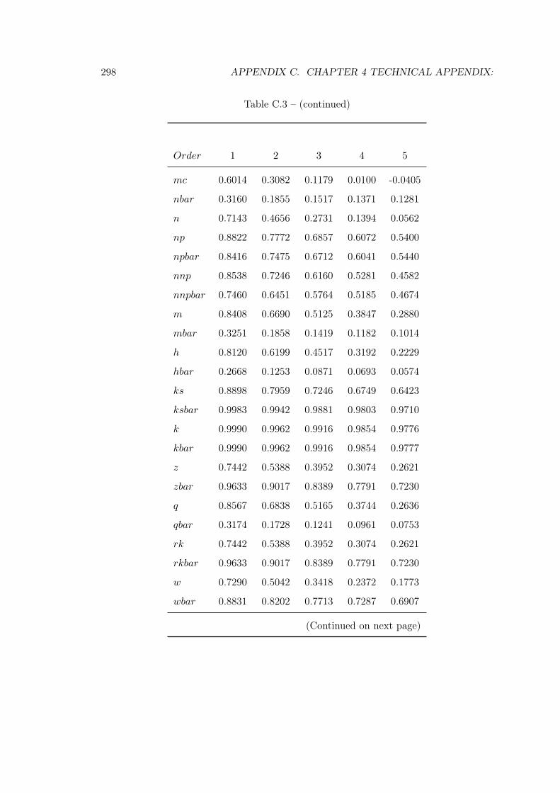
298 APPENDIX C. CHAPTER 4 TECHNICAL APPENDIX:
Table C.3 – (continued)
Order 1 2 3 4 5
mc 0.6014 0.3082 0.1179 0.0100 -0.0405
nbar 0.3160 0.1855 0.1517 0.1371 0.1281
n 0.7143 0.4656 0.2731 0.1394 0.0562
np 0.8822 0.7772 0.6857 0.6072 0.5400
npbar 0.8416 0.7475 0.6712 0.6041 0.5440
nnp 0.8538 0.7246 0.6160 0.5281 0.4582
nnpbar 0.7460 0.6451 0.5764 0.5185 0.4674
m 0.8408 0.6690 0.5125 0.3847 0.2880
mbar 0.3251 0.1858 0.1419 0.1182 0.1014
h 0.8120 0.6199 0.4517 0.3192 0.2229
hbar 0.2668 0.1253 0.0871 0.0693 0.0574
ks 0.8898 0.7959 0.7246 0.6749 0.6423
ksbar 0.9983 0.9942 0.9881 0.9803 0.9710
k 0.9990 0.9962 0.9916 0.9854 0.9776
kbar 0.9990 0.9962 0.9916 0.9854 0.9777
z 0.7442 0.5388 0.3952 0.3074 0.2621
zbar 0.9633 0.9017 0.8389 0.7791 0.7230
q 0.8567 0.6838 0.5165 0.3744 0.2636
qbar 0.3174 0.1728 0.1241 0.0961 0.0753
rk 0.7442 0.5388 0.3952 0.3074 0.2621
rkbar 0.9633 0.9017 0.8389 0.7791 0.7230
w 0.7290 0.5042 0.3418 0.2372 0.1773
wbar 0.8831 0.8202 0.7713 0.7287 0.6907
(Continued on next page)
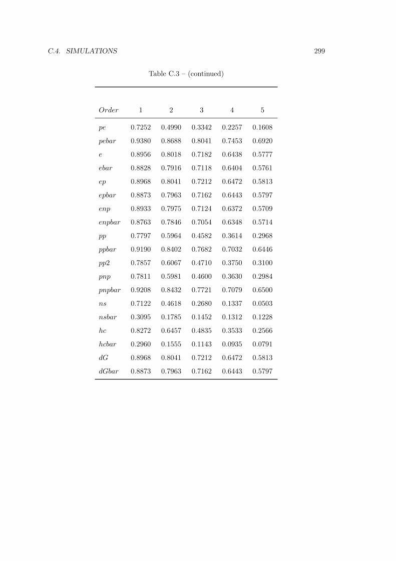
C.4. SIMULATIONS 299
Table C.3 – (continued)
Order 1 2 3 4 5
pe 0.7252 0.4990 0.3342 0.2257 0.1608
pebar 0.9380 0.8688 0.8041 0.7453 0.6920
e 0.8956 0.8018 0.7182 0.6438 0.5777
ebar 0.8828 0.7916 0.7118 0.6404 0.5761
ep 0.8968 0.8041 0.7212 0.6472 0.5813
epbar 0.8873 0.7963 0.7162 0.6443 0.5797
enp 0.8933 0.7975 0.7124 0.6372 0.5709
enpbar 0.8763 0.7846 0.7054 0.6348 0.5714
pp 0.7797 0.5964 0.4582 0.3614 0.2968
ppbar 0.9190 0.8402 0.7682 0.7032 0.6446
pp2 0.7857 0.6067 0.4710 0.3750 0.3100
pnp 0.7811 0.5981 0.4600 0.3630 0.2984
pnpbar 0.9208 0.8432 0.7721 0.7079 0.6500
ns 0.7122 0.4618 0.2680 0.1337 0.0503
nsbar 0.3095 0.1785 0.1452 0.1312 0.1228
hc 0.8272 0.6457 0.4835 0.3533 0.2566
hcbar 0.2960 0.1555 0.1143 0.0935 0.0791
dG 0.8968 0.8041 0.7212 0.6472 0.5813
dGbar 0.8873 0.7963 0.7162 0.6443 0.5797
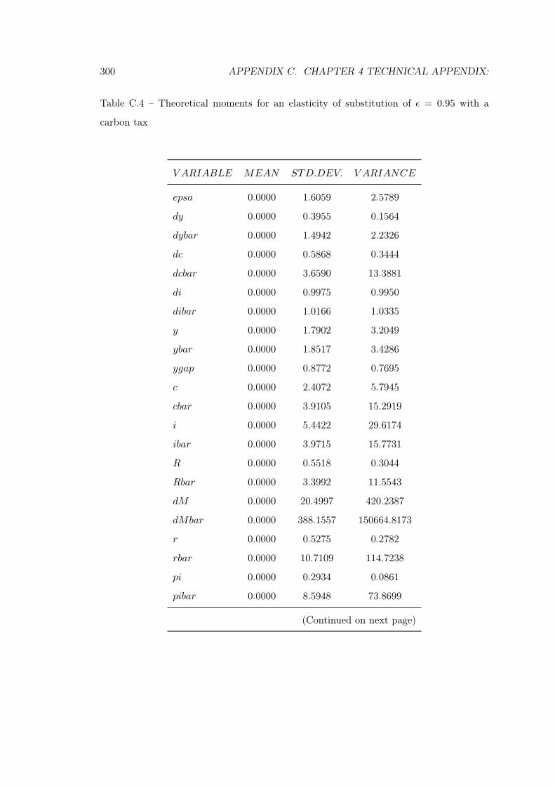
300 APPENDIX C. CHAPTER 4 TECHNICAL APPENDIX:
Table C.4 – Theoretical moments for an elasticity of substitution of ε = 0.95 with a
carbon tax
V ARIABLE MEAN STD.DEV. V ARIANCE
epsa 0.0000 1.6059 2.5789
dy 0.0000 0.3955 0.1564
dybar 0.0000 1.4942 2.2326
dc 0.0000 0.5868 0.3444
dcbar 0.0000 3.6590 13.3881
di 0.0000 0.9975 0.9950
dibar 0.0000 1.0166 1.0335
y 0.0000 1.7902 3.2049
ybar 0.0000 1.8517 3.4286
ygap 0.0000 0.8772 0.7695
c 0.0000 2.4072 5.7945
cbar 0.0000 3.9105 15.2919
i 0.0000 5.4422 29.6174
ibar 0.0000 3.9715 15.7731
R 0.0000 0.5518 0.3044
Rbar 0.0000 3.3992 11.5543
dM 0.0000 20.4997 420.2387
dMbar 0.0000 388.1557 150664.8173
r 0.0000 0.5275 0.2782
rbar 0.0000 10.7109 114.7238
pi 0.0000 0.2934 0.0861
pibar 0.0000 8.5948 73.8699
(Continued on next page)
C.4. SIMULATIONS 301
Table C.4 – (continued)
V ARIABLE MEAN STD.DEV. V ARIANCE
mc 0.0000 1.8250 3.3305
nbar 0.0000 1.6161 2.6119
n 0.0000 0.7621 0.5808
np 0.0000 2.6264 6.8982
npbar 0.0000 2.9852 8.9116
nnp 0.0000 0.7607 0.5787
nnpbar 0.0000 1.6151 2.6085
m 0.0000 38.3225 1468.6174
mbar 0.0000 227.6688 51833.0859
h 0.0000 23.5978 556.8556
hbar 0.0000 152.2848 23190.6696
ks 0.0000 2.1816 4.7596
ksbar 0.0000 2.2015 4.8468
k 0.0000 2.7412 7.5144
kbar 0.0000 2.0130 4.0520
z 0.0000 1.2766 1.6298
zbar 0.0000 0.3164 0.1001
q 0.0000 2.2045 4.8598
qbar 0.0000 7.3420 53.9044
rk 0.0000 1.4937 2.2310
rkbar 0.0000 2.1773 4.7408
w 0.0000 2.0492 4.1991
wbar 0.0000 2.1059 4.4349
(Continued on next page)
302 APPENDIX C. CHAPTER 4 TECHNICAL APPENDIX:
Table C.4 – (continued)
V ARIABLE MEAN STD.DEV. V ARIANCE
pe 0.0000 2.6940 7.2577
pebar 0.0000 2.2724 5.1640
e 0.0000 1.5351 2.3566
ebar 0.0000 1.6117 2.5975
ep 0.0000 1.8284 3.3430
epbar 0.0000 1.8928 3.5826
enp 0.0000 1.5994 2.5581
enpbar 0.0000 1.6753 2.8067
pp 0.0000 3.2365 10.4748
ppbar 0.0000 2.9049 8.4387
pp2 0.0000 3.2347 10.4635
pnp 0.0000 2.7813 7.7359
pnpbar 0.0000 2.4200 5.8562
ns 0.0000 0.7566 0.5725
nsbar 0.0000 1.6134 2.6029
hc 0.0000 36.3874 1324.0452
hcbar 0.0000 225.1723 50702.5851
dG 0.0000 3.6989 13.6817
dGbar 0.0000 3.8291 14.6622
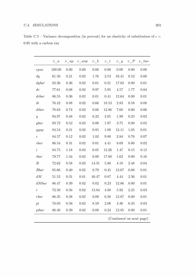
C.4. SIMULATIONS 303
Table C.5 – Variance decomposition (in percent) for an elasticity of substitution of ε =
0.95 with a carbon tax
e_a e_ap e_anp e_b e_i e_g e_P e_tao
epsa 100.00 0.00 0.00 0.00 0.00 0.00 0.00 0.00
dy 61.56 0.21 0.02 1.76 2.53 33.41 0.52 0.00
dybar 82.26 0.36 0.02 0.01 0.31 17.02 0.00 0.01
dc 77.61 0.08 0.02 9.97 5.95 4.57 1.77 0.04
dcbar 86.55 0.36 0.02 0.01 0.41 12.64 0.00 0.01
di 76.42 0.88 0.02 0.66 18.53 2.83 0.58 0.08
dibar 78.63 0.74 0.02 0.00 12.86 7.68 0.00 0.06
y 94.97 0.48 0.02 0.22 2.05 1.99 0.25 0.02
ybar 93.72 0.52 0.02 0.00 1.97 3.75 0.00 0.02
ygap 84.54 0.41 0.02 0.85 1.00 12.11 1.05 0.01
c 84.57 0.12 0.02 1.82 9.80 2.84 0.76 0.07
cbar 86.54 0.31 0.02 0.01 4.41 8.69 0.00 0.02
i 84.75 1.18 0.02 0.05 12.26 1.47 0.15 0.12
ibar 79.77 1.34 0.02 0.00 17.08 1.62 0.00 0.16
R 72.62 0.58 0.02 14.31 5.86 4.10 2.48 0.04
Rbar 85.66 0.40 0.02 0.79 0.45 12.67 0.00 0.01
dM 51.52 0.31 0.01 40.47 0.87 4.44 2.36 0.01
dMbar 86.47 0.39 0.02 0.02 0.23 12.86 0.00 0.01
r 72.50 0.56 0.02 13.84 4.88 5.92 2.25 0.03
rbar 86.35 0.38 0.02 0.09 0.28 12.87 0.00 0.01
pi 78.03 0.56 0.02 8.59 2.06 4.36 6.35 0.03
pibar 86.40 0.39 0.02 0.09 0.24 12.85 0.00 0.01
(Continued on next page)
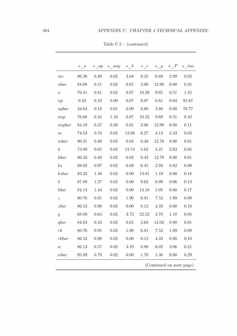
304 APPENDIX C. CHAPTER 4 TECHNICAL APPENDIX:
Table C.5 – (continued)
e_a e_ap e_anp e_b e_i e_g e_P e_tao
mc 86.30 0.49 0.02 3.04 0.25 6.89 2.99 0.02
nbar 84.08 0.51 0.02 0.01 2.06 12.96 0.00 0.35
n 76.41 0.81 0.02 0.87 10.29 9.65 0.51 1.45
np 6.43 0.10 0.00 0.07 0.87 0.81 0.04 91.67
npbar 24.64 0.18 0.01 0.00 0.60 3.80 0.00 70.77
nnp 76.68 0.34 1.16 0.87 10.32 9.69 0.51 0.42
nnpbar 84.19 0.37 0.28 0.01 2.06 12.98 0.00 0.11
m 74.53 0.53 0.02 12.08 6.27 4.12 2.43 0.03
mbar 86.31 0.40 0.02 0.02 0.48 12.76 0.00 0.01
h 73.09 0.65 0.02 13.74 5.62 4.21 2.63 0.05
hbar 86.33 0.40 0.02 0.02 0.43 12.78 0.00 0.01
ks 88.02 0.97 0.02 0.69 6.45 2.94 0.82 0.09
ksbar 83.32 1.48 0.02 0.00 13.81 1.19 0.00 0.18
k 87.89 1.27 0.02 0.00 9.62 0.99 0.06 0.13
kbar 84.13 1.44 0.02 0.00 13.18 1.05 0.00 0.17
z 80.76 0.91 0.02 1.90 6.81 7.52 1.99 0.09
zbar 86.52 0.90 0.02 0.00 8.12 4.33 0.00 0.10
q 68.09 0.64 0.02 3.73 22.52 3.78 1.18 0.05
qbar 84.83 0.43 0.02 0.01 2.68 12.02 0.00 0.01
rk 80.76 0.91 0.02 1.90 6.81 7.52 1.99 0.09
rkbar 86.52 0.90 0.02 0.00 8.12 4.33 0.00 0.10
w 86.13 0.57 0.02 3.19 0.80 6.02 3.06 0.21
wbar 95.89 0.78 0.02 0.00 1.70 1.30 0.00 0.29
(Continued on next page)
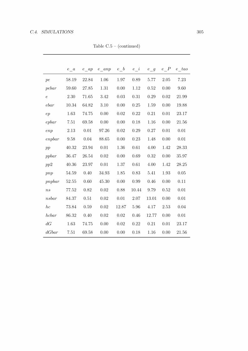
C.4. SIMULATIONS 305
Table C.5 – (continued)
e_a e_ap e_anp e_b e_i e_g e_P e_tao
pe 58.19 22.84 1.06 1.97 0.89 5.77 2.05 7.23
pebar 59.60 27.85 1.31 0.00 1.12 0.52 0.00 9.60
e 2.30 71.65 3.42 0.03 0.31 0.29 0.02 21.99
ebar 10.34 64.82 3.10 0.00 0.25 1.59 0.00 19.88
ep 1.63 74.75 0.00 0.02 0.22 0.21 0.01 23.17
epbar 7.51 69.58 0.00 0.00 0.18 1.16 0.00 21.56
enp 2.13 0.01 97.26 0.02 0.29 0.27 0.01 0.01
enpbar 9.58 0.04 88.65 0.00 0.23 1.48 0.00 0.01
pp 40.32 23.94 0.01 1.36 0.61 4.00 1.42 28.33
ppbar 36.47 26.54 0.02 0.00 0.69 0.32 0.00 35.97
pp2 40.36 23.97 0.01 1.37 0.61 4.00 1.42 28.25
pnp 54.59 0.40 34.93 1.85 0.83 5.41 1.93 0.05
pnpbar 52.55 0.60 45.30 0.00 0.99 0.46 0.00 0.11
ns 77.52 0.82 0.02 0.88 10.44 9.79 0.52 0.01
nsbar 84.37 0.51 0.02 0.01 2.07 13.01 0.00 0.01
hc 73.84 0.59 0.02 12.87 5.96 4.17 2.53 0.04
hcbar 86.32 0.40 0.02 0.02 0.46 12.77 0.00 0.01
dG 1.63 74.75 0.00 0.02 0.22 0.21 0.01 23.17
dGbar 7.51 69.58 0.00 0.00 0.18 1.16 0.00 21.56
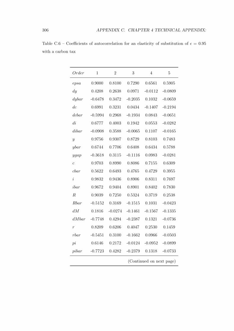
306 APPENDIX C. CHAPTER 4 TECHNICAL APPENDIX:
Table C.6 – Coefficients of autocorrelation for an elasticity of substitution of ε = 0.95
with a carbon tax
Order 1 2 3 4 5
epsa 0.9000 0.8100 0.7290 0.6561 0.5905
dy 0.4208 0.2638 0.0971 -0.0112 -0.0809
dybar -0.6478 0.3472 -0.2035 0.1032 -0.0659
dc 0.6991 0.3231 0.0434 -0.1407 -0.2194
dcbar -0.5994 0.2968 -0.1934 0.0843 -0.0651
di 0.6777 0.4003 0.1942 0.0553 -0.0282
dibar -0.0908 0.3588 -0.0065 0.1107 -0.0165
y 0.9756 0.9307 0.8729 0.8103 0.7483
ybar 0.6744 0.7706 0.6408 0.6434 0.5788
ygap -0.3618 0.3115 -0.1116 0.0983 -0.0281
c 0.9703 0.8990 0.8086 0.7155 0.6309
cbar 0.5622 0.6493 0.4765 0.4729 0.3955
i 0.9832 0.9436 0.8906 0.8311 0.7697
ibar 0.9672 0.9404 0.8901 0.8402 0.7830
R 0.9039 0.7250 0.5324 0.3719 0.2538
Rbar -0.5152 0.3169 -0.1515 0.1031 -0.0423
dM 0.1816 -0.0274 -0.1461 -0.1567 -0.1335
dMbar -0.7748 0.4294 -0.2387 0.1321 -0.0736
r 0.8209 0.6206 0.4047 0.2530 0.1459
rbar -0.5451 0.3100 -0.1662 0.0966 -0.0503
pi 0.6146 0.2172 -0.0124 -0.0952 -0.0899
pibar -0.7723 0.4282 -0.2379 0.1318 -0.0733
(Continued on next page)
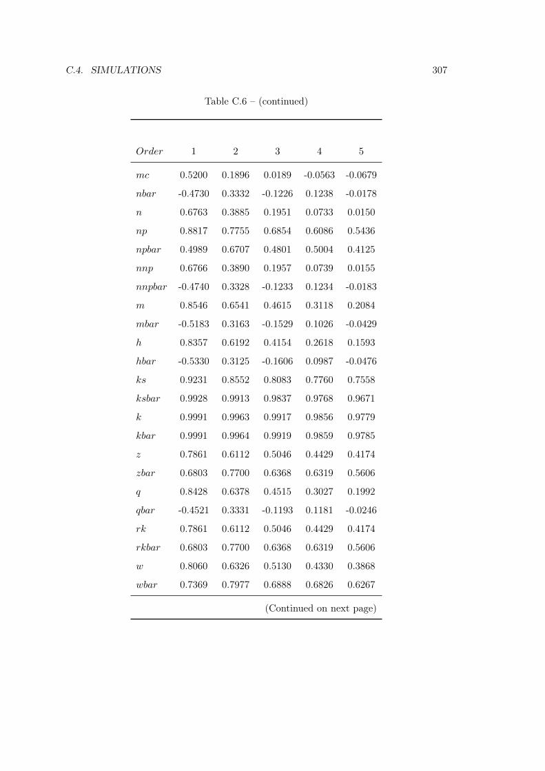
C.4. SIMULATIONS 307
Table C.6 – (continued)
Order 1 2 3 4 5
mc 0.5200 0.1896 0.0189 -0.0563 -0.0679
nbar -0.4730 0.3332 -0.1226 0.1238 -0.0178
n 0.6763 0.3885 0.1951 0.0733 0.0150
np 0.8817 0.7755 0.6854 0.6086 0.5436
npbar 0.4989 0.6707 0.4801 0.5004 0.4125
nnp 0.6766 0.3890 0.1957 0.0739 0.0155
nnpbar -0.4740 0.3328 -0.1233 0.1234 -0.0183
m 0.8546 0.6541 0.4615 0.3118 0.2084
mbar -0.5183 0.3163 -0.1529 0.1026 -0.0429
h 0.8357 0.6192 0.4154 0.2618 0.1593
hbar -0.5330 0.3125 -0.1606 0.0987 -0.0476
ks 0.9231 0.8552 0.8083 0.7760 0.7558
ksbar 0.9928 0.9913 0.9837 0.9768 0.9671
k 0.9991 0.9963 0.9917 0.9856 0.9779
kbar 0.9991 0.9964 0.9919 0.9859 0.9785
z 0.7861 0.6112 0.5046 0.4429 0.4174
zbar 0.6803 0.7700 0.6368 0.6319 0.5606
q 0.8428 0.6378 0.4515 0.3027 0.1992
qbar -0.4521 0.3331 -0.1193 0.1181 -0.0246
rk 0.7861 0.6112 0.5046 0.4429 0.4174
rkbar 0.6803 0.7700 0.6368 0.6319 0.5606
w 0.8060 0.6326 0.5130 0.4330 0.3868
wbar 0.7369 0.7977 0.6888 0.6826 0.6267
(Continued on next page)
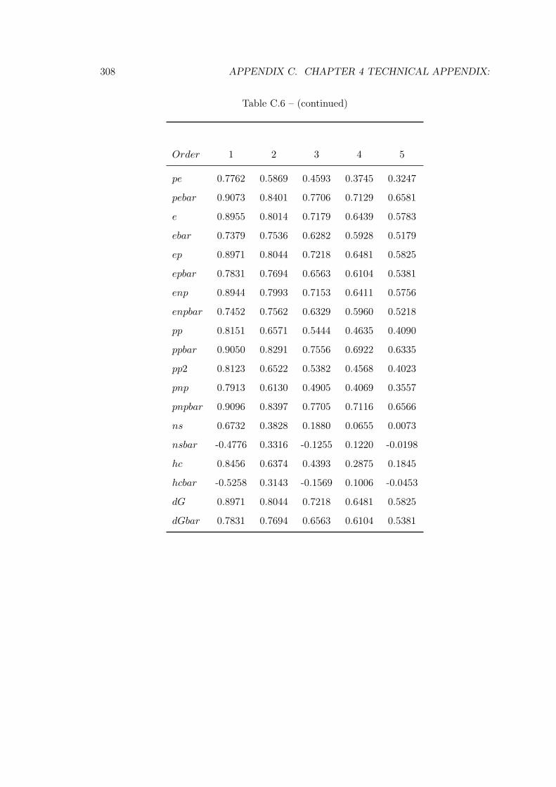
308 APPENDIX C. CHAPTER 4 TECHNICAL APPENDIX:
Table C.6 – (continued)
Order 1 2 3 4 5
pe 0.7762 0.5869 0.4593 0.3745 0.3247
pebar 0.9073 0.8401 0.7706 0.7129 0.6581
e 0.8955 0.8014 0.7179 0.6439 0.5783
ebar 0.7379 0.7536 0.6282 0.5928 0.5179
ep 0.8971 0.8044 0.7218 0.6481 0.5825
epbar 0.7831 0.7694 0.6563 0.6104 0.5381
enp 0.8944 0.7993 0.7153 0.6411 0.5756
enpbar 0.7452 0.7562 0.6329 0.5960 0.5218
pp 0.8151 0.6571 0.5444 0.4635 0.4090
ppbar 0.9050 0.8291 0.7556 0.6922 0.6335
pp2 0.8123 0.6522 0.5382 0.4568 0.4023
pnp 0.7913 0.6130 0.4905 0.4069 0.3557
pnpbar 0.9096 0.8397 0.7705 0.7116 0.6566
ns 0.6732 0.3828 0.1880 0.0655 0.0073
nsbar -0.4776 0.3316 -0.1255 0.1220 -0.0198
hc 0.8456 0.6374 0.4393 0.2875 0.1845
hcbar -0.5258 0.3143 -0.1569 0.1006 -0.0453
dG 0.8971 0.8044 0.7218 0.6481 0.5825
dGbar 0.7831 0.7694 0.6563 0.6104 0.5381

C.4. SIMULATIONS 309
Table C.7 – Theoretical moments for an elasticity of substitution of ε = 1.008 with a
carbon tax
V ARIABLE MEAN STD.DEV. V ARIANCE
epsa 0.0000 1.6059 2.5789
dy 0.0000 0.3815 0.1456
dybar 0.0000 0.4521 0.2044
dc 0.0000 0.4569 0.2088
dcbar 0.0000 1.1964 1.4315
di 0.0000 0.9548 0.9117
dibar 0.0000 0.9375 0.8789
y 0.0000 1.7379 3.0204
ybar 0.0000 1.6842 2.8366
ygap 0.0000 0.4855 0.2357
c 0.0000 2.0787 4.3208
cbar 0.0000 2.9557 8.7361
i 0.0000 5.4793 30.0232
ibar 0.0000 4.2574 18.1252
R 0.0000 0.3601 0.1296
Rbar 0.0000 0.8073 0.6518
dM 0.0000 14.9008 222.0324
dMbar 0.0000 57.4956 3305.7484
r 0.0000 0.4101 0.1682
rbar 0.0000 2.7309 7.4578
pi 0.0000 0.5094 0.2595
pibar 0.0000 3.7979 14.4238
(Continued on next page)
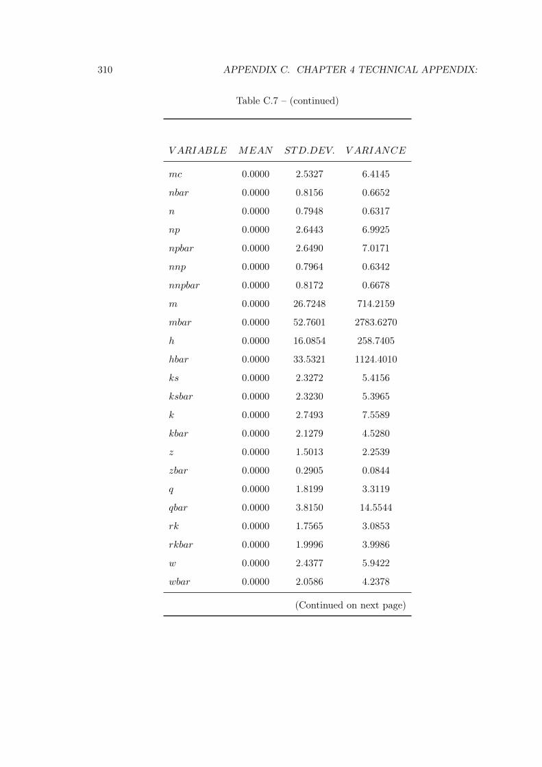
310 APPENDIX C. CHAPTER 4 TECHNICAL APPENDIX:
Table C.7 – (continued)
V ARIABLE MEAN STD.DEV. V ARIANCE
mc 0.0000 2.5327 6.4145
nbar 0.0000 0.8156 0.6652
n 0.0000 0.7948 0.6317
np 0.0000 2.6443 6.9925
npbar 0.0000 2.6490 7.0171
nnp 0.0000 0.7964 0.6342
nnpbar 0.0000 0.8172 0.6678
m 0.0000 26.7248 714.2159
mbar 0.0000 52.7601 2783.6270
h 0.0000 16.0854 258.7405
hbar 0.0000 33.5321 1124.4010
ks 0.0000 2.3272 5.4156
ksbar 0.0000 2.3230 5.3965
k 0.0000 2.7493 7.5589
kbar 0.0000 2.1279 4.5280
z 0.0000 1.5013 2.2539
zbar 0.0000 0.2905 0.0844
q 0.0000 1.8199 3.3119
qbar 0.0000 3.8150 14.5544
rk 0.0000 1.7565 3.0853
rkbar 0.0000 1.9996 3.9986
w 0.0000 2.4377 5.9422
wbar 0.0000 2.0586 4.2378
(Continued on next page)
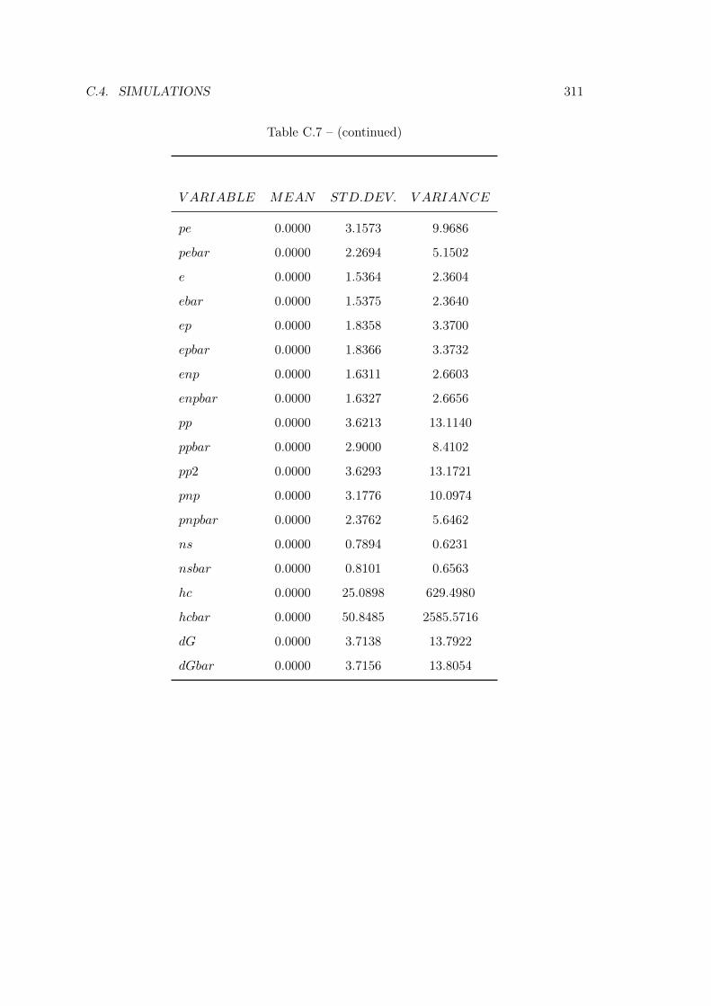
C.4. SIMULATIONS 311
Table C.7 – (continued)
V ARIABLE MEAN STD.DEV. V ARIANCE
pe 0.0000 3.1573 9.9686
pebar 0.0000 2.2694 5.1502
e 0.0000 1.5364 2.3604
ebar 0.0000 1.5375 2.3640
ep 0.0000 1.8358 3.3700
epbar 0.0000 1.8366 3.3732
enp 0.0000 1.6311 2.6603
enpbar 0.0000 1.6327 2.6656
pp 0.0000 3.6213 13.1140
ppbar 0.0000 2.9000 8.4102
pp2 0.0000 3.6293 13.1721
pnp 0.0000 3.1776 10.0974
pnpbar 0.0000 2.3762 5.6462
ns 0.0000 0.7894 0.6231
nsbar 0.0000 0.8101 0.6563
hc 0.0000 25.0898 629.4980
hcbar 0.0000 50.8485 2585.5716
dG 0.0000 3.7138 13.7922
dGbar 0.0000 3.7156 13.8054
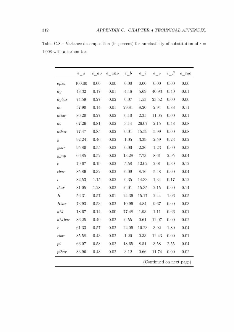
312 APPENDIX C. CHAPTER 4 TECHNICAL APPENDIX:
Table C.8 – Variance decomposition (in percent) for an elasticity of substitution of ε =
1.008 with a carbon tax
e_a e_ap e_anp e_b e_i e_g e_P e_tao
epsa 100.00 0.00 0.00 0.00 0.00 0.00 0.00 0.00
dy 48.32 0.17 0.01 4.46 5.69 40.93 0.40 0.01
dybar 74.59 0.27 0.02 0.07 1.53 23.52 0.00 0.00
dc 57.90 0.14 0.01 29.81 8.20 2.94 0.88 0.11
dcbar 86.20 0.27 0.02 0.10 2.35 11.05 0.00 0.01
di 67.26 0.81 0.02 3.14 26.07 2.15 0.48 0.08
dibar 77.47 0.85 0.02 0.01 15.59 5.99 0.00 0.08
y 92.24 0.46 0.02 1.05 3.39 2.59 0.23 0.02
ybar 95.80 0.55 0.02 0.00 2.36 1.23 0.00 0.03
ygap 66.85 0.52 0.02 13.28 7.73 8.61 2.95 0.04
c 79.67 0.19 0.02 5.58 12.02 2.01 0.39 0.12
cbar 85.89 0.32 0.02 0.09 8.16 5.48 0.00 0.04
i 82.53 1.15 0.02 0.35 14.33 1.34 0.17 0.12
ibar 81.05 1.28 0.02 0.01 15.35 2.15 0.00 0.14
R 56.31 0.57 0.01 24.39 15.17 2.44 1.06 0.05
Rbar 73.93 0.53 0.02 10.99 4.84 9.67 0.00 0.03
dM 18.67 0.14 0.00 77.48 1.93 1.11 0.66 0.01
dMbar 86.25 0.49 0.02 0.55 0.61 12.07 0.00 0.02
r 61.33 0.57 0.02 22.09 10.23 3.92 1.80 0.04
rbar 85.58 0.43 0.02 1.20 0.33 12.43 0.00 0.01
pi 66.07 0.58 0.02 18.65 8.51 3.58 2.55 0.04
pibar 83.96 0.48 0.02 3.12 0.66 11.74 0.00 0.02
(Continued on next page)
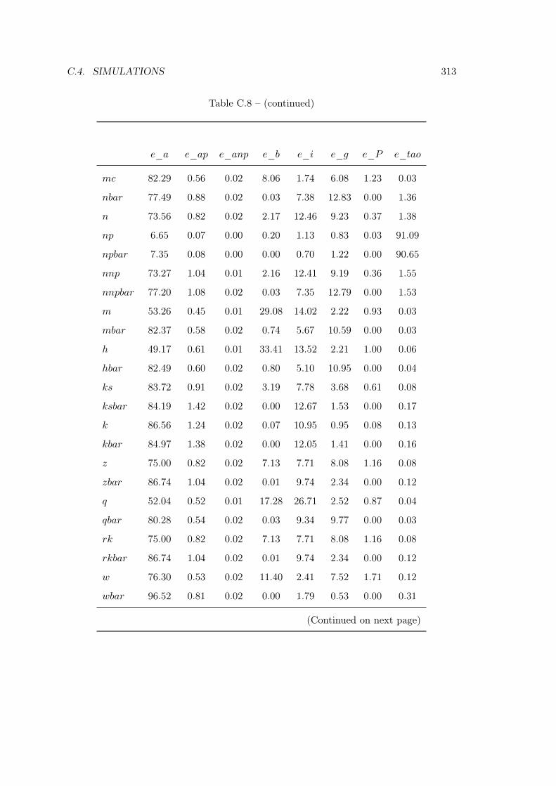
C.4. SIMULATIONS 313
Table C.8 – (continued)
e_a e_ap e_anp e_b e_i e_g e_P e_tao
mc 82.29 0.56 0.02 8.06 1.74 6.08 1.23 0.03
nbar 77.49 0.88 0.02 0.03 7.38 12.83 0.00 1.36
n 73.56 0.82 0.02 2.17 12.46 9.23 0.37 1.38
np 6.65 0.07 0.00 0.20 1.13 0.83 0.03 91.09
npbar 7.35 0.08 0.00 0.00 0.70 1.22 0.00 90.65
nnp 73.27 1.04 0.01 2.16 12.41 9.19 0.36 1.55
nnpbar 77.20 1.08 0.02 0.03 7.35 12.79 0.00 1.53
m 53.26 0.45 0.01 29.08 14.02 2.22 0.93 0.03
mbar 82.37 0.58 0.02 0.74 5.67 10.59 0.00 0.03
h 49.17 0.61 0.01 33.41 13.52 2.21 1.00 0.06
hbar 82.49 0.60 0.02 0.80 5.10 10.95 0.00 0.04
ks 83.72 0.91 0.02 3.19 7.78 3.68 0.61 0.08
ksbar 84.19 1.42 0.02 0.00 12.67 1.53 0.00 0.17
k 86.56 1.24 0.02 0.07 10.95 0.95 0.08 0.13
kbar 84.97 1.38 0.02 0.00 12.05 1.41 0.00 0.16
z 75.00 0.82 0.02 7.13 7.71 8.08 1.16 0.08
zbar 86.74 1.04 0.02 0.01 9.74 2.34 0.00 0.12
q 52.04 0.52 0.01 17.28 26.71 2.52 0.87 0.04
qbar 80.28 0.54 0.02 0.03 9.34 9.77 0.00 0.03
rk 75.00 0.82 0.02 7.13 7.71 8.08 1.16 0.08
rkbar 86.74 1.04 0.02 0.01 9.74 2.34 0.00 0.12
w 76.30 0.53 0.02 11.40 2.41 7.52 1.71 0.12
wbar 96.52 0.81 0.02 0.00 1.79 0.53 0.00 0.31
(Continued on next page)
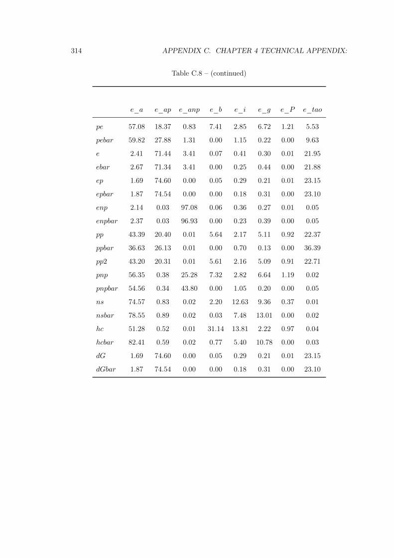
314 APPENDIX C. CHAPTER 4 TECHNICAL APPENDIX:
Table C.8 – (continued)
e_a e_ap e_anp e_b e_i e_g e_P e_tao
pe 57.08 18.37 0.83 7.41 2.85 6.72 1.21 5.53
pebar 59.82 27.88 1.31 0.00 1.15 0.22 0.00 9.63
e 2.41 71.44 3.41 0.07 0.41 0.30 0.01 21.95
ebar 2.67 71.34 3.41 0.00 0.25 0.44 0.00 21.88
ep 1.69 74.60 0.00 0.05 0.29 0.21 0.01 23.15
epbar 1.87 74.54 0.00 0.00 0.18 0.31 0.00 23.10
enp 2.14 0.03 97.08 0.06 0.36 0.27 0.01 0.05
enpbar 2.37 0.03 96.93 0.00 0.23 0.39 0.00 0.05
pp 43.39 20.40 0.01 5.64 2.17 5.11 0.92 22.37
ppbar 36.63 26.13 0.01 0.00 0.70 0.13 0.00 36.39
pp2 43.20 20.31 0.01 5.61 2.16 5.09 0.91 22.71
pnp 56.35 0.38 25.28 7.32 2.82 6.64 1.19 0.02
pnpbar 54.56 0.34 43.80 0.00 1.05 0.20 0.00 0.05
ns 74.57 0.83 0.02 2.20 12.63 9.36 0.37 0.01
nsbar 78.55 0.89 0.02 0.03 7.48 13.01 0.00 0.02
hc 51.28 0.52 0.01 31.14 13.81 2.22 0.97 0.04
hcbar 82.41 0.59 0.02 0.77 5.40 10.78 0.00 0.03
dG 1.69 74.60 0.00 0.05 0.29 0.21 0.01 23.15
dGbar 1.87 74.54 0.00 0.00 0.18 0.31 0.00 23.10
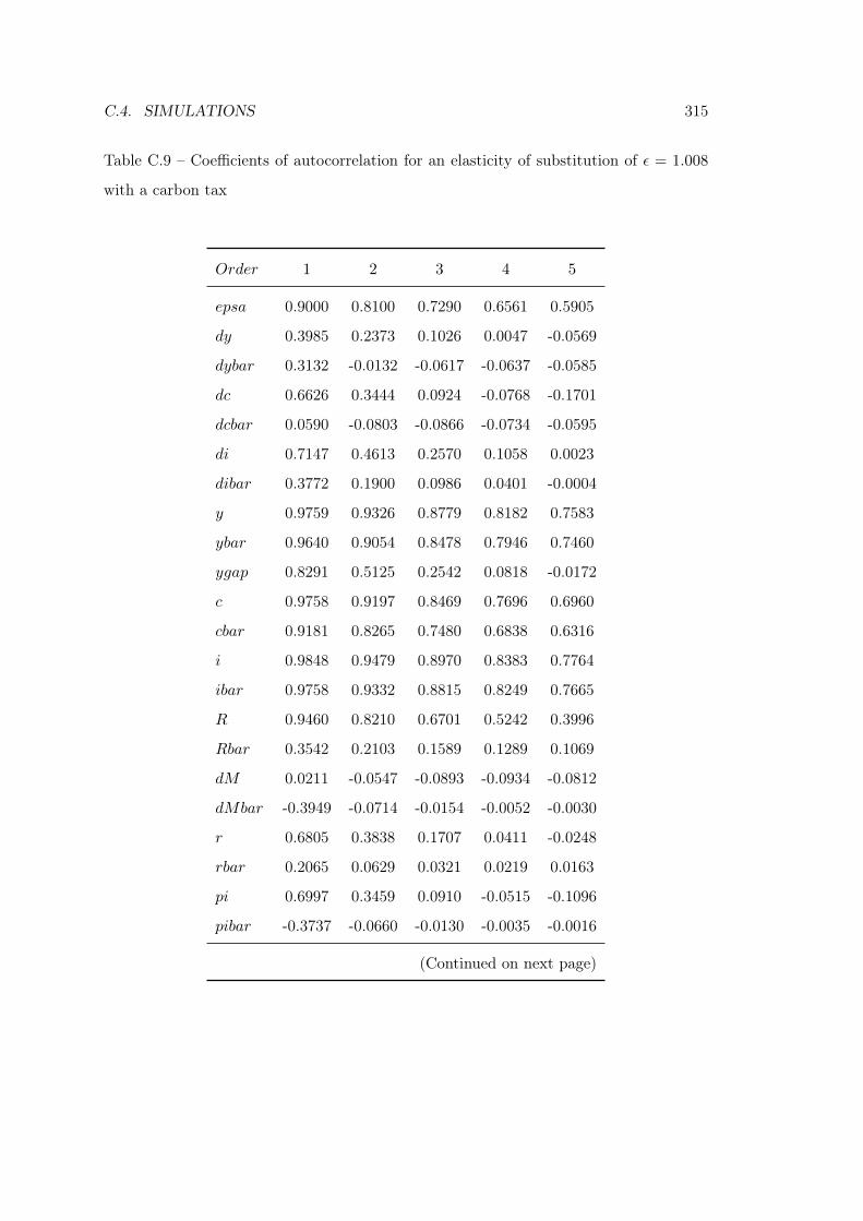
C.4. SIMULATIONS 315
Table C.9 – Coefficients of autocorrelation for an elasticity of substitution of ε = 1.008
with a carbon tax
Order 1 2 3 4 5
epsa 0.9000 0.8100 0.7290 0.6561 0.5905
dy 0.3985 0.2373 0.1026 0.0047 -0.0569
dybar 0.3132 -0.0132 -0.0617 -0.0637 -0.0585
dc 0.6626 0.3444 0.0924 -0.0768 -0.1701
dcbar 0.0590 -0.0803 -0.0866 -0.0734 -0.0595
di 0.7147 0.4613 0.2570 0.1058 0.0023
dibar 0.3772 0.1900 0.0986 0.0401 -0.0004
y 0.9759 0.9326 0.8779 0.8182 0.7583
ybar 0.9640 0.9054 0.8478 0.7946 0.7460
ygap 0.8291 0.5125 0.2542 0.0818 -0.0172
c 0.9758 0.9197 0.8469 0.7696 0.6960
cbar 0.9181 0.8265 0.7480 0.6838 0.6316
i 0.9848 0.9479 0.8970 0.8383 0.7764
ibar 0.9758 0.9332 0.8815 0.8249 0.7665
R 0.9460 0.8210 0.6701 0.5242 0.3996
Rbar 0.3542 0.2103 0.1589 0.1289 0.1069
dM 0.0211 -0.0547 -0.0893 -0.0934 -0.0812
dMbar -0.3949 -0.0714 -0.0154 -0.0052 -0.0030
r 0.6805 0.3838 0.1707 0.0411 -0.0248
rbar 0.2065 0.0629 0.0321 0.0219 0.0163
pi 0.6997 0.3459 0.0910 -0.0515 -0.1096
pibar -0.3737 -0.0660 -0.0130 -0.0035 -0.0016
(Continued on next page)
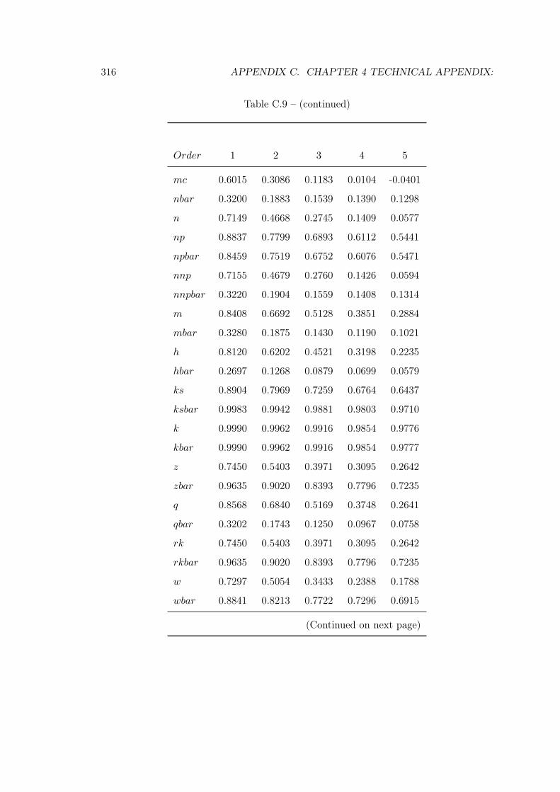
316 APPENDIX C. CHAPTER 4 TECHNICAL APPENDIX:
Table C.9 – (continued)
Order 1 2 3 4 5
mc 0.6015 0.3086 0.1183 0.0104 -0.0401
nbar 0.3200 0.1883 0.1539 0.1390 0.1298
n 0.7149 0.4668 0.2745 0.1409 0.0577
np 0.8837 0.7799 0.6893 0.6112 0.5441
npbar 0.8459 0.7519 0.6752 0.6076 0.5471
nnp 0.7155 0.4679 0.2760 0.1426 0.0594
nnpbar 0.3220 0.1904 0.1559 0.1408 0.1314
m 0.8408 0.6692 0.5128 0.3851 0.2884
mbar 0.3280 0.1875 0.1430 0.1190 0.1021
h 0.8120 0.6202 0.4521 0.3198 0.2235
hbar 0.2697 0.1268 0.0879 0.0699 0.0579
ks 0.8904 0.7969 0.7259 0.6764 0.6437
ksbar 0.9983 0.9942 0.9881 0.9803 0.9710
k 0.9990 0.9962 0.9916 0.9854 0.9776
kbar 0.9990 0.9962 0.9916 0.9854 0.9777
z 0.7450 0.5403 0.3971 0.3095 0.2642
zbar 0.9635 0.9020 0.8393 0.7796 0.7235
q 0.8568 0.6840 0.5169 0.3748 0.2641
qbar 0.3202 0.1743 0.1250 0.0967 0.0758
rk 0.7450 0.5403 0.3971 0.3095 0.2642
rkbar 0.9635 0.9020 0.8393 0.7796 0.7235
w 0.7297 0.5054 0.3433 0.2388 0.1788
wbar 0.8841 0.8213 0.7722 0.7296 0.6915
(Continued on next page)
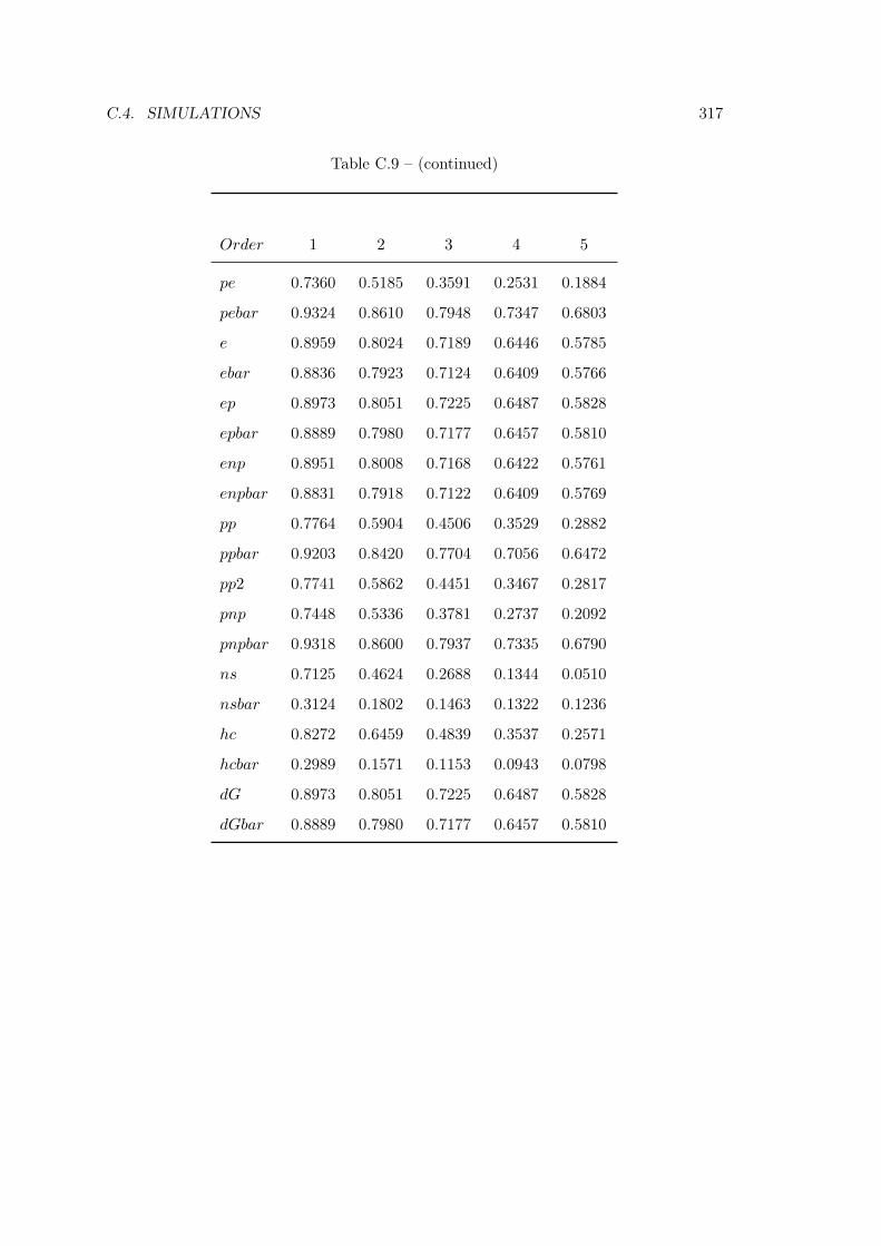
C.4. SIMULATIONS 317
Table C.9 – (continued)
Order 1 2 3 4 5
pe 0.7360 0.5185 0.3591 0.2531 0.1884
pebar 0.9324 0.8610 0.7948 0.7347 0.6803
e 0.8959 0.8024 0.7189 0.6446 0.5785
ebar 0.8836 0.7923 0.7124 0.6409 0.5766
ep 0.8973 0.8051 0.7225 0.6487 0.5828
epbar 0.8889 0.7980 0.7177 0.6457 0.5810
enp 0.8951 0.8008 0.7168 0.6422 0.5761
enpbar 0.8831 0.7918 0.7122 0.6409 0.5769
pp 0.7764 0.5904 0.4506 0.3529 0.2882
ppbar 0.9203 0.8420 0.7704 0.7056 0.6472
pp2 0.7741 0.5862 0.4451 0.3467 0.2817
pnp 0.7448 0.5336 0.3781 0.2737 0.2092
pnpbar 0.9318 0.8600 0.7937 0.7335 0.6790
ns 0.7125 0.4624 0.2688 0.1344 0.0510
nsbar 0.3124 0.1802 0.1463 0.1322 0.1236
hc 0.8272 0.6459 0.4839 0.3537 0.2571
hcbar 0.2989 0.1571 0.1153 0.0943 0.0798
dG 0.8973 0.8051 0.7225 0.6487 0.5828
dGbar 0.8889 0.7980 0.7177 0.6457 0.5810
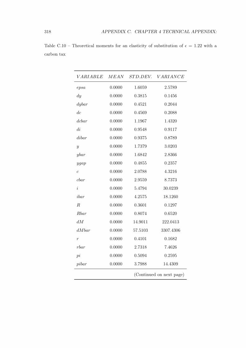
318 APPENDIX C. CHAPTER 4 TECHNICAL APPENDIX:
Table C.10 – Theoretical moments for an elasticity of substitution of ε = 1.22 with a
carbon tax
V ARIABLE MEAN STD.DEV. V ARIANCE
epsa 0.0000 1.6059 2.5789
dy 0.0000 0.3815 0.1456
dybar 0.0000 0.4521 0.2044
dc 0.0000 0.4569 0.2088
dcbar 0.0000 1.1967 1.4320
di 0.0000 0.9548 0.9117
dibar 0.0000 0.9375 0.8789
y 0.0000 1.7379 3.0203
ybar 0.0000 1.6842 2.8366
ygap 0.0000 0.4855 0.2357
c 0.0000 2.0788 4.3216
cbar 0.0000 2.9559 8.7373
i 0.0000 5.4794 30.0239
ibar 0.0000 4.2575 18.1260
R 0.0000 0.3601 0.1297
Rbar 0.0000 0.8074 0.6520
dM 0.0000 14.9011 222.0413
dMbar 0.0000 57.5103 3307.4306
r 0.0000 0.4101 0.1682
rbar 0.0000 2.7318 7.4626
pi 0.0000 0.5094 0.2595
pibar 0.0000 3.7988 14.4309
(Continued on next page)
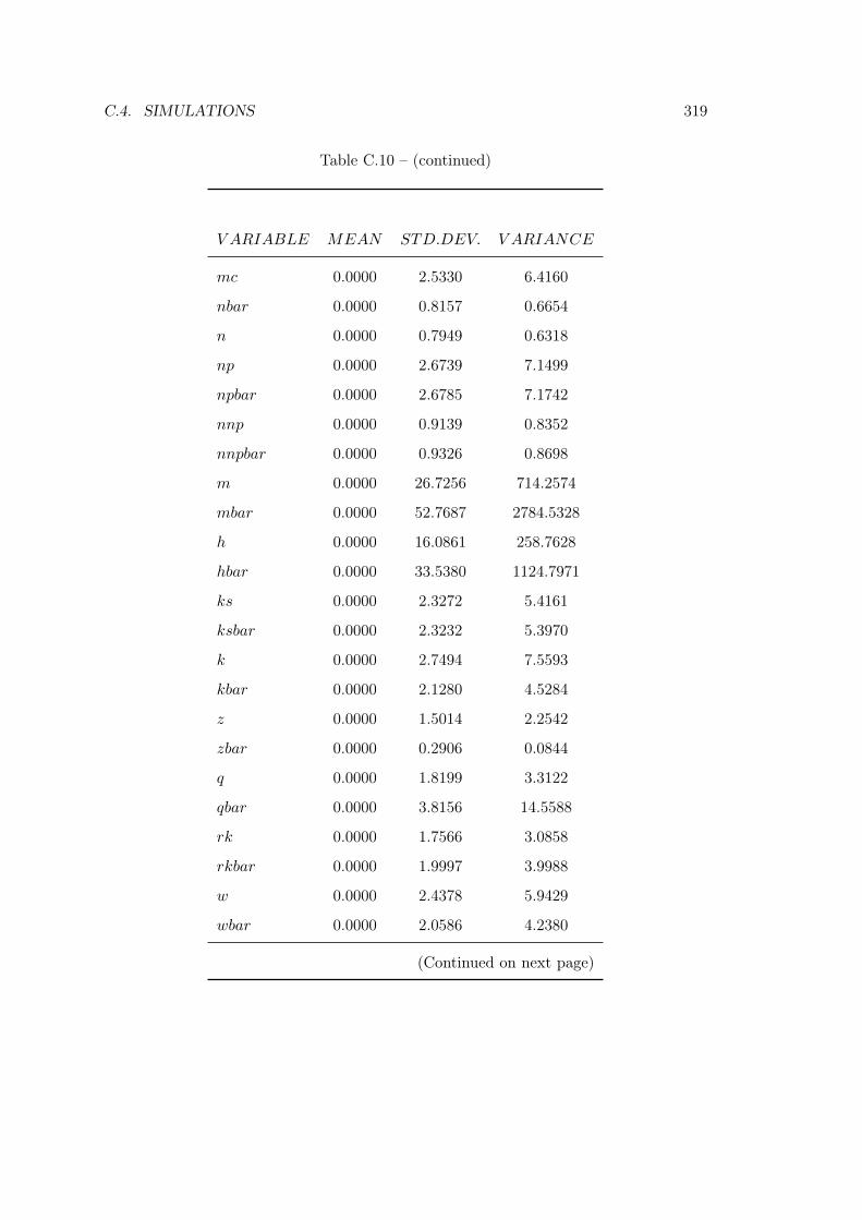
C.4. SIMULATIONS 319
Table C.10 – (continued)
V ARIABLE MEAN STD.DEV. V ARIANCE
mc 0.0000 2.5330 6.4160
nbar 0.0000 0.8157 0.6654
n 0.0000 0.7949 0.6318
np 0.0000 2.6739 7.1499
npbar 0.0000 2.6785 7.1742
nnp 0.0000 0.9139 0.8352
nnpbar 0.0000 0.9326 0.8698
m 0.0000 26.7256 714.2574
mbar 0.0000 52.7687 2784.5328
h 0.0000 16.0861 258.7628
hbar 0.0000 33.5380 1124.7971
ks 0.0000 2.3272 5.4161
ksbar 0.0000 2.3232 5.3970
k 0.0000 2.7494 7.5593
kbar 0.0000 2.1280 4.5284
z 0.0000 1.5014 2.2542
zbar 0.0000 0.2906 0.0844
q 0.0000 1.8199 3.3122
qbar 0.0000 3.8156 14.5588
rk 0.0000 1.7566 3.0858
rkbar 0.0000 1.9997 3.9988
w 0.0000 2.4378 5.9429
wbar 0.0000 2.0586 4.2380
(Continued on next page)
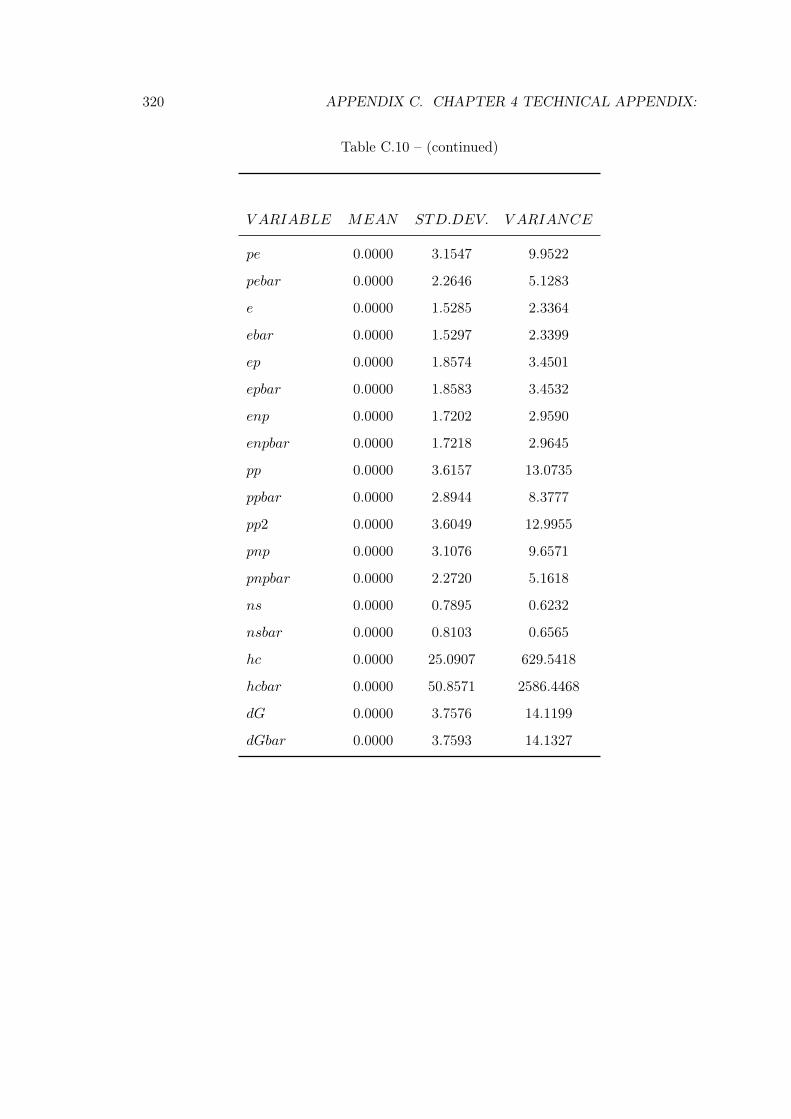
320 APPENDIX C. CHAPTER 4 TECHNICAL APPENDIX:
Table C.10 – (continued)
V ARIABLE MEAN STD.DEV. V ARIANCE
pe 0.0000 3.1547 9.9522
pebar 0.0000 2.2646 5.1283
e 0.0000 1.5285 2.3364
ebar 0.0000 1.5297 2.3399
ep 0.0000 1.8574 3.4501
epbar 0.0000 1.8583 3.4532
enp 0.0000 1.7202 2.9590
enpbar 0.0000 1.7218 2.9645
pp 0.0000 3.6157 13.0735
ppbar 0.0000 2.8944 8.3777
pp2 0.0000 3.6049 12.9955
pnp 0.0000 3.1076 9.6571
pnpbar 0.0000 2.2720 5.1618
ns 0.0000 0.7895 0.6232
nsbar 0.0000 0.8103 0.6565
hc 0.0000 25.0907 629.5418
hcbar 0.0000 50.8571 2586.4468
dG 0.0000 3.7576 14.1199
dGbar 0.0000 3.7593 14.1327
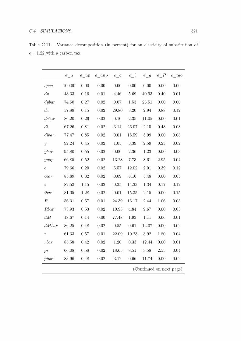
C.4. SIMULATIONS 321
Table C.11 – Variance decomposition (in percent) for an elasticity of substitution of
ε = 1.22 with a carbon tax
e_a e_ap e_anp e_b e_i e_g e_P e_tao
epsa 100.00 0.00 0.00 0.00 0.00 0.00 0.00 0.00
dy 48.33 0.16 0.01 4.46 5.69 40.93 0.40 0.01
dybar 74.60 0.27 0.02 0.07 1.53 23.51 0.00 0.00
dc 57.89 0.15 0.02 29.80 8.20 2.94 0.88 0.12
dcbar 86.20 0.26 0.02 0.10 2.35 11.05 0.00 0.01
di 67.26 0.81 0.02 3.14 26.07 2.15 0.48 0.08
dibar 77.47 0.85 0.02 0.01 15.59 5.99 0.00 0.08
y 92.24 0.45 0.02 1.05 3.39 2.59 0.23 0.02
ybar 95.80 0.55 0.02 0.00 2.36 1.23 0.00 0.03
ygap 66.85 0.52 0.02 13.28 7.73 8.61 2.95 0.04
c 79.66 0.20 0.02 5.57 12.02 2.01 0.39 0.12
cbar 85.89 0.32 0.02 0.09 8.16 5.48 0.00 0.05
i 82.52 1.15 0.02 0.35 14.33 1.34 0.17 0.12
ibar 81.05 1.28 0.02 0.01 15.35 2.15 0.00 0.15
R 56.31 0.57 0.01 24.39 15.17 2.44 1.06 0.05
Rbar 73.93 0.53 0.02 10.98 4.84 9.67 0.00 0.03
dM 18.67 0.14 0.00 77.48 1.93 1.11 0.66 0.01
dMbar 86.25 0.48 0.02 0.55 0.61 12.07 0.00 0.02
r 61.33 0.57 0.01 22.09 10.23 3.92 1.80 0.04
rbar 85.58 0.42 0.02 1.20 0.33 12.44 0.00 0.01
pi 66.08 0.58 0.02 18.65 8.51 3.58 2.55 0.04
pibar 83.96 0.48 0.02 3.12 0.66 11.74 0.00 0.02
(Continued on next page)
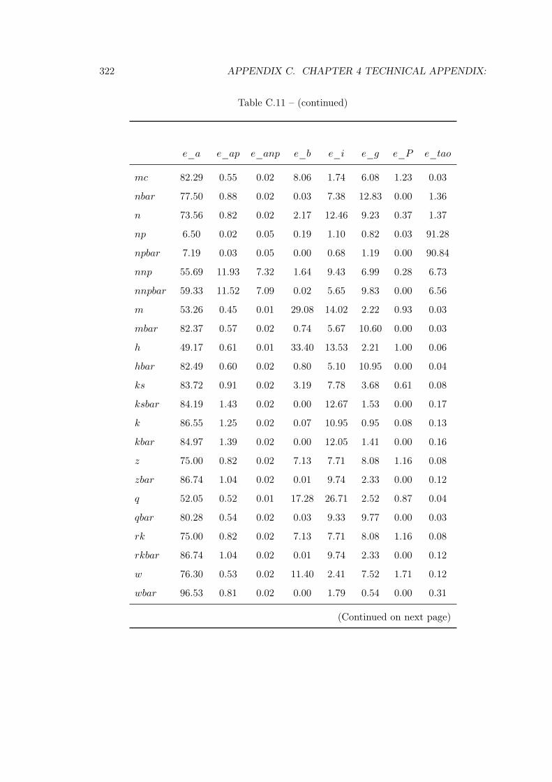
322 APPENDIX C. CHAPTER 4 TECHNICAL APPENDIX:
Table C.11 – (continued)
e_a e_ap e_anp e_b e_i e_g e_P e_tao
mc 82.29 0.55 0.02 8.06 1.74 6.08 1.23 0.03
nbar 77.50 0.88 0.02 0.03 7.38 12.83 0.00 1.36
n 73.56 0.82 0.02 2.17 12.46 9.23 0.37 1.37
np 6.50 0.02 0.05 0.19 1.10 0.82 0.03 91.28
npbar 7.19 0.03 0.05 0.00 0.68 1.19 0.00 90.84
nnp 55.69 11.93 7.32 1.64 9.43 6.99 0.28 6.73
nnpbar 59.33 11.52 7.09 0.02 5.65 9.83 0.00 6.56
m 53.26 0.45 0.01 29.08 14.02 2.22 0.93 0.03
mbar 82.37 0.57 0.02 0.74 5.67 10.60 0.00 0.03
h 49.17 0.61 0.01 33.40 13.53 2.21 1.00 0.06
hbar 82.49 0.60 0.02 0.80 5.10 10.95 0.00 0.04
ks 83.72 0.91 0.02 3.19 7.78 3.68 0.61 0.08
ksbar 84.19 1.43 0.02 0.00 12.67 1.53 0.00 0.17
k 86.55 1.25 0.02 0.07 10.95 0.95 0.08 0.13
kbar 84.97 1.39 0.02 0.00 12.05 1.41 0.00 0.16
z 75.00 0.82 0.02 7.13 7.71 8.08 1.16 0.08
zbar 86.74 1.04 0.02 0.01 9.74 2.33 0.00 0.12
q 52.05 0.52 0.01 17.28 26.71 2.52 0.87 0.04
qbar 80.28 0.54 0.02 0.03 9.33 9.77 0.00 0.03
rk 75.00 0.82 0.02 7.13 7.71 8.08 1.16 0.08
rkbar 86.74 1.04 0.02 0.01 9.74 2.33 0.00 0.12
w 76.30 0.53 0.02 11.40 2.41 7.52 1.71 0.12
wbar 96.53 0.81 0.02 0.00 1.79 0.54 0.00 0.31
(Continued on next page)
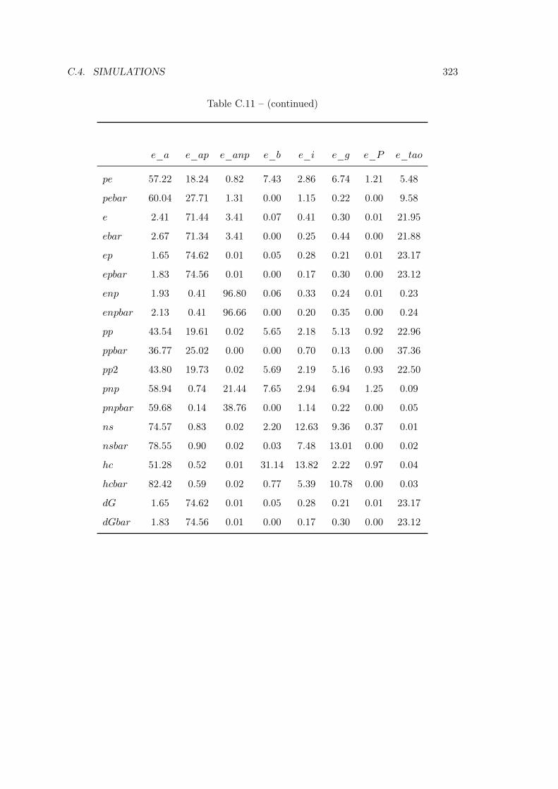
C.4. SIMULATIONS 323
Table C.11 – (continued)
e_a e_ap e_anp e_b e_i e_g e_P e_tao
pe 57.22 18.24 0.82 7.43 2.86 6.74 1.21 5.48
pebar 60.04 27.71 1.31 0.00 1.15 0.22 0.00 9.58
e 2.41 71.44 3.41 0.07 0.41 0.30 0.01 21.95
ebar 2.67 71.34 3.41 0.00 0.25 0.44 0.00 21.88
ep 1.65 74.62 0.01 0.05 0.28 0.21 0.01 23.17
epbar 1.83 74.56 0.01 0.00 0.17 0.30 0.00 23.12
enp 1.93 0.41 96.80 0.06 0.33 0.24 0.01 0.23
enpbar 2.13 0.41 96.66 0.00 0.20 0.35 0.00 0.24
pp 43.54 19.61 0.02 5.65 2.18 5.13 0.92 22.96
ppbar 36.77 25.02 0.00 0.00 0.70 0.13 0.00 37.36
pp2 43.80 19.73 0.02 5.69 2.19 5.16 0.93 22.50
pnp 58.94 0.74 21.44 7.65 2.94 6.94 1.25 0.09
pnpbar 59.68 0.14 38.76 0.00 1.14 0.22 0.00 0.05
ns 74.57 0.83 0.02 2.20 12.63 9.36 0.37 0.01
nsbar 78.55 0.90 0.02 0.03 7.48 13.01 0.00 0.02
hc 51.28 0.52 0.01 31.14 13.82 2.22 0.97 0.04
hcbar 82.42 0.59 0.02 0.77 5.39 10.78 0.00 0.03
dG 1.65 74.62 0.01 0.05 0.28 0.21 0.01 23.17
dGbar 1.83 74.56 0.01 0.00 0.17 0.30 0.00 23.12

324 APPENDIX C. CHAPTER 4 TECHNICAL APPENDIX:
Table C.12 – Coefficients of autocorrelation for an elasticity of substitution of ε = 1.22
with a carbon tax
Order 1 2 3 4 5
epsa 0.9000 0.8100 0.7290 0.6561 0.5905
dy 0.3985 0.2373 0.1026 0.0047 -0.0569
dybar 0.3131 -0.0132 -0.0617 -0.0637 -0.0585
dc 0.6626 0.3443 0.0924 -0.0768 -0.1701
dcbar 0.0589 -0.0803 -0.0865 -0.0734 -0.0595
di 0.7147 0.4613 0.2570 0.1058 0.0023
dibar 0.3771 0.1900 0.0986 0.0401 -0.0004
y 0.9759 0.9326 0.8779 0.8182 0.7583
ybar 0.9640 0.9054 0.8477 0.7946 0.7460
ygap 0.8291 0.5125 0.2541 0.0817 -0.0172
c 0.9758 0.9197 0.8469 0.7696 0.6960
cbar 0.9181 0.8265 0.7480 0.6838 0.6315
i 0.9848 0.9479 0.8970 0.8383 0.7764
ibar 0.9758 0.9332 0.8815 0.8250 0.7665
R 0.9460 0.8210 0.6700 0.5242 0.3996
Rbar 0.3541 0.2102 0.1589 0.1288 0.1069
dM 0.0211 -0.0547 -0.0893 -0.0935 -0.0812
dMbar -0.3950 -0.0713 -0.0154 -0.0052 -0.0030
r 0.6805 0.3838 0.1707 0.0411 -0.0248
rbar 0.2063 0.0629 0.0321 0.0219 0.0163
pi 0.6997 0.3459 0.0910 -0.0515 -0.1096
pibar -0.3737 -0.0659 -0.0130 -0.0035 -0.0016
(Continued on next page)

C.4. SIMULATIONS 325
Table C.12 – (continued)
Order 1 2 3 4 5
mc 0.6015 0.3085 0.1183 0.0104 -0.0401
nbar 0.3199 0.1883 0.1539 0.1390 0.1298
n 0.7149 0.4667 0.2745 0.1409 0.0577
np 0.8840 0.7806 0.6903 0.6123 0.5452
npbar 0.8471 0.7532 0.6764 0.6087 0.5480
nnp 0.7577 0.5460 0.3793 0.2597 0.1805
nnpbar 0.4520 0.3300 0.2853 0.2575 0.2358
m 0.8408 0.6692 0.5128 0.3851 0.2884
mbar 0.3279 0.1875 0.1429 0.1190 0.1021
h 0.8120 0.6202 0.4521 0.3198 0.2235
hbar 0.2695 0.1267 0.0879 0.0699 0.0579
ks 0.8904 0.7968 0.7258 0.6763 0.6437
ksbar 0.9983 0.9942 0.9881 0.9803 0.9710
k 0.9990 0.9962 0.9916 0.9854 0.9776
kbar 0.9990 0.9962 0.9916 0.9854 0.9777
z 0.7450 0.5403 0.3971 0.3094 0.2641
zbar 0.9635 0.9020 0.8393 0.7796 0.7235
q 0.8568 0.6840 0.5169 0.3748 0.2641
qbar 0.3200 0.1742 0.1250 0.0967 0.0758
rk 0.7450 0.5403 0.3971 0.3094 0.2641
rkbar 0.9635 0.9020 0.8393 0.7796 0.7235
w 0.7297 0.5054 0.3432 0.2387 0.1787
wbar 0.8841 0.8212 0.7722 0.7296 0.6915
(Continued on next page)

326 APPENDIX C. CHAPTER 4 TECHNICAL APPENDIX:
Table C.12 – (continued)
Order 1 2 3 4 5
pe 0.7357 0.5177 0.3582 0.2520 0.1874
pebar 0.9326 0.8612 0.7951 0.7350 0.6807
e 0.8959 0.8024 0.7189 0.6446 0.5785
ebar 0.8835 0.7922 0.7124 0.6409 0.5766
ep 0.8974 0.8052 0.7227 0.6489 0.5830
epbar 0.8891 0.7983 0.7180 0.6459 0.5812
enp 0.8955 0.8016 0.7178 0.6434 0.5773
enpbar 0.8846 0.7935 0.7137 0.6424 0.5782
pp 0.7761 0.5899 0.4499 0.3522 0.2875
ppbar 0.9204 0.8422 0.7706 0.7059 0.6475
pp2 0.7726 0.5834 0.4415 0.3427 0.2778
pnp 0.7368 0.5195 0.3602 0.2543 0.1897
pnpbar 0.9345 0.8643 0.7991 0.7400 0.6865
ns 0.7125 0.4623 0.2688 0.1344 0.0510
nsbar 0.3123 0.1802 0.1464 0.1322 0.1236
hc 0.8272 0.6459 0.4839 0.3537 0.2571
hcbar 0.2988 0.1571 0.1153 0.0943 0.0797
dG 0.8974 0.8052 0.7227 0.6489 0.5830
dGbar 0.8891 0.7983 0.7180 0.6459 0.5812
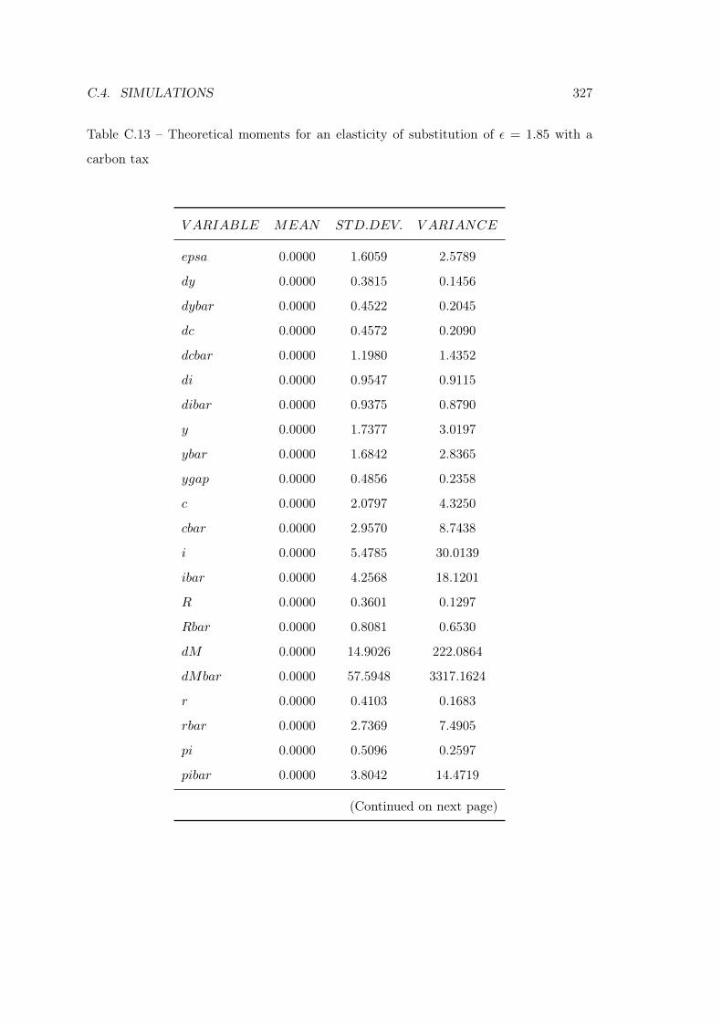
C.4. SIMULATIONS 327
Table C.13 – Theoretical moments for an elasticity of substitution of ε = 1.85 with a
carbon tax
V ARIABLE MEAN STD.DEV. V ARIANCE
epsa 0.0000 1.6059 2.5789
dy 0.0000 0.3815 0.1456
dybar 0.0000 0.4522 0.2045
dc 0.0000 0.4572 0.2090
dcbar 0.0000 1.1980 1.4352
di 0.0000 0.9547 0.9115
dibar 0.0000 0.9375 0.8790
y 0.0000 1.7377 3.0197
ybar 0.0000 1.6842 2.8365
ygap 0.0000 0.4856 0.2358
c 0.0000 2.0797 4.3250
cbar 0.0000 2.9570 8.7438
i 0.0000 5.4785 30.0139
ibar 0.0000 4.2568 18.1201
R 0.0000 0.3601 0.1297
Rbar 0.0000 0.8081 0.6530
dM 0.0000 14.9026 222.0864
dMbar 0.0000 57.5948 3317.1624
r 0.0000 0.4103 0.1683
rbar 0.0000 2.7369 7.4905
pi 0.0000 0.5096 0.2597
pibar 0.0000 3.8042 14.4719
(Continued on next page)
328 APPENDIX C. CHAPTER 4 TECHNICAL APPENDIX:
Table C.13 – (continued)
V ARIABLE MEAN STD.DEV. V ARIANCE
mc 0.0000 2.5345 6.4237
nbar 0.0000 0.8162 0.6662
n 0.0000 0.7951 0.6322
np 0.0000 2.7490 7.5568
npbar 0.0000 2.7533 7.5805
nnp 0.0000 1.4022 1.9663
nnpbar 0.0000 1.4157 2.0042
m 0.0000 26.7284 714.4094
mbar 0.0000 52.8157 2789.5034
h 0.0000 16.0881 258.8260
hbar 0.0000 33.5701 1126.9515
ks 0.0000 2.3274 5.4169
ksbar 0.0000 2.3230 5.3965
k 0.0000 2.7492 7.5578
kbar 0.0000 2.1279 4.5280
z 0.0000 1.5019 2.2556
zbar 0.0000 0.2905 0.0844
q 0.0000 1.8202 3.3132
qbar 0.0000 3.8188 14.5836
rk 0.0000 1.7572 3.0876
rkbar 0.0000 1.9996 3.9985
w 0.0000 2.4386 5.9467
wbar 0.0000 2.0587 4.2384
(Continued on next page)
C.4. SIMULATIONS 329
Table C.13 – (continued)
V ARIABLE MEAN STD.DEV. V ARIANCE
pe 0.0000 3.1401 9.8603
pebar 0.0000 2.2388 5.0124
e 0.0000 1.4859 2.2078
ebar 0.0000 1.4869 2.2109
ep 0.0000 1.9076 3.6390
epbar 0.0000 1.9083 3.6418
enp 0.0000 1.9053 3.6301
enpbar 0.0000 1.9068 3.6360
pp 0.0000 3.6070 13.0103
ppbar 0.0000 2.8843 8.3191
pp2 0.0000 3.5527 12.6217
pnp 0.0000 3.0214 9.1287
pnpbar 0.0000 2.1302 4.5379
ns 0.0000 0.7899 0.6239
nsbar 0.0000 0.8109 0.6576
hc 0.0000 25.0935 629.6820
hcbar 0.0000 50.9041 2591.2297
dG 0.0000 3.8592 14.8932
dGbar 0.0000 3.8606 14.9045
330 APPENDIX C. CHAPTER 4 TECHNICAL APPENDIX:
Table C.14 – Variance decomposition (in percent) for an elasticity of substitution of
ε = 1.85 with a carbon tax
e_a e_ap e_anp e_b e_i e_g e_P e_tao
epsa 100.00 0.00 0.00 0.00 0.00 0.00 0.00 0.00
dy 48.35 0.15 0.01 4.46 5.69 40.93 0.40 0.01
dybar 74.64 0.25 0.02 0.07 1.52 23.50 0.00 0.00
dc 57.89 0.16 0.02 29.77 8.20 2.94 0.88 0.13
dcbar 86.22 0.24 0.02 0.10 2.35 11.06 0.00 0.01
di 67.29 0.79 0.01 3.14 26.06 2.15 0.48 0.07
dibar 77.50 0.83 0.02 0.01 15.58 5.99 0.00 0.07
y 92.28 0.43 0.02 1.05 3.39 2.59 0.23 0.01
ybar 95.84 0.52 0.02 0.00 2.36 1.23 0.00 0.02
ygap 66.89 0.50 0.01 13.27 7.72 8.62 2.94 0.04
c 79.63 0.21 0.02 5.57 12.02 2.01 0.39 0.14
cbar 85.89 0.30 0.02 0.09 8.16 5.49 0.00 0.05
i 82.55 1.13 0.02 0.35 14.32 1.34 0.17 0.12
ibar 81.07 1.27 0.01 0.01 15.35 2.15 0.00 0.14
R 56.32 0.56 0.01 24.39 15.18 2.44 1.06 0.04
Rbar 73.97 0.50 0.02 10.96 4.83 9.68 0.00 0.03
dM 18.69 0.13 0.00 77.46 1.93 1.12 0.66 0.01
dMbar 86.28 0.46 0.02 0.55 0.61 12.07 0.00 0.01
r 61.35 0.56 0.01 22.08 10.23 3.93 1.80 0.04
rbar 85.61 0.40 0.02 1.19 0.33 12.44 0.00 0.01
pi 66.10 0.56 0.01 18.64 8.52 3.59 2.54 0.04
pibar 84.00 0.45 0.02 3.11 0.66 11.75 0.00 0.01
(Continued on next page)
C.4. SIMULATIONS 331
Table C.14 – (continued)
e_a e_ap e_anp e_b e_i e_g e_P e_tao
mc 82.32 0.53 0.02 8.05 1.74 6.08 1.23 0.02
nbar 77.52 0.87 0.02 0.03 7.37 12.84 0.00 1.36
n 73.58 0.81 0.02 2.17 12.45 9.23 0.37 1.37
np 6.23 0.21 0.33 0.18 1.05 0.78 0.03 91.17
npbar 6.90 0.22 0.33 0.00 0.66 1.14 0.00 90.76
nnp 23.96 29.43 26.42 0.71 4.05 3.01 0.12 12.30
nnpbar 26.09 28.92 26.01 0.01 2.48 4.32 0.00 12.16
m 53.28 0.43 0.01 29.07 14.03 2.23 0.93 0.03
mbar 82.40 0.55 0.02 0.74 5.66 10.60 0.00 0.03
h 49.19 0.60 0.01 33.39 13.53 2.21 1.00 0.06
hbar 82.52 0.58 0.02 0.80 5.09 10.96 0.00 0.04
ks 83.75 0.89 0.02 3.19 7.78 3.69 0.61 0.08
ksbar 84.21 1.41 0.01 0.00 12.66 1.53 0.00 0.17
k 86.58 1.23 0.02 0.07 10.94 0.95 0.08 0.13
kbar 84.99 1.38 0.02 0.00 12.05 1.41 0.00 0.16
z 75.03 0.80 0.02 7.13 7.71 8.08 1.16 0.08
zbar 86.76 1.03 0.02 0.01 9.73 2.33 0.00 0.12
q 52.07 0.51 0.01 17.27 26.71 2.52 0.87 0.04
qbar 80.32 0.51 0.02 0.03 9.32 9.78 0.00 0.02
rk 75.03 0.80 0.02 7.13 7.71 8.08 1.16 0.08
rkbar 86.76 1.03 0.02 0.01 9.73 2.33 0.00 0.12
w 76.33 0.50 0.02 11.39 2.41 7.52 1.71 0.11
wbar 96.56 0.78 0.02 0.00 1.79 0.54 0.00 0.30
(Continued on next page)
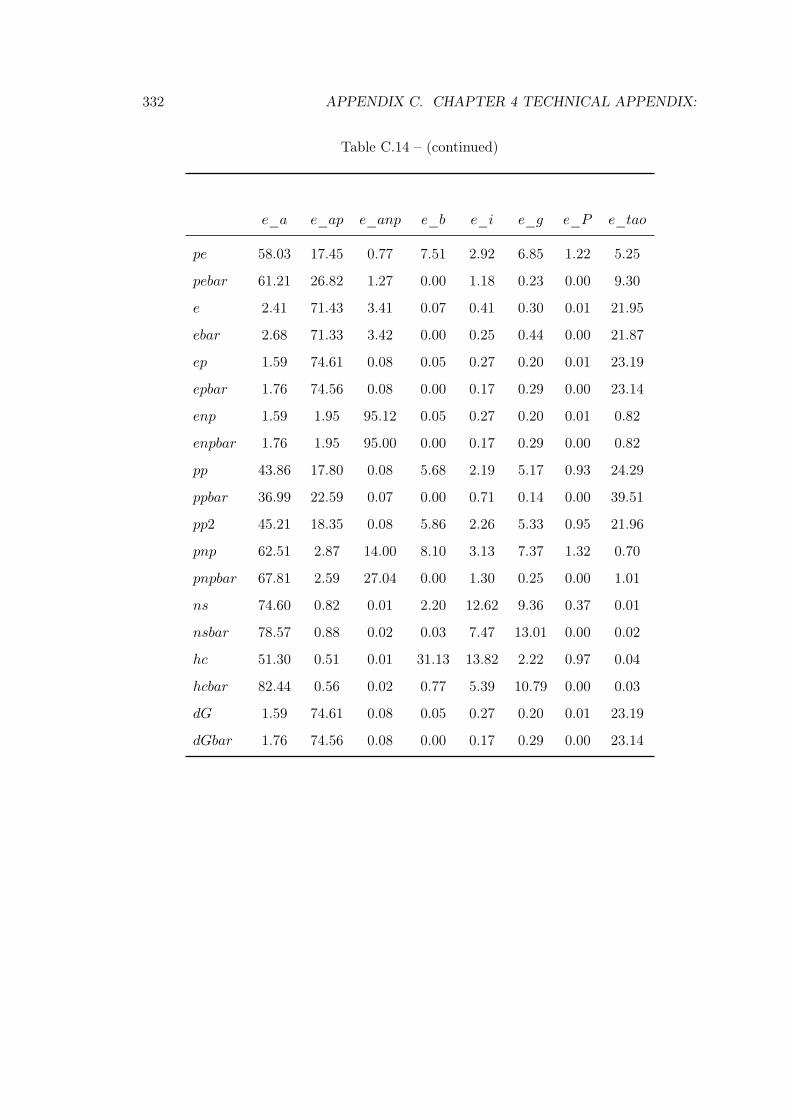
332 APPENDIX C. CHAPTER 4 TECHNICAL APPENDIX:
Table C.14 – (continued)
e_a e_ap e_anp e_b e_i e_g e_P e_tao
pe 58.03 17.45 0.77 7.51 2.92 6.85 1.22 5.25
pebar 61.21 26.82 1.27 0.00 1.18 0.23 0.00 9.30
e 2.41 71.43 3.41 0.07 0.41 0.30 0.01 21.95
ebar 2.68 71.33 3.42 0.00 0.25 0.44 0.00 21.87
ep 1.59 74.61 0.08 0.05 0.27 0.20 0.01 23.19
epbar 1.76 74.56 0.08 0.00 0.17 0.29 0.00 23.14
enp 1.59 1.95 95.12 0.05 0.27 0.20 0.01 0.82
enpbar 1.76 1.95 95.00 0.00 0.17 0.29 0.00 0.82
pp 43.86 17.80 0.08 5.68 2.19 5.17 0.93 24.29
ppbar 36.99 22.59 0.07 0.00 0.71 0.14 0.00 39.51
pp2 45.21 18.35 0.08 5.86 2.26 5.33 0.95 21.96
pnp 62.51 2.87 14.00 8.10 3.13 7.37 1.32 0.70
pnpbar 67.81 2.59 27.04 0.00 1.30 0.25 0.00 1.01
ns 74.60 0.82 0.01 2.20 12.62 9.36 0.37 0.01
nsbar 78.57 0.88 0.02 0.03 7.47 13.01 0.00 0.02
hc 51.30 0.51 0.01 31.13 13.82 2.22 0.97 0.04
hcbar 82.44 0.56 0.02 0.77 5.39 10.79 0.00 0.03
dG 1.59 74.61 0.08 0.05 0.27 0.20 0.01 23.19
dGbar 1.76 74.56 0.08 0.00 0.17 0.29 0.00 23.14

C.4. SIMULATIONS 333
Table C.15 – Coefficients of autocorrelation for an elasticity of substitution of ε = 1.85
with a carbon tax
Order 1 2 3 4 5
epsa 0.9000 0.8100 0.7290 0.6561 0.5905
dy 0.3985 0.2372 0.1025 0.0046 -0.0569
dybar 0.3129 -0.0135 -0.0618 -0.0637 -0.0584
dc 0.6626 0.3443 0.0923 -0.0768 -0.1701
dcbar 0.0582 -0.0804 -0.0864 -0.0732 -0.0594
di 0.7147 0.4612 0.2569 0.1057 0.0022
dibar 0.3767 0.1898 0.0986 0.0401 -0.0004
y 0.9759 0.9326 0.8778 0.8181 0.7582
ybar 0.9640 0.9053 0.8477 0.7945 0.7459
ygap 0.8289 0.5121 0.2537 0.0814 -0.0174
c 0.9758 0.9196 0.8468 0.7695 0.6960
cbar 0.9179 0.8263 0.7479 0.6836 0.6314
i 0.9848 0.9479 0.8970 0.8383 0.7764
ibar 0.9757 0.9332 0.8815 0.8250 0.7665
R 0.9460 0.8210 0.6699 0.5240 0.3994
Rbar 0.3533 0.2098 0.1586 0.1286 0.1067
dM 0.0212 -0.0547 -0.0893 -0.0935 -0.0812
dMbar -0.3953 -0.0711 -0.0153 -0.0052 -0.0030
r 0.6805 0.3837 0.1706 0.0410 -0.0249
rbar 0.2056 0.0626 0.0319 0.0218 0.0162
pi 0.6997 0.3458 0.0908 -0.0517 -0.1097
pibar -0.3742 -0.0657 -0.0129 -0.0035 -0.0016
(Continued on next page)
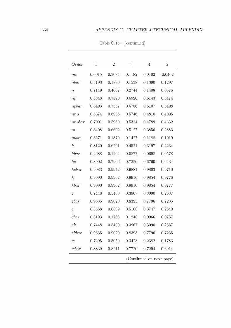
334 APPENDIX C. CHAPTER 4 TECHNICAL APPENDIX:
Table C.15 – (continued)
Order 1 2 3 4 5
mc 0.6015 0.3084 0.1182 0.0102 -0.0402
nbar 0.3193 0.1880 0.1538 0.1390 0.1297
n 0.7149 0.4667 0.2744 0.1408 0.0576
np 0.8848 0.7820 0.6920 0.6143 0.5474
npbar 0.8493 0.7557 0.6786 0.6107 0.5498
nnp 0.8374 0.6936 0.5746 0.4810 0.4095
nnpbar 0.7001 0.5960 0.5314 0.4789 0.4332
m 0.8408 0.6692 0.5127 0.3850 0.2883
mbar 0.3271 0.1870 0.1427 0.1188 0.1019
h 0.8120 0.6201 0.4521 0.3197 0.2234
hbar 0.2688 0.1264 0.0877 0.0698 0.0578
ks 0.8902 0.7966 0.7256 0.6760 0.6434
ksbar 0.9983 0.9942 0.9881 0.9803 0.9710
k 0.9990 0.9962 0.9916 0.9854 0.9776
kbar 0.9990 0.9962 0.9916 0.9854 0.9777
z 0.7448 0.5400 0.3967 0.3090 0.2637
zbar 0.9635 0.9020 0.8393 0.7796 0.7235
q 0.8568 0.6839 0.5168 0.3747 0.2640
qbar 0.3193 0.1738 0.1248 0.0966 0.0757
rk 0.7448 0.5400 0.3967 0.3090 0.2637
rkbar 0.9635 0.9020 0.8393 0.7796 0.7235
w 0.7295 0.5050 0.3428 0.2382 0.1783
wbar 0.8839 0.8211 0.7720 0.7294 0.6914
(Continued on next page)
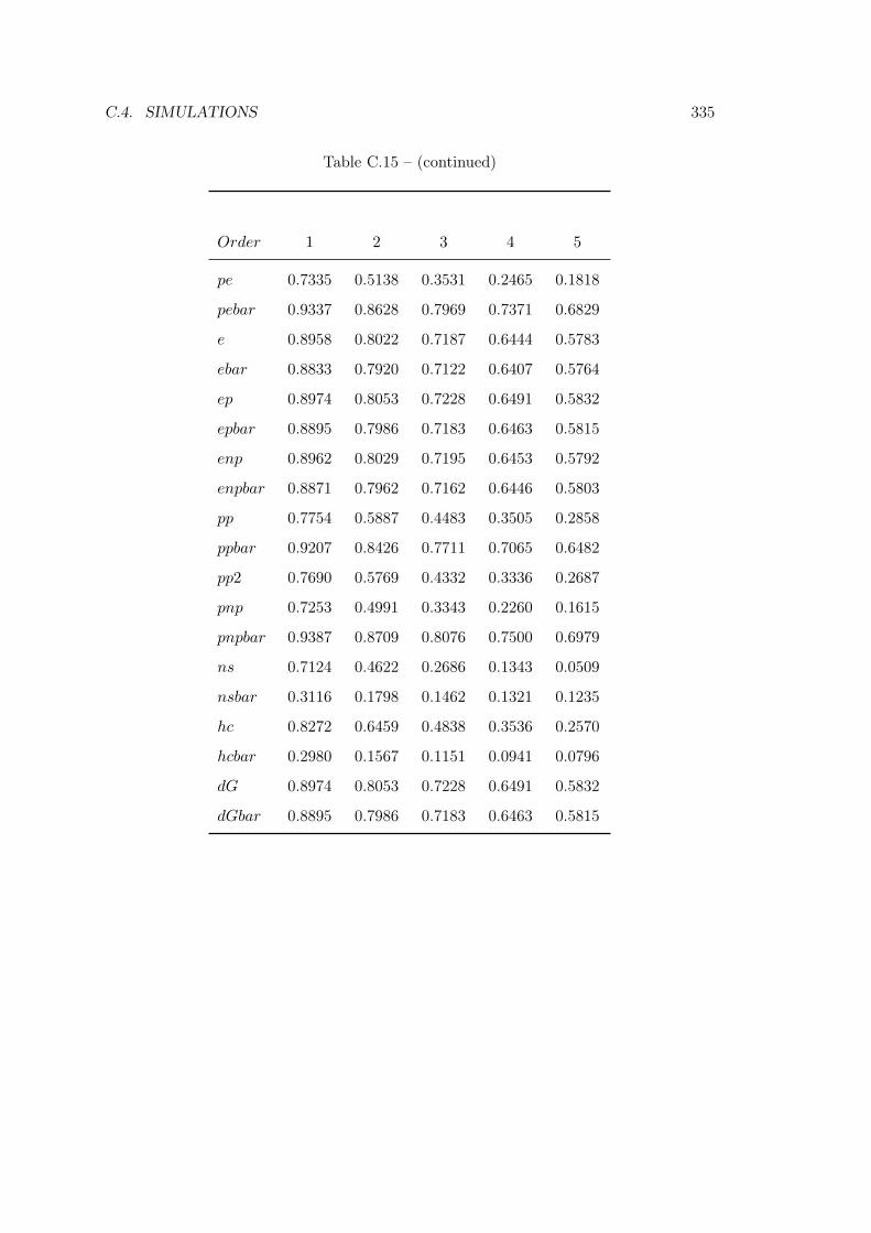
C.4. SIMULATIONS 335
Table C.15 – (continued)
Order 1 2 3 4 5
pe 0.7335 0.5138 0.3531 0.2465 0.1818
pebar 0.9337 0.8628 0.7969 0.7371 0.6829
e 0.8958 0.8022 0.7187 0.6444 0.5783
ebar 0.8833 0.7920 0.7122 0.6407 0.5764
ep 0.8974 0.8053 0.7228 0.6491 0.5832
epbar 0.8895 0.7986 0.7183 0.6463 0.5815
enp 0.8962 0.8029 0.7195 0.6453 0.5792
enpbar 0.8871 0.7962 0.7162 0.6446 0.5803
pp 0.7754 0.5887 0.4483 0.3505 0.2858
ppbar 0.9207 0.8426 0.7711 0.7065 0.6482
pp2 0.7690 0.5769 0.4332 0.3336 0.2687
pnp 0.7253 0.4991 0.3343 0.2260 0.1615
pnpbar 0.9387 0.8709 0.8076 0.7500 0.6979
ns 0.7124 0.4622 0.2686 0.1343 0.0509
nsbar 0.3116 0.1798 0.1462 0.1321 0.1235
hc 0.8272 0.6459 0.4838 0.3536 0.2570
hcbar 0.2980 0.1567 0.1151 0.0941 0.0796
dG 0.8974 0.8053 0.7228 0.6491 0.5832
dGbar 0.8895 0.7986 0.7183 0.6463 0.5815
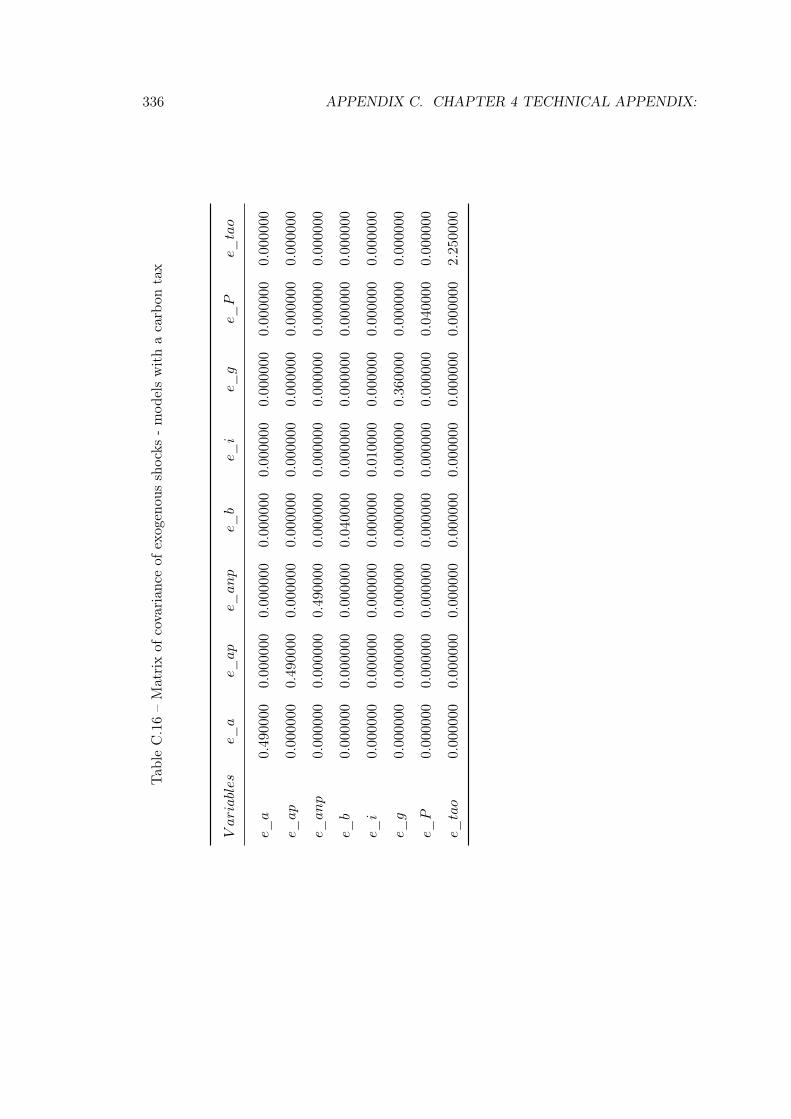
336 APPENDIX C. CHAPTER 4 TECHNICAL APPENDIX:
Tab
leC.16–Matrixof
covarian
ceof
exogenou
sshocks
-mod
elswithacarbon
tax
Variables
e_a
e_ap
e_anp
e_b
e_i
e_g
e_P
e_tao
e_a
0.490000
0.000000
0.000000
0.000000
0.000000
0.000000
0.000000
0.000000
e_ap
0.000000
0.490000
0.000000
0.000000
0.000000
0.000000
0.000000
0.000000
e_anp
0.000000
0.000000
0.490000
0.000000
0.000000
0.000000
0.000000
0.000000
e_b
0.000000
0.000000
0.000000
0.040000
0.000000
0.000000
0.000000
0.000000
e_i
0.000000
0.000000
0.000000
0.000000
0.010000
0.000000
0.000000
0.000000
e_g
0.000000
0.000000
0.000000
0.000000
0.000000
0.360000
0.000000
0.000000
e_P
0.000000
0.000000
0.000000
0.000000
0.000000
0.000000
0.040000
0.000000
e_tao
0.000000
0.000000
0.000000
0.000000
0.000000
0.000000
0.000000
2.250000
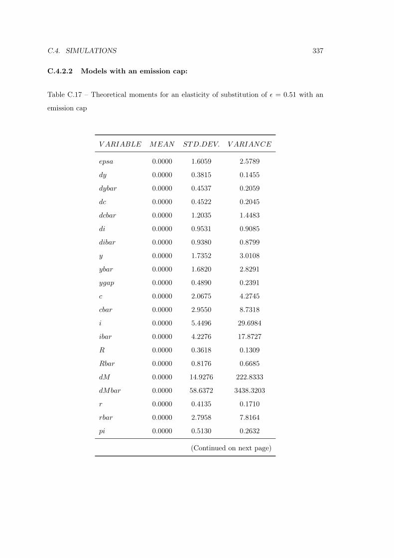
C.4. SIMULATIONS 337
C.4.2.2 Models with an emission cap:
Table C.17 – Theoretical moments for an elasticity of substitution of ε = 0.51 with an
emission cap
V ARIABLE MEAN STD.DEV. V ARIANCE
epsa 0.0000 1.6059 2.5789
dy 0.0000 0.3815 0.1455
dybar 0.0000 0.4537 0.2059
dc 0.0000 0.4522 0.2045
dcbar 0.0000 1.2035 1.4483
di 0.0000 0.9531 0.9085
dibar 0.0000 0.9380 0.8799
y 0.0000 1.7352 3.0108
ybar 0.0000 1.6820 2.8291
ygap 0.0000 0.4890 0.2391
c 0.0000 2.0675 4.2745
cbar 0.0000 2.9550 8.7318
i 0.0000 5.4496 29.6984
ibar 0.0000 4.2276 17.8727
R 0.0000 0.3618 0.1309
Rbar 0.0000 0.8176 0.6685
dM 0.0000 14.9276 222.8333
dMbar 0.0000 58.6372 3438.3203
r 0.0000 0.4135 0.1710
rbar 0.0000 2.7958 7.8164
pi 0.0000 0.5130 0.2632
(Continued on next page)
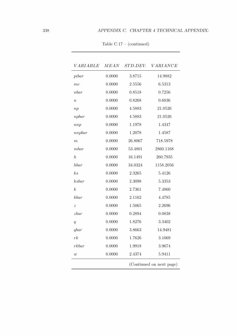
338 APPENDIX C. CHAPTER 4 TECHNICAL APPENDIX:
Table C.17 – (continued)
V ARIABLE MEAN STD.DEV. V ARIANCE
pibar 0.0000 3.8715 14.9882
mc 0.0000 2.5556 6.5313
nbar 0.0000 0.8518 0.7256
n 0.0000 0.8268 0.6836
np 0.0000 4.5883 21.0526
npbar 0.0000 4.5883 21.0526
nnp 0.0000 1.1978 1.4347
nnpbar 0.0000 1.2078 1.4587
m 0.0000 26.8067 718.5978
mbar 0.0000 53.4801 2860.1168
h 0.0000 16.1491 260.7935
hbar 0.0000 34.0324 1158.2056
ks 0.0000 2.3265 5.4126
ksbar 0.0000 2.3098 5.3353
k 0.0000 2.7361 7.4860
kbar 0.0000 2.1162 4.4785
z 0.0000 1.5065 2.2696
zbar 0.0000 0.2894 0.0838
q 0.0000 1.8276 3.3402
qbar 0.0000 3.8663 14.9481
rk 0.0000 1.7626 3.1069
rkbar 0.0000 1.9918 3.9674
w 0.0000 2.4374 5.9411
(Continued on next page)
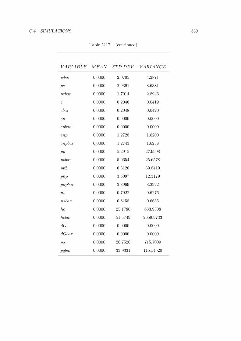
C.4. SIMULATIONS 339
Table C.17 – (continued)
V ARIABLE MEAN STD.DEV. V ARIANCE
wbar 0.0000 2.0705 4.2871
pe 0.0000 2.9391 8.6381
pebar 0.0000 1.7014 2.8946
e 0.0000 0.2046 0.0419
ebar 0.0000 0.2048 0.0420
ep 0.0000 0.0000 0.0000
epbar 0.0000 0.0000 0.0000
enp 0.0000 1.2728 1.6200
enpbar 0.0000 1.2743 1.6238
pp 0.0000 5.2915 27.9998
ppbar 0.0000 5.0654 25.6578
pp2 0.0000 6.3120 39.8419
pnp 0.0000 3.5097 12.3179
pnpbar 0.0000 2.8969 8.3922
ns 0.0000 0.7922 0.6276
nsbar 0.0000 0.8158 0.6655
hc 0.0000 25.1780 633.9308
hcbar 0.0000 51.5749 2659.9733
dG 0.0000 0.0000 0.0000
dGbar 0.0000 0.0000 0.0000
pq 0.0000 26.7526 715.7009
pqbar 0.0000 33.9331 1151.4520
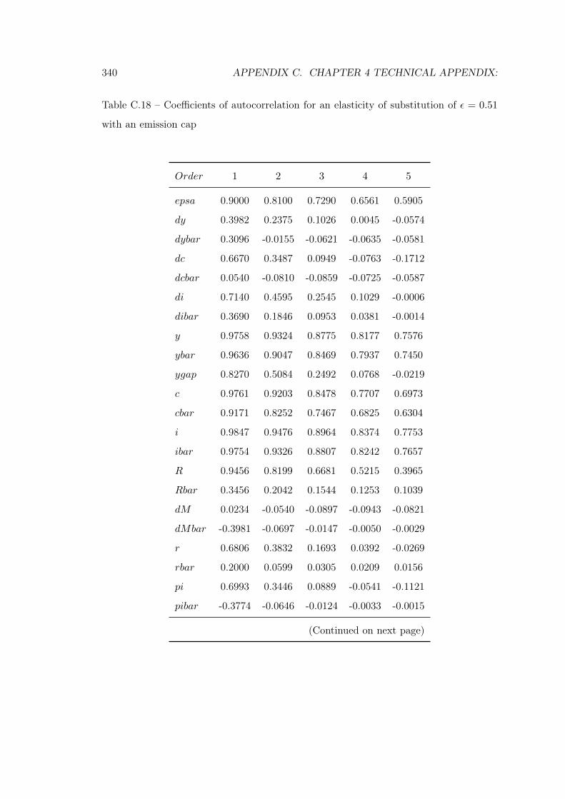
340 APPENDIX C. CHAPTER 4 TECHNICAL APPENDIX:
Table C.18 – Coefficients of autocorrelation for an elasticity of substitution of ε = 0.51
with an emission cap
Order 1 2 3 4 5
epsa 0.9000 0.8100 0.7290 0.6561 0.5905
dy 0.3982 0.2375 0.1026 0.0045 -0.0574
dybar 0.3096 -0.0155 -0.0621 -0.0635 -0.0581
dc 0.6670 0.3487 0.0949 -0.0763 -0.1712
dcbar 0.0540 -0.0810 -0.0859 -0.0725 -0.0587
di 0.7140 0.4595 0.2545 0.1029 -0.0006
dibar 0.3690 0.1846 0.0953 0.0381 -0.0014
y 0.9758 0.9324 0.8775 0.8177 0.7576
ybar 0.9636 0.9047 0.8469 0.7937 0.7450
ygap 0.8270 0.5084 0.2492 0.0768 -0.0219
c 0.9761 0.9203 0.8478 0.7707 0.6973
cbar 0.9171 0.8252 0.7467 0.6825 0.6304
i 0.9847 0.9476 0.8964 0.8374 0.7753
ibar 0.9754 0.9326 0.8807 0.8242 0.7657
R 0.9456 0.8199 0.6681 0.5215 0.3965
Rbar 0.3456 0.2042 0.1544 0.1253 0.1039
dM 0.0234 -0.0540 -0.0897 -0.0943 -0.0821
dMbar -0.3981 -0.0697 -0.0147 -0.0050 -0.0029
r 0.6806 0.3832 0.1693 0.0392 -0.0269
rbar 0.2000 0.0599 0.0305 0.0209 0.0156
pi 0.6993 0.3446 0.0889 -0.0541 -0.1121
pibar -0.3774 -0.0646 -0.0124 -0.0033 -0.0015
(Continued on next page)
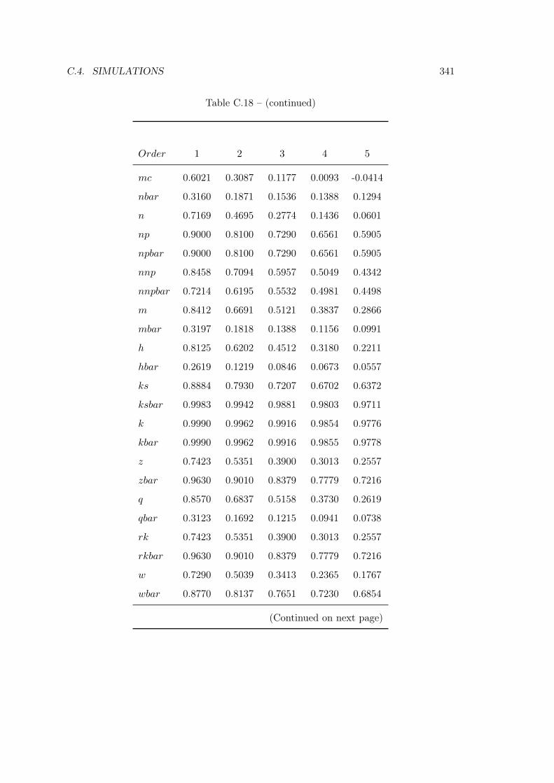
C.4. SIMULATIONS 341
Table C.18 – (continued)
Order 1 2 3 4 5
mc 0.6021 0.3087 0.1177 0.0093 -0.0414
nbar 0.3160 0.1871 0.1536 0.1388 0.1294
n 0.7169 0.4695 0.2774 0.1436 0.0601
np 0.9000 0.8100 0.7290 0.6561 0.5905
npbar 0.9000 0.8100 0.7290 0.6561 0.5905
nnp 0.8458 0.7094 0.5957 0.5049 0.4342
nnpbar 0.7214 0.6195 0.5532 0.4981 0.4498
m 0.8412 0.6691 0.5121 0.3837 0.2866
mbar 0.3197 0.1818 0.1388 0.1156 0.0991
h 0.8125 0.6202 0.4512 0.3180 0.2211
hbar 0.2619 0.1219 0.0846 0.0673 0.0557
ks 0.8884 0.7930 0.7207 0.6702 0.6372
ksbar 0.9983 0.9942 0.9881 0.9803 0.9711
k 0.9990 0.9962 0.9916 0.9854 0.9776
kbar 0.9990 0.9962 0.9916 0.9855 0.9778
z 0.7423 0.5351 0.3900 0.3013 0.2557
zbar 0.9630 0.9010 0.8379 0.7779 0.7216
q 0.8570 0.6837 0.5158 0.3730 0.2619
qbar 0.3123 0.1692 0.1215 0.0941 0.0738
rk 0.7423 0.5351 0.3900 0.3013 0.2557
rkbar 0.9630 0.9010 0.8379 0.7779 0.7216
w 0.7290 0.5039 0.3413 0.2365 0.1767
wbar 0.8770 0.8137 0.7651 0.7230 0.6854
(Continued on next page)

342 APPENDIX C. CHAPTER 4 TECHNICAL APPENDIX:
Table C.18 – (continued)
Order 1 2 3 4 5
pe 0.6835 0.4235 0.2366 0.1175 0.0510
pebar 0.9639 0.9051 0.8473 0.7942 0.7456
e 0.8947 0.8001 0.7157 0.6410 0.5748
ebar 0.8813 0.7900 0.7105 0.6395 0.5756
enp 0.8947 0.8001 0.7157 0.6410 0.5748
enpbar 0.8813 0.7900 0.7105 0.6395 0.5756
pp 0.8582 0.7363 0.6365 0.5565 0.4925
ppbar 0.8967 0.8108 0.7347 0.6665 0.6052
pp2 0.8706 0.7582 0.6640 0.5861 0.5217
pnp 0.7812 0.5983 0.4603 0.3636 0.2994
pnpbar 0.9174 0.8401 0.7701 0.7069 0.6499
ns 0.7130 0.4624 0.2682 0.1334 0.0498
nsbar 0.3057 0.1762 0.1437 0.1300 0.1217
hc 0.8277 0.6459 0.4830 0.3522 0.2550
hcbar 0.2908 0.1518 0.1116 0.0913 0.0772
pq 0.8850 0.7839 0.6955 0.6188 0.5523
pqbar 0.7654 0.5910 0.4632 0.3732 0.3115
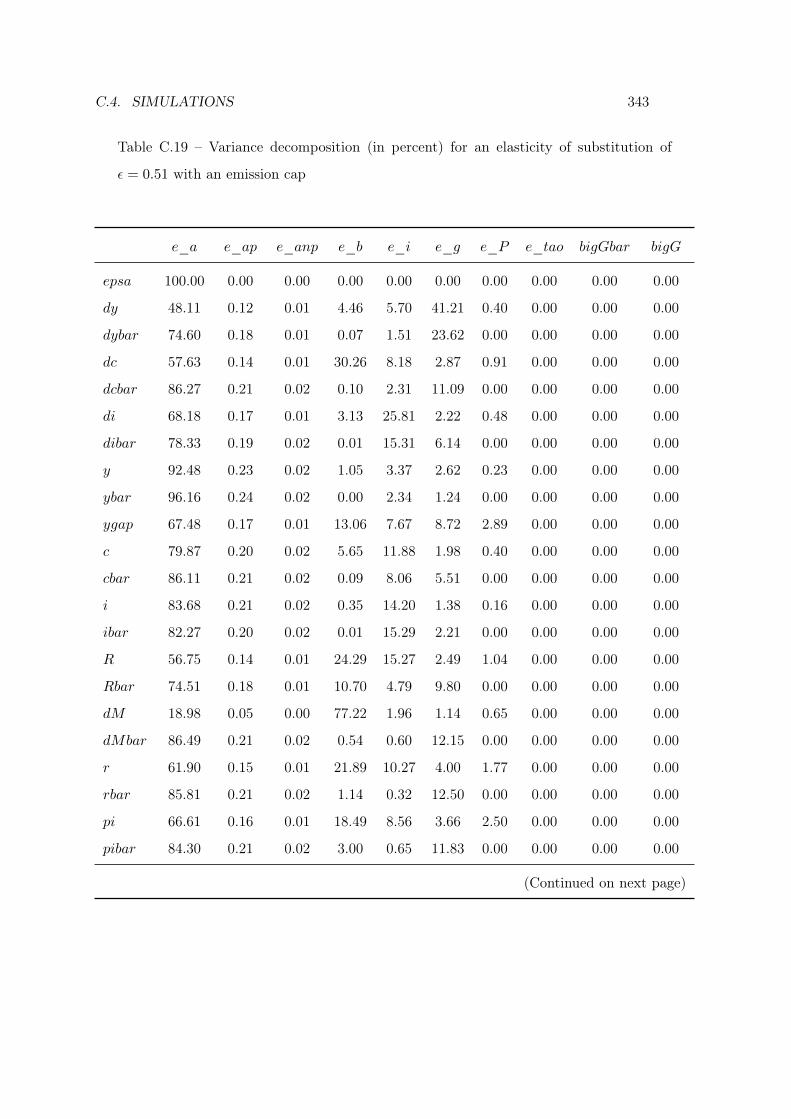
C.4. SIMULATIONS 343
Table C.19 – Variance decomposition (in percent) for an elasticity of substitution of
ε = 0.51 with an emission cap
e_a e_ap e_anp e_b e_i e_g e_P e_tao bigGbar bigG
epsa 100.00 0.00 0.00 0.00 0.00 0.00 0.00 0.00 0.00 0.00
dy 48.11 0.12 0.01 4.46 5.70 41.21 0.40 0.00 0.00 0.00
dybar 74.60 0.18 0.01 0.07 1.51 23.62 0.00 0.00 0.00 0.00
dc 57.63 0.14 0.01 30.26 8.18 2.87 0.91 0.00 0.00 0.00
dcbar 86.27 0.21 0.02 0.10 2.31 11.09 0.00 0.00 0.00 0.00
di 68.18 0.17 0.01 3.13 25.81 2.22 0.48 0.00 0.00 0.00
dibar 78.33 0.19 0.02 0.01 15.31 6.14 0.00 0.00 0.00 0.00
y 92.48 0.23 0.02 1.05 3.37 2.62 0.23 0.00 0.00 0.00
ybar 96.16 0.24 0.02 0.00 2.34 1.24 0.00 0.00 0.00 0.00
ygap 67.48 0.17 0.01 13.06 7.67 8.72 2.89 0.00 0.00 0.00
c 79.87 0.20 0.02 5.65 11.88 1.98 0.40 0.00 0.00 0.00
cbar 86.11 0.21 0.02 0.09 8.06 5.51 0.00 0.00 0.00 0.00
i 83.68 0.21 0.02 0.35 14.20 1.38 0.16 0.00 0.00 0.00
ibar 82.27 0.20 0.02 0.01 15.29 2.21 0.00 0.00 0.00 0.00
R 56.75 0.14 0.01 24.29 15.27 2.49 1.04 0.00 0.00 0.00
Rbar 74.51 0.18 0.01 10.70 4.79 9.80 0.00 0.00 0.00 0.00
dM 18.98 0.05 0.00 77.22 1.96 1.14 0.65 0.00 0.00 0.00
dMbar 86.49 0.21 0.02 0.54 0.60 12.15 0.00 0.00 0.00 0.00
r 61.90 0.15 0.01 21.89 10.27 4.00 1.77 0.00 0.00 0.00
rbar 85.81 0.21 0.02 1.14 0.32 12.50 0.00 0.00 0.00 0.00
pi 66.61 0.16 0.01 18.49 8.56 3.66 2.50 0.00 0.00 0.00
pibar 84.30 0.21 0.02 3.00 0.65 11.83 0.00 0.00 0.00 0.00
(Continued on next page)
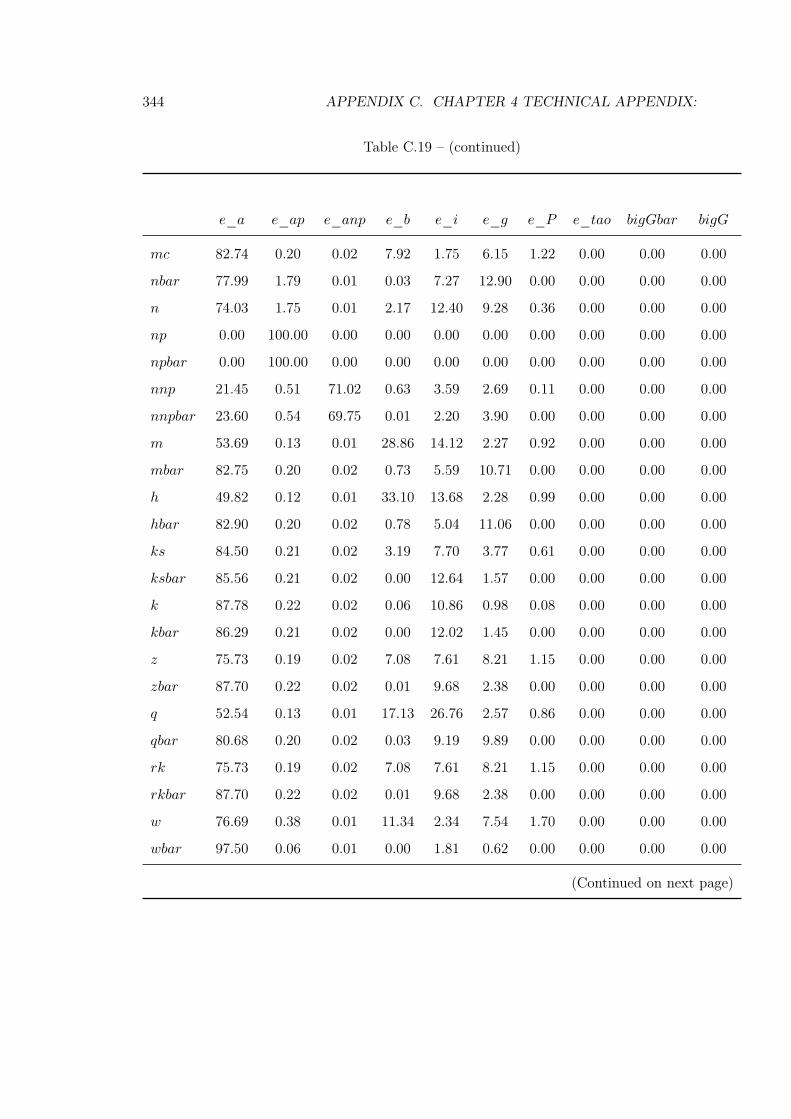
344 APPENDIX C. CHAPTER 4 TECHNICAL APPENDIX:
Table C.19 – (continued)
e_a e_ap e_anp e_b e_i e_g e_P e_tao bigGbar bigG
mc 82.74 0.20 0.02 7.92 1.75 6.15 1.22 0.00 0.00 0.00
nbar 77.99 1.79 0.01 0.03 7.27 12.90 0.00 0.00 0.00 0.00
n 74.03 1.75 0.01 2.17 12.40 9.28 0.36 0.00 0.00 0.00
np 0.00 100.00 0.00 0.00 0.00 0.00 0.00 0.00 0.00 0.00
npbar 0.00 100.00 0.00 0.00 0.00 0.00 0.00 0.00 0.00 0.00
nnp 21.45 0.51 71.02 0.63 3.59 2.69 0.11 0.00 0.00 0.00
nnpbar 23.60 0.54 69.75 0.01 2.20 3.90 0.00 0.00 0.00 0.00
m 53.69 0.13 0.01 28.86 14.12 2.27 0.92 0.00 0.00 0.00
mbar 82.75 0.20 0.02 0.73 5.59 10.71 0.00 0.00 0.00 0.00
h 49.82 0.12 0.01 33.10 13.68 2.28 0.99 0.00 0.00 0.00
hbar 82.90 0.20 0.02 0.78 5.04 11.06 0.00 0.00 0.00 0.00
ks 84.50 0.21 0.02 3.19 7.70 3.77 0.61 0.00 0.00 0.00
ksbar 85.56 0.21 0.02 0.00 12.64 1.57 0.00 0.00 0.00 0.00
k 87.78 0.22 0.02 0.06 10.86 0.98 0.08 0.00 0.00 0.00
kbar 86.29 0.21 0.02 0.00 12.02 1.45 0.00 0.00 0.00 0.00
z 75.73 0.19 0.02 7.08 7.61 8.21 1.15 0.00 0.00 0.00
zbar 87.70 0.22 0.02 0.01 9.68 2.38 0.00 0.00 0.00 0.00
q 52.54 0.13 0.01 17.13 26.76 2.57 0.86 0.00 0.00 0.00
qbar 80.68 0.20 0.02 0.03 9.19 9.89 0.00 0.00 0.00 0.00
rk 75.73 0.19 0.02 7.08 7.61 8.21 1.15 0.00 0.00 0.00
rkbar 87.70 0.22 0.02 0.01 9.68 2.38 0.00 0.00 0.00 0.00
w 76.69 0.38 0.01 11.34 2.34 7.54 1.70 0.00 0.00 0.00
wbar 97.50 0.06 0.01 0.00 1.81 0.62 0.00 0.00 0.00 0.00
(Continued on next page)
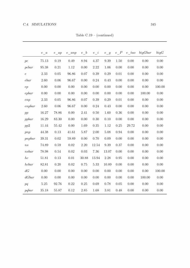
C.4. SIMULATIONS 345
Table C.19 – (continued)
e_a e_ap e_anp e_b e_i e_g e_P e_tao bigGbar bigG
pe 75.13 0.19 0.49 8.94 4.37 9.39 1.50 0.00 0.00 0.00
pebar 95.38 0.21 1.12 0.00 2.22 1.06 0.00 0.00 0.00 0.00
e 2.33 0.05 96.86 0.07 0.39 0.29 0.01 0.00 0.00 0.00
ebar 2.60 0.06 96.67 0.00 0.24 0.43 0.00 0.00 0.00 0.00
ep 0.00 0.00 0.00 0.00 0.00 0.00 0.00 0.00 0.00 100.00
epbar 0.00 0.00 0.00 0.00 0.00 0.00 0.00 0.00 100.00 0.00
enp 2.33 0.05 96.86 0.07 0.39 0.29 0.01 0.00 0.00 0.00
enpbar 2.60 0.06 96.67 0.00 0.24 0.43 0.00 0.00 0.00 0.00
pp 16.27 78.86 0.00 2.41 0.50 1.60 0.36 0.00 0.00 0.00
ppbar 16.29 83.30 0.00 0.00 0.30 0.10 0.00 0.00 0.00 0.00
pp2 11.44 55.42 0.00 1.69 0.35 1.12 0.25 29.72 0.00 0.00
pnp 44.38 0.13 41.61 5.87 2.00 5.08 0.94 0.00 0.00 0.00
pnpbar 39.31 0.02 59.89 0.00 0.70 0.09 0.00 0.00 0.00 0.00
ns 74.89 0.59 0.02 2.20 12.54 9.39 0.37 0.00 0.00 0.00
nsbar 78.98 0.54 0.02 0.03 7.36 13.07 0.00 0.00 0.00 0.00
hc 51.81 0.13 0.01 30.88 13.94 2.28 0.95 0.00 0.00 0.00
hcbar 82.81 0.20 0.02 0.75 5.33 10.89 0.00 0.00 0.00 0.00
dG 0.00 0.00 0.00 0.00 0.00 0.00 0.00 0.00 0.00 100.00
dGbar 0.00 0.00 0.00 0.00 0.00 0.00 0.00 0.00 100.00 0.00
pq 5.25 92.76 0.22 0.25 0.69 0.78 0.05 0.00 0.00 0.00
pqbar 35.18 55.87 0.12 2.85 1.68 3.81 0.48 0.00 0.00 0.00
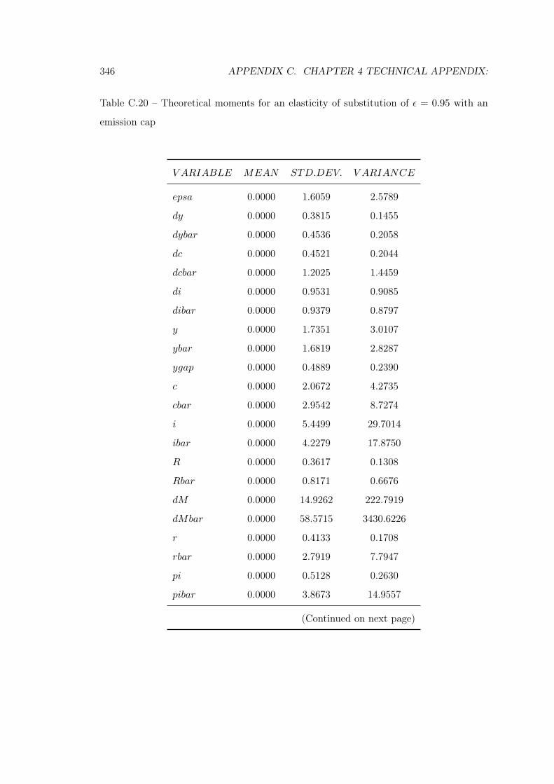
346 APPENDIX C. CHAPTER 4 TECHNICAL APPENDIX:
Table C.20 – Theoretical moments for an elasticity of substitution of ε = 0.95 with an
emission cap
V ARIABLE MEAN STD.DEV. V ARIANCE
epsa 0.0000 1.6059 2.5789
dy 0.0000 0.3815 0.1455
dybar 0.0000 0.4536 0.2058
dc 0.0000 0.4521 0.2044
dcbar 0.0000 1.2025 1.4459
di 0.0000 0.9531 0.9085
dibar 0.0000 0.9379 0.8797
y 0.0000 1.7351 3.0107
ybar 0.0000 1.6819 2.8287
ygap 0.0000 0.4889 0.2390
c 0.0000 2.0672 4.2735
cbar 0.0000 2.9542 8.7274
i 0.0000 5.4499 29.7014
ibar 0.0000 4.2279 17.8750
R 0.0000 0.3617 0.1308
Rbar 0.0000 0.8171 0.6676
dM 0.0000 14.9262 222.7919
dMbar 0.0000 58.5715 3430.6226
r 0.0000 0.4133 0.1708
rbar 0.0000 2.7919 7.7947
pi 0.0000 0.5128 0.2630
pibar 0.0000 3.8673 14.9557
(Continued on next page)
C.4. SIMULATIONS 347
Table C.20 – (continued)
V ARIABLE MEAN STD.DEV. V ARIANCE
mc 0.0000 2.5543 6.5246
nbar 0.0000 0.8500 0.7226
n 0.0000 0.8252 0.6810
np 0.0000 4.5883 21.0526
npbar 0.0000 4.5883 21.0526
nnp 0.0000 0.8158 0.6656
nnpbar 0.0000 0.8400 0.7056
m 0.0000 26.8030 718.4000
mbar 0.0000 53.4416 2856.0054
h 0.0000 16.1468 260.7186
hbar 0.0000 34.0064 1156.4384
ks 0.0000 2.3262 5.4112
ksbar 0.0000 2.3098 5.3352
k 0.0000 2.7361 7.4860
kbar 0.0000 2.1162 4.4783
z 0.0000 1.5061 2.2684
zbar 0.0000 0.2894 0.0838
q 0.0000 1.8273 3.3390
qbar 0.0000 3.8636 14.9275
rk 0.0000 1.7622 3.1052
rkbar 0.0000 1.9918 3.9674
w 0.0000 2.4374 5.9409
wbar 0.0000 2.0694 4.2826
(Continued on next page)
348 APPENDIX C. CHAPTER 4 TECHNICAL APPENDIX:
Table C.20 – (continued)
V ARIABLE MEAN STD.DEV. V ARIANCE
pe 0.0000 2.9345 8.6114
pebar 0.0000 1.7151 2.9417
e 0.0000 0.2855 0.0815
ebar 0.0000 0.2858 0.0817
ep 0.0000 0.0000 0.0000
epbar 0.0000 0.0000 0.0000
enp 0.0000 1.6025 2.5680
enpbar 0.0000 1.6044 2.5742
pp 0.0000 5.2913 27.9978
ppbar 0.0000 5.0647 25.6510
pp2 0.0000 6.3119 39.8399
pnp 0.0000 3.2108 10.3091
pnpbar 0.0000 2.4162 5.8381
ns 0.0000 0.7922 0.6275
nsbar 0.0000 0.8156 0.6652
hc 0.0000 25.1744 633.7528
hcbar 0.0000 51.5367 2656.0319
dG 0.0000 0.0000 0.0000
dGbar 0.0000 0.0000 0.0000
pq 0.0000 26.6456 709.9905
pqbar 0.0000 33.7554 1139.4238

C.4. SIMULATIONS 349
Table C.21 – Coefficients of autocorrelation for an elasticity of substitution of ε = 0.95
with an emission cap
Order 1 2 3 4 5
epsa 0.9000 0.8100 0.7290 0.6561 0.5905
dy 0.3982 0.2375 0.1026 0.0045 -0.0573
dybar 0.3097 -0.0153 -0.0620 -0.0635 -0.0581
dc 0.6670 0.3487 0.0949 -0.0763 -0.1712
dcbar 0.0544 -0.0810 -0.0860 -0.0726 -0.0588
di 0.7140 0.4596 0.2546 0.1030 -0.0005
dibar 0.3694 0.1847 0.0954 0.0381 -0.0014
y 0.9758 0.9324 0.8775 0.8177 0.7576
ybar 0.9636 0.9047 0.8469 0.7937 0.7450
ygap 0.8272 0.5087 0.2495 0.0770 -0.0217
c 0.9761 0.9203 0.8478 0.7707 0.6974
cbar 0.9172 0.8253 0.7469 0.6827 0.6305
i 0.9847 0.9476 0.8964 0.8374 0.7753
ibar 0.9754 0.9326 0.8807 0.8242 0.7657
R 0.9457 0.8200 0.6682 0.5216 0.3966
Rbar 0.3461 0.2045 0.1546 0.1254 0.1040
dM 0.0233 -0.0540 -0.0896 -0.0943 -0.0820
dMbar -0.3978 -0.0699 -0.0147 -0.0050 -0.0029
r 0.6806 0.3833 0.1694 0.0393 -0.0268
rbar 0.2006 0.0601 0.0306 0.0209 0.0156
pi 0.6994 0.3447 0.0890 -0.0539 -0.1120
pibar -0.3771 -0.0647 -0.0124 -0.0034 -0.0015
(Continued on next page)

350 APPENDIX C. CHAPTER 4 TECHNICAL APPENDIX:
Table C.21 – (continued)
Order 1 2 3 4 5
mc 0.6021 0.3087 0.1178 0.0094 -0.0413
nbar 0.3165 0.1874 0.1538 0.1390 0.1295
n 0.7170 0.4696 0.2775 0.1437 0.0602
np 0.9000 0.8100 0.7290 0.6561 0.5905
npbar 0.9000 0.8100 0.7290 0.6561 0.5905
nnp 0.7185 0.4726 0.2815 0.1482 0.0649
nnpbar 0.3215 0.1927 0.1587 0.1434 0.1335
m 0.8412 0.6691 0.5121 0.3837 0.2867
mbar 0.3203 0.1821 0.1390 0.1158 0.0993
h 0.8125 0.6202 0.4512 0.3180 0.2212
hbar 0.2624 0.1222 0.0847 0.0674 0.0558
ks 0.8885 0.7932 0.7209 0.6705 0.6374
ksbar 0.9983 0.9942 0.9881 0.9803 0.9711
k 0.9990 0.9962 0.9916 0.9854 0.9776
kbar 0.9990 0.9962 0.9916 0.9854 0.9778
z 0.7425 0.5353 0.3903 0.3016 0.2559
zbar 0.9630 0.9010 0.8380 0.7780 0.7217
q 0.8570 0.6837 0.5158 0.3731 0.2619
qbar 0.3128 0.1695 0.1217 0.0942 0.0738
rk 0.7425 0.5353 0.3903 0.3016 0.2559
rkbar 0.9630 0.9010 0.8380 0.7780 0.7217
w 0.7290 0.5040 0.3413 0.2366 0.1767
wbar 0.8774 0.8141 0.7655 0.7233 0.6857
(Continued on next page)

C.4. SIMULATIONS 351
Table C.21 – (continued)
Order 1 2 3 4 5
pe 0.6850 0.4262 0.2401 0.1213 0.0550
pebar 0.9634 0.9043 0.8465 0.7932 0.7445
e 0.8947 0.8002 0.7159 0.6411 0.5750
ebar 0.8814 0.7902 0.7107 0.6396 0.5757
enp 0.8947 0.8002 0.7159 0.6411 0.5750
enpbar 0.8814 0.7902 0.7107 0.6396 0.5757
pp 0.8582 0.7363 0.6365 0.5565 0.4925
ppbar 0.8967 0.8109 0.7348 0.6666 0.6052
pp2 0.8706 0.7582 0.6640 0.5861 0.5216
pnp 0.7468 0.5369 0.3820 0.2778 0.2132
pnpbar 0.9299 0.8575 0.7908 0.7303 0.6756
ns 0.7130 0.4625 0.2684 0.1335 0.0499
nsbar 0.3062 0.1765 0.1438 0.1302 0.1218
hc 0.8277 0.6459 0.4831 0.3522 0.2551
hcbar 0.2914 0.1521 0.1117 0.0914 0.0773
pq 0.8860 0.7854 0.6973 0.6207 0.5541
pqbar 0.7661 0.5922 0.4648 0.3750 0.3134
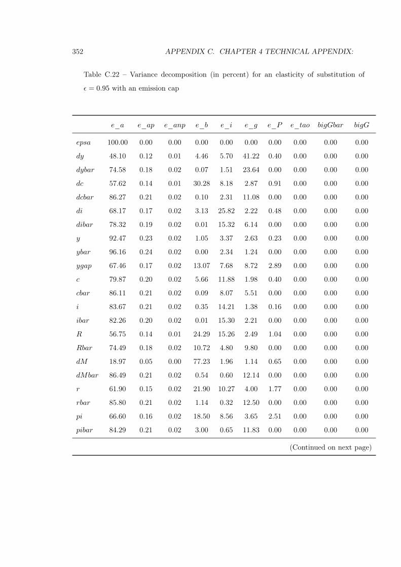
352 APPENDIX C. CHAPTER 4 TECHNICAL APPENDIX:
Table C.22 – Variance decomposition (in percent) for an elasticity of substitution of
ε = 0.95 with an emission cap
e_a e_ap e_anp e_b e_i e_g e_P e_tao bigGbar bigG
epsa 100.00 0.00 0.00 0.00 0.00 0.00 0.00 0.00 0.00 0.00
dy 48.10 0.12 0.01 4.46 5.70 41.22 0.40 0.00 0.00 0.00
dybar 74.58 0.18 0.02 0.07 1.51 23.64 0.00 0.00 0.00 0.00
dc 57.62 0.14 0.01 30.28 8.18 2.87 0.91 0.00 0.00 0.00
dcbar 86.27 0.21 0.02 0.10 2.31 11.08 0.00 0.00 0.00 0.00
di 68.17 0.17 0.02 3.13 25.82 2.22 0.48 0.00 0.00 0.00
dibar 78.32 0.19 0.02 0.01 15.32 6.14 0.00 0.00 0.00 0.00
y 92.47 0.23 0.02 1.05 3.37 2.63 0.23 0.00 0.00 0.00
ybar 96.16 0.24 0.02 0.00 2.34 1.24 0.00 0.00 0.00 0.00
ygap 67.46 0.17 0.02 13.07 7.68 8.72 2.89 0.00 0.00 0.00
c 79.87 0.20 0.02 5.66 11.88 1.98 0.40 0.00 0.00 0.00
cbar 86.11 0.21 0.02 0.09 8.07 5.51 0.00 0.00 0.00 0.00
i 83.67 0.21 0.02 0.35 14.21 1.38 0.16 0.00 0.00 0.00
ibar 82.26 0.20 0.02 0.01 15.30 2.21 0.00 0.00 0.00 0.00
R 56.75 0.14 0.01 24.29 15.26 2.49 1.04 0.00 0.00 0.00
Rbar 74.49 0.18 0.02 10.72 4.80 9.80 0.00 0.00 0.00 0.00
dM 18.97 0.05 0.00 77.23 1.96 1.14 0.65 0.00 0.00 0.00
dMbar 86.49 0.21 0.02 0.54 0.60 12.14 0.00 0.00 0.00 0.00
r 61.90 0.15 0.02 21.90 10.27 4.00 1.77 0.00 0.00 0.00
rbar 85.80 0.21 0.02 1.14 0.32 12.50 0.00 0.00 0.00 0.00
pi 66.60 0.16 0.02 18.50 8.56 3.65 2.51 0.00 0.00 0.00
pibar 84.29 0.21 0.02 3.00 0.65 11.83 0.00 0.00 0.00 0.00
(Continued on next page)

C.4. SIMULATIONS 353
Table C.22 – (continued)
e_a e_ap e_anp e_b e_i e_g e_P e_tao bigGbar bigG
mc 82.73 0.20 0.02 7.93 1.75 6.15 1.22 0.00 0.00 0.00
nbar 77.98 1.79 0.02 0.03 7.28 12.90 0.00 0.00 0.00 0.00
n 74.02 1.75 0.02 2.17 12.40 9.28 0.36 0.00 0.00 0.00
np 0.00 100.00 0.00 0.00 0.00 0.00 0.00 0.00 0.00 0.00
npbar 0.00 100.00 0.00 0.00 0.00 0.00 0.00 0.00 0.00 0.00
nnp 73.27 1.73 1.03 2.15 12.28 9.19 0.36 0.00 0.00 0.00
nnpbar 77.26 1.77 0.95 0.03 7.21 12.78 0.00 0.00 0.00 0.00
m 53.68 0.13 0.01 28.87 14.11 2.27 0.92 0.00 0.00 0.00
mbar 82.74 0.20 0.02 0.73 5.60 10.71 0.00 0.00 0.00 0.00
h 49.81 0.12 0.01 33.12 13.67 2.28 0.99 0.00 0.00 0.00
hbar 82.89 0.20 0.02 0.78 5.04 11.06 0.00 0.00 0.00 0.00
ks 84.49 0.21 0.02 3.19 7.70 3.77 0.61 0.00 0.00 0.00
ksbar 85.55 0.21 0.02 0.00 12.64 1.57 0.00 0.00 0.00 0.00
k 87.77 0.22 0.02 0.06 10.86 0.98 0.08 0.00 0.00 0.00
kbar 86.29 0.21 0.02 0.00 12.02 1.45 0.00 0.00 0.00 0.00
z 75.72 0.19 0.02 7.09 7.62 8.21 1.16 0.00 0.00 0.00
zbar 87.69 0.22 0.02 0.01 9.69 2.38 0.00 0.00 0.00 0.00
q 52.53 0.13 0.01 17.13 26.76 2.57 0.86 0.00 0.00 0.00
qbar 80.67 0.20 0.02 0.03 9.20 9.89 0.00 0.00 0.00 0.00
rk 75.72 0.19 0.02 7.09 7.62 8.21 1.16 0.00 0.00 0.00
rkbar 87.69 0.22 0.02 0.01 9.69 2.38 0.00 0.00 0.00 0.00
w 76.68 0.38 0.02 11.34 2.34 7.54 1.70 0.00 0.00 0.00
wbar 97.50 0.06 0.02 0.00 1.81 0.61 0.00 0.00 0.00 0.00
(Continued on next page)

354 APPENDIX C. CHAPTER 4 TECHNICAL APPENDIX:
Table C.22 – (continued)
e_a e_ap e_anp e_b e_i e_g e_P e_tao bigGbar bigG
pe 74.80 0.19 0.94 8.94 4.31 9.32 1.50 0.00 0.00 0.00
pebar 94.40 0.19 2.25 0.00 2.17 0.99 0.00 0.00 0.00 0.00
e 2.33 0.05 96.86 0.07 0.39 0.29 0.01 0.00 0.00 0.00
ebar 2.59 0.06 96.67 0.00 0.24 0.43 0.00 0.00 0.00 0.00
ep 0.00 0.00 0.00 0.00 0.00 0.00 0.00 0.00 0.00 100.00
epbar 0.00 0.00 0.00 0.00 0.00 0.00 0.00 0.00 100.00 0.00
enp 2.33 0.05 96.86 0.07 0.39 0.29 0.01 0.00 0.00 0.00
enpbar 2.59 0.06 96.67 0.00 0.24 0.43 0.00 0.00 0.00 0.00
pp 16.27 78.86 0.00 2.41 0.50 1.60 0.36 0.00 0.00 0.00
ppbar 16.28 83.31 0.00 0.00 0.30 0.10 0.00 0.00 0.00 0.00
pp2 11.43 55.42 0.00 1.69 0.35 1.12 0.25 29.72 0.00 0.00
pnp 55.71 0.15 26.53 7.14 2.73 6.57 1.16 0.00 0.00 0.00
pnpbar 53.36 0.04 45.43 0.00 1.00 0.18 0.00 0.00 0.00 0.00
ns 74.89 0.59 0.02 2.20 12.55 9.39 0.37 0.00 0.00 0.00
nsbar 78.97 0.54 0.02 0.03 7.37 13.06 0.00 0.00 0.00 0.00
hc 51.80 0.13 0.01 30.89 13.93 2.28 0.95 0.00 0.00 0.00
hcbar 82.80 0.20 0.02 0.75 5.33 10.89 0.00 0.00 0.00 0.00
dG 0.00 0.00 0.00 0.00 0.00 0.00 0.00 0.00 0.00 100.00
dGbar 0.00 0.00 0.00 0.00 0.00 0.00 0.00 0.00 100.00 0.00
pq 5.00 93.30 0.00 0.25 0.66 0.74 0.05 0.00 0.00 0.00
pqbar 34.89 56.34 0.01 2.86 1.64 3.77 0.49 0.00 0.00 0.00
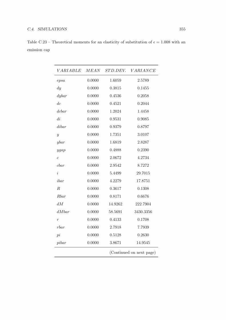
C.4. SIMULATIONS 355
Table C.23 – Theoretical moments for an elasticity of substitution of ε = 1.008 with an
emission cap
V ARIABLE MEAN STD.DEV. V ARIANCE
epsa 0.0000 1.6059 2.5789
dy 0.0000 0.3815 0.1455
dybar 0.0000 0.4536 0.2058
dc 0.0000 0.4521 0.2044
dcbar 0.0000 1.2024 1.4458
di 0.0000 0.9531 0.9085
dibar 0.0000 0.9379 0.8797
y 0.0000 1.7351 3.0107
ybar 0.0000 1.6819 2.8287
ygap 0.0000 0.4888 0.2390
c 0.0000 2.0672 4.2734
cbar 0.0000 2.9542 8.7272
i 0.0000 5.4499 29.7015
ibar 0.0000 4.2279 17.8751
R 0.0000 0.3617 0.1308
Rbar 0.0000 0.8171 0.6676
dM 0.0000 14.9262 222.7904
dMbar 0.0000 58.5691 3430.3356
r 0.0000 0.4133 0.1708
rbar 0.0000 2.7918 7.7939
pi 0.0000 0.5128 0.2630
pibar 0.0000 3.8671 14.9545
(Continued on next page)
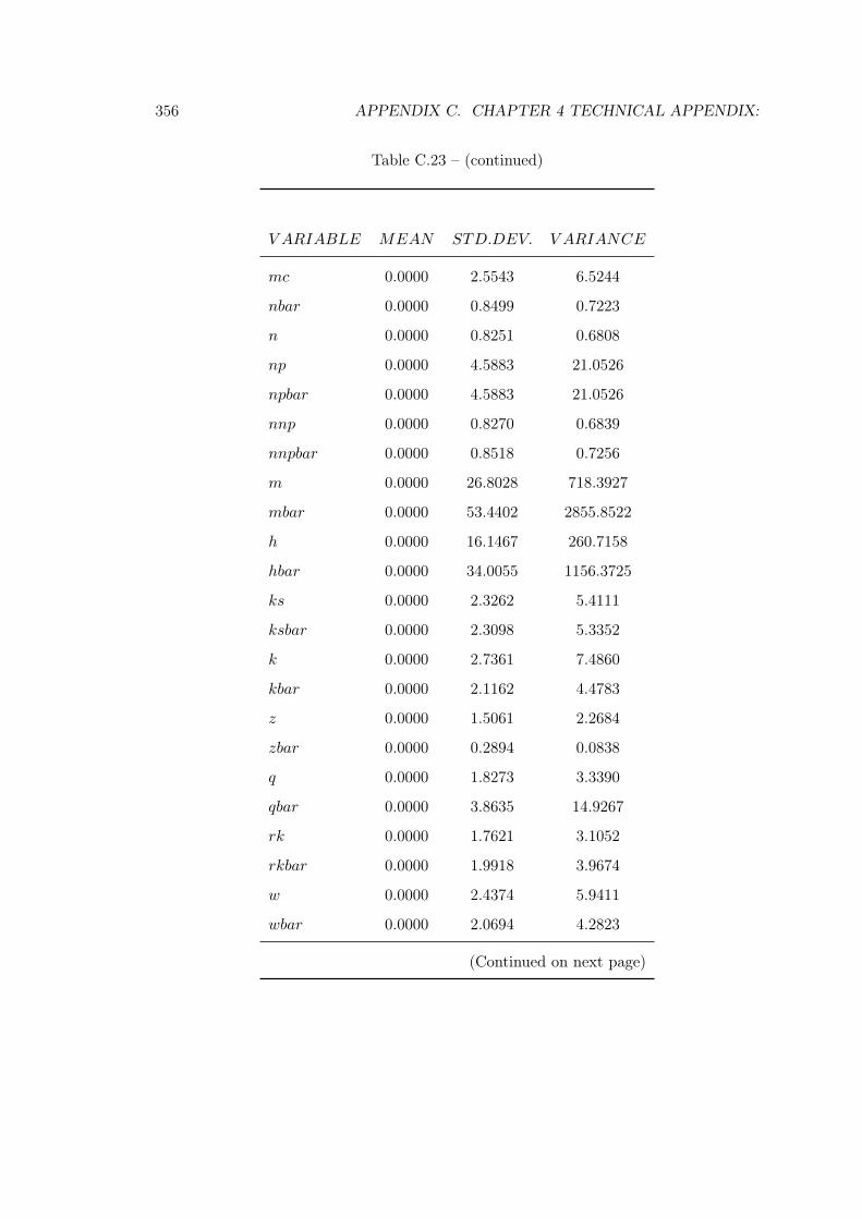
356 APPENDIX C. CHAPTER 4 TECHNICAL APPENDIX:
Table C.23 – (continued)
V ARIABLE MEAN STD.DEV. V ARIANCE
mc 0.0000 2.5543 6.5244
nbar 0.0000 0.8499 0.7223
n 0.0000 0.8251 0.6808
np 0.0000 4.5883 21.0526
npbar 0.0000 4.5883 21.0526
nnp 0.0000 0.8270 0.6839
nnpbar 0.0000 0.8518 0.7256
m 0.0000 26.8028 718.3927
mbar 0.0000 53.4402 2855.8522
h 0.0000 16.1467 260.7158
hbar 0.0000 34.0055 1156.3725
ks 0.0000 2.3262 5.4111
ksbar 0.0000 2.3098 5.3352
k 0.0000 2.7361 7.4860
kbar 0.0000 2.1162 4.4783
z 0.0000 1.5061 2.2684
zbar 0.0000 0.2894 0.0838
q 0.0000 1.8273 3.3390
qbar 0.0000 3.8635 14.9267
rk 0.0000 1.7621 3.1052
rkbar 0.0000 1.9918 3.9674
w 0.0000 2.4374 5.9411
wbar 0.0000 2.0694 4.2823
(Continued on next page)
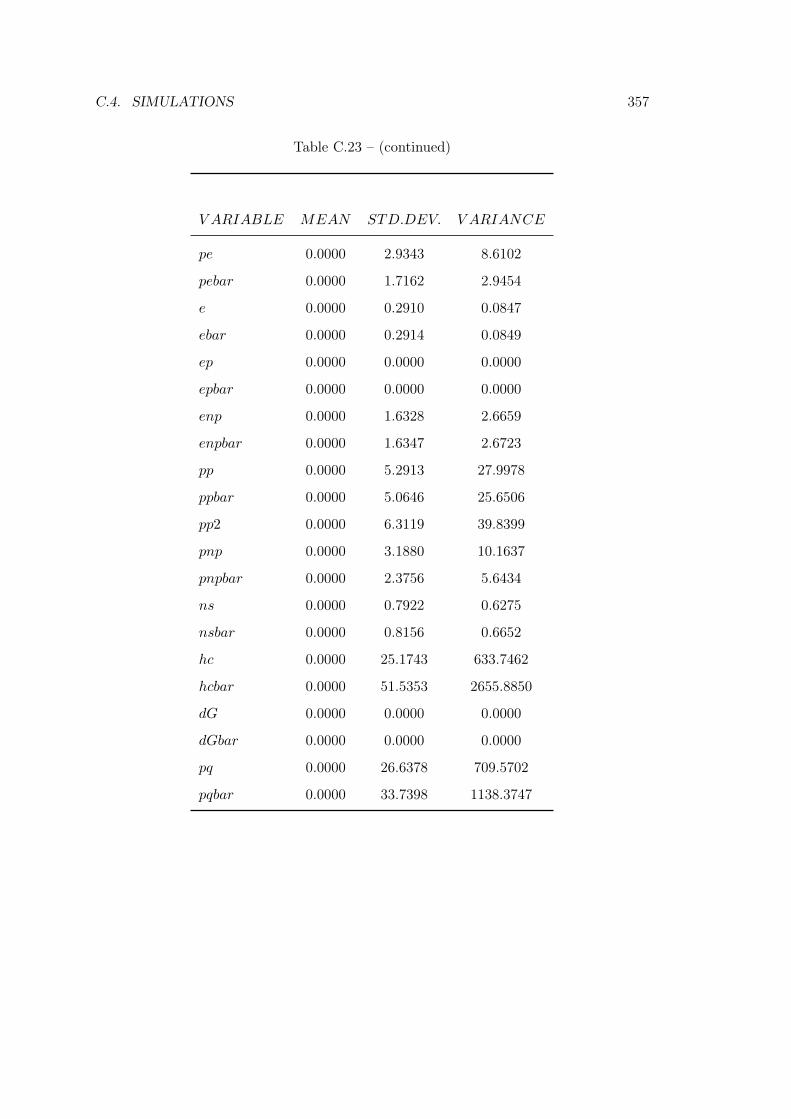
C.4. SIMULATIONS 357
Table C.23 – (continued)
V ARIABLE MEAN STD.DEV. V ARIANCE
pe 0.0000 2.9343 8.6102
pebar 0.0000 1.7162 2.9454
e 0.0000 0.2910 0.0847
ebar 0.0000 0.2914 0.0849
ep 0.0000 0.0000 0.0000
epbar 0.0000 0.0000 0.0000
enp 0.0000 1.6328 2.6659
enpbar 0.0000 1.6347 2.6723
pp 0.0000 5.2913 27.9978
ppbar 0.0000 5.0646 25.6506
pp2 0.0000 6.3119 39.8399
pnp 0.0000 3.1880 10.1637
pnpbar 0.0000 2.3756 5.6434
ns 0.0000 0.7922 0.6275
nsbar 0.0000 0.8156 0.6652
hc 0.0000 25.1743 633.7462
hcbar 0.0000 51.5353 2655.8850
dG 0.0000 0.0000 0.0000
dGbar 0.0000 0.0000 0.0000
pq 0.0000 26.6378 709.5702
pqbar 0.0000 33.7398 1138.3747
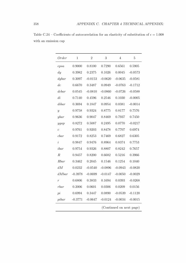
358 APPENDIX C. CHAPTER 4 TECHNICAL APPENDIX:
Table C.24 – Coefficients of autocorrelation for an elasticity of substitution of ε = 1.008
with an emission cap
Order 1 2 3 4 5
epsa 0.9000 0.8100 0.7290 0.6561 0.5905
dy 0.3982 0.2375 0.1026 0.0045 -0.0573
dybar 0.3097 -0.0153 -0.0620 -0.0635 -0.0581
dc 0.6670 0.3487 0.0949 -0.0763 -0.1712
dcbar 0.0545 -0.0810 -0.0860 -0.0726 -0.0588
di 0.7140 0.4596 0.2546 0.1030 -0.0005
dibar 0.3694 0.1847 0.0954 0.0381 -0.0014
y 0.9758 0.9324 0.8775 0.8177 0.7576
ybar 0.9636 0.9047 0.8469 0.7937 0.7450
ygap 0.8272 0.5087 0.2495 0.0770 -0.0217
c 0.9761 0.9203 0.8478 0.7707 0.6974
cbar 0.9172 0.8253 0.7469 0.6827 0.6305
i 0.9847 0.9476 0.8964 0.8374 0.7753
ibar 0.9754 0.9326 0.8807 0.8242 0.7657
R 0.9457 0.8200 0.6682 0.5216 0.3966
Rbar 0.3462 0.2045 0.1546 0.1254 0.1040
dM 0.0232 -0.0540 -0.0896 -0.0943 -0.0820
dMbar -0.3978 -0.0699 -0.0147 -0.0050 -0.0029
r 0.6806 0.3833 0.1694 0.0393 -0.0268
rbar 0.2006 0.0601 0.0306 0.0209 0.0156
pi 0.6994 0.3447 0.0890 -0.0539 -0.1120
pibar -0.3771 -0.0647 -0.0124 -0.0034 -0.0015
(Continued on next page)

C.4. SIMULATIONS 359
Table C.24 – (continued)
Order 1 2 3 4 5
mc 0.6021 0.3087 0.1178 0.0094 -0.0413
nbar 0.3165 0.1874 0.1538 0.1390 0.1295
n 0.7170 0.4696 0.2775 0.1437 0.0602
np 0.9000 0.8100 0.7290 0.6561 0.5905
npbar 0.9000 0.8100 0.7290 0.6561 0.5905
nnp 0.7170 0.4696 0.2775 0.1437 0.0602
nnpbar 0.3166 0.1874 0.1538 0.1390 0.1296
m 0.8412 0.6691 0.5121 0.3837 0.2867
mbar 0.3203 0.1821 0.1390 0.1158 0.0993
h 0.8125 0.6202 0.4512 0.3180 0.2212
hbar 0.2624 0.1222 0.0847 0.0674 0.0558
ks 0.8885 0.7932 0.7209 0.6705 0.6374
ksbar 0.9983 0.9942 0.9881 0.9803 0.9711
k 0.9990 0.9962 0.9916 0.9854 0.9776
kbar 0.9990 0.9962 0.9916 0.9854 0.9778
z 0.7425 0.5353 0.3903 0.3016 0.2560
zbar 0.9630 0.9010 0.8380 0.7780 0.7217
q 0.8570 0.6837 0.5159 0.3731 0.2620
qbar 0.3128 0.1695 0.1217 0.0942 0.0738
rk 0.7425 0.5353 0.3903 0.3016 0.2560
rkbar 0.9630 0.9010 0.8380 0.7780 0.7217
w 0.7290 0.5040 0.3413 0.2365 0.1767
wbar 0.8774 0.8141 0.7655 0.7233 0.6857
(Continued on next page)
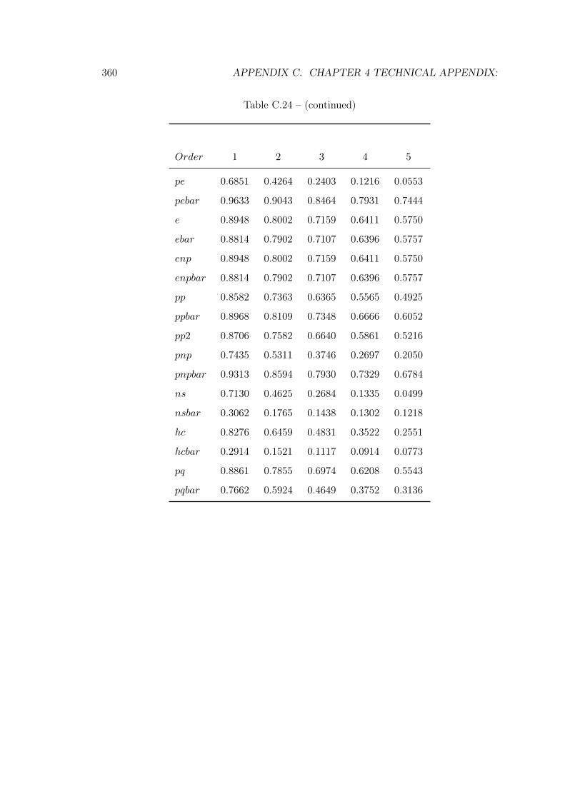
360 APPENDIX C. CHAPTER 4 TECHNICAL APPENDIX:
Table C.24 – (continued)
Order 1 2 3 4 5
pe 0.6851 0.4264 0.2403 0.1216 0.0553
pebar 0.9633 0.9043 0.8464 0.7931 0.7444
e 0.8948 0.8002 0.7159 0.6411 0.5750
ebar 0.8814 0.7902 0.7107 0.6396 0.5757
enp 0.8948 0.8002 0.7159 0.6411 0.5750
enpbar 0.8814 0.7902 0.7107 0.6396 0.5757
pp 0.8582 0.7363 0.6365 0.5565 0.4925
ppbar 0.8968 0.8109 0.7348 0.6666 0.6052
pp2 0.8706 0.7582 0.6640 0.5861 0.5216
pnp 0.7435 0.5311 0.3746 0.2697 0.2050
pnpbar 0.9313 0.8594 0.7930 0.7329 0.6784
ns 0.7130 0.4625 0.2684 0.1335 0.0499
nsbar 0.3062 0.1765 0.1438 0.1302 0.1218
hc 0.8276 0.6459 0.4831 0.3522 0.2551
hcbar 0.2914 0.1521 0.1117 0.0914 0.0773
pq 0.8861 0.7855 0.6974 0.6208 0.5543
pqbar 0.7662 0.5924 0.4649 0.3752 0.3136
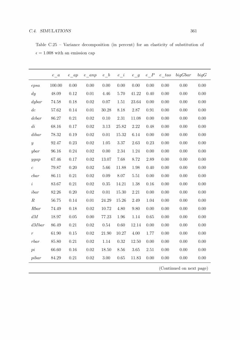
C.4. SIMULATIONS 361
Table C.25 – Variance decomposition (in percent) for an elasticity of substitution of
ε = 1.008 with an emission cap
e_a e_ap e_anp e_b e_i e_g e_P e_tao bigGbar bigG
epsa 100.00 0.00 0.00 0.00 0.00 0.00 0.00 0.00 0.00 0.00
dy 48.09 0.12 0.01 4.46 5.70 41.22 0.40 0.00 0.00 0.00
dybar 74.58 0.18 0.02 0.07 1.51 23.64 0.00 0.00 0.00 0.00
dc 57.62 0.14 0.01 30.28 8.18 2.87 0.91 0.00 0.00 0.00
dcbar 86.27 0.21 0.02 0.10 2.31 11.08 0.00 0.00 0.00 0.00
di 68.16 0.17 0.02 3.13 25.82 2.22 0.48 0.00 0.00 0.00
dibar 78.32 0.19 0.02 0.01 15.32 6.14 0.00 0.00 0.00 0.00
y 92.47 0.23 0.02 1.05 3.37 2.63 0.23 0.00 0.00 0.00
ybar 96.16 0.24 0.02 0.00 2.34 1.24 0.00 0.00 0.00 0.00
ygap 67.46 0.17 0.02 13.07 7.68 8.72 2.89 0.00 0.00 0.00
c 79.87 0.20 0.02 5.66 11.88 1.98 0.40 0.00 0.00 0.00
cbar 86.11 0.21 0.02 0.09 8.07 5.51 0.00 0.00 0.00 0.00
i 83.67 0.21 0.02 0.35 14.21 1.38 0.16 0.00 0.00 0.00
ibar 82.26 0.20 0.02 0.01 15.30 2.21 0.00 0.00 0.00 0.00
R 56.75 0.14 0.01 24.29 15.26 2.49 1.04 0.00 0.00 0.00
Rbar 74.49 0.18 0.02 10.72 4.80 9.80 0.00 0.00 0.00 0.00
dM 18.97 0.05 0.00 77.23 1.96 1.14 0.65 0.00 0.00 0.00
dMbar 86.49 0.21 0.02 0.54 0.60 12.14 0.00 0.00 0.00 0.00
r 61.90 0.15 0.02 21.90 10.27 4.00 1.77 0.00 0.00 0.00
rbar 85.80 0.21 0.02 1.14 0.32 12.50 0.00 0.00 0.00 0.00
pi 66.60 0.16 0.02 18.50 8.56 3.65 2.51 0.00 0.00 0.00
pibar 84.29 0.21 0.02 3.00 0.65 11.83 0.00 0.00 0.00 0.00
(Continued on next page)
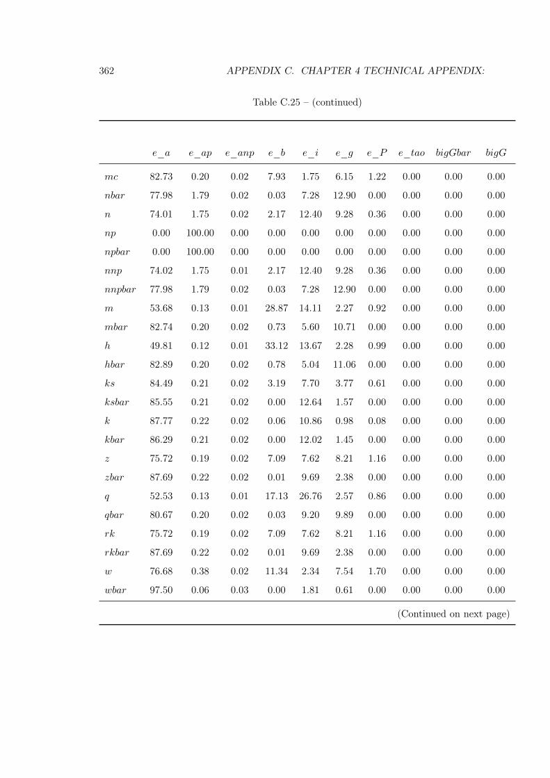
362 APPENDIX C. CHAPTER 4 TECHNICAL APPENDIX:
Table C.25 – (continued)
e_a e_ap e_anp e_b e_i e_g e_P e_tao bigGbar bigG
mc 82.73 0.20 0.02 7.93 1.75 6.15 1.22 0.00 0.00 0.00
nbar 77.98 1.79 0.02 0.03 7.28 12.90 0.00 0.00 0.00 0.00
n 74.01 1.75 0.02 2.17 12.40 9.28 0.36 0.00 0.00 0.00
np 0.00 100.00 0.00 0.00 0.00 0.00 0.00 0.00 0.00 0.00
npbar 0.00 100.00 0.00 0.00 0.00 0.00 0.00 0.00 0.00 0.00
nnp 74.02 1.75 0.01 2.17 12.40 9.28 0.36 0.00 0.00 0.00
nnpbar 77.98 1.79 0.02 0.03 7.28 12.90 0.00 0.00 0.00 0.00
m 53.68 0.13 0.01 28.87 14.11 2.27 0.92 0.00 0.00 0.00
mbar 82.74 0.20 0.02 0.73 5.60 10.71 0.00 0.00 0.00 0.00
h 49.81 0.12 0.01 33.12 13.67 2.28 0.99 0.00 0.00 0.00
hbar 82.89 0.20 0.02 0.78 5.04 11.06 0.00 0.00 0.00 0.00
ks 84.49 0.21 0.02 3.19 7.70 3.77 0.61 0.00 0.00 0.00
ksbar 85.55 0.21 0.02 0.00 12.64 1.57 0.00 0.00 0.00 0.00
k 87.77 0.22 0.02 0.06 10.86 0.98 0.08 0.00 0.00 0.00
kbar 86.29 0.21 0.02 0.00 12.02 1.45 0.00 0.00 0.00 0.00
z 75.72 0.19 0.02 7.09 7.62 8.21 1.16 0.00 0.00 0.00
zbar 87.69 0.22 0.02 0.01 9.69 2.38 0.00 0.00 0.00 0.00
q 52.53 0.13 0.01 17.13 26.76 2.57 0.86 0.00 0.00 0.00
qbar 80.67 0.20 0.02 0.03 9.20 9.89 0.00 0.00 0.00 0.00
rk 75.72 0.19 0.02 7.09 7.62 8.21 1.16 0.00 0.00 0.00
rkbar 87.69 0.22 0.02 0.01 9.69 2.38 0.00 0.00 0.00 0.00
w 76.68 0.38 0.02 11.34 2.34 7.54 1.70 0.00 0.00 0.00
wbar 97.50 0.06 0.03 0.00 1.81 0.61 0.00 0.00 0.00 0.00
(Continued on next page)

C.4. SIMULATIONS 363
Table C.25 – (continued)
e_a e_ap e_anp e_b e_i e_g e_P e_tao bigGbar bigG
pe 74.77 0.19 0.98 8.94 4.31 9.31 1.50 0.00 0.00 0.00
pebar 94.31 0.19 2.34 0.00 2.16 0.99 0.00 0.00 0.00 0.00
e 2.33 0.05 96.86 0.07 0.39 0.29 0.01 0.00 0.00 0.00
ebar 2.59 0.06 96.67 0.00 0.24 0.43 0.00 0.00 0.00 0.00
ep 0.00 0.00 0.00 0.00 0.00 0.00 0.00 0.00 0.00 100.00
epbar 0.00 0.00 0.00 0.00 0.00 0.00 0.00 0.00 100.00 0.00
enp 2.33 0.05 96.86 0.07 0.39 0.29 0.01 0.00 0.00 0.00
enpbar 2.59 0.06 96.67 0.00 0.24 0.43 0.00 0.00 0.00 0.00
pp 16.27 78.86 0.00 2.41 0.50 1.60 0.36 0.00 0.00 0.00
ppbar 16.28 83.31 0.00 0.00 0.30 0.10 0.00 0.00 0.00 0.00
pp2 11.43 55.42 0.00 1.69 0.35 1.12 0.25 29.72 0.00 0.00
pnp 56.77 0.16 25.12 7.26 2.80 6.71 1.18 0.00 0.00 0.00
pnpbar 54.92 0.04 43.82 0.00 1.03 0.19 0.00 0.00 0.00 0.00
ns 74.89 0.59 0.02 2.20 12.55 9.39 0.37 0.00 0.00 0.00
nsbar 78.97 0.54 0.02 0.03 7.37 13.06 0.00 0.00 0.00 0.00
hc 51.80 0.13 0.01 30.90 13.93 2.28 0.95 0.00 0.00 0.00
hcbar 82.80 0.20 0.02 0.75 5.33 10.89 0.00 0.00 0.00 0.00
dG 0.00 0.00 0.00 0.00 0.00 0.00 0.00 0.00 0.00 100.00
dGbar 0.00 0.00 0.00 0.00 0.00 0.00 0.00 0.00 100.00 0.00
pq 4.98 93.33 0.00 0.25 0.65 0.73 0.05 0.00 0.00 0.00
pqbar 34.86 56.38 0.01 2.86 1.64 3.77 0.49 0.00 0.00 0.00
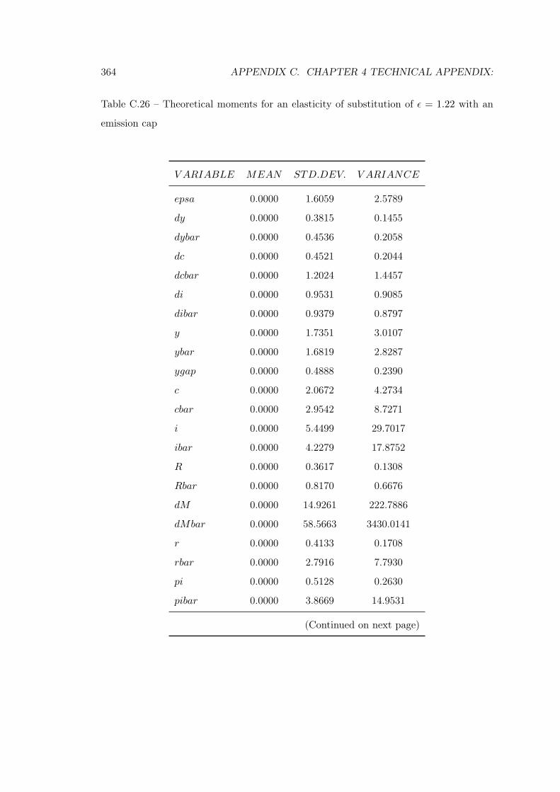
364 APPENDIX C. CHAPTER 4 TECHNICAL APPENDIX:
Table C.26 – Theoretical moments for an elasticity of substitution of ε = 1.22 with an
emission cap
V ARIABLE MEAN STD.DEV. V ARIANCE
epsa 0.0000 1.6059 2.5789
dy 0.0000 0.3815 0.1455
dybar 0.0000 0.4536 0.2058
dc 0.0000 0.4521 0.2044
dcbar 0.0000 1.2024 1.4457
di 0.0000 0.9531 0.9085
dibar 0.0000 0.9379 0.8797
y 0.0000 1.7351 3.0107
ybar 0.0000 1.6819 2.8287
ygap 0.0000 0.4888 0.2390
c 0.0000 2.0672 4.2734
cbar 0.0000 2.9542 8.7271
i 0.0000 5.4499 29.7017
ibar 0.0000 4.2279 17.8752
R 0.0000 0.3617 0.1308
Rbar 0.0000 0.8170 0.6676
dM 0.0000 14.9261 222.7886
dMbar 0.0000 58.5663 3430.0141
r 0.0000 0.4133 0.1708
rbar 0.0000 2.7916 7.7930
pi 0.0000 0.5128 0.2630
pibar 0.0000 3.8669 14.9531
(Continued on next page)

C.4. SIMULATIONS 365
Table C.26 – (continued)
V ARIABLE MEAN STD.DEV. V ARIANCE
mc 0.0000 2.5542 6.5241
nbar 0.0000 0.8496 0.7218
n 0.0000 0.8248 0.6803
np 0.0000 4.5883 21.0526
npbar 0.0000 4.5883 21.0526
nnp 0.0000 0.9028 0.8150
nnpbar 0.0000 0.9283 0.8617
m 0.0000 26.8027 718.3844
mbar 0.0000 53.4386 2855.6805
h 0.0000 16.1466 260.7127
hbar 0.0000 34.0044 1156.2987
ks 0.0000 2.3262 5.4110
ksbar 0.0000 2.3098 5.3352
k 0.0000 2.7361 7.4860
kbar 0.0000 2.1162 4.4783
z 0.0000 1.5061 2.2683
zbar 0.0000 0.2894 0.0838
q 0.0000 1.8273 3.3389
qbar 0.0000 3.8634 14.9259
rk 0.0000 1.7621 3.1051
rkbar 0.0000 1.9918 3.9674
w 0.0000 2.4376 5.9418
wbar 0.0000 2.0692 4.2815
(Continued on next page)
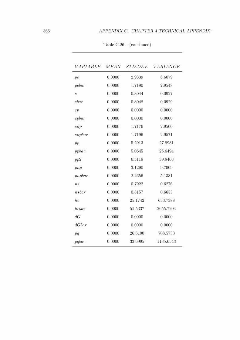
366 APPENDIX C. CHAPTER 4 TECHNICAL APPENDIX:
Table C.26 – (continued)
V ARIABLE MEAN STD.DEV. V ARIANCE
pe 0.0000 2.9339 8.6079
pebar 0.0000 1.7190 2.9548
e 0.0000 0.3044 0.0927
ebar 0.0000 0.3048 0.0929
ep 0.0000 0.0000 0.0000
epbar 0.0000 0.0000 0.0000
enp 0.0000 1.7176 2.9500
enpbar 0.0000 1.7196 2.9571
pp 0.0000 5.2913 27.9981
ppbar 0.0000 5.0645 25.6494
pp2 0.0000 6.3119 39.8403
pnp 0.0000 3.1290 9.7909
pnpbar 0.0000 2.2656 5.1331
ns 0.0000 0.7922 0.6276
nsbar 0.0000 0.8157 0.6653
hc 0.0000 25.1742 633.7388
hcbar 0.0000 51.5337 2655.7204
dG 0.0000 0.0000 0.0000
dGbar 0.0000 0.0000 0.0000
pq 0.0000 26.6190 708.5733
pqbar 0.0000 33.6995 1135.6543
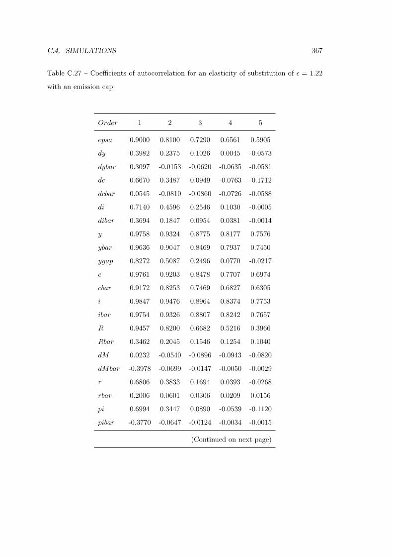
C.4. SIMULATIONS 367
Table C.27 – Coefficients of autocorrelation for an elasticity of substitution of ε = 1.22
with an emission cap
Order 1 2 3 4 5
epsa 0.9000 0.8100 0.7290 0.6561 0.5905
dy 0.3982 0.2375 0.1026 0.0045 -0.0573
dybar 0.3097 -0.0153 -0.0620 -0.0635 -0.0581
dc 0.6670 0.3487 0.0949 -0.0763 -0.1712
dcbar 0.0545 -0.0810 -0.0860 -0.0726 -0.0588
di 0.7140 0.4596 0.2546 0.1030 -0.0005
dibar 0.3694 0.1847 0.0954 0.0381 -0.0014
y 0.9758 0.9324 0.8775 0.8177 0.7576
ybar 0.9636 0.9047 0.8469 0.7937 0.7450
ygap 0.8272 0.5087 0.2496 0.0770 -0.0217
c 0.9761 0.9203 0.8478 0.7707 0.6974
cbar 0.9172 0.8253 0.7469 0.6827 0.6305
i 0.9847 0.9476 0.8964 0.8374 0.7753
ibar 0.9754 0.9326 0.8807 0.8242 0.7657
R 0.9457 0.8200 0.6682 0.5216 0.3966
Rbar 0.3462 0.2045 0.1546 0.1254 0.1040
dM 0.0232 -0.0540 -0.0896 -0.0943 -0.0820
dMbar -0.3978 -0.0699 -0.0147 -0.0050 -0.0029
r 0.6806 0.3833 0.1694 0.0393 -0.0268
rbar 0.2006 0.0601 0.0306 0.0209 0.0156
pi 0.6994 0.3447 0.0890 -0.0539 -0.1120
pibar -0.3770 -0.0647 -0.0124 -0.0034 -0.0015
(Continued on next page)
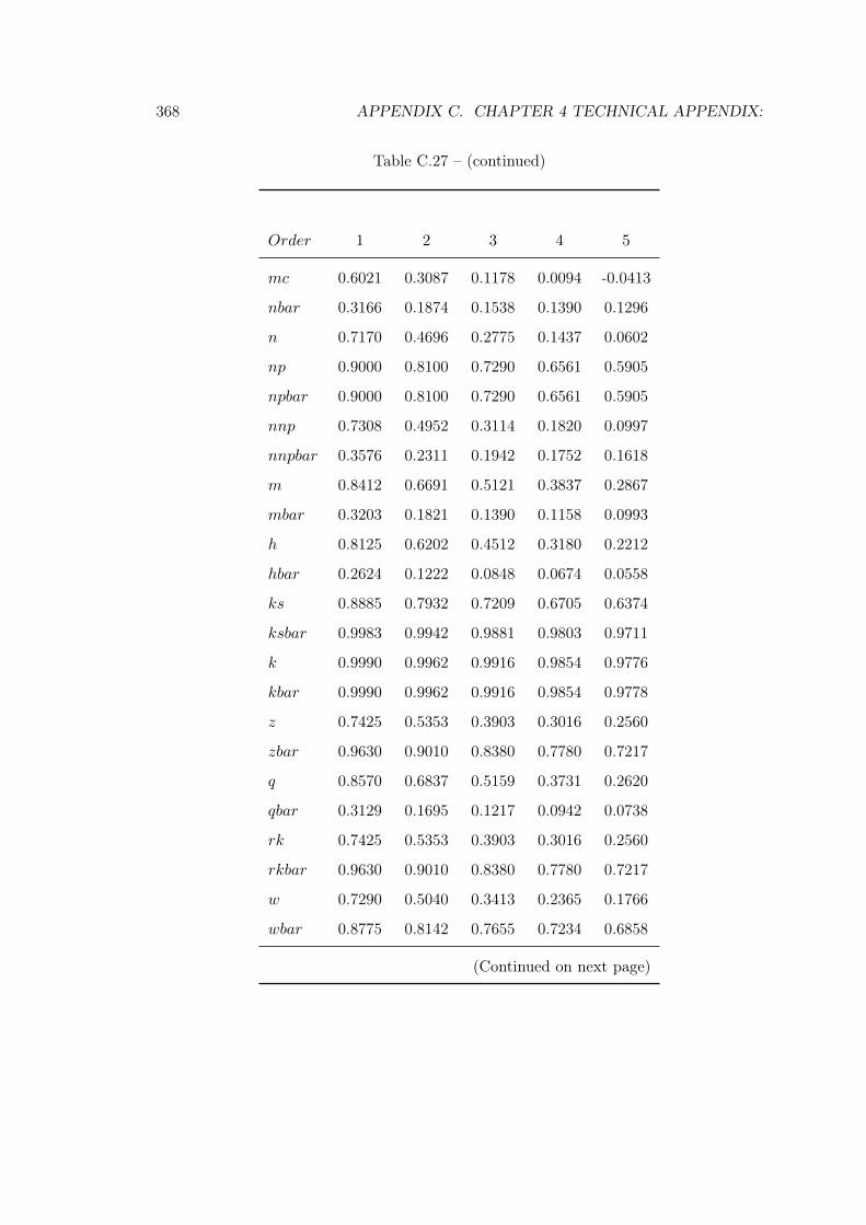
368 APPENDIX C. CHAPTER 4 TECHNICAL APPENDIX:
Table C.27 – (continued)
Order 1 2 3 4 5
mc 0.6021 0.3087 0.1178 0.0094 -0.0413
nbar 0.3166 0.1874 0.1538 0.1390 0.1296
n 0.7170 0.4696 0.2775 0.1437 0.0602
np 0.9000 0.8100 0.7290 0.6561 0.5905
npbar 0.9000 0.8100 0.7290 0.6561 0.5905
nnp 0.7308 0.4952 0.3114 0.1820 0.0997
nnpbar 0.3576 0.2311 0.1942 0.1752 0.1618
m 0.8412 0.6691 0.5121 0.3837 0.2867
mbar 0.3203 0.1821 0.1390 0.1158 0.0993
h 0.8125 0.6202 0.4512 0.3180 0.2212
hbar 0.2624 0.1222 0.0848 0.0674 0.0558
ks 0.8885 0.7932 0.7209 0.6705 0.6374
ksbar 0.9983 0.9942 0.9881 0.9803 0.9711
k 0.9990 0.9962 0.9916 0.9854 0.9776
kbar 0.9990 0.9962 0.9916 0.9854 0.9778
z 0.7425 0.5353 0.3903 0.3016 0.2560
zbar 0.9630 0.9010 0.8380 0.7780 0.7217
q 0.8570 0.6837 0.5159 0.3731 0.2620
qbar 0.3129 0.1695 0.1217 0.0942 0.0738
rk 0.7425 0.5353 0.3903 0.3016 0.2560
rkbar 0.9630 0.9010 0.8380 0.7780 0.7217
w 0.7290 0.5040 0.3413 0.2365 0.1766
wbar 0.8775 0.8142 0.7655 0.7234 0.6858
(Continued on next page)
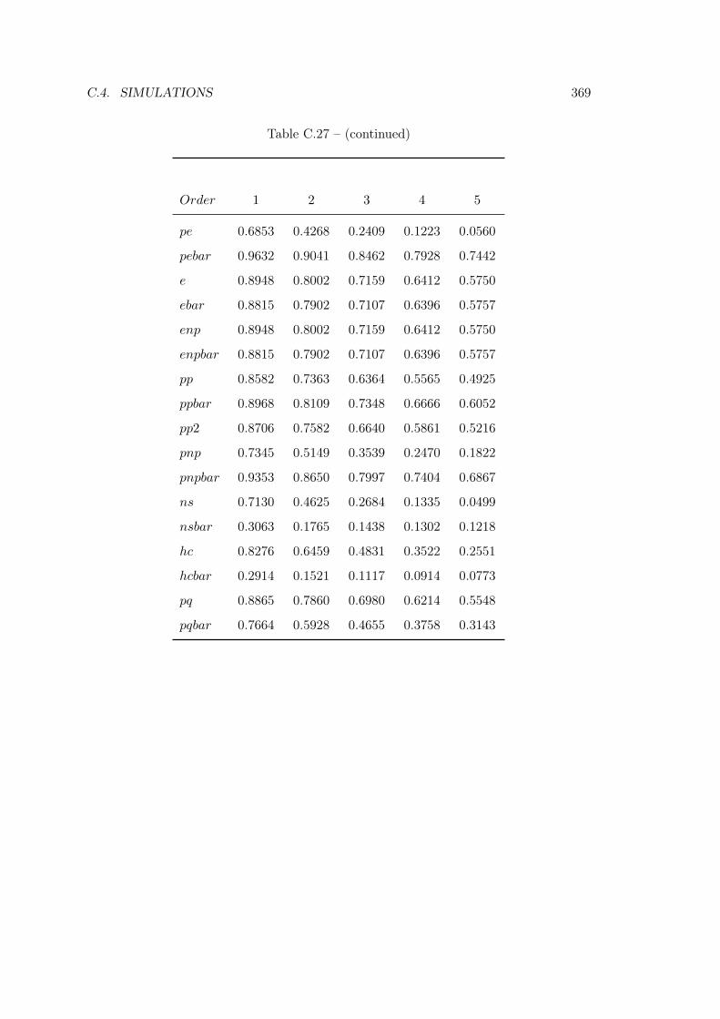
C.4. SIMULATIONS 369
Table C.27 – (continued)
Order 1 2 3 4 5
pe 0.6853 0.4268 0.2409 0.1223 0.0560
pebar 0.9632 0.9041 0.8462 0.7928 0.7442
e 0.8948 0.8002 0.7159 0.6412 0.5750
ebar 0.8815 0.7902 0.7107 0.6396 0.5757
enp 0.8948 0.8002 0.7159 0.6412 0.5750
enpbar 0.8815 0.7902 0.7107 0.6396 0.5757
pp 0.8582 0.7363 0.6364 0.5565 0.4925
ppbar 0.8968 0.8109 0.7348 0.6666 0.6052
pp2 0.8706 0.7582 0.6640 0.5861 0.5216
pnp 0.7345 0.5149 0.3539 0.2470 0.1822
pnpbar 0.9353 0.8650 0.7997 0.7404 0.6867
ns 0.7130 0.4625 0.2684 0.1335 0.0499
nsbar 0.3063 0.1765 0.1438 0.1302 0.1218
hc 0.8276 0.6459 0.4831 0.3522 0.2551
hcbar 0.2914 0.1521 0.1117 0.0914 0.0773
pq 0.8865 0.7860 0.6980 0.6214 0.5548
pqbar 0.7664 0.5928 0.4655 0.3758 0.3143

370 APPENDIX C. CHAPTER 4 TECHNICAL APPENDIX:
Table C.28 – Variance decomposition (in percent) for an elasticity of substitution of
ε = 1.22 with an emission cap
e_a e_ap e_anp e_b e_i e_g e_P e_tao bigGbar bigG
epsa 100.00 0.00 0.00 0.00 0.00 0.00 0.00 0.00 0.00 0.00
dy 48.09 0.12 0.01 4.46 5.70 41.22 0.40 0.00 0.00 0.00
dybar 74.58 0.18 0.02 0.07 1.51 23.64 0.00 0.00 0.00 0.00
dc 57.62 0.14 0.01 30.28 8.18 2.87 0.91 0.00 0.00 0.00
dcbar 86.27 0.21 0.02 0.10 2.31 11.08 0.00 0.00 0.00 0.00
di 68.16 0.17 0.02 3.13 25.82 2.22 0.48 0.00 0.00 0.00
dibar 78.32 0.19 0.02 0.01 15.32 6.14 0.00 0.00 0.00 0.00
y 92.47 0.23 0.02 1.05 3.37 2.63 0.23 0.00 0.00 0.00
ybar 96.16 0.24 0.03 0.00 2.34 1.24 0.00 0.00 0.00 0.00
ygap 67.46 0.17 0.02 13.07 7.68 8.72 2.89 0.00 0.00 0.00
c 79.87 0.20 0.02 5.66 11.88 1.98 0.40 0.00 0.00 0.00
cbar 86.11 0.21 0.02 0.09 8.07 5.51 0.00 0.00 0.00 0.00
i 83.67 0.21 0.02 0.35 14.21 1.38 0.16 0.00 0.00 0.00
ibar 82.26 0.20 0.02 0.01 15.30 2.21 0.00 0.00 0.00 0.00
R 56.75 0.14 0.01 24.29 15.26 2.49 1.04 0.00 0.00 0.00
Rbar 74.49 0.18 0.02 10.72 4.80 9.80 0.00 0.00 0.00 0.00
dM 18.97 0.05 0.00 77.23 1.96 1.14 0.65 0.00 0.00 0.00
dMbar 86.48 0.21 0.02 0.54 0.60 12.14 0.00 0.00 0.00 0.00
r 61.89 0.15 0.02 21.90 10.27 4.00 1.77 0.00 0.00 0.00
rbar 85.80 0.21 0.02 1.14 0.32 12.50 0.00 0.00 0.00 0.00
pi 66.60 0.16 0.02 18.50 8.56 3.65 2.51 0.00 0.00 0.00
pibar 84.29 0.21 0.02 3.00 0.65 11.83 0.00 0.00 0.00 0.00
(Continued on next page)
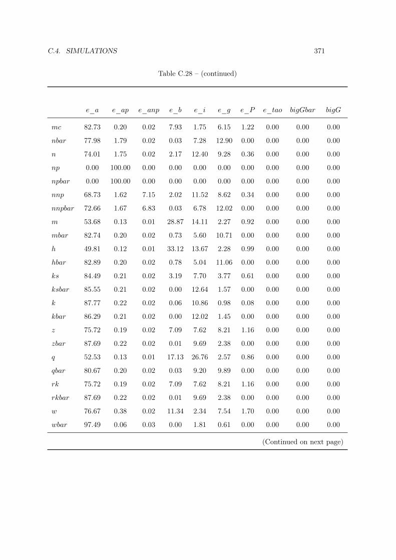
C.4. SIMULATIONS 371
Table C.28 – (continued)
e_a e_ap e_anp e_b e_i e_g e_P e_tao bigGbar bigG
mc 82.73 0.20 0.02 7.93 1.75 6.15 1.22 0.00 0.00 0.00
nbar 77.98 1.79 0.02 0.03 7.28 12.90 0.00 0.00 0.00 0.00
n 74.01 1.75 0.02 2.17 12.40 9.28 0.36 0.00 0.00 0.00
np 0.00 100.00 0.00 0.00 0.00 0.00 0.00 0.00 0.00 0.00
npbar 0.00 100.00 0.00 0.00 0.00 0.00 0.00 0.00 0.00 0.00
nnp 68.73 1.62 7.15 2.02 11.52 8.62 0.34 0.00 0.00 0.00
nnpbar 72.66 1.67 6.83 0.03 6.78 12.02 0.00 0.00 0.00 0.00
m 53.68 0.13 0.01 28.87 14.11 2.27 0.92 0.00 0.00 0.00
mbar 82.74 0.20 0.02 0.73 5.60 10.71 0.00 0.00 0.00 0.00
h 49.81 0.12 0.01 33.12 13.67 2.28 0.99 0.00 0.00 0.00
hbar 82.89 0.20 0.02 0.78 5.04 11.06 0.00 0.00 0.00 0.00
ks 84.49 0.21 0.02 3.19 7.70 3.77 0.61 0.00 0.00 0.00
ksbar 85.55 0.21 0.02 0.00 12.64 1.57 0.00 0.00 0.00 0.00
k 87.77 0.22 0.02 0.06 10.86 0.98 0.08 0.00 0.00 0.00
kbar 86.29 0.21 0.02 0.00 12.02 1.45 0.00 0.00 0.00 0.00
z 75.72 0.19 0.02 7.09 7.62 8.21 1.16 0.00 0.00 0.00
zbar 87.69 0.22 0.02 0.01 9.69 2.38 0.00 0.00 0.00 0.00
q 52.53 0.13 0.01 17.13 26.76 2.57 0.86 0.00 0.00 0.00
qbar 80.67 0.20 0.02 0.03 9.20 9.89 0.00 0.00 0.00 0.00
rk 75.72 0.19 0.02 7.09 7.62 8.21 1.16 0.00 0.00 0.00
rkbar 87.69 0.22 0.02 0.01 9.69 2.38 0.00 0.00 0.00 0.00
w 76.67 0.38 0.02 11.34 2.34 7.54 1.70 0.00 0.00 0.00
wbar 97.49 0.06 0.03 0.00 1.81 0.61 0.00 0.00 0.00 0.00
(Continued on next page)
372 APPENDIX C. CHAPTER 4 TECHNICAL APPENDIX:
Table C.28 – (continued)
e_a e_ap e_anp e_b e_i e_g e_P e_tao bigGbar bigG
pe 74.70 0.19 1.07 8.94 4.30 9.30 1.50 0.00 0.00 0.00
pebar 94.11 0.19 2.57 0.00 2.15 0.98 0.00 0.00 0.00 0.00
e 2.33 0.05 96.86 0.07 0.39 0.29 0.01 0.00 0.00 0.00
ebar 2.59 0.06 96.67 0.00 0.24 0.43 0.00 0.00 0.00 0.00
ep 0.00 0.00 0.00 0.00 0.00 0.00 0.00 0.00 0.00 100.00
epbar 0.00 0.00 0.00 0.00 0.00 0.00 0.00 0.00 100.00 0.00
enp 2.33 0.05 96.86 0.07 0.39 0.29 0.01 0.00 0.00 0.00
enpbar 2.59 0.06 96.67 0.00 0.24 0.43 0.00 0.00 0.00 0.00
pp 16.27 78.86 0.00 2.41 0.50 1.60 0.36 0.00 0.00 0.00
ppbar 16.27 83.32 0.00 0.00 0.30 0.10 0.00 0.00 0.00 0.00
pp2 11.44 55.42 0.00 1.69 0.35 1.12 0.25 29.72 0.00 0.00
pnp 59.70 0.16 21.22 7.57 3.00 7.11 1.24 0.00 0.00 0.00
pnpbar 59.53 0.05 39.04 0.00 1.14 0.24 0.00 0.00 0.00 0.00
ns 74.89 0.59 0.02 2.20 12.55 9.39 0.37 0.00 0.00 0.00
nsbar 78.97 0.54 0.02 0.03 7.37 13.06 0.00 0.00 0.00 0.00
hc 51.80 0.13 0.01 30.90 13.93 2.28 0.95 0.00 0.00 0.00
hcbar 82.80 0.20 0.02 0.75 5.33 10.89 0.00 0.00 0.00 0.00
dG 0.00 0.00 0.00 0.00 0.00 0.00 0.00 0.00 0.00 100.00
dGbar 0.00 0.00 0.00 0.00 0.00 0.00 0.00 0.00 100.00 0.00
pq 4.90 93.41 0.02 0.25 0.64 0.72 0.05 0.00 0.00 0.00
pqbar 34.76 56.48 0.03 2.87 1.62 3.76 0.48 0.00 0.00 0.00

C.4. SIMULATIONS 373
Table C.29 – Theoretical moments for an elasticity of substitution of ε = 1.85 with an
emission cap
V ARIABLE MEAN STD.DEV. V ARIANCE
epsa 0.0000 1.6059 2.5789
dy 0.0000 0.3815 0.1455
dybar 0.0000 0.4536 0.2058
dc 0.0000 0.4521 0.2044
dcbar 0.0000 1.2025 1.4461
di 0.0000 0.9531 0.9085
dibar 0.0000 0.9379 0.8797
y 0.0000 1.7351 3.0107
ybar 0.0000 1.6819 2.8288
ygap 0.0000 0.4889 0.2390
c 0.0000 2.0673 4.2736
cbar 0.0000 2.9543 8.7277
i 0.0000 5.4499 29.7012
ibar 0.0000 4.2279 17.8748
R 0.0000 0.3617 0.1308
Rbar 0.0000 0.8171 0.6677
dM 0.0000 14.9263 222.7952
dMbar 0.0000 58.5767 3431.2293
r 0.0000 0.4133 0.1708
rbar 0.0000 2.7922 7.7964
pi 0.0000 0.5128 0.2630
pibar 0.0000 3.8676 14.9583
(Continued on next page)
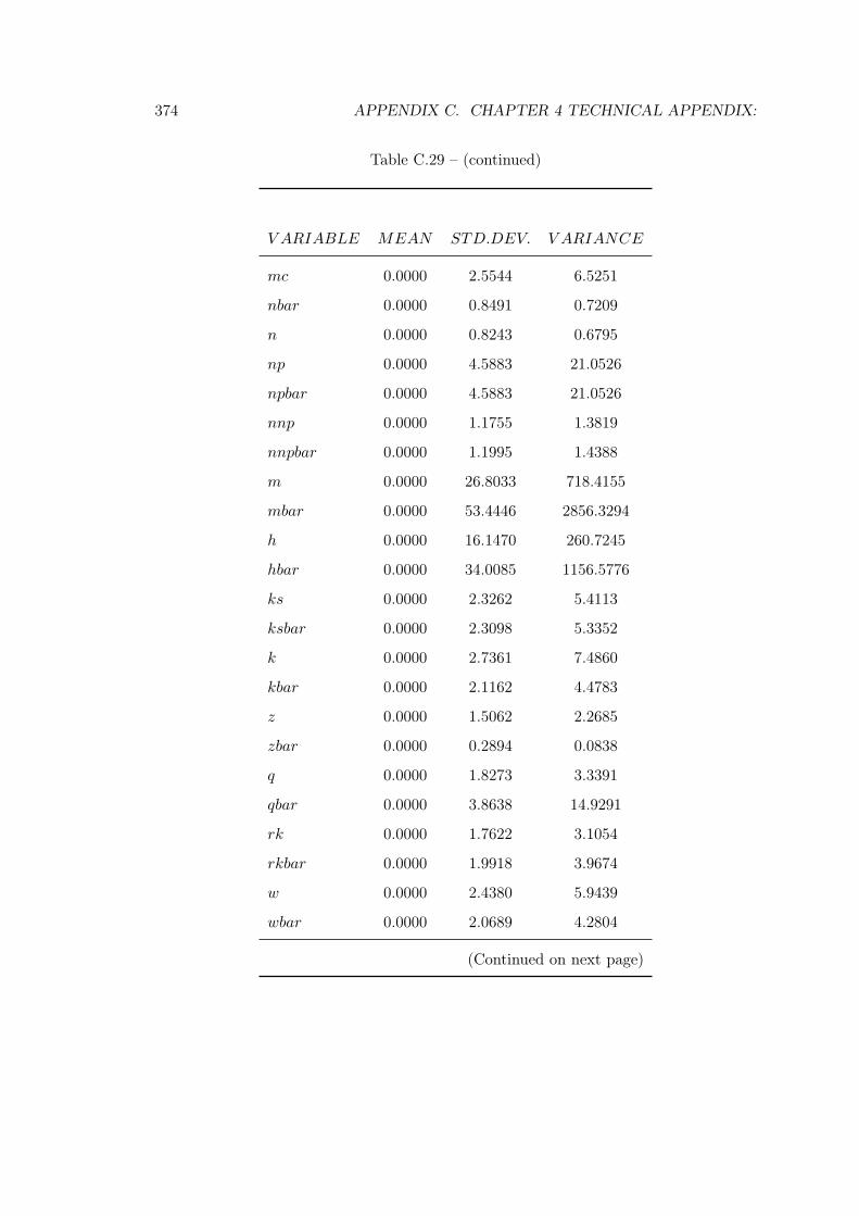
374 APPENDIX C. CHAPTER 4 TECHNICAL APPENDIX:
Table C.29 – (continued)
V ARIABLE MEAN STD.DEV. V ARIANCE
mc 0.0000 2.5544 6.5251
nbar 0.0000 0.8491 0.7209
n 0.0000 0.8243 0.6795
np 0.0000 4.5883 21.0526
npbar 0.0000 4.5883 21.0526
nnp 0.0000 1.1755 1.3819
nnpbar 0.0000 1.1995 1.4388
m 0.0000 26.8033 718.4155
mbar 0.0000 53.4446 2856.3294
h 0.0000 16.1470 260.7245
hbar 0.0000 34.0085 1156.5776
ks 0.0000 2.3262 5.4113
ksbar 0.0000 2.3098 5.3352
k 0.0000 2.7361 7.4860
kbar 0.0000 2.1162 4.4783
z 0.0000 1.5062 2.2685
zbar 0.0000 0.2894 0.0838
q 0.0000 1.8273 3.3391
qbar 0.0000 3.8638 14.9291
rk 0.0000 1.7622 3.1054
rkbar 0.0000 1.9918 3.9674
w 0.0000 2.4380 5.9439
wbar 0.0000 2.0689 4.2804
(Continued on next page)

C.4. SIMULATIONS 375
Table C.29 – (continued)
V ARIABLE MEAN STD.DEV. V ARIANCE
pe 0.0000 2.9337 8.6068
pebar 0.0000 1.7227 2.9678
e 0.0000 0.3216 0.1034
ebar 0.0000 0.3220 0.1037
ep 0.0000 0.0000 0.0000
epbar 0.0000 0.0000 0.0000
enp 0.0000 1.8775 3.5250
enpbar 0.0000 1.8797 3.5334
pp 0.0000 5.2915 27.9996
ppbar 0.0000 5.0644 25.6477
pp2 0.0000 6.3120 39.8417
pnp 0.0000 3.0377 9.2275
pnpbar 0.0000 2.0764 4.3114
ns 0.0000 0.7924 0.6279
nsbar 0.0000 0.8159 0.6657
hc 0.0000 25.1747 633.7668
hcbar 0.0000 51.5397 2656.3425
dG 0.0000 0.0000 0.0000
dGbar 0.0000 0.0000 0.0000
pq 0.0000 26.5975 707.4290
pqbar 0.0000 33.6385 1131.5513

376 APPENDIX C. CHAPTER 4 TECHNICAL APPENDIX:
Table C.30 – Coefficients of autocorrelation for an elasticity of substitution of ε = 1.85
with an emission cap
Order 1 2 3 4 5
epsa 0.9000 0.8100 0.7290 0.6561 0.5905
dy 0.3982 0.2375 0.1026 0.0045 -0.0573
dybar 0.3097 -0.0153 -0.0620 -0.0635 -0.0581
dc 0.6670 0.3487 0.0949 -0.0763 -0.1712
dcbar 0.0544 -0.0810 -0.0860 -0.0726 -0.0588
di 0.7140 0.4596 0.2546 0.1030 -0.0005
dibar 0.3694 0.1847 0.0954 0.0381 -0.0014
y 0.9758 0.9324 0.8775 0.8177 0.7576
ybar 0.9636 0.9047 0.8469 0.7937 0.7450
ygap 0.8272 0.5087 0.2495 0.0770 -0.0217
c 0.9761 0.9203 0.8478 0.7707 0.6974
cbar 0.9172 0.8253 0.7468 0.6827 0.6305
i 0.9847 0.9476 0.8964 0.8374 0.7753
ibar 0.9754 0.9326 0.8807 0.8242 0.7657
R 0.9457 0.8200 0.6681 0.5216 0.3966
Rbar 0.3461 0.2045 0.1546 0.1254 0.1040
dM 0.0233 -0.0540 -0.0896 -0.0943 -0.0821
dMbar -0.3979 -0.0698 -0.0147 -0.0050 -0.0029
r 0.6806 0.3833 0.1694 0.0393 -0.0268
rbar 0.2005 0.0601 0.0306 0.0209 0.0156
pi 0.6994 0.3447 0.0890 -0.0539 -0.1120
pibar -0.3771 -0.0647 -0.0124 -0.0034 -0.0015
(Continued on next page)
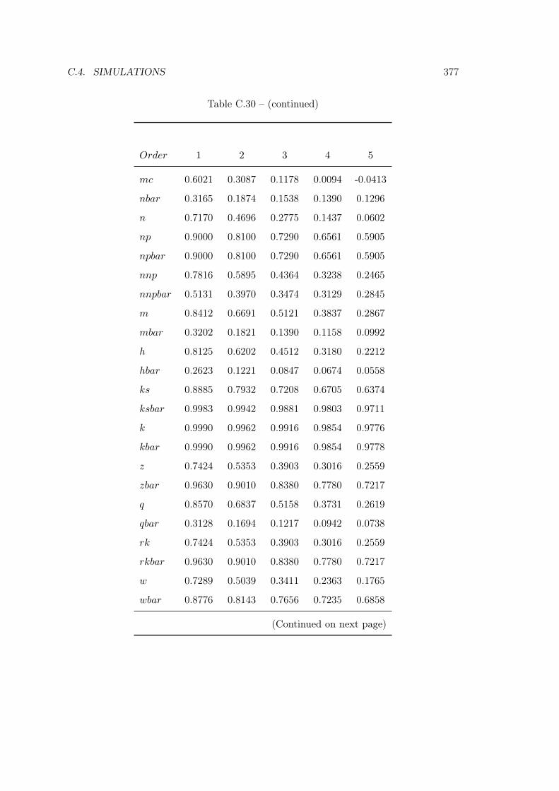
C.4. SIMULATIONS 377
Table C.30 – (continued)
Order 1 2 3 4 5
mc 0.6021 0.3087 0.1178 0.0094 -0.0413
nbar 0.3165 0.1874 0.1538 0.1390 0.1296
n 0.7170 0.4696 0.2775 0.1437 0.0602
np 0.9000 0.8100 0.7290 0.6561 0.5905
npbar 0.9000 0.8100 0.7290 0.6561 0.5905
nnp 0.7816 0.5895 0.4364 0.3238 0.2465
nnpbar 0.5131 0.3970 0.3474 0.3129 0.2845
m 0.8412 0.6691 0.5121 0.3837 0.2867
mbar 0.3202 0.1821 0.1390 0.1158 0.0992
h 0.8125 0.6202 0.4512 0.3180 0.2212
hbar 0.2623 0.1221 0.0847 0.0674 0.0558
ks 0.8885 0.7932 0.7208 0.6705 0.6374
ksbar 0.9983 0.9942 0.9881 0.9803 0.9711
k 0.9990 0.9962 0.9916 0.9854 0.9776
kbar 0.9990 0.9962 0.9916 0.9854 0.9778
z 0.7424 0.5353 0.3903 0.3016 0.2559
zbar 0.9630 0.9010 0.8380 0.7780 0.7217
q 0.8570 0.6837 0.5158 0.3731 0.2619
qbar 0.3128 0.1694 0.1217 0.0942 0.0738
rk 0.7424 0.5353 0.3903 0.3016 0.2559
rkbar 0.9630 0.9010 0.8380 0.7780 0.7217
w 0.7289 0.5039 0.3411 0.2363 0.1765
wbar 0.8776 0.8143 0.7656 0.7235 0.6858
(Continued on next page)
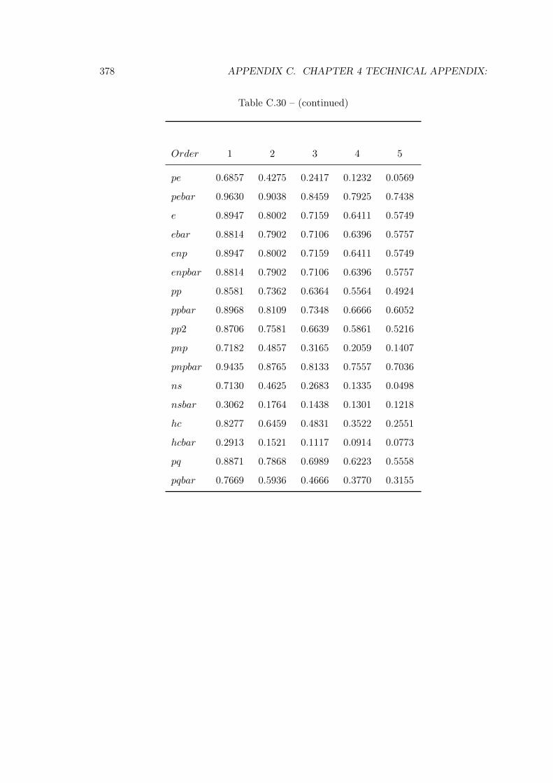
378 APPENDIX C. CHAPTER 4 TECHNICAL APPENDIX:
Table C.30 – (continued)
Order 1 2 3 4 5
pe 0.6857 0.4275 0.2417 0.1232 0.0569
pebar 0.9630 0.9038 0.8459 0.7925 0.7438
e 0.8947 0.8002 0.7159 0.6411 0.5749
ebar 0.8814 0.7902 0.7106 0.6396 0.5757
enp 0.8947 0.8002 0.7159 0.6411 0.5749
enpbar 0.8814 0.7902 0.7106 0.6396 0.5757
pp 0.8581 0.7362 0.6364 0.5564 0.4924
ppbar 0.8968 0.8109 0.7348 0.6666 0.6052
pp2 0.8706 0.7581 0.6639 0.5861 0.5216
pnp 0.7182 0.4857 0.3165 0.2059 0.1407
pnpbar 0.9435 0.8765 0.8133 0.7557 0.7036
ns 0.7130 0.4625 0.2683 0.1335 0.0498
nsbar 0.3062 0.1764 0.1438 0.1301 0.1218
hc 0.8277 0.6459 0.4831 0.3522 0.2551
hcbar 0.2913 0.1521 0.1117 0.0914 0.0773
pq 0.8871 0.7868 0.6989 0.6223 0.5558
pqbar 0.7669 0.5936 0.4666 0.3770 0.3155
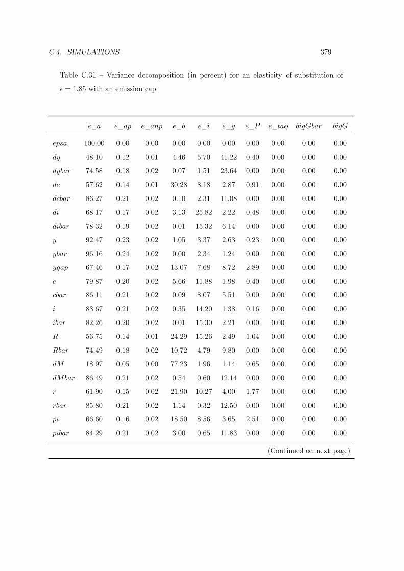
C.4. SIMULATIONS 379
Table C.31 – Variance decomposition (in percent) for an elasticity of substitution of
ε = 1.85 with an emission cap
e_a e_ap e_anp e_b e_i e_g e_P e_tao bigGbar bigG
epsa 100.00 0.00 0.00 0.00 0.00 0.00 0.00 0.00 0.00 0.00
dy 48.10 0.12 0.01 4.46 5.70 41.22 0.40 0.00 0.00 0.00
dybar 74.58 0.18 0.02 0.07 1.51 23.64 0.00 0.00 0.00 0.00
dc 57.62 0.14 0.01 30.28 8.18 2.87 0.91 0.00 0.00 0.00
dcbar 86.27 0.21 0.02 0.10 2.31 11.08 0.00 0.00 0.00 0.00
di 68.17 0.17 0.02 3.13 25.82 2.22 0.48 0.00 0.00 0.00
dibar 78.32 0.19 0.02 0.01 15.32 6.14 0.00 0.00 0.00 0.00
y 92.47 0.23 0.02 1.05 3.37 2.63 0.23 0.00 0.00 0.00
ybar 96.16 0.24 0.02 0.00 2.34 1.24 0.00 0.00 0.00 0.00
ygap 67.46 0.17 0.02 13.07 7.68 8.72 2.89 0.00 0.00 0.00
c 79.87 0.20 0.02 5.66 11.88 1.98 0.40 0.00 0.00 0.00
cbar 86.11 0.21 0.02 0.09 8.07 5.51 0.00 0.00 0.00 0.00
i 83.67 0.21 0.02 0.35 14.20 1.38 0.16 0.00 0.00 0.00
ibar 82.26 0.20 0.02 0.01 15.30 2.21 0.00 0.00 0.00 0.00
R 56.75 0.14 0.01 24.29 15.26 2.49 1.04 0.00 0.00 0.00
Rbar 74.49 0.18 0.02 10.72 4.79 9.80 0.00 0.00 0.00 0.00
dM 18.97 0.05 0.00 77.23 1.96 1.14 0.65 0.00 0.00 0.00
dMbar 86.49 0.21 0.02 0.54 0.60 12.14 0.00 0.00 0.00 0.00
r 61.90 0.15 0.02 21.90 10.27 4.00 1.77 0.00 0.00 0.00
rbar 85.80 0.21 0.02 1.14 0.32 12.50 0.00 0.00 0.00 0.00
pi 66.60 0.16 0.02 18.50 8.56 3.65 2.51 0.00 0.00 0.00
pibar 84.29 0.21 0.02 3.00 0.65 11.83 0.00 0.00 0.00 0.00
(Continued on next page)

380 APPENDIX C. CHAPTER 4 TECHNICAL APPENDIX:
Table C.31 – (continued)
e_a e_ap e_anp e_b e_i e_g e_P e_tao bigGbar bigG
mc 82.73 0.20 0.02 7.93 1.75 6.15 1.22 0.00 0.00 0.00
nbar 77.97 1.79 0.03 0.03 7.28 12.90 0.00 0.00 0.00 0.00
n 74.00 1.75 0.03 2.17 12.40 9.28 0.36 0.00 0.00 0.00
np 0.00 100.00 0.00 0.00 0.00 0.00 0.00 0.00 0.00 0.00
npbar 0.00 100.00 0.00 0.00 0.00 0.00 0.00 0.00 0.00 0.00
nnp 48.44 1.14 34.56 1.42 8.12 6.08 0.24 0.00 0.00 0.00
nnpbar 52.01 1.19 33.32 0.02 4.85 8.60 0.00 0.00 0.00 0.00
m 53.68 0.13 0.01 28.87 14.11 2.27 0.92 0.00 0.00 0.00
mbar 82.74 0.20 0.02 0.73 5.60 10.71 0.00 0.00 0.00 0.00
h 49.81 0.12 0.01 33.12 13.67 2.28 0.99 0.00 0.00 0.00
hbar 82.89 0.20 0.02 0.78 5.04 11.06 0.00 0.00 0.00 0.00
ks 84.49 0.21 0.02 3.19 7.70 3.77 0.61 0.00 0.00 0.00
ksbar 85.55 0.21 0.02 0.00 12.64 1.57 0.00 0.00 0.00 0.00
k 87.77 0.22 0.02 0.06 10.86 0.98 0.08 0.00 0.00 0.00
kbar 86.29 0.21 0.02 0.00 12.02 1.45 0.00 0.00 0.00 0.00
z 75.73 0.19 0.02 7.09 7.62 8.21 1.15 0.00 0.00 0.00
zbar 87.69 0.22 0.02 0.01 9.69 2.38 0.00 0.00 0.00 0.00
q 52.53 0.13 0.01 17.13 26.76 2.57 0.86 0.00 0.00 0.00
qbar 80.67 0.20 0.02 0.03 9.19 9.89 0.00 0.00 0.00 0.00
rk 75.73 0.19 0.02 7.09 7.62 8.21 1.15 0.00 0.00 0.00
rkbar 87.69 0.22 0.02 0.01 9.69 2.38 0.00 0.00 0.00 0.00
w 76.67 0.38 0.02 11.34 2.34 7.54 1.70 0.00 0.00 0.00
wbar 97.49 0.06 0.03 0.00 1.81 0.61 0.00 0.00 0.00 0.00
(Continued on next page)
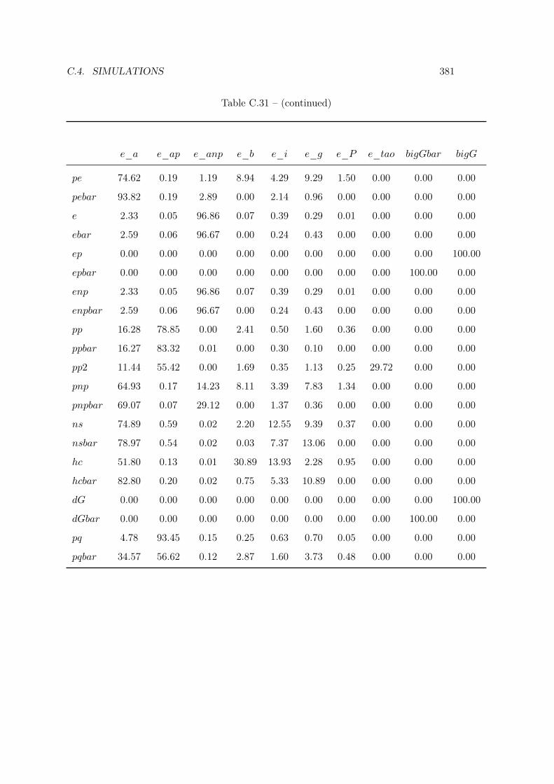
C.4. SIMULATIONS 381
Table C.31 – (continued)
e_a e_ap e_anp e_b e_i e_g e_P e_tao bigGbar bigG
pe 74.62 0.19 1.19 8.94 4.29 9.29 1.50 0.00 0.00 0.00
pebar 93.82 0.19 2.89 0.00 2.14 0.96 0.00 0.00 0.00 0.00
e 2.33 0.05 96.86 0.07 0.39 0.29 0.01 0.00 0.00 0.00
ebar 2.59 0.06 96.67 0.00 0.24 0.43 0.00 0.00 0.00 0.00
ep 0.00 0.00 0.00 0.00 0.00 0.00 0.00 0.00 0.00 100.00
epbar 0.00 0.00 0.00 0.00 0.00 0.00 0.00 0.00 100.00 0.00
enp 2.33 0.05 96.86 0.07 0.39 0.29 0.01 0.00 0.00 0.00
enpbar 2.59 0.06 96.67 0.00 0.24 0.43 0.00 0.00 0.00 0.00
pp 16.28 78.85 0.00 2.41 0.50 1.60 0.36 0.00 0.00 0.00
ppbar 16.27 83.32 0.01 0.00 0.30 0.10 0.00 0.00 0.00 0.00
pp2 11.44 55.42 0.00 1.69 0.35 1.13 0.25 29.72 0.00 0.00
pnp 64.93 0.17 14.23 8.11 3.39 7.83 1.34 0.00 0.00 0.00
pnpbar 69.07 0.07 29.12 0.00 1.37 0.36 0.00 0.00 0.00 0.00
ns 74.89 0.59 0.02 2.20 12.55 9.39 0.37 0.00 0.00 0.00
nsbar 78.97 0.54 0.02 0.03 7.37 13.06 0.00 0.00 0.00 0.00
hc 51.80 0.13 0.01 30.89 13.93 2.28 0.95 0.00 0.00 0.00
hcbar 82.80 0.20 0.02 0.75 5.33 10.89 0.00 0.00 0.00 0.00
dG 0.00 0.00 0.00 0.00 0.00 0.00 0.00 0.00 0.00 100.00
dGbar 0.00 0.00 0.00 0.00 0.00 0.00 0.00 0.00 100.00 0.00
pq 4.78 93.45 0.15 0.25 0.63 0.70 0.05 0.00 0.00 0.00
pqbar 34.57 56.62 0.12 2.87 1.60 3.73 0.48 0.00 0.00 0.00
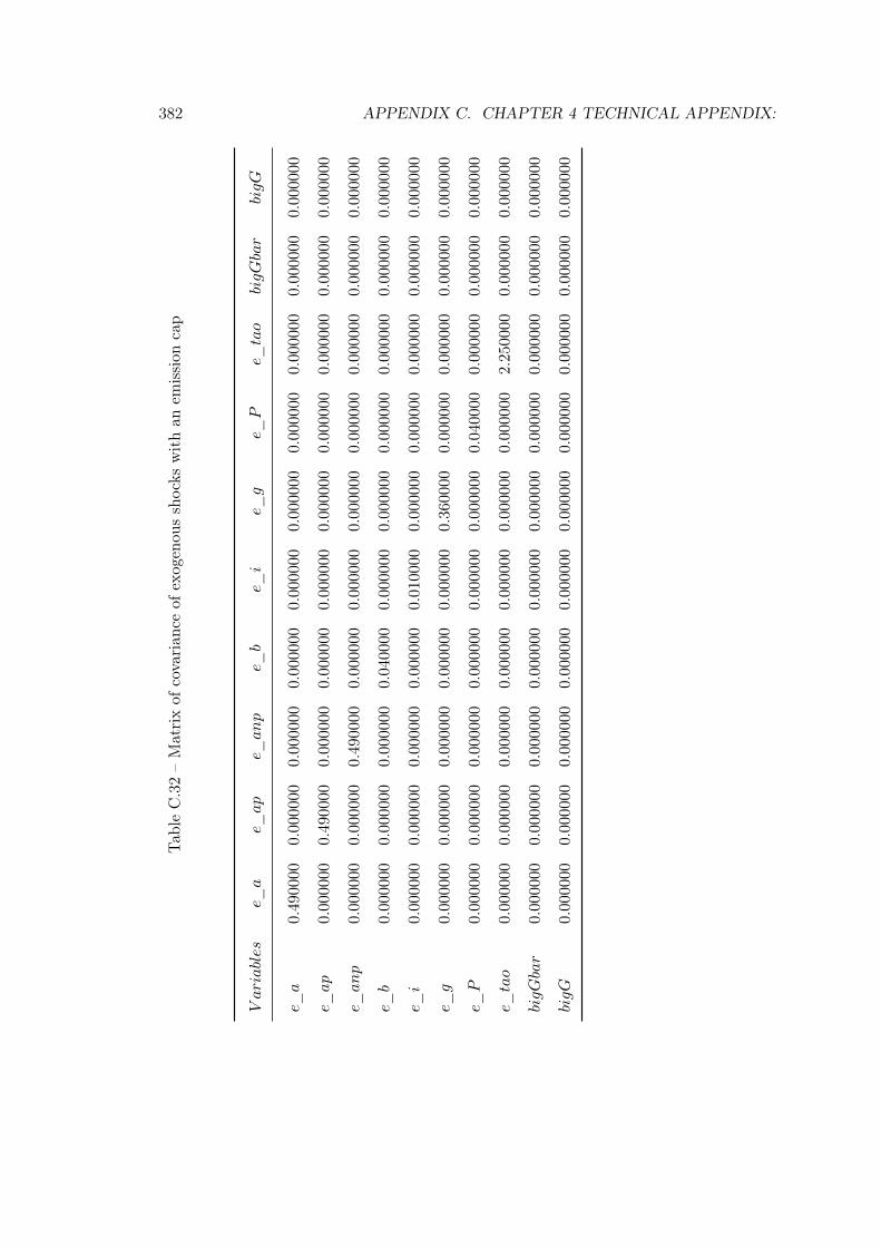
382 APPENDIX C. CHAPTER 4 TECHNICAL APPENDIX:
Tab
leC.32–Matrixof
covarian
ceof
exogenou
sshocks
withan
emission
cap
Variables
e_a
e_ap
e_anp
e_b
e_i
e_g
e_P
e_tao
bigGbar
bigG
e_a
0.490000
0.000000
0.000000
0.000000
0.000000
0.000000
0.000000
0.000000
0.000000
0.000000
e_ap
0.000000
0.490000
0.000000
0.000000
0.000000
0.000000
0.000000
0.000000
0.000000
0.000000
e_anp
0.000000
0.000000
0.490000
0.000000
0.000000
0.000000
0.000000
0.000000
0.000000
0.000000
e_b
0.000000
0.000000
0.000000
0.040000
0.000000
0.000000
0.000000
0.000000
0.000000
0.000000
e_i
0.000000
0.000000
0.000000
0.000000
0.010000
0.000000
0.000000
0.000000
0.000000
0.000000
e_g
0.000000
0.000000
0.000000
0.000000
0.000000
0.360000
0.000000
0.000000
0.000000
0.000000
e_P
0.000000
0.000000
0.000000
0.000000
0.000000
0.000000
0.040000
0.000000
0.000000
0.000000
e_tao
0.000000
0.000000
0.000000
0.000000
0.000000
0.000000
0.000000
2.250000
0.000000
0.000000
bigGbar
0.000000
0.000000
0.000000
0.000000
0.000000
0.000000
0.000000
0.000000
0.000000
0.000000
bigG
0.000000
0.000000
0.000000
0.000000
0.000000
0.000000
0.000000
0.000000
0.000000
0.000000
ECOLE DOCTORALE SCIENCES SOCIALES ET HUMANITES ED - 481
LABORATOIRE :
Centre d’Analyse Théorique et de Traitement des données économiques
Maxime.bouter[at]univ-pau.fr
Résumé :
Reconnue par les Nations-Unies comme l’un des huit objectifs du millénaire, la préservation de l’environnement, et par conséquent du climat, nécessite une intervention forte des pouvoirs publics afin d’endiguer les conséquences négatives liées au dérèglement climatique. La présente thèse se propose d’étudier quelques aspects des politiques climatiques et des conséquences qu’elles engendrent sur le cycle économique. Nous nous intéresserons tout d’abord à la question de la réversibilité du climat. L’une des particularités des gaz à effets de serre est leur durée de vie particulièrement longue. Si à l’échelle géologique, les puits de carbone pourraient absorber une majeure partie des émissions d’origine anthropogénique, à l’échelle humaine le réchauffement climatique apparaît comme irréversible sans une transformation de l’économie mondiale vers un modèle décarboné. En l’absence de la découverte d’une technologie capable de réduire drastiquement l’intensité carbone de l’énergie, le recours aux politiques publiques est la solution la plus à même de respecter la limite des 2°C d’ici la fin du 21ème siècle. Dans un deuxième temps, nous comparerons les conséquences de l’instauration de différents instruments de politique climatique (taxe carbone, marché des quotas, cible d’intensité) dans une économie qui est sujette à différents chocs exogènes (choc de productivité, choc sur le prix des énergies fossiles). A cette fin, nous utilisons un modèle RBC DSGE pour évaluer les conséquences économiques de ces différentes mesures. La mise en place d’un de ces instruments peut en effet avoir un effet récessif, ou au contraire être inefficace du point de vue du climat en période d’expansion. Nous recommandons ainsi l’utilisation jointe d’un marché des quotas, avec la mise en place d’un prix plancher du carbone afin d’atteindre l’objectif de réduction des émissions. Finalement, nous nous intéressons aux liens entre politique climatique et politique monétaire. Dans ce but, nous optimisons la règle de Taylor en présence soit d’un marché des quotas, ou d’une taxe carbone afin de faire des recommandations de politique monétaire. Nous montrons que les coefficients de la règle de Taylor qui maximisent le bien-être du consommateur sont sensiblement différents avec l’instauration d’une politique climatique. Il conviendrait ainsi de tenir compte, de ces effets pour conduire une politique environnementale la plus efficace possible.
Mots clés : Changement climatique, macroéconomie environnementale, politique environnementale, cycle économique, dynamique macroéconomique, politique monétaire
Abstract :
Recognised by the United Nations as one of the eight Millennium Development Goals, the preservation of the environment and consequently of the climate, requires strong intervention by public authorities in order to limit the negative consequences of climate change. This thesis proposes to study some aspects of climate policies and the consequences they have on the economic cycle. We first address the issue of climate reversibility. One of the particularities of greenhouse gases is their particularly long lifetime. While on a geological scale, carbon sinks could in theory absorb a major part of anthropogenic emissions, on a human scale global warming appears irreversible without a transformation of the world economy towards a decarbonised model. In the absence of the discovery of a technology capable of reducing the carbon intensity of energy, public policy seems to be the solution most likely to meet the 2°C limit by the end of the 21st century. Secondly, we compare the consequences of introducing different climate policy instruments (carbon tax, allowances market, intensity target) in an economy that is subject to different exogenous shocks (productivity shock, shock on the price of fossil fuels). To this end, we use an RBC DSGE model to assess the economic consequences of these different measures. The implementation of one of these instruments can indeed have a contractionary effect, or on the contrary be inefficient from a climate point of view in periods of expansion. We therefore recommend the joint use of an allowance market, with the establishment of a floor price for carbon in order to achieve the emission reduction target. Finally, we look at the links between climate policy and monetary policy. We optimise the Taylor rule in the presence of either an allowance market or a carbon tax in order to make monetary policy recommendations. We show that the Taylor rule coefficients that maximise consumer welfare are significantly different with the introduction of climate policy. These effects should therefore be taken into account in order to conduct the most effective environmental policy.
Keywords: Climate change, Environmental Macroeconomics, Environmental Policy, Business Cycle, New Keynesian Model, Macroeconomic Dynamics, Monetary Policy.
Classification: E32, E50, H2, O44, Q43, Q50, Q52, Q58.