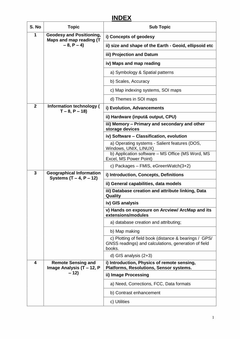
1

INDEX

S. No Topic Sub Topic

1 Geodesy and Positioning, Maps and map reading (T

– 8, P – 4)

i) Concepts of geodesy

ii) size and shape of the Earth - Geoid, ellipsoid etc

iii) Projection and Datum

iv) Maps and map reading

a) Symbology & Spatial patterns

b) Scales, Accuracy

c) Map indexing systems, SOI maps

d) Themes in SOI maps

2 Information technology ( T – 8, P – 18)

i) Evolution, Advancements

ii) Hardware (input& output, CPU)

iii) Memory – Primary and secondary and other storage devices

iv) Software – Classification, evolution

a) Operating systems - Salient features (DOS, Windows, UNIX, LINUX)

b) Application software – MS Office (MS Word, MS Excel, MS Power Point)

c) Packages – FMIS, eGreenWatch(3+2)

3 Geographical Information Systems (T – 4, P – 12)

i) Introduction, Concepts, Definitions

ii) General capabilities, data models

iii) Database creation and attribute linking, Data Quality

iv) GIS analysis

v) Hands on exposure on Arcview/ ArcMap and its extensions/modules

a) database creation and attributing;

b) Map making

c) Plotting of field book (distance & bearings / GPS/ GNSS readings) and calculations, generation of field books.

d) GIS analysis (2+3)

4 Remote Sensing and Image Analysis (T – 12, P

– 12)

i) Introduction, Physics of remote sensing, Platforms, Resolutions, Sensor systems.

ii) Image Processing

a) Need, Corrections, FCC, Data formats

b) Contrast enhancement

c) Utilities

2

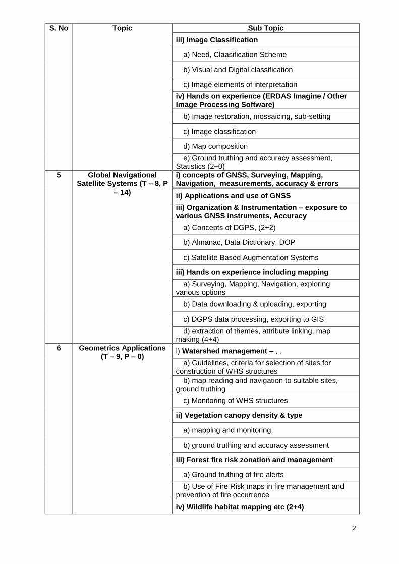
S. No Topic Sub Topic

iii) Image Classification

a) Need, Claasification Scheme

b) Visual and Digital classification

c) Image elements of interpretation

iv) Hands on experience (ERDAS Imagine / Other Image Processing Software)

b) Image restoration, mossaicing, sub-setting

c) Image classification

d) Map composition

e) Ground truthing and accuracy assessment, Statistics (2+0)

5 Global Navigational Satellite Systems (T – 8, P

– 14)

i) concepts of GNSS, Surveying, Mapping, Navigation, measurements, accuracy & errors

ii) Applications and use of GNSS

iii) Organization & Instrumentation – exposure to various GNSS instruments, Accuracy

a) Concepts of DGPS, (2+2)

b) Almanac, Data Dictionary, DOP

c) Satellite Based Augmentation Systems

iii) Hands on experience including mapping

a) Surveying, Mapping, Navigation, exploring various options

b) Data downloading & uploading, exporting

c) DGPS data processing, exporting to GIS

d) extraction of themes, attribute linking, map making (4+4)

6 Geometrics Applications (T – 9, P – 0)

i) Watershed management – , .

a) Guidelines, criteria for selection of sites for construction of WHS structures

b) map reading and navigation to suitable sites, ground truthing

c) Monitoring of WHS structures

ii) Vegetation canopy density & type

a) mapping and monitoring,

b) ground truthing and accuracy assessment

iii) Forest fire risk zonation and management

a) Ground truthing of fire alerts

b) Use of Fire Risk maps in fire management and prevention of fire occurrence

iv) Wildlife habitat mapping etc (2+4)

3

S. No Topic Sub Topic

7 Other Applications (T – 7, P – 10)

i) Hands on with GoogleEarth/ Bhuvan etc

a) Overlay of data in GoogleEarth*

b) Creation of new features and exporting*

c) Time Series Analysis*

ii) Hands on with Mobile Applications*

iii) Hands on with Village Cadastral Maps

a) Reading of maps with respect to Gazette notification

b) Exposure to Bhumi portal (1+1)

4

Chapter - I

Geodesy and Positioning, Maps and map reading

Definition: Geodesy is the science which deals with the methods of precise measurements of

elements of the surface of the earth and their treatment for the determination of geographic

positions on the surface of the earth. It also deals with the theory of size and shape of the earth.

Geodesy may be broadly divided into two branches, namely,

1. Geometric Geodesy. 2. Physical Geodesy.

Geometric geodesy appears to be purely geometrical science as it deals with the geometry

(shape and size) of the earth. Determination of geographical positions on the surface of earth can

be made by observing celestial bodies, and thus comes under geodetic astronomy, but this can be

included under geometric geodesy.

Physical geodesy is concerned with determining the Earth’s gravity field, which is

necessary for establishing heights. Earth gravity field is a physical entity and is involved in

most of the geodetic measurements, even the purely geometric ones. The measurement of

geodetic astronomy, triangulation and leveling, all make essential use of plumb line being the

direction of gravity vector. Thus, astro-geodetic methods which use astro determination of latitude,

longitude, and azimuth and geodetic operations e.g. triangulation, trilateration, base measurement

etc., may be considered as belonging to Physical geodesy fully as much as the gravimetric

methods.

Satellite Geodesy: Satellite geodesy comprises the observational and computational techniques

which allow the solution of geodetic problems by the use of precise measurements to, from or

between artificial, mostly near the earth satellites.

GEODESY AND POSITIONING - EARTH SHAPE MODELS

Flat earth models are still used for plane surveying, over distances short enough so

that earth curvature is insignificant (less than 10 km).

Spherical earth models (Earth centered model) represent the shape of the earth

with a sphere of a specified radius. Spherical earth models are often used for short

range navigation (VOR-DME) and for global distance approximations. Spherical

models fail to model the actual shape of the earth. The world is approximately a

sphere. The sphere is the shape that minimizes the potential energy of the

gravitational attraction of all the little mass elements for each other. The direction of

gravity is toward the center of the earth. It is the direction that a string takes when a

weight is at one end - that is a plumb bob.

Ellipsoidal earth models are required for accurate range and bearing calculations

over long distances. Ellipsoidal models define an ellipsoid with an equatorial radius

and a polar radius. The best of these models can represent the shape of the earth

over the smoothed, averaged sea-surface to within about one-hundred meters. The

equatorial radius is longer than the polar axis by about 23 km. The direction of gravity

does not point to the center of the earth.

Although the earth is an ellipsoid, its major and minor axes do not vary greatly. In fact,

its shape is so close to a sphere that it is often called a spheroid rather than an

5

ellipsoid. But sometimes, the spheroid confused people. SOI (Survey of India) often

call ellipsoid.

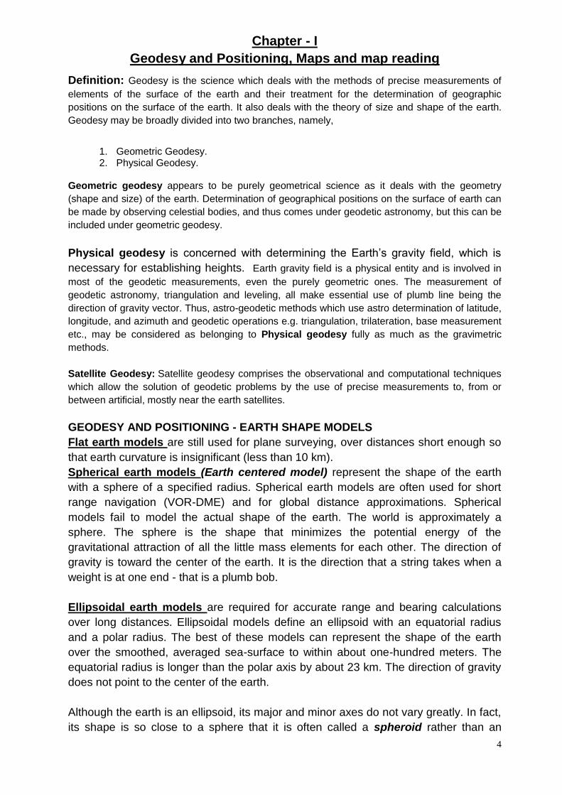
Spherical Earth’s surface - radius 6371

km

Meridians (lines of longitude) - passing

through Greenwich, England as prime

meridian or 0º longitude.

Parallels (lines of latitude)

using equator as 0º latitude.

Degrees-minutes-seconds (DMS),

Decimal degrees (DD)

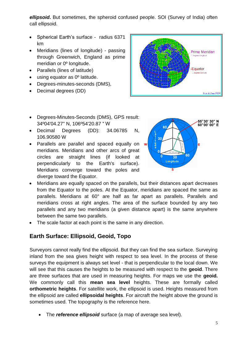
Degrees-Minutes-Seconds (DMS), GPS result:

34º04'04.27" N, 106º54'20.87 “ W

Decimal Degrees (DD): 34.06785 N,

106.90580 W

Parallels are parallel and spaced equally on

meridians. Meridians and other arcs of great

circles are straight lines (if looked at

perpendicularly to the Earth's surface).

Meridians converge toward the poles and

diverge toward the Equator.

Meridians are equally spaced on the parallels, but their distances apart decreases

from the Equator to the poles. At the Equator, meridians are spaced the same as

parallels. Meridians at 60° are half as far apart as parallels. Parallels and

meridians cross at right angles. The area of the surface bounded by any two

parallels and any two meridians (a given distance apart) is the same anywhere

between the same two parallels.

The scale factor at each point is the same in any direction.

Earth Surface: Ellipsoid, Geoid, Topo

Surveyors cannot really find the ellipsoid. But they can find the sea surface. Surveying

inland from the sea gives height with respect to sea level. In the process of these

surveys the equipment is always set level - that is perpendicular to the local down. We

will see that this causes the heights to be measured with respect to the geoid. There

are three surfaces that are used in measuring heights. For maps we use the geoid.

We commonly call this mean sea level heights. These are formally called

orthometric heights. For satellite work, the ellipsoid is used. Heights measured from

the ellipsoid are called ellipsoidal heights. For aircraft the height above the ground is

sometimes used. The topography is the reference here.

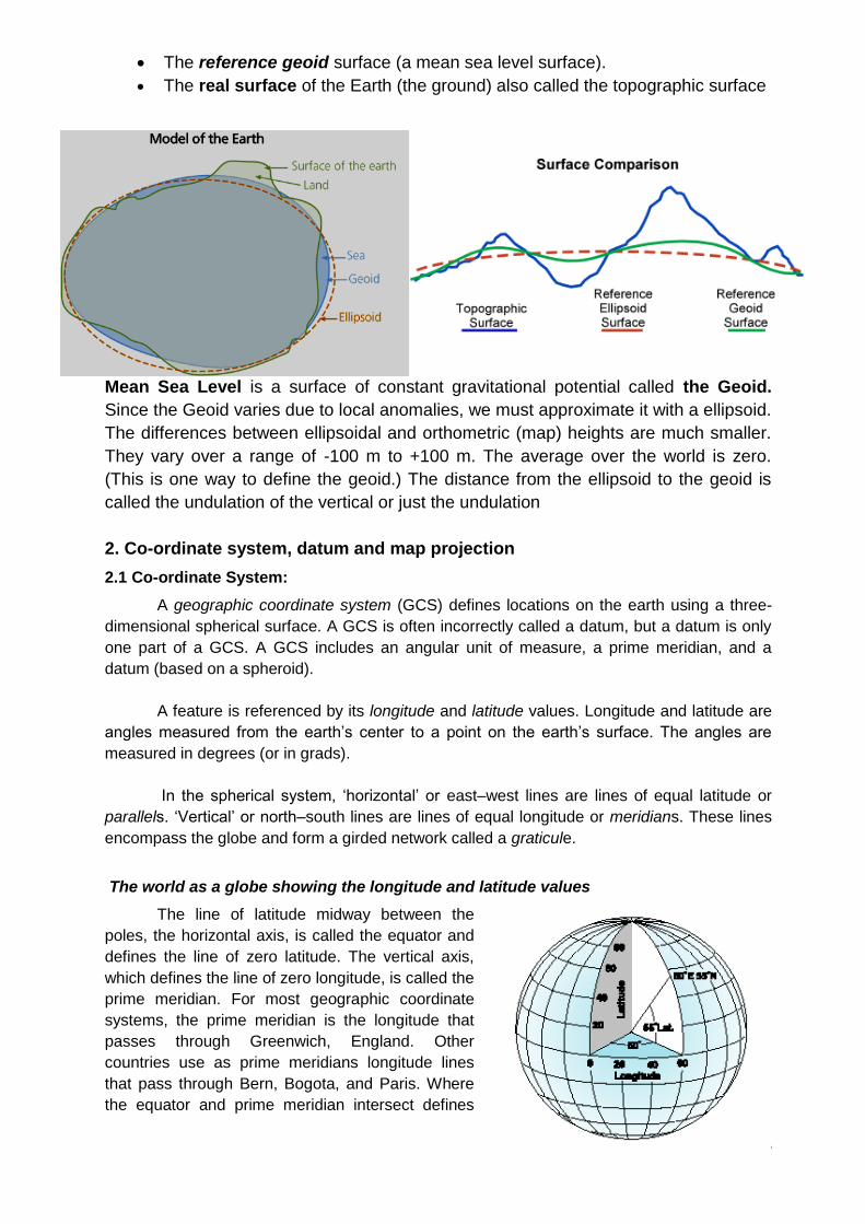
The reference ellipsoid surface (a map of average sea level).

6

The reference geoid surface (a mean sea level surface).

The real surface of the Earth (the ground) also called the topographic surface

Mean Sea Level is a surface of constant gravitational potential called the Geoid.

Since the Geoid varies due to local anomalies, we must approximate it with a ellipsoid.

The differences between ellipsoidal and orthometric (map) heights are much smaller.

They vary over a range of -100 m to +100 m. The average over the world is zero.

(This is one way to define the geoid.) The distance from the ellipsoid to the geoid is

called the undulation of the vertical or just the undulation

2. Co-ordinate system, datum and map projection

2.1 Co-ordinate System:

A geographic coordinate system (GCS) defines locations on the earth using a three-

dimensional spherical surface. A GCS is often incorrectly called a datum, but a datum is only

one part of a GCS. A GCS includes an angular unit of measure, a prime meridian, and a

datum (based on a spheroid).

A feature is referenced by its longitude and latitude values. Longitude and latitude are

angles measured from the earth’s center to a point on the earth’s surface. The angles are

measured in degrees (or in grads).

In the spherical system, ‘horizontal’ or east–west lines are lines of equal latitude or

parallels. ‘Vertical’ or north–south lines are lines of equal longitude or meridians. These lines

encompass the globe and form a girded network called a graticule.

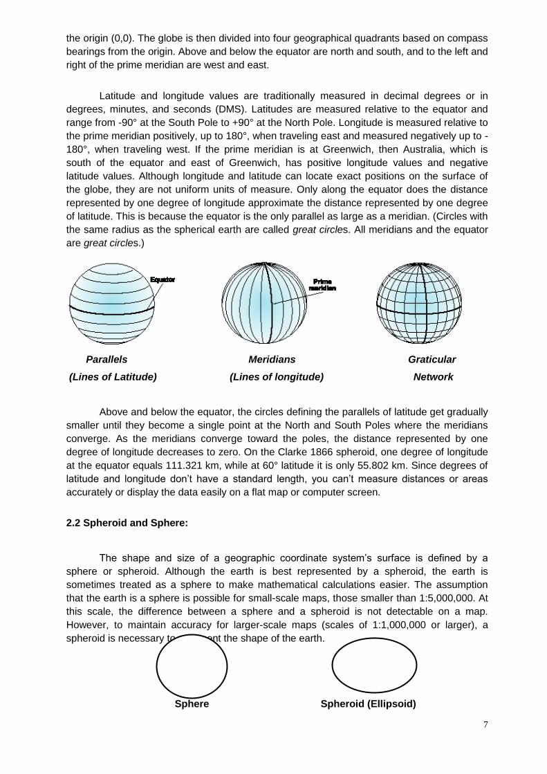
The world as a globe showing the longitude and latitude values

The line of latitude midway between the

poles, the horizontal axis, is called the equator and

defines the line of zero latitude. The vertical axis,

which defines the line of zero longitude, is called the

prime meridian. For most geographic coordinate

systems, the prime meridian is the longitude that

passes through Greenwich, England. Other

countries use as prime meridians longitude lines

that pass through Bern, Bogota, and Paris. Where

the equator and prime meridian intersect defines

7

the origin (0,0). The globe is then divided into four geographical quadrants based on compass

bearings from the origin. Above and below the equator are north and south, and to the left and

right of the prime meridian are west and east.

Latitude and longitude values are traditionally measured in decimal degrees or in

degrees, minutes, and seconds (DMS). Latitudes are measured relative to the equator and

range from -90° at the South Pole to +90° at the North Pole. Longitude is measured relative to

the prime meridian positively, up to 180°, when traveling east and measured negatively up to -

180°, when traveling west. If the prime meridian is at Greenwich, then Australia, which is

south of the equator and east of Greenwich, has positive longitude values and negative

latitude values. Although longitude and latitude can locate exact positions on the surface of

the globe, they are not uniform units of measure. Only along the equator does the distance

represented by one degree of longitude approximate the distance represented by one degree

of latitude. This is because the equator is the only parallel as large as a meridian. (Circles with

the same radius as the spherical earth are called great circles. All meridians and the equator

are great circles.)

Parallels Meridians Graticular

(Lines of Latitude) (Lines of longitude) Network

Above and below the equator, the circles defining the parallels of latitude get gradually

smaller until they become a single point at the North and South Poles where the meridians

converge. As the meridians converge toward the poles, the distance represented by one

degree of longitude decreases to zero. On the Clarke 1866 spheroid, one degree of longitude

at the equator equals 111.321 km, while at 60° latitude it is only 55.802 km. Since degrees of

latitude and longitude don’t have a standard length, you can’t measure distances or areas

accurately or display the data easily on a flat map or computer screen.

2.2 Spheroid and Sphere:

The shape and size of a geographic coordinate system’s surface is defined by a

sphere or spheroid. Although the earth is best represented by a spheroid, the earth is

sometimes treated as a sphere to make mathematical calculations easier. The assumption

that the earth is a sphere is possible for small-scale maps, those smaller than 1:5,000,000. At

this scale, the difference between a sphere and a spheroid is not detectable on a map.

However, to maintain accuracy for larger-scale maps (scales of 1:1,000,000 or larger), a

spheroid is necessary to represent the shape of the earth.

Sphere Spheroid (Ellipsoid)

8

A sphere is based on a circle, while a spheroid (or ellipsoid) is based on an ellipse.

The shape of an ellipse is defined by two radii. The longer radius is called the semi major axis,

and the shorter radius is called the semi minor axis. Rotating the ellipse around the semi

minor axis creates a spheroid. A spheroid is defined by the semi major axis ‘a’ and the semi

minor axis ‘b’ or by ‘a’ and the flattening. The flattening is the difference in length between the

two axes expressed as a fraction or a decimal.

The flattening, f, is f = (a - b) / a

The flattening is a small value, so usually the quantity 1/f is used instead. Sample

values are a = 6378137.0 meters 1/f = 298.257223563

The flattening ranges between zero and one. A flattening value of zero means the two

axes are equal, resulting in a sphere. The flattening of the earth is approximately 0.003353.

Another quantity is the square of the eccentricity, e, that, like the flattening, describes the

shape of a spheroid.

2.3 Defining Spheroid for Accurate Mapping:

The earth has been surveyed many times to better understand its surface features and

their peculiar irregularities. The surveys have resulted in many spheroids that represent the

earth. Generally, a spheroid is chosen to fit one country or a particular area. A spheroid that

best fits one region is not necessarily the same one that fits another region. Until recently,

North American data used a spheroid determined by Clarke in 1866. The semi major axis of

the Clarke 1866 spheroid is 6,378,206.4 meters, and the semi minor axis is 6,356,583.8

meters. Because of gravitational and surface feature variations, the earth is neither a perfect

sphere nor a perfect spheroid. Satellite technology has revealed several elliptical deviations;

for example, the South Pole is closer to the equator than the North Pole. Satellite determined

spheroids are replacing the older ground-measured spheroids. For example, the new standard

spheroid for North America is GRS 1980, whose radii are 6,378,137.0 and 6,356,752.31414

meters. Because changing a coordinate system’s spheroid changes all previously measured

values, many organizations don’t switch to newer (and more accurate) spheroids.

2.4 Datum:

While a spheroid approximates the shape of the earth, a datum defines the position of

the spheroid relative to the center of the earth. A datum provides a frame of reference for

measuring locations on the surface of the earth. It defines the origin and orientation of latitude

and longitude lines. Whenever you change the datum, or more correctly, the geographic

coordinate system, the coordinate values of your data will change. Here’s the coordinates in

DMS of a control point in Redlands on NAD 1983.

-117 12 57.75961 34 01 43.77884

Here’s the same point on NAD 1927.

-117 12 54.61539 34 01 43.72995

The longitude value differs by about a second while the latitude value is around 500th

of a second. In the last 15 years, satellite data has provided geodesists with new

measurements to define the best earth-fitting spheroid, which relates coordinates to the

9

earth’s center of mass. An earth-centered, or geocentric, datum uses the earth’s center of

mass as the origin. The most recently developed and widely used datum is the World

Geodetic System of 1984 (WGS84). It serves as the framework for location measurement

worldwide. A local datum aligns its spheroid to closely fit the earth’s surface in a particular

area. A point on the surface of the spheroid is matched to a particular position on the surface

of the earth. This point is known as the ‘origin point’ of the datum. The coordinates of the

origin point are fixed, and all other points are calculated from it. The coordinate system origin

of a local datum is not at the center of the earth. The center of the spheroid of a local datum is

offset from the earth’s center. The North American Datum of 1927 (NAD27) and the European

Datum of 1950 are local datum’s. NAD27 is designed to fit North America reasonably well,

while ED50 was created for use in Europe. A local datum is not suited for use outside the area

for which it was designed.

2.5 Map Projection:

The mathematical transformation of three-dimensional surface in to a two dimensional

surface is commonly referred as a map projection. One easy way to understand how map

projections alter spatial properties is to visualize shining a light through the earth onto a

surface, called the projection surface. A spheroid can’t be flattened to a plane any easier than

flattening a piece of orange peel—it will rip.

Representing the earth’s surface in two dimensions causes distortion in the shape,

area, distance, or direction of the data. A map projection uses mathematical formulas to relate

spherical coordinates on the globe to flat, planar coordinates.

Different projections cause different types of distortions. Some projections are

designed to minimize the distortion of one or two of the data’s characteristics. A projection

could maintain the area of a feature but alter its shape. In the above graphic, data near the

poles is stretched. The diagram on the next page shows how three-dimensional features are

compressed to fit onto a flat surface.

Map projections are designed for specific purposes. A map projection might be used

for large-scale data in a limited area, while another is used for a small-scale map of the world.

Map projections designed for small-scale data are usually based on spherical rather than

spheroid geographic coordinate systems.

2.5.1 Conformal projection

Conformal projections preserve local shape. Graticule lines on the globe are

perpendicular. To preserve individual angles describing the spatial relationships, a conformal

projection must show graticule lines intersecting at 90-degree angles on the map. This is

accomplished by maintaining all angles. The drawback is that the area enclosed by a series of

arcs may be greatly distorted in the process. No map projection can preserve shapes of larger

regions.

2.5.2 Equal area projections

Equal area projections preserve the area of displayed features. To do this, the other

properties of shape, angle, and scale are distorted. In equal area projections, the meridians

and parallels may not intersect at right angles. In some instances, especially maps of smaller

10

regions, shapes are not obviously distorted, and distinguishing an equal area projection from a

conformal projection may prove difficult unless documented or measured.

2.5.3 Equidistant projections:

Equidistant maps preserve the distances between certain points. Scale is not

maintained correctly by any projection throughout an entire map; however, there are, in most

cases, one or more lines on a map along which scale are maintained correctly. Most

projections have one or more lines for which the length of the line on a map is the same length

(at map scale) as the same line on the globe, regardless of whether it is a great or small circle

or straight or curved. Such distances are said to be true. For example, in the Sinusoidal

projection, the equator and all parallels are their true lengths. In other equidistant projections,

the equator and all meridians are true. Still others (e.g., Two-Point Equidistant) show true

scale between one or two points and every other point on the map. Keep in mind that no

projection is equidistant to and from all points on a map.

2.5.4 True-direction projections:

The shortest route between two points on a curved surface such as the earth is along

the spherical equivalent of a straight line on a flat surface. That is the great circle on which the

two points lie. True-direction or azimuthal projections maintain some of the great circle arcs,

giving the directions or azimuths of all points on the map correctly with respect to the center.

Some true-direction projections are also conformal, equal area, or equidistant.

The first step in projecting from one surface to another is to create one or more points

of contact. Each contact is called a point (or line) of tangency. Planar projection is tangential

to the globe at one point. Tangential cones and cylinders touch the globe along a line. If the

projection surface intersects the globe instead of merely touching its surface, the resulting

projection is a secant rather than a tangent case. Whether the contact is tangent or secant,

the contact point or lines are significant because they define locations of zero distortion. Lines

of true scale are often referred to as standard lines. In general, distortion increases with the

distance from the point of contact.

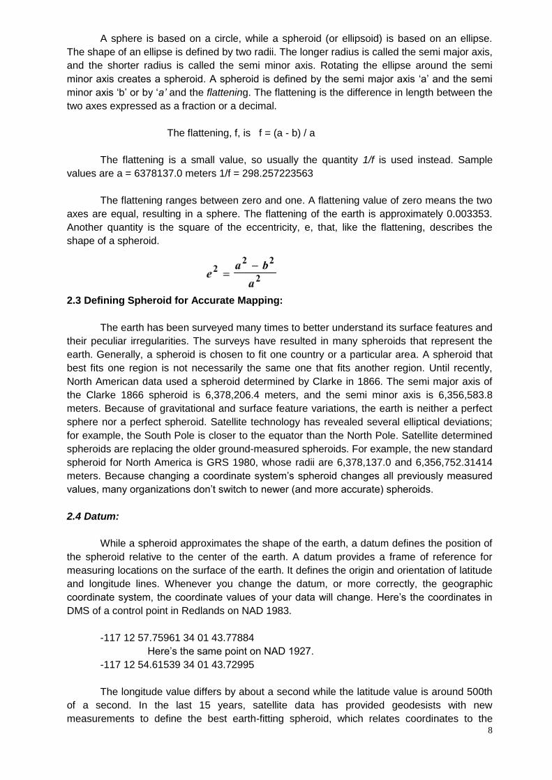
2.5.5 Conic projections:

The simplest conic projection is tangent to the globe along a line of latitude. This line is

called the standard parallel. The meridians are projected onto the conical surface, meeting at

the apex, or point, of the cone. Parallel lines of latitude are projected onto the cone as rings.

The cone is then ‘cut’ along any meridian to produce the final conic projection, which has

straight converging lines for meridians and concentric circular arcs for parallels. The meridian

opposite the cut line becomes the central meridian.

11

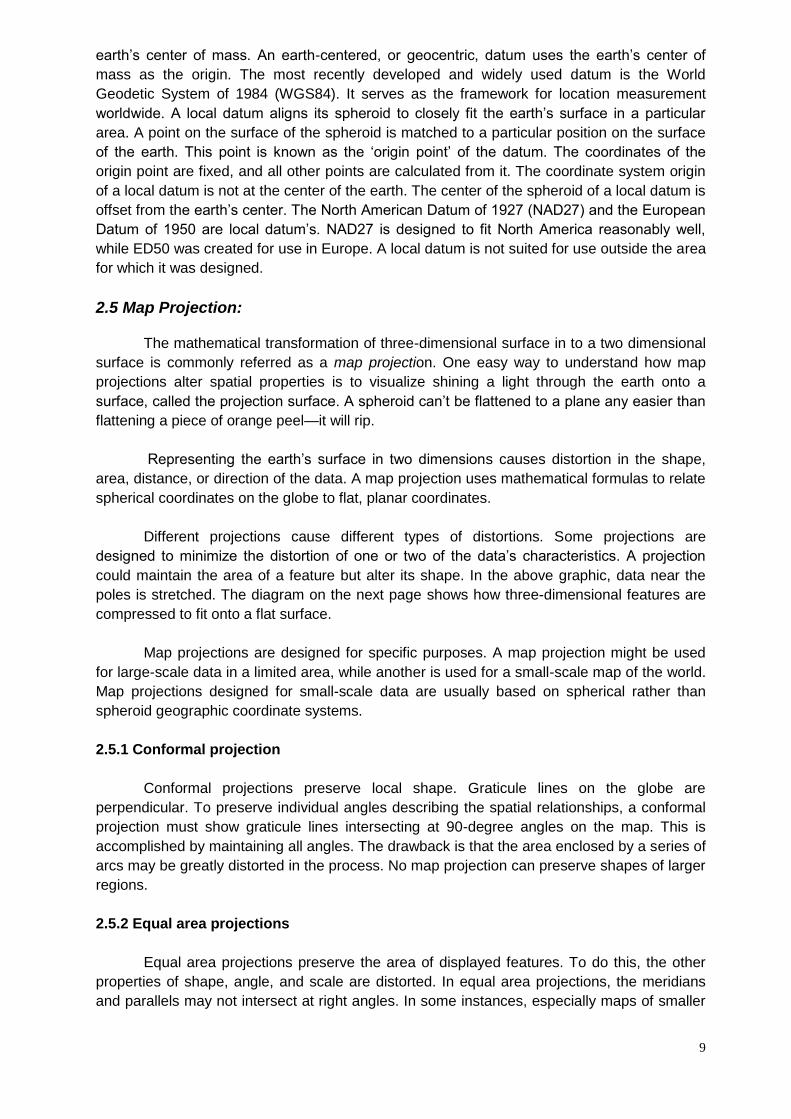
In general, distortion increases away from the standard parallel. Thus, cutting off the

top of the cone produces a more accurate projection. This is accomplished by not using the

polar region of the projected data. Conic projections are used for mid-latitude zones that have

an east-to-west orientation. Somewhat more complex conic projections contact the global

surface at two locations. These projections are called secant conic projections and are defined

by two standard parallels. It is also possible to define a secant projection by one standard

parallel and a scale factor.

The distortion pattern for secant projections is different between the standard parallels

than beyond them. Generally, a secant projection has less overall distortion than a tangent

case. On still more complex conic projections, the axis of the cone does not line up with the

polar axis of the globe. These are called oblique. The representation of geographic features

depends on the spacing of the parallels. When equally spaced, the projection is equidistant in

the north– south direction but neither conformal nor equal area such as the Equidistant Conic

projection. For small areas, the overall distortion is minimal. On the Lambert Conic Conformal

projection, the central parallels are spaced more closely than the parallels near the border,

and small geographic shapes are maintained for both small-scale and large-scale maps.

Finally, on the Albers Equal Area Conic

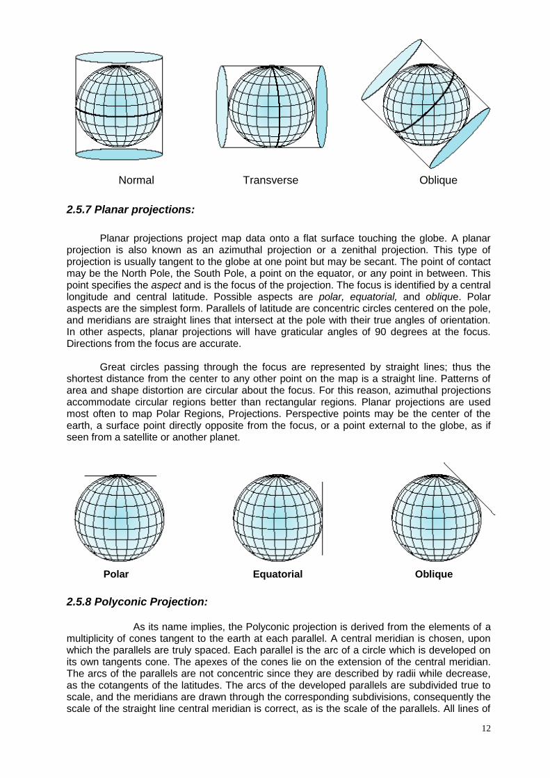
2.5.6 Cylindrical projections:

Cylindrical projections can also have tangent or secant cases. The Mercator projection

is one of the most common cylindrical projections, and the equator is usually its line of

tangency. Meridians are geometrically projected onto the cylindrical surface, and parallels are

mathematically projected, producing graticule angles of 90 degrees. The cylinder is ‘cut’ along

any meridian to produce the final cylindrical projection. The meridians are equally spaced,

while the spacing between parallel lines of latitude increases toward the poles. This projection

is conformal and displays true direction along straight lines. Rhumb lines, lines of constant

bearing, but not most great circles, are straight lines on a Mercator projection.

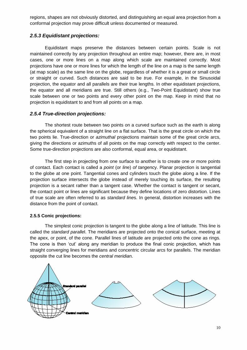
For more complex cylindrical projections the cylinder is rotated, thus changing the

tangent or secant lines. Transverse cylindrical projections such as the Transverse Mercator

use a meridian as the tangential contact or lines parallel to meridians as lines of secancy. The

standard lines then run north and south, along which the scale is true. Oblique cylinders are

rotated around a great circle line located anywhere between the equator and the meridians. In

these more complex projections, most meridians and lines of latitude are no longer straight. In

all cylindrical projections, the line of tangency or lines of secancy have no distortion and thus

are lines of equidistance. Other geographical properties vary according to the specific

projection.

12

Normal Transverse Oblique

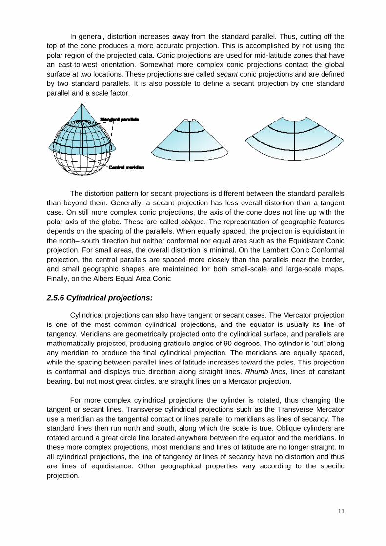
2.5.7 Planar projections:

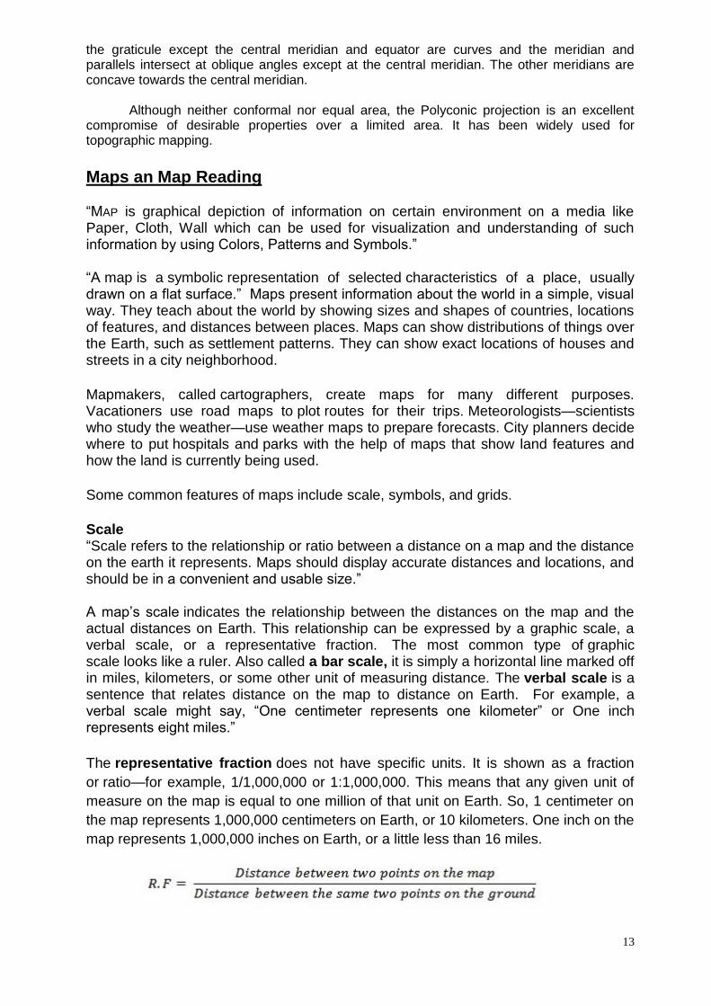
Planar projections project map data onto a flat surface touching the globe. A planar projection is also known as an azimuthal projection or a zenithal projection. This type of projection is usually tangent to the globe at one point but may be secant. The point of contact may be the North Pole, the South Pole, a point on the equator, or any point in between. This point specifies the aspect and is the focus of the projection. The focus is identified by a central longitude and central latitude. Possible aspects are polar, equatorial, and oblique. Polar aspects are the simplest form. Parallels of latitude are concentric circles centered on the pole, and meridians are straight lines that intersect at the pole with their true angles of orientation. In other aspects, planar projections will have graticular angles of 90 degrees at the focus. Directions from the focus are accurate.

Great circles passing through the focus are represented by straight lines; thus the shortest distance from the center to any other point on the map is a straight line. Patterns of area and shape distortion are circular about the focus. For this reason, azimuthal projections accommodate circular regions better than rectangular regions. Planar projections are used most often to map Polar Regions, Projections. Perspective points may be the center of the earth, a surface point directly opposite from the focus, or a point external to the globe, as if seen from a satellite or another planet.

Polar Equatorial Oblique

2.5.8 Polyconic Projection:

As its name implies, the Polyconic projection is derived from the elements of a multiplicity of cones tangent to the earth at each parallel. A central meridian is chosen, upon which the parallels are truly spaced. Each parallel is the arc of a circle which is developed on its own tangents cone. The apexes of the cones lie on the extension of the central meridian. The arcs of the parallels are not concentric since they are described by radii while decrease, as the cotangents of the latitudes. The arcs of the developed parallels are subdivided true to scale, and the meridians are drawn through the corresponding subdivisions, consequently the scale of the straight line central meridian is correct, as is the scale of the parallels. All lines of

13

the graticule except the central meridian and equator are curves and the meridian and parallels intersect at oblique angles except at the central meridian. The other meridians are concave towards the central meridian.

Although neither conformal nor equal area, the Polyconic projection is an excellent compromise of desirable properties over a limited area. It has been widely used for topographic mapping.

Maps an Map Reading

“MAP is graphical depiction of information on certain environment on a media like Paper, Cloth, Wall which can be used for visualization and understanding of such information by using Colors, Patterns and Symbols.”

“A map is a symbolic representation of selected characteristics of a place, usually drawn on a flat surface.” Maps present information about the world in a simple, visual way. They teach about the world by showing sizes and shapes of countries, locations of features, and distances between places. Maps can show distributions of things over the Earth, such as settlement patterns. They can show exact locations of houses and streets in a city neighborhood.

Mapmakers, called cartographers, create maps for many different purposes. Vacationers use road maps to plot routes for their trips. Meteorologists—scientists who study the weather—use weather maps to prepare forecasts. City planners decide where to put hospitals and parks with the help of maps that show land features and how the land is currently being used.

Some common features of maps include scale, symbols, and grids.

Scale “Scale refers to the relationship or ratio between a distance on a map and the distance on the earth it represents. Maps should display accurate distances and locations, and should be in a convenient and usable size.” A map’s scale indicates the relationship between the distances on the map and the actual distances on Earth. This relationship can be expressed by a graphic scale, a verbal scale, or a representative fraction. The most common type of graphic scale looks like a ruler. Also called a bar scale, it is simply a horizontal line marked off in miles, kilometers, or some other unit of measuring distance. The verbal scale is a sentence that relates distance on the map to distance on Earth. For example, a verbal scale might say, “One centimeter represents one kilometer” or One inch represents eight miles.”

The representative fraction does not have specific units. It is shown as a fraction

or ratio—for example, 1/1,000,000 or 1:1,000,000. This means that any given unit of

measure on the map is equal to one million of that unit on Earth. So, 1 centimeter on

the map represents 1,000,000 centimeters on Earth, or 10 kilometers. One inch on the

map represents 1,000,000 inches on Earth, or a little less than 16 miles.

14

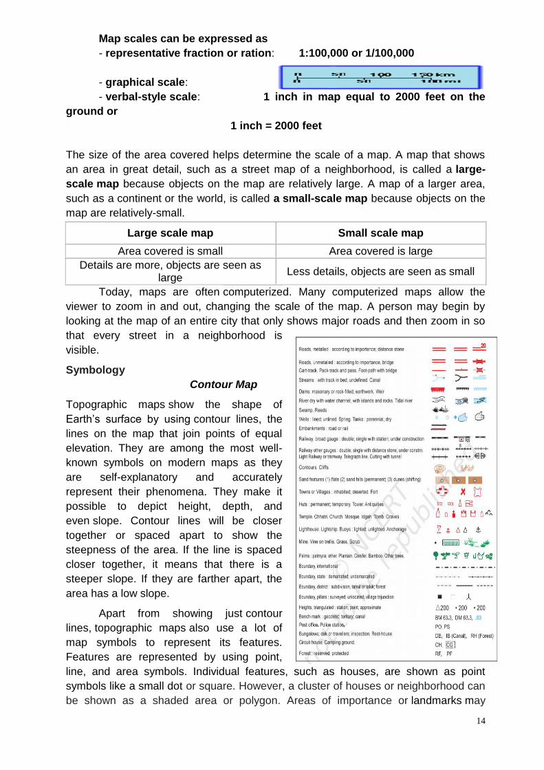
Map scales can be expressed as

- representative fraction or ration: 1:100,000 or 1/100,000

- graphical scale:

- verbal-style scale: 1 inch in map equal to 2000 feet on the

ground or

1 inch = 2000 feet

The size of the area covered helps determine the scale of a map. A map that shows

an area in great detail, such as a street map of a neighborhood, is called a large-

scale map because objects on the map are relatively large. A map of a larger area,

such as a continent or the world, is called a small-scale map because objects on the

map are relatively-small.

Large scale map Small scale map

Area covered is small Area covered is large

Details are more, objects are seen as large

Less details, objects are seen as small

Today, maps are often computerized. Many computerized maps allow the

viewer to zoom in and out, changing the scale of the map. A person may begin by

looking at the map of an entire city that only shows major roads and then zoom in so

that every street in a neighborhood is

visible.

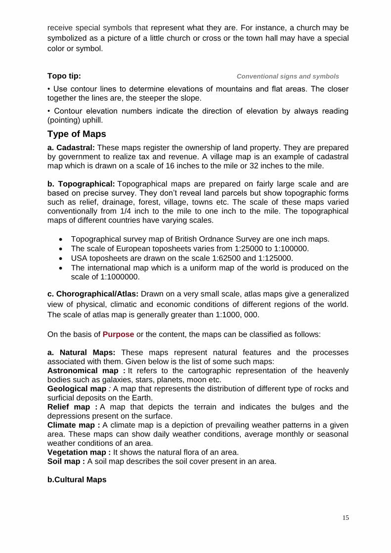
Symbology

Contour Map

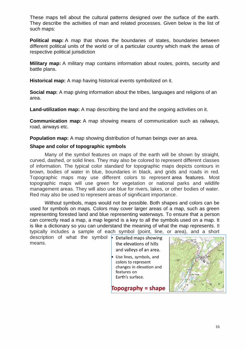
Topographic maps show the shape of

Earth’s surface by using contour lines, the

lines on the map that join points of equal

elevation. They are among the most well-

known symbols on modern maps as they

are self-explanatory and accurately

represent their phenomena. They make it

possible to depict height, depth, and

even slope. Contour lines will be closer

together or spaced apart to show the

steepness of the area. If the line is spaced

closer together, it means that there is a

steeper slope. If they are farther apart, the

area has a low slope.

Apart from showing just contour

lines, topographic maps also use a lot of

map symbols to represent its features.

Features are represented by using point,

line, and area symbols. Individual features, such as houses, are shown as point

symbols like a small dot or square. However, a cluster of houses or neighborhood can

be shown as a shaded area or polygon. Areas of importance or landmarks may

15

receive special symbols that represent what they are. For instance, a church may be

symbolized as a picture of a little church or cross or the town hall may have a special

color or symbol.

Topo tip: Conventional signs and symbols

• Use contour lines to determine elevations of mountains and flat areas. The closer together the lines are, the steeper the slope.

• Contour elevation numbers indicate the direction of elevation by always reading (pointing) uphill.

Type of Maps

a. Cadastral: These maps register the ownership of land property. They are prepared by government to realize tax and revenue. A village map is an example of cadastral map which is drawn on a scale of 16 inches to the mile or 32 inches to the mile. b. Topographical: Topographical maps are prepared on fairly large scale and are based on precise survey. They don’t reveal land parcels but show topographic forms such as relief, drainage, forest, village, towns etc. The scale of these maps varied conventionally from 1/4 inch to the mile to one inch to the mile. The topographical maps of different countries have varying scales.

Topographical survey map of British Ordnance Survey are one inch maps.

The scale of European toposheets varies from 1:25000 to 1:100000.

USA toposheets are drawn on the scale 1:62500 and 1:125000.

The international map which is a uniform map of the world is produced on the scale of 1:1000000.

c. Chorographical/Atlas: Drawn on a very small scale, atlas maps give a generalized

view of physical, climatic and economic conditions of different regions of the world.

The scale of atlas map is generally greater than 1:1000, 000.

On the basis of Purpose or the content, the maps can be classified as follows: a. Natural Maps: These maps represent natural features and the processes associated with them. Given below is the list of some such maps: Astronomical map : It refers to the cartographic representation of the heavenly bodies such as galaxies, stars, planets, moon etc. Geological map : A map that represents the distribution of different type of rocks and surficial deposits on the Earth. Relief map : A map that depicts the terrain and indicates the bulges and the depressions present on the surface. Climate map : A climate map is a depiction of prevailing weather patterns in a given area. These maps can show daily weather conditions, average monthly or seasonal weather conditions of an area. Vegetation map : It shows the natural flora of an area. Soil map : A soil map describes the soil cover present in an area.

b.Cultural Maps

16

These maps tell about the cultural patterns designed over the surface of the earth. They describe the activities of man and related processes. Given below is the list of such maps:

Political map: A map that shows the boundaries of states, boundaries between different political units of the world or of a particular country which mark the areas of respective political jurisdiction

Military map: A military map contains information about routes, points, security and battle plans.

Historical map: A map having historical events symbolized on it.

Social map: A map giving information about the tribes, languages and religions of an area.

Land-utilization map: A map describing the land and the ongoing activities on it.

Communication map: A map showing means of communication such as railways, road, airways etc. Population map: A map showing distribution of human beings over an area.

Shape and color of topographic symbols

Many of the symbol features on maps of the earth will be shown by straight, curved, dashed, or solid lines. They may also be colored to represent different classes of information. The typical color standard for topographic maps depicts contours in brown, bodies of water in blue, boundaries in black, and grids and roads in red. Topographic maps may use different colors to represent area features. Most topographic maps will use green for vegetation or national parks and wildlife management areas. They will also use blue for rivers, lakes, or other bodies of water. Red may also be used to represent areas of significant importance.

Without symbols, maps would not be possible. Both shapes and colors can be used for symbols on maps. Colors may cover larger areas of a map, such as green representing forested land and blue representing waterways. To ensure that a person can correctly read a map, a map legend is a key to all the symbols used on a map. It is like a dictionary so you can understand the meaning of what the map represents. It typically includes a sample of each symbol (point, line, or area), and a short description of what the symbol means.

17

Representative symbols should be vertically displayed and the symbols should

be horizontally centered. The symbols should be vertically centered with the

definitions. The definitions are supposed to be horizontally centered to the left.

Representing spatial phenomena

Symbols are used to represent geographic phenomena. Most phenomena can be represented by

using point, line, or area symbols. It is necessary to consider the spatial arrangement of the

phenomena to determine what kind of symbolization it will require. Discrete phenomena occur at

isolated points, whereas continuous phenomena occur everywhere. There are basically five types

of spatial dimensions that are used to classify phenomena for map symbolization. Point

phenomena are assumed to have no spatial extent and are said to be zero-dimensional.

These use point symbols on a map to indicate their location. An example of these would be trees

in a park. Linear phenomena are one-dimensional and have a length. This would include any

line feature on a map like roads. Areal phenomena are 2-D that has both a length and a width.

The best example of this would be a lake or other body of water. When volume comes into

consideration, it is broken down into two types, 2 ½ dimensions and 3-D. A good example of 2 ½ D

would be the elevation of a place above sea level, while 3-D being any three-dimensional objects.

UNITS OF MEASURE

British System: INCHES, FEET AND MILES Metric System: CMS, METERS AND KILOMETERS Real world Coordinate System: DEGREES MINUTES AND SECONDS GRIDS SCALE BARS

Map Accuracy

Map accuracy should be determined by the intended use of the map. Historically, map accuracy determined the scale at which the map would be drawn. Until recently it has been customary to specify the scale of aerial photography for digital orthophotos, planimetric features, and topographic features, and then apply the National Map Accuracy Standard or other similar standard to determine the accuracy of the map. Recent trends, however, are to treat accuracy as a property of the map to be reported, rather than a specification for producing the map. Positional accuracy can be illustrated as Relative Accuracy and Absolute Accuracy.

Positional Relative Accuracy as the measure of how objects are positioned relative to

each other. It is always illustrated as (+ or -) meter or feet or inch. For example: the

distance measurement between two electric poles on the ground and the distance

measurement between two poles on the map must be within certain relative accuracy

(+ or -) meter or feet or inch. Positional Absolute Accuracy as the indicator or

measure of how a spatial objects is accurately positioned on the map with respect to

its true position on the ground, within an absolute reference frame.

Horizontal accuracy: “For maps on publication scales larger than 1:25,000, not more than 10 percent of the points tested shall be in error by more than 1/30 inch, measured on the publication scale; for maps on publication scales of 1:20,000 or smaller, 1/50 inch.”

Vertical accuracy: as applied to contour maps on all publication scales, shall be such that “not more than 10 percent of the elevations tested shall be in error more than

18

one-half the contour interval.” In checking elevations taken from the map, the apparent vertical error may be decreased by assuming a horizontal displacement within the permissible horizontal error for a map of that scale.

The accuracy of any map may be tested by comparing the positions of points whose locations or elevations are shown upon it with corresponding positions as determined by surveys of a higher accuracy.

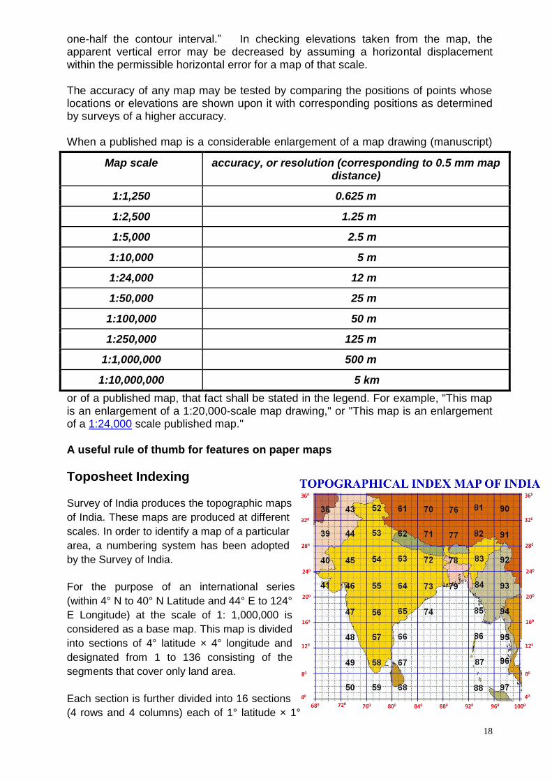
When a published map is a considerable enlargement of a map drawing (manuscript)

or of a published map, that fact shall be stated in the legend. For example, "This map is an enlargement of a 1:20,000-scale map drawing," or "This map is an enlargement of a 1:24,000 scale published map."

A useful rule of thumb for features on paper maps

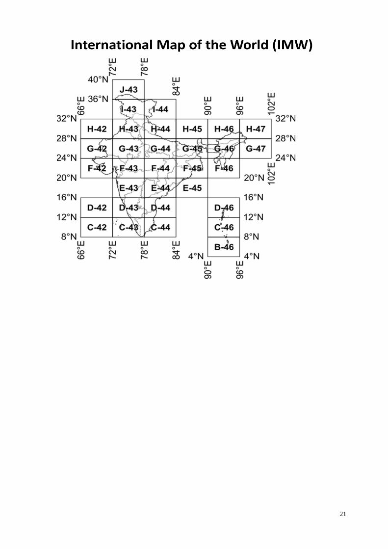
Toposheet Indexing

Survey of India produces the topographic maps

of India. These maps are produced at different

scales. In order to identify a map of a particular

area, a numbering system has been adopted

by the Survey of India.

For the purpose of an international series

(within 4° N to 40° N Latitude and 44° E to 124°

E Longitude) at the scale of 1: 1,000,000 is

considered as a base map. This map is divided

into sections of 4° latitude × 4° longitude and

designated from 1 to 136 consisting of the

segments that cover only land area.

Each section is further divided into 16 sections

(4 rows and 4 columns) each of 1° latitude × 1°

Map scale accuracy, or resolution (corresponding to 0.5 mm map distance)

1:1,250 0.625 m

1:2,500 1.25 m

1:5,000 2.5 m

1:10,000 5 m

1:24,000 12 m

1:50,000 25 m

1:100,000 50 m

1:250,000 125 m

1:1,000,000 500 m

1:10,000,000 5 km

19

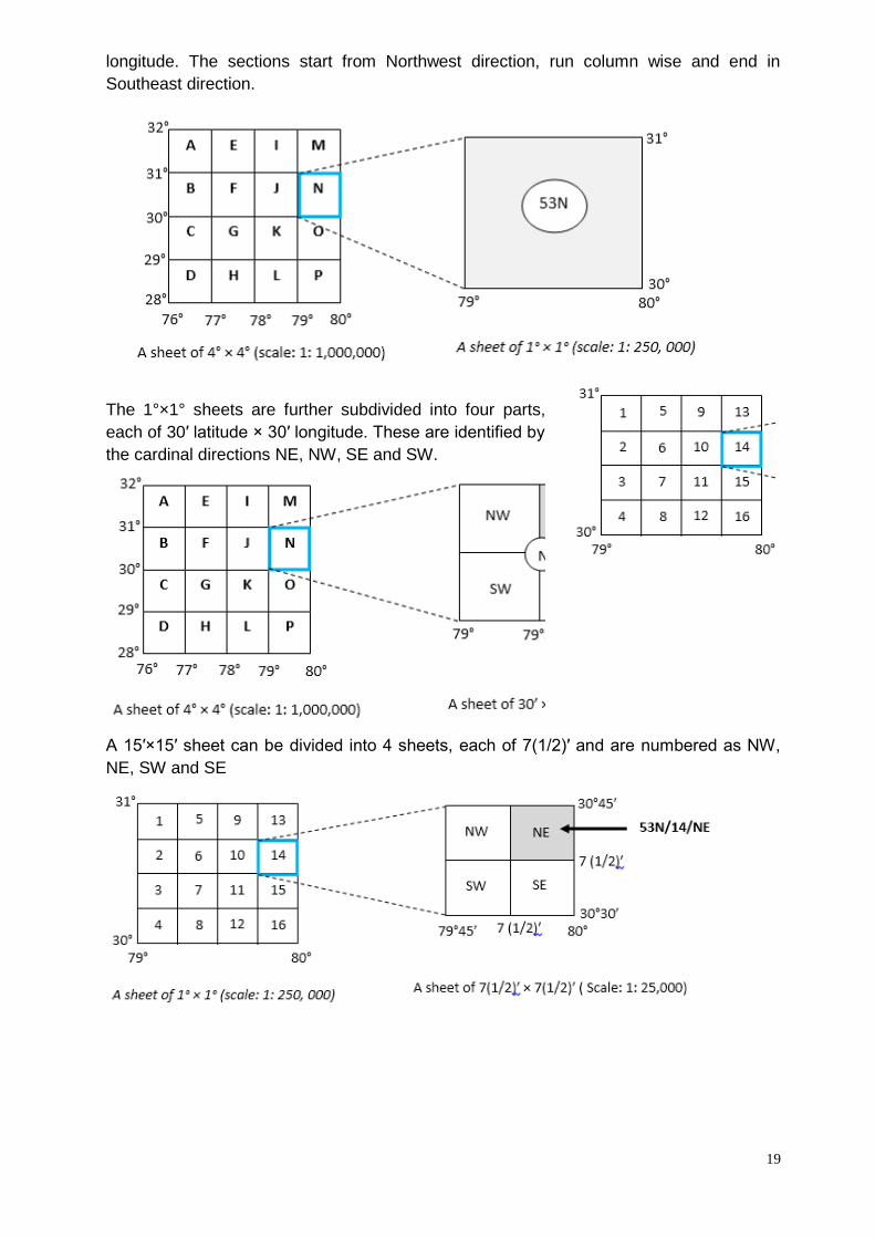
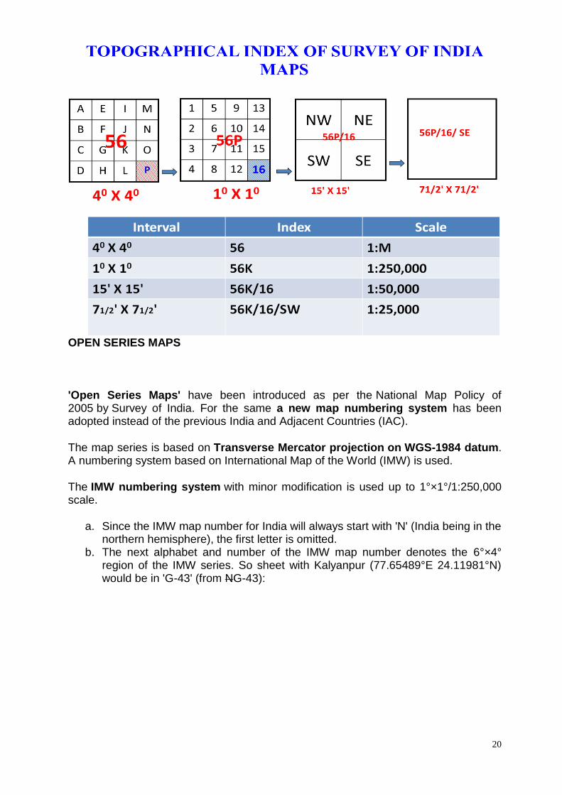
longitude. The sections start from Northwest direction, run column wise and end in

Southeast direction.

The 1°×1° sheets are further subdivided into four parts,

each of 30′ latitude × 30′ longitude. These are identified by

the cardinal directions NE, NW, SE and SW.

A 15′×15′ sheet can be divided into 4 sheets, each of 7(1/2)′ and are numbered as NW,

NE, SW and SE

20

OPEN SERIES MAPS

'Open Series Maps' have been introduced as per the National Map Policy of 2005 by Survey of India. For the same a new map numbering system has been adopted instead of the previous India and Adjacent Countries (IAC).

The map series is based on Transverse Mercator projection on WGS-1984 datum. A numbering system based on International Map of the World (IMW) is used.

The IMW numbering system with minor modification is used up to 1°×1°/1:250,000 scale.

a. Since the IMW map number for India will always start with 'N' (India being in the northern hemisphere), the first letter is omitted.

b. The next alphabet and number of the IMW map number denotes the 6°×4° region of the IMW series. So sheet with Kalyanpur (77.65489°E 24.11981°N) would be in 'G-43' (from NG-43):

21

22

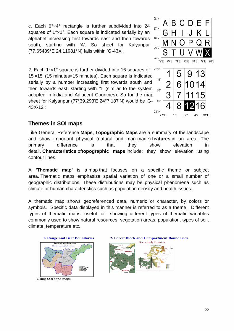
c. Each 6°×4° rectangle is further subdivided into 24

squares of 1°×1°. Each square is indicated serially by an

alphabet increasing first towards east and then towards

south, starting with 'A'. So sheet for Kalyanpur

(77.65489°E 24.11981°N) falls within 'G-43X':

2. Each 1°×1° square is further divided into 16 squares of

15'×15' (15 minutes×15 minutes). Each square is indicated

serially by a number increasing first towards south and

then towards east, starting with '1' (similar to the system

adopted in India and Adjacent Countries). So for the map

sheet for Kalyanpur (77°39.293'E 24°7.187'N) would be 'G-

43X-12':

Themes in SOI maps

Like General Reference Maps, Topographic Maps are a summary of the landscape

and show important physical (natural and man-made) features in an area. The

primary difference is that they show elevation in

detail. Characteristics oftopographic maps include: they show elevation using

contour lines.

A 'Thematic map' is a map that focuses on a specific theme or subject

area. Thematic maps emphasize spatial variation of one or a small number of

geographic distributions. These distributions may be physical phenomena such as

climate or human characteristics such as population density and health issues.

A thematic map shows georeferenced data, numeric or character, by colors or

symbols. Specific data displayed in this manner is referred to as a theme. Different

types of thematic maps, useful for showing different types of thematic variables

commonly used to show natural resources, vegetation areas, population, types of soil,

climate, temperature etc.,

23

Chapter – II

Information technology

కంప్యూటర్ 3కంప్యూటర్ ఆవశ్యకత – చరిత్ర : నేడు కంప్యూటర్ చేయని పని ఏదియూ లేదనుటలో అసత్యము లేదు .కంప్యూటర్

అనునది మానవ జీవన వ్యవస్థలో పెద్దపీఠ వేసికొనినది.

కంప్యూటర్ అనగా లెక్కవేయు సాధనము .కానీ అది లెక్కలు వేయుట తో మొదలుపెట్టి

కాలక్రమేణా అభివృద్ది చెంది మానవుడు చేయు పనులన్నియు చేయగల స్థితికి చేరినది .

మొదటగా దీనిని తయారు చేయునపుడు లెక్కలు చేయుట , తదుపరి టైపింగ్, తదుపరి ఎక ంట్లు,

డాటాబేస్, ప్రింటింగ్, ఆడియో, విడియో చివరకు రోబోట్లుగా అవతరించింది .పరిణామములో

మొదటగా భవన పరిమాణములో ఉండి , ఇప్పుడు చేతిలో ఇమిడే ఫోనుగా మారినది .సామర్ధ్యము

మొదట కె.బి.లలో ఉండి , ఇప్పుడు టి .బి.లలోకి వచ్చినది .ఖరీదు అతి సామాన్యుడు కూడా వాడుటకు

వీలు కలుగుచున్నది .ప్రతి రోజు లేచినపుడు చూసుకొనే డిజిటల్ వాచ్ , టి .వి. , వాషింగ్ మెషీన్,

మొబైల్ ఫోన్, ఏ .టి.ఏమ్ లు , బ్యాంకులు, ఆసుపత్రి, diagnostic Centre, బి .పి .షుగర్ చూచుకొను

మెషీన్లు, బస్సుటికెట్, రైల్ టికెట్, చ కధరల దుకాణములు, ఓటరు కార్డులు, ఆధార్

కార్డులు, కరెంటు బిల్లు, టెలిఫోన్ బిల్లు చివరకు దేవుని దర్శనమునకు టికెట్లు కూడా

కంప్యూటర్ ఉపయోగించుచున్నారు .

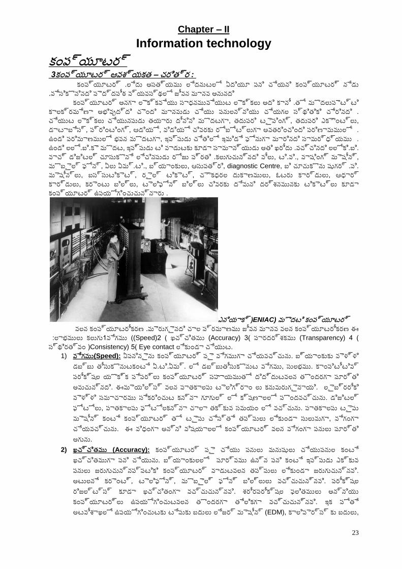
ఎనియాక్ (ENIAC) మొదటి కంప్యూటర్

ఈ కంప్యూటరీకరణ వలన మానవ జీవన ప్రమాణము చాల మెరుగైనది .కంప్యూటరీకరణ వలన

కలుగు లాభములు : 1 )వేగము (Speed) 2 ) ఖచ్చితము (Accuracy) 3) పారదర్శకము (Transparency) 4 )

స్థిరత్వం (Consistency) 5) Eye contact లేకుండా చేయుట.

1) వేగము(Speed): ఏపనినైను కంప్యూటర్ పై వేగముగా చేయవచ్చును. బ్యాంకుకు వెళ్ళి

డబ్బు తీసుకొనుటకంటే ఏ.టి.ఏమ్. లో డబ్బుతీసుకొనుట వేగము, సులభము. కాంపిటీటివ్

పరీక్షల యొక్క పేపర్లు కంప్యూటర్ సహాయముతో దిద్దుటవలన తొందరగా పూర్తి

అవుచున్నది. ఈమెయిల్స్ వలన పాతకాలపు టెలిగ్రాం లు కనుమరుగైనాయి. లైబ్రరీకి

వెళ్ళి సమాచారము సేకరించుట కన్నా గూగుల్ లో క్షణాలలో పొందవచ్చును. డిజిటల్

ఫోటోలు, పాతకాలపు ఫోటోలకన్నా చాలా తక్కువ సమయం లో వచ్చును. పాతకాలపు టైపు

మెషీన్ కంటే కంప్యూటర్ తో టైపు చేస్తే తప్పులు లేకుండా సులువుగా, వేగంగా

చేయవచ్చును. ఈ విధంగా అన్ని విషయాలలో కంప్యూటర్ వలన వేగంగా పనులు పూర్తి

అగును.

2) ఖచ్చితము (Accuracy): కంప్యూటర్ పై చేయు పనులు మనుషులు చేయుపనుల కంటే

ఖచ్చితముగా పని చేయును. బ్యాంకులలో పూర్వము ఉన్న పని కంటే ఇప్పుడు ఎక్కువ

పనులు జరుగుచున్నప్పటికి కంప్యూటర్ వాడుటవలన తప్పులు లేకుండా జరుగుచున్నవి.

అటులనే కరెంట్, టెలిఫోన్, మొబైల్ ఫోన్ బిల్లులు వచ్చుచున్నవి. పరీక్షల

రిజల్ట్స్ కూడా ఖచ్చితంగా వచ్చుచున్నవి. శరీరపరీక్షల ఫలితములు అన్నియు

కంప్యూటర్లు ఉపయోగించుటవలన తొందరగా తేలికగా వచ్చుచున్నవి. ఇక పోతే

అటవీశాఖలో ఉపయోగించుటకు టేపుకు బదులు లేజర్ మెషీన్ )EDM), కాలిపెర్స్ కు బదులు,

24

Abney level కు బదులు, Compass కు బదులు క్రొత్త, క్రొత్త ఎలక్ట్రానిక్ పరికరములు

వచ్చినవి. ఇవి మనుష్యులకంటే ఖచ్చితంగా పని చేయుచున్నవి.

3) పారదర్శకము (Transparency): పాతకాలమందు ఏ విషయము పూర్తిగా తెలిసేవి కాదు కదా,

కంప్యూటర్ వాడుటవలన పారదర్శకముగా నుండును. పరీక్ష ఫలితములు గానీ, ఉద్యోగ

నియామకములలో గానీ, నగదు మార్పిడి, కొనుగోళ్ళు విషయములుగాని మనము అవసరమైనచో

విపులంగా చూడవచ్చును. ఇందువలననే ఇప్పుడు భారత దేశములో ప్రభుత్వం అన్ని శాఖలను,

అన్ని వ్యాపార, బ్యాంకుల లావాదేవీలను కంప్యూటరీకరించుటకు నిశ్చయించినది.

దీనవలన టాక్స్ ఎగవేత దారులు, బ్లాక్ మార్కెట్ వ్యవహారాలు కట్టడిలో నుండును.

4) స్థిరత్వం (Consistency): కంప్యూటర్లు వాడక ముందు ఒకే సమాచారము వివిధ

విభాగములలో వేరు వేరుగా నుండెడిది. సమాచారము ఫారెస్టు గార్డ్ నుండి ఫారెస్టరు,

రే౦జి అధికారి, డివిజన్ అటవీ అధికారి, అటవీ సంరక్షణాధికారి, ముఖ్య ప్రధాన అటవీ

సరక్షణాధికారి వారికి చేరునప్పటికి చాలా కాలము గడచేది. ఇందువలన సమాచారము వివిధ

భాగములలో వేరు వేరుగా నుండెడిది. కాని కంప్యూటర్లు వాడుకలో ఎప్పటికప్పుడు

సమాచారము అప్ డేట్ అగుచున్నది. ఇటులనే రైలు టికెట్టు ఎక్కడ కొనునప్పటికి ఖాళీ

బెర్తుల సమాచారము కరెక్టుగా ఉండుటచే తేడాలు లేకుండా బుక్ చేయగలము.

5) Eye contact లేకుండా చేయుట: ప్రభుత్వ శాఖలలో పనులు చేయుటకు వివిధ వ్యక్తులను

కలువ వలసి వచ్చేది. దీని వలన ఆవ్యక్తుల యొక్క ఇష్టా ఇష్టాలపై పనులు జరిగేవి.

ఇప్పుడు కంప్యూటర్లు వాడకము వలన, వ్యక్తుల ప్రమేయం లేకుండా పనులు

జరుగుచున్నవి.

ఉదా :లైసెన్సులు , పాస్ పోర్టులు, పర్మిషన్లు వగైరాలు .దీ నినే ఈ-

గవర్నెస్ అందురు.

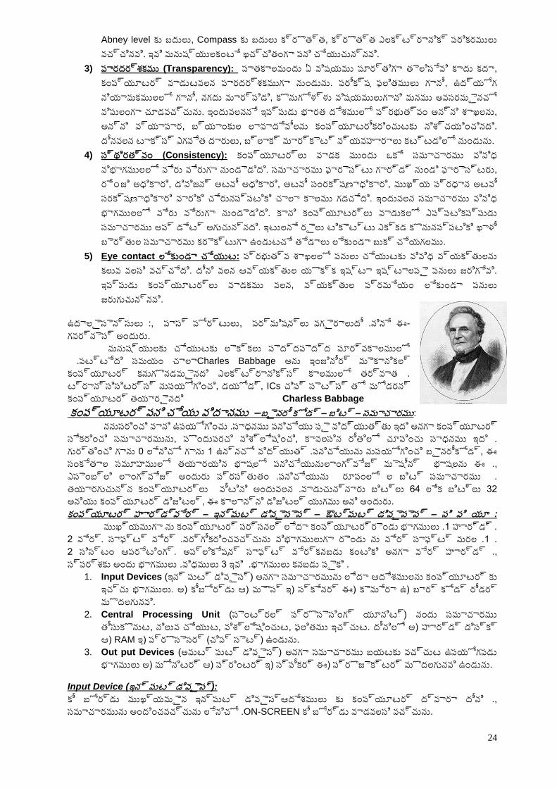
పూర్వకాలములో పెద్దపెద్ద లెక్కలు చేయుటకు మనుష్యులకు

చాలా సమయం పట్టేది . Charles Babbage అను ఇంజినీర్ మెకానికల్

కంప్యూటర్ కనుగొనడమైనది .తర్వాత కాలములో ఎలక్ట్రానిక్స్

నుపయోగించి ట్రాన్సిసిటర్స్ , డయోడ్, ICs చిప్ సెట్స్ తో మోడరన్

కంప్యూటర్ తయారైనది Charless Babbage

కంప్యూటర్ పని చేయు విదానము –బైనరీ కోడ్ – బిట్ – సమాచారము:

కంప్యూటర్ అనగా ఇది విద్యుత్తు పై పనిచేయు సాధనము .ఉపయోగించు వాని ననుసరించి

సమాచారమును సేకరించి , పొందుపరచి విశ్లేషించి, కావలసిన రీతిలో చూపించు సాధనము .ఇది

బైనరీకోడ్ నుపయోగించి పనిచేయును .విద్యుత్ ఉన్నచో 1 గాను లేనిచో 0 గాను గుర్తించి , ఈ

సంకేతాల సమూహములో తయారయిన భాషలో పనిచేయును .ఈ భాషలను మెషీన్ లాంగ్వేజ్ ,

ఎసెంబ్లి లాంగ్వేజ్ అందురు .సమాచారము బిట్ ల రూపంలో పనిచేయును .ప్రస్తుతం

తయారగుచున్న కంప్యూటర్లు 32 బిట్లు లేక 64 బిట్లు వాడుచున్నారు .అందువలన వీటిని

డిజిటల్ కంప్యూటర్ అనియు , ఈ కాలాన్ని డిజిటల్ యుగము అని అందురు.

కంప్యూటర్ హార్డ్వేర్ – ఇన్పుట్ డివైసెస్ – ఔట్పుట్ డివైసెస్ – సి పి యూ :

కంప్యూటర్ లేదా పర్సనల్ కంప్యూటర్ ను ముఖ్యముగా రెండు భాగములు .1 .హార్డ్

వేర్ 2 . సాఫ్ట్ వేర్ .మరల సాఫ్ట్ వేర్ ను రెండు విభాగములుగా వర్గీకరించవచ్చును . 1 .

ఆపరేటింగ్ సిస్టం 2 . అప్లికేషన్ సాఫ్ట్ వేర్ .హార్డ్ వేర్ అనగా కంటికి కనబడు ,

స్పర్శకు అందు భాగములు .పైకి కనబడు భాగములు .ఇవి 3 విధములు .

1. Input Devices (ఇన్ పుట్ డివైస్) అనగా సమాచారమును లేదా ఆదేశములను కంప్యూటర్ కు

ఇచ్చు భాగములు. అ( కీబోర్డు ఆ( మ స్ ఇ( స్కేనర్ ఈ( కెమేరా ఉ( బార్ కోడ్ రీడర్

మొదలగునవి.

2. Central Processing Unit (సెంట్రల్ ప్రొసెసింగ్ యూనిట్) నందు సమాచారము

తీసుకొనుట, నిలువ చేయుట, విశ్లేషించుట, ఫలితము ఇచ్చుట. దీనిలో అ( హార్డ్ డిస్క్

ఆ( RAM ఇ( ప్రొసెసర్ )చిప్ సెట్( ఉండును.

3. Out put Devices (అవుట్ పుట్ డివైస్) అనగా సమాచారము బయటకు వచ్చుట ఉపయోగపడు

భాగములు అ( మోనిటర్ ఆ( ప్రింటర్ ఇ( స్పీకర్ ఈ( ప్రొజెక్టర్ మొదలగునవి ఉండును.

Input Device (ఇన్ పుట్ డివైస్):

కీ బోర్డు ముఖ్యమైన ఇన్పుట్ డివైస్ .దీని ద్వారా కంప్యూటర్ కు ఆదేశములు ,

సమాచారమును అందించవచ్చును .లేనిచో ON-SCREEN కీ బోర్డు వాడవలసి వచ్చును.

25

రెండవ

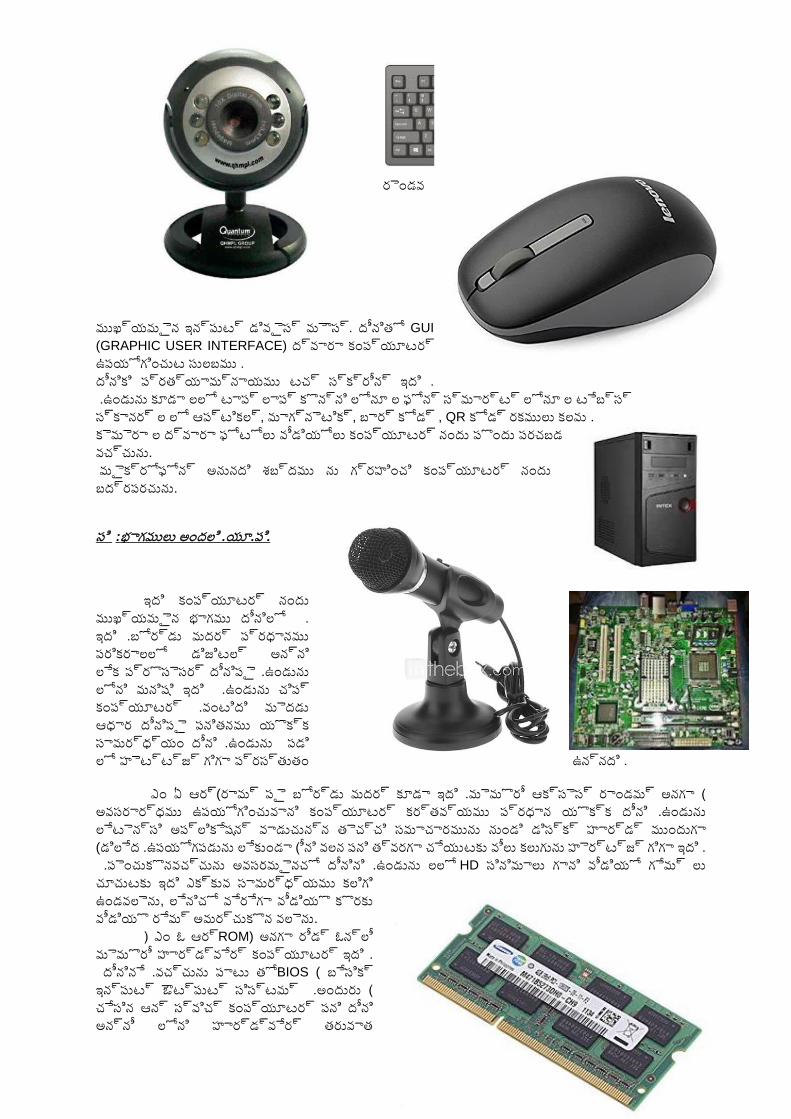
ముఖ్యమైన ఇన్పుట్ డివైస్ మ స్. దీనితో GUI

(GRAPHIC USER INTERFACE) ద్వారా కంప్యూటర్

ఉపయోగించుట సులబము .

దీనికి ప్రత్యామ్నాయము టచ్ స్క్రీన్ .ఇది

టేబ్స్ ల లోనూ స్మార్ట్ ఫోన్ ల లోనూ కొన్ని లాప్ టాప్ లలో కూడా ఉండును .

స్కానర్ ల లో ఆప్టికల్, మాగ్నెటిక్, బార్ కోడ్ , QR కోడ్ రకములు కలవు .

కెమెరా ల ద్వారా ఫోటోలు వీడియోలు కంప్యూటర్ నందు పొందు పరచబడ

వచ్చును.

మైక్రోఫోన్ అనునది శబ్దము ను గ్రహించి కంప్యూటర్ నందు

బద్రపరచును.

సి :భాగములు అందలి .యూ.పి.

ఇది కంప్యూటర్ నందు

ముఖ్యమైన భాగము .దీనిలో

ప్రధానము మదర్ బోర్డు .ఇది

అన్ని డిజిటల్ పరికరాలలో

ఉండును .దీనిపై ప్రొసెసర్ లేక

చిప్ ఉండును .ఇది మనిషి లోని

మెదడు వంటిది .కంప్యూటర్

యొక్క పనితనము దీనిపై ఆధార

పడి ఉండును .దీని సామర్ధ్యం

ప్రస్తుతం గిగా హెట్ట్జ్ లో ఉన్నది .

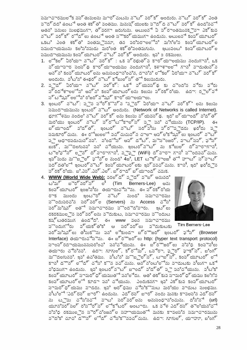
ఆర్ ఏ ఎం (రామ్ )అనగా రాండమ్ ఆక్సెస్ మెమొరీ .ఇది కూడా మదర్ బోర్డు పై

ఉండును .దీని యొక్క ప్రధాన కర్తవ్యము కంప్యూటర్ ఉపయోగించువాని అవసరార్ధము

ముందుగా హార్డ్ డిస్క్ నుండి సమాచారమును తెచ్చి వాడుచున్న అప్లికేషన్ లేటెన్సి

(డిలే )లేకుండా ఉపయోగపడును .ద ీని వలన పని త్వరగా చేయుటకు వీలు కలుగును .ఇది గిగా హెర్ట్జ్

లలో ఉండును .దీనిని అవసరమైనచో పెంచుకొనవచ్చును . HD సినిమాలు గాని వీడియో గేమ్ లు

చూచుటకు ఇది ఎక్కువ సామర్ధ్యము కలిగి

ఉండవలెను, లేనిచో వేరేగా వీడియొ కొరకు

వీడియొ రేమ్ అమర్చుకొన వలెను.

ఆర్ ఓ ఎం ( ROM) అనగా రీడ్ ఓన్లీ

మెమొరీ .ఇది కంప్యూటర్ హార్డ్వేర్

తో పాటు వచ్చును .దీనినే BIOS ( బేసిక్

ఇన్పుట్ ఔట్పుట్ సిస్టమ్ )అందురు .

దీని పని కంప్యూటర్ స్విచ్ ఆన్ చేసిన

తరువాత హార్డ్వేర్ లోని అన్నీ

26

భాగములు ఉత్తేజ పరచి ఆపరేటింగ్ సిస్టమ్ ను ఆక్టివేట్ చేయును .దీనినే ఫర్ మ్ వేర్

అనికూడా అందురు.

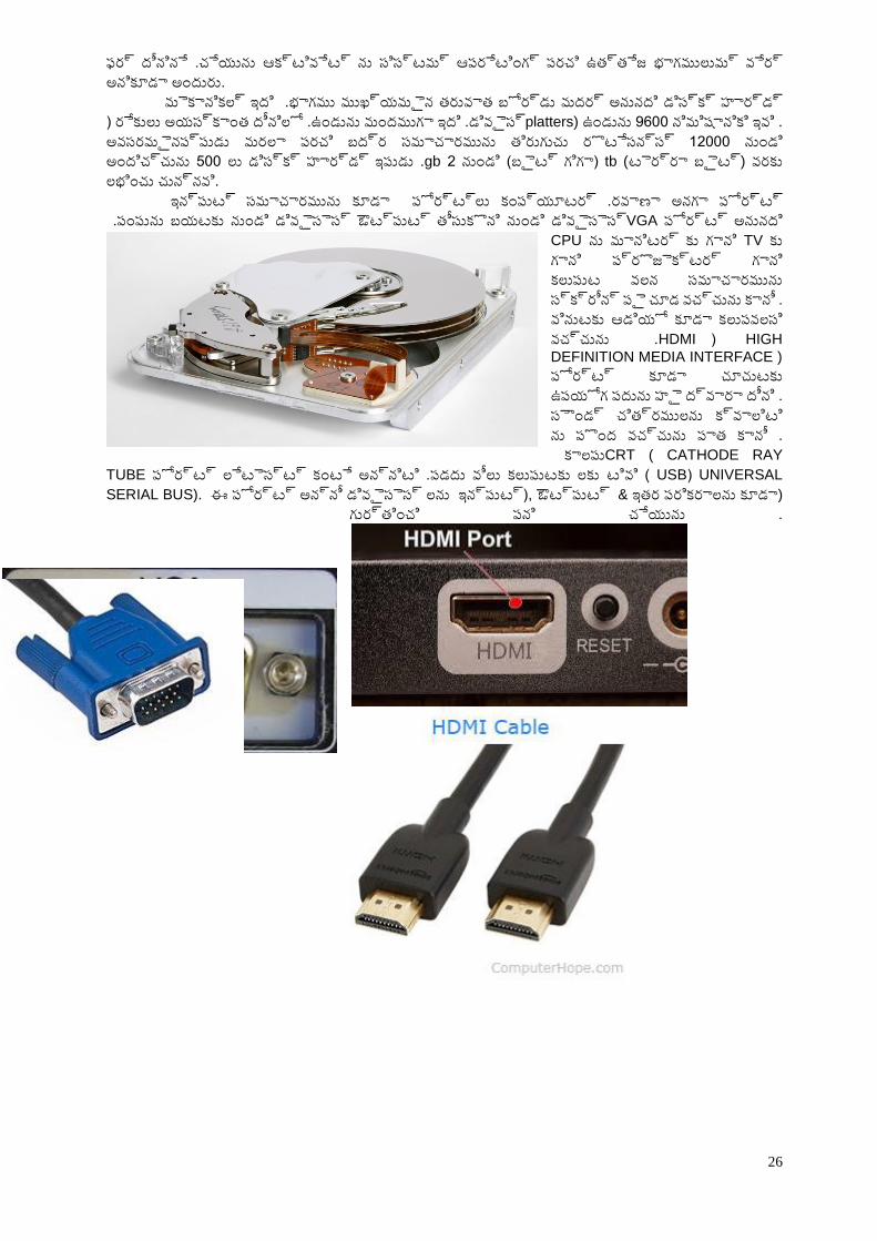
హార్డ్ డిస్క్ అనునది మదర్ బోర్డు తరువాత ముఖ్యమైన భాగము .ఇది మెకానికల్

డివైస్ .ఇది మందముగా ఉండును .దీనిలో అయస్కాంత రేకులు ( platters) ఉండును .ఇవి నిమిషానికి 9600

నుండి 12000 రొటేసన్స్ తిరుగుచు సమాచారమును బద్ర పరచి మరలా అవసరమైనప్పుడు

అందిచ్చును .ఇపుడు హార్డ్ డిస్క్ లు 500 gb (గిగా బైట్ )నుండి 2 tb (టెర్రా బైట్) వరకు

లభించు చున్నవి.

పోర్ట్ అనగా రవాణా .కంప్యూటర్ పోర్ట్లు కూడా సమాచారమును ఇన్పుట్

డివైసెస్ నుండి తీసుకొని ఔట్పుట్ డివైసెస్ నుండి బయటకు పంపును . VGA పోర్ట్ అనునది

CPU ను మానిటర్ కు గాని TV కు

గాని ప్రొజెక్టర్ గాని

కలుపుట వలన సమాచారమును

స్క్రీన్ పై చూడ వచ్చును .కానీ

వినుటకు ఆడియో కూడా కలుపవలసి

వచ్చును .HDMI ( HIGH

DEFINITION MEDIA INTERFACE )

పోర్ట్ కూడా చూచుటకు

ఉపయోగ పదును .దీని ద్వారా హై

క్వాలిటి చిత్రములను స ండ్

ను పొంద వచ్చును .కానీ పాత

కాలపు CRT ( CATHODE RAY

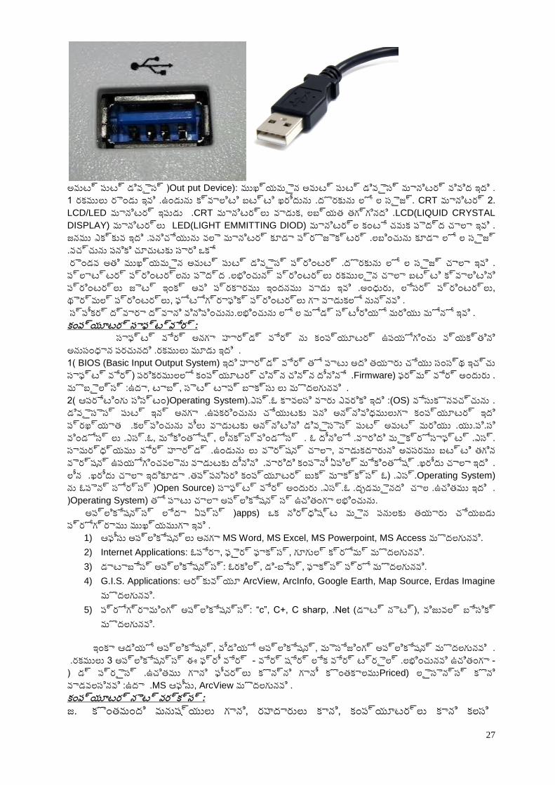
TUBE )విటి లకు కలుపుటకు వీలు పడదు .అన్నిటి కంటే లేటెస్ట్ పోర్ట్ USB ( UNIVERSAL

SERIAL BUS). ఈ పోర్ట్ అన్నీ డివైసెస్ లను (ఇన్పుట్ , ఔట్పుట్ & ఇతర పరికరాలను కూడా)

గుర్తించి పని చేయును .

27

అవుట్ పుట్ డివైస్ (Out put Device): ముఖ్యమైన అవుట్ పుట్ డివైస్ మానిటర్ .ఇది వివిద

సైజ్ ల లో దొరకును .ఖరీదును బట్టి క్వాలిటి ఉండును .ఇవి రెండు రకములు 1 . CRT మానిటర్ 2.

LCD/LED మానిటర్ .ఇపుడు CRT మానిటర్లు వాడుక, లబ్యత తగ్గినది .LCD(LIQUID CRYSTAL

DISPLAY) మానిటర్లు LED(LIGHT EMMITTING DIOD) మానిటర్ల కంటే చవుక .ఇవి చాలా పెద్ద

సైజ్ ల లో కూడా లబించును .ప్రొజెక్టర్ కూడా మానిటర్ వలె పనిచేయును .ఇది ఎక్కువ జనము

ఒకే సారి చూచుటకు పనికి వచ్చును.

రెండవ అతి ముఖ్యమైన అవుట్ పుట్ డివైస్ ప్రింటర్ .ఇవి చాలా సైజ్ ల లో దొరకును .

క్వాలిటిని బట్టి చాలా రకములైన ప్రింటర్లు లభించున్ .పెద్ద ప్రింటర్లను ప్లాట్టర్

అంధురు .ఇవి వాడు ఇందనము ప్రకారము అవి ఇంక్ జెట్ ప్రింటర్లు , లేసర్ ప్రింటర్లు,

థెర్మల్ ప్రింటర్లు, ఫోటోగ్రాఫిక్ ప్రింటర్లు గా వాడుకలో నున్నవి .

స్పీకర్ ద్వారా ద్వాని వినిపించును .ఇవి మోనో మరియు స్టీరియో మోడ్ ల లో లభించును.

కంప్యూటర్ సాఫ్ట్వేర్ :

సాఫ్ట్ వేర్ అనగా హార్డ్ వేర్ ను కంప్యూటర్ ఉపయోగించు వ్యక్తిని

అనుసంధాన పరచునది .ఇది మూడు రకములు .

1) BIOS (Basic Input Output System) ఇది హార్డ్ వేర్ తో పాటు అది తయారు చేయు సంస్థ ఇచ్చు

సాఫ్ట్ వేర్ .దీనినే చిన్న చిన్న కంప్యూటర్ పరికరములలో ( Firmware) ఫర్మ్ వేర్ అందురు .

ఉదా :మొబైల్స్ , టాబ్, సెట్ టాప్ బాక్సు లు మొదలగునవి .

2) ఆపరేటింగు సిస్టం(Operating System) :ఇది ఎవరికి వారు కావలసి ఓ.ఎస్. (OS) వేసుకొనవచ్చును .

ఇది కంప్యూటర్ అన్నివిధములుగా పని చేయుటకు ఉపకరించును .అనగా ఇన్ పుట్ డివైసెస్

సి.పి.యు .మరియు అవుట్ పుట్ డివైసెస్ అన్నిటిని వాడుటకు వీలు కల్పించును .ప్రఖ్యాత

ఓ.ఎస్ .లు విండోస్ , మేకింతోష్, లీనక్స్ .విండోస్ ఓ .ఎస్ .మైక్రోసాఫ్ట్ వారిది .దీనిలో

చాలా వెర్షన్ లు ఉండును .హార్డ్ వేర్ సామర్ధ్యము , వాడుకదారుని అవసరము బట్టి తగిన

వెర్షన్ ఉపయోగించవలెను .ఇది చాలా ఖరీదు .మేకింతోష్ ఏపిల్ కంపెనీ వారిది .దీనిని వాడుటకు

మాక్ బుక్ కంప్యూటర్ తప్పనిసరి .ఇదికూడా చాలా ఖరీదు .లీన క్స్ ఓ .ఎస్( . Operating System)

ను ఓపెన్ సోర్స్ (Open Source) సాఫ్ట్ వేర్ అందురు .ఇది ఉచితము .చాల దృడమైనది .ఓ.ఎస్ .

(Operating System) తో పాటు చాలా అప్లికేషన్ స్ ఉచితంగా లభించును.

అప్లికేషన్స్ లేదా ఏప్స్ (apps) ఒక నిర్ధిష్ట మైన పనులకు తయారు చేయబడు

ప్రోగ్రాము .ఇవి ముఖ్యముగా

1) ఆఫీసు అప్లికేషన్లు అనగా MS Word, MS Excel, MS Powerpoint, MS Access మొదలగునవి.

2) Internet Applications: ఓపేరా, ఫైర్ ఫాక్స్, గూగుల్ క్రోమ్ మొదలగునవి.

3) డాటాబేస్ అప్లికేషన్స్: ఓరకిల్, డి-బేస్, ఫాక్స్ ప్రో మొదలగునవి.

4) G.I.S. Applications: ఆర్కువ్యూ ArcView, ArcInfo, Google Earth, Map Source, Erdas Imagine

మొదలగునవి.

5) ప్రోగ్రామింగ్ అప్లికేషన్స్: “c”, C+, C sharp, .Net (డాట్ నెట్(, విజువల్ బేసిక్

మొదలగునవి.

ఇంకా ఆడియో అప్లికేషన్, వీడియో అప్లికేషన్, మెసేజింగ్ అప్లికేషన్ మొదలగునవి .

ఈ అప్లికేషన్స్ 3 రకములు . ఫ్రీ వేర్ - ఉచితంగా లభించునవి .ట్రైల్ వేర్ లేక షేర్ వేర్ -

కొంతకాలము గానీ కొన్ని ఫీచర్లు గాని ఉచితము .ప్రైస్ డ్ ( Priced) లైసెన్స్ కొని

వాడవలసినవి .ఉదా : MS ఆఫీసు, ArcView మొదలగునవి .

కంప్యూటర్ నెట్ వర్క్స్ :

జ. కొంతమంది మనుష్యులు గాని, రహదారులు కాని, కంప్యూటర్లు కాని కలసి

28

సమాచారములేక వస్తువులను మార్చుటను నెట్ వర్క్ అందురు. నెట్ వర్క్ ఎంత

పెద్దది ఉంటే అంత శక్తి వంతము. మనుష్యులకు పెద్ద నెట్ వర్క్ ఉండినచో

అతని పనులు సులభముగా, త్వరగా జరుగును. అటులనే ఏ ప్రాంతమునకైనా ఎక్కువ

నెట్ వర్క్ రోడ్లు ఉంటే అంత స కర్యముగా ఉండును. అటులనే కంప్యూటర్

ఒకటి ఎంత శక్తి వంతమైననూ, తన పరిసరాలలోని మిగిలిన కంప్యూటర్ల

సముదాయమును కలిసినపుడు మరింత శక్తివంతమగును. ఇటువంటి కంప్యూటర్ల

సముదాయమును కంప్యూటర్ నెట్ వర్క్ అందురు. ఇవి ౩ రకములు.

1. లోకల్ ఏరియా నెట్ వర్క్ : ఒక ప్రభుత్వ కార్యాలయము నందుగానీ, ఒక

వ్యాపార సంస్థ కార్యాలయము నందుగానీ, కళాశాలలో గానీ వాడుతున్న

అన్ని కంప్యూటర్లను అనుసంధానించిన, దానిని లోకల్ ఏరియా నెట్ వర్క్

అందురు. వీటిని ఈథర్ నెట్ కేబుల్స్ తో కలుపుదురు.

2. వైడ్ ఏరియా నెట్ వర్క్: ఒకే వ్యవస్థ కు చెందిన వేరు వేరు

ప్రదేశాలలోని అన్ని కంప్యూటర్లను కలుపు ప్రక్రియ. ఉదా: రైల్వే

స్టేషన్లలోని రిజర్వేషన్ కార్యాలయాలు.

3. ఇంటర్ నెట్: పైన పేర్కొన్న “వైడ్ ఏరియా నెట్ వర్క్” లను కలుపు

సముదాయమును ఇంటర్ నెట్ అందురు. )Network of Networks is called Internet).

భూగోళము నందలి నెట్ వర్క్ లను కలుపు వ్యవస్థ. ఇది బ్యాండ్ విడ్త్

మరియు ఇంటర్ నెట్ ప్రోటోకాల్స్ పై పని చేయును )TCP/IP). ఈ

బ్యాండ్ విడ్త్, ఇంటర్ నెట్ సర్వీసు ప్రొవైడరు ఖరీదు పై

సమకూర్చును. ఈ రోజులలో వచ్చుచున్న చాలా అప్లికేషన్లు ఇంటర్ నెట్

పై ఆధారపడుచున్నవి. విండోస్ అప్ డేట్, మెసెంజర్, వాట్సప్, ఫేస్

బుక్, మొదలగునవి పని చేయును. ఇంటర్నెట్ ను కేబుల్ ద్వారాగానీ,

టెలిఫోన్ లైన్ ద్వారాగానీ, వైఫై )WiFi) ద్వారా గానీ పొందవచ్చును.

ఇప్పుడు మొబైల్ ఫోన్ల నుండి 4జి, LET టెక్నాలజీ తో హాట్ స్పాట్

పద్దతిలో ఇంటర్నెట్ కంప్యూటర్లకు ఇవ్వవచ్చును. కానీ, ఇది ఖరీదైన

ప్రక్రియ. బి.ఎస్.ఎన్.ఎల్. బ్రాడ్ బ్యాండ్ చవుక.

4. WWW (World Wide Web): వరల్డ్ వైడ్ వెబ్ అనునది

టిమ్ బెర్నర్స్ లీ )Tim Berners-Lee) అను

కంప్యూటర్ ఇంజినీరు తయారుచేసెను. ఈ ప్రక్రియ

రాక ముందు ఇంటెర్ నెట్ నుండి సమాచారము

పొందుపరచిన సర్వర్ల )Servers) ను Access చేసి

పర్మిషన్ లతో సమాచారము పొందెడివారు. ఇట్లు

రకరకములైన సర్వర్లను వెదుకుట, సమాచారము పొందుట

కష్టతరముగ ఉండేది. ఈ www వలన సమాచారము

పొందుగోరు వ్యక్తికి ఆ సర్వర్లు వెదుకుటకు

పర్మిషన్లు తీసుకొను పని లేకుండా బ్ర జర్ ఇంటర్ ఫేస్ )Browser

Interface) తయారుచేసెను. ఈ బ్ర జర్లు http: (hyper text transport protocol)

సాంప్రదాయముననుసరించి పనిచేయును. ఈ బ్ర జర్లు వివిధ కంపెనీలు

తయారు చేసినవి. ఉదా: గూగుల్, క్రోమ్, ఒపేరా, ఫైర్ ఫాక్స్, బింగ్

మొదలగునవి. ఇవి ఉచితము. వీటిని మొబైల్స్, టాబ్స్, కంప్యూటర్ లో

కానీ డ న్ లోడ్ చేసి కొన వచ్చును. అన్నింటిలోను వాడుటకు వీలుగా ఒకే

విధముగా ఉండును. ఇవి ఇంటర్నెట్ బాండ్ విడ్త్ పై పనిచేయును. వీటికి

కంప్యూటర్ సామర్ధ్యముతో పనిలేదు. అతి తక్కువ సామర్ధ్యము కలిగిన

కంప్యూటర్లో కూడా పని చేయును. ఎందుకనగా ఇవి ఎక్కువ కంప్యూటర్

సామర్ధ్యము వాడదు. ఇవి అర్ధము చేసికొనుట మరియు వాడుట సులభము.

వీటిలో ‘ఎడ్రస్ బార్’ ఉండును. ఎడ్రస్ బార్ నందు మనకు కావలసిన ఎడ్రస్

ను టైపు చేసినచో వాటి సర్వర్లను అనుసంధానించును. దీనినే )url)

యూనివర్సల్ రిసోర్స్ లోకేటర్ అంటారు. ఒక వేళ ఎడ్రస్ తెలియనిచో

వివిధ రకములైన సెర్చింజన్ల సహాయముతో మనకు కావలసిన సమాచారమును

వెదికి చూచి డ న్ లోడ్ చేసికొనవచ్చును. ఉదా: గూగుల్, యాహూ, బింగ్

29

మొదలైనవి. ఈ బ్ర జర్లలో కంప్యూటర్లలో చేయు అన్ని పనులను

చేయవచ్చును. అనగ ఆఫీసులో ఉపయోగించు వర్డ్, ఎక్సెల్, పవర్ పాయింట్,

మెయిల్ మొదలగునవి. అంతే కాక విడియోలు, పాటలు, మేప్ లు చూడవచ్చును.

ఈ విధముగా వరల్డ్ వైడ్ వెబ్ మానవాళికి ఎన్నో విధాలుగా

ఉపయోగపడుచున్నది.

ఉదా: మెయిల్స్, బ్యాంకు పనులు, చెల్లింపులు, ధరఖాస్తు ఫారాలు, పరీక్షా

ఫలితాలు, రైలు, బస్సు టికెట్స్, సర్టిఫికెట్స్, ఇన్ కంటాక్స్,

ఆరోగ్య విషయాలు, కావల్సిన వస్తువులు కొనుట మొదలైనవి.

ఆఫీసు అప్ప్లికేసన్స్:

1. Microsoft Office Suite: అన్ని కార్యాలయముల మాదిరి ఈ శాఖలో కూడా పి.సి. వాడుట చేత

దానిలో విండోస్ ఓ.ఎస్. ఉన్నది. దానిపై ఎం.ఎస్. ఆఫీసు అప్లికేషన్ సాఫ్ట్ వేర్ లోడ్

చేయడం జరిగింది. ఈ Suit లొ Word, Excel, Powerpoint వాడుచున్నారు. Word ను మెమోలు,

లెటర్లు, ఆర్డరులు మొదలగు కరస్పాండెన్సుకు వాడుచున్నారు. Excel ను సాలరీ స్టేట్

మెంట్లు, ఎస్టిమేట్లు, ప్రోగ్రెస్ రిపోర్ట్లు, బడ్జేట్ వివరములకు

వాడుచున్నారు. Power point ను మీటింగులలోను, డిమానిష్ట్రేషన్ లకు, లెక్చర్లకు

వాడుచున్నారు. MS Outlook ను తెలిసినవారు మైల్ కోసం వాడుచున్నారు.

జి .ఎస్.ఐ.& జి:అప్ప్లికేసన్స్ .ఎస్.పి.

2. G.I.S. Softwares: G.I.S. Software లు అటవీశాఖ ప్రధాన కార్యాలయమునందు మరియు

డివిజన్ కార్యాలయములందు వాడుచున్నారు. ప్రధాన కార్యాలయమునందు వాడు సాఫ్ట్

వేర్లు 1. Arc Info 2. ERDAS Imagine 3. Arc View డివిజనల్ కార్యాలయములందు ఆర్క్

వ్యూ వాడుచున్నారు.

1. Arc Info: ఈ సాఫ్ట్ వేర్ ను ESRI కంపెనీ వారిది. దీనిని ఉపయోగించి మ్యాప్ లకు

కావలసిన థీమ్స్ తయారు చేయవచ్చును. పాతమ్యాపులను స్కానింగ్ చేయుటద్వారా,

శాటిలైట్ నుండి వచ్చిన ఇన్ఫర్మేషన్ ద్వారా లేక GPS ద్వారా వచ్చిన డాటాతో

వివిధ రకములైన థీమ్స్ / లేయర్స్ తయారు చేయవచ్చును. దీనిని వాడుటకు బాగుగా

తర్ఫీదు పొందిన నిపుణులు అవసరము.

2. Arc View: ఈ సాఫ్ట్ వేర్ కూడా ESRI కంపెనీ వారిది. దీనితో G.I.S. మ్యాపులను చూచుట,

కలుపుట, మ్యాపులను ప్రింట్లు తీయుట చేయవచ్చును. దీనికి కొద్దిపాటి శిక్షణ,

Hands on Practice ఉన్న పని జరుపుకొనవచ్చును.

3. ERDAS Imagine: ఇది ERDAS )Earth Resources Digital Analysis System) కంపెనీవారిది. ఈ

సాఫ్ట్ వేర్ లో శాటిలైట్ నుండి వచ్చు డిజిటల్ ఇమేజి లను విశ్లేషించి కావలసిన

సమాచారమును పొ౦దవచ్చును. ఇది నైపుణ్యము తో కూడుకున్న పని. అటవీశాఖవారు ప్రతీ

సంవత్సరం IRS IC/ID LISS IV డాటాను కొని అటవీ సాంద్రతను బేరీజు వేయుదురు. అట్టి

బేరీజు వేసిన సమాచారముని మ్యాపులుగా ముద్రించి )Ground True thing) గ్ర ండ్

ట్రూతింగ్ కు అటవీ బీట్ లకు పంపుతారు. అచట కరెక్షన్ జరిగిన తరువాత అటవీ

సాంద్రతను ప్రకటించుతారు.

FMIS (Forest Management Information System): అటవీశాఖ నందు TCS వారి సహకారముతో ఈ

సాఫ్ట్ వేర్ ను తయారుచేసిరి .దీనిని ఎం.ఐ.ఎస్( . Management Information System) అని కూడా

అందురు .G.I.S. వలె ఇది కూడా సమాచార వ్యవస్థ .కానీ ఇందులో మ్యాపులు ఉండవు . M.I.S. అనునది

ఈ రోజులలో అన్ని ప్రభుత్వ, ప్రైవేటు కార్యాలయాలలో ఉండవలసిన వ్యవస్థ .ఈ

సాఫ్ట్ వేర్ వలన ప్లానింగ్ మరియు మోనిటరింగ్ చేయవచ్చును .దీనిలో బడ్జెట్ , ఖర్చులు,

వి .ఎస్.ఎస్.లు , వాటి పనులు, అడవులు, ప్లాంటేషన్స్, డిపోలు, అమ్మకాలు, సిబ్బంది వారి జీత

భత్యాలు, అటవీ రక్షణ, అటవీఫలసాయము మొదలగు అన్ని విషయములు సమీకరించి, క్రోడీకరించి

నిర్ణయములు తీసుకొనవచ్చును .ఈ సాఫ్ట్ వేర్ నందు భాగములు( Modules)

30

31

Chapter - III

Fundamentals of Geographical Information System

3.1 Introduction:

The field of geographic information systems (GISs) is emerging as one of

today’s most exciting and progressive technical areas. GIS technology has evolved

during the past four decades and is only now starting to penetrate major industry

and service hubs. With such a wide array of new users, there exists not only

considerable interest in GIS but also a fair amount of uncertainty and

misunderstanding surrounding the discipline. Now it had gained widespread

acceptance throughout the transportation, business, traffic control and land

information system. Its origin can be traced to some geographers who thought of

storing the maps in computers. In 1962 GIS came in operational mode with

sponsoring of Canadian Federal government. It got a tremendous boost after

personal computers came into existence in

1980’s. PCs came withi n the reach of common people because of falling prices.

GIS and Remote Sensing are major parts of the spatial information. Each is a

means to an end neither is an end nor itself.

Now-a-days, most government departments, business and even individuals

are taking GIS software like word processing etc. Over the years, the maintenance

and management of utilities has been dramatically improved by the use of

Geographical Information System.

3.2 Concept of GIS:

GIS is seen by many, as spatial tool information systems. Information is derived

from the interpretation of data, which are symbolic representations of geographic

features. The value of information depends upon many things including its timeliness,

the context in which it is applied and the cost of collection, storage, manipulation and

presentation. Information is now a valuable asset. It is a commodity which can be

bought and sold for a high price. Information and its communication is one of the key

development processes and characteristics of contemporary societies.

Geographic information systems arose from activities in four different fields:

Cartography, which attempted to automate the manually dependent map-

making process by substituting the drawing work by vector digitization.

Computer graphics, which had many applications of digital vector data apart

from cartography, particularly in the design of buildings, machines and

facilities.

Databases, which created a general mathematical structure according to

which the problems of computer graphics and computer cartography could

be handled.

Remote Sensing, which created immense amounts of digital image data

in need of geocoded rectification and analysis

3.3 Definition of GIS:

32

• Geographical implies that locations of the data items are known, or can be

calculated, in terms of Geographic coordinates (Latitude, Longitude)

• Information implies that the data in a GIS are organized to yield useful

knowledge, often as colored maps and images, but also as statistical

graphics, tables, and various on-screen responses to interactive queries.

• System implies that a GIS is made up from several inter-related and linked

components with different functions.

• Thus, GIS have functional capabilities for data capture, input,

manipulation, transformation, visualization, combinations, query, analysis,

modeling and output.

Other definitions of GIS

“A set of tools for collecting storing retrieving at will, transforming and

displaying data from the real world for a particular set of purposes.”

“An organized collection of hardware, software, geographic data, and

personnel designed to efficiently capture, more, update, analyze and

display all forms of geographically referenced information (ESRI).”

These are very general descriptions for such a complex and wide ranging set of

tools. GIS is, in essence, a central repository of and analytical tool for

geographic data collected from various sources. The

developer can overlay the information from these various sources by means of

themes and layers, perform comprehensive analysis of the data, and portray it

graphically for the user.

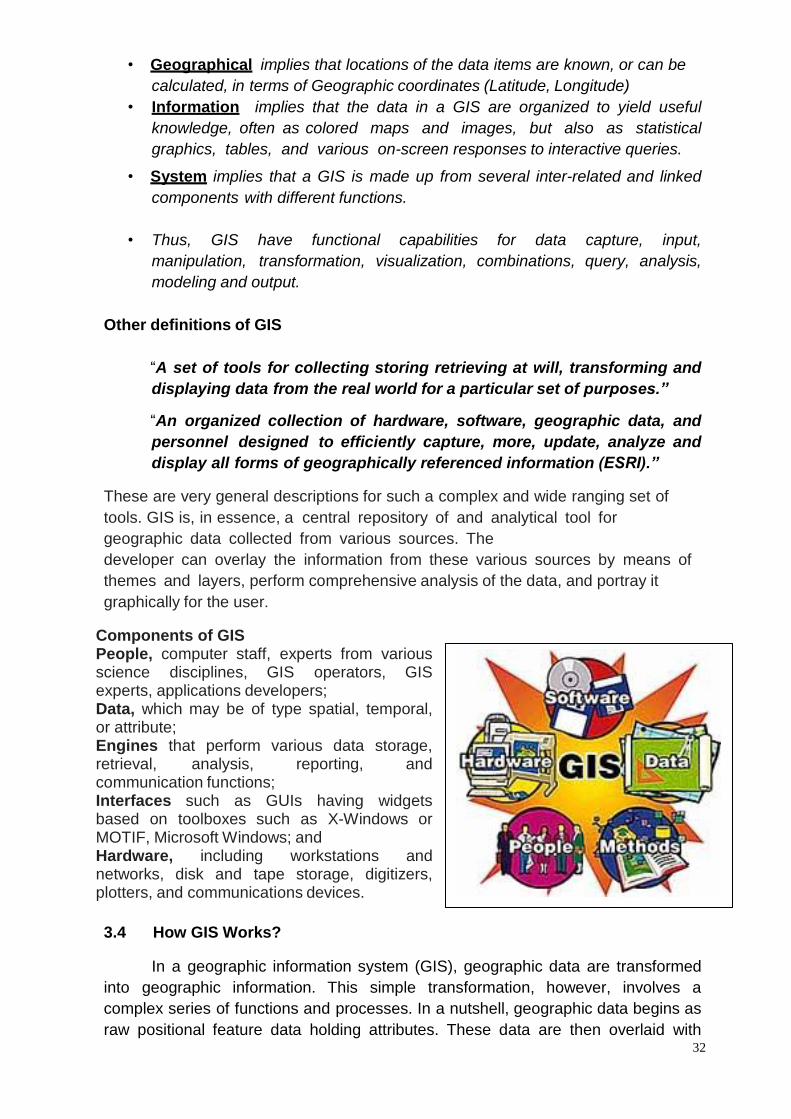
Components of GIS People, computer staff, experts from various science disciplines, GIS operators, GIS experts, applications developers; Data, which may be of type spatial, temporal, or attribute; Engines that perform various data storage, retrieval, analysis, reporting, and communication functions; Interfaces such as GUIs having widgets based on toolboxes such as X-Windows or MOTIF, Microsoft Windows; and Hardware, including workstations and networks, disk and tape storage, digitizers, plotters, and communications devices.

3.4 How GIS Works?

In a geographic information system (GIS), geographic data are transformed

into geographic information. This simple transformation, however, involves a

complex series of functions and processes. In a nutshell, geographic data begins as

raw positional feature data holding attributes. These data are then overlaid with

33

complementary and/or contrasting data sets, which form coincident relationships.

Data and relationships are analyzed, geoprocessed, and then presented as

geographic information products. These geographic information products are often

interactive software applications used to help people make decisions. GISs are

accessible to an array of users, from the expert GIS software developer to the GIS

novice project manager, and, subsequently, offer visualization to users throughout

the spectrum of skill levels. This diversity becomes a unique benefit of GIS and

explains how quickly it can become visible within an organization, as well as offering

project visibility to the public.

3.4.1 Flow of Information:

Geographic data originate from actual locations and physical

characteristics of features on or near the surface of the Earth (or other celestial

bodies such as Mars or the Moon). These raw, positional data are the start points

for every GIS modeling, relationships, and analysis. Raw data can come from a

range of sources, such as aerial photographs, previously digitized maps, and global

positioning systems. These types of digital and nondigital geographic resources are

readily available and, in many cases, are plentiful, well designed, and

comprehensive. Additionally, many digital sources are free. Other more labor

intensive sources are field data and measurements collected from site visits, and

transformed maps, whereby old hardcopy maps are first scanned into a computer

and then digitized.

In the most fundamental sense, raw data are either geographic data or are

transformed into geographic data through a GIS, and are in turn used to produce

geographic information products. Geographic information products are user-

conceived information results created through a GIS and a user’s ability to relate,

manipulate, and present overlaid geographic data. These products are used to

analyze data for a specific application.

The overall work of transforming data in a GIS can be summarized

through its three distinct procedures:

A GIS leverages the flexibility of geographic data. Raw data are static

(nonchanging) and offer only a limited amount of flexibility on real-world

applications. When raw data are transformed to geographic data through a

GIS, the capability for enhanced data use and analysis (i.e., data flexibility)

significantly increases. At a minimum, overlaying two geographic data

sources provides sufficient new information, better analytical means, and

additional flexibility to not only help someone visualize the real world but also

help them make an informed decision.

GIS performs functions and analysis within a single environment. These

data functions are the literal “doers” of a GIS solution and are known as

geo-processing and spatial analysis. These operations are available within a

single GIS environment and include the generation of features, buffers, view

34

sheds, and cross sections; the calculation of centroids, slopes, statistics,

and suitability; and the manipulation of feature attributes, smoothing of lines,

feature transformations, and clipping.

A GIS serves as a software application and creates useful

information products. GIS environments, foremost, serve as spatially

enabled enterprise data management systems and data repositories. These

systems are software applications that protect the value and usefulness of

the information related to your project. The end result is an information

product that enables the user to better manage his or her project.

Through this procedural flow of information, geographic data are transformed

into geographic information. GIS environments centralize both data collection and

information management to save time, minimizes technical effort, and automates

known repetitive administrative tasks.

The core data component of a GIS is often represented by a geographic data

model, which is an industry or discipline-specific template for geographic data. A

geographic data model offers the user flexibility in the design of the file

management and database hierarchy. Geographic data models typically utilize a

grid-based structure (known as raster) or a coordinate point structure (known as

vector).

Facilitating the model is one or more geo-databases. A geo-database is a

collection of geographic data sets, real-world object definitions, and relationships.

Comparable to a Microsoft Access file, a geo-database is a collection of

geographic data sets and geometric features. A geo-database furnishes the data

organizational structure and workflow process model for the creation and

maintenance of the core data product. In essence, the geo-database is the heart of a

GIS’s management capability.

3.4.2 Geographic Data

Geography is the study of the Earth’s surface and climate, and is the

founding science to a GIS. Geography furnishes information about the Earth and

distinguishes how features upon the Earth correlate with one another. For example,

a basic geographic study involves how climate and landform interrelate with

inhabitants, soil, and vegetation. Data collected from this study are geographically

oriented and are therefore geographic data. Any study with a geographic

component, regardless of form, produces geographic data.

By their very nature, geographic data comprise the physical locations of

objects on or near the surface of the Earth. Data are intimately concerned with the

properties of such objects and hold attributes that can be associated to other types

of geographic data. For example, a user can have two types of geographic data

about a 40-acre stretch of land in New Zealand: one detailing elevation above sea

level, and one detailing the various types of soil composition throughout the parcel.

35

Both forms of data can be combined for analysis in a GIS using the land parcel as

the common link. All physical relationships between layers of geographic data are

interpreted as coincident relationships, meaning that features coincide in real world

space. In the above example, the elevation data and soil composition data would go

on separate “layers” in the GIS.

Most standard GIS vector file formats consist of a feature file, an index file,

and a linked attribute table. A feature file contains geographic object feature

information, such as representative point, line, and polygon information. An index file

contains unique identifiers that comprise more detailed information and help speed

spatial feature queries. A linked attribute table is a matrixes table that contains

explicative attributes for a group of spatial features.

3.4.3Geo-referencing:

Many data sources lack formal spatial referencing. Some CAD and GIS data

sets are developed in a generic “design” space and have unique, often proprietary,

types of referencing that simply need reinterpretation to be spatially integrated into

a GIS environment. However, many of these sources are scanned raster data

(digital imagery) that have only the coordinates of a raw pixel grid from an original

scan. While these raster sources are often times unique and critical to a GIS

project, images also need to be referenced from scratch, spatially transformed into a

defined coordinate referencing system, then integrated and overlaid in a GIS

environment. This process is known as geo-referencing.

The ability to perform accurate and timely spatial referencing adds a measure

of customization to any GIS operation or project. Raster imagery, such as hardcopy

maps and aerial photography, is the most popular type of data to use with geo-

referencing, since it is the most commonly available type of data to use. Scanning

imagery also alleviates the need to perform time-consuming and repetitive

digitization efforts (i.e., transforming hardcopy to an electronic, digital file).

Geo-referencing is the art of selecting common point locations in the real

world using at least two data sources: an unreferenced source (such as a raster

map) and a referenced source of the same area providing positional information.

Basic geo-referencing procedures involve point selection and transformation. For

example, when a hardcopy map is scanned to an electronic file, it has no

relationship to any real-world coordinate system. The geo-referencing process

establishes (or in some cases reestablishes) the relationship between image pixel

locations and real-world locations. Geo-referencing is accomplished by first

selecting points on a source image (scanned raster map) with known coordinates

for the real-world surface location (benchmarks, grid ticks, road intersections, and

so on). These real- world coordinates are then linked to the corresponding pixel grid

coordinates in the raster source image. After the image is geo-referenced, each pixel

has a real-world coordinate value assigned to it.

3.4.4General Capabilities:

36

GIS can be used to store, display, and analyze geographic information in a

spatial or “map-like” configuration in a computer. When linked to a printer or plotter,

the GIS can generate top quality maps for reports, field operations or office use.

Many systems will perform complex analyses, overlay various layers of maps,

incorporate digital remote sensing imagery and global positioning systems data,

and conduct modeling operations. The various maps stored in the GIS database

can be displayed on the computer screen individually or overlaid on top of each

other. By overlaying multiple layers of map information for the same area, the GIS

help the analyst see relations between different aspects of the environment. Specific

map elements (such as polygons or points) can also be displayed independently or

in conjunction with other elements. Using the computer mouse (or cursor) map

elements on the screen are selected to reveal text or statistics linked to the map

elements.

3.4.5 Geo-processing:

Geo-processing is the fundamental process of creating a derived set of

geographic data from various existing data sets using operations such as feature

overlay and data conversion. In a typical geo-processing environment, the user

applies GIS functions to a group of geographic (input) data to yield a precise output

data set suitable for a particular application. Geo-processing functions run the gamut

from simple spatial clipping to more complex analytic operations. These software

functions can stand alone or be chained to other processes. This ultimately opens

the gates for virtually unlimited sets of geo-processing models and potentially

staggering sets of output data to solve specific problems.

Most professional GIS software environments include a mission-specific geo-

processing interface, or “workbench,” of geospatial dialogs and tools. These

software environments usually include extensible scripting tools and compilers to

automate, customize, and document geo-processing workflows. The most important

contribution of geo-processing to the GIS big picture is the automation of repetitive

tasks. Geo-processing is an elaborate turnkey for efficient and clean geographic

output.

Geo-processors come in different forms. Many geo-processing functions are

embedded in a GIS environment. A GIS environment is a package of integrated GIS

components: a geographic map control, a map layout designer, a data tree catalog,

and so forth, of which geo-processing is a member. However, many powerful stand-

alone software applications offer specific, related subsets of geo-processing

functionality. Some include file format translators or spatial referencing

transformation tools. Many professional GIS efforts actually require licensing

these stand-alone accessories in order to reap the often-advantageous outputs of

these stand-alone software applications.

Site selection is a prime example of a geo-processing application. Another is

the function of batch processing in a non interactive manner. Geo-processing

37

environments can be considered “robots” that automate geographic data processes

and provide storage of geographic data models. Geo-processing is very reliable.

There are eight categories of predominant geo-processing operations, or

families of operations:

Conversion: Conversion i s c o m p l e t e l y a n i s s u e o f f o r m a t t i n g . File

f o r m a t c o n v e r s i o n s (translations) and coordinate system referencing

conversions are the most common geo-processing conversion operations, and

serve to characterize the conversion family.

Overlay (union, intersecting): Overlay involves superimposing two or more

geographic data layers to discover relationships. In fact, overlay is intimately

associated with the discipline of set

Topology: This defines the rules for valid spatial relationships between features in a

geographic data layer.

Intersect: Geo-processing computes a geometric intersection of the input

features. The resultant features or portion of features common to all layers or

assigned groups of same shape type (called a feature class) will be written to the

output.

Union: Like intersect, union computes a geometric intersection of the input

features. All features with the overlapping attributes from the input features will be

written to the output feature class.

Extraction (clip, query): Like overlay, extraction is also intimately associated with

the discipline of set topology. Queries help select the geographic data to be clipped

or extracted, subject to a specific group of topology rules.

Proximity (buffer): Proximity is initiated through a query that selects geographic

features based on their distance or proximity from other features. Geographic

features include lines, points, and polygons.

Management (copy, create): GIS data management software is generally designed

to facilitate the organization of a user’s unique personal catalog (or collection) of

geographic data. The intrinsic forms of all types of geographic data are

accommodated by these applications.

Transformation: Typically in GIS, the term “transformation” means a spatial

transformation, such as a datum transformation or reprojection. Geo-processing,

however, introduces transformations of different types, such as temporal or

geometric transformations. This facet of flexibility finds favor among integrated user

interfaces, complementing comprehensive spatial analysis within a geo-processing

software environment.

3.4.6 Queries:

Once data are adequately geo-referenced and resident in a GIS, the user

can then create a query expression to find the relevant data for a specific

application. A query enables the user to search geographic data to collect location,

feature, and attribute information from a relational database management system or

geo-database. The most fundamental test of geographic coincidence between data

38

sources is a query by location in tandem with a targeting expression, such as

Intersection, Within distance of, Contained by, Share features with, Touch the

boundary of, Are crossed by the outline of, and Completely in.

Queries can also be executed on feature attribute tables and performed on

specific fields. Records are selected in this manner; each record (or “row”) in the

table corresponds and is linked to a distinct geographic feature data set. Features

conforming to certain attribute criteria can be selected and extracted using this

method.

Quite simply, queries are the user’s refining tool for taking the massive

available data and selecting only those pieces that pertain to the application at

hand. The absolute function of queries is a GIS staple. For example, population

information relating to administrative units or municipalities might be sorted to show

varying population densities among the municipalities. Such variations could then

be shown graphically as charts or histograms on the map.

3.4.7 Quick updates:

GIS can update maps and map attributes directly onto the computerized

map. A revised, updated hardcopy version of the map can then be printed quickly.

3.5 Structure of the GIS data:

Geographic data come from a variety of sources, such as digitized maps,

aerial photography, GPS, and field data. Valid geographic data serve as a collective true marker as to what level of detail and accuracy a GIS can potentially attain. But, in reality, this is only a half-truth. The manipulation of this geographic data is as important and, often, more suggestive of the outcome’s quality.

The appropriate structure of geographic data is considered a top reason why

a GIS succeeds or fails. Inappropriate data handling or structure predictably leads to inappropriate geographic information products. To this extent, a user’s grasp of the GIS application, the desired outcomes, and the geospatial system’s limits are detrimental to realizing how best to treat the geographic data. Ultimately, the successful structuring of geographic data requires a combination of understanding and sound decision making.

Cartographic (Spatial) - observations on spatially distributed features,

activities, or events –

Vector Data: Points, Lines (Arcs), Areas (Polygons)

Raster Data : Grid and Images

Non-Cartographic (Aspatial) - descriptive information in a database about the

cartographic features located on a map.

Attributes

Attribute Values

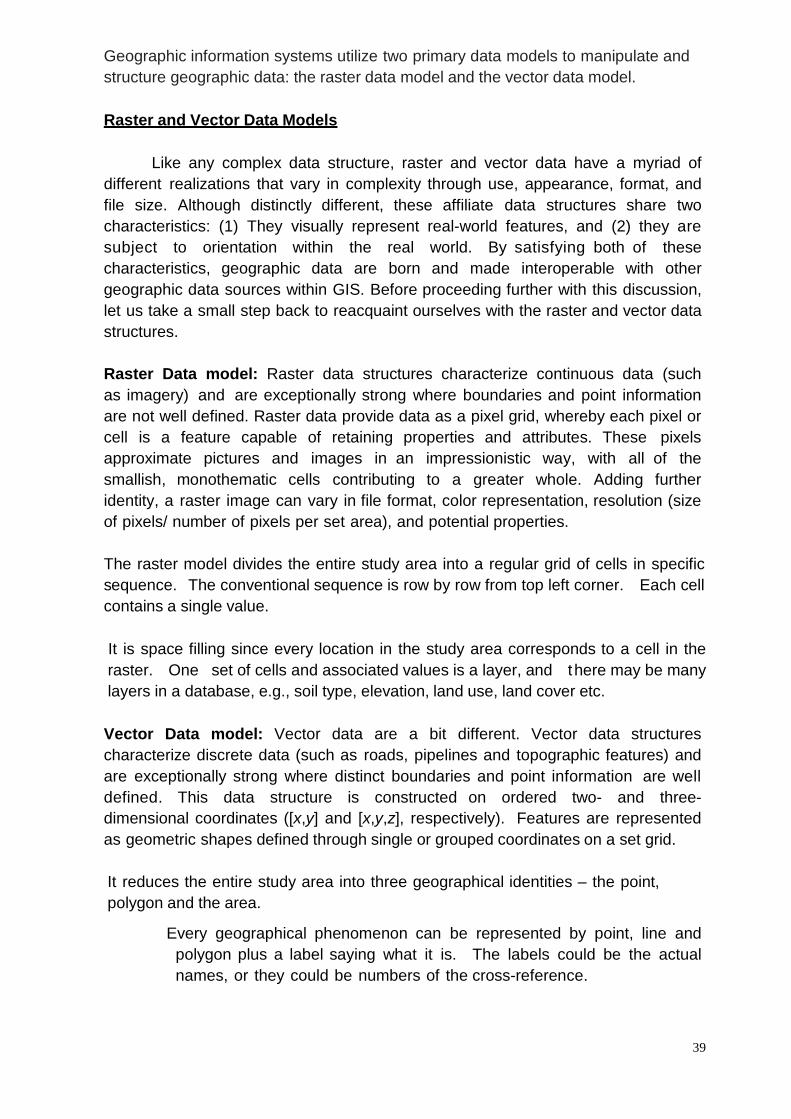
39

Geographic information systems utilize two primary data models to manipulate and

structure geographic data: the raster data model and the vector data model.

Raster and Vector Data Models

Like any complex data structure, raster and vector data have a myriad of

different realizations that vary in complexity through use, appearance, format, and

file size. Although distinctly different, these affiliate data structures share two

characteristics: (1) They visually represent real-world features, and (2) they are

subject to orientation within the real world. By satisfying both of these

characteristics, geographic data are born and made interoperable with other

geographic data sources within GIS. Before proceeding further with this discussion,

let us take a small step back to reacquaint ourselves with the raster and vector data

structures.

Raster Data model: Raster data structures characterize continuous data (such

as imagery) and are exceptionally strong where boundaries and point information

are not well defined. Raster data provide data as a pixel grid, whereby each pixel or

cell is a feature capable of retaining properties and attributes. These pixels

approximate pictures and images in an impressionistic way, with all of the

smallish, monothematic cells contributing to a greater whole. Adding further

identity, a raster image can vary in file format, color representation, resolution (size

of pixels/ number of pixels per set area), and potential properties.

The raster model divides the entire study area into a regular grid of cells in specific

sequence. The conventional sequence is row by row from top left corner. Each cell

contains a single value.

It is space filling since every location in the study area corresponds to a cell in the

raster. One set of cells and associated values is a layer, and there may be many

layers in a database, e.g., soil type, elevation, land use, land cover etc.

Vector Data model: Vector data are a bit different. Vector data structures

characterize discrete data (such as roads, pipelines and topographic features) and

are exceptionally strong where distinct boundaries and point information are well

defined. This data structure is constructed on ordered two- and three-

dimensional coordinates ([x,y] and [x,y,z], respectively). Features are represented

as geometric shapes defined through single or grouped coordinates on a set grid.

It reduces the entire study area into three geographical identities – the point,

polygon and the area.

Every geographical phenomenon can be represented by point, line and

polygon plus a label saying what it is. The labels could be the actual

names, or they could be numbers of the cross-reference.

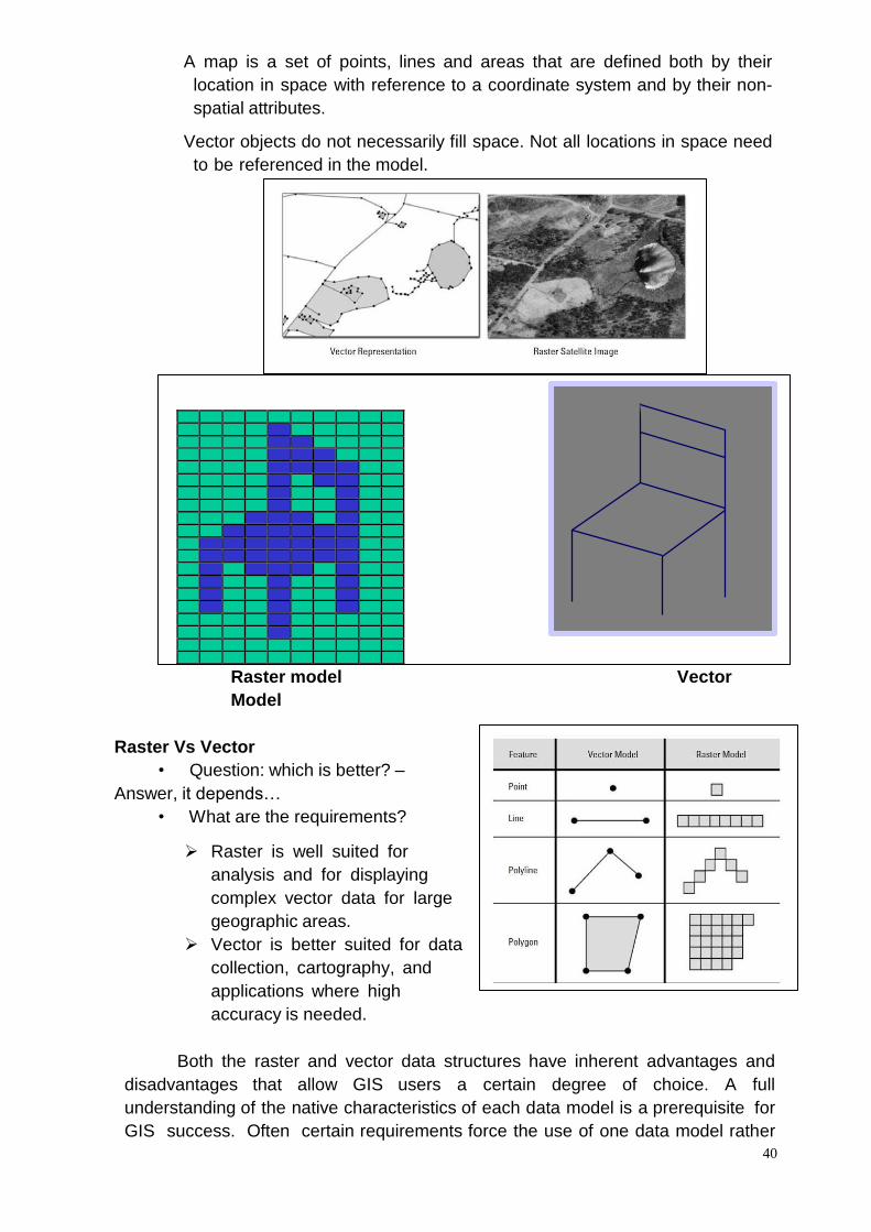
40

A map is a set of points, lines and areas that are defined both by their

location in space with reference to a coordinate system and by their non-

spatial attributes.

Vector objects do not necessarily fill space. Not all locations in space need

to be referenced in the model.

Raster model Vector

Model

Raster Vs Vector

• Question: which is better? –

Answer, it depends…

• What are the requirements?

Raster is well suited for

analysis and for displaying

complex vector data for large

geographic areas.

Vector is better suited for data

collection, cartography, and

applications where high

accuracy is needed.

Both the raster and vector data structures have inherent advantages and

disadvantages that allow GIS users a certain degree of choice. A full

understanding of the native characteristics of each data model is a prerequisite for

GIS success. Often certain requirements force the use of one data model rather

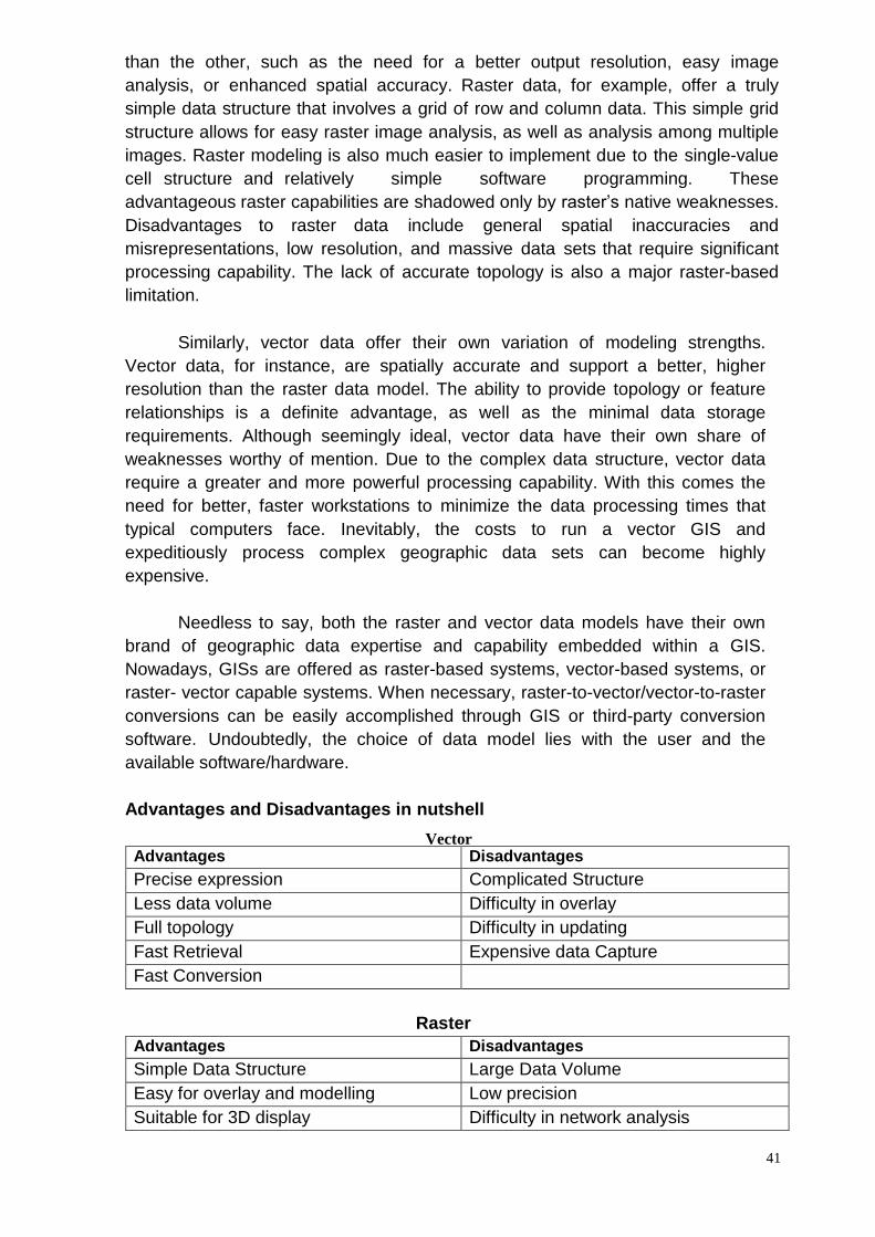
41

Vector

than the other, such as the need for a better output resolution, easy image

analysis, or enhanced spatial accuracy. Raster data, for example, offer a truly

simple data structure that involves a grid of row and column data. This simple grid

structure allows for easy raster image analysis, as well as analysis among multiple

images. Raster modeling is also much easier to implement due to the single-value

cell structure and relatively simple software programming. These

advantageous raster capabilities are shadowed only by raster’s native weaknesses.

Disadvantages to raster data include general spatial inaccuracies and

misrepresentations, low resolution, and massive data sets that require significant

processing capability. The lack of accurate topology is also a major raster-based

limitation.

Similarly, vector data offer their own variation of modeling strengths.

Vector data, for instance, are spatially accurate and support a better, higher

resolution than the raster data model. The ability to provide topology or feature

relationships is a definite advantage, as well as the minimal data storage

requirements. Although seemingly ideal, vector data have their own share of

weaknesses worthy of mention. Due to the complex data structure, vector data

require a greater and more powerful processing capability. With this comes the

need for better, faster workstations to minimize the data processing times that

typical computers face. Inevitably, the costs to run a vector GIS and

expeditiously process complex geographic data sets can become highly

expensive.

Needless to say, both the raster and vector data models have their own

brand of geographic data expertise and capability embedded within a GIS.

Nowadays, GISs are offered as raster-based systems, vector-based systems, or

raster- vector capable systems. When necessary, raster-to-vector/vector-to-raster

conversions can be easily accomplished through GIS or third-party conversion

software. Undoubtedly, the choice of data model lies with the user and the

available software/hardware.

Advantages and Disadvantages in nutshell

Advantages Disadvantages

Precise expression Complicated Structure

Less data volume Difficulty in overlay

Full topology Difficulty in updating

Fast Retrieval Expensive data Capture

Fast Conversion

Raster

Advantages Disadvantages

Simple Data Structure Large Data Volume

Easy for overlay and modelling Low precision

Suitable for 3D display Difficulty in network analysis

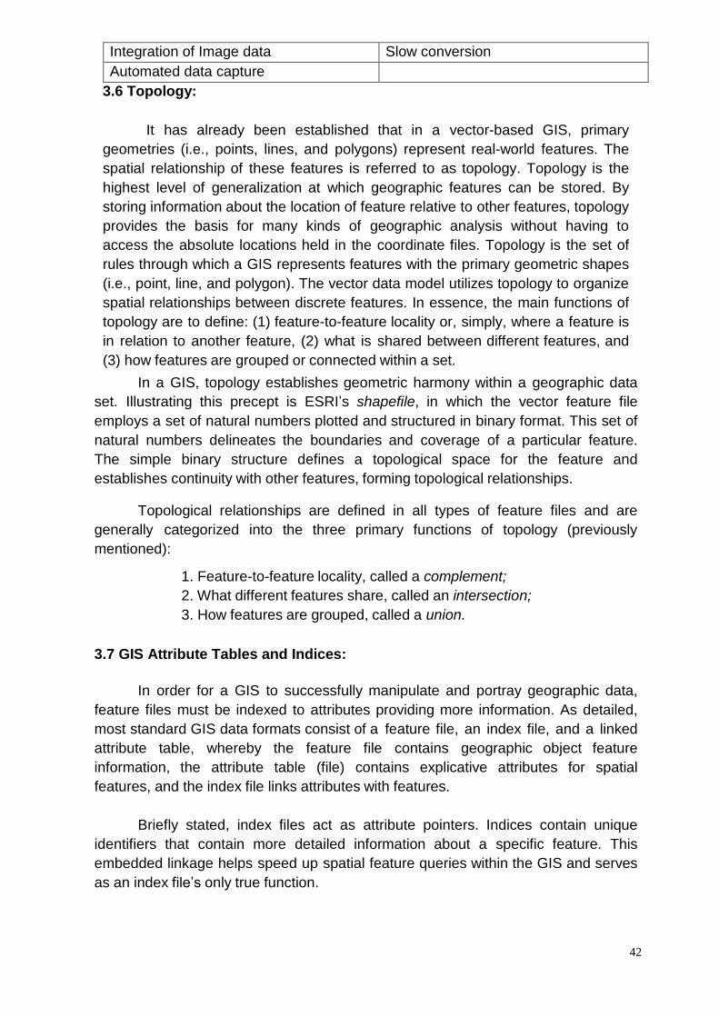
42

Integration of Image data Slow conversion

Automated data capture

3.6 Topology:

It has already been established that in a vector-based GIS, primary

geometries (i.e., points, lines, and polygons) represent real-world features. The

spatial relationship of these features is referred to as topology. Topology is the

highest level of generalization at which geographic features can be stored. By

storing information about the location of feature relative to other features, topology

provides the basis for many kinds of geographic analysis without having to

access the absolute locations held in the coordinate files. Topology is the set of

rules through which a GIS represents features with the primary geometric shapes

(i.e., point, line, and polygon). The vector data model utilizes topology to organize

spatial relationships between discrete features. In essence, the main functions of

topology are to define: (1) feature-to-feature locality or, simply, where a feature is

in relation to another feature, (2) what is shared between different features, and

(3) how features are grouped or connected within a set.

In a GIS, topology establishes geometric harmony within a geographic data

set. Illustrating this precept is ESRI’s shapefile, in which the vector feature file

employs a set of natural numbers plotted and structured in binary format. This set of

natural numbers delineates the boundaries and coverage of a particular feature.

The simple binary structure defines a topological space for the feature and

establishes continuity with other features, forming topological relationships.

Topological relationships are defined in all types of feature files and are

generally categorized into the three primary functions of topology (previously

mentioned):

1. Feature-to-feature locality, called a complement;

2. What different features share, called an intersection;

3. How features are grouped, called a union.

3.7 GIS Attribute Tables and Indices:

In order for a GIS to successfully manipulate and portray geographic data,

feature files must be indexed to attributes providing more information. As detailed,

most standard GIS data formats consist of a feature file, an index file, and a linked

attribute table, whereby the feature file contains geographic object feature

information, the attribute table (file) contains explicative attributes for spatial

features, and the index file links attributes with features.

Briefly stated, index files act as attribute pointers. Indices contain unique

identifiers that contain more detailed information about a specific feature. This

embedded linkage helps speed up spatial feature queries within the GIS and serves

as an index file’s only true function.

43

Geospatial attribute tables, on the other hand, drive the spatially enabled

database. There are various attribute field data types to handle the multitude of

data, differentiated by a specific form of data and the degree of precision. To

adequately handle the variants, attribute field data types signify different groupings

of data bits, such as incorporating sign (i.e., “+” or “−”), binary, mantissa, and

exponent bits, or signify data values, such as text, date, and object ID values. For

clarity of this discussion, an exponent defines repeated multiplication (i.e., in 23 = 2

x 2 x 2, the exponent is 3) and a mantissa is the value to the right of the decimal

point in a common logarithm (i.e., in log 196 = 2.2923, the mantissa is 0.2923).

The following attribute field data types are most common and are supported in

many major GIS environments:

Short Integer. A basic attribute data type that includes one signed bit and 15

binary bits.

Long Integer. A more complex form of the basic attribute type that

incorporates one

signed bit and 31 binary bits. As you can imagine, the Long Integer offers

greater precision than the Short Integer.

Float. Contains one signed bit, seven exponent bits, and 24 mantissa bits.

Double. A more complex form of the Float attribute type with one sign bit,

seven

exponent bits, and 56 mantissa bits. As with the Long Integer, the Double

attribute type holds greater precision than the Float attribute type.

Text. Contains varying forms of data, such as numbers, letters, and symbols.

The Text attribute type is a character string that can hold any amount of

characters, but each character is stored using eight bits (called a byte). An

interesting aspect to Text attribute data are that each text value in the same

field must have the same number of characters. To achieve this, end blanks

are used to fill in the empty slots.

Date. Though not apparent from the attribute data type name, a Date type

contains date and time data. The value is based upon a standard time format

and is automatically transformed into the current day and time within the

system’s local time zone.

BLOB. Short for Binary Large Object. A BLOB is a complex (and large)

object stored in the database that may include an image, sound, video, or

geometry. BLOBs allow users the ability to insert any type of multimedia data

into the geodatabase.

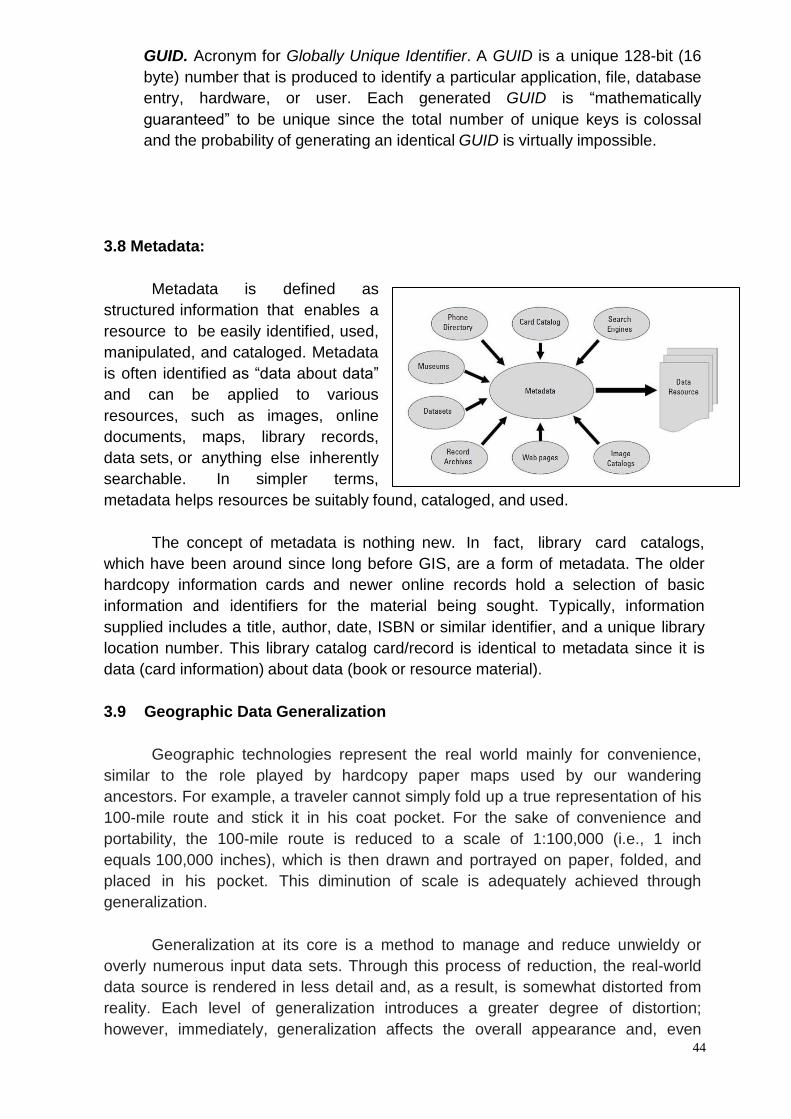
44

GUID. Acronym for Globally Unique Identifier. A GUID is a unique 128-bit (16

byte) number that is produced to identify a particular application, file, database

entry, hardware, or user. Each generated GUID is “mathematically

guaranteed” to be unique since the total number of unique keys is colossal

and the probability of generating an identical GUID is virtually impossible.

3.8 Metadata:

Metadata is defined as

structured information that enables a

resource to be easily identified, used,

manipulated, and cataloged. Metadata

is often identified as “data about data”

and can be applied to various

resources, such as images, online

documents, maps, library records,

data sets, or anything else inherently

searchable. In simpler terms,

metadata helps resources be suitably found, cataloged, and used.

The concept of metadata is nothing new. In fact, library card catalogs,

which have been around since long before GIS, are a form of metadata. The older

hardcopy information cards and newer online records hold a selection of basic

information and identifiers for the material being sought. Typically, information

supplied includes a title, author, date, ISBN or similar identifier, and a unique library

location number. This library catalog card/record is identical to metadata since it is

data (card information) about data (book or resource material).

3.9 Geographic Data Generalization

Geographic technologies represent the real world mainly for convenience,

similar to the role played by hardcopy paper maps used by our wandering

ancestors. For example, a traveler cannot simply fold up a true representation of his

100-mile route and stick it in his coat pocket. For the sake of convenience and

portability, the 100-mile route is reduced to a scale of 1:100,000 (i.e., 1 inch

equals 100,000 inches), which is then drawn and portrayed on paper, folded, and

placed in his pocket. This diminution of scale is adequately achieved through

generalization.

Generalization at its core is a method to manage and reduce unwieldy or

overly numerous input data sets. Through this process of reduction, the real-world

data source is rendered in less detail and, as a result, is somewhat distorted from

reality. Each level of generalization introduces a greater degree of distortion;

however, immediately, generalization affects the overall appearance and, even

45

more important, the precision of the output data. All geographic data are in some

way generalized. This is an inevitable, astringent process that alters the actual

character of the data into a simplified and shrunken model of the real world.

Ultimately, scale dictates the severity of generalization, varying in level from project

to project. For instance, a map drawn to 1:100,000 scale (smaller scale) is more

generalized than the same area drawn to 1:24,000 (larger scale), thus the smaller

the scale, the greater the level of generalization.

3.10 Projection: Display of 3D earth surface information on 2D plane surface

with user required accuracies of shape, size and distance. The idea of depicting

the Earth on a flat map is easy to imagine and rather simple to understand, but

the actual process of a map projection is complex. It will be discussed in detail

in Chapter I.

3.11 Types of GIS:

a) Desktop Mapping: Though not a true GIS, these systems are useful to

review map data for general planning purposes, do simple processing (such

as map queries and basic statistics) and output maps and graphics for

reports or meetings. They run on standard PC’s with a minimum of upgrades.

Many are user friendly and most useful to the non-GIS professional who

routinely needs to consult geographic information or map data.

b) Project level GIS: The project level GIS is a true GIS with complete

functionality, it usually involves a small number of users and is focused on

trying to “get an answer” to a specific problem. It usually is not so

concerned with issues such as standards and inter-operability between

different parties. Data sets frequently have a short life in terms of their

usefulness. Such a system would typically be PC based. Requirements for

inputs and outputs are determined according to the need to answer the

specific question that justified the acquisition of the GIS.

c) Corporate-level GIS: The corporate-level GIS usually serves multiple

parties or an unknown number of users with diverse needs and generates

data sets with a long life expectancy. Common hardware for these operations

includes single workstations or multiple workstations. Input and output

formats, procedures and methodology are frequently standardized and

documented to assure compatibility among the various users. These

characteristics make such a system complex. Consequently, it requires

extensive front-end planning and consensus building among the potential

users in order to determine their goals and needs for information and to

define and appropriate system, data and personnel requirements necessary

to achieve the goals and generate the information.

3.12 Use of GIS in simple terms:

46

Though collection of data is difficult once it is collected, it can be

stored safely in digital form (in computer) forever without damage,

which usually happens to our maps.

Once if a map is prepared accurately it can be printed in any scale

without any redrawing.

Large scale maps at smaller units (Beats) level can be joined for

creating maps at divisions or district level, very accurately within few

minutes.

Changes can be incorporated very easily in computer and it doesn’t

require any redrawing.

Same map can be generated even after 100s of years later.

New things can be known after overlay of different themes and a

new types of maps can be generated.

Work can be done faster than manually.

The work of decision makers and end users will become easier.

Map data is more secured and better organized.

Redundancy and other problems of multiple map sets are

eliminated.

Once a map is prepared accurately it can be printed in any scale

without any redrawing.

Same map can be generated after many years.

The work of decision-makers and end users will become easier

Map revisions are Easier and Faster.

Map data is easier to search, analyze and present.

Employees are more productive.

Mapping geographical characteristics for analysis

Modeling alternative processes for management plans

Managing a utility’s assets

Monitoring changes in environmental factors

47

Chapter - IV Fundamentals of Remote Sensing

4.1 Overview:

Remote sensing refers to the activities of recording, observing, and perceiving

(sensing) objects or events in far-away (remote) places. In remote sensing, the sensors are

not in direct contact with the objects or events being observed. Electromagnetic radiation

normally is used as the information carrier in remote sensing. The output of a remote

sensing system is usually an image representing the scene being observed. A further step

of image analysis and interpretation is required to extract useful information from the

image. In a more restricted sense, remote sensing refers to the science and technology of

acquiring information about the earth’s surface (i.e., land and ocean) and atmosphere

using sensors onboard airborne (e.g., aircraft or balloons) or spaceborne (e.g., satellites and

space shuttles) platforms.

Depending on the scope, remote sensing may be broken down into (1) satellite

remote sensing (when satellite platforms are used), (2) photography and photogrammetry

(when photographs are used to capture visible light), (3) thermal remote sensing (when the

thermal infrared portion of the spectrum is used), (4) radar remote sensing (when

microwave wavelengths are used), and (5) LiDAR remote sensing (when laser pulses are

transmitted toward the ground and the distance between the sensor and the ground is

measured based on the return time of each pulse).

A photograph is a good example of remote sensing. In fact on the advent of

development of photography technique, people started gathering information of land

surfaces with cameras, called terrestrial Remote Sensing. After invention of air crafts,

aerial photography has gained much prominence in collection of data of earth is resources,

though lesser effort was initiated well before with the help of Balloons. Even now aerial

photography is being used in most of the places for land resources management.

The technology of remote sensing evolved gradually into a scientific subject after

World War II. Its early development was driven mainly by military uses. Later, remotely

sensed data became widely applied for civil applications. The range of remote sensing

applications includes archaeology, agriculture, cartography, civil engineering, meteorology

and climatology, coastal studies, emergency response, forestry, geology, geographic

information systems, hazards, land use and land cover, natural disasters, oceanography,

water resources, and so on. Most recently, with the advent of high spatial resolution

imagery and more capable techniques, urban and related applications of remote sensing

have been rapidly gaining interest in the remote sensing community and beyond.

The first Remote sensing satellite was launched by USA ‘Landsat’ in the year 1982.

Since then many countries have launched different satellites with different capabilities

including India. India has launched its first R.S. Satellite IRS IA in the year 1988. Since

then it has launched IRC series IB, IC, ID and P series P1, P2, P3, P5, P6, Cartosat etc.

4.2 Definitions:

Collection of information about on object without actually being in contact with it is

called Remote Sensing.

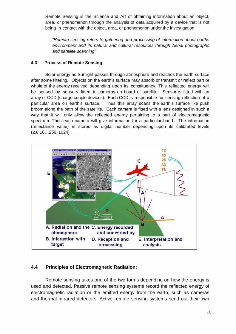
48

Remote Sensing is the Science and Art of obtaining information about an object,

area, or phenomenon through the analysis of data acquired by a device that is not

being in contact with the object, area, or phenomenon under the investigation.

“Remote sensing refers to gathering and processing of information about earths

environment and its natural and cultural resources through Aerial photographs

and satellite scanning”

4.3 Process of Remote Sensing:

Solar energy as Sunlight passes through atmosphere and reaches the earth surface

after some filtering. Objects on the earth’s surface may absorb or transmit or reflect part or

whole of the energy received depending upon its constituency. This reflected energy will

be sensed by sensors fitted in cameras on board of satellite. Sensor is fitted with an

array of CCD (charge couple devices). Each CCD is responsible for sensing reflection of a

particular area on earth’s surface. Thus this array scans the earth’s surface like push

broom along the path of the satellite. Each camera is fitted with a lens designed in such a

way that it will only allow the reflected energy pertaining to a part of electromagnetic

spectrum. Thus each camera will give information for a particular band. The information

(reflectance value) in stored as digital number depending upon its calibrated levels

(2,8,16…256, 1024).

4.4 Principles of Electromagnetic Radiation:

Remote sensing takes one of the two forms depending on how the energy is

used and detected. Passive remote sensing systems record the reflected energy of

electromagnetic radiation or the emitted energy from the earth, such as cameras

and thermal infrared detectors. Active remote sensing systems send out their own

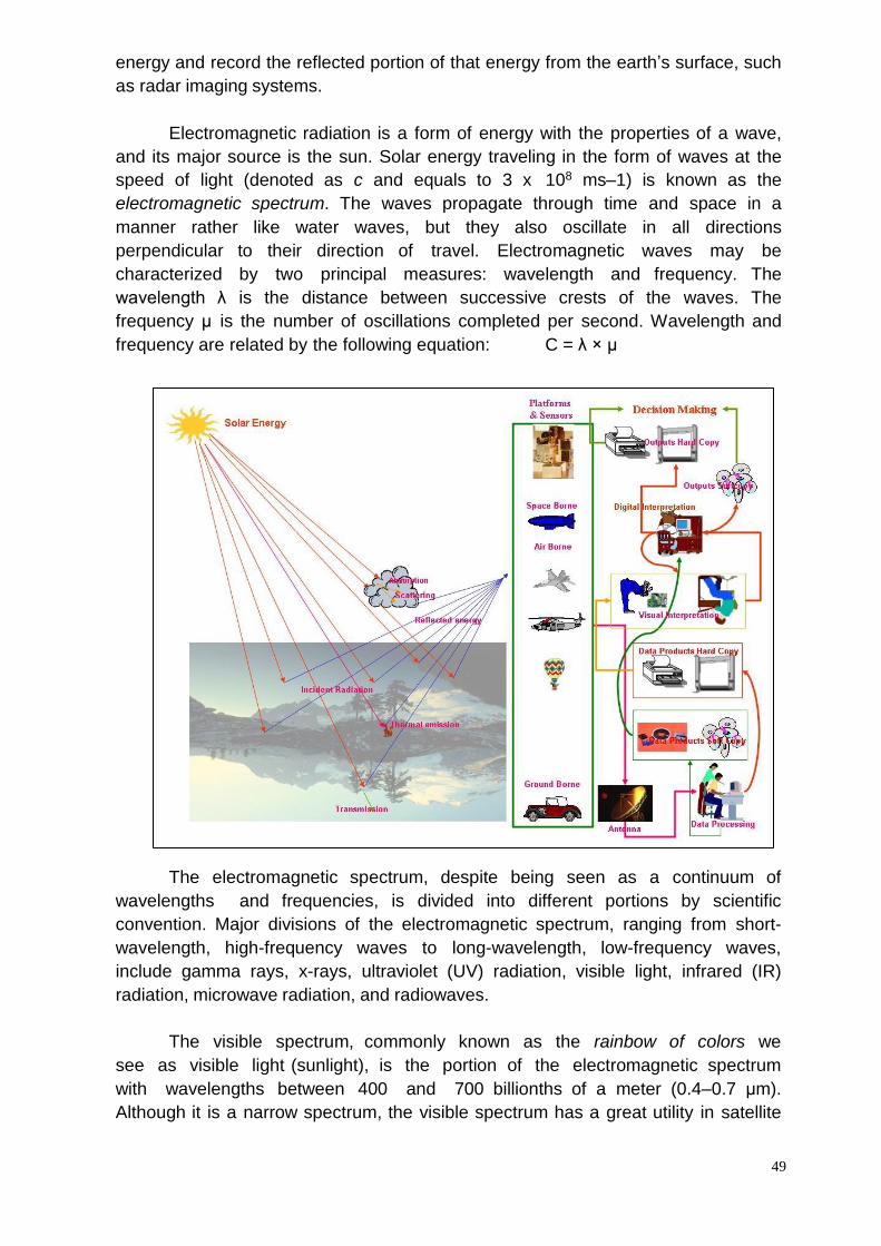
49

energy and record the reflected portion of that energy from the earth’s surface, such

as radar imaging systems.

Electromagnetic radiation is a form of energy with the properties of a wave,

and its major source is the sun. Solar energy traveling in the form of waves at the

speed of light (denoted as c and equals to 3 x 108 ms–1) is known as the

electromagnetic spectrum. The waves propagate through time and space in a

manner rather like water waves, but they also oscillate in all directions

perpendicular to their direction of travel. Electromagnetic waves may be

characterized by two principal measures: wavelength and frequency. The

wavelength λ is the distance between successive crests of the waves. The

frequency μ is the number of oscillations completed per second. Wavelength and

frequency are related by the following equation: C = λ × μ

The electromagnetic spectrum, despite being seen as a continuum of

wavelengths and frequencies, is divided into different portions by scientific

convention. Major divisions of the electromagnetic spectrum, ranging from short-

wavelength, high-frequency waves to long-wavelength, low-frequency waves,

include gamma rays, x-rays, ultraviolet (UV) radiation, visible light, infrared (IR)

radiation, microwave radiation, and radiowaves.

The visible spectrum, commonly known as the rainbow of colors we

see as visible light (sunlight), is the portion of the electromagnetic spectrum

with wavelengths between 400 and 700 billionths of a meter (0.4–0.7 μm).

Although it is a narrow spectrum, the visible spectrum has a great utility in satellite

50

remote sensing and for the identification of different objects by their visible colors in

photography.

The IR spectrum is the region of electromagnetic radiation that extends from

the visible region to about 1 mm (in wavelength). Infrared waves can be further

partitioned into the near-IR, mid-IR, and far- IR spectrum, which include thermal

radiation. IR radiation can be measured by using electronic detectors. IR images

obtained by sensors can yield important information on the health of crops and can

help in visualizing forest fires even when they are enveloped in an opaque curtain of

smoke.

Microwave radiation has a wavelength ranging from approximately 1 mm to

30 cm. Microwaves are emitted from the earth, from objects such as cars and

planes, and from the atmosphere. These microwaves can be detected to provide

information, such as the temperature of the object that emitted the microwave.

Because their wavelengths are so long, the energy available is quite small

compared with visible and IR wavelengths. Therefore, the fields of view must be

large enough to detect sufficient energy to record a signal. Most passive microwave

sensors thus are characterized by low spatial resolution.

Active microwave sensing systems (e.g., radar) provide their own source of

microwave radiation to illuminate the targets on the ground. A major advantage of

radar is the ability of the radiation to penetrate through cloud cover and most

weather conditions owing to its long wavelength. In addition, because radar is an

active sensor, it also can be used to image the ground at any time during the day or

night. These two primary advantages of radar, all-weather and day or night imaging,

make radar a unique sensing system.

The electromagnetic radiation reaching the earth’s surface is partitioned into

three types by interacting with features on the earth’s surface. Transmission refers

to the movement of energy through a surface. The amount of transmitted energy

depends on the wavelength and is measured as the ratio of transmitted radiation to

the incident radiation, known as transmittance. Remote sensing systems can

detect and record both reflected and emitted energy from the earth’s surface.

Reflectance is the term used to define the ratio of the amount of electromagnetic

radiation reflected from a surface to the amount originally striking the surface. When

a surface is smooth, we get specular reflection, where all (or almost all) of the

energy is directed away from the surface in a single direction. When the surface is

rough and the energy is reflected almost uniformly in all directions, diffuse reflection

occurs. Most features of the earth’s surface lie somewhere between perfectly

specular or perfectly diffuse reflectors. Whether a particular target reflects

specularly or diffusely or somewhere in between depends on the surface

roughness of the feature in comparison with the wavelength of the incoming

radiation. If the wavelengths are much smaller than the surface variations or the

particle sizes that make up the surface, diffuse reflection will dominate. Some

electromagnetic radiation is absorbed through electron or molecular reactions within

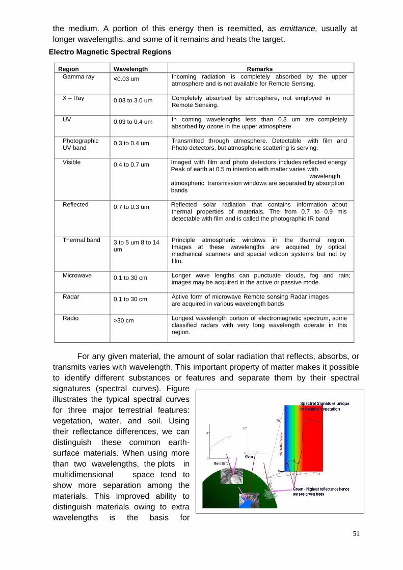
51

the medium. A portion of this energy then is reemitted, as emittance, usually at

longer wavelengths, and some of it remains and heats the target.

Electro Magnetic Spectral Regions

For any given material, the amount of solar radiation that reflects, absorbs, or

transmits varies with wavelength. This important property of matter makes it possible

to identify different substances or features and separate them by their spectral

signatures (spectral curves). Figure

illustrates the typical spectral curves

for three major terrestrial features:

vegetation, water, and soil. Using

their reflectance differences, we can

distinguish these common earth-

surface materials. When using more

than two wavelengths, the plots in

multidimensional space tend to

show more separation among the

materials. This improved ability to

distinguish materials owing to extra

wavelengths is the basis for

Region Wavelength Remarks

Gamma ray <0.03 um Incoming radiation is completely absorbed by the upper atmosphere and is not available for Remote Sensing.

X – Ray 0.03 to 3.0 um Completely absorbed by atmosphere, not employed in Remote Sensing.

UV 0.03 to 0.4 um In coming wavelengths less than 0.3 um are completely absorbed by ozone in the upper atmosphere

Photographic UV band

0.3 to 0.4 um Transmitted through atmosphere. Detectable with film and Photo detectors, but atmospheric scattering is serving.

Visible 0.4 to 0.7 um Imaged with film and photo detectors includes reflected energy Peak of earth at 0.5 m intention with matter varies with

wavelength atmospheric transmission windows are separated by absorption bands

Reflected band

0.7 to 0.3 um Reflected solar radiation that contains information about thermal properties of materials. The from 0.7 to 0.9 mis detectable with film and is called the photographic IR band

Thermal band 3 to 5 um 8 to 14 um

Principle atmospheric windows in the thermal region. Images at these wavelengths are acquired by optical mechanical scanners and special vidicon systems but not by film.

Microwave 0.1 to 30 cm Longer wave lengths can punctuate clouds, fog and rain; images may be acquired in the active or passive mode.

Radar 0.1 to 30 cm Active form of microwave Remote sensing Radar images are acquired in various wavelength bands

Radio >30 cm Longest wavelength portion of electromagnetic spectrum, some classified radars with very long wavelength operate in this region.

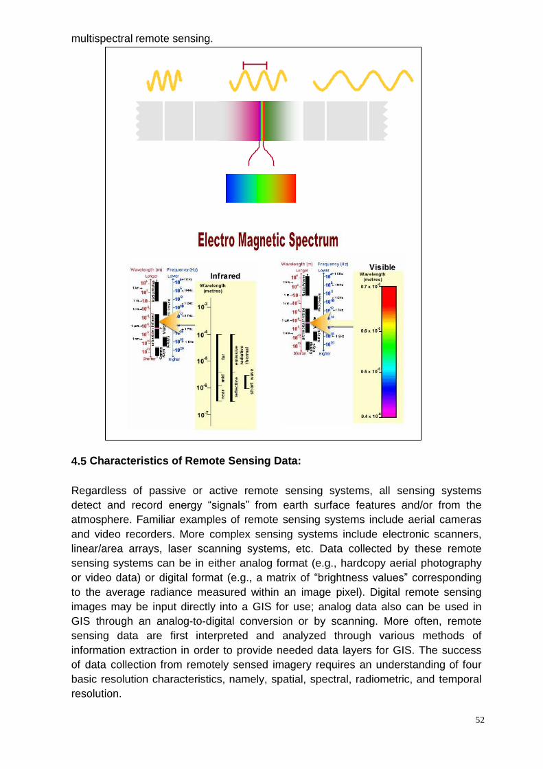
52

multispectral remote sensing.

4.5 Characteristics of Remote Sensing Data:

Regardless of passive or active remote sensing systems, all sensing systems

detect and record energy “signals” from earth surface features and/or from the

atmosphere. Familiar examples of remote sensing systems include aerial cameras

and video recorders. More complex sensing systems include electronic scanners,

linear/area arrays, laser scanning systems, etc. Data collected by these remote

sensing systems can be in either analog format (e.g., hardcopy aerial photography

or video data) or digital format (e.g., a matrix of “brightness values” corresponding

to the average radiance measured within an image pixel). Digital remote sensing

images may be input directly into a GIS for use; analog data also can be used in

GIS through an analog-to-digital conversion or by scanning. More often, remote

sensing data are first interpreted and analyzed through various methods of

information extraction in order to provide needed data layers for GIS. The success

of data collection from remotely sensed imagery requires an understanding of four

basic resolution characteristics, namely, spatial, spectral, radiometric, and temporal

resolution.

53

Spatial Resolution:

Spatial resolution is a measurement of the minimum distance between two objects

that will allow them to be differentiated from one another in an image and is a

function of sensor altitude, detector size, focal size, and system configuration

(Jensen, 2005). For aerial photography, spatial resolution is measured in resolvable

line pairs per millimeter, whereas for other sensors, it refers to the dimensions (in

meters) of the ground area that falls within the instantaneous field of view (IFOV)

of a single detector within an array or pixel size (Jensen, 2005). Spatial resolution

determines the level of spatial details that can be observed on the earth’s surface.

Coarse spatial resolution data may include a large number of mixed pixels, where

more than one land-cover type can be found within a pixel. Whereas fine spatial

resolution data considerably reduce the mixed-pixel problem, they may increase

internal variation within the land- cover types. Higher resolution also means the

need for greater data storage and higher cost and may introduce difficulties in image

processing for a large study area. The relationship between the geographic scale of

a study area and the spatial resolution of the remotesensing image has been

explored (Quattrochi and Goodchild, 1997). Generally speaking, on the local scale,

high spatial-resolution imagery, such as that employing IKONOS and QuickBird

data, is more effective. On the regional scale, medium-spatial- resolution imagery,

such as that employing Landsat Thematic Mapper/Enhanced Thematic Mapping

Plus (TM/ETM+) and Terra Advanced Spaceborne Thermal Emission and Reflection

Radiometer (ASTER) data, is used most frequently. On the continental or global

scale, coarse-spatial-resolution imagery, such as that employing Advanced Very

High Resolution Radiometer (AHVRR) and Moderate Resolution Imaging

Spectrometer (MODIS) data, is most suitable.

IRS 1C/1D PAN 5.8 Mt, WiFS 188.3 Mt, LISS III 23.5 & 70.5 Mt; Cartosat 1

2.5 m

NOAA AVHRR 1.1 KM at nadir and 2.4 & 6.9 KM offnadir; etc

Spectral Resolution:

Spectral resolution of a sensor refers to the number and size of the bands it

is able to record (Jensen, 2005). Spectral resolution is defined as the specific

wavelength intervals in the electromagnetic spectrum that a sensor can record or

Refers to the band width and the no. of bands used for collecting the data. For

example band 1 of the IRS-IC, LISS III sensor records energy between 0.52 to 0.59

µm in the visible spectrum.

Wide intervals in the electromagnetic spectrum are referred to as coarse

spectral resolution and narrow intervals are referred to as fine spectral resolution.

For example the IRS – IC, PAN sensor is considered to have coarse spectral

resolution because it records electromagnetic range between 0.5 to

0.75 µm. On the other hand, band 3 of IRS-IC LISS III Sensor has fine spectral

resolution because it records electromagnetic range between 0.62 to 0.68 µm.

AVHRR, onboard National Oceanographic and Atmospheric Administration’s

54

(NOAAs) Polar Orbiting Environmental Satellite (POES) platform, collects four or

five broad spectral bands (depending on the individual instrument) in the visible

(0.58–

0.68 μm, red), near-IR (0.725–1.1 μm), mid-IR (3.55–3.93 μm), and thermal IR

portions (10.3–11.3 and 11.5–12.5 μm) of the electromagnetic spectrum.

Temporal Resolution:

Temporal resolution refers to the amount of time it takes for a sensor to

return to a previously imaged location. Therefore, temporal resolution has an

important implication in change detection and environmental monitoring. Many

environmental phenomena constantly change over time, such as vegetation,

weather, forest fires, volcanoes, and so on. Temporal resolution is an important

consideration in remote sensing of vegetation because vegetation grows according

to daily, seasonal, and annual phenologic cycles. It is crucial to obtain anniversary

or near-anniversary images in change detection of vegetation. Anniversary images

greatly minimize the effect of seasonal differences (Jensen, 2005).

IRS 1C/1D PAN 5Days, LISS III 24 Days; NOAA AVHRR half day for TIR, one day

for Visible; MOS 1 &1a MESSR, VTIR and MSR 17 Days; Geostationary

Operational Environmental Satellite (GOES), 0.5/h;and Meteosat first

generation, every 30 minutes etc.

Radiometric Resolution:

Radiometric resolution refers to the sensitivity of a sensor to incoming

radiance, that is, how much change in radiance there must be on the sensor before

a change in recorded brightness value takes place (Jensen, 2005). Refers to the

no. of quantization levels into which the radiant flux reflected from the scene

elements is recorded. This is referred to by the number of bits into which the

recorded energy is divided for instance, in 8 bit data file values range from 0 to 255

for each pixel, but in 7 bit data the data file values for each pixel range form 0 to

127. The total intensity of the energy from 0 to the maximum amount the sensor

measures is broken down into 256 brightness values for 8 bit data and 128

brightness values for 7 bit data.

Coarse radiometric resolution would record a scene using only a few

brightness levels, that is, at very high contrast, whereas fine radiometric

resolution would record the same scene using many brightness levels. IRS

1C/1D PAN 6 Bits, LISS III 7 Bits; Landsat 7 ETM+ 8 Bits; SPOT 4&5 MLA 8 Bits;

AVHRR 10 Bits etc.

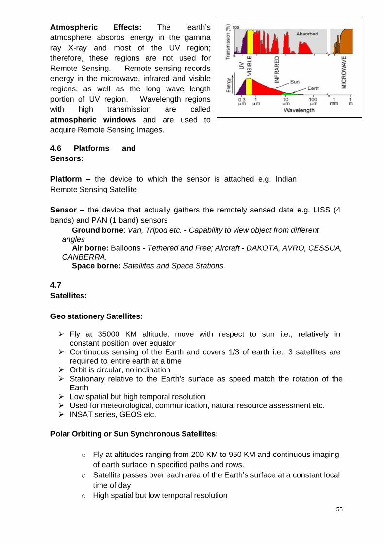
55

Atmospheric Effects: The earth’s

atmosphere absorbs energy in the gamma

ray X-ray and most of the UV region;

therefore, these regions are not used for

Remote Sensing. Remote sensing records

energy in the microwave, infrared and visible

regions, as well as the long wave length

portion of UV region. Wavelength regions

with high transmission are called

atmospheric windows and are used to

acquire Remote Sensing Images.

4.6 Platforms and

Sensors:

Platform – the device to which the sensor is attached e.g. Indian

Remote Sensing Satellite

Sensor – the device that actually gathers the remotely sensed data e.g. LISS (4

bands) and PAN (1 band) sensors

Ground borne: Van, Tripod etc. - Capability to view object from different angles Air borne: Balloons - Tethered and Free; Aircraft - DAKOTA, AVRO, CESSUA, CANBERRA. Space borne: Satellites and Space Stations

4.7

Satellites:

Geo stationery Satellites:

Fly at 35000 KM altitude, move with respect to sun i.e., relatively in constant position over equator

Continuous sensing of the Earth and covers 1/3 of earth i.e., 3 satellites are required to entire earth at a time

Orbit is circular, no inclination Stationary relative to the Earth's surface as speed match the rotation of the

Earth Low spatial but high temporal resolution Used for meteorological, communication, natural resource assessment etc. INSAT series, GEOS etc.

Polar Orbiting or Sun Synchronous Satellites:

o Fly at altitudes ranging from 200 KM to 950 KM and continuous imaging

of earth surface in specified paths and rows.

o Satellite passes over each area of the Earth’s surface at a constant local

time of day

o High spatial but low temporal resolution

56

o Orbital period approximately 102 to 105 min.

o Revisit the same area at specified intervals e.g. IRS 1C/1D 24 days etc.

o Generally inclined at 990 to withstand gravitational pull & more coverage

o Used for natural resource assessment viz.., Forestry, Geological,

Soil, Hydrological, Oceanographic, Agricultural etc., applications etc.

o IRS 1A/B, 1C/D; LandSat 1:7, SPOT 1:5, NOAA 1:12, MOS 1&1A etc.

Other Satellites: Spy Satellites, Candors, Iridium, Constellation of GPS Satellites

etc.

4.8

Sensors:

Passive systems: A passive sensor is a device that detects and responds

to some type of input from the physical environment. Passive

sensor technologies gather target data through the detection of vibrations,

light, radiation, heat or other phenomena occurring in the subject's

environment.

photographic camera, television camera, return beam vidicon (RBV),

electro- optical scanner

Active systems: An active sensor is a sensing device that requires an

external source of power to operate; active sensorscontrast with

passive sensors, which simply detect and respond to some type of input from

the physical environment.

RADAR, microwave, photographic camera with flash

light

a) Photographic camera

Metric camera

Strip camera

Multiband camera

b) Television camera

c) Electronic scanner

d) Thermal

scanner

e) Imaging spectrometer

4.9 Satellite

Coverage:

Remote sensing satellite roams around earth from pole to pole with an

inclination angle of 5 degrees, which may take 104 minutes for one round. The area

covered in one round is called path. The width of this path is called swath width and

is varied from satellite to satellite and camera to camera in the same satellite. Due to

earth’s rotation on its polar axis the path of the satellite changes from round to round,

thus it covers the entire area in 24 days (IRS IC). Adjacent scenes from different

57

paths are called Rows. The demarcation of coverage of earth as path & Row varies

from satellite to satellite.

4.10 Scanning System:

A scanning system employs single detector with a narrow field of view which

sweeps across the terrain to produce an image. When photons of electromagnetic

energy radiated or reflected from the terrain encounter the detector, an electrical

signal is produced that varies in proportion to the number of photons. The electrical

signal amplified, recorded on magnetic tape, and played back later to produce an

image. All scanning systems sweep the detectors field of view across the terrain in

a series of parallel scan lines.

Across-track scanner or Whisk-broom scanner

• Consists of a single detector and a rotating mirror

• Mirror is oriented in such a manner that, after one complete rotation, the

detector beam sweeps a straight line on the surface of the Earth across the

track of the satellite

• Scan lines are at right angles to the flight line

• Data collected within an arc below the aircraft typically of 900 to 1200

• Series of contiguous or just touching narrow strips of observation

Along-track scanner or Push-broom scanner

• Consists of thousands of equally-spaced detectors (CCD) which together act

as a linear camera, recording one entire line

• Size of the detectors determines the size of each ground resolution cell

• All scan lines in an array viewed simultaneously

IRS-P5 or CARTOSAT-1 – 2 Panchromatic solid state cameras (for generation of

stereoscopic images of the area along the track) working on the ‘push broom

scanning' concept

IRS P-6 or RESOURCESAT-1 – 3 solid state cameras (LISS-III &V and AWiFS)

working on the

‘push broom scanning' concept

Multi-spectral System:

The framing and scanning systems said above, record a single image that

represents a single band. For many Remote Sensing applications it is essential to

record a scene with multi-spectral images. Multiple images acquired at different

spectral bands. Multi-spectral images may be acquired by several methods.

Multiple Cameras or vidicons may be mounted together and aligned to photograph

the same area. The shutters are linked together and triggered simultaneously. A

58

typical cluster of four multi- spectral Cameras records three visible bands (blue at

0.4 to 0.5 µm, green at 0.5 to 0.6 µm and red at 0.6 to 0.7 µm).

4.11 Indian Satellites – IRS Series:

The IRS IA/IB satellites have a nominal altitude of 904 Km and an orbital

inclination of 99 degrees which makes them nearly polar. They are in sun

synchronous orbit which means that the orbit plane passes about the same angular

radii that the earth. This enables the spacecraft to cross the equator at the same

local time (10 to 10.30 am) every day. The orbital period is about 103 minutes and

the satellite completes 14 orbits per day. It takes 22 days to complete one cycle of

the globe in 308 orbits.

IRS – IC and P Series:

The IRS –IC/ID and P Series satellites are placed in a polar sun

synchronous orbit with ascending mode of 817 km with the local time of equator

crossing at 10.30 hrs. The satellite takes 101.35 min to complete one revolution

around the earth and completes 14 orbits a day. The entire earth is covered by 341

orbits during a 24 day cycle.

IRS- IC/ID and P Series offers the Remote sensing community a unique

combination of 3 cameras, one operating in the panchromatic and the other two in

multi-spectral bands. These payloads that operate in push broom scanning mode

using charge coupled devices (CCD) as detectors are unique in terms of their

resolution revisit period and application potential.

These satellites have following sensors.

Panchromatic Camera (PAN):

The Panchromatic Cameras enables the acquisition of images at resolution

of 5.8m which is the highest spatial resolution being offered by any civilian Remote

Sensing Satellite presently orbiting the earth. The Pan Camera operates in the

spectral range of 0.5-0.75m and provides a ground average of

70km. The camera has off nadir viewing capability with a visit frequency of 5 days,

which can provide stereo image.

Linear Image self scanner (LISS-III):

The 4 band multi spectral camera LISS-III provides the data of the earth’s

surface in the short- wave IR region besides visible and near IR regions of the

electromagnetic spectrum. LISS-III has a resolution of 23.5mts each in the visible

and near IR bands and 70mts in the short-wave-IR bond. The swath in the visible

and near IR bands in 141kms while the short-wave-IR has a swath of 148kms.

Wide field sensor (WiFS):

59

Wi FS is a 2-band camera, which enables the dynamic monitoring of natural

resources, and observes the same region once is every 5 days. The 2 bands

operates is the visible and near IR region with a spatial resolutions of 188.3mts and

a wide swath of 810 kms.

Advanced Wide field sensor (AWiFS):

AWiFS is a 2-band camera, which enables the dynamic monitoring of natural

resources, and observes the same region once is every 5 days. The 2 bands

operates is the visible and near IR region with a spatial resolutions of 56.25 m.

4.12 Hard copy: Output of an image on paper is called hard copy.

4.13 Soft copy: Output of an image in digital form is called soft copy. The digital

file format in important criteria as it requires a specific software to view and analyze

it. Secondly the out put has to be loaded on one of the media suitable for users’

hardware. Ex: Floppy, IO mega diskette, CD Rom, DAT, CCT, etc.

4.14 False Color Composite: It is a standard & universally accepted hard copy

format of output of multi-spectral data. The output will be generated by assigning

Blue color to green band, green color to Red band and Red color to Infra red band.

The concept behind this assignment of color is most of the information of earths

surface reflects in IR, where as blue band reflects much less. Secondly, human eye

can distinguish more tones of red than other the any other color. Hence it is

assigned to more informative bond IR. That is how it is called false color

composite. It can also be generated by assigning derived bands using band algebra

in place of various bands.

4.15 Data Formats:

Digital image analysis is usually conducted using raster data structures –

each image is treated as an array of values. Additional spectral channels form

additional arrays that register to one another. Each pixel is treated as a separate

unit, which can always be located within the image by its row and column

coordinates. Raster data structures offer advantages for manipulation of pixel

values by image processing systems, as it is easy to find and locate pixels and their

values. The advantages are usually apparent only when we need to represent not

the individual pixels but areas of pixels as discrete patches or regions. Then the

alternative structure – vector format – becomes more attractive. Vector format

uses polygonal patches and their boundaries as fundamental units for analysis and

manipulation. The vector format is not appropriate for digital analysis of remotely

sensed data, although sometimes we may wish to display the results of our analysis

using a vector format. Equipment and software for digital processing of remotely

sensed data almost always must be tailored for raster format.

Digital remote sensing data are often organized using one of the three

common formats used to organize image data. Consider an image consisting of four

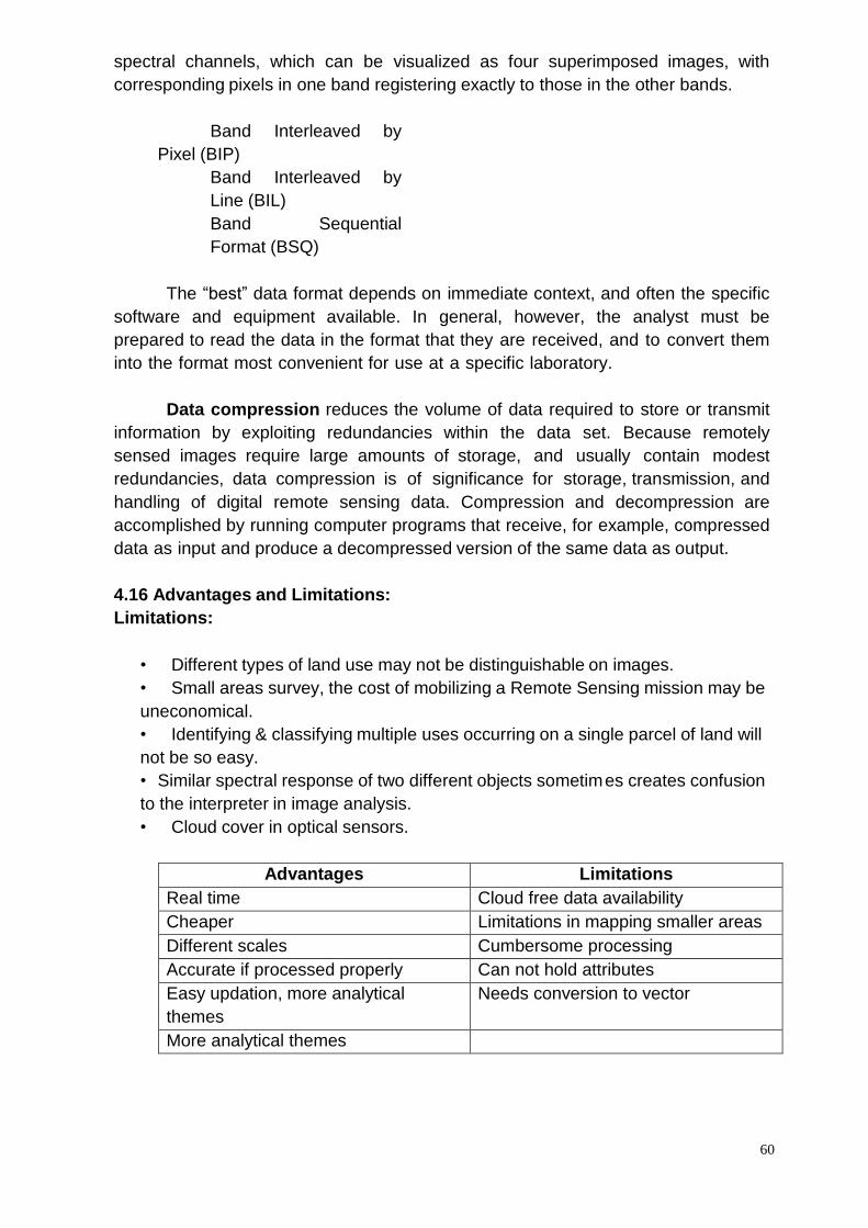
60

spectral channels, which can be visualized as four superimposed images, with

corresponding pixels in one band registering exactly to those in the other bands.

Band Interleaved by

Pixel (BIP)

Band Interleaved by

Line (BIL)

Band Sequential

Format (BSQ)

The “best” data format depends on immediate context, and often the specific

software and equipment available. In general, however, the analyst must be

prepared to read the data in the format that they are received, and to convert them

into the format most convenient for use at a specific laboratory.

Data compression reduces the volume of data required to store or transmit

information by exploiting redundancies within the data set. Because remotely

sensed images require large amounts of storage, and usually contain modest

redundancies, data compression is of significance for storage, transmission, and

handling of digital remote sensing data. Compression and decompression are

accomplished by running computer programs that receive, for example, compressed

data as input and produce a decompressed version of the same data as output.

4.16 Advantages and Limitations:

Limitations:

• Different types of land use may not be distinguishable on images.

• Small areas survey, the cost of mobilizing a Remote Sensing mission may be

uneconomical.

• Identifying & classifying multiple uses occurring on a single parcel of land will

not be so easy.

• Similar spectral response of two different objects sometimes creates confusion

to the interpreter in image analysis.

• Cloud cover in optical sensors.

Advantages Limitations

Real time Cloud free data availability

Cheaper Limitations in mapping smaller areas

Different scales Cumbersome processing

Accurate if processed properly Can not hold attributes

Easy updation, more analytical

themes

Needs conversion to vector

More analytical themes

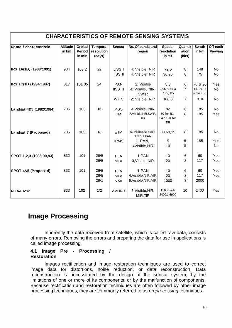
61

Image Processing

Inherently the data received from satellite, which is called raw data, consists of many errors. Removing the errors and preparing the data for use in applications is called image processing.

4.1 Image Pre - Processing / Restoration

Images rectification and image restoration techniques are used to correct

image data for distortions, noise reduction, or data reconstruction. Data reconstruction is necessitated by the design of the sensor system, by the limitations of one or more of its components, or by the malfunction of components. Because rectification and restoration techniques are often followed by other image processing techniques, they are commonly referred to as preprocessing techniques.

CHARACT ERIST ICS OF REMOT E SENSING SYST EMS

Name / characteristic

IRS 1A/1B, (1988/1991)

IRS 1C/1D (1994/1997)

Landsat 4&5 (1982/1984)

Landsat 7 (Proposed) SPOT 1,2,3 (1986,90,93)

SPOT 4&5 (Proposed)

NOAA 6:12

Altitude

in km

904

817

705

705

832

832

833

Orbital

Period

in min

103.2

101.35

103

103

101

101

102

Temporal

resolution

(days)

22

24

16

16

26/5

26/5

26/5

26/5

26/1

1/2

Sensor

LISS I

lISS II

PAN

lISS III

WiFS

MSS

TM

ETM

HRMSI

PLA

MLA

PLA

MLA

VMI

AVHRR

No. Of bands and

region

4; Visible, NIR

4; Visible, NIR

1; Visible

4; Visible, NIR,

SWIR

2; Visible, NIR

4,Visible, NIR

7,Visible,NIR,SWIR,

TIR

6, Visible,NIR,MIR,

1TIR, 1 PAN

1 PAN,

4Visible,NIR

1,PAN

3,Visible,NIR

1,PAN

4,Vis ible,NIR,MIR

5,Vis ible,NIR,MIR

5,Visible,NIR,

MIR,TIR

Spatial

resolution

in mt

72.5

36.25

5.8

23.5,B2:4 &

70.5, B5

188.3

82

30 f or B1-

5&7 120 f or

TIR

30,60,15

5

10

10

20

10

20

1000

1100,nadir

2400& 6900

Quantiz

ation

(bits)

8

8

6

7

7

6

8

8

6

8

6

8

6

8

8

10

Swath

in km

148

75

70 & 90

141,B2:4

& 148,B5

810

185

185

185

185

60

117

60

117

2000

2400

Off-nadir

Viewing

No

No

Yes

No

No

No

Yes

No

Yes

No

Yes

Yes

Yes

Yes

Yes

62

It involves those operations that are normally required prior to the main data analysis and extraction of information. Generally grouped as radiometric or geometric corrections

4.2 Sources of Errors - Internal & External

• Internal - Due to Sensor effects and determined from Pre-launch

measurements - Predictable & Unpredictable

• External - Due to Platform Perturbations, Atmosphere; variable in nature and determined from GCPs and Tracking data

4.3 Errors in imageries: Primarily the errors are of two types:

4.3.1 Radiometric errors: The scanners on satellite platform will have areas of CCDs. Each CCD is responsible for recording the reflections of a particular area on earth’s surface, which is also called as instantaneous field of view (IFOV). The width of the IFOV is termed as its spatial resolution. The reflections will be recorded as a digital number depending upon its (CCDs) radiometric resolution. As per example IRC IC camera is of 7-bit type i.e. it can differentiate the spectral reflection in 128 levels where 0 represents absolute black (total absorption) 127 represents total reflection i.e. pure white. Errors in this phenomenon are again of 3 types.

1) Calibration errors: - Recording the reflection in improper DN values instead

of its assigned range will cause the data un-usable. However every camera will have Calibration correction system, which will be programmed in such a way that periodical refinement is carried. In NRSA the 7 bit (128 levels) data of IRS IC, ID is being converted to 8 bit (256 levels) data as standard format of popular image processing software.

2) Pixel dropouts: - The CCD array is a line of CCDs that are equal to the swath

width of the camera divided by its spatial resolutions. For example IRS IC PAN will have 71000mts / 5.8mts = 12241 nos. Sometimes during scanning process, one or few CCDs may not function properly for an instant or for sometime, which may result in empty DN value for that pixel. These spots are called pixel dropouts.

3) Bad Lines: - When the CCD array totally fails to record for an instance or a

single CCD fails to record continuously lines of missing data appears in imagery. Most of the calibration errors will be rectified by the NRSA during generation of data, for all standard products. In precision product even the pixel dropouts, Bad lines will also be removed for extra price.

4.3.2 Geometric Errors: Errors relating to geometry of the features in image due to various factors are called geometrical errors. Sources of these errors are as follows:

a) Earth’s Curvature: - Surface of earth is curvaceous, so the features in the

center will be scanned true to scale, where as the borders will be reduced to smaller scale progressively from center to periphery.

b) Undulations an earth’s surface: - Though the elevation differences of earth

surface are negligible, when scanning from long distance they induce errors to some extent.

c) Central Perspective Projection: - As the scanners are designed on camera principles, errors of central perspective projection i.e. increase of distortion towards edges are induced in imagery.

63

d) Satellite positional errors: - As a moving object satellite is subjected to have positional

errors like Pitch, Roll & Yaw, which results in tilting of camera angle, thus causes greater distortion in image.

No corrections will be made by NRSA in standard products; geometric corrections will be carried in geo-coded products. All corrections will be made in standard products. The cost of the product will increase from standard to geo-coded to precision product. It is always economical to go for standard products, as they are very cheap compared to other products. 4.4 Corrections of Errors:

4.4.1 Need for Image Correction

To Compensate for Sensor errors and to achieve proper conditions to support image-data analysis and interpretation

Ensuring High Geometric accuracy / Fidelity for Cartographic applications

Registering multiple Images of like geometry and same geographic area coincident with respect to another For Mosaicking multiple scenes covering adjacent and overlapping spatial

regions For removing the errors caused by Sensor defects and Improper Calibration

data

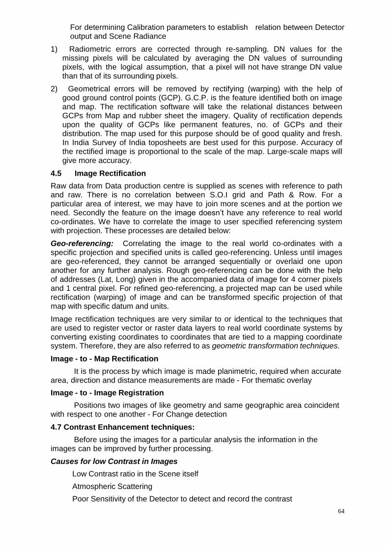
64

For determining Calibration parameters to establish relation between Detector output and Scene Radiance

1) Radiometric errors are corrected through re-sampling. DN values for the

missing pixels will be calculated by averaging the DN values of surrounding pixels, with the logical assumption, that a pixel will not have strange DN value than that of its surrounding pixels.

2) Geometrical errors will be removed by rectifying (warping) with the help of

good ground control points (GCP). G.C.P. is the feature identified both on image and map. The rectification software will take the relational distances between GCPs from Map and rubber sheet the imagery. Quality of rectification depends upon the quality of GCPs like permanent features, no. of GCPs and their distribution. The map used for this purpose should be of good quality and fresh. In India Survey of India toposheets are best used for this purpose. Accuracy of the rectified image is proportional to the scale of the map. Large-scale maps will give more accuracy.

4.5 Image Rectification

Raw data from Data production centre is supplied as scenes with reference to path and raw. There is no correlation between S.O.I grid and Path & Row. For a particular area of interest, we may have to join more scenes and at the portion we need. Secondly the feature on the image doesn’t have any reference to real world co-ordinates. We have to correlate the image to user specified referencing system with projection. These processes are detailed below:

Geo-referencing: Correlating the image to the real world co-ordinates with a specific projection and specified units is called geo-referencing. Unless until images are geo-referenced, they cannot be arranged sequentially or overlaid one upon another for any further analysis. Rough geo-referencing can be done with the help of addresses (Lat, Long) given in the accompanied data of image for 4 corner pixels and 1 central pixel. For refined geo-referencing, a projected map can be used while rectification (warping) of image and can be transformed specific projection of that map with specific datum and units.

Image rectification techniques are very similar to or identical to the techniques that are used to register vector or raster data layers to real world coordinate systems by converting existing coordinates to coordinates that are tied to a mapping coordinate system. Therefore, they are also referred to as geometric transformation techniques.

Image - to - Map Rectification

It is the process by which image is made planimetric, required when accurate

area, direction and distance measurements are made - For thematic overlay Image - to - Image Registration

Positions two images of like geometry and same geographic area coincident

with respect to one another - For Change detection 4.7 Contrast Enhancement techniques:

Before using the images for a particular analysis the information in the

images can be improved by further processing. Causes for low Contrast in Images

Low Contrast ratio in the Scene itself

Atmospheric Scattering

Poor Sensitivity of the Detector to detect and record the contrast

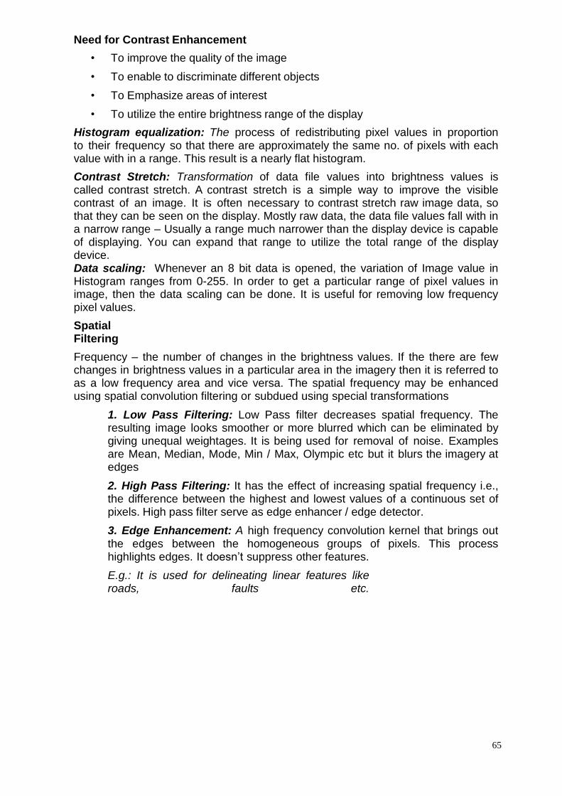
65

Need for Contrast Enhancement

• To improve the quality of the image

• To enable to discriminate different objects

• To Emphasize areas of interest

• To utilize the entire brightness range of the display Histogram equalization: The process of redistributing pixel values in proportion to their frequency so that there are approximately the same no. of pixels with each value with in a range. This result is a nearly flat histogram.

Contrast Stretch: Transformation of data file values into brightness values is called contrast stretch. A contrast stretch is a simple way to improve the visible contrast of an image. It is often necessary to contrast stretch raw image data, so that they can be seen on the display. Mostly raw data, the data file values fall with in a narrow range – Usually a range much narrower than the display device is capable of displaying. You can expand that range to utilize the total range of the display device. Data scaling: Whenever an 8 bit data is opened, the variation of Image value in Histogram ranges from 0-255. In order to get a particular range of pixel values in image, then the data scaling can be done. It is useful for removing low frequency pixel values.

Spatial Filtering

Frequency – the number of changes in the brightness values. If the there are few changes in brightness values in a particular area in the imagery then it is referred to as a low frequency area and vice versa. The spatial frequency may be enhanced using spatial convolution filtering or subdued using special transformations

1. Low Pass Filtering: Low Pass filter decreases spatial frequency. The resulting image looks smoother or more blurred which can be eliminated by giving unequal weightages. It is being used for removal of noise. Examples are Mean, Median, Mode, Min / Max, Olympic etc but it blurs the imagery at edges

2. High Pass Filtering: It has the effect of increasing spatial frequency i.e., the difference between the highest and lowest values of a continuous set of pixels. High pass filter serve as edge enhancer / edge detector.

3. Edge Enhancement: A high frequency convolution kernel that brings out the edges between the homogeneous groups of pixels. This process highlights edges. It doesn’t suppress other features.

E.g.: It is used for delineating linear features like roads, faults etc.

66

4.8 Utility process: 1. Mosaicking: If the area of interest exists in more than one image, we have to join

the images after geo-referencing them. Rectification can be done to original images either before mosaicking or to the mosaicked image afterwards. Whatever the case may be one should be continuous in edge matching particularly in mosaicking side scenes, as they come from different paths and time.

2. Subsetting: Depending upon the camera and satellite, the area, width of the

scene (swath) will change. Accordingly NRSA data center produces the square of swath as full scene. i.e. 70 km2 for PAN, 140 km2 for LISS-III. A full scene is divided into 9 sub scenes. Cutting of image from a scene is called subsetting.

3. Data Merging: Panchromatic data of IRS IC has 5.8mts. Spatial resolution with

which we can see the information clearly up to 1:10000 scale. As the information in this data is from wide band of visible region, it cannot be used individually for any analysis. Like wise LISS III multi-spectral data has 4 bands, but with poor spatial

67

resolution i.e. 23.5mts. Upon data merge we can obtain an image of 4 bands with the spatial resolution of PAN 5.8mts. Different software use different algorithms for this purpose.

4. Analytical Process: The object of Remote Sensing is to gather information about

earth for resource management. Unless until the images of Remote Sensing are analyzed, the purpose of Remote Sensing cannot be achieved. Depending upon the requirements of specific users the analytical process differs. As an example, a forester is interested in analysis of vegetation for different cover types, vegetation types, bio-mass calculations etc., where as a geo-morphologist is interested in identifying faults, dykes, drainage pattern etc. A watershed manager looks for land use land classes’ information, where as an agro-economist looks for crop patterns and crop estimates. Depending upon the need, the images are subjected to different analytical processes. Few of the processes are discussed below:

4.9 Band Rationing: IRS IC LISS-III image consists of 4 bands, out of which 3 bands i.e. green, red, near infrared are important for any analysis. Vegetation is more pronounced in NIR and Red. If rationing is done among these bands most of the information can be brought out as a single bond, which is termed as vegetation index.

a) R.V.I. (Ratio Vegetation Index): Deduction of Red band from Infra red band is called R.V.I. R.V.I. = (IR-R).

b) VI Vegetation index = IR/R

c) N.D.V.I (Normalized Difference Vegetation Index): Fractionalization of RVI with

(IR+R) to get a decimal number for better delineation of index, NDVI formula is used.

NDVI = IR-R IR+R

4.10 Principal Component Analysis: Principal Component analysis (or PCA) is often used as a method of data compression, it allows redundant data to be compacted into fewer bands – that is, the dimensionality of the data is reduced. The bands of PCA data are non-correlated and independent, and are often more interpretable, than the source data.

4.11 Classification: Segregating the information in an image basing on its color, tone, texture, shape, DN values and with the help of ground truthing is called classification. Classified images will give clear- cut information of resources (Thematic maps), which can be quantified.

4.12 AP Forest Department: APFD has procured multi-spectral data for entire state of Andhra Pradesh for the years 1988 (LISS-II – 36.0mts resolution), 1996 (PAN – 5.8mts) & 1996 (LISS-III – 23.5mts) 1998 (LISS-III), 1999 (LISS-III), 2000(LISS III), 2001(LISS III), 2002 (LISS III)&(PAN), 2003 (AWiFS), 2004 (LISS III), 2005 (LISS III), 2006 (LISS III), 2007 (LISS III), 2008 (LISS III), and Cartosat Stereopair 2005-2009

Object of the data procurement is to create 1:50000/1:10000 databases for

vegetation cover and types to use them in planning process; detecting the change in vegetation from 1988 to 1996 and subsequently every year.

68

Image Classification

Classification is the process of categorizing (information in an image into land cover classes or themes) the remotely sensed data into land cover classes or information.

5.1 What Is Image?

Image is the copy of object or landscape captured by scanner or photographic

materials using the Electro Magnetic Spectrum (energy) reflections from the object. It may be in analogue form like photograph or digital form as in the case of remote sensing imageries. There are two types.

Hard Copies: Which are produced generally in photography through chemical process ex: Arial photography. The digital data also can be converted into analog form to produce hard copies. Advantages of hard copies are, they can be usually interpreted without the need of computers for small jobs ex: Satellite imageries – FCC’s.

Soft Copies: These are the digital form of imagery. The information is stored in pixels (picture element) arranged in rows and columns. Each pixel will have a value assigned to it, which can be displayed on computer with a color or grey scale. The scalar differentiation will give an impression to the viewer. The advantage of digital image over analogue image is that the DN (Digital Number) values can be modified as per user’s interest for evolving more information. Another advantage of soft copy is, we can combine more images, captured from different cameras having difference bands, so that more understandable image can be displayed which will be useful for digital analysis for different classification which is also called as digital interpretation.

5.1 Necessity of classification:

Quantification of features is another important aspect of classification. Ex: Area

of vegetation water, wastelands etc.

It is also useful in finding out new feature classes, which are unheard of in particular locations with the help of ground truthing. Ex: Insect attacks, fire, etc.

Change detection of a particular area over a period of time. Requires

classification of Images of different people.

Classification is necessary for understanding different features, more than what human eye can perceive.

In general human eye can at the best distinguish very few colors/tones from an

image, through the interpretation keys like shape, size tone, texture, association, colors pattern help in distinguish different features, they are not sufficient to exactly delineate different types of features, as the modern R.S. cameras are using 8 bit cameras (256 tones in each color)

5.3 Image interpretation Strategies:

a) Field Observation: Field observations, as an approach to image

interpretation, are required when the image and its relationship to ground conditions are so imperfectly understood that the interpreter is forced to go to the field to make an identification.

b) Direct Recognition: Direct recognition is the application of an interpreter’s

experience, skill, and judgment to associate the image patterns with informational classes. The process is essentially a qualitative, subjective analysis of the image using the elements of image interpretation as visual and logical clues.

69

c) Interpretation by Inference: Interpretation by inference is the use of a visual distribution to map one that is not itself visible on the image. The visible distribution acts as a surrogate, or proxy (i.e., substitute) for the mapped distribution.

d) Deterministic Interpretation: Deterministic interpretations are based on

quantitatively expressed relationships that tie image characteristics to ground conditions. In contrast with the other methods, most information is derived from the image itself. Photogrammetric analysis of stereo pairs for terrain information is a good example.

e) Collateral Information: Collateral, or ancillary, information refers to non-image

information used to assist in the interpretation in the form of everyday experience and also formal training. In its narrower meaning, it refers instead to the explicit, conscious effort to employ maps, statistics, and similar material to aid in analysis of an image. In the context of image interpretation, use of collateral information is permissible, and certainly desirable, provided two conditions are satisfied.

f) Interpretive Overlays: Often in resource-oriented interpretations it is

necessary to search for complex associations of several related factors that together define the distribution or pattern of interest. For example, soil patterns may often be revealed by distinctive relationships between separate patterns of vegetation, slope, and drainage. The interpretive overlay approach to image interpretation is a way of deriving information from complex interrelationships between separate distributions recorded on remotely sensed images. From the information presented by several patterns, the interpreter can resolve information not conveyed by any single pattern.

g) Photomorphic Regions: In the first step the interpreter delineates regions of

uniform image appearance, using tone, texture, shadow, and the other elements of image interpretation as a means of separating regions. In the second step the interpreter must be able to match photomorphic regions to useful classes of interest to the interpreter. Delineation of photomorphic regions do not always correspond neatly to the categories of interest to the interpreter. The appearance of one region may be dominated by factors related to geology and topography, whereas that of another region on the same image may be controlled by the vegetation pattern. And the image appearance of a third region may be the result of the interaction of several other factors.

5.3 Types of Classification:

1. Visual Interpretation

2. Digital Interpretation

5.6.1 Visual Interpretation:

It is generally done for small areas where time and money is the constraint. It has

to be done only on hard copies. Interpretation skill is absolute necessary for this work. Image Interpretation Technique:

Image interpretation is defined as the act of examining images for identifying

objects and judging their significance. Interpreters study remotely sensed data and attempt through logical processes in detecting, identifying, classifying, measuring and evaluating the significances of physical and cultural objects, their patterns and special relationship. Image interpretation is a complex process of physical and psychological activities occurring in a sequence of time. The sequence begins with the detection and

70

identification of images and later by their measurements. The various aspects of image interpretation are listed below.

a) Detection: It is a process of “picking out” an object or element from

photo or through interpretation techniques. It may be detection of point or line locations e.g. agricultural field or small settlement.

b) Recognition and Identification: It is a process of classification or trying to

distinguish an object by its characteristics or patterns which are familiar on the image. Sometimes it is also termed as photo reading e.g. water features, streams, tanks, sands, etc.

c) Analysis: It is a process of resolving or separating a set of objects or

features having similar set of objects and the degree of reliability of these lines can also be indicated, e.g. sands as that of rivers.

d) Classification: It is a process of identification and grouping of objects or

features resolved by analysis.

e) Deduction: It is a process where references are drawn about the objects based on direct or indirect evidence of the information or phenomena under study. Deductions may be firmly confirmed by ground checks to avoid misclassification.

f) Idealization: It is a process of drawing ideal or standard representation from

what is actually identified and interpreted from the image or map e.g. set of symbols or colors to be adopted in wasteland maps etc.

Elements of Image Interpretation:

a) Color: Color is an important factor in classification of broads themes ex: blue-

water, Red- vegetation, grey-habitations, white-Barren lands, exposed clouds, sand, and Black-deep water/wet soils.

b) Tone: Tone within a color will give further differentiation among features ex:

Deep red thick vegetation, bright red – agriculture, Deep blue deep water, light blue – shallow water etc.

c) Texture: Different textures will give finer classes like smooth light red – Agriculture, coarse red – Scrub forest; smooth white – clouds, course white – exposed sand etc.

d) Shape: With shape, one can differentiate man made tanks with natural tanks

Agricultural lands with scrub forest, Parks and Grounds with wastelands, Roads with Rivers.

e) Size: Size will also delineate specific features like encroachments, habitations,

and tanks with reservoirs.

f) Pattern: Pattern will give information about features as in the case of clouds, waves in sea etc.

g) Association: Shades of clouds can be distinguished from dark tones with

the help of its association with clouds, like wise streams can be identified with its association of valleys and tanks etc.

h) Shadow: They are cast due to Sun’s illumination angle, size and shape of the

object or sensor- viewing angle. The shape and profile of shadows help in identifying different surface objects e.g. clouds, nature or hill slopes aspect etc. They also help in arriving at tree heights or building heights on aerial photos.

71

i) Location: The geographical site and location of the object often provide clue for identifying objects and understanding their genesis e.g. salt affected land-inland river/desert plains etc.

Advantage of Visual Interpretations:

i. It is very useful for smaller jobs as there is no need of other peripherals

ii. As it is done with human knowledge, differentiation of physical themes like

roads, rivers, tones, clouds, and shades is better delineated.

iii. Generalization is possible for quantification, which will give polygons of minimum mapping quality.

Disadvantages of Visual Interpretation:

i. This cannot be done for large areas, as the availability of skilled manpower is

difficult to get.

ii. Due to limitations of human vision, finer classification is not possible.

iii. Quantification of interpretation needs conversion to vector format, for which again computers are necessary.

iv. Due to ever increasing spatial resolutions, generalization of features is

becoming difficult.

v. Information available in different bands cannot be analyzed.

5.6.2 Digital Interpretation:

Image classification is the process of categorizing (all pixels in an image into land cover classes or themes) the remotely sensed data into land cover classes or information. Normally, multi-spectral data are used to perform the classification i.e., different feature types manifest different combinations of (DNs) digital numbers based on their inherent spectral reflectance and emittance properties. Spectral pattern recognition refers to the family of classification procedures those utilizes this pixel-by-pixel spectral information as the basis for automated land over classification.

Supervised Classification:

In this classification the image analyst “supervises” the pixel

categorization process by specifying, to the computer algorithm, representative sample sites of known cover type, called training areas, as used to compile a numerical “interpretation key” that describes the spectral attributes for each feature type of interest. Each pixel in the data set is then compared numerically to each category in the interpretation key and labeled with the name of the category it “looks most like”.

For example we are dealing with analysis of four channel (LISS III) data. For

each of the pixels shown along this line, the LISS III has measured scene radiance in terms of DNs recorded in each of five spectral bands of sensing; Green, Red, Near-infrared, shortwave infrared. Below the scan line, typical DNs measured over six differently land over types are shown. The vertical bars indicate the relative gray values in each spectral band. These five outputs represent a coarse description of spectral response patterns of various terrain features along the scan line. If these are distinct for each feature type, they may form the basis for image classification.

Basic steps involved in supervised classification.

72

The analyst identifies representative training areas and develops a numerical description of the spectral attributes of each land cover type of interest in the stage.

Each pixel in the image data set is categorized into the land cover class,

it most closely resembles. If the pixel is insufficiently similar to any training data set it is usually labeled ‘unknown’.

Being digital in character, the results may be used in a number of different

ways. Out products are thematic maps; tables of full scenes or sub scene are a statistics for the various land cover classes, and digital data files amenable to inclusion in a GIS. In the latter case the classification “output” becomes a GIS input.

The training stage: The training effort required in supervised classification is

both an art and science. It requires close interaction between the image analyst and the image data. It also required substantial reference data and a thorough knowledge of the geographic area to which the data apply. Most importantly the quality of the training process determines the success of the classification stage and therefore the value of information generated from the entire classification effort.

The over all objective of the training process is to assemble a set of statistics

that describe the spectral response pattern for each land over type to be classified in an image.

Unsupervised Classification:

The fundamental difference between these techniques is that supervised

classification involves a training step followed by a classification involves a training

step followed by a classification step. In the unsupervised approach the image data

are first classified by aggregating them into the natural spectral groupings or clusters

present in the scene. Then, the image analyst determines the land cover identity of

these spectral groups by comparing the classified image data to ground reference data.

Unsupervised classifiers do not utilizes training data as the basis for

classification. Thus family of classifiers involves algorithms that examine the unknown

pixels in an image and aggregate them into a number of classes based on the natural

groupings or clusters present in the image values. The basic premises is that values

within a given cover type should be close together in the measurement space,

whereas data in different classes should be comparatively well separated.

The result from unsupervised classification is spectral classes. Because them

are based solely on the natural groupings in the image values, the identity of the

spectral classes will not be initially known. The analyst must compare the classified

data with some form of reference data (such as larger scale imagery or maps) to

determine the identity and informational value of the spectral classes. Thus, in the

supervised approach we define useful information categories and then examine their

spectral seperability; in the unsupervised approach we determine spectrally

separable classes and then define their informational utility.

73

Basic Steps

• Specify the no. of classes

• Specify the convergence threshold

• Specify the accuracy level

• Specify the algorithm

• Specify the no. of iterations

• Regroup the nearly similar classes

• Assign colors

• Ground Truthing

• Refinement

• Ground Checking & Accuracy assessment

• Generation of Statistics, Maps & Reports Advantages of Digital Classification:

i. Each and every pixel in the image can be classified basing on its DN values.

ii. Any number of Band combinations can be used for delineating required

features using complex algorithms.

iii. Work can be done faster.

iv. Classification can be done number of times using different combination

of algorithm. v. Computation of results is easy.

vi. Conversion of Data into vector form after generalization is easy. Disadvantages of Digital Classification:

i. As the human involvement is reduced in delineation of features, unusual

results may results. ii. Needs good image processing software with skilled

personnel.

iii. Needs generalization before conversion to vector, which may result in increase of error.

5.4 Ground Truthing / Ground Checking

Process of establishing correlation between spectral signatures and ground

information. Ground truthing in remote sensing is the ground investigation that is carried out to give the sensing investigator or operational user a realistic portrait of the target and also necessary in research and operational applications. The ground observations can be obtained from regularly collected or already available data sometimes, but often a ground investigation data collection program must be specifically designed for the RS mission. Because the ground investigations are very costly, it is essential to determine which info is required to meet the needs of a particular activity. After the RS mission or operational period, the utility of the ground investigation data should be carefully examined, to determine whether the results of the ground investigation were compromised because of inadequate data, or whether the same conclusions would have been reached with fewer ground investigation.

74

5.4.1 Uses of ground truth data: The main uses of ground truth data are

• calibrating the radiometers, Spectrometers etc. • Interpretation of properties

• Training sets

• Verification

5.4.2 Test sites

Test sites are the small selected areas in which the necessary ancillary data will

be collected to gain the knowledge of the area that can be used to aid the interpretation of the entire area under question. The physical and biological characteristics of these sites shall be extensively studied, and a variety of RS data shall be tested over them. It is always advisable to choose the site for which already extensive field data is available, and if new site is to be chosen it should be easily accessible.

Ground investigation involves two kinds of observations i.e., Visual and Spectral

measurements depending upon the objective to be achieved. The visual ground truth involves observation such as color, shape, size, texture, temperature of the object of interest. The spectral observation involves measurement of spectral reflectance of a particular object, in-situ using specially designed equipment for this purpose.

5.4.3 Spectral signature

It can be defined as any remotely sensed parameter which directly or indirectly

characterizes the nature and/or condition of the object under investigation. This can be defined as a unique pattern of wavelengths radiated by an object. These are

Spectral variation – Variation in reflectivity and emissivity as a function of wavelength.

Spatial variation – Variation in reflectivity and emissivity with spatial position

(shape, size, texture of the object).

Temporal variation - of reflectivity and emissivity like that in diurnal and seasonal cycle.

Polarization variation – which are introduced by the material in the radiation

reflected or emitted by it.

Each of these four features of EMR may be independent at different times or different spectral bands. A measure of these variations and correlating them with the known features of an object provides signature of the object concerned. The knowledge of the state of polarization of the reflected radiation in addition to the spectral signatures of various objects in RS adds another dimension in interpretation of RS data. The degree of polarization and Stoke’s parameter are extremely useful in providing valuable data in discriminating the objects.

Verification of accuracy of classification is called ground truthing. It has to be done in the following steps.

i. Identifying different classes ii. Selection of points in different classes either systematically or randomly with

ratio suitable to time, money and accuracy available. iii. Collection of location of the selected points with references.

iv. Field work

v. Recording the findings in field

vi. Computerization & finding accuracy.

75

It can be done any number of times depending upon the accuracy needs. In

APFD the ground truthing is done by the people acquainted with the area (usually Beat officers), which is being used by the project scientists as training sets. Further the classified outputs are being sent to field for accuracy assessment.

5.4.4 Accuracy Assessment:

Accuracy Assessment is the quantitative identification and measurement of map

error. There is no simple, standardized, generally accepted methodology for

determining classification accuracy. The two of the most commonly employed

approaches an from a digital classification t the “known” identity of land cover in test

areas derived from reference data. One or combinations of the following, typically

represent the test areas.

1. Homogeneous test areas selected by the analyst.

2. Test pixels or areas selected randomly.

Test areas are areas of representative, uniform land cover that are

different from, and considerable more extensive than, training areas. They are often

located during the training, stage of supervised classification by intentionally

designating more candidate training areas than are actually needed to develop the

classification statistics. A subset of these may then be withheld for the post

classification accuracy assessment, again using a contingency table to express the

results (Table-I). The accuracies obtained in these areas represent at least a first

approximation to classification performance throughout the scene. However, being

homogeneous, test areas might not provide a valid indication of classification

accuracy at the individual pixel level of land cover variability.

Table.1 Contingency Table Resulting from Classifying Test Area Pixels

Known Categor y Type

Number of

Pixels

Percentag e correct

Number of pixels classified into category

1

2

3

4

5

6

1

2

3

4

5

6

5352

328

4284

945

2380

3048

97

66

84

42

80

72

5165

0

0

12

0

8

0

216

0

92

9

0

42

0

3599

228

28

48

44

108

16

397

78

18

53

4

482

132

1904

779

21

0

187

84

361

2195

Over all classification performance: 82.6% (total correct pixels/total pixels) Average performance by class: 73.5% (average of category accuracies).

1-Water, 2-Sand, 3-forest, 4-Urban, 5-Corm, 6-Hay

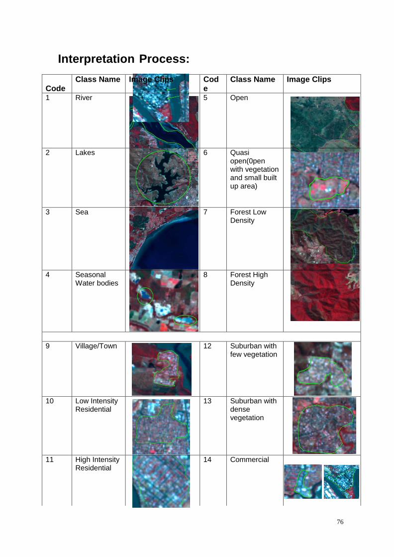
76

Interpretation Process:

Code

Class Name Image Clips Code

Class Name Image Clips

1 River 5 Open

2 Lakes 6 Quasi open(0pen with vegetation and small built up area)

3 Sea 7 Forest Low Density

4 Seasonal Water bodies

8 Forest High Density

9 Village/Town 12 Suburban with

few vegetation

10 Low Intensity Residential

13 Suburban with dense vegetation

11 High Intensity Residential

14 Commercial

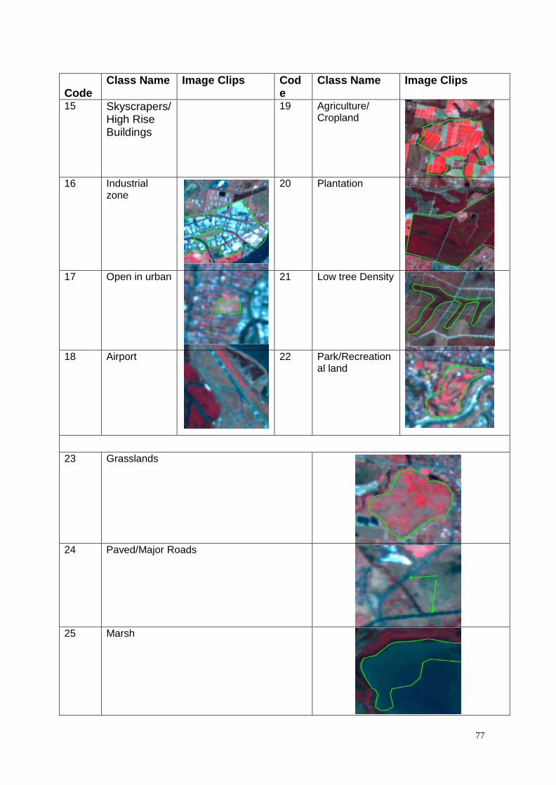
77

Code

Class Name Image Clips Code

Class Name Image Clips

15 Skyscrapers/ High Rise Buildings

19 Agriculture/ Cropland

16 Industrial zone

20 Plantation

17 Open in urban 21 Low tree Density

18 Airport 22 Park/Recreational land

23 Grasslands

24 Paved/Major Roads

25 Marsh

78

Data Browsing

Data browsing is one of the important aspects in creation of data base as per the

user specifications. Earlier the browsing was done at NRSA Data Center (NDC), NRSA,

Blanagar, Hyderabad, now these browsing facility is also available through the Internet

at http://www.nrsa.gov.in

The satellites revolve round the earth in predefined orbits and accordingly the

Remote Sensing data will be collected and organized at NDC with separate indexing

called Path and Rows. IRS 1A/1B is defined with same kind of Path and Rows as per the

configuration of the satellites. Where as the indexing pattern of the satellites of

IRS1C/1D is entirely different from the indexing of the satellite series 1A/1B.

The IRS 1C/1D is a three body stabilized satellites designed and launched in a

polar sun synchronous orbit at an altitude about 800kms. Each path is repeated after a

period of 24 days.

The referencing scheme of LISS III consists of 341 paths numbered from west to

east. Each path consists of 141 rows. Each LISS III scene covers an area of

141X141kms. The referencing scheme of LISS III over an India is shown here.

Fig: Path and Row scheme of IRS 1C/1D LISS III sensor over India

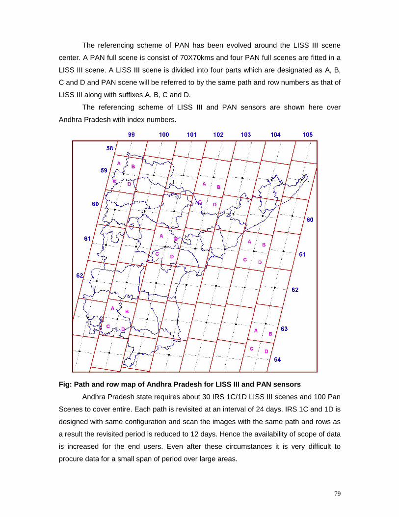
79

The referencing scheme of PAN has been evolved around the LISS III scene

center. A PAN full scene is consist of 70X70kms and four PAN full scenes are fitted in a

LISS III scene. A LISS III scene is divided into four parts which are designated as A, B,

C and D and PAN scene will be referred to by the same path and row numbers as that of

LISS III along with suffixes A, B, C and D.

The referencing scheme of LISS III and PAN sensors are shown here over

Andhra Pradesh with index numbers.

Fig: Path and row map of Andhra Pradesh for LISS III and PAN sensors

Andhra Pradesh state requires about 30 IRS 1C/1D LISS III scenes and 100 Pan

Scenes to cover entire. Each path is revisited at an interval of 24 days. IRS 1C and 1D is

designed with same configuration and scan the images with the same path and rows as

a result the revisited period is reduced to 12 days. Hence the availability of scope of data

is increased for the end users. Even after these circumstances it is very difficult to

procure data for a small span of period over large areas.

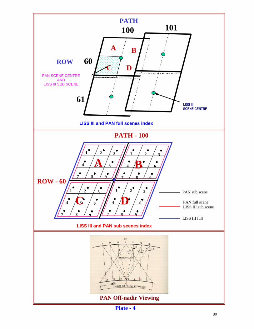
80

LISS III and PAN full scenes index

LISS III and PAN sub scenes index

Plate - 4

60

61

100 101 PATH

ROW

LISS III SCENE CENTRE

A B

C D PAN SCENE CENTRE

AND LISS III SUB SCENE

PATH - 100

ROW - 60

1 2 3

4 5 6

7 8 9

1 2 3

4 5 6

7 8 9

1 2 3

4 5 6

7 8 9

1 2 3

4 5 6

7 8 9

A B

D C

LISS III full

scene

PAN full scene

LISS III sub scene

PAN sub scene

PAN Off-nadir Viewing

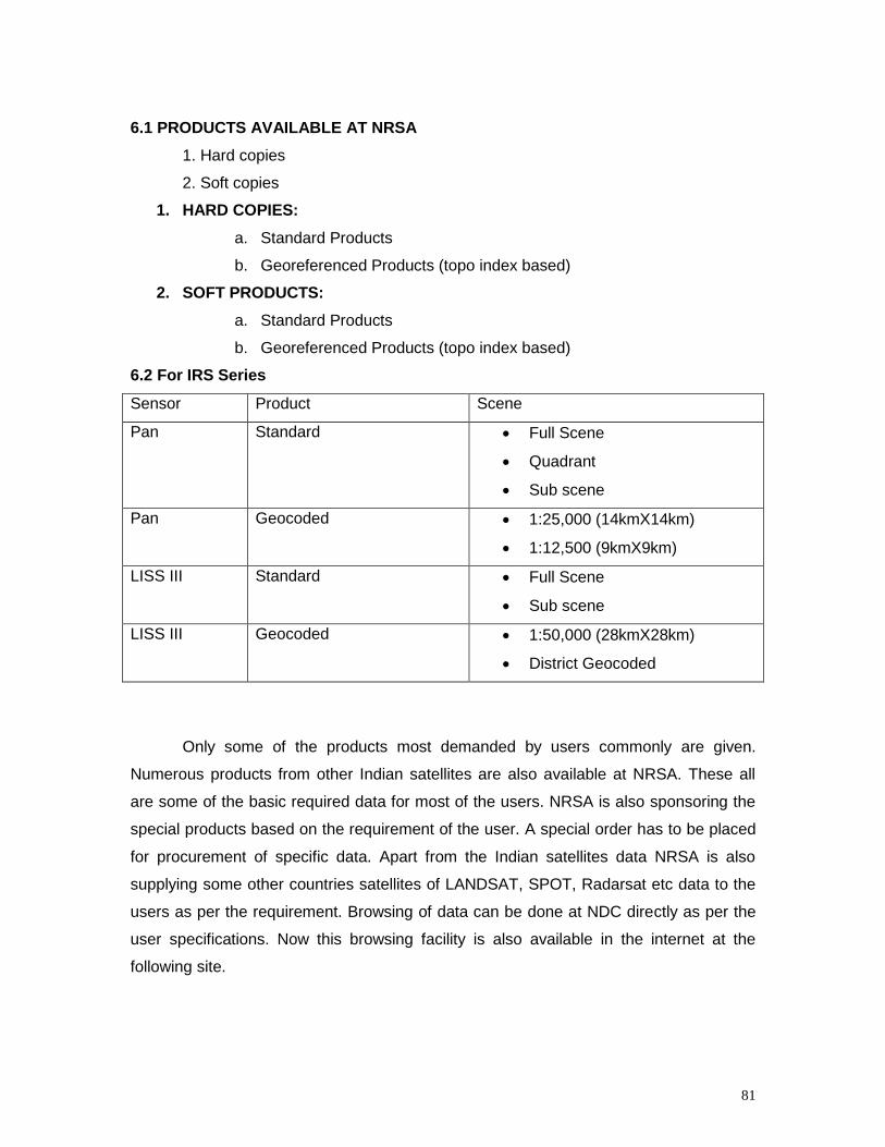
81

6.1 PRODUCTS AVAILABLE AT NRSA

1. Hard copies

2. Soft copies

1. HARD COPIES:

a. Standard Products

b. Georeferenced Products (topo index based)

2. SOFT PRODUCTS:

a. Standard Products

b. Georeferenced Products (topo index based)

6.2 For IRS Series

Sensor Product Scene

Pan Standard Full Scene

Quadrant

Sub scene

Pan Geocoded 1:25,000 (14kmX14km)

1:12,500 (9kmX9km)

LISS III Standard Full Scene

Sub scene

LISS III Geocoded 1:50,000 (28kmX28km)

District Geocoded

Only some of the products most demanded by users commonly are given.

Numerous products from other Indian satellites are also available at NRSA. These all

are some of the basic required data for most of the users. NRSA is also sponsoring the

special products based on the requirement of the user. A special order has to be placed

for procurement of specific data. Apart from the Indian satellites data NRSA is also

supplying some other countries satellites of LANDSAT, SPOT, Radarsat etc data to the

users as per the requirement. Browsing of data can be done at NDC directly as per the

user specifications. Now this browsing facility is also available in the internet at the

following site.

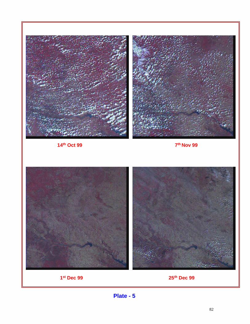
82

14th Oct 99 7th Nov 99

1st Dec 99 25th Dec 99

Plate - 5

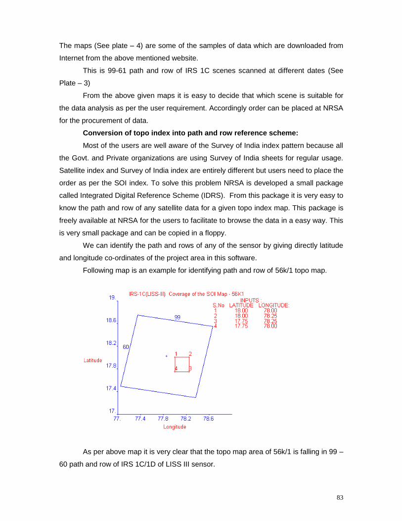
83

The maps (See plate – 4) are some of the samples of data which are downloaded from

Internet from the above mentioned website.

This is 99-61 path and row of IRS 1C scenes scanned at different dates (See

Plate – 3)

From the above given maps it is easy to decide that which scene is suitable for

the data analysis as per the user requirement. Accordingly order can be placed at NRSA

for the procurement of data.

Conversion of topo index into path and row reference scheme:

Most of the users are well aware of the Survey of India index pattern because all

the Govt. and Private organizations are using Survey of India sheets for regular usage.

Satellite index and Survey of India index are entirely different but users need to place the

order as per the SOI index. To solve this problem NRSA is developed a small package

called Integrated Digital Reference Scheme (IDRS). From this package it is very easy to

know the path and row of any satellite data for a given topo index map. This package is

freely available at NRSA for the users to facilitate to browse the data in a easy way. This

is very small package and can be copied in a floppy.

We can identify the path and rows of any of the sensor by giving directly latitude

and longitude co-ordinates of the project area in this software.

Following map is an example for identifying path and row of 56k/1 topo map.

As per above map it is very clear that the topo map area of 56k/1 is falling in 99 –

60 path and row of IRS 1C/1D of LISS III sensor.

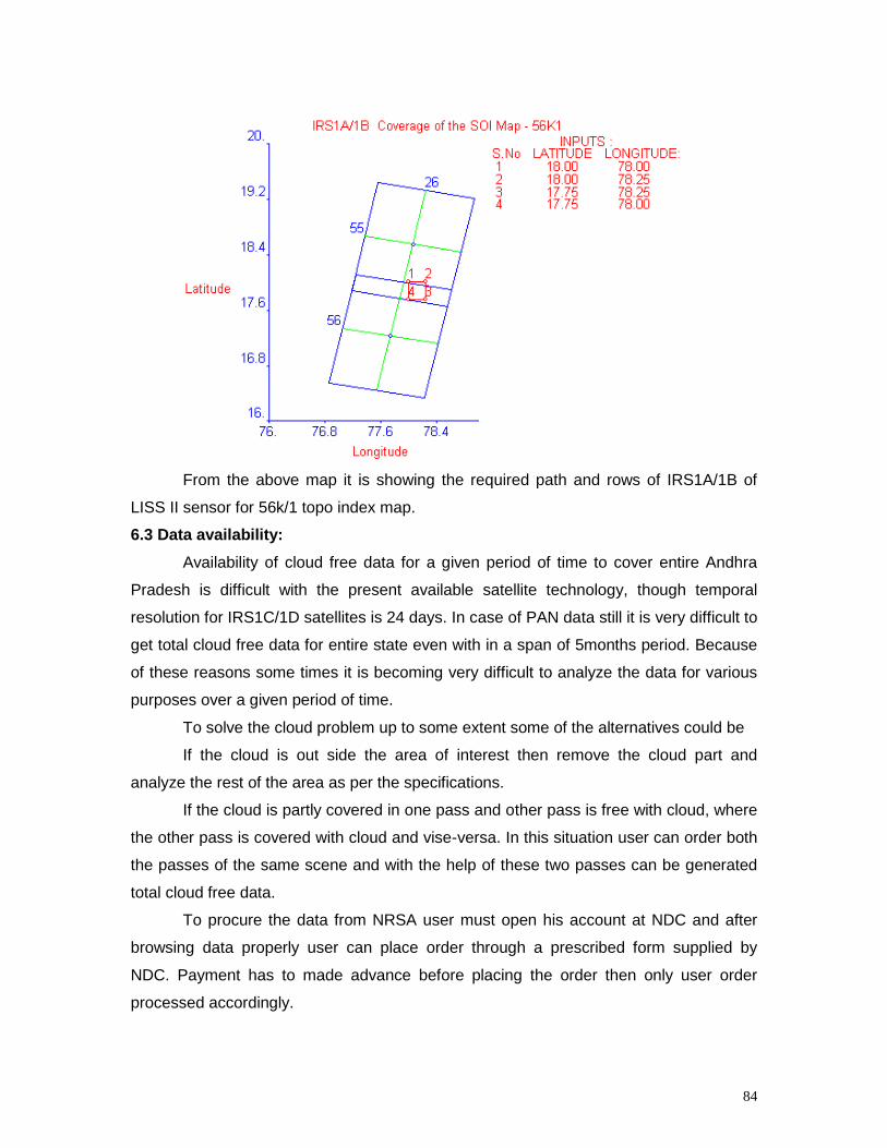
84

From the above map it is showing the required path and rows of IRS1A/1B of

LISS II sensor for 56k/1 topo index map.

6.3 Data availability:

Availability of cloud free data for a given period of time to cover entire Andhra

Pradesh is difficult with the present available satellite technology, though temporal

resolution for IRS1C/1D satellites is 24 days. In case of PAN data still it is very difficult to

get total cloud free data for entire state even with in a span of 5months period. Because

of these reasons some times it is becoming very difficult to analyze the data for various

purposes over a given period of time.

To solve the cloud problem up to some extent some of the alternatives could be

If the cloud is out side the area of interest then remove the cloud part and

analyze the rest of the area as per the specifications.

If the cloud is partly covered in one pass and other pass is free with cloud, where

the other pass is covered with cloud and vise-versa. In this situation user can order both

the passes of the same scene and with the help of these two passes can be generated

total cloud free data.

To procure the data from NRSA user must open his account at NDC and after

browsing data properly user can place order through a prescribed form supplied by

NDC. Payment has to made advance before placing the order then only user order

processed accordingly.

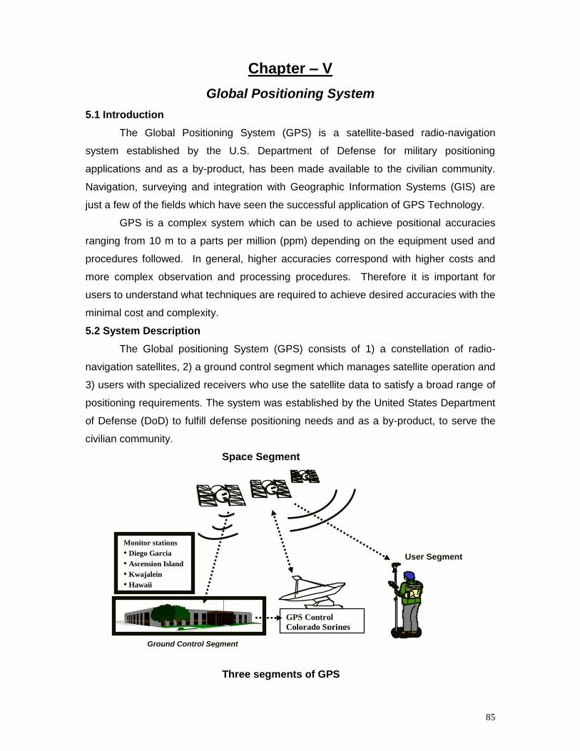
85

Chapter – V

Global Positioning System

5.1 Introduction

The Global Positioning System (GPS) is a satellite-based radio-navigation

system established by the U.S. Department of Defense for military positioning

applications and as a by-product, has been made available to the civilian community.

Navigation, surveying and integration with Geographic Information Systems (GIS) are

just a few of the fields which have seen the successful application of GPS Technology.

GPS is a complex system which can be used to achieve positional accuracies

ranging from 10 m to a parts per million (ppm) depending on the equipment used and

procedures followed. In general, higher accuracies correspond with higher costs and

more complex observation and processing procedures. Therefore it is important for

users to understand what techniques are required to achieve desired accuracies with the

minimal cost and complexity.

5.2 System Description

The Global positioning System (GPS) consists of 1) a constellation of radio-

navigation satellites, 2) a ground control segment which manages satellite operation and

3) users with specialized receivers who use the satellite data to satisfy a broad range of

positioning requirements. The system was established by the United States Department

of Defense (DoD) to fulfill defense positioning needs and as a by-product, to serve the

civilian community.

Space Segment

Three segments of GPS

Monitor stations

• Diego Garcia

• Ascension Island

• Kwajalein

• Hawaii

User Segment

GPS Control

Colorado Springs

Ground Control Segment

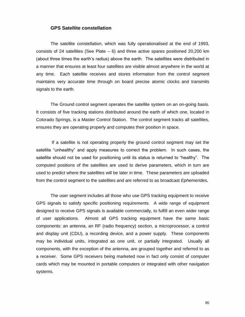
86

GPS Satellite constellation

The satellite constellation, which was fully operationalised at the end of 1993,

consists of 24 satellites (See Plate – 6) and three active spares positioned 20,200 km

(about three times the earth’s radius) above the earth. The satellites were distributed in

a manner that ensures at least four satellites are visible almost anywhere in the world at

any time. Each satellite receives and stores information from the control segment

maintains very accurate time through on board precise atomic clocks and transmits

signals to the earth.

The Ground control segment operates the satellite system on an on-going basis.

It consists of five tracking stations distributed around the earth of which one, located in

Colorado Springs, is a Master Control Station. The control segment tracks all satellites,

ensures they are operating properly and computes their position in space.

If a satellite is not operating properly the ground control segment may set the

satellite “unhealthy” and apply measures to correct the problem. In such cases, the

satellite should not be used for positioning until its status is returned to “healthy”. The

computed positions of the satellites are used to derive parameters, which in turn are

used to predict where the satellites will be later in time. These parameters are uploaded

from the control segment to the satellites and are referred to as broadcast Ephemerides.

The user segment includes all those who use GPS tracking equipment to receive

GPS signals to satisfy specific positioning requirements. A wide range of equipment

designed to receive GPS signals is available commercially, to fulfill an even wider range

of user applications. Almost all GPS tracking equipment have the same basic

components: an antenna, an RF (radio frequency) section, a microprocessor, a control

and display unit (CDU), a recording device, and a power supply. These components

may be individual units, integrated as one unit, or partially integrated. Usually all

components, with the exception of the antenna, are grouped together and referred to as

a receiver. Some GPS receivers being marketed now in fact only consist of computer

cards which may be mounted in portable computers or integrated with other navigation

systems.

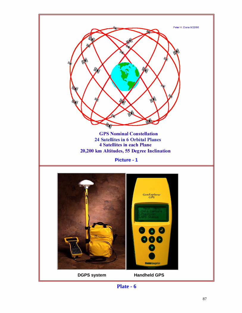
87

Picture - 1

DGPS system Handheld GPS

Plate - 6

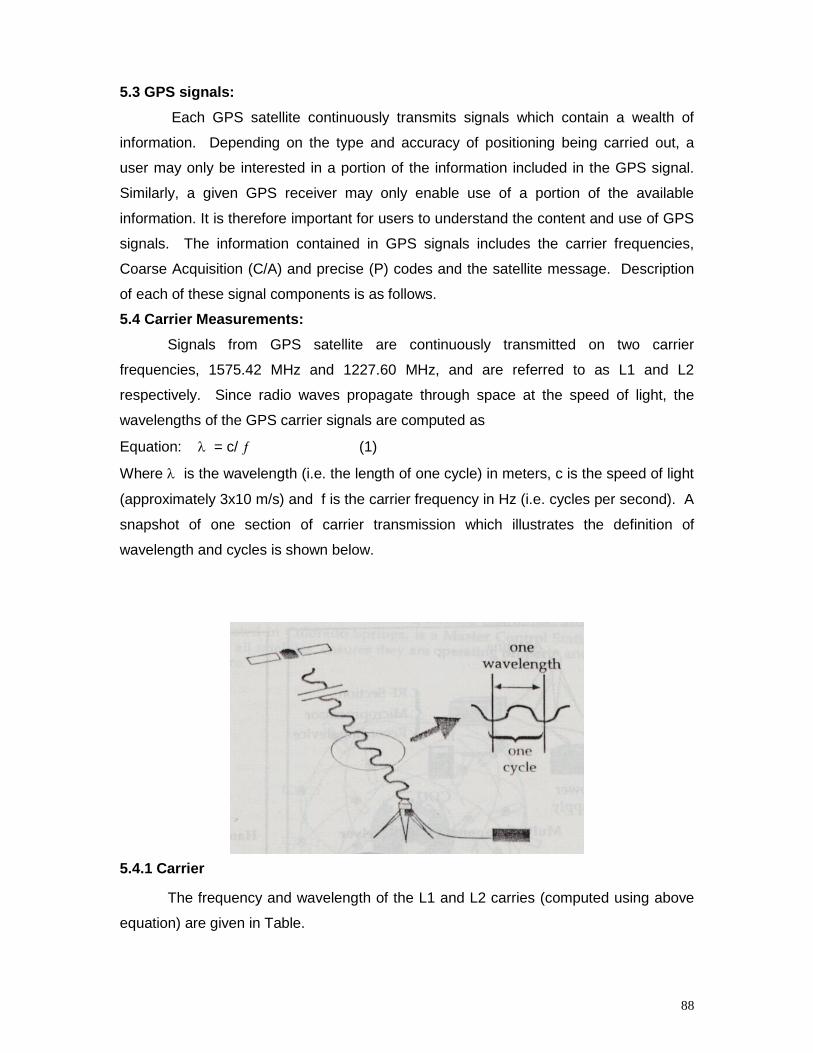
88

5.3 GPS signals:

Each GPS satellite continuously transmits signals which contain a wealth of

information. Depending on the type and accuracy of positioning being carried out, a

user may only be interested in a portion of the information included in the GPS signal.

Similarly, a given GPS receiver may only enable use of a portion of the available

information. It is therefore important for users to understand the content and use of GPS

signals. The information contained in GPS signals includes the carrier frequencies,

Coarse Acquisition (C/A) and precise (P) codes and the satellite message. Description

of each of these signal components is as follows.

5.4 Carrier Measurements:

Signals from GPS satellite are continuously transmitted on two carrier

frequencies, 1575.42 MHz and 1227.60 MHz, and are referred to as L1 and L2

respectively. Since radio waves propagate through space at the speed of light, the

wavelengths of the GPS carrier signals are computed as

Equation: = c/ (1)

Where is the wavelength (i.e. the length of one cycle) in meters, c is the speed of light

(approximately 3x10 m/s) and f is the carrier frequency in Hz (i.e. cycles per second). A

snapshot of one section of carrier transmission which illustrates the definition of

wavelength and cycles is shown below.

5.4.1 Carrier

The frequency and wavelength of the L1 and L2 carries (computed using above

equation) are given in Table.

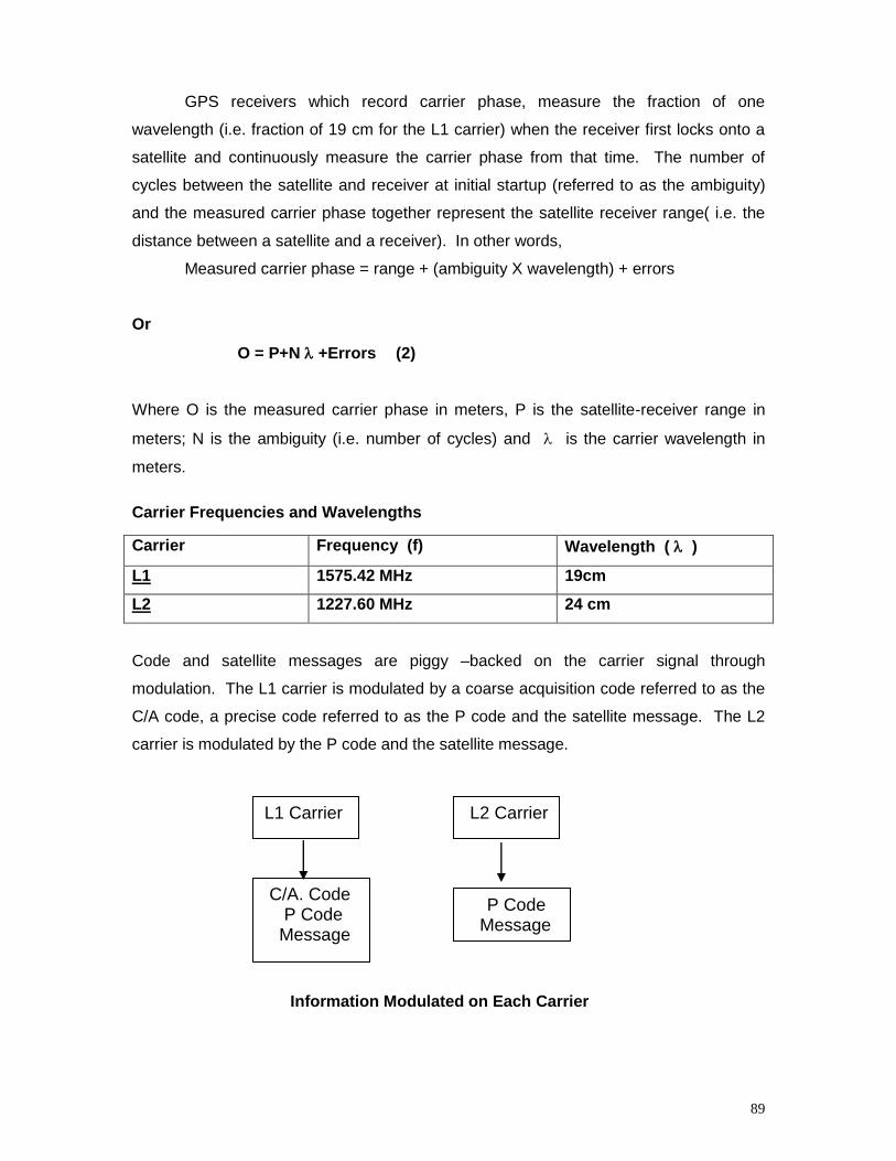
89

GPS receivers which record carrier phase, measure the fraction of one

wavelength (i.e. fraction of 19 cm for the L1 carrier) when the receiver first locks onto a

satellite and continuously measure the carrier phase from that time. The number of

cycles between the satellite and receiver at initial startup (referred to as the ambiguity)

and the measured carrier phase together represent the satellite receiver range( i.e. the

distance between a satellite and a receiver). In other words,

Measured carrier phase = range + (ambiguity X wavelength) + errors

Or

O = P+N +Errors (2)

Where O is the measured carrier phase in meters, P is the satellite-receiver range in

meters; N is the ambiguity (i.e. number of cycles) and is the carrier wavelength in

meters.

Carrier Frequencies and Wavelengths

Carrier Frequency (f) Wavelength ( )

L1 1575.42 MHz 19cm

L2 1227.60 MHz 24 cm

Code and satellite messages are piggy –backed on the carrier signal through

modulation. The L1 carrier is modulated by a coarse acquisition code referred to as the

C/A code, a precise code referred to as the P code and the satellite message. The L2

carrier is modulated by the P code and the satellite message.

Information Modulated on Each Carrier

L1 Carrier L2 Carrier

C/A. Code P Code Message

P Code Message

90

5.4.2 Code Measurements

It is the code measurements (also referred to as pseudo range measurements)

that enable instantaneous position determinations using GPS satellites. The code is

composed of a series of chips, which have values of 1 or 0. The C/A code has a

frequency of 1.023 MHz (i.e. 1.023 million chips per second) and the P code has a

frequency of 10.23 MHz.

The chip lengths of 293 m and 29.3 m for the C/A code and P code respectively

were computed using equation (1), letting be the chip length. Although the P code is

generally ten times more accurate than the C/A code, it is expected to be unavailable for

civilian use in 1993 when the full GPS constellation was complete. Meaning only C/A

code is worthy of consideration for civilian GPS applications.

Code measurements are the difference in time between when the code is

transmitted from a satellite and received at a GPS receiver, multiplied by the speed of

light. That is,

Measured code = speed of light x (reception time – transmission time)

OR

P = C (t - tt) (3)

Where P is the measured code, C is the speed of light, tt is the signal reception time

and tt is the signal transmission time. The code measurement is actually a direct

measurement of satellite – receiver range ( P ) , i.e.:

Measured code = range + errors

Or

P = P + Errors (4)

Comparison of Code (Pseudo-range) and Carrier Measurements:

At this point it is possible to make some brief comparisons of code and carrier

measurements. Carrier wavelengths (19cm for L1) are much shorter than the C/A code

chip length (293 m) and consequently can be measured more accurately and used to

achieve much higher positional accuracies than code measurements. Indeed the best

relative accuracies achieved using code measurements are usually a few meters, and

using carrier measurement are usually a few centimeters.

The problem with using carrier observations instead of code observations is

evident upon comparison of equations (2) and (4). With code observations a direct

measure of the satellite–receiver range is attained. With carrier observations the

91

ambiguity term (number of whole cycles) must be estimated before one may take

advantage of the carrier accuracy. Ambiguity estimation leads to complexities in the use

of carrier phase observations which do not exist with code observations. The

advantages and disadvantages of code and carrier observations are summarized in

Table below

5.4.3 Key Advantages and Disadvantages of Code and Carrier Observations

Code Carrier

Advantages Non-ambiguous simple High accuracy potential

Disadvantages Low accuracy More complex

5.5 Satellite message:

The satellite message, which is modulated on both L1 and L2 frequencies,

contains among other information, satellite broadcast ephemeredes and health status.

The ephemeredes include the parameters necessary to compute a satellite’s position

in space for a given time and the health status indicates if a satellite is healthy. Almost

all receivers use the broadcast ephemeredes in conjunction with code observations,

carrier observations or both to solve for a GPS receiver’s position in space.

5.6 Types of GPS positioning

Up to this point, the three segments of GPS have been described and the

components of signals broadcasted by the satellites have been explained. Major types

of possible positioning methods may now be defined. Note that only broad definitions

are presented here, while specific GPS positioning methods are addressed in detail in

several publications.

5.6.1 Single Point versus Relative Positioning:

Positioning with GPS may take the form of single point positioning or relative

positioning. In single point positioning coordinates of a receiver at an “unknown” point

are sought with respect to the earth’s reference frame by using the “known” positions of

the GPS satellites being tracked. Single point positioning is also referred to as absolute

positioning, and often just as point positioning. In relative positioning the coordinates of

a receiver at an “unknown” point are sought with respect to a receiver at a “known” point.

The concept of single point positioning is illustrated in Fig. below using the

broadcast ephemeredes; the position of any satellite at any point of time may be

computed.

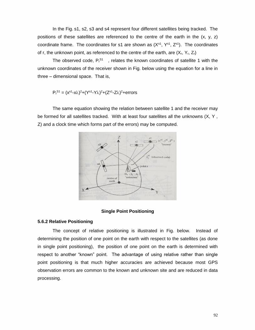
92

In the Fig. s1, s2, s3 and s4 represent four different satellites being tracked. The

positions of these satellites are referenced to the centre of the earth in the (x, y, z)

coordinate frame. The coordinates for s1 are shown as (Xs1, Ys1, Zs1). The coordinates

of r, the unknown point, as referenced to the centre of the earth, are (Xr, Yr, Zr)

The observed code, PrS1 , relates the known coordinates of satellite 1 with the

unknown coordinates of the receiver shown in Fig. below using the equation for a line in

three – dimensional space. That is,

PrS1 = (xs1-x)2+(Ys1-Y)2+(Zs1-Z)2+errors

The same equation showing the relation between satellite 1 and the receiver may

be formed for all satellites tracked. With at least four satellites all the unknowns (X, Y ,

Z) and a clock time which forms part of the errors) may be computed.

Single Point Positioning

5.6.2 Relative Positioning

The concept of relative positioning is illustrated in Fig. below. Instead of

determining the position of one point on the earth with respect to the satellites (as done

in single point positioning), the position of one point on the earth is determined with

respect to another “known” point. The advantage of using relative rather than single

point positioning is that much higher accuracies are achieved because most GPS

observation errors are common to the known and unknown site and are reduced in data

processing.

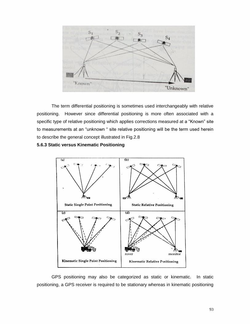
93

The term differential positioning is sometimes used interchangeably with relative

positioning. However since differential positioning is more often associated with a

specific type of relative positioning which applies corrections measured at a “Known” site

to measurements at an “unknown “ site relative positioning will be the term used herein

to describe the general concept illustrated in Fig.2.8

5.6.3 Static versus Kinematic Positioning

GPS positioning may also be categorized as static or kinematic. In static

positioning, a GPS receiver is required to be stationary whereas in kinematic positioning

94

a receiver collects GPS data while moving. The concepts of static and kinematic

positioning for both single point and relative positioning cases are illustrated in fig below.

Note that for kinematic relative positioning one receiver, referred to as a monitor , is left

stationary on a known point while a second receiver, referred to as a rover, is moved

over the path to be positioned.

5.6.4. Real –Time versus Post-Mission

GPS positions may be attained through real-time or post-mission processing. In

real –time processing, positions are computed almost instantaneously, on site. In post –

mission processing, data is combined and reduced after all data collection has been

completed. Real –time relative positioning requires a data link to transmit corrections

from a monitor receiver at a known point to a rover receiver at an unknown point. Post –

mission processing for relative positioning requires physically bringing together the data

from all receivers after an observation period. Even with real-time point positioning, for

many GPS applications it is still necessary to download data and enter it in a database

specific to the user’s application.

Very low accuracy code single point positioning is usually computed by GPS

receivers in real-time, whereas very high accuracy carrier relative positioning is almost

always dependent on post-mission processing. Real-time and spot –mission processing

options exist for methodologies which yield accuracies between these two extremes.

All GPS positioning may be classified as static or kinematic, single point or

relative, and real-time or post-mission. All users of GPS, no matter what the positioning

type used, must be aware of the best times for data collection, which brings about

discussion of satellite visibility and availability.

5.7. Satellite visibility and availability

Users of GPS must know where, when and what satellites should be tracked to

attain the best results. Terms used to describe satellite visibility are described, followed

by a discussion of satellite geometry, satellite azimuth and elevation, selective

availability and anti-spoofing.

The location of satellites with respect to a specific point on the earth is described

in terms of elevation angle and azimuth. The elevation angle is the angle from the

antenna between the horizontal and the line of sight to the satellite.

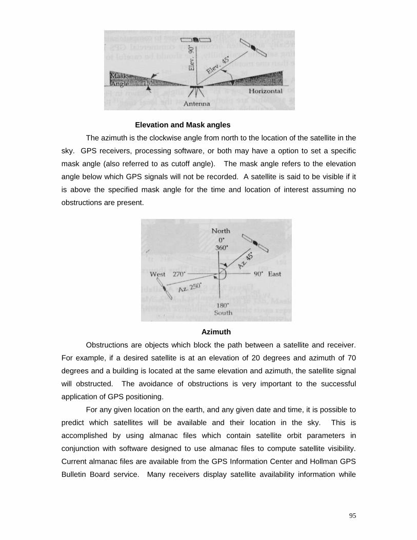
95

Elevation and Mask angles

The azimuth is the clockwise angle from north to the location of the satellite in the

sky. GPS receivers, processing software, or both may have a option to set a specific

mask angle (also referred to as cutoff angle). The mask angle refers to the elevation

angle below which GPS signals will not be recorded. A satellite is said to be visible if it

is above the specified mask angle for the time and location of interest assuming no

obstructions are present.

Azimuth

Obstructions are objects which block the path between a satellite and receiver.

For example, if a desired satellite is at an elevation of 20 degrees and azimuth of 70

degrees and a building is located at the same elevation and azimuth, the satellite signal

will obstructed. The avoidance of obstructions is very important to the successful

application of GPS positioning.

For any given location on the earth, and any given date and time, it is possible to

predict which satellites will be available and their location in the sky. This is

accomplished by using almanac files which contain satellite orbit parameters in

conjunction with software designed to use almanac files to compute satellite visibility.

Current almanac files are available from the GPS Information Center and Hollman GPS

Bulletin Board service. Many receivers display satellite availability information while

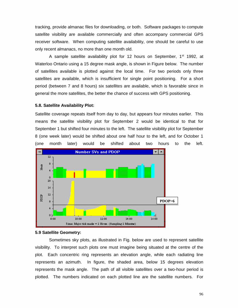
96

tracking, provide almanac files for downloading, or both. Software packages to compute

satellite visibility are available commercially and often accompany commercial GPS

receiver software. When computing satellite availability, one should be careful to use

only recent almanacs, no more than one month old.

A sample satellite availability plot for 12 hours on September, 1st 1992, at

Waterloo Ontario using a 15 degree mask angle, is shown in Figure below. The number

of satellites available is plotted against the local time. For two periods only three

satellites are available, which is insufficient for single point positioning. For a short

period (between 7 and 8 hours) six satellites are available, which is favorable since in

general the more satellites, the better the chance of success with GPS positioning.

5.8. Satellite Availability Plot:

Satellite coverage repeats itself from day to day, but appears four minutes earlier. This

means the satellite visibility plot for September 2 would be identical to that for

September 1 but shifted four minutes to the left. The satellite visibility plot for September

8 (one week later) would be shifted about one half hour to the left, and for October 1

(one month later) would be shifted about two hours to the left.

5.9 Satellite Geometry:

Sometimes sky plots, as illustrated in Fig. below are used to represent satellite

visibility. To interpret such plots one must imagine being situated at the centre of the

plot. Each concentric ring represents an elevation angle, while each radiating line

represents an azimuth. In figure, the shaded area, below 15 degrees elevation

represents the mask angle. The path of all visible satellites over a two-hour period is

plotted. The numbers indicated on each plotted line are the satellite numbers. For

PDOP>6

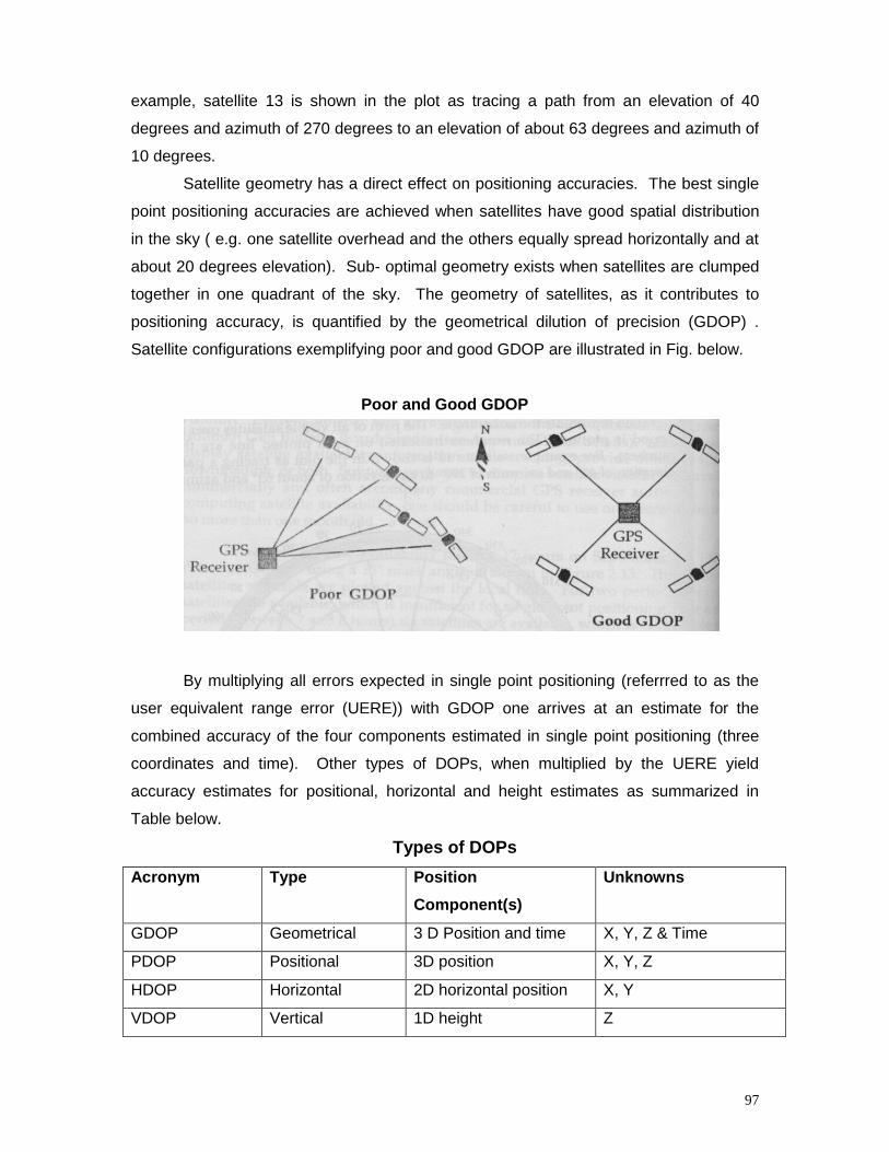
97

example, satellite 13 is shown in the plot as tracing a path from an elevation of 40

degrees and azimuth of 270 degrees to an elevation of about 63 degrees and azimuth of

10 degrees.

Satellite geometry has a direct effect on positioning accuracies. The best single

point positioning accuracies are achieved when satellites have good spatial distribution

in the sky ( e.g. one satellite overhead and the others equally spread horizontally and at

about 20 degrees elevation). Sub- optimal geometry exists when satellites are clumped

together in one quadrant of the sky. The geometry of satellites, as it contributes to

positioning accuracy, is quantified by the geometrical dilution of precision (GDOP) .

Satellite configurations exemplifying poor and good GDOP are illustrated in Fig. below.

Poor and Good GDOP

By multiplying all errors expected in single point positioning (referrred to as the

user equivalent range error (UERE)) with GDOP one arrives at an estimate for the

combined accuracy of the four components estimated in single point positioning (three

coordinates and time). Other types of DOPs, when multiplied by the UERE yield

accuracy estimates for positional, horizontal and height estimates as summarized in

Table below.

Types of DOPs

Acronym Type Position

Component(s)

Unknowns

GDOP Geometrical 3 D Position and time X, Y, Z & Time

PDOP Positional 3D position X, Y, Z

HDOP Horizontal 2D horizontal position X, Y

VDOP Vertical 1D height Z

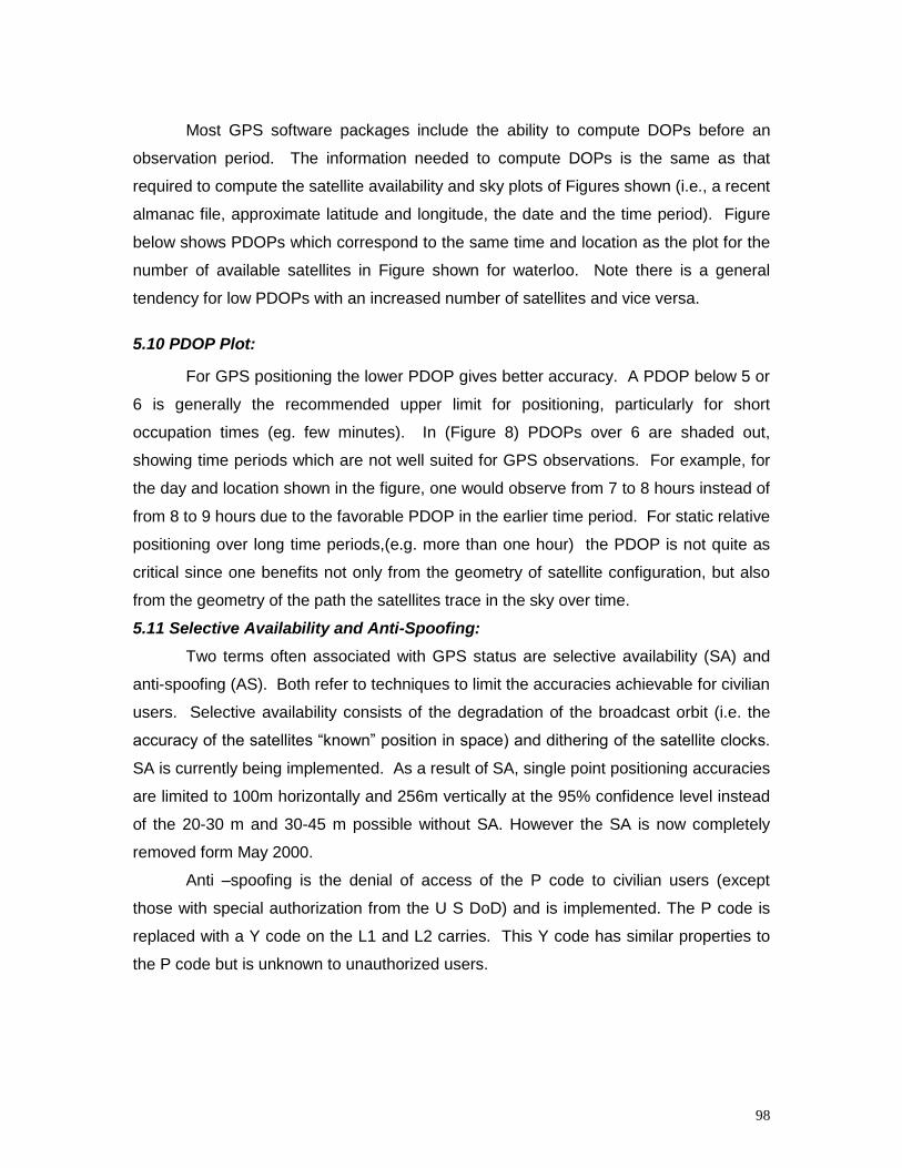
98

Most GPS software packages include the ability to compute DOPs before an

observation period. The information needed to compute DOPs is the same as that

required to compute the satellite availability and sky plots of Figures shown (i.e., a recent

almanac file, approximate latitude and longitude, the date and the time period). Figure

below shows PDOPs which correspond to the same time and location as the plot for the

number of available satellites in Figure shown for waterloo. Note there is a general

tendency for low PDOPs with an increased number of satellites and vice versa.

5.10 PDOP Plot:

For GPS positioning the lower PDOP gives better accuracy. A PDOP below 5 or

6 is generally the recommended upper limit for positioning, particularly for short

occupation times (eg. few minutes). In (Figure 8) PDOPs over 6 are shaded out,

showing time periods which are not well suited for GPS observations. For example, for

the day and location shown in the figure, one would observe from 7 to 8 hours instead of

from 8 to 9 hours due to the favorable PDOP in the earlier time period. For static relative

positioning over long time periods,(e.g. more than one hour) the PDOP is not quite as

critical since one benefits not only from the geometry of satellite configuration, but also

from the geometry of the path the satellites trace in the sky over time.

5.11 Selective Availability and Anti-Spoofing:

Two terms often associated with GPS status are selective availability (SA) and

anti-spoofing (AS). Both refer to techniques to limit the accuracies achievable for civilian

users. Selective availability consists of the degradation of the broadcast orbit (i.e. the

accuracy of the satellites “known” position in space) and dithering of the satellite clocks.

SA is currently being implemented. As a result of SA, single point positioning accuracies

are limited to 100m horizontally and 256m vertically at the 95% confidence level instead

of the 20-30 m and 30-45 m possible without SA. However the SA is now completely

removed form May 2000.

Anti –spoofing is the denial of access of the P code to civilian users (except

those with special authorization from the U S DoD) and is implemented. The P code is

replaced with a Y code on the L1 and L2 carries. This Y code has similar properties to

the P code but is unknown to unauthorized users.

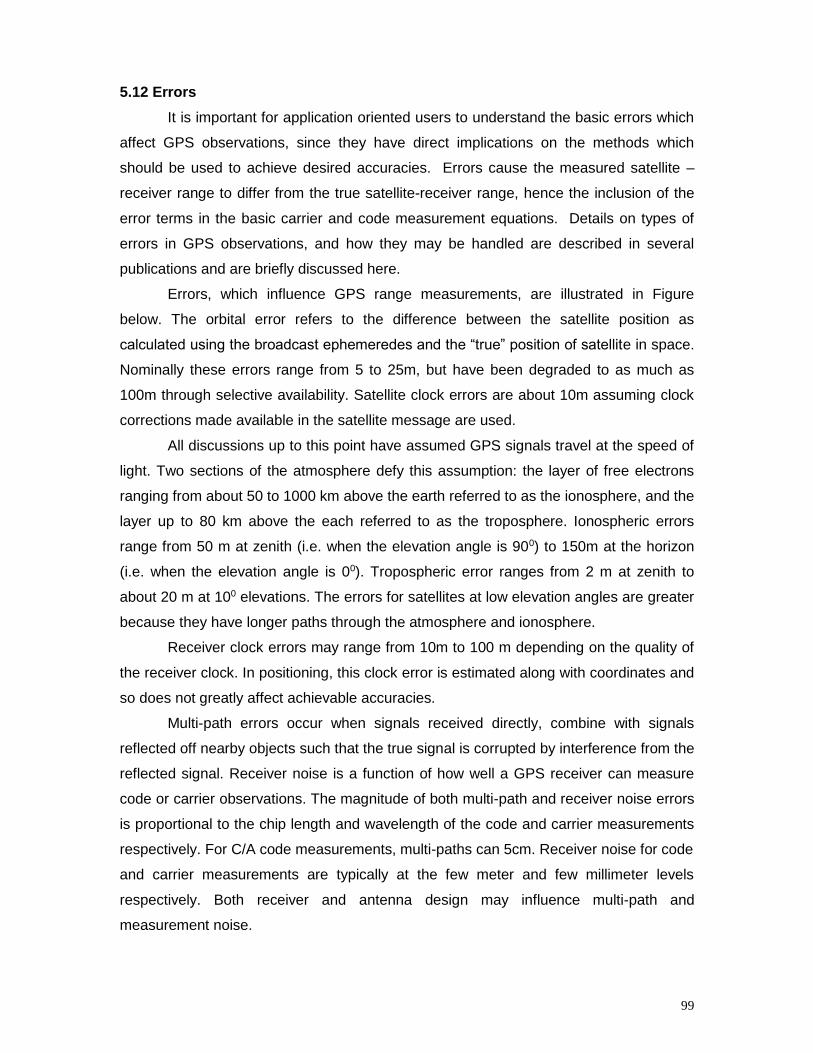
99

5.12 Errors

It is important for application oriented users to understand the basic errors which

affect GPS observations, since they have direct implications on the methods which

should be used to achieve desired accuracies. Errors cause the measured satellite –

receiver range to differ from the true satellite-receiver range, hence the inclusion of the

error terms in the basic carrier and code measurement equations. Details on types of

errors in GPS observations, and how they may be handled are described in several

publications and are briefly discussed here.

Errors, which influence GPS range measurements, are illustrated in Figure

below. The orbital error refers to the difference between the satellite position as

calculated using the broadcast ephemeredes and the “true” position of satellite in space.

Nominally these errors range from 5 to 25m, but have been degraded to as much as

100m through selective availability. Satellite clock errors are about 10m assuming clock

corrections made available in the satellite message are used.

All discussions up to this point have assumed GPS signals travel at the speed of

light. Two sections of the atmosphere defy this assumption: the layer of free electrons

ranging from about 50 to 1000 km above the earth referred to as the ionosphere, and the

layer up to 80 km above the each referred to as the troposphere. Ionospheric errors

range from 50 m at zenith (i.e. when the elevation angle is 900) to 150m at the horizon

(i.e. when the elevation angle is 00). Tropospheric error ranges from 2 m at zenith to

about 20 m at 100 elevations. The errors for satellites at low elevation angles are greater

because they have longer paths through the atmosphere and ionosphere.

Receiver clock errors may range from 10m to 100 m depending on the quality of

the receiver clock. In positioning, this clock error is estimated along with coordinates and

so does not greatly affect achievable accuracies.

Multi-path errors occur when signals received directly, combine with signals

reflected off nearby objects such that the true signal is corrupted by interference from the

reflected signal. Receiver noise is a function of how well a GPS receiver can measure

code or carrier observations. The magnitude of both multi-path and receiver noise errors

is proportional to the chip length and wavelength of the code and carrier measurements

respectively. For C/A code measurements, multi-paths can 5cm. Receiver noise for code

and carrier measurements are typically at the few meter and few millimeter levels

respectively. Both receiver and antenna design may influence multi-path and

measurement noise.

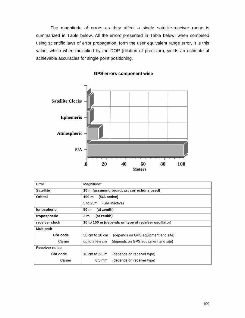
100

The magnitude of errors as they affect a single satellite-receiver range is

summarized in Table below. All the errors presented in Table below, when combined

using scientific laws of error propagation, form the user equivalent range error. It is this

value, which when multiplied by the DOP (dilution of precision), yields an estimate of

achievable accuracies for single point positioning.

GPS errors component wise

Error Magnitude*

Satellite 10 m (assuming broadcast corrections used)

Orbital 100 m (S/A active)

5 to 25m (S/A inactive)

Ionospheric 50 m (at zenith)

tropospheric 2 m (at zenith)

receiver clock 10 to 100 m (depends on type of receiver oscillator)

Multipath

C/A code

Carrier

50 cm to 20 cm (depends on GPS equipment and site)

up to a few cm (depends on GPS equipment and site)

Receiver noise

C/A code

Carrier

10 cm to 2-3 m (depends on receiver type)

0.5 mm (depends on receiver type)

Meters

S/A

Atmospheric

Ephemeris

Satellite Clocks

0 20 40 60 80 100

101

An error unique to carrier phase observations is the cycle slip. Recall from the

discussion preceding the carrier equation, that carrier phase is measured continuously,

but has an ambiguity term at the time of initial satellite lock. The failure to maintain

continuous lock on a satellite causes cycle slips, in which an integer number of

wavelengths may be lost. Cycle slips must be corrected through data processing if

carrier measurements are to be used to achieve sub-decimeter accuracy.

The wide range of accuracies and positioning techniques with GPS are a result

of the type of observations used (code, carrier or both) and the means for handling the

errors listed in Table above. When accuracies better than the 100 m achievable with

single point positioning are required, relative positioning should be employed. In relative

positioning most of the orbital, tropospheric and Ionospheric errors along the satellite-

receiver path are common to both sites and consequently their influence on the relative

positions is small. The closer the GPS receivers are to each other, the more common

are these errors and the greater the accuracy achieved through relative positioning.

Accordingly, the further apart the GPS receivers are far from each other, the less

common are these errors and the less accurate the relative positioning.

For precise static relative positioning, sophisticated means for handling errors are

employed which include combining observations through double differencing techniques

and using advanced modeling and estimation. Dual frequency receivers may be used to

almost totally remove errors due to the ionosphere in relative positioning over long

baselines.

List of Global Navigation Satellite Systems currently operational and in development 1 – GPS of the United States of America

GPS (Global Positioning System) is the United States system that uses 32

satellites that are in medium Earth Orbit. They are placed in six distinct orbital

planes, and older satellites are constantly replaced by new ones. It has been in

operation since 1978 and it is the most used navigation system that incorporates

satellites.

2 – GLONASS of Russia

GLONASS or Global Navigation Sputnik System is a Russian satellite

navigation system that is used for civilian operations. It makes use of radio

navigation satellites and is also utilized by the Aerospace Defence of the Russian

Forces. It consists of 24 full orbital constellations of satellites that allow for global

coverage.

102

3 – Galileo of the European Union

Galileo is the European Union satellite navigation system introduced in

2002. The European Space Agency also makes use of this system and is used

as an alternative to the United States GPS. It makes use of 30 satellites that are

in medium Earth orbit. It has been designed to be compatible with the GPS

system of US and receivers can make use of combined signals from GPS and

Galileo, mainly to increase the level of accuracy.

4 – BeiDou of People’s Republic of China

China has been using the system BeiDou for its military and civilian

navigation purposes. It is currently in the second generation and was formerly

known as COMPASS, and serves the Asia-Pacific region in addition to China. It

makes use of 30 Medium Earth Orbit Satellites and 5 satellites that are in

geostationary orbit.

5 – IRNSS or NAVIC of India

IRNSS (Indian Regional Navigation Satellite System) or NAVIC

(Navigation with Indian Constellation) is the satellite navigation system used by

the Indian Space Research Organization, which is directly controlled by the

Indian Government. It consists of 7 satellites out of which 3 are placed in

geostationary orbit while the other four are in geosynchronous orbit. It has a very

large signal footprint in comparison to the number of satellites in operation. All

satellites in the constellation have been launched from within India, and the

system will be fully operational in 2016.

6 – QZSS of Japan

The Quasi-Zenith Satellite System (QZSS) is a proposed three-satellite

regional time transfer system and enhancement for GPS covering Japan. The

first demonstration satellite was launched in September 2010.

Difference between GNSS and GPS

GNSS stands for Global Navigation Satellite System, and is an umbrella term that encompasses all global satellite positioning systems. This includes constellations of satellites orbiting over the earth’s surface and continuously transmitting signals that enable users to determine their position.

The Global Positioning System (GPS) is one component of the Global Navigation Satellite System. Specifically, it refers to the NAVSTAR Global Positioning System, a constellation of satellites developed by the United States Department of Defense (DoD). Originally, the Global Positioning System was developed for military use, but was later made accessible to civilians as well. GPS is now the most widely used GNSS in the world, and provides continuous positioning and timing information globally, under any weather conditions.

103

Besides GPS, the GNSS currently includes other satellite navigation systems, such as the Russian GLONASS, and may soon include others such as the European Union’s Galileo and China’s Beidou.

GNSS is used in collaboration with GPS systems to provide precise location positioning anywhere on earth. GNSS and GPS work together, but the main difference between GPS and GNSS is that GNSS-compatible equipment can use navigational satellites from other networks beyond the GPS system, and more satellites means increased receiver accuracy and reliability. All GNSS receivers are compatible with GPS, but GPS receivers are not necessarily compatible with GNSS.

Both GPS and GNSS consist of three major segments: the space segment (satellites), the ground segment (ground control stations), and the user segment (GNSS or GPS receivers), and the exact location of each satellite is known at any given moment. Satellites are continuously sending radio signals toward earth, which are picked up by GNSS or GPS receivers. The ground control stations that monitor the Global Navigation Satellite System continuously track satellites, update the positions of each and enable information on earth to be transmitted to the satellites.

Currently, GNSS/GPS is being used in a variety of fields where the use of precise, continually available position and time information is required, including agriculture, transportation, machine control, marine navigation, vehicle navigation, mobile communication and athletics.

5.13 GPS Technology in Forest Department:

1. Navigational GPS are required for use in forests for ground truthing, locational search

in Forest Inventory and for general perambulation. Here accuracy of 10mts is good

enough for the purpose. Hand held GPS equipment is best suited for this purpose and

was procured.

2. Surveying GPS are the differential GPS meant for accurate measurements (Sub-

meter accuracies). These are useful in demarcating Forest Block, surveying plantations,

Mining areas, Compensatory areas and encroachments, where accuracy is of

importance for this purpose APFD has procured two models i.e., Trimble and CMT. The

Trimble model can be effectively used to achieve the 3-D accuracy.

Now time has come to every forest officer to learn about the use, need and

intricacies of GPS technology to deploy it in their day-to-day for better management of

Forests.

104

Chapter – VI

Geomatics Applications

Watershed management 6.1 Introduction:

The “Water” is one of the five basic elements of life out of pancha bhuta

i.e. air, water, earth, fire and sky on the earth is the most essential element of life.

Earth has water covering about 3/4th of the total surface area but sufficient

water is not available both for drinking and irrigation in several parts of the world.

India is being one of them. Over the centuries population explosion,

urbanization, conversion of forests to agriculture, have multiplied the demand for

water. Fresh water problem is not limited to the arid climatic regions, even in

areas with good supply the access to safe water is becoming a critical problem.

Water on earth goes through a gigantic cycle of conversation to gaseous form by

evaporation and coming down again to earth as rainfall. For masses the main

source of water is the surface water that flows in streams, rivers and ground

water which are highly influenced by the adjoining forests.

In the India Rain water is the most important factor in Indian Agricultural

production. 75% of the total cropped area is under rain fed/ un-irrigated and

account for about 42% of the total food grain production. More than 78% of

cotton; 82% of oil seeds 96% of sorghum; 98% of the millets and as much as

62% of the rice and 38% of wheat of the country are grown under rain fed

conditions. Therefore country’s Development lies in the improvement in the

productivity of these crops. Since water is the major limiting factor for the

production of rain fed crops and precipitation is the only source of water in most

of rain fed regions, effective rain water management is vital to increase and

stabilized their yields. To effectively manage rain water forests play a vital role.

Scientific investigations onto forest – water relations began around the turn of the

20th century. It is proven after intensive research that

1. Reduction of forest cover increases water runoff

2. Establishment of forest cover in sparely vegetated land decreases water

yield.

3. Response to treatment is highly variable and for the most part, unpredictable.

In the areas where forests and agriculture are coexisting the influence of

the forest cover has great influence on the adjoining agriculture by way of

regulating the streams and long duration of the flow; reducing the silt yield,

increasing the ground water recharge. The dependence of the neighboring

villages on forests for several purposes and ever increasing populations has led

to the degrading of forest. In this complex situation classical management did

not yield expected results. Therefore the Government had started to find out

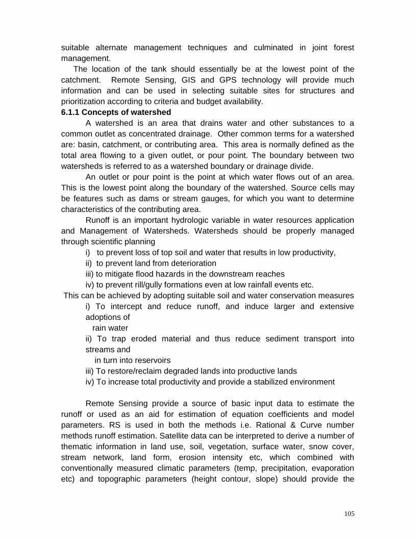
105

suitable alternate management techniques and culminated in joint forest

management.

The location of the tank should essentially be at the lowest point of the

catchment. Remote Sensing, GIS and GPS technology will provide much

information and can be used in selecting suitable sites for structures and

prioritization according to criteria and budget availability.

6.1.1 Concepts of watershed

A watershed is an area that drains water and other substances to a

common outlet as concentrated drainage. Other common terms for a watershed

are: basin, catchment, or contributing area. This area is normally defined as the

total area flowing to a given outlet, or pour point. The boundary between two

watersheds is referred to as a watershed boundary or drainage divide.

An outlet or pour point is the point at which water flows out of an area.

This is the lowest point along the boundary of the watershed. Source cells may

be features such as dams or stream gauges, for which you want to determine

characteristics of the contributing area.

Runoff is an important hydrologic variable in water resources application

and Management of Watersheds. Watersheds should be properly managed

through scientific planning

i) to prevent loss of top soil and water that results in low productivity,

ii) to prevent land from deterioration

iii) to mitigate flood hazards in the downstream reaches

iv) to prevent rill/gully formations even at low rainfall events etc.

This can be achieved by adopting suitable soil and water conservation measures

i) To intercept and reduce runoff, and induce larger and extensive

adoptions of

rain water

ii) To trap eroded material and thus reduce sediment transport into

streams and

in turn into reservoirs

iii) To restore/reclaim degraded lands into productive lands

iv) To increase total productivity and provide a stabilized environment

Remote Sensing provide a source of basic input data to estimate the

runoff or used as an aid for estimation of equation coefficients and model

parameters. RS is used in both the methods i.e. Rational & Curve number

methods runoff estimation. Satellite data can be interpreted to derive a number of

thematic information in land use, soil, vegetation, surface water, snow cover,

stream network, land form, erosion intensity etc, which combined with

conventionally measured climatic parameters (temp, precipitation, evaporation

etc) and topographic parameters (height contour, slope) should provide the

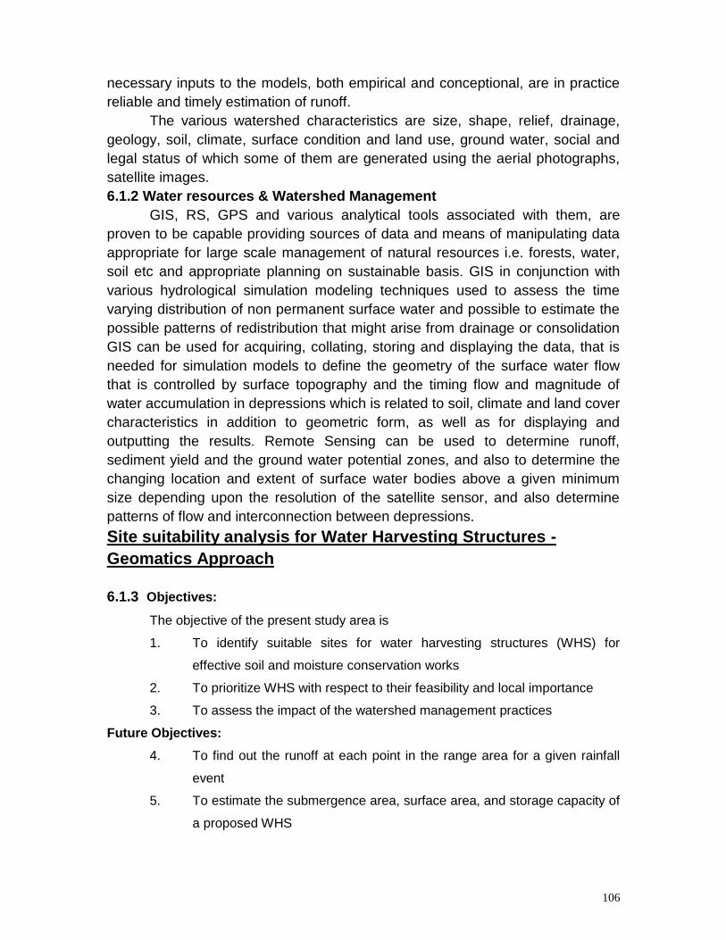
106

necessary inputs to the models, both empirical and conceptional, are in practice

reliable and timely estimation of runoff.

The various watershed characteristics are size, shape, relief, drainage,

geology, soil, climate, surface condition and land use, ground water, social and

legal status of which some of them are generated using the aerial photographs,

satellite images.

6.1.2 Water resources & Watershed Management

GIS, RS, GPS and various analytical tools associated with them, are

proven to be capable providing sources of data and means of manipulating data

appropriate for large scale management of natural resources i.e. forests, water,

soil etc and appropriate planning on sustainable basis. GIS in conjunction with

various hydrological simulation modeling techniques used to assess the time

varying distribution of non permanent surface water and possible to estimate the

possible patterns of redistribution that might arise from drainage or consolidation

GIS can be used for acquiring, collating, storing and displaying the data, that is

needed for simulation models to define the geometry of the surface water flow

that is controlled by surface topography and the timing flow and magnitude of

water accumulation in depressions which is related to soil, climate and land cover

characteristics in addition to geometric form, as well as for displaying and

outputting the results. Remote Sensing can be used to determine runoff,

sediment yield and the ground water potential zones, and also to determine the

changing location and extent of surface water bodies above a given minimum

size depending upon the resolution of the satellite sensor, and also determine

patterns of flow and interconnection between depressions.

Site suitability analysis for Water Harvesting Structures -

Geomatics Approach

6.1.3 Objectives:

The objective of the present study area is

1. To identify suitable sites for water harvesting structures (WHS) for

effective soil and moisture conservation works

2. To prioritize WHS with respect to their feasibility and local importance

3. To assess the impact of the watershed management practices

Future Objectives:

4. To find out the runoff at each point in the range area for a given rainfall

event

5. To estimate the submergence area, surface area, and storage capacity of

a proposed WHS

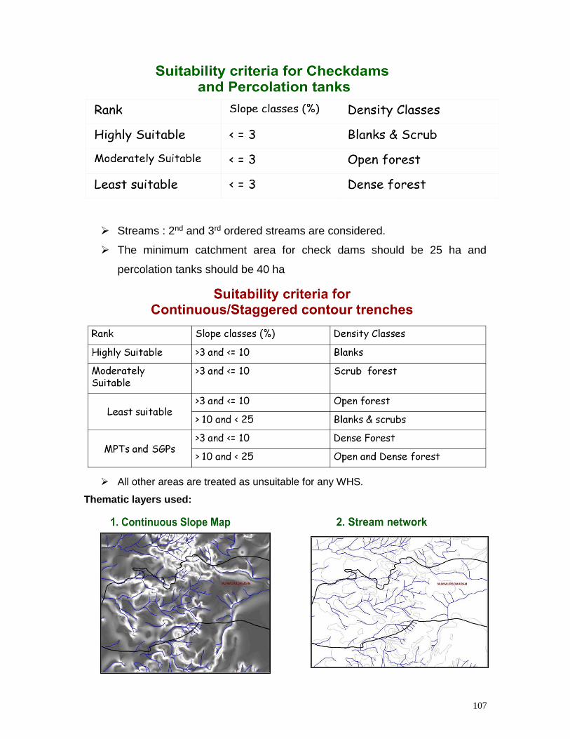
107

Streams : 2nd and 3rd ordered streams are considered.

The minimum catchment area for check dams should be 25 ha and

percolation tanks should be 40 ha

All other areas are treated as unsuitable for any WHS.

Thematic layers used:

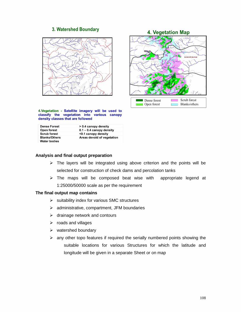
108

Analysis and final output preparation

The layers will be integrated using above criterion and the points will be

selected for construction of check dams and percolation tanks

The maps will be composed beat wise with appropriate legend at

1:25000/50000 scale as per the requirement

The final output map contains

suitability index for various SMC structures

administrative, compartment, JFM boundaries

drainage network and contours

roads and villages

watershed boundary

any other topo features if required the serially numbered points showing the

suitable locations for various Structures for which the latitude and

longitude will be given in a separate Sheet or on map

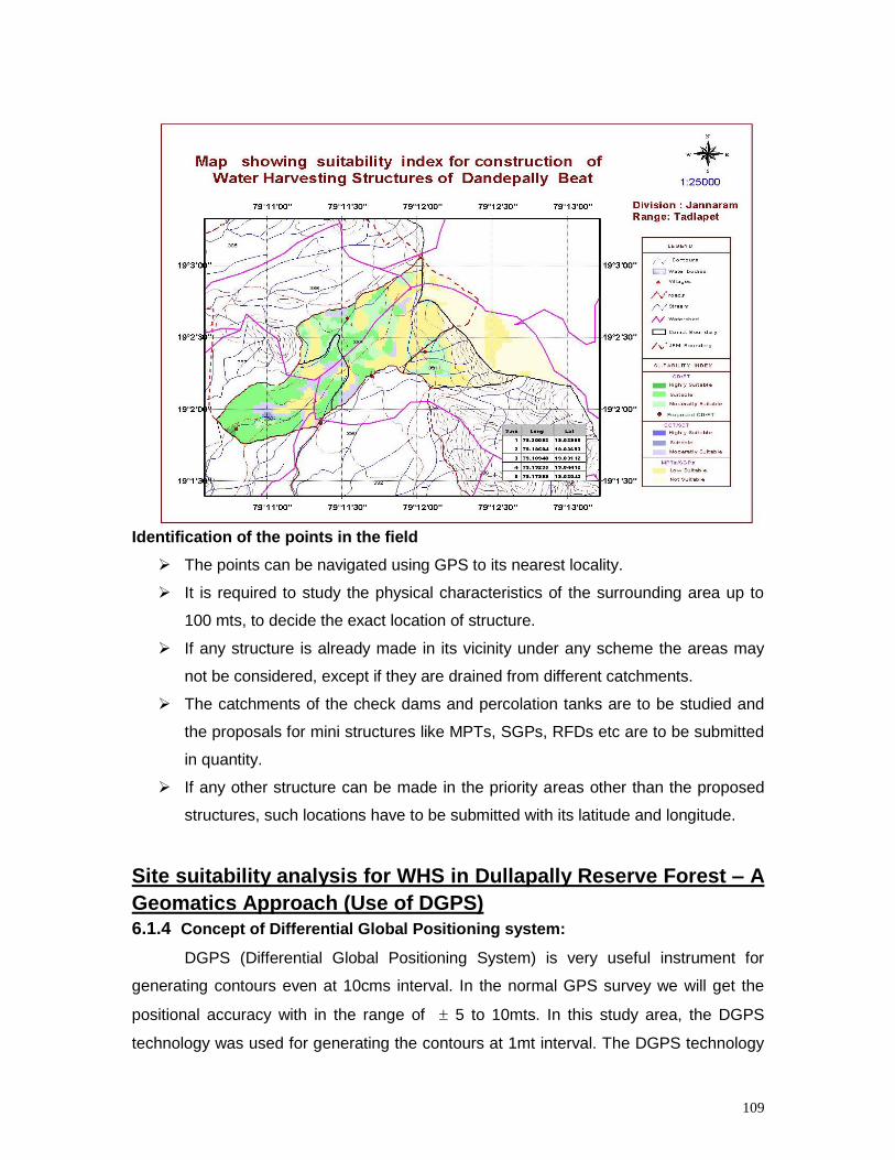
109

Identification of the points in the field

The points can be navigated using GPS to its nearest locality.

It is required to study the physical characteristics of the surrounding area up to

100 mts, to decide the exact location of structure.

If any structure is already made in its vicinity under any scheme the areas may

not be considered, except if they are drained from different catchments.

The catchments of the check dams and percolation tanks are to be studied and

the proposals for mini structures like MPTs, SGPs, RFDs etc are to be submitted

in quantity.

If any other structure can be made in the priority areas other than the proposed

structures, such locations have to be submitted with its latitude and longitude.

Site suitability analysis for WHS in Dullapally Reserve Forest – A

Geomatics Approach (Use of DGPS)

6.1.4 Concept of Differential Global Positioning system:

DGPS (Differential Global Positioning System) is very useful instrument for

generating contours even at 10cms interval. In the normal GPS survey we will get the

positional accuracy with in the range of 5 to 10mts. In this study area, the DGPS

technology was used for generating the contours at 1mt interval. The DGPS technology

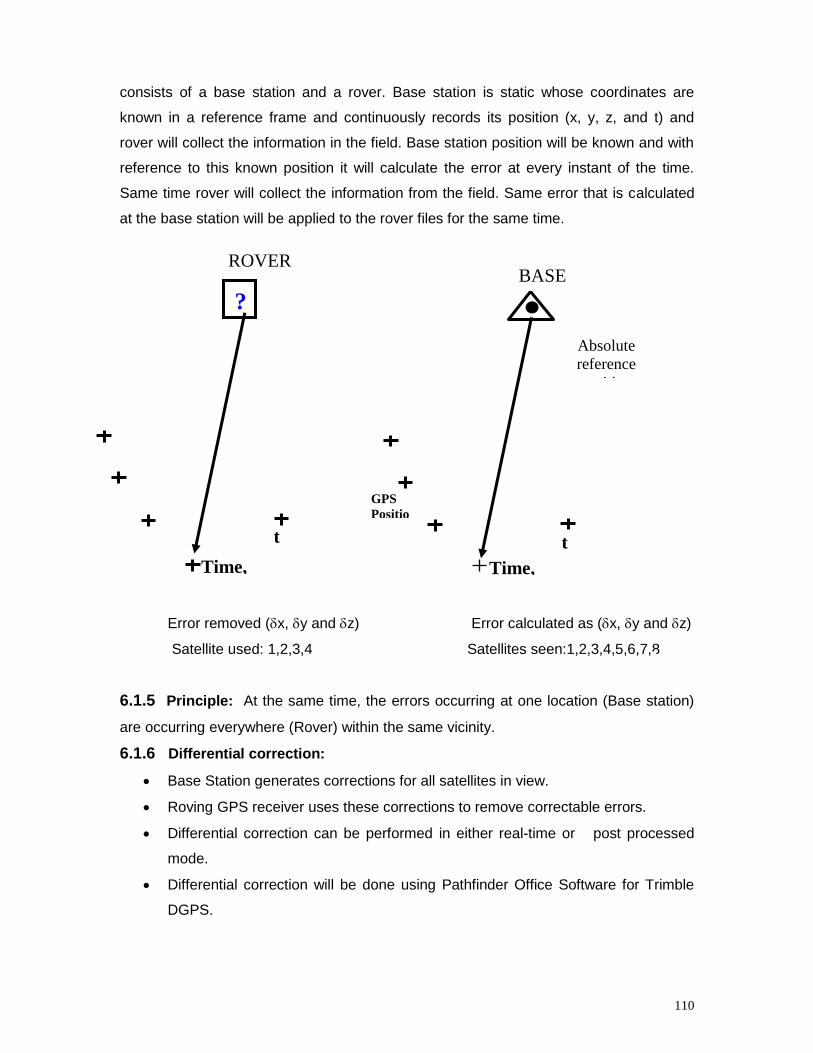
110

consists of a base station and a rover. Base station is static whose coordinates are

known in a reference frame and continuously records its position (x, y, z, and t) and

rover will collect the information in the field. Base station position will be known and with

reference to this known position it will calculate the error at every instant of the time.

Same time rover will collect the information from the field. Same error that is calculated

at the base station will be applied to the rover files for the same time.

Error removed (x, y and z) Error calculated as (x, y and z)

Satellite used: 1,2,3,4 Satellites seen:1,2,3,4,5,6,7,8

6.1.5 Principle: At the same time, the errors occurring at one location (Base station)

are occurring everywhere (Rover) within the same vicinity.

6.1.6 Differential correction:

Base Station generates corrections for all satellites in view.

Roving GPS receiver uses these corrections to remove correctable errors.

Differential correction can be performed in either real-time or post processed

mode.

Differential correction will be done using Pathfinder Office Software for Trimble

DGPS.

Time,

t

t

+1

Absolute

reference

position

BASE

?

Time,

t

t

+1

ROVER

R

GPS

Positio

ns

111

6.1.7 Dullapally reserve forest

The project area Dullapally Reserve Forest is situated on the ring road joining

NH7 and Medak state Highway in near by Dullapally village of Rangareddy District (See

Plate–13). This forest block is very near to Hyderabad city so that it is having an

importance in maintenance in environmental balance. It has an area of 526.6Ha

approximately. The area lies between 1733’34’’ - 17 31’56’’ North latitude and 78

26’26’’ - 7827’55’’ East longitude. The surrounding areas of this block are maximum

extent polluted by discharging waste chemicals and releasing CO2 etc.

6.1.8 Climate: The climate is generally hot. The average maximum temperature in the

summer months generally varies from 35 to 42C. The average minimum temperature

during winter varies from 10 to 22 c.

6.1.9 Rainfall: The District is generally deficient in rainfall. A major part of the district is

declared as the Drought prone area and schemes such as; Drought Prone Area

Program is intensively taken up in the district. The area receives rainfall mainly from

south west monsoon and partly from north east monsoon during the period June to

September rains received from SW monsoon and balance from N-E monsoon during

October to December. The average rainfall of the area is about 600mm in the recent

past.

6.1.10 Vegetation type: The forests occurring in the study areas posses general

characteristics of tropical thorny scrub forests as per Champion & Seth revised

classification of forest. All along the main stream which is passing through is having

close cover of density. The total area is fenced and protecting from grazing so that

existing root stock is coming up well.

Project area

Part of the Reserve Forest area is taken up for the treatment of Water Harvesting

Structures and area is about 277Ha.

6.1.11 Methodology:

The entire project work was carried out in 2 phases.

Phase I : GPS field and post processing work

112

Phase II : GIS for preparing base and final results.

Phase I: GPS Field and Post processing work:

a. Preliminary Reconnaissance Survey:

The total area is perambulated and prepared rough map with all the

features and elevation details before going for the actual field work. Total reserve

forest area is given to different organizations and these boundaries information

also recorded roughly on the map. Simultaneously while doing Reconnaissance

survey prepared rough plan for DGPS surveyed paths. Since the area is not

having too many undulations, the interval between the paths taken approximately

100mts apart on both the directions in such a way that to cover all the elevation

points in the study area. Same paths, which are prepared for field work is roughly

demarcated in the field to avoiding confusion during the field work.

b. Field work:

Actual fieldwork has started after completion of Reconnaissance survey.

Since the importance is to find out the elevations so that it is essential to do

differential corrections. Before going to the field it has been started the base

station which is arranged at AP Forest Academy.

In the first stage it has been surveyed all the areas for demarcation which

are handed over to the different organizations. As per the demarcation done in

the field during the Reconnaissance survey accordingly DGPS survey has been

completed by taking line feature and keeping interval between two readings as

10sec. During the DGPS survey Carrier phase has been put it on to get

maximum accuracy 3D positions along with the elevations. About 60% of the

area is got the readings with Carrier phase rest of the area is done with the

Code processing mode.

c. Post processing:

Every day after completion of field work immediately downloaded the rover

files and done the differential corrections using base files which are collected at

the base station. Total field work has been taken about 4days to complete the

area. All the rover files were downloaded and done the differential corrections

using DGPS software, Pathfinder Office.

In the nest stage all unwanted points which are identified as clusters were

edited in the software to avoid error in generation of contour and then other

related themes. All the files that are created everyday were grouped into a single

file after completion of the editing. From this final grouped file it will show the

distribution of points, and the areas which are not covered with elevation points

were demarcated on map and identified in the field. The elevation points were

taken in these areas with DGPS as a final field collection data. This final

113

collected field points added in to the grouped file. The final grouped file was

exported only positions with elevations into GIS platform i.e. ARC/INFO coverage

using different filters in the Pathfinder software to avoid maximum extent of

errors. The distributions of field-collected positions are shown in the plate.

GIS for preparing base and final results

Generation of contour layer:

The point cover that is exported from pathfinder office is again converted

in to TIN (Triangular Irregular Network) model using ARCTIN command in

ARC/INFO software. From TIN model it can be generated contour network at the

specified interval by using TINCONTOUR command in ARC/INFO contours are

generated directly from the tin within its zone of interpolation. The zone of

interpolation is defined by the convex hull, and/or the CLIP and ERASE features

incorporated when building the tin (See Plate-14).

Site suitability for water harvesting structures

The rainfall in the district is only seasonal. The S.W. monsoons contribute

2/3 of the total (June to September) and the balance from N.E. monsoon

(October to December). The rainfall is erratic and long dry spells occur in

between high intensity rains. In the Nallamalai Hills this causes not only crop

failure but also aggravated erosion. Suitable sites are to be located in the up

stream side to protect the crops from drought and check soil erosion. This also

increases the life of downside structures by arresting silt.

Criteria’s for selecting suitable sites for conserving water is given in the

Integrated Mission for Sustainable Development (IMSD); and the guide lines are

given by the Indian National Committee on Hydrology. The guidelines are given

in the Hand Book of Watershed, Govt of Andhra Pradesh. Drought prone area

program to select sites for water conservation are discussed here.

Rock Fill Dams:

In general rock fill dams are constructed at first and second order streams where

the initial water flow starts by accumulating water from the plain areas. In this study area

it is proposed RFD’s by considering the following criteria’s.

Minimum distance between two RFD’s has been considered as 25mts.

Almost at every 1mts. elevation i.e. vertical height has been proposed for two

successive RFD’s.

Check Dams:

114

In general these are constructed in lower order streams up to 3rd order with

medium slopes. These are proposed where water table fluctuations are very high and

the streams are influent and/or in internally effluent. A minimum catchment area of 25

ha should be there. The upstream slope of the area should be flat to gentle so as to

retain maximum quantity of water with less height of check dam (which is cost effective

too). The parameters to be considered are slope; rock type, thickness of watershed

strata; fracture; depths to bed rock, side slopes for economy of structures. The water

stored can be used for life saving irrigation by gravity irrigation. Proximity for village and

road is also considered.

Gabion structure:

In the study area along the main stream it has been proposed to construct

Gabion structures. The parameters that are considered for proposing these structures

are as follows.

Along the main stream the depth of the nala is little bit high so that the water flow

at this main stream is high. To retain the water flow in between the Check dams it has

been proposed for Gabion type structures all along the main stream in between to the

Check dams.

Percolation Tanks/Nala Bunds:

Nala bunds and percolation tanks are structure constructed across nalas

(streams) for checking velocity of runoff, increasing water percolation and increasing soil

moisture regime. Nala bunds are less expensive, smaller in dimension and constructed

using locally available material where as percolation tanks are large and more

expensive.

These are constructed to collect surface runoff coming from the catchment and

facilitate percolation of stored water into the soil substrata with a view to rise

groundwater level in the zone of influence of the nala bund/percolation tank to arrest

sediment yield which would otherwise reach the multipurpose reservoirs and reduce

their useful life. The sites should be selected in a relatively flatter nala reach; the slope of

the nala should not be more than 2 percent. As far as possible, the catchment area of

the percolation tank should not be less than 40 ha. There should be proper site for

construction of emergency spillway by the side of the tank. The nala bed should have

soils with adequate permeability and good fracture development to facilitate good

groundwater recharge.

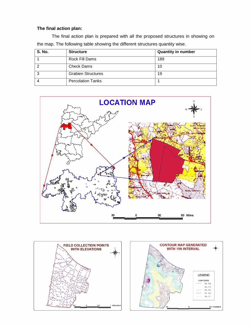
115

The final action plan:

The final action plan is prepared with all the proposed structures in showing on

the map. The following table showing the different structures quantity wise.

S. No. Structure Quantity in number

1 Rock Fill Dams 189

2 Check Dams 10

3 Grabien Structures 19

4 Percolation Tanks 1

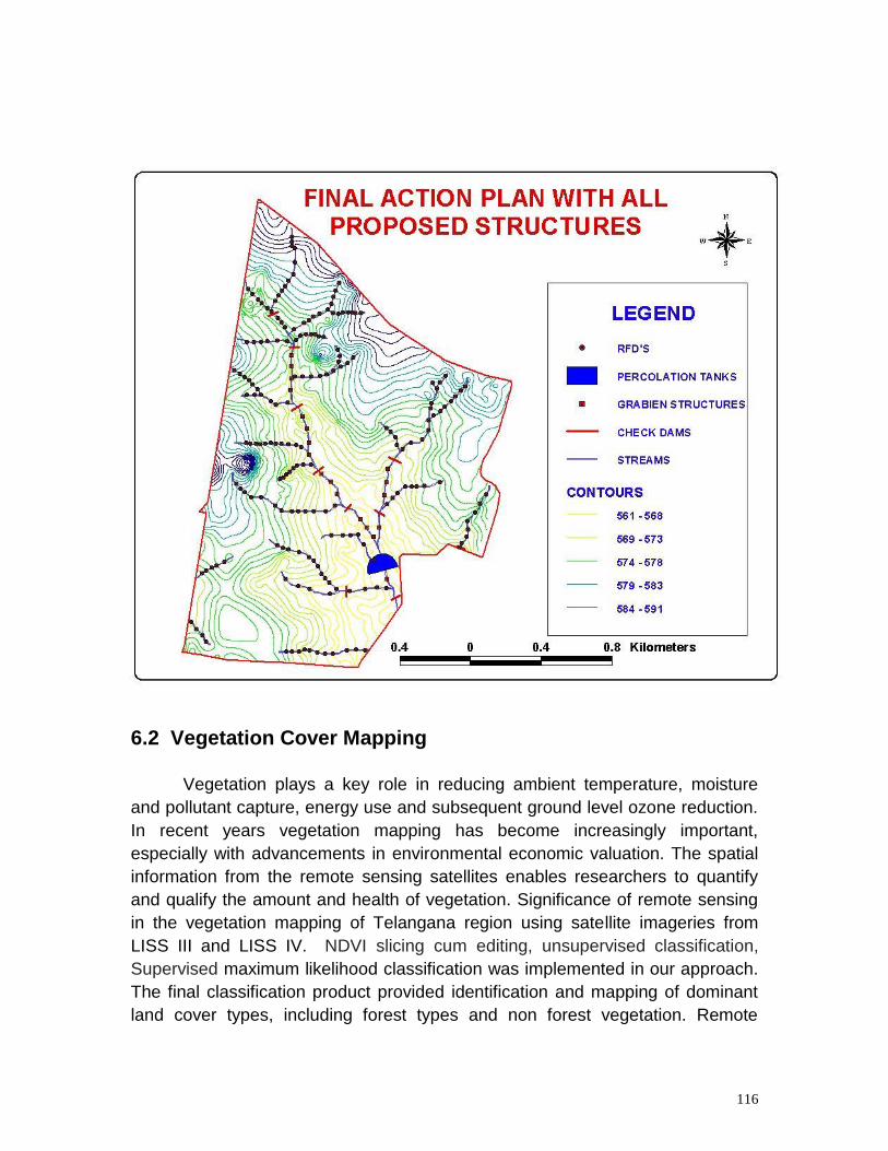
116

6.2 Vegetation Cover Mapping

Vegetation plays a key role in reducing ambient temperature, moisture

and pollutant capture, energy use and subsequent ground level ozone reduction.

In recent years vegetation mapping has become increasingly important,

especially with advancements in environmental economic valuation. The spatial

information from the remote sensing satellites enables researchers to quantify

and qualify the amount and health of vegetation. Significance of remote sensing

in the vegetation mapping of Telangana region using satellite imageries from

LISS III and LISS IV. NDVI slicing cum editing, unsupervised classification,

Supervised maximum likelihood classification was implemented in our approach.

The final classification product provided identification and mapping of dominant

land cover types, including forest types and non forest vegetation. Remote

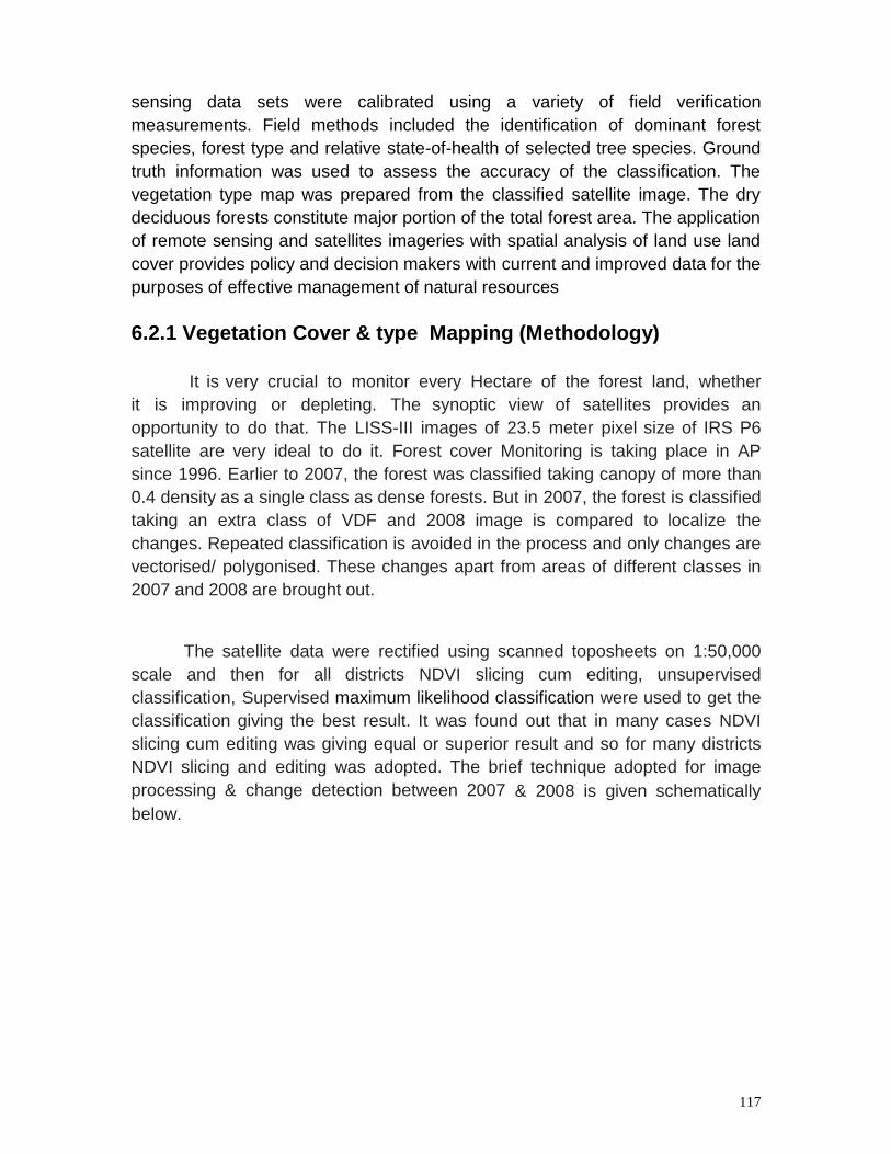
117

sensing data sets were calibrated using a variety of field verification

measurements. Field methods included the identification of dominant forest

species, forest type and relative state-of-health of selected tree species. Ground

truth information was used to assess the accuracy of the classification. The

vegetation type map was prepared from the classified satellite image. The dry

deciduous forests constitute major portion of the total forest area. The application

of remote sensing and satellites imageries with spatial analysis of land use land

cover provides policy and decision makers with current and improved data for the

purposes of effective management of natural resources

6.2.1 Vegetation Cover & type Mapping (Methodology)

It is very crucial to monitor every Hectare of the forest land, whether

it is improving or depleting. The synoptic view of satellites provides an

opportunity to do that. The LISS-III images of 23.5 meter pixel size of IRS P6

satellite are very ideal to do it. Forest cover Monitoring is taking place in AP

since 1996. Earlier to 2007, the forest was classified taking canopy of more than

0.4 density as a single class as dense forests. But in 2007, the forest is classified

taking an extra class of VDF and 2008 image is compared to localize the

changes. Repeated classification is avoided in the process and only changes are

vectorised/ polygonised. These changes apart from areas of different classes in

2007 and 2008 are brought out.

The satellite data were rectified using scanned toposheets on 1:50,000

scale and then for all districts NDVI slicing cum editing, unsupervised

classification, Supervised maximum likelihood classification were used to get the

classification giving the best result. It was found out that in many cases NDVI

slicing cum editing was giving equal or superior result and so for many districts

NDVI slicing and editing was adopted. The brief technique adopted for image

processing & change detection between 2007 & 2008 is given schematically

below.

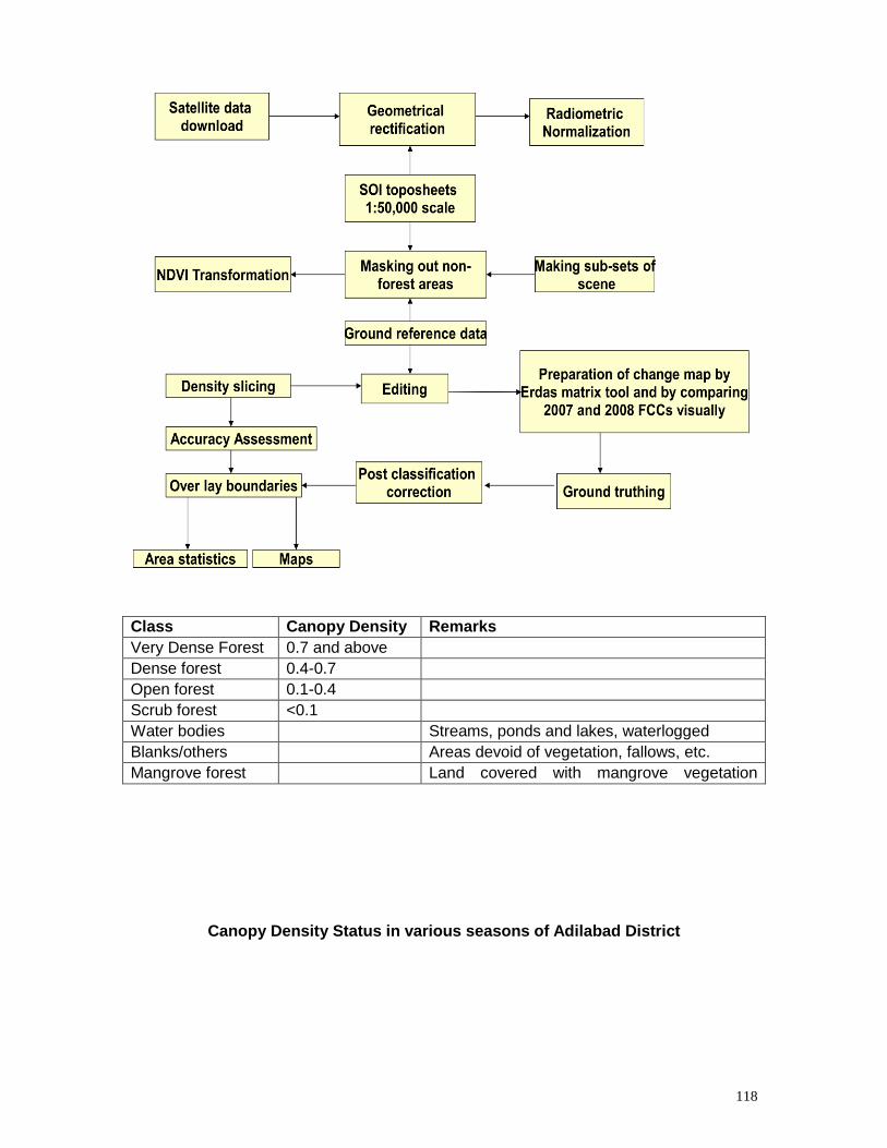
118

Class Canopy Density Remarks

Very Dense Forest 0.7 and above

Dense forest 0.4-0.7

Open forest 0.1-0.4

Scrub forest <0.1

Water bodies Streams, ponds and lakes, waterlogged

areas etc Blanks/others Areas devoid of vegetation, fallows, etc.

Mangrove forest Land covered with mangrove vegetation

irrespective of density.

Canopy Density Status in various seasons of Adilabad District

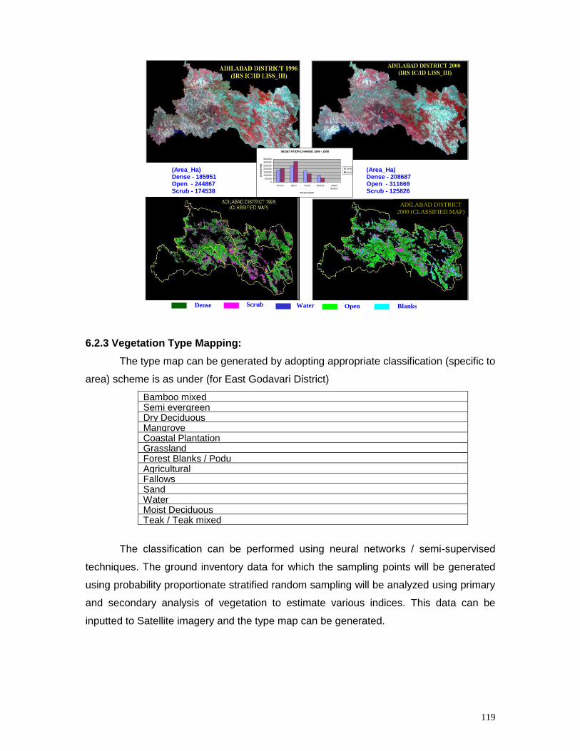
119

6.2.3 Vegetation Type Mapping:

The type map can be generated by adopting appropriate classification (specific to

area) scheme is as under (for East Godavari District)

Bamboo mixed Semi evergreen Dry Deciduous Mangrove Coastal Plantation Grassland Forest Blanks / Podu Agricultural Fallows Sand Water Moist Deciduous Teak / Teak mixed

The classification can be performed using neural networks / semi-supervised

techniques. The ground inventory data for which the sampling points will be generated

using probability proportionate stratified random sampling will be analyzed using primary

and secondary analysis of vegetation to estimate various indices. This data can be

inputted to Satellite imagery and the type map can be generated.

Dense Open Scrub Blanks

Water

ADILABAD DISTRICT

2000 (CLASSIFIED MAP)

VEGETATION CHANGE 1996 - 2000

0

50000

100000

150000

200000

250000

300000

350000

Dense Open Scrub Blanks Water

Bodies

Forest Cover

(Are

a in

Ha

)

1996

2000(Area_Ha) Dense - 185951 Open - 244867 Scrub - 174538

(Area_Ha) Dense - 208687 Open - 311669 Scrub - 125826

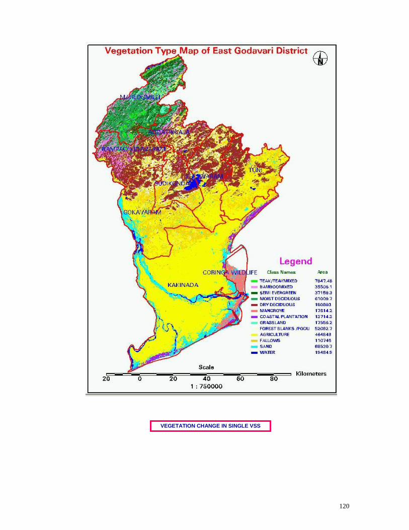
120

VEGETATION CHANGE IN SINGLE VSS

121

Forest Fire Risk Zonation Mapping

6.3 Introduction

Forest is one of the most important renewable natural resources and has

significant role in the human life and environment. Forest not only produce wood, both

commercial timber and fuel wood, but they also protect wildlife and give them suitable

environment, maintain the watershed balance and groundwater content, protect the soil

fertility, and absorb carbon and another pollutant gasses from the atmosphere. All of

these forest functions influence to the continuity of life and has a global aspect. Due to

natural causes and human activity forest has been degrading, both forest area

degradation and forest condition and quality. Forest area decreased in huge number

annually. Forest quality degrades on its productivity, degrade in biodiversity, and

degrade on its capability to fulfill the forest function. One of the main causes that

responsible to forest degradation is forest fire. Roughly 175 million acres of forest and

grassland are burned each year worldwide. Due to large-scale human deforestation

activities, grassland fires, and naturally occurring wild fires around the world, biomass

burning is a major source of greenhouse gases and aerosols (tiny liquid or solid particles

suspended in the atmosphere). These “emission products” significantly impact

atmospheric chemistry, clouds, and the Earth’s atmosphere.

AMEENGUDA - 1996 AMEENGUDA - 1998

DATE OF PASS: 3rd Nov’96 DATE OF PASS: 11th Dec’98

AMEENGUDA 1999 AMEENGUDA 2000

DENSE – 239.90 OPEN – 774.49 SCRUB – 466.10 BLANKS – 37.79

DENSE – 367.20 OPEN – 884.62 SCRUB – 249.24 BLANKS – 17.22

DENSE 341.22 OPEN 900.05 SCRUB 194.74 BLANKS 71.36

DENSE 380.79 OPEN 842.63 SCRUB 235.29 BLANKS 53.97

DATE OF PASS: DEC’99 DATE OF PASS: 6th Nov’2k

Area in Ha

122

Forest fires are a calamity for forests of temperature climate zones in view of the

fact that the damage they cause to the forest economy is considerably greater than all

the damage caused by harmful insects and diseases of wood taken together. Forest

fires retard the vital activity of forest crops, subsequently encouraging the multiplication

of pests and fungal diseases. Fire destroys not only greenwood and harvested timber,

but also construction material in the forest many species of animals and edible birds as

well as fodder grown for domestic animals, etc. Forest fires destroy the raw material

resources of the timber industry, causing untimely closure of industrial bases or their

transfer to the other regions. In case of large fires which acquire the character of natural

calamity, the extent of atmospheric smoke content can be so high that water and air

transport come to a standstill for long periods.

In spite of the development of many fire control methods and techniques, large

forest fires continue to remain a common phenomenon. Therefore, the problem of

controlling forest fires has been and remains a most urgent issue in the forest economy

of our country.

A study made by the Forest Survey of India reveals that 51% of the forest area in

Assam and Gujarat, 93% in Arunachal Pradesh, 67% in Bihar, 69% in Himachal

Pradesh, 46% in Jammu and Kashmir, 76% in Madhya Pradesh, 94% in Meghalaya and

Orissa, 87% in Nagaland, 58% in Uttar Pradesh and 33% in West Bengal is subject to

repeated annual fires.

In Andhra Pradesh 23% of geographical area is covered under forest which is

very vital for maintaining the ecological balance of state. Forest consists of basically

Southern Dry mixed Deciduous type with species like Teak, Terminalia, Anogeissus,

Bamboo, Dalbergia, Lannea etc., The leaf fall starts towards the end of the December

and along with dry grass it forms a highly combustible material for forest fires. Fire takes

place due to natural and anthropogenic activities.

6.3.1 Forest Fire – Main causes:

The causes of the forest fires can be classified in three main categories

i) Natural

ii) Intentional/deliberate due to man and

iii) Unintentional/accidental due to man.

6.3.2 Natural:

123

Natural fires occur mainly due to lightning or sometimes due to rolling stones

and rubbing of dry bamboos with each other in the strong wind. Nothing can be done to

avert such fires.

6.3.3 Intentional/Deliberate:

Intentional/deliberate are the ones most commonly reported. Fires are set in

forests for inducing luscious growth of grass for better grazing. Villagers sometime set

fire to drive away the game destroying their crops and to catch the wild animals running

away. The enmity with forest staff is also responsible for incendiary activities in forest

areas by neighboring rural population. Fires are also caused by villagers for collecting

minor forest produce (MFP) like honey, mahua, flowers etc. that fall on the ground.

Sparks from coal-fired railway locomotives may also cause forest fires. Nothing much

can be done to prevent a fire if it is a willful act on the part of local dwellers. However,

occurrence of the fire can be averted if it is the result of unintentional activities of the

innocent tribal or the natural factors.

6.3.4 Unintentional/Accidental:

Unintentional/accidental fires occur in a forest due to careless throwing of match-

sticks and burning ends of cigarettes/bidis carrying of naked fire by people passing

through forests, spread of fire from labor camps and recreation or picnic sites. These are

the factors governed by parameters like vicinity to settlements and distances from roads.

For any area to be prone to fire depends on many factors such as vegetation

type/density, soil type, humidity of the area, vicinity to settlements, distances from roads

and the host of others. While it is not possible to account the natural occurrences or the

deliberate attempts, the areas prone to accidental fires can be mapped.

6.3.5 Factors influencing forest fires:

To ignite a fire there are three prerequisites 1.Fuel 2. Heat and 3. Oxygen. All

these elements have to be present for a fire to start and continue burning. Fire basically,

depends on fuels (type, quality etc.) than on any other factor. Forest fuels can be

classified into three categories i.e. ground fuels, surface fuels and aerial fuels. Ground

fuels include duff, decayed wood & humus. A surface fuel consists of loose litter like

freshly filled foliage, twigs, etc. It also includes herbaceous plants and low shrubs. Aerial

fuels include the under story and upper canopy.

The prominent among the possible factors leading to accidental fires are

Vegetation type/density:

124

Dry and dense vegetation is obviously more susceptible to fire than the moist and

sparse one. Vegetation with less than 10% moisture content ignites readily, while the

moist take time in igniting/burning.

Climatic factors:

Of the four environmental factors viz., climatic, edaphic, physiographic and biotic,

climatic factors influence fires the most. The climatic regime determines the vegetation in

a region and hence plays dominant role in ascertaining the fire-prone sites. Drier the

climate, more prone would be the site.

Physiographic factors:

Physiographic factors, viz., altitude, aspect and topography, influence climatic

conditions, and therefore, indirectly affect the vegetation. Aspect plays vital role in

spreading of the fire. Southern slopes exposed to direct rays of Sun are more vulnerable

to catching fire.

The physical shape and the features also contribute a lot to the stating and

spreading of fire. On a upward slope warm air raises & cause, preheating of the fuel,

because of which fire moves faster on upward slope than on flat ground or down ward

slope. An upward slope also provides the connectivity of the flames to the fuels and fire

moves faster upwards. It is seen through number of observations that slope can be more

important than wind in determining the rate of fire spread.

The aspect determines how much sunlight it receives. In India Southern &

Western aspect receive most sunlight and so they are much warmer and drier than

northern aspects, which get least sunlight. Northern aspects have also more moisture

and they stay green for longer period. Southern and western aspects have a longer fire

seasons, and longer burning period per fire incidence than northern aspects.

Edaphic factors:

Soil and vegetation are mutually dependent on each other. If soil influences

growth of plants, vegetation adds to richness of soil and thus is an important factor.

Distance from roads:

The man, animal and vehicular movement and activities on the road provide

enough scope for accidental/man-made fire. Nearer the roads would be the chance

of fire.

Vicinity to settlements:

The areas near to the habitats/settlements are more prone to fire since the

habits/cultural practices of the inhabitants can lead to incidental fire.

125

6.3.6 Fire and Deforestation In India about 2-3% of forest areas are affected annually by fire and on an

average over 34000 ha forest areas are burnt by fire every year. (Anon, 1991)

Continuous fire can charge the composition of species in vegetation, which may slowly

give way for more fire resistant and scrub type of forests which may further lead to total

opening of the area leading to soil erosion etc.

6.3.7 Study of forest fire using Remote Sensing and GIS Remote Sensing and GIS technologies can be effectively used to

1. Mapping of fire burn areas

2. Fire prone area zonation Satellites like Indian Remote Satellite (IRS), Land sat, Spot, and NOAA are

highly useful in monitoring changing earth environment and its natural resources by

providing a synoptic view of large area in multi-spectral and multi-temporal domains. The

Vegetation type and density maps can be prepared from RS Data.

Satellite borne sensors have borne effectively and extensively used for providing

information on natural calamity like floor, earthquake, and drought and of course forest

fires.

The risk of forest fire is pressing problem in Indian subcontinent because of

presence of various types of forest and particularly extensive presence of Dry

deciduous, and moist deciduous forests, both tropical & subtropical zones. The presence

of longer dry period from winter to summer makes the forests more vulnerable for fire

accident.

The evaluation of this risk is therefore of primary important in the context of

environment & forest management. Remote Sensing helps in providing a number of

layers of thematic information required for interactive the analysis through Geographical

Information System (GIS).

6.3.8 Need of present study

The study area Bhadrachalam south Division in Andhra Pradesh is dominated by

Southern dry mixed deciduous forests with lot of grass as under story hence highly

vulnerable for fire incidences. The areas of semi evergreen / moist mixed forests are

relatively less vulnerable to fires but the influence from adjoining areas may ignite fire.

Every year the forests are burnt due to number of causes. In this background the area

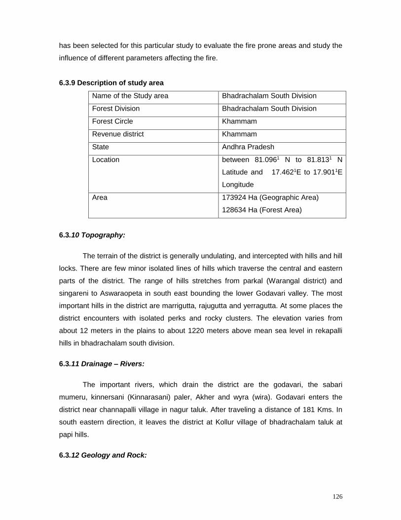
126

has been selected for this particular study to evaluate the fire prone areas and study the

influence of different parameters affecting the fire.

6.3.9 Description of study area

Name of the Study area Bhadrachalam South Division

Forest Division Bhadrachalam South Division

Forest Circle Khammam

Revenue district Khammam

State Andhra Pradesh

Location between 81.0961 N to 81.8131 N

Latitude and 17.4621E to 17.9011E

Longitude

Area

173924 Ha (Geographic Area)

128634 Ha (Forest Area)

6.3.10 Topography:

The terrain of the district is generally undulating, and intercepted with hills and hill

locks. There are few minor isolated lines of hills which traverse the central and eastern

parts of the district. The range of hills stretches from parkal (Warangal district) and

singareni to Aswaraopeta in south east bounding the lower Godavari valley. The most

important hills in the district are marrigutta, rajugutta and yerragutta. At some places the

district encounters with isolated perks and rocky clusters. The elevation varies from

about 12 meters in the plains to about 1220 meters above mean sea level in rekapalli

hills in bhadrachalam south division.

6.3.11 Drainage – Rivers:

The important rivers, which drain the district are the godavari, the sabari

mumeru, kinnersani (Kinnarasani) paler, Akher and wyra (wira). Godavari enters the

district near channapalli village in nagur taluk. After traveling a distance of 181 Kms. In

south eastern direction, it leaves the district at Kollur village of bhadrachalam taluk at

papi hills.

6.3.12 Geology and Rock:

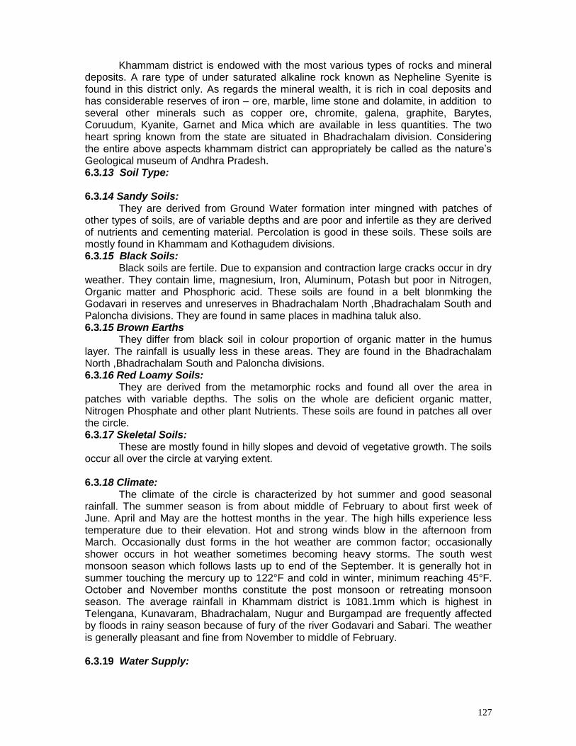
127

Khammam district is endowed with the most various types of rocks and mineral deposits. A rare type of under saturated alkaline rock known as Nepheline Syenite is found in this district only. As regards the mineral wealth, it is rich in coal deposits and has considerable reserves of iron – ore, marble, lime stone and dolamite, in addition to several other minerals such as copper ore, chromite, galena, graphite, Barytes, Coruudum, Kyanite, Garnet and Mica which are available in less quantities. The two heart spring known from the state are situated in Bhadrachalam division. Considering the entire above aspects khammam district can appropriately be called as the nature’s Geological museum of Andhra Pradesh. 6.3.13 Soil Type: 6.3.14 Sandy Soils:

They are derived from Ground Water formation inter mingned with patches of other types of soils, are of variable depths and are poor and infertile as they are derived of nutrients and cementing material. Percolation is good in these soils. These soils are mostly found in Khammam and Kothagudem divisions. 6.3.15 Black Soils:

Black soils are fertile. Due to expansion and contraction large cracks occur in dry weather. They contain lime, magnesium, Iron, Aluminum, Potash but poor in Nitrogen, Organic matter and Phosphoric acid. These soils are found in a belt blonmking the Godavari in reserves and unreserves in Bhadrachalam North ,Bhadrachalam South and Paloncha divisions. They are found in same places in madhina taluk also. 6.3.15 Brown Earths

They differ from black soil in colour proportion of organic matter in the humus layer. The rainfall is usually less in these areas. They are found in the Bhadrachalam North ,Bhadrachalam South and Paloncha divisions. 6.3.16 Red Loamy Soils:

They are derived from the metamorphic rocks and found all over the area in patches with variable depths. The solis on the whole are deficient organic matter, Nitrogen Phosphate and other plant Nutrients. These soils are found in patches all over the circle. 6.3.17 Skeletal Soils:

These are mostly found in hilly slopes and devoid of vegetative growth. The soils occur all over the circle at varying extent. 6.3.18 Climate: The climate of the circle is characterized by hot summer and good seasonal rainfall. The summer season is from about middle of February to about first week of June. April and May are the hottest months in the year. The high hills experience less temperature due to their elevation. Hot and strong winds blow in the afternoon from March. Occasionally dust forms in the hot weather are common factor; occasionally shower occurs in hot weather sometimes becoming heavy storms. The south west monsoon season which follows lasts up to end of the September. It is generally hot in summer touching the mercury up to 122°F and cold in winter, minimum reaching 45°F. October and November months constitute the post monsoon or retreating monsoon season. The average rainfall in Khammam district is 1081.1mm which is highest in Telengana, Kunavaram, Bhadrachalam, Nugur and Burgampad are frequently affected by floods in rainy season because of fury of the river Godavari and Sabari. The weather is generally pleasant and fine from November to middle of February. 6.3.19 Water Supply:

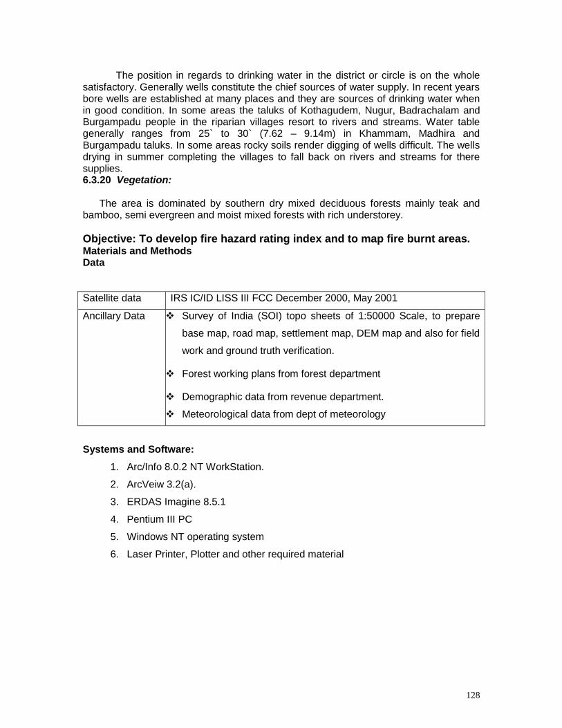
128

The position in regards to drinking water in the district or circle is on the whole

satisfactory. Generally wells constitute the chief sources of water supply. In recent years bore wells are established at many places and they are sources of drinking water when in good condition. In some areas the taluks of Kothagudem, Nugur, Badrachalam and Burgampadu people in the riparian villages resort to rivers and streams. Water table generally ranges from 25` to 30` (7.62 – 9.14m) in Khammam, Madhira and Burgampadu taluks. In some areas rocky soils render digging of wells difficult. The wells drying in summer completing the villages to fall back on rivers and streams for there supplies. 6.3.20 Vegetation:

The area is dominated by southern dry mixed deciduous forests mainly teak and bamboo, semi evergreen and moist mixed forests with rich understorey.

Objective: To develop fire hazard rating index and to map fire burnt areas. Materials and Methods Data

Satellite data IRS IC/ID LISS III FCC December 2000, May 2001

Ancillary Data Survey of India (SOI) topo sheets of 1:50000 Scale, to prepare

base map, road map, settlement map, DEM map and also for field

work and ground truth verification.

Forest working plans from forest department

Demographic data from revenue department.

Meteorological data from dept of meteorology

Systems and Software:

1. Arc/Info 8.0.2 NT WorkStation.

2. ArcVeiw 3.2(a).

3. ERDAS Imagine 8.5.1

4. Pentium III PC

5. Windows NT operating system

6. Laser Printer, Plotter and other required material

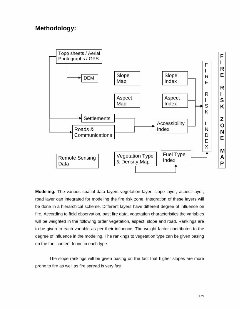
129

Methodology:

Modeling: The various spatial data layers vegetation layer, slope layer, aspect layer,

road layer can integrated for modeling the fire risk zone. Integration of these layers will

be done in a hierarchical scheme. Different layers have different degree of influence on

fire. According to field observation, past fire data, vegetation characteristics the variables

will be weighted in the following order vegetation, aspect, slope and road. Rankings are

to be given to each variable as per their influence. The weight factor contributes to the

degree of influence in the modeling. The rankings to vegetation type can be given basing

on the fuel content found in each type.

The slope rankings will be given basing on the fact that higher slopes are more

prone to fire as well as fire spread is very fast.

Topo sheets / Aerial Photographs / GPS

Remote Sensing Data

Roads & Communications

Settlements

Vegetation Type & Density Map

DEM Slope Map

Aspect Map

Slope Index

Aspect Index

Accessibility Index

Fuel Type Index

FIRE RISK ZONE MA

P

FIRE RISK INDEX

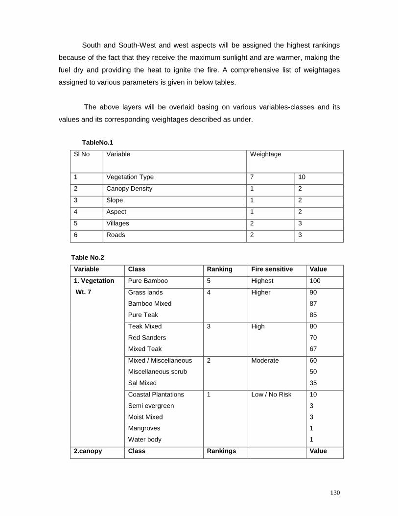
130

South and South-West and west aspects will be assigned the highest rankings

because of the fact that they receive the maximum sunlight and are warmer, making the

fuel dry and providing the heat to ignite the fire. A comprehensive list of weightages

assigned to various parameters is given in below tables.

The above layers will be overlaid basing on various variables-classes and its

values and its corresponding weightages described as under.

TableNo.1

Sl No Variable Weightage

1 Vegetation Type 7 10

2 Canopy Density 1 2

3 Slope 1 2

4 Aspect 1 2

5 Villages 2 3

6 Roads 2 3

Table No.2

Variable Class Ranking Fire sensitive Value

1. Vegetation

Wt. 7

Pure Bamboo 5 Highest 100

Grass lands

Bamboo Mixed

Pure Teak

4 Higher 90

87

85

Teak Mixed

Red Sanders

Mixed Teak

3 High 80

70

67

Mixed / Miscellaneous

Miscellaneous scrub

Sal Mixed

2 Moderate 60

50

35

Coastal Plantations

Semi evergreen

Moist Mixed

Mangroves

Water body

1 Low / No Risk 10

3

3

1

1

2.canopy Class Rankings Value

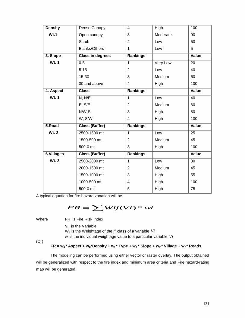
131

Density

Wt.1

Dense Canopy

Open canopy

Scrub

Blanks/Others

4

3

2

1

High

Moderate

Low

Low

100

90

50

5

3. Slope

Wt. 1

Class in degrees Rankings Value

0-5

5-15

15-30

30 and above

1

2

3

4

Very Low

Low

Medium

High

20

40

60

100

4. Aspect

Wt. 1

Class Rankings Value

N, N/E

E, S/E

N/W,S

W, S/W

1

2

3

4

Low

Medium

High

High

40

60

80

100

5.Road

Wt. 2

Class (Buffer) Rankings Value

2500-1500 mt

1500-500 mt

500-0 mt

1

2

3

Low

Medium

High

25

45

100

6.Villages

Wt. 3

Class (Buffer) Rankings Value

2500-2000 mt

2000-1500 mt

1500-1000 mt

1000-500 mt

500-0 mt

1

2

3

4

5

Low

Medium

High

High

High

30

45

55

100

75

A typical equation for fire hazard zonation will be

iwViWijFR *)(

Where FR is Fire Risk Index

Vi is the Variable

Wij is the Weightage of the jth class of a variable Vi

wi is the individual weightage value to a particular variable Vi

(Or) FR = wa * Aspect + wd*Density + wt * Type + ws * Slope + wv * Village + wr * Roads

The modeling can be performed using either vector or raster overlay. The output obtained

will be generalized with respect to the fire index and minimum area criteria and Fire hazard-rating

map will be generated.

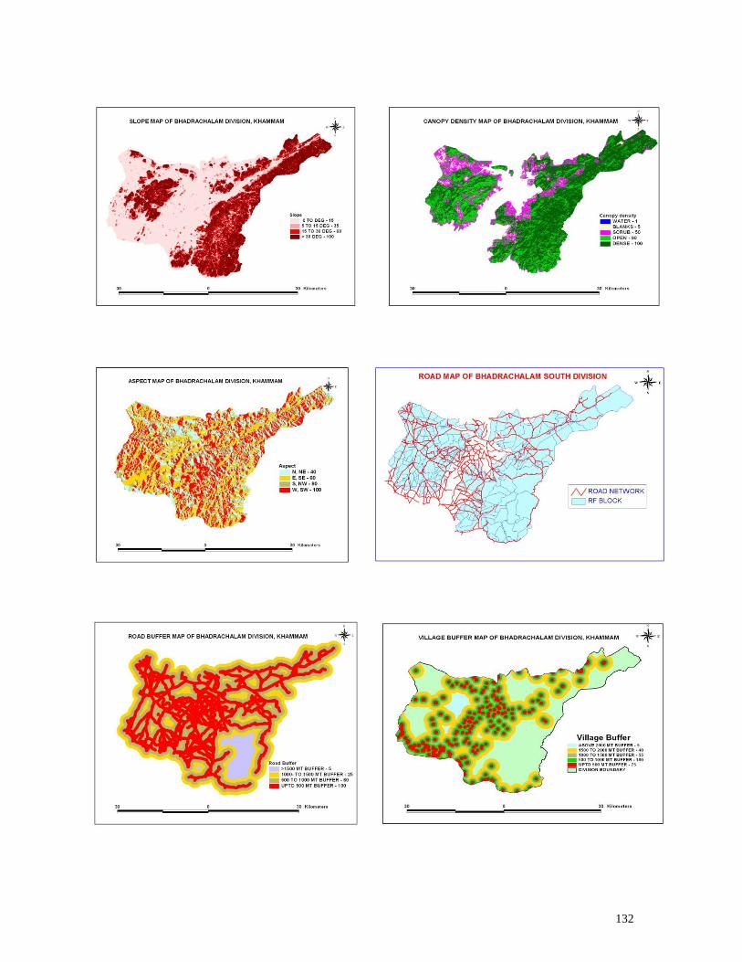
132

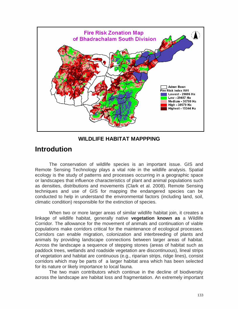
133

WILDLIFE HABITAT MAPPPING

Introdution

The conservation of wildlife species is an important issue. GIS and Remote Sensing Technology plays a vital role in the wildlife analysis. Spatial ecology is the study of patterns and processes occurring in a geographic space or landscapes that influence characteristics of plant and animal populations such as densities, distributions and movements (Clark et al. 2008). Remote Sensing techniques and use of GIS for mapping the endangered species can be conducted to help in understand the environmental factors (including land, soil, climatic condition) responsible for the extinction of species. When two or more larger areas of similar wildlife habitat join, it creates a linkage of wildlife habitat, generally native vegetation known as a Wildlife Corridor. The allowance for the movement of animals and continuation of viable populations make corridors critical for the maintenance of ecological processes. Corridors can enable migration, colonization and interbreeding of plants and animals by providing landscape connections between larger areas of habitat. Across the landscape a sequence of stepping stones (areas of habitat such as paddock trees, wetlands and roadside vegetation are discontinuous), lineal strips of vegetation and habitat are continuous (e.g., riparian strips, ridge lines), consist corridors which may be parts of a larger habitat area which has been selected for its nature or likely importance to local fauna.

The two main contributors which continue in the decline of biodiversity across the landscape are habitat loss and fragmentation. An extremely important

134

role in the maintenance of biodiversity is played by the corridors, but they can only partly compensate for the overall habitat loss produced by the fragmentation of the natural landscape. Therefore, it is important, for the maintenance of the vegetation remnants and vegetated corridors for enhanced network across all lands both private and public. In this way private landscapes can contribute to wider landscape conservation efforts by enhancing and linking existing reserves and conservation networks.

Objective: The objective of wildlife habitat mapping is to provide input to land-

use planning by providing estimated habitat values for wildlife species of

management concern.

The evolution of GIS, the Global Positioning System (GPS), and Remote

Sensing (RS) technologies has enabled the collection and analysis of field data in ways that were not possible before the arrival of computers (Sonti 2015). An analysis of the complex inter relationship among the various environmental factors existing over a geographical area involves us in the study of wildlife habitat suitability. In order to identify the most suitable and moderately suitable habitats, each model of GIS should be applied.

Each model involves a study of life consisting requisite factors

food and cover including forest type,

topography,

water resource,

distance from human activity center and other factors

Data required

Field investigations with GPS

Satellite imagery ( Type, Density can be derived)

SOI topographic maps

Thematic layers includes o Water resources o Slope and aspect o Road network o Village locations

The GIS database can be integrated in a complex GIS environment to

generate the suitable habitat maps. Suitability is the ability of the habitat in its current condition to support a particular species. The GIS model is used to generate a habitat map by assigning ratings to different habitat types, based on the needs of the species for particular life requisites. These kinds of maps are very useful in obtaining a clear idea about habitat suitability for animal species and wild life corridors.

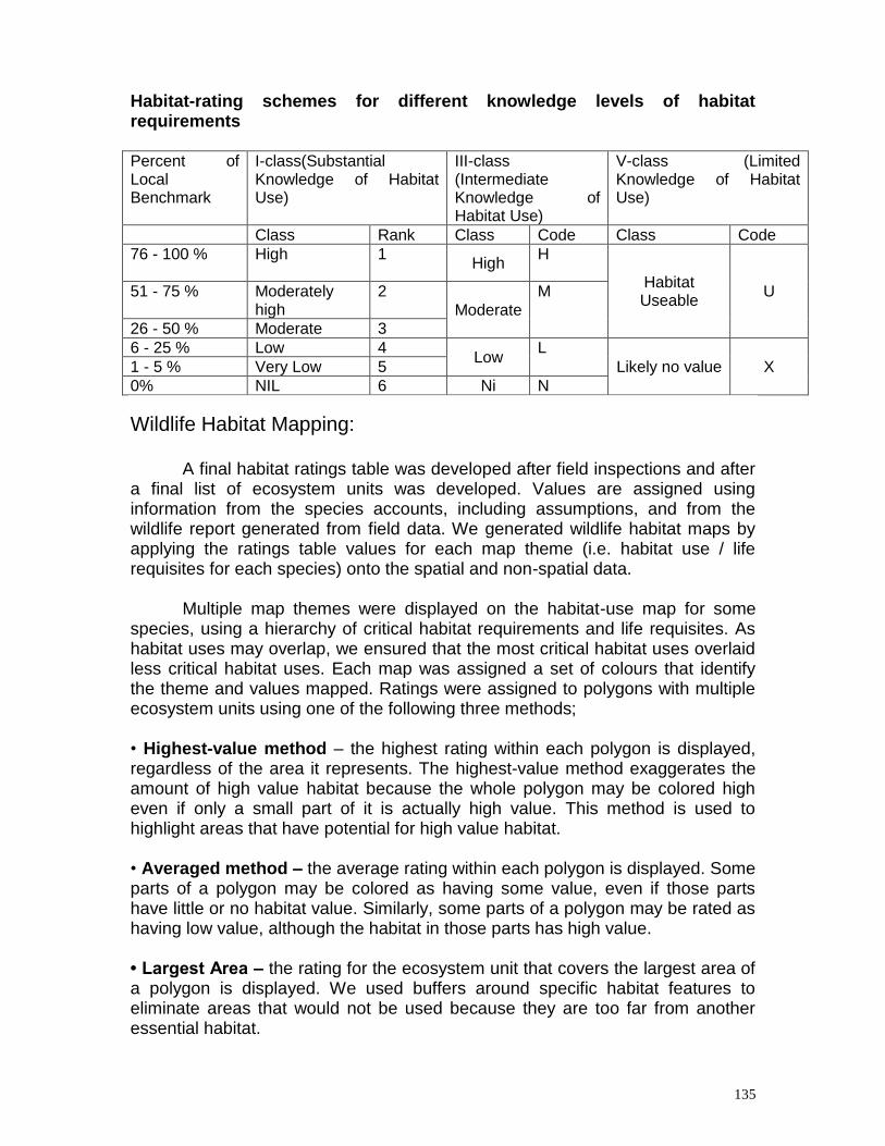
135

Habitat-rating schemes for different knowledge levels of habitat requirements Percent of Local Benchmark

I-class(Substantial Knowledge of Habitat Use)

III-class (Intermediate Knowledge of Habitat Use)

V-class (Limited Knowledge of Habitat Use)

Class Rank Class Code Class Code

76 - 100 % High 1

High H

Habitat Useable

U 51 - 75 % Moderately high

2

Moderate

M

26 - 50 % Moderate 3

6 - 25 % Low 4 Low

L

Likely no value X 1 - 5 % Very Low 5

0% NIL 6 Ni N

Wildlife Habitat Mapping: A final habitat ratings table was developed after field inspections and after a final list of ecosystem units was developed. Values are assigned using information from the species accounts, including assumptions, and from the wildlife report generated from field data. We generated wildlife habitat maps by applying the ratings table values for each map theme (i.e. habitat use / life requisites for each species) onto the spatial and non-spatial data.

Multiple map themes were displayed on the habitat-use map for some species, using a hierarchy of critical habitat requirements and life requisites. As habitat uses may overlap, we ensured that the most critical habitat uses overlaid less critical habitat uses. Each map was assigned a set of colours that identify the theme and values mapped. Ratings were assigned to polygons with multiple ecosystem units using one of the following three methods;

• Highest-value method – the highest rating within each polygon is displayed, regardless of the area it represents. The highest-value method exaggerates the amount of high value habitat because the whole polygon may be colored high even if only a small part of it is actually high value. This method is used to highlight areas that have potential for high value habitat. • Averaged method – the average rating within each polygon is displayed. Some parts of a polygon may be colored as having some value, even if those parts have little or no habitat value. Similarly, some parts of a polygon may be rated as having low value, although the habitat in those parts has high value. • Largest Area – the rating for the ecosystem unit that covers the largest area of a polygon is displayed. We used buffers around specific habitat features to eliminate areas that would not be used because they are too far from another essential habitat.