Geometria e Topologia - CiteSeerX

Geometria e TopologiaEditor Convidado: Carlos Florentino

Rui AlbuquerqueGeometria dos espaços de gwistor . . . . . . . . . . . . . . . . . . . . . . . . . . . . . . . . . . . . . 71

Ethan CotterillCounting maps from curves to projective space via graph theory . . . . . . 75

Rosa Sena-DiasSpectral theory for toric orbifolds . . . . . . . . . . . . . . . . . . . . . . . . . . . . . . . . . . . . . 79

Pedro Macias Marques, Helena SoaresMonads on Segre varieties . . . . . . . . . . . . . . . . . . . . . . . . . . . . . . . . . . . . . . . . . . . . . 83

Leonor Godinho, Silvia SabatiniTowards classifying Hamiltonian torus actions with isolated fixed points. . . . . . . . . . . . . . . . . . . . . . . . . . . . . . . . . . . . . . . . . . . . . . . . . . . . . . . . . . . . . . . . . . . . . . . 87

Pedro VazOn Jaeger’s HOMFLY-PT expansions, branching rules and link homology:a progress report . . . . . . . . . . . . . . . . . . . . . . . . . . . . . . . . . . . . . . . . . . . . . . . . . . . . . . 91

Orlando Neto, Pedro C. SilvaWaldhausen decomposition and Systems of PDEs . . . . . . . . . . . . . . . . . . . . . 95

Encontro Nacional da SPM 2012, Geometria e Topologia, p. 69

Geometria dos espaços de gwistor

Rui AlbuquerqueDepartamento de Matemática da Universidade de ÉvoraRua Romão Ramalho, 597000-671 Évora, Portugale-mail: [email protected]

Resumo: Breve introdução ao espaço de gwistor, a estrutura G2 naturalexistente no fibrado de esferas tangente π : SM →M de qualquer variedaderiemanniana M , orientável e de dimensão 4.

Abstract Brief introduction to gwistor space or the natural G2-structureassociated to any oriented riemannian 4-manifold.

palavras-chave: fibrado esferas; estrutura G2; métrica de Einstein.

keywords: tangent sphere bundle; G2 structure; Einstein manifold.

1 Estruturas G2

Seja T um espaço euclidiano orientado de dimensão 4 e fixemos um vectoru ∈ S3 ⊂ T , onde S3 denota a esfera de raio 1. Qualquer outro vector de Tescreve-se de forma única como λu+X, com λ ∈ R, X ∈ u⊥.

Reparamos então que T suporta uma estrutura quaterniónica natural,ou seja, uma estrutura de álgebra de divisão isomorfa a H, com a métricaeuclidiana inicial e tal que u é o elemento unidade. Com efeito, a operaçãoproduto é dada por

(λ1u+X)(λ2u+ Y ) = (λ1λ2 − 〈X,Y 〉)u+ λ2X + λ1Y +X × Y ,

sendo × um produto-cruzado, definido em u⊥ pela identidade 〈X × Y,Z〉 =vol(u,X, Y, Z) para qualquer triplo X,Y, Z ∈ u⊥. A operação de conjugaçãoem T compatível é descrita obviamente por λu+X = λu−X.

Lembremos agora que a maior álgebra de divisão normada com elementounidade que existe, a álgebra dos octoniões O = H⊕eH, pode ser encontradaatravés do processo de Cayley-Dickson:

(z1, z2) · (z3, z4) = (z1z3 − z4z2, z4z1 + z2z3), ∀zi ∈ H.

Note-se que e é um novo elemento de quadrado −1, como o é i em C = R⊕iRou j em H = C⊕ jC; porém, não só por si definem tais vectores a estrutura

Encontro Nacional da SPM 2012, Geometria e Topologia, pp. 71–74

72 Geometria dos espaços de gwistor

desejada (há muitos quádruplos ortonormados i, j, k, e na mesma relação).A operação de produto é suficiente. Por outras palavras, e voltando aoespaço T acima, interessam-nos as estruturas de módulo de T sobre H e ade T ⊕ T ' R.1⊕ R7 sobre O. Finalmente temos

G2 = AutO

que é grupo de Lie simples, compacto, simplesmente conexo, de dimensão 14.Elementos de G2 preservam a unidade 1 e a métrica, bem como a orientação,logo G2 ⊂ SO(7).

Tal grupo de Lie encontra-se entre as poucas classes de grupos de Liesimples dando origem a uma geometria riemanniana, dita excepcional, actu-almente muito em voga em geometria e física. Surge como um dos possíveisgrupos de holonomia irredutível de variedades riemannianas não simétricas(classificação descrita num bem conhecido resultado de M. Berger de 1955).Mas G2 ⊂ SO(7) só aparece de modo irredutível em variedades de dimensão7. Sabe-se que existem mesmo variedades com aquele grupo de holonomia(R. Bryant, 1987).

Uma estrutura G2 numa variedade S, de dimensão 7, é definida poruma 3-forma φ estável, i.e.

• ∃ um produto vectorial tal que φ(X,Y, Z) = 〈X ·Y,Z〉, o qual correspondeao produto octoniónico dos imaginários puros R7 ⊂ O, ou

• φ = e456 + e014 + e025 + e036 − e126 − e234 − e315 nalgum referencial (pordefinição, eijk = ei ∧ ej ∧ ek), ou

• φ pertence a certa GL(7)-órbita aberta de Λ3T ∗S (dim 35 = 49− 14).

A existência de tal 3-forma implica a redução do grupo de estrutura GL(7)da variedade S para SO(7) ⊃ G2, de forma única. Com efeito:

φ determina a orientação e uma única métrica sobre S.

Como acontece noutras geometrias, a holonomia da variedade riemanni-ana e orientada (S, φ) reduz-se a G2 = g ∈ SO(7) : g∗φ = φ se ∇gφ = 0,onde ∇g denota a conexão de Levi-Civita. Neste caso, S diz-se uma varie-dade G2. A topologia de S é condicionada, cf. [6].

Um teorema de A. Gray garante: ∇gφ = 0 se e só se dφ = 0 e d ∗ φ =0. Tais equações são raramente satisfeitas nos espaços que se conhecemactualmente; interessam-nos, por outro lado, parte das equações. φ diz-secalibrada se dφ ∈ Λ4T ∗S se anula. E φ diz-se cocalibrada se d ∗ φ se anula.


Rui Albuquerque 73

2 O espaço de gwistorSeja (M, g) uma variedade riemanniana, orientada, de dimensão 4 e seja

SM = u ∈ TM : ‖u‖ = 1.

Seja π : TM −→ M o fibrado vectorial tangente. Tem-se dπ : TTM −→π∗TM , morfismo de fibrados sobre TM . Como bem se sabe da geometriaclássica de TM , identifica-se ker dπ ' π∗TM de forma natural. A conexão∇g sobre M permite escrever TTM = H∇

g ⊕ ker dπ ' π∗TM ⊕ π∗TM .O fibrado, dito vertical, ker dπ contém uma secção canónica, U , que emcada ponto u ∈ SM toma o valor u ∈ π∗TM . Não é dificil provar queTSM = U⊥ ⊂ TTM . Reproduzindo a construção algébrica da secção 1,com estrutura métrica óbvia em (π∗TM)u = T , fica demonstrado o

Teorema 2.1 SM admite uma estrutura G2 natural.

A tal estrutura damos o nome espaço G2-twistor ou gwistor de M .Sobre o espaço de gwistor podemos sempre construir, localmente, um

referencial móvel ortonormado directo, e0 = u, e1, e2, e3 ∈ H∇g , sistema

depois reproduzido como Uu, e4, e5, e6 ∈ ker dπ no subespaço vertical, demodo a descrever as seguintes formas globais de SM :

α = 3-forma volume nas fibras de SM = e456 , θ = e0 ,

α1 = e156 + e264 + e345 , α2 = e126 + e234 + e315 ,

α3 = e123 , vol = π∗volM = e0123 = θ ∧ α3 .

Sendo U e e0 campos definidos globalmente, em boa verdade a estrutura deSM reduziu-se a SO(3). Note-se que já se conheciam a métrica (de Sasaki)em SM , o campo vectorial e0 ∈ XSM e logo a 1-forma θ, a qual verifica(dθ)3∧θ 6= 0, implicando o resultado que diz que (SM, 1

4g,12θ, 2e0) constitui

uma estrutura métrica de contacto (Y. Tashiro).Finalmente,

φ = α2 − α+ θ ∧ dθ .Observamos ainda que se pode generalizar a construção do espaço de gwistorcom H∇ provindo de qualquer conexão métrica ∇ em M .

Agora, sobre SM definem-se r = ru = r∇g (u, u), ρ = r∇

g ( , U) =(ricU)[. Tem-se que d∗φ = ρ∧vol e que dφ = 2θ∧α1−r vol−RUα+(dθ)2

onde

RUα := dα =∑

0≤i<j≤3Rij01e

ij56 +Rij02eij64 +Rij03e

ij45 .


74 Geometria dos espaços de gwistor

Teorema 2.2 Tem-se sempre dφ 6= 0; Temos d ∗ φ = 0 se e só se (M, g) évariedade de Einstein.

Exemplos. 1. seM = H4 é o espaço hiperbólico real com curvatura seccional−2, então SM = SH4 = SO0(4,1)

SO(3) é de tipo puro W3 = τ ∈ Λ3 : τ ∧ φ =τ ∧ ∗φ = 0:

dφ = ∗τ = ∗(2θ ∧ dθ + 6α) , d ∗ φ = 0 .

2. espaços simétricos de rank 1 geram espaços de gwistor homogéneos,

SS4 = V5,2 , SCP2 = SU(3)U(1) = N1,1 , SH2

C = SU(2, 1)U(1) .

Outros resultados sobre G2 e novos desenvolvimentos na teoria dos es-paços de gwistor encontram-se na bibliografia.

Referências[1] R. Albuquerque e I. Salavessa, “The G2 sphere of a 4-manifold”, Mo-

natsh. Math., Vol. 158, Issue 4 (2009), pp. 335–348.

[2] R. Albuquerque e I. Salavessa, “Erratum to: The G2 sphere of a 4-manifold”, Monatsh. Math., Vol. 160, Issue 1 (2010), pp. 109–110.

[3] R. Albuquerque, “On the G2 bundle of a Riemannian 4-manifold”, J.Geom. Phys., Vol. 60 (2010), pp. 924–939.

[4] R. Albuquerque, “On the characteristic connection of gwistor space”,Central European J. Math., Vol. 11, Issue 1 (2013), pp. 149–160.

[5] R. Albuquerque, “Variations of gwistor space”, http://arxiv.org/abs/1107.5358v2

[6] D. Joyce, Riemannian Holonomy Groups and Calibrated Geometry, Ox-ford University Press, Oxford Graduate Texts in Mathematics, 2009.


http://arxiv.org/ abs/1107.5358v2

http://arxiv.org/ abs/1107.5358v2

Counting maps from curves to projective space viagraph theory

Ethan CotterillCMUC, Universidade de Coimbrae-mail: [email protected]

1 Brill–Noether theory on reducible curvesIn Brill–Noether theory, one studies linear series on curves, in order to understand whena curve C of genus g comes equipped with a nondegenerate morphism of degree d to Pr.For a general curve [C] ∈ Mg, a basic answer is provided by the Brill–Noether theoremof Griffiths and Harris, which establishes that C admits such a morphism if and only ifthe invariant

ρ(d, g, r) = g − (r + 1)(g − d+ r)

is nonnegative, in which case ρ also computes the dimension of the space of linear series grd

of degree d and rank r on C. The Brill–Noether question also admits natural extensions,obtained by imposing incidence conditions on the images of the linear series in question.Namely, given integers m ≥ d and s ≥ d− r, let µ(d, r, s) := d− r(s+ 1− d+ r) denotethe virtual dimension of space of inclusions

gs−d+rm−d + p1 + · · ·+ pd → gs

m (1)

on a fixed curve. When the curve C in question is smooth, and the gsm is a subspace

V ⊂ H0(C,L) of global sections of a line bundle L, such inclusions correspond to d-tuplesof points p1, . . . , pd ∈ C for which the natural evaluation map

ev : V → H0(C,L/L(−p1 − · · · − pd)) (2)

satisfies rank(ev) = d− r. Geometrically, such d-tuples determine d-secant (d− r − 1)-planes to the image of the gs

m. In [3], we showed that when ρ = 0 and µ < 0, there areno inclusions (1) on a general curve:

Theorem 1.1. If ρ = 0 and µ < 0, then a general curve C admits no linear series gsm

with d-secant (d− r − 1)-planes.

Our proof of Theorem 1.1 is a natural generalization of the Brill–Noether proof given in[5, Ch. 5] and is based on an analysis of (limit) linear series on certain reducible curvesof compact type.


76 Counting maps from curves to projective space via graph theory

2 Counting secant planes via graph theoryAn immediate corollary of Theorem 1.1 is that when ρ=0 and µ=−1, curves with linearseries gs

m with d-secant (d − r − 1)-planes determine a divisor in Mg. The case r = 1is particularly natural: in that case, exceptional secant planes correspond to d-tuples ofpoints for which the evaluation maps (2) fail to be surjective. We show [4, Thm 2]:Theorem 2.1. The coefficients of the homology classes of secant-plane divisors inMg,realized as linear combinations of standard generators over Q, are explicit linear combi-nations of hypergeometric series of type 3F2.The key ingredient for proving Theorem 2, which is of interest in its own right, is thefollowing auxiliary result [3, Thm 4]:Theorem 2.2. The generating series for the virtual number Nd of d-secant (d−2)-planesto a degree-m curve C of genus g in P2d−2 is∑

d≥0Nd(g,m) =

( 2(1 + 4z)1/2 + 1

)2g−2−m

· (1 + 4z)g−1

2 . (3)

Two ingredients enter into our proof of Theorem 2.2. The first is Porteous’ formula, whichcomputes the homology class of the locus of d-secant (d − 2)-planes as a determinantin the Chern classes of the so-called dth tautological bundle L[d] over the dth Cartesianproduct Cd, whose fiber over (p1, . . . , pd) ∈ Cd is H0(L/L(−p1−· · ·−pd)). The second isa combinatorial analysis of the resulting intersection-theoretic formula, which amountsto a weighted count of subgraphs of the complete graph Kd on d vertices.

3 Linear series on metric graphsIn the preceding section, graphs naturally arose in connection with counting (secantplanes to) morphisms via the formalism of intersection theory. But graph theory alsointervenes in a natural way as a result of degeneration, via the passage from a nodalcurve to the dual graph recording the incidences of its components. There is a theory ofcomplete linear series on metric graphs with R-valued edge lengths due to Baker–Norine[1] and Mikhalkin–Zharkov [6]. Concretely, a (complete) linear series |D| on a metricgraph Γ is a configuration D of points in Γ, modulo an equivalence relation defined bypiecewise-linear functions. Moreover, there is an explicit combinatorial burning algorithmdue to Dhar for computing the rank of a configuration of points D ∈ Div(Γ); see [2].Contrasting examples in genus four. Figure (a) shows two metric graphs of genus4 (here, as in the remainder of the article, we assume that all weights on vertices are 0).The top graph Γ1 pictured is planar, and the 3 circles determine a degree-3 configurationD1 of trivial rank. Indeed, a fire that burns from p will be repelled by the 3 points in thesupport of D1, which then evolve at equal velocity against the incoming fire. Assuming


Ethan Cotterill 77

the planar graph has generic edge lengths, a sin-gle point p1 of D1 will arrive at a vertex v1 ofΓ1, at which point a fire burning from p willapproach v1 (and p1) from 2 distinct directionsand all of Γ1 will burn. By contrast, the config-uration D2 of 3 points on the complete bipartitegraph Γ2 = K3,3 evolves in such a way that atat no time will any fire based at any point p ap-proach any point in the support of D2 along twodistinct directions. It follows that r(D1) ≥ 1,and in fact the rank of D1 is precisely 1.

4 The gonality of tree-decomposed graphsThe contrast between the behavior of degree-3 configurations on the planar genus-4graph Γ1 and on Γ2 = K3,3 is instructive. In fact, it is not hard to check that Γ1 and Γ2each admit two degree-3 configurations of rank 1, as predicted by Brill–Noether theoryfor curves of genus 4. However, on Γ1, these configurations depend strongly on themetric structure: each is obtained by placing 2 points on 2 out of 3 inner (resp., outer)“rim" vertices, and a third point along a “spoke" at distance from an outer (resp., inner)vertex at distance equal to the length of the shortest spoke. On Γ2, on the other hand,each rank-1 configuration is associated to a choice of one of the two sets of 3 verticesalong which Γ2 decomposes as a union of three 4-edged trees.Definition/construction. Let V = v1, . . . , vn, n ≥ 3 denote a fixed set of vertices,and let T1, T2, and T3 denote three trees each containing V as vertices but which areotherwise pairwise disjoint. The three trees Ti, 1 ≤ i ≤ 3 glue naturally to a graph Γ;we say that Γ admits a tree decomposition (T1, T2, T3) rooted along V .

Some of the most famous graphs of genus at most 10 admit such tree decompositions:besides K3,3, the examples of the so-called Petersen, Heawood, and Pappus graphs ingenera 6, 8, and 10 (respectively) are tree-decomposable.Theorem 4.1 (Existence of rank-one series on tree-decomposed graphs). Suppose thatthe metric graph Γ admits a tree decomposition rooted on n ≥ 3 vertices V . Then Vdetermines a rank-one, degree-n divisor D on Γ.

Proof. The result follows from the burning algorithm.Namely, fix any choice of basepoint p from which to burn, say p ∈ T1 without loss of generality. Any fire burning fromp along T1 is repelled by the points p1, . . . , pn of D supported along V , which then evolveat equal velocity along T1 away from V . The burning process iterates until ultimately thefire is extinguished by at least one of the points pi, which proves that r(D)≥1. Similarly,


78 Counting maps from curves to projective space via graph theory

to prove that r(D)<2, it suffices to allow two successive fires to burn from p1 : the first firesimply has the effect of canceling out p1, while the second burns through all of Γ.

Definition. A graph (or a curve) Γ of genus g is n-gonal whenever n = minj ∈ Z>0 :∃ a g1

j on Γ.Theorem 4.2. K3,3, Petersen, Heawood, and Pappus are 3-gonal, 4-gonal, 5-gonal, and6-gonal graphs, respectively.Proof sketch. It is easy to exhibit tree decompositions of these graphs rooted on n = 3, 4,5, and 6 vertices, respectively. Whence, by Theorem 4.1, it suffices to prove that eachof these n-rooted tree-decomposed graphs admits no degree-(n− 1) configurations D ofpositive rank. Replacing D by a linearly equivalent configuration if necessary, we mayassume that each point in Supp(D) appears with multiplicity at most 2. It remains tocarry out a case-by-case inspection using the burning algorithm.It is not hard to produce graphs that decompose as unions of trees rooted on n ≥ 3vertices but are α-gonal with α < n. So additional conditions are needed to ensure thatn-gonality is achieved. Theorem 4.2 and experimentation give some evidence that itsuffices to maximize the minimal cycle length, or girth, of Γ.Conjecture 4.1. A metric graph Γ that admits a tree-decomposition (T1, T2, T3) rootedon n vertices is n-gonal provided girth(Γ) is maximal for the combinatorial type of(T1, T2, T3).

Acknowledgement. I amgrateful formany illuminating conversationswith S. Backman,J. Neves, M. Melo, D. Pinto, andF. Viviani related to linear series on metric graphs.

References[1] M. Baker and S. Norine, Riemann–Roch and Abel–Jacobi theory on a finite graph,

Adv. Math. 215 (2007), no. 2, 766–788.

[2] F. Cools, J. Draisma, S. Payne, and E. Robeva, A tropical proof of the Brill–Noethertheorem, Adv. Math. 230 (2012), 759–776.

[3] E. Cotterill, Geometry of curves with exceptional secant planes: linear series alongthe general curve, Math. Zeit. 267 (2011), no. 3-4, 549–582.

[4] E. Cotterill, Effective divisors on Mg associated to curves with exceptional secantplanes, Manuscripta Math. 138 (2012), no. 1-2, 171–202.

[5] J. Harris and I. Morrison, “Moduli of curves", Springer, 1998.

[6] G. Mikhalkin and I. Zharkov, Tropical curves, their Jacobians and theta functions,Contemp. Math. 465 (2007), 203–231.


Spectral theory for toric orbifoldsRosa Sena-Dias

Centro de Análise Matemática, Geometria e Sistemas DinâmicosDepartamento de Matemática, Instituto Superior Técnicoe-mail: [email protected]

Abstract This informal note is a written version of the talk I gave at the Geome-try/Topology session of the Portuguese Mathematical Society meeting. The talk ad-dressed the toric version of the classical Riemannian geometry question “How muchabout a toric manifold can you recover from the spectrum of its Laplacian for a toricmetric?”. This problem was first proposed by Miguel Abreu. This is a very informalreport on some progress towards answering that question. This is joint work with E.Dryden and V. Guillemin

1 IntroductionWe start by giving a somewhat precise statement of the result we shall discuss.Theorem 1.1. The equivariant spectrum of a toric Kahler metric on a generic toricorbifold determines the toric orbifold up to symplectomorphisms and two possibilities.One of the goals of this note is to explain the words in the above theorem and thecontext in which it arises. But mainly what we want to underline here is that the abovetranslates into a very elementary count. One that could essentially be carried out by amotivated high-school student.

2 CombinatoricsWe start by describing the elementary count.Question 2.1. How many convex polytopes in R2 are there with given(1) Number of sides d,(2) Length of sides,(3) Direction of sides up to sign?Note that 3 and 2 determine the edge vectors up to sign. A priori it seems that thereare 2dd! choices as one needs to choose signs and an ordering for the edge vectors.Claim 2.2. Generically there are at most 2 polytopes with data 3, 2 and 1.To back this claim we will describe two small propositions. The next one is fun!Proposition 2.3 (The most obtuse angle lemma). Let P be a convex polytope inR2. Lete1, · · · , ed denote the ordered edge vectors of P where we take the negative orientation in


80 Spectral theory for toric orbifolds

the plane to orient ∂P . The angle between e1 and e2 is themost obtuse angle among the angles

〈e1, ei i = 2, · · · dProof. Draw a picture! Assume e1 is (1, 0). Draw all the edges at the end of e1 as aspray. If you choose the second edge to be one whose angle is not the most obtuse anglewith e1 you will eventually have to put the edge corresponding to that angle in (after theone you chose for second). You won’t be able to do that without violating convexity.

Using the above notation, this implies that there is a unique ordering of the edge vectorse1, · · · , ed that closes up into a convex polytope. Next we deal with the choice of sign.Using the notation in the statement of the proposition we have

d∑i=1

ei = 0,

in R2. Suppose there was another choice for the signs of e1, · · · , ed that led to a closedconvex polytope say s1e1, · · · , sded where si = ±1, i = 1, · · · d. Then we would have

d∑i=1

siei = 0.

Unless all the si’s are 1 or they are all −1, by adding these two relations we would get∑i∈I

ei = 0,

where I is a proper subset of 1, · · · , d. This means that there is a proper subset ofthe set of edges op P that closes up to give a convex polytope. If this is the case we saythat P has subpolytopes. The point isProposition 2.4. Generic convex polytopes in R2 have no subpolytopesNote that there are polytopes with subpolytopes. A particularly simple (and important)instance of this is the case when P has parallel edges. Carefully putting these twopropositions together one can see that generically the answer to question 2.1 is 2 (or0). There are two choices for the signs of the polytopes’ edges and a single choice forthe ordering of the sides. The two choices are P and P flipped. We could make thequestion harder by allowing for parallel edges and prescribing the sum of lengths of sideswith a given direction. We can only handle the case when there are two or three pairsof parallel sides: the more pairs of sides there are the harder the question gets. Thesequestions are related to the Minkowsi problem. See [K] for more details.

3 Toric GeometryThis section is essentially to set up notation. See [A] and [G] for more details.


Rosa Sena-Dias 81

Definition 3.1. Let (X2n, ω, J) be a Kahler manifold/orbifold where ω is a symplecticform and J is a compatible almost complex structure on X. Then (X,ω, J) is said to betoric if it admits a Hamiltonian holomorphic Tn- action.Such an action admits a moment map φ : X → Lie(Tn)∗ = Rn, φ(X) is a convex polytopein Rn and is called the moment polytope ofX. In the manifold case, it is actually a specialtype of polytope and it satisfies an integrality condition (which we will not describe here)called the Delzant condition. This polytope determines the symplectic structure of theunderlying manifold. In the orbifold case, you need extra information in the form ofintegral weights attached to each facet that encodes the orbifold structure (see [LT]).Again, the weighted polytope of a toric orbifold determines it up to symplectomorphism.Note that (ω, J) determine a torus-invariant Kähler metric on X.

4 Spectral geometryA Riemannian manifold (X, g) admits a Laplace-Beltrami operator 4g : L2 → L2. Itgeneralizes the usual Laplace operator on Rn.Definition 4.1. The spectrum of (X, g) is the set of eigenvalues of the operator 4g :L2 → L2

It is well know that when X is compact the spectrum of (X, g) is a discrete subset of R+

and each eigenvalue admits a finite dimensional eigenspace. An isometry between twoRiemannian manifolds (X, g), (Y, h) is a map F : X → Y such that F ∗h = g. We have

4(f F ) = (4f) F, f ∈ L2(Y ).

Therefore if two manifolds are isometric they have the same spectrum. Is the reversetrue? More preciselyQuestion 4.2. Does the spectrum of (X, g) determine (X, g) up to isometry?This is a very classical question in Riemannian geometry. The answer is know to be no inthis much generality. In fact the spectrum of (X; g) does even determine the underlyingX up to diffeomorphism. On the other hand it is known that the spectrum of (X, g)determines the dimension and the volume of X among other things. The question weare addressing here isQuestion 4.3. Does the spectrum of a toric Kahler metric on a compact toric mani-fold/orbifold determine the toric manifold/orbifold itself?This question was first posed by Abreu. Together with Emily Dryden and VictorGuillemin we used equivariant spectrum to make some progress on this. We now givea precise definition of equivariant spectrum. Let (X,ω, J) be a toric orbifold. For eachθ ∈ Tn we have an isometry of X, Fθ. This commutes with the Laplacian and inducesa a Tn representation for each eigenvalue. Such a representation is determined by anintegral weight α ∈ Zn, which one can obtain by diagonalizing the representation.


82 Spectral theory for toric orbifolds

Definition 4.4. The equivariant spectrum of a toric orbifold is the list of all the eigen-values of the Laplacian on the orbifold together with the weights of the action induced byTn on the corresponding eigenspaces.In [DGS2] we proveTheorem 4.5. LetX be a generic toric orbifold with a fixed torus action and a toricKählermetric. Then the equivariant spectrumofX determines themoment polytope P of O, andhence the equivariant symplectomorphism type ofX, up to two choices and up to translation.Our main tool is an asymptotic expansion for the heat kernel on an orbifold in thepresence of an isometry. This turns out to “concentrate" on the fixed point set of theisometry. A manifold version of this was first discovered by Donnely. By applyingthis to our Tn-family of isometries we show that the equivariant spectrum actuallydetermines the directions orthogonal to the facets of the moment polytope as well as thecorresponding volumes. We then use results similar to the ones described in section 2 toget our results.

5 Concluding remarksTogether with Emily Dryden and Victor Guillemin we also show that the equivariantspectrum determines if the toric Kahler metric is extremal and obtain some results inthe manifold setting. It would of course be very interesting to understand if equivariantspectrum contains strictly more information than spectrum or not.

References[A] M. Abreu, Kähler geometry of toric manifolds in symplectic coordinates, in “Sym-

plectic and Contact Topology: Interactions and Perspectives” (eds. Y.Eliashberg,B.Khesin and F.Lalonde), Fields Institute Communications 35, American Mathe-matical Society (2003), 1–24.

[DGS1] E. Dryden; V. Guillemin; R. Sena-Dias, Hearing Delzant polytopes from theequivariant spectrum, Trans. Amer. Math. Soc. 364 (2012), no. 2, 887–910.

[DGS2] E. Dryden; V. Guillemin; R. Sena-Dias, Equivariant inverse spectral theory andtoric orbifolds, Adv. Math. 231 (2012), no. 3-4, 1271–1290

[G] V. Guillemin, Kähler structures on toric varieties, J. Differential Geom. 40 (1994),no. 2, 285–309.

[K] D. Klain, The Minkowski problem for polytopes, Adv. Math., 185 (2004), no. 2,270–288.

[LT] E. Lerman; S. Tolman, Hamiltonian torus actions on symplectic orbifolds and toricvarieties, Trans. Amer. Math. Soc. 349 (1997), no. 10, 4201–4230.


Monads on Segre varietiesPedro Macias Marques

Universidade de Évora, CIMARua Romão Ramalho, 597000-671 Évora, Portugale-mail: [email protected]

Helena SoaresISCTE – IUL, BRU – IULAv. das Forças Armadas1649-026 Lisboa, Portugale-mail: [email protected]

Resumo: Construímos uma família de mónadas sobre a variedade de Segredo tipo

0 // OPl×Pm(−1,−1)a // ObPl×Pm// OPl×Pm(1, 1)c // 0

e damos uma caracterização cohomológica de feixes livres de torsão que sãocohomologia destas mónadas.

Abstract We construct a family of monads on the Segre variety of type


and give a cohomological characterisation of torsion free sheaves that arethe cohomology of these monads.

palavras-chave: mónadas; variedade de Segre; caracterização cohomológica.

keywords: monads; Segre variety; cohomological characterisation.

1 IntrodutionGiven a smooth projective variety X over an algebraically closed field K ofcharacteristic 0, a monad on X is a complex

M• : 0 // A α// B

β// C // 0

of coherent sheaves on X, with α an injective map and β surjective. The co-herent sheaf E := kerβ/ imα is called the cohomology (sheaf) of the monadM•.


84 Monads on Segre varieties

Monads were introduced by Horrocks in the sixties, in [3], and since thenthey have proved very useful objects for constructing vector bundles andstudying their properties. For example, in [4], Horrocks gave a characteriza-tion of vector bundles on Pn in terms of monads, proving that every vectorbundle E on Pn is the cohomology sheaf of a monad, with A and C beinga direct sum of line bundles and B satisfying H1(B(k)

)= Hn−1(B(k)

)= 0,

for all k ∈ Z, and H i(B(k)

)= H i

(E(k)

), for all 1 < k < n− 1.

When studying monads a first essential step is to determine their existence.Fløystad classified for which a, b and c and n there exist monads of type

0 // OPn(−1)a // ObPn// OPn(1)c // 0, (1.1)

and Costa and Miró-Roig proved a similar classification for monads on thequadric hypersurface Qn ⊂ Pn+1 of the form

0 // OQn(−1)a // ObQn// OQn(1)c // 0.

(see [2] and [1], respectively). The generalisation of these results, namely, toexistence of monads over other varieties is proposed in [5].

In the present paper we address the problem of the existence of monadson X = Pl × Pm, with l,m ≥ 2. Based on Fløystad’s and Costa and Miró--Roig’s ideas, we provide an example of monads of type


which cannot be obtained as restrictions from monads on Pn.Furthermore, we give a cohomological characterization of torsion-free

sheaves on X that are the cohomology of these monads.

2 Monads on Segre varietiesLet l and m be natural numbers, with l,m ≥ 2. Consider the Segre embed-ding Pl × Pm //Plm+l+m , with homogeneous coordinates [z00 : · · · : zlm] inPlm+l+m. The Segre variety is defined by the polynomials

zabzcd − zadzcb,

with 0 ≤ a, c ≤ l and 0 ≤ b, d ≤ m. We wish to construct a monad using aneven number of linear forms in S := C[z00 : · · · : zlm] and we will use thesepolynomials to do this. Since

zabzcd = 14

((zab + zcd)2 − (zab − zcd)2

),


Pedro Macias Marques, Helena Soares 85

we can write uabcd = zab + zcd and vabcd = zab − zcd and get for any point inthe Segre variety

uabcd2 − vabcd2 − uadcb2 + vadcb

2 = 0.

Therefore, for any quadruple qabcd := (uabcd, vabcd, uadcb, vadcb) if any threeentries are zero, so is the fouth. Let s =

⌊l+1

2

⌋and t =

⌊m+1

2

⌋and let

p be an integer such that 0 ≤ p ≤ st and (l + 1)(m+ 1)− p is even. Sete := (l+1)(m+1)−p

2 and consider the following list of quadruples as the oneabove:

q0011, q0213, . . . , q0,2t−2,1,2t−1,

q2031, q2233, . . . , q2,2t−2,3,2t−1,

. . .

q2s−2,0,2s−1,1, q2s−2,2,2s−1,3, . . . , q2s−2,2t−2,2s−1,2t−1.

Now choose the first p quadruples of this list and for 1 ≤ i ≤ p, letw3i−2, w3i−1, and w3i be the first three entries of each quadruple, and letw3p+1, . . . , w2e be the variables zab not involved in the chosen quadruples.

Let k ≥ 1 and let A1, A2 ∈M(k+e−1)×k(S) and B1, B2 ∈Mk×(k+e−1)(S)be the matrices with entries in S := K[z00, . . . , zlm], given by

B1 =

w1 . . . we. . . . . .

w1 . . . we

, B2 =

we+1 . . . w2e. . . . . .

we+1 . . . w2e

,A1 = B1

T , and A2 = B2T , and note that B1A2 = B2A1.

Let A =[A2 −A1

]Tand B =

[B1 B2

], and let

0 // OPl×Pm(−1,−1)k α// O2k+lm+l+m−1−p

Pl×Pm β// OPl×Pm(1, 1)k // 0

be the sequence with maps α and β defined by matrices A and B, respec-tively. Now A and B fail to have maximal rank k if and only if w0, . . . , w2eare all zero, which, as we have seen, cannot happen in the Segre variety. Inparticular, α is injective and β is surjective, and since BA = 0, this sequenceyields a monad. Moreover, its cohomology E is a locally free sheaf of ranklm+ l +m− 1− p.

More generally, torsion-free sheaves on Pl × Pm with the same rank andChern polynomial as E are uniquely determined by the following result (see[6]):


86 Monads on Segre varieties

Theorem 2.1. Let E be a torsion-free sheaf on Pl × Pm and let H be thedivisor corresponding to OPl×Pm(1, 1). Then E is the cohomology sheaf of amonad of type


if and only if rk(E) = b− a− c, ct(E) = 1(1+Ht)a(1−Ht)c , and, for

0 ≤ j ≤ l +m, −l + 1 ≤ s ≤ 1, and −m+ 1 ≤ t ≤ 1 satisfyings+ t = −j + 2, at most one of the groups Hq

((Ω−sPl (−s) Ω−t

Pm(−t))⊗ E

)is non-zero.

Remark 2.2. Fløystad proved that there is a monad of type (1.1) if and onlyif b ≥ 2c+ n− 1 and b ≥ a+ c, or b ≥ a+ c+ n. Any monad on Pn, withn = lm+ l +m, restricts to a monad on Pl × Pm embedded in Pn as a Segrevariety. However, if we take a = c = k and b = 2k + lm+ l+m− 1− p, thefirst condition above is satisfied if and only if p = 0 and the second neverholds, so we see that for 0 < p ≤ st the monads described above cannot beobtained as restrictions from monads on Pn.

Both authors are partially supported by project PTDC/MAT/099275/2008.

References[1] L. Costa andR.M.Miró-Roig, “Monads and instanton bundles on smooth

hyperquadrics”, Math. Nachr., Vol. 2, No. 282 (2009), pp. 169–179.

[2] G. Fløystad, “Monads on projective spaces”, Comm. Algebra, Vol. 28,No. 12 (2000), pp. 5503–5516.

[3] G. Horrocks, “Vector bundles on the punctured spectrum of a localring”, Proc. London Math. Soc. Vol. 14, No. 4 (1964), pp. 689–713.

[4] G. Horrocks, Construction of bundles on Pn, Les équations de Yang-Mills (A. Douady, J.–L. Verdier, eds.), Séminaire E. N. S. 1977–78,Astérique 71–72 (1980), pp. 197–203.

[5] M. Jardim and R. M. Miró-Roig, “On the Semistability of InstantonSheaves Over Certain Projective Varieties”, Comm. Algebra, Vol. 36,No. 1 (2008), pp. 288–298.

[6] P. Macias Marques and H. Soares, “Cohomological characterisation ofmonads”, preprint (2012).


Towards classifying Hamiltonian torus actionswith isolated fixed points

Leonor GodinhoInstituto Superior TécnicoAv. Rovisco Pais1049-001 Lisbon, Portugale-mail: [email protected]

Silvia SabatiniÉcole Polytechnique Fédérale de LausanneRoute Cantonale1015 Lausanne, Switzerlande-mail: [email protected]

Abstract Let (M,ω) be a compact symplectic manifold, and T a compactreal torus. A natural question to ask is the following: what are the topo-logical implications of the existence of an effective Hamiltonian T action on(M,ω)? In particular, is it possible to classify all the possible cohomologyrings and Chern classes that can arise?

We address this question when the number of fixed points is finite, andanalyze closely the case in which the number of fixed points is minimal. Inthis case, we answer the questions above when dim(M) 6 6 and T = S1,recovering results obtained by Karshon and Tolman, and when dim(M) = 8and T = (S1)2.

keywords: Torus actions; fixed points; cohomology ring; Chern classes.

1 IntroductionGiven a compact manifold M and a compact Lie group G, it is a naturalquestion to ask whetherM admits a (smooth, non-trivial)G action. Anotherway of looking at the same problem is to try to characterize the topologicalimplications of such an action. For example, what can we say about thecohomology ring and the Pontrjagin classes of M?

This question is strictly related to the Petrie conjecture. Indeed in [6]the author conjectured that ifM is homotopically equivalent to the complexprojective space CPn and it is acted on by a circle, then its Pontrjaginclasses agree with the ones of CPn ; the general proof of this conjectureis still missing. More recently Tolman [7] addressed a similar question in


88 Towards classifying Hamiltonian torus actions

the symplectic category: given a compact symplectic manifold (M,ω) ofdimension 2n with a Hamiltonian circle action and n+ 1 fixed points 1, is itpossible to characterize all the possible cohomology rings and characteristicclasses that can arise? She proved that in order to answer this question, it issufficient to characterize the S1 representations at the fixed point set. Moreprecisely, let J be an S1-invariant almost complex structure compatible withω, and MS1 the set of fixed points. Then for every P ∈ MS1 , the isotropyaction of S1 on the tangent space at P can be written as

λ · (z1, . . . , zn) = (λw1P z1, . . . , λwnP zn)

(here we identify TPM with Cn). So the S1 action on TM |MS1 is completely

characterized by the multiset of weights of the S1 action, i.e. the multisetof integers

W =⊎

P∈MS1

w1P , . . . , wnP ,

which, by the result of Tolman mentioned above, determines the (equivari-ant) cohomology ring and (equivariant) total Chern class.

The problem of finding effective formulas involving these integers hasbeen widely studied in literature (see [2, 4, 7]). However the equationsknown, which mostly come from localization formulas in equivariant coho-mology and K-theory, are high-degree polynomial equations in the weights;thus they can be used to check whether a multi-set of integers can be a setof weights of the S1 representation on TM |

MS1 , but cannot be in generalsolved to find them.

2 An algorithm that determines the isotropy ac-tion

In [1], Godinho and I gave new tools to approach this problem. Namely,we introduced an explicit algorithm that gives linear relations among theweights, and it relies on the following crucial result. If cj ∈ H2j(M,Z)denotes the j-th Chern class of the tangent bundle, 2n the dimension ofM , and Np the number of fixed points with exactly p negative weights, forp = 0, . . . , n, then the Chern number c1cn−1[M ] only depends on n and Np,for p = 0, . . . , n. (see [1, Theorem 1.2 and Corollary 3.1]).

1In this case, n + 1 is exactly the minimal number of fixed points of the action, andthe Betti numbers of M agree with those of CP n.


Leonor Godinho, Silvia Sabatini 89

Based on this result, we construct an algorithm that uses a combinationof Mathematica and C++ to determine a family of vector spaces whichcontain the lattices of the weights of all possible S1 actions on M , such thatthe sum of the absolute value of the weights at each fixed point is bounded bya constant, given as a data of the problem. (The files of the algorithm can befound at http://www.math.ist.utl.pt/~lgodin/MinimalActions.html.)

In many cases the last condition can be replaced by a certain positivitycondition, under which the algorithm is automatically finite. Using this,we were able to classify quickly all the possible Hamiltonian circle actionswith minimal number of fixed points on a compact symplectic manifold ofdimension less than 8, recovering the results obtained in [3] and [7]. Whendim(M) = 8 we proved that

Theorem 1. If the action extends to a 2-torus action or if none ofthe weights is one then the isotropy representations must agree with theones of the standard circle action on the complex projective space CP 4, andthe cohomology ring and Chern classes agree with the ones of CP 4.

In dimension 8, the existence of an action that does not satisfy the hypothe-ses in Theorem 1 is strictly related to the existence of a fake projectivespace with a specific list of Chern numbers (see [8]) and of a compactsymplectic non-Kahlerizable manifold with a Hamiltonian circle action andfive fixed points. Since it is not known whether these manifolds exist, we arecurrently working on trying to determine a family of weights not satisfyingthe hypotheses of Theorem 1, and then constructing, as in [5], a symplecticmanifold with such an action.

Since the algorithm works in any dimension and any number of fixedpoints, we do believe that this new computational approach will be veryuseful for the explicit construction of compact symplectic manifolds withvery interesting properties.

References[1] Godinho L. and S. Sabatini, “New tools for classifying Hamiltonian

circle actions with isolated fixed points”. Preprint. arXiv:1206.3195v1[math.SG].

[2] Hattori A., “S1 actions on unitary manifolds and quasi-ample line bun-dles”, J. Fac. Sci. Univ. Tokyo Sect. IA, Math., Vol. 31 (1984), 433–486.


http://www.math.ist.utl.pt/~lgodin/MinimalActions.html

90 Towards classifying Hamiltonian torus actions

[3] Karshon, Y., “Periodic Hamiltonian flows on four dimensional mani-folds”, Memoirs Amer. Math. Soc., Vol. 672 (1999).

[4] Li P., K. Liu, “Circle action and some vanishing results on manifolds”,Int. J. of Math., Vol. 22 (2011), 1603–1610.

[5] McDuff D., “Some 6-dimensional Hamiltonian S1-manifolds”, J. Topol-ogy, Vol. 2 (2009), 589–623.

[6] T. Petrie “Smooth S1 actions on homotopy complex projective spacesand related topics”, Bull. Math. Soc., Vol. 78 (1972), 105–153.

[7] S. Tolman “On a symplectic generalization of Petrie’s conjecture”,Trans. Amer. Math. Soc., Vol. 362 (2010), 3963–3996.

[8] Yeung, S.- K., “Uniformization of fake projective four spaces”, ActaMath. Vietnamica, Vol. 35 (2010), 199–205.


On Jaeger’s HOMFLY-PT expansions, branchingrules and link homology: a progress report

Pedro VazCAMGSD, Instituto Superior TécnicoLisboa, Portugale-mail: [email protected]

Endereço actualIRMP, Université Catholique de LouvainLouvain-la-Neuve, Belgiume-mail: [email protected]

Resumo: Descrevemos a expansão HOMFLY-PT de Jaeger para opolinómio de Kauffman e como a generalizar a outros invariantes quânti-cos utilizando as “regras de ramificação” para representações de álgebras deLie. Apresentamos um programa para a construção de expansões de Jaegerpara homologias de enlaces.

Abstract We describe Jaeger’s HOMFLY-PT expansion of the Kauffmanpolynomial and how to generalize it to other quantum invariants using theso-called “branching rules” for Lie algebra representations. Wepresent a pro-gram which aims to construct Jaeger expansions for link homology theories.

palavras-chave: Invariante quântico, regras de ramificação, homologia deenlaces.

keywords: Quantum invariant, branching rules, link homology.

1 Link polynomials and Jaeger expansionsThis story starts with two celebrated invariant polynomials of links.

Definition 1.1. The Kauffman polynomial F = F (a, q) is the unique in-variant of framed unoriented links satisfying

F( )

− F( )

= (q − q−1)(F( )

− F( ) )

F

( )= a−2q F

( )and F

( )= a2q−1 − a−2q

q − q−1 + 1.

Definition 1.2. The HOMFLY-PT polynomial P = P (a, q) is the uniqueinvariant of oriented links satisfying


92 HOMFLY-PT expansions and link homology

aP( )

− a−1P( )

= (q − q−1)P( )

and P( )

= a− a−1

q − q−1 .

In 1989 François Jaeger showed that the Kauffman polynomial of a link Lcan be obtained as a weighted sum of HOMFLY-PT polynomials on certainlinks associated to L. Consider the following formalism[ ]

= (q − q−1)([ ]

−[ ])

+[ ]

+[ ]

+[ ]

+[ ]

[ ]=[ ]

+[ ]

where the r.h.s. is evaluated to HOMFLY-PT polynomials completed withinformation about rotation numbers: [ ~D] = (a−1q)rotDP ( ~D) (of course weonly take the diagrams which are globally coherently oriented).

The proof of the following can be found in [1].

Theorem 1.3 (F. Jaeger, 1989). Let D be a diagram of a link L and X(D)denote the set of crossings of D. The sum∑

σ ∈ X(D)[σ] = F (D) (1)

is a HOMFLY-PT expansion of the Kauffman polynomial of L.

It is not hard to see how to extend this expansion to tangles (see [5]). Toexplain this expansion we look into the representation theory of quantumenveloping algebras of the simple Lie algebras (QEAs). It is known thatthe HOMFLY-PT polynomial is related to the representation theory of theQEAs of type An−1 (e.g. sln) and that in turn the Kauffman polynomialis related to the QEAs of types Bn, Cn and Dn (so2n+1, sp2n and so2n)respectively). Taking a = qn in F (a, q) and P (a, q) we obtain the so2n andthe sln polynomials respectively.

Following N. Reshetikhin and V. Turaev there is a functor from the cate-gory of tangles whose arcs are colored by irreducible finite dimensional (f.d.)representations of a QEA g to the (tensor) category of f.d. representations ofg (see [3, 4]). In other words, for each of these tangles there is a g-invariantmap which depends only on the (regular) isotopy class of the tangle whichgives a full isotopy invariant in the cases we are interested in. So whatwe really have in Theorem 1.3 is an sln-expansion of the so2n-polynomial(the case where all strands are colored by the fundamental representation)!There are other (2-variable) HOMFLY-PT expansions of F (a, q) resultingin sln-expansions of the so2n+1 and sp2n polynomials after the specializationa = qn. For example the assignment [6]


Pedro Vaz 93

[ ]Bn

=(q − q−1)([ ]

Bn

+[ ]

Bn

+[ ]

Bn

−[ ]

Bn

−[ ]

Bn

−[ ]

Bn

)+[ ]

Bn

+[ ]

Bn

+[ ]

Bn

+[ ]

Bn

+[ ]

Bn

−[ ]

Bn

−[ ]

Bn

−[ ]

Bn

−[ ]

Bn[ ]Bn

=[ ]

Bn

+[ ]

Bn

+[ ]

Bn

where [ ~D]Bn = a− rotDP ( ~D) and a dashed line means the correspondingstrand is to be erased, gives an sln-expansion of the so2n+1-polynomial.

2 Branching rules, link homology and categorifi-cation

Let us give an explanation for this phenomenon. An inclusion l → g of Liealgebras (resp. QEAs) gives rise to functors (Ind and Res) between theircategories of representations. In general Res does not send an irreducibleover g to an irreducible over l. The branching rules tell us how to expressan irreducible over g as a direct sum of irreducibles over l.

This is what we had before! For example, the expression[ ]

Dn=[ ]

Dn+[ ]

Dn, which can be obtained from the extension of Theorem 1.3 to

tangles, is a diagrammatic interpretation of the isomorphism Vfund(so2n) ∼=Vfund(sln)⊕V ∗fund(sln) for so2n ⊃ sln, and

[ ]Bn

=[ ]

Bn+[ ]

Bn+[ ]

Bncorre-

sponds to Vfund(so2n+1)∼=Vfund(sln)⊕V ∗fund(sln)⊕Vtriv(sln) for so2n+1⊃sln.The general picture of categorification of quantum link invariants, pio-

neered by M. Khovanov [2] upgrades the representations W appearing inthe RT picture to categories Cg(W ) (which are required to satisfy certainproperties) and the RT map fRT to a (derived) functor FRT between (thederived categories of) these categories. Again, the isomorphism class of thisfunctor depends only on the isotopy class of the tangle. The categorificationof fRT for general f.d. irreducible representations of QEAs was constructedby B. Webster in [7, 8] in its full generality.

W ∗1⊗W2⊗W1

W ∗3 ⊗W3⊗W2

Invg(W,W ′)

∈fRT

Cg(W ∗1 ,W2,W1)

Cg(W ∗3 ,W3,W2)

Fung(Cg(W ), Cg(W ′))

∈FRT

We can try to use Webster’s work to construct categorical l-expansions forthe categorified g-RT invariants.


94 HOMFLY-PT expansions and link homology

The categories Cg appearing in [7] extend to linear combinations of (arbi-trary) f.d. irreducibles of g which means that Webster’s functors extend to(formal) linear combinations of tangles.Definition 2.1. A categorical Jaeger expansion consists of (i) categorifiedbranching rules i.e. a functor Cg(V g)→Cl(⊕iV l

i ) for l⊂ g, which is full andbijective on objects, and (ii) its extension to corresponding decompositionsof the “tangle functors”. Here V g and each of the V l

i are irreducible f.d.representations of g and l respectively (resp. tensor products of such repre-sentations).

Although (ii) seems desirable from the topological point of view (workstill in progress), the fulfillment of (i) is already very interesting, due to thepotential applications to areas like representation theory and physics.Theorem 2.2. There are functors Cg(V g) → Cl(⊕iV l

i ) categorifying thebranching rules for sln+1 ⊃ sln (for all representations and tensor productsof minuscule representations), so2n, so2n+1 ⊃ sln (for fundamental repre-sentations and their tensor products).

References[1] L. Kauffman, Knots and Physics, World Scientific, Singapore, 1991.[2] M. Khovanov, “A categorification of the Jones polynomial”, Duke.

Math. J., Vol. 101, No. 3 (2000), pp. 359–426.[3] N. Reshetikhin e V. Turaev, “Ribbon graphs and their invariants de-

rived from quantum groups”, Commun. Math. Phys., Vol. 127, No. 1(1990), pp. 1–26.

[4] V. Turaev, “The Yang-Baxter equation and invariants of links”, Invent.Math., Vol. 92, No. 3 (1988), pp. 527–553.

[5] P. Vaz e E. Wagner, “A remark on BMW algebra, q-Schur algebras andcategorification”, arXiv:1203.4628v1 [math.QA] (2012).

[6] P. Vaz e E. Wagner, “(work in progress)”, 2012.[7] B. Webster, “Knot invariants and higher representation theory I:

diagrammatic and geometric categorification of tensor products”,arXiv:1001.2020v7 [math.GT] (2011).

[8] B. Webster, “Knot invariants and higher representation theory II:the categorification of quantum knot invariants”, arXiv:1005.4559v5[math.GT] (2011).


Waldhausen decomposition and Systems of PDEs

Orlando Neto

CMAF, Universidade de Lisboa,

Faculdade de Ciências da Universidade de Lisboa

Av. Professor Gama Pinto, 2 1699-003 Lisboa, Portugal,

e-mail: [email protected]

Pedro C. Silva

Universidade Técnica de Lisboa,

Instituto Superior de Agronomia, CEF,

Tapada da Ajuda, 1349-017, Lisboa, Portugal

e-mail: [email protected]

Resumo: Apresentamos uma generalização em dimensão superior da noçãode sistema local rígido utilizando a decomposição de Waldhausen da 3-esferaS

3 associada a uma curva plana.

Abstract: We present a higher dimensional generalization of the notionof rigid local system using the Waldhausen decomposition of a 3-sphere S

3

associated to a plane curve.

palavras-chave: Sistema Local Rígido; decomposição de Waldhausen.

keywords: Rigid Local System; Waldhausen decomposition.

1 Ordinary differential equations

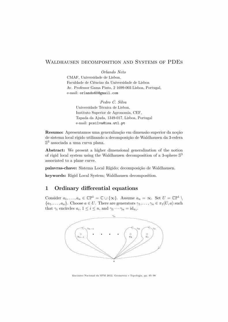
Consider a1, . . . , an ∈ CP1 = C ∪ ∞. Assume an = ∞. Set U = CP

1 \a1, . . . , an. Choose a ∈ U . There are generators γ1, . . . , γn ∈ π1(U, a) suchthat γi encircles ai, 1 ≤ i ≤ n, and γ1 · · · γn = idπ1

.

γ1

a

a2 a1an−1

γ2γn−1

γn


96 Waldhausen decomposition and systems of PDEs

LetPu = 0 (1)

be a linear differential equation with holomorphic coefficients in CP1 and

regular singularities at a1, . . . , an. Let f1, . . . , fk be a basis of the vectorspace La of the germs of solutions of (1) at a. Given γ ∈ π1(U, a) andf ∈ La, let γ · f be the element of La obtained by analytic continuation of falong γ. There is a matrix Φγ = (aij(γ)) such that γ · fi =

∑j aij(γ)fj . The

map γ 7→ Φγ is a linear representation of π1(U, a), called the monodromy of(1). The Riemann-Hilbert correspondence states that the monodromy mapdefines a dictionary between linear differential equations on P

1, with regularsingularities at a1, . . . , an, and linear representations of π1(U, a).

Set Ai = Φγi, i = 1, . . . , n. The set (X−1A1X, . . . , X−1AnX) : X ∈

GLk(C) is called the simultaneous conjugacy class of (A1, . . . , An). We saythat (1), Φ and (A1, ...An) are rigid if the simultaneous conjugacy class of(A1, . . . , An) is determined by the conjugacy classes of Ai, i = 1, . . . , n, i.e.,by the local monodromies around ai, i = 1, . . . , n. Although it is quite easy tocalculate the local monodromies of (1), it is very hard to compute the globalmonodromy (unless (1) is rigid!). This fact was first noticed by Riemannin his study of the hypergeometric differential equation (see [1]). Equationswith this type of property were called free from accessory parameters. Thenotion of rigidity, recently introduced by Katz (see [4]), is a very ambitiousreformulation of the notion of equation free from accessory parameters andrenovated the interest in this classical field.

2 Systems of partial differential equations

The Riemann-Hilbert correspondence has a higher dimensional generaliza-tion namely, a dictionary between regular holonomic D-modules (which,locally, are systems of PDEs) and perverse sheaves. If we assume that theD-module verifies some generic conditions, the associated perverse sheaf isdetermined by a linear representation of the fundamental group of the com-plement of the singular locus of the D-module (see [2], [5]).

Appel and others considered classes of systems of PDEs in CP2 and

CP1 × CP

1, that can be reconstructed from their local monodromies, i.e.,from their Riemann schemes. These systems of PDEs would be naturalcandidates of two dimensional rigid D-modules, if we knew how to introducesuch concept. As Haraoka noticed in [3], in order to generalize the conceptof rigidity, we first need to have a good definition of local monodromy near


Orlando Neto e Pedro C. Silva 97

a singular point of the singular locus of the D-module. We propose here asolution for this problem (see [7]).

Let Y ⊂ C2 be the plane curve parametrized by ϕ(t) = (t4, t6 + t7). We

call y = x3/2 + x7/4 the Puiseux expansion of Y and 3/2, 7/4 the Puiseux

exponents of Y . They are topological invariants that determine the topologyof Y . Set ∆ε = (x, y) ∈ C

2 : |x|, |y| < ε. Consider the plane curvesY0 = y = 0, Y1 = y = x3/2 and Y2 = Y . The intersections of Yi,i = 0, 1, 2, with the 3-dimensional sphere ∂∆ε define iterated torus knotsdenoted Γi, i = 0, 1, 2. We can choose tubular neighboorhoods Ti of Γi,i = 0, 1, 2, such that Ti+1 ⊂ int(Ti), i = 0, 1. The connected componentsof ∂∆ε \ ∪2

i=0∂Ti have a very simple structure: they are Seifert manifolds.Roughly speaking, ∂Ti, i = 0, 1, 2, define a Waldhausen decomposition of∂∆ε adapted to the knots Γi. Moreover, the tori surfaces ∂Ti, i = 0, 1, 2,are uniquely determined modulo isotopy (see [10]).

We say that a linear representation Φ of π1(C2 \ Y ) is rigid if its iso-morphism class is determined by the restriction of Φ to π1(∂Ti), i = 0, 1, 2.Since ∂Ti ≃ S

1 × S1, this restriction is determined by conjugacy classes of

pairs of commuting matrices, which we call local monodromy of Φ along ∂Ti.When Y is weighted homogeneous and contains the x and y-axis, every

irreducible representation Φ of π1(C2 \ Y ) is isomorphic to the pullbackof a representation Ψ of π1(CP1 \ finite set) twisted by a representation ofrank 1, via the morphism induced by (x, y) 7→ (yk : xn) for some pair ofcoprime integers k, n. Moreover, Φ is rigid with respect to the Waldhausendecompositions of ∂∆ε adapted to the link ∂∆ε∩Y if and only if Ψ is rigid inthe punctured Riemann sphere (see [7]), which shows the close relationshipbetween the two definitions of rigidity.

Example 2.1 Consider the system of partial differential equations,

ϑu = λu, Qu = 0, (2)

where ϑ = 2x∂x + 3y∂y, Q = ∂2x − (3/2)2x∂2

y . Set v = y−λ/3u. Since v isconstant along the integral curves of ϑ, there is a multivalued holomorphicfunction f on CP

1 such that

u = yλ/3f(y2/x3). (3)

Applying Q to the right hand side of (3) we conclude that f is the solution ofan hypergeometric differential equation, and thus that (2) is rigid. Moreover,the solutions of (2) ramify along the weighted homogeneous curve y2 = x3.


98 Waldhausen decomposition and systems of PDEs

The authors of [9] classified the DC2-modules “with simple characteristics”ramified along a weighted homogeneous curve Y . They found a definitionof system of PDEs “free from acessory parameters” that is quite natural forthis class of systems of PDEs. Moreover, the trick performed to system (2) ofExample 2.1 can be extended to this class of systems. The system (2) is freefrom acessory parameters if and only if the associated differential equationon CP

1 is free from accessory parameters. The authors of [9] remarked thatthey did not found as many systems free from acessory parameters as itwould be expected. We show in [7] that replacing “simple characteristics” by“multiplicity one”, a class only ‘slightly bigger’ (see [6]), we can find rigid D-modules of multiplicity 1 along Y with prescribed local monodromies aroundthe irreducible components of Y . We extend in [8] the previous result toarbitrary plane curves with irreducible tangent cone.

References

[1] L. Ahlfords, Complex Analysis, McGraw-Hill, 1979.

[2] P. Deligne, Equations Differentielles a Points Singuliers Reguliers, Lec-ture Notes in Mathematics 163, Springer Verlag, 1970.

[3] Y. Haraoka, “Studies in Deformation of Fuchsian Systems from the View-point of Rigidity”, RIMS Kokyuroku Bessatsu, B5 (2008), pp. 51–60.

[4] N. Katz, Rigid Local Systems, Princeton University Press, 1995.

[5] O. Neto, “A Microlocal Riemann-Hilbert correspondence”, Compositio

Mathematica, Vol. 127, No. 03 (2001), pp. 229–241.

[6] O. Neto and P. C. Silva, “On regular holonomic systems with solutionsramified along yk = xn”, Pacific Journal of Mathematics 207 (2002),pp. 463–487.

[7] O. Neto and P. C. Silva, “Higher dimensional Rigid Local systems”(submitted).

[8] O. Neto and P. C. Silva, “Rigid Local systems and Plane Curves” (inpreparation).

[9] M. Sato, M. Kashiwara, T. Kimura and T. Oshima,“Micro-local anal-ysis of prehomogeneous vector spaces”, Inventiones Mathematicae,Vol. 62, No. 1 (1980), pp. 117–179.

[10] Lê Dung Trang, “Plane curve singularities and carousels”, Annales de

l’Institut Fourier, Grenoble, Vol. 53, No. 4 (2003), pp. 1117–1139.


Geometria e Topologia - CiteSeerX

Documents

Transcript of Geometria e Topologia - CiteSeerX