Geologia Marina - Moodle@Units

Corso di Geologia Marina 2018-19

Università di TriesteLAUREA MAGISTRALE IN GEOSCIENZE

Curriculum GeofisicoCurriculum Geologico Ambientale

Anno accademico 2018 – 2019

Geologia Marina

Parte I

Modulo 2.2 Metodi indiretti: Rilievi acustici e sismica a riflessione

DocenteRiccardo Geletti

Email: [email protected]


Summary

• IntroductionThe seismic sectionSeismic interpretation softwareSeismic data web sites Seismic trace display

• Raw data e final seismic section: elements of multichannel seismic processing

• Resolution: vertical and lateralDeconvolutionMigration

• Velocity analysis and Depth migration• Coherent Noise in the seismic data: multiple reflections• Gas seeping features• Some case studies• Conclusion• Questions• Bibliography


• INTRODUCTIONThe Seismic method is the powerful geophysical techniques for imaging the

Earth’s interior.This artificial source method involve the generation of seismic waves whose

propagation velocities and transmission paths through the subsurface are mapped toprovide information on the distribution of geological boundaries at depth.

An alternative method of investigation subsurface geology is, of course, by drillingboreholes, but these are expensive and provide information only at discrete locations.Nevertheless, seismic surveying does not dispense with the need for drilling because itcan give a geological meaning to the seismic reflectors.

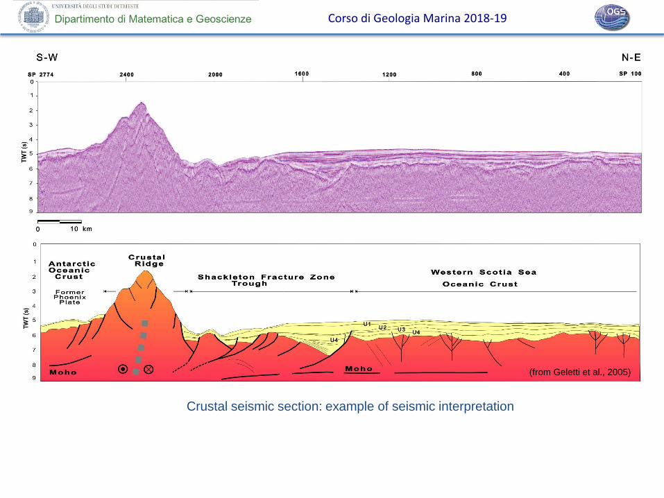
Seismic Reflection Interpretation• Fundamental in applied research to geosciences• Provides information regarding:

• geometries of stratigraphic sequences• geometries of structural and tectonic elements• velocity of seismic waves• lithological characteristics

The seismic interpretation attributes geological meaning to geophysical data and produces reconstructions of:2D sections, structural maps, fault systems, slumping and geo-hazard etc.


(from Geletti et al., 2005)

Crustal seismic section: example of seismic interpretation


Interpretation software

Seismic section

Position map of 2D seismic

survey by an interpretation

software


Seismic data websites:

• http://unmig.sviluppoeconomico.gov.it/videpi/

• http://see-atlas.leeds.ac.uk:8080/home.jsp

ViDEPI Project

well

http://unmig.sviluppoeconomico.gov.it/videpi/

http://see-atlas.leeds.ac.uk:8080/home.jsp


ViDEPI dataset


Position map of the seismic profiles of the Italian geophysical exploration projects MS and CROP

acquired in 1969 – 1982 and 1991-1995 respectively


Examples of vintage crustal seismic sections MS 1 acquired in Tyrrenian Sea in 1969

10 km

1 s (TWT)

Mars

iliV

avilo

v


Tim

e (

twt)

Amplitude+- 0 +-

Seismogram: this is an example of a single trace of a

seismic profile as shown in the figure above

0

Example of a part of seismic line displayed in

wiggle/variable area. On the right is shown a

single trace that constitutes the section above

(seismogram)

GELETTI & BUSETTI, 2011


Seismic section displayed in “variable area”


Seismic section displayed in “variable density” in grey scale


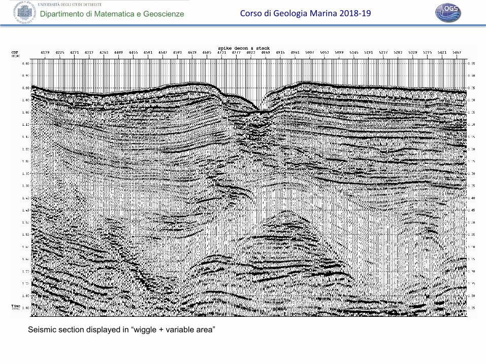
Seismic section displayed in “wiggle + variable area”


Seismic section displayed in grey scale variable density with the “enhanced reflections” in red colour


Raw data

(shot gathers)

Processed data

(stack section)

MultiChannel

Seismic reflection

data (MCS)


Reflected P wave

(normal polarity)

V2>V1

V3>>V2

V4<<V3

Shot

Reflected P wave

(reverse polarity)

V1

Dep

th (

m)

3000 m0 m

Example of wavefront simulation in a stratified medium


Distance (offset in meters)

Tim

e twt (s)

Shot gather


Example of «processing flow chart» that

define two different output: Pre-Stack Time

Migration (PSTM) and Pre-Stack Depth

Migration (PSDM). This sequence has been

applied to «crustal data» with «long offset

streamer».

The main steps are the following:

Reformating

Editing

Sorting

Gaining

Deconvolution

Velocity analysis

NMO correction and stacking

Migration


Shot

gather

CDP

gather

to

Common Depth Point (CDP)

Fold = n. Channel x Group int.

2 x Shot int.

Example of Sorting

Fold = 120 x 12.5 = 30

2 x 25


The progressive change of shape of an original spike

pulse during its propagation through the ground due to

the effects of absorption. (After Anstey, 1977)

A shot before and after gain correction.

Gain correction


Some of the

processing steps

From Geletti & Busetti 2011, JGR

a) CDP gather (after Sorting operation);

b) NMO correction with the velocity function picked in d;

c) Stack on 20 CDP gathers after NMO correction;

d) Semblance with velocity function picked;

e) Migrated section & MB swath bathymetry

d

eProcessing flow


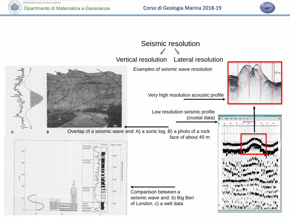
Seismic resolution

Vertical resolution Lateral resolution

Examples of seismic wave resolution

Very high resolution acoustic profile

Low resolution seismic profile

(crustal data)

Overlap of a seismic wave and: A) a sonic log, B) a photo of a rock

face of about 40 m

Comparison between a

seismic wave and: b) Big Ben

of London, c) a well data


Very high resolution CHIRP profile (sweep 2-7 kHz)

High penetration seismic line; in the

shallow part (see the zoom above)

the dominant frequency is c. 40 Hz.

TW

T (

ms)

Mass-transport deposits

Mass-transport deposits

100 m

s

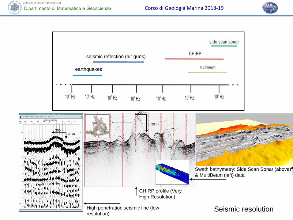
Seismic resolution

?


Factors affecting horizontal and vertical seismic resolution


High penetration seismic line (low

resolution)

CHIRP profile (Very

High Resolution)

Swath bathymetry: Side Scan Sonar (above)

& MultiBeam (left) data

200 m20 m

earthquakes

seismic reflection (air guns)

20 m

200 m

Seismic resolution


Vertical Resolution

The relationship between velocity (v), dominant frequency (f) and wavelegth (λ = v/f).

Threshold for vertical resolution


Lateral Resolution

Definition of the Frensnel zone AA’

Threshold for lateral resolution

(t0 = 2z/v, r=OA)


Example of high penetration (low resolution)

multichannel seismic reflection profile (CROP

project) in Central Adriatic Sea.

40 km depth

30 km depth

Seismic resolution

Vertical resolution = 75 m

Lateral resolution = 4840 m

(v=6 km/s; f = 20 Hz)


Examples of two seismic sections acquired by different sources: (left) by 2 GI guns (11,6 l); (right) by an array of 16 air guns (70 l)

Seismic resolution


Stack

Factors affecting horizontal and vertical seismic resolution: processing solution


Example of the effect of the

deconvolution on the definition of

seismic data (synthetic data). The

deconvolution "shrinks" the wavelet

as shown in the figure (synthetic

data)

Before the

deconvolution

After the

deconvolution

Vertical resolution

Deconvolution


Seismic stack section a) before and b) after deconvolution (Yilmaz, 2001)

Vertical resolution


• Consider a source-detector (s-d) on the surface of a

medium of costant seismic velocity. For a given

reflection time, the reflection point may be anywhere

on the arc of a circle centred on the s-d position. On a

non migrated seismic section the point is mapped to

be immediately below the s-d.

• A planar-dipping record surface derived from a non-

migrated seismic section (blu line) and its associated

reflector surface (red line).

Migration

True dip

Apparent dip

Lateral resolution


Lateral resolution

a) A sharp synclinla feature in a reflecting

interface, and

b) (b) the resultant «bow-tie» shape of the

reflection event on the non-migrated

seismic section.


Example of seismic reflection profile across two buried channels (a) non-migrated section with the presence of «bow-tie»

effect (red ellipses) and b) after migration

Lateral resolution: migration

a) b)


2D migration is an imperfect process on the «strike line»

2D migration


2D and 3D migration

The image shows an example of a 3D geological

model with two anticlinals (green and yellow object)

and a direct fault (red and blue objects).

The seismic data along line 6 shows the comparative

effects of 2D and 3D migration (from French, 1974).

Only 3-D migration is able to provide a seismic

profile faithful to the real situation of pending layers.

However, the 2-D migration provides an often

satisfactory result for interpretation.

From French, 1974


Example of 2D migrated seismic profile with the presence of salt domes, some of which are lateral to the vertical plane of

the section.

Salt dome

2D migration

Lateral

salt dome

Lateral

salt dome


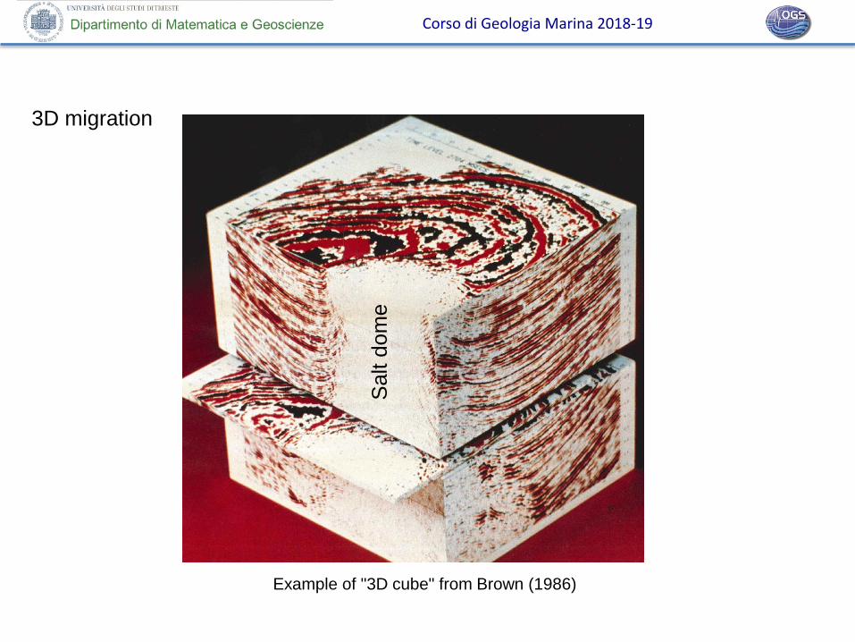
Example of "3D cube" from Brown (1986)

Salt d

om

e

3D migration


Diffraction

from faulted layer

Migration: diffraction collapse

In general, the different depositional / erosional

and tectonic events occurring during the

geological evolution of an area, determine

irregularities along the stratigraphic horizons

(reflectors) due to fractures, erosion, sedimentary

accumulations, etc. These represent points of

inhomogeneity that originate diffractions. Below

there is a synthetic seismic section with the

diffraction caused by a fault for example.


FAULTS

Example of faults in the geological layers.

The faults represent points of inhomogeneity that originate diffractions. You can see the geological

layers that are dislocated by the faults


(a) (b)

Seismic section (a) before and (b) after migration: the diffractions have been collapsed and the faults are evident.

The presence of diffractions can sometimes create difficulties of interpretation: the point of breakage of the

reflector is not easily identifiable in the non-migrated section. In the case b) the section was migrated and the

base of the salt layer is more evident then in stack section a)

Migration: diffraction collapse


Blow up of the previous seismic image


Geologic model

x,y,z

Seismic section:

x,y,t

Velocity

Velocity field of the seismic waves is the

parameter that allow to get the geologic

model from the seismic section


Velocity analysis

A: a common mid-point trace gather

(left) and semblance coherence

contour (right).

Peaks in coherence give the

stacking velocity. (yellow line)

B: The same common mid-point

trace gather of A with the normal

move-out correction (NMO ) after

the velocity picking (yellow

function). The interval velocity (red

function) associated to this

stacking velocity it will use in

migration process.

The field velocity section can be obtained from the seismic

data using the stack velocities. We are going to flatten the

reflections in CDP gather as in the image, picking the

maximum coherence in the semblance. In this way velocity

functions are obtained which we will interpolate with the

others in order to have a section.


Example of Pre Stack Depth Migrated section with its velocity field superimposed (see next slide for the interpretation)

Velocity field and depth migrated seismic section


(from Micallef et al., 2018)Example of Pre Stack Time/Depth Migration section and the interpretation superimposed

with velocity function.

Depth migrated seismic section


Image of a Pre-Stack Depth Migrated section (PSDM) and its velocity field used to migration (from Saule et al. 2016)

Depth migrated seismic section

Note the high-velocity layer with a semi-transparent seismic signature with no stratification inside it. This is the Messinian salt layer (halite)

in a seismic profile acquired in Ionian Sea.


Time Migrated section with salt intrusion


Depth migrated section


Time migrated section

Depth migrated section

Pull up velocity effect:

example of a salt dome

In presence of salt domes, in the seismic section we can

observe the pull up velocity effect. This is due to the

presence of high-velocity salt dome over the deep

reflector in that sector of the profile. When we migrate in

depth this effect is corrected with a right velocity function.


(Above) Result of data processing in time domain: the pull-up event (red circles) of about 200 ms occurs beneath a salt dome

and affects the underlying layers. (below) Result of Pre-Stack Depth Migration (PSDM) showing flattened pullup event.

(modified from Dal Cin et al. 2016)

Pull up velocity effect


Dal Cin et al., 2016. Petroleum Geosciences

Interpretation


Vertical Seismic Profiling (VSP)

in seismic interpretation

Example of correlation of well data (VSP) with the

seismic section for geological interpretation

In some case we have a borehole across the seismic section and we can

correlate these two type of data. From this we can therefore give a lithological

meaning to the individual reflectors of the seismic profile passing through the

well. In the image below and on the right, we can see an example of correlation

between the seismic profile and the data obtained from the registration of the

VSP in a borehole. The VSP was made after the geologic sampling in the

same borehole.

Well


- MULTIPLE REFLECTIONS –The problem of cherent noise in marine seismic profiles

Long-path multiples appear as distinct events.

Short-path multiples are added to primary

reflections and tend to come from shallow

subsurface phenomena

The marine seismic dataset is often characterized by the

presence of multiple reflections that affect the quality of

the section itself. The multiple are the coherent noise that

it leads to the misinterpretation of real reflective horizons.

There are a lot of type of coherence noise, but the first

water bottom multiple reflections are the most frequently.


In this slide on the left it shows a schematic model of ray paths of the sea floor reflector (in blue color), a deep reflector at

450 m (in green color) and a multiple ray path in red. On the right there is a cdp gather before and after normal move out

correction (velocity correction) and its stack section where you can see that the multiple reflection is attenuated, but no

eliminated..

MULTIPLE REFLECTIONS


Three CMP gathers before (left) and after (right) NMO correction.Note that the primaries have been flattened and the multiples

have been undercorrected after NMO correction. As a result, multiple energy has been attenuated on the stacked section

(center) relative to primary energy (from Yilmaz 2001)



M1

M2

Example of seismic stack section with multiple reflections (M1 and M2)



Gas seeping features

Mud volcanoes and pockmarks

Geletti, 2008

Geletti & Busetti, JGR 2011

Geletti, 2008

Sub Bottom Profilers (CHIRP)

with pockmarks

MB data with pockmarks

Seismic line & MB image with

mud volcano

Schematic model of

gas seeping related

upward fluid migration

Some example of gas seeping features. Sea bed fluid flow, also known as submarine seepages, involves the flow of gas and liquids

through the seabed. This geological phenomenon has widespread implications in seabed slope instability, drilling hazard, hazards to

seabed installations and so on. Seabed fluid flow affects seabed morphology (pockmarks, mud volcanoes). Natural fluid emissions also

have a significant impact on the composition of the oceans and atmosphere: methane emissions have important implications for the

global climate change.


Example of upward fluid migration and the correlated gas seepage features in a seismic profile

(modified from Geletti & Busetti, JGR - 2011)

Gas seeping features

Mud volcanoes and pockmarks

Geletti & Busetti, JGR 2011


Seismic horizon

with normal polarity

Phase inversion and

changing dominant

frequency Enhance amplitude reflector with reverse polarity

BSR

Dominant frequency 40 Hz

Dominant frequency 20 Hz

Example of seismic imaging

where there is free gas in the

sediments under the gas

hydrate zone (Antarctica)

Gas seismic

signature


Echosounder CHIRP profile where there are gas evidences

GAS (acoustic mask)

GAS (enhanced reflections)GAS Plumes

Faults

Geletti 20052.5 km

10 m


Examples of bright spot (R1, R2 and R3) in a seismic section (no migrated)


CASE HISTORY - 1:

Gas seeps linked to salt structures in the

Central Adriatic Sea (Geletti et al., 2008)

The analyses of about 800 km of Chirp sub-bottom profilers and

600 km2 of Multibeam data acquired during the 2005 and 2007

surveys of the R/V OGS Explora, and their correlation with one

new, and several public, multichannel seismic profiles, allow us to

propose a relation between the distribution of gas seepages,

fracture systems and deep salt features present in the Central

Adriatic Sea. Gas seepage is evident from pockmarks on the

seabed and in the shallow sub-bottom, where acoustic chimneys

and bright spots have been highlighted and analyzed. The Mid-

Adriatic Depression (MAD) is a distinct morphological feature in

the Central Adriatic Sea elongated in a NE-SW direction. The area

is affected by salt doming of Triassic evaporites which cause the

two main alignments of the Mid-Adriatic Ridge as far as the

Palagruza High and the Jabuka Ridge. These salt tectonics have

existed since, at least, Paleogene times and are still active: they

characterize sectors with less resistance to deformation produced

by successive regional compressive regimes that have affected the

area differently during the different geodynamic phases. Gas- seep

features are distributed preferentially above and along the fracture

systems produced above and around the salt mounds.


Dia

piric

str

uctu

re

Dia

piric

str

uctu

re

Dia

piric

str

uctu

re

Dia

piric

str

uctu

re

Crustal seismic profile CROP- M15


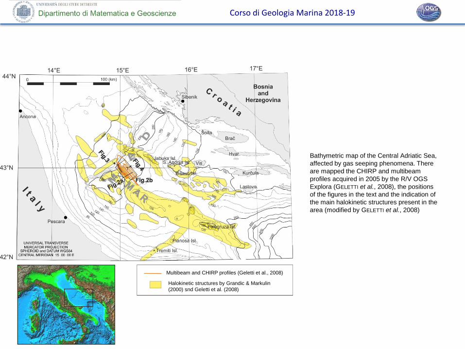
Bathymetric map of the Central Adriatic Sea,

affected by gas seeping phenomena. There

are mapped the CHIRP and multibeam

profiles acquired in 2005 by the R/V OGS

Explora (GELETTI et al., 2008), the positions

of the figures in the text and the indication of

the main halokinetic structures present in the

area (modified by GELETTI et al., 2008)

Multibeam and CHIRP profiles (Geletti et al., 2008)

Halokinetic structures by Grandic & Markulin

(2000) snd Geletti et al. (2008)


10 m

100 m

Gas plume in water columnGas plume

Gas in the sediments

Pockmark

Dia

piric

str

uctu

re

a) Image of the seismic reflection profile with the

evidence of bright spots indicating the presence of gas

in the Plio-Quaternary sediments, b) multibeam

bathymetry (MB) and a pseudo 3D image (c) with

CHIRP profile and MB where it is highlighting a

system of active faults along which some pockmarks

can be identified. The seismic line shows the

presence of a deep diapiric structure that also

deforms the sea floor

Detail of the CHIRP line with evidence of gas plume


Seismic section with

gas seeps features

Pseudo 3D image of a pockmarks visible on

two orthogonal CHIRP profiles

Image of Pockmarks in MB data

In this slide there are some images of gas/fluid presences within the

sediments. On the right, above you see an image of pockmarks on swath

bathymetry of multibeam. Below, two chirp profiles. On the left side you

see a seismic section where at a deep of 400/450 m there are seismic

anomalies below superficial gas evidence in chirp profiles


Chirp sub-bottom profile (a) crossing the Palagruza High in a W-E direction.The western

margin shows a high density of mounds, more evident on Multibeam data (b), and in the blow-

up of the Chirp profile (c). (d) A very fine detail shows a bottom feature characterized by an

acoustic transparent zone denoting high absorption of the signal by a strong reflecting

seafloor: this seismic facies and the morphology on the Multibeam (b) could suggest a coral

bank origin for this feature.


CASE HISTORY - 2: THE OTRANTO CHANNEL

MS-29 seismic profile, Otranto Channel

Ionian/South Adriatic basin

Apulia Carbonate Platform

P l i o – Q u a t e r n a r y s e d i m e n t a r y s e q u e n c e

Platform margin

Ms

Ls

MsM

Gas seepages related to deep features in the Otranto Channel (South Adriatic Sea) -

OCSS15 project - (Otranto Channel gaS Seepages)


A) Sketch model of fault-

linked development of

deep-water coral mounds

in the North Sea. The

arrows indicate nutrient-

rich fluid hydrocarbon

seepage (from HOVLAND,

2005). B) CHIRP profile

acquired during the

OCSS15 cruise in the

central Otranto Channel

zone, showing Coral

mounds over a fault

Seabed structures on Chirp profile, Multibeam data (GELETTI, 2008) corresponding

to the bottom features previously highlighted on the MS-29 seismic profile (below).

Sub-Bottom profile crossing the deep water mound, showing possible sediment

drifts deposits with weak layers within the carbonate mound. The internal

structures are poorly imaged due to the strong reflectivity of the sea floor. Along

the MS-29 seismic profile a micro-fracture system (black arrows) was recognized

and associated to differential sediment compaction. The micro-facture web

represent the pathway along which the gas migrate from the bright spots (BS)

toward the seabed.


Seabed structures (carbonate mounds ) on the seismic profiles (low & medium

resolution), CHIRP and Multibeam (MB). (Geletti, 2008; Del Ben et al., 2008;

Romeo et al. 2011).

Migrate section

Stack sectionCHIRP

profile

MB


CHIRP profile

(OCSS15 cruise)

with a mound on

which the corals

were sampled

Detail of the CHIRP line with evidence of gas plumes

A) Chirp profile crossing some of the mud volcanoes calibrated

by two gravity corers during the OCSS15 acquisition project.

This CHIRP line was acquired on the seismic profile (B) of the

same cruise: the sea bottom features are related to gas

accumulations evidenced by some inclined bright spots. The

image in B is a preliminary seismic stack section.

Figures from Geletti

et al., 2018


Conclusion - 1

The Multi-Channel Seismic Reflection (MCS) method is:

• The most widespread method for the geophysical prospecting of the subsoil,

fundamental in the exploration of hydrocarbon reservoir.

• It provides more detailed information than any other non-invasive method on

stratigraphy, structure and properties of materials.

• It uses arrival times, amplitude and phase of the echoes from the discontinuity in

the elastic properties present in the subsoil to obtain its position and physical

properties (acoustic impedance, velocity propagation of seismic waves, elastic

parameters, ...).

Disadvantages of the MCS method:

• High costs of data acquisition (R/V OGS Explora ship time - > 15-20 K€ a day)

• Complex signal processing required

• Numerous specialized people needed

• For a survey, numerous permits and authorizations are required


The seismic reflection interpretation attributes geological meaning to geophysical data.

Interpretation provides information on:

• geometry of stratigraphic sequences and structural/tectonic elements

• seismic wave velocity

• Lithological characteristics

Applications for reconstructions of 2D section, structural maps, fault systems,

slumping and seismic hazard.

The interpretation is made by a team of geologists / geophysicists / physicists with

different skills who work in synergy.

“Interpretation is a combination of both art and science “ (Lines and Newrick, 2004)

Conclusion - 2


Questions

1. What is a seismic section?

2. What is the difference between seismic and geological section?

3. What is the vertical scale in a seismic section?

4. Which is the difference between seismic stack section and migrated section?

5. What is a diffraction?

6. What is a «bow-tie» event?

7. What is a multiple reflection?

8. What are the advantages of a migrated section?

9. Which seismic parameter is fundamental in depth migration?

10. Which is the first reflection in a marine seismic section?

11. What is the acoustic basement?

12. What is a « bright spot» in a seismic section?

13. What are the seismic characters that identify the possible presence of gas in the sediments?

14. What are the gas seeping structures?

15. What is the best acoustic method to study these structures?


Bibliography:

• AN INTRODUCTION TO GEOPHYSICAL EXPLORATION, di Philip KEAREY, Michael

BROOKS, Ian HILL; (2002) – Blackwell Science – ISBN 0-632-04929-4.

• MARINE GEOPHYSICS, E. J. W. JONES; (1999) – Wiley – ISBN 0-471-98694-1

• SEISMIC DATA ANALYSIS (Vol. I & II), Öz YILMAZ; (2001) – SEG – Vol. I ISBN 1-56080-

098-4; Vol. II ISBN 1-56080-098-2

• Lines and Newrick - FUNDAMENTALS OF GEOPHYSICAL INTERPRETATION

• Sheriff and Geldart - EXPLORATION SEISMOLOGY

• Anstey - SEISMIC INTERPRETATION - The Physical Aspects

• Herron – FIRST STEP IN SEISMIC INTERPRETATION

• Hovland & Jadd - Seabed Pockmarks and Seepages

• Jadd & Hovland – Seabed Fluid Flow

Websites:

• ViDEPI: http://unmig.sviluppoeconomico.gov.it/videpi/

• Virtual Seismic Atlas: http://see-atlas.leeds.ac.uk:8080/home.jsp

http://unmig.sviluppoeconomico.gov.it/videpi/

http://see-atlas.leeds.ac.uk:8080/home.jsp

Geologia Marina - Moodle@Units

Documents

Transcript of Geologia Marina - Moodle@Units