University of Plymouth

PEARL https://pearl.plymouth.ac.uk

04 University of Plymouth Research Theses 01 Research Theses Main Collection

2009

GENETIC BIODIVERSITY OF THE

EUROPEAN BARNACLE

CHTHAMALUS MONTAGUI

FONTANI, SONIA

http://hdl.handle.net/10026.1/2733

University of Plymouth

All content in PEARL is protected by copyright law. Author manuscripts are made available in accordance with

publisher policies. Please cite only the published version using the details provided on the item record or

document. In the absence of an open licence (e.g. Creative Commons), permissions for further reuse of content

should be sought from the publisher or author.

GENETIC BIODIVERSITY OF THE EUROPEAN BARNACLE CHTHAMALUS MONTAGUI

by

SONIA FONTANI

A thesis submitted to the University of Plymouth in partial fulfilment for the degree of

DOCTOR OF PHILOSOPHY

School of Biological Science Faculty of Sciences

In collaboration with Marine Biological Association of the UK, Plymouth

ENEA - Marine Environment Research Centre S. Teresa, Italy

June 2009

SONIA FONTANI

GENETIC BIODIVERSITY OF THE EUROPEAN BARNACLE CHTHAMALUS MONTAGUI

Abstract

Biodiversity ultimately is genetic diversity. Genetic diversity within species is eroded before negative trends in biodiversity become evident as loss of species or habitats. Hence, monitoring biodiversity at the genetic level may indicate what will happen at higher levels of organisation if the trend is allowed to continue.

There is a pervasive belief that marine ecosystems are less vulnerable to biodiversity loss than terrestrial ones, due to marine species' high dispersal ability and connectivity, large geographic ranges, low genetic differentiation among populations and high genetic variation within populations. Many studies offer compelling evidence that it is not so: loss of genetic variation due to natural and anthropogenic factors has been detected even in marine species with potentially high dispersal.

In this context the genetic pattern of the European barnacle Chthama/us montagui, a species with high dispersal capability, was investigated from three different perspectives using polymorphic microsatellite loci as molecular markers.

The effect of structures created to protect coastal areas in the Adriatic Sea, was investigated to test the hypothesis that artificial substrates can act as "corridors" facilitating gene flow among previously isolated populations.

The genetic pattern of central populations was compared to that of peripheral/marginal populations over the range of C. montagui in the UK, to test the hypothesis that marginal and peripheral populations tend to be less genetically variable than central ones.

For both studies results were consistent with the formulated hypotheses at the 3 analysed loci.

Finally, a broader survey of the NE Atlantic and Mediterranean range of this barnacle was carried out to assess spatial scales of genetic variation. A clear differentiation between Atlantic and Mediterranean samples was detected; however, the major source of genetic variation was within sites at a very small spatial scale.

The information gained generates insights for marine genetic management and conservation planning.

1

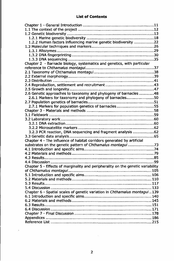
List of Contents

Chapter 1 - General Introduction ......................................................... 11 1.1 The context of the project ............................................................. 12 1.2 Genetic biodiversity ...................................................................... 13

1.2.1 Marine genetic biodiversity ...................................................... 18 1.2.2 Human factors influencing marine genetic biodiversity ................ 22

1.3 Molecular techniques and markers .................................................. 26 1. 3.1 Allozymes .............................................................................. 29 1.3.2 DNA fingerprinting ............... ~ .................................................. 30 1.3.3 DNA sequencing ..................................................................... 35

Chapter 2 - Barnacle biology, systematics and genetics, with particular reference to Chthama/us montagui ....................................................... 37 2.1 Taxonomy of Chthamalus montagui ................................................ 38 2.2 External morphology ..................................................................... 39 2.3 Distribution ................................................................................. 41 2.4 Reproduction, settlement and recruitment ...................................... .43 2.5 Growth and longevity .................................................................... 47 2.6 Genetic approaches to taxonomy and phylogeny of barnacles ........... .48

2.6.1 Markers for taxonomy and phylogeny of barnacles ...................... 50 2. 7 Population genetics of barnacles ..................................................... 51

2. 7.1 Markers for population genetics of barnacles .............................. 55 Chapter 3- Materials and methods ...................................................... 56 3.1 Fieldwork ................................................................ , ................... 59 3.2 Laboratory work ........................................................................... 60

3.2.1 DNA extraction ....................................................................... 60 3.2.2 Microsatellite markers ............................................................. 62 3.2.3 PCR reaction, DNA sequencing and fragment analysis ................. 62

3.3 Genetic data analysis .................................................................... 65 Chapter 4 - The influence of habitat corridors generated by artificial substrates on the genetic pattern of Chthamalus montagui ..................... 73 4.1 Introduction and specific alms ........................................................ 74 4.2 Materials and methods .................................................................. 79 4.3 Results ........................................................................................ 85 4.4 Discussion ................................................................................... 99 Chapter 5 - Effects of marginality and peripherality on the genetic variability of Chthamalus montagui ................................................................... 105 5.1 Introduction and specific aims ...................................................... 106 5.2 Materials and methods ................................................................ 110 5.3 Results ...................................................................................... 117 5.4 Discussion ................................................................................. 133 Chapter 6 - Spatial scales of genetic variation in Chthama/us montagui .. 139 6.1 Introduction and specific aims ...................................................... 140 6.2 Materials and methods ................................................................ 145 6.3 Results ...................................................................................... 151 6.4 Discussion ................................................................................. 171 Chapter 7 - Final Discussion .............................................................. 178 Appendices ..................................................................................... 186 Reference List ................................................................................. 215

2

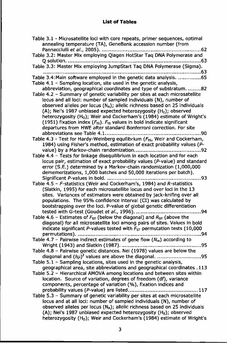
List of Tables

Table 3.1 - Microsatellite loci with core repeats, primer sequences, optimal annealing temperature {TA), GeneBank accession number (from Pannacciulli et al., 2005) .............................................................. 62

Table 3.2: Master Mix employing Qiagen HotStar Taq DNA Polymerase and Q solution ................................................................................... 63

Table 3.3: Master Mix employing JumpStart Taq DNA Polymerase (Sigma) . ................................................................................................. 63

Table 3.4:Main software employed in the genetic data analysis ............... 65 Table 4.1 - Sampling location, site used in the genetic analysis,

abbreviation, geographical coordinates and type of substratum ......... 82 Table 4.2 - Summary of genetic variability per sites at each microsatellite

locus and all loci: number of sampled individuals (N), number of observed alleles per locus (NA); allelic richness based on 25 individuals (A); Nel's 1987 unbiased expected heterozygosity (HE); observed heterozygosity (H0 ); Weir and Cockerham's (1984) estimate of Wright's (1951) fixation index (F15). F1s values in bold indicate significant departures from HWE after standard Bonferroni correction. For site abbreviations see Table 4.1. .......................................................... 90

Table 4.3 - Test for Hardy-Weinberg equilibrium {F15, Weir and Cockerham, 1984) using Fisher's method, estimation of exact probability values (P-value) by a Markov-chain randomization ......................................... 92

Table 4.4 - Tests for linkage disequilibrium in each location and for each locus pair, estimation of exact probability values (P-value) and standard error (S.E.) determined by a Markov-chain randomization (1,000,000 dememorlzations, 1,000 batches and 50,000 iterations per batch). Significant P-values in bold ........................................................... 93

Table 4.5 - F-statistics (Weir and Cockerham's, 1984) and R-statistics (Siatkin, 1995) for each microsatellite locus and over loci in the 13 sites. Variances of estimators were obtained by jack-knifing over all populations. The 95% confidence interval (Cl) was calculated by bootstrapping over the loci. P-value of global genetic differentiation tested with G-test (Goudet et al., 1996) ......................................... 94

Table 4.6- Estimates of Fsr (below the diagonal) and RsT (above the diagonal) for all microsatellite loci among pairs of sites. Values in bold indicate significant P-values tested with FsT permutation tests (10,000 permutations) ............................................................................. 94

Table 4. 7 - Pairwise indirect estimates of gene flow (Nm) according to Wright (1943) and Slatkin (1987) .................................................. 95

Table 4.8- Pairwise genetic distances. Nei (1978) values are below the diagonal and (8j.J)2 values are above the diagonal. ........................... 95

Table 5.1 - Sampling locations, sites used in the genetic analysis, geographical area, site abbreviations and geographical coordinates .113

Table 5.2- Hierarchical AMOVA among locations and between sites within location. Source of variation, degrees of freedom (df), variance components, percentage of variation (%), fixation indices and probability values (P-value) are listed ........................................... l17

Table 5.3 - Summary of genetic variability per sites at each microsatellite locus and at all loci: number of sampled individuals (N), number of observed alleles per locus (NA); allelic richness based on 25 individuals (A); Nei's 1987 unbiased expected heterozygosity (HE); observed heterozygosity {H0 ); Weir and Cockerham's {1984) estimate of Wright's

3

(1951) fixation index (F,5 ). F,5 values in bold indicate significant departures from HWE after standard Bonferronl correction. Peripheral (Sk2 and Fr2) and marginal (Mi1) populations are in italics ............. 122

Table 5.4 - Tests for linkage disequilibrium at each sites and for each locus pair, estimation of exact probability values (P-value) and standard error (S.E.) determined by a Markov-chain randomization (1,000,000 dememorizations, 1,000 batches and 50,000 iterations per batch). Significant P-values in bold. Peripheral (Sk2 and Fr2) and marginal (Mi1) populatlons are in italics ..................................................... 124

Table 5.5- F-statlstlcs (Weir and Cockerham, 1984) and R-statistics (Siatkin, 1995) for each microsatellite locus and over loci in the 17 sites. Variances of estimators were obtained by jack-knifing over all sites. The 95% confidence interval (Cl) was calculated by bootstrapping over loci. P-value value of global genetic differentiation tested with G-test (Goudet et al., 1996) ....................................... 125

Table 5.6 - Estimates of Fsr (below diagonal) and Rsr (above diagonal) for all microsatellite loci between pairs of sites. Values in bold indicate significant P-values tested with Fsr permutation tests (10,000 permutations). Peripheral (Sk2 and Fr2) and marginal (Mi1) populations are in Italics .............................................................................. 126

Table 6.1 -Sampling location, site used in the genetic analysis, abbreviation, geographical coordinates and basin of origin .............. 147

Table 6.2 - Summary of genetic variability per site at each microsatellite locus and all loci: number of sampled individuals (N); number of observed alleles per locus (NA); allelic richness based on 13 individuals (A); Nei's 1987 unbiased expected heterozygosity (He); observed heterozygosity (H0 ); Weir and Cockerham's (1984) estimate of Wright's (1951) fixation index (F,s). F,s values in bold indicate significant departures from HWE after standard Bonferroni correction. For site abbreviations see Table 6.1. ........................................................ 158

Table 6. 3 - F-statistics (Weir and Cockerham, 1984) and R-statistics (Siatkin, 1995) for each microsatellite locus and over loci in the 18 populatlons. Varlances of estimators were obtained by jack-knifing over all populations. The 95% confidence interval (Cl) was calculated by bootstrapping over the loci. P-value of global genetic differentiation tested with G-test (Goudet et al., 1996) ....................................... 161

Table 6.4 - Estimates of FsT (below the diagonal) and RsT (above the diagonal) for all microsatellite loci among pairs of sites. Values in bold indicate significant P-values tested with FsT permutation tests (10,000 permutations) ........................................................................... 162

Table 6.5 - Pairwise genetic distances. Nei (1978) values are below the diagonal and (o1J)2 values are above the diagonal. ......................... 163

Table 6.6- Hierarchical AMOVA among samples grouped in two groups ('basins'): group 1, Atlantic locations; group 2, Mediterranean locations. Source of variation, degrees of freedom (df), variance components, percentage of variation (%), fixation indices and probability value (P-value) are listed ........................................................................ 168

Table 6. 7 - Hierarchical AMOVA among samples as Implemented in HIERFSTAT. Pairwise Fsr estimates and P-value between basins, among locations within basins, among sites within locations and within sites . ............................................................................................... 168

Table 6.8 - Hierarchical AMOVA among the Mediterranean locations with two sites per location. Source of variation, degrees of freedom (df),

4

variance components, percentage of variation (%), fixation Indices and probability value (P-value) are listed ............................................ 168

Table 6.9- Hierarchical AMOVA among the Atlantic locations with .two sites per location. Source of variation, degrees of freedom (df), variance components, percentage of variation (%), fixation indices and probability value (P-value) are listed ............................................ 168

Table 6.10: Mean proportion of membership of each sample (location/site) to each cluster (K=2) ................................................................. 169

Table 6.11: Mean proportion of membership of each sample (location/site) to each cluster (K=3) ................................................................. 170

5

List of Figures

Figure 1.1 - Qualitative representation of the relative strengths and weaknesses of different molecular markers (from Belfiore and Anderson, 2001) .......................................................................... 36

Figure 2.1 - Photo of C. montagui (a) and of C. stellatus (b) by Prof. A.J. Southward, published on MarLIN web site ....................................... 39

Figure 2.2 Arrangement of shell plates of Chthamalus spp .. Scutum (S); tergum (T); carena (C); rostrum (R); lateral (L); careno-lateral (CL) (Relini, 1980) .............................................................................. 40

Figure 2.3- Outline sketches of C. montagui (a) and C. stellatus (b) (Hawkins and Jones, 1992) .......................................................... .41

Figure 3.1- Experimental design for sampling ....................................... ,59 Figure 4.1 -Sampling locations in the central/northern Adriatic Sea ......... 81 Figure 4.2 - Type of substratum characteristic of the central/northern

Adriatic Sea ................................................................................ 81 Figure 4.3 - Non-metric multidimensional scaling analysis (nMDS) of 13

samples based on Nei's (1978) genetic distance. Stress value = 0.11 (For abbreviations see Table 4.1) ................................................... 96

Figure 4.4 - Reduced major axis regression showing relationships between genetic and geographical distances for all 13 locations. Genetic distances based on Fsr (r=-0.0725 P-value= 0.7580) ....................... 97

Figure 4.5 - Reduced major axis regression showing relationships between genetic and geographical distances for all 13 locations. Genetic distances based on RsT (r=-0.0935; P-value= 0.8330) ..................... 97

Figure 5.1 -Geographical distribution of C. montagui in the UK and Ireland (from Hawklns and Jones, 1992) ................................................. 109

Figure 5.2 - Northern UK sampling locations ....................................... 111 Figure 5.3 - Southern UK sampling locations ....................................... 112 Figure 5.4 - Non-metric multidimensional scaling analysis (nMDS) among 17

samples based on Fsr (Weir and Cockerham, 1984). Stress value= 0.166 (for abbreviations see Table 4.1) ........................................ 128

Figure 5.5 - Non-metric multidimensional scaling analysis (nMDS) among 17 sites based on Nei's (1978) genetic distance. Stress value= 0.176 (for abbreviations see Table 4.1) ....................................................... 129

Figure 5.6 - UPGMA consensus tree based on Cavalli-Sforza and Edwards (1967) genetic distances; bootstrap (10,000 replicates) percentages are shown at nodes (for abbreviations see Table 4.1 ). Peripheral and marginal populations are in italics ................................................ 130

Figure 6.1 - Sampling locations of Chthama/us montagui . ..................... 146 Figure 6.2 - Allelic richness (A) and expected heterozygosity (B) at locus

CM 2/15 per site. For site abbreviations see Table 6.1 ................... 160 Figure 6.3 - Allelic richness (A) and expected heterozygosity (B) per site at

locus CM 5/23. For site abbreviations see Table 6.1 ...................... 160 Figure 6.4- Allelic richness (A), expected heterozygosity (B) per site over

all loci. For site abbreviations see Table 6.1. ................................ 161 Figure 6.5 - Non-metric multidimensional scaling analysis (nMDS) of 18

sites based on Rsr (Weir and Cockerham, 1984). Stress value= 0.026 (for abbreviations see Table 6.1) ................................................. 164

Figure 6.6 - Non metric multidimensional scaling analysis (nMDS) of 18 sites based on Nei's (1978) genetic distance. Stress value= 0.005 (for abbreviations see Table 6.1) ....................................................... 165

6

Figure 6. 7 - UPGMA consensus tree based on Cavalli-Sforza and Edwards (1967) genetic distances; bootstrap (10,000 replicates) percentages are shown at nodes (for abbreviations see Table 6.1) ..................... 166

Figure 6.8 - Reduced major axis regression showing relationships between genetic and geographical distances for all 18 samples. Genetic distances based on Nel (1978) (r= 0. 774; P-value= 0.001) ............ 167

Figure 6.9: Clustering analysis conducted in STRUCTURE 2.2 (K=2). In the bar plot, each vertical bar along the x axis represents one of 534 individuals grouped by location/site (see abbreviation in Table 6.1); the Y-axis represents the estimated proportion of membership of each Individual to each cluster (represented by different colours) ............ 169

Figure 6.10: Clustering analysis conducted in STRUCTURE 2.2 (K=3). In the bar plot, each vertical bar along the x axis represents one of 534 individuals grouped by location/site (see abbreviation in Table 6.1); the Y-axis represents the estimated proportion of membership of each Individual to each cluster (represented by different colours) ............ 170

7

List of Appendices

Appendix 3.1: TBE (10x} electrophoresis buffer recipe .......................... 187 Appendix 3.2: DNA Salting-Out extraction protocol (modified after Aljanabi

& Martinez, 1997) ...................................................................... 187 Appendix 4.1 - Allele frequencies of the Adriatic samples of Chthama/us

montagui at three microsatellite loci. For abbreviations see Table 4.1. ............................................................................................... 189

Appendix 5.1 - Allele frequencies of the UK samples of C. montagui at three microsatellite loci. Peripheral (Sk2 and Fr2) and marginal (Mi1) population are in italics. For abbreviations see Table 5.1.. ............... 194

Appendix 5.2 - Test for Hardy-Weinberg equilibrium (F1s, Weir and Cockerham, 1984} for the 17 UK samples using Fisher's method, estimation of exact probability values (P-value) by Markov-chain randomization (10,000 dememorizations, 100 batches and 5,000 iterations per batch). Peripheral (Sk2 and Fr2) and marginal (Mi1) populations are in italics. For abbreviations see Table 5.1. .............. 197

Appendix 6.1 - Allele frequencies of the Atlantic and Mediterranean samples of Chthamalus montagui at six microsatellite loci. For site abbreviations see Table 6.1 ............................................................................ 199

Appendix 6.2 - Test for Hardy-Weinberg equilibrium (F1s, Weir and Cockerham, 1984) using Fisher's method, and estimation of exact probability values (P-value) by Markov-chain randomization (10,000 dememorizations, 100 batches and 5,000 iterations per batch). For abbreviations see Table 6.1 ......................................................... 206

Appendix 6.3 - Tests for linkage disequilibrium in each location and for each locus pair, estimation of exact probability values (P-value) and standard error (S.E.) determined by Markov-chain randomization (10,000 dememorizations, 1,00 batches and 5,000 iterations per batch). Significant P-values in bold ......................................................... 209

8

Acknowledgements

This work was funded by the EU project EUMAR - European Marine Genetic Biodiversity (FPS, contract EVK3-CT-2001-00048), that also gave me support through a three year grant.

Most of the activities of my PhD were carried out in the molecular ecology laboratory of the ENEA - Marine Environment Research Centre - S. Teresa (La Spezia, Italy). I take this opportunity to thank the Director of the Centre and all the research and administrative staff working at S. Teresa.

Thanks go also to the Marine Biological Association of the UK (Plymouth, UK), involved in the EUMAR project as well, for hosting me in several occasions to carry out fieldwork and discuss aims and results of my PhD project.

I wish to thank especially Federica Pannacciulli for her support, her precious help and encouragement during all this work, for stimulating discussion and providing inputs and ideas while writing.

Thanks to John Bishop for his support and useful suggestions and comments during the writing-up phase.

I would like also to thank Jamie Vala and Fabio Conte for help with the fieldwork; Ferruccio Maltagliati for useful suggestions and help in the data analysis and Piero Cossu for helpful software support.

9

Author's declaration

At no time during the registration for the degree of Doctor of Philosophy I have been registered for any other University award without prior agreement of the Graduate Committee.

This PhD project was part of a larger three year project titled "EUMAR -European Marine Genetic Biodiversity" financed by the EU, within the fifth Framework Programme, running from January 2002 until June 2005 . The work was carried out at ENEA - Marine Environmental Research Centre - S. Teresa (Italy) in collaboration with the Marine Biological Association of the United Kingdom.

In June 2005 I attended the summer course "Marine Evolutionary and Ecological genomics" financed by the EU within the European network on Marine Genomics (MGE) and held at the Stazione Zoologica "A. Dohrn", Naples (Italy).

Oral presentation at Workshops/Conferences: Fontani S. "The effect of marginality and peripherality on the genetics of intertidal

barnacles". II EUMAR meeting, 14-17 November 2002, La Spezia, Italy. Fontani S. "Habitat fragmentation in the Azorean archipelago: sample collection for

investigating habitat fragmentation effects on the genetic pattern of two barnacle species with different dispersal modes". Ill EUMAR meeting, 4-6 November 2003, Antwerpen , Belgium.

Vala J., Fontani S. and Pannacciulli F.G. "Influence of corridors, generated by artificial substrates, on the genetic pattern of intertidal barnacles", 39th European Marine Biology Symposium, Genoa, 21-24 July 2004.

Fontani S. and Pannacciulli F.G. "Population genetic structure of Chthama/us montagui in the NE Atlantic and Mediterranean Sea", Final EUMAR meeting, 28 February - 5 March 2005, Tjarno Marinbiologiska Laboratorium, Stromstad, Sweden.

Fontani S. and Pannacciulli F.G. "The effect of marginality and peripherality on the genetics of Chthamalus montagui", Final EUMAR meeting, 28 February - 5 March 2005, Tjarno Marinbiologiska Laboratorium, Stromstad, Sweden.

Milana V., Fontani S. and Pannacciulli, F.G. "The genetic pattern of Tesseropora atlantica and Chthama/us stellatus in the Azorean archipelago" Final EUMAR meeting, 28 February - 5 March 2005, Tjarno Marinbiologiska Laboratorium, Stromstad, Sweden.

Pannacciulli F.G. and Fontani S. "Genetic structure of the barnacle Chthamalus montagui (Crustacea: Cirripedia) in the North-East Atlantic and Mediterranean Sea", First Conference of the Italian Society for Evolutionary Biology, 24-26 August 2005, Ferrara, Italy.

Poster presentations: Fontani S. and Pannacciulli F.G. "The effect of marginality and

peripherality on the genetics of intertidal barnacles", 39th European Marine Biology Symposium, Genoa, 21-24 July 2004.

Word count of the main body of the Thesis: 35,400.

10

Chapter 1

General Introduction

11

1.1 The context of the project

My PhD research programme was part of a larger three year project titled

"EUMAR - European Marine Genetic Biodiversity" financed by the EU, within

the fifth Framework Programme, running from January 2002 until June

2005.

The overall objective of EUMAR was to find means to progress from general

ideas about biodiversity, via a firm knowledge base and through the results

of the project, to guidelines for genetic biodiversity management in the

coastal zone. This aim was achieved by combining genetic and

demographic modelling and empirical data to estimate short- and long-term

effects of different threats to genetic diversity.

A broad range of model species (littorinids, dogwhelks, limpets,

polychaetes, barnacles etc.), all from coastal habitats but with different life

histories and demographic characters, were investigated by seven European

partner laboratories. The first part of the project referred to natural levels

of spatial and temporal genetic variation, to identify the scales on which

human activities may act. The second one assessed anthropogenic impacts,

such as the introduction of artificial habitats, habitat fragmentation and

artificial selection. My project focussed on barnacles and investigated the

genetic patterns in relation to spatial scales, peripheral/marginal

populations and artificial substrates.

12

1.2 Genetic biodiversity Biodiversity is a word with multiple meanings depending on the biological

scale to which it is applied (Thorne-Miller and Catena, 1991; Norse, 1993;

Heywood and Watson, 1995; Ormond et al., 1997).

In the text of the Convention on Biological Diversity held in 1992 in Rio de

Janeiro, "Biological Diversity" is defined as "the variability among living

organisms from all sources including, inter alia, terrestrial, marine and other

aquatic ecosystems and the ecological complexes of which they are part;

this includes diversity within species, between species and of ecosystems"

[Article 2] (ISCBD, 1994).

Given these various scales of biodiversity, the biological diversity of an area

is conveniently described at three levels:

1. Infra-specific or genetic diversity is the variation among individuals within

a population and among populations of a plant or animal species. The

genetic makeup of a species is variable between populations of a species

within its geographic range. Loss of a population results in a loss of genetic

diversity for that species and a reduction of total biological diversity for the

region (Feral, 2002).

2. Species diversity is the total number and abundance of plant and animal

species in an area. The number of species currently described on Earth is

between 1.4 and 1. 7 million (Stork, 1988; Wilson, 1992), but the Global

Diversity Assessment suggests a conservative estimate of 1. 75 million

(Heywood and Watson, 1995; Duffy and Lloyd, 2007). More species have

been described on land than in the sea (Gray, 1997), but some authors

suggest that in the deep sea there are from 10 million (Grassle and

Maciolek, 1992) to 500,000 (May 1992; Briggs, 1994) undescribed species.

13

3. The third level concerns the variety of natural communities or

ecosystems within an area. These communities may be representative of or

even endemic to the area. It is within these ecosystems that all life dwells

(Feral, 2002).

In the Biodiversity Convention an ecosystem is defined as "a dynamic

complex of plant, animal and micro-organism communities and their non­

living environment interacting as functional unit". The boundaries of such

systems are loosely defined and are especially difficult to demarcate in the

sea since the fluxes of energy and material within and exported from a

system are rarely known. The most frequently used quantitative measure

of biodiversity for a given marine area is habitat diversity rather than

ecosystem diversity (Gray, 1997). In ecological terms, physical areas and

biotic components that they contain are termed habitats. Habitats have

clear boundaries and they are easier to envision (e.g. a coral reef, an

estuary). Three levels of habitat diversity can be distinguished: alpha

(within-habitat), beta (between-habitat) and gamma (landscape) diversity.

The last one, defined as a mosaic of habitats over larger scales, often

hundreds of kilometres, Is important in relation to blodiversity conservation

(Gray, 1997).

It is clearly important, therefore, to specify what scale (hence, what type of

diversity) is being studied. However, biodiversity is dynamic in its nature

and covers a complex set of relationships within and between these

different levels of organisation. Species and their populations are in

continuous evolutionary change (Feral, 2002).

14

Genetic diversity is at the lowest hierarchy in this biodiversity sequence,

which enhances - not diminishes - its importance (Templeton et al.,

2001). Genetic differences among individuals within a species provide the

foundation for diversity among species and ultimately the foundation for the

diversity among ecosystems. Genetic diversity determines the ecological

and evolutionary potential of species (Feral, 2002); it is the raw material of

evolutionary change, including adaptation and speciation (Templeton et al.,

2001). Without genetic diversity, a population cannot evolve, and it cannot

adapt to environmental change. It is the clay for evolutionary adaptation

and ultimately speciation, and its role is fundamental in the ability of a

species to persist when challenged by various environmental pressures (e.g.

disease outbreak, food shortage, climate change) (AIIendorf and Luikart,

2007).

The ultimate view of biodiversity is that it is genetic diversity (Avise and

Hamrick, 1996). Even if this seems an extreme view, the fact that

biodiversity changes at the genetic level often precede changes at species

and ecosystem levels cannot be ignored. That is, before the negative

trends in biodiversity are observed as loss of species or habitats, the

genetic diversity within species will be eroded. Thus, assessing biodiversity

at the genetic level may be an indicator of what will happen at higher levels

of organization in a particular area.

Genetic diversity is created by the process of mutation, which is

responsible for allelic diversity (alternative forms of genes at the same locus

- alleles). The allelic diversity within a reproducing population is translated

into genotypic diversity through the mechanisms of gamete formation and

15

union (system of mating): during gamete formation, alleles at different loci

are put together into various combinations by the processes of

recombination and assortment, which greatly augments the potential for

genotypic diversity (Templeton et al., 2001).

Mutation and recombination are the processes by which new alleles are

created and they should be equally transmitted from one generation to

another, but allelic frequencies can change in populations, such that some

variants may increase in frequency at the expense of others. In fact, their

evolutionary fates are governed by three other forces: natural selection,

migration and genetic drift (Hartl and Clark, 1997; Weir, 1990; Thorpe and

Smartt, 1995; Feral, 2002).

Natural selection operates via differential survival and reproductive

success of individuals: organisms having advantageous variations are more

likely to survive and reproduce than organisms lacking them. Those

individuals with well-adapted phenotypes will make a great contribution on

to the next generation. Consequently, adaptive variants will become more

prevalent through the generations, while harmful or less useful ones will be

eliminated. This means that some alleles will increase in frequency, while

others decrease and some may be lost. This process plays a leading role in

evolution (Ayala, 1982).

Genetic drift is the accumulation of random events that change the

makeup of a gene pool slightly, but often compound over time. The process

alters the gene frequencies of a population by chance events that determine

which allele will be carried forward while others disappear (Feral, 2002).

16

The importance of genetic drift as a source of genetic differentiation is

inversely related to population size. When the reproducing population is

large, the allele frequency of each successive population is expected to vary

little from the frequency of its parent population unless there are selective

pressures acting on those alleles. On the other hand, when the effective

breeding population is small, random processes can cause a

disproportionately greater deviation from the expected result. Therefore,

small populations are more subject to genetic drift than large ones (Cavalli­

Sforza and Edwards, 1967).

Migration or gene flow occurs when individuals move from one population

to another and interbreed with the latter. Gene flow does not change allele

frequencies for the whole species, but may change them locally when the

allele frequencies in the migrants are different from those in resident

individuals (Ayala, 1982).

Genetic drift, which causes the local breeding population to lose allelic

diversity, decreases genetic variation within population but Increases

genetic differentiation among populations, whereas gene flow, which brings

new allelic diversity Into the local population, increases variation within, but

reduces differentiation among local populations (Templeton et al., 2001).

The balance between drift, selection and gene flow and its impact on

genetic variation in the local population's gene pool is important for three

reasons: (a) the possibility that genetic uniformity makes populations more

likely to experience high infection rates and rapid spread of pathogens; (b)

the possibility that loss of local genetic diversity will increase inbreeding,

17

reducing the population's ability to respond to environmental change

through the process of adaptation, with a progressive reduction of

population size, increasing the risk of a bottleneck, in which a significant

percentage of a population is killed or otherwise prevented from

reproducing; and (c) the possibility that local adaptations will be unable to

spread throughout the species from their local population of origin, leading

to speciation (Templeton et al., 2001).

Therefore, loss of genetic variation within and among populations may

reduce the overall evolutionary potential of species; thus, the first step in

biodiversity conservation is to acquire knowledge of genetic diversity and of

the dynamic mechanisms through which is regulated (Cognetti and

Maltagllatl, 2004).

1.2.1 Marine genetic biodiversity

In the marine domain there are more animal phyla than on land: 35 phyla

occur In the sea but only 11 on land. Phyletic diversity is highest on the

seabed; of 35 marine phyla only 11 are represented in the pelagic realm.

Although the pelagic realm has an enormous volume compared with the

benthic realm, most of marine species diversity is benthic rather than

pelagic. This is probably a consequence of the fact that the marine fauna

originated in benthic sediments (Gray, 1997).

Moreover, in general, marine species have higher genetic diversity than

freshwater and terrestrial species (Gray, 1997). In a comparative study

Ward et al. (1994) showed that average heterozygosity was similar in

18

marine and freshwater subpopulations, but was considerably less in

freshwater species than in marine species counterparts.

Spatial scales In the marine environment can vary by more than ten orders

of magnitude (Butman and Carlton, 1995), and genetic diversity occurs over

different spatial scales, at distances ranging from a few millimetres to

several thousand kilometres. The scale at which physical distance between

organisms determines the level of genetic relationships among them varies

among species in relation to their respective life cycles and dispersal

capabilities ( Procaccini and Malatgliati, 2004).

In general terms, marine species are thought to disperse further, have

higher gene flow, larger geographic ranges, lower levels of genetic

differentiation among populations, and higher levels of genetic variation

within populations (Feral, 2002). In fact, about 70% of benthic marine

species are characterised in their life cycle by high dispersal and migratory

capabilities through a planktonic phase. Many planktonic larvae spend

several weeks, or even months in the plankton, where they can potentially

be widely dispersed by currents and can cross any discernible barrier

(Scheltema, 1971, 1983; Palumbi, 1994). Furthermore, marine populations

tend to be large, with very high fecundities, and explosive reproductive

potential. For these reasons, marine species are viewed as consisting of

very widely distributed populations that are not strongly genetically

structured and appear to act as large, panmictic units (Palumbi, 1994).

They often represent a serious challenge to the allopatric speciation model,

where a population is broken up into smaller units by a physical barrier, so

19

that drift, mutation and divergent selection can generate genetic differences

that lead to intrinsic barriers to reproduction (Palumbi, 1994).

Genetic studies of marine invertebrates have generally provided good

support for this challenge to allopatrlc speciation (levinton and Koehn,

1976; Gyllensten, 1985; Waples, 1987; Palumbi and Wilson, 1990;

MacMillan et al., 1992; Ward et al., 1994; Palumbi, 1995). However, an

increasing number of exceptions to this idea of large-scale panmixia have

been identified: several studies have reported high genetic differentiation

among populations even in marine species with potentially high dispersal

(Winans, 1980; Doherty et al., 1995; Johnson and Black, 1995; lavery et

al., 1996; Palumbi et al., 1997; Huang et al. 2000; Nesb0 et al., 2000;

Riginos and Nachman, 2001;} and many sibling species complexes, closely

related with very low genetic distances, have been detected from coral reefs

to the deep sea implying recent species formation (Knowlton, 1993;

Palumbi, 1997; Gray, 2001}. Furthermore, genetic pools of the majority of

widely distributed species are rarely homogenous from one end of their

geographical distribution to the other (Burton, 1983; Reeb and Avise, 1990;

Watts et al., 1990; Karl and Avise, 1992; Hilbish, 1996; Neigel, 1997).

Although the predominant mechanisms leading to population subdivision

and promoting genetic divergence are not always clear (Palumbl, 1994 },

several factors may be important either singly or in combination. Among

them biological factors such as larval behaviour, selection on recruits,

species interaction and local adaptation have to be considered (Schmidt and

Rand, 1999; Jones et al. 1999, Swearer et al. 1999, luttikhuizen et al.

2003, Taylor and Hellberg, 2003; Jenkins, 2005). Moreover, a large

20

number of mechanisms of reproductive isolation such as differences in

spawning time, mate recognition, environmental tolerance and gamete

compatibility have been implicated in marine speciation events {Palumbi,

1994).

Other mechanisms that might enhance genetic differentiation in the marine

environment are historical environmental factors (Bert, 1986; Palumbi,

1994; Lavery et al., 1996), isolation by distance {Palumbi et al., 1997;

Johnson and Black, 1998), habitat discontinuities (Winans, 1980; Burton

and Feldman, 1981; Doherty et al., 1995; Johnson and Black, 1995) and

chemical-physical barriers such as gradients of temperature, salinity,

nutrients and/or the presence of local eddies, gyres and current reversals

(Palumbi, 1994, Neigel, 1997).

Therefore, the ocean is not as continuous as it appears, but is to some

degree a fragmented habitat, with "invisible" barriers that can be complex

and sometimes sharper than on land; these can affect the dispersal of the

planktonic larvae and consequently the gene flow and population genetic

structure of species (Qulnteiro et al., 2007; Palumbi, 1994).

Hence, in light of the changing paradigm of the marine environment and the

genetic population structure of the species within it, there is a need for a

better understanding of the geographic patterns and the spatial scales of

genetic structuring In the sea and the factors that shape and maintain

them. One of the main objectives of this project has been to collect

information on the scales of genetic spatial differentiation in the marine

environment using the barnacle Chthamalus montagui as the target species.

21

Moreover, particular consideration should be given to peripheral and

marginal populations when studying the geographic pattern of genetic

differentiation. Peripheral populations are here defined as those at the edge

of the core distribution of the species, whereas marginal populations are

those living in atypical ecological environments for that species. Peripheral

and marginal populations are often genetically different from central

populations living in the typical habitat of the species. They can present

unique genetic characteristics due to their geographic isolation and/or

selection, producing adaptation to exceptional conditions (Johannesson and

Andre, 2006). In some studies reduced genetic variation has been detected

within them (Lesica and Allendorf, 1995; Palumbi, 1997; Schwartz et al.,

2003).

Hence, in order to develop strategies for conservation of marine genetic

biodiversity conservation it is important to investigate these vulnerable

populations. One of the aims of this project has been the study of peripheral

and marginal populations of Chthama/us montagui in the UK.

1.2.2 Human factors influencing marine genetic biodiversity

Biodiversity has been defined above at several levels of biological

organization, including genes, species, communities, and ecosystems (Feral,

2002; Meffe and Carroll, 1997). Human activities cause massive impacts on

biodiversity at all these levels (Templeton, 2001). In particular, they can

have dramatic effects on the amount and distribution of genetic diversity

within species, directly altering the dynamics of evolution itself with respect

22

to the fundamental processes of adaptation and speciation (Templeton,

2001).

Most of the threats to marine biodiversity are in the coastal zone and are a

direct result of the human population and its growth. It is estimated that

more than 67% of the human population lives within 60 km of the shore

line and the population is steadily increasing (Gray, 1997). This puts

increasing pressure on coastal areas to provide more housing, more food,

more recreation, more jobs etc.

Marine ecosystems were in the past considered effectively infinite,

therefore, human activities like fishing or waste disposal were not

considered as significant threats. This misconception is further exacerbated

by the still quite pervasive belief that biodiversity in marine ecosystems is

generally much less vulnerable to extinction caused by anthropogenic

influences than biodiversity in terrestrial ecosystems (Backeljau, 2003).

Yet, compelling evidence indicates that marine ecosystems are undergoing

rapid and radical degradation (as suggested by symptoms such as

collapsing fisheries, coral bleaching, marine epidemics, algal blooms,

invasive species, mass mortalities, etc.) (Lubchenco, 2003). Moreover, the

risk of extinction in marine species may be far greater than is generally

assumed due to several factors, mostly related to human activities, such as

overexploitation, pollution, introduction of alien invasive species and habitat

alteration and/or destruction (Roberts and Hawkins, 1999).

23

The last of these is one of the primary impacts of human activities. Coastal

areas are a complex mosaic of habitats, variously interspersed and

interconnected. Human activities often modify natural patterns of coastal

landscapes, causing habitat modification or fragmentation, thus altering the

level of isolation and connectivity among populations (Abbiati, 2003).

Habitat fragmentation and related impacts at both genetic and species

levels have received wide attention in terrestrial habitats for predicting for

example the consequences of urban development (Newman, 2000), but this

is a quite new concept In the marine environment. Continuous shorelines

can be interrupted by coastal cities and harbours, populations previously

connected can be separated, and thus become smaller and more isolated.

Small and isolated populations lose genetic variation at a high rate by

genetic drift, through a reduction of the gene flow and alteration of

metapopulation structure (Templeton, 2001). Habitat destruction might

also lead to losses of certain biotopes and this might have adverse effects

on the part of evolution guided by natural selection (Johannesson, 2003).

On the other hand, artificial substrates such as breakwaters for beach

protection, jetties, seawalls, pontoons and pier pilings, which have become

ubiquitous features of open coasts (Bacchiocchi and Airoldi, 2003}, bays

(Sammarco et al., 2004) and estuaries (Chapman and Bulleri, 2003} can

provide suitable substrata for hard-bottom benthic organisms. Some of

these can be non-Indigenous species, which can spread in this novel habitat

(Bulleri and Airoldi, 2005). In general, these artificial habitats can act as

stepping stones along coastlines, increasing the gene flow among formerly

isolated populations and reducing local genetic variation among populations

24

(Abbiati, 2003). Their effect in altering the natural genetic pattern of

populations is the reverse of habitat fragmentation.

One of the objectives of this project has been to investigate the effect of the

artificial substrates on the genetic biodiversity of the barnacle Chthamalus

montagui in the Adriatic Sea.

To conclude, there is a need to acquire knowledge about patterns and

processes that can affect marine biodiversity, in order to establish effective

management and conservation plans. It is only by considering genetic

diversity, too often neglected by stakeholders, that a given plan will have

long-term success (Maltagliati, 2003). Today this is possible thanks to

molecular techniques and markers developed in recent decades.

25

1.3 Molecular techniques and markers

The application of techniques using molecular markers to research

questions in ecology and evolution delimits a recently defined discipline

called "Molecular Ecology" (Schierwater et al., 1994; Carvalho, 1998; Feral,

2002). Molecular markers reveal variations in the DNA nucleotide sequence

among individual genomes (polymorphisms, due to point mutation,

insertion, deletion or translocation etc.). They may provide useful

information at different levels: population structure, phylogenetic

relationships, patterns of historical biogeography, levels of gene flow,

analysis of parentage and relatedness.

Before describing the different markers and molecular techniques available

for the estimation of genetic variation, it is important to consider that

sequence changes occur at a rate that is more or less proportional to time,

and the number of mutations which differentiate two genomes is

proportional to the time of disjunction between them (the molecular clock

hypothesis - Zuckerkandl and Pauling, 1965). Therefore, the resolution of

the molecular techniques used should match the time scale of interest.

Moreover, it is worth remembering that DNA is composed of coding regions

(genes) and non-coding regions, the latter generally representing the higher

percentage of the whole genome. Non-coding regions can either be

functional, with a role in the regulation of transcription or can apparently

lack a known function. Mutations, which can accumulate more easily in

non-functional regions, together with the recombination happening during

26

meiotic events, determines the existence of individual-specific "DNA

fingerprints".

An ideal class of molecular marker is polymorphic, eo-dominant, heritable

and expressed in a stable way, distributed throughout the genome, easy to

detect and score; it has to give reliable and reproducible results using a

methodology that can be applied to different species.

Molecular markers can investigate both nuclear DNA and cytoplasmic

genomes such as mitochondrial DNA.

Nuclear DNA

The nuclear genome is generally present in diploid condition and undergoes

biparental inheritance, with recombination between homologous

chromosomes during meiosis (prior to the haploid phase, typically restricted

to the gametes in animals). Single-locus nuclear genes are particularly

useful in detecting functional polymorphisms and population structure.

Some nuclear genes have multiple copies in the genome; ribosomal DNA

repeats are easily assayed and have been used extensively for systematic

studies (HIIIis and Dixon, 1991). Many coding gene regions are conserved

but flanked by non-conserved spacer regions. The spacers often show

variation at the individual and population levels offering information on

population structure and levels of gene flow.

Mitochondrial DNA

The cytoplasmic mtDNA occurs in high copy numbers. It is normally

inherited from the female parent so that each copy is identical. The

relatively rapid rate of sequence divergence, the maternal-haploid

inheritance, and the absence of recombination, which makes it a single

27

heritable unit (effectively a single locus with multiple alleles) in the great

majority of cases, make mitochondrial DNA valuable for examining

population structure. It is now classically used in population biology and

has become a major tool for investigating relationships among populations

and closely related taxa (Moritz, 1994; Avise, 2000). It has greatly

' contributed to the establishment of phylogeography (Avise, 2000). There

has been an increasing number of mtDNA studies, and these have used

either coding or non-coding regions.

In the past, information at the genetic level was limited mainly by the

availability of tools and techniques. In the last two decades many molecular

markers have been developed and new sophisticated techniques have

become increasingly available (Avise, 1994; Skibinski, 1994; Slatkln et al.,

1995; Thorpe and Smartt, 1995; Burton, 1996; Ferraris and Palumbi, 1996;

Carvalho, 1998). A methodological revolution came from the Polymerase

Chain Reaction (PCR) (Mulls and Faloona, 1987; Sakai et al., 1988): this

technique is basically a primer extension reaction for amplifying specific

nucleic acids in vitro. The use of a thermostable polymerase, Taq (first

isolated from the hot spring bacterium Thermus aquaticus), allows a short

stretch of DNA (usually fewer than 300 bp) to be amplified to about a

million fold so that one can determine its size, nucleotide sequence etc. The

stretch of DNA to be amplified, called target sequence, is identified by

specific pair of DNA primers, oligonucleotides usually about 20 nucleotides

in length. The quantities of produced DNA are sufficient to be directly

visualised on a gel by fluorescence after colouration with stains such as

Ethidium Bromide. Furthermore, it is now possible to work with very small

28

initial amounts of DNA, as virtually one single cell is enough (Feral, 2002) to

get about a million of copies of the target DNA.

The main markers and techniques for detecting genetic variation are

described below.

1.3.1 Allozymes

Allozymes are protein markers that can be considered the precursor of the

molecular markers. The analysis of enzyme variation has been in

widespread use for four decades since the works of Harris (1966) and

Lewontin and Hubby (1966). Allozymes are eo-dominant markers and allow

the investigation of variation in the expression of DNA regions codifying for

specific functional proteins.

Electrophoresis is used to distinguish protein alleles by their different rates

of migration through a gel in an electric field, followed by visualisation by

histochemical staining. New alleles, consequence of a mutation, can be

detected (Feral, 2002). This technique is simple, rapid and inexpensive

with limited requirements for equipment; in this sense it is a basic method

for studies of genetic variation and it has proved to be robust and applicable

to most living organisms. Drawbacks are that protein studies investigate

only a limited fraction of DNA, they cannot take into consideration silent

mutations in the coding regions they target, and they thus underestimate

the real genetic variation. Moreover enzyme isoforms can be influenced by

post-translation modifications induced by the metabolic state, and they are

sometimes under heavy selection (Johannesson et al., 1995), which may

sometimes limit their use as markers of gene flow. However, protein

29

analysis is still considered a valid tool for studies of diversity at individual

and population levels, in species where sufficient variability exists

(Procaccini and Maltagliati, 2004).

1.3.2 DNA fingerprinting

DNA fingerprinting techniques compile individual-specific genetic

fingerprints and include analyses of DNA repeated sequences and of random

interspersed regions. Several techniques belong to this class, as described

next.

Restriction Fragment Length Polymorphism (RFLP) Restriction endonucleases (RE) (Linn and Arber, 1968; Avlse, 1994) are

highly specific enzymes that cleave DNA wherever a particular nucleotide

sequence occurs (usually 4-6 bp). When the DNA is digested with such an

enzyme, it is cut into fragments. Different individuals may produce a

different number of restriction fragments, or homologous fragments may

differ in size.

The technique is based on the comparison of the size and number of DNA

fragments obtained through digestion of DNA by RE and separated by

electrophoresis (Lessa and Applebaum, 1993). Differences between

individuals in size and number of restriction fragments can arise from

mutations creating or destroying cleavage recognition sites; additionally,

differences in size between homologous restriction fragments can be

created by insertions or deletions between cleavage sites. Restriction

digestion followed by RFLP analysis is typically carried out on PCR products

30

(PCR-RFLP), although organismal DNA (e.g. purified mtDNA) was originally

used.

VNTR - Variable Number of Tandem Repeats and SSR -Simple Sequence Repeats VNTR, referred as minisatellites, are relatively small fragments with repeat

sequences from ten to a few hundred base pairs (Jeffreys et al., 1985a,b;

Nakamura et al., 1987) and SSR, defined as microsatellites, have tandem

repeats of short sequence motifs (shorter than 8-10 bp). These stretches of

DNA are widely distributed throughout the genomes of plants and animals

(Jarne and Lagoda, 1996). They are numerous and highly variable as there

is strong variability in the number of repeats at such a given locus that

corresponds to relatively high mutation rates (errors of replication, unequal

crossing over, polymerase slippage, gene conversion).

They are inherited in a eo-dominant, Mendelian and neutral fashion,

therefore they can be present with one or two alleles in a single individual,

depending on whether the locus is homo- or heterozygous. Specific primers

are needed to amplify these DNA stretches, and stringent PCR reaction

conditions guarantee reproducibility of the method. Several loci can be

examined for each individual providing a multilocus genotype, and several

alleles for each locus can be present in a single population, which makes

these markers a powerful tool for population genetic studies. Detection of

allele sizes was traditionally based on the use of radioactively labelled PCR

primers; nowadays it is common to use fluorescent primers in automatic

sequencers.

31

RAPD, AFLP, DALP and ISSR These four techniques refer to the analysis of the presence/absence of

multiple fragments amplified via PCR using primers of arbitrary sequence,

and produce high numbers of polymorphic markers without prior knowledge

of the target DNA (see Williams et al., 1990; Hadrys et al., 1992; O'Hanlon

et al., 2000). Compared to other molecular techniques, they are relatively

cheap, quick and simple, and do not require the development of specific

primers for the studied species. All four techniques produce multi-locus

fingerprints with polymorphism represented by the presence or absence of

bands. The treatment of data obtained with this class of markers (dominant

data) allows the genetic relationships among individuals to be assessed, but

requires assumptions to obtain estimates of within-population genetic

variability, such as heterozygosity (Lynch and Milligan, 1994).

RAPD - Random Amplified Polymorphic DNA

The RAPD technique (Williams et al., 1990) involves amplification of

genomic DNA fragments through PCR using a single short primer of

arbitrary sequence to screen the whole genome. The individual DNA

fingerprint comprises a series of anonymous DNA fragments produced in the

amplification that may, in combination, be highly polymorphic. There is the

possibility that small fragments are not visualised, so genetic variation may

be hidden. Moreover, low stringency in PCR conditions for RAPD (short

primers, low annealing temperature) poses a potential problem for

reproducibility (Ferraris and Palumbi, 1996). This may be controlled by

careful optimisation and standardisation of the protocol to improve

repeatability of results, followed by controls and evaluations of the

consistency between different laboratories.

32

AFLP - Amplified Fragment Length Polymorphism

This technique Is based on the selective PCR amplification of restriction

fragments from a total digest of genomic DNA. Polymorphism detected by

the AFLP technique is usually more robust since generic primers with more

stringent reaction conditions are used (Vas et al., 1987).

DALP - Direct Amplification of Length Polymorphism

This technique uses longer and more stable PCR primers than RAPD

(Desmarais et al., 1998). All the fragments generated can be directly

sequenced with the same two universal M13 sequencing primers. This

strategy combines the advantages of a high-resolution fingerprint technique

and the possibility of characterising the polymorphisms.

ISSR - Inter-Simple Sequence Repeats

This technique is based on the amplification of DNA fragments between two

microsatellite motifs (Wolfe and Listen, 1998) using a single primer that

targets the repeat itself, with 1-3 bases that anchor the primer at the 3' or

5' end of the repeated sequence. It is technically simple, provides highly

reproducible results and generates abundant polymorphisms in many

systems.

SSCP, TGGE and DGGE

These three techniques allow the detection of sequence differences among

PCR products from a target gene by looking at changes In fragment

conformation and stability through different gel separation methods. These

techniques thus allow rapid detection of sequence variation without

generating explicit sequence information.

33

SSCP - Single Strand Conformation Polymorphism

SSCP is based on the principle that changes in DNA sequences alter the

folding of single-strand DNA, which affects its electrophoretic mobility (Orita

et al., 1989; Hayashi, 1992; Sunnucks et al., 2000). The mobility of the

single-strand DNA, electrophoresed under non-denaturing conditions, is

determined by both fragment length and secondary structure, which is

sequence-dependent. A fragment may adopt several conformations for any

given set of electrophoretic conditions and these are visualised as separate

bands in the gel. A single base change is sufficient to alter secondary

structure and hence mobility (Ferraris and Palumbi, 1996).

TGGE - Temperature Gradient Gel Electrophoresis

TGGE is based on differences in melting temperature of double-stranded

DNA or RNA sequences (Hence et al., 1994). The heat is used as a source

of energy to make the hydrogen bonds thermodynamically unstable. DNA

or RNA fragments with point mutations will show a different melting

behaviour (due to different melting temperature: Tm) and thus different

conformation compared to wild type DNA. By applying a temperature

gradient during the electrophoretic separation of DNA or RNA, fragments of

identical length but different sequence can be separated.

DGGE - Denaturing Gradient Gel Electrophoresis

DGGE relies on the variations in the stability of DNA duplexes due to

nucleotide sequence differences, this method detects mutations by

separating PCR amplified DNA fragments on a denaturing gradient gel

(Myers et al., 1987). DGGE results in high probabilities of detection of DNA

sequence differences, but requires special equipment to regulate

temperature, and/or the pouring of gradient gels. For occasional use, these

34

requirements can be prohibitive, and for large-scale screening, the

accumulated costs are high.

1.3.3 DNA sequencing

DNA sequencing, determining the exact sequence of bases, allows direct

analysis of mutations In PCR amplified DNA fragments. Two methods for

sequence determination have been available for more than twenty years:

Maxam and Gilbert (1977; 1980) and Sanger et al. (1977). The most

commonly used is the Sanger methodology (Sanger et al., 1977; Avise,

1994; Ferraris and Palumbl, 1996) which is applied in automatic

sequencers: primers are labelled with fluorochromes and DNA sequences

are visualized by means of specific software. DNA sequence analysis is by

far the most precise genotyping method. Recent development of high­

throughput new-generation sequencing, such as parallel pyrosequencing,

has markedly reduced the cost and duration of large-scale sequencing

projects.

A new class of marker, derived from sequence analysis, is the SNP (Single

Nucleotide Polymorphism). The technique is based on the analysis of single

base differences (SNPs) in genomic DNA. At each position, different

sequence alternatives (alleles) can exist in individuals within populations.

Large population screenings can be performed by PCR (Kuhner et al., 2000;

Nielsen, 2000).

Figure 1.1 shows a qualitative representation of the relative strengths and

weaknesses of different molecular markers strategies. Approaches are

compared in relation to information per marker, the number of markers

35

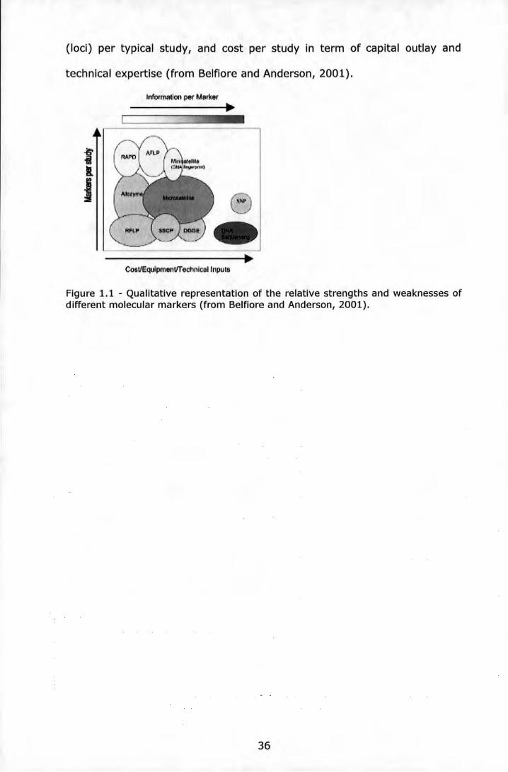
(loci) per typical study, and cost per study in term of capital outlay and

technical expertise (from Belfiore and Anderson, 2001).

lnfoonallon per M811c:er

f .. i

Cost/Equipment/Technical inputs

Figure 1.1 - Qualitative representation of the relative strengths and weaknesses of different molecular markers (from Belfiore and Anderson, 2001).

36

Chapter 2

Barnacle biology, systeli11atics and

genetics, with particu.lar

reference to

Chthamalus montagui

37

The target species of this study Is the barnacle Chthama/us montagui.

Barnacles are sessile hermaphroditic crustaceans, almost ubiquitous in

littoral communities and one of their dominant components; they are the

most characteristic organisms of the eulittoral zone throughout the world

(Stephenson and Stephenson, 1972).

This account is not intended as a review of all the literature available on the

subject, but as an introduction to some aspects and selected information

useful to better understand the target species and give an overview of the

studies carried out on barnacle population genetics, taxonomy and

phylogeny.

2.1 Taxonomy of Chthamalus montagui (Southward, 1976)

PHYLUM Crustacea

CLASS Maxillopoda

SUBCLASS Cirripedia

ORDER Thoracica

SUB-ORDER Balanomorpha

FAMILY Chthamalidae

GENUS Chthamalus (Ranzoni 1818)

SPECIES Chthamalus montagui (Southward, 1976)

Chthamalus montagui was identified as distinct species by Southward

(1976); previously it was considered a variety of Chthamalus stel/atus (Poli

38

1874). The two species, which often overlap on the shore, were

distinguished (Southward, 1976) on the basis of their different morphology

(in particular the shape of the opercular plates and the setation of the cirri)

and distribution on the shore (vertical zonation and sheltered vs. exposed

locations). The taxonomic separation was confirmed by genetic studies

employing allozymes (Dando et al., 1979), where the two species showed

different electrophoretic mobility for eight enzymes, four of which were

classified as species-specific. Further work carried out by Dando et al. in

1981 and in 1987 provided strong evidence in support of this. More

recently, Perez-Losada et al. (2008) combined DNA sequence data from 3

nuclear genes with morphological characters of different species,

representing almost all the Thoracica families, to assess tempo and mode of

barnacle evolution: they confirmed that Chthama/us stellatus and

Chthamalus montagui are two distinct species, although very close.

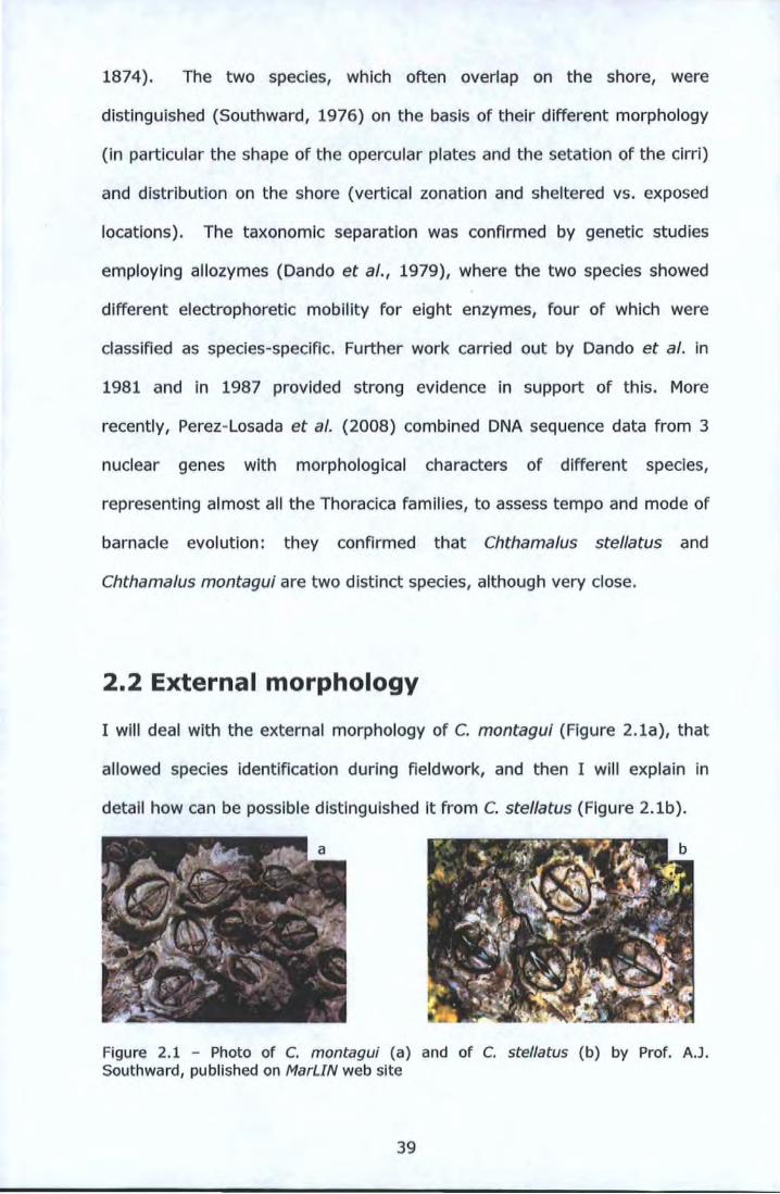
2.2 External morphology

I will deal with the external morphology of C. montagui (Figure 2.1a), that

allowed species identification during fieldwork, and then I will explain in

detail how can be possible distinguished it from C. stellatus (Figure 2.1b ).

Figure 2.1 - Photo of C. montagui (a) and of C. stellatus (b) by Prof. A.J. Southward, published on MarLIN web site

39

The shell of C. montagui, with six coarsely ridged wall plates, is brownish or

greyish, usually conical to low conical, but often elongated or even columnar

when barnacles live crowded together at the higher tidal levels. The surface

is nearly always corroded, often punctuated, and the sutures are frequently

obscure or obliterated. The opercular opening is almost always kite-shaped

or subquadrangular; the joint between the tergum and scutum crosses the

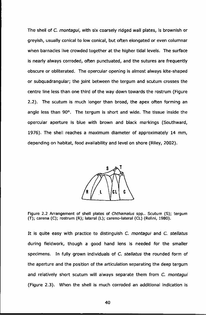
centre line less than one third of the way down towards the rostrum (Figure

2.2). The scutum is much longer than broad, the apex often forming an

angle less than 90°. The tergum is short and wide. The tissue inside the

opercular aperture is blue with brown and black markings (Southward,

1976). The shell reaches a maximum diameter of approximately 14 mm,

depending on habitat, food availability and level on shore (Riley, 2002).

Figure 2.2 Arrangement of shell plates of Chthama/us spp .. Scutum (S); tergum (T); carena (C); rostrum (R); lateral (L); careno-lateral (CL) (Rellni, 1980).

It is quite easy with practice to distinguish C. montagui and C. stellatus

during fieldwork, though a good hand lens is needed for the smaller

specimens. In fully grown individuals of C. stellatus the rounded form of

the aperture and the position of the articulation separating the deep tergum

and relatively short scutum will always separate them from C. montagui

(Figure 2.3). When the shell is much corroded an additional indication is

40

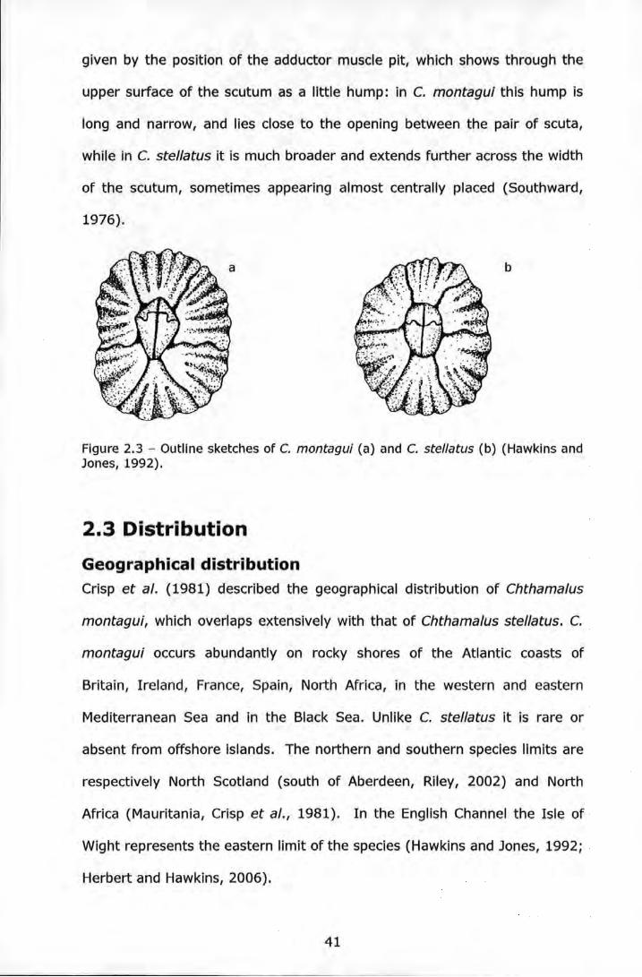
given by the position of the adductor muscle pit, which shows through the

upper surface of the scutum as a little hump: in C. montagui this hump is

long and narrow, and lies close to the opening between the pair of scuta,

while in C. stellatus it is much broader and extends further across the width

of the scutum, sometimes appearing almost centrally placed (Southward,

1976).

b

Figure 2.3 - Outline sketches of C. montagui (a) and C. stellatus (b) (Hawkins and Jones, 1992).

2.3 Distribution

Geographical distribution Crisp et al. (1981) described the geographical distribution of Chthamalus

montagui, which overlaps extensively with that of Chthamalus stellatus. C.

montagui occurs abundantly on rocky shores of the Atlantic coasts of

Britain, Ireland, France, Spain, North Africa, in the western and eastern

Mediterranean Sea and in the Black Sea. Unlike C. stellatus it is rare or

absent from offshore islands. The northern and southern species limits are

respectively North Scotland (south of Aberdeen, Riley, 2002) and North

Africa (Mauritania, Crisp et al., 1981). In the English Channel the Isle of

Wight represents the eastern limit of the species (Hawkins and Jones, 1992;

Herbert and Hawkins, 2006).

41

Horizontal and vertical distribution With regard to the vertical and horizontal distribution on the shore,

barnacles are considered the main colonizer on moderately exposed shores.

They are generally limited by physical factors towards the upper limit and

by biological ones at the lower {Connell, 1961, 1972; Pannacciulli and

Relini, 2000). Brief immersion, and consequent problems with desiccation

and poor food supply, are limiting on the high shore. Mid and low shore

barnacles, instead, are constantly competing for space (Connell, 1961;

1972; Pannacciulli and Relini, 2000) and are more subjected to predation

and to the destructive force of wave action.

The vertical and horizontal distribution of C. montagui has been extensively

investigated (Southward, 1976; Crisp et al., 1981; Burrows et al., 1992,

Pannacciulli and Relini, 2000}, and compared to that of C. stellatus. It

appears that the two species can be separated by habitat: C. montagui is

more common in sheltered, embayed and semi-estuarine sites, while C.

stellatus prevails on wave-beaten open coasts. Where they overlap, C.

montagui is dominant in the upper barnacle zone (mean high water of

spring tides, MHWS and mean high water of neap tides, MHWN), while C.

stellatus is more common lower down (mean tide level, MTL, and below)

(Pannacciulli and Relini, 2000).

The leading factors in producing the different adult distribution in the two

Chthamalus species seem to be larval dispersal, development and

settlement (Burrows et al., 1999). It has been demonstrated (Jenkins et

al., 2005) that active substratum selection by cyprlds at settlement

determines adult vertical and horizontal distribution. The role of post-

42

settlement mortality (Delany et al., 2003) and morphological characters

(Foster, 1971) can also contribute to these differences. The morphology of

the opercular plates of C. montagui is in fact believed to confer a better

resistance to desiccation stress, which allows this species to colonise the

upper shore. Moreover, it has been suggested (Burrows, 1988) that C.

montagui juveniles may require a certain amount of exposure to air in order

to consolidate and harden their shell plates, a characteristic that would

make low sites on the shore relatively unsuitable for this species. This is

confirmed also by a study carried out by Power et al. (2001), from which it

appears that C. montagui avoids wet areas at settlement and/or suffers

higher post-settlement mortality in damper sites.

2.4 Reproduction, settlement and recruitment Barnacles are hermaphroditic organisms. They generally reproduce by

cross-fertilisation by performing internal fertilisation by pseudo-copulation

(Kiepal, 1990), which imposes extremely restricted mating distances limited

by the length of the penis (in Semibalanus balanoides for instance the penis

is about two to three times the shell length, Stubbings, 1975).

In isolated conditions, when the nearest neighbour is too far away for

copulation to occur, Chthama/us species may self-fertilise (Barnes and

Crisp, 1956; Barnes and Barnes, 1958; Pannacclulli and Bishop, 2003).

This ability allows them to survive also at very low densities. However, it

has been noted that in self-fertilising individuals oviposition is delayed, and

eggs can be slightly abnormal and less viable (Barnes and Crisp, 1956;

Barnes and Barnes, 1958).

43

C. montagui is capable of breeding in its first year (Burrows, 1988}, about

9-10 months after settlement (Southward and Crisp, 1954). It seems that it

attains sexual maturity when the rostro-carinal diameter reaches 4.5 mm

(O'Riordan et al., 1992).

Barnacles then brood developing embryos within their mantle cavity before

releasing larvae into the plankton. Crisp (1950), Crisp and Davies (1955),

Le Reste (1965}, and Achituv and Barnes (1976), suggested that

Chthama/us produces several broods each year. Burrows (1988) from in

vivo laboratory experiments estimated that C. montagui embryos at 15°C

took approximately 23 days to develop completely to the stage at which

larval release occurred. Taking into account the time of development of

each brood and the proportion of time each individual spent brooding

annually, Burrows calculated that C. montagui had an average of between 1

to 2 broods per year at high shore level, 2 or 3 broods per year at mid

shore, and 2.5 to 4 broods per year at low level. A study carried out on

experimental plates in Lough Hyne, South-West Ireland (O'Riordan et al.,

1992}, Indicated that the number of broods not only differed with shore

levels, but also with year classes (older barnacles producing more broods).

Patel and Crisp (1960) from laboratory experiments observed that

Chthamalus (probably C. montagui, because specimens were collected in

Anglesey where C. stellatus is rare) would only breed at temperatures equal

to or above l5°C. According to Hines (1978), the length of the breeding

season of Chthama/us spp. is usually broadly defined by temperature and

the production of broods is limited by food availability and by the

temperature-dependent development rate of the brood in the mantle cavity.

44

Burrows et al. (1992) found that the onset of breeding by C. montagui

coincided with a rise in sea temperature above 10°C. This implies that the

beginning and the length of the breeding season should vary with latitude,

becoming progressively shorter going North.

It is possible to compare the breeding season throughout most of the range

of distribution of the species: from February to early October in the

Mediterranean (Relini, 1983), from April to early October in northern Spain

(Miyares, 1986), from April to September/October in south-western England

(Burrows et al., 1992), from June to August;September in mid-Wales

(Kendall and Bedford, 1987) and from June to August/September in south­

western Scotland (Barnes, 1972). From these studies it appears that the

main effect of latitude is on the onset of breeding: four months separated

the beginning of the season In the Mediterranean, February, and In SW

Scotland, June, whereas the cessation of breeding at all sites occurred in

September or early October.

When the embryonic development in the mantle cavity is completed,

Chthamalus releases the larvae into the plankton in the first of six naupliar

instars. A hatching substance, a prostaglandin-like compound (Clare et al.,

1982; 1985) found only in thoracican barnacles, is produced by adult tissue

only at a certain time of the year and is able to stimulate larval release.

Burrows et al. (1992) related larval release of Chthamalus spp. to blooms of

flagellates. From laboratory experiments (Burrows et al., 1999) it emerged

that larvae of C. montagui, cultured at 19°C, reached stage VI and were

ready to settle in 11 days. Development time in culture may, however, be

shorter than in natural conditions. The range of larval dispersal in barnacles

45

can vary, and is likely to be influenced by both large-scale (e.g. offshore

hydrodynamic processes, Barnes, 1956; Ralmondi, 1990) and small-scale

(e.g. local water turbulence, O'Riordan, 2004). In some cirripedes dispersal

Is estimated to be in the order of 15 to 20 km per generation (Strathmann,

1974; Crisp, 1976)

Jenkins (2005) demonstrated that the basic pattern of adult Chthamalus

distribution is established at settlement, when planktonic cyprids

Irreversibly attach to substratum. He demonstrated that cyprids actively

select the substratum and that selection is operated not only on the

horizontal gradient of wave exposure, but also over the vertical gradient of

the shore. However, post-settlement mortality in the early life of newly

settled marine invertebrates can be extremely high and have a strong

modifying effect on the characteristic adult pattern (Gosseil and Qian,

1997).

Delany et al. (2003) found that mortality after settlement was the most

significant factor in determining the distribution of C. montagui and C.

stellatus on the shores of SW Ireland. These results were confirmed also by

Power et al. (2006) who implicated differential mortality patterns in

individuals up to the age of 11 months in determining patterns of

distribution of both species. This means that the recruitment phase, that

determines which barnacles survive settlement and become part of the

adult breeding population, is very important in structuring intertidal

communities (O'Riordan et al., 2004). For this reason recruitment has been

used as a variable in modelling: a model of open populations with space­

limited recruitment was developed with direct application to C. montagui

46

(Hyder et al., 2001) and another was produced to estimate the effects of

recruitment disturbance on two interacting barnacle species, Semibalanus

balanoides and C. montagui (Svensson et al., 2006).

Timing of settlement is linked to the reproductive period and it may be

influenced by interrelated factors such as latitude, temperature and food

availability as well as shore height (O'Riordan et al., 2004). In North Italy,

for instance, recruitment of C. montagui begins in May (Pannacciulli and

Relini, 1999), which is earlier than in SW Ireland but later than in NW Spain

(O'Riordan et al., 2004), in agreement with the latitudinal pattern.

2.5 Growth and longevity Once barnacles are fixed in place, they cannot detach again (Crisp, 1955).

All species grow faster in early life and slower later; in addition chthamalids,

like others barnacles, become tubular in shape when crowded (Southward

and Crisp, 1965). The growth rate can be influenced by abiotic

(temperature, light, current, exposure to wave action, tidal level and

surface contour) and biotic (food supply, population density, competing

organisms, parasites, reproduction, size, species and age) factors (Crisp

and Bourget, 1985).

Burrows (1988) observed that rates of growth of Chthamalus montagui

were remarkably consistent over gradients of both tidal height and exposure

to wave action. Growth was found to virtually cease during the winter and

begin again the following spring (Burrows, 1988). This evidence could be

explained through the slowing effect of low temperatures on cirral activity

and consequently on food intake.

47

Photographic monitoring over a twenty year period of selected groups of

chthamalids along the Ligurian coast (Italy) showed that on relatively

sheltered shores, specimens of C. montagui survived for at least 10 years

(Pannacciulli, 1991).

2.6 Genetic approaches to taxonomy and phylogeny of barnacles

Phylogenetic analysis aims to discover the evolutionary relationships among

organisms. The level of similarity in genetic data reflects that of relatedness

among organisms, from single individuals to populations and higher

taxonomic levels (Procaccini and Maltagliati, 2004 ). Theory predicts that in

two related organisms, neutral mutations on DNA sequences accumulate

linearly since their last common ancestor (Kimura, 1983). This assumption

gives the basis for the molecular clock hypothesis (Zuckerkandl and Pauling,

1965; Arbogast et al., 2002) which, calibrated with data coming from

paleontological and morphological analyses, allows the dating of

phylogenetic relationships among organisms.

Genetic analyses have been used extensively to investigate various aspects

of barnacle taxonomy (Dando, 1987). In particular, some species

complexes of the genus Chthama/us were resolved using allozyme

electrophoresis. Dando et al. (1979) compared the electrophoretic mobility

of thirteen enzymes in Chthama/us stellatus and Chthama/us montagui.

They showed that the two species differed entirely for the mobility of eight

enzymes and had species-specific alleles for a further four. The separation

of the two species, initially based on morphological and ecological

48

characters (Southward, 1976), found further support in the genetic studies.

Power et al. (1999) using mtDNA (COl and COII)-RFLP analysis from

selected adults and cyprids of C. stellatus and C. montagui, showed clear

differentiation between the two species and confirmed the use of size to

distinguish cyprids of the two species.

Recently, Perez-Losada et at (2008) combined morphological data with DNA

sequencing from 3 nuclear genes (185, 285 and H3) for almost all families

of Thoracica, to assess the tempo and mode of barnacle evolution. They

rearranged thoracican classification based on estimated phylogenetic

relationships.

Tsang et al. (2007) elucidated the taxonomic status of the acorn barnacles

Tetraclita japonica and Tetraclita formosana using mtDNA sequencing (COl

and Control Region) combined with morphological data.

A phylogenetic study of chthamaloids (Cirripedia; Thoracica;

Chthamaloidea) was carried out by Fisher et al. in 2004. Partial sequences

of the mitochondrial genes COl and 165 rDNA were analysed in eight taxa

of chthamaloid barnacles. Phylograms based on 165 rDNA were generally

consistent with the traditional phylogeny of the Chthamaloldea. It is

interesting to highlight that slight differences in 165 sequence diversity

between Chthamalus stellatus from Plymouth (UK) and Israel were shown;

these results are in agreement with the trend in genetic diversity, in terms

of allozyme heterozygosity and allelic diversity, between Mediterranean and

Atlantic populations found by Pannacciulli et al. (1997a).

49

The analyses of COl by Fisher et al. (2004) resulted in phylogenetically

meaningless trees, with most branches stemming from the common basal

node. It was suggested that in the chthamaloids, at least at inter-generic

level, polymorphism in the COl gene was saturated due to the fast rate of

nucleotide substitutions that did not affect the encoded protein, and thus

could not resolve the relationships within this superfamily.

2.6.1 Markers for taxonomy and phylogeny of barnacles

To summarize, DNA sequencing has been the preferred technique used in

phylogenetic studies. The DNA regions most examined in barnacles were:

COl, COil, Control Region, 125 and 165 for the mtDNA (Power et al. 1999;

Fisher et al., 2004; 5imon-Biecher et al., 2007; Tsang et al., 2007); 185,

285, H3 in the nDNA (Perez-Losada et al., 2008). Earlier, allozymes were

employed for taxonomical studies (Dando et al., 1979; Dando, 1987).

50

2. 7 Population genetics of barnacles Studies of genetic variability at population level allow the understanding of

genetic relationships among individuals within a population and between

populations over time and space (Procaccini and Maltagliati, 2004). I

focused my attention on population genetic studies of barnacles and on the

markers employed to assess them.

Many projects have focused on population genetics: they studied "how

Mendel's laws and other genetic principles can be applied to entire

populations" (Hartl et al., 1989).

A population is a group of organisms of the same species that is relatively

isolated from other such groups; Individuals of the same population

frequently interbreed but individuals in different populations rarely or never

do. Genetic differences can thus accumulate between populations, and can

be characterised in terms of allele or haplotype frequencies. The main

evolutionary forces that can cause divergence in allele/haplotype

frequencies are selection, genetic drift and mutation. The first of these can

be related to habitat characteristics, and the second to effective population

size. Gene flow between populations will reduce differentiation and will

relate to migration rate and to species dispersal capabilities (Carvalho,

1998; Procaccini and Maltagliati, 2004). A general association exists thus

between mode of dispersal and the degree of genetic differentiation among

populations (Bohonak, 1999).

In marine systems, larval dispersal ability has often been hypothesized as

the primary determinant of population genetic structure (Burton, 1983;

51

Hedgecock, 1986; Palumbi, 1995). As Todd (1998) argued, analyses of

population genetic heterogeneity provide an indirect mean of assessing the

scale of realized larval dispersal and whether or not populations are

demographically open or closed over a given range.

For species with a long-lived planktonic larva, such as barnacles, the

population structure on the large scale (10 to 100 km) is the product of the

interaction between selection and present or historical patterns of gene flow

(Hilbish, 1985; Reeb and Avlse, 1990; Karl and Avise, 1992; Holm and

Bourget, 1994).

A study of asymmetric migration events across the marine biogeographic

boundary of Point Conception (California, USA) was carried out by Wares et

al. (2001). Patterns of genetic diversity were investigated, using

mitochondrial DNA (mtDNA) Cytochrome Oxidase I (COl) sequence data, for

the barnacles Balanus glandula and Chthamalus fissus, to test the

hypothesis that gene flow in a species with a pelagic larva may be limited

by temperature gradients and ocean currents that can affect species

distributions by erecting barriers to dispersal of planktonic larvae. The

tested hypothesis was confirmed by the results of the cladistic analyses.

Many studies have investigated phylogeographic relationships among

populations. A well-defined pattern of genetic variation, using mtDNA

sequence data, was found in the goose barnacle Polllcipes pol/icipes within

its distribution range in the North East Atlantic (Quinteiro et al., 2007);

coastal currents and mesoscale hydrodynamics were identified as the main

factors determining the population genetic structure.

52

York et al. (2008), using a combined approach of mtDNA sequence and

microsatellite data, examined both historic and contemporary processes

that shaped the biogeography of the barnacle Catomerus polymerus in

Australia. The mtDNA data provided information regarding the history and

origin of the current populations, showing a deep phylogeographical split

within southern Australia, strongly correlated with a phylogeographical

barrier In the Bass Strait region: the emergence of the Bassi an Isthmus,

during glacial periods, promoted allopatric speciation in the southern

Australian marine environment. The microsatellite data, instead, gave the

opportunity to examine the species' contemporary structure, indicating

significant genetic divergence between the eastern and western lineages of

Catomerus polymerus and suggesting the presence of four subregions.

A deep genetic dine between southern (from about Monterey Bay

southward) and northern (from northern California through Alaska)

populations of the barnacle Balanus glandula was described by Wares et al.

(2005). COl mtDNA sequence data, combined with coalescence estimators

of the separation time for these two regions, suggested that a late

Pleistocene event, more than 100.000 years ago, could have been

responsible for the initial separation that was later maintained by

oceanographic mechanisms or natural selection.

Dufresne et al. {2002) compared patterns of genetic structure at potentially

selected loci (two allozymes) and neutral molecular markers (six

microsatellltes) in the barnacle Semibalanus balanoides from the Gulf of St.

Lawrence to assess the possible role of selection and gene flow in the

53

genetic structuring of barnacle populations on a large geographical scale.

Results supported the hypothesis that the broad scale pattern of allozyme

allelic shifts is maintained by selection. Other studies confirm that selection

can be strictly related to habitat characteristics (Procaccini and Maltagllati,

2004).

In Semibalanus balanoides a close relationship between genotype

frequencies at the Mannose-6-Phospate Isomerase (MPI) locus and the

degree of physical stress experienced by barnacles in distinct habitat types

on the shore has been well documented (Schmidt and Rand, 1999).

Furthermore, it was demonstrated that in S. balanoides selection acts over

a short time interval within the life cycle, occurring between metamorphosis

and early juvenile stages (Schmidt and Rand, 2001).

Population genetic studies have also been carried out to investigate the

origins and sources of barnacle invasions in geographical areas outside the

species' natural range.

Zardus et al. (2005} investigated the origins and incursions of the Atlantic

barnacle Chthamalus proteus in the Pacific. They characterized genetic

variation in native and introduced populations, by using direct sequencing of

mtDNA (COl}, and tried to match regions to determine if there were

multiple geographical sources and introduction points for this barnacle.

Sources of invasion of the north eastern Pacific barnacle Balanus glandula In

Japan and Argentina were examined by Geller et al. (2008} by comparing

COl and EF1 (Nuclear Elongation factor 1 alpha) genotypes of native vs.

54

introduced populations. The same markers were used by Simon-Biecher et

al. (2008) to trace the origin of this barnacle species along the south

western African shores.

other population genetic studies were carried out to assess the effects of

pollution on organism genotypes. Patarnello et al. (1991) investigated, by

electrophoretic analysis of the polymorphic loci MPI, PGI and PGM, the

effects of thermal and chemical pollution on the genetic structure of Balanus

amphitrite populations from Venice lagoon. Data confirmed that selection is

mainly attributable to heavy metals.

Finally, focussing the attention on our target species, Chthamalus montagui,

it has to be mention that the existence of Atlantic and Mediterranean forms

of Chthamalus montagui was established by analyzing the polymorphism of

15 allozymes (Dando and Southward, 1981). The results of this study were

confirmed by Pannacciulli (1995) and Pannacciulll et al. (1997a), who

investigated the population genetic structure of Chthamalus montagui and

Chthamalus stellatus over their North-East Atlantic and Mediterranean

distribution, using six and four allozymes respectively. Electrophoretic data

were analysed using a technique based on Wright's F-statistics (Pannacciulli

et al., 1997b). In each species a single locus showed marked differentiation

between Atlantic and Mediterranean localities.

2.7.1 Markers for population genetics of barnacles

Many different markers were applied in the population genetic studies

mentioned above.

55

Allozymes, such as MPI, PGI, PGM, GOT, PEP etc., have been employed

extensively in studies of geographical population differentiation and gene­

flow {under the general assumption of neutrality) and taxonomy {Dando

and Southward, 1981; Patarnello, 1991; Pannacciulli et al., 1997a; Schmidt

and Rand, 1999 and 2001).

The most common DNA-based markers utilized were microsatellites

{Dufresne et al., 2002; York et al., 2008) and the COl locus of the mtDNA

{Wares et al., 2005; Zardus et al., 2005; Quinteiro et al., 2007; Geller et

al., 2008; Simon-Biecher et al., 2008). MtDNA is considered to be a good

marker for the examination of historical patterns, while the rapid rate of

mutation of microsatellites make them ideal for investigating contemporary

population structure and the ecological factors responsible {York et al.,

2008). In 2001 Chu et al., explored the possibility of using the first internal

transcribed spacer {ITS-1) of ribosomal DNA as a molecular marker for

studying inter- and intra-specific genetic variation in crustaceans. The

outcome of this work showed that ITS-1 is highly divergent among different

crustaceans and could be an appropriate marker for molecular systematics

at species and population level.

The role of selection in maintaining genetic polymorphisms at allozyme loci

has been reported in many marine species. It is not clear whether the

allozyme loci themselves or other loci, in close linkage with allozymes, are

the targets of selection {Mitton, 1998). Dufresne et al. {2002) suggested

comparing patterns of genetic structure at putatively selected loci with

those obtained from more neutral markers such as mtDNA and/or

microsatellites. Gene flow and drift should equally affect all neutral loci,

56

whereas selection is more likely to be locus-specific (Lewontin and

Krakauer, 1973). When they are not linked to selected genes, microsatellite

markers are potentially good markers for analyses assuming that they are

located mostly in non-coding regions (Queller et al., 1993). Nevertheless,

Dufresne et al. (2002) indicated that microsatellites may not always behave

in a neutral way and have to be used cautiously, especially when evidence

for genetic structuring relies on only a few assayed loci without a priori

knowledge or a comparison with potentially selected loci. In response to

these considerations, many studies have been carried out using a multi­

marker approach (Schmidt and Rand, 1999, 2001; Rand et al., 2001;

Dufresne et al., 2002; Simon-Biecher et al.,2008; York et al., 2008).

Isolation and characterization of microsatellite markers in the acorn

barnacle Semibalanus balanoides were carried out by Dufresne et al.

(1999). Later, seven highly polymorphic microsatellite markers were

isolated from Chthamalus montagui by Pannacciulli et al. (2005). This work

was very useful for this PhD, as the markers found direct application in the

population genetic studies of this project.

57

I

r·. ~.

. ;'::-­-'

. ,·

• .• 1.

-. ' ' ~ . . ~ '

' .. ..

'·

.~~c;~til~pt~r 31 '

• • '·- - I "I ,, -- • -

·M 1i~te·ruals '·CI_illd:· 1m·et:lr.od·s:

'58

.___:___ ·-

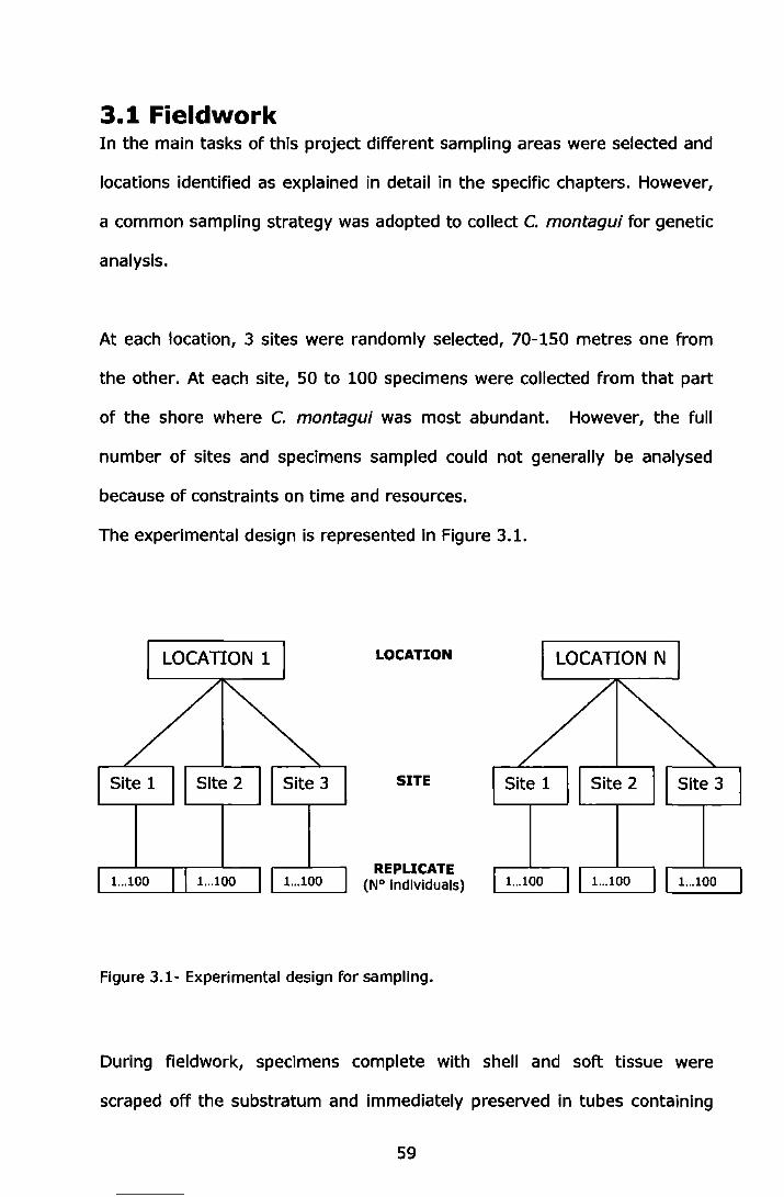
3.1 Fieldwork In the main tasks of this project different sampling areas were selected and

locations identified as explained in detail in the specific chapters. However,

a common sampling strategy was adopted to collect C. montagui for genetic

analysis.

At each location, 3 sites were randomly selected, 70-150 metres one from

the other. At each site, 50 to 100 specimens were collected from that part

of the shore where C. montagui was most abundant. However, the full

number of sites and specimens sampled could not generally be analysed

because of constraints on time and resources.

The experimental design is represented in Figure 3.1.

LOCATION

SITE

REPUCATE (N° Individuals)

Figure 3.1- Experimental design for sampling.

During fieldwork, specimens complete with shell and soft tissue were

scraped off the substratum and immediately preserved in tubes containing

59

ethanol (95% EtOH). Several individuals from the same site were stored in

the same tube, which was labelled with the name of the location, site and

date of sampling. Upon arrival in the laboratory, samples were kept at -

20°C until dissection and genetic analysis.

3.2 Laboratory work

3.2.1 DNA extraction

DNA was extracted from the soft tissue of each individual. The whole animal

was pulled out with a pair of forceps from the bottom part of the shell, the

side that attaches to the substratum, making sure not to include gonads or

egg masses that are often present in the mantle cavity.

The following techniques for DNA extraction were tested to find the most

suitable one for C. montagui: Phenol-Chloroform standard protocol

(Sambrook et al., 1989), DNA extraction kits (Qiagen DNAeasy Extraction

Kit and Gentra PureGene), guanidinium thiocyanate-phenol-chloroform

extraction (Chomczynski and Sacchi, 1987) and Salting-Out extraction

(Aijanabi and Martinez, 1997).

The quantity and quality of the extracted DNA was assessed by Tris Borate

EDTA (TBE, recipe in Appendix 3.1) agarose gel electrophoresis (1%

agarose) and visualised by fluorescence after staining with Ethidium

Bromide (electrophoretic run of about 30 min at 100 mA). DNA

concentration was roughly estimated by comparing the intensity of the DNA

bands with those of a 100 bp ladder (New England Biolabs) and appropriate

dilutions were established. The quality and dilution of the extracted DNA

60

was further tested by verifying the outcome of the PCR amplification

employing microsatelllte markers.

After screening, the Salting-Out extraction method (modified after Aljanabi

and Martinez, 1997) was selected as the most suitable for Chthama/us

montagui specimens as it gave very good results, lt was cheap and safe to

handle.

DNA extractions were carried out following the protocol listed in Appendix

3.2. DNA was extracted from 32 individuals at each site investigated in the

project.

61

3.2.2 Microsatellite markers

Microsatellites were employed as molecular markers for the population

genetic studies. The different tasks of the project employed a variable

number of microsatellite loci, three to six, to detect genetic variation. These

microsatellites were developped specifically for Chthamalus montagui by

Pannacciulli et al. (2005) and proved to be highly polymorphic. Details of

the six loci employed are reported in Table 3.1.

Table 3.1 - Mlcrosatellite loci with core repeats, primer sequences, optimal annealing temperature (TA), GeneBank accession number (from Pannacciulli et al., 2005).

Locus Repeat in clone Primer sequence (5'-3') TA GeneBank

(OC) no

CM2/15 {CAho F: GTACGAGTGGCTTCGCTTG 55 AY847005

R: ATGTTTGCCATGATGTAGGC CM 4/5 (AChgTCGC(ACb F:TGCTCACAAACCATGACTGG 45

AY847007 R:ACGCTAAAGAGGCACATTCG CM 5/23 (AC)J(GC)s(AC)36 F: CGCTCTCCCTCAAAACTCC 50

AY847010 R:ACCGTGAGTAACAGCATACG

CM 4/3 (GTh~T{GTh F:TGCTCACAAACCATGACTGG

50 R: ACGCTAAAGAGGCACATTCG AY847006

CM 5/18 (TGhTA{TGhTT{TGhJ F:TGATTGTCGGTTTAGCAACG 45 AY847009 R:TCACTGTGAAGTCTGACATGG

CM 9/11 {GT)13AG{GTho F:ACAAGCCTTCGCCTCATTCC

60 R:CCCACTTATCAACGCTTCTGC AY847012

3.2.3 PCR reaction, DNA sequencing and fragment analysis

DNA amplification was performed by Polymerase Chain Reaction (PCR)

using two different Master Mixes, depending on the TAQ Polymerase

available. The two Master Mixes differed as one employed Qiagen HotStar

Taq DNA Polymerase (Table 3.2), Q solution and appropriate buffer (with

62

DMSO etc.), while the other used Slgma JumpStart Taq DNA Polymerase

(Table 3.3).

Table 3.2: Master Mix employing Qiagen HotStar Taq DNA Polymerase and Q solution.

Initial ~mount for sample Final

concentration (IJI) concentration

Water 6.2

Buffer* 10 X 1 1X

Q solution 5X 0.7 0.35X

dNTPs 2.5mM 0.8 0.2mM

Primer F 100 IJM 0.1 11JM Primer R 100 IJM 0.1 11JM

DNA 25-50 ng/IJI 1 2.5-5 ng/IJI

Hot StarTaq 5 U/IJI 0.05 0.025 U/IJI

Final Volume 10 IJI

*Buffer contained 15 mM MgCI2

Table 3.3: Master Mix employing JumpStart Taq DNA Polymerase (Sigma).

Initial Amount for sample Final

Concentration (IJI) Concentration

Water 6.9

Buffer* 10 X 1 1X

dNTPs 2.5 mM 0.8 0.2mM

Primer F 100 IJM 0.1 11JM Primer R 100 IJM 0.1 11JM

DNA 25-50 ng/IJI 1 2.5-5 ng/IJI

Jump Star Taq 2.5 U/IJI 0.1 0.025 U/IJI

Final Volume 10 IJI

*Buffer contained 15 mM MgCI2

The amplification, carried out on an ABI 3700 thermocycler, consisted of an

initial denaturation at 95°C for 15 min, 33 cycles of denaturation at 95°C

for 30 sec, annealing for 30 sec at a locus-specific temperature and

extension at 72°C for 30 sec, followed by a final step of 72°C for 10 min.

63

Details of the primer pairs, including annealing temperatures, are listed in

Table 3.1.

To allow later screening of the PCR products on a sequencer, one member

of each primer pair employed in the PCR reaction was end-labelled with a

fluorophore (6-FAM, HEX or NED, Applied Biosystems). In detail: CM 2/15

and CM 5/18 primers were labelled with NED (yellow); CM 4/5 and CM 4/3

with HEX (green) and CM 5/23 and CM 9/11 with 6-FAM (blue). The choice

of fluorophore for each primer was made on the basis of the expected

amplified product size. In fact, pairs of primers that delivered products of

similar sizes were labelled differently. Pairs of primers that, instead,

produced products of clearly different sizes could be labelled with the same

colour and potentially be run in the same sequencing gel, while still allowing

separate pattern interpretation.

Prior to the sequencer run, PCR products were checked and visualised on

TBE agarose gel (1.5 %) after staining with Ethidium Bromide using a 500

bp ladder (New England Biolabs) as reference (electrophoretic run of about

1.30 h at 100 mA).

PCR products were then diluted (from 1:20 up to 1: 70) and, for each

individual, products from the following sets of primers, marked with

different fluorophores, were combined in one of the 96 wells of a

sequencing plate: CM 2/15 (NED), CM 4/5 (HEX) plus CM 5/23 (6-FAM);

and CM 5/18 (NED), CM 4/3 (HEX) plus CM 9/11 (6-FAM). This strategy

was adopted to make the best use of the 4 capillary system of the 3100

Avant ABI capillary DNA sequencer employed in this study. In this way it

64

was possible to get information on three different microsatellites in the

same run. All runs also included a reference standard, the 500 bp ROX

ladder (Applied Blosystems). Fragment lengths were detected and analysed

using GENE Scan software (ABI). Single peaks were measured directly

while, when stutter bands were present, only the highest peak was taken

into account. For each locus, all data resulting from the analysis of all

individuals in the study and from several sequenclng runs were plotted on a

size-frequency graph, recording values to the first decimal point. This

allowed grouping of data that, despite minor differences in size, represented

a single allele. In this way allele sizes were established at each locus. When

an allele was represented a single time or only a very few times, the

sequencing gel was checked again to confirm the existence of the allele.

3.3 Genetic data analysis Genetic data analysis was carried out using software packages specific for

population genetic studies. Table 3.4 lists the main software employed.

Table 3.4:Main software employed in the genetic data analysis.

Software Version Reference GENETIX 4.03 Belkhir et al., 1996 ARLEQUIN 3.1 Excoffier et al., 2005 GENEPOP 4.0 Rousset, 2008 FSTAT 2.9.3 Goudet, 2001 RSTCAL 3.12 Goodman, 1997 MICROSAT 1.5d Minch et al., 1996 PHYLIP 3.68 Felsestein, 2005 HIERFSTAT 0.04-3 Goudet, 2005 STRUCTURE 2 Pritchard et al., 2000 STATISTICA 6.1 Statsoft Inc., 1997

Below is a brief overview (following Procaccini and Maltagliati, 2004) of the

main parameters calculated for genetic data analysis.

65

Fit to Hardy-Weinberg equilibrium The Hardy-Weinberg law (Hardy, 1908; Weinberg, 1908; Stern, 1943)

predicts that under stable conditions after a generation of random mating,

genotype frequencies throughout a population at a specified gene reach a

specific equilibrium value. This value can be defined by the square of the

allelic frequencies.

If we consider that there are only two alleles (A and a) with allele

frequencies respectively of p and q, the three possible genotypes are AA,

Aa, aa and their frequency follows the binomial expansion of:

The frequency of the genotype AA will be p2 , Aa will be 2pq, and aa will be

q2 ; populations are considered to be in Hardy-Weinberg equilibrium when

homozygotes and heterozygotes are in these proportions. The assumptions

for equilibrium are that the population is idealized: infinite in size to

eliminate genetic drift, sexually reproducing, randomly mating and diploid.

Moreover, gene pool frequencies will remain unchanged if no mechanisms

that can cause evolution are acting on the population: in other words

mutation, selection and migration should not occur. Hence, a large,

randomly-mating, non-evolving population should follow the Hardy-

Weinberg law (Ayala, 1982).

Heterozygosity Heterozygosity is often one of the first parameters calculated from a data

set as it can tell a great deal about structure and even history of a

population. For instance, very low heterozygosity values can indicate severe

effects of small population sizes (population bottlenecks or metapopulation

dynamics that severely reduce the level of genetic variation compared to

what is expected). In particular the expected heterozygosity, HE, or gene

66

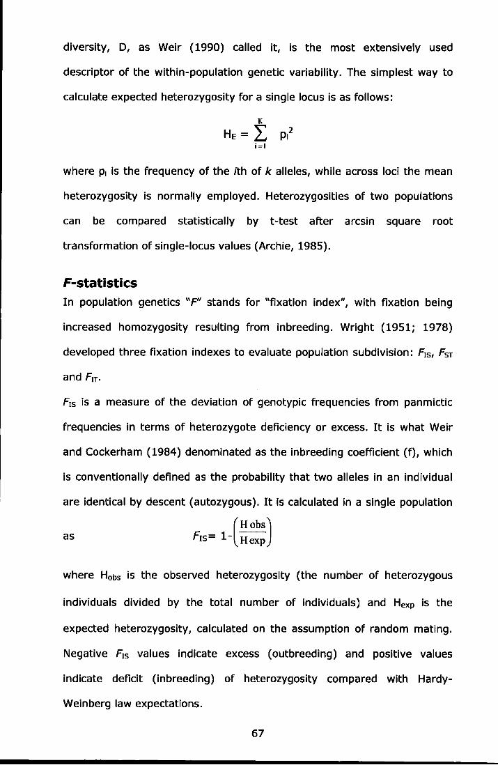
diversity, D, as Weir (1990) called it, is the most extensively used

descriptor of the within-population genetic variability. The simplest way to

calculate expected heterozygosity for a single locus is as follows:

where P1 Is the frequency of the ith of k alleles, while across loci the mean

heterozygosity is normally employed. Heterozygosities of two populations

can be compared statistically by t-test after arcsin square root

transformation of single-locus values (Archie, 1985).

F-statistics In population genetics "P' stands for "fixation index", with fixation being

increased homozygosity resulting from inbreeding. Wright (1951; 1978)

developed three fixation indexes to evaluate population subdivision: F1s, FsT

and Frr.

F1s is a measure of the deviation of genotypic frequencies from panmictic

frequencies in terms of heterozygote deficiency or excess. It is what Weir

and Cockerham (1984) denominated as the inbreeding coefficient (f), which

is conventionally defined as the probability that two alleles in an individual

are identical by descent (autozygous). It is calculated in a single population

as

where Hobs is the observed heterozygosity (the number of heterozygous

individuals divided by the total number of individuals) and Hexp is the

expected heterozygosity, calculated on the assumption of random mating.

Negative F1s values indicate excess (outbreeding) and positive values

indicate deficit (inbreeding) of heterozygosity compared with Hardy-

Weinberg law expectations.

67

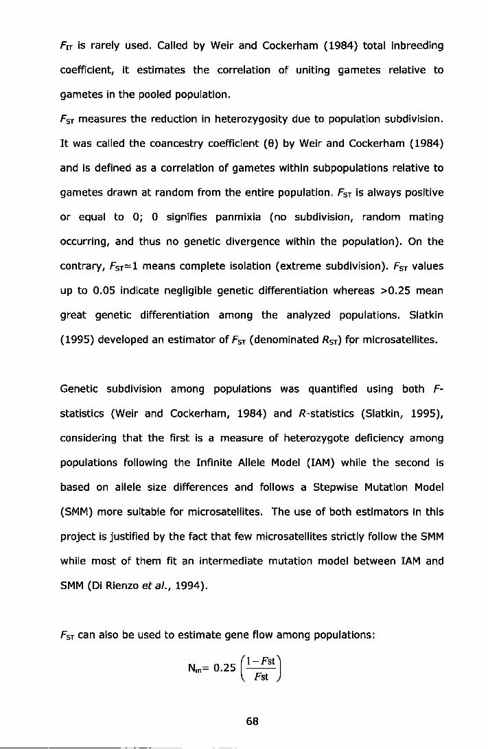
Frr is rarely used. Called by Weir and Cockerham (1984) total inbreeding

coefficient, it estimates the correlation of uniting gametes relative to

gametes in the pooled population.

fsT measures the reduction in heterozygosity due to population subdivision.

It was called the coancestry coefficient (8) by Weir and Cockerham (1984)

and is defined as a correlation of gametes within subpopulations relative to

gametes drawn at random from the entire population. fsT is always positive

or equal to 0; 0 signifies panmixia (no subdivision, random mating

occurring, and thus no genetic divergence within the population). On the

contrary, FST=1 means complete isolation (extreme subdivision). FST values

up to 0.05 indicate negligible genetic differentiation whereas >0.25 mean

great genetic differentiation among the analyzed populations. Slatkin

{1995) developed an estimator of fsT (denominated RST) for microsatellites.

Genetic subdivision among populations was quantified using both F-

statistics (Weir and Cockerham, 1984) and R-statistics {Siatkin, 1995),

considering that the first is a measure of heterozygote deficiency among

populations following the Infinite Allele Model (lAM) while the second is

based on allele size differences and follows a Stepwise Mutation Model

(SMM) more suitable for microsatellites. The use of both estimators in this

project is justified by the fact that few microsatellites strictly follow the SMM

while most of them fit an intermediate mutation model between lAM and

SMM (Di Rienzo et al., 1994).

fsT can also be used to estimate gene flow among populations:

Nm= 0.25 (1- Fst) Fst

68

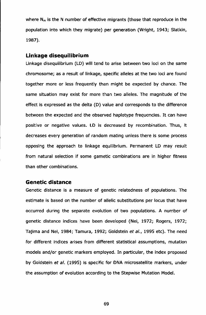
where Nm is the N number of effective migrants (those that reproduce in the

population into which they migrate) per generation (Wright, 1943; Slatkin,

1987).

Linkage disequilibrium Linkage disequilibrium (LD) will tend to arise between two loci on the same

chromosome; as a result of linkage, specific alleles at the two loci are found

together more or less frequently than might be expected by chance. The

same situation may exist for more than two alleles. The magnitude of the

effect is expressed as the delta (D) value and corresponds to the difference

between the expected and the observed haplotype frequencies. It can have

positive or negative values. LD is decreased by recombination. Thus, it

decreases every generation of random mating unless there is some process

opposing the approach to linkage equilibrium. Permanent LD may result

from natural selection if some gametic combinations are in higher fitness

than other combinations.

Genetic distance Genetic distance is a measure of genetic reiatedness of populations. The

estimate is based on the number of allelic substitutions per locus that have

occurred during the separate evolution of two populations. A number of

genetic distance indices have been developed (Nei, 1972; Rogers, 1972;

Tajima and Nei, 1984; Tamura, 1992; Goldstein et al., 1995 etc). The need

for different indices arises from different statistical assumptions, mutation

models and/or genetic markers employed. In particular, the index proposed

by Goldstein et al. (1995) is specific for DNA microsatellite markers, under

the assumption of evolution according to the Stepwise Mutation Model.

69

Genetic distance-based methods of phylogenetic tree inference There are numerous variations of genetic distance-based methods (UPGMA,

Neighbor-joining, Fitch-Margoliash, etc.) which all rely on generating a

matrix of pairwise differences (or distances) or similarities. In its simplest

form, one could merely count the number of differences between all

possible pairs of sequences, and then use a clustering algorithm to cluster

together those sequences with the smallest number of differences.

Bootstrapping The bootstrap (Efron, 1979) is a general re-sampling technique for

estimating the distribution of statistics. The basic idea behind bootstrap

concerns the estimation of variance in an unknown distribution from which

data are re-sampled randomly. The bootstrapping procedure constructs a

number of arbitrary data sets. Re-sampling is performed "r" times (usually

1,000<r< 100,000) obtaining r estimations of the parameter that is

calculated. One of the applications of bootstrap in population genetics is the

estimation of confidence intervals for parameters such as F1s, Frr, Fsr, Nm,

etc. Another important application is the assessment of robustness of the

nodes of phylogeographic trees. In this approach, instead of a set of values

x1, x2 ... , xn, the starting point is a table of populations scored for a set of

characters (e.g. type of alleles, allelic frequencies). The procedure consists

of bootstrapping across characters, hence re-sampling and replacing

characters of the original data matrix at random, and calculating the tree

for each re-sampling. Bootstrap values annotated on the nodes of the tree

representing the total data set indicate the percentage of re-samplings in

which a given node has been generated.

70

Jackknifing The function of jackknifing is similar to bootstrapping, to generate a

distribution for statistics that permits the calculation of dispersion

estimates. The distribution is generated by re-sampling the original data set

with replacement to produce "pseudoreplicate" data sets; jackknifing

produces a limited number of pseudoreplicates, each containing all but one

of the original data elements. For a data set with 20 elements, 20

pseudoreplicate data sets will be generated, each lacking a different data

element.

Mantel's test The Mantel's test (Mantel, 1967) assesses the probability that two distance

matrices are independent from one another; it has been used to detect

isolation by distance among populations. In this approach the matrices of

the geographic distances and of genetic distances among populations are

compared.

Analysis of molecular variance Analysis of molecular variance (AMOVA, Excoffier et al., 1992) allows the

partitioning of molecular variation into hierarchical levels, for which the

significance of departures from the null hypothesis can be tested. AMOVA is

based on the proposal that the sum of squares in conventional analysis of

variance can be expressed as the sum of squared distances between pairs

of phenotypes (Hoeffding, 1948).

A hierarchical AMOVA partitions the total variance into covariance

components due to intra-individual, inter-individual, and/or inter-population

differences.

71

Bayesian clustering analysis The Bayeslan clustering method developed by Pritchard et al., 2000 was

used to Infer population structure, This approach differs from the analyses

described above as individuals are assigned to clusters (p-opulations) based

exClusively on their individual genotypes. Individual genotypes are

assigned to clusters on a probablllstic basis, which Identifies the affinities of

individual multilocus genotypes to genetic populations and aims to delineate

populations that are, as far as possible, in hiardy-Weinberg and linkage

equilibrium (Evanno et al., 2005~.

The details of the statistical data analysis carried out in the different tasks

ofthe project are explained in the following specific chapters.

72

Chapter 4

The influence of habitat corridors

generated by artificial substrates

on the genetic pattern of

Chthamalus montagui

73

same time, in the introduction of hard-bottom habitats with the occurrence

of new species in the area (Airoldi et al., 2005).

These changes in species composition, abundance and diversity represent a

substantial modification of the characteristics of the native biotope

(Angermeier, 1994) and can have important consequences in the

functioning of the coastal ecosystem (Loreau et al., 2001).

In fact, the system of artificial structures provides novel habitats for the

colonization of marine organisms and often supports the invasion of non­

indigenous species (Holloway and Keough 2002; Lambert and Lambert

2003; Thornber et al. 2004). Bulleri and Airoldi (2005), for instance,

studied the distribution and the dynamics of the spread of a non-indigenous

green alga, Codium fragile sp. tomentosoides, at a variety of spatial scales

on the breakwaters along the north-east Adriatic coast. They identified

some of the mechanisms of its successful establishment; experiments

indicated that the sheltered habitat on the landward side of the breakwaters

offered particularly favourable conditions for the growth of this macroalga,

promoting its spread along formerly exposed sandy shores. Therefore,

these structures offer suitable habitat for species living on hard substrata

(among them also invaders) and enhance their further spread, by

functioning as "corridors" across areas of unsuitable habitat (e.g. across

sandy or muddy areas). Thus artificial substrates may act as stepping

stones, disrupting natural barriers and facilitating the dispersal of a species

across habitats and regions that naturally would be poorly connected

(Abbiati, 2003).

75

4.1 Introduction and specific aims In the last centuries, humans have become a major force able to change

landscapes at a variety of spatial and temporal scales (Ayensu et al., 1999).

This is also true for coastal areas, where the population is steadily

increasing and the worldwide trend is towards urbanisation (Gray, 1997).

Artificial structures, such as pier pilings, floating pontoons, breakwaters and

seawalls have become common features of landscape in shallow coastal

waters of urbanised areas and in some areas they have replaced

considerable portions of natural habitats (Chapman and Bulleri, 2003).

Along most European coasts hard defence structures to protect coastal

areas, have proliferated leading to severe alteration of the coast. Under

future global climate change scenarios, the intensity of storms and height of

sea level are predicted to increase, augmenting the need for introducing

these coastal defence structures (Airoldi et al., 2005). In some regions, for

instance the Italian Adriatic coast, they already cover over half of the

shoreline, resulting in dramatic changes to the coastal landscape and

environment (Bacchiocchi and Airoldi, 2003).

The type and magnitude of the changes induced by these structures can

vary considerably depending on the environmental setting where they are

built. However, the construction of these hard defence structures in areas

dominated by sandy shores always results in a local loss of soft-bottom

habitats with the associated assemblages of animals and plants and, at the

74

same time, in the introduction of hard-bottom habitats with the occurrence

of new species in the area (Airoldi et al., 2005).

These changes in species composition, abundance and diversity represent a

substantial modification of the characteristics of the native biotope

(Angermeier, 1994) and can have important consequences in the

functioning of the coastal ecosystem (Loreau et al., 2001).

In fact, the system of artificial structures provides novel habitats for the

colonization of marine organisms and often supports the invasion of non­

indigenous species (Holloway and Keough 2002; Lambert and Lambert

2003; Thornber et al. 2004 ). Bulleri and Airoldi (2005), for instance,

studied the distribution and the dynamics of the spread of a non-indigenous

green alga, Codium fragile sp. tomentosoides, at a variety of spatial scales

on the breakwaters along the north-east Adriatic coast. They identified

some of the mechanisms of its successful establishment; experiments

indicated that the sheltered habitat on the landward side of the breakwaters

offered particularly favourable conditions for the growth of this macroalga,

promoting its spread along formerly exposed sandy shores. Therefore,

these structures offer suitable habitat for species living on hard substrata

(among them also invaders) and enhance their further spread, by

functioning as "corridors" across areas of unsuitable habitat (e.g. across

sandy or muddy areas). Thus artificial substrates may act as stepping

stones, disrupting natural barriers and facilitating the dispersal of a species

across habitats and regions that naturally would be poorly connected

(Abbiati, 2003).

75

Increased connectivity among populations will increase the gene flow within

a species (Palumbi, 2003). Coastal defence structures could have the

reverse effect compared to fragmentation, by acting as "corridors" to

facilitate gene flow among previously isolated populations. Increasing gene

flow can have a homogenizing effect, reducing local adaptation within a

species and thus, on a larger timescale, decreasing the evolution of new

species (Palumbi, 2003).

The relative dispersal ability of a species should be considered when

investigating the connectivity among populations in the marine environment

and the function of habitat corridors on its movement and colonization

patterns (Micheli and Peterson, 1999; Darcy, 2005).

Moreover, the study of habitat "corridors", which have been well

documented theoretically and empirically in terrestrial systems (Henein and

Merriam 1990; Merriam and Lanoue 1990; Haddad 1999; Tewksbury et al.

2002), is relatively new to marine environments. Some studies revealed

that the definition of corridor has to be expanded in the marine domain,

where not only stationary habitat patches but also rafting on living pelagic

organisms and drifting on inanimate objects can act as a corridor (Carlton,

1985; Irlandi and Crawford, 1997; Micheli and Peterson, 1999; Goodsell

and Connel, 2002; Darcy, 2005). Brooks and Bell (2001), for example,

demonstrated that drift algae provide a mobile corridor to epiphytic

amphipods for dispersal within a seagrass landscape.

Naturally, effectiveness of artificial hard substrates as ecological corridors

will depend on the suitability of the substrate as a settling environment for

76

rock dwelling organisms (Abbiati, 2003}. Connell and Glasby (1999}

examined subtidal epibiota on natural reefs and six common urban

structures (sandstone retaining walls, fibreglass and concrete pontoons,

concrete pillngs, and wooden pilings both with and without bark} in

Australia; they discovered that no one type of artificial substratum

supported the same suite of epibiota as the natural reef. The differences

between composition of substratum (sandstone versus concrete} and

habitat type (rocky reef versus pontoon} were also explored (Connell,

2000}. It was highlighted that these new artificial substrata do not function

as complete analogues of natural rocky shores (Connell and Glasby, 1999}.

Hence, the exact nature of artificial substrates might also affect population

genetic structuring, since unsuitable substrates might not allow the

establishment of viable populations. Clearly, the spacing and surface

characteristics of these new substrata could both affect local or regional

genetic biodiversity. Population genetic studies on this specific subject are

quite rare in the literature.

In the EUMAR project the possible effects of artificial substrates on genetic

biodiversity were tested on a suite of intertidal species having different

presumed dispersal capabilities and life histories such as the periwinkles

Littorina littorea and Melarhaphe neritoides (supposed to be long dispersed

species} and the limpet Patella caerulea (short dispersing}.

My task in the project was to investigate the "corridor effect" created by

artificial substrates along the Adriatic coast on the population genetics of

the barnacle Chthama/us montagui, by employing three microsatellite loci

77

as molecular markers. Two types of locations were selected for this study:

those with natural rocky shores and those offering only artificial substrata to

settling barnacles. The two types of locations were interspersed to: a) allow

investigations on the potential effect of artificial substrata acting as bridges

between stretches of natural rocky shores, b) avoid geographical bias in the

results when comparing artificial versus natural substrata. The study

included also comparisons between barnacle populations from natural

versus artificial shores to control for the selection that could be operated by

the type of substratum.

An analogous population genetic study was carried out within EUMAR on the

limpet Patella caerulea along the Adriatic coast, using allozymes and

microsatellites. Moreover, a large-scale study on the effects of hard

defence structures in the North Adriatic Sea was carried out using this

limpet as target species (DELOS and EUMAR projects) combining field

investigations and spatial population models (Airoldi et al., 2005).

If population genetic differentiation is detected between natural shores

linked by a potential artificial corridor in this study, this will imply that the

artificial substrates are not acting as a corridor for genetic exchange. If,

conversely, there is no genetic differentiation, this will be consistent with an

effect of artificial substrates, although it will not allow a definite conclusion

in the absence of historical data on levels of differentiation prior to the

construction of the coastal defences.

78

4.2 Materials and methods

Study area The north and central coasts of the Adriatic Sea are a flat, alluvional system

that stretches almost uninterrupted for more than 300 km. The area is

moderately exposed to wave action and the few limestone rocky shores

occurring in the region generally offer few naturally sheltered habitats. The

area is subject to a relatively large tidal excursion (about 80 cm) in

comparison with other regions of the Mediterranean basin, and receives

inputs of freshwater and nutrients from the Po river (Bulleri and Airoldi,

2005)

Severe erosion, together with poor coastal defence policies, has led to

proliferation of artificial hard structures over more than 60% of the

shoreline (Cencini, 1998). This has resulted in more than 190 km of

breakwaters, groynes, seawalls and jetties. The construction of hard

structures along the coast was particularly intense in the '70s and '80s, but

is still ongoing (Bacchiocchi and Airoldi, 2003).

My fieldwork in the Adriatic covered a variety of coastal structures at

several locations, from Trieste to Portonovo. The most frequent

constructions, built with large blocks of quarried rock (long axis ranging

from 1 to 3 m), are set in two different ways: (1) perpendicular to the shore

(groynes}, intended to retain or arrest the long-shore movement of

sediment and being on average about 150 m long and (2) parallel to the

coast line (breakwaters) on shallow sedlments at a distance of about 220 m

from the shore, intended to reduce wave action and being 100 m long on

average and separated one from the other by gaps of about 20 m. Both

79

these defence structures extend about 2-3 m above and below mean low

water level (MLLW), thus providing both intertidal and subtidal habitats for

marine life (Bacchiocchi and Airoldi, 2003).

Sampling Sample collection of Chthamalus montagui specimens was carried out in

February - March 2003 in the central and northern part of the Adriatic Sea

{Table 4.1). Figure 4.1 shows the 10 sampling locations. Figure 4.2

represents the distribution of substrata in this coastal area, which is

dominated by sandy beaches and for this reason is protected by artificial

substrates.

At each location 3 sites were selected (70-150 metres one from the other).

At each site 50 to 100 specimens were collected from that part of the shore

where they were most abundant. A single site, or sometimes two sites, was

analysed per location, with 32 individuals per site (although not all

individuals were successfully analysed for each locus).

80

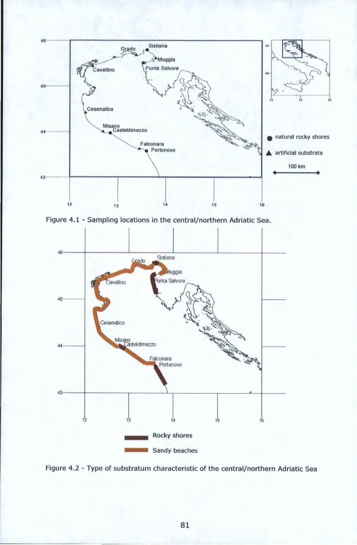
46------~--------------------------------------------------,

45i---4

43------~----------~----------~,-----------~r-------~--~

12 13 14 15 16

10 15

e natural rocky shores

A artificial substrata

100km

Figure 4.1 - Sampling locations in the central/northern Adriatic Sea.

44----i

~------r-----------r---------~r-----------.--------L--+------

12 14

Rocky shores

Sandy beaches

16

Figure 4.2 - Type of substratum characteristic of the central/northern Adriatic Sea

81

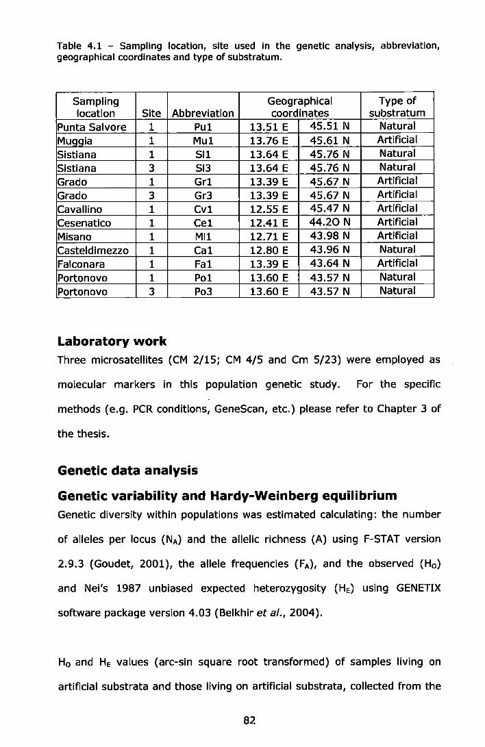
Table 4.1 - Sampling location, site used in the genetic analysis, abbreviation, geographical coordinates and type of substratum.

Sampling Geographical Type of location Site Abbreviation coordinates substratum

Punta Salvore 1 Pu1 13.51 E 45.51 N Natural Muggia 1 Mu1 13.76 E 45.61 N Artificial

Sistiana 1 Si1 13.64 E 45.76 N Natural Sistiana 3 Si3 13.64 E 45.76 N Natural Grado 1 Gr1 13.39 E 45.67 N Artificial Grado 3 Gr3 13.39 E 45.67 N Artificial Cavallino 1 Cv1 12.55 E 45.47 N Artificial Cesenatico 1 Ce1 12.41 E 44.20 N Artificial Misano 1 Mi1 12.71 E 43.98 N Artificial Casteldlmezzo 1 Ca1 12.80 E 43.96 N Natural Falconara 1 Fa1 13.39 E 43.64 N Artificial Portonovo 1 Po1 13.60 E 43.57 N Natural Portonovo 3 Po3 13.60 E 43.57 N Natural

Laboratory work Three microsatellites (CM 2/15; CM 4/5 and Cm 5/23) were employed as

molecular markers in this population genetic study. For the specific

methods (e.g. PCR conditions, GeneScan, etc.) please refer to Chapter 3 of

the thesis.

Genetic data analysis

Genetic variability and Hardy-Weinberg equilibrium Genetic diversity within populations was estimated calculating: the number

of alleles per locus (NA) and the allelic richness (A) using F-STAT version

2.9.3 (Goudet, 2001), the allele frequencies (FA), and the observed (Ho)

and Nei's 1987 unbiased expected heterozygosity (HE) using GENETIX

software package version 4.03 (Belkhir et al., 2004).

H0 and HE values (arc-sin square root transformed) of samples living on

artificial substrata and those living on artificial substrata, collected from the

82

nearest locations (artificial vs. natural locations}, were compared using t-

tests.

Single and multilocus F1s were estimated using Weir and Cockerham's

(1984} fixation index. Departures from Hardy-Weinberg equilibrium (HWE)

were tested using Fisher's exact test, using the null hypothesis Ho = no

heterozygote deficiency, with the level of significance determined by a

Markov-chaln randomization (10,000 dememorizations, 100 batches and

5000 Iterations per batch) using GENEPOP version 4.0 (Rousset, 2008).

Significance levels for multiple comparisons of loci across samples were

adjusted using a standard Bonferroni correction (Rice, 1989}.

Tests for linkage disequilibrium (LD) were performed at all loci in each

population and for each locus pair across all populations using GENEPOP;

estimation of exact probability values was carried out by Markov-chain

randomization ( 1,000,000 dememorizations, 1,000 batches and 50,000

iterations per batch).

Population structure The level of population genetic differentiation was assessed using Weir and

Cockerham's {1984) estimators of F-statistics (Frr or F and Fsr or 9)

calculated with the software F-STAT version 2.9.3 (Goudet, 2001}.

Variances of F-statistic estimators were obtained by jack-knifing over all

populations according to Weir (1990). The 95% confidence interval was

calculated by bootstrapping over the loci with 1000 pseudoreplicates using

the software GENETIX.

83

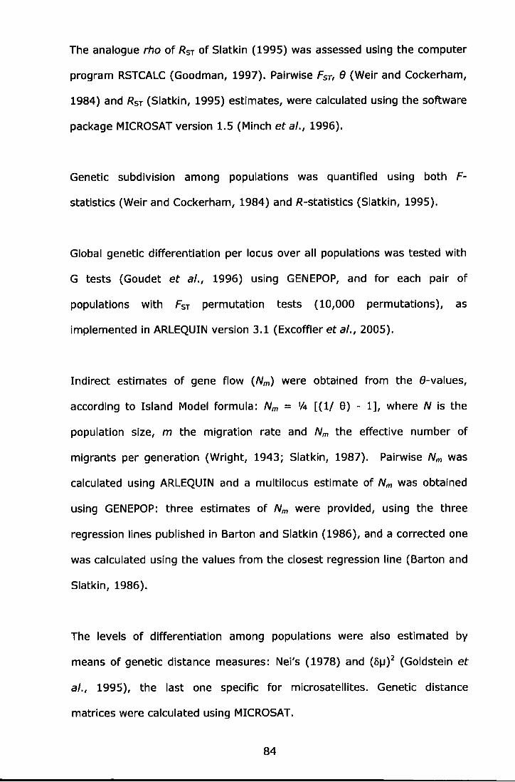
The analogue rho of RST of Slatkin (1995) was assessed using the computer

program RSTCALC (Goodman, 1997). Pairwise Fsr, B (Weir and Cockerham,

1984) and Rsr (Siatkin, 1995) estimates, were calculated using the software

package MICROSAT version 1.5 (Minch et al., 1996).

Genetic subdivision among populations was quantified using both F­

statistics (Weir and Cockerham, 1984) and R-statistics (Siatkin, 1995).

Global genetic differentiation per locus over all populations was tested with

G tests (Goudet et al., 1996) using GENEPOP, and for each pair of

populations with Fsr permutation tests (10,000 permutations), as

implemented in ARLEQUIN version 3.1 (Excoffier et al., 2005).

Indirect estimates of gene flow (Nm) were obtained from the B-values,

according to Island Model formula: Nm = 1/4 [{1/ 9) - 1], where N is the

population size, m the migration rate and Nm the effective number of

migrants per generation (Wright, 1943; Slatkin, 1987). Pairwise Nm was

calculated using ARLEQUIN and a multilocus estimate of Nm was obtained

using GENEPOP: three estimates of Nm were provided, using the three

regression lines published in Barton and Slatkin (1986), and a corrected one

was calculated using the values from the closest regression line (Barton and

Slatkin, 1986).

The levels of differentiation among populations were also estimated by

means of genetic distance measures: Nei's (1978) and {li1J) 2 {Goldstein et

al., 1995), the last one specific for microsatellites. Genetic distance

matrices were calculated using MICROSAT.

84

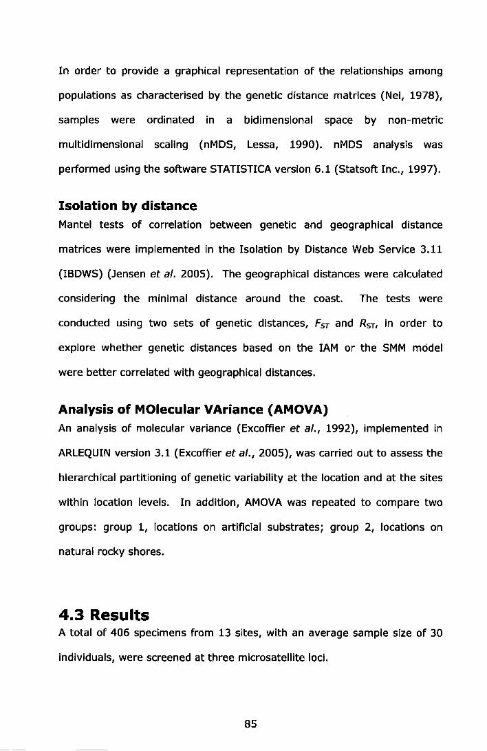
In order to provide a graphical representation of the relationships among

populations as characterised by the genetic distance matrices (Nei, 1978),

samples were ordinated in a bldimenslonal space by non-metric

multidimensional scaling (nMDS, Lessa, 1990). nMDS analysis was

performed using the software STATISTICA version 6.1 (Statsoft Inc., 1997).

Isolation by distance Mantel tests of correlation between genetic and geographical distance

matrices were implemented in the Isolation by Distance Web Service 3.11

(IBDWS) (Jensen et al. 2005). The geographical distances were calculated

considering the minimal distance around the coast. The tests were

conducted using two sets of genetic distances, FsT and RsT, in order to

explore whether genetic distances based on the lAM or the SMM model

were better correlated with geographical distances.

Analysis of MOlecular VAriance (AMOVA) An analysis of molecular variance (Excoffier et al., 1992), implemented in

ARLEQUIN version 3.1 (Excoffier et al., 2005), was carried out to assess the

hierarchical partitioning of genetic variability at the location and at the sites

within location levels. In addition, AMOVA was repeated to compare two

groups: group 1, locations on artificial substrates; group 2, locations on

natural rocky shores.

4.3 Results A total of 406 specimens from 13 sites, with an average sample size of 30

individuals, were screened at three microsatellite loci.

85

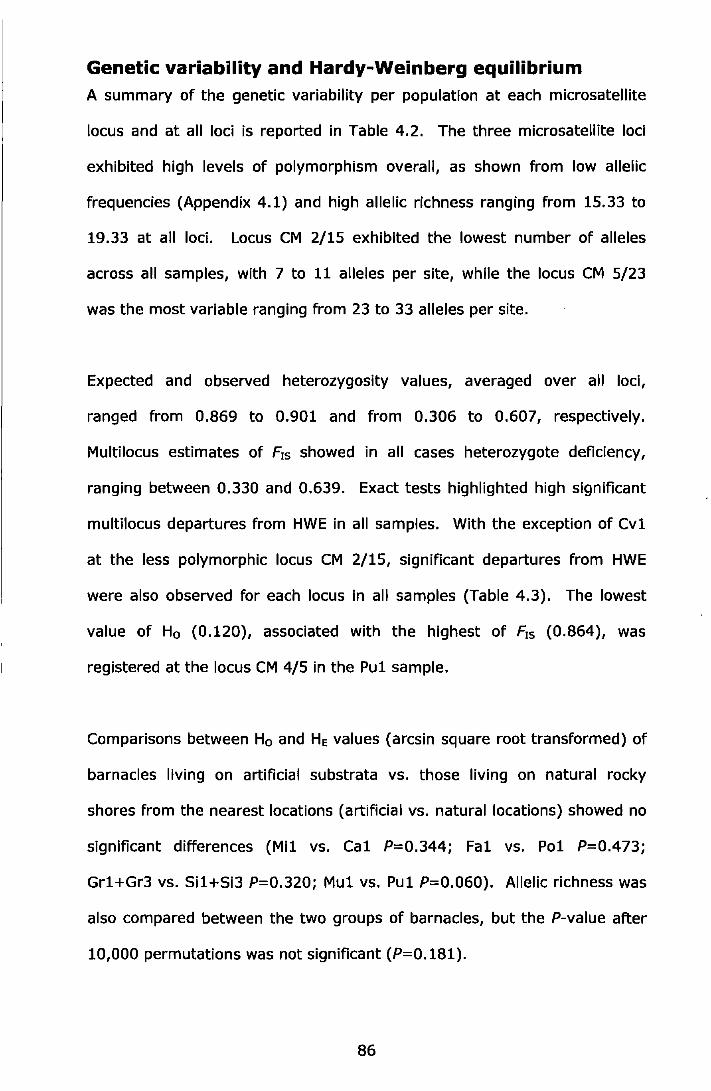
Genetic variability and Hardy-Weinberg equilibrium A summary of the genetic variability per population at each microsatellite

locus and at all loci is reported in Table 4.2. The three microsatellite loci

exhibited high levels of polymorphism overall, as shown from low allelic

frequencies (Appendix 4.1) and high allelic richness ranging from 15.33 to

19.33 at all loci. Locus CM 2/15 exhibited the lowest number of alleles

across all samples, with 7 to 11 alleles per site, while the locus CM 5/23

was the most variable ranging from 23 to 33 alleles per site.

Expected and observed heterozygosity values, averaged over all loci,

ranged from 0.869 to 0.901 and from 0.306 to 0.607, respectively.

Multilocus estimates of F15 showed in all cases heterozygote deficiency,

ranging between 0.330 and 0.639. Exact tests highlighted high significant

multilocus departures from HWE in all samples. With the exception of Cv1

at the less polymorphic locus CM 2/15, significant departures from HWE

were also observed for each locus in all samples (Table 4.3). The lowest

value of Ho (0.120), associated with the highest of F1s (0.864), was

registered at the locus CM 4/5 in the Pu1 sample.

Comparisons between Ho and HE values (arcsin square root transformed) of

barnacles living on artificial substrata vs. those living on natural rocky

shores from the nearest locations (artificial vs. natural locations) showed no

significant differences (Mi1 vs. Ca1 P=0.344; Fa1 vs. Po1 P=0.473;

Grl+Gr3 vs. Si1+Si3 P=0.320; Mu1 vs. Pu1 P=0.060). Allelic richness was

also compared between the two groups of barnacles, but the P-value after

10,000 permutations was not significant (P=0.181).

86

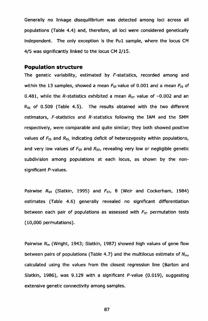
Generally no linkage disequilibrium was detected among loci across all

populations (Table 4.4) and, therefore, all loci were considered genetically

independent. The only exception is the Pu1 sample, where the locus CM

4/5 was significantly linked to the locus CM 2/15.

Population structure The genetic variability, estimated by F-statistics, recorded among and

within the 13 samples, showed a mean Fsr value of 0.001 and a mean F,s of

0.481, while the R-statistics exhibited a mean Rsr value of -0.002 and an

R,s of 0.509 (Table 4.5). The results obtained with the two different

estimators, F-statistics and R-statistics following the lAM and the SMM

respectively, were comparable and quite similar; they both showed positive

values of F15 and R15, indicating deficit of heterozygosity within populations,

and very low values of Fsr and R5r, revealing very low or negligible genetic

subdivision among populations at each locus, as shown by the non-

significant P-values.

Pairwise Rsr (Siatkin, 1995) and F5 r, 9 (Weir and Cockerham, 1984)

estimates (Table 4.6) generally revealed no significant differentiation

between each pair of populations as assessed with Fsr permutation tests

(10,000 permutations).

Pairwise Nm (Wright, 1943; Slatkin, 1987) showed high values of gene flow

between pairs of populations (Table 4. 7) and the multilocus estimate of Nm,

calculated using the values from the closest regression line (Barton and

Slatkin, 1986), was 9.129 with a significant P-value (0.019), suggesting

extensive genetic connectivity among samples.

87

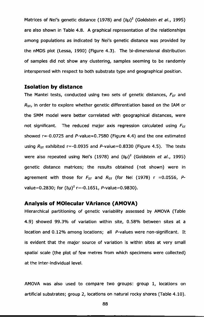
Matrices of Nei's genetic distance (1978) and (B1J)2 (Goldstein et al., 1995)

are also shown in Table 4.8. A graphical representation of the relationships

among populations as indicated by Nei's genetic distance was provided by

the nMDS plot (lessa, 1990) (Figure 4.3). The bi-dimensional distribution

of samples did not show any clustering, samples seeming to be randomly

interspersed with respect to both substrate type and geographical position.

Isolation by distance The Mantel tests, conducted using two sets of genetic distances, Fsr and

Rsr, in order to explore whether genetic differentiation based on the lAM or

the SMM model were better correlated with geographical distances, were

not significant. The reduced major axis regression calculated using Fsr

showed r=-0.0725 and P-value=0.7580 (Figure 4.4) and the one estimated

using Rsr exhibited r=-0.0935 and P-value=0.8330 (Figure 4.5). The tests

were also repeated using Nei's (1978) and (B1J)2 (Goldstein et al., 1995)

genetic distance matrices; the results obtained (not shown) were in

agreement with those for Fsr and Rsr (for Nei (1978) r =0.0556, P­

value=0.2830; for (B1J)2 r=-0.1651, P-value=0.9830).

Analysis of MOlecular VAriance (AMOVA) Hierarchical partitioning of genetic variability assessed by AMOVA (Table

4.9) showed 99.3% of variation within site, 0.58% between sites at a

location and 0.12% among locations; all P-values were non-significant. It

is evident that the major source of variation is within sites at very small

spatial scale (the plot of few metres from which specimens were collected)

at the inter-individual level.

AMOVA was also used to compare two groups: group 1, locations on

artificial substrates; group 2, locations on natural rocky shores (Table 4.10).

88

The percentages of variation between groups and within group were

negligible and P-values were not significant.

89

Table 4.2 - Summary of genetic variability per sites at each microsatellite locus and all loci: number of sampled individuals (N), number of observed alleles per locus (NA); allelic richness based on 25 individuals (A); Nei's 1987 unbiased expected heterozygosity (He); observed heterozygosity (H0 ); Weir and Cockerham's (1984) estimate of Wright's (1951) fixation index (F15). F15 values in bold indicate significant departures from HWE after standard Bonferroni correction. For site abbreviations see Table 4.1.

SITES LOCUS Pu1 Mu1 Si1 Si3 Gr1 Gr3 CV1 Ce1 Mi1 Ca1 Fa1 Po1 Po3 Cm2/15 N 30 28 31 32 29 29 32 30 29 31 32 30 28 NA 7 9 10 7 10 7 11 10 9 10 11 9 7 A 6.33 8.77 9.54 6.73 9.69 6.85 9.81 9.77 8.55 9.53 9.99 8.66 6.77 HE 0.681 0.725 0.814 0.768 0.771 0.757 0.778 0.815 0.748 0.784 0.789 0.816 0.708 Ho 0.267 0.429 0.548 0.531 0.621 0.552 0.625 0.667 0.483 0.484 0.500 0.400 0.429 F1s 0.612 0.414 0.330 0.312 0.198 0.274 0.199 0.185 0.359 0.387 0.370 0.514 0.399 Cm4/5 N 25 29 27 28 27 29 26 30 30 30 29 28 29 NA 14 18 15 11 13 13 11 15 16 17 17 15 14 A 14.00 17.10 14.69 10.84 12.70 12.67 10.96 14.40 15.08 15.89 16.12 14.73 13.64 Ho 0.869 0.904 0.874 0.845 0.881 0.856 0.793 0.908 0.823 0.896 0.908 0.869 0.890 H_o_ 0.120 0.310 0.222 0.214 0.333 0.241 0.154 0.500 0.267 0.400 0.379 0.250 0.241 6.s_ 0.864 0.661 0.749 0.750 0.626 0.722 0.809 0.454 0.680 0.558 0.587 0.716 0.732 Cm5/23 N 32 28 27 30 27 28 32 29 29 28 31 29 29 NA 32 31 28 30 30 27 29 33 32 26 23 27 25 A 28.23 29.41 27.00 27.43 28.99 25.82 25.78 30.60 29.85 24.86 21.63 25.58 23.39 Ho 0.965 0.979 0.966 0.969 0.976 0.968 0.958 0.978 0.978 0.967 0.960 0.969 0.956 Ho 0.531 0.714 0.519 0.600 0.556 0.536 0.656 0.655 0.552 0.571 0.516 0.586 0.517 Fr~ 0.454 0.274 0.468 0.385 0.436 0.451 0.319 0.334 0.440 0.413 0.466 0.399 0.464

90

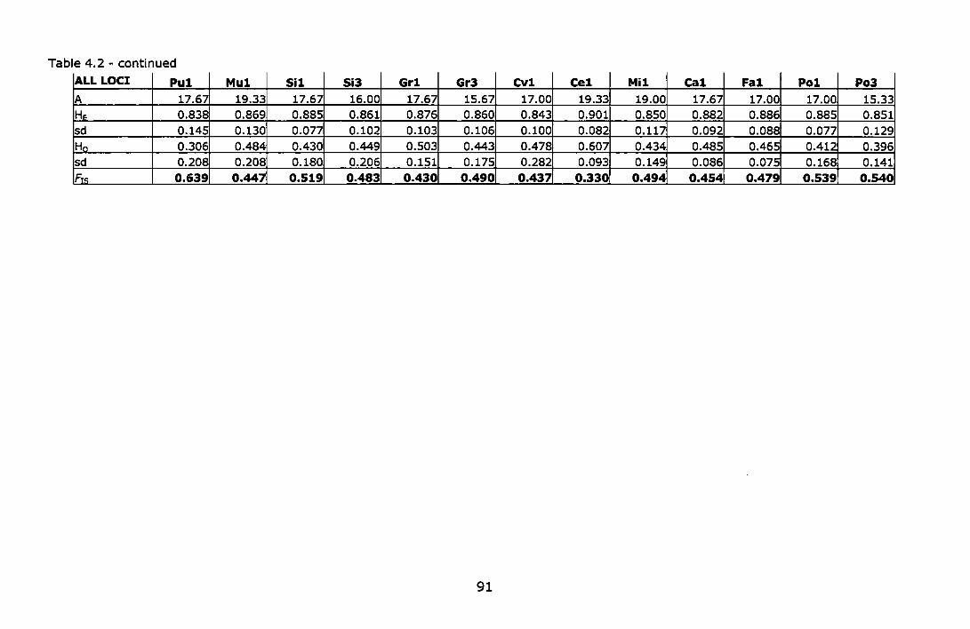
Table 4.2 - continued

ALL LOCI Pu1 Mu1 Si1 Si3 Gr1 Gr3 Cv1 Ce1 Mi1 Ca1 Fa1 Po1 Po3 A 17.67 19.33 17.67 16.00 17.67 15.67 17.00 19.33 19.00 17.67 17.00 17.00 15.33 HE 0.838 0.869 0.885 0.861 0.876 0.860 0.843 0.901 0.850 0.882 0.886 0.885 0.851 sd 0.145 0.130 0.077 0.102 0.103 0.106 0.100 0.082 0.117 0.092 0.088 0.077 0.129 Ho 0.306 0.484 0.430 0.449 0.503 0.443 0.478 0.607 0.434 0.485 0.465 0.412 0.396 sd 0.208 0.208 0.180 0.206 0.151 0.175 0.282 0.093 0.149 0.086 0.075 0.168 0.141 Fts 0.639 0.447 0.519 0.483 0.430 0.490 0.437 0.330 0.494 0.454 0.479 0.539 0.540

91

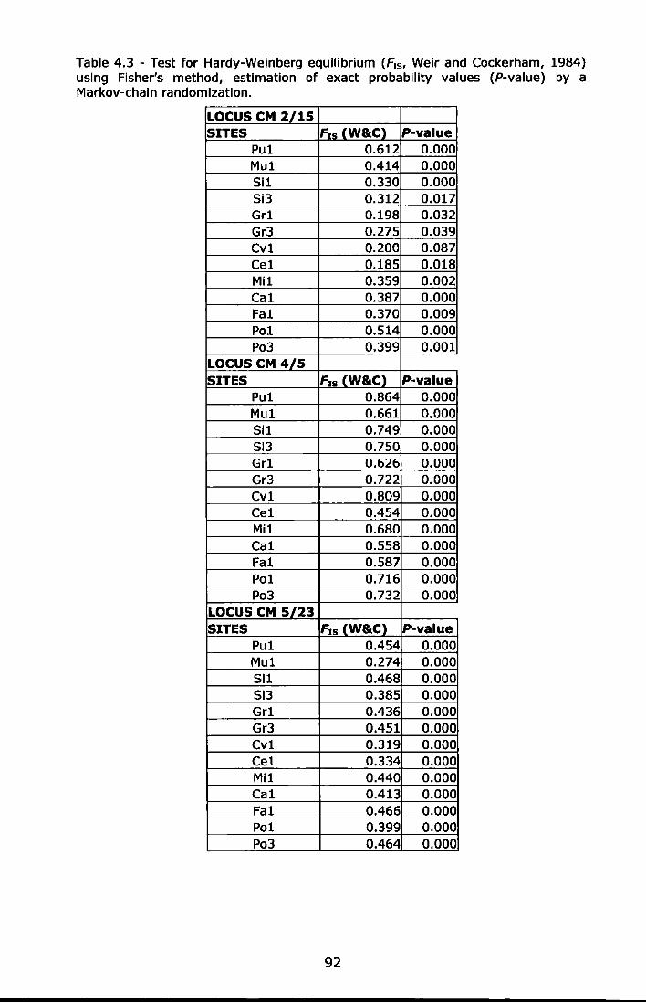
Table 4.3 - Test for Hardy-Welnberg equilibrium (F15, Weir and Cockerham, 1984) using Fisher's method, estimation of exact probability values (P-value) by a Markov-chain randomizatlon.

LOCUS CM 2/15 SITES F1s (W&C) P-value

Pu1 0.612 0.000 Mu1 0.414 0.000 511 0.330 0.000 513 0.312 0.017 Gr1 0.198 0.032 Gr3 0.275 0.039 Cv1 0.200 0.087 Ce1 0.185 0.018 Mi1 0.359 0.002 Ca1 0.387 0.000 Fa1 0.370 0.009 Po1 0.514 0.000 Po3 0.399 0.001

LOCUS CM 4/5 SITES F1s (W&C) P-value

Pu1 0.864 0.000 Mu1 0.661 0.000 511 0.749 0.000 513 0.750 0.000 Gr1 0.626 0.000 Gr3 0.722 0.000 Cv1 0.809 0.000 Ce1 0.454 0.000 Mi1 0.680 0.000 Ca1 0.558 0.000 Fa1 0.587 0.000 Po1 0.716 0.000 Po3 0.732 0.000

LOCUS CM 5/23 SITES F1s (W&C) P-value

Pu1 0.454 0.000 Mu1 0.274 0.000 511 0.468 0.000 513 0.385 0.000 Gr1 0.436 0.000 Gr3 0.451 0.000 Cv1 0.319 0.000 Ce1 0.334 0.000 Mi1 0.440 0.000 Ca1 0.413 0.000 Fa1 0.466 0.000 Po1 0.399 0.000 Po3 0.464 0.000

92

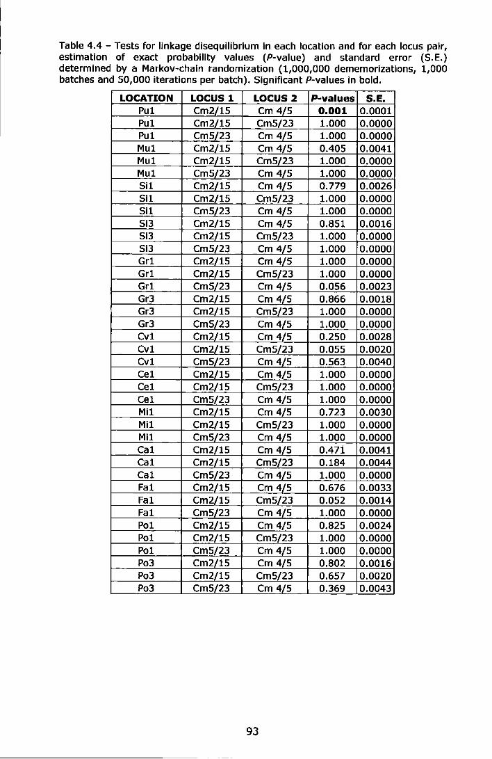
Table 4.4 - Tests for linkage disequilibrium In each location and for each locus pair, estimation of exact probability values (P-value) and standard error (S.E.) determined by a Markov-chaln randomization (1,000,000 dememorlzatlons, 1,000 batches and 50,000 iterations per batch). Significant P-values in bold.

LOCATION LOCUS 1 LOCUS 2 P-values S.E. Pul Cm2/15 Cm 4/5 0.001 0.0001 Pul cmi/15 CmS/23 1.000 0.0000 Pul CmS/23 Cm 4/5 1.000 0.0000 Mul Cm2/15 Cm 4/5 0.405 0.0041 Mul Cm2/15 Cm5/23 1.000 0.0000 Mul Cm5l23 Cm 4/5 1.000 0.0000 Sil Cm2/15 Cm 4/5 0.779 0.0026 Sil Cm2/15 Cm5/23 1.000 0.0000 Sil Cm5J23 Cm 4/5 1.000 0.0000 Si3 Cm2/15 Cm 4/5 0.851 0.0016 Si3 Cm2/15 Cm5/23 1.000 0.0000 Si3 cmS/23 Cm 4/5 1.000 0.0000 Grl Cm2/15 Cm 4/5 1.000 0.0000 Grl Cm2/15 CmS/23 1.000 0.0000 Grl Cm5/23 Cm 4/5 0.056 0.0023 Gr3 Cm2/15 Cm 4/5 0.866 0.0018 Gr3 Cm2/15 Cm5/23 1.000 0.0000 Gr3 Cm5/23 cm 4/5 1.000 0.0000 Cvl Cm2/15 Cm 4/5 0.250 0.0028 Cvl Cm2/15 Cm5/23 0.055 0.0020 Cvl Cm5/23 Cm 4/5 0.563 0.0040 Cel Cm2/15 Cm 4/5 1.000 0.0000 Cel Cm2/15 Cm5/23 1.000 0.0000 Cel Cm5/23 Cm 4/5 1.000 0.0000 Mil Cm2/15 Cm 4/5 0.723 0.0030 Mil Cm2/15 Cm5/23 1.000 0.0000 Mil Cm5/23 Cm 4/5 1.000 0.0000 Cal Cm2/15 Cm 4/5 0.471 0.0041 Cal Cm2/15 Cm5/23 0.184 0.0044 Cal Cm5/23 Cm 4/5 1.000 0.0000 Fal Cm2/15 cm 4/5 0.676 0.0033 Fal Cm2/15 Cm5/23 0.052 0.0014 Fal Cm5/23 Cm 4/5 1.000 0.0000 Pal Cm2/15 Cm 4/5 0.825 0.0024 Pal Cm2/15 Cm5/23 1.000 0.0000 Pal Cm5/23 Cm 4l5 1.000 0.0000 Po3 Cm2/15 Cm 4/5 0.802 0.0016 Po3 Cm2/15 Cm5/23 0.657 0.0020 Po3 Cm5/23 Cm 4/5 0.369 0.0043

93

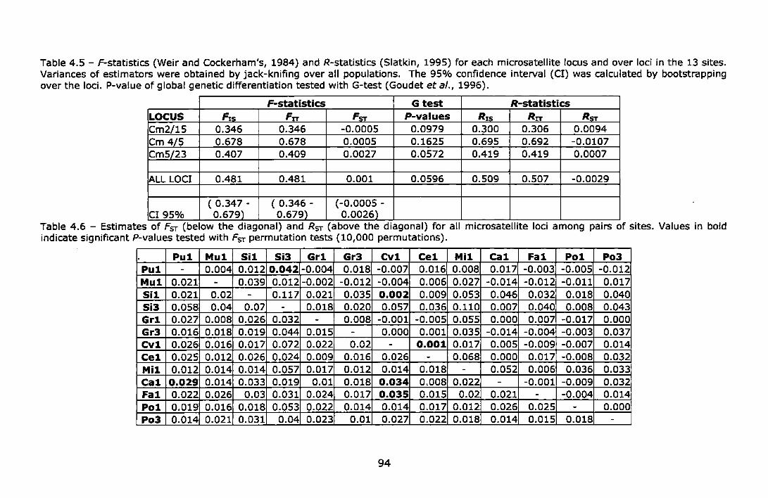
Table 4.5 - F-statistics (Weir and Cockerham's, 1984) and R-statistics (Siatkin, 1995) for each microsatellite locus and over loci in the 13 sites. Variances of estimators were obtained by jack-knifing over all populations. The 95% confidence interval (Cl) was calculated by bootstrapping over the loci. P-value of global genetic differentiation tested with G-test (Goudet et al., 1996).

F-statistics G test R-statistics LOCUS Fxs Frr Fsr P-values Rxs Rrr Rsr Cm2/15 0.346 0.346 -0.0005 0.0979 0.300 0.306 0.0094 Cm 4/5 0.678 0.678 0.0005 0.1625 0.695 0.692 -0.0107 Cm5/23 0.407 0.409 0.0027 0.0572 0.419 0.419 0.0007

!ALL LOCI 0.481 0.481 0.001 0.0596 0.509 0.507 -0.0029

( 0.347- ( 0.346- (-0.0005-CI 95% 0.679) 0.679) 0.0026)

Table 4.6 - Estimates of Fsr (below the d1agonal) and Rsr (above the d1agonal) for all m1crosatelhte loc1 among pa1rs of sites. Values in bold indicate significant P-values tested with Fsr permutation tests (10,000 permutations).

Pu1 Mu1 Si1 Si3 Gr1 Gr3 Cv1 Ce1 Mi1 Ca1 Fa1 Pal Pa3 Pu1 - 0.004 0.012 0.042 -0.004 0.018 -0.007 0.016 0.008 0.017 -0.003 -0.005 -0.012 Mu1 0.021 - 0.039 0.012 -0.002 -0.012 -0.004 0.006 0.027 -0.014 -0.012 -0.011 0.017 Si1 0.021 0.02 - 0.117 0.021 0.035 0.002 0.009 0.053 0.046 0.032 0.018 0.040 Si3 0.058 0.04 0.07 - 0.018 0.020 0.057 0.036 0.110 0.007 0.040 0.008 0.043 Gr1 0.027 0.008 0.026 0.032 - 0.008 -0.001 -0.005 0.055 0.000 0.007 -0.017 0.000 Gr3 0.016 0.018 0.019 0.044 0.015 - 0.000 0.001 0.035 -0.014 -0.004 -0.003 0.037 Cv1 0.026 0.016 0.017 0.072 0.022 0.02 - 0.001 0.017 0.005 -0.009 -0.007 0.014 Ce1 0.025 0.012 0.026 0.024 0.009 0.016 0.026 - 0.068 0.000 0.017 -0.008 0.032 Mi1 0.012 0.014 0.014 0.057 0.017 0.012 0.014 0.018 - 0.052 0.006 0.036 0.033 Ca1 0.029 0.014 0.033 0.019 0.01 0.018 0.034 0.008 0.022 - -0.001 -0.009 0.032 Fa1 0.022 0.026 0.03 0.031 0.024 0.017 0.035 0.015 0.02 0.021 - -0.004 0.014 Pal 0.019 0.016 0.018 0.053 0.022 0.014 0.014 0.017 0.012 0.026 0.025 - 0.000 Pa3 0.014 0.021 0.031 0.04 0.023 0.01 0.027 0.022 0.018 0.014 0.015 0.018 -

94

Table 4.7- Pairwise indirect estimates of gene flow (Nm) according to Wright (1943) and Slatkin (1987).

Pu1 Mu1 Si1 Si3 Gr1 Gr3 Cv1 Ce1 Mi1 Ca1 Fa1 Po1 Po3 Pul -Mu1 15.24 -Sil 24.60 76.12 -Si3 14.46 31.34 49.56 -Gr1 13.54 inf 50.74 138.41 -Gr3 18.96 36.11 40.88 36.12 42.11 -CV1 18.48 27.54 23.68 17.38 22.64 19.00 -Ce1 13.13 165.54 56.02 63.27 inf 46.22 15.37 -Mi1 20.55 80.65 33.56 24.15 32.73 153.95 24.71 34.68 -ca1 11.05 64.09 30.90 126.18 inf 31.00 10.77 inf 20.93 -Fa1 19.13 15.08 28.24 32.05 17.86 29.78 11.79 38.36 20.76 19.86 -Po1 23.31 50.56 55.53 22.42 24.50 55.25 47.51 36.77 80.13 17.71 17.59 -Po3 27.92 27.50 20.89 25.29 22.02 376.32 14.42 24.46 33.43 63.65 46.57 38.08 -

\Z Table 4.8- Pairwise genet1c d1stances. Ne1 (1978) values are below the d1agonal and (li!J) values are above the d1agonal.

Pu1 Mu1 Si1 Si3 Grl Gr3 Cv1 Ce1 Mi1 Ca1 Fa1 Po1 Po3 Pu1 - 6.314 2.230 12.141 1.933 11.865 1.502 2.710 5.937 8.969 4.504 2.284 0.740 Mu1 0.067 - 14.035 3.920 5.042 1.000 2.825 3.089 5.583 0.411 0.742 2.476 7.909 Si1 0.071 0.071 - 23.749 6.899 20.760 4.574 7.842 8.788 18.098 10.228 8.099 3.964 Si3 0.327 0.228 0.462 - 5.828 5.802 10.596 4.746 17.981 2.351 7.694 4.116 10.590 Gr1 0.106 0.006 0.106 0.160 - 10.282 3.654 0.556 11.226 5.996 5.587 0.454 0.938 Gr3 0.037 0.057 0.059 0.245 0.041 - 5.968 6.975 7.318 0.895 2.150 6.417 14.457 CVl 0.095 0.043 0.048 0.464 0.075 0.064 - 2.751 2.319 5.113 1.130 2.419 3.762 Ce1 0.084 0.014 0.111 0.108 0.008 0.038 0.099 - 9.750 3.696 3.847 0.222 2.481 Mi1 0.019 0.027 0.031 0.340 0.046 0.016 0.029 0.044 - 8.920 2.290 8.639 10.379 Ca1 0.124 0.035 0.166 0.070 0.004 0.059 0.165 0.005 0.084 - 2.233 3.222 10.016 Fa1 0.076 0.133 0.141 0.167 0.117 0.056 0.175 0.051 0.070 0.098 - 3.134 7.066 Pol 0.049 0.047 0.055 0.368 0.103 0.032 0.021 0.072 0.014 0.141 0.141 - 2.042 Po3 0.031 0.075 0.137 0.207 0.090 0.007 0.107 0.078 0.054 0.027 0.032 0.056 -

95

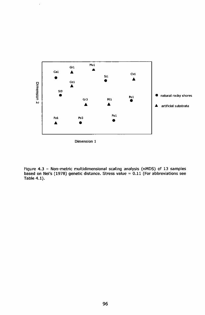
Mul Grl

cat A A

CVl

• Sll

• A 0 Cel

3" A (1)

Sl3 ::J

"' • • natural rocky shores (5" Pal ::J Gr3 Mll • N

A A ... artificial substrata

Pul Fat Po3

A • •

Dimension 1

Figure 4.3 - Non-metric multidimensional scaling analysis (nMDS) of 13 samples based on Nei's (1978) genetic distance. Stress value = 0.11 (For abbreviations see Table 4.1).

96

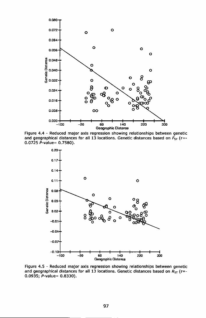
0.080

0.072

0.064

0.056

~ 0.048

:!1i ~ 0.040 .. 0:: l; 0.032

0.024

0.016

0.008

0 0

0 0 0

0

00

0.000+--+--+---+---+---+--+--+--+--+-....... -100 -20 60 140 220 300

Geographic Distance

Figure 4.4 - Reduced major axis regression showing relationships between genetic and geographical distances for all 13 locations. Genetic distances based on Fsr (r=-0.0725 P-value= 0.7580).

-n.1o+-+-+-+--t---11--+--+--+---+----i -100 -20 80 140 220 300

Geographic Distance

Figure 4.5 - Reduced major axis regression showing relationships between genetic and geographical distances for all 13 locations. Genetic distances based on Rsr (r=-0.0935; P-value= 0.8330).

97

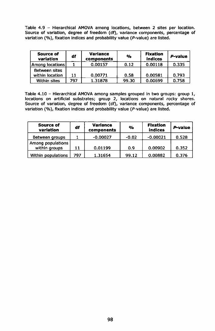
Table 4.9 - Hierarchical AMOVA among locations, between 2 sites per location. Source of variation, degree of freedom (df), variance components, percentage of variation (%}, fixation indices and probability value (P-value) are listed.

Source of df Variance 0/o Fixation P-value variation components Indices Among locations 1 0.00157 0.12 0.00118 0.335

Between sites within location 11 0.00771 0.58 0.00581 0.793

Within sites 797 1.31878 99.30 0.00699 0.758

Table 4.10 - Hierarchical AMOVA among samples grouped In two groups: group 1, locations on artificial substrates; group 2, locations on natural rocky shores. Source of variation, degree of freedom (df), variance components, percentage of variation (%}, fixation indices and probability value (P-value) are listed.

Source of df Variance 0/o Fixation P-value variation components indices

Between groups 1 -0.00027 -0.02 -0.00021 0.528 Among populations

within groups 11 0.01199 0.9 0.00902 0.352

Within populatlons 797 1.31654 99.12 0.00882 0.376

98

4.4 Discussion In this study, the population genetic structure of the barnacle Chthamalus

montagui was investigated by employing three highly polymorphic

microsatellite loci at 13 sites along the Adriatic coast to assess the potential

"corridor effect" created by artificial substrates, built to protect the coast.

Negligible levels of genetic subdivision were detected among locations, as

revealed from the low and non-significant values of FsT and RsT and the high

estimates of gene flow (Nm) between all pairs of populations. All the

samples screened along the Adriatic coast seem to act as a large panmitic

population. This was also confirmed by the nMDS analysis based on the

genetic distances among populations and by the Mantel test that did not

show any significant correlation between genetic and geographical distance

matrices. These results should be viewed in relation to the dispersal

capability of the species. Simulations of one-dimensional stepping-stone

model of population structure showed that isolation by distance is most

obvious when comparing populations separated by 2-5 times the mean

larval dispersal distance {Palumbi, 2003).

The range of larval dispersal in barnacles has been estimated to be in the

order of 15-20 km per generation (Strathmann, 1974; Crisp, 1976). If we

consider the sampling locations of this study, the furthest-separated rocky

shores without intervening natural hard substrate are Casteldimezzo (Ca1)

and Sistiana (Si1), about 200 km apart. This distance is higher than the

estimated potential larval dispersal of barnacles, therefore artificial

substrates could act as stepping stones or "corridors" among previously

isolated populations.

99

Support for this hypothesis comes from an investigation using a

combination of field studies and spatial population models to investigate the

large scale effects of the hard structures in the north Adriatic Sea on the

limpet Patella caerulea (Airoldi et al., 2005). Model simulations of the

dispersal and survival of P. caerulea showed that the maximum dispersal

distance of this species is far less than the distance between natural rocky

reefs in the area. Thus, prior to the deployment of the artificial structures,

the gene flow between native populations in Trieste and Ancona was

probably limited. Furthermore, connectivity matrix simulatlons showed that

if a few more structures were built in the area the result for this species

would have been equivalent to a continuous rocky coast. On the contrary, if

structures were removed from the system the proportion of occupied

structures would decrease. Results also revealed that some structures were

mainly sinks while others acted as both sources and sinks, depending on

their location. In summary the number, extent and the spatial arrangement

of the structures seem to influence the realised larval dispersal of P.

caerulea (Airoldi et al., 2005).

However, it is important to highlight that P. caerula is assumed to be a

short-dispersal species, whereas C. montagui is a long-dispersal species.

The range of larval dispersal estimated for barnacles (Strathmann, 1974;

Crisp, 1976) can vary and is likely to be influenced by different factors, such

as offshore hydrodynamic processes at a large scale (Barnes, 1956;

Raimondi, 1990) or local water turbulence at a small scale (O'Riordan,

2004). The Adriatic Sea is a semi-enclosed elongated basin, separated from

North to South Into three sub-basins, characterized by a cyclonic circulation,

100

by eddies and gyres that lead to the formation of deep water in the

Northern and Middle Adriatic (Mantziafou and Lascartos, 2004). These

oceanographic processes can promote or increase species dispersal

capability. Thus, the detected low genetic differentiation among populations

can be related not only to the artificial substrates, but also to the effective

dispersal ability of C. montagui possibly enhanced by local oceanographic

factors.

Moreover, the AMOVA results confirmed that genetic variation among

locations and between sites within a location are negligible (less than 1 %)

and showed that the major source of genetic variability is within sites,

accounting for 99.3% of the total genetic variation. Analogous results were

found in the study carried out within EUMAR in the same area, along the

Adriatic coast, on the limpet P. caerulea using allozymes and microsatellites

(Bertozzi, 2005).

In fact, the 13 barnacle populations screened in my study showed high

levels of genetic variability, low allelic frequencies, high expected

heterozygosity and a large number of alleles per population at each of the

analysed loci (the most polymorphic one, CM 5/23, ranging from 23 to 33

alleles).

Looking at genetic variability within populations, it appears that all samples

exhibited strong deviations from HWE showing highly significant values of

F15 at all loci. Heterozygosity deficits are frequently observed in marine

invertebrates (Zouros and Foltz, 1984; Gaffney 1994; David et al. 1997;

Ayre and Hughes, 2000; Ridgway et al. 2001; Addison and Hart 2004;

101

Duran et al. 2004; Le Goff-Vitry et al. 2004; Andrade and Solferini, 2007;

Costantini et al., 2007) including barnacles (Veliz et al., 2006; York et al.,

2008). The most common explanations for the heterozygote deficiency are

technical factors, such as the presence of null alleles (Foltz, 1986; Callen et

al., 1993; Puebla et al., 2008), and (or) biological factors, such as

inbreeding or Wahlund effect {Pogson et al., 1995; Duran et al., 2004;

Plutchack et al., 2006; Costantinl et al., 2007). In this study I do not

favour the hypothesis of null alleles, because all F,5 estimates were positive,

significant and consistent across all loci, and it seems highly improbable

that all loci exhibit null alleles with such a constant frequency.

The heterozygote deficiencies observed are thus probably due to biological

factors, but it is not easy to give an actual explanation on this basis.

Inbreeding remains an unlikely explanation for barnacles, which have wide

dispersal as larvae, and have large populations that are not subject to

drastic reduction in size.

The Wahlund effect refers to reduction of heterozygosity caused by

subpopulation structure, and could affect all polymorphic loci similarly

(Pogson et al., 1995). If two or more subpopulations have different allele

frequencies then the overall heterozygosity is reduced, even if the

subpopulations themselves are in HWE; the underlying causes of this

population subdivision could be geographic barriers to gene flow followed by

genetic drift in the subpopulations. However, no evidence of population

differentiation was detected in this study.

102

Furthermore, comparisons between the genetic pattern of barnacles living

on natural rocky shores and those living on artificial substrata were carried

out to investigate the possible selection that could be operated by the type

of substratum. No significant differences were detected comparing the

mean number of alleles, the allele frequencies, the heterozygosity and the

partitioning of genetic variance between the two groups of populations. It

is important to take into account that the use of putatively neutral markers,

such as microsatellites, could not detect such phenomena even if, in some

cases, these markers may not behave in a neutral way (Dufresne et al.,

2002).

Support for these findings comes from the study on the limpet P. caerulea

(Bertozzi, 2005): no genetic difference between samples collected from

natural rocks and from artificial structures was shown by allozymes,

markers considered under selection.

Moreover, other population genetic studies carried out along the European

coast within EUMAR, on different sorts of natural and artificial substrates, on

the periwinkles Littorina littorea and Melarhaphe neritoides, using mtDNA as

a molecular marker, did not reveal any significant effect of substrate type

on the population genetic pattern of these intertidal organisms.

To conclude, detecting the corridor effect in this barnacle species is not an

easy task due to the possible masking effect of local spatial genetic

variation and efficient larval mixing. However, the collected data do not

allow rejection of the hypothesis that artificial substrates act as "corridors"

103

among populations favouring gene flow and promoting homogeneous

genetic patterns.

Furthermore, the nature of the substratum (artificial vs. natural) did not

promote genetic differentiation in barnacles, suggesting that the type of

substratum does not selectively affect survival during settlement and

recruitment on the basis of the tested markers.

104

Chapter 5

Effects of marginality and

peri·pherality on the genetic

variability of

Chthamalus montagui

105

5.1 Introduction and specific aims The importance of intraspecific genetic diversity in natural populations is

well established, as already explained in the general introduction of this

thesis, and has been identified as a global priority for conservation (Crozier

1997; Avise and Hamrick, 1996). Genetic diversity is the clay for

evolutionary adaptation and ultimately speciation, its role is fundamental to

the ability of a species to persist when challenged by various environmental

pressures (AIIendorf and Luikart, 2007).

However, the distribution of genetic variation is often non-uniform and

partitioned throughout a species' natural distribution (Lind et al., 2007).

Populations living at the edge of the species' geographical range, referred to

here as peripheral, or/and those at the extreme of the species'

environmental tolerance within its geographical range, referred to here as

marginal populations, often show a different pattern of genetic variability

compared to populations living in the central part of the species'

geographical range, here denominated central populations (Lesica and

Allendorf 1995).

Peripheral and marginal populations are often relatively small and isolated

from central populations; gene flow is reduced and the probability that they

are founded by a small number of individuals is high (Levin, 1970; Lawton,

1993). Reduced gene flow, small population size and founder effect will

promote genetic drift and result in less genetic variation and increased

differentiation of these populations (AIIendorf, 1986; McCommas and Bryan,

1990; Lesica and Allendorf 1995).

106

Empirical data mostly support the prediction that peripheral populations are

less genetically variable compared to core populations of the same species

(Lesica and Allendorf, 1995; Lammi et al., 1999; Schwartz et al., 2003).

For instance, a study carried out on the population genetics of a marine

bivalve, Plnctada maxima, throughout the Indo-Australlan archipelago using

microsatellite markers, demonstrated that, as the geographical distance of a

population increased from the centre of the species' distribution, allelic

richness and observed heterozygosity correspondingly decreased, showing

the lowest genetic diversity in peripheral populations (Lind et al., 2007).

In addition, many species at the edge of their range occur in unusual or

atypical habitats (Lawton, 1993, Holt and Keitt, 2000; Pulliam, 2000;

Maurer and Taper 2002). Peripheral and marginal populations are,

therefore, under extreme selection pressure: local adaptation to exceptional

conditions may result in anomalous and sometimes unique genetic patterns

(Garcia-Ramos and Kirkpatrick 1997; Bouza et al., 1999). Furthermore,

these populations, which are smaller and inhabit a more stressful

environment than central ones, are more likely to pass through severe

bottlenecks that will further reduce their genetic variability (Chakraborty

and Nei 1977; Booy et al., 2000).

Given that peripheral and marginal populations are often both genetically

distinct and more vulnerable, it follows that they have for long been

recognized as "evolutionary laboratories" potentially favourable for

speciation (Carson and Templeton, 1984; Garcia-Ramos and Kirkpatrick,

1997) and for this reason are of special interest in conservation biology

107

(Lesica and Allendorf, 1995). If we consider the marine environment, more

data are needed to assess the importance and vulnerability of peripheral

and marginal populations in order to develop adequate management

strategies for marine genetic biodiversity conservation.

Within the EUMAR project, a meta-analysls of population genetic data from

29 species inhabiting the Baltic Sea was performed. The low salinity Baltic

Sea is a perfect "natural laboratory", as it represents a geographically

peripheral ecosystem and at the same time an ecologically extreme and

marginal marine environment (Johannesson and Andre, 2006).

My task in the EUMAR project was to compare the genetic pattern of central

populations vs. peripheral/marginal populations of Chthama/us montagui,

over the whole range of its distribution in the UK, to assess the genetic

diversity of the species in these peculiar conditions, using three

microsatellites as molecular markers.

The British coast is a very appropriate study area for this purpose. The

geographical distribution of the target species in the UK (Figure 5.1} has its

northern limit in northern Scotland, due to low water temperature, while in

the English Channel the Isle of Wight represents the eastern limit of the

species, due to lack of rocky substratum suitable for barnacle settlement

(Hawkins and Jones, 1992; Herbert and Hawkins, 2006). Moreover,

decreasing salinity and increasing sedimentation moving into the Bristol

Channel provide an ecologically marginal habitat for the species.

108

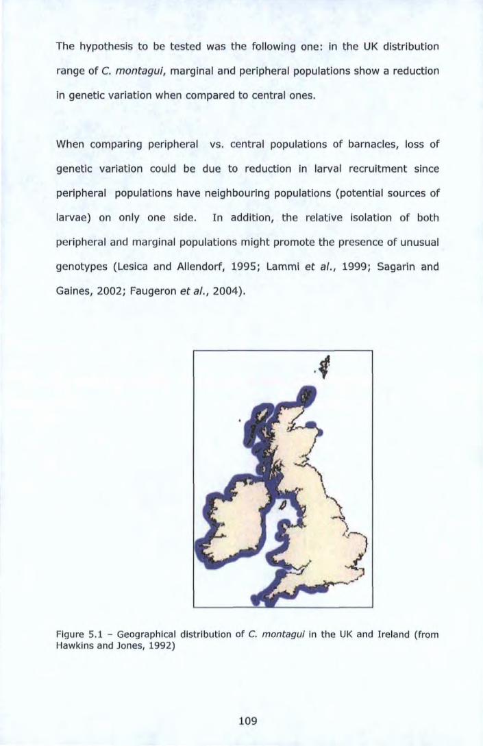
The hypothesis to be tested was the following one: in the UK distribution

range of C. montagui, marginal and peripheral populations show a reduction

in genetic variation when compared to central ones.

When comparing peripheral vs. central populations of barnacles, loss of

genetic variation could be due to reduction in larval recruitment since

peripheral populations have neighbouring populations (potential sources of

larvae) on only one side. In addition, the relative isolation of both

peripheral and marginal populations might promote the presence of unusual

genotypes (Lesica and Allendorf, 1995; Lammi et al., 1999; Sagarin and

Gaines, 2002; Faugeron et al., 2004 ).

Figure 5.1 - Geographical distribution of C. montagui in the UK and Ireland (from Hawkins and Jones, 1992)

109

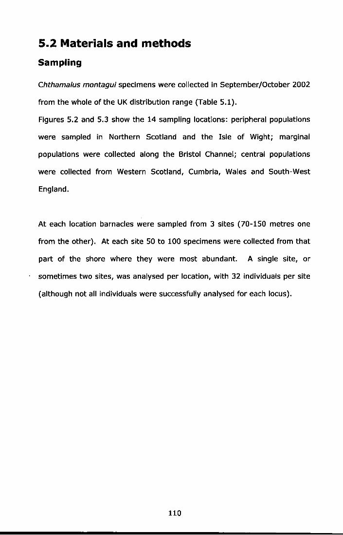
5.2 Materials and methods

Sampling

Chthamalus montagui specimens were collected in September/October 2002

from the whole of the UK distribution range (Table 5.1).

Figures 5.2 and 5.3 show the 14 sampling locations: peripheral populations

were sampled in Northern Scotland and the Isle of Wight; marginal

populations were collected along the Bristol Channel; central populations

were collected from Western Scotland, Cumbria, Wales and South-West

England.

At each location barnacles were sampled from 3 sites (70-150 metres one

from the other). At each site 50 to 100 specimens were collected from that

part of the shore where they were most abundant. A single site, or

sometimes two sites, was analysed per location, with 32 individuals per site

(although not all Individuals were successfully analysed for each locus).

110

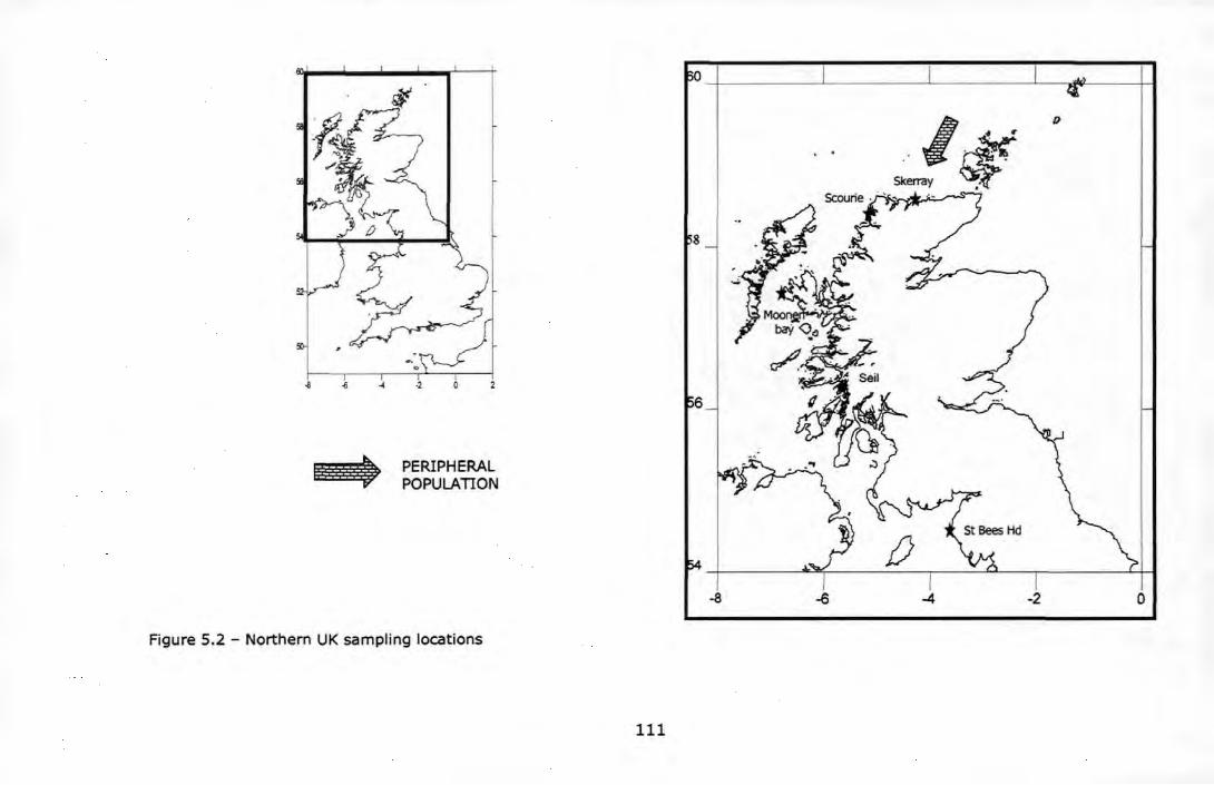
PERIPHERAL POPULATION

Figure 5.2 - Northern UK sampling locations

111

8

6

.. 1¥ Skerray ~

/}

Scourie . · -~~~~E.J~.::__,.-.-

-2 0

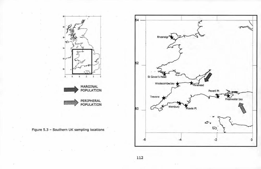
MARGINAL POPULATION

Figure 5.3 - Southern UK sampling locations

2

0

-6

112

Rhosneigr

Trevone

\ .. ,.

-4 -2 0

Table 5.1 - Sampling locations, sites used in the genetic analysis, geographical area, site abbreviations and geographical coordinates

Sampling Site Area Abbreviation Geographical location coordinates

Skerray 2 Scotland Sk2 4.28 w 58.54 N Scourie 2 Scotland Sc2 5.16 w 58.40 N Moonen Bay 1 Isle of Skye Mol 6.79 w 57.42 N Moonen Bay 3 Isle of Skye Mo3 6.79W 57.42 N Sell 1 Isle of Seil Sel 5.64W 56.27 N Sell 3 Isle of Sell Se3 5.64W 56.27 N St Bees 2 Cumbria Be2 3.62 w 54.51 N Rhosneiqr 2 Isle of Anglesey Rh2 4.53 w 53.23 N St Govan's Head 2 Pembrokeshire Go2 4.94W 51.60 N Minehead 1 Somerset Mil 3.43 w 51.21 N Woolacombe 2 Devon Wo2 4.21 w 51.17 N Trevone 2 Cornwall Tr2 4.99W 50.54 N Wemburv 2 Devon We2 4.09W 50.30 N Prawle Point 1 Devon Prl 3.73 w 50.20 N Prawle Point 3 Devon Pr3 3.73 w 50.20 N Peveril Point 2 Dorset Pe2 1.95 w 50.61 N Freshwater Bay 2 Isle of Wiqht Fr2 1.41 w 50.63 N

Laboratory work Three microsatellites (CM 2/15, CM 4/5 and Cm 5/23) were employed as

molecular markers in this population genetic study. For the specific

methods (e.g. PCR conditions, GeneScan, etc.) please refer to Chapter 3 of

the thesis.

Genetic data analysis

Analysis of MOlecular VAriance (AMOVA) An analysis of molecular variance (Excoffier et al., 1992), implemented in

ARLEQUIN version 3.1 (Excoffier et al., 2005), was carried out to assess the

hierarchical partitioning of genetic variability at the levels of location and of

sites within locations.

113

Genetic variability and Hardy-Weinberg equilibrium Genetic diversity within population was estimated calculating: the number

of alleles per locus (NA) and the allelic richness (A) using F-STAT version

2.9.3 (Goudet, 2001), the allele frequencies (FA), and the observed (Ho)

and Nei's 1987 unbiased expected heterozygosity (He) using GENETIX

software package version 4.03 (Belkhir et al., 2004).

Single and' multilocus F15 were estimated using Weir and Cockerham's

(1984) fixation index. Departures from Hardy-Weinberg equilibrium (HWE)

were tested using Fisher's exact test, using the null hypothesis Ho = no

heterozygote deficiency, with the level of significance determined by

Markov-chain randomization ( 10,000 dememorizatlons, 100 batches and

5,000 iterations per batch) using GENEPOP version 4.0 (Rousset, 2008).

Significance levels for multiple comparisons of loci across samples were

adjusted using a standard Bonferroni correction (Rice, 1989).

Tests for linkage disequilibrium (LD) were performed at all loci in each

population and for each locus pair across all populations using GENEPOP;

estimation of exact probability values was by Markov-chain randomization

(1,000,000 dememorizations, 1,000 batches and 50,000 iterations per

batch).

Population structure The level of population genetic differentiation was assessed using Weir and

Cockerham's (1984) estimators of F-statistics (Frr or F and Fsr or 8)

calculated with the software F-STAT version 2.9.3 (Goudet, 2001).

Variances of F-statistic estimators were obtained by jack-knifing over all

populations according to Weir (1990). The 95% confidence interval was

114

calculated by bootstrapping over the loci with 1,000 pseudoreplicates using

the software GENETIX.

The analogue rho of the Rsr of Slatkin (1995) was assessed using the

computer program RSTCALC (Goodman, 1997). Pairwise Fsr, 8 (Weir and

Cockerham, 1984) and Rsr (Siatkin, 1995) estimates were calculated using

the software package MICROSAT version 1.5 (Minch et al., 1996).

Global genetic differentiation per locus over all populations was tested with

G tests (Goudet et al., 1996) using GENEPOP, and for each pair of

populations with Fsr permutation tests (10000 permutations), as

implemented in ARLEQUIN version 3.1 (Excoffier et al., 2005).

The level of differentiation among populations was also estimated by means

of genetic distance measures: Nei's (1978) distance and (B1J)2 (Goldstein et

al., 1995), the last one specific for microsatellites. Genetic distance

matrices were calculated using MICROSAT.

In order to provide a graphical representation of the relationships among

populations, as characterised by the pairwise Fsr, 8 (Weir and Cockerham,

1984) estimates and by the genetic distance matrices (Nei, 1978), samples

were ordinated in a bidimensional space by means of non-metric

multidimensional scaling (nMDS, Lessa, 1990). nMDS analysis was

performed using the software STATISTICA version 6.1 (Statsoft Inc., 1997).

A phylogenetic tree of samples was constructed using the UPGMA method

implemented in the software package PHYLIP version 3.68 (Felsenstein,

115

2005). The Seqboot subprogram was used to produce a large number of

bootstrapped data sets (10,000 replicates). The distance matrices (Cavalli­

Sforza and Edwards, 1967) of the multiple datasets were calculated with the

subprogram Genedist The UPGMA trees were constructed with the Neighbor

subprogram and a majority rule consensus tree, following the method of

Margush and McMorris (1981), was assessed by the subprogram Consense.

Isolation by distance Mantel tests of correlations between genetic and geographical distance

matrices, were implemented in the Isolation by Distance Web Service 3.11

(IBDWS) (Jensen et al. 2005). The geographical distances were calculated

considering the minimal distance around the coast. The tests were

conducted using two sets of parameters, Fsr and Nei (1978), in order to

explore whether genetic distances were better correlated than Fsr with

geographical distances.

116

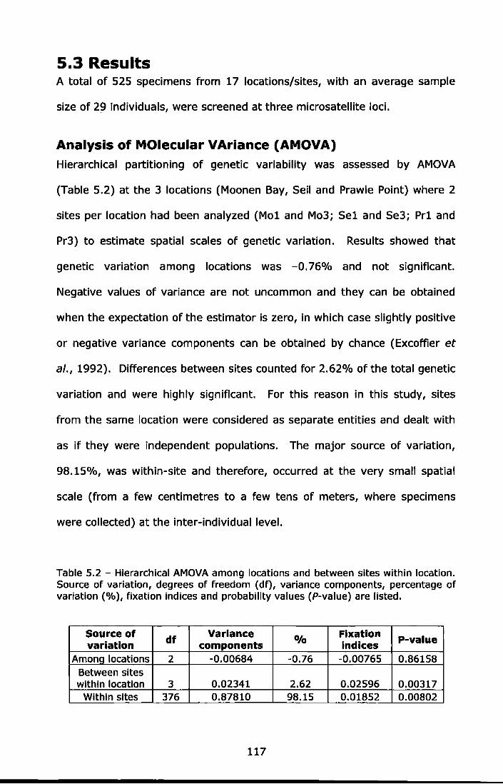
5.3 Results A total of 525 specimens from 17 locations/sites, with an average sample

size of 29 Individuals, were screened at three microsatellite loci.

Analysis of MOlecular VAriance (AMOVA) Hierarchical partitioning of genetic variability was assessed by AMOVA

(Table 5.2} at the 3 locations (Moonen Bay, Seil and Prawle Point) where 2

sites per location had been analyzed (Mol and Mo3; Sel and Se3; Prl and

Pr3) to estimate spatial scales of genetic variation. Results showed that

genetic variation among locations was -0.76% and not significant.

Negative values of variance are not uncommon and they can be obtained

when the expectation of the estimator is zero, in which case slightly positive

or negative variance components can be obtained by chance (Excoffier et

al., 1992). Differences between sites counted for 2.62% of the total genetic

variation and were highly significant. For this reason in this study, sites

from the same location were considered as separate entities and dealt with

as if they were independent populations. The major source of variation,

98.15%, was within-site and therefore, occurred at the very small spatial

scale (from a few centimetres to a few tens of meters, where specimens

were collected) at the inter-individual level.

Table 5.2 - Hierarchical AMOVA among locations and between sites within location. Source of variation, degrees of freedom (df), variance components, percentage of variation (%), fixation indices and probability values (P-value) are listed.

Source of df Variance Ofo

Fixation P-value variation components Indices Among locations 2 -0.00684 -0.76 -0.00765 0.86158

Between sites within location 3 0.02341 2.62 0.02596 0.00317

Within sites 376 0.87810 98.15 0.01852 0.00802

117

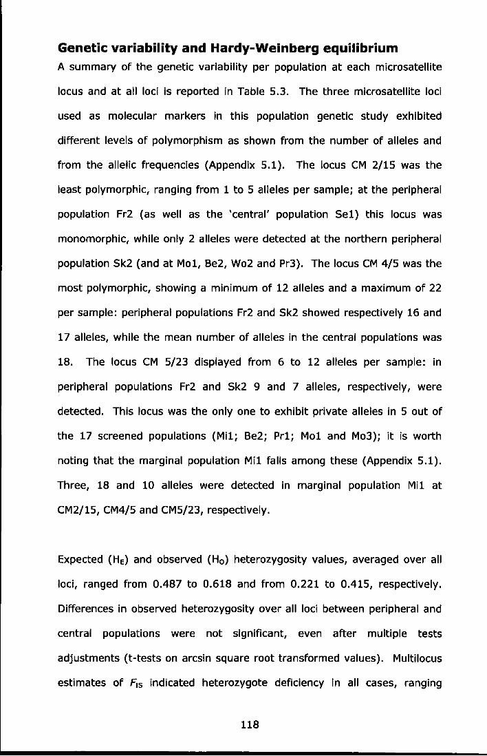
Genetic variability and Hardy-Weinberg equilibrium A summary of the genetic variability per population at each microsatellite

locus and at all loci is reported in Table 5.3. The three microsatellite loci

used as molecular markers in this population genetic study exhibited

different levels of polymorphism as shown from the number of alleles and

from the allelic frequencies (Appendix 5.1). The locus CM 2/15 was the

least polymorphic, ranging from 1 to 5 alleles per sample; at the peripheral

population Fr2 (as well as the 'central' population Sel) this locus was

monomorphic, while only 2 alleles were detected at the northern peripheral

population Sk2 (and at Mol, Be2, Wo2 and Pr3). The locus CM 4/5 was the

most polymorphic, showing a minimum of 12 alleles and a maximum of 22

per sample: peripheral populations Fr2 and Sk2 showed respectively 16 and

17 alleles, while the mean number of alleles in the central populations was

18. The locus CM 5/23 displayed from 6 to 12 alleles per sample: in

peripheral populations Fr2 and Sk2 9 and 7 alleles, respectively, were

detected. This locus was the only one to exhibit private alleles in 5 out of

the 17 screened populations (Mil; Be2; Prl; Mol and Mo3); it is worth

noting that the marginal population Mil falls among these (Appendix 5.1).

Three, 18 and 10 alleles were detected in marginal population Mil at

CM2/15, CM4/5 and CM5/23, respectively.

Expected {HE) and observed (Ho) heterozygosity values, averaged over all

loci, ranged from 0.487 to 0.618 and from 0.221 to 0.415, respectively.

Differences in observed heterozygosity over all loci between peripheral and

central populations were not significant, even after multiple tests

adjustments (t-tests on arcsin square root transformed values). Multilocus

estimates of F1s indicated heterozygote deficiency in all cases, ranging

118

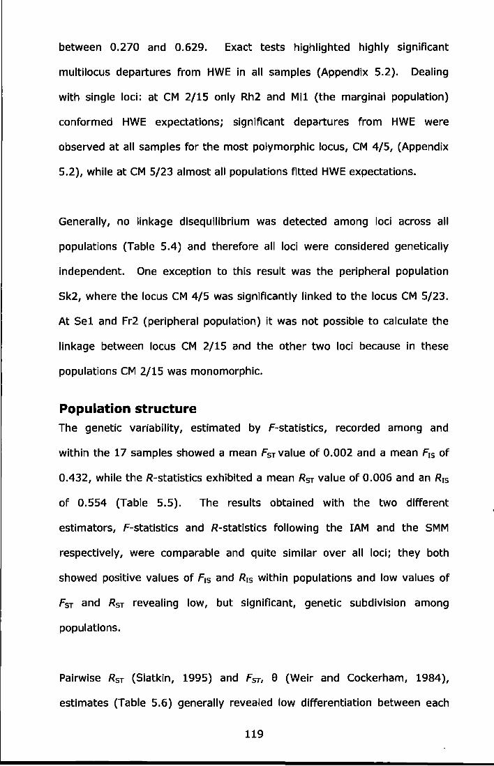
between 0.270 and 0.629. Exact tests highlighted highly significant

multilocus departures from HWE in all samples (Appendix 5.2). Dealing

with single loci: at CM 2/15 only Rh2 and Ml1 (the marginal population)

conformed HWE expectations; significant departures from HWE were

observed at all samples for the most polymorphic locus, CM 4/5, (Appendix

5.2), while at CM 5/23 almost all populations fitted HWE expectations.

Generally, no linkage disequilibrium was detected among loci across all

populations (Table 5.4) and therefore all loci were considered genetically

independent. One exception to this result was the peripheral population

Sk2, where the locus CM 4/5 was significantly linked to the locus CM 5/23.

At Se1 and Fr2 (peripheral population) it was not possible to calculate the

linkage between locus CM 2/15 and the other two loci because in these

populations CM 2/15 was monomorphic.

Population structure The genetic variability, estimated by F-statistics, recorded among and

within the 17 samples showed a mean Fsr value of 0.002 and a mean F15 of

0.432, while the R-statistics exhibited a mean Rsr value of 0.006 and an R15

of 0.554 (Table 5.5). The results obtained with the two different

estimators, F-statlstlcs and R-statistics following the lAM and the SMM

respectively, were comparable and quite similar over all loci; they both

showed positive values of F1s and R1s within populations and low values of

Fsr and Rsr revealing low, but significant, genetic subdivision among

populations.

Pairwise Rsr (Siatkin, 1995) and Fsr, 9 (Weir and Cockerham, 1984),

estimates (Table 5.6) generally revealed low differentiation between each

119

pair of populations, but some comparisons were significant, as assessed

with FST permutation tests (10,000 permutations). A graphical

representation of the relationships among populations, as reported in

pairwise F5r, 8 (Weir and Cockerham, 1984} was provided by the nMDS

(Lessa, 1990) (Figure 5.4). The bi-dimensional distribution of populations

showed that the peripheral populations Sk2 and Fr2 were separated from

the others (and from each other), while the marginal population Mil was

close to the central populations.

Matrices of Nei's genetic distance (1978) and (o1J)2 (Goldstein et al., 1995),

are shown in Table 5. 7. The nMDS plot (Lessa, 1990), built using the

genetic distance matrix (Nei, 1978), provided a graphical representation of

the relationship among populations (Figure 5.5). This result confirmed that

previously obtained with pairwise Fsr estimates: peripheral populations, Sk2

and Fr2, were far from the others, while the marginal population Mi1 was

located near the central populations.

The UPGMA phylogenetic tree (Figure 5.6), constructed using a large

number of bootstrapped data sets (10,000 replicates), based on distance

matrices (Cavalli-Sforza and Edwards, 1967}, supported the idea that

peripheral populations were genetically differentiated from central ones. It

showed that the northern peripheral population Sk2 was split from the

others and that Fr2, the eastern peripheral one, was clustered with the

marginal population Mi1 and separated from the other samples; it has to be

said that bootstrap support at the relevant nodes was quite low suggesting

a cautious approach to the interpretation of these results.

120

Isolation by distance Mantel tests, conducted using two sets of genetic distances, Fsr and Nei

(1978), were not significant. The reduced major axis regression calculated

using Fsr showed r=0.105 and P-value=0.153 (Figure 5. 7) and the one

estimated using Nei (1978) exhibited r=0.113 and P-value=0.115 (Figure

5.8}.

121

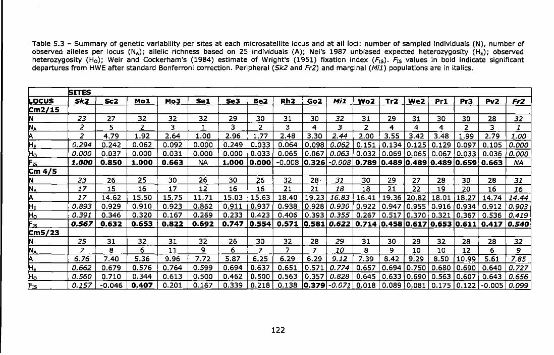
Table 5.3 -Summary of genetic variability per sites at each microsatellite locus and at all loci: number of sampled individuals (N), number of observed alleles per locus (NA)i allelic richness based on 25 individuals (A); Nei's 1987 unbiased expected heterozygosity (He); observed heterozygosity (H0 ); Weir and Cockerham's (1984) estimate of Wright's (1951) fixation index (F15). F15 values in bold indicate significant departures from HWE after standard Bonferroni correction. Peripheral (Sk2 and Fr2) and marginal (Mi1) populations are in italics.

!siTES LOCUS Sk2 Sc2 Mol Mo3 Sel Se3 Be2 Rh2 Go2 Mil Wo2 Tr2 We2 Prl Pr3 Pv2 Fr2 Cm2/15 N 23 27 32 32 32 29 30 31 30 32 31 29 31 30 30 28 32 NA 2 5 2 3 1 3 2 3 4 3 2 4 4 4 2 3 1 A 2 4.79 1.92 2.64 1.00 2.96 1.77 2.48 3.30 2.44 2.00 3.55 3.42 3.48 1.99 2.79 1.00 He 0.294 0.242 0.062 0.092 0.000 0.249 0.033 0.064 0.098 0.062 0.151 0.134 0.125 0.129 0.097 0.105 0.000 Ho 0.000 0.037 0.000 0.031 0.000 0.000 0.033 0.065 0.067 0.063 0.032 0.069 0.065 0.067 0.033 0.036 0.000 F1s 1.000 0.850 1.000 0.663 NA 1.000 0.000 -0.008 0.326 -0.008 0.789 0.489 0.489 0.489 0.659 0.663 NA Cm4/5 N 23 26 25 30 26 30 26 32 28· 31 30 29 27 28 30 28 31 NA 17 15 16 17 12 16 16 21 21 18 18 21 22 19 20 16 16 ~ 17 14.62 15.50 15.75 11.71 15.03 15.63 18.40 19.23 16.83 16.41 19.36 20.82 18.01 18.27 14.74 14.44 HF 0.893 0.929 0.910 0.923 0.862 0.911 0.937 0.938 0.928 0.930 0.922 0.947 0.955 0.916 0.934 0.912 0.903 Ho 0.391 0.346 0.320 0.167 0.269 0.233 0.423 0.406 0.393 0.355 0.267 0.517 0.370 0.321 0.367 0.536 0.419 Frs 0.567 0.632 0.653 0.822 0.692 0.747 0.554 0.571 0.581 0.622 0.714 0.458 0.617 0.653 0.611 0.417 0.540 Cm5/23 N 25 31 32 31 32 26 30 32 28 29 31 30 29 32 28 28 32 NA 7 8 6 11 9 6 7 7 7 10 8 9 10 10 12 6 9 A 6.76 7.40 5.36 9.96 7.72 5.87 6.25 6.29 6.29 9.12 7.39 8.42 9.29 8.50 10.99 5.61 7.85 He 0.662 0.679 0.576 0.764 0.599 0.694 0.637 0.651 0.571 0.774 0.657 0.694 0.750 0.680 0.690 0.640 0.727 Ho 0.560 0.710 0.344 0.613 0.500 0.462 0.500 0.563 0.357 0.828 0.645 0.633 0.690 0.563 0.607 0.643 0.656 Frs 0.157 -0.046 0.407 0.201 0.167 0.339 0.218 0.138 0.379 -0.071 0.018 0.089 0.081 0.175 0.122 -0.005 0.099

122

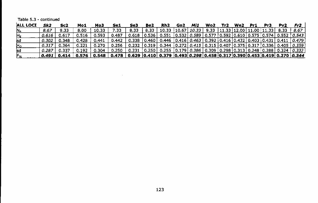
Table 5.3- continued ALL LOCI Sk2 Sc2 Mol Mol Sel Se3 Bel Rh2 Go2 Mil Wo2 Tr2 We2 Prl Pr3 Pv2 Fr2 NA 8.67 9.33 8.00 10.33 7.33 8.33 8.33 10.33 10.67 10.33 9.33 11.33 12.00 11.00 11.33 8.33 8.67 HE 0.616 0.617 0.516 0.593 0.487 0.618 0.536 0.551 0.532 0.589 0.577 0.592 0.610 0.575 0.574 0.552 0.543 sd 0.302 0.348 0.428 0.441 0.442 0.338 0.460 0.446 0.416 0.463 0.392 0.416 0.432 0.403 0.431 0.411 0.479 Ho 0.317 0.364 0.221 0.270 0.256 0.232 0.319 0.344 0.272 0.415 0.315 0.407 0.375 0.317 0.336 0.405 0.359 lsd 0.287 0.337 0.192 0.304 0.250 0.231 0.250 0.255 0.179 0.386 0.309 0.298 0.313 0.248 0.288 0.324 0.332 F1s 0.49l 0.414 0.576 0.548 0.478 0.629 0.410 0.379 0.493 0.298 0.458 0.317 0.390 0.453 0.419 0.270 0.344

123

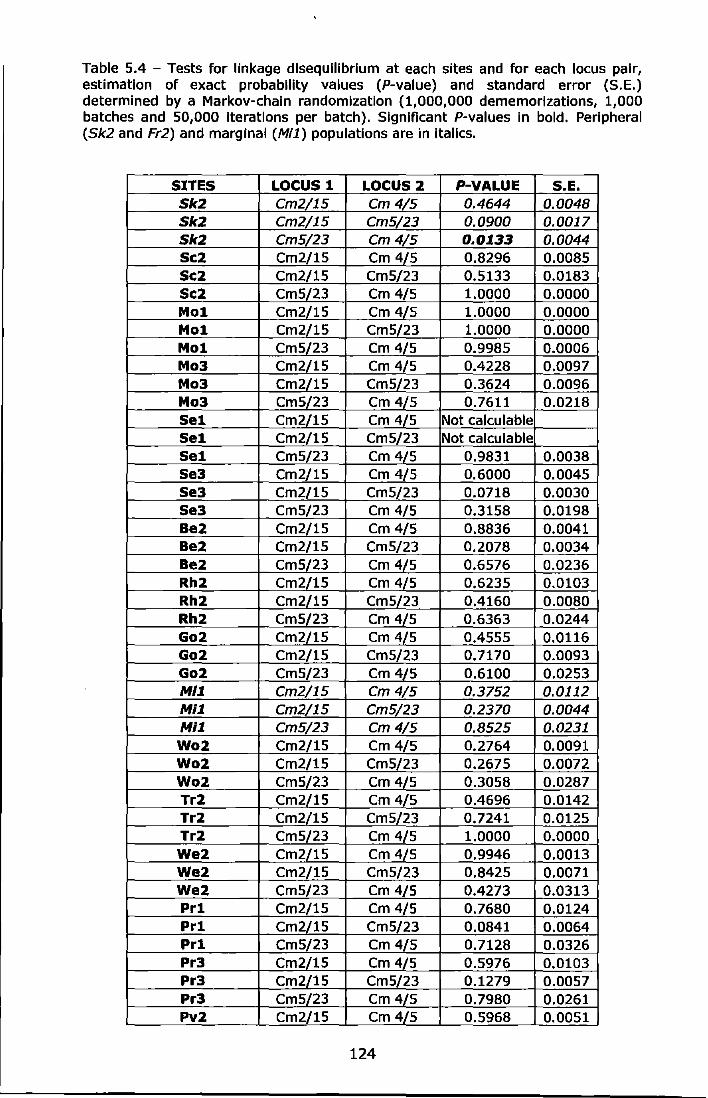
Table 5.4 - Tests for linkage disequilibrium at each sites and for each locus pair, estimation of exact probability values {P-value) and standard error (S.E.) determined by a Markov-chain randomization (1,000,000 dememorlzations, 1,000 batches and 50,000 Iterations per batch). Significant P-values in bold. Peripheral (Sk2 and Fr2) and marginal (Mi1) populations are in Italics.

SITES LOCUS 1 LOCUS 2 P-VALUE S.E. Sk2 Cm2/15 Cm4/5 0.4644 0.0048 Sk2 Cm2/15 Cm5/23 0.0900 0.0017 Sk2 Cm5/23 Cm4/5 0.0.133 0.0044 Sc2 Cm2/15 Cm 4/5 0.8296 0.0085 Sc2 Cm2/15 Cm5/23 0.5133 0.0183 Sc2 Cm5/23 Cm 4/5 1.0000 0.0000 Mol Cm2/15 Cm 4/5 1.0000 0.0000 Mol Cm2/15 Cm5/23 1.0000 0.0000 Mol Cm5[23 Cm 4/5 0.9985 0.0006 Mo3 Cm2/15 Cm 4/5 0.4228 0.0097 Mo3 Cm2/15 Cm5/23 0.3624 0.0096 Mo3 Cm5/23 Cm 4/5 0.7611 0.0218 Sel Cm2/15 cm 4/5 Not calculable Sel Cm2/15 Cm5/23 Not calculable Sel Cm5/23 Cm 4/5 0.9831 0.0038 Se3 Cm2/15 Cm 4/5 0.6000 0.0045 Se3 Cm2/15 Cm5/23 0.0718 0.0030 Se3 Cm5/23 Cm 4/5 0.3158 0.0198 Be2 Cm2/15 cm 4/5 0.8836 0.0041 Be2 Cm2/15 Cm5/23 0.2078 0.0034 Be2 Cm5/23 Cm 4/5 0.6576 0.0236 Rh2 Cm2/15 Cm 4/5 0.6235 0.0103 Rh2 Cm2/15 Cm5/23 0.4160 0.0080 Rh2 Cm5/23 Cm 4/5 0.6363 0.0244 Go2 Cm2/15 Cm 4/5 0.4555 0.0116 Go2 Cm2/15 Cm5/23 0.7170 0.0093 Go2 Cm5/23 Cm 4/5 0.6100 0.0253 M/.1 Cm2/15 Cm4/5 0.3752 0.0112 M/.1 Cm2/15 Cm5/23 0.2370 0.0044 Mi.1 Cm5/23 Cm4/5 0.8525 0.0231 Wo2 Cm2/15 Cm 4/5 0.2764 0.0091 Wo2 Cm2/15 Cm5/23 0.2675 0.0072 Wo2 Cm5/23 Cm 4/5 0.3058 0.0287 Tr2 Cm2/15 Cm 4/5 0.4696 0.0142 Tr2 Cm2/15 Cm5/23 0.7241 0.0125 Tr2 Cm5/23 Cm 4/5 1.0000 0.0000 We2 Cm2/15 Cm 4/5 0.9946 0.0013 We2 Cm2/15 Cm5/23 0.8425 0.0071 We2 Cm5/23 Cm 4/5 0.4273 0.0313 Prl Cm2/15 Cm 4/5 0.7680 0.0124 Prl Cm2/15 Cm5/23 0.0841 0.0064 Prl Cm5/23 Cm 4/5 0.7128 0.0326 Pr3 Cm2/15 Cm 4/5 0.5976 0.0103 Pr3 Cm2/15 Cm5/23 0.1279 0.0057 Pr3 Cm5/23 Cm 4/5 0.7980 0.0261 Pv2 Cm2/15 cm 4/5 0.5968 0.0051

124

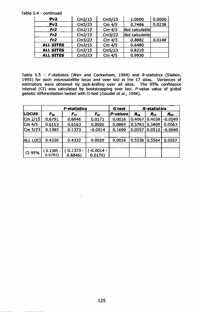
Table 5.4 - continued

Pv2 Cm2j_15 Cm5/23 1.0000 0.0000 Pv2 Cm5/23 Cm 4/5 0.7466 0.0238 Fr2 Cm2/15 Cm4/5 Not calculable Fr2 Cm2/15 Cm5/23 Not calculable Fr2 Cm5/23 Cm4/5 0.8881 0.0148

ALL SITES Cm2/15 Cm 4/5 0.6480 ALL SITES Cm2/15 Cm5/23 0.8210 ALL SITES Cm5/23 Cm 4/5 0.9930

Table 5.5 - F-statistics (Weir and Cockerham, 1984) and R-statistics (Siatkin, 1995) for each microsatelllte locus and over loci in the 17 sites. Variances of estimators were obtained by jack-knifing over all sites. The 95% confidence interval (Cl) was calculated by bootstrapping over loci. P-value value of global genetic differentiation tested with G-test (Goudet et al., 1996).

F-statistics Gtest R-statlstics LOCUS FJS Frr FsT P..values R1s Rrr RST Cm 2/15 0.6791 0.6846 0.0171 0.0016 0.4067 0.4038 -0.0049 Cm 4/5 0.6153 0.6163 0.0026 0.0864 0.5783 0.5809 0.0063 Cm 5/23 0.1385 0.1373 -0.0014 0.1690 0.0557 0.0510 -0.0049

ALL LOCI 0.4320 0.4332 0.0020 0.0016 0.5538 0.5564 0.0057

Cl 95% ( 0.1385- ( 0.1373- (-0.0014-0.6791) 0.6846) 0.0170)

125

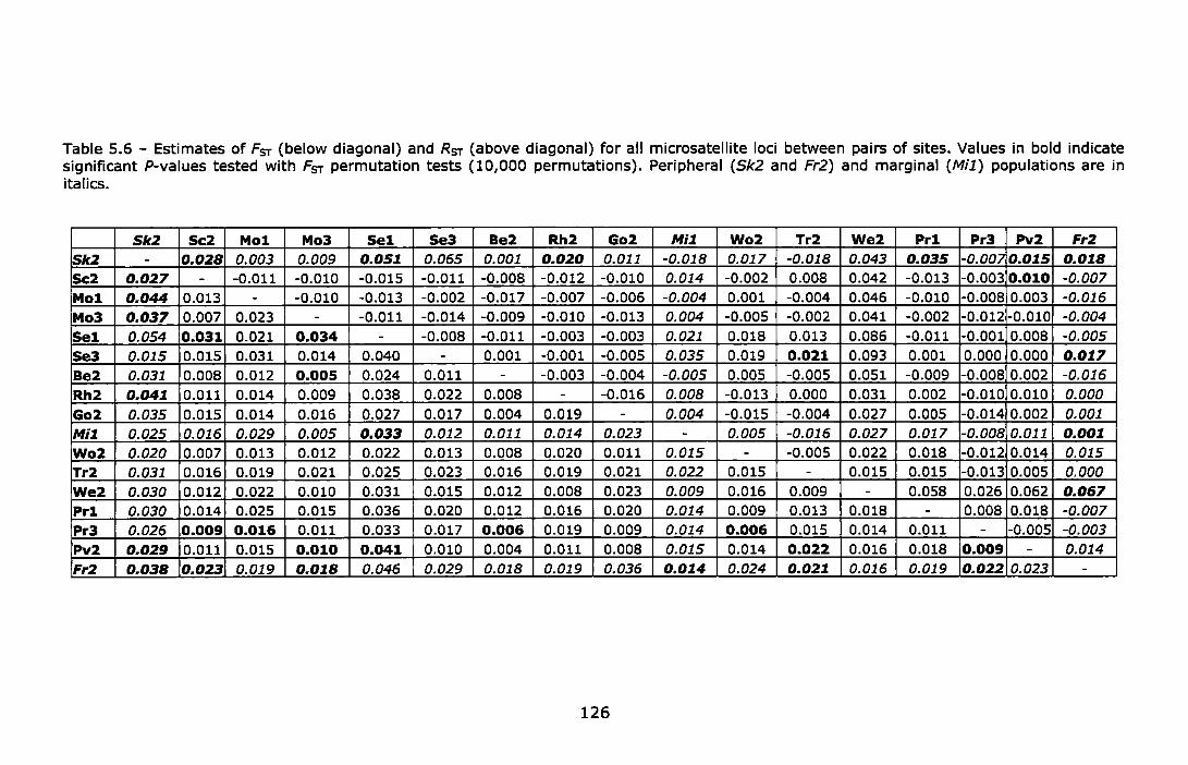
Table 5.6 - Estimates of Fsr (below diagonal) and Rsr (above diagonal) for all microsatellite loci between pairs of sites. Values in bold indicate significant P-values tested with Fsr permutation tests (10,000 permutations). Peripheral (Sk2 and Fr2) and marginal (Mil) populations are in italics.

Sk2 Sc2 Mol Mo3 Sel Se3 Be2 Rh2 Go2 Mil Wo2 Tr2 We2 Prl Pr3 Pv2 Fr2 Sk2 - 0.028 0.003 0.009 0.051 0.065 0.001 0.020 0.011 -0.018 0.017 -0.018 0.043 0.035 -0.00-, 0.015 0.018 Sc2 0.027 - -0.011 -0.010 -0.015 -0.011 -0.008 -0.012 -0.010 0.014 -0.002 0.008 0.042 -0.013 -0.003 0.010 -0.007

Mol 0.044 0.013 - -0.010 -0.013 -0.002 -0.017 -0.007 -0.006 -0.004 0.001 -0.004 0.046 -0.010 -0.008 0.003 -0.016

Mo3 0.037 0.007 0.023 - -0.011 -0.014 -0.009 -0.010 -0.013 0.004 -0.005 -0.002 0.041 -0.002 -0.012 -0.010 -0.004

Sel 0.054 0.031 0.021 0.034 - -0.008 -0.011 -0.003 -0.003 0.021 0.018 0.013 0.086 -0.011 -0.001 0.008 -0.005

Se3 0.015 0.015 0.031 0.014 0.040 - 0.001 -0.001 -0.005 0.035 0.019 0.021 0.093 0.001 0.000 0.000 0.017 Be2 0.031 0.008 0.012 0.005 0.024 0.011 - -0.003 -0.004 -0.005 0.005 -0.005 0.051 -0.009 -0.008 0.002 -0.016

Rh2 0.041 0.011 0.014 0.009 0.038 0.022 0.008 - -0.016 0.008 -0.013 0.000 0.031 0.002 -0.010 0.010 0.000

Go2 0.035 0.015 0.014 0.016 0.027 0.017 0.004 0.019 - 0.004 -0.015 -0.004 0.027 0.005 -0.014 0.002 0.001 Mi1 0.025 0.016 0.029 0.005 0.033 0.012 0.011 0.014 0.023 - 0.005 -0.016 0.027 0.017 -0.008 0.011 0.001 Wo2 0.020 0.007 0.013 0.012 0.022 0.013 0.008 0.020 0.011 0.015 - -0.005 0.022 0.018 -0.012 0.014 0.015 Tr2 0.031 0.016 0.019 0.021 0.025 0.023 0.016 0.019 0.021 0.022 0.015 - 0.015 0.015 -0.013 0.005 0.000

We2 0.030 0.012 0.022 0.010 0.031 0.015 0.012 0.008 0.023 0.009 0.016 0.009 - 0.058 0.026 0.062 0.067 Prl 0.030 0.014 0.025 0.015 0.036 0.020 0.012 0.016 0.020 0.014 0.009 0.013 0.018 - 0.008 0.018 -0.007

Pr3 0.026 0.009 0.016 0.011 0.033 0.017 0.006 0.019 0.009 0.014 0.006 0.015 0.014 0.011 - -0.005 -0.003

Pv2 0.029 0.011 0.015 0.010 0.041 0.010 0.004 0.011 0.008 0.015 0.014 0.022 0.016 0.018 0.009 - 0.014

Fr2 0.038 0.023 0.019 0.018 0.046 0.029 0.018 0.019 0.036 0.014 0.024 0.021 0.016 0.019 0.022 0.023 -

126

Table 5.7- Pairwise genetic distances. Nei (1978) values are below the diagonal and (OIJ)2 values are above the diagonal. Peripheral (Sk2 and Fr2) and marginal (Mi1) populations are in italics.

Sk2 Sc2 Mol Mo3 Sel Se3 Be2 Rh2 Go2 Mil Wo2 Tr2 We2 Prl Pr3 Pv2 Fr2 isk2 - 2.500 1.994 3.114 4.805 4.805 2.002 0.829 0.860 0.006 0.227 0.006 3.348 3.533 0.585 5.543 1.398 Sc2 0.028 - 0.066 0.053 0.388 0.388 0.083 0.495 0.486 2.277 1.473 2.547 11.127 0.132 0.694 0.711 0.186 Mol 0.039 -0.001 - 0.156 0.638 0.638 0.002 0.371 0.372 1.787 1.206 2.062 10.284 0.222 0.486 0.935 0.054 Mo3 0.043 -0.003 0.014 - 0.185 0.185 0.168 0.808 0.786 2.866 1.977 3.170 12.475 0.068 1.026 0.388 0.371 Sel 0.045 0.017 0.012 0.024 - 0.168 0.159 0.888 0.875 2.959 2.102 3.291 12.755 0.019 1.115 0.372 0.381 Se3 0.009 0.010 0.021 0.008 0.000 - 0.650 1.740 1.709 4.493 3.343 4.877 15.630 0 . .146 2.076 0.088 1.048 Be2 0.024 -0.007 0.003 -0.006 0.014 -0.003 - 0.398 0.399 1.794 1.238 2.076 10.344 0.224 0.504 0.931 0.058 Rh2 0.042 0.000 0.006 0.000 0.031 0.016 -0.001 - 0.002 0.715 0.260 0.835 6.941 1.089 0.033 2.299 0.169 Go2 0.030 0.003 0.005 0.007 0.018 0.006 -0.005 0.013 - 0.747 0.272 0.862 7.007 1.084 0.035 2.254 0.176 Mil 0.022 0.011 0.023 -0.006 0.022 0.005 0.001 0.006 0.016 - 0.192 0.019 3.631 3.254 0.489 5.208 1.225 Wo2 0.013 -0.004 0.003 0.004 0.010 0.004 -0.002 0.015 0.002 0.009 - 0.205 4.521 2.397 0.171 4.072 0.769 Tr2 0.032 0.010 0.009 0.018 0.012 0.021 0.007 0.013 0.014 0.019 0.008 - 3.212 3.620 0.597 5.639 1.455 We2 0.033 0.004 0.011 0.002 0.018 0.010 0.001 -0.004 0.015 0.000 0.010 0.000 - 13.410 6.383 17.149 8.860 Prl 0.029 0.007 0.017 0.009 0.027 0.015 0.003 0.010 0.013 0.008 0.001 0.006 0.013 - 1.337 0.330 0.486 Pr3 0.023 -0.001 0.006 0.003 0.023 0.010 -0.005 0.014 -0.001 0.007 -0.004 0.008 0.007 0.003 - 2.610 0.232 Pv2 0.024 0.000 0.006 0.001 0.034 -0.001 -0.006 0.003 -0.001 0.007 0.007 0.017 0.008 0.012 0.000 - 1.432 Fr2 0.036 0.015 0.012 0.011 0.040 0.025 0.012 0.013 0.033 0.006 0.020 0.016 0.008 0.013 0.016 0.018 -

127

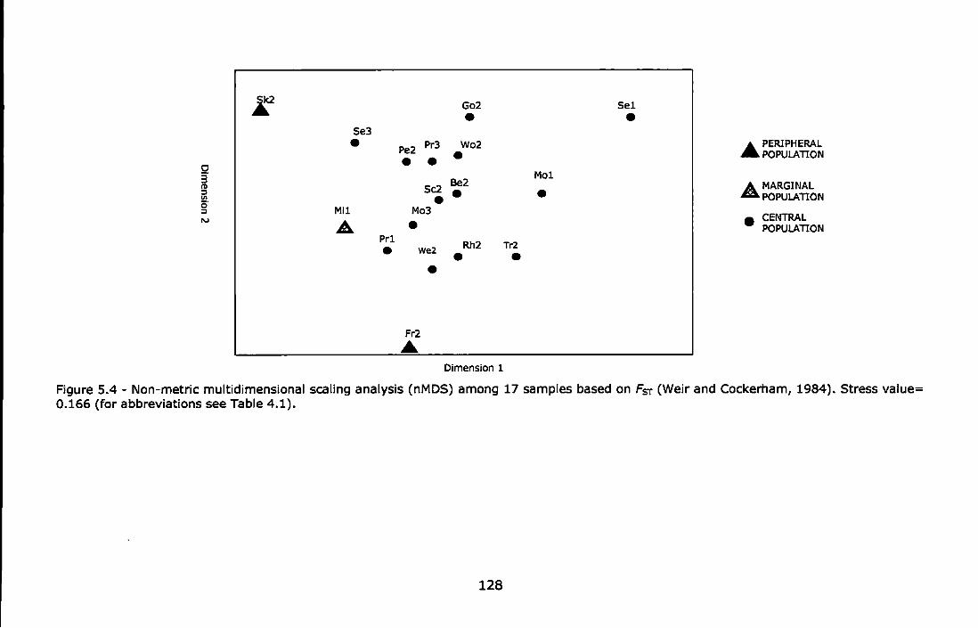
r Go2 Sel

• • Se3

• Pr3 Wo2 .... PERIPHERAL Pe2 • POPULATION c • • 3 Be2

Mol (I) Sc2 A MARGINAL :::1 • • U> • POPULATION 0 :::1 Mll Mo3

"' A • • CENTRAL POPULATION

Prl Rh2 Tr2 • we2 • • •

Fr2 ... Dimension 1

Figure 5.4 - Non-metric multidimensional scaling analysis (nMDS) among 17 samples based on Fsr (Weir and Cockerham, 1984). Stress value= 0.166 (for abbreviations see Table 4.1).

128

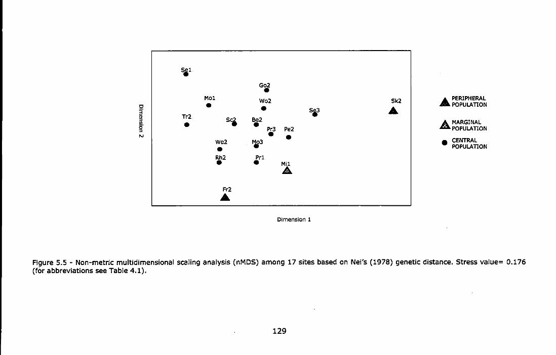
5,1

Go2 • Mol Wo2 51<2 A. PERIPHERAL

c • • A. POPULATION

3 5,3

"' Tr2. :::1 5cj Be2 A MARGINAL Ul • • 0 :::1 Pr3 Pe2 POPULATION N • • We2 rr3

• CENTRAL

• POPULATION

Rh2 Prl • • Mil

A

Fr2 .... Dimension 1

Figure 5.5- Non-metric multidimensional scaling analysis (nMDS) among 17 sites based on Nei's (1978) genetic distance. Stress value= 0.176 (for abbreviations see Table 4.1).

129

34

-

481 I

22 48 r l

34 I

29 1

34

22 I 70 I

I 22 66 I

511 I

34

I 59 I

0.012 0.008 0.004 0.000

Fr2

Mil

Be2

Mo3

Go2

Prl

Pr3

Rh2

We2

Pe2

Se3 Mol

Wo2

Sc2

Tr2

Sel Sk2

Figure 5.6 - UPGMA consensus tree based on Cavalli-Sforza and Edwards (1967) genetic distances; bootstrap (10,000 replicates) percentages are shown at nodes (for abbreviations see Table 4.1). Peripheral and marginal populations are in italics.

130

0.048

~ 0.036

:!1i ~ 0.030 ii <: c; 0.024

0.006

0

0

0

oO 0

0 00

0

0 0

o.oao+-+--+--f------!1--l--+--+--+--+-~ -1000 -400 199 799 1399 1999

Geographic Distance

Figure 5.7 - Reduced major axis regression showing relationship between genetic and geographical distances for all 17 sites. Genetic distances based on Fsr (r=O.lOS; P-value=0.1530).

131

-400

00

0

0

0

0 0

0

199 799 Geographic Distance

0

1399 1999

Figure 5.8 - Reduced major axis regression showing relationship between genetic and geographical distances for all 17 sites. Genetic distances based on Nei (1978) (r=0.113; P-value=O.llS).

132

5.4 Discussion In this study the population genetic structure of the barnacle Chthamalus

montagui was investigated over its whole distribution range in the UK, by

analysing specimens from 17 locations/sites using three microsatellite

markers. The aim was to assess the contribution of peripheral and marginal

populations to the genetic diversity of the species.

Initially, spatial scales of genetic variation were investigated by analysing 2

sites from each of 3 locations. AMOVA results showed that differences

among locations were not significant, while among sites within locations

differences were still relatively small (2.62% of total variation) but

significant, suggesting that, for the analysed loci, barnacle samples showed

detectable differences over a distance of just a few hundred meters. An

explanation for this could relate to the limited sample of the genome, three

microsatellite loci, that was tested. A wider screening of the genome could

provide a different pattern and possibly highlight similarities between sites

of the same location. The major source of genetic variation (98.15%),

instead, lays among individuals within sites therefore at a very small spatial

scale (the plot of few tens of metres from which specimens were collected).

This is often observed in population genetic studies of marine invertebrates

employing microsatellites, suggesting that the high sensitivity and ability in

detecting genetic variation of these molecular markers could be responsible

for the observed pattern (e.g. Bertozzi, 1995; Costantini et al., 2007; Lind

et al.,.2007; York et al., 2008). Nevertheless, the high genetic variation

detected within sites could be attributed not only to the sensitivity of the

molecular markers employed, but also to the biology and ecology of C.

montagui. Barnacles brood developing embryos within the mantle cavity

133

before releasing larvae that feed and pass through several instars in the

plankton. The released larvae spend a few weeks in the water column

dispersing offshore, before finding a suitable substratum on which to settle,

metamorphose and start the sessile phase. These features make it likely

that barnacles originating from distant parental populations grow next to

each other on the shore and partly explain the large genetic variability

recorded within sites.

It is very important to bear in mind the life history and biology of C.

montagui when focussing attention on ecologically marginal or peripheral

populations. Due to the fact that these are located at the edge of the

species' geographical and ecological distribution, it follows that they have

neighbouring source populations in only one direction along the coast and

as a result potentially receive a reduced amount of larval recruitment and

gene flow.

The results obtained in this study do not disprove the hypothesis that

peripheral populations are less genetically variable than central ones.

Peripheral populations showed a slight lower multilocus mean number of

alleles compared to the central ones. Fr2, the population at the eastern

limit of the species distribution, showed a monomorphic locus (CM 2/15)

and Sk2, the most northerly population, displayed linkage disequilibrium

between the loci CM 4/5 and CM 5/23, a fact that was not recorded in any

other sample. Linkage disequilibrium can be generated for instance by

bottlenecks (Templeton, 2006).

134

Mil, the marginal population, showed a number of alleles similar to the

central populations. Nevertheless, at locus CM 5/23, Mi1 exhibited an

unusual genotype, showing a private allele. However, other populations also

had private alleles at this locus.

Many other studies, carried out on different organisms, already

demonstrated that reduced genetic variation and presence of unusual

genotypes are quite common in peripheral and marginal populations, often

isolated or adapted to exceptional environmental conditions (Lesica and

Allendorf, 1995; Lamml et al., 1999; Schwartz et al., 2003; Johannesson

and Andre, 2006; Lind et al., 2007).

It is worth noting that no significant differences of expected and observed

heterozygosity values over all loci were detected in t-tests between

peripheral and central populations. Expected heterozygosity has been

widely used as a measure of genetic variation, however Allendorf (1986)

compared the effects of bottlenecks on the loss of alleles and on the

reduction in heterozygosity. Population bottlenecks of short duration had

little effect on heterozygosity, but reduced severely the number of alleles

present. Heterozygosity provides a good measure of the capability of a

population to respond to selection immediately following a drastic event.

Nevertheless, the number of alleles is a more important indicator for the

long-term response to selection and survival of populations and species

(AIIendorf, 1986).

Furthermore, multilocus estimates of F1s showed in all cases heterozygote

deficiency, and exact tests highlighted highly significant multilocus

135

departures from HWE in all samples. Heterozygosity deficits have been

frequently observed in marine invertebrates (Zouros and Foltz, 1984;

Gaffney, 1994; Davld et al., 1997; Ayre and Hughes, 2000; Ridgway et al.,

2001; Addison and Hart, 2004; Duran et al., 2004; Le Goff-Vitry et al.,

2004; Andrade and Solferini, 2007; Costantini et al., 2007) including

barnacles (Veliz et al., 2006; York et al., 2008). The most common

explanations for heterozygosity deficiency are: technical factors, such as the

presence of null alleles (Foltz, 1986; Callen et al., 1993), and (or) biological

factors, such as inbreeding or Wahlund effect (Pogson et al., 1995; Duran et

al. 2004; Plutchack et al., 2006; Costantlni et al., 2007).

It is difficult to provide an exact explanation for our findings, probably

technical and biological factors could have mutually contributed. In fact, if

we consider that locus CM 5/23 fitted HWE expectations while the other two

loci did not, it can be suggested that some technical factors could have

affected the two non-fitting loci.

Indices of genetic subdivision among populations, Fsr and Rsr estimators,

showed quite low, but significant, mean values over all loci, revealing slight

genetic differentiation.

Mantel tests conducted using two sets of genetic distances, Fsr and Nei

(1978), to detect isolation by distance were not significant. These results

are probably strictly related to the dispersal capability of the species; in

fact, simulations using the one-dimensional stepping-stone model for

population structure showed that isolation by distance is most obvious when

comparing populations separated by 2-5 times the mean larval dispersal

136

distance (Palumbi, 2003). In our case the most distant populations (Sk2

and Fr2) were separated by nearly 1400 km of coastline that, while larval

dispersal of barnacles in the open sea is in the order of 15-20 km

(Strathmann, 1974; Crisp, 1976), meaning that genetic structuring should

start to occur in samples that were at least 30-75 km distant. Given the

fact that our sampling locations were interspersed at moderate distances

(ranging from 25 to 332 km) along the coast, potentially allowing exchange

of larvae between them, we should expect no genetic isolation at least in

those population pairs that were geographically closer.

In conclusion, the results of this study are broadly consistent with the

hypothesis that peripherality affects the genetic pattern of the barnacle

Chthama/us montagui, in terms of reduced genetic variability and slight

increased differentiation of peripheral populations compared to central ones.

Therefore, peripheral populations could be more sensitive to environmental

pressures, by being less genetically variable and consequently less capable

of coping with environmental changes, and should receive special attention

in blodiversity conservation action plans (Crozier, 1997; Lesica and

Allendorf 1995).

However, it is worth noting that the ability to draw definitive conclusions on

the genetic pattern of barnacles based on the screening of just a few loci is

limited.

Furthermore, it is important to highlight that the choice of molecular marker

to employ seems to be of great importance for investigating loss of genetic

137

variability within a species. In fact, the meta-analysis carried out by

Johannesson and Andre (2006) on 29 species in the Baltic Sea showed that

on average Baltic populations were less genetically variable than Atlantic

ones: it emerged that this pattern was not related to dispersal capability,

generation time of species and taxonomic group of organisms, but that was

strongly related to the type of genetic marker employed (mitochondrial DNA

loci displayed a loss of genetic diversity of about 50% while nuclear ones of

only 10%).

Further investigations on this topic should be carried out using different

markers in order to assess population fitness and to make predictions on

the importance of maintaining genetic diversity within populations (Booy et

a/, 2000).

138

Chapter 6

Spatial scales of genetic variation

in Chthamalus mon,tagui

139

6.1 Introduction and specific aims The origin and maintenance of genetic diversity is a central issue in

evolutionary biology. Managing marine genetic biodiversity requires

detailed information on the spatial scales of population genetic structuring

and differentiation. These scales are a function of the balance between

gene flow, genetic drift, mutation and selection and are therefore strongly

influenced by life history characteristics such as developmental modes

(direct vs planktonic developers), larval dispersal capacity (short- vs long-

lived planktonic larval stages}, breeding systems (asexuality vs selfing vs

outcrossing), etc. Hence, these life-history features, combined with the

niche characteristics and environmental tolerance of marine organisms, will

ultimately shape the geographic patterning of genetic biodiversity in marine

ecosystems and the scales at which this patterning is apparent.

Obviously, the complexity of the interactions between these underlying

factors makes it very difficult to generalize about patterns and scales of

spatial genetic variation in the marine environment or to make predictions

about them. Moreover, understanding these processes in the marine realm

is particularly difficult, as barriers to gene flow are not as obvious as they

can be in the terrestrial environment. It was long expected that

populations of marine species could reach panmixia over a broad

geographical range.

However, historical environmental factors related to habitat, currents and

glaciations (Roy et al. 1996; Wares, 2002) combined with species-specific

traits may play an important role in shaping the pattern of inter- and

140

intraspecific differentiation, although the relative contribution of each one

remains hard to disentangle. These ancestral interactions combined with

present-day environmental patterns are reflected in the biogeographical

realm (Longhurst, 1998) and are the focus of marine phylogeographical

investigations.

As reviewed by Patarnello et al. (2007), there are several documented

examples of phylogeographical breaks in the marine environment. Well

known cases include:

- the Southern Ocean and the formation of the Antarctic Polar Front

(20-30 million years ago (Ma)) (Bargelloni et al., 2000);

- the Equatorial Pacific and Atlantic Oceans and the formation of the

Isthmus of Panama (3.1-3.5 Ma) (Avise, 2000);

- the northern and southern Atlantic Shelf of North America (Cape

Hatteras) where the Labrador Current and Gulf Stream have met on

and off during the Quaternary (Weinberg et al., 2003);

- Cape Canaveral in the Florida Keys (reviewed in Avise, 1992);

- the Indo-Pacific region north and south of the Flores and Java Seas

(Barber et al., 2000);

- the NE Atlantic Ocean and Mediterranean Sea (Patarnello, 2007);

- the Baltic Sea and the North Sea (7500 years ago) (Oisen et al.,

2004).

Results of these studies showed that vicariance, separating the populations

on either side of a given boundary, did not affect the different taxa in the

same way over the same geographical range. Life history characteristics,

e.g. dispersal capabilities, could be responsible for the different patterns, as

141

generally long-dispersed species can overcome geographical barriers. A

homogenizing effect can also be provided by extinction/recolonization

events of a given area. In fact, extinction of one of two lineages followed

by recolonisation by members of the other lineage results in a genetic

homogenization over the entire distribution range of the species.

The NE Atlantic/Mediterranean area, the object of the present study, is a

very young system that has been subjected to rapid changes in

configuration and climate over the last six million years (Peres, 1967; Blanc,

1968). The combination of events such as the opening and closing of the

Strait of Gibraltar, advances and contractions of glaciations during the

Quaternary, and changes in current patterns, quite certainly contributed

towards generating diversity. The present-day Mediterranean biota is

largely the result of colonization, mostly frorh the Atlantic Ocean (Aimada et

al., 2001; Domingues et al., 2005) and to a minor extent from the Red Sea.

In fact, after an isolation and desiccation period that lasted about 0.5

million years, during the 'Messinian salinity crisis' (MSC) (up to 5.33 Ma),

re-flooding of the Mediterranean basin was possible because of the inflow of

Atlantic waters through the newly opened Strait of Gibraltar.

Up to 18% of the world's marine biodiversity, including more than 8500

species of macroscopic organisms, resides in this semi-enclosed basin

(Longhurst, 1998; Bianchi and Morri, 2000). The high biodiversity recorded

in the Mediterranean could partly be the product of the many taxonomical

studies that have focused on this region, but the total diversity is still very

high when considering that the Mediterranean Sea represents only 0.82% of

the surface area and 0.32% of the volume of the world's oceans. In

142

addition, endemic species constitute 28% of the Mediterranean fauna (Fredj

et al., 1992), although this value seems to decrease with increasing depth

(Fredj et al., 1985). Euraphia depressa is an example of a Mediterranean

endemic (Kensler et al., 1965; Crisp et al., 1981}, and is one of only three

intertidal barnacles found in this basin.

The literature provides many instances, in different marine species, of

intraspecific genetic differentiation between the NE Atlantic and

Mediterranean area. Patarnello et al. (2007) reviewed more than 70 papers

revealing patterns of partial or complete genetic isolation between Atlantic

and Mediterranean populations, explored by a variety of molecular markers

(allozymes, mtDNA, microsatellites, etc.), and concluded that there is no

obvious relationship between species' life history and dispersal ability and

the level of genetic differentiation recorded between the two basins.

Genetic structuring of intertidal barnacles in the NE Atlantic and

Mediterranean area has already received some attention. Dando et al.

( 1979) compared, by allozyme studies, the populations of Chthama/us

montagui from the Adriatic and SW England and found that the two differed.

The same authors (1981), still employing electrophoretic analyses,

suggested the existence of "Atlantic" and "Mediterranean" forms of C.

montagui and hypothesised that for this barnacle speciation might be in

progress. In this study they observed a sharp change in

phosphoglucomutase (PGM) allozyme frequency along the SE coast of Spain

and suggested that, during periods of glaciations and interglaciations

associated with marine regression and transgression in the Pleistocene, the

Atlantic and Mediterranean populations of C. montagui became physically

143

separated and then diverged genetically. The maintenance of separation of

the two populations was explained by the presence of opposing coastal

currents leaving long sandy beaches which created a reproductive barrier

between the two populations. These results were confirmed by Pannacciulli

et al. (1997a) in a more comprehensive study employing the same markers

and including samples of C. montagui from most of its geographical range.

Based on differences in allozyme frequencies of PGM and of glutamate­

oxalacetate transaminase (GOT), the authors suggested that the Atlantic

and Mediterranean forms of C. montagui are sibling species and that the

present oceanographic conditions are the main cause for the genetic

separation between the two forms as the Almeria-Oran front restricts larval

dispersion.

Previous works on Chthamalus montagui were extended in this study, by

investigating spatial scales of genetic differentiation of this barnacle species,

with extensive larval dispersal, over its distribution range in the NE Atlantic

and Mediterranean Sea. Six microsatellite loci were used as molecular

markers, these sensitive markers allowed the investigation of fine scale

spatial variation that the previous studies employing allozymes could not

address.

144

6.2 Materials and methods

Sampling Sample collection of Chthamalus montagui specimens was carried out in

different periods:

UK samples were collected in September/October 2002;

- Adriatic Sea samples were collected in February/March 2003;

Samples from Baia, Vigo, Almeria and Molyvos were collected in

August/September 2003.

The 12 sampling locations are shown in Figure 6.1 and listed in Table 6.1.

At 6 locations a single sampling site was analysed. At the remaining 6, two

sites (indicated by the 2 stars) 300-600 m apart were analysed. Thirty-two

individuals were processed per site (although not all individuals were

successfully analysed for each locus).

145

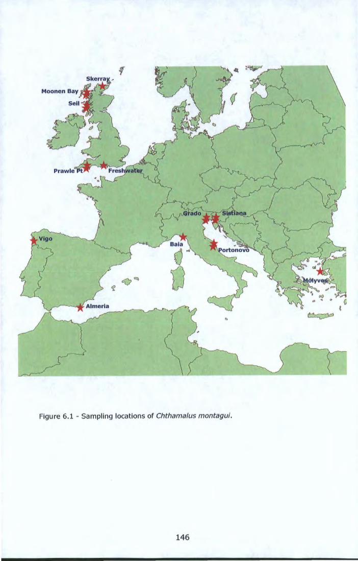
~-~1 /--=--------Figure 6.1 - Sampling locations of Chthamalus montagui.

146

Table 6.1 - Sampling location, site used in the genetic analysis, abbreviation, geographical coordinates and basin of origin.

Sampling Site Abbreviation Geographical Basin location coordinates Skerray 2 Sk2 4.28 w 58.54 N Atlantic Moonen Bay 1 Mol 6.79 w 57.42 N Atlantic Moonen Bay 3 Mo3 6.79 w 57.42 N Atlantic Sell 1 Sel 5.64W 56.27 N Atlantic Sell 3 Se3 5.64W 56.27 N Atlantic Prawle Point 1 Prl 3.73 w 50.20 N Atlantic Prawle Point 3 Pr3 3.73 w 50.20 N Atlantic Freshwater Bay 2 Fr2 1.41 w 50.63 N Atlantic Vi go 1 Vi go 8.99 w 43.28 N Atlantic Almeria 1 Alme 2.19 w 36.72 N Mediterranean Baia Blu 1 Baia 9.89 E 44.08 N Mediterranean Sistiana 1 Sil 13.64 E 45.76 N Mediterranean Sistiana 3 Si3 13.64 E 45.76 N Mediterranean Grado 1 Grl 13.39 E 45.67 N Mediterranean Grado 3 Gr3 13.39 E 45.67 N Mediterranean Portonovo 1 Pol 13.60 E 43.57 N Mediterranean Portonovo 3 Po3 13.60 E 43.57 N Mediterranean Molyvos 1 Moly 26.17 E 39.37 N Mediterranean

Laboratory work Six microsatellites (CM 2/15; CM 4/5; Cm 5/23; CM 4/3; CM 5/18; CM

9/11) were employed as molecular markers in this population genetic study.

For the specific methods (e.g. PCR conditions, GeneScan, etc.) please refer

to Chapter 3 of the thesis.

Genetic data analysis

Genetic variability and Hardy-Weinberg equilibrium Genetic diversity within populations was estimated by calculating: the

number of alleles per locus (NA) and the allelic richness (A) using F-STAT

version 2.9.3 (Goudet, 2001), the allele frequencies (FA), and the observed

(Ho) and Nei's 1987 unbiased expected heterozygosity (He) using GENETIX

software package version 4.03 (Belkhir et al., 2004).

147

Single and multilocus Frs were estimated using Weir and Cockerham's

(1984) fixation index. Departures from Hardy-Weinberg equilibrium (HWE)

were tested using Fisher's exact test, using the null hypothesis Ho = no

heterozygote deficiency, with the level of significance determined by

Markov-chain randomization ( 10,000 dememorizations, 100 batches and

5000 iterations per batch) using GENEPOP version 4.0 (Rousset, 2008).

Significance levels for multiple comparisons of loci across samples were

adjusted using a standard Bonferroni correction (Rice, 1989).

Tests for linkage disequilibrium were performed at all loci in each population

and for each locus pair across all populations using GENEPOP; estimation of

exact probability values was by Markov-chain randomization (10,000

dememorizations, 100 batches and 5,000 iterations per batch).

Population structure The level of population genetic differentiation was assessed using Weir and

Cockerham's ( 1984) estimators of F-statistics (Frr or F and Fsr or 8)

calculated with the software F-STAT version 2.9.3 (Goudet, 2001).

Variances of F-statlstic estimators were . obtained by jack-knifing over all

populations according to Weir (1990). The 95% confidence interval was

calculated by bootstrapping over the loci with 1,000 pseudoreplicates using

the software GENETIX.

The analogue rho of RsT of Slatkin (1995) was assessed using the computer

program RSTCALC (Goodman, 1997). Pairwise Fsr, 8 (Weir and Cockerham,

1984) and RsT (Siatkin, 1995) estimates, were calculated using the software

package MICROSAT version 1.5 (Minch et al., 1996).

148

Global genetic differentiation per locus over all populations was tested with

G tests (Goudet et al., 1996) using GENEPOP, and for each pair of

populations with FsT permutation tests (10,000 permutations), as

implemented in ARLEQUIN version 3.1 (Excoffier et al., 2005).

The levels of differentiation among populations were also estimated by

means of genetic distance measures: Nei's (1978) distance and (o1J)2

(Goldstein et al., 1995), the latter specific for microsatellites. Genetic

distance matrices were calculated using MICROSAT.

In order to provide a graphical representation of the relationships among

populations as characterised by the pairwise Rsr and genetic distance

matrices (Nei, 1978), samples were ordinated in a bidimensional space by

non-metric multidimensional scaling (nMDS, Lessa, 1990). nMDS analysis

was performed using the software STATISTICA version 6.1 (Statsoft Inc.,

1997).

A phylogenetic tree was constructed using the UPGMA method implemented

in the software package PHYLIP version 3.68 (Felsenstein, 2005). The

Seqboot subprogram was used to produce a large number of bootstrapped

data sets (10,000 replicates). The distance matrices (Cavalli-Sforza and

Edwards, 1967) of the multiple datasets were calculated with the

subprogram Genedlst. The UPGMA trees were constructed with the

Neighbor subprogram and a majority rule consensus tree, following the

method of Margush and McMorris (1981), was assessed by the subprogram

Consense.

149

Isolation by distance Mantel tests of correlation between genetic and geographical distance

matrices were implemented in the Isolation by Distance Web Service 3.11

(IBDWS) (Jensen et al. 2005). Nei's (1978) genetic distance was used.

The geographical distances were calculated as the minimal distance around

the coast.

Analysis of MOlecular VAriance (AMOVA) An analysis of molecular variance (Excoffier et al., 1992), implemented in

ARLEQUIN version 3.1 (Excoffier et al., 2005), was carried out to assess the

hierarchical partitioning of genetic variability between basins, among

locations within basins and within locations. For this purpose samples were

divided into two groups, each one representing a basin, according to the

results of the UPGMA phylogenetic tree.

A further AMOVA was carried out as implemented in HIERFSTAT (Goudet,

2005), to allow the assessment of the hierarchical partitioning of genetic

variation at three different levels (ARLEQUIN only allows two). Pairwise FST

estimates and P-values between basins, among locations within basins,

between sites within locations and within sites were calculated.

Moreover, AMOVA was repeated in ARLEQUIN, analysing Atlantic and

Mediterranean datasets separately, and only using data from locations with

two sites, to assess the hierarchical partitioning of genetic variability among

locations and between sites within locations in the two separate basins.

Bayesian clustering analysis Population structure was further Investigated using Bayesian clustering

analysis implemented in STRUCTURE 2.2 (Pritchard et al., 2000). Each

150

individual was assigned to probable common clusters based on the similarity

of their multilocus genotypes at the six microsatellite loci. Mean and

variance of log likelihoods of the number of clusters for K = 1 to K = 18

were Inferred from multilocus genotypes by running STRUCTURE five times

with 1,000,000 repetitions each (burn-in=lOO,OOO iterations) under the

admixture ancestry model and the assumption of correlated allele

frequencies among samples as suggested in Falush et al. (2003}. The mean

membership of each individual described the likelihood of that individual's

belonging to the respective clusters.

6.3 Results A total of 534 specimens from 18 sites, with an average sample size of 30

individuals, were screened at six microsatellite loci.

Genetic variability and Hardy-Weinberg equilibrium A summary of the genetic variability per population at each microsatellite

locus and at all loci is reported in Table 6.2. The six microsatellite loci used

as molecular markers in this population genetic study exhibited different

levels of polymorphism as shown by the number of alleles (NA} or, better,

by the allelic richness (A), which accounts for sample size biases, as well as

by the expected heterozygosity (HE) and the allelic frequencies (Appendix

6.1).

The locus CM 2/15 and the locus CM 5/23 were the least and the most

polymorphic microsatellites, respectively, ranging from 1 to 10 alleles per

sample and 6 to 30 alleles per sample. Allelic richness and expected

heterozygosity at these two loci (Figure 6.2 and 6.3) showed a wide

difference between Atlantic and Mediterranean sites. CM 2/15 was

monomorphic at Fr2 and Se1 and CM 5/23 exhibited its minimum value of A

151

(4.44) at Mol and the maximum (19.77) at Moly. Samples from Alme

showed the lowest values of A (2.805 at CM 2/15 and 8.06 at CM 5/23) and

HE (0.273 at Cm 2/15 and 0.637 at Cm 5/23) amongst the Mediterranean

samples, and were comparable to the Atlantic sites.

The locus CM 4/3, at which A ranged from 2.99 to 11.86 and HE from 0.522

to 0.912, exhibited private alleles in 7 out of the 18 screened populations

(Sk2, Sel, Prl, Fr2, Alme, Bala and Moly); Fr2 showed 4 private alleles at

this locus (Appendix 6.1). The highest A (14.45) and HE (0.943) values at

the locus CM 4/5 were registered in Alme samples and the lowest ones in

Moly (A=5.84; HE=0.624).

A and HE values per site averaged over all loci are shown in Figure 6.4. A

ranged from 8.50 (Sel) to 14.33 (Sil), HE from 0.608 (Sel) to 0.849 (Sil).

Atlantic sites exhibited lower A and HE values compared to the

Mediterranean ones; Alme samples showed the lowest values of the

Mediterranean sites (A=l0.67; HE=0.692).

Observed heterozygosity (Ho) over all loci ranged between 0.262 (SK2) and

0.524 (Baia); among Atlantic samples Prl, Pr3 and Mol showed higher

values compared to the others of 0.387, 0.463 and 0.442, respectively.

Multilocus estimates of F15 were all positive, ranging from 0.314 to 0.629

(Table 6.2). Exact tests revealed highly significant multilocus departures

from HWE in all samples (Appendix 6.2).

Generally no linkage disequilibrium was detected among loci across all

popuiations (Appendix 6.3) and, therefore, all loci were considered

152

genetically independent. Nevertheless, three exceptions to this rule were

registered: CM 5/23 and CM 4/5 were significantly linked in Sk2 samples;

CM 4/5 and CM 5/18 were significantly linked In Mo3 samples; and CM 5/23

and CM 9/11 were significantly linked in Pr3 samples.

Population structure The genetic variability, estimated by F-statistics, recorded among and

within the 18 samples, showed a mean Fsr value of 0.097 and a mean F1s of

0.515, while the R-statistics exhibited a mean Rsr value of 0.390 and an R1s

of 0.438 (Table 6.3). Positive and high values of F1s and R1s indicated deficit

of heterozygosity within populations. The highest Fsr value (0.212) was

registered at the locus CM 2/15 and the highest Rsr value (0.622) was

recorded at locus CM 5/23. The two different estimators, F-statistics and R-

statistics following the lAM and the SMM respectively, revealed genetic

subdivision among populations, as shown by the highly significant P-values

of global genetic differentiation.

Pairwise Rsr (Siatkin, 1995) and Fsr, 9 (Weir and Cockerham, 1984)

estimates (Table 6.4) generally revealed significant differentiation between

each pair of populations, as assessed with Fsr permutation tests (10,000

permutations)

Matrices of Nei's genetic distance (1978) and (o1J) 2 (Goldstein et al., 1995),

are reported in Table 6.5.

Graphical representations of the relationships among populations, as

indicated by palrwise Rsr (Siatkin, 1995) and Nel's genetic distance (1978)

matrices, were provided by the nMDS plots (Lessa, 1990). The bi-

153

dimensional distribution of populatlons based on Rsr (Figure 6.5) showed

three main clusters: 1. Adriatic samples, with Moly very close to them; 2.

most of the Atlantic samples (Sk2, Fr2, Sel, Se3, Mo3 and Vigo), with Alme

very close to them; 3. three Atlantic sites (Prl, Pr3 and Mol). Baia was

located between clusters 1 and 2.

The nMDS plot based on Nei's genetic distance (Figure 6.6) showed the

same three main clusters as noted for Rsr, but Moly was separated from the

Adriatic samples, Alme was placed closer to cluster 3 than cluster 2, and

Baia was no longer between clusters 1 and 2.

The UPGMA phylogenetlc tree (Figure 6. 7), constructed using a large

number of bootstrapped data sets (10,000 replicates) based on distance

matrices (Cavalli-Sforza and Edwards, 1967), showed two main clusters

very well supported by high bootstrap percentages at the nodes: 1.

Mediterranean samples (bootstrap 99%}; 2. Atlantic samples plus Almeria

(bootstrap 88%). A further separation into two sub-clusters was revealed

within cluster 2: as previously observed in the nMDS plots, three sites

among the Atlantic samples (Prl, Pr3 and Mol) were clustered together and

separated from the others; Mol and Mo3 thus appeared in different sub­

clusters. Baia was separated from the other Mediterranean samples within

cluster 1, and the bootstrap percentage at the relevant node was very high

(99%). Moreover, separation between Molyvos and the Adriatic samples

was suggested, but it was not very well supported by the bootstrap

percentage at the node (43%). It is worth noting that within the cluster of

Adriatic samples, the 2 sites within the same location (Sil and Si3; Grl and

Gr3; Pol and Po3) were clustered together.

154

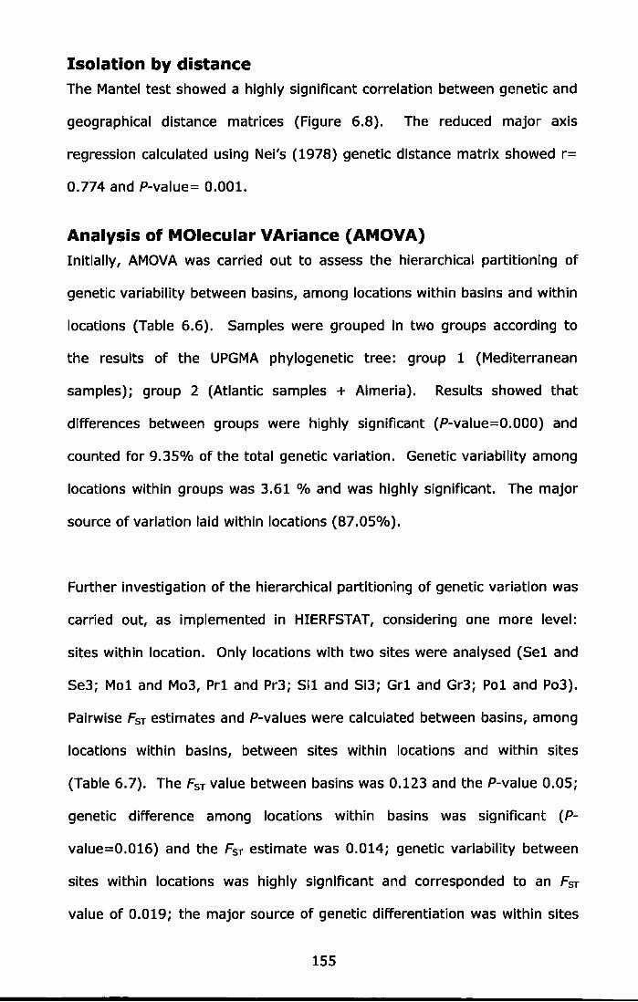
Isolation by distance The Mantel test showed a highly significant correlation between genetic and

geographical distance matrices (Figure 6.8). The reduced major axis

regression calculated using Nei's (1978) genetic distance matrix showed r=

0. 774 and P-value= 0.001.

Analysis of MOlecular VAriance (AMOVA) Initially, AMOVA was carried out to assess the hierarchical partitioning of

genetic variability between basins, among locations within basins and within

locations (Table 6.6). Samples were grouped in two groups according to

the results of the UPGMA phylogenetic tree: group 1 (Mediterranean

samples); group 2 (Atlantic samples + Almeria). Results showed that

differences between groups were highly significant (P-vaiue=O.OOO) and

counted for 9.35% of the total genetic variation. Genetic variability among

locations within groups was 3.61 % and was highly significant. The major

source of variation laid within locations (87.05%).

Further investigation of the hierarchical partitioning of genetic variation was

carried out, as implemented in HIERFSTAT, considering one more level:

sites within location. Only locations with two sites were analysed (Sel and

Se3; Mol and Mo3, Prl and Pr3; Sil and Si3; Grl and Gr3; Pol and Po3).

Pairwise Fsr estimates and P-values were calculated between basins, among

locations within basins, between sites within locations and within sites

(Table 6.7). The Fsr value between basins was 0.123 and the P-value 0.05;

genetic difference among locations within basins was significant (P-

value=0.016) and the Fsr estimate was 0.014; genetic variability between

sites within locations was highly significant and corresponded to an Fsr

value of 0.019; the major source of genetic differentiation was within sites

155

and had an Fsr estimate of 0.454. To further investigate the highly

significant genetic differentiation between sites within locations, AMOVA was

repeated for the Mediterranean and Atlantic locations separately.

Results for the Mediterranean locations (Sistiana, Grade and Portonovo)

showed that genetic variation among locations was not significant (P-

value=0.068) and counted for only 0.94% of the total genetic variability

(Table 6.8). Differences between sites (Sil and Si3; Grl and Gr3; Pol and

Po3) counted for 0.58% of the total genetic variation and were not

significant (P-value=O. 764 ). The major source of variation 98.48% laid

within site and therefore resided in the very small spatial scale (the plot of

few metres from which specimens were collected) at the inter-individual

level.

Results for the Atlantic locations (Sell, Moonen Bay, Prawle Pt) showed that

genetic variation among locations was not significant (P-value=0.457) and

counted for 1.5% of the total genetic variability (Table 6.9). In this case

differences between sites (Sel and Se3; Mol and Mo3; Prl and Pr3) were

highly significant and counted for 3.19% of the total genetic variation. The

major source of variation was, as all the other cases, within sites: 95.32%

of the total genetic variability.

Bayesian clustering analysis STRUCTURE analyses recovered the highest posterior probabilities of the

data for two (K=2; In P of data=-12279.2) and three (K=3; In P of data=-

11887. 7) clusters. The runs performed for K> 3 did not show any different

structure.

156

For K = 2, samples were separated into two clear clusters (Figure 6.9)

(cluster 1: Baia, 511, 513, Grl, Gr3, Pol, Po3, Moly; cluster 2: Sk2, Mol,

Mo3, 5el, 5e3, Prl, Pr3, Fr2, Vigo, Alme). Mediterranean and Atlantic

samples were clustered separately, except for that the Almeria sample

behaved as an Atlantic sample, although it showed the lowest proportion of

membership (0.85) of the samples included in cluster 1 (Table 6.10). The

highest probability of assignment of a member to a cluster was 0.99 for

Mol samples in cluster 2 and 0.98 for Gr3 samples in cluster 1 (Table 6.10).

The subdivision of samples into three clusters (K=3) (Figure 6.10)

confirmed the separation between Mediterranean (cluster 1) and Atlantic

samples. The latter were further split into two clusters (cluster 2: 5k2,

Mo3, 5el, 5e3, Fr2, Vigo, Alme; cluster 3: Mol, Prl, Pr3). The mean

proportion of membership of samples to each cluster is shown in Table

6.11. This confirmed the results obtained with the UPGMA phylogenetic tree

and nMD5 plots. Note that Mol and Mo3 again fall into different clusters in

the K=3 analysis.

157

Table 6.2 - Summary of genetic variability per site at each microsatellite locus and all loci: number of sampled individuals (N); number of observed alleles per locus (NA)i allelic richness based on 13 individuals (A); Nei's 1987 unbiased expected heterozygosity (He); observed heterozygosity (H0 }; Weir and Cockerham's (1984) estimate of Wright's {1951) fixation index (F15). F15 values in bold indicate significant departures from HWE after standard Bonferroni correction. For site abbreviations see Table 6.1.

LOCUS SITES CM2/15 Sk2 Mol Mol Sel Se3 Prl Pr3 Fr2 Vigo AI me Baia Sil Si3 Grl Gr3 Pol Po3 Molv N 23 32 32 32 29 30 30 32 24 23 23 31 32 29 29 30 28 22 NA 2 2 3 1 3 4 2 1 2 3 9 10 7 10 7 9 7 8 A 2 1.651 2.058 1 2.678 2.55 1.825 1 1.911 2.805 7.295 7.772 5.904 7.882 5.973 7.492 5.36 7.261 H~ 0.294 0.062 0.092 0.000 0.249 0.129 0.097 0.000 0.120 0.273 0.787 0.814 0.768 0.771 0.757 0.816 0.708 0.801 Ho 0.000 0.000 0.031 0.000 0.000 0.067 0.033 0.000 0.042 0.044 0.391 0.548 0.531 0.621 0.552 0.400 0.429 0.591 Frs 1.000 1.000 0.663 - 1.000 0.489 0.659 - 0.657 0.844 0.508 0.330 0.312 0.198 0.274 0.514 0.399 0.267 CM4/5 N 23 25 30 26 30 28 30 31 22 23 24 27 28 27 29 28 29 23 NA 17 16 17 12 16 19 20 16 14 18 11 15 11 13 13 15 14 7 A 12.79 12.04 12.54 9.65 12.17 13.80 14.05 11.39 12.03 14.45 9.33 11.53 8.90 10.14 10.32 11.64 11.04 5.842 H. 0.893 0.910 0.923 0.862 0.911 0.916 0.934 0.903 0.929 0.943 0.872 0.874 0.845 0.881 0.856 0.870 0.890 0.624 H_a_ 0.391 0.320 0.167 0.269 0.233 0.321 0.367 0.419 0.318 0.391 0.208 0.222 0.214 0.333 0.241 0.250 0.241 0.348

Ers 0.567 0.653 0.8~ 0.692 0.747 0.653 0.611 0.540 0.663 0.590 0.765 0.749 0.750 0.626 0.722 0.716 0.732 0.448 CM5/23 N 25 32 31 32 26 32 28 32 24 22 24 27 30 27 28 29 29 24 NA 7 6 11 9 6 10 12 9 7 11 14 28 30 30 27 27 25 29 A 5.41 4.44 7.73 5.90 5.14 6.41 8.15 6.32 5.64 8.06 9.63 18.28 18.44 19.53 18.02 18.04 16.52 19.77 H. 0.662 0.576 0.764 0.599 0.694 0.680 0.690 0.727 0.690 0.637 0.746 0.967 0.970 0.976 0.968 0.969 0.956 0.978 Hn 0.560 0.344 0.613 0.500 0.462 0.563 0.607 0.656 0.542 0.364 0.792 0.519 0.600 0.556 0.536 0.586 0.517 0.500 Frs 0.157 0.407 0.201 0.167 0.339 0.175 0.122 0.099 0.218 0.435 -0.063 0.468 0.385 0.436 0.451 0.39.9 0.464 0.494

158

Table 6.2 - continued

CM4/3 Sk2 Mol Mo3 Se1 Se3 Pr1 Pr3 Fr2 Vi go Alme Baia Si1 Si3 Gr1 Gr3 Po1 Po3 Molv N 16 21 15 13 21 21 21 21 15 22 25 18 19 25 24 22 25 24 NA 7 13 3 5 10 10 14 10 7 7 9 8 10 8 9 10 9 9 A 6.72 10.94 2.99 5.00 9.24 9.02 11.86 8.87 6.9., 6.10 7.41 7.15 8.86 6.94 7.73 8.79 7.10 7.699 HE 0.796 0.899 0.522 0.625 0.870 0.855 0.912 0.775 0.635 0.648 0.825 0.824 0.873 0.786 0.836 0.876 0.769 0.847 Ho 0.063 0.429 0.067 0.077 0.143 0.143 0.333 0.048 0.000 0.136 0.440 0.333 0.632 0.280 0.333 0.273 0.480 0.292 FT<; 0.879 0.397 0.987 0.806 0.867 0.885 0.577 0.930 1.071 0.800 0.339 0.396 0.169 0.558 0.575 0.628 0.200 0.572 LOCUS SITES CM5/18 Sk2 Mol Mo3 Se1 Se3 Pr1 Pr3 Fr2 ViCIO AI me Baia Si1 Si3 Gr1 Gr3 Po1 Po3 Molv N 25 25 24 26 23 29 25 31 24 25 25 20 21 25 25 23 19 24 NA 8 8 11 8 8 8 6 11 10 9 9 11 11 11 6 8 5 9 A 6.01 5.38 7.89 6.46 6.61 5.19 4.59 7.38 7.34 6.79 6.51 8.96 8.28 7.60 4.70 6.24 4.56 6.299 H, 0.595 0.605 0.661 0.621 0.651 0.549 0.614 0.627 0.598 0.716 0.530 0.735 0.612 0.606 0.441 0.536 0.538 0.614 Hn 0.320 0.880 0.542 0.346 0.435 0.379 0.720 0.484 0.375 0.400 0.440 0.700 0.429 0.360 0.360 0.391 0.105 0.333 F,.. 0.467 -0.469 0.183 0.447 0.337 0.313 -0.177 0.231 0.377 0.446 0.172 0.048 0.305 0.411 0.186 0.275 0.809 0.463 CM9/11 N 25 25 22 22 22 27 25 31 22 22 24 20 21 25 25 22 25 25 N_A 16 11 16 16 16 17 16 17 17 16 17 14 15 12 17 12 17 23 A 13.18 9.01 13.06 13.81 13.49 12.34 11.7S 12.50 14.15 12.98 12.81 11.49 11.87 9.09 11.79 8.80 11.86 16.3 HE 0.937 0.791 0.932 0.944 0.939 0.869 0.851 0.927 0.933 0.933 0.901 0.880 0.826 0.780 0.873 0.727 0.825 0.958 Ho 0.240 0.680 0.455 0.409 0.364 0.852 0.720 0.323 0.364 0.364 0.875 0.600 0.476 0.280 0.920 0.591 0.560 0.880 Fts 0.748 0.143 0.518 0.572 0.618 0.020 0.156 0.656 0.616 0.616 0.029 0.323 0.429 0.646 -0.055 0.191 0.326 0.083 ALL LOCI A 9.50 9.33 10.17 8.50 9.83 11.33 11.67 10.67 9.50 10.67 11.50 14.33 14.00 14.00 13.17 13.50 12.83 14.17 Ho 0.696 0.641 0.649 0.608 0.719 0.666 0.683 0.660 0.651 0.692 0.777 0.849 0.816 0.800 0.788 0.799 0.781 0.804 sd 0.237 0.317 0.315 0.331 0.258 0.297 0.314 0.342 0.298 0.246 0.133 0.078 0.120 0.124 0.183 0.151 0.148 0.157 l-lo_ 0.262 0.442 0.312 0.267 0.273 0.387 0.463 0.322 0.273 0.283 0.524 0.487 0.480 0.405 0.490 0.415 0.389 0.491 sd 0.209 0.306 0.255 0.194 0.181 0.288 0.270 0.256 0.210 0.153 0.255 0.177 0.151 0.147 0.243 0.147 0.178 0.222 FIS 0.629 0.314 0.524 0.568 0.626 0.424 0.326 0.517 0.586 0.596 0.330 0.431 0.416 0.499 0.383 0.485 0.507 0.395

159

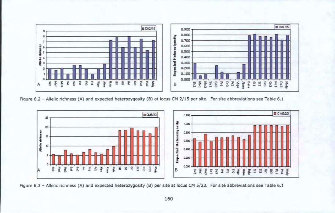
.01112/15 s 0.900

8 :!' 0.800

1 ... 0.700 G ..

:;:: 6

I s .. .;.c.

.~ 0.600 N G .. 0.500 IJ .,

0.400 :z: .. i 3

"CC 0.300 IJ 2

• • I • I 1 I I I I I I I 0

w 0.200 ., A. X 0.100 "' 0.000

- -•• •• • 11) 3: ~ 11) 11) "tJ !' :::' $; )> aJ la <.0 G) ~ "tJ "tJ ~ A IS ~ !. ~ :::lo. w .... "" 3 .. .... :::lo. ~ ~ " ... " . , .. oC

B

Figure 6.2- Allelic richness (A) and expected heterozygosity (B) at locus CM 2/15 per site. For site abbreviations see Table 6.1

25

20 01 : • '6 • • 'C .t

10 :i 2

5 ... .. ll D a l' (j

0

~ <.0

~ ~ 11) 11) ., !' ~ <

~ !. ~ :::lo. w N .;;;· ... 0

)> aJ la <.0 Wl G)

3 .. .... :::lo. w • ;;;-

la 0v15123

1-

-

"tJ "tJ ~ !'!.. " 0 ... oC

t200 r-----------------------------~~~D~C~M5==a~3

l tOOO+-----------------------~~-=~~--~~ ... G

.!!1 O.tm +-----------------------,;g....;y.-liil-411-111-1~11-l N 0 .. i 0.~~-=~~~~~--H-~~~~~----~--~~~-~~~ :z: "CC 0.~ ~~~~~~~~--o-~~~~~~--~--~~1-1~~ IJ w ., =- 0.200 tu-llll-llt-tlt-ill'f-I',Hr.t-f't-D--e--t.t--G----ft-1~1--Mt:-flt-IIH

"' B

Figure 6.3 -Allelic richness (A) and expected heterozygosity (B) per site at locus CM 5/23. For site abbreviations see Table 6.1

160

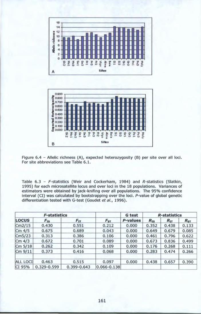
16 .------------------------------. 14+-----------------~.,rwr-~--~

=12 +----------=~----~~~~~~~

= 10+=--~-,~~~~~~~~~~~~ ~8 -t.-~~ ............ ~~---~..-!~~~~~~ .. . ~ 6 -t.-~----..-.. ...... ~~---~~~~.,..~~~ l 4 -t.-~----..-.. ...... ~~---~~~~~~~~ '3!

A

2 -t.-~----..-.. ...... ~~---~~~~~~~~ o ~~~~~~y.~~.y~~~~~~

~ ~ ~ ~ ~ ~ ~ ~ ~ ~ f ~ ~ ~ ~ ~ ~ ~ ~ ~ & ~ w~w ~ ~~ ~ ~ w ~ w ~& ~

Sites

0~.-----------------------------. lo~+-----------------~~~~~~ "' ;o.7oo +-------t~------.-i~ ..... -...~~~ ·~ 0.600 -+e--------..-'1~~-------~ ...... ~~------.!---.t~ .0~~~~~~~~~~~~~~~~~

~0.400~~~~~~~~~~~~~~~~

~0300~~~~~~~~~~~~~~~

~0200~---~ ...... ~~---~..-..~ ..... ---~~~ :,o.1oo ~---~ ...... ~~------..-..~ ..... -...~~~ ~ODOO~~-Y~~~~~~~~~~-Y~

B

~ ~ ~ ~ ~ ~ ~ ~ ~ ~ ~ ~ ~ ~ ~ ~ ~ ~ ~ ~ ~ ~w- w~~~ ~-w ~ w~w~

Sitas

Figure 6.4 - Allelic richness (A), expected heterozygosity (B) per site over all loci. For site abbreviations see Table 6.1.

Table 6.3 - F-statistics (Weir and Cockerham, 1984) and R-statistics (Siatkin, 1995) for each microsatellite locus and over loci in the 18 populations. Variances of estimators were obtained by jack-knifing over all populations. The 95% confidence interval (Cl) was calculated by bootstrapping over the loci. P-value of global genetic differentiation tested with G-test (Goudet et al., 1996).

F-statistics G test R-statlstics LOCUS F1s Frr FsT P-values R1s Rrr Cm2/15 0.430 0.551 0.212 0.000 0.352 0.438 Cm 4/5 0.675 0.689 0.043 0.000 0.649 0.679 Cm5/23 0.313 0.386 0.106 0.000 0.461 0.796 Cm 4/3 0.672 0.701 0.089 0.000 0.673 0.836 Cm 5/18 0.262 0.342 0.109 0.000 0 .176 0.268 Cm 9/11 0.373 0.416 0.068 0.000 0 .283 0.474

~LL LOCI 0.463 0.515 0.097 0.000 0.438 0.657 Cl 95% 0.329-0 .599 0.399-0.643 0.066-0.138

161

RsT 0.133 0.085 0.622 0.499 0.111 0.266

0.390

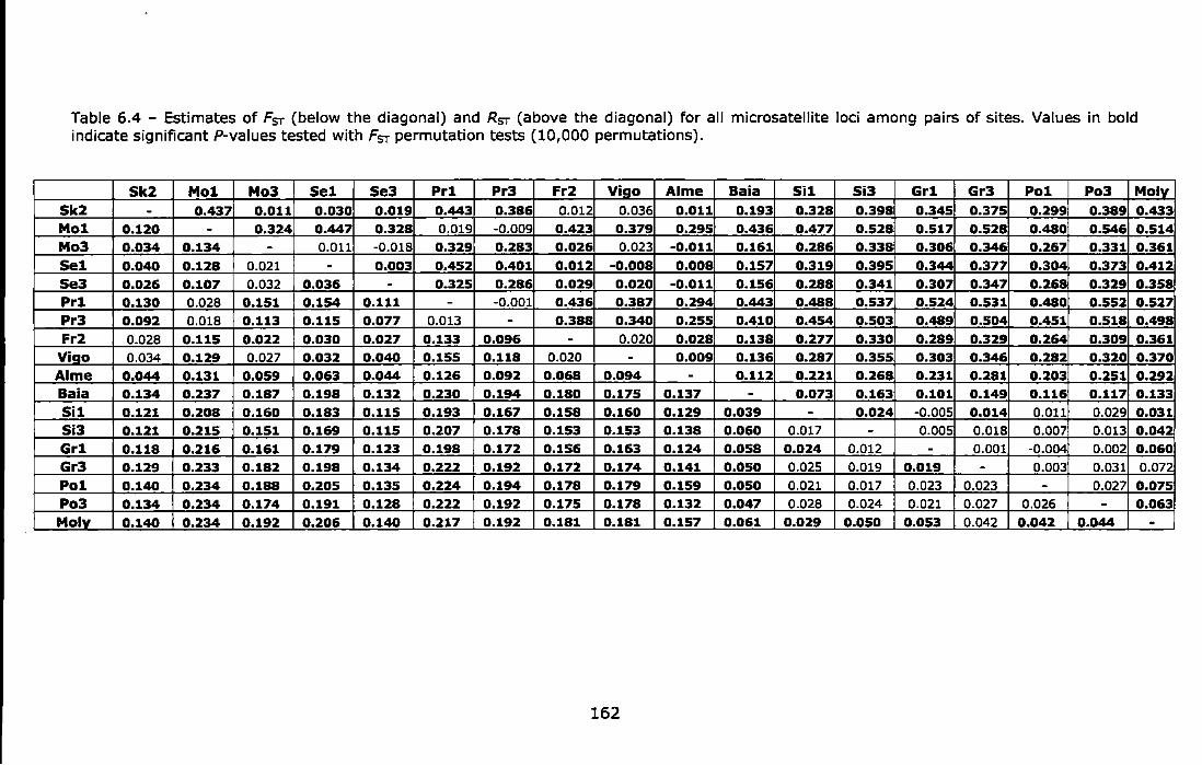
Table 6.4 - Estimates of Fsr (below the diagonal) and Rsr (above the diagonal) for all microsatellite loci among pairs of sites. Values in bold indicate significant P-values tested with Fsr permutation tests (10,000 permutations).

Sk2 Mol Mo3 Sel Se3 Prl Pr3 Fr2 Vi go Alme Baia Sil Si3 Grl Gr3 Pol Po3 Moly Sk2 - 0.437 0.011 0.030 0.019 0.443 0.386 0.012 0.036 0.011 0.193 0.328 0.398 0.345 0.375 0.299 0.389 0.433

Mol 0.120 - 0.324 0.447 0.328 0.019 -0.009 0.423 0.379 0.295 0.436 0.477 0.528 0.517 0.528 0.480 0.546 0.514

Mo3 0.034 0.134 - 0.011 -0.018 0.329 0.283 0.026 0.023 -0.011 0.161 0.286 0.338 0.306 0.346 0.267 0.331 0.361

Sel 0.040 0.128 0.021 - 0.003 0.452 0.401 0.012 -0.008 0.008 0.157 0.319 0.395 0.344 0.377 0.304 0.373 0.412

Se3 0.026 0.107 0.032 0.036 - 0.325 0.286 0.029 0.020 -0.011 0.156 0.288 0.341 0.307 0.347 0.268 0.329 0.358

Prl 0.130 0.028 0.151 0.154 0.111 - ·0.001 0.436 0.387 0.294 0.443 0.488 0.537 0.524 0.531 0.480 0.552 0.527

Pr3 0.092 0.018 0.113 0.115 0.077 0.013 - 0.388 0.340 0.255 0.410 0.454 0.503 0.489 0.504 0.451 0.518 0.498

Fr2 0.028 0.115 0.022 0.030 0.027 0.133 0.096 - 0.020 0.028 0.138 0.277 0.330 0.289 0.329 0.264 0.309 0.361 Vi go 0.034 0.129 0.027 0.032 0.040 0.155 0.118 0.020 - 0.009 0.136 0.287 0.355 0.303 0.346 0.282 0.320 0.370

AI me 0.044 0.131 0.059 0.063 0.044 0.126 0.092 0.068 0.094 - 0.112 0.221 0.268 0.231 0.281 0.203 0.251 0.292 Baia 0.134 0.237 0.187 0.198 0.132 0.230 0.194 0.180 0.175 0.137 - 0.073 0.163 0.101 0.149 0.116 0.117 0.133

Sil 0.121 0.208 0.160 0.183 0.115 0.193 0.167 0.158 0.160 0.129 0.039 - 0.024 -0.005 0.014 0.011 0.029 0.031

Si3 0.121 0.215 0.151 0.169 0.115 0.207 0.178 0.153 0.153 0.138 0.060 0.017 - 0.005 0.018 0.007 0.013 0.042

Grl 0.118 0.216 0.161 0.179 0.123 0.198 0.172 0.156 0.163 0.124 0.058 0.024 0.012 - 0.001 ·0.004 0.002 0.060

Gr3 0.129 0.233 0.182 0.198 0.134 0.222 0.192 0.172 0.174 0.141 0.050 0.025 0.019 0.019 - 0.003 0.031 0.072

Pol 0.140 0.234 0.188 0.205 0.135 0.224 0.194 0.178 0.179 0.159 0.050 0.021 0.017 0.023 0.023 - 0.027 0.075

Po3 0.134 0.234 0.174 0.191 0.128 0.222 0.192 0.175 0.178 0.132 0.047 0.028 0.024 0.021 0.027 0.026 - 0.063

Molv 0.140 0.234 0.192 0.206 0.140 0.217 0.192 0.181 0.181 0.157 0.061 0.029 0.050 0.053 0.042 0.042 0.044 -

162

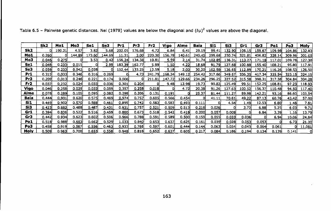
Table 6.5- Pairwise genetic distances. Nei (1978) values are below the diagonal and (oiJ)2 values are above the diagonal.

Sk2 Mol Mo3 Sel Se3 Prl Pr3 Fr2 Vi go Alme Baia Sil Si3 Grl Gr3 Pol Po3 Molv Sk2 0 190.21 4.57 3.82 5.68 202.05 176.68 4.72 6.84 6.41 29.19 99.41 132.90 106.15 159.67 109.98 104.86 132.83 Mol 0.260 0 144.89 173.60 144.69 11.31 3.00 220.30 156.78 140.61 240.45 299.68 330.74 321.81 406.82 328.14 309.96 301.05 Mo3 0.046 0.275 0 3.53 0.42 156.24 134.38 10.81 5.59 2.14 31.74 102.85 136.31 113.27 171.18 117.01 109.78 127.30 Sel 0.048 0.233 0.015 0 2.99 183.39 162.77 5.99 1.50 4.22 18.68 91.79 127.68 100.88 155.40 108.21 95.80 117.91 Se3 0.036 0.233 0.042 0.038 0 152.44 133.25 12.59 5.18 2.00 30.20 102.58 136.65 112.89 170.21 116.26 108.53 126.50 Prl 0.315 0.033 0.346 0.316 0.269 0 4.73 241.79 168.34 149.12 254.42 317.66 349.67 336.35 417.34 335.54 323.15 324.15 Pr3 0.209 0.013 0.246 0.221 0.174 0.006 0 211.81 147.72 129.66 234.26 296.25 327.52 315.58 398.31 317.38 304.84 304.28 Fr2 0.037 0.232 0.024 0.033 0.036 0.301 0.204 0 9.48 13.98 19.73 90.82 125.49 99.51 152.25 108.81 97.23 118.93

Vi go 0.046 0.258 0.029 0.033 0.059 0.357 0.258 0.018 0 4.72 20.38 91.26 127.63 100.52 156.37 110.48 94.50 117.40 Alme 0.078 0.289 0.105 0.095 0.082 0.298 0.206 0.131 0.191 0 25.37 81.44 111.27 89.98 142.21 93.16 86.60 105.54 Baia 0.444 0.901 0.620 0.575 0.469 0.974 0.757 0.605 0.566 0.454 0 41.11 70.61 49.22 87.13 60.76 43.42 57.00 Sil 0.449 0.902 0.570 0.588 0.461 0.895 0.742 0.583 0.583 0.493 0.111 0 4.54 1.49 12.53 6.80 1.48 7.81 Si3 0.423 0.882 0.488 0.487 0.431 0.931 0.757 0.521 0.509 0.513 0.216 0.026 0 3.72 6.88 5.25 6.03 9.71 Grl 0.394 0.836 0.522 0.516 0.459 0.800 0.673 0.518 0.542 0.418 0.200 0.057 0.008 0 6.84 3.39 1.16 13.79 Gr3 0.442 0.934 0.623 0.602 0.506 0.966 0.788 0.591 0.589 0.500 0.159 0.055 0.033 0.036 0 6.94 10.06 24.84 Pol 0.518 0.988 0.683 0.662 0.529 1.033 0.840 0.653 0.637 0.625 0.161 0.039 0.028 0.053 0.053 0 6.73 21.30 Po3 0.458 0.919 0.567 0.556 0.463 0.933 0.768 0.597 0.601 0.444 0.144 0.063 0.054 0.043 0.064 0.061 0 11.081 Molv 0.509 0.963 0.700 0.653 0.558 0.948 0.818 0.652 0.637 0.605 0.217 0.084 0.186 0.194 0.134 0.139 0.141 0

163

0 3' "' ::l

"' er ::l N

si si Gr3e Gr.

Po. •Pol

Moly

•

A ATLANTIC SITES

e MEDITERRANEAN SITES

Baia

Fr],. ~3 SkA_AM~

A Jl..el Alme V1go

• A

•

Dimension 1

Figure 6.5 - Non-metric multidimensional scaling analysis (nMDS) of 18 sites based on Rsr (Weir and Cockerham, 1984). Stress value= 0.026 (for abbreviations see Table 6.1).

164

Prl A PrJ

Mol .A .A

Alme

•

..Sel A A ASeJ

Sk2-. ..a. Fr2 A MoJ

Vlgo A A

A ATLANTIC SITES

e MEDITERRANEAN SITES

Dimension 1

Moly

•

511 SIJ

•• Grl GrJ

• • Pol PoJ

• •

Bala

•

Figure 6.6 - Non metric multidimensional scaling analysis (nMDS) of 18 sites based on Nei's {1978) genetic distance. Stress value= 0.005 (for abbreviations see Table 6.1).

165

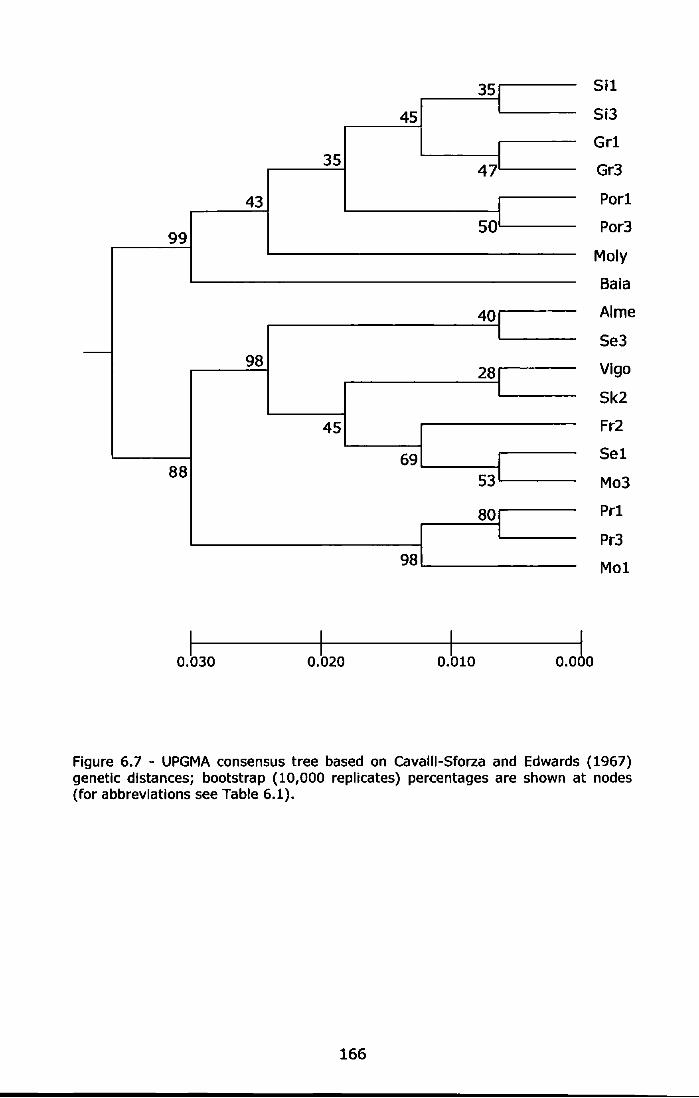
35

43

99

- 98

45

88

351

45 L

I

471

I

so1

401 I

281 I

69 j

53 1

801 I

98

Sil

Si3

Grl

Gr3

Porl

Por3

Moly

Bala

Alme

Se3

Vi go

Sk2

Fr2

Sel

Mo3

Prl

Pr3

Mol

Figure 6.7 - UPGMA consensus tree based on Cavaiii-Sforza and Edwards (1967) genetic distances; bootstrap (10,000 replicates) percentages are shown at nodes (for abbreviations see Table 6.1).

166

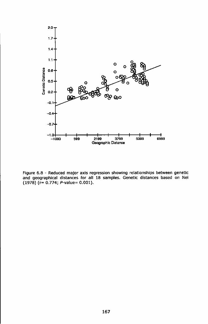
-1.o+--+--+--+--l---+--+-+-+--+--t -1000 599 2199 3799 5399 6999

Geographic Distance

Figure 6.8 - Reduced major axis regression showing relationships between genetic and geographical distances for all 18 samples. Genetic distances based on Nei (1978) (r= 0.774; P-value= 0.001).

167

Table 6.6 - Hierarchical AMOVA among samples grouped in two groups ('basins'): group 1, Atlantic locations; group 2, Mediterranean locations. Source of variation, degrees of freedom (df), variance components, percentage of variation (%), fixation Indices and probability value (P-value) are listed.

Source of df Variance 0/o Fixation P..value variation components indices

Between basins 1 0.24126 9.35 0.09346 0.000 Among locations 16 0.09313 3.61 0.0398 0.000

within basin Within locations 1050 2.24709 87.05 0.12953 0.000

Table 6.7 - Hierarchical AMOVA among samples as implemented in HIERFSTAT. Pairwise Fsr estimates and P-value between basins, among locations within basins, among sites within locations and within sites.

Fsr P-value Between basins Among locations Between sites Within

within basins within locations sites

Total 0.123 0.135 0.152 0.537

Between basins 0.050 0.014 0.032 0.472

Among locations 0.016 0.019 0.464 within basins

Between sites 0.005 0.454 within locations

Table 6.8 - Hierarchical AMOVA among the Mediterranean locations with two sites per location. Source of variation, degrees of freedom (df), variance components, percentage of variation (%), fixation Indices and probability value (P-value) are listed.

Source of df Variance 0/o Fixation P..value variation components indices

Among locations 2 0.02378 0.94 0.00941 0.068 Between sites

3 0.01455 0.58 0.00581 0.764 within location

Within sites 364 2.48927 98.48 0.01516 0.118

Table 6.9 - Hierarchical AMOVA among the Atlantic locations with two sites per location. Source of variation, degrees of freedom (df), variance components, percentage of variation (%), fixation indices and probability value (P-value) are listed.

Source of df Variance 0/o

Fixation P-value variation components indices Among locations 2 0.03213 1.5 0.01495 0.457

Between sites within location 3 0.0685 3.19 0.03236 0.000

Within sites 376 2.04815 95.32 0.04683 0.000

168

Proportion of individual membership

1.00

0.80

0.80

0.40

0.20

0.00

Sk2 Mol Mo3 Sel Se3 Prl Pr3 Fr2 Vigo Alme Baia Sil Si3 Grl Gr3 Pol Po3 Moly

Figure 6.9: Clustering analysis conducted in STRUCTURE 2.2 (K=2). In the bar plot, each vertical bar along the x axis represents one of 534 individuals grouped by location/site (see abbreviation in Table 6.1); the Y-axis represents the estimated proportion of membership of each individual to each cluster (represented by different colours).

Table 6.10: Mean proportion of membership of each sample (location/site) to each cluster (K=2).

Sk2 Mol Mo3 Sel Se3 Prl Pr3 Fr2 Vi go AI me Baia Sil Si3 Grl Gr3 Pol Po3 Molv Cluster 1 0.13 0.01 0 .06 0.04 0 .13 0.04 0.08 0.02 0.06 0.16 0.96 0.96 0.95 0.93 0.98 0.94 0.92 0.94 Cluster 2 0.87 0.99 0 .94 0 .97 0 .87 0 .96 0.92 0.98 0.94 0.85 0.04 0.04 0.06 0.07 0.02 0.06 0 .08 0.06

169

Proportion of individual membership

1.00

0.80

0.60

0.40

0.20

0.00

Figure 6.10: Clustering analysis conducted in STRUCTURE 2.2 (K=3). In the bar plot, each vertical bar along the x axis represents one of 534 individuals grouped by location/site (see abbreviation in Table 6.1) ; the Y-axis represents the estimated proportion of membership of each individua l to each cluster (represented by different colours) .

Table 6.11: Mean proportion of membership of each sample (location/site) to each cluster {K=3).

5 1<2 Mol Mo3 Sel Se3 Prl Pr3 Fr2 Vi go AI me Baia Sil Si3 Grl Gr3 Pol Po3 Moly Cluster 1 0.10 0 .02 0.03 0.03 0 .08 0 .03 0 .08 0 .02 0.05 0 .14 0.92 0.91 0 .90 0 .90 0.96 0 .89 0.90 0.88 Cluster 2 0 .66 0 .19 0.72 0 .74 0.58 0 .20 0 .20 0 .84 0.63 0.59 0.05 0.04 0 .07 0 .05 0.02 0.06 0 .09 0.06 Cluster 3 0 .24 0 .80 0.25 0.24 0.34 0 .77 0.73 0.15 0.33 0.27 0 .03 0.05 0 .03 0.05 0.02 0.06 0 .02 0.06

170

6.4 Discussion In this study spatial scales of genetic differentiation of the barnacle

Chthamalus montagui were investigated over its distribution range in the NE

Atlantic and Mediterranean Sea using six microsatellite loci as molecular

markers.

The results showed that Atlantic and Mediterranean populations are

genetically different and confirmed previous work on this subject carried out

using allozymes (Dando and Southward, 1981; Pannacciulli et al., 1997a).

The analysis of molecular variance revealed that differences between

Atlantic and Mediterranean samples were highly significant and counted for

9.35% of the total genetic variation.

Dando and Southward (1981) suggested that the history of the

Mediterranean, combined with the present hydrographic pattern, might

have promoted and maintained differentiation of Mediterranean populations

of C. montagui. Following the Messinian salinity crisis (ea 5.5 million years

ago) (Hsu et al. 1977; McCullach and De-Deckker, 1989), communication

between the Atlantic and Mediterranean was re-established, and fully

marine conditions were restored during the Pliocene (5.4 to 1.8 million

years ago). In the Pleistocene (1.8 to 0 million years ago), and particularly

during the Quaternary, a series of glacial and interglacial periods with

associated marine regressions and transgressions affected the area (Blanc,

1968). Atlantic and Mediterranean populations of Chthamalus spp. may

have become physically isolated during these cycles and differentiated

genetically.

171

Mediterranean populations exhibited higher genetic variability than Atlantic

ones, as already indicated by allozyme studies (Pannacciulli et al., 1997a).

In the present study allelic richness and mean expected heterozygosity,

averaged over all microsatellite loci, was higher in the samples from the

Mediterranean basin than in those from the Atlantic (Table 6.2). The loci

CM 2/15 and CM 5/23 were the most variable among populations and

showed a wide difference between Atlantic and Mediterranean sites (Figure

6.2 and 6.3). CM 2/15 was monomorphic at two Atlantic sites (Fr2 and

Sel) and the allelic richness of CM 5/23 ranged from 4.44 at the Atlantic

site Mol to 19.77 at the Eastern Mediterranean site Moly (Table 6.2).

It is important to highlight that the Almeria sample behaved, at all loci, as

an Atlantic sample. In fact, looking at the population genetic subdivision,

as shown by the nMDS plots or by the UPGMA phylogenetic tree, Almeria

was always clustered with the Atlantic populations. This evidence was also

supported by the results of the Bayesian clustering analysis, showing high

mean proportion of membership (85%) of the Almeria individuals to the

Atlantic population cluster.

These results supported the hypothesis that the Almeria-Oran front is the

major barrier to gene flow between the Atlantic and Mediterranean basins.

This front has been suggested as the location of a phylogeographical break

(Avise et al., 1987), not only for Chthamalus montagui (Dando and

Southward, 1981; Pannacciulli et al., 1997a), but also for other organisms

like Myti/us gal/oprovincia/is (Quesada et al., 1995; Sanjuan et al., 1996),

Ostrea edu/is (Saavedra et al., 1993), and Meganyctiphanes norvegica

(Zane et al., 2000). The Almeria-Oran front is a zone of turbulence in the

172

Alboran Sea {Tintore et al., 1988) that may restrict larval dispersal in both

directions. The Alboran Sea is a mixture of Atlantic waters flowing into the

Mediterranean basin from the North Atlantic (occupying the upper layer of

the Alboran Sea), and Mediterranean waters flowing westward (in the lower

layer). If the hydrographic barrier persists, genetic divergence could

conceivably lead to allopatric or parapatrlc speciation.

The higher genetic variability of the Mediterranean populations compared to

the Atlantic ones could also be related to hydrographic patterns. The

unidirectional surface circulation from the Atlantic to the Mediterranean

through the Strait of Gibraltar might produce asymmetrical gene flow in this

direction and promote differentiation (Endler, 1977). Alleles originating In

the Mediterranean population could be prevented from spreading to the

Atlantic, while those arising in the Atlantic could spread readily into the

Mediterranean Sea. This explanation has been put forward by Saavedra et

al. (1993) for a similar pattern of allelic diversity in the oyster Ostrea edulis.

Moreover, selection under different environmental regimes could be

considered a likely cause of genetic differentiation between Atlantic and

Mediterranean basins in Chthamalus. For instance, salinity, summer and

winter water temperatures, and tidal range differ between the NE Atlantic

and the Mediterranean (Mclellan, 1965; Fairbridge, 1966). Intertidal

barnacles in the Mediterranean undergo extreme environmental conditions,

particularly in the summer when they experience long periods of exposure

to the air as wave action, the only way for upper shore barnacles to get

water, is reduced. Hence, the higher genetic variability recorded in

populations from this basin could be a reponse to the difficult environment

173

In which they have to survive as it provides greater plasticity to a constantly

changing environment.

Focussing attention at the basin scale, a genetic subdivision was detected

between the western and eastern Mediterranean samples. The population

from the Ligurian Sea (Baia) was separated from the others, as shown by

nMDS plots and the UPGMA phylogenetic tree, and in terms of genetic

variability (allelic richness and expected heterozygosity) exhibited an

intermediate pattern (Figure 6.4) between the Atlantic and the eastern

Mediterranean samples.

The Strait of Sicily, which is well recognised in oceanography as a physico­

chemical and morphological threshold between the two sub-basins of the

Mediterranean Sea, could act as a hydrographical barrier to the gene flow.

Moreover, the different physical-chemical characteristics (e.g. water

temperature and salinity) of the western and eastern Mediterranean could

also affect the genetic pattern of barnacle populations.

Furthermore, in the eastern sub-basin, the samples from Molyvos showed a

slight genetic differentiation from those of the Adriatic Sea, as seen in the

nMDS plot and the UPGMA tree. It could be interesting to compare their

pattern with those of samples from the Black Sea. Pannacciulli et al., 1997a

analysed samples of Chthamalus montagui from the Black Sea using

allozymes, and found a great genetic similarity to Mediterranean

populations, despite the geographical separation and the hydrographic

barrier of the Bosphorus. The predominant movement of water is from the

Black Sea into the Mediterranean, but, during autumn, surface waters can

174

flow in the opposite direction (Pektas, 1958). Barnacle larvae could be

transported with these currents, allowing an exchange of larvae between

the two seas (Pannacciulli et al., 1997a); for this reason Black Sea samples

could be genetically very close to the Molyvos samples.

Focussing attention on the Atlantic basin, population genetic subdivision

featured two clusters, as indicated by nMDS plots, UPGMA phylogenetic tree

and also confirmed by Bayeslan clustering analysis. The first cluster

included most of the screened populations and the second one was

represented by three populations (Mol, Prl and Pr3). This result was quite

surprising considering that the Mol sample did not cluster with Mo3: the

two sites, within the same location, were 200-300 apart. Moonen Bay and

Prawle Point are both wide and open rocky shores within the core

distribution of the species, and no unusual environmental feature was noted

in either place during collection of the samples. Moreover, they are about

1000 km far apart and the IBD results showed a significant overall

correlation between genetic and geographical distances.

Before offering ecological speculations on this matter, it is worth noting that

samples from Mol, Prl and Pr3 (but not Mo3) were run on the sequencer in

the same plate; some technical factors could be responsible for the

observed genetic pattern. However, further investigations on these samples

are needed.

The different genetic pattern detected at Mol and Mo3 provides the

opportunity to discuss the small spatial scale of genetic variation:

differences between sites within the same location. AMOVA results for the

175

Atlantic locations (Seil, Moonen Bay, Prawle Pt) showed that genetic

variation among locations (hundreds of km apart from one another) counted

for 1.5% of the total genetic variability, while differences between sites

(from 100 to 300 m apart) were highly significant and counted for 3.19% of

the total genetic variation. Otherwise, it could be related to the presence of

the Mol samples that exhibited a divergent pattern from the others.

AMOVA results for the Mediterranean locations (Sistlana; Grado; Portonovo)

showed that differences between sites accounted for just 0.58% of the total

genetic variation and were not significant. Nevertheless, the major source

of variation, 95.32% of the total genetic variability in the Atlantic sites and

98.48% in the Mediterranean ones, laid within sites and therefore, resided

in the very small spatial scale (the plot of few meters from which specimens

were collected) at the inter-individual level. The life history of this barnacle

with high dispersal capabilities might be responsible for this pattern: the

released larvae spend a few weeks in the water column dispersing offshore,

before finding a suitable substratum on which to settle, metamorphose and

start the sessile phase. For this reason it could be possible to have

barnacles originating from distant parental locations settling next to each

other on the shore, which could partly explain the large genetic variability

recorded within sites.

Furthermore, differentiation at a very small scale has been often observed

in population genetic studies of marine invertebrates employing

microsatellites, suggesting that the high sensitivity and ability in detecting

genetic variation of these molecular markers could also affect the observed

176

pattern (e.g. Bertozzi, 1995; Costantini et al., 2007; Lind et al.,.2007; York

et al., 2008).

Moreover, it is worth mentioning that all samples exhibited highly significant

multilocus departures from HWE, while using allozymes Chthamalus

montagui samples were in conformity to HWE (Pannacciulll et al., 1997a).

Heterozygosity deficits have frequently been observed in marine

invertebrates (Zouros and Foltz, 1984; Gaffney, 1994; David et al., 1997;

Ayre and Hughes, 2000; Ridgway et al., 2001; Addison and Hart, 2004;

Duran et al., 2004; Le Goff-Vitry et al., 2004; Andrade and Solferini, 2007;

Costantini et al., 2007) including barnacles and using microsatellite markers

(Veliz et al., 2006; York et al., 2008). The most common explanations for

heterozygote deficiency are: technical factors, such as the presence of null

alleles and or stutter peaks (Foltz, 1986; Callen et al., 1993; Puebla et al.,

2008), and biological factors, such as inbreeding or the Wahlund effect

(Pogson et al., 1995; Duran et al. 2004; Plutchack et al., 2006; Costantini

et al., 2007). It is difficult to provide an exact explanation for our findings,

probably technical and biological factors could have both contributed.

To conclude, we can assert that the marine environment is far from the

homogeneous habitat for which it has been taken, and expectations of

marine genetic biodiversity have potentially been grossly underestimated,

particularly in widely dispersing species. The investigation of spatial scales

of genetic diversity provides useful insights on species population genetic

structure. This information is relevant to marine biodiversity management

and conservation action plans.

177

·~--

. ~·'- ·. ,. . '-

•'

·' j

I

r I

I I•

1.18 . ·-'"

Briefly re-state the results of the three data chapters (Ch. 4, 5, and 6).

The results of the sampling of artificial and natural substrates in the Adriatic

Sea were consistent with the hypothesis that man-made structures can act

as corridors for genetic exchange between distant rocky shores, since very

little genetic differentiation was detected between distant localities.

However, in the absence of historical genetic data from the region, firm

conclusions could not be drawn.

A study of localities around the UK lent some support to the idea that edge­

of-range populations tend to have reduced genetic variability and may also

harbour unusual genotypes. However, the small number of peripheral (2)

and marginal (1) populations that could be studied rendered such

conclusions provisional, and some populations designated as mid-range

shared similar characteristics.

The above two studies utilized three microsatellite loci. A broader survey of

the NE Atlantic and Mediterranean range of C. montagui using six

microsatelllte loci documented clear differentiation between Atlantic and

Mediterranean populations; the Mediterranean sample from Almeria in

southern Spain was Atlantic in character, supporting the suggestion that the

Almeria-Oran front, rather than the Strait of Gibraltar, is the main

biogeographical boundary between the two basins. Genetic diversity was

consistently higher In the Mediterranean than in the Atlantic.

Although a general pattern of isolation by distance was apparent in the

broad-scale survey, two replicate samples from one Atlantic shore, taken a

179

few hundred metres apart, were clearly distinct. The natural or artefactual

cause of this differentiation requires investigation. Throughout the project,

the great majority of genetic variation was present within sampling sites,

suggesting efficient larval mixing and the dominance of inter-individual

variation over geographical differentiation, but spatial patchiness within

sites on a scale of centimetres cannot be discounted from the data

obtained.

Modern techniques offer a number of molecular markers for population

genetic studies. In this project microsatellites were employed as suitable

markers to investigate the genetic pattern of the barnacle Chthamalus

montagui. Their rapid rate of mutation and their position in the non-coding

region of the DNA make mlcrosatellites ideal for investigating contemporary

population structure (York et al., 2008) as putatively neutral markers

(Dufresne et al., 2002).

The six microsatellite loci screened in this study were highly polymorphic.

At the locus Cm 5/23, which was the most variable, 41 alleles were scored

over all samples and a maximum of 33 alleles was detected in one

population. This is not uncommon: Puebla et al. (2008), investigating the

genetic structure of the snow crab Chionecetes opilio in the NW Atlantic,

employed eight microsatellites, one of which showed 54 alleles in one single

population. However, many other population genetic studies have

employed microsatellite loci that were much less polymorphic (e.g.

Costantini et al., 2007; Lind et al., 2007; Lukoschek et al., 2008).

180

A high number of alleles implies low frequency of individual alleles and high

genetic variability among individuals. In fact, as revealed from the analyses

of molecular variance carried out in the different tasks of this project, in C.

montagui the main source of variation lies always within sites, at a spatial

scale of few tens of meters. This is often observed in population genetic

studies of marine invertebrates employing microsatellites, suggesting the

high sensitivity and ability of these molecular markers in detecting inter­

individual genetic variation (e.g. Bertozzl, 1995; Costantini et al., 2007;

Lind et al., 2007; York et al., 2008). Nevertheless, the biology and ecology

of C. montagui should be also taken into account. Barnacles brood

developing embryos within the mantle cavity before releasing larvae that

feed and pass through several instars in the plankton. The released larvae

spend a few weeks In the water column dispersing offshore, before finding a

suitable substratum on which to settle, metamorphose and start the sessile

phase. These features make it likely that barnacles originating from distant

parental populations grow next to each other on the shore and partly

explain the large genetic variability recorded within sites.

In all tasks of the project the screened populations exhibited large positive

F15 values over all loci reflecting departures from HWE and exact tests

highlighted highly significant multilocus heterozygote deficiency. (An

exception to this general pattern was the CmS/23 locus in the UK-based

study of peripherality and marginality). Heterozygosity deficits have

frequently been observed in marine invertebrates (Ayre and Hughes, 2000;

Ridgway et al., 2001; Addison and Hart, 2004; Duran et al., 2004; Le Goff­

Vitry et al., 2004; Andrade and Solferini, 2007; Costantini et al., 2007;

Puebla et al., 2008) including barnacles (Veliz et al., 2006; York et al.,

181

2008) and attempts to explain these deficits have Involved a range of

technical and/or biological factors (Zouros and Foltz, 1984; Gaffney, 1994;

David et al., 1997; Pudovskis et al., 2001; Addison and Hart, 2005;

Plutchack et al., 2006; Brownlow et al., 2008).

One of the most commonly suggested contributors to heterozygote

deficiency in microsatellites is the presence of null alleles (Foltz, 1986;

Callen et al., 1993). Null alleles represent base-pair mutations In the

primer regions which cause primer binding to weaken and/or fail, resulting

in a failure to amplify certain alleles (Paetkau and Strobeck, 1995). While

microsatellite regions are often highly polymorphic due to a high rate of

mutation through replication slippage and proofreading events, the flanking

regions surrounding microsatellite repeat regions are generally considered

to be more conserved. However, as hypothesized by Brownlow et al.

{2008), when the microsatellite loci exhibit very high levels of

polymorphism it is also possible that the flanking sequences are undergoing

increased levels of mutation, reducing the effectiveness of primer binding.

This explanation could apply to the microsatellites screened in this project,

or at least to the most polymorphic ones, such as Cm 5/23. Nevertheless, I

do not favour the hypothesis of null alleles, because heterozygote deficiency

was significant and consistent across all loci, and it seems highly improbable

that all loci exhibit null alleles with such a constant frequency.

Another technical factor could be the presence of stutter peaks {Puebla et

al., 2008). Stutter peaks were observed at two loci {Cm 4/5 and Cm 4/3);

however, in the case of doubts or scoring difficulties I repeated the analysis

at least two times randomly after a period of time to avoid scoring bias.

182

Artifacts of scoring genotypes are an obvious possibility, but I am confident

of the scoring. Moreover, some loci did not exhibit stutter peaks making

straightforward the interpretation of the electropherogram.

Among the biological factors, it is necessary to consider the Wahlund effect,

which refers to reduction of heterozygosity due to the inadvertent sampling

of individuals from two different sympatric subpopulations with different

allele frequencies, and could (but would not necessarily) affect all

polymorphic loci similarly (Pogson et al., 1995; Plutchack et al., 2006).

However, no evidence of subpopulation genetic subdivision was detected in

this study.

Addison and Hart (2005) documented an unexpected correlation between

life history traits (such as dispersal ability and breeding systems) and

deviations from the HWE. Barnacles generally reproduce by cross­

fertilisation by pseudo-copulation (Kiepal, 1990), which can only take place

when one individual is within penile distance of potential mates (Anderson,

1994). Nevertheless, they are hermaphroditic organisms and self­

fertilisation has been inferred in Chthamalus (Barnes and Crisp, 1956;

Barnes and Barnes, 1958; Pannacciulli and Bishop, 2003). Inbreeding, in

the sense of selfing, could be a possible explanation of multllocus

heterozygote deficiency observed in the analysed samples. Nevertheless, it

is difficult to provide an exact explanation for our findings, and technical

and biological factors could both have contributed.

It is important to highlight that the ability to draw definitive conclusions

concerning the genetic pattern of barnacles based on the screening of just a

183

few loci is limited. In particular, for those tasks of the project where just

three microsatellite loci were examined due to constraints of time and

money, it could be worth increasing the number of microsatellite loci and/or

the number of different classes of marker employed.

In general, a multi-marker approach should be preferred, as Dufresne et al.

(2002) suggested. Microsatellites may not always behave in a neutral way

and have to be used cautiously, especially when evidence for genetic

structuring relies on only a few assayed loci without a priori knowledge or

comparison with potentially selected loci. Many studies are carried out

using more than one marker investigating different parts of the genome and

allowing useful comparisons among them (e.g. Schmidt and Rand, 1999 and

2001; Rand et al., 2001; Simon-Biecher et al., 2008; York et al., 2008). A

wider screening of the genetic pattern could provide a more comprehensive

assessment and, therefore, more robust conclusions.

Previous population genetic studies carried out on Chthamalus montagui

employed allozymes (Dando and Southward, 1981; Pannacciulli et al.,

1997a). Future studies on this species could, for instance, employ markers

that target genes of the mtDNA. Specific primers have been developed to

amplify Cytochrome oxydase I and the Control Region of the congeneric

species Chthamalus steffatus (Milana, 2005): the same primers could

perhaps find application also in C. montagui. Moreover, ISSRs (Inter

Simple Sequence Repeats) could be considered as alternative markers: they

were also employed in a population genetic study involving two barnacle

species, c. steffatus and Tesseropora atlantica, in the archipelago of the

Azores (Pannacciulli et al., in preparation) and they were used in a number

184

of recent population genetic investigations on marine invertebrates (Casu et

al., 2005, 2006 and 2008; Maltagliatl et al., 2006; De Aranzamendi et al.,

2008).

It is worth noting that further investigations are needed for the three UK

populations (Mol, Prl and Pr3) that were clustered together and

differentiated from the other Atlantic ones. It is suggested to repeat the

screening of the six analysed microsatellite loci and/or to proceed to

investigate a wider part of the genome employing other markers.

To conclude, it has to be mentioned that C. montagui has proved to be a

very good model organism for genetic studies. This barnacle species is very

easy to sample, due to its abundance and accessibility on the shore; DNA

extraction can easily be carried out using a simple, safe and cheap method

(Salting-Out extraction) that provides very good quality DNA; and the

microsatellite markers employed amplified well and were relatively easy to

score.

185

· ·A,ppen:dices

i86

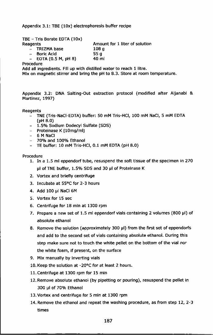
Appendix 3.1: TBE ( 10x) electrophoresis buffer recipe

TBE- Tris Borate EDTA (10x) Reagents

- TRIZMA base - Boric Acid - EDTA (0.5 M, pH 8)

Procedure

Amount for 1 liter of solution 108 g 55 g 40 ml

Add all Ingredients. Fill up with distilled water to reach 1 litre. Mix on magnetic stirrer and bring the pH to 8.3. Store at room temperature.

Appendix 3.2: DNA Salting-Out extraction protocol (modified after Aljanabi & Martinez, 1997)

Reagents - TNE (Tris-NaCI-EDTA) buffer: 50 mM Tris-HCI, 100 mM NaCI, 5 mM EDTA

(pH 8.0) 1.5% Sodium Dodecyl Sulfate (SOS) Proteinase K [10mg/ml] 6 M NaCI 70% and 100% Ethanol TE buffer: 10 mM Tris-HCI, 0.1 mM EDTA (pH 8.0)

Procedure 1. In a 1.5 ml eppendorf tube, resuspend the soft tissue of the specimen in 270

jJI of TNE buffer, 1.5% SOS and 30 jJI of Proteinase K

2. Vortex and briefly centrifuge

3. Incubate at 55°C for 2-3 hours

4. Add 100 jJI NaCI 6M

5. Vortex for 15 sec

6. Centrifuge for 18 mln at 1300 rpm

7. Prepare a new set of 1.5 ml eppendorf vials containing 2 volumes (BOO jJI) of

absolute ethanol

8. Remove the solution (approximately 300 jJI) from the first set of eppendorfs

and add to the second set of vials containing absolute ethanol. During this

step make sure not to touch the white pellet on the bottom of the vial nor

the white foam, If present, on the surface

9. Mix manually by inverting vials

10. Keep the solution at -20°C for at least 2 hours.

11. Centrifuge at 1300 rpm for 15 min

12. Remove absolute ethanol (by pipetting or pouring), resuspend the pellet in

300 jJI of 70% Ethanol

13. Vortex and centrifuge for 5 min at 1300 rpm

14. Remove the ethanol and repeat the washing procedure, as from step 12, 2-3

times

187

15. Dry the pellet in air at room temperature or in a thermoblock set at 37°C

leaving the top of the vial open

16. Resuspend the pellet in 30 !JI of TE buffer

17. Vortex and centrifuge briefly

18. Keep the resuspended pellet at 4°C overnight to facilitate dissolving

19. Store the extracted DNA at -20°C.

188

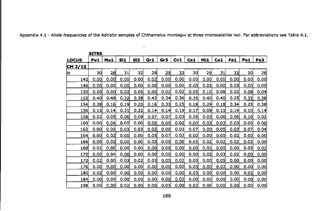
Appendix 4.1 -Allele frequencies of the Adriatic samples of Chthamalus montagui at three microsatellite loci. For abbreviations see Table 4.1.

SITES LOCUS Pul Mul Sil Si3 Grl Gr3 Cvl Cel Mil Cal Fal Pol Po3 CM 2/15 N 30 28 31 32 29 29 32 30 29 31 32 30 28

142 0.00 0.00 0.00 0.00 0.02 0.00 0.00 0.00 0.00 0.00 0.00 0.00 0.00

146 0.00 0.00 0.00 0.00 0.00 0.00 0.00 0.00 0.02 0.00 0.03 0.00 0.00

150 0.00 0.00 0.02 0.06 0.00 0.02 0.02 0.05 0.10 0.08 0.02 0.08 0.04

152 0.40 0.48 0.32 0.38 0.43 0.34 0.36 0 . .35 0.40 0.40 0.25 0.32 0.38

154 0.38 0.16 0.19 0.20 0.16 0.33 0.25 0.18 0.29 0.18 0.34 0.25 0.38

156 0.15 0.14 0.21 0.22 0.14 0.14 0.19 0.17 0.09 0.15 0.19 0.10 0.14

158 0.02 0.05 0.06 0.09 0.07 0.07 0.03 0.05 0.03 0.00 0.06 0.10 0.02 160 0.00 0.04 0.05 0.00 0.05 0.00 0.02 0.00 0.03 0.03 0.03 0.00 0.00

162 0.00 0.05 0.03 0.03 0.02 0.00 0.03 0.07 0.00 0.05 0.03 0.07 0.04

164 0.00 0.02 0.00 0.00 0.05 0.07 0.02 0.00 0.00 0.00 0.02 0.00 0.00

166 0.00 0.02 0.00 0.00 0.03 0.00 0.06 0.05 0.02 0.02 0.02 0.02 0.00

168 0.02 0.00 0.00 0.00 0.00 0.00 0.00 0.00 0.00 0.00 0.00 0.05 0.02

170 0.00 0.04 0.06 0.00 0.00 0.00 0.00 0.00 0.02 0.03 0.02 0.00 0.00

172 0.02 0.00 0.03 0.02 0.03 0.00 0.02 0.00 0.00 0.05 0.00 0.00 0.00

176 0.00 0.00 0.00 0.00 0.00 0.00 0.00 0.03 0.00 0.02 0.00 0.00 0.00 180 0.02 0.00 0.00 0.00 0.00 0.00 0.00 0.03 0.00 0.00 0.00 0.02 0.00

184 0.00 0.00 0.00 0.00 0.00 0.00 0.02 0.00 0.00 0.00 0.00 0.00 0.00

198 0.00 0.00 0.02 0.00 0.00 0.03 0.00 0.02 0.00 0.00 0.00 0.00 0.00

189

Appendix 4.1 -continued

SITES LOCUS Pu1 CM 4/5 N 25

74 0.32

78 0.04

80 0.10

82 0.00

94 0.00

98 0.04

100 0.08

102 0.00

104 0.04

106 0.06

108 0.00

110 0.02

112 0.04

114 0.04

116 0.04

118 0.02

120 0.04

122 0.00

124 0.00

126 0.12

128 0.00

130 0.00

Mu1

29 0.26

0.02

0.07 0.02

0.00 0.05 0.03

0.03

0.10

0.07 0.00

0.05

0.02 0.09

0.02

0.02

0.07

0.03

0.00 0.00

0.00 0.00

Si1 Sil Gr1

27 28 27

0.31 0.29 0.26 0.00 0.00 0.02

0.02 0.07 0.00 0.06 0.00 0.00

0.00 0.07 0.00

0.04 0.16 0.11 0.07 0.00 0.06

0.06 0.02 0.00

0.07 0.00 0.04

0.11 0.21 0.15 0.00 0.00 0.00

0.06 0.00 0.00

0.02 0.00 0.09

0.02 0.04 0.11

0.00 0.04 0.00

o.oo 0.00 0.04

0.04 0.04 0.07

0.04 0.00 0.02

0.00 0.04 0.00 0.00 0.00 0.00

0.00 0.00 0.02

0.07 0.00 0.00

Grl CV1 Ce1 Mi1 Ca1 Fa1 Po1 Pol

29 26 30 30 30 29 28 29

0.33 0.42 0.18 0.40 0.18 0.21 0.32 0.26

0.00 0.08 0.07 0.07 0.02 0.09 o.oo 0.00 0.00 0.00 0.03 0.05 0.05 0.05 0.05 0.07

0.00 0.00 0.00 0.05 0.02 0.09 0.00 0.03

0.03 0.00 0.00 0.00 0.00 0.02 0.00 0.00 0.10 0.06 0.07 0.05 0.18 0.07 0.05 0.14 0.07 0.04 0.08 0.07 0.05 0.05 0.04 0.00

0.00 0.00 0.02 0.02 0.00 0.03 0.04 0.00 0.07 0.13 0.08 0.05 0.00 0.00 0.13 0.09 0.14 0.00 0.18 0.08 0.18 0.17 0.04 0.10 0.00 0.02 0.03 0.00 0.03 0.02 0.00 0.05

0.00 0.00 0.00 0.00 0.00 0.02 0.05 0.00 0.05 0.00 0.08 0.03 0.07 0.02 0.04 0.03

0.02 0.06 0.07 0.03 0.05 0.07 0.00 0.03

0.00 0.04 0.03 0.02 0.00 0.00 0.07 0.02 0.05 0.00 0.03 0.00 0.02 0.00 0.04 0.00

0.00 0.00 0.00 0.02 0.02 0.03 o.oo 0.00

0.05 0.04 0.00 0.00 0.02 0.00 0.00 0.09 0.00 0.04 0.00 0.03 0.03 0.02 0.07 0.03 0.00 0.00 0.00 0.00 0.00 0.00 0.00 0.02

0.00 0.00 0.00 0.00 0.00 0.00 0.00 0.00 0.03 0.00 0.00 0.02 0.00 0.00 0.00 0.00

190

Appendix 4.1 -continued 132 0.00 0.00 0.02 0.00 0.00 0.00 0.00 0.00 0.00 0.03 0.00 0.00 0.03 134 0.00 0.02 0.00 0.00 0.00 0.00 0.00 0.00 0.00 0.02 0.00 0.00 0.00

136 0.00 o.cio 0.00 0.00 0.00 0.00 0.00 0.00 0.00 0.00 0.02 0.00 0.00 138 0.00 0.00 0.00 0.00 0.02 0.00 0.00 0.00 0.00 0.00 0.00 0.02 0.00

140 0.00 0.00 0.00 0.00 0.00 0.02 0.00 0.00 0.00 0.03 0.00 0.00 0.00

146 0.00 0.03 0.00 0.00 0.00 0.00 0.08 0.00 0.00 0.00 0.00 0.00 0.00

150 0.00 0.00 0.00 0.00 0.00 0.00 0.00 0.00 0.00 0.00 0.03 0.00 0.00

158 0.00 0.00 0.00 0.00 0.00 0.03 0.00 0.00 0.00 0.00 0.00 0.04 0.00 160 0.00 0.00 0.00 0.04 0.00 0.00 0.00 0.00 0.00 0.00 0.00 0.00 0.00 164 0.00 0.00 0.00 0.00 0.00 0.00 0.00 0.02 0.00 0.00 0.00 0.00 0.00

166 0.00 0.00 0.00 0.00 0.00 0.00 0.00 0.02 0.00 0.00 0.00 0.00 0.00 172 0.00 0.00 0.00 0.00 0.00 0.00 0.00 0.00 0.02 0.00 0.00 0.00 0.00 176 0.00 0.00 0.00 0.00 0.00 0.00 0.00 0.00 0.00 0.00 0.00 0.02 0.00

POPULATIONS

LOCUS Pu1 Mu1 Si1 Si3 Gr1 Gr3 CV1 Ce1 Mi1 Ca1 Fa1 Pal Po3

CM 5/23

N 32 28 27 30 27 28 32 29 29 28 31 29 29

162 0.00 0.00 0.00 0.00 0.00 0.00 0.00 0.00 0.00 0.00 0.00 0.00 0.02

172 0.02 0.00 0.02 0.00 0.04 0.00 0.00 0.00 0.00 0.00 0.00 0.00 0.00 174 0.14 0.00 0.13 0.00 0.00 0.00 0.00 0.00 0.00 0.00 0.00 0.07 0.02

176 0.06 0.00 0.02 0.00 0.00 0.00 0.00 0.00 0.00 0.00 0.00 0.00 0.00 178 0.00 0.00 0.00 0.00 0.06 0.00 0.00 0.02 0.00 0.00 0.00 0.00 0.00 180 0.00 0.05 0.00 0.02 0.00 0.02 0.03 0.02 0.00 0.04 0.08 0.05 0.07

182 0.02 0.00 0.00 0.00 0.02 0.00 0.00 0.00 0.00 0.00 0.00 0.02 0.00

184 0.00 0.00 0.00 0.00 0.00 0.00 0.00 0.02 0.00 0.00 0.00 0.00 0.00 186 0.00 0.04 0.00 0.00 0.00 0.00 0.00 0.00 0.03 0.00 0.00 0.00 0.00

191

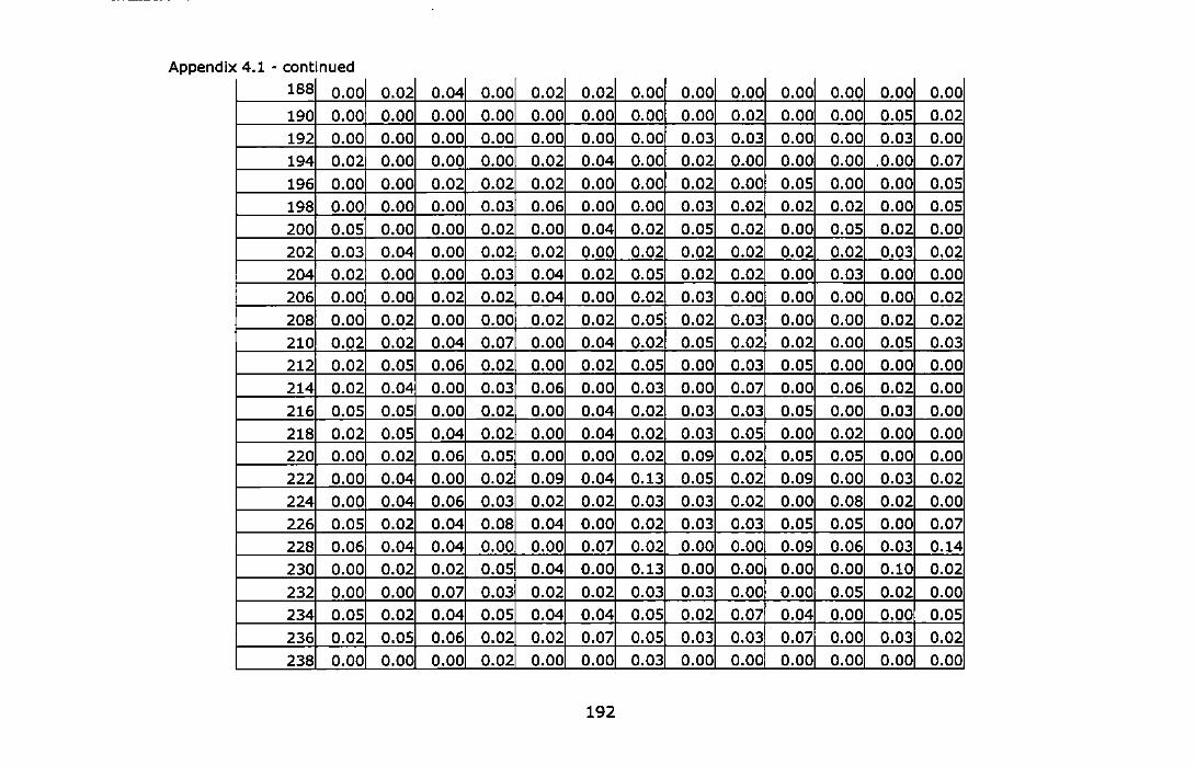
Appendix 4.1 -continued 188 0.00 0.02 0.04 0.00 0.02 0.02 0.00 0.00 0.00 0.00 0.00 0.00 0.00

190 0.00 0.00 0.00 0.00 0.00 0.00 0.00 0.00 0.02 0.00 0.00 0.05 0.02

192 0.00 0.00 0.00 0.00 0.00 0.00 0.00 0.03 0.03 0.00 0.00 0.03 0.00

194 0.02 0.00 0.00 0.00 0.02 0.04 0.00 0.02 0.00 0.00 0.00 .0.00 0.07

196 0.00 0.00 0.02 0.02 0.02 0.00 0.00 0.02 0.00 0.05 0.00 0.00 0.05

198 0.00 0.00 0.00 0.03 0.06 0.00 0.00 0.03 0.02 0.02 0.02 0.00 0.05

200 0.05 0.00 0.00 0.02 0.00 0.04 0.02 0.05 0.02 0.00 0.05 0.02 0.00

202 0.03 0.04 0.00 0.02 0.02 0.00 0.02 0.02 0.02 0.02 0.02 0.03 0.02

204 0.02 0.00 0.00 0.03 0.04 0.02 0.05 0.02 0.02 0.00 0.03 0.00 0.00

206 0.00 0.00 0.02 0.02 0.04 0.00 0.02 0.03 0.00 0.00 0.00 0.00 0.02

208 0.00 0.02 0.00 0.00 0.02 0.02 0.05 0.02 0.03 0.00 0.00 0.02 0.02

210 0.02 0.02 0.04 0.07 0.00 0.04 0.02 0.05 0.02 0.02 0.00 0.05 0.03

212 0.02 0.05 0.06 0.02 0.00 0.02 0.05 0.00 0.03 0.05 0.00 0.00 0.00

214 0.02 0.04 0.00 0.03 0.06 0.00 0.03 0.00 0.07 0.00 0.06 0.02 0.00

216 0.05 0.05 0.00 0.02 0.00 0.04 0.02 0.03 0.03 0.05 0.00 0.03 0.00

218 0.02 0.05 0.04 0.02 0.00 0.04 0.02 0.03 0.05 0.00 0.02 0.00 0.00

220 0.00 0.02 0.06 0.05 0.00 0.00 0.02 0.09 0.02 0.05 0.05 0.00 0.00

222 0.00 0.04 0.00 0.02 0.09 0.04 0.13 0.05 0.02 0.09 0.00 0.03 0.02

224 0.00 0.04 0.06 0.03 0.02 0.02 0.03 0.03 0.02 0.00 0.08 0.02 0.00

226 0.05 0.02 0.04 0.08 0.04 0.00 0.02 0.03 0.03 0.05 0.05 0.00 0.07

228 0.06 0.04 0.04 0.00 0.00 0.07 0.02 0.00 0.00 0.09 0.06 0.03 0.14

230 0.00 0.02 0.02 0.05 0.04 0.00 0.13 0.00 0.00 0.00 0.00 0.10 0.02

232 0.00 0.00 0.07 0.03 0.02 0.02 0.03 0.03 0.00 0.00 0.05 0.02 0.00

234 0.05 0.02 0.04 0.05 0.04 0.04 0.05 0.02 0.07 0.04 0.00 0.00 0.05

236 0.02 0.05 0.06 0.02 0.02 0.07 0.05 0.03 0.03 0.07 0.00 0.03 0.02

238 0.00 0.00 0.00 0.02 0.00 0.00 0.03 0.00 0.00 0.00 0.00 0.00 0.00

192

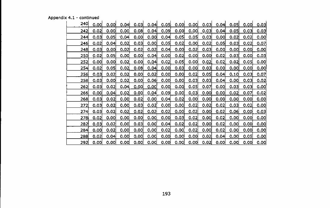
Appendix 4.1 -continued

240 0.00 0.00 0.04 0.03 0.04 0.05 0.00 0.00 0.03 0.04 0.05 0.00 0.03

242 0.02 0.00 0.00 0.08 0.04 0.09 0.00 0.00 0.03 0.04 0.05 0.03 0.03

244 0.03 0.05 ·o.o4 0.00 0.00 0.04 0.05 0.05 0.03 0.00 0.02 0.02 0.00 246 0.02 0.04 0.02 0.03 0.00 0.05 0.02 0.00 0.02 0.05 0.03 0.02 0.07

248 0.03 0.00 0.02 0.02 0.02 0.04 0.00 0.02 0.03 0.00 0.00 0.00 0.00

250 0.02 0.05 0.00 0.00 0.04 0.00 0.02 0.00 0.00 0.02 0.03 0.00 0.03

252 0.00 0.00 0.02 0.00 0.04 0.02 0.05 0.00 0.02 0.02 0.02 0.05 0.00

254 0.02 0.05 0.02 0.08 0.04 0.00 0.03 0.00 0.03 0.00 0.00 0.00 0.00

256 0.03 0.02 0.02 0.00 0.02 0.00 0.00 0.02 0.05 0.04 0.10 0.03 0.07

258 0.03 0.00 0.02 0.00 0.06 0.00 0.00 0.03 0.03 0.04 0.00 0.03 0.02

262 0.03 0.02 0.04 0.00 0.00 0.00 0.00 0.05 0.07 0.00 0.03 0.03 0.00

266 0.00 0.04 0.02 0.00 0.04 0.09 0.00 0.03 0.00 0.00 0.02 0.07 0.02

268 0.03 0.02 0.00 0.02 0.00 0.04 0.02 0.00 0.00 0.00 0.00 0.00 0.00

272 0.03 0.02 0.00 0.03 0.02 0.00 0.00 0.02 0.02 0.02 0.03 0.02 0.00

274 0.03 0.02 0.02 0.02 0.02 0.02 0.00 0.02 0.00 0.02 0.06 0.00 0.03

278 0.02 0.00 0.00 0.00 0.00 0.00 0.03 0.02 0.00 0.02 0.00 0.00 0.00

282 0.03 0.02 0.00 0.03 0.00 0.04 0.02 0.02 0.00 0.02 0.00 0.00 0.00

284 0.00 0.02 0.00 0.00 0.00 0.02 0.00 0.02 0.00 0.02 0.00 0.00 0.00

288 0.02 0.04 0.00 0.00 0.00 0.00 0.00 0.00 0.02 0.04 0.00 0.05 0.00

292 0.00 0.00 0.00 0.00 0.00 0.00 0.00 0.00 0.02 0.00 0.00 0.00 0.00

193

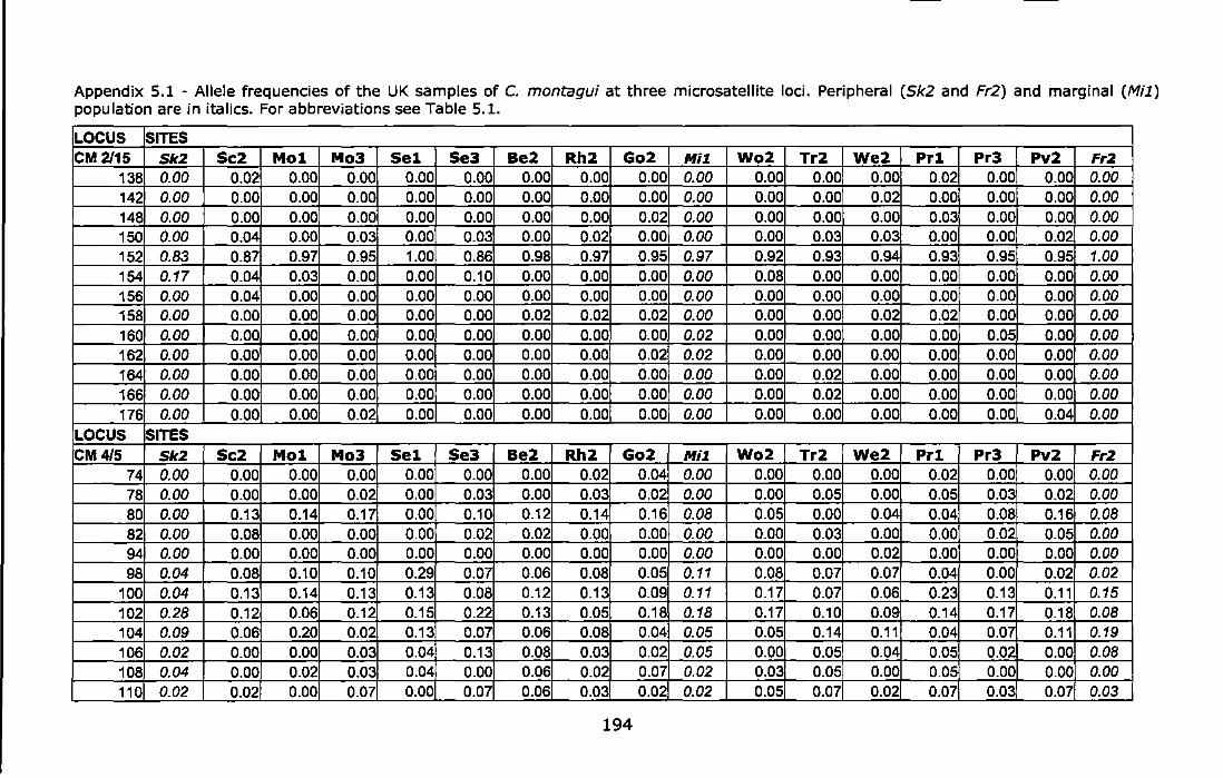
Appendix 5.1 - Allele frequencies of the UK samples of C. montagui at three microsatellite loci. Peripheral (Sk2 and Fr2) and marginal (Mil) population are in italics. For abbreviations see Table 5.1.

LOCUS SITES CM 2115 Sk2 Sc2 Mol Mo3 Sel Se3 Be2 Rh2 Go2 Mil Wo2 Tr2 We2 Prl Pr3 Pv2 Fr2

138 0.00 0.02 0.00 0.00 0.00 0.00 0.00 0.00 0.00 0.00 0.00 0.00 0.00 0.02 0.00 0.00 0.00 142 0.00 0.00 0.00 0.00 0.00 0.00 0.00 0.00 0.00 0.00 0.00 0.00 0.02 0.00 0.00 0.00 0.00 148 0.00 0.00 0.00 0.00 0.00 0.00 0.00 0.00 0.02 0.00 0.00 0.00 0.00 0.03 0.00 0.00 0.00 150 0.00 0.04 0.00 0.03 0.00 0.03 0.00 0.02 0.00 0.00 0.00 0.03 0.03 0.00 0.00 0.02 0.00 152 0.83 0.87 0.97 0.95 1.00 0.86 0.98 0.97 0.95 0.97 0.92 0.93 0.94 0.93 0.95 0.95 1.00 154 0.17 0.04 0.03 0.00 0.00 0.10 0.00 0.00 0.00 0.00 0.08 0.00 0.00 0.00 0.00 0.00 0.00 156 0.00 0.04 0.00 0.00 0.00 0.00 0.00 0.00 0.00 0.00 0.00 0.00 0.00 0.00 0.00 0.00 0.00 158 0.00 0.00 0.00 0.00 0.00 0.00 0.02 0.02 0.02 0.00 0.00 0.00 0.02 0.02 0.00 0.00 0.00 160 0.00 0.00 0.00 0.00 0.00 0.00 0.00 0.00 0.00 0.02 0.00 0.00 0.00 0.00 0.05 0.00 0.00 162 0.00 0.00 0.00 0.00 0.00 0.00 0.00 0.00 0.02 0.02 0.00 0.00 0.00 0.00 0.00 0.00 0.00 164 0.00 0.00 0.00 0.00 0.00 0.00 0.00 0.00 0.00 0.00 0.00 0.02 0.00 0.00 0.00 0.00 0.00 166 0.00 0.00 0.00 0.00 0.00 0.00 0.00 0.00 0.00 0.00 0.00 0.02 0.00 0.00 0.00 0.00 0.00 176 0.00 0.00 0.00 0.02 0.00 0.00 0.00 0.00 0.00 0.00 0.00 0.00 0.00 0.00 0.00 0.04 0.00

LOCUS SITES CM4/5 Sk2 Sc2 Mol Mo3 Sel Se3 Be2 Rh2 Go2 Mil Wo2 Tr2 We2 Prl Pr3 Pv2 Fr2

74 0.00 0.00 0.00 0.00 0.00 0.00 0.00 0.02 0.04 0.00 0.00 0.00 0.00 0.02 0.00 0.00 0.00 78 0.00 0.00 0.00 0.02 0.00 0.03 0.00 0.03 0.02 0.00 0.00 0.05 0.00 0.05 0.03 0.02 0.00 80 0.00 0.13 0.14 0.17 0.00 0.10 0.12 0.14 0.16 0.08 0.05 0.00 0.04 0.04 0.08 0.16 0.08 82 0.00 0.08 0.00 0.00 0.00 0.02 0.02 0.00 0.00 0.00 0.00 0.03 0.00 0.00 0.02 0.05 0.00 94 0.00 0.00 0.00 0.00 0.00 0.00 0.00 0.00 0.00 0.00 0.00 0.00 0.02 0.00 0.00 0.00 0.00 98 0.04 0.08 0.10 0.10 0.29 0.07 0.06 0.08 0.05 0.11 0.08 0.07 0.07 0.04 0.00 0.02 0.02

100 0.04 0.13 0.14 0.13 0.13 0.08 0.12 0.13 0.09 0.11 0.17 0.07 0.06 0.23 0.13 0.11 0.15 102 0.28 0.12 0.06 0.12 0.15 0.22 0.13 0.05 0.18 0.18 0.17 0.10 0.09 0.14 0.17 0.18 0.08 104 0.09 0.06 0.20 0.02 0.13 0.07 0.06 0.08 0.04 0.05 0.05 0.14 0.11 0.04 0.07 0.11 0.19 106 0.02 0.00 0.00 0.03 0.04 0.13 0.08 0.03 0.02 0.05 0.00 0.05 0.04 0.05 0.02 0.00 0.08 108 0.04 0.00 0.02 0.03 0.04 0.00 0.06 0.02 0.07 0.02 0.03 0.05 0.00 0.05 0.00 0.00 0.00 110 0.02 0.02 0.00 O.Q7 0.00 0.07 0.06 0.03 0.02 0.02 0.05 0.07 0.02 0.07 0.03 0.07 0.03

194

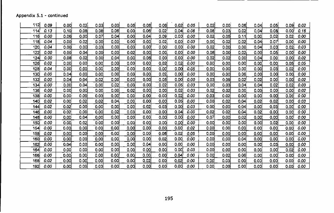
Appendix 5.1 - continued

112 0.09 0.00 0.02 0.03 0.00 0.05 0.08 0.06 0.02 0.05 0.02 0.00 0.06 0.04 0.05 0.09 0.02 114 0.13 0.10 0.08 0.08 0.06 0.00 0.06 0.02 0.04 0.06 0.08 O.Q3 0.02 0.04 0.08 0.00 0.16 116 0.00 0.06 0.00 0.07 0.04 0.00 0.04 0.09 0.00 0.00 0.02 0.05 0.11 0.00 0.02 0.02 0.00 118 0.04 0.00 0.02 0.00 0.00 0.00 0.00 0.02 0.00 0.03 0.00 0.02 0.02 0.04 0.07 0.00 0.00 120 0.04 0.00 0.00 0.03 0.00 0.03 0.00 0.00 0.00 0.00 0.02 0.00 0.00 0.04 0.03 0.02 0.03 122 0.00 0.00 0.04 0.00 0.00 0.02 0.00 0.00 0.00 0.00 0.08 0.00 0.02 0.00 0.05 0.00 0.00 124 0.00 0.08 0.02 0.00 0.04 0.00 0.06 0.00 0.00 0.00 0.02 0.02 0.00 0.04 0.00 0.00 0.02 126 0.02 0.00 0.00 0.00 0.00 0.00 0.00 0.02 0.02 0.00 0.00 0.00 0.00 0.00 0.00 0.05 0.05 128 0.04 0.00 0.00 0.00 0.00 0.00 0.00 0.00 0.00 0.05 0.00 0.00 0.00 0.00 0.03 0.02 0.00 130 0.00 0.04 0.00 0.00 0.00 0.03 0.00 0.02 0.00 0.00 0.00 0.00 0.06 0.00 0.00 0.00 0.00 132 0.00 0.04 0.04 0.02 0.00 0.00 0.00 0.05 0.00 0.00 0.03 0.09 0.02 0.02 0.00 0.00 0.02 134 0.00 0.00 0.04 0.00 0.02 0.03 0.00 0.02 0.05 0.03 0.00 0.03 0.04 0.04 0.02 0.02 0.03 136 0.00 0.00 0.00 0.00 0.00 0.02 0.00 0.00 0.02 0.03 0.02 0.02 0.00 0.00 0.00 0.00 0.02 138 0.00 0.00 0.00 0.03 0.00 0.00 0.00 0.00 0.02 0.00 0.03 0.02 0.00 0.00 0.00 0.05 0.00 140 0.02 0.00 0.02 0.02 0.04 0.00 0.00 0.00 0.05 0.00 0.00 0.02 0.04 0.02 0.02 0.00 0.03 144 0.02 0.02 0.00 0.00 0.00 0.00 0.02 0.03 0.00 0.03 0.00 0.00 0.04 0.00 0.03 0.00 0.00 146 0.00 0.02 0.00 0.00 0.02 0.03 0.00 0.00 0.04 0.00 0.02 0.02 0.04 0.02 0.00 0.00 0.00 148 0.00 0.00 0.04 0.00 0.00 0.00 0.00 0.00 0.00 0.00 0.07 0.00 0.02 0.00 0.00 0.00 0.00 150 0.00 0.00 0.02 0.00 0.00 0.00 0.00 0.00 0.00 0.00 0.00 0.00 0.00 0.00 0.02 0.00 0.00 154 0.00 0.00 0.00 0.00 0.00 0.00 0.00 0.00 0.00 0.02 0.00 0.00 0.00 0.00 0.00 0.00 0.00 158 0.02 0.00 0.00 0.00 0.00 0.00 0.00 0.08 0.02 0.05 0.00 0.00 0.00 0.00 0.00 0.00 0.00 160 0.00 0.00 0.00 0.00 0.00 0.00 0.00 0.02 0.00 0.00 0.00 0.00 0.04 0.00 0.00 0.00 0.00 162 0.00 0.04 0.00 0.00 0.00 0.00 0.04 0.00 0.00 0.00 0.00 0.00 0.00 0.00 0.03 0.00 0.00 164 0.00 0.00 0.00 0.00 0.00 0.00 0.00 0.00 0.00 0.03 0.00 0.00 0.00 0.00 0.00 0.02 0.00 166 0.00 0.00 0.00 0.00 0.00 0.00 0.00 0.00 0.04 0.00 0.00 0.02 0.06 0.00 0.00 0.00 0.00 168 0.02 0.00 0.00 0.00 0.00 0.00 0.02 0.00 0.02 0.00 0.00 0.03 0.00 0.00 0.00 0.00 0.00 192 0.00 0.00 0.00 0.03 0.00 0.00 0.00 0.00 0.00 0.00 0.00 0.00 0.00 0.00 0.00 0.00 0.00

195

Appendix 5.1 -continued

LOCUS lsiTES CM 5/23 Sk2 Sc2 Mol Mo3 Se1 Se3 Be2 Rh2 Go2 Mi1 Wo2 Tr2 We2 Pr1 Pr3 Pv2 Fr2

158 0.00 0.00 0.02 0.00 0.00 0.00 0.00 0.00 0.00 0.00 0.00 0.00 0.00 0.02 0.00 0.00 0.00 162 0.00 0.00 0.00 0.02 0.00 0.04 0.00 0.00 0.00 0.00 0.02 0.00 0.02 0.02 0.00 0.00 0.00 164 0.00 0.00 0.00 0.02 0.00 0.00 0.00 0.00 0.02 0.00 0.00 0.05 0.00 0.00 0.02 0.00 0.00 166 0.00 0.02 0.00 0.00 0.00 0.00 0.00 0.03 0.00 0.00 0.00 0.00 0.02 0.00 0.02 0.00 0.00 170 0.00 0.03 0.00 0.03 0.03 0.00 0.02 0.02 0.02 0.02 O.Q3 0.02 0.05 0.00 0.04 0.00 0.02 172 0.00 0.02 0.00 0.05 0.02 0.00 0.00 0.00 0.00 0.03 0.00 0.00 0.02 0.02 0.04 0.02 0.02 174 0.02 0.05 0.00 0.03 0.02 0.06 0.03 0.03 0.02 0.05 0.05 0.00 0.03 0.00 0.04 0.04 0.05 176 0.50 0.52 0.61 0.42 0.61 0.48 0.55 0.50 0.63 0.38 0.55 0.52 0.43 0.50 0.54 0.54 0.42 178 0.30 0.23 0.22 0.21 0.16 0.23 0.22 0.31 0.18 0,26 0.19 0.18 0.24 0.27 0.14 0.25 0.30 180 0.08 0.08 0.11 0.15 0.11 0.17 0.15 0.09 0.13 0.14 0.10 0.03 0.10 0.03 0.09 0.14 0.09 182 0.02 0.00 0.00 0.03 0.03 0.02 0.02 0.00 0.02 0.07 0.05 0.07 0.05 0.08 0.02 0.00 0.08 184 0.00 0.06 0.03 0.03 0.00 0.00 0.00 0.00 0.00 0.02 0.02 0.03 0.03 0.05 0.04 0.02 0.00 186 0.06 0.00 0.00 0.00 0.02 0.00 0.00 0.02 0.00 0.02 0.00 0.08 0.00 0.02 0.00 0.00 0.02 188 0.02 0.00 0.00 0.00 0.00 0.00 0.00 0.00 0.00 0.00 0.00 0.00 0.00 0.00 0.02 0.00 0.02 190 0.00 0.00 0.00 0.02 0.00 0.00 0.00 0.00 0.00 0.00 0.00 0.00 0.00 0.00 0.00 0.00 0.00 192 0.00 0.00 0.00 0.00 0.00 0.00 0.00 0.00 0.00 0.00 0.00 0.00 0.00 0.02 0.00 0.00 0.00 194 0.00 0.00 0.00 0.00 0.02 0.00 0.00 0.00 0.00 0.00 0.00 0.02 0.00 0.00 0.00 0.00 0.00 202 0.00 0.00 0.00 0.00 0.00 0.00 0.00 0.00 0.00 0.02 0.00 0.00 0.00 0.00 0.00 0.00 0.00 210 0.00 0.00 0.00 0.00 0.00 0.00 0.00 0.00 0.00 0.00 0.00 0.00 0.00 0.00 0.02 0.00 0.00 216 0.00 0.00 0.00 0.00 0.00 0.00 0.02 0.00 0.00 0.00 0.00 0.00 0.00 0.00 0.00 0.00 0.00 218 0.00 0.00 0.02 0.00 0.00 0.00 0.00 0.00 0.00 0.00 0.00 0.00 0.00 0.00 0.00 0.00 0.00

196

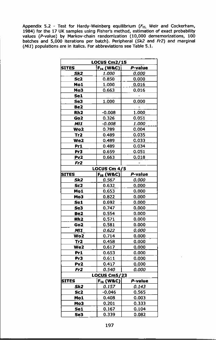
Appendix 5.2 - Test for Hardy-Weinberg equilibrium (F15, Weir and Cockerham, 1984) for the 17 UK samples using Fisher's method, estimation of exact probability values (P-value) by Markov-chaln randomlzation (10,000 dememorizations, 100 batches and 5,000 iterations per batch). Peripheral (Sk2 and Fr2) and marginal (Mi1} populations are in Italics. For abbreviations see Table 5.1.

LOCUS CmZ/15 SITES Frs CW&Cl P..value

Sk2 1.000 0.000 ScZ 0.850 0.000 Mol 1.000 0.016 Mo3 0.663 0.016 Sel -Se3 1.000 0.000 BeZ -RhZ -0.008 1.000 GoZ 0.326 0.051 M/:1 -0.008 1.000 WoZ 0.789 0.004 TrZ 0.489 0.035 WeZ 0.489 0.033 Prl 0.489 0.034 Pr3 0.659 0.051 PvZ 0.663 0.018 Fr2 -

LOCUS Cm 4/5 SITES Frs (W&C) P-value

Sk2 0.567 0.000 ScZ 0.632 0.000 Mol 0.653 0.000 Mo3 0.822 0.000 Sel 0.692 0.000 Se3 0.747 0.000 BeZ 0.554 0.000 RhZ 0.571 0.000 GoZ 0.581 0.000 M/1 0.622 0.000 WoZ 0.714 0.000 TrZ 0.458 0.000 WeZ 0.617 0.000 Prl 0.653 0.000 Pr3 0.611 0.000 PvZ 0.417 0.000 Fr2 0.540 0.000

LOCUS Cm5/23 SITES Fr,. CW&Cl P-value

Sk2 0.157 0.143 ScZ -0.046 0.565 Mol 0.408 0.003 Mo3 0.201 0.333 Sel 0.167 0.104 Se3 0.339 0.082

197

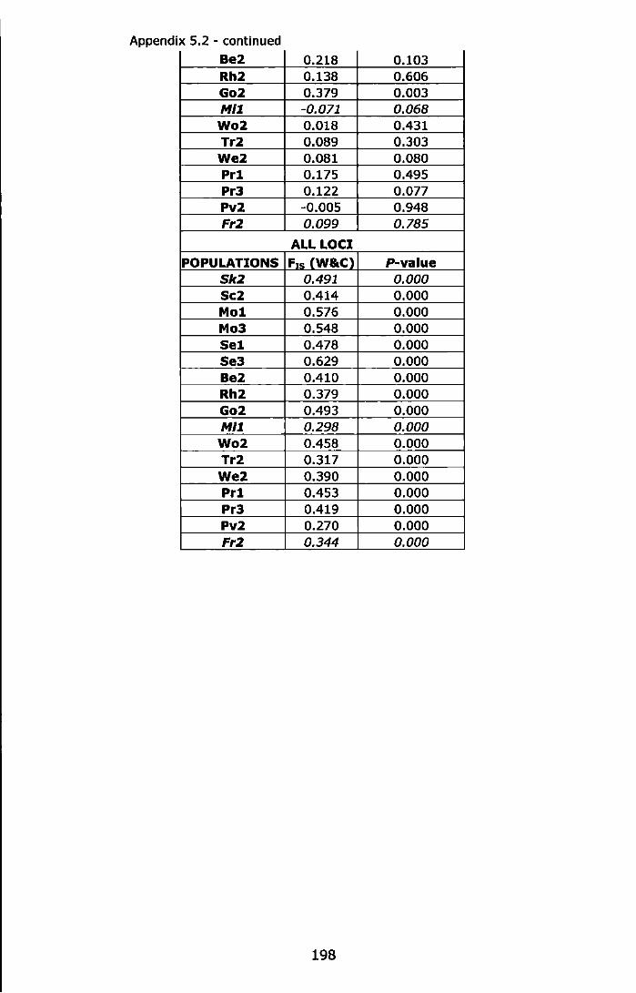
Appendix 5.2 - continued

Be2 0.218 0.103 Rh2 0.138 0.606 Go2 0.379 0.003 Mll -0.071 0.068 Wo2 0.018 0.431 Tr2 0.089 0.303 We2 0.081 0.080 Prl 0.175 0.495 Pr3 0.122 0.077 Pv2 -0.005 0.948 Fr2 0.099 0.785

ALL LOCI POPULATION$ F1s (W&C) P-value

Sk2 0.491 0.000 Sc2 0.414 0.000 Mol 0.576 0.000 Mol 0.548 0.000 Sel 0.478 0.000 Se3 0.629 0.000 Be2 0.410 0.000 Rh2 0.379 0.000 Go2 0.493 0.000 Mi1 0.298 0.000 Wo2 0.458 0.000 Tr2 0.317 0.000 We2 0.390 0.000 Prl 0.453 0.000 Pr3 0.419 0.000 Pv2 0.270 0.000 Fr2 0.344 0.000

198

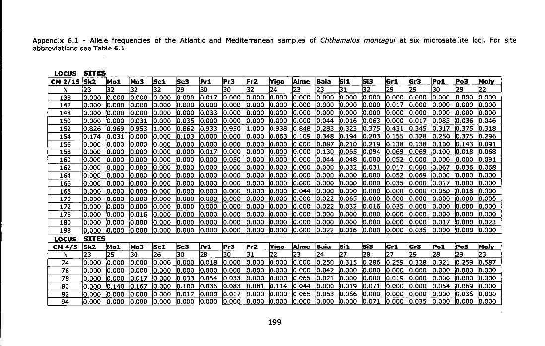
Appendix 6.1 - Allele frequencies of the Atlantic and Mediterranean samples of Chthamalus montagui at six microsatellite loci. For site abbreviations see Table 6.1

LOCUS SITES CM 2/15 Sk2 Mol Mo3 Sel Se3 Prl Pr3 Fr2 Viqo ~me Baia Sil Si3 Grl Gr3 Pol Po3 Molv

N 23 32 32 32 29 30 30 32 24 23 23 31 32 29 29 30 28 22 138 0.000 0.000 0.000 0.000 0.000 0.017 0.000 0.000 0.000 0.000 0.000 0.000 0.000 0.000 0.000 0.000 0.000 0.000 142 0.000 0.000 0.000 0.000 0.000 0.000 0.000 0.000 0.000 0.000 0.000 0.000 0.000 0.017 0.000 0.000 0.000 0.000 148 0.000 0.000 0.000 0.000 0.000 0.033 0.000 0.000 0.000 0.000 0.000 0.000 0.000 0.000 0.000 0.000 0.000 0.000 150 0.000 0.000 0.031 0.000 0.035 0.000 0.000 0.000 0.000 0.000 0.044 0.016 0.063 0.000 0.017 0.083 0.036 0.046 152 0.826 0.969 0.953 1.000 0.862 0.933 0.950 1.000 0.938 0.848 0.283 0.323 0.375 0.431 0.345 0.317 0.375 0.318 154 0.174 0.031 0.000 0.000 0.103 0.000 0.000 0.000 0.063 0.109 0.348 0.194 0.203 0.155 0.328 0.250 0.375 0.296 156 0.000 0.000 0.000 0.000 0.000 0.000 0.000 0.000 0.000 0.000 0.087 0.210 0.219 0.138 0.138 0.100 0.143 0.091 158 0.000 0.000 0.000 0.000 0.000 0.017 0.000 0.000 0.000 0.000 0.130 0.065 0.094 0.069 0.069 0.100 0.018 0.068 160 0.000 0.000 0.000 0.000 0.000 0.000 0.050 0.000 0.000 0.000 0.044 0.048 0.000 0.052 0.000 0.000 0.000 0.091 162 0.000 0.000 0.000 0.000 0.000 0.000 0.000 0.000 0.000 0.000 0.000 0.032 0.031 0.017 0.000 0.067 0.036 0.068 164 0.000 0.000 0.000 0.000 0.000 0.000 0.000 0.000 0.000 0.000 0.000 0.000 0.000 0.052 0.069 0.000 0.000 0.000 166 0.000 0.000 0.000 0.000 0.000 0.000 0.000 0.000 0.000 0.000 0.000 0.000 0.000 0.035 0.000 0.017 0.000 0.000 168 0.000 0.000 0.000 0.000 0.000 0.000 0.000 0.000 0.000 0.044 0.000 0.000 0.000 0.000 0.000 0.050 0.018 0.000 170 0.000 0.000 0.000 0.000 0.000 0.000 0.000 0.000 0.000 0.000 0.022 0.065 0.000 0.000 0.000 0.000 0.000 0.000 172 0.000 0.000 0.000 0.000 0.000 0.000 0.000 0.000 0.000 0.000 0.022 0.032 0.016 0.035 0.000 0.000 0.000 0.000 176 0.000 0.000 0.016 0.000 0.000 0.000 0.000 0.000 0.000 0.000 0.000 0.000 0.000 0.000 0.000 0.000 0.000 0.000 180 0.000 0.000 0.000 0.000 0.000 0.000 0.000 0.000 0.000 0.000 0.000 0.000 0.000 0.000 0.000 0.017 0.000 0.023 198 0.000 0.000 0.000 0.000 0.000 0.000 0.000 0.000 0.000 0.000 0.022 0.016 0.000 0.000 0.035 0.000 0.000 0.000

LOCUS SITES CM4/5 Sk2 Mol Mo3 Sel Se3 Prl Pr3 Fr2 Viqo AI me Baia Sil Si3 Grl Gr3 Pol Po3 Molv

N 23 25 30 26 30 28 30 31 22 23 24 27 28 27 29 28 29 23 74 0.000 0.000 0.000 0.000 0.000 0.018 0.000 0.000 0.000 0.000 0.250 0.315 0.286 0.259 0.328 0.321 0.259 0.587 76 0.000 0.000 0.000 0.000 0.000 0.000 0.000 0.000 0.000 0.000 0.042 0.000 0.000 0.000 0.000 0.000 0.000 0.000 78 0.000 0.000 0.017 0.000 0.033 0.054 0.033 0.000 0.000 0.065 0.021 0.000 0.000 0.019 0.000 0.000 0.000 0.000 80 0.000 0.140 0.167 0.000 0.100 0.036 0.083 0.081 0.114 0.044 0.000 0.019 0.071 0.000 0.000 0.054 0.069 0.000 82 0.000 0.000 0.000 0.000 0.017 0.000 0.017 0.000 0.000 0.065 0.063 0.056 0.000 0.000 0.000 0.000 0.035 0.000 94 0.000 0.000 0.000 0.000 0.000 0.000 0.000 0.000 0.000 0.000 0.000 0.000 0.071 0.000 0.035 0.000 0.000 0.000

199

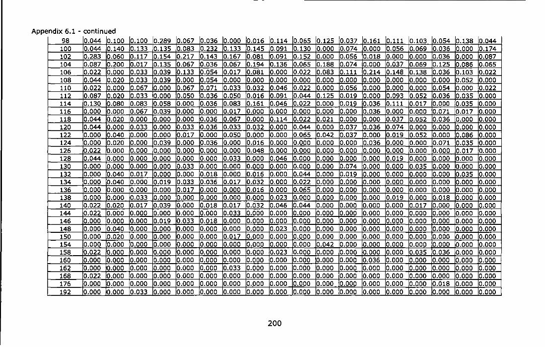
Appendix 6.1 -continued

98 0.044 0.100 0.100 0.289 0.067 0.036 0.000 0.016 0.114 0.065 0.125 0.037 0.161 0.111 0.103 0.054 0.138 0.044 100 0.044 0.140 0.133 0.135 0.083 0.232 0.133 0.145 0.091 0.130 0.000 0.074 0.000 0.056 0.069 0.036 0.000 0.174 102 0.283 0.060 0.117 0.154 0.217 0.143 0.167 0.081 0.091 0.152 0.000 0.056 0.018 0.000 0.000 0.036 0.000 0.087 104 0.087 0.200 0.017 0.135 0.067 0.036 0.067 0.194 0.136 0.065 0.188 0.074 0.000 0.037 0.069 0.125 0.086 0.065 106 0.022 0.000 0.033 0.039 0.133 0.054 0.017 0.081 0.000 0.022 0.083 0.111 0.214 0.148 0.138 0.036 0.103 0.022 108 0.044 0.020 0.033 0.039 0.000 0.054 0.000 o.ooo 0.000 0.000 0.000 0.000 0.000 0.000 0.000 0.000 0.052 0.000 110 0.022 0.000 0.067 0.000 0.067 0.071 0.033 0.032 0.046 0.022 0.000 0.056 0.000 0.000 0.000 0.054 0.000 0.022 112 0.087 0.020 0.033 0.000 0.050 0.036 0.050 0.016 0.091 0.044 0.125 0.019 0.000 0.093 0.052 0.036 0.035 0.000 114 0.130 0.080 0.083 0.058 0.000 0.036 0.083 0.161 0.046 0.022 0.000 0.019 0.036 0.111 0.017 0.000 0.035 0.000 116 0.000 0.000 0.067 0.039 0.000 0.000 0.017 0.000 0.000 0.000 0.000 0.000 0.036 0.000 0.000 0.071 0.017 0.000 118 0.044 0.020 0.000 0.000 0.000 0.036 0.067 0.000 0.114 0.022 0.021 0.000 0.000 0.037 0.052 0.036 0.000 0.000 120 0.044 0.000 0.033 0.000 0.033 0.036 0.033 0.032 0.000 0.044 0.000 0.037 0.036 0.074 0.000 0.000 0.000 0.000 122 0.000 0.040 0.000 0.000 0.017 0.000 0.050 o.ooo 0.000 0.065 0.042 0.037 0.000 0.019 0.052 0.000 0.086 0.000 124 0.000 0.020 0.000 0.039 0.000 0.036 0.000 0.016 0.000 0.000 0.000 0.000 0.036 0.000 0.000 0.071 0.035 0.000 126 0.022 0.000 0.000 0.000 0.000 0.000 0.000 0.048 0.000 0.000 0.000 0.000 0.000 0.000 0.000 0.000 0.017 0.000 128 0.044 0.000 0.000 0.000 0.000 0.000 0.033 0.000 0.046 0.000 0.000 0.000 0.000 0.019 0.000 0.000 0.000 0.000 130 0.000 0.000 0.000 0.000 0.033 0.000 0.000 0.000 0.000 0.000 0.000 0.074 0.000 0.000 0.035 0.000 0.000 0.000 132 0.000 0.040 0.017 0.000 0.000 0.018 0.000 0.016 0.000 0.044 0.000 0.019 0.000 0.000 0.000 0.000 0.035 0.000 134 0.000 0.040 0.000 0.019 0.033 0.036 0.017 0.032 0.000 0.022 0.000 0.000 0.000 0.000 0.000 0.000 0.000 0.000 136 0.000 0.000 0.000 0.000 0.017 0.000 0.000 0.016 0.000 0.065 0.000 0.000 0.000 0.000 0.000 0.000 0.000 0.000 138 0.000 0.000 0.033 0.000 0.000 0.000 0.000 0.000 0.023 0.000 0.000 0.000 0.000 0.019 0.000 0.018 0.000 0.000 140 0.022 0.020 0.017 0.039 0.000 0.018 0.017 0.032 0.046 0.044 0.000 0.000 0.000 0.000 0.017 0.000 0.000 0.000 144 0.022 0.000 0.000 0.000 0.000 0.000 0.033 0.000 0.000 0.000 0.000 0.000 0.000 0.000 0.000 0.000 0.000 0.000 146 0.000 0.000 0.000 0.019 0.033 0.018 0.000 0.000 0.000 0.000 0.000 0.000 0.000 0.000 0.000 0.000 0.000 0.000 148 0.000 0.040 0.000 0.000 0.000 0.000 0.000 0.000 0.023 0.000 0.000 0.000 0.000 0.000 0.000 0.000 0.000 0.000 150 0.000 0.020 0.000 0.000 0.000 0.000 0.017 0.000 0.000 0.000 0.000 0.000 0.000 0.000 0.000 0.000 0.000 0.000 154 0.000 0.000 0.000 0.000 0.000 0.000 0.000 0.000 0.000 0.000 0.042 0.000 0.000 0.000 0.000 0.000 0.000 0.000 158 0.022 0.000 0.000 0.000 0.000 0.000 0.000 0.000 0.023 0.000 0.000 0.000 0.000 0.000 0.035 0.036 0.000 0.000 160 0.000 0.000 0.000 0.000 0.000 0.000 0.000 0.000 0.000 0.000 0.000 0.000 0.036 0.000 0.000 0.000 0.000 0.000 162 0.000 0.000 0.000 0.000 0.000 0.000 0.033 0.000 0.000 0.000 0.000 0.000 0.000 0.000 0.000 0.000 0.000 0.000 168 0.022 0.000 0.000 0.000 0.000 0.000 0.000 0.000 0.000 0.000 0.000 0.000 0.000 0.000 0.000 0.000 0.000 0.000 176 0.000 0.000 0.000 0.000 0.000 0.000 0.000 0.000 0.000 0.000 0.000 0.000 0.000 0.000 0.000 0.018 0.000 0.000 192 0.000 0.000 0.033 0.000 0.000 0.000 0.000 0.000 0.000 0.000 0.000 0.000 0.000 0.000 0.000 0.000 0.000 0.000

200

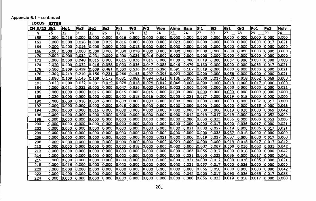
Appendix 6.1 -continued LOCUS SITES

CM 5/23 Sk2 Mol Mo3 Sel Se3 Pr1 Pr3 Fr2 Vlgo Alme Baia Si1 Si3 Gr1 Gr3 Po1 Po3 Moly N 25 32 31 32 26 32 28 32 24 22 24 27 30 27 28 29 29 24

158 0.000 0.016 0.000 0.000 0.000 0.016 0.000 0.000 0.000 0.000 0.000 0.000 0.000 0.000 0.000 0.000 0.000 0.000 162 0.000 0.000 0.016 0.000 0.039 0.016 0.000 0.000 0.000 0.023 0.000 0.000 0.000 0.000 0.000 0.000 0.017 0.021 164 0.000 0.000 0.016 0.000 0.000 0.000 0.018 0.000 0.000 0.000 0.000 0.000 0.000 0.000 0.000 0.000 0.000 0.000 166 0.000 0.000 0.000 0.000 0.000 0.000 0.018 0.000 0.000 0.000 0.000 0.000 0.000 0.000 0.000 0.000 0.000 0.000 170 0.000 0.000 0.032 0.031 0.000 0.000 0.036 0.016 0.000 0.023 0.000 0.000 0.000 0.000 0.000 0.000 0.000 0.000 172 0.000 0.000 0.048 0.016 0.000 0.016 0.036 0.016 0.000 0.000 0.000 0.019 0.000 0.037 0.000 0.000 0.000 0.000 174 0.020 0.000 0.032 0.016 0.058 0.000 0.036 0.047 0.083 0.046 0.479 0.130 0.000 0.000 0.000 0.069 0.017 0.021 176 0.500 0.609 0..419 0.609 0.481 0.500 0.536 0.422 0.396 0.591 0.167 0.019 0.000 0.000 0.000 0.000 0.000 0.021 178 0.300 0.219 0.210 0.156 0.231 0.266 0.143 0.297 0.396 0.023 0.000 0.000 0.000 0.056 0.000 0.000 0.000 0.021 180 0.080 0.109 0.145 0.109 0.173 0.031 0.089 0.094 0.021 0.136 0.000 0.000 0.017 0.000 0.018 0.052 0.069 0.000 182 0.020 0.000 0.032 0.031 0.019 0.078 0.018 0.078 0.042 0.046 0.000 0.000 0.000 0.019 0.000 0.017 0.000 0.000 184 0.000 0.031 0.032 0.000 0.000 0.047 0.036 0.000 0.042 0.023 0.000 0.000 0.000 0.000 0.000 0.000 0.000 0.021 186 0.060 0.000 0.000 0.016 0.000 0.016 0.000 0.016 0.000 0.000 0.000 0.000 0.000 0.000 0.000 0.000 0.000 0.000 188 0.020 0.000 0.000 0.000 0.000 0.000 0.018 0.016 0.000 0.000 0.021 0.037 0.000 0.019 0.018 0.000 0.000 0.000 190 0.000 0.000 0.016 0.000 0.000 0.000 0.000 0.000 0.000 0.000 0.000 0.000 0.000 0.000 0.000 0.052 0.017 0.000 192 0.000 0.000 0.000 0.000 0.000 0.016 0.000 0.000 0.000 0.000 0.000 0.000 0.000 0.000 0.000 0.035 0.000 0.063 194 0.000 0.000 0.000 0.016 0.000 0.000 0.000 0.000 0.000 0.000 0.000 0.000 0.000 0.019 0.036 0.000 0.069 0.042 196 0.000 0.000 0.000 0.000 0.000 0.000 0.000 0.000 0.000 0.000 0.042 0.019 0.017 0.019 0.000 0.000 0.052 0.000 198 0.000 0.000 0.000 0.000 0.000 0.000 0.000 0.000 0.000 0.000 0.000 0.000 0.033 0.056 0.000 0.000 0.052 0.000 200 0.000 0.000 0.000 0.000 0.000 0.000 0.000 0.000 0.000 0.000 0.000 0.000 0.017 0.000 0.036 0.017 0.000 0.021 202 0.000 0.000 0.000 0.000 0.000 0.000 0.000 0.000 0.000 0.000 0.021 0.000 0.017 0.019 0.000 0.035 0.017 0.021 204 0.000 0.000 0.000 0.000 0.000 0.000 0.000 0.000 0.000 0.000 0.000 0.000 0.033 0.037 0.018 0.000 0.000 0.000 206 0.000 0.000 0.000 0.000 0.000 0.000 0.000 0.000 0.021 0.000 0.000 0.019 0.017 0.037 0.000 0.000 0.017 0.000 208 0.000 0.000 0.000 0.000 0.000 0.000 0.000 0.000 0.000 0.023 0.000 0.000 0.000 0.019 0.018 0.017 0.017 0.042 210 0.000 0.000 0.000 0.000 0.000 0.000 0.018 0.000 0.000 0.000 0.000 0.037 0.067 0.000 0.036 0.052 0.035 0.042 212 0.000 0.000 0.000 0.000 0.000 0.000 0.000 0.000 0.000 0.000 0.063 0.056 0.017 0.000 0.018 0.000 0.000 0.042 214 0.000 0.000 0.000 0.000 0.000 0.000 0.000 0.000 0.000 0.000 0.021 0.000 0.033 0.056 0.000 0.017 0.000 0.042 216 0.000 0.000 0.000 0.000 0.000 0.000 0.000 0.000 0.000 0.000 0.021 0.000 0.017 0.000 0.036 0.035 0.000 0.021 218 0.000 0.016 0.000 0.000 0.000 0.000 0.000 0.000 0.000 0.000 0.021 0.037 0.017 0.000 0.036 0.000 0.000 0.000 220 0.000 0.000 0.000 0.000 0.000 0.000 0.000 0.000 0.000 0.000 0.000 0.056 0.050 0.000 0.000 0.000 0.000 0.042 222 0.000 0.000 0.000 0.000 0.000 0.000 0.000 0.000 0.000 0.000 0.042 0.000 0.017 0.093 0.036 0.035 0.017 0.083 224 0.000 0.000 0.000 0.000 0.000 0.000 0.000 0.000 0.000 0.000 0.000 0.056 0.033 0.019 0.018 0.017 0.000 0.000

201

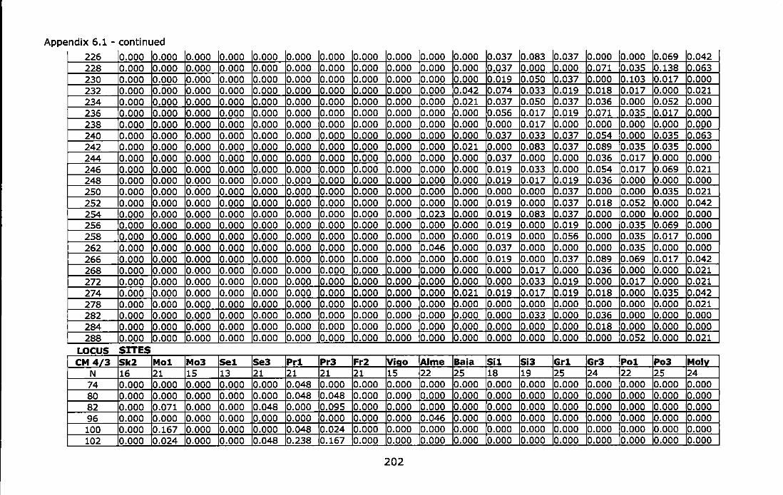
Appendix 6.1 -continued

226 0.000 0.000 0.000 0.000 0.000 0.000 0.000 0.000 0.000 0.000 0.000 0.037 0.083 0.037 0.000 0.000 0.069 0.042 228 0.000 0.000 0.000 0.000 0.000 0.000 0.000 0.000 0.000 0.000 0.000 0.037 0.000 0.000 0.071 0.035 0.138 0.063 230 0.000 0.000 0.000 0.000 0.000 0.000 0.000 0.000 0.000 0.000 0.000 0.019 0.050 0.037 0.000 0.103 0.017 0.000 232 0.000 0.000 0.000 0.000 0.000 0.000 0.000 0.000 0.000 0.000 0.042 0.074 0.033 0.019 0.018 0.017 0.000 0.021 234 0.000 0.000 0.000 0.000 0.000 0.000 0.000 0.000 0.000 0.000 0.021 0.037 0.050 0.037 0.036 0.000 0.052 0.000 236 0.000 0.000 0.000 0.000 0.000 0.000 0.000 0.000 0.000 0.000 0.000 0.056 0.017 0.019 0.071 0.035 0.017 0.000 238 0.000 0.000 0.000 0.000 0.000 0.000 0.000 0.000 0.000 0.000 0.000 0.000 0.017 0.000 0.000 0.000 0.000 0.000 240 0.000 0.000 0.000 0.000 0.000 0.000 0.000 0.000 0.000 0.000 0.000 0.037 0.033 0.037 0.054 0.000 0.035 0.063 242 0.000 0.000 0.000 0.000 0.000 0.000 0.000 0.000 0.000 0.000 0.021 0.000 0.083 0.037 0.089 0.035 0.035 0.000 244 0.000 0.000 0.000 0.000 0.000 0.000 0.000 0.000 0.000 0.000 0.000 0.037 0.000 0.000 0.036 0.017 0.000 0.000 246 0.000 0.000 0.000 0.000 0.000 0.000 0.000 0.000 0.000 0.000 0.000 0.019 0.033 0.000 0.054 0.017 0.069 0.021 248 0.000 0.000 0.000 0.000 0.000 0.000 0.000 0.000 0.000 0.000 0.000 0.019 0.017 0.019 0.036 0.000 0.000 0.000 250 0.000 0.000 0.000 0.000 0.000 0.000 0.000 0.000 0.000 0.000 0.000 0.000 0.000 0.037 0.000 0.000 0.035 0.021 252 0.000 0.000 0.000 0.000 0.000 0.000 0.000 0.000 0.000 0.000 0.000 0.019 0.000 0.037 0.018 0.052 0.000 0.042 254 0.000 0.000 0.000 0.000 0.000 0.000 0.000 0.000 0.000 0.023 0.000 0.019 0.083 0.037 0.000 0.000 0.000 0.000 256 0.000 0.000 0.000 0.000 0.000 0.000 0.000 0.000 0.000 0.000 0.000 0.019 0.000 0.019 0.000 0.035 0.069 0.000 258 0.000 0.000 0.000 0.000 0.000 0.000 0.000 0.000 0.000 0.000 0.000 0.019 0.000 0.056 0.000 0.035 0.017 0.000 262 0.000 0.000 0.000 0.000 0.000 0.000 0.000 0.000 0.000 0.046 0.000 0.037 0.000 0.000 0.000 0.035 0.000 0.000 266 0.000 0.000 0.000 0.000 0.000 0.000 0.000 0.000 0.000 0.000 0.000 0.019 0.000 0.037 0.089 0.069 0.017 0.042 268 0.000 0.000 0.000 0.000 0.000 0.000 0.000 0.000 0.000 0.000 0.000 0.000 0.017 0.000 0.036 0.000 0.000 0.021 272 0.000 0.000 0.000 0.000 0.000 0.000 0.000 0.000 0.000 0.000 0.000 0.000 0.033 0.019 0.000 0.017 0.000 0.021 274 0.000 0.000 0.000 0.000 0.000 0.000 0.000 0.000 0.000 0.000 0.021 0.019 0.017 0.019 0.018 0.000 0.035 0.042 278 0.000 0.000 0.000 0.000 0.000 0.000 0.000 0.000 0.000 0.000 0.000 0.000 0.000 0.000 0.000 0.000 0.000 0.021 282 0.000 0.000 0.000 0.000 0.000 0.000 0.000 0.000 0.000 0.000 0.000 0.000 0.033 0.000 0.036 0.000 0.000 0.000 284 0.000 0.000 0.000 0.000 0.000 0.000 0.000 0.000 0.000 0.000 0.000 0.000 0.000 0.000 0.018 0.000 0.000 0.000 288 0.000 0.000 0.000 0.000 0.000 0.000 0.000 0.000 0.000 0.000 0.000 0.000 0.000 0.000 0.000 0.052 0.000 0.021

LOCUS SITES CM4/3 Sk2 Mol Mo3 Se1 Se3 Pr1 Pr3 Fr2 Viao AI me Baia Si1 Si3 Gr1 Gr3 Po1 Po3 Molv

N 16 21 15 13 21 21 21 21 15 22 25 18 19 25 24 22 25 24 74 0.000 0.000 0.000 0.000 0.000 0.048 0.000 0.000 0.000 0.000 0.000 0.000 0.000 0.000 0.000 0.000 0.000 0.000 80 0.000 0.000 0.000 0.000 0.000 0.048 0.048 0.000 0.000 0.000 0.000 0.000 0.000 0.000 0.000 0.000 0.000 0.000 82 0.000 0.071 0.000 0.000 0.048 0.000 0.095 0.000 0.000 0.000 0.000 0.000 0.000 0.000 0.000 0.000 0.000 0.000 96 0.000 0.000 0.000 0.000 0.000 0.000 0.000 0.000 0.000 0.046 0.000 0.000 0.000 0.000 0.000 0.000 0.000 0.000 100 0.000 0.167 0.000 0.000 0.000 0.048 0.024 0.000 0.000 0.000 0.000 0.000 0.000 0.000 0.000 0.000 0.000 0.000 102 0.000 0.024 0.000 0.000 0.048 0.238 0.167 0.000 0.000 0.000 0.000 0.000 0.000 0.000 0.000 0.000 0.000 0.000

202

Appendix 6.1 -continued 104 0.000 0.214 0.000 0.000 0.000 0.238 0.167 0.000 0.000 0.000 0.000 0.000 0.000 0.000 0.000 0.023 0.000 0.000 106 0.000 0.095 0.000 0.000 0.000 0.000 0.048 0.000 0.067 0.000 0.000 0.000 0.000 0.000 0.000 0.000 0.000 0.000 112 0.000 0.000 0.000 0.000 0.000 0.048 0.000 0.000 0.000 0.000 0.000 0.000 0.000 0.000 0.000 0.000 0.000 0.000 116 0.000 0.024 0.000 0.000 0.000 0.048 0.024 0.000 0.000 0.000 0.000 0.000 0.000 0.000 0.000 0.000 0.000 0.000 120 0.000 0.000 0.000 0.000 0.000 0.000 0.048 0.048 0.000 0.000 0.000 0.000 0.000 0.000 0.000 0.000 0.000 0.000 124 0.000 0.048 0.000 0.000 0.000 0.048 0.000 0.000 0.000 0.000 0.000 0.000 0.000 0.000 0.000 0.000 0.000 0.000 130 0.000 0.000 0.000 0.000 0.048 0.000 0.048 0.000 0.000 0.046 0.000 0.000 0.000 0.000 0.000 0.068 0.000 0.000 140 0.000 0.000 0.000 0.000 0.000 0.000 0.000 0.000 0.000 0.000 0.000 0.000 0.000 0.000 0.000 0.000 0.000 0.042 174 0.250 0.071 0.300 0.231 0.143 0.191 0.167 0.095 0.067 0.568 0.320 0.250 0.211 0.380 0.271 0.136 0.420 0.188 176 0.344 0.143 0.633 0.577 0.262 0.000 0.048 0.452 0.600 0.136 0.020 0.028 0.132 0.000 0.000 0.000 0.020 0.000 178 0.063 0.048 0.000 0.000 0.000 0.000 0.000 0.000 0.000 0.000 0.000 0.000 0.026 0.000 0.000 0.000 0.000 0.000 188 0.188 0.048 0.000 0.000 0.000 0.000 0.000 0.024 0.067 0.023 0.140 0.194 0.053 0.040 0.146 0.114 0.040 0.250 190 0.000 0.000 0.000 0.000 0.071 0.000 0.048 0.095 0.000 0.136 0.060 0.028 0.026 0.020 0.083 0.046 0.020 0.063 192 0.000 0.024 0.067 0.077 0.191 0.048 0.048 0.000 0.067 0.000 0.180 0.278 0.158 0.060 0.063 0.227 0.160 0.167 194 0.063 0.000 0.000 0.077 0.000 0.000 0.024 0.048 0.067 0.000 0.080 0.083 0.105 0.140 0.021 0.159 0.160 0.188 196 0.000 0.000 0.000 0.000 0.095 0.000 0.000 0.000 0.000 0.000 0.160 0.028 0.026 0.100 0.021 0.023 0.120 0.063 198 0.063 0.000 0.000 0.000 0.000 0.000 0.000 0.000 0.000 0.000 0.000 0.111 0.211 0.220 0.250 0.159 0.040 0.021 202 0.000 0.024 0.000 0.000 0.000 0.000 0.000 0.000 0.000 0.000 0.000 0.000 0.053 0.040 0.104 0.000 0.000 0.021 204 0.000 0.000 0.000 0.039 0.000 0.000 0.000 0.000 0.000 0.000 0.000 0.000 0.000 0.000 0.000 0.000 0.000 0.000 206 0.000 0.000 0.000 0.000 0.000 0.000 0.000 0.000 0.000 0.000 0.020 0.000 0.000 0.000 0.000 0.000 0.000 0.000 208 0.000 0.000 0.000 0.000 0.048 0.000 0.000 0.000 0.000 0.000 0.000 0.000 0.000 0.000 0.000 0.000 0.020 0.000 212 0.000 0.000 0.000 0.000 0.048 0.000 0.000 0.000 0.067 0.000 0.000 0.000 0.000 0.000 0.042 0.046 0.000 0.000 224 0.000 0.000 0.000 0.000 0.000 0.000 0.000 0.000 0.000 0.000 0.020 0.000 0.000 0.000 0.000 0.000 0.000 0.000 228 0.000 0.000 0.000 0.000 0.000 0.000 0.000 0.048 0.000 0.000 0.000 0.000 0.000 0.000 0.000 0.000 0.000 0.000 234 0.000 0.000 0.000 0.000 0.000 0.000 0.000 0.000 0.000 0.046 0.000 0.000 0.000 0.000 0.000 0.000 0.000 0.000 236 0.000 0.000 0.000 0.000 0.000 0.000 0.000 0.048 0.000 0.000 0.000 0.000 0.000 0.000 0.000 0.000 0.000 0.000 244 0.000 0.000 0.000 0.000 0.000 0.000 0.000 0.048 0.000 0.000 0.000 0.000 0.000 0.000 0.000 0.000 0.000 0.000 246 0.000 0.000 0.000 0.000 0.000 0.000 0.000 0.095 0.000 0.000 0.000 0.000 0.000 0.000 0.000 0.000 0.000 0.000 254 0.031 0.000 0.000 0.000 0.000 0.000 0.000 0.000 0.000 0.000 0.000 0.000 0.000 0.000 0.000 0.000 0.000 0.000

LOCUS SITES CM 5/18 Sk2 Mol Mo3 Sel Se3 Prl Pr3 Fr2 Vi go Alme Baia Sil Si3 Grl Gr3 Pol Po3 Molv

N 25 25 24 26 23 29 25 31 24 25 25 20 21 25 25 23 19 24 70 0.000 0.000 0.000 0.000 0.000 0.000 0.000 0.000 0.000 0.000 0.000 0.000 0.000 0.020 0.000 0.000 0.000 0.000 76 0.020 0.000 0.000 0.000 0.000 0.000 0.000 0.000 0.021 0.000 0.040 0.000 0.000 0.000 0.020 0.000 0.000 0.021 92 0.000 0.000 0.000 0.000 0.000 0.000 0.000 0.000 0.021 0.000 0.000 0.000 0.000 0.000 0.000 0.000 0.000 0.000

203

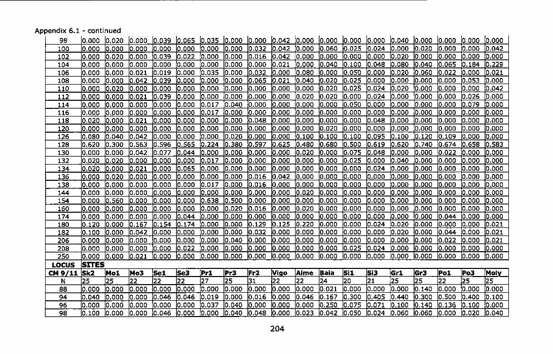
Appendix 6.1 -continued

98 0.000 0.020 0.000 0.039 0.065 0.035 0.000 0.000 0.042 0.000 0.000 0.000 0.000 0.040 0.000 0.000 0.000 0.000 100 0.000 0.000 0.000 0.000 0.000 0.000 0.000 0.032 0.042 0.000 0.060 0.025 0.024 0.000 0.020 0.000 0.000 0.042 102 0.000 0.020 0.000 0.039 0.022 0.000 0.000 0.016 0.042 0.000 0.000 0.000 0.000 0.020 0.000 0.000 0.000 0.000 104 0.000 0.000 0.000 0.000 0.000 0.000 0.000 0.000 0.021 0.000 0.040 0.100 0.048 0.080 0.040 0.065 0.184 0.229 106 0.000 0.000 0.021 0.019 0.000 0.035 0.000 0.032 0.000 0.080 0.000 0.050 0.000 0.020 0.060 0.022 0.000 0.021 108 0.000 0.000 0.042 0.039 0.000 0.000 0.000 0.065 0.021 0.040 0.020 0.025 0.000 0.000 0.000 0.000 0.053 0.000 110 0.000 0.020 0.000 0.000 0.000 0.000 0.000 0.000 0.000 0.000 0.020 0.025 0.024 0.020 0.000 0.000 0.000 0.042 112 0.000 0.000 0.021 0.039 0.000 0.000 0.000 0.000 0.000 0.020 0.020 0.000 0.024 0.000 0.000 0.000 0.026 0.000 114 0.000 0.000 0.000 0.000 0.000 0.017 0.040 0.000 0.000 0.000 0.000 0.050 0.000 0.000 0.000 0.000 0.079 0.000 116 0.000 0.000 0.000 0.000 0.000 0.017 0.000 0.000 0.000 0.000 0.000 0.000 0.000 0.000 0.000 0.000 0.000 0.000 118 0.020 0.000 0.021 0.000 0.000 0.000 0.000 0.048 0.000 0.000 0.000 0.000 0.048 0.000 0.000 0.000 0.000 0.000 120 0.000 0.000 0.000 0.000 0.000 0.000 0.000 0.000 0.000 0.000 0.020 0.000 0.000 0.000 0.000 0.000 0.000 0.000 126 0.080 0.040 0.042 0.000 0.000 0.000 0.020 0.000 0.000 0.100 0.100 0.100 0.095 0.100 0.120 0.109 0.000 0.000 128 0.620 0.300 0.563 0.596 0.565 0.224 0.380 0.597 0.625 0.480 0.680 0.500 0.619 0.620 0.740 0.674 0.658 0.583 130 0.000 0.000 0.042 0.077 0.044 0.000 0.000 0.000 0.000 0.020 0.000 0.075 0.048 0.000 0.000 0.022 0.000 0.000 132 0.020 0.020 0.000 0.000 0.000 0.017 0.000 0.000 0.000 0.000 0.000 0.025 0.000 0.040 0.000 0.000 0.000 0.000 134 0.020 0.000 0.021 0.000 0.065 0.000 0.000 0.000 0.000 0.000 0.000 0.000 0.024 0.000 0.000 0.000 0.000 0.000 136 0.000 0.020 0.000 0.000 0.000 0.000 0.000 0.016 0.042 0.000 0.000 0.000 0.000 0.000 0.000 0.000 0.000 0.000 138 0.000 0.000 0.000 0.000 0.000 0.017 0.000 0.016 0.000 0.000 0.000 0.000 0.000 0.000 0.000 0.000 0.000 0.000 144 0.000 0.000 0.000 0.000 0.000 0.000 0.000 0.000 0.000 0.020 0.000 0.000 0.000 0.000 0.000 0.000 0.000 0.000 154 0.000 0.560 0.000 0.000 0.000 0.638 0.500 0.000 0.000 0.000 0.000 0.000 0.000 0.000 0.000 0.000 0.000 0.000 160 0.000 0.000 0.000 0.000 0.000 0.000 0.020 0.016 0.000 0.020 0.000 0.000 0.000 0.000 0.000 0.000 0.000 0.000 174 0.000 0.000 0.000 0.000 0.044 0.000 0.000 0.000 0.000 0.000 0.000 0.000 0.000 0.000 0.000 0.044 0.000 0.000 180 0.120 0.000 0.167 0.154 0.174 0.000 0.000 0.129 0.125 0.220 0.000 0.000 0.024 0.020 0.000 0.000 0.000 0.021 182 0.100 0.000 0.042 0.000 0.000 0.000 0.000 0.032 0.000 0.000 0.000 0.000 0.000 0.020 0.000 0.044 0.000 0.021 206 0.000 0.000 0.000 0.000 0.000 0.000 0.040 0.000 0.000 0.000 0.000 0.000 0.000 0.000 0.000 0.022 0.000 0.021 208 0.000 0.000 0.000 0.000 0.022 0.000 0.000 0.000 0.000 0.000 0.000 0.025 0.024 0.000 0.000 0.000 0.000 0.000 250 0.000 0.000 0.021 0.000 0.000 0.000 0.000 0.000 0.000 0.000 0.000 0.000 0.000 0.000 0.000 0.000 0.000 0.000

LOCUS SITES CM 9/11 Sk2 Mol Mo3 Se1 Se3 Pr1 Pr3 Fr2 Vi go AI me Baia Si1 Si3 Gr1 Gr3 Po1 Po3 Molv

N 25 25 22 22 22 27 25 31 22 22 24 20 21 25 25 22 25 25 88 0.000 0.000 0.000 0.000 0.000 0.000 0.000 0.000 0.000 0.000 0.021 0.000 0.000 0.000 0.140 0.000 0.000 0.000 94 0.040 0.000 0.000 0.046 0.046 0.019 0.000 0.016 0.000 0.046 0.167 0.300 0.405 0.440 0.300 0.500 0.400 0.100 96 0.000 0.000 0.000 0.000 0.000 0.037 0.040 0.000 0.000 0.000 0.250 0.075 0.071 0.100 0.140 0.136 0.100 0.000 98 0.100 0.000 0.000 0.046 0.000 0.000 0.040 0.048 0.000 0.023 0.042 0.050 0.024 0.060 0.060 0.000 0.020 0.040

204

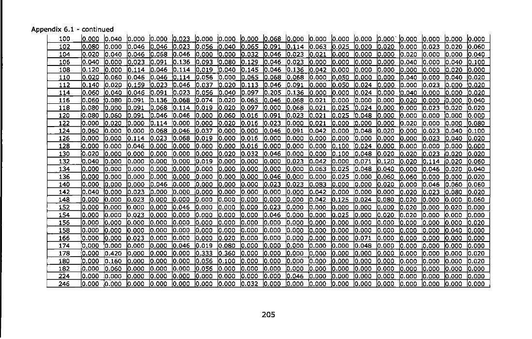
Appendix 6.1 -continued 100 0.000 0.040 0.000 0.000 0.023 0.000 0.000 0.000 0.068 0.000 0.000 0.000 0.000 o.ooo· 0.000 0.000 0.000 0.000 102 0.080 0.000 0.046 0.046 0.023 0.056 0.040 0.065 0.091 0.114 0.063 0.025 0.000 0.020 0.000 0.023 0.020 0.060 104 0.020 0.040 0.046 0.068 0.046 0.000 0.000 0.032 0.046 0.023 0.021 0.000 0.000 0.000 0.020 0.000 0.000 0.040 106 0.040 0.000 0.023 0.091 0.136 0.093 0.080 0.129 0.046 0.023 0.000 0.000 0.000 0.000 0.040 0.000 0.040 0.100 108 0.120 0.000 0.114 0.046 0.114 0.019 0.040 0.145 0.046 0.136 0.042 0.000 0.000 0.000 0.000 0.000 0.020 0.000 110 0.020 0.060 0.046 0.046 0.114 0.056 0.000 0.065 0.068 0.068 0.000 0.050 0.000 0.000 0.040 0.000 0.040 0.020 112 0.140 0.020 0.159 0.023 0.046 0.037 0.020 0.113 0.046 0.091 0.000 0.050 0.024 0.000 0.000 0.023 0.000 0.020 114 0.060 0.040 0.046 0.091 0.023 0.056 0.040 0.097 0.205 0.136 0.000 0.000 0.024 0.000 0.040 0.000 0.000 0.020 116 0.060 0.080 0.091 0.136 0.068 0.074 0.020 0.065 0.046 0.068 0.021 0.000 0.000 0.000 0.020 0.000 0.000 0.040 118 0.080 0.000 0.091 0.068 0.114 0.019 0.020 0.097 0.000 0.068 0.021 0.025 0.024 0.000 0.000 0.023 0.020 0.020 120 0.080 0.060 0.091 0.046 0.046 0.000 0.060 0.016 0.091 0.023 0.021 0.025 0.048 0.000 0.000 0.000 0.000 0.000 122 0.000 0.020 0.000 0.114 0.000 0.000 0.020 0.016 0.023 0.000 0.021 0.000 0.000 0.000 0.020 0.000 0.000 0.080 124 0.060 0.000 0.000 0.068 0.046 0.037 0.000 0.000 0.046 0.091 0.042 0.000 0.048 0.020 0.000 0.023 0.040 0.100 126 0.000 0.000 0.114 0.023 0.068 0.019 0.000 0.016 0.000 0.000 0.000 0.000 0.000 0.000 0.000 0.023 0.040 0.020 128 0.000 0.000 0.046 0.000 0.000 0.000 0.000 0.016 0.000 0.000 0.000 0.100 0.024 0.000 0.000 0.000 0.000 0.000 130 0.020 0.000 0.000 0.000 0.000 0.000 0.020 0.032 0.046 0.000 0.000 0.100 0.048 0.020 0.020 0.023 0.020 0.020 132 0.040 0.000 0.000 0.000 0.000 0.019 0.000 0.000 0.000 0.023 0.042 0.000 0.071 0.120 0.020 0.114 0.020 0.060 134 0.000 0.000 0.000 0.000 0.000 0.000 0.000 0.000 0.000 0.000 0.063 0.025 0.048 0.040 0.000 0.046 0.020 0.040 136 0.000 0.000 0.000 0.000 0.000 0.000 0.000 0.000 0.046 0.000 0.000 0.025 0.000 0.060 0.060 0.000 0.000 0.020 140 0.000 0.000 0.000 0.046 0.000 0.000 0.000 0.000 0.023 0.023 0.083 0.000 0.000 0.020 0.000 0.046 0.060 0.060 142 0.040 0.000 0.023 0.000 0.000 0.000 0.000 0.000 0.000 0.000 0.042 0.000 0.000 0.000 0.020 0.023 0.080 0.020 148 0.000 0.000 0.023 0.000 0.000 0.000 0.000 0.000 0.000 0.000 0.042 0.125 0.024 0.080 0.020 0.000 0.000 0.060 152 0.000 0.000 0.000 0.000 0.046 0.000 0.000 0.000 0.023 0.000 0.000 0.000 0.000 0.000 0.020 0.000 0.020 0.000 154 0.000 0.000 0.023 0.000 0.000 0.000 0.000 0.000 0.046 0.000 0.000 0.025 0.000 0.020 0.020 0.000 0.000 0.000 156 0.000 0.000 0.000 0.000 0.000 0.000 0.000 0.000 0.000 0.000 0.000 0.000 0.000 0.000 0.000 0.000 0.000 0.020 158 0.000 0.000 0.000 0.000 0.000 0.000 0.000 0.000 0.000 0.000 0.000 0.000 0.000 0.000 0.000 0.000 0.040 0.000 166 0.000 0.000 0.023 0.000 0.000 0.000 0.020 0.000 0.000 0.000 0.000 0.000 0.071 0.000 0.000 0.000 0.000 0.000 174 0.000 0.000 0.000 0.000 0.046 0.019 0.080 0.000 0.000 0.000 0.000 0.000 0.048 0.000 0.000 0.000 0.000 0.000 178 0.000 0.420 0.000 0.000 0.000 0.333 0.360 0.000 0.000 0.000 0.000 0.000 0.000 0.000 0.000 0.000 0.000 0.020 180 0.000 0.160 0.000 0.000 0.000 0.056 0.100 0.000 0.000 0.000 0.000 0.000 0.000 0.000 0.000 0.000 0.000 0.020 182 0.000 0.060 0.000 0.000 0.000 0.056 0.000 0.000 0.000 0.000 0.000 0.000 0.000 0.000 0.000 0.000 0.000 0.000 224 0.000 0.000 0.000 0.000 0.000 0.000 0.000 0.000 0.000 0.046 0.000 0.000 0.000 0.000 0.000 0.000 0.000 0.000 246 0.000 0.000 0.000 0.000 0.000 0.000 0.000 0.032 0.000 0.000 0.000 0.000 0.000 0.000 0.000 0.000 0.000 0.000

205

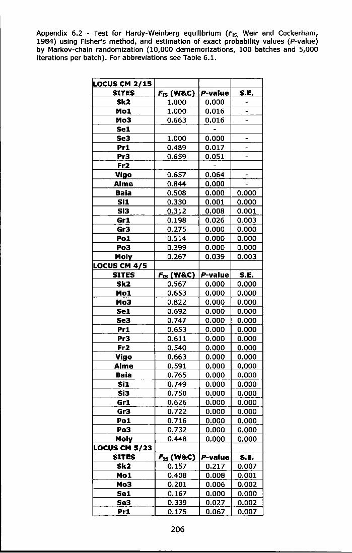
Appendix 6.2 - Test for Hardy-Weinberg equilibrium (F15, Weir and Cockerham, 1984) using Fisher's method, and estimation of exact probability values (P-value) by Markov-chaln randomlzatlon (10,000 dememorlzations, 100 batches and 5,000 iterations per batch). For abbreviations see Table 6.1.

LOCUS CM 2/15 SITES F1s (W8tC) P-value S.E. Sk2 1.000 0.000 -Mol 1.000 0.016 -Mo3 0.663 0.016 -Sel -Se3 1.000 0.000 -Prl 0.489 0.017 -Pr3 0.659 0.051 -Fr2 -

Vi go 0.657 0.064 -AI me 0.844 0.000 -Baia 0.508 0.000 0.000 Sll 0.330 0.001 0.000 Si3 0.312 0.008 0.001 Grl 0.198 0.026 0.003 Gr3 0.275 0.000 0.000 Pol 0.514 0.000 0.000 Po3 0.399 0.000 0.000 Molv 0.267 0.039 0.003

LOCUS CM 4/5 SITES F1s (W8tC) P-value S.E. Sk2 0.567 0.000 0.000 Mol 0.653 0.000 0.000 Mo3 0.822 0.000 0.000 Sel 0.692 0.000 0.000 Se3 0.747 0.000 0.000 Prl 0.653 0.000 0.000 Pr3 0.611 0.000 0.000 Fr2 0.540 0.000 0.000

Vi go 0.663 0.000 0.000 AI me 0.591 0.000 0.000 Baia 0.765 0.000 0.000 Sll 0.749 0.000 0.000 Sl3 0.750 0.000 0.000 Grl 0.626 0.000 0.000 Gr3 0.722 0.000 0.000 Pol 0.716 0.000 0.000 Po3 0.732 0.000 0.000 Moly 0.448 0.000 0.000

LOCUS CM 5/23 SITES F,., (W8tC) P-value S.E. Skl 0.157 0.217 0.007 Mol 0.408 0.008 0.001 Mo3 0.201 0.006 0.002 Sel 0.167 0.000 0.000 Se3 0.339 0.027 0.002 Prl 0.175 0.067 0.007

206

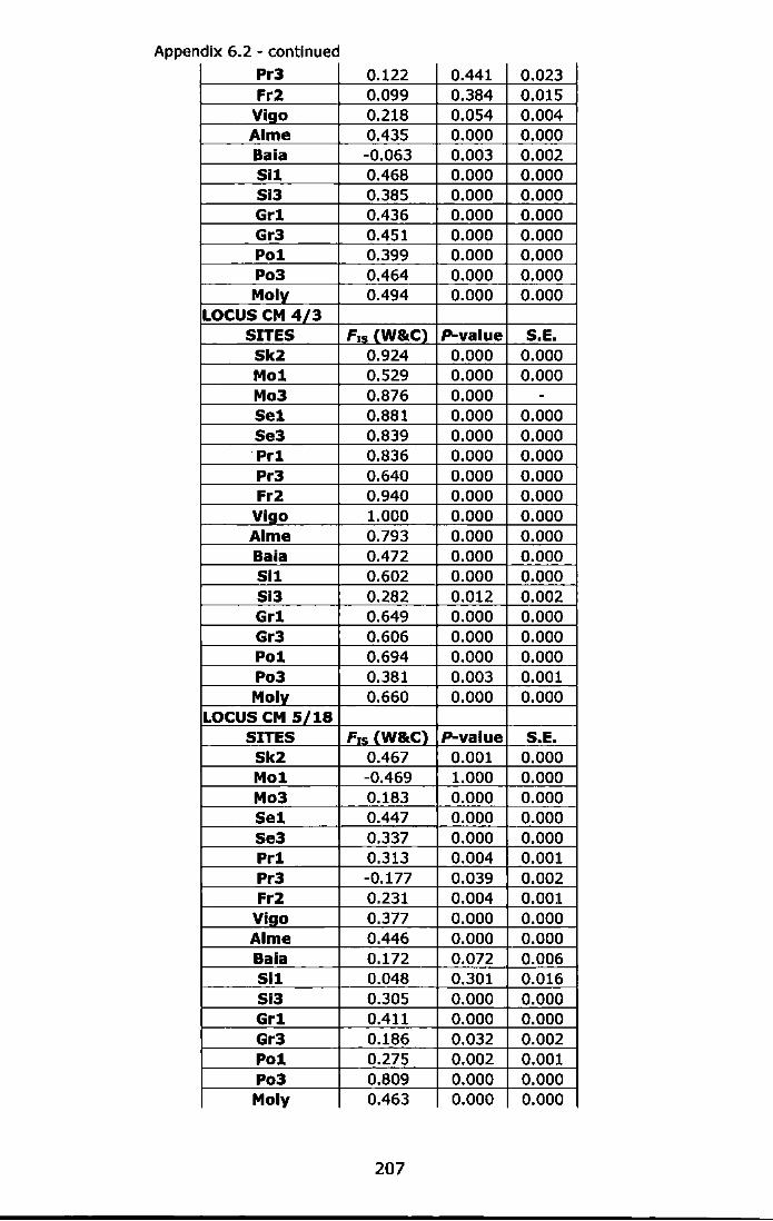
Appendix 6.2 - continued

Pr3 0.122 0.441 0.023 Fr2 0.099 0.384 0.015

Vlgo 0.218 0.054 0.004 AI me 0.435 0.000 0.000 Baia -0.063 0.003 0.002 Sil 0.468 0.000 0.000 Sl3 0.385 0.000 0.000 Grl 0.436 0.000 0.000 Gr3 0.451 0.000 0.000 Pol 0.399 0.000 0.000 Po3 0.464 0.000 0.000 Moly 0.494 0.000 0.000

LOCUS CM 4/3 SITES F1s (W&C) P-value S.E.

Sk2 0.924 0.000 0.000 Mol 0.529 0.000 0.000 Mo3 0.876 0.000 -Sel 0.881 0.000 0.000 Se3 0.839 0.000 0.000 Prl 0.836 0.000 0.000 Pr3 0.640 0.000 0.000 Fr2 0.940 0.000 0.000

VI go 1.000 0.000 0.000 Alme 0.793 0.000 0.000 Baia 0.472 0.000 0.000 Sil 0.602 0.000 0.000 Sl3 0.282 0.012 0.002 Grl 0.649 0.000 0.000 Gr3 0.606 0.000 0.000 Pol 0.694 0.000 0.000 Po3 0.381 0.003 0.001 Moly 0.660 0.000 0.000

LOCUS CM 5/18 SITES F1s (W&C} P-value S.E.

Sk2 0.467 0.001 0.000 Mol -0.469 1.000 0.000 Mo3 0.183 0.000 0.000 Sel 0.447 0.000 0.000 Se3 0.337 0.000 0.000 Prl 0.313 0.004 0.001 Pr3 -0.177 0.039 0.002 Fr2 0.231 0.004 0.001

Vigo 0.377 0.000 0.000 AI me 0.446 0.000 0.000 Bala 0.172 0.072 0.006 Sll 0.048 0.301 0.016 Sl3 0.305 0.000 0.000 Grl 0.411 0.000 0.000 Gr3 0.186 0.032 0.002 Pol 0.275 0.002 0.001 Po3 0.809 0.000 0.000 Moly 0.463 0.000 0.000

207

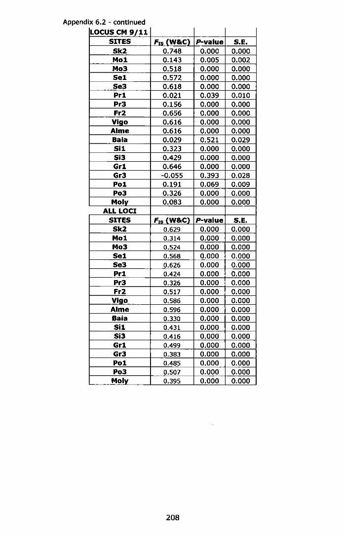
Appendix 6.2 - continued

LOCUS CM 9/11 SITES F15 (W&C) P-value S.E. Sk2 0.748 0.000 0.000 Mol 0.143 0.005 0.002 Mol 0.518 0.000 0.000 Sel 0.572 0.000 0.000 Sel 0.618 0.000 0.000 Prl 0.021 0.039 0.010 Prl 0.156 0.000 0.000 Fr2 0.656 0.000 0.000

Vi go 0.616 0.000 0.000 Alme 0.616 0.000 0.000 Baia 0.029 0.521 0.029 Sil 0.323 0.000 0.000 Sil 0.429 0.000 0.000 Grl 0.646 0.000 0.000 Grl -0.055 0.393 0.028 Pol 0.191 0.069 0.009 Pol 0.326 0.000 0.000 Moly 0.083 0.000 0.000

ALL LOCI SITES F1s (W&C) P-value S.E. Sk2 0.629 0.000 0.000 Mol 0.314 0.000 0.000 Mol 0.524 0.000 0.000 Sel 0.568 0.000 0.000 Sel 0.626 0.000 0.000 Prl 0.424 0.000 0.000 Prl 0.326 0.000 0.000 Fr2 0.517 0.000 0.000

Vi go 0.586 0.000 0.000 AI me 0.596 0.000 0.000 Baia 0.330 0.000 0.000 Sil 0.431 0.000 0.000 Sil 0.416 0.000 0.000 Grl 0.499 0.000 0.000 Grl 0.383 0.000 0.000 Pol 0.485 0.000 0.000 Pol 0.507 0.000 0.000 Moly 0.395 0.000 0.000

208

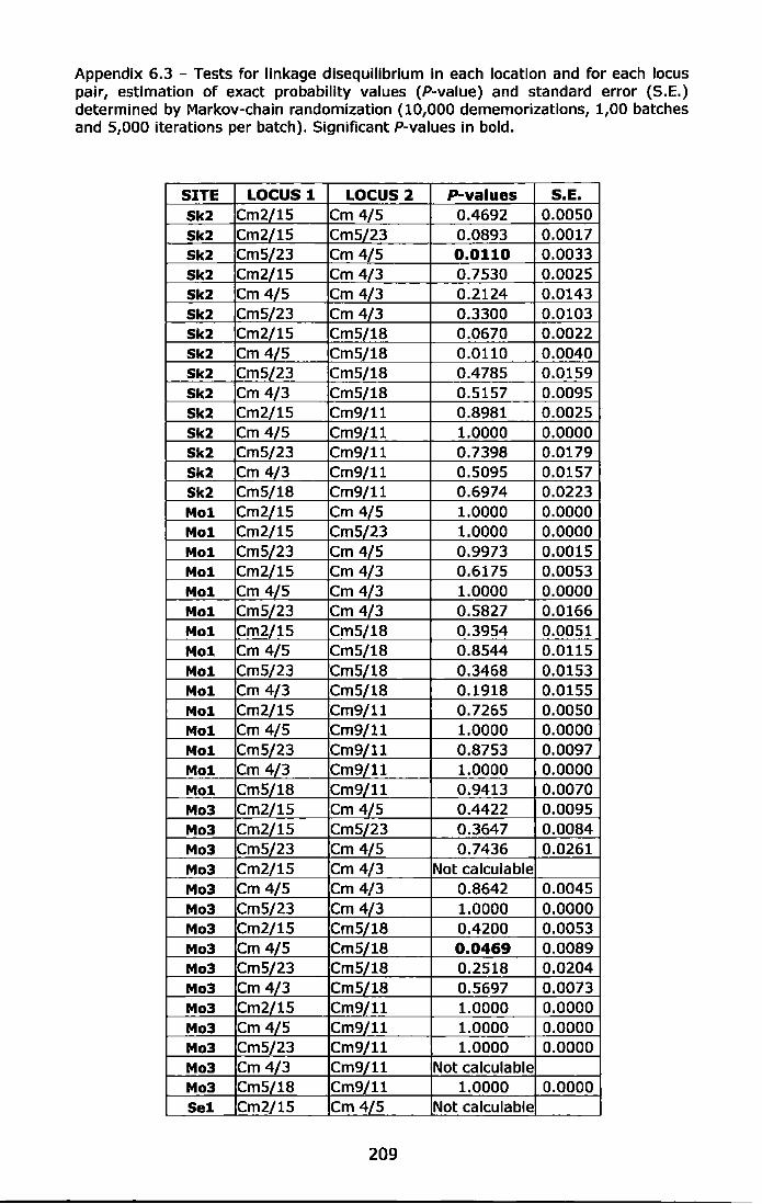
Appendix 6.3 - Tests for linkage disequilibrium in each location and for each locus pair, estimation of exact probability values (P-value) and standard error (S.E.) determined by Markov-chain randomlzation (10,000 dememorizatlons, 1,00 batches and 5,000 iterations per batch). Significant P-values in bold.

SITE LOCUS 1 LOCUS 2 P-values S.E. Sk2 Cm2/15 Cm 4/5 0.4692 0.0050 Sk2 Cm2/15 Cm5/23 0.0893 0.0017 Sk2 Cm5/23 Cm 4/5 0.0110 0.0033 Sk2 Cm2/15 Cm 4/3 0.7530 0.0025 Sk2 Cm 4/5 Cm 4/3 0.2124 0.0143 Sk2 Cm5/23 Cm 4/3 0.3300 0.0103 Sk2 Cm2/15 Cm5/18 0.0670 0.0022 Sk2 Cm 4/5 Cm5/18 0.0110 0.0040 Sk2 Cm5/23 Cm5/18 0.4785 0.0159 Sk2 Cm 4/3 Cm5/18 0.5157 0.0095 Sk2 Cm2/15 Cm9/11 0.8981 0.0025 Sk2 Cm 4/5 Cm9/11 1.0000 0.0000 Sk2 Cm5/23 Cm9/ll 0.7398 0.0179 Sk2 Cm 4/3 Cm9/11 0.5095 0.0157 Sk2 Cm5/18 Cm9/ll 0.6974 0.0223 Mol Cm2/15 Cm 4/5 1.0000 0.0000 Mol Cm2/15 Cm5/23 1.0000 0.0000 Mol Cm5/23 Cm 4/5 0.9973 0.0015 Mol Cm2/15 Cm 4/3 0.6175 0.0053 Mol Cm 4/5 Cm 4/3 1.0000 0.0000 Mol Cm5/23 Cm 4/3 0.5827 0.0166 Mol Cm2/15 Cm5/18 0.3954 0.0051 Mol Cm 4/5 Cm5/18 0.8544 0.0115 Mol Cm5/23 Cm5/18 0.3468 0.0153 Mol Cm 4/3 Cm5/18 0.1918 0.0155 Mol Cm2/15 Cm9/11 0.7265 0.0050 Mol Cm 4/5 Cm9/ll 1.0000 0.0000 Mol Cm5/23 Cm9/11 0.8753 0.0097 Mol Cm 4/3 Cm9/11 1.0000 0.0000 Mol Cm5/18 Cm9/11 0.9413 0.0070 Mo3 Cm2/15 Cm 4/5 0.4422 0.0095 Mo3 Cm2/15 Cm5/23 0.3647 0.0084 Mo3 Cm5/23 Cm 4/5 0.7436 0.0261 Mo3 Cm2/15 Cm 4/3 Not calculable Mo3 Cm4/5 Cm 4/3 0.8642 0.0045 Mo3 Cm5/23 Cm 4/3 1.0000 0.0000 Mo3 Cm2/15 Cm5/18 0.4200 0.0053 Mo3 Cm 4/5 Cm5/18 0.0469 0.0089 Mo3 Cm5/23 Cm5/18 0.2518 0.0204 Mo3 Cm 4/3 Cm5/18 0.5697 0.0073 Mo3 Cm2/15 Cm9/11 1.0000 0.0000 Mo3 Cm 4/5 Cm9/11 1.0000 0.0000 Mo3 Cm5/23 Cm9/11 1.0000 0.0000 Mo3 Cm4/3 Cm9/11 Not calculable Mo3 Cm5/18 Cm9/11 1.0000 0.0000 Sel Cm2/15 Cm4/5 Not calculable

209

Appendix 6.3 - continued Sel Cm2/15 Cm5/23 Not calculable Sel Cm5/23 Cm4/5 0.9776 0.0054 Sel Cm2/15 Cm4/3 Not calculable Sel Cm 4/5 Cm4/3 1.0000 0.0000 Sel Cm5/23 Cm4/3 0.3053 0.0059 Sel Cm2/15 Cm5/18 Not calculable Sel Cm 4/5 Cm5/18 0.6158 0.0199 Sel Cm5/23 Cm5/18 0.4785 0.0198 Sel Cm 4/3 Cm5/18 0.0715 0.0043 Sel Cm2/15 Cm9/11 Not calculable Sel Cm 4/5 Cm9/11 1.0000 0.0000 Sel Cm5/23 Cm9/11 1.0000 0.0000 Sel Cm 4/3 Cm9/11 Not calculable Sel Cm5/18 Cm9/11 1.0000 0.0000 Se3 Cm2/15 Cm 4/5 0.5920 0.0057 Se3 Cm2/15 Cm5/23 0.0715 0.0030 Se3 Cm5/23 Cm 4/5 0.3013 0.0201 Se3 Cm2/15 Cm 4/3 1.0000 0.0000 Se3 Cm 4/5 Cm 4/3 0.4420 0.0220 Se3 Cm5/23 Cm 4/3 0.6964 0.0145 Se3 Cm2/15 Cm5/18 0.5554 0.0090 Se3 Cm4/5 Cm5/18 0.3442 0.0235 Se3 Cm5/23 Cm5/18 0.0298 0.0052 Se3 Cm4/3 Cm5/18 0.9875 0.0027 Se3 Cm2/15 Cm9/11 0.7768 0.0076 Se3 Cm 4/5 Cm9/11 1.0000 0.0000 Se3 Cm5/23 Cm9/11 1.0000 0.0000 Se3 Cm4/3 Cm9/11 1.0000 0.0000 Se3 Cm5/18 Cm9/11 0.4976 0.0229 Prl Cm2/15 Cm 4/5 0.7355 0.0129 Prl Cm2/15 Cm5/23 0.0865 0.0064 Prl Cm5/23 Cm4/5 0.6523 0.0305 Prl Cm2/15 Cm4/3 0.3036 0.0090 Prl Cm 4/5 Cm4/3 0.0001 0.0001 Prl Cm5/23 Cm 4/3 0.8699 0.0140 Prl Cm2/15 Cm5/18 0.1391 0.0068 Prl Cm 4/5 Cm5/18 0.9426 0.0103 Prl Cm5/23 Cm5/18 0.5250 0.0235 Prl Cm 4/3 Cm5/18 0.1181 0.0065 Prl Cm2/15 Cm9/11 0.5931 0.0134 Prl Cm 4/5 Cm9/11 0.1700 0.0308 Prl Cm5/23 Cm9/11 0.1563 0.0192 Prl Cm 4/3 Cm9/11 1.0000 0.0000 Prl Cm5/18 Cm9/11 0.5026 0.0212 Pr3 Cm2/15 Cm4/5 0.5963 0.0113 Pr3 Cm2/15 Cm5/23 0.1257 0.0071 Pr3 Cm5/23 Cm4/5 0.8331 0.0221 Pr3 Cm2/15 Cm4/3 0.7221 0.0051 Pr3 Cm 4/5 Cm4/3 0.1436 0.0239 Pr3 Cm5/23 Cm4/3 0.1363 0.0218 Pr3 Cm2/15 Cm5/18 0.0587 0.0027 Pr3 Cm 4/5 Cm5/18 0.1122 0.0138 Pr3 Cm5/23 Cm5/18 0.1108 0.0148

210

Appendix 6.3 - continued Pr3 Cm 4/3 Cm5/18 0.4444 0.0141 Pr3 Cm2/15 Cm9/11 0.3001 0.0088 Pr3 Cm 4/5 Cm9/ll 1.0000 0.0000 Pr3 Cm5/23 Cm9/11 0.0147 0.0085 Pr3 Cm 4/3 Cm9/11 0.2534 0.0274 Pr3 Cm5/18 Cm9/11 0.9188 0.0103 Fr2 Cm2/15 Cm 4/5 Not calculable Fr2 Cm2/15 Cm5/23 Not calculable Fr2 Cm5/23 Cm 4/5 0.8668 0.0171 Fr2 Cm2/15 Cm 4/3 Not calculable Fr2 Cm 4/5 Cm 4/3 0.7283 0.0213 Fr2 Cm5/23 Cm4/3 0.5938 0.0130 Fr2 Cm2/15 Cm5/18 Not calculable Fr2 Cm 4/5 Cm5/18 0.3787 0.0308 Fr2 Cm5/23 Cm5/18 0.7171 0.0192 Fr2 Cm 4/3 Cm5/18 0.1784 0.0148 Fr2 Cm2/15 Cm9/ll Not calculable Fr2 Cm4/5 Cm9/11 1.0000 0.0000 Fr2 Cm5/23 Cm9/11 0.3907 0.0287 Fr2 Cm 4/3 Cm9/11 0.2670 0.0201 Fr2 Cm5/18 Cm9/11 0.0958 0.0153

Vi go Cm2/15 Cm 4/5 1.0000 0.0000 Vi go Cm2/15 Cm5/23 0.1254 0.0035 Vi go Cm5/23 Cm 4/5 1.0000 0.0000 Vi go Cm2/15 Cm 4/3 0.6978 0.0055 Vi go Cm 4/5 Cm 4/3 0.1645 0.0094 Vi go Cm5/23 Cm 4/3 0.9441 0.0036 VI go Cm2/15 Cm5/18 0.1133 0.0063 Vi go Cm 4/5 Cm5/18 0.5487 0.0223 Vi go Cm5/23 Cm5/18 0.0809 0.0075 Vi go Cm 4/3 Cm5/18 0.9676 0.0043 Vlgo Cm2/15 Cm9/ll 0.3902 0.0087 Vi go Cm 4/5 Cm9/11 1.0000 0.0000 Vi go Cm5/23 Cm9/11 0.6715 0.0190 Vi go Cm 4/3 Cm9/11 0.0524 0.0060 Vi go Cm5/18 Cm9/11 0.8823 0.0137 Alme Cm2/15 Cm 4/5 0.3356 0.0138 Alme Cm2/15 Cm5/23 0.1842 0.0082 Alme Cm5/23 Cm 4/5 1.0000 0.0000 Alme Cm2/15 Cm 4/3 0.2498 0.0075 Alme Cm 4/5 Cm4/3 0.5086 0.0208 Alme Cm5/23 Cm4/3 0.9592 0.0044 Alme Cm2/15 Cm5/18 0.3274 0.0093 Alme Cm 4/5 Cm5/18 0.6171 0.0243 Alme Cm5/23 Cm5/18 0.5289 0.0181 Alme Cm 4/3 Cm5/18 0.1538 0.0096 Alme Cm2/15 Cm9/11 0.8541 0.0061 Alme Cm 4/5 Cm9/11 0.0710 0.0171 Alme Cm5/23 Cm9/11 1.0000 0.0000 Alme Cm 4/3 Cm9/ll 0.8689 0.0102 Alme Cm5/18 Cm9/11 1.0000 0.0000 Baia Cm2/15 Cm4/5 0.0988 0.0119 Bala Cm2/15 Cm5123 0.0941 0.0138

211

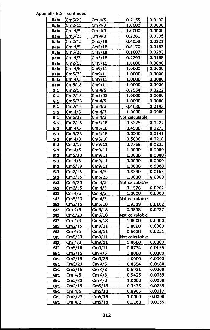
Appendix 6.3 - continued Baia Cm5/23 Cm4/5 0.2155 0.0192 Sal a Cm2/15 Cm 4/3 1.0000 0.0000 Sal a Cm4/5 Cm 4/3 1.0000 0.0000 Sal a Cm5/23 Cm 4/3 0.2381 0.0195 Sal a Cm2/15 Cm5/18 0.4058 0.0221 Sal a Cm 4/5 Cm5/18 0.6170 0.0183 Sal a Cm5/23 Cm5/18 0.1607 0.0203 Sal a Cm 4/3 Cm5/18 0.2293 0.0188 Bala Cm2/15 Cm9/11 1.0000 0.0000 Bala Cm4/5 Cm9/11 1.0000 0.0000 Baia Cm5/23 Cm9/11 1.0000 0.0000 Sal a Cm4/3 Cm9/11 1.0000 0.0000 Sal a Cm5/18 Cm9/11 1.0000 0.0000 511 Cm2/15 Cm 4/5 0.7554 0.0222 511 Cm2/15 Cm5/23 1.0000 0.0000 511 Cm5/23 Cm 4/5 1.0000 0.0000 511 Cm2/15 Cm 4/3 0.4620 0.0192 511 Cm 4/5 Cm 4/3 1.0000 0.0000 511 Cm5/23 Cm4/3 Not calculable 511 Cm2/15 Cm5/18 0.5275 0.0222 511 Cm 4/5 Cm5/18 0.4508 0.0275 511 Cm5/23 Cm5/18 0.0540 0.0141 511 Cm 4/3 Cm5/18 0.5606 0.0218 511 Cm2/15 Cm9/11 0.3759 0.0232 511 Cm 4/5 Cm9/11 1.0000 0.0000 511 Cm5/23 Cm9/11 1.0000 0.0000 511 Cm 4/3 Cm9/11 0.0000 0.0000 511 Cm5/18 Cm9/11 1.0000 0.0000 513 Cm2/15 Cm 4/5 0.8340 0.0165 513 Cm2/15 CmS/23 1.0000 0.0000 513 Cm5/23 Cm 4/5 Not calculable 513 Cm2/15 Cm 4/3 0.1576 0.0202 513 Cm 4/5 Cm 4/3 1.0000 0.0000 513 Cm5/23 Cm 4/3 Not calculable 513 Cm2/15 CmS/18 0.9389 0.0102 513 Cm4/5 Cm5/18 0.3838 0.0227 513 Cm5/23 Cm5/18 Not calculable 513 Cm 4/3 Cm5/18 1.0000 0.0000 513 Cm2/15 Cm9/11 1.0000 0.0000 513 Cm 4/5 Cm9/11 0.6638 0.0251 513 Cm5/23 Cm9/11 Not calculable 513 Cm 4/3 Cm9/11 1.0000 0.0000 513 Cm5/18 Cm9/11 0.8734 0.0155 Gr1 Cm2/15 Cm 4/5 1.0000 0.0000 Gr1 Cm2/15 Cm5/23 1.0000 0.0000 Gr1 Cm5/23 Cm4/5 0.0554 0.0180 Gr1 Cm2/15 Cm4/3 0.6931 0.0200 Gr1 Cm 4/5 Cm4/3 0.9425 0.0069 Gr1 Cm5/23 Cm4/3 1.0000 0.0000 Gr1 Cm2/15 Cm5/18 0.3475 0.0285 Gr1 Cm 4/5 Cm5/18 0.9965 0.0017 Grl Cm5/23 Cm5/18 1.0000 0.0000 Gr1 Cm 4/3 Cm5/18 0.1160 0.0155

212

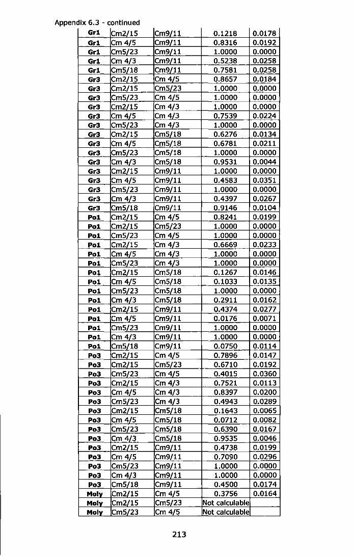
Appendix 6.3 - continued Grl Cm2/15 Cm9/11 0.1218 0.0178 Grl Cm4/5 Cm9/11 0.8316 0.0192 Grl Cm5/23 Cm9L11 1.0000 0.0000 Grl Cm 4/3 Cm9/11 0.5238 0.0258 Grl Cm5/18 Cm9/ll 0.7581 0.0258 Gr3 Cm2/15 Cm4/5 0.8657 0.0184 Gr3 Cm2/15 Cm5/23 1.0000 0.0000 Gr3 Cm5/23 Cm 4/5 1.0000 0.0000 Gr3 Cm2/15 Cm 4/3 1.0000 0.0000 Gr3 Cm 4/5 Cm 4/3 0.7539 0.0224 Gr3 Cm5/23 Cm4/3 1.0000 0.0000 Gr3 Cm2/15 Cm5/18 0.6276 0.0134 Gr3 Cm 4/5 Cm5/18 0.6781 0.0211 Gr3 Cm5/23 Cm5/18 1.0000 0.0000 Gr3 Cm 4/3 Cm5/18 0.9531 0.0044 Gr3 Cm2/15 Cm9/11 1.0000 0.0000 Gr3 Cm 4/5 Cm9/11 0.4583 0.0351 Gr3 Cm5/23 Cm9/11 1.0000 0.0000 Gr3 Cm 4/3 Cm9/11 0.4397 0.0267 Gr3 Cm5/18 Cm9/11 0.9146 0.0104 Pol Cm2/15 Cm4/5 0.8241 0.0199 Pol Cm2/15 Cm5/23 1.0000 0.0000 Pol Cm5/23 Cm4/5 1.0000 0.0000 Pol Cm2/15 Cm4/3 0.6669 0.0233 Pol Cm 4/5 Cm 4/3 1.0000 0.0000 Pol Cm5/23 Cm 4/3 1.0000 0.0000 Pol Cm2/15 Cm5/18 0.1267 0.0146 Pol Cm4/5 Cm5/18 0.1033 0.0135 Pol Cm5/23 Cm5/18 1.0000 0.0000 Pol Cm 4/3 Cm5/18 0.2911 0.0162 Pol Cm2/15 Cm9/11 0.4374 0.0277 Pol Cm 4/5 Cm9/11 0.0176 0.0071 Pol Cm5/23 Cm9/11 1.0000 0.0000 Pol Cm4/3 Cm9/11 1.0000 0.0000 Pol Cm5/18 Cm9/11 0.0750 0.0114 Po3 Cm2/15 Cm4/5 0.7896 0.0147 Po3 Cm2/15 Cm5/23 0.6710 0.0192 Po3 Cm5/23 Cm 4/5 0.4015 0.0360 Po3 Cm2/15 Cm 4/3 0.7521 0.0113 Po3 Cm 4/5 Cm4/3 0.8397 0.0200 Po3 Cm5/23 Cm4/3 0.4943 0.0289 Po3 Cm2/15 Cm5/18 0.1643 0.0065 Po3 Cm 4/5 Cm5/18 0.0712 0.0082 Po3 Cm5/23 Cm5/18 0.6390 0.0167 Po3 Cm 4/3 Cm5/18 0.9535 0.0046 Po3 Cm2/15 Cm9/11 0.4738 0.0199 Po3 Cm 4/5 Cm9/11 0.7090 0.0296 Po3 Cm5/23 Cm9/11 1.0000 0.0000 Po3 Cm4/3 Cm9/11 1.0000 0.0000 Po3 Cm5/18 Cm9/11 0.4500 0.0174 Moly Cm2/15 Cm 4/5 0.3756 0.0164 Moly Cm2/15 Cm5/23 Not calculable Mo!Y_ Cm5/23 Cm 4/5 Not calculable

213

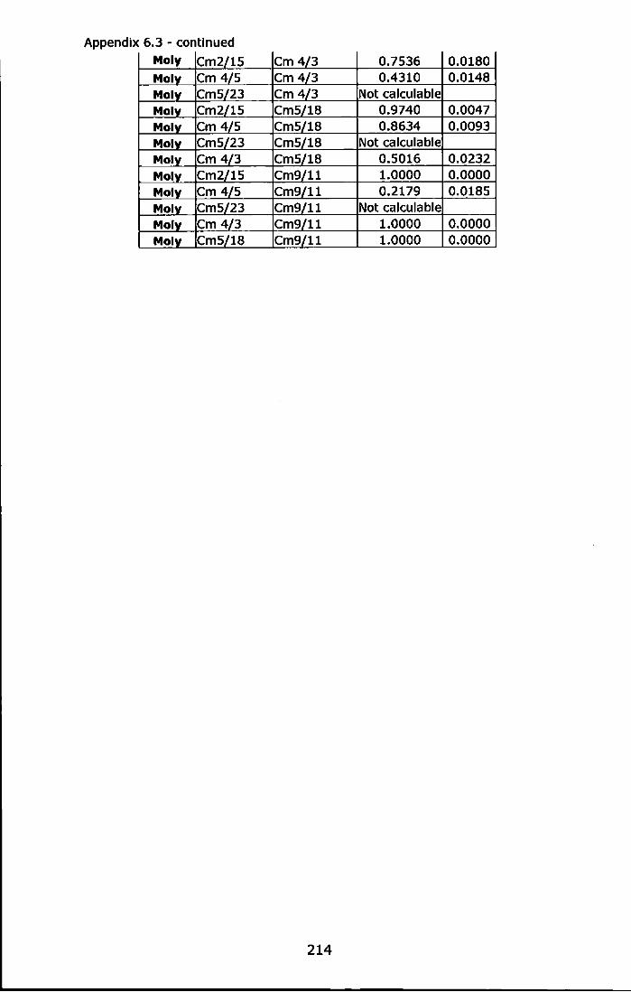
Appendix 6.3 - continued Moly Cm2/15 Cm4/3 0.7536 0.0180 Moly Cm 4/5 Cm4/3 0.4310 0.0148 Moly Cm5/23 Cm4/3 Not calculable Moly Cm2/15 Cm5/18 0.9740 0.0047 Moly Cm 4/5 Cm5/18 0.8634 0.0093 Moly Cm5/23 Cm5/18 Not calculable Moly Cm 4/3 Cm5/18 0.5016 0.0232 Moly Cm2/15 Cm9/11 1.0000 0.0000 Moly Cm 4/5 Cm9/11 0.2179 0.0185 Moly Cm5/23 Cm9/11 Not calculable Moly Cm 4/3 Cm9/11 1.0000 0.0000 Moly Cm5/18 Cm9/11 1.0000 0.0000

214

Reference List

Abbiati,M. (2003). Introduction to topic three "Effects of human activities in altering genetic characteristics and gene flow in the marine environment". In: Electronic conference on 'Genetic Biodiversity in Marine Ecosystems -Measurement, Understanding and Management' - Summary of discussions, eds. K. Hiscock, et al.: Flanders Marine Institute, Oostende, Belgium, 31-34.

Achituv,Y., Barnes,H. (1976). Studies in biochemistry of Cirripede eggs. 5. Changes in general biochemical composition during development of Chthama/us stellatus (Poll). Journal of Experimental Marine Biology and Ecology 22, 263-267.

Addison,J.A., Hart,M.W. (2004). Analysis of population genetic structure of the green sea urchin (Strongy/ocentrotus droebachiensis) using microsatellites. Marine Biology 144, 251.

Addison,J.A., Hart,M.W. (2005). Spawning, copulation and inbreeding coefficients In marine invertebrates. Biology Letters 1, 450-453.

Airoldi,L., Abbiati,M., Beck,M.W., Hawkins,S.J., Jonsson,P.R., Martin,D., Moschella,P.S., Sundelof,A., Thompson,R.C., Aberg,P. (2005). An ecological perspective on the deployment and design of low-crested and other hard coastal defence structures. Coastal Engineering 52, 1073-1087.

Aljanabi,S.M., Martinez,l. (1997). Universal and rapid salt-extraction of high quality genomic DNA for PCR based techniques. Nucleic Acids Research 25, 4692-4693.

Allendorf,F.W. (1986). Genetic drift and the loss of alleles versus heterozygosity. Zoo Biology 5, 181-190.

Allendorf,F.W., Luikart,G. (2007). Conservation and the genetics of populations. Blackwell Publishing, Maiden, MA, 642 pp.

Almada,V.C., Oliveira,R.F., Goncalves,E.J., Almeida,A.J., Santos,R.S., Wirtz,P. (2001). Patterns of diversity of the north-eastern Atlantic blennild fish fauna (Pisces: Blennlidae). Global Ecology and Biogeography 10, 411-422.

Anderson,D.T. (1994). Barnacles: structure, function, development and evolution. Chapman & Hall, London.

Andrade,S.C.S., Solferini,V.N. (2007). Fine-scale genetic structure overrides macro-scale structure in a marine snail: non random recruitment, demographic events or selection? Biological Journal of the Linnean Society 91, 23-36.

215

Angermeier,P.L. (1994). Does biodiversity include artificial diversity. Conservation Biology 8, 600-602.

Arbogast,B.S., Edwards,S.V., Wakeley,J., Beerli,P., Slowinski,J.B. (2002). Estimating divergence times from molecular data on phylogenetic and population genetic timescales. Annual Review of Ecology and Systematics 33, 707-740.

Archie,J.W. (1985). Statistical analysis of heterozygosity data: independent sample comparisons. Evolution 39, 623-637.

Avise,J.C. (1992}. Molecular population structure and biogeographic history of a regional fauna: a case history with lessons for conservation biology. Oikos 63, 62-76.

Avise,J.C. (1994). Molecular markers natural history and evolution. Kluwer Academic Publishers, Boston.

Avise,J.C. (2000). Phylogeography: the history and formation of species. Harvard University Press, Cambridge.

Avise,J.C., Arnold,J., Baii,R.M., Bermingham,E., Lamb,T., Neigei,J.E., Reeb,C.A., Saunders,N.C. (1987). Intraspecific phylogeography - the mitochondrial DNA bridge between population genetics and systematics. Annual Review of Ecology and Systematics 18, 489-522.

Avise,J.C., Hamrick,J.L. (1996). Conservation genetics. Case histories from nature. Chapman & Hall, New York.

Ayala,F.J. (1982). Population and evolutionary genetics: a primer. Benjamin/Cummings, Menlo Park, CA.

Ayensu,E., Claasen,D.V., Collins,M., Dearing,A., Fresco,L., Gadgii,M., Gitay,H., Glaser,G., Lohn,C.L., Krebs,J., Lenton,R., Lubchenco,L., McNeely,J.A., Mooney,H.A., Pinstrup-Andersen,P., Ramos,M., Raven,P., Reld,W.V., Samper,C., Sarukhan,J., Schei,P., Tundisi,J.G., Watson,R.T., Xu,G.H., Zakri,A.H. (1999). Ecology - international ecosystem assessment. Science 286, 685-686.

Ayre,D.J., Hughes,T.P. (2000). Genotypic diversity and gene flow in brooding and spawning corals along the Great Barrier Reef, Australia. Ecology 54, 1590-1605.

Bacchiocchi,F., Airoldi,L. (2003). Distribution and dynamics of epibiota on hard structures for coastal protection. Estuarine Coastal and Shelf Science 56, 1157-1166.

Backeljau,T. (2003). Introduction to topic one "Measuring managing and conserving genetic resources in natural marine systems". In: Electronic conference on 'Genetic Biodiverslty in Marine Ecosystems - Measurement, Understanding and Management' - Summary of discussions, eds. K. Hiscock, et al.: Flanders Marine Institute, Oostende, Belgium, 13-17.

Barber,P.H., Palumbi,S.R., Erdmann,M.V., Moosa,M.K. (2000). Biogeography - a marine Wallace's line? Nature 406, 692-693.

216

Bargelloni,L., Zane,L., Derome,N., Lecointre,G., Patarnello,T. (2000). Molecular zoogeography of Antarctic euphausiids and notothenioids: from species phylogenles to intraspecific patterns of genetic variation. Antarctic Science 12, 259-268.

Barnes,H. (1972). The season changes in body weight and biochemical composition of the warm-temperate cirripede Chthamalus stellatus (Poli). Journal of Experimental Marine Biology and Ecology 8, 89-100.

Barnes,H., Barnes,M. (1958). Further observations on self-fertilization in Chthamalus species. Ecology 39, 550.

Barnes,H., Crisp,D.J. (1956). Evidence of self-fertilization in certain species of barnacles. Journal of the Marine Biological Association of the UK 35, 631-639.

Barton,N.H., Slatkin,M. (1986). A quasi-equilibrium theory of the distribution of rare alleles in a subdivided population. Heredity 56, 409-415.

Belfiore,N.M., Anderson,S.L. (2001). Effects of contaminants on genetic patterns in aquatic organisms: a review. Mutation Research-Reviews in Mutation Research 489, 97-122.

Belkhir,K., Borsa,P., Chlkhi,L., Raufaste,N., Bonhomme,F. (2004 ). GENETIX 4.05, logiciel sous Windows TM pour la genetique des populatlons. Laboratoire Genome, Populations, Interactions, CNRS UMR 5000, Universite de Montpellier 11, Montpellier, France.

Bert,T.M. {1986). Speciation in western Atlantic stone crabs (genus Menippe): the role of geological processes and climatic events in the formation and distribution of species. Marine Biology 93, 157-170.

Bertozzi,F. (2005). Genetic structure of Patella caerulea In the Adriatic basin. PhD Thesis, University of Bologna, Italy.

Blanchi,C.N., Morri,C. (2000). Marine biodiverslty of the Mediterranean Sea: situation, problems and prospects for future research. Marine Pollution Bulletin 40, 367-376.

Blanc,J.J. {1968). Sedimentary geology of the Mediterranean Sea. Oceanography and Marine Biology an Annual Review 6, 377-454.

Bohonak,A.J. {1999). Dispersal, gene flow, and population structure. Quarterly Review of Biology 74, 21-45.

Booy,G., Hendriks,R.J.J., Smulders,M.J.M., Van Groenendaei,J.M., Vosman,B. (2000). Genetic diversity and the survival of populations. Plant Biology 2, 379-395.

Bouza,C., Arias,J., Castro,J., Sanchez,L., Martinez,P. {1999). Genetic structure of brown trout, Salmo trutta L., at the southern limit of the distribution range of the anadromous form. Molecular Ecology 8, 1991-2001.

217

Briggs,J.C. {1994). Species diversity: land and sea compared. Systematic Biology 43, 130-135.

Brooks,R.A., Beii,S.S. {2001). Mobile corridors in marine landscapes: enhancement of fauna! exchange at seagrass/sand ecotones. Journal of Experimental Marine Biology and Ecology 264, 67-84.

Brownlow,R.J., Dawson,D.A., Horsburgh,G.J., Beii,J.J., Fish,J.D. {2008). A method for genotype validation and primer assessment in heterozygote­deficient species, as demonstrated in the prosobranch mollusc Hydrobia u/vae. BMC Genetics 9, 55.

Bulleri,F., Airoldi,L. {2005). Artificial marine structures facilitate the spread of a non-indigenous green alga, Codium fragile ssp tomentosoides, in the north Adriatic Sea. Journal of Applied Ecology 42, 1063-1072.

Burrows,M.T. {1988). The comparative biology of Chthamalus stellatus {Poll) and Chthamalus montagui Southward. PhD Thesis, University of Manchester, UK, 318pp.

Burrows,M.T., Hawkins,S.J., Southward,A.J. {1992). A comparison of reproduction in eo-occurring chthamalid barnacles, Chthamalus stellatus {Poll) and Chthama/us montagui Southward. Journal of Experimental Marine Biology and Ecology 160, 229-249.

Burrows,M.T., Hawkins,S.J., Southward,A.J. (1999). Larval development of the Intertidal barnacles - Chthamalus stellatus and Chthamalus montagui. Journal of the Marine Biological Association of the United Kingdom 79, 93-101.

Burton,R.S. (1983). Protein polymorphism and genetic differentiation of marine invertebrate populations. Marine Biology Letters 4, 193-206.

Burton,R.S. (1996). Molecular tools in marine ecology. Journal of Experimental Marine Biology and Ecology 200, 85-101.

Burton,R.S., Feldman,M.W. (1981). Population genetics of Tigriopus californicus: II. Differentiation among neighboring populations. Evolution 35, 1192-1205.

Butam,C.A., Carlton,J.T. (1995). Understanding marine biodiversity: a research agenda. National Academy Press, USA.

Callen,D.F., Thompson,A.D., Shen,Y., Phillips,H.A., Richards,R.I., Mulley,J.C., Sutherland,G.R. (1993). Incidence and origin of null alleles in the (AC)n microsatellite markers. American Journal of Human Genetics 52, 922-927.

Carlton,J.T., Scanlon,J.A. (1985). Progression and dispersal of an introduced alga: Codium fragile ssp. Tomentosoides (Chlorophyta) on the Atlantic coast on North America. Botanica Marina 28, 155-165.

Carson,H.L., Templeton,A.R. (1984). Genetic revolutions in relation to speclation phenomena - the founding of new populations. Annual Review of Ecology and Systematics 15, 97-131.

218

Carvalho,G.R. {1998). Molecular ecology: ong1ns and approach. In: Advances In molecular ecology, ed. G.R. Carvalho: lOS Press, Amsterdam, 1-23.

Casu,M., Casu,D., Lai,T., Cossu,P., Curini-Galletti,M. (2006). Inter-simple sequence repeat markers reveal strong genetic differentiation among populations of the endangered mollusc Patella ferruginea (Gastropoda: Patellidae) from two Sardinian marine protected areas. Marine Biology 149, 1163-1174.

Casu,M., Casu,D., Lai,T., Cossu,P., Curini-Galletti,M. {2008). A molecular tool for genetic surveys in the red coral (Corallium rubrum): an Inter­Simple Sequence Repeats (ISSRs) perspective. Biochemical Systematics and Ecology 36, 77-83.

Casu,M., Maltagliati,F., Cossu,P., Lai,T., Galletti,M.C., Castelli,A., Commlto,J.A. (2005). Fine-grained spatial genetic struct1,1re in the bivalve Gemma gemma from Maine and Virginia (USA), as revealed by Inter-Simple Sequence Repeat markers. Journal of Experimental Marine Biology and Ecology 325, 46-54.

Cavalli-Sforza,L.L., Edwards,A.W.F. (1967). Phylogenetic analysis: models and estimation procedures. American Journal of Human Genetics 19, 233-257.

Cencini,C. (1998). Physical processes and human activities in the evolution of the Po delta, Italy. Journal of Coastal Research 14, 774-793.

Chakraborty,R., Nei,M. {1977). Bottleneck effects on average heterozygosity and genetic distance with Stepwise Mutation Model. Evolution 31, 347-356.

Chapman,M.G., Bulleri,F. {2003). Intertidal seawalls - new features of landscape in intertidal environments. Landscape and Urban Planning 62, 159-172.

Chomczynski,P., Sacchi,N. {1987). Single-step method of RNA isolation by acid guanidinium thiocyanate-phenol-chloroform extraction. Analytical Biochemistry 162, 156-159.

Chu,K.H., Li,C.P., Ho,H.Y. (2001). The first internal transcribed spacer {ITS-1) of ribosomal DNA as a molecular marker for phylogenetic and population analyses in Crustacea. Marine Biotechnology 3, 355-361.

Clare,A.S., Walker,G., Holland,D.L., Crisp,D.J. (1982). Barnacle egg hatching - a novel role for a prostaglandin-like compound. Marine Biology Letters 3, 113-120.

Clare,A.S., Walker,G., Holland,D.L., Crisp,D.J. (1985). The hatching substance of the barnacle, Ba/anus ba/anoides (L). Proceedings of the Royal Society of London Series B-Biological Sciences 224, 131-147.

Cognetti,G., Maltagliati,F. (2004). Strategies of genetic biodiversity conservation in the marine environment. Marine Pollution Bulletin 48, 811-812.

219

Conneii,J.H. (1961). The influence of interspecific competition and other factors on the distribution of the barnacle Chthamalus ste/latus. Ecology 42, 710-723.

Conneii,J.H. (1972). Community Interactions on marine rocky intertidal shores. Annual Reviews Ecological Systematics 3, 169-193.

Conneii,J.H. (2000). Floating pontoons create novel habitats for subtidal epibiota. Journal of Experimental Marine Biology and Ecology 247, 183-194.

Conneii,J.H., Glasby,T.M. (1999). Do urban structures influence local abundances and diversity of subtldal eplblota? A case study from Sydney Harbour, Australia. Marine Environmental Research 47, 373-387.

Costantini,F., Fauvelot,C., Abbiati,M. (2007). Genetic structuring of the temperate gorgonian coral (Coral/ium rubrum) across the western Mediterranean Sea revealed by microsatellltes and nuclear sequences. Molecular Ecology 16, 5168-5182.

Crisp,D.J. (1950). Breeding and distribution of Chthamalus ste/latus. Nature 166, 311-312.

Crisp,D.J. {1976). The role of the pelagic larva. In: Perspectives in experimental biology, ed. P.S. Davies: Pergamon Press, Oxford, 145-155.

Crisp,D.J., Bourget,E. (1985). Growth in barnacles. Advances in Marine Biology 22, 199-244.

Crisp,D.J., Davies,P.A. (1955). Observations in vivo on the breeding of Elminius modestus grown on glass slides. Journal of the Marine Biological Association of the UK 34, 357-380.

Crisp,D.J., Southward,A.J., Southward,E.C. (1981). On the distribution of the Intertidal barnacles Chthama/us ste/latus, Chthamalus montagui and Euraphia depressa. Journal of the Marine Biological Association of the United Kingdom 61, 359-380.

Crozier,R.H. (1997). Preserving the information content of species: genetic diversity, phylogeny, and conservation worth. Annual Review of Ecology and Systematics 28, 243-268.

Dando,P.R. (1987). Biochemical genetics of barnacles and their taxonomy. In: Barnacle biology, ed. A.J. Southward: A.A. Balkema, Rotterdam, 73-87.

Dando,P.R., Southward,A.J. (1981). Existence of Atlantic and Mediterranean forms of Chthamalus montagui (Crustacea, Cirripedla} in the Western Mediterranean. Marine Biology Letters 2, 239-248.

Dando,P.R., Southward,A.J., Crisp,D.J. (1979). Enzyme variation in Chthamalus stellatus and Chthama/us montagui (Crustacea, Cirripedia) -evidence for the presence of Chthama/us montagui In the Adriatic. Journal of the Marine Biological Association of the United Kingdom 59, 307-320.

220

Darcy,M.C., Eggleston,D.B. (2005). Do habitat corridors influence animal dispersal and colonization in estuarine systems? Landscape Ecology 20, 841-855.

David,P., Perdieu,M.A., Pernot,A.F., Jarne,P. (1997). Fine-grained spatial and temporal population genetic structure in the marine bivalve Spisu/a ova/is. Evolution 51, 1318-1322.

de Aranzamendi,M.C., Sahade,R., Tatian,M., Chiappero,M.B. (2008). Genetic differentiation between morphotypes in the Antarctic limpet Nacel/a conclnna as revealed by inter-simple sequence repeat markers. Marine Biology 154, 875-885.

Delany,J., Myers,A.A., McGrath,D., O'Riordan,R.M., Power,A.M. {2003). Role of post-settlement mortality and 'supply-side' ecology in setting patterns of intertidal distribution in the chthamalid barnacles Chthama/us montagui and C. stellatus. Marine Ecology Progress Series 249, 207-214.

Desmarais,E.I., Lanneluci,I., Lagnei,J. {1998). Direct amplification of length polymorphisms (DALP), or how to get and characterize new genetic markers in many species. Nucleic Acids Research 26, 1458-1465.

Di Rienzo,A., Peterson,A.C., Garza,J.C., Valdes,A.M., Slatkin,M., Freimer,N.B. {1994). Mutational processes of simple-sequence repeat loci in human-populations. Proceedings of the National Academy of Sciences of the United States of America 91, 3166-3170.

Doherty,P.J., Planes,S., Mather,P. (1995). Gene flow and larval duration In seven species of fish from the Great Barrier Reef. Ecology 76, 2373-2391.

Domingues,V.S., Bucciarelli,G., Almada,V.C., Bernardi,G. (2005). Historical colonization and demography of the Mediterranean damselfish, Chromis chromis. Molecular Ecology 14, 4051-4063.

Duffy,J.E., Lloyd,J. (2007). Blodlversity. In: Encyclopaedia of Earth, ed. C. J. Cleveland: Environmental Information Coalition, National Council for Science and the Environment, Washington, D.C. · http://www .eoearth .org/article/Biodlverslty

Dufresne,F., Bourget,E., Bernatchez,L. (2002). Differential patterns of spatial divergence in microsatellite and allozyme alleles: further evidence for locus-specific selection in the acorn barnacle, Semiba/anus ba/anoides? Molecular Ecology 11, 113-123.

Dufresne,F., Parent,M., Bernatchez,L. (1999). Isolation and characterization of microsatellite markers in the acorn barnacle Semiba/anus ba/anoides. Molecular Ecology 8, 1558-1559.

Duran,S., Pascuai,M., Estoup,A., Turon,X. (2004). Strong population structure in the marine sponge Crambe crambe (Poecilosclerida) as revealed by microsatellite markers. Molecular Ecology 13, 511-522.

Efron,B. (1979). Bootstrap methods: another look at the jackknife. Annals of Statistics 7, 1-26.

221

Endler,J.A. (1977). Geographic variation, speciation and dines. Princeton University Press, Princeton, New Jersey.

Evanno,G., Regnaut,S., Goudet,J. (2005). Detecting the number of clusters of Individuals using the software STRUCTURE: a simulation study. Molecular Ecology 14, 2611-2620.

Excoffier,L., Lavai,G., Schneider,S. (2005). Arlequin. Version. 3.0: an integrated software package for population genetics data analysis. Evolutionary Bloinformatics Online 1, 47-50.

Excoffier,L., Smouse,P., Quattro,J. (1992). Analysis of molecular variance inferred from metric distances among DNA haplotypes: application to human mitochondrial DNA restriction data. Genetics 131, 479-491.

Falrbridge,R.W. (1966). The encyclopedia of oceanography. Relnhold Publishing Corporation, New York.

Falush,D., Stephens,M., Pritchard,J.K. (2003). Inference of population structure using multi locus genotype data: linked loci and correlated allele frequencies. Genetics 164, 1567-1587.

Faugeron,S., Martlnez,E.A., Correa,J.A., Cardenas,L., Destombe,C., Valero,M. (2004). Reduced genetic diversity and increased population differentiation in peripheral and overharvested populations of Gigartina skottsbergii (Rhodophyta, Gigartinales) in southern Chile. Journal of Phycology 40, 454-462.

Felsenstein,J. (2005). PHYUP (Phylogeny Inference Package). [3.68]. Department of Genome Sciences, University of Washington, Seattle.

Ferraris,J.D., Palumbi,S.R. (1996). Molecular zoology: advances, strategies, and protocols. Wiley-Liss, New York.

Ferai,J.P. (2002). How useful are the genetic markers in attempts to understand and manage marine biodiversity? Journal of Experimental Marine Biology and Ecology 268, 145.

Fisher,T., Katcoff,D.J., Achituv,Y. (2004). A phylogenetic study of chthamaloids (Cirripedia; Thoracica; Chthamaloidae) based on 16S rDNA and COl sequence analysis. Biological Journal of the Linnean Society 83, 39-45.

Foltz,D.W. (1986). Null alleles as a possible cause of heterozygote deficiencies in the oyster Crassostrea virginica and other bivalves. Evolution 40, 869-870.

Foster,B.A. (1971). Desiccation as a factor in the intertidal zonation of barnacles. Marine Biology 8, 12-29.

Fredj,G., Bellan Santini,D., Meinardi,M. (1992). Knowledge on the Mediterranean marine fauna. In: Speciation and biogeography In the Mediterranean Sea, ed. D. Bellan: M us. Oceanographique, Monaco, France: 133-145.

222

Fredj,G., Laubier,L. (1985). The deep Mediterranean benthos. In: Mediterranean marine ecosystems, ed. M. Molraitou-Apostolopoulou, V. Kiortsis: Plenum Publishing Corporation, 109-146.

Gaffney,P.M. (1994). Heterosis and heterozygote deficiencies in marine bivalves: more light? In: Genetics and evolution of aquatic organisms, ed. A.R. Beaumont: Chapman & Hall, London, 146-153.

Garcia-Ramos,G., Kirkpatrick,M. (1997). Genetic models of adaptation and gene flow in peripheral populations. Evolution 51, 21-28.

Geller,J., Sotka,E.E., Kado,R., Palumbi,S.R., Schwindt,E. (2008). Sources of invasions of a northeastern Pacific acorn barnacle, Balanus glandula, in Japan and Argentina. Marine Ecology Progress Series 358, 211-218.

Goldstein,D.B., Linares,A.R., Cavalli-Sforza,L.L., Feldman,M.W. (1995). Genetic absolute dating based on microsatellites and the origin of modern humans. Proceedings of the National Academy of Sciences of the United States of America 92, 6723-6727.

Goodman,S.J. (1997). RSTCALC: a collection of computer programs for calculating estimates of genetic differentiation from microsatellite data and determining their significance. Molecular Ecology 6, 881-885.

Goodseii,P.J., Conneii,S.D. (2002). Can habitat loss be treated independently of habitat configuration? Implications for rare and common taxa in fragmented landscapes. Marine Ecology Progress Series 239, 37-44.

Gosselin,L.A., Qian,P.Y. (1997). Juvenile mortality in benthic marine invertebrates. Marine Ecology Progress Series 146, 265-282.

Goudet,J. (2001). FSTAT, a program to estimate and test gene diversities and fixation indices (version 2.9.3). Available from: http://www. unil.ch/izea/softwares/fstat. html.

Goudet,J. (2005). Hierfstat, a package for R to compute and test variance components and F statistics. Molecular Ecology Notes 5, 184-186.

Goudet,J., Raymond,M., De Meeus,T., Rousset,F. (1996). Testing differentiation In diploid populations. Genetics 144, 1933-1940.

Grassle,J.F., Maciolek,N.J. (1992). Deep-sea species richness: regional and local diversity estimates from quantitative bottom samples. American Naturalist 139, 313-341.

Gray,J.S. (1997). Marine biodiversity: patterns, threats and conservation needs. Biodiversity and Conservation 6, 153-175.

Gray,J.S. (2001). Marine diversity: the paradigms in patterns of species richness examined. Scientia Marina 65, 41-56.

Gyllensten,U. (1985}. The genetic structure of fish: differences in the intraspecific distribution of biochemical genetic variation between marine anadromous and freshwater species. Journal of Fish Biology 26, 691-699.

223

Haddad,N.M. (1999). Corridor and distance effects on interpatch movements: a landscape experiment with butterflies. Ecological Applications 9, 612-622.

Hadrys,H., Balick,M., Schierwater,B. (1992). Applications of random amplified polymorphic DNA (RAPD) in molecular ecology. Molecular Ecology 1, 55-63.

Hardy,G.H. (1908). Mendelian proportions in a mixed population. Science 28, 49-50.

Harris,H. (1966). Enzyme polymorphism in man. Proceedings of the Royal Society of London Series B-Biological Sciences 164, 298-310.

Harti,D.L., Clark,G. (1997). Principles of population genetics. Sinauer Associates, Sunderland, Massachusetts.

Hawkins,S.J., Jones,H.D. (1992). Rocky Shores. In: Marine conservation society, Marine course field guide 1: IMMEL Publishing, London, 144 pp.

Hayashi,K. (1992). PCR-SSCP: a method for detection of mutations. Genetic Analysis Biomolecular Engineering 9, 73-79.

Hedgecock,D. (1986). Is gene flow from pelagic larval dispersal important in the adaptation and evolution of marine invertebrates. Bulletin of Marine Science 39, 550-564.

Henco,K., Harders,J., Wlese,U., Rlesner,D. (1994). Temperature gradient gel electrophoresis (TGGE) for the detection of polymorphic DNA and RNA. Methods in Molecular Biology 31, 211-228.

Henein,K., Merriam,G. (1990). The elements of connectivity where corridor quality is variable. Landscape Ecology 4, 157-170.

Herbert,R.J.H., Hawkins,S.J. (2006). Effect of rock type on the recruitment and early mortality of the barnacle Chthamalus montagui. Journal of Experimental Marine Biology and Ecology 334, 96-108.

Heywood,V.H., Watson,R.T. (1995). Global Biodlversity Assessment. Cambridge Univ. Press, Cambridge.

Hilbish,T.J. (1985). Demographic and temporal structure of an allele frequency dine in the mussel Mytilus edulis. Marine Biology 86, 163-171.

Hilbish,T.J. (1996). Population genetics of marine species: the interaction of natural selection and historically differentiated populations. Journal of Experimental Marine Biology and Ecology 200, 67-83.

Hillls,D.M., Dlxon,M.T. (1991). Ribosomal DNA: molecular evolution and phylogenetic inference. Quarterly Review of Biology 66, 411-463.

Hines,A.H. (1978). Reproduction in three species of intertidal barnacles from Central California. Biological Bulletin 154, 262-281.

Hoeffding,W. (1948). A class of statistics with asymptotically normal distribution. Annals of Mathematical Statistics 19, 293-325.

224

Holloway,M.G., Keough,M.J. (2002). An introduced polychaete affects recruitment and larval abundance of sessile invertebrates. Ecological Applications 12, 1803-1823.

Holm,E.R., Bourget,E. (1994). Selection and population genetic structure of the barnacle Semibalanus balanoides in the Northwest Atlantic and Gulf of St-Lawrence. Marine Ecology Progress Series 113, 247-256.

Holt,R.D., Keitt,T.H. (2000). Alternative causes for range limits: a metapopulation perspective. Ecology Letters 3, 41-47.

Hsi.i,K.J., Montadert,L., Bernoulli,D., Cita,M.B., Erickson,A., Garrison,R.E., Kidd,R.B., Melieres,F., Mi.iller,C., Wright,R. (1977). History of the Mediterranean salinity crisis. Nature 267, 399-403.

Huang,B.X., Peakaii,R., Hanna,P.J. (2000). Analysis of genetic structure of blacklip abalone (Haliotis rubra) populations using RAPD, minisatellite, and microsatellite markers. Marine Biology 136, 207-216.

Hyder,K., Aberg,P., Johnson,M.P., Hawkins,S.J. (2001). Models of open populatlons with space-limited recruitment: extension of theory and application to the barnacle Chthama/us montagui. Journal of Animal Ecology 70, 853-863.

Irlandi,E.A., Crawford,M.K. (1997). Habitat linkages: the effect of intertidal saltmarshes and adjacent subtidal habitats on abundance, movement, and growth of an estuarine fish. Oecologia 110, 222-230.

ISCBD (Interim Secretariat of the Convention on Biological Diversity) (1994). Convention on biological diversity: text and annexes (UNEP/CBD/94/1). United Nations Environment Programme, Geneva.

Jarne,P., Lagoda,P.J.L. (1996). Microsatellites, from molecules to populations and back. Trends in Ecology & Evolution 11, 424-429.

Jeffreys,A.J., Wilson,V., Thein,S.L. (1985a). Hypervariable "minisatellite" regions in human DNA. Nature 314, 67-73.

Jeffreys,A.J., Wilson,V., Thein,S.L. (1985b). Individual-specific "fingerprints" of human DNA. Nature 316, 76-79.

Jenkins,S.R. (2005). Larval habitat selection, not larval supply, determines settlement patterns and adult distribution in two chthamalid barnacles. Journal of Animal Ecology 74, 893-904.

Jensen,J.L., Bohonak,A.J., Kelley,S.T. (2005). Isolation by distance, web service. Biomedical Central Genetics 6, 13-18.

Johannesson,K. (2003). Evolution in Littorina: ecology matters. Journal of Sea Research 49, 107-117.

Johannesson,K., Andre,C. (2006). Life on the margin: genetic isolation and diversity loss in a peripheral marine ecosystem, the Baltic Sea. Molecular Ecology 15, 2013-2029.

225

Johannesson,K., Johannesson,B., Lundgren,U. (1995). Strong natural selection causes microscale allozyme variation in a marine snail. Proceedings of the National Academy of Sciences of the United States of America 92, 2602-2606.

Johnson,M.S., Black,R. (1995). Neighbourhood size and the importance of barriers to gene flow in an intertidal snail. Heredity 75, 142-154.

Johnson,M.S., Black,R. (1998). Effects of isolation by distance and geographical discontinuity on genetic subdivision of Littorina cingulata. Marine Biology 132, 295-303.

Jones,G.P., Milicich,M.J., Emslie,M.J., Lunow,C. (1999). Self-recruitment in a coral reef fish population. Nature 402, 802-804.

Kari,S.A., Avise,J.C. (1992). Balancing selection at allozyme loci In oysters: implications from nuclear RFLPs. Science 256, 100-102.

Kendaii,M.A., Bedford,M.L. (1987). Reproduction and recruitment of the barnacle Chthamalus montagui at Aberystwyth (Mid-Wales). Marine Ecology Progress Series 38, 305-308.

Kensler,C.B., Bhatnagar,K.M., Crisp,D.J. (1965). Distribution and ecological variation of Chthama/us species in the Mediterranean area. Vie et Milieu (ser B) 16, 271-294.

Kimura,M. (1991). The neutral theory of molecular evolution - a review of recent evidence. Japanese Journal of Genetics 66, 367-386.

Klepai,W. (1990). The fundamentals of insemination in Cirripedes. Oceanography and Marine Biology 28, 353-379.

Knowlton,N. (1993). Sibling species in the sea. Annual Reviews Ecological Systematics 24, 189-216.

Kuhner,M.K., Beerli,P., Yamato,J., Felsenstein,J. (2000). Usefulness of single nucleotide polymorphism data for estimating population parameters. Genetics 156, 439-447.

Lambert,C.C., Lambert,G. (2003). Persistence and differential distribution of non-indigenous ascidians in harbours of the Southern California Bight. Marine Ecology Progress Series 259, 145-161.

Lammi,A., Siikamaki,P., Mustajarvi,K. (1999). Genetic diversity, population size, and fitness in central and peripheral populations of a rare plant Lychnis viscaria. Conservation Biology 13, 1069-1078.

Lavery,S., Moritz,C., Fielder,D.R. (1996). Indo-Pacific population structure and evolutionary history of the coconut crab Birgus /atro. Molecular Ecology 5, 557-570.

Lawton,J.H. (1993). Range, population abundance and conservation. Trends in Ecology & Evolution 8, 409-413.

Le Goff-vitry,M.C., Pybus,O.G., Rogers,A.D. (2004). Genetic structure of the deep-sea coral Lophelia pertusa in the northeast Atlantic revealed by

226

microsatellltes and internal transcribed spacer sequences. Molecular Ecology 13, 537-549.

Le Reste, L. (1965}. Contribution a l'etude des larves de cirripedes dans le Golfe de Marseille. Recull des Travaux de la Station Marine d'Endoume 38(54}, 33-121.

Lesica,P., Allendorf,F.W. (1995}. When are peripheral populations valuable for conservation. Conservation Biology 9, 753-760.

Lessa,E.P. (1990}. Multidimensional-analysis of geographic genetic­structure. Systematic Zoology 39, 242-252.

Lessa,E.P., Applebaum,G. (1993}. Screening techniques for detecting allelic variation in DNA sequences. Molecular Ecology 2, 119-129.

Levin,D.A. (1970}. Developmental instability and evolution in peripheral isolates. American Naturalist 104, 343-353.

Levinton,J.S., Koehn,R.K. (1976}. Population genetics of mussels. In: Marine mussels: their ecology and physiology, ed. B.L. Bayne: Cambridge Univ. Press, London, 357-384.

Lewontin,R.C., Hubby,J.L. (1966). A molecular approach to the study of genic heterozygosity in natural populations. 11. Amount of variation and degree of heterozygosity in natural populations of Drosophila pseudoobscura. Genetics 54, 595-609.

Lewontin,R.C., Krakauer,J. (1973). Distribution of gene frequency as a test of the theory of selective neutrality of polymorphisms. Genetics 74, 174-195.

Lind,C.E., Evans,B.S., Taylor,J.J.U., Jerry,D.R. (2007). Population genetics of a marine bivalve, Pinctada maxima, throughout the Indo-Australian Archipelago shows differentiation and decreased diversity at range limits. Molecular Ecology 16, 5193-5203.

Linn,S., Arber,W. (1968). Host specificity of DNA produced by Escherichia coli, X. In vitro restriction of phage fd replicative form. Proceedings of the National Academy of Sciences of the United States of America 59, 1300-1306.

Longhurst,A. (1998). Ecological Geography of the Sea. Academic Press, Cajarc, France.

Loreau,M., Naeem,S., Inchausti,P., Bengtsson,J., Grime,J.P., Hector,A., Hooper,D.U., Huston,M.A., Raffaelli,D., Schmid,B., Tilman,D., Wardle,D.A. (2001). Ecology - biodiversity and ecosystem functioning: current knowledge and future challenges. Science 294, 804-808.

Lubchenco,J. (2003}. Plugging a hole in the ocean: the emerging science of marine reserves. Ecological Applications 13, 53-57.

Lukoschek,V., Waycott,M., Keogh,J.S. (2008). Relative information content of polymorphic microsatellites and mitochondrial DNA for inferring dispersal

227

and population genetic structure in the olive sea snake, Aipysurus /aevis. Molecular Ecology 17, 3062-3077.

Luttikhuizen,P.C., Drent,J., Van Delden,W., Piersma,T. (2003). Spatially structured genetic variation in a broadcast spawning bivalve: quantitative vs. molecular traits. Journal of Evolutionary Biology 16, 260-272.

Lynch,M., Milligan,B.G. (1994). Analysis of population genetic structure with RAPD markers. Molecular Ecology 3, 91-99.

MacMillan,W.O., Raff,R.A., Palumbi,S.R. (1992). Population consequences of developmental evolution in sea urchins He/iocidaris). Evolution 46, 1299-1309.

genetic (genus

Maltagliati,F. (2003). Introduction to topic one "Measuring managing and conserving genetic resources in natural marine systems". In: Electronic conference on 'Genetic Biodiversity in Marine Ecosystems - Measurement, Understanding and Management' - Summary of discussions, eds. K. Hiscock, et al.: Flanders Marine Institute, Oostende, Belgium, 10-12.

Maltagliati,F., Lai,T., Casu,M., Valdesalici,S., Castelli,A. (2006). Identification of endangered Mediterranean cyprinodontiform fish by means of DNA inter-simple sequence repeats (ISSRs). Biochemical Systematics and Ecology 34, 626-634.

Mantei,N. (1967). The detection of disease clustering and a generalizated regression approach. Cancer Research 27, 209-220.

Mantziafou,A., Lascaratos,A. (2004 ). An eddy resolving numerical study of the general circulation and deep-water formation in the Adriatic Sea. Deep­Sea Research I 51, 921-952.

Marg,ush,T., McMorris,F.R. (1981). Consensus N-Trees. Bulletin of Mathematical Biology 43, 239-244.

Maurer,B.A., Taper,M.L. (2002). Connecting geographical distributions with population processes. Ecology Letters 5, 223-231.

Maxam,A.M., Gilbert,W. (1977). A new method for sequencing DNA. Proceedings of the National Academy of Sciences of the United States of America 74, 560-564.

Maxam,A.M., Gilbert,W. (1980). Sequencing end-labelled DNA with base­specific chemical cleavages. Methods in Enzymology 65, 499-559.

May,R.M. (1992). Bottoms up for the oceans. Nature 357, 278-279.

McCommas,S.A., Bryant,E.H. (1990). Loss of electrophoretic variation in serially bottlenecked populations. Heredity 64, 315-321.

McCullach,M.T., De-Deckker,P. (1989). Sr isotope constraints on the Mediterranean environment at the end of the Messinian salinity crisis. Nature 342, 62-65.

McLellan,H.J. (1965). Elements of Physical Oceanography. Oxford: Pergamon Press.

228

Meffe,G.K., Carroii,C.R. (1997}. Principles of conservation biology. Sinauer, Sunderland, MA.

Merriam,G., Lanoue,A. (1990}. Corridor use by small mammals: field measurement for three experimental types of Peromyscus leucopus. Landscape Ecology 4, 123-131.

Micheli,F., Peterson,C.H. (1999}. Estuarine vegetated habitats as corridors for predator movements. Conservation Biology 13, 869-881.

Milana,V. (2005}. Frammentazione dell'habitat e diverslta genetica: uno studio su Tesseropora atlantica e Chthamalus stellatus (Crustacea, Cirripedia}, specie a differente dispersione larvale, daii'Arcipelago delle Azzorre. Master Thesis, University of La Sapienza, Rome.

Minch,E., Ruiz-Linares,A., Goldsteln,D., Feldman,M., and Cavalli-Sforza,L.L. (1996}. Microsat (version 1.5}: a computer program for calculating various statistics on microsatellite allele data. Stanford University Medical Center, Stanford, CA.

Mitton,J.B. (1998}. Molecular markers and natural selection. In: Advances in molecular ecology, ed. G.R. Carvalho: lOS Press, Amsterdam, 225-241.

Miyares,M.P. (1986}. Estudio del horizonte de Chthamalus-Patella en el littoral Asturiano. PhD Thesis, University of Oviedo, 209 pp.

Moritz,C. (1994). Applications of mitochondrial DNA analysis in conservation: a critical review. Molecular Ecology 3, 401-411.

Mulis,K.B., Faloona,F.A. (1987}. Specific synthesis of DNA in vitro via polymerase catalyzed chain reaction. Methods in Enzymology 155, 335-350.

Myers,R.M., Maniatls,T., Lerman,L.S. (1987}. Detection and localization of single base changes by denaturing gradient gel electrophoresis. Methods in Enzymology 155, 501-527.

Nakamura,T., Leppert,M., O'Connei,P., Wolff,R., Holm,T., Culver,M., Martin,C., Fujimoto,E., Hoff,M., Kulmin,E., White,R.L. (1987}. Variable number of tandem repeat (VNTR} markers for human gene mapping. Nature 235, 1616-1622.

Nei,M. (1972}. Genetic distance estimates between populations. American Naturalist 106, 283-292.

Nei,M. (1978). Estimation of average heterozygosity and genetic distance from a small number of individuals. Genetics 89, 590.

Nei,M. (1987). Molecular evolutionary genetics. Columbia University Press, New York.

Neigei,J.E. (1997}. Population genetics and demography of marine species. In: Marine biodiversity. Patterns and processes, eds. R.F.G. Ormond, J.D. Gage, M.V. Angel: Cambridge Univ. Press, Cambridge, 274-292.

229

Nesbra,C.L., Rueness,E.K., Iverson,S.A., Skagen,D. W ., Jakobsen,K.S. (2000). Phylogeography and population history of Atlantic mackerel (Scomber scombrus L.): a genealogical approach reveals genetic structuring among the eastern Atlantic stocks. Proceedings of the Royal Society of London Series B Biological Sciences 267, 281-292.

Newman,E.I. (2000). Applied ecology and environmental management. Blackwell Science, Oxford.

Nielsen,R. (2000). Estimation of population parameters and recombination rates from single nucleotide polymorphisms. Genetics 154, 931-942.

Norse,E.A. (1993). Global marine biological diversity. A strategy for building conservation into decision making. Island Press, Washington, DC.

O'Hanlon,P.C., Peakaii,R., Briese,D.T. (2000). A review of new PCR-based genetic markers and their utility to weed ecology. Weed Research 40, 239-254.

O'Riordan,R.M., Arenas,F., Arrontes,J., Castro,J.J., Cruz,T., Delany,J., Martinez,B., Fernandez,C., Hawkins,S.J., McGrath,D., Myers,A.A., Oliveros,J., Pannacciulli,F.G., Power,A.M., Relini,G., Rico,J.M., Silva,T. (2004 ). Spatial variation in the recruitment of the intertidal barnacles Chthama/us montagui Southward and Chthama/us stellatus (Poli) (Crustacea: Cirripedia) over an European scale. Journal of Experimental Marine Biology and Ecology 304, 243-264.

O'Riordan,R.M., Myers,A.A., Cross,T.F. (1992). Brooding in the intertidal barnacles Chthama/us stel/atus (Poli) and Chthamalus montagui Southward in South-Western Ireland. Journal of Experimental Marine Biology and Ecology 164, 135-145.

Olsen,J.L., Stam,W.T., Coyer,J.A., Reusch,T.B.H., Billingham,M., Bostrom,C., Calvert,E., Christie,H., Granger,S., La Lumiere,R., Milchakova,N., Oudot-Le Secq,M.P., Procaccini,G., Sanjabi,B., Serrao,E., Veldsink,J., Widdicombe,S., Wyllie-Echeverria,S. (2004 ). North Atlantic phylogeography and large-scale population differentiation of the seagrass Zostera marina L.. Molecular Ecology 13, 1923-1941.

Orita,M., Iwahana,H., Kanazawa,H., Hayashi,K., Sekiya,T. (1989). Detection of polymorphisms of human DNA by gel electrophoresis as single-strand conformation polymorphisms. Proceedings of the National Academy of Sciences of the United States of America 86, 2766-2770.

Ormond,R.F.G., Gage,J.D., Angei,M.V. (1997). Marine biodiversity. Patterns and processes. Cambridge Univ. Press, Cambridge.

Paetkau,D., Strobeck,C. (1995). The molecular basis and evolutionary history of a microsatellite null allele in bears. Molecular Ecology 4, 519-520.

Palumbi,S.R. (1994). Genetic divergence, reproductive isolation, and marine speciation. Annual Reviews Ecological Systematics 25, 547-572.

230

Palumbi,S.R. (1995}. Using genetics as an indirect estimator of larval dispersal. In: Ecology of marine invertebrate larvae, ed. L.M. McEdwards: CRC Press, Boca Raton, FL, 369-387.

Palumbi,S.R. (2003}. Population genetics, demographic connectivity, and the design of marine reserves. Ecological Applications 13, S146-S158.

Palumbi,S.R., Grabowsky,G., Duda,T., Geyer,L., Tachino,N. (1997}. Speciation and population genetic structure in tropical Pacific Sea urchins. Evolution 51, 1506-1517.

Palumbi,S.R., Wilson,A.C. (1990}. Mitochondrial DNA diversity in the sea urchins Stronglyocentrotus prupuratus and S. droebachiensis. Evolution 44, 403-415.

Pannacciulli,F.G. (1991}. Dinamica di popolazioni di (Crustacea, Cirripedia} della costa ligure. Master Thesis, Genoa, Italy.

Chthamalidae University of

Pannacciulli,F.G. (1995}. Population ecology and genetics of European species of intertidal barnacles. PhD Thesis, University of Liverpool, UK.

Pannacciulli,F.G., Bishop,J.D.D. (2003). Fertilization in isolated individuals of Chthamalus montagui (Crustacea, Cirripedia}. Biologia Marina Mediterranea 10, 265-266.

Pannacciulli,F.G., Bishop,J.D.D., Hawkins,S.J. (1997a). Genetic structure of populations of two species of Chthama/us (Crustacea: Cirripedia} in the north-east Atlantic and Mediterranean. Marine Biology 128, 73-82.

Pannacciulli,F.G., Bishop,J.D.D., Hawkins,S.J. (1997b}. Change of fixation index f 15 with the progressive pooling of samples reveals Atlantic­Mediterranean genetic differentiation in two species of littoral barnacles. Biologia Marina Mediterranea 4, 668-672.

Pannacciulli,F.G., Manetti,G., Maltagliati,F. (in preparation). Genetic diversity in two barnacle species, Chthama/us stellatus and Tesseropora atlantica (Crustacea, Clrripedia), with different larval dispersal modes in the archipelago of the Azores.

Pannacciulli,F.G., Piyapattanakorn,S., Blshop,J.D.D., Hawkins,S.J., Maclean,N. (2005}. Isolation of highly polymorphic microsatellite markers from the intertidal barnacle Chthama/us montagui Southward. Molecular Ecology Notes 5, 641-643.

Pannacciulli,F.G., Relini,G. (1999). Time of settlement in barnacles of the genus Chthamalus in the Gulf of Genoa (Ligurlan Sea} and in the Gulf of Trleste (North Adriatic Sea) Italy. Biologia Marina Mediterranea 6, 411-414.

Pannacciulli,F.G., Relini,G. (2000). The vertical distribution of Chthamalus montagui and Chthamalus stellatus (Crustacea, Cirripedia) in two areas of the NW Mediterranean Sea. Hydrobiologia 426, 105-112.

231

Patarnello,T., Guinez,R., Battaglia,B. (1991}. Effects of pollution on heterozygosity in the barnacle Balanus amphltrite {Cirripedia, Thoracica). Marine Ecology Progress Series 70, 237-243.

Patarnello,T., Volckaert,F.A.M.J., Castllho,R. (2007}. Pillars of Hercules: is the Atlantic-Mediterranean transition a phylogeographical break? Molecular Ecology 16, 4426-4444.

Patei,B., Crisp,D.J. (1960}. Rates of development of the embryos of several species of barnacle. Physiological Zoology 33, 104-119.

Pektas,H. {1958}. The influence of the Mediterranean water on the hydrography of the Black Sea. Rapport et Proces-Verbaux des Reunions de la Commission Internationale pour !'Exploration Scientifique de la Mer Mediterranee 14, 85-93.

Peres,J.M. {1967}. The Mediterranean benthos. Oceanography and Marine Biology an Annual Review 5, 449-533.

Perez-Losada,M., Harp,M., Hoeg,J.T., Achituv,Y., Jones,D., Watanabe,H., Crandaii,K.A. (2008). The tempo and mode of barnacle evolution. Molecular Phylogenetics and Evolution 46, 328-346.

Plutchak,L.L., Simmons,R.E., Woodruff,D.S. (2006). Multilocus allozyme heterozygote deficiencies in Crepidu/a onyx: geographic and temporal patterns among adult snails in Mission Bay, California. Journal of Molluscan Studies 72, 337-348.

Pogson,G.H., Mesa,K.A., Boutilier,R.G. (1995}. Genetic population structure and gene flow in the Atlantic cod Gadus morhua: a comparison of allozyme and nuclear RFLP loci. Genetics 139, 375-385.

Power,A.M., Delany,J., McGrath,D., Myers,A.A., O'Riordan,R.M. (2006}. Patterns of adult abundance in Chthama/us stellatus (Poll} and C. montagui Southward (Crustacea: Cirripedia} emerge during late recruitment. Journal of Experimental Marine Biology and Ecology 332, 151-165.

Power,A.M., Myers,A.A., O'Riordan,R.M., McGrath,D., Delany,J. (2001}. An investigation into rock surface wetness as a parameter contributing to the distribution of the intertidal barnacles Chthamalus stellatus and Chthama/us montagui. Estuarine Coastal and Shelf Science 52, 349-356.

Power,A.M., Piyapattanakorn,S., O'Riordan,R.M., Iyengar,A., Myers,A.A., Hawklns,S.J., Delany,J., McGrath,D., Maclean,N. (1999). Verification of cyprid size as a tool in the identification of two European species of Chthama/us barnacles using mtDNA-RFLP analysis. Marine Ecology Progress Series 191, 251-256.

Pritchard,J.K., Stephens,M., Donnelly,P. (2000}. Inference of population structure using multilocus genotype data. Genetics 155, 945-959.

Procaccini,G., Maltagliati,F. (2004). Methodological approaches to the analysis of genetic diversity in benthic organisms. In: Methods for sampling and study of Mediterranean marine benthos, eds. M.C. Gambi, M. Dappiano: Biologia Marina Mediterranea 11 (Suppl.}, 481-519.

232

Pudovskis,M.S., Johnson,M.S., Black,R. (2001}. Genetic divergence of peripherally disjunct populatlons of the gastropod Batillarie/la estuarina in the Houtman Abrolhos Islands, Western Australia. Molecular Ecology 10 , 2605-2616.

Puebla,O., Sevigny,J.M., Sainte-Marie,B., Brethes,J.C., Burmeister,A., Dawe,E.G., Moriyasu,M. (2008). Population genetic structure of the snow crab (Chionoecetes opilio) at the Northwest Atlantic scale. Canadian Journal of Fisheries and Aquatic Sciences 65, 425-436.

Pulliam,H.R. (2000}. On the relationship between niche and distribution. Ecology Letters 3, 349-361.

Queller,C.R., Strassmann,J.E., Hughes,C.R. (1993). Microsatellites and kinship. Trends in Ecology and Evolution 8, 285-288.

Quesada,H., Beynon,C.M., Skibinski,D.O.F. (1995}. A mitochondriai-DNA discontinuity in the mussel Mytilus ga/loprovincia/is Lmk - Plelstocene vicariance biogeography and secondary intergradation. Molecular Biology and Evolution 12, 521-524.

Quinteiro,J., Rodriguez-Castro,J., Rey-Mendez,M. (2007). Population genetic structure of the stalked barnacle Pol/icipes pollicipes (Gmelin, 1789) in the northeastern Atlantic: influence of coastal currents and mesoscale hydrographic structures. Marine Biology 153, 47-60.

Raimondi,P.T. (1990}. Patterns, mechanisms, consequences of variability in settlement and recruitment of an intertidal barnacle. Ecological Monographs 60, 283-309.

Rand,D.M., Sackton,T.B., Spaeth,P.S., Schmidt,P.S. (2001). Ecological genetics of the MPI polymorphism in the acorn barnacle Semibalanus balanoides. American Zoologist 41, 1563.

Reeb,C.A., Avise,J.C. (1990). A genetic discontinuity in a continuously distributed species: mitochondrial DNA in the American oyster, Crassostrea virginica. Genetics 124, 397-406.

Relini,G. (1983). Remarks on the ecology of Chthamalids in the Ligurian Sea. Rapport et Proces-Verbaux des Reunions de la Commission Internationale pour !'Exploration Scientifique de la Mer Mediterranee 28 (3}, 273-275.

Relini,G. (1980) Cirripedi toracici. Guide peril riconoscimento delle specie animali delle acque lagunari e costlere italiane. Vol. 2. C.N.R., Genova.

Rice,W.R. (1989). Analyzing tables of statistical tests. Evolution 43, 223-225.

Ridgway,T., Hoegh-Guldberg,O., Ayre,D.J. {2001). Panmixia in Pocil/opora verrucosa from South Africa. Marine Biology 139, 175-181.

Riginos,C., Nachman,M.W. (2001). Population subdivision in marine environments: the contributions of biogeography, geographical distance and

233

discontinuous habitat to genetic differentiation in a blennioid fish, Axoc/inus nigricaudus. Molecular Ecology 10, 1439-1453.

Riley,K. (2002). Chthamalus montagui. Montagu's stellate barnacle. Marine Life Information Network: Biology and Sensitivity Key Information Sub­programme [on-line]. Plymouth: Marine Biological Association of the United Kingdom. Available from: http://www. marlin .a c. uk/species/Chtha malusmontagui. htm

Roberts,C.M., Hawkins,J.P. (1999}. Extinction risk in the sea. Trends in Ecology & Evolution 14, 241-246.

Rogers,J. (1972}. Measures of genetic similarity and genetic distance. In: Studies in Genetics VII: Univ. Texas Publ. 7213, 145-153.

Rousset,F. (2008}. Genepop'007: a complete reimplementation of the Genepop software for Windows and Linux. Molecular Ecology Resources 8, 103-106.

Roy,K., Valentine,J.W., Jablonski,D., Kidweii,S.M. (1996}. Scales of climatic variability and time averaging in Pleistocene biotas: implications for ecology and evolution. Trends in Ecology & Evolution 11, 458-463.

Saavedra,C., Zapata,C., Guerra,A., Alvarez,G. (1993}. Allozyme variation in European populations of the oyster Ostrea edu/is. Marine Biology 115, 85-95.

Sagarin,R.D., Gaines,S.D. (2002}. The "abundant center" distribution: to what extent is it a biogeographic rule? Ecology Letters 5, 137-147.

Sakai,R.K., Delfet,D.H., Stoffei,S., Sharf,S.J., Higushi,R., Horn,G.T., Mulis,K.B., Erlich,H.A. (1988}. Primer directed amplification of DNA with a thermostable DNA polymerase. Science 239, 487-491.

Sambrook,J., Fritsch,E.F., Maniatis,T. (1989}. Molecular cloning: a laboratory manual, 2nd Ed. Cold Spring Harbor Laboratory Press, New York.

Sammarco,P.W., Atchison,A.D., Boland,G.S. (2004}. Expansion of coral communities within the northern Gulf of Mexico via offshore oil and gas platforms. Marine Ecology Progress Series 280, 129-143.

Sanger,F., Nicklen,S., Coulson,A.R. (1977}. DNA sequencing with chain­terminating inhibitors. Proceedings of the National Academy of Sciences of the United States of America 74, 5463-5467.

Sanjuan,A., Comesana,A.S., DeCarlos,A. (1996}. Macrogeographic differentiation by mtDNA restriction site analysis in the SW European Myti/us galloprovlncialis Lmk. Journal of Experimental Marine Biology and Ecology 198, 89-100.

Scheltema,R.S. (1971}. Larval dispersal as a mean of genetic exchange between geographically separated populations of shoal-water benthic marine gastropods. Biological Bulletin 140, 284-322.

234

Scheltema,R.S., Williams,I.P. (1983). Long distance dispersal of planktonic larvae and the biogeography and evolution of some Polynesian and Western Pacific molluscs. Bulletin of Marine Science 33, 545-565.

Schierwater,B., Streit,B., Wagner,G.P., Desalle,R. (1994). Molecular ecology and evolution: approaches and applications. Birkhauser Verlag, Basel, Boston, Berlin.

Schmidt,P.S., Rand,D.M. (1999). Intertidal microhabitat and selection at MPI: interlocus contrasts in the northern acorn barnacle, Semibalanus balanoides. Evolution 53, 135-146.

Schmidt,P.S., Rand,D.M. (2001). Adaptive maintenance of genetic polymorphism in an intertidal barnacle: habitat- and life-stage-specific survivorship of MPI genotypes. Evolution 55, 1336-1344.

Schwartz,M.K., Mills,l.S., Ortega,Y., Ruggiero,l.F., Allendorf,F.W. (2003). Landscape location affects genetic variation of Canada lynx (Lynx canadensis). Molecular Ecology 12, 1807-1816.

Simon-Biecher,N., Granevitze,Z., Achituv,Y. (2008). Balanus glandula: from North-West America to the west coast of South Africa. African Journal of Marine Science 30, 85-92.

Simon-Biecher,N., Huchon,D., Achituv,Y. (2007). Phylogeny of coral­inhabiting barnacles (Cirripedia; Thoracica; Pyrgomatidae) based on 12S, 16S and 18S rDNA analysis. Molecular Phylogenetics and Evolution 44, 1333-1341.

Skibinski,D.O.F. (1994). The potential of DNA techniques in the population and evolutionary genetics of aquatic invertebrates. In: Genetics and evolution of aquatic organisms, ed. A.R. Beaumont: Chapman & Hall, London, 177-199.

Slatkin,M. (1987). Gene flow and the geographic structure of natural populations. Science 236, 787-792.

Slatkin,M., Hindar,K., Michalakis,Y. (1995). Processes of genetic diversification. In: Global biodiversity assessment, eds. V.H. Heywood, R.T. Watson: UNEP-Cambridge Univ. Press, Cambridge, 213-225.

Southward,A.J. (1976). Taxonomic status and distribution of Chthamalus stellatus (Cirripedia) in Northeast Atlantic region - with a key to common intertidal barnacles of Britain. Journal of the Marine Biological Association of the United Kingdom 56, 1007-1028.

Southward,A.J., Crisp,D.J. (1954). Recent changes in the distribution of the intertidal barnacles Chthama/us stellatus Poli and Balanus ba/anoldes l. in the British Isles. Journal of Animal Ecology 23, 163-177.

Southward,A.J., Crisp,D.J. (1965). Activity rhythms of barnacles in relation to respiration and feeding. Journal of the Marine Biological Association of the United Kingdom 45, 161-185.

235

Statsoft, Inc. (1997). Statistica for Windows. [6.1]. Statsoft Incorporation, Tula.

Stephenson,T.A., Stephenson,A. (1972). Life between tide marks on rocky shores. W.H. Freeman & Co, San Francisco.

Stern,C. (1943). The Hardy-Weinberg law. Science 97, 137-138.

Stork,N. (1988). Insect diversity: facts, fiction and speculation. Biological Journal of the Linnean Society 35, 321-337.

Strathmann,R.R. (1974). The spread of sibling larvae of sedentary marine invertebrates. American Naturalist 108, 29-44.

Stubbings,H.G. (1975). Ba/anus balanoides. Liverpool University Press, Liverpool.

Sunnucks,P., Wilson,A.C., Beheregaray,L.B., Zenger,K., French,J., Taylor,A.C. (2000). SSCP is not so difficult: the application and utility of single-stranded conformation polymorphism in evolutionary biology and molecular ecology. Molecular Ecology 9, 1699-1710.

Svensson,C.J., Johansson,E., Aberg,P. (2006). Competing species in a changing climate: effects of recruitment disturbances on two interacting barnacle species. Journal of Animal Ecology 75, 765-776.

Swearer,S.E., Caselle,J.E., Lea,D.W., Warner,R.R. (1999). Larval retention and recruitment in an island population of a coral-reef fish. Nature 402, 799-802.

Tajima,F., Nei,M. (1984). Estimation of evolutionary distance between nucleotide sequences. Molecular Biology and Evolution 1, 269-285.

Tamura,K. (1992). Estimation of the number of nucleotide substitutions when there are strong transition-transversion and G+C content biases. Molecular Biology and Evolution 9, 678-687.

Taylor,M.S., Hellberg,M.E. (2003). Genetic evidence for local retention of pelagic larvae in a Caribbean reef fish. Science 299, 107-109.

Templeton,A.R. (2006). Population genetics and microevolutionary theory. John Wlley & Sons, 512 pp.

Templeton,A.R., Robertson,R.J., Brisson,J., Strasburg,J. (2001). Disrupting evolutionary processes: the effect of habitat fragmentation on collared lizards in the Missouri Ozarks. Proceedings of the National Academy of Sciences of the United States of America 98, 5426-5432. ·

Tewksbury,J.J., Levey,D.J., Haddad,N.M., Sargent,S., Orrock,J.L., Weldon,A., Danielson,B.J., Brlnkerhoff,J., Damschen,E.I., Townsend,P. (2002). Corridors affect plants, animals, and their interactions in fragmented landscapes. Proceedings of the National Academy of Sciences of the United States of America 99, 12923-12926.

236

Thorne-Miller,B., Catena,J. (1991). The living ocean. Understanding and protecting marine biodiversity. Island Press, Washington, DC.

Thornber,C., Kinlan,B.P., Graham,M.H., Stachowicz,J.J. (2004). Population ecology of the invasive kelp Undaria pinnatifida in California: environmental and biological controls on demography. Marine Ecology Progress Series 268, 69-80.

Thorpe,J.P., Smartt,J. (1995). Genetic diversity as a component of biodiversity. In: Global biodiversity assessment, eds. V.H. Heywood, R.T. Watson: UNEP-Cambridge Univ. Press, Cambridge, 57-88.

Tintore,J., Laviolette,P.E., Blade,!., Cruzado,A. (1988). A study of an intense density front in the eastern Alboran-Sea - the Almeria-Oran front. Journal of Physical Oceanography 18, 1384-1397.

Todd,C.D. (1998). Larval supply and recruitment of benthic invertebrates: do larvae always disperse as much as we believe? Hydrobiologia 376, 1-21.

Tsang, L. M. et al. (2007) Lack of mtDNA and morphological differentiation between two acorn barnacles Tetraclita japonica and T. formosana differing in parietes colours and geographical distribution. Marine Biology 15, 147-55.

Veliz,D., Duchesne,P., Bourget,E., Bernatchez,L. (2006). Genetic evidence for kin aggregation in the intertidal acorn barnacle (Semibalanus balanoides). Molecular Ecology 15, 4193-4202.

Vos,P., Hogers,R., Bleeker,M. (1995). AFLP: a new technique for DNA fingerprinting. Nucleic Acids Research 23, 4407-4414.

Waples,R.S. (1987). A multispecies approach to the analysis of gene flow in marine shore fishes. Evolution 41, 385-400.

Ward,R.D., Woodwark,M., Skibinski,D.O.F. (1994). A comparison of genetic diversity levels in marine, freshwater, and anadromous fishes. Journal of Fish Biology 44, 213-232.

Wares,J.P. (2002). Community genetics in the Northwestern Atlantic intertidal. Molecular Ecology 11, 1131-1144.

Wares,J.P., Cunningham,C.W. (2005). Diversification before the most recent glaciation in Balanus glandula. Biological Bulletin 208, 60-68.

Watts,R.J., Johnson,M.S., Black,R. (1990). Effects of recruitment on genetic patchiness in the urchin Echinometra mathaei in Western Australia. Marine Biology 105, 145-151.

Weinberg,J.R., Dahlgren,T.G., Trowbridge,N., Halanych,K.M. (2003). Genetic differences within and between species of deep-sea crabs (Chaceon) from the North Atlantic Ocean. Biological Bulletin 204, 318-326.

Weinberg,W. (1908). Ober den nachweis der vererbung beim menschen. Jahreshefte des Vereins fUr vaterlandische Naturkunde in WOrttemberg 64, 369-382.

237

I I

f r f

I {

V

Weir,B.S. (1990). Genetic data analysis. Methods for discrete population genetic data. Sinauer, Sunderland, MA.

Weir,B.S., Cockerham,C.C. (1984). Estimating F-statistics for the analysis of population structure. Evolution 38, 1358-1370.

Williams,G.K., Kubelik,A.R., Livak,K.J., Rafalski,J.A., Tingey,S.V. (1990). DNA polymorphisms amplified by arbitrary primers are useful as genetic markers. Nucleic Acids Research 18, 6531-6535.

Wilson,E.O. (1992). The diversity of life. Harvard University Press, Cambridge, MA.

Winans,G.A. (1980). Geographic variation in the milkfish Chanos chanos. I. Biochemical evidence. Evolution 34, 558-574.

Wolfe,A.D., Liston,A. (1998). Contributions of PCR based method to plant systematics and evolutionary biology. In: Molecular systematics of Plants 11: DNA Sequencing, eds. D.E. Soltis, P. Soltis, J.J. Doyle: Kluwer Academic Press, Boston, 43-86.

Wright,S. (1943). Isolation by distance. Genetics 28, 114-138.

Wright,S. (1951). The genetical structure of populations. Annals of Eugenics 15, 323-354.

Wright,S. (1978). Evolution and genetics of populations. Vol. 2. Variability within and among natural populations. University of Chicago Press, Chicago.

York,K.L., Blacket,M.J., Appleton,B.R. (2008). The Bassian Isthmus and the major ocean currents of southeast Australia influence the phylogeography and population structure of a southern Australian intertidal barnacle Catomerus po/ymerus (Darwin). Molecular Ecology 17, 1948-1961.

Zane,L., Ostellari,L., Maccatrozzo,L., Bargelloni,L., Cuzin-Roudy,J., Buchholz,F., Patarnello,T. (2000}. Genetic differentiation In a pelagic crustacean (Meganyctiphanes norvegica: Euphausiacea) from the North East Atlantic and the Mediterranean Sea. Marine Biology 136, 191-199.

Zardus,J.D., Hadfield,M.G. (2005). Multiple origins and incursions of the Atlantic barnacle Chthama/us proteus in the Pacific. Molecular Ecology 14, 3719-3733.

Zouros,E., Foltz,D.W. (1984). Possible explanations of heterozygote deficiency in bivalve mollusks. Malacologia 25, 583-591.

Zuckerkandi,E., Pauling,L. (1965). Evolutionary divergence and convergence in proteins. In: Evolving genes and proteins, eds. V. Bryson, H.J. Vogel: Academic Press, New York, 97-166.

238

'I!WY.piHjni bit e mail: info@piHini.bi"I