gender differences in job search: trading off commute against ...
46
GENDER DIFFERENCES IN JOB SEARCH: TRADING OFF COMMUTE AGAINST WAGE ∗ THOMAS LE BARBANCHON ROLAND RATHELOT ALEXANDRA ROULET We relate gender differences in willingness to commute to the gender wage gap. Using French administrative data on job search criteria, we first document that unemployed women have a lower reservation wage and a shorter maximum acceptable commute than their male counterparts. We identify indifference curves between wage and commute using the joint distributions of reservation job at- tributes and accepted job bundles. Indifference curves are steeper for women, who value commute around 20% more than men. Controlling in particular for the pre- vious job, newly hired women are paid after unemployment 4% less per hour and have a 12% shorter commute than men. Through the lens of a job search model where commuting matters, we estimate that gender differences in commute valu- ation can account for a 0.5 log point hourly wage deficit for women, that is, 14% of the residualized gender wage gap. Finally, we use job application data to test the robustness of our results and to show that female workers do not receive less demand from far-away employers, confirming that most of the gender gap in commute is supply-side driven. JEL Codes: J16, J22, J31, J64, R20. ∗ We thank J´ erome Adda, Ghazala Azmat, Luc Behaghel, Mich` ele Belot, Pierre Cahuc, Xavier d’Haultfoeuille, Jeanne Ganault, Larry Katz, Philipp Kircher, Rafael Lalive, Rasmus Lentz, Paolo Masella, Emily Oster, Barbara Petrongolo, Jesse Shapiro, Etienne Wasmer; participants to the CEPR-IZA Labor Symposium, SOLE Meeting, NBER SI 2019, Mismatch-Matching Copenhagen workshop; semi- nar participants at Berlin, Bergen, Berkeley, Bocconi, Bologna, Brown, Cambridge, CREST, Edinburgh, EUI, INSEAD, Lausanne, Lyon-GATE, Maastricht, NYU Abu Dhabi, Paris Sud, PSE, Royal Holloway, Sciences Po, Sussex, UCL and Warwick, as well as four anonymous reviewers for helpful comments. We are grateful to Pˆ ole Emploi, in particular Anita Bonnet, for letting us access their data. The views ex- pressed herein are those of the authors and do not necessarily reflect those of P ˆ ole Emploi. We are also grateful to Alan Krueger and Andreas Mueller for making the data from their survey on job seekers publicly available. The financial support of the ERC StG 758190 “ESEARCH” is gratefully acknowledged. The technology to access the data remotely is supported by a public grant overseen by the French National Research Agency (ANR) as part of the Investissements d’avenir pro- gram (ANR-10-EQPX-17 – Centre d’acc ` es s´ ecuris´ e aux donn ´ ees, CASD). Roulet ac- knowledges financial support from INSEAD, through The Patrick Cescau/Unilever C The Author(s) 2020. Published by Oxford University Press on behalf of Presi- dent and Fellows of Harvard College. This is an Open Access article distributed un- der the terms of the Creative Commons Attribution-NonCommercial-NoDerivs licence (http://creativecommons.org/licenses/by-nc-nd/4.0/), which permits non-commercial reproduc- tion and distribution of the work, in any medium, provided the original work is not altered or transformed in any way, and that the work is properly cited. For commercial re-use, please contact [email protected] The Quarterly Journal of Economics (2021), 381–426. doi:10.1093/qje/qjaa033. Advance Access publication on October 17, 2020. 381 Downloaded from https://academic.oup.com/qje/article/136/1/381/5928590 by guest on 26 May 2022
-
Upload
khangminh22 -
Category
Documents
-
view
0 -
download
0
Transcript of gender differences in job search: trading off commute against ...
GENDER DIFFERENCES IN JOB SEARCH: TRADING OFFCOMMUTE AGAINST WAGE∗
THOMAS LE BARBANCHON
ROLAND RATHELOT
ALEXANDRA ROULET
We relate gender differences in willingness to commute to the gender wagegap. Using French administrative data on job search criteria, we first documentthat unemployed women have a lower reservation wage and a shorter maximumacceptable commute than their male counterparts. We identify indifference curvesbetween wage and commute using the joint distributions of reservation job at-tributes and accepted job bundles. Indifference curves are steeper for women, whovalue commute around 20% more than men. Controlling in particular for the pre-vious job, newly hired women are paid after unemployment 4% less per hour andhave a 12% shorter commute than men. Through the lens of a job search modelwhere commuting matters, we estimate that gender differences in commute valu-ation can account for a 0.5 log point hourly wage deficit for women, that is, 14%of the residualized gender wage gap. Finally, we use job application data to testthe robustness of our results and to show that female workers do not receiveless demand from far-away employers, confirming that most of the gender gap incommute is supply-side driven. JEL Codes: J16, J22, J31, J64, R20.
∗We thank Jerome Adda, Ghazala Azmat, Luc Behaghel, Michele Belot,Pierre Cahuc, Xavier d’Haultfoeuille, Jeanne Ganault, Larry Katz, Philipp Kircher,Rafael Lalive, Rasmus Lentz, Paolo Masella, Emily Oster, Barbara Petrongolo,Jesse Shapiro, Etienne Wasmer; participants to the CEPR-IZA Labor Symposium,SOLE Meeting, NBER SI 2019, Mismatch-Matching Copenhagen workshop; semi-nar participants at Berlin, Bergen, Berkeley, Bocconi, Bologna, Brown, Cambridge,CREST, Edinburgh, EUI, INSEAD, Lausanne, Lyon-GATE, Maastricht, NYU AbuDhabi, Paris Sud, PSE, Royal Holloway, Sciences Po, Sussex, UCL and Warwick,as well as four anonymous reviewers for helpful comments. We are grateful to PoleEmploi, in particular Anita Bonnet, for letting us access their data. The views ex-pressed herein are those of the authors and do not necessarily reflect those of PoleEmploi. We are also grateful to Alan Krueger and Andreas Mueller for making thedata from their survey on job seekers publicly available. The financial support ofthe ERC StG 758190 “ESEARCH” is gratefully acknowledged. The technology toaccess the data remotely is supported by a public grant overseen by the FrenchNational Research Agency (ANR) as part of the Investissements d’avenir pro-gram (ANR-10-EQPX-17 – Centre d’acces securise aux donnees, CASD). Roulet ac-knowledges financial support from INSEAD, through The Patrick Cescau/Unilever
C© The Author(s) 2020. Published by Oxford University Press on behalf of Presi-dent and Fellows of Harvard College. This is an Open Access article distributed un-der the terms of the Creative Commons Attribution-NonCommercial-NoDerivs licence(http://creativecommons.org/licenses/by-nc-nd/4.0/), which permits non-commercial reproduc-tion and distribution of the work, in any medium, provided the original work is not alteredor transformed in any way, and that the work is properly cited. For commercial re-use, pleasecontact [email protected] Quarterly Journal of Economics (2021), 381–426. doi:10.1093/qje/qjaa033.Advance Access publication on October 17, 2020.
381
Dow
nloaded from https://academ
ic.oup.com/qje/article/136/1/381/5928590 by guest on 26 M
ay 2022
382 THE QUARTERLY JOURNAL OF ECONOMICS
I. INTRODUCTION
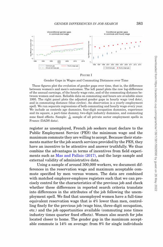
Several nonexclusive mechanisms have been recently put for-ward to explain the persistence of a gender gap in wages, such asgender differences in time flexibility (e.g., Bertrand, Goldin, andKatz 2010; Goldin 2014) and the so-called child penalty (e.g., Adda,Dustmann, and Stevens 2017; Kleven, Landais, and Søgaard2019). This article explores a somewhat overlooked yet related as-pect: gender differences in willingness to commute. Indeed, com-mute is a job attribute with large gender differences. In OECDcountries, women on average spend 22 minutes a day commut-ing, while men spend 33 minutes.1 In France, after controlling forworkers’ observable characteristics, the gender commute gap, thatis, the difference between women’s and men’s commute (in logs),still amounts to −10% to −15%. Gender differentials in commutedecreased over time in a similar manner as gender gaps in annualearnings or in hourly wages, even when adjusted for workers’ ex-perience, occupation, industry, and part-time status (Figure I).
In this article, we estimate how much men and women arewilling to trade in terms of wage for a shorter commute and studythe relationship between gender differences in this commute val-uation and the gender wage gap. Hereafter, we do not take a standon whether differences in commute valuation come from individ-ual preferences or constraints resulting from household decisions.Average commute valuations are difficult to identify from realizedlabor market outcomes, because equilibrium outcomes are pinneddown by marginal workers and because standard data sets do notmeasure all relevant job attributes and workers’ productivity thatmay confound the wage effect of the attribute of interest (Brown1980; Hwang, Reed, and Hubbard 1992). Moreover, frictions in thematching of workers and jobs often blur the compensating differ-entials of job attributes (Altonji and Paxson 1992; Bonhomme andJolivet 2009; Rupert, Stancanelli, and Wasmer 2009). To overcomethese difficulties, recent research makes use of choice experimentsto directly estimate the workers’ willingness to pay for particularjob attributes (Flory, Leibbrandt, and List 2014; Mas and Pallais2017; Wiswall and Zafar 2017; Maestas et al. 2018).
We also rely on incentivized elicitation of preferences byexploiting a unique feature of French institutions: when they
Endowed Fund for Research in Leadership and Diversity. All errors are our own.Le Barbanchon is also affiliated with CEPR, IGIER, IZA, and J-PAL, Rathelotwith CAGE, CEPR, and J-PAL, and Roulet with CEPR.
1. See Chart LMF2.6.A in the OECD family database:http://www.oecd.org/els/family/database.htm.
Dow
nloaded from https://academ
ic.oup.com/qje/article/136/1/381/5928590 by guest on 26 M
ay 2022
GENDER DIFFERENCES IN JOB SEARCH 383
FIGURE I
Gender Gaps in Wages and Commuting Distances over Time
These figures plot the evolution of gender gaps over time, that is, the differencebetween women’s and men’s outcomes. The left panel plots the raw log-differenceof the annual earnings, of the hourly wage rate, and of the commuting distance be-tween women and men. Reliable data on commuting and hours are available since1995. The right panel plots the adjusted gender gaps in hourly wage (red dots),and in commuting distance (blue circles). An observation is a yearly employmentspell. We run separate regressions of both commuting and hourly wage every year.We include as controls age dummies, four-digit occupation dummies, experienceand its square, a part-time dummy, two-digit industry dummies, and commutingzone fixed effects. Sample: 1
60 sample of all private sector employment spells inFrance (DADS data).
register as unemployed, French job seekers must declare to thePublic Employment Service (PES) the minimum wage and themaximum commute they are willing to accept. Because their state-ments matter for the job search services provided by the PES, theyhave an incentive to be attentive and answer truthfully. We thuscombine the advantages in terms of incentives from field experi-ments such as Mas and Pallais (2017), and the large sample andexternal validity of administrative data.
Using a sample of around 300,000 workers, we document dif-ferences in the reservation wage and maximum acceptable com-mute specified by men versus women. The data are combinedwith matched employer-employee registers such that we can pre-cisely control for the characteristics of the previous job and checkwhether these differences in reported search criteria translateinto differences in the attributes of the job following the unem-ployment spell. We find that unemployed women have a full-timeequivalent reservation wage that is 4% lower than men, control-ling finely for the previous job (wage bins, three-digit occupation,etc.) and the job opportunities available (commuting zone timesindustry times quarter fixed effects). Women also search for jobslocated closer to home. The gender gap in the maximum accept-able commute is 14% on average: from 8% for single individuals
Dow
nloaded from https://academ
ic.oup.com/qje/article/136/1/381/5928590 by guest on 26 M
ay 2022
384 THE QUARTERLY JOURNAL OF ECONOMICS
without children to 24% for married individuals with children.These gender differences in reservation job attributes translateinto women getting paid lower wages and having a shorter com-mute upon reemployment.
The close connection between the gender gap in job searchcriteria and that observed for wages and commuting in the over-all working population suggests that supply-side considerationsmay be an important driver of the latter. We introduce a searchmodel where the commute matters, similar to Van Den Berg andGorter (1997), to (i) guide our identification of whether womenhave steeper indifference curves between wage and commute thancomparable men, and (ii) assess the extent to which the genderwage gap is accounted for by gender differences in willingness topay (WTP) for a shorter commute. The model yields a reservationwage curve that gives for every commute the lowest wage that thejob seeker is willing to accept. The slope of the reservation wagecurve is equal to the WTP parameter.
Using reemployment outcomes, in deviation from the reserva-tion wage and commute, we draw the respective acceptance fron-tier of jobs, separately for women and men. For non–minimumwage workers, the acceptance frontier indeed identifies the reser-vation wage curve. We estimate the WTP for a shorter commutefor women and men and obtain that this parameter is significantlyhigher for women. The value of commuting time amounts to 80%of the gross hourly wage for men and 98% for women. Identifica-tion of the WTP relies on assumptions about how declared searchcriteria should be interpreted: for our main strategy, we assumethat job seekers declare one point of their reservation wage curveto the public employment service. We check the robustness of ourresults to other interpretations of declared search criteria.
We feed the estimated WTP parameter for women into the jobsearch model and calibrate the other parameters in line with ourdata, again for women. Keeping all these other parameters fixed,we simulate a shock that reduces WTP by 18.2%, which is equalto the residualized gender difference in commute valuation thatwe have estimated, and look at the effect of this shock on the wageand commute in the next job. We find that gender differences incommute valuation can account for a 0.5 log point hourly wagedeficit for women, that is, 14% of the gender gap in residualizedwages. This suggests that the contribution to the gender wagegap of gender differences in commute valuation is of the sameorder of magnitude as other well-studied job attributes, such as
Dow
nloaded from https://academ
ic.oup.com/qje/article/136/1/381/5928590 by guest on 26 M
ay 2022
GENDER DIFFERENCES IN JOB SEARCH 385
flexible working time and/or job security (see Wiswall and Zafar2017, who find that gender differences in students’ preferences forfuture earnings growth, probability of dismissal, and work hoursflexibility, account for a quarter of the gender earnings gap).
Finally, we perform two robustness exercises using data fromaround 3 million job applications to vacancies posted at the FrenchPES. First, we use a conditional logit model to study the ef-fect of the commute distance between the vacancy’s workplaceand the worker’s home on the probability of the worker apply-ing for the vacancy. We estimate gender-specific coefficients, andinclude job-ad fixed effects to take care of unobserved correlatedamenities. The choice model yields a significant gender gap incommute valuation of between 14% and 23%, which corroboratesour findings using declared search criteria. Second, we studyhiring decisions by employers in response to job applications totest whether gender differences in the reservation commute couldcome from women internalizing a lower labor demand from far-away employers. Within-vacancy regressions show that the hir-ing rate decreases with the commute distance of the applicant,but not at a significantly faster rate for women. This suggeststhat labor demand is not more specifically tilted toward close-by candidates for women than for men. This supports our viewthat gender gaps in commute are primarily driven by supply-sideconsiderations.
This article relates to several lines of research. First webring gender differences in commuting distances into the promi-nent literature on the gender wage gap (Bertrand 2011; Goldin2014; Olivetti and Petrongolo 2016; Blau and Kahn 2017). Genderdifferences in commuting time/distance have been documentedin the urban planning (MacDonald 1999; Crane 2007) and thehealth and well-being literature (Stutzer and Frey 2008; Roberts,Hodgson, and Dolan 2011; Clark et al. 2019) but have not beenanalyzed in relation to the gender wage gap.2 Recent researchon the gender wage gap provides event study evidence thatthe birth of the first child creates a large deterioration in howwomen subsequently fare in the labor market compared with men
2. In a recent paper, Petrongolo and Ronchi (2020) apply our method to es-timate the WTP for a shorter commute, adapting it to British data on job-to-jobtransitions. The gender difference in WTP that they find has a similar magnitudeto ours. Fluchtmann et al. (2020) also use application data and show that Danishwomen are less likely to apply for further-away jobs.
Dow
nloaded from https://academ
ic.oup.com/qje/article/136/1/381/5928590 by guest on 26 M
ay 2022
386 THE QUARTERLY JOURNAL OF ECONOMICS
(Angelov, Johansson, and Lindahl 2016; Kleven, Landais, andSøgaard 2019; Kleven et al. 2019). Our study sheds light ona potential mechanism for the so-called child penalty: the factthat women prefer shorter commutes, possibly to be able to dropoff/pick up children from school/daycare more easily. Yet it alsosuggests that gender differences in the value of commute time arenot only driven by children. Even among single individuals with-out children, we find a difference between men’s and women’scommute valuation that is statistically significant. Moreover, al-though the commute channel may have similar origins to thehours flexibility channel (Bertrand, Goldin, and Katz 2010; Goldin2014; Goldin and Katz 2016; Bolotnyy and Emanuel 2019), weshow that it contributes to the gender wage gap on top of genderdifferences in working hours preferences.3
Second, our article is related to the literature on compen-sating differentials. We bring to the literature on gender dif-ferences in compensating differentials the focus on commutevaluation (Filer 1985; Mas and Pallais 2017; Wiswall andZafar 2017; Maestas et al. 2018). We bring to prior work onthe wage versus commute trade-off the focus on gender hetero-geneity (Van Ommeren, Van Den Berg, and Gorter 2000; Mulalic,Van Ommeren, and Pilegaard 2014; Guglielminetti et al. 2015).4
One exception is Manning (2003), who finds in the cross sectionin the United Kingdom that the effect on wages of commutingis larger for women with children than for men.5 A final contri-bution of our article—this one methodological—is to show howdata on the joint distribution of reservation job attributes andrealized job bundles can be used to identify the key preferenceparameter for the wage versus commute trade-off. We provide
3. Our article is also related to Caldwell and Danieli (2019), who show thatcommute distances are an important component of the more restricted employ-ment opportunity set for women. Our results are also in line with those ofButikofer, Løken, and Willen (2019), who find that building a bridge betweenDenmark and Sweden increased commutes and wages of men more than women.
4. The large literature in transport economics on the value of travel time tendsto focus on heterogeneity across income groups rather than gender differences (fora review, see Small 2012).
5. Van Ommeren and Fosgerau (2009) also find that the marginal costs ofcommuting are larger for women than for men, but the difference is not preciselyestimated and is insignificant.
Dow
nloaded from https://academ
ic.oup.com/qje/article/136/1/381/5928590 by guest on 26 M
ay 2022
GENDER DIFFERENCES IN JOB SEARCH 387
the first estimates of the heterogeneity of this parameter acrossgender.6
The remainder of the article is organized as follows. Section IIdescribes the data. Section III presents the reduced-form evidenceon gender differences in job search criteria and reemployment out-comes separately. Section IV explains how the commute valuationis identified from the joint distribution of search criteria and re-alized outcomes and shows that women have steeper indifferencecurves between wage and commute than men. Section V estimatesthe share of the gender wage gap accounted for by gender differ-ences in willingness to pay for a shorter commute. Section VIprovides further evidence of gender differences in commute valu-ation using application data. Section VII concludes. All appendixmaterial can be found in the Online Appendix.
II. DATA DESCRIPTION
II.A. Data Sources and Sample
Our sample is drawn from a matched data set of French unem-ployment and employment registers. Information on unemploy-ment spells derives from the fichier historique (FH) of the Frenchpublic employment service (Pole Emploi), and that on employmentspells comes from the declarations administratives de donnees so-ciales (DADS) built by the French Institute of Statistics (Insee)from firms’ fiscal declarations. Legal protection of private infor-mation allows the matching for a subpopulation with a samplingrate of 1 in 12.
Our sample includes unemployment insurance (UI) claimantswhose unemployment spell starts between 2006 and 2012.7 Werestrict the sample to people who lost their jobs involuntarily,be it a permanent or a temporary/fixed-term contract. We ob-serve their employment history from 2004 to 2012, from whichwe define (i) the last job before unemployment (last employmentspell ending before they become unemployed) and (ii) the next jobafter unemployment (first employment spell starting after their
6. Black, Kolesnikova, and Taylor (2014) analyze the link between commutingand labor force participation of women.
7. The year 2006 is when the search criteria variables start to be asked, and2012 is when the merge between our two main data sets stops. We focus on newclaims from the regular UI rules, excluding workers in the culture and arts indus-tries (intermittents du spectacle) and from temporary help agencies (interimaires).
Dow
nloaded from https://academ
ic.oup.com/qje/article/136/1/381/5928590 by guest on 26 M
ay 2022
388 THE QUARTERLY JOURNAL OF ECONOMICS
unemployment spell starts).8 Our main sample comprises around320,000 unemployment spells.
II.B. Reservation Wage and Maximum Acceptable Commute
When registering as unemployed in France, people are askedabout the type of job they are seeking, their reservation wage, andmaximum acceptable commute.9 Online Appendix Figure C1 is ascreenshot of the online registration form. First, people are askedwhich occupation they are looking for. The preferred occupationmay be different from their previous one. Second, in response tothe reservation wage question: “What minimum gross wage do youaccept to work for?,” they indicate an amount and choose a unit(hourly, monthly, or annual). Third, people are asked for theirmaximum acceptable commute or reservation commute: “Whatlength of daily commute (one way) would you accept?” Job seek-ers can reply either in minutes or in kilometers. They cannotmove to the next page of the registration website without report-ing this information. Before job seekers answer the questions ontheir desired occupation, reservation wage, and maximum com-mute, they state whether they are willing to accept a temporarycontract or a part-time job (see the screenshot in Online AppendixFigure C2).
All this information enables caseworkers from the public em-ployment service to select the vacancies they will propose to jobseekers.10 If browsing through vacancies is costly, standard the-ory suggests that the best response of job seekers is to revealtheir true reservation wage and other job characteristics to thePES. Moreoever we are confident that the monitoring/sanctioningrole of the PES does not lead job seekers to misreport their reser-vation wage and commute. When monitoring the search activitiesof job seekers, caseworkers are legally required to compare theposted wages of vacancies to which job seekers apply to their past
8. We apply the standard restrictions in the employment registers to analyzemeaningful jobs. We exclude jobs tagged as annex by the data producer. We restrictthe sample to employers from the private sector.
9. This section follows closely the description of the reservation wage data inLe Barbanchon, Rathelot, and Roulet (2019).
10. The services that the PES offers to unemployed job seek-ers are described in the PPAE (Projet Personnalise d’acces a l’emploi),cf. article L5411-6-1 of the Labor Code, https://www.legifrance.gouv.fr/affichCodeArticle.do?idArticle=LEGIARTI000037388467&cidTexte=LEGITEXT000006072050&dateTexte=20190101).
Dow
nloaded from https://academ
ic.oup.com/qje/article/136/1/381/5928590 by guest on 26 M
ay 2022
GENDER DIFFERENCES IN JOB SEARCH 389
wage or the usual wage in the occupation searched for—not totheir reservation wage. As for the commute, they compare it withpredetermined targets (1 hour or 30 kilometers), not to the statedreservation commute. Whether the desired number of workinghours and type of labor contract are used for monitoring/sanctionspurposes is less clear. The law states that “If the desired job isfull-time, job seekers cannot be forced to accept part-time jobs,”which may induce UI claimants to strategically report that theyare seeking a full-time job. Regarding the labor contract, thereare no published/explicit guidelines. That being said, concerns ofstrategic reporting bias are minimal in the French context, wherethe PES is rated low in terms of mobility demands and sanc-tions relative to international standards (Venn 2012). In practice,no sanctions are imposed. Only 0.5% of unemployment spells inour sample are ended by the PES for failing to comply with job-search requirements. Moreover, search criteria are not significantpredictors of being sanctioned (see Online Appendix Table D1).We understand that caseworkers are mostly active in their coun-seling role where their objective is aligned with that of the jobseekers.
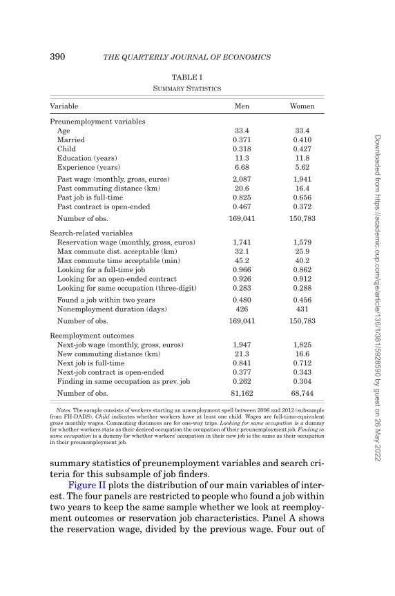
II.C. Summary Statistics
Table I contains the raw summary statistics from our sam-ple. Prior to being unemployed, women earned on average €1,941gross a month (full-time equivalent) and their average commutewas 16.4 kilometers, for men it was €2,087 and 20.6 kilometers.The commute measure in the employment registers is the dis-tance between the centroids of the municipality of the workplaceand the municipality of residence. There are more than 34,000municipalities in France, so municipality centroids proxy well foractual locations. When workers reside and work in the same mu-nicipality (24.7% of the sample), we proxy for their commute bythe average distance between two random locations within themunicipality.
The average monthly gross reservation wage (full-time equiv-alent) of job seekers in our sample is €1,579 for women and €1,741for men. The maximum acceptable commute (one way) is 26 kilo-meters for women who report in distance and 40 minutes forwomen who report in time. The corresponding figures for menare 32 kilometers and 45 minutes. Close to half the sample finda job within two years. Online Appendix Table D2 reports the
Dow
nloaded from https://academ
ic.oup.com/qje/article/136/1/381/5928590 by guest on 26 M
ay 2022
390 THE QUARTERLY JOURNAL OF ECONOMICS
TABLE ISUMMARY STATISTICS
Variable Men Women
Preunemployment variablesAge 33.4 33.4Married 0.371 0.410Child 0.318 0.427Education (years) 11.3 11.8Experience (years) 6.68 5.62
Past wage (monthly, gross, euros) 2,087 1,941Past commuting distance (km) 20.6 16.4Past job is full-time 0.825 0.656Past contract is open-ended 0.467 0.372
Number of obs. 169,041 150,783
Search-related variablesReservation wage (monthly, gross, euros) 1,741 1,579Max commute dist. acceptable (km) 32.1 25.9Max commute time acceptable (min) 45.2 40.2Looking for a full-time job 0.966 0.862Looking for an open-ended contract 0.926 0.912Looking for same occupation (three-digit) 0.283 0.288
Found a job within two years 0.480 0.456Nonemployment duration (days) 426 431
Number of obs. 169,041 150,783
Reemployment outcomesNext-job wage (monthly, gross, euros) 1,947 1,825New commuting distance (km) 21.3 16.6Next job is full-time 0.841 0.712Next-job contract is open-ended 0.377 0.343Finding in same occupation as prev. job 0.262 0.304
Number of obs. 81,162 68,744
Notes. The sample consists of workers starting an unemployment spell between 2006 and 2012 (subsamplefrom FH-DADS). Child indicates whether workers have at least one child. Wages are full-time-equivalentgross monthly wages. Commuting distances are for one-way trips. Looking for same occupation is a dummyfor whether workers state as their desired occupation the occupation of their preunemployment job. Finding insame occupation is a dummy for whether workers’ occupation in their new job is the same as their occupationin their preunemployment job.
summary statistics of preunemployment variables and search cri-teria for this subsample of job finders.
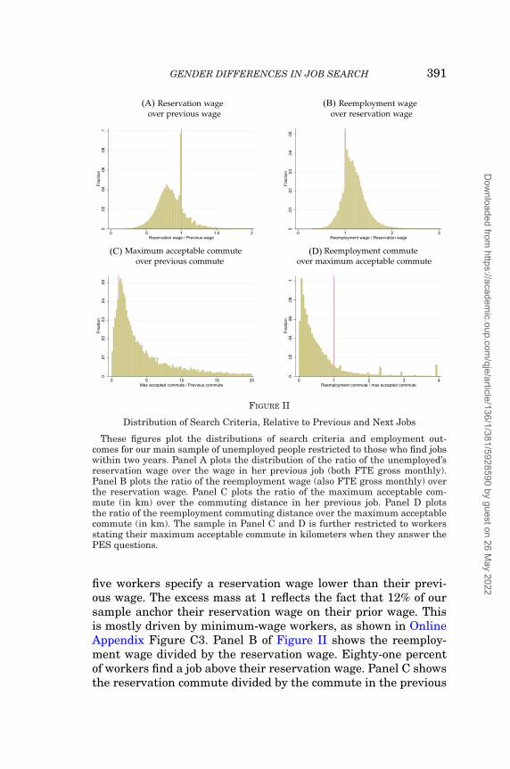
Figure II plots the distribution of our main variables of inter-est. The four panels are restricted to people who found a job withintwo years to keep the same sample whether we look at reemploy-ment outcomes or reservation job characteristics. Panel A showsthe reservation wage, divided by the previous wage. Four out of
Dow
nloaded from https://academ
ic.oup.com/qje/article/136/1/381/5928590 by guest on 26 M
ay 2022
GENDER DIFFERENCES IN JOB SEARCH 391
(D)(C)
(B)(A)
FIGURE II
Distribution of Search Criteria, Relative to Previous and Next Jobs
These figures plot the distributions of search criteria and employment out-comes for our main sample of unemployed people restricted to those who find jobswithin two years. Panel A plots the distribution of the ratio of the unemployed’sreservation wage over the wage in her previous job (both FTE gross monthly).Panel B plots the ratio of the reemployment wage (also FTE gross monthly) overthe reservation wage. Panel C plots the ratio of the maximum acceptable com-mute (in km) over the commuting distance in her previous job. Panel D plotsthe ratio of the reemployment commuting distance over the maximum acceptablecommute (in km). The sample in Panel C and D is further restricted to workersstating their maximum acceptable commute in kilometers when they answer thePES questions.
five workers specify a reservation wage lower than their previ-ous wage. The excess mass at 1 reflects the fact that 12% of oursample anchor their reservation wage on their prior wage. Thisis mostly driven by minimum-wage workers, as shown in OnlineAppendix Figure C3. Panel B of Figure II shows the reemploy-ment wage divided by the reservation wage. Eighty-one percentof workers find a job above their reservation wage. Panel C showsthe reservation commute divided by the commute in the previous
Dow
nloaded from https://academ
ic.oup.com/qje/article/136/1/381/5928590 by guest on 26 M
ay 2022
392 THE QUARTERLY JOURNAL OF ECONOMICS
job. Most job seekers (91%) report a maximum acceptable com-mute greater than their previous commute. Panel D shows thecommute on reemployment divided by the reservation commute:81% of unemployed individuals end up commuting less than theirreservation commute.
To further describe these variables, we plot in OnlineAppendix Figure C4 the raw distributions of monthly reserva-tion wages and maximum acceptable commutes. They illustratethat workers do not answer some default option or very roundnumbers. This suggests that workers pay attention to their an-swers. Moreover, Online Appendix Table D4 shows how job searchcriteria predict job-finding rates. We see that a larger maximumacceptable commute increases the job-finding rate, while a higherreservation wage reduces it, controlling for the characteristics ofthe previous job and workers (including age, education, marital,and parental status). This suggests that the search criteria mea-sures do capture some meaningful information that correspondsto the theoretical notion of a reservation wage and of a reservationcommute.
III. GENDER DIFFERENCES IN JOB SEARCH CRITERIA AND
REEMPLOYMENT OUTCOMES
In this section, we document how job search criteria and reem-ployment outcomes vary across gender. We first estimate averagegender gaps in reservation and accepted job attributes. Second, wedocument the heterogeneity in gender gaps by family structure,by worker’s age, and by geography. Third, we provide evidence insupport of the external validity of our results, by looking at job-to-job transitions and by using survey data on U.S. job seekers.
III.A. Average Gender Gaps in Reservation Wage and Commuteand in Reemployment Outcomes
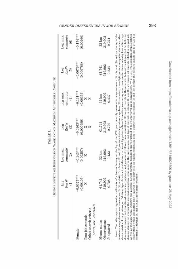
We first estimate gender gaps in reservation wage and inreservation commute. Table II shows results from regressions ofa reservation job attribute on a female dummy. In columns (1),(3), and (5), the outcome is the reservation wage in logs, while incolumns (2), (4), and (6) it is the maximum acceptable commute,also in logs. In columns (1) and (2), we control for worker char-acteristics (age dummies, years of education dummies, maritalstatus, parenthood, and work experience), for the characteristics
Dow
nloaded from https://academ
ic.oup.com/qje/article/136/1/381/5928590 by guest on 26 M
ay 2022
GENDER DIFFERENCES IN JOB SEARCH 393
TA
BL
EII
GE
ND
ER
EF
FE
CT
ON
RE
SE
RV
AT
ION
WA
GE
AN
DO
NM
AX
IMU
MA
CC
EP
TA
BL
EC
OM
MU
TE
Log
Log
max
.L
ogL
ogm
ax.
Log
Log
max
.R
esW
com
mu
teR
esW
com
mu
teR
esW
com
mu
te(1
)(2
)(3
)(4
)(5
)(6
)
Fem
ale
−0.0
377*
**−0
.143
***
−0.0
363*
**−0
.131
***
−0.0
676*
**−0
.174
***
(0.0
0105
)(0
.003
57)
(0.0
0099
9)(0
.003
53)
(0.0
0078
6)(0
.002
60)
Pas
tjo
bco
ntr
ols
XX
XX
Oth
erse
arch
crit
eria
XX
(hou
rs,o
cc.,
con
trac
t)
Mea
n:m
ales
€1,
741
32km
€1,
741
32km
€1,
741
32km
Obs
erva
tion
s31
9,90
231
9,90
231
9,90
231
9,90
231
9,90
231
9,90
2R
-squ
ared
0.72
80.
433
0.72
90.
437
0.53
40.
274
Not
es.
Th
eta
ble
repo
rts
regr
essi
onco
effi
cien
tsof
afe
mal
edu
mm
yon
the
log
ofth
eF
TE
gros
sm
onth
lyre
serv
atio
nw
age
(col
um
ns
(1),
(3),
and
(5))
and
onth
elo
gof
the
max
imu
mac
cept
able
com
mu
te(c
olu
mn
s(2
),(4
),an
d(6
)).I
nco
lum
ns
(1)
and
(2),
con
trol
sin
clu
depr
evio
us
wag
ebi
ns
(20
dum
mie
s),t
hre
e-di
git
prev
iou
soc
cupa
tion
dum
mie
s,ot
her
char
acte
rist
ics
ofth
epr
evio
us
job
(fu
ll-t
ime,
type
ofco
ntr
act,
and
dist
ance
toh
ome)
,log
pote
nti
albe
nefi
tdu
rati
on,c
omm
uti
ng
zon
eti
mes
quar
ter
tim
esin
dust
ryfi
xed
effe
cts,
age
dum
mie
s,ex
peri
ence
and
edu
cati
ondu
mm
ies,
mar
ital
stat
us,
and
pres
ence
ofch
ildr
en.I
nco
lum
ns
(3)a
nd
(4),
we
add
con
trol
sfo
rth
eot
her
attr
ibu
tes
ofth
ejo
bse
arch
edfo
r:fu
ll-t
ime
dum
my,
dum
my
for
wh
eth
erth
ese
arch
edoc
cupa
tion
isth
esa
me
asth
epr
evio
us
one,
and
type
ofco
ntr
act.
Inco
lum
ns
(5)
and
(6),
we
rem
ove
all
con
trol
sre
late
dto
the
past
job,
asw
ell
aspa
stex
peri
ence
,in
dust
ry,
and
pote
nti
albe
nefi
tdu
rati
on.
Sta
nda
rder
rors
clu
ster
edat
the
wor
ker
leve
lar
ein
pare
nth
eses
.**
*p
<.0
1.T
he
esti
mat
ion
drop
ssi
ngl
eton
obse
rvat
ion
sw
ith
inco
mm
uti
ng
zon
e×
quar
ter
×in
dust
ryce
lls
(or
wit
hin
com
mu
tin
gzo
ne
×qu
arte
rce
lls
inco
lum
ns
(5)
and
(6))
,so
that
the
effe
ctiv
esa
mpl
esi
zeis
270,
934
inco
lum
ns
(1)
thro
ugh
(4)
and
319,
691
inco
lum
ns
(5)
and
(6).
Dow
nloaded from https://academ
ic.oup.com/qje/article/136/1/381/5928590 by guest on 26 M
ay 2022
394 THE QUARTERLY JOURNAL OF ECONOMICS
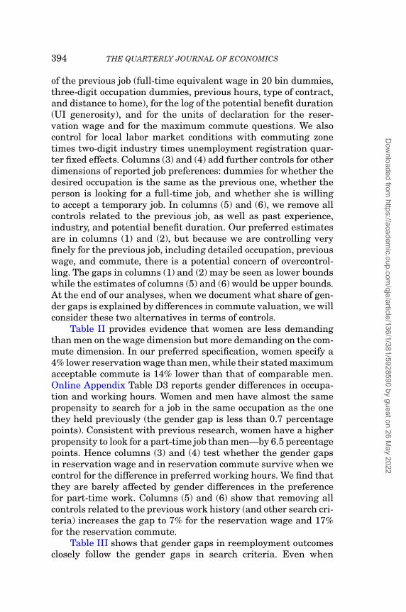
of the previous job (full-time equivalent wage in 20 bin dummies,three-digit occupation dummies, previous hours, type of contract,and distance to home), for the log of the potential benefit duration(UI generosity), and for the units of declaration for the reser-vation wage and for the maximum commute questions. We alsocontrol for local labor market conditions with commuting zonetimes two-digit industry times unemployment registration quar-ter fixed effects. Columns (3) and (4) add further controls for otherdimensions of reported job preferences: dummies for whether thedesired occupation is the same as the previous one, whether theperson is looking for a full-time job, and whether she is willingto accept a temporary job. In columns (5) and (6), we remove allcontrols related to the previous job, as well as past experience,industry, and potential benefit duration. Our preferred estimatesare in columns (1) and (2), but because we are controlling veryfinely for the previous job, including detailed occupation, previouswage, and commute, there is a potential concern of overcontrol-ling. The gaps in columns (1) and (2) may be seen as lower boundswhile the estimates of columns (5) and (6) would be upper bounds.At the end of our analyses, when we document what share of gen-der gaps is explained by differences in commute valuation, we willconsider these two alternatives in terms of controls.
Table II provides evidence that women are less demandingthan men on the wage dimension but more demanding on the com-mute dimension. In our preferred specification, women specify a4% lower reservation wage than men, while their stated maximumacceptable commute is 14% lower than that of comparable men.Online Appendix Table D3 reports gender differences in occupa-tion and working hours. Women and men have almost the samepropensity to search for a job in the same occupation as the onethey held previously (the gender gap is less than 0.7 percentagepoints). Consistent with previous research, women have a higherpropensity to look for a part-time job than men—by 6.5 percentagepoints. Hence columns (3) and (4) test whether the gender gapsin reservation wage and in reservation commute survive when wecontrol for the difference in preferred working hours. We find thatthey are barely affected by gender differences in the preferencefor part-time work. Columns (5) and (6) show that removing allcontrols related to the previous work history (and other search cri-teria) increases the gap to 7% for the reservation wage and 17%for the reservation commute.
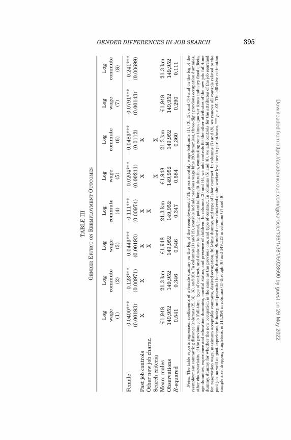
Table III shows that gender gaps in reemployment outcomesclosely follow the gender gaps in search criteria. Even when
Dow
nloaded from https://academ
ic.oup.com/qje/article/136/1/381/5928590 by guest on 26 M
ay 2022
GENDER DIFFERENCES IN JOB SEARCH 395
TA
BL
EII
IG
EN
DE
RE
FF
EC
TO
NR
EE
MP
LO
YM
EN
TO
UT
CO
ME
S
Log
Log
Log
Log
Log
Log
Log
Log
wag
eco
mm
ute
wag
eco
mm
ute
wag
eco
mm
ute
wag
eco
mm
ute
(1)
(2)
(3)
(4)
(5)
(6)
(7)
(8)
Fem
ale
−0.0
400*
**−0
.123
***
−0.0
443*
**−0
.111
***
−0.0
204*
**−0
.048
3***
−0.0
791*
**−0
.241
***
(0.0
0193
)(0
.009
71)
(0.0
0193
)(0
.009
74)
(0.0
0211
)(0
.011
2)(0
.001
43)
(0.0
0699
)P
ast
job
con
trol
sX
XX
XX
XO
ther
new
job
char
ac.
XX
Sea
rch
crit
eria
XX
Mea
n:m
ales
€1,
948
21.3
km€
1,94
821
.3km
€1,
948
21.3
km€
1,94
821
.3km
Obs
erva
tion
s14
9,95
214
9,95
214
9,95
214
9,95
214
9,95
214
9,95
214
9,95
214
9,95
2R
-squ
ared
0.54
10.
346
0.54
60.
347
0.58
40.
360
0.29
00.
111
Not
es.
Th
eta
ble
repo
rts
regr
essi
onco
effi
cien
tsof
afe
mal
edu
mm
yon
the
log
ofth
ere
empl
oym
ent
FT
Egr
oss
mon
thly
wag
e(c
olu
mn
s(1
),(3
),(5
),an
d(7
))an
don
the
log
ofth
ere
empl
oym
ent
com
mu
tin
gdi
stan
ce(c
olu
mn
s(2
),(4
),(6
),an
d(8
)).I
nco
lum
ns
(1)a
nd
(2),
con
trol
sin
clu
depr
evio
us
wag
ebi
ns
(20
dum
mie
s),t
hre
e-di
git
prev
iou
soc
cupa
tion
dum
mie
s,ot
her
char
acte
rist
ics
ofth
epr
evio
us
job
(fu
ll-t
ime,
type
ofco
ntr
act,
and
dist
ance
toh
ome)
,log
pote
nti
albe
nefi
tdu
rati
on,c
omm
uti
ng
zon
eti
mes
quar
ter
tim
esin
dust
ryfi
xed
effe
cts,
age
dum
mie
s,ex
peri
ence
and
edu
cati
ondu
mm
ies,
mar
ital
stat
us,
and
pres
ence
ofch
ildr
en.I
nco
lum
ns
(3)
and
(4),
we
add
con
trol
sfo
rth
eot
her
attr
ibu
tes
ofth
en
ewjo
b:fu
ll-t
ime
dum
my,
dum
my
for
wh
eth
erth
en
ewoc
cupa
tion
isth
esa
me
asth
epr
evio
us
one,
and
type
ofco
ntr
act.
Inco
lum
ns
(5)
and
(6),
we
add
con
trol
sfo
rth
eat
trib
ute
sof
the
job
sear
ched
for:
rese
rvat
ion
wag
e,m
axim
um
acce
ptab
leco
mm
ute
,des
ired
occu
pati
on,f
ull
-tim
edu
mm
y,an
dty
peof
labo
rco
ntr
act.
Inco
lum
ns
(7)
and
(8),
we
rem
ove
all
con
trol
sre
late
dto
the
past
job,
asw
ell
aspa
stex
peri
ence
,in
dust
ry,a
nd
pote
nti
albe
nefi
tdu
rati
on.S
tan
dard
erro
rscl
ust
ered
atth
ew
orke
rle
vel
are
inpa
ren
thes
es.*
**p
<.0
1.T
he
effe
ctiv
ees
tim
atio
nsa
mpl
esi
ze,d
ropp
ing
sin
glet
ons,
is11
4,39
4in
colu
mn
s(1
)th
rou
gh(6
)an
d14
9,11
3in
colu
mn
s(7
)an
d(8
).
Dow
nloaded from https://academ
ic.oup.com/qje/article/136/1/381/5928590 by guest on 26 M
ay 2022
396 THE QUARTERLY JOURNAL OF ECONOMICS
controlling finely for the previous job characteristics, the genderwage gap amounts to 4% (column (1)), and the gender commutegap to 12% (column (2)). These differences survive when we controlfor other attributes of the new job in columns (3) and (4): part-time,type of contract, and change of occupation. In columns (5) and (6),we control for the search criteria (reservation wage, maximum ac-ceptable commute, and others). With the search-related controls,magnitudes are roughly halved: the gender wage gap amounts to2% and the gender commute gap to 5%. Columns (7) and (8) showthat the gender gaps double when removing all controls relatedto the previous work history to 8% for wages and 24% for com-muting distances. The parallel between Tables II and III buildsconfidence in the validity of the answers to the search strategyquestions asked by the French PES. Moreover, it suggests thatgender gaps in realized job outcomes are partly driven by laborsupply. This is further hinted at in the heterogeneity analyses inSection III.B.
By construction, the sample in Table III—containing only jobseekers who found a job within two years—is a subset of that ofTable II. Online Appendix Table D4 rules out major differentialselection into employment across gender. Without controlling forthe type of job looked for, but controlling precisely for the pre-vious job characteristics, the probability of women finding a jobwithin two years is 2.4 percentage points lower than that of men.This difference becomes insignificant when we control for all thecharacteristics of the job sought.
1. Flexibility in Working Hours. From a theoretical perspec-tive, individuals with a high value of nonworking time shouldvalue both a short commute and working-hours flexibility. InTable II, column (4), we show that women state a preference forshorter commutes on top of their preference for part-time jobs,by controlling for preferred hours. In Panel C of Online AppendixTable D3, we estimate gender gaps in search criteria, restrict-ing the sample to job seekers who previously held a full-timejob and who are likely to hold similar preferences for working-hours flexibility. We find an average gender gap in the maxi-mum acceptable commute of a similar magnitude as for the wholesample.
2. Mobility Decisions. Willingness to commute might also in-teract with residential mobility decisions, raising a concern that
Dow
nloaded from https://academ
ic.oup.com/qje/article/136/1/381/5928590 by guest on 26 M
ay 2022
GENDER DIFFERENCES IN JOB SEARCH 397
these decisions do not affect men and women similarly, whichcould introduce some biases in gender gaps estimates. Around15% of job seekers change municipality between their initial reg-istration at the PES (when they declare their search criteria)and their next job. We find no gender differences in this propor-tion, neither conditional on our set of controls nor unconditionally.However reemployment commute depends on residential mobil-ity: among men, commute is 15% shorter for those who moved,whereas among women it is 4% shorter for those who moved. Thegender difference in commute is thus smaller for movers. Includ-ing movers in our analysis attenuates the gender commute gapestimate but the magnitude of the difference is small (see OnlineAppendix Table D5, Panel D).
3. Residential Sorting. In the main analysis, we introducecommuting zone fixed effects to control for local labor market con-ditions. In Online Appendix Table D6, we further control for mu-nicipality fixed effects. This barely affects the gender gaps in thereservation wage and commute, and in the reemployment wageand commute.
III.B. Heterogeneity by Family Structure, Age, and Geography
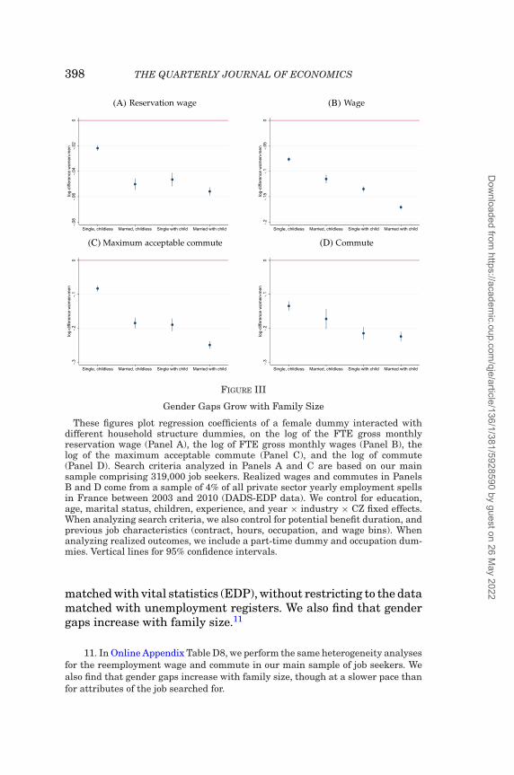
1. Heterogeneity by Family Structure. In Figure III , we re-port gender differences by marital status and the presence ofchildren. These gender gaps are obtained by interacting the gen-der dummy with the interaction between marital status and thepresence of at least one child in specifications similar to that ofTables II and III. Online Appendix Table D7 reports the detailedestimation results. The upper left panel of Figure III shows thatthe gender gap in reservation wages is larger for married jobseekers and parents: married mothers have a 6% lower reserva-tion wage than do married fathers. Interestingly, there is still a2% gap among single individuals without children. Similarly, thebottom-left panel shows that the gender gap in the reservationcommute increases with family size. While single women with-out children are willing at most to commute 8% less than com-parable men, the difference increases to around 18% for eithermarried workers without children or single workers with at leastone child and to even 24% for married workers with at least onechild.
The right panels report the same heterogeneity analyses forwages and commutes in the general population. For these pan-els, we use a sample of the employer-employee registers (DADS)
Dow
nloaded from https://academ
ic.oup.com/qje/article/136/1/381/5928590 by guest on 26 M
ay 2022
398 THE QUARTERLY JOURNAL OF ECONOMICS
(D)(C)
(B)(A)
FIGURE III
Gender Gaps Grow with Family Size
These figures plot regression coefficients of a female dummy interacted withdifferent household structure dummies, on the log of the FTE gross monthlyreservation wage (Panel A), the log of FTE gross monthly wages (Panel B), thelog of the maximum acceptable commute (Panel C), and the log of commute(Panel D). Search criteria analyzed in Panels A and C are based on our mainsample comprising 319,000 job seekers. Realized wages and commutes in PanelsB and D come from a sample of 4% of all private sector yearly employment spellsin France between 2003 and 2010 (DADS-EDP data). We control for education,age, marital status, children, experience, and year × industry × CZ fixed effects.When analyzing search criteria, we also control for potential benefit duration, andprevious job characteristics (contract, hours, occupation, and wage bins). Whenanalyzing realized outcomes, we include a part-time dummy and occupation dum-mies. Vertical lines for 95% confidence intervals.
matched with vital statistics (EDP), without restricting to the datamatched with unemployment registers. We also find that gendergaps increase with family size.11
11. In Online Appendix Table D8, we perform the same heterogeneity analysesfor the reemployment wage and commute in our main sample of job seekers. Wealso find that gender gaps increase with family size, though at a slower pace thanfor attributes of the job searched for.
Dow
nloaded from https://academ
ic.oup.com/qje/article/136/1/381/5928590 by guest on 26 M
ay 2022
GENDER DIFFERENCES IN JOB SEARCH 399
(D)(C)
(B)(A)
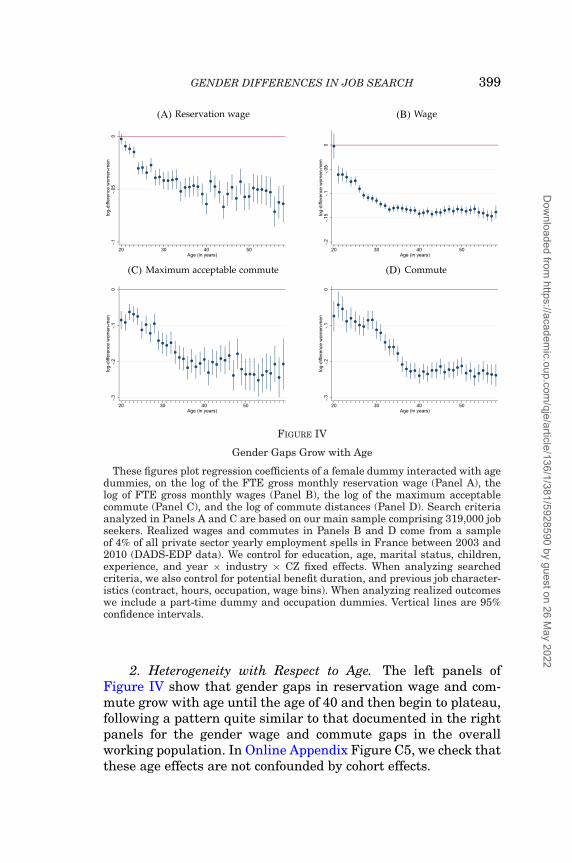
FIGURE IV
Gender Gaps Grow with Age
These figures plot regression coefficients of a female dummy interacted with agedummies, on the log of the FTE gross monthly reservation wage (Panel A), thelog of FTE gross monthly wages (Panel B), the log of the maximum acceptablecommute (Panel C), and the log of commute distances (Panel D). Search criteriaanalyzed in Panels A and C are based on our main sample comprising 319,000 jobseekers. Realized wages and commutes in Panels B and D come from a sampleof 4% of all private sector yearly employment spells in France between 2003 and2010 (DADS-EDP data). We control for education, age, marital status, children,experience, and year × industry × CZ fixed effects. When analyzing searchedcriteria, we also control for potential benefit duration, and previous job character-istics (contract, hours, occupation, wage bins). When analyzing realized outcomeswe include a part-time dummy and occupation dummies. Vertical lines are 95%confidence intervals.
2. Heterogeneity with Respect to Age. The left panels ofFigure IV show that gender gaps in reservation wage and com-mute grow with age until the age of 40 and then begin to plateau,following a pattern quite similar to that documented in the rightpanels for the gender wage and commute gaps in the overallworking population. In Online Appendix Figure C5, we check thatthese age effects are not confounded by cohort effects.
Dow
nloaded from https://academ
ic.oup.com/qje/article/136/1/381/5928590 by guest on 26 M
ay 2022

400 THE QUARTERLY JOURNAL OF ECONOMICS
3. Heterogeneity by Geography. Online Appendix Figure C6shows the heterogeneity in the gender gaps between the Paris re-gion and the rest of France. There is a large heterogeneity in trans-portation modes between these two zones. Indeed, using surveydata from the French statistical agency (Insee) on mode of trans-portation for commute (Mobilites professionnelles survey), we findthat the share of people who commute by public transport in theParis region is on average 43%, whereas in the rest of France thisshare is on average 7%. In Online Appendix Figure C6, we seethat gender gaps in reservation/realized wages and commute aresignificantly larger outside of the Paris region, where a worker’smain option for commute is driving.
III.C. External Validity
Online Appendix Table D10 reports estimates of the gendergap in reservation wages found in other studies, for the UnitedStates, the United Kingdom, and Germany (e.g., Feldstein andPoterba 1984; Brown, Roberts, and Taylor 2011; Caliendo, Lee,and Mahlstedt 2017). Although the majority of these studies arenot focused on the gender gap, they report coefficients of a genderdummy in Mincerian regressions of reservation wages. Women inthe United States, in the United Kingdom, and in Germany alsostate lower reservation wages than comparable men. The order ofmagnitude of these gaps is comparable to our findings for France,but our administrative data on labor market outcomes and reser-vation wages yield estimates that are much more precise than inprevious literature. To the best of our knowledge, no comparablestudies report gender gaps in other dimensions of job search, al-though the survey of Krueger and Mueller (2016) asks workersabout their willingness to commute. We use these data made pub-licly available by the authors to compute the gender gap in desiredcommute time in the United States (which, to our knowledge, hasnot been analyzed so far). Table IV shows that U.S. women searchfor jobs that can be reached with 26% less commuting time.
We have provided evidence on gender differences in prefer-ences of the unemployed and in job characteristics after a periodof unemployment, but do we observe similar patterns for job-to-jobtransitions? In Online Appendix Table D11, we report the resultsof the same regression as in Table III for the population of em-ployed workers switching jobs. The gender gaps in the new wageand commute are very close to what is observed for unemployed
Dow
nloaded from https://academ
ic.oup.com/qje/article/136/1/381/5928590 by guest on 26 M
ay 2022
GENDER DIFFERENCES IN JOB SEARCH 401
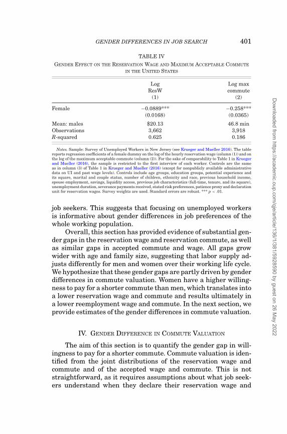
TABLE IVGENDER EFFECT ON THE RESERVATION WAGE AND MAXIMUM ACCEPTABLE COMMUTE
IN THE UNITED STATES
Log Log maxResW commute
(1) (2)
Female −0.0889*** −0.258***(0.0168) (0.0365)
Mean: males $20.13 46.8 minObservations 3,662 3,918R-squared 0.625 0.186
Notes. Sample: Survey of Unemployed Workers in New Jersey (see Krueger and Mueller 2016). The tablereports regression coefficients of a female dummy on the log of the hourly reservation wage (column (1)) and onthe log of the maximum acceptable commute (column (2)). For the sake of comparability to Table 1 in Kruegerand Mueller (2016), the sample is restricted to the first interview of each worker. Controls are the sameas in column (3) of Table 1 in Krueger and Mueller (2016) (except for nonpublicly available administrativedata on UI and past wage levels). Controls include age groups, education groups, potential experience andits square, marital and couple status, number of children, ethnicity and race, previous household income,spouse employment, savings, liquidity access, previous job characteristics (full-time, tenure, and its square),unemployment duration, severance payments received, stated risk preferences, patience proxy and declarationunit for reservation wages. Survey weights are used. Standard errors are robust. *** p < .01.
job seekers. This suggests that focusing on unemployed workersis informative about gender differences in job preferences of thewhole working population.
Overall, this section has provided evidence of substantial gen-der gaps in the reservation wage and reservation commute, as wellas similar gaps in accepted commute and wage. All gaps growwider with age and family size, suggesting that labor supply ad-justs differently for men and women over their working life cycle.We hypothesize that these gender gaps are partly driven by genderdifferences in commute valuation. Women have a higher willing-ness to pay for a shorter commute than men, which translates intoa lower reservation wage and commute and results ultimately ina lower reemployment wage and commute. In the next section, weprovide estimates of the gender differences in commute valuation.
IV. GENDER DIFFERENCE IN COMMUTE VALUATION
The aim of this section is to quantify the gender gap in will-ingness to pay for a shorter commute. Commute valuation is iden-tified from the joint distributions of the reservation wage andcommute and of the accepted wage and commute. This is notstraightforward, as it requires assumptions about what job seek-ers understand when they declare their reservation wage and
Dow
nloaded from https://academ
ic.oup.com/qje/article/136/1/381/5928590 by guest on 26 M
ay 2022
402 THE QUARTERLY JOURNAL OF ECONOMICS
maximum acceptable commute. We first introduce a job searchmodel that allows us to be explicit and to formalize these choices.
IV.A. A Search Model Where Commuting Matters
We consider a random job search model where commutingmatters (Van Den Berg and Gorter 1997). The instantaneous util-ity of being employed in a job with log-wage w = log W and com-mute τ is given by u(W, τ ) = log W − ατ . The parameter α mea-sures the willingness to pay for a shorter commute and may differbetween men and women. This is the key preference parameterwe want to identify. It can be thought of as an individual prefer-ence/cost parameter or as a reduced-form parameter that is theoutcome of household bargaining on gender task specialization.
Job matches are destroyed at the exogenous rate q. Whileunemployed, workers receive flow utility b and draw job offers atthe rate λ from the cumulative distribution function of log-wageand commute H. The job search model admits a standard solution,which is summarized in the following Bellman equation for theunemployment value U:
rU = b + λ
r + q
∫ ∞
0
∫ ∞
01{w−ατ>rU }(w − ατ − rU )dH(w, τ ),
where r is the discount rate.Job seekers accept all jobs that are such that w − ατ > rU.
For a job next door, that is, when τ = 0, the reservation log-wageis φ(0) = rU. For a commute τ , the reservation log-wage is: φ(τ ) =rU + ατ . This allows us to define a reservation log-wage curve:
φ(τ ) = φ(0) + ατ.
The reservation log-wage curve follows the indifference curve inthe log-wage/commute plane with utility level rU. Note that theslope of the reservation log-wage curve is the parameter α, so thatidentifying the reservation curve yields the willingness to pay fora shorter commute. Replacing rU by φ(0) in the Bellman equation,we obtain the solution for the intercept of the reservation log-wagecurve:
(1) φ(0) = b + λ
r + q
∫ ∞
0
∫ ∞
φ(0)+ατ
(w − φ(0) − ατ )dH(w, τ ).
Dow
nloaded from https://academ
ic.oup.com/qje/article/136/1/381/5928590 by guest on 26 M
ay 2022
GENDER DIFFERENCES IN JOB SEARCH 403
This solves the model. For the sake of completeness, we ex-press the average commute and log-wage in the next job, E(τn)and E(wn):
E(τn) = 1p
∫ ∞
0
∫ ∞
φ(0)+ατ
τdH(w, τ )(2)
E(wn) = 1p
∫ ∞
0
∫ ∞
φ(0)+ατ
wdH(w, τ ),(3)
where p = ∫ ∞0
∫ ∞φ(0)+ατ
dH(w, τ ) is the probability of accepting a joboffer.
IV.B. Identifying the Commute Valuation
To identify the parameter α, the willingness to pay for ashorter commute, we need to relate the search criteria measuresto variables in the model. The PES question about the reservationwage does not explicitly anchor the commute dimension. Symmet-rically, the question about the maximum acceptable commute doesnot specify the wage to consider. Without further information, wemay consider two main interpretations:
• Interpretation 1: Job seekers answer a pair (τ ∗, φ∗) of jobattributes that lies on their reservation wage curve, so thatφ∗ = φ(0) + ατ ∗.
• Interpretation 2: Job seekers report the reservation wageφ(0) corresponding to the minimum possible commute (0)and the reservation commute φ−1(w) corresponding to thelargest wage they could get, w.
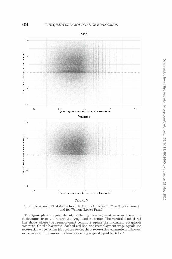
Interpretation 2 differs from Interpretation 1 in that it im-plies that workers do not accept jobs that are both close to theirreservation wage and close to their maximum acceptable commute(see Online Appendix Figure C7 for an illustration of these two in-terpretations). Figure V shows the joint density of reemploymentwage and commute, relative to the reservation wage and commute,for men (upper panel) and women (lower panel). By construction,the plot is restricted to workers finding jobs.12 Consistent withthe job search model, most of the density mass is in the upper
12. We convert the maximum commuting time for those who declare in minutesinto kilometers, assuming that average commuting speed is 35 km/hour.
Dow
nloaded from https://academ
ic.oup.com/qje/article/136/1/381/5928590 by guest on 26 M
ay 2022
404 THE QUARTERLY JOURNAL OF ECONOMICS
FIGURE V
Characteristics of Next Job Relative to Search Criteria for Men (Upper Panel)and for Women (Lower Panel)
The figure plots the joint density of the log reemployment wage and commutein deviation from the reservation wage and commute. The vertical dashed redline shows where the reemployment commute equals the maximum acceptablecommute. On the horizontal dashed red line, the reemployment wage equals thereservation wage. When job seekers report their reservation commute in minutes,we convert their answers in kilometers using a speed equal to 35 km/h.
Dow
nloaded from https://academ
ic.oup.com/qje/article/136/1/381/5928590 by guest on 26 M
ay 2022
GENDER DIFFERENCES IN JOB SEARCH 405
left quadrant: workers accept jobs paying more than their reser-vation wage and closer to home than their reservation commute.Importantly, we do not observe the missing mass predicted byInterpretation 2 in the bottom right corner of the upper left quad-rant, where the accepted jobs are both just above the reservationwage and just below the maximum acceptable commute. This istrue for both men and women. Figure V provides suggestive ev-idence in favor of Interpretation 1. We adopt Interpretation 1 inour main analysis, and we provide a robustness analysis underInterpretation 2 in Online Appendix A. In Online Appendix A, wealso consider a variant of Interpretation 2 (denoted Interpreta-tion 2 bis), where job seekers report the reservation wage φ(τ 25)corresponding to the first quartile of potential commute and thereservation commute φ−1(w75) corresponding to the third quartilein the potential wage distribution.13
To identify the reservation log-wage curve, we leverage thetheoretical insight that accepted job bundles are above the reser-vation wage curve in the commute/wage plane. As a consequence,the frontier of the convex hull of accepted jobs draws the indif-ference curve delivering the reservation utility. This result holdsunder some regularity conditions for the job offer distribution.The job offer probability density function must be bounded frombelow, so there is no region of the commute/wage plane where theacceptance strategy is degenerate and thus less informative.
The identification strategy of the WTP for a shorter commuteα proceeds in two steps. First, under Interpretation 1, reservationcurves pass through the point where the job bundle equals thedeclared reservation wage and maximum acceptable commute.This yields one first point of the reservation wage curve. The sec-ond step amounts to rotating potential reservation wage curvesaround the declared reservation job bundle and choosing the reser-vation curve most consistent with the acceptance strategy of thejob search model. We then identify the average slope of the reser-vation curve by minimizing the sum of squared distances to thereservation curve of accepted bundles that are observed below thereservation curve. We discuss in Section IV.C how classical mea-surement error and other mechanisms may generate accepted jobsbelow the reservation wage curve in our data.
Figure VI illustrates the identification strategy. In the log-wage-commute plane, we plot the jobs accepted by 10 workers
13. We thank a referee for suggesting this third interpretation. Note that theargument also makes Interpretation 1 more likely than Interpretation 2 bis.
Dow
nloaded from https://academ
ic.oup.com/qje/article/136/1/381/5928590 by guest on 26 M
ay 2022

406 THE QUARTERLY JOURNAL OF ECONOMICS
FIGURE VI
Estimation Strategy for the Slope of the Reservation Log-Wage Curve in theLog-Wage-Commute Plane
The figure illustrates the estimation strategy for the slope of the indifferencecurve in the log-wage-commute plane. Jobs accepted by workers with reportedreservation wage φ∗ and reservation commute τ ∗ are drawn as green dots. UnderInterpretation 1, reservation wage curves go through the (τ ∗, φ∗) job. We drawtwo potential reservation wage curves: the solid and the dashed lines. There arethree accepted jobs below the dashed line, while there are only two below the solidline. Moreover, jobs below the dashed line are further away from the dashed line(distances in red and dashed) than jobs below the solid line are distant from thesolid line (distances in red and solid). Our estimation strategy chooses the solidline as the reservation wage curve.
with the same reported reservation wage φ∗ and reservation com-mute τ ∗. Under Interpretation 1, the reservation wage curvegoes through (τ ∗, φ∗). We draw two potential reservation wagecurves: the solid and dashed lines. There are three accepted jobsbelow the dashed line, while there are only two accepted jobs be-low the solid line. Moreover, jobs below the dashed line are furtheraway from the dashed line than jobs below the solid line are dis-tant from the solid line. In practice, the estimator minimizes thenumber of accepted jobs that are observed below the reservationcurve, weighting more the jobs that are further away from thereservation curve. The estimation strategy picks up the solid line.Note that the identification strategy does not require any assump-tions on the exact position of the declared reservation job bundleon the reservation curve: it can be anywhere on the curve.
Dow
nloaded from https://academ
ic.oup.com/qje/article/136/1/381/5928590 by guest on 26 M
ay 2022
GENDER DIFFERENCES IN JOB SEARCH 407
We now define the estimator in formal terms. We denote(τ i, wi) the pair of commute and wage accepted by individual i,(τ ∗
i , φ∗i ) her declared reservation strategy, and dα,τ ∗
i ,φ∗i(τi, wi) the
distance of the job bundle (τ i, wi) to the reservation curve of slopeα passing through (τ ∗
i , φ∗i ). We use as a norm the Euclidean dis-
tance between the job bundle and its projection on the reservationline. We further denote Bα the set of accepted job bundles belowthe reservation curve (Bα = {i|wi < φ∗
i + α(τi − τ ∗i )}). We define the
following estimator of the slope α:
(4) α = argminα
∑i∈Bα
pi(dα,τ ∗
i ,φ∗i(τi, wi)
)2,
where pi are individual weights that we define to make sure thatthe distribution of covariates of men matches that of women. Wecompute pi using inverse probability weighting (Hirano, Imbens,and Ridder 2003). In a first step, we estimate a logit model ofbeing a woman using as covariates the controls Xi from the maingender gap regressions. These include worker characteristics (age,education, family status, and work experience), previous job char-acteristics (past wage, past commute, part-time, labor contract,and occupation) and fixed effects for past industry, commutingzone, and separation year. Using the estimated logit model, wepredict the probability to be a female p(Xi). In a second step, wedefine the weights for men as pi = p(Xi )
1− p(Xi ). We run the estimation
of α separately for women and men.Last, we restrict the estimation to non–minimum wage work-
ers. The job acceptance strategy of minimum wage workers isdegenerate, as there exists a commute threshold such that min-imum wage jobs with commute below this threshold yield morethan the reservation utility. We select all job seekers declaringa reservation wage at least 5% above the minimum wage. Thisrepresents 45.8% of our sample. We verify that our main resultsfrom Section III hold in the non–minimum wage workers sample(see Online Appendix Tables D3, D5, and D9). Online AppendixTable D3 shows that the gender gaps in search criteria are similarin this sample, with the gap in reservation wage being one per-centage point greater, as expected. We verify the robustness of ourresults to alternative definitions of the non–minimum wageworker sample.
Dow
nloaded from https://academ
ic.oup.com/qje/article/136/1/381/5928590 by guest on 26 M
ay 2022
408 THE QUARTERLY JOURNAL OF ECONOMICS
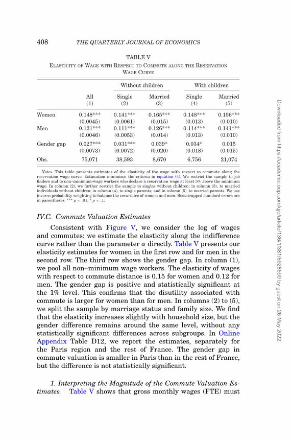
TABLE VELASTICITY OF WAGE WITH RESPECT TO COMMUTE ALONG THE RESERVATION
WAGE CURVE
Without children With children
All Single Married Single Married(1) (2) (3) (4) (5)
Women 0.148*** 0.141*** 0.165*** 0.148*** 0.156***(0.0045) (0.0061) (0.015) (0.013) (0.010)
Men 0.121*** 0.111*** 0.126*** 0.114*** 0.141***(0.0046) (0.0053) (0.014) (0.013) (0.010)
Gender gap 0.027*** 0.031*** 0.039* 0.034* 0.015(0.0073) (0.0072) (0.020) (0.018) (0.015)
Obs. 75,071 38,593 8,670 6,756 21,074
Notes. This table presents estimates of the elasticity of the wage with respect to commute along thereservation wage curve. Estimation minimizes the criteria in equation (4). We restrict the sample to jobfinders and to non–minimum-wage workers who declare a reservation wage at least 5% above the minimumwage. In column (2), we further restrict the sample to singles without children; in column (3), to marriedindividuals without children; in column (4), to single parents; and in column (5), to married parents. We useinverse probability weighting to balance the covariates of women and men. Bootstrapped standard errors arein parentheses. *** p < .01, * p < .1.
IV.C. Commute Valuation Estimates
Consistent with Figure V, we consider the log of wagesand commutes: we estimate the elasticity along the indifferencecurve rather than the parameter α directly. Table V presents ourelasticity estimates for women in the first row and for men in thesecond row. The third row shows the gender gap. In column (1),we pool all non–minimum wage workers. The elasticity of wageswith respect to commute distance is 0.15 for women and 0.12 formen. The gender gap is positive and statistically significant atthe 1% level. This confirms that the disutility associated withcommute is larger for women than for men. In columns (2) to (5),we split the sample by marriage status and family size. We findthat the elasticity increases slightly with household size, but thegender difference remains around the same level, without anystatistically significant differences across subgroups. In OnlineAppendix Table D12, we report the estimates, separately forthe Paris region and the rest of France. The gender gap incommute valuation is smaller in Paris than in the rest of France,but the difference is not statistically significant.
1. Interpreting the Magnitude of the Commute Valuation Es-timates. Table V shows that gross monthly wages (FTE) must
Dow
nloaded from https://academ
ic.oup.com/qje/article/136/1/381/5928590 by guest on 26 M
ay 2022

GENDER DIFFERENCES IN JOB SEARCH 409
be increased by 12% to compensate men for a doubling in thecommuting distance. Given the average commute of 18.6 kilo-meters and the average monthly wage of €2,018, an increase of18.6 kilometers has to be compensated by an increase of €242 (=0.12 * 2,018) of the monthly wage. The monthly compensatingdifferential for one extra kilometer is about €13. Assuming thatfull-time employees commute 22 days a month on average (ex-cluding weekends), the daily compensating differential amountsto 59 cents (= 13
22 ). How does it compare with the opportunitycost of the time spent commuting? For an increase of one kilome-ters in the home-work distance, workers spend 3.4 minutes moretime commuting per day (assuming an average commuting speedof 35 km/hour). Workers in our sample have an hourly rate of€13.2, which translates into 22 cents a minute. Consequently, thecompensating differential for men is 0.8 times the hourly wage(= 59
3.4×22 ). For women, with an elasticity of 14.8%, we obtain acompensating differential of 0.98 times the hourly wage. Theseestimates of compensating differentials belong to the range of es-timates in the literature. Mulalic, Van Ommeren, and Pilegaard(2014) report that estimates of the value of travel time range from20% to 100% of hourly gross wages (Small 1992; Small, Winston,and Yan 2005; Small and Verhoef 2007; Small 2012).
2. Robustness. In Online Appendix Table D13, we show therobustness of the elasticity estimates to other definitions of mini-mum wage workers and find similar elasticities and gender gapsin commute valuation. However, when we include minimum wageworkers in the estimation sample, the gender gap in commutevaluation is significantly lower and statistically significant at the10% level only. This is expected because minimum wage workershave a degenerate wage offer distribution. Online Appendix TableD14 shows some other robustness tests of the elasticity estimates.Column (1) does not use inverse probability weighting to balancethe male and female sample on covariates. Column (2) restrictsthe sample to workers who declare their maximum commute inkilometers. Column (3) excludes workers with a large deviationbetween the accepted commute and the reservation commute, forwhom nonlinearities are a potential concern. In column (4), weadopt another minimization criteria: the number of accepted bun-dles below the reservation wage curve (without weighting them bytheir distance to the curve). Results are robust to these changes ofspecification. In column (5), we restrict the estimation sample to
Dow
nloaded from https://academ
ic.oup.com/qje/article/136/1/381/5928590 by guest on 26 M
ay 2022
410 THE QUARTERLY JOURNAL OF ECONOMICS
individuals who worked full-time in their previous job. The gen-der difference in elasticity is smaller when we hold constant thepast hours worked, but still significant. This suggests that genderdifferences in commute valuation come on top of potential genderdifferences in hours flexibility.
In Online Appendix A, we adopt alternative interpretationsof the reported reservation job (φ∗, τ ∗) (Interpretation 2 and 2 bis).We find again that women have a significantly higher willingnessto pay for a shorter commute than men: 23.8% higher under In-terpretation 2 and 15.1% higher under Interpretation 2 bis (seeOnline Appendix Tables A1 and A2).
3. Accepted Job Bundles below the Reservation Wage Curve?Several mechanisms may explain why we observe accepted jobbundles below the reservation wage curve. First, it could be dueto measurement error in reservation or accepted job attributes. InOnline Appendix Table D14, column (6), we add white noise to thedata and show that our results are robust to measurement error,with some attenuation bias. This suggests that our main estimateis a lower bound of gender gaps in WTP for a shorter commute.Nonstationarity in job search behaviors is a second possible mech-anism, as we pin down the reservation wage curve using reserva-tion job attributes declared at the beginning of the spell. We findthat the share of workers who accept jobs that are above theirreservation wage curve is 3 percentage points lower for workerswho have one more year of unemployment (from an initial shareof 83%). This makes duration dependence a marginal contrib-utor to points below the reservation wage curve. The existenceof other job amenities is a third possible mechanism. Assumingthat workers declare their reservation job attributes conditionalon other amenities being at their average, they may accept jobsbelow the reservation wage curve when amenities are high. Aslong as the mechanism generating accepted jobs below the reser-vation wage curve is independent of wage and commute offers,the WTP estimator in equation (4) is still valid, as our simula-tions related to measurement error suggest. In Section VI.B, wepropose an alternative estimation of the gender gap in commutevaluation, based on an empirical model of application choice. Thisapproach is robust to unobserved nonwage job amenities that arepotentially correlated with wages and commute and provides sim-ilar estimates of the gender gap in WTP.
Dow
nloaded from https://academ
ic.oup.com/qje/article/136/1/381/5928590 by guest on 26 M
ay 2022
GENDER DIFFERENCES IN JOB SEARCH 411
In this section, we have showed that women have a 22%higher willingness to pay for a shorter commute ( 0.027
0.121 = 0.223,see Table V column (1)). This result comes from a new (to the bestof our knowledge) identification strategy that leverages uniquedata on job search criteria. The identification strategy mostly re-lies on the form of the utility function when employed and onthe reservation strategy embedded in standard job search mod-els. Specifically, the commute valuation parameter is separatelyidentified from the other model parameters, as long as the job of-fer distributions are not degenerate. This is worth noting, as analternative hypothesis supporting the gender gaps documented inSection III could be that men and women do not draw job offersfrom the same distributions when unemployed (even if they hadsimilar jobs before unemployment). Even in this case, our resulton gender differences in willingness to pay for a shorter commutestill holds. Next we draw the implications of the gender differencesin commute valuation for the gender wage gap.
V. IMPLICATIONS FOR THE GENDER WAGE GAP
Because women must be compensated more than men to ac-cept far-away jobs, they are more likely to work close to homein jobs that pay relatively less. To what extent do gender differ-ences in commute valuation contribute to the gender wage gap?To quantify this, we first calibrate the job search model above,using the previous estimate of the WTP for a shorter commute.Second, we perform counterfactual simulations where we shockthis commute valuation parameter.
V.A. Calibration of the Job Search Model
We calibrate the model, restricting our sample to non–minimum wage workers on which we have estimated the WTPfor a shorter commute, α. We proceed as follows.
First, we calibrate r such that the yearly discount rate is 12%(following Van Den Berg 1990) and the match destruction rate qis equal to the inverse of the length of jobs in the subsample ofinterest (for the median job seeker, a job spell lasts 12 months).Second, we observe in the data the pair (τ ∗, φ∗), which is a point onthe reservation curve, and the previous section yields an estimateof the commute valuation α. We can build the full reservationcurve; in particular we deduce φ(0) = φ∗ − ατ ∗.
Dow
nloaded from https://academ
ic.oup.com/qje/article/136/1/381/5928590 by guest on 26 M
ay 2022

412 THE QUARTERLY JOURNAL OF ECONOMICS
Knowing the reservation curve, we use the empirical mea-sures of the expectation and variance of the residualized log ofthe reemployment wage wn and commute τn to pin down the joboffer distributions (see equations (2) and (3) for expectations). Weresidualize the reemployment wage and commute with the samecovariates as in the main gender gap regressions. This aims atfocusing on wage and commute variations arising from randomsearch. We assume that log-wage and commute are drawn inde-pendently from the distributions F and G, respectively. The dis-tribution of the log-wage offers F is a gamma distribution and weestimate its shape kF and scale θF. For the distribution of commuteoffer G, we assume the following probability density function, de-fined over the support 0 to 100 kilometers:
g(τ ) = γ (τ ; kG, θG) + τ.
The distribution G is a mixture of a gamma distribution withshape kG and scale θG and of a linear distribution. The functionalform of G is consistent with the distribution of distances betweenjob seekers’ residence and workplaces of vacancies posted on theFrench PES website (see Online Appendix Figure C8). Intuitively,the linear term accounts for the increase in further-away jobswhen the disk of radius τ centered on the worker’s residence ex-pands over a two-dimensional uniform density of jobs. For F andG, there are four moments to pin down four parameters by GMMestimation.
We use the observed job-finding rate to determine the job offerarrival rate λ. Namely, we use the fact that the job-finding rateshould be equal to:
λ
∫ ∞
0
∫ ∞
φ(0)+ατ
dF(w)dG(τ ).
The flow unemployment utility b is finally obtained as the solutionof equation (1). The quantities involved in the calibration andthe resulting structural parameters are summarized in OnlineAppendix Table D15 for the sample of women.
V.B. Decomposition of the Gender Wage Gap
The counterfactuals are obtained as follows. Keeping all otherstructural parameters unchanged (r, q, λ, F(), G(), and b), we re-place the commute valuation parameters α we have estimated for
Dow
nloaded from https://academ
ic.oup.com/qje/article/136/1/381/5928590 by guest on 26 M
ay 2022
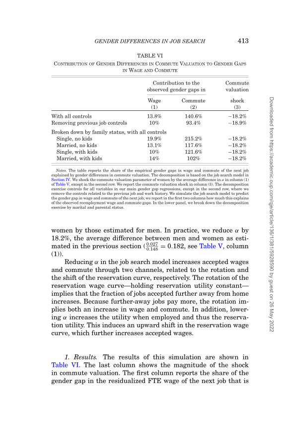
GENDER DIFFERENCES IN JOB SEARCH 413
TABLE VICONTRIBUTION OF GENDER DIFFERENCES IN COMMUTE VALUATION TO GENDER GAPS
IN WAGE AND COMMUTE
Contribution to the Commuteobserved gender gaps in valuation
Wage Commute shock(1) (2) (3)
With all controls 13.8% 140.6% −18.2%Removing previous job controls 10% 93.4% −18.9%
Broken down by family status, with all controlsSingle, no kids 19.9% 215.2% −18.2%Married, no kids 13.1% 117.6% −18.2%Single, with kids 10% 121.6% −18.2%Married, with kids 14% 102% −18.2%
Notes. The table reports the share of the empirical gender gaps in wage and commute of the next jobexplained by gender differences in commute valuation. The decomposition is based on the job search model inSection IV. We shock the commute valuation parameter of women by the average difference in α in column (1)of Table V, except in the second row. We report the commute valuation shock in column (3). The decompositionexercise controls for all variables in our main gender gap regressions, except in the second row, where weremove the controls related to the previous job and work history. We simulate the job search model to predictthe gender gap in wage and commute of the next job; we report in the first two columns how much this explainsof the observed reemployment wage and commute gaps. In the lower panel, we break down the decompositionexercise by marital and parental status.
women by those estimated for men. In practice, we reduce α by18.2%, the average difference between men and women as esti-mated in the previous section ( 0.027
0.148 = 0.182, see Table V, column(1)).
Reducing α in the job search model increases accepted wagesand commute through two channels, related to the rotation andthe shift of the reservation curve, respectively. The rotation of thereservation wage curve—holding reservation utility constant—implies that the fraction of jobs accepted further away from homeincreases. Because further-away jobs pay more, the rotation im-plies both an increase in wage and commute. In addition, lower-ing α increases the utility when employed and thus the reserva-tion utility. This induces an upward shift in the reservation wagecurve, which further increases accepted wages.
1. Results. The results of this simulation are shown inTable VI. The last column shows the magnitude of the shockin commute valuation. The first column reports the share of thegender gap in the residualized FTE wage of the next job that is
Dow
nloaded from https://academ
ic.oup.com/qje/article/136/1/381/5928590 by guest on 26 M
ay 2022
414 THE QUARTERLY JOURNAL OF ECONOMICS
explained by the reduction in α.14 The second column does thesame exercise for commute. In the upper panel, we perform the de-composition for women, whatever their family status. We find thatgender differences in commute valuation (i.e., in α as estimated inSection IV) explain 13.8% of the residualized FTE wage gap, thatis, a 0.5 log point hourly wage deficit for women. These differencesin α explain more than 100% of the differences in commute. Notethat fully explaining the gender commute gap is not a mechanicalresult, and it did not need to be the case. Men and women arelikely to differ along other dimensions than α that we hold con-stant in the simulations, and these differences in other dimensionsmay trigger differences in observed commute as well. In OnlineAppendix Table D17, we perform another simulation exercisewhere the reduction in commute valuation is such that the ex-plained share of the gender gap in commute of the next job isexactly equal to 100%. The resulting explained shares of observedwage gaps are around 10%, a bit lower but fairly similar to thosein Table VI.
As the previous jobs of the unemployed are likely to dependon their commute valuation, we also perform the decompositionexercise removing past wages and past commutes from the listof controls. This leads to three main changes. First, we cali-brate the model with higher residualized variances of acceptedwages and commutes. Second, the gender gap in commute valu-ation slightly increases from 18.2% to 18.9% when the inverse-probability weights of the WTP estimator do not include the pastjob attributes (see the third column in Table VI). Third, the ob-served gender gaps in accepted wages and commutes that we aretrying to explain (i.e., the denominator for columns (1) and (2))are larger.15 Although the second change increases the simulatedgender gaps in accepted jobs, the third change tends to decreasethe fraction explained. All in all, we obtain that gender gaps incommute valuation explain 10% of the observed gender wage gap,that is, 0.8 log points of the FTE wage deficit of women, and 93%of the observed commute gap (see second row in Table VI). This isbroadly consistent with the previous results.
14. The denominator of this ratio comes from the estimation of gender gaps inreemployment outcomes in the non–minimum wage sample, see Online AppendixTable D5 and D9.
15. On the non–minimum wage workers sample, the gender gaps in acceptedwage and accepted commute amount to 7.7% and 25.3%, respectively, when we donot control for past jobs.
Dow
nloaded from https://academ
ic.oup.com/qje/article/136/1/381/5928590 by guest on 26 M
ay 2022

GENDER DIFFERENCES IN JOB SEARCH 415
2. Heterogeneity by Family Status. In the lower panel ofTable VI, we perform the decomposition exercise broken downby family status. The model is calibrated for each subgroup sep-arately. Online Appendix Table D16 provides the values of esti-mated/calibrated parameters for all subgroups. We conclude fromTable V that there is no statistically significant heterogeneity ingender gaps in commute valuation: we choose here to shock allsubgroups using the same average gender gap in WTP. We findthat gender gaps in commute valuation explain between 10% and20% of the wage gap, depending on the subgroup but with no clearpattern as a function of family size.
3. Robustness to Alternative Interpretations of the ReportedSearch Criteria. Online Appendix A shows a decomposition ex-ercise under alternative interpretations of the reported reserva-tion job (φ∗, τ ∗) (Interpretations 2 and 2 bis). In Online AppendixTable A3, the share of gender wage gap explained by gender differ-ences in commute valuation is between 9% and 15%. Overall, ourdecomposition exercise delivers robust results, suggesting that ameaningful share of the gender wage gap can be explained bygender differences in commute valuation.
4. Discussion. In the simulations above, we account for theendogenous response of the workers’ reservation utility. This is apartial equilibrium approach, to the extent that we do not accountfor employers’ response. In a model with endogenous wage offerdistributions, reducing the commute valuation parameter as wedo above would push further toward higher wages because it in-creases workers’ reservation utility and employers would respondby offering higher wages. Such general equilibrium effects a laBlack (1995) would strengthen the contribution of the gender gapin commute valuation to the gender wage gap. Consequently, wesee our main results above as lower bounds.
Although our empirical results in Section III include a richset of covariates to control for differences in employment oppor-tunities, one may still be concerned that a gender differential inthe distribution of offered wages may explain the gender gap inobserved commutes. We quantify this alternative explanation us-ing our calibrated job search model. We compute the elasticitiesof realized wages and commutes with respect to the expectationof wage offers (via the location parameter of the gamma distribu-tion). We find that a shock of 12% on the expectation of wage offers
Dow
nloaded from https://academ
ic.oup.com/qje/article/136/1/381/5928590 by guest on 26 M
ay 2022
416 THE QUARTERLY JOURNAL OF ECONOMICS
is necessary to account for the 4% gender gap in realized wages,and that this shock can only explain a third of the 12% gender gapin realized commutes. Although we cannot rule out that womenand men have different wage offer distributions, even conditionalon the covariates we introduce, the exercise shows that differen-tials in the wage distributions alone are unlikely to generate theobserved differentials in commutes.
Overall, the decomposition results rank gender differences inWTP for a shorter commute as an important driver of the genderwage gap. Mas and Pallais (2017) find that “with a 20 percentcompensating differential for both work at home and workinga fixed schedule instead of an irregular one, the differences bygender in the prevalence of these arrangements would only leadto a 1.7 percent raw gender wage gap or a 2.0 percent gap withcontrols.” Wiswall and Zafar (2017) find that gender differencesin students’ preferences for future earnings growth, probability ofdismissal, and working-hours flexibility, account for one quarterof the gender earnings gap. Bertrand, Goldin, and Katz (2010) findthat for MBA graduates, 30% of the gender wage gap is accountedfor by gender differences in hours of work a week.
VI. FURTHER INSIGHTS FROM APPLICATION DATA
In this section, we present further insights using applicationdata. We leverage a rich administrative data set that records ap-plications of job seekers to vacancies posted at the French PESand their hiring outcomes.16 We first estimate a conditional logitmodel of application choices with job ad fixed effects, and we showthat the commute distance between the vacancy workplace andthe applicants’ residence has a larger influence (by around 20%)for women than for men. This is in line with the gender gap incommute valuation estimated in Section IV. This shows the ro-bustness of our main results to (i) relying on actual behaviorsonly (without using reported search criteria) and (ii) the con-cern of unobserved correlated amenities. Second, we study la-bor demand. We find that firms do not specifically lower theirhiring of women compared with men when applicants live furtheraway.
16. See Behaghel, Crepon, and Le Barbanchon (2015) for previous analysis ofapplication data at the French PES.
Dow
nloaded from https://academ
ic.oup.com/qje/article/136/1/381/5928590 by guest on 26 M
ay 2022

GENDER DIFFERENCES IN JOB SEARCH 417
VI.A. Application Data
French employers typically post vacancies on the PES web-site and advertise them through local agencies. In 2010, vacan-cies posted at PES represented 60% of all hires in France (au-thors’ calculation). Workers registered as job seekers may applythrough the PES website or local agencies. This generates entriesinto an application data set at the vacancy × worker identifierlevel. We can thus analyze workers’ application choices as a func-tion of the attributes of the vacancies. Furthermore, caseworkersrecord the application outcome: hired or not. This allows us to an-alyze the hiring outcome in the pool of applicants, and to get closerto labor demand.17 We observe more than 3 million applicationsfor the sample of workers described in Section II.A.18 We restrictthe sample to applications from 2010 to 2012, because we do notobserve the vacancy workplace before 2010.
Table VII reports summary statistics for applications, vacan-cies, and applicants. Panel A reports statistics at the applicationlevel. Around 5% of applications lead to hiring. The average com-mute between the vacancy workplace and the applicant’s home is19 kilometers, very similar to the average commute reported inTable I. The posted wage is on average €1,539. This is 25% lowerthan the average previous wage of the main sample of job seekersin Table I, and close to the legal minimum wage of around €1,400in 2010–2012. Indeed, 44% of vacancies report the minimum wageas their posted wage. All vacancies report an occupation and a re-quired qualification (low- or high-skilled blue collar work, low- orhigh-skilled employee, or manager). For almost half of the appli-cations, the applicant meets the required qualification. Similarly,in almost half of the cases, the applicant selects a job in theirpreferred occupation.
Almost one applicant out of four is hired from a vacancyposted by the PES (see Table VII, Panel C). This builds con-fidence in the relevance of PES postings and applications for
17. In general, hiring is an equilibrium outcome resulting from the interactionof labor supply and labor demand. In our setting, we analyze hirings of workersapplying for detailed job ads (including wages). We thus argue that if employersoffer the job to an applicant, it is likely that she accepts the offer. Consequently,hirings in our setting are rather informative of employers’ choice among applicants.
18. The sample of applicants is larger than the main sample described inSection II. To maximize statistical power, we also include workers who do notclaim unemployment benefits.
Dow
nloaded from https://academ
ic.oup.com/qje/article/136/1/381/5928590 by guest on 26 M
ay 2022
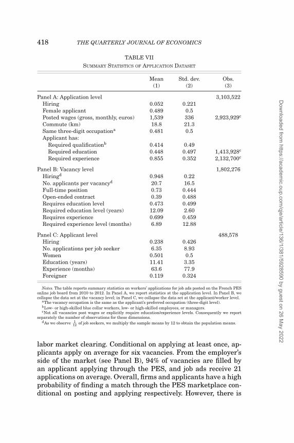
418 THE QUARTERLY JOURNAL OF ECONOMICS
TABLE VIISUMMARY STATISTICS OF APPLICATION DATASET
Mean Std. dev. Obs.(1) (2) (3)
Panel A: Application level 3,103,522Hiring 0.052 0.221Female applicant 0.489 0.5Posted wages (gross, monthly, euros) 1,539 336 2,923,929c
Commute (km) 18.8 21.3Same three-digit occupationa 0.481 0.5Applicant has:
Required qualificationb 0.414 0.49Required education 0.448 0.497 1,413,928c
Required experience 0.855 0.352 2,132,700c
Panel B: Vacancy level 1,802,276Hiringd 0.948 0.22No. applicants per vacancyd 20.7 16.5Full-time position 0.73 0.444Open-ended contract 0.39 0.488Requires education level 0.473 0.499Required education level (years) 12.09 2.60Requires experience 0.699 0.459Required experience level (months) 6.89 12.88
Panel C: Applicant level 488,578Hiring 0.238 0.426No. applications per job seeker 6.35 8.93Women 0.501 0.5Education (years) 11.41 3.35Experience (months) 63.6 77.9Foreigner 0.119 0.324
Notes. The table reports summary statistics on workers’ applications for job ads posted on the French PESonline job board from 2010 to 2012. In Panel A, we report statistics at the application level. In Panel B, wecollapse the data set at the vacancy level; in Panel C, we collapse the data set at the applicant/worker level.
aThe vacancy occupation is the same as the applicant’s preferred occupation (three-digit level).bLow- or high-skilled blue collar workers, low- or high-skilled employees, or managers.cNot all vacancies post wages or explicitly require education/experience levels. Consequently we report
separately the number of observations for these dimensions.dAs we observe 1
12 of job seekers, we multiply the sample means by 12 to obtain the population means.
labor market clearing. Conditional on applying at least once, ap-plicants apply on average for six vacancies. From the employer’sside of the market (see Panel B), 94% of vacancies are filled byan applicant applying through the PES, and job ads receive 21applications on average. Overall, firms and applicants have a highprobability of finding a match through the PES marketplace con-ditional on posting and applying respectively. However, there is
Dow
nloaded from https://academ
ic.oup.com/qje/article/136/1/381/5928590 by guest on 26 M
ay 2022
GENDER DIFFERENCES IN JOB SEARCH 419
still selection into PES posting for firms and into PES applying forworkers. This is certainly an issue when measuring the numberof applicants for a given vacancy or the overall search intensityof a given job seeker. For example, some applicants directly applythrough company websites. It is unclear though why this selec-tion should be differential by gender. We argue that this selectionmargin leads to second-order bias when documenting gender dif-ferences in the influence of job attributes on application choices, orwhen analyzing the gender hiring gap as a function of applicants’characteristics.
VI.B. Gender Differences in Commute Valuation in anApplication Model
In this section, we analyze the application data from the jobseeker’s perspective. We fit an econometric model of applicationchoices and study how commute affects the application decisiondifferentially for women and men. One recurrent issue when iden-tifying the influence of one attribute in choice models is that otherunobserved amenities may be correlated with the job attribute ofinterest. This may confound the parameter of interest. However,as commute is a match-specific attribute, correlated amenitiesare less problematic because we can control for unobserved jobattributes common to all workers. Holding constant these job at-tributes, we test whether workers who live closer to the workplacehave a higher propensity to apply for the job.
We define the choice set of workers as follows. For each jobseeker who registers in a given quarter, we assign her the vacan-cies that are (i) in her commuting zone of residence, (ii) in thesame three-digit occupation as the one she is looking for, and (iii)posted in the quarter following her registration. Our data give usthe vacancies to which the individual worker applies within herchoice set. We restrict the sample to job seekers who make at leastone such application. We estimate a conditional logit model for theprobability of applying for these vacancies controlling for job adfixed effects. In a structural choice model, the application deci-sion depends on posted wages, but the wage coefficient cannot beidentified when job ad fixed effects are included. On the contrary,the coefficient on commuting distance is still identified in thismodel as commuting varies across workers paired with the samevacancy. We further interact the job ad fixed effects with gender toaccount for unobserved job characteristics that men and womenmay value differentially. The probability that worker i applies for
Dow
nloaded from https://academ
ic.oup.com/qje/article/136/1/381/5928590 by guest on 26 M
ay 2022
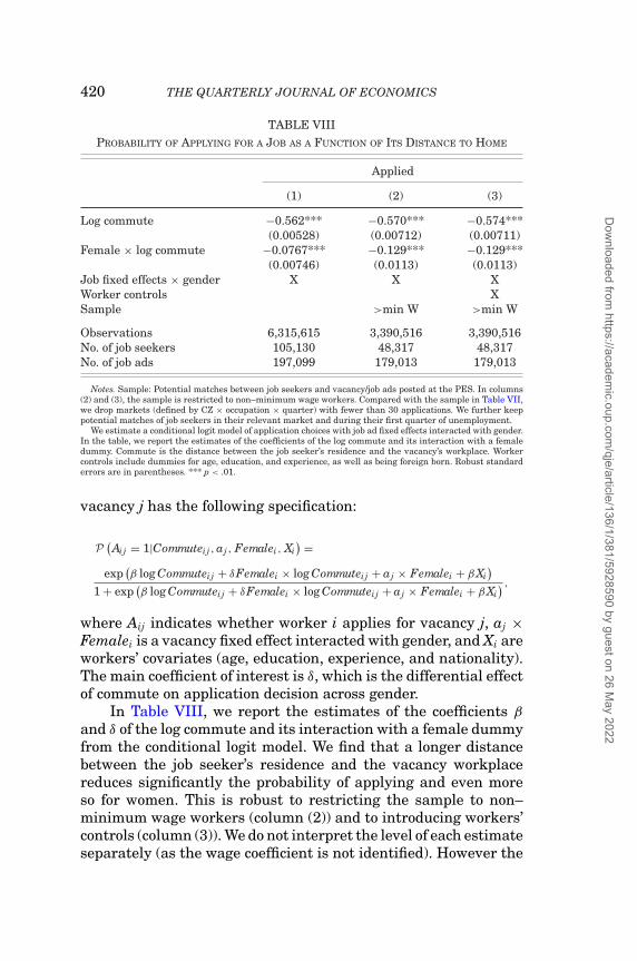
420 THE QUARTERLY JOURNAL OF ECONOMICS
TABLE VIIIPROBABILITY OF APPLYING FOR A JOB AS A FUNCTION OF ITS DISTANCE TO HOME
Applied
(1) (2) (3)
Log commute −0.562*** −0.570*** −0.574***(0.00528) (0.00712) (0.00711)
Female × log commute −0.0767*** −0.129*** −0.129***(0.00746) (0.0113) (0.0113)
Job fixed effects × gender X X XWorker controls XSample >min W >min W
Observations 6,315,615 3,390,516 3,390,516No. of job seekers 105,130 48,317 48,317No. of job ads 197,099 179,013 179,013
Notes. Sample: Potential matches between job seekers and vacancy/job ads posted at the PES. In columns(2) and (3), the sample is restricted to non–minimum wage workers. Compared with the sample in Table VII,we drop markets (defined by CZ × occupation × quarter) with fewer than 30 applications. We further keeppotential matches of job seekers in their relevant market and during their first quarter of unemployment.
We estimate a conditional logit model of application choices with job ad fixed effects interacted with gender.In the table, we report the estimates of the coefficients of the log commute and its interaction with a femaledummy. Commute is the distance between the job seeker’s residence and the vacancy’s workplace. Workercontrols include dummies for age, education, and experience, as well as being foreign born. Robust standarderrors are in parentheses. *** p < .01.
vacancy j has the following specification:
P (Aij = 1|Commuteij , aj , Femalei, Xi
) =exp
(β log Commuteij + δFemalei × log Commuteij + aj × Femalei + βXi
)1 + exp
(β log Commuteij + δFemalei × log Commuteij + aj × Femalei + βXi
) ,
where Aij indicates whether worker i applies for vacancy j, aj ×Femalei is a vacancy fixed effect interacted with gender, and Xi areworkers’ covariates (age, education, experience, and nationality).The main coefficient of interest is δ, which is the differential effectof commute on application decision across gender.
In Table VIII, we report the estimates of the coefficients β
and δ of the log commute and its interaction with a female dummyfrom the conditional logit model. We find that a longer distancebetween the job seeker’s residence and the vacancy workplacereduces significantly the probability of applying and even moreso for women. This is robust to restricting the sample to non–minimum wage workers (column (2)) and to introducing workers’controls (column (3)). We do not interpret the level of each estimateseparately (as the wage coefficient is not identified). However the
Dow
nloaded from https://academ
ic.oup.com/qje/article/136/1/381/5928590 by guest on 26 M
ay 2022
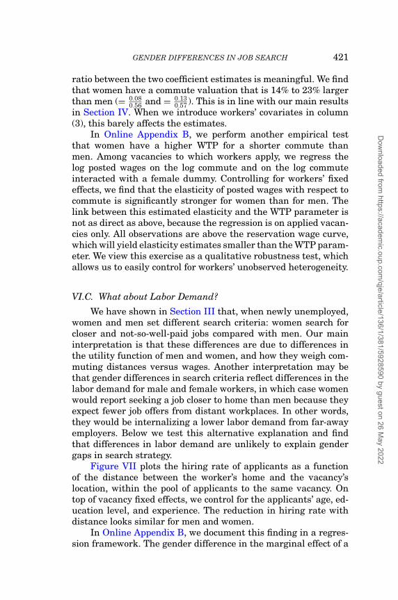
GENDER DIFFERENCES IN JOB SEARCH 421
ratio between the two coefficient estimates is meaningful. We findthat women have a commute valuation that is 14% to 23% largerthan men (= 0.08
0.56 and = 0.130.57 ). This is in line with our main results
in Section IV. When we introduce workers’ covariates in column(3), this barely affects the estimates.
In Online Appendix B, we perform another empirical testthat women have a higher WTP for a shorter commute thanmen. Among vacancies to which workers apply, we regress thelog posted wages on the log commute and on the log commuteinteracted with a female dummy. Controlling for workers’ fixedeffects, we find that the elasticity of posted wages with respect tocommute is significantly stronger for women than for men. Thelink between this estimated elasticity and the WTP parameter isnot as direct as above, because the regression is on applied vacan-cies only. All observations are above the reservation wage curve,which will yield elasticity estimates smaller than the WTP param-eter. We view this exercise as a qualitative robustness test, whichallows us to easily control for workers’ unobserved heterogeneity.
VI.C. What about Labor Demand?
We have shown in Section III that, when newly unemployed,women and men set different search criteria: women search forcloser and not-so-well-paid jobs compared with men. Our maininterpretation is that these differences are due to differences inthe utility function of men and women, and how they weigh com-muting distances versus wages. Another interpretation may bethat gender differences in search criteria reflect differences in thelabor demand for male and female workers, in which case womenwould report seeking a job closer to home than men because theyexpect fewer job offers from distant workplaces. In other words,they would be internalizing a lower labor demand from far-awayemployers. Below we test this alternative explanation and findthat differences in labor demand are unlikely to explain gendergaps in search strategy.
Figure VII plots the hiring rate of applicants as a functionof the distance between the worker’s home and the vacancy’slocation, within the pool of applicants to the same vacancy. Ontop of vacancy fixed effects, we control for the applicants’ age, ed-ucation level, and experience. The reduction in hiring rate withdistance looks similar for men and women.
In Online Appendix B, we document this finding in a regres-sion framework. The gender difference in the marginal effect of a
Dow
nloaded from https://academ
ic.oup.com/qje/article/136/1/381/5928590 by guest on 26 M
ay 2022
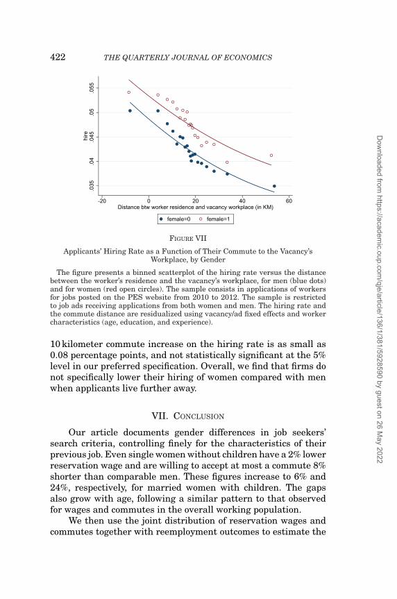
422 THE QUARTERLY JOURNAL OF ECONOMICS
FIGURE VII
Applicants’ Hiring Rate as a Function of Their Commute to the Vacancy’sWorkplace, by Gender
The figure presents a binned scatterplot of the hiring rate versus the distancebetween the worker’s residence and the vacancy’s workplace, for men (blue dots)and for women (red open circles). The sample consists in applications of workersfor jobs posted on the PES website from 2010 to 2012. The sample is restrictedto job ads receiving applications from both women and men. The hiring rate andthe commute distance are residualized using vacancy/ad fixed effects and workercharacteristics (age, education, and experience).
10 kilometer commute increase on the hiring rate is as small as0.08 percentage points, and not statistically significant at the 5%level in our preferred specification. Overall, we find that firms donot specifically lower their hiring of women compared with menwhen applicants live further away.
VII. CONCLUSION
Our article documents gender differences in job seekers’search criteria, controlling finely for the characteristics of theirprevious job. Even single women without children have a 2% lowerreservation wage and are willing to accept at most a commute 8%shorter than comparable men. These figures increase to 6% and24%, respectively, for married women with children. The gapsalso grow with age, following a similar pattern to that observedfor wages and commutes in the overall working population.
We then use the joint distribution of reservation wages andcommutes together with reemployment outcomes to estimate the
Dow
nloaded from https://academ
ic.oup.com/qje/article/136/1/381/5928590 by guest on 26 M
ay 2022
GENDER DIFFERENCES IN JOB SEARCH 423
slope of reservation wage curves. We find that the value of com-mute time amounts to 80% of the gross hourly wage for men and98% for women, a difference that is statistically significant. Webuild a job search model where commuting matters and showthat our estimated gender differences in commute valuation canaccount for around 14% of the residualized gender gap in hourlywage on reemployment. We show that our estimated gender gap incommute valuation is robust to using a different approach, basedon applications data. We also provide evidence that the genderdifferences in search criteria are not driven by labor demand.
By highlighting the importance of gender differences in will-ingness to commute and linking it to the gender wage gap, we shedlight on possible ways to further reduce gender wage inequality.Technological progress that lowers the firms’ cost of remote workhas the potential to further decrease the gender wage gap (Bloomet al. 2014). More generally, public policies on urban planning andtransportation have the potential to change commuting patternsdifferently for men and women and may have differential effectson their relative wages (e.g., Redding and Turner 2015; Butikofer,Løken, and Willen 2019). On a related note, offering financial sub-sidies to job seekers who apply for or accept more distant jobs mayaffect men and women differently, and thus the gender wage gap(Glover and Roulet 2018).
BOCCONI UNIVERSITY
UNIVERSITY OF WARWICK
INSEAD
SUPPLEMENTARY MATERIAL
An Online Appendix for this article can be found at TheQuarterly Journal of Economics online (qje.oxfordjournal.org).
DATA AVAILABILITY
Code replicating the tables and figures in this article canbe found in Le Barbanchon, Roulet, and Rathelot (2020), in theHarvard Dataverse, doi: 10.7910/DVN/16QOSR.
REFERENCES
Adda, Jerome, Christian Dustmann, and Katrien Stevens, “The Career Costs ofChildren,” Journal of Political Economy, 125 (2017), 293–337.
Dow
nloaded from https://academ
ic.oup.com/qje/article/136/1/381/5928590 by guest on 26 M
ay 2022
424 THE QUARTERLY JOURNAL OF ECONOMICS
Altonji, Joseph G., and Christina H. Paxson, “Labor Supply, Hours Constraints,and Job Mobility,” Journal of Human Resources, 27 (1992), 256–278.
Angelov, Nikolay, Per Johansson, and Erica Lindahl, “Parenthood and the GenderGap in Pay,” Journal of Labor Economics, 34 (2016), 545–579.
Behaghel, Luc, Bruno Crepon, and Thomas Le Barbanchon, “Unintended Effectsof Anonymous Resumes,” American Economic Journal: Applied Economics, 7(2015), 1–27.
Bertrand, Marianne, “New Perspectives on Gender,” in Handbook of Labor Eco-nomics volume 4, O. Ashenfelter and D. Card, eds. (Amsterdam: Elsevier,2011), 1543–1590.
Bertrand, Marianne, Claudia Goldin, and Lawrence F. Katz, “Dynamics of theGender Gap for Young Professionals in the Financial and Corporate Sectors,”American Economic Journal: Applied Economics, 2 (2010), 228–255.
Black, Dan A., “Discrimination in an Equilibrium Search Model,” Journal of LaborEconomics, 13 (1995), 309–334.
Black, Dan A., Natalia Kolesnikova, and Lowell J. Taylor, “Why Do So Few WomenWork in New York (and So Many in Minneapolis)? Labor Supply of MarriedWomen across US Cities,” Journal of Urban Economics, 79 (2014), 59–71.
Blau, Francine D., and Lawrence M. Kahn, “The Gender Wage Gap: Extent,Trends, and Explanations,” Journal of Economic Literature, 55 (2017), 789–865.
Bloom, Nicholas, James Liang, John Roberts, and Zhichun Jenny Ying, “DoesWorking from Home Work? Evidence from a Chinese Experiment,” QuarterlyJournal of Economics, 130 (2014), 165–218.
Bolotnyy, Valentin, and Natalia Emanuel, “Why Do Women Earn Less Than Men?Evidence from Bus and Train Operators,” Mimeo, Harvard University, 2019.
Bonhomme, Stephane, and Gregory Jolivet, “The Pervasive Absence of Compen-sating Differentials,” Journal of Applied Econometrics, 24 (2009), 763–795.
Brown, Charles, “Equalizing Differences in the Labor Market,” Quarterly Journalof Economics, 94 (1980), 113–134.
Brown, Sarah, Jennifer Roberts, and Karl Taylor, “The Gender Reservation WageGap: Evidence from British Panel Data,” Economics Letters, 113 (2011), 88–91.
Butikofer, Aline, Løken Katrin, and Alexander Willen, “Building Bridges andWidening Gaps: Efficiency Gains and Equity Concerns of Labor Market Ex-pansions,” NHH Working Paper No. 2017-10, 2019.
Caldwell, Sydnee, and Oren Danieli, “Outside Options in the Labor Market,”Mimeo, Harvard University, 2019.
Caliendo, Marco, Wang-Sheng Lee, and Robert Mahlstedt, “The Gender Wage Gapand the Role of Reservation Wages: New Evidence for Unemployed Workers,”Journal of Economic Behavior & Organization, 136 (2017), 161–173.
Clark, Ben, Kiron Chatterjee, Adam Martin, and Adrian Davis, “How CommutingAffects Subjective Wellbeing,” Transportation (2019), doi: 10.1007/s11116-019-09983-9.
Crane, Randall, “Is There a Quiet Revolution in Women’s Travel? Revisiting theGender Gap in Commuting,” Journal of the American Planning Association,73 (2007), 298–316.
Feldstein, Martin, and James Poterba, “Unemployment Insurance and ReservationWages,” Journal of Public Economics, 23 (1984), 141–167.
Filer, Randall K., “Male-Female Wage Differences: The Importance of Com-pensating Differentials,” Industrial and Labor Relations Review, 38 (1985),426–437.
Flory, Jeffrey A., Andreas Leibbrandt, and John A. List, “Do CompetitiveWorkplaces Deter Female Workers? A Large-Scale Natural Field Exper-iment on Job Entry Decisions,” Review of Economic Studies, 82 (2014),122–155.
Fluchtmann, Jonas, Anita M. Glenny, Nikolaj Harmon, and Jonas Maibom, “TheGender Application Gap: Do Men and Women Apply for the Same Jobs?”Mimeo, University of Copenhagen, 2020.
Dow
nloaded from https://academ
ic.oup.com/qje/article/136/1/381/5928590 by guest on 26 M
ay 2022
GENDER DIFFERENCES IN JOB SEARCH 425
Glover, Dylan, and Alexandra Roulet, “Geographic Mobility and the Gender WageGap: Evidence from a Randomized Experiment,” INSEAD Working Paper,2018.
Goldin, Claudia, “A Grand Gender Convergence: Its Last Chapter,” American Eco-nomic Review, 104 (2014), 1091–1119.
Goldin, Claudia, and Lawrence F. Katz, “A Most Egalitarian Profession: Phar-macy and the Evolution of a Family-Friendly Occupation,” Journal of LaborEconomics, 34 (2016), 705–746.
Guglielminetti, Elisa, Rafael Lalive, Philipp Ruh, and Etienne Wasmer, “SpatialSearch Strategies of Job Seekers and the Role of Unemployment Insurance,”Sciences Po Working Paper, 2015.
Hirano, Keisuke, Guido W. Imbens, and Geert Ridder, “Efficient Estimation ofAverage Treatment Effects Using the Estimated Propensity Score,” Econo-metrica, 71 (2003), 1161–1189.
Hwang, Hae-Shin, W. Reed, and Carlton Hubbard, “Compensating Wage Differen-tials and Unobserved Productivity,” Journal of Political Economy, 100 (1992),835–858.
Kleven, Henrik, Camille Landais, Johanna Posch, Andreas Steinhauer, and JosefZweimuller, “Child Penalties across Countries: Evidence and Explanations,”AEA Papers and Proceedings, 109 (2019), 122–126.
Kleven, Henrik, Camille Landais, and Jakob Egholt Søgaard, “Children and Gen-der Inequality: Evidence from Denmark,” American Economic Journal: Ap-plied Economics, 11 (2019), 181–209.
Krueger, Alan B., and Andreas I. Mueller, “A Contribution to the Empirics ofReservation Wages,” American Economic Journal: Economic Policy, 8 (2016),142–179.
Le Barbanchon, Thomas, Roland Rathelot, and Alexandra Roulet, “UnemploymentInsurance and Reservation Wages: Evidence from Administrative Data,” Jour-nal of Public Economics, 171 (2019), 1–17.
Le Barbanchon, Thomas, Alexandra Roulet, and Roland Rathelot, “ReplicationData for: ‘Gender Differences in Job Search: Trading off Commute againstWage’,” (2020), Harvard Dataverse, doi: 10.7910/DVN/16QOSR.
MacDonald, Heather I., “Women’s Employment and Commuting: Explaining theLinks,” Journal of Planning Literature, 13 (1999), 267–283.
Maestas, Nicole, Kathleen J. Mullen, David Powell, Till von Wachter, and Jef-frey B. Wenger, “The Value of Working Conditions in the United States andImplications for the Structure of Wages,” NBER Working Paper no. 25204,2018.
Manning, Alan, “The Real Thin Theory: Monopsony in Modern Labour Markets,”Labour Economics, 10 (2003), 105–131.
Mas, Alexandre, and Amanda Pallais, “Valuing Alternative Work Arrangements,”American Economic Review, 107 (2017), 3722–3759.
Mulalic, Ismir, Jos N. Van Ommeren, and Ninette Pilegaard, “Wages and Commut-ing: Quasi-natural Experiments’ Evidence from Firms that Relocate,” Eco-nomic Journal, 124 (2014), 1086–1105.
Olivetti, Claudia, and Barbara Petrongolo, “The Evolution of Gender Gaps inIndustrialized Countries,” Annual Review of Economics, 8 (2016), 405–434.
Petrongolo, Barbara, and Maddalena Ronchi, “Gender Gaps and the Structure ofLocal Labor Markets,” Labour Economics, 64 (2020), 101819.
Redding, Stephen J., and Matthew A. Turner, “Transportation Costs and the Spa-tial Organization of Economic Activity,” in Handbook of Regional and UrbanEconomics, volume 5, Gilles Duranton, J. Vernon Henderson and William C.Strange, volume 5, eds. (Amsterdam: Elsevier, 2015), 1339–1398.
Roberts, Jennifer, Robert Hodgson, and Paul Dolan, “It’s Driving Her Mad: GenderDifferences in the Effects of Commuting on Psychological Health,” Journal ofHealth Economics, 30 (2011), 1064–1076.
Rupert, Peter, Elena Stancanelli, and Etienne Wasmer, “Commuting, Wages andBargaining Power,” Annals of Economics and Statistics, 95/96 (2009), 201–220.
Small, Kenneth A., Urban Transportation Economics (Chur: Harwood, 1992).
Dow
nloaded from https://academ
ic.oup.com/qje/article/136/1/381/5928590 by guest on 26 M
ay 2022
426 THE QUARTERLY JOURNAL OF ECONOMICS
———, “Valuation of Travel Time,” Economics of Transportation, 1 (2012), 2–14.Small, Kenneth A., and Erik T. Verhoef, The Economics of Urban Transportation
(London: Routledge, 2007).Small, Kenneth A., Clifford Winston, and Jia Yan, “Uncovering the Distribution
of Motorists’ Preferences for Travel Time and Reliability,” Econometrica, 73(2005), 1367–1382.
Stutzer, Alois, and Bruno Frey, “Stress That Doesn’t Pay: The Commuting Para-dox,” Scandinavian Journal of Economics, 110 (2008), 339–366.
Van Den Berg, Gerard J., “Nonstationarity in Job Search Theory,” Review of Eco-nomic Studies, 57 (1990), 255–277.
Van Den Berg, Gerard J., and Cees Gorter, “Job Search and Commuting Time,”Journal of Business and Economic Statistics, 15 (1997), 269–281.
Van Ommeren, Jos N., and Mogens Fosgerau, “Workers’ Marginal Costs of Com-muting,” Journal of Urban Economics, 65 (2009), 38–47.
Van Ommeren, Jos N., Gerard J. Van Den Berg, and Cees Gorter, “Estimating theMarginal Willingness to Pay for Commuting,” Journal of Regional Science, 40(2000), 541–563.
Venn, Danielle, “Eligibility Criteria for Unemployment Benefits: Quantitative In-dicators for OECD and EU Countries,” OECD Social, Employment and Migra-tion Working Papers 131, 2012.
Wiswall, Matthew, and Basit Zafar, “Preference for the Workplace, Investment inHuman Capital, and Gender,” Quarterly Journal of Economics, 133 (2017),457–507.
Dow
nloaded from https://academ
ic.oup.com/qje/article/136/1/381/5928590 by guest on 26 M
ay 2022