Gender Classification from Facial Images using PCA and SVM
48
Gender Classification from Facial Images using PCA and SVM Chandrakamal Sinha Department of Biotechnology and Medical Engineering National Institute of Technology Rourkela Rourkela – 769 008, India brought to you by CORE View metadata, citation and similar papers at core.ac.uk provided by ethesis@nitr
-
Upload
khangminh22 -
Category
Documents
-
view
4 -
download
0
Transcript of Gender Classification from Facial Images using PCA and SVM

Gender Classification from Facial
Images using PCA and SVM
Chandrakamal Sinha
Department of Biotechnology and Medical Engineering
National Institute of Technology Rourkela
Rourkela – 769 008, India
brought to you by COREView metadata, citation and similar papers at core.ac.uk
provided by ethesis@nitr
Gender Classification from Facial
Images using PCA and SVM
Thesis submitted in
June 2013
to the department of
Department of Biotechnology and Medical Engineering
of
National Institute of Technology Rourkela
in partial fulfillment of the requirements
for the degree of
Master of Technology
by
Chandrakamal sinha
(Roll 211BM1218)
under the supervision of
Dr.Pankaj Kumar Sa
Department of Biotechnology and Medical Engineering
National Institute of Technology Rourkela
Rourkela – 769 008, India

Department of Biotechnology and Medical Engineering
National Institute of Technology Rourkela
Rourkela-769 008, India. www.nitrkl.ac.in
June 1, 2013
Certificate
This is to certify that the work in the thesis entitled Gender Classification from
Facial Images using PCA and SVM by Chandrakamal Sinha , bearing
roll number 211BM1218, is a record of an original research work carried out by him
under my supervision and guidance in partial fulfillment of the requirements for
the award of the degree of Master of Technology in Biotechnology and Biomedical
Engineering. Neither this thesis nor any part of it has been submitted for any degree
or academic award elsewhere.
Supervisor Departmental Cordinator
Pankaj Kumar Sa Kunal Pal
Assistant Professor Assistant Professor
Department of CSE, Department of BM,
NIT Rourkela NIT Rourkela

Acknowledgment
I would take this Opportunity to express my gratitude to Dr.Pankaj Kumar Sa,
Assistant Professor, Computer science, National Institute of Technology Rourkela,
for his valuable suggestions and cooperation at various stages. I appreciate his
explanation that helped me to understand the insight of the work.
I would like to thank Dr.Kunal Pal, Assistant Professor, Biotechnology and
Medical Engineering, National Institute of Technology Rourkela, for introducing
me to Image Processing.
I am thankful to my senior Susant Panigrahi, and Suman Kumar Choudhary for
their help in completion of project. I am also thankful to my all lab mates for their
active cooperation.
Chandrakamal Sinha
Abstract
Biometrics is the use of physical characteristics like face, fingerprints, iris etc.
of an individual for personal identification. Some of the challenging problems of
face biometrics are face detection, face recognition, and face identification. These
problems are being researched by the computer vision community for the last
few decades. Considering the large population, the authentication process of an
individual usually consumes a significant amount of time. One of the possible
solutions is to divide the population into two halves based on gender. This will help
to reduce the search space of authentication to almost half of the existing data and
save substantial amount of time. Gender identification through face demands use
of strong discriminative features and robust classifiers to separate the female and
male faces without any ambiguity.
In this thesis, an investigation has been made on gender classification through
facial images using principal component analysis (PCA), and support vector
machine (SVM). PCA is a dimensionality reduction technique, which is used to
represent each image as a feature vector in a low dimensional subspace. SVM is a
binary classifier for which PCA is the input in the form of features and predicts
which of the two possible classes forms the output.
Initially face region is extracted using a proposed skin colour segmentation
approach. The face region is then subjected to PCA for feature extraction, which
encodes second order statistics of data. These principal components are fed as
input to SVM for classification.
Keywords:Biometrics, Gender Classification, Face Detection, PCA, EigenValue, EigenVector,
SVM.
Contents
Certificate ii
Acknowledgement iii
Abstract iv
List of Figures vii
List of Tables viii
1 Introduction 1
1.1 Conventional Identification Techniques . . . . . . . . . . . . . . . . . 2
1.2 Biometrics . . . . . . . . . . . . . . . . . . . . . . . . . . . . . . . . . 2
1.3 Modules of a Biometric System . . . . . . . . . . . . . . . . . . . . . 6
1.4 Gender classification using facial image . . . . . . . . . . . . . . . . . 7
1.5 Proposed Methodology . . . . . . . . . . . . . . . . . . . . . . . . . . 7
1.6 Data Base Used in the Research . . . . . . . . . . . . . . . . . . . . . 8
1.7 Performance measures used for classifier . . . . . . . . . . . . . . . . 9
1.8 Thesis Organization . . . . . . . . . . . . . . . . . . . . . . . . . . . . 10
2 Literature Review 12
3 Face Detection 16
3.1 Skin colour Detection . . . . . . . . . . . . . . . . . . . . . . . . . . . 16
v

3.2 Algorithm for Brightness Compensation . . . . . . . . . . . . . . . . 17
3.3 Algorithm for Skin Colour Detection . . . . . . . . . . . . . . . . . . 18
3.4 Morphological Processing . . . . . . . . . . . . . . . . . . . . . . . . . 19
4 Principal Component Analysis and Support Vector Machine 24
4.1 Preparation of Training set . . . . . . . . . . . . . . . . . . . . . . . . 25
4.2 Eigenface Generation . . . . . . . . . . . . . . . . . . . . . . . . . . . 25
4.3 Reconstruction of an Image . . . . . . . . . . . . . . . . . . . . . . . 28
4.4 Support Vector Machine based Classifiers . . . . . . . . . . . . . . . . 29
4.5 Optimal Separating hyper plane . . . . . . . . . . . . . . . . . . . . . 29
4.6 Architecture of SVM . . . . . . . . . . . . . . . . . . . . . . . . . . . 30
4.7 Kernels in SVM . . . . . . . . . . . . . . . . . . . . . . . . . . . . . . 32
4.8 Result . . . . . . . . . . . . . . . . . . . . . . . . . . . . . . . . . . . 34
5 Conclusion 35
Bibliography 37
vi

List of Figures
1.1 A generic biometric system . . . . . . . . . . . . . . . . . . . . . . . . 3
1.2 Classification to reduce search space . . . . . . . . . . . . . . . . . . . 5
1.3 Modules of a Biometric System . . . . . . . . . . . . . . . . . . . . . 6
1.4 Steps Required in Gender Classification from facial image . . . . . . . 8
1.5 Images from IIT Kanpur Database . . . . . . . . . . . . . . . . . . . 9
3.1 Steps followed in Face Detection for male face . . . . . . . . . . . . . 21
3.2 Steps followed in Face Detection for female face . . . . . . . . . . . . 22
3.3 Face Detection for male and female faces from IIT Kanpur Database 23
4.1 Eigen Faces for Female Data base . . . . . . . . . . . . . . . . . . . . 26
4.2 Eigen Faces for Male Data base . . . . . . . . . . . . . . . . . . . . . 27
4.3 Variance Plot for the first thirty principal components for male and
female data base. . . . . . . . . . . . . . . . . . . . . . . . . . . . . . 27
4.4 Image Reconstruction from linear Combination of Eigen vectors . . . 28
4.5 The optimal hyper plane separating two classes [27] . . . . . . . . . . 30
4.6 Support vectors in SVM [28] . . . . . . . . . . . . . . . . . . . . . . . 31
vii

List of Tables
1.1 Confusion matrix for a binary class problem . . . . . . . . . . . . . . 10
4.1 Confusion matrix obtained from SVM using Polynomial kernel . . . . 34
4.2 Confusion matrix obtained from SVM using RBF kernel . . . . . . . 34
viii

Chapter 1
Introduction
Face is considered to be the most characteristic feature of human beings which
contains identity and emotions. Faces differ from person to person; they are
semi-rigid, semi-flexible, culturally significant, and part of our individual entity, and
thus needs good computing techniques for face recognition and classification. Face
is considered to be the most acceptable biometric trait than others because image
capturing and prediction of images is easier than other traits. For a real time system,
the size of database is large. In order to reduce the search space of a database, divide
it into two halves (male and female), for this classification is needed. Classification
reduces the search space at the time of identification. Gender classification can be
used as indexing technique to reduce the search space for automatic face recognition.
Gender recognition is important because it finds its strong applications in fields
of authentication, search engine accuracy, demographic data collection, human
computer interaction, access control and surveillance, involving frontal facial images.
There are several large applications such as US VISIT (United States Visitor And
Immigrant Status Indicator Technology) and India’s UID (Unique Identification
Authority of India ) project that store face images [1]. So far many techniques
have been proposed that can be used as a distinct feature from facial images, which
are given to binary classifier. These feature extraction techniques are mainly based
on geometric and appearance. Geometric features are mainly based on distance
1
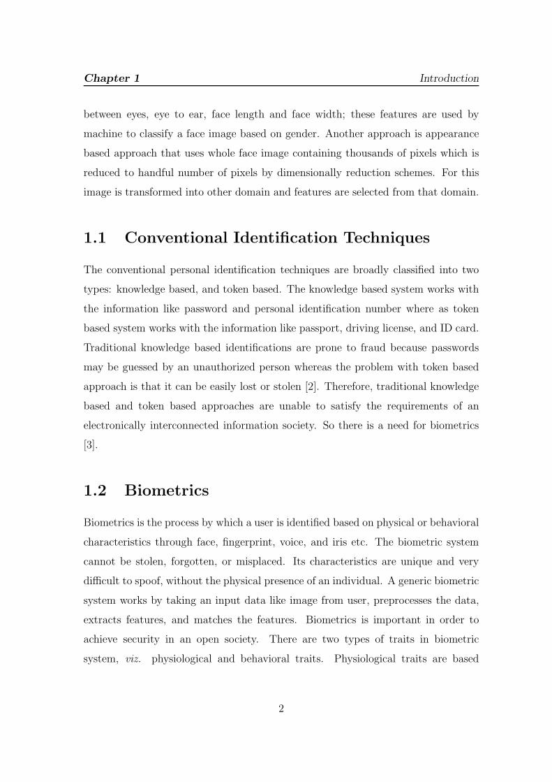
Chapter 1 Introduction
between eyes, eye to ear, face length and face width; these features are used by
machine to classify a face image based on gender. Another approach is appearance
based approach that uses whole face image containing thousands of pixels which is
reduced to handful number of pixels by dimensionally reduction schemes. For this
image is transformed into other domain and features are selected from that domain.
1.1 Conventional Identification Techniques
The conventional personal identification techniques are broadly classified into two
types: knowledge based, and token based. The knowledge based system works with
the information like password and personal identification number where as token
based system works with the information like passport, driving license, and ID card.
Traditional knowledge based identifications are prone to fraud because passwords
may be guessed by an unauthorized person whereas the problem with token based
approach is that it can be easily lost or stolen [2]. Therefore, traditional knowledge
based and token based approaches are unable to satisfy the requirements of an
electronically interconnected information society. So there is a need for biometrics
[3].
1.2 Biometrics
Biometrics is the process by which a user is identified based on physical or behavioral
characteristics through face, fingerprint, voice, and iris etc. The biometric system
cannot be stolen, forgotten, or misplaced. Its characteristics are unique and very
difficult to spoof, without the physical presence of an individual. A generic biometric
system works by taking an input data like image from user, preprocesses the data,
extracts features, and matches the features. Biometrics is important in order to
achieve security in an open society. There are two types of traits in biometric
system, viz. physiological and behavioral traits. Physiological traits are based
2
Chapter 1 Introduction
on measurements and data derived from direct measurement of a part of the
human body. Examples of physiological trait includes face, iris, fingerprint etc.
Behavioral biometric is a biometric characteristic that is learned and acquired
over time rather than one based primarily on biology. Examples of behavioral
biometrics includes voice pattern, signature recognition, gait pattern recognition,
and keystrokes. Biometrics has been widely used in forensic applications such
criminal identification, prison security, and has a very strong potential to be widely
adopted in civilian applications such as electronic banking, electronic commerce, and
access control [4].
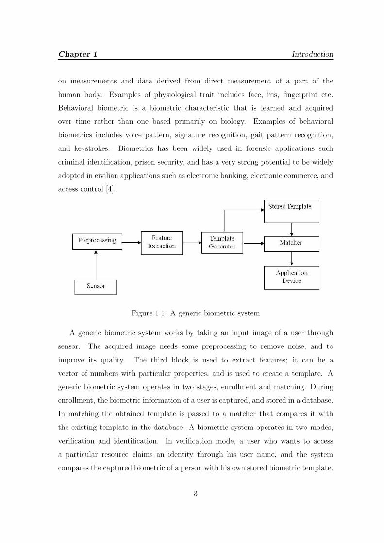
Figure 1.1: A generic biometric system
A generic biometric system works by taking an input image of a user through
sensor. The acquired image needs some preprocessing to remove noise, and to
improve its quality. The third block is used to extract features; it can be a
vector of numbers with particular properties, and is used to create a template. A
generic biometric system operates in two stages, enrollment and matching. During
enrollment, the biometric information of a user is captured, and stored in a database.
In matching the obtained template is passed to a matcher that compares it with
the existing template in the database. A biometric system operates in two modes,
verification and identification. In verification mode, a user who wants to access
a particular resource claims an identity through his user name, and the system
compares the captured biometric of a person with his own stored biometric template.
3
Chapter 1 Introduction
Therefore, it corresponds to one to one (1:1) comparison. In the identification
mode, the system compares the captured biometric template of a user with the all
stored templates of the database, and finds the best matching from all comparison.
Therefore, face identification is one is too many (1: N) comparison, where N is the
size of data base. The performance of any biometric system is measured with two
parameters, False Accept Rate (FAR) and False Reject Rate (FRR). FAR is the
possibility that the system will incorrectly accept an access attempt made by an
unauthorized user. FAR in biometrics, is the measure of the invalid inputs which
are incorrectly accepted. FRR is the possibility that system will incorrectly reject
an access made by an authorized user. FRR in biometrics, is the measure of the
rejections of the authorized users who should have been verified. The rates of false
accept, and false reject in the identification mode with database size S is given as
[5],
FARS = 1− (1− FAR)S ≈ S × FAR (1.1)
FRRS = FRR (1.2)
Number of false accept = S × FARS ≈ S2 × FAR (1.3)
For any Real time application the size of database is large, Due to which a biometric
system suffers from a computational burden, which increases the search time leading
to the percentage increase in FARS. The Performance of biometric system depends
upon accuracy and speed. Speed depends upon the size of database and is inversely
proportional to size of data base, where as accuracy depends upon underlying
algoriyhm. From the above equation the false accept rates can be reduced in two
ways. First, is by reducing the FAR , and the other way is by reducing the size of
data base S .The FAR of a system entirely depends upon the algorithm used and
cannot be reduce significantly. The search space is directly proportional to the size
of data base. If the database can be divided into two categories, then the search
space can be reduced. This can be achieved by some classification techniques or
clustering methods.
4
Chapter 1 Introduction
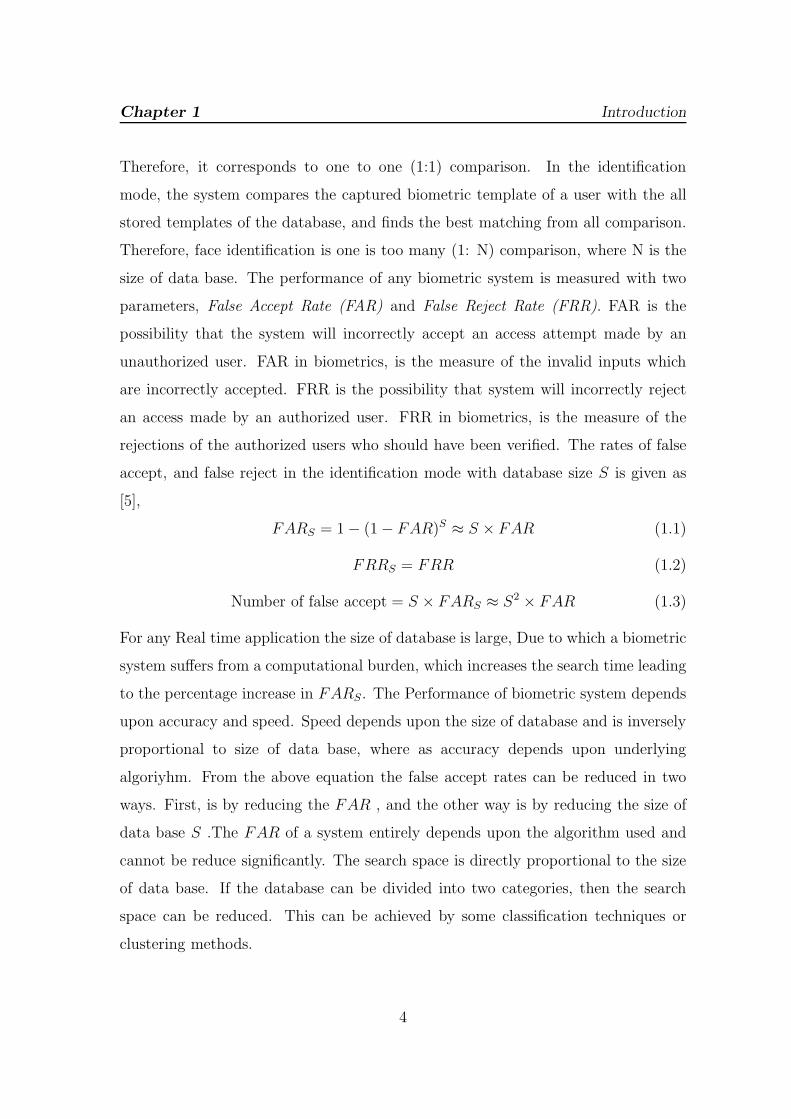
Figure 1.2: Classification to reduce search space
During Identification, the system is performing 1:N matching. The performance
can be improved by reducing the number of templates against which the query has
to be matched. This can be done using classification. Classification divides the data
base into approximately two halves viz. male and female. In any face identification
system, if the database is divided into male and female categories then search space
can be reduced by half of the original database. The reduction of search space is
given as:
FARN×L = 1− (1− FAR)N×L ≈ N × L× FAR (1.4)
Where L is the fraction by which the search space is reduced. The reduction of search
space reduces the search time of identification, viz. the number of templates that is
to be matched against query is reduced. This can be achieved by using classification
techniques. A classifier maps or assigns the input features to particular labels, which
is trained with known patterns.
5
Chapter 1 Introduction
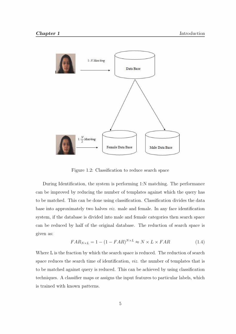
1.3 Modules of a Biometric System
Figure 1.3: Modules of a Biometric System
1. Portal. It is the gate through which the user who has been successfully
authenticated is allowed to access an object.
2. Central controlling unit. It receives the authentication request, controls the
biometric authentication process and returns the results of user authentication.
3. Input Device. It is a biometric data acquisition device which captures the
biometric trait of the user.
4. Feature Extraction. The goal of Feature Extraction technique is to preprocess
the capture data and extract suitable features for the matching algorithm.
5. Storage. It is the database of the user where the template of the user is stored.
6. Matching Algorithm compares the captured biometric trait of the user with
the stored database.
6
Chapter 1 Introduction
1.4 Gender classification using facial image
Gender classification using facial images has become an important area of research
during past several years. It is easy for human to identify male or female by seeing a
face, but it is a difficult task for the computer. Machines need some meaningful data
to perform the identification. There exist some distinguishable features between
male and female which are used by machine to classify a face image based on
gender. Gender recognition is a pattern recognition problem. Pattern recognition
can be divided into two classes, one and two stage pattern recognition systems. One
stage pattern recognition system classifies input data directly. Two stage pattern
recognition systems consist of feature extractor, followed by some form of classifier.
Gender Classification is a binary Classification problem therefore Machine needs
an appropriate data (feature) and a classifier for Gender Classification. Gender
classification approaches are categorized into two classes based on feature extraction.
These are Appearance based features which is known as Global features, and the
Geometric based features which is known as Local features. In Geometric based
method, features are extracted from some facial features points like face, nose
and eyes. Geometric features which are invariant to scale, tilt and rotation such
as distances, angles and relationships between facial points are usually extracted.
These features represent human face and provide input to a trained classifier which
performs classification. Geometric features are sensitive to lighting conditions and
changes in facial expression and lose information located at ears and hair, which
represent important information for Gender identification.
1.5 Proposed Methodology
In general, the first step in any recognition process, is to choose good discriminating
features, which is followed by a classifier. Classification of faces is a problem
of pattern recognition. A well known problem of pattern recognition is curse of
dimensionality which implies that more features do not necessarily imply a better
7

Chapter 1 Introduction
Figure 1.4: Steps Required in Gender Classification from facial image
classification success rate. In our work face region is detected from given image using
skin color segmentation. The extracted face region is subjected to PCA algorithm.
For dimensionality reduction PCA is used in current work which encodes second
order statistics of data and is fed as input to the classifier.
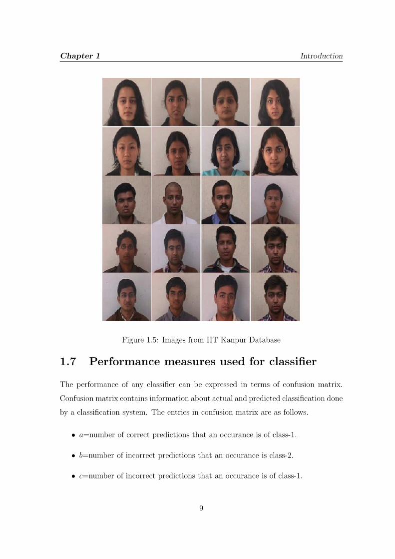
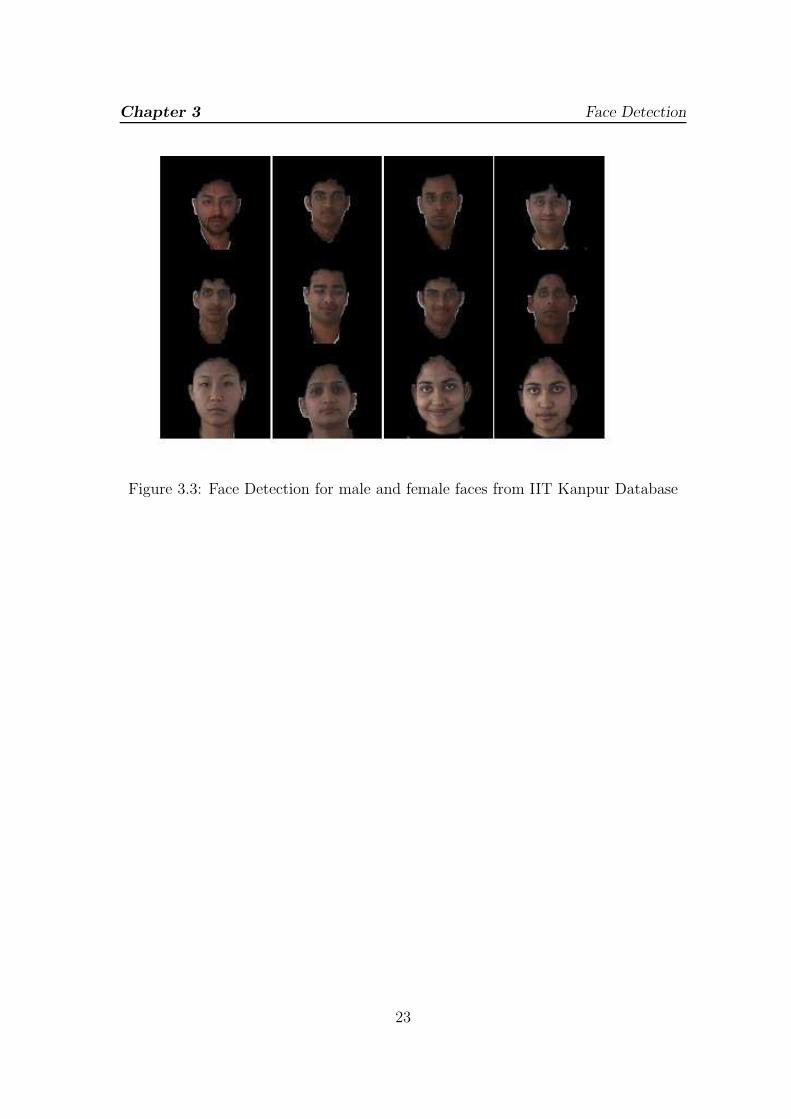
1.6 Data Base Used in the Research
The database contains images of 40 distinct subjects with eleven different poses for
each individual that included looking front, looking left, looking up towards left,
looking up towards right. In addition to variation in pose the data set contains
images with four emotions that are neutral, smile, laughter, sad. All the images
have been taken in a bright homogenous background with the subjects in an upright,
frontal position [6].
8
Chapter 1 Introduction
Figure 1.5: Images from IIT Kanpur Database
1.7 Performance measures used for classifier
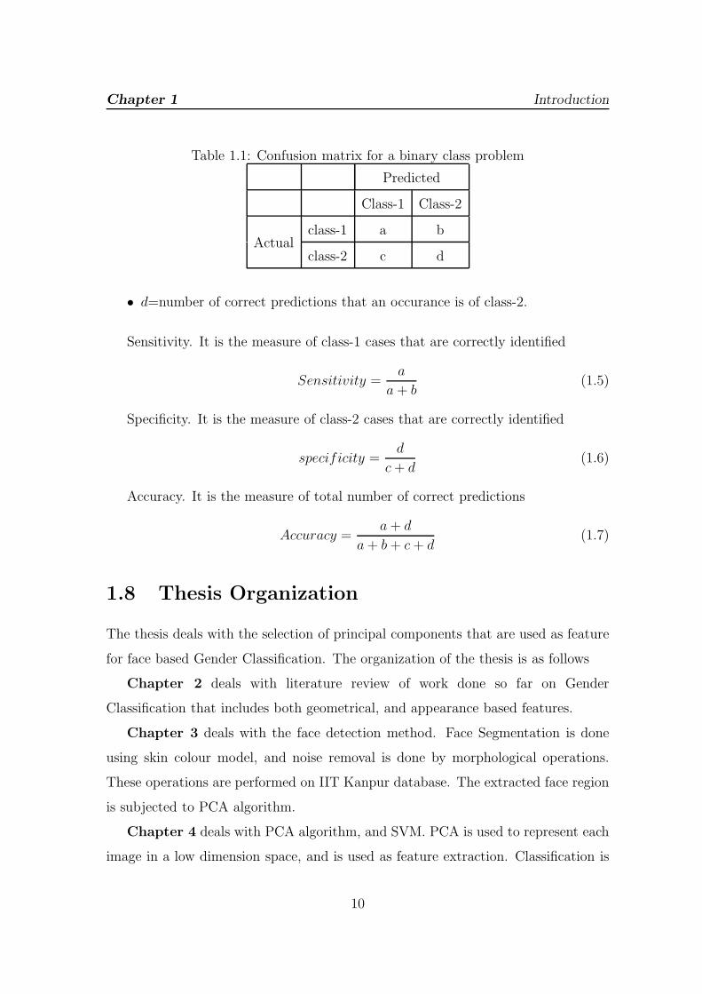
The performance of any classifier can be expressed in terms of confusion matrix.
Confusion matrix contains information about actual and predicted classification done
by a classification system. The entries in confusion matrix are as follows.
• a=number of correct predictions that an occurance is of class-1.
• b=number of incorrect predictions that an occurance is class-2.
• c=number of incorrect predictions that an occurance is of class-1.
9
Chapter 1 Introduction
Table 1.1: Confusion matrix for a binary class problem
Predicted
Class-1 Class-2
Actualclass-1 a b
class-2 c d
• d=number of correct predictions that an occurance is of class-2.
Sensitivity. It is the measure of class-1 cases that are correctly identified
Sensitivity =a
a + b(1.5)
Specificity. It is the measure of class-2 cases that are correctly identified
specificity =d
c+ d(1.6)
Accuracy. It is the measure of total number of correct predictions
Accuracy =a+ d
a+ b+ c+ d(1.7)
1.8 Thesis Organization
The thesis deals with the selection of principal components that are used as feature
for face based Gender Classification. The organization of the thesis is as follows
Chapter 2 deals with literature review of work done so far on Gender
Classification that includes both geometrical, and appearance based features.
Chapter 3 deals with the face detection method. Face Segmentation is done
using skin colour model, and noise removal is done by morphological operations.
These operations are performed on IIT Kanpur database. The extracted face region
is subjected to PCA algorithm.
Chapter 4 deals with PCA algorithm, and SVM. PCA is used to represent each
image in a low dimension space, and is used as feature extraction. Classification is
10

Chapter 1 Introduction
done using SVM, the kernel function used is RBF. An attempt has been made to
improve the accuracy of a biometric system.
Chapter 5 deals with future scope of the research work.
11
Chapter 2
Literature Review
Initially, the researchers stared with local features. Cottrell and Metacalfe used a
non linear encoder/decoder for high dimensional data to reduce the dimension of
whole face images and classified the gender based on reduced input features. In
1991, Gollomb et al. [7] Used a neural network, SEXNET, to identify gender from
a 30 x 30 face images which was compressed using 900x40x900 fully connected back
propagation network. The network SEXNET was trained to produce values of one
for male and zero for female faces. It was tested for 90 face images (45 males and 45
females) which produce an average error rate of 8.1% compared to an average error
rate of 11.6% from a study of five human faces.
In 1993, Burton et al. [8] Reported 85% accuracy rate after locating 73 facial
points. The extracted facial points are considered as features and are fed as input
to the discriminant analysis classifier to classify gender. The Author in [9] used
Enhanced PCA-SIFT for feature extraction. The Enhanced PCA-SIFT was used
to calculate the projection matrix of male and female face images respectively and
select the projection of input images by clustering method to obtain features with
more discrimination, and then a membership algorithm based on LVQ is employed
in FSVM, which imply an accuracy of 93.5%. The authors in [10] investigated
on gender classification with low resolution thumbnail faces (21 by 21 pixels) from
FERET face database using Support vector machine. The error rate was found
12
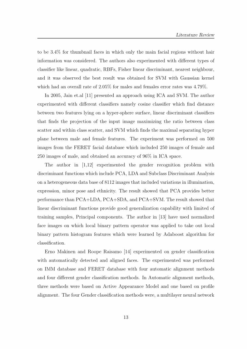
Literature Review
to be 3.4% for thumbnail faces in which only the main facial regions without hair
information was considered. The authors also experimented with different types of
classifier like linear, quadratic, RBFs, Fisher linear discriminant, nearest neighbour,
and it was observed the best result was obtained for SVM with Gaussian kernel
which had an overall rate of 2.05% for males and females error rates was 4.79%.
In 2005, Jain et.al [11] presented an approach using ICA and SVM. The author
experimented with different classifiers namely cosine classifier which find distance
between two features lying on a hyper-sphere surface, linear discriminant classifiers
that finds the projection of the input image maximizing the ratio between class
scatter and within class scatter, and SVM which finds the maximal separating hyper
plane between male and female features. The experiment was performed on 500
images from the FERET facial database which included 250 images of female and
250 images of male, and obtained an accuracy of 96% in ICA space.
The author in [1,12] experimented the gender recognition problem with
discriminant functions which include PCA, LDA and Subclass Discriminant Analysis
on a heterogeneous data base of 8112 images that included variations in illumination,
expression, minor pose and ethnicity. The result showed that PCA provides better
performance than PCA+LDA, PCA+SDA, and PCA+SVM. The result showed that
linear discriminant functions provide good generalization capability with limited of
training samples, Principal components. The author in [13] have used normalized
face images on which local binary pattern operator was applied to take out local
binary pattern histogram features which were learned by Adaboost algorithm for
classification.
Erno Makinen and Roope Raisamo [14] experimented on gender classification
with automatically detected and aligned faces. The experimented was performed
on IMM database and FERET database with four automatic alignment methods
and four different gender classification methods. In Automatic alignment methods,
three methods were based on Active Appearance Model and one based on profile
alignment. The four Gender classification methods were, a multilayer neural network
13

Literature Review
with pixel based input, an SVM with pixel based input, a discrete Ad boost with
haar like features, and an SVM with LBP features. The author concluded that the
automatic face alignment methods did not increase the classification rate where as
manual alignment increased the classification rate. The classification accuracy was
dependent on face image resizing before or after alignment. The best classification
rate was obtained with SVM using pixel based input images of size 36 × 36. The
authors in [15] have used Gabor features to represent each facial image. Each face
image was convolved with Gabor kernel of 3 scales and 4 orientations that amounted
to 12 face images. The feature extracted using Gabor filter was used in fuzzy LDA
for face age classification.
The author in [16] used a Gabor filter with multi scale and multi orientation
to a face image to obtained Gabor Magnitude Pictures (GMP). Each GMP is
operated with local binary pattern to obtain a LGBP image (local Gabor binary
pattern). Each LGBP image is divided into non overlapping rectangular regions,
from which spatial histograms are extracted. To map each LGBP feature into one
dimensional sub-space, LGBMP-LDA and LGBMP-CCL were used. LGBMP-LDA
was used using linear discriminant analysis (LDA) for dimensionality reduction, and
LGBMP-CCL was used to project LGBP feature on to the class centre connecting
line. The Classification was done using Support Vector Machine (SVM) and the
experiment was done on CAS-PEAL face data base and the result found was better
than SVMs+Gabor, SVMs+Gray scale Pixel and SVMs+LBP approach.
In 2010, Jabid et.al [17] proposed a novel approach of representing the facial
images by Local Directional pattern (LDP). The face area was divided into small
regions, from which LDP histograms were extracted and concatenated into a single
vector. The experiment was performed on FERET database, which involved 1100
male faces and 900 female faces. Each face image was cropped and normalized to
100×100 pixels. The face feature generated using LDP was used to classify into male
and female faces using classifier support vector machine. The accuracy achieved by
SVM on FERET database was 95.05%.
14

Literature Review
The author in [18] used Continuous Wavelet Transforms for finding feature for
each male and female face. The Wavelet Coefficient obtained was given to support
vector machine for classification. The experiment was performed on ORL database
containing 400 images including both male and female. The kernel used for SVM
was linear and the classification accuracy obtained was 98% compared to Radon
Transform and Discrete Wavelet Transform.
15
Chapter 3
Face Detection
In biometrics, face detection is the process to locate human face in an image. Face
detection is a challenging task due to variations in pose, scale, orientation, lighting
conditions and partial occlusions [19]. So far many approaches have been proposed
for face detection which included colour based,neural networks and feature based
tecniques. Neural network based face detection methods are highly accurate, but
are slow and suffers from computational burden [20]. In our work, skin colour based
approach is used for face detection, which is robust, simple and effective.
3.1 Skin colour Detection
The purpose of Skin colour segmentation is used to determine whether the Image
pixel is a skin colour or non skin colour. Good skin colour segmentation is one which
segment every skin colour whether it is blackish, yellowish, or whitish. The goal of
skin colour analysis is to reject non skin colour regions from a selected image [21].
This includes the process of colour conversion of the image to some colour spaces.
There are different colour spaces that have been used. Widely used colour spaces
are RGB, HSV, CMYK and YCbCr.
In YCbCr colour model, the luminance information is contained in Y component,
and the chrominance information is contained in Cb and Cr. To convert the RGB
16

Chapter 3 Face Detection
image into YCbCr image, separate the Chroma component Cb and Cr. Y component
represent the luminance information which has more variation that is this component
can be discarded, Cb and Cr component are used.
Cb is the difference between blue and luma component and Cr is the difference
between red and luma component. Y in YCbCr represents the luminance component
and Cb and Cr represents the chrominance component
Cr=R-Y
Cb=B-Y
3.2 Algorithm for Brightness Compensation
An RGB image I of size m×n is the input to our algorithm. Brightness compensated
image is obtained from an RGB by applying Algorithm.
C = R′, G′, B′ (3.1)
Where
R’=R×mR, G’=G×mG, and B’=B ×mB
and mR,mG,mB are the scaling factors.
1. Extract the R, G, B components
• R = I(:, :, 1);
• G = I(:, :, 2);
• B = I(:, :, 3);
2. Compute the average value of R,G,B Component of image I.
RI =1
mn
m∑
i=1
n∑
j=1
Ri,j (3.2)
GI =1
mn
m∑
i=1
n∑
j=1
Gi,j (3.3)
17
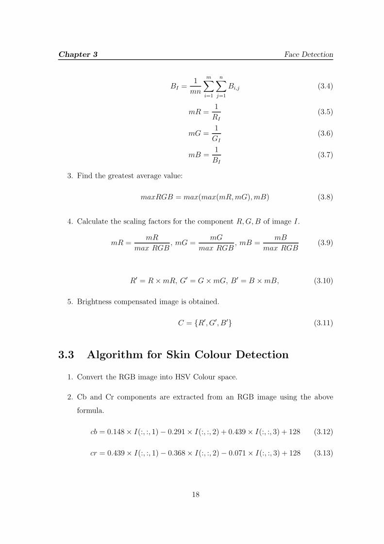
Chapter 3 Face Detection
BI =1
mn
m∑
i=1
n∑
j=1
Bi,j (3.4)
mR =1
RI
(3.5)
mG =1
GI
(3.6)
mB =1
BI
(3.7)
3. Find the greatest average value:
maxRGB = max(max(mR,mG), mB) (3.8)
4. Calculate the scaling factors for the component R,G,B of image I.
mR =mR
max RGB, mG =
mG
max RGB, mB =
mB
max RGB(3.9)
R′ = R×mR, G′ = G×mG, B′ = B ×mB, (3.10)
5. Brightness compensated image is obtained.
C = R′, G′, B′ (3.11)
3.3 Algorithm for Skin Colour Detection
1. Convert the RGB image into HSV Colour space.
2. Cb and Cr components are extracted from an RGB image using the above
formula.
cb = 0.148× I(:, :, 1)− 0.291× I(:, :, 2) + 0.439× I(:, :, 3) + 128 (3.12)
cr = 0.439× I(:, :, 1)− 0.368× I(:, :, 2)− 0.071× I(:, :, 3) + 128 (3.13)
18
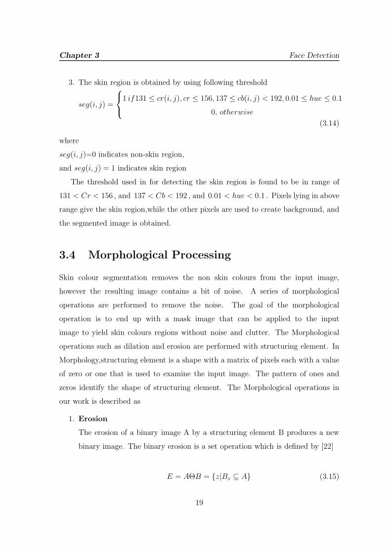
Chapter 3 Face Detection
3. The skin region is obtained by using following threshold
seg(i, j) =
1 if131 ≤ cr(i, j), cr ≤ 156, 137 ≤ cb(i, j) < 192, 0.01 ≤ hue ≤ 0.1
0, otherwise
(3.14)
where
seg(i, j)=0 indicates non-skin region,
and seg(i, j) = 1 indicates skin region
The threshold used in for detecting the skin region is found to be in range of
131 < Cr < 156 , and 137 < Cb < 192 , and 0.01 < hue < 0.1 . Pixels lying in above
range give the skin region,while the other pixels are used to create background, and
the segmented image is obtained.
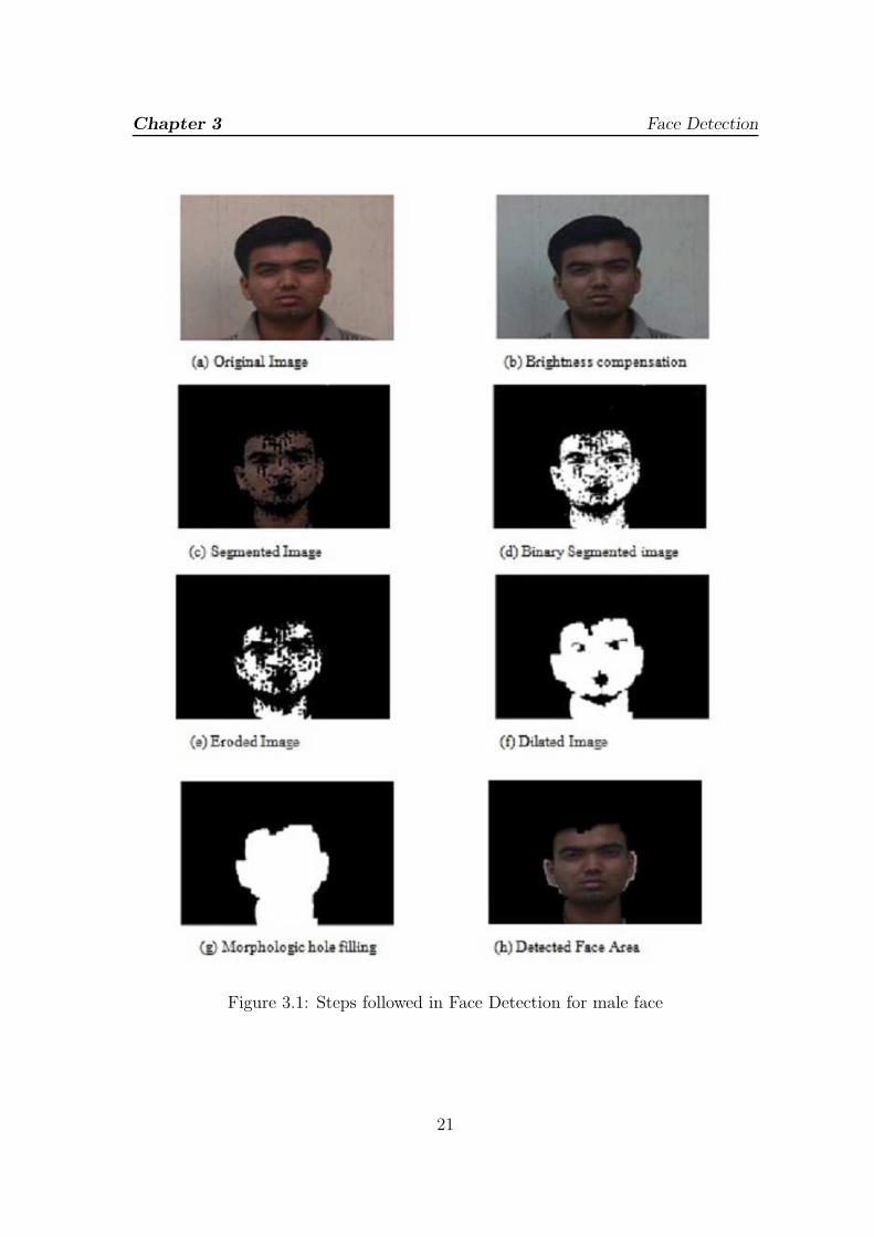
3.4 Morphological Processing
Skin colour segmentation removes the non skin colours from the input image,
however the resulting image contains a bit of noise. A series of morphological
operations are performed to remove the noise. The goal of the morphological
operation is to end up with a mask image that can be applied to the input
image to yield skin colours regions without noise and clutter. The Morphological
operations such as dilation and erosion are performed with structuring element. In
Morphology,structuring element is a shape with a matrix of pixels each with a value
of zero or one that is used to examine the input image. The pattern of ones and
zeros identify the shape of structuring element. The Morphological operations in
our work is described as
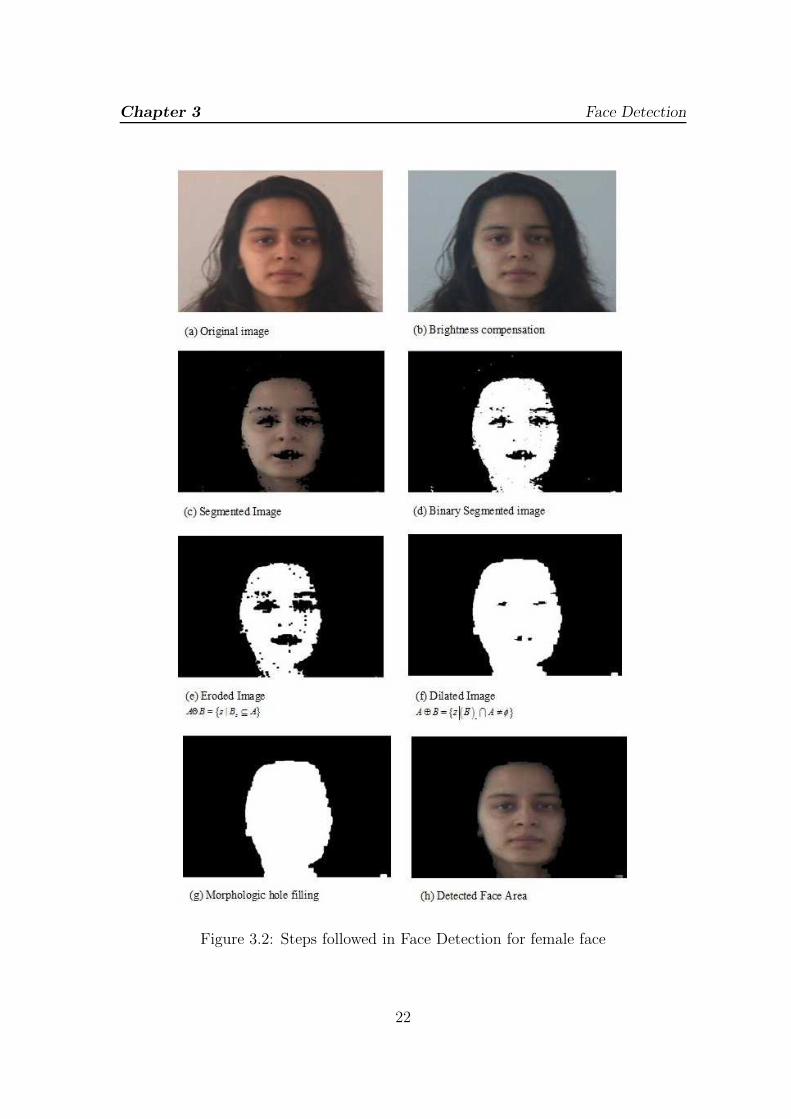
1. Erosion
The erosion of a binary image A by a structuring element B produces a new
binary image. The binary erosion is a set operation which is defined by [22]
E = AΘB = z|Bz ⊆ A (3.15)
19

Chapter 3 Face Detection
Erosion of A by B is the set of pixel locations z where the structuring element
translated to location z, overlaps only with the foreground pixels in A.
E(x, y) =
1 if B fitsA
0 otherwise(3.16)
The structuring element is a matrix of pixels, each with a value of ones in all
pixel locations.
2. Dilation
The dilation of a binary image A by a structuring element B produces a new
binary image. The binary dilation can be written as:
D = A⊕
B =
z|(B)z ∩ A = φ
(3.17)
where B is the reflection of the structuring element, B and φ is the empty set.
Dilation of A by B is the set of pixel locations z where the reflected structuring
element overlaps with foreground pixels in A when translated to z.
D =
1 if B hitsA
0 otherwise.(3.18)
3. Morphological Hole filling
Hole can be defined as a background region surrounded by a connected border
of foreground pixels. Hole filling is used to fill image regions and holes to keep
the faces as single connected region.
20
Chapter 3 Face Detection
Figure 3.1: Steps followed in Face Detection for male face
21
Chapter 3 Face Detection
Figure 3.2: Steps followed in Face Detection for female face
22
Chapter 3 Face Detection
Figure 3.3: Face Detection for male and female faces from IIT Kanpur Database
23

Chapter 4
Principal Component Analysis and
Support Vector Machine
PCA is a mathematical tool which was invented in 1901 by Karl Pearson which is
helpful to perform operations like prediction, redundancy removal, feature extraction
and data compression, therefore finds its strong application in image recognition and
image compression. It is a dimensionality reduction technique by which the observed
variable is transformed into smaller dimensionality of feature space. It performs a
transformation on a matrix of Observed variables (variables correlated to each other)
to a new coordinate system which contains fewer variables (uncorrelated variables)
that can best define the observed variables. These uncorrelated variables are known
as Principal Components, which are arranged in decreasing order of their variance
such that the first principal component has the largest variance. The main idea of
using PCA is to express the large 1-D vector of pixels constructed from 2-D facial
image into the compact principal components of the feature space known as Eigen
space projection [23]. It is a technique to find patterns in high dimensional data.
The pattern contains redundant information, mapping it to a feature vector can
reduce the redundancy and can preserve most of the intrinsic information content
of the pattern.
24
Chapter 4 Principal Component Analysis and Support Vector Machine
4.1 Preparation of Training set
The images are aligned in a folder and resized to a particular dimension. Let a face
image I(x, y) be a two-dimensional N × N array of 8 bit intensity values. Each
face image is then converted to a column vector of dimension N2,which represents a
point in N2 dimensional space. A training matrix is created by taking different face
images, where each column corresponds to a specific face image.Let total number of
images is M, which consitutes a training matrix of dimension N2× M. Let training
images are Γ1,Γ2,Γ3,Γ4.......ΓM which construct the training matrix Γ.
4.2 Eigenface Generation
A mean image ψ is calculated from training matrix
ψ =1
M
M∑
i=1
Γi (4.1)
A mean corrected image is calculated by subtracting mean image from each image
vector. Let Φi be defined as mean centered image
Φi = Γi − ψ (4.2)
The mean corrected images are subjected to PCA to find the M orthogonal vectors.
The orthogonal vectors are calculated from covariance matrix. A covariance matrix
is constructed as
C = AAT (4.3)
Where A is a matrix composed of A = [φ1φ2φ3φ4.....φM ] of dimension of N2 ×M .
Therefore, the dimension of the covariance matrix becomes N2×N2 . Calculation of
Eigen vectors from this dimension will result in computational burden. A common
theorem in linear algebra states that vectors Vi and scalars λi can be obtained by
solving the eigenvectors and Eigen values of the M ×M matrix AT×A . Let Vi be
the Eigen vector of the of AT×A such that
ATAVi = λVi (4.4)
25

Chapter 4 Principal Component Analysis and Support Vector Machine
Now multiplying the above equation with A on both sides,
AATAVi = AλVi (4.5)
ei = AVi (4.6)
From the above equation it can be concluded that Vi is the Eigen vector of ATA and
AVi is the Eigen vector of AAT . The Eigen vectors are arranged with the decreasing
values of Eigen values. The Eigen vector associated with largest Eigen value is
one that reflects the greatest variance in the image and the smallest Eigen value is
associated with the Eigen vectors that find least variance. The Eigen vectors are
known as Eigen faces [24]. The Eigen faces obtained from the training data base are
as shown in figure below.
Figure 4.1: Eigen Faces for Female Data base
Above are the top most Eigen faces that are generated from the training set. A
facial image can be projected on to the subspace by computing
Ω = [w1w2w3....wm] (4.7)
Where wi = eTi φi. wi is the ith coordinate of the facial image in new space
which is known to be principal component. The vectors ei are also images and look
26

Chapter 4 Principal Component Analysis and Support Vector Machine
Figure 4.2: Eigen Faces for Male Data base
like faces known as Eigenfaces. Ω describes the contribution of each Eigenface in
representing the facial image.
Figure 4.3: Variance Plot for the first thirty principal components for male and
female data base.
The Eigen vector associated with largest Eigen value is one that reflects the
greatest variance in the image, and the smallest Eigen value is associated with
the Eigen vectors that find least variance. The first Eigen vector accounts for 55
variance in the dataset, while the first 20 eigenvectors together account for 90%,
27
Chapter 4 Principal Component Analysis and Support Vector Machine
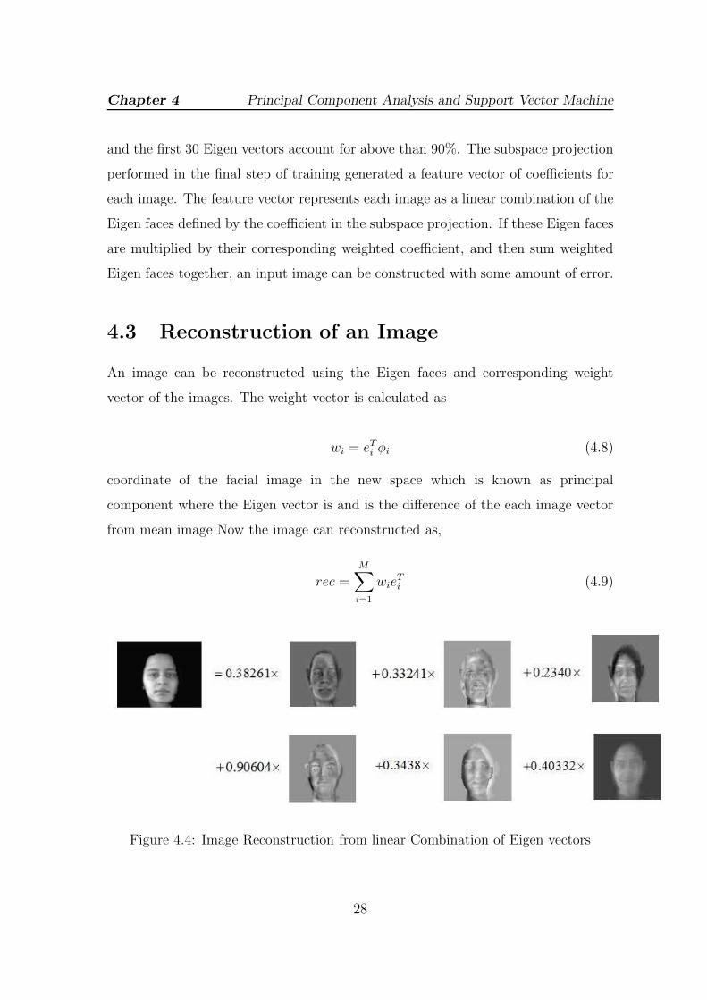
and the first 30 Eigen vectors account for above than 90%. The subspace projection
performed in the final step of training generated a feature vector of coefficients for
each image. The feature vector represents each image as a linear combination of the
Eigen faces defined by the coefficient in the subspace projection. If these Eigen faces
are multiplied by their corresponding weighted coefficient, and then sum weighted
Eigen faces together, an input image can be constructed with some amount of error.
4.3 Reconstruction of an Image
An image can be reconstructed using the Eigen faces and corresponding weight
vector of the images. The weight vector is calculated as
wi = eTi φi (4.8)
coordinate of the facial image in the new space which is known as principal
component where the Eigen vector is and is the difference of the each image vector
from mean image Now the image can reconstructed as,
rec =
M∑
i=1
wieTi (4.9)
Figure 4.4: Image Reconstruction from linear Combination of Eigen vectors
28
Chapter 4 Principal Component Analysis and Support Vector Machine
4.4 Support Vector Machine based Classifiers
Classification of data is important in machine learning where data points are spread
in high dimensional space. Each data point belongs to one of the two classes, and
the goal is to decide which class a new data point will be in. Gender classification is
a binary classification problem, therefore Support vector machine is used for gender
classification. SVM are supervised learning systems which can analyze and recognize
the data very well. Support vector machine is a computer algorithm that learns by
example to assign labels to object. SVM was developed by Vpnik to reduce error on
training data set and finds its implementation in the fields of breast cancer diagnosis,
Bioinformatics, hand written digit recognition and image based gender classification.
For example, an SVM can learn to recognize handwritten digits by examining a large
collection of scanned images of handwritten to zeroes and ones. SVM is an algorithm
for maximizing a particular mathematical function with respect to a given collection
of data [25]. The basic SVM takes a set of input data’s and predicts, for each given
input, which of two possible classes forms the output, making it a non-probabilistic
binary linear classifier. A support vector machine constructs a hyper plane in a
high dimensional space, which can be used for classification and regression. A good
separation is achieved by the hyper plane that has the largest distance to the nearest
training data set [26]. SVM separates the dataset into training and testing data sets,
where each sample in the training set contains one target value and observed features.
SVM classifiers generate a decision boundary based on the training data set, which
helps in predicting the target value of the testing dataset.
4.5 Optimal Separating hyper plane
The black circles points and the white circle points represent class +1 and -1. A
hyper plane separates the data class of +1 and -1 and maximizes the margin. Margin
is the distance between the classifier and the nearest data point of each class. The
bold line is the optimal hyper plane, which maximizes the margin as well as separates
29

Chapter 4 Principal Component Analysis and Support Vector Machine
Figure 4.5: The optimal hyper plane separating two classes [27]
the data point successfully. The optimal hyper plane means a hyper plane which
separates the two class with maximum margin.
4.6 Architecture of SVM
Let X1, X2, X3, X4......Xi be the input layer of size m, and X be the input vector in
n dimensional space Rn . Let K(X,X1), K(X,X2), K(X,3 ), K(X,X4).......K(X,Xi)
be the hidden layer of mi linear product kernel , W be the weight vector having
weighted elements w1, w2, w3, w4........wm, b is the bias defined in the real dimensional
space. y is the output which makes decision for classification.
For training set of instance label pairs X i, yi , where i=1 to number of inputs m,
X i ∈ Rn ,yi ∈ −1, 1 both defined in real dimension space. SVM finds a hyperplane
which is defined as
y = sign 〈w.X〉+ b (4.10)
30

Chapter 4 Principal Component Analysis and Support Vector Machine
Figure 4.6: Support vectors in SVM [28]
The decision boundary for the classification purpose is defined as
wTΦ(X) + b = 0 (4.11)
where w ∈ Rn , and Φ(X) is the kernel function of X, and b is the position of
hyper plane in real dimension space R. The hyperplane is constructed such that it
satisfies the inequality for both the classes.
wTΦ(Xi) + b ≥ +1, if yi = +1 (4.12)
wTΦ(Xi) + b ≤ +1, if yi = −1 (4.13)
The equation (4.12) and (4.13) can be wirtten together as
yi[
wTΦ(Xi) + b]
≥ +1, i = 1, 2, .....m (4.14)
31
Chapter 4 Principal Component Analysis and Support Vector Machine
where, Xi is the sample value of the input vector X, and yi is the corresponding
value of the target output y. The optimal hyper plane should satisfy following criteria
yi[
wTΦ(xi) + b]
≥ +1 (4.15)
0 ≤ yi[
wTΦ(xi) + b]
< 1 (4.16)
yi[
wTΦ(xi) + b]
< 0 (4.17)
The equation (4.15) states that the vectors that fall outside the band and are
correctly classified. The equation (4.16) states that the vectors falling inside the band
and is correctly classified and equation (4.17) states that the vectors are misclassified
vectors. All the above three cases can be restricted by introducing a new set of non
negative slack variable ξ
yi[
wTΦ(xi) + b]
≥ 1− ξi, And ξi ≥ 0 (4.18)
4.7 Kernels in SVM
Kernels Methods are class of algorithms for pattern analysis. The task performed
in pattern analysis is to study the relation in principal components, correlations,
classification, clusters, and in data points. Kernels approach the Problem by
mapping the data into a high dimensional feature space, where each coordinate
corresponds to one feature of the data set. With the help of kernel function it
is possible to compute the inner products between images of all pairs of data
in the feature space. This approach is known as kernel trick. The kernel trick
is used to map patterns in higher dimension space. The kernel trick can be
implemented to algorithms which depend upon dot product between two vectors and
the corresponding dot product can be replaced by a kernel function for mapping of
patterns into higher dimensional space. The kernel functions available for SVM are
• Linear kernel. Linear kernel is the summation of inner product
32

Chapter 4 Principal Component Analysis and Support Vector Machine
x, xi and a constant d
K(x, xi) = xTxi + d (4.19)
• Polynomial kernel. Polynomial kernel is suitable for normalized data sets
as it is non stationary kernel
K(x, xi) = (βxTxi + d)p (4.20)
P is the polynomial degree; d is constant and β is slope. These parameters
can be adjusted
• Radial basis function. The kernel function used for SVM is Gaussian kernel
which is the example of radial basis function. The Gaussian kernel is given by
K(x, xi) =
(
‖x− xi‖2
2σ2
)
(4.21)
33

Chapter 4 Principal Component Analysis and Support Vector Machine
4.8 Result
A Data set of 50 male, and 50 female faces are taken, that included frontal faces.
A training set is prepared that corresponds to the principal components for male
and female faces, 70 coefficients corresponding to 35 male, and 35 female faces. A
testing set was prepared that included 30 coefficients, corresponding to 15 male, and
15 female faces.
Table 4.1: Confusion matrix obtained from SVM using Polynomial kernel
Predicted
Male Female
ActualMale 15 0
Female 4 11
Accuracy = 86.6667%
Table 4.2: Confusion matrix obtained from SVM using RBF kernel
Predicted
Male Female
ActualMale 15 0
Female 2 13
Accuracy = 93.33%
34
Chapter 5
Conclusion
In this thesis, an attempt has been made to classify gender from facial image. The
face portion is extracted from a given input image using skin colour model, and
morphological operations. The training data set is prepared for male, and female
faces that included detected face regions. Gender Classification is divided into two
steps, feature selection and classification. The feature extraction algorithm used is
PCA. PCA is used to represent each image as a feature vector, and these principal
components are trained and tested using support vector machine.
The face region is detected in the first stage of our work. Once the face is
detected in binary image, eye region, center of eye, mouth, lip shape, nose tip, and
width can be located. These pixels can be given as input to support vector machine.
The database used in the research work does not contain any facial images having
spectacles. The facial image involving specs need to be identified correctly which is
a challenging issue.
Pixels in an image represent a large degree of correlation. By using pixels as
features, there will be redundant information. This redundancy can be removed by
using PCA. The principal component of the image give uncorrelated coefficients.
Thus, using Principal Component as feature seems to be a reasonable choice which
is achieved using Principal Component Analysis.
PCA removes the second order dependencies from the the data, but still there
35

Conclusion
exists higher order dependencies in data. Higher order dependencies among data
can be removed using Independent Component Analysis(ICA) which is an extension
of PCA.
Representation of a multivariate data by means of an appropriate transformation
is an important research issue in field of pattern recognition. The process of finding
such representation of data is known as feature extraction. Most of the work is
being done on finding suitable feature extraction technique, in our work Principal
Component is used as feature. Feature extraction method such as Radon Transform,
Hought Transform and Wavelet Transform exists, and can be used as features which
may improve the classification performance.
36

Bibliography
[1] T. I. Dhamecha, A. Sankaran, R. Singh, and M. Vatsa. Is gender classification across ethnicity
feasible using discriminant functions? In 2011 International Joint Conference on Biometrics,
IJCB 2011, 2011.
[2] S Jayaraman, T Veerakumar, and S Esakkirajan. Digital Image Processing. Tata McGraw-Hill
Education, 2009.
[3] N. K. Ratha, J. H. Connell, and R. M. Bolle. Biometrics break-ins and band-aids. Pattern
Recognition Letters, 24(13):2105–2113, 2003.
[4] Ruud M. Bolle and Andrew W. Senoir. Guide To Biometrics. Springer-Verlag, New York,
2009.
[5] David Maltoni. Guide To Biometrics. Springer-Verlag, New York, 2009.
[6] Vidit Jain and Amitabha Mukherjee. The indian face database, 2002.
[7] H. . Kim, D. Kim, Z. Ghahramani, and S. Y. Bang. Appearance-based gender classification
with gaussian processes. Pattern Recognition Letters, 27(6):618–626, 2006.
[8] A M Burton, Vicki Bruce, and Neal Dench. What’s the difference between men and women?
evidence from facial measurement. Perception, 22(2):153–176, 1993.
[9] Y. Wang and N. Zhang. Gender classification based on enhanced PCA-SIFT facial features.
In 2009 1st International Conference on Information Science and Engineering, ICISE 2009,
pages 1262–1265, 2009.
[10] M. . Yang and B. Moghaddam. Gender classification using support vector machines. In IEEE
International Conference on Image Processing, volume 2, pages 471–474, 2000.
[11] A. Jain, J. Huang, and S. Fang. Gender identification using frontal facial images. In
IEEE International Conference on Multimedia and Expo, ICME 2005, volume 2005, pages
1082–1085, 2005.
37
Bibliography
[12] Srinivas Gutta and Harry Wechsler. Gender and ethnic classification of human faces using
hybrid classifiers. In Proceedings of the International Joint Conference on Neural Networks,
volume 6, pages 4084–4089, 1999.
[13] Z. Yang and H. Ai. Demographic classification with local binary patterns, volume 4642 LNCS.
2007.
[14] E. Makinen and R. Raisamo. Evaluation of gender classification methods with automatically
detected and aligned faces. IEEE Transactions on Pattern Analysis and Machine Intelligence,
30(3):541–547, 2008.
[15] F. Gao and H. Ai. Face age classification on consumer images with gabor feature and fuzzy
LDA method, volume 5558 LNCS. 2009.
[16] B. Xia, H. Sun, and B. . Lu. Multi-view gender classification based on local gabor binary
mapping pattern and support vector machines. In Proceedings of the International Joint
Conference on Neural Networks, pages 3388–3395, 2008.
[17] T. Jabid, Md H. Kabir, and O. Chae. Gender classification using local directional pattern
(ldp). In Proceedings - International Conference on Pattern Recognition, pages 2162–2165,
2010.
[18] Amjath Fareeth Basha1 and Gul Shaira Banu Jahangeer. Face gender image classification
using various wavelet transform and support vector machine with various kernels. International
Journal of Computer Science Issues, 9(2), 2012.
[19] R. Xiao, M. . Li, and H. . Zhang. Robust multipose face detection in images. IEEE
Transactions on Circuits and Systems for Video Technology, 14(1):31–41, 2004.
[20] Rajib Sarkar, Sambit Bakshi, and Pankaj K. Sa. A real-time model for multiple human face
tracking from low-resolution surveillance videos. Procedia Technology, 6:1004 – 1010, 2012.
[21] Amanpreet Kaur and B.V Kranthi. Comparison between YCbCr color space and CIE lab color
space for skin color segmentations. International Journal of Applied Information Systems,
3(4), 2012.
[22] Rafael Gonzalez and Richard Woods. Digital Image Processing. Addison Wesley, 1992.
[23] Kyungnam Kim. Face recognition using principle component analysis. In Proceedings -
International Conference on computer vision and Pattern Recognition, pages 586–591, 1996.
[24] M. Turk and A. Pentland. Eigenfaces for recognition. Journal of cognitive neuroscience,
3(1):71–86, 1991. Cited By (since 1996):5652.
38

Bibliography
[25] W. S. Noble. What is a support vector machine? Nature biotechnology, 24(12):1565–1567,
2006.
[26] W. Caesarendra, A. Widodo, and B. . Yang. Combination of probability approach and support
vector machine towards machine health prognostics. Probabilistic Engineering Mechanics,
26(2):165–173, 2011.
[27] C. J. C. Burges. A tutorial on support vector machines for pattern recognition. Data Mining
and Knowledge Discovery, 2(2):121–167, 1998.
[28] C. Cortes and V. Vapnik. Support-vector networks. Machine Learning, 20(3):273–297, 1995.
[29] J. A. K. Suykens and J. Vandewalle. Least squares support vector machine classifiers. Neural
Processing Letters, 9(3):293–300, 1999.
39