Gasc A, Sueur J, Pavoine S, Pellens R, Grandcolas P (2013) Biodiversity sampling using a global...

Biodiversity Sampling Using a Global Acoustic Approach:Contrasting Sites with Microendemics in New CaledoniaAmandine Gasc1,2*, Jerome Sueur1, Sandrine Pavoine2,3, Roseli Pellens1, Philippe Grandcolas1

1 Departement Systematique et Evolution, Museum national d’Histoire naturelle, Paris, France, 2 Departement Ecologie et Gestion de la Biodiversite, Museum national

d’Histoire naturelle, Paris, France, 3 Department of Zoology, University of Oxford, Oxford, United Kingdom

Abstract

New Caledonia is a Pacific island with a unique biodiversity showing an extreme microendemism. Many species distributionsobserved on this island are extremely restricted, localized to mountains or rivers making biodiversity evaluation andconservation a difficult task. A rapid biodiversity assessment method based on acoustics was recently proposed. Thismethod could help to document the unique spatial structure observed in New Caledonia. Here, this method was applied inan attempt to reveal differences among three mountain sites (Mandjelia, Koghis and Aoupinie) with similar ecologicalfeatures and species richness level, but with high beta diversity according to different microendemic assemblages. In eachsite, several local acoustic communities were sampled with audio recorders. An automatic acoustic sampling was run onthese three sites for a period of 82 successive days. Acoustic properties of animal communities were analysed without anyspecies identification. A frequency spectral complexity index (NP) was used as an estimate of the level of acoustic activityand a frequency spectral dissimilarity index (Df) assessed acoustic differences between pairs of recordings. As expected, theindex NP did not reveal significant differences in the acoustic activity level between the three sites. However, the acousticvariability estimated by the index Df, could first be explained by changes in the acoustic communities along the 24-hourcycle and second by acoustic dissimilarities between the three sites. The results support the hypothesis that global acousticanalyses can detect acoustic differences between sites with similar species richness and similar ecological context, but withdifferent species assemblages. This study also demonstrates that global acoustic methods applied at broad spatial andtemporal scales could help to assess local biodiversity in the challenging context of microendemism. The method could bedeployed over large areas, and could help to compare different sites and determine conservation priorities.

Citation: Gasc A, Sueur J, Pavoine S, Pellens R, Grandcolas P (2013) Biodiversity Sampling Using a Global Acoustic Approach: Contrasting Sites withMicroendemics in New Caledonia. PLoS ONE 8(5): e65311. doi:10.1371/journal.pone.0065311

Editor: David L. Roberts, University of Kent, United Kingdom

Received August 23, 2012; Accepted April 29, 2013; Published May 29, 2013

Copyright: � 2013 Gasc et al. This is an open-access article distributed under the terms of the Creative Commons Attribution License, which permits unrestricteduse, distribution, and reproduction in any medium, provided the original author and source are credited.

Funding: This work was supported by a CNRS INEE PhD grant, the BIONEOCAL ANR (Agence National de la Recherche) and the FRB (Fondation pour la Recherchesur la Biodiversite) grant BIOSOUND. The funders had no role in study design, data collection and analysis, decision to publish, or preparation of the manuscript.

Competing Interests: The authors have declared that no competing interests exist.

* E-mail: [email protected]

Introduction

New Caledonia has been classified as one of the 25 most

important hotspots of biodiversity conservation regarding the

number of endemic species and degree of threat [1]. Kier et al. [2]

also ranked New Caledonia as the terrestrial region with the

highest level of endemism. As an example, 19% of bird, 67% of

mammal, 86% of reptile and 76% of plant species are endemic to

this Pacific island at the regional scale [1]. The emphasis put on

regional endemism and biogeography masks another remarkable

feature of New Caledonia, the extremely high level of local

endemism, hereafter called microendemism. The so-called micro-

endemic species of plants, lizards or insects show a very short

distributional range, limited to small mountains or rivers of New

Caledonia. According to recent studies, this local endemism

mainly originated through recent allopatric speciation with little

ecological differentiation [3], with the notable exception of

adaptation to metalliferous soils derived from ultramafic rocks

covering one third of the island [4]. In this paradigm, the island

can be considered as a wonderful natural laboratory for evolution,

where many questions regarding speciation and endemism can be

studied through a large time window of 37 million years (e.g.,

[3,5–8]).

Microendemism also bears strong consequences for conserva-

tion since very short distributional ranges increase the risk of

species extinction, facing three principal threats that are nickel

mining, fire and invasive species (reviewed in [9]). The origin and

composition of this threatened biodiversity have to be quickly

described and deciphered, both to allow theoretical studies of

speciation and evolution to be conducted and to permit the

establishment of conservation policies. It is therefore necessary to

rapidly characterize sites and their communities. However, such a

task is made complex because sites differ not only by distinct

species combinations within the same local pool, but also by the

fact that each mountain or river usually shows local endemics

formed by allopatric speciation (e.g., [7–8,10]). Inventorying in

New Caledonia has proved to be a fastidious and slow process due

to a complex landscape, a small local scientific community, and

long distance isolation from most academic centres. The level of

species richness in New Caledonia is particularly high throughout

the island. Comparing species richness of sites is not likely to be

very informative [9]. Establishing complementarities of different

sites in terms of species composition should help in establishing

conservation priorities for the diversity evaluation and conserva-

tion of New Caledonia [11–12].

PLOS ONE | www.plosone.org 1 May 2013 | Volume 8 | Issue 5 | e65311

Therefore, inventorying and evaluation processes need to be

enhanced and speeded up by using other approaches. In this

respect, inventories based on passive acoustic methods have

demonstrated convincing advantages as they are non invasive,

allow large automatic sampling, can be simultaneously used on

several taxa, and provide very large temporal and spatial data sets

[13–14]. Similar to classical inventory methods, passive acoustics

can potentially be used to identify species directly by ear [15–16]

or by automatic identification methods [17–20]. However,

identification of singing species by human observers is partly

subjective depending on the experience and listening skills of the

observer and to the difficulty of handling large samples. Automatic

identification processes, which aim at finding species-specific

songs, require an important sound reference database. Such an

approach seems very complex to undertake in New Caledonia

where species richness is particularly high, and where species

acoustic diversity has not yet been fully registered and described.

Facing these difficulties, a global acoustic passive method might

therefore be especially helpful to provide new data on local animal

diversity [21].

The global acoustic method consists of analysing the acoustic

output of animal communities by measuring how diverse or

complex a community’s signal is, in terms of spectral and/or

temporal acoustic properties, without any species identification.

Such measures of acoustic complexity have been linked previously

to the number of singing species [21–22] and to the number of

vocalizations [23]. Following Diamond and Case [24], who

defined a community as an entity that ‘‘comprises the populations

of some or all species coexisting at a site or in a region’’, an

acoustic community could be seen as a collection of sounds

produced by all living organisms in a given habitat over a specified

time. In this case, the species compete for the sound space, which

is itself a sound resource. Two complementary approaches are

currently developed for a rapid acoustic survey, one to evaluate the

acoustic diversity level of each community based on a measure of

acoustic signal complexity (a diversity), and the other to compute

acoustic distances between pairs of communities (b diversity) [21].

The aim of this study is to evaluate the capacity of the global

acoustic method to detect dissimilarity between sites that are

otherwise known to be similar with respect both to species richness

and ecological context but distinct regarding species composition

and microendemics. To do this, three sites on the main island have

been selected because of two characteristics: a high and

comparable level of species richness and differences in species

composition mainly due to microendemism. These sites were

selected according to a census based on all published phylogenetic

and inventory studies so far (see Table S1), and on Global

Biodiversity Inventory Facility (GBIF) records from collection

databases. Automatic recorders collected acoustic data on these

three sites. Distance based acoustic indices and statistical analyses

assessed the acoustic dissimilarities among the three different sites.

The study can be seen as a very stringent test of the capacity of

the global acoustic method to detect dissimilarity of biodiversity,

given that allopatric speciation with niche conservatism, which is

important in New Caledonia, is expected to maximize ecological

similarity between sites. According to this capacity to detect

dissimilarity, the global acoustic method could be an effective and

efficient new approach to contrast sites of high biodiversity value.

Materials and Methods

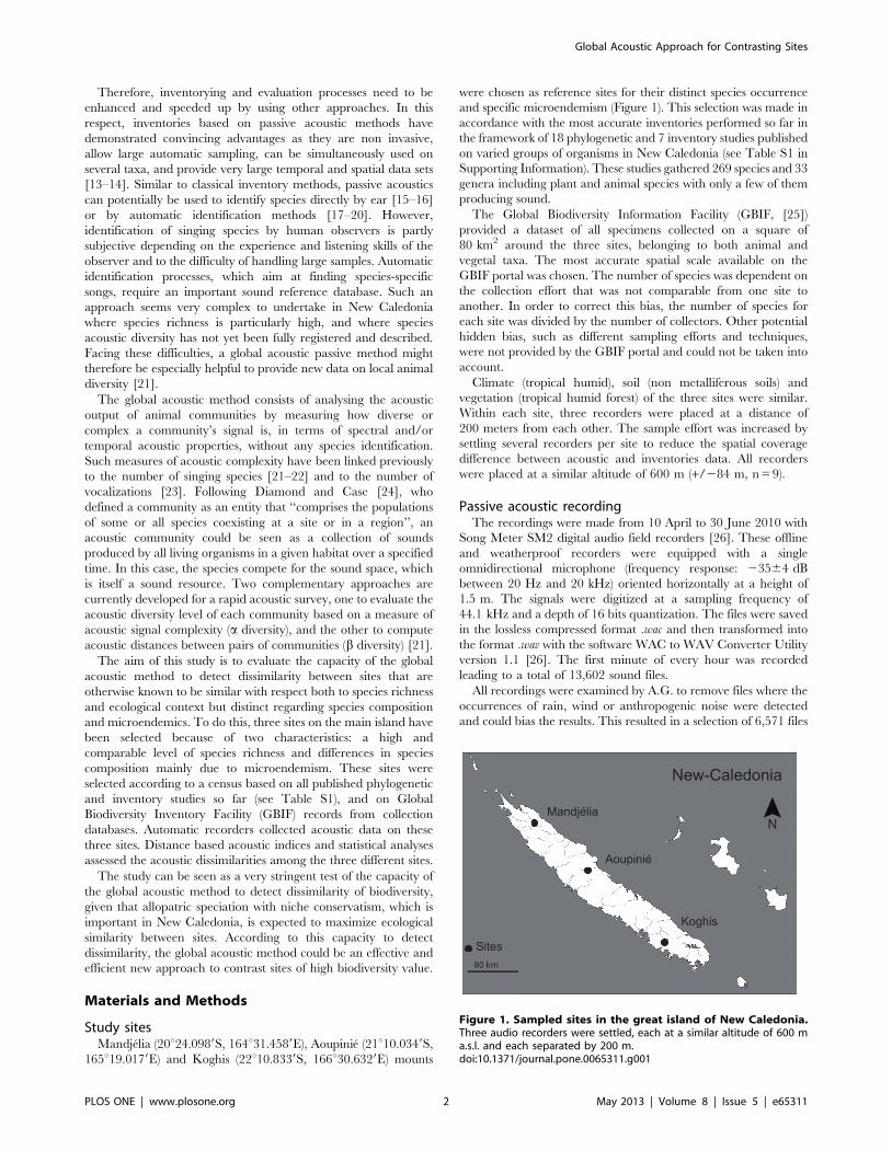
Study sitesMandjelia (20u24.0989S, 164u31.4589E), Aoupinie (21u10.0349S,

165u19.0179E) and Koghis (22u10.8339S, 166u30.6329E) mounts

were chosen as reference sites for their distinct species occurrence

and specific microendemism (Figure 1). This selection was made in

accordance with the most accurate inventories performed so far in

the framework of 18 phylogenetic and 7 inventory studies published

on varied groups of organisms in New Caledonia (see Table S1 in

Supporting Information). These studies gathered 269 species and 33

genera including plant and animal species with only a few of them

producing sound.

The Global Biodiversity Information Facility (GBIF, [25])

provided a dataset of all specimens collected on a square of

80 km2 around the three sites, belonging to both animal and

vegetal taxa. The most accurate spatial scale available on the

GBIF portal was chosen. The number of species was dependent on

the collection effort that was not comparable from one site to

another. In order to correct this bias, the number of species for

each site was divided by the number of collectors. Other potential

hidden bias, such as different sampling efforts and techniques,

were not provided by the GBIF portal and could not be taken into

account.

Climate (tropical humid), soil (non metalliferous soils) and

vegetation (tropical humid forest) of the three sites were similar.

Within each site, three recorders were placed at a distance of

200 meters from each other. The sample effort was increased by

settling several recorders per site to reduce the spatial coverage

difference between acoustic and inventories data. All recorders

were placed at a similar altitude of 600 m (+/284 m, n = 9).

Passive acoustic recordingThe recordings were made from 10 April to 30 June 2010 with

Song Meter SM2 digital audio field recorders [26]. These offline

and weatherproof recorders were equipped with a single

omnidirectional microphone (frequency response: 23564 dB

between 20 Hz and 20 kHz) oriented horizontally at a height of

1.5 m. The signals were digitized at a sampling frequency of

44.1 kHz and a depth of 16 bits quantization. The files were saved

in the lossless compressed format .wac and then transformed into

the format .wav with the software WAC to WAV Converter Utility

version 1.1 [26]. The first minute of every hour was recorded

leading to a total of 13,602 sound files.

All recordings were examined by A.G. to remove files where the

occurrences of rain, wind or anthropogenic noise were detected

and could bias the results. This resulted in a selection of 6,571 files

Figure 1. Sampled sites in the great island of New Caledonia.Three audio recorders were settled, each at a similar altitude of 600 ma.s.l. and each separated by 200 m.doi:10.1371/journal.pone.0065311.g001

Global Acoustic Approach for Contrasting Sites


(53% for Aoupinie, 48% for Mandjelia and 49% for Koghis, see

Table S2).

No specific permits were required for the described field studies

because a passive acoustic method was used in an unprotected

public location. This also implies that the study did not involve

endangered or protected species. The acoustic recordings were

deposited in the sound library of the Museum national d’Histoire

naturelle (Paris, France, contact: [email protected]).

Acoustic activity levelA level of acoustic activity was defined as the number of song

types and was assessed by ear by A.G. for each recording. A song

type was identified as any unique acoustic sequence that can be

differentiated by a human ear based on frequency and time-

amplitude features.Three levels were used: (1) ‘‘Moderate to high

activity’’ where more than two different song types were identified,

(2) ‘‘Low activity’’ where one or two different song types occurred,

and (3) ‘‘Null activity’’ where no animal songs could be detected

(see Table S3). This scale was designed to fulfil aural discrimina-

tion constraints on a very large data set (6,571 files). In particular,

it was not possible to clearly distinguish more than two song types

in complex recordings. This characterisation of the acoustic

activity level was also built for an easy use by other potential

observers. The acoustic activity detected was mainly due to bird,

Orthoptera and cicada species, but no species identification was

achieved.

Acoustic complexity index NPA new index was developed to assess acoustic complexity. This

index, named NP for ‘‘Number of Peaks’’, counts the number of

major frequency peaks obtained on a mean spectrum scaled

between 0 and 1. A mean spectrum was obtained for each audio

file by computing a short-time Fourier transform (STFT, non

overlapping window size = 512 samples = 11 ms). A specific

function was developed within the ‘seewave’ package [27] of the

R environment [28] to process the automatic detection of

frequency spectral peaks of each mean spectrum. All peaks of

the spectrum were first detected and then selected using amplitude

and frequency thresholds. The first selection factor was based on

the amplitude slopes of each peak. Only peaks with slopes higher

than 0.01 were kept. The second selection factor was based on

frequency. In cases where consecutive peaks were less than 200 Hz

apart, only the highest peak in amplitude was kept. NP was simply

defined as the number of peaks after detection and selection of

peaks.

Acoustic dissimilarity indexGlobal differences were measured using the acoustic frequency

spectral dissimilarity index, named Df for ‘‘Dissimilarity of

frequencies’’, as defined by Sueur et al. [21]. This index has been

shown to be sensitive to the diversity of the community

assemblages information [29]. Df was computed according to:

Df ~0:5|sum S1(f ){S2(f )j j,

where S1( f )and S2( f ) are the probability mass functions of the

mean spectra of the two recordings to be compared. Each function

was the result of a STFT with a non overlapping window of 512

samples ( = 11 ms).

Df was assessed between all pairs of audio files leading to a

dissimilarity matrix. Each recording was associated with a

recording time, a day, a recorder, and a site. To factor out the

differences between days with different weather conditions, the

differences between each recording were averaged over all

available days leading to a matrix with dimensions 216*216

( = (3 sites * 3 recorders * 24 time periods ) * (3 sites * 3 recorders *

24 time periods)). Then, the matrix was transformed by the

Lingoes approach to reach Euclidean properties [30].

Background noise reductionA preliminary analysis was conducted to test whether differences

between pairs of recordings could be due to different background

noises and not to different biotic sounds. The dissimilarity matrix

obtained solely with recordings with background noise (Null

activity) was analyzed with a Principal Coordinate Analysis

(PCoA) [31] in order to visualize whether the factors ‘‘Site’’

(Figure S1A) and ‘‘Time’’ (Figure S1B) could explain the acoustic

variability, and to identify which factor was the most important in

explaining the acoustic differences observed. Each point projected

in the resulting multidimensional space represented one recorder

at one recording time. The role of the ‘‘Site’’ and ‘‘Time’’ factors

in explaining the acoustic differences between sites due to

background noise was evaluated with a distance-based Redun-

dancy Analysis (dbRDA) [32] applied on the acoustic dissimilarity

matrix. Associated to the dbRDA, a permutation test was applied

with 1,000 permutations considering each factor independently.

This ensured that the permutations used to test the factor ‘‘Site’’,

were constrained by the factor ‘‘Time’’ and vice versa. The dbRDA

results highlighted differences between sites when considering only

files with noise (p = 0.001, Figure S1C). To check that these

differences between sites were not due to time differences, the

dbRDA associated to the permutation test was also applied with

the factor ‘‘Time’’ (p = 0.437, Figure S1D). These preliminary

results led to the application of a filtering process on all files to

remove the noise associated to the sites as much as possible before

calculating the acoustic indices. For each site, all recordings with

null activity were selected and averaged to obtain the mean

spectrum of ambient noise that was computed using a STFT based

on a non-overlapping sliding function window of 512 samples

( = 11 ms). The mean spectrum of each file was subtracted by the

mean spectrum of ambient noise of the local site. This subtraction

was weighted by the amplitude level of each recording as follows:

Sc(f )~M|S(f ){MiSni(f ),

where Sc( f ) is the probability mass function of the mean spectrum

corrected, S( f ) is the probability mass function of the original

mean spectrum, Sni( f ) is the probability mass function of the mean

spectrum of the ambient noise of the site i, M the amplitude level

of the recording and Mi the mean of amplitude levels of files

containing ambient noise for the site i. The amplitude level

parameter M was obtained following:

M~median(A(t))|2(1{depth) with 0vMv1,

where A(t) is the amplitude envelope and depth is signal

quantization (here, 16 bits). Only the files with ‘‘Moderate to

high activity’’ and ‘‘Low activity’’ were kept for subsequent

analyses.

Statistical analysesIn order to evaluate the reliability of NP in revealing the acoustic

activity detected by ear, the distribution of NP values measured

before ambient noise reduction were compared between pairwise

groups of activity level (moderate to high activity, low activity, null

activity) with a non parametric Mann-Whitney test with a Holm



correction for multiple tests. The same procedure was carried out

to test the differences between NP values among sites, measured on

spectra after ambient noise reduction.

The two factors ‘‘Site’’ and ‘‘Time’’ were considered to explain

the acoustic variability contained in the dissimilarity matrix values.

First, a PCoA and then, a dbRDA permutation test (1000

permutations) considering each factor independently, were applied

as explained above (see Background reduction section). In order to

quantify the acoustic differences between each pair of sites, the

Euclidean distances of the barycentre of the points associated to

the three levels of the factor ‘‘Site’’ were calculated, which

corresponds to Rao’s disc coefficient of dissimilarity between sites

[33–34].

A last step was made to validate the PCoA and dbRDA results

considering the factor ‘‘Site’’. To ensure that these results were not

biased by an unbalanced number of recordings per hour for each

site, due to recordings being discarded because of bad weather

conditions, the analyses were done a second time on a balanced

subsample of hours from the averaged dissimilarity matrix. Six

hours (1, 3, 4, 18, 20 and 21 h) with balanced samples were

selected. The dimension of this submatrix was 54*54 ( = (3 sites * 3

recorders * 6 time periods) * (3 sites * 3 recorders * 6 time

periods)). This submatrix was analysed with a dbRDA with site as

a factor. The results were compared with the complete dissimi-

larity matrix with all hours included.

A final analysis was performed to detail the frequency spectral

differences between the three sites. The dbRDA was used to

potentially highlight acoustic differences between sites but was

considered inappropriate to provide details regarding these

differences. A specific analysis was developed to identify the

frequency bins where differences occur. As already described, the

mean spectrum was composed of 256 frequency bins and the Df

index was the sum of these 256 differences between two mean

spectra. Here, the 256 frequency bin differences calculated were

not summed up but analysed independently. Instead of a single Df

matrix, 256 matrices were analysed, one for each frequency bin.

For each frequency bin, a between-site distance value was

computed with the Rao’s disc coefficient from the 256 matrices.

This between-site distance was compared with the distribution of

frequency peaks obtained for all sites.

All statistical analyses were performed with the R software

including the package ‘ade4’ [35].

Results

Phylogenetic and GBIF dataFrom the 18 phylogenetic and 7 inventory datasets analysed, the

percentage of microendemics calculated was 12.50% for Mandje-

lia, 15.38% for Aoupinie and 23.73% for Koghis. From the GBIF

data , the ratio of endemic species to the number of collectors was

4.89 for Mandjelia, 3.76 for Aoupinie and 4.71 for Koghis.

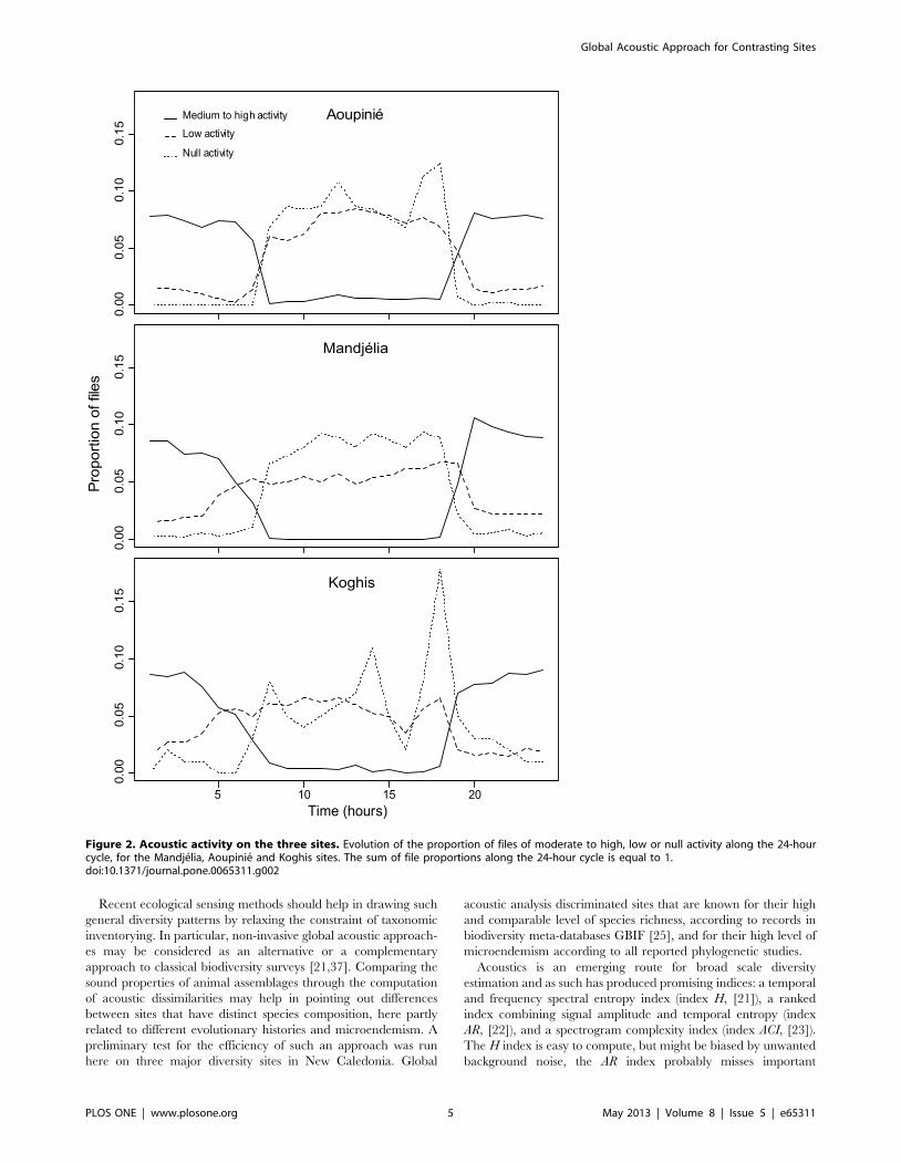
Acoustic activity levelThe acoustic activity level determined by ear showed variations

along the 24-hour cycle (Figure 2). The recordings with high

activity mainly occurred from 19 h to 7 h, whereas files with low

and medium activity mainly occurred from 7 h to 18 h.

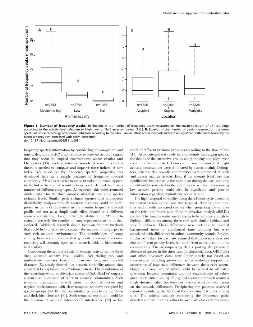
The comparison between the level of animal activity determined

by ear and the number of frequency peaks measured on the mean

spectrum before ambient noise reduction highlighted an increase

of NP with the level of animal activity (p,0.0001, Figure 3A). NP

did not differ significantly between the three sites (Aoupinie-

Mandjelia: p = 0.96; Aoupinie-Koghis: p = 0.17; Mandjelia-

Koghis: p = 0.57, Figure 3B).

Acoustic dissimilarityThe PCoA showed that the acoustic variability could first be

explained by the factor ‘‘Time’’, and then by the factor ‘‘Site’’.

The acoustic variability explained by the two first axes was

associated with the factor ‘‘Time’’ (Figure 4A; axis 1: 1.92% and

axis 2: 1.33% of variability explained). The first axis separated the

night and day periods, whereas the second axis separated the

middle of the day from the remaining hours of the 24-hour cycle.

Hours were organized successively around the 24-hour rhythm.

Axes 3 and 4 explained the variability due to the factor ‘‘Site’’

(Figure 4B; axis 3: 1.28% and axis 4: 1.12% of variability

explained), independent of the variability already explained by

axes 1 and 2. Mandjelia and Koghis appeared closer to each other

than to Aoupinie as shown by a major overlap of the inertia

ellipses. However, the rather flat distribution of eigenvalues

indicated that the first four axes do not explain the entire

variability.

This approach was thus complemented by the dbRDA, which

was first applied with the factor ‘‘Time’’ and then with the factor

‘‘Site’’. This analysis validated the fact that the two factors could

explain the acoustic distances variability (effect of difference

among hours R2 = 0.852 for the first axis, R2 = 0.911 for second

axis, and effect of differences among sites R2 = 0.863 for the first

axis and R2 = 0.726 for the second axis; the third and fourth axes

were independent of the first and second axes displaying temporal

tendencies). Both axes fully discriminate the recording samples as a

function of ‘‘Time’’ (Figure 5A) and ‘‘Site’’ (Figure 5B). The sites

and hours were significantly different as shown by the dbRDA

tests (p = 0.001 for both). A dbRDA was computed on a subset of

the original data consisting of balanced samples. This dbRDA

showed a similar full discrimination of sites (p = 0.001, see Figure

S2) indicating that site discrimination, observed on the original

matrix (216*216, Figure 5B), could not be due to unbalanced

samples. Rao’s coefficient of dissimilarity was 0.36 between

Aoupinie and Mandjelia, 0.36 between Aoupinie and Koghis,

and 0.33 between Mandjelia and Koghis. These results indicate

that the three sites were acoustically distinct and were roughly at

even acoustic distances.

The distribution of the frequency peaks detected on all

recordings covered almost all the frequency range sampled, from

0.043 to 22.05 kHz (Figure 6). The distribution showed six main

modes, around 0.5 kHz, 1.3 kHz, 4 kHz, 10 kHz, 11.5 kHz and

14.5 kHz respectively (Figure 6, grey histogram). The between-site

distance based on the Df index showed important variations

corresponding to the first three modes of the frequency peak

distribution, i.e. around 0.5 kHz, 1.3 kHz, and 4 kHz (Figure 6,

plain line).

Discussion and Conclusions

Biodiversity distribution can be considered at nested temporal

and spatial scales, from a broad (e.g. continental) to a narrow (e.g.

a local altitudinal transect) scale [36]. However, describing such

patterns requires the collection of considerable field-based data

sets. These data are especially difficult to obtain in regions that are

megadiverse and where species are under severe extinction threat,

the so-called biodiversity hotspots [1–2]. From this point of view,

New Caledonia shows an extremely high level of species richness

and microendemism that is not yet sufficiently understood for

efficient conservation efforts [3]. In such rich ecosystems, all local

research on biodiversity from evolutionary biology to ecosystem

management relies on classical species inventories that are time

consuming and constrained by the availability of taxonomic

expertise [9].



Recent ecological sensing methods should help in drawing such

general diversity patterns by relaxing the constraint of taxonomic

inventorying. In particular, non-invasive global acoustic approach-

es may be considered as an alternative or a complementary

approach to classical biodiversity surveys [21,37]. Comparing the

sound properties of animal assemblages through the computation

of acoustic dissimilarities may help in pointing out differences

between sites that have distinct species composition, here partly

related to different evolutionary histories and microendemism. A

preliminary test for the efficiency of such an approach was run

here on three major diversity sites in New Caledonia. Global

acoustic analysis discriminated sites that are known for their high

and comparable level of species richness, according to records in

biodiversity meta-databases GBIF [25], and for their high level of

microendemism according to all reported phylogenetic studies.

Acoustics is an emerging route for broad scale diversity

estimation and as such has produced promising indices: a temporal

and frequency spectral entropy index (index H, [21]), a ranked

index combining signal amplitude and temporal entropy (index

AR, [22]), and a spectrogram complexity index (index ACI, [23]).

The H index is easy to compute, but might be biased by unwanted

background noise, the AR index probably misses important

Figure 2. Acoustic activity on the three sites. Evolution of the proportion of files of moderate to high, low or null activity along the 24-hourcycle, for the Mandjelia, Aoupinie and Koghis sites. The sum of file proportions along the 24-hour cycle is equal to 1.doi:10.1371/journal.pone.0065311.g002



frequency spectral information by considering only amplitude and

time scales, and the ACI is not sensitive to constant acoustic signals

that may occur in tropical environments where cicadas and

Orthoptera [38] produce sustained sounds. A research effort is

therefore needed to compare and improve these indices. A new

index, NP, based on the frequency spectral properties was

developed here as a simple measure of frequency spectral

complexity. NP is less sensitive to ambient noise and would appear

to be linked to animal sound activity level, defined here as a

number of different song types. As expected, this index returned

similar values for the three sampled sites that have close species

richness levels. Similar peak richness ensures that subsequent

dissimilarity analyses through acoustic distances could be inter-

preted in terms of differences in the acoustic frequency spectral

profile and not as a simple scale effect related to a different

acoustic activity level. To go further, the ability of the NP index to

estimate precisely the number of song types needs to be further

explored. Additional research should focus on the new methods

that could help to estimate accurately the number of song types in

such rich acoustic environments. The identification of songs

coming from several species that generate a complex acoustic

recording will certainly open new research fields in bioacoustics

and ecology.

Considering the temporal scale of acoustic activity on the three

sites, acoustic activity level profiles (NP) during day and

multivariate analyses based on pairwise frequency spectral

distances (Df) clearly showed that acoustic variability among sites

could first be explained by a 24-hour pattern. The distribution of

the recordings within multivariate spaces (PCoA, dbRDA) suggests

a structured succession of different acoustic communities. Such

temporal organization is well known in both temperate and

tropical environments with clear temporal windows occupied by

specific groups [39–40], the best-studied periods being the dawn

and dusk bird choruses [41]. Such temporal separation could be

the outcome of acoustic inter-specific interference [42] or the

result of different predator pressures according to the time of day

[43]. As no attempt was made here to identify the singing species,

the details of the successive groups along the day and night cycle

could not be estimated. However, it was obvious that night

acoustic communities were dominated by insects, mainly Orthop-

tera, whereas day acoustic communities were composed of birds

and insects such as cicadas. Even if the acoustic level here was

significantly higher during the night than during the day, sampling

should not be restricted to the night period as information during

low activity periods could also be significant and provide

information regarding dissimilarity between sites.

The high temporal variability along the 24-hour cycle overcame

the spatial variability that was first targeted. However, the three

sites undoubtedly appeared distinct when projecting the samples

on the third and fourth axes of the multivariate analysis (dbRDA

results). The rapid acoustic survey seems to be sensitive enough to

highlight differences among three sites with similar habitats and

specific richness. These differences were not due to residual

background noise or unbalanced time sampling but were

associated with differences in animal community sounds. Besides,

similar NP values for each site ensured that differences were not

due to different activity levels, but to different acoustic community

compositions. The accompanying data reporting the presence/

absence of species in the three sites (phylogenetic data, GBIF data

and other inventory data) were unfortunately not based on

standardized sampling protocols, but nevertheless support the

occurrence of important differences between the species assem-

blages, a strong part of which could be related to allopatric

speciation between mountains and the establishment of subse-

quent microendemism [3]. The global acoustic approach returns a

single distance value, but does not provide accurate information

on the acoustic differences. Deciphering the patterns observed

requires identifying the bands of the spectrum that differ among

sites. The original analysis comparing the frequency peaks

detected and the distance values between sites for each frequency

Figure 3. Number of frequency peaks. A: Boxplot of the number of frequency peaks measured on the mean spectrum of all recordingsaccording to the activity level (Medium to High, Low or Null) assessed by ear (A.G.). B: Boxplot of the number of peaks measured on the meanspectrum of the recordings after noise reduction according to the sites. Similar letters above boxplots indicate no significant differences found by theMann-Whitney test corrected with Holm correction.doi:10.1371/journal.pone.0065311.g003



revealed that most of the acoustic differences were occurring over

a sharp frequency band below 7 kHz. This 7 kHz limit might be

peculiar to our study and should not be blindly considered as a

reference threshold for other studies. Interpreting these acoustic

differences in details would require a perfect and exhaustive

knowledge of singing species which is unfortunately outside the

scope of the present study and actually highly difficult to reach in

such a megadiverse region. Numerous insect and bird species

endemic to New Caledonia can produce sound but the Agnotecous

cricket genus was the single microendemic species producing song

in the phylogenetic studies (see Table S1). Agnotecous species are

known to produce sound above 9 kHz with a dominant frequency

between 12 and 19 kHz, well above the 7 kHz threshold

mentioned above [44–45]. The global acoustic method seems

unable to detect the differences potentially due to the Agnotecous

species as the distance value between sites was flat at this frequency

range. This effect might be due to a frequency turnover from one

Figure 4. Principal Coordinate Analysis (PCoA) on the acousticdissimilarity matrix. A: Eigenvalue bar plot. B: Results of PCoAapplied to the acoustic dissimilarities among recordings with factor‘‘Time’’ as a supplementary variable subsequently projected on themap. Projection along the axes 1 and 2. C: Results of PCoA applied tothe acoustic dissimilarities among recordings with the spatial factor‘‘Site’’ (A: Aoupinie, K: Koghis, M: Mandjelia). Projection along the axes 3and 4. The dispersion ellipses surround the position of a time period(Figure 4A) or of a site (Figure 4B) providing an index of the dispersionaround the time/site centroid (67% of recordings collected at a giventime or at a site are expected to be in the associated ellipse).doi:10.1371/journal.pone.0065311.g004

Figure 5. Distance-based ReDundancy Analysis (dbRDA). A:Results of dbRDA applied to the acoustic distances among recordings,with factor ‘‘Time’’ as an explanatory variable. B: Results of dbRDAapplied to the acoustic distances among recordings, with factor ‘‘Site’’as an explanatory variable (A: Aoupinie, K: Koghis, M: Mandjelia). Thelength of the arrows represents residuals: each arrow connects theposition of a recording predicted by the time in which it was done orthe site in which it was done (where the arrow starts) to its real positionbased on raw data (real acoustic composition where the arrow ends).doi:10.1371/journal.pone.0065311.g005



Agnotecous species to another, on a similar frequency range. However,

since most birds, Orthoptera and cicada species sing below 8 kHz, the

threshold of biophony assessment in soundscape ecology [46], this

could explain the between-site acoustic differences. New Caledonia

counts 183 bird species including 23 regional endemics [47]. Due to

their high dispersion level, birds could not be considered as narrow

microendemics such as insects, lizards or plants species, limited to one

small mountain. However, some bird species were described as being

restricted to a part of the island as in the case of eleven species of birds

inventoried in New Caledonia [48–49]. This could partially explain the

between-site acoustic differences. Unfortunately, other singing groups

(e.g., Orthoptera or cicadas) are too poorly known in the island and this

prevents making detailed interpretations about the differences observed

in this study.

As in the case of any other sampling methods, acoustic sampling

method may be biased in some cases. For example, the distances

between the targeted individuals and the sampling device (here the

microphone), the vegetation structure or the individual behaviour

(here the singing repertoire) could have an impact on the value

calculated from the sample (here the acoustic indices). Massive

sampling as the one done here (more than 6 000 samples) should,

however, buffer such biases. As demonstrated in preliminary

analyses, different background noises could generate significant

differences between sites and lead to biased results. An appropriate

processing of background noise is therefore decisive when

undertaking acoustic comparisons. The question of acoustic bias

for a rapid acoustic survey method should be estimated in

controlled environments in further research programmes.

Overall, even if the global acoustic approach was limited to

three sites with three points per site, it nevertheless has the

potential of revealing compositional differences between sites and

could therefore help in conservation management. Such a clear

message from acoustics was not trivial as the sites showed a low

level of ecological differentiation, and produced an equivalent

acoustic activity level, under similar environmental parameters.

These first results need to be supported by other study cases, but

they open up new possibilities for biodiversity estimation and

monitoring on a large scale. Numerous recorders could be deployed

over a vast territory covering different sites and habitats. Such a

global acoustic sampling could be achieved quite quickly and could

be especially useful in hotspots where exploring biodiversity is an

urgent task and where inventorying the diversity is very difficult

because it has to rely on long-term sampling by experts.

Microendemism is a well-identified challenge for local conservation

policies, which requires an improvement in the number, size and

quality of protected areas [9,50]. Detecting dissimilarity and

complementarity between sites could help in delimiting areas to

conserve and the rapid acoustic survey would appear to be a

pertinent approach as it is non-invasive and is a large-scale method.

Supporting Information

Figure S1 Acoustic differences between the ambientnoises of the three sites. The ambient noises coming from the

different sites measured on files with null animal activity. A:

Results of Principal Coordinate Analysis (PCoA) applied to the

acoustic dissimilarities among recordings with factor ‘‘Site’’ as a

supplementary variable subsequently projected on the map (A:

Aoupinie, K: Koghis, M: Mandjelia). B: Results of PCoA applied

to the acoustic dissimilarities among recordings, with factor

‘‘Hours’’ as a supplementary variable subsequently projected on

the map. C: results of Distance-based ReDundancy Analysis

(dbRDA) applied to the acoustic dissimilarities among recordings,

with factor ‘‘Site’’ as an explanatory variable (A: Aoupinie, K:

Koghis, M: Mandjelia). D: Results of dbRDA applied to the

acoustic dissimilarities among recordings, with factor ‘‘Hour’’ as

an explanatory variable. The dispersion ellipses surround the

position of a site (Figure S1A) or of a time period (Figure S1B)

providing an index of the dispersion of recording points around

the site/time centroids (67% of recordings collected at a given time

or at a site are expected to be in the associated ellipse).

(EPS)

Figure 6. Histogram of the frequency used among all recordings. For each frequency, the value is the number of times that this frequencyappeared as a peak among the mean spectra. The line is the difference measured between sites for each frequency.doi:10.1371/journal.pone.0065311.g006



Figure S2 Acoustic differences between sites measuredon a balanced sub-sample of hours. Results of Distance-

based ReDundancy Analysis (dbRDA) measured on a balanced

sub-sample of hours, applied to the acoustic dissimilarities among

recordings, with factor ‘‘Site’’ as an explanatory variable (A:

Aoupinie, K: Koghis, M: Mandjelia).

(EPS)

Table S1 Data describing the biodiversity of the threesites through 14 genera and 4 families. Since these data

come from phylogenies and inventories based on different

geographical sampling, specimens are not sampled in every site.

The main number determines the presence or absence of the taxa

on the site, whereas the number in parenthesis determines whether

the authors sampled on the site (1) or not (0).

(DOC)

Table S2 Number and percentage of files associated todifferent noise types and number of files after exclusionof the noisy files for each site.(DOC)

Table S3 Number and percentage of files with differentactivity levels for each site after the exclusion of noisyfiles.(DOC)

Acknowledgments

We would like to thank Christian Mille for elements of bibliography of

New Caledonia. We would like to thank Herve Jourdan and Edouard

Bourguet for their help when collecting the acoustic data. We thank Dr.

James F. C. Windmill (University of Strathclyde, Glasgow) and Dr. Yoland

Savriama (St. John’s University, New York) and Theresa Murtagh for

improving the language of the manuscript. We would like to thank the two

anonymous referees and Alex Kirschel for their helpful comments on the

manuscript.

Author Contributions

Conceived and designed the experiments: AG JS SP PG. Performed the

experiments: AG PG. Analyzed the data: AG SP JS. Contributed reagents/

materials/analysis tools: AG JS SP RP PG. Wrote the paper: AG JS SP RP

PG.

References

1. Myers N, Mittermeier RA, Mittermeier CG, da Fonseca GA, Kent J (2000).

Biodiversity hotspots for conservation priorities. Nature 403: 853–8.

2. Kier G, Kreft H, Lee TM, Jetz W, Ibisch PL, et al. (2009) A global assessment of

endemism and species richness across island and mainland regions. Proc Natl

Acad Sci USA 23: 9322–9327.

3. Grandcolas P, Murienne J, Robillard T, Desutter-Grandcolas L, Jourdan H,

et al. (2008) New Caledonia: A very old Darwinian island? Philos

Trans R Soc B Biol Sci 363: 3309–3317.

4. Pillon Y, Munzinger J, Amir H, Lebrun M (2010) Ultramafic soils and species

sorting in the flora of New Caledonia. J Ecol 98: 1108–1116.

5. Nattier R, Robillard T, Desutter-Grandcolas L, Couloux A, Grandcolas P (2011)

Older than New Caledonia emergence? A molecular phylogenetic study of the

eneopterine crickets (Orthoptera: Grylloidea). J Biogeogr 38: 2195–2209.

6. Murienne J, Pellens R, Budinoff RB, Wheeler WC, Grandcolas P (2008)

Phylogenetic analysis of the endemic New Caledonian cockroach Lauraesilpha.

Testing competing hypotheses of diversification. Cladistics 24: 802–812.

7. Murienne J, Guilbert E, Grandcolas P (2009). Species diversity in the New

Caledonian endemic genera Cephalidiosus and Nobarnus (Insecta: Heteroptera:

Tingidae), an approach using phylogeny and species distribution modeling.

Biol J Linn Soc Lond 97: 177–184.

8. Espeland M, Johanson KA (2010) The effect of environmental diversification on

species diversification in New Caledonian caddisflies (Insecta: Trichoptera:

Hydropsychidae). J Biogeogr 37: 879–890.

9. Pellens R, Grandcolas P (2010) Conservation and management of the

biodiversity in a hotspot characterized by short range endemism and rarity:

the challenge of New Caledonia. In: Rescigno V, Maletta S, editors. Biodiversity

Hotspots. New York: Nova Science Publishers. pp. 139–151.

10. Nattier R, Grandcolas P, Elias M, Desutter-Grandcolas L, Jourdan H, et al.

(2013) Secondary sympatry caused by range expansion informs on the dynamics

of microendemism in New Caledonia. PLoS ONE 7(11): e48047.

11. Faith DP, Walker PA (1996) How do indicator groups provide information

about the relative biodiversity of different sets of areas? On hotspots,

complementarity and pattern-based approaches. Biodiversity Letters 3: 18–25.

12. Margules CR, Pressey RL (2000) Systematic conservation planning. Nature 405:

243–253.

13. Acevedo MA, Villanueva-Rivera LJ (2006) Using automated digital recording

systems as effective tools for the monitoring of birds and amphibians. Wildlife

Society Bulletin 34: 211–214.

14. Wimmer J, Towsey M, Planitz B, Williamson I, Roe P (2012) Analysing

environmental acoustic data through collaboration and automation. Future

Gener Comput Syst 29: 560–568.

15. Riede K (1993) Monitoring Biodiversity: analysis of Amazonian Rainforest

Sounds. Ambio 22: 546–548.

16. Dawson DK, Efford MG (2009) Bird population density estimated from acoustic

signals. J Appl Ecol 46: 1201–1209.

17. Brandes TS (2008) Automated sound recording and analysis techniques for bird

surveys and conservation. Bird Conservation International 18: S163–S173.

18. Acevedo MA, Corrada-Bravo CJ, Corrada-Bravo H, Villanueva-Rivera LJ, Aide

TM (2009) Automated classification of bird and amphibian calls using machine

learning: A comparison of methods. Ecol Inform 4: 206–214.

19. Han NC, Muniandy SV, Dayou J (2011) Acoustic classification of Australian

anurans based on hybrid spectral-entropy approach. Applied Acoustics 72: 639–

645.

20. Towsey M, Planitz B, Nantes A, Wimmer J, Roe P (2012) A toolbox for animal

call recognition. Bioacoustics 2: 107–125.

21. Sueur J, Pavoine S, Hamerlynck O, Duvail S (2008) Rapid Acoustic Survey for

Biodiversity Appraisal. PLoS ONE 3: e4065.

22. Depraetere M, Pavoine S, Jiguet F, Gasc A, Duvail S, et al. (2012) Monitoring

animal diversity using acoustic indices: Implementation in a temperate

woodland. Ecol Indic 13: 46–54.

23. Pieretti N, Farina A, Morri D (2011) A new methodology to infer the singing

activity of an avian community: The Acoustic Complexity Index (ACI). Ecol

Indic 11: 868–873.

24. Diamond J, Case TJ (1986) Community Ecology. New York: Harper and Row.

407 .

25. GBIF (2012) GBIF data portal from: http://data.gbif.org/welcome.htm.

26. Wildlife Acoustics, Inc. Bioacoustics Software and Field Recording Equipment

website. Available: http://www.wildlifeacoustics.com/. Accessed 2010 May 26.

27. Sueur J, Aubin T, Simonis C (2008) Seewave, a free modular tool for sound

analysis and synthesis. Bioacoustics 18: 213–226.

28. R Development Core Team R (2010) A language and environment for statistical

computing. Vienna: R Foundation for Statistical Computing. 409 p.

29. Gasc A, Sueur J, Jiguet F, Devictor V, Grandcolas P, et al. (2013) Assessing

biodiversity with sound: do acoustic diversity indices reflect phylogenetic and

functional diversities of bird communities? Ecological Indicators 25: 279–287.

30. Lingoes JC (1971) Some Boundary Conditions for a Monotone Analysis of

Symmetric Matrices. Psychometrika 36: 195–203.

31. Gower JC (1966) Some Distance Properties of Latent Root and Vector Methods

Used in Multivariate Analysis. Biometrika 53: 325–338.

32. Legendre P, Anderson MJ (1999) Distance-based redundancy analysis: Testing

multispecies responses in multifactorial ecological experiments. Ecol Monogr 69:

512–512.

33. Rao CR (1982) Diversity and dissimilarity coefficients: a unified approach.

Theor Popul Biol 21: 24–43.

34. Pavoine S, Dufour AB, Chessel D (2004) From dissimilarities among species to

dissimilarities among communities: a double principal coordinate analysis.

J Theor Biol 228: 523–537.

35. Dray S, Dufour AB (2007) The ade4 package: implementing the duality diagram

for ecologists. J Stat Softw 22: 1–20.

36. Cox CB, Moore PD (2005) Biogeography: an ecological and evolutionary

approach. Oxford: Blackwell Science Ltd. 506 p.

37. Sueur J, Gasc A, Grandcolas P, Pavoine S (2012) Global estimation of animal

diversity using automatic acoustic sensors. In: Le Gaillard JF, Guarini JM, Gaill

F, editors. Sensors for ecology. Paris: CNRS. pp. 99–117.

38. Boulard M (2006) Acoustic Signals, Diversity and Behaviour of cicadas (Cicadae,

Hemiptera).In: Drosopoulos S, Claridge MF, editors. Insect sounds and

communication, physiology, behaviour, ecology and evolution. Boca raton:

Taylor and Francis. pp. 331–350.

39. Riede K (1997) Bioacoustic monitoring of insect communities in Bornean

rainforest canopy. In: Stork NE, Adis JA, editors. Canopy Arthropods. London:

Chapman & Hall. pp. 442–452.

40. Mann D, Locascio J, Coleman F, Koenig C (2009) Goliath grouper Epinephelus

itajara sound production and movement patterns on aggregation sites. Endanger

Species Res 7: 229–236.

41. Henwood K, Fabrick A (1979) A quantitative analysis of the dawn chorus:

temporal selection for communicatory optimization. Am Nat 114: 260–274.



42. Ficken RW, Popp JW, Matthiae PE (1985) Avoidance of acoustic interference by

ovenbirds. Wilson Bulletin 97: 569–571.

43. Heller KG, Von Helversen D (1993) Calling Behavior in Bush-Crickets of the

Genus Poecilimon with Differing Communication-Systems (Orthoptera, Tettigo-

nioidea, Phaneropteridae). J Insect Behav 6: 361–377.

44. Desutter-Grandcolas L, Robillard T (2006) Phylogenetic systematics and

evolution of Agnotecous in New Caledonia (Orthoptera : Grylloidea, Eneopter-

idae). Syst Entomol 31: 65–92.

45. Robillard T, Nattier R, Desutter-Grandcolas L (2010) New species of the New

Caledonian endemic genus Agnotecous (Orthoptera, Grylloidea, Eneopterinae,

Lebinthini). Zootaxa 2559: 17–35.

46. Pijanowski BC, Villanueva-Rivera LJ, Dumyahn SL, Farina A, Krause BL, et al.

(2011). Soundscape Ecology: The science of Sound in the Landscape Bioscience61: 203–216.

47. Desmoulins F, Barre N (2005) Oiseaux des forets seches de Nouvelle-Caledonie.

Paıta: IAC-Programme foret seche. 105 p.48. Boncoraglio G, Saino N (2007) Habitat structure and the evolution of bird song:

a meta-analysis of the evidence for the acoustic adaptation hypothesis. FunctEcol 21: 134–142.

49. Ey E, Fischer J (2009) The ‘‘Acoustic Adaptation Hypothesis’’ - a Review of the

Evidence from Birds, Anurans and Mammals. Bioacoustics 19: 21–48.50. Jaffre T, Munzinger J, Lowry PP (2010) Threats to the conifer species found on

New Caledonia’s ultramafic massifs and proposals for urgently needed measuresto improve their protection. Biodivers Conserv 19: 1485–1502.



Gasc A, Sueur J, Pavoine S, Pellens R, Grandcolas P (2013) Biodiversity sampling using a global...

Documents

Transcript of Gasc A, Sueur J, Pavoine S, Pellens R, Grandcolas P (2013) Biodiversity sampling using a global...