Volume II Issue 1(3) Summer 2011

5

GAME COMPLETE ANALYSIS OF BERTRAND DUOPOLY

David CARFÌ Faculty of Economics, Department DESMAS

University of Messina, Italy davidcarfi71@yahoo.it Emanuele PERRONE Faculty of Economics

University of Messina, Italy e_perrone@alice.it

Abstract:

In this paper we apply the Complete Analysis of Differentiable Games [introduced by D. Carfì in (Carfi 2010), (Carfi 2009), (Carfi 2009), and (Carfi 2009)] and already employed by himself and others in (Carfi 2011), (Carfi 2010), (Carfi 2009)] to the classic Bertrand Duopoly (1883), classic oligopolistic market in which there are two enterprises producing the same commodity and selling it in the same market. In this classic model, in a competitive background, the two enterprises employ as possible strategies the unit prices of their product, contrary to the Cournot duopoly, in which the enterprises decide to use the quantities of the commodity produced as strategies. The main solutions proposed in literature for this kind of duopoly (as in the case of Cournot duopoly) are the Nash equilibrium and the Collusive Optimum, without any subsequent critical exam about these two kinds of solutions. The absence of any critical quantitative analysis is due to the relevant lack of knowledge regarding the set of all possible outcomes of this strategic interaction. On the contrary, by considering the Bertrand Duopoly as a differentiable game (games with differentiable payoff functions) and studying it by the new topological methodologies introduced by D. Carfì, we obtain an exhaustive and complete vision of the entire payoff space of the Bertrand game (this also in asymmetric cases with the help of computers) and this total view allows us to analyze critically the classic solutions and to find other ways of action to select Pareto strategies. In order to illustrate the application of this topological methodology to the considered infinite game, several compromise pricing-decisions are considered, and we show how the complete study gives a real extremely extended comprehension of the classic model.

Keywords: duopoly, normal form games, microeconomic policy, complete study, bargaining solutions. JEL Classification: D7, C71, C72, C78

1. Introduction

We consider a duopoly (1, 2) with production fixed cost f and production variable cost a function v of the produced quantity, for both the producers; we shall assume the function v equal 0.

The demand for enterprise 1 is the affine reaction function Q1, from the Euclidean plane of price bi-strategies R2 into the real line of quantities to be produced R – the demand Q1 (p) is the aggregate reaction of consumers in the market to the pair p of prices imposed by the two enterprises (see for a general theory of reactions (Carfi, and Ricciardello 2009), (Carfi 2009), (Carfi 2009), (Carfi, and Ricciardello 2011) - defined by:

Q1(p) = b + a1p1 + a2p2 (1.1) that is by the equality Q1(p) = b + (a|p), (1.2) for every pair of prices p, where a is a pair of real numbers whose first component is negative and whose

second component is positive, where b is a non-negative real and where (a|p) is the standard Euclidean scalar product of the two vectors a and p.

The components of the pair p are determined by the two enterprises 1 and 2, respectively. The demand for the enterprise 2 is the function Q2 defined, in a perfectly analogous way as the first one,

by Q2(p) = b + a1p2 + a2p1, that is (1.3) Q2(p) = b + (a-|p), (1.4) for every pair of prices p, where a- is the symmetric pair of a.

Theoretical and Practical Research in Economic Fields

6

The classic way to solve the duopoly (see for instance: Davide Vannoni, and Massimiliano Piacenza, University of Torino, Faculty of Economics, Appunti di Microeconomia - Corso C - Lezione 10, A. A. 2009/2010) is to determine the curves of best price reaction, for example, for enterprise 1, we consider the profit function P1 defined by

P1 (p1,q1) = p1q1 – f (1.5) that, on the reaction demand function Q1, assumes the form g1(p) = P1 (p1 ,Q1 (p)) = p1(b + a1p1 + a2p2) – f, (1.6) for every price p2, fixed by the enterprise 2, the price of maximum profit for enterprise 1 must satisfy the

following stationary condition D1(g1)(p) = b + 2a1p1 + a2p2 = 0. (1.7) We note that the second derivative of the function g1( . ,p2) is negative ( 2a1 < 0), hence the above

stationary condition is not only necessary but also sufficient in order to obtain maxima, we so determine the classic reaction curve of enterprise 1, the line of equation

p1 = b/(2a1) + p2a2/(2a1). (1.8) Symmetrically, the reaction curve of enterprise 2 is the line p2 = b/(2a1) + p1a2/(2a1). (1.9) Now, by the intersection of the two reaction curves, we obtain the fixed-point equation p1 = b/(2a1) + (b/(2a1) + p1a2/(2a1))a2/(2a1), (1.10) and so finally we obtain the equilibrium price of the enterprise 1, and the same of enterprise 2: p2 = p1 = - b/(2a1 + a2). (1.11) Another classic solution is the symmetric collusive point C = (c,c) determined by maximization of the

function H defined by H(c) = P1 (c ,Q1 (c,c)) + P2 (c ,Q2 (c,c)) = 2c(b + (a1 + a2)c) – 2f, (1.12) for every c. But also in this case, an accurate analysis of this point is impossible since we do not know the geometry

of the payoff space.

2. Formal Description of Bertrand’s Normal Form Game It will be a non-linear two - players gain game (f, >) (see also (6, Carfì 2009), (8, Carfì 2009), and (9, Carfì

2009). The two players/enterprises shall be called Emil and Frances (following Aubin’s books (Aubin 1982) and (Aubin 1998).

Assumption 1 (strategy sets). The two players produce and offer the same commodity at the following prices: 𝓍 ∊ ℝ≥ for Emil and 𝓎 ∊ ℝ≥ for Frances. In more precise terms: the payoff function f of the game is defined on a subset of the positive cone of the Cartesian plane ℝ2, interpreted as a space of bi-prices. We assume (by simplicity) that the set of all strategies (of each player) is the interval E = [0, +∞].

Assumption 2 (symmetry of the game). The game will be assumed symmetric with respect to the players. In other terms, the payoff pair f(x,y) is the symmetric of the pair f(y,x).

Assumption 3 (form of demand functions). Let the demand function Q1 (defined on E2) of the first player be given by:

Volume II Issue 1(3) Summer 2011

7

Q1(𝓍,𝓎) = 𝓊 - 2𝓍 + 𝓎, (2.1) for every positive price pair (𝓍, 𝓎) and let analogously the demand function of the second enterprise be

given by Q2(𝓍,𝓎) = 𝓊 - 2𝓎 + 𝓍, (2.2) for every positive bi-strategy (𝓍, 𝓎), where u is a positive constant (representing, obviously, the quantity

Qi(0,0) demanded of good i, by the market, when both prices are fixed to be 0). Remark (about elasticity). The demand’s elasticity of the two functions with respect to the corresponding

price is: e1(Q1)(𝓍,𝓎) = ∂1Q1(𝓍,𝓎)(𝓍/Q1(𝓍,𝓎)) = -2𝓍/(𝓊 - 2𝓍 + 𝓎), and (2.3) e2(Q2)(𝓍,𝓎) = ∂2Q2(𝓍,𝓎)(𝓎/Q2(𝓍,𝓎)) = -2𝓎/(𝓊 - 2𝓎 + 𝓍), (2.4) for every positive bi-strategy (𝓍, 𝓎). Their values are negative, according to the economic law: produced quantities are decreasing with

respect to their prices. So, if Emil (or Frances) increases his price, the consumers’ demand will diminish. Assumption 4 (payoff functions). First player’s profit function is defined, classically, by the revenue ƒ1(𝓍,𝓎) = 𝓍 Q1(𝓍,𝓎) – c = 𝓍(𝓊 - 2𝓍 + 𝓎) – c, (2.5) for every positive bi-strategy (𝓍, 𝓎). Symmetrically, for Frances, the profit function is defined by ƒ2(𝓍,𝓎) = 𝓎 Q2(𝓍,𝓎) – c = 𝓎(𝓊 - 2𝓎 + 𝓍) – c, (2.6) for every positive bi-strategy (𝓍, 𝓎), where the positive constant c is the fixed cost. So we assume the

variable cost to be 0 (this is not a great limitation for our example, since our interest is the interaction between the two players and the presence of the variable cost does not change our approach).

The bi-gain function is so defined by ƒ(𝓍,𝓎) = (𝓍(𝓊 - 2𝓍 + 𝓎), 𝓎(𝓊 - 2𝓎 + 𝓍)) – (c, c), (2.7) for every bi-strategy (𝓍, 𝓎) of the game in the unbounded square E2.

3. Study of the Bertrand’s Normal Form Game

When the fixed cost is zero, we can assume that Emil and Frances have the compact strategy sets 𝙴 = 𝙵 = [0, 𝓊], (3.1)

indeed we have the following property.

Property. A necessary condition in order to obtain both the quantities Qi(𝓍,𝓎) positive is that the pair of prices (𝓍,𝓎) lies in the square E2.

Proof. The reader can easily prove the above interesting property, by imposing the positivity conditions for the affine functions Qi.

The improper Bertrand game. Besides, we will consider an extension of the Bertrand game with strategy spaces 𝙴 = 𝙵 = [-𝓊, 𝓊], in order to obtain a wider vision of the game itself by enlarging the bi-strategy space.

Payoff function to examine. When the fixed cost c is zero (this assumption determines only a “reversible” translation of the gain space), the bi-gain function ƒ from the compact square [0, 𝓊]2 into the bi-gain plane ℝ2 (respectively the function ƒ from the square [-𝓊, 𝓊]2 into the same plane ℝ2) is defined by:

Theoretical and Practical Research in Economic Fields

8

ƒ(𝓍,𝓎) = (𝓍(𝓊 - 2𝓍 + 𝓎), 𝓎(𝓊 - 2𝓎 + 𝓍)), (3.2) for every bi-strategy (𝓍, 𝓎) in the square S = [0, 𝓊]2 (respectively, in the square S = [-𝓊, 𝓊]2 ) which is the convex envelope of its vertices, denoted by A, B, C, D starting from the origin (or from (- 𝓊, 𝓊)) and going anticlockwise.

When the characteristic price 𝓊 is 1, we will obtain the payoff vector function defined by

ƒ(𝓍,𝓎) = (𝓍(1 - 2𝓍 + 𝓎), 𝓎(1 - 2𝓎 + 𝓍)), (3.3) on the strategy square 𝚂 = [0, 1]2 (or 𝚂 = [-1, 1]2).

Now, we must find the critical space of the game and its image by the function ƒ, before representing

ƒ(𝚂). For, we determine (as explained in (3, Carfi 2010), (6, Carfì 2009), (8, Carfì 2009), and (9, Carfì 2009) firstly the Jacobian matrix of the function ƒ at any point (𝓍, 𝓎) - denoted by 𝙹ƒ(𝓍,𝓎). We will have, in vector form, the pair of gradients:

𝙹ƒ(𝓍,𝓎) = ((𝓎 - 4𝓍 + 1, 𝓍), (𝓎, - 4𝓎 + 𝓍 + 1)), (3.4) and concerning the determinant of the above pair of vectors

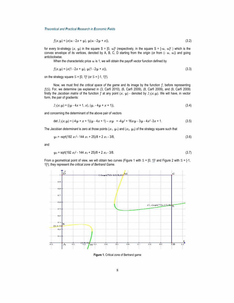
det 𝙹ƒ(𝓍,𝓎) = (-4𝓎 + 𝓍 + 1)(𝓎 - 4𝓍 + 1) – 𝓍𝓎 = -4𝓎2 + 16𝓍𝓎 - 3𝓎 - 4𝓍2 -3𝓍 + 1. (3.5) The Jacobian determinant is zero at those points (𝓍1, 𝓎1) and (𝓍2, 𝓎2) of the strategy square such that

𝓎1 = -sqrt(192 𝓍12 - 144 𝓍1 + 25)/8 + 2 𝓍1 - 3/8, (3.6) and

𝓎2 = sqrt(192 𝓍22 - 144 𝓍2 + 25)/8 + 2 𝓍2 - 3/8. (3.7) From a geometrical point of view, we will obtain two curves (Figure 1 with 𝚂 = [0, 1]2 and Figure 2 with 𝚂 = [-1, 1]2); they represent the critical zone of Bertrand Game.

Figure 1. Critical zone of Bertrand game

Volume II Issue 1(3) Summer 2011

9

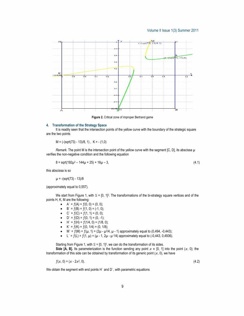
Figure 2. Critical zone of improper Bertrand game

4. Transformation of the Strategy Space It is readily seen that the intersection points of the yellow curve with the boundary of the strategic square

are the two points M = (-(sqrt(73) - 13)/8, 1) , K = - (1,0)

Remark. The point M is the intersection point of the yellow curve with the segment [C, D], its abscissa µ

verifies the non-negative condition and the following equation

8 = sqrt(192µ2 – 144µ + 25) + 16µ – 3, (4.1) this abscissa is so

µ = -(sqrt(73) - 13)/8

(approximately equal to 0,557).

We start from Figure 1, with 𝚂 = [0, 1]2. The transformations of the bi-strategy square vertices and of the points H, K, M are the following:

Aˈ = ƒ(A) = ƒ(0, 0) = (0, 0);; Bˈ = ƒ(B) = ƒ(1, 0) = (-1, 0); Cˈ = ƒ(C) = ƒ(1, 1) = (0, 0);; Dˈ = ƒ(D) = ƒ(0, 1) = (0, -1); Hˈ = ƒ(H) = ƒ(1/4, 0) = (1/8, 0);; Kˈ = ƒ(K) = ƒ(0, 1/4) = (0, 1/8);; Mˈ = ƒ(M) = ƒ(µ, 1) = (2µ - µ2/4, µ - 1) approximately equal to (0,494, -0,443); Lˈ = ƒ(L) = ƒ(1, µ) = (µ - 1, 2µ - µ 2/4) approximately equal to (-0,443, 0,4936).

Starting from Figure 1, with 𝚂 = [0, 1]2, we can do the transformation of its sides. Side [A, B]. Its parameterization is the function sending any point 𝓍 ∊ [0, 1] into the point (𝓍, 0); the

transformation of this side can be obtained by transformation of its generic point (𝓍, 0), we have

ƒ(𝓍, 0) = (𝓍 - 2𝓍2, 0). (4.2) We obtain the segment with end points Hˈ and Dˈ, with parametric equations

Theoretical and Practical Research in Economic Fields

10

X = 𝓍 - 2𝓍2 and Y = 0, (4.3)

with 𝓍 in the unit interval. Side [B, C]. It is parametrized by:

(𝓍 = 1, 𝓎 ∊ [0, 1]);

the figure of the generic point is

ƒ(1, 𝓎) = (𝓎 – 1, -2𝓎2 + 2𝓎). (4.4)

We can obtain the parabola passing through the points Cˈ, Lˈ, Dˈ with parametric equations

X = 𝓎 – 1 and Y = -2𝓎2 + 2𝓎. (4.5)

Side [C, D]. Its parameterization is:

(𝓍 ∊ [0, 1], 𝓎 = 1); the transformation of its generic point is

ƒ(𝓍, 1) = (-2𝓍2 + 2𝓍, 𝓍 - 1). (4.6) We can obtain the parabola passing through the points Bˈ, Mˈ, Cˈ with parametric equations

X = -2𝓍2 + 2𝓍 and Y = 𝓍 - 1. (4.7)

Side [D, A]. Its parameterization is

(𝓍 = 0, 𝓎 ∊ [0, 1]); the transformation of its generic point is

ƒ(0, 𝓎) = (0, -2𝓎2). (4.8) We obtain the segment [Kˈ, Bˈ] with parametric equations

X = 0 and Y = -2𝓎2, (4.9) with 𝓎 in the unit interval.

Now, we find the transformation of the critical zone. The parameterization of the critical zone is defined by the equations

𝓎1 = - sqrt(192𝓍12 - 144𝓍1 + 25)/8 + 2𝓍1 - 3/8 (3.6) and

𝓎2 = sqrt(192𝓍22 - 144𝓍2 + 25)/8 + 2𝓍2 - 3/8. (3.7) The parametrization of the GREEN ZONE is

(𝓍 ∊ [0, 1], 𝓎 = 𝓎1);

the transformation of its generic point is

ƒ(𝓍,𝓎1) = (𝓍 - 2𝓍2 + 𝓍𝓎1, 𝓎1 - 2𝓎21 + 𝓍𝓎1), (4.10)

Volume II Issue 1(3) Summer 2011

11

a parametrization of the YELLOW ZONE is

(𝓍 ∊ [0, 1], 𝓎 = 𝓎2);

the transformation of its generic point is

ƒ(𝓍,𝓎2) = (𝓍 - 2𝓍2 + 𝓍𝓎2, 𝓎2 - 2𝓎22 + 𝓍𝓎2). (4.11) The transformation of the Green Zone has parametric equations

X = 𝓍 - 2𝓍2 + 𝓍𝓎1 and Y = 𝓎1 - 2𝓎21 + 𝓍𝓎1, (4.12) and the transformation of the Yellow Zone has parametric equations

X = 𝓍 - 2𝓍2 + 𝓍𝓎2 and Y = 𝓎2 - 2𝓎22 + 𝓍𝓎2. (4.13) We have two colored curves in green and black (Figure 4.1), breaking by two points of discontinuity T and U obtained by resolving the following equation

192𝓍2 - 144𝓍 + 25 = 0; (4.14) the solutions of the above equation are

𝓍1 = - (sqrt(6) - 9)/24, 𝓍2 = (sqrt(6) + 9)/24, (4.15) and then, replacing them in the parametrical equations of the critical zone, and putting t = 9 + sqrt(6) with s = - sqrt(t2/3 - 6t + 25)/8 and u = 9 - sqrt(6) with v = - sqrt(-6u + u2/3 + 25)/8 we obtain:

T1 = (t(s + t/12 - 3/8))/24 - t2/288 + t/24; T2 = -2(s + t/12 - 3/8)2 + s +(t(s + t/12 - 3/8))/24 + t/12 - 3/8,

and, U1 = ((u/12 + v - 3/8)u)/24 + u/24 - u2/288; U2 = ((u/12 + v - 3/8)u)/24 + u/12 - 2(u/12 + v - 3/8)2 + v - 3/8.

So, we obtain - approximately - the point

T = (0,298, 0,185),

and the point

U = (0,171, 0,159).

Theoretical and Practical Research in Economic Fields

12

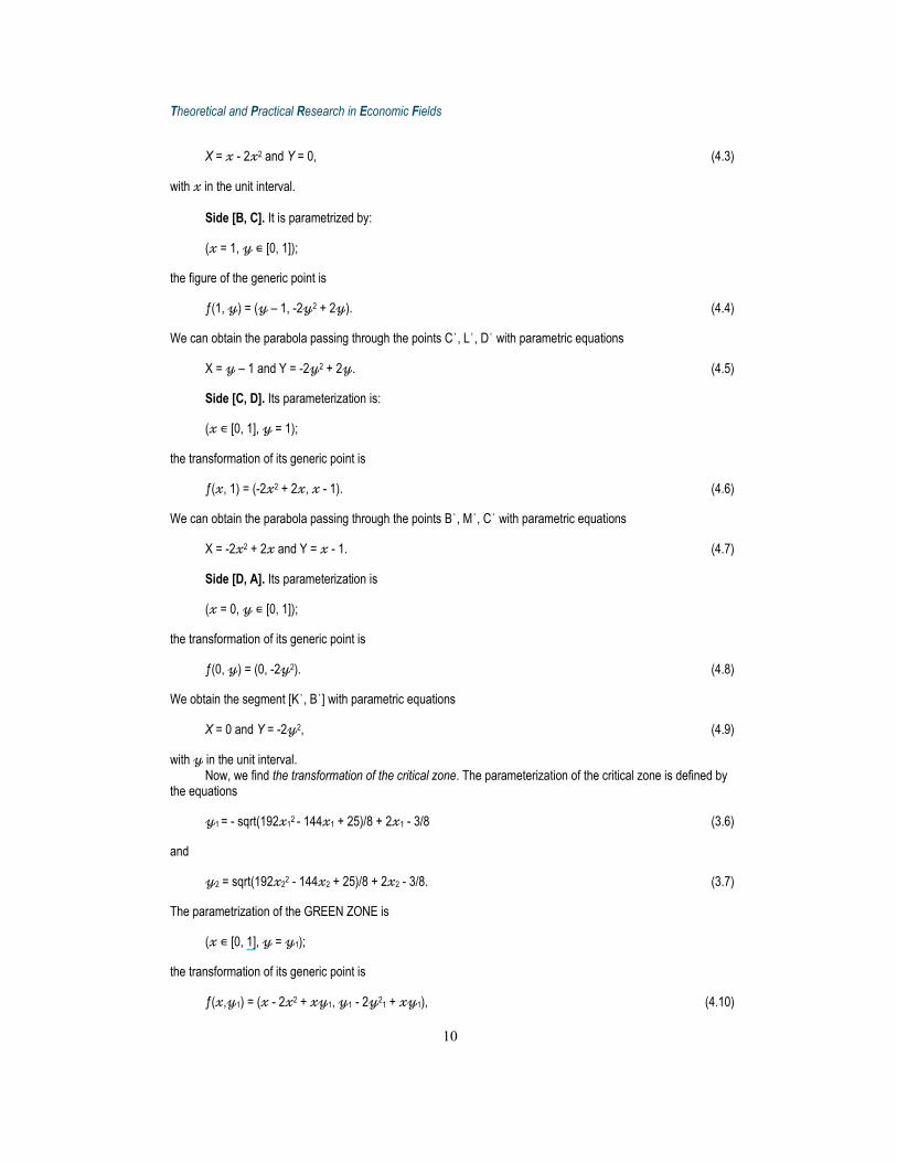
Figure 3. Payoff space of Bertrand game Payoff space of the improper Bertrand’s game

Starting from the Figure 2 with 𝚂 = [-1, 1]2; the projections of bi-strategy square’s points are the following: Aˈ = ƒ(A) = ƒ(-1, -1) = (-2, -2); Bˈ = ƒ(B) = ƒ(1, -1) = (-2, -4); Cˈ = ƒ(C) = ƒ(1, 1) = (0, 0);; Dˈ = ƒ(D) = ƒ(-1, 1) = (-4, -2); Hˈ = ƒ(H) = ƒ(0, -1) = (0, -3); Kˈ = ƒ(K) = ƒ(-1, 0) = (-3, 0); Mˈ = ƒ(M) = ƒ(µ, 1) = (2µ - µ2/4, µ - 1) approximately equal to (0,494, -0,443); Lˈ = ƒ(L) = ƒ(1, µ) = (µ - 1, 2µ - µ 2/4) approximately equal to (-0,443, 0,4936).

Starting from Figure 2 with 𝚂 = [-1, 1]2, we can do the transformation of its sides. Side [A, B]. Its parametric form is

(𝓍 ∊ [-1, 1], 𝓎 = -1);

the transformation of its generic point is

ƒ(𝓍, -1) = (-2𝓍2, -𝓍 – 3). (4.16) We can obtain the parabola passing through the points Aˈ, Hˈ, Bˈ with

X = -2𝓍2 and 𝑌 = -𝓍 – 3. (4.17) Side [B, C]. Its parameterization is

(𝓍 = 1, 𝓎 ∊ [-1, 1]); the transformation of its generic point is

ƒ(1, 𝓎) = (𝓎 -1, -2𝓎2 + 2𝓎). (4.18) We can obtain the parabola passing through the points Bˈ, Lˈ, Cˈ with

X = 𝓎 -1 and 𝑌 = -2𝓎2 + 2𝓎. (4.19) Side [C, D]. Its parameterization is

Volume II Issue 1(3) Summer 2011

13

(𝓍 ∊ [-1, 1], 𝓎 = 1); the transformation of its generic point is

ƒ(𝓍, 1) = (-2𝓍2 + 2𝓍, 𝓍 - 1). (4.20)

We can obtain the parabola passing through the points Cˈ, Mˈ, Dˈ with parametric equations

X = -2𝓍2 + 2𝓍 and 𝑌 = 𝓍 - 1. (4.21) Side [D, A]. Its parameterization is

(𝓍 = -1, 𝓎 ∊ [-1, 1]); the transformation of its generic point is

ƒ(-1, 𝓎) = (-𝓎 – 3, -2𝓎2). (4.22) We can obtain the parabola passing through the points Dˈ, Kˈ, Aˈ with parametric equations

X = -𝓎 – 3 and 𝑌 = -2𝓎2. (4.23)

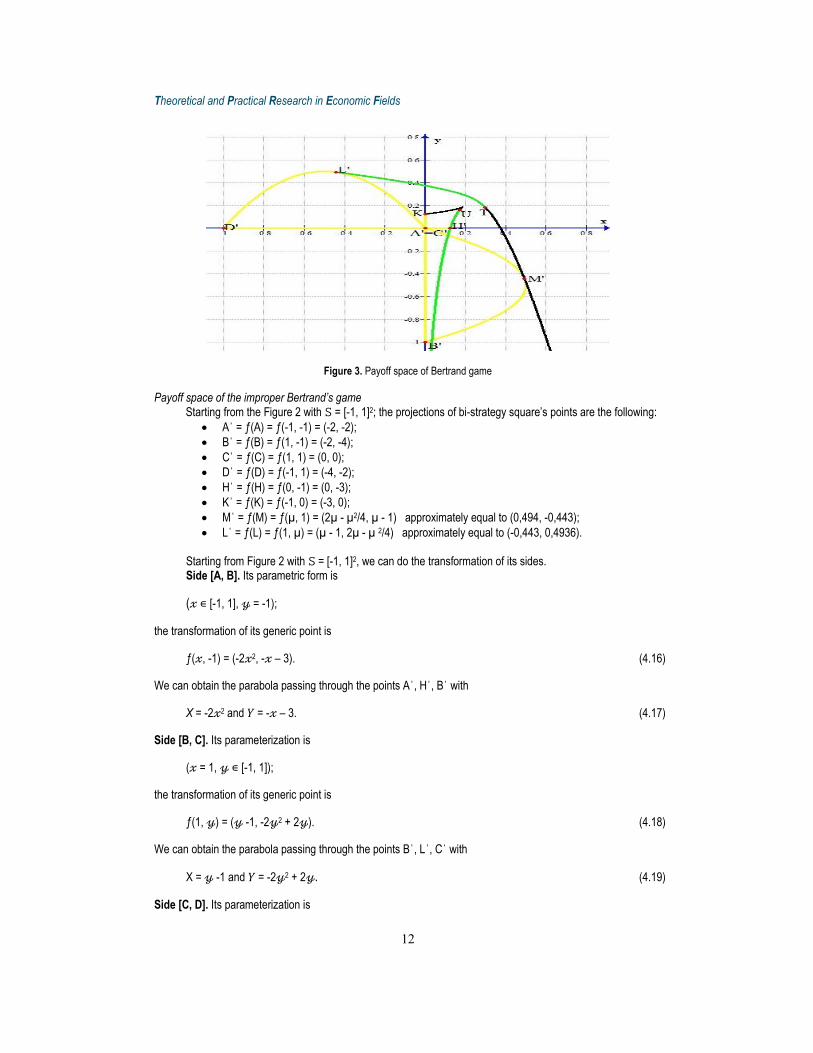
For the transformation of the critical zone and the coordinates of the points of discontinuity please refer to the case𝚂 = [0, 1]2, we must remember only to widen the interval considered from 𝓍, 𝓎 ∊ [0, 1] to 𝓍, 𝓎 ∊ [-1, 1].

Figure 4. Payoff space of the improper Bertrand game

5. Non-cooperative Friendly Phase

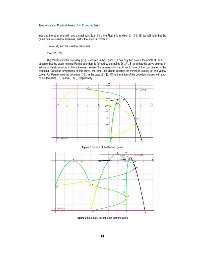
Examining the Figure 3, in which 𝚂 = [0, 1]2, we will note that the game has two shadow extremes, that is the shadow minimum 𝛼 = (-1, -1) and the shadow maximum 𝛽 = (1/2, 1/2).

The Pareto minimal boundary of the payoff space ƒ(𝚂) is showed in the Figure 5 by the union of two segments

[Aˈ, Bˈ] ∪ [Dˈ, Aˈ], and it is colored in orange. The Pareto maximal boundary of the payoff space ƒ(𝚂) is the union of the two curve segments, on the

transformations of the critical zone, with extreme points the pair of points (Lˈ, T) and (T, Mˈ). They are colored in green and in black. Both Emil, and Frances do not control the Pareto maximal boundary; they could reach the point L' and M' of the boundary, but the solution is not many satisfactory for them. In fact, a player will suffer a

Theoretical and Practical Research in Economic Fields

14

loss and the other one will have a small win. Examining the Figure 4, in which 𝚂 = [-1, 1]2, we will note that the game has two shadow extremes, that is the shadow minimum

𝛼 = (-4, -4) and the shadow maximum

𝛽 = (1/2, 1/2).

The Pareto minimal boundary ƒ(𝚂) is showed in the Figure 6, it has only two points, the points Dˈ and Bˈ;

observe that the weak minimal Pareto boundary is formed by the points Dˈ, Aˈ, Bˈ and that the curve colored in yellow is Pareto minimal in the ultra-weak sense, this means only that if we fix one of the coordinate, in the canonical Cartesian projections of this curve, the other coordinate reaches its minimum exactly on the yellow curve. For Pareto maximal boundary ƒ(𝚂), in the case 𝚂 = [0, 1]2, is the union of the boundary curves with end-points the pairs (Lˈ, T) and (T, Mˈ), respectively.

Figure 5 Extrema of the Bertrand game

Figure 6. Extrema of the improper Bertrand game

Volume II Issue 1(3) Summer 2011

15

6. Properly non-cooperative (egoistic) Phase Now, we will consider the best reply correspondences between the two players Emil and Frances, in the

cases 𝚂 = [0, 1]2 and 𝚂 = [-1, 1]2. If Frances sells the commodity at the price 𝓎, Emil, in order to reply rationally, should maximize his partial

profit function

ƒ1(∙, 𝓎) : 𝓍 ↦ 𝓍(1 - 2𝓍 + 𝓎), (6.1) on the compact interval [0, 1] or [-1, 1].

According to the Weierstrass theorem, there is at least one Emil’s strategy maximizing that partial profit

function and, by Fermàt theorem, the Emil’s best reply strategy to Frances’ strategy 𝓎 is the only price

B1(𝓎) = 𝓍* := (1/4)(𝓎 + 1). (6.2) Indeed, the partial derivative

ƒ1(∙, 𝓎)ˈ(𝓍) = -4𝓍 + 1 + 𝓎, (6.3) is positive for 𝓍 < 𝓍* and negative for 𝓍 > 𝓍*. So, the Emil’s best reply correspondence is the function B1 from the interval [0, 1] into the interval [0,1], defined by

𝓎 ↦ (1/4)(𝓎 + 1), (6.4)

in the proper case, and B1 from [-1, 1] into [-1,1], defined by

𝓎 ↦ (1/4)(𝓎 + 1), (6.5) in the improper one.

As we already observe, our Bertrand game is a symmetric game, therefore the Frances’ best reply

correspondence is the function B2 from [0, 1] into [0,1], defined by

𝓍 ↦ (1/4)(𝓍 + 1), (6.6) In the proper case, or the function B2 from [-1, 1] into [-1,1] defined by

𝓍 ↦ (1/4)(𝓍 + 1), (6.7) in the improper one.

The Nash equilibrium is the fixed point of the symmetric Cartesian product function B of the pair of two reaction functions (B2,B1) defined (canonically) from the Cartesian product of the domains into the Cartesian product of the co-domains (in inverse order), by

B : (𝓍, 𝓎) ↦ (B1(𝓎), B2(𝓍)), (6.8)

that is the only bi-strategy (x,y) satisfying the below system of linear equations

𝓍 = (1/4)(𝓎 + 1), 𝓎 = (1/4)(𝓍 + 1), (6.9)

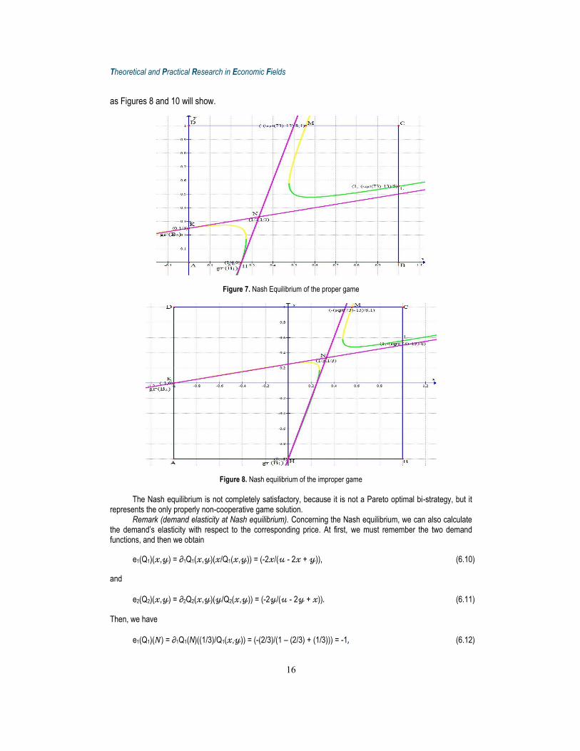
that is the point N = (1/3, 1/3) - as we can see also from the two Figures 7 and 8 - which determines a bi-gain

Nˈ = (2/9, 2/9),

Theoretical and Practical Research in Economic Fields

16

as Figures 8 and 10 will show.

Figure 7. Nash Equilibrium of the proper game

Figure 8. Nash equilibrium of the improper game The Nash equilibrium is not completely satisfactory, because it is not a Pareto optimal bi-strategy, but it

represents the only properly non-cooperative game solution. Remark (demand elasticity at Nash equilibrium). Concerning the Nash equilibrium, we can also calculate

the demand’s elasticity with respect to the corresponding price. At first, we must remember the two demand functions, and then we obtain

e1(Q1)(𝓍,𝓎) = ∂1Q1(𝓍,𝓎)(𝓍/Q1(𝓍,𝓎)) = (-2𝓍/(𝓊 - 2𝓍 + 𝓎)), (6.10)

and

e2(Q2)(𝓍,𝓎) = ∂2Q2(𝓍,𝓎)(𝓎/Q2(𝓍,𝓎)) = (-2𝓎/(𝓊 - 2𝓎 + 𝓍)) (6.11)

Then, we have

e1(Q1)(𝑁) = ∂1Q1(N)((1/3)/Q1(𝓍,𝓎)) = (-(2/3)/(1 – (2/3) + (1/3))) = -1 (6.12)

Volume II Issue 1(3) Summer 2011

17

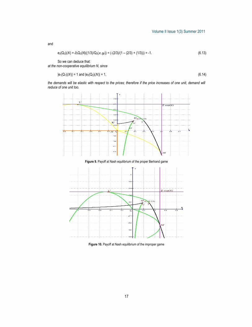
and

e2(Q2)(𝑁) = ∂2Q2(N)((1/3)/Q2(𝓍,𝓎)) = (-(2/3)/(1 – (2/3) + (1/3))) = -1 (6.13)

So we can deduce that: at the non-cooperative equilibrium N, since

|e1(Q1)(𝑁)| = 1 and |e2(Q2)(𝑁)| = 1, (6.14) the demands will be elastic with respect to the prices; therefore if the price increases of one unit, demand will reduce of one unit too.

Figure 9. Payoff at Nash equilibrium of the proper Bertrand game

Figure 10. Payoff at Nash equilibrium of the improper game

Theoretical and Practical Research in Economic Fields

18

7. Defensive and Offensive Phase Players’ conservative values are obtained through their worst gain functions. Worst gain functions. On the square 𝚂 = [0, 1]2, Emil’s worst gain function is defined by

ƒ#1(𝓍) = inf𝓎 ∊ 𝙵 𝓍(1 - 2𝓍 + 𝓎) = 𝓍 - 2𝓍2, (7.1)

its maximum will be

v#1 = sup𝓍 ∊ 𝙴 (ƒ#1(𝓍)) = sup𝓍 ∊ 𝙴 (𝓍 - 2𝓍2) = 1/8, (7.2)

attained at the conservative strategy 𝓍# = 1/4. Symmetrically, Frances’ worst gain function is defined by

ƒ#2(𝓎) = 𝓎 - 2𝓎2, (7.3) its maximum will be v#2 = 1/8 attained at the unique conservative strategy 𝓎# = 1/4.

Conservative bi-value. The conservative bi-value is

v# = (v#1, v#2) = (1/8, 1/8).

The worst offensive multifunctions are determined by the study of the worst gain functions. The Frances’ worst offensive reaction multifunction 𝖮2 is defined by 𝖮2(𝓍) = 0, for every Emil’s strategy 𝓍; indeed, fixed an Emil’s strategy 𝓍 the Frances’ strategy 0 minimizes the partial profit function ƒ1(𝓍, .). Symmetrically, the Emil’s worst offensive correspondence versus Frances is defined by 𝖮1(𝓎) = 0, for every Frances’ strategy 𝓎.

The dominant offensive strategy is 0 for both players. Indeed the offensive correspondences are constant. The offensive equilibrium A = (0,0) bring to the payoff Aˈ = (0, 0), in which the profit is zero for both

players. The core of the payoff space (in the sense introduced by J.P. Aubin) is the part of the Pareto maximal

boundary contained in the cone of upper bounds of the conservative bi-value v#; the conservative bi-value gives us a bound for the choice of cooperative bi-strategies.

Conservative phase of the Extended Bertrand game If the strategy space is the extended square 𝚂 = [-1, 1]2, Emil’s worst gain function is defined by

ƒ#1(𝓍) = inf𝓎 ∊ 𝙵 𝓍(1 - 2𝓍 + 𝓎) = -2𝓍2, (7.4) its maximum will be

v#1 = sup𝓍 ∊ 𝙴 (ƒ#1(𝓍)) = sup𝓍 ∊ 𝙴 (-2𝓍2) = 0, (7.5)

attained at the conservative strategy 𝓍# = 0. Symmetrically, Frances’ worst gain function is defined by

ƒ#2(𝓎) = -2𝓎2, (7.6)

its maximum will be v#2 = 0, attained at the conservative point 𝓎# = 0. The conservative bivalue in the improper case is

v# = (v#1, v#2) = (0, 0).

The worst offensive multifunctions can be determined by the study of the worst gain functions.

For every strategy Emil could choose, he has the minimum gain when Frances sells his commodity at the price -1. This result is unusual from an economic point of view, but it can make sense in a short period deep competition.

Volume II Issue 1(3) Summer 2011

19

Then Frances’ worst offensive multifunction is defined by 𝖮2(𝓍) = -1, for every Emil’s strategy 𝓍; symmetrically, we obtain 𝖮1(𝓎) = -1, for every Frances’ strategy 𝓎. The dominant offensive strategy is -1 for both players, and the offensive (dominant) equilibrium A = (-1, -1) brings to the point Aˈ = (-2, -2), in which a severe loss is registered for both players. The conservative knot of the game is the point (0, 0), whose image is the point (0, 0), which coincides with the point Cˈ.

The core of the payoff space is the part of Pareto maximal boundary contained into the cone of upper bounds of the conservative bi-value v#; this bounds the choice of cooperative bi-strategies. 8. Cooperative Phase

When there is an agreement between the two players, the best compromise solution (in the sense introduced by J.P. Aubin) is the pair of strategies (1/2, 1/2), showed graphically in the Figures 11 and 12. This compromise bi-strategy determines the bi-gain (1/4, 1/4).

Figure 11. Conservative study

Figure 11. The core and the Kalai-Smorodinsky payoff of the proper game

Theoretical and Practical Research in Economic Fields

20

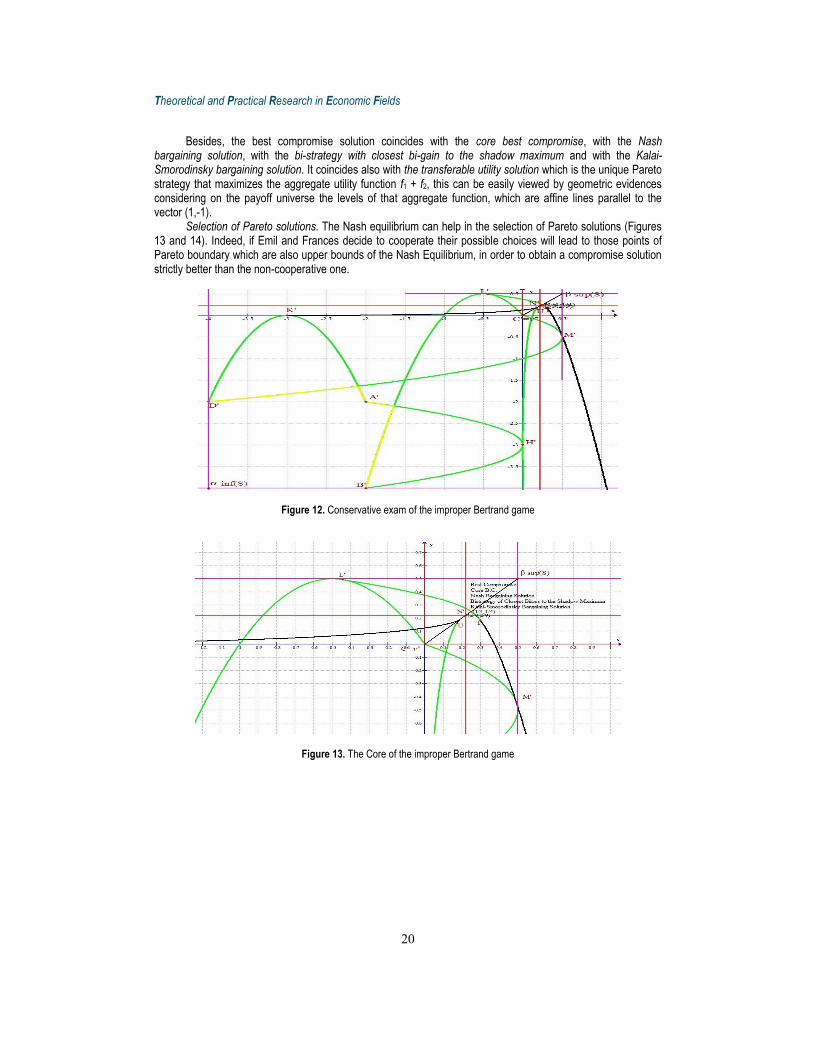
Besides, the best compromise solution coincides with the core best compromise, with the Nash bargaining solution, with the bi-strategy with closest bi-gain to the shadow maximum and with the Kalai-Smorodinsky bargaining solution. It coincides also with the transferable utility solution which is the unique Pareto strategy that maximizes the aggregate utility function f1 + f2, this can be easily viewed by geometric evidences considering on the payoff universe the levels of that aggregate function, which are affine lines parallel to the vector (1,-1).

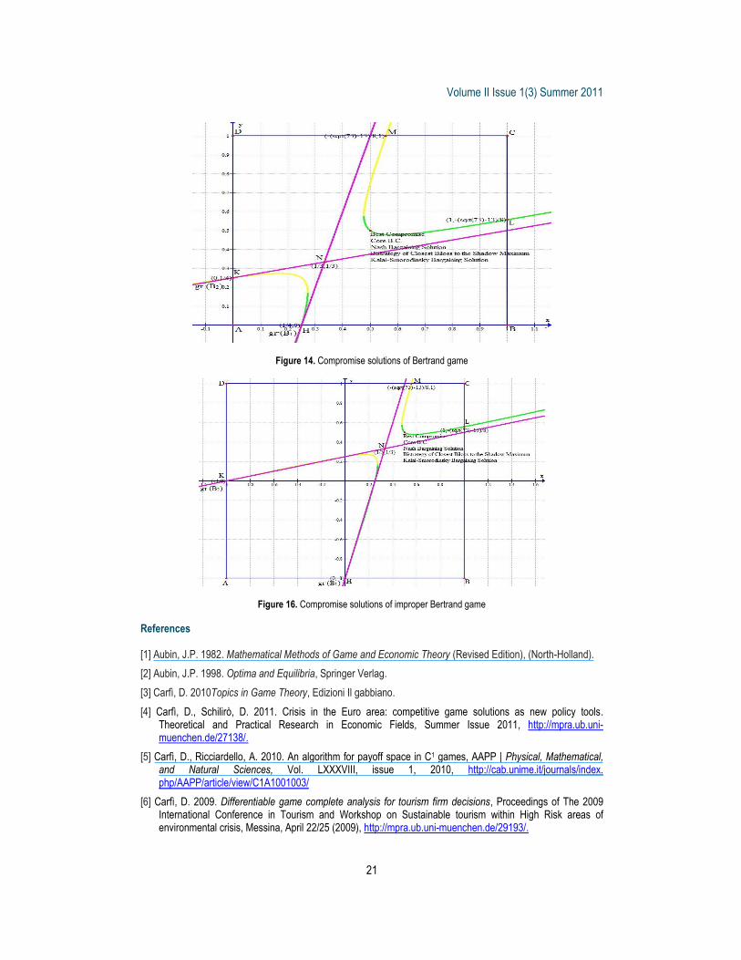
Selection of Pareto solutions. The Nash equilibrium can help in the selection of Pareto solutions (Figures 13 and 14). Indeed, if Emil and Frances decide to cooperate their possible choices will lead to those points of Pareto boundary which are also upper bounds of the Nash Equilibrium, in order to obtain a compromise solution strictly better than the non-cooperative one.

Figure 12. Conservative exam of the improper Bertrand game

Figure 13. The Core of the improper Bertrand game

Volume II Issue 1(3) Summer 2011

21

Figure 14. Compromise solutions of Bertrand game

Figure 16. Compromise solutions of improper Bertrand game References [1] Aubin, J.P. 1982. Mathematical Methods of Game and Economic Theory (Revised Edition), (North-Holland). [2] Aubin, J.P. 1998. Optima and Equilibria, Springer Verlag. [3] Carfì, D. 2010Topics in Game Theory, Edizioni Il gabbiano. [4] Carfì, D., Schilirò, D. 2011. Crisis in the Euro area: competitive game solutions as new policy tools.

Theoretical and Practical Research in Economic Fields, Summer Issue 2011, http://mpra.ub.uni-muenchen.de/27138/.

[5] Carfì, D., Ricciardello, A. 2010. An algorithm for payoff space in C1 games, AAPP | Physical, Mathematical, and Natural Sciences, Vol. LXXXVIII, issue 1, 2010, http://cab.unime.it/journals/index. php/AAPP/article/view/C1A1001003/

[6] Carfì, D. 2009. Differentiable game complete analysis for tourism firm decisions, Proceedings of The 2009 International Conference in Tourism and Workshop on Sustainable tourism within High Risk areas of environmental crisis, Messina, April 22/25 (2009), http://mpra.ub.uni-muenchen.de/29193/.

Theoretical and Practical Research in Economic Fields

22

[7] Carfì, D. 2009. Globalization and Differentiable General Sum Games, Proceeding of 3rd International Symposium Globalization and convergence in economic thought, Faculty of Economics - Communication and Economic Doctrines Department - The Bucharest Academy of Economic Studies - Bucharest December 11/12 (2009).

[8] Carfì, D. 2009. Payoff space and Pareto boundaries of C1 Games, APPS vol. 2009, http://www.mathem.pub.ro/apps/v11/a11.htm.

[9] Carfì, D. 2009. Complete study of linear infinite games, Proceedings of the International Geometry Center - Proceedings of the International Conference “Geometry in Odessa 2009”, Odessa, 25 - 30 May 2009 - vol. 2 n. 3 (2009), http://proceedings.d-omega.org/.

[10] Carfì, D. 2008. Optimal boundaries for decisions, Atti dell'Accademia Peloritana dei Pericolanti - Classe di Scienze Fisiche, Matematiche e Naturali Vol. LXXXVI, (2008), http://cab.unime.it/journals /index.php/AAPP/article/view/376

[11] Carfì, D., Ricciardello, A. 2009. Non-reactive strategies in decision-form games, AAPP | Physical, Mathematical, and Natural Sciences, Vol. LXXXVII, issue 1, pp. 1-18, http://cab.unime.it/ journals/index.php/AAPP/article/view/C1A0902002/0

[12] Carfì, D. 2009. Decision-form games, Proceedings of the IX SIMAI Congress, Rome, 22 - 26 September 2008, Communications to SIMAI congress, vol. 3, (2009) pp. 1-12, http://cab.unime.it/journals/ index.php/congress/article/view/307.

[13] Carfì, D. 2009. Reactivity in decision-form games, MPRA - paper 29001, University Library of Munich, Germany, http://mpra.ub.uni-muenchen.de/29001/.

[14] Carfì, D., and Ricciardello, A. 2011. Mixed Extensions of decision-form games, MPRA - paper 28971, University Library of Munich, Germany, http://mpra.ub.uni-muenchen.de/28971/.