http://www.cambridge.org/9780521855938

This page intentionally left blank

Galaxies in the Universe: An Introduction

Galaxies are the places where gas turns into luminous stars, powered by nuclearreactions that also produce most of the chemical elements. But the gas and stars areonly the tip of an iceberg: a galaxy consists mostly of dark matter, which we knowonly by the pull of its gravity. The ages, chemical composition and motions of thestars we see today, and the shapes that they make up, tell us about each galaxy’spast life. This book presents the astrophysics of galaxies since their beginnings inthe early Universe. This Second Edition is extensively illustrated with the mostrecent observational data. It includes new sections on galaxy clusters, gammaray bursts and supermassive black holes. Chapters on the large-scale structure andearly galaxies have been thoroughly revised to take into account recent discoveriessuch as dark energy.

The authors begin with the basic properties of stars and explore the MilkyWay before working out towards nearby galaxies and the distant Universe, wheregalaxies can be seen in their early stages. They then discuss the structures ofgalaxies and how galaxies have developed, and relate this to the evolution ofthe Universe. The book also examines ways of observing galaxies across theelectromagnetic spectrum, and explores dark matter through its gravitational pullon matter and light.

This book is self-contained, including the necessary astronomical background,and homework problems with hints. It is ideal for advanced undergraduate studentsin astronomy and astrophysics.

LINDA SPARKE is a Professor of Astronomy at the University of Wisconsin, anda Fellow of the American Physical Society.

JOHN GALLAGHER is the W. W. Morgan Professor of Astronomy at the Universityof Wisconsin and is editor of the Astronomical Journal.

Galaxies inthe Universe:

An Introduction

Second Edition

Linda S. SparkeJohn S. Gallagher IIIUniversity of Wisconsin, Madison

CAMBRIDGE UNIVERSITY PRESS

Cambridge, New York, Melbourne, Madrid, Cape Town, Singapore, São Paulo

Cambridge University PressThe Edinburgh Building, Cambridge CB2 8RU, UK

First published in print format

ISBN-13 978-0-521-85593-8

ISBN-13 978-0-521-67186-6

ISBN-13 978-0-511-29472-3

© L. Sparke and J. Gallagher 2007

2007

Information on this title: www.cambridge.org/9780521855938

This publication is in copyright. Subject to statutory exception and to the provision of relevant collective licensing agreements, no reproduction of any part may take place without the written permission of Cambridge University Press.

ISBN-10 0-511-29472-7

ISBN-10 0-521-85593-4

ISBN-10 0-521-67186-8

Cambridge University Press has no responsibility for the persistence or accuracy of urls for external or third-party internet websites referred to in this publication, and does not guarantee that any content on such websites is, or will remain, accurate or appropriate.

Published in the United States of America by Cambridge University Press, New York

www.cambridge.org

hardback

paperback

paperback

eBook (EBL)

eBook (EBL)

hardback

Contents

Preface to the second edition page vii

1 Introduction 1

1.1 The stars 2

1.2 Our Milky Way 26

1.3 Other galaxies 37

1.4 Galaxies in the expanding Universe 46

1.5 The pregalactic era: a brief history of matter 50

2 Mapping our Milky Way 58

2.1 The solar neighborhood 59

2.2 The stars in the Galaxy 67

2.3 Galactic rotation 89

2.4 Milky Way meteorology: the interstellar gas 95

3 The orbits of the stars 110

3.1 Motion under gravity: weighing the Galaxy 111

3.2 Why the Galaxy isn’t bumpy: two-body relaxation 124

3.3 Orbits of disk stars: epicycles 133

3.4 The collisionless Boltzmann equation 140

4 Our backyard: the Local Group 151

4.1 Satellites of the Milky Way 156

4.2 Spirals of the Local Group 169

4.3 How did the Local Group galaxies form? 172

4.4 Dwarf galaxies in the Local Group 183

4.5 The past and future of the Local Group 188

v

vi Contents

5 Spiral and S0 galaxies 191

5.1 The distribution of starlight 192

5.2 Observing the gas 206

5.3 Gas motions and the masses of disk galaxies 214

5.4 Interlude: the sequence of disk galaxies 222

5.5 Spiral arms and galactic bars 225

5.6 Bulges and centers of disk galaxies 236

6 Elliptical galaxies 241

6.1 Photometry 242

6.2 Motions of the stars 254

6.3 Stellar populations and gas 266

6.4 Dark matter and black holes 273

7 Galaxy groups and clusters 278

7.1 Groups: the homes of disk galaxies 279

7.2 Rich clusters: the domain of S0 and elliptical galaxies 292

7.3 Galaxy formation: nature, nurture, or merger? 300

7.4 Intergalactic dark matter: gravitational lensing 303

8 The large-scale distribution of galaxies 314

8.1 Large-scale structure today 316

8.2 Expansion of a homogeneous Universe 325

8.3 Observing the earliest galaxies 335

8.4 Growth of structure: from small beginnings 344

8.5 Growth of structure: clusters, walls, and voids 355

9 Active galactic nuclei and the early history of galaxies 365

9.1 Active galactic nuclei 366

9.2 Fast jets in active nuclei, microquasars, and γ-ray bursts 383

9.3 Intergalactic gas 390

9.4 The first galaxies 397

Appendix A. Units and conversions 407Appendix B. Bibliography 411Appendix C. Hints for problems 414

Index 421

Preface to the second edition

This text is aimed primarily at third- and fourth-year undergraduate students ofastronomy or physics, who have undertaken the first year or two of university-levelstudies in physics. We hope that graduate students and research workers in relatedareas will also find it useful as an introduction to the field. Some backgroundknowledge of astronomy would be helpful, but we have tried to summarize thenecessary facts and ideas in our introductory chapter, and we give references tobooks offering a fuller treatment. This book is intended to provide more thanenough material for a one-semester course, since instructors will differ in theirpreferences for areas to emphasize and those to omit. After working through it,readers should find themselves prepared to tackle standard graduate texts such asBinney and Tremaine’s Galactic Dynamics, and review articles such as those inthe Annual Reviews of Astronomy and Astrophysics.

Astronomy is not an experimental science like physics; it is a natural sciencelike geology or meteorology. We must take the Universe as we find it, and deducehow the basic properties of matter have constrained the galaxies that happened toform. Sometimes our understanding is general but not detailed. We can estimatehow much water the Sun’s heat can evaporate from Earth’s oceans, and indeed thisis roughly the amount that falls as rain each day; wind speeds are approximatelywhat is required to dissipate the solar power absorbed by the ground and theair. But we cannot predict from physical principles when the wind will blowor the rain fall. Similarly, we know why stellar masses cannot be far larger orsmaller than they are, but we cannot predict the relative numbers of stars that areborn with each mass. Other obvious regularities, such as the rather tight relationsbetween a galaxy’s luminosity and the stellar orbital speeds within it, are notyet properly understood. But we trust that they will yield their secrets, just asthe color–magnitude relation among hydrogen-burning stars was revealed as amass sequence. On first acquaintance galaxy astronomy can seem confusinglyfull of disconnected facts; but we hope to convince you that the correct analogyis meteorology or botany, rather than stamp-collecting.

vii

viii Preface to the second edition

We have tried to place material which is relatively more difficult or more intri-cate at the end of each subsection. Students who find some portions heavy goingat a first reading are advised to move to the following subsection and return later tothe troublesome passage. Some problems have been included. These aim mainlyat increasing a reader’s understanding of the calculations and appreciation of themagnitudes of quantities involved, rather than being mathematically demanding.Often, material presented in the text is amplified in the problems; more casualreaders may find it useful to look through them along with the rest of the text.

Boldface is used for vectors; italics indicate concepts from physics, or spe-cialist terms from astronomy which the reader will see again in this text, or willmeet in the astronomical literature. Because they deal with large distances andlong timescales, astronomers use an odd mixture of units, depending on the prob-lem at hand; Appendix A gives a list, with conversion factors. Increasing theconfusion, many of us are still firmly attached to the centimeter–gram–secondsystem of units. For electromagnetic formulae, we give a parallel-text transla-tion between these and units of the Systeme Internationale d’Unites (SI), whichare based on meters and kilograms. In other cases, we have assumed that read-ers will be able to convert fairly easily between the two systems with the aid ofAppendix A. Astronomers still disagree significantly on the distance scale of theUniverse, parametrized by the Hubble constant H0. We often indicate explic-itly the resulting uncertainties in luminosity, distance, etc., but we otherwiseadopt H0 = 75 km s−1 Mpc−1. Where ages are required or we venture acrossa substantial fraction of the cosmos, we use the benchmark cosmology with�� = 0.7, �m = 0.3, and H0 = 70 km s−1 Mpc−1.

We will use an equals sign (=) for mathematical equality, or for measuredquantities known to greater accuracy than a few percent; approximate equality (≈)usually implies a precision of 10%–20%, while ∼ (pronounced ‘twiddles’) meansthat the relation holds to no better than about a factor of two. Logarithms are tobase 10, unless explicitly stated otherwise. Here, and generally in the professionalliterature, ranges of error are indicated by ± symbols, or shown by horizontal orvertical bars in graphs. Following astronomical convention, these usually refer to1σ error estimates calculated by assuming a Gaussian distribution (which is oftenrather a bad approximation to the true random errors). For those more accustomedto 2σ or 3σ error bars, this practice makes discrepancies between the results ofdifferent workers appear more significant than is in fact the case.

This book is much the better for the assistance, advice, and warnings of ourcolleagues and students. Eric Wilcots test flew a prototype in his undergraduateclass; our colleagues Bob Bless, Johan Knapen, John Mathis, Lynn Matthews, andAlan Watson read through the text and helped us with their detailed comments;Bob Benjamin tried to set us right on the interstellar medium. We are particularlygrateful to our many colleagues who took the time to provide us with figures orthe material for figures; we identify them in the captions. Bruno Binggeli, DapHartmann, John Hibbard, Jonathan McDowell, Neill Reid, and Jerry Sellwood

Preface to the second edition ix

re-analyzed, re-ran, and re-plotted for us, Andrew Cole integrated stellar energyoutputs, Evan Gnam did orbit calculations, and Peter Erwin helped us out withsome huge and complex images. Wanda Ashman turned our scruffy sketchesinto line drawings. For the second edition, Bruno Binggeli made us an improvedportrait of the Local Group, David Yu helped with some complex plots, and TammySmecker-Hane and Eric Jensen suggested helpful changes to the problems. Muchthanks to all!

Linda Sparke is grateful to the University of Wisconsin for sabbatical leavein the 1996–7 and 2004–5 academic years, and to Terry Millar and the Uni-versity of Wisconsin Graduate School, the Vilas Foundation, and the WisconsinAlumni Research Foundation for financial support. She would also like to thankthe directors, staff, and students of the Kapteyn Astronomical Institute (Gronin-gen University, Netherlands), the Mount Stromlo and Siding Spring Observato-ries (Australian National University, Canberra), and the Isaac Newton Institutefor Mathematical Sciences (Cambridge University, UK) and Yerkes Observatory(University of Chicago), for their hospitality while much of the first edition waswritten. She is equally grateful to the Dominion Astrophysical Observatory ofCanada, the Max Planck Institute for Astrophysics in Garching, Germany, andthe Observatories of the Carnegie Institute of Washington (Pasadena, California)for refuge as we prepared the second edition. We are both most grateful to ourcolleagues in Madison for putting up with us during the writing. Jay Gallagheralso thanks his family for their patience and support for his work on ‘The Book’.

Both of us appear to lack whatever (strongly recessive?) genes enable accurateproofreading. We thank our many helpful readers for catching bugs in the firstedition, which we listed on a website. We will do the same for this edition, andhope also to provide the diagrams in machine-readable form: please see links fromour homepages, which are currently at www.astro.wisc.edu/∼sparke and ∼jsg.

1

Introduction

Galaxies appear on the sky as huge clouds of light, thousands of light-years across:see the illustrations in Section 1.3 below. Each contains anywhere from a millionstars up to a million million (1012); gravity binds the stars together, so they donot wander freely through space. This introductory chapter gives the astronomicalinformation that we will need to understand how galaxies are put together.

Almost all the light of galaxies comes from their stars. Our opening sectionattempts to summarize what we know about stars, how we think we know it, andwhere we might be wrong. We discuss basic observational data, and we describethe life histories of the stars according to the theory of stellar evolution. Even thenearest stars appear faint by terrestrial standards. Measuring their light accuratelyrequires care, and often elaborate equipment and procedures. We devote the finalpages of this section to the arcana of stellar photometry: the magnitude system,filter bandpasses, and colors.

In Section 1.2 we introduce our own Galaxy, the Milky Way, with its charac-teristic ‘flying saucer’ shape: a flat disk with a central bulge. In addition to theirstars, our Galaxy and others contain gas and dust; we review the ways in whichthese make their presence known. We close this section by presenting some of thecoordinate systems that astronomers use to specify the positions of stars within theMilky Way. In Section 1.3 we describe the variety found among other galaxies anddiscuss how to measure the distribution of light within them. Only the brightestcores of galaxies can outshine the glow of the night sky, but most of their lightcomes from the faint outer parts; photometry of galaxies is even more difficultthan for stars.

One of the great discoveries of the twentieth century is that the Universe is notstatic, but expanding; the galaxies all recede from each other, and from us. OurUniverse appears to have had a beginning, the Big Bang, that was not so far in thepast: the cosmos is only about three times older than the Earth. Section 1.4 dealswith the cosmic expansion, and how it affects the light we receive from galaxies.Finally, Section 1.5 summarizes what happened in the first million years after theBig Bang, and the ways in which its early history has determined what we see today.

1

2 Introduction

1.1 The stars

1.1.1 Star light, star bright . . .

All the information we have about stars more distant than the Sun has been deducedby observing their electromagnetic radiation, mainly in the ultraviolet, visible, andinfrared parts of the spectrum. The light that a star emits is determined largelyby its surface area, and by the temperature and chemical composition – the rel-ative numbers of each type of atom – of its outer layers. Less directly, we learnabout the star’s mass, its age, and the composition of its interior, because thesefactors control the conditions at its surface. As we decode and interpret the mes-sages brought to us by starlight, knowledge gained in laboratories on Earth aboutthe properties of matter and radiation forms the basis for our theory of stellarstructure.

The luminosity of a star is the amount of energy it emits per second, measuredin watts, or ergs per second. Its apparent brightness or flux is the total energyreceived per second on each square meter (or square centimeter) of the observer’stelescope; the units are W m−2, or erg s−1 cm−2. If a star shines with equal bright-ness in all directions, we can use the inverse-square law to estimate its luminosityL from the distance d and measured flux F :

F = L

4πd2. (1.1)

Often, we do not know the distance d very well, and must remember in subsequentcalculations that our estimated luminosity L is proportional to d2. The Sun’s totalor bolometric luminosity is L� = 3.86 × 1026 W, or 3.86 × 1033 erg s−1. Starsdiffer enormously in their luminosity: the brightest are over a million times moreluminous than the Sun, while we observe stars as faint as 10−4L�.

Lengths in astronomy are usually measured using the small-angle formula.If, for example, two stars in a binary pair at distance d from us appear separatedon the sky by an angle α, the distance D between the stars is given by

α (in radians) = D/d. (1.2)

Usually we measure the angle α in arcseconds: one arcsecond (1′′) is 1/60 ofan arcminute (1′) which is 1/60 of a degree. Length is often given in terms ofthe astronomical unit, Earth’s mean orbital radius (1 AU is about 150 millionkilometers) or in parsecs, defined so that, when D = 1 AU and α = 1′′, d =1 pc = 3.09 × 1013 km or 3.26 light-years.

The orbit of two stars around each other can allow us to determine their masses.If the two stars are clearly separated on the sky, we use Equation 1.2 to measure thedistance between them. We find the speed of the stars as they orbit each other fromthe Doppler shift of lines in their spectra; see Section 1.2. Newton’s equation for

1.1 The stars 3

the gravitational force, in Section 3.1, then gives us the masses. The Sun’s mass,as determined from the orbit of the Earth and other planets, is M� = 2×1030 kg,or 2 × 1033 g.

Stellar masses cover a much smaller range than their luminosities. The mostmassive stars are around 100M�. A star is a nuclear-fusion reactor, and a ball ofgas more massive than this would burn so violently as to blow itself apart in shortorder. The least massive stars are about 0.075M�. A smaller object would neverbecome hot enough at its center to start the main fusion reaction of a star’s life,turning hydrogen into helium.

Problem 1.1 Show that the Sun produces 10 000 times less energy per unit mass

than an average human giving out about 1 W kg−1.

The radii of stars are hard to measure directly. The Sun’s radius R� = 6.96 ×105 km, but no other star appears as a disk when seen from Earth with a normaltelescope. Even the largest stars subtend an angle of only about 0.05′′, 1/20 ofan arcsecond. With difficulty we can measure the radii of nearby stars with aninterferometer; in eclipsing binaries we can estimate the radii of the two starsby measuring the size of the orbit and the duration of the eclipses. The largeststars, the red supergiants, have radii about 1000 times larger than the Sun, whilethe smallest stars that are still actively burning nuclear fuel have radii around0.1R�.

A star is a dense ball of hot gas, and its spectrum is approximately that of ablackbody with a temperature ranging from just below 3000 K up to 100 000 K,modified by the absorption and emission of atoms and molecules in the star’souter layers or atmosphere. A blackbody is an ideal radiator or perfect absorber.At temperature T , the luminosity L of a blackbody of radius R is given by theStefan–Boltzmann equation:

L = 4π R2σSBT 4, (1.3)

where the constant σSB = 5.67×10−8 W m−2 K−4. For a star of luminosity L and

radius R, we define an effective temperature Teff as the temperature of a blackbodywith the same radius, which emits the same total energy. This temperature isgenerally close to the average for gas at the star’s ‘surface’, the photosphere. Thisis the layer from which light can escape into space. The Sun’s effective temperatureis Teff ≈ 5780 K.

Problem 1.2 Use Equation 1.3 to estimate the solar radius R� from its luminosity

and effective temperature. Show that the gravitational acceleration g at the surface

is about 30 times larger than that on Earth.

4 Introduction

Problem 1.3 The red supergiant star Betelgeuse in the constellation Orion has

Teff ≈ 3500 K and a diameter of 0.045′′. Assuming that it is 140 pc from us, show

that its radius R ≈ 700R�, and that its luminosity L ≈ 105L�.

Generally we do not measure all the light emitted from a star, but only whatarrives in a given interval of wavelength or frequency. We define the flux perunit wavelength Fλ by setting Fλ(λ)�λ to be the energy of the light receivedbetween wavelengths λ and λ + �λ. Because its size is well matched to thetypical accuracy of their measurements, optical astronomers generally measurewavelength in units named after the nineteenth-century spectroscopist AndersAngstrom: 1 A = 10−8 cm or 10−10 m. The flux Fλ has units of W m−2 A−1 orerg s−1 cm−2 A−1. The flux per unit frequency Fν is defined similarly: the energyreceived between frequencies ν and ν + �ν is Fν(ν)�ν, so that Fλ = (ν2/c)Fν .Radio astronomers normally measure Fν in janskys: 1 Jy = 10−26 W m−2 Hz−1.

The apparent brightness F is the integral over all frequencies or wavelengths:

F ≡∫ ∞

0Fν(ν) dν =

∫ ∞

0Fλ(λ) dλ. (1.4)

The hotter a blackbody is, the bluer its light: at temperature T , the peak of Fλ

occurs at wavelength

λmax = [2.9/T (K)] mm. (1.5)

For the Sun, this corresponds to yellow light, at about 5000 A; human bodies, theEarth’s atmosphere, and the uncooled parts of a telescope radiate mainly in theinfrared, at about 10 μm.

1.1.2 Stellar spectra

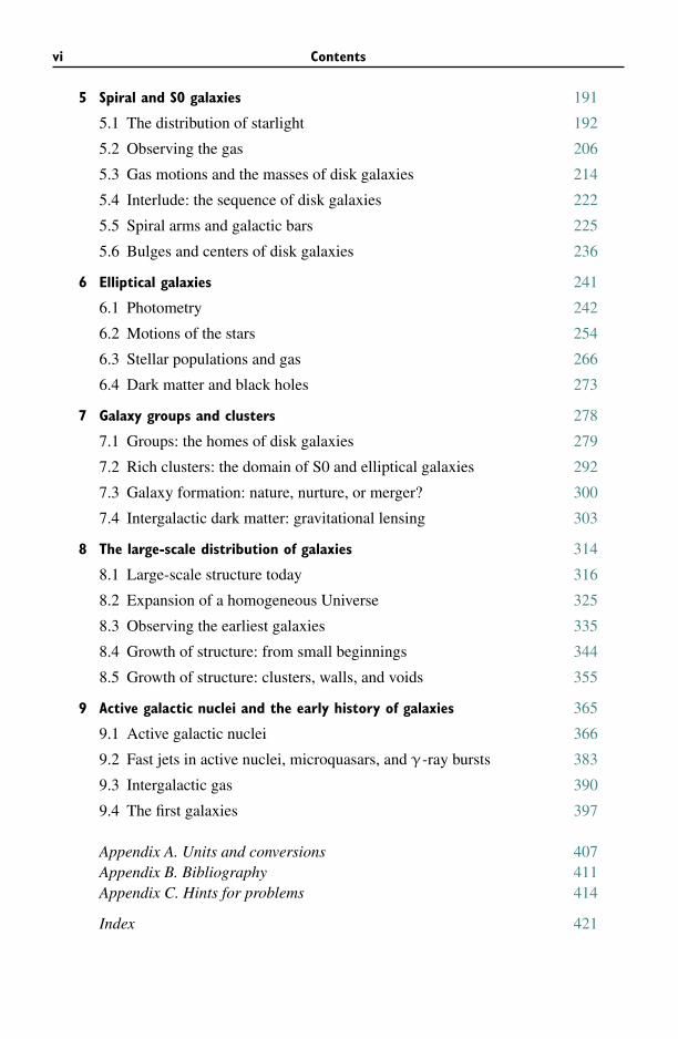
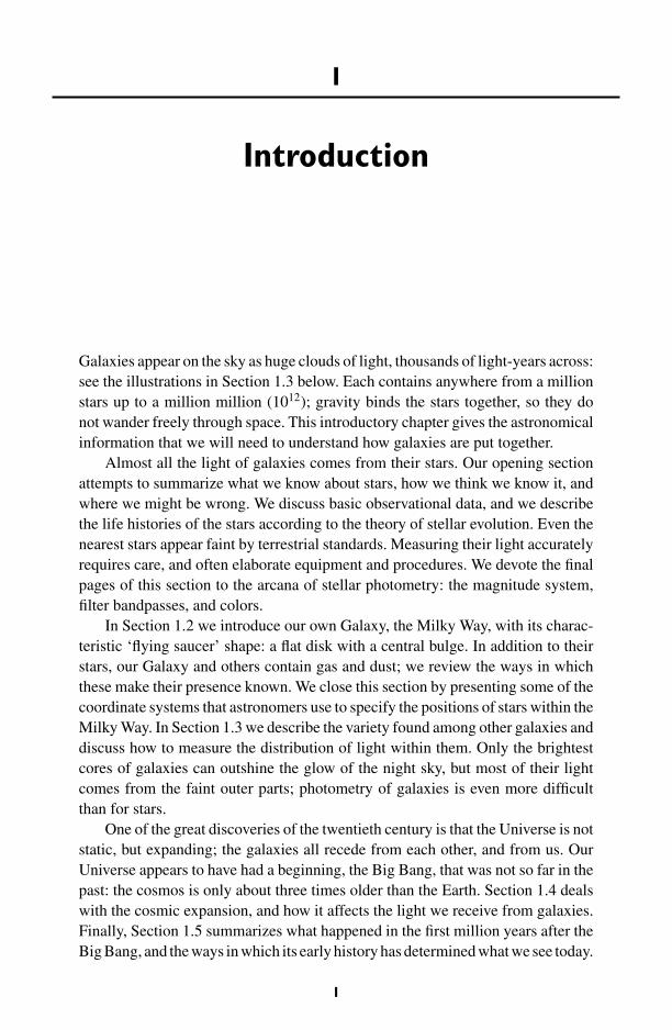
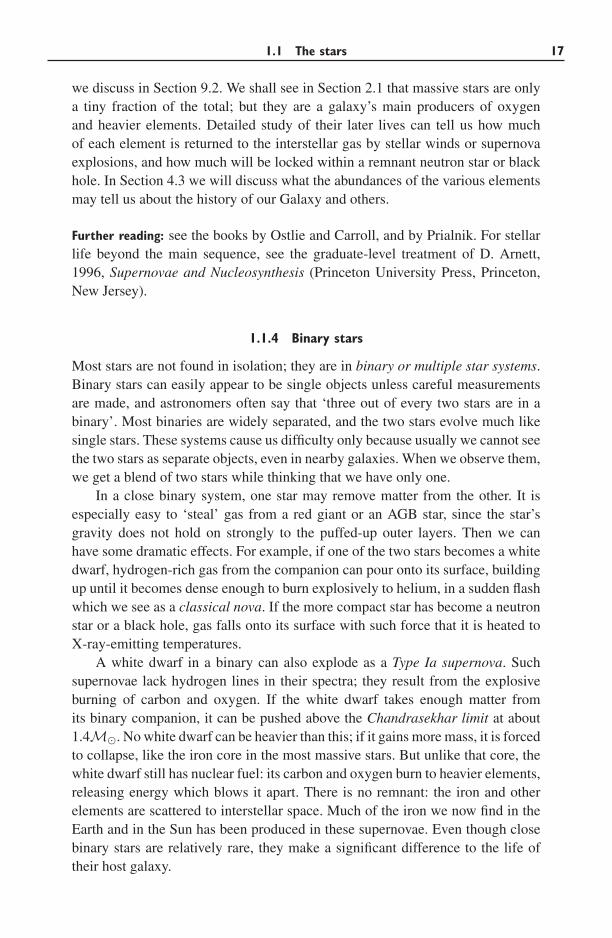
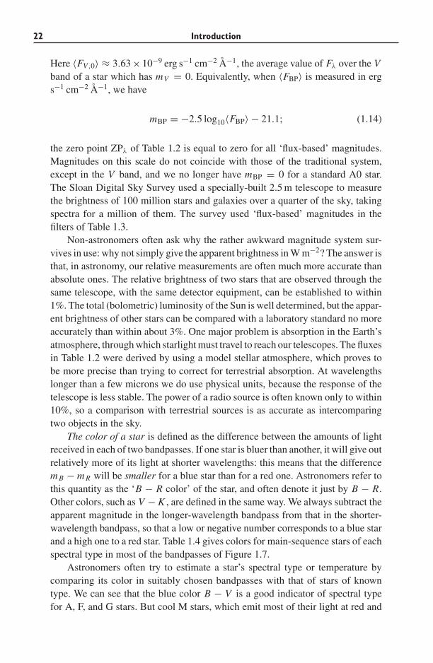
Figure 1.1 shows Fλ for a number of commonly observed types of star, arranged inorder from coolest to hottest. The hottest stars are the bluest, and their spectra showabsorption lines of highly ionized atoms; cool stars emit most of their light at redor infrared wavelengths, and have absorption lines of neutral atoms or molecules.Astronomers in the nineteenth century classified the stars according to the strengthof the Balmer lines of neutral hydrogen HI, with A stars having the strongest lines,B stars the next strongest, and so on; many of the classes subsequently fell intodisuse. In the 1880s, Antonia Maury at Harvard realized that, when the classeswere arranged in the order O B A F G K M, the strengths of all the spectral lines,not just those of hydrogen, changed continuously along the sequence. The firstlarge-scale classification was made at Harvard College Observatory between 1911and 1949: almost 400 000 stars were included in the Henry Draper Catalogue andits supplements. We now know that Maury’s spectral sequence lists the stars inorder of decreasing surface temperature. Each of the classes has been subdivided

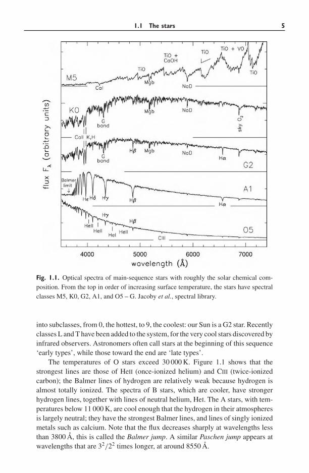
1.1 The stars 5

Fig. 1.1. Optical spectra of main-sequence stars with roughly the solar chemical com-

position. From the top in order of increasing surface temperature, the stars have spectral

classes M5, K0, G2, A1, and O5 – G. Jacoby et al., spectral library.

into subclasses, from 0, the hottest, to 9, the coolest: our Sun is a G2 star. Recentlyclasses L and T have been added to the system, for the very cool stars discovered byinfrared observers. Astronomers often call stars at the beginning of this sequence‘early types’, while those toward the end are ‘late types’.

The temperatures of O stars exceed 30 000 K. Figure 1.1 shows that thestrongest lines are those of HeII (once-ionized helium) and CIII (twice-ionizedcarbon); the Balmer lines of hydrogen are relatively weak because hydrogen isalmost totally ionized. The spectra of B stars, which are cooler, have strongerhydrogen lines, together with lines of neutral helium, HeI. The A stars, with tem-peratures below 11 000 K, are cool enough that the hydrogen in their atmospheresis largely neutral; they have the strongest Balmer lines, and lines of singly ionizedmetals such as calcium. Note that the flux decreases sharply at wavelengths lessthan 3800 A, this is called the Balmer jump. A similar Paschen jump appears atwavelengths that are 32/22 times longer, at around 8550 A.

6 Introduction

In F stars, the hydrogen lines are weaker than in A stars, and lines of neutralmetals begin to appear. G stars, like the Sun, are cooler than about 6000 K. Themost prominent absorption features are the ‘H and K’ lines of singly ionizedcalcium (CaII), and the G band of CH at 4300 A. These were named in 1815by Joseph Fraunhofer, who discovered the strong absorption lines in the Sun’sspectrum, and labelled them from A to K in order from red to blue. Lines ofneutral metals, such as the pair of D lines of neutral sodium (NaI) at 5890 A and5896 A, are stronger than in hotter stars.

In K stars, we see mainly lines of neutral metals and of molecules such asTiO, titanium oxide. At wavelengths below 4000 A metal lines absorb much ofthe light, creating the 4000 A break. The spectrum of the M star, cooler than about4000 K, shows deep absorption bands of TiO and of VO, vanadium oxide, as wellas lines of neutral metals. This is not because M stars are rich in titanium, butbecause these molecules absorb red light very efficiently, and the atmosphere iscool enough that they do not break apart. L stars have surface temperatures belowabout 2500 K, and most of the titanium and vanadium in their atmospheres iscondensed onto dust grains. Hence bands of TiO and VO are much weaker than inM stars; lines of neutral metals such as cesium appear, while the sodium D linesbecome very strong and broad. T stars are those with surfaces cooler than 1400 K;their spectra show strong lines of water and methane, like the atmospheres of giantplanets.

We can measure masses for these dwarfs by observing them in binary sys-tems, and comparing with evolutionary models. Such work indicates a massM ≈ 0.15M� for a main-sequence M5 star, while M ≈ 0.08M� for a sin-gle measured L0–L1 binary. Counting the numbers of M, L, and T dwarfs inthe solar neighborhood shows that objects below 0.3M� contribute little to thetotal mass in the Milky Way’s thin disk. ‘Stars’ cooler than about L5 have toolittle mass to sustain hydrogen burning in their cores. They are not true stars, butbrown dwarfs, cooling as they contract slowly under their own weight. Over itsfirst 100 Myr or so, a given brown dwarf can cool from spectral class M to L, oreven T; the temperature drops only slowly during its later life.

The spectrum of a galaxy is composite, including the light from a mixture ofstars with different temperatures. The hotter stars give out most of the blue light,and the lines observed in the blue part of the spectrum of a galaxy such as theMilky Way are typically those of A, F, or G stars. O and B stars are rare and sodo not contribute much of the visible light, unless a galaxy has had a recent burstof star formation. In the red part of the spectrum, we see lines from the coolerK stars, which produce most of the galaxy’s red light. Thus the blue part of thespectrum of a galaxy such as the Milky Way shows the Balmer lines of hydrogenin absorption, while TiO bands are present in the red region.

It is much easier to measure the strength of spectral lines relative to theflux at nearby wavelengths than to determine Fλ(λ) over a large range in wave-length. Absorption and scattering by dust in interstellar space, and by the Earth’s

1.1 The stars 7

4000 4500 50000

1

2

3

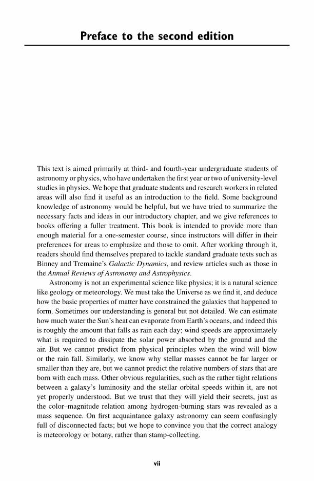
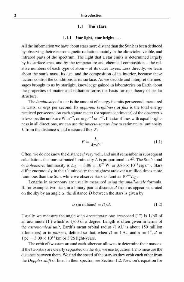
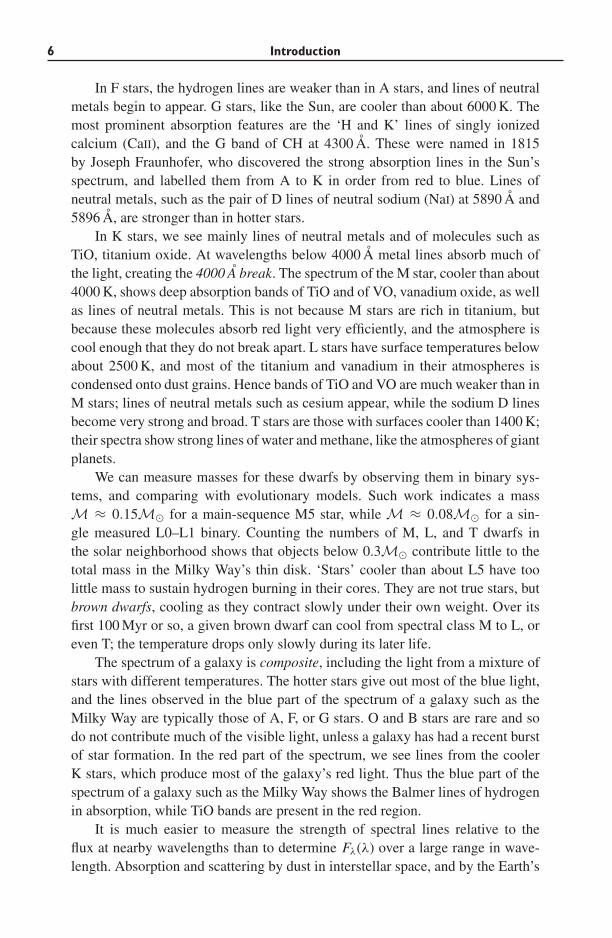
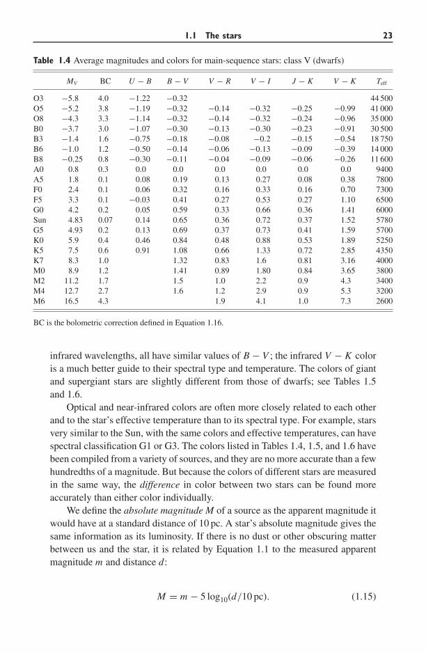
Fig. 1.2. Spectra of an A1 dwarf, an A3 giant, and an A3 supergiant: the most luminous

star has the narrowest spectral lines – G. Jacoby et al., spectral library.

atmosphere, affects the blue light of stars more than the red; blue and red lightalso propagate differently through the telescope and the spectrograph. In prac-tice, stellar temperatures are often estimated by comparing the observed depths ofabsorption lines in their spectra with the predictions of a model stellar atmosphere.This is a computer calculation of the way light propagates through a stellar atmo-sphere with a given temperature and composition; it is calibrated against stars forwhich Fλ has been measured carefully.

The lines in stellar spectra also give us information about the surface gravity.Figure 1.2 shows the spectra of three stars, all classified as A stars because theoverall strength of their absorption lines is similar. But the Balmer lines of theA dwarf are broader than those in the giant and supergiant stars, because atomsin its photosphere are more closely crowded together: this is known as the Starkeffect. If we use a model atmosphere to calculate the surface gravity of the star,and we also know its mass, we can then find its radius. For most stars, the surfacegravity is within a factor of three of that in the Sun; these stars form the mainsequence and are known as dwarfs, even though the hottest of them are very largeand luminous.

All main-sequence stars are burning hydrogen into helium in their cores. Forany particular spectral type, these stars have nearly the same mass and luminosity,because they have nearly identical structures: the hottest stars are the most massive,the most luminous, and the largest. Main-sequence stars have radii between 0.1R�

8 Introduction

and about 25R�: very roughly,

R ∼ R�( MM�

)0.7

and L ∼ L�( MM�

)α

, (1.6)

where α ≈ 5 for M ∼< M�, and α ≈ 3.9 for M� ∼< M ∼< 10M�. For the mostmassive stars with M ∼> 10M�, L ∼ 50L�(M/M�)2.2. Giant and supergiantstars have a lower surface gravity and are much more distended; the largest starshave radii exceeding 1000R�. Equation 1.3 tells us that they are much brighterthan main-sequence stars of the same spectral type. Below, we will see that theyrepresent later stages of a star’s life. White dwarfs are not main-sequence stars,but have much higher surface gravity and smaller radii; a white dwarf is onlyabout the size of the Earth, with R ≈ 0.01R�. If we define a star by its propertyof generating energy by nuclear fusion, then a white dwarf is no longer a starat all, but only the ashes or embers of a star’s core; it has exhausted its nuclearfuel and is now slowly cooling into blackness. A neutron star is an even smallerstellar remnant, only about 20 km across, despite having a mass larger than theSun’s.

Further reading: for an undergraduate-level introduction to stars, see D. A. Ostlieand B. W. Carroll, 1996, An Introduction to Modern Stellar Astrophysics (Addison-Wesley, Reading, Massachusetts); and D. Prialnik, 2000, An Introduction tothe Theory of Stellar Structure and Evolution (Cambridge University Press,Cambridge, UK).

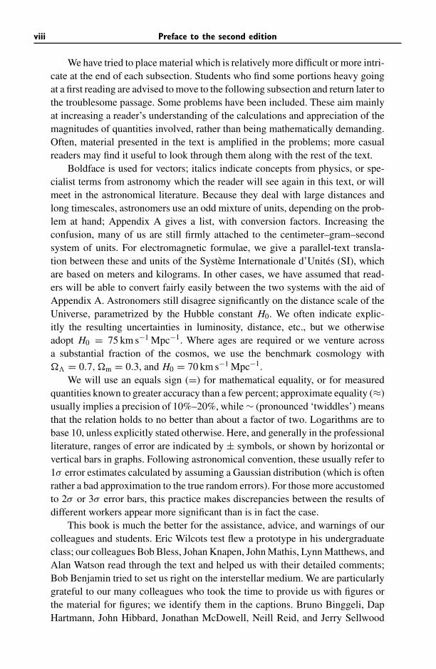
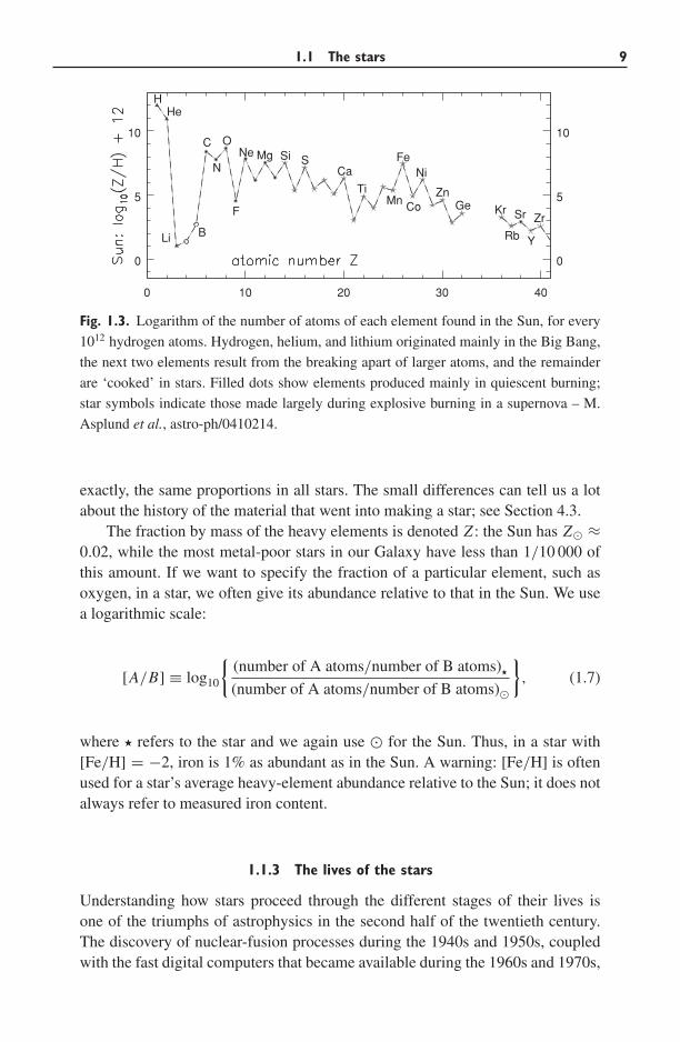
The strength of a given spectral line depends on the temperature of the starin the layers where the line is formed, and also on the abundance of the variouselements. By comparing the strengths of various lines with those calculated fora hot gas, Cecelia Payne-Gaposhkin showed in 1925 that the Sun and other starsare composed mainly of hydrogen. The surface layers of the Sun are about 72%hydrogen, 26% helium, and about 2% of all other elements, by mass. Astronomersrefer collectively to the elements heavier than helium as heavy elements or metals,even though substances such as carbon, nitrogen, and oxygen would not normallybe called metals.

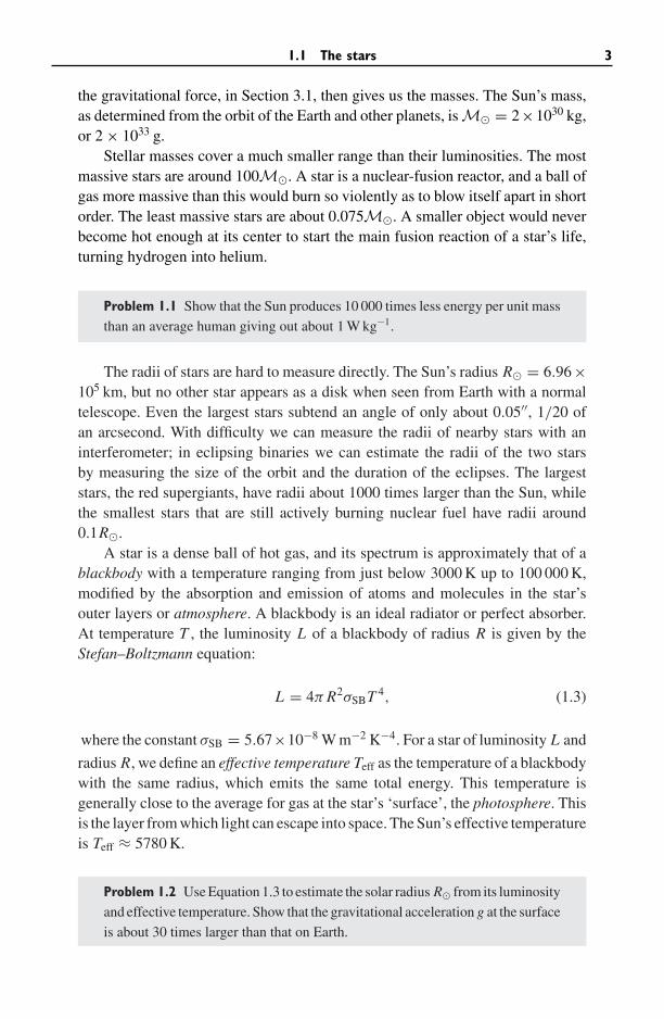
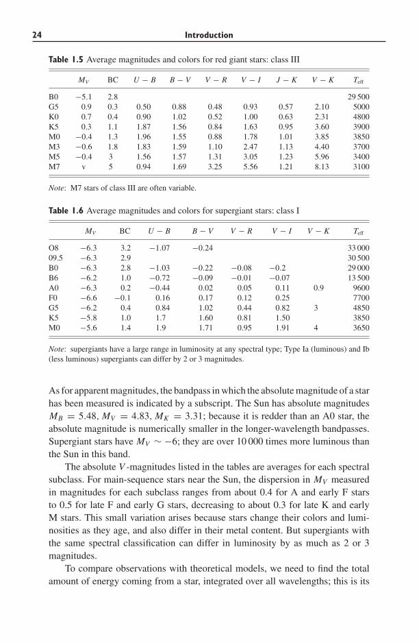
There is a good reason to distinguish hydrogen and helium from the rest ofthe elements. These atoms were created in the aftermath of the Big Bang, lessthan half an hour after the Universe as we now know it came into existence;the neutrons and protons combined into a mix of about three-quarters hydrogen,one-quarter helium, and a trace of lithium. Since then, the stars have burnedhydrogen to form helium, and then fused helium into heavier elements; see thenext subsection. Figure 1.3 shows the abundances of the commonest elements inthe Sun’s photosphere. Even oxygen, the most plentiful of the heavy elements, isover 1000 times rarer than hydrogen. The ‘metals’ are found in almost, but not

1.1 The stars 9

0 10 20 30 40

0

5

10

HHe

Li B

C

N

O

F

Ne Mg Si SCa

TiMn

Fe

Co

Ni

ZnGe Kr

Rb

Sr

Y

Zr

0

5

10

Fig. 1.3. Logarithm of the number of atoms of each element found in the Sun, for every

1012 hydrogen atoms. Hydrogen, helium, and lithium originated mainly in the Big Bang,

the next two elements result from the breaking apart of larger atoms, and the remainder

are ‘cooked’ in stars. Filled dots show elements produced mainly in quiescent burning;

star symbols indicate those made largely during explosive burning in a supernova – M.

Asplund et al., astro-ph/0410214.

exactly, the same proportions in all stars. The small differences can tell us a lotabout the history of the material that went into making a star; see Section 4.3.

The fraction by mass of the heavy elements is denoted Z : the Sun has Z� ≈0.02, while the most metal-poor stars in our Galaxy have less than 1/10 000 ofthis amount. If we want to specify the fraction of a particular element, such asoxygen, in a star, we often give its abundance relative to that in the Sun. We usea logarithmic scale:

[A/B] ≡ log10

{(number of A atoms/number of B atoms)(number of A atoms/number of B atoms)�

}, (1.7)

where refers to the star and we again use � for the Sun. Thus, in a star with[Fe/H] = −2, iron is 1% as abundant as in the Sun. A warning: [Fe/H] is oftenused for a star’s average heavy-element abundance relative to the Sun; it does notalways refer to measured iron content.

1.1.3 The lives of the stars

Understanding how stars proceed through the different stages of their lives isone of the triumphs of astrophysics in the second half of the twentieth century.The discovery of nuclear-fusion processes during the 1940s and 1950s, coupledwith the fast digital computers that became available during the 1960s and 1970s,

10 Introduction

has given us a detailed picture of the evolution of a star from a protostellar gascloud through to extinction as a white dwarf, or a fiery death in a supernovaexplosion.

We are confident that we understand most aspects of main-sequence starsfairly well. A long-standing discrepancy between predicted nuclear reactions inthe Sun’s core and the number of neutrinos detected on Earth was recently resolvedin favor of the stellar modellers: neutrinos are produced in the expected numbers,but many had changed their type along the way to Earth. Our theories falter at thebeginning of the process – we do not know how to predict when a gas cloud willform into stars, or what masses these will have – and toward its end, especiallyfor massive stars with M ∼> 8M�, and for stars closely bound in binary systems.This remaining ignorance means that we do not yet know what determines the rateat which galaxies form their stars; the quantity of elements heavier than heliumthat is produced by each type of star; and how those elements are returned to theinterstellar gas, to be incorporated into future generations of stars.

The mass of a star almost entirely determines its structure and ultimate fate;chemical composition plays a smaller role. Stars begin their existence as cloudsof gas that become dense enough to start contracting under the inward pull oftheir own gravity. Compression heats the gas, making its pressure rise to supportthe weight of the exterior layers. But the warm gas then radiates away energy,reducing the pressure, and allowing the cloud to shrink further. In this protostellarstage, the release of gravitational energy counterbalances that lost by radiation. Asa protostar, the Sun would have been cooler than it now is, but several times moreluminous. This phase is short: it lasted only 50 Myr for the Sun, which will burnfor 10 Gyr on the main sequence. So protostars do not make a large contributionto a galaxy’s light.

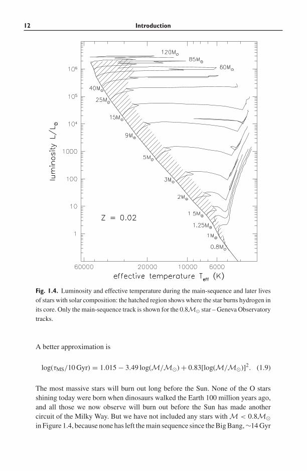
The temperature at the center rises throughout the protostellar stage; whenit reaches about 107 K, the star is hot enough to ‘burn’ hydrogen into helium bythermonuclear fusion. When four atoms of hydrogen fuse into a single atom ofhelium, 0.7% of their mass is set free as energy, according to Einstein’s formulaE = Mc2. Nuclear reactions in the star’s core now supply enough energy tomaintain the pressure at the center, and contraction stops. The star is now quitestable: it has begun its main-sequence life. Table 1.1 gives the luminosity andeffective temperature for stars of differing mass on the zero-age main sequence;these are calculated from models for the internal structure, assuming the samechemical composition as the Sun. Each solid track on Figure 1.4 shows howthose quantities change over the star’s lifetime. A plot like this is often called aHertzsprung–Russell diagram, after Ejnar Hertzsprung and Henry Norris Russell,who realized around 1910 that, if the luminosity of stars is plotted against theirspectral class (or color or temperature), most of the stars fall close to a diagonalline which is the main sequence. The temperature increases to the left on thehorizontal axis to correspond to the ordering O B A F G K M of the spectralclasses. As the star burns hydrogen to helium, the mean mass of its constituent

1.1 The stars 11

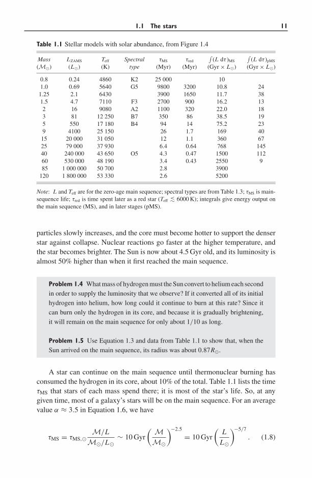
Table 1.1 Stellar models with solar abundance, from Figure 1.4

Mass LZAMS Teff Spectral τMS τred

∫(L dτ )MS

∫(L dτ )pMS

(M�) (L�) (K) type (Myr) (Myr) (Gyr × L�) (Gyr × L�)

0.8 0.24 4860 K2 25 000 101.0 0.69 5640 G5 9800 3200 10.8 241.25 2.1 6430 3900 1650 11.7 381.5 4.7 7110 F3 2700 900 16.2 132 16 9080 A2 1100 320 22.0 183 81 12 250 B7 350 86 38.5 195 550 17 180 B4 94 14 75.2 239 4100 25 150 26 1.7 169 4015 20 000 31 050 12 1.1 360 6725 79 000 37 930 6.4 0.64 768 14540 240 000 43 650 O5 4.3 0.47 1500 11260 530 000 48 190 3.4 0.43 2550 985 1 000 000 50 700 2.8 3900

120 1 800 000 53 330 2.6 5200

Note: L and Teff are for the zero-age main sequence; spectral types are from Table 1.3; τMS is main-sequence life; τred is time spent later as a red star (Teff ∼< 6000 K); integrals give energy output onthe main sequence (MS), and in later stages (pMS).

particles slowly increases, and the core must become hotter to support the denserstar against collapse. Nuclear reactions go faster at the higher temperature, andthe star becomes brighter. The Sun is now about 4.5 Gyr old, and its luminosity isalmost 50% higher than when it first reached the main sequence.

Problem 1.4 What mass of hydrogen must the Sun convert to helium each second

in order to supply the luminosity that we observe? If it converted all of its initial

hydrogen into helium, how long could it continue to burn at this rate? Since it

can burn only the hydrogen in its core, and because it is gradually brightening,

it will remain on the main sequence for only about 1/10 as long.

Problem 1.5 Use Equation 1.3 and data from Table 1.1 to show that, when the

Sun arrived on the main sequence, its radius was about 0.87R�.

A star can continue on the main sequence until thermonuclear burning hasconsumed the hydrogen in its core, about 10% of the total. Table 1.1 lists the timeτMS that stars of each mass spend there; it is most of the star’s life. So, at anygiven time, most of a galaxy’s stars will be on the main sequence. For an averagevalue α ≈ 3.5 in Equation 1.6, we have

τMS = τMS,�M/L

M�/L�∼ 10 Gyr

( MM�

)−2.5

= 10 Gyr

(L

L�

)−5/7

. (1.8)

12 Introduction

Fig. 1.4. Luminosity and effective temperature during the main-sequence and later lives

of stars with solar composition: the hatched region shows where the star burns hydrogen in

its core. Only the main-sequence track is shown for the 0.8M� star – Geneva Observatory

tracks.

A better approximation is

log(τMS/10 Gyr) = 1.015 − 3.49 log(M/M�) + 0.83[log(M/M�)]2. (1.9)

The most massive stars will burn out long before the Sun. None of the O starsshining today were born when dinosaurs walked the Earth 100 million years ago,and all those we now observe will burn out before the Sun has made anothercircuit of the Milky Way. But we have not included any stars with M < 0.8M�in Figure 1.4, because none has left the main sequence since the Big Bang, ∼14 Gyr

1.1 The stars 13

20000 10000 6000

1000

10000

10000 4000

500

1000

5000

10000

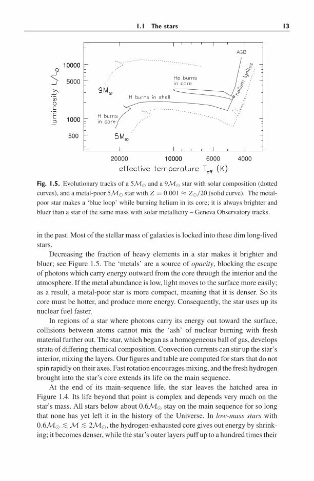
Fig. 1.5. Evolutionary tracks of a 5M� and a 9M� star with solar composition (dotted

curves), and a metal-poor 5M� star with Z = 0.001 ≈ Z�/20 (solid curve). The metal-

poor star makes a ‘blue loop’ while burning helium in its core; it is always brighter and

bluer than a star of the same mass with solar metallicity – Geneva Observatory tracks.

in the past. Most of the stellar mass of galaxies is locked into these dim long-livedstars.

Decreasing the fraction of heavy elements in a star makes it brighter andbluer; see Figure 1.5. The ‘metals’ are a source of opacity, blocking the escapeof photons which carry energy outward from the core through the interior and theatmosphere. If the metal abundance is low, light moves to the surface more easily;as a result, a metal-poor star is more compact, meaning that it is denser. So itscore must be hotter, and produce more energy. Consequently, the star uses up itsnuclear fuel faster.

In regions of a star where photons carry its energy out toward the surface,collisions between atoms cannot mix the ‘ash’ of nuclear burning with freshmaterial further out. The star, which began as a homogeneous ball of gas, developsstrata of differing chemical composition. Convection currents can stir up the star’sinterior, mixing the layers. Our figures and table are computed for stars that do notspin rapidly on their axes. Fast rotation encourages mixing, and the fresh hydrogenbrought into the star’s core extends its life on the main sequence.

At the end of its main-sequence life, the star leaves the hatched area inFigure 1.4. Its life beyond that point is complex and depends very much on thestar’s mass. All stars below about 0.6M� stay on the main sequence for so longthat none has yet left it in the history of the Universe. In low-mass stars with0.6M� ∼< M ∼< 2M�, the hydrogen-exhausted core gives out energy by shrink-ing; it becomes denser, while the star’s outer layers puff up to a hundred times their

14 Introduction

former size. The star now radiates its energy over a larger area, so Equation 1.3tells us that its surface temperature must fall; it becomes cool and red. This is thesubgiant phase.

When the temperature just outside the core rises high enough, hydrogen startsto burn in a surrounding shell: the star becomes a red giant. Helium ‘ash’ isdeposited onto the core, making it contract further and raising its temperature.The shell then burns hotter, so more energy is produced, and the star becomesgradually brighter. During this phase, the tracks of stars with M ∼< 2M� lieclose together at the right of Figure 1.4, forming the red giant branch. Stars withM ∼< 1.5M� give out most of their energy as red giants and in later stages; seeTable 1.1. By contrast with main-sequence stars, the luminosity and color of ared giant depend very little on its mass; so the giant branches in stellar systemsof different ages can be very similar. Just as on the main sequence, stars with lowmetallicity are somewhat bluer and brighter.

As it contracts, the core of a red giant becomes dense enough that the electronsof different atoms interact strongly with each other. The core becomes degenerate;it starts to behave like a solid or a liquid, rather than a gas. When the temperatureat its core has increased to about 108 K, helium ignites, burning to carbon; thisreleases energy that heats the core. In a gas, expansion would dampen the rateof nuclear reactions to produce a steady flow of energy. But the degenerate corecannot expand; instead, like a liquid or solid, its density hardly changes, so burningis explosive, as in an uncontrolled nuclear reactor on Earth. This is the helium flash,which occurs at the very tip of the red giant branch in Figure 1.4. In about 100 s,the core of the star heats up enough to turn back into a normal gas, which thenexpands.

On the red giant branch, the star’s luminosity is set by the mass of its heliumcore. When the helium flash occurs, the core mass is almost the same for all starsbelow ∼2M�; so these stars should reach the same luminosity at the tip of the redgiant branch. In any stellar population more than 2–3 Gyr old, stars above 2M�have already completed their lives; if the metal abundance is below ∼0.5Z�, thered giants have almost the same color. So the apparent brightness at the tip of thered giant branch can be used to find the distance of a nearby galaxy.

Helium is now steadily burning in the core, and hydrogen in a surroundingshell. In Figure 1.4, we see that stars of M� to 2M� stay cool and red during thisphase; they are red clump stars. In Figure 2.2, showing the luminosity and colorof stars close to the Sun, we see a concentration of stars in the red clump. Bluehorizontal branch stars are in the same stage of burning. In these, little materialremains in the star’s outer envelope, so the outer gas is relatively transparent toradiation escaping from the hot core. Stars that are less massive or poorer in heavyelements than the red clump will become horizontal branch stars.

Helium burning provides less energy than hydrogen burning. We see fromTable 1.1 that this phase lasts no more than 30% as long as the star’s main-sequence life. Once the core has used up its helium, it must again contract, and

1.1 The stars 15

the outer envelope again swells. The star moves onto the asymptotic giant branch(AGB); it now burns both helium and hydrogen in shells, and it is more luminousand cooler than it was as a red giant. This is as far as we can follow its evolutionin Figure 1.4.

On the AGB, both of the shells undergo pulses of very rapid burning, duringwhich the loosely held gas of the outer layers is lost as a stellar superwind.Eventually the hot naked core is exposed, as a white dwarf : its ultraviolet radiationionizes the ejected gas, which is briefly seen as a planetary nebula. White dwarfsnear the Sun have masses around 0.6M�, meaning that at least half of the star’soriginal material has been lost. The white dwarf core can do no further burning,and it gradually cools.

Stars of intermediate mass, from 2M� up to 6M� or 8M�, follow muchthe same history, up to the point when helium ignites in the core. Because theircentral density is lower at a given temperature, the helium core does not becomedegenerate before it begins to burn. These stars also become red, but Figure 1.4shows that they are brighter than red giants; their tracks lie above the place wherethose of the lower-mass stars come together. Once helium burning is under way,the stars become bluer; some of them become Cepheid variables, F- and G-typesupergiant stars which pulsate with periods between one and fifty days. Cepheidsare very useful to astronomers, because the pulsation cycle betrays the star’sluminosity: the most massive stars, which are also the most luminous, have thelongest periods. So once we have measured the period and apparent brightness,we can use Equation 1.1 to find the star’s distance. Cepheids are bright enough tobe seen far beyond the Milky Way. In the 1920s, astronomers used them to showthat other galaxies existed outside our own.

Once the core has used up its helium, these stars become red again; theyare asymptotic giant branch stars, with both hydrogen and helium burning inshells. Rapid pulses of burning dredge gas up from the deep interior, bringing tothe surface newly formed atoms of elements such as carbon, and heavier atomswhich have been further ‘cooked’ in the star by the s-process: the slow captureof neutrons. For example, the atmospheres of some AGB stars show traces of theshort-lived radioactive element technetium. The stellar superwind pushes pollutedsurface gas out into the interstellar environment; these AGB stars are a majorsource of the elements carbon and nitrogen in the Galaxy.

An intermediate-mass star makes a spectacular planetary nebula, as its outerlayers are shed and subsequently ionized by the hot central core. The core thencools to become a white dwarf. Stars at the lower end of this mass range leave acore which is mainly carbon and oxygen; remnants of slightly more massive starsare a mix of oxygen, neon, and magnesium. We know that white dwarfs cannothave masses above 1.4M�; so these stars put most of their material back into theinterstellar gas.

In massive stars, with M ∼> 8M�, the carbon, oxygen, and other elementsleft as the ashes of helium burning will ignite in their turn. The star Betelgeuse

16 Introduction

is now a red supergiant burning helium in its core. It probably began its main-sequence life 10–20 Myr ago, with a mass between 12M� and 17M�. It willstart to burn heavier elements, and finally explode as a supernova, within another2 Myr. After their time on the main sequence, massive stars like Betelgeuse spendmost of their time as blue or yellow supergiants; Deneb, the brightest star in theconstellation Cygnus, is a yellow supergiant. Helium starts to burn in the coreof a 25M� star while it is a blue supergiant, only slightly cooler than it was onthe main sequence. Once the core’s helium is exhausted, this star becomes a redsupergiant; but mass loss can then turn it once again into a blue supergiant beforethe final conflagration.

The later lives of stars with M ∼> 40M� are still uncertain, because theydepend on how much mass has been lost through strong stellar winds, and onill-understood details of the earlier convective mixing. A star of about 50M�may lose mass so rapidly that it never becomes a red supergiant, but is strippedto its nuclear-burning core and is seen as a blue Wolf–Rayet star. These arevery hot stars, with characteristic strong emission lines of helium, carbon, andnitrogen coming from a fast stellar wind; the wind is very poor in hydrogen,since the star’s outer layers were blown off long before. Wolf–Rayet stars liveless than 10 Myr, so they are seen only in regions where stars have recentlyformed.

Once helium burning has finished in the core, a massive star’s life is very nearlyover. The carbon core quietly burns to neon, magnesium, and heavier elements.But this process is rapid, giving out little energy; most of that energy is carriedoff by neutrinos, weakly interacting particles which easily escape through thestar’s outer layers. A star that started on its main-sequence life with 10M� ∼<M ∼< 40M� will burn its core all the way to iron. Such a core has no furthersource of energy. Iron is the most tightly bound of all nuclei, and it would requireenergy to combine its nuclei into yet heavier elements. The core collapses, and itsneutrons are squeezed so tightly that they become degenerate. The outer layers ofthe star, falling in at a tenth of the speed of light, bounce off this suddenly rigidcore, and are ejected in a blazing Type II supernova. Supernova 1987A whichexploded in the Large Magellanic Cloud was of this type, which is distinguishedby strong lines of hydrogen in its spectrum. The core of the star, incorporatingthe heavier elements such as iron, is either left as a neutron star or implodes as ablack hole. The gas that escapes is rich in oxygen, magnesium, and other elementsof intermediate atomic mass.

A star with an initial mass between 8M� and 10M� also ends its life as aType II supernova, but by a slightly different process; the core probably collapsesbefore it has burned to iron. After the explosion, a neutron star may remain, orthe star may blow itself apart completely, like the Type Ia supernovae describedbelow. A Wolf–Rayet star also becomes a supernova. Because its hydrogen hasbeen lost, hydrogen lines are missing from the spectrum, and it is classified asType Ic. These supernovae may be responsible for the energetic γ-ray bursts that

1.1 The stars 17

we discuss in Section 9.2. We shall see in Section 2.1 that massive stars are onlya tiny fraction of the total; but they are a galaxy’s main producers of oxygenand heavier elements. Detailed study of their later lives can tell us how muchof each element is returned to the interstellar gas by stellar winds or supernovaexplosions, and how much will be locked within a remnant neutron star or blackhole. In Section 4.3 we will discuss what the abundances of the various elementsmay tell us about the history of our Galaxy and others.

Further reading: see the books by Ostlie and Carroll, and by Prialnik. For stellarlife beyond the main sequence, see the graduate-level treatment of D. Arnett,1996, Supernovae and Nucleosynthesis (Princeton University Press, Princeton,New Jersey).

1.1.4 Binary stars

Most stars are not found in isolation; they are in binary or multiple star systems.Binary stars can easily appear to be single objects unless careful measurementsare made, and astronomers often say that ‘three out of every two stars are in abinary’. Most binaries are widely separated, and the two stars evolve much likesingle stars. These systems cause us difficulty only because usually we cannot seethe two stars as separate objects, even in nearby galaxies. When we observe them,we get a blend of two stars while thinking that we have only one.

In a close binary system, one star may remove matter from the other. It isespecially easy to ‘steal’ gas from a red giant or an AGB star, since the star’sgravity does not hold on strongly to the puffed-up outer layers. Then we canhave some dramatic effects. For example, if one of the two stars becomes a whitedwarf, hydrogen-rich gas from the companion can pour onto its surface, buildingup until it becomes dense enough to burn explosively to helium, in a sudden flashwhich we see as a classical nova. If the more compact star has become a neutronstar or a black hole, gas falls onto its surface with such force that it is heated toX-ray-emitting temperatures.

A white dwarf in a binary can also explode as a Type Ia supernova. Suchsupernovae lack hydrogen lines in their spectra; they result from the explosiveburning of carbon and oxygen. If the white dwarf takes enough matter fromits binary companion, it can be pushed above the Chandrasekhar limit at about1.4M�. No white dwarf can be heavier than this; if it gains more mass, it is forcedto collapse, like the iron core in the most massive stars. But unlike that core, thewhite dwarf still has nuclear fuel: its carbon and oxygen burn to heavier elements,releasing energy which blows it apart. There is no remnant: the iron and otherelements are scattered to interstellar space. Much of the iron we now find in theEarth and in the Sun has been produced in these supernovae. Even though closebinary stars are relatively rare, they make a significant difference to the life oftheir host galaxy.

18 Introduction

A Type Ia supernova can be as bright as a whole galaxy, with a luminosityof 2 × 109L� ∼< L ∼<2 × 1010L�. The more luminous the supernova, the longerits light takes to fade. So, if we monitor its apparent brightness over the weeksfollowing the explosion, we can estimate its intrinsic luminosity, and use Equa-tion 1.1 to find the distance. Recently, Type Ia supernovae have been observed ingalaxies more than 1010 light-years away; they are used to probe the structure ofthe distant Universe.

1.1.5 Stellar photometry: the magnitude system

Optical astronomers, and those working in the nearby ultraviolet and infraredregions, often express the apparent brightness of a star as an apparent magnitude.Originally, this was a measure of how much dimmer a star appeared to the eyein comparison with the bright A0 star α Lyrae (Vega). The brightest stars in thesky were of first magnitude, the next brightest were second magnitude, and so on:brighter stars have numerically smaller magnitudes. The apparent magnitudes m1

and m2 of two stars with measured fluxes F1 and F2 are related by

m1 − m2 = −2.5 log10(F1/F2). (1.10)

So if m2 = m1 + 1, star 1 appears about 2.5 times brighter than star 2. Themagnitude scale is close to that of natural logarithms: a change of 0.1 magnitudescorresponds to about a 10% difference in brightness.

Problem 1.6 Show that, if two stars of the same luminosity form a close binary

pair, the apparent magnitude of the pair measured together is about 0.75 magni-

tudes brighter than either star individually.

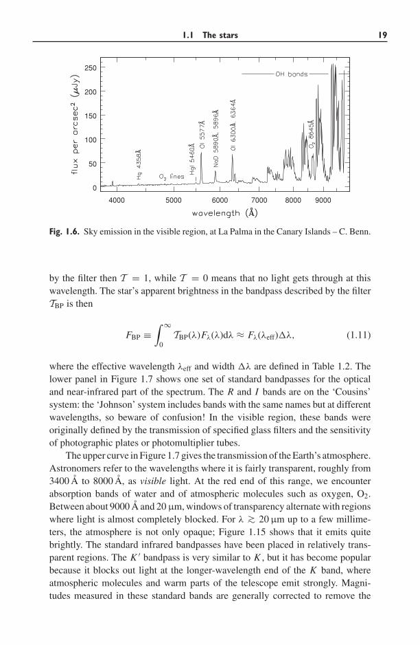
We have referred glibly to ‘measuring a star’s spectrum’. But in fact, thisis almost impossible. At far-ultraviolet wavelengths below 912 A, even smallamounts of hydrogen gas between us and the star absorb much of its light. TheEarth’s atmosphere blocks out light at wavelengths below 3000 A, or longer thana few microns. In addition to the light pollution caused by humans, the night skyitself emits light. Figure 1.6 shows that the sky is relatively dim between 4000 Aand 5500 A; at longer wavelengths, emission from atoms and molecules in theEarth’s atmosphere is increasingly intrusive. Taking high-resolution spectra offaint stars is also costly in telescope time. For all these reasons, we often settleinstead for measuring the amount of light that we receive over various broad rangesof wavelength. Thus, our magnitudes and apparent brightness most often refer toa specific region of the spectrum.

We define standard filter bandpasses, each specified by the fraction of light0 ≤ T (λ) ≤ 1 that it transmits at wavelength λ. When all the star’s light is passed

1.1 The stars 19

4000 5000 6000 7000 8000 9000

0

50

100

150

200

250

Fig. 1.6. Sky emission in the visible region, at La Palma in the Canary Islands – C. Benn.

by the filter then T = 1, while T = 0 means that no light gets through at thiswavelength. The star’s apparent brightness in the bandpass described by the filterTBP is then

FBP ≡∫ ∞

0TBP(λ)Fλ(λ)dλ ≈ Fλ(λeff)�λ, (1.11)

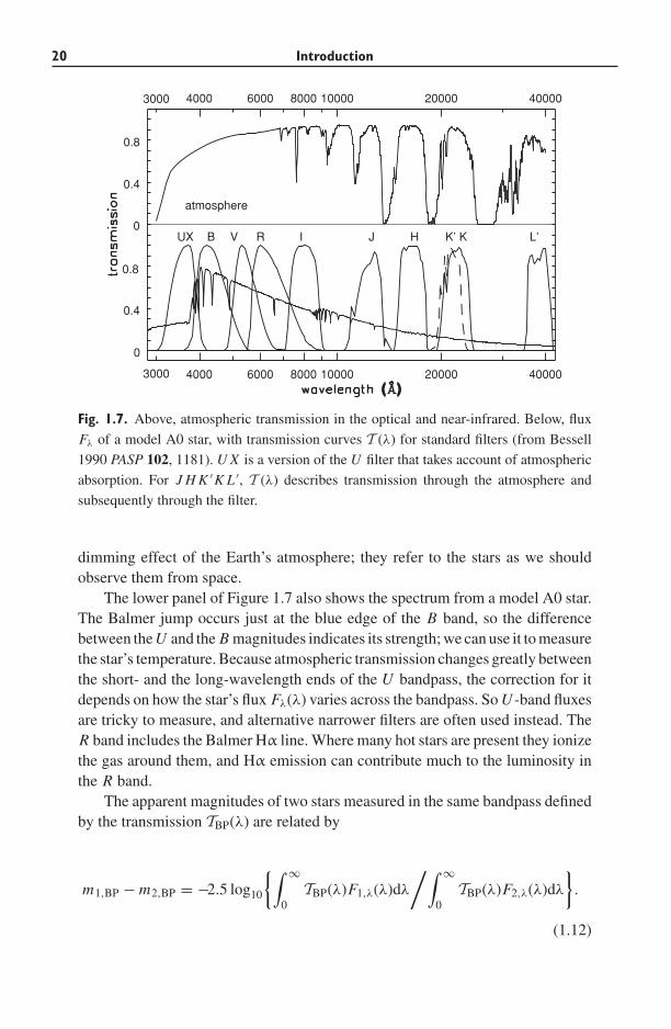
where the effective wavelength λeff and width �λ are defined in Table 1.2. Thelower panel in Figure 1.7 shows one set of standard bandpasses for the opticaland near-infrared part of the spectrum. The R and I bands are on the ‘Cousins’system: the ‘Johnson’ system includes bands with the same names but at differentwavelengths, so beware of confusion! In the visible region, these bands wereoriginally defined by the transmission of specified glass filters and the sensitivityof photographic plates or photomultiplier tubes.

The upper curve in Figure 1.7 gives the transmission of the Earth’s atmosphere.Astronomers refer to the wavelengths where it is fairly transparent, roughly from3400 A to 8000 A, as visible light. At the red end of this range, we encounterabsorption bands of water and of atmospheric molecules such as oxygen, O2.Between about 9000 A and 20 μm, windows of transparency alternate with regionswhere light is almost completely blocked. For λ ∼> 20 μm up to a few millime-ters, the atmosphere is not only opaque; Figure 1.15 shows that it emits quitebrightly. The standard infrared bandpasses have been placed in relatively trans-parent regions. The K ′ bandpass is very similar to K , but it has become popularbecause it blocks out light at the longer-wavelength end of the K band, whereatmospheric molecules and warm parts of the telescope emit strongly. Magni-tudes measured in these standard bands are generally corrected to remove the

20 Introduction

4000 6000 8000 10000 20000 40000

4000 6000 8000 10000 20000 40000

UX B V R I J H K’ K L’

3000

3000

0

0.4

0.8

0

0.4

0.8

atmosphere

Fig. 1.7. Above, atmospheric transmission in the optical and near-infrared. Below, flux

Fλ of a model A0 star, with transmission curves T (λ) for standard filters (from Bessell

1990 PASP 102, 1181). U X is a version of the U filter that takes account of atmospheric

absorption. For J H K ′K L ′, T (λ) describes transmission through the atmosphere and

subsequently through the filter.

dimming effect of the Earth’s atmosphere; they refer to the stars as we shouldobserve them from space.

The lower panel of Figure 1.7 also shows the spectrum from a model A0 star.The Balmer jump occurs just at the blue edge of the B band, so the differencebetween the U and the B magnitudes indicates its strength; we can use it to measurethe star’s temperature. Because atmospheric transmission changes greatly betweenthe short- and the long-wavelength ends of the U bandpass, the correction for itdepends on how the star’s flux Fλ(λ) varies across the bandpass. So U -band fluxesare tricky to measure, and alternative narrower filters are often used instead. TheR band includes the Balmer Hα line. Where many hot stars are present they ionizethe gas around them, and Hα emission can contribute much to the luminosity inthe R band.

The apparent magnitudes of two stars measured in the same bandpass definedby the transmission TBP(λ) are related by

m1,BP − m2,BP = −2.5 log10

{∫ ∞

0TBP(λ)F1,λ(λ)dλ

/∫ ∞

0TBP(λ)F2,λ(λ)dλ

}.

(1.12)

1.1 The stars 21

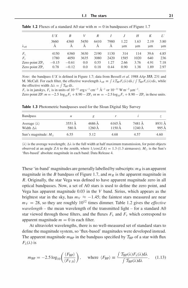
Table 1.2 Fluxes of a standard A0 star with m = 0 in bandpasses of Figure 1.7

U X B V R I J H K L ′

3660 4360 5450 6410 7980 1.22 1.63 2.19 3.80λeff A A A A A μm μm μm μm

Fλ 4150 6360 3630 2190 1130 314 114 39.6 4.85Fν 1780 4050 3635 3080 2420 1585 1020 640 236Zero point ZPλ −0.15 −0.61 0.0 0.55 1.27 2.66 3.76 4.91 7.18Zero point ZPν 0.78 −0.12 0.0 0.18 0.44 0.90 1.38 1.89 2.97

Note: the bandpass U X is defined in Figure 1.7; data from Bessell et al. 1988 AAp 333, 231 andM. McCall. For each filter, the effective wavelength λeff ≡ ∫

λTBP Fλ(λ) dλ/∫TBP Fλ(λ) dλ, while

the effective width �λ = ∫TBP dλ.

Fν is in janskys, Fλ is in units of 10−12 erg s−1 cm−2 A−1 or 10−11 W m−2 μm−1.Zero point ZP: m = −2.5 log10 Fλ + 8.90 − ZPλ or m = −2.5 log10 Fν + 8.90 − ZPν in these units.

Table 1.3 Photometric bandpasses used for the Sloan Digital Sky Survey

Bandpass u g r i z

Average 〈λ〉 3551 A 4686 A 6165 A 7481 A 8931 AWidth �λ 580 A 1260 A 1150 A 1240 A 995 A

Sun’s magnitude: M� 6.55 5.12 4.68 4.57 4.60

〈λ〉 is the average wavelength; �λ is the full width at half maximum transmission, for point objectsobserved at an angle Z A to the zenith, where 1/cos(Z A) = 1.3 (1.3 airmasses); M� is the Sun’s‘flux-based’ absolute magnitude in each band: Data Release 4.

These ‘in-band’ magnitudes are generally labelled by subscripts: m B is an apparentmagnitude in the B bandpass of Figure 1.7, and m R is the apparent magnitude inR. Originally, the star Vega was defined to have apparent magnitude zero in alloptical bandpasses. Now, a set of A0 stars is used to define the zero point, andVega has apparent magnitude 0.03 in the V band. Sirius, which appears as thebrightest star in the sky, has mV ≈ −1.45; the faintest stars measured are nearmV = 28, so they are roughly 1012 times dimmer. Table 1.2 gives the effectivewavelength – the mean wavelength of the transmitted light – for a standard A0star viewed through those filters, and the fluxes Fλ and Fν which correspond toapparent magnitude m = 0 in each filter.

At ultraviolet wavelengths, there is no well-measured set of standard stars todefine the magnitude system, so ‘flux-based’ magnitudes were developed instead.The apparent magnitude mBP in the bandpass specified by TBP of a star with fluxFλ(λ) is

mBP = −2.5 log10

( 〈FBP〉〈FV,0〉

), where 〈FBP〉 ≡

∫TBP(λ)Fλ(λ)dλ∫

TBP(λ)dλ. (1.13)

22 Introduction

Here 〈FV,0〉 ≈ 3.63 × 10−9 erg s−1 cm−2 A−1, the average value of Fλ over the Vband of a star which has mV = 0. Equivalently, when 〈FBP〉 is measured in ergs−1 cm−2 A−1, we have

mBP = −2.5 log10〈FBP〉 − 21.1; (1.14)

the zero point ZPλ of Table 1.2 is equal to zero for all ‘flux-based’ magnitudes.Magnitudes on this scale do not coincide with those of the traditional system,except in the V band, and we no longer have mBP = 0 for a standard A0 star.The Sloan Digital Sky Survey used a specially-built 2.5 m telescope to measurethe brightness of 100 million stars and galaxies over a quarter of the sky, takingspectra for a million of them. The survey used ‘flux-based’ magnitudes in thefilters of Table 1.3.

Non-astronomers often ask why the rather awkward magnitude system sur-vives in use: why not simply give the apparent brightness in W m−2? The answer isthat, in astronomy, our relative measurements are often much more accurate thanabsolute ones. The relative brightness of two stars that are observed through thesame telescope, with the same detector equipment, can be established to within1%. The total (bolometric) luminosity of the Sun is well determined, but the appar-ent brightness of other stars can be compared with a laboratory standard no moreaccurately than within about 3%. One major problem is absorption in the Earth’satmosphere, through which starlight must travel to reach our telescopes. The fluxesin Table 1.2 were derived by using a model stellar atmosphere, which proves tobe more precise than trying to correct for terrestrial absorption. At wavelengthslonger than a few microns we do use physical units, because the response of thetelescope is less stable. The power of a radio source is often known only to within10%, so a comparison with terrestrial sources is as accurate as intercomparingtwo objects in the sky.

The color of a star is defined as the difference between the amounts of lightreceived in each of two bandpasses. If one star is bluer than another, it will give outrelatively more of its light at shorter wavelengths: this means that the differencem B − m R will be smaller for a blue star than for a red one. Astronomers refer tothis quantity as the ‘B − R color’ of the star, and often denote it just by B − R.Other colors, such as V − K , are defined in the same way. We always subtract theapparent magnitude in the longer-wavelength bandpass from that in the shorter-wavelength bandpass, so that a low or negative number corresponds to a blue starand a high one to a red star. Table 1.4 gives colors for main-sequence stars of eachspectral type in most of the bandpasses of Figure 1.7.

Astronomers often try to estimate a star’s spectral type or temperature bycomparing its color in suitably chosen bandpasses with that of stars of knowntype. We can see that the blue color B − V is a good indicator of spectral typefor A, F, and G stars. But cool M stars, which emit most of their light at red and

1.1 The stars 23

Table 1.4 Average magnitudes and colors for main-sequence stars: class V (dwarfs)

MV BC U − B B − V V − R V − I J − K V − K Teff

O3 −5.8 4.0 −1.22 −0.32 44 500O5 −5.2 3.8 −1.19 −0.32 −0.14 −0.32 −0.25 −0.99 41 000O8 −4.3 3.3 −1.14 −0.32 −0.14 −0.32 −0.24 −0.96 35 000B0 −3.7 3.0 −1.07 −0.30 −0.13 −0.30 −0.23 −0.91 30 500B3 −1.4 1.6 −0.75 −0.18 −0.08 −0.2 −0.15 −0.54 18 750B6 −1.0 1.2 −0.50 −0.14 −0.06 −0.13 −0.09 −0.39 14 000B8 −0.25 0.8 −0.30 −0.11 −0.04 −0.09 −0.06 −0.26 11 600A0 0.8 0.3 0.0 0.0 0.0 0.0 0.0 0.0 9400A5 1.8 0.1 0.08 0.19 0.13 0.27 0.08 0.38 7800F0 2.4 0.1 0.06 0.32 0.16 0.33 0.16 0.70 7300F5 3.3 0.1 −0.03 0.41 0.27 0.53 0.27 1.10 6500G0 4.2 0.2 0.05 0.59 0.33 0.66 0.36 1.41 6000Sun 4.83 0.07 0.14 0.65 0.36 0.72 0.37 1.52 5780G5 4.93 0.2 0.13 0.69 0.37 0.73 0.41 1.59 5700K0 5.9 0.4 0.46 0.84 0.48 0.88 0.53 1.89 5250K5 7.5 0.6 0.91 1.08 0.66 1.33 0.72 2.85 4350K7 8.3 1.0 1.32 0.83 1.6 0.81 3.16 4000M0 8.9 1.2 1.41 0.89 1.80 0.84 3.65 3800M2 11.2 1.7 1.5 1.0 2.2 0.9 4.3 3400M4 12.7 2.7 1.6 1.2 2.9 0.9 5.3 3200M6 16.5 4.3 1.9 4.1 1.0 7.3 2600

BC is the bolometric correction defined in Equation 1.16.

infrared wavelengths, all have similar values of B − V ; the infrared V − K coloris a much better guide to their spectral type and temperature. The colors of giantand supergiant stars are slightly different from those of dwarfs; see Tables 1.5and 1.6.

Optical and near-infrared colors are often more closely related to each otherand to the star’s effective temperature than to its spectral type. For example, starsvery similar to the Sun, with the same colors and effective temperatures, can havespectral classification G1 or G3. The colors listed in Tables 1.4, 1.5, and 1.6 havebeen compiled from a variety of sources, and they are no more accurate than a fewhundredths of a magnitude. But because the colors of different stars are measuredin the same way, the difference in color between two stars can be found moreaccurately than either color individually.

We define the absolute magnitude M of a source as the apparent magnitude itwould have at a standard distance of 10 pc. A star’s absolute magnitude gives thesame information as its luminosity. If there is no dust or other obscuring matterbetween us and the star, it is related by Equation 1.1 to the measured apparentmagnitude m and distance d:

M = m − 5 log10(d/10 pc). (1.15)

24 Introduction

Table 1.5 Average magnitudes and colors for red giant stars: class III

MV BC U − B B − V V − R V − I J − K V − K Teff

B0 −5.1 2.8 29 500G5 0.9 0.3 0.50 0.88 0.48 0.93 0.57 2.10 5000K0 0.7 0.4 0.90 1.02 0.52 1.00 0.63 2.31 4800K5 0.3 1.1 1.87 1.56 0.84 1.63 0.95 3.60 3900M0 −0.4 1.3 1.96 1.55 0.88 1.78 1.01 3.85 3850M3 −0.6 1.8 1.83 1.59 1.10 2.47 1.13 4.40 3700M5 −0.4 3 1.56 1.57 1.31 3.05 1.23 5.96 3400M7 v 5 0.94 1.69 3.25 5.56 1.21 8.13 3100

Note: M7 stars of class III are often variable.

Table 1.6 Average magnitudes and colors for supergiant stars: class I

MV BC U − B B − V V − R V − I V − K Teff

O8 −6.3 3.2 −1.07 −0.24 33 00009.5 −6.3 2.9 30 500B0 −6.3 2.8 −1.03 −0.22 −0.08 −0.2 29 000B6 −6.2 1.0 −0.72 −0.09 −0.01 −0.07 13 500A0 −6.3 0.2 −0.44 0.02 0.05 0.11 0.9 9600F0 −6.6 −0.1 0.16 0.17 0.12 0.25 7700G5 −6.2 0.4 0.84 1.02 0.44 0.82 3 4850K5 −5.8 1.0 1.7 1.60 0.81 1.50 3850M0 −5.6 1.4 1.9 1.71 0.95 1.91 4 3650

Note: supergiants have a large range in luminosity at any spectral type; Type Ia (luminous) and Ib(less luminous) supergiants can differ by 2 or 3 magnitudes.

As for apparent magnitudes, the bandpass in which the absolute magnitude of a starhas been measured is indicated by a subscript. The Sun has absolute magnitudesMB = 5.48, MV = 4.83, MK = 3.31; because it is redder than an A0 star, theabsolute magnitude is numerically smaller in the longer-wavelength bandpasses.Supergiant stars have MV ∼ −6; they are over 10 000 times more luminous thanthe Sun in this band.

The absolute V -magnitudes listed in the tables are averages for each spectralsubclass. For main-sequence stars near the Sun, the dispersion in MV measuredin magnitudes for each subclass ranges from about 0.4 for A and early F starsto 0.5 for late F and early G stars, decreasing to about 0.3 for late K and earlyM stars. This small variation arises because stars change their colors and lumi-nosities as they age, and also differ in their metal content. But supergiants withthe same spectral classification can differ in luminosity by as much as 2 or 3magnitudes.

To compare observations with theoretical models, we need to find the totalamount of energy coming from a star, integrated over all wavelengths; this is its

1.1 The stars 25

bolometric luminosity Lbol. Because we cannot measure all the light of a star, weuse models of stellar atmospheres to find how much energy is emitted in the regionsthat we do not observe directly. Then, we can define a bolometric magnitude Mbol.The zero point of the scale is set by fixing the Sun’s absolute bolometric magnitudeas Mbol,� = 4.75. The second column in each of Tables 1.4, 1.5, and 1.6 givesthe bolometric correction, the amount that must be subtracted from MV to obtainthe bolometric magnitude:

Mbol = MV − BC. (1.16)

For the Sun, BC ≈ 0.07. Bolometric corrections are small for stars that emit mostof their light in the blue–green part of the spectrum. They are large for hot stars,which give out most of their light at bluer wavelengths, and for the cool red stars.A warning: some astronomers prefer to define the bolometric correction with a +sign in Equation 1.16.

Finally, stellar and galaxy luminosities are often expressed as multiples of theSun’s luminosity. From near-ultraviolet wavelengths to the near-infrared rangeat a few microns, we say that a star has L = 10L� in a given bandpass if itsluminosity in that bandpass is ten times that of the Sun in the same bandpass.But at frequencies at which the Sun does not emit much radiation, such as theX-ray and the radio, a source is generally said to have L = 10L� in a givenspectral region if its luminosity there is ten times the Sun’s bolometric luminosity.Occasionally, this latter definition is used for all wavebands.

Problem 1.7 A star cluster contains 200 F5 stars at the main-sequence turnoff,

and 20 K0III giant stars. Use Tables 1.2 and 1.4 to show that its absolute V -

magnitude MV ≈ −3.25 and its color B − V ≈ 0.68. (These values are similar

to those of the 4 Gyr-old cluster M67: see Table 2.2.)

Problem 1.8 After correcting for dust dimming (see Section 1.2), the star Betel-

geuse has average apparent magnitude mV = 0 and V − K ≈ 5. (Like many

supergiants, it is variable: mV changes by roughly a magnitude over 100–400

days.) Taking the distance d = 140 pc, find its absolute magnitude in V and in

K.

Show that Betelgeuse has LV ≈ 1.7 × 104LV,� while at K its luminosity

is much larger compared with the Sun: L K ≈ 4.1 × 105L K ,�. Using Table 1.4

to find a rough bolometric correction for a star with V − K ≈ 5, show that

Mbol ≈ −8, and the bolometric luminosity Lbol ≈ 1.2 × 105Lbol,�. Looking

back at Problem 1.3, show that the star radiates roughly 4.6 × 1031 W. (The

magnitude system can sometimes be confusing.)

26 Introduction

Ro

nucleus

thin disk

thick disk

bulge

Galactic halo

metal-poorglobular clusters

metal-richglobular clusters

dark matter(everywhere)

HI gasSun

neutralhydrogencloud

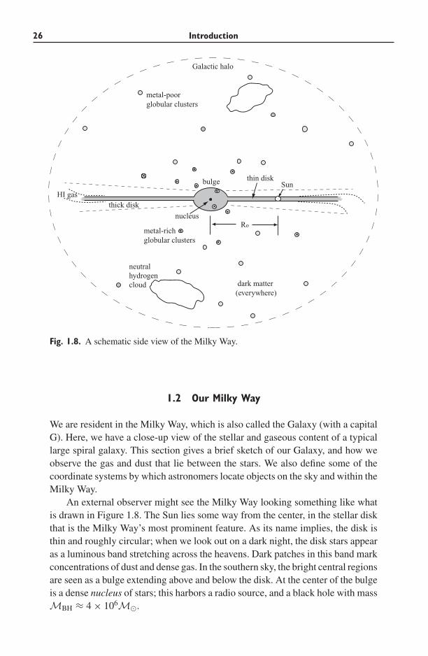
Fig. 1.8. A schematic side view of the Milky Way.

1.2 Our Milky Way

We are resident in the Milky Way, which is also called the Galaxy (with a capitalG). Here, we have a close-up view of the stellar and gaseous content of a typicallarge spiral galaxy. This section gives a brief sketch of our Galaxy, and how weobserve the gas and dust that lie between the stars. We also define some of thecoordinate systems by which astronomers locate objects on the sky and within theMilky Way.

An external observer might see the Milky Way looking something like whatis drawn in Figure 1.8. The Sun lies some way from the center, in the stellar diskthat is the Milky Way’s most prominent feature. As its name implies, the disk isthin and roughly circular; when we look out on a dark night, the disk stars appearas a luminous band stretching across the heavens. Dark patches in this band markconcentrations of dust and dense gas. In the southern sky, the bright central regionsare seen as a bulge extending above and below the disk. At the center of the bulgeis a dense nucleus of stars; this harbors a radio source, and a black hole with massMBH ≈ 4 × 106M�.

1.2 Our Milky Way 27

We generally measure distances within the Galaxy in kiloparsecs: 1 kpc is1000 pc, or about 3×1016 km. The Milky Way’s central bulge is a few kiloparsecsin radius, while the stellar disk stretches out to at least 15 kpc, with the Sun about8 kpc from the center. The density n of stars in the disk drops by about a factorof e as we move out in radius R by one scale length h R , so that n(R) ∝ e−R/h R .Estimates for h R lie in the range 2.5−4.5 kpc.

The thin disk contains 95% of the disk stars, and all of the young massivestars. Its scale height, the distance we must move in the direction perpendicularto the disk to see the density fall by a factor of e, is 300–400 pc. The rest of thestars form the thick disk, which has a larger scale height of about 1 kpc. We willsee in Chapter 2 that stars of the thick disk were made earlier in the Galaxy’shistory than those of the thin disk, and they are poorer in heavy elements. The gasand dust of the disk lie in a very thin layer; near the Sun’s position, most of theneutral hydrogen gas is within 100 pc of the midplane. The thickness of the gaslayer increases roughly in proportion to the distance from the Galactic center.

Both the Milky Way’s disk and its bulge are rotating. Stars in the disk orbitthe Galactic center at about 200 km s−1, so the Sun takes roughly 250 Myr tocomplete its orbit. Disk stars follow nearly circular orbits, with small additionalrandom motions amounting to a few tens of kilometers per second. Bulge stars havelarger random velocities. We will see in Chapter 3 that this means they must orbitthe center with a lower average speed, closer to 100 km s−1. Stars and globularclusters of the metal-poor halo do not have any organized rotation around thecenter of the galaxy. Like comets in the solar system, their orbits follow randomdirections, and are often eccentric: the stars spend most of their time in the outerreaches of the Galaxy but plunge deeply inward at pericenter.

In all, the luminosity of the disk is about (15–20) × 109L�, and the massin stars is around 60 × 109M�. For the bulge L ≈ 5 × 109L�, while the massof stars is about 20 × 109M�. The halo stars form only a small fraction of theGalaxy’s mass, accounting for no more than about 109M�. When we measurethe orbital speeds of gas, stars, and star clusters at large distances from the centerof the Milky Way, and use Equation 3.20 to find the mass required to keep themin those orbits, we find that the total mass of the Galaxy must be more than justthat present in the stars and gas. In particular, most of the Galaxy’s mass appearsto lie more than 10 kpc from the center, where there are relatively few stars. Wecall this the dark matter and usually assume, without a compelling reason, that itlies in a roughly spherical dark halo. The nature of the unseen material makingup the dark halo of our Galaxy and others is one of the main fields of research inastronomy today.

1.2.1 Gas in the Milky Way

In the neighborhood of the Sun, we find about one star in every 10 pc3. Thediameter of a solar-type star is only about 10−7 pc, so most of interstellar space

28 Introduction

is empty of stars; but it is filled with gas and dust. This dilute material makesitself apparent both by absorbing radiation from starlight that travels through itand by its own emission. We receive radiation from gas within the Milky Waythat is ionized (the atoms have lost one or more of their electrons), from neutralatoms, and from molecules. The radiation can be in the form of emission lines, oras continuum emission, a continuous spectrum without lines.

Atoms and ions radiate when one of their electrons makes a quantum jumpto a lower energy level; the line photon carries off energy equal to the differ-ence between the states. If m-times-ionized element X (written X+m) captures anelectron it becomes X+(m−1), which typically forms in an excited state. As thisnewly recombined ion relaxes to its ground state, a whole cascade of recombina-tion radiation is emitted. Transitions between barely bound high levels produceradio-frequency photons, whereas electrons falling to lower levels give visiblelight: the Balmer lines of hydrogen correspond to transitions down to level n = 2.We observe these transitions in HII regions around hot stars, where hydrogen isalmost completely ionized. Transitions to the lowest energy levels give rise tomore energetic photons. When H+ captures an electron to become neutral, and itselectron drops from n = 2 into the ground state n = 1, it gives out an ultravioletphoton of the Lyman-α line at 1216 A (10.2 eV). In heavier atoms, the lowest-level electrons are more tightly bound, and transitions to these states correspondto X-ray photons. From very hot gas we often see the 6.7 keV K line of Fe+24,24-times-ionized iron.

Gas can be photoionized: energetic photons liberate electrons from theiratoms. O and B stars produce ultraviolet photons with wavelength below 912 A,or energy above 13.6 eV, which are required to ionize hydrogen from its groundstate. These stars develop HII regions, but cooler stars do not. Atoms can also beexcited up to higher levels by collisions with electrons. Collisional ionization isimportant when the gas temperature T is high enough that the average particleenergy kBT is comparable to νhP, the energy of the emitted photon that corre-sponds to the difference between the levels. When atom A collides with atom Bto form the excited state A∗, we can have the reaction

A + B −→ A∗ + B, A∗ −→ A + νhP.

However, we see an emission line only if state A∗ decays before collidingyet again. Either the decay must be rapid, or the gas density quite low. Forbiddenlines violate the quantum-mechanical rules that specify the most probable tran-sitions (electric dipole) by which an atom could return to its ground state. These‘rule-breaking’ transitions occur via less-probable slower pathways. They are notobserved in dense laboratory plasmas because A∗ typically collides before it candecay. The electron of a hydrogen atom takes only 10−8 s to move from leveln = 3 to n = 2 by radiating an Hα photon, but for forbidden lines this is typically1 s or longer. At the critical density ncrit the line is close to its maximum strength;

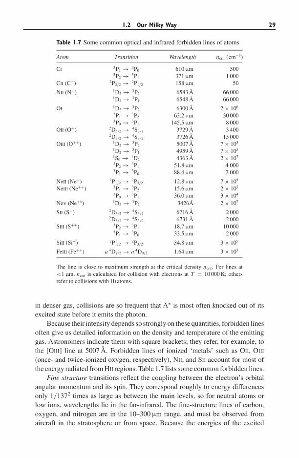
1.2 Our Milky Way 29

Table 1.7 Some common optical and infrared forbidden lines of atoms

Atom Transition Wavelength ncrit (cm−3)

CI 3P1 → 3P0 610 μm 5003P2 → 3P1 371 μm 1 000

CII (C+) 2P3/2 → 2P1/2 158 μm 50

NII (N+) 1D2 → 3P2 6583 A 66 0001D2 → 3P1 6548 A 66 000

OI 1D2 → 3P2 6300 A 2 × 106

3P1 → 3P2 63.2 μm 30 0003P0 → 3P1 145.5 μm 8 000

OII (O+) 2D5/2 → 4S3/2 3729 A 3 4002D3/2 → 4S3/2 3726 A 15 000

OIII (O++) 1D2 → 3P2 5007 A 7 × 105

1D2 → 3P1 4959 A 7 × 105

1S0 → 1D2 4363 A 2 × 107

3P2 → 3P1 51.8 μm 4 0003P1 → 3P0 88.4 μm 2 000

NeII (Ne+) 2P1/2 → 2P3/2 12.8 μm 7 × 105

NeIII (Ne++) 3P1 → 3P2 15.6 μm 2 × 105

3P0 → 3P1 36.0 μm 3 × 104

NeV (Ne+4) 1D2 → 3P2 3426A 2 × 107

SII (S+) 2D5/2 → 4S3/2 6716 A 2 0002D3/2 → 4S3/2 6731 A 2 000

SIII (S++) 3P2 → 3P1 18.7 μm 10 0003P1 → 3P0 33.5 μm 2 000

SiII (Si+) 2P1/2 → 2P3/2 34.8 μm 3 × 105

FeIII (Fe++) a 4D7/2 → a 4D9/2 1.64 μm 3 × 105

The line is close to maximum strength at the critical density ncrit. For lines at<1 μm, ncrit is calculated for collision with electrons at T = 10 000 K; othersrefer to collisions with HI atoms.

in denser gas, collisions are so frequent that A∗ is most often knocked out of itsexcited state before it emits the photon.

Because their intensity depends so strongly on these quantities, forbidden linesoften give us detailed information on the density and temperature of the emittinggas. Astronomers indicate them with square brackets; they refer, for example, tothe [OIII] line at 5007 A. Forbidden lines of ionized ‘metals’ such as OII, OIII

(once- and twice-ionized oxygen, respectively), NII, and SII account for most ofthe energy radiated from HII regions. Table 1.7 lists some common forbidden lines.

Fine structure transitions reflect the coupling between the electron’s orbitalangular momentum and its spin. They correspond roughly to energy differencesonly 1/1372 times as large as between the main levels, so for neutral atoms orlow ions, wavelengths lie in the far-infrared. The fine-structure lines of carbon,oxygen, and nitrogen are in the 10–300 μm range, and must be observed fromaircraft in the stratosphere or from space. Because the energies of the excited

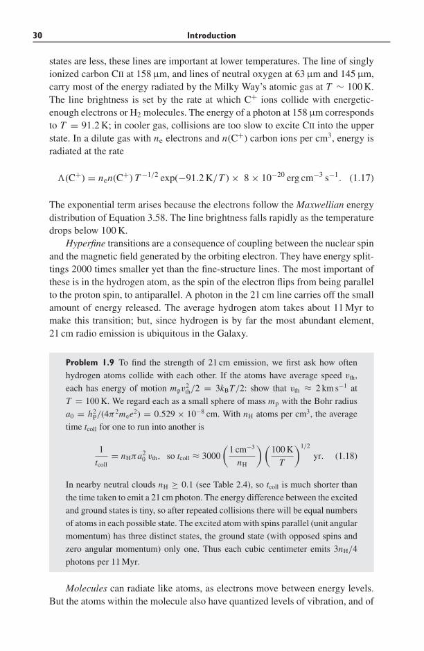
30 Introduction

states are less, these lines are important at lower temperatures. The line of singlyionized carbon CII at 158 μm, and lines of neutral oxygen at 63 μm and 145 μm,carry most of the energy radiated by the Milky Way’s atomic gas at T ∼ 100 K.The line brightness is set by the rate at which C+ ions collide with energetic-enough electrons or H2 molecules. The energy of a photon at 158 μm correspondsto T = 91.2 K; in cooler gas, collisions are too slow to excite CII into the upperstate. In a dilute gas with ne electrons and n(C+) carbon ions per cm3, energy isradiated at the rate

�(C+) = nen(C+) T −1/2 exp(−91.2 K/T ) × 8 × 10−20 erg cm−3 s−1. (1.17)

The exponential term arises because the electrons follow the Maxwellian energydistribution of Equation 3.58. The line brightness falls rapidly as the temperaturedrops below 100 K.

Hyperfine transitions are a consequence of coupling between the nuclear spinand the magnetic field generated by the orbiting electron. They have energy split-tings 2000 times smaller yet than the fine-structure lines. The most important ofthese is in the hydrogen atom, as the spin of the electron flips from being parallelto the proton spin, to antiparallel. A photon in the 21 cm line carries off the smallamount of energy released. The average hydrogen atom takes about 11 Myr tomake this transition; but, since hydrogen is by far the most abundant element,21 cm radio emission is ubiquitous in the Galaxy.

Problem 1.9 To find the strength of 21 cm emission, we first ask how often

hydrogen atoms collide with each other. If the atoms have average speed vth,

each has energy of motion mpv2th/2 = 3kBT/2: show that vth ≈ 2 km s−1 at

T = 100 K. We regard each as a small sphere of mass mp with the Bohr radius

a0 = h2P/(4π2mee2) = 0.529 × 10−8 cm. With nH atoms per cm3, the average

time tcoll for one to run into another is

1

tcoll= nHπa2

0 vth, so tcoll ≈ 3000

(1 cm−3

nH

)(100 K

T

)1/2

yr. (1.18)

In nearby neutral clouds nH ≥ 0.1 (see Table 2.4), so tcoll is much shorter than

the time taken to emit a 21 cm photon. The energy difference between the excited

and ground states is tiny, so after repeated collisions there will be equal numbers

of atoms in each possible state. The excited atom with spins parallel (unit angular

momentum) has three distinct states, the ground state (with opposed spins and

zero angular momentum) only one. Thus each cubic centimeter emits 3nH/4

photons per 11 Myr.

Molecules can radiate like atoms, as electrons move between energy levels.But the atoms within the molecule also have quantized levels of vibration, and of

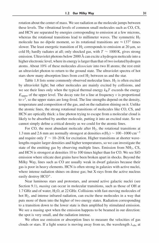
1.2 Our Milky Way 31

rotation about the center of mass. We see radiation as the molecule jumps betweenthese levels. The vibrational levels of common small molecules such as CO, CS,and HCN are separated by energies corresponding to emission at a few microns,whereas the rotational transitions lead to millimeter waves. The symmetric H2

molecule has no dipole moment, so its rotational transitions are ≈ 1372 timesslower. The least energetic transition of H2 corresponds to emission at 20 μm, socold H2 hardly radiates at all; only shocked gas, with T ∼ 1000 K, gives strongemission. Ultraviolet photons below 2000 A can excite a hydrogen molecule into ahigher electronic level, where its energy is larger than that of two isolated hydrogenatoms. About 10% of these molecules dissociate into two H atoms; the rest emitan ultraviolet photon to return to the ground state. The ultraviolet spectra of hotstars show many absorption lines from cool H2 between us and the star.

Table 1.8 lists some commonly observed molecular lines. H2 is often excitedby ultraviolet light; but other molecules are mainly excited by collisions, andwe see their lines only when the typical thermal energy kBT exceeds the energyEupper of the upper level. The decay rate for a line at frequency ν is proportionalto ν3, so the upper states are long-lived. The line strengths depend on the density,temperature and composition of the gas, and on the radiation shining on it. Unlikethe atomic lines, the strong rotational transitions of molecules like CO, CS, andHCN are optically thick: a line photon trying to escape from a molecular cloud islikely to be absorbed by another molecule, putting it into an excited state. So wecannot simply define a critical density as we could for the atomic lines.

For CO, the most abundant molecule after H2, the rotational transitions at1.3 mm and 2.6 mm are normally strongest at densities n(H2) ∼ 100 –1000 cm−3

and require only T ∼ 10–20 K for excitation. Higher transitions at shorter wave-lengths require larger densities and higher temperatures, so we can investigate thestate of the emitting gas by observing multiple lines. Emission from NH3, CS,and HCN is strongest at densities 10 to 100 times higher than for CO. We see SiOemission where silicate dust grains have been broken apart in shocks. Beyond theMilky Way, lines such as CO are usually weak in dwarf galaxies because theirgas is poor in heavy elements. HCN is often strong in galaxies with active nuclei,where intense radiation shines on dense gas; but X-rays from the active nucleuseasily destroy HCO+.

Near luminous stars and protostars, and around active galactic nuclei (seeSection 9.1), masing can occur in molecular transitions, such as those of OH at1.7 GHz and of water, H2O, at 22 GHz. Collisions with fast-moving molecules ofhot H2, and intense infrared radiation, can excite these molecules in a way thatputs more of them into the higher of two energy states. Radiation correspondingto a transition down to the lower state is then amplified by stimulated emission.We see a masing spot when the emission happens to be beamed in our direction:the spot is very small, and the radiation intense.

We often use emission or absorption lines to measure the velocities of gasclouds or stars. If a light source is moving away from us, the wavelength λobs at

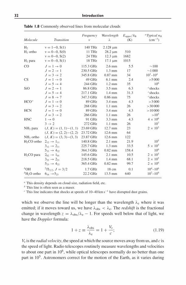
32 Introduction

Table 1.8 Commonly observed lines from molecular clouds

Frequency Wavelength Eupper/kBaTypical nH

Molecule Transition ν λ (K) (cm−3)

H2 v = 1−0, S(1) 140 THz 2.128 μmH2 ortho v = 0−0, S(0) 11 THz 28.2 μm 510

v = 0−0, S(2) 24 THz 12.3 μm 1682H2 para v = 0−0, S(1) 18 THz 17.1 μm 1015

CO J = 1 → 0 115.3 GHz 2.6 mm 5.5 ∼100J = 2 → 1 230.5 GHz 1.3 mm 17 ∼1 000J = 3 → 2 345.8 GHz 0.87 mm 34 103–104

CS J = 1 → 0 49 GHz 6.1 mm 2.4 >5 000J = 5 → 4 244 GHz 1.2 mm 35 106

SiO J = 2 → 1 86.8 GHz 3.5 mm 6.3 cshocksJ = 5 → 4 217.1 GHz 1.4 mm 31.3 cshocksJ = 8 → 7 347.3 GHz 0.86 mm 75 cshocks

HCO+ J = 1 → 0 89 GHz 3.4 mm 4.3 >3 000J = 3 → 2 268 GHz 1.1 mm 26 >30 000

HCN J = 1 → 0 89 GHz 3.4 mm 4.3 >10 000J = 3 → 2 266 GHz 1.1 mm 26 >105

HNC 1 → 0 91 GHz 3.3 mm 4.3 4 × 106

3 → 2 272 GHz 1.1 mm 26 107

NH3 para (J, K ) = (1, 1)−(1, 1) 23.69 GHz 12.7 mm 23 2 × 103

(J, K ) = (2, 2)−(2, 2) 23.72 GHz 12.6 mm 64NH3 ortho (J, K ) = (3, 3)−(3, 3) 23.87 GHz 12.6 mm 122H2CO ortho 212 → 111 140.8 GHz 2.1 mm 21.9 105

312 → 211 225.7 GHz 1.3 mm 33.5 5 × 105

533 → 432 364.3 GHz 0.82 mm 158.4 106

H2CO para 202 → 101 145.6 GHz 2.1 mm 10.5 2 × 105

322 → 221 218.5 GHz 1.4 mm 68.1 2 × 105

523 → 422 365.4 GHz 0.82 mm 99.7 2 × 106

bOH 2�3/2, J = 3/2 1.7 GHz 18 cm 0.1 104–106

bH2O ortho 616 →523 22.2 GHz 13.5 mm 640 107–109

a This density depends on cloud size, radiation field, etc.b This line is often seen as a maser.c This line indicates that shocks at speeds of 10–40 km s−1 have disrupted dust grains.

which we observe the line will be longer than the wavelength λe where it wasemitted; if it moves toward us, we have λobs < λe. The redshift is the fractionalchange in wavelength z = λobs/λe − 1. For speeds well below that of light, wehave the Doppler formula:

1 + z ≡ λobs

λe= 1 + Vr

c; (1.19)

Vr is the radial velocity, the speed at which the source moves away from us, and c isthe speed of light. Radio telescopes routinely measure wavelengths and velocitiesto about one part in 106, while optical telescopes normally do no better than onepart in 105. Astronomers correct for the motion of the Earth, as it varies during

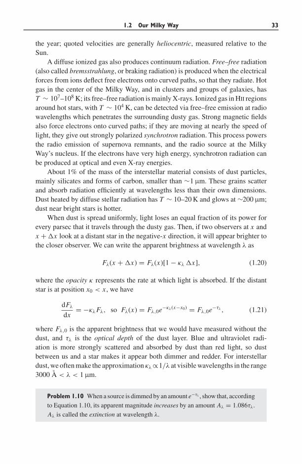
1.2 Our Milky Way 33

the year; quoted velocities are generally heliocentric, measured relative to theSun.

A diffuse ionized gas also produces continuum radiation. Free–free radiation(also called bremsstrahlung, or braking radiation) is produced when the electricalforces from ions deflect free electrons onto curved paths, so that they radiate. Hotgas in the center of the Milky Way, and in clusters and groups of galaxies, hasT ∼ 107–108 K; its free–free radiation is mainly X-rays. Ionized gas in HII regionsaround hot stars, with T ∼ 104 K, can be detected via free–free emission at radiowavelengths which penetrates the surrounding dusty gas. Strong magnetic fieldsalso force electrons onto curved paths; if they are moving at nearly the speed oflight, they give out strongly polarized synchrotron radiation. This process powersthe radio emission of supernova remnants, and the radio source at the MilkyWay’s nucleus. If the electrons have very high energy, synchrotron radiation canbe produced at optical and even X-ray energies.

About 1% of the mass of the interstellar material consists of dust particles,mainly silicates and forms of carbon, smaller than ∼1 μm. These grains scatterand absorb radiation efficiently at wavelengths less than their own dimensions.Dust heated by diffuse stellar radiation has T ∼ 10–20 K and glows at ∼200 μm;dust near bright stars is hotter.

When dust is spread uniformly, light loses an equal fraction of its power forevery parsec that it travels through the dusty gas. Then, if two observers at x andx + �x look at a distant star in the negative-x direction, it will appear brighter tothe closer observer. We can write the apparent brightness at wavelength λ as

Fλ(x + �x) = Fλ(x)[1 − κλ �x], (1.20)

where the opacity κ represents the rate at which light is absorbed. If the distantstar is at position x0 < x , we have

dFλ

dx= −κλFλ, so Fλ(x) = Fλ,0e−κλ(x−x0) = Fλ,0e−τλ, (1.21)

where Fλ,0 is the apparent brightness that we would have measured without thedust, and τλ is the optical depth of the dust layer. Blue and ultraviolet radi-ation is more strongly scattered and absorbed by dust than red light, so dustbetween us and a star makes it appear both dimmer and redder. For interstellardust, we often make the approximation κλ ∝1/λ at visible wavelengths in the range3000 A < λ < 1 μm.

Problem 1.10 When a source is dimmed by an amount e−τλ , show that, according

to Equation 1.10, its apparent magnitude increases by an amount Aλ = 1.086τλ.

Aλ is called the extinction at wavelength λ.

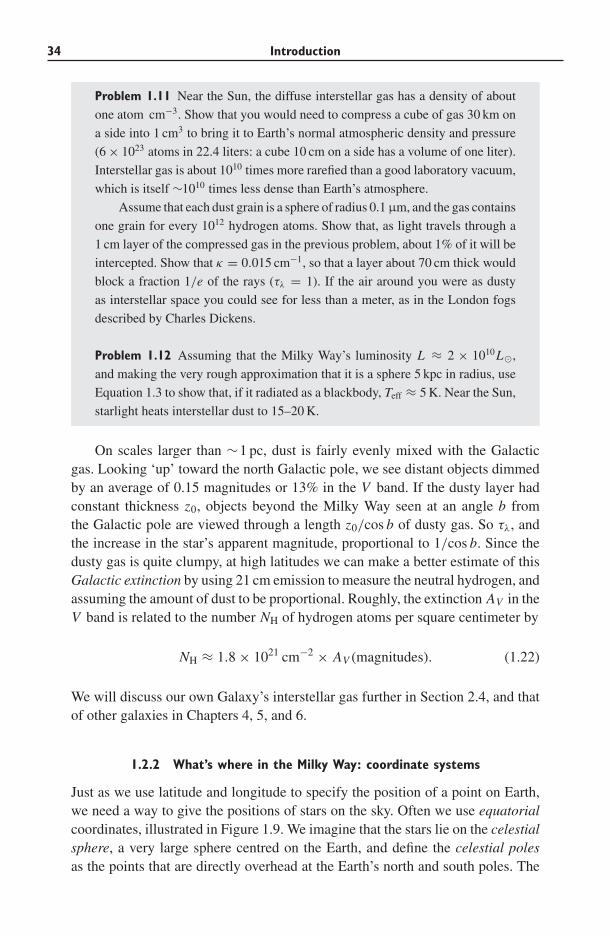
34 Introduction

Problem 1.11 Near the Sun, the diffuse interstellar gas has a density of about

one atom cm−3. Show that you would need to compress a cube of gas 30 km on

a side into 1 cm3 to bring it to Earth’s normal atmospheric density and pressure

(6 × 1023 atoms in 22.4 liters: a cube 10 cm on a side has a volume of one liter).

Interstellar gas is about 1010 times more rarefied than a good laboratory vacuum,

which is itself ∼1010 times less dense than Earth’s atmosphere.

Assume that each dust grain is a sphere of radius 0.1 μm, and the gas contains

one grain for every 1012 hydrogen atoms. Show that, as light travels through a

1 cm layer of the compressed gas in the previous problem, about 1% of it will be

intercepted. Show that κ = 0.015 cm−1, so that a layer about 70 cm thick would

block a fraction 1/e of the rays (τλ = 1). If the air around you were as dusty

as interstellar space you could see for less than a meter, as in the London fogs

described by Charles Dickens.

Problem 1.12 Assuming that the Milky Way’s luminosity L ≈ 2 × 1010L�,

and making the very rough approximation that it is a sphere 5 kpc in radius, use

Equation 1.3 to show that, if it radiated as a blackbody, Teff ≈ 5 K. Near the Sun,

starlight heats interstellar dust to 15–20 K.

On scales larger than ∼1 pc, dust is fairly evenly mixed with the Galacticgas. Looking ‘up’ toward the north Galactic pole, we see distant objects dimmedby an average of 0.15 magnitudes or 13% in the V band. If the dusty layer hadconstant thickness z0, objects beyond the Milky Way seen at an angle b fromthe Galactic pole are viewed through a length z0/cos b of dusty gas. So τλ, andthe increase in the star’s apparent magnitude, proportional to 1/cos b. Since thedusty gas is quite clumpy, at high latitudes we can make a better estimate of thisGalactic extinction by using 21 cm emission to measure the neutral hydrogen, andassuming the amount of dust to be proportional. Roughly, the extinction AV in theV band is related to the number NH of hydrogen atoms per square centimeter by

NH ≈ 1.8 × 1021 cm−2 × AV (magnitudes). (1.22)

We will discuss our own Galaxy’s interstellar gas further in Section 2.4, and thatof other galaxies in Chapters 4, 5, and 6.

1.2.2 What’s where in the Milky Way: coordinate systems

Just as we use latitude and longitude to specify the position of a point on Earth,we need a way to give the positions of stars on the sky. Often we use equatorialcoordinates, illustrated in Figure 1.9. We imagine that the stars lie on the celestialsphere, a very large sphere centred on the Earth, and define the celestial polesas the points that are directly overhead at the Earth’s north and south poles. The

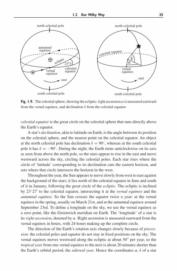
1.2 Our Milky Way 35

celestial equator

δα

autumnal equinox

vernalequinox

south celestial pole

north celestial pole

23 .5oecliptic

celestialequator

east east

vernalequinox

south celestial pole

north celestial pole

Fig. 1.9. The celestial sphere, showing the ecliptic: right ascension α is measured eastward

from the vernal equinox, and declination δ from the celestial equator.

celestial equator is the great circle on the celestial sphere that runs directly abovethe Earth’s equator.

A star’s declination, akin to latitude on Earth, is the angle between its positionon the celestial sphere, and the nearest point on the celestial equator. An objectat the north celestial pole has declination δ = 90◦, whereas at the south celestialpole it has δ = −90◦. During the night, the Earth turns anticlockwise on its axisas seen from above the north pole, so the stars appear to rise in the east and movewestward across the sky, circling the celestial poles. Each star rises where thecircle of ‘latitude’ corresponding to its declination cuts the eastern horizon, andsets where that circle intersects the horizon in the west.

Throughout the year, the Sun appears to move slowly from west to east againstthe background of the stars; it lies north of the celestial equator in June and southof it in January, following the great circle of the ecliptic. The ecliptic is inclinedby 23◦27′ to the celestial equator, intersecting it at the vernal equinox and theautumnal equinox. So the Sun crosses the equator twice a year: at the vernalequinox in the spring, usually on March 21st, and at the autumnal equinox aroundSeptember 23rd. To define a longitude on the sky, we use the vernal equinox asa zero point, like the Greenwich meridian on Earth. The ‘longitude’ of a star isits right ascension, denoted by α. Right ascension is measured eastward from thevernal equinox in hours, with 24 hours making up the complete circle.

The direction of the Earth’s rotation axis changes slowly because of preces-sion: the celestial poles and equator do not stay in fixed positions on the sky. Thevernal equinox moves westward along the ecliptic at about 50′′ per year, so thetropical year from one vernal equinox to the next is about 20 minutes shorter thanthe Earth’s orbital period, the sidereal year. Hence the coordinates α, δ of a star

36 Introduction

bl

GCφ

R

z

GCR o

Fig. 1.10. Left, Sun-centred Galactic longitude l and latitude b; right, cylindrical polar

coordinates R, φ, z with the origin at the Galactic center.

will depend on which year we take as the reference for our coordinate system.Astronomers generally use coordinates relative to the 1950 or 2000 equinox, orthe equinox of the current year. Computer programs easily convert between thesesystems. But more than one astronomer has pointed a telescope in the wrongdirection by forgetting to specify the equinox.

The stars that have reached their highest point in the sky at any moment alllie on a great circle passing through the celestial poles and through the zenith, thepoint directly overhead. These stars all have the same right ascension. On the dateof the autumnal equinox, in September, the position of the vernal equinox, andall stars with right ascension zero, are highest in the sky at midnight. Three hourslater, when the Earth has made an eighth of a turn on its axis, the stars further east,with right ascension 3h, will be at their highest; and so on through the night. So thepositions of the stars can be used to tell the time. At any moment, the right ascensionof the stars that are at their highest gives the local star time, or sidereal time: allobservatories have clocks telling sidereal time, as well as the usual civil time.

Problem 1.13 Draw a diagram to show that, as the Earth circles the Sun during

the course of a year, relative to the stars it makes 366 14 rotations on its axis. The

number of sidereal days in a year is one more than the number of solar days,

which are measured from midnight to midnight. So a sidereal day lasts only

23h56m.

To give the positions of stars as we see them in relation to the Milky Way,we use the Sun-centred system of Galactic latitude and longitude shown in theleft panel of Figure 1.10. The center of the Galaxy lies in the direction α =17h42m24s, δ = −28◦55′ (equinox 1950). Galactic longitude l is measured in theplane of the disk from the Sun–center line, defined as l = 0, toward the directionof the Sun’s rotation, l = 90◦. The region 0 < l < 180◦ is sometimes calledthe ‘northern’ half of the Galaxy, because it is visible from the Earth’s northernhemisphere, while 180◦ < l < 360◦ is the ‘southern’ Galaxy. The latitude b

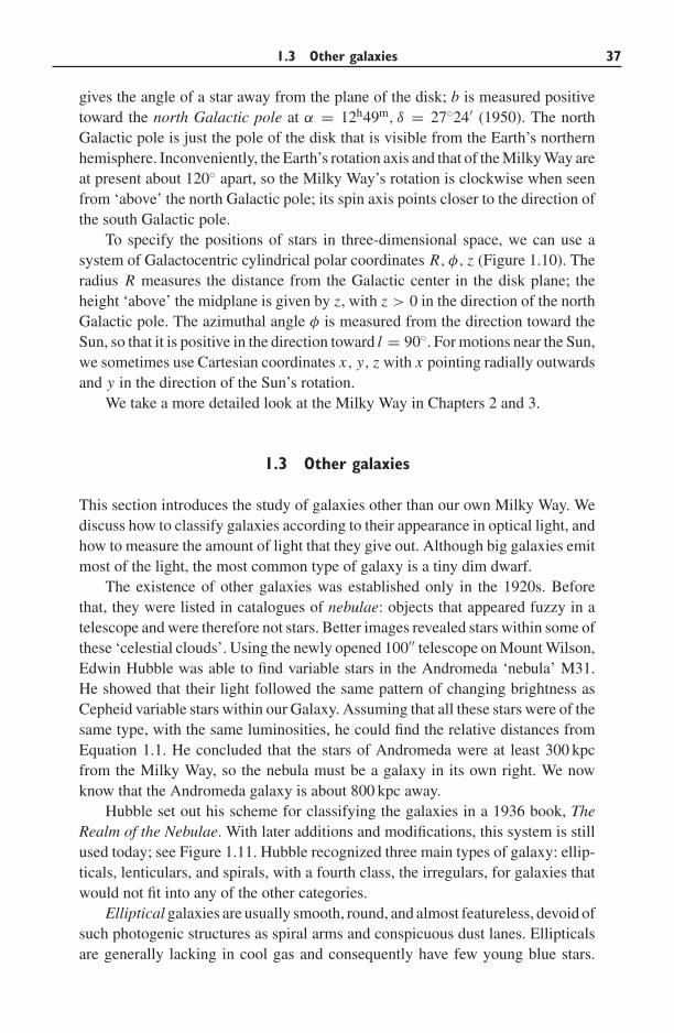
1.3 Other galaxies 37

gives the angle of a star away from the plane of the disk; b is measured positivetoward the north Galactic pole at α = 12h49m, δ = 27◦24′ (1950). The northGalactic pole is just the pole of the disk that is visible from the Earth’s northernhemisphere. Inconveniently, the Earth’s rotation axis and that of the Milky Way areat present about 120◦ apart, so the Milky Way’s rotation is clockwise when seenfrom ‘above’ the north Galactic pole; its spin axis points closer to the direction ofthe south Galactic pole.

To specify the positions of stars in three-dimensional space, we can use asystem of Galactocentric cylindrical polar coordinates R, φ, z (Figure 1.10). Theradius R measures the distance from the Galactic center in the disk plane; theheight ‘above’ the midplane is given by z, with z > 0 in the direction of the northGalactic pole. The azimuthal angle φ is measured from the direction toward theSun, so that it is positive in the direction toward l = 90◦. For motions near the Sun,we sometimes use Cartesian coordinates x, y, z with x pointing radially outwardsand y in the direction of the Sun’s rotation.

We take a more detailed look at the Milky Way in Chapters 2 and 3.

1.3 Other galaxies

This section introduces the study of galaxies other than our own Milky Way. Wediscuss how to classify galaxies according to their appearance in optical light, andhow to measure the amount of light that they give out. Although big galaxies emitmost of the light, the most common type of galaxy is a tiny dim dwarf.

The existence of other galaxies was established only in the 1920s. Beforethat, they were listed in catalogues of nebulae: objects that appeared fuzzy in atelescope and were therefore not stars. Better images revealed stars within some ofthese ‘celestial clouds’. Using the newly opened 100′′ telescope on Mount Wilson,Edwin Hubble was able to find variable stars in the Andromeda ‘nebula’ M31.He showed that their light followed the same pattern of changing brightness asCepheid variable stars within our Galaxy. Assuming that all these stars were of thesame type, with the same luminosities, he could find the relative distances fromEquation 1.1. He concluded that the stars of Andromeda were at least 300 kpcfrom the Milky Way, so the nebula must be a galaxy in its own right. We nowknow that the Andromeda galaxy is about 800 kpc away.

Hubble set out his scheme for classifying the galaxies in a 1936 book, TheRealm of the Nebulae. With later additions and modifications, this system is stillused today; see Figure 1.11. Hubble recognized three main types of galaxy: ellip-ticals, lenticulars, and spirals, with a fourth class, the irregulars, for galaxies thatwould not fit into any of the other categories.

Elliptical galaxies are usually smooth, round, and almost featureless, devoid ofsuch photogenic structures as spiral arms and conspicuous dust lanes. Ellipticalsare generally lacking in cool gas and consequently have few young blue stars.

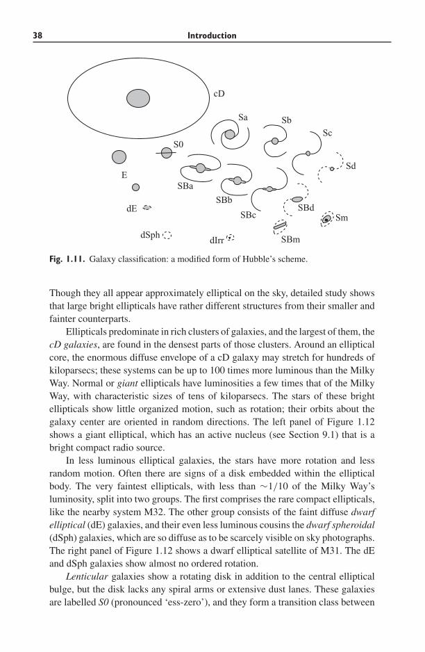
38 Introduction

cD

dE

dIrr

S0

E

Sa

SBa

Sc

dSph SBm

Sm

Sd

SBd

Sb

SBb

SBc

Fig. 1.11. Galaxy classification: a modified form of Hubble’s scheme.

Though they all appear approximately elliptical on the sky, detailed study showsthat large bright ellipticals have rather different structures from their smaller andfainter counterparts.

Ellipticals predominate in rich clusters of galaxies, and the largest of them, thecD galaxies, are found in the densest parts of those clusters. Around an ellipticalcore, the enormous diffuse envelope of a cD galaxy may stretch for hundreds ofkiloparsecs; these systems can be up to 100 times more luminous than the MilkyWay. Normal or giant ellipticals have luminosities a few times that of the MilkyWay, with characteristic sizes of tens of kiloparsecs. The stars of these brightellipticals show little organized motion, such as rotation; their orbits about thegalaxy center are oriented in random directions. The left panel of Figure 1.12shows a giant elliptical, which has an active nucleus (see Section 9.1) that is abright compact radio source.

In less luminous elliptical galaxies, the stars have more rotation and lessrandom motion. Often there are signs of a disk embedded within the ellipticalbody. The very faintest ellipticals, with less than ∼1/10 of the Milky Way’sluminosity, split into two groups. The first comprises the rare compact ellipticals,like the nearby system M32. The other group consists of the faint diffuse dwarfelliptical (dE) galaxies, and their even less luminous cousins the dwarf spheroidal(dSph) galaxies, which are so diffuse as to be scarcely visible on sky photographs.The right panel of Figure 1.12 shows a dwarf elliptical satellite of M31. The dEand dSph galaxies show almost no ordered rotation.

Lenticular galaxies show a rotating disk in addition to the central ellipticalbulge, but the disk lacks any spiral arms or extensive dust lanes. These galaxiesare labelled S0 (pronounced ‘ess-zero’), and they form a transition class between

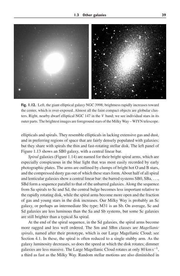
1.3 Other galaxies 39

Fig. 1.12. Left, the giant elliptical galaxy NGC 3998; brightness rapidly increases toward

the center, which is over-exposed. Almost all the faint compact objects are globular clus-

ters. Right, nearby dwarf elliptical NGC 147 in the V band; we see individual stars in its

outer parts. The brightest images are foreground stars of the Milky Way – WIYN telescope.

ellipticals and spirals. They resemble ellipticals in lacking extensive gas and dust,and in preferring regions of space that are fairly densely populated with galaxies;but they share with spirals the thin and fast-rotating stellar disk. The left panel ofFigure 1.13 shows an SB0 galaxy, with a central linear bar.

Spiral galaxies (Figure 1.14) are named for their bright spiral arms, which areespecially conspicuous in the blue light that was most easily recorded by earlyphotographic plates. The arms are outlined by clumps of bright hot O and B stars,and the compressed dusty gas out of which these stars form. About half of all spiraland lenticular galaxies show a central linear bar: the barred systems SB0, SBa, . . .,SBd form a sequence parallel to that of the unbarred galaxies. Along the sequencefrom Sa spirals to Sc and Sd, the central bulge becomes less important relative tothe rapidly rotating disk, while the spiral arms become more open and the fractionof gas and young stars in the disk increases. Our Milky Way is probably an Scgalaxy, or perhaps an intermediate Sbc type; M31 is an Sb. On average, Sc andSd galaxies are less luminous than the Sa and Sb systems, but some Sc galaxiesare still brighter than a typical Sa spiral.

At the end of the spiral sequence, in the Sd galaxies, the spiral arms becomemore ragged and less well ordered. The Sm and SBm classes are Magellanicspirals, named after their prototype, which is our Large Magellanic Cloud; seeSection 4.1. In these, the spiral is often reduced to a single stubby arm. As thegalaxy luminosity decreases, so does the speed at which the disk rotates; dimmergalaxies are less massive. The Large Magellanic Cloud rotates at only 80 km s−1,a third as fast as the Milky Way. Random stellar motions are also diminished in

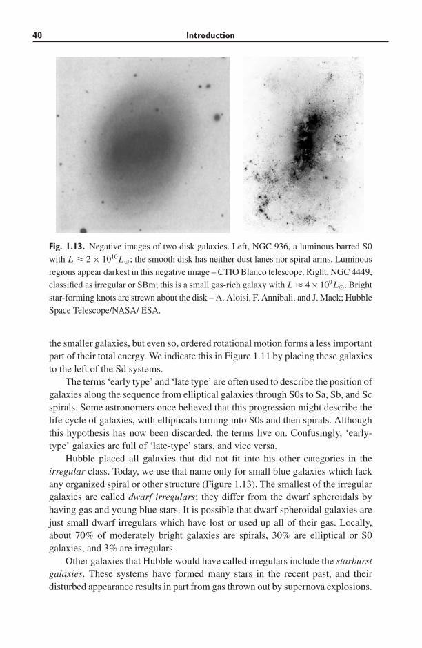
40 Introduction

Fig. 1.13. Negative images of two disk galaxies. Left, NGC 936, a luminous barred S0

with L ≈ 2 × 1010L�; the smooth disk has neither dust lanes nor spiral arms. Luminous

regions appear darkest in this negative image – CTIO Blanco telescope. Right, NGC 4449,

classified as irregular or SBm; this is a small gas-rich galaxy with L ≈ 4 × 109L�. Bright

star-forming knots are strewn about the disk – A. Aloisi, F. Annibali, and J. Mack; Hubble

Space Telescope/NASA/ ESA.

the smaller galaxies, but even so, ordered rotational motion forms a less importantpart of their total energy. We indicate this in Figure 1.11 by placing these galaxiesto the left of the Sd systems.

The terms ‘early type’ and ‘late type’ are often used to describe the position ofgalaxies along the sequence from elliptical galaxies through S0s to Sa, Sb, and Scspirals. Some astronomers once believed that this progression might describe thelife cycle of galaxies, with ellipticals turning into S0s and then spirals. Althoughthis hypothesis has now been discarded, the terms live on. Confusingly, ‘early-type’ galaxies are full of ‘late-type’ stars, and vice versa.

Hubble placed all galaxies that did not fit into his other categories in theirregular class. Today, we use that name only for small blue galaxies which lackany organized spiral or other structure (Figure 1.13). The smallest of the irregulargalaxies are called dwarf irregulars; they differ from the dwarf spheroidals byhaving gas and young blue stars. It is possible that dwarf spheroidal galaxies arejust small dwarf irregulars which have lost or used up all of their gas. Locally,about 70% of moderately bright galaxies are spirals, 30% are elliptical or S0galaxies, and 3% are irregulars.

Other galaxies that Hubble would have called irregulars include the starburstgalaxies. These systems have formed many stars in the recent past, and theirdisturbed appearance results in part from gas thrown out by supernova explosions.

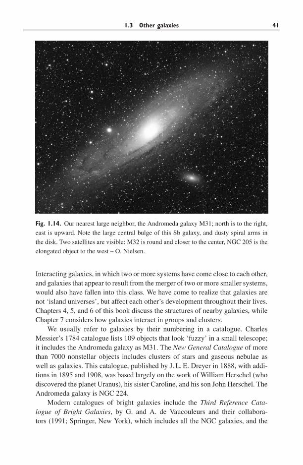
1.3 Other galaxies 41

Fig. 1.14. Our nearest large neighbor, the Andromeda galaxy M31; north is to the right,

east is upward. Note the large central bulge of this Sb galaxy, and dusty spiral arms in

the disk. Two satellites are visible: M32 is round and closer to the center, NGC 205 is the

elongated object to the west – O. Nielsen.

Interacting galaxies, in which two or more systems have come close to each other,and galaxies that appear to result from the merger of two or more smaller systems,would also have fallen into this class. We have come to realize that galaxies arenot ‘island universes’, but affect each other’s development throughout their lives.Chapters 4, 5, and 6 of this book discuss the structures of nearby galaxies, whileChapter 7 considers how galaxies interact in groups and clusters.

We usually refer to galaxies by their numbering in a catalogue. CharlesMessier’s 1784 catalogue lists 109 objects that look ‘fuzzy’ in a small telescope;it includes the Andromeda galaxy as M31. The New General Catalogue of morethan 7000 nonstellar objects includes clusters of stars and gaseous nebulae aswell as galaxies. This catalogue, published by J. L. E. Dreyer in 1888, with addi-tions in 1895 and 1908, was based largely on the work of William Herschel (whodiscovered the planet Uranus), his sister Caroline, and his son John Herschel. TheAndromeda galaxy is NGC 224.

Modern catalogues of bright galaxies include the Third Reference Cata-logue of Bright Galaxies, by G. and A. de Vaucouleurs and their collabora-tors (1991; Springer, New York), which includes all the NGC galaxies, and the

42 Introduction

Uppsala General Catalogue of Galaxies, by P. Nilson (1973; Uppsala Observa-tory), with its southern extension, the ESO/Uppsala Survey of the ESO(B) Atlas, byA. Lauberts (1982; European Southern Observatory). Galaxies that emit brightly inthe radio, X-rays, etc., also appear in catalogues of those sources. Many recent cat-alogues are published electronically; for example, NASA’s Extragalactic Database(http://ned.ipac.caltech.edu).

Further reading: E. Hubble, 1936, The Realm of the Nebulae (Yale UniversityPress; reprinted by Dover, New York); for pictures to illustrate Hubble’s classifi-cation, see A. Sandage, 1961, The Hubble Atlas of Galaxies (Carnegie Instituteof Washington; Washington, DC). A recent graduate text on galaxy classificationis S. van den Bergh, 1998, Galaxy Morphology and Classification (CambridgeUniversity Press, Cambridge, UK).

1.3.1 Galaxy photometry

Unlike stars, galaxies do not appear as points of light; they extend across the sky.Turbulence in the Earth’s atmosphere has the effect of blurring galaxy images; thisis known as seeing. Because of it, a ground-based optical telescope rarely showsdetails smaller than about 1/3′′. For sharper images, we must use a telescope inspace or resort to techniques such as interferometry or adaptive optics.

Although the classification of galaxies is still based on their appearance inoptical images, most work on galaxies is quantitative, measuring how much light,at what wavelengths, is emitted by the different regions. The surface brightness ofa galaxy I (x) is the amount of light per square arcsecond on the sky at a particularpoint x in the image. Consider a small square patch of side D in a galaxy that weview from a distance d , so that it subtends an angle α = D/d on the sky. If thecombined luminosity of all the stars in this region is L , its apparent brightness Fis given by Equation 1.1; then the surface brightness is

I (x) ≡ F

α2= L/(4πd2)

D2/d2= L

4π D2. (1.23)

I is usually given in mag arcsec−2 (the apparent magnitude of a star that appearsas bright as one square arcsecond of the galaxy’s image), or in L� pc−2. Thesurface brightness at any point does not depend on distance unless d is so largethat the expansion of the Universe has the effect of reducing I (x); we discuss thisfurther in Section 8.3. Contours of constant surface brightness on a galaxy imageare called isophotes. Equation 1.23 shows that the position of an isophote withinthe galaxy is independent of the observer’s distance.

We generally measure surface brightness in a fixed wavelength band, just asfor stellar photometry. The centers of galaxies reach only IB ≈ 18 mag arcsec−2

or IR ≈ 16 mag arcsec−2, and the stellar disks are much fainter. Galaxies do not

1.3 Other galaxies 43

have sharp edges, so we often measure their sizes within a fixed isophote. Onepopular choice is the 25th-magnitude isophote in the blue B band, denoted R25.This is about 1% of the sky level on an average night; before CCD photometry(see Section 5.1), it was close to the limit of what could be measured reliably.Another option is the Holmberg radius at IB(x) = 26.5 mag arcsec−2. To find theluminosity of the whole galaxy, we measure how the amount of light coming fromwithin a given radius grows as that radius is moved outward, and we extrapolateto reach the total.

Problem 1.14 In a galaxy at a distance of d Mpc, what would be the apparent

B-magnitude of a star like our Sun? In this galaxy, show that 1′′ on the sky

corresponds to 5d pc. If the surface brightness IB = 27 mag arcsec−2, how much

B-band light does one square arcsecond of the galaxy emit, compared with a

star like the Sun? Show that this is equivalent to L� pc−2 in the B band, but that

II = 27 mag arcsec−2 corresponds to only 0.3L� pc−2 in the I band.

Table 1.9 gives the surface brightness of the night sky measured in the band-passes of Figure 1.7. These are approximate average values, since the sky bright-ness depends on solar activity (the sunspot cycle), the observatory’s location onEarth, and the direction in the sky. Typically, the sky is brighter than all but theinner core of a galaxy, and on a moonlit night even the center can disappear into thebright sky. From Earth’s surface, optical observations of galaxies must generallybe made during the dark of the moon.

If our eyes could perceive colors at such low light levels, we would see the skyglowing red with emission in the bands of atmospheric molecules. In the near-infrared at 2 μm, from most observatory sites the sky is over a thousand timesbrighter than it would be in space. Figure 1.15 shows how steeply its emission risesat longer wavelengths, in the thermal infrared. The high cold South Pole is the bestEarth-based site at these wavelengths, but the sky is still enormously brighter thanfrom space. Standard infrared filters are chosen to lie where the atmosphere is mosttransparent. Between these regions, we see a blackbody spectrum correspondingto the temperature of the opaque layers.

We can cut down the sky light by designing our filters to exclude someof the strongest lines; using the K ′ filter instead of K blocks out about two-thirds of the emission. But Table 1.9 makes clear that, when we observe fromthe ground, the infrared sky is always brighter than the galaxy. To find thesurface brightness accurately, we must measure the brightness of a patch ofblank sky as it changes throughout the night just as accurately as we measurethe galaxy-plus-sky; the small difference between the two gives I (x). A tele-scope in space gives us a much darker sky at red and infrared wavelengths.We can also observe in the near-ultraviolet, where the sky brightness is yetlower.

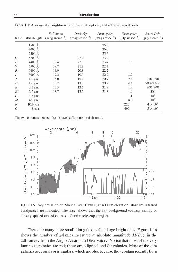
44 Introduction

Table 1.9 Average sky brightness in ultraviolet, optical, and infrared wavebands

Full moon Dark sky From space From space South PoleBand Wavelength ( mag arcsec−2) ( mag arcsec−2) ( mag arcsec−2) (μJy arcsec−2) (μJy arcsec−2)

1500 A 25.02000 A 26.02500 A 25.6

U 3700 A 22.0 23.2B 4400 A 19.4 22.7 23.4 1.8V 5500 A 19.7 21.8 22.7R 6400 A 19.9 20.9 22.2I 8000 A 19.2 19.9 22.2 3.2J 1.2 μm 15.0 15.0 20.7 2.4 300–600H 1.6 μm 13.7 13.7 20.9 4.4 800–2 000K 2.2 μm 12.5 12.5 21.3 1.9 300–700K ′ 2.2 μm 13.7 13.7 21.3 1.9 500L 3.3 μm 1.1 105

M 4.9 μm 8.0 106

N 10.6 μm 220 4 × 107

Q 19 μm 400 3 × 108

The two columns headed ‘from space’ differ only in their units.

2 4 6 8 10 20

K

L

MN

Q

1.5 1.55 1.6

Fig. 1.15. Sky emission on Mauna Kea, Hawaii, at 4000 m elevation; standard infrared

bandpasses are indicated. The inset shows that the sky background consists mainly of

closely spaced emission lines – Gemini telescope project.

There are many more small dim galaxies than large bright ones. Figure 1.16shows the number of galaxies measured at absolute magnitude M(BJ ), in the2dF survey from the Anglo-Australian Observatory. Notice that most of the veryluminous galaxies are red; these are elliptical and S0 galaxies. Most of the dimgalaxies are spirals or irregulars, which are blue because they contain recently born

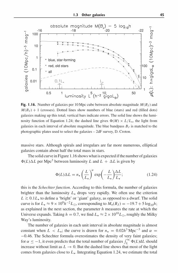
1.3 Other galaxies 45

-16 -18 -20 -22

0.01

0.1

1

10

100

red, old stars

all

blue, star-forming

0.5 1 5 10 501

10

100

Fig. 1.16. Number of galaxies per 10 Mpc cube between absolute magnitude M(BJ ) and

M(BJ ) + 1 (crosses). Dotted lines show numbers of blue (stars) and red (filled dots)

galaxies making up this total; vertical bars indicate errors. The solid line shows the lumi-

nosity function of Equation 1.24; the dashed line gives �(M) × L/L, the light from

galaxies in each interval of absolute magnitude. The blue bandpass BJ is matched to the

photographic plates used to select the galaxies – 2dF survey, D. Croton.

massive stars. Although spirals and irregulars are far more numerous, ellipticalgalaxies contain about half the total mass in stars.

The solid curve in Figure 1.16 shows what is expected if the number of galaxies�(L)�L per Mpc3 between luminosity L and L + �L is given by

�(L)�L = n

(L

L

)α

exp

(− L

L

)�L

L

; (1.24)

this is the Schechter function. According to this formula, the number of galaxiesbrighter than the luminosity L drops very rapidly. We often use the criterionL ∼> 0.1L to define a ‘bright’ or ‘giant’ galaxy, as opposed to a dwarf. The solidcurve is for L ≈ 9 × 109h−2L�, corresponding to M(BJ ) = −19.7 + 5 log10h;as explained in the next section, the parameter h measures the rate at which theUniverse expands. Taking h = 0.7, we find L ≈ 2 × 1010L�, roughly the MilkyWay’s luminosity.

The number of galaxies in each unit interval in absolute magnitude is almostconstant when L < L; the curve is drawn for n = 0.02h3 Mpc−3 and α =−0.46. The Schechter formula overestimates the density of very faint galaxies;for α ≤ −1, it even predicts that the total number of galaxies

∫∞L �(L)dL should

increase without limit as L → 0. But the dashed line shows that most of the lightcomes from galaxies close to L. Integrating Equation 1.24, we estimate the total

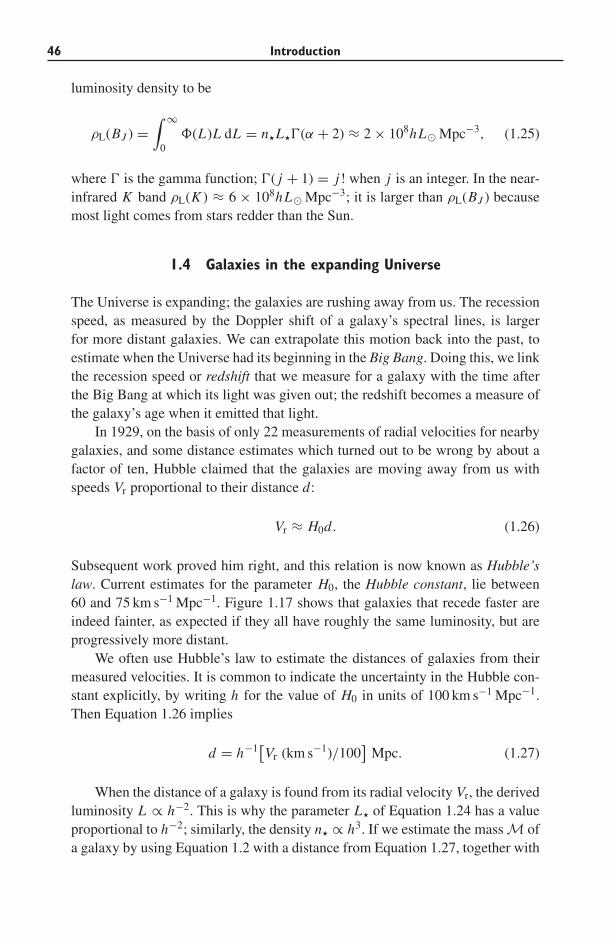
46 Introduction

luminosity density to be

ρL(BJ ) =∫ ∞

0�(L)L dL = nL�(α + 2) ≈ 2 × 108hL� Mpc−3, (1.25)

where � is the gamma function; �( j + 1) = j! when j is an integer. In the near-infrared K band ρL(K ) ≈ 6 × 108hL� Mpc−3; it is larger than ρL(BJ ) becausemost light comes from stars redder than the Sun.

1.4 Galaxies in the expanding Universe

The Universe is expanding; the galaxies are rushing away from us. The recessionspeed, as measured by the Doppler shift of a galaxy’s spectral lines, is largerfor more distant galaxies. We can extrapolate this motion back into the past, toestimate when the Universe had its beginning in the Big Bang. Doing this, we linkthe recession speed or redshift that we measure for a galaxy with the time afterthe Big Bang at which its light was given out; the redshift becomes a measure ofthe galaxy’s age when it emitted that light.

In 1929, on the basis of only 22 measurements of radial velocities for nearbygalaxies, and some distance estimates which turned out to be wrong by about afactor of ten, Hubble claimed that the galaxies are moving away from us withspeeds Vr proportional to their distance d:

Vr ≈ H0d. (1.26)

Subsequent work proved him right, and this relation is now known as Hubble’slaw. Current estimates for the parameter H0, the Hubble constant, lie between60 and 75 km s−1 Mpc−1. Figure 1.17 shows that galaxies that recede faster areindeed fainter, as expected if they all have roughly the same luminosity, but areprogressively more distant.

We often use Hubble’s law to estimate the distances of galaxies from theirmeasured velocities. It is common to indicate the uncertainty in the Hubble con-stant explicitly, by writing h for the value of H0 in units of 100 km s−1 Mpc−1.Then Equation 1.26 implies

d = h−1[Vr (km s−1)/100]

Mpc. (1.27)

When the distance of a galaxy is found from its radial velocity Vr, the derivedluminosity L ∝ h−2. This is why the parameter L of Equation 1.24 has a valueproportional to h−2; similarly, the density n ∝ h3. If we estimate the mass M ofa galaxy by using Equation 1.2 with a distance from Equation 1.27, together with

1.4 Galaxies in the expanding Universe 47

0.01 0.05 0.1 0.5

12

14

16

18

Fig. 1.17. Apparent magnitude in the V band for the brightest galaxies in rich galaxy

clusters. The magnitude increases proportionally to the logarithm of the redshift z, as we

expect if the galaxy’s distance is proportional to its recession speed cz – data from J. E.

Gunn and J. B. Oke 1975 ApJ 195, 255.

Newton’s equation for the gravitational force (see Section 3.1), then we have thatM ∝ h−1.

If the average speeds of the galaxies had always remained constant, they wouldhave been on top of each other at a time tH before the present, where

tH = 1

H0= 9.78h−1 Gyr = 15 Gyr × 67 km s−1 Mpc−1

H0. (1.28)

This is called the Hubble time; we can use it as a rough estimate of the age of theUniverse, the time since the Big Bang.

Problem 1.15 If a galaxy has absolute magnitude M , use Equations 1.1 and

1.27 to show that its apparent magnitude m is related to the redshift z = Vr/c of

Equation 1.19 by m = M + 5 log10 z + C , where C is a constant, the same for

all objects. Draw an approximate straight line through the points in Figure 1.17;

check that its slope is roughly what you would expect if the brightest galaxy in

a rich cluster always had the same luminosity.

Using Hubble’s law to find approximate distances for galaxies, we can exam-ine their distribution in space: Figure 8.3 shows the region of the 2dF survey ofFigure 1.16. We do not see galaxies spread uniformly through space, but concen-trated into groups and clusters. Within rich clusters, the galaxies’ orbits give thempeculiar velocities up to 1500 km s−1. So, if we use Equation 1.27 to find their

48 Introduction

positions, they will appear to be closer or more distant than they really are. Agalaxy’s measured radial velocity Vr has two components: the cosmic expansion,and a peculiar velocity Vpec. Equation 1.26 should be modified to read

Vr = H0d + Vpec. (1.29)

Between the clusters, we will see in Chapter 8 that individual galaxies andsmall groups lie along filaments or in large sheets. The groups and associationsof galaxies within these filaments and sheets are less rich than clusters, but morenumerous. Our Milky Way and its neighbor Andromeda form part of the LocalGroup, which includes a few dozen smaller systems within a radius of 1–2 Mpc.Between the sheets and filaments are vast nearly empty regions; in these voids,we see only a few isolated galaxies.

1.4.1 Densities and ages

In Section 8.2 we will examine the dynamics of the cosmic expansion, and howit is related to the density of matter and energy in the Universe. If the averagedensity is now greater than the critical density, the expansion can in future reverseto a contraction; if it is less, the galaxies continue to recede forever. The criticaldensity is

ρcrit(now) = 3H 20

8πG= 1.9 × 10−29h2 g cm−3

= 2.8 × 1011h2M� Mpc−3. (1.30)

For H0 = 67 km s−1 Mpc−1, this is equivalent to a good-sized galaxy in eachmegaparsec cube, or about five hydrogen atoms per m3. If matter in the Universehas exactly this density, the time t0 from the Big Bang to the present day is

t0 = 2

3H0≈ 10 Gyr ×

(67 km s−1 Mpc−1

H0

). (1.31)

If the average density exceeds ρcrit, the Universe is younger than this, whereasif the density is less, it is older. We shall see that the density is unlikely to begreater than the critical value, so the time since the Big Bang is at least that givenby Equation 1.31. The present age t0 can be larger than tH only if the equationsof General Relativity are modified by including dark energy, which pushes thegalaxies away from each other.

We will see in the following section that normal matter makes up onlyabout 4% of the critical density. In the current benchmark model for the cosmicexpansion, the total density has exactly the critical value, and H0 = 70 km s−1

Mpc−1. Matter makes up 30% of ρcrit, but most of it is dark. The dark matterprobably consists of particles that, like neutrinos, are weakly interacting – or we

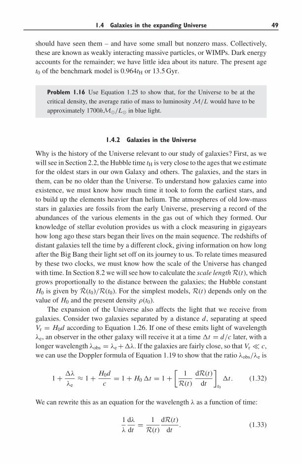
1.4 Galaxies in the expanding Universe 49

should have seen them – and have some small but nonzero mass. Collectively,these are known as weakly interacting massive particles, or WIMPs. Dark energyaccounts for the remainder; we have little idea about its nature. The present aget0 of the benchmark model is 0.964tH or 13.5 Gyr.

Problem 1.16 Use Equation 1.25 to show that, for the Universe to be at the

critical density, the average ratio of mass to luminosity M/L would have to be

approximately 1700hM�/L� in blue light.

1.4.2 Galaxies in the Universe

Why is the history of the Universe relevant to our study of galaxies? First, as wewill see in Section 2.2, the Hubble time tH is very close to the ages that we estimatefor the oldest stars in our own Galaxy and others. The galaxies, and the stars inthem, can be no older than the Universe. To understand how galaxies came intoexistence, we must know how much time it took to form the earliest stars, andto build up the elements heavier than helium. The atmospheres of old low-massstars in galaxies are fossils from the early Universe, preserving a record of theabundances of the various elements in the gas out of which they formed. Ourknowledge of stellar evolution provides us with a clock measuring in gigayearshow long ago these stars began their lives on the main sequence. The redshifts ofdistant galaxies tell the time by a different clock, giving information on how longafter the Big Bang their light set off on its journey to us. To relate times measuredby these two clocks, we must know how the scale of the Universe has changedwith time. In Section 8.2 we will see how to calculate the scale length R(t), whichgrows proportionally to the distance between the galaxies; the Hubble constantH0 is given by R(t0)/R(t0). For the simplest models, R(t) depends only on thevalue of H0 and the present density ρ(t0).

The expansion of the Universe also affects the light that we receive fromgalaxies. Consider two galaxies separated by a distance d, separating at speedVr = H0d according to Equation 1.26. If one of these emits light of wavelengthλe, an observer in the other galaxy will receive it at a time �t = d/c later, with alonger wavelength λobs = λe +�λ. If the galaxies are fairly close, so that Vr � c,we can use the Doppler formula of Equation 1.19 to show that the ratio λobs/λe is

1 + �λ

λe≈ 1 + H0d

c= 1 + H0 �t = 1 +

[1

R(t)

dR(t)

dt

]t0

�t . (1.32)

We can rewrite this as an equation for the wavelength λ as a function of time:

1

λ

dλ

dt= 1

R(t)

dR(t)

dt. (1.33)

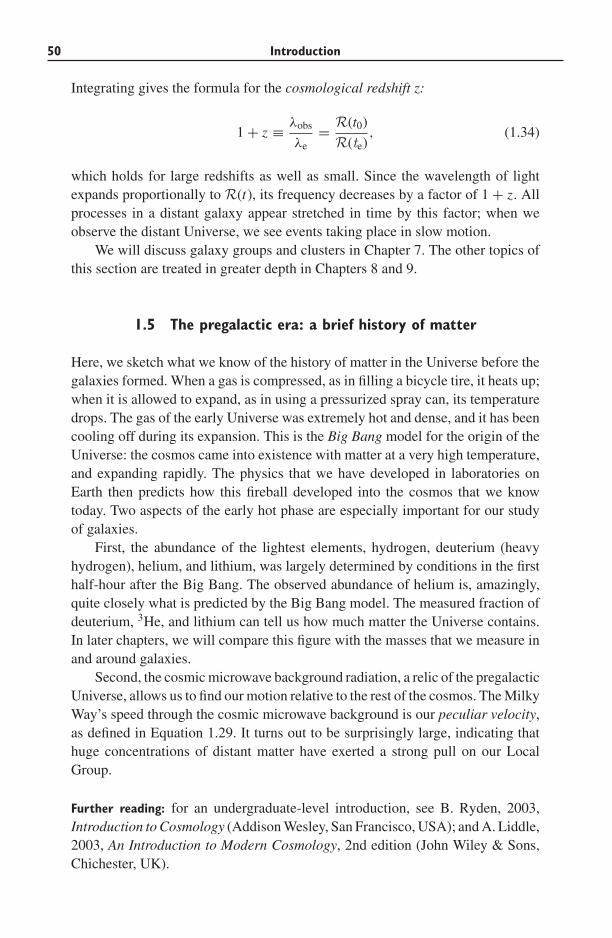
50 Introduction

Integrating gives the formula for the cosmological redshift z:

1 + z ≡ λobs

λe= R(t0)

R(te), (1.34)

which holds for large redshifts as well as small. Since the wavelength of lightexpands proportionally to R(t), its frequency decreases by a factor of 1 + z. Allprocesses in a distant galaxy appear stretched in time by this factor; when weobserve the distant Universe, we see events taking place in slow motion.

We will discuss galaxy groups and clusters in Chapter 7. The other topics ofthis section are treated in greater depth in Chapters 8 and 9.

1.5 The pregalactic era: a brief history of matter

Here, we sketch what we know of the history of matter in the Universe before thegalaxies formed. When a gas is compressed, as in filling a bicycle tire, it heats up;when it is allowed to expand, as in using a pressurized spray can, its temperaturedrops. The gas of the early Universe was extremely hot and dense, and it has beencooling off during its expansion. This is the Big Bang model for the origin of theUniverse: the cosmos came into existence with matter at a very high temperature,and expanding rapidly. The physics that we have developed in laboratories onEarth then predicts how this fireball developed into the cosmos that we knowtoday. Two aspects of the early hot phase are especially important for our studyof galaxies.

First, the abundance of the lightest elements, hydrogen, deuterium (heavyhydrogen), helium, and lithium, was largely determined by conditions in the firsthalf-hour after the Big Bang. The observed abundance of helium is, amazingly,quite closely what is predicted by the Big Bang model. The measured fraction ofdeuterium, 3He, and lithium can tell us how much matter the Universe contains.In later chapters, we will compare this figure with the masses that we measure inand around galaxies.

Second, the cosmic microwave background radiation, a relic of the pregalacticUniverse, allows us to find our motion relative to the rest of the cosmos. The MilkyWay’s speed through the cosmic microwave background is our peculiar velocity,as defined in Equation 1.29. It turns out to be surprisingly large, indicating thathuge concentrations of distant matter have exerted a strong pull on our LocalGroup.

Further reading: for an undergraduate-level introduction, see B. Ryden, 2003,Introduction to Cosmology (Addison Wesley, San Francisco, USA); and A. Liddle,2003, An Introduction to Modern Cosmology, 2nd edition (John Wiley & Sons,Chichester, UK).

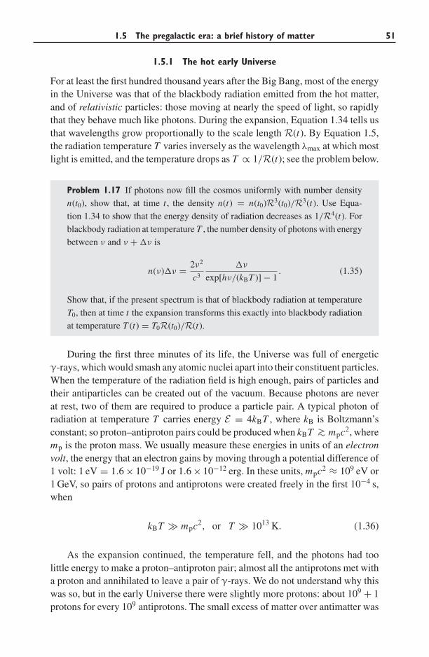
1.5 The pregalactic era: a brief history of matter 51

1.5.1 The hot early Universe

For at least the first hundred thousand years after the Big Bang, most of the energyin the Universe was that of the blackbody radiation emitted from the hot matter,and of relativistic particles: those moving at nearly the speed of light, so rapidlythat they behave much like photons. During the expansion, Equation 1.34 tells usthat wavelengths grow proportionally to the scale length R(t). By Equation 1.5,the radiation temperature T varies inversely as the wavelength λmax at which mostlight is emitted, and the temperature drops as T ∝ 1/R(t); see the problem below.

Problem 1.17 If photons now fill the cosmos uniformly with number density

n(t0), show that, at time t , the density n(t) = n(t0)R3(t0)/R3(t). Use Equa-

tion 1.34 to show that the energy density of radiation decreases as 1/R4(t). For

blackbody radiation at temperature T , the number density of photons with energy

between ν and ν + �ν is

n(ν)�ν = 2ν2

c3

�ν

exp[hν/(kBT )] − 1. (1.35)

Show that, if the present spectrum is that of blackbody radiation at temperature

T0, then at time t the expansion transforms this exactly into blackbody radiation

at temperature T (t) = T0R(t0)/R(t).

During the first three minutes of its life, the Universe was full of energeticγ-rays, which would smash any atomic nuclei apart into their constituent particles.When the temperature of the radiation field is high enough, pairs of particles andtheir antiparticles can be created out of the vacuum. Because photons are neverat rest, two of them are required to produce a particle pair. A typical photon ofradiation at temperature T carries energy E = 4kBT , where kB is Boltzmann’sconstant; so proton–antiproton pairs could be produced when kBT ∼> mpc2, wheremp is the proton mass. We usually measure these energies in units of an electronvolt, the energy that an electron gains by moving through a potential difference of1 volt: 1 eV = 1.6 × 10−19 J or 1.6 × 10−12 erg. In these units, mpc2 ≈ 109 eV or1 GeV, so pairs of protons and antiprotons were created freely in the first 10−4 s,when

kBT � mpc2, or T � 1013 K. (1.36)

As the expansion continued, the temperature fell, and the photons had toolittle energy to make a proton–antiproton pair; almost all the antiprotons met witha proton and annihilated to leave a pair of γ-rays. We do not understand why thiswas so, but in the early Universe there were slightly more protons: about 109 + 1protons for every 109 antiprotons. The small excess of matter over antimatter was

52 Introduction

left over to form the galaxies. The photons produced in the annihilation are seentoday as the cosmic microwave background.

Electrons are about 2000 times less massive than protons: their rest energymec2 is only 0.5 MeV. So the radiation still produced pairs of electrons and anti-electrons (positrons, e+), until the temperature dropped a thousandfold, to T ∼1010 K. Before this time, the reaction

e− + e+ ←→ νe + νe

could produce electron neutrinosνe and their antiparticles νe. The great abundanceof electrons, positrons, and neutrinos allowed neutrons to turn into protons, andvice versa, through reactions such as

e− + p ←→ n + νe, νe + p ←→ n + e+, n ←→ p + e− + νe.

In equilibrium at temperature T , there would have been slightly fewer neutronsthan protons, since the neutron mass mn is larger. The ratio of neutrons to protonswas given by

n/p = e−Q/(kBT ), where Q = (mn − mp)c2 = 1.293 MeV. (1.37)

Neutrinos are very weakly interacting particles; from the Sun, 1015 of them flyharmlessly through each square meter of the Earth’s surface every second. Onlyin the extremely hot material of supernova cores, or in the early Universe, dothey have an appreciable chance of reacting with other particles. While electron–positron pairs were still numerous, the density of neutrinos was high enough tokeep the balance between neutrons and protons at this equilibrium level. But later,once kBT ∼< 0.8 MeV or t ∼> 1 s, expansion had cooled the matter and neutrinosso much that a neutron or proton was very unlikely to interact with a neutrino.The neutrons froze out, with n/p ≈ 1/5.

1.5.2 Making the elements

Neutrons can survive if they are bound up in the nuclei of atoms, but free neutronsare not stable; they decay exponentially into a proton, an electron, and an anti-neutrino νe. After a time τn = 886 ± 1 s, which is also the mean lifetime, thenumber is reduced by a factor 1/e. Very few neutrons would now be left, if theyhad not combined with protons to form deuterium, a nucleus of ‘heavy hydrogen’containing a neutron and a proton, by the reaction

n + p → D + γ;

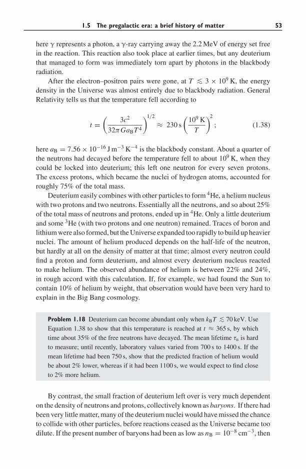
1.5 The pregalactic era: a brief history of matter 53

here γ represents a photon, a γ-ray carrying away the 2.2 MeV of energy set freein the reaction. This reaction also took place at earlier times, but any deuteriumthat managed to form was immediately torn apart by photons in the blackbodyradiation.

After the electron–positron pairs were gone, at T ∼< 3 × 109 K, the energydensity in the Universe was almost entirely due to blackbody radiation. GeneralRelativity tells us that the temperature fell according to

t =(

3c2

32πGaBT 4

)1/2

≈ 230 s

(109 K

T

)2

; (1.38)

here aB = 7.56 × 10−16 J m−3 K−4 is the blackbody constant. About a quarter ofthe neutrons had decayed before the temperature fell to about 109 K, when theycould be locked into deuterium; this left one neutron for every seven protons.The excess protons, which became the nuclei of hydrogen atoms, accounted forroughly 75% of the total mass.

Deuterium easily combines with other particles to form 4He, a helium nucleuswith two protons and two neutrons. Essentially all the neutrons, and so about 25%of the total mass of neutrons and protons, ended up in 4He. Only a little deuteriumand some 3He (with two protons and one neutron) remained. Traces of boron andlithium were also formed, but the Universe expanded too rapidly to build up heaviernuclei. The amount of helium produced depends on the half-life of the neutron,but hardly at all on the density of matter at that time; almost every neutron couldfind a proton and form deuterium, and almost every deuterium nucleus reactedto make helium. The observed abundance of helium is between 22% and 24%,in rough accord with this calculation. If, for example, we had found the Sun tocontain 10% of helium by weight, that observation would have been very hard toexplain in the Big Bang cosmology.

Problem 1.18 Deuterium can become abundant only when kBT ∼< 70 keV. Use

Equation 1.38 to show that this temperature is reached at t ≈ 365 s, by which

time about 35% of the free neutrons have decayed. The mean lifetime τn is hard

to measure; until recently, laboratory values varied from 700 s to 1400 s. If the

mean lifetime had been 750 s, show that the predicted fraction of helium would

be about 2% lower, whereas if it had been 1100 s, we would expect to find close

to 2% more helium.

By contrast, the small fraction of deuterium left over is very much dependenton the density of neutrons and protons, collectively known as baryons. If there hadbeen very little matter, many of the deuterium nuclei would have missed the chanceto collide with other particles, before reactions ceased as the Universe became toodilute. If the present number of baryons had been as low as nB = 10−8 cm−3, then

54 Introduction

as many as 1% of the deuterium nuclei would remain. If the density were now ashigh as nB = 2 × 10−6 cm−3, we would expect to find less than one deuteriumnucleus for each 109 atoms of hydrogen.

Deuterium also burns readily to helium inside stars. So to measure how muchwas made in the Big Bang, we must look for old metal-poor stars that have notburned the deuterium in their outer layers, or at intergalactic clouds of gas thathave not yet formed many stars. Our best measurements show one deuteriumnucleus for every 20 000 or 30 000 atoms of hydrogen. Along with measurementsof 3He and lithium, these show that the combined density of neutrons and protonstoday is

nB = (2.5 ± 0.5) × 10−7 cm−3, or ρB = (5−7) × 109M� Mpc−3. (1.39)

This is much less than the critical density of Equation 1.30: the ratio is

0.02h−2 ∼< ρB/ρcrit ∼< 0.025h−2, (1.40)

where h is Hubble’s constant H0 in units of 100 km s−1 Mpc−1. Observations seemto require h ∼> 0.6, so neutrons and protons cannot make up more than about 7%of ρcrit. Since h ∼< 0.75, baryons account for no less than 3% of the critical density.In the benchmark model, ρB = 0.045ρcrit. We will find in Section 5.3 that this ismore mass than we can see as the gas and luminous stars of galaxies; at least partof their ‘dark stuff’ must consist of normal matter.

Problem 1.19 The Universe must contain at least as much matter as that of

the neutrons and protons: use Equations 1.39 and 1.25 to show that the average

mass-to-light ratio must exceed 50h−1M�/L�.

1.5.3 Recombination: light and matter uncoupled

The next few hundred thousand years of the Universe’s history were rather bor-ing. Its density had dropped too low for nuclear reactions, and the backgroundradiation was energetic enough to ionize hydrogen and disrupt other atoms. Thecosmos was filled with glowing gas, like the inside of a fluorescent light. Pho-tons could not pass freely through this hot plasma, but they were scattered byfree electrons. Matter would not collapse under its own gravity to form stars orother dense objects, because the pressure of the radiation trapped inside was toohigh.

The density of radiation decreases with the scale length R(t) as T 4 ∝ R−4(t).So after some time it must drop below that of matter, which falls only as R−3(t).In the benchmark model, at this time of matter–radiation equality radiation had

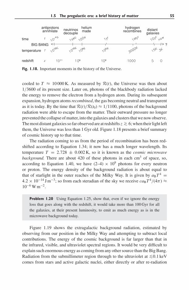
1.5 The pregalactic era: a brief history of matter 55

temperature

time

redshift

BIG BANG ?

antiprotonsannihilate neutrinos

decouple

heliummade

hydrogenrecombines distant

galaxies

Fig. 1.18. Important moments in the history of the Universe.

cooled to T ≈ 10 000 K. As measured by R(t), the Universe was then about1/3600 of its present size. Later on, photons of the blackbody radiation lackedthe energy to remove the electron from a hydrogen atom. During its subsequentexpansion, hydrogen atoms recombined, the gas becoming neutral and transparentas it is today. By the time that R(t)/R(t0) ≈ 1/1100, photons of the backgroundradiation were able to escape from the matter. Their outward pressure no longerprevented the collapse of matter, into the galaxies and clusters that we now observe.The most distant galaxies so far observed are at redshifts z ∼> 6; when their light leftthem, the Universe was less than 1 Gyr old. Figure 1.18 presents a brief summaryof cosmic history up to that time.

The radiation coming to us from the period of recombination has been red-shifted according to Equation 1.34; it now has a much longer wavelength. Itstemperature T = 2.728 ± 0.002 K, so it is known as the cosmic microwavebackground. There are about 420 of these photons in each cm3 of space, so,according to Equation 1.40, we have (2–4) × 109 photons for every neutronor proton. The energy density of the background radiation is about equal tothat of starlight in the outer reaches of the Milky Way. It is given by aBT 4 =4.2 × 10−14 J m−3; so from each steradian of the sky we receive caBT 4/(4π ) ≈10−6 W m−2.

Problem 1.20 Using Equation 1.25, show that, even if we ignore the energy

loss that goes along with the redshift, it would take more than 100 Gyr for all

the galaxies, at their present luminosity, to emit as much energy as is in the

microwave background today.

Figure 1.19 shows the extragalactic background radiation, estimated byobserving from our position in the Milky Way and attempting to subtract localcontributions. The energy of the cosmic background is far larger than that inthe infrared, visible, and ultraviolet spectral regions. It would be very difficult toexplain such enormous energy as coming from any other source than the Big Bang.Radiation from the submillimeter region through to the ultraviolet at ∼<0.1 keVcomes from stars and active galactic nuclei, either directly or after re-radiation

56 Introduction

radio X-ray gamma

UVvisible

IR

FIR

Fig. 1.19. Extragalactic background radiation: the vertical logarithmic scale shows energy

density per decade in frequency or wavelength. Arrows show upper and lower limits.

The curve peaking at λ ∼ 1 mm is the cosmic microwave background; the far-infrared

background is the light of stars and active galactic nuclei, re-radiated by dust – T. Ressell

and D. Scott.

by heated dust. The high-energy ‘tail’ in X-rays and γ-rays is mainly from activenuclei. Since photons lose energy in an expanding Universe, almost all this radia-tion, aside from that in the microwave background, must have been emitted overthe past ∼10 Gyr, at times corresponding to redshifts z ∼< 3.

The microwave background is now very close to a blackbody spectrum; it isalso extremely uniform. Between different parts of the sky, we see small irreg-ularities in its temperature that are just a few parts in 100 000 – with only oneexception. In the direction l = 265◦, b = 48◦ the peak wavelength is shorter thanaverage, and the temperature higher, by a little more than 0.1%. In the oppositedirection, the temperature is lower by the same amount. This difference reflectsthe Sun’s motion through the background radiation. If T0 is the temperature mea-sured by an observer at rest relative to the backgound radiation, then an observermoving with relative speed V � c would measure a temperature T (θ ) at an angleθ to the direction of motion, given by

T (θ ) ≈ T0(1 + V cos θ/c). (1.41)

1.5 The pregalactic era: a brief history of matter 57

For the Sun, V = 370 km s−1. Taking into account the Sun’s orbit about theMilky Way, and the Milky Way’s motion relative to nearby galaxies, we findthat our Local Group has a peculiar motion of Vpec ≈ 600 km s−1 relative to thebackground radiation and to the Universe as a whole. The Local Group’s motionis unexpectedly and troublingly large: we discuss it further in Chapter 8.

2

Mapping our Milky Way

Our position in the Milky Way’s disk gives us a detailed and close-up viewof a fairly typical large spiral galaxy. We begin this chapter by looking at theSun’s immediate vicinity. Examining the closest stars gives us a sample ofthe disk stuff, and we can ask how many stars of each luminosity, mass, com-position, and age are present. Combining this information with theories of stellarevolution, we investigate the star-forming past of the solar neighborhood.

In Section 2.2 we venture further afield. Measuring stellar distances allowsus to map out the Milky Way’s structure: the thin and thick disks, the metal-poor halo, and the central bulge. Star clusters, where all the members were borntogether, with the same initial composition, are especially useful; comparing theircolor–magnitude diagrams with the predictions of stellar models yields the ageand composition jointly with the cluster’s distance. We find that the youngest starsbelong to the disk, and are relatively rich in elements heavier than helium, whereasthe stars of the metal-poor halo are extremely old.

Most of the Milky Way’s stars and almost all of its gas lie in the disk,orbiting the center like the planets around the Sun. Section 2.3 deals with theGalaxy’s rotation: how we measure it, and how we use it to find the distribu-tion of gas within the disk. By contrast with motions in the solar system, therotational speed of material in the furthest part of the disk is nearly the sameas that for gas at the Sun’s position. To prevent this distant gas from flying offinto intergalactic space, a large amount of mass must be concealed in the outerreaches of the Milky Way, in a form that emits very little light, or none at all: thedark matter.

Measured by mass, the Milky Way has only a tenth as much gas as stars;but the gas has profound effects. The densest gas clouds collapse to make newstars; and at the end of its life a star pollutes the gas with dust and heavy elementsproduced by its nuclear burning. Section 2.4 discusses the complex processes thatheat, ionize, and push around the Milky Way’s gas, and how these affect the paceat which stars are born.

58

2.1 The solar neighborhood 59

2.1 The solar neighborhood

In this section, we consider the closest stars, the Sun’s immediate neighbors. Weask what kinds of stars are present, and in what numbers? How many are on themain sequence, and how many are in the later stages of their lives? How manywere formed recently, and how many are very old? To answer these questions, wemust first find out how far away the stars are.

The distances of astronomical objects are in general extremely difficult tomeasure, but they are essential for our understanding of their nature. The lumi-nosities of stars and galaxies are always derived by using the inverse-square law(Equation 1.1). We usually find linear dimensions from a measured angular sizeon the sky and an estimated distance, and our calculations of masses usuallydepend on those size estimates. Many astronomical disputes come down to anargument over how far away something is; so astronomers have had good rea-son to develop a wide range of inventive and sometimes bizarre techniques formeasuring distances.

Triangulation, or trigonometric parallax, allows us to measure distances onlyfor the nearest stars. We then compare more distant stars with similar stars closeat hand, assuming that stars with similar spectra have the same luminosity andfinding the relative distance from their relative apparent brightness. Those distantstars in turn are used to estimate distances to the nearest galaxies, those closeenough that we can pick out individual stars. This cosmic distance ladder is thenextended to more distant galaxies by comparing them with nearby systems. Therelative distances at each stage of comparison are often quite well determined –in astronomy, this means to within a few percent – but the accumulation of errorsat each stage can leave extragalactic distances uncertain by as much as a factor oftwo. Occasionally we are lucky enough to find a way of circumventing some of thelower rungs of the ladder, to measure directly the distance to an object beyond thereach of trigonometric parallax. These opportunities are much prized; we discusssome of them in Section 2.2 below.

In general, the relative distances of two stars or galaxies can be found farmore accurately than the absolute distance (in meters, or light-years) to eitherone. The parsec was adopted in 1922 by the International Astronomical Unionto specify stellar distances in units of the Earth’s mean distance from the Sun,the astronomical unit. With interplanetary spacecraft, and measurements of thereflection times for light or radio waves bounced from the surfaces of planets, wenow know the scale of the solar system to within one part in a million; we retainthe parsec for historical reasons. Within the Galaxy, distances are sometimes givenin units of R0, the Galactocentric radius of the Sun.

2.1.1 Trigonometric parallax

Within a few hundred parsecs, we can use trigonometric parallax to find stellardistances. As the Earth orbits the Sun, our viewing position changes, and closer

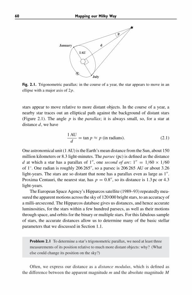
60 Mapping our Milky Way

1AU

January

July

p

d

Fig. 2.1. Trigonometric parallax: in the course of a year, the star appears to move in an

ellipse with a major axis of 2p.

stars appear to move relative to more distant objects. In the course of a year, anearby star traces out an elliptical path against the background of distant stars(Figure 2.1). The angle p is the parallax; it is always small, so, for a star atdistance d, we have

1 AU

d= tan p ≈ p (in radians). (2.1)

One astronomical unit (1 AU) is the Earth’s mean distance from the Sun, about 150million kilometers or 8.3 light-minutes. The parsec (pc) is defined as the distanced at which a star has a parallax of 1′′, one second of arc: 1′′ = 1/60 × 1/60of 1◦. One radian is roughly 206 265′′, so a parsec is 206 265 AU or about 3.26light-years. The stars are so distant that none has a parallax even as large as 1′′.Proxima Centauri, the nearest star, has p = 0.8′′, so its distance is 1.3 pc or 4.3light-years.

The European Space Agency’s Hipparcos satellite (1989–93) repeatedly mea-sured the apparent motions across the sky of 120 000 bright stars, to an accuracy ofa milli-arcsecond. The Hipparcos database gives us distances, and hence accurateluminosities, for the stars within a few hundred parsecs, as well as their motionsthrough space, and orbits for the binary or multiple stars. For this fabulous sampleof stars, the accurate distances allow us to determine many of the basic stellarparameters that we discussed in Section 1.1.

Problem 2.1 To determine a star’s trigonometric parallax, we need at least three

measurements of its position relative to much more distant objects: why? (What

else could change its position on the sky?)

Often, we express our distance as a distance modulus, which is defined asthe difference between the apparent magnitude m and the absolute magnitude M

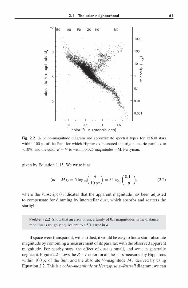
2.1 The solar neighborhood 61

1

10

100

1000

0.1

0.01

0.001

0 0.5 1 1.5

10

5

0

−5B0 A0 F0 G0 K0 M0

Fig. 2.2. A color–magnitude diagram and approximate spectral types for 15 630 stars

within 100 pc of the Sun, for which Hipparcos measured the trigonometric parallax to

<10%, and the color B − V to within 0.025 magnitudes – M. Perryman.

given by Equation 1.15. We write it as

(m − M)0 ≡ 5 log10

(d

10 pc

)= 5 log10

(0.1′′

p

), (2.2)

where the subscript 0 indicates that the apparent magnitude has been adjustedto compensate for dimming by interstellar dust, which absorbs and scatters thestarlight.

Problem 2.2 Show that an error or uncertainty of 0.1 magnitudes in the distance

modulus is roughly equivalent to a 5% error in d.

If space were transparent, with no dust, it would be easy to find a star’s absolutemagnitude by combining a measurement of its parallax with the observed apparentmagnitude. For nearby stars, the effect of dust is small, and we can generallyneglect it. Figure 2.2 shows the B−V color for all the stars measured by Hipparcoswithin 100 pc of the Sun, and the absolute V -magnitude MV derived by usingEquation 2.2. This is a color–magnitude or Hertzsprung–Russell diagram; we can

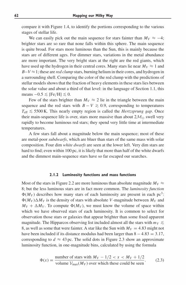
62 Mapping our Milky Way

compare it with Figure 1.4, to identify the portions corresponding to the variousstages of stellar life.

We can easily pick out the main sequence for stars fainter than MV ≈ −4;brighter stars are so rare that none falls within this sphere. The main sequenceis quite broad. For stars more luminous than the Sun, this is mainly because thestars are of different ages. For dimmer stars, variations in the metal abundanceare more important. The very bright stars at the right are the red giants, whichhave used up the hydrogen in their central cores. Many stars lie near MV ≈ 1 andB−V ≈1; these are red clump stars, burning helium in their cores, and hydrogen ina surrounding shell. Comparing the color of the red clump with the predictions ofstellar models shows that the fraction of heavy elements in these stars lies betweenthe solar value and about a third of that level: in the language of Section 1.1, thismeans −0.5 ∼< [Fe/H] ∼< 0.

Few of the stars brighter than MV ≈ 2 lie in the triangle between the mainsequence and the red stars with B − V ∼> 0.9, corresponding to temperaturesTeff ∼< 5500 K. This nearly empty region is called the Hertzsprung gap. Oncetheir main-sequence life is over, stars more massive than about 2M� swell veryrapidly to become luminous red stars; they spend very little time at intermediatetemperatures.

A few stars fall about a magnitude below the main sequence; most of theseare metal-poor subdwarfs, which are bluer than stars of the same mass with solarcomposition. Four dim white dwarfs are seen at the lower left. Very dim stars arehard to find; even within 100 pc, it is likely that more than half of the white dwarfsand the dimmest main-sequence stars have so far escaped our searches.

2.1.2 Luminosity functions and mass functions

Most of the stars in Figure 2.2 are more luminous than absolute magnitude MV ≈8; but the less luminous stars are in fact more common. The luminosity function�(MV ) describes how many stars of each luminosity are present in each pc3:�(MV )�MV is the density of stars with absolute V -magnitude between MV andMV + �MV . To compute �(MV ), we must know the volume of space withinwhich we have observed stars of each luminosity. It is common to select forobservation those stars or galaxies that appear brighter than some fixed apparentmagnitude. The Hipparcos observing list included almost all the stars with mV ∼<8, as well as some that were fainter. A star like the Sun with MV = 4.83 might nothave been included if its distance modulus had been larger than 8 − 4.83 = 3.17,corresponding to d ≈ 43 pc. The solid dots in Figure 2.3 show an approximateluminosity function, in one-magnitude bins, calculated by using the formula

�(x) = number of stars with MV − 1/2 < x < MV + 1/2

volume Vmax(MV ) over which these could be seen. (2.3)

2.1 The solar neighborhood 63

0

5

10

0

5

10

15 10 5 0 −5

light

mass

number

Fig. 2.3. The histogram shows the luminosity function �(MV ) for nearby stars: solid

dots from stars of Figure 2.2, open circles from Reid et al. 2002 AJ 124, 2721. Lines

with triangles show LV �(MV ), light from stars in each magnitude bin; the dotted curve

is for main-sequence stars alone, the solid curve for the total. The dashed curve gives

M�MS(MV ), the mass in main-sequence stars. Units are L� or M� per 10 pc cube;

vertical bars show uncertainty, based on numbers of stars in each bin.

Problem 2.3 Show that the volume in Equation 2.3 is Vmax(M) ≈ 4πd3max/3,

where dmax is the smaller of 100 pc and 10 pc × 100.2(8−M). Using Table 1.4 for

MV , find dmax for an M4 dwarf. Why are you surprised to see such faint stars in

Figure 2.2?

It is quite difficult to determine the faint end of the luminosity function, sincedim stars are hard to find. The bright end of �(MV ) also presents problems;because luminous stars are rare, we will not find enough of them unless we surveya volume larger than our 100 pc sphere. But stars are not spread out uniformly inspace. For example, their density falls as we go further out of the Milky Way’sdisk in the direction of the Galactic poles. So, if we look far afield for luminousstars, the average density in our search region is lower than it is near the Sun’sposition. Finally, many stars are in binary systems so close that they are mistakenfor a brighter single star. Despite these uncertainties, it is clear that dim stars areoverwhelmingly more numerous than bright ones.

Figure 2.3 also shows how much of the V -band light is emitted by starsof each luminosity: stars in the range from MV to MV + �MV contribute anamount LV �(MV )�MV of the total. Almost all the light comes from the brighterstars, mainly A and F main-sequence stars and K giants. Rare luminous starssuch as main-sequence O and B stars, and bright supergiants, contribute morelight than all the stars dimmer than the Sun; so the total luminosity of a galaxy

64 Mapping our Milky Way

depends strongly on whether it has recently been active in making these massiveshort-lived stars. If we had measured our luminosity function at ultraviolet wave-lengths rather than in the V band at 5500 A, almost all the light would be fromO and B stars. The near-infrared light, at a few microns, comes mainly from theluminous red stars.

We can use the tables of Section 1.1 to find the bolometric luminosity Lbol

from the V -band luminosity LV , and then use Table 1.1, or the mass–luminosityrelation of Equation 1.6, to calculate the average mass of a main-sequence star ateach luminosity. In Figure 2.3, the dashed curve shows the mass in main-sequencestars with absolute magnitude between MV and MV + �MV . The red giants makea tiny contribution, since they are even less massive than main-sequence stars ofthe same luminosity. Almost all the mass is in K and M dwarfs, stars so faint thatwe cannot see them in galaxies beyond the Milky Way and its satellites. The starsthat emit most of the light account for hardly any of the mass.

The luminosity function of Figure 2.3 corresponds to about 65 stars in each1000 pc3, with a luminosity equivalent to 40L� in the V band. About 75% of thelight comes from main-sequence stars, which have mass totalling about 30M�.The averaged mass-to-light ratio M/L gives a measure of the proportion of mas-sive luminous stars to dim stars. We find M/LV ≈ 1 for the main-sequence starsalone, and M/LV ≈ 0.74 for all the stars, when we measure M in solar massesand LV as a fraction of the Sun’s V -band luminosity. Even including white dwarfsand the interstellar gas, the mass-to-light ratio M/LV ∼< 2 locally. In Section 2.3,we will see that the ratio of mass to light for the Milky Way as a whole is muchlarger than that for this sample of stars near the Sun. The outer Galaxy containsunseen mass, in a form other than the stars and interstellar gas found near the Sun.

Using models of stellar evolution, we can work backward from the present-daystellar population to find how many stars were born with each mass. We define theinitial luminosity function, �(MV ), such that �(MV )�MV is the number of starsformed that had absolute magnitude between MV and MV +�MV when they wereon the main sequence. Stars less massive than the Sun have main-sequence lives of10 Gyr or longer. Counting the numbers of faint white dwarfs indicates that starshave been forming in the local disk only for a time τgal ≈ 8–10 Gyr, so the first-born K dwarfs have evolved very little. For these low-mass stars, �(MV ) is almostthe same as the present-day luminosity function �(MV ). But O, B, and A starsburn out rapidly, and only those most recently born are still on the main sequence.

We can calculate the initial luminosity function if we assume that the diskhas been forming stars at a uniform rate throughout its history. If �MS(MV ) is thepresent-day luminosity function for main-sequence stars alone, and a star remainson the main sequence with absolute magnitude MV for a time τMS(MV ), then

�(MV ) = �MS(MV ) for τMS(MV ) ≥ τgal,

= �MS(MV ) × τgal

τMS(MV )when τMS(MV ) < τgal. (2.4)

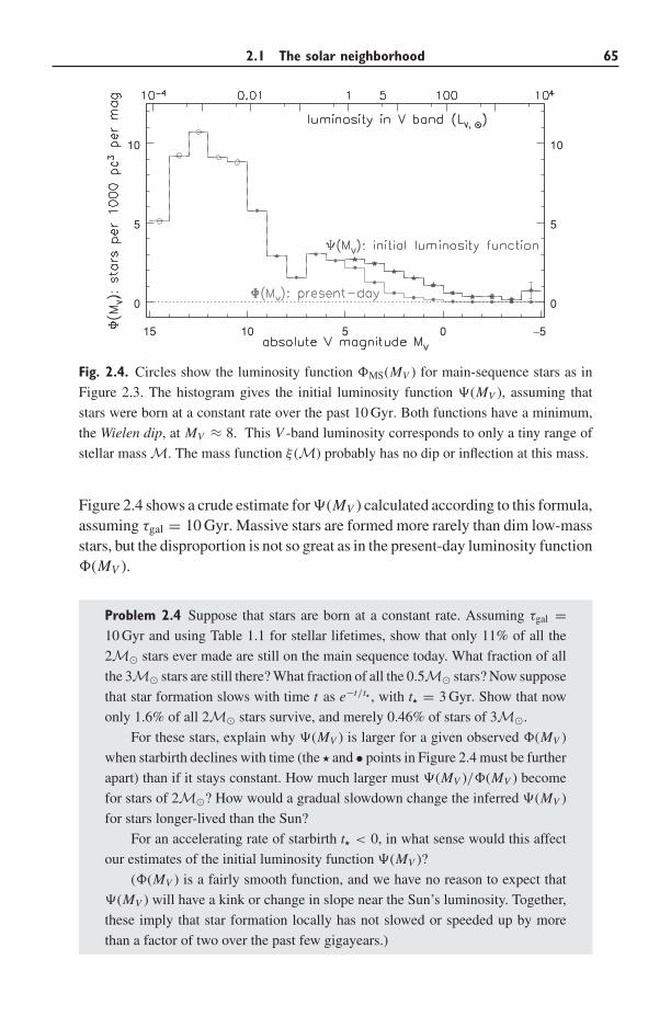
2.1 The solar neighborhood 65

0

5

10

0

5

10

15 10 5 0 −5

Fig. 2.4. Circles show the luminosity function �MS(MV ) for main-sequence stars as in

Figure 2.3. The histogram gives the initial luminosity function �(MV ), assuming that

stars were born at a constant rate over the past 10 Gyr. Both functions have a minimum,

the Wielen dip, at MV ≈ 8. This V -band luminosity corresponds to only a tiny range of

stellar mass M. The mass function ξ (M) probably has no dip or inflection at this mass.

Figure 2.4 shows a crude estimate for �(MV ) calculated according to this formula,assuming τgal = 10 Gyr. Massive stars are formed more rarely than dim low-massstars, but the disproportion is not so great as in the present-day luminosity function�(MV ).

Problem 2.4 Suppose that stars are born at a constant rate. Assuming τgal =10 Gyr and using Table 1.1 for stellar lifetimes, show that only 11% of all the

2M� stars ever made are still on the main sequence today. What fraction of all

the 3M� stars are still there? What fraction of all the 0.5M� stars? Now suppose

that star formation slows with time t as e−t/t , with t = 3 Gyr. Show that now

only 1.6% of all 2M� stars survive, and merely 0.46% of stars of 3M�.

For these stars, explain why �(MV ) is larger for a given observed �(MV )

when starbirth declines with time (the and • points in Figure 2.4 must be further

apart) than if it stays constant. How much larger must �(MV )/�(MV ) become

for stars of 2M�? How would a gradual slowdown change the inferred �(MV )

for stars longer-lived than the Sun?

For an accelerating rate of starbirth t < 0, in what sense would this affect

our estimates of the initial luminosity function �(MV )?

(�(MV ) is a fairly smooth function, and we have no reason to expect that

�(MV ) will have a kink or change in slope near the Sun’s luminosity. Together,

these imply that star formation locally has not slowed or speeded up by more

than a factor of two over the past few gigayears.)

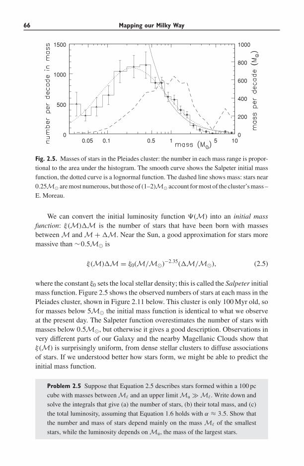
66 Mapping our Milky Way

0

200

400

600

800

1000

0.05 0.1 0.5 1 5 100

500

1000

1500

Fig. 2.5. Masses of stars in the Pleiades cluster: the number in each mass range is propor-

tional to the area under the histogram. The smooth curve shows the Salpeter initial mass

function, the dotted curve is a lognormal function. The dashed line shows mass: stars near

0.25M� are most numerous, but those of (1–2)M� account for most of the cluster’s mass –

E. Moreau.

We can convert the initial luminosity function �(M) into an initial massfunction: ξ (M)�M is the number of stars that have been born with massesbetween M and M + �M. Near the Sun, a good approximation for stars moremassive than ∼0.5M� is

ξ (M)�M = ξ0(M/M�)−2.35(�M/M�), (2.5)

where the constant ξ0 sets the local stellar density; this is called the Salpeter initialmass function. Figure 2.5 shows the observed numbers of stars at each mass in thePleiades cluster, shown in Figure 2.11 below. This cluster is only 100 Myr old, sofor masses below 5M� the initial mass function is identical to what we observeat the present day. The Salpeter function overestimates the number of stars withmasses below 0.5M�, but otherwise it gives a good description. Observations invery different parts of our Galaxy and the nearby Magellanic Clouds show thatξ (M) is surprisingly uniform, from dense stellar clusters to diffuse associationsof stars. If we understood better how stars form, we might be able to predict theinitial mass function.

Problem 2.5 Suppose that Equation 2.5 describes stars formed within a 100 pc

cube with masses between M� and an upper limit Mu � M�. Write down and

solve the integrals that give (a) the number of stars, (b) their total mass, and (c)

the total luminosity, assuming that Equation 1.6 holds with α ≈ 3.5. Show that

the number and mass of stars depend mainly on the mass M� of the smallest

stars, while the luminosity depends on Mu, the mass of the largest stars.

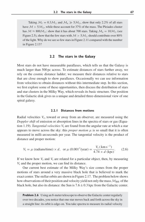
2.2 The stars in the Galaxy 67

Taking M� = 0.3M� and Mu � 5M�, show that only 2.2% of all stars

have M > 5M�, while these account for 37% of the mass. The Pleiades cluster

has M ≈ 800M�: show that it has about 700 stars. Taking Mu = 10M� (see

Figure 2.5), show that the few stars with M > 5M� should contribute over 80%

of the light. Why do we see so few stars in Figure 2.11 compared with the number

in Figure 2.13?

2.2 The stars in the Galaxy

Most stars do not have measurable parallaxes, which tells us that the Galaxy ismuch larger than 500 pc across. To estimate distances of stars further away, werely on the cosmic distance ladder; we measure their distances relative to starsthat are close enough to show parallaxes. Occasionally we can use informationfrom velocities to obtain distances without this intermediate step. In this section,we first explore some of these opportunities, then discuss the distribution of starsand star clusters in the Milky Way, which reveals its basic structure. Our positionin the Galactic disk gives us a unique and detailed three-dimensional view of onespiral galaxy.

2.2.1 Distances from motions

Radial velocities Vr, toward or away from an observer, are measured using theDoppler shift of emission or absorption lines in the spectra of stars or gas (Equa-tion 1.19). Tangential velocities Vt are found from the angular rate at which a starappears to move across the sky: this proper motion μ is so small that it is oftenmeasured in milli-arcseconds per year. The tangential velocity is the product ofdistance and proper motion:

Vt = μ (radians/time) × d, or μ (0.001′′/year) = Vt ( km s−1)

4.74 × d (kpc). (2.6)

If we know how Vr and Vt are related for a particular object, then, by measuringVr and the proper motion, we can find its distance.

Our current best estimate of the Milky Way’s size comes from the propermotions of stars around a very massive black hole that is believed to mark theexact center. The stellar orbits are shown in Figure 2.17. The problem below showshow observations of their position and velocity yield not only the massMBH of theblack hole, but also its distance: the Sun is 7.6 ± 0.3 kpc from the Galactic center.

Problem 2.6 Using an 8-meter telescope to observe the Galactic center regularly

over two decades, you notice that one star moves back and forth across the sky in

a straight line: its orbit is edge-on. You take spectra to measure its radial velocity

68 Mapping our Milky Way

yapocenter

pericenter

y

velocity

Fig. 2.6. Left, orbits of two stars around a point mass at the origin. Filled dots are at

equal time intervals P/10, open dots at ±0.01P from pericenter. Right, velocity in the

horizontal direction. A distant observer looking along the x-axis sees the radial velocity

vx repeat exactly when the orbit is symmetric about the plane x = 0 of the sky (solid line);

this does not happen if the orbit is misaligned (dotted line).

Vr, and find that this repeats exactly each time the star is at the same point in the

sky. You are in luck: the furthest points of the star’s motion on the sky are also

when it is closest to the black hole (pericenter) and furthest from it (apocenter),

as in Figure 2.6. You measure the separation s of these two points on the sky,

and the orbital period P . Assuming that the black hole provides almost all the

gravitational force, follow these steps to find both the mass MBH of the black

hole and its distance d from us.

From the definition below Equation 2.1, show that the orbit’s semi-major

axis a = 0.5 AU×(s/1′′)(d/1 pc). You observe s = 0.248′′: what would a be at a

distance of 8 kpc? At the two extremes of its motion across the sky, the star’s radial

velocity is Va = 473 km s−1 and Vp = 7 326 km s−1: at which point is it closest

to the black hole? The orbit’s eccentricity is e; explain why the conservation of

angular momentum requires that Vp(1 − e) = Va(1 + e), and show that, here,

e = 0.876.

At distance r from the black hole moving at speed V , the star has kinetic

energy KE = mV 2/2 and potential energy PE = −GmMBH/r . Since the

total energy KE + PE does not change during the orbit, show that

V 2p − V 2

a = GMBH

a× 4e

1 − e2. (2.7)

Measuring v in km s−1,MBH inM�, and a in parsecs, G = 4.3 ×10−3. Convert

a to AU to show thatMBH/M� = 3822(a/1 AU). Because m � MBH, we can

use Kepler’s third law: P2 (in years) = a3 (in AU)/MBH (in M�) . You measure

P = 15.24 yr; use Equation 2.7 to eliminate MBH/a and show that a = 942 AU

and MBH = 3.6 × 106M�. What is the distance to the Galactic center?

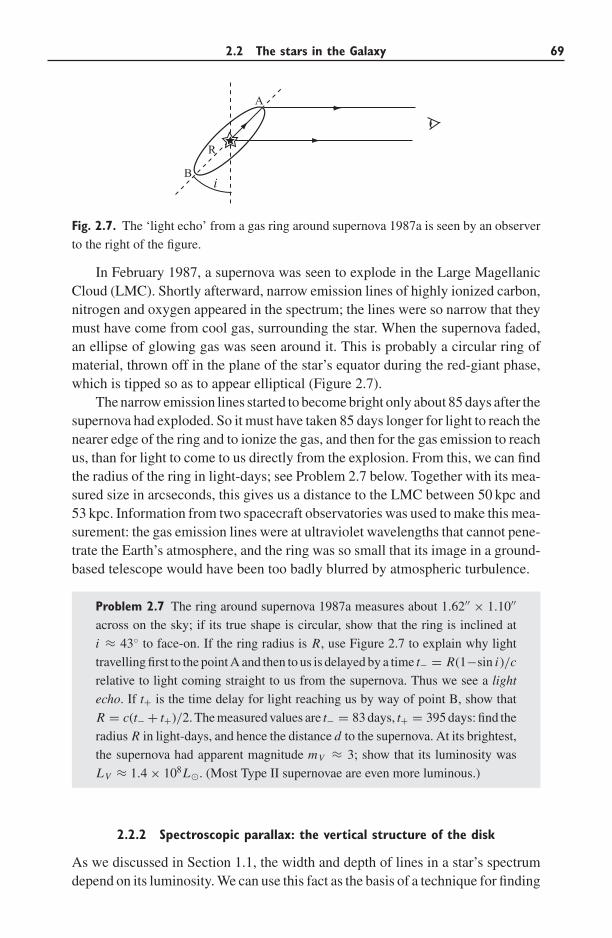
2.2 The stars in the Galaxy 69

i

R

A

B

Fig. 2.7. The ‘light echo’ from a gas ring around supernova 1987a is seen by an observer

to the right of the figure.

In February 1987, a supernova was seen to explode in the Large MagellanicCloud (LMC). Shortly afterward, narrow emission lines of highly ionized carbon,nitrogen and oxygen appeared in the spectrum; the lines were so narrow that theymust have come from cool gas, surrounding the star. When the supernova faded,an ellipse of glowing gas was seen around it. This is probably a circular ring ofmaterial, thrown off in the plane of the star’s equator during the red-giant phase,which is tipped so as to appear elliptical (Figure 2.7).

The narrow emission lines started to become bright only about 85 days after thesupernova had exploded. So it must have taken 85 days longer for light to reach thenearer edge of the ring and to ionize the gas, and then for the gas emission to reachus, than for light to come to us directly from the explosion. From this, we can findthe radius of the ring in light-days; see Problem 2.7 below. Together with its mea-sured size in arcseconds, this gives us a distance to the LMC between 50 kpc and53 kpc. Information from two spacecraft observatories was used to make this mea-surement: the gas emission lines were at ultraviolet wavelengths that cannot pene-trate the Earth’s atmosphere, and the ring was so small that its image in a ground-based telescope would have been too badly blurred by atmospheric turbulence.

Problem 2.7 The ring around supernova 1987a measures about 1.62′′ × 1.10′′

across on the sky; if its true shape is circular, show that the ring is inclined at

i ≈ 43◦ to face-on. If the ring radius is R, use Figure 2.7 to explain why light

travelling first to the point A and then to us is delayed by a time t− = R(1−sin i)/c

relative to light coming straight to us from the supernova. Thus we see a light

echo. If t+ is the time delay for light reaching us by way of point B, show that

R = c(t− + t+)/2. The measured values are t− = 83 days, t+ = 395 days: find the

radius R in light-days, and hence the distance d to the supernova. At its brightest,

the supernova had apparent magnitude mV ≈ 3; show that its luminosity was

LV ≈ 1.4 × 108L�. (Most Type II supernovae are even more luminous.)

2.2.2 Spectroscopic parallax: the vertical structure of the disk

As we discussed in Section 1.1, the width and depth of lines in a star’s spectrumdepend on its luminosity. We can use this fact as the basis of a technique for finding

70 Mapping our Milky Way

stellar distances. For example, a star with the spectrum of an F2 main-sequencestar is roughly as luminous as other F2 dwarfs with about the same chemicalcomposition. If we can measure a parallax for one of these, then Equation 2.1tells us its distance, and hence its luminosity and that of all similar F2 stars. So ifwe then measure our more distant star’s apparent brightness and can compensatefor the dimming caused by interstellar dust, Equation 1.1 will tell us its distance.This method is called spectroscopic parallax because it should give the sameinformation as that we gain by measuring the trigonometric parallax: namely, thestar’s distance.

Spectroscopic parallax works well for some types of star and poorly for others.The luminosities of main-sequence stars can often be found to within 10%, leadingto 5% uncertainties in their distance. But in K giants, the temperature in theatmosphere is almost the same, no matter what the luminosity; the giant branchis almost vertical in Figure 1.4. The best we can hope for is to determine theluminosity to within 0.5 in the absolute magnitude, and hence the distance to 25%.

Taking high-quality spectra for many faint stars demands long hours of obser-vation on large telescopes. A ‘poor man’s variant’ is to estimate the spectral typeof a star from its color, and to rely on other indications to establish whetherit is a dwarf or a giant. This method of photometric parallax can be reason-ably successful if the measured color changes substantially with the luminosityof the observed stars, and if we can correct for the effects of interstellar dust.Results are best when we observe a cluster of stars; with measurements of manystars, we can estimate both the cluster’s distance and the reddening caused bydust.

When we look out perpendicular to the Galactic disk and select the sharpstellar images from among the fuzzy shapes of distant galaxies, almost all the redstars fainter than apparent magnitude mV ≈ 14 are K and M dwarfs. (At a distanceof 1 kpc, what would be the apparent magnitude of a K or M giant with MV ≈ 0?)There is little dust in this direction to dim and redden the stars, so the V − I colorshould be a good indication of the spectral type. The stellar densities in Figure 2.8were compiled using photometric distances determined by measuring the V − Icolors of 12 500 stars with apparent magnitude mV < 19 in the direction of thesouth Galactic pole. The late G and early K dwarfs are bluer than red giants, andthere are very few giant stars of the same color to mislead us.

Using the Galaxy-centred spherical polar coordinates R, φ, z of Figure 1.10,we often approximate the density n(R, z, S) of stars of a particular type S by adouble-exponential form

n(R, z, S) = n(0, 0, S)exp[−R/h R(S)]exp[−|z|/hz(S)], (2.8)

where h R is called the scale length of the disk and hz is the scale height. Figure 2.8shows that, near the midplane, hz ≈ 300–350 pc for K dwarfs, while for moremassive and shorter-lived stars, such as the A dwarfs, it is smaller, hz ∼< 200 pc.

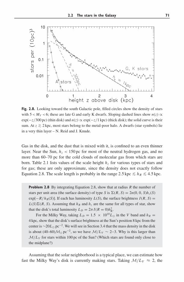
2.2 The stars in the Galaxy 71

0 1 2 3 4

0.01

0.1

1

10

Fig. 2.8. Looking toward the south Galactic pole, filled circles show the density of stars

with 5< MV <6; these are late G and early K dwarfs. Sloping dashed lines show n(z) ∝exp(−z/300 pc) (thin disk) and n(z) ∝ exp(−z/1 kpc) (thick disk); the solid curve is their

sum. At z ∼> 2 kpc, most stars belong to the metal-poor halo. A dwarfs (star symbols) lie

in a very thin layer – N. Reid and J. Knude.

Gas in the disk, and the dust that is mixed with it, is confined to an even thinnerlayer. Near the Sun, hz < 150 pc for most of the neutral hydrogen gas, and nomore than 60–70 pc for the cold clouds of molecular gas from which stars areborn. Table 2.1 lists values of the scale height hz for various types of stars andfor gas; these are only approximate, since the density does not exactly followEquation 2.8. The scale length is probably in the range 2.5 kpc ∼< h R ∼< 4.5 kpc.

Problem 2.8 By integrating Equation 2.8, show that at radius R the number of

stars per unit area (the surface density) of type S is �(R, S) = 2n(0, 0, S)hz(S)

exp[−R/h R(S)]. If each has luminosity L(S), the surface brightness I (R, S) =L(S)�(R, S). Assuming that h R and hz are the same for all types of star, show

that the disk’s total luminosity L D = 2π I (R = 0)h2R.

For the Milky Way, taking L D = 1.5 × 1010L� in the V band and h R =4 kpc, show that the disk’s surface brightness at the Sun’s position 8 kpc from the

center is ∼20L� pc−2. We will see in Section 3.4 that the mass density in the disk

is about (40–60)M� pc−2, so we have M/LV ∼ 2−3. Why is this larger than

M/LV for stars within 100 pc of the Sun? (Which stars are found only close to

the midplane?)

Assuming that the solar neighborhood is a typical place, we can estimate howfast the Milky Way’s disk is currently making stars. Taking M/LV ≈ 2, the

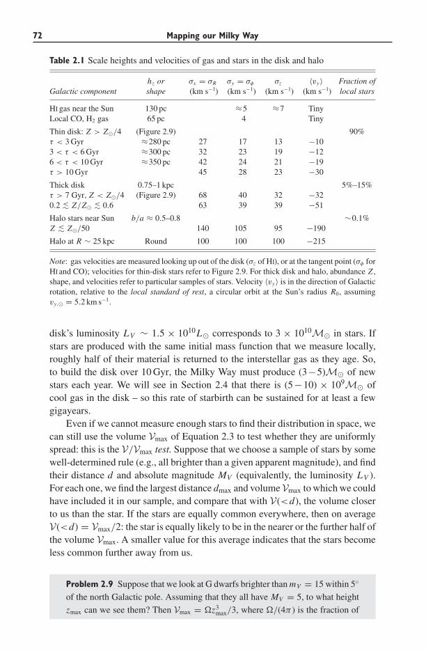
72 Mapping our Milky Way

Table 2.1 Scale heights and velocities of gas and stars in the disk and halo

hz or σx = σR σy = σφ σz 〈vy〉 Fraction ofGalactic component shape (km s−1) (km s−1) (km s−1) (km s−1) local stars

HI gas near the Sun 130 pc ≈5 ≈7 TinyLocal CO, H2 gas 65 pc 4 Tiny

Thin disk: Z > Z�/4 (Figure 2.9) 90%τ < 3 Gyr ≈280 pc 27 17 13 −103 < τ < 6 Gyr ≈300 pc 32 23 19 −126 < τ < 10 Gyr ≈350 pc 42 24 21 −19τ > 10 Gyr 45 28 23 −30

Thick disk 0.75–1 kpc 5%–15%τ > 7 Gyr, Z < Z�/4 (Figure 2.9) 68 40 32 −320.2 ∼< Z/Z� ∼< 0.6 63 39 39 −51

Halo stars near Sun b/a ≈ 0.5–0.8 ∼0.1%Z ∼< Z�/50 140 105 95 −190

Halo at R ∼ 25 kpc Round 100 100 100 −215

Note: gas velocities are measured looking up out of the disk (σz of HI), or at the tangent point (σφ forHI and CO); velocities for thin-disk stars refer to Figure 2.9. For thick disk and halo, abundance Z ,shape, and velocities refer to particular samples of stars. Velocity 〈vy〉 is in the direction of Galacticrotation, relative to the local standard of rest, a circular orbit at the Sun’s radius R0, assumingvy,� = 5.2 km s−1.

disk’s luminosity LV ∼ 1.5 × 1010L� corresponds to 3 × 1010M� in stars. Ifstars are produced with the same initial mass function that we measure locally,roughly half of their material is returned to the interstellar gas as they age. So,to build the disk over 10 Gyr, the Milky Way must produce (3−5)M� of newstars each year. We will see in Section 2.4 that there is (5−10) × 109M� ofcool gas in the disk – so this rate of starbirth can be sustained for at least a fewgigayears.

Even if we cannot measure enough stars to find their distribution in space, wecan still use the volume Vmax of Equation 2.3 to test whether they are uniformlyspread: this is the V/Vmax test. Suppose that we choose a sample of stars by somewell-determined rule (e.g., all brighter than a given apparent magnitude), and findtheir distance d and absolute magnitude MV (equivalently, the luminosity LV ).For each one, we find the largest distance dmax and volumeVmax to which we couldhave included it in our sample, and compare that with V(<d), the volume closerto us than the star. If the stars are equally common everywhere, then on averageV(<d) = Vmax/2: the star is equally likely to be in the nearer or the further half ofthe volume Vmax. A smaller value for this average indicates that the stars becomeless common further away from us.

Problem 2.9 Suppose that we look at G dwarfs brighter than mV = 15 within 5◦

of the north Galactic pole. Assuming that they all have MV = 5, to what height

zmax can we see them? Then Vmax = �z3max/3, where �/(4π ) is the fraction of

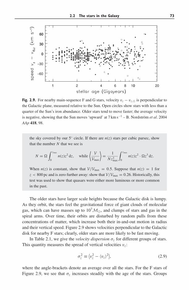
2.2 The stars in the Galaxy 73

1 2 4 6 8 10 20

30

60

0

30

60

1 0

0

30

60

Fig. 2.9. For nearby main-sequence F and G stars, velocity vz − vz,� is perpendicular to

the Galactic plane, measured relative to the Sun. Open circles show stars with less than a

quarter of the Sun’s iron abundance. Older stars tend to move faster; the average velocity

is negative, showing that the Sun moves ‘upward’ at 7 km s−1 – B. Nordstrom et al. 2004

AAp 418, 98.

the sky covered by our 5◦ circle. If there are n(z) stars per cubic parsec, show

that the number N that we see is

N = �

∫ zmax

0n(z)z2 dz, while

⟨ VVmax

⟩= 1

N z3max

∫ zmax

0n(z)z2 · �z3 dz.

When n(z) is constant, show that V/Vmax = 0.5. Suppose that n(z) = 1 for

z < 800 pc and is zero further away: show that V/Vmax = 0.26. Historically, this

test was used to show that quasars were either more luminous or more common

in the past.

The older stars have larger scale heights because the Galactic disk is lumpy.As they orbit, the stars feel the gravitational force of giant clouds of moleculargas, which can have masses up to 107M�, and clumps of stars and gas in thespiral arms. Over time, their orbits are disturbed by random pulls from theseconcentrations of matter, which increase both their in-and-out motion in radiusand their vertical speed. Figure 2.9 shows velocities perpendicular to the Galacticdisk for nearby F stars; clearly, older stars are more likely to be fast moving.

In Table 2.1, we give the velocity dispersion σz for different groups of stars.This quantity measures the spread of vertical velocities vz:

σ 2z ≡ ⟨

v2z − 〈vz〉2⟩, (2.9)

where the angle-brackets denote an average over all the stars. For the F stars ofFigure 2.9, we see that σz increases steadily with the age of the stars. Groups

74 Mapping our Milky Way

of stars that live for only a short time never attain a large velocity dispersion.Main-sequence A stars live no more than a gigayear; for them, σz is only a fewkilometers per second, whereas the average for G dwarfs like our 5 Gyr-old Sunis about 30 km s−1.

Table 2.1 also gives velocity dispersions in the disk plane: as shown inFigure 1.10, σx = σR is measured radially outward from the Galactic center,and σy = σφ refers to motion in the direction of the disk’s rotation. Older stars ofa given spectral type have both higher speeds in the vertical direction and largerrandom motions in the plane of the disk than younger stars. The more rapid thestars’ vertical motion, the more time they spend further from the midplane ofthe disk; accordingly, the scale height hz is larger. Generally, σR ∼> σφ ∼> σz .The velocity 〈vy〉 gives the asymmetric drift, the speed relative to a circular orbitin the disk at the Sun’s position. It is systematically negative. Groups of stars withlarger velocity dispersion lag most strongly: we will see why in Section 3.3.

The stars within about 400 pc of the midplane belong mainly to the thin disk ofthe Galaxy. At greater heights, Figure 2.8 shows that the density of K dwarfs doesnot decrease as fast as predicted by Equation 2.8; these ‘extra’ stars belong to thethick disk. The density of the thick disk is often described by Equation 2.8, withhz ≈ 1 kpc, but the true vertical distribution is not very well known. (In fact, theproblem of finding scale heights for both the thin and the thick disk simultaneouslyfrom a single measured run of n(z) is ill posed: small errors or random variationsin n(z) cause huge changes in the values of hz that we infer.)

Stars of the thick disk make up 10% of the total near the Sun at z ≈ 0, and thenumber of thick-disk stars per square parsec is only 30% of that of stars in the thindisk. Unlike the thin disk, which is still forming stars, the thick disk includes noO, B, or A stars, so it must be older than about 3 Gyr. Because the luminous youngstars are absent, the thick disk will have a higher mass-to-light ratio M/L than thethin disk. Thus its contribution to the luminosity will be somewhat below 30%.

Problem 2.10 Thin-disk stars make up 90% of the total in the midplane while

10% belong to the thick disk, but hz for the thin disk is roughly three times

smaller than for the thick disk. Starting from Equation 2.8, show that the sur-

face density of stars per square parsec follows �(R, thin disk) ≈ 3�(R, thick

disk).

Most stars in the thin disk have heavy-element abundances between the solarlevel and about half-solar, though some are more metal-poor. The spectra of thick-disk stars generally show a smaller fraction of heavy elements, with most havingZ�/10 ∼< Z ∼< Z�/2. When we see stars with ages and compositions char-acteristic of the thick disk near the Sun, they have rapid vertical motions, withσz ∼> 40 km s−1, so they have enough energy to travel a kiloparsec or more abovethe midplane.

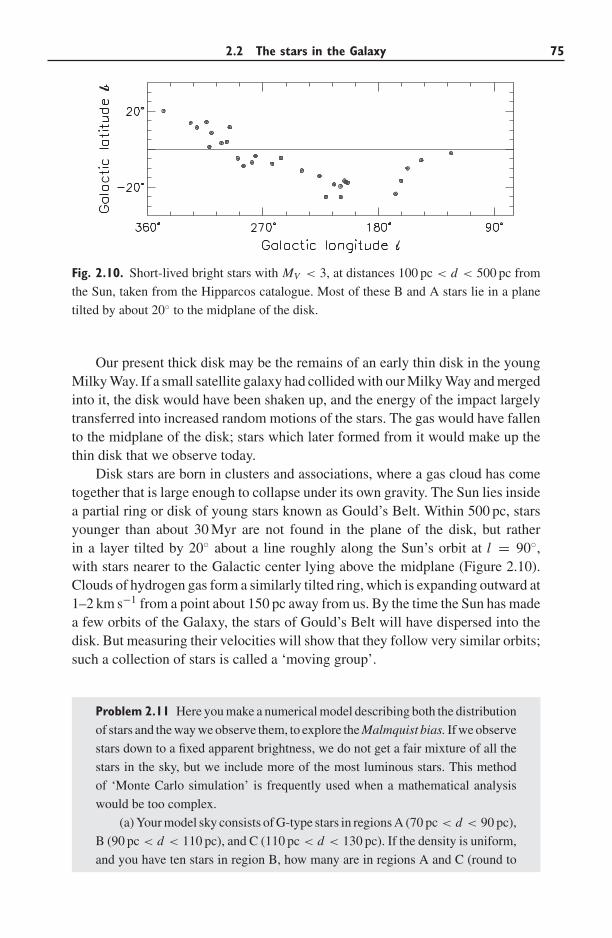
2.2 The stars in the Galaxy 75

Fig. 2.10. Short-lived bright stars with MV < 3, at distances 100 pc < d < 500 pc from

the Sun, taken from the Hipparcos catalogue. Most of these B and A stars lie in a plane

tilted by about 20◦ to the midplane of the disk.

Our present thick disk may be the remains of an early thin disk in the youngMilky Way. If a small satellite galaxy had collided with our Milky Way and mergedinto it, the disk would have been shaken up, and the energy of the impact largelytransferred into increased random motions of the stars. The gas would have fallento the midplane of the disk; stars which later formed from it would make up thethin disk that we observe today.

Disk stars are born in clusters and associations, where a gas cloud has cometogether that is large enough to collapse under its own gravity. The Sun lies insidea partial ring or disk of young stars known as Gould’s Belt. Within 500 pc, starsyounger than about 30 Myr are not found in the plane of the disk, but ratherin a layer tilted by 20◦ about a line roughly along the Sun’s orbit at l = 90◦,with stars nearer to the Galactic center lying above the midplane (Figure 2.10).Clouds of hydrogen gas form a similarly tilted ring, which is expanding outward at1–2 km s−1 from a point about 150 pc away from us. By the time the Sun has madea few orbits of the Galaxy, the stars of Gould’s Belt will have dispersed into thedisk. But measuring their velocities will show that they follow very similar orbits;such a collection of stars is called a ‘moving group’.

Problem 2.11 Here you make a numerical model describing both the distribution

of stars and the way we observe them, to explore the Malmquist bias. If we observe

stars down to a fixed apparent brightness, we do not get a fair mixture of all the

stars in the sky, but we include more of the most luminous stars. This method

of ‘Monte Carlo simulation’ is frequently used when a mathematical analysis

would be too complex.

(a) Your model sky consists of G-type stars in regions A (70 pc < d < 90 pc),

B (90 pc < d < 110 pc), and C (110 pc < d < 130 pc). If the density is uniform,

and you have ten stars in region B, how many are in regions A and C (round to

76 Mapping our Milky Way

the nearest integer)? For simplicity, let all the stars in region A be at d = 80 pc,

those in B at 100 pc, and those in C at 120 pc.

G stars do not all have exactly the same luminosity; if the variation corre-

sponds to about 0.3 magnitudes, what fractional change in luminosity is this? For

each of your stars, roll a die, note the number N1 on the upturned face, and give

your star MV = MV,� + 0.2 × (N1 − 3.5). If you like to program, you can use

more stars, place them randomly in space, and choose the absolute magnitudes

from a Gaussian random distribution, with mean MV,� and variance 0.3.

(b) To ‘observe’ your sky, use a ‘telescope’ that can ‘see’ only stars brighter

than apparent magnitude mV = 10; these stars are your sample. How different is

their mean absolute magnitude from that for all the stars that you placed in your

sky?

What is the average distance of all the stars in your sample? Suppose you

assumed that your sample stars each had the average luminosity for all the stars

in your sky, and then calculated their distances from their apparent magnitudes:

what would you find for their average distance? In which sense would you make

an error?

(c) Metal-poor main-sequence stars are bluer for a given luminosity, so they

must be fainter at a particular spectral type; if the star’s fraction by weight of

heavy elements is Z , then �MV ≈ −0.87 log10(Z/Z�). For each of your stars,

roll the die again, note the number N2, set Z/Z� = (N2 + 0.5)/6 and change its

absolute magnitude from part (a) by �MV .

Observe them again with the same telescope. For your sample of stars,

calculate the average Z of those that fall in regions B and C. Are these more or

less metal-rich than all the stars that you placed in your sky?

(Errors in measurement have the same kind of effect as a spread in the

true luminosity of a class of stars or galaxies. You can make corrections if you

know what your measurement errors are; but most people are too optimistic and

underestimate their errors!)

2.2.3 Distances to star clusters

If we can observe not just a single star, but an entire cluster of stars that are allat the same distance and that were formed together out of the same gaseous rawmaterial, we can make a much more accurate estimate of the distance. The Pleiadescluster, shown in Figure 2.11, contains about 700 stars that appear brighter thanmV = 17.

The color–magnitude diagram of Figure 2.12 shows that most of the starsare still on the main sequence, but those brighter than mV ≈ 5, that can be seenwithout a telescope or binoculars, have left it to become blue giants. The mainsequence is much narrower than it is in Figure 2.2, because all the stars are thesame age and have the same abundance of heavy elements. Stars with the lowestmasses have not yet reached the main sequence, and some of them are still

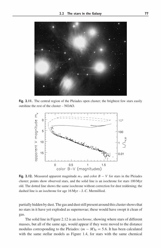
2.2 The stars in the Galaxy 77

Fig. 2.11. The central region of the Pleiades open cluster; the brightest few stars easily

outshine the rest of the cluster – NOAO.

1

100

0.01

0 0.5 1 1.5

15

10

5

0

Fig. 2.12. Measured apparent magnitude mV and color B − V for stars in the Pleiades

cluster; points show observed stars, and the solid line is an isochrone for stars 100 Myr

old. The dotted line shows the same isochrone without correction for dust reddening; the

dashed line is an isochrone for age 16 Myr – J.-C. Mermilliod.

partially hidden by dust. The gas and dust still present around this cluster shows thatno stars in it have yet exploded as supernovae; these would have swept it clean ofgas.

The solid line in Figure 2.12 is an isochrone, showing where stars of differentmasses, but all of the same age, would appear if they were moved to the distancemodulus corresponding to the Pleiades: (m − M)0 = 5.6. It has been calculatedwith the same stellar models as Figure 1.4, for stars with the same chemical

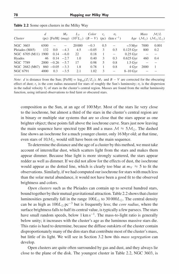
78 Mapping our Milky Way

Table 2.2 Some open clusters in the Milky Way

d MV LV Color rc σr Mass M/LCluster (pc) [Fe/H] (mag) (103 L�) (B − V ) (pc) (km s−1 ) Age (M�) (M�/L�)

NGC 3603 6500 − − 20 000 −0.3 0.5 − <5 Myr 7000 0.001Pleiades (M45) 132 0.0 −4.3 4.5 −0.05 3 0.5 0.125 Gyr 800 0.2NGC 6705 (M11) 1900 0.14 −6.0 22 0.18 1 − 0.25 Gyr − −Hyades 46 0.14 −2.7 1.0 0.40 3 0.3 0.625 Gyr 460 0.4NGC 7789 2000 −0.26 −5.7 17 0.98 5 0.8 1.5 Gyr − −NGC 2682 (M67) 860 −0.05 −3.3 1.8 0.78 1 0.8 4 Gyr 2000 1NGC 6791 4000 0.3 −3.5 2.1 1.02 3 − 8–10 Gyr − −

Note: d is distance from the Sun; [Fe/H] = log10(Z/Z�); MV and B − V are corrected for the obscuringeffect of dust; rc is the core radius measured for stars of roughly the Sun’s luminosity; σr is the dispersionin the radial velocity Vr of stars in the cluster’s central region. Masses are found from the stellar luminosityfunction, using infrared observations to find faint or obscured stars.

composition as the Sun, at an age of 100 Myr. Most of the stars lie very closeto the isochrone, but almost a third of the stars in the cluster’s central region arein binary or multiple star systems that are so close that the stars appear as onebrighter object; these points fall above the isochrone curve. Stars just now leavingthe main sequence have spectral type B8 and a mass M ≈ 5M�. The dashedline shows an isochrone for a much younger cluster, only 16 Myr old; at that time,even stars of 10M� would still have been on the main sequence.

To determine the distance and the age of a cluster by this method, we must takeaccount of interstellar dust, which scatters light from the stars and makes themappear dimmer. Because blue light is more strongly scattered, the stars appearredder as well as dimmer. If we did not allow for the effects of dust, the isochronewould appear as the dotted line, which is clearly too blue at mV ≈ 5 to fit theobservations. Similarly, if we had computed our isochrone for stars with much lessthan the solar metal abundance, it would not have been a good fit to the observedbrightness and colors.

Open clusters such as the Pleiades can contain up to several hundred stars,bound together by their mutual gravitational attraction. Table 2.2 shows that clusterluminosities generally fall in the range 100L� to 30 000L�. The central densitycan be as high as 100L� pc−3 but is frequently less; the core radius, where thesurface brightness falls to half its central value, is typically a few parsecs. The starshave small random speeds, below 1 km s−1. The mass-to-light ratio is generallybelow unity; it increases with the cluster’s age as the luminous massive stars die.This ratio is hard to determine, because the diffuse outskirts of the cluster containdisproportionately many of the dim stars that contribute most of the cluster’s mass,but little of its light. We will see in Section 3.2 how this mass segregation candevelop.

Open clusters are quite often surrounded by gas and dust, and they always lieclose to the plane of the disk. The youngest cluster in Table 2.2, NGC 3603, is

2.2 The stars in the Galaxy 79

near the Galactic center. Only ∼1% of its visible light can reach us, so we muststudy it in the infrared. In other galaxies, we see open clusters in the spiral arms.Unfortunately we cannot see most of the Milky Way’s open clusters, becausevisible light does not travel well through the dust in the disk. We can make a fairlycomplete map of the clusters only within about 5 kpc of the Sun.

Only about 5% of the 1200 or so known open clusters are more than 1 Gyr old,and most have ages less than 300 Myr; the nearby Hyades cluster is about 600 Myrold. Because most of a cluster’s light comes from its brightest stars, the color ofits total or integrated light gives us a rough estimate of its age. For example, thePleiades cluster has B − V = −0.05, close to the color of its most luminous starsthat are still on the main sequence; see Table 1.4. As the massive stars die, andmore of the cluster’s light comes from red giants, its color becomes redder. We canuse observations of nearby clusters, and the theory of stellar evolution, to relatea cluster’s color to its age and metal abundance. When we observe star clustersin other galaxies, generally we measure only the integrated light. Comparing acluster’s color with clusters in the Milky Way gives us an estimate of its age andthe composition of its stars.

Outside Gould’s Belt, most of the known open clusters younger than 300 Myrlie within 50 pc of the Galactic midplane. The older clusters, like the old starsof the thin disk, have a larger scale height, hz ≈ 375 pc. Clusters older than agigayear are found mainly in the outer Galaxy, beyond the Sun’s orbit, wherethe gravitational forces are weaker. They are also relatively well populated andcompact. Younger clusters are scattered more uniformly in Galactocentric radius;many have larger sizes or fewer members, and so are more fragile and prone tofall apart. Since the gravitational attraction of open clusters does not bind themtogether very strongly, they tend to be pulled apart as they pass through the spiralarms of the disk, and also to dissolve because of the gravitational pull of thecluster stars on each other. The old clusters that we see today are probably therobust survivors of a much larger population.

NGC 3603 is a very young and massive cluster; in the central parsec areseveral O3 stars, each with L ∼ 30 000L�. The stars are no more than 5 Myr old,and may be younger. Because its most massive stars are still shining, it is hugelymore luminous than the other clusters in Table 2.2. It is a smaller version of thesuper-star-clusters formed in starburst galaxies. Here, starbirth is so vigorous thatit will consume the galaxy’s supply of cool gas within ∼300 Myr. (Recall fromSection 2.2 that the Milky Way will not run out of gas for at least 2–3 Gyr.) Wewill discuss starbursts further in Section 7.1.

Since elements heavier than helium are produced in the interiors of stars,they become more abundant as the Universe ages. Figure 2.9 showed that F starsolder than 10 Gyr are much more likely to be iron-poor than are the younger stars.So we might expect that old open clusters, which formed earlier in the life ofthe Milky Way, should have lower metal abundances than the younger clusters.Surprisingly, this is not so; the old cluster NGC 6791 is as metal-rich as the Sun.

80 Mapping our Milky Way

Table 2.3 Some globular clusters in the Milky Way, and one belonging to the Fornax

dwarf spheroidal galaxy

d MV LV rc rt σr

Cluster (kpc) [Fe/H] (mag) (103 L�) (pc) (pc) (km s−1)

NGC 5139 ω Cen 5.2 −1.6a −10.2 1100 4 70 20NGC 104 47 Tuc 4.5 −0.71 −9.5 500 0.5 50 11NGC 7078 M15 10.8 −2.15 −9.3 440 <0.01b 85 12NGC 6341 M92 8.5 −2.15 −8.3 180 0.5 35 5NGC 7099 M30 9.1 −2.13 −7.6 95 <0.1b 45 5NGC 6121 M4 1.73 −1.2 −7.2 60 0.5 25 4

Pal 13 24.3 −1.9 −3.8 3 0.5 >50 0.6–0.9NGC 1049 Fornax 3 140 −2.0 −7.8 100 1.6 >50 9

Note: d is distance from the Sun; [Fe/H] = log10(Z/Z�); rc is the core radius, rt is the tidal ortruncation radius; and σr is the dispersion in the radial velocity Vr of stars in the central region.a 20%–30% of the stars of ω Centauri’s core are more metal-rich.b A collapsed core: see Section 3.2.

There is considerable scatter in the chemical composition of open clusters at allages. The buildup of metals in the Galaxy must have proceeded quite unevenly:some regions even recently were relatively poor in these elements. Open clustersfurther from the Galactic center are more likely to be metal-poor; the outer MilkyWay seems to be enriching itself more slowly than the inner parts.

The globular clusters are very different from open clusters; they contain farmore stars, much more tightly packed. The brightest of the Milky Way’s 150 orso known globulars is ω Centauri; with L ≈ 106L� it contains about a millionstars. In Figure 2.13 we see 47 Tucanae, another luminous cluster; Table 2.3 showsthat dimmer clusters range down to 104L�. The stellar density is roughly constantinside the core radius: rc ≈ 5 pc. The stars of globular clusters have higher randomspeeds σr than those of stars in the open clusters of Table 2.2. Globular clustersaround Fornax, a small nearby dwarf galaxy, are very similar to those in the MilkyWay. At some outer radius rt, usually beyond 30 pc, the density of stars dropssharply toward zero. This is the tidal radius or truncation radius. Stars beyondthis point are so loosely bound to the cluster that they can be swept away by the‘tidal’ gravitational force of the Milky Way as the cluster orbits around it. We willstudy this process further in Section 4.1.

None of the Milky Way’s globular clusters is younger than several gigayears,and most are much older. The two color–magnitude diagrams of Figure 2.14 showno young stars at all. The globular cluster 47 Tucanae is more than 10 Gyr old. Itsstars have only 15% of the solar abundance of metals, so the main sequence endswith stars a little bluer and more luminous than the Sun. As in the Pleiades, themain sequence is very narrow because all the stars are the same age and have thesame composition. Brighter stars fall on a narrow red giant branch, or on the hor-izontal branch with MV ≈ 0. Like the local disk stars that populate the red clump

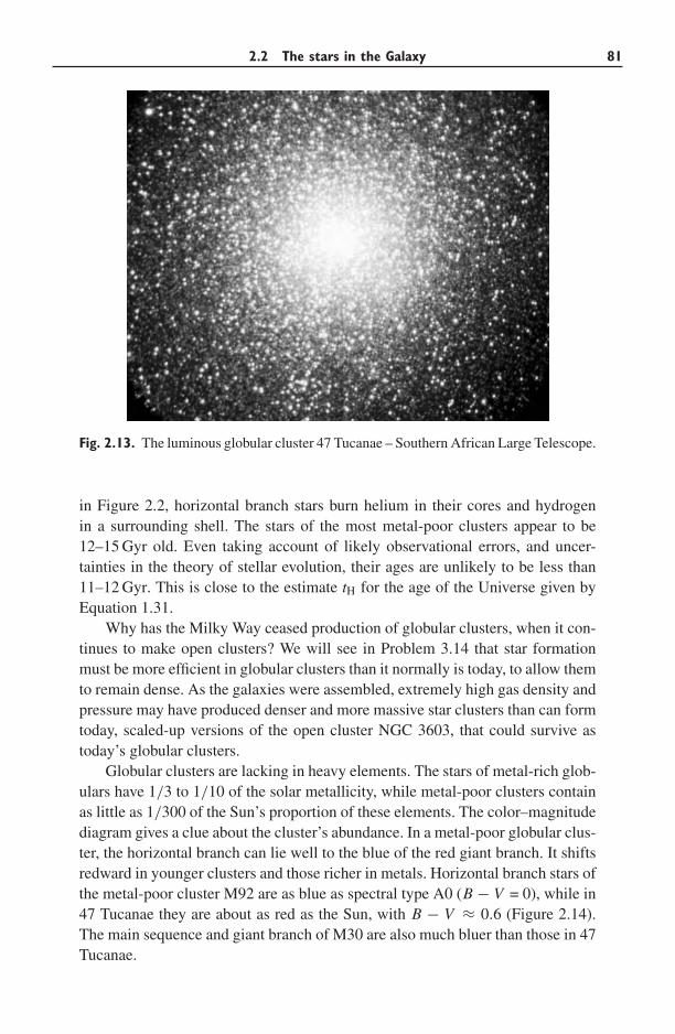
2.2 The stars in the Galaxy 81

Fig. 2.13. The luminous globular cluster 47 Tucanae – Southern African Large Telescope.

in Figure 2.2, horizontal branch stars burn helium in their cores and hydrogenin a surrounding shell. The stars of the most metal-poor clusters appear to be12–15 Gyr old. Even taking account of likely observational errors, and uncer-tainties in the theory of stellar evolution, their ages are unlikely to be less than11–12 Gyr. This is close to the estimate tH for the age of the Universe given byEquation 1.31.

Why has the Milky Way ceased production of globular clusters, when it con-tinues to make open clusters? We will see in Problem 3.14 that star formationmust be more efficient in globular clusters than it normally is today, to allow themto remain dense. As the galaxies were assembled, extremely high gas density andpressure may have produced denser and more massive star clusters than can formtoday, scaled-up versions of the open cluster NGC 3603, that could survive astoday’s globular clusters.

Globular clusters are lacking in heavy elements. The stars of metal-rich glob-ulars have 1/3 to 1/10 of the solar metallicity, while metal-poor clusters containas little as 1/300 of the Sun’s proportion of these elements. The color–magnitudediagram gives a clue about the cluster’s abundance. In a metal-poor globular clus-ter, the horizontal branch can lie well to the blue of the red giant branch. It shiftsredward in younger clusters and those richer in metals. Horizontal branch stars ofthe metal-poor cluster M92 are as blue as spectral type A0 (B − V = 0), while in47 Tucanae they are about as red as the Sun, with B − V ≈ 0.6 (Figure 2.14).The main sequence and giant branch of M30 are also much bluer than those in 47Tucanae.

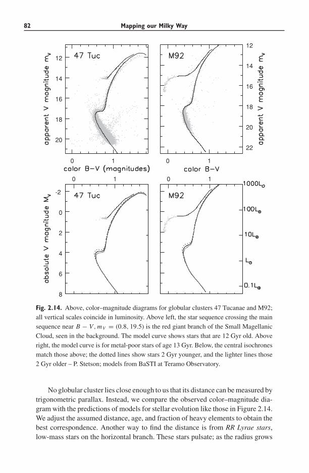
82 Mapping our Milky Way

0 1

8

6

4

2

0

-2

0 1

0 1

20

18

16

14

12

0 1

22

20

18

16

14

12

Fig. 2.14. Above, color–magnitude diagrams for globular clusters 47 Tucanae and M92;

all vertical scales coincide in luminosity. Above left, the star sequence crossing the main

sequence near B − V, mV = (0.8, 19.5) is the red giant branch of the Small Magellanic

Cloud, seen in the background. The model curve shows stars that are 12 Gyr old. Above

right, the model curve is for metal-poor stars of age 13 Gyr. Below, the central isochrones

match those above; the dotted lines show stars 2 Gyr younger, and the lighter lines those

2 Gyr older – P. Stetson; models from BaSTI at Teramo Observatory.

No globular cluster lies close enough to us that its distance can be measured bytrigonometric parallax. Instead, we compare the observed color–magnitude dia-gram with the predictions of models for stellar evolution like those in Figure 2.14.We adjust the assumed distance, age, and fraction of heavy elements to obtain thebest correspondence. Another way to find the distance is from RR Lyrae stars,low-mass stars on the horizontal branch. These stars pulsate; as the radius grows

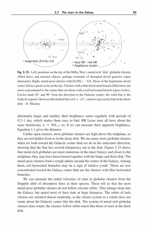
2.2 The stars in the Galaxy 83

bulge/disk: [Fe/H]>-0.8 blue HB red HBSagittarius cluster

Fig. 2.15. Left, positions on the sky of the Milky Way’s metal-rich ‘disk’ globular clusters

(filled dots), and unusual objects, perhaps remnants of disrupted dwarf galaxies (open

diamonds). Right, metal-poor clusters with [Fe/H]< −0.8. Those of the Sagittarius dwarf

(stars) fall in a great circle on the sky. Clusters with a blue horizontal branch (filled dots) are

more concentrated to the center than are those with a red horizontal branch (open circles).

Circles mark 20◦ and 90◦ from the direction to the Galactic center; the solid line is the

Galactic equator. Between the dashed lines at b = ±5◦, clusters may easily hide in the dusty

disk – D. Mackey.

alternately larger and smaller, their brightness varies regularly with periods of0.2–1 day, which makes them easy to find. RR Lyrae stars all have about thesame luminosity, L ≈ 50L�; so, if we can measure their apparent brightness,Equation 1.1 gives the distance.

Unlike open clusters, most globular clusters are high above the midplane, sothey are not hidden from us in the dusty disk. We see many more globular clusterswhen we look toward the Galactic center than we do in the anticenter direction,showing that the Sun lies several kiloparsecs out in the disk. Figure 2.15 showsthat metal-rich globulars are more numerous in the inner Galaxy and closer to themidplane; they may have been formed together with the bulge and thick disk. Themetal-poor clusters form a rough sphere around the center of the Galaxy. Amongthem, red horizontal branches may be a sign of relative youth. Those are lessconcentrated toward the Galaxy center than are the clusters with blue horizontalbranches.

We can measure the radial velocities of stars in globular clusters from theDoppler shift of absorption lines in their spectra. These tell us that the mostmetal-poor globular clusters do not follow circular orbits. They plunge deep intothe Galaxy, but spend most of their time at large distances. The orbits of haloclusters are oriented almost randomly, so the cluster system as a whole does notrotate about the Galactic center like the disk. The system of metal-rich globularclusters does rotate; the clusters follow orbits much like those of stars in the thickdisk.

84 Mapping our Milky Way

Stars are made from dense gas clouds: so we might expect the Milky Way’soldest stars to be in its dense center. Instead, they are in the halo globular clusters,its most extended component. How did this happen? Our Milky Way, like othersizable galaxies, is a cannibal: it has eaten its closest neighbors and satellites. Wewill see in Section 7.1 how gravity slows the motion of two galaxies that comeclose; if the effect is strong enough they spiral in toward each other and merge.The Sagittarius dwarf (see Section 4.1), our closest satellite galaxy, is partiallydigested and falling apart. A half-dozen metal-poor globular clusters follow orbitsso similar to it that they almost certainly belonged to this dwarf, but are now partof the Milky Way’s halo. The globular cluster ω Centauri contains stars withdiffering metal abundances, unlike a true star cluster. Perhaps it is all that remainsof a dense dwarf galaxy after its outer stars were torn away. The Magellanic Cloudswill share the Sagittarius dwarf’s fate within 3–5 Gyr. Some astronomers believethat the ‘blue’ metal-poor clusters in Figure 2.15 joined the Milky Way when itswallowed their parent galaxies.

The metal-poor halo of the Milky Way consists of the halo globular clusters,and roughly 100 times more individual metal-poor stars, some with less than10−5 of the Sun’s abundance. Locally, only one star in a thousand belongs to themetal-poor halo. They follow orbits similar to those of metal-poor globulars, andso are moving very fast relative to the Sun. We can pick out a few nearby halostars by their unusually high proper motions. The blue horizontal branch stars,distinctive variable stars such as the RR Lyrae, and red giants stand out clearly fromamong the more numerous foreground disk stars. Metal-poor globular clusters andstars of the metal-poor halo have been found as far as 100 kpc from the Galacticcenter.

Most halo stars seem to be as old as the metal-poor globular clusters. Aswith open clusters, the globular clusters that we see today are the few survivorsof a larger population. Some halo stars must be the remains of globular clustersthat dissolved or were torn apart by the Milky Way’s gravity (see Sections 3.2and 4.1). The globular cluster Palomar 5 has probably lost 90% of its stars; twospectacular stellar tails extend away from it more than 10◦ across the sky. Manyglobular clusters in the far reaches of the Milky Way, like Palomar 13 in Table 2.3,have relatively few members. If clusters like this had been formed closer to theGalactic center, they would have been torn apart long ago. The metal-poor haloalso contains various ‘moving groups’ of stars that follow a common orbit, and areprobably the remains of captured satellite systems. A stream of carbon stars and Mgiants apparently stripped from the Sagittarius dwarf galaxy stretches around thesky.

The most useful approach to mapping the metal-poor halo has been to guessat the luminosity function and the density of stars in the disk, bulge, and halo,and then use Monte Carlo techniques to calculate how many stars of each spec-tral type one expects to see in a particular area of the sky with a given apparentbrightness. We then adjust the guesses to achieve the best correspondence with

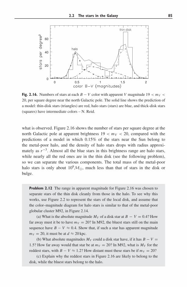
2.2 The stars in the Galaxy 85

0 0.5 1 1.5 20

20

40

60

halo

thin disk

Fig. 2.16. Numbers of stars at each B − V color with apparent V magnitude 19 < mV <

20, per square degree near the north Galactic pole. The solid line shows the prediction of

a model: thin-disk stars (triangles) are red, halo stars (stars) are blue, and thick-disk stars

(squares) have intermediate colors – N. Reid.

what is observed. Figure 2.16 shows the number of stars per square degree at thenorth Galactic pole at apparent brightness 19 < mV < 20, compared with thepredictions of a model in which 0.15% of the stars near the Sun belong tothe metal-poor halo, and the density of halo stars drops with radius approxi-mately as r−3. Almost all the blue stars in this brightness range are halo stars,while nearly all the red ones are in the thin disk (see the following problem),so we can separate the various components. The total mass of the metal-poorhalo stars is only about 109M�, much less than that of stars in the disk orbulge.

Problem 2.12 The range in apparent magnitude for Figure 2.16 was chosen to

separate stars of the thin disk cleanly from those in the halo. To see why this

works, use Figure 2.2 to represent the stars of the local disk, and assume that

the color–magnitude diagram for halo stars is similar to that of the metal-poor

globular cluster M92, in Figure 2.14.

(a) What is the absolute magnitude MV of a disk star at B − V = 0.4? How

far away must it be to have mV = 20? In M92, the bluest stars still on the main

sequence have B − V ≈ 0.4. Show that, if such a star has apparent magnitude

mV = 20, it must be at d ≈ 20 kpc.

(b) What absolute magnitudes MV could a disk star have, if it has B − V =1.5? How far away would that star be at mV = 20? In M92, what is MV for the

reddest stars, with B − V ≈ 1.2? How distant must these stars be if mV = 20?

(c) Explain why the reddest stars in Figure 2.16 are likely to belong to the

disk, while the bluest stars belong to the halo.

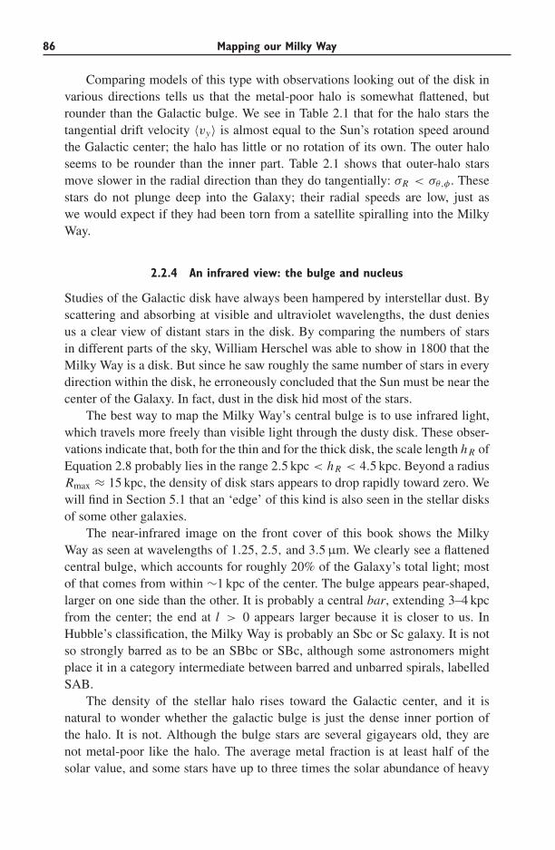
86 Mapping our Milky Way

Comparing models of this type with observations looking out of the disk invarious directions tells us that the metal-poor halo is somewhat flattened, butrounder than the Galactic bulge. We see in Table 2.1 that for the halo stars thetangential drift velocity 〈vy〉 is almost equal to the Sun’s rotation speed aroundthe Galactic center; the halo has little or no rotation of its own. The outer haloseems to be rounder than the inner part. Table 2.1 shows that outer-halo starsmove slower in the radial direction than they do tangentially: σR < σθ,φ . Thesestars do not plunge deep into the Galaxy; their radial speeds are low, just aswe would expect if they had been torn from a satellite spiralling into the MilkyWay.

2.2.4 An infrared view: the bulge and nucleus

Studies of the Galactic disk have always been hampered by interstellar dust. Byscattering and absorbing at visible and ultraviolet wavelengths, the dust deniesus a clear view of distant stars in the disk. By comparing the numbers of starsin different parts of the sky, William Herschel was able to show in 1800 that theMilky Way is a disk. But since he saw roughly the same number of stars in everydirection within the disk, he erroneously concluded that the Sun must be near thecenter of the Galaxy. In fact, dust in the disk hid most of the stars.

The best way to map the Milky Way’s central bulge is to use infrared light,which travels more freely than visible light through the dusty disk. These obser-vations indicate that, both for the thin and for the thick disk, the scale length h R ofEquation 2.8 probably lies in the range 2.5 kpc < h R < 4.5 kpc. Beyond a radiusRmax ≈ 15 kpc, the density of disk stars appears to drop rapidly toward zero. Wewill find in Section 5.1 that an ‘edge’ of this kind is also seen in the stellar disksof some other galaxies.

The near-infrared image on the front cover of this book shows the MilkyWay as seen at wavelengths of 1.25, 2.5, and 3.5 μm. We clearly see a flattenedcentral bulge, which accounts for roughly 20% of the Galaxy’s total light; mostof that comes from within ∼1 kpc of the center. The bulge appears pear-shaped,larger on one side than the other. It is probably a central bar, extending 3–4 kpcfrom the center; the end at l > 0 appears larger because it is closer to us. InHubble’s classification, the Milky Way is probably an Sbc or Sc galaxy. It is notso strongly barred as to be an SBbc or SBc, although some astronomers mightplace it in a category intermediate between barred and unbarred spirals, labelledSAB.

The density of the stellar halo rises toward the Galactic center, and it isnatural to wonder whether the galactic bulge is just the dense inner portion ofthe halo. It is not. Although the bulge stars are several gigayears old, they arenot metal-poor like the halo. The average metal fraction is at least half of thesolar value, and some stars have up to three times the solar abundance of heavy

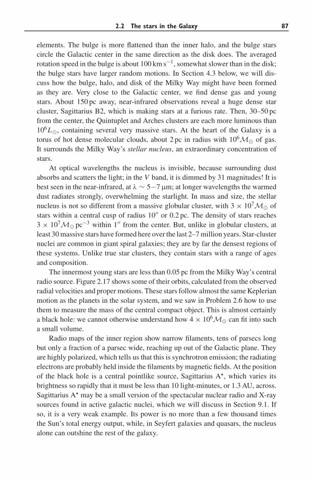
2.2 The stars in the Galaxy 87

elements. The bulge is more flattened than the inner halo, and the bulge starscircle the Galactic center in the same direction as the disk does. The averagedrotation speed in the bulge is about 100 km s−1, somewhat slower than in the disk;the bulge stars have larger random motions. In Section 4.3 below, we will dis-cuss how the bulge, halo, and disk of the Milky Way might have been formedas they are. Very close to the Galactic center, we find dense gas and youngstars. About 150 pc away, near-infrared observations reveal a huge dense starcluster, Sagittarius B2, which is making stars at a furious rate. Then, 30–50 pcfrom the center, the Quintuplet and Arches clusters are each more luminous than106L�, containing several very massive stars. At the heart of the Galaxy is atorus of hot dense molecular clouds, about 2 pc in radius with 106M� of gas.It surrounds the Milky Way’s stellar nucleus, an extraordinary concentration ofstars.

At optical wavelengths the nucleus is invisible, because surrounding dustabsorbs and scatters the light; in the V band, it is dimmed by 31 magnitudes! It isbest seen in the near-infrared, at λ ∼ 5−7 μm; at longer wavelengths the warmeddust radiates strongly, overwhelming the starlight. In mass and size, the stellarnucleus is not so different from a massive globular cluster, with 3 × 107M� ofstars within a central cusp of radius 10′′ or 0.2 pc. The density of stars reaches3 × 107M� pc−3 within 1′′ from the center. But, unlike in globular clusters, atleast 30 massive stars have formed here over the last 2–7 million years. Star-clusternuclei are common in giant spiral galaxies; they are by far the densest regions ofthese systems. Unlike true star clusters, they contain stars with a range of agesand composition.

The innermost young stars are less than 0.05 pc from the Milky Way’s centralradio source. Figure 2.17 shows some of their orbits, calculated from the observedradial velocities and proper motions. These stars follow almost the same Keplerianmotion as the planets in the solar system, and we saw in Problem 2.6 how to usethem to measure the mass of the central compact object. This is almost certainlya black hole: we cannot otherwise understand how 4 × 106M� can fit into sucha small volume.

Radio maps of the inner region show narrow filaments, tens of parsecs longbut only a fraction of a parsec wide, reaching up out of the Galactic plane. Theyare highly polarized, which tells us that this is synchrotron emission; the radiatingelectrons are probably held inside the filaments by magnetic fields. At the positionof the black hole is a central pointlike source, Sagittarius A, which varies itsbrightness so rapidly that it must be less than 10 light-minutes, or 1.3 AU, across.Sagittarius A may be a small version of the spectacular nuclear radio and X-raysources found in active galactic nuclei, which we will discuss in Section 9.1. Ifso, it is a very weak example. Its power is no more than a few thousand timesthe Sun’s total energy output, while, in Seyfert galaxies and quasars, the nucleusalone can outshine the rest of the galaxy.

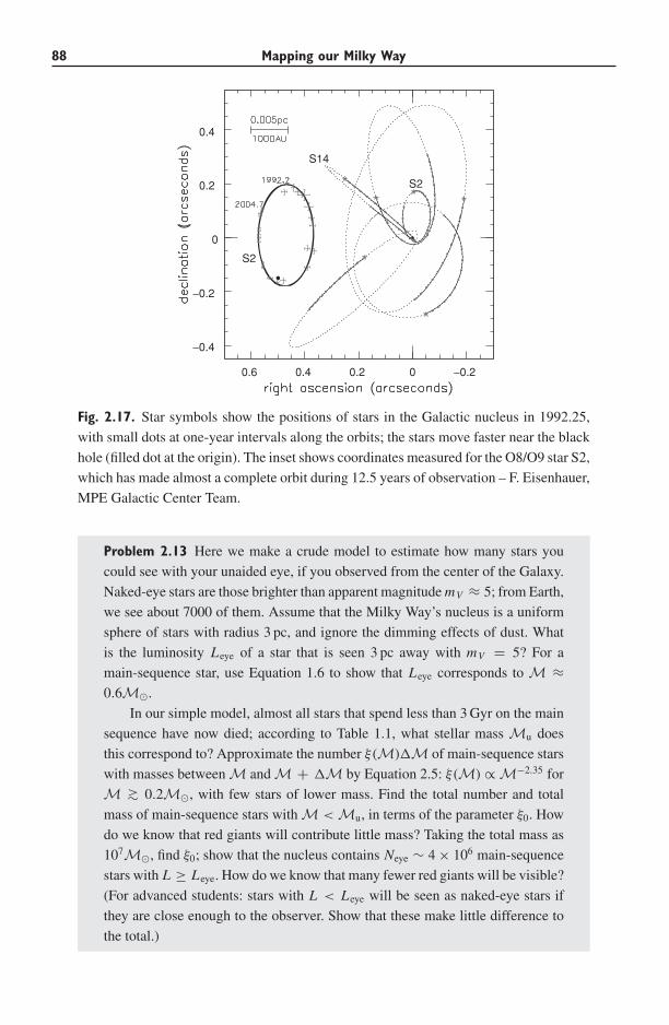
88 Mapping our Milky Way

0.6 0.4 0.2 0 −0.2

−0.4

−0.2

0

0.2

0.4

S2

S14

S2

Fig. 2.17. Star symbols show the positions of stars in the Galactic nucleus in 1992.25,

with small dots at one-year intervals along the orbits; the stars move faster near the black

hole (filled dot at the origin). The inset shows coordinates measured for the O8/O9 star S2,

which has made almost a complete orbit during 12.5 years of observation – F. Eisenhauer,

MPE Galactic Center Team.

Problem 2.13 Here we make a crude model to estimate how many stars you

could see with your unaided eye, if you observed from the center of the Galaxy.

Naked-eye stars are those brighter than apparent magnitude mV ≈ 5; from Earth,

we see about 7000 of them. Assume that the Milky Way’s nucleus is a uniform

sphere of stars with radius 3 pc, and ignore the dimming effects of dust. What

is the luminosity Leye of a star that is seen 3 pc away with mV = 5? For a

main-sequence star, use Equation 1.6 to show that Leye corresponds to M ≈0.6M�.

In our simple model, almost all stars that spend less than 3 Gyr on the main

sequence have now died; according to Table 1.1, what stellar mass Mu does

this correspond to? Approximate the number ξ (M)�M of main-sequence stars

with masses between M and M + �M by Equation 2.5: ξ (M) ∝ M−2.35 for

M ∼> 0.2M�, with few stars of lower mass. Find the total number and total

mass of main-sequence stars with M < Mu, in terms of the parameter ξ0. How

do we know that red giants will contribute little mass? Taking the total mass as

107M�, find ξ0; show that the nucleus contains Neye ∼ 4 × 106 main-sequence

stars with L ≥ Leye. How do we know that many fewer red giants will be visible?

(For advanced students: stars with L < Leye will be seen as naked-eye stars if

they are close enough to the observer. Show that these make little difference to

the total.)

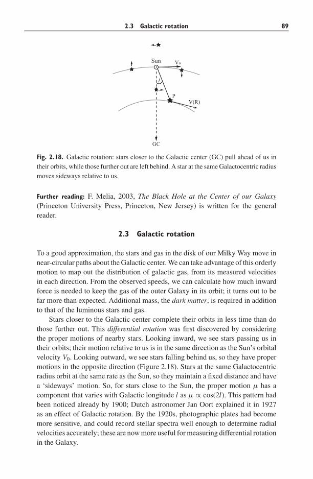
2.3 Galactic rotation 89

V(R)

Vo

GC

l

Sun

P

Fig. 2.18. Galactic rotation: stars closer to the Galactic center (GC) pull ahead of us in

their orbits, while those further out are left behind. A star at the same Galactocentric radius

moves sideways relative to us.

Further reading: F. Melia, 2003, The Black Hole at the Center of our Galaxy(Princeton University Press, Princeton, New Jersey) is written for the generalreader.

2.3 Galactic rotation

To a good approximation, the stars and gas in the disk of our Milky Way move innear-circular paths about the Galactic center. We can take advantage of this orderlymotion to map out the distribution of galactic gas, from its measured velocitiesin each direction. From the observed speeds, we can calculate how much inwardforce is needed to keep the gas of the outer Galaxy in its orbit; it turns out to befar more than expected. Additional mass, the dark matter, is required in additionto that of the luminous stars and gas.

Stars closer to the Galactic center complete their orbits in less time than dothose further out. This differential rotation was first discovered by consideringthe proper motions of nearby stars. Looking inward, we see stars passing us intheir orbits; their motion relative to us is in the same direction as the Sun’s orbitalvelocity V0. Looking outward, we see stars falling behind us, so they have propermotions in the opposite direction (Figure 2.18). Stars at the same Galactocentricradius orbit at the same rate as the Sun, so they maintain a fixed distance and havea ‘sideways’ motion. So, for stars close to the Sun, the proper motion μ has acomponent that varies with Galactic longitude l as μ ∝ cos(2l). This pattern hadbeen noticed already by 1900; Dutch astronomer Jan Oort explained it in 1927as an effect of Galactic rotation. By the 1920s, photographic plates had becomemore sensitive, and could record stellar spectra well enough to determine radialvelocities accurately; these are now more useful for measuring differential rotationin the Galaxy.

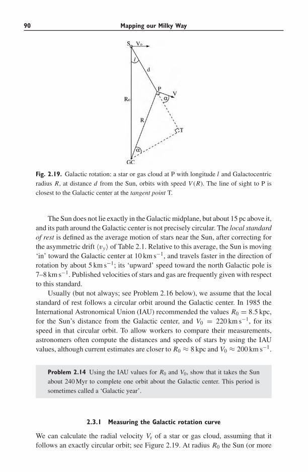
90 Mapping our Milky Way

Fig. 2.19. Galactic rotation: a star or gas cloud at P with longitude l and Galactocentric

radius R, at distance d from the Sun, orbits with speed V (R). The line of sight to P is

closest to the Galactic center at the tangent point T.

The Sun does not lie exactly in the Galactic midplane, but about 15 pc above it,and its path around the Galactic center is not precisely circular. The local standardof rest is defined as the average motion of stars near the Sun, after correcting forthe asymmetric drift 〈vy〉 of Table 2.1. Relative to this average, the Sun is moving‘in’ toward the Galactic center at 10 km s−1, and travels faster in the direction ofrotation by about 5 km s−1; its ‘upward’ speed toward the north Galactic pole is7–8 km s−1. Published velocities of stars and gas are frequently given with respectto this standard.

Usually (but not always; see Problem 2.16 below), we assume that the localstandard of rest follows a circular orbit around the Galactic center. In 1985 theInternational Astronomical Union (IAU) recommended the values R0 = 8.5 kpc,for the Sun’s distance from the Galactic center, and V0 = 220 km s−1, for itsspeed in that circular orbit. To allow workers to compare their measurements,astronomers often compute the distances and speeds of stars by using the IAUvalues, although current estimates are closer to R0 ≈ 8 kpc and V0 ≈ 200 km s−1.

Problem 2.14 Using the IAU values for R0 and V0, show that it takes the Sun

about 240 Myr to complete one orbit about the Galactic center. This period is

sometimes called a ‘Galactic year’.

2.3.1 Measuring the Galactic rotation curve

We can calculate the radial velocity Vr of a star or gas cloud, assuming that itfollows an exactly circular orbit; see Figure 2.19. At radius R0 the Sun (or more

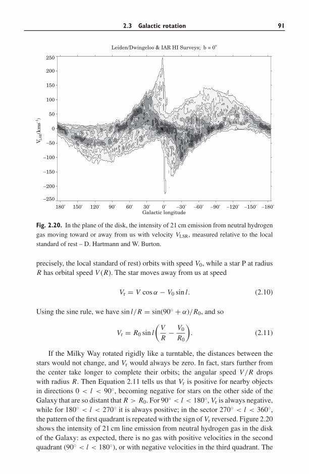
2.3 Galactic rotation 91

−180o−150o−120o−90o−60o−30o0o30o60o90o120o150o180o

Galactic longitude

−250

−200

−150

−100

−50

0

50

100

150

200

250

V LS

R (km

s−1)

Leiden/Dwingeloo & IAR HI Surveys; b = 0o

Fig. 2.20. In the plane of the disk, the intensity of 21 cm emission from neutral hydrogen

gas moving toward or away from us with velocity VLSR, measured relative to the local

standard of rest – D. Hartmann and W. Burton.

precisely, the local standard of rest) orbits with speed V0, while a star P at radiusR has orbital speed V (R). The star moves away from us at speed

Vr = V cos α − V0 sin l. (2.10)

Using the sine rule, we have sin l/R = sin(90◦ + α)/R0, and so

Vr = R0 sin l

(V

R− V0

R0

). (2.11)

If the Milky Way rotated rigidly like a turntable, the distances between thestars would not change, and Vr would always be zero. In fact, stars further fromthe center take longer to complete their orbits; the angular speed V/R dropswith radius R. Then Equation 2.11 tells us that Vr is positive for nearby objectsin directions 0 < l < 90◦, becoming negative for stars on the other side of theGalaxy that are so distant that R > R0. For 90◦ < l < 180◦, Vr is always negative,while for 180◦ < l < 270◦ it is always positive; in the sector 270◦ < l < 360◦,the pattern of the first quadrant is repeated with the sign of Vr reversed. Figure 2.20shows the intensity of 21 cm line emission from neutral hydrogen gas in the diskof the Galaxy: as expected, there is no gas with positive velocities in the secondquadrant (90◦ < l < 180◦), or with negative velocities in the third quadrant. The

92 Mapping our Milky Way

dark narrow bands extending across many degrees in longitude show where gashas been piled up, and its velocity changed, by gravitational forces in the spiralarms.

Problem 2.15 For a simple model of the Galaxy with R0 = 8 kpc and

V (R) = 220 km s−1 everywhere, find Vr(l) for gas in circular orbit at R =4, 6, 10, and 12 kpc. Do this by varying the Galactocentric azimuth φ around

each ring; find d for each (φ, R), and hence the longitude l and Vr. Make a plot

similar to Figure 2.20 showing the gas on these rings. In Figure 2.20 itself, explain

where the gas lies that corresponds to (l ∼ 50◦, V > 0); (l ∼ 50◦, V < 0); (l ∼120◦, V < 0); (l ∼ 240◦, V > 0); (l ∼ 300◦, V > 0); and (l ∼ 300◦, V < 0).

Where is the gas at (l ∼ 120◦, V > 0)?

Problem 2.16 Suppose that gas in the Galaxy does not follow exactly circular

orbits, but in addition has a velocity U (R, l) radially outward from the Galactic

center; stars near the Sun have an outward motion U0. Show that gas at point P

in Figure 2.19 recedes from us at speed

Vr = R0 sin l

(V

R− V0

R0

)− R0 cos l

(U

R− U0

R0

)+ d

U

R. (2.12)

Suppose now that the Sun is moving outward with speed U0 > 0, but that gas

in the rest of the Galaxy follows circular orbits; how should velocities measured

in the direction l = 180◦ differ from zero? For gas at a given radius R, in

which direction are the extrema (maxima or minima) of VR shifted away from

l = 90◦ and l = 270◦? Use Figure 2.20 to show that the Sun and the local

standard of rest are probably moving outward from the Galactic center.

When our star or gas cloud is close to the Sun, so that d � R, we can neglectterms in d2; using the cosine rule for triangle S–P–GC then gives R ≈ R0−d cos l.The radial velocity of Equation 2.11 becomes

Vr ≈ R0 sin l

(V

R

)′(R − R0) ≈ d sin(2l)

[− R

2

(V

R

)′]R0

≡ d A sin(2l), (2.13)

where we use the prime for differentiation with respect to R. The constant A,named after Oort, is measured as 14.8 ± 0.8 km s−1 kpc−1.

The proper motion of a star at P relative to the Sun can be calculated in asimilar way. From Figure 2.19, the tangential velocity is

Vt = V sin α − V0 cos l. (2.14)

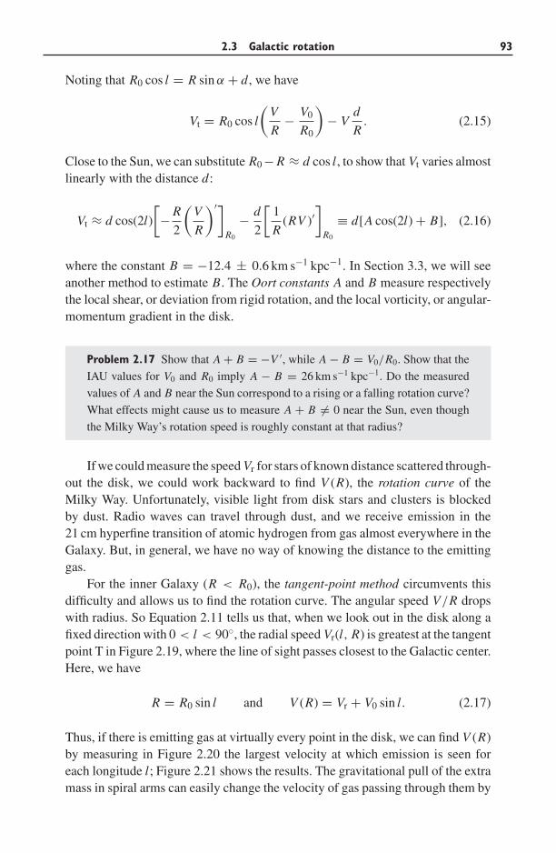
2.3 Galactic rotation 93

Noting that R0 cos l = R sin α + d , we have

Vt = R0 cos l

(V

R− V0

R0

)− V

d

R. (2.15)

Close to the Sun, we can substitute R0 − R ≈ d cos l, to show that Vt varies almostlinearly with the distance d:

Vt ≈ d cos(2l)

[− R

2

(V

R

)′]R0

− d

2

[1

R(RV )′

]R0

≡ d[A cos(2l) + B], (2.16)

where the constant B = −12.4 ± 0.6 km s−1 kpc−1. In Section 3.3, we will seeanother method to estimate B. The Oort constants A and B measure respectivelythe local shear, or deviation from rigid rotation, and the local vorticity, or angular-momentum gradient in the disk.

Problem 2.17 Show that A + B = −V ′, while A − B = V0/R0. Show that the

IAU values for V0 and R0 imply A − B = 26 km s−1 kpc−1. Do the measured

values of A and B near the Sun correspond to a rising or a falling rotation curve?

What effects might cause us to measure A + B �= 0 near the Sun, even though

the Milky Way’s rotation speed is roughly constant at that radius?

If we could measure the speed Vr for stars of known distance scattered through-out the disk, we could work backward to find V (R), the rotation curve of theMilky Way. Unfortunately, visible light from disk stars and clusters is blockedby dust. Radio waves can travel through dust, and we receive emission in the21 cm hyperfine transition of atomic hydrogen from gas almost everywhere in theGalaxy. But, in general, we have no way of knowing the distance to the emittinggas.

For the inner Galaxy (R < R0), the tangent-point method circumvents thisdifficulty and allows us to find the rotation curve. The angular speed V/R dropswith radius. So Equation 2.11 tells us that, when we look out in the disk along afixed direction with 0 < l < 90◦, the radial speed Vr(l, R) is greatest at the tangentpoint T in Figure 2.19, where the line of sight passes closest to the Galactic center.Here, we have

R = R0 sin l and V (R) = Vr + V0 sin l. (2.17)

Thus, if there is emitting gas at virtually every point in the disk, we can find V (R)by measuring in Figure 2.20 the largest velocity at which emission is seen foreach longitude l; Figure 2.21 shows the results. The gravitational pull of the extramass in spiral arms can easily change the velocity of gas passing through them by

94 Mapping our Milky Way

0 0.5 1

160

200

240

280

1.5 2 2.5

160

200

240

280

Fig. 2.21. Left, the Milky Way’s rotation from the tangent-point method, taking V0 =200 km s−1; dots show velocities of northern HI gas with l > 270◦; the curve gives results

from southern gas at l < 90◦. The tangent-point method fails at R ∼< 0.2R0 (open circles)

because this gas follows oval orbits in the Galactic bar. Right, the rotation speed of the

outer Galaxy, calculated for V0 = 200 km s−1 (filled circles) and for V0 = 220 km s−1

(open circles); crosses show estimated errors – W. B. Burton and M. Honma.

10–20 km s−1. If the tangent point falls close to an arm, then the rotation speedfound by using Equation 2.17 will differ from the average speed of an orbit at thatGalactocentric radius.

Measuring rotation speeds in the outer Galaxy is harder. We must first findthe distances to associations of young stars by the methods of spectroscopic orphotometric parallax. Their velocity Vr is then measured from the emission linesof hot or cool gas around the stars. The stellar distances are often not very welldetermined, but they are good enough to tell us that the rotation speed V (R) doesnot decline much in the outer Galaxy, and may even rise further.

2.3.2 Dark matter in the Milky Way

In Section 3.1 we will see that, for a spherical system, the speed V in a circularorbit at radius R is related to the mass M(<R) interior to that radius by the exactequation

M(<R) = RV 2/G. (2.18)

When R is measured in parsecs, time in megayears, and M in M�, Newton’sgravitational constant G = 4.5 × 10−3. For orbits in a flattened disk, this formulagives M(< R) to within 10% − 15%. Since V (R) does not decline, the massof the Milky Way must increase almost linearly with radius, even far beyondthe Sun where there are very few stars. Later, we will see that this discrepancybetween the distributions of light and mass is generally present in spiral galaxies.Astronomers often refer to it as the ‘missing mass’or ‘dark matter’ problem.

2.4 Milky Way meteorology: the interstellar gas 95

Galaxies presumably contain a large amount of matter that gives out virtually nolight; this nonluminous mass is assumed to lie in a dark halo.

Problem 2.18 Use Equation 2.18 to find the mass M(< R0) within a sphere

of radius R0 about the Galactic center. What is the average density within that

sphere, in M� pc−3? Show that this is about 105 times larger than the critical

density of Equation 1.30.

Taking h R = 4 kpc in Equation 2.8, show that 60% of the Milky Way’s disk

lies within the Sun’s orbit. Taking LV = 5×109L� for the bulge and 15×109L�for the disk, show that the mass-to-light ratio M/L(<R0) ≈ 5. Using the result

of Problem 2.8, explain why we believe that no more than half of the mass within

R0 is dark matter.

Problem 2.19 The Galaxy’s HI disk extends outward to about 2.5R0. From

Figure 2.21, show that the mass M(<2.5R0) ≈ 2 × 1011M�, so that the mass-

to-light ratio M/LV ∼> 10. How does this compare with what we found in

Problem 2.8? Where is most of the Milky Way’s dark matter?

Problem 2.20 Consider the spherical density distribution ρH(r ) with

4πGρH(r ) = V 2H

r2 + a2H

, (2.19)

where VH and aH are constants; what is the mass M(<r ) contained within radius

r? Use Equation 2.18 to show that the speed V (r ) of a circular orbit at radius r

is given by

V 2(r ) = V 2H[1 − (aH/r )arctan(r/aH)], (2.20)

and sketch V (r ) as a function of radius. This density law is often used to represent

the mass of a galaxy’s dark halo – why?

2.4 Milky Way meteorology: the interstellar gas

Between the Milky Way’s stars lies the gas from which they were made, and towhich they return the heavy elements produced by their nuclear burning. Almostall of the gas lies in the disk. Although its mass is less than 10% of that in stars, itgives the Galaxy many of its distinctive properties. Without gas, the Milky Waywould be an S0 galaxy, not a spiral: our disk would have no hot young starsand no spiral pattern. Only about half of the Galaxy’s starlight escapes freelyinto intergalactic space; dusty interstellar gas absorbs the rest. The front covershows the Milky Way’s gas, dust and stars observed at wavelengths from radio toγ-rays.

96 Mapping our Milky Way

Like the stellar disk, the Galaxy’s interstellar material is subject to gravity,which ultimately causes the densest gas to collapse into new stars. But we mustalso consider other forces, which can safely be ignored when discussing stellarmotions: gas pressure, magnetic forces, and the pressure of cosmic rays. The gasis heated and ionized by stellar radiation; it is shocked and set into motion by faststellar winds, violent supernova explosions, and passage through the spiral arms.Like the Earth’s atmosphere, the interstellar medium is in complex motion.

2.4.1 Mapping the gas layer

Unlike stars, gas does not come in units of standard size. The mass of a clumpof gas is not directly linked to its temperature, or any other quantity that wecould measure independently of its distance. So the distances of gas clouds arevery uncertain, except in special cases: for example, when we know that the gassurrounds a star. When we see absorption lines from interstellar gas in the spectrumof a star, we know that the gas is closer to us than the star. For gas in circularorbits in the Milky Way’s disk, we can calculate a kinematic distance. From itsspectral line emission, we find how much gas is moving at each radial velocityVr in the direction at longitude l. Then, from the rotation curve V (R), we can useEquation 2.11 to estimate its distance. Thus we can build up a picture of how theMilky Way’s gas is distributed.

When all of its radiation reaches us without being absorbed, the mass of gasmoving with a particular velocity is proportional to the intensity of the radiation atthe corresponding wavelength. Visible light is strongly absorbed by the interstellardust, whereas radio waves can travel through the dusty gas. But, in the disk,we often look through enough material that radio waves from distant gas arepartially absorbed by gas closer to us: the emission is optically thick. The 21 cmline of neutral hydrogen, HI, is optically thick in the inner parts of the Galaxy.Dense cool clouds, where the gas is largely molecular, are often traced by themillimeter-wavelength lines of 12CO, which are nearly always optically thick.Thus much of the molecular gas may be hidden from our direct view.

Recall from Section 1.2 that we do not see emission lines from cool molecularhydrogen, because H2 is a symmetric molecule. The next most abundant moleculein the dense gas is carbon monoxide, with roughly one CO molecule for every 104

of H2. On large scales, we can measure the total amount of atomic and moleculargas by comparing the numbers of energetic cosmic rays (see below), detected asthey zip through the Earth’s atmosphere, with the brightness in γ-rays, which areproduced as cosmic rays hit the gas atoms in the Galactic plane. By comparing inturn with observations in CO, we can find the average ratio XCO of the columndensity of molecular hydrogen to CO emission in the lowest rotational transition.In the Milky Way XCO is fairly uniform in the disk. It is higher in the central fewhundred parsecs and in starbursts, where very vigorous star formation gives riseto a strong radiation field.

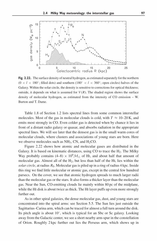
2.4 Milky Way meteorology: the interstellar gas 97

0 5 10 15 20 250

5

10

15

Fig. 2.22. The surface density of neutral hydrogen, as estimated separately for the northern

(0 < l < 180◦; filled dots) and southern (180◦ < l < 360◦; open circles) halves of the

Galaxy. Within the solar circle, the density is sensitive to corrections for optical thickness;

outside, it depends on what is assumed for V (R). The shaded region shows the surface

density of molecular hydrogen, as estimated from the intensity of CO emission – W.

Burton and T. Dame.

Table 1.8 of Section 1.2 lists spectral lines from some common interstellarmolecules. Most of the gas in molecular clouds is cold, with T ≈ 10–20 K, andemits most strongly in CO. Even colder gas is detected when by chance it lies infront of a distant radio galaxy or quasar, and absorbs radiation in the appropriatespectral lines. We will see later that the densest gas is in the small warm cores ofmolecular clouds, where clusters and associations of young stars are born. Herewe observe molecules such as NH3, CN, and H2CO.

Figure 2.22 shows how atomic and molecular gases are distributed in theGalaxy. It is based on kinematic distances, using CO to trace the H2. The MilkyWay probably contains (4–8) × 109M� of HI, and about half that amount ofmolecular gas. Almost all of the H2, but less than half of the HI, lies within thesolar circle, at radius R0. Molecular gas is piled up in a ring of radius 4 kpc. Insidethis ring we find little molecular or atomic gas, except in the central few hundredparsecs. On the cover, we see that atomic hydrogen spreads to much larger radiithan the molecular gas or the stars. It also forms a thicker layer than the moleculargas. Near the Sun, CO-emitting clouds lie mainly within 80 pc of the midplane,while the HI disk is about twice as thick. The HI layer puffs up even more stronglyfurther out.

As in other spiral galaxies, the dense molecular gas, dust, and young stars areconcentrated into the spiral arms: see Section 5.5. The Sun lies just outside theSagittarius–Carina arm, which can be traced for almost a full turn around the disk.Its pitch angle is about 10◦, which is typical for an Sbc or Sc galaxy. Lookingaway from the Galactic center, we see a short nearby arm-spur in the constellationof Orion. Roughly 2 kpc further out lies the Perseus arm, which shows up in

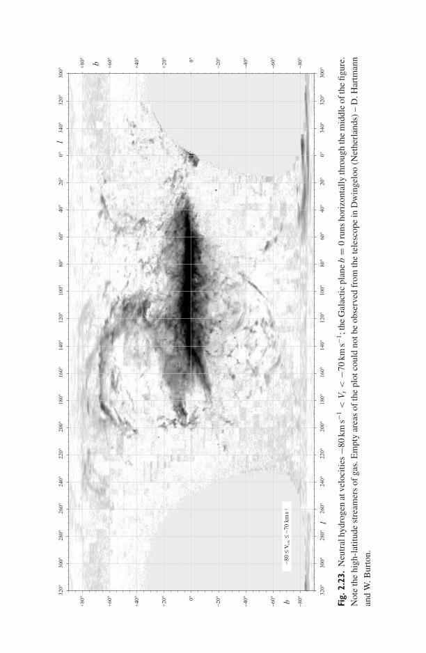
320°

300°

280°

260°

240°

220°

200°

180°

160°

120°

100°

80°

140°

60°

40°

20°

0°34

0°32

0°30

0°l

320°

300°

280°

260°

240°

220°

200°

180°

160°

120°

100°

80°

140°

60°

40°

20°

0°34

0°32

0°30

0°l

− 80°

− 60°

−40°

−20°0 °

+20

°

+40

°

+60

°

+80

°

b

− 80°

−60°

−40°

− 20°0°

+20

°

+40

°

+60

°

+80

°

b−

≤≤

−80

70 k

ms

v LSR

− 1

Fig.

2.23

.N

eutr

alhy

drog

enat

velo

citie

s−8

0km

s−1<

Vr<

−70

kms−1

;the

Gal

actic

plan

eb

=0

runs

hori

zont

ally

thro

ugh

the

mid

dle

ofth

efig

ure.

Not

eth

ehi

gh-l

atitu

dest

ream

ers

ofga

s.E

mpt

yar

eas

ofth

epl

otco

uld

notb

eob

serv

edfr

omth

ete

lesc

ope

inD

win

gelo

o(N

ethe

rlan

ds)

–D

.Har

tman

n

and

W.B

urto

n.

2.4 Milky Way meteorology: the interstellar gas 99

Figure 2.20 as a dark ridge at l > 90◦, VLSR ≈ 50 km s−1. However, we do nothave a picture of our whole spiral pattern. Dust blocks our view through the diskin visible light, and kinematic distances for the gas are unreliable, because thegravitational tug of the spiral arms pulls it out of circular rotation.

Figure 2.23 shows atomic gas far above the Galactic plane. Looking awayfrom the Galactic center toward l = 180◦, from Equation 2.11 we expect thatgas in circular orbit has Vr ∼ 0, moving neither toward us nor away. Instead,the gas near b = +70◦ is approaching at >70 km s−1. The high-velocity cloudsof HI rain down on the disk even faster, at over 100 km s−1. Some of these maybe disk material that has been thrown up above the midplane by supernovae orwinds from hot massive stars, so that it is now falling back. Others, like the gasin the Magellanic Stream (Section 4.1), come from beyond the Milky Way. Wedo not generally know the distances to these clouds and so cannot estimate theirmasses. If they resemble those found around our neighbor M31 (see Section 4.2),most lie within 50 kpc of the disk, with masses 104M� to 107M�. Infallinghigh-velocity clouds may add metal-poor gas to the disk, potentially solving theG-dwarf problem which we discuss in Section 4.3.

Beyond 1–2 kpc from the Galactic plane, almost all the gas is hot or warm.We can probe clouds of warm gas in the halo of our Galaxy and others by lookingat the absorption lines they produce in the ultraviolet spectra of distant stars orquasars: see Section 9.3. In dense warm gas, light is absorbed by low ions suchas MgII. The more diffuse clouds are highly ionized; we see lines of CIV andNV. We also see absorption in lines of OVI, which arises in gas at ∼3 × 105 K,where Figure 2.25 shows that cooling is most rapid. This material must lie at theboundaries between the warm clouds and the hottest gas at ∼106 K.

Within about 3 kpc of the Galactic center, inside the ring of dense gas, theaverage surface density of H2 drops below 5M� pc−2. At these radii, both atomicand molecular gas lie in a disk tilted 10◦–20◦ from the plane b = 0, with gasat positive longitudes lying below that plane and that at l < 0 above it. We donot know what caused the tilt, nor why it persists. The tilted-disk gas is not incircular rotation. Instead, emission is observed at negative velocities for l > 0,and at positive velocities at negative longitudes, which by Equation 2.11 wouldnot be allowed for circular motion. The emission at ‘forbidden’ velocities can beexplained by the barlike Galactic bulge that we discussed in Section 2.2. Underthe bar’s gravitational force, the gas must follow oval orbits that take it alternatelytoward and away from the Galactic center.

The central 200 pc of the Galactic bulge is a gas-rich region which is activelyforming stars; it harbors at least 108M� of molecular gas, or about 10% ofthe total in the Milky Way. The material in the outer part of this region formsthe inner edge of the tilted disk, its density now so high that the gas has becomepredominantly molecular. Further in, dense gas is again found close to the planeb = 0; here it is drawn out into long arcs and filaments as it orbits the centralblack hole.

100 Mapping our Milky Way

There is so much dust in the Milky Way’s disk that we cannot see optical andultraviolet light from this central region. We observe X-rays from a hot plasmawith T ≈ 107 K, filling the spaces around the denser and cooler clouds. TheGalaxy’s gravity is too weak to hold onto such hot gas; it may be escaping as awind into intergalactic space.

2.4.2 A physical picture

The interstellar gas is a multiphase medium. On scales between 1 pc and about1 kpc, the hot, warm, and cool phases are all mixed together. Most of the atoms arein the dense cool phases, but diffuse warm and hot gas occupy most of the volume.The cold molecular and atomic material is over 10 000 times denser than the hotplasma – a contrast larger than that between air and water. So we can often think ofclouds of cool gas moving with little hindrance through the more diffuse medium.

The densest gas is in a few thousand giant molecular clouds in the spiralarms. Any cloud with NH ∼> 1020 H atoms cm−2, or roughly M� pc−2, becomeslargely molecular, since the ultraviolet photons that can break up H2 moleculesdo not penetrate to greater depth. (Unshielded molecules are highly vulnerable:near the Sun, photons of ambient starlight destroy them in only a few hundredyears.) The clouds can be larger than 20 pc, with masses above 105M�, anddensities >∼ 200 H2 molecules cm−3, rising above 104 cm−3 in their cores. Theyare surrounded by cool HI, forming large complexes up to ∼100 pc across with107M� of gas. Between the arms, the clouds are smaller: typically M ∼ 40M�,sizes are ∼2 pc, and densities hardly rise above nH ∼ 100 cm−3. In the central200 pc, the clouds are denser (nH ≈ 104 cm−3) and hotter (typically around 70 K)than those near the Sun.

The cool atomic hydrogen is less dense than molecular clouds, with nH ∼25 cm−3 and T ≤ 80 K. Near the Sun, about half of the HI is much warmer, withT ∼ 8000 K and nH ∼ 0.3 cm−3. This neutral gas is mixed with warm ionizedgas, with the same temperature and pressure. Clouds of warm gas are themselvesenveloped in hot diffuse plasma with nH ∼ 0.002 cm−3 and T ∼ 106 K. Atthese temperatures hydrogen and helium are almost completely ionized by violentcollisions with fast-moving electrons. Our Sun itself is moving through a warmcloud, a parsec in size and roughly 50% ionized, which lies within an irregularlyshaped and expanding local bubble of hot gas, 100 pc across. At 1–2 kpc abovethe midplane, we still find clouds of HI, but the proportions of warm ionized gasand hot plasma are larger. Table 2.4 gives a summary of the various phases ofthe interstellar gas. Notice that the product nHT = p/kB is approximately thesame for the cool HI clouds, for the warm gas, and for the hot plasma: they arein pressure balance. We will see why below, and discuss why the hot, warm, andcool phases have the temperatures that they do.

Only O and B stars emit many photons above 13.6 eV, the energy required toionize hydrogen from its ground state. When one of these begins to shine, its ultra-violet light first breaks up the surrounding H2 molecules into atomic hydrogen,

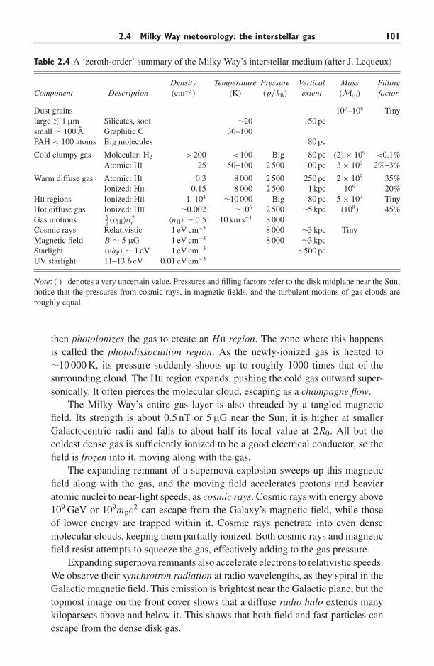
2.4 Milky Way meteorology: the interstellar gas 101

Table 2.4 A ‘zeroth-order’ summary of the Milky Way’s interstellar medium (after J. Lequeux)

Density Temperature Pressure Vertical Mass FillingComponent Description (cm−3) (K) (p/kB) extent (M�) factor

Dust grains 107–108 Tinylarge ∼< 1 μm Silicates, soot ∼20 150 pcsmall ∼ 100 A Graphitic C 30–100PAH < 100 atoms Big molecules 80 pc

Cold clumpy gas Molecular: H2 >200 <100 Big 80 pc (2) × 109 <0.1%Atomic: HI 25 50–100 2 500 100 pc 3 × 109 2%–3%

Warm diffuse gas Atomic: HI 0.3 8 000 2 500 250 pc 2 × 109 35%Ionized: HII 0.15 8 000 2 500 1 kpc 109 20%

HII regions Ionized: HII 1–104 ∼10 000 Big 80 pc 5 × 107 TinyHot diffuse gas Ionized: HII ∼0.002 ∼106 2 500 ∼5 kpc (108) 45%Gas motions 3

2 〈ρHI〉σ 2r 〈nH〉 ∼ 0.5 10 km s−1 8 000

Cosmic rays Relativistic 1 eV cm−3 8 000 ∼3 kpc TinyMagnetic field B ∼ 5 μG 1 eV cm−3 8 000 ∼3 kpcStarlight 〈νhP〉 ∼ 1 eV 1 eV cm−3 ∼500 pcUV starlight 11–13.6 eV 0.01 eV cm−3

Note: ( ) denotes a very uncertain value. Pressures and filling factors refer to the disk midplane near the Sun;notice that the pressures from cosmic rays, in magnetic fields, and the turbulent motions of gas clouds areroughly equal.

then photoionizes the gas to create an HII region. The zone where this happensis called the photodissociation region. As the newly-ionized gas is heated to∼10 000 K, its pressure suddenly shoots up to roughly 1000 times that of thesurrounding cloud. The HII region expands, pushing the cold gas outward super-sonically. It often pierces the molecular cloud, escaping as a champagne flow.

The Milky Way’s entire gas layer is also threaded by a tangled magneticfield. Its strength is about 0.5 nT or 5 μG near the Sun; it is higher at smallerGalactocentric radii and falls to about half its local value at 2R0. All but thecoldest dense gas is sufficiently ionized to be a good electrical conductor, so thefield is frozen into it, moving along with the gas.

The expanding remnant of a supernova explosion sweeps up this magneticfield along with the gas, and the moving field accelerates protons and heavieratomic nuclei to near-light speeds, as cosmic rays. Cosmic rays with energy above109 GeV or 109mpc2 can escape from the Galaxy’s magnetic field, while thoseof lower energy are trapped within it. Cosmic rays penetrate into even densemolecular clouds, keeping them partially ionized. Both cosmic rays and magneticfield resist attempts to squeeze the gas, effectively adding to the gas pressure.

Expanding supernova remnants also accelerate electrons to relativistic speeds.We observe their synchrotron radiation at radio wavelengths, as they spiral in theGalactic magnetic field. This emission is brightest near the Galactic plane, but thetopmost image on the front cover shows that a diffuse radio halo extends manykiloparsecs above and below it. This shows that both field and fast particles canescape from the dense disk gas.

102 Mapping our Milky Way

The interstellar gas is in motion on large and small scales. Like stars, inter-stellar gas clouds do not follow exactly circular orbits about the Galactic center.They also have random motions: typically about 5 km s−1 for molecular cloudsand 8−10 km s−1 for clouds of atomic gas. Even within molecular clouds, gas inthe denser cores must be in motion: the observed width of CO lines corresponds tovelocities of 1−10 km s−1, while the thermal speeds for CO molecules are below0.1 km s−1 (see the problem below). Motions that are faster than the local speedof sound, which is roughly the thermal speed of atoms or molecules in the gas,give rise to shocks. Here the gas velocity changes sharply across a narrow region,and energy of motion is converted into heat.

We do not know exactly how these motions arise, just as we cannot predictthe Earth’s weather in detail even though we know that winds derive their energyfrom sunlight heating the air and the ground. The interstellar gas may be turbulent,with energy passed successively from motions on larger scales to smaller. Modelsof subsonic turbulence predict that random speeds σ measured inside a cloud ofsize L should increase as σ ∝ L1/3. This is approximately true for the atomic andmolecular gas.

Problem 2.21 For molecules of H2 in a cloud with T = 20 K, n(H2) =200 cm−3, calculate the sound speed cs: kBT = μmHc2

s , where μmH is the

molecular mass. What is the sound speed for CO molecules in this same cloud?

From Table 2.4, what is the sound speed for cool HI and for warm neutral gas?

Show that cool HI clouds move through the warm interstellar medium at speeds

close to the sound speed of that warm gas. An HII region cannot expand into the

surrounding gas faster than this sound speed: how fast is that when T ≈ 104 K?

If its temperature does not change, show that an HII region 1 pc across with

nH = 103 cm−3 would take 1 Myr to expand until its pressure balances that of

the warm diffuse gas.

The Milky Way’s dust absorbs nearly half of its ultraviolet and opticalstarlight. Most of this energy warms the grains, which radiate in the infrared, aswe see in the fifth and sixth panels on the front cover. Cool interstellar gas containsabout one grain of dust per 1012 hydrogen atoms: on average, one grain per 100-meter cube. Most obviously, dust absorbs the visible light of stars, which wouldotherwise travel through the gas. Absorption by dust diminishes sharply towardthe infrared. Since dust most efficiently absorbs light of wavelengths smaller thanthe grain size, this tells us that most grains have sizes ∼<0.3 μm.

Problem 2.22 Use the blackbody equations of Section 1.1 to find the approx-

imate temperature of a dust grain that radiates mainly at 150 μm. Show that a

large dust grain 1 pc from an O star with L = 106L� will be heated to roughly

this temperature. (Remember that a grain of radius rg absorbs starlight over an

area πr2g , but emits from its whole surface.) The galaxy M82 is undergoing a

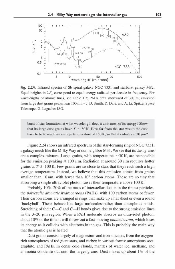
2.4 Milky Way meteorology: the interstellar gas 103

5 10 50 100 5000.1

0.5

1

5

10

50

100

Fig. 2.24. Infrared spectra of Sb spiral galaxy NGC 7331 and starburst galaxy M82.

Equal heights in λFλ correspond to equal energy radiated per decade in frequency. For

wavelengths of atomic lines, see Table 1.7; PAHs emit shortward of 30 μm; emission

from large dust grains peaks near 100 μm – J. D. Smith, D. Dale, and A. Li: Spitzer Space

Telescope; G. Lagache: ISO.

burst of star formation: at what wavelength does it emit most of its energy? Show

that its large dust grains have T ∼ 50 K. How far from the star would the dust

have to be to reach an average temperature of 150 K, so that it radiates at 30 μm?

Figure 2.24 shows an infrared spectrum of the star-forming ring of NGC 7331,a galaxy much like the Milky Way or our neighbor M31. We see that its dust grainsare a complex mixture. Large grains, with temperatures ∼30 K, are responsiblefor the emission peaking at 100 μm. Radiation at around 30 μm requires hottergrains at T ∼> 100 K. Few grains are so close to stars that they reach such a highaverage temperature. Instead, we believe that this emission comes from grainssmaller than 10 nm, with fewer than 106 carbon atoms. These are so tiny thatabsorbing a single ultraviolet photon raises their temperature above 100 K.

Probably 10%–20% of the mass of interstellar dust is in the tiniest particles,the polycyclic aromatic hydrocarbons (PAHs), with 100 carbon atoms or fewer.Their carbon atoms are arranged in rings that make up a flat sheet or even a round‘buckyball’. These behave like large molecules rather than amorphous solids.Stretching of their C—C and C—H bonds gives rise to the strong emission linesin the 3–20 μm region. When a PAH molecule absorbs an ultraviolet photon,about 10% of the time it will throw out a fast-moving photoelectron, which losesits energy as it collides with electrons in the gas. This is probably the main waythat the atomic gas is heated.

Dust grains consist largely of magnesium and iron silicates, from the oxygen-rich atmospheres of red giant stars, and carbon in various forms: amorphous soot,graphite, and PAHs. In dense cold clouds, mantles of water ice, methane, andammonia condense out onto the larger grains. Dust makes up about 1% of the

104 Mapping our Milky Way

mass of interstellar material, and more in denser gas. In gas of approximatelysolar composition, elements heavier than helium hold only 2% of the mass. Thus,in dense clouds, almost all of the carbon, oxygen, magnesium, etc. must be in dust,leaving the gas depleted of those elements. Dust grains are continually knockedapart as they collide with fast-moving atoms and with each other, and built up byabsorbing atoms of interstellar gas onto their surfaces. The material now presentin a grain has probably been there for less than 500 Myr.

The surface of grains is the main site where hydrogen molecules are made.These form only slowly in a gas, because the atoms rarely encounter each other andthen find it difficult to lose energy to become bound in a molecule, since the processis strongly forbidden because of symmetry. At typical densities nH ∼ 100 cm−3,atomic hydrogen would take 1013 yr to form H2. When the atoms can be absorbedonto grains to ‘find’ each other there, and then transfer excess energy to the grainto release a bound molecule, H2 forms ∼108 times faster.

Problem 2.23 In a very simple model, H atoms that collide with a grain stick

to it for long enough to find a partner; the pair departs as a molecule of H2.

In a cloud at T = 50 K, show that the thermal speed of Problem 1.9 is vth ≈1 km s−1. From Problem 1.11, take the grain radius a = 0.1μm and number

density ng = 10−12nH. Show that an H atom collides with a grain after an average

time (ngπa2vth)−1 or 10 Myr × (1 cm−3/nH). The Sun, and gas orbiting along

with it, takes 5%–10% of a ‘Galactic year’ (see Problem 2.14) to pass through a

spiral arm. Show that this is long enough for an HI cloud with nH = 100 cm−3

to become largely molecular.

The interstellar gas is an ‘open’ system: it needs a continuous energy supply.A star like our Sun will not change its orbit significantly within a Hubble time,unless the Milky Way has a near-collision with another galaxy: the stellar disk andbulge are close to equilibrium. By contrast, the gas layer is like a pan of boilingwater; unless energy is supplied to it, the gas will cool rapidly, and the randommotions of the clouds will dissipate. Energy is added to the interstellar gas bystellar radiation, by collisions with cosmic rays, and mechanically by supernovae,stellar winds, and Galactic rotation which stretches the magnetic field.

As one example, we can ask how quickly ionized hydrogen reverts to a neutralstate. In each cubic centimeter, neutral atoms are produced at a rate which increasesas the number of electrons, ne, times the number of protons, np ≈ ne, timesthe rate at which they encounter each other and recombine, which depends onthe temperature Te of the (lighter and faster-moving) electrons. Thus electronsrecombine at the rate

− dne

dt= n2

eα(Te) with α(Te) ≈ 2 × 10−13(

Te

104 K

)−3/4

cm3 s−1.

(2.21)

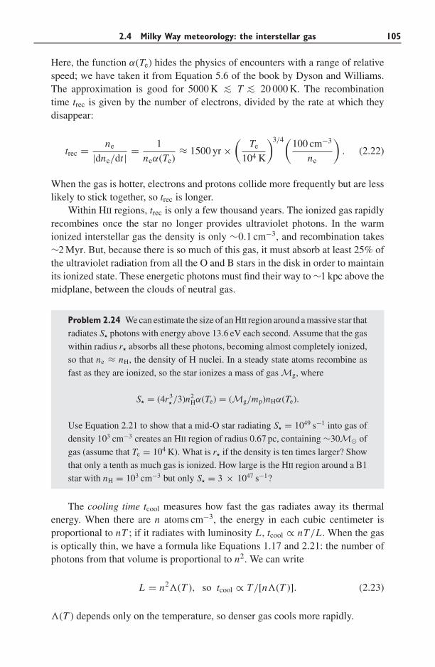
2.4 Milky Way meteorology: the interstellar gas 105

Here, the function α(Te) hides the physics of encounters with a range of relativespeed; we have taken it from Equation 5.6 of the book by Dyson and Williams.The approximation is good for 5000 K ∼< T ∼< 20 000 K. The recombinationtime trec is given by the number of electrons, divided by the rate at which theydisappear:

trec = ne

|dne/dt | = 1

neα(Te)≈ 1500 yr ×

(Te

104 K

)3/4(100 cm−3

ne

). (2.22)

When the gas is hotter, electrons and protons collide more frequently but are lesslikely to stick together, so trec is longer.

Within HII regions, trec is only a few thousand years. The ionized gas rapidlyrecombines once the star no longer provides ultraviolet photons. In the warmionized interstellar gas the density is only ∼0.1 cm−3, and recombination takes∼2 Myr. But, because there is so much of this gas, it must absorb at least 25% ofthe ultraviolet radiation from all the O and B stars in the disk in order to maintainits ionized state. These energetic photons must find their way to ∼1 kpc above themidplane, between the clouds of neutral gas.

Problem 2.24 We can estimate the size of an HII region around a massive star that

radiates S photons with energy above 13.6 eV each second. Assume that the gas

within radius r absorbs all these photons, becoming almost completely ionized,

so that ne ≈ nH, the density of H nuclei. In a steady state atoms recombine as

fast as they are ionized, so the star ionizes a mass of gas Mg, where

S = (4r3 /3)n2

Hα(Te) = (Mg/mp)nHα(Te).

Use Equation 2.21 to show that a mid-O star radiating S = 1049 s−1 into gas of

density 103 cm−3 creates an HII region of radius 0.67 pc, containing ∼30M� of

gas (assume that Te = 104 K). What is r if the density is ten times larger? Show

that only a tenth as much gas is ionized. How large is the HII region around a B1

star with nH = 103 cm−3 but only S = 3 × 1047 s−1?

The cooling time tcool measures how fast the gas radiates away its thermalenergy. When there are n atoms cm−3, the energy in each cubic centimeter isproportional to nT ; if it radiates with luminosity L , tcool ∝ nT/L . When the gasis optically thin, we have a formula like Equations 1.17 and 2.21: the number ofphotons from that volume is proportional to n2. We can write

L = n2�(T ), so tcool ∝ T/[n�(T )]. (2.23)

�(T ) depends only on the temperature, so denser gas cools more rapidly.

106 Mapping our Milky Way

Table 2.5 Main processes that cool the interstellar gas

Temperature Cooling process Spectral region

>107 K Free–free X-ray107 K < T < 108 K Iron resonance lines X-ray105 K < T < 107 K Metal resonance lines UV, soft X-ray8000 K < T < 105 K C, N, O, Ne forbidden lines IR, opticalWarm neutral gas: ∼8000 K Lyman-α, [OI] 1216 A, 6300 A100 K < T < 1000 K [OI], [CII], H2 Far IR: 63 μm, 158 μmT ∼ 10−50 K CO rotational transitions Millimeter-wave

0.3110100

100

1

0.01

Fig. 2.25. For gas of solar composition, luminosity L , from each cubic centimeter (solid

curve), and cooling time tcool (broken curve). Above 10 000 K we set nH = 1 cm−3; the gas

is optically thin, and L = n2�(T ). Below 10 000 K the thermal pressure p/kB = 3000, and

cosmic-ray and ultraviolet fluxes are as measured near the Sun; we set NH = 1019 cm−2,

so almost all H is atomic – M. Wolfire and G. Hensler.

Figure 2.25 shows the cooling curve for gas of roughly solar composition,and Table 2.5 lists the main processes that carry away energy. Above about107 K, almost all the atoms are fully ionized, and the gas cools by free–freeradiation (see Section 1.2). Roughly �(T ) ∝ √

T , so tcool ∝ √T /n; we can

see from Figure 2.25 that hotter gas needs longer to cool. At lower temperaturesthe resonance lines of iron and other metals become the main coolants. They arevery efficient, so �(T ) rises steeply between 106 and 104 K; gas cannot remainlong at temperatures between that of the hot and warm phases of the interstellarmedium. In neutral gas below about 8000 K, the energy loss drops sharply. It alsodepends on the column density NH, which determines how far ultraviolet pho-tons penetrate to ionize atoms and dissociate molecules. Almost all of the coolingbelow 107 K depends on elements heavier than hydrogen and helium; so, in themetal-poor gas of the first galaxies, it would have been much weaker than it istoday.

2.4 Milky Way meteorology: the interstellar gas 107

Various processes heat the Milky Way’s gas, replacing the lost energy. Thediffuse hot gas was heated to ∼106 K, as it passed through the shock caused bythe expanding remnant of a supernova. At the densities observed near the Sun,Figure 2.25 shows that it cools rapidly, within 104−105 yr, condensing into coolerclouds. Near the Sun’s position, a given region is crossed by a supernova shockabout once per 1−5 Myr, reheating the gas. Far from the midplane the hot gas isless dense, and cooling times can reach 1 Gyr.

Clouds of warm and cool HI gas are warmed by photoelectric heating, asultraviolet light of stars falls onto the smallest dust grains. They are cooled byfar-infrared lines of oxygen and carbon. When the gas temperature falls below∼100 K, collisions among gas atoms are not energetic enough to excite the far-infrared atomic lines. In molecular clouds, energy is lost mainly in the millimeter-wavelength lines of CO. Table 1.8 shows that the lowest rotational level liesonly 5.5 K above the ground state, so it is excited by collisions in gas near thattemperature or above. The main source of heat is cosmic rays, which penetrateright through the clouds; they strip electrons from gas atoms, which then sharetheir energy as they bump into electrons in the gas. Molecular clouds are dark; onlyfar-infrared and longer wavelengths of light can reach the interior. The infraredlight warms the dust grains, which in turn prevent even the densest and darkestclouds from cooling below ∼10 K (see Problem 1.12).

Unlike stars, the warm and cool gas clouds are large enough that they occa-sionally collide with one another. So, like molecules in a gas, they exert pressure.The random speeds of HI clouds are typically σr ∼ 10 km s−1, and the volume-averaged density 〈nHI〉 ∼ 0.5 cm−3 near the Sun; so the density of kinetic energy3〈ρHI〉σ 2

r /2 is equivalent to p/kB ∼ 8000. Table 2.4 shows that this is much largerthan the thermal pressure of the gas, but about the same as the pressures contributedby magnetic fields and cosmic rays.

This rough equality is no accident. The Milky Way’s magnetic field takesmost of its energy from differential rotation, which tends to pull gas at smallradii ahead of that further out. The magnetic field is frozen into the gas, so fieldlines connecting clouds at different radii are stretched out as the Galaxy rotates,strengthening the field. Random motions of the gas clouds, the pressure of cosmicrays, and disturbances from stellar winds and supernova explosions also stretch andtangle the field. The strength of the field depends on the vigor of these processes.

As they collide, much of the clouds’ bulk motion is converted to heat, whichis radiated away. The clouds’ random motion would cease within 10−30 Myr ifthey were not shaken about by supernova explosions, winds from HII regions, thepull of magnetic fields, and passage through spiral arms. Thus we see that energyis continually transferred among cloud motions, magnetic field, and cosmic rays.In very complex processes, often the energies of the various motions are drivento be equal on average, just as kinetic energy is on average distributed equallyamong the colliding molecules of gas in a room. Here, each component exertsroughly equal pressure.

108 Mapping our Milky Way

New stars are born in the Milky Way’s dense molecular clouds. These cloudsare at much higher pressure than the surrounding atomic gas, because they mustresist the inward pull of their own gravity. We will see in Section 8.5 that gravitywill cause a gas cloud of density ρ and temperature T to collapse on itself, if itsdiameter exceeds the Jeans length

λJ = cs

√π

Gρ;

here cs is the sound speed c2s = kBT/(μmH), and μmH is the mean molecular

mass. The mass MJ within this sphere is the Jeans mass:

MJ ≡ π

6λ3

Jρ =(

1

μmH

)2 (kBT

G

)3/2 (4πn

3

)−1/2π3

3√

3

≈ 20

(T

10 K

)3/2 (100 cm−3

n

)1/2

M�. (2.24)

If gas pressure is not enough to prevent it, the cloud collapses after approximatelya free-fall time (see Equation 3.23 in Section 3.1):

tff =√

1

Gρ≈ 108

√nH

yr. (2.25)

When do we expect collapse to be so rapid? A gas heats up as it is compressed, sothe Jeans mass increases according to Equation 2.24. Unless it can radiate awaythis heat, gas pressure will slow the collapse. Thus the cooling time must be short:tcool � tff. If T does not grow, the Jeans mass decreases as the density rises, andthe original cloud can break into smaller fragments which themselves collapseindependently. This continues until the densest fragments become optically thick;they heat up and begin to shine as protostars.

Table 2.4 shows that the Galaxy has (1–2) × 109M� in molecular clouds,at densities above 100 cm−3, and T ∼ 10–20 K. According to Equations 2.24and 2.25, any of these clouds larger than 60M� should collapse within about10 Myr. Converting all of the Galaxy’s molecular material to stars in this wayyields ∼100M� yr−1 of new stars – far more than the (3–5)M� yr−1 of new starsthat we observe. Either a collapsing molecular cloud turns very little of its massinto stars, or something – perhaps ‘frozen’ magnetic fields or turbulent motions –must slow the collapse.

Just as water passes between solid, liquid, and vapor phases in Earth’s atmo-sphere, so interstellar material passes continually between different phases. AsHI gas cools or is compressed in a spiral arm, more of it converts to thedense cold phase. When atomic clouds become dense enough that ultravioletlight cannot penetrate their interiors, H2 forms on dust grains. The molecular

2.4 Milky Way meteorology: the interstellar gas 109

clouds lose heat and gradually contract, forming new stars if they are not firstdisrupted. As new massive stars shine on the remains of the dense cloud in whichthey were born, their ultraviolet photons split H2 molecules apart, then ionize theatoms to form an HII region. This expands, breaking out of the molecular cloudto mix with the warm ionized medium.

Near the end of their lives, we saw in Section 1.1 that low-mass stars becomered giants and supergiants, shedding dusty gas enriched in heavy elements pro-duced by their nuclear burning. Supernova explosions also release dust and heavyelements. Even though the energy in these explosions is only ∼1% of that instarlight, supernovae are the main source of the Galaxy’s hot gas and cosmic rays.Their shock waves heat surrounding gas to over a million degrees, sweep up andso strengthen the magnetic field, and accelerate cosmic rays.

Once massive stars have destroyed their natal molecular cloud with ultravioletradiation, stellar winds, and supernova explosions, no further stars can be bornthere until the gas has had time to cool and become dense again. If a galaxyundergoes a starburst (see Section 7.1), turning most of its cool gas into starswithin ∼<300 Myr, repeated supernova explosions in a small volume can heat upso much gas that it forces its way out of the galaxy as a superwind. The averagestellar birthrate in the Milky Way is set by this feedback loop: too-vigorous starformation in a particular region inhibits further starbirth. In a large galaxy likeours, an expanding supernova compresses cool gas in nearby regions of the disk,and can trigger collapse of the densest parts to make new stars. Thus star formationcan ‘spread like a disease’ across the face of the galaxy. We will see in Section 4.4that a dwarf galaxy is more likely to have episodes of rapid starbirth across theentire system, interspersed with quiet periods.

Further reading: two undergraduate texts are J. E. Dyson and D. A. Williams, 1997,The Physics of the Interstellar Medium, 2nd edition; and D. C. B. Whittet, 1992,Dust in the Galactic Environment (both from Institute of Physics Publishing,London and Bristol, UK). On the origin of cosmic rays, see M. S. Longair, 1994,High Energy Astrophysics, 2nd edition, Chapters 17–21 of Volume 2, Stars, theGalaxy and the Interstellar Medium (Cambridge University Press, Cambridge,UK). On the graduate level, see J. Lequeux, The Interstellar Medium (Englishtranslation, 2004; Springer, Berlin and Heidelberg, Germany).

3

The orbits of the stars

Stars travel around the Galaxy, and galaxies orbit within their groups and clusters,under the force of gravity. Stars are so much denser than the interstellar gas throughwhich they move that neither gas pressure nor the forces from embedded magneticfields can deflect them from their paths. If we know how mass is distributed, wecan find the resulting gravitational force, and from this we can calculate how thepositions and velocities of stars and galaxies will change over time.

But we can also use the stellar motions to tell us where the mass is. Aswe discovered in Chapter 2, much of the matter in the Milky Way cannot beseen directly. Its radiation may be absorbed, as happens for the visible light ofstars in the dusty disk. Some material simply emits too weakly: dense cloudsof cold gas do not show up easily in radio-telescope maps. The infamous darkmatter still remains invisibly mysterious. But, since the orbits of stars take themthrough different regions of the galaxies they inhabit, their motions at the time weobserve them have been affected by the gravitational fields through which theyhave travelled earlier. So we can use the equations for motion under gravity toinfer from observed motions how mass is distributed in those parts of galaxiesthat we cannot see directly.

Newton’s law of gravity, and methods for computing the gravitational forces,are introduced in Section 3.1. Usually we can consider the stars as point masses,because their sizes are small compared with the distances between them. Sincegalaxies contain anywhere between a million stars and 1012 of them, we usu-ally want to look at the average motion of many stars, rather than following theindividual orbit of each one. We prove the virial theorem, relating average stellarspeeds to the depth of the gravitational potential well in which they move. Orbitaldynamics and the virial theorem are our tools to find masses of star clusters andgalaxies.

The gravitational potential of a galaxy or star cluster can be regarded as thesum of a smooth component, the average over a region containing many stars,and the very deep potential well around each individual star. In Section 3.2, we

110

3.1 Motion under gravity: weighing the Galaxy 111

will see that the motion of stars within a galaxy is determined almost entirely bythe smooth part of the force. Two-body encounters, transferring energy betweenindividual stars, can be important within dense star clusters. We discuss howthese encounters change the cluster’s structure, eventually causing it to disperseor ‘evaporate’.

Section 3.3 covers the epicycle theory, which is a way to simplify thecalculation of motions for stars like the Sun, that follow very nearly circular orbitswithin a galaxy’s disk. Using epicycles, we can explain the observed motions ofdisk stars near the Sun. Section 3.4 is the most technical of the book: it introducesthe collisionless Boltzmann equation, linking the number of stars moving withgiven velocity at each point in space to the gravitational force acting on them. Wesurvey a few of its many uses, such as finding the mass density in the Galacticdisk near the Sun. We remind readers of Plato’s warning (Timaeus, 91d): theinnocent and lightminded, who believe that astronomy can be studied by lookingat the heavens without knowledge of mathematics, will return in the next life asbirds.

Symbols. We use boldface to indicate a vector quantity. The energy and angularmomentum of a star are given by E and L; E is energy per unit mass, while Land its components denote angular momentum per unit mass. F is used both fora force and for force per unit mass, depending on the context.

3.1 Motion under gravity: weighing the Galaxy

Newton’s law of gravity tells us that a point mass M attracts a second massm separated from it by distance r, causing the velocity v of m to change accordingto

d

dt(mv) = −GmM

r3r, (3.1)

where G is Newton’s gravitational constant. In a cluster of N stars with massesmα (α = 1, 2, . . . , N ), at positions xα, we can add the forces on star α from allthe other stars:

d

dt(mαvα) = −

∑β

α �=β

Gmαmβ

|xα − xβ |3 (xα − xβ). (3.2)

The mass mα cancels out of this equation, so the acceleration dvα/dt isindependent of the star’s mass: light and heavy objects fall equally fast. This isthe principle of equivalence between gravitational and inertial mass, which is thebasis for the general theory of relativity. We can write the force from the cluster on

112 The orbits of the stars

a star of mass m at position x as the gradient of the gravitational potential �(x):

d

dt(mv) = −m ∇�(x), with �(x) = −

∑α

Gmα

|x − xα| for x �= xα, (3.3)

where we have chosen an arbitrary integration constant so that �(x) → 0 at largedistances. If we think of a continuous distribution of matter in a galaxy or starcluster, the potential at point x is given by an integral over the density ρ(x′) at allother points:

�(x) = −∫

Gρ(x′)|x − x′| d3x′, (3.4)

and the force F per unit mass is

F(x) = −∇�(x) = −∫

Gρ(x′)(x − x′)|x − x′|3 d3x′. (3.5)

The integral relation of Equation 3.4 can be turned into a differential equation.Applying ∇2 to both sides, we have

∇2�(x) = −∫

Gρ(x′)∇2(

1

|x − x′|)

d3x′. (3.6)

In three dimensions, differentiating with respect to the variable x gives, for x �= x′

(check by trying it in Cartesian coordinates),

∇(

1

|x − x′|)

= − x − x′

|x − x′|3 , and ∇2(

1

|x − x′|)

= 0. (3.7)

So the integrand on the right-hand side of Equation 3.6 is zero outside a smallsphere Sε(x) of radius ε centred on x. If we take ε small enough that the densityρ is almost constant inside the sphere, we have

∇2�(x) ≈ −Gρ(x)∫

Sε(x)∇2(

1

|x − x′|)

d3x′

= −Gρ(x)∫

Sε(x)∇2

x′

(1

|x − x′|)

dV ′; (3.8)

in the last step, ∇2x′ means that the derivative is taken with respect to the variable

x′, instead of x. (Check in Cartesian coordinates that the two ∇2s are equal forany function of |x − x′|.)

Now we can use the divergence theorem: for any smooth-enough function f ,the volume integral of ∇2

x′ f over the interior of any volume is equal to the integral

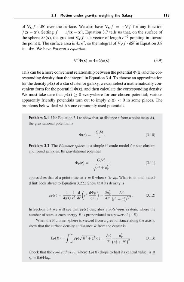
3.1 Motion under gravity: weighing the Galaxy 113

of ∇x′ f · dS′ over the surface. We also have ∇x′ f = −∇ f for any functionf (x − x′). Setting f = 1/|x − x′|, Equation 3.7 tells us that, on the surface ofthe sphere Sε(x), the gradient ∇x′ f is a vector of length ε−2 pointing in towardthe point x. The surface area is 4πε2, so the integral of ∇x′ f · dS′ in Equation 3.8is −4π . We have Poisson’s equation:

∇2�(x) = 4πGρ(x). (3.9)

This can be a more convenient relationship between the potential �(x) and the cor-responding density than the integral in Equation 3.4. To choose an approximationfor the density ρ(x) of a star cluster or galaxy, we can select a mathematically con-venient form for the potential �(x), and then calculate the corresponding density.We must take care that ρ(x) ≥ 0 everywhere for our chosen potential; variousapparently friendly potentials turn out to imply ρ(x) < 0 in some places. Theproblems below deal with some commonly used potentials.

Problem 3.1 Use Equation 3.1 to show that, at distance r from a point mass M,

the gravitational potential is

�(r ) = −GMr

. (3.10)

Problem 3.2 The Plummer sphere is a simple if crude model for star clusters

and round galaxies. Its gravitational potential

�P(r ) = − GM√r2 + a2

P

(3.11)

approaches that of a point mass at x = 0 when r � aP. What is its total mass?

(Hint: look ahead to Equation 3.22.) Show that its density is

ρP(r ) = 1

4πG

1

r2

d

dr

(r2 d�P

dr

)= 3a2

P

4π

M(r2 + a2

P

)5/2 . (3.12)

In Section 3.4 we will see that ρP(r ) describes a polytropic system, where the

number of stars at each energy E is proportional to a power of (−E).

When the Plummer sphere is viewed from a great distance along the axis z,

show that the surface density at distance R from the center is

�P(R) =∫ ∞

−∞ρP(

√R2 + z2)dz = M

π

a2P(

a2P + R2

)2 . (3.13)

Check that the core radius rc, where �P(R) drops to half its central value, is at

rc ≈ 0.644aP.

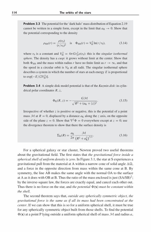
114 The orbits of the stars

Problem 3.3 The potential for the ‘dark halo’ mass distribution of Equation 2.19

cannot be written in a simple form, except in the limit that aH → 0. Show that

the potential corresponding to the density

ρSIS(r ) = ρ(r0)

(r/r0)2is �SIS(r ) = V 2

H ln(r/r0), (3.14)

where r0 is a constant and V 2H = 4πGr2

0 ρ(r0): this is the singular isothermal

sphere. The density has a cusp: it grows without limit at the center. Show that

both �SIS and the mass within radius r have no finite limit as r → ∞, and that

the speed in a circular orbit is VH at all radii. The singular isothermal sphere

describes a system in which the number of stars at each energy E is proportional

to exp[−E/(2V 2H)].

Problem 3.4 A simple disk model potential is that of the Kuzmin disk: in cylin-

drical polar coordinates R, z,

�K(R, z) = − GM√R2 + (aK + |z|)2

. (3.15)

Irrespective of whether z is positive or negative, this is the potential of a point

mass M at R = 0, displaced by a distance aK along the z axis, on the opposite

side of the plane z = 0. Show that ∇2� = 0 everywhere except at z = 0; use

the divergence theorem to show that there the surface density is

�K(R) = aK

2π

M(R2 + a2

K

)3/2 . (3.16)

For a spherical galaxy or star cluster, Newton proved two useful theoremsabout the gravitational field. The first states that the gravitational force inside aspherical shell of uniform density is zero. In Figure 3.1, the star at S experiences agravitational pull from the material at A within a narrow cone of solid angle ��,and a force in the opposite direction from mass within the same cone at B. Bysymmetry, the line AB makes the same angle with the normal OA to the surfaceat A as it does with OB at B. Thus the ratio of the mass enclosed is just (SA/SB)2;by the inverse-square law, the forces are exactly equal, and cancel each other out.Thus there is no force on the star, and the potential �(x) must be constant withinthe shell.

The second theorem says that, outside any spherically symmetric object, thegravitational force is the same as if all its mass had been concentrated at thecenter. If we can show that this is so for a uniform spherical shell, it must be truefor any spherically symmetric object built from those shells. To find the potential�(x) at a point P lying outside a uniform spherical shell of mass M and radius a,

3.1 Motion under gravity: weighing the Galaxy 115

Fig. 3.1. The gravitational force inside a uniform hollow sphere with its center at O.

a

PQ

P'Q'

PQ

P'

r r

Q'

Fig. 3.2. The gravitational potential outside a uniform spherical shell.

at distance r from the center, we can add the contributions �� from small patchesof the shell. On the left of Figure 3.2, the mass in a narrow cone of opening solidangle �� around Q′ contributes

��[x(P)] = − GM|x(P) − x(Q′)|

��

4π. (3.17)

Now think of the potential �′ at point P′, lying at distance a from the center insidea sphere of the same mass M, but now with radius r . On the right in Figure 3.2,we see that the contribution ��′ from material in the same cone, which cuts thelarger sphere at Q, is

��′[x(P′)] = − GM|x(P′) − x(Q)|

��

4π. (3.18)

But, because PQ′ = P′Q, this is equal to ��[x(P)]. So, when we integrate overthe whole sphere,

�[x(P)] = �′[x(P′)] = �′[x = 0] = −GMr

; (3.19)

the potential and force at P are exactly the same as if all the mass of the spherewith radius a had been concentrated at its center.

116 The orbits of the stars

These two theorems tell us that, within any spherical object with density ρ(r ),the gravitational force toward the center is just the sum of the inward forces fromall the matter inside that radius. The acceleration V 2/r of a star moving withspeed V (r ) in an orbit of radius r about the center must be provided by the inwardgravitational force −Fr(r ). So, if M(<r ) is the mass within radius r , we have

V 2(r )

r= −Fr(r ) = GM(<r )

r2. (3.20)

We already used this equation in Section 2.3 to find the mass of the Milky Way.Whenever we can find gas or stars in near-circular orbit within a galaxy, this is byfar the simplest and most reliable way to estimate the mass.

For a point mass, we have V (r ) ∝ r−1/2; in a spherical galaxy the rotationspeed can never fall more rapidly than this. The potential �(r ) is

�(r ) = −[

GM(<r )

r+ 4πG

∫ ∞

rρ(r ′)r ′ dr ′

](3.21)

(check that differentiating this with respect to r gives you back Equation 3.20).We see that �(r ) is not equal to −GM(< r )/r , unless all the mass lies withinradius r . But Equation 3.4 implies that, at a great distance from any system withfinite mass Mtot,

�(x) −→ −GMtot

|x| . (3.22)

Problem 3.5 Use Equation 3.20 to show that, if the density ρ in a spherical

galaxy is constant, then a star following a circular orbit moves so that its angular

speed �(r ) = V (r )/r is constant. Show that a star moving on a radial orbit, i.e.,

in a straight line through the center, would oscillate harmonically in radius with

period

P =√

3π

Gρ∼ 3tff, where tff ≡

√1/Gρ. (3.23)

The free-fall time tff is roughly the time that a gas cloud of density ρ would take

to collapse under its own gravity, if it is not held up by pressure. Show that, if

you bored a hole through the center of the Earth to the other side, and dropped

an egg down it, then (ignoring air resistance, outflows of molten lava, etc.) you

could return about an hour and a half later to retrieve the egg as it returned to its

starting point.

Problem 3.6 From the Sun’s orbital speed of 200 km s−1, find the mass within

its orbit at r = 8 kpc. Show that the average density inside a sphere of this radius

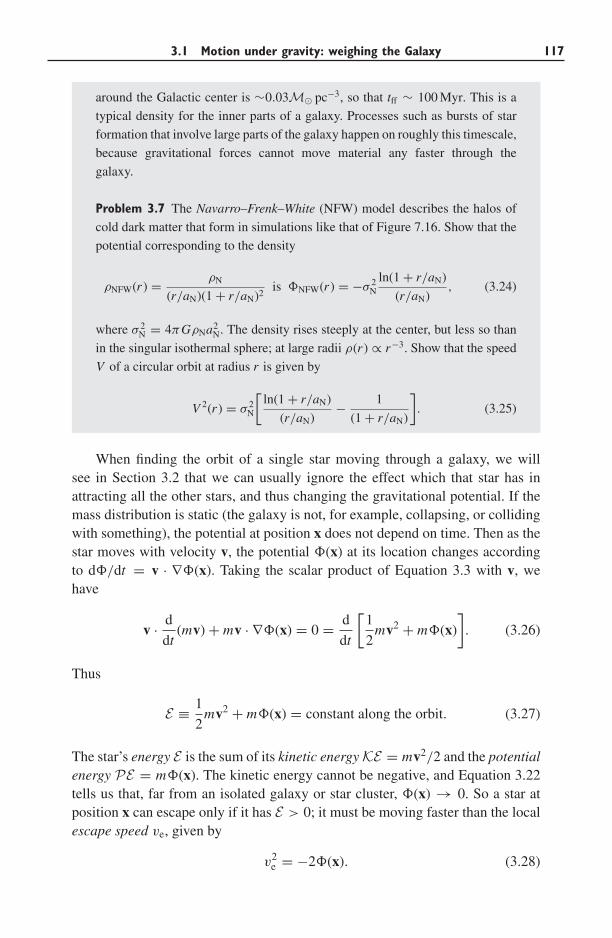
3.1 Motion under gravity: weighing the Galaxy 117

around the Galactic center is ∼0.03M� pc−3, so that tff ∼ 100 Myr. This is a

typical density for the inner parts of a galaxy. Processes such as bursts of star

formation that involve large parts of the galaxy happen on roughly this timescale,

because gravitational forces cannot move material any faster through the

galaxy.

Problem 3.7 The Navarro–Frenk–White (NFW) model describes the halos of

cold dark matter that form in simulations like that of Figure 7.16. Show that the

potential corresponding to the density

ρNFW(r ) = ρN

(r/aN)(1 + r/aN)2is �NFW(r ) = −σ 2

Nln(1 + r/aN)

(r/aN), (3.24)

where σ 2N = 4πGρNa2

N. The density rises steeply at the center, but less so than

in the singular isothermal sphere; at large radii ρ(r ) ∝ r−3. Show that the speed

V of a circular orbit at radius r is given by

V 2(r ) = σ 2N

[ln(1 + r/aN)

(r/aN)− 1

(1 + r/aN)

]. (3.25)

When finding the orbit of a single star moving through a galaxy, we willsee in Section 3.2 that we can usually ignore the effect which that star has inattracting all the other stars, and thus changing the gravitational potential. If themass distribution is static (the galaxy is not, for example, collapsing, or collidingwith something), the potential at position x does not depend on time. Then as thestar moves with velocity v, the potential �(x) at its location changes accordingto d�/dt = v · ∇�(x). Taking the scalar product of Equation 3.3 with v, wehave

v · d

dt(mv) + mv · ∇�(x) = 0 = d

dt

[1

2mv2 + m�(x)

]. (3.26)

Thus

E ≡ 1

2mv2 + m�(x) = constant along the orbit. (3.27)

The star’s energy E is the sum of its kinetic energy KE = mv2/2 and the potentialenergy PE = m�(x). The kinetic energy cannot be negative, and Equation 3.22tells us that, far from an isolated galaxy or star cluster, �(x) → 0. So a star atposition x can escape only if it has E > 0; it must be moving faster than the localescape speed ve, given by

v2e = −2�(x). (3.28)

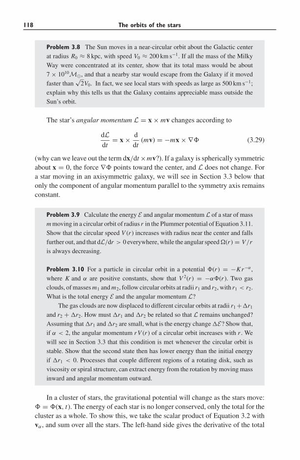
118 The orbits of the stars

Problem 3.8 The Sun moves in a near-circular orbit about the Galactic center

at radius R0 ≈ 8 kpc, with speed V0 ≈ 200 km s−1. If all the mass of the Milky

Way were concentrated at its center, show that its total mass would be about

7 × 1010M�, and that a nearby star would escape from the Galaxy if it moved

faster than√

2V0. In fact, we see local stars with speeds as large as 500 km s−1;

explain why this tells us that the Galaxy contains appreciable mass outside the

Sun’s orbit.

The star’s angular momentum L = x × mv changes according to

dLdt

= x × d

dt(mv) = −mx × ∇� (3.29)

(why can we leave out the term dx/dt ×mv?). If a galaxy is spherically symmetricabout x = 0, the force ∇� points toward the center, and L does not change. Fora star moving in an axisymmetric galaxy, we will see in Section 3.3 below thatonly the component of angular momentum parallel to the symmetry axis remainsconstant.

Problem 3.9 Calculate the energy E and angular momentum L of a star of mass

m moving in a circular orbit of radius r in the Plummer potential of Equation 3.11.

Show that the circular speed V (r ) increases with radius near the center and falls

further out, and that dL/dr > 0 everywhere, while the angular speed �(r ) = V/r

is always decreasing.

Problem 3.10 For a particle in circular orbit in a potential �(r ) = −Kr−α ,

where K and α are positive constants, show that V 2(r ) = −α�(r ). Two gas

clouds, of masses m1 and m2, follow circular orbits at radii r1 and r2, with r1 < r2.

What is the total energy E and the angular momentum L?

The gas clouds are now displaced to different circular orbits at radii r1 +�r1

and r2 + �r2. How must �r1 and �r2 be related so that L remains unchanged?

Assuming that �r1 and �r2 are small, what is the energy change �E? Show that,

if α < 2, the angular momentum r V (r ) of a circular orbit increases with r . We

will see in Section 3.3 that this condition is met whenever the circular orbit is

stable. Show that the second state then has lower energy than the initial energy

if �r1 < 0. Processes that couple different regions of a rotating disk, such as

viscosity or spiral structure, can extract energy from the rotation by moving mass

inward and angular momentum outward.

In a cluster of stars, the gravitational potential will change as the stars move:� = �(x, t). The energy of each star is no longer conserved, only the total for thecluster as a whole. To show this, we take the scalar product of Equation 3.2 withvα, and sum over all the stars. The left-hand side gives the derivative of the total

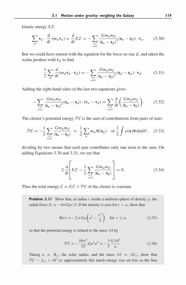
3.1 Motion under gravity: weighing the Galaxy 119

kinetic energy KE :

∑α

vα · d

dt(mαvα) = d

dtKE = −

∑α,βα �=β

Gmαmβ

|xα − xβ |3 (xα − xβ) · vα. (3.30)

But we could have started with the equation for the force on star β, and taken thescalar product with vβ to find

1

2

∑β

d

dt(mβvβ · vβ) = −

∑α,βα �=β

Gmαmβ

|xα − xβ |3 (xβ − xα) · vβ. (3.31)

Adding the right-hand sides of the last two equations gives

−∑α,βα �=β

Gmαmβ

|xα − xβ |3 (xα − xβ) · (vα − vβ) =∑α,βα �=β

d

dt

(Gmαmβ

|xα − xβ |)

. (3.32)

The cluster’s potential energy PE is the sum of contributions from pairs of stars:

PE = −1

2

∑α,βα �=β

Gmαmβ

|xα − xβ | = 1

2

∑α

mα�(xα) or1

2

∫ρ(x)�(x)dV ; (3.33)

dividing by two means that each pair contributes only one term to the sum. Onadding Equations 3.30 and 3.31, we see that

2d

dt

⎡⎢⎣KE − 1

2

∑α,βα �=β

Gmαmβ

|xα − xβ |

⎤⎥⎦ = 0. (3.34)

Thus the total energy E = KE + PE of the cluster is constant.

Problem 3.11 Show that, at radius r inside a uniform sphere of density ρ, the

radial force Fr = −4πGρr/3. If the density is zero for r > a, show that

�(r ) = −2 πGρ

(a2 − r2

3

)for r ≤ a, (3.35)

so that the potential energy is related to the mass M by

PE = −16π2

15Gρ2a5 = −3

5

GM2

a. (3.36)

Taking a = R�, the solar radius, and the mass M = M�, show that

PE ∼ L� × 107 yr; approximately this much energy was set free as the Sun

120 The orbits of the stars

contracted from a diffuse cloud of gas to its present size. Since the Earth is about

4.5 Gyr old, and the Sun has been shining for at least this long, it clearly has

another energy source – nuclear fusion.

Problem 3.12 Show that, for the Plummer sphere of Equation 3.12,

PE = −3π

32

GM2

aP. (3.37)

We will use this result to find the masses of star clusters.

According to Equation 3.34, the stars in an isolated cluster can change theirkinetic and potential energies, as long as the sum of these remains constant. Asthey move further apart, their potential energy increases, and their speeds mustdrop so that the kinetic energy can decrease. If the stars moved so far apart thattheir speeds dropped to zero, and then just stayed there, the system could stillsatisfy this equation. But star clusters cannot remain in this state: Equation 3.2makes clear that the stars are accelerated into motion. The virial theorem tells ushow, on average, the kinetic and potential energies are in balance.

To prove this theorem, we return to Equation 3.2, but we now add an externalforce Fext; this might represent, for example, the gravitational pull of a galaxy ona star cluster within it. We take the scalar product with xα and sum over all thestars to find

∑α

d

dt(mαvα) · xα = −

∑α,βα �=β

Gmαmβ

|xα − xβ |3 (xα − xβ) · xα +∑

α

Fαext · xα. (3.38)

We would have had a similar equation if we had started with the β force:

∑β

d

dt(mβvβ) · xβ = −

∑α,βα �=β

Gmαmβ

|xα − xβ |3 (xβ − xα) · xβ +∑β

Fβext · xβ. (3.39)

The left-hand sides of these two equations are the same; each is equal to

1

2

∑α

d2

dt2(mαxα · xα) −

∑α

mαvα · vα = 1

2

d2 I

dt2− 2KE, (3.40)

where I is the moment of inertia of the system:

I ≡∑

α

mαxα · xα. (3.41)

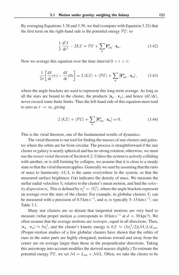
3.1 Motion under gravity: weighing the Galaxy 121

By averaging Equations 3.38 and 3.39, we find (compare with Equation 3.32) thatthe first term on the right-hand side is the potential energy PE : so

1

2

d2 I

dt2− 2KE = PE +

∑α

Fαext · xα. (3.42)

Now we average this equation over the time interval 0 < t < τ :

1

2τ

[dI

dt(τ ) − dI

dt(0)

]= 2 〈KE〉 + 〈PE〉 +

∑α

⟨Fα

ext · xα

⟩, (3.43)

where the angle brackets are used to represent this long-term average. As long asall the stars are bound to the cluster, the products |xα · vα|, and hence |dI/dt |,never exceed some finite limits. Thus the left-hand side of this equation must tendto zero as τ → ∞, giving

2 〈KE〉 + 〈PE〉 +∑

α

⟨Fα

ext · xα

⟩ = 0. (3.44)

This is the virial theorem, one of the fundamental results of dynamics.The virial theorem is our tool for finding the masses of star clusters and galax-

ies where the orbits are far from circular. The process is straightforward if the starcluster or galaxy is nearly spherical and has no strong rotation; otherwise, we mustuse the tensor virial theorem of Section 6.2. Unless the system is actively collidingwith another, or is still forming by collapse, we assume that it is close to a steadystate so that the virial theorem applies. Generally we start by assuming that the ratioof mass to luminosity M/L is the same everywhere in the system, so that themeasured surface brightness I (x) indicates the density of mass. We measure thestellar radial velocities Vr relative to the cluster’s mean motion, and find the veloc-ity dispersion σr. This is defined by σ 2

r = 〈Vr2〉, where the angle brackets represent

an average over the stars of the cluster. For example, in globular clusters Vr canbe measured with a precision of 0.5 km s−1, and σr is typically 5–15 km s−1; seeTable 3.1.

Many star clusters are so distant that tangential motions are very hard tomeasure (what proper motion μ corresponds to 10 km s−1 at d = 30 kpc?). Weoften assume that the average motions are isotropic, equal in all directions. Then,〈vα · vα〉 ≈ 3σ 2

r , and the cluster’s kinetic energy is KE ≈ (3σ 2r /2)(M/L)L tot.

(Proper-motion studies of a few globular clusters have shown that the orbits ofstars in the outer parts are highly elongated; motions toward and away from thecenter are on average larger than those in the perpendicular directions. Takingthis anisotropy into account modifies the derived masses slightly.) To estimate thepotential energy PE , we set M = L tot × M/L . Often, we take the cluster to be

122 The orbits of the stars

Table 3.1 Dynamical quantities for globular and open clusters in the Milky Way

σr log10 ρc rc trelax,c Mass M/LV

Cluster (km s−1) (M� pc−3) (pc) (Myr) (103M�) (M�/L�)

NGC 5139 ω Cen 20 3.1 4 5000 2600 2.5NGC 104 47 Tuc 11 4.9 0.7 50 800 1.5NGC 7078 M15 12 >7 <0.1 <1 900 2NGC 6341 M92 5 5.2 0.5 2 200 1NGC 6121 M4 4 4–5 0.5 30 60 1

Pal 13 ∼0.8 2 1.7 10 3 3–7NGC 1049 Fornax 3 9 3.5 1.6 600 400 ∼3

Open cluster Pleiades 0.5 0.5 3 100 0.8 0.2

Note: σr is the dispersion in radial velocity Vr in the cluster core; ρc is central density; trelax,c isthe relaxation time at the cluster’s center found using Equation 3.55 with V = √

3σr, 〈m∗〉 =0.3M�, and � = rc/1 AU. Clusters with upper limits to rc probably have collapsed cores.

spherically symmetric. Then, from its surface brightness, we can find the volumedensity of stars and hence the potential energy: see the problem below.

Problem 3.13 For a random sample of stars in a globular cluster, σr ≈ 10 km s−1;

the surface brightness can be fit approximately by the Plummer model of Equa-

tion 3.13 with aP = 10 pc. Assuming that the cluster is spherical and contains no

unseen dark matter, use the virial theorem to show that its massM ≈ 2×106M�.

What did you assume about the stars’ random motions?

Another tactic is to measure the cluster’s core radius rc, where the measuredsurface brightness I (x) has fallen to half its central value. The core radii of globularclusters are generally about 10 pc, but can be larger (Table 2.3). We can write thepotential energy as PE = −GM2/(2ηrc) for some constant η ∼ 1. For example,the homogeneous sphere of Problem 3.1 has rc = √

3a/2, and using Equation 3.36yields η = 5/(3

√3) ≈ 0.96. For the Plummer model of Problem 3.12, η ≈ 2.6.

Ignoring external forces from the rest of the Galaxy, Equation 3.44 gives thecluster’s mass as

M ≈ 6ησ 2r rc/G. (3.45)

Sometimes it is easier to measure the cluster’s central surface brightness I (x = 0)than its total luminosity. If we write L tot ≈ 4πr2

c I (0)/3, and for the velocitydispersion we take σr(0), the observed central value, then

ML

≈ 9

2π

σ 2r (0)

G I (0)rc. (3.46)

3.1 Motion under gravity: weighing the Galaxy 123

This equation is correct to within a few percent in a spherical system where σr isexactly constant everywhere (the isothermal model of Section 3.4). It is a fairlygood approximation for a wide range of cluster-like and galaxy-like potentials(see Richstone and Tremaine 1986 AJ 92, 72).

Most globular clusters have masses in the range 104M� to 106M�. Table 3.1shows that typically the mass-to-light ratio 1 ∼< M/L ∼< 4. It is larger than thatmeasured in Section 2.1 for the immediate solar neighborhood, which is notsurprising since all the bright massive stars in these old clusters have now died.But it is much less than what we found in Problem 2.18 for the Milky Way as awhole: globular clusters do not seem to contain much, if any, ‘dark matter’. Openclusters are less dense than globular clusters, and their stars have smaller randomspeeds. The mass-to-light ratios in Table 2.2 are even lower than those in globularclusters because luminous stars are still on the main sequence.

Problem 3.14 Suppose that an isolated cluster of stars is initially in equilibrium.

If a fraction f of its mass is suddenly removed so that the mass mα of each

becomes (1− f )mα , by what factor do the kinetic and potential energies change?

If the initial potential energy is PE0, show that the total energy E0 = PE0/2,

and afterward it is E1 = (1 − f )(1 − 2 f )E0. So, if f > 0.5, the stars are no

longer bound together. Use the virial theorem to show that, when the stars come

to a new equilibrium, the average distance between them is larger by a factor

(1 − f )/(1 − 2 f ).

The fast winds from massive stars, and their final explosion as supernovae,

blow away any cluster gas that was not initially converted into stars. In the Milky

Way’s disk, we see many clumps of young stars that were born together but are

now dissolving; they became unbound as leftover gas was expelled. Globular

clusters must have formed in a different way, using up almost all their gas, or

else the clusters would not have remained as dense as they now are.

To find the average motion of one star within an unchanging cluster potential,we can regard the gravity of all the other stars as giving rise to an external force.For each star, the virial theorem now tells us that

〈v2〉 = 〈∇�(x) · x〉. (3.47)

(For a star following a circular orbit in a spherically symmetric potential �(r ),check that this gives the same orbital speed V (r ) as Equation 3.20.) In the outerparts of any cluster, the magnitude of ∇� · x begins to decrease with radius.Just as for planets in the solar system, stars in the central parts of a clusteror galaxy generally move faster than those spending most of their time in theoutskirts.

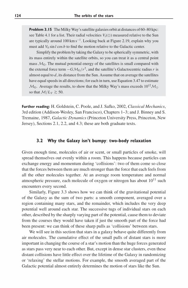
124 The orbits of the stars

Problem 3.15 The Milky Way’s satellite galaxies orbit at distances of 60–80 kpc:

see Table 4.1 for a list. Their radial velocities Vr(�) measured relative to the Sun

are typically around 100 km s−1. Looking back at Figure 2.19, explain why you

must add V0 sin l cos b to find the motion relative to the Galactic center.

Simplify the problem by taking the Galaxy to be spherically symmetric, with

its mass entirely within the satellite orbits, so you can treat it as a central point

mass MG. The mutual potential energy of the satellites is small compared with

the external force term −GMG/r2, and the satellite’s Galactocentric radius r is

almost equal to d, its distance from the Sun. Assume that on average the satellites

have equal speeds in all directions; for each in turn, use Equation 3.47 to estimate

MG. Average the results, to show that the Milky Way’s mass exceeds 1012M�so that M/LV ∼> 50.

Further reading: H. Goldstein, C. Poole, and J. Safko, 2002, Classical Mechanics,3rd edition (Addison-Wesley, San Francisco), Chapters 1–3; and J. Binney and S.Tremaine, 1987, Galactic Dynamics (Princeton University Press, Princeton, NewJersey), Sections 2.1, 2.2, and 4.3; these are both graduate texts.

3.2 Why the Galaxy isn’t bumpy: two-body relaxation

Given enough time, molecules of air or scent, or small particles of smoke, willspread themselves out evenly within a room. This happens because particles canexchange energy and momentum during ‘collisions’: two of them come so closethat the forces between them are much stronger than the force that each feels fromall the other molecules together. At an average room temperature and normalatmospheric pressure, each molecule of oxygen or nitrogen has about 1011 suchencounters every second.

Similarly, Figure 3.3 shows how we can think of the gravitational potentialof the Galaxy as the sum of two parts: a smooth component, averaged over aregion containing many stars, and the remainder, which includes the very deeppotential well around each star. The successive tugs of individual stars on eachother, described by the sharply varying part of the potential, cause them to deviatefrom the courses they would have taken if just the smooth part of the force hadbeen present: we can think of these sharp pulls as ‘collisions’ between stars.

We will see in this section that stars in a galaxy behave quite differently fromair molecules. The cumulative effect of the small pulls of distant stars is moreimportant in changing the course of a star’s motion than the huge forces generatedas stars pass very near to each other. But, except in dense star clusters, even thesedistant collisions have little effect over the lifetime of the Galaxy in randomizingor ‘relaxing’ the stellar motions. For example, the smooth averaged part of theGalactic potential almost entirely determines the motion of stars like the Sun.

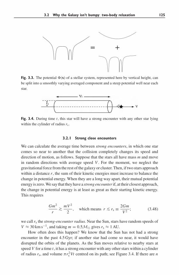
3.2 Why the Galaxy isn’t bumpy: two-body relaxation 125

= +

Fig. 3.3. The potential �(x) of a stellar system, represented here by vertical height, can

be split into a smoothly varying averaged component and a steep potential well near each

star.

Fig. 3.4. During time t , this star will have a strong encounter with any other star lying

within the cylinder of radius rs.

3.2.1 Strong close encounters

We can calculate the average time between strong encounters, in which one starcomes so near to another that the collision completely changes its speed anddirection of motion, as follows. Suppose that the stars all have mass m and movein random directions with average speed V . For the moment, we neglect thegravitational force from the rest of the galaxy or cluster. Then, if two stars approachwithin a distance r , the sum of their kinetic energies must increase to balance thechange in potential energy. When they are a long way apart, their mutual potentialenergy is zero. We say that they have a strong encounter if, at their closest approach,the change in potential energy is at least as great as their starting kinetic energy.This requires

Gm2

r ∼>mV 2

2, which means r ∼< rs ≡ 2Gm

V 2; (3.48)

we call rs the strong-encounter radius. Near the Sun, stars have random speeds ofV ≈ 30 km s−1, and taking m = 0.5M� gives rs ≈ 1 AU.

How often does this happen? We know that the Sun has not had a strongencounter in the past 4.5 Gyr; if another star had come so near, it would havedisrupted the orbits of the planets. As the Sun moves relative to nearby stars atspeed V for a time t , it has a strong encounter with any other stars within a cylinderof radius rs, and volume πr2

s Vt centred on its path; see Figure 3.4. If there are n

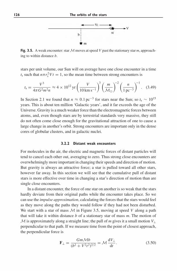
126 The orbits of the stars

Fig. 3.5. A weak encounter: starMmoves at speed V past the stationary star m, approach-

ing to within distance b.

stars per unit volume, our Sun will on average have one close encounter in a timets such that nπr2

s V t = 1, so the mean time between strong encounters is

ts = V 3

4πG2m2n≈ 4 × 1012 yr

(V

10 km s−1

)3 ( m

M�

)−2 ( n

1 pc−3

)−1

. (3.49)

In Section 2.1 we found that n ≈ 0.1 pc−3 for stars near the Sun; so ts ∼ 1015

years. This is about ten million ‘Galactic years’, and it far exceeds the age of theUniverse. Gravity is a much weaker force than the electromagnetic forces betweenatoms, and, even though stars are by terrestrial standards very massive, they stilldo not often come close enough for the gravitational attraction of one to cause alarge change in another’s orbit. Strong encounters are important only in the densecores of globular clusters, and in galactic nuclei.

3.2.2 Distant weak encounters

For molecules in the air, the electric and magnetic forces of distant particles willtend to cancel each other out, averaging to zero. Thus strong close encounters areoverwhelmingly more important in changing their speeds and direction of motion.But gravity is always an attractive force; a star is pulled toward all other stars,however far away. In this section we will see that the cumulative pull of distantstars is more effective over time in changing a star’s direction of motion than aresingle close encounters.

In a distant encounter, the force of one star on another is so weak that the starshardly deviate from their original paths while the encounter takes place. So wecan use the impulse approximation, calculating the forces that the stars would feelas they move along the paths they would follow if they had not been disturbed.We start with a star of mass M in Figure 3.5, moving at speed V along a paththat will take it within distance b of a stationary star of mass m. The motion ofM is approximately along a straight line; the pull of m gives it a small motion V⊥perpendicular to that path. If we measure time from the point of closest approach,the perpendicular force is

F⊥ = GmMb

(b2 + V 2t2)3/2= M dV⊥

dt. (3.50)

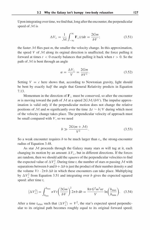
3.2 Why the Galaxy isn’t bumpy: two-body relaxation 127

Upon integrating over time, we find that, long after the encounter, the perpendicularspeed of M is

�V⊥ = 1

M

∫ ∞

−∞F⊥(t)dt = 2Gm

bV; (3.51)

the faster M flies past m, the smaller the velocity change. In this approximation,the speed V of M along its orginal direction is unaffected; the force pulling itforward at times t < 0 exactly balances that pulling it back when t > 0. So thepath of M is bent through an angle

α = �V⊥V

= 2Gm

bV 2. (3.52)

Setting V = c here shows that, according to Newtonian gravity, light shouldbe bent by exactly half the angle that General Relativity predicts in Equation7.13.

Momentum in the direction of F⊥ must be conserved, so after the encounterm is moving toward the path of M at a speed 2GM/(bV ). The impulse approx-imation is valid only if the perpendicular motion does not change the relativepositions of M and m significantly over the time �t ∼ b/V during which mostof the velocity change takes place. The perpendicular velocity of approach mustbe small compared with V , so we need

b � 2G(m + M)

V 2. (3.53)

So a weak encounter requires b to be much larger than rs, the strong-encounterradius of Equation 3.48.

As star M proceeds through the Galaxy many stars m will tug at it, eachchanging its motion by an amount �V⊥, but in different directions. If the forcesare random, then we should add the squares of the perpendicular velocities to findthe expected value of �V 2

⊥. During time t, the number of stars m passing M withseparations between b and b+�b is just the product of their number density n andthe volume V t · 2πb �b in which these encounters can take place. Multiplyingby �V 2

⊥ from Equation 3.51 and integrating over b gives the expected squaredspeed: after time t,

⟨�V 2

⊥⟩ = ∫ bmax

bmin

nV t

(2Gm

bV

)2

2πb db = 8πG2m2nt

Vln

(bmax

bmin

). (3.54)

After a time trelax such that 〈�V 2⊥〉 = V 2, the star’s expected speed perpendic-

ular to its original path becomes roughly equal to its original forward speed;

128 The orbits of the stars

the ‘memory’ of its initial path has been lost. Defining � ≡ (bmax/bmin), wefind that this relaxation time is much shorter than the strong-encounter time tsof Equation 3.49:

trelax = V 3

8πG2m2n ln �= ts

2 ln �

≈ 2 × 109 yr

ln �

(V

10 km s−1

)3 ( m

M�

)−2 ( n

103 pc−3

)−1

. (3.55)

It is not clear what value we should take for �. Our derivation is certainlynot valid if b < rs, and we usually take bmin = rs and bmax to be equal tothe size of the whole stellar system. For stars near the Sun, rs = 1 AU, and300 pc ∼< bmax ∼< 30 kpc, giving ln � ≈ 18–22; the exact values of bmin and bmax

are clearly not important. Although the many weak pulls of distant stars changethe direction of motion of a star like the Sun more rapidly than do the very infre-quent close encounters, the time required is still ∼1013 yr, much longer than theage of the Universe. So, when calculating the motion of stars like the Sun, wecan ignore the pulls of individual stars, and consider all the stars to move in thesmoothed-out potential of the entire Galaxy. We will take advantage of this factin the next section, where we examine the orbits of stars in the Milky Way’sdisk.

Table 3.1 gives the average random speed σr and the relaxation time at thecenters of a number of Galactic globular clusters. In ω Centauri, the largest, trelax isabout 5 Gyr. This is much longer than the time tcross ≈ 0.5 Myr that a star takes tomove across the core. We can safely calculate the path of a star over a few orbitsby using only the smoothed part of the gravitational force. But, to understandhow globular clusters change throughout the lifetime of the Galaxy, we must takeaccount of energy exchanges between individual stars. The central parts of mostclusters have been affected by relaxation.

Problem 3.16 Assuming an average stellar mass of 0.5M� and � = rc/1 AU,

use the information in Table 3.1 to find the relaxation time trelax at the center of

the globular cluster 47 Tucanae. Show that the crossing time tcross ≈ 2rc/σr ∼10−3trelax.

The open clusters are comparable in size to globular clusters, but they havemuch lower densities, typically n ∼ 10 pc−3 or less, and the stars move moreslowly, σr ∼ 1 km s−1. For an average stellar mass of 0.5M� Equation 3.55predicts trelax ∼ 50 Myr, while for rc = 2−3 pc the crossing time is about 5 Myr.So, within ten crossing times, the cumulative effect of weak encounters can changethe stellar orbits radically. It is exceptionally difficult to calculate how the structure

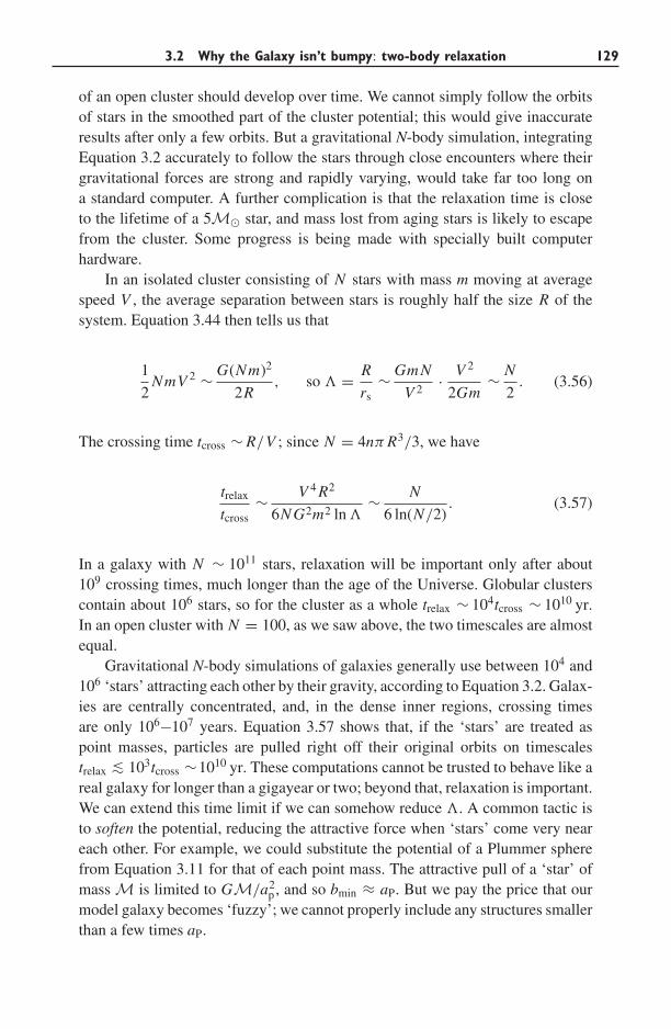
3.2 Why the Galaxy isn’t bumpy: two-body relaxation 129

of an open cluster should develop over time. We cannot simply follow the orbitsof stars in the smoothed part of the cluster potential; this would give inaccurateresults after only a few orbits. But a gravitational N-body simulation, integratingEquation 3.2 accurately to follow the stars through close encounters where theirgravitational forces are strong and rapidly varying, would take far too long ona standard computer. A further complication is that the relaxation time is closeto the lifetime of a 5M� star, and mass lost from aging stars is likely to escapefrom the cluster. Some progress is being made with specially built computerhardware.

In an isolated cluster consisting of N stars with mass m moving at averagespeed V , the average separation between stars is roughly half the size R of thesystem. Equation 3.44 then tells us that

1

2NmV 2 ∼ G(Nm)2

2R, so � = R

rs∼ Gm N

V 2· V 2

2Gm∼ N

2. (3.56)

The crossing time tcross ∼ R/V ; since N = 4nπ R3/3, we have

trelax

tcross∼ V 4 R2

6N G2m2 ln �∼ N

6 ln(N/2). (3.57)

In a galaxy with N ∼ 1011 stars, relaxation will be important only after about109 crossing times, much longer than the age of the Universe. Globular clusterscontain about 106 stars, so for the cluster as a whole trelax ∼ 104tcross ∼ 1010 yr.In an open cluster with N = 100, as we saw above, the two timescales are almostequal.

Gravitational N-body simulations of galaxies generally use between 104 and106 ‘stars’ attracting each other by their gravity, according to Equation 3.2. Galax-ies are centrally concentrated, and, in the dense inner regions, crossing timesare only 106−107 years. Equation 3.57 shows that, if the ‘stars’ are treated aspoint masses, particles are pulled right off their original orbits on timescalestrelax ∼< 103tcross ∼1010 yr. These computations cannot be trusted to behave like areal galaxy for longer than a gigayear or two; beyond that, relaxation is important.We can extend this time limit if we can somehow reduce �. A common tactic isto soften the potential, reducing the attractive force when ‘stars’ come very neareach other. For example, we could substitute the potential of a Plummer spherefrom Equation 3.11 for that of each point mass. The attractive pull of a ‘star’ ofmass M is limited to GM/a2

p, and so bmin ≈ aP. But we pay the price that ourmodel galaxy becomes ‘fuzzy’; we cannot properly include any structures smallerthan a few times aP.

130 The orbits of the stars

Problem 3.17 Gravitational N-body simulations of galactic disks often confine

all the particles to a single plane: instead of n stars per unit volume we have Nper unit area. The term 2πb db in Equation 3.54 is replaced by 2 db – why? Show

that now trelax does not depend on �, but only on bmin, and that taking bmin = rs

yields trelax/tcross = V 2/(4G RmN ). If the mass density mN is fixed, this ratio

is independent of the number of simulation particles.

3.2.3 Effects of two-body relaxation

While a star moves in the smoothed potential of a star cluster, Equation 3.27 tellsus that its orbit does not depend on whether it is heavy or light, but only on itsposition or velocity. If the smoothed potential �(x) does not change with time,the energy of the star remains constant. By contrast, two-body ‘collisions’ allowtwo stars to exchange energy and momentum in a way that depends on both theirmasses; this is known as two-body relaxation.

Just as for the air molecules in a room, the exchanges on average will shiftthe velocities of the stars toward the most probable way of sharing the availableenergy: this is a Maxwellian distribution. The fraction f of stars with velocities v

between v and v + �v is given by fM(E) 4πv2 �v, where

fM(E) ∝ exp

( −EkBT

)= exp

{−[

m�(x) + mv2

2

]/(kBT )

}, (3.58)

where kB is Boltzmann’s constant. The ‘temperature’ T depends on the energyof the system: it is higher when the stars are moving faster. The problem belowshows that, for stars of mass m, T is related to the average of the squared velocitiesby

1

2m〈v2(x)〉 = 3

2kBT . (3.59)

Just as oxygen molecules in the Earth’s atmosphere move less rapidly than thelighter hydrogen molecules, heavier stars in a Maxwellian distribution move onaverage more slowly than the less massive ones.

Problem 3.18 Explain why the velocity dispersion is given by

〈v2(x)〉 =∫ ∞

0v2 exp

(− mv2

2kBT

)4πv2 dv

/∫ ∞

0exp

(− mv2

2kBT

)4πv2 dv.

Write both integrals as multiples of∫∞

0 x2e−x2dx to show that Equation 3.59

holds.

3.2 Why the Galaxy isn’t bumpy: two-body relaxation 131

As it pushes their velocity distribution toward the Maxwellian form, two-body relaxation causes stars to evaporate from the cluster. The distribution fM(E)includes a small number of stars with arbitrarily high energy; but any stars movingfaster than the escape speed ve given by Equation 3.28 are not bound to thecluster and will escape. In a cluster of N stars with masses mα at positions xα,Equation 3.33 tells us that the average kinetic energy needed for escape is

⟨1

2mv2

e (x)

⟩= − 1

N

∑α

mα�(xα) = − 2

NPE = 4

NKE, (3.60)

wherePE andKE are the potential and kinetic energy of the cluster as a whole; wehave used Equation 3.44, the virial theorem, in the last step. The average kineticenergy needed for escape is just four times the average for each star, or 6kBT , sothe fraction of escaping stars in the Maxwellian distribution fM is

∫ ∞√

12kBT/mfM(E)v2 dv

/∫ ∞

0fM(E)v2 dv = 0.0074 ≈ 1

136. (3.61)

These stars leave the cluster; after a further time trelax, new stars are promotedabove the escape energy, and depart in their turn. The cluster loses a substantialfraction of its stars over an evaporation time

tevap ∼ 136trelax. (3.62)

In the observed globular clusters, tevap is longer than the age of the Universe;any clusters with very short evaporation times presumably dissolved before wecould observe them. For open clusters tevap is only a few gigayears. In practice,these clusters fall apart even more rapidly, since evaporation is helped along by therepeated gravitational tugs from the spiral arms and from giant clouds of moleculargas in the disk.

Two-body relaxation also leads to mass segregation. Heavier stars congregateat the cluster center, while lighter stars are expelled toward the periphery; wesee the result in Figure 3.6. If initially the cluster stars are thoroughly mixed,with similar orbital speeds, the more massive stars will have larger kinetic energy.But, in a Maxwellian distribution, their kinetic energies must be equal. Thus, onaverage, a massive star will be moving slower after a ‘collision’ than it did before.It then sinks to an orbit of lower energy; the cluster center fills up with stars thathave too little energy to go anywhere else. But, as the cluster becomes centrallyconcentrated, these tightly bound stars must move faster than those further out,increasing their tendency to give up energy.

Meanwhile, the upwardly mobile lighter stars have gained energy from theirencounters, but spend it in moving out to the suburbs. Their new orbits requireslower motion than before, so they have become even poorer in kinetic energy.

132 The orbits of the stars

0 5 10 15

0 2 4 6

1

10

100

Fig. 3.6. In the Pleiades open cluster, stars with masses above M� (dashed histogram)

are more concentrated toward the center than stars with M < M� (solid histogram) –

J. D. Adams.

Mass segregation is a runaway process: the lightest stars are pushed outward intoan ever-expanding diffuse outer halo, while the heavier stars form an increasinglydense core at the center. Almost all star clusters have been affected by masssegregation. The smallest and least luminous stars, that carry most of the cluster’smass (recall Figure 2.3), are dispersed far from the center. So we must be careful totrace them when estimating the cluster’s mass or the stellar mass function. Pairs ofstars bound in a tight binary will effectively behave like a single more-massive star,sinking to the core. The X-ray sources in globular clusters are binaries in whicha main-sequence star orbits a white dwarf or neutron star; they are all found nearthe cluster center.

Even if all the stars in a cluster have exactly the same mass, stars on low-energy orbits close to the center have higher orbital speeds than do those furtherout. So the inner stars tend to lose energy, while the outer stars gain it. Over time,some stars are expelled from the cluster core into the expanding halo, while theremaining core contracts. The core becomes denser, while the outer parts puff upand become more diffuse. Calculations for clusters of equal-mass stars predict that,after (12–20)trelax, the core radius shrinks to zero, as the central density increaseswithout limit: this is core collapse. A cluster that is near this state should have asmall dense core and a diffuse halo, as we see for M15 in Figure 3.7.

What happens to a cluster after core collapse? In the dense core, binary starsbecome important sources of energy. Just as two-body ‘collisions’ tend to removeenergy from fast-moving stars, so encounters between single stars and a tightbinary pair will on average take energy from the binary. The energy is transferredto the single star, while the binary is forced closer. Depending on how many arepresent, binaries may supply so much energy to the stars around them that thecore of the cluster starts to re-expand.

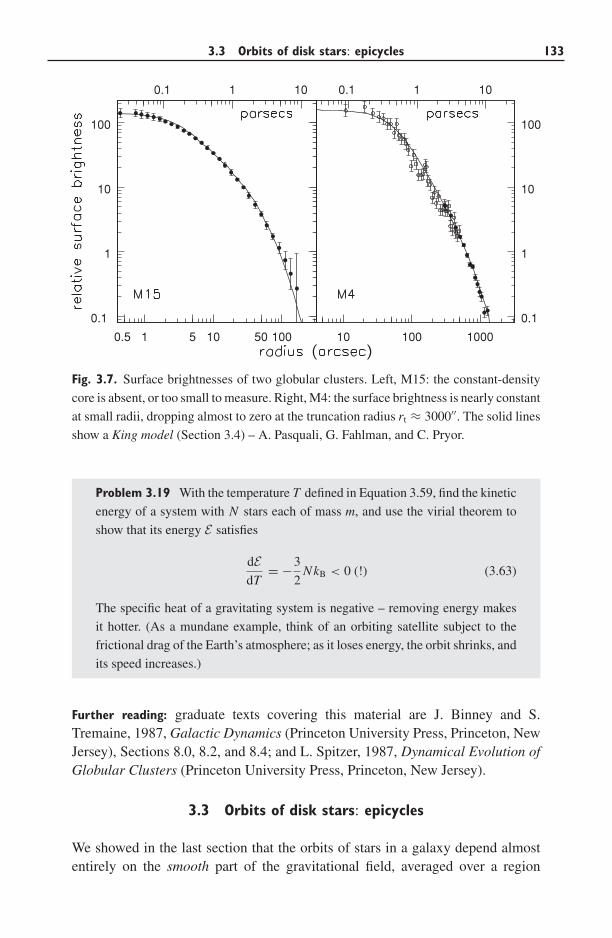
3.3 Orbits of disk stars: epicycles 133

0.1 1 10

1 10 100

0.1

1

10

100

0.5 5 50 10 100 1000

0.1

1

10

100

0.1 1 10

Fig. 3.7. Surface brightnesses of two globular clusters. Left, M15: the constant-density

core is absent, or too small to measure. Right, M4: the surface brightness is nearly constant

at small radii, dropping almost to zero at the truncation radius rt ≈ 3000′′. The solid lines

show a King model (Section 3.4) – A. Pasquali, G. Fahlman, and C. Pryor.

Problem 3.19 With the temperature T defined in Equation 3.59, find the kinetic

energy of a system with N stars each of mass m, and use the virial theorem to

show that its energy E satisfies

dEdT

= −3

2NkB < 0 (!) (3.63)

The specific heat of a gravitating system is negative – removing energy makes

it hotter. (As a mundane example, think of an orbiting satellite subject to the

frictional drag of the Earth’s atmosphere; as it loses energy, the orbit shrinks, and

its speed increases.)

Further reading: graduate texts covering this material are J. Binney and S.Tremaine, 1987, Galactic Dynamics (Princeton University Press, Princeton, NewJersey), Sections 8.0, 8.2, and 8.4; and L. Spitzer, 1987, Dynamical Evolution ofGlobular Clusters (Princeton University Press, Princeton, New Jersey).

3.3 Orbits of disk stars: epicycles

We showed in the last section that the orbits of stars in a galaxy depend almostentirely on the smooth part of the gravitational field, averaged over a region

134 The orbits of the stars

containing many stars. From now on, when we refer to gravitational forces orpotentials, we will mean this averaged quantity. Often, the smoothed potential hassome symmetries which simplify the orbit calculations. In this section, we lookat the orbits of stars in an axisymmetric galaxy.

Like the planets circling the Sun, the stars in the Milky Way’s disk followorbits that are nearly, but not quite, circular, and lie almost in the same plane.In the Galactocentric cylindrical polar coordinates (R, φ, z) of Section 1.2, themidplane of the disk is at z = 0 and the center at R = 0. If we are preparedto overlook non-axisymmetric structures such as an inner bar, the spiral arms,and local features such as Gould’s Belt (Section 2.2), the smoothed gravitationalpotential is independent of φ. Thus ∂�/∂φ = 0, and there is no force in the φ

direction; a star conserves its angular momentum about the axis z. On writing Lz

for the z angular momentum per unit mass, for each star we have

d

dt(R2φ) = 0, so Lz ≡ R2φ = constant. (3.64)

Since the potential does not change with time, � = �(R, z). We can write theequation of motion in the radial direction as

R = Rφ2 − ∂�

∂ R= −∂�eff

∂ R, where �eff ≡ �(R, z) + Lz

2

2R2. (3.65)

The effective potential �eff(R, z; Lz) behaves like a potential energy for the star’smotion in R and z. By the same reasoning as that which led us to Equation 3.27,multiplying Equation 3.65 by R and integrating shows that, for a star moving inthe midplane z = 0,

1

2R2 + �eff(R, z = 0; Lz) = constant. (3.66)

Figure 3.8 shows �eff(R, z = 0; Lz) for the Plummer potential of Equation 3.11.Since R2 ≥ 0, the L2

z term in �eff acts as an ‘angular-momentum barrier’, pre-venting a star with Lz �= 0 from coming closer to the axis R = 0 than someperigalactic radius where R = 0. Unless it has enough energy to escape from theGalaxy, each star must remain within some apogalactic outer limit.

The star’s vertical motion is given by

z = −∂�

∂z(R, z) = −∂�eff

∂z(R, z). (3.67)

If the ‘top’ and ‘bottom’ halves of the disk are mirror images of each other, then�(R, z) = �(R, −z), and the z force is zero in the plane z = 0. Let Rg be theaverage value of R for the star’s orbit; we will define it more precisely below.Expanding �(R, z) in a Taylor series around (Rg, 0), we make fractional errors

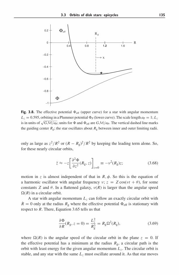
3.3 Orbits of disk stars: epicycles 135

1.20.8 1.60.4 1.2R

0.2

0

−0.2

−0.4

−0.6

−0.8

−1

Φ

Rg

★

x

Φeff

Fig. 3.8. The effective potential �eff (upper curve) for a star with angular momentum

Lz = 0.595, orbiting in a Plummer potential �P (lower curve). The scale length aP = 1; Lz

is in units of√

GM/aP; units for � and �eff are GM/aP. The vertical dashed line marks

the guiding center Rg; the star oscillates about Rg between inner and outer limiting radii.

only as large as z2/R2 or (R − Rg)2/R2 by keeping the leading term alone. So,for these nearly circular orbits,

z ≈ −z

[∂2�

∂z2(Rg, z)

]z=0

≡ −ν2(Rg)z; (3.68)

motion in z is almost independent of that in R, φ. So this is the equation ofa harmonic oscillator with angular frequency ν; z = Z cos(νt + θ ), for someconstants Z and θ . In a flattened galaxy, ν(R) is larger than the angular speed�(R) in a circular orbit.

A star with angular momentum Lz can follow an exactly circular orbit withR = 0 only at the radius Rg where the effective potential �eff is stationary withrespect to R. There, Equation 3.65 tells us that

∂�

∂ R(Rg, z = 0) = L2

z

R3g

= Rg�2(Rg), (3.69)

where �(R) is the angular speed of the circular orbit in the plane z = 0. Ifthe effective potential has a minimum at the radius Rg, a circular path is theorbit with least energy for the given angular momentum Lz . The circular orbit isstable, and any star with the same Lz must oscillate around it. As that star moves

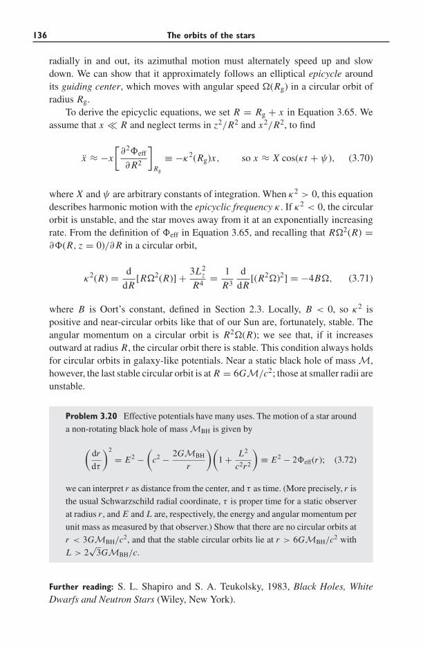
136 The orbits of the stars

radially in and out, its azimuthal motion must alternately speed up and slowdown. We can show that it approximately follows an elliptical epicycle aroundits guiding center, which moves with angular speed �(Rg) in a circular orbit ofradius Rg.

To derive the epicyclic equations, we set R = Rg + x in Equation 3.65. Weassume that x � R and neglect terms in z2/R2 and x2/R2, to find

x ≈ −x

[∂2�eff

∂ R2

]Rg

≡ −κ2(Rg)x, so x ≈ X cos(κt + ψ), (3.70)

where X and ψ are arbitrary constants of integration. When κ2 > 0, this equationdescribes harmonic motion with the epicyclic frequency κ . If κ2 < 0, the circularorbit is unstable, and the star moves away from it at an exponentially increasingrate. From the definition of �eff in Equation 3.65, and recalling that R�2(R) =∂�(R, z = 0)/∂ R in a circular orbit,

κ2(R) = d

dR[R�2(R)] + 3L2

z

R4= 1

R3

d

dR[(R2�)2] = −4B�, (3.71)

where B is Oort’s constant, defined in Section 2.3. Locally, B < 0, so κ2 ispositive and near-circular orbits like that of our Sun are, fortunately, stable. Theangular momentum on a circular orbit is R2�(R); we see that, if it increasesoutward at radius R, the circular orbit there is stable. This condition always holdsfor circular orbits in galaxy-like potentials. Near a static black hole of mass M,however, the last stable circular orbit is at R = 6GM/c2; those at smaller radii areunstable.

Problem 3.20 Effective potentials have many uses. The motion of a star around

a non-rotating black hole of mass MBH is given by

(dr

dτ

)2

= E2 −(

c2 − 2GMBH

r

)(1 + L2

c2r2

)≡ E2 − 2�eff(r ); (3.72)

we can interpret r as distance from the center, and τ as time. (More precisely, r is

the usual Schwarzschild radial coordinate, τ is proper time for a static observer

at radius r , and E and L are, respectively, the energy and angular momentum per

unit mass as measured by that observer.) Show that there are no circular orbits at

r < 3GMBH/c2, and that the stable circular orbits lie at r > 6GMBH/c2 with

L > 2√

3GMBH/c.

Further reading: S. L. Shapiro and S. A. Teukolsky, 1983, Black Holes, WhiteDwarfs and Neutron Stars (Wiley, New York).

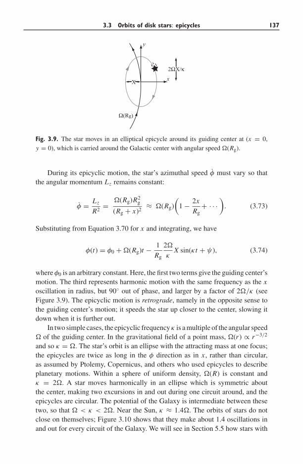
3.3 Orbits of disk stars: epicycles 137

Xx

y

Ω(Rg)

2ΩX/κ

Fig. 3.9. The star moves in an elliptical epicycle around its guiding center at (x = 0,

y = 0), which is carried around the Galactic center with angular speed �(Rg).

During its epicyclic motion, the star’s azimuthal speed φ must vary so thatthe angular momentum Lz remains constant:

φ = Lz

R2= �(Rg)R2

g

(Rg + x)2≈ �(Rg)

(1 − 2x

Rg+ · · ·

). (3.73)

Substituting from Equation 3.70 for x and integrating, we have

φ(t) = φ0 + �(Rg)t − 1

Rg

2�

κX sin(κt + ψ), (3.74)

where φ0 is an arbitrary constant. Here, the first two terms give the guiding center’smotion. The third represents harmonic motion with the same frequency as the xoscillation in radius, but 90◦ out of phase, and larger by a factor of 2�/κ (seeFigure 3.9). The epicyclic motion is retrograde, namely in the opposite sense tothe guiding center’s motion; it speeds the star up closer to the center, slowing itdown when it is further out.

In two simple cases, the epicyclic frequency κ is a multiple of the angular speed� of the guiding center. In the gravitational field of a point mass, �(r ) ∝ r−3/2

and so κ = �. The star’s orbit is an ellipse with the attracting mass at one focus;the epicycles are twice as long in the φ direction as in x , rather than circular,as assumed by Ptolemy, Copernicus, and others who used epicycles to describeplanetary motions. Within a sphere of uniform density, �(R) is constant andκ = 2�. A star moves harmonically in an ellipse which is symmetric aboutthe center, making two excursions in and out during one circuit around, and theepicycles are circular. The potential of the Galaxy is intermediate between thesetwo, so that � < κ < 2�. Near the Sun, κ ≈ 1.4�. The orbits of stars do notclose on themselves; Figure 3.10 shows that they make about 1.4 oscillations inand out for every circuit of the Galaxy. We will see in Section 5.5 how stars with

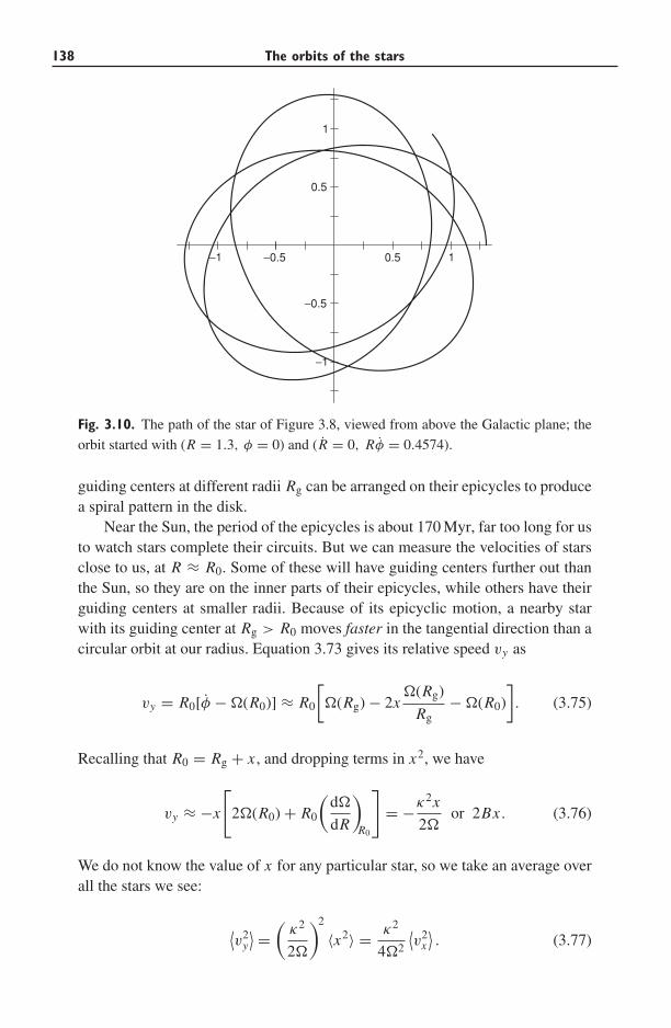
138 The orbits of the stars

10.5−0.5−1

1

0.5

−0.5

−1

Fig. 3.10. The path of the star of Figure 3.8, viewed from above the Galactic plane; the

orbit started with (R = 1.3, φ = 0) and (R = 0, Rφ = 0.4574).

guiding centers at different radii Rg can be arranged on their epicycles to producea spiral pattern in the disk.

Near the Sun, the period of the epicycles is about 170 Myr, far too long for usto watch stars complete their circuits. But we can measure the velocities of starsclose to us, at R ≈ R0. Some of these will have guiding centers further out thanthe Sun, so they are on the inner parts of their epicycles, while others have theirguiding centers at smaller radii. Because of its epicyclic motion, a nearby starwith its guiding center at Rg > R0 moves faster in the tangential direction than acircular orbit at our radius. Equation 3.73 gives its relative speed vy as

vy = R0[φ − �(R0)] ≈ R0

[�(Rg) − 2x

�(Rg)

Rg− �(R0)

]. (3.75)

Recalling that R0 = Rg + x , and dropping terms in x2, we have

vy ≈ −x

[2�(R0) + R0

(d�

dR

)R0

]= −κ2x

2�or 2Bx . (3.76)

We do not know the value of x for any particular star, so we take an average overall the stars we see:

⟨v2

y

⟩ = (κ2

2�

)2

〈x2〉 = κ2

4�2

⟨v2

x

⟩. (3.77)

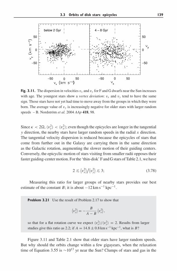
3.3 Orbits of disk stars: epicycles 139

−50 50

−50

0

50

below 2 Gyr

−50 50

−50

0

50

4 – 8 Gyr

0 0

Fig. 3.11. The dispersion in velocities vx and vy for F and G dwarfs near the Sun increases

with age. The youngest stars show a vertex deviation: vx and vy tend to have the same

sign. Those stars have not yet had time to move away from the groups in which they were

born. The average value of vy is increasingly negative for older stars with larger random

speeds – B. Nordstrom et al. 2004 AAp 418, 98.

Since κ < 2�, 〈v2y〉 < 〈v2

x 〉; even though the epicycles are longer in the tangentialy direction, the nearby stars have larger random speeds in the radial x direction.The tangential velocity dispersion is reduced because the epicycles of stars thatcome from further out in the Galaxy are carrying them in the same directionas the Galactic rotation, augmenting the slower motion of their guiding centers.Conversely, the epicyclic motion of stars visiting from smaller radii opposes theirfaster guiding-center motion. For the ‘thin-disk’ F and G stars of Table 2.1, we have

2 ∼<⟨v2

x

⟩/⟨v2

y

⟩∼< 3; (3.78)

Measuring this ratio for larger groups of nearby stars provides our bestestimate of the constant B; it is about −12 km s−1 kpc−1.

Problem 3.21 Use the result of Problem 2.17 to show that

⟨v2

y

⟩ = − B

A − B

⟨v2

x

⟩,

so that for a flat rotation curve we expect 〈v2x 〉/〈v2

y〉 = 2. Results from larger

studies give this ratio as 2.2; if A = 14.8 ± 0.8 km s−1 kpc−1, what is B?

Figure 3.11 and Table 2.1 show that older stars have larger random speeds.But why should the orbits change within a few gigayears, when the relaxationtime of Equation 3.55 is ∼1013 yr near the Sun? Clumps of stars and gas in the

140 The orbits of the stars

spiral arms have pulled on passing starts, each time tugging them further from acircular orbit.

The observant reader will have noticed that, in averaging, we did not takeaccount of any radial variations in the density of stars. In fact, the stellar densityis higher in the inner Galaxy, so that near the Sun we see more stars with guidingcenters at smaller radii than stars that visit us from the outer Galaxy. The majorityof stars will be on the outer parts of their epicycles, with x > 0; so, accordingto Equation 3.76, the average tangential motion of stars near the Sun shouldfall behind the circular velocity. This prediction is borne out in Figure 3.11 andTable 2.1; the average 〈vy〉 is negative, an effect known as asymmetric drift. Thedrift is stronger for groups of older stars, with larger random speeds, since theirorbits deviate further from circular motion.

Problem 3.22 Show from Equation 3.71 that, within a spherical galaxy of

constant density, κ = 2�, and the Oort constants are A = 0 and B = −�. For

the ‘dark-halo’ potential of Equation 2.19, find �(r ) and κ(r ). Check that they

agree at small radii with those for a uniform sphere of density V 2H/(4πGa2

H), and

that κ → √2� as r becomes large. Plot �, κ , and � − κ/2 against radius for

0 < r < 5aH. Show that � − κ/2 approaches zero both as r → 0 and as r

becomes large. We will see in Section 5.5 that this is why two-armed spirals are

so prominent in galaxy disks.

Problem 3.23 We saw in Section 2.3 that the Sun has vx ≈ −10 km s−1 and vy ≈5 km s−1; how do we know that its guiding center radius Rg > R0? Assuming

the Milky Way’s rotation curve to be roughly flat, with V (R) = R�(R) =200 km s−1 and R0 = 8 kpc, find κ and Oort’s constant B. Use Equations 3.70

and 3.76 to show that the extent of the Sun’s radial excursions is X = 0.35 kpc,

and that Rg ≈ 8.2 kpc.

3.4 The collisionless Boltzmann equation

In the last section, we looked at the orbit of an individual star in the Galaxy’sgravitational field. We can also describe the stars in a galaxy as we usually describeatoms in a gas: not by following the path of each atom, but by asking aboutthe density of atoms in a particular region and about their average motion. Forsimplicity, we assume here that all the stars have the same mass m.

The distribution function f (x, v, t) gives the probability density in the six-dimensional phase space of (x, v). The average number of particles (stars or atoms)in a cube of sides �x, �y, and �z centred at x, that have x velocity between vx

and vx + �vx , y velocity between vy and vy + �vy , and z velocity between vz

and vz + �vz , is

f (x, v, t)�x �y �z �vx �vy �vz. (3.79)

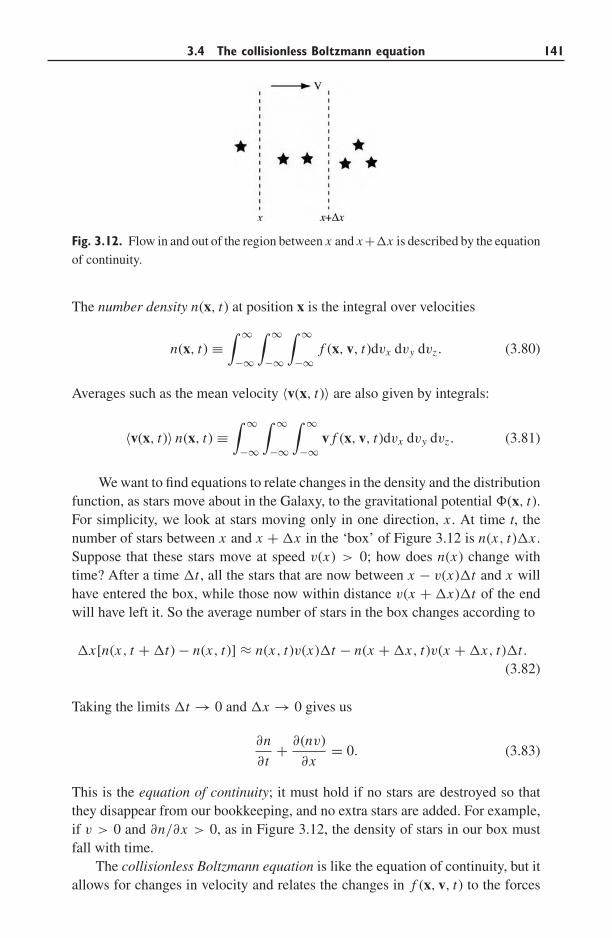
3.4 The collisionless Boltzmann equation 141

Fig. 3.12. Flow in and out of the region between x and x +�x is described by the equation

of continuity.

The number density n(x, t) at position x is the integral over velocities

n(x, t) ≡∫ ∞

−∞

∫ ∞

−∞

∫ ∞

−∞f (x, v, t)dvx dvy dvz. (3.80)

Averages such as the mean velocity 〈v(x, t)〉 are also given by integrals:

〈v(x, t)〉 n(x, t) ≡∫ ∞

−∞

∫ ∞

−∞

∫ ∞

−∞v f (x, v, t)dvx dvy dvz. (3.81)

We want to find equations to relate changes in the density and the distributionfunction, as stars move about in the Galaxy, to the gravitational potential �(x, t).For simplicity, we look at stars moving only in one direction, x . At time t, thenumber of stars between x and x + �x in the ‘box’ of Figure 3.12 is n(x, t)�x .Suppose that these stars move at speed v(x) > 0; how does n(x) change withtime? After a time �t , all the stars that are now between x − v(x)�t and x willhave entered the box, while those now within distance v(x + �x)�t of the endwill have left it. So the average number of stars in the box changes according to

�x[n(x, t + �t) − n(x, t)] ≈ n(x, t)v(x)�t − n(x + �x, t)v(x + �x, t)�t.(3.82)

Taking the limits �t → 0 and �x → 0 gives us

∂n

∂t+ ∂(nv)

∂x= 0. (3.83)

This is the equation of continuity; it must hold if no stars are destroyed so thatthey disappear from our bookkeeping, and no extra stars are added. For example,if v > 0 and ∂n/∂x > 0, as in Figure 3.12, the density of stars in our box mustfall with time.

The collisionless Boltzmann equation is like the equation of continuity, but itallows for changes in velocity and relates the changes in f (x, v, t) to the forces

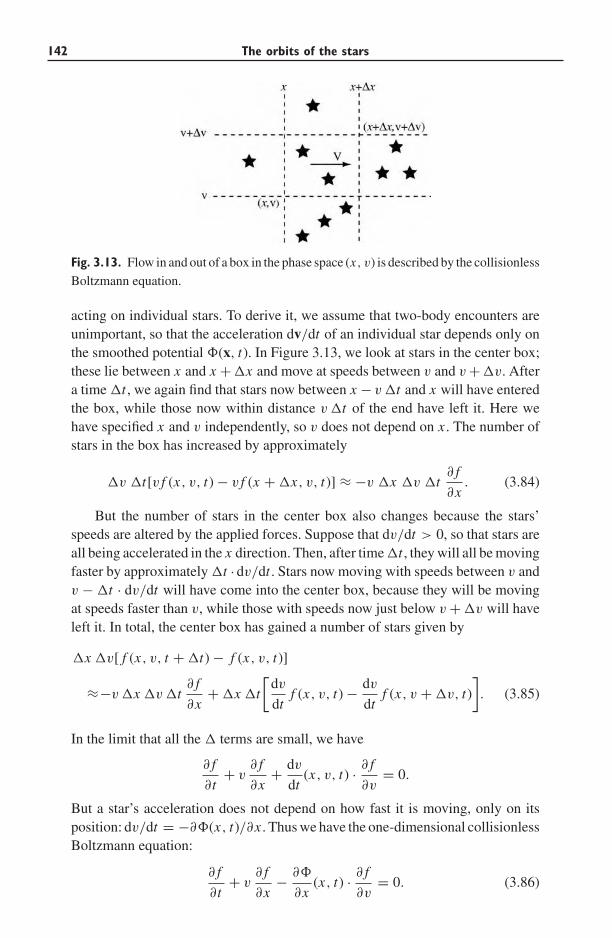
142 The orbits of the stars

Fig. 3.13. Flow in and out of a box in the phase space (x, v) is described by the collisionless

Boltzmann equation.

acting on individual stars. To derive it, we assume that two-body encounters areunimportant, so that the acceleration dv/dt of an individual star depends only onthe smoothed potential �(x, t). In Figure 3.13, we look at stars in the center box;these lie between x and x +�x and move at speeds between v and v +�v. Aftera time �t , we again find that stars now between x − v �t and x will have enteredthe box, while those now within distance v �t of the end have left it. Here wehave specified x and v independently, so v does not depend on x . The number ofstars in the box has increased by approximately

�v �t[v f (x, v, t) − v f (x + �x, v, t)] ≈ −v �x �v �t∂ f

∂x. (3.84)

But the number of stars in the center box also changes because the stars’speeds are altered by the applied forces. Suppose that dv/dt > 0, so that stars areall being accelerated in the x direction. Then, after time �t , they will all be movingfaster by approximately �t · dv/dt . Stars now moving with speeds between v andv − �t · dv/dt will have come into the center box, because they will be movingat speeds faster than v, while those with speeds now just below v + �v will haveleft it. In total, the center box has gained a number of stars given by

�x �v[ f (x, v, t + �t) − f (x, v, t)]

≈−v �x �v �t∂ f

∂x+ �x �t

[dv

dtf (x, v, t) − dv

dtf (x, v + �v, t)

]. (3.85)

In the limit that all the � terms are small, we have

∂ f

∂t+ v

∂ f

∂x+ dv

dt(x, v, t) · ∂ f

∂v= 0.

But a star’s acceleration does not depend on how fast it is moving, only on itsposition: dv/dt = −∂�(x, t)/∂x . Thus we have the one-dimensional collisionlessBoltzmann equation:

∂ f

∂t+ v

∂ f

∂x− ∂�

∂x(x, t) · ∂ f

∂v= 0. (3.86)

3.4 The collisionless Boltzmann equation 143

In three dimensions, the collisionless Boltzmann equation takes the form

∂ f (x, v, t)

∂t+ v · ∇ f − ∇� · ∂ f

∂v= 0. (3.87)

Equation 3.87 holds if stars are neither created nor destroyed, and if they alsochange their positions and velocities smoothly. Close encounters between starscan alter their velocities much faster than their motion changes in the smoothedpotential. When these are important, we include their effects as an extra ‘colli-sional’ term on the right-hand side.

Often, we do not solve the collisionless Boltzmann equation explicitly, butrather integrate to take velocity-moments. Integrating Equation 3.86 over velocity,and using the definitions 3.80 and 3.81, we find

∂n(x, t)

∂t+ ∂

∂x(n(x, t)〈v(x, t)〉) − ∂�

∂x(x, t)[ f ]∞−∞ = 0. (3.88)

When f (x, v, t) is well behaved, tending to zero as |v| → ∞, the last term iszero. We arrive back at Equation 3.83, with the velocity v = 〈v(x, t)〉.

Multiplying Equation 3.86 by v and then integrating gives

∂

∂t[n(x, t)〈v(x, t)〉] + ∂

∂x[n(x, t)〈v2(x, t)〉] = −n(x, t)

∂�

∂x; (3.89)

here the average of the squared velocity 〈v2〉 is defined just as for 〈v〉, and we haveintegrated by parts, assuming that f v → 0 as |v| → ∞. The velocity dispersionσ is defined by 〈v2(x, t)〉 = 〈v(x, t)〉2 + σ 2; rearranging terms with the help ofEquation 3.88 and dividing by n, we have

∂〈v〉∂t

+ 〈v〉 ∂〈v〉∂x

= −∂�

∂x− 1

n

∂

∂x[nσ 2(x, t)]. (3.90)

This is analogous to Euler’s equation of fluid mechanics, with the term in σ 2

replacing the pressure force −∂p/∂x . In a fluid, the equation of state specifies thepressure at a given density and temperature. For a stellar system there is no suchrelation; but sometimes we can make progress by using measured quantities, asin the next subsection.

3.4.1 Mass density in the Galactic disk

We can use the collisionless Boltzmann equation and the observed vertical motionsof stars to find the mass in the Galactic disk near the Sun. We select a tracerpopulation of stars (for example, the K dwarf stars) and measure its density n(z)at height z above the disk’s midplane. Our coordinates are now (z, vz) instead of(x, v). We assume that the potential �(z) does not change with time, and that ourstars are well mixed, so that the distribution function f and the density n are also

144 The orbits of the stars

time-steady. Looking high above the plane, 〈vz〉n(z) → 0; so Equation 3.88 tellsus that the mean velocity 〈vz〉 = 0 everywhere. In Equation 3.90, we write σz forthe velocity dispersion; the terms on the left-hand side vanish, giving

d

dz

[n(z)σ 2

z

] = −∂�

∂zn(z). (3.91)

So, if we measure how the density of our stars and their velocity dispersion changewith z, we can find the vertical force at any height.

Poisson’s equation, Equation 3.9, relates that force to the mass density ρ(x)of the Galaxy. Assuming that the Milky Way is axisymmetric, so that ρ and �

depend only on (R, z), we have

4πGρ(R, z) = ∇2�(R, z) = ∂2�

∂z2+ 1

R

∂

∂ R

(R

∂�

∂ R

). (3.92)

The density ρ(R, z) here includes all the mass in the disk: luminous stars, gas,white dwarfs, brown dwarfs, black holes, and dark matter. Writing ∂�/∂ R =V 2(R)/R, where V (R) is the rotation speed in a circular orbit at radius R, we have

4πGρ(R, z) = d

dz

{− 1

n(z)

d

dz

[n(z)σ 2

z

]}+ 1

R

d

dR[V 2(R)]. (3.93)

Near the Sun, V (R) is nearly constant, so the last term is very small. Thedensity ρ(R0, 0) in the midplane of the disk has recently been estimated from thevelocities of nearby A stars, measured with the Hipparcos satellite, to be in therange (70–100)M� per 1000 pc3.

To find the volume density ρ, the observationally determined quantityn(z) has to be differentiated twice, which amplifies small errors. We can moreaccurately determine the surface mass density �(< z) within some distance zof the midplane. Assuming that the disk is symmetric about z = 0, we integrateEquation 3.93 to find

2πG�(<z) ≡ 2πG∫ z

−zρ(z′)dz′ ≈ − 1

n(z)

d

dz

[n(z)σ 2

z

]. (3.94)

Jan Oort in 1932 was the first to try this, measuring n(z) for bright F dwarfsand K giants. He assumed that σz did not vary with height, and found that�(<700 pc) ≈ 90M� pc−2. But, beyond a kiloparsec from the midplane, thefunction he derived for �(<z) began to decrease, indicating anti-gravitating matterwith ρ(z) < 0, or, more probably, a failure of the hypothesis that σz is constant.

Recent work with fainter K dwarf stars, which are more numerous and moreevenly spread out in space, indicates that σz increases with height. At 250 pcfrom the plane, the vertical dispersion σz ≈ 20 km s−1, growing to 30 km s−1 at

3.4 The collisionless Boltzmann equation 145

z ∼1 kpc; at greater heights, a larger fraction of the stars belongs to the thick disk.Taking account of the increasing dispersion, these studies find �(<1100 pc) ≈(70–80 M� pc−2. Some of this mass must be in the halo, so the surface densityof the disk itself is probably between 50M� and 60M� pc−2.

We can compare this dynamical estimate with the mass that has beenobserved in gas and stars. Near the Sun, molecular gas probably amounts to∼2M� pc−2. There is roughly 8M� pc−2 of neutral atomic hydrogen, and about2M� pc−2 of ionized gas, though all these numbers are uncertain by at least 30%.Main-sequence stars more massive than M dwarfs, and the giants, are easilycounted in surveys; making allowance for the hard-to-find low-mass stars andstellar remnants such as white dwarfs and neutron stars gives a total of about(25–40)M� pc−2 in stars. Thus the mass in gas and stars is (40–55)M� pc−2.We see that the disk does not contain much of the Galaxy’s ‘dark matter’.

Problem 3.24 Use the divergence theorem to show that the potential at height

z above a uniform sheet of matter with surface density � is

�(x) = 2πG�|z|. (3.95)

Show that the vertical force does not depend on z, and check that ∇2� = 0

when z �= 0. Suppose that the mass of the Galaxy was all in a flat uniform

disk; use Equation 3.91 to find the density n(z) of K dwarfs, assuming that they

have a constant velocity dispersion σz . As in the Earth’s atmosphere, where the

acceleration of gravity is also nearly independent of height, show that n(z) drops

by a factor of e as |z| increases by hz = σ 2z /(2πG�). Estimate hz near the Sun,

taking σz = 20 km s−1.

3.4.2 Integrals of motion, and some of their uses

Often we are interested in solutions of the collisionless Boltzmann equation thatdescribe stars moving in an unchanging gravitational potential �(x), such thattheir distribution function is also constant. Then, it is frequently useful to writef (x, v) in terms of integrals of the motion. These are functions I(x, v) of a star’sposition x and velocity v that remain constant along its orbit. One example isthe energy per unit mass, E(x, v) = v2/2 + �(x), which is an integral of themotion whenever the potential �(x) does not depend on time. In an axisymmetricpotential �(R, z, t), the z component of the angular momentum Lz is an integral;in a spherical potential, the total angular momentum L is an integral.

For any function I that is constant along the orbit, we have

d

dtI(x, v) ≡ ∂x

∂t· ∇I + ∂v

∂t· ∂I

∂v= 0, or v · ∇I − ∇� · ∂I

∂v= 0. (3.96)

146 The orbits of the stars

This looks suspiciously like Equation 3.87, which we can write as

d f

dt≡ ∂ f

∂t+ v · ∂ f

∂x+ ∂v

∂t· ∂ f

∂v= 0. (3.97)

So the phase-space density f (x, v, t) around any particular star remains constantalong its orbit. Where the density n(x) becomes higher, the dispersion in velocitiesof the surrounding stars must increase, and any function f (x, v) that is a time-independent solution to the collisionless Boltzmann equation is itself an integral ofthe motion. Conversely, if f (I1, I2, . . .) is any function of integrals of the motionI1, I2, . . ., then f is a steady-state solution of the equations of motion. Often it iseasy to write down at least some of the integrals of motion, and this is one way toget started on constructing time-steady solutions of the collisionless Boltzmannequation.

For example, Equation 3.68 tells us that, for disk stars on nearly circular orbits,motion perpendicular to the Galactic disk is independent of that in the disk plane,so the energy of vertical motion Ez = �(R0, z) + v2

z /2 is an integral of motion.If we select some tracer population of stars that are easy to find and measure,and which are also well mixed so that their distribution function f (z, vz) is notchanging with time, we can write

f(z, vz) = f (Ez) = f

(�(R0, z) + 1

2v2

z

). (3.98)

If we guessed at f (Ez) and the potential �(R0, z), we could integrate f overvelocities to find the corresponding density n(z) and the velocity dispersionσz at any height z. Conversely, if we measured n(z) and guessed at f (Ez), wecould find the potential �(R0, z) by using Equation 3.91. For example, we couldtake

f (Ez) = n0√2πσ 2

exp(−Ez/σ2) for Ez < 0; (3.99)

stars with Ez ≥ 0 would escape, so we must set f = 0 there. Integrating over vz

shows the density n and velocity dispersion σz to be

n(z) = n0 exp[−�(R0, z)/σ 2], and σz = σ . (3.100)

If n(z) and σ 2 are measured, we can calculate the potential �(R0, z) by usingEquation 3.91; if � and σ 2 are known, we can find the corresponding densityn(z).

If we also have some reason to think that the stars described by the dis-tribution function f provide all the gravitational force, then the density n(x, t)

3.4 The collisionless Boltzmann equation 147

found by integrating f (x, v, t) over velocities must be equal to the densityρ(x, t) in Poisson’s Equation 3.9. In this case, we say that f provides a self-consistent model for the system. Many different self-consistent models can giverise to the same gravitational potential �(x, t); the density n(x, t) is the samefor all of these, but the form of f , and hence the velocities of the stars, willbe different.

Problem 3.25 For stars moving vertically in the Galactic disk, suppose the

distribution function f (z, vz) to be given by Equation 3.99. When the disk is

symmetric about the plane z = 0, then d�(z)/dz = 0 at z = 0, and we can

choose �(0) = 0 too. Find the integral giving the density of stars n(z): what is

n(0)?

To construct a self-consistent model, let �(z) = σ 2φ(z), and let the average

mass of the stars be m; show from Poisson’s equation that

2 d2φ/dy2 = e−φ, where y = z/z0 and z20 = σ 2/(8πGmn0).

Integrate this once to find dφ/dy, and then again (substituting u = e−φ/2) to

find φ(y) and hence �(z). Show that the number density of stars is n(z) =n0 sech2[z/(2z0)]. What is its approximate form at large |z|?

In a spherically symmetric gravitational potential �(r ), any function f (E, L)of the energy E and angular momentum L per unit mass that does not includeany unbound stars will describe one possible steady distribution of stars in thatgravitational field. If we choose f = f (E) then the random speeds are isotropic,the same in all directions.

Problem 3.26 When the distribution function for stars in a spherical system

depends only on their energy, so that f (x, v, t) = f (E), explain why the velocity

dispersion is the same in all directions:

⟨v2

x

⟩ ≡ 1

n(x)

∫f

[�(x) + v2

2

]v2

x dvx dvy dvz = ⟨v2

y

⟩ = ⟨v2

z

⟩. (3.101)

If we choose a form for f (E), we can then calculate the density n(r ) asa function of the potential �(r ). Then we use Poisson’s equation to find whichpotentials �(r ) lead to a self-consistent model, with n(r ) ∝ ρ(r ). For the Plummersphere, we can combine Equations 3.11 and 3.12 to find

ρP(r ) = − 3a2p

4πG5M4�5

P(r ). (3.102)

148 The orbits of the stars

Taking the distribution function

f (E) = k(−E)N−3/2 for E < 0, (3.103)

where k and N are constants, the density is given by

n(r ) =∫ E=0

v=0k

[−�(x) − v2

2

]N−3/2

4πv2 dv. (3.104)

Defining a new variable θ by v2 = −2�(r )cos2θ , we can integrate to showthat n(r ) ∝ (−�)N . Thus the distribution function fP(E) = k(−E)7/2 gives aself-consistent model for the Plummer sphere. Its mass M is proportional to theconstant k, while the depth of the central potential �(r = 0) sets the radius aP.

Problem 3.27 Fill in the algebraic steps needed to derive Equations 3.102–

3.104.

By analogy with expression 3.99, we might also try the isothermal distributionfunction

fI(E) = n0

(2πσ 2)3/2exp

{−[�(r ) + v2

2

]/σ 2}

for E < 0, (3.105)

as a first guess for representing a spherical galaxy or star cluster. As in the planarcase, Equation 3.100 gives us n(r ). Putting this on the right-hand side of Poisson’sequation, we get

4πGρ(r ) = 1

r2

d

dr

(r2 d�

dr

)= 4πGmn0 exp

[−�(r )

σ 2

]. (3.106)

To find �(r ), we must integrate this equation outward from r = 0. If the potentialis smooth at the center, the radial force there must be zero, so we must start withd�/dr = 0. But, however we choose �(r = 0), we find that the total mass isinfinite. We should have expected this result, since, if the mass had been finite, theescape speed ve of Equation 3.28 would drop below the average random speed σ

at some radius. But that would contradict our assumption that all the stars werebound to the system.

Problem 3.28 Show that, in the potential �SIS of Equation 3.14, the density

ρ(r ) corresponding to fI(E) is exactly equal to ρSIS, if σ 2 = 2πGρ0r20 , and all

the stars have mass m so that ρ0 ≡ mn0 = ρ(r0). The distribution function fI(E)

gives a self-consistent model for the singular isothermal sphere; show that the

average random speed σ is 1/√

2 times the speed in a circular orbit.

3.4 The collisionless Boltzmann equation 149

Only if we reduce the number of stars with energies close to the escape energydoes f give a self-consistent model with finite mass. The King models, sometimescalled ‘lowered isothermal models’, provide a good description of non-rotatingglobular clusters and open clusters:

fK(E) = n0

(2πσ 2)3/2exp

[−(

�(r ) + v2

2

)/σ 2 − 1

]for E < 0. (3.107)

When we integrate this to find n(r ), and then solve Poisson’s equation, the term‘−1’ acts to reduce the number of stars with high kinetic energy in the outerregions. The average random speed decreases and the density drops abruptly tozero at some truncation radius corresponding to the outer radius rt of Table 2.3and Figure 3.7.

Including a term involving angular momentum alters the balance betweenstars on nearly circular orbits and those that follow eccentric orbits. For example,the distribution function

fA(E, L) = fK(E)exp[− L2/(2σ 2r2

a

)](3.108)

leads to a density n(r ) which is not very different from that associated with fK(E),but it describes a cluster with fewer stars on the near-circular orbits that havehigh angular momentum. The effect is especially strong in the outer regions,where the angular momentum of a circular orbit is largest; outside the anisotropyradius ra, stars have a decided preference for nearly radial orbits. We see evi-dence for this kind of velocity distribution in some globular clusters and ellipticalgalaxies.

If the distribution function f depends on only one component of the angularmomentum, for example Lz , it can describe a system that is flattened along the zaxis. For example, if

f (E, Lz) = f (E)L2z for E > 0, (3.109)

for some function f , then very few stars have orbits taking them close to the z axis,with Lz ≈ 0, but relatively many will follow near-circular orbits in the equatorialplane, with large Lz . Postulating that f = f (E, Lz) seems at first sight to beuseful for describing the motions of stars in the Galactic disk. Since vR and vz

enter the expression for f in the same way, stars must have equal random motionsin those two directions:

n(x)⟨v2

z

⟩ ≡ ∫f

[�(x) + v2

2, Rvφ

]v2

z dvR dvφ dvz = n(x)⟨v2

R

⟩. (3.110)

150 The orbits of the stars

But we saw in Section 2.2 that, near the Sun, disk stars have larger random speedsin R than they have in the vertical direction z. They cannot have a distributionf (E, Lz), but f must depend on a third integral of motion. Curiously, it can beproven that, in a general axisymmetric potential �(R, z), there is no function ofposition and velocity other than E and Lz that is conserved along a star’s orbit. Thisdynamical puzzle will resurface in Section 6.2, when we discuss stellar motionsin elliptical galaxies.

Further reading: J. Binney and S. Tremaine, 1987, Galactic Dynamics (PrincetonUniversity Press, Princeton, New Jersey), Section 4.4.

4

Our backyard: the Local Group

The Local Group contains roughly three dozen galaxies within a sphere abouta megaparsec in radius, centred between the Milky Way and our nearest largeneighbor, the Andromeda galaxy M31. Figure 4.1 shows the brighter members.The three most prominent are M31, the Milky Way, and M33; according to theclassification of Section 1.3, these are all spiral galaxies. M31 is about 50% moreluminous than the Milky Way, while M33 is only 20% as luminous. Between them,these three galaxies emit 90% of the visible light of the Local Group. The onlyelliptical galaxy is M32, a satellite to M31. The remaining systems are irregulargalaxies, or the even less luminous dwarf irregulars, dwarf ellipticals, and dwarfspheroidals. Many of these smaller galaxies are in orbit either around the MilkyWay or around M31.

Table 4.1 lists known and probable members of the Local Group within amegaparsec of the Sun. The apparent brightness of each member is generallyknown to within 10%, except for the Milky Way, where our location within thedisk presents special problems. Distances to Local Group galaxies are derived bypicking out individual stars, measuring their apparent brightness, and estimatingtheir true luminosity, using methods such as the period–luminosity relation forCepheid variables. In this way, distances to the ten or so brightest galaxies canbe measured to within 10%. But fewer stars are available in the less luminousgalaxies, so the distances are less certain; for some dwarfs, they are known to nobetter than a factor of two.

Galaxies are not scattered at random within the Local Group; many smallmembers are satellites of M31 or the Milky Way. The right-hand part of Figure 4.2shows that most of the Milky Way’s 11 known satellites lie close to a single plane –they may have formed from a single gas cloud captured into an orbit around theMilky Way. The Andromeda galaxy also has its brood of satellites; but manysmall systems are ‘free fliers’, remote from any larger galaxy. The Local Groupis likely to contain still-undiscovered dwarf galaxies; in particular, galaxies canhide behind dust in the Milky Way’s disk. The Local Group contains three spiralgalaxies, but only one, small, elliptical. As is typical of groups, it is rich in

151

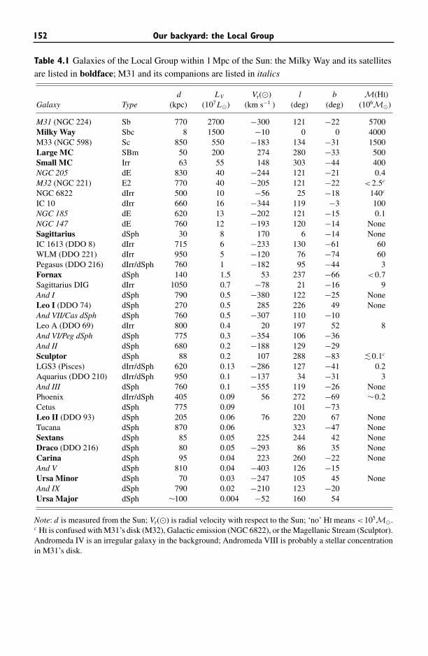
152 Our backyard: the Local Group

Table 4.1 Galaxies of the Local Group within 1 Mpc of the Sun: the Milky Way and its satellites

are listed in boldface; M31 and its companions are listed in italics

d LV Vr(�) l b M(HI)Galaxy Type (kpc) (107 L�) (km s−1 ) (deg) (deg) (106M�)

M31 (NGC 224) Sb 770 2700 −300 121 −22 5700Milky Way Sbc 8 1500 −10 0 0 4000M33 (NGC 598) Sc 850 550 −183 134 −31 1500Large MC SBm 50 200 274 280 −33 500Small MC Irr 63 55 148 303 −44 400NGC 205 dE 830 40 −244 121 −21 0.4M32 (NGC 221) E2 770 40 −205 121 −22 <2.5c

NGC 6822 dIrr 500 10 −56 25 −18 140c

IC 10 dIrr 660 16 −344 119 −3 100NGC 185 dE 620 13 −202 121 −15 0.1NGC 147 dE 760 12 −193 120 −14 NoneSagittarius dSph 30 8 170 6 −14 NoneIC 1613 (DDO 8) dIrr 715 6 −233 130 −61 60WLM (DDO 221) dIrr 950 5 −120 76 −74 60Pegasus (DDO 216) dIrr/dSph 760 1 −182 95 −44 3Fornax dSph 140 1.5 53 237 −66 <0.7Sagittarius DIG dIrr 1050 0.7 −78 21 −16 9And I dSph 790 0.5 −380 122 −25 NoneLeo I (DDO 74) dSph 270 0.5 285 226 49 NoneAnd VII/Cas dSph dSph 760 0.5 −307 110 −10Leo A (DDO 69) dIrr 800 0.4 20 197 52 8And VI/Peg dSph dSph 775 0.3 −354 106 −36And II dSph 680 0.2 −188 129 −29Sculptor dSph 88 0.2 107 288 −83 ∼<0.1c

LGS3 (Pisces) dIrr/dSph 620 0.13 −286 127 −41 0.2Aquarius (DDO 210) dIrr/dSph 950 0.1 −137 34 −31 3And III dSph 760 0.1 −355 119 −26 NonePhoenix dIrr/dSph 405 0.09 56 272 −69 ∼0.2Cetus dSph 775 0.09 101 −73Leo II (DDO 93) dSph 205 0.06 76 220 67 NoneTucana dSph 870 0.06 323 −47 NoneSextans dSph 85 0.05 225 244 42 NoneDraco (DDO 216) dSph 80 0.05 −293 86 35 NoneCarina dSph 95 0.04 223 260 −22 NoneAnd V dSph 810 0.04 −403 126 −15Ursa Minor dSph 70 0.03 −247 105 45 NoneAnd IX dSph 790 0.02 −210 123 −20Ursa Major dSph ∼100 0.004 −52 160 54

Note: d is measured from the Sun; Vr(�) is radial velocity with respect to the Sun; ‘no’ HI means <105M�.c HI is confused with M31’s disk (M32), Galactic emission (NGC 6822), or the Magellanic Stream (Sculptor).Andromeda IV is an irregular galaxy in the background; Andromeda VIII is probably a stellar concentrationin M31’s disk.

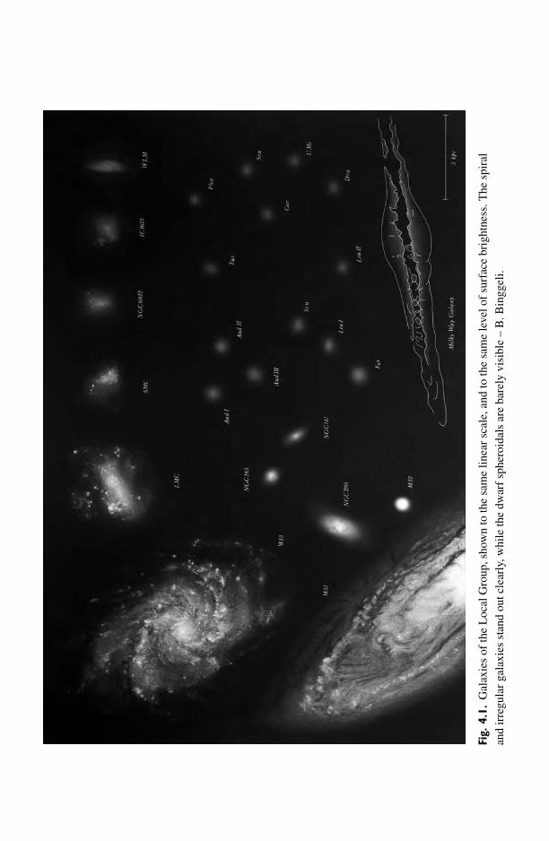
Fig.

4.1.

Gal

axie

sof

the

Loc

alG

roup

,sho

wn

toth

esa

me

linea

rsc

ale,

and

toth

esa

me

leve

lof

surf

ace

brig

htne

ss.T

hesp

iral

and

irre

gula

rga

laxi

esst

and

outc

lear

ly,w

hile

the

dwar

fsp

hero

idal

sar

eba

rely

visi

ble

–B

.Bin

ggel

i.

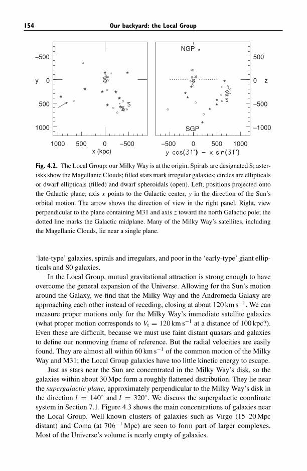
154 Our backyard: the Local Group

NGP

SGP

−500 0 500 1000

−1000

−500

0

500

z

1000 500 0 −500

1000

500

0

−500

x (kpc)

y

Fig. 4.2. The Local Group: our Milky Way is at the origin. Spirals are designated S; aster-

isks show the Magellanic Clouds; filled stars mark irregular galaxies; circles are ellipticals

or dwarf ellipticals (filled) and dwarf spheroidals (open). Left, positions projected onto

the Galactic plane; axis x points to the Galactic center, y in the direction of the Sun’s

orbital motion. The arrow shows the direction of view in the right panel. Right, view

perpendicular to the plane containing M31 and axis z toward the north Galactic pole; the

dotted line marks the Galactic midplane. Many of the Milky Way’s satellites, including

the Magellanic Clouds, lie near a single plane.

‘late-type’ galaxies, spirals and irregulars, and poor in the ‘early-type’ giant ellip-ticals and S0 galaxies.

In the Local Group, mutual gravitational attraction is strong enough to haveovercome the general expansion of the Universe. Allowing for the Sun’s motionaround the Galaxy, we find that the Milky Way and the Andromeda Galaxy areapproaching each other instead of receding, closing at about 120 km s−1. We canmeasure proper motions only for the Milky Way’s immediate satellite galaxies(what proper motion corresponds to Vt = 120 km s−1 at a distance of 100 kpc?).Even these are difficult, because we must use faint distant quasars and galaxiesto define our nonmoving frame of reference. But the radial velocities are easilyfound. They are almost all within 60 km s−1 of the common motion of the MilkyWay and M31; the Local Group galaxies have too little kinetic energy to escape.

Just as stars near the Sun are concentrated in the Milky Way’s disk, so thegalaxies within about 30 Mpc form a roughly flattened distribution. They lie nearthe supergalactic plane, approximately perpendicular to the Milky Way’s disk inthe direction l = 140◦ and l = 320◦. We discuss the supergalactic coordinatesystem in Section 7.1. Figure 4.3 shows the main concentrations of galaxies nearthe Local Group. Well-known clusters of galaxies such as Virgo (15–20 Mpcdistant) and Coma (at 70h−1 Mpc) are seen to form part of larger complexes.Most of the Universe’s volume is nearly empty of galaxies.

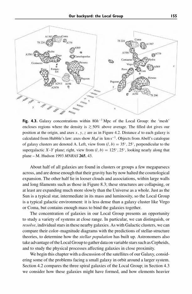
Our backyard: the Local Group 155

Fig. 4.3. Galaxy concentrations within 80h−1 Mpc of the Local Group: the ‘mesh’

encloses regions where the density is ∼> 50% above average. The filled dot gives our

position at the origin, and axes x, y, z are as in Figure 4.2. Distance d to each galaxy is

calculated from Hubble’s law: axes show H0d in km s−1. Objects from Abell’s catalogue

of galaxy clusters are denoted A. Left, view from (l, b) = 35◦, 25◦, perpendicular to the

supergalactic X–Y plane; right, view from (l, b) = 125◦, 25◦, looking nearly along that

plane – M. Hudson 1993 MNRAS 265, 43.

About half of all galaxies are found in clusters or groups a few megaparsecsacross, and are dense enough that their gravity has by now halted the cosmologicalexpansion. The other half lie in looser clouds and associations, within large wallsand long filaments such as those in Figure 8.3; these structures are collapsing, orat least are expanding much more slowly than the Universe as a whole. Just as theSun is a typical star, intermediate in its mass and luminosity, so the Local Groupis a typical galactic environment: it is less dense than a galaxy cluster like Virgoor Coma, but contains enough mass to bind the galaxies together.

The concentration of galaxies in our Local Group presents an opportunityto study a variety of systems at close range. In particular, we can distinguish, orresolve, individual stars in these nearby galaxies. As with Galactic clusters, we cancompare their color–magnitude diagrams with the predictions of stellar-structuretheories, to determine how the stellar population has built up. Astronomers alsotake advantage of the Local Group to gather data on variable stars such as Cepheids,and to study the physical processes affecting galaxies in close proximity.

We begin this chapter with a discussion of the satellites of our Galaxy, consid-ering some of the problems facing a small galaxy in orbit around a larger system.Section 4.2 compares the three spiral galaxies of the Local Group; in Section 4.3we consider how these galaxies might have formed, and how elements heavier

156 Our backyard: the Local Group

than helium are built up by their stars. In Section 4.4 we discuss the various kindsof dwarf galaxies; finally, we consider briefly what the motions of Local Groupgalaxies tell us about its ultimate fate.

Further reading: a recent graduate text is S. van den Bergh, 2000, The Galaxies ofthe Local Group (Cambridge University Press, Cambridge, UK).

4.1 Satellites of the Milky Way

The most prominent companion galaxies to the Milky Way are the two MagellanicClouds; in the southern sky, they are easily visible to the naked eye, even amongcity lights. These gas-rich galaxies are forming new stars and star clusters inabundance. John Herschel, who extended his father William’s nebula-hunting tothe southern skies, noted in 1851 that ‘there are nebulae in abundance, bothregular and irregular; globular clusters in every state of condensation; andobjects of a nebulous character quite peculiar, which have no analogue in anyother region of the heavens. Such is the concentration of these objects [starclusters] . . . which very far exceeds the average of any other, even the most crowdedpart of the nebular heavens’ (Outlines of Astronomy, Longmans, London, p. 164).Like the Milky Way, the Magellanic Clouds have stars and star clusters with awide range of ages. They contain variable stars, which we can compare with thoseof our Galaxy, and calibrate for use as ‘standard candles’ in estimating distancesto galaxies beyond the Local Group.

By contrast, the Galaxy’s dwarf spheroidal companions are so diffuse thatthey are almost invisible on the sky. These systems of elderly and middle-agedstars contain hardly any gaseous material from which to make fresh stars. The starsof the dwarf spheroidals contain so little mass that some of these small galaxiesmay be in the process of dissolving, as they are pulled apart by the Milky Way’sgravitational field.

4.1.1 The Magellanic Clouds

The Large Magellanic Cloud (LMC) measures 15◦ × 13◦ on the sky, so its longdimension is about 14 kpc; the Small Magellanic Cloud (SMC) covers 7◦ × 4◦,extending roughly 8 kpc. The LMC has about 10% of the Milky Way’s luminosity,L ≈ 2×109L�, and is the fourth most luminous member of the Local Group; theSMC is about ten times fainter; see Table 4.1. The LMC, the prototype of the Smclass of ‘Magellanic spirals’, is basically a flat disk, tilted by about 45◦ relativeto the plane of the sky; the rotation speed measured from the HI gas reaches80 km s−1. It has a strong bar, with only one stubby spiral arm (Figure 4.4).The disk gas does not rotate symmetrically about the bar; instead, the orbits arecentred about 0.9 kpc or 1◦ to the northwest of the brightest region. The SMC

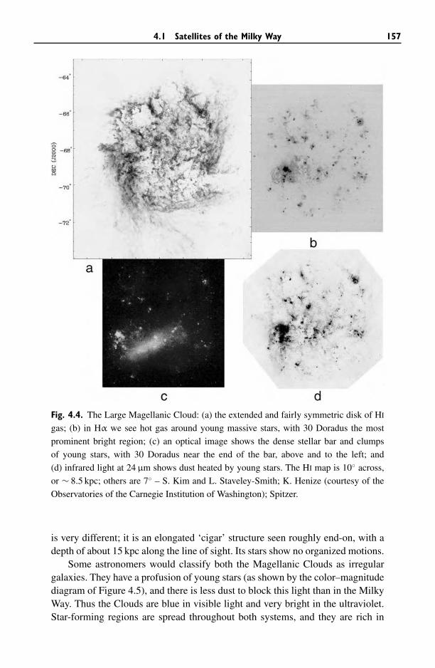
4.1 Satellites of the Milky Way 157

Fig. 4.4. The Large Magellanic Cloud: (a) the extended and fairly symmetric disk of HI

gas; (b) in Hα we see hot gas around young massive stars, with 30 Doradus the most

prominent bright region; (c) an optical image shows the dense stellar bar and clumps

of young stars, with 30 Doradus near the end of the bar, above and to the left; and

(d) infrared light at 24 μm shows dust heated by young stars. The HI map is 10◦ across,

or ∼ 8.5 kpc; others are 7◦ – S. Kim and L. Staveley-Smith; K. Henize (courtesy of the

Observatories of the Carnegie Institution of Washington); Spitzer.

is very different; it is an elongated ‘cigar’ structure seen roughly end-on, with adepth of about 15 kpc along the line of sight. Its stars show no organized motions.

Some astronomers would classify both the Magellanic Clouds as irregulargalaxies. They have a profusion of young stars (as shown by the color–magnitudediagram of Figure 4.5), and there is less dust to block this light than in the MilkyWay. Thus the Clouds are blue in visible light and very bright in the ultraviolet.Star-forming regions are spread throughout both systems, and they are rich in

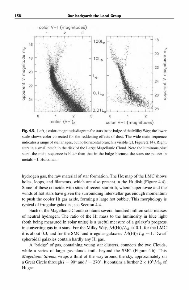
158 Our backyard: the Local Group

Fig. 4.5. Left, a color–magnitude diagram for stars in the bulge of the Milky Way; the lower

scale shows color corrected for the reddening effects of dust. The wide main sequence

indicates a range of stellar ages, but no horizontal branch is visible (cf. Figure 2.14). Right,

stars in a small patch in the disk of the Large Magellanic Cloud. Note the luminous blue

stars; the main sequence is bluer than that in the bulge because the stars are poorer in

metals – J. Holtzman.

hydrogen gas, the raw material of star formation. The Hα map of the LMC showsholes, loops, and filaments, which are also present in the HI disk (Figure 4.4).Some of these coincide with sites of recent starbirth, where supernovae and thewinds of hot stars have given the surrounding interstellar gas enough momentumto push the cooler HI gas aside, forming a large hot bubble. This morphology istypical of irregular galaxies; see Section 4.4.

Each of the Magellanic Clouds contains several hundred million solar massesof neutral hydrogen. The ratio of the HI mass to the luminosity in blue light(both being measured in solar units) is a useful measure of a galaxy’s progressin converting gas into stars. For the Milky Way, M(HI)/L B ≈ 0.1, for the LMCit is about 0.3, and for the SMC and irregular galaxies, M(HI)/L B ∼ 1. Dwarfspheroidal galaxies contain hardly any HI gas.

A ‘bridge’ of gas, containing young star clusters, connects the two Clouds,while a series of large gas clouds trails beyond the SMC (Figure 4.6). ThisMagellanic Stream wraps a third of the way around the sky, approximately ona Great Circle through l = 90◦ and l = 270◦. It contains a further 2 × 108M� ofHI gas.

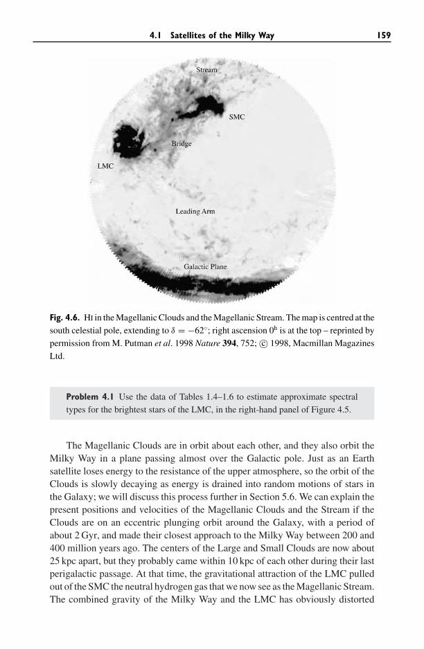
4.1 Satellites of the Milky Way 159

Fig. 4.6. HI in the Magellanic Clouds and the Magellanic Stream. The map is centred at the

south celestial pole, extending to δ = −62◦; right ascension 0h is at the top – reprinted by

permission from M. Putman et al. 1998 Nature 394, 752; c© 1998, Macmillan Magazines

Ltd.

Problem 4.1 Use the data of Tables 1.4–1.6 to estimate approximate spectral

types for the brightest stars of the LMC, in the right-hand panel of Figure 4.5.

The Magellanic Clouds are in orbit about each other, and they also orbit theMilky Way in a plane passing almost over the Galactic pole. Just as an Earthsatellite loses energy to the resistance of the upper atmosphere, so the orbit of theClouds is slowly decaying as energy is drained into random motions of stars inthe Galaxy; we will discuss this process further in Section 5.6. We can explain thepresent positions and velocities of the Magellanic Clouds and the Stream if theClouds are on an eccentric plunging orbit around the Galaxy, with a period ofabout 2 Gyr, and made their closest approach to the Milky Way between 200 and400 million years ago. The centers of the Large and Small Clouds are now about25 kpc apart, but they probably came within 10 kpc of each other during their lastperigalactic passage. At that time, the gravitational attraction of the LMC pulledout of the SMC the neutral hydrogen gas that we now see as the Magellanic Stream.The combined gravity of the Milky Way and the LMC has obviously distorted

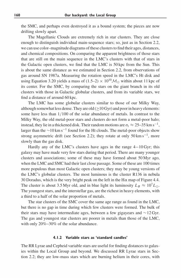
160 Our backyard: the Local Group

the SMC, and perhaps even destroyed it as a bound system; the pieces are nowdrifting slowly apart.

The Magellanic Clouds are extremely rich in star clusters. They are closeenough to distinguish individual main-sequence stars; so, just as in Section 2.2,we can use color–magnitude diagrams of these clusters to find their ages, distances,and chemical compositions. On comparing the apparent brightness of those starsthat are still on the main sequence in the LMC’s clusters with that of stars inthe Galactic open clusters, we find that the LMC is 50 kpc from the Sun. Thisis about the same distance as we estimated in Section 2.2, from observations ofgas around SN 1987a. Measuring the rotation speed in the LMC’s HI disk andusing Equation 3.20 yields a mass of (1.5–2) × 1010M� within about 11 kpc ofits center. For the SMC, by comparing the stars on the giant branch in its oldclusters with those in Galactic globular clusters, and from its variable stars, wefind a distance of around 60 kpc.

The LMC has some globular clusters similar to those of our Milky Way,although somewhat less dense. They are old (≥10 Gyr) and poor in heavy elements:some have less than 1/100 of the solar abundance of metals. In contrast to theMilky Way, the old metal-poor stars and clusters do not form a metal-poor halo;instead, they lie in a thickened disk. Their random motions are σr ≈ 25−35 km s−1,larger than the ∼10 km s−1 found for the HI clouds. The metal-poor objects showstrong asymmetric drift (see Section 2.2); they rotate at only 50 km s−1, moreslowly than the gas disk.

Hardly any of the LMC’s clusters have ages in the range 4−10 Gyr; thisgalaxy may have made very few stars during that period. There are many youngerclusters and associations; some of these may have formed about 50 Myr ago,when the LMC and SMC had their last close passage. Some of these are 100 timesmore populous than most Galactic open clusters; they may be young versions ofthe LMC’s globular clusters. The most luminous is the cluster R136 in nebula30 Doradus, which is the very bright peak on the left in the Hα map of Figure 4.4.The cluster is about 3.5 Myr old, and in blue light its luminosity L B ≈ 107L�.The youngest stars, and the interstellar gas, are the richest in heavy elements, witha third to a half of the solar proportion of metals.

The star clusters of the SMC cover the same age range as found in the LMC,but there is no gap in time during which few clusters were formed. The bulk oftheir stars may have intermediate ages, between a few gigayears and ∼12 Gyr.The gas and youngest star clusters are poorer in metals than those of the LMC,with only 20%−30% of the solar abundance.

4.1.2 Variable stars as ‘standard candles’

The RR Lyrae and Cepheid variable stars are useful for finding distances to galax-ies within the Local Group and beyond. We discussed RR Lyrae stars in Sec-tion 2.2; they are low-mass stars which are burning helium in their cores, with

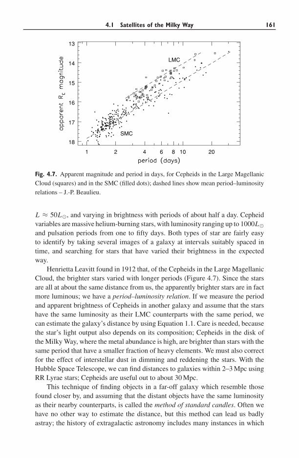
4.1 Satellites of the Milky Way 161

1 2 4 6 8 10 20

18

17

16

15

14

13

SMC

LMC

Fig. 4.7. Apparent magnitude and period in days, for Cepheids in the Large Magellanic

Cloud (squares) and in the SMC (filled dots); dashed lines show mean period–luminosity

relations – J.-P. Beaulieu.

L ≈ 50L�, and varying in brightness with periods of about half a day. Cepheidvariables are massive helium-burning stars, with luminosity ranging up to 1000L�and pulsation periods from one to fifty days. Both types of star are fairly easyto identify by taking several images of a galaxy at intervals suitably spaced intime, and searching for stars that have varied their brightness in the expectedway.

Henrietta Leavitt found in 1912 that, of the Cepheids in the Large MagellanicCloud, the brighter stars varied with longer periods (Figure 4.7). Since the starsare all at about the same distance from us, the apparently brighter stars are in factmore luminous; we have a period–luminosity relation. If we measure the periodand apparent brightness of Cepheids in another galaxy and assume that the starshave the same luminosity as their LMC counterparts with the same period, wecan estimate the galaxy’s distance by using Equation 1.1. Care is needed, becausethe star’s light output also depends on its composition; Cepheids in the disk ofthe Milky Way, where the metal abundance is high, are brighter than stars with thesame period that have a smaller fraction of heavy elements. We must also correctfor the effect of interstellar dust in dimming and reddening the stars. With theHubble Space Telescope, we can find distances to galaxies within 2−3 Mpc usingRR Lyrae stars; Cepheids are useful out to about 30 Mpc.

This technique of finding objects in a far-off galaxy which resemble thosefound closer by, and assuming that the distant objects have the same luminosityas their nearby counterparts, is called the method of standard candles. Often wehave no other way to estimate the distance, but this method can lead us badlyastray; the history of extragalactic astronomy includes many instances in which

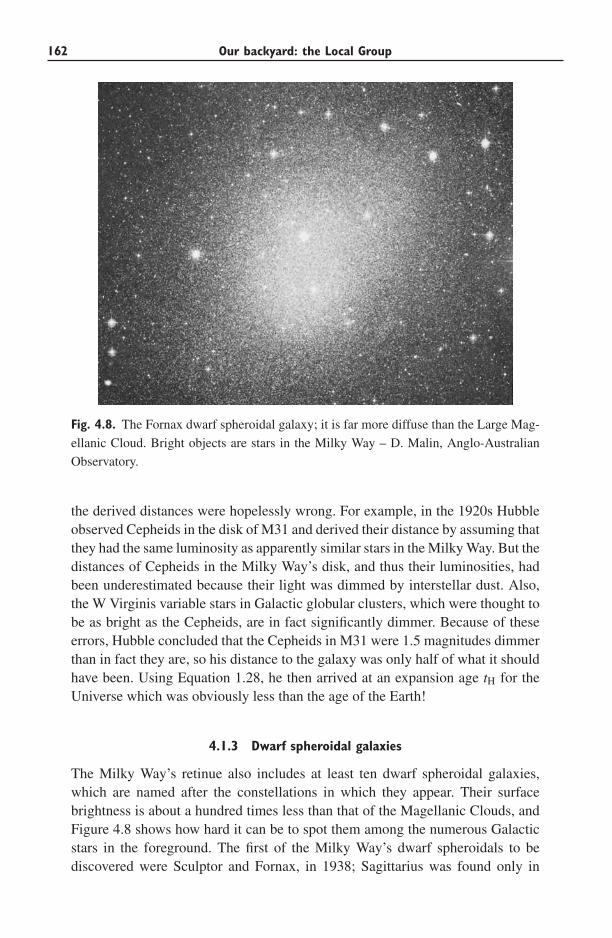
162 Our backyard: the Local Group

Fig. 4.8. The Fornax dwarf spheroidal galaxy; it is far more diffuse than the Large Mag-

ellanic Cloud. Bright objects are stars in the Milky Way – D. Malin, Anglo-Australian

Observatory.

the derived distances were hopelessly wrong. For example, in the 1920s Hubbleobserved Cepheids in the disk of M31 and derived their distance by assuming thatthey had the same luminosity as apparently similar stars in the Milky Way. But thedistances of Cepheids in the Milky Way’s disk, and thus their luminosities, hadbeen underestimated because their light was dimmed by interstellar dust. Also,the W Virginis variable stars in Galactic globular clusters, which were thought tobe as bright as the Cepheids, are in fact significantly dimmer. Because of theseerrors, Hubble concluded that the Cepheids in M31 were 1.5 magnitudes dimmerthan in fact they are, so his distance to the galaxy was only half of what it shouldhave been. Using Equation 1.28, he then arrived at an expansion age tH for theUniverse which was obviously less than the age of the Earth!

4.1.3 Dwarf spheroidal galaxies

The Milky Way’s retinue also includes at least ten dwarf spheroidal galaxies,which are named after the constellations in which they appear. Their surfacebrightness is about a hundred times less than that of the Magellanic Clouds, andFigure 4.8 shows how hard it can be to spot them among the numerous Galacticstars in the foreground. The first of the Milky Way’s dwarf spheroidals to bediscovered were Sculptor and Fornax, in 1938; Sagittarius was found only in

4.1 Satellites of the Milky Way 163

Table 4.2 Dwarf galaxies, compared with the nuclear star cluster of M33, and three Milky Way

globular clusters

LV σr rc rt tsf M/LV log10(Z/Z�)System (107 L�) (km s−1) (pc) (pc) (Gyr) (M�/L�) range

NGC 147 dE 12 20−30 260 1000 3−5 7 ± 3 −1.5 to −0.7NGC 185 dE 13 20 170 2000 <0.5 5 ± 2 −1.2 to −0.8Pegasus dIrr 1 9(HI) 500(HI) <0.1 2−4 −2.3 to −1.7Fornax dSph 1.5 13 400 5000 <2 ∼15 −2 to −0.4M33 nucleus 0.25 24 <0.4 <1: ∼1 −1.9 to −0.7Sculptor dSph 0.2 9 200 2000 >10 ∼10 −2.6 to −0.8ω Cen gc 0.1 20 4 70 >10 2.5 −1.6 to −1.2M15 gc 0.04 12 <0.01 85 >10 2 −2.15Carina dSph 0.04 7 200 900 2–10 ∼40 −2.7 to −0.3M92 gc 0.02 5 0.5 50 >10 1.5 −2.15

Note: The velocity dispersion σr is highest at the center; at the core radius rc, the surface brightness fallsto half its central value, dropping to near zero at truncation radius rt; tsf the time since last significant starformation, with : indicating an uncertain value; Z/Z� is metal abundance compared with that of the Sun.HI denotes a measurement from HI gas, not stars; globular clusters are labelled gc.

1994 and the Ursa Major system in 2005. Almost certainly, the Local Groupcontains still-undiscovered dwarf galaxies of low surface brightness. In contrastto the Magellanic Clouds, the dwarf spheroidals are effectively gas-free, and theycontain hardly any stars younger than 1−2 Gyr. All of them have some very oldstars, such as RR Lyrae variables which require at least 10 Gyr to evolve to thatstage. These systems began forming their stars as early as did ‘giant’ galaxies likethe Milky Way.

The smallest of the dwarf spheroidal galaxies are only about as luminous as thelarger globular clusters, although their radii are much larger (Table 4.2). But oursatellite dwarf spheroidals are really galaxies, not just another form of star cluster.Fornax, and probably Sagittarius, have globular clusters of their own. Unlike starclusters within the Milky Way, the dwarf galaxies did not form all their stars atonce; they all include stars born over several gigayears, from gas with differingproportions of heavy elements. Figure 4.9 shows the color–magnitude diagram forstars in the Carina dwarf, along with computed isochrones for metal-poor stars.Only about 2% of the stars are younger than about 2.5 Gyr, and the rest appear tohave been born in three bursts, approximately 3, 7, and 15 Gyr ago. Even the mostluminous of the dwarf spheroidals are only about 1/30 as rich in heavy elementsas the Sun, and the less luminous systems are even more metal-poor; see Table 4.2.According to a simple model to be discussed in Section 4.3, we would expect agalaxy that had turned all its gas into stars to have roughly the solar abundance ofheavy elements. Their low metallicity suggests that these galaxies lost much oftheir metal-enriched gas into intergalactic space.

Using the information in Table 4.2, we can estimate the masses of dwarfspheroidal galaxies from their sizes and the radial velocities of their stars. Stellar

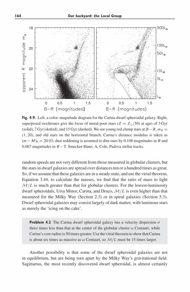
164 Our backyard: the Local Group

0 0.5 1 1.5

24

22

20

18

0 0.5 1 1.5

Fig. 4.9. Left, a color–magnitude diagram for the Carina dwarf spheroidal galaxy. Right,

superposed isochrones give the locus of metal-poor stars (Z = Z�/50) at ages of 3 Gyr

(solid), 7 Gyr (dotted), and 15 Gyr (dashed). We see young red clump stars at B− R, m R =(1, 20), and old stars on the horizontal branch. Carina’s distance modulus is taken as

(m − M)0 = 20.03; dust reddening is assumed to dim stars by 0.108 magnitudes in B and

0.067 magnitudes in R – T. Smecker-Hane; A. Cole, Padova stellar tracks.

random speeds are not very different from those measured in globular clusters, butthe stars in dwarf galaxies are spread over distances ten or a hundred times as great.So, if we assume that these galaxies are in a steady state, and use the virial theorem,Equation 3.44, to calculate the masses, we find that the ratio of mass to lightM/L is much greater than that for globular clusters. For the lowest-luminositydwarf spheroidals, Ursa Minor, Carina, and Draco, M/L is even higher than thatmeasured for the Milky Way (Section 2.3) or in spiral galaxies (Section 5.3).Dwarf spheroidal galaxies may consist largely of dark matter, with luminous starsas merely the ‘icing on the cake’.

Problem 4.2 The Carina dwarf spheroidal galaxy has a velocity dispersion σ

three times less than that at the center of the globular cluster ω Centauri, while

Carina’s core radius is 50 times greater. Use the virial theorem to show that Carina

is about six times as massive as ω Centauri, so M/L must be 15 times larger.

Another possibility is that some of the dwarf spheroidal galaxies are notin equilibrium, but are being torn apart by the Milky Way’s gravitational field.Sagittarius, the most recently discovered dwarf spheroidal, is almost certainly

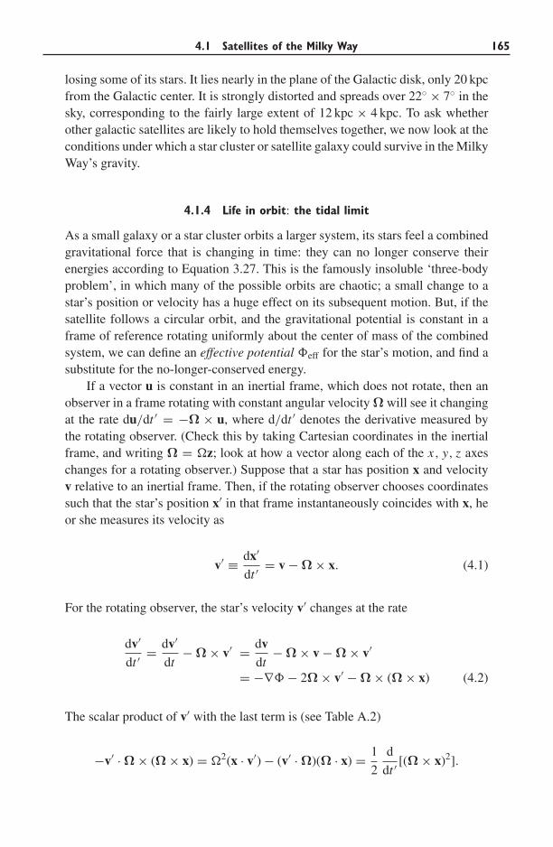
4.1 Satellites of the Milky Way 165

losing some of its stars. It lies nearly in the plane of the Galactic disk, only 20 kpcfrom the Galactic center. It is strongly distorted and spreads over 22◦ × 7◦ in thesky, corresponding to the fairly large extent of 12 kpc × 4 kpc. To ask whetherother galactic satellites are likely to hold themselves together, we now look at theconditions under which a star cluster or satellite galaxy could survive in the MilkyWay’s gravity.

4.1.4 Life in orbit: the tidal limit

As a small galaxy or a star cluster orbits a larger system, its stars feel a combinedgravitational force that is changing in time: they can no longer conserve theirenergies according to Equation 3.27. This is the famously insoluble ‘three-bodyproblem’, in which many of the possible orbits are chaotic; a small change to astar’s position or velocity has a huge effect on its subsequent motion. But, if thesatellite follows a circular orbit, and the gravitational potential is constant in aframe of reference rotating uniformly about the center of mass of the combinedsystem, we can define an effective potential �eff for the star’s motion, and find asubstitute for the no-longer-conserved energy.

If a vector u is constant in an inertial frame, which does not rotate, then anobserver in a frame rotating with constant angular velocity Ω will see it changingat the rate du/dt ′ = −Ω × u, where d/dt ′ denotes the derivative measured bythe rotating observer. (Check this by taking Cartesian coordinates in the inertialframe, and writing Ω = �z; look at how a vector along each of the x, y, z axeschanges for a rotating observer.) Suppose that a star has position x and velocityv relative to an inertial frame. Then, if the rotating observer chooses coordinatessuch that the star’s position x′ in that frame instantaneously coincides with x, heor she measures its velocity as

v′ ≡ dx′

dt ′ = v − Ω × x. (4.1)

For the rotating observer, the star’s velocity v′ changes at the rate

dv′

dt ′ = dv′

dt− Ω × v′ = dv

dt− Ω × v − Ω × v′

= −∇� − 2Ω × v′ − Ω × (Ω × x) (4.2)

The scalar product of v′ with the last term is (see Table A.2)

−v′ · Ω × (Ω × x) = �2(x · v′) − (v′ · Ω)(Ω · x) = 1

2

d

dt ′ [(Ω × x)2].

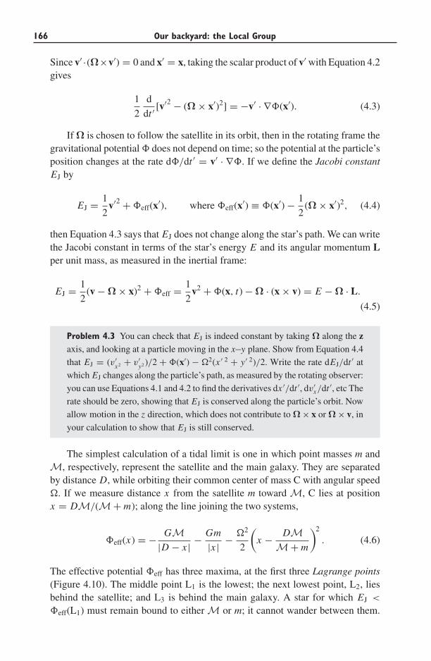
166 Our backyard: the Local Group

Since v′ ·(Ω×v′) = 0 and x′ = x, taking the scalar product of v′ with Equation 4.2gives

1

2

d

dt ′ [v′2 − (Ω × x′)2] = −v′ · ∇�(x′). (4.3)

If Ω is chosen to follow the satellite in its orbit, then in the rotating frame thegravitational potential � does not depend on time; so the potential at the particle’sposition changes at the rate d�/dt ′ = v′ · ∇�. If we define the Jacobi constantEJ by

EJ = 1

2v′2 + �eff(x′), where �eff(x′) ≡ �(x′) − 1

2(Ω × x′)2, (4.4)

then Equation 4.3 says that EJ does not change along the star’s path. We can writethe Jacobi constant in terms of the star’s energy E and its angular momentum Lper unit mass, as measured in the inertial frame:

EJ = 1

2(v − Ω × x)2 + �eff = 1

2v2 + �(x, t) − Ω · (x × v) = E − Ω · L.

(4.5)

Problem 4.3 You can check that EJ is indeed constant by taking Ω along the zaxis, and looking at a particle moving in the x−y plane. Show from Equation 4.4

that EJ = (v′x2 + v′

y2 )/2 + �(x′) − �2(x ′ 2 + y′ 2)/2. Write the rate dEJ/dt ′ at

which EJ changes along the particle’s path, as measured by the rotating observer:

you can use Equations 4.1 and 4.2 to find the derivatives dx ′/dt ′, dv′x/dt ′, etc The

rate should be zero, showing that EJ is conserved along the particle’s orbit. Now

allow motion in the z direction, which does not contribute to Ω × x or Ω × v, in

your calculation to show that EJ is still conserved.

The simplest calculation of a tidal limit is one in which point masses m andM, respectively, represent the satellite and the main galaxy. They are separatedby distance D, while orbiting their common center of mass C with angular speed�. If we measure distance x from the satellite m toward M, C lies at positionx = DM/(M + m); along the line joining the two systems,

�eff(x) = − GM|D − x | − Gm

|x | − �2

2

(x − DM

M + m

)2

. (4.6)

The effective potential �eff has three maxima, at the first three Lagrange points(Figure 4.10). The middle point L1 is the lowest; the next lowest point, L2, liesbehind the satellite; and L3 is behind the main galaxy. A star for which EJ <

�eff(L1) must remain bound to either M or m; it cannot wander between them.

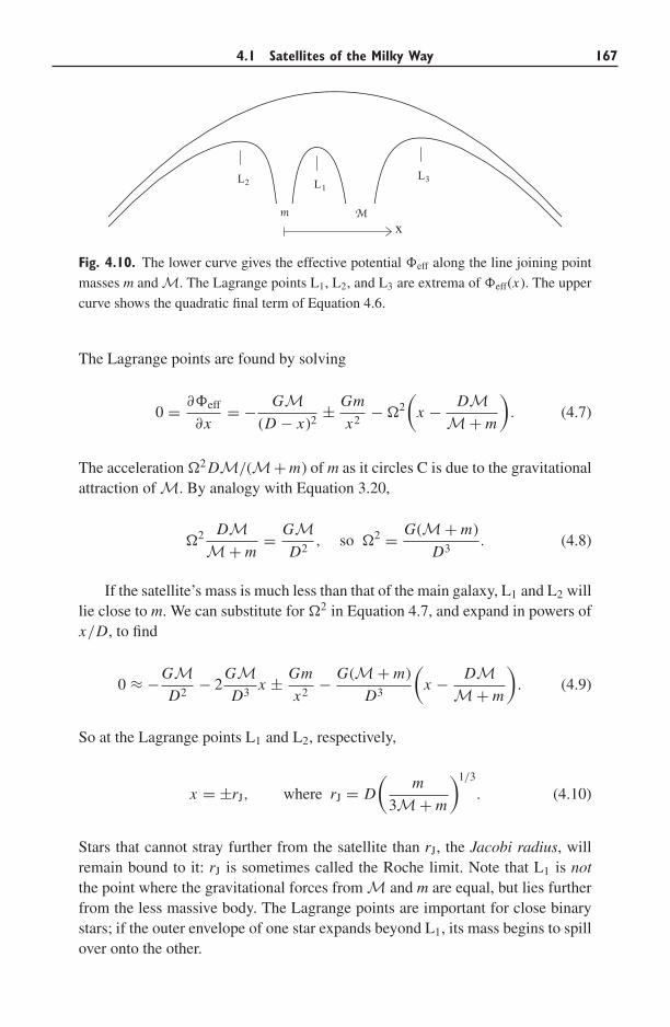
4.1 Satellites of the Milky Way 167

Mm

LLL 3

12

x

Fig. 4.10. The lower curve gives the effective potential �eff along the line joining point

masses m and M. The Lagrange points L1, L2, and L3 are extrema of �eff(x). The upper

curve shows the quadratic final term of Equation 4.6.

The Lagrange points are found by solving

0 = ∂�eff

∂x= − GM

(D − x)2± Gm

x2− �2

(x − DM

M + m

). (4.7)

The acceleration �2 DM/(M+ m) of m as it circles C is due to the gravitationalattraction of M. By analogy with Equation 3.20,

�2 DMM + m

= GMD2

, so �2 = G(M + m)

D3. (4.8)

If the satellite’s mass is much less than that of the main galaxy, L1 and L2 willlie close to m. We can substitute for �2 in Equation 4.7, and expand in powers ofx/D, to find

0 ≈ −GMD2

− 2GMD3

x ± Gm

x2− G(M + m)

D3

(x − DM

M + m

). (4.9)

So at the Lagrange points L1 and L2, respectively,

x = ±rJ, where rJ = D

(m

3M + m

)1/3

. (4.10)

Stars that cannot stray further from the satellite than rJ, the Jacobi radius, willremain bound to it: rJ is sometimes called the Roche limit. Note that L1 is notthe point where the gravitational forces from M and m are equal, but lies furtherfrom the less massive body. The Lagrange points are important for close binarystars; if the outer envelope of one star expands beyond L1, its mass begins to spillover onto the other.

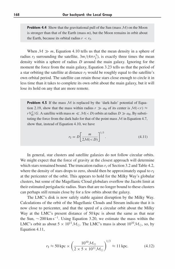
168 Our backyard: the Local Group

Problem 4.4 Show that the gravitational pull of the Sun (mass M) on the Moon

is stronger than that of the Earth (mass m), but the Moon remains in orbit about

the Earth, because its orbital radius r < rJ.

When M � m, Equation 4.10 tells us that the mean density in a sphere ofradius rJ surrounding the satellite, 3m/(4πr3

J ), is exactly three times the meandensity within a sphere of radius D around the main galaxy. Ignoring for themoment the force from the main galaxy, Equation 3.23 tells us that the period ofa star orbiting the satellite at distance rJ would be roughly equal to the satellite’sown orbital period. The satellite can retain those stars close enough to circle it inless time than it takes to complete its own orbit about the main galaxy, but it willlose its hold on any that are more remote.

Problem 4.5 If the mass M is replaced by the ‘dark-halo’ potential of Equa-

tion 2.19, show that the mass within radius r � aH of its center is M(<r ) ≈r V 2

H/G. A satellite with mass m � M(< D) orbits at radius D � aH. By substi-

tuting the force from the dark halo for that of the point mass M in Equation 4.7,

show that, instead of Equation 4.10, we have

rJ = D

[m

2M(< D)

]1/3

. (4.11)

In general, star clusters and satellite galaxies do not follow circular orbits.We might expect that the force of gravity at the closest approach will determinewhich stars remained bound. The truncation radius rt of Section 3.2 and Table 4.2,where the density of stars drops to zero, should then be approximately equal to rJ

at the pericenter of the orbit. This appears to hold for the Milky Way’s globularclusters, but some of the Magellanic Cloud globulars overflow the Jacobi limit attheir estimated perigalactic radius. Stars that are no longer bound to these clusterscan perhaps still remain close by for a few orbits about the galaxy.

The LMC’s disk is now safely stable against disruption by the Milky Way.Calculations of the orbit of the Magellanic Clouds and Stream indicate that it isnow close to pericenter, and that the speed of a circular orbit about the MilkyWay at the LMC’s present distance of 50 kpc is about the same as that nearthe Sun, ∼200 km s−1. Using Equation 3.20, we estimate the mass within theLMC’s orbit as about 5 × 1011M�. The LMC’s mass is about 1010M�, so, byEquation 4.11,

rJ ≈ 50 kpc ×(

1010M�2 × 5 × 1011M�

)1/3

≈ 11 kpc. (4.12)

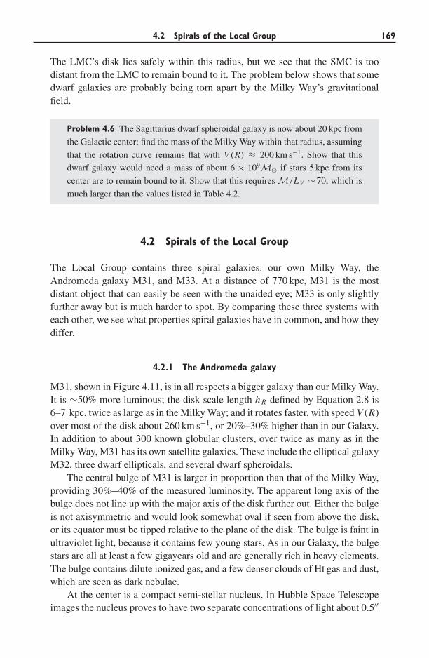
4.2 Spirals of the Local Group 169

The LMC’s disk lies safely within this radius, but we see that the SMC is toodistant from the LMC to remain bound to it. The problem below shows that somedwarf galaxies are probably being torn apart by the Milky Way’s gravitationalfield.

Problem 4.6 The Sagittarius dwarf spheroidal galaxy is now about 20 kpc from

the Galactic center: find the mass of the Milky Way within that radius, assuming

that the rotation curve remains flat with V (R) ≈ 200 km s−1. Show that this

dwarf galaxy would need a mass of about 6 × 109M� if stars 5 kpc from its

center are to remain bound to it. Show that this requires M/LV ∼70, which is

much larger than the values listed in Table 4.2.

4.2 Spirals of the Local Group

The Local Group contains three spiral galaxies: our own Milky Way, theAndromeda galaxy M31, and M33. At a distance of 770 kpc, M31 is the mostdistant object that can easily be seen with the unaided eye; M33 is only slightlyfurther away but is much harder to spot. By comparing these three systems witheach other, we see what properties spiral galaxies have in common, and how theydiffer.

4.2.1 The Andromeda galaxy

M31, shown in Figure 4.11, is in all respects a bigger galaxy than our Milky Way.It is ∼50% more luminous; the disk scale length h R defined by Equation 2.8 is6–7 kpc, twice as large as in the Milky Way; and it rotates faster, with speed V (R)over most of the disk about 260 km s−1, or 20%–30% higher than in our Galaxy.In addition to about 300 known globular clusters, over twice as many as in theMilky Way, M31 has its own satellite galaxies. These include the elliptical galaxyM32, three dwarf ellipticals, and several dwarf spheroidals.

The central bulge of M31 is larger in proportion than that of the Milky Way,providing 30%−40% of the measured luminosity. The apparent long axis of thebulge does not line up with the major axis of the disk further out. Either the bulgeis not axisymmetric and would look somewhat oval if seen from above the disk,or its equator must be tipped relative to the plane of the disk. The bulge is faint inultraviolet light, because it contains few young stars. As in our Galaxy, the bulgestars are all at least a few gigayears old and are generally rich in heavy elements.The bulge contains dilute ionized gas, and a few denser clouds of HI gas and dust,which are seen as dark nebulae.

At the center is a compact semi-stellar nucleus. In Hubble Space Telescopeimages the nucleus proves to have two separate concentrations of light about 0.5′′

170 Our backyard: the Local Group

Fig. 4.11. The Andromeda galaxy, M31: (a) in ultraviolet light; (b) B-band image shows

the prominent bulge; (c) infrared light of warm dust at 24 μm; (d) Hα image shows the

‘ring of fire’ and HII regions in the spiral arms; (e) HI gas; and (f) emission of CO tracing

dense molecular gas – K. Gordon. (a) Galex FUV, D. Thilker et al. 2005 ApJ 619, L67;

(b) and (d) D. Thilker and R. Walterbos; (c) Spitzer; K. Gordon et al. 2005 ApJ 638, L87;

(e) R. Braun et al.; and (f) Nieten et al. 2006 AAp 453, 459.

or 2 pc apart. One of these harbors a dense central object, probably a black holeof mass MBH ∼3 × 106M�. The other may be a star cluster which has spiralledinto the center under the influence of dynamical friction (see Section 7.1). Unlikethat of the Milky Way, the nucleus of M31 is impressively free of gas and dust.

Just as in the Milky Way, the metal-poor globular clusters of M31 followdeeply plunging orbits; the cluster system shows little or no ordered rotation. Butthe bulge also continues smoothly outward as a luminous spheroid. Most of thestars a few kiloparsecs above the disk plane are not those of a metal-poor halo;they are relatively metal-rich, and they probably form a fast-rotating system. It isas if M31’s bulge has ‘overflowed’, largely swamping the metal-poor halo.

Like the Milky Way, M31 is a cannibal galaxy. The metal-rich halo stars areroughly 6 Gyr old; they and much of the bulge probably arrived as M31 mergedwith another metal-rich (and so fairly massive: see Section 4.3) galaxy. A hugestream of stars over 100 kpc long has been found, passing from northwest of thegalaxy to the southeast. These stars are also more metal-rich than those of the MilkyWay’s halo; they may have been stripped as M31 swallowed a sizable galaxy.

4.2 Spirals of the Local Group 171

Circling the bulge at a radius of about 10 kpc, the star-forming ‘ring of fire’ isclearly visible in Figure 4.11. Most of the young disk stars lie in this ring or justoutside it; on average, M31’s disk forms stars at a slower rate than does that of theMilky Way. Ionized gas in HII regions around the young massive stars glows redin Hα; in the far-infrared we see the dust heated by those stars, and the CO mapshows the dense gas from which they formed. Just outside this ring, ultraviolet-bright young stars and strings of HII regions in the disk trace segments of fairlytightly wound spiral arms, where gas, dust, and stars have been compressed to ahigher density. However, there is no clear large-scale spiral pattern. Because of itslarge bulge and moderately tightly wound spiral arms, and the relative paucity ofgas and recent star formation in the inner disk, we classify M31 as an Sb galaxy,whereas our Milky Way is Sbc or Sc.

M31 has about (4−6) × 109M� of neutral hydrogen, about 50% more thanthe Milky Way. Molecular gas is probably a smaller fraction of the total, so theratio of gas mass to stellar luminosity is lower than that in our Galaxy. Figure 4.11shows that the HI is concentrated at the ring of fire; but, as in the Milky Way, thegas extends to larger radii than the stellar disk. In the region of the spiral arms,high-resolution maps show holes in the HI disk, up to a kiloparsec across; at theiredges, shells containing (103−107)M� of dense HI gas are moving outward at10–30 km s−1. At this rate, most of the holes would have taken a few megayears toreach their present sizes. Sometimes an association of massive O and B stars lieswithin the hole; winds from these massive stars, and recent supernova explosions,have blown away the cool gas. Holes in the inner parts of the disk tend to besmaller, perhaps because the gas is denser or the magnetic field stronger, so it isharder to push cool material out of the way.

If we measure the velocity of the HI gas at each point, we can use the fact thatthe clouds follow near-circular orbits to build up a three-dimensional picture of thegas disk. The outer parts are not flat but bent into an ‘S’ shape; the stellar disk isvisibly warped in the same sense. An ‘S’ warp in the outer parts of spiral galaxiesis quite common; the Milky Way’s own disk is warped in this way, and systemswith a flat disk are probably in a minority. As in our Galaxy, the HI layer flares outto become thicker at greater distances from the center. Some outlying clumps ofHI gas clearly do not share the disk’s rotation; lying up to 50 kpc from the center,they are the analogues of the Milky Way’s high-velocity clouds (Section 2.4). Theclouds are ∼1 kpc across with (105−106)M� of HI . Several of them lie along thesame path as the giant star stream, with roughly the same velocities; perhaps theywere stripped from the same satellite galaxy. Another lies close in both positionand velocity to the dwarf elliptical NGC 205.

4.2.2 M33: a late-type spiral

The other spiral in the Local Group, M33, is definitely an Sc or an Scd galaxy. Itsbulge is tiny; the spiral arms are more open than those in M31 and not as smooth,

172 Our backyard: the Local Group

consisting mainly of bright blue concentrations of recently formed stars. M33 isa smaller and much less luminous galaxy than the Milky Way; the scale length issmall, h R ≈ 1.7 kpc, and the rotation speed V (R) rises only to 120 km s−1.

When observed in the Hα emission line, M33 displays a complex networkof loops, filaments, and shells, like those in the LMC (Figure 4.4) and in theviolently star-forming irregular galaxy IC 10 (see Section 4.4 below). Supernovaexplosions, and the winds from stars, heat the surrounding gas and drive it away,thus affecting the location and rate of future starbirth. Such feedback has a strongeffect on the way that galaxies come into being from lumps of primordial gas, andon their subsequent development.

M33 is relatively richer in HI gas than M31 or the Milky Way; there is littleCO emission, reflecting either a lack of molecular gas or a smaller ratio of COto H2 than in the Milky Way. The latter is more likely, since the disk is rich inyoung stars, which are born in the dense cores of molecular clouds. Comparedwith the Milky Way, relatively more of the HI gas is in the warm component andless in cold dense clouds. As in M31, the HI layer has large holes, often centred onstar-forming regions in the disk. M33’s neutral-gas disk is very extended. The HI

continues out at least to 3 Holmberg radii or about 30 kpc, which is a substantialfraction of the ∼200 kpc separating the galaxy from M31. One rather massivecloud with 106M� of gas lies about 15 kpc from M33’s center; a streamer of HI

gas links it to the disk. The outer disk is warped, possibly by tides from M31.At the center of M33, we find a dense nuclear star cluster, with no more than

a small bulge around it. This cluster is more luminous than any Galactic globular,with LV ≈ 2.5×106L�; its core is tiny, so the stellar density exceeds 107L� pc−3.In contrast to the single generation of stars in a globular cluster, M33’s nucleuscontains old, middle-aged, and young stars. There is no sign of a black hole: ifone is present, MBH ∼< 104M�, far less than in the Milky Way and in M31. Butwe do see evidence for a power source other than ordinary stars. M33’s nucleusis the single brightest X-ray source of the Local Group, equivalent to several ofthe normal binary sources.

M33 is only two or three times more luminous than the LMC, yet it has a muchmore symmetric spiral pattern. Low-luminosity galaxies are in general more likelythan larger systems to resemble the LMC in having a strong central bar, with thebrightest parts of the galaxy off-center from the outer disk. But the morphologyclearly depends on factors other than the galaxy’s luminosity alone.

4.3 How did the Local Group galaxies form?

We can now sketch a picture for the formation of the Milky Way and the othergalaxies of the Local Group, starting from the hot dense early Universe that wediscussed in Section 1.5. Roughly 350 000 years after the brilliant beginning of theBig Bang, photons of the cosmic fireball no longer had enough energy to ionize

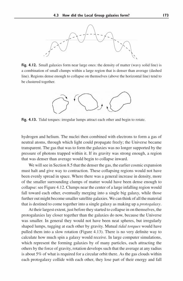
4.3 How did the Local Group galaxies form? 173

Fig. 4.12. Small galaxies form near large ones: the density of matter (wavy solid line) is

a combination of small clumps within a large region that is denser than average (dashed

line). Regions dense enough to collapse on themselves (above the horizontal line) tend to

be clustered together.

Fig. 4.13. Tidal torques: irregular lumps attract each other and begin to rotate.

hydrogen and helium. The nuclei then combined with electrons to form a gas ofneutral atoms, through which light could propagate freely; the Universe becametransparent. The gas that was to form the galaxies was no longer supported by thepressure of photons trapped within it. If its gravity was strong enough, a regionthat was denser than average would begin to collapse inward.

We will see in Section 8.5 that the denser the gas, the earlier cosmic expansionmust halt and give way to contraction. These collapsing regions would not havebeen evenly spread in space. Where there was a general increase in density, moreof the smaller surrounding clumps of matter would have been dense enough tocollapse: see Figure 4.12. Clumps near the center of a large infalling region wouldfall toward each other, eventually merging into a single big galaxy, while thosefurther out might become smaller satellite galaxies. We can think of all the materialthat is destined to come together into a single galaxy as making up a protogalaxy.

At their largest extent, just before they started to collapse in on themselves, theprotogalaxies lay closer together than the galaxies do now, because the Universewas smaller. In general they would not have been neat spheres, but irregularlyshaped lumps, tugging at each other by gravity. Mutual tidal torques would havepulled them into a slow rotation (Figure 4.13). There is no very definite way tocalculate how much spin a galaxy would receive. In large computer simulations,which represent the forming galaxies by of many particles, each attracting theothers by the force of gravity, rotation develops such that the average at any radiusis about 5% of what is required for a circular orbit there. As the gas clouds withineach protogalaxy collide with each other, they lose part of their energy and fall

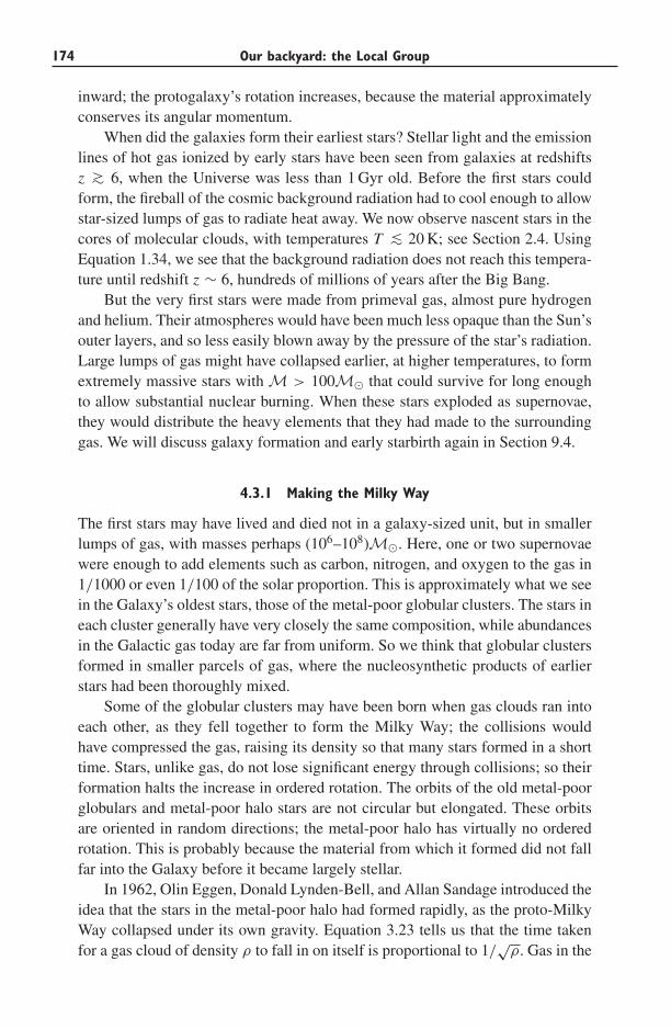
174 Our backyard: the Local Group

inward; the protogalaxy’s rotation increases, because the material approximatelyconserves its angular momentum.

When did the galaxies form their earliest stars? Stellar light and the emissionlines of hot gas ionized by early stars have been seen from galaxies at redshiftsz ∼> 6, when the Universe was less than 1 Gyr old. Before the first stars couldform, the fireball of the cosmic background radiation had to cool enough to allowstar-sized lumps of gas to radiate heat away. We now observe nascent stars in thecores of molecular clouds, with temperatures T ∼< 20 K; see Section 2.4. UsingEquation 1.34, we see that the background radiation does not reach this tempera-ture until redshift z ∼ 6, hundreds of millions of years after the Big Bang.

But the very first stars were made from primeval gas, almost pure hydrogenand helium. Their atmospheres would have been much less opaque than the Sun’souter layers, and so less easily blown away by the pressure of the star’s radiation.Large lumps of gas might have collapsed earlier, at higher temperatures, to formextremely massive stars with M > 100M� that could survive for long enoughto allow substantial nuclear burning. When these stars exploded as supernovae,they would distribute the heavy elements that they had made to the surroundinggas. We will discuss galaxy formation and early starbirth again in Section 9.4.

4.3.1 Making the Milky Way

The first stars may have lived and died not in a galaxy-sized unit, but in smallerlumps of gas, with masses perhaps (106–108)M�. Here, one or two supernovaewere enough to add elements such as carbon, nitrogen, and oxygen to the gas in1/1000 or even 1/100 of the solar proportion. This is approximately what we seein the Galaxy’s oldest stars, those of the metal-poor globular clusters. The stars ineach cluster generally have very closely the same composition, while abundancesin the Galactic gas today are far from uniform. So we think that globular clustersformed in smaller parcels of gas, where the nucleosynthetic products of earlierstars had been thoroughly mixed.

Some of the globular clusters may have been born when gas clouds ran intoeach other, as they fell together to form the Milky Way; the collisions wouldhave compressed the gas, raising its density so that many stars formed in a shorttime. Stars, unlike gas, do not lose significant energy through collisions; so theirformation halts the increase in ordered rotation. The orbits of the old metal-poorglobulars and metal-poor halo stars are not circular but elongated. These orbitsare oriented in random directions; the metal-poor halo has virtually no orderedrotation. This is probably because the material from which it formed did not fallfar into the Galaxy before it became largely stellar.

In 1962, Olin Eggen, Donald Lynden-Bell, and Allan Sandage introduced theidea that the stars in the metal-poor halo had formed rapidly, as the proto-MilkyWay collapsed under its own gravity. Equation 3.23 tells us that the time takenfor a gas cloud of density ρ to fall in on itself is proportional to 1/

√ρ. Gas in the

4.3 How did the Local Group galaxies form? 175

substructure of lumps that made the stars would have been denser than average,so material should have started to contract sooner, and turned into stars before thegalaxy-sized cloud had gone far in its own collapse. The problem below shows thatthe whole process could have been completed within a few tenths of a gigayear.

Problem 4.7 For a galaxy like our Milky Way with a mass of 1011M� and radius

10 kpc, find the average density. The virial theorem tells us that, if a galaxy of stars

collapses from rest, then, after it has come to equilibrium, it will be eight times

denser than at the start: see the discussion following Problem 8.31. Show that,

for the proto-Milky Way, the free-fall time of Equation 3.23 was tff ∼ 300 Myr.

This is about ten times longer than a protostar of solar mass takes to reach the

main sequence. For the Sculptor dwarf with M ∼ 2 × 107M� and radius 2 kpc

(Table 4.2), show that the average density is only 1/40 of the Milky Way’s, so

the collapse time tff ∼ 2 Gyr.

By contrast, the material that became the Milky Way’s rotating disk had tolose a considerable amount of its energy. We saw in Section 3.3 that a circle isthe orbit of lowest energy for a given angular momentum. Today’s thin-disk starsoccupy nearly circular orbits because they were born from gas that had lost almostas much energy as possible. The thick-disk stars, and the more metal-rich globularclusters, predate most of the thin disk. They may have been born from gas cloudsthat had yielded up less of their energy, but still formed a somewhat flattenedrotating system. By the time that the earliest thin-disk stars were born, 8–10 Gyrago, heavy elements produced by earlier generations of stars had enriched the gas,to perhaps 10%−20% of the solar abundance.

Today, disk gas near the Sun follows nearly circular orbits with speed V (R) ≈200 km s−1. If tidal torques gave this material a rotational speed only 5% of thatneeded for a circular orbit, the gas must subsequently have fallen inward until itreached an orbit appropriate for its angular momentum. We can use Equation 3.29to estimate where the local gas must have been when the tidal torques wereoperating. If the Milky Way’s gravitational potential corresponds to a flat rotationcurve, with V (R) constant, then this gas must have fallen in from a distanceR ∼ 100 kpc; the gas around galaxies must have extended much further out atearlier times. The disk material had to remain gaseous as it moved inward, formingonly very few stars, so that it could continue to radiate away energy. It may havebeen able to do this because it was much less dense than the gas that had earliergiven birth to the globular clusters.

The color–magnitude diagram of Figure 4.5 shows no horizontal branch inthe Galactic bulge. Even allowing for their higher metal content, very few of thebulge stars can be as old as the globular clusters. The over-whelming majorityhave ages less than 8–10 Gyr, and some may be much younger. We do not yetknow how the bulge stars were made. They may have formed in the dense center

176 Our backyard: the Local Group

of the protogalactic gas that was to make up the Milky Way; the bulge might havegrown out of a dense inner region of the disk; or its stars may be the remains ofdense clusters that fell victim to dynamical friction, and spiralled into the center;see Section 7.1. The central kiloparsec of galaxies such as M33 and the LMC isnot as dense as the inner Milky Way; the low density may have prevented a bulgefrom developing.

Once the dense central bulge had come into being, the gravitational forceof the whole Galaxy would have helped it to hold onto its gas. By trapping thehot and fast-moving debris from supernovae, the bulge formed large numbers ofmetal-rich stars. Both in the Local Group and beyond (see Section 6.3), the starsof more luminous galaxies are richer in heavy elements. Their stronger gravityprevents metal-bearing gas from escaping, and it is incorporated into stars.

Much of the Milky Way’s dark matter is in its outskirts, beyond most of thestars of the disk. In Section 5.3 we will see that the same is true of most spiralgalaxies. Why does nonluminous material lie mainly in the Galaxy’s outer reaches?Since its composition remains unknown, we lack a definite answer. However, ifwe presume that all forms of matter were mixed evenly at early times, then thedark matter must have had less opportunity than the star-stuff to get rid of itsenergy. It would then be left on orbits taking it far from the Galactic center. A darkhalo of the weakly interacting massive particles (WIMPs) of Section 1.5 couldnever radiate away energy as heat; so it is bound to remain more extended thanthe gaseous and stellar body. If the dark matter consists of compact objects suchas brown dwarfs or black holes, we would expect that these formed very early inthe Milky Way’s collapse, probably predating even the globular clusters.

The Milky Way is still under construction today. As we saw in Section 2.2,stars of the Sagittarius dwarf spheroidal galaxy are being added to the Galactichalo. Near the Sun, groups of young metal-poor halo stars have been found, thatmay be the remnants of another partially digested dwarf galaxy. The orbit of theMagellanic Clouds has been shrinking, and in Section 7.1we will see that the LMCwill probably fall into the Milky Way within 3–5 Gyr. Like meteoric cratering inthe solar system, these late additions represent the final stages of assembly.

4.3.2 The buildup of heavy elements

During its life, a galaxy turns gas into stars. Each star burns hydrogen and helium toform heavier elements, which are returned to the interstellar gas at the end of its life.We might define a ‘clock’ for galactic aging by the mass of stars born and of metalsproduced, per unit mass of gas that was present initially. Near the Sun, we see somecorrespondence between the time told by this ‘metal-production clock’ and timeas measured by stellar aging; Figure 4.14 shows that older disk stars in generalcontain little iron, while recently formed stars have larger abundances. We saw inSection 2.2 that the open clusters of the Milky Way’s thin disk are both youngerand more metal-rich than the stars and globular clusters of the thick disk, whilethe globular clusters of the halo are the oldest and the poorest in heavy elements.

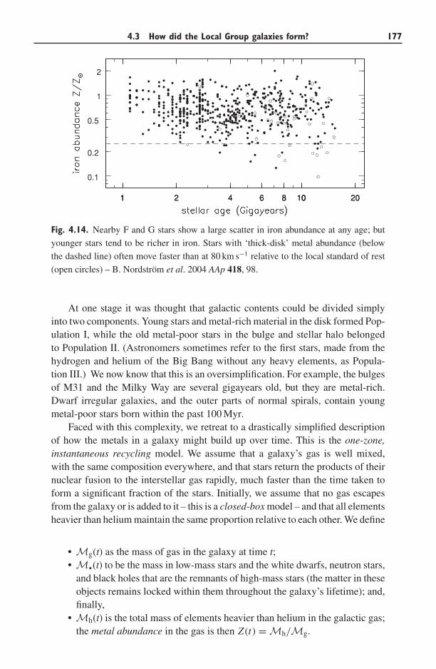
4.3 How did the Local Group galaxies form? 177

1 2 4 6 8 10 20

0.2

2

1 2 4 6 8 10 20

0.5

1 0

0.1

1

Fig. 4.14. Nearby F and G stars show a large scatter in iron abundance at any age; but

younger stars tend to be richer in iron. Stars with ‘thick-disk’ metal abundance (below

the dashed line) often move faster than at 80 km s−1 relative to the local standard of rest

(open circles) – B. Nordstrom et al. 2004 AAp 418, 98.

At one stage it was thought that galactic contents could be divided simplyinto two components. Young stars and metal-rich material in the disk formed Pop-ulation I, while the old metal-poor stars in the bulge and stellar halo belongedto Population II. (Astronomers sometimes refer to the first stars, made from thehydrogen and helium of the Big Bang without any heavy elements, as Popula-tion III.) We now know that this is an oversimplification. For example, the bulgesof M31 and the Milky Way are several gigayears old, but they are metal-rich.Dwarf irregular galaxies, and the outer parts of normal spirals, contain youngmetal-poor stars born within the past 100 Myr.

Faced with this complexity, we retreat to a drastically simplified descriptionof how the metals in a galaxy might build up over time. This is the one-zone,instantaneous recycling model. We assume that a galaxy’s gas is well mixed,with the same composition everywhere, and that stars return the products of theirnuclear fusion to the interstellar gas rapidly, much faster than the time taken toform a significant fraction of the stars. Initially, we assume that no gas escapesfrom the galaxy or is added to it – this is a closed-box model – and that all elementsheavier than helium maintain the same proportion relative to each other. We define

• Mg(t) as the mass of gas in the galaxy at time t;• M(t) to be the mass in low-mass stars and the white dwarfs, neutron stars,

and black holes that are the remnants of high-mass stars (the matter in theseobjects remains locked within them throughout the galaxy’s lifetime); and,finally,

• Mh(t) is the total mass of elements heavier than helium in the galactic gas;the metal abundance in the gas is then Z (t) = Mh/Mg.

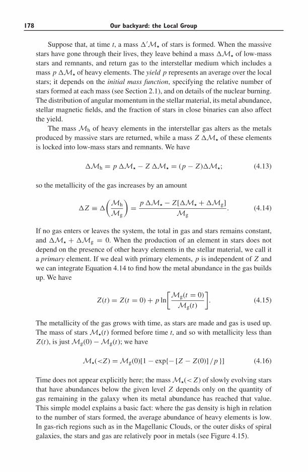
178 Our backyard: the Local Group

Suppose that, at time t, a mass �′M of stars is formed. When the massivestars have gone through their lives, they leave behind a mass �M of low-massstars and remnants, and return gas to the interstellar medium which includes amass p �M of heavy elements. The yield p represents an average over the localstars; it depends on the initial mass function, specifying the relative number ofstars formed at each mass (see Section 2.1), and on details of the nuclear burning.The distribution of angular momentum in the stellar material, its metal abundance,stellar magnetic fields, and the fraction of stars in close binaries can also affectthe yield.

The mass Mh of heavy elements in the interstellar gas alters as the metalsproduced by massive stars are returned, while a mass Z �M of these elementsis locked into low-mass stars and remnants. We have

�Mh = p �M − Z �M = (p − Z )�M; (4.13)

so the metallicity of the gas increases by an amount

�Z ≡ �

(Mh

Mg

)= p �M − Z [�M + �Mg]

Mg. (4.14)

If no gas enters or leaves the system, the total in gas and stars remains constant,and �M + �Mg = 0. When the production of an element in stars does notdepend on the presence of other heavy elements in the stellar material, we call ita primary element. If we deal with primary elements, p is independent of Z andwe can integrate Equation 4.14 to find how the metal abundance in the gas buildsup. We have

Z (t) = Z (t = 0) + p ln

[Mg(t = 0)

Mg(t)

]. (4.15)

The metallicity of the gas grows with time, as stars are made and gas is used up.The mass of stars M(t) formed before time t, and so with metallicity less thanZ (t), is just Mg(0) − Mg(t); we have

M(<Z ) = Mg(0)[1 − exp{− [Z − Z (0)] /p }] (4.16)

Time does not appear explicitly here; the mass M(< Z ) of slowly evolving starsthat have abundances below the given level Z depends only on the quantity ofgas remaining in the galaxy when its metal abundance has reached that value.This simple model explains a basic fact: where the gas density is high in relationto the number of stars formed, the average abundance of heavy elements is low.In gas-rich regions such as in the Magellanic Clouds, or the outer disks of spiralgalaxies, the stars and gas are relatively poor in metals (see Figure 4.15).

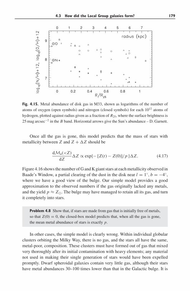
4.3 How did the Local Group galaxies form? 179

0 1 2 3 4 5 6 7

0 0.2 0.4 0.6 0.8 1

7

8

9

Fig. 4.15. Metal abundance of disk gas in M33, shown as logarithms of the number of

atoms of oxygen (open symbols) and nitrogen (closed symbols) for each 1012 atoms of

hydrogen, plotted against radius given as a fraction of R25, where the surface brightness is

25 mag arcsec−2 in the B band. Horizontal arrows give the Sun’s abundance – D. Garnett.

Once all the gas is gone, this model predicts that the mass of stars withmetallicity between Z and Z + �Z should be

dM(<Z )

dZ�Z ∝ exp{− [Z (t) − Z (0)]/p }�Z . (4.17)

Figure 4.16 shows the number of G and K giant stars at each metallicity observed inBaade’s Window, a partial clearing of the dust in the disk near l = 1◦, b = −4◦,where we have a good view of the bulge. Our simple model provides a goodapproximation to the observed numbers if the gas originally lacked any metals,and the yield p ≈ Z�. The bulge may have managed to retain all its gas, and turnit completely into stars.

Problem 4.8 Show that, if stars are made from gas that is initially free of metals,

so that Z (0) = 0, the closed-box model predicts that, when all the gas is gone,

the mean metal abundance of stars is exactly p.

In other cases, the simple model is clearly wrong. Within individual globularclusters orbiting the Milky Way, there is no gas, and the stars all have the same,metal-poor, composition. These clusters must have formed out of gas that mixedvery thoroughly after its initial contamination with heavy elements; any materialnot used in making their single generation of stars would have been expelledpromptly. Dwarf spheroidal galaxies contain very little gas, although their starshave metal abundances 30–100 times lower than that in the Galactic bulge. It is

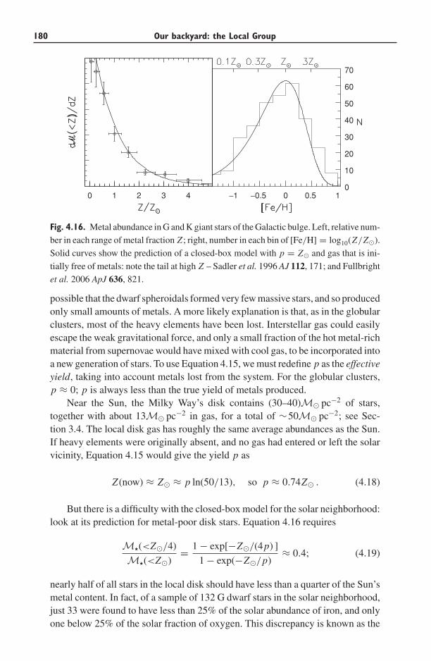
180 Our backyard: the Local Group

−1 −0.5 0 0.5 10

10

20

30

40

50

60

70

0 1 2 3 4

Fig. 4.16. Metal abundance in G and K giant stars of the Galactic bulge. Left, relative num-

ber in each range of metal fraction Z ; right, number in each bin of [Fe/H] = log10(Z/Z�).

Solid curves show the prediction of a closed-box model with p = Z� and gas that is ini-

tially free of metals: note the tail at high Z – Sadler et al. 1996 AJ 112, 171; and Fullbright

et al. 2006 ApJ 636, 821.

possible that the dwarf spheroidals formed very few massive stars, and so producedonly small amounts of metals. A more likely explanation is that, as in the globularclusters, most of the heavy elements have been lost. Interstellar gas could easilyescape the weak gravitational force, and only a small fraction of the hot metal-richmaterial from supernovae would have mixed with cool gas, to be incorporated intoa new generation of stars. To use Equation 4.15, we must redefine p as the effectiveyield, taking into account metals lost from the system. For the globular clusters,p ≈ 0; p is always less than the true yield of metals produced.

Near the Sun, the Milky Way’s disk contains (30–40)M� pc−2 of stars,together with about 13M� pc−2 in gas, for a total of ∼50M� pc−2; see Sec-tion 3.4. The local disk gas has roughly the same average abundances as the Sun.If heavy elements were originally absent, and no gas had entered or left the solarvicinity, Equation 4.15 would give the yield p as

Z (now) ≈ Z� ≈ p ln(50/13), so p ≈ 0.74Z� . (4.18)

But there is a difficulty with the closed-box model for the solar neighborhood:look at its prediction for metal-poor disk stars. Equation 4.16 requires

M(<Z�/4)

M(<Z�)= 1 − exp[−Z�/(4p) ]

1 − exp(−Z�/p)≈ 0.4; (4.19)

nearly half of all stars in the local disk should have less than a quarter of the Sun’smetal content. In fact, of a sample of 132 G dwarf stars in the solar neighborhood,just 33 were found to have less than 25% of the solar abundance of iron, and onlyone below 25% of the solar fraction of oxygen. This discrepancy is known as the

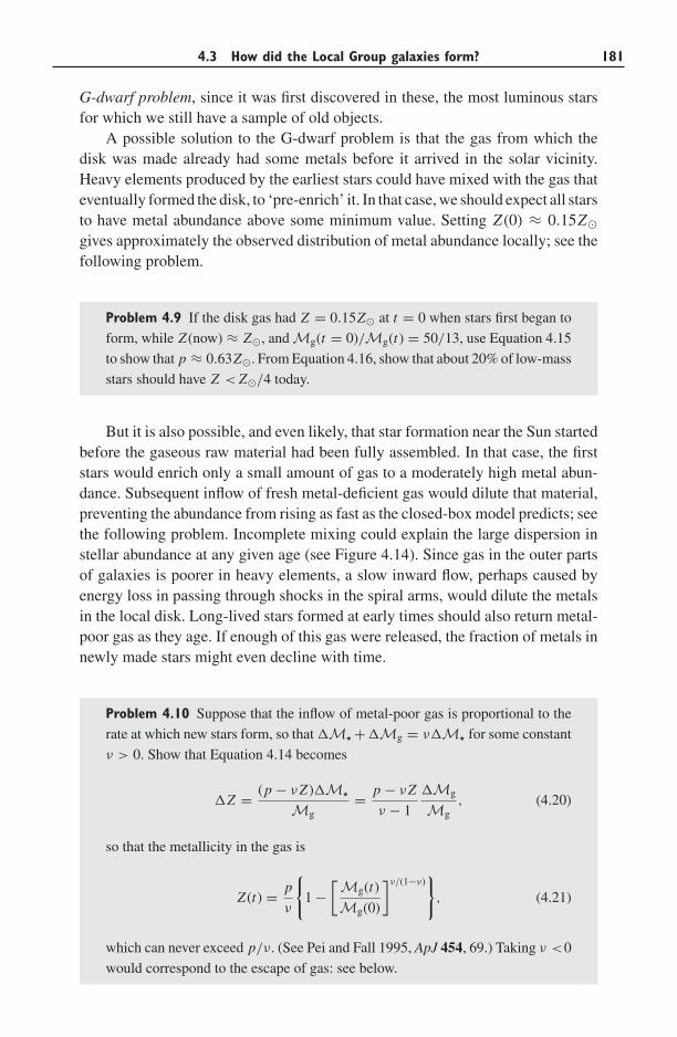
4.3 How did the Local Group galaxies form? 181

G-dwarf problem, since it was first discovered in these, the most luminous starsfor which we still have a sample of old objects.

A possible solution to the G-dwarf problem is that the gas from which thedisk was made already had some metals before it arrived in the solar vicinity.Heavy elements produced by the earliest stars could have mixed with the gas thateventually formed the disk, to ‘pre-enrich’ it. In that case, we should expect all starsto have metal abundance above some minimum value. Setting Z (0) ≈ 0.15Z�gives approximately the observed distribution of metal abundance locally; see thefollowing problem.

Problem 4.9 If the disk gas had Z = 0.15Z� at t = 0 when stars first began to

form, while Z (now) ≈ Z�, and Mg(t = 0)/Mg(t) = 50/13, use Equation 4.15

to show that p ≈ 0.63Z�. From Equation 4.16, show that about 20% of low-mass

stars should have Z < Z�/4 today.

But it is also possible, and even likely, that star formation near the Sun startedbefore the gaseous raw material had been fully assembled. In that case, the firststars would enrich only a small amount of gas to a moderately high metal abun-dance. Subsequent inflow of fresh metal-deficient gas would dilute that material,preventing the abundance from rising as fast as the closed-box model predicts; seethe following problem. Incomplete mixing could explain the large dispersion instellar abundance at any given age (see Figure 4.14). Since gas in the outer partsof galaxies is poorer in heavy elements, a slow inward flow, perhaps caused byenergy loss in passing through shocks in the spiral arms, would dilute the metalsin the local disk. Long-lived stars formed at early times should also return metal-poor gas as they age. If enough of this gas were released, the fraction of metals innewly made stars might even decline with time.

Problem 4.10 Suppose that the inflow of metal-poor gas is proportional to the

rate at which new stars form, so that �M +�Mg = ν�M for some constant

ν > 0. Show that Equation 4.14 becomes

�Z = (p − νZ )�M

Mg= p − νZ

ν − 1

�Mg

Mg, (4.20)

so that the metallicity in the gas is

Z (t) = p

ν

{1 −

[Mg(t)

Mg(0)

]ν/(1−ν)}

, (4.21)

which can never exceed p/ν. (See Pei and Fall 1995, ApJ 454, 69.) Taking ν <0

would correspond to the escape of gas: see below.

182 Our backyard: the Local Group

0.001 0.01 0.1 1

1

10

5

−3 −2 −1 0

0

0.5

1

Fig. 4.17. Oxygen is more abundant relative to iron in metal-poor stars. Filled dots show

stars of the Milky Way’s halo, open dots represent thick-disk stars, following a slightly

different relation from that for the thin-disk stars (star symbols) – T. Bensby.

The abundances of heavy elements vary relative to each other: Figure 4.17shows that stars with low metal abundance have more oxygen relative to the amountof iron than do stars like the Sun. This happens because these elements are madein stars of different masses. Stars more massive than 10M� end their lives byexploding as a Type II supernova. They release mainly lighter elements with fewerthan about 30 neutrons and protons, such as oxygen, silicon, and magnesium, backinto the interstellar gas. Most of the heavier nuclei such as iron, which are made inthe star’s core, are swallowed up into the remnant neutron star or black hole. Thesemassive stars go through their lives within 100 Myr, whereas the local disk hasmade its stars fairly steadily over the last 8–10 Gyr; so the instantaneous-recyclingassumption is reasonable.

Not all of the ‘lighter’ heavy elements are produced in very massive stars.Stars only slightly more massive than the Sun do not become supernovae, but addcarbon and nitrogen to the interstellar gas. These elements are produced duringhelium burning, and the stars dredge them up into the envelope during heliumflashes. Later, at the tip of the asymptotic giant branch, those outer layers areejected; see Section 1.1. Carbon and silicates often condense as dust grains in thecool stellar atmosphere. These stars often take far longer than 100 Myr to maketheir contribution to the Galaxy’s store of heavy elements.

The main source of iron is supernovae of Type Ia. We saw in Section 1.1 thatthese occur when a white dwarf in a binary system collapses under its own gravity.If matter is added to a white dwarf in a binary system, taking its mass above theChandrasekhar limit of 1.4M�, it can no longer support its own weight, and itimplodes. This heats the interior, triggering nuclear burning, which blows the starapart. No remnant is left; all the iron, nickel, and elements of similar atomic massare released back to the interstellar gas. Many of the stars that explode as Type Ia

4.4 Dwarf galaxies in the Local Group 183

supernovae do so only at ages of a gigayear or more; instantaneous recycling is apoor approximation. In stars formed during the first few gigayears of a galaxy’slife, we expect the ratio of elements such as oxygen and magnesium to iron to behigher than it is in the Sun.

To predict the metal abundance of stars in a galaxy, we first need to estimate thebirthrate of stars at each mass. We can then calculate how much of each element isreleased back to the interstellar gas over time. In the Milky Way, long-lived starsthat were born soon after the disk formed are now returning metal-poor gas, sothe abundance of heavy elements in the gas is growing only slowly. The chemicalcomposition of the new stars also depends on how gas moves within the galaxy,since Figure 4.15 shows that the clock of metal enrichment runs more slowlyin the outer regions. We require chemodynamical models, which are still underdevelopment.

Further reading: for a graduate-level treatment of this subject, see B. E. J. Pagel,1997, Nucleosynthesis and Chemical Evolution of Galaxies (Cambridge Univer-sity Press, Cambridge, UK) Chapters 7 and 8; and D. Arnett, 1996, Supernovaeand Nucleosynthesis (Princeton University Press, Princeton, New Jersey).

4.4 Dwarf galaxies in the Local Group

The Local Group contains two main types of dwarf galaxies. In galaxies of the firsttype, the dwarf ellipticals and the much more diffuse dwarf spheroidals, almostall the stars are at least a few gigayears old. These systems contain little gas tomake any new stars. By contrast, dwarf irregulars are tiny, gas-rich galaxies withactive star formation, and a profusion of recently formed blue stars. Like the dwarfspheroidals of Section 4.1, the dwarf irregulars are diffuse systems. While all theLocal Group’s dwarf ellipticals, and most of its dwarf spheroidal galaxies, orbiteither the Milky Way or M31, many of the dwarf irregulars are not satellites oflarger systems, but ‘free fliers’. We can use color–magnitude diagrams to chartthe star-forming histories of these different varieties of dwarf, and to investigatethe relationship between them.

Remarkably, all the dwarf galaxies of the Local Group contain some stars onthe horizontal branch, which may include RR Lyrae variables. Horizontal branchstars are at least 10 Gyr old, so the dwarf galaxies made their first stars in the first2–3 Gyr of cosmic history. We will see in Section 8.5 that cosmological modelswith cold dark matter predict exactly this behavior.

4.4.1 Dwarf ellipticals and dwarf spheroidals

We discussed the Milky Way’s dwarf spheroidals in Section 4.1: they are not muchmore luminous than a globular cluster, but so diffuse as to be almost invisible onthe sky. Andromeda’s dwarf spheroidals are yet harder to observe; they appear to

184 Our backyard: the Local Group

be very similar to our own. The dwarf ellipticals are more luminous versions of thedwarf spheroidals, with L ∼>3 × 107L� or MV ∼< −14. In the Local Group, theyare represented by three of M31’s satellites: NGC 147, NGC 185, and NGC 205.Table 4.2 shows that their sizes are similar to those of the dwarf spheroidals, butthey are more luminous, so the stellar density is higher.

Because they are close to Andromeda, the dwarf ellipticals are vulnerable totidal damage. In NGC 205 the random speed of the stars is greater at larger radii,instead of being smaller as Equation 3.47 would imply for an isolated galaxy,because M31 is pulling at the outer stars. Both dwarf spheroidals and dwarfellipticals appear quite oval on the sky rather than round, yet their stars show nopattern of ordered rotation. We will see in Section 6.2 that these galaxies mayhave no axis of symmetry; their shapes are probably triaxial.

Both NGC 205 and NGC 185 show a few patches of dust, and we can tracesmall amounts of cool gas by its HI and CO emission. Most of the stars in thesetwo dwarf ellipticals date from at least 5 Gyr ago. Near the center, however, asmall number (amounting to no more than 106M�) have ages between 100 and500 Myr; gas lost by the old stars may have supplied the raw material for continuedstarbirth. By contrast, NGC 147, although otherwise similar, shows no sign of veryrecent star formation. Its nuclear region contains a very few stars in early middleage, born only a few gigayears ago. In the outer parts, the overwhelming majorityis at least 5 Gyr old.

M32, the most luminous satellite of M31, contains virtually no cool gas andhas no stars younger than a few gigayears. But Figure 4.18 shows its centralbrightness to be one of the highest yet measured for any galaxy. High-resolutionimages from the Hubble Space Telescope reveal no constant-brightness inner core;the density continues to climb, to ∼>106L� pc−3 within the central parsec. A blackhole of a few million solar masses may lurk at its center. Although its luminosityis within the normal range for dwarf ellipticals, its very high density suggests thatM32 is a miniature version of a normal or ‘giant’ elliptical galaxy.

Perhaps M32 is only the remnant center of a much larger galaxy. It lacksglobular clusters, whereas the less luminous dwarf elliptical satellites of M31 dohave them. The stars at its center are red, and approximately as rich as the Sun inheavy elements; this is typical of more massive galaxies, that have stronger gravityto confine metal-rich gas from exploding stars; see Section 6.4. The outer regionsof M32 still have an elliptical shape, but its long axis is twisted away from thatof the inner regions. Tidal forces of M31 have probably affected the orbits of theoutermost stars. We cannot yet measure the distances well enough to know howfar M32 is from M31, or whether it could have passed close enough for M31’sgravity to strip off the outer stars, as described in Section 4.1.

The motion of the stars in M32 is intermediate between that in the disk ofthe Milky Way and that in its metal-poor halo. The galaxy is slightly flattened,and its stars orbit in a common direction, but they also have considerable randommotions. We can measure the degree of ordered rotation in a galaxy by the ratio

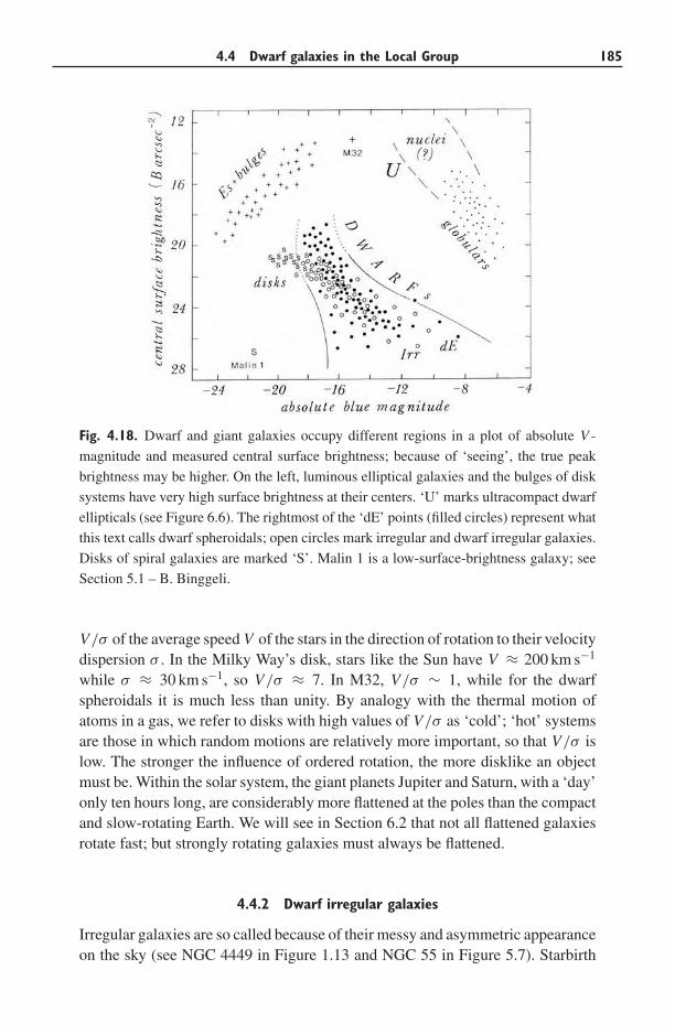
4.4 Dwarf galaxies in the Local Group 185

Fig. 4.18. Dwarf and giant galaxies occupy different regions in a plot of absolute V -

magnitude and measured central surface brightness; because of ‘seeing’, the true peak

brightness may be higher. On the left, luminous elliptical galaxies and the bulges of disk

systems have very high surface brightness at their centers. ‘U’ marks ultracompact dwarf

ellipticals (see Figure 6.6). The rightmost of the ‘dE’ points (filled circles) represent what

this text calls dwarf spheroidals; open circles mark irregular and dwarf irregular galaxies.

Disks of spiral galaxies are marked ‘S’. Malin 1 is a low-surface-brightness galaxy; see

Section 5.1 – B. Binggeli.

V/σ of the average speed V of the stars in the direction of rotation to their velocitydispersion σ . In the Milky Way’s disk, stars like the Sun have V ≈ 200 km s−1

while σ ≈ 30 km s−1, so V/σ ≈ 7. In M32, V/σ ∼ 1, while for the dwarfspheroidals it is much less than unity. By analogy with the thermal motion ofatoms in a gas, we refer to disks with high values of V/σ as ‘cold’; ‘hot’ systemsare those in which random motions are relatively more important, so that V/σ islow. The stronger the influence of ordered rotation, the more disklike an objectmust be. Within the solar system, the giant planets Jupiter and Saturn, with a ‘day’only ten hours long, are considerably more flattened at the poles than the compactand slow-rotating Earth. We will see in Section 6.2 that not all flattened galaxiesrotate fast; but strongly rotating galaxies must always be flattened.

4.4.2 Dwarf irregular galaxies

Irregular galaxies are so called because of their messy and asymmetric appearanceon the sky (see NGC 4449 in Figure 1.13 and NGC 55 in Figure 5.7). Starbirth

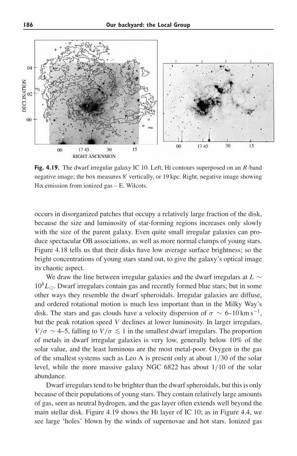
186 Our backyard: the Local Group

Fig. 4.19. The dwarf irregular galaxy IC 10. Left, HI contours superposed on an R-band

negative image; the box measures 8′ vertically, or 19 kpc. Right, negative image showing

Hα emission from ionized gas – E. Wilcots.

occurs in disorganized patches that occupy a relatively large fraction of the disk,because the size and luminosity of star-forming regions increases only slowlywith the size of the parent galaxy. Even quite small irregular galaxies can pro-duce spectacular OB associations, as well as more normal clumps of young stars.Figure 4.18 tells us that their disks have low average surface brightness; so thebright concentrations of young stars stand out, to give the galaxy’s optical imageits chaotic aspect.

We draw the line between irregular galaxies and the dwarf irregulars at L ∼108L�. Dwarf irregulars contain gas and recently formed blue stars; but in someother ways they resemble the dwarf spheroidals. Irregular galaxies are diffuse,and ordered rotational motion is much less important than in the Milky Way’sdisk. The stars and gas clouds have a velocity dispersion of σ ∼ 6–10 km s−1,but the peak rotation speed V declines at lower luminosity. In larger irregulars,V/σ ∼ 4–5, falling to V/σ ∼< 1 in the smallest dwarf irregulars. The proportionof metals in dwarf irregular galaxies is very low, generally below 10% of thesolar value, and the least luminous are the most metal-poor. Oxygen in the gasof the smallest systems such as Leo A is present only at about 1/30 of the solarlevel, while the more massive galaxy NGC 6822 has about 1/10 of the solarabundance.

Dwarf irregulars tend to be brighter than the dwarf spheroidals, but this is onlybecause of their populations of young stars. They contain relatively large amountsof gas, seen as neutral hydrogen, and the gas layer often extends well beyond themain stellar disk. Figure 4.19 shows the HI layer of IC 10; as in Figure 4.4, wesee large ‘holes’ blown by the winds of supernovae and hot stars. Ionized gas

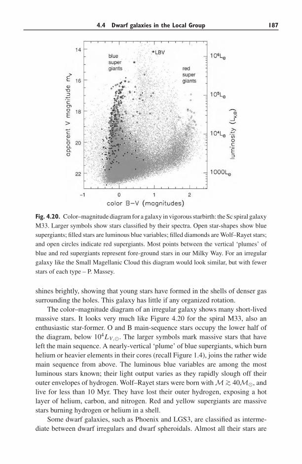
4.4 Dwarf galaxies in the Local Group 187

Fig. 4.20. Color–magnitude diagram for a galaxy in vigorous starbirth: the Sc spiral galaxy

M33. Larger symbols show stars classified by their spectra. Open star-shapes show blue

supergiants; filled stars are luminous blue variables; filled diamonds are Wolf–Rayet stars;

and open circles indicate red supergiants. Most points between the vertical ‘plumes’ of

blue and red supergiants represent fore-ground stars in our Milky Way. For an irregular

galaxy like the Small Magellanic Cloud this diagram would look similar, but with fewer

stars of each type – P. Massey.

shines brightly, showing that young stars have formed in the shells of denser gassurrounding the holes. This galaxy has little if any organized rotation.

The color–magnitude diagram of an irregular galaxy shows many short-livedmassive stars. It looks very much like Figure 4.20 for the spiral M33, also anenthusiastic star-former. O and B main-sequence stars occupy the lower half ofthe diagram, below 104LV,�. The larger symbols mark massive stars that haveleft the main sequence. A nearly-vertical ‘plume’ of blue supergiants, which burnhelium or heavier elements in their cores (recall Figure 1.4), joins the rather widemain sequence from above. The luminous blue variables are among the mostluminous stars known; their light output varies as they rapidly slough off theirouter envelopes of hydrogen. Wolf–Rayet stars were born with M ∼> 40M�, andlive for less than 10 Myr. They have lost their outer hydrogen, exposing a hotlayer of helium, carbon, and nitrogen. Red and yellow supergiants are massivestars burning hydrogen or helium in a shell.

Some dwarf galaxies, such as Phoenix and LGS3, are classified as interme-diate between dwarf irregulars and dwarf spheroidals. Almost all their stars are

188 Our backyard: the Local Group

more than a few gigayears old, but they contain a little gas and a few young stars.Fornax has a few stars as young as 500 Myr, so this dwarf spheroidal galaxy musthave had some gas until quite recently. The Carina dwarf spheroidal made mostof its stars in a few discrete episodes (see Figure 4.9); at times of peak starbirth itmay have been a miniature version of Sextans A. Because of their similar struc-tures, small irregulars like the Pegasus dwarf may be at an early stage, while dwarfspheroidals represent the late stages, in the life of a similar type of galaxy. In thedwarf spheroidals, which orbit close to the Galaxy or M31, gas may have been com-pressed by interactions with these large galaxies, perhaps encouraging more starsto form earlier on. By now these galaxies have used up or blown out all their gas,while the dwarf irregulars, perhaps benefiting from a quieter life, still retain theirs.

Galaxies such as the LMC might represent a transitional class between spiralgalaxies and the dwarf irregulars. Like a spiral galaxy, the LMC is basicallya rotating disk, but it lacks regular or symmetric spiral structure, and randommotions account for more of the kinetic energy of stars and gas: V/σ ∼ 4 forthe old stars. The brightest region of the LMC, the central bar, is off center withrespect to the outer part of the disk; such lopsidedness is also common in dwarfirregulars. The neutral-hydrogen layer of the LMC has ‘holes’ similar to those inIC 10, but they are smaller in proportion to the galaxy’s size.

In the Local Group and beyond, dwarf galaxies are not simply smaller or lessluminous versions of bigger and brighter galaxies. Table 4.2 shows that dwarfelliptical galaxies all have about the same physical size; the core radius is alwaysrc ∼ 200 pc. Thus Figure 4.18 implies that the more luminous dwarfs have highersurface brightness. But, among the normal or ‘giant’ ellipticals, the most luminousgalaxies are also the most diffuse. We will see in Section 6.1 that the core radius isso much larger at higher luminosity that among these the central surface brightnessis lower in the most luminous systems. Because of these contrasting trends, wethink that dwarf galaxies probably developed by processes different from thosethat produced the giant spiral and elliptical galaxies.

4.5 The past and future of the Local Group

The galaxies of the Local Group are no longer expanding away from each otheraccording to Hubble’s law. Their mutual gravitational attraction, and that of anymatter present between the galaxies, has been strong enough to pull the groupmembers back toward each other. The Milky Way and M31 are now approachingeach other; these two galaxies will probably come near to a head-on collisionwithin a few gigayears. We can use the orbits to make an estimate of the totalmass within the Local Group. Readers will not be surprised that this analysisreveals yet more ‘dark matter’.

We start by assuming that all the mass of the Local Group lies in or very closeto the Milky Way or M31, and we treat these two galaxies as point masses m and

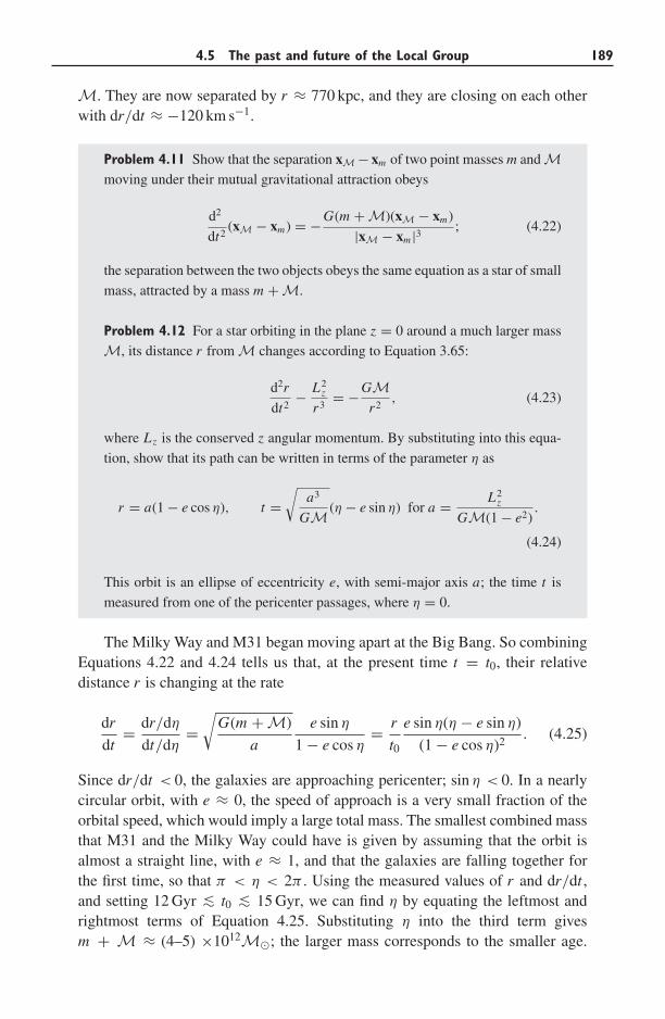
4.5 The past and future of the Local Group 189

M. They are now separated by r ≈ 770 kpc, and they are closing on each otherwith dr/dt ≈ −120 km s−1.

Problem 4.11 Show that the separation xM − xm of two point masses m and Mmoving under their mutual gravitational attraction obeys

d2

dt2(xM − xm) = −G(m + M)(xM − xm)

|xM − xm |3 ; (4.22)

the separation between the two objects obeys the same equation as a star of small

mass, attracted by a mass m + M.

Problem 4.12 For a star orbiting in the plane z = 0 around a much larger mass

M, its distance r from M changes according to Equation 3.65:

d2r

dt2− L2

z

r3= −GM

r2, (4.23)

where Lz is the conserved z angular momentum. By substituting into this equa-

tion, show that its path can be written in terms of the parameter η as

r = a(1 − e cos η), t =√

a3

GM (η − e sin η) for a = L2z

GM(1 − e2).

(4.24)

This orbit is an ellipse of eccentricity e, with semi-major axis a; the time t is

measured from one of the pericenter passages, where η = 0.

The Milky Way and M31 began moving apart at the Big Bang. So combiningEquations 4.22 and 4.24 tells us that, at the present time t = t0, their relativedistance r is changing at the rate

dr

dt= dr/dη

dt/dη=√

G(m + M)

a

e sin η

1 − e cos η= r

t0

e sin η(η − e sin η)

(1 − e cos η)2. (4.25)

Since dr/dt < 0, the galaxies are approaching pericenter; sin η < 0. In a nearlycircular orbit, with e ≈ 0, the speed of approach is a very small fraction of theorbital speed, which would imply a large total mass. The smallest combined massthat M31 and the Milky Way could have is given by assuming that the orbit isalmost a straight line, with e ≈ 1, and that the galaxies are falling together forthe first time, so that π < η < 2π . Using the measured values of r and dr/dt ,and setting 12 Gyr ∼< t0 ∼< 15 Gyr, we can find η by equating the leftmost andrightmost terms of Equation 4.25. Substituting η into the third term givesm + M ≈ (4–5) ×1012M�; the larger mass corresponds to the smaller age.

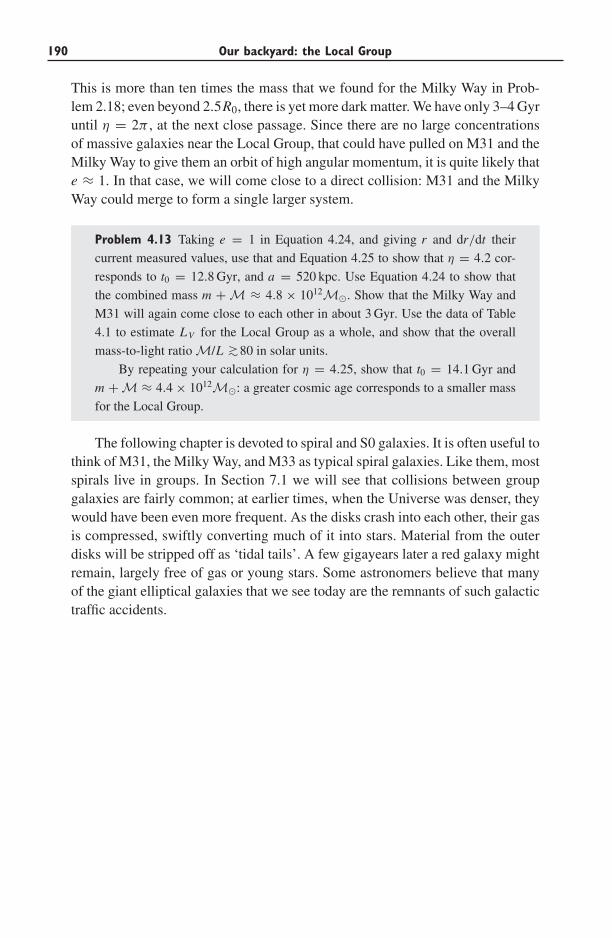
190 Our backyard: the Local Group

This is more than ten times the mass that we found for the Milky Way in Prob-lem 2.18; even beyond 2.5R0, there is yet more dark matter. We have only 3–4 Gyruntil η = 2π , at the next close passage. Since there are no large concentrationsof massive galaxies near the Local Group, that could have pulled on M31 and theMilky Way to give them an orbit of high angular momentum, it is quite likely thate ≈ 1. In that case, we will come close to a direct collision: M31 and the MilkyWay could merge to form a single larger system.

Problem 4.13 Taking e = 1 in Equation 4.24, and giving r and dr/dt their

current measured values, use that and Equation 4.25 to show that η = 4.2 cor-

responds to t0 = 12.8 Gyr, and a = 520 kpc. Use Equation 4.24 to show that

the combined mass m + M ≈ 4.8 × 1012M�. Show that the Milky Way and

M31 will again come close to each other in about 3 Gyr. Use the data of Table

4.1 to estimate LV for the Local Group as a whole, and show that the overall

mass-to-light ratio M/L ∼>80 in solar units.

By repeating your calculation for η = 4.25, show that t0 = 14.1 Gyr and

m + M ≈ 4.4 × 1012M�: a greater cosmic age corresponds to a smaller mass

for the Local Group.

The following chapter is devoted to spiral and S0 galaxies. It is often useful tothink of M31, the Milky Way, and M33 as typical spiral galaxies. Like them, mostspirals live in groups. In Section 7.1 we will see that collisions between groupgalaxies are fairly common; at earlier times, when the Universe was denser, theywould have been even more frequent. As the disks crash into each other, their gasis compressed, swiftly converting much of it into stars. Material from the outerdisks will be stripped off as ‘tidal tails’. A few gigayears later a red galaxy mightremain, largely free of gas or young stars. Some astronomers believe that manyof the giant elliptical galaxies that we see today are the remnants of such galactictraffic accidents.

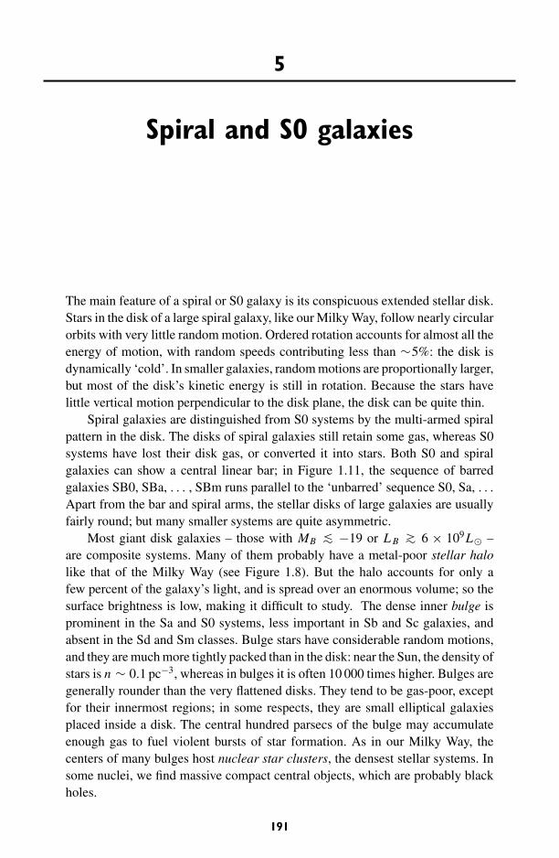
5

Spiral and S0 galaxies

The main feature of a spiral or S0 galaxy is its conspicuous extended stellar disk.Stars in the disk of a large spiral galaxy, like our Milky Way, follow nearly circularorbits with very little random motion. Ordered rotation accounts for almost all theenergy of motion, with random speeds contributing less than ∼5%: the disk isdynamically ‘cold’. In smaller galaxies, random motions are proportionally larger,but most of the disk’s kinetic energy is still in rotation. Because the stars havelittle vertical motion perpendicular to the disk plane, the disk can be quite thin.

Spiral galaxies are distinguished from S0 systems by the multi-armed spiralpattern in the disk. The disks of spiral galaxies still retain some gas, whereas S0systems have lost their disk gas, or converted it into stars. Both S0 and spiralgalaxies can show a central linear bar; in Figure 1.11, the sequence of barredgalaxies SB0, SBa, . . . , SBm runs parallel to the ‘unbarred’ sequence S0, Sa, . . .

Apart from the bar and spiral arms, the stellar disks of large galaxies are usuallyfairly round; but many smaller systems are quite asymmetric.

Most giant disk galaxies – those with MB ∼< −19 or L B ∼> 6 × 109L� –are composite systems. Many of them probably have a metal-poor stellar halolike that of the Milky Way (see Figure 1.8). But the halo accounts for only afew percent of the galaxy’s light, and is spread over an enormous volume; so thesurface brightness is low, making it difficult to study. The dense inner bulge isprominent in the Sa and S0 systems, less important in Sb and Sc galaxies, andabsent in the Sd and Sm classes. Bulge stars have considerable random motions,and they are much more tightly packed than in the disk: near the Sun, the density ofstars is n ∼ 0.1 pc−3, whereas in bulges it is often 10 000 times higher. Bulges aregenerally rounder than the very flattened disks. They tend to be gas-poor, exceptfor their innermost regions; in some respects, they are small elliptical galaxiesplaced inside a disk. The central hundred parsecs of the bulge may accumulateenough gas to fuel violent bursts of star formation. As in our Milky Way, thecenters of many bulges host nuclear star clusters, the densest stellar systems. Insome nuclei, we find massive compact central objects, which are probably blackholes.

191

192 Spiral and S0 galaxies

Spirals are the most common of the giant galaxies, and produce most of thevisible light in the local Universe. In the opening section we investigate the stellarcontent of the disks of spiral and S0 galaxies; Section 5.2 considers the gaseouscomponent, and its relationship to the stars. In Section 5.3 we discuss the rotationcurves of spiral galaxies, and what these reveal about the gravitational forces. Inmost spirals, the force required to maintain the outermost disk material in its orbitcannot be accounted for by the visible portion of the galaxy, its stars and gas. Thedifference is attributed to ‘dark’ material, which we detect only by its gravity.We then pause, in Section 5.4, to consider how much the scheme of Figure 1.11,classifying galaxies according to their appearance in visible light, can tell us abouttheir other properties. Spiral arms and galactic bars form the topic of Section 5.5;these common and prominent features prove surprisingly difficult to understand.In Section 5.6 we discuss bulges and nuclei, and speculate on how they are relatedto the rest of the galaxy.

5.1 The distribution of starlight

The light coming to us directly from the stars of present-day disk galaxies ismainly in the near-infrared region of the spectrum: old stars, such as K giants, giveout most of their light at wavelengths close to 1μm. Much of the blue light of hotmassive stars is intercepted by surrounding dust, and re-radiated in the far-infrared,beyond ∼10 μm. Visible light is next in importance; ultraviolet photons do notcarry much of the energy, except in irregular galaxies where dust is less plentiful,and the light of young hot stars more easily escapes absorption. Historically,galaxies have been studied mainly by optical photography. Although infrareddetectors are rapidly improving, optical images still yield most of our informationabout galactic structure.

5.1.1 Astronomical array detectors

The standard detector for optical extragalactic astronomy is now the charge-coupled device, or CCD; the same devices are used to record images in mod-ern video and electronic cameras. A CCD consists of a thin silicon wafer thatwill absorb light (Figure 5.1). A photon’s energy sets free one or more electron–hole pairs; the electrons are collected and amplified, to produce an output signalthat should be linearly proportional to the number of photons absorbed. Not everyincoming photon produces an electron–hole pair; we define the quantum efficiencyas the ratio of detected photoelectrons to incident photons. In an excellent CCD,quantum efficiency can peak above 90%, for red light with 5000 A ∼< λ ∼< 7000 A.CCDs are analogue detectors: photons are converted into a current which isthen amplified, rather than measured individually as they are in photon-countingsystems such as photomultiplier tubes.

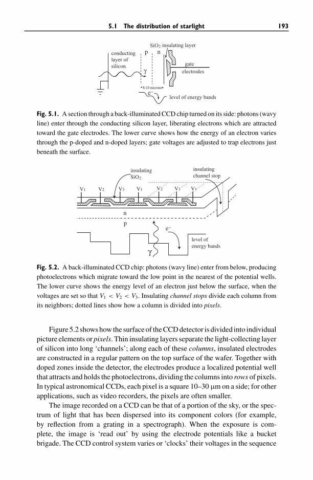
5.1 The distribution of starlight 193

8-10 microns

p n

γgate

e−

insulating layer

electrodes

level of energy bands

conductinglayer ofsilicon

2SiO

Fig. 5.1. A section through a back-illuminated CCD chip turned on its side: photons (wavy

line) enter through the conducting silicon layer, liberating electrons which are attracted

toward the gate electrodes. The lower curve shows how the energy of an electron varies

through the p-doped and n-doped layers; gate voltages are adjusted to trap electrons just

beneath the surface.

insulatingSiO2

V1 V2 V3

insulatingchannel stop

level ofenergy bands

e−

n

p

γ

V1V1 V3V2

Fig. 5.2. A back-illuminated CCD chip: photons (wavy line) enter from below, producing

photoelectrons which migrate toward the low point in the nearest of the potential wells.

The lower curve shows the energy level of an electron just below the surface, when the

voltages are set so that V1 < V2 < V3. Insulating channel stops divide each column from

its neighbors; dotted lines show how a column is divided into pixels.

Figure 5.2 shows how the surface of the CCD detector is divided into individualpicture elements or pixels. Thin insulating layers separate the light-collecting layerof silicon into long ‘channels’; along each of these columns, insulated electrodesare constructed in a regular pattern on the top surface of the wafer. Together withdoped zones inside the detector, the electrodes produce a localized potential wellthat attracts and holds the photoelectrons, dividing the columns into rows of pixels.In typical astronomical CCDs, each pixel is a square 10–30 μm on a side; for otherapplications, such as video recorders, the pixels are often smaller.

The image recorded on a CCD can be that of a portion of the sky, or the spec-trum of light that has been dispersed into its component colors (for example,by reflection from a grating in a spectrograph). When the exposure is com-plete, the image is ‘read out’ by using the electrode potentials like a bucketbrigade. The CCD control system varies or ‘clocks’ their voltages in the sequence

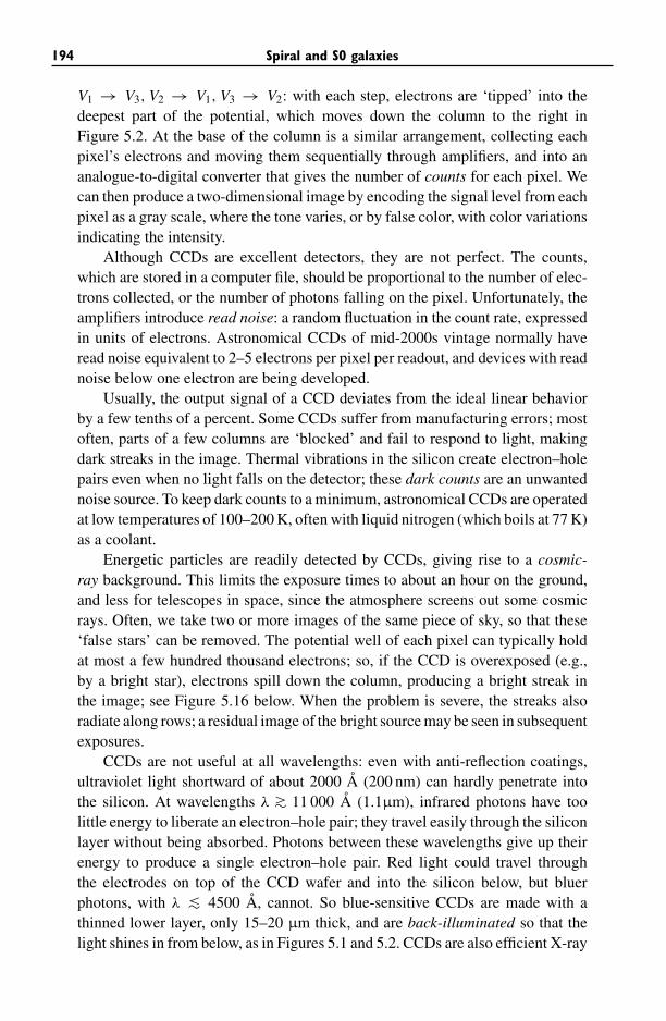
194 Spiral and S0 galaxies

V1 → V3, V2 → V1, V3 → V2: with each step, electrons are ‘tipped’ into thedeepest part of the potential, which moves down the column to the right inFigure 5.2. At the base of the column is a similar arrangement, collecting eachpixel’s electrons and moving them sequentially through amplifiers, and into ananalogue-to-digital converter that gives the number of counts for each pixel. Wecan then produce a two-dimensional image by encoding the signal level from eachpixel as a gray scale, where the tone varies, or by false color, with color variationsindicating the intensity.

Although CCDs are excellent detectors, they are not perfect. The counts,which are stored in a computer file, should be proportional to the number of elec-trons collected, or the number of photons falling on the pixel. Unfortunately, theamplifiers introduce read noise: a random fluctuation in the count rate, expressedin units of electrons. Astronomical CCDs of mid-2000s vintage normally haveread noise equivalent to 2–5 electrons per pixel per readout, and devices with readnoise below one electron are being developed.

Usually, the output signal of a CCD deviates from the ideal linear behaviorby a few tenths of a percent. Some CCDs suffer from manufacturing errors; mostoften, parts of a few columns are ‘blocked’ and fail to respond to light, makingdark streaks in the image. Thermal vibrations in the silicon create electron–holepairs even when no light falls on the detector; these dark counts are an unwantednoise source. To keep dark counts to a minimum, astronomical CCDs are operatedat low temperatures of 100–200 K, often with liquid nitrogen (which boils at 77 K)as a coolant.

Energetic particles are readily detected by CCDs, giving rise to a cosmic-ray background. This limits the exposure times to about an hour on the ground,and less for telescopes in space, since the atmosphere screens out some cosmicrays. Often, we take two or more images of the same piece of sky, so that these‘false stars’ can be removed. The potential well of each pixel can typically holdat most a few hundred thousand electrons; so, if the CCD is overexposed (e.g.,by a bright star), electrons spill down the column, producing a bright streak inthe image; see Figure 5.16 below. When the problem is severe, the streaks alsoradiate along rows; a residual image of the bright source may be seen in subsequentexposures.

CCDs are not useful at all wavelengths: even with anti-reflection coatings,ultraviolet light shortward of about 2000 A (200 nm) can hardly penetrate intothe silicon. At wavelengths λ ∼> 11 000 A (1.1μm), infrared photons have toolittle energy to liberate an electron–hole pair; they travel easily through the siliconlayer without being absorbed. Photons between these wavelengths give up theirenergy to produce a single electron–hole pair. Red light could travel throughthe electrodes on top of the CCD wafer and into the silicon below, but bluerphotons, with λ ∼< 4500 A, cannot. So blue-sensitive CCDs are made with athinned lower layer, only 15–20 μm thick, and are back-illuminated so that thelight shines in from below, as in Figures 5.1 and 5.2. CCDs are also efficient X-ray

5.1 The distribution of starlight 195

detectors; at wavelengths below 1000 A, each photon produces many electron–hole pairs. The number of electrons is proportional to the photon energy, so theCCD also provides spectral information. In this respect, energetic particles likecosmic rays behave similarly to X-rays, and CCDs are sometimes used to detectthem.

When measuring light from an object using a CCD, the astronomer mustcompensate for the fact that the pixels are not exactly uniform: some are moresensitive than others. Flat fields, images of blank twilight sky, or a diffuse screen(often called the ‘white spot’) on the interior of the telescope dome, are taken tomeasure and to correct for this effect. The CCD must be calibrated, by observingstars of known brightness to determine how many counts correspond to a givenflux or magnitude. To produce an image of a galaxy, we must subtract out thecontribution of the night sky, since only the brightest parts of galaxies are brighterthan the sky: see Section 1.3. We routinely measure surface brightnesses downto ∼< 1% of the sky level by using dome or sky flat fields. Special techniques arerequired to do much better, because the CCD’s sensitivity changes slowly duringthe night, limiting the accuracy of the flat fields.

We can estimate the quality of measurements with a CCD by calculatinga signal-to-noise ratio, S/N . The simplest case is when statistical noise in thenumber of detected photons is the main source of error. We say that the CCDhas a gain g if a signal with C counts in some pixel corresponds to S detectedphotons (or equivalently, S electrons captured), where S = gC . The number ofphotons arriving at that pixel from the galaxy under study has a random fluctuationof approximately

√S; so the noise or 1σ error in S is N = √

gC . When weare photon-noise-limited, then S/N = √

gC ; this is the lowest possible level ofnoise.

The read noise R of a CCD is given in units of photoelectrons; including this,we can write S/N = gC/

√gC + R2. At low signal levels, R is the dominant noise

source; we are read-noise-limited. In this case R2 � gC and the signal-to-noiseratio S/N grows linearly with exposure time t . When photon noise dominates,S/N ∝ √

gC , which grows only as√

t , and doubling the signal-to-noise ratio of ameasurement requires that we observe four times longer. Extending this approachto include other noise sources, such as flat field errors, gives us a basis to predictthe performance of real CCDs and other similar detectors.

We may wish to measure the surface brightness I (x), the amount of lightper square arcsecond at position x in the image of a galaxy, or the flux Fλ in aspectrum. A CCD records only the total amount of light falling on each pixelduring an exposure; it gives us no information on where a photon has landedwithin the pixel. So we can measure the angular size of a feature in the imageonly if its light is spread over at least two pixels on the CCD. To produce animage of the sky showing details 1′′ across, the pixels must correspond to a size

∼< 0.5′′ on the image. Similarly, to obtain a spectrum with wavelength resolution�λ, our spectrograph must disperse light in this wavelength interval over at least

196 Spiral and S0 galaxies

two pixels on the CCD. The physical size of CCDs is limited, currently to about10 cm×10 cm; so we must compromise between high resolution and a large fieldof view. Images of objects extending over a large region on the sky are sometimesbuilt up from a mosaic of several exposures, each covering only part of the object.In using a CCD, we must match its properties to those of the instrument for whichit serves as the detector and those of the telescope; see the following problem.

Problem 5.1 You have a CCD camera with 2048 × 2048 pixels, each 24 μm

square. The angle that a pixel covers on the sky is the angle that it subtends at a

distance FL, the focal length of the telescope. This in turn depends on the focal

ratio, f , and the diameter D of the mirror: FL = f D. Show that each pixel

corresponds to 5′′/( f D), where D is in meters, and the whole CCD covers a

region 168′/( f D) across.

You can use this camera on a 0.6 m telescope with f = 7.5 (usually written

f/7.5), on a 4 m telescope at f/7.5, or at the prime focus of the 4 m telescope,

which has f/2.3. What is its pixel scale and field of view at each location? If

atmospheric seeing blurs the image to 0.8′′ across, where would you want to use

the camera in order to get the sharpest images? If you take images of a nearby

galaxy 10′ across, which option would you use to obtain a brightness profile I (x)

for the entire galaxy?

Array detectors with large numbers of pixels are used for astronomical obser-vations from X-rays into the infrared. The physical mechanisms that convert pho-tons into an electrical signal depend on the spectral region, but the basic principlesare similar to those for CCDs, and the signal-to-noise ratio S/N for an observa-tion depends similarly on the number of photons detected and the sources ofnoise within the instrument. Unlike CCDs, most of the devices used for X-ray andultraviolet observations count photons; each detected photon produces exactlyone output count, so read noise is absent. But the speed of the electronics thenlimits both the maximum rate at which photons arriving at any one pixel can becounted and the counting rate across the entire array. A photon-counting devicemay saturate when observing a bright source.

Infrared detectors, like CCDs, are analogue devices; they rely on a variety ofphysical processes. In the thermal infrared, at wavelengths ∼>2 μm, telescopes andthe Earth’s atmosphere, at temperatures ∼300 K, radiate strongly. This extra lightmust be taken into account when estimating the expected signal-to-noise ratio.Cooled telescopes in space can observe in the infrared without this unwantedbackground, but must still contend with the emission of warm dust in the solarsystem. At radio frequencies, instead of detecting photons, we take advantage ofthe wave nature of light; see Section 5.2. Our current perspective on galaxies hasbeen heavily influenced by our ability to observe at many wavelengths, spanningthe electromagnetic spectrum.

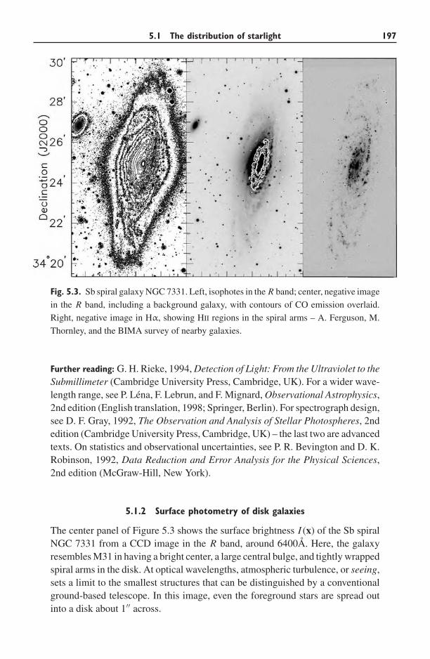
5.1 The distribution of starlight 197

Fig. 5.3. Sb spiral galaxy NGC 7331. Left, isophotes in the R band; center, negative image

in the R band, including a background galaxy, with contours of CO emission overlaid.

Right, negative image in Hα, showing HII regions in the spiral arms – A. Ferguson, M.

Thornley, and the BIMA survey of nearby galaxies.

Further reading: G. H. Rieke, 1994, Detection of Light: From the Ultraviolet to theSubmillimeter (Cambridge University Press, Cambridge, UK). For a wider wave-length range, see P. Lena, F. Lebrun, and F. Mignard, Observational Astrophysics,2nd edition (English translation, 1998; Springer, Berlin). For spectrograph design,see D. F. Gray, 1992, The Observation and Analysis of Stellar Photospheres, 2ndedition (Cambridge University Press, Cambridge, UK) – the last two are advancedtexts. On statistics and observational uncertainties, see P. R. Bevington and D. K.Robinson, 1992, Data Reduction and Error Analysis for the Physical Sciences,2nd edition (McGraw-Hill, New York).

5.1.2 Surface photometry of disk galaxies

The center panel of Figure 5.3 shows the surface brightness I (x) of the Sb spiralNGC 7331 from a CCD image in the R band, around 6400A. Here, the galaxyresembles M31 in having a bright center, a large central bulge, and tightly wrappedspiral arms in the disk. At optical wavelengths, atmospheric turbulence, or seeing,sets a limit to the smallest structures that can be distinguished by a conventionalground-based telescope. In this image, even the foreground stars are spread outinto a disk about 1′′ across.

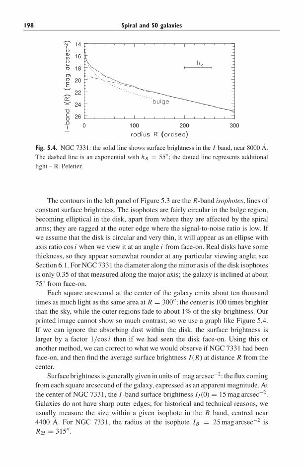
198 Spiral and S0 galaxies

0 100 200 300

26

24

22

20

18

16

14

Fig. 5.4. NGC 7331: the solid line shows surface brightness in the I band, near 8000 A.

The dashed line is an exponential with h R = 55′′; the dotted line represents additional

light – R. Peletier.

The contours in the left panel of Figure 5.3 are the R-band isophotes, lines ofconstant surface brightness. The isophotes are fairly circular in the bulge region,becoming elliptical in the disk, apart from where they are affected by the spiralarms; they are ragged at the outer edge where the signal-to-noise ratio is low. Ifwe assume that the disk is circular and very thin, it will appear as an ellipse withaxis ratio cos i when we view it at an angle i from face-on. Real disks have somethickness, so they appear somewhat rounder at any particular viewing angle; seeSection 6.1. For NGC 7331 the diameter along the minor axis of the disk isophotesis only 0.35 of that measured along the major axis; the galaxy is inclined at about75◦ from face-on.

Each square arcsecond at the center of the galaxy emits about ten thousandtimes as much light as the same area at R = 300′′; the center is 100 times brighterthan the sky, while the outer regions fade to about 1% of the sky brightness. Ourprinted image cannot show so much contrast, so we use a graph like Figure 5.4.If we can ignore the absorbing dust within the disk, the surface brightness islarger by a factor 1/cos i than if we had seen the disk face-on. Using this oranother method, we can correct to what we would observe if NGC 7331 had beenface-on, and then find the average surface brightness I (R) at distance R from thecenter.

Surface brightness is generally given in units of mag arcsec−2: the flux comingfrom each square arcsecond of the galaxy, expressed as an apparent magnitude. Atthe center of NGC 7331, the I -band surface brightness II (0) = 15 mag arcsec−2.Galaxies do not have sharp outer edges; for historical and technical reasons, weusually measure the size within a given isophote in the B band, centred near4400 A. For NGC 7331, the radius at the isophote IB = 25 mag arcsec−2 isR25 = 315′′.

5.1 The distribution of starlight 199

Problem 5.2 Show that a central surface brightness of 15 mag arcsec−2 in the

I band corresponds to 18 000L� pc−2; explain why this does not depend on

the galaxy’s distance. About how far does IB = 25 mag arcsec−2 fall below the

brightness of the night sky, given in Table 1.9?

Integrating the surface brightness over the whole of an image such as theone in Figure 5.3, and extrapolating to allow for those parts of the galaxy toofaint to measure reliably, gives the total apparent magnitude. Catalogues usuallygive these in the B band, or the V band at 5500 A. A face-on galaxy wouldbe brighter than the same galaxy seen at an angle, since starlight leaving thedisk at a slant must travel further through the absorbing layer of interstellar dustin the disk. So, to compare the true brightnesses of galaxies that we observeat different inclinations, we must try to compensate for dust dimming. Finally,we must correct for the effect of foreground dust, within our own Milky Way.Catalogues often quote total magnitudes corrected to face-on viewing, denotedby 0. For NGC 7331, the corrected total B-magnitude is B0

T = 9.37, and in V itis V 0

T = 8.75, so (B − V )0 ≈ 0.6; taken as a whole, the galaxy is about the samecolor as the Sun.

In the stellar disk, when we average over features like spiral arms, the surfacebrightness I (R) often follows approximately an exponential form,

I (R) = I (0) exp(−R/h R), (5.1)

as we expect if the density of stars in the disk varies according to the double-exponential formula of Equation 2.8. The long-dashed line in Figure 5.4 showsthe exponential slope with scale length h R = 55′′. For most disk galaxies, 1 kpc ∼<h R ∼<10 kpc. When measured in the B band rather than in I , h R is typically about20% longer because the disks become redder toward the center. The inner part ofthe disk is typically richer in heavy elements (as Figure 4.15 shows for M33), andmetal-rich stars are redder (Figure 1.5). The outer disk may have a larger fractionof young blue stars, or it may be less heavily reddened by dust; frequently it ishard to separate these effects. The exponential part of the stellar disk in many,though not all, disk galaxies appears to end at some radius Rmax, usually in therange 10–30 kpc or (3–5)h R . Beyond Rmax the surface brightness decreases moresharply; but this is not the edge of the galaxy, since HI gas and some disk starsmay be found still further out.

Problem 5.3 For NGC 7331, the radial velocity Vr = 820 km s−1; if

H0 = 60 km s−1 Mpc−1, find its distance by using Hubble’s law, Equation 1.27.

Show that its V -band luminosity LV ≈5 × 1010LV,�. Is NGC 7331 more or less

luminous than the Milky Way and M31? Show that h R ≈ 3.6 kpc. What is the disk

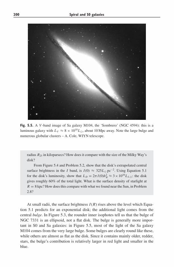
200 Spiral and S0 galaxies

Fig. 5.5. A V -band image of Sa galaxy M104, the ‘Sombrero’ (NGC 4594): this is a

luminous galaxy with LV ≈ 8 × 1010L�, about 10 Mpc away. Note the large bulge and

numerous globular clusters – A. Cole, WIYN telescope.

radius R25 in kiloparsecs? How does it compare with the size of the Milky Way’s

disk?

From Figure 5.4 and Problem 5.2, show that the disk’s extrapolated central

surface brightness in the I band, is I (0) ≈ 325L� pc−2. Using Equation 5.1

for the disk’s luminosity, show that L D = 2π I (0)h2R ≈ 3×1010L I,�: the disk

gives roughly 60% of the total light. What is the surface density of starlight at

R = 8 kpc? How does this compare with what we found near the Sun, in Problem

2.8?

At small radii, the surface brightness I (R) rises above the level which Equa-tion 5.1 predicts for an exponential disk; the additional light comes from thecentral bulge. In Figure 5.3, the rounder inner isophotes tell us that the bulge ofNGC 7331 is an ellipsoid, not a flat disk. The bulge is generally more impor-tant in S0 and Sa galaxies: in Figure 5.5, most of the light of the Sa galaxyM104 comes from the very large bulge. Some bulges are clearly round like these,while others are almost as flat as the disk. Since it contains mainly older, redder,stars, the bulge’s contribution is relatively larger in red light and smaller in theblue.

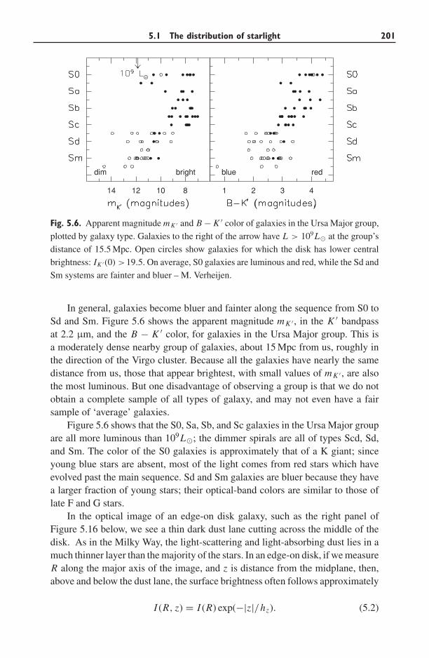
5.1 The distribution of starlight 201

14 12 10 8

dim bright

1 2 3 4

redblue

Fig. 5.6. Apparent magnitude mK ′ and B − K ′ color of galaxies in the Ursa Major group,

plotted by galaxy type. Galaxies to the right of the arrow have L > 109L� at the group’s

distance of 15.5 Mpc. Open circles show galaxies for which the disk has lower central

brightness: IK ′ (0) >19.5. On average, S0 galaxies are luminous and red, while the Sd and

Sm systems are fainter and bluer – M. Verheijen.

In general, galaxies become bluer and fainter along the sequence from S0 toSd and Sm. Figure 5.6 shows the apparent magnitude mK ′ , in the K ′ bandpassat 2.2 μm, and the B − K ′ color, for galaxies in the Ursa Major group. This isa moderately dense nearby group of galaxies, about 15 Mpc from us, roughly inthe direction of the Virgo cluster. Because all the galaxies have nearly the samedistance from us, those that appear brightest, with small values of mK ′ , are alsothe most luminous. But one disadvantage of observing a group is that we do notobtain a complete sample of all types of galaxy, and may not even have a fairsample of ‘average’ galaxies.

Figure 5.6 shows that the S0, Sa, Sb, and Sc galaxies in the Ursa Major groupare all more luminous than 109L�; the dimmer spirals are all of types Scd, Sd,and Sm. The color of the S0 galaxies is approximately that of a K giant; sinceyoung blue stars are absent, most of the light comes from red stars which haveevolved past the main sequence. Sd and Sm galaxies are bluer because they havea larger fraction of young stars; their optical-band colors are similar to those oflate F and G stars.

In the optical image of an edge-on disk galaxy, such as the right panel ofFigure 5.16 below, we see a thin dark dust lane cutting across the middle of thedisk. As in the Milky Way, the light-scattering and light-absorbing dust lies in amuch thinner layer than the majority of the stars. In an edge-on disk, if we measureR along the major axis of the image, and z is distance from the midplane, then,above and below the dust lane, the surface brightness often follows approximately

I (R, z) = I (R) exp(−|z|/hz). (5.2)

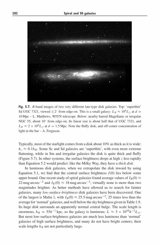
202 Spiral and S0 galaxies

Fig. 5.7. B-band images of two very different late-type disk galaxies. Top: ‘superthin’

Sd UGC 7321, viewed ∼< 2◦ from edge-on. This is a small galaxy: L B ≈ 109L� at d =10 Mpc – L. Matthews, WIYN telescope. Below: nearby barred Magellanic or irregular

NGC 55, about 10◦ from edge-on. Its linear size is about half that of UGC 7321, and

L B ≈ 2 × 109L� at d = 1.5 Mpc. Note the fluffy disk, and off-center concentration of

light in the bar – A. Ferguson.

Typically, most of the starlight comes from a disk about 10% as thick as it is wide:hz ≈ 0.1h R . Some Sc and Sd galaxies are ‘superthin’, with even more extremeflattening, while in Sm and irregular galaxies the disk is quite thick and fluffy(Figure 5.7). In other systems, the surface brightness drops at high z less rapidlythan Equation 5.2 would predict: like the Milky Way, they have a thick disk.

In luminous disk galaxies, when we extrapolate the disk inward by usingEquation 5.1, we find that the central surface brightness I (0) lies below someupper bound. One recent study of spiral galaxies found average values of IB(0) ≈22 mag arcsec−2 and IK (0) ≈ 18 mag arcsec−2; virtually none is more than twomagnitudes brighter. As better methods have allowed us to search for faintergalaxies, many low-surface-brightness disk galaxies have been discovered. Oneof the largest is Malin 1, with IB(0) ≈ 25.5 mag arcsec−2, 25 times less than theaverage for ‘normal’ galaxies, and well below the sky brightness given in Table 1.9.Its huge disk surrounds an apparently normal central bulge. The scale length isenormous, h R = 55h−1 kpc, so the galaxy is luminous: L ≈ 3 × 1010h−2L�.But most low-surface-brightness galaxies are much less luminous than ‘normal’galaxies of high surface brightness, and many do not have bright centers; theirscale lengths h R are not particularly large.

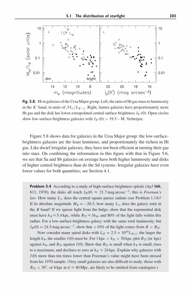
5.1 The distribution of starlight 203

14 12 10 8

0.01

0.1

1

10

dim bright

22 20 18 16

0.01

0.1

1

10

Fig. 5.8. HI in galaxies of the Ursa Major group. Left, the ratio of HI gas mass to luminosity

in the K ′ band, in units of M�/L K ′,�. Right, fainter galaxies have proportionately more

HI gas and the disk has lower extrapolated central surface brightness IK ′ (0). Open circles

show low-surface-brightness galaxies with IK ′(0) > 19.5 – M. Verheijen.

Figure 5.8 shows data for galaxies in the Ursa Major group: the low-surface-brightness galaxies are the least luminous, and proportionately the richest in HI

gas. Like dwarf irregular galaxies, they have not been efficient at turning their gasinto stars. On combining the information in this figure with that in Figure 5.6,we see that Sa and Sb galaxies on average have both higher luminosity and disksof higher central brightness than do the Sd systems. Irregular galaxies have evenlower values for both quantities; see Section 4.1.

Problem 5.4 According to a study of high-surface-brightness spirals (ApJ 160,

811; 1970), the disks all reach IB(0) ≈ 21.7 mag arcsec−2; this is Freeman’s

law. How many L� does the central square parsec radiate (see Problem 1.14)?

If its absolute magnitude MB = −20.5, how many L� does the galaxy emit in

the B band? If we ignore light from the bulge, show that the exponential disk

must have h R ≈5.4 kpc, while R25 ≈3h R , and 80% of the light falls within this

radius. For a low-surface-brightness galaxy with the same total luminosity, but

IB(0) = 24.5 mag arcsec−2, show that <10% of the light comes from R < R25.

Now consider many spiral disks with L B = 2.5 × 1010L B,�; the larger the

length h R , the smaller I (0) must be. For 1 kpc < h R < 30 kpc, plot R25 (in kpc)

against h R , and R25 against I (0). Show that R25 is small when h R is small, rises

to a maximum, and declines to zero at h R ≈ 24 kpc. Explain why galaxies with

I (0) more than ten times lower than Freeman’s value might have been missed

from his 1970 sample. (Very small galaxies are also difficult to study: those with

R25 < 30′′, or 6 kpc at d ≈ 40 Mpc, are likely to be omitted from catalogues.)

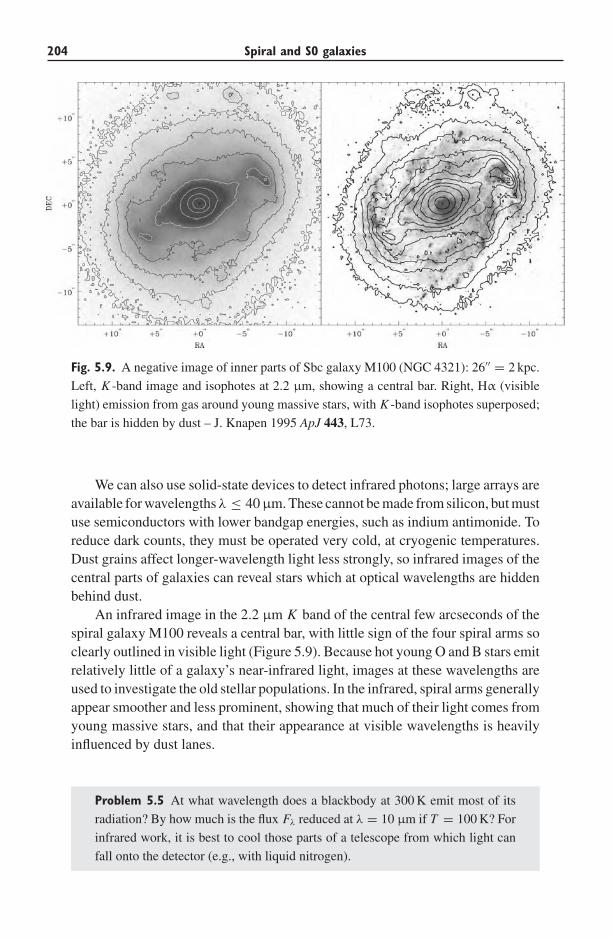
204 Spiral and S0 galaxies

Fig. 5.9. A negative image of inner parts of Sbc galaxy M100 (NGC 4321): 26′′ = 2 kpc.

Left, K -band image and isophotes at 2.2 μm, showing a central bar. Right, Hα (visible

light) emission from gas around young massive stars, with K -band isophotes superposed;

the bar is hidden by dust – J. Knapen 1995 ApJ 443, L73.

We can also use solid-state devices to detect infrared photons; large arrays areavailable for wavelengths λ ≤ 40 μm. These cannot be made from silicon, but mustuse semiconductors with lower bandgap energies, such as indium antimonide. Toreduce dark counts, they must be operated very cold, at cryogenic temperatures.Dust grains affect longer-wavelength light less strongly, so infrared images of thecentral parts of galaxies can reveal stars which at optical wavelengths are hiddenbehind dust.

An infrared image in the 2.2 μm K band of the central few arcseconds of thespiral galaxy M100 reveals a central bar, with little sign of the four spiral arms soclearly outlined in visible light (Figure 5.9). Because hot young O and B stars emitrelatively little of a galaxy’s near-infrared light, images at these wavelengths areused to investigate the old stellar populations. In the infrared, spiral arms generallyappear smoother and less prominent, showing that much of their light comes fromyoung massive stars, and that their appearance at visible wavelengths is heavilyinfluenced by dust lanes.

Problem 5.5 At what wavelength does a blackbody at 300 K emit most of its

radiation? By how much is the flux Fλ reduced at λ = 10 μm if T = 100 K? For

infrared work, it is best to cool those parts of a telescope from which light can

fall onto the detector (e.g., with liquid nitrogen).

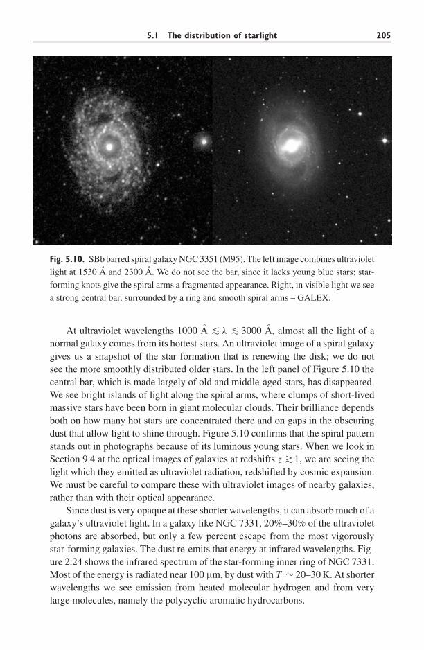
5.1 The distribution of starlight 205

Fig. 5.10. SBb barred spiral galaxy NGC 3351 (M95). The left image combines ultraviolet

light at 1530 A and 2300 A. We do not see the bar, since it lacks young blue stars; star-

forming knots give the spiral arms a fragmented appearance. Right, in visible light we see

a strong central bar, surrounded by a ring and smooth spiral arms – GALEX.

At ultraviolet wavelengths 1000 A ∼< λ ∼< 3000 A, almost all the light of anormal galaxy comes from its hottest stars. An ultraviolet image of a spiral galaxygives us a snapshot of the star formation that is renewing the disk; we do notsee the more smoothly distributed older stars. In the left panel of Figure 5.10 thecentral bar, which is made largely of old and middle-aged stars, has disappeared.We see bright islands of light along the spiral arms, where clumps of short-livedmassive stars have been born in giant molecular clouds. Their brilliance dependsboth on how many hot stars are concentrated there and on gaps in the obscuringdust that allow light to shine through. Figure 5.10 confirms that the spiral patternstands out in photographs because of its luminous young stars. When we look inSection 9.4 at the optical images of galaxies at redshifts z ∼>1, we are seeing thelight which they emitted as ultraviolet radiation, redshifted by cosmic expansion.We must be careful to compare these with ultraviolet images of nearby galaxies,rather than with their optical appearance.

Since dust is very opaque at these shorter wavelengths, it can absorb much of agalaxy’s ultraviolet light. In a galaxy like NGC 7331, 20%–30% of the ultravioletphotons are absorbed, but only a few percent escape from the most vigorouslystar-forming galaxies. The dust re-emits that energy at infrared wavelengths. Fig-ure 2.24 shows the infrared spectrum of the star-forming inner ring of NGC 7331.Most of the energy is radiated near 100 μm, by dust with T ∼ 20–30 K. At shorterwavelengths we see emission from heated molecular hydrogen and from verylarge molecules, namely the polycyclic aromatic hydrocarbons.

206 Spiral and S0 galaxies

The disks of spiral galaxies are not bright in X-rays. The interstellar gas is cooland supernova remnants expand supersonically; gas heated by their strong shocks,the hot winds of young stars, and binary stars are the main sources of X-rays. Ina starburst (see Section 5.6 below), the stellar winds and supernova remnantsoverlap to heat a bubble of gas that can break through surrounding dense gas toleave the galaxy as a superwind.

5.2 Observing the gas

Most of the gas of a spiral galaxy is found in the disk; the cool atomic (HI ) andmolecular (H2) hydrogen form the raw material out of which the galaxy makesnew stars. In Section 5.1, we saw how to locate concentrations of gas indirectly, bylooking in optical images for the dark obscuring dust lanes. Cool gas can be seendirectly by its emission in spectral lines at radio wavelengths, which propagateunhindered through the dusty disk. If it is ionized by the ultraviolet radiation ofhot stars, or by a shock wave, we see it in optical emission lines such as Hα.Because we observe the gas in its spectral lines, we can also measure its velocityat each point within the galaxy, and so explore its motion.

5.2.1 Radio-telescope arrays

We observe cool gas mainly at radio wavelengths, longer than about a millimeter.Because of the longer wavelengths, radio telescopes have fuzzier vision thanoptical telescopes. When observing at wavelength λ with a telescope of diameterD, sources that lie within an angle λ/D of each other on the sky will appearblended together: this is the diffraction limit, which no telescope can escape. Atoptical wavelengths of λ ≈ 5000 A, the diffraction limit would allow images assharp as 1′′ from a small telescope of D = 10 cm, while at 1 mm we would needa telescope 200 m across to achieve the same resolution. The largest single-dishradio telescopes are about 100 m in diameter, and most are a few tens of metersacross; so in general their images are not as sharp as those from optical telescopes.To make an image with 1′′ resolution at λ = 20 cm would require a telescope 40 kmin diameter; a single dish of this size would collapse under its own weight. Atcentimeter wavelengths, and increasingly in the millimeter region as well, we usean array of smaller telescopes for aperture synthesis.

To see how aperture synthesis works, we can think of radio waves as oscil-lating electric and magnetic fields. If the wavelength is λ, the electric fieldE ∝ cos(2πct/λ); the voltage V induced at the focus of a radio telescope isproportional to the electric field E at that instant. Suppose that we observe withtwo telescopes, as in Figure 5.11. Waves from a source at elevation θ must travelan extra distance d cos θ to arrive at telescope 2, so the wavecrests, and the peaksin voltage, are delayed by a time d cos θ/c relative to those at telescope 1. The

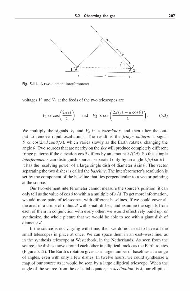
5.2 Observing the gas 207

θ1 2

dd cos θ

Fig. 5.11. A two-element interferometer.

voltages V1 and V2 at the feeds of the two telescopes are

V1 ∝ cos

(2πct

λ

)and V2 ∝ cos

(2π (ct − d cos θ )

λ

). (5.3)

We multiply the signals V1 and V2 in a correlator, and then filter the out-put to remove rapid oscillations. The result is the fringe pattern: a signalS ∝ cos(2πd cos θ/λ), which varies slowly as the Earth rotates, changing theangle θ . Two sources that are nearby on the sky will produce completely differentfringe patterns if the elevation cos θ differs by an amount λ/(2d). So this simpleinterferometer can distinguish sources separated only by an angle λ/(d sin θ) –it has the resolving power of a large single dish of diameter d sin θ . The vectorseparating the two dishes is called the baseline. The interferometer’s resolution isset by the component of the baseline that lies perpendicular to a vector pointingat the source.

Our two-element interferometer cannot measure the source’s position: it canonly tell us the value of cos θ to within a multiple of λ/d. To get more information,we add more pairs of telescopes, with different baselines. If we could cover allthe area of a circle of radius d with small dishes, and examine the signals fromeach of them in conjunction with every other, we would effectively build up, orsynthesize, the whole picture that we would be able to see with a giant dish ofdiameter d .

If the source is not varying with time, then we do not need to have all thesmall telescopes in place at once. We can space them in an east–west line, asin the synthesis telescope at Westerbork, in the Netherlands. As seen from thesource, the dishes move around each other in elliptical tracks as the Earth rotates(Figure 5.12). The Earth’s rotation gives us a large number of baselines at a rangeof angles, even with only a few dishes. In twelve hours, we could synthesize amap of our source as it would be seen by a large elliptical telescope. When theangle of the source from the celestial equator, its declination, is δ, our elliptical

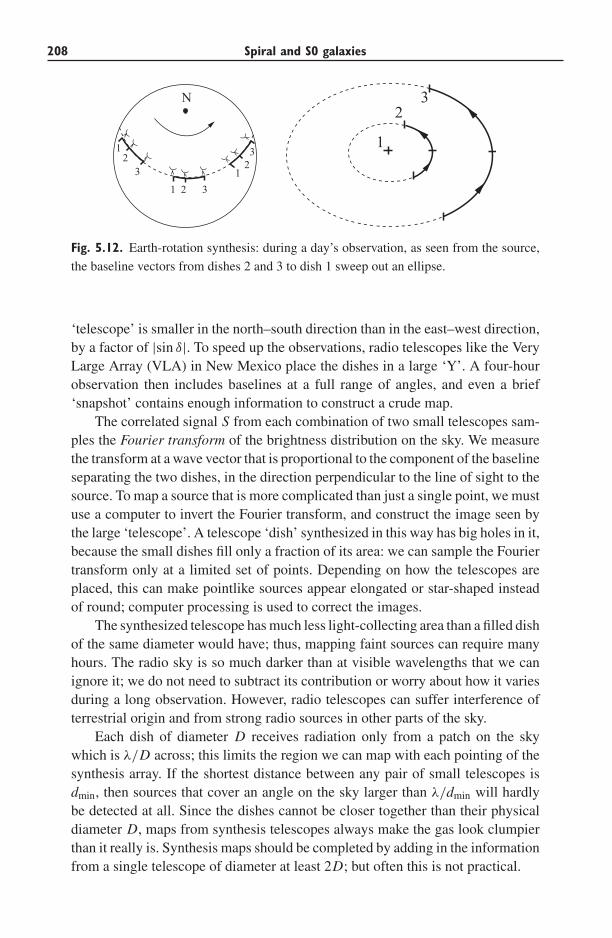
208 Spiral and S0 galaxies

1

23N

1 2 3

12

312

3

Fig. 5.12. Earth-rotation synthesis: during a day’s observation, as seen from the source,

the baseline vectors from dishes 2 and 3 to dish 1 sweep out an ellipse.

‘telescope’ is smaller in the north–south direction than in the east–west direction,by a factor of |sin δ|. To speed up the observations, radio telescopes like the VeryLarge Array (VLA) in New Mexico place the dishes in a large ‘Y’. A four-hourobservation then includes baselines at a full range of angles, and even a brief‘snapshot’ contains enough information to construct a crude map.

The correlated signal S from each combination of two small telescopes sam-ples the Fourier transform of the brightness distribution on the sky. We measurethe transform at a wave vector that is proportional to the component of the baselineseparating the two dishes, in the direction perpendicular to the line of sight to thesource. To map a source that is more complicated than just a single point, we mustuse a computer to invert the Fourier transform, and construct the image seen bythe large ‘telescope’. A telescope ‘dish’ synthesized in this way has big holes in it,because the small dishes fill only a fraction of its area: we can sample the Fouriertransform only at a limited set of points. Depending on how the telescopes areplaced, this can make pointlike sources appear elongated or star-shaped insteadof round; computer processing is used to correct the images.

The synthesized telescope has much less light-collecting area than a filled dishof the same diameter would have; thus, mapping faint sources can require manyhours. The radio sky is so much darker than at visible wavelengths that we canignore it; we do not need to subtract its contribution or worry about how it variesduring a long observation. However, radio telescopes can suffer interference ofterrestrial origin and from strong radio sources in other parts of the sky.

Each dish of diameter D receives radiation only from a patch on the skywhich is λ/D across; this limits the region we can map with each pointing of thesynthesis array. If the shortest distance between any pair of small telescopes isdmin, then sources that cover an angle on the sky larger than λ/dmin will hardlybe detected at all. Since the dishes cannot be closer together than their physicaldiameter D, maps from synthesis telescopes always make the gas look clumpierthan it really is. Synthesis maps should be completed by adding in the informationfrom a single telescope of diameter at least 2D; but often this is not practical.

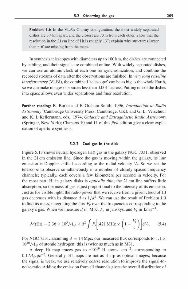
5.2 Observing the gas 209

Problem 5.6 In the VLA’s C-array configuration, the most widely separated

dishes are 3.4 km apart, and the closest are 73 m from each other. Show that the

resolution in the 21 cm line of HI is roughly 13′′; explain why structures larger

than ∼6′ are missing from the maps.

In synthesis telescopes with diameters up to 100 km, the dishes are connectedby cabling, and their signals are combined online. With widely separated dishes,we can use an atomic clock at each one for synchronization, and combine therecorded streams of data after the observations are finished. In very long baselineinterferometry (VLBI), the combined ‘telescope’ can be as big as the whole Earth,so we can make images of sources less than 0.001′′ across. Putting one of the dishesinto space allows even wider separations and finer resolution.

Further reading: B. Burke and F. Graham-Smith, 1996, Introduction to RadioAstronomy (Cambridge University Press, Cambridge, UK); and G. L. Verschuurand K. I. Kellermann, eds., 1974, Galactic and Extragalactic Radio Astronomy(Springer, New York); Chapters 10 and 11 of this first edition give a clear expla-nation of aperture synthesis.

5.2.2 Cool gas in the disk

Figure 5.13 shows neutral hydrogen (HI) gas in the galaxy NGC 7331, observedin the 21 cm emission line. Since the gas is moving within the galaxy, its lineemission is Doppler shifted according to the radial velocity Vr. So we set thetelescope to observe simultaneously in a number of closely spaced frequencychannels; typically, each covers a few kilometers per second in velocity. Forthe most part, HI in galaxy disks is optically thin; the 21 cm line suffers littleabsorption, so the mass of gas is just proportional to the intensity of its emission.Just as for visible light, the radio power that we receive from a given cloud of HI

gas decreases with its distance d as 1/d2. We can use the result of Problem 1.9to find its mass, integrating the flux Fν over the frequencies corresponding to thegalaxy’s gas. When we measure d in Mpc, Fν in janskys, and Vr in km s−1,

M(HI) = 2.36 × 105M� × d2∫

Fν

[1421 MHz ×

(1 − Vr

c

)]dVr. (5.4)

For NGC 7331, assuming d = 14 Mpc, our measured flux corresponds to 1.1 ×1010M� of atomic hydrogen; this is twice as much as in M31.

A deep HI map traces gas to ∼1019 H atoms cm−2, corresponding to0.1M� pc−2. Generally, HI maps are not as sharp as optical images; becausethe signal is weak, we use relatively coarse resolution to improve the signal-to-noise ratio. Adding the emission from all channels gives the overall distribution of

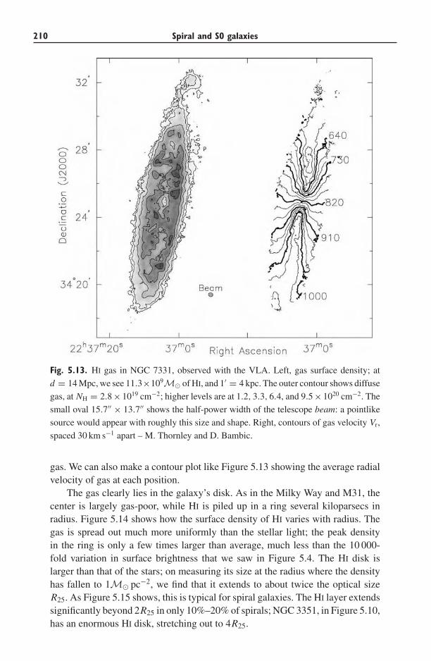
210 Spiral and S0 galaxies

Fig. 5.13. HI gas in NGC 7331, observed with the VLA. Left, gas surface density; at

d = 14 Mpc, we see 11.3×109M� of HI, and 1′ = 4 kpc. The outer contour shows diffuse

gas, at NH = 2.8 × 1019 cm−2; higher levels are at 1.2, 3.3, 6.4, and 9.5 × 1020 cm−2. The

small oval 15.7′′ × 13.7′′ shows the half-power width of the telescope beam: a pointlike

source would appear with roughly this size and shape. Right, contours of gas velocity Vr,

spaced 30 km s−1 apart – M. Thornley and D. Bambic.

gas. We can also make a contour plot like Figure 5.13 showing the average radialvelocity of gas at each position.

The gas clearly lies in the galaxy’s disk. As in the Milky Way and M31, thecenter is largely gas-poor, while HI is piled up in a ring several kiloparsecs inradius. Figure 5.14 shows how the surface density of HI varies with radius. Thegas is spread out much more uniformly than the stellar light; the peak densityin the ring is only a few times larger than average, much less than the 10 000-fold variation in surface brightness that we saw in Figure 5.4. The HI disk islarger than that of the stars; on measuring its size at the radius where the densityhas fallen to 1M� pc−2, we find that it extends to about twice the optical sizeR25. As Figure 5.15 shows, this is typical for spiral galaxies. The HI layer extendssignificantly beyond 2R25 in only 10%–20% of spirals; NGC 3351, in Figure 5.10,has an enormous HI disk, stretching out to 4R25.

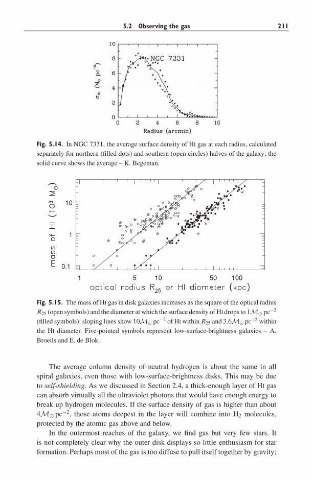
5.2 Observing the gas 211

Fig. 5.14. In NGC 7331, the average surface density of HI gas at each radius, calculated

separately for northern (filled dots) and southern (open circles) halves of the galaxy; the

solid curve shows the average – K. Begeman.

1 5 10 50 100

0.1

1

10

Fig. 5.15. The mass of HI gas in disk galaxies increases as the square of the optical radius

R25 (open symbols) and the diameter at which the surface density of HI drops to 1M� pc−2

(filled symbols): sloping lines show 10M� pc−2 of HI within R25 and 3.6M� pc−2 within

the HI diameter. Five-pointed symbols represent low-surface-brightness galaxies – A.

Broeils and E. de Blok.

The average column density of neutral hydrogen is about the same in allspiral galaxies, even those with low-surface-brightness disks. This may be dueto self-shielding. As we discussed in Section 2.4, a thick-enough layer of HI gascan absorb virtually all the ultraviolet photons that would have enough energy tobreak up hydrogen molecules. If the surface density of gas is higher than about4M� pc−2, those atoms deepest in the layer will combine into H2 molecules,protected by the atomic gas above and below.

In the outermost reaches of the galaxy, we find gas but very few stars. Itis not completely clear why the outer disk displays so little enthusiasm for starformation. Perhaps most of the gas is too diffuse to pull itself together by gravity;

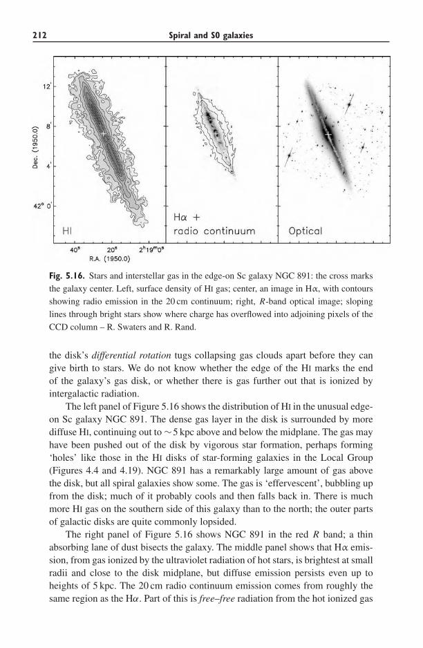
212 Spiral and S0 galaxies

Fig. 5.16. Stars and interstellar gas in the edge-on Sc galaxy NGC 891: the cross marks

the galaxy center. Left, surface density of HI gas; center, an image in Hα, with contours

showing radio emission in the 20 cm continuum; right, R-band optical image; sloping

lines through bright stars show where charge has overflowed into adjoining pixels of the

CCD column – R. Swaters and R. Rand.

the disk’s differential rotation tugs collapsing gas clouds apart before they cangive birth to stars. We do not know whether the edge of the HI marks the endof the galaxy’s gas disk, or whether there is gas further out that is ionized byintergalactic radiation.

The left panel of Figure 5.16 shows the distribution of HI in the unusual edge-on Sc galaxy NGC 891. The dense gas layer in the disk is surrounded by morediffuse HI, continuing out to ∼5 kpc above and below the midplane. The gas mayhave been pushed out of the disk by vigorous star formation, perhaps forming‘holes’ like those in the HI disks of star-forming galaxies in the Local Group(Figures 4.4 and 4.19). NGC 891 has a remarkably large amount of gas abovethe disk, but all spiral galaxies show some. The gas is ‘effervescent’, bubbling upfrom the disk; much of it probably cools and then falls back in. There is muchmore HI gas on the southern side of this galaxy than to the north; the outer partsof galactic disks are quite commonly lopsided.

The right panel of Figure 5.16 shows NGC 891 in the red R band; a thinabsorbing lane of dust bisects the galaxy. The middle panel shows that Hα emis-sion, from gas ionized by the ultraviolet radiation of hot stars, is brightest at smallradii and close to the disk midplane, but diffuse emission persists even up toheights of 5 kpc. The 20 cm radio continuum emission comes from roughly thesame region as the Hα. Part of this is free–free radiation from the hot ionized gas

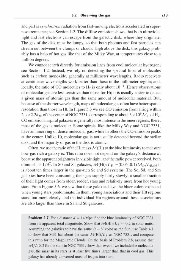
5.2 Observing the gas 213

and part is synchrotron radiation from fast-moving electrons accelerated in super-nova remnants; see Section 1.2. The diffuse emission shows that both ultravioletlight and fast electrons can escape from the galactic disk, where they originate.The gas of the disk must be lumpy, so that both photons and fast particles canstream out between the clumps or clouds. High above the disk, this galaxy prob-ably has a halo of hot gas like that of the Milky Way, at temperatures close to amillion degrees.

We cannot search directly for emission lines from cool molecular hydrogen;see Section 1.2. Instead, we rely on detecting the spectral lines of moleculessuch as carbon monoxide, generally at millimeter wavelengths. Radio receiversat centimeter wavelengths work better than those in the millimeter region; and,locally, the ratio of CO molecules to H2 is only about 10−4. Hence observationsof molecular gas are less sensitive than those for HI; it is usually easier to detecta given mass of atomic gas than the same amount of molecular material. But,because of the shorter wavelength, maps of molecular gas often have better spatialresolution than those in HI. In Figure 5.3 we see CO emission from a ring within2′, or 2.2h R , of the center of NGC 7331, corresponding to about 3×109M� of H2.CO emission in spiral galaxies is generally most intense in the inner regions; there,most of the gas is molecular. Some spirals, like the Milky Way and NGC 7331,have an inner ring of dense molecular gas, while in others the CO emission peaksat the center. Unlike HI, molecular gas is not usually detected beyond the stellardisk, and the majority of gas in the disk is atomic.

Often, we use the ratio of the HI massM(HI) to the blue luminosity to measurehow gas-rich a galaxy is. This ratio does not depend on the galaxy’s distance d,because the apparent brightness in visible light, and the radio power received, bothdiminish as 1/d2. In S0 and Sa galaxies, M(HI)/L B ∼ (0.05–0.1)M�/L B,�; itis about ten times larger in the gas-rich Sc and Sd systems. The Sc, Sd, and Smgalaxies have been consuming their gas supply fairly slowly; a smaller fractionof their light comes from older, redder, stars and relatively more from hot youngstars. From Figure 5.6, we saw that these galaxies have the bluer colors expectedwhen young stars predominate. In them, young associations and their HII regionsstand out more clearly, and the individual HII regions around these associationsare also larger than those in Sa and Sb galaxies.

Problem 5.7 For a distance d = 14 Mpc, find the blue luminosity of NGC 7331

from its apparent total magnitude. Show that M(HI)/L B ≈ 0.2 in solar units.

Assuming the galaxies to have the same B − V color as the Sun, use Table 4.1

to show that M31 has about the same M(HI)/L B as NGC 7331, and compute

this ratio for the Magellanic Clouds. On the basis of Problem 2.8, assume that

M/L ∼>2 for the stars in NGC 7331; show that, even if we include the molecular

gas, the mass in its stars is at least five times larger than that in cool gas. This

galaxy has already converted most of its gas into stars.

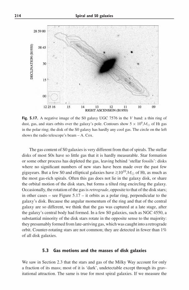
214 Spiral and S0 galaxies

Fig. 5.17. A negative image of the S0 galaxy UGC 7576 in the V band: a thin ring of

dust, gas, and stars orbits over the galaxy’s pole. Contours show 5 × 109M� of HI gas

in the polar ring; the disk of the S0 galaxy has hardly any cool gas. The circle on the left

shows the radio telescope’s beam – A. Cox.

The gas content of S0 galaxies is very different from that of spirals. The stellardisks of most S0s have so little gas that it is hardly measurable. Star formationor some other process has depleted the gas, leaving behind ‘stellar fossils’: diskswhere no significant numbers of new stars have been made over the past fewgigayears. But a few S0 and elliptical galaxies have ∼>1010M� of HI, as much asthe most gas-rich spirals. Often this gas does not lie in the galaxy disk, or sharethe orbital motion of the disk stars, but forms a tilted ring encircling the galaxy.Occasionally, the rotation of the gas is retrograde, opposite to that of the disk stars;in other cases – see Figure 5.17 – it orbits as a polar ring, perpendicular to thegalaxy’s disk. Because the angular momentum of the ring and that of the centralgalaxy are so different, we think that the gas was captured at a late stage, afterthe galaxy’s central body had formed. In a few S0 galaxies, such as NGC 4550, asubstantial minority of the disk stars rotate in the opposite sense to the majority:they presumably formed from late-arriving gas, which was caught into a retrogradeorbit. Counter-rotating stars are not common; they are detected in fewer than 1%of all disk galaxies.

5.3 Gas motions and the masses of disk galaxies

We saw in Section 2.3 that the stars and gas of the Milky Way account for onlya fraction of its mass; most of it is ‘dark’, undetectable except through its grav-itational attraction. The same is true for most spiral galaxies. If we measure the

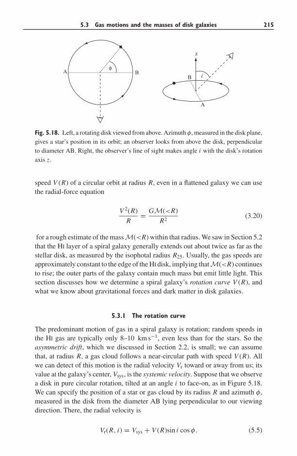
5.3 Gas motions and the masses of disk galaxies 215

A

B

z

iA B

Fig. 5.18. Left, a rotating disk viewed from above. Azimuth φ, measured in the disk plane,

gives a star’s position in its orbit; an observer looks from above the disk, perpendicular

to diameter AB. Right, the observer’s line of sight makes angle i with the disk’s rotation

axis z.

speed V (R) of a circular orbit at radius R, even in a flattened galaxy we can usethe radial-force equation

V 2(R)

R= GM(<R)

R2(3.20)

for a rough estimate of the massM(<R) within that radius. We saw in Section 5.2that the HI layer of a spiral galaxy generally extends out about twice as far as thestellar disk, as measured by the isophotal radius R25. Usually, the gas speeds areapproximately constant to the edge of the HI disk, implying thatM(<R) continuesto rise; the outer parts of the galaxy contain much mass but emit little light. Thissection discusses how we determine a spiral galaxy’s rotation curve V (R), andwhat we know about gravitational forces and dark matter in disk galaxies.

5.3.1 The rotation curve

The predominant motion of gas in a spiral galaxy is rotation; random speeds inthe HI gas are typically only 8–10 km s−1, even less than for the stars. So theasymmetric drift, which we discussed in Section 2.2, is small; we can assumethat, at radius R, a gas cloud follows a near-circular path with speed V (R). Allwe can detect of this motion is the radial velocity Vr toward or away from us; itsvalue at the galaxy’s center, Vsys, is the systemic velocity. Suppose that we observea disk in pure circular rotation, tilted at an angle i to face-on, as in Figure 5.18.We can specify the position of a star or gas cloud by its radius R and azimuth φ,measured in the disk from the diameter AB lying perpendicular to our viewingdirection. There, the radial velocity is

Vr(R, i) = Vsys + V (R)sin i cos φ. (5.5)

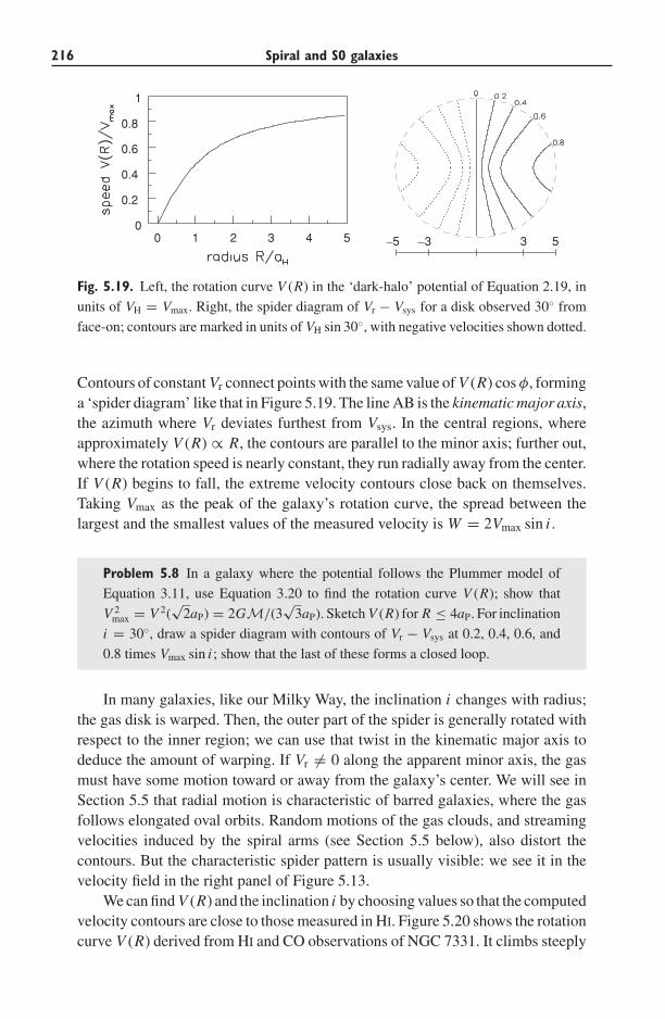
216 Spiral and S0 galaxies

0 1 2 3 4 50

0.2

0.4

0.6

0.8

1

3 3 5 5

Fig. 5.19. Left, the rotation curve V (R) in the ‘dark-halo’ potential of Equation 2.19, in

units of VH = Vmax. Right, the spider diagram of Vr − Vsys for a disk observed 30◦ from

face-on; contours are marked in units of VH sin 30◦, with negative velocities shown dotted.

Contours of constant Vr connect points with the same value of V (R) cos φ, forminga ‘spider diagram’ like that in Figure 5.19. The line AB is the kinematic major axis,the azimuth where Vr deviates furthest from Vsys. In the central regions, whereapproximately V (R) ∝ R, the contours are parallel to the minor axis; further out,where the rotation speed is nearly constant, they run radially away from the center.If V (R) begins to fall, the extreme velocity contours close back on themselves.Taking Vmax as the peak of the galaxy’s rotation curve, the spread between thelargest and the smallest values of the measured velocity is W = 2Vmax sin i .

Problem 5.8 In a galaxy where the potential follows the Plummer model of

Equation 3.11, use Equation 3.20 to find the rotation curve V (R); show that

V 2max = V 2(

√2aP) = 2GM/(3

√3aP). Sketch V (R) for R ≤ 4aP. For inclination

i = 30◦, draw a spider diagram with contours of Vr − Vsys at 0.2, 0.4, 0.6, and

0.8 times Vmax sin i ; show that the last of these forms a closed loop.

In many galaxies, like our Milky Way, the inclination i changes with radius;the gas disk is warped. Then, the outer part of the spider is generally rotated withrespect to the inner region; we can use that twist in the kinematic major axis todeduce the amount of warping. If Vr �= 0 along the apparent minor axis, the gasmust have some motion toward or away from the galaxy’s center. We will see inSection 5.5 that radial motion is characteristic of barred galaxies, where the gasfollows elongated oval orbits. Random motions of the gas clouds, and streamingvelocities induced by the spiral arms (see Section 5.5 below), also distort thecontours. But the characteristic spider pattern is usually visible: we see it in thevelocity field in the right panel of Figure 5.13.

We can find V (R) and the inclination i by choosing values so that the computedvelocity contours are close to those measured in HI. Figure 5.20 shows the rotationcurve V (R) derived from HI and CO observations of NGC 7331. It climbs steeply

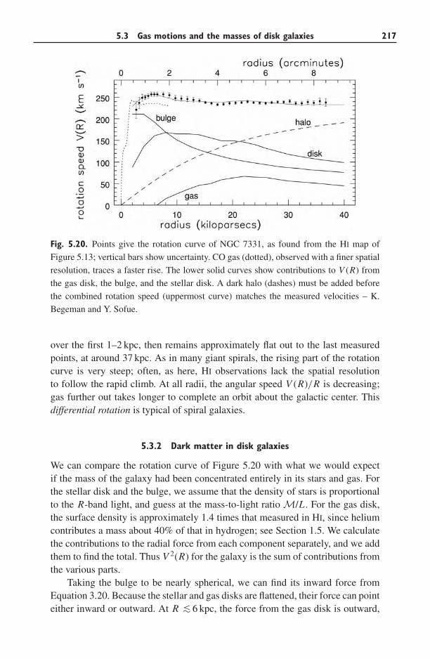
5.3 Gas motions and the masses of disk galaxies 217

Fig. 5.20. Points give the rotation curve of NGC 7331, as found from the HI map of

Figure 5.13; vertical bars show uncertainty. CO gas (dotted), observed with a finer spatial

resolution, traces a faster rise. The lower solid curves show contributions to V (R) from

the gas disk, the bulge, and the stellar disk. A dark halo (dashes) must be added before

the combined rotation speed (uppermost curve) matches the measured velocities – K.

Begeman and Y. Sofue.

over the first 1–2 kpc, then remains approximately flat out to the last measuredpoints, at around 37 kpc. As in many giant spirals, the rising part of the rotationcurve is very steep; often, as here, HI observations lack the spatial resolutionto follow the rapid climb. At all radii, the angular speed V (R)/R is decreasing;gas further out takes longer to complete an orbit about the galactic center. Thisdifferential rotation is typical of spiral galaxies.

5.3.2 Dark matter in disk galaxies

We can compare the rotation curve of Figure 5.20 with what we would expectif the mass of the galaxy had been concentrated entirely in its stars and gas. Forthe stellar disk and the bulge, we assume that the density of stars is proportionalto the R-band light, and guess at the mass-to-light ratio M/L . For the gas disk,the surface density is approximately 1.4 times that measured in HI, since heliumcontributes a mass about 40% of that in hydrogen; see Section 1.5. We calculatethe contributions to the radial force from each component separately, and we addthem to find the total. Thus V 2(R) for the galaxy is the sum of contributions fromthe various parts.

Taking the bulge to be nearly spherical, we can find its inward force fromEquation 3.20. Because the stellar and gas disks are flattened, their force can pointeither inward or outward. At R ∼< 6 kpc, the force from the gas disk is outward,

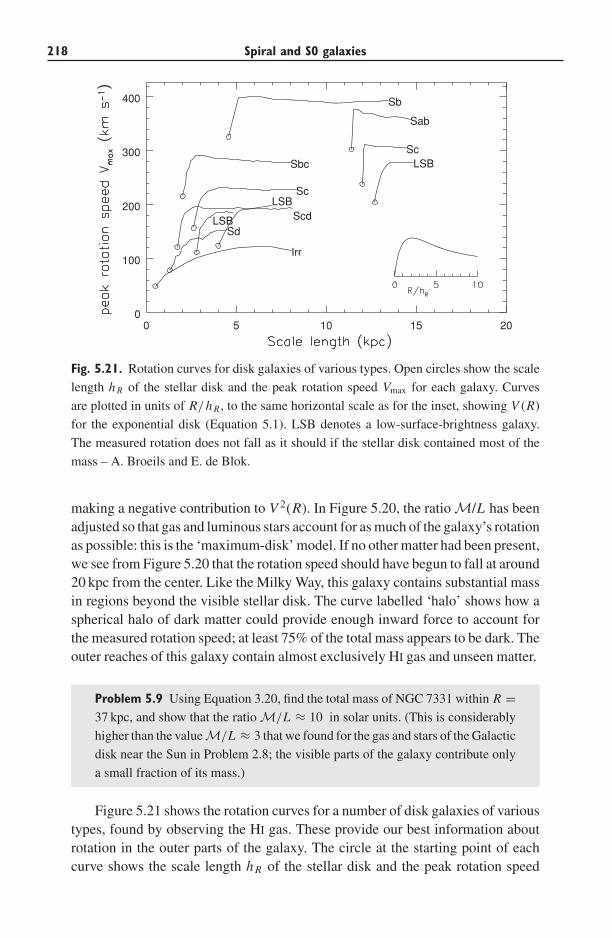
218 Spiral and S0 galaxies

0 5 10 15 200

100

200

300

400

Irr

Sc

Sd

Sb

Sbc

Sc

Sab

Scd

LSB

LSB

LSB

Fig. 5.21. Rotation curves for disk galaxies of various types. Open circles show the scale

length h R of the stellar disk and the peak rotation speed Vmax for each galaxy. Curves

are plotted in units of R/h R , to the same horizontal scale as for the inset, showing V (R)

for the exponential disk (Equation 5.1). LSB denotes a low-surface-brightness galaxy.

The measured rotation does not fall as it should if the stellar disk contained most of the

mass – A. Broeils and E. de Blok.

making a negative contribution to V 2(R). In Figure 5.20, the ratio M/L has beenadjusted so that gas and luminous stars account for as much of the galaxy’s rotationas possible: this is the ‘maximum-disk’ model. If no other matter had been present,we see from Figure 5.20 that the rotation speed should have begun to fall at around20 kpc from the center. Like the Milky Way, this galaxy contains substantial massin regions beyond the visible stellar disk. The curve labelled ‘halo’ shows how aspherical halo of dark matter could provide enough inward force to account forthe measured rotation speed; at least 75% of the total mass appears to be dark. Theouter reaches of this galaxy contain almost exclusively HI gas and unseen matter.

Problem 5.9 Using Equation 3.20, find the total mass of NGC 7331 within R =37 kpc, and show that the ratio M/L ≈ 10 in solar units. (This is considerably

higher than the valueM/L ≈ 3 that we found for the gas and stars of the Galactic

disk near the Sun in Problem 2.8; the visible parts of the galaxy contribute only

a small fraction of its mass.)

Figure 5.21 shows the rotation curves for a number of disk galaxies of varioustypes, found by observing the HI gas. These provide our best information aboutrotation in the outer parts of the galaxy. The circle at the starting point of eachcurve shows the scale length h R of the stellar disk and the peak rotation speed

5.3 Gas motions and the masses of disk galaxies 219

Vmax, while the horizontal extent shows the number of scale lengths out to whichthe rotation was measured. Beyond its peak, V (R) remains fairly steady; it doesnot drop as it should if the mass of the galaxy had been in an exponential disk.As in NGC 7331, the higher-than-expected rotation requires an additional inwardforce, which we ascribe to a dark halo.

Peak rotation speeds in spiral galaxies are usually 150–300 km s−1. Theyrarely rise above 400 km s−1, and the fastest measured rotation is about 500 km s−1,in the S0/Sa galaxy UGC 12591. Larger galaxies, with longer scale lengths h R ,generally rotate more rapidly; these tend to be the Sa and Sb galaxies, rather thanthe Sc, Sd, and Sm systems. The rotation curves of Sa and Sb galaxies initiallyclimb steeply, showing that relatively more of their mass is closer to the center.In these systems, the luminous matter in the disk and the bulge is concentrated atsmall radii, and the dark matter in the halo also becomes very dense there. In Sdand Sm galaxies, the rotation speed increases more gradually. These galaxies donot have large bulges, and Figure 5.8 showed us that their luminous disks have lowcentral surface brightness. The rotation curves show that the dark halo also lackscentral concentration; its core, where the density is nearly constant, must be largerin relation to the galaxy’s stellar disk. Most low-surface-brightness galaxies rotateslowly, with gently ascending rotation curves like those of Sd or Sm galaxies; butthere are some with higher speeds and faster-rising rotation curves.

The proportion of dark matter required to explain these rotation curves variesfrom about 50% in Sa and Sb galaxies to 80%–90% in Sd and Sm galaxies. Theremay be yet more dark material out beyond the last point where we have observed HI

gas; the ‘total mass’ of a spiral galaxy measured in this way is only a lower bound.We must turn to the orbital motion of galaxies in binary pairs or groups to studythe dark matter at larger radii: look back at Section 4.5, or forward to Chapter 7.

Galaxies and their dark matter do not provide enough mass to halt the cosmicexpansion. For most galaxies, we must use Hubble’s law and the recession speedVsys to give a rough estimate of the distance d . Equation 1.27 tells us that

d ≈ h−1[Vsys ( km s−1)/100] Mpc, (1.27)

where h = H0/100 km s−1 Mpc−1. So when we estimate the luminosity L of agalaxy from its apparent brightness by using Equation 1.1, L ∝ h−2. The massinferred from Equation 3.20 depends on the Hubble constant as M ∝ h−1, sothe mass-to-light ratios derived from the rotation curves of spiral galaxies followM/L ∝ h. For most spirals, we find 5h ∼< M/L ∼< 25h, in units of the Sun’smass and blue luminosity.

From Equation 1.25, the blue light of all the galaxies averages out to 2 ×108hL� Mpc−3. So if the mass-to-light ratio for each were roughly the same asthat for the gas-rich disk systems where we observe HI gas, they would contribute adensity ρgal ∼ (1−5)×109h2M� Mpc−3, less than 0.02 of the critical density ρcrit

given by Equation 1.30. The dark matter in galaxies is far short of what would be

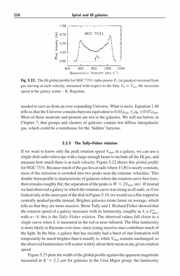
220 Spiral and S0 galaxies

Fig. 5.22. The HI global profile for NGC 7331: radio power Fν (in janskys) received from

gas moving at each velocity, measured with respect to the Sun; V0 = Vsys, the recession

speed at the galaxy center – K. Begeman.

needed to save us from an ever-expanding Universe. What is more, Equation 1.40tells us that the Universe contains baryons equivalent to 0.03ρcrit ∼<ρB ∼<0.07ρcrit.Most of those neutrons and protons are not in the galaxies. We will see below, inChapter 7, that groups and clusters of galaxies contain hot diffuse intergalacticgas, which could be a storehouse for the ‘hidden’ baryons.

5.3.3 The Tully–Fisher relation

If we want to know only the peak rotation speed Vmax in a galaxy, we can use asingle-dish radio telescope with a large enough beam to include all the HI gas, andmeasure how much there is at each velocity. Figure 5.22 shows this global profilefor NGC 7331. Because much of the gas lies at radii where V (R) is nearly constant,most of the emission is crowded into two peaks near the extreme velocities. Thisdouble-horn profile is characteristic of galaxies where the rotation curve first rises,then remains roughly flat; the separation of the peaks is W ≈ 2Vmax sin i . If insteadwe had observed a galaxy in which the rotation curve was rising at all radii, or if welooked only at the inner part of the disk in Figure 5.19, we would see a flat-topped orcentrally peaked profile instead. Brighter galaxies rotate faster on average, whichtells us that they are more massive. Brent Tully and J. Richard Fisher showed thatthe rotation speed of a galaxy increases with its luminosity, roughly as L ∝V α

max,with α∼ 4: this is the Tully–Fisher relation. The observed values fall closer to asingle curve when L is measured in the red or near-infrared. The blue luminosityis more likely to fluctuate over time, since young massive stars contribute much ofthe light. In the blue, a galaxy that has recently had a burst of star formation willtemporarily be much brighter than it usually is, while Vmax remains unchanged; sothe observed luminosities will scatter widely about their mean at any given rotationspeed.

Figure 5.23 plots the width of the global profile against the apparent magnitudemeasured at K ′ ≈ 2.2 μm for galaxies in the Ursa Major group; the luminosity

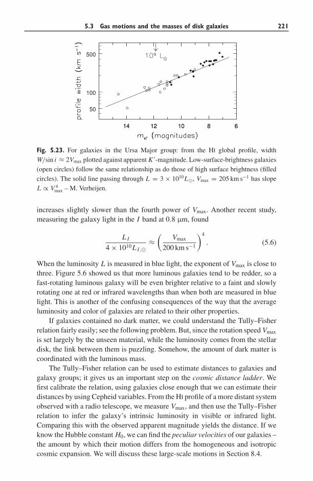
5.3 Gas motions and the masses of disk galaxies 221

14 12 10 8 6

100

14 12 10 8 6

50

500

Fig. 5.23. For galaxies in the Ursa Major group: from the HI global profile, width

W/sin i ≈ 2Vmax plotted against apparent K ′-magnitude. Low-surface-brightness galaxies

(open circles) follow the same relationship as do those of high surface brightness (filled

circles). The solid line passing through L = 3 × 1010L�, Vmax = 205 km s−1 has slope

L ∝ V 4max – M. Verheijen.

increases slightly slower than the fourth power of Vmax. Another recent study,measuring the galaxy light in the I band at 0.8 μm, found

L I

4 × 1010L I,�≈(

Vmax

200 km s−1

)4

. (5.6)

When the luminosity L is measured in blue light, the exponent of Vmax is close tothree. Figure 5.6 showed us that more luminous galaxies tend to be redder, so afast-rotating luminous galaxy will be even brighter relative to a faint and slowlyrotating one at red or infrared wavelengths than when both are measured in bluelight. This is another of the confusing consequences of the way that the averageluminosity and color of galaxies are related to their other properties.

If galaxies contained no dark matter, we could understand the Tully–Fisherrelation fairly easily; see the following problem. But, since the rotation speed Vmax

is set largely by the unseen material, while the luminosity comes from the stellardisk, the link between them is puzzling. Somehow, the amount of dark matter iscoordinated with the luminous mass.

The Tully–Fisher relation can be used to estimate distances to galaxies andgalaxy groups; it gives us an important step on the cosmic distance ladder. Wefirst calibrate the relation, using galaxies close enough that we can estimate theirdistances by using Cepheid variables. From the HI profile of a more distant systemobserved with a radio telescope, we measure Vmax, and then use the Tully–Fisherrelation to infer the galaxy’s intrinsic luminosity in visible or infrared light.Comparing this with the observed apparent magnitude yields the distance. If weknow the Hubble constant H0, we can find the peculiar velocities of our galaxies –the amount by which their motion differs from the homogeneous and isotropiccosmic expansion. We will discuss these large-scale motions in Section 8.4.

222 Spiral and S0 galaxies

Problem 5.10 Ignoring the bulge, use Equation 3.20 to explain why we might

expect the mass M of a spiral galaxy to follow approximately

M ∝ V 2maxh R .

Show from Equation 5.1 that L = 2π I (0)h2R , and hence that, if the ratio M/L

and the central surface brightness I (0) are constant, then L ∝ V 4max. In fact I (0)

is lower in low-surface-brightness galaxies: show that, if these objects follow

the same Tully–Fisher relation, they must have higher mass-to-light ratios, with

approximately M/L ∝ 1/√

I (0).

Problem 5.11 NGC 7331 has apparent magnitude m I = 7.92. Using Table 1.4

to find MI for the Sun, and estimating Vmax from the flat part of the rotation

curve in Figure 5.20, show that Equation 5.6 gives its distance as d ≈ 16 Mpc.

If Vmax = V0 = 200 km s−1 for the Milky Way, what does Equation 5.6 predict

for its luminosity L I ? This differs from LV given in Table 4.1; what might cause

the discrepancy? If a galaxy has a peak rotation speed Vmax = 200 km s−1, and

its apparent magnitude is mK ′ = 13, use Figure 5.23 to show that it is about

20 times more distant than the Ursa Major galaxies.

5.4 Interlude: the sequence of disk galaxies

Edwin Hubble defined the progression from S0 galaxies through Sa to Sc spiralsalmost completely by the appearance of the spiral arms in visible light. Spiralarms are absent from the disks of S0 galaxies, while ‘as the sequence progresses,the arms increase in bulk at the expense of the nuclear region, unwinding as theygrow, until in the end they are widely open and the nucleus is inconspicuous’:the ‘nucleus’ here is what we would today call the galaxy’s bulge. Hubble’soriginal scheme has since been extended to include the Sd galaxies, which almostcompletely lack a bulge, and the Magellanic Sm systems. Nearby galaxies arestill classified by a human expert, comparing optical images of the systems understudy with those of galaxies that have already been assigned a type.

The modified Hubble classification is useful because other characteristics ofgalaxies are linked with their position along the sequence. Table 5.1 lists these,beginning with the spiral structure. Some are linked fairly directly with the spiralproperties: for example, S0 galaxies, which lack the hot young stars that outlinespiral arms, are redder than Sc and Sd galaxies. Figure 5.24 shows spectra of an S0galaxy, an Sb, and an Sc. Most of the light of the S0 galaxy emerges at the longestwavelengths, where we see absorption lines characteristic of cool K stars. In theblue, we see the H and K lines of calcium, and the G band, features characteristicof the hotter solar-type stars that produce most of the light at these wavelengths;see Section 1.1. There is little light at wavelengths shorter than 4000 A and no

5.4 Interlude: the sequence of disk galaxies 223

Table 5.1 The sequence of luminous disk galaxies

Characteristic S0–Sa Sb–Sc Sd–Sm

Spiral arms Absent or tight Open spiralColor Red: late G star Early G star Blue: late F stara B − V 0.7–0.9 0.6–0.9 0.4–0.8au − r 2.5–3 1–3 1.5–2.5Young stars Few Relatively manyHII regions Few, small More, brighterGas Little gas Much gasM(HI)/L B ∼<0.05–0.1 ∼0.25 to >1

Luminous Less luminousL B (1–4) × 1010 L� (<0.1–2) × 1010 L�I (0) High central brightness Low central brightness

Massive Less massiveM(<R) (0.5–3) × 1011M� (<0.2–1) × 1011M�Rotation Fast-rising V (R) Slowly rising V (R)

aSee Tables 1.2 and 1.3 for definitions of these wavelength bands.

prominent emission lines. By contrast, the Sc galaxy emits most of its light inthe blue and near-ultraviolet part of the spectrum; the light comes mainly fromhot young stars, which also heat and ionize the gas responsible for the prominentemission lines. The uppermost spectrum is for a starburst galaxy, where manystars have recently been born: see Section 5.6. We saw from Figure 5.8 that Scand Sd galaxies contain a higher proportion of gas than do the Sa and Sb systems.So perhaps it is not surprising that Sc and Sd galaxies have made a larger fractionof their stars in the past gigayear.

Galactic bulges are much brighter at their centers than the disks; see Figure 5.4.Thus galaxies early in the sequence have higher central brightness I (0). Whengalaxies are too distant to allow a clear view of the spiral arms, Figure 5.25 showsthat we can base a classification on the degree to which their light is concentratedtoward the center. We can also calculate the coarseness or asymmetry, both ofwhich measure how far the galaxy’s appearance differs from an axially symmetricdisk. Both spiral arms and patches of vigorous star formation are absent in S0galaxies; Figure 5.25 shows how they become more prominent along the sequencefrom Sb to Sm. Distant galaxies can also be classified on the basis of their spectra:Figures 8.5 and 9.15 make use of such a scheme.

Figure 5.6 showed us that S0 and Sa galaxies are on average more luminousthan Sd and Sm systems, and we saw in the previous section that they also aregenerally more massive. Somehow, more luminous and more massive galaxiesknow that they must develop into one of the former types, while smaller systemsbecome Sd and Sm galaxies. But all the relations we have described in this sectionhold true only on average. Although the S0, Sa, and Sb galaxies tend to have highercentral surface brightness than do Sd systems, low-surface-brightness S0 galaxiesare also found. Some S0 galaxies are less luminous than some Sm galaxies;the S0 systems NGC 404 and NGC 5102 both have L B ∼< 109L�. Sc galaxies

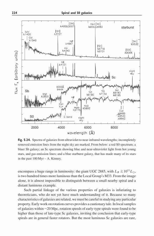
224 Spiral and S0 galaxies

2000 4000 6000 8000

starburst

Sc

Sb

S0

Fig. 5.24. Spectra of galaxies from ultraviolet to near-infrared wavelengths; incompletely

removed emission lines from the night sky are marked. From below: a red S0 spectrum; a

bluer Sb galaxy; an Sc spectrum showing blue and near-ultraviolet light from hot young

stars, and gas emission lines; and a blue starburst galaxy, that has made many of its stars

in the past 100 Myr – A. Kinney.

encompass a huge range in luminosity: the giant UGC 2885, with L B ∼>1011L�,is two hundred times more luminous than the Local Group’s M33. From the imagealone, it is almost impossible to distinguish between a small nearby spiral and adistant luminous example.

Such partial linkage of the various properties of galaxies is infuriating totheoreticians, who do not yet have much understanding of it. Because so manycharacteristics of galaxies are related, we must be careful in studying any particularproperty. Early work on rotation curves provides a cautionary tale. In local samplesof galaxies within ∼20 Mpc, rotation speeds of early-type spirals were found to behigher than those of late-type Sc galaxies, inviting the conclusion that early-typespirals are in general faster rotators. But the most luminous Sc galaxies are rare,

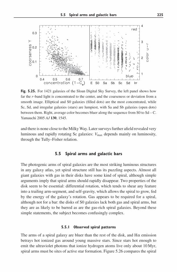
5.5 Spiral arms and galactic bars 225

0.4 0.5 0.6 0.70

0.1

0.2

0.3

1

2

3

4

E S0 Sa Sb Sc Sd Irr

Fig. 5.25. For 1421 galaxies of the Sloan Digital Sky Survey, the left panel shows how

far the r -band light is concentrated to the center, and the coarseness or deviation from a

smooth image. Elliptical and S0 galaxies (filled dots) are the most concentrated, while

Sc, Sd, and irregular galaxies (stars) are lumpiest, with Sa and Sb galaxies (open dots)

between them. Right, average color becomes bluer along the sequence from S0 to Sd – C.

Yamauchi 2005 AJ 130, 1545.

and there is none close to the Milky Way. Later surveys further afield revealed veryluminous and rapidly rotating Sc galaxies: Vmax depends mainly on luminosity,through the Tully–Fisher relation.

5.5 Spiral arms and galactic bars

The photogenic arms of spiral galaxies are the most striking luminous structuresin any galaxy atlas, yet spiral structure still has its puzzling aspects. Almost allgiant galaxies with gas in their disks have some kind of spiral, although simplearguments imply that spiral arms should rapidly disappear. Two properties of thedisk seem to be essential: differential rotation, which tends to shear any featureinto a trailing arm-segment, and self-gravity, which allows the spiral to grow, fedby the energy of the galaxy’s rotation. Gas appears to be required for a spiral,although not for a bar: the disks of S0 galaxies lack both gas and spiral arms, butthey are as likely to be barred as are the gas-rich spiral galaxies. Beyond thesesimple statements, the subject becomes confusingly complex.

5.5.1 Observed spiral patterns

The arms of a spiral galaxy are bluer than the rest of the disk, and Hα emissionbetrays hot ionized gas around young massive stars. Since stars hot enough toemit the ultraviolet photons that ionize hydrogen atoms live only about 10 Myr,spiral arms must be sites of active star formation. Figure 5.26 compares the spiral

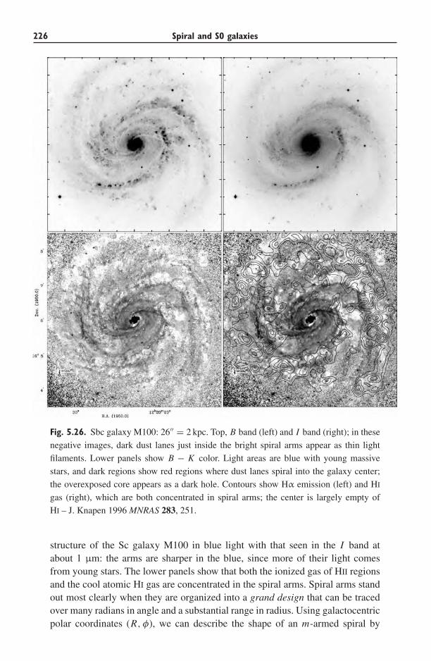
226 Spiral and S0 galaxies

Fig. 5.26. Sbc galaxy M100: 26′′ = 2 kpc. Top, B band (left) and I band (right); in these

negative images, dark dust lanes just inside the bright spiral arms appear as thin light

filaments. Lower panels show B − K color. Light areas are blue with young massive

stars, and dark regions show red regions where dust lanes spiral into the galaxy center;

the overexposed core appears as a dark hole. Contours show Hα emission (left) and HI

gas (right), which are both concentrated in spiral arms; the center is largely empty of

HI – J. Knapen 1996 MNRAS 283, 251.

structure of the Sc galaxy M100 in blue light with that seen in the I band atabout 1 μm: the arms are sharper in the blue, since more of their light comesfrom young stars. The lower panels show that both the ionized gas of HII regionsand the cool atomic HI gas are concentrated in the spiral arms. Spiral arms standout most clearly when they are organized into a grand design that can be tracedover many radians in angle and a substantial range in radius. Using galactocentricpolar coordinates (R, φ), we can describe the shape of an m-armed spiral by

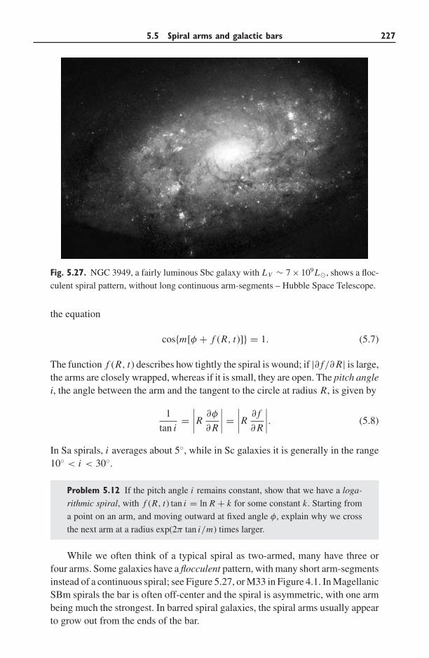
5.5 Spiral arms and galactic bars 227

Fig. 5.27. NGC 3949, a fairly luminous Sbc galaxy with LV ∼ 7 × 109L�, shows a floc-

culent spiral pattern, without long continuous arm-segments – Hubble Space Telescope.

the equation

cos{m[φ + f (R, t)]} = 1. (5.7)

The function f (R, t) describes how tightly the spiral is wound; if |∂ f/∂ R| is large,the arms are closely wrapped, whereas if it is small, they are open. The pitch anglei, the angle between the arm and the tangent to the circle at radius R, is given by

1

tan i=∣∣∣∣R ∂φ

∂ R

∣∣∣∣ =∣∣∣∣R ∂ f

∂ R

∣∣∣∣. (5.8)

In Sa spirals, i averages about 5◦, while in Sc galaxies it is generally in the range10◦ < i < 30◦.

Problem 5.12 If the pitch angle i remains constant, show that we have a loga-

rithmic spiral, with f (R, t) tan i = ln R + k for some constant k. Starting from

a point on an arm, and moving outward at fixed angle φ, explain why we cross

the next arm at a radius exp(2π tan i/m) times larger.

While we often think of a typical spiral as two-armed, many have three orfour arms. Some galaxies have a flocculent pattern, with many short arm-segmentsinstead of a continuous spiral; see Figure 5.27, or M33 in Figure 4.1. In MagellanicSBm spirals the bar is often off-center and the spiral is asymmetric, with one armbeing much the strongest. In barred spiral galaxies, the spiral arms usually appearto grow out from the ends of the bar.

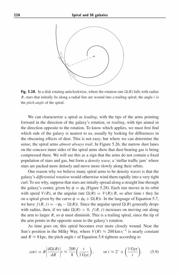
228 Spiral and S0 galaxies

i

Fig. 5.28. In a disk rotating anticlockwise, where the rotation rate �(R) falls with radius

R, stars that initially lie along a radial line are wound into a trailing spiral; the angle i is

the pitch angle of the spiral.

We can characterize a spiral as leading, with the tips of the arms pointingforward in the direction of the galaxy’s rotation, or trailing, with tips aimed inthe direction opposite to the rotation. To know which applies, we must first findwhich side of the galaxy is nearest to us, usually by looking for differences inthe obscuring effects of dust. This is not easy; but where we can determine thesense, the spiral arms almost always trail. In Figure 5.26, the narrow dust laneson the concave inner sides of the spiral arms show that dust-bearing gas is beingcompressed there. We will see this as a sign that the arms do not contain a fixedpopulation of stars and gas, but form a density wave, a ‘stellar traffic jam’ wherestars are packed more densely and move more slowly along their orbits.

One reason why we believe many spiral arms to be density waves is that thegalaxy’s differential rotation would otherwise wind them rapidly into a very tightcurl. To see why, suppose that stars are initally spread along a straight line throughthe galaxy’s center, given by φ = φ0 (Figure 5.28). Each star moves in its orbitwith speed V (R), at the angular rate �(R) = V (R)/R, so after time t they lieon a spiral given by the curve φ = φ0 + �(R)t . In the language of Equation 5.7,we have f (R, t) = −φ0 − �(R)t . Since the angular speed �(R) generally dropswith radius, then, if we take �(R) > 0, f (R, t) increases on moving out alongthe arm to larger R, so φ must diminish. This is a trailing spiral, since the tip ofthe arm points in the opposite sense to the galaxy’s rotation.

As time goes on, this spiral becomes ever more closely wound. Near theSun’s position in the Milky Way, where V (R) ≈ 200 km s−1 is nearly constantand R ≈ 8 kpc, the pitch angle i of Equation 5.8 tightens according to

cot i = R

∣∣∣∣d�(R)

dR

∣∣∣∣t ≈ 200

8

(t

1 Gyr

), or i ≈ 2◦ ×

(1 Gyr

t

). (5.9)

5.5 Spiral arms and galactic bars 229

After only a gigayear, this spiral should be much tighter than those observed in Scgalaxies like our own. Any initial spiral pattern would suffer a similar winding-up;the stars of the spiral arms must perpetually be renewed.

5.5.2 Theories for spiral structure

Spiral structure is a complex phenomenon, and it is likely that no single process isresponsible for the whole range of observed structures. Some galaxies, particularlythose with flocculent spiral arms, may simply recreate their spiral patterns everyfew rotation periods. Once a cloud of gas has made its first stars, blast wavesfrom the supernova explosions of short-lived massive stars will compress thesurrounding gas. This may trigger the birth of yet more stars, so that star formationpropagates through the gas. Differential rotation then draws the cloud out into asegment of a trailing spiral arm. By the time this fragment is strongly stretched,the gas will have been used up, the hot stars will have faded, and the region willhave blended back into the disk. This model of self-propagating star formationwill work only if the pace of starbirth can be regulated so that it neither dies outcompletely nor sets the whole disk afire, exhausting it of gas. It may be able toexplain the fragmentary spiral arms of a galaxy like M33, but is less likely toapply to a system like M100: in Figure 5.26, the spiral arms can be traced overmore than 180◦.

A spiral pattern can last longer if the stars that make it up are not on circularorbits, but are arranged in a particular order in their slightly eccentric paths: thisis called a kinematic spiral. In Section 3.3, we saw that a star’s path on a nearlycircular orbit can be described as the sum of circular motion of a guiding center,at the rate �(Rg) appropriate to its radius Rg, and an epicyclic oscillation movingthe star in and out. The azimuth of the guiding center is φgc = �(Rg)t , whileepicyclic motion causes the star’s radius to vary as

R = Rg + x = Rg + X cos(κt + ψ). (3.70)

Here X is the amplitude of the radial motion, κ is the epicyclic frequency, andthe constant ψ prescribes the initial radius. If we start by placing stars with theirguiding centers spread around the circle at Rg, and set ψ = 2φgc(0) for each ofthem, they will lie on an oval, with its long axis pointing along φ = 0.

At a later time t , the guiding centers move, so that φgc(t) = φgc(0) + �t . Thestars advance on their epicycles, to lie at radius R = Rg + x , where

x = X cos{κt + 2[φgc(t) − �t]} = X cos[(2� − κ)t − 2φgc(t)]. (5.10)

The long axis of the oval now points along the direction where

(2� − κ)t − 2φ = 0, or φ = (� − κ/2)t ≡ �pt. (5.11)

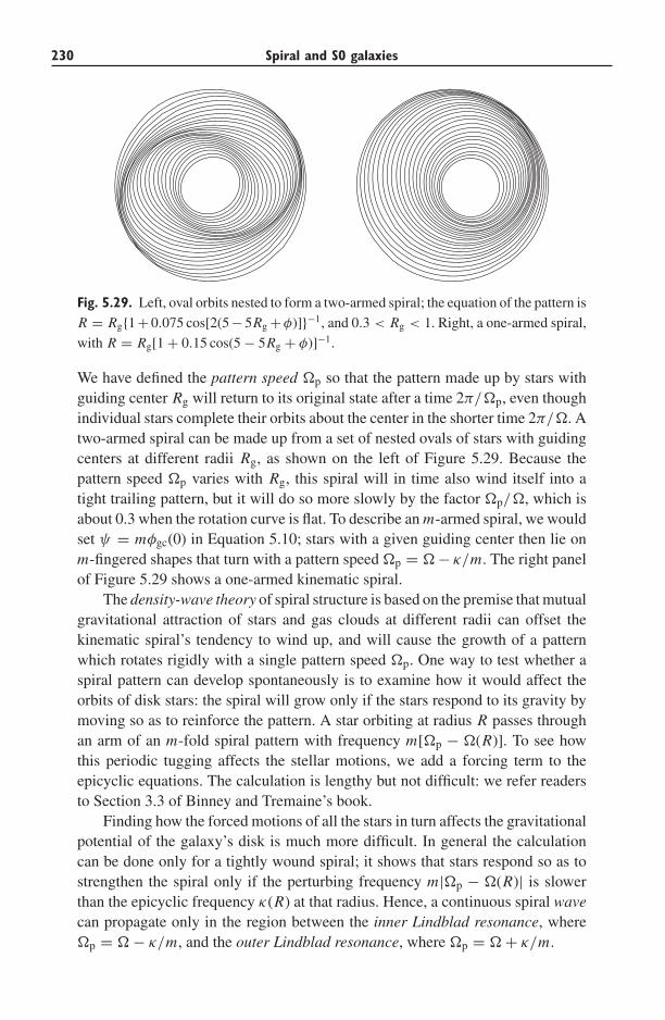
230 Spiral and S0 galaxies

Fig. 5.29. Left, oval orbits nested to form a two-armed spiral; the equation of the pattern is

R = Rg{1 + 0.075 cos[2(5 − 5Rg +φ)]}−1, and 0.3 < Rg < 1. Right, a one-armed spiral,

with R = Rg[1 + 0.15 cos(5 − 5Rg + φ)]−1.

We have defined the pattern speed �p so that the pattern made up by stars withguiding center Rg will return to its original state after a time 2π/�p, even thoughindividual stars complete their orbits about the center in the shorter time 2π/�. Atwo-armed spiral can be made up from a set of nested ovals of stars with guidingcenters at different radii Rg, as shown on the left of Figure 5.29. Because thepattern speed �p varies with Rg, this spiral will in time also wind itself into atight trailing pattern, but it will do so more slowly by the factor �p/�, which isabout 0.3 when the rotation curve is flat. To describe an m-armed spiral, we wouldset ψ = mφgc(0) in Equation 5.10; stars with a given guiding center then lie onm-fingered shapes that turn with a pattern speed �p = � − κ/m. The right panelof Figure 5.29 shows a one-armed kinematic spiral.

The density-wave theory of spiral structure is based on the premise that mutualgravitational attraction of stars and gas clouds at different radii can offset thekinematic spiral’s tendency to wind up, and will cause the growth of a patternwhich rotates rigidly with a single pattern speed �p. One way to test whether aspiral pattern can develop spontaneously is to examine how it would affect theorbits of disk stars: the spiral will grow only if the stars respond to its gravity bymoving so as to reinforce the pattern. A star orbiting at radius R passes throughan arm of an m-fold spiral pattern with frequency m[�p − �(R)]. To see howthis periodic tugging affects the stellar motions, we add a forcing term to theepicyclic equations. The calculation is lengthy but not difficult: we refer readersto Section 3.3 of Binney and Tremaine’s book.

Finding how the forced motions of all the stars in turn affects the gravitationalpotential of the galaxy’s disk is much more difficult. In general the calculationcan be done only for a tightly wound spiral; it shows that stars respond so as tostrengthen the spiral only if the perturbing frequency m|�p − �(R)| is slowerthan the epicyclic frequency κ(R) at that radius. Hence, a continuous spiral wavecan propagate only in the region between the inner Lindblad resonance, where�p = � − κ/m, and the outer Lindblad resonance, where �p = � + κ/m.

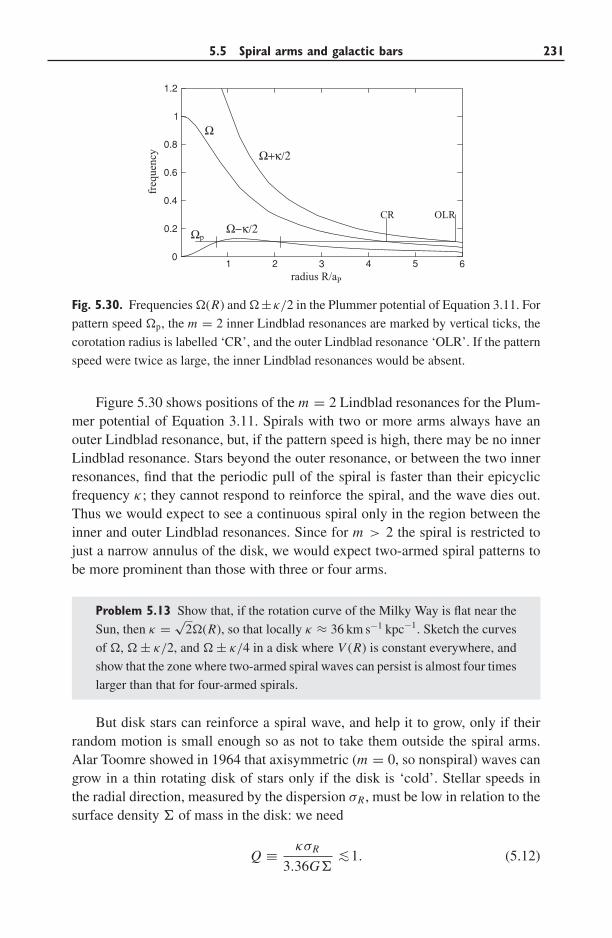
5.5 Spiral arms and galactic bars 231

654321

1.2

1

0.8

0.6

0.4

0.2

0

OLRCR

p

radius R/aP

freq

uenc

y

Fig. 5.30. Frequencies �(R) and �±κ/2 in the Plummer potential of Equation 3.11. For

pattern speed �p, the m = 2 inner Lindblad resonances are marked by vertical ticks, the

corotation radius is labelled ‘CR’, and the outer Lindblad resonance ‘OLR’. If the pattern

speed were twice as large, the inner Lindblad resonances would be absent.

Figure 5.30 shows positions of the m = 2 Lindblad resonances for the Plum-mer potential of Equation 3.11. Spirals with two or more arms always have anouter Lindblad resonance, but, if the pattern speed is high, there may be no innerLindblad resonance. Stars beyond the outer resonance, or between the two innerresonances, find that the periodic pull of the spiral is faster than their epicyclicfrequency κ; they cannot respond to reinforce the spiral, and the wave dies out.Thus we would expect to see a continuous spiral only in the region between theinner and outer Lindblad resonances. Since for m > 2 the spiral is restricted tojust a narrow annulus of the disk, we would expect two-armed spiral patterns tobe more prominent than those with three or four arms.

Problem 5.13 Show that, if the rotation curve of the Milky Way is flat near the

Sun, then κ = √2�(R), so that locally κ ≈ 36 km s−1 kpc−1. Sketch the curves

of �, � ± κ/2, and � ± κ/4 in a disk where V (R) is constant everywhere, and

show that the zone where two-armed spiral waves can persist is almost four times

larger than that for four-armed spirals.

But disk stars can reinforce a spiral wave, and help it to grow, only if theirrandom motion is small enough so as not to take them outside the spiral arms.Alar Toomre showed in 1964 that axisymmetric (m = 0, so nonspiral) waves cangrow in a thin rotating disk of stars only if the disk is ‘cold’. Stellar speeds inthe radial direction, measured by the dispersion σR , must be low in relation to thesurface density � of mass in the disk: we need

Q ≡ κσR

3.36G� ∼<1. (5.12)

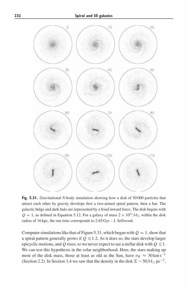
232 Spiral and S0 galaxies

Fig. 5.31. Gravitational N-body simulation showing how a disk of 50 000 particles that

attract each other by gravity develops first a two-armed spiral pattern, then a bar. The

galactic bulge and dark halo are represented by a fixed inward force. The disk begins with

Q = 1, as defined in Equation 5.12. For a galaxy of mass 2 × 1011M� within the disk

radius of 16 kpc, the run time corresponds to 2.65 Gyr – J. Sellwood.

Computer simulations like that of Figure 5.31, which began with Q = 1, show thata spiral pattern generally grows if Q ∼<1.2. As it does so, the stars develop largerepicyclic motions, and Q rises; so we never expect to see a stellar disk with Q ∼<1.We can test this hypothesis in the solar neighborhood. Here, the stars making upmost of the disk mass, those at least as old as the Sun, have σR ≈ 30 km s−1

(Section 2.2). In Section 3.4 we saw that the density in the disk � ∼50M� pc−2,

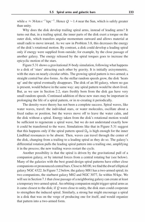
5.5 Spiral arms and galactic bars 233

while κ ≈ 36 km s−1 kpc−1. Hence Q ∼1.4 near the Sun, which is safely greaterthan unity.

Why does the disk develop trailing spiral arms, instead of leading arms? Itturns out that, in a trailing spiral, the inner parts of the disk exert a torque on theouter disk, which transfers angular momentum outward and allows material atsmall radii to move inward. As we saw in Problem 3.8, this decreases the energyof the disk’s rotational motion. By contrast, a disk could develop a leading spiralonly if energy were supplied from outside; for example, by the close passage ofanother galaxy. The energy released by the spiral torques goes to increase theepicyclic motion of the stars.

Figure 5.31 shows a gravitational N-body simulation, following what happensto a disk of ‘stars’ attracting each other by gravity. It is initially axisymmetric,with the stars on nearly circular orbits. The growing spiral pattern is two-armed; astraight central bar also forms. As the stellar random speeds grow, the disk ‘heatsup’ and the spiral eventually disappears. The disk of an S0 galaxy, where no gasis present, would behave in the same way: any spiral pattern would be short-lived.But, as we saw in Section 2.2, stars freshly born from the disk gas have verysmall random speeds. Continued addition of these new stars may be important inprolonging the life of a spiral pattern, or in re-creating it periodically.

The density-wave theory has not been a complete success. Spiral waves, likewater waves, travel: the individual stars, or water molecules, oscillate about afixed radius or position, but the waves move off to leave the water calm, andthe disk without a spiral. Energy taken from the disk’s rotational motion wouldbe sufficient to regenerate a spiral wave, but we do not understand exactly howit could be transferred to the wave. Simulations like that in Figure 5.31 suggestthat this happens only if the spiral pattern speed �p is high enough for the innerLindblad resonances to be absent. Then, waves can travel through the center ofthe disk, changing from a trailing to a leading spiral as they do so. The galaxy’sdifferential rotation pulls the leading spiral pattern into a trailing one, amplifyingit in the process; the new trailing waves restart the cycle.

Another possibility is that the spiral is driven by the gravitational pull of acompanion galaxy, or by internal forces from a central rotating bar (see below).Many of the galaxies with the best grand-design spiral patterns have either closecompanions or pronounced central bars. Close to M100, we find the dwarf ellipticalgalaxy NGC 4322. In Figure 7.2 below, the galaxy M81 has a two-armed spiral; itstwo companions, the starburst galaxy M82 and NGC 3077, lie within 50 kpc. Wewill see in Section 7.1 that close passage of a neighboring galaxy can create at leasta temporary two-armed spiral. An orbiting companion might trigger spiral arms asit came closest to the disk; if Q were close to unity, the disk stars could cooperateto strengthen the induced spiral. Similarly, a strong bar might encourage a spiralin a disk that was on the verge of producing one for itself, and would organizethat pattern into a two-armed form.

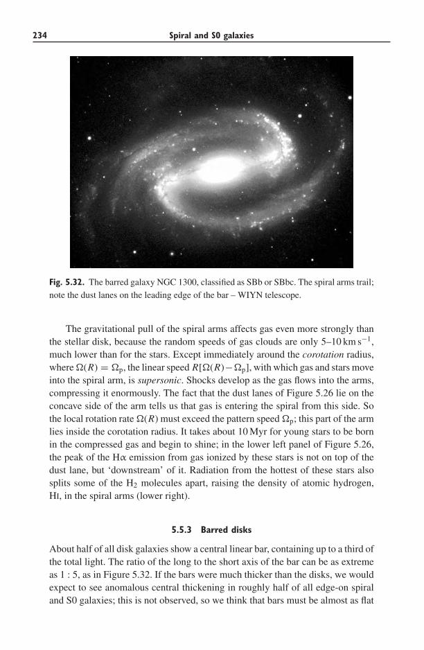
234 Spiral and S0 galaxies

Fig. 5.32. The barred galaxy NGC 1300, classified as SBb or SBbc. The spiral arms trail;

note the dust lanes on the leading edge of the bar – WIYN telescope.

The gravitational pull of the spiral arms affects gas even more strongly thanthe stellar disk, because the random speeds of gas clouds are only 5–10 km s−1,much lower than for the stars. Except immediately around the corotation radius,where �(R) = �p, the linear speed R[�(R)−�p], with which gas and stars moveinto the spiral arm, is supersonic. Shocks develop as the gas flows into the arms,compressing it enormously. The fact that the dust lanes of Figure 5.26 lie on theconcave side of the arm tells us that gas is entering the spiral from this side. Sothe local rotation rate �(R) must exceed the pattern speed �p; this part of the armlies inside the corotation radius. It takes about 10 Myr for young stars to be bornin the compressed gas and begin to shine; in the lower left panel of Figure 5.26,the peak of the Hα emission from gas ionized by these stars is not on top of thedust lane, but ‘downstream’ of it. Radiation from the hottest of these stars alsosplits some of the H2 molecules apart, raising the density of atomic hydrogen,HI, in the spiral arms (lower right).

5.5.3 Barred disks

About half of all disk galaxies show a central linear bar, containing up to a third ofthe total light. The ratio of the long to the short axis of the bar can be as extremeas 1 : 5, as in Figure 5.32. If the bars were much thicker than the disks, we wouldexpect to see anomalous central thickening in roughly half of all edge-on spiraland S0 galaxies; this is not observed, so we think that bars must be almost as flat

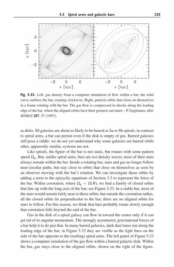
5.5 Spiral arms and galactic bars 235

Fig. 5.33. Left, gas density from a computer simulation of flow within a bar; the solid

curve outlines the bar, rotating clockwise. Right, particle orbits that close on themselves

in a frame rotating with the bar. The gas flow is compressed in shocks along the leading

edge of the bar, where the aligned orbits have their greatest curvature – P. Englmaier, after

MNRAS 287, 57 (1997).

as disks. S0 galaxies are about as likely to be barred as Sa or Sb spirals; in contrastto spiral arms, a bar can persist even if the disk is empty of gas. Barred galaxiesstill pose a riddle: we do not yet understand why some galaxies are barred whileother, apparently similar, systems are not.

Like spirals, the figure of the bar is not static, but rotates with some patternspeed �p. But, unlike spiral arms, bars are not density waves; most of their starsalways remain within the bar. Inside a rotating bar, stars and gas no longer follownear-circular paths, but stay close to orbits that close on themselves as seen byan observer moving with the bar’s rotation. We can investigate these orbits byadding a term to the epicyclic equations of Section 3.3 to represent the force ofthe bar. Within corotation, where �p < �(R), we find a family of closed orbitsthat line up with the long axis of the bar; see Figure 5.33. In a stable bar, most ofthe stars would remain fairly near to these orbits, but outside the corotation radius,all the closed orbits lie perpendicular to the bar; there are no aligned orbits forstars to follow. For this reason, we think that bars probably rotate slowly enoughthat corotation falls beyond the end of the bar.

Gas in the disk of a spiral galaxy can flow in toward the center only if it canget rid of its angular momentum. The strongly asymmetric gravitational forces ofa bar help it to do just that. In many barred galaxies, dark dust lanes run along theleading edge of the bar; in Figure 5.32 they are visible as the light lines on theside of the bar opposite to the (trailing) spiral arms. The left panel of Figure 5.33shows a computer simulation of the gas flow within a barred galactic disk. Withinthe bar, gas stays close to the aligned orbits, shown on the right of the figure.

236 Spiral and S0 galaxies

At the ends, the flow converges sharply, and gas pressure becomes important. Ashock forms, compressing the gas and dust along the leading edge of the bar, aswe see in NGC 1300.

In the shock, the gas loses part of the energy of its forward motion as heat, soit drops down onto more tightly bound orbits closer to the center of the galaxy.This energy dissipation continues until the gas meets the rounder orbits that lieperpendicular to the bar; then, inflow stops, and the gas piles up in a central ring.The dust lanes produced in simulations where the corotation radius is only slightlybeyond the end of the bar look most like those we observe in real barred galaxies.So we believe that the pattern speed �p is usually high, and rotation is almost asfast as it can be; corotation lies just beyond the bar’s end.

Because the spiral arms in barred galaxies usually appear to start from theends of the bar, it is often assumed that bar and spiral share the same pattern speedand always maintain the same relative alignment. This need not be the case: inFigure 5.31, the outer spiral has a lower pattern speed than the bar. But the eye joinsthe spiral pattern to the bar, so that the arms always appear to start near the end ofthe bar. There is nothing to prevent a galaxy from developing a bar that rotates faster(or slower) than the pattern of a surrounding spiral, or from having two or moreindependent spirals with discrepant pattern speeds or different numbers of arms.

Further reading: D. M. Elmegreen, 1998, Galaxies and Galactic Structure(Prentice-Hall, Englewood Cliffs, New Jersey), unfortunately now out of print,treats spiral structure on an undergraduate level; and Chapter 6 of J. Binney and S.Tremaine, 1987, Galactic Dynamics (Princeton University Press, Princeton, NewJersey) gives a graduate-level discussion of the theory.

5.6 Bulges and centers of disk galaxies

Bulges, along with the centers of small elliptical galaxies, are some of the densestknown stellar systems (see Figure 4.18). The Milky Way’s bulge is largely hiddenfrom us by dust; but when we look at M31 through a small telescope or binoculars,or at an ‘underexposed’ optical image of a disk galaxy, only the bright bulge isvisible. In Figure 5.4, the surface brightness at the center of NGC 7331 rises tofifty times that of the inward-extrapolated exponential disk. The bulge is the ‘bigcity’ of a disk galaxy: a centrally placed dense region, where old and new stars arecrammed tightly together. Within the central few parsecs we can find a hundredmillion stars, packed into a nuclear cluster; these in turn often harbor a large blackhole. In these tiny central regions, densities are enormous, and timescales short.

5.6.1 Bulges

In the images of two edge-on galaxies in Figures 5.5 and 5.16, the bulges appear asround ellipsoids. Other bulges are quite flattened, almost like bright central disks.

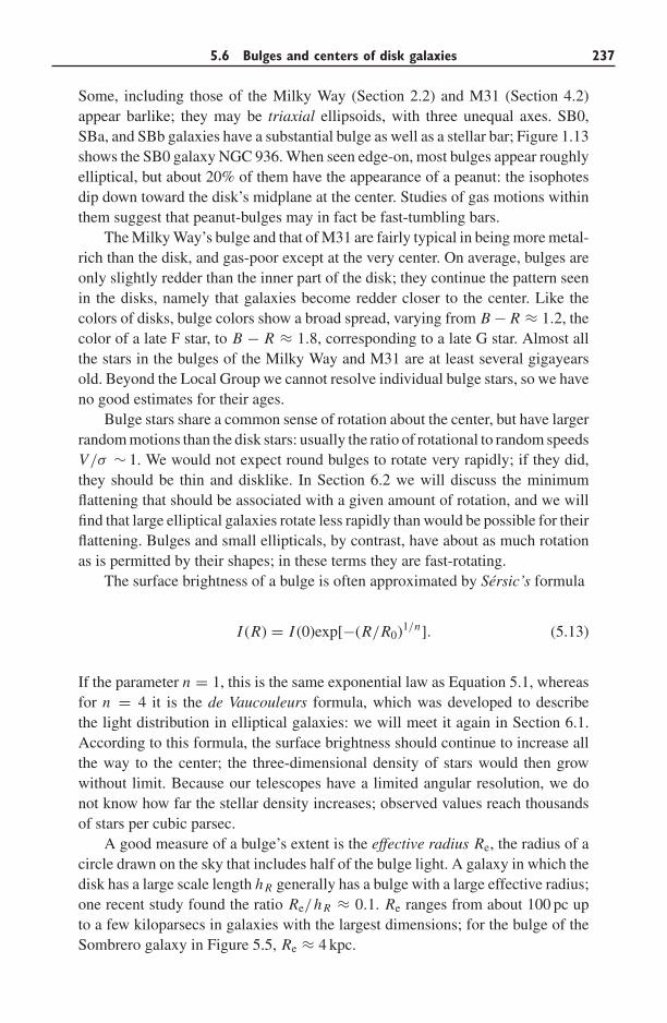
5.6 Bulges and centers of disk galaxies 237

Some, including those of the Milky Way (Section 2.2) and M31 (Section 4.2)appear barlike; they may be triaxial ellipsoids, with three unequal axes. SB0,SBa, and SBb galaxies have a substantial bulge as well as a stellar bar; Figure 1.13shows the SB0 galaxy NGC 936. When seen edge-on, most bulges appear roughlyelliptical, but about 20% of them have the appearance of a peanut: the isophotesdip down toward the disk’s midplane at the center. Studies of gas motions withinthem suggest that peanut-bulges may in fact be fast-tumbling bars.

The Milky Way’s bulge and that of M31 are fairly typical in being more metal-rich than the disk, and gas-poor except at the very center. On average, bulges areonly slightly redder than the inner part of the disk; they continue the pattern seenin the disks, namely that galaxies become redder closer to the center. Like thecolors of disks, bulge colors show a broad spread, varying from B − R ≈ 1.2, thecolor of a late F star, to B − R ≈ 1.8, corresponding to a late G star. Almost allthe stars in the bulges of the Milky Way and M31 are at least several gigayearsold. Beyond the Local Group we cannot resolve individual bulge stars, so we haveno good estimates for their ages.

Bulge stars share a common sense of rotation about the center, but have largerrandom motions than the disk stars: usually the ratio of rotational to random speedsV/σ ∼ 1. We would not expect round bulges to rotate very rapidly; if they did,they should be thin and disklike. In Section 6.2 we will discuss the minimumflattening that should be associated with a given amount of rotation, and we willfind that large elliptical galaxies rotate less rapidly than would be possible for theirflattening. Bulges and small ellipticals, by contrast, have about as much rotationas is permitted by their shapes; in these terms they are fast-rotating.

The surface brightness of a bulge is often approximated by Sersic’s formula

I (R) = I (0)exp[−(R/R0)1/n]. (5.13)

If the parameter n = 1, this is the same exponential law as Equation 5.1, whereasfor n = 4 it is the de Vaucouleurs formula, which was developed to describethe light distribution in elliptical galaxies: we will meet it again in Section 6.1.According to this formula, the surface brightness should continue to increase allthe way to the center; the three-dimensional density of stars would then growwithout limit. Because our telescopes have a limited angular resolution, we donot know how far the stellar density increases; observed values reach thousandsof stars per cubic parsec.

A good measure of a bulge’s extent is the effective radius Re, the radius of acircle drawn on the sky that includes half of the bulge light. A galaxy in which thedisk has a large scale length h R generally has a bulge with a large effective radius;one recent study found the ratio Re/h R ≈ 0.1. Re ranges from about 100 pc upto a few kiloparsecs in galaxies with the largest dimensions; for the bulge of theSombrero galaxy in Figure 5.5, Re ≈ 4 kpc.

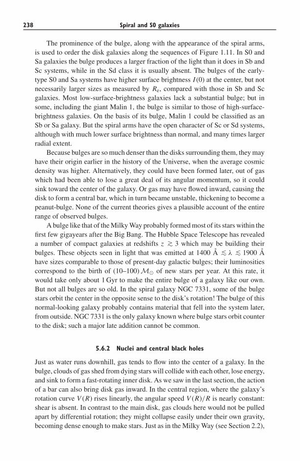
238 Spiral and S0 galaxies

The prominence of the bulge, along with the appearance of the spiral arms,is used to order the disk galaxies along the sequences of Figure 1.11. In S0 andSa galaxies the bulge produces a larger fraction of the light than it does in Sb andSc systems, while in the Sd class it is usually absent. The bulges of the early-type S0 and Sa systems have higher surface brightness I (0) at the center, but notnecessarily larger sizes as measured by Re, compared with those in Sb and Scgalaxies. Most low-surface-brightness galaxies lack a substantial bulge; but insome, including the giant Malin 1, the bulge is similar to those of high-surface-brightness galaxies. On the basis of its bulge, Malin 1 could be classified as anSb or Sa galaxy. But the spiral arms have the open character of Sc or Sd systems,although with much lower surface brightness than normal, and many times largerradial extent.

Because bulges are so much denser than the disks surrounding them, they mayhave their origin earlier in the history of the Universe, when the average cosmicdensity was higher. Alternatively, they could have been formed later, out of gaswhich had been able to lose a great deal of its angular momentum, so it couldsink toward the center of the galaxy. Or gas may have flowed inward, causing thedisk to form a central bar, which in turn became unstable, thickening to become apeanut-bulge. None of the current theories gives a plausible account of the entirerange of observed bulges.

A bulge like that of the Milky Way probably formed most of its stars within thefirst few gigayears after the Big Bang. The Hubble Space Telescope has revealeda number of compact galaxies at redshifts z ∼> 3 which may be building theirbulges. These objects seen in light that was emitted at 1400 A ∼< λ ∼< 1900 Ahave sizes comparable to those of present-day galactic bulges; their luminositiescorrespond to the birth of (10–100) M� of new stars per year. At this rate, itwould take only about 1 Gyr to make the entire bulge of a galaxy like our own.But not all bulges are so old. In the spiral galaxy NGC 7331, some of the bulgestars orbit the center in the opposite sense to the disk’s rotation! The bulge of thisnormal-looking galaxy probably contains material that fell into the system later,from outside. NGC 7331 is the only galaxy known where bulge stars orbit counterto the disk; such a major late addition cannot be common.

5.6.2 Nuclei and central black holes

Just as water runs downhill, gas tends to flow into the center of a galaxy. In thebulge, clouds of gas shed from dying stars will collide with each other, lose energy,and sink to form a fast-rotating inner disk. As we saw in the last section, the actionof a bar can also bring disk gas inward. In the central region, where the galaxy’srotation curve V (R) rises linearly, the angular speed V (R)/R is nearly constant:shear is absent. In contrast to the main disk, gas clouds here would not be pulledapart by differential rotation; they might collapse easily under their own gravity,becoming dense enough to make stars. Just as in the Milky Way (see Section 2.2),

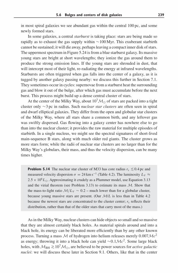
5.6 Bulges and centers of disk galaxies 239

in most spiral galaxies we see abundant gas within the central 100 pc, and somenewly formed stars.

In some galaxies, a central starburst is taking place: stars are being made sorapidly as to exhaust the gas supply within ∼100 Myr. This exuberant starbirthcannot be sustained; it will die away, perhaps leaving a compact inner disk of stars.The uppermost spectrum in Figure 5.24 is from a blue starburst galaxy. Its massiveyoung stars are bright at short wavelengths; they ionize the gas around them toproduce the strong emission lines. If the young stars are shrouded in dust, thatwill intercept most of their light, re-radiating the energy at infrared wavelengths.Starbursts are often triggered when gas falls into the center of a galaxy, as it istugged by another galaxy passing nearby: we discuss this further in Section 7.1.They sometimes occur in cycles: supernovae from a starburst heat the surroundinggas and blow it out of the bulge, after which gas must accumulate before the nextburst. This process might build up a dense central cluster of stars.

At the center of the Milky Way, about 107M� of stars are packed into a tightcluster only ∼3 pc in radius. Such nuclear star clusters are often seen in spiraland dwarf elliptical galaxies. They differ from the open and globular star clustersof the Milky Way, where all stars share a common birth, and any leftover gaswas swiftly dispersed. Gas flowing into a galaxy center has nowhere else to gothan into the nuclear cluster; it provides the raw material for multiple episodes ofstarbirth. In a single nucleus, we might see the spectral signatures of short-livedmain-sequence B stars, along with much older red giants. The cluster grows asmore stars form; while the radii of nuclear star clusters are no larger than for theMilky Way’s globulars, their mass, and thus the velocity dispersion, can be manytimes higher.

Problem 5.14 The nuclear star cluster of M33 has core radius rc ∼< 0.4 pc and

measured velocity dispersion σ = 24 km s−1 (Table 4.2). The luminosity LV ≈2.5 × 106L�. Approximating it crudely as a Plummer model, use Equation 3.13

and the virial theorem (see Problem 3.13) to estimate its mass M. Show that

the mass-to-light ratio M/LV ∼ 0.2 – much lower than for a globular cluster,

because young massive stars are present. (Our M/L is less than in Table 4.2

because the newest stars are concentrated to the cluster center; rc reflects their

distribution, rather than that of the older stars that carry most of the mass.)

As in the Milky Way, nuclear clusters can hide objects so small and so massivethat they are almost certainly black holes. As material spirals around and into ablack hole, its energy can be liberated more efficiently than by any other knownprocess. Turning a mass M of hydrogen into helium releases merely 0.007Mc2

as energy; throwing it into a black hole can yield ∼0.1Mc2. Some large blackholes, with MBH ∼>107M�, are believed to be power sources for active galacticnuclei: we will discuss these later in Section 9.1. Others, like that in the center

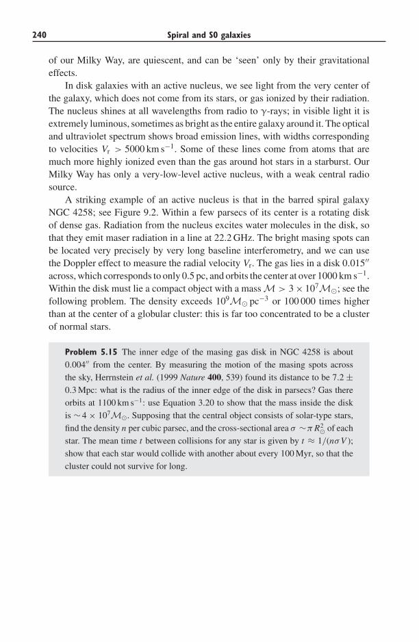
240 Spiral and S0 galaxies

of our Milky Way, are quiescent, and can be ‘seen’ only by their gravitationaleffects.

In disk galaxies with an active nucleus, we see light from the very center ofthe galaxy, which does not come from its stars, or gas ionized by their radiation.The nucleus shines at all wavelengths from radio to γ-rays; in visible light it isextremely luminous, sometimes as bright as the entire galaxy around it. The opticaland ultraviolet spectrum shows broad emission lines, with widths correspondingto velocities Vr > 5000 km s−1. Some of these lines come from atoms that aremuch more highly ionized even than the gas around hot stars in a starburst. OurMilky Way has only a very-low-level active nucleus, with a weak central radiosource.

A striking example of an active nucleus is that in the barred spiral galaxyNGC 4258; see Figure 9.2. Within a few parsecs of its center is a rotating diskof dense gas. Radiation from the nucleus excites water molecules in the disk, sothat they emit maser radiation in a line at 22.2 GHz. The bright masing spots canbe located very precisely by very long baseline interferometry, and we can usethe Doppler effect to measure the radial velocity Vr. The gas lies in a disk 0.015′′

across, which corresponds to only 0.5 pc, and orbits the center at over 1000 km s−1.Within the disk must lie a compact object with a mass M > 3 × 107M�; see thefollowing problem. The density exceeds 109M� pc−3 or 100 000 times higherthan at the center of a globular cluster: this is far too concentrated to be a clusterof normal stars.

Problem 5.15 The inner edge of the masing gas disk in NGC 4258 is about

0.004′′ from the center. By measuring the motion of the masing spots across

the sky, Herrnstein et al. (1999 Nature 400, 539) found its distance to be 7.2 ±0.3 Mpc: what is the radius of the inner edge of the disk in parsecs? Gas there

orbits at 1100 km s−1: use Equation 3.20 to show that the mass inside the disk

is ∼ 4 × 107M�. Supposing that the central object consists of solar-type stars,

find the density n per cubic parsec, and the cross-sectional area σ ∼π R2� of each

star. The mean time t between collisions for any star is given by t ≈ 1/(nσ V );

show that each star would collide with another about every 100 Myr, so that the

cluster could not survive for long.

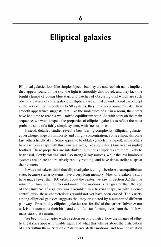
6

Elliptical galaxies

Elliptical galaxies look like simple objects; but they are not. As their name implies,they appear round on the sky; the light is smoothly distributed, and they lack thebright clumps of young blue stars and patches of obscuring dust which are suchobvious features of spiral galaxies. Ellipticals are almost devoid of cool gas, exceptat the very center; in contrast to S0 systems, they have no prominent disk. Theirsmooth appearance suggests that, like the molecules of air in a room, their starshave had time to reach a well-mixed equilibrium state. As with stars on the mainsequence, we would expect the properties of elliptical galaxies to reflect the mostprobable state of a fairly simple system, with ‘no surprises’.

Instead, detailed studies reveal a bewildering complexity. Elliptical galaxiescover a huge range of luminosity and of light concentration. Some ellipticals rotatefast, others hardly at all. Some appear to be oblate (grapefruit shaped), while othershave a triaxial shape with three unequal axes, like a squashed (American or rugby)football. These properties are interlinked: luminous ellipticals are more likely tobe triaxial, slowly rotating, and also strong X-ray sources, while the less luminoussystems are oblate and relatively rapidly rotating, and have dense stellar cusps attheir centers.

It was a mistake to think that elliptical galaxies might be close to an equilibriumstate, because stellar systems have a very long memory. Most of a galaxy’s starshave made fewer than 100 orbits about the center; we saw in Section 3.2 that therelaxation time required to randomize their motions is far greater than the ageof the Universe. If a galaxy was assembled in a triaxial shape, or with a densecentral cusp, these characteristics would not yet have been erased. The varietyamong elliptical galaxies suggests that they originated by a number of differentpathways. Present-day elliptical galaxies are ‘fossils’ of the earlier Universe; ourtask is to reconstruct their birth and youthful star-forming lives from the old low-mass stars that remain.

We begin this chapter with a section on photometry: how the images of ellip-tical galaxies appear in visible light, and what this tells us about the distributionof stars within them. Section 6.2 discusses stellar motions, and how the rotation

241

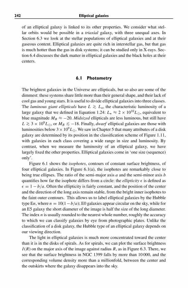
242 Elliptical galaxies

of an elliptical galaxy is linked to its other properties. We consider what stel-lar orbits would be possible in a triaxial galaxy, with three unequal axes. InSection 6.3 we look at the stellar populations of elliptical galaxies and at theirgaseous content. Elliptical galaxies are quite rich in interstellar gas, but that gasis much hotter than the gas in disk systems; it can be studied only in X-rays. Sec-tion 6.4 discusses the dark matter in elliptical galaxies and the black holes at theircenters.

6.1 Photometry

The brightest galaxies in the Universe are ellipticals, but so also are some of thedimmest: these systems share little more than their general shape, and their lack ofcool gas and young stars. It is useful to divide elliptical galaxies into three classes.The luminous giant ellipticals have L ∼> L, the characteristic luminosity of alarge galaxy that we defined in Equation 1.24: L ≈ 2 × 1010L�, equivalent toblue magnitude MB ≈ −20. Midsized ellipticals are less luminous, but still haveL ∼> 3 × 109L�, or MB ∼< −18. Finally, dwarf elliptical galaxies are those withluminosities below 3×109L�. We saw in Chapter 5 that many attributes of a diskgalaxy are determined by its position in the classification scheme of Figure 1.11,with galaxies in each class covering a wide range in size and luminosity. Bycontrast, when we measure the luminosity of an elliptical galaxy, we havelargely fixed the other properties. Elliptical galaxies come in ‘one size (sequence)only’.

Figure 6.1 shows the isophotes, contours of constant surface brightness, offour elliptical galaxies. In Figure 6.1(a), the isophotes are remarkably close tobeing true ellipses. The ratio of the semi-major axis a and the semi-minor axis bquantifies how far the isophote differs from a circle: the ellipticity ε is defined asε = 1 − b/a. Often the ellipticity is fairly constant, and the position of the centerand the direction of the long axis remain stable, from the bright inner isophotes tothe faint outer contours. This allows us to label elliptical galaxies by the Hubbletype En, where n = 10(1−b/a); E0 galaxies appear circular on the sky, while foran E5 galaxy the short diameter of the image is half the size of the long diameter.The index n is usually rounded to the nearest whole number, roughly the accuracyto which we can classify galaxies by eye from photographic plates. Unlike theclassification of a disk galaxy, the Hubble type of an elliptical galaxy depends onour viewing direction.

The light in elliptical galaxies is much more concentrated toward the centerthan it is in the disks of spirals. As for spirals, we can plot the surface brightnessI (R) on the major axis of the image against radius R, as in Figure 6.3. There, wesee that the surface brightness in NGC 1399 falls by more than 10 000, and thecorresponding volume density more than a millionfold, between the center andthe outskirts where the galaxy disappears into the sky.

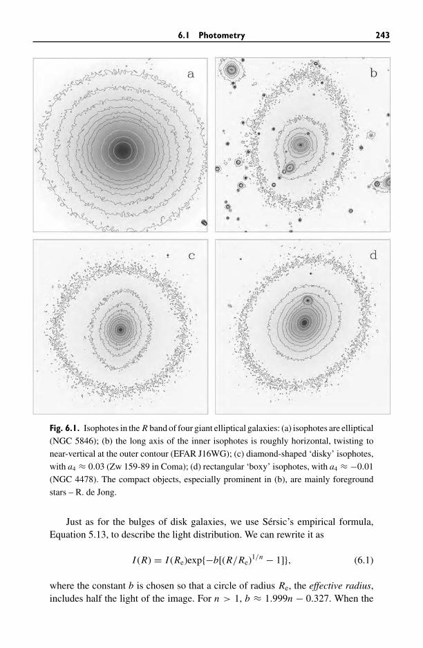
6.1 Photometry 243

Fig. 6.1. Isophotes in the R band of four giant elliptical galaxies: (a) isophotes are elliptical

(NGC 5846); (b) the long axis of the inner isophotes is roughly horizontal, twisting to

near-vertical at the outer contour (EFAR J16WG); (c) diamond-shaped ‘disky’ isophotes,

with a4 ≈ 0.03 (Zw 159-89 in Coma); (d) rectangular ‘boxy’ isophotes, with a4 ≈ −0.01

(NGC 4478). The compact objects, especially prominent in (b), are mainly foreground

stars – R. de Jong.

Just as for the bulges of disk galaxies, we use Sersic’s empirical formula,Equation 5.13, to describe the light distribution. We can rewrite it as

I (R) = I (Re)exp{−b[(R/Re)1/n − 1]}, (6.1)

where the constant b is chosen so that a circle of radius Re, the effective radius,includes half the light of the image. For n > 1, b ≈ 1.999n − 0.327. When the

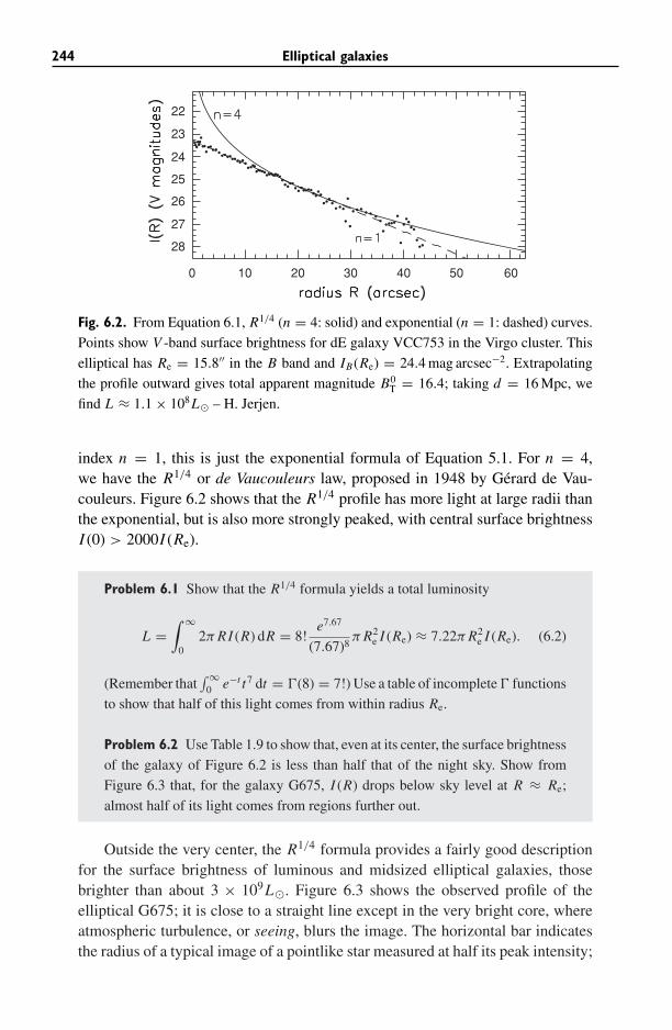
244 Elliptical galaxies

0 10 20 30 40

28

27

26

25

24

23

22

50 60

Fig. 6.2. From Equation 6.1, R1/4 (n = 4: solid) and exponential (n = 1: dashed) curves.

Points show V -band surface brightness for dE galaxy VCC753 in the Virgo cluster. This

elliptical has Re = 15.8′′ in the B band and IB(Re) = 24.4 mag arcsec−2. Extrapolating

the profile outward gives total apparent magnitude B0T = 16.4; taking d = 16 Mpc, we

find L ≈ 1.1 × 108L� – H. Jerjen.

index n = 1, this is just the exponential formula of Equation 5.1. For n = 4,we have the R1/4 or de Vaucouleurs law, proposed in 1948 by Gerard de Vau-couleurs. Figure 6.2 shows that the R1/4 profile has more light at large radii thanthe exponential, but is also more strongly peaked, with central surface brightnessI (0) > 2000I (Re).

Problem 6.1 Show that the R1/4 formula yields a total luminosity

L =∫ ∞

02π RI (R) dR = 8!

e7.67

(7.67)8π R2

e I (Re) ≈ 7.22π R2e I (Re). (6.2)

(Remember that∫∞

0 e−t t7 dt = �(8) = 7!) Use a table of incomplete � functions

to show that half of this light comes from within radius Re.

Problem 6.2 Use Table 1.9 to show that, even at its center, the surface brightness

of the galaxy of Figure 6.2 is less than half that of the night sky. Show from

Figure 6.3 that, for the galaxy G675, I (R) drops below sky level at R ≈ Re;

almost half of its light comes from regions further out.

Outside the very center, the R1/4 formula provides a fairly good descriptionfor the surface brightness of luminous and midsized elliptical galaxies, thosebrighter than about 3 × 109L�. Figure 6.3 shows the observed profile of theelliptical G675; it is close to a straight line except in the very bright core, whereatmospheric turbulence, or seeing, blurs the image. The horizontal bar indicatesthe radius of a typical image of a pointlike star measured at half its peak intensity;

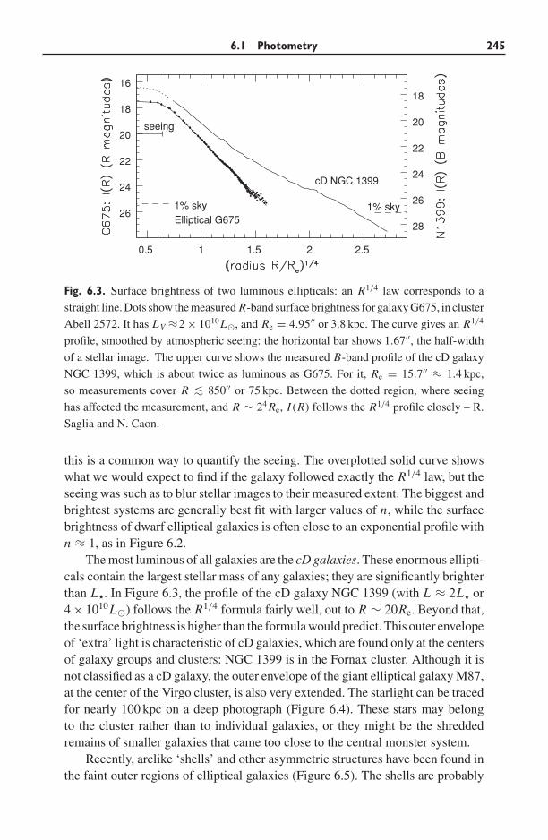
6.1 Photometry 245

0.5 1 1.5 2 2.5

26

24

22

20

18

16

1% skyElliptical G675

seeing

28

26

24

22

20

18

1% sky

cD NGC 1399

Fig. 6.3. Surface brightness of two luminous ellipticals: an R1/4 law corresponds to a

straight line. Dots show the measured R-band surface brightness for galaxy G675, in cluster

Abell 2572. It has LV ≈2 × 1010L�, and Re = 4.95′′ or 3.8 kpc. The curve gives an R1/4

profile, smoothed by atmospheric seeing: the horizontal bar shows 1.67′′, the half-width

of a stellar image. The upper curve shows the measured B-band profile of the cD galaxy

NGC 1399, which is about twice as luminous as G675. For it, Re = 15.7′′ ≈ 1.4 kpc,

so measurements cover R ∼< 850′′ or 75 kpc. Between the dotted region, where seeing

has affected the measurement, and R ∼ 24 Re, I (R) follows the R1/4 profile closely – R.

Saglia and N. Caon.

this is a common way to quantify the seeing. The overplotted solid curve showswhat we would expect to find if the galaxy followed exactly the R1/4 law, but theseeing was such as to blur stellar images to their measured extent. The biggest andbrightest systems are generally best fit with larger values of n, while the surfacebrightness of dwarf elliptical galaxies is often close to an exponential profile withn ≈ 1, as in Figure 6.2.

The most luminous of all galaxies are the cD galaxies. These enormous ellipti-cals contain the largest stellar mass of any galaxies; they are significantly brighterthan L. In Figure 6.3, the profile of the cD galaxy NGC 1399 (with L ≈ 2L or4 × 1010L�) follows the R1/4 formula fairly well, out to R ∼ 20Re. Beyond that,the surface brightness is higher than the formula would predict. This outer envelopeof ‘extra’ light is characteristic of cD galaxies, which are found only at the centersof galaxy groups and clusters: NGC 1399 is in the Fornax cluster. Although it isnot classified as a cD galaxy, the outer envelope of the giant elliptical galaxy M87,at the center of the Virgo cluster, is also very extended. The starlight can be tracedfor nearly 100 kpc on a deep photograph (Figure 6.4). These stars may belongto the cluster rather than to individual galaxies, or they might be the shreddedremains of smaller galaxies that came too close to the central monster system.

Recently, arclike ‘shells’ and other asymmetric structures have been found inthe faint outer regions of elliptical galaxies (Figure 6.5). The shells are probably

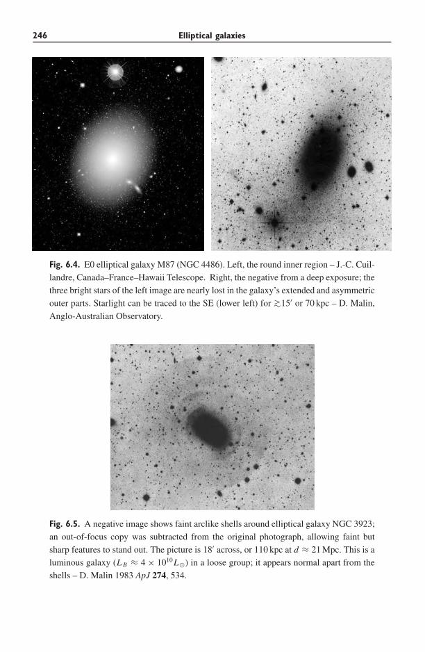
246 Elliptical galaxies

Fig. 6.4. E0 elliptical galaxy M87 (NGC 4486). Left, the round inner region – J.-C. Cuil-

landre, Canada–France–Hawaii Telescope. Right, the negative from a deep exposure; the

three bright stars of the left image are nearly lost in the galaxy’s extended and asymmetric

outer parts. Starlight can be traced to the SE (lower left) for ∼>15′ or 70 kpc – D. Malin,

Anglo-Australian Observatory.

Fig. 6.5. A negative image shows faint arclike shells around elliptical galaxy NGC 3923;

an out-of-focus copy was subtracted from the original photograph, allowing faint but

sharp features to stand out. The picture is 18′ across, or 110 kpc at d ≈ 21 Mpc. This is a

luminous galaxy (L B ≈ 4 × 1010L�) in a loose group; it appears normal apart from the

shells – D. Malin 1983 ApJ 274, 534.

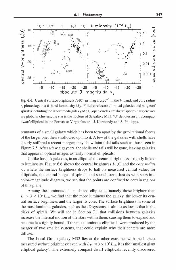
6.1 Photometry 247

−5 −10 −15 −20 −25

25

20

15

10

−5 −10 −15 −20 −25

0.001

0.01

0.1

1

10

Fig. 6.6. Central surface brightness IV (0), in mag arcsec−2 in the V band, and core radius

rc plotted against B-band luminosity MB . Filled circles are elliptical galaxies and bulges of

spirals (including the Andromeda galaxy M31); open circles are dwarf spheroidals; crosses

are globular clusters; the star is the nucleus of Sc galaxy M33. ‘U’ denotes an ultracompact

dwarf elliptical in the Fornax or Virgo cluster – J. Kormendy and S. Phillipps.

remnants of a small galaxy which has been torn apart by the gravitational forcesof the larger one, then swallowed up into it. A few of the galaxies with shells haveclearly suffered a recent merger; they show faint tidal tails such as those seen inFigure 7.5. After a few gigayears, the shells and tails will be gone, leaving galaxiesthat appear in optical images as fairly normal ellipticals.

Unlike for disk galaxies, in an elliptical the central brightness is tightly linkedto luminosity. Figure 6.6 shows the central brightness IV (0) and the core radiusrc, where the surface brightness drops to half its measured central value, forellipticals, the central bulges of spirals, and star clusters. Just as with stars in acolor–magnitude diagram, we see that the points are confined to certain regionsof this plane.

Among the luminous and midsized ellipticals, namely those brighter thanL ∼ 3 × 109L�, we find that the more luminous the galaxy, the lower its cen-tral surface brightness and the larger its core. The surface brightness in some ofthe most luminous galaxies, such as the cD systems, is almost as low as that in thedisks of spirals. We will see in Section 7.1 that collisions between galaxiesincrease the internal motion of the stars within them, causing them to expand andbecome less tightly bound. If the most luminous ellipticals were produced by themerger of two smaller systems, that could explain why their centers are morediffuse.

The Local Group galaxy M32 lies at the other extreme, with the highestmeasured surface brightness: even with LV ≈ 3 × 108L�, it is the ‘smallest giantelliptical galaxy’. The extremely compact dwarf ellipticals recently discovered

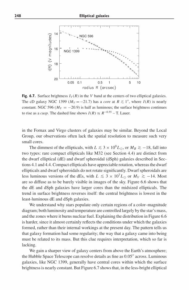
248 Elliptical galaxies

0.05 0.1 0.5 1 5 1020

18

16

14

NGC 1399

NGC 596

Fig. 6.7. Surface brightness IV (R) in the V band at the centers of two elliptical galaxies.

The cD galaxy NGC 1399 (MV =−21.7) has a core at R ∼< 1′′, where I (R) is nearly

constant. NGC 596 (MV = −20.9) is half as luminous; the surface brightness continues

to rise as a cusp. The dashed line shows I (R) ∝ R−0.55 – T. Lauer.

in the Fornax and Virgo clusters of galaxies may be similar. Beyond the LocalGroup, our observations often lack the spatial resolution to measure such verysmall cores.

The dimmest of the ellipticals, with L ∼< 3 × 109L�, or MB ∼> −18, fall intotwo types: rare compact ellipticals like M32 (see Section 4.4) are distinct fromthe dwarf elliptical (dE) and dwarf spheroidal (dSph) galaxies described in Sec-tions 4.1 and 4.4. Compact ellipticals have appreciable rotation, whereas the dwarfellipticals and dwarf spheroidals do not rotate significantly. Dwarf spheroidals areless luminous versions of the dEs, with L ∼< 3 × 107L� or MV ∼> −14. Mostare so diffuse as to be barely visible in images of the sky. Figure 6.6 shows thatthe dE and dSph galaxies have larger cores than the midsized ellipticals. Thetrend in surface brightness reverses itself: the central brightness is lowest in theleast-luminous dE and dSph galaxies.

We understand why stars populate only certain regions of a color–magnitudediagram; both luminosity and temperature are controlled largely by the star’s mass,and the zones where it burns nuclear fuel. Explaining the distribution in Figure 6.6is harder, since it almost certainly reflects the conditions under which the galaxiesformed, rather than their internal workings at the present day. The pattern tells usthat galaxy formation had some regularity; the way that a galaxy came into beingmust be related to its mass. But this clue requires interpretation, which so far islacking.

We gain a sharper view of galaxy centers from above the Earth’s atmosphere;the Hubble Space Telescope can resolve details as fine as 0.05′′ across. Luminousgalaxies, like NGC 1399, generally have central cores within which the surfacebrightness is nearly constant. But Figure 6.7 shows that, in the less-bright elliptical

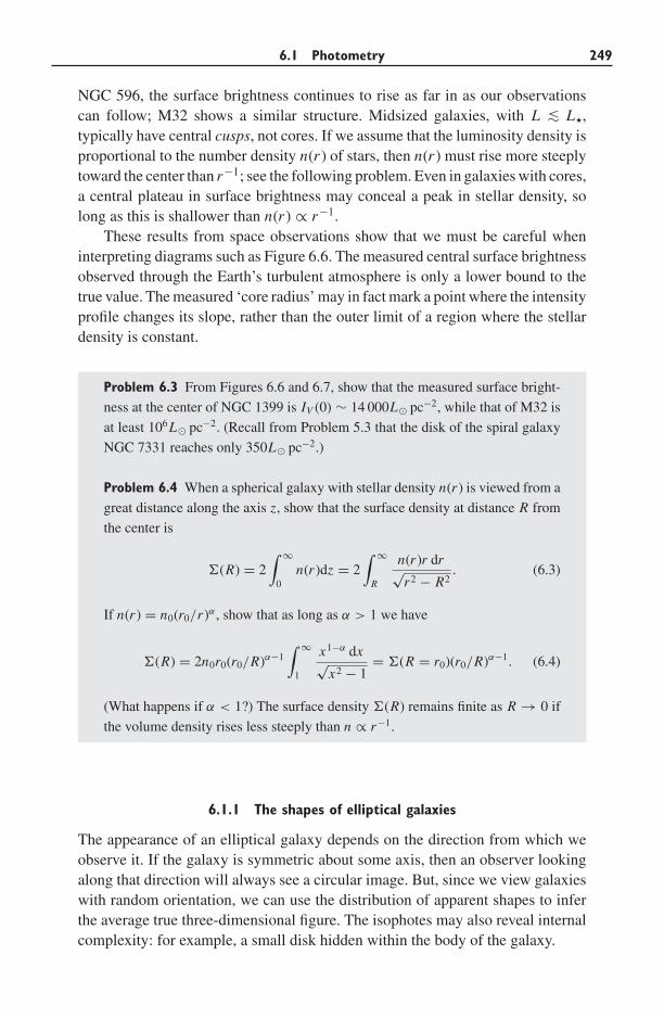
6.1 Photometry 249

NGC 596, the surface brightness continues to rise as far in as our observationscan follow; M32 shows a similar structure. Midsized galaxies, with L ∼< L,typically have central cusps, not cores. If we assume that the luminosity density isproportional to the number density n(r ) of stars, then n(r ) must rise more steeplytoward the center than r−1; see the following problem. Even in galaxies with cores,a central plateau in surface brightness may conceal a peak in stellar density, solong as this is shallower than n(r ) ∝ r−1.

These results from space observations show that we must be careful wheninterpreting diagrams such as Figure 6.6. The measured central surface brightnessobserved through the Earth’s turbulent atmosphere is only a lower bound to thetrue value. The measured ‘core radius’ may in fact mark a point where the intensityprofile changes its slope, rather than the outer limit of a region where the stellardensity is constant.

Problem 6.3 From Figures 6.6 and 6.7, show that the measured surface bright-

ness at the center of NGC 1399 is IV (0) ∼ 14 000L� pc−2, while that of M32 is

at least 106L� pc−2. (Recall from Problem 5.3 that the disk of the spiral galaxy

NGC 7331 reaches only 350L� pc−2.)

Problem 6.4 When a spherical galaxy with stellar density n(r ) is viewed from a

great distance along the axis z, show that the surface density at distance R from

the center is

�(R) = 2∫ ∞

0n(r )dz = 2

∫ ∞

R

n(r )r dr√r2 − R2

. (6.3)

If n(r ) = n0(r0/r )α , show that as long as α > 1 we have

�(R) = 2n0r0(r0/R)α−1∫ ∞

1

x1−α dx√x2 − 1

= �(R = r0)(r0/R)α−1. (6.4)

(What happens if α < 1?) The surface density �(R) remains finite as R → 0 if

the volume density rises less steeply than n ∝ r−1.

6.1.1 The shapes of elliptical galaxies

The appearance of an elliptical galaxy depends on the direction from which weobserve it. If the galaxy is symmetric about some axis, then an observer lookingalong that direction will always see a circular image. But, since we view galaxieswith random orientation, we can use the distribution of apparent shapes to inferthe average true three-dimensional figure. The isophotes may also reveal internalcomplexity: for example, a small disk hidden within the body of the galaxy.

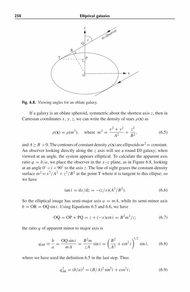
250 Elliptical galaxies

z

xO

P

Q

R

T

to observer

i

Fig. 6.8. Viewing angles for an oblate galaxy.

If a galaxy is an oblate spheroid, symmetric about the shortest axis z, then inCartesian coordinates x, y, z, we can write the density of stars ρ(x) as

ρ(x) = ρ(m2), where m2 = x2 + y2

A2+ z2

B2, (6.5)

and A≥ B >0. The contours of constant density ρ(x) are ellipsoids m2 = constant.An observer looking directly along the z axis will see a round E0 galaxy; whenviewed at an angle, the system appears elliptical. To calculate the apparent axisratio q = b/a, we place the observer in the x−z plane, as in Figure 6.8, lookingat an angle 0◦ < i <90◦ to the axis z. The line of sight grazes the constant-densitysurface m2 = x2/A2 + z2/B2 at the point T where it is tangent to this ellipse; sowe have

tan i = dx/dz = −(z/x)(A2/B2). (6.6)

So the elliptical image has semi-major axis a = m A, while its semi-minor axisb = OR = OQ sin i . Using Equations 6.5 and 6.6, we have

OQ = OP + PQ = z + (−x)cot i = B2m2/z; (6.7)

the ratio q of apparent minor to major axis is

qobl ≡ b

a= OQ sin i

m A= B2m

z Asin i =

(B2

A2+ cot2 i

)1/2

sin i, (6.8)

where we have used the definition 6.5 in the last step. Thus

q2obl = (b/a)2 = (B/A)2 sin2i + cos2i ; (6.9)

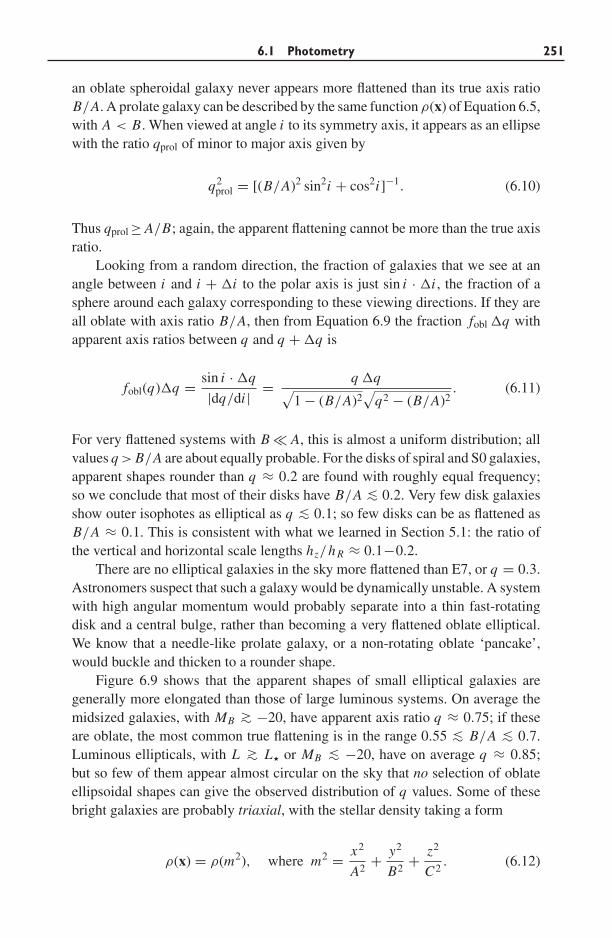
6.1 Photometry 251

an oblate spheroidal galaxy never appears more flattened than its true axis ratioB/A. A prolate galaxy can be described by the same function ρ(x) of Equation 6.5,with A < B. When viewed at angle i to its symmetry axis, it appears as an ellipsewith the ratio qprol of minor to major axis given by

q2prol = [(B/A)2 sin2i + cos2i]−1. (6.10)

Thus qprol ≥ A/B; again, the apparent flattening cannot be more than the true axisratio.

Looking from a random direction, the fraction of galaxies that we see at anangle between i and i + �i to the polar axis is just sin i · �i , the fraction of asphere around each galaxy corresponding to these viewing directions. If they areall oblate with axis ratio B/A, then from Equation 6.9 the fraction fobl �q withapparent axis ratios between q and q + �q is

fobl(q)�q = sin i · �q

|dq/di | = q �q√1 − (B/A)2

√q2 − (B/A)2

. (6.11)

For very flattened systems with B � A, this is almost a uniform distribution; allvalues q > B/A are about equally probable. For the disks of spiral and S0 galaxies,apparent shapes rounder than q ≈ 0.2 are found with roughly equal frequency;so we conclude that most of their disks have B/A ∼< 0.2. Very few disk galaxiesshow outer isophotes as elliptical as q ∼< 0.1; so few disks can be as flattened asB/A ≈ 0.1. This is consistent with what we learned in Section 5.1: the ratio ofthe vertical and horizontal scale lengths hz/h R ≈ 0.1−0.2.

There are no elliptical galaxies in the sky more flattened than E7, or q = 0.3.Astronomers suspect that such a galaxy would be dynamically unstable. A systemwith high angular momentum would probably separate into a thin fast-rotatingdisk and a central bulge, rather than becoming a very flattened oblate elliptical.We know that a needle-like prolate galaxy, or a non-rotating oblate ‘pancake’,would buckle and thicken to a rounder shape.

Figure 6.9 shows that the apparent shapes of small elliptical galaxies aregenerally more elongated than those of large luminous systems. On average themidsized galaxies, with MB ∼> −20, have apparent axis ratio q ≈ 0.75; if theseare oblate, the most common true flattening is in the range 0.55 ∼< B/A ∼< 0.7.Luminous ellipticals, with L ∼> L or MB ∼< −20, have on average q ≈ 0.85;but so few of them appear almost circular on the sky that no selection of oblateellipsoidal shapes can give the observed distribution of q values. Some of thesebright galaxies are probably triaxial, with the stellar density taking a form

ρ(x) = ρ(m2), where m2 = x2

A2+ y2

B2+ z2

C2. (6.12)

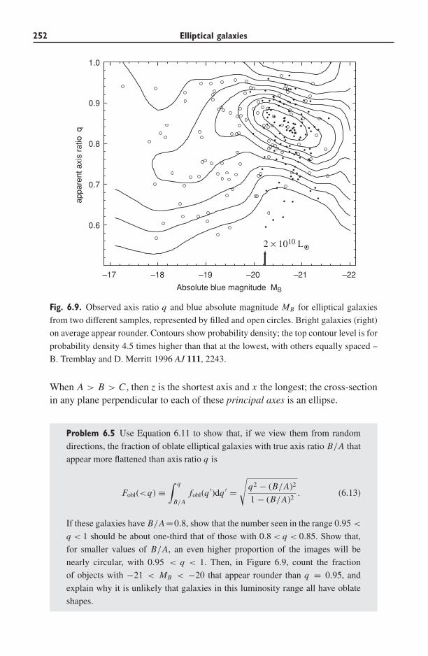
252 Elliptical galaxies

appa

rent

axi

s ra

tio q

Absolute blue magnitude MB

–17 –18 –19 –20 –21 –22

1.0

0.9

0.8

0.7

0.6

2 × 1010 L

Fig. 6.9. Observed axis ratio q and blue absolute magnitude MB for elliptical galaxies

from two different samples, represented by filled and open circles. Bright galaxies (right)

on average appear rounder. Contours show probability density; the top contour level is for

probability density 4.5 times higher than that at the lowest, with others equally spaced –

B. Tremblay and D. Merritt 1996 AJ 111, 2243.

When A > B > C , then z is the shortest axis and x the longest; the cross-sectionin any plane perpendicular to each of these principal axes is an ellipse.

Problem 6.5 Use Equation 6.11 to show that, if we view them from random

directions, the fraction of oblate elliptical galaxies with true axis ratio B/A that

appear more flattened than axis ratio q is

Fobl(<q) ≡∫ q

B/Afobl(q

′)dq ′ =√

q2 − (B/A)2

1 − (B/A)2. (6.13)

If these galaxies have B/A=0.8, show that the number seen in the range 0.95 <

q < 1 should be about one-third that of those with 0.8 < q < 0.85. Show that,

for smaller values of B/A, an even higher proportion of the images will be

nearly circular, with 0.95 < q < 1. Then, in Figure 6.9, count the fraction

of objects with −21 < MB < −20 that appear rounder than q = 0.95, and

explain why it is unlikely that galaxies in this luminosity range all have oblate

shapes.

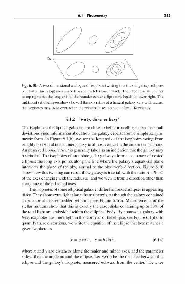
6.1 Photometry 253

Fig. 6.10. A two-dimensional analogue of isophote twisting in a triaxial galaxy: ellipses

on a flat surface (top) are viewed from below left (lower panel). The left ellipse still points

to top right; but the long axis of the rounder center ellipse now heads to lower right. The

rightmost set of ellipses shows how, if the axis ratios of a triaxial galaxy vary with radius,

the isophotes may twist even when the principal axes do not – after J. Kormendy.

6.1.2 Twisty, disky, or boxy?

The isophotes of elliptical galaxies are close to being true ellipses; but the smalldeviations yield information about how the galaxy departs from a simple axisym-metric form. In Figure 6.1(b), we see the long axis of the isophotes swing fromroughly horizontal in the inner galaxy to almost vertical at the outermost isophote.An observed isophote twist is generally taken as an indication that the galaxy maybe triaxial. The isophotes of an oblate galaxy always form a sequence of nestedellipses; the long axis points along the line where the galaxy’s equatorial planeintersects the plane of the sky, normal to the observer’s direction. Figure 6.10shows how this twisting can result if the galaxy is triaxial, with the ratio A : B : Cof the axes changing with the radius m, and we view it from a direction other thanalong one of the principal axes.

The isophotes of some elliptical galaxies differ from exact ellipses in appearingdisky. They show extra light along the major axis, as though the galaxy containedan equatorial disk embedded within it; see Figure 6.1(c). Measurements of thestellar motions show that this is exactly the case; disks containing up to 30% ofthe total light are embedded within the elliptical body. By contrast, a galaxy withboxy isophotes has more light in the ‘corners’ of the ellipse; see Figure 6.1(d). Toquantify these distortions, we write the equation of the ellipse that best matches agiven isophote as

x = a cos t, y = b sin t, (6.14)

where x and y are distances along the major and minor axes, and the parametert describes the angle around the ellipse. Let �r (t) be the distance between thisellipse and the galaxy’s isophote, measured outward from the center. Then, we

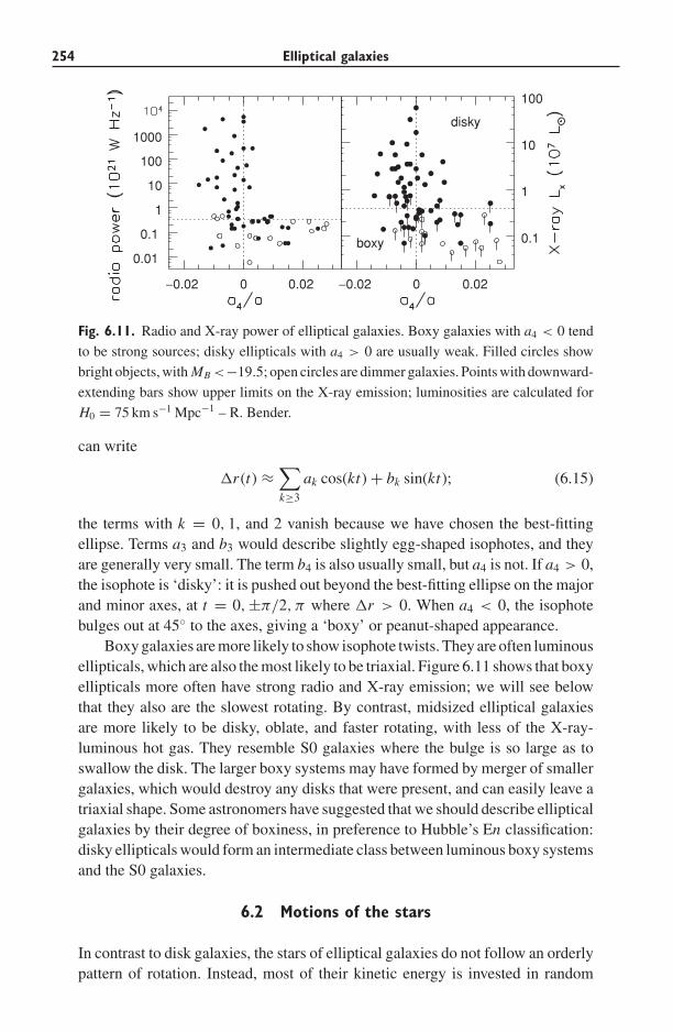
254 Elliptical galaxies

−0.02 0 00.02

0.01

0.1

1

10

100

1000

−0.02 0.02

0.1

1

10

100

boxy

disky

Fig. 6.11. Radio and X-ray power of elliptical galaxies. Boxy galaxies with a4 < 0 tend

to be strong sources; disky ellipticals with a4 > 0 are usually weak. Filled circles show

bright objects, with MB <−19.5; open circles are dimmer galaxies. Points with downward-

extending bars show upper limits on the X-ray emission; luminosities are calculated for

H0 = 75 km s−1 Mpc−1 – R. Bender.

can write

�r (t) ≈∑k≥3

ak cos(kt) + bk sin(kt); (6.15)

the terms with k = 0, 1, and 2 vanish because we have chosen the best-fittingellipse. Terms a3 and b3 would describe slightly egg-shaped isophotes, and theyare generally very small. The term b4 is also usually small, but a4 is not. If a4 > 0,the isophote is ‘disky’: it is pushed out beyond the best-fitting ellipse on the majorand minor axes, at t = 0, ±π/2, π where �r > 0. When a4 < 0, the isophotebulges out at 45◦ to the axes, giving a ‘boxy’ or peanut-shaped appearance.

Boxy galaxies are more likely to show isophote twists. They are often luminousellipticals, which are also the most likely to be triaxial. Figure 6.11 shows that boxyellipticals more often have strong radio and X-ray emission; we will see belowthat they also are the slowest rotating. By contrast, midsized elliptical galaxiesare more likely to be disky, oblate, and faster rotating, with less of the X-ray-luminous hot gas. They resemble S0 galaxies where the bulge is so large as toswallow the disk. The larger boxy systems may have formed by merger of smallergalaxies, which would destroy any disks that were present, and can easily leave atriaxial shape. Some astronomers have suggested that we should describe ellipticalgalaxies by their degree of boxiness, in preference to Hubble’s En classification:disky ellipticals would form an intermediate class between luminous boxy systemsand the S0 galaxies.

6.2 Motions of the stars

In contrast to disk galaxies, the stars of elliptical galaxies do not follow an orderlypattern of rotation. Instead, most of their kinetic energy is invested in random

6.2 Motions of the stars 255

motion. Just as a spiral galaxy’s luminosity is linked to its rotation speed, the moreluminous ellipticals have a higher velocity dispersion; we can use this relation todetermine distances to galaxies. Many astronomers were surprised to find thatelliptical galaxies rotate as slowly as they do; it shows that the stars have notrelaxed into anything close to a most probable final state. Elliptical galaxies stillretain considerable information about their origins.

6.2.1 Measuring stellar velocities

Measuring the orbital velocities of stars within galaxies is relatively difficult. Wecan quite easily find the speed of a cool or warm gas cloud using the Dopplershift at the bright peak of an emission line, such as Hα from warm ionized gas, orthe radio-frequency 21 cm line of neutral atomic hydrogen. But for stars, we mustuse absorption features in the spectra; many of these are not narrow atomic lines,but have an appreciable intrinsic spread in wavelength. We will see below that wemust be concerned not just with the position of the line center, but with its widthand often its shape as well; measuring these demands a high signal-to-noise ratioand long observations.

The absorption-line spectra of galaxies are usually measured with a long-slitspectrograph. The slit is placed across the galaxy; reflection from a grating thenspreads the light in wavelength along the perpendicular direction before it fallsonto a detector, most commonly a CCD; see Section 5.1. Sometimes fiber-opticbundles are used instead; the fibers collect light from various positions across theface of the galaxy and deliver it onto the grating. Light entering at the ends ofthe slit, or through fibers placed far from the galaxy, allows the observer to recordthe emission of the night sky (often with that of distant street lights). Except nearits center, the sky is brighter than the galaxy; so we must subtract its spectrumfrom what we measure, to recover that of the galaxy.

The light of all the stars in a galaxy is the sum of their individual spectra, eachDoppler-shifted in wavelength according to their motion. Their orbital motioncauses lines in the summed spectrum to be wider and shallower than those ofan individual star. We will see in Section 6.3 that most of the light of ellipticalgalaxies comes from G and K giant stars. Typically we observe some nearbystars of these types as templates for comparison. We take these spectra with thesame telescope and spectrograph setup as for the galaxy, so that we can correctfor instrumental effects. For example, a spectrograph broadens the lines by anamount �λ corresponding to the spectral resolution; generally λ/�λ ∼> 5000 forthese observations, giving a resolution of 60 km s−1.

Elliptical galaxies contain little cool dusty gas, so their light is quite closeto the sum of what is emitted by all their stars. Let us write the energy receivedfrom a typical star, when it is at rest with respect to an observer, as Fλ,(λ)�λ

between wavelengths λ and λ+�λ. We choose Cartesian coordinates x, y, z withz pointing from our position toward the galaxy. Then, if the star moves away fromus with velocity vz � c, the light that we receive at wavelength λ was emitted

256 Elliptical galaxies

at wavelength λ[1 − vz/c]. To find the spectrum at position x, y on the galaxyimage, we must integrate over all the stars along our line of sight. Approximatingthe number density of stars at position x with z velocities between vz and vz +�vz

as f (x, vz)�vz , the observed spectrum is

Fλ,g(x, y, λ) =∫ ∞

−∞Fλ,(λ[1 − vz/c])

{∫ ∞

−∞f (x, vz)dz

}dvz. (6.16)

If we knew the distribution function f (x, v) for each type of star, and theirspectra Fλ,(λ) were exactly the same as those of our template stars, we coulduse Equation 6.16 to construct the galaxy’s spectrum. In practice, we usuallyguess at a form for the integral of f (x, vz) along the line of sight, the term incurly braces, depending on a few parameters. We then choose those parametersto reproduce the galaxy’s observed spectrum as well as possible. A commonchoice is the Gaussian form∫ ∞

−∞f (x, vz)dz ∝ exp

[−(vz − Vr)2/(2σ 2

r

)]; (6.17)

here σr(x, y), usually written simply as σ , is the velocity dispersion of the stars,while Vr(x, y) is the mean radial velocity at that position. Rotation is evident as agradient in Vr(x, y) across the face of the system. When the spectrum is measuredto high precision, the Gaussian might not provide an adequate approximation.For example, in some disky ellipticals a long ‘tail’ of rapidly moving starsshows that a fast-rotating disk is buried within the slower-rotating body of thegalaxy.

Figure 6.12 shows the mean radial velocity and velocity dispersion measuredalong the major axis of the cD galaxy NGC 1399 out to a distance of about5Re, where the surface brightness has fallen more than 100-fold below its centrallevel. In a spiral galaxy like our own, the ordered rotation of disk stars is almostten times faster than their random speeds; but in this elliptical, we see a peakrotation speed Vmax � σr. We would not expect elliptical galaxies to rotate asrapidly as spirals, since they are not disks; but we will see in the next subsectionthat most of them do not even rotate as fast as they ‘ought to’ for their roundershapes.

Problem 6.6 The core radius rc of NGC 1399 is ∼5′′ or 400 pc. Use Equation

3.46 to combine the measured dispersion σr from Figure 6.12 with the result of

Problem 6.3, to show that the mass-to-light ratio in the central parts isM/LV ∼ 7.

This is only slightly larger than that in the Milky Way’s globular clusters

(Section 3.1), suggesting that the core of this galaxy contains little dark matter.

Further reading: for more on spectroscopic techniques, see Chapter 3 of D. F.Gray, 1992, The Observation and Analysis of Stellar Photospheres, 2nd edition(Cambridge University Press, Cambridge, UK). For the analysis, see Chapter 11

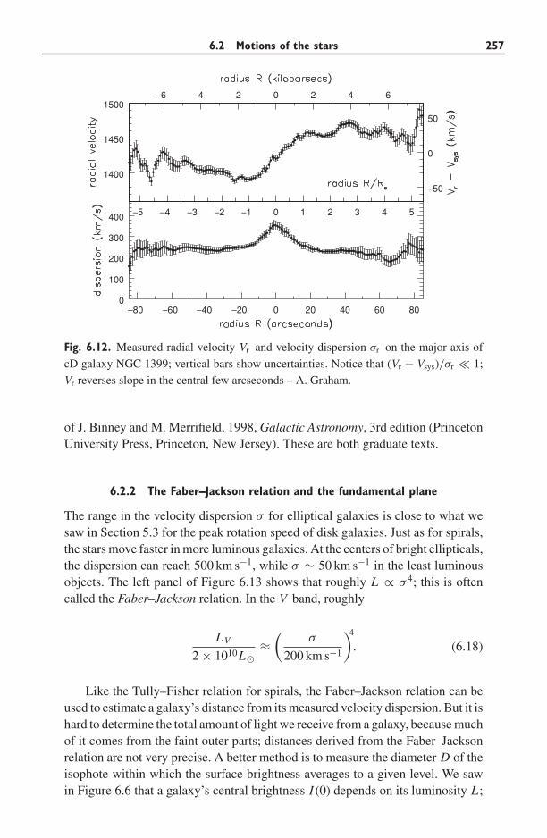
6.2 Motions of the stars 257

−6 −4 −2 0 2 4 6

−5 −4 −3 −2 −1 0 1 2 3 4 5

−50

0

50

1400

1450

1500

−80 −60 −40 −20 0 20 40 60 800

100

200

300

400

Fig. 6.12. Measured radial velocity Vr and velocity dispersion σr on the major axis of

cD galaxy NGC 1399; vertical bars show uncertainties. Notice that (Vr − Vsys)/σr � 1;

Vr reverses slope in the central few arcseconds – A. Graham.

of J. Binney and M. Merrifield, 1998, Galactic Astronomy, 3rd edition (PrincetonUniversity Press, Princeton, New Jersey). These are both graduate texts.

6.2.2 The Faber–Jackson relation and the fundamental plane

The range in the velocity dispersion σ for elliptical galaxies is close to what wesaw in Section 5.3 for the peak rotation speed of disk galaxies. Just as for spirals,the stars move faster in more luminous galaxies. At the centers of bright ellipticals,the dispersion can reach 500 km s−1, while σ ∼ 50 km s−1 in the least luminousobjects. The left panel of Figure 6.13 shows that roughly L ∝ σ 4; this is oftencalled the Faber–Jackson relation. In the V band, roughly

LV

2 × 1010L�≈(

σ

200 km s−1

)4

. (6.18)

Like the Tully–Fisher relation for spirals, the Faber–Jackson relation can beused to estimate a galaxy’s distance from its measured velocity dispersion. But it ishard to determine the total amount of light we receive from a galaxy, because muchof it comes from the faint outer parts; distances derived from the Faber–Jacksonrelation are not very precise. A better method is to measure the diameter D of theisophote within which the surface brightness averages to a given level. We sawin Figure 6.6 that a galaxy’s central brightness I (0) depends on its luminosity L;

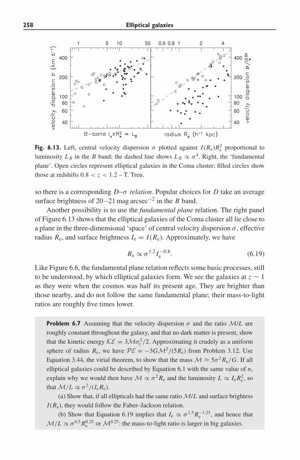
258 Elliptical galaxies

1 5 10 50

40

60

80100

200

400

0.6 0.8 1 2 4

40

60

80100

200

400

Fig. 6.13. Left, central velocity dispersion σ plotted against I (Re)R2e proportional to

luminosity L B in the B band; the dashed line shows L B ∝ σ 4. Right, the ‘fundamental

plane’. Open circles represent elliptical galaxies in the Coma cluster; filled circles show

those at redshifts 0.8 < z < 1.2 – T. Treu.

so there is a corresponding D−σ relation. Popular choices for D take an averagesurface brightness of 20−21 mag arcsec−2 in the B band.

Another possibility is to use the fundamental plane relation. The right panelof Figure 6.13 shows that the elliptical galaxies of the Coma cluster all lie close toa plane in the three-dimensional ‘space’ of central velocity dispersion σ , effectiveradius Re, and surface brightness Ie = I (Re). Approximately, we have

Re ∝ σ 1.2 I −0.8e . (6.19)

Like Figure 6.6, the fundamental plane relation reflects some basic processes, stillto be understood, by which elliptical galaxies form. We see the galaxies at z ∼ 1as they were when the cosmos was half its present age. They are brighter thanthose nearby, and do not follow the same fundamental plane; their mass-to-lightratios are roughly five times lower.

Problem 6.7 Assuming that the velocity dispersion σ and the ratio M/L are

roughly constant throughout the galaxy, and that no dark matter is present, show

that the kinetic energy KE = 3Mσ 2r /2. Approximating it crudely as a uniform

sphere of radius Re, we have PE = −3GM2/(5Re) from Problem 3.12. Use

Equation 3.44, the virial theorem, to show that the mass M ≈ 5σ 2 Re/G. If all

elliptical galaxies could be described by Equation 6.1 with the same value of n,

explain why we would then have M ∝ σ 2 Re and the luminosity L ∝ Ie R2e , so

that M/L ∝ σ 2/(Ie Re).

(a) Show that, if all ellipticals had the same ratio M/L and surface brightess

I (Re), they would follow the Faber–Jackson relation.

(b) Show that Equation 6.19 implies that Ie ∝ σ 1.5 R−1.25e , and hence that

M/L ∝ σ 0.5 R0.25e or M0.25: the mass-to-light ratio is larger in big galaxies.

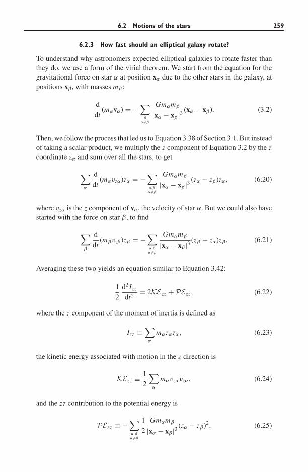
6.2 Motions of the stars 259

6.2.3 How fast should an elliptical galaxy rotate?

To understand why astronomers expected elliptical galaxies to rotate faster thanthey do, we use a form of the virial theorem. We start from the equation for thegravitational force on star α at position xα due to the other stars in the galaxy, atpositions xβ , with masses mβ :

d

dt(mαvα) = −

∑β

α �=β

Gmαmβ

|xα − xβ |3 (xα − xβ). (3.2)

Then, we follow the process that led us to Equation 3.38 of Section 3.1. But insteadof taking a scalar product, we multiply the z component of Equation 3.2 by the zcoordinate zα and sum over all the stars, to get

∑α

d

dt(mαvzα)zα = −

∑α,βα �=β

Gmαmβ

|xα − xβ |3 (zα − zβ)zα, (6.20)

where vzα is the z component of vα, the velocity of star α. But we could also havestarted with the force on star β, to find

∑β

d

dt(mβvzβ)zβ = −

∑α,βα �=β

Gmαmβ

|xα − xβ |3 (zβ − zα)zβ. (6.21)

Averaging these two yields an equation similar to Equation 3.42:

1

2

d2 Izz

dt2= 2KE zz + PE zz, (6.22)

where the z component of the moment of inertia is defined as

Izz ≡∑

α

mαzαzα, (6.23)

the kinetic energy associated with motion in the z direction is

KE zz ≡ 1

2

∑α

mαvzαvzα, (6.24)

and the zz contribution to the potential energy is

PE zz ≡ −∑α,βα �=β

1

2

Gmαmβ

|xα − xβ |3 (zα − zβ)2. (6.25)

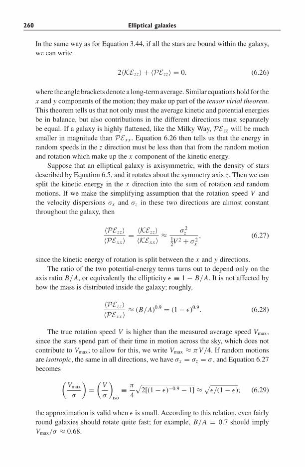
260 Elliptical galaxies

In the same way as for Equation 3.44, if all the stars are bound within the galaxy,we can write

2〈KE zz〉 + 〈PE zz〉 = 0. (6.26)

where the angle brackets denote a long-term average. Similar equations hold for thex and y components of the motion; they make up part of the tensor virial theorem.This theorem tells us that not only must the average kinetic and potential energiesbe in balance, but also contributions in the different directions must separatelybe equal. If a galaxy is highly flattened, like the Milky Way, PE zz will be muchsmaller in magnitude than PE xx . Equation 6.26 then tells us that the energy inrandom speeds in the z direction must be less than that from the random motionand rotation which make up the x component of the kinetic energy.

Suppose that an elliptical galaxy is axisymmetric, with the density of starsdescribed by Equation 6.5, and it rotates about the symmetry axis z. Then we cansplit the kinetic energy in the x direction into the sum of rotation and randommotions. If we make the simplifying assumption that the rotation speed V andthe velocity dispersions σx and σz in these two directions are almost constantthroughout the galaxy, then

〈PE zz〉〈PE xx 〉 = 〈KE zz〉

〈KE xx 〉 ≈ σ 2z

12V

2 + σ 2x

, (6.27)

since the kinetic energy of rotation is split between the x and y directions.The ratio of the two potential-energy terms turns out to depend only on the

axis ratio B/A, or equivalently the ellipticity ε ≡ 1 − B/A. It is not affected byhow the mass is distributed inside the galaxy; roughly,

〈PE zz〉〈PE xx 〉 ≈ (B/A)0.9 = (1 − ε)0.9. (6.28)

The true rotation speed V is higher than the measured average speed Vmax,since the stars spend part of their time in motion across the sky, which does notcontribute to Vmax; to allow for this, we write Vmax ≈ πV/4. If random motionsare isotropic, the same in all directions, we have σx = σz = σ , and Equation 6.27becomes

(Vmax

σ

)=(

V

σ

)iso

≡ π

4

√2[(1 − ε)−0.9 − 1] ≈

√ε/(1 − ε); (6.29)

the approximation is valid when ε is small. According to this relation, even fairlyround galaxies should rotate quite fast; for example, B/A = 0.7 should implyVmax/σ ≈ 0.68.

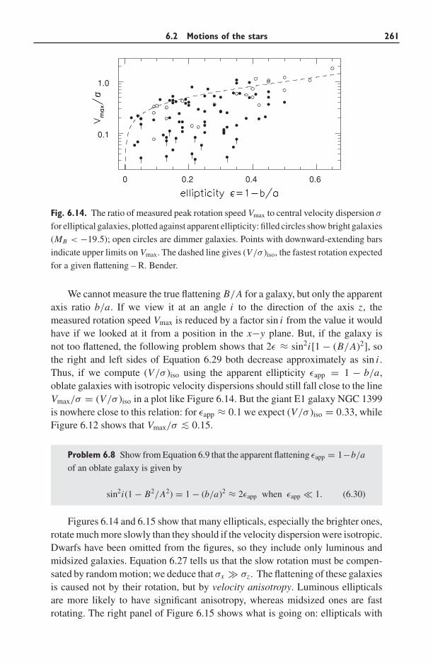
6.2 Motions of the stars 261

0 0.2 0.4 0.6

0.1

1.0

Fig. 6.14. The ratio of measured peak rotation speed Vmax to central velocity dispersion σ

for elliptical galaxies, plotted against apparent ellipticity: filled circles show bright galaxies

(MB < −19.5); open circles are dimmer galaxies. Points with downward-extending bars

indicate upper limits on Vmax. The dashed line gives (V/σ )iso, the fastest rotation expected

for a given flattening – R. Bender.

We cannot measure the true flattening B/A for a galaxy, but only the apparentaxis ratio b/a. If we view it at an angle i to the direction of the axis z, themeasured rotation speed Vmax is reduced by a factor sin i from the value it wouldhave if we looked at it from a position in the x−y plane. But, if the galaxy isnot too flattened, the following problem shows that 2ε ≈ sin2i[1 − (B/A)2], sothe right and left sides of Equation 6.29 both decrease approximately as sin i .Thus, if we compute (V/σ )iso using the apparent ellipticity εapp = 1 − b/a,oblate galaxies with isotropic velocity dispersions should still fall close to the lineVmax/σ = (V/σ )iso in a plot like Figure 6.14. But the giant E1 galaxy NGC 1399is nowhere close to this relation: for εapp ≈ 0.1 we expect (V/σ )iso = 0.33, whileFigure 6.12 shows that Vmax/σ ∼< 0.15.

Problem 6.8 Show from Equation 6.9 that the apparent flattening εapp = 1−b/a

of an oblate galaxy is given by

sin2i(1 − B2/A2) = 1 − (b/a)2 ≈ 2εapp when εapp � 1. (6.30)

Figures 6.14 and 6.15 show that many ellipticals, especially the brighter ones,rotate much more slowly than they should if the velocity dispersion were isotropic.Dwarfs have been omitted from the figures, so they include only luminous andmidsized galaxies. Equation 6.27 tells us that the slow rotation must be compen-sated by random motion; we deduce that σx � σz . The flattening of these galaxiesis caused not by their rotation, but by velocity anisotropy. Luminous ellipticalsare more likely to have significant anisotropy, whereas midsized ones are fastrotating. The right panel of Figure 6.15 shows what is going on: ellipticals with

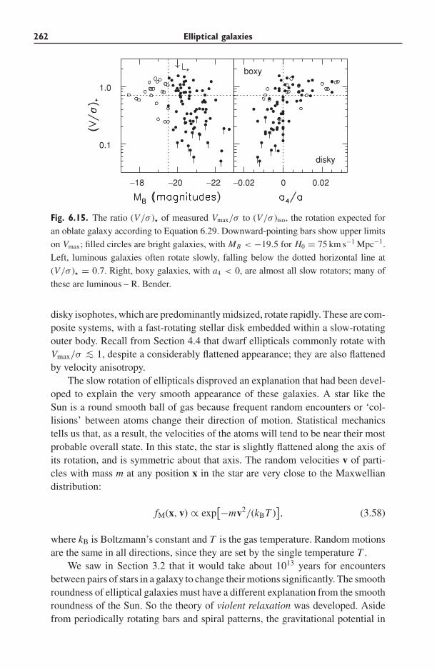
262 Elliptical galaxies

−18 −20 −22

0.1

1.0

−0.02 0 0.02

boxy

disky

Fig. 6.15. The ratio (V/σ ) of measured Vmax/σ to (V/σ )iso, the rotation expected for

an oblate galaxy according to Equation 6.29. Downward-pointing bars show upper limits

on Vmax; filled circles are bright galaxies, with MB < −19.5 for H0 = 75 km s−1 Mpc−1.

Left, luminous galaxies often rotate slowly, falling below the dotted horizontal line at

(V/σ ) = 0.7. Right, boxy galaxies, with a4 < 0, are almost all slow rotators; many of

these are luminous – R. Bender.

disky isophotes, which are predominantly midsized, rotate rapidly. These are com-posite systems, with a fast-rotating stellar disk embedded within a slow-rotatingouter body. Recall from Section 4.4 that dwarf ellipticals commonly rotate withVmax/σ ∼< 1, despite a considerably flattened appearance; they are also flattenedby velocity anisotropy.

The slow rotation of ellipticals disproved an explanation that had been devel-oped to explain the very smooth appearance of these galaxies. A star like theSun is a round smooth ball of gas because frequent random encounters or ‘col-lisions’ between atoms change their direction of motion. Statistical mechanicstells us that, as a result, the velocities of the atoms will tend to be near their mostprobable overall state. In this state, the star is slightly flattened along the axis ofits rotation, and is symmetric about that axis. The random velocities v of parti-cles with mass m at any position x in the star are very close to the Maxwelliandistribution:

fM(x, v) ∝ exp[−mv2/(kBT )

], (3.58)

where kB is Boltzmann’s constant and T is the gas temperature. Random motionsare the same in all directions, since they are set by the single temperature T .

We saw in Section 3.2 that it would take about 1013 years for encountersbetween pairs of stars in a galaxy to change their motions significantly. The smoothroundness of elliptical galaxies must have a different explanation from the smoothroundness of the Sun. So the theory of violent relaxation was developed. Asidefrom periodically rotating bars and spiral patterns, the gravitational potential in

6.2 Motions of the stars 263

normal galaxies today appears to change only slowly over time; so Equation 3.27tells us that a star’s energy E is almost constant along its orbit. But while lumps ofmatter were falling together to form the galaxy, the potential �(x, t) at any pointx would swing up and down by large amounts, changing the star’s energy. Thisprocess was expected to mix stars among the various orbits, giving them equalrandom motions in all directions.

The observed slow rotation of elliptical galaxies tells us that violent relaxationwas not complete. The stars in these galaxies, unlike the atoms of gas that makeup stars, retain information about the way in which they were assembled. Inparticular, they might not have relaxed enough for the galaxy to develop an axis ofsymmetry. A further indication of only partial mixing is given by the rotation curveof Figure 6.12. The innermost part of the galaxy NGC 1399 seems to rotate in theopposite direction to the outer regions. These kinematically decoupled cores havebeen found increasingly often, as the precision of measurement improves. Someelliptical galaxies also show a gradient in the mean velocity Vr when measurementsare made along the apparent minor axis. This state could not last long in anaxisymmetric galaxy, but we will see below that it can persist if the potential istriaxial. Minor-axis rotation is generally reckoned as one further piece of evidencethat at least some elliptical galaxies have triaxial shapes.

6.2.4 Stellar orbits in a triaxial galaxy

To understand the implications of a triaxial elliptical galaxy, we must study theorbits that stars would follow in such a system. One of the simplest triaxial poten-tials is the triaxial harmonic oscillator

�HO(x) = 1

2

(ω2

x x2 + ω2y y2 + ω2

z z2) (6.31)

with ωx < ωy < ωz . This describes the gravitational force inside a homo-geneous galaxy described by Equation 6.12 with A, B, and C held fixed, andconstant density ρ(m2) for m ≤ 1; there is no mass outside that ellipsoidal sur-face. A star in this potential would follow independent harmonic motion in thex, y, and z directions, with frequencies ωx , ωy, and ωz , respectively; these arecomplicated functions of the axis ratios A : B : C . Unless the frequencies arerational multiples of each other, this orbit completely fills a rectangular block,with sides parallel to the axes: we call it a box orbit. We saw in Section 3.3that a star moving in an axisymmetric potential must stay away from the centerunless its angular momentum is exactly zero; by contrast, a star on a box orbitcan travel right to the origin. A box orbit has no fixed sense of angular momen-tum. The sign of Lz reverses as the orbit reaches the ‘edge’ of the block in thex and y directions, and similarly for Lx and L y; so each of these is zero onaverage.

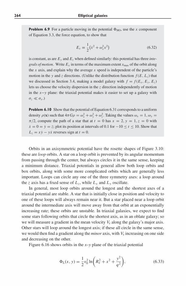
264 Elliptical galaxies

Problem 6.9 For a particle moving in the potential �HO, use the x component

of Equation 3.3, the force equation, to show that

Ex ≡ 1

2

(x2 + ω2

x x2)

(6.32)

is constant, as are Ey and Ez when defined similarly: this potential has three inte-

grals of motion. Write Ex in terms of the maximum extent xmax of the orbit along

the x axis, and explain why the average x speed is independent of the particle’s

motion in the y and z directions. (Unlike the distribution function f (E, Lz) that

we discussed in Section 3.4, making a model galaxy with f = f (Ex , Ey, Ez)

lets us choose the velocity dispersion in the z direction independently of motion

in the x−y plane: the triaxial potential makes it easier to set up a galaxy with

σz � σx .)

Problem 6.10 Show that the potential of Equation 6.31 corresponds to a uniform

density ρ(x) such that 4πGρ = ω2x + ω2

y + ω2z . Taking the values ωx = 1, ωy =

π/2, compute the path of a star that at t = 0 has x = 2, y = 1, z = 0 with

x = 0 = y = z; plot its position at intervals of 0.1 for −10 ≤ t ≤ 10. Show that

Lz = x y − yx reverses sign at t = 0.

Orbits in an axisymmetric potential have the rosette shapes of Figure 3.10:these are loop orbits. A star on a loop orbit is prevented by its angular momentumfrom passing through the center, but always circles it in the same sense, keepinga minimum distance. Triaxial potentials in general allow both loop orbits andbox orbits, along with some more complicated orbits which are generally lessimportant. Loops can circle any one of the three symmetry axes: a loop aroundthe z axis has a fixed sense of Lz , while Lx and L y oscillate.

In general, most loop orbits around the longest and the shortest axes of atriaxial potential are stable. A star that is initially close in position and velocity toone of these loops will always remain near it. But a star placed near a loop orbitaround the intermediate axis will move away from that orbit at an exponentiallyincreasing rate; these orbits are unstable. In triaxial galaxies, we expect to findsome stars following orbits that circle the shortest axis, as in an oblate galaxy; sowe will measure a gradient in the mean velocity Vr along the galaxy’s major axis.Other stars will loop around the longest axis; if these all circle in the same sense,we would then find a gradient along the minor axis, with Vr increasing on one sideand decreasing on the other.

Figure 6.16 shows orbits in the x–y plane of the triaxial potential

�L(x, y) = 1

2v2

0 ln

(Re

2 + x2 + y2

q2

), (6.33)

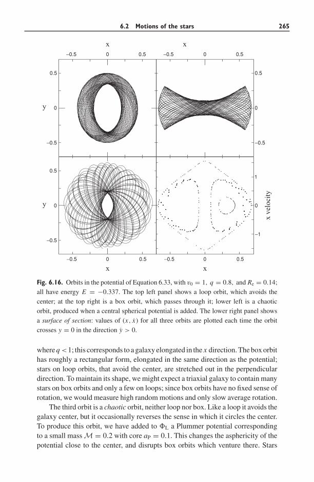
6.2 Motions of the stars 265

−0.5 0 0.5 −0.5 0 0.5

−0.5 0 0.5 −0.5 0 0.5

−0.5

0

0.5

−0.5

0

0.5

−0.5

0

0.5

−1

0

1

xx

x x

x ve

loci

ty

y

y

Fig. 6.16. Orbits in the potential of Equation 6.33, with v0 = 1, q = 0.8, and Re = 0.14;

all have energy E = −0.337. The top left panel shows a loop orbit, which avoids the

center; at the top right is a box orbit, which passes through it; lower left is a chaotic

orbit, produced when a central spherical potential is added. The lower right panel shows

a surface of section: values of (x, x) for all three orbits are plotted each time the orbit

crosses y = 0 in the direction y > 0.

where q <1; this corresponds to a galaxy elongated in the x direction. The box orbithas roughly a rectangular form, elongated in the same direction as the potential;stars on loop orbits, that avoid the center, are stretched out in the perpendiculardirection. To maintain its shape, we might expect a triaxial galaxy to contain manystars on box orbits and only a few on loops; since box orbits have no fixed sense ofrotation, we would measure high random motions and only slow average rotation.

The third orbit is a chaotic orbit, neither loop nor box. Like a loop it avoids thegalaxy center, but it occasionally reverses the sense in which it circles the center.To produce this orbit, we have added to �L a Plummer potential correspondingto a small mass M = 0.2 with core aP = 0.1. This changes the asphericity of thepotential close to the center, and disrupts box orbits which venture there. Stars

266 Elliptical galaxies

on this chaotic orbit do not support the elongation of the galaxy. If a potential�(x) has too many chaotic orbits, it may be impossible to make a self-consistentmodel, in which the density of stars on their orbits gives rise to the potential �.In particular, the inner regions of a galaxy might not be able to remain triaxial ifa big black hole grows at the center.

Problem 6.11 Show that, if the density of stars ρ(r ) = ρ0(r0/r )α , then the mass

within radius r follows M(<r ) ∝ r3−α , and the radial force

Fr(r ) = −GM(<r )

r2∝ r1−α.

We see that Fr(r ) → 0 at small radii if the density increases more slowly than

r−1. Recall that this is the same condition as we found in Problem 6.4 for the

surface density �(R) to remain finite at the center.

(If the forces tend to zero at the center of a triaxial potential, box orbits will

exist much as in the triaxial harmonic oscillator. Otherwise, many of the boxes

are replaced by chaotic orbits. Galaxies with central luminous cusps are probably

not triaxial near their centers.)

A compact way of showing a number of orbits is a surface of section plot, as inthe lower right of Figure 6.16. Each time the orbit crosses the x axis in the directiony > 0, we plot the value of x and the x velocity x . The points made by the looporbit fall along the small closed curve on the left; the orbit always transits the xaxis anticlockwise. The points from the box orbit lie on the largest curve, circlingaround the origin. This orbit has no fixed sense of circulation, but crosses the x axiswith y > 0 both on x > 0 and on x < 0; x is large whenever x is small, as the par-ticle passes close to the center. The chaotic orbit shows both senses of circulationabout the center; but, like the loop, it avoids the origin. The points from this orbitdo not fall on a curve at all; their more disorderly distribution betrays the differ-ence between a chaotic orbit, and the non-chaotic or regular boxes and loops. Thediscovery and exploration of chaotic properties was one of the major developmentsof twentieth-century mathematics; we refer interested readers to the books below.

Further reading: at the graduate level, Sections 3.3, 3.4, and 4.3 of J. Binney andS. Tremaine, 1987, Galactic Dynamics (Princeton University Press, Princeton,New Jersey). For a clear discussion of chaotic orbits, written for the generalreader, see I. Stewart, 1990, Does God Play Dice? The Mathematics of Chaos(Blackwell, Cambridge, Massachusetts).

6.3 Stellar populations and gas

Unlike spiral and irregular galaxies, elliptical galaxies conspicuously lack lumi-nous blue stars; the brightest stars are red giants and stars on the asymptotic giantbranch (AGB; see Section 1.1). We cannot see individual stars directly in galaxies

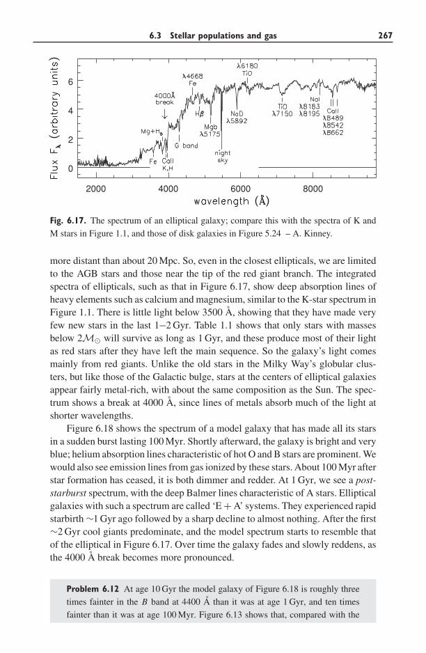
6.3 Stellar populations and gas 267

2000 4000 6000 8000

0

2

4

6

Fig. 6.17. The spectrum of an elliptical galaxy; compare this with the spectra of K and

M stars in Figure 1.1, and those of disk galaxies in Figure 5.24 – A. Kinney.

more distant than about 20 Mpc. So, even in the closest ellipticals, we are limitedto the AGB stars and those near the tip of the red giant branch. The integratedspectra of ellipticals, such as that in Figure 6.17, show deep absorption lines ofheavy elements such as calcium and magnesium, similar to the K-star spectrum inFigure 1.1. There is little light below 3500 A, showing that they have made veryfew new stars in the last 1−2 Gyr. Table 1.1 shows that only stars with massesbelow 2M� will survive as long as 1 Gyr, and these produce most of their lightas red stars after they have left the main sequence. So the galaxy’s light comesmainly from red giants. Unlike the old stars in the Milky Way’s globular clus-ters, but like those of the Galactic bulge, stars at the centers of elliptical galaxiesappear fairly metal-rich, with about the same composition as the Sun. The spec-trum shows a break at 4000 A, since lines of metals absorb much of the light atshorter wavelengths.

Figure 6.18 shows the spectrum of a model galaxy that has made all its starsin a sudden burst lasting 100 Myr. Shortly afterward, the galaxy is bright and veryblue; helium absorption lines characteristic of hot O and B stars are prominent. Wewould also see emission lines from gas ionized by these stars. About 100 Myr afterstar formation has ceased, it is both dimmer and redder. At 1 Gyr, we see a post-starburst spectrum, with the deep Balmer lines characteristic of A stars. Ellipticalgalaxies with such a spectrum are called ‘E + A’ systems. They experienced rapidstarbirth ∼1 Gyr ago followed by a sharp decline to almost nothing. After the first∼2 Gyr cool giants predominate, and the model spectrum starts to resemble thatof the elliptical in Figure 6.17. Over time the galaxy fades and slowly reddens, asthe 4000 A break becomes more pronounced.

Problem 6.12 At age 10 Gyr the model galaxy of Figure 6.18 is roughly three

times fainter in the B band at 4400 A than it was at age 1 Gyr, and ten times

fainter than it was at age 100 Myr. Figure 6.13 shows that, compared with the

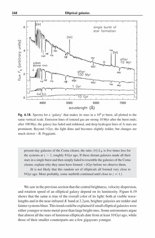
268 Elliptical galaxies

Fig. 6.18. Spectra for a ‘galaxy’ that makes its stars in a 108 yr burst, all plotted to the

same vertical scale. Emission lines of ionized gas are strong 10 Myr after the burst ends;

after 100 Myr, the galaxy has faded and reddened, and deep hydrogen lines of A stars are

prominent. Beyond 1 Gyr, the light dims and becomes slightly redder, but changes are

much slower – B. Poggianti.

present-day galaxies of the Coma cluster, the ratio M/L B is five times less for

the systems at z ∼ 1, roughly 8 Gyr ago. If these distant galaxies made all their

stars in a single burst and then simply faded to resemble the galaxies of the Coma

cluster, explain why they must have formed <1Gyr before we observe them.

(It is not likely that this random set of ellipticals all formed very close to

9 Gyr ago. More probably, some starbirth continued until close to z = 1.)

We saw in the previous section that the central brightness, velocity dispersion,and rotation speed of an elliptical galaxy depend on its luminosity. Figure 6.19shows that the same is true of the overall color of its light: both at visible wave-lengths and in the near-infrared K band at 2.2μm, brighter galaxies are redder andfainter systems bluer. This trend could be explained if small elliptical galaxies wereeither younger or more metal-poor than large bright ones. Some astronomers arguethat almost all the stars of luminous ellipticals date from at least 10 Gyr ago, whilethose of their smaller counterparts are a few gigayears younger.

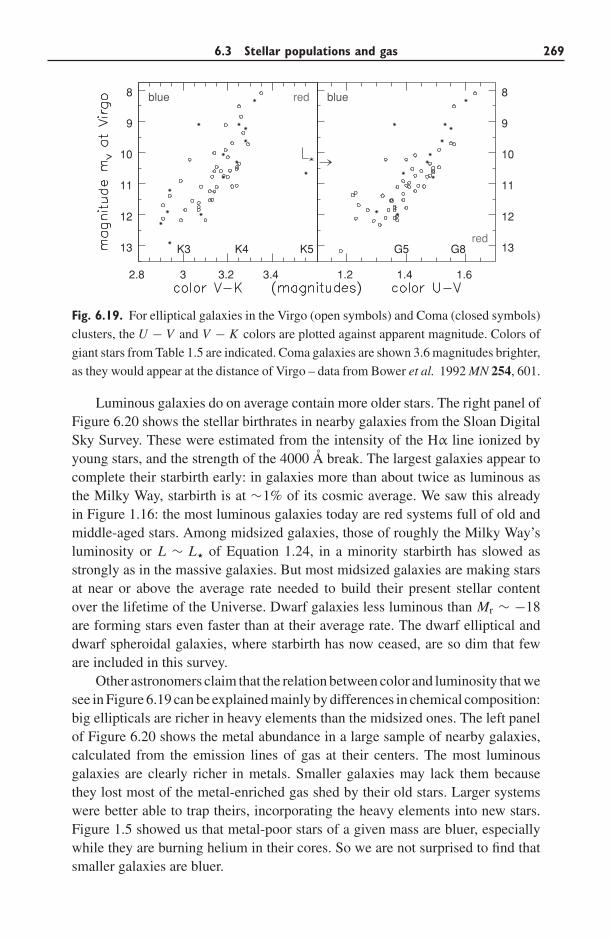
6.3 Stellar populations and gas 269

2.8 3 3.2 3.4

13

12

11

10

9

8 redblue

K3 K4 K5

1.2 1.4 1.6

13

12

11

10

9

8

red

blue

G5 G8

Fig. 6.19. For elliptical galaxies in the Virgo (open symbols) and Coma (closed symbols)

clusters, the U − V and V − K colors are plotted against apparent magnitude. Colors of

giant stars from Table 1.5 are indicated. Coma galaxies are shown 3.6 magnitudes brighter,

as they would appear at the distance of Virgo – data from Bower et al. 1992 MN 254, 601.

Luminous galaxies do on average contain more older stars. The right panel ofFigure 6.20 shows the stellar birthrates in nearby galaxies from the Sloan DigitalSky Survey. These were estimated from the intensity of the Hα line ionized byyoung stars, and the strength of the 4000 A break. The largest galaxies appear tocomplete their starbirth early: in galaxies more than about twice as luminous asthe Milky Way, starbirth is at ∼1% of its cosmic average. We saw this alreadyin Figure 1.16: the most luminous galaxies today are red systems full of old andmiddle-aged stars. Among midsized galaxies, those of roughly the Milky Way’sluminosity or L ∼ L of Equation 1.24, in a minority starbirth has slowed asstrongly as in the massive galaxies. But most midsized galaxies are making starsat near or above the average rate needed to build their present stellar contentover the lifetime of the Universe. Dwarf galaxies less luminous than Mr ∼ −18are forming stars even faster than at their average rate. The dwarf elliptical anddwarf spheroidal galaxies, where starbirth has now ceased, are so dim that feware included in this survey.

Other astronomers claim that the relation between color and luminosity that wesee in Figure 6.19 can be explained mainly by differences in chemical composition:big ellipticals are richer in heavy elements than the midsized ones. The left panelof Figure 6.20 shows the metal abundance in a large sample of nearby galaxies,calculated from the emission lines of gas at their centers. The most luminousgalaxies are clearly richer in metals. Smaller galaxies may lack them becausethey lost most of the metal-enriched gas shed by their old stars. Larger systemswere better able to trap theirs, incorporating the heavy elements into new stars.Figure 1.5 showed us that metal-poor stars of a given mass are bluer, especiallywhile they are burning helium in their cores. So we are not surprised to find thatsmaller galaxies are bluer.

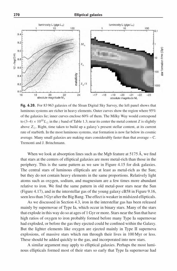
270 Elliptical galaxies

Fig. 6.20. For 83 963 galaxies of the Sloan Digital Sky Survey, the left panel shows that

luminous systems are richer in heavy elements. Outer curves show the region where 95%

of the galaxies lie; inner curves enclose 60% of them. The Milky Way would correspond

to (3–4) × 1010L� in the z band of Table 1.3; near its center the metal content Z is slightly

above Z�. Right, time taken to build up a galaxy’s present stellar content, at its current

rate of starbirth. In the most luminous systems, star formation is now far below its cosmic

average. Many small galaxies are making stars considerably faster than that average – C.

Tremonti and J. Brinchmann.

When we look at absorption lines such as the Mgb feature at 5175 A, we findthat stars at the centers of elliptical galaxies are more metal-rich than those in theperiphery. This is the same pattern as we saw in Figure 4.15 for disk galaxies.The central stars of luminous ellipticals are at least as metal-rich as the Sun;but they do not contain heavy elements in the same proportions. Relatively lightatoms such as oxygen, sodium, and magnesium are a few times more abundantrelative to iron. We find the same pattern in old metal-poor stars near the Sun(Figure 4.17), and in the interstellar gas of the young galaxy cB58 in Figure 9.16,seen less than 3 Gyr after the Big Bang. The effect is weaker in midsized ellipticals.

As we discussed in Section 4.3, iron in the interstellar gas has been releasedmainly by supernovae of Type Ia, which occur in binary stars. Many of the starsthat explode in this way do so at ages of 1 Gyr or more. Stars near the Sun that havehigh ratios of oxygen to iron probably formed before many Type Ia supernovaehad exploded, or before the gas they ejected could be confined within the Galaxy.But the lighter elements like oxygen are ejected mainly in Type II supernovaexplosions, of massive stars which run through their lives in 100 Myr or less.These should be added quickly to the gas, and incorporated into new stars.

A similar argument may apply to elliptical galaxies. Perhaps the most lumi-nous ellipticals formed most of their stars so early that Type Ia supernovae had

6.3 Stellar populations and gas 271

not yet begun to add iron to the galactic gas. Or these galaxies may have lackedType Ia supernovae, because they made relatively more of the massive stars,or fewer binaries. Another possibility is that, early on, the products of Type Iasupernova explosions were able to leave the galaxy, perhaps mixing with thehot X-ray-emitting gas of a surrounding cluster of galaxies. The gas ejected inType II supernova explosions moves slower, and so is easier to confine within thegalaxy.

Surprisingly, despite their lack of young hot stars, elliptical galaxies (andthe bulges of disk systems) are not dark at ultraviolet wavelengths. Metal-richellipticals tend to be brightest, suggesting that the sources are not old metal-poorstars on the horizontal branch, like the ones we see in globular clusters. Instead,the emission presumably comes from old metal-rich stars that have left the mainsequence and then lost most of their hydrogen envelope, exposing the hot stellarcore. No such stars are found near the Sun, since the Milky Way’s disk is tooyoung. So we have not been able to study them in detail, and models remainuncertain.

X-ray sources in elliptical galaxies include active galactic nuclei; stellar bina-ries where material is accreted onto a black hole or neutron star, or burns on thesurface of a white dwarf; and hot gas at temperatures T ∼> 106 K, either filling thegalaxy or localized in stellar atmospheres, stellar winds, or supernova remnants.Most elliptical galaxies lack an active nucleus, and X-rays come mainly from thehot interstellar medium. Their supernova remnants are not strong X-ray sources.When supernova remnants expand into the cool and warm gas of a galaxy diskwhere T ∼< 104 K, they are highly supersonic and create strong shocks that heat gasto X-ray-emitting temperatures. But in an elliptical galaxy the remnants expandinto the hot gas with barely supersonic speeds, developing only weak shocks.When the galaxy is gas-poor, stellar binaries are the most important sources ofX-rays.

We should not be surprised that ellipticals today largely lack new stars, sincemost now contain very little cool gas from which to make any. At first glance, ellip-ticals seem generally free of dust and gas. According to Hubble, ‘small patches ofobscuring material are occasionally silhouetted against the luminous background,but otherwise these nebulae present no structural details’. Closer examinationshows that almost all of them have some dust in the nuclear regions, which ispresumably mixed with cold gas. But only 5%−10% of normal ellipticals containenough atomic hydrogen or molecular gas to be detectable – which means thatmost big elliptical galaxies have less than (108−109)M� of cool gas, while a largeSc galaxy contains almost 1010M�.

A minority of elliptical galaxies, especially those with ‘peculiarities’ such asouter shells or obvious dust lanes, go against this trend: a few have as much coolgas as a large spiral. Where HI gas is plentiful, it often forms a ring well outsidethe stellar body of the galaxy, and it frequently orbits about an axis that is nowhereclose to the short axis of the galaxy’s image or the rotation axis of its stars. The

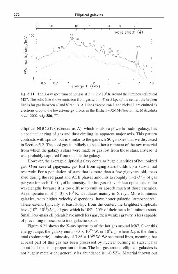
272 Elliptical galaxies

1

10

100

0.5 0.7 11 2 3 4 7 10

30 20 10 7 234

Fig. 6.21. The X-ray spectrum of hot gas at T ∼ 2×107 K around the luminous elliptical

M87. The solid line shows emission from gas within 4′ or 5 kpc of the center; the broken

line is for gas between 4′ and 8′ radius. All lines except iron L and nickel L are emitted as

electrons drop to the lowest-energy orbits, in the K shell – XMM-Newton: K. Matsushita

et al. 2002 AAp 386, 77.

elliptical NGC 5128 (Centaurus A), which is also a powerful radio galaxy, hasa spectacular ring of gas and dust circling its apparent major axis. This patterncontrasts with spirals, but is similar to the gas-rich S0 galaxies that we discussedin Section 5.2. The cool gas is unlikely to be either a remnant of the raw materialfrom which the galaxy’s stars were made or gas lost from those stars. Instead, itwas probably captured from outside the galaxy.

However, the average elliptical galaxy contains huge quantities of hot ionizedgas. Over several gigayears, gas lost from aging stars builds up a substantialreservoir. For a population of stars that is more than a few gigayears old, massshed during the red giant and AGB phases amounts to roughly (1–2)M� of gasper year for each 1010L� of luminosity. The hot gas is invisible at optical and radiowavelengths because it is too diffuse to emit or absorb much at those energies.At temperatures of (1–3) ×107 K, it radiates mainly in X-rays. More luminousgalaxies, with higher velocity dispersions, have hotter galactic ‘atmospheres’.These extend typically at least 30 kpc from the center; the brightest ellipticalshave (109−1011)M� of gas, which is 10%−20% of their mass in luminous stars.Small, low-mass ellipticals have much less gas; their weaker gravity is less capableof preventing its escape to intergalactic space.

Figure 6.21 shows the X-ray spectrum of the hot gas around M87. Over thisenergy range, the galaxy emits ∼3 × 1035 W, or 109L�, where L� is the Sun’stotal (bolometric) luminosity of 3.86 × 1026 W. We see metal lines, meaning thatat least part of this gas has been processed by nuclear burning in stars; it hasabout half the solar proportion of iron. The hot gas around elliptical galaxies isnot hugely metal-rich; generally its abundance is ∼0.5Z�. Material thrown out

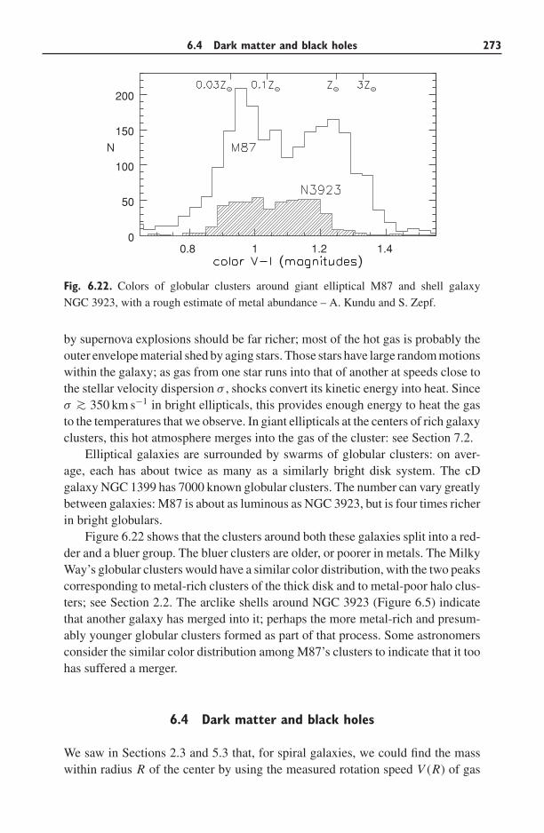
6.4 Dark matter and black holes 273

0.8 1 1.2 1.40

50

100

150

200

Fig. 6.22. Colors of globular clusters around giant elliptical M87 and shell galaxy

NGC 3923, with a rough estimate of metal abundance – A. Kundu and S. Zepf.

by supernova explosions should be far richer; most of the hot gas is probably theouter envelope material shed by aging stars. Those stars have large random motionswithin the galaxy; as gas from one star runs into that of another at speeds close tothe stellar velocity dispersion σ , shocks convert its kinetic energy into heat. Sinceσ ∼> 350 km s−1 in bright ellipticals, this provides enough energy to heat the gasto the temperatures that we observe. In giant ellipticals at the centers of rich galaxyclusters, this hot atmosphere merges into the gas of the cluster: see Section 7.2.

Elliptical galaxies are surrounded by swarms of globular clusters: on aver-age, each has about twice as many as a similarly bright disk system. The cDgalaxy NGC 1399 has 7000 known globular clusters. The number can vary greatlybetween galaxies: M87 is about as luminous as NGC 3923, but is four times richerin bright globulars.

Figure 6.22 shows that the clusters around both these galaxies split into a red-der and a bluer group. The bluer clusters are older, or poorer in metals. The MilkyWay’s globular clusters would have a similar color distribution, with the two peakscorresponding to metal-rich clusters of the thick disk and to metal-poor halo clus-ters; see Section 2.2. The arclike shells around NGC 3923 (Figure 6.5) indicatethat another galaxy has merged into it; perhaps the more metal-rich and presum-ably younger globular clusters formed as part of that process. Some astronomersconsider the similar color distribution among M87’s clusters to indicate that it toohas suffered a merger.

6.4 Dark matter and black holes

We saw in Sections 2.3 and 5.3 that, for spiral galaxies, we could find the masswithin radius R of the center by using the measured rotation speed V (R) of gas

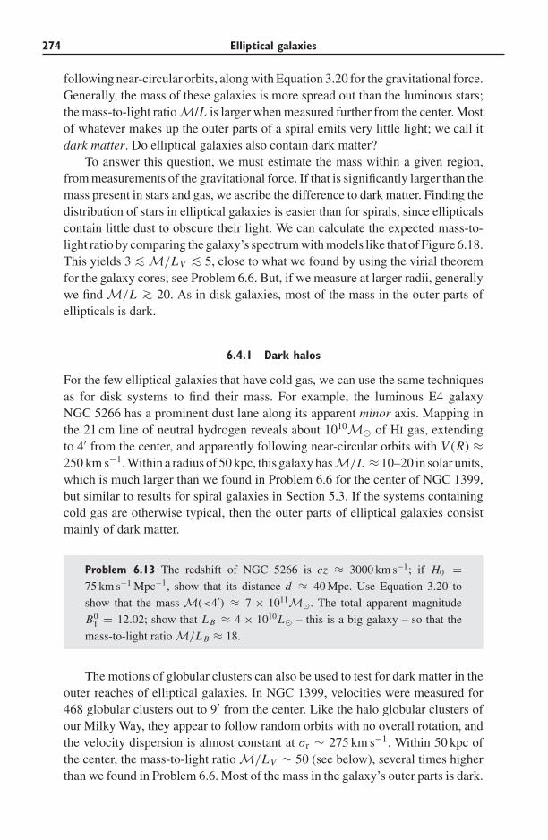
274 Elliptical galaxies

following near-circular orbits, along with Equation 3.20 for the gravitational force.Generally, the mass of these galaxies is more spread out than the luminous stars;the mass-to-light ratioM/L is larger when measured further from the center. Mostof whatever makes up the outer parts of a spiral emits very little light; we call itdark matter. Do elliptical galaxies also contain dark matter?

To answer this question, we must estimate the mass within a given region,from measurements of the gravitational force. If that is significantly larger than themass present in stars and gas, we ascribe the difference to dark matter. Finding thedistribution of stars in elliptical galaxies is easier than for spirals, since ellipticalscontain little dust to obscure their light. We can calculate the expected mass-to-light ratio by comparing the galaxy’s spectrum with models like that of Figure 6.18.This yields 3 ∼< M/LV ∼< 5, close to what we found by using the virial theoremfor the galaxy cores; see Problem 6.6. But, if we measure at larger radii, generallywe find M/L ∼> 20. As in disk galaxies, most of the mass in the outer parts ofellipticals is dark.

6.4.1 Dark halos

For the few elliptical galaxies that have cold gas, we can use the same techniquesas for disk systems to find their mass. For example, the luminous E4 galaxyNGC 5266 has a prominent dust lane along its apparent minor axis. Mapping inthe 21 cm line of neutral hydrogen reveals about 1010M� of HI gas, extendingto 4′ from the center, and apparently following near-circular orbits with V (R) ≈250 km s−1. Within a radius of 50 kpc, this galaxy hasM/L ≈10–20 in solar units,which is much larger than we found in Problem 6.6 for the center of NGC 1399,but similar to results for spiral galaxies in Section 5.3. If the systems containingcold gas are otherwise typical, then the outer parts of elliptical galaxies consistmainly of dark matter.

Problem 6.13 The redshift of NGC 5266 is cz ≈ 3000 km s−1; if H0 =75 km s−1 Mpc−1, show that its distance d ≈ 40 Mpc. Use Equation 3.20 to

show that the mass M(<4′) ≈ 7 × 1011M�. The total apparent magnitude

B0T = 12.02; show that L B ≈ 4 × 1010L� – this is a big galaxy – so that the

mass-to-light ratio M/L B ≈ 18.

The motions of globular clusters can also be used to test for dark matter in theouter reaches of elliptical galaxies. In NGC 1399, velocities were measured for468 globular clusters out to 9′ from the center. Like the halo globular clusters ofour Milky Way, they appear to follow random orbits with no overall rotation, andthe velocity dispersion is almost constant at σr ∼ 275 km s−1. Within 50 kpc ofthe center, the mass-to-light ratio M/LV ∼ 50 (see below), several times higherthan we found in Problem 6.6. Most of the mass in the galaxy’s outer parts is dark.

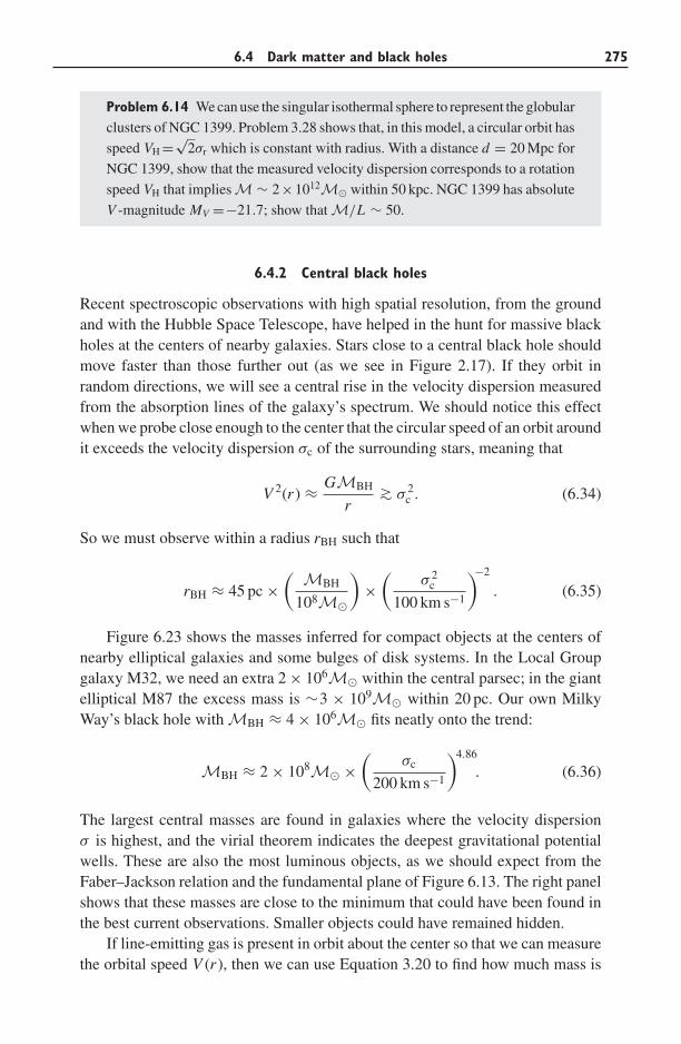
6.4 Dark matter and black holes 275

Problem 6.14 We can use the singular isothermal sphere to represent the globular

clusters of NGC 1399. Problem 3.28 shows that, in this model, a circular orbit has

speed VH =√2σr which is constant with radius. With a distance d = 20 Mpc for

NGC 1399, show that the measured velocity dispersion corresponds to a rotation

speed VH that implies M ∼ 2×1012M� within 50 kpc. NGC 1399 has absolute

V -magnitude MV =−21.7; show that M/L ∼ 50.

6.4.2 Central black holes

Recent spectroscopic observations with high spatial resolution, from the groundand with the Hubble Space Telescope, have helped in the hunt for massive blackholes at the centers of nearby galaxies. Stars close to a central black hole shouldmove faster than those further out (as we see in Figure 2.17). If they orbit inrandom directions, we will see a central rise in the velocity dispersion measuredfrom the absorption lines of the galaxy’s spectrum. We should notice this effectwhen we probe close enough to the center that the circular speed of an orbit aroundit exceeds the velocity dispersion σc of the surrounding stars, meaning that

V 2(r ) ≈ GMBH

r ∼> σ 2c . (6.34)

So we must observe within a radius rBH such that

rBH ≈ 45 pc ×( MBH

108M�

)×(

σ 2c

100 km s−1

)−2

. (6.35)

Figure 6.23 shows the masses inferred for compact objects at the centers ofnearby elliptical galaxies and some bulges of disk systems. In the Local Groupgalaxy M32, we need an extra 2 × 106M� within the central parsec; in the giantelliptical M87 the excess mass is ∼3 × 109M� within 20 pc. Our own MilkyWay’s black hole with MBH ≈ 4 × 106M� fits neatly onto the trend:

MBH ≈ 2 × 108M� ×(

σc

200 km s−1

)4.86

. (6.36)

The largest central masses are found in galaxies where the velocity dispersionσ is highest, and the virial theorem indicates the deepest gravitational potentialwells. These are also the most luminous objects, as we should expect from theFaber–Jackson relation and the fundamental plane of Figure 6.13. The right panelshows that these masses are close to the minimum that could have been found inthe best current observations. Smaller objects could have remained hidden.

If line-emitting gas is present in orbit about the center so that we can measurethe orbital speed V (r ), then we can use Equation 3.20 to find how much mass is

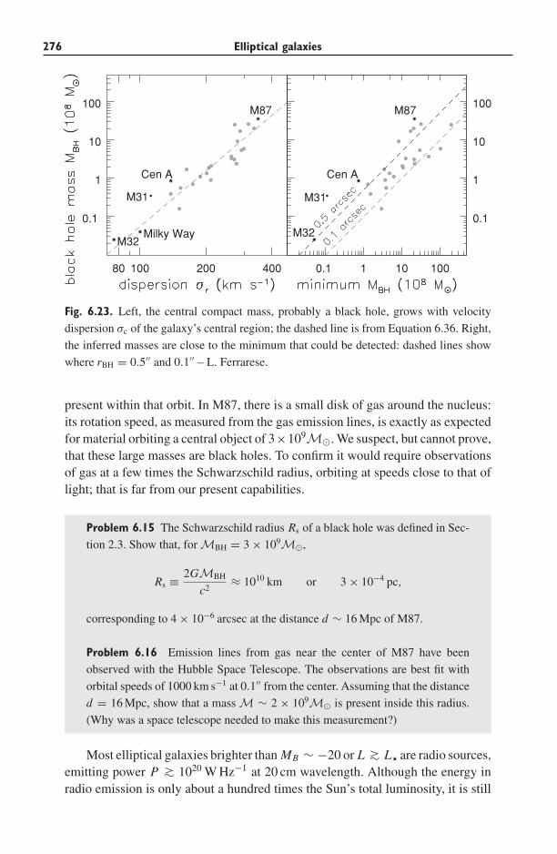
276 Elliptical galaxies

80 100 200 400

0.1

1

10

100

Cen A

M32

M31

M87

Milky Way

0.1 1 10 100

0.1

1

10

100

M32

M31

M87

Cen A

Fig. 6.23. Left, the central compact mass, probably a black hole, grows with velocity

dispersion σc of the galaxy’s central region; the dashed line is from Equation 6.36. Right,

the inferred masses are close to the minimum that could be detected: dashed lines show

where rBH = 0.5′′ and 0.1′′ – L. Ferrarese.

present within that orbit. In M87, there is a small disk of gas around the nucleus:its rotation speed, as measured from the gas emission lines, is exactly as expectedfor material orbiting a central object of 3×109M�. We suspect, but cannot prove,that these large masses are black holes. To confirm it would require observationsof gas at a few times the Schwarzschild radius, orbiting at speeds close to that oflight; that is far from our present capabilities.

Problem 6.15 The Schwarzschild radius Rs of a black hole was defined in Sec-

tion 2.3. Show that, for MBH = 3 × 109M�,

Rs ≡ 2GMBH

c2≈ 1010 km or 3 × 10−4 pc,

corresponding to 4 × 10−6 arcsec at the distance d ∼ 16 Mpc of M87.

Problem 6.16 Emission lines from gas near the center of M87 have been

observed with the Hubble Space Telescope. The observations are best fit with

orbital speeds of 1000 km s−1 at 0.1′′ from the center. Assuming that the distance

d = 16 Mpc, show that a mass M ∼ 2 × 109M� is present inside this radius.

(Why was a space telescope needed to make this measurement?)

Most elliptical galaxies brighter than MB ∼ −20 or L ∼> L are radio sources,emitting power P ∼> 1020 W Hz−1 at 20 cm wavelength. Although the energy inradio emission is only about a hundred times the Sun’s total luminosity, it is still

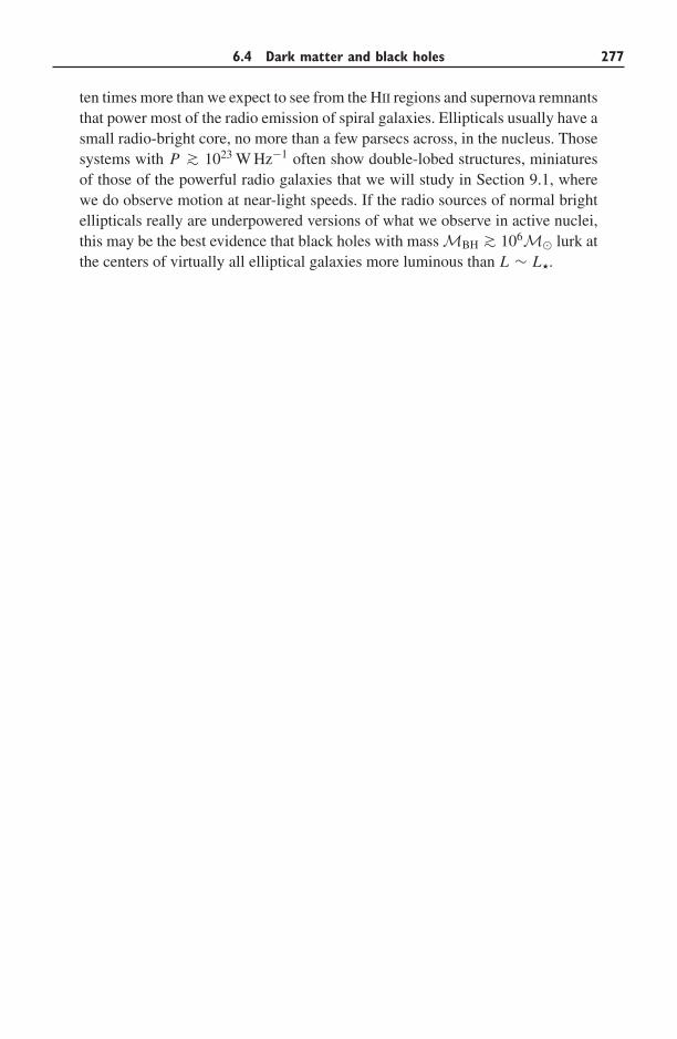
6.4 Dark matter and black holes 277

ten times more than we expect to see from the HII regions and supernova remnantsthat power most of the radio emission of spiral galaxies. Ellipticals usually have asmall radio-bright core, no more than a few parsecs across, in the nucleus. Thosesystems with P ∼> 1023 W Hz−1 often show double-lobed structures, miniaturesof those of the powerful radio galaxies that we will study in Section 9.1, wherewe do observe motion at near-light speeds. If the radio sources of normal brightellipticals really are underpowered versions of what we observe in active nuclei,this may be the best evidence that black holes with mass MBH ∼> 106M� lurk atthe centers of virtually all elliptical galaxies more luminous than L ∼ L.

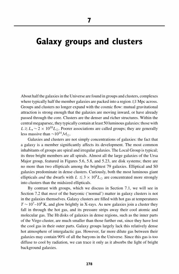
7

Galaxy groups and clusters

About half the galaxies in the Universe are found in groups and clusters, complexeswhere typically half the member galaxies are packed into a region ∼<1 Mpc across.Groups and clusters no longer expand with the cosmic flow: mutual gravitationalattraction is strong enough that the galaxies are moving inward, or have alreadypassed through the core. Clusters are the denser and richer structures. Within thecentral megaparsec, they typically contain at least 50 luminous galaxies: those withL ∼> L ∼ 2 × 1010L�. Poorer associations are called groups; they are generallyless massive than ∼1014M�.

Galaxies and clusters are not simply concentrations of galaxies: the fact thata galaxy is a member significantly affects its development. The most commoninhabitants of groups are spiral and irregular galaxies. The Local Group is typical;its three bright members are all spirals. Almost all the large galaxies of the UrsaMajor group, featured in Figures 5.6, 5.8, and 5.23, are disk systems; there areno more than two ellipticals among the brightest 79 galaxies. Elliptical and S0galaxies predominate in dense clusters. Curiously, both the most luminous giantellipticals and the dwarfs with L ∼< 3 × 109L� are concentrated more stronglyinto clusters than the midsized ellipticals.

By contrast with groups, which we discuss in Section 7.1, we will see inSection 7.2 that most of the baryonic (‘normal’) matter in galaxy clusters is notin the galaxies themselves. Galaxy clusters are filled with hot gas at temperaturesT ∼107–108 K, and glow brightly in X-rays. As new galaxies join a cluster theyfall in through the hot gas, and its pressure strips away their cool atomic andmolecular gas. The HI disks of galaxies in dense regions, such as the inner partsof the Virgo cluster, are much smaller than those further out, since they have lostthe cool gas in their outer parts. Galaxy groups largely lack this relatively densehot atmosphere of intergalactic gas. However, far more dilute gas between theirgalaxies may contain 90% of all the baryons in the Universe. Since this gas is toodiffuse to cool by radiation, we can trace it only as it absorbs the light of brightbackground galaxies.

278

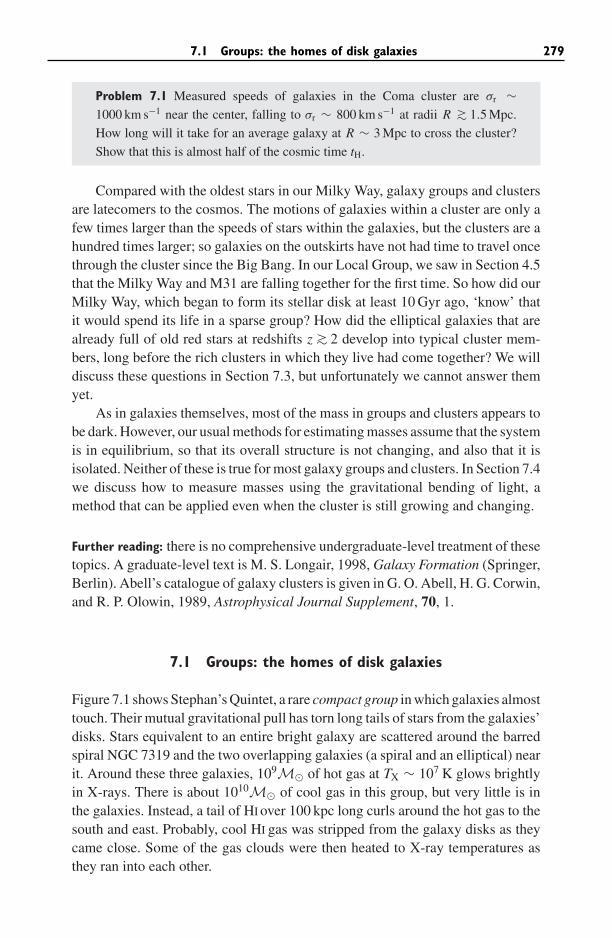
7.1 Groups: the homes of disk galaxies 279

Problem 7.1 Measured speeds of galaxies in the Coma cluster are σr ∼1000 km s−1 near the center, falling to σr ∼ 800 km s−1 at radii R ∼> 1.5 Mpc.

How long will it take for an average galaxy at R ∼ 3 Mpc to cross the cluster?

Show that this is almost half of the cosmic time tH.

Compared with the oldest stars in our Milky Way, galaxy groups and clustersare latecomers to the cosmos. The motions of galaxies within a cluster are only afew times larger than the speeds of stars within the galaxies, but the clusters are ahundred times larger; so galaxies on the outskirts have not had time to travel oncethrough the cluster since the Big Bang. In our Local Group, we saw in Section 4.5that the Milky Way and M31 are falling together for the first time. So how did ourMilky Way, which began to form its stellar disk at least 10 Gyr ago, ‘know’ thatit would spend its life in a sparse group? How did the elliptical galaxies that arealready full of old red stars at redshifts z ∼> 2 develop into typical cluster mem-bers, long before the rich clusters in which they live had come together? We willdiscuss these questions in Section 7.3, but unfortunately we cannot answer themyet.

As in galaxies themselves, most of the mass in groups and clusters appears tobe dark. However, our usual methods for estimating masses assume that the systemis in equilibrium, so that its overall structure is not changing, and also that it isisolated. Neither of these is true for most galaxy groups and clusters. In Section 7.4we discuss how to measure masses using the gravitational bending of light, amethod that can be applied even when the cluster is still growing and changing.

Further reading: there is no comprehensive undergraduate-level treatment of thesetopics. A graduate-level text is M. S. Longair, 1998, Galaxy Formation (Springer,Berlin). Abell’s catalogue of galaxy clusters is given in G. O. Abell, H. G. Corwin,and R. P. Olowin, 1989, Astrophysical Journal Supplement, 70, 1.

7.1 Groups: the homes of disk galaxies

Figure 7.1 shows Stephan’s Quintet, a rare compact group in which galaxies almosttouch. Their mutual gravitational pull has torn long tails of stars from the galaxies’disks. Stars equivalent to an entire bright galaxy are scattered around the barredspiral NGC 7319 and the two overlapping galaxies (a spiral and an elliptical) nearit. Around these three galaxies, 109M� of hot gas at TX ∼ 107 K glows brightlyin X-rays. There is about 1010M� of cool gas in this group, but very little is inthe galaxies. Instead, a tail of HI over 100 kpc long curls around the hot gas to thesouth and east. Probably, cool HI gas was stripped from the galaxy disks as theycame close. Some of the gas clouds were then heated to X-ray temperatures asthey ran into each other.

280 Galaxy groups and clusters

Fig. 7.1. Stephan’s Quintet (compact group Hickson 92) is ∼85 Mpc distant and 80 kpc

across, or 3.2′ on the sky. North is at the top and east is to the left. NGC 7319, the barred

spiral, has an active nucleus: it is a Seyfert 2. The large spiral in the lower center, NGC

7320, is not a group member; it is in the foreground with a much smaller redshift – D. J.

Pisano, WIYN telescope.

The observed motion of the galaxies and the stellar tails lets us reconstruct partof the group’s history. The spiral NGC 7318b (one of the two overlapping galaxies)has only just arrived in the group, tearing out the bright stellar trail leading fromone of the spiral arms in NGC7319. Its cool gas is now being stripped away.To the south, the longer but more diffuse tail of stars curves toward the smallgalaxy NGC 7320c, 140 kpc to the east; this passed through the group ∼500 Myrago, and will return. Stephan’s Quintet has about twice as much gas as the MilkyWay, and three times as much stellar light. One could imagine that its galaxiesbegan life much like our Milky Way, losing their gas in repeated collisions andnear-misses.

Problem 7.2 Suppose that gas atoms and galaxies in a group move at the same

average random speed σ along each direction. At temperature T , the average

energy of a gas particle is 3kBT/2, where kB is Boltzmann’s constant. If the gas

is mainly ionized hydrogen, these particles are protons and electrons; show that,

if the atom’s kinetic energy (3mp/2)σ 2 is shared equally between them, then

T ≈ (mp/2)σ 2

kB≈ 5 × 106

(σ

300 km s−1

)2

K. (7.1)

Hot gas in a group or cluster is usually close to this virial temperature.

7.1 Groups: the homes of disk galaxies 281

Fig. 7.2. The group around the large Sc spiral galaxy M81, about 3.5 Mpc distant. Left,

negative image in visible light; the elongated object north of M81 is starburst galaxy M82;

NGC 3077 is to the southeast. Right, map in HI to the same spatial scale – M. Yun.

Problem 7.3 The energies of X-ray photons are measured in kilo-electron-volts

(keV), 1000 times the energy that an electron gains in moving through a one-

volt potential. In Stephan’s Quintet, the gas radiates X-rays with typical energy

kBTX = 0.5 keV; show that this implies TX ≈ 6 × 106 K. The speeds Vr of the

galaxies along our line of sight have a dispersion σr ∼ 350 km s−1. Show that

the kinetic energy of a hydrogen atom moving at speed σr is roughly equal to

the one-dimensional energy kBT/2 for each of two particles (a proton and an

electron) at T = 7 × 106 K. Thus, as group galaxies run into each other, the

energy of their motion can heat gas to the observed temperature.

Figure 7.2 shows the sparse group around the nearby spiral M81. We see only afew intergalactic stars, but the galaxies are connected by long streamers of atomichydrogen torn from their disks as they passed close to one another. Because the HI

layer of a spiral galaxy extends much further in radius than its main stellar disk,the gas disks are more easily damaged. Here, almost all of the gas that was tornfrom the galaxies has remained cool. Similarly, in Figure 4.6, we see HI gas fromthe Magellanic Clouds pulled out into a stream around the Milky Way.

Only half of galaxy groups contain gas hot enough to shine in X-rays, whichrequires T ∼>3 × 106 K. Those groups are generally more populous, and includeat least one elliptical galaxy. For example, the group of 15 galaxies within 1 Mpcaround the S0 galaxy NGC 1550 (including two ellipticals) radiates 4 × 109L� inX-rays, 100 times more than Stephan’s Quintet. X-ray spectral lines of 24-timesionized iron, and of multiply-ionized oxygen, magnesium, and sulfur, show thatelements heavier than helium are present in a few tenths of the solar proportions.

282 Galaxy groups and clusters

Iron lines at ∼1 keV tell us that the innermost gas of the NGC 1550 group has abouthalf the solar metal abundance Z�, while at 200 kpc from the center Z ≈ 0.1Z�.

Our usual tricks can tell us the mass of a galaxy group: we watch somethingthat moves, and apply the equations of Newton’s gravity. In the NGC 1550 group,the velocity dispersion of the galaxies is σr = 310 km s−1. If we assume that thegroup is isolated and in equilibrium, and approximate its density by the Plummersphere of Equations 3.12 and 3.37 with aP = 100 kpc, then Equation 3.44 (thevirial theorem) tells us that its mass M is

3Mσ 2r

2= KE = −PE

2= 3π

64

GM2

aP, so M ≈ 2 × 1013M�.

When a group contains hot gas we have another way to find its mass, as we didfor elliptical galaxies in Section 6.4. We first estimate the X-ray temperature TX

from spectral lines. The gas is diffuse, so we can use Equation 2.23 from Section 2.4to find the density. When TX ∼>107 K, gas of roughly the Sun’s composition losesenergy mainly by free–free radiation, also called thermal bremsstrahlung. If eachcubic centimeter contains n atoms, its luminosity is

LX = n2�(TX), where � ≈ 3 × 10−27T 1/2X erg s−1. (7.2)

(Look back at Figure 2.25 to see how slowly � increases with temperature.) Sowe can work backward from the measured surface brightness IX to find n.

The equation of hydrostatic equilibrium tells us how much gravity is neededto prevent the hot gas from blowing away as a wind. Its pressure p must becounterbalanced by an inward pull: if ρ(r ) is the gas density, then, in a sphericalgalaxy,

dp

dr= −ρ(r )

GM(<r )

r2. (7.3)

We write the average mass m of a gas particle as m = μmp: for fully ionizedhydrogen μ = 0.5, whereas μ ≈ 0.6 for gas of solar composition. For a perfectgas at temperature T and density ρ, we have

p = ρ

μmpkBT , so M(<r ) = kB

μmp

r2

Gρ(r )

d

dr(−ρT ). (7.4)

Problem 7.4 Suppose that the hot gas of a group has a uniform temperature TX,

and outside the very center the surface brightness in X-rays drops with radius R

as IX ∝ R−γ . Writing the gas density ρ(r ) ∝ r−β , use Equation 7.2 to show that

the luminosity per cubic centimeter follows L(r ) ∝ r−2β . Now use the result of

Problem 6.4 to show that γ = 2β − 1.

7.1 Groups: the homes of disk galaxies 283

In the NGC 1550 group, TX = 1.6 × 107 K and ρ(r ) ∝ r−1.1 out to 200 kpc

from the center. Use Equation 7.4 to show that the group’s mass is roughly

1013M�. The hot gas itself accounts for 8 × 1011M�, while the light of the

galaxies adds up to L B ≈ 8 × 1010M�. The mass-to-light ratio of the stars is

unlikely to be more than what we found for the old stars at the center of NGC

1399 in Problem 6.6. Show that the mass of hot gas is at least twice that in all

the stars, so the group contains about eight times as much mass as is present in

the galaxies and hot gas.

In general, the mass-to-light ratio of groups is in the range 80 ∼< M/L ∼<300M�/L�. Stars and gas hot enough to shine in X-rays typically make up lessthan 10% of the total. Groups as a whole appear to contain several times moremass than what we found in Section 5.3 from the rotation curves of individualspirals. Either the dark matter halo of each galaxy extends several times furtherout than the HI disk gas with which we measure its rotation, or substantial massis present between the galaxies as a ‘group halo’.

Problem 7.5 Suppose that all galaxy groups share a common form for the density

ρ(r ): for example, the Plummer sphere of Equations 3.12 and 3.37. If all groups

have the same radius aP, and their mass is proportional to the number of members

N , show that the virial theorem predicts that σr ∝ √N . This is roughly what we

see in Figure 7.3. Points for the sparsest groups lie above this relation: show that

those groups should have smaller radii.

Figure 7.3 shows that the speeds of group galaxies are σr ∼100–500 km s−1,not much faster than the motion of stars within the galaxies. Because of their lowrelative speeds, gravity has more time to pull strongly at the gas and stars in theouter parts of other galaxies as they pass. In the next subsection, we see how thiscan lead two galaxies to merge and become one.

7.1.1 Close encounters between galaxies: dynamical friction

We use the methods of Section 3.2 to examine what happens as two galaxies passclose to one another: part of their energy of forward motion is transferred to motionof the stars within them. Thus, as they separate, they travel more slowly than theydid on their approach. If the galaxies are then moving too sluggishly to escapefrom one another, their orbits bring them back together to encounter each otheragain. Usually, they end by merging.

In Figure 7.4, as in Figure 3.5, an object of mass M moves at speed V past astar of mass m at a distance b from its path. But now M is one of our galaxies,while the star m belongs to another: so M/m ∼108–1011 (!) As the two galaxies

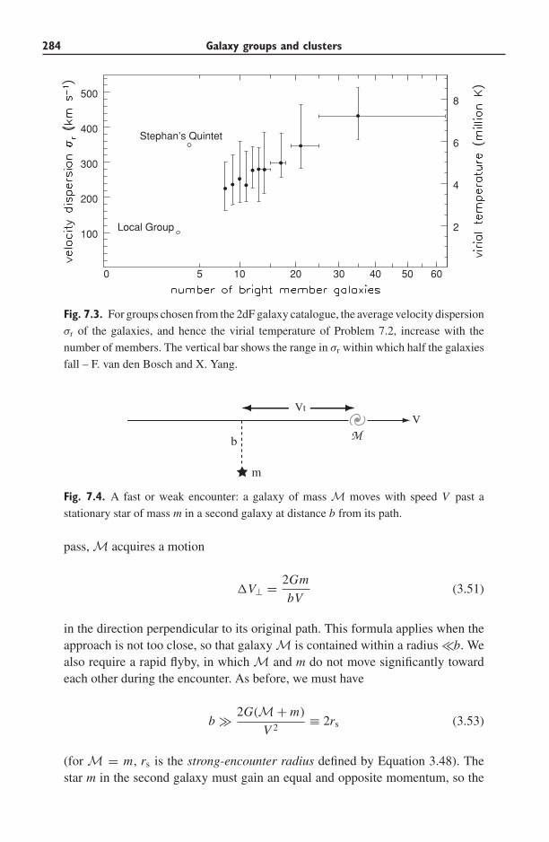
284 Galaxy groups and clusters

100

200

300

400

500

Local Group

Stephan’s Quintet

0 5 10 20 30 40 50 60

2

4

6

8

Fig. 7.3. For groups chosen from the 2dF galaxy catalogue, the average velocity dispersion

σr of the galaxies, and hence the virial temperature of Problem 7.2, increase with the

number of members. The vertical bar shows the range in σr within which half the galaxies

fall – F. van den Bosch and X. Yang.

VtV

b

m

M

Fig. 7.4. A fast or weak encounter: a galaxy of mass M moves with speed V past a

stationary star of mass m in a second galaxy at distance b from its path.

pass, M acquires a motion

�V⊥ = 2Gm

bV(3.51)

in the direction perpendicular to its original path. This formula applies when theapproach is not too close, so that galaxy M is contained within a radius �b. Wealso require a rapid flyby, in which M and m do not move significantly towardeach other during the encounter. As before, we must have

b � 2G(M + m)

V 2≡ 2rs (3.53)

(for M = m, rs is the strong-encounter radius defined by Equation 3.48). Thestar m in the second galaxy must gain an equal and opposite momentum, so the

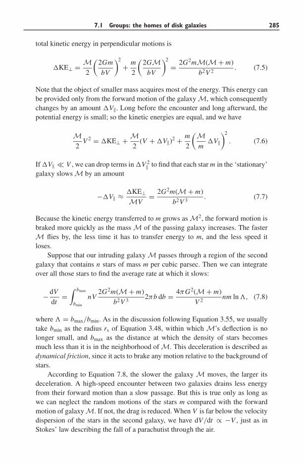
7.1 Groups: the homes of disk galaxies 285

total kinetic energy in perpendicular motions is

�KE⊥ = M2

(2Gm

bV

)2

+ m

2

(2GM

bV

)2

= 2G2mM(M + m)

b2V 2. (7.5)

Note that the object of smaller mass acquires most of the energy. This energy canbe provided only from the forward motion of the galaxy M, which consequentlychanges by an amount �V‖. Long before the encounter and long afterward, thepotential energy is small; so the kinetic energies are equal, and we have

M2

V 2 = �KE⊥ + M2

(V + �V‖)2 + m

2

(Mm

�V‖)2

. (7.6)

If �V‖ � V , we can drop terms in �V 2‖ to find that each star m in the ‘stationary’

galaxy slows M by an amount

−�V‖ ≈ �KE⊥MV

= 2G2m(M + m)

b2V 3. (7.7)

Because the kinetic energy transferred to m grows as M2, the forward motion isbraked more quickly as the mass M of the passing galaxy increases. The fasterM flies by, the less time it has to transfer energy to m, and the less speed itloses.

Suppose that our intruding galaxy M passes through a region of the secondgalaxy that contains n stars of mass m per cubic parsec. Then we can integrateover all those stars to find the average rate at which it slows:

− dV

dt=∫ bmax

bmin

nV2G2m(M + m)

b2V 32πb db = 4πG2(M + m)

V 2nm ln �, (7.8)

where � = bmax/bmin. As in the discussion following Equation 3.55, we usuallytake bmin as the radius rs of Equation 3.48, within which M’s deflection is nolonger small, and bmax as the distance at which the density of stars becomesmuch less than it is in the neighborhood of M. This deceleration is described asdynamical friction, since it acts to brake any motion relative to the background ofstars.

According to Equation 7.8, the slower the galaxy M moves, the larger itsdeceleration. A high-speed encounter between two galaxies drains less energyfrom their forward motion than a slow passage. But this is true only as long aswe can neglect the random motions of the stars m compared with the forwardmotion of galaxy M. If not, the drag is reduced. When V is far below the velocitydispersion of the stars in the second galaxy, we have dV/dt ∝ −V , just as inStokes’ law describing the fall of a parachutist through the air.

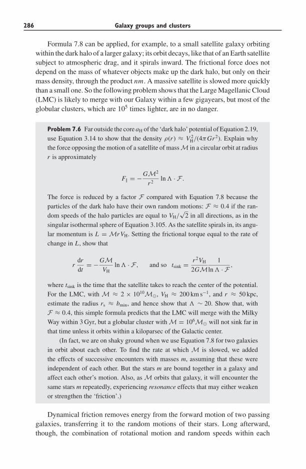
286 Galaxy groups and clusters

Formula 7.8 can be applied, for example, to a small satellite galaxy orbitingwithin the dark halo of a larger galaxy; its orbit decays, like that of an Earth satellitesubject to atmospheric drag, and it spirals inward. The frictional force does notdepend on the mass of whatever objects make up the dark halo, but only on theirmass density, through the product nm. A massive satellite is slowed more quicklythan a small one. So the following problem shows that the Large Magellanic Cloud(LMC) is likely to merge with our Galaxy within a few gigayears, but most of theglobular clusters, which are 105 times lighter, are in no danger.

Problem 7.6 Far outside the core aH of the ‘dark halo’ potential of Equation 2.19,

use Equation 3.14 to show that the density ρ(r ) ≈ V 2H/(4πGr2). Explain why

the force opposing the motion of a satellite of mass M in a circular orbit at radius

r is approximately

F‖ = −GM2

r2ln � · F .

The force is reduced by a factor F compared with Equation 7.8 because the

particles of the dark halo have their own random motions: F ≈ 0.4 if the ran-

dom speeds of the halo particles are equal to VH/√

2 in all directions, as in the

singular isothermal sphere of Equation 3.105. As the satellite spirals in, its angu-

lar momentum is L = Mr VH. Setting the frictional torque equal to the rate of

change in L , show that

rdr

dt= −GM

VHln � · F, and so tsink = r2VH

2GM1

ln � · F ,

where tsink is the time that the satellite takes to reach the center of the potential.

For the LMC, with M ≈ 2 × 1010M�, VH ≈ 200 km s−1, and r ≈ 50 kpc,

estimate the radius rs ≈ bmin, and hence show that � ∼ 20. Show that, with

F ≈ 0.4, this simple formula predicts that the LMC will merge with the Milky

Way within 3 Gyr, but a globular cluster with M = 106M� will not sink far in

that time unless it orbits within a kiloparsec of the Galactic center.

(In fact, we are on shaky ground when we use Equation 7.8 for two galaxies

in orbit about each other. To find the rate at which M is slowed, we added

the effects of successive encounters with masses m, assuming that these were

independent of each other. But the stars m are bound together in a galaxy and

affect each other’s motion. Also, as M orbits that galaxy, it will encounter the

same stars m repeatedly, experiencing resonance effects that may either weaken

or strengthen the ‘friction’.)

Dynamical friction removes energy from the forward motion of two passinggalaxies, transferring it to the random motions of their stars. Long afterward,though, the combination of rotational motion and random speeds within each

7.1 Groups: the homes of disk galaxies 287

galaxy will be lower than before the collision. To see why, suppose that, beforethe encounter, the internal kinetic energy of one of the galaxies was KE0. ByEquation 3.44, the virial theorem, the potential energy PE0 = −2KE0; so itsinternal energy E0 must be

E0 = KE0 + PE0 = −KE0. (7.9)

Dynamical friction increases the energy in random stellar motions, and hencethe galaxy’s internal energy, by �KE . The system is less strongly bound, so itexpands. Long after the encounter, when it is once again in virial equilibrium, thekinetic energy is less than before:

KE1 = −(E0 + �KE) = KE0 − �KE . (7.10)

The stars that acquire the most energy escape from the galaxy; those receivingless remain loosely attached, as a bloated outer envelope. In a spiral or S0 galaxy,the energy added to vertical motions thickens the stellar disk.

If two galaxies pass by one another at the high speeds typical of rich galaxyclusters, they are unlikely to slow each other enough to become a bound pair.They separate, leaving both somewhat dishevelled. But in groups the galaxiestravel more slowly, not much faster than the stellar motions within them; so aclose passage is far more disturbing. Almost all galaxies that we now see in theprocess of merging are group members.

Many group galaxies show evidence of near-miss encounters. These can pusha galaxy into making a bar or spiral that would not have done so if it had beenalone. Like M81, many galaxies with spectacular two-armed spirals have closecompanions. Mergers and near-misses also force disk gas in toward the galaxy’scenter. Because the changing gravity pulls material away from its near-circularorbits, gas streams converge from different directions. As we discussed in Sec-tion 5.5, this causes shocks that remove energy from the gas, letting some of itfall inward. If it reaches the galaxy’s center, it can grow a massive black hole orfuel activity in the nucleus. Both NGC 7319 in Stephan’s Quintet and M81 areSeyfert galaxies, a type of active nucleus that we discuss in Section 9.1.

7.1.2 Galaxy mergers and starbursts

If an encounter has drained enough energy from the galaxies’ orbital motionto leave them bound to each other, they will probably merge. Figure 7.5 showsthree views of what appears to be such a merger in progress, and Figure 7.6shows a computer simulation of the collision that may have led to it. This isa gravitational N-body simulation, in which roughly 106 particles attract eachother by the gravitational force of Equation 3.2. In fact, we cannot solve theseequations exactly; it is too much work to calculate the forces between 1012 different

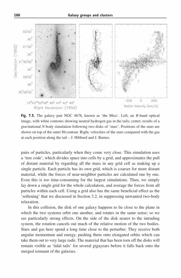
288 Galaxy groups and clusters

Fig. 7.5. The galaxy pair NGC 4676, known as ‘the Mice’. Left, an R-band optical

image, with white contours showing neutral hydrogen gas in the tails; center, results of a

gravitational N-body simulation following two disks of ‘stars’. Positions of the stars are

shown on top of the outer HI contour. Right, velocities of the stars compared with the gas

at each position along the tail – J. Hibbard and J. Barnes.

pairs of particles, particularly when they come very close. This simulation usesa ‘tree code’, which divides space into cells by a grid, and approximates the pullof distant material by regarding all the mass in any grid cell as making up asingle particle. Each particle has its own grid, which is coarser for more distantmaterial, while the forces of near-neighbor particles are calculated one by one.Even this is too time-consuming for the largest simulations. Then, we simplylay down a single grid for the whole calculation, and average the forces from allparticles within each cell. Using a grid also has the same beneficial effect as the‘softening’ that we discussed in Section 3.2, in suppressing unwanted two-bodyrelaxation.

In this collision, the disk of one galaxy happens to lie close to the plane inwhich the two systems orbit one another, and rotates in the same sense; so wesee particularly strong effects. On the side of the disk nearer to the intrudingsystem, the rotation cancels out much of the relative motion of the two bodies.Stars and gas here spend a long time close to the perturber. They receive bothangular momentum and energy, pushing them onto elongated orbits which cantake them out to very large radii. The material that has been torn off the disks willremain visible as ‘tidal tails’ for several gigayears before it falls back onto themerged remnant of the galaxies.

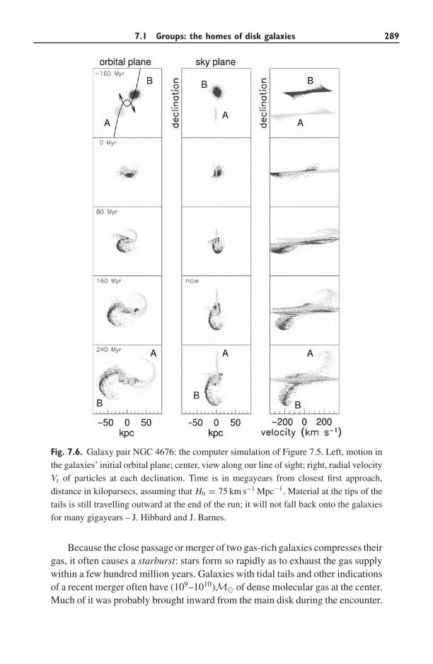
7.1 Groups: the homes of disk galaxies 289

Fig. 7.6. Galaxy pair NGC 4676: the computer simulation of Figure 7.5. Left, motion in

the galaxies’ initial orbital plane; center, view along our line of sight; right, radial velocity

Vr of particles at each declination. Time is in megayears from closest first approach,

distance in kiloparsecs, assuming that H0 = 75 km s−1 Mpc−1. Material at the tips of the

tails is still travelling outward at the end of the run; it will not fall back onto the galaxies

for many gigayears – J. Hibbard and J. Barnes.

Because the close passage or merger of two gas-rich galaxies compresses theirgas, it often causes a starburst: stars form so rapidly as to exhaust the gas supplywithin a few hundred million years. Galaxies with tidal tails and other indicationsof a recent merger often have (109–1010)M� of dense molecular gas at the center.Much of it was probably brought inward from the main disk during the encounter.

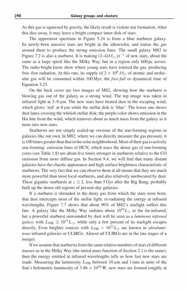
290 Galaxy groups and clusters

As this gas is squeezed by gravity, the likely result is violent star formation. Afterthis dies away, it may leave a bright compact inner disk of stars.

The uppermost spectrum in Figure 5.24 is from a blue starburst galaxy.Its newly-born massive stars are bright in the ultraviolet, and ionize the gasaround them to produce the strong emission lines. The small galaxy M82 inFigure 7.2 is also a starburst. It is making (2–4)M� yr−1 of new stars, about thesame as a large spiral like the Milky Way, but in a region only 600 pc across.The radio-bright knots show where young stars have ionized the gas, producingfree–free radiation. At this rate, its supply of 2 × 108M� of atomic and molec-ular gas will be consumed within 100 Myr, the free-fall or dynamical time ofEquation 3.23.

On the back cover are two images of M82, showing how the starburst isblowing gas out of the galaxy as a strong wind. The top image was taken ininfrared light at 3–9 μm. The new stars have heated dust in the escaping wind,which glows ‘red’ at 8 μm while the stellar disk is ‘blue’. The lower one showsdust lanes crossing the whitish stellar disk; the purple color shows emission in theHα line from the wind, which removes about as much mass from the galaxy as itturns into new stars.

Starbursts are not simply scaled-up versions of the star-forming regions ingalaxies like our own. In M82, where we can directly measure the gas pressure, itis 100 times greater than that in the solar neighborhood. More of their gas is activelystar-forming: emission lines of HCN, which trace the dense gas of star-formingcores (see Table 1.8) are about five times stronger in starbursts relative to the COemission from more diffuse gas. In Section 9.4, we will find that many distantgalaxies have the chaotic appearance and high surface brightness characteristic ofstarbursts. The very fact that we can observe them at all means that they are muchmore powerful than most local starbursts, and also relatively unobscured by dust.These gigantic starbursts at z ∼> 2, less than 5 Gyr after the Big Bang, probablybuilt up the dense old regions of present-day galaxies.

If a starburst is shrouded in the dusty gas from which the stars were born,that dust intercepts most of the stellar light, re-radiating the energy at infraredwavelengths. Figure 7.7 shows that about 90% of M82’s starlight suffers thisfate. A galaxy like the Milky Way radiates about 1010L� in the far-infrared,but a powerful starburst surrounded by dust will be seen as a luminous infraredgalaxy with LFIR ∼> 1011L�, while only a few percent of its starlight escapesdirectly. Even brighter sources with LFIR > 1012L� are known as ultralumi-nous infrared galaxies or ULIRGs. Almost all ULIRGs are in the late stages of amerger.

If we assume that starbursts form the same relative numbers of stars of differentmasses as in the Milky Way (the initial mass function of Section 2.1 is the same),then the energy emitted at infrared wavelengths tells us how fast new stars aremade. Measuring the luminosity LFIR between 10 μm and 1 mm in units of theSun’s bolometric luminosity of 3.86 × 1026 W, new stars are formed roughly at

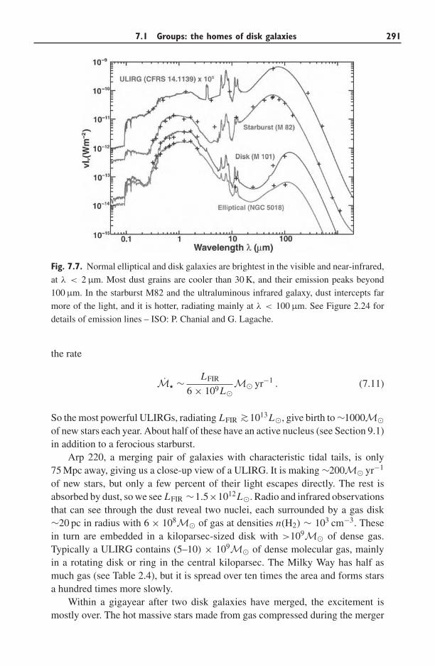
7.1 Groups: the homes of disk galaxies 291

Fig. 7.7. Normal elliptical and disk galaxies are brightest in the visible and near-infrared,

at λ < 2 μm. Most dust grains are cooler than 30 K, and their emission peaks beyond

100 μm. In the starburst M82 and the ultraluminous infrared galaxy, dust intercepts far

more of the light, and it is hotter, radiating mainly at λ < 100 μm. See Figure 2.24 for

details of emission lines – ISO: P. Chanial and G. Lagache.

the rate

M ∼ LFIR

6 × 109L�M� yr−1 . (7.11)

So the most powerful ULIRGs, radiating LFIR ∼>1013L�, give birth to ∼1000M�of new stars each year. About half of these have an active nucleus (see Section 9.1)in addition to a ferocious starburst.

Arp 220, a merging pair of galaxies with characteristic tidal tails, is only75 Mpc away, giving us a close-up view of a ULIRG. It is making ∼200M� yr−1

of new stars, but only a few percent of their light escapes directly. The rest isabsorbed by dust, so we see LFIR ∼1.5×1012L�. Radio and infrared observationsthat can see through the dust reveal two nuclei, each surrounded by a gas disk∼20 pc in radius with 6 × 108M� of gas at densities n(H2) ∼ 103 cm−3. Thesein turn are embedded in a kiloparsec-sized disk with >109M� of dense gas.Typically a ULIRG contains (5–10) × 109M� of dense molecular gas, mainlyin a rotating disk or ring in the central kiloparsec. The Milky Way has half asmuch gas (see Table 2.4), but it is spread over ten times the area and forms starsa hundred times more slowly.

Within a gigayear after two disk galaxies have merged, the excitement ismostly over. The hot massive stars made from gas compressed during the merger

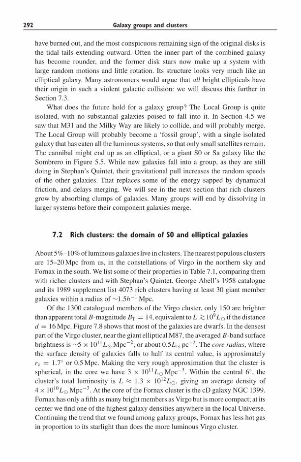
292 Galaxy groups and clusters

have burned out, and the most conspicuous remaining sign of the original disks isthe tidal tails extending outward. Often the inner part of the combined galaxyhas become rounder, and the former disk stars now make up a system withlarge random motions and little rotation. Its structure looks very much like anelliptical galaxy. Many astronomers would argue that all bright ellipticals havetheir origin in such a violent galactic collision: we will discuss this further inSection 7.3.

What does the future hold for a galaxy group? The Local Group is quiteisolated, with no substantial galaxies poised to fall into it. In Section 4.5 wesaw that M31 and the Milky Way are likely to collide, and will probably merge.The Local Group will probably become a ‘fossil group’, with a single isolatedgalaxy that has eaten all the luminous systems, so that only small satellites remain.The cannibal might end up as an elliptical, or a giant S0 or Sa galaxy like theSombrero in Figure 5.5. While new galaxies fall into a group, as they are stilldoing in Stephan’s Quintet, their gravitational pull increases the random speedsof the other galaxies. That replaces some of the energy sapped by dynamicalfriction, and delays merging. We will see in the next section that rich clustersgrow by absorbing clumps of galaxies. Many groups will end by dissolving inlarger systems before their component galaxies merge.

7.2 Rich clusters: the domain of S0 and elliptical galaxies

About 5%–10% of luminous galaxies live in clusters. The nearest populous clustersare 15–20 Mpc from us, in the constellations of Virgo in the northern sky andFornax in the south. We list some of their properties in Table 7.1, comparing themwith richer clusters and with Stephan’s Quintet. George Abell’s 1958 catalogueand its 1989 supplement list 4073 rich clusters having at least 30 giant membergalaxies within a radius of ∼1.5h−1 Mpc.

Of the 1300 catalogued members of the Virgo cluster, only 150 are brighterthan apparent total B-magnitude BT = 14, equivalent to L ∼>109L� if the distanced = 16 Mpc. Figure 7.8 shows that most of the galaxies are dwarfs. In the densestpart of the Virgo cluster, near the giant elliptical M87, the averaged B-band surfacebrightness is ∼5 × 1011L� Mpc−2, or about 0.5L� pc−2. The core radius, wherethe surface density of galaxies falls to half its central value, is approximatelyrc = 1.7◦ or 0.5 Mpc. Making the very rough approximation that the cluster isspherical, in the core we have 3 × 1011L� Mpc−3. Within the central 6◦, thecluster’s total luminosity is L ≈ 1.3 × 1012L�, giving an average density of4×1010L� Mpc−3. At the core of the Fornax cluster is the cD galaxy NGC 1399.Fornax has only a fifth as many bright members as Virgo but is more compact; at itscenter we find one of the highest galaxy densities anywhere in the local Universe.Continuing the trend that we found among galaxy groups, Fornax has less hot gasin proportion to its starlight than does the more luminous Virgo cluster.

7.2 Rich clusters: the domain of S0 and elliptical galaxies 293

Table 7.1 Nearby galaxy clusters, compared with a distant cluster and a nearby group

Coma Perseus RDCS Stephan’sVirgo Fornax A1656 A426 1252.9–2927 Quintet

Distance (Mpc) 16 20 100 80 a z = 1.24 85Number of galaxies >109 L� 150 30 450 350 120 4B-band starlight L B (1010 L�) 130 20 500 300 b300 7Velocity dispersion σr (km s−1) 700–800 350 ∼1000 1300→600 800 350Core rc (kpc) 400 200 200 250 100 25

X-ray LX (1010 L�) 1.3 0.03 25 50 20 0.005Temperature TX (107 K) 2 1–2 9 7 7 0.6cHot gas MX (1010M�) 2 000 ∼>60 7 000 7 000 2 000 ∼>0.07cMass M (1010M�) 20 000 5 000 40 000 50 000 20 000 100

M/L B 150 250 80 180 b ∼200 14M/MX 10 80 6 7 10 >1000

a At z = 1.24 the benchmark cosmology gives dL = 8.5 Gpc, dA = 1.7 Gpc.b Luminosity in the z band at 9000 A. c Mass within 1 Mpc of the cluster’s center.X-ray telescopes are less sensitive to gas with TX ∼< 107 K, so masses MX may be underestimated.

100

75

50

25

0

N

−23 −21 −19 −17 −15MB

Irr dIrr

spirals

S0E

dE dS0

dSph

Fig. 7.8. The Virgo cluster: numbers of galaxies of various types between absolute magni-

tude MB and MB +1. The luminosity function �(L) depends on galaxy type; the Schechter

function of Equation 1.24 is only an average. Here, most bright galaxies with MB ∼<−20

are spirals; there are many faint ellipticals and even fainter dwarf galaxies. The heavy

solid curve shows the total – H. Jerjen.

Problem 7.7 Use the result of Problem 6.3 for NGC 1399’s central surface

brightness, and assume that all this light comes from the core of radius rc = 2′′

or 650 pc, to find the core luminosity density. Show that the luminosity density at

the center of the Virgo cluster is 2500 times greater than average for the Universe

as a whole (see Equation 1.25), but the core of NGC 1399 is 107 times denser

yet. Stars are packed far more tightly into galaxies than galaxies are packed into

clusters.

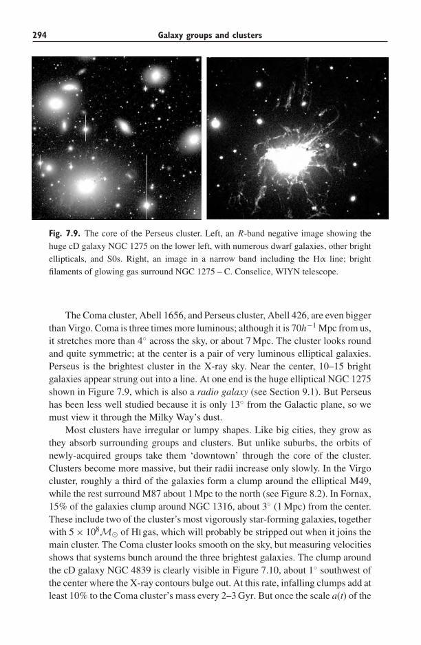
294 Galaxy groups and clusters

Fig. 7.9. The core of the Perseus cluster. Left, an R-band negative image showing the

huge cD galaxy NGC 1275 on the lower left, with numerous dwarf galaxies, other bright

ellipticals, and S0s. Right, an image in a narrow band including the Hα line; bright

filaments of glowing gas surround NGC 1275 – C. Conselice, WIYN telescope.

The Coma cluster, Abell 1656, and Perseus cluster, Abell 426, are even biggerthan Virgo. Coma is three times more luminous; although it is 70h−1 Mpc from us,it stretches more than 4◦ across the sky, or about 7 Mpc. The cluster looks roundand quite symmetric; at the center is a pair of very luminous elliptical galaxies.Perseus is the brightest cluster in the X-ray sky. Near the center, 10–15 brightgalaxies appear strung out into a line. At one end is the huge elliptical NGC 1275shown in Figure 7.9, which is also a radio galaxy (see Section 9.1). But Perseushas been less well studied because it is only 13◦ from the Galactic plane, so wemust view it through the Milky Way’s dust.

Most clusters have irregular or lumpy shapes. Like big cities, they grow asthey absorb surrounding groups and clusters. But unlike suburbs, the orbits ofnewly-acquired groups take them ‘downtown’ through the core of the cluster.Clusters become more massive, but their radii increase only slowly. In the Virgocluster, roughly a third of the galaxies form a clump around the elliptical M49,while the rest surround M87 about 1 Mpc to the north (see Figure 8.2). In Fornax,15% of the galaxies clump around NGC 1316, about 3◦ (1 Mpc) from the center.These include two of the cluster’s most vigorously star-forming galaxies, togetherwith 5 × 108M� of HI gas, which will probably be stripped out when it joins themain cluster. The Coma cluster looks smooth on the sky, but measuring velocitiesshows that systems bunch around the three brightest galaxies. The clump aroundthe cD galaxy NGC 4839 is clearly visible in Figure 7.10, about 1◦ southwest ofthe center where the X-ray contours bulge out. At this rate, infalling clumps add atleast 10% to the Coma cluster’s mass every 2–3 Gyr. But once the scale a(t) of the

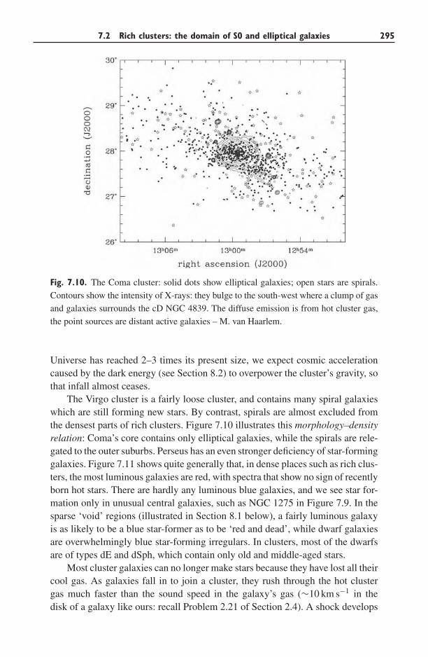
7.2 Rich clusters: the domain of S0 and elliptical galaxies 295

Fig. 7.10. The Coma cluster: solid dots show elliptical galaxies; open stars are spirals.

Contours show the intensity of X-rays: they bulge to the south-west where a clump of gas

and galaxies surrounds the cD NGC 4839. The diffuse emission is from hot cluster gas,

the point sources are distant active galaxies – M. van Haarlem.

Universe has reached 2–3 times its present size, we expect cosmic accelerationcaused by the dark energy (see Section 8.2) to overpower the cluster’s gravity, sothat infall almost ceases.

The Virgo cluster is a fairly loose cluster, and contains many spiral galaxieswhich are still forming new stars. By contrast, spirals are almost excluded fromthe densest parts of rich clusters. Figure 7.10 illustrates this morphology–densityrelation: Coma’s core contains only elliptical galaxies, while the spirals are rele-gated to the outer suburbs. Perseus has an even stronger deficiency of star-forminggalaxies. Figure 7.11 shows quite generally that, in dense places such as rich clus-ters, the most luminous galaxies are red, with spectra that show no sign of recentlyborn hot stars. There are hardly any luminous blue galaxies, and we see star for-mation only in unusual central galaxies, such as NGC 1275 in Figure 7.9. In thesparse ‘void’ regions (illustrated in Section 8.1 below), a fairly luminous galaxyis as likely to be a blue star-former as to be ‘red and dead’, while dwarf galaxiesare overwhelmingly blue star-forming irregulars. In clusters, most of the dwarfsare of types dE and dSph, which contain only old and middle-aged stars.

Most cluster galaxies can no longer make stars because they have lost all theircool gas. As galaxies fall in to join a cluster, they rush through the hot clustergas much faster than the sound speed in the galaxy’s gas (∼10 km s−1 in thedisk of a galaxy like ours: recall Problem 2.21 of Section 2.4). A shock develops

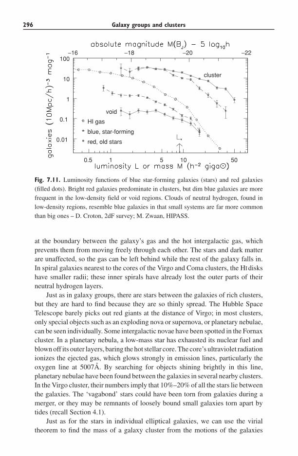
296 Galaxy groups and clusters

−16 −18 −20 −22

0.01

0.1

1

10

100

red, old stars

blue, star-forming

HI gas

cluster

void

0.5 1 5 10 50

Fig. 7.11. Luminosity functions of blue star-forming galaxies (stars) and red galaxies

(filled dots). Bright red galaxies predominate in clusters, but dim blue galaxies are more

frequent in the low-density field or void regions. Clouds of neutral hydrogen, found in

low-density regions, resemble blue galaxies in that small systems are far more common

than big ones – D. Croton, 2dF survey; M. Zwaan, HIPASS.

at the boundary between the galaxy’s gas and the hot intergalactic gas, whichprevents them from moving freely through each other. The stars and dark matterare unaffected, so the gas can be left behind while the rest of the galaxy falls in.In spiral galaxies nearest to the cores of the Virgo and Coma clusters, the HI diskshave smaller radii; these inner spirals have already lost the outer parts of theirneutral hydrogen layers.

Just as in galaxy groups, there are stars between the galaxies of rich clusters,but they are hard to find because they are so thinly spread. The Hubble SpaceTelescope barely picks out red giants at the distance of Virgo; in most clusters,only special objects such as an exploding nova or supernova, or planetary nebulae,can be seen individually. Some intergalactic novae have been spotted in the Fornaxcluster. In a planetary nebula, a low-mass star has exhausted its nuclear fuel andblown off its outer layers, baring the hot stellar core. The core’s ultraviolet radiationionizes the ejected gas, which glows strongly in emission lines, particularly theoxygen line at 5007A. By searching for objects shining brightly in this line,planetary nebulae have been found between the galaxies in several nearby clusters.In the Virgo cluster, their numbers imply that 10%–20% of all the stars lie betweenthe galaxies. The ‘vagabond’ stars could have been torn from galaxies during amerger, or they may be remnants of loosely bound small galaxies torn apart bytides (recall Section 4.1).

Just as for the stars in individual elliptical galaxies, we can use the virialtheorem to find the mass of a galaxy cluster from the motions of the galaxies

7.2 Rich clusters: the domain of S0 and elliptical galaxies 297

within it. The rate at which the spiral galaxies in the outskirts of the Virgocluster fall in toward the center depends on the mass at smaller radii: we inferM ≈ 2 × 1014M�, so the mass-to-light ratio M/L ∼ 150M�/L�. The massis only approximate, because the clusters are neither spherical nor in dynamicalequilibrium.

Problem 7.8 In the Coma cluster, the core radius measured from the galaxy den-

sity is rc = 200 kpc from Table 7.1. Make a crude model by assuming the cluster

to be a Plummer sphere; from Problem 3.2, show that aP ≈ 300 kpc. Taking the

average velocity dispersion σr from Table 7.1, use the result of Problem 3.11 and

follow the method of Problem 3.13 to show that M∼ 7 × 1014M�, implying

M/L ∼150M�/L�.

As for groups, we can use Equation 7.4 to find the cluster masses fromobservations of hot gas. In the Virgo cluster, this yields M ∼ 3 × 1014M�within 6◦ or 1.7 Mpc of the cluster’s center. It is more than we found from themotions of the galaxies, because the gas can be traced to larger radii. A recentstudy of 32 clusters using this method found that the mass-to-light ratio mostlylies in the range 180 ∼<M/L ∼< 300. These ratios are much greater than therange 5h ∼<M/L ∼< 25h that we found for individual spiral galaxies in Sec-tion 5.3, or for ellipticals in Problems 6.6 and 6.14. Like the hot gas (see below),most of a cluster’s dark matter must lie between the galaxies rather than withinthem.

7.2.1 Hot gas in clusters of galaxies

Galaxy clusters do not really deserve their name: they are huge accumulations ofX-ray-luminous hot gas, cohabiting with a few galaxies. The mass of hot gas isroughly equal to that in stars in a poorer cluster like Fornax; it rises to a ratio of10 : 1 in the richest systems like Coma. Table 7.1 shows that the largest clustershave been least efficient at turning their gas into stars. By contrast with groupslike Stephan’s Quintet, there is so much hot gas in rich clusters that it cannot allhave been stripped from the galaxies. The hot gas fills the whole cluster, and canoften be traced to larger radii than can the stellar light.

Figure 7.12 shows that the most luminous clusters contain the hottest gas, withtemperatures of up to 108 K. As in groups, the cluster gas is roughly at the virialtemperature predicted from the velocity dispersion σr of the galaxies. Because newclumps of galaxies are continually added to a cluster, both its X-ray luminosity andthe virial temperature should grow over time. Models predict that the temperatureincreases faster, so that a cluster with a particular luminosity should be cooler atearlier times. But we see no sign of this effect in Figure 7.12, even for clustersat z ∼ 1 when the Universe was half its present age. Perhaps winds from earlystarburst galaxies and active nuclei also added energy to the gas.

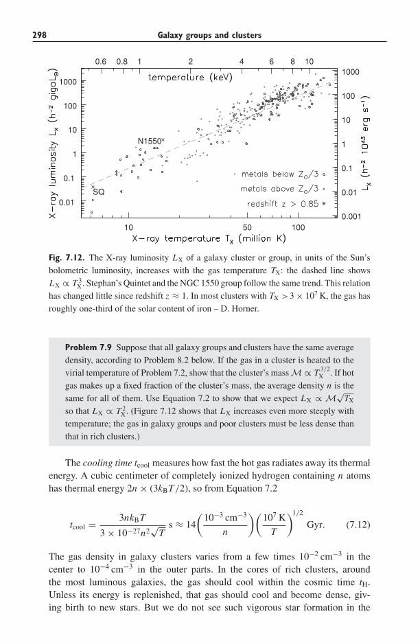
298 Galaxy groups and clusters

0.6 0.8 1 2 4 6 8 10

0.001

0.01

0.1

1

10

100

1000

10 50 100

0.01

0.1

1

10

100

1000

SQ

N1550

Fig. 7.12. The X-ray luminosity LX of a galaxy cluster or group, in units of the Sun’s

bolometric luminosity, increases with the gas temperature TX: the dashed line shows

LX ∝ T 3X. Stephan’s Quintet and the NGC 1550 group follow the same trend. This relation

has changed little since redshift z ≈ 1. In most clusters with TX >3 × 107 K, the gas has

roughly one-third of the solar content of iron – D. Horner.

Problem 7.9 Suppose that all galaxy groups and clusters have the same average

density, according to Problem 8.2 below. If the gas in a cluster is heated to the

virial temperature of Problem 7.2, show that the cluster’s mass M ∝ T 3/2X . If hot

gas makes up a fixed fraction of the cluster’s mass, the average density n is the

same for all of them. Use Equation 7.2 to show that we expect LX ∝ M√

TX

so that LX ∝ T 2X. (Figure 7.12 shows that LX increases even more steeply with

temperature; the gas in galaxy groups and poor clusters must be less dense than

that in rich clusters.)

The cooling time tcool measures how fast the hot gas radiates away its thermalenergy. A cubic centimeter of completely ionized hydrogen containing n atomshas thermal energy 2n × (3kBT/2), so from Equation 7.2

tcool = 3nkBT

3 × 10−27n2√

Ts ≈ 14

(10−3 cm−3

n

)(107 K

T

)1/2

Gyr. (7.12)

The gas density in galaxy clusters varies from a few times 10−2 cm−3 in thecenter to 10−4 cm−3 in the outer parts. In the cores of rich clusters, aroundthe most luminous galaxies, the gas should cool within the cosmic time tH.Unless its energy is replenished, that gas should cool and become dense, giv-ing birth to new stars. But we do not see such vigorous star formation in the

7.2 Rich clusters: the domain of S0 and elliptical galaxies 299

central galaxy. So we believe that the gas is reheated, perhaps by hot windsfrom supernovae, or the outflows from radio sources that we will discuss inSection 9.1. Gas in the outskirts will remain hot for >10 Gyr, so it cannot formstars.

Problem 7.10 Around NGC 1399 at the center of the Fornax cluster, the X-ray

emission from hot gas extends out to radii of 100 kpc. The gas temperature TX ≈1.5×107 K; within 45′′ or 5 kpc of the center, the density nH ≈ 0.02 cm−3, falling

approximately as nH ∝ r−1. Show that tcool ≈ 0.5 Gyr in the core, increasing to

10 Gyr at r = 100 kpc.

Galaxy clusters often appear lumpier in an X-ray image than at optical wave-lengths. On the lower right of Figure 7.10, we see X-rays from the clump aroundthe galaxy NGC 4839 in the Coma cluster. Here, the gas is only half as hot as themain cluster. At the ‘neck’ in the X-ray contours, temperatures roughly double to108 K where the clump gas meets the main cluster. In the Perseus cluster, we seelow-density ‘bubbles’ in the central X-ray gas, which probably were blown byenergetic outflows from the radio galaxy NGC 1275. Most galaxy clusters todayare still growing; even their centers are not always near equilibrium, since theyare disturbed as newly-added galaxies fall through them.

The hot cluster gas contains iron and other heavy elements in roughly one-thirdof the solar proportion: see Figure 7.12. Gas near the center is more metal-rich;neither infalling clumps of galaxies nor the outflows from active galaxies havebeen able to mix it with the rest of the cluster gas. Although these heavy elementsmust have been ‘cooked’ by nuclear burning in stars, most of a cluster’s supplyof metals is now in the hot gas. Perhaps they were made in galactic stars, and theforce of supernova explosions carried metal-bearing material out into the cluster.Or perhaps many early stars formed in smaller clumps which later fell together tomake galaxies, releasing metal-enriched gas as they merged. However, the starsof the galaxies themselves are as metal-rich as the Milky Way. So, if the metalswere made inside the galaxies, these systems must have been very efficient atproducing heavy elements.

The hot gas itself accounts for roughly a tenth of the mass of a luminous cluster,but much less in systems with TX < (2–3) × 107 K. If we take M/L B = 4–8for the stars of the galaxies, then stars and hot gas together make up roughly asixth of the cluster’s mass. This is close to the cosmic average for the benchmarkcosmology of Section 1.5, so galaxy clusters appear to be a ‘fair sample’ of the mixof dark and luminous material. By contrast, baryons are more concentrated intogalaxies: recall from Problem 2.18 that at most half the mass inside the Sun’s orbitaround the Milky Way can be dark. In galaxy groups, we find too little luminousgas and stars for the amount of dark matter. Some baryons may have been lost,blown out during episodes of violent star formation; others may be hidden as verydilute gas between the galaxies.

300 Galaxy groups and clusters

Table 7.2 The cosmic baryon budget

Where it is Density (10−3ρcrit)

Total (benchmark cosmology) 45Intergalactic gas

Diffuse and ionized ≈40Damped Lyman-α clouds 1

Hot gas in clusters and Es 1.8Stars and stellar remnants

Stars in Es and bulges 1.5Stars in disks 0.55Dead stars 0.48Brown dwarfs 0.14

Cool gas in galaxies 0.78

We can find only 10% of the baryons, which make up ∼< 15% ofthe matter, which is ∼<30% of the critical density – M. Fukugita andP. J. E. Peebles 2004 ApJ 616, 643.

7.2.2 Where have all the baryons gone?

Throughout this book, we have seen that the stars and gas within galaxies formonly a fraction of their mass. Table 7.2 shows that luminous and dead stars,together with the cool gas in galaxy disks, make up only (3–4) × 10−3ρcrit. ButEquation 1.40 tells us that baryons (neutrons and protons) in the Universe accountfor a fraction �B of the critical density, where 0.03 ∼< �B ∼< 0.07. The stars andthe cool gas together contribute only 10% of this total. Where is the rest?

The hot X-ray-emitting gas in clusters of galaxies holds nearly as much mass asall the stars. In groups, there is cool gas between the galaxies: recall the HIstream-ers of the M81 group, in Figure 7.2. The amount of ionized gas that they mightaccomodate is unknown; but it could be large, since galaxy groups are more numer-ous than rich clusters. If gas is heated close to the virial temperature of Figure 7.3as the group forms, then Equation 7.12 shows that, if n < 10−3 cm−2, its low den-sity will prevent it from cooling. It would remain ionized up to the present; sinceit does not absorb in the Lyman-α line, it would be almost impossible to detect.

In Section 9.3 we will discuss the intergalactic gas, which we can investigatethrough the absorption lines it produces in the spectra of distant objects. Thedensest gas is in the damped Lyman-α clouds, which are mainly neutral and atomic,and contain more cool gas than there is in today’s galaxies. But they leave us farfrom balancing the account. Most of the baryons are likely to be in the Lyman-αforest, the most diffuse gas, in which hydrogen is almost completely ionized.

7.3 Galaxy formation: nature, nurture, or merger?

Clusters are not simply places where galaxies are more densely packed: clus-ter galaxies themselves are different. Figure 7.11 shows that the largest red

7.3 Galaxy formation: nature, nurture, or merger? 301

galaxies, the ellipticals and cD galaxies, live in dense regions of rich clusters,while starforming spirals and irregulars inhabit less crowded regions. This segre-gation is puzzling, because the stars of elliptical galaxies may be almost as oldas the Universe, while we will see in Section 8.1 that galaxy clusters are stillcoming together today. As a galaxy forms, how can it know whether it will end up‘downtown’ in the cluster core, or as a spiral in the suburbs? We do not understandthis process yet, and have only some hints.

In Section 4.3 we took a brief look at the origin of galaxies. Early in cosmichistory, dark matter was evenly spread, mixed with baryons in the form of hotgas. In slightly denser regions, clumps of matter were pulled together under theirown gravity. The larger clumps absorbed smaller ones that fell into them, muchas we see in galaxy clusters today. As clumps collided, their gas was compressedand heated. If it was dense enough to cool, the gas lost energy and fell inward.The particles of dark matter could not lose energy, so the central parts of a galaxyconsist mainly of cool gas and luminous stars. Where the heated gas was toodiffuse it did not cool, and its pressure prevented it from flowing inward.

Perhaps elliptical galaxies are not as old as their stars. We know that somenearby ellipticals have recently eaten other galaxies. They show faint shells andother asymmetries in the outer parts (Section 6.1); stars in the core rotate differentlyfrom those in the main galaxy (Section 6.2); cold gas orbits at seemingly randominclination (Section 6.3). We will see in Section 9.4 that 5%–10% of fairly brightgalaxies at z ∼ 1 appear to be in the throes of a major merger. At this rate,between one and two thirds of today’s fairly luminous galaxies (with L ∼> 0.4L)underwent a major merger within the past 5 Gyr. Did all elliptical galaxies formby merger of smaller galaxies, so that their stars were born before the galaxy hadcompletely assembled? If so, we could understand why they live in rich clusters,which grow by adding smaller clumps of galaxies. The clumps are excellent sitesfor mergers because their galaxies have fairly low random speeds, as we discussedin Section 7.1.

What should a merger remnant look like, long after the initial disturbance andsubsequent vigorous starbirth? That depends on whether the colliding systemscontained gas, or only stars and dark matter. When two galaxies of about the samesize merge, their stellar disks are destroyed. When cool gas is present, a disk wherenew stars will be born can be rebuilt. Without cool gas, no new stars can form; theremnant will have only old and middle-aged stars. For these, the virial theoremmakes a strong prediction: the merged system should become less dense.

Problem 7.11 Suppose that a galaxy is made from N identical fragments, each

of mass M and size R. In each one, the average separation between any two stars

(or particles of dark matter) is R/2; so the potential energy PE ≈ −GM2/R,

as in Equation 3.56. Use Equation 3.44 to show that each fragment has energy

PE/2, so that, while they are well separated and moving toward each other only

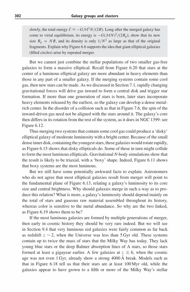
302 Galaxy groups and clusters

slowly, the total energy E ≈ −GM2 N/(2R). Long after the merged galaxy has

come to virial equilibrium, its energy is −G(MN )2/(2Rg); show that its new

size Rg = N R, and its density is only 1/N 2 as large as that of the original

fragments. Explain why Figure 6.6 supports the idea that giant elliptical galaxies

(filled circles) arise by repeated merger.

But we cannot just combine the stellar populations of two smaller gas-freegalaxies to form a massive elliptical. Recall from Figure 6.20 that stars at thecenter of a luminous elliptical galaxy are more abundant in heavy elements thanthose in any part of a smaller galaxy. If the merging systems contain some coolgas, then new stars can be made. As we discussed in Section 7.1, rapidly changinggravitational forces will drive gas inward to form a central disk and trigger starformation. If more than one generation of stars is born, later stars incorporateheavy elements released by the earliest, so the galaxy can develop a dense metal-rich center. In the disorder of a collision such as that in Figure 7.6, the spin of theinward-driven gas need not be aligned with the stars around it. The galaxy’s corethen differs in its rotation from the rest of the system, as it does in NGC 1399: seeFigure 6.12.

Thus merging two systems that contain some cool gas could produce a ‘disky’elliptical galaxy of moderate luminosity with a bright center. Because of the smalldense inner disk, containing the youngest stars, these galaxies would rotate rapidly,as Figure 6.15 shows that disky ellipticals do. Some of these in turn might collideto form the most luminous ellipticals. Gravitational N-body simulations show thatthe result is likely to be triaxial, with a ‘boxy’ shape. Indeed, Figure 6.11 showsthat boxy systems are the most luminous.

But we still have some potentially awkward facts to explain. Astronomerswho do not agree that most elliptical galaxies result from merger will point tothe fundamental plane of Figure 6.13, relating a galaxy’s luminosity to its coresize and central brightness. Why should galaxies merge in such a way as to pro-duce this relation? What is more, a galaxy’s luminosity should depend mainly onthe total of stars and gaseous raw material assembled throughout its history,whereas color is sensitive to the metal abundance. So why are the two linked,as Figure 6.19 shows them to be?

If the most luminous galaxies are formed by multiple generations of merger,then early in cosmic history they should be very rare indeed. But we will seein Section 9.4 that very luminous red galaxies were fairly common as far backas redshift z ∼ 2, when the Universe was less than 5 Gyr old. These systemscontain up to twice the mass of stars that the Milky Way has today. They lackyoung blue stars or the deep Balmer absorption lines of A stars, so those starsformed at least a gigayear earlier. A few galaxies at z ∼> 6, when the cosmicage was not even 1 Gyr, already show a strong 4000 A break. Models such asthat in Figure 6.18 tell us that their stars are at least 100 Myr old, while thegalaxies appear to have grown to a fifth or more of the Milky Way’s stellar

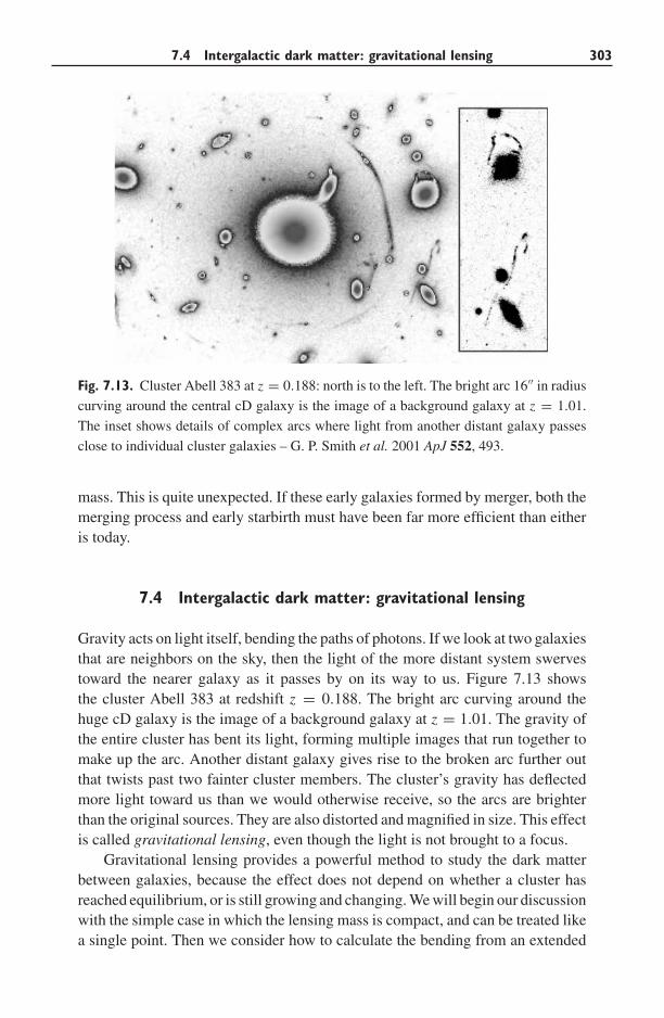
7.4 Intergalactic dark matter: gravitational lensing 303

Fig. 7.13. Cluster Abell 383 at z = 0.188: north is to the left. The bright arc 16′′ in radius

curving around the central cD galaxy is the image of a background galaxy at z = 1.01.

The inset shows details of complex arcs where light from another distant galaxy passes

close to individual cluster galaxies – G. P. Smith et al. 2001 ApJ 552, 493.

mass. This is quite unexpected. If these early galaxies formed by merger, both themerging process and early starbirth must have been far more efficient than eitheris today.

7.4 Intergalactic dark matter: gravitational lensing

Gravity acts on light itself, bending the paths of photons. If we look at two galaxiesthat are neighbors on the sky, then the light of the more distant system swervestoward the nearer galaxy as it passes by on its way to us. Figure 7.13 showsthe cluster Abell 383 at redshift z = 0.188. The bright arc curving around thehuge cD galaxy is the image of a background galaxy at z = 1.01. The gravity ofthe entire cluster has bent its light, forming multiple images that run together tomake up the arc. Another distant galaxy gives rise to the broken arc further outthat twists past two fainter cluster members. The cluster’s gravity has deflectedmore light toward us than we would otherwise receive, so the arcs are brighterthan the original sources. They are also distorted and magnified in size. This effectis called gravitational lensing, even though the light is not brought to a focus.

Gravitational lensing provides a powerful method to study the dark matterbetween galaxies, because the effect does not depend on whether a cluster hasreached equilibrium, or is still growing and changing. We will begin our discussionwith the simple case in which the lensing mass is compact, and can be treated likea single point. Then we consider how to calculate the bending from an extended

304 Galaxy groups and clusters

L

d LS

S′L′

O

α

θβy

S

Sd

d

imageplane

x

I

b

Lens

Fig. 7.14. The gravity of the mass M at L bends light from a distant source at S′ toward

the observer at O; the source appears instead at position I.

‘lens’ such as a galaxy or cluster. Lensing allows us to study distant objects thatwould otherwise be far too faint. Some of the best-studied galaxies at high redshift,such as cB58 in Figure 9.16, are strongly brightened in this way. But we mustbeware of lensing when taking a census of any type of distant object.

7.4.1 Microlensing: light bent by a compact object

The Sun’s bending of light provided one of the first tests of Einstein’s GeneralRelativity. During the total solar eclipse of 1919, an expedition led by ArthurEddington took photographs of the sky around the obscured Sun. They foundthat light was bent as shown in Figure 7.14, so that nearby stars appeared to havemoved very slightly away from the calculated position of the Sun’s center. Einsteinpredicted that light passing at distance b from a mass M is bent by an angle α

given by

α ≈ 4GMbc2

= 2Rs

b. (7.13)

Here Rs is the Schwarzschild radius 2GM/c2, about 3 km for an object of theSun’s mass. The approximation holds as long as the bending is small, with α � 1.This formula prescribes exactly twice the bending that we get by applying Equa-tion 3.51 to particles travelling at speed c.

Using this formula, we can calculate where the image of a distant source willappear, if a point object of mass M is placed in front of it to act as a gravitationallens. If the lens L in Figure 7.14 had been absent, we would have seen the star S′

at an angle β on the sky from the direction to L; β ≈ y/dS if the distance dS � y.Because the light is bent by an amount α, the star appears instead at an angle θ to

7.4 Intergalactic dark matter: gravitational lensing 305

that direction; θ ≈ x/dS if dS � x . If x is the distance between the line OL and I,the star’s apparent position in the image plane, then Figure 7.14 shows that, whenbending is small, x − y = αdLS. Finally, the impact parameter b = θdLens as longas dS � b. Using Equation 7.13 for α, we divide by dS to find

θ − β = αdLS

dS= 1

θ

4GMc2

dLS

dLensdS≡ 1

θθ2

E; (7.14)

the angle θE is called the Einstein radius. We have a quadratic equation for theangular distance θ between L and the star’s image:

θ2 − βθ − θ2E = 0, so θ± =

β ±√

β2 + 4θ2E

2. (7.15)

A star exactly behind the lens, with β = 0, will be seen as a circle of light on thesky, with radius θE. When β > 0, the image at θ+ is further from the lens, withθ+ > β, and it lies outside the Einstein radius: θ+ > θE. These exterior imageswere the ones seen around the eclipsed Sun. The image at θ− is inverted; it lieswithin the Einstein radius, on the opposite side of the lens.

Problem 7.12 Show that, when dLens = 1 AU � dS, then θ − β ≈ α. When

light from a distant star S is bent by the Sun’s gravity, show that the Einstein

radius θE ≈ 40′′. The Sun’s disk has a diameter of 30′ or 0.5◦; show that starlight

that just grazes the Sun’s surface would be bent by about 2′′, making the star

appear further from the Sun’s center.

Quite regularly, one star in the Milky Way’s bulge is gravitationally lensedby another in the disk. The images θ+ and θ− are then too close to distinguishindividually. But we can tell that a star is lensed because it appears to becomebrighter (see below). Because of the small size of the Einstein ring, gravitationallensing by compact objects in the halo of a galaxy is often called microlensing.

Problem 7.13 If the lens L is an object of mass M� at distance dLens from us,

show that the Einstein radius for a star at distance dS = 2dLens is

θE =√

Rs

dLens≈ 2 × 10−3

√1 kpc

dLensarcsec. (7.16)

If our point-mass lens is in front of a small extended patch of brightness, itsimage will be two patches around θ±. Gravitational lensing leaves the surfacebrightness I (x) unchanged, so the apparent brightness of each image of a sourceis just proportional to its area. Consider a region S′ that is a segment of an annulus

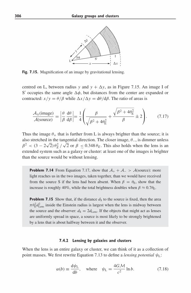
306 Galaxy groups and clusters

LS'

I

x

y

Δy

Δφ

Δx

Fig. 7.15. Magnification of an image by gravitational lensing.

centred on L, between radius y and y + �y, as in Figure 7.15. An image I ofS′ occupies the same angle �φ, but distances from the center are expanded orcontracted: x/y = θ/β while �x/�y = dθ/dβ. The ratio of areas is

A±(image)

A(source)=∣∣∣∣ θβ dθ

dβ

∣∣∣∣= 1

4

⎛⎝ β√

β2 + 4θ2E

+√

β2 + 4θ2E

β± 2

⎞⎠. (7.17)

Thus the image θ+ that is further from L is always brighter than the source; it isalso stretched in the tangential direction. The closer image, θ−, is dimmer unlessβ2 < (3 − 2

√2) θ2

E /√

2 or β <∼ 0.348 θE . This also holds when the lens is anextended system such as a galaxy or cluster: at least one of the images is brighterthan the source would be without lensing.

Problem 7.14 From Equation 7.17, show that A+ + A− > A(source): more

light reaches us in the two images, taken together, than we would have received

from the source S if the lens had been absent. When β = θE, show that the

increase is roughly 40%, while the total brightness doubles when β ≈ 0.7θE.

Problem 7.15 Show that, if the distance dS to the source is fixed, then the area

πθ2Ed2

Lens inside the Einstein radius is largest when the lens is midway between

the source and the observer: dS = 2dLens. If the objects that might act as lenses

are uniformly spread in space, a source is most likely to be strongly brightened

by a lens that is about halfway between it and the observer.

7.4.2 Lensing by galaxies and clusters

When the lens is an entire galaxy or cluster, we can think of it as a collection ofpoint masses. We first rewrite Equation 7.13 to define a lensing potential ψL:

α(b) ≡ dψL

db, where ψL = 4GM

c2ln b. (7.18)

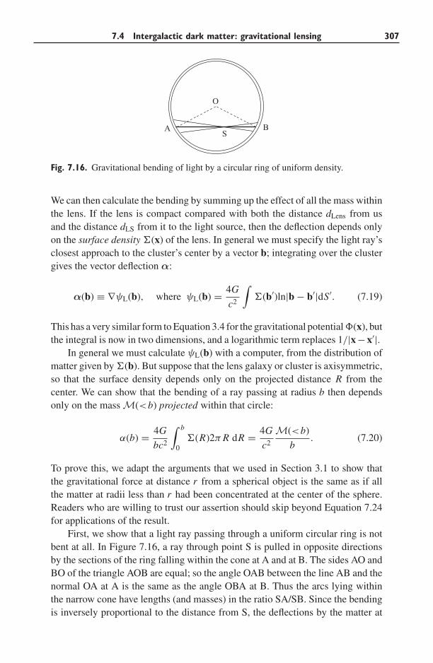
7.4 Intergalactic dark matter: gravitational lensing 307

O

A BS

Fig. 7.16. Gravitational bending of light by a circular ring of uniform density.

We can then calculate the bending by summing up the effect of all the mass withinthe lens. If the lens is compact compared with both the distance dLens from usand the distance dLS from it to the light source, then the deflection depends onlyon the surface density �(x) of the lens. In general we must specify the light ray’sclosest approach to the cluster’s center by a vector b; integrating over the clustergives the vector deflection α:

α(b) ≡ ∇ψL(b), where ψL(b) = 4G

c2

∫�(b′)ln|b − b′|dS′. (7.19)

This has a very similar form to Equation 3.4 for the gravitational potential �(x), butthe integral is now in two dimensions, and a logarithmic term replaces 1/|x − x′|.

In general we must calculate ψL(b) with a computer, from the distribution ofmatter given by �(b). But suppose that the lens galaxy or cluster is axisymmetric,so that the surface density depends only on the projected distance R from thecenter. We can show that the bending of a ray passing at radius b then dependsonly on the mass M(<b) projected within that circle:

α(b) = 4G

bc2

∫ b

0�(R)2π R dR = 4G

c2

M(<b)

b. (7.20)

To prove this, we adapt the arguments that we used in Section 3.1 to show thatthe gravitational force at distance r from a spherical object is the same as if allthe matter at radii less than r had been concentrated at the center of the sphere.Readers who are willing to trust our assertion should skip beyond Equation 7.24for applications of the result.

First, we show that a light ray passing through a uniform circular ring is notbent at all. In Figure 7.16, a ray through point S is pulled in opposite directionsby the sections of the ring falling within the cone at A and at B. The sides AO andBO of the triangle AOB are equal; so the angle OAB between the line AB and thenormal OA at A is the same as the angle OBA at B. Thus the arcs lying withinthe narrow cone have lengths (and masses) in the ratio SA/SB. Since the bendingis inversely proportional to the distance from S, the deflections by the matter at

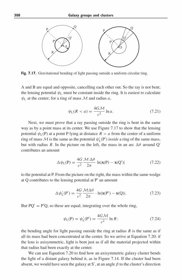
308 Galaxy groups and clusters

a

PQ

P'Q'

PQ

P'

R R

Q'

O

Fig. 7.17. Gravitational bending of light passing outside a uniform circular ring.

A and B are equal and opposite, cancelling each other out. So the ray is not bent;the lensing potential ψL must be constant inside the ring. It is easiest to calculateψL at the center; for a ring of mass M and radius a,

ψL(R < a) = 4GMc2

ln a. (7.21)

Next, we must prove that a ray passing outside the ring is bent in the sameway as by a point mass at its center. We use Figure 7.17 to show that the lensingpotential ψL(P) at a point P lying at distance R > a from the center of a uniformring of mass M is the same as the potential ψ ′

L(P′) inside a ring of the same mass,but with radius R. In the picture on the left, the mass in an arc �θ around Q′

contributes an amount

�ψL(P) = 4G

c2

M�θ

2πln|x(P) − x(Q′)| (7.22)

to the potential at P. From the picture on the right, the mass within the same wedgeat Q contributes to the lensing potential at P′ an amount

�ψ ′L(P′) = 4G

c2

M�θ

2π· ln|x(P′) − x(Q)|. (7.23)

But PQ′ = P′Q, so these are equal; integrating over the whole ring,

ψL(P) = ψ ′L(P′) = 4GM

c2ln R : (7.24)

the bending angle for light passing outside the ring at radius R is the same as ifall its mass had been concentrated at the center. So we arrive at Equation 7.20: ifthe lens is axisymmetric, light is bent just as if all the material projected withinthat radius had been exactly at the center.

We can use Equation 7.20 to find how an axisymmetric galaxy cluster bendsthe light of a distant galaxy behind it, as in Figure 7.14. If the cluster had beenabsent, we would have seen the galaxy at S′, at an angle β to the cluster’s direction

7.4 Intergalactic dark matter: gravitational lensing 309

OL. Instead, we see its image I at an angle θ to OL. Equation 7.14 is now modifiedto read

θ − β = α(θ)dLS

dS= 1

θ· 4GM(<b)

c2

dLS

dLensdS. (7.25)

Remembering that b = θdLens, we can rewrite this in terms of �crit, the criticaldensity for lensing:

β = θ

[1 − 1

�crit

M(<b)

πb2

], where �crit ≡ c2

4πG

dS

dLensdLS. (7.26)

The quantity M(<b)/(πb2) is just the average surface density within radius b;usually the surface density �(R) declines from a peak at the center, so this averagewill fall as well. If the central density exceeds �crit, then the image of a sourceat β = 0, exactly in line with the cluster’s center, will be a thin circular Einsteinring, of angular size θE = bE/dLens, where bE is the radius where the averagedensity falls to the critical value:

M(<bE)

πb2E

= �crit. (7.27)

If the central surface density is less than �crit, then the cluster cannot producemultiple images of any source behind it; no ring is seen.

Problem 7.16 Show that, when the lensing object is a point mass, Equa-

tions 7.27 and 7.14 give the same result for the Einstein radius θE.

Problem 7.17 If a lens at distance dLens bends the light of a much more distant

galaxy, so that dS and dLS � dLens, show that the critical density is

�crit ≈ 2 × 104

(100 Mpc

dLens

)M� pc−2, (7.28)

and that the mass projected within angle θE of the center is

M(< θE) ≈(

dLens

100 Mpc

)(θE

1′′

)2

1010M�. (7.29)

Use the results of Problems 6.3 and 6.6 to show that in the cD galaxy NGC 1399

we have roughly 6 × 104M� pc−2. At the center of the Virgo cluster we see

0.5L� pc−2, which for M/L ∼150 corresponds to <100M� pc−2. We expect

to see lensed arcs around individual luminous galaxies, but clusters with giant

arcs like Abell 383 are far more massive than Virgo, and often at dLens >

1 Gpc.

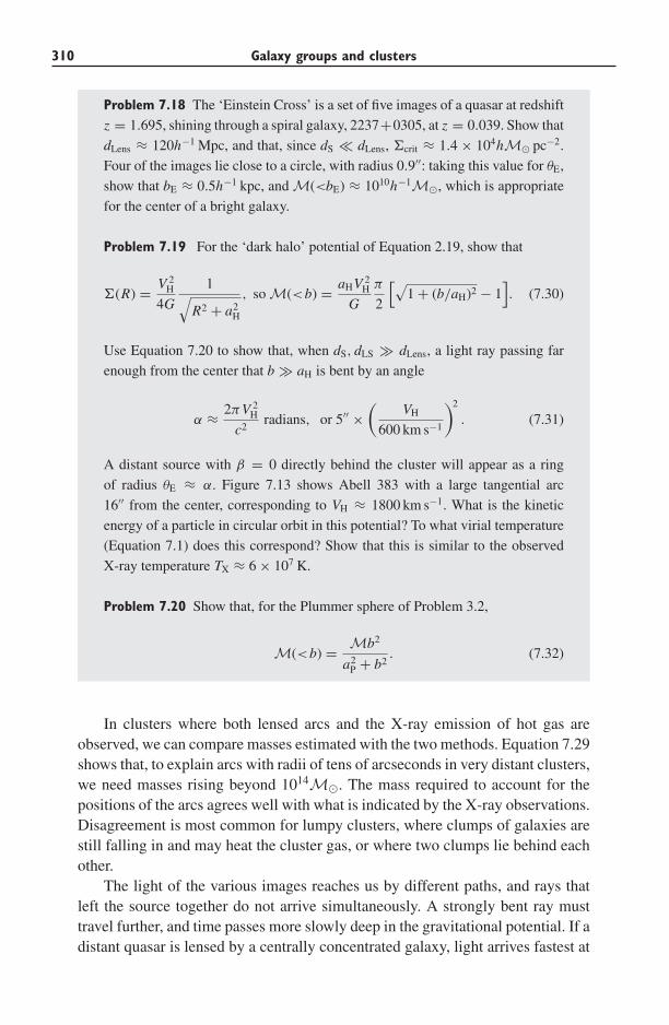
310 Galaxy groups and clusters

Problem 7.18 The ‘Einstein Cross’ is a set of five images of a quasar at redshift

z = 1.695, shining through a spiral galaxy, 2237+0305, at z = 0.039. Show that

dLens ≈ 120h−1 Mpc, and that, since dS � dLens, �crit ≈ 1.4 × 104hM� pc−2.

Four of the images lie close to a circle, with radius 0.9′′: taking this value for θE,

show that bE ≈ 0.5h−1 kpc, and M(<bE) ≈ 1010h−1M�, which is appropriate

for the center of a bright galaxy.

Problem 7.19 For the ‘dark halo’ potential of Equation 2.19, show that

�(R) = V 2H

4G

1√R2 + a2

H

, so M(<b) = aHV 2H

G

π

2

[√1 + (b/aH)2 − 1

]. (7.30)

Use Equation 7.20 to show that, when dS, dLS � dLens, a light ray passing far

enough from the center that b � aH is bent by an angle

α ≈ 2πV 2H

c2radians, or 5′′ ×

(VH

600 km s−1

)2

. (7.31)

A distant source with β = 0 directly behind the cluster will appear as a ring

of radius θE ≈ α. Figure 7.13 shows Abell 383 with a large tangential arc

16′′ from the center, corresponding to VH ≈ 1800 km s−1. What is the kinetic

energy of a particle in circular orbit in this potential? To what virial temperature

(Equation 7.1) does this correspond? Show that this is similar to the observed

X-ray temperature TX ≈ 6 × 107 K.

Problem 7.20 Show that, for the Plummer sphere of Problem 3.2,

M(<b) = Mb2

a2P + b2

. (7.32)

In clusters where both lensed arcs and the X-ray emission of hot gas areobserved, we can compare masses estimated with the two methods. Equation 7.29shows that, to explain arcs with radii of tens of arcseconds in very distant clusters,we need masses rising beyond 1014M�. The mass required to account for thepositions of the arcs agrees well with what is indicated by the X-ray observations.Disagreement is most common for lumpy clusters, where clumps of galaxies arestill falling in and may heat the cluster gas, or where two clumps lie behind eachother.

The light of the various images reaches us by different paths, and rays thatleft the source together do not arrive simultaneously. A strongly bent ray musttravel further, and time passes more slowly deep in the gravitational potential. If adistant quasar is lensed by a centrally concentrated galaxy, light arrives fastest at

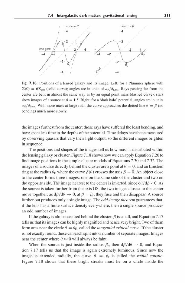
7.4 Intergalactic dark matter: gravitational lensing 311

−4 −22 44

2

4

−2

−4

−4 −22 44

2

4

−2

−4

Fig. 7.18. Positions of a lensed galaxy and its image. Left, for a Plummer sphere with

�(0) = 6�crit (solid curve); angles are in units of aP/dLens. Rays passing far from the

center are bent in almost the same way as by an equal point mass (dashed curve): stars

show images of a source at β = 1.5. Right, for a ‘dark halo’ potential; angles are in units

aH/dLens. With more mass at large radii the curve approaches the dotted line θ = β (no

bending) much more slowly.

the images furthest from the center: those rays have suffered the least bending, andhave spent less time in the depths of the potential. Time delays have been measuredby observing quasars that vary their light output, so the different images brightenin sequence.

The positions and shapes of the images tell us how mass is distributed withinthe lensing galaxy or cluster. Figure 7.18 shows how we can apply Equation 7.26 tofind image positions in the simple cluster models of Equations 7.30 and 7.32. Theimages of a source directly behind the cluster are a point at θ = 0, and an Einsteinring at the radius θE where the curve β(θ ) crosses the axis β = 0. An object closeto the center forms three images: one on the same side of the cluster and two onthe opposite side. The image nearest to the center is inverted, since dθ/dβ <0. Asthe source is taken further from the axis OS, the two images closest to the centermove together: as dβ/dθ → 0, at β = βr, they fuse and then disappear. A sourcefurther out produces only a single image. The odd-image theorem guarantees that,if the lens has a finite surface density everywhere, then a single source producesan odd number of images.

If the galaxy is almost centred behind the cluster, β is small, and Equation 7.17tells us that its images can be highly magnified and hence very bright. Two of themform arcs near the circle θ = θE, called the tangential critical curve. If the clusteris not exactly round, these can each split into a number of separate images. Imagesnear the center where θ ≈ 0 will always be faint.

When the source is just inside the radius βr, then dβ/dθ → 0, and Equa-tion 7.17 tells us that the image is again extremely luminous. Since now theimage is extended radially, the curve β = βr is called the radial caustic.Figure 7.18 shows that these bright streaks must lie on a circle inside the

312 Galaxy groups and clusters

Einstein radius, at θ = θr; this is called the radial critical curve. In the leftpanel, the cluster has the density of a Plummer sphere, and θE = √

5aP/dLens.The right panel shows critical points for a cluster with the potential of thedark halo of Equation 2.19. The Einstein radius θE is larger in relation toθr than for the Plummer model, because its mass is less concentrated to thecenter.

Problem 7.21 For the Plummer model, show that the surface density (Equa-

tion 3.13) drops to half its central value at the core radius rc = 0.644aP. What

is rc for the ‘dark halo’ potential of Problem 7.19? Taking the central density to

be 2�crit, 4�crit, and finally 10�crit, find the Einstein radius θE for the Plummer

model in units of rc/dLens. Now do the same for the dark halo. (For a wide range

of central density, and for many cluster-like potentials, dLensθE is a few times the

core radius.)

Problem 7.22 In the galaxy cluster Abell 383 of Figure 7.13, a radial arc

lies 2′′ ≈ θr from the center. The large tangential arc of Figure 7.13 is at

16′′ ≈ θE. Find dLens, assuming H0 = 70 km s−1 Mpc−1 (if you have read Sec-

tion 8.3: use the angular size distance dA and the benchmark cosmology). Show

that dLensθE ∼50 kpc; the cluster’s core radius rc will be a few times smaller.

From Equation 7.29, show that the mass projected within the tangential arc is

M(< θE) ∼ 2 × 1013M�. The luminosity within θE corresponds to LV ∼4 × 1011L�, so M/L ∼ 50. (A model placing both radial and tangential arcs

at the observed positions has rc ≈ 40 kpc; in the X-ray-emitting gas, the core is

twice as large.)

7.4.3 Weak gravitational lensing

When galaxies lie behind a cluster but well outside its Einstein radius, their imagesare weakly magnified and slightly stretched in the tangential direction. Figure 7.15shows why the image of a round galaxy will be an ellipse, with tangential andradial axes in the ratio x/y : �x/�y or |dβ/dθ | : |β/θ |. The shear γ measures thedifference in the amount that the image has been compressed in the two directions.For an image at distance b � θEdLens from the cluster’s center we have

γ ≡ 1

2

(dβ

dθ− β

θ

)= �(<b) − �(b)

�crit. (7.33)

Here �(<b) = M(<b)/(πb2) is the average surface density of matter projectedwithin radius b, and �(b) is the surface density at that radius.

7.4 Intergalactic dark matter: gravitational lensing 313

Problem 7.23 Derive Equation 7.33 from Equation 7.26. Why must we specify

θ � θE? Show that, if the surface density �(R) is constant, then we have

θ ∝ β. Use Figure 7.15 to explain why images of a round galaxy will be circular:

the shear is zero. This mass-sheet degeneracy means that we can always add a

uniform sheet of matter to our model cluster without changing the shapes of the

images.

Measuring the average shape of many galaxies in the background that havebeen weakly distorted allows us to estimate the shear, and hence the distributionof mass in the outer parts of galaxy clusters. Generally the results agree with whatwe found from the hot gas. But, for some clusters, weak lensing indicates a highermass. These may be composites, with one cluster behind the other. Some distantclusters have even been discovered by the signature of their weak lensing alone.

Weak lensing has also been used to study the halos of individual bright galax-ies. To do this, we measure the average shape of more distant galaxies that lie closeto the nearby lensing system on the sky, and then average these results over manylens-galaxies. Recent studies show that the dark halo of a typical bright elliptical orS0 galaxy, with L ∼ L, extends to at least 200 kpc and has mass ∼>1012h−1M�;so the mass-to-light ratio M/L > 50 in solar units. So dark halos are larger andmore massive than we were able to show by measuring rotation in the outer partsof disk galaxies. Blue galaxies that are still making stars are brighter for a givendark-halo mass. The halo appears to be slightly aspherical, distorted in the samesense as the galaxy’s stellar body.

Unlike galaxies themselves, groups and clusters do not separate cleanly fromone another: we will see in the next chapter how they are connected by walls andfilaments of luminous galaxies. Weak lensing lets us measure how the dark matteris distributed in this structure, but the calculation is more complex. The light ofa distant source is bent many times as it passes by each of these large structureson its way to us, so we cannot make the approximation of Equation 7.19, thatall the bending takes place at a single lens-distance dLens. Instead, we must usecomputers to calculate it.

Further reading: a detailed presentation of gravitational lensing is given by P.Schneider, J. Ehlers, and E. E. Falco, 1992, Gravitational Lenses (Springer, NewYork); this is an advanced text. A popular book is N. Cohen, 1989, Gravity’s Lens:Views of the New Cosmology (Wiley, New York).

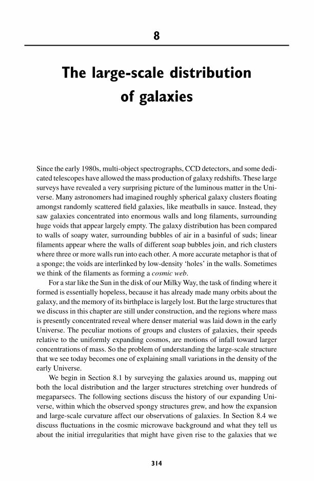
8

The large-scale distributionof galaxies

Since the early 1980s, multi-object spectrographs, CCD detectors, and some dedi-cated telescopes have allowed the mass production of galaxy redshifts. These largesurveys have revealed a very surprising picture of the luminous matter in the Uni-verse. Many astronomers had imagined roughly spherical galaxy clusters floatingamongst randomly scattered field galaxies, like meatballs in sauce. Instead, theysaw galaxies concentrated into enormous walls and long filaments, surroundinghuge voids that appear largely empty. The galaxy distribution has been comparedto walls of soapy water, surrounding bubbles of air in a basinful of suds; linearfilaments appear where the walls of different soap bubbles join, and rich clusterswhere three or more walls run into each other. A more accurate metaphor is that ofa sponge; the voids are interlinked by low-density ‘holes’ in the walls. Sometimeswe think of the filaments as forming a cosmic web.

For a star like the Sun in the disk of our Milky Way, the task of finding where itformed is essentially hopeless, because it has already made many orbits about thegalaxy, and the memory of its birthplace is largely lost. But the large structures thatwe discuss in this chapter are still under construction, and the regions where massis presently concentrated reveal where denser material was laid down in the earlyUniverse. The peculiar motions of groups and clusters of galaxies, their speedsrelative to the uniformly expanding cosmos, are motions of infall toward largerconcentrations of mass. So the problem of understanding the large-scale structurethat we see today becomes one of explaining small variations in the density of theearly Universe.

We begin in Section 8.1 by surveying the galaxies around us, mapping outboth the local distribution and the larger structures stretching over hundreds ofmegaparsecs. The following sections discuss the history of our expanding Uni-verse, within which the observed spongy structures grew, and how the expansionand large-scale curvature affect our observations of galaxies. In Section 8.4 wediscuss fluctuations in the cosmic microwave background and what they tell usabout the initial irregularities that might have given rise to the galaxies that we

314

Fig.

8.1.

Posi

tions

of14

650

brig

htga

laxi

es,i

nG

alac

ticlo

ngitu

del

and

latit

ude

b.M

any

liene

arth

esu

perg

alac

ticpl

ane,

appr

oxim

atel

yal

ong

the

Gre

atC

ircl

el=

140◦

and

l=

320◦

(hea

vylin

e);V

mar

ksth

eL

ocal

Voi

d.G

alax

ies

near

the

plan

e

b=

0of

the

Milk

yW

ay’s

disk

are

hidd

enby

dust

–T.

Kol

atta

ndan

dO

.Lah

av.

316 The large-scale distribution of galaxies

see today. We will see how we can use the observed peculiar motions of galaxiesto estimate how much matter is present. The final section asks how dense systemssuch as galaxies developed from these small beginnings.

Further reading: B. Ryden, 2003, Introduction to Cosmology (Addison Wesley, SanFrancisco, USA) and A. Liddle, 2003, An Introduction to Modern Cosmology, 2ndedition (John Wiley & Sons, Chichester, UK) are undergraduate texts on roughlythe level of this book. On the graduate level, see M. S. Longair, 1998, GalaxyFormation (Springer, Berlin) and T. Padmanabhan, 1993, Structure Formation inthe Universe (Cambridge University Press, Cambridge, UK).

8.1 Large-scale structure today

As we look out into the sky, it is quite clear that galaxies are not spread uniformlythrough space. Figure 8.1 shows the positions on the sky of almost 15 000 brightgalaxies, taken from three different catalogues compiled from optical photographs.Very few of them are seen close to the plane of the Milky Way’s disk at b = 0,and this region is sometimes called the Zone of Avoidance. The term is unfair:surveys in the 21 cm line of neutral hydrogen, and in far-infrared light, show thatgalaxies are indeed present, but their visible light is obscured by dust in the MilkyWay’s disk. Dense areas on the map mark rich clusters: the Virgo cluster is closeto the north Galactic pole, at b = 90◦. Few galaxies are seen in the Local Void,stretching from l = 40◦, b = −20◦ across to l = 0, b = 30◦.

The galaxy clusters themselves are not spread evenly on the sky: those withinabout 100 Mpc form a rough ellipsoid lying almost perpendicular to the MilkyWay’s disk. Its midplane, the supergalactic plane, is well defined in the northernGalactic hemisphere (b > 0), but becomes rather scruffy in the south. The poleor Z axis of the supergalactic plane points to l = 47.4◦, b = 6.3◦. We take thesupergalactic X direction in the Galactic plane, pointing to l = 137.3◦, b = 0,while the Y axis points close to the north Galactic pole at b = 90◦, so that Y ≈ 0along the Zone of Avoidance. The supergalactic plane is close to the Great Circlethrough Galactic longitude l = 140◦ and l = 320◦, shown as a heavy line inFigure 8.1. It passes through the Ursa Major group of Figures 5.6 and 5.8, andthe four nearby galaxy clusters described in Section 7.2; the Virgo cluster at rightascension α = 12h, declination δ = 12◦; Perseus at α = 3h, δ = 40◦; Fornax atα = 4h, δ = −35◦; and the Coma cluster at α = 13h, δ = 28◦, almost at the northGalactic pole.

Figure 8.2 shows the positions of the elliptical galaxies within about 20 Mpc,tracing out the Virgo and Fornax clusters. The distances to these galaxies havebeen found by analyzing surface brightness fluctuations. Even though they aretoo far away for us to distinguish individual bright stars, the number N of starsfalling within any arcsecond square on the image has some random variation.

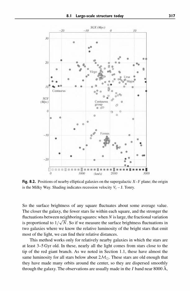
8.1 Large-scale structure today 317

Fig. 8.2. Positions of nearby elliptical galaxies on the supergalactic X–Y plane; the origin

is the Milky Way. Shading indicates recession velocity Vr – J. Tonry.

So the surface brightness of any square fluctuates about some average value.The closer the galaxy, the fewer stars lie within each square, and the stronger thefluctuations between neighboring squares: when N is large, the fractional variationis proportional to 1/

√N . So if we measure the surface brightness fluctuations in

two galaxies where we know the relative luminosity of the bright stars that emitmost of the light, we can find their relative distances.

This method works only for relatively nearby galaxies in which the stars areat least 3–5 Gyr old. In these, nearly all the light comes from stars close to thetip of the red giant branch. As we noted in Section 1.1, these have almost thesame luminosity for all stars below about 2M�. These stars are old enough thatthey have made many orbits around the center, so they are dispersed smoothlythrough the galaxy. The observations are usually made in the I band near 8000 A,

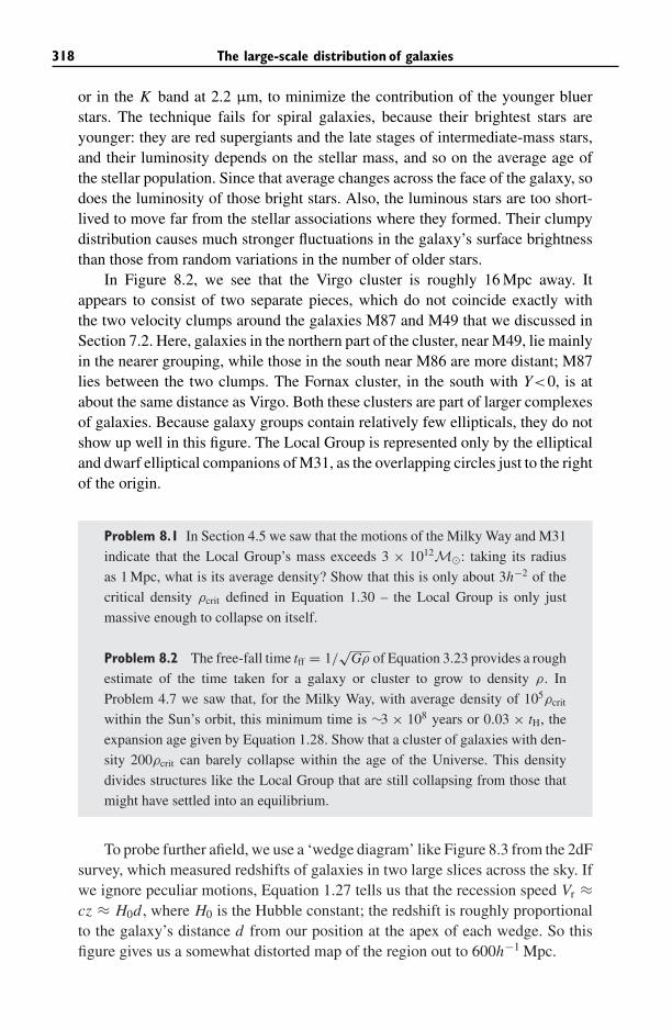
318 The large-scale distribution of galaxies

or in the K band at 2.2 μm, to minimize the contribution of the younger bluerstars. The technique fails for spiral galaxies, because their brightest stars areyounger: they are red supergiants and the late stages of intermediate-mass stars,and their luminosity depends on the stellar mass, and so on the average age ofthe stellar population. Since that average changes across the face of the galaxy, sodoes the luminosity of those bright stars. Also, the luminous stars are too short-lived to move far from the stellar associations where they formed. Their clumpydistribution causes much stronger fluctuations in the galaxy’s surface brightnessthan those from random variations in the number of older stars.

In Figure 8.2, we see that the Virgo cluster is roughly 16 Mpc away. Itappears to consist of two separate pieces, which do not coincide exactly withthe two velocity clumps around the galaxies M87 and M49 that we discussed inSection 7.2. Here, galaxies in the northern part of the cluster, near M49, lie mainlyin the nearer grouping, while those in the south near M86 are more distant; M87lies between the two clumps. The Fornax cluster, in the south with Y<0, is atabout the same distance as Virgo. Both these clusters are part of larger complexesof galaxies. Because galaxy groups contain relatively few ellipticals, they do notshow up well in this figure. The Local Group is represented only by the ellipticaland dwarf elliptical companions of M31, as the overlapping circles just to the rightof the origin.

Problem 8.1 In Section 4.5 we saw that the motions of the Milky Way and M31

indicate that the Local Group’s mass exceeds 3 × 1012M�: taking its radius

as 1 Mpc, what is its average density? Show that this is only about 3h−2 of the

critical density ρcrit defined in Equation 1.30 – the Local Group is only just

massive enough to collapse on itself.

Problem 8.2 The free-fall time tff = 1/√

Gρ of Equation 3.23 provides a rough

estimate of the time taken for a galaxy or cluster to grow to density ρ. In

Problem 4.7 we saw that, for the Milky Way, with average density of 105ρcrit

within the Sun’s orbit, this minimum time is ∼3 × 108 years or 0.03 × tH, the

expansion age given by Equation 1.28. Show that a cluster of galaxies with den-

sity 200ρcrit can barely collapse within the age of the Universe. This density

divides structures like the Local Group that are still collapsing from those that

might have settled into an equilibrium.

To probe further afield, we use a ‘wedge diagram’ like Figure 8.3 from the 2dFsurvey, which measured redshifts of galaxies in two large slices across the sky. Ifwe ignore peculiar motions, Equation 1.27 tells us that the recession speed Vr ≈cz ≈ H0d , where H0 is the Hubble constant; the redshift is roughly proportionalto the galaxy’s distance d from our position at the apex of each wedge. So thisfigure gives us a somewhat distorted map of the region out to 600h−1 Mpc.

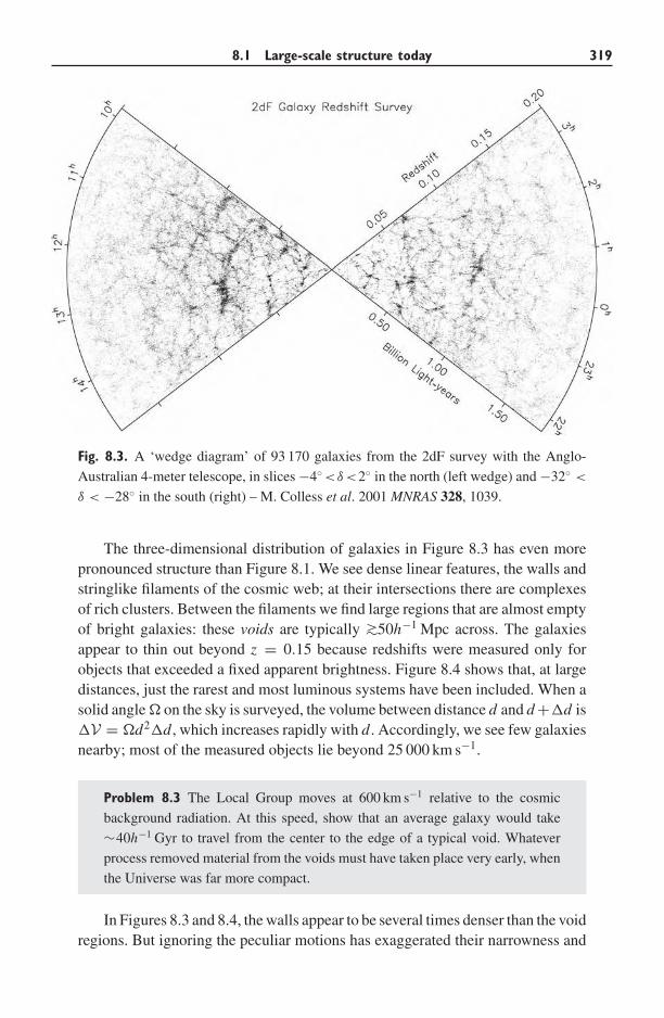
8.1 Large-scale structure today 319

Fig. 8.3. A ‘wedge diagram’ of 93 170 galaxies from the 2dF survey with the Anglo-

Australian 4-meter telescope, in slices −4◦ <δ<2◦ in the north (left wedge) and −32◦ <

δ < −28◦ in the south (right) – M. Colless et al. 2001 MNRAS 328, 1039.

The three-dimensional distribution of galaxies in Figure 8.3 has even morepronounced structure than Figure 8.1. We see dense linear features, the walls andstringlike filaments of the cosmic web; at their intersections there are complexesof rich clusters. Between the filaments we find large regions that are almost emptyof bright galaxies: these voids are typically ∼>50h−1 Mpc across. The galaxiesappear to thin out beyond z = 0.15 because redshifts were measured only forobjects that exceeded a fixed apparent brightness. Figure 8.4 shows that, at largedistances, just the rarest and most luminous systems have been included. When asolid angle � on the sky is surveyed, the volume between distance d and d +�d is�V = �d2�d, which increases rapidly with d . Accordingly, we see few galaxiesnearby; most of the measured objects lie beyond 25 000 km s−1.

Problem 8.3 The Local Group moves at 600 km s−1 relative to the cosmic

background radiation. At this speed, show that an average galaxy would take

∼40h−1 Gyr to travel from the center to the edge of a typical void. Whatever

process removed material from the voids must have taken place very early, when

the Universe was far more compact.

In Figures 8.3 and 8.4, the walls appear to be several times denser than the voidregions. But ignoring the peculiar motions has exaggerated their narrowness and

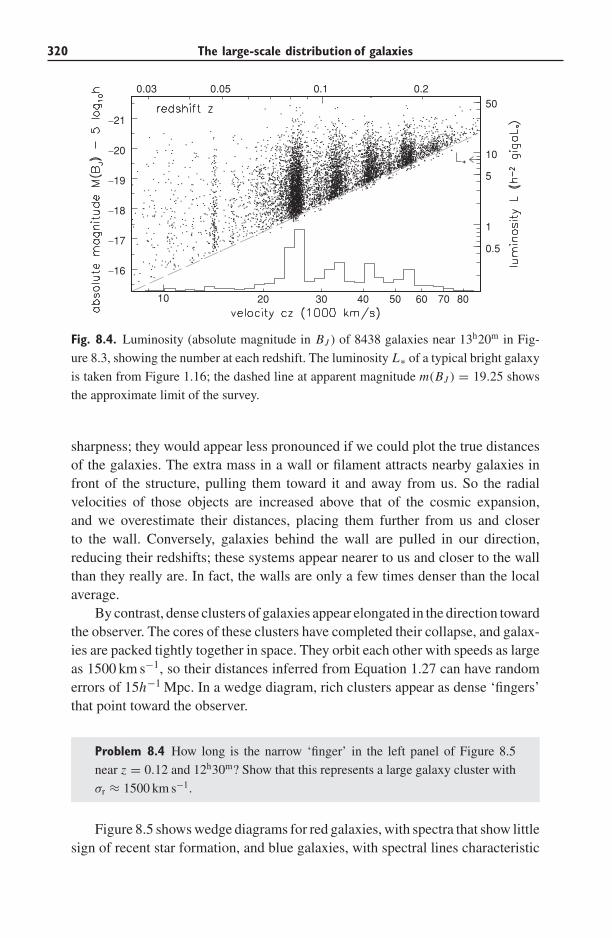
320 The large-scale distribution of galaxies

0.20.10.050.03

10 20 30 40 50 60 70 80

1

10

0.5

5

50

Fig. 8.4. Luminosity (absolute magnitude in BJ ) of 8438 galaxies near 13h20m in Fig-

ure 8.3, showing the number at each redshift. The luminosity L∗ of a typical bright galaxy

is taken from Figure 1.16; the dashed line at apparent magnitude m(BJ ) = 19.25 shows

the approximate limit of the survey.

sharpness; they would appear less pronounced if we could plot the true distancesof the galaxies. The extra mass in a wall or filament attracts nearby galaxies infront of the structure, pulling them toward it and away from us. So the radialvelocities of those objects are increased above that of the cosmic expansion,and we overestimate their distances, placing them further from us and closerto the wall. Conversely, galaxies behind the wall are pulled in our direction,reducing their redshifts; these systems appear nearer to us and closer to the wallthan they really are. In fact, the walls are only a few times denser than the localaverage.

By contrast, dense clusters of galaxies appear elongated in the direction towardthe observer. The cores of these clusters have completed their collapse, and galax-ies are packed tightly together in space. They orbit each other with speeds as largeas 1500 km s−1, so their distances inferred from Equation 1.27 can have randomerrors of 15h−1 Mpc. In a wedge diagram, rich clusters appear as dense ‘fingers’that point toward the observer.

Problem 8.4 How long is the narrow ‘finger’ in the left panel of Figure 8.5

near z = 0.12 and 12h30m? Show that this represents a large galaxy cluster with

σr ≈ 1500 km s−1.

Figure 8.5 shows wedge diagrams for red galaxies, with spectra that show littlesign of recent star formation, and blue galaxies, with spectral lines characteristic

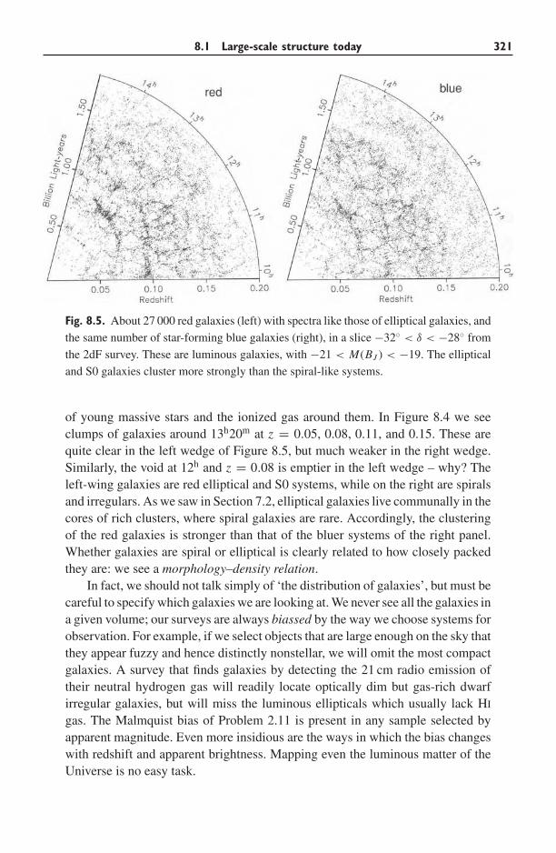
8.1 Large-scale structure today 321

Fig. 8.5. About 27 000 red galaxies (left) with spectra like those of elliptical galaxies, and

the same number of star-forming blue galaxies (right), in a slice −32◦ < δ < −28◦ from

the 2dF survey. These are luminous galaxies, with −21 < M(BJ ) < −19. The elliptical

and S0 galaxies cluster more strongly than the spiral-like systems.

of young massive stars and the ionized gas around them. In Figure 8.4 we seeclumps of galaxies around 13h20m at z = 0.05, 0.08, 0.11, and 0.15. These arequite clear in the left wedge of Figure 8.5, but much weaker in the right wedge.Similarly, the void at 12h and z = 0.08 is emptier in the left wedge – why? Theleft-wing galaxies are red elliptical and S0 systems, while on the right are spiralsand irregulars. As we saw in Section 7.2, elliptical galaxies live communally in thecores of rich clusters, where spiral galaxies are rare. Accordingly, the clusteringof the red galaxies is stronger than that of the bluer systems of the right panel.Whether galaxies are spiral or elliptical is clearly related to how closely packedthey are: we see a morphology–density relation.

In fact, we should not talk simply of ‘the distribution of galaxies’, but must becareful to specify which galaxies we are looking at. We never see all the galaxies ina given volume; our surveys are always biassed by the way we choose systems forobservation. For example, if we select objects that are large enough on the sky thatthey appear fuzzy and hence distinctly nonstellar, we will omit the most compactgalaxies. A survey that finds galaxies by detecting the 21 cm radio emission oftheir neutral hydrogen gas will readily locate optically dim but gas-rich dwarfirregular galaxies, but will miss the luminous ellipticals which usually lack HI

gas. The Malmquist bias of Problem 2.11 is present in any sample selected byapparent magnitude. Even more insidious are the ways in which the bias changeswith redshift and apparent brightness. Mapping even the luminous matter of theUniverse is no easy task.

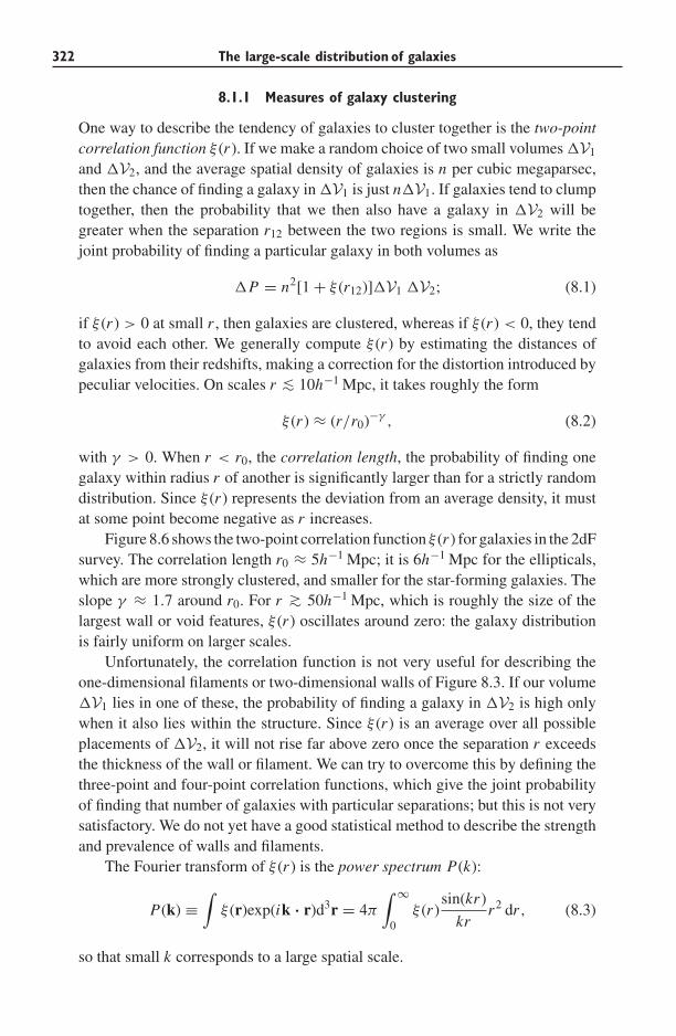
322 The large-scale distribution of galaxies

8.1.1 Measures of galaxy clustering

One way to describe the tendency of galaxies to cluster together is the two-pointcorrelation function ξ (r ). If we make a random choice of two small volumes �V1

and �V2, and the average spatial density of galaxies is n per cubic megaparsec,then the chance of finding a galaxy in �V1 is just n�V1. If galaxies tend to clumptogether, then the probability that we then also have a galaxy in �V2 will begreater when the separation r12 between the two regions is small. We write thejoint probability of finding a particular galaxy in both volumes as

�P = n2[1 + ξ (r12)]�V1 �V2; (8.1)

if ξ (r ) > 0 at small r , then galaxies are clustered, whereas if ξ (r ) < 0, they tendto avoid each other. We generally compute ξ (r ) by estimating the distances ofgalaxies from their redshifts, making a correction for the distortion introduced bypeculiar velocities. On scales r ∼< 10h−1 Mpc, it takes roughly the form

ξ (r ) ≈ (r/r0)−γ , (8.2)

with γ > 0. When r < r0, the correlation length, the probability of finding onegalaxy within radius r of another is significantly larger than for a strictly randomdistribution. Since ξ (r ) represents the deviation from an average density, it mustat some point become negative as r increases.

Figure 8.6 shows the two-point correlation function ξ (r ) for galaxies in the 2dFsurvey. The correlation length r0 ≈ 5h−1 Mpc; it is 6h−1 Mpc for the ellipticals,which are more strongly clustered, and smaller for the star-forming galaxies. Theslope γ ≈ 1.7 around r0. For r ∼> 50h−1 Mpc, which is roughly the size of thelargest wall or void features, ξ (r ) oscillates around zero: the galaxy distributionis fairly uniform on larger scales.

Unfortunately, the correlation function is not very useful for describing theone-dimensional filaments or two-dimensional walls of Figure 8.3. If our volume�V1 lies in one of these, the probability of finding a galaxy in �V2 is high onlywhen it also lies within the structure. Since ξ (r ) is an average over all possibleplacements of �V2, it will not rise far above zero once the separation r exceedsthe thickness of the wall or filament. We can try to overcome this by defining thethree-point and four-point correlation functions, which give the joint probabilityof finding that number of galaxies with particular separations; but this is not verysatisfactory. We do not yet have a good statistical method to describe the strengthand prevalence of walls and filaments.

The Fourier transform of ξ (r ) is the power spectrum P(k):

P(k) ≡∫

ξ (r)exp(ik · r)d3r = 4π

∫ ∞

0ξ (r )

sin(kr )

krr2 dr , (8.3)

so that small k corresponds to a large spatial scale.

8.1 Large-scale structure today 323

0

0.1

0.1 1 10 100

0.01

0.1

1

10

0.01 0.1 1

0

0.5

1

1.5

2

2.5100 10 1

Fig. 8.6. Left, the correlation function ξ (s) for the 2dF galaxies, at small (circles, left

logarithmic scale) and large (triangles, right linear scale) separations; vertical bars show

uncertainties. ξ (s) is calculated assuming that Hubble’s law holds exactly: the ‘fingers’ of

Figure 8.5 reduce ξ (s) on scales r ∼< 1 Mpc, but infall to the walls makes clustering look

stronger on scales near r0. The dashed line shows ξ (r ), corrected for these effects. Right,

the variance σR of Equation 8.4, describing how much the average density varies between

regions of size R – S. Maddox and S. Cole.

Since ξ (r ) is dimensionless, P(k) has the dimensions of a volume. The func-tion sin(kr )/kr is positive for |kr | < π , and it oscillates with decreasing amplitudeas kr becomes large; so, very roughly, P(k) will have its maximum when k−1 isclose to the radius where ξ (r ) drops to zero. In Figure 8.17 we show P(k) cal-culated by combining the 2dF galaxy survey with observations of the cosmicmicrowave background.

Problem 8.5 Prove the last equality of Equation 8.3. One method is to write the

volume integral for P(k) in spherical polar coordinates r, θ, φ and set k · r =kr cos θ . Show that, because ξ (r ) describes departures from the mean density,

Equation 8.1 gives∫∞

0 ξ (r )r2 dr = 0, and hence P(k) → 0 as k → 0.

Problem 8.6 Show that the power spectrum P(k) ∝ kn corresponds to a corre-

lation function ξ (r ) ∝ r−(3+n). Hence γ ≈ 1.5 implies n ≈ −1.5. Figure 8.17

shows that when k is large P(k) declines roughly as k−1.8, about as expected.

Another way to describe the non-uniformity of the galaxy distribution is toask how likely we are to find a given deviation from the average density. Wecan write the local density at position x as a multiple of the mean level ρ, asρ(x) = ρ[1 + δ(x)], and let δR be the fractional deviation δ(x) averaged within asphere of radius R. When we take the average 〈δR〉 over all such spheres, this must

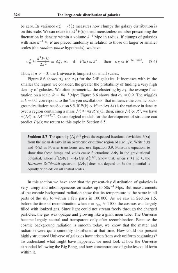
324 The large-scale distribution of galaxies

be zero. Its variance σ 2R = 〈δ2

R〉 measures how clumpy the galaxy distribution ison this scale. We can relate it to k3 P(k), the dimensionless number prescribing thefluctuation in density within a volume k−1 Mpc in radius. If clumps of galaxieswith size k−1 ≈ R are placed randomly in relation to those on larger or smallerscales (the random-phase hypothesis), we have

σ 2R ≈ k3 P(k)

2π2≡ �2

k ; so, if P(k) ∝ kn, then σR ∝ R−(n+3)/2. (8.4)

Thus, if n > −3, the Universe is lumpiest on small scales.Figure 8.6 shows σR (or �k) for the 2dF galaxies. It increases with k: the

smaller the region we consider, the greater the probability of finding a very highdensity of galaxies. We often parametrize the clustering by σ8, the average fluc-tuation on a scale R = 8h−1 Mpc: Figure 8.6 shows that σ8 ≈ 0.9. The wigglesat k ∼ 0.1 correspond to the ‘baryon oscillations’ that influence the cosmic back-ground radiation: see Section 8.5. If P(k) ∝ kn and σ (M) is the variance in densityover a region containing a mass M ≈ 4π R3ρ/3, then, since M ∝ R3, we haveσ (M) ∝ M−(n+3)/6. Cosmological models for the development of structure canpredict P(k); we return to this topic in Section 8.5.

Problem 8.7 The quantity 〈�2k〉1/2 gives the expected fractional deviation |δ(x)|

from the mean density in an overdense or diffuse region of size 1/k. Write δ(x)

and �(x) as Fourier transforms and use Equation 3.9, Poisson’s equation, to

show that these lumps and voids cause fluctuations ��k in the gravitational

potential, where k2|��k | ∼ 4πGρ〈�2k〉1/2. Show that, when P(k) ∝ k, the

Harrison–Zel’dovich spectrum, |��k | does not depend on k: the potential is

equally ‘rippled’ on all spatial scales.

In this section we have seen that the present-day distribution of galaxies isvery lumpy and inhomogeneous on scales up to 50h−1 Mpc. But measurementsof the cosmic background radiation show that its temperature is the same in allparts of the sky to within a few parts in 100 000. As we saw in Section 1.5,before the time of recombination when z = zrec ≈ 1100, the cosmos was largelyfilled with ionized gas. Since light could not stream freely through the chargedparticles, the gas was opaque and glowing like a giant neon tube. The Universebecame largely neutral and transparent only after recombination. Because thecosmic background radiation is smooth today, we know that the matter andradiation were quite smoothly distributed at that time. How could our presenthighly structured Universe of galaxies have arisen from such uniform beginnings?To understand what might have happened, we must look at how the Universeexpanded following the Big Bang, and how concentrations of galaxies could formwithin it.

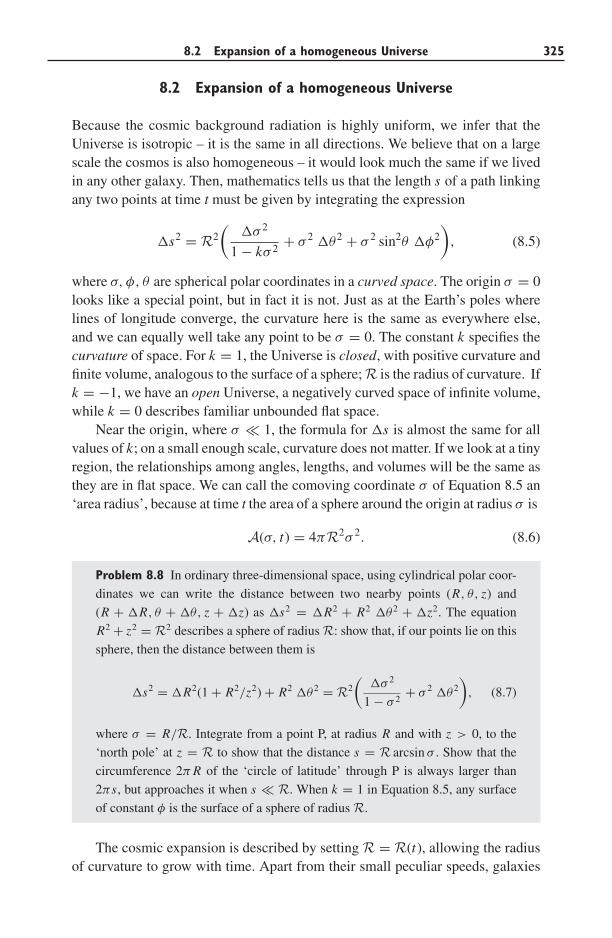
8.2 Expansion of a homogeneous Universe 325

8.2 Expansion of a homogeneous Universe

Because the cosmic background radiation is highly uniform, we infer that theUniverse is isotropic – it is the same in all directions. We believe that on a largescale the cosmos is also homogeneous – it would look much the same if we livedin any other galaxy. Then, mathematics tells us that the length s of a path linkingany two points at time t must be given by integrating the expression

�s2 = R2(

�σ 2

1 − kσ 2+ σ 2 �θ2 + σ 2 sin2θ �φ2

), (8.5)

where σ, φ, θ are spherical polar coordinates in a curved space. The origin σ = 0looks like a special point, but in fact it is not. Just as at the Earth’s poles wherelines of longitude converge, the curvature here is the same as everywhere else,and we can equally well take any point to be σ = 0. The constant k specifies thecurvature of space. For k = 1, the Universe is closed, with positive curvature andfinite volume, analogous to the surface of a sphere; R is the radius of curvature. Ifk = −1, we have an open Universe, a negatively curved space of infinite volume,while k = 0 describes familiar unbounded flat space.

Near the origin, where σ � 1, the formula for �s is almost the same for allvalues of k; on a small enough scale, curvature does not matter. If we look at a tinyregion, the relationships among angles, lengths, and volumes will be the same asthey are in flat space. We can call the comoving coordinate σ of Equation 8.5 an‘area radius’, because at time t the area of a sphere around the origin at radius σ is

A(σ, t) = 4πR2σ 2. (8.6)

Problem 8.8 In ordinary three-dimensional space, using cylindrical polar coor-

dinates we can write the distance between two nearby points (R, θ, z) and

(R + �R, θ + �θ, z + �z) as �s2 = �R2 + R2 �θ2 + �z2. The equation

R2 + z2 = R2 describes a sphere of radius R: show that, if our points lie on this

sphere, then the distance between them is

�s2 = �R2(1 + R2/z2) + R2 �θ2 = R2

(�σ 2

1 − σ 2+ σ 2 �θ2

), (8.7)

where σ = R/R. Integrate from a point P, at radius R and with z > 0, to the

‘north pole’ at z = R to show that the distance s = R arcsin σ . Show that the

circumference 2π R of the ‘circle of latitude’ through P is always larger than

2πs, but approaches it when s � R. When k = 1 in Equation 8.5, any surface

of constant φ is the surface of a sphere of radius R.

The cosmic expansion is described by setting R = R(t), allowing the radiusof curvature to grow with time. Apart from their small peculiar speeds, galaxies

326 The large-scale distribution of galaxies

remain at points with fixed values of σ, φ, θ ; so these are called comovingcoordinates. The separation d of two galaxies is just the length s of the short-est path between them. So, if they stay at fixed comoving coordinates, d expandsproportionally to R(t): Hubble’s law is just one symptom of the expansion ofcurved space. Equation 8.5 tells us that the two systems are carried away fromeach other at a speed

Vr = d = R(t)

R(t)d ≡ H (t)d. (8.8)

Here H (t) is the Hubble parameter, which at present has the value H0. Equation 8.8describes the average motion of the galaxies; we defer discussion of the peculiarmotions that develop from the gravitational pull of near neighbors until Section 8.4below.

General Relativity tells us that the distance between two events happening atdifferent times and in different places depends on the motion of the observer. Butall observers will measure the same proper time τ along a path through space andtime connecting the events, which is found by integrating

�τ 2 = �t2 − �s2/c2. (8.9)

Light rays always travel along paths of zero proper time, �τ = 0. If we placeourselves at the origin of coordinates, then the light we receive from a galaxy atcomoving distance σe has followed the radial path

c �t

R(t)= − �σ√

1 − kσ 2. (8.10)

The light covers less comoving distance per unit of time as the scale length R(t)of the Universe grows. We can integrate this equation for a wavecrest that sets offat time te, arriving at our position now at time t0:

c∫ t0

te

dt

R(t)=∫ σe

0

dσ√1 − kσ 2

. (8.11)

Suppose that another wavecrest sets off later, by a time �te. We receive it at timet0 + �t , given by the same equation with the new departure and arrival times.The galaxy’s comoving position σe, and the integral on the right-hand side ofEquation 8.11, have not changed. So the left-hand side also stays constant:

∫ t0+�t

te+�te

dt

R(t)=∫ t0

te

dt

R(t), so

�teR(te)

= �t

R(t0), (8.12)

as long as �t � R(t)/R(t). Thus all processes in the distant galaxy appearto be slowed down by the factor R(t0)/R(te). If �te is the time between two

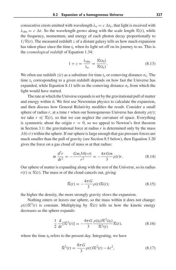
8.2 Expansion of a homogeneous Universe 327

consecutive crests emitted with wavelength λe = c �te, that light is received withλobs = c �t . So the wavelength grows along with the scale length R(t), whilethe frequency, momentum, and energy of each photon decay proportionally to1/R(t). The measured redshift z of a distant galaxy tells us how much expansionhas taken place since the time te when its light set off on its journey to us. This isthe cosmological redshift of Equation 1.34:

1 + z = λobs

λe= R(t0)

R(te). (8.13)

We often use redshift z(t) as a substitute for time te or comoving distance σe. Thetime te corresponding to a given redshift depends on how fast the Universe hasexpanded, while Equation 8.11 tells us the comoving distance σe from which thelight would have started.

The rate at which the Universe expands is set by the gravitational pull of matterand energy within it. We first use Newtonian physics to calculate the expansion,and then discuss how General Relativity modifies the result. Consider a smallsphere of radius r , at a time t when our homogeneous Universe has density ρ(t);we take r � R(t), so that we can neglect the curvature of space. Everythingis symmetric about the origin r = 0, so we appeal to Newton’s first theoremin Section 3.1: the gravitational force at radius r is determined only by the massM(<r ) within the sphere. If our sphere is large enough that gas pressure forces aremuch smaller than the pull of gravity (see Section 8.5 below), then Equation 3.20gives the force on a gas cloud of mass m at that radius:

md2r

dt2= −GmM(<r)

r2= −4πGm

3ρ(t)r . (8.14)

Our sphere of matter is expanding along with the rest of the Universe, so its radiusr (t) ∝ R(t). The mass m of the cloud cancels out, giving

R(t) = −4πG

3ρ(t)R(t); (8.15)

the higher the density, the more strongly gravity slows the expansion.Nothing enters or leaves our sphere, so the mass within it does not change:

ρ(t)R3(t) is constant. Multiplying by R(t) tells us how the kinetic energydecreases as the sphere expands:

1

2

d

dt[R2(t)] = −4πG

3

ρ(t0)R3(t0)

R2(t)R(t), (8.16)

where the time t0 refers to the present day. Integrating, we have

R2(t) = 8πG

3ρ(t)R2(t) − kc2, (8.17)

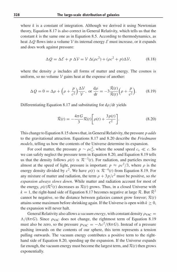
328 The large-scale distribution of galaxies

where k is a constant of integration. Although we derived it using Newtoniantheory, Equation 8.17 is also correct in General Relativity, which tells us that theconstant k is the same one as in Equation 8.5. According to thermodynamics, asheat �Q flows into a volume V its internal energy E must increase, or it expandsand does work against pressure:

�Q = �E + p �V = V �(ρc2) + (ρc2 + p)�V, (8.18)

where the density ρ includes all forms of matter and energy. The cosmos isuniform, so no volume V gains heat at the expense of another:

�Q = 0 = �ρ +(ρ + p

c2

)�VV , or

dρ

dt= −3

R(t)

R(t)

(ρ + p

c2

). (8.19)

Differentiating Equation 8.17 and substituting for dρ/dt yields

R(t) = −4πG

3R(t)

[ρ(t) + 3p(t)

c2

]. (8.20)

This change to Equation 8.15 shows that, in General Relativity, the pressure p addsto the gravitational attraction. Equations 8.17 and 8.20 describe the Friedmannmodels, telling us how the contents of the Universe determine its expansion.

For cool matter, the pressure p ∼ ρc2s , where the sound speed cs � c. So

we can safely neglect the pressure term in Equation 8.20, and Equation 8.19 tellsus that the density follows ρ(t) ∝ R−3(t). For radiation, and particles movingalmost at the speed of light, pressure is important: p ≈ ρc2/3, where ρ is theenergy density divided by c2. We have ρ(t) ∝ R−4(t) from Equation 8.19. Forany mixture of matter and radiation, the term ρ + 3p/c2 must be positive, so theexpansion always slows down. While matter and radiation account for most ofthe energy, ρ(t)R2(t) decreases as R(t) grows. Thus, in a closed Universe withk = 1, the right-hand side of Equation 8.17 becomes negative at large R. But R2

cannot be negative, so the distance between galaxies cannot grow forever; R(t)attains some maximum before shrinking again. If the Universe is open with k ≥ 0,the expansion will never halt.

General Relativity also allows a vacuum energy, with constant density ρVAC =�/(8πG). Since ρVAC does not change, the rightmost term of Equation 8.19must also be zero, so the pressure pVAC = −�c2/(8πG). Instead of a pressurepushing inwards on the contents of our sphere, this term represents a tensionpulling outwards. The vacuum energy contributes a positive term to the right-hand side of Equation 8.20, speeding up the expansion. If the Universe expandsfar enough, the vacuum energy must become the largest term, andR(t) then growsexponentially.

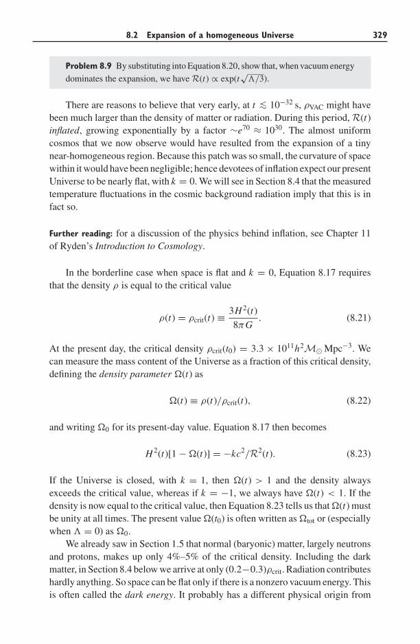
8.2 Expansion of a homogeneous Universe 329

Problem 8.9 By substituting into Equation 8.20, show that, when vacuum energy

dominates the expansion, we have R(t) ∝ exp(t√

�/3).

There are reasons to believe that very early, at t ∼< 10−32 s, ρVAC might havebeen much larger than the density of matter or radiation. During this period, R(t)inflated, growing exponentially by a factor ∼e70 ≈ 1030. The almost uniformcosmos that we now observe would have resulted from the expansion of a tinynear-homogeneous region. Because this patch was so small, the curvature of spacewithin it would have been negligible; hence devotees of inflation expect our presentUniverse to be nearly flat, with k = 0. We will see in Section 8.4 that the measuredtemperature fluctuations in the cosmic background radiation imply that this is infact so.

Further reading: for a discussion of the physics behind inflation, see Chapter 11of Ryden’s Introduction to Cosmology.

In the borderline case when space is flat and k = 0, Equation 8.17 requiresthat the density ρ is equal to the critical value

ρ(t) = ρcrit(t) ≡ 3H 2(t)

8πG. (8.21)

At the present day, the critical density ρcrit(t0) = 3.3 × 1011h2M� Mpc−3. Wecan measure the mass content of the Universe as a fraction of this critical density,defining the density parameter �(t) as

�(t) ≡ ρ(t)/ρcrit(t), (8.22)

and writing �0 for its present-day value. Equation 8.17 then becomes

H 2(t)[1 − �(t)] = −kc2/R2(t). (8.23)

If the Universe is closed, with k = 1, then �(t) > 1 and the density alwaysexceeds the critical value, whereas if k = −1, we always have �(t) < 1. If thedensity is now equal to the critical value, then Equation 8.23 tells us that �(t) mustbe unity at all times. The present value �(t0) is often written as �tot or (especiallywhen � = 0) as �0.

We already saw in Section 1.5 that normal (baryonic) matter, largely neutronsand protons, makes up only 4%–5% of the critical density. Including the darkmatter, in Section 8.4 below we arrive at only (0.2−0.3)ρcrit. Radiation contributeshardly anything. So space can be flat only if there is a nonzero vacuum energy. Thisis often called the dark energy. It probably has a different physical origin from

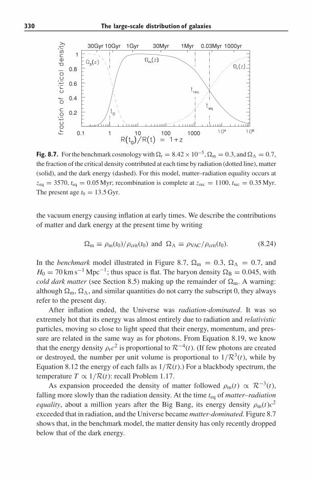
330 The large-scale distribution of galaxies

0.1 1 10 100 1000

0.2

0.4

0.6

0.8

1

1000yr0.03Myr1Myr30Myr1Gyr10Gyr30Gyr

Fig. 8.7. For the benchmark cosmology with�r = 8.42×10−5,�m = 0.3, and�� = 0.7,

the fraction of the critical density contributed at each time by radiation (dotted line), matter

(solid), and the dark energy (dashed). For this model, matter–radiation equality occurs at

zeq = 3570, teq = 0.05 Myr; recombination is complete at zrec = 1100, trec = 0.35 Myr.

The present age t0 = 13.5 Gyr.

the vacuum energy causing inflation at early times. We describe the contributionsof matter and dark energy at the present time by writing

�m ≡ ρm(t0)/ρcrit(t0) and �� ≡ ρVAC/ρcrit(t0). (8.24)

In the benchmark model illustrated in Figure 8.7, �m = 0.3, �� = 0.7, andH0 = 70 km s−1 Mpc−1; thus space is flat. The baryon density �B = 0.045, withcold dark matter (see Section 8.5) making up the remainder of �m. A warning:although �m, ��, and similar quantities do not carry the subscript 0, they alwaysrefer to the present day.

After inflation ended, the Universe was radiation-dominated. It was soextremely hot that its energy was almost entirely due to radiation and relativisticparticles, moving so close to light speed that their energy, momentum, and pres-sure are related in the same way as for photons. From Equation 8.19, we knowthat the energy density ρrc2 is proportional to R−4(t). (If few photons are createdor destroyed, the number per unit volume is proportional to 1/R3(t), while byEquation 8.12 the energy of each falls as 1/R(t).) For a blackbody spectrum, thetemperature T ∝ 1/R(t): recall Problem 1.17.

As expansion proceeded the density of matter followed ρm(t) ∝ R−3(t),falling more slowly than the radiation density. At the time teq of matter–radiationequality, about a million years after the Big Bang, its energy density ρm(t)c2

exceeded that in radiation, and the Universe became matter-dominated. Figure 8.7shows that, in the benchmark model, the matter density has only recently droppedbelow that of the dark energy.

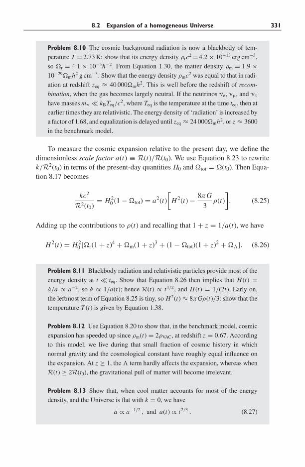
8.2 Expansion of a homogeneous Universe 331

Problem 8.10 The cosmic background radiation is now a blackbody of tem-

perature T = 2.73 K: show that its energy density ρrc2 = 4.2 × 10−13 erg cm−3,

so �r = 4.1 × 10−5h−2. From Equation 1.30, the matter density ρm = 1.9 ×10−29�mh2 g cm−3. Show that the energy density ρmc2 was equal to that in radi-

ation at redshift zeq ≈ 40 000�mh2. This is well before the redshift of recom-

bination, when the gas becomes largely neutral. If the neutrinos νe, νμ, and ντ

have masses mν � kBTeq/c2, where Teq is the temperature at the time teq, then at

earlier times they are relativistic. The energy density of ‘radiation’ is increased by

a factor of 1.68, and equalization is delayed until zeq ≈ 24 000�mh2, or z ≈ 3600

in the benchmark model.

To measure the cosmic expansion relative to the present day, we define thedimensionless scale factor a(t) ≡ R(t)/R(t0). We use Equation 8.23 to rewritek/R2(t0) in terms of the present-day quantities H0 and �tot = �(t0). Then Equa-tion 8.17 becomes

kc2

R2(t0)= H 2

0 (1 − �tot) = a2(t)

[H 2(t) − 8πG

3ρ(t)

]. (8.25)

Adding up the contributions to ρ(t) and recalling that 1 + z = 1/a(t), we have

H 2(t) = H 20 [�r(1 + z)4 + �m(1 + z)3 + (1 − �tot)(1 + z)2 + ��]. (8.26)

Problem 8.11 Blackbody radiation and relativistic particles provide most of the

energy density at t � teq. Show that Equation 8.26 then implies that H (t) =a/a ∝ a−2, so a ∝ 1/a(t); hence R(t) ∝ t1/2, and H (t) = 1/(2t). Early on,

the leftmost term of Equation 8.25 is tiny, so H 2(t) ≈ 8πGρ(t)/3: show that the

temperature T (t) is given by Equation 1.38.

Problem 8.12 Use Equation 8.20 to show that, in the benchmark model, cosmic

expansion has speeded up since ρm(t) = 2ρVAC, at redshift z = 0.67. According

to this model, we live during that small fraction of cosmic history in which

normal gravity and the cosmological constant have roughly equal influence on

the expansion. At z ≥ 1, the � term hardly affects the expansion, whereas when

R(t) ≥ 2R(t0), the gravitational pull of matter will become irrelevant.

Problem 8.13 Show that, when cool matter accounts for most of the energy

density, and the Universe is flat with k = 0, we have

a ∝ a−1/2 , and a(t) ∝ t2/3 . (8.27)

332 The large-scale distribution of galaxies

Show that, if k = 0, then Equation 8.27 holds when zeq � 1 + z � (��/�m)1/3,

whereas at very late times a(t) ∝ exp (t√

�/3). If the curvature is negative, with

�tot = �r + �m + �� < 1, the third term of Equation 8.26 exceeds the second

when 1 + z < (1 − �tot)/�m. Expansion then proceeds almost at a constant

speed, with a(t) ∝ t ; it is barely slowed by the matter, and not accelerated by

dark energy until (1 + z)2 < ��/(1 − �tot).

Equation 8.27 is a good description of the expansion over much of cosmichistory. In particular, most of the structure of galaxy clusters and voids that wesee today developed after the Universe became matter-dominated, but before thedark energy became important.

Problem 8.14 Even if the cosmos has infinite volume, we can observe only a

finite part of it because light travels at a finite speed. From Equation 8.11, light

reaching us at time t has travelled no further than the distance σH given by

c∫ t

0

dt ′

R(t ′)≡∫ σH

0

dσ√1 − kσ 2

, (8.28)

so we cannot see beyond our horizon, at comoving radius σH. Explain why only

points within σH(t) of each other can exchange signals or particles before time

t . Use Equation 8.27 to show that, while the Universe was matter-dominated,

R(t)σH ≈ 3ct ; at the time trec of recombination R(trec)σH ≈ 0.43 Mpc in the

benchmark model of Figure 8.7. We will see below that a sphere of matter with

this diameter would cover only about 2◦ on the sky. So it is very surprising that the

cosmic microwave background has almost the same spectrum across the whole

sky.

An inflationary cosmology can explain this horizon problem. When R(t) ∝exp (t

√�/3) after some initial time ti, show that when t � ti

∫ t

ti

dt ′

R(t ′)≈√

3

�

1

R(ti)so R(t)σH ≈ c

√3

�

R(tf)

R(ti). (8.29)

For ti ∼ 10−35 s and√

3/� ∼ ti as in most inflationary models, show that,

when inflation ends at tf ≈ 70ti, the horizon distance R(tf)σH ≈ ctf × e70/70 ≈3.6 × 1028ctf or ∼7 km. After inflation, the Universe is radiation-dominated, so

a(t) ∝ t1/2. Show that, by the time of matter–radiation equality at ∼0.35 Myr,

this distance has grown by z(teq)/z(tf) to about 30 Gpc. Inflation expands a region

within which light signals could be exchanged, until it is much larger than the

entire Universe that we can see today.

Further reading: on cosmic horizons, see Chapter 10 of the book by Padmanabhan.

8.2 Expansion of a homogeneous Universe 333

8.2.1 How old is that galaxy? Lookback times and ages

Because light travels at a finite speed, we see a younger cosmos as we look towardmore distant galaxies at higher redshifts. As we observe a galaxy at redshift z, atwhat time te did those photons leave on their journey toward us? Equation 8.13tells us that they arrive today at time t0 with redshift 1 + z = R(t0)/R(te). Lightfrom another galaxy at a smaller redshift z − �z must have been emitted slightlylater by a small interval �te, when R(te) was larger by �R = R(te)�te. Since

�z = −�R R(t0)

R2(te), we have �te = − 1

H (te)

�z

1 + z, (8.30)

where H (t) ≡ R(t)/R(t) is the Hubble parameter. Integrating the second relationgives us the lookback time t0 − te:

t0 − te =∫ z

0

1

H (t)

dz′

1 + z′ . (8.31)

At redshifts z ∼< zeq, when the density of radiation is no longer important, wecan calculate this time simply for two special cases: a flat Universe with k = 0,and one with matter only, so that � = 0. When the densities of dark energy andof matter must add to give �m + �� = 1,

te =∫ ∞

z

1

H (z′)dz′

1 + z′ =∫ ∞

z

dz′

H0(1 + z′)[�m(1 + z′)3 + ��]1/2, (8.32)

which integrates to

te = 2

3H0√

��

ln

(1 + cos θ

sin θ

), where tan2θ ≡ (1 − ��)

��

(1 + z)3. (8.33a)

Even if k �= 0, this formula is accurate to within a few percent if we replace ��

by 0.3�� + 0.7(1 −�m), so long as this quantity is positive. For � = 0, we have

te =∫ ∞

z

1

H0√

1 + �0z

dz′

(1 + z′)2,

where �0 = �m is the present-day value of the density parameter �(t). We haveexact expressions when �0 = 1 and the density is equal to the critical value, orin an empty Universe with �0 = 0:

t0 − te =

⎧⎪⎪⎨⎪⎪⎩

1

H0

∫ z

0

dz′

(1 + z′)5/2= 2

3H0

[1 − 1

(1 + z)3/2

]if �0 = 1,

1

H0

∫ z

0

dz′

(1 + z′)2= 1

H0

z

(1 + z)for �0 = 0 .

(8.33b)

334 The large-scale distribution of galaxies

1 2 3 4 5 60

0.2

0.4

0.6

0.8

1

1

2

3

4

1 2 3 4 5 6

0.1

1

10

Fig. 8.8. Left, lookback time t0 − te to an object seen with redshift z, in units of the Hubble

time tH; the right-hand scale and right curve-segments show te itself. Right, comoving

volume per unit redshift,R−3(t)dV/dz, in units (c/H0)3. The solid line is for � = 0, �m =1; the dashed line shows � = 0 = �m; the dotted line is for the benchmark model.

Early in the matter-dominated era, the curvature term that we left out of Equa-tion 8.32 will be tiny and the �� term is also small, so

te ≈ 2

3H0√

�m

1

(1 + z)3/2when

�m

�r� 1 + z �

(��

�m

)1/3

and1

�m. (8.34)

Problem 8.15 Nearby, Hubble’s law tells us that an object at distance d recedes

with speed Vr = cz = H0d. The lookback time is just the time that light takes

to cover this distance, so t0 − te = d/c = z/H0. Show that both parts of

Equation 8.33 agree with this in the limit z � 1.

Problem 8.16 Show that, if � = 1 in a matter-dominated Universe, then H (t) =2/(3t), so that the time t0 since the Big Bang is two-thirds of our simple estimate

tH = 1/H0 in Equation 1.28. From Equation 8.21, show that the density falls as

1/t2.

Equation 8.33 also tells us t0, the present age of the Universe. When � = 0,this is always less than our simple estimate tH = 1/H0 in Equation 1.28. For anempty Universe with � = 0, t0 = H−1

0 = tH, whereas for �0 = 1 the age is onlytwo-thirds as large. For a fixed value of H0, Figure 8.8 shows that the lookbacktime in gigayears to a given redshift z is longer in the case �0 = 0 than for �0 = 1,but the galaxies are older: the time te is longer. When � > 0 and k = 0 so theUniverse is flat, t0 exceeds the Hubble time tH = 1/H0 if the matter density islow, with �m ∼< 0.2. For example, �� = 0.9, �m = 0.1 yields t0 = 1.3tH. In thebenchmark model, the age is 0.964tH or 13.5 Gyr.

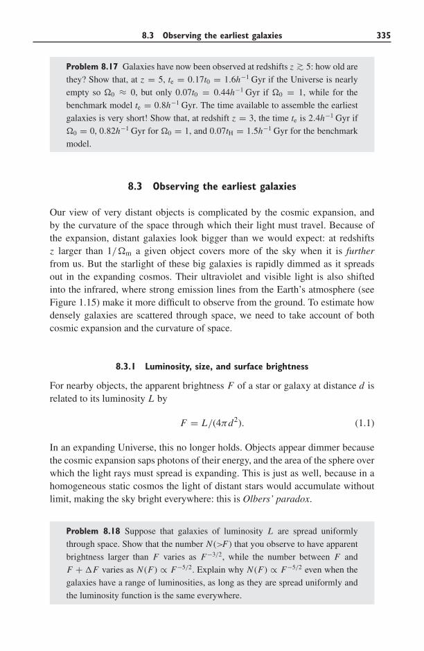
8.3 Observing the earliest galaxies 335

Problem 8.17 Galaxies have now been observed at redshifts z ∼> 5: how old are

they? Show that, at z = 5, te = 0.17t0 = 1.6h−1 Gyr if the Universe is nearly

empty so �0 ≈ 0, but only 0.07t0 = 0.44h−1 Gyr if �0 = 1, while for the

benchmark model te = 0.8h−1 Gyr. The time available to assemble the earliest

galaxies is very short! Show that, at redshift z = 3, the time te is 2.4h−1 Gyr if

�0 = 0, 0.82h−1 Gyr for �0 = 1, and 0.07tH = 1.5h−1 Gyr for the benchmark

model.

8.3 Observing the earliest galaxies

Our view of very distant objects is complicated by the cosmic expansion, andby the curvature of the space through which their light must travel. Because ofthe expansion, distant galaxies look bigger than we would expect: at redshiftsz larger than 1/�m a given object covers more of the sky when it is furtherfrom us. But the starlight of these big galaxies is rapidly dimmed as it spreadsout in the expanding cosmos. Their ultraviolet and visible light is also shiftedinto the infrared, where strong emission lines from the Earth’s atmosphere (seeFigure 1.15) make it more difficult to observe from the ground. To estimate howdensely galaxies are scattered through space, we need to take account of bothcosmic expansion and the curvature of space.

8.3.1 Luminosity, size, and surface brightness

For nearby objects, the apparent brightness F of a star or galaxy at distance d isrelated to its luminosity L by

F = L/(4πd2). (1.1)

In an expanding Universe, this no longer holds. Objects appear dimmer becausethe cosmic expansion saps photons of their energy, and the area of the sphere overwhich the light rays must spread is expanding. This is just as well, because in ahomogeneous static cosmos the light of distant stars would accumulate withoutlimit, making the sky bright everywhere: this is Olbers’ paradox.

Problem 8.18 Suppose that galaxies of luminosity L are spread uniformly

through space. Show that the number N (>F) that you observe to have apparent

brightness larger than F varies as F−3/2, while the number between F and

F + �F varies as N (F) ∝ F−5/2. Explain why N (F) ∝ F−5/2 even when the

galaxies have a range of luminosities, as long as they are spread uniformly and

the luminosity function is the same everywhere.

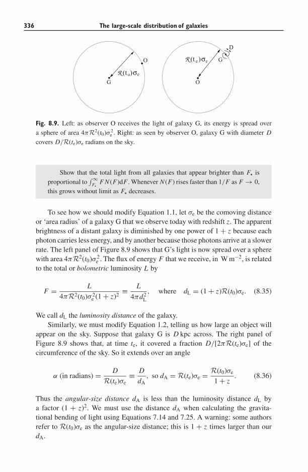
336 The large-scale distribution of galaxies

G O

O G

D

eoR σ(t )

eeR (t )σ

Fig. 8.9. Left: as observer O receives the light of galaxy G, its energy is spread over

a sphere of area 4πR2(t0)σ 2e . Right: as seen by observer O, galaxy G with diameter D

covers D/R(te)σe radians on the sky.

Show that the total light from all galaxies that appear brighter than F is

proportional to∫∞

FF N (F)dF . Whenever N (F) rises faster than 1/F as F → 0,

this grows without limit as F decreases.

To see how we should modify Equation 1.1, let σe be the comoving distanceor ‘area radius’ of a galaxy G that we observe today with redshift z. The apparentbrightness of a distant galaxy is diminished by one power of 1 + z because eachphoton carries less energy, and by another because those photons arrive at a slowerrate. The left panel of Figure 8.9 shows that G’s light is now spread over a spherewith area 4πR2(t0)σ 2

e . The flux of energy F that we receive, in W m−2, is relatedto the total or bolometric luminosity L by

F = L

4πR2(t0)σ 2e (1 + z)2

≡ L

4πd2L

, where dL = (1 + z)R(t0)σe. (8.35)

We call dL the luminosity distance of the galaxy.Similarly, we must modify Equation 1.2, telling us how large an object will

appear on the sky. Suppose that galaxy G is D kpc across. The right panel ofFigure 8.9 shows that, at time te, it covered a fraction D/[2πR(te)σe] of thecircumference of the sky. So it extends over an angle

α (in radians) = D

R(te)σe≡ D

dA, so dA = R(te)σe = R(t0)σe

1 + z. (8.36)

Thus the angular-size distance dA is less than the luminosity distance dL bya factor (1 + z)2. We must use the distance dA when calculating the gravita-tional bending of light using Equations 7.14 and 7.25. A warning: some authorsrefer to R(t0)σe as the angular-size distance; this is 1 + z times larger than ourdA.

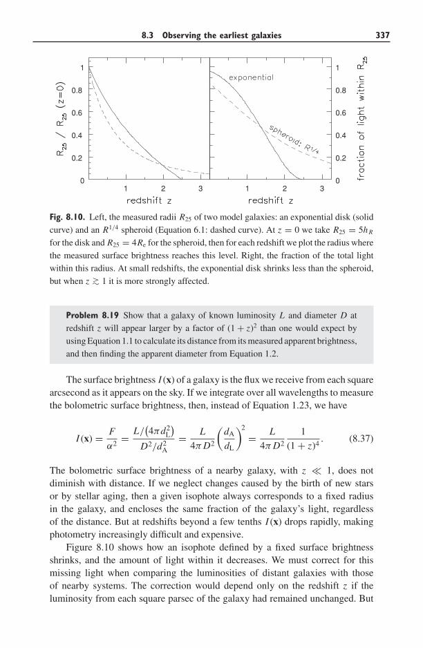
8.3 Observing the earliest galaxies 337

1 2 30

0.2

0.4

0.6

0.8

1

1 2 30

0.2

0.4

0.6

0.8

1

Fig. 8.10. Left, the measured radii R25 of two model galaxies: an exponential disk (solid

curve) and an R1/4 spheroid (Equation 6.1: dashed curve). At z = 0 we take R25 = 5h R

for the disk and R25 = 4Re for the spheroid, then for each redshift we plot the radius where

the measured surface brightness reaches this level. Right, the fraction of the total light

within this radius. At small redshifts, the exponential disk shrinks less than the spheroid,

but when z ∼> 1 it is more strongly affected.

Problem 8.19 Show that a galaxy of known luminosity L and diameter D at

redshift z will appear larger by a factor of (1 + z)2 than one would expect by

using Equation 1.1 to calculate its distance from its measured apparent brightness,

and then finding the apparent diameter from Equation 1.2.

The surface brightness I (x) of a galaxy is the flux we receive from each squarearcsecond as it appears on the sky. If we integrate over all wavelengths to measurethe bolometric surface brightness, then, instead of Equation 1.23, we have

I (x) = F

α2= L/

(4πd2

L

)D2/d2

A

= L

4π D2

(dA

dL

)2

= L

4π D2

1

(1 + z)4. (8.37)

The bolometric surface brightness of a nearby galaxy, with z � 1, does notdiminish with distance. If we neglect changes caused by the birth of new starsor by stellar aging, then a given isophote always corresponds to a fixed radiusin the galaxy, and encloses the same fraction of the galaxy’s light, regardlessof the distance. But at redshifts beyond a few tenths I (x) drops rapidly, makingphotometry increasingly difficult and expensive.

Figure 8.10 shows how an isophote defined by a fixed surface brightnessshrinks, and the amount of light within it decreases. We must correct for thismissing light when comparing the luminosities of distant galaxies with thoseof nearby systems. The correction would depend only on the redshift z if theluminosity from each square parsec of the galaxy had remained unchanged. But

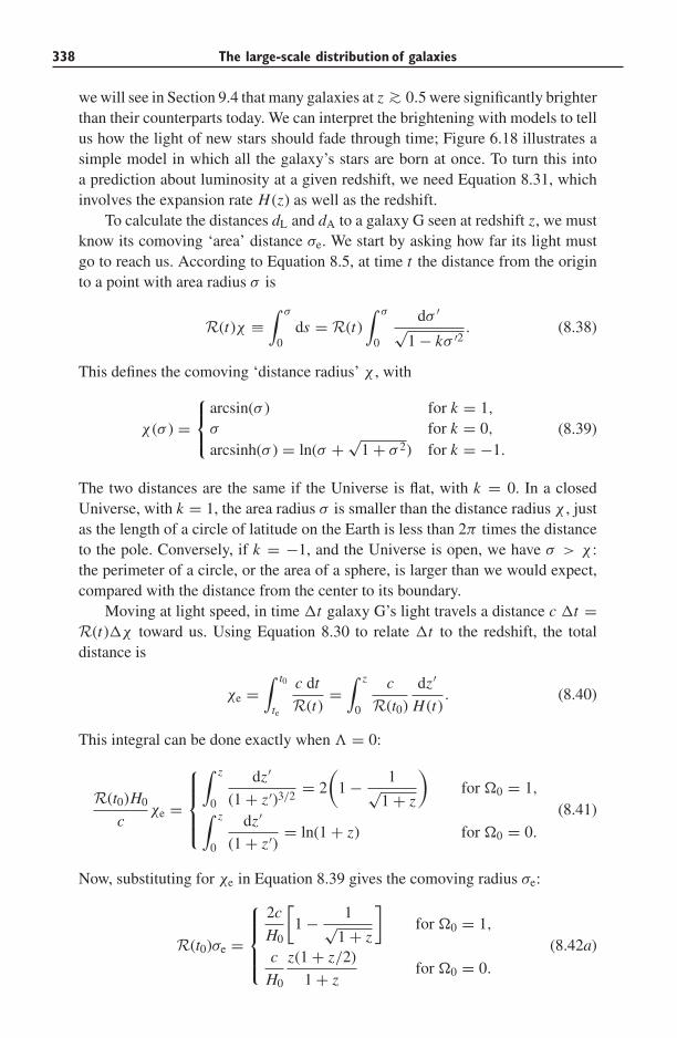
338 The large-scale distribution of galaxies

we will see in Section 9.4 that many galaxies at z ∼> 0.5 were significantly brighterthan their counterparts today. We can interpret the brightening with models to tellus how the light of new stars should fade through time; Figure 6.18 illustrates asimple model in which all the galaxy’s stars are born at once. To turn this intoa prediction about luminosity at a given redshift, we need Equation 8.31, whichinvolves the expansion rate H (z) as well as the redshift.

To calculate the distances dL and dA to a galaxy G seen at redshift z, we mustknow its comoving ‘area’ distance σe. We start by asking how far its light mustgo to reach us. According to Equation 8.5, at time t the distance from the originto a point with area radius σ is

R(t)χ ≡∫ σ

0ds = R(t)

∫ σ

0

dσ ′√

1 − kσ ′2 . (8.38)

This defines the comoving ‘distance radius’ χ , with

χ (σ ) =⎧⎨⎩

arcsin(σ ) for k = 1,

σ for k = 0,

arcsinh(σ ) = ln(σ + √1 + σ 2) for k = −1.

(8.39)

The two distances are the same if the Universe is flat, with k = 0. In a closedUniverse, with k = 1, the area radius σ is smaller than the distance radius χ , justas the length of a circle of latitude on the Earth is less than 2π times the distanceto the pole. Conversely, if k = −1, and the Universe is open, we have σ > χ :the perimeter of a circle, or the area of a sphere, is larger than we would expect,compared with the distance from the center to its boundary.

Moving at light speed, in time �t galaxy G’s light travels a distance c �t =R(t)�χ toward us. Using Equation 8.30 to relate �t to the redshift, the totaldistance is

χe =∫ t0

te

c dt

R(t)=∫ z

0

c

R(t0)

dz′

H (t). (8.40)

This integral can be done exactly when � = 0:

R(t0)H0

cχe =

⎧⎪⎪⎨⎪⎪⎩

∫ z

0

dz′

(1 + z′)3/2= 2

(1 − 1√

1 + z

)for �0 = 1,∫ z

0

dz′

(1 + z′)= ln(1 + z) for �0 = 0.

(8.41)

Now, substituting for χe in Equation 8.39 gives the comoving radius σe:

R(t0)σe =

⎧⎪⎪⎨⎪⎪⎩

2c

H0

[1 − 1√

1 + z

]for �0 = 1,

c

H0

z(1 + z/2)

1 + zfor �0 = 0.

(8.42a)

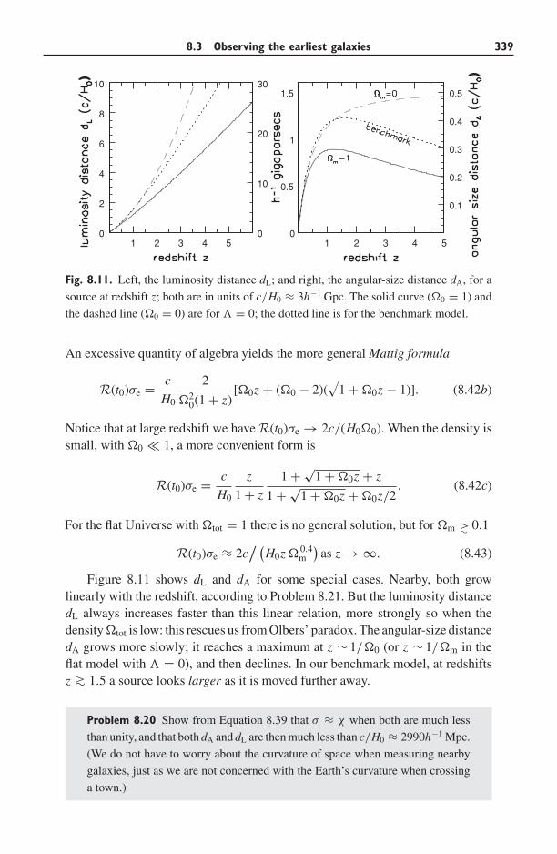
8.3 Observing the earliest galaxies 339

1 2 3 4 50

2

4

6

8

10

0

10

20

30

1 2 3 4 5

0.1

0.2

0.3

0.4

0.5

0

0.5

1

1.5

Fig. 8.11. Left, the luminosity distance dL; and right, the angular-size distance dA, for a

source at redshift z; both are in units of c/H0 ≈ 3h−1 Gpc. The solid curve (�0 = 1) and

the dashed line (�0 = 0) are for � = 0; the dotted line is for the benchmark model.

An excessive quantity of algebra yields the more general Mattig formula

R(t0)σe = c

H0

2

�20(1 + z)

[�0z + (�0 − 2)(√

1 + �0z − 1)]. (8.42b)

Notice that at large redshift we have R(t0)σe → 2c/(H0�0). When the density issmall, with �0 � 1, a more convenient form is

R(t0)σe = c

H0

z

1 + z

1 + √1 + �0z + z

1 + √1 + �0z + �0z/2

. (8.42c)

For the flat Universe with �tot = 1 there is no general solution, but for �m >∼ 0.1

R(t0)σe ≈ 2c/ (

H0z � 0.4m

)as z → ∞. (8.43)

Figure 8.11 shows dL and dA for some special cases. Nearby, both growlinearly with the redshift, according to Problem 8.21. But the luminosity distancedL always increases faster than this linear relation, more strongly so when thedensity �tot is low: this rescues us from Olbers’ paradox. The angular-size distancedA grows more slowly; it reaches a maximum at z ∼ 1/�0 (or z ∼ 1/�m in theflat model with � = 0), and then declines. In our benchmark model, at redshiftsz ∼> 1.5 a source looks larger as it is moved further away.

Problem 8.20 Show from Equation 8.39 that σ ≈ χ when both are much less

than unity, and that both dA and dL are then much less than c/H0 ≈ 2990h−1 Mpc.

(We do not have to worry about the curvature of space when measuring nearby

galaxies, just as we are not concerned with the Earth’s curvature when crossing

a town.)

340 The large-scale distribution of galaxies

Problem 8.21 Use Equation 8.40 to show that, when the redshift z � 1, both

dL and dA tend to the distance that we would normally calculate from the redshift

z: dA = R(te)σe → c/H0 ≈ dL. From Equation 8.42b, show that, when � = 0

and the redshift is large, dA → 2c/(H0z�m).

Problem 8.22 With Mbol,� = 4.75, L = 2 × 1010L�, and H0 = 70 km s−1

Mpc−1, show that, if � = 0, an L galaxy at redshift z = 3 would have mbol =25.2 if �0 = 1, or mbol = 26.6 for �0 = 0, whereas mbol = 26.1 in the

benchmark cosmology.

Problem 8.23 Show that, in a low-density Universe with �0 = 0, dA → c/(2H0)

at large redshifts. Use Figure 8.11 to show that the angle subtended by an object

10 kpc across is always at least 1.4h arcsec for �0 = 0, and ∼>3h arcsec if �0 = 1.

(The star-forming regions of Figure 9.14 have radii of 0.1–0.2 arcseconds; so

these bright patches are ∼<1 kpc across.)

8.3.2 Galaxy spectra and photometric redshifts

In practice we do not measure bolometric luminosities; we measure the appar-ent brightness in a specific band of wavelength or frequency. Cosmic expansionchanges a galaxy’s color: when we observe in a particular waveband, the lightwe now see was radiated in a bluer part of the spectrum. Suppose that, at time te,a galaxy that we see at redshift z has luminosity Lλ(λ, te)�λ in the wavelengthrange from λ to λ + �λ. The apparent brightness FBP in a bandpass BP thattransmits all the light between wavelengths λ1 and λ2 is given by Equation 8.35,if we take the luminosity L to be the energy emitted at wavelengths that will passthrough our bandpass when we receive it. So

FBP = 1

4πd2L

∫ λ2/(1+z)

λ1/(1+z)Lλ(λ, te)dλ

= 1

4πd2L

1

1 + z

∫ λ2

λ1

Lλ[λ/(1 + z), te]dλ. (8.44)

For a nearby galaxy, Equation 1.15 tells us how to calculate its apparentmagnitude at any distance. But at large redshift we must add two more terms: theapparent magnitude mBP in this bandpass is

mBP = MBP + 5 log10

(dL

10 pc

)+ kBP(z) + eBP(z). (8.45)

The absolute magnitude MBP is the apparent magnitude that the galaxy wouldhave if seen from a distance of 10 pc, emitting as it does at the present time t0.

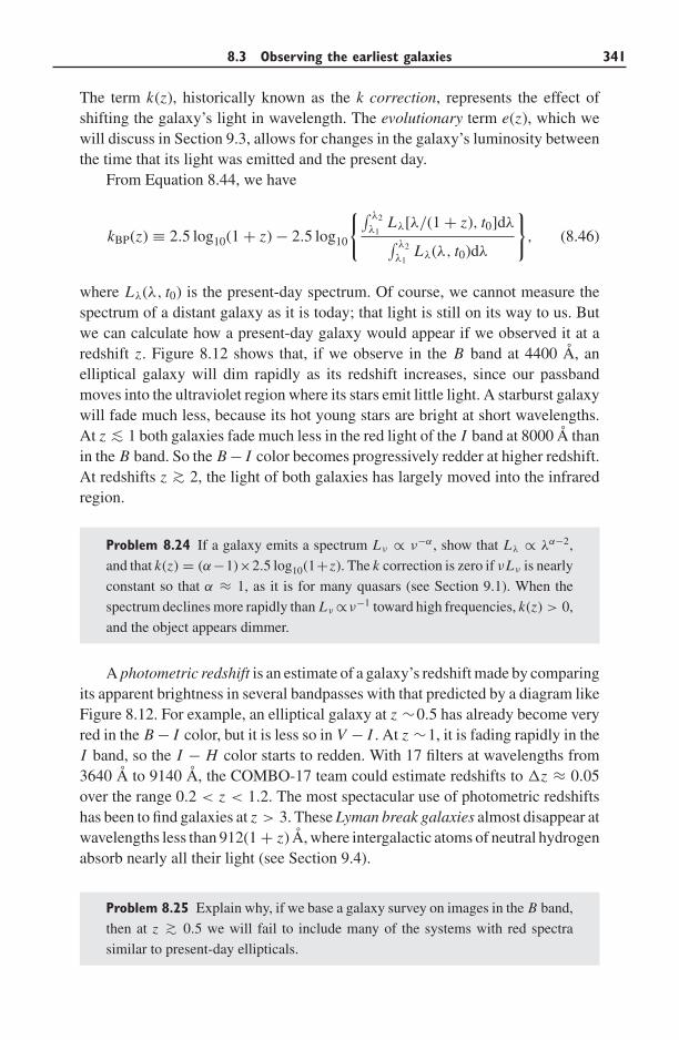
8.3 Observing the earliest galaxies 341

The term k(z), historically known as the k correction, represents the effect ofshifting the galaxy’s light in wavelength. The evolutionary term e(z), which wewill discuss in Section 9.3, allows for changes in the galaxy’s luminosity betweenthe time that its light was emitted and the present day.

From Equation 8.44, we have

kBP(z) ≡ 2.5 log10(1 + z) − 2.5 log10

{∫ λ2λ1

Lλ[λ/(1 + z), t0]dλ∫ λ2λ1

Lλ(λ, t0)dλ

}, (8.46)

where Lλ(λ, t0) is the present-day spectrum. Of course, we cannot measure thespectrum of a distant galaxy as it is today; that light is still on its way to us. Butwe can calculate how a present-day galaxy would appear if we observed it at aredshift z. Figure 8.12 shows that, if we observe in the B band at 4400 A, anelliptical galaxy will dim rapidly as its redshift increases, since our passbandmoves into the ultraviolet region where its stars emit little light. A starburst galaxywill fade much less, because its hot young stars are bright at short wavelengths.At z ∼< 1 both galaxies fade much less in the red light of the I band at 8000 A thanin the B band. So the B − I color becomes progressively redder at higher redshift.At redshifts z ∼> 2, the light of both galaxies has largely moved into the infraredregion.

Problem 8.24 If a galaxy emits a spectrum Lν ∝ ν−α , show that Lλ ∝ λα−2,

and that k(z) = (α−1)×2.5 log10(1+z). The k correction is zero if νLν is nearly

constant so that α ≈ 1, as it is for many quasars (see Section 9.1). When the

spectrum declines more rapidly than Lν ∝ν−1 toward high frequencies, k(z) > 0,

and the object appears dimmer.

A photometric redshift is an estimate of a galaxy’s redshift made by comparingits apparent brightness in several bandpasses with that predicted by a diagram likeFigure 8.12. For example, an elliptical galaxy at z ∼0.5 has already become veryred in the B − I color, but it is less so in V − I . At z ∼1, it is fading rapidly in theI band, so the I − H color starts to redden. With 17 filters at wavelengths from3640 A to 9140 A, the COMBO-17 team could estimate redshifts to �z ≈ 0.05over the range 0.2 < z < 1.2. The most spectacular use of photometric redshiftshas been to find galaxies at z > 3. These Lyman break galaxies almost disappear atwavelengths less than 912(1 + z) A, where intergalactic atoms of neutral hydrogenabsorb nearly all their light (see Section 9.4).

Problem 8.25 Explain why, if we base a galaxy survey on images in the B band,

then at z ∼> 0.5 we will fail to include many of the systems with red spectra

similar to present-day ellipticals.

342 The large-scale distribution of galaxies

z=0

0

2

4

6

8

0

2

4

6

8

0

2

4

6

8

0

2

4

6

8

0

2

4

6

8

0

2

4

6

8 z=0.5

0

2

4

6

8

0

2

4

6

8

0

2

4

6

8 z=1.5

0.1 0.15 0.2 0.3 0.4 0.6 0.8 1 1.5 2 3 4

Fig. 8.12. Spectra of two model galaxies: the stars of the bluer system formed in a single

burst 100 Myr ago, while those of the redder galaxy are all 4 Gyr old. Vertical lines show

B, I, H, and L wavelength regions from Figure 1.7. The top panel shows the emitted

light of each galaxy, while the lower panels illustrate how the redshift affects the relative

brightness in each bandpass. The energy in each wavelength region is proportional to the

area under the curve – S. Charlot.

8.3.3 How many galaxies? Space densities

To trace the formation of galaxies through cosmic history, we must take accountof the expansion in counting the number within any given volume. The numberof objects that we will see between redshifts z and z + �z is proportional to thecorresponding volume of space �V . This is just the product of the areaA(σe, te) =4πR2(te)σ 2

e of the sphere containing the galaxy at the time its light was emittedand the distance c|�te| that the light travels toward us in the time correspondingto this interval in redshift. From Equations 8.30 and 8.31, we have

Ac|�te|�z

≈ dVdz

= 4πcR2(t0)σ 2e

H (z)(1 + z)3, (8.47)

where we replaced R(te) by R(t0)/(1 + z) in the last step.The volume �V at redshift z will expand to fill a volume �V(1 + z)3 by

the present day: we refer to �V(1 + z)3 as the comoving volume. If the numberof galaxies in the Universe had always remained constant, then the comovingdensity, the number in each unit of comoving volume, would not change. If thereare presently n0 of a particular galaxy type in each cubic gigaparsec, then between

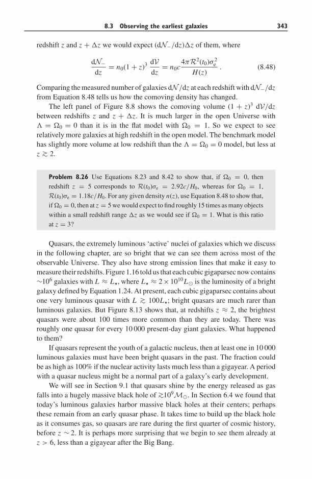
8.3 Observing the earliest galaxies 343

redshift z and z + �z we would expect (dN−/dz)�z of them, where

dN−dz

= n0(1 + z)3 dVdz

= n0c4πR2(t0)σ 2

e

H (z). (8.48)

Comparing the measured number of galaxies dN /dz at each redshift with dN−/dzfrom Equation 8.48 tells us how the comoving density has changed.

The left panel of Figure 8.8 shows the comoving volume (1 + z)3 dV/dzbetween redshifts z and z + �z. It is much larger in the open Universe with� = �0 = 0 than it is in the flat model with �0 = 1. So we expect to seerelatively more galaxies at high redshift in the open model. The benchmark modelhas slightly more volume at low redshift than the � = �0 = 0 model, but less atz ∼> 2.

Problem 8.26 Use Equations 8.23 and 8.42 to show that, if �0 = 0, then

redshift z = 5 corresponds to R(t0)σe = 2.92c/H0, whereas for �0 = 1,

R(t0)σe = 1.18c/H0. For any given density n(z), use Equation 8.48 to show that,

if �0 = 0, then at z = 5 we would expect to find roughly 15 times as many objects

within a small redshift range �z as we would see if �0 = 1. What is this ratio

at z = 3?

Quasars, the extremely luminous ‘active’ nuclei of galaxies which we discussin the following chapter, are so bright that we can see them across most of theobservable Universe. They also have strong emission lines that make it easy tomeasure their redshifts. Figure 1.16 told us that each cubic gigaparsec now contains∼106 galaxies with L ≈ L, where L ≈ 2×1010L� is the luminosity of a brightgalaxy defined by Equation 1.24. At present, each cubic gigaparsec contains aboutone very luminous quasar with L ∼> 100L; bright quasars are much rarer thanluminous galaxies. But Figure 8.13 shows that, at redshifts z ≈ 2, the brightestquasars were about 100 times more common than they are today. There wasroughly one quasar for every 10 000 present-day giant galaxies. What happenedto them?

If quasars represent the youth of a galactic nucleus, then at least one in 10 000luminous galaxies must have been bright quasars in the past. The fraction couldbe as high as 100% if the nuclear activity lasts much less than a gigayear. A periodwith a quasar nucleus might be a normal part of a galaxy’s early development.

We will see in Section 9.1 that quasars shine by the energy released as gasfalls into a hugely massive black hole of ∼>109M�. In Section 6.4 we found thattoday’s luminous galaxies harbor massive black holes at their centers; perhapsthese remain from an early quasar phase. It takes time to build up the black holeas it consumes gas, so quasars are rare during the first quarter of cosmic history,before z ∼ 2. It is perhaps more surprising that we begin to see them already atz > 6, less than a gigayear after the Big Bang.

344 The large-scale distribution of galaxies

10

100

1000

0.01

0.1

1

0 2 4 6

0.9250.90.80.70.50.3

Fig. 8.13. The curve shows the density of very radio-loud (νLν > 3 × 1010Lbol,� at

2.7 GHz) quasars, triangles show optically-bright quasars (L ∼> 100L); both are most

common at redshifts z ∼ 2. Numbers of quasars bright in soft X-rays (filled dots) and

hard X-rays (open dots) follow the same pattern. Density per comoving Gpc3 is calculated

using the benchmark model – J. Wall.

8.4 Growth of structure: from small beginnings

The cosmic background radiation is almost, but not quite, uniform: across thesky, its temperature differs by a few parts in 105. These tiny differences tell ushow lumpy the cosmos was at the time trec of recombination, when the radi-ation cooled enough for neutral atoms to form. Quantum fluctuations in thefield responsible for inflation left their imprint as irregularities in the densityof matter and radiation. Most versions of inflation predict that fluctuations shouldobey the random-phase hypothesis, and that the power spectrum P(k) ∝ k (seeProblem 8.7): we will call these the benchmark initial fluctuations. Equation 8.4then tells us that the density varies most strongly on small spatial scales orlarge k.

The largest features, extending a degree or more across the sky, tell us aboutthat early physics. Smaller-scale irregularities are modified by the excess grav-itational pull toward regions of high density and by the pressure of that densergas. Observing them tells us about the geometry of the Universe and its mattercontent. After recombination, dense regions rapidly became yet denser as sur-rounding matter fell into them. By observing the peculiar motions of infallinggalaxies, we can probe the large-scale distribution of mass today and compare itwith what is revealed by the light of the galaxies.

8.4.1 Fluctuations in the cosmic microwave background radiation

How did the distribution of matter affect the cosmic background radiation as weobserve it today? To reach us from an overdense region, radiation has to climb

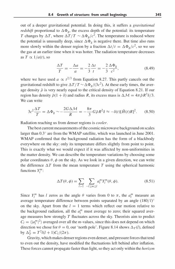
8.4 Growth of structure: from small beginnings 345

out of a deeper gravitational potential. In doing this, it suffers a gravitationalredshift proportional to ��g, the excess depth of the potential: its temperatureT changes by �T , where �T/T ∼��g/c2. The temperature is reduced wherethe potential is unusually deep, since ��g is negative there. But time also runsmore slowly within the denser region by a fraction �t/t = ��g/c2, so we seethe gas at an earlier time when it was hotter. The radiation temperature decreasesas T ∝ 1/a(t), so

�T

T= −�a

a= −2

3

�t

t= −2

3

��g

c2, (8.49)

where we have used a ∝ t2/3 from Equation 8.27. This partly cancels out thegravitational redshift to give �T/T ∼��g/(3c2). At these early times, the aver-age density ρ is very nearly equal to the critical density of Equation 8.21. If ourregion has density ρ(1 + δ) and radius R, its excess mass is �M = 4πρR3δ/3.We can write

3c2 �T

T= ��g ∼−2G�M

R= −8π

3GρR2δ ≈ −δ(t)[H (t)R]2. (8.50)

Radiation reaching us from denser regions is cooler.The best current measurements of the cosmic microwave background on scales

larger than 0.3◦ are from the WMAP satellite, which was launched in June 2001.WMAP confirmed that the background radiation has the form of a blackbodyeverywhere on the sky: only its temperature differs slightly from point to point.This is exactly what we would expect if it was affected by non-uniformities inthe matter density. We can describe the temperature variations by choosing somepolar coordinates θ, φ on the sky. As we look in a given direction, we can writethe difference �T from the mean temperature T using the spherical harmonicfunctions Y m

l :

�T (θ, φ) =∑l>1

∑−l≤m≤l

aml Y m

l (θ, φ). (8.51)

Since Y ml has l zeros as the angle θ varies from 0 to π , the am

l measure anaverage temperature difference between points separated by an angle (180/ l)◦

on the sky. Apart from the l = 1 terms which reflect our motion relative tothe background radiation, all the am

l must average to zero; their squared aver-age measures how strongly T fluctuates across the sky. Theorists aim to predictCl = 〈|am

l |2〉 averaged over all the m-values, since this does not depend on whichdirection we chose for θ = 0, our ‘north pole’. Figure 8.14 shows �T (l), definedby �2

T = T 2l(l + 1)Cl/(2π ).Gravity, which makes denser regions even denser, and pressure forces that tend

to even out the density, have modified the fluctuations left behind after inflation.These forces cannot propagate faster than light, so they act only within the horizon

346 The large-scale distribution of galaxies

2 10 40 100 200 400 600 800 1000 1200 1400 1600

0.20.512520

0

20

40

60

80

3050100200

Fig. 8.14. Temperature fluctuations �T in the cosmic microwave background: triangular

points combine data from many experiments, circles are from WMAP. Horizontal bars

show the range of angular scales. Curves show predictions for the benchmark model

(solid), for a flat model with half as many baryons (dotted), and for �0 = 0.3, � = 0

(dashed). The second, third, and subsequent peaks correspond to regions that sound waves

could cross twice, three times, etc., before recombination. When l is small, we have few

aml to average over (only five for l = 2), and vertical bars indicate larger uncertainties –

M. Tegmark, CMBFAST.

scale of Problem 8.14. When the gas became transparent, the comoving distanceσH to the horizon was

R(trec)σH = 3ctrec = 2c

H (trec)≈ 2c

H0√

�m(1 + zrec)3/2, (8.52)

where we used Equation 8.26 in the last step. (Why can we ignore ��?) A regionof this size will expand to 184/(h2�m)1/2 Mpc by today. Because inflation leftus with P(k) ∝ k, on larger scales (at small l), we should expect �T (l) to risesmoothly as l increases.

The angle θH that the horizon covers on the sky depends on �� and �m

through the angular-size distance dA. When � = 0 and �0z � 1, Equation 8.42tells us that dA → 2c/(H0z�0). So only points separated by less than the angle

θH ≈ R(trec)σH

dA(trec)≈√

�0

zrec≈ 2◦ ×

√�0 (8.53)

can communicate before time trec. The lower the matter density, the smaller thisangle should be. Detailed calculation shows that, if �0 = 1, �T is largest onscales just less than a degree, where we see the main acoustic peak in Figure 8.14.

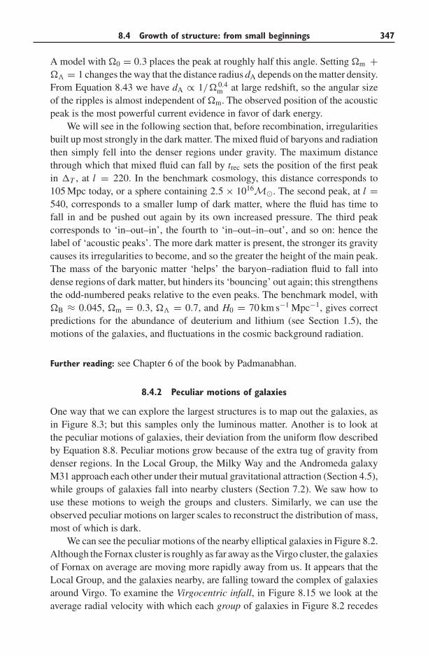
8.4 Growth of structure: from small beginnings 347

A model with �0 = 0.3 places the peak at roughly half this angle. Setting �m +�� = 1 changes the way that the distance radius dA depends on the matter density.From Equation 8.43 we have dA ∝ 1/� 0.4

m at large redshift, so the angular sizeof the ripples is almost independent of �m. The observed position of the acousticpeak is the most powerful current evidence in favor of dark energy.

We will see in the following section that, before recombination, irregularitiesbuilt up most strongly in the dark matter. The mixed fluid of baryons and radiationthen simply fell into the denser regions under gravity. The maximum distancethrough which that mixed fluid can fall by trec sets the position of the first peakin �T , at l = 220. In the benchmark cosmology, this distance corresponds to105 Mpc today, or a sphere containing 2.5 × 1016M�. The second peak, at l =540, corresponds to a smaller lump of dark matter, where the fluid has time tofall in and be pushed out again by its own increased pressure. The third peakcorresponds to ‘in–out–in’, the fourth to ‘in–out–in–out’, and so on: hence thelabel of ‘acoustic peaks’. The more dark matter is present, the stronger its gravitycauses its irregularities to become, and so the greater the height of the main peak.The mass of the baryonic matter ‘helps’ the baryon–radiation fluid to fall intodense regions of dark matter, but hinders its ‘bouncing’ out again; this strengthensthe odd-numbered peaks relative to the even peaks. The benchmark model, with�B ≈ 0.045, �m = 0.3, �� = 0.7, and H0 = 70 km s−1 Mpc−1, gives correctpredictions for the abundance of deuterium and lithium (see Section 1.5), themotions of the galaxies, and fluctuations in the cosmic background radiation.

Further reading: see Chapter 6 of the book by Padmanabhan.

8.4.2 Peculiar motions of galaxies

One way that we can explore the largest structures is to map out the galaxies, asin Figure 8.3; but this samples only the luminous matter. Another is to look atthe peculiar motions of galaxies, their deviation from the uniform flow describedby Equation 8.8. Peculiar motions grow because of the extra tug of gravity fromdenser regions. In the Local Group, the Milky Way and the Andromeda galaxyM31 approach each other under their mutual gravitational attraction (Section 4.5),while groups of galaxies fall into nearby clusters (Section 7.2). We saw how touse these motions to weigh the groups and clusters. Similarly, we can use theobserved peculiar motions on larger scales to reconstruct the distribution of mass,most of which is dark.

We can see the peculiar motions of the nearby elliptical galaxies in Figure 8.2.Although the Fornax cluster is roughly as far away as the Virgo cluster, the galaxiesof Fornax on average are moving more rapidly away from us. It appears that theLocal Group, and the galaxies nearby, are falling toward the complex of galaxiesaround Virgo. To examine the Virgocentric infall, in Figure 8.15 we look at theaverage radial velocity with which each group of galaxies in Figure 8.2 recedes

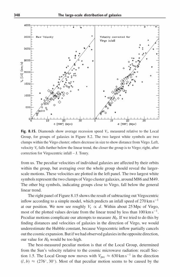
348 The large-scale distribution of galaxies

Fig. 8.15. Diamonds show average recession speed Vr, measured relative to the Local

Group, for groups of galaxies in Figure 8.2. The two largest white symbols are two

clumps within the Virgo cluster; others decrease in size to show distance from Virgo. Left,

velocity Vr falls further below the linear trend, the closer the group is to Virgo; right, after

correction for Virgocentric infall – J. Tonry.

from us. The peculiar velocities of individual galaxies are affected by their orbitswithin the group, but averaging over the whole group should reveal the larger-scale motions. These velocities are plotted in the left panel. The two largest whitesymbols represent the two clumps of Virgo cluster galaxies, around M86 and M49.The other big symbols, indicating groups close to Virgo, fall below the generallinear trend.

The right panel of Figure 8.15 shows the result of subtracting out Virgocentricinflow according to a simple model, which predicts an infall speed of 270 km s−1

at our position. We now see roughly Vr ∝ d . Within about 25 Mpc of Virgo,most of the plotted values deviate from the linear trend by less than 100 km s−1.Peculiar motions complicate our attempts to measure H0. If we tried to do this byfinding distances and velocities of galaxies in the direction of Virgo, we wouldunderestimate the Hubble constant, because Virgocentric inflow partially cancelsout the cosmic expansion. But if we had observed galaxies in the opposite direction,our value for H0 would be too high.

The best-measured peculiar motion is that of the Local Group, determinedfrom the Sun’s velocity relative to the cosmic microwave radiation: recall Sec-tion 1.5. The Local Group now moves with Vpec ≈ 630 km s−1 in the direction(l, b) ≈ (276◦, 30◦). Most of that peculiar motion seems to be caused by the

8.4 Growth of structure: from small beginnings 349

gravitational pull of very distant matter, tugging at both us and the Virgo cluster.The velocities of galaxies furthest from the Virgo cluster, which are mostly onthe opposite side of the sky, lie mainly above the sloping line in the right panelof Figure 8.15. This is what we would expect if more distant matter were pullingVirgo and Fornax apart.

Both the local velocity dispersion and the Local Group’s motion towardthe Virgo cluster are significantly less than our motion relative to the cosmicmicrowave background. The flow of galaxies through space is ‘cold’ on smallscales: galaxies within tens of megaparsecs of each other share a large fraction oftheir peculiar velocity.

Problem 8.27 Here you use Monte Carlo simulation to show that the peculiar

velocities of nearby galaxies must be very close to that of the Milky Way, or

Hubble could never have discovered the cosmic expansion from his sample of

22 local galaxies.

Your model sky consists of galaxies in regions A (1 Mpc < d < 3 Mpc), B

(3 Mpc < d < 5 Mpc), C (5 Mpc < d < 7 Mpc), and D (7 Mpc < d < 9 Mpc).

If the density is uniform, and you have four galaxies in region B, how many

are in regions A, C, and D (round to the nearest integer)? For simplicity, put

all the objects in region A at d = 2 Mpc, those in B at 4 Mpc, those in C at

6 Mpc, and those in D at 8 Mpc. Now assign peculiar velocities at random to

the galaxies. For each one, roll a die, note the number N on the upturned face,

and give your galaxy a radial velocity Vr = H0d + (N − 3.5) × 350 km s−1,

taking H0 = 70 km s−1 Mpc−1. (If you like to program you can use more

galaxies; place them randomly in space, and choose the peculiar velocities

from a Gaussian random distribution with zero mean and standard deviation of

600 km s−1.)

Plot both Vr and also the average velocity in each region against the distance

d; is there a clear trend? How many of your model galaxies have negative radial

velocities? How does your plot compare with the right panel of Figure 8.15?

Hubble found no galaxies beyond the Local Group that are approaching us.

8.4.3 How do peculiar velocities build up?

Peculiar velocities tend to die away as the Universe expands, because a mov-ing galaxy keeps overtaking others, until it reaches the region where its motionmatches that of the cosmic expansion. We can imagine two nearby comovingobservers, P and Q, at rest relative to the background radiation; they recede fromeach other only because of cosmic expansion. A galaxy passes observer P headingtoward Q with a peculiar motion Vpec, and arrives there after a time ≈d/Vpec. If Pand Q are close enough that Vpec � H (t)d , their separation remains almost con-stant as the galaxy travels between them. But relative to observer Q, the galaxymoves only at speed Vpec − H (t)d . The galaxy’s speed, relative to a comoving

350 The large-scale distribution of galaxies

observer at its current position, has decreased at the rate

dVpec

dt= − H (t)d

d/Vpec= −Vpec

R(t)

R(t). (8.54)

Integrating this shows that Vpec ∝ 1/R(t); a galaxy’s peculiar velocity Vpec fallsin exactly the same way as the momentum of a photon is reduced according toEquation 8.12.

If peculiar velocities simply decreased according to Equation 8.54, thenshortly after recombination at z ≈ 1100, the material of the Local Group wouldhave been moving at nearly the speed of light. But this would have caused shocksin the gas and huge distortions in the cosmic microwave background. In fact, thepeculiar motions of the galaxies were generated quite recently, by their mutualgravitational attraction. When some part of the Universe contains more matter thanaverage, its increased gravity brakes the expansion more strongly. Where there isless matter than average, the expansion is faster; the region becomes even morediffuse relative to its surroundings. So the galaxies move relative to the cosmicbackground: they acquire peculiar motions.

To calculate how this happens, suppose that the average density of matteris ρm(t), and the average expansion is described by the scale factor a(t) andthe Hubble parameter H (t). Locally, within the volume we are studying we canwrite

ρm(t) = ρm(t)[1 + δ(t)], and a(t) = a(t)[1 − ε(t)]. (8.55)

If our region is approximately spherical, the matter outside will not exert anygravitational force within it; it will behave just like part of a denser, more slowlyexpanding, cosmos. Where �m[1 + δ(t)] > 1 so the local density exceeds thecritical value, expansion can be halted to form bound groups and clusters ofgalaxies.

Life is much simpler if we stay in the linear regime, where δ and ε of Equa-tion 8.55 are much less than unity. We saw in the discussion following Equa-tion 8.4 that this applies to structures with sizes larger than about 8h−1 Mpc:their density differs by only a small fraction from the cosmic average. When wesubstitute the expressions for ρm(t) and a(t) into Equation 8.25, we can thenignore terms in δ2, δε, ε2, and higher powers of these variables. Rememberingthat a(t)H (t) = a(t) and that terms involving only barred average quantities willcancel out, Equation 8.25 becomes

�[H 2

0 (1 − �tot)]+ 2

da

dt

d

dt[aε(t)] + 8πG

3ρ(t)a2(t)[δ(t) − 2ε(t)] = 0. (8.56)

Here the first term represents the change in the present density and expansion ratewithin our denser region.

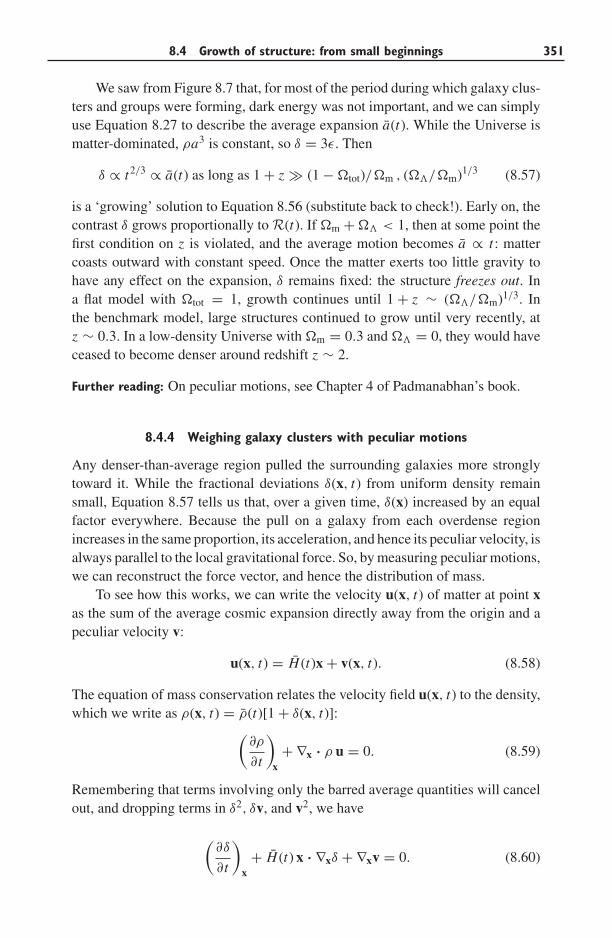
8.4 Growth of structure: from small beginnings 351

We saw from Figure 8.7 that, for most of the period during which galaxy clus-ters and groups were forming, dark energy was not important, and we can simplyuse Equation 8.27 to describe the average expansion a(t). While the Universe ismatter-dominated, ρa3 is constant, so δ = 3ε. Then

δ ∝ t2/3 ∝ a(t) as long as 1 + z � (1 − �tot)/�m , (��/�m)1/3 (8.57)

is a ‘growing’ solution to Equation 8.56 (substitute back to check!). Early on, thecontrast δ grows proportionally to R(t). If �m + �� < 1, then at some point thefirst condition on z is violated, and the average motion becomes a ∝ t : mattercoasts outward with constant speed. Once the matter exerts too little gravity tohave any effect on the expansion, δ remains fixed: the structure freezes out. Ina flat model with �tot = 1, growth continues until 1 + z ∼ (��/�m)1/3. Inthe benchmark model, large structures continued to grow until very recently, atz ∼ 0.3. In a low-density Universe with �m = 0.3 and �� = 0, they would haveceased to become denser around redshift z ∼ 2.

Further reading: On peculiar motions, see Chapter 4 of Padmanabhan’s book.

8.4.4 Weighing galaxy clusters with peculiar motions

Any denser-than-average region pulled the surrounding galaxies more stronglytoward it. While the fractional deviations δ(x, t) from uniform density remainsmall, Equation 8.57 tells us that, over a given time, δ(x) increased by an equalfactor everywhere. Because the pull on a galaxy from each overdense regionincreases in the same proportion, its acceleration, and hence its peculiar velocity, isalways parallel to the local gravitational force. So, by measuring peculiar motions,we can reconstruct the force vector, and hence the distribution of mass.

To see how this works, we can write the velocity u(x, t) of matter at point xas the sum of the average cosmic expansion directly away from the origin and apeculiar velocity v:

u(x, t) = H (t)x + v(x, t). (8.58)

The equation of mass conservation relates the velocity field u(x, t) to the density,which we write as ρ(x, t) = ρ(t)[1 + δ(x, t)]:(

∂ρ

∂t

)x+ ∇x · ρ u = 0. (8.59)

Remembering that terms involving only the barred average quantities will cancelout, and dropping terms in δ2, δv, and v2, we have

(∂δ

∂t

)x+ H (t) x · ∇xδ + ∇xv = 0. (8.60)

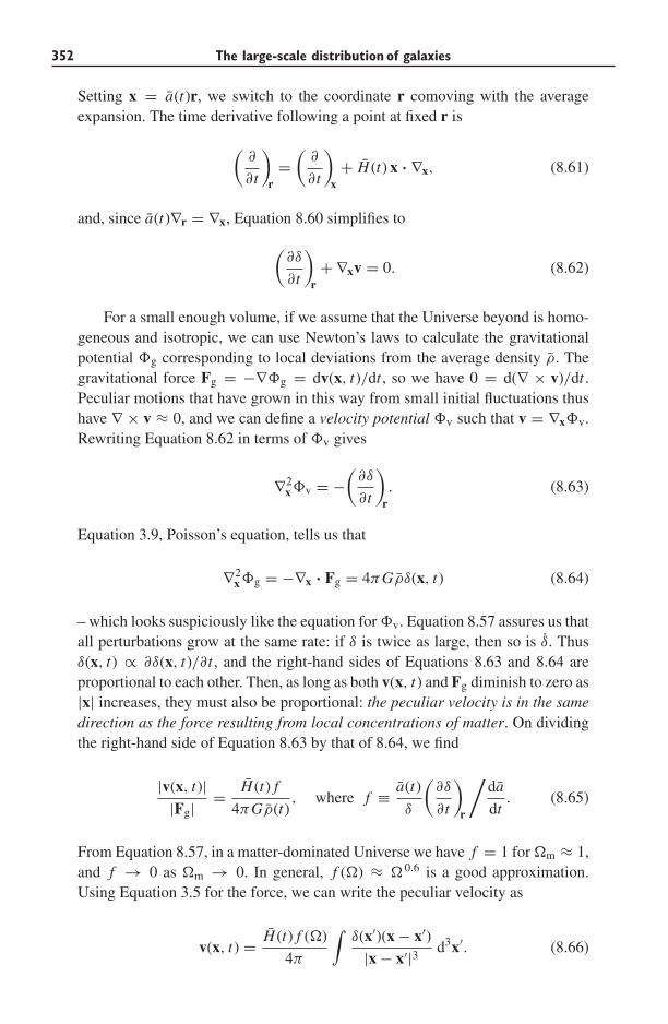
352 The large-scale distribution of galaxies

Setting x = a(t)r, we switch to the coordinate r comoving with the averageexpansion. The time derivative following a point at fixed r is

(∂

∂t

)r=(

∂

∂t

)x+ H (t) x · ∇x, (8.61)

and, since a(t)∇r = ∇x, Equation 8.60 simplifies to

(∂δ

∂t

)r+ ∇xv = 0. (8.62)

For a small enough volume, if we assume that the Universe beyond is homo-geneous and isotropic, we can use Newton’s laws to calculate the gravitationalpotential �g corresponding to local deviations from the average density ρ. Thegravitational force Fg = −∇�g = dv(x, t)/dt , so we have 0 = d(∇ × v)/dt .Peculiar motions that have grown in this way from small initial fluctuations thushave ∇ × v ≈ 0, and we can define a velocity potential �v such that v = ∇x�v.Rewriting Equation 8.62 in terms of �v gives

∇2x�v = −

(∂δ

∂t

)r. (8.63)

Equation 3.9, Poisson’s equation, tells us that

∇2x�g = −∇x · Fg = 4πGρδ(x, t) (8.64)

– which looks suspiciously like the equation for �v. Equation 8.57 assures us thatall perturbations grow at the same rate: if δ is twice as large, then so is δ. Thusδ(x, t) ∝ ∂δ(x, t)/∂t , and the right-hand sides of Equations 8.63 and 8.64 areproportional to each other. Then, as long as both v(x, t) and Fg diminish to zero as|x| increases, they must also be proportional: the peculiar velocity is in the samedirection as the force resulting from local concentrations of matter. On dividingthe right-hand side of Equation 8.63 by that of 8.64, we find

|v(x, t)||Fg| = H (t) f

4πGρ(t), where f ≡ a(t)

δ

(∂δ

∂t

)r

/da

dt. (8.65)

From Equation 8.57, in a matter-dominated Universe we have f = 1 for �m ≈ 1,and f → 0 as �m → 0. In general, f (�) ≈ � 0.6 is a good approximation.Using Equation 3.5 for the force, we can write the peculiar velocity as

v(x, t) = H (t) f (�)

4π

∫δ(x′)(x − x′)

|x − x′|3 d3x′. (8.66)

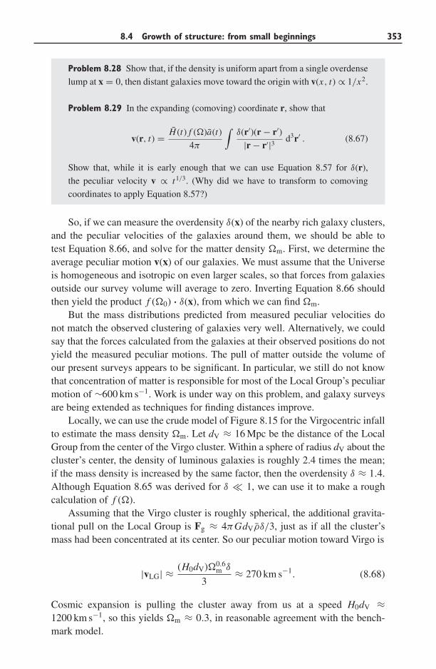
8.4 Growth of structure: from small beginnings 353

Problem 8.28 Show that, if the density is uniform apart from a single overdense

lump at x = 0, then distant galaxies move toward the origin with v(x, t) ∝ 1/x2.

Problem 8.29 In the expanding (comoving) coordinate r, show that

v(r, t) = H (t) f (�)a(t)

4π

∫δ(r′)(r − r′)

|r − r′|3 d3r′ . (8.67)

Show that, while it is early enough that we can use Equation 8.57 for δ(r),

the peculiar velocity v ∝ t1/3. (Why did we have to transform to comoving

coordinates to apply Equation 8.57?)

So, if we can measure the overdensity δ(x) of the nearby rich galaxy clusters,and the peculiar velocities of the galaxies around them, we should be able totest Equation 8.66, and solve for the matter density �m. First, we determine theaverage peculiar motion v(x) of our galaxies. We must assume that the Universeis homogeneous and isotropic on even larger scales, so that forces from galaxiesoutside our survey volume will average to zero. Inverting Equation 8.66 shouldthen yield the product f (�0) · δ(x), from which we can find �m.

But the mass distributions predicted from measured peculiar velocities donot match the observed clustering of galaxies very well. Alternatively, we couldsay that the forces calculated from the galaxies at their observed positions do notyield the measured peculiar motions. The pull of matter outside the volume ofour present surveys appears to be significant. In particular, we still do not knowthat concentration of matter is responsible for most of the Local Group’s peculiarmotion of ∼600 km s−1. Work is under way on this problem, and galaxy surveysare being extended as techniques for finding distances improve.

Locally, we can use the crude model of Figure 8.15 for the Virgocentric infallto estimate the mass density �m. Let dV ≈ 16 Mpc be the distance of the LocalGroup from the center of the Virgo cluster. Within a sphere of radius dV about thecluster’s center, the density of luminous galaxies is roughly 2.4 times the mean;if the mass density is increased by the same factor, then the overdensity δ ≈ 1.4.Although Equation 8.65 was derived for δ � 1, we can use it to make a roughcalculation of f (�).

Assuming that the Virgo cluster is roughly spherical, the additional gravita-tional pull on the Local Group is Fg ≈ 4πGdVρδ/3, just as if all the cluster’smass had been concentrated at its center. So our peculiar motion toward Virgo is

|vLG| ≈ (H0dV)�0.6m δ

3≈ 270 km s−1. (8.68)

Cosmic expansion is pulling the cluster away from us at a speed H0dV ≈1200 km s−1, so this yields �m ≈ 0.3, in reasonable agreement with the bench-mark model.

354 The large-scale distribution of galaxies

8.4.5 Tidal torques: how did galaxies get their spin?

The Sun rotates for the same reason that water swirls around the plug-hole as it runsout of a sink. The material originally had a small amount of angular momentumρx × v about its center in a random sense. This is approximately conserved asthe fluid is drawn radially inward, so as |x| decreases the rotation described by vmust speed up. But galaxies and clusters do not owe their rotation to early randommotions; this peculiar motion arises from irregular lumps of matter pulling oneach another by gravity, as illustrated in Figure 4.13.

In Problem 8.29 we saw that, while the Universe is matter-dominated, peculiarvelocities grow as t1/3, while the distance d between galaxies follows a(t) ∝ t2/3.So angular momentum builds up as d × v ∝ t as long as we remain in the linearregime with δ(t) � 1. It stops increasing when the dense region starts to collapseon itself, as we will discuss in Section 8.5. The denser the initial lump, the soonerit collapses and the less time it has to spin up. But tidal torques are stronger indenser regions, so, in a cosmos filled with cold dark matter, objects acquire thesame average angular momentum in relation to their mass and energy.

To measure how important a galaxy’s angular momentum is, we note that agalaxy of radius R, mass M, and angular momentum L will rotate with angularspeed ω ∼L/(MR2). The angular speed ωc of a circular orbit at radius R is givenby ω2

c R ∼GM/R2. The energy E ∼−GM2/R (see Problem 3.36 and recall thevirial theorem). So the ratio

λ = ω

ωc= L

MR2× R3/2

√GM

= L|E |1/2

GM5/2(8.69)

tells us how far the galaxy is supported against collapse by rotation, rather thanpressure or random motion of its stars. Gravitational N -body simulations show thatthe distribution of galaxies we observe would not spin up collapsing lumps verystrongly: we expect 0.01 < λ < 0.1. This is similar to what we see in ellipticalgalaxies, but disk galaxies like our Milky Way have λ ≈ 0.5. The parameter λ

can increase if material loses energy to move inward, as a gas disk can do byradiation.

This argument already tells us that the Milky Way has a dark halo – otherwiseits disk would not have time to form. Without a halo, L and M do not change asthe proto-disk moves inward, so its radius must shrink 100-fold to increase E bythe same factor. Disk material near the Sun must originate 800 kpc from the center,but the mass M(<R) within that radius would be just what now lies between theSun’s orbit and the Galactic center. Equation 3.20 shows that the orbital periodwould then be 1000 times longer than that in the Sun’s current orbit, or about240 Gyr. The Galaxy would shrink at roughly the same rate; it would take severaltimes longer than the age of the Universe to make the disk.

But in Problem 3.5 we saw that the Milky Way hasM/L ∼> 50; at least 90% ofits mass is dark. Because the dark halo cannot lose energy and shrink, the gas that

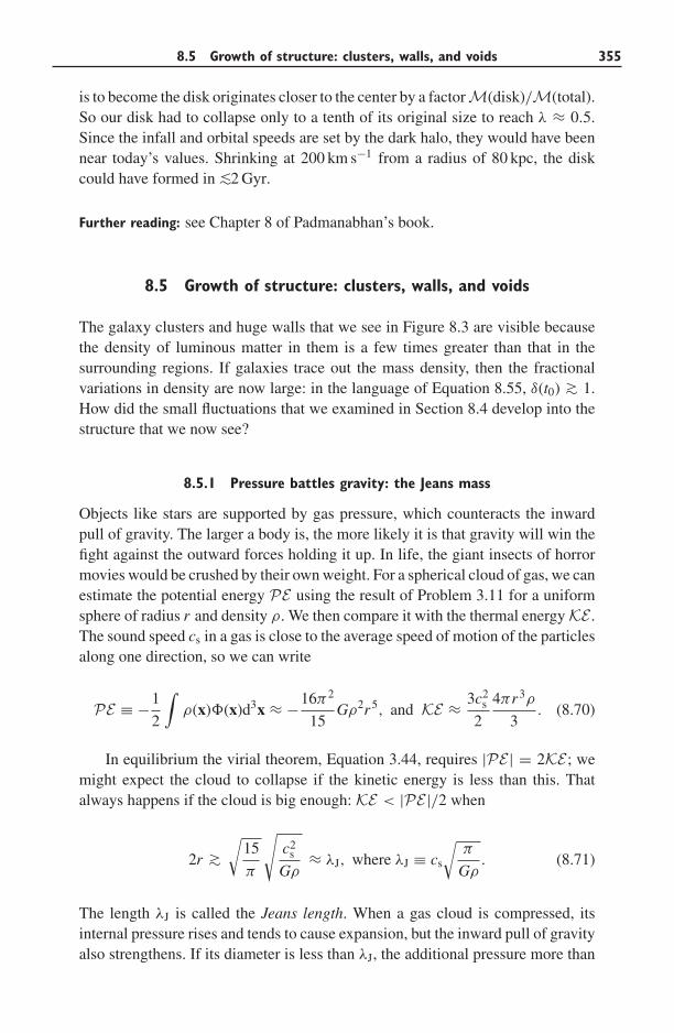
8.5 Growth of structure: clusters, walls, and voids 355

is to become the disk originates closer to the center by a factorM(disk)/M(total).So our disk had to collapse only to a tenth of its original size to reach λ ≈ 0.5.Since the infall and orbital speeds are set by the dark halo, they would have beennear today’s values. Shrinking at 200 km s−1 from a radius of 80 kpc, the diskcould have formed in ∼<2 Gyr.

Further reading: see Chapter 8 of Padmanabhan’s book.

8.5 Growth of structure: clusters, walls, and voids

The galaxy clusters and huge walls that we see in Figure 8.3 are visible becausethe density of luminous matter in them is a few times greater than that in thesurrounding regions. If galaxies trace out the mass density, then the fractionalvariations in density are now large: in the language of Equation 8.55, δ(t0) ∼> 1.How did the small fluctuations that we examined in Section 8.4 develop into thestructure that we now see?

8.5.1 Pressure battles gravity: the Jeans mass

Objects like stars are supported by gas pressure, which counteracts the inwardpull of gravity. The larger a body is, the more likely it is that gravity will win thefight against the outward forces holding it up. In life, the giant insects of horrormovies would be crushed by their own weight. For a spherical cloud of gas, we canestimate the potential energy PE using the result of Problem 3.11 for a uniformsphere of radius r and density ρ. We then compare it with the thermal energy KE .The sound speed cs in a gas is close to the average speed of motion of the particlesalong one direction, so we can write

PE ≡ −1

2

∫ρ(x)�(x)d3x ≈ −16π2

15Gρ2r5, and KE ≈ 3c2

s

2

4πr3ρ

3. (8.70)

In equilibrium the virial theorem, Equation 3.44, requires |PE | = 2KE ; wemight expect the cloud to collapse if the kinetic energy is less than this. Thatalways happens if the cloud is big enough: KE < |PE |/2 when

2r ∼>√

15

π

√c2

s

Gρ≈ λJ, where λJ ≡ cs

√π

Gρ. (8.71)

The length λJ is called the Jeans length. When a gas cloud is compressed, itsinternal pressure rises and tends to cause expansion, but the inward pull of gravityalso strengthens. If its diameter is less than λJ, the additional pressure more than

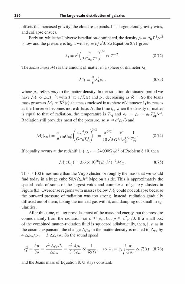
356 The large-scale distribution of galaxies

offsets the increased gravity: the cloud re-expands. In a larger cloud gravity wins,and collapse ensues.

Early on, while the Universe is radiation-dominated, the densityρr = aBT 4/c2

is low and the pressure is high, with cs = c/√

3. So Equation 8.71 gives

λJ = c2(

π

3GaBT 4

)1/2

∝ T −2. (8.72)

The Jeans mass MJ is the amount of matter in a sphere of diameter λJ:

MJ ≡ π

6λ3

Jρm, (8.73)

where ρm refers only to the matter density. In the radiation-dominated period wehave MJ ∝ ρmT −6, with T ∝ 1/R(t) and ρm decreasing as R−3. So the Jeansmass grows asMJ ∝ R3(t); the mass enclosed in a sphere of diameter λJ increasesas the Universe becomes more diffuse. At the time teq when the density of matteris equal to that of radiation, the temperature is Teq and ρm = ρr = aBT 4

eq/c2.Radiation still provides most of the pressure, so p ≈ c2ρr/3 and

MJ(teq) = π

6ρm(teq)

(πc4/3

GaBT 4eq

)3/2

= π5/2

18√

3

c4

G3/2a1/2B

1

T 2eq

. (8.74)

If equality occurs at the redshift 1 + zeq = 24 000�mh2 of Problem 8.10, then

MJ(Teq) = 3.6 × 1016(�mh2)−2M�. (8.75)

This is 100 times more than the Virgo cluster, or roughly the mass that we wouldfind today in a huge cube 50/(�mh2) Mpc on a side. This is approximately thespatial scale of some of the largest voids and complexes of galaxy clusters inFigure 8.3. Overdense regions with masses below MJ could not collapse becausethe outward pressure of radiation was too strong. Instead, radiation graduallydiffused out of them, taking the ionized gas with it, and damping out small irreg-ularities.

After this time, matter provides most of the mass and energy, but the pressurecomes mainly from the radiation: so ρ ≈ ρm, but p ≈ c2ρr/3. If a small boxof the combined matter–radiation fluid is squeezed adiabatically, then, just as inthe cosmic expansion, the change �ρm in the matter density is related to �ρr by4 �ρm/ρm = 3 �ρr/ρr. So the sound speed

c2s = ∂p

∂ρ= c2 �ρr/3

�ρm= c2

3

4ρr

3ρm∝ 1

R(t), so λJ = cs

√π

Gρm∝ R(t) (8.76)

and the Jeans mass of Equation 8.73 stays constant.

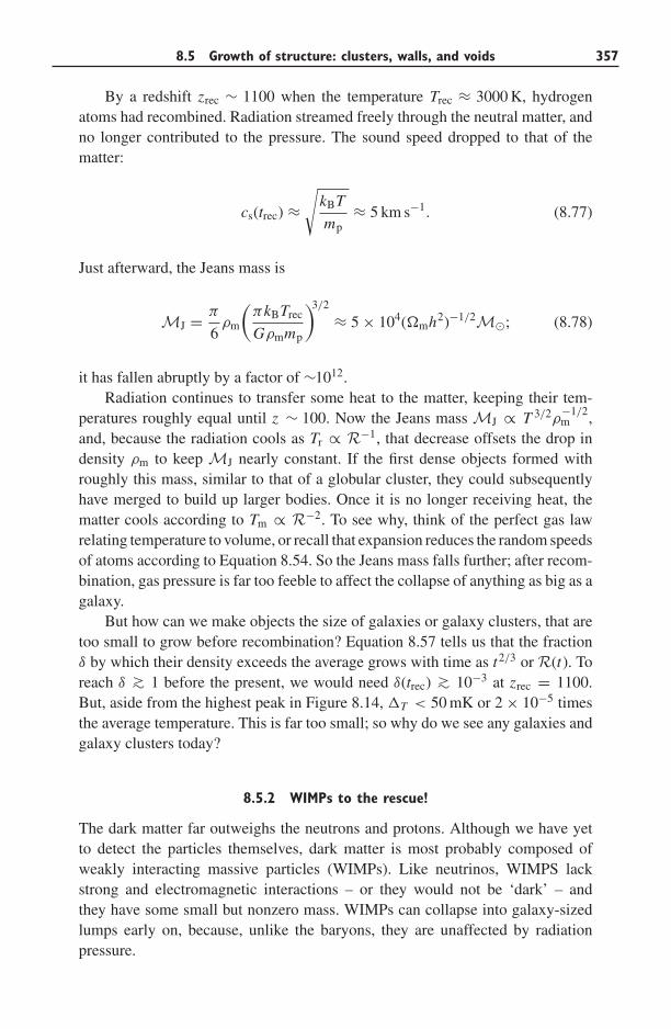
8.5 Growth of structure: clusters, walls, and voids 357

By a redshift zrec ∼ 1100 when the temperature Trec ≈ 3000 K, hydrogenatoms had recombined. Radiation streamed freely through the neutral matter, andno longer contributed to the pressure. The sound speed dropped to that of thematter:

cs(trec) ≈√

kBT

mp≈ 5 km s−1. (8.77)

Just afterward, the Jeans mass is

MJ = π

6ρm

(πkBTrec

Gρmmp

)3/2

≈ 5 × 104(�mh2)−1/2M�; (8.78)

it has fallen abruptly by a factor of ∼1012.Radiation continues to transfer some heat to the matter, keeping their tem-

peratures roughly equal until z ∼ 100. Now the Jeans mass MJ ∝ T 3/2ρ−1/2m ,

and, because the radiation cools as Tr ∝ R−1, that decrease offsets the drop indensity ρm to keep MJ nearly constant. If the first dense objects formed withroughly this mass, similar to that of a globular cluster, they could subsequentlyhave merged to build up larger bodies. Once it is no longer receiving heat, thematter cools according to Tm ∝ R−2. To see why, think of the perfect gas lawrelating temperature to volume, or recall that expansion reduces the random speedsof atoms according to Equation 8.54. So the Jeans mass falls further; after recom-bination, gas pressure is far too feeble to affect the collapse of anything as big as agalaxy.

But how can we make objects the size of galaxies or galaxy clusters, that aretoo small to grow before recombination? Equation 8.57 tells us that the fractionδ by which their density exceeds the average grows with time as t2/3 or R(t). Toreach δ ∼> 1 before the present, we would need δ(trec) ∼> 10−3 at zrec = 1100.But, aside from the highest peak in Figure 8.14, �T < 50 mK or 2 × 10−5 timesthe average temperature. This is far too small; so why do we see any galaxies andgalaxy clusters today?

8.5.2 WIMPs to the rescue!

The dark matter far outweighs the neutrons and protons. Although we have yetto detect the particles themselves, dark matter is most probably composed ofweakly interacting massive particles (WIMPs). Like neutrinos, WIMPS lackstrong and electromagnetic interactions – or they would not be ‘dark’ – andthey have some small but nonzero mass. WIMPs can collapse into galaxy-sizedlumps early on, because, unlike the baryons, they are unaffected by radiationpressure.

358 The large-scale distribution of galaxies

To describe this collapse, we can follow the same calculation as for the Jeanslength and Jeans mass, but for WIMPs with density ρw and typical random speedscw. Instead of Equation 8.73, we find that a dense region has too little kineticenergy and falls in on itself if it contains a mass larger than

MJ,wimp = π

6ρw

(πc2

w

Gρw

)3/2

. (8.79)

While the WIMPs are relativistic, their Jeans mass is high and grows with timejust as in the radiation-dominated case. A slightly overdense region that is notactively collapsing simply disperses, as WIMPs stream out of it at light speed.All structure smaller than the horizon scale of Problem 8.14 is erased in thisway.

But as soon as the speed cw of random motions drops appreciably below c/√

3,the Jeans mass starts to fall. Very roughly, all dense clumps of WIMPs that arelarger than the horizon scale at the time when they cease moving relativisticallynow begin to collapse. Since inflation left behind fluctuations with a power spec-trum P(k) rising with k, lumps just larger than this will have the highest densities.The more massive the WIMPs, the smaller the horizon scale when they cease tomove relativistically, and the smaller and denser the structures that form.

Neutrinos, with masses of a few electron-volts, remain relativistic until almostteq, when the comoving size of the horizon is ∼16(h2�m)−1 Mpc. Such light par-ticles are called hot dark matter. If the dark matter is hot, we still have difficultyin understanding how something as small as a galaxy or even a galaxy clus-ter can form. WIMPs massive enough that their sound speed cw fell below thespeed of light long before the time teq of matter–radiation equality are called colddark matter. The most popular WIMP candidates have masses ∼>1 GeV; theirrandom motions drop well below light speed when T < 1013 K, only 10−6 safter the Big Bang, when the mass MH(WIMP) within the horizon was lessthan M�.

As it escaped from the contracting clouds of WIMPs, the radiation tookthe normal matter with it. So both of these should be quite evenly spread atrecombination, and the temperature of the cosmic background radiation shouldbe nearly the same across the whole sky. At recombination, as the matter becameneutral and was freed of the radiation pressure, it fell into the already-denseclumps of WIMPs. Fluctuations in the density of normal matter could thengrow far more rapidly than Equation 8.57 allows, building up the galaxies andclusters.

If the dark matter is cold, galaxies themselves would be built from successivemerger of these smaller fragments. We call this the bottom-up picture becausegalaxies form early, and then fall together to form clusters and larger structures.Figure 8.16 shows results from a gravitational N-body simulation following theway that gravity amplifies small initial ripples in an expanding Universe of cold

8.5 Growth of structure: clusters, walls, and voids 359

Fig. 8.16. A slice 20h−1 Mpc thick, through a gravitational N-body simulation with cold

dark matter, viewed at the present day. Side frames show magnified views of dense clumps;

galaxy groups would form in these ‘dark halos’ – D. Weinberg.

dark matter. The figure shows a stage of the calculation representing the presentday. Notice the profusion of small dense clumps linked by the filamentary cosmicweb, and that smaller structures look like denser, scaled-down copies of largerones. The densest regions, shown in the side boxes, have ceased to expand andhave fallen back on themselves. Gas would accumulate there, cooling to formclusters of luminous galaxies.

Figure 8.17 combines the information from WMAP in Figure 8.14 withthat from the 2dF galaxy survey in Figures 8.3–8.5 to estimate the powerspectrum P(k) for matter today. Using a model close to the benchmark cosmology,Dr. Sanchez deduced from the irregularities in the cosmic microwave backgroundwhat the distribution of WIMPS and baryons must have been at the time trec. Hethen calculated how the concentrations of WIMPS became denser according toEquation 8.57, while baryons fell into them. The results agree with P(k) mea-sured from the galaxies of 2dF in the region where they overlap. On these scales,luminous galaxies are distributed in the same way as the dark matter, and both arewell described by the model curve. Does this mean that we have now solved allthe problems of cosmology? One might hope for a physical understanding of thedark energy, which is now simply inserted as a term in the Friedmann equations.But for the large structures that we have discussed in this chapter, the benchmarkcosmology and benchmark initial fluctuations give an excellent account of whatwe can observe.

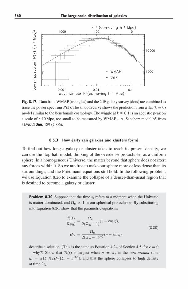
360 The large-scale distribution of galaxies

0.001 0.01 0.1

1000 100 10

1000

10000

Fig. 8.17. Data from WMAP (triangles) and the 2dF galaxy survey (dots) are combined to

trace the power spectrum P(k). The smooth curve shows the prediction from a flat (k = 0)

model similar to the benchmark cosmology. The wiggle at k ≈ 0.1 is an acoustic peak on

a scale of ∼10 Mpc, too small to be measured by WMAP – A. Sanchez: model b5 from

MNRAS 366, 189 (2006).

8.5.3 How early can galaxies and clusters form?

To find out how long a galaxy or cluster takes to reach its present density, wecan use the ‘top-hat’ model, thinking of the overdense protocluster as a uniformsphere. In a homogeneous Universe, the matter beyond that sphere does not exertany forces within it. So we are free to make our sphere more or less dense than itssurroundings, and the Friedmann equations still hold. In the following problem,we use Equation 8.26 to examine the collapse of a denser-than-usual region thatis destined to become a galaxy or cluster.

Problem 8.30 Suppose that the time t0 refers to a moment when the Universe

is matter-dominated, and �m > 1 in our spherical protocluster. By substituting

into Equation 8.26, show that the parametric equations

R(t)

R(t0)= �m

2(�m − 1)(1 − cos η),

(8.80)

H0t = �m

2(�m − 1)3/2(η − sin η)

describe a solution. (This is the same as Equation 4.24 of Section 4.5, for e = 0

– why?) Show that R(t) is largest when η = π , at the turn-around time

tta = π�m/[2H0(�m − 1)3/2], and that the sphere collapses to high density

at time 2tta.

8.5 Growth of structure: clusters, walls, and voids 361

At time t0, suppose that this denser region is expanding at the same rate as

its surroundings, and that t0 is early enough that we can apply Equation 8.27:

R(t) ∝ t2/3 so that ρ(t) ∝ 1/t2, and t0 H0 = 2/3. Using the result of Prob-

lem 8.16, show that, between t0 and tta, the density ρout outside the sphere drops

such that

ρout(tta)

ρout(t0)=[

9π2

16

�2m

(1 − �m)3

]while inside

ρin(tta)

ρin(t0)=(

�m − 1

�m

)3

. (8.81)

So ρin(tta)/ρout(tta) = (3π/4)2. As it turns around and begins to collapse, this

sphere is roughly 5.6 times denser than its surroundings.

Just as the free-fall time of Equation 3.23 is the same for all particles in a sphereof uniform density, the collapse time 2tta is the same throughout this sphere. So,in our simple model, all the particles reach the center at the same moment. In thereal cosmos, they would have small random motions which prevent this. The darkmatter and any stars present will undergo violent relaxation (see Section 6.2) asthey settle into virial equilibrium. Gas can lose energy by radiating heat away as itis compressed. Once our protocluster settles into equilibrium, the virial theoremtells us that its energy E1 = PE1 + KE1 = −PE1/2. The final energy E1 can beno greater than the total energy E0 = PE0 when it was at rest at time tta, poisedbetween expansion and contraction: so we must have PE1 < 2PE0.

Problem 8.31 Use Equation 3.33 for the potential energy PE of a galaxy of

stars to show that, if the distances between stars all shrink by a factor f , so the

density increases as 1/ f 3, then PE increases as 1/ f .

If we make the too-simple approximation that the collapse is homologous,so that all distances between particles shrink by an equal factor, Problem 8.31tells us that our protocluster’s final radius is no more than half as large as it wasat turn-around, and the density is at least eight times greater. Meanwhile, thecosmos continues to expand, and its average density has dropped at least fourtimes since tta (why?). So at the time that it reaches virial equilibrium, our clusteris 4×8×5.6 ≈ 180 times denser than the critical density for the Universe aroundit: recall Problem 8.2. In a galaxy cluster, we define the radius r200 such that,within it, the average density is 200 times the critical density; r200 is sometimescalled the virial radius. At larger radii, the cluster cannot yet be relaxed and invirial equilibrium. Even the relaxed core will be disturbed when new galaxies fallthrough it as they join the cluster.

We can use the ‘top-hat’ model to estimate when the galaxies and clusterscould have formed. Within the Sun’s orbit, the Milky Way’s density averagesto 105ρcrit. So when it collapsed at time 2tta, the average cosmic density was no

362 The large-scale distribution of galaxies

more than 500 times the present critical density; �m = 0.3, so this is 1700 timesthe present average density. The average density varies as (1 + z)3, so the collapsewas at 1 + z ≤ (1700)1/3 ≈ 12. It could have been later, since the gas can radiateaway energy, and become denser than the virial theorem predicts. But it could nothave taken place any earlier.

Problem 8.32 In Problem 7.7 we found that, in the core of the Virgo cluster,

luminous galaxies are packed 2500 times more densely than the cosmic average.

Assuming that dark and luminous matter are well mixed in the cluster, show that

its core could not have assembled before redshift z = 1.3. How early could the

central region of NGC 1399, from Problem 6.4, come together?

8.5.4 Using galaxies to test model cosmologies

How well does the benchmark cosmology with cold dark matter account for realgalaxies? Its huge success is to explain why the cosmic microwave backgroundis so smooth, while the distribution of galaxies is so lumpy. We can even explainthe shape of the power spectrum P(k) in Figure 8.17, which describes the non-uniformity. That power spectrum requires that the smallest lumps of matter arenow densest, as we saw in Figure 8.6. Problem 8.30 shows that they are the first tostop expanding and collapse on themselves. So we might expect that all galaxieswill contain some very dense regions, which should have made stars early on. Eventhe smallest galaxies should have some very old stars – as we saw in Section 4.4for the dwarf galaxies of the Local Group.

Structures that collapsed most recently should be larger and less dense thanthose that formed earlier. Using Equation 8.21 for the critical density, we can findthe mass M200 measured within the virial radius r200:

M200 = 4

3πr3

200 × 200ρcrit = 100r3200 H 2(t)

G, (8.82)

while the speed of a circular orbit at that radius is

V 2c (r200) = GM200

r200, so M200(t) = V 3

c (r200)

10G H (t). (8.83)

So, if we measure rotational or random speeds near the radius r200 (or if they donot change very much with radius), the mass or luminosity should increase steeplywith those measured speeds.

We see this pattern in the Tully–Fisher relation for disk galaxies (Figure 5.23),the fundamental plane for elliptical galaxies (Figure 6.13), and the relationbetween temperature and X-ray luminosity for gas in galaxy clusters (Figure 7.12).

8.5 Growth of structure: clusters, walls, and voids 363

In the past the Hubble parameter H (t) was larger, so we expect that temperaturesand speeds were higher for a given mass or luminosity. Figure 6.13 shows thiseffect, but in Figure 7.12 galaxy clusters at z ∼1 follow the same relation as localobjects. Adding gas to simulations like that of Figure 8.16 does result in modelgalaxies that follow Tully and Fisher’s dependence of mass on rotation speed. Butthe ‘galaxies’ fail to gather enough gas from large distances, so the disk has toolittle angular momentum and its radius is too small.

The slope of P(k) in Figure 8.17 means that small objects will be far morenumerous than large ones. The smallest have roughly the solar mass, since this isthe massMH(WIMP) within the horizon when the random motions of the WIMPsdrop below near-light speeds. The halo of a galaxy like the Milky Way is made bymerging many thousands of smaller objects, most of which are torn apart. Thosethat fall in relatively late survive today as distinct objects: satellite dark halos.In models such as that in Figure 8.16 a Milky-Way-sized dark halo will have∼300 dark satellites massive enough to have Vc > 10 km s−1. But the real MilkyWay only has ten or so luminous satellites. Choosing ‘warm’ dark matter, forwhich the random motions remained relativistic until the mass within the horizonMH(WIMP) ∼> 109M�, would erase all but the largest satellites. Some theoriesof particle physics include a ‘sterile neutrino’ with mass ∼1 keV, which wouldhave this property. Other possibilities are that their first few stars blew all theremaining gas out of most of these dark halos, or that fierce ultraviolet and X-rayradiation from the first galaxies heated it so far that it could not cool to make newstars. The Milky Way would then have 10 luminous satellites and 290 dark ones.

Another facet of the same difficulty is that we see large objects ‘too early’in cosmic history. In Section 9.4 we will find that some massive galaxies haveformed more than 1011M� of stars, corresponding to more than 1012M� of darkmatter, less than 2 Gyr after the Big Bang, at z ∼> 3. The benchmark model withcold dark matter predicts that such early ‘monster’ galaxies should be extremelyrare; it is not clear whether the model already conflicts with the observations.

If the dark matter is cold, then all galaxies should have very dense cores.Figure 8.6 shows that σR , the variation in density on lengthscale R, rises at smallR or large k. So the first regions to collapse will be the smallest and also thedensest. Equation 8.83 shows that the velocities of particles within them willalso be low, because H (t) is large. So the positions and velocities of these firstobjects are tightly grouped: the density in phase space is high. Simulations likeFigure 8.16 show that, as the galaxy is built, such objects fall together into a verydense center: the density of WIMPs follows ρw ∝ r−α, where 1 ∼< α ∼< 1.5. TheNavarro–Frenk–White model of Equation 3.24 was developed to describe thiscentral cusp. The prevalence of dwarfs in galaxy clusters (see Figure 7.8) showsthat they must indeed be robust, and hence dense, to avoid being torn apart by tidalforces. But the stars we observe are never as concentrated as this model requiresthe WIMPS to be, and the rotation curves of spiral galaxies in Figure 5.21 alsoseem to rise more gently than this form of ρw would allow.

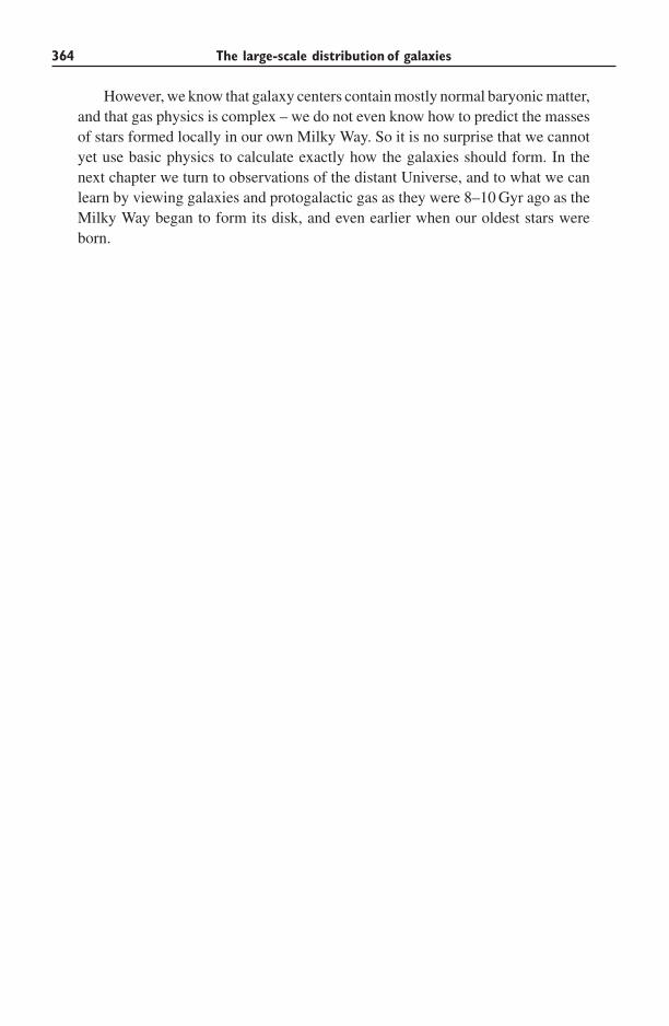
364 The large-scale distribution of galaxies

However, we know that galaxy centers contain mostly normal baryonic matter,and that gas physics is complex – we do not even know how to predict the massesof stars formed locally in our own Milky Way. So it is no surprise that we cannotyet use basic physics to calculate exactly how the galaxies should form. In thenext chapter we turn to observations of the distant Universe, and to what we canlearn by viewing galaxies and protogalactic gas as they were 8–10 Gyr ago as theMilky Way began to form its disk, and even earlier when our oldest stars wereborn.

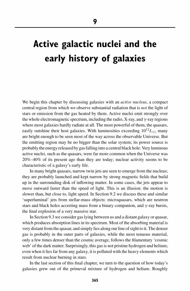
9

Active galactic nuclei and theearly history of galaxies

We begin this chapter by discussing galaxies with an active nucleus, a compactcentral region from which we observe substantial radiation that is not the light ofstars or emission from the gas heated by them. Active nuclei emit strongly overthe whole electromagnetic spectrum, including the radio, X-ray, and γ-ray regionswhere most galaxies hardly radiate at all. The most powerful of them, the quasars,easily outshine their host galaxies. With luminosities exceeding 1012L�, manyare bright enough to be seen most of the way across the observable Universe. Butthe emitting region may be no bigger than the solar system; its power source isprobably the energy released by gas falling into a central black hole. Very luminousactive nuclei, such as the quasars, were far more common when the Universe was20%–40% of its present age than they are today; nuclear activity seems to becharacteristic of a galaxy’s early life.

In many bright quasars, narrow twin jets are seen to emerge from the nucleus;they are probably launched and kept narrow by strong magnetic fields that buildup in the surrounding disk of inflowing matter. In some cases, the jets appear tomove outward faster than the speed of light. This is an illusion: the motion isslower than, but close to, light speed. In Section 9.2 we discuss these and similar‘superluminal’ jets from stellar-mass objects: microquasars, which are neutronstars and black holes accreting mass from a binary companion, and γ-ray bursts,the final explosion of a very massive star.

In Section 9.3 we consider gas lying between us and a distant galaxy or quasar,which produces absorption lines in its spectrum. Most of the absorbing material isvery distant from the quasar, and simply lies along our line of sight to it. The densergas is probably in the outer parts of galaxies, while the most tenuous material,only a few times denser than the cosmic average, follows the filamentary ‘cosmicweb’ of the dark matter. Surprisingly, this gas is not pristine hydrogen and helium;even when it lies far from any galaxy, it is polluted with the heavy elements whichresult from nuclear burning in stars.

In the last section of this final chapter, we turn to the question of how today’sgalaxies grew out of the primeval mixture of hydrogen and helium. Roughly

365

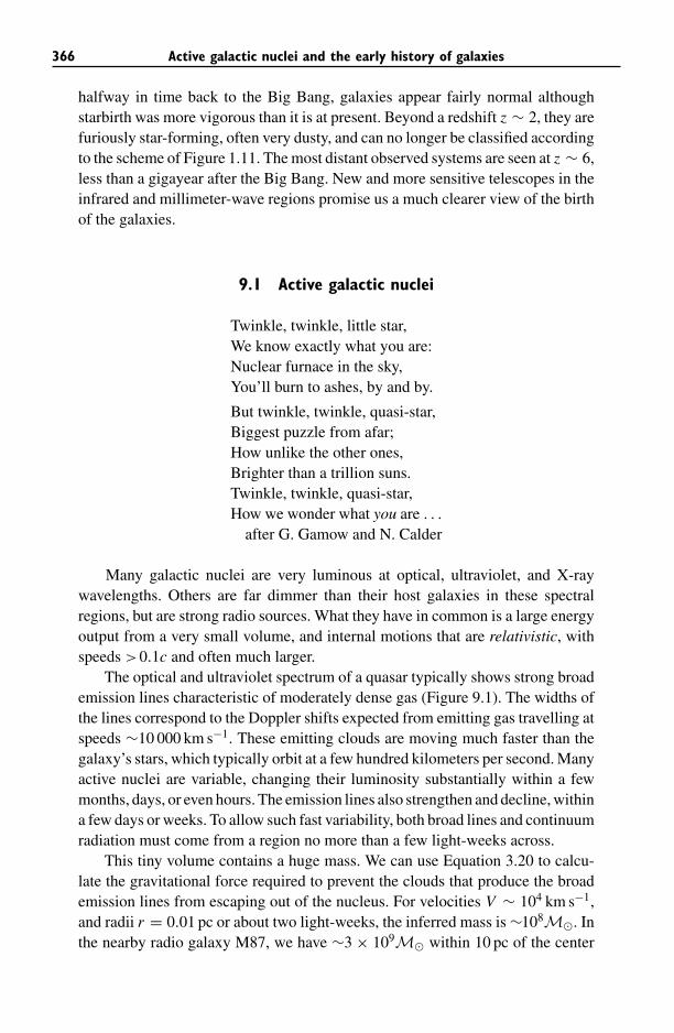
366 Active galactic nuclei and the early history of galaxies

halfway in time back to the Big Bang, galaxies appear fairly normal althoughstarbirth was more vigorous than it is at present. Beyond a redshift z ∼ 2, they arefuriously star-forming, often very dusty, and can no longer be classified accordingto the scheme of Figure 1.11. The most distant observed systems are seen at z ∼ 6,less than a gigayear after the Big Bang. New and more sensitive telescopes in theinfrared and millimeter-wave regions promise us a much clearer view of the birthof the galaxies.

9.1 Active galactic nuclei

Twinkle, twinkle, little star,We know exactly what you are:Nuclear furnace in the sky,You’ll burn to ashes, by and by.

But twinkle, twinkle, quasi-star,Biggest puzzle from afar;How unlike the other ones,Brighter than a trillion suns.Twinkle, twinkle, quasi-star,How we wonder what you are . . .

after G. Gamow and N. Calder

Many galactic nuclei are very luminous at optical, ultraviolet, and X-raywavelengths. Others are far dimmer than their host galaxies in these spectralregions, but are strong radio sources. What they have in common is a large energyoutput from a very small volume, and internal motions that are relativistic, withspeeds >0.1c and often much larger.

The optical and ultraviolet spectrum of a quasar typically shows strong broademission lines characteristic of moderately dense gas (Figure 9.1). The widths ofthe lines correspond to the Doppler shifts expected from emitting gas travelling atspeeds ∼10 000 km s−1. These emitting clouds are moving much faster than thegalaxy’s stars, which typically orbit at a few hundred kilometers per second. Manyactive nuclei are variable, changing their luminosity substantially within a fewmonths, days, or even hours. The emission lines also strengthen and decline, withina few days or weeks. To allow such fast variability, both broad lines and continuumradiation must come from a region no more than a few light-weeks across.

This tiny volume contains a huge mass. We can use Equation 3.20 to calcu-late the gravitational force required to prevent the clouds that produce the broademission lines from escaping out of the nucleus. For velocities V ∼ 104 km s−1,and radii r = 0.01 pc or about two light-weeks, the inferred mass is ∼108M�. Inthe nearby radio galaxy M87, we have ∼3 × 109M� within 10 pc of the center

9.1 Active galactic nuclei 367

1000800600 2000 3000 4000 60000

1

2

3

4

Fig. 9.1. The ultraviolet and optical spectrum of an ‘average’ radio-quiet quasar – R. Telfer

et al. 2002 Ap J 565, 773.

(Problem 6.16). The only way to pack the mass of a hundred million suns into aregion little bigger than the solar system is as a black hole. We then expect theactive nucleus to generate its power within a few times the Schwarzschild radiusRs. For a mass MBH, this is

Rs = 2GMBH

c2≈ 3 × MBH

M�km. (9.1)

Problem 9.1 Show that, for a black hole with the Earth’s mass, Rs ≈ 1 cm,

whereas if MBH = 108M�, Rs ≈ 2AU or 15 light-minutes. What is Rs for the

black hole in the Seyfert galaxy NGC 4258, of Problem 5.15?

Broad emission lines from a galactic nucleus were first reported in 1907, in theearly days of galaxy spectroscopy, but no systematic study was made until 1943.Then, Carl Seyfert published a list of 12 galaxies in which the nuclear spectrumshowed strong broad emission lines of ions that could be excited only by photonsmore energetic than those of the young stars that ionize HII regions. These werelater divided into the Seyfert 1 class, with very broad emission lines like those ofFigure 9.1, and Seyfert 2 spectra with lines ∼<1000 km s−1 wide. Most of Seyfert’sgalaxies were spirals, but his list included the huge cD galaxy NGC 1275 at thecenter of the Perseus cluster of galaxies, which is an elliptical; see Figure 7.9.Table 9.1 shows that 1%–2% of luminous galaxies have Seyfert nuclei.

In the 1950s, as radio astronomy blossomed, many of the strongest radiosources were found to be associated with luminous elliptical galaxies; these arenow called radio galaxies. In many of these, twin radio-bright lobes, each up to1 Mpc across, straddle the galaxy. The radio emission is nonthermal, producedby energetic particles moving through magnetic fields. For some years, radio

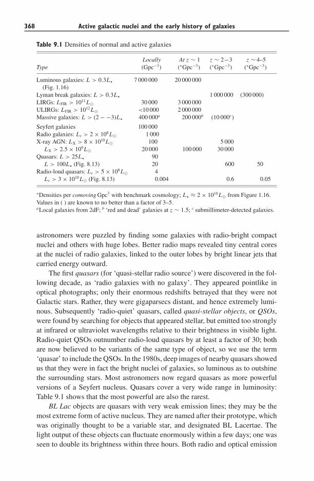
368 Active galactic nuclei and the early history of galaxies

Table 9.1 Densities of normal and active galaxies

Locally At z ∼ 1 z ∼ 2−3 z ∼ 4–5Type (Gpc−3) (∗Gpc−3) (∗Gpc−3) (∗Gpc−3)

Luminous galaxies: L > 0.3L 7 000 000 20 000 000(Fig. 1.16)

Lyman break galaxies: L > 0.3L 1 000 000 (300 000)LIRGs: LFIR > 1011 L� 30 000 3 000 000ULIRGs: LFIR > 1012 L� <10 000 2 000 000Massive galaxies: L > (2 − −3)L 400 000a 200 000b (10 000c)

Seyfert galaxies 100 000Radio galaxies: L r > 2 × 108 L� 1 000X-ray AGN: LX > 8 × 1010 L� 100 5 000

LX > 2.5 × 109 L� 20 000 100 000 30 000Quasars: L > 25L 90

L > 100L (Fig. 8.13) 20 600 50Radio-loud quasars: L r > 5 × 108 L� 4

L r > 3 × 1010 L� (Fig. 8.13) 0.004 0.6 0.05

∗Densities per comoving Gpc3 with benchmark cosmology; L ≈ 2 × 1010 L� from Figure 1.16.Values in ( ) are known to no better than a factor of 3–5.aLocal galaxies from 2dF; b ‘red and dead’ galaxies at z ∼ 1.5; c submillimeter-detected galaxies.

astronomers were puzzled by finding some galaxies with radio-bright compactnuclei and others with huge lobes. Better radio maps revealed tiny central coresat the nuclei of radio galaxies, linked to the outer lobes by bright linear jets thatcarried energy outward.

The first quasars (for ‘quasi-stellar radio source’) were discovered in the fol-lowing decade, as ‘radio galaxies with no galaxy’. They appeared pointlike inoptical photographs; only their enormous redshifts betrayed that they were notGalactic stars. Rather, they were gigaparsecs distant, and hence extremely lumi-nous. Subsequently ‘radio-quiet’ quasars, called quasi-stellar objects, or QSOs,were found by searching for objects that appeared stellar, but emitted too stronglyat infrared or ultraviolet wavelengths relative to their brightness in visible light.Radio-quiet QSOs outnumber radio-loud quasars by at least a factor of 30; bothare now believed to be variants of the same type of object, so we use the term‘quasar’ to include the QSOs. In the 1980s, deep images of nearby quasars showedus that they were in fact the bright nuclei of galaxies, so luminous as to outshinethe surrounding stars. Most astronomers now regard quasars as more powerfulversions of a Seyfert nucleus. Quasars cover a very wide range in luminosity:Table 9.1 shows that the most powerful are also the rarest.

BL Lac objects are quasars with very weak emission lines; they may be themost extreme form of active nucleus. They are named after their prototype, whichwas originally thought to be a variable star, and designated BL Lacertae. Thelight output of these objects can fluctuate enormously within a few days; one wasseen to double its brightness within three hours. Both radio and optical emission

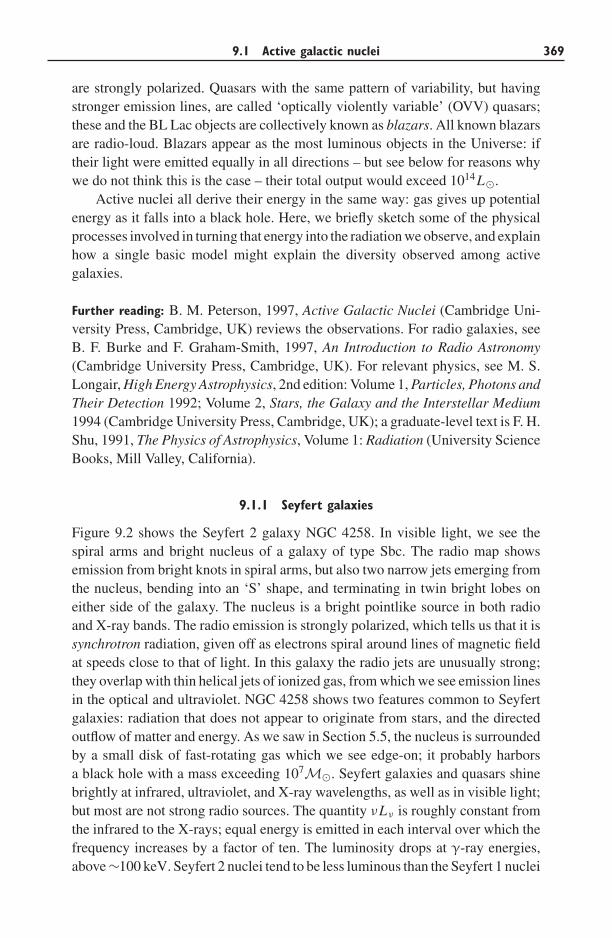
9.1 Active galactic nuclei 369

are strongly polarized. Quasars with the same pattern of variability, but havingstronger emission lines, are called ‘optically violently variable’ (OVV) quasars;these and the BL Lac objects are collectively known as blazars. All known blazarsare radio-loud. Blazars appear as the most luminous objects in the Universe: iftheir light were emitted equally in all directions – but see below for reasons whywe do not think this is the case – their total output would exceed 1014L�.

Active nuclei all derive their energy in the same way: gas gives up potentialenergy as it falls into a black hole. Here, we briefly sketch some of the physicalprocesses involved in turning that energy into the radiation we observe, and explainhow a single basic model might explain the diversity observed among activegalaxies.

Further reading: B. M. Peterson, 1997, Active Galactic Nuclei (Cambridge Uni-versity Press, Cambridge, UK) reviews the observations. For radio galaxies, seeB. F. Burke and F. Graham-Smith, 1997, An Introduction to Radio Astronomy(Cambridge University Press, Cambridge, UK). For relevant physics, see M. S.Longair, High Energy Astrophysics, 2nd edition: Volume 1, Particles, Photons andTheir Detection 1992; Volume 2, Stars, the Galaxy and the Interstellar Medium1994 (Cambridge University Press, Cambridge, UK); a graduate-level text is F. H.Shu, 1991, The Physics of Astrophysics, Volume 1: Radiation (University ScienceBooks, Mill Valley, California).

9.1.1 Seyfert galaxies

Figure 9.2 shows the Seyfert 2 galaxy NGC 4258. In visible light, we see thespiral arms and bright nucleus of a galaxy of type Sbc. The radio map showsemission from bright knots in spiral arms, but also two narrow jets emerging fromthe nucleus, bending into an ‘S’ shape, and terminating in twin bright lobes oneither side of the galaxy. The nucleus is a bright pointlike source in both radioand X-ray bands. The radio emission is strongly polarized, which tells us that it issynchrotron radiation, given off as electrons spiral around lines of magnetic fieldat speeds close to that of light. In this galaxy the radio jets are unusually strong;they overlap with thin helical jets of ionized gas, from which we see emission linesin the optical and ultraviolet. NGC 4258 shows two features common to Seyfertgalaxies: radiation that does not appear to originate from stars, and the directedoutflow of matter and energy. As we saw in Section 5.5, the nucleus is surroundedby a small disk of fast-rotating gas which we see edge-on; it probably harborsa black hole with a mass exceeding 107M�. Seyfert galaxies and quasars shinebrightly at infrared, ultraviolet, and X-ray wavelengths, as well as in visible light;but most are not strong radio sources. The quantity νLν is roughly constant fromthe infrared to the X-rays; equal energy is emitted in each interval over which thefrequency increases by a factor of ten. The luminosity drops at γ-ray energies,above ∼100 keV. Seyfert 2 nuclei tend to be less luminous than the Seyfert 1 nuclei

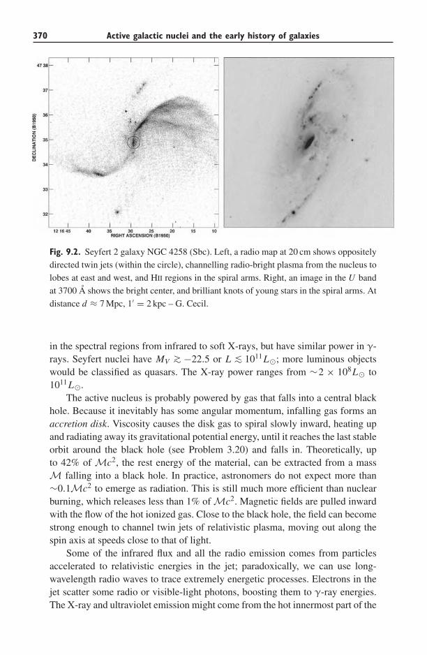
370 Active galactic nuclei and the early history of galaxies

Fig. 9.2. Seyfert 2 galaxy NGC 4258 (Sbc). Left, a radio map at 20 cm shows oppositely

directed twin jets (within the circle), channelling radio-bright plasma from the nucleus to

lobes at east and west, and HII regions in the spiral arms. Right, an image in the U band

at 3700 A shows the bright center, and brilliant knots of young stars in the spiral arms. At

distance d ≈ 7 Mpc, 1′ = 2 kpc – G. Cecil.

in the spectral regions from infrared to soft X-rays, but have similar power in γ-rays. Seyfert nuclei have MV ∼> −22.5 or L ∼< 1011L�; more luminous objectswould be classified as quasars. The X-ray power ranges from ∼2 × 108L� to1011L�.

The active nucleus is probably powered by gas that falls into a central blackhole. Because it inevitably has some angular momentum, infalling gas forms anaccretion disk. Viscosity causes the disk gas to spiral slowly inward, heating upand radiating away its gravitational potential energy, until it reaches the last stableorbit around the black hole (see Problem 3.20) and falls in. Theoretically, upto 42% of Mc2, the rest energy of the material, can be extracted from a massM falling into a black hole. In practice, astronomers do not expect more than∼0.1Mc2 to emerge as radiation. This is still much more efficient than nuclearburning, which releases less than 1% of Mc2. Magnetic fields are pulled inwardwith the flow of the hot ionized gas. Close to the black hole, the field can becomestrong enough to channel twin jets of relativistic plasma, moving out along thespin axis at speeds close to that of light.

Some of the infrared flux and all the radio emission comes from particlesaccelerated to relativistic energies in the jet; paradoxically, we can use long-wavelength radio waves to trace extremely energetic processes. Electrons in thejet scatter some radio or visible-light photons, boosting them to γ-ray energies.The X-ray and ultraviolet emission might come from the hot innermost part of the

9.1 Active galactic nuclei 371

disk, or from the jet; the visible light probably originates further out in the diskor jet. Additional infrared light may be emitted by surrounding dust grains heatedby the nuclear radiation.

The light of a Seyfert nucleus is intense enough to exert considerable pressureon gas around it. If that outward push is too strong, no gas can fall into thecenter, and the nucleus runs out of fuel. So we have a limit on the luminositythat it could sustain. For a spherically symmetric object, we can calculate at whatpoint radiation pressure just balances the inward force of gravity. We assumethat the gas near the nucleus is fully ionized hydrogen, and we calculate theoutward force due to Thomson scattering by the electrons; scattering from protonsis much less efficient because of their larger mass. The cross-section σT of eachelectron is

σT = e4

6πε20c4m2

e

(SI) or8πe4

3c4m2e

(cgs) = 6.653 × 10−25 cm2, (9.2)

where e is the charge on the electron and me is its mass. If the central sourceemits photons carrying luminosity L , these have momentum L/c, so an electronat radius r receives momentum σTL/(4πr2c) each second.

The electrons cannot move outward unless they take the protons with them;electrostatic forces are strong enough to prevent the positive and negative chargesfrom separating. So we must compare the combined outward force on the protonand the electron with the inward force of gravity on both of them. If the centralobject has mass M, radiation pressure and gravity balance when

GM(me + mp)

r2≈ GMmp

r2= σTL

4πr2c, (9.3)

where mp is the proton mass. The Eddington luminosity LE is the largest value ofL that still allows material to fall inward:

LE = 4πGMmpc

σT≈ 1.3 × 1031 M

M�W ≈ 30 000 × M

M�L�, (9.4)

where L� is the Sun’s bolometric luminosity of 3.86 × 1026 W. Stars like theSun come nowhere near the Eddington luminosity, though the brightest super-giants approach it. Although part of the radiation of a Seyfert nucleus comesout in a directed jet, its total luminosity is unlikely to be more than a few timesgreater than LE. If L ∼ 109L� then Equation 9.4 shows that the central massmust exceed 107M�, to avoid blowing away all the gas that could fuel the activenucleus.

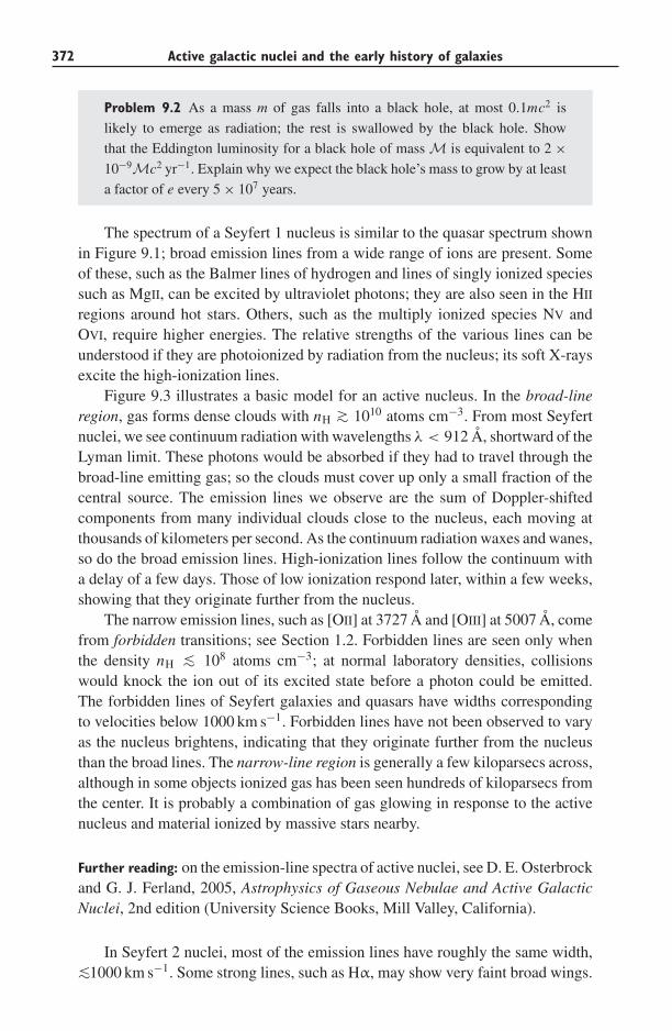
372 Active galactic nuclei and the early history of galaxies

Problem 9.2 As a mass m of gas falls into a black hole, at most 0.1mc2 is

likely to emerge as radiation; the rest is swallowed by the black hole. Show

that the Eddington luminosity for a black hole of mass M is equivalent to 2 ×10−9Mc2 yr−1. Explain why we expect the black hole’s mass to grow by at least

a factor of e every 5 × 107 years.

The spectrum of a Seyfert 1 nucleus is similar to the quasar spectrum shownin Figure 9.1; broad emission lines from a wide range of ions are present. Someof these, such as the Balmer lines of hydrogen and lines of singly ionized speciessuch as MgII, can be excited by ultraviolet photons; they are also seen in the HII

regions around hot stars. Others, such as the multiply ionized species NV andOVI, require higher energies. The relative strengths of the various lines can beunderstood if they are photoionized by radiation from the nucleus; its soft X-raysexcite the high-ionization lines.

Figure 9.3 illustrates a basic model for an active nucleus. In the broad-lineregion, gas forms dense clouds with nH ∼> 1010 atoms cm−3. From most Seyfertnuclei, we see continuum radiation with wavelengths λ < 912 A, shortward of theLyman limit. These photons would be absorbed if they had to travel through thebroad-line emitting gas; so the clouds must cover up only a small fraction of thecentral source. The emission lines we observe are the sum of Doppler-shiftedcomponents from many individual clouds close to the nucleus, each moving atthousands of kilometers per second. As the continuum radiation waxes and wanes,so do the broad emission lines. High-ionization lines follow the continuum witha delay of a few days. Those of low ionization respond later, within a few weeks,showing that they originate further from the nucleus.

The narrow emission lines, such as [OII] at 3727 A and [OIII] at 5007 A, comefrom forbidden transitions; see Section 1.2. Forbidden lines are seen only whenthe density nH ∼< 108 atoms cm−3; at normal laboratory densities, collisionswould knock the ion out of its excited state before a photon could be emitted.The forbidden lines of Seyfert galaxies and quasars have widths correspondingto velocities below 1000 km s−1. Forbidden lines have not been observed to varyas the nucleus brightens, indicating that they originate further from the nucleusthan the broad lines. The narrow-line region is generally a few kiloparsecs across,although in some objects ionized gas has been seen hundreds of kiloparsecs fromthe center. It is probably a combination of gas glowing in response to the activenucleus and material ionized by massive stars nearby.

Further reading: on the emission-line spectra of active nuclei, see D. E. Osterbrockand G. J. Ferland, 2005, Astrophysics of Gaseous Nebulae and Active GalacticNuclei, 2nd edition (University Science Books, Mill Valley, California).

In Seyfert 2 nuclei, most of the emission lines have roughly the same width,

∼<1000 km s−1. Some strong lines, such as Hα, may show very faint broad wings.

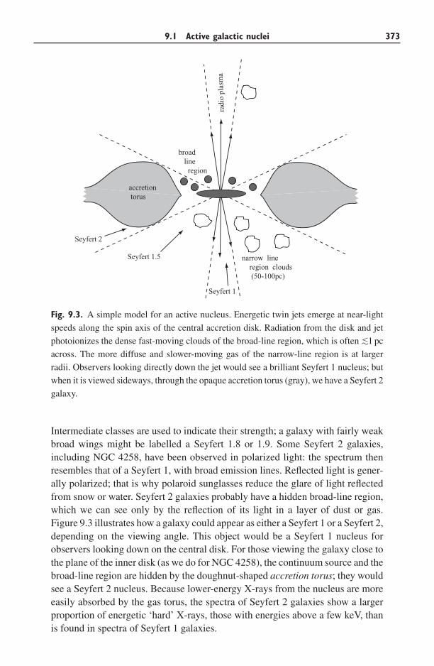
9.1 Active galactic nuclei 373

Seyfert 2

Seyfert 1.5

Seyfert 1

radi

o pl

asm

a

broad line region

narrow line region clouds (50-100pc)

accretion torus

Fig. 9.3. A simple model for an active nucleus. Energetic twin jets emerge at near-light

speeds along the spin axis of the central accretion disk. Radiation from the disk and jet

photoionizes the dense fast-moving clouds of the broad-line region, which is often ∼<1 pc

across. The more diffuse and slower-moving gas of the narrow-line region is at larger

radii. Observers looking directly down the jet would see a brilliant Seyfert 1 nucleus; but

when it is viewed sideways, through the opaque accretion torus (gray), we have a Seyfert 2

galaxy.

Intermediate classes are used to indicate their strength; a galaxy with fairly weakbroad wings might be labelled a Seyfert 1.8 or 1.9. Some Seyfert 2 galaxies,including NGC 4258, have been observed in polarized light: the spectrum thenresembles that of a Seyfert 1, with broad emission lines. Reflected light is gener-ally polarized; that is why polaroid sunglasses reduce the glare of light reflectedfrom snow or water. Seyfert 2 galaxies probably have a hidden broad-line region,which we can see only by the reflection of its light in a layer of dust or gas.Figure 9.3 illustrates how a galaxy could appear as either a Seyfert 1 or a Seyfert 2,depending on the viewing angle. This object would be a Seyfert 1 nucleus forobservers looking down on the central disk. For those viewing the galaxy close tothe plane of the inner disk (as we do for NGC 4258), the continuum source and thebroad-line region are hidden by the doughnut-shaped accretion torus; they wouldsee a Seyfert 2 nucleus. Because lower-energy X-rays from the nucleus are moreeasily absorbed by the gas torus, the spectra of Seyfert 2 galaxies show a largerproportion of energetic ‘hard’ X-rays, those with energies above a few keV, thanis found in spectra of Seyfert 1 galaxies.

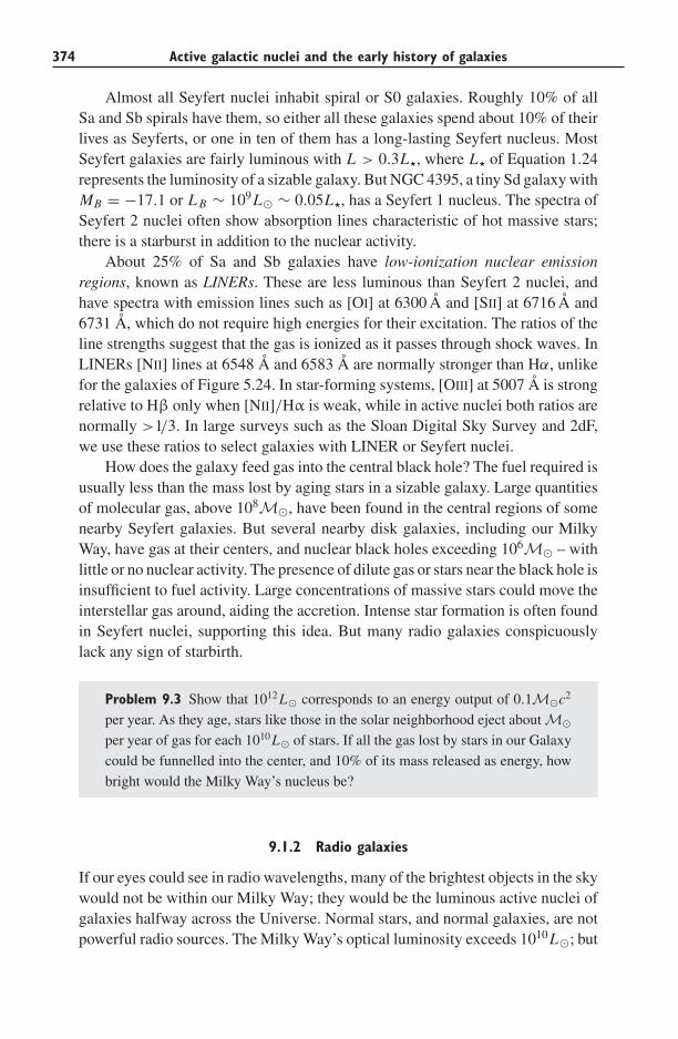
374 Active galactic nuclei and the early history of galaxies

Almost all Seyfert nuclei inhabit spiral or S0 galaxies. Roughly 10% of allSa and Sb spirals have them, so either all these galaxies spend about 10% of theirlives as Seyferts, or one in ten of them has a long-lasting Seyfert nucleus. MostSeyfert galaxies are fairly luminous with L > 0.3L, where L of Equation 1.24represents the luminosity of a sizable galaxy. But NGC 4395, a tiny Sd galaxy withMB = −17.1 or L B ∼ 109L� ∼ 0.05L, has a Seyfert 1 nucleus. The spectra ofSeyfert 2 nuclei often show absorption lines characteristic of hot massive stars;there is a starburst in addition to the nuclear activity.

About 25% of Sa and Sb galaxies have low-ionization nuclear emissionregions, known as LINERs. These are less luminous than Seyfert 2 nuclei, andhave spectra with emission lines such as [OI] at 6300 A and [SII] at 6716 A and6731 A, which do not require high energies for their excitation. The ratios of theline strengths suggest that the gas is ionized as it passes through shock waves. InLINERs [NII] lines at 6548 A and 6583 A are normally stronger than Hα, unlikefor the galaxies of Figure 5.24. In star-forming systems, [OIII] at 5007 A is strongrelative to Hβ only when [NII]/Hα is weak, while in active nuclei both ratios arenormally >1/3. In large surveys such as the Sloan Digital Sky Survey and 2dF,we use these ratios to select galaxies with LINER or Seyfert nuclei.

How does the galaxy feed gas into the central black hole? The fuel required isusually less than the mass lost by aging stars in a sizable galaxy. Large quantitiesof molecular gas, above 108M�, have been found in the central regions of somenearby Seyfert galaxies. But several nearby disk galaxies, including our MilkyWay, have gas at their centers, and nuclear black holes exceeding 106M� – withlittle or no nuclear activity. The presence of dilute gas or stars near the black hole isinsufficient to fuel activity. Large concentrations of massive stars could move theinterstellar gas around, aiding the accretion. Intense star formation is often foundin Seyfert nuclei, supporting this idea. But many radio galaxies conspicuouslylack any sign of starbirth.

Problem 9.3 Show that 1012L� corresponds to an energy output of 0.1M�c2

per year. As they age, stars like those in the solar neighborhood eject about M�per year of gas for each 1010L� of stars. If all the gas lost by stars in our Galaxy

could be funnelled into the center, and 10% of its mass released as energy, how

bright would the Milky Way’s nucleus be?

9.1.2 Radio galaxies

If our eyes could see in radio wavelengths, many of the brightest objects in the skywould not be within our Milky Way; they would be the luminous active nuclei ofgalaxies halfway across the Universe. Normal stars, and normal galaxies, are notpowerful radio sources. The Milky Way’s optical luminosity exceeds 1010L�; but

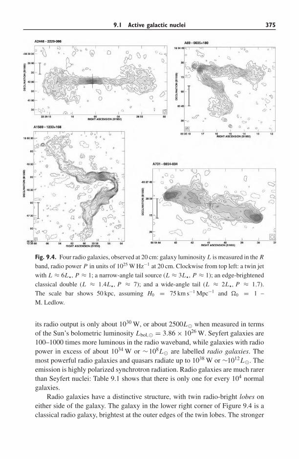
9.1 Active galactic nuclei 375

Fig. 9.4. Four radio galaxies, observed at 20 cm: galaxy luminosity L is measured in the R

band, radio power P in units of 1025 W Hz−1 at 20 cm. Clockwise from top left: a twin jet

with L ≈ 6L, P ≈ 1; a narrow-angle tail source (L ≈ 3L, P ≈ 1); an edge-brightened

classical double (L ≈ 1.4L, P ≈ 7); and a wide-angle tail (L ≈ 2L, P ≈ 1.7).

The scale bar shows 50 kpc, assuming H0 = 75 km s−1 Mpc−1 and �0 = 1 –

M. Ledlow.

its radio output is only about 1030 W, or about 2500L� when measured in termsof the Sun’s bolometric luminosity Lbol,� = 3.86 × 1026 W. Seyfert galaxies are100–1000 times more luminous in the radio waveband, while galaxies with radiopower in excess of about 1034 W or ∼108L� are labelled radio galaxies. Themost powerful radio galaxies and quasars radiate up to 1038 W or ∼1012L�. Theemission is highly polarized synchrotron radiation. Radio galaxies are much rarerthan Seyfert nuclei: Table 9.1 shows that there is only one for every 104 normalgalaxies.

Radio galaxies have a distinctive structure, with twin radio-bright lobes oneither side of the galaxy. The galaxy in the lower right corner of Figure 9.4 is aclassical radio galaxy, brightest at the outer edges of the twin lobes. The stronger

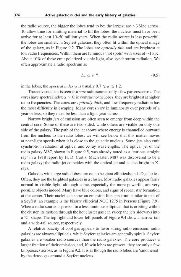
376 Active galactic nuclei and the early history of galaxies

the radio source, the bigger the lobes tend to be; the largest are ∼3 Mpc across.To allow time for emitting material to fill the lobes, the nucleus must have beenactive for at least 10–50 million years. When the radio source is less powerful,the lobes are smaller; in Seyfert galaxies, they often fit within the optical imageof the galaxy, as in Figure 9.2. The lobes are optically thin and are brightest atlow radio frequencies. Within them are luminous ‘hot spots’ with sizes of ∼1 kpc.About 10% of these emit polarized visible light, also synchrotron radiation. Weoften approximate a radio spectrum as

Lν ∝ ν−α; (9.5)

in the lobes, the spectral index α is usually 0.7 ∼< α ∼< 1.2.The active nucleus is seen as a core radio source, only a few parsecs across. The

cores have spectral index α ∼ 0; in contrast to the lobes, they are brightest at higherradio frequencies. The cores are optically thick, and low-frequency radiation hasthe most difficulty in escaping. Many cores vary in luminosity over periods of ayear or less; so they must be less than a light-year across.

Narrow bright jets of emission are often seen to emerge from deep within thecentral core. Some of these are two-sided, while others are visible on only oneside of the galaxy. The path of the jet shows where energy is channelled outwardfrom the nucleus to the radio lobes; we will see below that this matter movesat near-light speeds when it is close to the galactic nucleus. Some jets also emitsynchrotron radiation at optical and X-ray wavelengths. The optical jet of theradio galaxy M87, shown in Figure 9.5, was already noted as a ‘curious straightray’ in a 1918 report by H. D. Curtis. Much later, M87 was discovered to be aradio galaxy; the radio jet coincides with the optical jet and is also bright in X-rays.

Galaxies with large radio lobes turn out to be giant ellipticals and cD galaxies.Often, they are the brightest galaxies in a cluster. Most radio galaxies appear fairlynormal in visible light, although some, especially the more powerful, are verypeculiar objects indeed. Many have blue colors, and signs of recent star formationat the center. Their nuclei can show an emission-line spectrum similar to that ofa Seyfert: an example is the bizarre elliptical NGC 1275 in Perseus (Figure 7.9).When a radio source is present in a less luminous elliptical that is orbiting withinthe cluster, its motion through the hot cluster gas can sweep the jets sideways intoa ‘C’ shape. The top right and lower left panels of Figure 9.4 show a narrow-tailand a wide-tail source, respectively.

A relative paucity of cool gas appears to favor strong radio emission: radiogalaxies are always ellipticals, while Seyfert galaxies are generally spirals. Seyfertgalaxies are weaker radio sources than the radio galaxies. The core produces alarger fraction of their emission, and, if twin lobes are present, they are only a fewkiloparsecs across, as in Figure 9.2. It is as though the radio lobes are ‘smothered’by the dense gas around a Seyfert nucleus.

9.1 Active galactic nuclei 377

Fig. 9.5. A one-sided jet in the elliptical galaxy M87. Top, in visible light near 8000 A,

from the Hubble Space Telescope, the jet emerges from the glare of the galaxy’s center;

round white spots are globular clusters. Below, the image at 2 cm shows the radio-bright

plasma; 1 arcsec ≈ 80 pc – J. Biretta.

9.1.3 Synchrotron emission from radio galaxies

The energy stored in the lobes of a giant radio galaxy is enormous. To estimateit, we use results from the books by Longair and by Shu, which readers shouldconsult for more detail. Longair uses SI units, and Shu the cgs system which isstill common in astronomical publications. An accelerated charge q radiates awayits energy E at the rate

− dEdt

= q2|a|26πε0c3

(SI) or2q2|a|2

3c3(cgs), (9.6)

where a is the acceleration in the frame where the charge is instantaneously atrest (see formula 3.9 of Longair’s book or Chapter 16 of Shu’s). The radiation ispolarized, with its electric vector perpendicular to the direction of the acceleration:we can think of the charge dragging its electric field lines along as it moves, asin Figure 9.6. In a uniform magnetic field B, an electron spirals around the fieldlines with frequency

νL = eB

2πme(SI) or

eB

2πmec(cgs). (9.7)

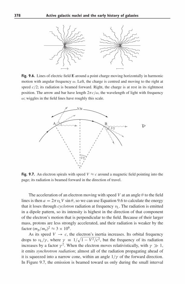
378 Active galactic nuclei and the early history of galaxies

Fig. 9.6. Lines of electric field E around a point charge moving horizontally in harmonic

motion with angular frequency ω. Left, the charge is centred and moving to the right at

speed c/2; its radiation is beamed forward. Right, the charge is at rest in its rightmost

position. The arrow and bar have length 2πc/ω, the wavelength of light with frequency

ω; wiggles in the field lines have roughly this scale.

1/γ

1/γ

VΔt

A B

Fig. 9.7. An electron spirals with speed V ≈ c around a magnetic field pointing into the

page; its radiation is beamed forward in the direction of travel.

The acceleration of an electron moving with speed V at an angle θ to the fieldlines is then a = 2πνLV sin θ , so we can use Equation 9.6 to calculate the energythat it loses through cyclotron radiation at frequency νL. The radiation is emittedin a dipole pattern, so its intensity is highest in the direction of that componentof the electron’s motion that is perpendicular to the field. Because of their largermass, protons are less strongly accelerated, and their radiation is weaker by thefactor (mp/me)2 ≈ 3 × 106.

As its speed V → c, the electron’s inertia increases. Its orbital frequencydrops to νL/γ , where γ ≡ 1/

√1 − V 2/c2, but the frequency of its radiation

increases by a factor γ 2. When the electron moves relativistically, with γ � 1,it emits synchrotron radiation; almost all of the radiation propagating ahead ofit is squeezed into a narrow cone, within an angle 1/γ of the forward direction.In Figure 9.7, the emission is beamed toward us only during the small interval

9.1 Active galactic nuclei 379

�t ∼ 2/νL when the electron is between points A and B. The arrival of that energyis squeezed into an even shorter time. Photons from point B are emitted later thanthose from A by a time �t , but their arrival is delayed only by

�t(1 − V/c) ≈ �t/(2γ 2) ∼ 1/(γ 2νL). (9.8)

Thus the frequency of the light received is not νL/γ , but roughly γ 2νL. A moreaccurate calculation (see Chapter 18 of both Longair’s book and Shu’s book)shows that most power is emitted close to the frequency

νc = 3

2γ 2νL = 4.2γ 2

(B

1 G or 10−6 T

)MHz. (9.9)

Problem 9.4 Show that, in a radio lobe where B ≈ 10 μG, an electron radiating

at 5 GHz must have γ ∼ 104.

Equation 9.6 tells us how fast the electron loses its energy. We first computeits four-velocity �u and four-vector acceleration �a = d�u/dτ , where τ is the propertime of Equation 8.9. In the instantaneous restframe of the spiralling electron�a = (0, a), so |a|2 of Equation 9.6 is equal to |�a · �a|. But �a · �a is a Lorentzinvariant, the same for all uniformly moving observers; we can compute it inour observer’s frame. There, dt/dτ = γ ; apart from radiative losses, γ remainsconstant as the electron circles the field lines, so we have

�u ≡ d�xdτ

= d�xdt

dt

dτ= γ

(1v

)and

d�udτ

= γ 2(

0dv/dt

)= �a. (9.10)

Since |dv/dt | = 2π (νL/γ )V sin θ , the product |�a · �a| = (2πγ νLV sin θ )2;the radiated energy −dE/dt ∝ γ 2. (Compare this with Longair’s derivation offormula 18.5.)

To calculate how fast the energy of an average electron decays, we assumethat they move in random directions, so that sin2θ averages to 2/3. When γ � 1,the energy loss is

− dEdt

= 4

3σTcUmagγ

2, where Umag = B2

2μ0(SI), or

B2

8π(cgs). (9.11)

Roughly half the electron’s energy E = γ mec2 is gone after a time

t1/2 = E2

∣∣∣∣ dt

dE

∣∣∣∣ ≈ 170

(10−5 G or 10−11 T

B

)2(1000

γ

)Myr. (9.12)

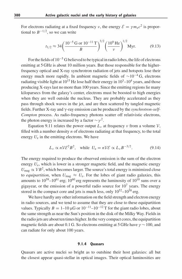
380 Active galactic nuclei and the early history of galaxies

For electrons radiating at a fixed frequency ν, the energy E = γ mec2 is propor-tional to B−1/2, so we can write

t1/2 ≈ 34

(10−5 G or 10−11 T

B

)3/2(109 Hz

ν

)1/2

Myr. (9.13)

For the fields of 10−5 G believed to be typical in radio lobes, the life of electronsemitting at 5 GHz is about 10 million years. But those responsible for the higher-frequency optical and X-ray synchrotron radiation of jets and hotspots lose theirenergy much more rapidly. In ambient magnetic fields of ∼10−4 G, electronsradiating visible light at 1015 Hz lose half their energy in 103–104 years, and thoseproducing X-rays last no more than 100 years. Since the emitting regions lie manykiloparsecs from the galaxy’s center, electrons must be boosted to high energieswhen they are well outside the nucleus. They are probably accelerated as theypass through shock waves in the jet, and are then scattered by tangled magneticfields. Further X-ray and γ-ray emission can be produced by the synchrotron-self-Compton process. As radio-frequency photons scatter off relativistic electrons,the photon energy is increased by a factor ∼γ 2.

Equation 9.11 relates the power output Lν at frequency ν from a volume V ,filled with a number density n of electrons radiating at that frequency, to the totalenergy Ue in the emitting electrons. We have

Lν ∝ nVE2 B2, while Ue = nVE ∝ Lν B−3/2. (9.14)

The energy required to produce the observed emission is the sum of the electronenergy Ue, which is lower in a stronger magnetic field, and the magnetic energyUmag ∝ VB2, which becomes larger. The source’s total energy is minimized closeto equipartition, when Umag ≈ Ue. For the lobes of giant radio galaxies, thisamounts to 1059–1061 erg; 1060 erg represents the luminosity of 1010 suns over agigayear, or the emission of a powerful radio source for 107 years. The energystored in the compact core and jets is much less, only 1052–1058 erg.

We have hardly any other information on the field strength and electron energyin radio sources, and we tend to assume that they are close to these equipartitionvalues. Typically B = 1–10 μG or 10−11–10−12 T for the giant radio lobes, aboutthe same strength as near the Sun’s position in the disk of the Milky Way. Fields inthe radio jets are about ten times higher. In the very compact cores, the equipartitionmagnetic fields are about 0.1 G. So electrons emitting at 5 GHz have γ ∼100, andcan radiate for only about 100 years.

9.1.4 Quasars

Quasars are active nuclei so bright as to outshine their host galaxies: all butthe closest appear quasi-stellar in optical images. Their optical luminosities are

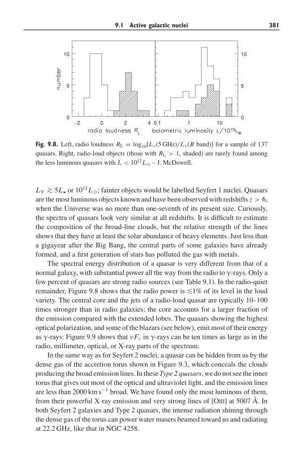
9.1 Active galactic nuclei 381

−2 0 2 40

5

10

0.1 1 100

5

10

Fig. 9.8. Left, radio loudness RL = log10[Lν(5 GHz)/Lν(B band)] for a sample of 137

quasars. Right, radio-loud objects (those with RL > 1, shaded) are rarely found among

the less luminous quasars with L < 1012L� – J. McDowell.

LV ∼> 5L or 1011L�; fainter objects would be labelled Seyfert 1 nuclei. Quasarsare the most luminous objects known and have been observed with redshifts z > 6,when the Universe was no more than one-seventh of its present size. Curiously,the spectra of quasars look very similar at all redshifts. It is difficult to estimatethe composition of the broad-line clouds, but the relative strength of the linesshows that they have at least the solar abundance of heavy elements. Just less thana gigayear after the Big Bang, the central parts of some galaxies have alreadyformed, and a first generation of stars has polluted the gas with metals.

The spectral energy distribution of a quasar is very different from that of anormal galaxy, with substantial power all the way from the radio to γ-rays. Only afew percent of quasars are strong radio sources (see Table 9.1). In the radio-quietremainder, Figure 9.8 shows that the radio power is ∼<1% of its level in the loudvariety. The central core and the jets of a radio-loud quasar are typically 10–100times stronger than in radio galaxies; the core accounts for a larger fraction ofthe emission compared with the extended lobes. The quasars showing the highestoptical polarization, and some of the blazars (see below), emit most of their energyas γ-rays: Figure 9.9 shows that νFν in γ-rays can be ten times as large as in theradio, millimeter, optical, or X-ray parts of the spectrum.

In the same way as for Seyfert 2 nuclei, a quasar can be hidden from us by thedense gas of the accretion torus shown in Figure 9.3, which conceals the cloudsproducing the broad emission lines. In these Type 2 quasars, we do not see the innertorus that gives out most of the optical and ultraviolet light, and the emission linesare less than 2000 km s−1 broad. We have found only the most luminous of them,from their powerful X-ray emission and very strong lines of [OIII] at 5007 A. Inboth Seyfert 2 galaxies and Type 2 quasars, the intense radiation shining throughthe dense gas of the torus can power water masers beamed toward us and radiatingat 22.2 GHz, like that in NGC 4258.

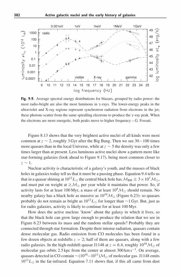
382 Active galactic nuclei and the early history of galaxies

0.0001

0.001

0.01

0.1

1

10

100

1000

0.001eV 1eV 1keV 1MeV 1GeV

9 10 11 12 13 14 15 16 17 18 19 20 21 22 23 24 25

42

43

44

45

46

47

48

49radio

visible X-ray gamma

Fig. 9.9. Average spectral energy distributions for blazars, grouped by radio power: the

most radio-bright are also the most luminous in γ-rays. The lower-energy peaks in the

ultraviolet and X-ray regions represent synchrotron radiation from electrons in the jet;

these photons scatter from the same spiralling electrons to produce the γ-ray peak. When

the electrons are more energetic, both peaks move to higher frequency – G. Fossati.

Figure 8.13 shows that the very brightest active nuclei of all kinds were mostcommon at z ∼ 2, roughly 3 Gyr after the Big Bang. Then we see 30−100 timesmore quasars than in the local Universe, while at z ∼ 5 the density was only a fewtimes larger than at present. Less luminous active nuclei show a pattern more likestar-forming galaxies (look ahead to Figure 9.17), being most common closer toz ∼ 1.

Nuclear activity is characteristic of a galaxy’s youth, and the masses of blackholes in galaxies today tell us that it must be a passing phase. Equation 9.4 tells usthat in a quasar shining at 1012L� the central black hole has MBH ∼> 3×107M�,and must put on weight at ∼>M� per year while it maintains that power. So, ifactivity lasts for at least 100 Myr, a mass of at least 109M� should remain. Nonearby galaxy has a black hole as massive as 1010M� (Figure 6.23): so quasarsprobably do not remain as bright as 1012L� for longer than ∼1 Gyr. But, just asfor radio galaxies, activity is likely to continue for at least 100 Myr.

How does the active nucleus ‘know’ about the galaxy in which it lives, sothat the black hole can grow large enough to produce the relation that we see inFigure 6.23 between its mass and the random stellar speeds? Probably they areconnected through star formation. Despite their intense radiation, quasars containdense molecular gas. Radio emission from CO molecules has been found in afew dozen objects at redshifts z > 2; half of them are quasars, along with a fewradio galaxies. In the high-redshift quasar J1148 at z = 6.4, roughly 1010M� ofmolecular gas orbits 2.5 kpc from the center at almost 300 km s−1. On average,quasars detected in CO contain ∼ (1010−1011)M� of molecular gas. J1148 emits1013L� in the far-infrared. Equation 7.11 shows that, if this all came from dust

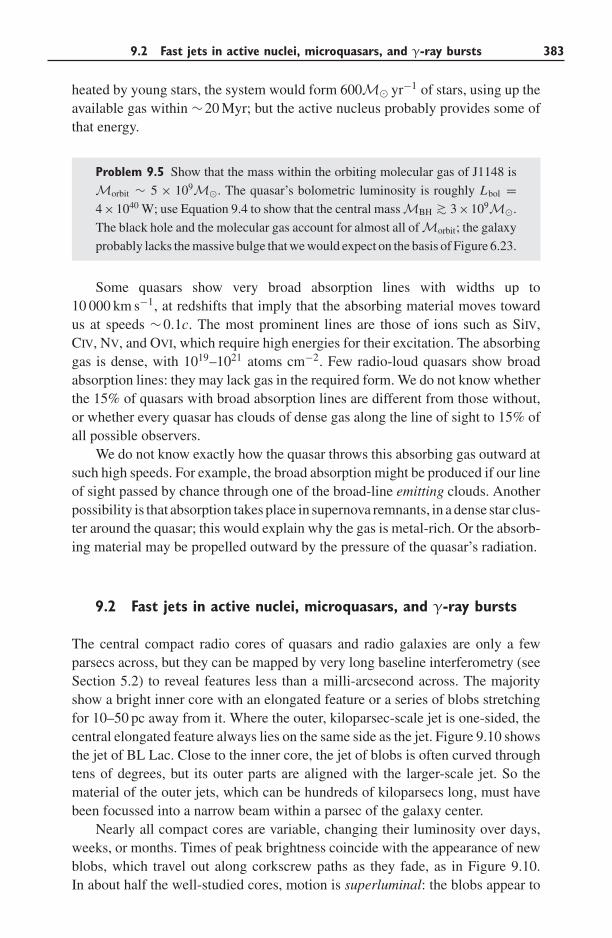
9.2 Fast jets in active nuclei, microquasars, and γ-ray bursts 383

heated by young stars, the system would form 600M� yr−1 of stars, using up theavailable gas within ∼20 Myr; but the active nucleus probably provides some ofthat energy.

Problem 9.5 Show that the mass within the orbiting molecular gas of J1148 is

Morbit ∼ 5 × 109M�. The quasar’s bolometric luminosity is roughly Lbol =4×1040 W; use Equation 9.4 to show that the central mass MBH ∼> 3×109M�.

The black hole and the molecular gas account for almost all of Morbit; the galaxy

probably lacks the massive bulge that we would expect on the basis of Figure 6.23.

Some quasars show very broad absorption lines with widths up to10 000 km s−1, at redshifts that imply that the absorbing material moves towardus at speeds ∼0.1c. The most prominent lines are those of ions such as SiIV,CIV, NV, and OVI, which require high energies for their excitation. The absorbinggas is dense, with 1019–1021 atoms cm−2. Few radio-loud quasars show broadabsorption lines: they may lack gas in the required form. We do not know whetherthe 15% of quasars with broad absorption lines are different from those without,or whether every quasar has clouds of dense gas along the line of sight to 15% ofall possible observers.

We do not know exactly how the quasar throws this absorbing gas outward atsuch high speeds. For example, the broad absorption might be produced if our lineof sight passed by chance through one of the broad-line emitting clouds. Anotherpossibility is that absorption takes place in supernova remnants, in a dense star clus-ter around the quasar; this would explain why the gas is metal-rich. Or the absorb-ing material may be propelled outward by the pressure of the quasar’s radiation.

9.2 Fast jets in active nuclei, microquasars, and γ-ray bursts

The central compact radio cores of quasars and radio galaxies are only a fewparsecs across, but they can be mapped by very long baseline interferometry (seeSection 5.2) to reveal features less than a milli-arcsecond across. The majorityshow a bright inner core with an elongated feature or a series of blobs stretchingfor 10–50 pc away from it. Where the outer, kiloparsec-scale jet is one-sided, thecentral elongated feature always lies on the same side as the jet. Figure 9.10 showsthe jet of BL Lac. Close to the inner core, the jet of blobs is often curved throughtens of degrees, but its outer parts are aligned with the larger-scale jet. So thematerial of the outer jets, which can be hundreds of kiloparsecs long, must havebeen focussed into a narrow beam within a parsec of the galaxy center.

Nearly all compact cores are variable, changing their luminosity over days,weeks, or months. Times of peak brightness coincide with the appearance of newblobs, which travel out along corkscrew paths as they fade, as in Figure 9.10.In about half the well-studied cores, motion is superluminal: the blobs appear to

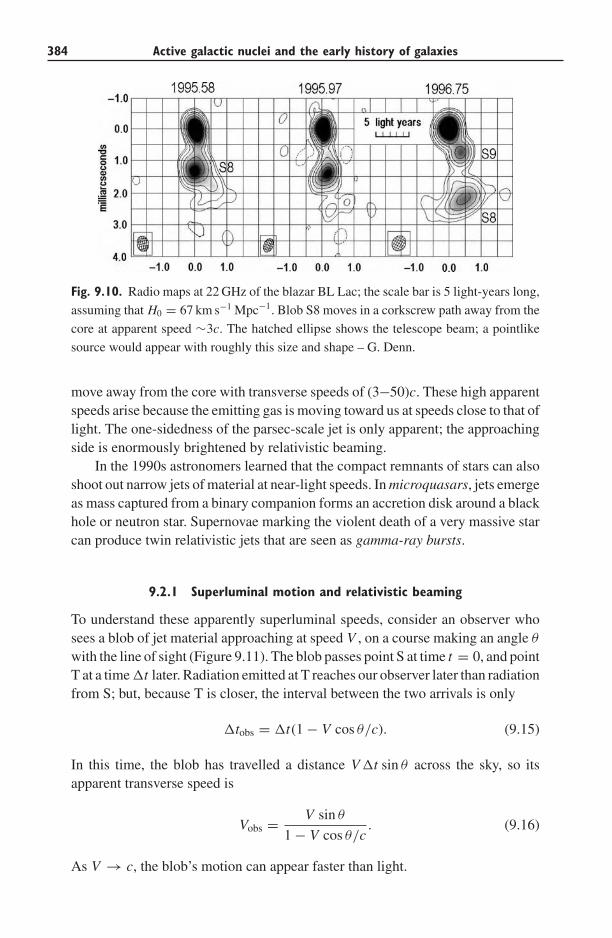
384 Active galactic nuclei and the early history of galaxies

Fig. 9.10. Radio maps at 22 GHz of the blazar BL Lac; the scale bar is 5 light-years long,

assuming that H0 = 67 km s−1 Mpc−1. Blob S8 moves in a corkscrew path away from the

core at apparent speed ∼3c. The hatched ellipse shows the telescope beam; a pointlike

source would appear with roughly this size and shape – G. Denn.

move away from the core with transverse speeds of (3−50)c. These high apparentspeeds arise because the emitting gas is moving toward us at speeds close to that oflight. The one-sidedness of the parsec-scale jet is only apparent; the approachingside is enormously brightened by relativistic beaming.

In the 1990s astronomers learned that the compact remnants of stars can alsoshoot out narrow jets of material at near-light speeds. In microquasars, jets emergeas mass captured from a binary companion forms an accretion disk around a blackhole or neutron star. Supernovae marking the violent death of a very massive starcan produce twin relativistic jets that are seen as gamma-ray bursts.

9.2.1 Superluminal motion and relativistic beaming

To understand these apparently superluminal speeds, consider an observer whosees a blob of jet material approaching at speed V , on a course making an angle θ

with the line of sight (Figure 9.11). The blob passes point S at time t = 0, and pointT at a time �t later. Radiation emitted at T reaches our observer later than radiationfrom S; but, because T is closer, the interval between the two arrivals is only

�tobs = �t(1 − V cos θ/c). (9.15)

In this time, the blob has travelled a distance V �t sin θ across the sky, so itsapparent transverse speed is

Vobs = V sin θ

1 − V cos θ/c. (9.16)

As V → c, the blob’s motion can appear faster than light.

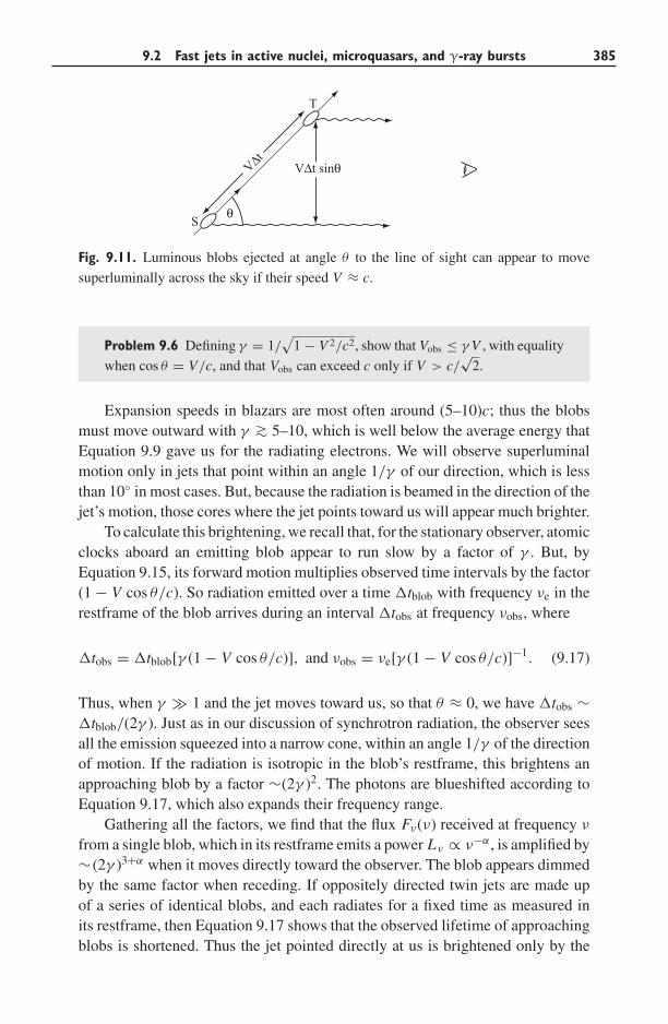
9.2 Fast jets in active nuclei, microquasars, and γ-ray bursts 385

θS

T

VΔt

VΔt sinθ

Fig. 9.11. Luminous blobs ejected at angle θ to the line of sight can appear to move

superluminally across the sky if their speed V ≈ c.

Problem 9.6 Defining γ = 1/√

1 − V 2/c2, show that Vobs ≤ γ V , with equality

when cos θ = V/c, and that Vobs can exceed c only if V > c/√

2.

Expansion speeds in blazars are most often around (5–10)c; thus the blobsmust move outward with γ ∼> 5–10, which is well below the average energy thatEquation 9.9 gave us for the radiating electrons. We will observe superluminalmotion only in jets that point within an angle 1/γ of our direction, which is lessthan 10◦ in most cases. But, because the radiation is beamed in the direction of thejet’s motion, those cores where the jet points toward us will appear much brighter.

To calculate this brightening, we recall that, for the stationary observer, atomicclocks aboard an emitting blob appear to run slow by a factor of γ . But, byEquation 9.15, its forward motion multiplies observed time intervals by the factor(1 − V cos θ/c). So radiation emitted over a time �tblob with frequency νe in therestframe of the blob arrives during an interval �tobs at frequency νobs, where

�tobs = �tblob[γ (1 − V cos θ/c)], and νobs = νe[γ (1 − V cos θ/c)]−1. (9.17)

Thus, when γ � 1 and the jet moves toward us, so that θ ≈ 0, we have �tobs ∼�tblob/(2γ ). Just as in our discussion of synchrotron radiation, the observer seesall the emission squeezed into a narrow cone, within an angle 1/γ of the directionof motion. If the radiation is isotropic in the blob’s restframe, this brightens anapproaching blob by a factor ∼(2γ )2. The photons are blueshifted according toEquation 9.17, which also expands their frequency range.

Gathering all the factors, we find that the flux Fν(ν) received at frequency ν

from a single blob, which in its restframe emits a power Lν ∝ ν−α, is amplified by∼ (2γ )3+α when it moves directly toward the observer. The blob appears dimmedby the same factor when receding. If oppositely directed twin jets are made upof a series of identical blobs, and each radiates for a fixed time as measured inits restframe, then Equation 9.17 shows that the observed lifetime of approachingblobs is shortened. Thus the jet pointed directly at us is brightened only by the

386 Active galactic nuclei and the early history of galaxies

factor (2γ )2+α, while the receding jet is dimmed by the same factor. For compactcores, α ∼ 0; thus, when γ ∼ 5–10, the jet travelling toward the observer appears(2γ )4 ∼ 104–106 times brighter than that heading away. Often, we see only thematerial heading toward us, as a one-sided jet; the receding half is almost invisible.We have a much better chance of detecting as bright sources those objects for whichthe jet points nearly in our direction, which explains why about half of observedbright radio cores show superluminal motion.

Blazars always have strong radio emission from a compact core. They aregenerally found in ellipticals; probably they are radio galaxies where we lookdirectly down the jet. Its relativistic motion makes the approaching half of the jetappear so bright as to outshine the accretion disk and the line-emitting regions.Blazars are strongly variable; some have doubled their optical and radio brightnessover a few days. This fast variation is natural, since by Equation 9.17 the time forany change in the jet’s luminosity is shortened by the factor γ (1−V cos θ/c). Thevisible light of most quasars is polarized at levels of a few percent, indicating thatpart of it may be synchrotron radiation from the jet. But in blazars, polarizationcan be as high as 20%; much more of the radiation comes from the jet. Onlyone in every thousand quasars is a blazar; but, because they are brightened byforward beaming, these objects account for a few percent of observed brightquasars.

9.2.2 Microquasars: relativistic jets in stellar binaries

In the 1990s, astronomers were startled to discover radio jets emerging at close tolight speed from stellar-mass black holes. In a microquasar, a massive star transfersmass onto an accretion disk around a black-hole or neutron-star companion. Thesesystems were long known as X-ray sources, and about 10% of them are also radio-loud; so the fast jets should not have come as a surprise. The jets are quite narrow,with opening angles less than 10◦, and the radio emission is synchrotron, justas in active nuclei. At least two of the dozen or so known microquasars showsuperluminal motion.

Because the central mass is only a few M�, the accretion disk around amicroquasar is hotter than that in an active nucleus, and emits most of its poweras X-rays rather than ultraviolet light. To calculate its temperature, we look at theenergy lost by a gas cloud of mass m in circular orbit around a massMBH, movingfrom radius r to r − �r . Its initial energy is

E = −GmMBH

2r, so �E = −GmMBH

2r2�r. (9.18)

This energy is transferred to the portion of the disk between r and r +�r , whichmust get rid of it. If it does that by radiating as a blackbody at temperature T , itsluminosity is σSBT 4 per unit area. Remembering that a disk has two sides, when

9.2 Fast jets in active nuclei, microquasars, and γ-ray bursts 387

a mass M flows inward per unit time we have

GMMBH

2r2�r = σSBT 4 × 4πr �r, so T 4(r ) = GMMBH

8πr3σSB. (9.19)

If the inflowing mass is converted to energy with some efficiency ε ≈ 10%, wecan measure M in units of the mass LE/(εc2) required to radiate at the Eddingtonluminosity of Equation 9.4. Writing r in units of the Schwarzschild radius Rs =2GMBH/c2, we have

T 4(r ) = 1

GMBH

(r

Rs

)−3( MLE/(εc2)

)c5mp

16εσTσSB. (9.20)

So the temperature near the inner edge of a disk accreting near its Eddington limitdecreases with the mass of the black hole, as M−1/4

BH .These arguments are not quite right, since we have ignored the fact that matter

can fall in only when angular momentum is carried outward in the disk. Sinceenergy is transported along with it, the disk at r � Rs radiates three times asmuch energy as is given by Equation 9.19, while the inner disk radiates less.

Problem 9.7 Recall from Problem 3.20 that the last stable orbit around a non-

rotating black hole is at 3Rs. Show that, when MBH = M� and M is near the

Eddington limit, the inner edge of the disk is at T ≈ 3 × 107 K, corresponding

to a photon energy of 2.6 keV. Assuming that the orbital speed of material there

is given by Equation 3.20, show that the orbital period P ≈ 3 × 10−4 s.

The material is already collimated into a narrow jet within 10 AU of the centralsource, and the jet travels for a few parsecs rather than megaparsecs. We can watchas bright clumps travel out from the nucleus and fade within a month or two ratherthan over decades or centuries, as in an active nucleus. These clumps seem tobe ejected when the source enters an X-ray-bright state – perhaps as material inthe accretion disk swirls rapidly inward and onto the central object. The jet mayspeed up, so we see bright knots of radio emission as the faster material runs intothe slower plasma ahead of it. Microquasars are a remarkable demonstration thatgravitational and electromagnetic forces can operate on all spatial scales.

Further reading: Chapter 16 of M. S. Longair, High Energy Astrophysics, 2ndedition (Cambridge University Press, Cambridge, UK).

9.2.3 Fast jets from exploding stars: gamma-ray bursts

Gamma-ray bursts (GRBs) were discovered in the 1960s by satellites watchingfor nuclear bomb tests. They are short, intense spurts of γ-rays, with peak energies

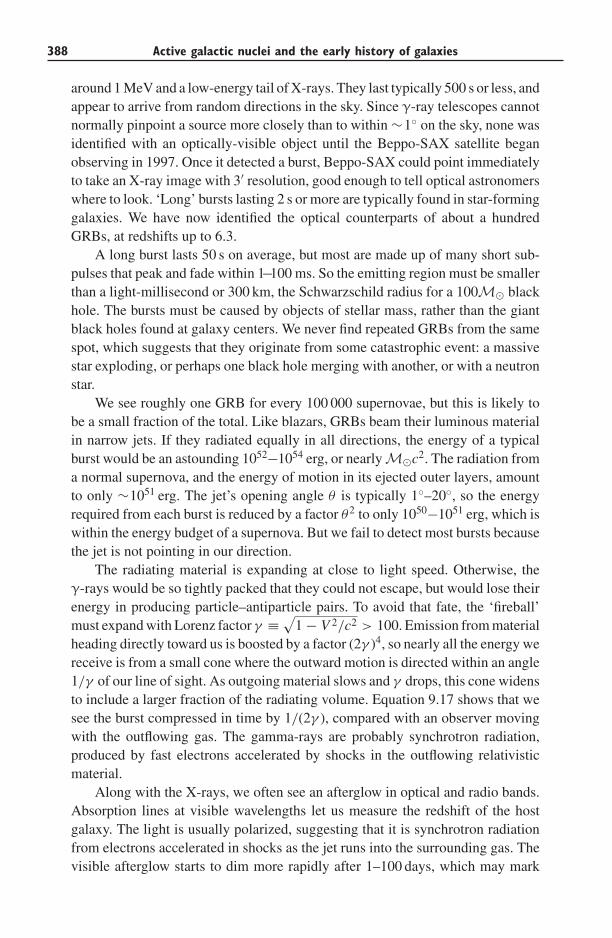
388 Active galactic nuclei and the early history of galaxies

around 1 MeV and a low-energy tail of X-rays. They last typically 500 s or less, andappear to arrive from random directions in the sky. Since γ-ray telescopes cannotnormally pinpoint a source more closely than to within ∼1◦ on the sky, none wasidentified with an optically-visible object until the Beppo-SAX satellite beganobserving in 1997. Once it detected a burst, Beppo-SAX could point immediatelyto take an X-ray image with 3′ resolution, good enough to tell optical astronomerswhere to look. ‘Long’ bursts lasting 2 s or more are typically found in star-forminggalaxies. We have now identified the optical counterparts of about a hundredGRBs, at redshifts up to 6.3.

A long burst lasts 50 s on average, but most are made up of many short sub-pulses that peak and fade within 1−100 ms. So the emitting region must be smallerthan a light-millisecond or 300 km, the Schwarzschild radius for a 100M� blackhole. The bursts must be caused by objects of stellar mass, rather than the giantblack holes found at galaxy centers. We never find repeated GRBs from the samespot, which suggests that they originate from some catastrophic event: a massivestar exploding, or perhaps one black hole merging with another, or with a neutronstar.

We see roughly one GRB for every 100 000 supernovae, but this is likely tobe a small fraction of the total. Like blazars, GRBs beam their luminous materialin narrow jets. If they radiated equally in all directions, the energy of a typicalburst would be an astounding 1052−1054 erg, or nearly M�c2. The radiation froma normal supernova, and the energy of motion in its ejected outer layers, amountto only ∼1051 erg. The jet’s opening angle θ is typically 1◦–20◦, so the energyrequired from each burst is reduced by a factor θ2 to only 1050−1051 erg, which iswithin the energy budget of a supernova. But we fail to detect most bursts becausethe jet is not pointing in our direction.

The radiating material is expanding at close to light speed. Otherwise, theγ-rays would be so tightly packed that they could not escape, but would lose theirenergy in producing particle–antiparticle pairs. To avoid that fate, the ‘fireball’must expand with Lorenz factor γ ≡

√1 − V 2/c2 > 100. Emission from material

heading directly toward us is boosted by a factor (2γ )4, so nearly all the energy wereceive is from a small cone where the outward motion is directed within an angle1/γ of our line of sight. As outgoing material slows and γ drops, this cone widensto include a larger fraction of the radiating volume. Equation 9.17 shows that wesee the burst compressed in time by 1/(2γ ), compared with an observer movingwith the outflowing gas. The gamma-rays are probably synchrotron radiation,produced by fast electrons accelerated by shocks in the outflowing relativisticmaterial.

Along with the X-rays, we often see an afterglow in optical and radio bands.Absorption lines at visible wavelengths let us measure the redshift of the hostgalaxy. The light is usually polarized, suggesting that it is synchrotron radiationfrom electrons accelerated in shocks as the jet runs into the surrounding gas. Thevisible afterglow starts to dim more rapidly after 1–100 days, which may mark

9.2 Fast jets in active nuclei, microquasars, and γ-ray bursts 389

the time when outflowing material has slowed so that 1/γ ∼ θ , so we receiveradiation from the entire approaching jet. The jet also begins to expand sideways(since the opening angle is now comparable to the Mach number M ∼ 1/γ ),causing its density and emissivity to drop. The radio afterglow becomes strongonly a day or so after the burst, and can remain fairly bright for a year or more.During this time the outward motion slows to well below c and the expansionbecomes spherical, so we can reliably estimate the total energy in the outward-moving material. Many bursts seem to have roughly the same amount of energyin the relativistic outflow, roughly 1051 erg divided between prompt emission andthe afterglow.

After some long bursts, the declining curve of visible light shows a bump thatrises to a maximum after ∼20(1 + z) days and then fades. In some well-observedcases, broad emission lines identify the bump as the light of a Type Ic supernovathat exploded at the same time as the burst. Such an explosion is thought to markthe end of life for a rotating star that had a mass of (20−40)M� when it was onthe main sequence. As the star’s iron core collapses, enough other material mayjoin it that the core cannot become a stable neutron star, but forms a black holeinstead. The rest of the star’s material has too much angular momentum to falldirectly into the black hole. Most of it is expelled in the explosion, but ∼0.1M� isthought to form a short-lived accretion disk around the black hole, which channelstwin outflowing jets as shown in Figure 9.3.

Short GRBs, lasting less than 2 s, have a much fainter afterglow. The first wasidentified only in 2005; GRB 050724 was relatively close, in an elliptical galaxyat z = 0.26. The burst itself was at least ten times fainter than a typical long burst,and the afterglow at least a hundred times dimmer. This may have been a mergerbetween two neutron stars (expected to be 10 000 times rarer than a supernova),or even between a neutron star and a black hole. These bursts would be shorterthan one from a collapsing massive star because both partners are already verycompact.

Gamma-ray bursts may have been relatively more frequent in the early Uni-verse, since it is easier to make very massive stars when metals are absent fromthe gas. (If these first-generation stars were all massive, and have now ended theirlives, this would explain why we see none in the Milky Way today.) Gamma-raysare neither scattered by dust nor readily absorbed by the interstellar gas, so theycan help us to probe starbirth in the most distant galaxies. Some of the burstsdetected by our present γ-ray telescopes are likely to be at redshifts z ∼ 10 orhigher, too distant for us to see the afterglow at longer wavelengths. If a betterunderstanding allows us to estimate redshifts from the X-ray and γ-ray emission,we could use GRBs to trace the earliest massive stars.

Further reading: J. I. Katz, 2002, The Biggest Bangs: The Mystery of Gamma RayBursts (Oxford University Press, Oxford, UK) is written for the general reader.

390 Active galactic nuclei and the early history of galaxies

9.3 Intergalactic gas

In the spectra of most quasars, we see multiple systems of absorption lines, atsignificantly lower redshifts than the emission. Most of the lines are narrow; theirwidths correspond to internal motions slower than 100 km s−1, although theirredshifts imply that the gas is travelling away from the quasar and toward usat almost light speed. In fact, this gas is nowhere near the quasar, but simplyintercepts its light. Counting the baryons in galaxies and clusters today showsthat their formation was not very efficient: recall Table 7.2. Most of the baryonsremain in diffuse clouds, that we see only when they intercept the light of a distantsource. This is the reservoir from which gas flowed into the nascent galaxies, andwhich continues to feed them to the present day.

Absorption lines are usually identified in groups that show a simple pattern,such as the Lyman series of hydrogen, or doublets of magnesium and carbon. Asmall wavelength difference makes it easier, since a single measured spectrum islikely to show both lines of a pair. The MgII lines at 2796.3 A and 2803.5 A fallinto the visible window when the absorbing cloud’s redshift is 0.2 ∼< zabs ∼< 1.5,and the CIV lines at 1548.2 A and 1550.8 A do so for 1.1 ∼< zabs ∼< 3.5. TheOVI lines at 1031.9 A and 1037.6 A are harder to observe, since they can be lostamong the lines of the Lyman-α forest (see below). Once the absorption redshiftis known, isolated lines of other elements can often be found.

The intergalactic gas ranges from clouds of largely neutral material, which areas dense as present-day galactic disks, to diffuse gas where the fraction of neutralatoms is 10−3 or less. The number N of absorption lines with N (HI) hydrogenatoms along the line of sight approximately follows N ∝ N (HI)−1.5: the verydiffuse clouds are the most common, but the densest of them contain almost all ofthe neutral gas. The absorbing material is not pristine, but already contains heavyelements produced by nuclear burning in stars.

9.3.1 Neutral gas: damped Lyman-α clouds

If the column density of neutral gas exceeds N (HI) ≈ 2 × 1020 cm−2, theLyman-α (Lyα) line is optically thick with prominent damping wings: these arecalled damped Lyα clouds. This gas density corresponds to 1.5M� pc−2, whichis typical for the outer HI disks of galaxies today: see Section 5.2. A Lyman-limitcloud has N (HI) ∼> 2 × 1017 cm−2; it absorbs almost all photons that have enoughenergy to ionize a hydrogen atom, so the quasar’s measured flux drops nearly tozero at wavelengths just short of 912(1 + zabs) A. The damped Lyα clouds arelargely neutral, but most of the hydrogen in the Lyman-limit clouds is ionized.The spectrum of Figure 9.12 shows a damped Lyα line with zabs = 2.827; the col-umn density is close to 2 × 1020 cm−2. Damped Lyα clouds in front of radio-loudquasars can also be detected by their absorption in the 21 cm line of HI. Counting

9.3 Intergalactic gas 391

Fig. 9.12. The spectrum of quasar 1425+6039 with zem = 3.173: broad Lyα emission at

1216 A is redshifted to the visible region. At shorter wavelengths, narrow absorption lines

of the Lyα forest are dense. The squarish profile at 4650 A is a damped line of Lyα, at

zabs = 2.827. The arrow shows absorption at the same redshift in the CIV doublet with rest

wavelength near 1550 A: the inset reveals distinct absorption components from multiple

gas clouds – L. Lu and M. Rauch.

the number of clouds in the spectrum of a typical quasar tells us that they containenough dense gas to make the disks of present-day spiral and irregular galaxies.

Problem 9.8 Suppose that there are n(z) = n0(1 + z)3 damped Lyα clouds per

Mpc3 at redshift z, each with cross-sectional area σ . Explain why we expect to see

through n(z)σ l of them along a length l of the path toward the quasar. Use Equa-

tion 8.47 to show that between z and z + �z the path �l = c�z/[H (z)(1 + z)],

so the number per unit redshift is

dNdz

�z = n(z)σc �z

H (z)(1 + z)≡ n0σc

H0�z

dX (z)

dz, (9.21)

where (using Equation 8.26 for the second equality)

dX (z)

dz= H0(1 + z)2

H (z)= (1 + z)2√

�m(1 + z)3 + (1 − �tot)(1 + z)2 + ��

.

Show that, if the Universe is flat and �tot = 1, then at early times

X (z) = 2

3√

�m[(1 + z)3/2 − 1] while (1 + z)3 � ��/�m. (9.22)

Locally we find dN /dz ≈ 0.045; if the cross-sectionσ does not change, show that

we expect dN /dz ≈ 0.16 at z = 3. At z = 5 we observe dN /dz ≈ 0.4. Show

that this is roughly twice what we expect if σ is constant: this result indicates

that there were more absorbing clouds, or each was larger.

392 Active galactic nuclei and the early history of galaxies

Problem 9.9 Suppose that the clouds of Problem 9.8 are uniform spheres of

radius r with density nH hydrogen atoms cm−3. Their mass is given by M =(4/3)πr3nHμmH, where the mean mass per hydrogen atom is μmH (μ ≈ 1.3

for a gas with 75% hydrogen and 25% helium by weight), and the average

column density N (HI) ≈ rnH. Show that, for neutral clouds,M ≈ σμmH N (HI),

where σ = πr2 is the cross-section and N (HI) the column density of hydrogen

atoms. Use Equation 9.21 to show that the density ρg of neutral gas at redshift

z is

ρg(z) ≡ n(z)M = μmH

cN (HI)

dNdz

H (z)(1 + z).

If this gas survived unchanged to the present day, explain why it would now

represent a fraction �g of the critical density of Equation 8.21, where

�g ≡ n0Mρcrit(t0)

=[

μmH H0

ρcrit(t0)c

]N (HI)

dNdz

/dX

dz. (9.23)

This fraction depends on the present-day Hubble constant as �g(z) ∝ h−1 –

why? Show that the term in square brackets is 1.2 × 10−23h−1 cm2. Taking

dN /dz = 0.2, and an average N (HI) = 1021 cm−2 at z ∼ 2, show that for the

benchmark cosmology dX/dz = 3.0 and �g(z = 2) ≈ 10−3.

We saw in Table 7.2 that the neutral atomic and molecular gas now in galaxydisks corresponds to �g ∼ 8 × 10−4, while stars in the disks of galaxies nowmake up � ∼ 6 × 10−4. So there is about enough neutral gas in the damped Lyα

clouds at z ∼ 2 to make the galaxy disks that we see today. But, if the benchmarkcosmology is correct, �g has remained at this level over 6 Gyr between redshifts0.7 ∼< z ∼< 5, when half of the stars in disks like the Milky Way’s were born.So we think that the damped Lyα clouds have been replenished, as more tenuousionized gas flowed into them and became dense enough to recombine.

Are the damped Lyα clouds simply gas in the disks of galaxies? We do notreally know. The HI disks of nearby galaxies are large and numerous enoughto account for the absorption features at z ∼< 1. At least half of them should becaused by less luminous galaxies with L ≤ 0.2L, since these have relativelylarge HI disks. When zabs < 1.5, we can often see a bright patch of stars withinan arcsecond or so of the quasar on the sky, at the same redshift as the dampedLyα cloud. These systems are a mix of star-forming disk galaxies, irregulars, andcompact knots of star formation, with luminosities 0.02L < L < 3L. At higherredshifts, Problem 9.8 shows that the galaxies must be larger or more numerousthan they are today, to provide enough absorption lines. Lyman break galaxies at2 ∼< z ∼< 3, selected because they are bright in the ultraviolet, usually give riseto Lyα absorption if they lie within 300 kpc of the path to a quasar. Typically,

9.3 Intergalactic gas 393

the closer the quasar’s light passes to the galaxy, the denser is the absorbing gas.Curiously, a third of Lyman break galaxies seem to produce no Lyα absorptionat all.

Problem 9.10 At present, the density of L galaxies is roughly n of Equation

1.24, or 0.02h3 Mpc−3. Figure 1.16 shows that about half of them are disk galax-

ies, so, taking h = 0.7, we now have n0 ≈ 0.003 Mpc−3 bright spiral galaxies.

At z ∼ 3, we see dN /dz ≈ 0.25. If galaxies had already assembled their disks

by then, we would expect the density n(z) ≈ n0(1 + z)3. For the benchmark

cosmology, show that dX/dz = 3.6, and use Equation 9.21 to show that we must

have σ = 2500 kpc2, so that the absorbing material extends to radii ∼30 kpc.

Figure 5.15 shows that the HI disk of a galaxy like the Milky Way with M(HI) =1010M� extends almost to this radius.

9.3.2 Metals in the intergalactic gas

Damped Lyα clouds contain metals and dust, as well as hydrogen and helium: wesee lines of low ions such as MgII, ZnII, and CrII along with high-ionization linessuch as CIV and SiIV. In Figure 9.12, there is a cluster of CIV lines at zabs = 2.83near 5920 A; they come from the same gas as is producing the damped Lyα

absorption. In less dense clouds with N (HI) ∼> 1016 cm−2, the strongest metallines are of low-ionization species such as MgII, SiII, and OI, which in present-day galaxies are found along with neutral hydrogen in their disks. CIV and SiIVlines, which are characteristic of the diffuse hot gas of today’s galactic halos,become more common when N (HI) is yet lower. Such complexes of metal linesare generally 300–500 km s−1 wide, but the widths of individual components rangedown to 10 km s−1, corresponding to T ∼<105 K. A plasma in thermal equilibriumat this temperature would contain very few CIV ions; so the absorbing gas isprobably ionized by intergalactic radiation from quasars, or by hot stars bornwithin it.

All damped Lyα clouds cause absorption in MgII, but the reverse is not true.At a given redshift, lines of MgII are about ten times as common as damped Lyα

systems, while CIV lines are yet more frequent. So the gas responsible for theMgII absorption must cover a larger area than that producing the damped Lyα

features. Strong MgII absorption generally occurs within 40h−1 Mpc, and weakerabsorption up to 80h−1 Mpc, of a galaxy. Gas causing CIV absorption usuallyextends 50–100 kpc, but sometimes is seen 200 kpc away. Where gravitationallensing has produced multiple images of a quasar separated by ∼ 1 arcsec onthe sky, the two light paths are ∼10 kpc apart as they pass through the absorber.Strong lines of CIV in the two quasar spectra differ when the paths to the imagesare separated by more than 20−50 kpc, giving the rough size of these complexesof absorbing clouds.

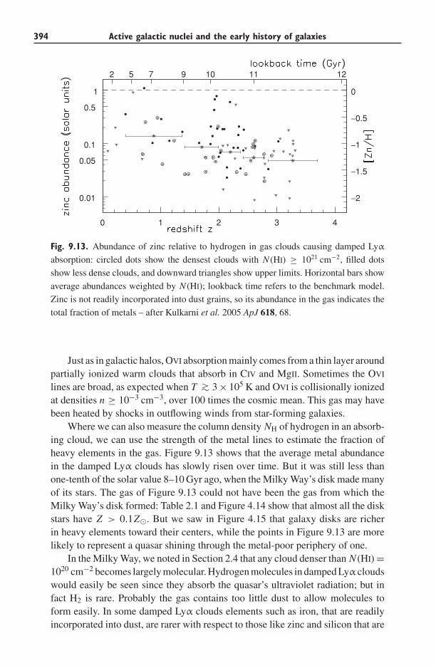
394 Active galactic nuclei and the early history of galaxies

0 1 2 3 4

0.01

0.05

0.1

0.5

1

−2

−1.5

−1

−0.5

0

1211109752

Fig. 9.13. Abundance of zinc relative to hydrogen in gas clouds causing damped Lyα

absorption: circled dots show the densest clouds with N (HI) ≥ 1021 cm−2, filled dots

show less dense clouds, and downward triangles show upper limits. Horizontal bars show

average abundances weighted by N (HI); lookback time refers to the benchmark model.

Zinc is not readily incorporated into dust grains, so its abundance in the gas indicates the

total fraction of metals – after Kulkarni et al. 2005 ApJ 618, 68.

Just as in galactic halos, OVI absorption mainly comes from a thin layer aroundpartially ionized warm clouds that absorb in CIV and MgII. Sometimes the OVI

lines are broad, as expected when T ∼> 3 × 105 K and OVI is collisionally ionizedat densities n ≥ 10−3 cm−3, over 100 times the cosmic mean. This gas may havebeen heated by shocks in outflowing winds from star-forming galaxies.

Where we can also measure the column density NH of hydrogen in an absorb-ing cloud, we can use the strength of the metal lines to estimate the fraction ofheavy elements in the gas. Figure 9.13 shows that the average metal abundancein the damped Lyα clouds has slowly risen over time. But it was still less thanone-tenth of the solar value 8–10 Gyr ago, when the Milky Way’s disk made manyof its stars. The gas of Figure 9.13 could not have been the gas from which theMilky Way’s disk formed: Table 2.1 and Figure 4.14 show that almost all the diskstars have Z > 0.1Z�. But we saw in Figure 4.15 that galaxy disks are richerin heavy elements toward their centers, while the points in Figure 9.13 are morelikely to represent a quasar shining through the metal-poor periphery of one.

In the Milky Way, we noted in Section 2.4 that any cloud denser than N (HI) =1020 cm−2 becomes largely molecular. Hydrogen molecules in damped Lyα cloudswould easily be seen since they absorb the quasar’s ultraviolet radiation; but infact H2 is rare. Probably the gas contains too little dust to allow molecules toform easily. In some damped Lyα clouds elements such as iron, that are readilyincorporated into dust, are rarer with respect to those like zinc and silicon that are

9.3 Intergalactic gas 395

not. These clouds must have begun to produce a little dust, but the ratio of dust togas is ∼30 times smaller than Equation 1.22 gives for the Milky Way.

Absorption lines of CII∗, excited C+, at 1335.7 A indicate that far-ultravioletphotons are heating the dust grains, just as they do in the Milky Way. The heat istransmitted to the surrounding gas, and carbon excited to CII∗ re-radiates most ofit away at 158 μm (see Table 2.5). From the strength of the CII∗ absorption wecan estimate how much heat is re-radiated; it is far more than can be supplied bythe intergalactic radiation field. These damped Lyα clouds must have their ownsource of ultraviolet photons – they are forming stars. In a few cases, we haveeven seen the Lyα emission of those stars. The inferred pace of starbirth is rapidenough at redshifts z ∼ 2–4 that it would use up all the gas of the damped Lyα

clouds within ∼2 Gyr – further evidence that those clouds are replenished fromthe reservoir of more diffuse gas.

If these metal lines indeed trace gas that now lies in galaxies or galaxygroups, their redshifts should be clumped in much the same way as for thegalaxies. As expected, if a CIV absorption line is detected, it is more probableto find a second line nearby in velocity, but the effect disappears for separationsbeyond 500 km s−1. The same is true for lines of OVI that lie closer together than750 km s−1. These speeds are somewhat higher than the rotation speeds of galax-ies, or the velocity dispersion within groups of galaxies. But this is roughly thethickness of the velocity peaks in Figure 8.4, which correspond to looking througha wall or filament of galaxies.

9.3.3 The Lyman-α forest

At column densities below N (HI) ∼2 × 1017 cm−2, ultraviolet photons penetratethrough a gas cloud, and most of the hydrogen is ionized. When N (HI) ∼<3 ×1014 cm−2, we usually detect only the Lyα lines of hydrogen, although deepspectroscopy can reveal weak CIV and OVI lines. The dense profusion of hydrogenabsorption lines at wavelengths just short of the quasar’s Lyα emission is theLyman-α forest. While we detect the forest through its neutral hydrogen, almostall the gas is ionized; HI forms only a tiny fraction, often less than 0.1% of the total.But these clouds may be the Universe’s main repository of neutrons and protons.

In Figure 9.12 we see that forest clouds can remove a substantial fractionof the quasar’s light just shortward of its Lyα emission line, leaving the averageintensity lower than that on the long-wavelength side of the emission line: theGunn–Peterson effect. Between the lines of the Lyα forest in Figure 9.12, thelight level is the same on both sides of the emission line. The Lyα line saturatesat N (HI) ∼ 1014 cm−2, so there must be hardly any HI gas between the absorbingclouds. This is typical for quasars at redshift z ∼< 5.8. But in many objects withz ∼> 6, we see a Gunn–Peterson trough: all the light just shortward of the Lyα

emission line is missing, having been absorbed by diffuse neutral gas at z ∼> 5.8.The earliest quasars and star-forming galaxies shone on gas that had become

neutral at the time of recombination, at zrec ≈ 1100. They formed HII regions,

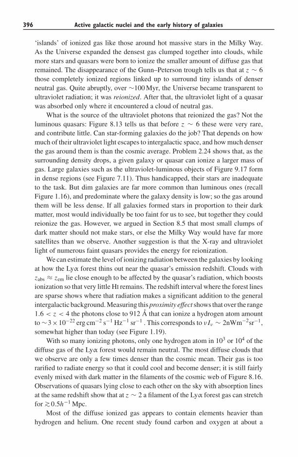
396 Active galactic nuclei and the early history of galaxies

‘islands’ of ionized gas like those around hot massive stars in the Milky Way.As the Universe expanded the densest gas clumped together into clouds, whilemore stars and quasars were born to ionize the smaller amount of diffuse gas thatremained. The disappearance of the Gunn–Peterson trough tells us that at z ∼ 6those completely ionized regions linked up to surround tiny islands of denserneutral gas. Quite abruptly, over ∼100 Myr, the Universe became transparent toultraviolet radiation; it was reionized. After that, the ultraviolet light of a quasarwas absorbed only where it encountered a cloud of neutral gas.

What is the source of the ultraviolet photons that reionized the gas? Not theluminous quasars: Figure 8.13 tells us that before z ∼ 6 these were very rare,and contribute little. Can star-forming galaxies do the job? That depends on howmuch of their ultraviolet light escapes to intergalactic space, and how much denserthe gas around them is than the cosmic average. Problem 2.24 shows that, as thesurrounding density drops, a given galaxy or quasar can ionize a larger mass ofgas. Large galaxies such as the ultraviolet-luminous objects of Figure 9.17 formin dense regions (see Figure 7.11). Thus handicapped, their stars are inadequateto the task. But dim galaxies are far more common than luminous ones (recallFigure 1.16), and predominate where the galaxy density is low; so the gas aroundthem will be less dense. If all galaxies formed stars in proportion to their darkmatter, most would individually be too faint for us to see, but together they couldreionize the gas. However, we argued in Section 8.5 that most small clumps ofdark matter should not make stars, or else the Milky Way would have far moresatellites than we observe. Another suggestion is that the X-ray and ultravioletlight of numerous faint quasars provides the energy for reionization.

We can estimate the level of ionizing radiation between the galaxies by lookingat how the Lyα forest thins out near the quasar’s emission redshift. Clouds withzabs ≈ zem lie close enough to be affected by the quasar’s radiation, which boostsionization so that very little HI remains. The redshift interval where the forest linesare sparse shows where that radiation makes a significant addition to the generalintergalactic background. Measuring this proximity effect shows that over the range1.6 < z < 4 the photons close to 912 A that can ionize a hydrogen atom amountto ∼3×10−22 erg cm−2 s−1 Hz−1 sr−1 . This corresponds to ν Iν ∼ 2nWm−2sr−1,somewhat higher than today (see Figure 1.19).

With so many ionizing photons, only one hydrogen atom in 103 or 104 of thediffuse gas of the Lyα forest would remain neutral. The most diffuse clouds thatwe observe are only a few times denser than the cosmic mean. Their gas is toorarified to radiate energy so that it could cool and become denser; it is still fairlyevenly mixed with dark matter in the filaments of the cosmic web of Figure 8.16.Observations of quasars lying close to each other on the sky with absorption linesat the same redshift show that at z ∼ 2 a filament of the Lyα forest gas can stretchfor ∼>0.5h−1 Mpc.

Most of the diffuse ionized gas appears to contain elements heavier thanhydrogen and helium. One recent study found carbon and oxygen at about a

9.4 The first galaxies 397

Fig. 9.14. A section of the Hubble Ultra Deep Field in blue (B, left) and red (i , right)

light. Redshifts of selected galaxies are marked. Note the normal-looking spiral at z ∼< 1

to the right of the center, and the merging group to the left – Space Telescope Science

Institute.

thousandth of the solar level, although about 30% of the clouds were even moremetal-poor with Z ∼ Z�/3000. If many stars were formed early in small galaxies,the products of their nucleosynthesis would be spread throughout the Lyα forest.How much of the heavy elements should they make? Adding up the ultravioletlight from the galaxies of Figure 9.17, we find that by z ∼ 2.5 they alone wouldproduce enough metals to give an average abundance ∼Z�/30 if mixed evenlythrough the baryons. So why do we see only 0.001Z� in the Lyα forest, whichcontains most of the baryons? This is known as the missing metals problem. Forlack of definite information, we conclude that the missing metals are hidden inhighly ionized states in hot gas that is too diffuse to cool.

9.4 The first galaxies

Figure 9.14 shows part of the Hubble Ultra Deep Field, a region of the sky wheredeep images have been taken with the Hubble Space Telescope in four colors,roughly the U, B, i , and z passbands of Tables 1.2 and 1.3. Some of the galaxiesin this field are small nearby objects, but others are known to have redshifts up toz ∼ 5. These look more irregular and asymmetric than present-day systems. Butwe see them by light that was emitted in the ultraviolet, by their young massivestars, and Figure 5.10 shows that the ultraviolet images of nearby normal galaxies

398 Active galactic nuclei and the early history of galaxies

can look very different from those in visible light. Local star-forming galaxies arealso apt to look ragged in the ultraviolet.

Even when we observe in the infrared to map out light that was emitted atvisible wavelengths, only the most luminous of the galaxies at z ∼ 1 can beclassified according to Figure 1.11. By redshift z ∼> 2, hardly any of the luminouspatches in Figure 9.14 resemble the spirals and ellipticals of our nearby Universe.They have irregular shapes, very high surface brightness, and the bright blue colorsof starbursts. They are much smaller than present-day galaxies, only 0.1′′–0.2′′

across. These may be only protogalactic fragments that will merge to form thegalaxies, or the centers of galaxies that are not yet full-grown.

A galaxy’s light output changes with time as new stars are born and age,affecting both its color and luminosity. Although we cannot normally test whetheran individual galaxy was brighter or fainter in the past than it is now, we cancompare the average population of galaxies at the present day with that at higherredshifts. We can make a model by specifying the star-forming history, and usingour knowledge of stellar evolution to calculate how its spectrum should changewith time. This amounts to finding the evolutionary term e(z) in Equation 8.46.We then test the model by calculating how many galaxies of a given type should befound. For example, if galaxy disks have built up their stars at a steady rate, thenthey should always have roughly the same number of young blue stars, while thered stars build up over time. If elliptical galaxies made all their stars at redshiftsz ∼> 3, we can see from the starburst model of Figure 6.18 that their stars shouldhave been both bluer and brighter in the past.

Figure 9.15 represents a look backward over at least half of the Universe’shistory, showing the numbers of galaxies at each luminosity per comoving volume.The number of red galaxies, with spectra showing only old stars, is about the sameas today. We know that the population of stars that makes up each galaxy at z ∼ 1will have faded by the present, as in Figure 6.18. So these galaxies must makenew stars, or grow by eating their companions as we discussed in Section 7.1; orelse new bright red galaxies have been produced. For example, a blue galaxy thatceases forming stars will become red.

At z ∼ 1 the number of blue galaxies that are actively forming new stars waslarger at each luminosity than it is today. Each one was about three times brighter,or else there were more blue galaxies in the past. We cannot blame stellar fading:today’s blue galaxies have formed new stars in the past gigayear, or they would nowbe red, not blue. The extra starbirth is not caused by starbursts in galaxy mergers;fewer than 10% of the galaxies that contribute to Figure 9.15 are merging. Instead,normal galaxies like our own must have made stars more rapidly than they do now.These systems should redden over time, as old stars make up more of their mass;and indeed the average color of a star-forming galaxy is now redder than it was atz ∼ 1.

We can compare the observed rate of starbirth in a galaxy with what is neededto build up the stars that we see over the lifetime of the Universe; a starburst galaxyis one that makes stars much faster than this average rate. We saw in Section 2.1

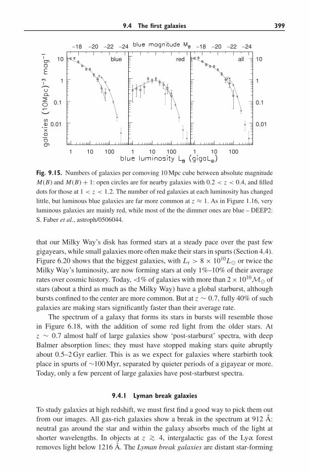
9.4 The first galaxies 399

−18 −20 −22 −24 −18 −20 −22 −24

0.01

0.1

1

10 blue red

0.01

0.1

1

10all

1 10 100 1 10 100 1 10 100

Fig. 9.15. Numbers of galaxies per comoving 10 Mpc cube between absolute magnitude

M(B) and M(B) + 1: open circles are for nearby galaxies with 0.2 < z < 0.4, and filled

dots for those at 1 < z < 1.2. The number of red galaxies at each luminosity has changed

little, but luminous blue galaxies are far more common at z ≈ 1. As in Figure 1.16, very

luminous galaxies are mainly red, while most of the the dimmer ones are blue – DEEP2:

S. Faber et al., astroph/0506044.

that our Milky Way’s disk has formed stars at a steady pace over the past fewgigayears, while small galaxies more often make their stars in spurts (Section 4.4).Figure 6.20 shows that the biggest galaxies, with L r > 8 × 1010L� or twice theMilky Way’s luminosity, are now forming stars at only 1%–10% of their averagerates over cosmic history. Today, <1% of galaxies with more than 2×1010M� ofstars (about a third as much as the Milky Way) have a global starburst, althoughbursts confined to the center are more common. But at z ∼ 0.7, fully 40% of suchgalaxies are making stars significantly faster than their average rate.

The spectrum of a galaxy that forms its stars in bursts will resemble thosein Figure 6.18, with the addition of some red light from the older stars. Atz ∼ 0.7 almost half of large galaxies show ‘post-starburst’ spectra, with deepBalmer absorption lines; they must have stopped making stars quite abruptlyabout 0.5–2 Gyr earlier. This is as we expect for galaxies where starbirth tookplace in spurts of ∼100 Myr, separated by quieter periods of a gigayear or more.Today, only a few percent of large galaxies have post-starburst spectra.

9.4.1 Lyman break galaxies

To study galaxies at high redshift, we must first find a good way to pick them outfrom our images. All gas-rich galaxies show a break in the spectrum at 912 A:neutral gas around the star and within the galaxy absorbs much of the light atshorter wavelengths. In objects at z ∼> 4, intergalactic gas of the Lyα forestremoves light below 1216 A. The Lyman break galaxies are distant star-forming

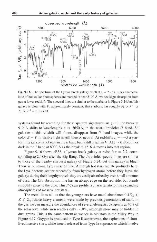
400 Active galactic nuclei and the early history of galaxies

1200 1300 1400 1500 1600

0

2

4

64500 5000 5500 6000

Fig. 9.16. The spectrum of the Lyman break galaxy cB58 at z = 2.723. Lines character-

istic of hot stellar photospheres are marked ∗; near 5100 A, we see MgII absorption from

gas at lower redshift. The spectral lines are similar to the starburst in Figure 5.24, but this

galaxy is bluer with Fν approximately constant; that starburst has roughly Fλ ∝ λ−1 or

Fν ∝ ν−1 – C. Steidel.

systems found by searching for these spectral signatures. At z ∼ 3, the break at912 A shifts to wavelengths λ ≈ 3650 A, in the near-ultraviolet U band. Sogalaxies at this redshift will almost disappear from U -band images, while thecolor B − V in visible light is still blue or neutral. At redshifts z ∼ 4−5 a star-forming galaxy is not seen in the B band but is still bright in V . At z ∼ 6 it becomesdark in the I band at 8000 A as the break at 1216 A moves into that region.

Figure 9.16 shows cB58, a Lyman break galaxy at redshift z = 2.7, corre-sponding to 2.4 Gyr after the Big Bang. The ultraviolet spectral lines are similarto those of the nearby starburst galaxy of Figure 5.24, but this galaxy is bluer.There is no strong Lyα emission line. Although hot stars radiate profusely here,the Lyα photons scatter repeatedly from hydrogen atoms before they leave thegalaxy; during their lengthy travels they are easily absorbed by even small amountsof dust. The CIV absorption line has an abrupt edge on the red side, but blendssmoothly away to the blue. This P Cygni profile is characteristic of the expandingatmospheres of massive hot stars.

The metal lines tell us that the young stars have metal abundance 0.4Z� ∼<Z ∼< Z�; those heavy elements were made by previous generations of stars. Inthe gas we can measure the abundances of several elements; oxygen is at 40% ofthe solar level while iron reaches only ∼10%, although more may be hidden indust grains. This is the same pattern as we see in old stars in the Milky Way inFigure 4.17. Oxygen is produced in Type II supernovae, the explosions of short-lived massive stars, while iron is released from Type Ia supernovae which involve

9.4 The first galaxies 401

low-mass long-lived stars. So oxygen is added to the gas within ∼10 Myr after thefirst significant star formation, whereas iron will be released only ∼1 Gyr later.Together with a low level of nitrogen, also made in low-mass stars (see Section 4.2),this ratio suggests that cB58 made most of its stars in the past 250 Myr.

We see blueshifted absorption lines showing that gas is streaming outward;this is typical for Lyman break galaxies. In cB58 the wind moves outward at250 km s−1, carrying off about as much mass as the galaxy turns into new stars.At least some of this metal-bearing material will escape to intergalactic space.Stars are made from dense gas, so it is not surprising to detect radio-frequencylines from molecules such as CO. In cB58 we find ∼109M� of molecular gas,enough to form stars at its current rate for only about 50 Myr. This gas is denseenough to absorb 80% of the ultraviolet light of the young stars, re-radiatingenergy LFIR ∼ 1011L� in the far-infrared.

Observing these distant galaxies in visible or near-infrared light, we receiveenergy emitted in the ultraviolet, which comes only from their most massive andrecently born stars. To infer the pace of starbirth, we must guess at the initial massfunction, giving the proportions of massive and less-massive stars. In cB58, theP Cygni profile of the CIV line and the shapes of other lines tell us that, at leastamong its massive stars, this galaxy has roughly the same initial mass functionas the Milky Way. We can measure the ultraviolet luminosity Lλ(1500 A) in the

hybrid units of 3.86 × 1026 W A−1

; recall that L� = 3.86 × 1026 W is the Sun’sbolometric luminosity. Then, if the initial mass function has the Salpeter form ofEquation 2.5 for M ∼> 0.1M�, stars are produced at the rate

M ∼ (3–5) × 10−7Lλ(1500 A)M� yr−1. (9.24)

Making M� yr−1 in stars corresponds to Lλ(1500 A) ∼ 3 × 106L�A−1

, or aluminosity λLλ ∼ 4 × 109L�. For a more realistic mass function that includesfewer low-mass stars, M is only half as large for a given ultraviolet luminosity.

The best estimate of starbirth would be to add the rate given by Equation 9.24to that given by Equation 7.11, which measures the stellar light intercepted bydust and re-radiated in the far-infrared. Typically, the more vigorous the starbirth,the larger the fraction of the young stars’ light intercepted by dust. Most of theLyman break galaxies studied at z ∼ 3 make (10–50)M� yr−1 of new stars;cB58 produces ∼40M� yr−1. This is modest compared with 200M� yr−1 in thenearby ultraluminous merging system Arp 220 or the submillimeter galaxies (seebelow). Today ∼5M� yr−1 of stars are born in a large spiral galaxy like the MilkyWay, while rates for typical local starbursts range up to 30M� yr−1.

Lyman break galaxies are very bright because of their short-lived massivestars: they are typically several times more luminous in visible light than anL galaxy defined by Figure 1.16. Figure 6.18 shows that, between roughly50 Myr and 1 Gyr after a starburst, the Balmer jump near 4000 A increases instrength. Using it to date the current episode of starbirth, we find that the fastest

402 Active galactic nuclei and the early history of galaxies

star-formers have typically been making stars for only 30−100 Myr, while themore sedate galaxies have continued for ∼>1 Gyr. The color of light emitted atvisible wavelengths gives information on older stars, which represent most of themass. We find that Lyman break galaxies are not massive: a few have assembled5 × 1010M� of stars, roughly the same as the Milky Way today, but most aresmall systems like cB58 with M ∼ 1010M�.

Because the light must be spread out in wavelength, spectroscopy of thesefaint galaxies is very demanding. Some of the best-observed high-redshift galaxiesappear many times brighter because of gravitational lensing: their light is bent asit passes through a galaxy cluster on its way to us (see Section 7.4). Light fromcB58 is amplified about 30-fold in this way. Otherwise, spectroscopy of the mostdistant galaxies is a task for the large 8–10 m telescopes.

Very bright Lyman break galaxies are seen to z ∼> 6; BD38 at z = 5.515 is anexample. The spectrum looks much like that of cB58 in Figure 9.16, although wesee it barely 1 Gyr after the Big Bang. It was then making 140M� yr−1 of newstars, in an episode that had already lasted ∼200 Myr. These are not the galaxy’sfirst stars; the strength of their spectral lines shows that they already are half asmetal-rich as the Sun. Observations with the Spitzer Space Telescope at 4.5 μmshow the red light of (1−6)×1010M� of stars with ages of 600−700 Myr. Thesesystems are quite small: BD38 is one of the largest, but is only 1.6 kpc in radius.In contrast to the very gas-rich objects that we discuss below, an active nucleusof any kind is rare; we see them in only a few percent of Lyman break galaxies.

Problem 9.11 At optical and near-infrared wavelengths, the flux Fλ from each

square arcsecond of the night sky increases roughly as Fλ ∝ λ2.5. To measure

the energy that a galaxy emits near the Lyα line at 1216 A, we must observe near

1216(1+ z) A. Explain why the measured flux Fλ from each square arcsecond of

the galaxy’s image decreases as (1+z)5, so that Fλ(galaxy)/Fλ(sky) ∝ (1+z)−7.5.

Lyα emission from protogalaxies at z ∼ 5 is hard to see without an 8–10 m

telescope.

9.4.2 Hidden stars: submillimeter galaxies and molecular gas

Even locally, galaxies with intense star formation hide most of the blue and ultra-violet light of their young stars behind dusty gas. As we saw in Section 7.1, onlya few percent of this light escapes from a starburst galaxy like M82 or Arp 220.On average, about two-thirds of the ultraviolet light escapes from local galaxies;the rest is absorbed to warm the grains of dust, and re-radiated in the infrared. Atz ∼ 1, most stars were made in dusty places: the energy of starlight emerges mainlyas the infrared light of luminous infrared galaxies (LIRGs) with LFIR > 1011L�,making ∼>50M� yr−1 of new stars (see Equation 7.11). At higher redshifts, dustystarbursts become even more common. Just as some quasars have large quantities

9.4 The first galaxies 403

of molecular gas around their centers, so many of the most luminous star-forminggalaxies have nuclear activity. The active nuclei are conspicuous in X-rays, whichcan shine out through the dusty gas, but star formation still contributes most oftheir energy output.

We saw in Section 7.1 that galaxy mergers can trigger a starburst. These arerare today, and contribute little to the total of star formation. Locally, fewer than1% of Milky-Way-sized galaxies are locked in close interaction and likely to mergesoon with a comparably large system. Even at z ∼ 1, roughly a third of LIRGsare normal-looking spiral galaxies; a quarter are irregulars; in another quarter,the light is concentrated into a compact center. Only 20% are clearly undergoingmajor mergers, though these are the most powerful sources. But, at redshiftsz = 2−3, the far-infrared light comes predominantly from ultraluminous infraredgalaxies (ULIRGs), with LFIR > 1012L�, forming more than 200M� yr−1 ofnew stars. Many of the ULIRGs show signs of recent or ongoing merger. It isnot simply that our telescopes are not powerful enough to see dimmer objects: atthese wavelengths, adding up the light of the ULIRGs accounts for almost all ofthe background radiation shown in Figure 1.19.

In observing dusty galaxies, Equation 8.46 comes to our aid: the term k(z) is solarge and negative that the measured flux of a galaxy atλ ∼ 1 mm is nearly constantover the range 1 ∼< z ∼< 10. Some of the most vigorously star-forming galaxieswere found first by searching at 850 μm for the redshifted emission of warmdust. In an optical image, these submillimeter galaxies are faint with irregular andcomplex shapes, and often seem to be merging with a neighbor. At these redshifts,lines from the 3 → 2 and 4 → 3 transitions of the CO molecule (see Table 1.8)are shifted to around 3 mm, where they can be observed from the ground.

One object studied in this way, J02399 at z = 2.8, lies behind a galaxy clusterwhere gravitational lensing makes it appear 2.5 times brighter. With LFIR ∼1013L�, Equation 7.11 indicates that it is making 600M� yr−1 of new stars. Atthis rate, its supply of 6 × 1010M� of molecular gas will last only 100 Myr. Thegas lies in a ring at radius 8 kpc, rotating at 420 km s−1, so the mass inside is3 × 1011M�. Recall from Section 2.3 and Problem 6.6 that most of the mass inthe central few kiloparsecs of a galaxy is stars and gas, not dark matter. If J02399is similar, the galaxy has built ∼2 × 1011M� of stars – too many for the currentburst, unless by coincidence we see it on the point of exhausting its gas.

The most luminous galaxies discovered at 850 μm have redshifts 1.5 < z <

3.5. Like the very powerful quasars of Figure 8.13, but unlike bright star-forminggalaxies (look ahead to Figure 9.17), their numbers peak at z ∼ 2. Most contain∼2 × 1010M� of molecular gas, far more than the Lyman break galaxies, and tentimes as much as the Milky Way. But this is only enough to fuel their starbirth for20–40 Myr. The gas usually lies in a ring or disk within 2 kpc of the center rotatingat 400–500 km s−1, enclosing a mass ∼>1011M�. They contain ∼3 × 1010M�of young stars, and possibly many more old stars. The gas and young stars aloneamount to 5×1010M�, which is roughly the mass of normal (baryonic) matter in

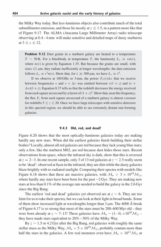
404 Active galactic nuclei and the early history of galaxies

the Milky Way today. But less-luminous objects also contribute much of the totalsubmillimeter emission, and those lie mostly at z ∼< 1.5, in a pattern more like thatof Figure 9.17. The ALMA (Atacama Large Millimeter Array) radio telescopeobserving at 0.4−4 mm will make sensitive and detailed maps of dusty starburstsat 3 ∼< z ∼< 12.

Problem 9.12 Dust grains in a starburst galaxy are heated to a temperature

T ∼ 50 K. For a blackbody at temperature T , the luminosity Lν ∝ νn(ν),

where n(ν) is given by Equation 1.35. But because the grains are small, with

sizes ∼<1 μm, they radiate inefficiently at longer wavelengths: the dust emission

follows Lν ∝ ν3n(ν). Show that, for λ � 300 μm, we have Lν ∝ ν4.

If we observe at 100 GHz or 3 mm, the power Fν(ν)�ν that we receive

between frequencies ν and ν + �ν was emitted between ν(1 + z) and (ν +�ν)(1 + z). Equation 8.37 tells us that the redshift decreases the energy received

from each square arcsecond by a factor of (1 + z)4. Show that, near this frequency,

the flux Fν from each square arcsecond of a starburst galaxy is almost constant

for redshifts 5 ∼< z ∼< 20. Once we have large telescopes with sensitive detectors

in this spectral region, we should be able to see extremely distant star-forming

galaxies.

9.4.3 Old, red, and dead?

Figure 6.20 shows that the most optically-luminous galaxies today are makinghardly any new stars. When did the earliest galaxies finish building their stellarbodies? Locally, almost all red galaxies are red because they lack young blue stars;only a few, like the starburst M82, are red because dust hides those stars. Recentobservations from space, where the infrared sky is dark, show that this is reversedat z = 2−3. In one recent sample, only 3 of 13 red galaxies at z ∼ 2.5 really seemto be ‘dead’: observed at 8μm in the infrared, they are dim while the dusty galaxiesblaze brightly with re-radiated starlight. Comparing their spectra with models likeFigure 6.18 shows that these are massive galaxies, with M > 3 × 1010M�,where hardly any stars have been born for the past ∼2 Gyr. They are making newstars at less than 0.1% of the average rate needed to build the galaxy in the 2.6 Gyrsince the Big Bang.

The earliest ‘red and dead’ galaxies yet observed are at z ∼ 6. They are toofaint for us to take their spectra, but we can look at their light in broad bands. Someof them show increased light at wavelengths longer than 3 μm. The 4000 A breakof Figure 6.17 is so strong that most of the stars must be 200–600 Myr old – theywere born already at z ∼ 7–13! These galaxies have M ∼ (1– 4) ×1010M� –they have made stars equivalent to 20%−50% of the Milky Way.

By z ∼ 1.5 or 4.2 Gyr after the Big Bang, red galaxies with roughly the samestellar mass as the Milky Way, M > 5 × 1010M�, probably contain more thanhalf the stars in the galaxies. A few real monsters even have M > 1011M� at

9.4 The first galaxies 405

0.8 1 2 4 6 8 100

0.05

0.1

0.15

0.2

1 now234567

Fig. 9.17. Star formation per comoving Mpc3, derived from light emitted at ultraviolet

wavelengths, calculated for the benchmark cosmology. Stars show points measured in the

ultraviolet by Galex, and filled circles are from Lyman break galaxies. The mass of stars

formed in any time interval is proportional to the area under the points – E. Stanway and

A. Barger.

z ≈ 1.5. Since there is roughly six times more dark matter in the Universe thanbaryonic material, these objects must have dark halos of ∼1012M�. According tothe cold dark matter models of Section 8.5, such massive halos should be very rareat early times. Their stars are about as metal-rich as the Sun, and have ages around2 Gyr, so the last significant starbirth was at z ∼ 3. Forming (300–500)M� yr−1

of new stars, it would take only 300 Myr (a typical timescale for starbursts) forthe ‘hidden’ systems of the last subsection to build up these masses. The mostluminous of the dusty starbursts discovered at 850 μm might have developed firstinto these ‘red and dead’ galaxies, and then into today’s luminous ellipticals.

9.4.4 The star-forming history of the Universe

Using variants of Equation 9.24, we can estimate how fast the ultraviolet-luminousgalaxies formed their stars. According to Figure 9.17 most stars in the Universewere born at z ∼ 1, between 5 and 8 Gyr after the Big Bang. Star-forming galaxiesseem to have flourished later than the luminous active nuclei of Figure 8.13, whichreach their peak at z ∼ 2. It also shows less extreme variation: starbirth today isonly about five times less vigorous than it was at its peak, whereas at z ∼ 4 it isat roughly half the peak level.

At z ∼> 0.7 much of the ultraviolet radiation of young stars is absorbed bydust, and Figure 9.17 includes a correction based on the color of the ultravioletlight. But virtually no ultraviolet light escapes from the dustiest systems such asthe submillimeter galaxies, so they will be missed from the plot. We have also

406 Active galactic nuclei and the early history of galaxies

missed fainter star-forming galaxies, even if they host much of the starbirth. Butthe number of stars formed should not be less than that given in Figure 9.17.

The rate at which those stars have produced metals is related to the ultravioletluminosity of their massive stars. We must add up the yield of heavy elementsfrom supernovae resulting from stars of each mass, which are known to within

about a factor of two. Measuring the ultraviolet flux in the same units of L� A−1

as for Equation 9.24, we find that elements heavier than helium are produced atthe rate

MZ ∼ 8 × 10−9Lλ(1500 A)M� yr−1. (9.25)

We also had to assume here that high-mass stars, with M ∼> 6M�, are formed inthe relative proportions specified by the Salpeter function of Equation 2.5. Luckily,all such stars burn roughly the same fraction of their gas into metals, so Equation9.25 is not very sensitive to the initial mass function adopted.

According to Figure 9.17, roughly a quarter of all the stars had formed byz = 2, and they should have released enough metals to give an average abundance∼Z�/30 if mixed evenly throughout the baryons. At the end of the previoussection we saw that this level is already higher than what we observe. If manysmall star-forming galaxies contributed to reionization, then even more ‘missingmetals’ must be hidden in diffuse gas.

Is our picture of the life of distant galaxies consistent with what we see in theLocal Group, where we can take spectra of individual bright stars to reconstructthe star-forming history? About half of its stellar mass is in the bulges of M31 andthe Milky Way, and in Chapter 4 we saw that most of these stars are probably oldenough to predate z ∼ 1.5. The Milky Way’s disk has formed stars steadily over thepast few gigayears. The disk of M31 is more luminous but has fewer young stars,suggesting that the pace of starbirth has slackened over that period. Averaging overthe Local Group, starbirth appears to have been at its most vigorous 8–13 Gyr inthe past, perhaps somewhat earlier than the peak in Figure 9.17. However, theatmospheres of the stars that we see locally all contain elements heavier thanhelium; very few have less than 10−3 of the Sun’s metal abundance. We havefound no ‘fossils’ from the earliest stellar generation, formed out of hydrogenand helium alone. Thus further studies both of nearby and of distant galaxies areneeded in order to tell us whether Figure 9.17 fairly represents cosmic starbirth.New instruments that can observe at longer wavelengths, such as ALMA and theplanned James Webb Space Telescope, will help us to pierce through the dust toexplore the birth of the galaxies.

Appendix A

Units and conversions

Table A.1 Units and prefixes

magnitudes see Section 1.1arcsecond 1′′ = (1/60) × 1′; 1/206 265 radiansarcminute 1′ = (1/60) × 1◦

angstrom A = 10−10 m = 0.1 nmnanometer nm = 10−9 mmicron μm = 10−6 m = 10−4 cmcentimeter cm = 10−2 mjansky Jy = 10−26 W m−2 Hz−1

joule J = 107 erg or 107 g cm2 s−2

watt W = 107 erg s−1

micro μ 1 μ s = 10−6 s: microsecondmilli m 1 mJy = 10−3 Jy: millijanskykilo k 1 km = 103 m: kilometermega M 1 Mpc = 106 pc: megaparsecgiga G 1 Gyr = 109 yr: gigayear

Table A.2 Conversion factors

Sound speed in atomic hydrogen cs = √kBT/mp = 9 km s−1 ×√

T/104 KSurface density M� pc−2 = 1.25 × 1020 H atoms cm−2

Volume density M� pc−3 = 6.7 × 10−23 g cm−3

or 44 H atoms cm−3

Surface brightness L� pc−2 = 27 mag arcsec−2 in BLuminosity MB = −20, L B = 1.6 × 1010 L�

MB = −18, L B = 2.5 × 109 L�MB = −16, L B = 3.9 × 108 L�

Speed 1 km s−1 = 1.023 pc Myr−1

Gravitational constant G = 4.5 × 10−3 if mass is in M�,distance in pc, time in Myr

Vector products A × (B × C) = (A · C)B − (A · B)C(A × B) · (C × D) = (A · C)(B · D) − (A · D)(B · C)

407

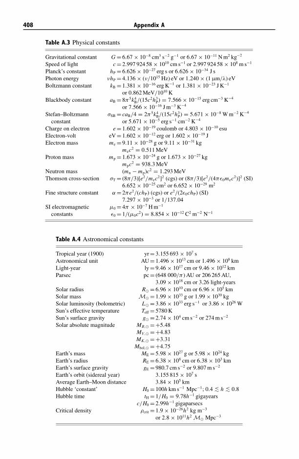
408 Appendix A

Table A.3 Physical constants

Gravitational constant G = 6.67 × 10−8 cm3 s−2 g−1 or 6.67 × 10−11 N m2 kg−2

Speed of light c = 2.997 924 58 × 1010 cm s−1 or 2.997 924 58 × 108 m s−1

Planck’s constant hP = 6.626 × 10−27 erg s or 6.626 × 10−34 J sPhoton energy νhP = 4.136 × (ν/1015 Hz) eV or 1.240 × (1 μm/λ) eVBoltzmann constant kB = 1.381 × 10−16 erg K−1 or 1.381 × 10−23 J K−1

or 0.862 MeV/1010 KBlackbody constant aB = 8π5k4

B/(15c2h3P) = 7.566 × 10−15 erg cm−3 K−4

or 7.566 × 10−16 J m−3 K−4

Stefan–Boltzmann σSB = caB/4 = 2π5k4B/(15c2h3

P) = 5.671 × 10−8 W m−2 K−4

constant or 5.671 × 10−5 erg s−1 cm−2 K−4

Charge on electron e = 1.602 × 10−19 coulomb or 4.803 × 10−10 esuElectron-volt eV = 1.602 × 10−12 erg or 1.602 × 10−19 JElectron mass me = 9.11 × 10−28 g or 9.11 × 10−31 kg

mec2 = 0.511 MeVProton mass mp = 1.673 × 10−24 g or 1.673 × 10−27 kg

mpc2 = 938.3 MeVNeutron mass (mn − mp)c2 = 1.293 MeVThomson cross-section σT = (8π/3)[e2/mec2]2 (cgs) or (8π/3)[e2/(4πε0mec2)]2 (SI)

6.652 × 10−25 cm2 or 6.652 × 10−29 m2

Fine structure constant α = 2πe2/(chP) (cgs) or e2/(2ε0chP) (SI)7.297 × 10−3 or 1/137.04

SI electromagnetic μ0 = 4π × 10−7 H m−1

constants ε0 = 1/(μ0c2) = 8.854 × 10−12 C2 m−2 N−1

Table A.4 Astronomical constants

Tropical year (1900) yr = 3.155 693 × 107 sAstronomical unit AU = 1.496 × 1013 cm or 1.496 × 108 kmLight-year ly = 9.46 × 1017 cm or 9.46 × 1012 kmParsec pc = (648 000/π) AU or 206 265 AU,

3.09 × 1018 cm or 3.26 light-yearsSolar radius R� = 6.96 × 1010 cm or 6.96 × 105 kmSolar mass M� = 1.99 × 1033 g or 1.99 × 1030 kgSolar luminosity (bolometric) L� = 3.86 × 1033 erg s−1 or 3.86 × 1026 WSun’s effective temperature Teff = 5780 KSun’s surface gravity g� = 2.74 × 104 cm s−2 or 274 m s−2

Solar absolute magnitude MB,� = +5.48MV,� = +4.83MK ,� = +3.31

Mbol,� = +4.75Earth’s mass ME = 5.98 × 1027 g or 5.98 × 1024 kgEarth’s radius RE = 6.38 × 108 cm or 6.38 × 103 kmEarth’s surface gravity gE = 980.7 cm s−2 or 9.807 m s−2

Earth’s orbit (sidereal year) 3.155 815 × 107 sAverage Earth–Moon distance 3.84 × 105 kmHubble ‘constant’ H0 = 100h km s−1 Mpc−1; 0.4 ∼< h ∼< 0.8Hubble time tH = 1/H0 = 9.78h−1 gigayears

c/H0 = 2.99h−1 gigaparsecsCritical density ρcrit = 1.9 × 10−26h2 kg m−3

or 2.8 × 1011h2 M� Mpc−3

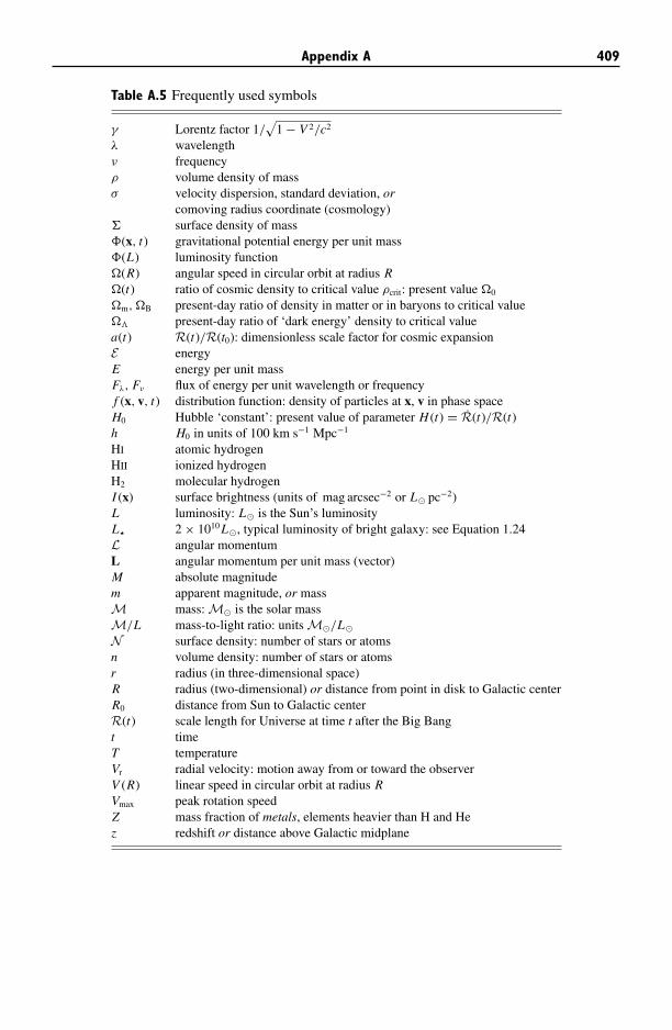
Appendix A 409

Table A.5 Frequently used symbols

γ Lorentz factor 1/√

1 − V 2/c2

λ wavelengthν frequencyρ volume density of massσ velocity dispersion, standard deviation, or

comoving radius coordinate (cosmology)� surface density of mass�(x, t) gravitational potential energy per unit mass�(L) luminosity function�(R) angular speed in circular orbit at radius R�(t) ratio of cosmic density to critical value ρcrit: present value �0

�m, �B present-day ratio of density in matter or in baryons to critical value�� present-day ratio of ‘dark energy’ density to critical valuea(t) R(t)/R(t0): dimensionless scale factor for cosmic expansionE energyE energy per unit massFλ, Fν flux of energy per unit wavelength or frequencyf (x, v, t) distribution function: density of particles at x, v in phase spaceH0 Hubble ‘constant’: present value of parameter H (t) = R(t)/R(t)h H0 in units of 100 km s−1 Mpc−1

HI atomic hydrogenHII ionized hydrogenH2 molecular hydrogenI (x) surface brightness (units of mag arcsec−2 or L� pc−2)L luminosity: L� is the Sun’s luminosityL 2 × 1010 L�, typical luminosity of bright galaxy: see Equation 1.24L angular momentumL angular momentum per unit mass (vector)M absolute magnitudem apparent magnitude, or massM mass: M� is the solar massM/L mass-to-light ratio: units M�/L�N surface density: number of stars or atomsn volume density: number of stars or atomsr radius (in three-dimensional space)R radius (two-dimensional) or distance from point in disk to Galactic centerR0 distance from Sun to Galactic centerR(t) scale length for Universe at time t after the Big Bangt timeT temperatureVr radial velocity: motion away from or toward the observerV (R) linear speed in circular orbit at radius RVmax peak rotation speedZ mass fraction of metals, elements heavier than H and Hez redshift or distance above Galactic midplane

410 Appendix A

Table A.6 Astronomical buzzwords

Early-type star hot: early in spectral sequence OBAFGKMLate-type star cool: late in spectral sequence OBAFGKMDwarf star main-sequence star (except for ‘white dwarf’)Early-type galaxy E or S0: ‘early’ in Hubble sequenceLate-type galaxy spiral or irregular: ‘late’ in Hubble sequenceDwarf galaxy luminosity L ∼< 109 L�Metals elements heavier than heliumRedshift z Doppler shift (λobs − λe)/λe

Radial velocity Vr motion away from or toward the observerTangential velocity Vt motion perpendicular to the observerScale length or height distance over which density falls by factor of e

Appendix B

Bibliography

We have drawn for our presentation on the following graduate texts:J. Binney & S. Tremaine, 1987, Galactic Dynamics (Princeton University Press, Princeton,

New Jersey), on the dynamics of galaxies and star clusters; F. Combes, P. Boisse, A.Mazure, & A. Blanchard, Galaxies and Cosmology, 2nd edition (English translation,2002; Springer, Heidelberg, Germany), covering similar ground to our text; and J.Binney & M. Merrifield, 1998, Galactic Astronomy, 3rd edition (Princeton UniversityPress, Princeton, New Jersey), which gives a comprehensive review of observationsof our Galaxy and others.

On a similar level to this book, see S. Phillipps, 2005, The Structure and Evolution ofGalaxies (Wiley, Chichester, UK) and P. Schneider, Extragalactic Astronomy andCosmology: An Introduction (English translation, 2006; Springer, Heidelberg/Berlin,Germany).

At a more elementary level, see M. H. Jones & R. J. Lambourne (eds.), 2003, An Intro-duction to Galaxies and Cosmology (Cambridge University Press and the OpenUniversity, Cambridge, UK).

More specialized references are given under chapter headings below.

Chapter 1

Introductions to stellar structure on an undergraduate level include D. A. Ostlie & B.W. Carroll, 1996, An Introduction to Modern Stellar Astrophysics (Addison-Wesley,Reading, Massachusetts); A. C. Phillips, 1994, The Physics of Stars (Wiley, Chich-ester, UK); and D. Prialnik, 2000, An Introduction to the Theory of Stellar Structureand Evolution (Cambridge University Press, Cambridge, UK).

Graduate texts include C. J. Hansen & S. D. Kawaler, 1994, Stellar Interiors: PhysicalPrinciples, Structure, and Evolution (Springer, New York); D. Arnett, 1996, Super-novae and Nucleosynthesis (Princeton University Press, Princeton, New Jersey) forstellar evolution beyond the main sequence; and M. Salaris and S. Cassisi, 2005,Evolution of Stars and Stellar Populations (Wiley, Chichester, UK).

Hubble’s original account of galaxy classification is given in E. Hubble, 1936, The Realmof the Nebulae (Yale University Press; reprinted by Dover, New York); it is illustratedin A. Sandage, 1961, The Hubble Atlas of Galaxies (Carnegie Institute of Washing-ton, Washington, DC). Modern treatments include S. van den Bergh, 1998, GalaxyMorphology and Classification (Cambridge University Press, Cambridge, UK).

411

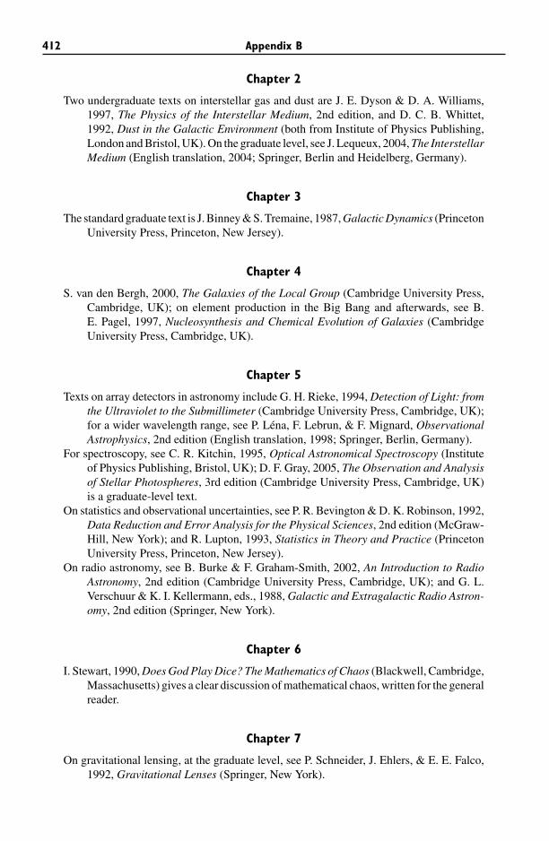
412 Appendix B

Chapter 2

Two undergraduate texts on interstellar gas and dust are J. E. Dyson & D. A. Williams,1997, The Physics of the Interstellar Medium, 2nd edition, and D. C. B. Whittet,1992, Dust in the Galactic Environment (both from Institute of Physics Publishing,London and Bristol, UK). On the graduate level, see J. Lequeux, 2004, The InterstellarMedium (English translation, 2004; Springer, Berlin and Heidelberg, Germany).

Chapter 3

The standard graduate text is J. Binney & S. Tremaine, 1987, Galactic Dynamics (PrincetonUniversity Press, Princeton, New Jersey).

Chapter 4

S. van den Bergh, 2000, The Galaxies of the Local Group (Cambridge University Press,Cambridge, UK); on element production in the Big Bang and afterwards, see B.E. Pagel, 1997, Nucleosynthesis and Chemical Evolution of Galaxies (CambridgeUniversity Press, Cambridge, UK).

Chapter 5

Texts on array detectors in astronomy include G. H. Rieke, 1994, Detection of Light: fromthe Ultraviolet to the Submillimeter (Cambridge University Press, Cambridge, UK);for a wider wavelength range, see P. Lena, F. Lebrun, & F. Mignard, ObservationalAstrophysics, 2nd edition (English translation, 1998; Springer, Berlin, Germany).

For spectroscopy, see C. R. Kitchin, 1995, Optical Astronomical Spectroscopy (Instituteof Physics Publishing, Bristol, UK); D. F. Gray, 2005, The Observation and Analysisof Stellar Photospheres, 3rd edition (Cambridge University Press, Cambridge, UK)is a graduate-level text.

On statistics and observational uncertainties, see P. R. Bevington & D. K. Robinson, 1992,Data Reduction and Error Analysis for the Physical Sciences, 2nd edition (McGraw-Hill, New York); and R. Lupton, 1993, Statistics in Theory and Practice (PrincetonUniversity Press, Princeton, New Jersey).

On radio astronomy, see B. Burke & F. Graham-Smith, 2002, An Introduction to RadioAstronomy, 2nd edition (Cambridge University Press, Cambridge, UK); and G. L.Verschuur & K. I. Kellermann, eds., 1988, Galactic and Extragalactic Radio Astron-omy, 2nd edition (Springer, New York).

Chapter 6

I. Stewart, 1990, Does God Play Dice? The Mathematics of Chaos (Blackwell, Cambridge,Massachusetts) gives a clear discussion of mathematical chaos, written for the generalreader.

Chapter 7

On gravitational lensing, at the graduate level, see P. Schneider, J. Ehlers, & E. E. Falco,1992, Gravitational Lenses (Springer, New York).

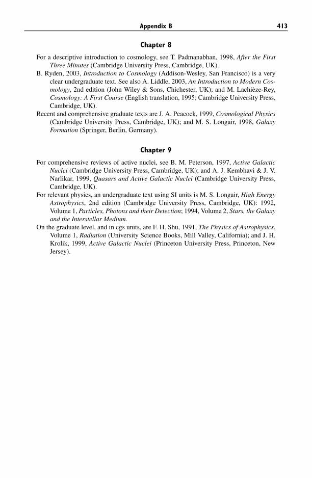
Appendix B 413

Chapter 8

For a descriptive introduction to cosmology, see T. Padmanabhan, 1998, After the FirstThree Minutes (Cambridge University Press, Cambridge, UK).

B. Ryden, 2003, Introduction to Cosmology (Addison-Wesley, San Francisco) is a veryclear undergraduate text. See also A. Liddle, 2003, An Introduction to Modern Cos-mology, 2nd edition (John Wiley & Sons, Chichester, UK); and M. Lachieze-Rey,Cosmology: A First Course (English translation, 1995; Cambridge University Press,Cambridge, UK).

Recent and comprehensive graduate texts are J. A. Peacock, 1999, Cosmological Physics(Cambridge University Press, Cambridge, UK); and M. S. Longair, 1998, GalaxyFormation (Springer, Berlin, Germany).

Chapter 9

For comprehensive reviews of active nuclei, see B. M. Peterson, 1997, Active GalacticNuclei (Cambridge University Press, Cambridge, UK); and A. J. Kembhavi & J. V.Narlikar, 1999, Quasars and Active Galactic Nuclei (Cambridge University Press,Cambridge, UK).

For relevant physics, an undergraduate text using SI units is M. S. Longair, High EnergyAstrophysics, 2nd edition (Cambridge University Press, Cambridge, UK): 1992,Volume 1, Particles, Photons and their Detection; 1994, Volume 2, Stars, the Galaxyand the Interstellar Medium.

On the graduate level, and in cgs units, are F. H. Shu, 1991, The Physics of Astrophysics,Volume 1, Radiation (University Science Books, Mill Valley, California); and J. H.Krolik, 1999, Active Galactic Nuclei (Princeton University Press, Princeton, NewJersey).

Appendix C

Hints for problems

Problem 1.14 See Table 1.4 for the Sun’s absolute magnitude MV , and remember that

MB = MV + (B − V ), while MI = MV − (V − I ).

Problem 1.20 The energy in the background radiation is 1054 J Mpc−3. The Sun radi-

ates 4 × 1026 W or 1043 J Gyr−1; so, from Equation 1.25, galaxies emit about 2 ×1051 J Mpc−3 Gyr−1. Even though the galaxies were brighter in the past, all the starlight

radiated since the Big Bang falls far short of the energy in the cosmic background

radiation.

Problem 2.4 If the rate of starbirth at time t is B(t), then, for stars that spend time

τMS < τgal on the main sequence, the initial luminosity function �(MV ) is related to the

present-day luminosity function �MS by

�(MV ) = �MS(MV ) ×∫ τgal

0B(t) dt

/∫ τgal

τgal−τMS

B(t)dt .

The faster B(t) declines with time, the more of these short-lived stars must be born to

yield the numbers that we see today.

Problem 2.5 Taking L ∝ M3.5 for each star, the number N of stars and their total

luminosity L are

N = ξ0

∫ Mu

Ml

( MM�

)−2.35 dMM�

, L = L�ξ0

∫ Mu

Ml

( MM�

)−2.35+3.5 dMM�

.

The integral for N and that for the total mass both diverge as the lower limit Ml → 0,

while that for L becomes large as Mu increases. Almost all the light of a young cluster

comes from the few most massive stars. At ages beyond 2–3 Gyr light comes mainly from

red giants, which reach roughly the same luminosity independently of the star’s initial

mass.

414

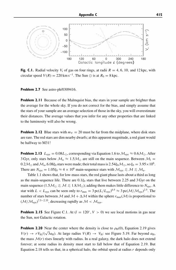
Appendix C 415

−100

−50

0

50

100

180 120 60 0 300 240 180

Fig. C.1. Radial velocity Vr of gas on four rings, at radii R = 4, 6, 10, and 12 kpc, with

circular speed V (R) = 220 km s−1. The Sun � is at R0 = 8 kpc.

Problem 2.7 See astro-ph/0309416.

Problem 2.11 Because of the Malmquist bias, the stars in your sample are brighter than

the average for the whole sky. If you do not correct for the bias, and simply assume that

the stars of your sample are an average selection of those in the sky, you will overestimate

their distances. The average values that you infer for any other properties that are linked

to the luminosity will also be wrong.

Problem 2.12 Blue stars with mV = 20 must be far from the midplane, where disk stars

are rare. The red stars are dim nearby dwarfs; at this apparent magnitude, a red giant would

be halfway to M31!

Problem 2.13 Leye = 0.08L�, corresponding via Equation 1.6 to Meye ≈ 0.6M�. After

3 Gyr, only stars below Mu ≈ 1.5M� are still on the main sequence. Between Ml =0.2M� andMu, 6.08ξ0 stars were made; their total mass is 2.54ξ0M�, so ξ0 = 3.95×106.

There are Neye = 1.05ξ0 ≈ 4 × 106 main-sequence stars with Meye ∼< M ∼< Mu.

Table 1.1 shows that, for low-mass stars, the red giant phase lasts about a third as long

as the main-sequence life. There are 0.1ξ0 stars that live between 2.25 and 3 Gyr on the

main sequence (1.5M� ∼< M ∼< 1.8M�); adding them makes little difference to Neye. A

star with L < Leye can be seen only to rmax = 3 pc(L/Leye)0.5 ≈ 3 pc(M/Meye)2.5. The

number of stars between M and M+ �M within the sphere rmax(M) is proportional to

(M/Meye)7.5−2.35, decreasing rapidly as M < Meye.

Problem 2.15 See Figure C.1. At (l = 120◦, V > 0) we see local motions in gas near

the Sun, not Galactic rotation.

Problem 2.20 Near the center where the density is close to ρH(0), Equation 2.19 gives

V (r ) → r VH/(√

3aH). At large radius V (R) → VH: see Figure 5.19. Far beyond aH,

the mass M(r ) rises linearly with radius. In a real galaxy, the dark halo does not extend

forever; at some radius its density must start to fall below that of Equation 2.19. But

Equation 2.18 tells us that, in a spherical halo, the orbital speed at radius r depends only

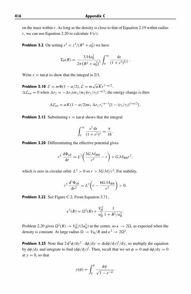
416 Appendix C

on the mass within r . As long as the density is close to that of Equation 2.19 within radius

r , we can use Equation 2.20 to calculate V (r ).

Problem 3.2 On setting s2 = z2/(R2 + a2P) we have

�P(R) = 3Ma2P

2π(R2 + a2

P

)2

∫ ∞

0

ds

(1 + s2)5/2.

Write s = tan φ to show that the integral is 2/3.

Problem 3.10 E = m�(1 − α/2), L = m√

αKr1−α/2.

�Ltot = 0 when �r2 = −�r1(m1/m2)(r1/r2)−α/2; the energy change is then

�Etot = αK (1 − α/2)m1 �r1 r−α−11 [1 − (r1/r2)1+α/2] .

Problem 3.12 Substituting s = tan φ shows that the integral

∫ ∞

0

s2 ds

(1 + s2)3= π

16.

Problem 3.20 Differentiating the effective potential gives

r4 d�eff

dr= L2

(3GMBH

c2− r

)+ GMBHr2,

which is zero in circular orbit: L2 > 0 so r > 3GM/c2. For stability,

r5 d2�eff

dr2= L2

(r − 6GMBH

c2

)> 0.

Problem 3.22 See Figure C.2. From Equation 3.71,

κ2(R) = �2(R) + V 2H

a2H

1

1 + R2/a2H

.

Problem 2.20 gives �2(R) → V 2H/(3a2

H) at the center, so κ → 2�, as expected when the

density is constant. At large radius � → VH/R and κ2 → 2�2.

Problem 3.25 Note that 2 d2φ/dy2 · dφ/dy = d(dφ/dy)2/dy, so multiply the equation

by dφ/dy and integrate to find (dφ/dy)2. Then, recall that we set φ = 0 and dφ/dy = 0

at y = 0, so that

y(φ) =∫ φ

0

dψ√1 − e−ψ

.

Appendix C 417

0 1 2 3 4 50

0.2

0.4

0.6

0.8

1

1.2

Fig. C.2. For a circular orbit at radius R in the ‘dark-halo’ potential, the angular velocity

� (solid curve), the epicyclic frequency κ (dashed curve), and � − κ/2 (dotted curve).

The units are VH/aH.

Setting u = e−ψ/2, and then t = sech u, and integrating yields e−φ/2 = sech(y/2). At

large z, n(z) = n0e−φ → 4n0e−|z|/z0 ; the midplane density n0 is four times lower than the

inward extrapolation of the exponential.

Problem 4.1 The brightest blue stars in this region have V − I ≈ 0 ≈ MV ; they are

main-sequence stars, of late B or early A types. The brightest red stars are K giants,

not supergiants. Just as we found few supergiants among the solar-neighborhood stars of

Figure 2.2, such rare very luminous stars are missing from this small patch of the LMC’s

disk.

Problem 4.4 The Jacobi radius rJ = 0.01 AU, while the average distance between Earth

and Moon rEM = 0.0026 AU. The ratio of the gravitational forces from Earth and Sun is

(m/M)(1 AU/rEM)2 ≈ 0.5.

Problem 4.5 Since m � M, the mass center C is at the halo center. What rotation rate �

must you choose to follow m in its circular orbit? In Equation 4.7, you can find ∂�H/∂x

from M(<r ).

Problem 4.10 We have yet another reason to think that gas is entering the Galaxy. The

Milky Way’s disk produces (3–5)M� of new stars each year (Section 2.1) which will use up

our (5–10) × 109M� of disk gas within 1–3 Gyr. Dying stars return (M� to 2M�) of gas

per year, which is not enough to avoid exhausting the supply. If gas flows into the disk

from outside, we avoid the uncomfortable conclusion that we see the Milky Way and other

spiral galaxies at the very end of their star-forming lives.

Problem 5.1 At the 0.6 m telescope: 1.1′′ pixel; 37′ field. At 4 m prime focus: 0.54′′ pixel;

18′ field. For 4 m f/7.5: 0.167′′ pixel; 5.7′ field. If seeing is 0.8′′, the image at f/7.5 will

be no sharper than at prime focus; the entire galaxy fits into the field of view only at the

0.6 m telescope.

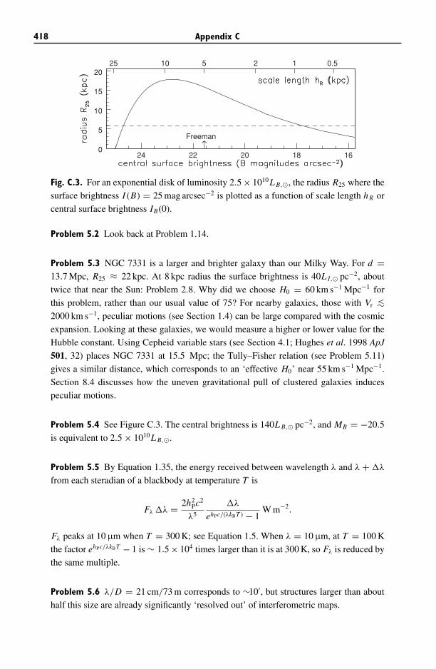
418 Appendix C

24 22 20 18 16

0.515 225 10

Freeman

0

5

10

15

20

Fig. C.3. For an exponential disk of luminosity 2.5 × 1010L B,�, the radius R25 where the

surface brightness I (B) = 25 mag arcsec−2 is plotted as a function of scale length h R or

central surface brightness IB(0).

Problem 5.2 Look back at Problem 1.14.

Problem 5.3 NGC 7331 is a larger and brighter galaxy than our Milky Way. For d =13.7 Mpc, R25 ≈ 22 kpc. At 8 kpc radius the surface brightness is 40L I,� pc−2, about

twice that near the Sun: Problem 2.8. Why did we choose H0 = 60 km s−1 Mpc−1 for

this problem, rather than our usual value of 75? For nearby galaxies, those with Vr ∼<2000 km s−1, peculiar motions (see Section 1.4) can be large compared with the cosmic

expansion. Looking at these galaxies, we would measure a higher or lower value for the

Hubble constant. Using Cepheid variable stars (see Section 4.1; Hughes et al. 1998 ApJ

501, 32) places NGC 7331 at 15.5 Mpc; the Tully–Fisher relation (see Problem 5.11)

gives a similar distance, which corresponds to an ‘effective H0’ near 55 km s−1 Mpc−1.

Section 8.4 discusses how the uneven gravitational pull of clustered galaxies induces

peculiar motions.

Problem 5.4 See Figure C.3. The central brightness is 140L B,� pc−2, and MB = −20.5

is equivalent to 2.5 × 1010L B,�.

Problem 5.5 By Equation 1.35, the energy received between wavelength λ and λ + �λ

from each steradian of a blackbody at temperature T is

Fλ �λ = 2h2Pc2

λ5

�λ

ehPc/(λkBT ) − 1W m−2.

Fλ peaks at 10 μm when T = 300 K; see Equation 1.5. When λ = 10 μm, at T = 100 K

the factor ehPc/λkBT − 1 is ∼ 1.5 × 104 times larger than it is at 300 K, so Fλ is reduced by

the same multiple.

Problem 5.6 λ/D = 21 cm/73 m corresponds to ∼10′, but structures larger than about

half this size are already significantly ‘resolved out’ of interferometric maps.

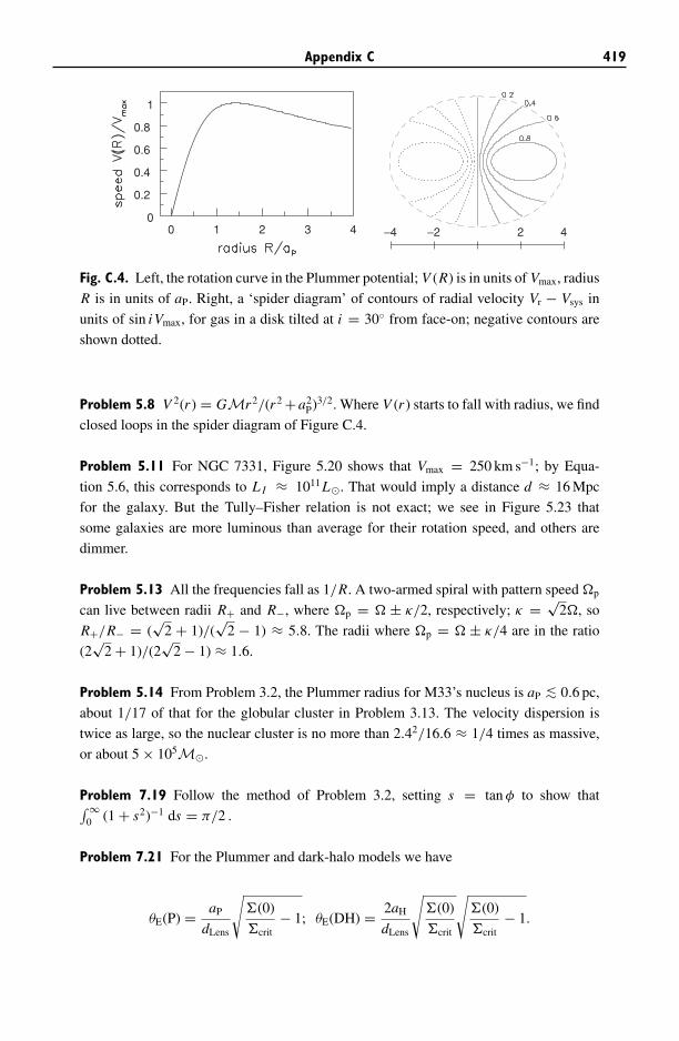
Appendix C 419

0 1 2 3 40

0.2

0.4

0.6

0.8

1

2−2 4−4

Fig. C.4. Left, the rotation curve in the Plummer potential; V (R) is in units of Vmax, radius

R is in units of aP. Right, a ‘spider diagram’ of contours of radial velocity Vr − Vsys in

units of sin iVmax, for gas in a disk tilted at i = 30◦ from face-on; negative contours are

shown dotted.

Problem 5.8 V 2(r ) = GMr2/(r2 +a2P)3/2. Where V (r ) starts to fall with radius, we find

closed loops in the spider diagram of Figure C.4.

Problem 5.11 For NGC 7331, Figure 5.20 shows that Vmax = 250 km s−1; by Equa-

tion 5.6, this corresponds to L I ≈ 1011L�. That would imply a distance d ≈ 16 Mpc

for the galaxy. But the Tully–Fisher relation is not exact; we see in Figure 5.23 that

some galaxies are more luminous than average for their rotation speed, and others are

dimmer.

Problem 5.13 All the frequencies fall as 1/R. A two-armed spiral with pattern speed �p

can live between radii R+ and R−, where �p = � ± κ/2, respectively; κ = √2�, so

R+/R− = (√

2 + 1)/(√

2 − 1) ≈ 5.8. The radii where �p = � ± κ/4 are in the ratio

(2√

2 + 1)/(2√

2 − 1) ≈ 1.6.

Problem 5.14 From Problem 3.2, the Plummer radius for M33’s nucleus is aP ∼< 0.6 pc,

about 1/17 of that for the globular cluster in Problem 3.13. The velocity dispersion is

twice as large, so the nuclear cluster is no more than 2.42/16.6 ≈ 1/4 times as massive,

or about 5 × 105M�.

Problem 7.19 Follow the method of Problem 3.2, setting s = tan φ to show that∫∞0 (1 + s2)−1 ds = π/2 .

Problem 7.21 For the Plummer and dark-halo models we have

θE(P) = aP

dLens

√�(0)

�crit− 1; θE(DH) = 2aH

dLens

√�(0)

�crit

√�(0)

�crit− 1.

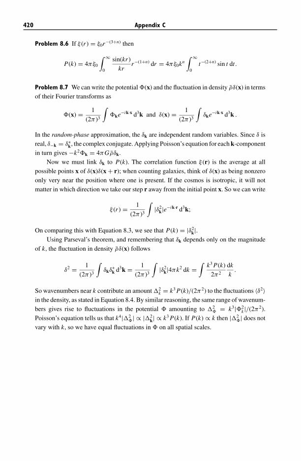
420 Appendix C

Problem 8.6 If ξ (r ) = ξ0r−(3+n) then

P(k) = 4πξ0

∫ ∞

0

sin(kr )

krr−(1+n) dr = 4πξ0kn

∫ ∞

0t−(2+n) sin t dt.

Problem 8.7 We can write the potential �(x) and the fluctuation in density ρδ(x) in terms

of their Fourier transforms as

�(x) = 1

(2π)3

∫�ke−ik·x d3k and δ(x) = 1

(2π)3

∫δke−ik·x d3k .

In the random-phase approximation, the δk are independent random variables. Since δ is

real, δ−k = δ∗k, the complex conjugate. Applying Poisson’s equation for each k-component

in turn gives −k2�k = 4πGρδk.

Now we must link δk to P(k). The correlation function ξ (r) is the average at all

possible points x of δ(x)δ(x + r); when counting galaxies, think of δ(x) as being nonzero

only very near the position where one is present. If the cosmos is isotropic, it will not

matter in which direction we take our step r away from the initial point x. So we can write

ξ (r ) = 1

(2π )3

∫|δ2

k|e−ik·r d3k;

On comparing this with Equation 8.3, we see that P(k) = |δ2k|.

Using Parseval’s theorem, and remembering that δk depends only on the magnitude

of k, the fluctuation in density ρδ(x) follows

δ2 = 1

(2π )3

∫δkδ

∗k d3k = 1

(2π )3

∫|δ2

k|4πk2 dk =∫

k3 P(k)

2π2

dk

k.

So wavenumbers near k contribute an amount �2k = k3 P(k)/(2π2) to the fluctuations 〈δ2〉

in the density, as stated in Equation 8.4. By similar reasoning, the same range of wavenum-

bers gives rise to fluctuations in the potential � amounting to �2� = k3|�2

k |/(2π2).

Poisson’s equation tells us that k4|�2�| ∝ |�2

k| ∝ k3 P(k). If P(k) ∝ k then |�2�| does not

vary with k, so we have equal fluctuations in � on all spatial scales.

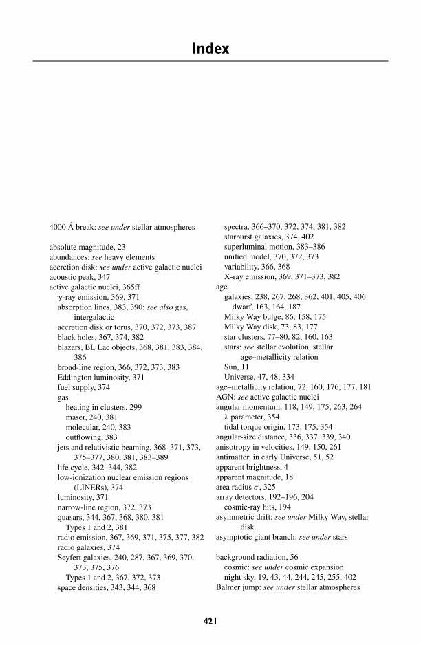
Index

4000 A break: see under stellar atmospheres

absolute magnitude, 23abundances: see heavy elementsaccretion disk: see under active galactic nucleiacoustic peak, 347active galactic nuclei, 365ff

γ-ray emission, 369, 371absorption lines, 383, 390: see also gas,

intergalacticaccretion disk or torus, 370, 372, 373, 387black holes, 367, 374, 382blazars, BL Lac objects, 368, 381, 383, 384,

386broad-line region, 366, 372, 373, 383Eddington luminosity, 371fuel supply, 374gas

heating in clusters, 299maser, 240, 381molecular, 240, 383outflowing, 383

jets and relativistic beaming, 368–371, 373,375–377, 380, 381, 383–389

life cycle, 342–344, 382low-ionization nuclear emission regions

(LINERs), 374luminosity, 371narrow-line region, 372, 373quasars, 344, 367, 368, 380, 381

Types 1 and 2, 381radio emission, 367, 369, 371, 375, 377, 382radio galaxies, 374Seyfert galaxies, 240, 287, 367, 369, 370,

373, 375, 376Types 1 and 2, 367, 372, 373

space densities, 343, 344, 368

spectra, 366–370, 372, 374, 381, 382starburst galaxies, 374, 402superluminal motion, 383–386unified model, 370, 372, 373variability, 366, 368X-ray emission, 369, 371–373, 382

agegalaxies, 238, 267, 268, 362, 401, 405, 406

dwarf, 163, 164, 187Milky Way bulge, 86, 158, 175Milky Way disk, 73, 83, 177star clusters, 77–80, 82, 160, 163stars: see stellar evolution, stellar

age–metallicity relationSun, 11Universe, 47, 48, 334

age–metallicity relation, 72, 160, 176, 177, 181AGN: see active galactic nucleiangular momentum, 118, 149, 175, 263, 264

λ parameter, 354tidal torque origin, 173, 175, 354

angular-size distance, 336, 337, 339, 340anisotropy in velocities, 149, 150, 261antimatter, in early Universe, 51, 52apparent brightness, 4apparent magnitude, 18area radius σ , 325array detectors, 192–196, 204

cosmic-ray hits, 194asymmetric drift: see under Milky Way, stellar

diskasymptotic giant branch: see under stars

background radiation, 56cosmic: see under cosmic expansionnight sky, 19, 43, 44, 244, 245, 255, 402

Balmer jump: see under stellar atmospheres

421

422 Index

bars: see under disks of galaxiesbaryon oscillations, 323, 346, 347, 359baryons

cosmic density, 48, 53, 54, 220, 300,397

benchmark cosmology: see under cosmicexpansion

Big Bang nucleosynthesis, 9, 50, 52Big Bang: see cosmic expansionbinary stars, 2, 17, 157, 182,

270Lagrange points, 166, 167microquasars, 386, 387star clusters, 132Type Ia supernova, 17, 18X-rays, 17, 271

black holesactive nuclei, 367, 374, 382from supernovae, 16galaxy center, 169, 172, 184, 239, 240, 266,

273, 275–277, 287, 382microquasars, 387Milky Way center, 67, 68, 86–88orbits around, 136Schwarzschild radius, 276, 304, 367stellar binaries, 271

blackbody radiation, 3, 4, 33, 43, 51,331

blazars, BL Lac objects: see under activegalactic nuclei

bolometric correction, 21, 23–25bolometric luminosity, 2, 25bremsstrahlung: see free–free radiationbrown dwarfs, 6bulges of galaxies, 169, 170, 191, 200,

236–238, 247, 275Milky Way, 26, 86, 87, 99, 158, 175,

180rotation, 87, 237

counter-rotation, 214

celestial poles, 34Cepheid variable stars, 15, 37

period–luminosity relation, 161Chandrasekhar limit, 17, 182charge-coupled device (CCD), 192–196closed-box model: see under heavy elementsclosed Universe, 325clusters of galaxies: see groups and clusters of

galaxiescollisional ionization, 28collisionless Boltzmann equation, 140ffcollisions and mergers: see galaxy collisions

and mergerscolor, definition, 22

comovingcoordinates, 326, 352density, 342volume, 342, 343

coolingcurve for gas, 105, 106, 299time, 105, 106, 298, 299

coordinatescomoving, 326equatorial (α, δ), 34Galactic (l, b), 36Galactocentric (R, φ, z), 37supergalactic, 154, 316

core collapse of star cluster, 132core radius, 78, 80, 113, 122, 132, 163, 247,

249, 292correlation function ξ (r ): see large-scale

structurecosmic background radiation (CMB): see

under cosmic expansioncosmic expansion 46ff, 325ff

age of Universe, 47, 81, 333, 334angular-size distance, 336, 338, 339area radius σ , 325background radiation, 50–56, 344, 356,

357baryon oscillations: see under large-scale

structurefluctuations, 344–347, 359

benchmark model, 48, 330, 334initial fluctuations, 344, 359, 362

cold dark matter, 358, 359, 362, 363, 405WIMPs, 176, 357, 358, 363

comoving length and volume, 342, 343, 352cosmological constant �: see dark energy,

inflationcosmological redshift, 50, 326, 327, 336dark energy, 48, 295, 329, 347dark matter: see separate entrydensity parameter �(t), 329distance radius χ , 338Friedmann models, 328growth of fluctuations: see under large-scale

structurehorizon, 332, 356hot dark matter, 358inflation, 328, 329, 332, 344lookback time, 333–335luminosity distance, 336, 338, 339matter-dominated Universe, 330, 331, 334,

351, 352, 353matter–radiation equality, 55, 330, 331, 356Olbers’ paradox, 335, 339photometric redshifts, 340, 341, 342radiation-dominated Universe, 330, 356

Index 423

recombination, 54, 55, 324, 331, 332, 344reionization, 395, 396scale factor a(t), 331scale length R(t), 326surface brightness dimming, 337

cosmic rays, 101, 107, 109, 375effect on array detectors, 194

counter-rotation, 214, 238, 263critical density ρcrit, 48critical surface density �crit, 309crossing time tcross, 128curved space, 325

D–σ relation for ellipticals, 258damped Lyman-α clouds, 390–395dark energy, 48, 295, 329, 347dark matter, 27, 48, 54

between galaxies, 188–190, 283, 297, 299,310, 312

cold, 176, 358, 359, 362, 363, 405galaxies, 164, 176, 217–221, 256, 258,

273–275, 283hot, 358large-scale structure, 358Milky Way, 94, 95, 123, 145weakly interacting massive particles, 49,

176, 357, 358de Vaucouleurs law, 244, 245declination: see coordinates, equatorialdensity parameter �(t), 329deuterium

produced in Big Bang, 50, 52, 54diffraction limit, 206disks of galaxies, 39, 41, 169, 191ff: see also

Milky Wayasymmetric drift, 160barred, 39, 40, 86, 191, 204, 232, 234ffclassification, 39, 222exponential law, 70, 71, 198, 199, 337

scale height hz , 27, 71–74, 202scale length h R , 27, 71, 86, 169, 171, 199,

202formation, 175, 181, 392, 393gas, 170–172, 206, 212, 226, 236

atomic, 157, 209–212, 220, 223, 226, 392dusty, 205, 212, 234, 235, 239ionized, 157, 212, 226molecular, 213

low-surface-brightness, 185, 186, 201, 202,203, 211, 218

mass density, 143, 144radial gradients, 179, 199radio emission, 212, 213rotation, 39, 156, 169, 184ff

differential, 89, 217, 225, 228

spiral pattern, 39, 172, 191, 204, 222, 223,225ff, 235, 287

Q parameter, 232corotation radius, 231, 233, 235, 236density-wave theory, 228, 230, 233flocculent, 227Lindblad resonances, 230, 231pattern speed, 230–236pitch angle, 227, 228theories, 229

stability, 135, 136, 231–233star formation, 170, 205, 212, 239, 270stellar content, 157, 158, 170, 192, 197ff,

222ffthick disk, 27, 71, 72, 74, 75, 83, 202thin disk, 27, 71, 72, 74, 75Tully–Fisher relation, 220, 221, 222, 362vertical motions, 144–147warps, 171, 172, 216

distanceangular size, 336, 337, 339, 340kinematic, 96luminosity, 336, 337, 339modulus, 60

distance radius χ , 338distances to galaxies, 160

Cepheids, 160, 161kinematics, 257redshifts, 46standard candles, 160–162supernovae, 18, 69tip of red giant branch, 14, 316, 317Tully–Fisher relation, 221, 222

distances to starsclusters, 76, 81, 160inverse-square law, 2, 18period–luminosity relation, 161photometric parallax, 70, 71spectroscopic parallax, 70trigonometric parallax, 59, 60

distribution function, 140Maxwellian, 130polytrope, 147

Doppler shift: see under redshiftdust, 6, 33, 34, 56, 78, 182

active nuclei, 371disk galaxies, 103, 169–171, 182, 192, 201,

204, 212, 226, 234, 235elliptical galaxies, 39, 184, 271, 302emission spectrum, 103, 205, 291extinction and scattering, 33, 34formation, 104heating, 34, 102, 103, 107, 290, 291high-redshift galaxies, 400, 402, 404, 405intergalactic gas, 395

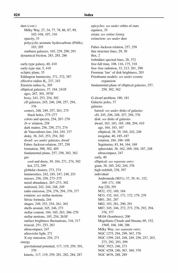
424 Index

dust (cont.)Milky Way, 27, 34, 77, 78, 86, 87, 99,

102–104, 107, 316opacity, 33polycyclic aromatic hydrocarbons (PAHs),

103, 205starburst galaxies, 103, 239, 290, 291

dynamical friction, 283, 285, 286

early-type galaxy, 40, 410early-type star, 5, 410ecliptic plane, 35Eddington luminosity, 371, 372, 387effective radius Re, 237, 243Einstein radius θE, 305elliptical galaxies, 37, 184, 241ff

ages, 267, 301, 397ffboxy, 243, 253, 254, 302cD galaxies, 245, 246, 248, 257, 294,

376centers, 248, 249, 257, 263, 275

black holes, 275–277colors and spectra, 254, 267–270D–σ relation, 258dark matter, 256, 258, 273, 274de Vaucouleurs law, 244, 245, 337disky, 38, 243, 253, 254, 302dwarf: see under galaxies, dwarfFaber–Jackson relation, 257, 258formation, 300, 302, 405fundamental plane, 257, 258, 302, 362gas

cool and dusty, 39, 184, 271, 274, 302hot, 272, 299

globular clusters, 273, 274luminosities, 242, 245, 247, 248, 251masses, 256, 258, 273–275metal abundance, 267–273, 302midsized, 242, 244, 248, 249radio emission, 254, 276, 294, 376, 377rotation: see stellar motionsSersic formula, 244shapes, 249, 253, 254, 261, 262shells around, 245, 246, 273stellar content, 184, 185, 263, 266–270stellar motions, 185, 254, 263ffsurface brightness fluctuations, 316, 317triaxial, 251, 253, 263ultracompact, 247ultraviolet light, 271X-ray emission, 254, 271

energygravitational potential, 117, 119, 259, 301,

370kinetic, 117, 119, 259, 281, 282, 284, 287

epicycles: see under orbits of starsequinox, 35errata: see online listingextinction: see under dust

Faber–Jackson relation, 257, 258fine structure lines, 29, 30flux, 2forbidden spectral lines, 28, 372free-fall time, 108, 116, 175, 318free–free radiation, 33, 213, 281, 290Freeman ‘law’ of disk brightness, 203Friedmann models: see under cosmic

expansionfundamental plane of elliptical galaxies, 257,

258, 302, 362

G-dwarf problem, 180, 181Galactic poles, 37galaxies

barred: see under disks of galaxiescD, 245, 246, 248, 257, 294, 376disk: see disks of galaxiesdwarf, 163, 183, 185, 188, 294, 410

age, 164, 183, 187elliptical, 38, 39, 184, 242, 248irregular, 40, 185–187rotation, 184, 186–188Sagittarius, 83, 84, 164, 169spheroidal, 38, 162, 169, 184, 187, 248ultracompact, 247

early, 40elliptical: see separate entrygiant, 38, 185, 242, 244, 376high redshift, 238, 397individual

Andromeda (M31), 37, 39, 41, 152,169–171, 188

Arp 220, 291M32, 152, 169, 184M33, 152, 163, 171, 172, 179, 239M81, 281, 287M82, 103, 281, 290, 291M87, 245, 246, 272, 273, 276, 292, 294,

376, 377M104 (Sombrero), 200Magellanic Clouds and Stream, 69, 152,

156ff, 168, 188, 286Milky Way: see separate entryNGC 1275, 294, 299, 367, 376NGC 1399, 245, 248, 249, 256, 257, 263,

273, 292, 293, 299NGC 3923, 246, 273NGC 4258, 240, 367, 369, 370NGC 4676, 288, 289

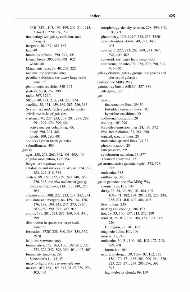
Index 425

NGC 7331, 103, 197–199, 209–211, 213,216–218, 220, 236, 238

interacting: see galaxy collisions andmergers

irregular, 40, 157, 185–187late, 40luminous infrared, 290, 291, 403Lyman break, 393, 399, 401, 402

winds, 401Magellanic type, 39, 40, 202, 222nucleus: see separate entrypeculiar velocities: see under large-scale

structurephotometric redshifts, 340–342post-starburst, 267, 399radio, 367, 374ffS0, 38, 40, 191, 213, 214, 223, 224satellite, 38, 151, 159, 169, 285, 286, 363Seyfert: see under active galactic nucleispiral: see disks of galaxiesstarburst, 40, 224, 233, 239, 281, 287, 288,

291, 297, 374, 399, 404active nucleus cohabiting, 402dusty, 290, 291, 402winds, 109, 290, 401

see also Lyman break galaxiessubmillimeter, 403

galaxyages, 238, 267, 268, 362, 401, 405, 406angular momentum, 173, 354bulges: see separate entrycatalogues and surveys, 22, 41, 42, 224, 279,

283, 292, 318, 374centers, 99, 169, 172, 239, 240, 248, 249,

276, 363: see also nucleus of galaxycusps in brightness, 114, 117, 249, 266,

363classification, 38ff, 222, 223, 237, 242, 254collisions and mergers, 84, 159, 164, 170,

176, 188, 190, 245, 246, 273, 283ff,287–289, 290, 292, 300, 302

colors, 199, 201, 223, 237, 269, 302, 341,399

distribution in space: see large-scalestructure

formation, 172ff, 238, 300, 318, 354, 362,397ff

halo: see separate entryluminosities, 152, 163, 186, 199, 201, 203,

223, 224, 242, 398, 399, 401, 402, 405luminosity function, 293

Schechter’s L, 43, 45mass-to-light ratio: see separate entrymasses, 163, 164, 169, 213, 214ff, 239, 274,

403, 404

morphology–density relation, 278, 295, 300,320, 321

photometry, 42ff, 197ff, 243, 253, 335ffspace densities, 43–46, 49, 293, 342,

405spectra, 6, 222, 223, 267, 268, 341, 367,

398–400, 402spheroid: see under halo, metal-poorstar-formation rates, 72, 238, 270, 290, 399,

401–406galaxy clusters, galaxy groups: see groups and

clusters of galaxiesGalaxy: see Milky Waygamma-ray bursts (GRBs), 387–389

afterglow, 388gas

atomicfine structure lines, 29, 30forbidden emission lines, 103hyperfine transitions, 30

collisional ionization, 28cooling, 105, 298forbidden emission lines, 28, 103, 372free–free radiation, 33, 281, 290ionized, spectral lines, 28molecular, spectral lines, 30, 31photoionization, 28ram pressure, 295synchrotron radiation, 33, 377Thomson scattering, 371

gas around active galactic nuclei, 372, 373,383

molecular, 383outflowing, 383

gas in galaxies: see also Milky Waycosmic rays, 101, 109dusty, 33, 34, 39, 86, 102–104, 107,

169–171, 182, 184, 201, 212, 226, 234,235, 271, 400, 402, 404, 405

flow in bars, 235heating and cooling, 106, 107hot, 28, 33, 100, 157, 213, 272, 299ionized, 28, 101, 102, 104, 157, 170, 212,

226HII region, 28, 101, 105

magnetic fields, 101, 109masers, 31, 240molecular, 30, 31, 100, 102, 108, 172, 213,

289, 401formation, 104

neutral hydrogen, 30, 100–102, 152, 157,158, 170, 171, 186, 203, 209–214, 220,223, 226, 271, 274, 295, 296, 392,393

high-velocity clouds, 99, 159

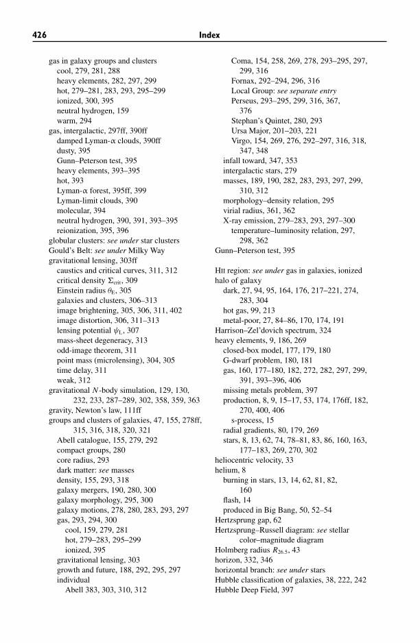
426 Index

gas in galaxy groups and clusterscool, 279, 281, 288heavy elements, 282, 297, 299hot, 279–281, 283, 293, 295–299ionized, 300, 395neutral hydrogen, 159warm, 294

gas, intergalactic, 297ff, 390ffdamped Lyman-α clouds, 390ffdusty, 395Gunn–Peterson test, 395heavy elements, 393–395hot, 393Lyman-α forest, 395ff, 399Lyman-limit clouds, 390molecular, 394neutral hydrogen, 390, 391, 393–395reionization, 395, 396

globular clusters: see under star clustersGould’s Belt: see under Milky Waygravitational lensing, 303ff

caustics and critical curves, 311, 312critical density �crit, 309Einstein radius θE, 305galaxies and clusters, 306–313image brightening, 305, 306, 311, 402image distortion, 306, 311–313lensing potential ψL, 307mass-sheet degeneracy, 313odd-image theorem, 311point mass (microlensing), 304, 305time delay, 311weak, 312

gravitational N -body simulation, 129, 130,232, 233, 287–289, 302, 358, 359, 363

gravity, Newton’s law, 111ffgroups and clusters of galaxies, 47, 155, 278ff,

315, 316, 318, 320, 321Abell catalogue, 155, 279, 292compact groups, 280core radius, 293dark matter: see massesdensity, 155, 293, 318galaxy mergers, 190, 280, 300galaxy morphology, 295, 300galaxy motions, 278, 280, 283, 293, 297gas, 293, 294, 300

cool, 159, 279, 281hot, 279–283, 295–299ionized, 395

gravitational lensing, 303growth and future, 188, 292, 295, 297individual

Abell 383, 303, 310, 312

Coma, 154, 258, 269, 278, 293–295, 297,299, 316

Fornax, 292–294, 296, 316Local Group: see separate entryPerseus, 293–295, 299, 316, 367,

376Stephan’s Quintet, 280, 293Ursa Major, 201–203, 221Virgo, 154, 269, 276, 292–297, 316, 318,

347, 348infall toward, 347, 353intergalactic stars, 279masses, 189, 190, 282, 283, 293, 297, 299,

310, 312morphology–density relation, 295virial radius, 361, 362X-ray emission, 279–283, 293, 297–300

temperature–luminosity relation, 297,298, 362

Gunn–Peterson test, 395

HII region: see under gas in galaxies, ionizedhalo of galaxy

dark, 27, 94, 95, 164, 176, 217–221, 274,283, 304

hot gas, 99, 213metal-poor, 27, 84–86, 170, 174, 191

Harrison–Zel’dovich spectrum, 324heavy elements, 9, 186, 269

closed-box model, 177, 179, 180G-dwarf problem, 180, 181gas, 160, 177–180, 182, 272, 282, 297, 299,

391, 393–396, 406missing metals problem, 397production, 8, 9, 15–17, 53, 174, 176ff, 182,

270, 400, 406s-process, 15

radial gradients, 80, 179, 269stars, 8, 13, 62, 74, 78–81, 83, 86, 160, 163,

177–183, 269, 270, 302heliocentric velocity, 33helium, 8

burning in stars, 13, 14, 62, 81, 82,160

flash, 14produced in Big Bang, 50, 52–54

Hertzsprung gap, 62Hertzsprung–Russell diagram: see stellar

color–magnitude diagramHolmberg radius R26.5, 43horizon, 332, 346horizontal branch: see under starsHubble classification of galaxies, 38, 222, 242Hubble Deep Field, 397

Index 427

Hubble’s law, 46, 47, 326Hubble constant H0, 46, 326Hubble time tH, 47, 334parameter H (t), 326

hydrostatic equilibrium, 282hyperfine transitions, 30

impulse approximation, 126inflation: see cosmic expansionintegrals of motion, 145, 264intergalactic medium: see gas in galaxy groups

and clusters and gas, intergalacticinterstellar medium: see gas in galaxiesisochrones, 77, 82, 164

Jacobi constant EJ, 166jansky (Jy), 4, 407Jeans

instability, 355–357length, 108mass, 108, 356–358

jets and relativistic beaming, 368–371, 373,375–378, 380–388

k correction: see redshift, photometrickinematic distance, 96Kuzmin disk, 114

L galaxy: see galaxy luminosity functionLagrange points, 166, 167large-scale structure, 314ff

acoustic peak, 347baryon oscillations, 323, 346, 347, 359cold dark matter, 359, 362correlation function ξ (r ), 322–324density fluctuations, 318, 323, 324

growth, 173, 344fffluctuations in CMB, 344–347, 359Harrison–Zel’dovich spectrum, 324Jeans instability, 355–357peculiar velocities, 50, 314, 319, 348–353power spectrum P(k), 322–324, 346, 359,

362, 363random-phase hypothesis, 324, 344supergalactic plane, 155, 315, 316walls and voids, 48, 295, 314, 315, 318–320,

355, 359, 396late-type galaxy, 40, 410late-type star, 5, 410Local Group, 48, 151ff, 318, 406

collisions and mergers, 159, 164, 170, 176growth and future, 188membership, 152peculiar velocity, 56

local standard of rest, 89lookback time, 333, 334low-surface-brightness galaxy: see under disks

of galaxiesluminosity

bolometric, 25in-band: see under photometry, magnitude

systemluminosity distance, 336, 337, 339luminosity function

galaxies, 44, 45, 293, 399stellar, 62–65

luminous infrared galaxies (LIRGs), 290, 291,402, 403

Lyman-α forest, 395–397, 399Lyman-limit clouds, 390

Magellanic Clouds, Magellanic Stream: seeunder galaxies, individual

magnetic field, 171, 377active nuclei, 370, 380Milky Way, 87, 102, 107

magnitude systems: see under photometryMalmquist bias, 75, 415maser, 31

galaxy nucleus, 240, 381mass function, stellar

initial, 66, 401, 406Salpeter, 66, 401, 406

mass modelsdark halo, 95, 114, 168, 216, 286, 310, 311

singular isothermal sphere, 114, 148King model, 149Kuzmin disk, 114Navarro–Frenk–White (NFW), 117, 363Plummer sphere, 113, 118, 120, 147, 216,

282, 310, 311polytrope, 113, 147self-consistent, 147, 148, 266softened potential, 129truncation (tidal) radius, 149

mass segregation, 78, 131, 132mass-to-light ratio

galaxies, 163, 164, 169, 213, 217–220, 222,239, 256, 258, 273–275

galaxy groups and clusters, 283, 297, 299,312

Milky Way, 64, 71, 74, 123on larger scales, 49, 190star clusters, 78, 122

massesblack holes, 68, 87, 88, 276, 277galaxies, 94, 95, 124, 160, 163, 214ff, 223,

274, 403, 404

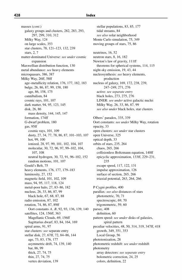
428 Index

masses (cont.)galaxy groups and clusters, 282, 283, 293,

297, 299, 310, 312Milky Way, 124on large scales, 353star clusters, 78, 121–123, 132, 239stars, 2, 7

matter-dominated Universe: see under cosmicexpansion

Maxwellian distribution function, 130metal abundance: see heavy elementsmicroquasars, 386, 387Milky Way, 26ff, 58ff

age–metallicity relation, 176, 177, 182, 183bulge, 26, 86, 87, 99, 158, 180

age, 86, 158, 175cannibalism, 84cosmic rays, 101, 107dark matter, 94, 95, 123, 145disk, 26, 86

mass density, 144, 145, 147formation, 174ffG-dwarf problem, 180gas, 95ff

cosmic rays, 101, 109dusty, 27, 34, 77, 78, 86, 87, 101–103, 107hot, 99, 100ionized, 28, 97, 99, 101, 102, 104, 107molecular, 30, 72, 96, 97, 99–102, 104,

107, 108neutral hydrogen, 30, 72, 91, 96–102, 152random motions, 101, 107

Gould’s Belt, 75heavy elements, 176, 177, 179–183luminosity, 27, 152magnetic field, 101, 102, 109mass, 94, 95, 117, 118, 124metal-poor halo, 27, 83–86, 182nucleus, 26, 33, 86, 87, 99

black hole, 67, 68, 87, 88radio emission, 87, 102rotation, 74, 86, 87, 89ff

Oort constants A, B, 92, 93, 136, 139, 140satellites, 124, 156ff, 363

Magellanic Clouds, 69, 156ffSagittarius dwarf, 83, 84, 164, 169

spiral arms, 91, 97star clusters: see separate entrystellar disk, 27, 67ff, 72, 84–86, 144

age, 73, 83, 176, 177asymmetric drift, 74, 139, 140bar, 86, 99thick, 27, 74, 75thin, 27, 74, 75vertex deviation, 139

stellar populations, 83, 85, 177tidal streams, 84see also solar neighborhood

Monte Carlo simulation, 75, 349moving groups of stars, 75, 86

neutrinos, 16, 52neutron stars, 8, 16, 182Newton’s law of gravity, 111ff

theorems for spherical systems, 114, 115night-sky emission, 19, 43, 44nucleosynthesis: see heavy elements,

productionnucleus of galaxy, 169, 172, 238, 239,

247–249, 271, 276active: see separate entryblack holes, 273, 275, 276LINER: see under active galactic nucleiMilky Way, 26, 33, 86, 87, 99see also under black holes, star clusters

Olbers’ paradox, 335, 339Oort constants: see under Milky Way, rotationopacity, 33open clusters: see under star clustersopen Universe, 325optical depth, 33orbits of stars, 235, 264

chaos, 265, 266collisionless Boltzmann equation, 140ffepicyclic approximation, 133ff, 229–231,

235escape speed, 117, 122, 131impulse approximation, 126surface of section, 265, 266triaxial potential, 263, 264, 266

P Cygni profiles, 400parallax: see also distances of stars

photometric, 70, 71spectroscopic, 69, 70trigonometric, 59, 60

parsec, 408definition, 60

pattern speed: see under disks of galaxies,spiral pattern

peculiar velocities, 48, 50, 314, 319, 347ff, 418growth, 349, 351, 353Local Group, 56

photoionization, 28photometric redshift: see under redshiftphotometry

array detectors: see separate entrybolometric correction, 24, 25colors, definition, 22

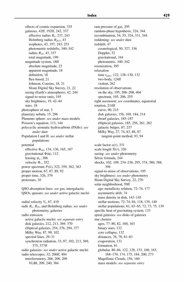
Index 429

effects of cosmic expansion, 335galaxies, 42ff, 192ff, 242, 337

effective radius Re, 237, 243Holmberg radius R26.5, 43isophotes, 43, 197, 243, 253photometric redshifts, 340–342radius R25, 43, 337total magnitude, 199

magnitude system, 18ffabsolute magnitude, 23apparent magnitude, 18definition, 18flux-based, 21Johnson, Cousins, 18, 21Sloan Digital Sky Survey, 21, 22

seeing (Earth’s atmosphere), 42, 244signal-to-noise ratio, 195sky brightness, 19, 42–44stars, 18

photosphere of star, 3planetary nebula, 15, 296Plummer sphere: see under mass modelsPoisson’s equation, 113, 144polycyclic aromatic hydrocarbons (PAHs): see

under dustPopulation I and II: see under stellar

populationspotential

effective �eff, 134, 136, 165, 167gravitational �(x), 112lensing ψL, 306velocity �v, 352

power spectrum P(k), 322, 359, 362, 363proper motion, 67, 87, 89, 92proper time, 326, 379protostars, 10

QSO absorption lines: see gas, intergalacticQSOs, quasars: see under active galactic nuclei

radial velocity Vr, 67, 410radii Re, R25, and Holmberg radius: see under

photometry, galaxiesradio emission

active galactic nuclei: see separate entrydisk galaxies, 212, 213, 369, 370elliptical galaxies, 254, 276, 294, 377Milky Way, 87, 99, 102spectral lines, 29–31synchrotron radiation, 33, 87, 102, 213, 369,

375, 377ffradio galaxies: see under active galactic nucleiradio telescopes, 32, 206ff, 404

interferometry, 206, 208, 209VLBI, 209, 240, 384

ram pressure of gas, 295random-phase hypothesis, 324, 344recombination, 54, 55, 324, 331, 344reddening: see under dustredshift, 47

cosmological, 50, 327, 336Doppler, 32gravitational, 344photometric, 340–342

reionization, 395relaxation

time trelax, 122, 128–130, 132two-body, 124ffviolent, 262

resolution of observationson the sky, 195, 206–208, 404spectrum, 195, 206, 255

right ascension: see coordinates, equatorialrotation, 214ff

curve, 90, 215disk galaxies, 156, 169, 184, 214dwarf galaxies, 185–187elliptical galaxies, 185, 256, 261, 262galactic bulges, 87, 237Milky Way, 27, 74, 83, 86, 87

tangent-point method, 93, 94

scale factor a(t), 331scale length R(t), 326seeing: see under photometrySersic formula, 244shocks, 102, 109, 234–236, 295, 374, 380, 388,

394signal-to-noise of observations, 195sky brightness: see under photometrySloan Digital Sky Survey, 22, 270solar neighborhood, 59ff

age–metallicity relation, 72–74, 177asymmetric drift, 74mass density in disk, 143–145stellar motions, 72–74, 84, 118, 139, 140stellar populations, 61, 63–65, 72, 73, 75, 139

specific heat of gravitating system, 133spiral galaxies: see disks of galaxiesstar clusters

ages, 77–80, 82, 160, 163binary stars, 132core collapse, 132distances, 76, 78, 81–83evaporation, 131formation, 81globular, 80–84, 122, 128, 133, 160, 163,

168–170, 174, 175, 184, 200, 273Magellanic Clouds, 156, 160mass models: see separate entry

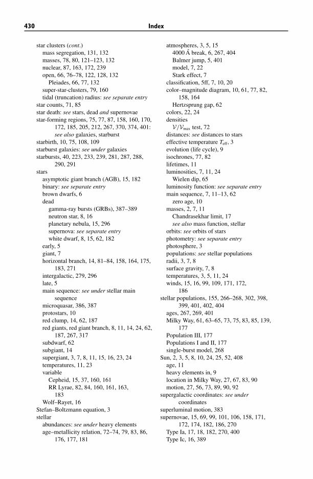
430 Index

star clusters (cont.)mass segregation, 131, 132masses, 78, 80, 121–123, 132nuclear, 87, 163, 172, 239open, 66, 76–78, 122, 128, 132

Pleiades, 66, 77, 132super-star-clusters, 79, 160tidal (truncation) radius: see separate entry

star counts, 71, 85star death: see stars, dead and supernovaestar-forming regions, 75, 77, 87, 158, 160, 170,

172, 185, 205, 212, 267, 370, 374, 401:see also galaxies, starburst

starbirth, 10, 75, 108, 109starburst galaxies: see under galaxiesstarbursts, 40, 223, 233, 239, 281, 287, 288,

290, 291stars

asymptotic giant branch (AGB), 15, 182binary: see separate entrybrown dwarfs, 6dead

gamma-ray bursts (GRBs), 387–389neutron star, 8, 16planetary nebula, 15, 296supernova: see separate entrywhite dwarf, 8, 15, 62, 182

early, 5giant, 7horizontal branch, 14, 81–84, 158, 164, 175,

183, 271intergalactic, 279, 296late, 5main sequence: see under stellar main

sequencemicroquasar, 386, 387protostars, 10red clump, 14, 62, 187red giants, red giant branch, 8, 11, 14, 24, 62,

187, 267, 317subdwarf, 62subgiant, 14supergiant, 3, 7, 8, 11, 15, 16, 23, 24temperatures, 11, 23variable

Cepheid, 15, 37, 160, 161RR Lyrae, 82, 84, 160, 161, 163,

183Wolf–Rayet, 16

Stefan–Boltzmann equation, 3stellar

abundances: see under heavy elementsage–metallicity relation, 72–74, 79, 83, 86,

176, 177, 181

atmospheres, 3, 5, 154000 A break, 6, 267, 404Balmer jump, 5, 401model, 7, 22Stark effect, 7

classification, 5ff, 7, 10, 20color–magnitude diagram, 10, 61, 77, 82,

158, 164Hertzsprung gap, 62

colors, 22, 24densities

V/Vmax test, 72distances: see distances to starseffective temperature Teff, 3evolution (life cycle), 9isochrones, 77, 82lifetimes, 11luminosities, 7, 11, 24

Wielen dip, 65luminosity function: see separate entrymain sequence, 7, 11–13, 62

zero age, 10masses, 2, 7, 11

Chandrasekhar limit, 17see also mass function, stellar

orbits: see orbits of starsphotometry: see separate entryphotosphere, 3populations: see stellar populationsradii, 3, 7, 8surface gravity, 7, 8temperatures, 3, 5, 11, 24winds, 15, 16, 99, 109, 171, 172,

186stellar populations, 155, 266–268, 302, 398,

399, 401, 402, 404ages, 267, 269, 401Milky Way, 61, 63–65, 73, 75, 83, 85, 139,

177Population III, 177Populations I and II, 177single-burst model, 268

Sun, 2, 3, 5, 8, 10, 24, 25, 52, 408age, 11heavy elements in, 9location in Milky Way, 27, 67, 83, 90motion, 27, 56, 73, 89, 90, 92

supergalactic coordinates: see undercoordinates

superluminal motion, 383supernovae, 15, 69, 99, 101, 106, 158, 171,

172, 174, 182, 186, 270Type Ia, 17, 18, 182, 270, 400Type Ic, 16, 389

Index 431

Type II, 16, 182, 270see also gamma-ray bursts

synchrotron radiation: see under radio emission

tangent point, 90, 93tangential velocity Vt, 67, 92temperature

effective temperature Teff, 3stellar system, 133virial, 283

tensor virial theorem, 259, 260, 262thermal infrared, 43Thomson scattering, 371tidal effects, 172ff, 175, 287, 288, 290, 292

torques, 173, 354truncation (tidal) radius, 80, 133, 149, 163, 167Tully–Fisher relation, 220–222, 362

Universe: see also cosmic expansion,large-scale structure

age, 47, 48, 81, 333benchmark cosmology, 48, 330cosmic background radiation: see under

cosmic expansiondark energy, 48, 329dark matter, 48density

average, 220, 329, 331, 353, 404baryons, 53, 54, 220, 300, 393, 397critical, 48, 49, 329dark energy, 330luminosity, 46, 405matter, 330radiation, 330

homogeneity and isotropy, 56, 325

V/Vmax test, 72vacuum energy: see cosmic expansion, dark

energy

vertex deviation: see under Milky Way, stellardisk

very long baseline interferometry (VLBI): seeunder radio telescopes

Virgocentric infall, 347, 348, 353virial

radius, 318, 361, 362temperature, 283tensor virial theorem, 259, 260, 262theorem, 120, 121, 260, 281–283, 287, 301,

361visible light, 19

website: see prefacewhite dwarf: see under stars, deadWielen dip, 65winds

galaxies, 109, 290, 394, 401P Cygni profiles, 400stars, 15, 16, 99, 109, 158, 171, 172, 186

Wolf–Rayet stars, 16

X-ray emission, 28active galactic nuclei, 369, 371–373, 380,

382binary stars, 17, 132, 157

microquasars, 386, 387disk galaxies, 157, 172, 206elliptical galaxies, 254, 271, 272galaxies, 33galaxy groups and clusters, 279–283, 293,

295, 297–300Milky Way, 99

yield of heavy elements, 178

zero-age main sequence: see under stellar mainsequence

zone of avoidance, 316