Abstract—The anti-lock braking systems installed on vehicles

for safe and effective braking, are high-order nonlinear and time-variant. Using fuzzy logic controllers increase efficiency of such systems, but impose a high computational complexity as well. The main concept introduced by this paper is reducing computational complexity of fuzzy controllers by deploying problem-solution data structure. Unlike conventional methods that are based on calculations, this approach is based on data oriented modeling.

Keywords—ABS, Fuzzy controller, PSDS, Time-Memory trade

off, Data oriented modeling.

I. INTRODUCTION NTI LOCK braking system (ABS) is now a common feature on most vehicles. It was first developed in 1950s

for aircrafts, but then was too expensive for road vehicles. The first ABS for vehicles appeared in the late 1960s. Although it was commercially unsuccessful, the associated researches fostered a number of other commercial products [2]. Since then, ingenious mechanical ABSs have been developed, but the real growth in ABS technology was made possible by the invention of integrated electronics and microcomputers in 1970s. As a result ABS controllers have moved inevitably to microcomputer based methods [2].

When braking force is applied to a rolling wheel, it will begin to slip. In a normal driving condition the vehicle velocity is almost the same as the wheel velocity, but If braking force is applied, these two velocities will be different. Slip is defined as the difference between the vehicle velocity, Vveh and the wheel circumferential velocity, Vwhl normalized to the vehicle velocity, and denoted by λ :

veh

whlveh

VVV −

=λ

Manuscript received February 28, 2006. A. Habibizad Navin thanks the

Islamic Azad University of Tabriz for grant No. 43852. A. Habibizad Navin is with the Computer Engineering Department of

Islamic Azad University of Tabriz, Iran. He is also colborating with the IAUT Computer Research Laboratories, CRL. (phone: +98–914 412 5973; fax: +98–411–3320725; e-mail: ManHabibi@yahoo.com).

E. Shahamatnia is with the AI Department of Islamic Azad University of Qazvin, Iran. He is a member of ACM and Young Researchers Club. (e-mail: E.Shahamatnia@ACM.org).

M. Naghian Fesharaki is with the Computer Department of Islamic Azad University, Science and Research Branch, Tehran, Iran.

M. Teshnelab is with the Computer Department of Islamic Azad University, Science and Research Branch, Tehran, Iran.

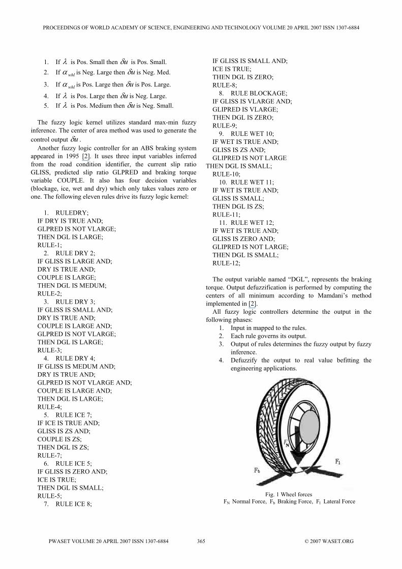
If sufficient braking force is applied, the wheel will “lock up”, that is, slide without turning at all. During the wheel lockup, vehicle greatly loses steering control and the friction force which stops the vehicle is reduced. The braking wheel provides two-forces, the lateral force, FL and the braking force, FB as shown in Fig. 1. These two forces are induced from FN, the weight of the vehicle. The first, FL, provides the vehicle steering control and the lateral stability, while the second, FB, provides the braking forces, which stop the vehicle. These forces are nonlinear function of slip [5], [6] as shown in Fig. 2.

The lateral force is greatest at the zero slip. When slip increase, the lateral force decrease, that is, the ability to steer and control the direction of the vehicle is decreased. The brake force is zero at zero slip, and it has a peak value when the slip is close to 0.2. Most control strategies define their performance goal as maintaining slip near a value of 0.2 throughout the braking trajectory. Because in this area the braking force is close to maximum and the lateral force is sufficiently large to providing the lateral stability.

Not only the braking force and the lateral force are nonlinear function of slip but also slip is nonlinearly related to many other factors, such as maximum road coefficient of friction, temperature of the brake lining, temperature of the brake fluid, pedal force, wearing of tire, initial speed of vehicle and etc. These factors are varying with time. This means braking system is a high-order nonlinear time variant system. Therefore there is no classical equation for braking system control. The knowledge base methods can be used for effective controlling of this system. [4] Uses neural network, [3] introduces fuzzy logic controller and [1] give an optimal fuzzy logic controller. The fuzzy logic controller is an effective controller for ABS but it has a high computing complexity. We use Problem-Solution Data Structure for almost removing this complexity.

II. FUZZY LOGIC CONTROLLER Using fuzzy logic controllers for ABSs was introduced by

D. P. Madau, et al, in 1993 [3]. It compromises two input variables; slip λ and wheel accelerationα , for generating the control output uδ , which controls the force applied to the brake lining. It also has following five rules to drive the fuzzy logic kernel:

Fuzzy Based Problem-Solution Data Structure as a Data Oriented Model for ABS Controlling Ahmad Habibizad Navin, Mehdi Naghian Fesharaki, Mohamad Teshnelab, and Ehsan Shahamatnia

A

PROCEEDINGS OF WORLD ACADEMY OF SCIENCE, ENGINEERING AND TECHNOLOGY VOLUME 20 APRIL 2007 ISSN 1307-6884

PWASET VOLUME 20 APRIL 2007 ISSN 1307-6884 364 © 2007 WASET.ORG

1. If λ is Pos. Small then uδ is Pos. Small. 2. If whlα is Neg. Large then uδ is Neg. Med.

3. If whlα is Pos. Large then uδ is Pos. Large.

4. If λ is Pos. Large then uδ is Neg. Large. 5. If λ is Pos. Medium then uδ is Neg. Small.

The fuzzy logic kernel utilizes standard max-min fuzzy

inference. The center of area method was used to generate the control output uδ .

Another fuzzy logic controller for an ABS braking system appeared in 1995 [2]. It uses three input variables inferred from the road condition identifier, the current slip ratio GLISS, predicted slip ratio GLPRED and braking torque variable COUPLE. It also has four decision variables (blockage, ice, wet and dry) which only takes values zero or one. The following eleven rules drive its fuzzy logic kernel:

1. RULEDRY;

IF DRY IS TRUE AND; GLPRED IS NOT VLARGE; THEN DGL IS LARGE; RULE-1;

2. RULE DRY 2; IF GLISS IS LARGE AND; DRY IS TRUE AND; COUPLE IS LARGE; THEN DGL IS MEDUM; RULE-2;

3. RULE DRY 3; IF GLISS IS SMALL AND; DRY IS TRUE AND; COUPLE IS LARGE AND; GLPRED IS NOT VLARGE; THEN DGL IS LARGE; RULE-3;

4. RULE DRY 4; IF GLISS IS MEDUM AND; DRY IS TRUE AND; GLPRED IS NOT VLARGE AND; COUPLE IS LARGE AND; THEN DGL IS LARGE; RULE-4;

5. RULE ICE 7; IF ICE IS TRUE AND; GLISS IS ZS AND; COUPLE IS ZS; THEN DGL IS ZS; RULE-7;

6. RULE ICE 5; IF GLISS IS ZERO AND; ICE IS TRUE; THEN DGL IS SMALL; RULE-5;

7. RULE ICE 8;

IF GLISS IS SMALL AND; ICE IS TRUE; THEN DGL IS ZERO; RULE-8;

8. RULE BLOCKAGE; IF GLISS IS VLARGE AND; GLIPRED IS VLARGE; THEN DGL IS ZERO; RULE-9;

9. RULE WET 10; IF WET IS TRUE AND; GLISS IS ZS AND; GLIPRED IS NOT LARGE

THEN DGL IS SMALL; RULE-10;

10. RULE WET 11; IF WET IS TRUE AND; GLISS IS SMALL; THEN DGL IS ZS; RULE-11;

11. RULE WET 12; IF WET IS TRUE AND; GLISS IS ZERO AND; GLIPRED IS NOT LARGE; THEN DGL IS SMALL; RULE-12;

The output variable named “DGL”, represents the braking

torque. Output defuzzification is performed by computing the centers of all minimum according to Mamdani’s method implemented in [2].

All fuzzy logic controllers determine the output in the following phases:

1. Input in mapped to the rules. 2. Each rule governs its output. 3. Output of rules determines the fuzzy output by fuzzy

inference. 4. Defuzzify the output to real value befitting the

engineering applications.

Fig. 1 Wheel forces

FN Normal Force, Fb Braking Force, Fl Lateral Force

PROCEEDINGS OF WORLD ACADEMY OF SCIENCE, ENGINEERING AND TECHNOLOGY VOLUME 20 APRIL 2007 ISSN 1307-6884

PWASET VOLUME 20 APRIL 2007 ISSN 1307-6884 365 © 2007 WASET.ORG

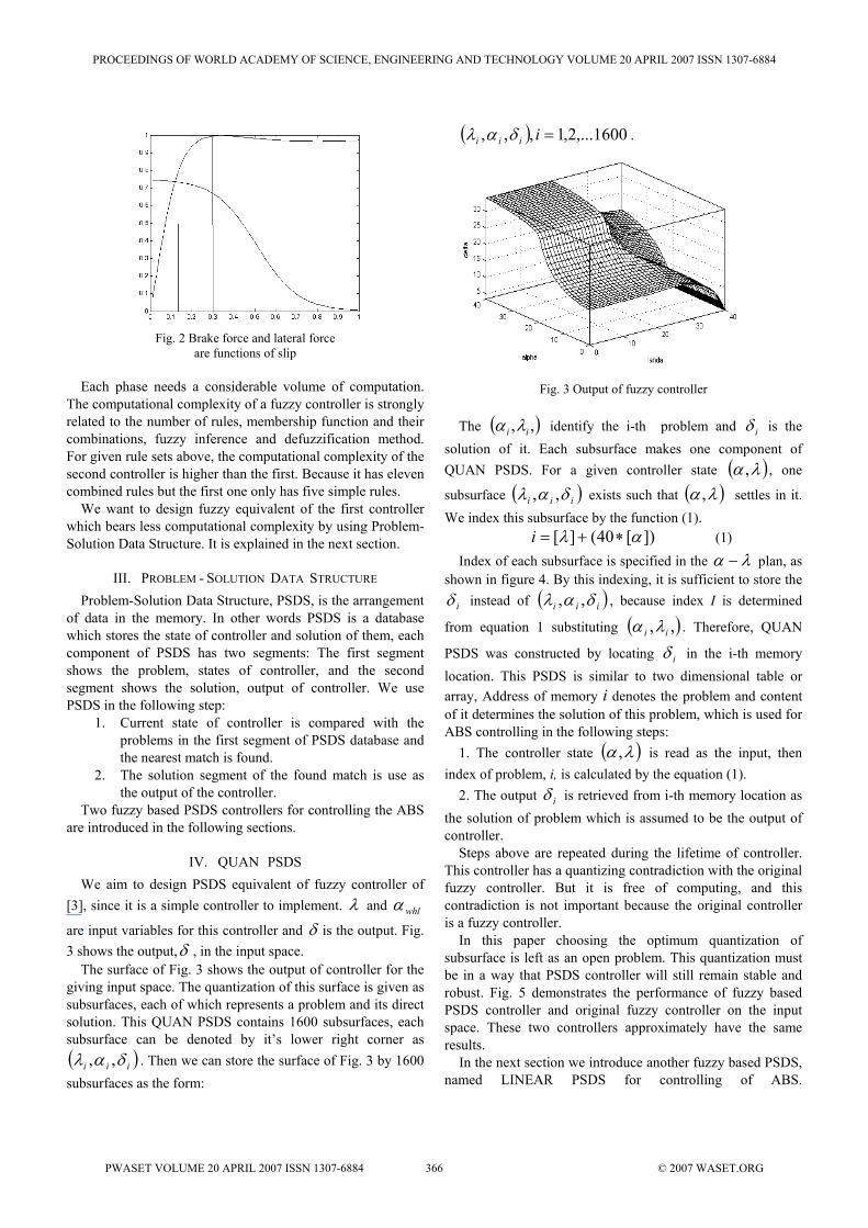
Fig. 2 Brake force and lateral force

are functions of slip

Each phase needs a considerable volume of computation. The computational complexity of a fuzzy controller is strongly related to the number of rules, membership function and their combinations, fuzzy inference and defuzzification method. For given rule sets above, the computational complexity of the second controller is higher than the first. Because it has eleven combined rules but the first one only has five simple rules.

We want to design fuzzy equivalent of the first controller which bears less computational complexity by using Problem-Solution Data Structure. It is explained in the next section.

III. PROBLEM - SOLUTION DATA STRUCTURE Problem-Solution Data Structure, PSDS, is the arrangement

of data in the memory. In other words PSDS is a database which stores the state of controller and solution of them, each component of PSDS has two segments: The first segment shows the problem, states of controller, and the second segment shows the solution, output of controller. We use PSDS in the following step:

1. Current state of controller is compared with the problems in the first segment of PSDS database and the nearest match is found.

2. The solution segment of the found match is use as the output of the controller.

Two fuzzy based PSDS controllers for controlling the ABS are introduced in the following sections.

IV. QUAN PSDS We aim to design PSDS equivalent of fuzzy controller of

[3], since it is a simple controller to implement. λ and whlα

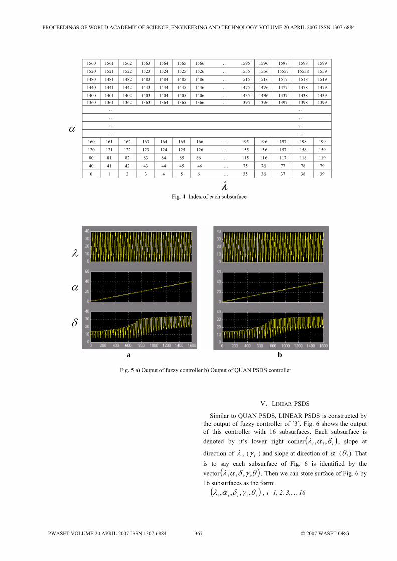
are input variables for this controller and δ is the output. Fig. 3 shows the output,δ , in the input space.

The surface of Fig. 3 shows the output of controller for the giving input space. The quantization of this surface is given as subsurfaces, each of which represents a problem and its direct solution. This QUAN PSDS contains 1600 subsurfaces, each subsurface can be denoted by it’s lower right corner as ( )iii δαλ ,, . Then we can store the surface of Fig. 3 by 1600 subsurfaces as the form:

( ) 1600,...2,1,,, =iiii δαλ .

Fig. 3 Output of fuzzy controller The ( ),, ii λα identify the i-th problem and iδ is the

solution of it. Each subsurface makes one component of QUAN PSDS. For a given controller state ( )λα , , one

subsurface ( )iii δαλ ,, exists such that ( )λα , settles in it. We index this subsurface by the function (1).

])[40(][ αλ ∗+=i (1)

Index of each subsurface is specified in the λα − plan, as shown in figure 4. By this indexing, it is sufficient to store the

iδ instead of ( )iii δαλ ,, , because index I is determined

from equation 1 substituting ( ),, ii λα . Therefore, QUAN

PSDS was constructed by locating iδ in the i-th memory location. This PSDS is similar to two dimensional table or array, Address of memory i denotes the problem and content of it determines the solution of this problem, which is used for ABS controlling in the following steps:

1. The controller state ( )λα , is read as the input, then index of problem, i, is calculated by the equation (1).

2. The output iδ is retrieved from i-th memory location as the solution of problem which is assumed to be the output of controller.

Steps above are repeated during the lifetime of controller. This controller has a quantizing contradiction with the original fuzzy controller. But it is free of computing, and this contradiction is not important because the original controller is a fuzzy controller.

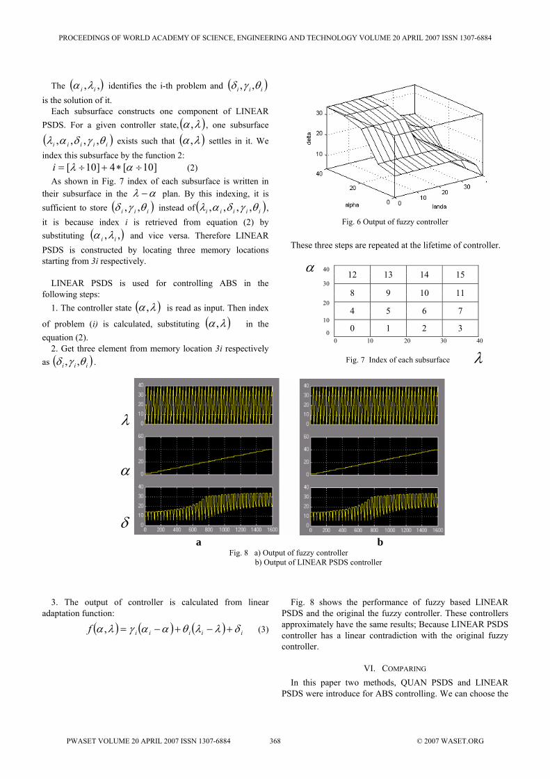
In this paper choosing the optimum quantization of subsurface is left as an open problem. This quantization must be in a way that PSDS controller will still remain stable and robust. Fig. 5 demonstrates the performance of fuzzy based PSDS controller and original fuzzy controller on the input space. These two controllers approximately have the same results.

In the next section we introduce another fuzzy based PSDS, named LINEAR PSDS for controlling of ABS.

PROCEEDINGS OF WORLD ACADEMY OF SCIENCE, ENGINEERING AND TECHNOLOGY VOLUME 20 APRIL 2007 ISSN 1307-6884

PWASET VOLUME 20 APRIL 2007 ISSN 1307-6884 366 © 2007 WASET.ORG

V. LINEAR PSDS

Similar to QUAN PSDS, LINEAR PSDS is constructed by the output of fuzzy controller of [3]. Fig. 6 shows the output of this controller with 16 subsurfaces. Each subsurface is denoted by it’s lower right corner ( )iii δαλ ,, , slope at

direction of λ , ( iγ ) and slope at direction of α ( iθ ). That is to say each subsurface of Fig. 6 is identified by the vector ( )θγδαλ ,,,, . Then we can store surface of Fig. 6 by 16 subsurfaces as the form:

( )iiiii θγδαλ ,,,, , i=1, 2, 3,..., 16

1560 1561 1562 1563 1564 1565 1566 … 1595 1596 1597 1598 1599

1520 1521 1522 1523 1524 1525 1526 … 1555 1556 15557 15558 1559

1480 1481 1482 1483 1484 1485 1486 … 1515 1516 1517 1518 1519

1440 1441 1442 1443 1444 1445 1446 … 1475 1476 1477 1478 1479

1400 1401 1402 1403 1404 1405 1406 … 1435 1436 1437 1438 1439 1360 1361 1362 1363 1364 1365 1366 … 1395 1396 1397 1398 1399

. . . . . .

. . . . . .

. . . . . .

. . . . . .

160 161 162 163 164 165 166 … 195 196 197 198 199

120 121 122 123 124 125 126 … 155 156 157 158 159

80 81 82 83 84 85 86 … 115 116 117 118 119

40 41 42 43 44 45 46 … 75 76 77 78 79

0 1 2 3 4 5 6 … 35 36 37 38 39

Fig. 4 Index of each subsurface λ

α

a b

Fig. 5 a) Output of fuzzy controller b) Output of QUAN PSDS controller

δ

α

λ

PROCEEDINGS OF WORLD ACADEMY OF SCIENCE, ENGINEERING AND TECHNOLOGY VOLUME 20 APRIL 2007 ISSN 1307-6884

PWASET VOLUME 20 APRIL 2007 ISSN 1307-6884 367 © 2007 WASET.ORG

The ( ),, ii λα identifies the i-th problem and ( )iii θγδ ,, is the solution of it.

Each subsurface constructs one component of LINEAR PSDS. For a given controller state, ( )λα , , one subsurface

( )iiiii θγδαλ ,,,, exists such that ( )λα , settles in it. We index this subsurface by the function 2:

]10[4]10[ ÷∗+÷= αλi (2) As shown in Fig. 7 index of each subsurface is written in

their subsurface in the αλ − plan. By this indexing, it is sufficient to store ( )iii θγδ ,, instead of ( )iiiii θγδαλ ,,,, , it is because index i is retrieved from equation (2) by substituting ( ),, ii λα and vice versa. Therefore LINEAR PSDS is constructed by locating three memory locations starting from 3i respectively.

LINEAR PSDS is used for controlling ABS in the

following steps: 1. The controller state ( )λα , is read as input. Then index

of problem (i) is calculated, substituting ( )λα , in the equation (2).

2. Get three element from memory location 3i respectively as ( )iii θγδ ,, .

3. The output of controller is calculated from linear adaptation function:

( ) ( ) ( ) iiiiif δλλθααγλα +−+−=, (3)

Fig. 6 Output of fuzzy controller

These three steps are repeated at the lifetime of controller.

Fig. 8 shows the performance of fuzzy based LINEAR PSDS and the original the fuzzy controller. These controllers approximately have the same results; Because LINEAR PSDS controller has a linear contradiction with the original fuzzy controller.

VI. COMPARING In this paper two methods, QUAN PSDS and LINEAR

PSDS were introduce for ABS controlling. We can choose the

a b

Fig. 8 a) Output of fuzzy controller b) Output of LINEAR PSDS controller

δ

α

λ

40

12 13 14 15 30

8 9 10 11 20

4 5 6 7 10

0 0 1 2 3 0 10 20 30 40

Fig. 7 Index of each subsurface

α

λ

PROCEEDINGS OF WORLD ACADEMY OF SCIENCE, ENGINEERING AND TECHNOLOGY VOLUME 20 APRIL 2007 ISSN 1307-6884

PWASET VOLUME 20 APRIL 2007 ISSN 1307-6884 368 © 2007 WASET.ORG

elements of any PSDS in a way that it operates the same results as the original fuzzy controller. PSDS controllers bear much less computational complexity compared with fuzzy controllers. Still two PSDS controllers introduced here, differ in memory consumption and computational complexity; QUAN PSDS uses 1600 but LINEAR PSDS uses 16 memory locations. LINEAR PSDS uses adaptation function to provide output, but QUAN PSDS gets output without any calculation. In the other word QUAN PSDS needs more memory locations, than LINEAR PSDS does, but it is faster than LINEAR PSDS.

VII. CONCLUSION Fuzzy logic is an effective method using the knowledge for

ABS controlling, but it suffers from the high computational complexity.

In this paper we introduced fuzzy based PSDS for ABS controlling. Unlike conventional calculation based methods, PSDS is an approach based on data oriented modeling which has proved to be in good conformity with computer structure and hence increase efficiency [7]. This method has the following advantages:

1. We get a fast fuzzy based controller. 2. If fast monitoring of Vwhl is provided, then we will get a

real time fuzzy based controller. 3. By using the PSDS method, input space is divided into

subspaces. We can tune the output in each subsurface then we can get local optimization. Tuning iδ in QUAN PSDS

and ( )iii θγδ ,, in LINEAR PSDS for getting local optimization is left as an open problem. This means we can optimize the fuzzy controller by PSDS method.

4. One of most important issues in ABS controlling is the prediction of maximum friction coefficient. This parameter can be predicted from sequence of much recently used PSDS elements (Sequence of controller states). This prediction by sequence of recently used PSDS elements is left as an open problem.

The PSDS is an infant method, it will grow and shine.

REFERENCES [1] Georg F. Mauer, “A Fuzzy logic controller for an ABS braking system,”

IEEE Trans. on Fuzzy Systems, Vol. 3, No. 4, November 1995. [2] P.E. Wellstead and N.B.O.L. Pettit, “Analysis and redesign of an

antilock braking system controller,” IEE Proc. Control Theory Appl., Vol. 144, No. 5, pp. 413-426, September 1997.

[3] D. P. Madau, F. Yuan, L. I. Davis, Jr., and L. A. Feldkamp, “Fuzzy Logic Anti-Lock Brake System for a Limited Range Coefficient of Friction Surface,” IEEE Proc. Int. Con. on Fuzzy Systems, pp. 883-888, March 1993.

[4] L. I. Davis, Jr., G. V. Puskorius, F. Yuan and L. A Feldkamp (1991), “Neural Network Modeling and Control of an Anti-Lock Brake System,” Proceedings of the Intelligent Vehicle ’92 Conference, Ypsilanti, Michigan, June 29-July 1, 1992,.

[5] Fangjun Jiang and Zhiqiang Gao, “An Adaptive Nonlinear Filter Approach to Vehicle Velocity Estimation for ABS”, IEEE Proc. of Int.

Con. on Control Applications, pp. 490-495, Anchorage, September 2000.

[6] A. Mirzaei, M. Moallem, B. Mirzaeian, “Designing a Genetic-Fuzzy Anti-Lock Brake System Controller”, IEEE Proc. of Int. Symp. on Intelligent Control, Limassol, pp. 1252-1256, June 2005.

[7] A. Habibizad Navin, M. Naghian Fesharaki, M. Teshnelab, E. Shahamatnia, “Data Oriented Modeling of Uniform Random Variable: Applied Approach (Accepted for publication)”, 4th International Conference on Mathematics and Statistics, to be published. Vienna, Austria. May 2007.

PROCEEDINGS OF WORLD ACADEMY OF SCIENCE, ENGINEERING AND TECHNOLOGY VOLUME 20 APRIL 2007 ISSN 1307-6884

PWASET VOLUME 20 APRIL 2007 ISSN 1307-6884 369 © 2007 WASET.ORG