Fuel Flow Control Issue in Jet Engines - CORE Scholar

Wright State University Wright State University

CORE Scholar CORE Scholar

Browse all Theses and Dissertations Theses and Dissertations

2007

Fuel Flow Control Issue in Jet Engines: An Evolvable Hardware Fuel Flow Control Issue in Jet Engines: An Evolvable Hardware

Approach Approach

Kshitij S. Deshpande Wright State University

Follow this and additional works at: https://corescholar.libraries.wright.edu/etd_all

Part of the Computer Sciences Commons

Repository Citation Repository Citation Deshpande, Kshitij S., "Fuel Flow Control Issue in Jet Engines: An Evolvable Hardware Approach" (2007). Browse all Theses and Dissertations. 210. https://corescholar.libraries.wright.edu/etd_all/210

This Thesis is brought to you for free and open access by the Theses and Dissertations at CORE Scholar. It has been accepted for inclusion in Browse all Theses and Dissertations by an authorized administrator of CORE Scholar. For more information, please contact [email protected].

https://corescholar.libraries.wright.edu/

https://corescholar.libraries.wright.edu/etd_all

https://corescholar.libraries.wright.edu/etd_comm

https://corescholar.libraries.wright.edu/etd_all?utm_source=corescholar.libraries.wright.edu%2Fetd_all%2F210&utm_medium=PDF&utm_campaign=PDFCoverPages

http://network.bepress.com/hgg/discipline/142?utm_source=corescholar.libraries.wright.edu%2Fetd_all%2F210&utm_medium=PDF&utm_campaign=PDFCoverPages

https://corescholar.libraries.wright.edu/etd_all/210?utm_source=corescholar.libraries.wright.edu%2Fetd_all%2F210&utm_medium=PDF&utm_campaign=PDFCoverPages

mailto:[email protected]

FUEL FLOW CONTROL ISSUE IN JET ENGINES: AN EVOLVABLE HARDWARE APPROACH

A thesis submitted in partial fulfillment of the requirements for the degree of

Master of Science

By

KSHITIJ S. DESHPANDE B.E., Pune University, India, 2002

Wright State University 2007

WRIGHT STATE UNIVERSITY

SCHOOL OF GRADUATE STUDIES

Nov 16, 2007 I HEREBY RECOMMEND THAT THE THESIS PREPARED UNDER MY SUPERVISION BY Kshitij Deshpande ENTITLED Fuel Flow Control Issue in Jet Engines: An Evolvable Hardware Approach BE ACCEPTED IN PARTIAL FULFILLMENT OF THE REQUIREMENTS FOR THE DEGREE OF Master of Science

______________________________________________ John Gallagher, Ph.D. Thesis Director

______________________________________________ Thomas Sudkamp, Ph.D. Department Chair Committee on Final Examination ______________________________________________ John Gallagher, Ph.D. ______________________________________________ Mateen M.Rizki, Ph.D. ______________________________________________ Thomas Hartrum, Ph.D. ______________________________________________ Joseph F. Thomas, Jr., Ph.D. Dean, School of Graduate Studies

iii

ABSTRACT

Deshpande, Kshitij S. MS, Department of Computer Science and Engineering, Wright State University, 2007. Fuel Flow Control Issue in Jet Engines: An Evolvable Hardware Approach.

Dealing with unexpected dynamic loads in Jet and Turbine engines have always

been a matter of concern and an active area of research. This thesis is an initial

attempt to apply Evolvable Hardware methods for augmenting classical control

methods in a generic turbine engine model. In this work, the Air Force Research

Laboratory Generic Turbine Engine Model was converted into C and interfaced

with a simulation of a EH VLSI control chip currently under development. The

simulated EH device was allowed to evolve to augment the simulated engine’s

standard FADEC controller so that the whole system could tolerate unexpected,

large loads to its low-pressure compression shaft. The unassisted FADEC is not

capable of this and will catastrophically fail when asked to do so. We will show

that the chip can evolve an effective augmentative controller with relatively little

computational expenditure and discuss how these techniques might be applied to

similar problems in the future.

iv

Table of Contents

Chapter 1............................................................................................................................ 1 1.1 Introduction and Overview............................................................................................ 1 1.2 Fuel Control: A More Detailed View............................................................................ 3 1.3 Handling the Fuel Flow Control Issue .......................................................................... 6 1.3.1 CTRNN-EH Augmentative Control........................................................................... 6 Chapter 2............................................................................................................................ 9 2.1 Evolutionary Computation ............................................................................................ 9 2.1.1 Evolutionary Algorithms.......................................................................................... 10 2.1.2 Terms used in EAs ................................................................................................... 11 2.2 The MiniPopulationary Algorithm.............................................................................. 13 2.3 Fuel Control Issue in Jet and Turbine Engines ........................................................... 17 2.3.1 Fuel Control Issue in Turboprop Jet Engines: Revisited ......................................... 17 2.4 ICF Jet Engine with a FADEC................................................................................... 19 2.4.1 Mathematical Representation of LP shaft speed:..................................................... 21 2.5 Non EH Control Schemes for Handling Fuel Control Issue ...................................... 23 2.5.1 CTRNN-EH Augmentative Control......................................................................... 25 Chapter 3.......................................................................................................................... 28 3.1 Introduction ................................................................................................................. 28 3.2 The Model Overview .................................................................................................. 29 3.2.1 Maps ......................................................................................................................... 30 3.2.2 The Engine Modules ................................................................................................ 32 3.2.3 The Engine Modules in Detail ................................................................................ 33 3.3 The Simulation Engine Model .................................................................................... 50 3.4 Conversion of MATLAB-Simulink to C++ version .................................................. 53 3.4.1 Transfer Function: .................................................................................................... 53 3.4.2 The Conversion Process:.......................................................................................... 54 3.4.3 Engine Modules in C++: .......................................................................................... 54 3.4.4 Integrating the C++ Classes ..................................................................................... 56 3.4.5 The Engine.cpp class................................................................................................ 59 3.4.6 The run.cpp file ........................................................................................................ 61 3.5 Custom Math Libraries............................................................................................... 62 3.6 Pros and Cons of Modular Approach......................................................................... 63 3.7 Simulation Inputs and Set Up...................................................................................... 64 3.7.1 The Simulation Process............................................................................................ 67 3.7.1.1 Simulation of Engine Model in Matlab-Simulink environment............................ 67 3.7.1.2 Simulation of Engine Model in C++ environment................................................ 69 3.8 Comparison of outputs between MATLAB-Simulink and the C++ version ............. 70 3.9 Plots............................................................................................................................ 71

v

Chapter 4.......................................................................................................................... 73 4.1 Evolvable Hardware (EH): An Unconventional Methodology................................... 73 4.2 CTRNN-EH Devices................................................................................................... 74 4.3 CTRNN-EH: Augmentation Control to handle Fuel Flow ......................................... 76 4.3.1 Conventional PI-Controllers versus CTRNN-EH.................................................... 76 4.3.2 Issues with Conventional PI-Controllers................................................................. 76 4.3.3 CTRNN-EH Control: A Possible Solution.............................................................. 77 Chapter 5.......................................................................................................................... 79 5.1 CTRNN-EH Controller ............................................................................................... 79 5.1.1 The Simulated Engine Model................................................................................... 79 5.1.2 Interfacing CTRNN device to Simulated Engine and FADEC controller ............... 80 5.1.3 Performance Evaluation ........................................................................................... 82 5.1.4 Acceptable Controller .............................................................................................. 82 5.2 Performance of CTRNN-EH Controllers.................................................................... 85 5.3 Analysis of Acceptable CTRNN-EH Controller......................................................... 87 5.4 Future Work ............................................................................................................... 90 References ........................................................................................................................ 91

vi

List of Figures Figure 2.1: LP Shaft block ................................................................................................ 21 Figure 2.2: Plot of LP shaft speed with constant load of 120KW..................................... 22 Figure 2.3: Plot of LP shaft speed with corrected FADEC and constant load of 120KW 24 Figure 2.4: Two FADEC’s augmentation control architecture ........................................ 25 Figure 2.5: CTRNN-EH + FADEC augmentation control architecture............................ 26 Figure 3.1: Example of the Turbine Module with I/O ...................................................... 30 Figure 3.2: Compressor Map............................................................................................. 31 Figure 3.3: Turbine Maps.................................................................................................. 32 Figure 3.4: Simplified Inlet Module.................................................................................. 34 Figure 3.5: Simplified Compressor Module...................................................................... 36 Figure 3.6: Simplified Combustor Module ....................................................................... 40 Figure 3.7: Simplified Turbine Module ............................................................................ 40 Figure 3.8: Simplified Mixer Module ............................................................................... 44 Figure 3.9: Simplified Nozzle Module.............................................................................. 45 Figure 3.10: Simplified Shaft Module .............................................................................. 46 Figure 3.11: Simplified Turbine Cooling Module ............................................................ 48 Figure 3.12: Simplified FADEC Module.......................................................................... 49 Figure 3.13: Engine gas path schematic............................................................................ 51 Figure 3.14: Actual Simulation Model with two Spools................................................... 52 Figure 3.15: A Simple Circuit ........................................................................................... 53 Figure 3.16: Engine Controller ......................................................................................... 65 Figure 3.17: Engine model Flight Envelop ....................................................................... 68 Figure 3.18: Plots for Flight Envelope .............................................................................. 71 Figure 3.19: Plots for Flight Envelope .............................................................................. 72 Figure 4.1: An Evolvable Hardware Controller. ............................................................... 74 Figure 5.1: CTRNN device interfaced with Simulated Engine and FADEC.................... 81 Figure 5.2: LP Shaft Speed with acceptable controller..................................................... 83 Figure 5.3: LP Shaft Speed with un-acceptable controller................................................ 84 Figure 5.4: LP Shaft Speed of acceptable controllers (FADEC+CTRNN) ...................... 86 Figure 5.5 WFR command from the augmentative controller (FADEC+CTRNN).......... 88

vii

List of Tables

Table 3.1: Parent modules and instantiated components .................................................. 32 Table 3.2: Inlet Module Data ............................................................................................ 34 Table 3.3: Compressor Module Data ................................................................................ 35 Table 3.4: Fan Hub Data ................................................................................................... 37 Table 3.5: HPC Data. ........................................................................................................ 38 Table 3.6: Combustor Module Data.................................................................................. 39 Table 3.7: Turbine Module Data ....................................................................................... 41 Table 3.8: HPT Data values .............................................................................................. 42 Table 3.9: LPT Data Values.............................................................................................. 43 Table 3.10: Mixer Module Data........................................................................................ 45 Table 3.11: Nozzle Module Data ...................................................................................... 46 Table 3.12: Shaft Module Data ......................................................................................... 47 Table 3.13: HP Shaft Module Data ................................................................................... 47 Table 3.14: Shaft Module Data ......................................................................................... 47 Table 3.15: FADEC - Scheduled N1 Module Data........................................................... 49 Table 3.16: Engine Design Specifications ........................................................................ 50 Table 5.1: Statistics of Controllers Evolved with different Configurations...................... 85

viii

ACKNOWLEDGMENTS

I would like to thank my advisor Dr. John Gallagher, who has given me tremendous

support throughout my graduate career. I would also like to thank Dr. Mateen Rizki and

Dr. Thomas Hartrum for their timely feedback and suggestions about my Thesis work.

Additionally, I would like to thank Dr. Mitch Wolff and his students for their support.

Lastly I would like to thank my family for helping me stay strong during my graduate

studies.

ix

Dedicated to

My Advisor: Dr. John Gallagher

My Parents: Aai and Baba

My Grand parents: Aji and Ajoba

1

Chapter 1

Fuel Flow Control in Turbine Jet Engines

1.1 Introduction and Overview Military aircrafts are increasingly required to carry more mission-critical electronics,

weapons, and sensor systems. Therefore, efforts to extract the largest amount of power

possible from the aircraft’s turbine engines are growing in importance. A high-quality

fuel control systems is one critical component in maximizing usable power output, as

properly designed fuel systems manage fuel consumption to maximize fuel economy,

while being able to provide burst power when needed. Through the years, much effort

has gone into the design of highly sophisticated fuel flow controllers that based on

current operational needs, estimate the correct amount of fuel fed to the combustor. The

overriding concern of the controller is to command fuel sufficient to maintain the cruise

with respect to flight altitude, atmospheric pressure, ambient temperature, and net load on

the engine. The controller must also be able to adjust fuel flow to compensate in a timely

2

manner for transient auxiliary loads without burning too much fuel, as that would

negatively impact fuel economy.

Advances have been made in the development of highly accurate closed loop electronic

controllers that determine optimal amount of fuel required for the present flight

conditions. However, all these controllers have to be pre-designed and calibrated as per

the aircraft application and operating conditions. Military aircrafts, more so than civilian

models, are adapted to changing mission profiles by adding weapons and avionics

systems that the original designers may not have anticipated. These system additions

could change the airframe and energy requirements so much that the original fuel control

systems fail. One alternative would be to redesign the fuel control system from scratch to

accommodate the new power loads. However, this could be time consuming and degrade

the war fighter’s ability to quickly and effectively reconfigure aircraft to take advantage

of opportunities as they present. Another alternative would be to provide a self-

configuring “augmentative controller” that rides side-by-side with existing fuel control

devices. This augmentative controller would learn how to work with the existing

controller to manage fuel loads in a way that preserves safe flight, provides power as

needed by the new systems, and maintains fuel economy.

This Thesis is an initial exploration into the application of Evolvable Hardware systems

that act as “augmentative controllers” as described above. In this work, a simulation of

an evolvable hardware chip was combined with a simulation of a realistic turbine engine

(The Air Force Research Laboratory’s Generic Turbine Engine Model), and a fuel

3

controller for that engine (Fully Automated Digital Electronic Controller – FADEC).

The chip was expected to learn how to augment fuel commands from the FADEC to

properly accommodate significant, unexpected, loads to the engine’s low-pressure

turbine. Such loads are known to “crash” the FADEC, causing the aircraft to stall. Our

goal was to show the chip could learn to “patch” this hole in the FADEC and allow

effective tapping of power from the LP shaft.

1.2 Fuel Control: A More Detailed View The Jet engines can be categorized into two types, single spool engines and dual spool

engines. Single spool engines have a single shaft that runs through the length of the

engine connecting the compressor and the turbine. Dual spool engines have two shafts,

the high-pressure shaft spins coaxially with, and on the outside of the low-pressure shaft.

The two shafts rotate independently of one another. This has the advantage of increasing

power efficiency and decoupling the compression (low pressure shaft) and turbine (high

pressure shaft) duties so that compression can be more easily maintained even in the

presence of continually changing turbine demands. This design prevents the jet engine

from a sudden stall associated with auxiliary shaft loads and potential loss of

compression.

In a typical jet engine, air enters the engine face and passes through a fixed inlet guide

vane ring. The air is drawn in and compressed by the high-pressure compressor that is

driven by a single stage turbine.

4

From the high -pressure compressor, air is fed to the diffuser and then to the annular

through-flow combustor. Fuel is sprayed into the combustor, where it mixes with the

compressed air and ignites to provide high-energy gas to drive the turbines and provide

the propulsive jet. The gas is accelerated through a nozzle, which is cooled with

compressor bleed air, and is then expanded through the single stage axial high-pressure

turbine, also cooled. The high-pressure turbine drives the high-pressure compressor and

the accessory gearbox via a tower shaft and bevel gear in front of the high-pressure

compressor. The gas is then accelerated through the second stage turbine nozzle, and is

expanded through the single stage axial low-pressure turbine, which is also cooled with

bleed air. The remaining energy in the gas can then be used to provide thrust to propel the

aircraft. A fixed convergent nozzle at the end of the jet-pipe creates a throat that

accelerates the airflow to high velocity to provide thrust.

Any aircraft, be it a civilian or military, has to be able to fly safely even if it receives

random loads on its High Pressure or Low Pressure Shafts. High Pressure shafts are

usually tapped for driving auxiliary electrical loads. Low Pressure shafts, being

responsible for maintaining engine compression, are more often associated with loads

related to atmospheric conditions (atmospheric pressure differences, loads due to foreign

bodies getting stuck in turbo fan, etc.). In addition some UAVs like the Global Hawk that

cruise at altitudes of 65,000 ft have an additional requirement for maintaining cruising

flight without loss of altitude due loads switching on and off randomly.

To meet these contingencies the engine can operate at higher thrusts than those

corresponding to the non-dimensional condition for the design at cruise. In practice this

5

normally means a demand for higher fuel flow into the combustion chamber. This fuel

flow in engine is controlled by the FADEC controller that provides good response and

accuracy over a range of certain parameters like Altitude, Inlet Pressure, Temperature,

N1 (low pressure shaft) speed and N2 (high pressure shaft) speed respectively. The fuel

control, using feedback, responds to power lever setting (PLA) to match commanded

power and fan speed. Among the engine operating parameters that the control typically

uses are N1 and N2, the temperature and pressure at the inlet and within the compressor

stage, and the exhaust nozzle orientation. Whenever the aircraft ascends to a certain

altitude the fuel system of the engine tries to maintain the net thrust (in fact the lift drag

ratio L/D).

In any Jet Engine the maximum Lift drag ratio is maintained not by increasing the fuel

input to the combustor, and hence increasing turbine temperatures that further reduce

engine life, but by compensating it by a higher bypass ratio and increase in altitude.

However, if a load is applied to the LP shaft of the engine at a given altitude, the FADEC

detects a drop in LP shaft speed with respect to present ambient conditions and

commands a higher Fuel Flow to Pressure Ratio (WFR) to the Fuel pump. The ambient

conditions remaining the same and with Fuel Pump calibrated for the present load

conditions, fuel flow from the pump is increased by dropping the valve and thus reducing

the spill off. This helps in ramping up the speed of LP shaft to the desired value.

6

But the FADEC fails to meet these expectations at an altitude of 60,000ft and with full

load of 120KW applied to LP shaft. The commanded WFR value was observed to

saturate at 17 and does not increase further to compensate for the speed drop.

This shortcoming of the FADEC leads to a loss of altitude subsequently resulting in a

crash. In addition for military application maintaining the cruise at 60,000 ft is crucial as

the Global Hawk being a survey flight, a small loss in altitude would result into it being

destroyed by the enemy missiles.

1.3 Handling the Fuel Flow Control Issue

One way to handle the above problem would be to redesign the FADEC. Another

possibility is to create a controller that runs in parallel to the original FADEC and learns

how to augment FADEC generated control efforts to deal properly with large HP shaft

loads at high altitudes. In this thesis, we will explore the use of Evolvable Hardware

devices that learn how to provide such augmentation.

1.3.1 CTRNN-EH Augmentative Control

Unlike the conventional approach where controllers are designed for a specific task,

CTRNN-EH devices provide an out of the box approach. Conventional controllers do not

or have very restricted control over the final controller design. Their control strategies are

merely restricted to adjustment of offsets of few or more parameters.

7

The field of EH has broadened our horizons by promising us novel automated techniques

to create control devices. These automated techniques are based on the process of natural

evolution that finds complex solutions in the search space. Evolutionary Algorithms

(EA) serve the purpose of providing automated search techniques that help in exploring

best possible solutions for the problem in hand by exploiting the search space. EAs are

search algorithms that use the process of natural evolution by recombining and crossover

of its candidate solutions.

An EH device can be thought of as an adaptive controller in the sense that it will

continuously adapt to the changes in the engine parameters and the FADEC output. This

automatic adaptive approach will be enabled by CTRNN-EH method. A CTRNN-EH is

thus a combination of an EA and a hardware continuous time recurrent neural network

(CTRNN) into a single EH device.

This Thesis will demonstrate the application of CTRNN-EH method for engine transient

stability control.

Chapter two will deal with the background material about MiniPopulation Evolutionary

Algorithms used as the CTRNN-EH’s configuration generation engine in this work. After

that it will discuss the problem to be solved in detail.

Chapter 3 will discuss about the need and details about the conversion of MATLAB-

Simulink simulation model into C++.

Chapter 4 gives the reader complete details about the control scheme adopted for the

problem. This is followed by a chapter discussing performance of CTRNN-EH

controllers.

8

Chapter 5 provides justifications on the advantages with these controllers and analyzes

the scope of future work.

9

Chapter 2

Background and Literature Review

This chapter will discuss the background required for understanding the work presented

in this thesis. The following will be discussed:

1) The field of Evolutionary Computing and EA’s

2) The MiniPop EA used for the Thesis work.

3) The Fuel Flow Control issue in detail

4) Approaches to deal with the fuel control issue.

2.1 Evolutionary Computation Evolutionary computation is inspired by the process of natural evolution and is a major

field of research in computer science [2]. The idea for “automated problem solving”

based on Darwinian principles was developed in the forties [2].

Evolutionary computation makes use of the changes and development in the population

and is basically an iterative process. The evolutionary process is inspired by the

biological evolutionary mechanisms.

10

Recombination and Mutation are the basic operators that are used to introduce diversity

in the population and make subtle changes in individuals [2].

Three different interpretations of this idea were developed through years by scientists.

Evolutionary programming was introduced by Lawrence J. Fogel, while John Henry

Holland called his method a genetic algorithm [2, 3, 4]. Ingo Rechenberg and Hans-Paul

Schwefel introduced evolution strategies [5]. From the early nineties they are seen as

different dialects of one technology, called evolutionary computing. In the early nineties,

another stream of genetic programming emerged [2].

These terminologies denote the whole field by evolutionary computing and consider

evolutionary programming, evolution strategies, genetic algorithms, and genetic

programming as sub-areas.

2.1.1 Evolutionary Algorithms

An Evolutionary algorithm (EA) is a “generic population-based meta-heuristic

optimization algorithm” [6].

EAs have a population of candidate solutions. Candidate solutions can be represented as

bit-strings or as real valued vectors. The precision of these usually depends on and is

restricted based on the hardware used.

The basic mechanisms like recombination and mutation as mentioned above are applied

to the population to promote diversity and evolve new off-springs.

The result of recombination and mutation of candidates generate a novel child.

Every individual is associated with a term called fitness function or a cost function.

11

The fitness function determines the susceptibility of the solutions to survive in the

environment.

A simple and basic EA is given as [2]:

1. Begin

2. Initialize a population of n individuals by random generation

3. Determine fitness of each individual using an appropriate fitness or a cost

function

4. Select parents for the process of reproduction

5. Use genetic operators like crossover and mutation to produce new offsprings.

6. Perform selection to pick population members for the next generation

7. If the desired or terminating criterion is met, report the best candidate and stop,

else go to step 3.

2.1.2 Terms used in EAs

1. Representation: The problem to be solved should be first encoded into a form on

which an EA can operate. The real world problem should be suitably represented

in either binary coded values or real values so that it does not loose its

significance upon conversion and repeated application of genetic operators.

2. Population: This refers to the pool of candidate solutions. Each member of the

population refers to a point in the search space. Hence some members tend to be

current champions while others represent different points in the space that can

lead to better solutions in future. Population of such candidate solutions help in

12

overcoming the issues of EA being trapped at local optimum. This helps is

persuading the search for obtaining a global optimum solution.

3. Fitness Function: It is a particular type of objective function that evaluates

candidate solutions between bad and the best. The fitness score obtained helps in

selecting individuals for EA operations for subsequent evaluation cycles. Since

for the fuel flow control problem we are concerned with achieving desired speed

over certain cruise duration, the average sum of error will be an appropriate

fitness function.

4. Parent Selection: Parent selection is done to improve the quality in solutions.

During the selection process candidates with higher fitness values are likely to be

chosen than the ones having lower fitness values. But selection techniques make

sure to select candidates with lower fitness values in order to avoid greedy search

and confinement to local optima. There are couple of methods available for parent

selection like:

a) Roulette Wheel selection

b) Rank Based selection

c) Stochastic Universal Sampling [15] and

d) Tournament selection

5. Recombination: Recombination is an N-ary operator that leads to the evolution

of novel candidate solutions from N candidate solutions. Usually the term

crossover is associated with binary bit-strings in genetic algorithms. There are

different types of crossover techniques like single point, two point and n-point.

Any of these crossover techniques lead to evolution of offspring’s with improved

13

or higher fitness values so that they have higher chances of participating in

subsequent reproduction cycles.

6. Mutation: This operator is used to further create diversity in the population. At

times the intervals or chromosomes become similar to each other as a result of

repeated recombination. However, mutation can be used to maintain the diversity

and broaden the range of evolutionary search. Mutation is probabilistic, for

example in case of a genetic algorithm it is used to flip bits based on a random

number that decides if a particular bit will be flipped or not.

7. Survivor Selection: The size of population chosen before initializing the

population is fixed throughout the evolution process. This signifies that in

subsequent evolution cycles individuals with low fitness score be replaced with

those having a better fitness score. There exist two techniques namely age based

replacement and fitness based replacement. Age based methods eliminate older

individuals while fitness based methods eliminate or replace individuals with low

fitness scores.

2.2 The MiniPopulationary Algorithm

MiniPop [7] is a mutation driven EA that uses simple search operators and a small

population. MiniPop is simple and thus can be implemented easily in hardware. Being

easy it is amenable for analysis. In addition to its simplicity, MiniPop has been proven to

be an effective search algorithm for many CTRNN-EH problems [7]. The simple

Minipop Algorithm is given in code listing 1 [7].

14

MINIPOP(N, L, MRATE, MAXEVALS)

1. eval := 0

2. for i := 1 to N do

3. pop[i] = RANDOM_BITSTRING(L)

4. fitness[i] = EVALUATE(pop[i])

5. eval := eval + 1

6. done

7. i := 1

8. while eval < MAXEVALS do

9. if eval MODULO RF = 0 then

10. j := BEST_SOLUTION(pop)

11. old_fitness := fitness[j]

12. new_fitness := EVALUATE(pop[j])

13. eval := eval + 1

14. fitness[j] := (1-RW)*old_fitness

+ RW * new_fitness

15. else if i <= N then

16. mutant := MUTATE(pop[i], MRATE)

17. mfitness := EVALUATE(mutant)


19. if mfitness > fitness[i] then

20. pop[i] := mutant

21. fitness[i]: = mfitness

15

22. endif

23. i := i + 1

24. else

25. mutant := RANDOM_BITSTRING(L)

26. mfitness := EVALUATE(mutant)


28. j := WORST_SOLUTION(pop)

29. if mfitness > fitness[j] then

30. pop[j] := mutant

31. fitness[j] := mfitness

32. endif

33. i := 1

34. endif

35. done

36. j := BEST_SOLUTION(pop)

37. return pop[j]

Code Listing 3.1: Pseudocode for the standard MiniPop algorithm.

The MiniPop algorithm starts by initializing the population. This is done by randomly

creating N bit strings and is represented by lines 1-6 in the above code-listing.

Initialization is followed by evolving the solutions and is represented by lines 8 – 35 that

form the main loop.

16

The mutation tournament and the hyper-mutation tournament both drive the search

process. In the mutation tournament a candidate solution competes with its mutated

version. The winner of this tournament replaces the original candidate.

In the case of hyper-mutation tournament, a candidate solution in the population

competes with a randomly generated bit-string. In case the hyper-mutant wins, it

replaces the candidate solution.

The hypermutation tournament helps in removing poor individuals from the population

and hence allows the EA to make large jumps across the search space [8].

A single tournament is executed in the main loop and the selection is done based on the

index variable. This index variable points to the candidate that will be competing in next

tournament [8]. The hyper-mutation tournament is executed once all candidate solutions

have competed in the mutation tournament. Finally, the index variable is set to point to

the first candidate solution and the process is repeated. The MAXEVALS variable

denotes the maximum number of evaluations to be performed and the evolution process

terminates when this value is reached. At the end the Minipop algorithm returns the best

solution evolved so far from the population.

17

2.3 Fuel Control Issue in Jet and Turbine Engines In chapter one, we introduced the FADEC’s inability to control for large loads at high

altitudes. In this section we will discuss this issue in greater detail.

2.3.1 Fuel Control Issue in Turboprop Jet Engines: Revisited

Maintaining steady cruise at any given altitude is an implicit requirement of any jet

turbine engine. A jet engine is a dynamic system and thus undergoes a lot of changes in

load conditions during cruise.

Loads [11] can be categorized into:

1) Drag on the Engine due to environmental conditions like Pressure, Temperature,

Altitude, Clouds, and foreign bodies getting stuck in to propellers.

2) Self weight and load due to weight of Cargo, Passengers, weapons and

ammunition in the Airplane.

3) Auxiliary load on HP Shaft and

4) Auxiliary on LP Shaft.

Loads 1, 3 and 4 are dynamic loads while load number 2 is a static load.

In order to maintain the state commanded by the pilot, the engine tries to maintain the

state of the aircraft by burning an appropriate quantity of fuel. The amount of fuel burned

is equivalent to:

1) The volume required to keep the engine and hence the airplane cruising with just

the weight of aircraft and the engine and

2) Volume required for maintaining cruise commanded by the pilot with auxiliary-

dynamic load.

Failure to handle loads without maintaining the cruise conditions in highly undesirable.

18

Control systems that can handle dynamic load have been researched and developed over

the years.

Some of the types include:

1) Mechanical controllers consisting of gears and valves

2) Hydraulic Control Systems

3) Electronic Control Systems

Mechanical systems have low precision due to limitations on time constants and

dynamics of the mechanical components of the system. Hydraulic systems are more

effective than mechanical ones, but still have similar limits due to relatively slow

dynamic response. With the introduction of electronic fuel pumps and high-speed valves

it is now possible to have very fast and precise controllers for determining the fuel input

to the combustor. Several Electronic Controllers have been designed that provide control

signals to these fuel pumps. We will discuss one such fuel flow controller in following

section.

19

2.4 ICF Jet Engine with a FADEC In present Thesis we consider a Turboprop engine equipped with an electronic fuel flow

controller named the “Full Authority Digital Electronics Control” (FADEC) [12]. A

FADEC is a proportional integral control that provides good response and accuracy over

a range of parameters like Altitude, Inlet Pressure and Temperature, N1 (LP shaft speed)

speed and N2 (HP shaft) speed respectively [1, 12]. The fuel control, using feedback,

responds to power lever setting/ Pilots Lever Angle (PLA) to match commanded power

and fan speed. The control typically makes use of the low and high-pressure shaft speeds.

In addition, other parameters like the compressor and turbine temperature and pressure at

the inlet and exhaust are also significant. Depending on the engine and flight conditions,

such as command for peak acceleration from cruise, the control selects one parameter

over the other on which to "close the loop" for fuel flow to the engine. Ideally, the output

from each loop (for each engine operating parameter) produces the same scheduled fuel

flow (WF/P3 ratio) at all times, and if that were true, selecting one loop over another

would be invisible in the sense that there would be no immediate change in Fuel Flow to

Pressure ratio (WFR) at selection. This is not the case, however, because the parameters

have different relationships to engine operation at any instant and thus one may command

more or less WFR ratio than another at any instant in time, creating a significant stability

problem when selecting one channel over another. When selection is carried in this way,

the loops can have significant divergence, producing erratic control. This erratic behavior

is obvious especially at altitudes of 60,000 ft and with LP shaft running at full load.

For purposes of this work, we will define two flight envelopes, with and without load.

The envelopes are as follows:

20

Normal Flight Envelope [1] without Load

1. For time=0 to 5 seconds: N1=87%; altitude = sea level; Mach number = 0;

2. At time=5 seconds N1 is ramped up to 100% in one second (pre take off)

3. At time = 15 seconds Mach number is ramped up from 0 to 0.6, in 3 seconds

4. At time = 20 seconds, altitude is increased in incremental steps to 10,000 ft and

reaches 10,000 feet before 30 seconds

5. At time = 40 seconds, altitude is increased to 30,000 ft



8. At time = 70 seconds, altitude is increased to 60,000 ft and the airplane is

allowed to cruise

Flight Envelope with Load











21

10. At around 80 seconds LP shaft is loaded further with 120KW and the aircraft is

allowed to cruise.

In order to cut down the computational costs involved in initialization we have initialized

the jet engine directly to the problem state I.E. PLA setting 100%,, Mach number 0.6,

Altitude 60,000ft. The LP shaft is loaded 3 seconds after the engine has been initialized

and achieves the target design speed of 8700 RPM.

2.4.1 Mathematical Representation of LP shaft speed:

The Fuel Flow to Pressure Ratio (WFR) calculated by schedule fuel controller FADEC is

fed as input to the HMU. Additional inputs to the HMU unit are [1]:

1) Compressor output pressure and

2) Percentage HP shaft speed

The fuel input WF to the combustor is calculated based on these three inputs, through a

fuel flow schedule and is intended to maintain LP shaft speed (N1) at the command level.

The LP Shaft speed is a function of net torque on the LP shaft and is given by:

t N1(t) = ∫ (TorqueLPT) - (Torque(Tip+Hub) + TorqueLPAGB ) + N10

t0

The Simulink block representation of the above equation [1] is given as:

TorqueLPT

TorqueTip+Hub TorqueLPAGB

N1 (rpm)

Figure 2.1 : LP Shaft block

22

Plot of LP Shaft Speed against Time (ms) with Un-corrected

FADEC

7400

7600

7800

8000

8200

8400

8600

8800

0 2000 4000 6000 8000 10000 12000 14000 16000

Time Steps (ms)

N1 RPM

Figure 2.2 : Plot of LP shaft speed with constant load of 120KW

In order to maintain desired flight state of the aircraft the LP shaft speed should be

maintained constant and should be equal to that commanded by PLA setting.

Whenever, a load is applied to the LP shaft it is done at the auxiliary gear box.

Increasing the load from 0KW to a positive value increases the load torque on the LP

shaft. In order to maintain N1 at desired value the driving torque provided by LP turbine

should be increased. This can be done by increasing the output of HP turbine.

Output of HP turbine depends on the flow of hot exhaust gases from the combustor.

Hence the output from the combustor determines the value of driving torque (LPT

Torque) developed by the LP turbine. This is possible by increasing the fuel input to the

combustor. Now the fuel input is a function of WFR output of the FADEC.

23

Thus our goal will be to accurately determine the value of WFR fed to the HMU.

2.5 Non EH Control Schemes for Handling Fuel Control Issue Before considering EH augmentative control of the engine, we first will consider some

simple modifications to the FADEC itself to help demonstrate that simple FADEC

redesign would not sufficiently address the problem. We consider two types of fixes:

1) Modification of the present FADEC controller for handling LP shaft loads at higher

altitudes.

2) Provision of an additional FADEC controller to provide an augmentation control to the

existing FADEC.

Case 1 controller does work and exhibit a reasonable recovery of LP shaft speed and

hence the altitude. The present FADEC controller can be modified for providing higher

Fuel Flow to Pressure Ratio (WFR) values by changing the schedules flow interpolation

to ‘Interpolation-Extrapolation’ from ‘End-Interpolation’. However, this is done at the

cost of an increased recovery time called the ‘response time’. In addition, the response

time parameter depends on the magnitude of load applied. It has been found from

experiments that load with higher magnitude result in higher speed dip than those with

lower magnitudes. Loads with significant magnitudes may drive the LP shaft speeds well

below the recovery range. This drop is malicious for any jet engine and hence the aircraft.

24

Figure 2.3: Plot of LP shaft speed with corrected FADEC and a constant load of

120KW

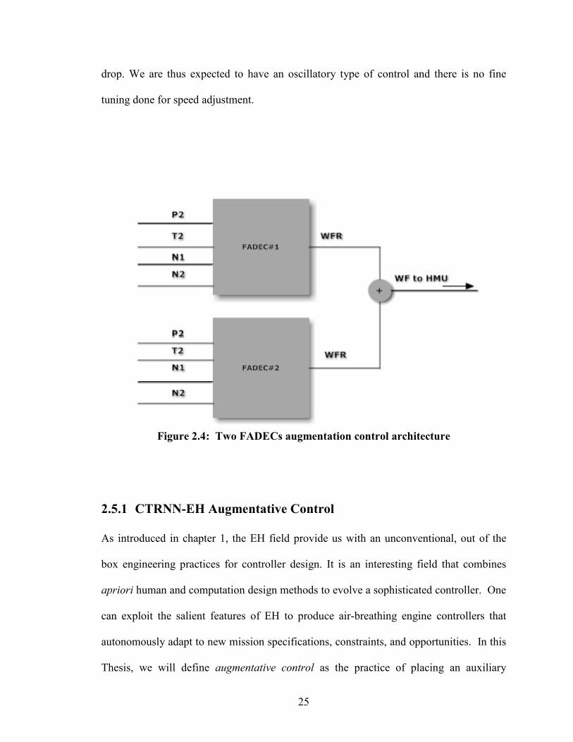
Case 2 controllers provide a practically infeasible solution as both FADECs will be

providing same output I.E. WFR ratios to the Fuel pump or HMU unit. An augmentation

control developed as shown in the figure below will thus command twice the value with

single FADEC controller. This in turn will command the fuel pump for a double amount

of fuel flow. Once the speed recovers and starts to increase above that set by PLA

command, both FADECs will try to decrease the WFR command. Since both controllers

reduce WFR by same magnitude and at same instant of time, the N1 speed again starts to

LP Shaft Speed with Corrected FADEC

8000

8100

8200

8300

8400

8500

8600

8700

8800

8900

0 10000 20000 30000 40000 50000 60000 70000

Time Steps (us)

25

drop. We are thus expected to have an oscillatory type of control and there is no fine

tuning done for speed adjustment.

Figure 2.4: Two FADECs augmentation control architecture

2.5.1 CTRNN-EH Augmentative Control

As introduced in chapter 1, the EH field provide us with an unconventional, out of the

box engineering practices for controller design. It is an interesting field that combines

apriori human and computation design methods to evolve a sophisticated controller. One

can exploit the salient features of EH to produce air-breathing engine controllers that

autonomously adapt to new mission specifications, constraints, and opportunities. In this

Thesis, we will define augmentative control as the practice of placing an auxiliary

26

controller in parallel with a primary controller in such a way that the second controller

adds offsets to the efforts commanded to the primary controllers. Figure 2.4 shows the

possible architecture.

Figure 2.5: CTRNN-EH + FADEC augmentation control architecture

We adopted the Mini Population (MINIPOP) Evolutionary Algorithm as the CTRNN-

EH’s configuration generation engine in this work.

In order to carry out simulations by interfacing the MINIPOP enabled CTRNN-EH

device to the existing engine model, we translated the Air Force Research Laboratory

(AFRL) generic turbine engine model from MATLAB/Simulink into the C++

programming language. This was done to enable easy integration with existing CTRNN-

EH simulations and allow low-cost runs on our Beowulf computational cluster. The C++

27

language model was validated against the MATLAB/ Simulink original, but as of yet, not

against live engine data.

Chapter 3 gives details of both the C++ and Simulink version of the Engine Model.

28

Chapter 3

The ICF Engine Model

3.1 Introduction

Both the MATLAB-Simulink and C++ versions of the engine model are a prototype non-

augmented, turbofan engine models [1].

Both the models have following characteristics:

1) Physics based

2) Component based

3) Incorporate engine dimensions, component maps and inertia

They satisfy following requirements [1]:

1) The entire flight envelop of the engine is simulated.

2) The engine steady state behavior is accurately represented especially at design point.

3) Transient engine behavior is represented.

4) All inputs simulate engine control inputs like fuel flow, bleed demand, or ambient

conditions like Mach number, atmospheric pressure and temperature.

5) Inputs and outputs can be configured in a manner whereby they can be used for

developing and testing engine controls.

29

3.2 The Model Overview

Component based approach is used while constructing the engine model for ease of

modification and replacement of different engine components. Each component can be

instantiated from a software module that is developed to represent the functioning of that

particular type of component. Each module can function as an independent component if

it is provided with its own set of input and outputs. For example [1] the turbine module

can be used as a stand-alone turbine component and it can be used to instantiate high and

low pressure turbines in the engine model.

The turbine module is shown in Figure 3.1 [1].

Since the turbine and compressor maps are available in a lumped fashion and not in a

stage-by-stage fashion, a lumped approach was used to create each module [1].

In same sense, the combustor module simulates combustion of a lumped amount of fuel

and air in a control volume.

30

Figure 3.1: Example of the Turbine Module with I/O

This lumped approach does not violate any of the model requirements.

3.2.1 Maps Compressor Maps:

A "compressor flow map" [17] quantifies the performance of an impeller, an example of

which is shown below. The x-axis on the map is the amount of uncompressed air entering

one turbo. This flow is either represented as a volume or mass flow. The y-axis represents

the “ratio of the air pressure at the discharge opening to the air pressure at the inlet”.

The efficiency flow map is a representation of the efficiency of “the adiabatic heating” of

the air. Higher values signify less excess heating of the air.

The surge line shown in the map below divides the region into stable and unstable flow.

The region above the surge line is that of an unstable flow. A surge basically causes an

abrupt reversal of air flow through the compressor which is undesired.

W out required

Cooling flow stream

Core flowStream – Win

N - RPM

W in required

W out stream

Torque

{From upstreamcomponent

From downstreamcomponent

To upstreamcomponent

To downstreamcomponent

To workeg. compressor + shaft inertia +

work extractionFrom shaft

Turbine

Flow and Efficiency Maps

Volume, Area and Design speed

W out required

Cooling flow stream

Core flowStream – Win

N - RPM

W in required

W out stream

Torque

{From upstreamcomponent

From downstreamcomponent

To upstreamcomponent

To downstreamcomponent

To workeg. compressor + shaft inertia +

work extractionFrom shaft

Turbine

Flow and Efficiency Maps

Volume, Area and Design speed

31

Figure 3.2: Compressor Map

Turbine Maps:

The turbine map of Engine model used for this Thesis [16] is shown below. In this

particular case, the x-axis is the pressure ratio while the y-axis is some measure of flow,

usually non-dimensional flow or, as in this case, corrected flow, but not real flow.

Figure 3.3 shows the flow and efficiency maps for the high pressure turbine. As can be

observed from the figure it shows plots for different values of turbine speed (rotational).

“Unlike a compressor, surge does not occur in a turbine”[16]. This is because the flow

through the unit is from high to low pressure. Due to this a surge line does not exist for a

turbine map.

32

Figure 3.3: Turbine Maps

3.2.2 The Engine Modules

The major software modules [1] were created along with the mode as listed below:

Parent Module Instantiated Component Model

1 Compressor Fan Hub, Fan Tip, HPC, LPC

2 Turbine HPT, LPT

3 Combustor Combustor and Afterburner

4 Nozzle Exhaust Nozzle

5 Inlet Inlet conditions

6 Mixer Mixer/ By Pass ratio calculator

7 Shaft Fan shaft, Core shaft

8 Cooling Combustor cooling, HPT cooling, LPT cooling

9 FADEC Control Scheduled N1 through WF

Table 3.1: Parent modules and instantiated components

33

The modules obey fundamental laws of physics like “conservation of mass, momentum,

and energy” [1]. The equations for modules are derived based on above these. Each

module is further composed of “static/steady-state and dynamic” sub-modules. The

dynamic module for compressor and turbine is based on “volume dynamics” [1], while

the dynamics for shafts are based on “mass and moment of inertia”. Flow conditions are

obtained from maps by using the input states and “static equations” [1].

In addition to compressor maps, gas tables are also required for calculating enthalpy,

specific heat and universal gas constant for pure air and fuel air mixture. They are a

function of temperature, pressure and fuel-air ratio in various components. [1]

3.2.3 The Engine Modules in Detail This section gives details of each module that are used in creating an engine model. A

Real time simulation of all the modules is feasible by interfacing and interaction of

instances of all modules. “The real time dynamic simulation consists of a set of first

order differential equations [1, 13] that are integrated using fixed time step of 1 ms”.

34

� Inlet

Figure 3.4: Simplified Inlet Module

Stagnation pressure (P2) and temperature (T2) of the inlet air are calculated by this

module based on altitude, Mach number and standard day air conditions and inlet losses

[1]. “Non-standard day temperatures” can also be simulated.

In the simulation setup the inlet component is instantiated from the inlet module.

The inlet module inputs, outputs and design data are shown in Table 3.2 [1].

Inputs Outputs Design Data Required

• Raw required

flow downstream

- Fan

• Altitude

• Mach Number

• Ambient Pressure

and Temperature

• P2, T2

• Atmosphere tables

• Intake Area

• Reference Reynolds

number

Table 3.2: Inlet Module Data

35

� Compressor

The compressor module inputs, outputs and design data are shown in Table 3.3 [1].


• Raw required

flow downstream

• Raw shaft speed

• Input stream:

raw flow,

pressure,

temperature,

Fuel Air Ratio

(FAR)

• Raw flow demand

from upstream

component

• Torque required

• Surge status

• Bleed flow stream:

raw flow, pressure,

temperature, Fuel

Air Ratio (FAR).

• Output flow stream:

raw flow, pressure,

temperature, Fuel

Air Ratio (FAR)

• Flow map

• Efficiency map

• Design speed

• Flow areas

• Lumped volume

• Reference time

constant


number

Table 3.3: Compressor Module Data

36

Figure 3.5: Simplified Compressor Module

Figure 3.5 shows the compressor module [1]. The static sub-module calculates the Flow,

efficiency, exit temperature, surge margin and required shaft torque. The map values of

corrected flow, efficiency and pressure ratio are functions of corrected speed and Rline

(arbitrary parameter) [1]. The output of maps sub-component is adjusted using a

“Reynolds correction factor”. This factor is a function of inlet pressure and temperature.

Maps are built at one particular inlet condition and are required to be adjusted to the

operating conditions. This is accomplished by Reynolds correction factor. “The exit

temperature is a function of inlet temperature, pressure ratio and efficiency” [1]. The

volume dynamics sub-component computes the compressor exhaust pressure by

“integrating over time the difference between airflow delivered downstream and airflow

required downstream at exhaust temperature” [1].

The compressor module in this model is instantiated as Fan and High Pressure

Compressor (HPC).

37

a) Fan:

The fan is split into:

1) The fan tip component and

2) The fan hub component.

The Fan Tip and the Fan Hub run on the same shaft and hence have same speed. They are

mounted on the LP shaft. Air flow to the bypass stream is provided by the fan tip while

“fan hub provides air to the core stream” [1]. The net torque required to run the LP shaft

is a sum of the torques required to run the fan tip and the fan hub. Both the components

have the same inlet but the downstream demands set the “allocated portion” of the flow.

Table 3.4 [1] lists the inputs and outputs for the fan hub


• Raw required

flow downstream

- HPC

• Raw shaft speed –

N1 from Outer

shaft

• Input stream:

Raw flow Not set,

P2 , T2, Fuel Air

Ratio (FAR)=0

• Raw flow demand from

upstream component-Inlet

• Torque required

• Surge status

• Bleed flow stream: Bleed

amount set to zero

• Output flow stream: raw flow

from map, P2.5, T2.5, Fuel

Air Ratio (FAR)=0

• Flow map – obtained

from AFRL

• Efficiency map –

obtained from AFRL

• Design Cor speed

• Lumped downstream

volume


number

Table 3.4: Fan Hub Data

38

b) High Pressure Compressor (HPC):

The High Pressure Compressor (HPC) is mounted on the high pressure (HP) shaft. It

compresses the air received from the fan hub and expels it to the combustor. The High

Pressure Turbine (HPT) provides the driving torque required to run the HPC. Both HPC

and HPT are mounted on the HP shaft. Table 3.5 [1] provides the values of the HPC data.

Inputs Outputs Design Data

Required

• Raw required

flow downstream

- Combustor

• Raw shaft speed –

N2 from Core

shaft

• Input stream:

Raw flow from

fan, P2.5 , T2.5,

FAR=0

• Raw flow demand

from upstream

component-Fan Tip

• Torque required

• Surge status

• Bleed flow stream:

Bleed amount set to

0.18


raw flow from map,

P3, T3, FAR=0

• Flow map –

obtained from

AFRL


obtained from

AFRL


• Lumped

downstream

volume

• Reference time

constant


number

Table 3.5: HPC Data

39

� Combustor

The inlet conditions and fuel flow (WF) input to the combustor as determined by the

FADEC are used to calculate the combustor exhaust mixture fuel/air, temperature,

pressure. The pressure loss is computed with reference to the “ASME orifice

calculations” [1].

Table 3.6 [1] provides the values of Combustor data.


• Fuel flow – WF input

from Control

• Required flow

downstream – from

HPT

• Input stream:

raw flow from HPC,

P3, T3, Fuel Air Ratio

(FAR)=0

• Raw flow demand

from HPC


raw flow, P4, T4, Fuel

Air Ratio (FAR)

• Lumped downstream

volume

• Heat value of fuel

• Reference time constant


numbers

• Panel hole diameters

Table 3.6: Combustor Module Data

40

Figure 3.6: Simplified Combustor Module

The dynamic heat storage term represents the ability of the casing and liner to

dynamically store and release heat that depends on the combustor gas temperature.

� Turbine

The simplified turbine module is shown in figure 3.7 [1, 14]. Table 3.7 [1] has the data

listing for turbine module (Figure 3.4).

Figure 3.7: Simplified Turbine Module

41


• Raw required flow

downstream

• Raw shaft speed

• Input stream:

raw flow, pressure,

temperature, FAR

• Input from

compressor

Bleeds

• Raw flow demand

from upstream

component

• Torque


raw flow, pressure,

temperature, FAR

• Flow map

• Efficiency map

• Design speed

• Flow areas

• Lumped volume

• Reference time

constant


number

Table 3.7: Turbine Module Data

The “turbine module flow and efficiency” are obtained from the turbine maps and are

“functions of corrected speed and pressure ratio (Pin/Pout)” [1]. Reynolds correction

factor is helps in obtaining the map outputs at operating conditions. The volume

dynamics sub-component computes the exhaust pressure based on thermodynamic

properties of air [1]. The difference between airflow delivered to the volume and airflow

exit from the same volume is integrated over time to obtain the exhaust pressure.

42

a) High Pressure Turbine

The High Pressure Turbine (HPT) is mounted on the HP shaft. HPC is also mounted on

the same shaft and is driven by the HPT. The core stream flow from the combustor is

mixed with the cooling flow and is then passed to the HPT. It then provides core stream

flow to the Low Pressure Turbine.

The HPT provides output to the HPT cooling system and then further to the Low Pressure

Turbine. Table 3.8 [1,14] provides HPT data values.


• Raw required flow

downstream – from LPT

• Raw shaft speed = N2

from core shaft

• Input stream:

Combustor cooling raw

flow , P41, T41, Fuel

Air Ratio (FAR)

• Raw flow demand

from combustor

• Torque


Map raw flow, P45,

T45, Fuel Air Ratio

(FAR)

• Flow map – from

AFRL


from AFRL


• Lumped volume

• Reference time

constant


number

Table 3.8: HPT Data values

43

b) Low Pressure Turbine

The low pressure turbine (LPT) drives the LP shaft. It drives the fan by providing the

required torque. It receives core stream flow from HPT and provides flow to the

mixer. In the model, the HPT exhaust mixes with compressor bleed. This

homogenous stream is received by LPT. Table 3.9 [1, 14] has LPT data values.

Table 3.9: LPT Data Values


• Raw required

flow downstream

– from HPT

• Raw shaft speed

= N1 from outer

shaft

• Input stream:

HPT cooling raw

flow , P45, T45,

Fuel Air Ratio

(FAR)

• Raw flow

demand from

HPT

• Torque

• Output flow

stream:

Map raw flow,

P5, T5, Fuel Air

Ratio (FAR)

• Flow map – from

AFRL

• Efficiency map – from

AFRL


• Lumped volume

• Design pressure ratio

44

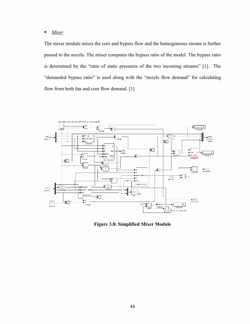
� Mixer

The mixer module mixes the core and bypass flow and the homogeneous stream is further

passed to the nozzle. The mixer computes the bypass ratio of the model. The bypass ratio

is determined by the “ratio of static pressures of the two incoming streams” [1]. The

“demanded bypass ratio” is used along with the “nozzle flow demand” for calculating

flow from both fan and core flow demand. [1]

Figure 3.8: Simplified Mixer Module

45


• Core Stream – from

LPT

• Bypass Stream –

from Fan Tip/duct

• Outlet stream to nozzle

• Bypass ratio

• Bypass duct area

• Core exhaust area

Table 3.10: Mixer Module Data

� Nozzle

Figure 3.9: Simplified Nozzle Module

The “mass flow and the exit temperature of the gas product ejected into the atmosphere”

[1] are calculated in the nozzle module. The parameters like nozzle discharge coefficient,

nozzle area, nozzle inlet flow conditions, and ambient pressure are used in computing

46

above parameters. The output flow from the nozzle is the flow demanded by the

upstream components [1]. Table 3.11 [1] shows Nozzle Module Data.


Required

• Ambient Pressure

Input stream: from

Mixer Wtotal, P6,

T6, Fuel Air Ratio

(FAR)

• Upstream flow demand – to

mixer


Wtotal, pressure (ambient)

temperature, Fuel Air Ratio

(FAR)

• Nozzle throat

area

Table 3.11: Nozzle Module Data

� Shaft

The shaft module “simulates the shaft dynamics” [1]. It is associated with driving torque

and load torque. The shaft speed (RPM) is obtained by dynamically integrating the

difference between the driving and the load torque. The turbines provide the driving

torque while and the load torque is due to compressor or auxiliary loads like gear box.

Figure 3.10: Simplified Shaft Module

47


• Driving Torque

• Load Torque

• RPM

• Shaft Moment of Inertia

• Connections

Table 3.12: Shaft Module Data

a) Core Shaft

The core shaft connects HPT to HPC. Table 3.13 [1] shows core shaft data.


• Driving Torque from

HPT

• Load Torque – from

HPC

• RPM – To HPT and

HPC

• Shaft Moment of

Inertia

Table 3.13: HP Shaft Module Data

b) Fan Shaft

The core shaft connects LPT to Fan. Table 3.14 [1] shows fan shaft data.


Required

• Driving Torque from

LPT

• Load Torque – from

Fan (Tip+Hub)

• RPM – To LPT and LPC

• Shaft Moment of

Inertia

Table 3.14: LP Shaft Module Data

48

� Cooling

Figure 3.11: Simplified Turbine Cooling Module

The cooling module simulates the cooling of the exhaust streams from the combustor and

the turbines. The cooling modules mix core and the compressor bleed flow to cool the

exhaust streams. A homogenous stream is a result of two input streams mainly a hot and

a cold stream [1]. This single stream serves as an input to its downstream component.

a) Combustor Cooling

The combustor is cooled by a homogeneous stream obtained by mixing the combustor

exhaust with compressor bleed flow.

b) Turbine Cooling

The HPT exhaust gases are mixed with some percentage of the HPC to achieve Turbine

cooling. The cooling is divided into two parts.

49

� FADEC (Fully Automatic Digital Electronic Controller) - Scheduled Fuel Flow

Figure 3.12: Simplified FADEC Module

This module calculates the fuel flow to pressure ratio (WFR) that serves an input

command to the hydro-mechanical unit (HMU). The HMU then internally resolves the

Fuel Flow which is a function of compressor exhaust pressure P3.Thus the WFR

determined by the FADEC is equivalent to that required to maintain the commanded LP

shaft speed. Table 3.15 [1] shows the data for FADEC module.

Table 3.15: FADEC - Scheduled N1 Module Data


• Altitude

• Mach number

• DTamb

• PLA(N1-

demand)

• WF/P3

(Fuel Flow

to

Combustor)

• Maps of scheduled N1 v/s

altitude, T2 and PLA.

• Integral and proportional

transfer constants

50

3.3 The Simulation Engine Model

Table 3.16 [1] lists the design specification of the simulated turbofan engine model:

Sr.

No.

Specification Value

1 Number of spools 2

2 Bypass ratio 4.9

3 N1 design 8700 RPM

4 N2 design 14700 RPM

5 Altitude design 65,000 ft

6 Max altitude 70,000 feet

7 Mach number design 0.65

7 Max Mach number 0.65

8 Afterburner None

9 Max recommended steady state T4 3000 R

Table 3.16: Engine Design Specifications

The following components are attached to the LP shaft of the engine:

1. Fan

2. Low pressure turbine (LPT)

3. LP Accessory Gearbox

51

Following components are attached to the HP shaft of the engine:

1. High pressure compressor (HPC)

2. High pressure turbine (HPT)

3. HP Accessory Gearbox

Figure 3.13 [1] has a schematic diagram of the engine gas path. The schematic is a

representation of the Simulink set up of the model.

Figure 3.13: Engine gas path schematic

52

Figure 3.14: Actual Simulation Model with two Spools

53

Figure 3.14 [14] shows the screen shot of the entire simulation model in MATLAB/

Simulink.

3.4 Conversion of MATLAB-Simulink to C++ version

This section describes the steps involved in conversion of MATLAB-Simulink version of

the Engine Model and discusses the details of its C++ version.

The MATLAB-Simulink version follows module based, lumped approach and that has

been followed up in C++ version.

3.4.1 Transfer Function:

A transfer function can be defined as the ratio of the output and input amplitudes. In

reference to the Figure 3.16, [18] the frequency response, is given by

H(f) = Vout

Vin

= 1 .

2 ∏ f R C + 1 Figure 3.15: A Simple Circuit

It is obvious that the input and output of the transfer function is complex exponential

having the same frequency. A transfer function completely describes how the “circuit

processes the input complex exponential to produce the output complex exponential”

[18]. In other words, the transfer function summarizes a circuit’s function. This fact leads

54

us to obtain transfer functions for each individual engine component. These components

are then integrated to build the final simulation engine model.

3.4.2 The Conversion Process:

Following Steps were followed while converting the MATLAB-Simulink model to C++

version:

1) Transfer Functions were obtained manually for all the 14 modules. Transfer functions

were obtained recursively for all sub modules.

2) These Transfer functions were suitably converted into C++ format and coded under

respective functions. Some of these transfer functions were required to be interfaced

with custom developed Math libraries for obtaining final output values.

3.4.3 Engine Modules in C++:

Thus the C++ version includes following classes in upstream to downstream order:

1) Inlet.cpp : This is a C++ class that represents the Inlet module in

Simulink.

2) Tip.cpp : This is a C++ class that represents the Tip module in

Simulink.

3) Hub.cpp : This is a C++ class that represents the Hub module in

Simulink.

55

4) Compressor.cpp : This is a C++ class that represents the Compressor module in

Simulink.

5) Combustor.cpp : This is a C++ class that represents the Combustor module in

Simulink.

6) Combcooling.cpp : This is a C++ class that represents the Combustor stream

coolant module in Simulink.

7) HPT.cpp : This is a C++ class that represents the Combustor module in

Simulink.

8) HPTcool1.cpp : This is a C++ class that represents the HPT inter cooler stage

1 module in Simulink.

9) HPTcool2.cpp : This is a C++ class that represents the HPT inter cooler stage

2 module in Simulink.

10) LPT.cpp : This is a C++ class that represents the Combustor module in

Simulink.

11) Mixer.cpp : This is a C++ class that represents the Mixer module in

Simulink.

12) Nozzle.cpp : This is a C++ class that represents the Nozzle module in

Simulink.

13) BypassDuct.cpp : This is a C++ class that represents the Bypass duct module in

Simulink.

14) FADEC.cpp : This is a C++ class that represents the FADEC module in

Simulink.

56

15) HMU.cpp : This is a C++ class that represents the HMU module (Fuel

Pump) in Simulink.

3.4.4 Integrating the C++ Classes

The MATLAB-Simulink model is a closed loop model. There is a flow of

information from downstream to upstream and hence the output of each module

serves as input to its upstream component and represents the required flow upstream.

This required flow is then used as a reference for all calculations in subsequent time

steps for all static and dynamic components of respective modules.

Each module is connected to one or many downstream modules thus providing their

respective outputs as inputs to their downstream components.

o Variables :

Object oriented programming concepts have been followed throughout the C++

model. All variables of respective modules are declared to be private while public set

and get methods have been provided to set and retrieve value of these variables in any

other module.

o Constants :

All constants for the entire model have been maintained in a file named “constants.h”.

The constant values have been # defined in separate sections suitably commented for

each separate module. The file generally follows an upstream to downstream flow.

57

o Lookup Tables :

MATLAB-Simulink version defines different types of lookup tables. All lookup table

data in MATLAB is interpreted as a Matrix. Following are its types:

1) 1-D Tables: This is a Matrix of size n x 1.

2) 2-D Tables: This is a Matrix of size n x 2.

3) 3-D Tables: This is a Matrix of size n x m x k. The 3rd dimension k in MATLAB is

interpreted as a page. Hence n x m represents rows and columns respectively.

All the above tables have been converted into arrays of respective dimensions for the

C++ version.

The lookup table data was converted into C++ format by a hand coded MATLAB

function. Consistency of values was verified by a separate C++ code.

o Functions:

All modules are consistent in the sense that each module has following set of common

functions:

1) getInstance() function: This accepts instance(s) of upstream component(s).

Exception is the Engine.cpp class that accepts initial values of ambient

parameters like Pamb, Tamb, Mach #, PLA(Pilot Lever Angle). This

method is responsible for creating a single instance of every class. The

method suitably instantiates desired variables and returns an instance of

the class.

58

2) retInstance() function: This function returns an existing instance of a class.

It returns null if the class has not been instantiated. A null return then

initializes respective parameters to initial conditions.

3) calculate() function : This function calls all sub functions to carry out all

computations for each module. These mainly include calls to functions for

performing calculations for Reynolds Correction, Gas Tables, Maps

(Compressor and Turbines), Dynamics of respective module, Flow,

Pressure, Temperature and Torque.

4) calcOut() function : This function sets the output structure to output values

calculated for the entire module. This will be served as input to its

respective downstream component.

5) destroy() function: This function acts like a destructor and is responsible

for garbage collection.

o Singleton Pattern:

Singleton pattern is a design pattern that allows the creation of only one instance of a

class. This is especially useful when a single object is required to coordinate across the

system.

In order to implement the Singleton pattern following conditions have been met:

1) Constructors of all classes are declared as protected.

59

2) A separate getInstance() function has been provided that creates an object for a

particular class and returns a reference to it. This function makes sure that only

one object is created during entire simulation process.

Singleton design pattern has been implemented in order to preserve the state of each

component of the engine at every single instant of time. This helps in achieving dynamic

behavior of all the engine components and hence a successful simulation.

3.4.5 The Engine.cpp class

This class has a run method that invokes the getInstance() function of all modules of the

Engine model. Since the engine model simulated real-time behavior of an actual jet

engine the previous state of the engine needs to be maintained.

This has been done by using the Singleton class concept. A Singleton class is a class that

enables users to create a single instance of the class. A Singleton instance thus helps us to

maintain state of the engine and perform all operations in closed loop form.

The instances of all modules are created in an upstream to downstream manner since the

flow of information is from downstream to upstream.

This method of instance creation mandates us to initialize values of variables that will be

calculated further downstream. Hence, each module as per its requirement has a set of

variables initialized to appropriate values.

60

o Shaft Dynamics:

Computations of both HP and LP shaft speeds is done by separate functions

namely calcN1() and calcN2().

o Load Demands:

Both HP and LP auxiliary gear box that simulate load on respective HP and LP shafts

have been coded as separate functions namely HPAGBDmd() and LPAGBDmd().

o getInstance() Function:

This function is distinct from other modules in the sense that it accepts initial values

as parameters required for cranking the engine.

In addition it initializes file pointers for all parameters to be logged in vector format

for future reference and analysis.

o Ambient Conditions:

Ambient conditions like Altitude, Mach # and PLA can be set through respective

public functions setAlt, setTamb, setMachn, setPLA.

In order to properly initialize and run the Engine the calculate() function of all

downstream components are executed in an orderly fashion. However, the calculate

functions for FADEC and HMU modules are called at the end. This is because their

output values depend on the inputs of engine components.

61

This requires the output of FADEC and HMU be initialized to suitable value for

performing calculations at iteration 1. (or simulation time step 0).

The Engine class calls retInstance() function of modules for retrieving class instances in

order to retrieve values from downstream components for calculation of shaft speeds.

These speeds are fed as inputs to Tip and Hub modules.

3.4.6 The run.cpp file

This is a startup or “crank” for the engine. It has the main method and hence is

responsible for putting the engine into action.

It creates an engine instance and then calls its public run function.

The entire flight envelope is simulated by making a repetitive call to this run function.

The run.cpp also makes a call to the public function freeall() of Engine class. The

freeall() function in turn makes subsequent call to all destroy function of respective

modules.

Consistency has been maintained with the Simulink Model by providing manual controls

for:

1) Altitude Adjustment: This has been provided by a function calcAlt() defined in

run.cpp. This function calculates the values for ambient pressure and temperature

that are passed as arguments to the getInstance() method in Engine class during

initialization. In addition these values are passed as arguments to setPamb() and

setTamb() function for setting these values in Engine class.

62

2) Mach number Adjustment : This has been provided by a setter method in Engine

class. The setMachn() method in Engine class accepts Mach Number as a double

value. This can vary from 0 – 0.65.

3) PLA control: This has been provided by a setter method setPLA() in the Engine

class. This sets the value of private variable PLA declared in the Engine class.

The method setPLA() accepts an argument of type double.

3.5 Custom Math Libraries

The Engine model includes differential equations and State Space equations for

calculation of parameters like LP and HP shaft speed.

In addition due to Compressor maps and Gas Tables almost 80% of the model depends

on parameter calculation using interpolation techniques.

Following are the Interpolation tables/techniques used by this model:

1) Standard Linear interpolation

2) 2-D linear interpolation

3) 3-D linear interpolation and

4) 3-D interpolation using Pre-lookup

Separate Math functions have been provided in files:

a) interpol2dfunc.cpp and

b) commonfuncs.cpp

State space equations have been implemented using the Runge Kutta Method, while

integration has been carried out using Euler’s Method.. All integral functions have been

in-lined in the code.

63

3.6 Pros and Cons of Modular Approach

Pros:

The Modular approach followed here enables us for:

1. Easy modification for simulating other turbofan engine models.

2. Interfacing with simulated controllers, for testing and validation.

3. Easy debugging and

4. Maintenance

Cons:

1. Large number of class files due to modular approach.

2. Keeping track of all instances including creation and destruction.

64

3.7 Simulation Inputs and Set Up

The simulation has three inputs. Altitude and Mach number are the ambient inputs and

N1-demand is set by the PLA. All inputs can be changed by varying respective

SimuLink slider control or by passing required value to the setter methods in C++

version. The range/limits of inputs are as follows:

1) Altitude : The range of this ambient input is sea level to 70,000 feet [1].

The altitude input is fed to the input module.

2) Mach number: The aircraft mach number is and its effect on stagnation pressure

(P2) and temperature (T2) is simulated.

The range for this parameter is 0 to 0.65 [1].

3) PLA : This control input demands the percentage speed of the LP shaft

(N1).

The PLA input is fed to the FADEC that calculated the WF/P3

ratios (WFR).

65

Figure 3.16: Engine Controller

The simulation engine model follows N1 design with a rated speed of 8700 RPM. Day

atmospheric conditions like the altitude, pressure and temperature are simulated by this

model. Appropriate amount of fuel is fed to the combustor after calculating the error

between the commanded N1 by the PLA and the actual LP shaft speed (N1). [1]

The simulation is unable to simulate: [1]

1) Actuator dynamics

2) Sensor measurement except T45 sensor or noise.

66

The model outputs are values of various parameters like:

1. Pressure

2. Temperature

3. Flow at different points in the gas path

4. Torque and

5. Speed.

All of the model outputs can be viewed and logged to secondary storage during the

simulation.

67

3.7.1 The Simulation Process

This section provides guidelines on running the model in Simulink.

3.7.1.1 Simulation of Engine Model in Matlab/Simulink environment

The Matlab/SimuLink version can be simulated as follows:

1. Open Matlab – This will open the MATLAB environment and display the command

window.

2. Load the model – On the Matlab command prompt type Wf_pump1. This loads and

sets up environment compatible to executing the Matlab/Simulink model in Linux

environment. After initial setup is done, the Simulink model is displayed.

3. Model Inputs – All the inputs are controlled through the Simulink slider controls

SimuLink. The model provides three (3) input slider controls:

• PLA – This sets the N1 demand

• Altitude – This sets the desired altitude for the aircraft

• Mach number – This sets the Mach number for the aircraft.

The values can be set by either moving the slider control or by manually entering

numeric values. Lower and upper bounds can also be set manually.

4. Starting Simulation – The simulation can be started by pressing F5 key or by clicking

the ‘►’ symbol on the toolbar. Initial conditions are set while the model is loaded in

step 2 and by default they are set to following values: altitude = 0, Mach number = 0

68

and N1 (PLA) demand = 87%. Figure 3.17[1] shows the engine flight envelope and

the points where the simulation is started.

10 K

20 K

65 K

0.2 0.3 0.65

10 K

20 K

65 K

0.2 0.3 0.65

Figure 3.17: Engine model Flight Envelop

5. The slider controls can be used to vary LP shaft speed (N1) demand, altitude and

Mach number. N1 can be varied from 87% to 109%. while Altitude and Mach

number can be varied from sea level to 65,000 feet and 0 to 0.65 respectively. The

simulation time elapsed is displayed on the status bar. Maximum simulation time can

be set through the configuration menu in Simulink.

6. Simulation can be stopped by clicking on ‘■’ (Stop) symbol on the Simulink toolbar.

69

3.7.1.2 Simulation of Engine Model in C++ environment

A Makefile is provided to compile and link all the modules.

Following are the compatibility details:

1) Operating System : UNIX OR Linux Any variant

2) Compiler : g++

3) Hardware : Pentium IV with 1GB RAM and a 2 GB HDD free space.

4) Simulation:

During the entire flight enveloped Altitude, Mach Number and PLA variations are

done in the file run.cpp. This file can be modified appropriately to make changes

in the flight envelope. However, if the initial conditions are changed

then the initialization parameters also need to be changed.

Present code initializes the parameters for the engine at sea level, PLA setting

87% and Mach number equal to zero (0).

Note: It is mandatory to have a class containing the main method in order to

compile and execute the code.

The Make file generates object files and an executable named ICF_Engine.

Invoke this executable to fire the engine and continue with the simulation.

70

3.8 Comparison of outputs between MATLAB-Simulink and

the C++ version Both the versions were executed using same initial conditions and with the same flight

envelope.

The simulation scenario is as follows:






5. From 30 seconds to 40 seconds, it simulates cruising at 10,000 ft and 0.5 Mach

number

6. At 40 seconds, Mach number is reduced to 0.2 and the engine is brought to sea level.

7. At sea level, at around 60 seconds, the Mach number and N1 are simultaneously

reduced to 0 and 91% respectively.

The fuel input Wf is calculated based on the other three input, through a fuel flow

schedule and is intended to maintain N1 at the command level.

71

3.9 Plots

Figure 3.18: Plots for Flight Envelope

72

Figure 3.19: Plots for Flight Envelope

The error calculated between both MATLAB and C++ versions for these graphs was of

the order of 0.01 % provided that the variations in all controls were done at the same

instants of time.

73

Chapter 4

CTRNN-EH - Augmentative Control

This chapter gives through details about the concept of Evolvable Hardware (EH) and its

integration with CTRNN. The chapter begins with an introduction to evolvable hardware,

followed by details about CTRNN-EH devices. This is followed by a discussion about the

drawbacks associated with the conventional PI-controllers and CTRNN-EH as a probable

solution. This chapter concludes by discussing the augmentative control approach used

for solving the instability issue.

4.1 Evolvable Hardware (EH): An Unconventional

Methodology

Computational design methods and conventional techniques do help us in the

development of sophisticated controllers. However, there are certain situations in which

in-the-field self-design and augmentation of control would be useful. These situations

occur when a system in the field is tasked to accomplish unexpected mission.

Evolvable hardware (EH) [8, 9] is an electronic device that can be reconfigured by using

the techniques of natural evolution. EH has been classified as one of the sub-fields of

74

computer science and engineering and is an “emerging subspecialty within Evolutionary

computation in which one uses EAs to evolve designs for machines” [24].

EH plays an important role in adapting a piece of hardware to accomplish such

unprecedented tasks. It thus can be viewed as a step towards adaptive hardware in which

designers are not required to go through back to the drawing board and redesign the

system for the new mission.

4.2 CTRNN-EH Devices

Figure 4.1: An Evolvable Hardware Controller.

Figure 4.1 [9] shows a conceptual block diagram of an EH based control device. The

interface between the reconfigurable control hardware and the controlled device is typical

of that between controller and plant in any feedback control system.

The only major difference is that the controller can be reconfigured by an EA that

evolves controller configurations based upon controller operational fitness as reported by

75

a problem specific evaluation module. CTRNN-EH is a combination of an EA and a

hardware continuous time recurrent neural network (CTRNN) into a single EH device.

Continuous time recurrent neural networks (CTRNNs) are constructed from analog

components [23] that approximate the operation of natural neurons. CTRNNs can be

inexpensively simulated and built from common electrical components or in custom

VLSI importantly for EH purposes. CTRNNs are universal dynamic approximators [21],

meaning they are in principle capable of evolving to embody any control law.

Mathematically, CTRNNs are networks of Hopfield continuous model neurons with

unconstrained connection weight matrices. [21, 22]

An individual neuron’s activity is expressed as:

(4.1)

where y is the state of each neuron, τ is its time constant, wji is the strength of the

connection from the jth to the ith neuron, θ is a bias term, and σ is the standard logistic

activation function, and Ii(t) represents a weighted sensory input with strength s.

Electrically, CTRNN neurons are low pass filters that receive weighted inputs from other

neurons or from the outside world. Before being presented to the other neurons or to

effectors as control efforts, the output of each neuron’s low pass filter is passed through a

sigmoid squashing function. In each neuron, the time constant of the filter, the bias for

the sigmoid squashing function, and the time constant of the filter are all tunable.

τ i

dy i

dt= −yi + w jiσ y j +θ j( )+ siIi

j=1

N

∑ (t) i =1,K,N

76

The weights on signal connections among neurons and to and from the outside world are

also tunable.

4.3 CTRNN-EH: Augmentation Control to handle Fuel Flow

Control Issue

This thesis presents a probable CTRNN-EH approach to the jet/turbine engine fuel flow

control issue. In this section we discuss the advantages of this approach over other

control schemes.

4.3.1 Conventional PI-Controllers versus CTRNN-EH

Proportional-Integral controllers are the most widely used conventional controllers in

industrial control systems. The proportional part is responsible to provide control signals

that are directly proportional to the error between the reference signal and the actual

output while the integrator provides signals proportional to the integral of the error. We

will not be discussing this control scheme in detail as it is out of scope for this thesis.

However, we will discuss the disadvantages associated with these controllers followed by

the benefits of CTRNN-EH control.

4.3.2 Issues with Conventional PI-Controllers

Conventional PI-controllers are usually designed for the laws of the controlled device’s

system and control dynamics. They are designed taking into account little instability

77

issues. Instability caused due to un-conventional operating conditions like loading the LP

shaft was never considered.

This leads to the PI controllers being ineffective as they fail to adapt to the unanticipated

conditions.

This unusual loading of LP shaft at high altitudes leads to a dynamic change in the

controlled domain that requires the controller to be redesigned. It is generally not feasible

to redesign a controller every time the control domain changes.

Pre-design stage for traditional controllers like the PI-controller, need complete

understanding of dynamics of the controlled system. If the designer lacks this then it is

almost impossible to come up with an appropriate controller for particular conditions.

In addition, complex control problems lead to a complex controller design.

4.3.3 CTRNN-EH Control: A Possible Solution

EH methodology makes no assumption that the control should be a linear proportional

feed back controller. This property makes it possible to provide an effective control and

provide a solution for above discussed issues.

Conventional controllers require a thorough understanding about the controlled systems

while CTRNN-EH is believed to function well even in the absence of this knowledge.

A CTRNN is an analog neuromorphic [8] component in the CTRNN-EH chip [8, 23].

This component learns the dynamics of the system and reconfigures itself to adapt to the

dynamics of the system. Thus it changes its parameters like weights, biases for providing

an effective on-the-fly controller design based on the current system state caused by its

previous configuration.

78

The CTRNN is an unsupervised controller and thus has the capability to provide a better

control in every following step. This helps in achieving best desired control effort. This

helps us to understand that a CTRNN-EH device is never designed for a specific system.

The capability of CTRNN to control to complex systems depends on the number of

neurons itself. Providing the CTRNN with sufficient number of neurons makes it capable

to deal with any complicated system. This can also be supported by the fact that the

initial conditions and the architecture itself may be the same for different types of

controlled systems.

79

Chapter 5

CTRNN-EH Controller Interface to ICF

Engine Model

5.1 CTRNN-EH Controller

This chapter will give details about the CTRNN-EH control scheme employed in this

work to account for the fuel flow control issues associated with the simulated ICF Engine

model.

5.1.1 The Simulated Engine Model

Transfer functions representing the engine model were stated that represents the engine at

different cruise states. The model consists of HMU (Hydro Mechanical Unit)/Fuel Pump

that serves as the controlled system and four parameters namely Inlet Pressure,

Temperature, HP Shaft Speed and LP shaft Speed as sensor inputs. The Engine operates

at different states from take-off to steady cruise to landing. These states are based on

ambient conditions like Pressure, Temperature, Mach number and Altitude above sea

80

level. Original MATLAB/Simulink version of the model was converted to C++ version

for the ease of interfacing with existing CTRNN libraries.

C++ language simulations of all the above states were carried out and were confirmed to

be faithful reproductions of their respective engine states.

The instability issue associated with the engine at an altitude of 60,000 with a load of

120KW applied to LP shaft was also observed to be consistent with its MATLAB

version.

The simulation carried out for instability issue assumed an altitude of 60,000 ft above sea

level, PLA setting of 100%, LP shaft speed (N1) 8700RPM with a Mach number of 0.6.

5.1.2 Interfacing CTRNN device to Simulated Engine and FADEC

Controller

A ten Neuron fully connected CTRNN was chosen as this configuration was observed to

evolve reasonable solutions. MiniPop was used as an EA component.

The CTRNN device was interfaced to the simulated Engine Model and the FADEC

controller as shown in the figure 5.1. Each neuron received five(5) inputs :

1) Inlet Pressure (P2) psi

2) Inlet Temperature (T2) deg F

3) HP Shaft Speed (N1) RPM

4) LP Shaft Speed (N2) RPM

5) FADEC output (WFR) lb/hr psi

81

Figure 5.1: CTRNN device interfaced with Simulated Engine and FADEC

The CTRNN device provided augmentative control by operating in parallel with the

FADEC. The CTRNN thus controlled the output WFR to the HMU that served the

purpose of maintaining cruise altitude even when the LP shaft was loaded.

Limits were set on the range of WFR. WFR could range from 6 to 40.

82

5.1.3 Performance Evaluation

The performance was evaluated by the error function used by EA while searching for

good controllers. Type of error function greatly influences the quality of controllers

CTRNN-EH device evolves.

The error function used in this work was the average sum of the difference between

desired and actual speed of the LP shaft. This error function determines the stability of

the engine and it can be understood that as the error is reduced the LP shaft achieves

desired speed. This helps in maintaining appropriate shaft speed and hence the cruise

altitude. A stable engine has a low error value. Figures 5.2 and 5.3 show the graphical

output of a stable and unstable engine.

5.1.4 Acceptable Controller

An acceptable controller can be defined as a controller that satisfies minimum

requirements. Following requirements were expected to be met by an ‘Acceptable

Controller’:

1) The cruise altitude should be maintained with load maintained on the engine for a

simulation period of time.

2) The controller should provide an augmentation control by commanding

appropriate WFR

The simulation period was determined to be for 1 minute (60,000 ms). This time was

acceptable as the engine was observed to go to an unstable state within 7s. In the

absence of proper control and failure to recover the LP shaft speed, the LP shaft RPM

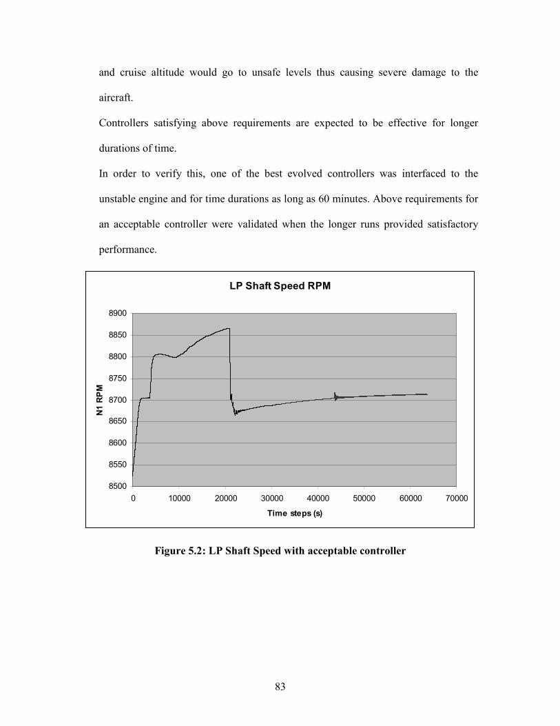
83

and cruise altitude would go to unsafe levels thus causing severe damage to the

aircraft.

Controllers satisfying above requirements are expected to be effective for longer

durations of time.

In order to verify this, one of the best evolved controllers was interfaced to the

unstable engine and for time durations as long as 60 minutes. Above requirements for

an acceptable controller were validated when the longer runs provided satisfactory

performance.

LP Shaft Speed RPM

8500

8550

8600

8650

8700

8750

8800

8850

8900

0 10000 20000 30000 40000 50000 60000 70000

Time steps (s)

N1 RPM

Figure 5.2: LP Shaft Speed with acceptable controller

84

Figure 5.3 LP Shaft Speed with un-acceptable controller

85

5.2 Performance of CTRNN-EH Controllers

This section will discuss the performance of the CTRNN-EH controllers.

Controller architecture and details about augmentation controller were discussed in

previous section. This controller is expected to provide augmentation control by

determining the effective Fuel flow to pressure ratio (WFR) that is required to maintain

the LP shaft RPM at desired value.

Following configurations were evolved:

Sr. No. Configuration Acceptable

1 NEURONS # : 10

Mutation Rate : 0.05

No

2 NEURONS # : 10

Mutation Rate : 0.85

Yes

Table 5.1: Statistics of Controllers Evolved with different Configurations

The performance was evaluated using following evaluation function:

Fitness =∑ abs (N1desired – N1calculated)

n

where, n (time steps) is the duration of the cruise at 60,000 ft and with LP shaft loaded

with 120KW.

24 Controllers for each of the above mentioned configurations were evolved.

Unacceptable controllers were observed to act like fixed point controllers.

In that the CTRNN controller was observed to provide 100% output of its set capacity.

86

The evolved fixed point controllers were observed to cause an over shoot in LP shaft

speed. A continued operation of any driving shaft leads to the development of high

mechanical stresses that finally cause a permanent mechanical failure.

The overshoot was observed to be 8866 RPM which is 176 RPM above the design levels.

Such high values are definitely never recommended in case of automotive applications.

However, it can be seen from the table that we were able to evolve four (4) controllers

with an average fitness value of 48.7935. These controllers were observed to initially

over shoot the LP shaft speed but later they effectively reduced the Fuel Flow to Pressure

ratio (WFR) output that allowed the speed to recover to the value of 8712. This can be

observed from Figure 5.2.

An overshoot of mere 12 RPM is considered to be satisfactory enough to maintain the

engine operation for longer duration of time.

Figure 5.4: LP Shaft Speed of Acceptable controllers (FADEC+CTRNN)

87

Figure 5.4 shows the plot of LP shaft speed against time for all four acceptable

controllers.

It was thus inferred from all above experiments that the fuel flow control issue associated

with the conventional controllers can be solved using CTRNN-EH approach.

5.3 Analysis of Acceptable CTRNN-EH Controller

It can be observed from the Figure 5.2 that the augmentative control with CTRNN drives

the LP shaft speed from a higher value of 8866 RPM to an acceptable range in about 14s.

The augmentation control with CTRNN-EH device operating in parallel with FADEC has

been discussed in previous section. When the LP shaft is loaded with an auxiliary load of

120KW the shaft speed drops. In order to recover this speed to the commanded value (by

the PLA), the FADEC controller increases the Fuel Flow to Pressure ratio (WFR)

command to the HMU. However, the existing FADEC was never designed for loads of

such high magnitudes on the LP shaft at high altitudes.

The CTRNN-EH device compensates this inability of the FADEC controller by providing

additional WFR command required to command a higher fuel flow to the combustor.

The CTRNN-EH controller is basically provided with five (5) inputs namely:

1) Inlet Pressure

2) Inlet Temperature

3) LP Shaft Speed

4) HP Shaft Speed and

5) WFR output from FADEC

88

As can be observed from the Figure 5.2 the LP shaft is loaded with 120KW from the LP

Auxiliary gear box at around 4s.

WFR command From CTRNN+FADEC Augmentative control

0

5

10

15

20

25

30

35

40

45

0 5000 10000 15000 20000 25000 30000 35000

time steps (s)

WFR

Figure 5.5 WFR command from the augmentative controller (FADEC+CTRNN)

The CTRNN controller at this point acts as a fixed point controller providing 100%

output. This does help in preventing undershoot in the LP shaft speed. However, an

overshoot is observed in the LP shaft speed.

The FADEC however immediately anticipates this overshoot and acts by reducing its

WFR command.

At about 6s, the FADEC output reaches its lower bound. This helps in ceasing the linear

increase of LP shaft speed. However, the CTRNN output continues to remain the same.

89

The net WFR command from the augmentative controller however is still above the value

that is sufficient to maintain the shaft speed at 8700 RPM with full load on LP shaft.

This leads to an increase in LP shaft speed. This increase can be observed to continue till

20s of simulation time. As can be observed from the Figure 5.3, the net FADEC+CTRNN

output remains constant from 10s to 20s. After 20s, it can be observed from Figure 5.2

that the CTRNN controller comes out of its fixed point role and provides a control effort

in order to ramp down the LP shaft speed to a lower acceptable value.

At about 21s, the CTRNN is successful in recovering the LP shaft speed to 8700 RPM.

However, the CTRNN controller is observed to continue with a reduced WFR output.

The reduced WFR command causes LP shaft speed to drop to 8666.029 RPM.

A reduction in LP shaft speed below its desired value is immediately detected by the

FADEC controller and it thus acts by providing an increased WFR command.

This helps in recovering the speed to 8700 RPM.

It can also be observed from Figure 5.3 that the net WFR output stabilizes as the desired

LP shaft speed reaches its desired value.

The reasons for the acceptable controllers obtained with such a high mutation rate are not

know at this point of time and further exploration is left for future work.

90

5.4 Future Work

There remain two future goals to be accomplished.

The first goal would be to understand the behavior of presently evolved “acceptable”

controllers.

Second task would be to evolve more number of controllers that have very small or

almost no overshoot during its entire cruise at 60,000ft with an LP shaft load of 120KW.

In addition we have to run more number of experiments with lower mutation rates. This

can be worked out by experimenting with different CTRNN configurations and variable

scaling factor.

In the present runs a scaling factor of 25 was selected. This value was used because of the

fact that the maximum range of WFR command for the corrected FADEC controller was

observed to be forty. Since the uncorrected/present FADEC can generate a maximum

value of 15 the deficit required to ramp up the speed was estimated to be twenty-five.

Such a high value might be because of a significant drop of 500 RPM in the engine

speed. As we have observed from the results that the recovery time for CTRNN

controller is less than that of corrected FADEC, we can say that a lower scaling factor

could be sufficient to recover the LP shaft speed to the desired value.

A lower scaling factor will hence reduce the search space and will help in finding a

solution even with lower mutation rates.

91

References

[1] G. Mink, Chief Engineer, Scientific Monitoring, Inc, “ICF Generic Engine Model

Documentation” version 2.3 10-10-2003

[2] A.E. Eiben, J.E. Smith, Introduction to Evolutionary Computing, Springer, 2003.

[3] J.H. Holland, Genetic algorithms and the optimal allocation of trails. SIAM J. of

Computing, 2 pp. 88-105, 1973

[4] J.H. Holland, Adaptation in Natural and Artificial Systems, MIT Press,

Cambridge M.A. 1992.

[5] Simon Haykin, Neural networks : a comprehensive foundation, Upper Saddle

River, N.J. : Prentice Hall, c1999

[6] K.A. DeJong, Evolutionary Computation: unified approach, MIT Press,

Cambridge 2003

[7] Kramer G.R. and Gallagher JC. “An Analysis of the Search Performance of a

Mini-Population Evolutionary Algorithm for a Robot-Locomotion Control

Problem”

[8] S. Vigraham and J. Gallagher. “A case for using minipop as the evolutionary

algoritm in a CTRNN-EH control device: an analysis of area requirements and

search efficacy”.

92

[9] Gallagher, J., Vigraham, S., Kramer, G.R. “A Case Study in Evolvable Hardware

for Control”. IEEE Magazine

[10] Online Resource: http://www.soton.ac.uk/~jps7/Aircraft Design

Resources/Brandt Introduction to Aeronautics/Ch5Performance.doc.

“CHAPTER 5: PERFORMANCE AND CONSTRAINT ANALYSIS”

[11] Nicholas Cumpsty. “Jet propulsion: a simple guide to the aerodynamics and

thermodynamic design and performance of jet engines” , Cambridge University

Press, 2003

[12] Online Resource: FADEC (Fully Authorized Digital Electronic Control) :

http://en.wikipedia.org/wiki/FADEC

[13] Michael Corbett, Jessica Williams, Mitch Wolff, Eric Walters, Jason Wells,

Peter Lamm. “Transient Turbine Engine Modeling and Real-Time System

Integration Prototyping”

[14] Air Force Research Labs (AFRL). “ICF Generic Engine Model” - version 2.3.0”

[15] Whitley, D., “A Genetic Algorithm Tutorial,” Tech rep., Colorado State

University

[16] Turbine Maps : en.wikipedia.org/wiki/Turbine_map

[17] Compressor Maps: en.wikipedia.org/wiki/Compressor_map

[18] Don Johnson. "Transfer Functions" - Version 2.18: May 10, 2007

http://cnx.org/content/m0028/latest/. http://creativecommons.org/licenses/by/1.0.

[19] Bjarne Stroustrup. The C++ programming language, Addison-Wesley, c1997

[20] Partha Kuchana. Software architecture design patterns in Java, Auerbach

Publications, 2004

93

[21] J.C. Gallagher, S.K. Boddhu, and S.A. Vigraham. “A reconfigurable continuous

time recurrent neural network for evolvable hardware applications”

[22] J.C. Gallagher. “A Dynamical Systems Analysis of the Neural Basis of Behavior

in an Artificial Autonomous Agent”. PhD thesis, Case Western Reserve

University,1998.

[23] S. Vigraham. “Supressing Parasitic Oscillations In a Simulated Combustor: An

Evolvable Hardware Approach” Masters Thesis, Wright State University, 2003

[24] John C. Gallagher, Saranyan Vigraham, and Gregory Kramer. “A Family of

Compact Genetic Algorithms for Intrinsic Evolvable Hardware”. IEEE

Transactions on evolutionary computation, vol. 8, no. 2, April 2004.

Fuel Flow Control Issue in Jet Engines - CORE Scholar

Documents

Transcript of Fuel Flow Control Issue in Jet Engines - CORE Scholar