Focussed ModelSelection forLongitudinal DataTristan CurteisMaster’s Thesis, Spring 2018

This master’s thesis is submitted under the master’s programme Modellingand Data Analysis, with programme option Statistics and Data Analysis, atthe Department of Mathematics, University of Oslo. The scope of the thesisis 60 credits.

The front page depicts a section of the root system of the exceptionalLie group E8, projected into the plane. Lie groups were invented by theNorwegian mathematician Sophus Lie (1842–1899) to express symmetries indifferential equations and today they play a central role in various parts ofmathematics.

Focussed Model Selection for Longitudinal Data

Tristan Curteis

Master’s Thesis, Spring 2018

Abstract

Longitudinal data arise when repeated measurements are taken on individuals overtime. Commonly used models for such data are multivariate linear models, linearmixed effect models and generalised linear mixed models. This thesis begins byproviding a detailed overview of these classes of models within the context of lon-gitudinal data. Attention is then turned to model selection for such data. Whenselecting between models, one typically aims to come as close as one may to the un-derlying truth, without regard to the particular questions of interest. In contrast, thefocussed information criterion (FIC) (Claeskens & Hjort 2003) approaches model se-lection with the goal of answering specific questions as accurately as possible. In thisthesis, a multivariate slightly misspecified framework is put forward, within whichthe FIC is applicable as a covariate selector for multivariate linear models, linearmixed effect models, and generalised linear mixed models. Alternative approachesto focussed model selection for multivariate linear models and a selection of quantit-ies of interest are also formulated.

Acknowledgements

A list of acknowledgements can never make amends for the time and effort given,nor reach all of those one is indebted to. Nevertheless, I am grateful to friends SuryaTahora, and Dr. Snehal Shah for initial orientation and encouragement, even if thethesis took on a direction of its own. Thank you Matthew and Simon for your friend-ship, and for the opportunity to discuss statistical concepts. Thank you Kylie andLewys for your time and patience. Lastly, and most importantly, I am grateful to mysupervisor, Ørnulf Borgan, for granting me the right balance between guidance andindependence. It has been fun working with you.

Contents

1 Introduction 11.1 Longitudinal and clustered data . . . . . . . . . . . . . . . . . . . . 11.2 Model selection . . . . . . . . . . . . . . . . . . . . . . . . . . . . 11.3 Structure of thesis . . . . . . . . . . . . . . . . . . . . . . . . . . . 3

2 Linear Regression for Longitudinal Data 52.1 Linear regression for longitudinal data . . . . . . . . . . . . . . . . 52.2 Modelling the mean . . . . . . . . . . . . . . . . . . . . . . . . . . 6

2.2.1 Parametric trends . . . . . . . . . . . . . . . . . . . . . . . 62.2.2 Semi-parametric trend . . . . . . . . . . . . . . . . . . . . 8

2.3 Modelling the covariance . . . . . . . . . . . . . . . . . . . . . . . 82.3.1 Examples of variance-covariance pattern models . . . . . . 9

2.4 Linear mixed effect models . . . . . . . . . . . . . . . . . . . . . . 122.4.1 The general linear mixed effect model . . . . . . . . . . . . 122.4.2 The conditional distribution defined in the general LME model 132.4.3 The marginal model implied by the general LME model . . 142.4.4 The random effects model . . . . . . . . . . . . . . . . . . 142.4.5 Random intercept models . . . . . . . . . . . . . . . . . . 152.4.6 A random intercept and slope model . . . . . . . . . . . . . 17

2.5 Estimation . . . . . . . . . . . . . . . . . . . . . . . . . . . . . . . 172.5.1 Maximum likelihood . . . . . . . . . . . . . . . . . . . . . 182.5.2 Restricted maximum likelihood . . . . . . . . . . . . . . . 192.5.3 A note on model selection . . . . . . . . . . . . . . . . . . 202.5.4 Predicting random effects . . . . . . . . . . . . . . . . . . 21

2.6 Model diagnostics for linear models . . . . . . . . . . . . . . . . . 222.7 Dataset illustration . . . . . . . . . . . . . . . . . . . . . . . . . . 22

2.7.1 Exploratory analysis . . . . . . . . . . . . . . . . . . . . . 232.7.2 Random effects model . . . . . . . . . . . . . . . . . . . . 252.7.3 Random intercept and slope model . . . . . . . . . . . . . . 262.7.4 Model assumptions . . . . . . . . . . . . . . . . . . . . . . 27

2.8 Concluding remarks . . . . . . . . . . . . . . . . . . . . . . . . . . 292.8.1 A short comparison of the general LME model and the LM . 29

iii

2.8.2 Summary of chapter . . . . . . . . . . . . . . . . . . . . . 29

3 Generalised Linear Mixed Models 313.1 Formulating a GLMM . . . . . . . . . . . . . . . . . . . . . . . . 31

3.1.1 Conditional moments of a GLMM . . . . . . . . . . . . . . 323.1.2 The marginal distribution derived from the GLMM . . . . . 33

3.2 Examples . . . . . . . . . . . . . . . . . . . . . . . . . . . . . . . 343.2.1 A Bernoulli GLMM . . . . . . . . . . . . . . . . . . . . . 343.2.2 A Poisson GLMM . . . . . . . . . . . . . . . . . . . . . . 35

3.3 Estimation . . . . . . . . . . . . . . . . . . . . . . . . . . . . . . . 363.3.1 Maximum likelihood . . . . . . . . . . . . . . . . . . . . . 36

3.4 Data illustration . . . . . . . . . . . . . . . . . . . . . . . . . . . . 373.4.1 A plausible model . . . . . . . . . . . . . . . . . . . . . . 373.4.2 Results . . . . . . . . . . . . . . . . . . . . . . . . . . . . 38

3.5 Chapter summary . . . . . . . . . . . . . . . . . . . . . . . . . . . 42

4 The Focussed Information Criterion for Clustered Data 434.1 FIC for independent data . . . . . . . . . . . . . . . . . . . . . . . 43

4.1.1 Framework and goal . . . . . . . . . . . . . . . . . . . . . 444.1.2 Score vectors and the expected information matrix . . . . . 464.1.3 Limiting distributions . . . . . . . . . . . . . . . . . . . . . 484.1.4 FIC scores . . . . . . . . . . . . . . . . . . . . . . . . . . 50

4.2 FIC for clustered data . . . . . . . . . . . . . . . . . . . . . . . . . 514.2.1 Framework for using FIC for data with independent clusters 52

4.3 FIC for multivariate linear regression, with and without random effects 544.3.1 The focus as solely a function of regression parameters . . . 574.3.2 Simulations . . . . . . . . . . . . . . . . . . . . . . . . . . 584.3.3 Data illustration . . . . . . . . . . . . . . . . . . . . . . . . 65

4.4 FIC for generalised linear mixed models . . . . . . . . . . . . . . . 744.4.1 Derivations of information matrices of a logistic GLMM with

a random intercept. . . . . . . . . . . . . . . . . . . . . . . 744.4.2 Data illustration . . . . . . . . . . . . . . . . . . . . . . . . 77

4.5 Chapter summary . . . . . . . . . . . . . . . . . . . . . . . . . . . 79

5 Derivations of Mean Squared Error Formulae 815.1 MSE formula for a focus that is a general linear combination of re-

gression parameters . . . . . . . . . . . . . . . . . . . . . . . . . . 815.1.1 Data illustration . . . . . . . . . . . . . . . . . . . . . . . . 84

5.2 Extension to a multivariate focus . . . . . . . . . . . . . . . . . . . 855.3 Accounting for uncertainty in the variance components . . . . . . . 87

5.3.1 A simulation study . . . . . . . . . . . . . . . . . . . . . . 895.4 Mean squared prediction error formulae . . . . . . . . . . . . . . . 925.5 Chapter summary . . . . . . . . . . . . . . . . . . . . . . . . . . . 93

iv

6 Summary and Further Topics 956.1 Summary of thesis . . . . . . . . . . . . . . . . . . . . . . . . . . 956.2 Further topics . . . . . . . . . . . . . . . . . . . . . . . . . . . . . 95

A Appendix A 101A.1 Results on derivatives of the determinant and inverse of a matrix . . 101A.2 Expectation of a quadratic form of mean-zero variables . . . . . . . 101A.3 Derivation of Jθθ,N . . . . . . . . . . . . . . . . . . . . . . . . . 102A.4 Derivatives of Σ1(θ) and Σ0(θ) with respect to θ . . . . . . . . . . 103A.5 Result (5.18) . . . . . . . . . . . . . . . . . . . . . . . . . . . . . 103

B Appendix B 105B.1 Figures from the simulations of Section 4.3.2 . . . . . . . . . . . . 105B.2 Tables from the simulations of Section 4.3.2 . . . . . . . . . . . . . 115

C Appendix C 117

D Appendix D 119D.1 R code . . . . . . . . . . . . . . . . . . . . . . . . . . . . . . . . . 119

v

Chapter 1

Introduction

1.1 Longitudinal and clustered dataLongitudinal data arise when measurements are taken repeatedly on the same sub-ject or individual throughout time (Fitzmaurice et al. 2004a). For example, individu-als randomised to different treatment groups may be observed on several occasions.Such a setting results in the measurements of any individual having temporal correl-ation, which must be accounted for in a statistical analysis (Laird & Ware 1982).

Similarly, clustered data are a more general form of longitudinal data. A com-monly used example of non-longitudinal clustered data is exam results of studentsfrom different classes. The results of students within the same class are more likely,in comparison with students of different classes, to be similar. Thus, in this example,the class forms a cluster and the students form the units within each cluster. Forlongitudinal data, the repeated measurements of an individual form the units, and theindividuals the clusters. In the school example, the within-cluster correlations are nottemporal, but are still very much present.

In the regression setting, conceptually, independence means that, once havingaccounted for a principle set of variables, the connection or similarity between out-comes is considered weak or distant enough for any similarity between them to beattributable to chance. For longitudinal data, the measurements of different individu-als, may (in general) be considered independent. For clustered data, the differentclusters (i.e. the classes in the school example) may be considered independent. Thewithin-cluster units, or within-individual measurements may not.

1.2 Model selectionFor clustered or longitudinal data, multivariate linear regression, linear mixed effectmodels, generalised linear mixed models, and marginal models are commonly usedclasses of models. However, even within a given class, there is not just one modelfrom which to draw conclusions. Generally, there is a list of competing models from

1

which to choose, though this can often be shortened to some extent by consider-ing what assumptions may be appropriate at the outset. The design of a study willalso inform (or even determine) the form of a mean structure prior to model selec-tion (Stroup 2012). Nevertheless, the statistician is regularly placed in a position ofchoice: is this model any better than the next? Combining the results from all modelsis also possible (Claeskens et al. 2008, Ch. 7), but how much should each model berelied upon?

A standard approach to model selection is to find the model which comes asclose to the true data generating mechanism as possible. This is directly targetedby the Akaike information criterion (AIC), whose theoretical basis is in minimisingthe statistical distance from the true model (Claeskens et al. 2008, p.30). Selectionof covariates via hypothesis tests (e.g. Wald or likelihood ratio tests) is also a com-monly used means of model selection. The conditional AIC (cAIC) is an alternativeinformation criterion for selection between mixed effect models (i.e. linear mixedeffect models or generalised linear mixed models), whose goal is the same as that ofthe AIC but suitable when the focus of inference is at the level of a cluster, ratherthan the level of the population (Vaida & Blanchard 2005).

The focussed information criterion (FIC) (Claeskens & Hjort 2003, Claeskenset al. 2008) approaches model selection from a focussed point of view. Research inany field attempts to address specific questions which, in the sphere of parametricmodels, can be formulated as mathematical expressions in terms of parameters. Thegoal of the FIC is to estimate the parameters of interest as precisely as possible,thereby answering research questions as accurately as one may.

In longitudinal studies, there are specific questions to be addressed. Typically,variance-covariance or scale parameters are treated as nuisance parameters, and hy-potheses addressing these questions can be formulated in terms of the regressioncoefficients (Fitzmaurice et al. 2004a). Questions such as, ‘Is there a positive trendwith time?’, and ‘Are the mean slopes of these two treatment groups parallel?’ arefrequently of interest (Fitzmaurice et al. 2004a). Thus, a focussed approach to modelselection for longitudinal data is conceptually suitable, and is the main topic of thisthesis.

The FIC, as formulated in Claeskens & Hjort (2003), is designed for independ-ent data, though it is noted in Claeskens et al. (2008, p.259) that the extension tomultivariate models is straightforward (and hence also for models of longitudinaldata). FIC formula are also given in Cunen et al. (2017, 2018) for linear mixed effect(LME) models with an application to whale ecology. A quasi-FIC (QFIC) and associ-ated model averaging schemes have also been introduced for selection of covariatesin marginal models (which involve generalised estimating equations) for clustereddata (Yang et al. 2017).

2

1.3 Structure of thesisThis thesis is structured as follows. In Chapter 2, a comprehensive overview of linearmodels for longitudinal data with and without random effects is given. That is, lin-ear models (LMs) without random effects and linear mixed effect (LME) models arediscussed in the context of longitudinal data, with a psychological clinical trial data-set used as an illustration. Chapter 3 gives an overview of generalised linear mixedmodels (GLMMs), with an application to binary longitudinal data. Chapter 4 beginswith introducing the FIC for independent data as in Claeskens & Hjort (2003). Then,how the FIC is applicable to multivariate models of clustered (and in particular lon-gitudinal) data within a slightly misspecified framework is made explicit. Examplesare then given for multivariate linear regression and for a logistic GLMM. Lastly,in Chapter 5, alternative methods to arrive at focussed model selection formulae forlinear models and a subset of quantities of interest are derived.

The focus of application in this thesis is on longitudinal data. All of the theory,however, is applicable to clustered data. Therefore in application, (since it is gener-ally people that are studied over time) the term ‘individual’ will be used instead ofthe term ‘cluster’. With the exception of Chapter 2, which also lays out particularfeatures of longitudinal data, the term ‘clusters’ will be used for the theoretical partsthat are relevant to both longitudinal and clustered data.

3

Chapter 2

Linear Regression for LongitudinalData

This chapter discusses linear regression for longitudinal data. The first part dealswith linear regression without random effects and is based upon Chapters 2-7 ofFitzmaurice et al. (2004a). The second part discusses linear mixed effect (LME)models and is sourced from Bryk & Raudenbush (1992) and Galecki & Burzykowski(2013). Estimation and model diagnostics are then discussed for both classes ofmodels simultaneously. Finally, a real data set is used to illustrate the LME model inaction.

2.1 Linear regression for longitudinal data

Linear regression is one of the most commonly used statistical models. The principalassumption of ordinary linear regression is that the errors are independent of eachother. This is reasonable in many situations. However, when the data exhibits aclustered structure, as is the case for longitudinal data where repeated measurementsare clustered within individuals, this assumption is unacceptable. This is due to therebeing dependency between measurements: given an individual’s measurement at onepoint in time, we have information on the same individual’s measurement at anotherpoint in time.

Assuming independence between individuals (clusters) i = 1, ..., N , but notbetween the ni measurements (units) for a given individual (cluster), the linear model(LM) for longitudinal (or clustered) data is

yi = X iβ + εi, εi ∼ Nni(0,Σi(θ)), (2.1)

where yi is the ni× 1 vector of continuous responses for the ith individual;X i is anni × p design matrix for the ith individual; β is a p × 1 vector of regression coeffi-cients; and εi is the ni × 1 vector of random errors for the ith individual, which is

5

assumed to be normally distributed, mean zero, with a positive semi-definite, sym-metric variance-covariance matrix Σi(θ), itself dependent upon parameters θ.

Typically, the first column of the design matrix will consist of a column of ones(the intercept term), and each remaining column of the design matrix will correspondto a particular covariate or interaction between covariates. Generally, it is the regres-sion coefficients that are of primary interest, as many scientific hypotheses can beformulated in terms of the regression coefficients.

Note that linear regression for uncorrelated data and homogeneous variance(when Σi = σ2I) is a special case of the LM (2.1). In fact, the variance-covariancematrix Σi(θ) specifies the correlation of within-individual measurements, an im-portant feature of longitudinal modelling. This variance-covariance matrix can bemodelled in different ways. The inclusion of random effects in the mean structureimplicitly induces a structure on the covariance. Alternatively, certain structures canbe explicitly imposed upon Σi, which usually exploit some pattern in the repeatedmeasurements.

The variance-covariance matrix Σi(θ) need not vary between individuals whenthe study design is balanced and there is complete data. That is, the subscript imay be dropped and it may be assumed that all individuals share the same variance-covariance. Furthermore, notice that the between-individual measurements are as-sumed to be independent. This is usually a sound assumption to make as the meas-urements of different individuals within a study do not usually influence one another.There are exceptions to this, however. For example, if two participants are living inthe same household.

2.2 Modelling the meanThe mean trend of a response over time can be modelled in one of two different ways:treating time as discrete, or as continuous. With time continuous, the mean structureis a parametric or semi-parametric function of time (e.g. linear, or piece-wise linear),and relatively few parameters are required regardless of the number of measurementoccasions.

2.2.1 Parametric trendsConsider the situation where we have two groups (e.g. girls and boys) measured forthe same outcome on multiple occasions. If the change in mean response over timeseems to be constant for both groups, though at possibly different rates, the followingmodel for the mean response could be insightful:

E[yij] = β0 + β1groupi + β2tij + β3tijgroupi,

for i = 1, ..., N , j = 1, ..., ni; where groupi is an indicator variable (taking values 0or 1) for the group of individual i; tij is the time at occasion j (the subscript i allows

6

individuals to have different sets of times i.e. an unbalanced design); and the thirdterm is an interaction between time and group. So, a β3 significantly different fromzero would indicate a significant difference in rate of linear change in response overtime between the two groups.

The same model given in terms of the matrix formulation of (2.1) is

E

yi1

...yini

=

1 groupi ti1 ti1groupi...

......

...1 groupi tini tinigroupi

β0

β1

β2

β3

Note that, above, the two groups are modelled to have different mean outcomes atbaseline. That is, when t = 0, the reference group has mean baseline score β0 andthe non-reference group a mean score of β0 + β1. Such an assumption is reasonableat the outset in an observational study, where individuals are grouped according tonaturally existing characteristics. But in studies where individuals are randomised todifferent groups after baseline measurement e.g. treatment and placebo, there is noreason to assume different baseline scores; the means can be assumed to coincide.

Another important assumption of the model is that there is linear change inthe response variable over time for both groups. Such an assumption may not beappropriate if the mean profiles do not change at a constant rate. In such cases, amodel with quadratic time may be appropriate. For example,

E[yij] = β0 + β1groupi + β2tij + β3t2ij + β4tijgroupi + β5t

2ijgroupi,

for i = 1, ..., N , j = 1, ..., ni; where β3 is now the mean change in response for thereference group for every unit change in time squared; and β5 an interaction termbetween group and time squared. Such a model allows a convex or concave changein the mean response over time at different rates for both groups.

It should be noted that introducing a quadratic term (or higher order term) fortime results in colinearity between predictors. Time and time squared will be almostperfectly correlated which can lead to computational problems. It is wise to centrethe variable time to avoid such an issue. Choice of centering is not usually a problemin balanced designs: the mean time will suffice. But in unbalanced designs, the meantime may not have a clear interpretation for all individuals (as not all individuals mayhave been participating in the study at the mean time), and so a meaningful value forall individuals may be chosen.

One can easily imagine how these models generalise to multiple categorical orcontinuous covariates. Higher order polynomials in time and randomly-varying (withtime) covariates are also possible, but the interpretation of regression coefficientsbecomes more challenging.

7

2.2.2 Semi-parametric trendAn alternative to assuming a smooth change in mean response over the whole studyperiod is to assume piece-wise smoothness. That is, to break the study period up intosections, and to assume a parametric trend (usually defined by a polynomial) overeach individual section.

For example, suppose there is a sharp change in behaviour in the mean responseat time u. Then the model for the mean response could be

E[yij] = β0 + β1groupi + β2tij + β3(tij − u)+ + β4tijgroupi + β5(tij − u)+groupi,

for i = 1, ..., N , and j = 1, ..., ni, where (tij−u)+ equals (tij−u) if u ≥ tij and zerootherwise. The first term captures the mean baseline score of the reference group;β0+β1 the mean baseline score of the non-reference group; β2 the change in responseof the reference group induced by a unit increase in time prior to time u; β2 + β3 isthe effect of a unit increase in time on the response of the reference group after timeu; β4 is the additional change in response for the non-reference group before timeu (in comparison with the reference group); and β4 + β5 is the additional change inresponse of the non-reference group after time u.

The above model assumes linear change in response before and after time u forboth groups, though the slopes of any group need not be the same before and aftertime u. The time u in this model, where the joining of two differentiable curves meet,is known as a knot. There are methods to decide on the best locations for the knotsof any model, but this will not be discussed in this thesis.

2.3 Modelling the covarianceIn longitudinal studies, there are typically three sources of variability. The first isbetween-subject variability, which is simply that there will be a spread in responsetendencies among participants. Some individuals will tend to have an above aver-age response, some below average, and others somewhere in the middle. The secondsource is within-subject variability. This source accounts for the fact that the underly-ing process being measured for any individual (be it biological, psychological etc.) isconstantly undergoing change. Because of this, there will be fluctuations in responseover time for any given individual. The third source of variability is measurementerror. Conceptually, this source of error is that even when two measurements aretaken as close together in time as possible, such that one would expect identical res-ults to be produced, the results are still not totally consistent due to the measurementinstrument being used. When the instrument of measurement is a psychometric test,for example, this can be a substantial source of error.

These factors account in different ways for the general characteristics of correl-ation between repeated measures in longitudinal studies. The correlations betweenrepeated measures for a given individual arising in such studies:

8

• are positive,

• generally decrease as time between measurements increases,

• rarely approach zero, no matter how much time has passed between measure-ments,

• rarely approach one, no matter how little time between measurements.

Why is it important to take into account correlation between measurements? Ifpositive correlations between measurements are not taken into account, estimates ofthe variance (or variances if allowing for heterogeneity) will be inflated. These incor-rectly estimated variances influence the standard errors of the regression coefficientsand thereby affect statistical inference. So, failure to account for correlation betweenmeasurements results in faulty inference.

But the correlation between measurements is not a nuisance; it is the strengthof a longitudinal study. Being able to account for the positive correlation results inmore efficient estimates of the mean response at each occasion. In effect, the modelstaking into account correlation borrow information from all occasions to obtain moreprecise estimates of the mean response. This results in smaller standard errors forthe regression parameters and thereby greater power to detect the effect of covariateson changes in the response over time. In this way, longitudinal studies capitaliseon correlated measurements, a feature not possible in comparison of two separatecohorts in a cross-sectional study for example.

There are two options for modelling the covariance: to leave the matrix un-structured (but necessarily still symmetric and semi-positive definite) or to apply astructure. The application of a structure can either be done directly via variance-covariance pattern modelling, or indirectly through the introduction of random ef-fects. First, variance-covariance pattern models will be discussed. Linear modelswith random effects will be discussed subsequently.

2.3.1 Examples of variance-covariance pattern modelsLeaving the covariance matrix unstructured (aside from the symmetry and semi-positive definite requirements) may be suitable when the design is balanced and thereare few measurement occasions. However, since n variance parameters and n(n−1)

2

covariance parameters are required (where n is the number of measurement occa-sions), various patterns are generally applied (especially when n is large) to reducethe parameter burden. In the following, ρ is assumed to be a parameter in the interval[0,1).

The compound symmetric structure is conceptually suited to studies where theordering of within-cluster measurements does not matter (not the case for longitud-inal studies) as the correlation between any pair of measurements is the same. The

9

compound symmetric structure is

Cov(εi) = σ2

1 ρ · · · ρ ρρ 1 · · · ρ ρ...

... . . . ......

ρ ρ · · · 1 ρρ ρ · · · ρ 1

, (2.2)

where σ2 is the variance which is assumed homogeneous across measurements. Wewill see this structure again later in this chapter, as it arises naturally when individual-specific random intercepts are introduced.

The auto-regressive structure assumes a Markov-type dependency on the errors:that the errors at one occasion depend upon the errors at the previous occasion, andthus correlations decay with time. The system of equations (e.g. Cressie & Wikle2011, p.87) relating each error to the previous error is

εij = ρεij−1 + σwij, j = 2, ..., ni

εi1 ∼ N(0, σ2),

where wij are N(0, (1 − ρ2)) random variables. When this structure is imposed onthe errors, their variance-covariance matrix becomes

Cov(εi) = σ2

1 ρ · · · ρn−2 ρn−1

ρ 1 · · · ρn−1 ρn−2

...... . . . ...

...ρn−2 ρn−1 · · · 1 ρρn−1 ρn−2 · · · ρ 1

,

which only requires two parameters, and where n is the number of measurements.The Toeplitz covariance pattern

Cov(εi) = σ2

1 ρ1 · · · ρn−2 ρn−1

ρ1 1 · · · ρn−1 ρn−2...

... . . . ......

ρn−2 ρn−1 · · · 1 ρ1

ρn−1 ρn−2 · · · ρ1 1

assumes that pairwise measurements equally distant in time share the same pairwisecorrelations (0 ≤ ρ1, ..., ρn−1 < 1).

The exponential covariance structure generalises the auto-regressive structure tosettings where the time between measurement occasions are not necessarily evenlyspaced. The covariance between the jth and kth response for subject i is of the form

Cov(εij, εik) = σ2ρ|tij−tik|,

10

which implies exponential decay in correlation between measurements with the pro-gression of time.

In spatial statistics, a nugget effect is often included to account for discontinuit-ies in the correlation function at the origin (Cressie & Wikle 2011, p.123). That is,whenever one moves the smallest of distances from one location to a new location,there will a drop in correlation between measurements at both locations. In this way,measurements at two different locations are modelled as never perfectly correlated.Although I have not seen this in longitudinal literature yet, the same principle can beapplied to longitudinal data where the only ‘spatial’ dimension is time. When the dif-ference in time between two measurements is zero (i.e. it is the same measurement),there is perfect correlation between two measurements. But when there is even thesmallest of time lags between measurements, the correlation can no longer be per-fect. In this manner, the nugget effect can account for the fact that no measurementinstrument is totally reliable and/or that there is within-individual variability in theresponse.

For example, the nugget effect, κ, can be added to the exponential correlationpattern as

Corr(εij, εik) =

(1− κ)ρ|tij−tik|, if |tij − tik| ≥ 0,

1, if |tij − tik| = 0,

with 0 < κ < 1 small.Note that a nugget effect is already implicitly implied for non-continuous cor-

relation functions, such as the compound-symmetric and auto-regressive structures.So, including a nugget effect only offers a potential improvement for continuouscorrelation functions.

The above covariance patterns all assume homogeneity of variance. That is, thevariance is assumed to be constant across time. This can be unrealistic in longit-udinal studies where there are typically differing degrees in spread of the responsesfrom baseline to the end of the study. There are different ways to to accommodateheterogeneity into these covariance patterns. For example (Galecki & Burzykowski2013), assume no structure and allow n different variance parameters to be estimated,or define the variance in terms of a function that depends upon unknown parameterse.g. Var(εij) = |tij|δ, or Var(εij) = e|tij |δ, with δ an unknown parameter.

Choosing an appropriate model for the variances and covariances is a matter ofbalance. One neither wants models that are too simple and fail to catch the intricaciesof the covariance patterns, nor models that are too complex with too many parametersto be estimated. This balance of getting things just right is the case of a bias versusvariance trade-off, and will be discussed in detail later.

11

2.4 Linear mixed effect modelsIntroducing random effects into the LM (2.1) is an alternative means to account forcorrelation between repeated measurements. Doing so creates a new class of models:linear mixed effect (LME) models. Since LME models are used in many differentfields, they go by many different names. LME models are also known as multi-level models, random-effects models, linear mixed models, and random coefficientmodels. In particular, they are also termed hierarchical linear models which stressesthe hierarchy of the data structure.

Typically, longitudinal data have a two-level hierarchy: there is the level of anindividual’s measurements (level-1), and a between-individual level (level-2). Thereare variables which relate to between-individual differences, e.g. gender, that do notchange with time, and there are variables at the within-individual level which dochange with time, e.g. time itself. One can also imagine higher levels to the hier-archy: the individuals may be grouped within schools or hospitals which have theirown associated variables. The inclusion of a random effect at the between-individuallevel posits a diversity in the response accountable for by between-individual differ-ences that have not been explained by the covariates. As such, linear mixed effectsmodels offer a natural way to account for heterogeneity at different levels of thedata-hierarchy.

Furthermore, the inclusion of random-effects partitions the variability in thedata. The variability due to within-individual fluctuations and between-individualdiversity can be separated, a feature not possible with the variance-covariance patternmodels seen in Section 2.3.1. This separation of the variance facilitates inference atboth the level of the individual and at the level of the population. Which means that,along with the population mean trend, individual-specific trajectories can be chartedover time.

2.4.1 The general linear mixed effect modelAs originally put forward by Laird & Ware (1982), the general LME model for in-dividuals (clusters) i = 1, ..., N of j = n1, ..., nN measurements (units) respectivelyis

yi = X iβ +Zibi + εi, (2.3)

where yi is the ni × 1 continuous outcome vector; the X i is the ni × p fixed effectdesign matrix; β is a p×1 vector of fixed effects coefficients;Zi and bi are the ni×kmatrix of random effect covariates and the k× 1 vector of random effect coefficientsrespectively; and εi is an ni × 1 vector of random errors, which explain variabilityin the response of individual (cluster) i not accounted for by the fixed effect, X iβ,or random effect, Zibi components of the mean structure. This is in contrast tothe errors of (2.1) which account for variability unexplained by the marginal meanstructure,X iβ, the fixed effect part alone.

12

In the general LME model it is assumed that

εi ∼ Nni(0,Ri), bi ∼ Nk(0,D), (2.4)

where εi are independent of bi, and the εi and bi are both themselves assumed inde-pendent for all i = 1, ..., N .

The fixed effects coefficients are common to all individuals (note the absence ofsubscript i). They represent the influence that the fixed effects covariates have on thepopulation mean response. The random effect coefficients are individual-specific anddescribe the expected difference between individual i’s outcome and the populationmean response (McNeish et al. 2017). In fact, it is the inclusion of the random effectsterm that differentiates the general LME model from the LM (2.1). Alternatively, onecan view the LM (2.1) as a special case of the general LME model with the randomeffect coefficients set equal to zero.

The general LME model (as presented above) is the most general form of a 2-level LME model. Extension to a greater number of levels is straightforward and isdiscussed in, for example, Galecki & Burzykowski (2013).

2.4.2 The conditional distribution defined in the general LMEmodel

The general LME model specifies the unconditional distribution of the random ef-fects, bi, and the conditional distribution of the response given the random effects,yi|bi. Both are assumed to be multivariate normal. The random effects need notbe considered normal, but doing so is mathematically and computationally simpler.1

Therefore, random effects will be considered normal throughout. The distribution ofbi is given in (2.4); the expectation and variance of the conditional distribution of theresponse given the random effects are

E[yi|bi] = X iβ +Zibi,

andCov(yi|bi) = Ri,

respectively, where Cov(·) denotes the variance-covariance matrix.In theory, the only constraints on Ri and D are that they are symmetric and

semi-positive definite. However, since these matrices are determined by parametersto be estimated, certain structures are often imposed to reduce the number of paramet-ers, especially when sample sizes are small. In fact, it is the modeller who selects thespecification of these structures, which model the within-individual dependency, andhow the random effects of one covariate covary with another respectively (McNeish

1It is suggested in Stroup (2012, p.11) that non-normal random effects will be commonly used inthe future. Just as how linear and generalised linear models would have been too advanced 30 yearsago, but are now ubiquitous in statistics.

13

et al. 2017). IfRi is not diagonal, εi no longer accounts purely for within-individualvariability, a feature which may be desirable to retain. In addition, estimation of twogeneral structures can be difficult due to identifiability reasons (Fitzmaurice et al.2004a, p.195). Therefore, unless otherwise stated, D is considered to be a generalsemi-positive definite symmetric matrix, and Ri will be regarded as a diagonal mat-rix with homogeneous variances. That is,Ri = σ2Ini .

2.4.3 The marginal model implied by the general LME modelFrom the general LME model (2.3), it can be seen that, marginally,

Cov(yi) =Cov(X iβ +Zibi + εi)

=Cov(Zibi) + Cov(εi)

=ZiDZᵀi + σ2Ini . (2.5)

Thus, marginally, correlations between repeated-measurements are accounted for. Inaddition, it is the particular form of the random effect design matrix that determinesthe type of association between repeated-measurements. This is in contrast to the LMof Section 2.1 where the correlations were modelled explicitly. Furthermore, sinceE[yi] = X iβ, the general LME model implies the existence of a marginal model,namely

yi ∼ Nni(X iβ,ZiDZᵀi + σ2Ini). (2.6)

Three classes of sub-models of the general LME model will now be discussed.

2.4.4 The random effects modelThe random effects model, sometimes called the unconstrained or null-model, is theleast complicated sub-model of the general LME model and corresponds to a one-way analysis of variance (ANOVA) with random effects. No covariates are taken intoaccount at any level and the model is formulated as

yij = β0 + bi + εij, (2.7)

whereεij ∼ N(0, σ2) and bi ∼ N(0, d11) (2.8)

are independent for all individuals i = 1, ..., N , and for all within individual meas-urements j = n1, ..., nN . That is, the response for each individual is predicted bythe overall mean β0; bi are the individual-specific deviations away from the overallmean; and εij are the within-individual errors. The parameters d11 and σ2 describe thebetween and within-individual variances respectively. In other words, they providea measure of the response dispersion due to differences between individuals and dueto within-individual differences respectively.

14

The random effects model is unrealistically simple for most applications. Nev-ertheless, it is useful as an initial step in a statistical analysis of two-level hierarchicaldata, as it allows the statistician to gauge to what extent each level accounts for thetotal variation. Specifically, from the random effects model, we are able to extractthe intraclass correlation coefficient (ICC) defined as

d11

σ2 + d11

, (2.9)

which gives the proportion of the total variability of the response that is accountedfor by the between-individual variation.

The random-effects model can also be formulated using a system of equationsthat clearly illustrate the two-level nature of the data. The level-1, within-individual,model is

yij = γ0i + εij. (2.10)

The individual-specific intercepts γ0i (note the subscript i) are allowed to vary foreach individual and become the response in the level-2, between-individual, model.This is

γ0i = β0 + bi, (2.11)

which states that the only between-individual differences are in terms of intercepts.To see the equivalence with Equation (2.7), substitute Equation (2.11) back intoEquation (2.10).

2.4.5 Random intercept modelsIntroducing the level-1 covariate time tij as an explanation for within-individual dif-ferences, the level-1 model becomes

yij = γ0i + γ1itij + εij,

and the between-individual model can be formulated as

γ0i = β0 + b0i,

γ1i = β1. (2.12)

Combining the above system of equations gives the combined model

yij = β0 + β1tij + b0i + εij. (2.13)

The above is an example of a random intercept model. Introducing a (level-2) covariate, e.g. treatment group, into Equation (2.12) allows slopes to vary fordifferent values of the covariate, producing a non-randomly varying slopes model.

15

Induced compound symmetric structure

Consider now a more general random intercept model allowing for the possibilityof several covariates. In particular, let X i be the ith cluster’s fixed effects designmatrix, and β be the vector of fixed effect regression coefficients, as in the generalLME model (2.3).

For the random intercept model with independent and identically distributedwithin-individual error terms, the marginal variance-covariance matrix of the re-sponse is given by

Cov(yi) =Cov(X iβ + 1bi + εi)

=Cov(1bi + εi)

=1Cov(bi)1ᵀ + Cov(εi)

=1d111ᵀ + σ2Ini ,

where 1 is a column vector of ones; X i is the design matrix of fixed effect cov-ariates; σ2 describes the within-individual variation; and d11 the between-individualvariation. This can be written as

Cov(yi) =

σ2 + d11 d11 · · · d11 d11

d11 σ2 + d11 · · · d11 d11...

... . . . ......

d11 d11 · · · σ2 + d11 d11

d11 d11 · · · d11 σ2 + d11

.

That is, the random intercept model induces a compound symmetric structure [see(2.2)] on the variance-covariance of the response. Note, however, that this is onlythe case when the within-individual errors are assumed independent and identicallydistributed, and does not hold in general (Hedeker & Gibbons 2006).

The essential assumption of both the random effects model and random interceptmodels is that individuals are allowed to differ randomly only in terms of their inter-cepts. That is, with the exception of non-randomly varying slope models, the fittedslopes of different individuals are the same. Indeed, the random effect model in-volves no slope at all. Such an assumption may be acceptable for some applications.However, empirical evidence and theoretical reasoning may be to the contrary, andallowing the slopes to vary randomly for each individual is often a valuable modellingapproach (Bryk & Raudenbush 1992). Furthermore, inducing a compound symmet-ric structure on the mean marginal (or population) trend is unsuitable for longitudinaldata, where correlations generally decay with time (Fitzmaurice et al. 2004a).

16

2.4.6 A random intercept and slope modelIntroducing a random effect in Equation (2.12) allows the slope to vary randomly foreach individual and results in the following random intercept and slope model:

yij = β0 + β1tij + b0i + b1itij + εij. (2.14)

This corresponds to including both a column of ones, and a column for time, tij , inboth the fixed effect design matrix, X i, and the random effect design matrix, Zi, ofthe general LME model (2.3). The model assumes that there is a between-individualvariability both in terms of intercepts, and in terms of slopes. The combination β1 +b1i has the interpretation as the individual-specific effect of a unit increase in time onthe expected response.

Marginally, we have that

Var(yij) = Var(β0 + β1tij + b0i + b1itij + εij)

= Var(b0i) + Var(b1itij) + 2Cov(b0i, b1itij) + Var(εij)= d11 + d22t

2ij + 2d12tij + σ2,

which means that the variance is a quadratic function in time, and whose coefficientsare determined by the elements of the variance-covariance matrix of the random ef-fects. This is similar for the marginal response covariances (Fitzmaurice et al. 2004a,p.197) and is a particular case of Equation (2.5). This means that the model (2.14)accounts for a quadratic time dependence in the marginal response.

2.5 EstimationTwo types of estimation procedures will be discussed here: maximum likelihood(ML), and restricted maximum likelihood (REML). Both of these procedures requirean expression for the joint density of the data (or transformed data in the case ofREML). Since random effects are unobserved, it is reasonable to produce parameterestimates (of the fixed effect and variance-covariance components) for the generalLME (2.3) based on the implied marginal model (2.6) (Galecki & Burzykowski2013). This model, (2.6), is a special case of the LM (2.1), so estimation for both theLM and the LME model will be discussed simultaneously. To this end, consider

yi ∼ N(X iβ, σ2Σ∗i (φ)),

a re-parameterisation of (2.1), with σ2 factorised such that σ2Σ∗i (φ) = Σ(θ) forlater convenience. The parameters φ are defined such that θ = (σ2,φᵀ)ᵀ. Forthe special case of the marginal mixed effects model (2.6), we have σ2Σ∗i (φ) =σ2(ZiD

∗(φ)Zᵀi + Ini), with σ2D∗(φ) = D(φ), and where φ are the parameters of

random effect covariance matrix,D.

17

2.5.1 Maximum likelihoodMaximum likelihood (ML) estimation is one of the most common methods used toobtain parameter estimates. The idea is this: given the data, which parameter valuesmaximise the likelihood that the data was generated by the model under considera-tion?

Under model (2.5), the joint density of the response for individual (cluster) i is

f(yi) = (2πσ2)−ni2 |Σ∗i (φ)|−

12 exp

(− 1

2σ2(yi −X iβ)ᵀΣ∗−1

i (φ)(yi −X iβ)

),

where | · | denotes the matrix-determinant. The contribution to the log-likelihoodfrom one individual (cluster) is thus

`ML,i(β, σ2,φ;yi) = −1

2

[ni log 2πσ2 + log |Σ∗i (φ)|

+1

σ2(yi −X iβ)ᵀΣ∗−1

i (φ)(yi −X iβ)].

The log-likelihood, assuming independence between individuals (clusters), is

`ML,N(β, σ2,φ;y) = −1

2

N∑i=1

[ni log 2πσ2 + log |Σ∗i (φ)|

+1

σ2(yi −X iβ)ᵀΣ∗−1

i (φ)(yi −X iβ)], (2.15)

where y is a stack of all the yi vectors. This marginal log-likelihood can be maxim-ised via profiling out β and respectively σ2 as illustrated in Galecki & Burzykowski(2013). Alternatively, one may differentiate (2.15) with respect to β, σ2 and φ dir-ectly, then equate to zero and re-arrange to form an iterative system of equations(Gumedze & Dunne 2011). For differentiating (2.15) see Section A.1 of Appendix A,where expressions are given for the derivatives of the log-determinant of the variance-covariance matrix and its inverse with respect to its parameters. We will return tothese derivatives again in Section 4.3.

The regression parameters and the factor σ2 at the mth step of the iterationprocedure are given by

β(m) =( N∑i=1

XᵀiΣ∗−1i (φ(m−1))X i

)−1N∑i=1

XᵀiΣ∗−1i (φ(m−1))yi, (2.16)

σ2(m) =

1∑Ni=1 ni

N∑i=1

(yi −X iβ(m))ᵀΣ∗−1

i (φ(m−1))(yi −X iβ(m)), (2.17)

18

respectively. The variance-covariance parameters φ at the mth step solve the r-dimensional system of equations (indexed by j = 1, ..., r, where r is the dimensionof φ)

N∑i=1

Tr

Σ∗−1i (φ(m))

∂Σ∗i

∂φj

=

1

σ2(m−1)

N∑i=1

(yi −X iβ(m−1))ᵀΣ∗−1

i

∂Σ∗i

∂φjΣ∗−1

i (yi −X iβ(m−1)), (2.18)

and where Σ∗i = Σ∗i (φ(m)) is the estimated variance-covariance matrix at the mth

step.The first step in the iteration procedure is to assign a starting value to φ, which

is then used to obtain estimates of β and σ2 via (2.16) and (2.17). Using (2.18), thevalues of β and σ2 are then used to update the variance components φ, which in turnserve to update the estimates of β and σ2. This procedure of repeatedly alternat-ing between estimating both β and σ2 and then φ is continued until convergence isreached.

2.5.2 Restricted maximum likelihoodIt is well known that estimates of variance components via ML are downwardlybiased. This is because the ML estimators neglect the fact that the regression para-meters are also being estimated, which results in a reduction in degrees of freedom.Restricted maximum likelihood estimation (REML) on the other hand, allows forunbiased estimates of the variance components. This can be accomplished by usinga projection matrix that removes the regression parameters prior to constructing thelikelihood (shown in Gumedze & Dunne 2011, p.1926).

By profiling out the regression coefficients, the relationship between the log-likelihood, and restricted-log-likelihood is given in Galecki & Burzykowski (2013,p.197) as

`REML,N(σ2,φ) = `ML,N(β(φ), σ2,φ) +p

2log σ2 − 1

2log∣∣∣ N∑i=1

XᵀiΣ∗−1i (φ)X i

∣∣∣,(2.19)

where β(φ) is the generalised least squares (GLS) estimator

β(φ) =( N∑i=1

XᵀiΣ∗−1i (φ)X i

)−1N∑i=1

XᵀiΣ∗−1i (φ)yi, (2.20)

and where p is the number of regression parameters.Finding the maximiser of (2.19), either via profiling on σ2 or via an iterative

scheme, results in finding unbiased estimates of the variance-covariance components.

19

In particular, the REML estimator of σ2, expressed here as a function ofφ is (Galecki& Burzykowski 2013)

σ2REML =

1(∑Ni=1 ni

)− p

N∑i=1

(yi −X iβ(φ))ᵀΣ∗−1i (φ)(yi −X iβ(φ)),

which, in contrast to (2.17), accounts for the fact that β is also being estimated. Theestimated variance-covariance components may then be substituted into the expres-sion (2.20) to find REML estimates for the regression parameters.

2.5.3 A note on model selectionThe models for the mean and the covariance are inter-dependent (e.g. Fitzmauriceet al. 2004a, p.163). This is because the variance-covariance matrix is defined forthe errors which are the response minus the mean trend. When the mean is mis-specified, for example when linear growth is used with non-linearly behaving data,additional variance crops up in the covariance matrix of the errors. To avoid model-ling a covariance matrix that is not representative of the actual covariation, but is aconsequence of a misspecified mean, covariance model selection (or random effectselection for the case of LME models) should first be performed on a maximal meanstructure (or maximal fixed effect structure) which has minimal bias. Model selec-tion for the mean trend may then be looked into once a variance-covariance modelhas been chosen.

For balanced longitudinal data, the maximal mean structure may be formed byincluding time as a categorical variable since this imposes no specific time trend onthe data (e.g. Fitzmaurice et al. 2004a, p.173). At this stage, since REML producesunbiased estimates of the variance-covariance parameters, REML is the preferredestimation procedure, and particularly so for smaller samples.2 Comparison of dif-ferent variance-covariance structures may then be carried out via, for example, theAkaike information criterion (AIC) based on the maximised restricted log-likelihood,ˆ

REML,N (e.g. Claeskens et al. 2008, p.271)

AICREML = 2(ˆREML,N − s),

where s is the number of variance-covariance parameters.Once the covariance model (or random effect structure) has been chosen and

different mean structures are to be compared, the REML log-likelihood is of no use.This is because models with different mean structures require a different transform-ation of the data to construct the restricted log-likelihood.3 Hence, it is not possible

2The discrepancy between ML and ML diminishes asN grows relative to the number of regressionparameters (Fitzmaurice et al. 2004a, p.101).

3This aspect of constructing the restricted log-likelihood has not been demonstrated here, seeGumedze & Dunne (2011, p.1926) for more details.

20

to use the restricted log-likelihood for comparison of different mean structures (e.g.Galecki & Burzykowski 2013, p.87). Rather, one might use the ML based AIC,

AICML = 2(ˆML,N − s),

as a selection criterion, where here, in contrast to AICREML, s denotes the total num-ber of model parameters.

One can view the AIC as a trade-off between fit and complexity. The former be-ing captured by the (potentially restricted) log-likelihood component, the latter by thepenalty in terms of number of parameters. In addition, the aim of the AIC criterion isto minimise the distance between the candidate models and the true underlying datamechanism (Claeskens et al. 2008, p.30). As formulated above, models with largerAIC are preferred.

For LME models, an alternative to the AIC when focus is at the level of the indi-vidual is the conditional AIC (cAIC) introduced by Vaida & Blanchard (2005). ThecAIC maximises the conditional (given the random effects) log-likelihood and usestwice the effective number of model parameters as a penalty term. A corrected ver-sion of the cAIC which accounts for the fact that the variance-covariance parametershave to be estimated is given in Greven & Kneib (2010).

2.5.4 Predicting random effectsFor the LME model, it is common to use

bi = DZᵀi Σ−1

i (yi −X iβ) (2.21)

as predictors of individual-specific deviations, bi, from the fixed-effect parameters.These are found by plugging in relevant estimators into the conditional means

E[bi|yi] = DZᵀiΣ−1i (yi −X iβ),

where the dependence of Σi andD on θ and φ respectively is implicit.The uncertainty in the predictor (2.21) is4

Cov(bi) = DZᵀiΣ−1i

Σi −X i

(N∑i=1

X iΣ−1i X

ᵀi

)−1

Xᵀi

Σ−1i ZiD. (2.22)

However, to generate prediction intervals, the quantity

Cov(bi − bi) = D − Cov(bi), (2.23)

which accounts for the variability of the random variable and for uncertainty in pre-diction (though not for uncertainty in estimation of variance-covariance parameters),is used (e.g. Fitzmaurice et al. 2004a, p.208).

4See the relevant part of Formula (9.30) in McCulloch & Searle (2001, p.256.).

21

2.6 Model diagnostics for linear modelsFor the general LME model, residuals pertaining to either the marginal (2.6) or theconditional model (2.3) may be defined (Galecki & Burzykowski 2013, p.265). Forthe LM (2.1), only marginal residuals can be defined.

The marginal residuals obtained for individual i are

rm,i = yi −X iβ,

where yi are observed, and X iβ is the marginal mean trend. Since the data areclustered, the residuals obtained for any given individual will be correlated. To ‘de-correlate’ and simultaneously standardise the residuals, the Cholesky transform maybe applied to give the transformed residuals

r∗m,i = L−1i rm,i,

whereLi is the lower triangular matrix satisfying the Cholesky-decompositionLiLᵀi =

Σi. So, the particular form ofLi depends on the particular form of variance-covariancepattern or random effect structure. For the LM (2.1), these transformed residuals canbe inspected in the same way as how residuals arising from ordinary linear regressionare inspected e.g. graphical checks for homoskedasticity.

For the LME model, the conditional residuals for individual i may also bedefined as

rc,i = yi −X iβ −Zibi.

However, these residuals are ‘contaminated’ in that they may be confounded withthe random effects bi. Therefore, for LME models, Santos Nobre and da MottaSinger (as cited in Galecki & Burzykowski 2013, p.266) suggest using the marginalresiduals to assess propriety of the marginal mean trend. The conditional residualsmay be reserved for detecting outlying observations, and homoskedasticity.

In the general LME model, assumptions are also made on the random effects, bi.According to Verbeke and Molenberghs (as cited in Galecki & Burzykowski 2013,p.265), the distribution of bi does not necessarily represent that of bi. Therefore,checking normality of bi via e.g. Q-Q plots is of little use. However, such plots maybe useful for detecting outliers. It is also worth mentioning that both normality ofresiduals (for both the LM and the LME model) (e.g. Fitzmaurice et al. 2004a, p.61),and normality of the random effects (particularly if inference concerns only the βs)are not too critical assumptions (Verbeke and Molenberghs as cited in Galecki &Burzykowski 2013, p.265).

2.7 Dataset illustrationA dataset from a psychological clinical trial will be used here to illustrate the LMEmodel in action. The dataset is explored at length in Hedeker & Gibbons (2006)

22

and was obtained from its accompanying website (Hedeker 2006). The trial fol-lows 66 patients with depression for a period of 5 weeks. All of whom received thesame treatment consisting of a daily dosage of antidepressant Imipramine. The con-tinuous response to be analysed is the Hamilton Depression Rating Scale (HAMD)score. The scale measures 17 variables each on either a 3 or 5 item scale (summedto produce a continuous summary statistic) and is administered by, preferably, twoindependent interviewers (Hamilton 1960). The HAMD scores were recorded at thebeginning and end of a first placebo week, and then at the end of each of the follow-ing four treatment weeks (Hedeker & Gibbons 2006). Patients were diagnosed witheither endogenous depression or non-endogenous depression, where endogenous de-pression is depression due to internal or biological causes, and non-endogenous de-pression is caused by external factors such as social or familial reasons (Hedeker &Gibbons 2006).

As is often the case in psychological research (McNeish et al. 2017), not allindividuals were observed at each time point, resulting in missing data. Even thoughneither the LM nor the LME model require complete data (Fitzmaurice et al. 2004a),a complete case analysis involving N = 46 patients is performed here. The R pack-age plyr (Wickham 2011) was used to help select the subset of patients with nomissing data.

For simplicity of illustration, the specific drug-levels in the blood, measuredas stochastic, time-varying covariates will be ignored. Instead, covariates of interestwill be t, time in weeks from beginning of treatment treated as continuous, and binarycovariate ed, taking value 1 if a patient has endogenous depression, and 0 if a patienthas non-endogenous depression. Attention will also be given to the interaction termbetween t and ed. This being said, the purpose of this illustration is to show LMEmodels in action, not to draw definitive conclusions about the trial itself.

2.7.1 Exploratory analysis

Figures 2.1 and 2.2 show a scatterplot and box plot of the observed HDRS scores forthe two types of diagnosis for the depressed patients respectively. The figures wereput together using the lattice (Sarkar 2008) package.

The negative trend in both plots suggest that, in general, both groups of patients’depression scores are reduced over time. It also appears that non-endogenous patientsstart with lower depression scores at baseline. In addition, notice that the negativetrend begins even before the treatment starts. An explanation of this could be regres-sion to the mean, as patients recruited are likely to have more extreme depressionthan average at baseline. The slight decline during the placebo week could also bea case of what is described by Rosenthal & Rosnow (1991) as reactive observation,where the mere fact that patients are enrolled in a study and observed by therapistscould induce a reduction in depression. The box plot shows increasing variabilityin the response as time increases. This suggests different rates of improvement for

23

different individuals, implying that a model involving random slopes could be useful.It could also mean that the assumption of constant variances may not be appropriate,or that the stochastic time-varying drug-levels in the blood (ignored in our analysis)are influential.

Week

Ham

ilton

Dep

ress

ion

Rat

ing

Sca

le

0

10

20

30

40

−1 0 1 2 3 4

nonendogenous

−1 0 1 2 3 4

endogeneous

Figure 2.1: A spaghetti plot of observed scores against time for all patients with com-plete data. Patients are separated according to their diagnosis as endogenous (right)or not (left). Week -1 is the placebo week. Treatment begins from the beginning ofweek 0.

For the following, the placebo week is ignored and concentration is on fittingLME models during the period of treatment. With the treatment period defined as thebeginning of week 0, baseline is considered to be the measurement at the end of week-1. All models are fit using the lme command from the nlme package (Pinheiro et al.2016). The parameter estimates are presented in tables that were generated using thepackage stargazer (Hlavac 2015). Estimates relating to random effects have beenadded to the tables manually.

24

Week

Ham

ilton

Dep

ress

ion

Rat

ing

Sca

le

0

10

20

30

40

−1 0 1 2 3 4

nonendogenous

−1 0 1 2 3 4

endogeneous

Figure 2.2: A box plot of scores against time for all patients with complete data,separated according to diagnosis. Week -1 is a placebo week. Treatment begins fromthe beginning of week 0.

2.7.2 Random effects model

As part of the data exploration, a random effects model was fitted. As explained inSection 2.4.4, the random effects model is used as a preliminary step in model fittingin order to extract the ICC, not as a realistic model of the data. The random effectsmodel is

hdij = β0 + bi + εij, (2.24)

for i = 1, ..., 46, j = 0, ..., 4, where β0 is the overall mean HAMD score, and bi theindividual deviations from the mean score.

Table 2.1 contains the REML parameter estimates obtained from this model.Extracting the between and within-individual variances enables calculation of theICC. The ICC of the complete data set is 0.37, which suggests that the between-individual variation is accountable for over a third of the total variation. So, takinginto account the effect of clustering is certainly worthwhile.

25

Table 2.1: Parameter estimates from the random effects model.

HDRS score

Fixed Effects:Intercept 16.422∗∗∗

Random effects:σ 5.61√d11 4.34∗p < .05; ∗∗p < .01; ∗∗∗p < .001

2.7.3 Random intercept and slope modelConsider the following random intercept and slope model:

hdij = β0 + β1edi + β2tij + β3tijedi + bi0 + bi1tij + εij,

for all i = 1, ..., 46, j = 0, ..., 4.This corresponds to having fixed effect and random effect design matrices

X i =

1 edi ti0 ti0edi...

......

...1 edi ti4 ti4edi

and Zi =

1 ti0...

...1 ti4

in the general LME model respectively.

With this set up, the fixed effect parameters can be interpreted in the follow-ing way: β0 represents the mean baseline HAMD score for the reference group,non-endogenous depressed patients; β1 is the effect diagnosis as an endogenous de-pressed patient has on the mean baseline score; β2 is the effect on the HAMD scoreof a non-endogenous patient due to a one week change in time; β3 represents theadditional change in score due to a one week increase in time for endogenous de-pressed patients. For patient i, bi0 is the difference from the mean baseline score ofthe depression group to which patient i belongs, and bi1 is the difference in rate fromthe average rate of change of HAMD score of the depression group to which patienti belongs.

The parameter estimates from the above model are presented in Table 2.2. Sig-nificance of covariates were tested using exact (under the model) t-tests. The effectof diagnosis as an endogenous depressed patient on the mean baseline score is a sig-nificant variable at the 0.05 level, suggesting differences between groups at baseline.The coefficient of time is negative and significant at the 0.05 level, suggesting a gen-eral improvement for the reference group over the course of the study. The coefficientof the interaction term was estimated to be -0.46, suggesting that the endogenous pa-tients improve faster over time compared with non-endogenous patients, but this termwas not statistically significant.

26

The variances of the random effect parameters can be interpreted as follows:provided the sample of patients are representative of their respective populations,95% of all non-endogenous patients have baseline HAMD scores ranging between19.87±Z0.975 ×

√11.32 = (12.45, 27.29); and over 90% of all non-endogenous pa-

tients have negative slopes (−2.18 + Z0.90 ×√

2.42 = −0.19 < 0).This being said, the results should be taken lightly: the analysis was based only

on patients with complete data, who could be a biased subset of the initial sample;the specific levels of antidepressant and its chemical transformation in the bloodmeasured each week were ignored; and a linear time effect may be simplistic.

Table 2.2: Parameter estimates from the random intercept and slope model.

HDRS score

Fixed effects:Intercept 19.87∗∗∗

Endo 2.94∗

Time −2.18∗∗∗

Time:Endo −0.46Random effects:σ2 11.32d11 14.33d12 -0.41d22 2.42∗p < .05; ∗∗p < .01; ∗∗∗p < .001

2.7.4 Model assumptions

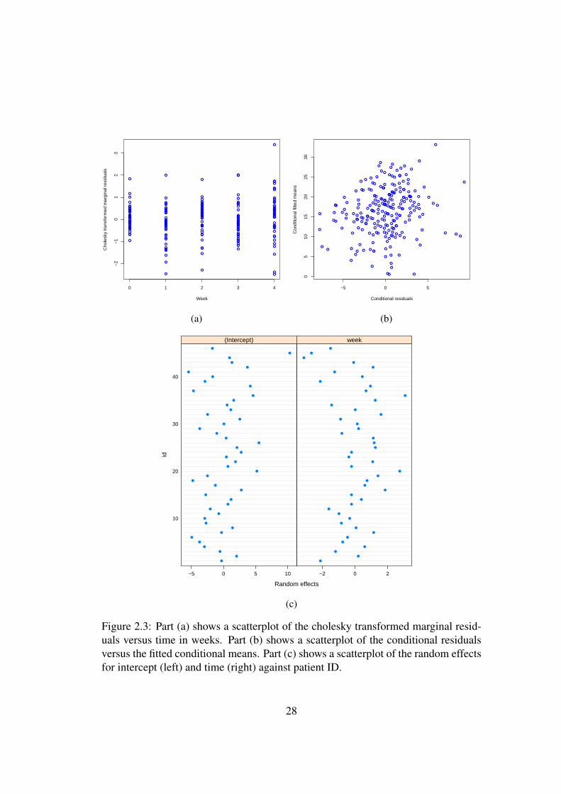
It is difficult to detect any pattern in the scatterplot of marginal residuals versus themarginal mean. But, there appears to be slight variation between weeks (see Fig-ure 2.3a) in whether the residuals are centered slightly above or below zero, perhapssuggesting linear time is too simplistic. With less variability at the more extreme val-ues of the fitted conditional means, Figure 2.3b suggests that homoskedastic within-individual errors could be improved upon.

Figure 2.3c shows a scatterplot of the random effects for both intercept and timeplotted against patient ID number. Individual 45 has an outlying HAMD score atbaseline; individuals 20, 36, 44 and 45 have potentially outlying slopes.

27

0 1 2 3 4

−2

−1

01

23

Week

Cho

lesk

y tr

ansf

orm

ed m

argi

nal r

esid

uals

(a)

−5 0 5

05

1015

2025

30Conditional residuals

Con

ditio

nal f

itted

mea

ns

(b)

Random effects

id

10

20

30

40

−5 0 5 10

(Intercept)

−2 0 2

week

(c)

Figure 2.3: Part (a) shows a scatterplot of the cholesky transformed marginal resid-uals versus time in weeks. Part (b) shows a scatterplot of the conditional residualsversus the fitted conditional means. Part (c) shows a scatterplot of the random effectsfor intercept (left) and time (right) against patient ID.

28

2.8 Concluding remarks

2.8.1 A short comparison of the general LME model and the LMModelling the variability via introducing random effects in the linear model accountsfor the correlations between repeated measurements with relatively few paramet-ers, regardless of the number of measurement occasions. This is in contrast to thevariance-covariance pattern models of Section 2.3.1, whose simplicity (in terms ofnumber of parameters) may depend upon the number of units within each cluster.

Furthermore, when the data is inherently hierarchical (longitudinal data are, in-deed, always hierarchical), a hierarchical approach is natural. Introducing randomeffects takes into account the fact that the variability in the data can be separated intodifferent levels of the hierarchy, meaning that variability due to within-individualfluctuations in the response, and due to between-individual differences can be separ-ated. This facilitates inference at both the level of the individual, and at the level ofthe population.

This being said, the inclusion of random effects imposes additional assumptions[see (2.4)] that the linear model (2.1) avoids. Even prior to analysis and model selec-tion, the choice of inclusion or exclusion of random effects can be made based on twofactors. Firstly, the subject-matter or scientific knowledge may determine suitabilityof assumptions. How to determine whether an effect should be fixed or random isdiscussed in Stroup (2012, p.38) and depends largely upon whether the effect can bethought of as arising from a probability distribution. Secondly, the target of inferenceshould also be considered: including random effects may be unnecessary if the goalof the study is inference at the level of the population. More details on this are givenin McNeish et al. (2017).

2.8.2 Summary of chapterThis chapter began by describing linear regression without random effects for lon-gitudinal data. It was shown how the mean trend can be modelled as a function oftime, and how within-cluster dependency can be taken care of by a covariance pat-tern model. Random effects were then introduced as an alternative means to accountfor this dependency, and the general linear mixed effect model was presented. Ran-dom effect, random intercept, and random intercept and slope models were described.Subsequently, model diagnostics and estimation via ML and REML for LME modelsand the LM were explained. Finally, a clinical trial data set was used to demonstratean application of LME models.

I hope to have distinguished differences between the LM and the LME modelfrom a number of standpoints. And also, since Chapter 4 discusses model selectionfor multivariate models where the focus is on parameters, not random effects, shownhow, marginally, the LME model is a special case of the LM.

29

Chapter 3

Generalised Linear Mixed Models

When the response variable is no longer continuous, is asymmetric or has heavy tails,a more general class of models is required than the linear models of Chapter 2. Forexample, when the response is a binary (e.g. success/failure) or count variable (e.g.the number of accidents), the linear models of Chapter 2 are of limited use.

The joint density of non-Normal multivariate data is not straightforward to spe-cify. This is because specifying the joint distribution of a non-normal multivariateresponse without introducing random effects requires specifying more than just thepair-wise associations (the correlations in the linear model); higher order associ-ations must also be specified, which typically entails a large number of parameters(Fitzmaurice et al. 2004a).

Thus, for non-Normal multivariate data, two methods are commonly used: mar-ginal models (or population-averaged models) and generalised linear mixed models(GLMMs) (or subject-specific models). Marginal models avoid specification of thejoint density of the data altogether (Liang & Zeger 1986), whereas GLMMs specifythe joint density of a cluster via a conditional model making use of random effects.

GLMMs will be the focus of this chapter. They can be thought of as a gener-alisation of generalised linear models (GLMs) to clustered, or correlated data, andcan also be considered a generalisation of the LME model to non-Normal or discretedata.

3.1 Formulating a GLMMA GLMM requires four components:

• the conditional distribution of the response for the ith cluster and jth unit giventhe random effects, yij|bi,

• a linear predictor, xᵀijβ + zᵀijbi,

• a link function, g(·),

31

• the distribution of the random effects, bi.

The exponential family of distributions includes a large number of commonlyused distributions e.g. Poisson, binomial, gamma and so on. The conditional distri-bution of the response in a GLMM given the random effects must be a member of theexponential family. This means that, given the random effects, the conditional distri-bution of the response (of cluster i and unit j) can be written in the form (McCulloch& Searle 2001, p.221)

fyij |bi(yij|ηij, φ) = exp(yijηij − a(ηij)

φ− c(yij, φ)

)(3.1)

with independence assumed for all i = 1, ..., N , and conditional independence giventhe random effects for all j = 1, ..., ni. We have that φ is a scale parameter; a(·) isa function that determines the specific distribution, for example, a(x) = ex for thePoisson distribution, and a(x) = log(1 + ex) for the Bernoulli distribution (Wand2007); c(yij, φ) is a constant that makes the expression integrate to one; and theparameter ηij is known as the canonical parameter.

The link function g(·) relates the expected value of the (i, j)th response condi-tional on the random effects to the linear predictor xᵀ

ijβ + zᵀijbi, where xᵀij and zᵀij

are the jth rows of the ith fixed effect and random effect design matrices respectively.That is, we have

g(E[yij|bi]) = xᵀijβ + zᵀijbi.

Note that, the linear predictor, xᵀijβ + zᵀijbi, is linear not necessarily in terms of the

covariates, but in terms of the regression coefficients and random effects.To complete the specification, we (typically) have that the bi are mean zero,

normally distributed, and with variance-covariance matrixD.At this point, it is worth noting why GLMMs get their name. The models are

linear in the regression coefficients, mixed because the linear predictor includes fixedand random effects, and generalised because of the presence of a link function whichneed not be the identity.

The canonical link, which is unique to each distribution, is such that g(E[yij|bi]) =ηij (De Jong et al. 2008, p.66). For example, as we will see in Section 3.2, thecanonical link of the Poisson distribution is log(x), and the canonical link of theBernoulli distribution is the logit link log( x

1−x). Furthermore, for the canonical link,the canonical parameter becomes equal to the linear predictor. That is, we haveηij = xᵀ

ijβ + zᵀijbi.

3.1.1 Conditional moments of a GLMMThe conditional moments of model (3.1) can be found as illustrated in De Jong et al.(2008, p.37). In particular, we have

E[yij|bi] = a′(ηij),

32

where a′ is the derivative of a with respect to ηij . Furthermore, we have

Var(yij|bi) = φV (E[yij|bi]),

where V (·) = a′′(·) is known as the variance function and relates the conditionalvariance to the conditional mean.

3.1.2 The marginal distribution derived from the GLMMThe marginal distribution of the ith cluster is

fyi(yi) =

∫fyi,bi(yi, bi)dbi

=

∫fyi|bi(yi|bi)fbi(bi)dbi

=

∫ ni∏j=1

fyij |bi(yij|bi)fbi(bi)dbi, (3.2)

where the third equality follows from independence of the (i, j)th response given therandom effects. Thus, by specifying the conditional distribution of the response andthe distribution of random effects, an expression for the marginal density is obtain-able. Using the rule of double expectations, we have that marginally (McCulloch &Searle 2001, p.222)

E[yij] = E[E[yij|bi]] = E[g−1(xᵀijβ +Zᵀ

ijbi)].

Thus, only for the identity link do we have E[yij] = xᵀijβ. This means that, for non-

identity link functions, xᵀijβ does not have the interpretation as the marginal mean

trend; the LME model (2.3) is indeed a special case. The regression coefficients ofa model which does not have the identity link, can be interpreted in terms of thecorresponding transform, g(·), of the expected response, or must be transformed viathe inverse of the link function, g−1(·) , to be interpretable on the same scale as theexpected response.

In addition, the regression coefficients of a GLMM have an interpretation at thelevel of the cluster. This is because the regression coefficients must be interpretedwhile holding bi fixed. For interpreting effects of continuous covariates, one shouldconsider the conditional mean response of a given cluster with a specific bi. Whereas,for interpreting binary or categorical covariates, one should contrast two differentclusters (perhaps of different covariate values) but that have the same random effect(Fitzmaurice et al. 2004a, p.361). This interpretation at the level of the cluster is acharacteristic of GLMMs, and, as such, the target of inference of GLMMs is the levelof the cluster. LME models are an exception in that both an interpretation at the levelof the cluster and at the marginal level are available; for GLMMs without an identitylink, this is not possible.

33

Lastly, it is worth mentioning that marginal models (or population averagedmodels), which posit no distributional assumptions and which specify only the mar-ginal moments, are an alternative means for modelling non-Normal clustered or lon-gitudinal data (Liang & Zeger 1986). The target of inference of such models is thelevel of the population (e.g. Fitzmaurice et al. 2004a, p.291).

3.2 Examples

3.2.1 A Bernoulli GLMMSuppose that the response of interest is binary, taking values 0 and 1. Then, aBernoulli GLMM with logit link can be formulated as

fyij |bi(yij|bi) =pyijij (1− pij)(1−yij), (3.3)

log( pij

1− pij

)=xᵀ

ijβ + zᵀijbi,

bi ∼ N(0,D),

where pij = P (yij = 1|bi) is the probability of unit j of cluster i taking value oneconditional on bi, and 1−pij is the probability of unit j of cluster i taking value zero.Such a model assumes a natural between-cluster diversity in the tendency to respondpositively. The logit link function is the logarithm of the odds that yij|bi takes value1, where the odds are given by

pij1− pij

. Thus, it is the odds that are log-linear in the

regression coefficients.To see how (3.3) is of the form (3.1) note that

pyijij (1− pij)(1−yij) = exp(yij log(pij) + (1− yij) log(1− pij))

= exp(yij log

( pij1− pij

)+ log(1− pij)

), (3.4)

from which it follows that the canonical parameter takes the form

ηij = log( pij

1− pij

),

and, thus, the logit link is the canonical link for the Bernoulli distribution. In addition,inverting this relationship gives

pij =eηij

1 + eηij. (3.5)

Substitution of (3.5) into the second term in the exponent of (3.4) and forming acommon denominator yields (3.1).

34

For the Bernoulli distribution then, we have that the scale parameter φ = 1and the constant c(yij, φ) is zero. Furthermore, it is well known that E[yij|bi] = pijand Var(yij|bi) = pij(1 − pij). So, the conditional variance of a Bernoulli randomvariable depends only on the conditional expectation. This is not necessarily the casefor other distributions, whose variance may also depend upon the scale parameter(Stroup 2012, p.125).

Note that, in practice, for binary data and relatively few units within clusters,there is rarely enough variability in the data to estimate more random effect paramet-ers than that of the variance of a random intercept (Fitzmaurice et al. 2004a, p.344).

3.2.2 A Poisson GLMMWhen the response is a count variable (that is, taking values 0,1,...), the Poissondistribution may be appropriate. This is in contrast to binary data whose distributionis necessarily Bernoulli (Fitzmaurice et al. 2004a).

A Poisson GLMM with its canonical log-link can be expressed as

fyij |bi(yij|bi) =λyijij

yij!e−λij ,

log λij = xᵀijβ + zᵀijbi,

bi ∼ N(0,D),

where λij = E[yij|bi] is the expected count of unit j in cluster i. Re-writing theconditional distribution as

exp(yij log λij − λij − log(yij!)),

it becomes visible that the log-link is indeed canonical since ηij takes the form log λij .We also have that φ = 1, c(yij, φ) = log(yij!) and a(ηij) = eηij .

For longitudinal data, the measurement occasions may not be equally separated.To account for this, an offset, Tij , the length of the measurement interval from timej − 1 to time j, may be introduced into the linear predictor to give

log λij = log Tij + xᵀijβ + zᵀijbi.

Re-arranging this gives

log(λijTij

)= xᵀ

ijβ + zᵀijbi,

from whichλijTij

gets the interpretation as the expected rate of counts at time j, a more

easily interpretable measure across unevenly spread measurement occasions.The Poisson model imposes the rather restrictive assumption that E[yij|bi] =

Var(yij|bi) = λij . Overdispersion is what occurs if Var(yij|bi) > E[yij|bi], andtends to be the case more often than not (Fitzmaurice et al. 2004a, p.297). So overd-ispersion has to, in general, be accounted for if the Poisson model is to be of any usein application.

35

3.3 Estimation

3.3.1 Maximum likelihoodMaximum likelihood is a commonly used method for estimation of parameters in aGLMM. Taking the logarithm of (3.2) gives

log(fyi(yi)) = log

(∫ ni∏j=1

fyij |bi(yij|bi)fbi(bi)dbi

),

which, summed over all clusters and inserting expressions for the densities fyij |bi(yij|bi)and fbi(bi), gives the marginal log-likelihood of model (3.1) as

`N(β,θ|y) =

N∑i=1

log

(∫1

√2π|D| 12

exp(− 1

2bᵀiD

−1bi +

ni∑j=1

[yijηij − a(ηij)

φ− c(yij, φ)

])dbi

),

(3.6)

where y is a stack of all clusters, and where θ is a vector including scale parameterφ, and the variance-covariance parameters of the random effects.

The integrals in (3.6) are analytically intractable. For the situations we are in-terested in (clustered/longitudinal data), it is suitable to maximise (3.6) numerically,which involves numerical integration (McCulloch & Searle 2001, p.226). For relat-ively low dimensions of random effects, Gauss-Hermite quadrature may be used (asin McCulloch & Searle 2001, p.270) to perform such integration.

In particular, for a univariate random effect, bi ∼ N(0, σ2b ), (3.6) is expressible

asN∑i=1

log

(∫h(bi)

1√2πσb

e−1

2σ2b

b2idbi

),

where

h(bi) = exp

(ni∑j=1

[yijηij − a(ηij)

φ− c(yij, φ)

]),

and the dependency of h on bi is through the canonical parameter ηij . After a trans-formation of variable, such a sum of integrals becomes of the form

N∑i=1

log

(∫h(√

2σbbi)e−b

2i

√π

), (3.7)

and can be approximated via Gauss-Hermite quadrature (e.g. McCulloch & Searle2001) as

N∑i=1

log

(K∑k=1

h(√

2σbxk)wk√π

),

36

where K is the number of evaluation points, xk, and wk their corresponding weights.These can be obtained via, for example, using the statmod package (Smyth 2005) inR.

3.4 Data illustrationA randomised, double blind, clinical trial dataset comparing two oral treatments fortoe nail infection is now considered. The dataset was obtained from the accompany-ing website (Fitzmaurice et al. 2004b) of the textbook Applied Longitudinal Analysis(Fitzmaurice et al. 2004a, p.355). The response of interest is the degree of onycho-lysis (extent of separation of the nail from the nail bed), which is measured as a binaryvariable (0 = none or mild, 1 = moderate or severe). 294 patients were measured ona maximum of 7 occasions during a period of 18.5 months. There is some spread inthe exact timing of measurements, but measurements were obtained at baseline, andat (more or less) 1, 2, 3, 6, 9 and 12 months after baseline. Patients were randomisedto two anti-fungal oral treatments (B=) Itraconazole and (A=) Terbinafine at baseline(Fitzmaurice et al. 2004b). Table 3.1 shows the number of severe or moderate casesfor treatments A and B for all 7 visits.

Table 3.1: The number of severe or moderate cases by treatment group for each ofthe seven visits.

1 2 3 4 5 6 7A 55 48 40 29 8 8 6B 54 49 44 29 14 10 14

A large number of patients dropped out throughout the course of the study res-ulting in an incomplete data set. Nevertheless, an all-available data analysis will beconducted. For such an analysis to be valid, the reasons for missing data should beunconnected to either the observed or unobserved values, meaning that the observedvalues of the remainers (those that do not drop out) must be a random sample of thecorresponding values in the population, which is likely an unrealistic assumption.

3.4.1 A plausible modelThe glmmML command from the R package glmmML (Broström 2017) was used tofit model (3.3) with logit link and the following linear predictor:

log( pij

1− pij

)= β0 + β1tij + β2tijgroupi + bi, (3.8)

where pij is the probability of moderate or severe onycholysis at occasion j for indi-vidual i; tij is the exact time in months; and groupi is the binary treatment group vari-able (reference group = Treatment B, non-reference group = Treatment A). Since the

37

treatment groups were generated by randomisation (not by pre-existing distinguish-ing factors as in the depression data set (2.7)), it makes sense to assume that bothgroups have the same intercept at baseline. Furthermore, allowing separate slopes forboth treatment groups facilitates comparison of both treatments. For obtaining MLestimates of the parameters, Gauss-Hermite quadrature with 30 quadrature pointswas used to approximate the integrals involved in maximising the log-likelihood.

3.4.2 Results

The parameter estimates obtained via ML are given in Table 3.2. Significance ofestimates was judged using the asymptotic properties of ML estimators (with theinverse of the observed information matrix as the estimated covariance matrix of themodel parameters). The negative (and significant) value for β1 means that TreatmentB is effective in reducing the probability/odds of a severe response at the level of theindividual. However, since the interaction term in the linear model is also negative(β2 = −0.14) and significant at the 0.05 level (p-value = 0.028), Treatment A can beconcluded as more efficient than Treatment B at the level of the individual.

Table 3.2: Parameter estimates from model (3.8).

Binary outcome

Fixed Effects:Intercept -1.70∗∗∗

tij -0.39∗∗∗

tijgroupi -0.14∗

Random effects:σb 4.01∗p < .05; ∗∗p < .01; ∗∗∗p < .001

On the scale of the linear predictor, the parameter estimates are not so easilyinterpretable. Instead, suppose that we are interested in understanding the change inodds of onycholysis with time for both treatments at the level of the individual. Sincethe variable month is modelled as linear, the effect on the odds of severe response bya unit increase in time is the same regardless of when the unit increase takes place.For any month x up to one month before the end of study (unless a forecast beyondthe study period is to be made), we have that for individual i of treatment group B

38

with random intercept bi,

Estimated odds of severe onycholysis for individual i|bi, group = B, t = x+ 1

Estimated odds of severe onycholysis for individual i|bi, group = B, t = x

=eβ0+β1(x+1)+bi

eβ0+β1x+bi

=eβ1 ≈ 0.68.

That is, the odds of moderate or severe onycholysis for any individual in group Bis estimated to be roughly 32% smaller after one additional month of treatment. Inthis way, by defining odds ratios and arriving at a multiplicative effect, the parameterestimates are more readily interpretable.

Similarly, for an individual in group A we have that,

Estimated odds of severe onycholysis for individual i|bi, group = A, t = x+ 1

Estimated odds of severe onycholysis for individual i|bi, group = A, t = x

=eβ0+β1(x+1)+β2(x+1)+bi

eβ0+β1x+β2x+bi

=eβ1+β2 ≈ 0.59.

This means that the odds of moderate or severe onycholysis for any individual ingroup A is estimated to be roughly 41% smaller after one additional month of treat-ment. So, the odds of moderate or severe onycholysis is reduced more by each ad-ditional month of Treatment A compared with Treatment B at the level of the indi-vidual.

Given the fixed effect parameter estimates and estimates of the realised valuesof the random effects, which together form estimates of the individual specific lin-ear predictors, estimates of the individual specific probabilities can be obtained by

application of the inverse logit transform,ex

1 + ex. The estimated individual specific

probabilities are plotted against time for treatment group A in Figure 3.1 and treat-ment group B in Figure 3.2.

From these plots it is visible that, by the end of the study, there is a selectionof patients in group B that have slightly higher probabilities of a moderate or severeoutcome in comparison with those in group A. It is also of note that a typical patient(i.e. with random effect set to its mean of zero) has a baseline probability of 0.15 (forboth groups). Thus, there are many probability trajectories hidden in the lower leftcorners of Figure 3.1 and Figure 3.2.

Finally, it may be of interest to know, as a measure of treatment efficacy forboth groups, what fraction of individuals have probability greater than one half ofmoderate or severe onycholysis after 3 months of treatment. It turns out that 20%of individuals in group A had a probability of severe onycholysis greater than onehalf after 3 months of treatment, whereas 24% of individuals in group B had such aprobability.

39

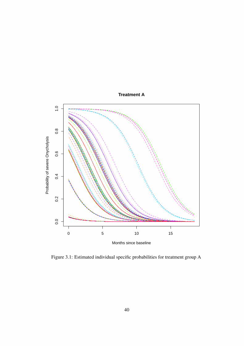
0 5 10 15

0.0

0.2

0.4

0.6

0.8

1.0

Treatment A

Months since baseline

Pro

babi

lity

of s

ever

e O

nych

olys

is

Figure 3.1: Estimated individual specific probabilities for treatment group A

40

0 5 10 15

0.0

0.2

0.4

0.6

0.8

1.0

Treatment B

Months since baseline

Pro

babi

lity

of s

ever

e O

nych

olys

is

Figure 3.2: Estimated individual specific probabilities for treatment group B

41

3.5 Chapter summaryThis chapter has presented essential theory of generalised linear mixed models. Inparticular, the exponential class of distributions was introduced, and the componentsof a general GLMM explained. The Bernoulli and Poisson models were given asexamples of the general GLMM. Estimation via ML was then discussed along withGauss-Hermite quadrature as a means for approximating the integrals of the likeli-hood. An application to a binary clinical trial dataset involving comparison of twotreatments for toe-nail infection was then presented. Attention was given to inter-pretation of regression coefficients which, due to the presence of a non-identity linkfunction, is not as straightforward as the Normal model.

42

Chapter 4

The Focussed Information Criterionfor Clustered Data

In any field in which clustered or longitudinal data are collected (as with any field ofresearch), there are specific questions to be answered. For the models of Chapter 2and Chapter 3, these questions are typically formulated in terms of the regressioncoefficients. In general, model selection has traditionally been based around finding amodel which fits the data well with as few parameters as possible, and without regardto the particular questions at hand. As discussed in Section 2.5.3, the Akaike inform-ation criterion (AIC), for example, facilitates such model selection. In this chapter,the focussed information criterion (FIC), a model selection criterion for targeting spe-cific questions, as introduced by Claeskens & Hjort (2003), Claeskens et al. (2008),is presented. In addition, a multivariate framework is developed, within which theFIC becomes available as a covariate selector for multivariate LMs, LME modelsand GLMMs. This is followed by some theoretical results, a simulation study, andlongitudinal data illustrations.

4.1 FIC for independent data

The focussed information criterion (FIC) is a model selection criterion that ranksmodels in terms of their appropriateness for a given purpose, or goal. The goal isto precisely estimate a parameter of primary interest, henceforth called the focusparameter. The focus parameter could be, for example, an interaction effect, anexpected response, a rate ratio and so on.

The ability of a model to precisely estimate the focus is determined by the FICscores which, for each model, are unbiased estimators of the mean squared error(MSE) of the limiting distribution of the focus. These estimators are derived usingthe large sample asymptotic theory of maximum likelihood (ML) estimators. In thissection, the FIC scores for the regression setting with independent data are given.For which, the setting is laid out and the main steps regarding asymptotic results are

43

presented. Initially, a multiple linear regression example will be used to familiarisethe reader with the score vectors and information matrices. A natural extension ofthe FIC to multivariate models will then be presented in Section 4.2. Until then,keep in mind for this section that we are working with a sample of n independentobservations (no clustering).

4.1.1 Framework and goalUnder contention are a list of models ranging from the narrow model (of fewestparameters) to the widest model (of most parameters), all of which are nested withinthe wide model. The parameters ν, of dimension p, are included in every model.However, only the wide model includes the parameter vector γ, of dimension q, inits entirety. The models in-between the wide and narrow models contain only someof the components of γ. For this reason, ν is said to be protected, whereas γ is saidto be unprotected.

The candidate models are within a locally misspecified framework. That is, datayi, which are assumed to be independent given covariates xi, are generated by thewide model

fwide,n = f(yi|xi,ν0,γ0 + δ/√n), (4.1)

which is assumed to be true. Furthermore, ν0 is the true value of ν, whereas γ0 issaid to be the null value of γ, and γ0 + δ/

√n is the true value of γ.

That is, we have a sequence of true wide models for each sample size n, and,as n grows, the true value of γ approaches γ0. So, fwide,n, the true data generatingmechanism, is assumed to be a distance δ/

√n away from the narrow model in terms

of the unprotected γ parameters. When δ =√n(γ − γ0) = 0, we have that γ = γ0,

and we are back at the narrow model. In other words, fwide(ν,γ0) = fnarr(ν). Amodel in-between the wide and narrow, model S say, where S is a subset of 1, ..., q,contains the γj with j ∈ S, and sets γj = γ0,j for those j /∈ S.

Thus, the locally misspecified framework allows us to consider a range of mod-els that are small perturbations away from a narrow model. Such a framework fa-cilitates questions such as ‘How far from the narrow model is too far (in terms ofuncertainty introduced by more parameters)?’, and ‘How close to the narrow modelis too close (in terms of simplicity: too few parameters)?’. It may be that a truevalue that changes with sample size is conceptually bothering, but this is not how theframework is to be interpreted: the principal advantage of this framework (as we willsee) is that it leads to attractive asymptotic results (Claeskens et al. 2008, p.128).

The focus parameter is defined as µ = µ(ν,γ), a function of the model para-meters. For example, the focus could be prediction of the mean response given a setof covariates, or a particular quantile of the true data generating mechanism. The aimof FIC is to estimate the MSE of the limiting distribution of the focus parameter foreach of the models. The model with smallest estimated MSE of the limiting distri-bution of the focus provides the most precise estimate of the focus parameter and is

44

therefore deemed the best by FIC. It is well-known that the MSE is expressible as thesum of a term for bias squared and a term for variance (e.g. Casella & Berger 2002,p.330). This means that for any estimator µ of the true focus parameter value µ0, onemay write its MSE in estimation as

MSE(µ) = E[(µ− µ0)2]

= (E[µ− µ0])2 + E[µ2]− E[µ]2

= bias2(µ) + Var(µ).

The FIC procedure involves estimating the mean squared error of the limiting distri-bution of the focus by finding separate estimators for the bias squared and varianceof the limiting distribution and summing both.

Example

As a simple example, consider a linear regression model with constant variance σ2,intercept β0, and covariate x1 with effect β1. Alternative models consist of includingor excluding two more covariates x2 and x3. The goal is to find the best model forestimating the expected response when the covariates take on values (x1, x2, x3) =(a, b, c), say. That is, the focus of interest is µ = µ(β,γ) = E[yi|x1 = a, x2 =b, x3 = c], and the wide model under consideration is

N(β0 + β1x1,i + γ0x2,i + γ1x3,i, σ2).

The protected parameters are

ν =

σ2

β0

β1

,

and the unprotected parameters are

γ =

(γ0

γ1

),

which have null value γ0 = (0, 0)ᵀ.The narrow model is therefore,

N(β0 + β1x1,i, σ2),

and the two models in-between the wide and narrow are

N(β0 + β1x1,i + γ0x2,i, σ2),

N(β0 + β1x1,i + γ1x3,i, σ2),

which correspond to setting γ = (γ0, 0)ᵀ and γ = (0, γ1)ᵀ respectively.

45

Introducing two extra parameters may reduce the bias in estimation of the meanresponse, but doing so will also increase the number of parameters to be estimated,resulting in more uncertainty in the estimation of parameters. So here, the FIC willhelp the statistician find the best balance between a biased estimator with less un-certainty (variance) and a less biased, but more uncertain estimator of the meanresponse. This bias versus variance trade-off is called the Goldilocks principle in(Cressie & Wikle 2011, p.7).1

4.1.2 Score vectors and the expected information matrixTo be able to show the main steps in the derivation of the FIC, necessary quantitiesas in Claeskens & Hjort (2003) will first be introduced.

Provided sufficient smoothness in the model parameters about the null point(ν0,γ0), each observation has an associated score vector(

u(yi|xi)v(yi|xi)

)=

(∂ log f(yi|xi,ν0,γ0)/∂ν∂ log f(yi|xi,ν0,γ0)/∂γ

), (4.2)

where xi is the associated vector of covariates for observation i. For each observa-tion, there is an associated expected information matrix, which evaluated at the nullpoint is

J i = −E

[(∂2 log f(yi|xi,ν0,γ0)

∂ν∂νᵀ∂2 log f(yi|xi,ν0,γ0)

∂ν∂γᵀ

∂2 log f(yi|xi,ν0,γ0)∂γ∂νᵀ

∂2 log f(yi|xi,ν0,γ0)∂γ∂γᵀ

)],

and, under the wide model, is equal to the variance-covariance matrix of the scorevector

J i = Var0

(∂ log f(yi|xi,ν0,γ0)/∂ν∂ log f(yi|xi,ν0,γ0)/∂γ

).

Averaged over all observations, this becomes

J full,n =1

n

n∑i=1

J i =

(J00,n J01,n

J10,n J11,n

),

where, averaged over all observations and evaluated at the null value, J00,n is ofdimension p × p and is the variance of the components of the score correspondingto the protected parameters ν; J11,n is of dimension q × q and is the variance of thescore of the unprotected parameters γ; J01,n, of dimension p × q, is the covariancebetween the ν and γ components of the score. Finally, being a symmetric matrix,J10,n is the transpose of J01,n.

Under certain conditions, as n tends to infinity, J full,n tends to the (p+q)×(p+q)limiting information matrix of the wide model (4.1)

Jwide =

(J00 J01

J10 J11

),

1In the children’s story, Goldilocks is a little girl who wants things just right.

46

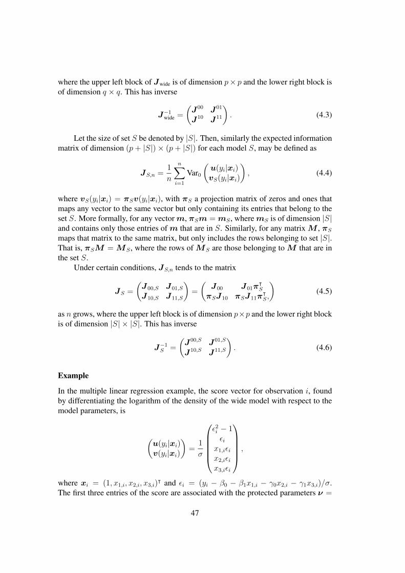
where the upper left block of Jwide is of dimension p× p and the lower right block isof dimension q × q. This has inverse

J−1wide =

(J00 J01

J10 J11

). (4.3)

Let the size of set S be denoted by |S|. Then, similarly the expected informationmatrix of dimension (p+ |S|)× (p+ |S|) for each model S, may be defined as

JS,n =1

n

n∑i=1

Var0

(u(yi|xi)vS(yi|xi)

), (4.4)

where vS(yi|xi) = πSv(yi|xi), with πS a projection matrix of zeros and ones thatmaps any vector to the same vector but only containing its entries that belong to theset S. More formally, for any vectorm, πSm = mS , wheremS is of dimension |S|and contains only those entries of m that are in S. Similarly, for any matrix M , πSmaps that matrix to the same matrix, but only includes the rows belonging to set |S|.That is, πSM = MS , where the rows of MS are those belonging to M that are inthe set S.

Under certain conditions, JS,n tends to the matrix

JS =

(J00,S J01,S

J10,S J11,S

)=

(J00 J01π

ᵀS

πSJ10 πSJ11πᵀS,

)(4.5)

as n grows, where the upper left block is of dimension p×p and the lower right blockis of dimension |S| × |S|. This has inverse

J−1S =

(J00,S J01,S

J10,S J11,S

). (4.6)

Example

In the multiple linear regression example, the score vector for observation i, foundby differentiating the logarithm of the density of the wide model with respect to themodel parameters, is

(u(yi|xi)v(yi|xi)

)=

1

σ

ε2i − 1εi

x1,iεix2,iεix3,iεi

,

where xi = (1, x1,i, x2,i, x3,i)ᵀ and εi = (yi − β0 − β1x1,i − γ0x2,i − γ1x3,i)/σ.

The first three entries of the score are associated with the protected parameters ν =

47

(σ, β0, β1)ᵀ, and the last two entries of the score are associated with the unprotectedparameters γ = (γ0, γ1)ᵀ.

Differentiating again, taking minus the expected value and averaging over allobservations gives

J full,n =1

nσ2

n∑i=1

2 0 0 0 00 1 x1,i x2,i x3,i

0 x1,i x21,i x1,ix2,i x1,ix3,i

0 x2,i x1,ix2,i x22,i x2,ix3,i

0 x3,i x1,ix2,i x2,ix3,i x23,i

=

(2σ2 00 1

nσ2

∑ni=1 xix

ᵀi

).

(4.7)Note that in order for J full,n to tend to Jwide a necessary condition is that 1

nσ2

∑ni=1 xix

ᵀi

converges as n grows.In our example, S can range from (the narrow) S = ∅ to (the wide) S = 1, 2.

When only γ0 is included as an extra parameter, S = 1 and the required projectionmatrix is thus πs = (1, 0). The expected information matrix corresponding to thismodel (including γ0 not γ1) is

JS,n =1

nσ2

n∑i=1

2 0 0 00 1 x1,i x2,i

0 x1,i x21,i x1,ix2,i

0 x2,i x1,ix2,i x22,i

,

where for example the lower right hand block (here only one entry), J11,S [see (4.5)],which corresponds to the parameter γ0 alone, is calculated as

J11,S =πSJ11πᵀS

=1

nσ2

n∑i=1

(1 0

)( x22,i x2,ix3,i

x2,ix3,i x23,i

)(10

)=

1

nσ2

n∑i=1

x22,i.

4.1.3 Limiting distributionsThe score vectors and information matrices have now been introduced. The mainsteps required to derive the limiting distribution of the focus parameter will now beshown. For full details and in particular regularity conditions, the reader is referredto Section 3.1 and the appendix of Hjort & Claeskens (2003).

The averages of the score vectors defined for each observation in (4.2) areun = 1

n

∑ni=1 u(yi|xi) and vn = 1

n

∑ni=1 v(yi|xi). Under the locally misspecified

sequence of models (4.1), and due to independence of observations, it can be shownthat the averaged score vector for model S has the following limiting distribution asn grows: ( √

nun√nvS,n

)d→ Np+|S|

((J01δπSJ11δ

),JS

). (4.8)

48

The limiting distribution is not centered at zero because the score vectors are evalu-ated at the narrow model and thus away from the true wide model.

The maximum likelihood estimators of model S, (νS, γS), can be written interms of the averaged score vector via a Taylor expansion, and thereby their limitingdistribution is determined to be( √

n(νS − ν0)√n(γS − γ0,S)

)d→ Np+|S|

(J−1S

(J01δπSJ11δ

),J−1

S

). (4.9)

In particular, the limiting distribution of the wide model’s unprotected paramet-ers is

Dn = δwide =√n(γwide − γ0)

d→D ∼ N(δ,Q),

whereQ is the lower right hand corner of J−1wide, see (4.3). That isQ = J11, and can

be written (using a result on the inverse of block matrices, see e.g. Harville (1997,p.100)) as

Q = (J11 − J10J−100 J01)−1. (4.10)

For the following, define for submodel S the bottom-right corner of J−1S , i.e.

the asymptotic variance covariance of γS , as

QS = J11,S = (J11,S − J10,SJ−100,SJ01,S)−1 = (πSQ

−1πᵀS)−1,

of dimension |S| × |S|, and

GS = πᵀSQSπSQ

−1

of dimension q × q.Then, the limiting distribution of the focus parameter can be found by applying

the delta method to the limiting distribution of the maximum likelihood estimators,(4.9). Specifically, the limiting distribution of the focus as estimated by model S canbe written as

√n(µS − µ0)

d→ N(ωᵀ(I −GS)δ, τ 20 + ωᵀGSQG

ᵀSω), (4.11)

where µ0 is the true value of the focus,

ω = J10J−100

∂µ

∂ν− ∂µ

∂γ(4.12)

is a column vector of dimension q;

τ 20 =

(∂µ

∂ν

)ᵀ

J−100

∂µ

∂ν(4.13)

is a scalar; and where partial derivatives in both ω and τ 20 are evaluated at the null

point (ν0,γ0).

49

The quantity τ 20 can be thought of as the minimal variance of the limiting dis-

tribution of the focus that persists in all models under consideration. In fact, it is thevariance of the limiting distribution of the focus as estimated by the narrow model.Note that τ 2

0 does not depend on γ and so is common to all models. In contrast, ωdepends on γ and so is different for each model.

The narrow and wide models are special cases of (4.11) with

√n(µnarr − µ0)

d→ N(ωᵀδ, τ 20 ),

√n(µwide − µ0)

d→ N(0, τ 20 + ωᵀQω).

Since the wide model is assumed true, the limiting distribution of its estimatorof the focus is centered at zero, i.e. the bias disappears. The penalty the wide modelpays for this is increased uncertainty due to more parameters having to be estimated.This is captured by the addition of ωᵀQω to the narrow variance. The bias andvariance of those models in-between the wide and narrow will vary according towhich unprotected parameters they involve.

Since the quantities introduced here (GS,Q,ω, τ2,QS) all involve inverses of

sums of matrices, it is no longer worth continuing with the linear model example.Exact expressions are difficult to obtain, and not required.

4.1.4 FIC scoresThe FIC scores are calculated by estimating the MSE of the limiting distribution ofthe focus for each model. The MSE of the limiting distribution of the focus, (4.11),as estimated by model S is

MSES = ωᵀ(I −GS)δδᵀ(I −GS)ᵀω + τ 20 + ωᵀGSQG

ᵀSω,

with I the q × q identity matrix, and where the first term is for the bias squared, andthe second and third combined are the variance.

The FIC score for model S is constructed by estimating each term of MSES .This is straightforward for the variance as each element is simply replaced by itsconsistent estimator. However, the bias squared term requires a little more thought.In particular, δδᵀ can be estimated by DnD

ᵀn, but this estimator overshoots by the

amount Q. To see this, note that, for any multivariate random variable X , wehave E[XXᵀ] = E[X]E[X]ᵀ + Cov(X). Since the expected value and variance-covariance of the limiting distribution ofDn are δ andQ respectively [see (4.1.3)],

E[DnDᵀn] = E[Dn]E[Dn]ᵀ + Cov(Dn) ≈ δδᵀ +Q.

So, a more appropriate, asymptotically unbiased, estimator of bias squared isDnDᵀn−

Q. Furthermore, since this estimator may end up being negative, not desirable for asquared term, it is truncated at zero.

50

The FIC score for model S, an asymptotically unbiased estimator of MSESadjusted to avoid being a negative bias squared term, is then

FICS = max(

0, ωᵀ(I − GS)(DnDᵀn − Q)(I − GS)ᵀω

)+ τ 2

0 + ωᵀGSQGᵀ

Sω.

(4.14)Special cases of the above for the narrow and wide model are

FICnarr = max(

0, ωᵀ(DnDᵀn − Q)ω

)+ τ 2

0 ,

FICwide = τ 20 + ωᵀQω.

The interpretation being that the narrow model has largest bias squared term, butsmallest variance in its estimation of the focus. Whereas, the widest model has nobias (since assumed as the true model) but largest variance. The rest of the modelswill, in varying degrees, have less bias but more variance than the narrow model, andmore bias but less variance than the wide model. The model with lowest FIC scorestrikes the best balance in this bias versus variance trade-off in the estimation of thefocus parameter.

Since both ω and τ 20 depend on the focus, different focus parameters will lead to

different MSEs of the focus limiting distributions, and thereby different FIC scores.This implies that different models may be be ranked differently by FIC when thepurpose, the focus parameter, changes.

In Claeskens et al. (2008), τ 20 is dropped from the FIC scores since it is common

to all models and therefore does not affect their relative ranking. However, it is keptin here, since the FIC scores then retain their interpretation as unbiased estimates ofthe MSE of the limiting distribution of the estimated focus.

Finally, note that in practice (Claeskens et al. 2008, p.154), any consistent estim-ator of Jwide will do; either evaluating at the narrow (νnarr,γ0) or the wide (ν, γ) (orany model in-between) is acceptable. Furthermore, if an expression for the expectedinformation is difficult to obtain, or difficult to arrive at numerically, the observedinformation matrix may serve as an approximation. For incomplete data this be-comes especially relevant, as to arrive at the expected information one has to takeinto consideration the missing data mechanism (e.g. Gregoire et al. 2012, p.336).

4.2 FIC for clustered dataAs we have seen, the FIC scores are based upon the limiting distributions of the fo-cus parameter estimators (4.11), which are derived from the limiting distribution ofML estimators (4.9), and which are themselves derived from the limiting distribu-tions of the averaged score vector (4.8). The derivation of the limiting distributionsof the averaged score vector given in Hjort & Claeskens (2003) makes use of theindependence of the data points conditional on the covariates. In fact, the limitingdistributions are first derived in the independent and identically distributed case (i.e.

51

not the regression setting), and are then said to be generalisable to allow for covari-ates. In the regression setting discussed above, independence of observations giventhe covariates is assumed. This being said, a small adjustment can be made to de-rive the same FIC scores under the assumption of independence between clusters,rather than independence between observations. Such an adjustment, which allowsfor within-cluster dependency, will now be presented.

Since choice between variance-covariance or random effect structures wouldlead to null parameters on the border of their parameter space (for example, sincevariance parameters are constrained to be positive), and therefore asymptotic nor-mality would become an issue, the variance components will be assumed protected.For the FIC to be presented, choice is only between covariates and the focus µ isallowed to be a function of both regression parameters and variance-covariance para-meters.

4.2.1 Framework for using FIC for data with independent clustersAssume that the multivariate response yi for cluster i is generated by the true widemodel

fwide,N = f(yi|X i,ν0,γ0 + δ/√N). (4.15)

Here, N is the number of clusters with different clusters assumed independent;X i isthe matrix of covariates for cluster i; ν = (θ,β) is the vector of protected parametersof length p with true value ν0 = (θ0,β0), where θ, of dimension p1, is the vector ofvariance components, and β are the protected regression parameters of dimension p2;and δ/

√N is the distance of the wide model from the null value γ0 of the unprotected

regression parameters γ of dimension q. That is, a multivariate locally misspecifiedframework is assumed, with the number of units within each cluster, n, fixed, and thesequence of models indexed by the number of clusters N .

Assuming sufficient smoothness of the log-density about the null point (ν0,γ0),define the score vector for cluster i as(

u(yi|X i)v(yi|X i)

)=

(∂ log f(yi|X i,ν0,γ0)/∂ν∂ log f(yi|X i,ν0,γ0)/∂γ

). (4.16)

The expected information matrix obtained from one cluster, evaluated at (ν0,γ0) isthus

J i = −E

[(∂2 log f(yi|Xi,ν0,γ0)

∂ν∂νᵀ∂2 log f(yi|Xi,ν0,γ0)

∂ν∂γᵀ

∂2 log f(yi|Xi,ν0,γ0)∂γ∂νᵀ

∂2 log f(yi|Xi,ν0,γ0)∂γ∂γᵀ

)],

which under the wide model is equal to

Var0

(∂ log f(yi|X i,ν0,γ0)/∂ν∂ log f(yi|X i,ν0,γ0)/∂γ

).

52

Averaging over all clusters we get

J full,N =1

N

N∑i=1

J i =

(J00,N J01,N

J10,N J11,N

), (4.17)

where, averaged over all clusters and evaluated at (ν0,γ0), the upper left block,J00,N of dimension p × p, corresponds to the variance of the score of the protectedparameters; the lower right block, J11,N of dimension q × q, corresponds to thevariance of the score of the unprotected parameters.

Under certain conditions, J full,N tends, as the number of clusters grows, to

Jwide =

(J00 J01

J10 J11

)(4.18)

evaluated at the narrow. Similarly, definitions of the same form as (4.3), (4.4), (4.5)and (4.6) can be given for J−1

wide, JS,N , JS , and J−1S . In particular, using the projec-

tion matrices πS , JS can be defined as in (4.5), but in terms of the matrix (4.18).Now, define the cluster averages of the scores (4.16) (but defined for model S) to

be uN = 1N

∑Ni=1 u(yi|X i) and vS,N = 1

N

∑Ni=1 vS(yi|X i). Due to independence

between clusters, the limiting distribution of these averaged scores will be of thesame form as (4.8), but in terms of the Fisher information matrix (4.18). This beingso, the limiting distribution of the ML estimators are of the same form as (4.9), but interms of (4.18). And similarly with the limiting distribution of the focus parametersestimators (4.11) where, again, the relevant Fisher information matrix upon whichτ 2

0 , ω, Q and GS are based is now (4.18). It is important to note that the limitsconsidered here are no longer the growth of the total number of observations, butrather the number of clusters N . This means that the addition of information (interms of data) comes from the addition of more and more clusters, and the numberof units within each cluster remains fixed.

The consequence of these equivalent (cluster) limiting distributions is that FICscores for models of clustered data are the same form as that of independent data.For model S we have

FICS = max(

0, ωᵀ(I − GS)(DNDᵀN − Q)(I − GS)ᵀω

)+ τ 2

0 + ωᵀGSQGᵀ

Sω,

(4.19)with the difference from (4.14) being that the Fisher information matrix to be es-timated for the estimates τ 2

0 , ω, Q is that of (4.18), and with DN now given by√N(γwide − γ0).

Since the multivariate LM (2.1), the general LME model (2.3), and GLMMs(3.2) all have an expression for the joint density, and thereby expected informa-tion matrices, formula (4.19) is applicable to these classes of models for selectingbetween covariates for a given variance-covariance or random effect structure. Notethat for LME and GLMMs, the focus of interest should indeed be a parameter and

53

not include a random effect. Application of (4.19) to these classes of models, alongwith finding expressions for information matrices and data illustrations will be thefocus of the rest of this chapter.

4.3 FIC for multivariate linear regression, with andwithout random effects

Consider the situation where clustered data are generated by a wide model which ismultivariate Normal of the following form:

yi ∼ N(Xp,iβ +Xu,iγ,Σi(θ)). (4.20)

The matrix of covariates Xp,i appears in all models and is therefore said to be pro-tected, whereas Xu,i is a matrix of covariates that is considered unprotected: not allof its columns appear in every model. Define the vector of parameters ξ = (ν,γ) =(θ,β,γ), with θ and β the protected variance-covariance and regression parametersrespectively; the γ parameters are unprotected regression parameters. That is, we areworking with a fixed (chosen) variance-covariance structure, but looking to choose amean structure.

The fixed, chosen, variance-covariance structure can indeed be induced by in-troducing random effects. As discussed in Chapter 2, marginally the LME model canbe expressed as (4.20), but where Σi(θ) takes on the specific form ZiDZ

ᵀi + σ2Ini .

Furthermore, since any focus parameter must necessarily be at the marginal level (Atthe level of the individual, a random variable, bi, which is not a parameter, wouldbecome involved.), we will consider the marginal LME model to be simply a specialcase of (4.20).

As we have seen, the FIC scores require estimates of the components of the ex-pected information matrix. Although analytical expressions for these components arenot strictly necessary, they may be useful. Therefore, expressions for the informationmatrices of model (4.20) will now be derived.

Formulae for the components of the expected information matrix in the case ofcorrelated data for linear regression are given in Mardia & Marshall (1984). Clustereddata are a special case of the the more general correlated data, which does not en-force independence between clusters (or even define clusters as such). The resultsgiven in Mardia & Marshall (1984) are used here but adjusted for the case where thecorrelation is solely within clusters, and where two sets of regression parameters aredefined: those that are protected and those that are unprotected. Some details omittedin Mardia & Marshall (1984) are given here in Appendix A.

The full log-likelihood for model (4.20), assuming independence between clusters,

54

is

`N = −N∑i=1

1

2

[ni log(2π) + log |Σi(θ)|

+ (yi −Xp,iβ −Xu,iγ)ᵀΣ−1i (θ)(yi −Xp,iβ −Xu,iγ)

].

Differentiating with respect to β and γ gives

∂`N∂β

=N∑i=1

Xᵀp,iΣ

−1i (θ)(yi −Xp,iβ −Xu,iγ)

and∂`N∂γ

=N∑i=1

Xᵀu,iΣ

−1i (θ)(yi −Xp,iβ −Xu,iγ)

respectively. Using Equation (A.4) of Appendix A, the kth element of the derivativeof `N with respect to θ is given by(∂`N

∂θ

)k

=N∑i=1

−1

2

[Tr

Σ−1i (θ)

∂Σi(θ)

∂θk

+ εᵀi

∂Σ−1i (θ)

∂θkεi

],

where εi = (yi −Xp,iβ −Xu,iγ).The observed information matrix can be written as

− 1

N

∂2`N∂ξ∂ξᵀ

= − 1

N

N∑i=1

`θθ `ᵀβθ `ᵀγθ`βθ `ββ `ᵀγβ`γθ `γβ `γγ

,

where, for example, `ββ =∂2`N∂β∂βᵀ . For which, we have

`ββ = −Xᵀp,iΣ

−1i (θ)Xp,i,

`γγ = −Xᵀu,iΣ

−1i (θ)Xu,i,

`βγ = −Xᵀp,iΣ

−1i (θ)Xu,i.

In addition, the kth column of `βθ and `γθ are

(`βθ)k = Xᵀp,i

∂Σ−1i (θ)

∂θkεi

and

(`γθ)k = Xᵀu,i

∂Σ−1i (θ)

∂θkεi

55

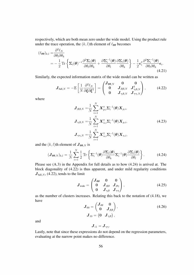
respectively, which are both mean zero under the wide model. Using the product ruleunder the trace operation, the (k, l)th element of `θθ becomes

(`θθ)k,l =∂2`N∂θl∂θk

=− 1

2Tr

Σi(θ)−1∂

2Σi(θ)

∂θl∂θk+∂Σ−1

i (θ)

∂θl

∂Σi(θ)

∂θk

− 1

2εᵀi∂2Σ−1

i (θ)

∂θl∂θkεi.

(4.21)

Similarly, the expected information matrix of the wide model can be written as

J full,N = −E[

1

N

∂2`N∂ξ∂ξᵀ

]=

Jθθ,N 0 00 Jββ,N Jᵀ

γβ,N

0 Jγβ,N Jγγ,N

, (4.22)

where

Jββ,N =1

N

N∑i=1

Xᵀp,iΣ

−1i (θ)Xp,i,

Jγβ,N =1

N

N∑i=1

Xᵀu,iΣ

−1i (θ)Xp,i, (4.23)

Jγγ,N =1

N

N∑i=1

Xᵀu,iΣ

−1i (θ)Xu,i,

and the (k, l)th element of Jθθ,N is

(Jθθ,N)k,l =1

N

N∑i=1

1

2Tr

Σ−1i (θ)

∂Σi(θ)

∂θkΣ−1i (θ)

∂Σi(θ)

∂θl

. (4.24)

Please see (A.3) in the Appendix for full details as to how (4.24) is arrived at. Theblock diagonality of (4.22) is thus apparent, and under mild regularity conditionsJ full,N , (4.22), tends to the limit

Jwide =

Jθθ 0 00 Jββ Jβγ0 Jγβ Jγγ

, (4.25)

as the number of clusters increases. Relating this back to the notation of (4.18), wehave

J00 =

(J θθ 00 Jββ

), (4.26)

J10 =(0 Jγβ

),

andJ11 = Jγγ .

Lastly, note that since these expressions do not depend on the regression parameters,evaluating at the narrow point makes no difference.

56

The case of the marginal LME model

Since the marginal variance-covariance takes the form Σi = ZiDZᵀi +σ2Ini for the

marginal LME model [see (2.5)], the variance-covariance component of its expectedinformation matrix also has a particular form.

For the case of a general random effect variance-covariance matrix, D, a com-pact expression (making use of elimination matrices, and the vec(·) operator) is givenin Demidenko (2013, p.124). For the special case of constant variance and independ-ence between random effect components, that is, when Σi = σ2

bZiZᵀi + σ2Ini , and

D = σ2bIk is diagonal (e.g. independence between random intercepts and slopes),

we have that, by (4.24), Jθθ is of the form

1

N

N∑i=1

1

2

Tr

Σ−1i Σ−1

i

Tr

Σ−1i ZiZ

ᵀiΣ−1i

TrZᵀiΣ−1i Σ−1

i Zi

TrZᵀiΣ−1i Zi(Z

ᵀiΣ−1i Zi)

ᵀ ,

where the upper left corner corresponds to the within-cluster error variance σ2, thelower right corner corresponds to the variance of the random effects σ2

b , and the off-diagonals correspond to the cross-terms. This corresponds to the lower right entry ofEquation (6.62) in McCulloch & Searle (2001), but where there are only two levelsof the data-hierarchy and hence only one vector of random effects.

4.3.1 The focus as solely a function of regression parametersConsider the limiting expected information matrix of the Normal model, partitionedinto blocks as in (4.25). In general, for discrete GLMMs (e.g. Binary, Poisson) theblock diagonal nature does not hold. So the results in this section only (with someexceptions) apply to the Normal model.

When the focus parameter, µ, is not a function of the variance-covariance para-meters, the quantities τ 2

0 , ω andQ drop their dependency upon the component of theexpected information matrix corresponding to the variance-covariance parameters,Jθθ. For instance, since in this case,

∂µ

∂ν=

( ∂µ∂θ∂µ∂β

)=

(0∂µ∂β

),

we have that

τ 20 =

(0(∂µ∂β

)ᵀ)(Jθθ 00 Jββ

)−1( 0∂µ∂β

)=(0(∂µ∂β

)ᵀ)(J−1θθ 00 J−1

ββ

)(0∂µ∂β

)=

(∂µ

∂β

)ᵀ

J−1ββ

∂µ

∂β. (4.27)

57

In a similar manner, the expressions for ω andQ reduce to

ω = JγβJ−1ββ

∂µ

∂β− ∂µ

∂γ, (4.28)

andQ = (Jγγ − JγβJ−1

ββJᵀγβ)−1. (4.29)

This result makes the FIC scores slightly simpler to arrive at for a focus that ispurely a function of the regression parameters (using the explicit formula for Jθθ,(4.24) can be a cumbersome activity). Furthermore, since J−1

θθ is the covariancematrix of the limiting distribution of the variance-covariance parameters, increasingthe number of θs in the model does not, in theory, increase the uncertainty, nor affectthe bias of the estimator of a focus parameter that is only in terms of the regressionparameters.

This means that, within an asymptotic framework and prior to estimation, providedthe focus is a function of the βs alone, there may be little to gain in terms of meansquared error by attempting to restrict the number of variance-covariance parametersin the model: the uncertainty in the θs should not influence the uncertainty of theβs. Asymptotically, both sets of parameters draw their information from independ-ent sources, albeit the same data. Thus, in terms of choice of variance-covariancematrix when the focus is on the regression parameters, there may be little advantageto a simpler model.

Since the expressions (4.23) have to be estimated (usually by plugging in theinverse of the estimated variance-covariance matrix), this could introduce some un-certainty into the focus that is purely a function of the βs. To see to what extent theabove conclusion holds in practice (after estimation), a simulation study was con-sidered. If this result does indeed hold true, there could be implications for howto go about choosing a variance-covariance matrix when the interest is only in theregression parameters.

4.3.2 SimulationsFor foci that are only a function of the regression parameters, does the choice ofcovariance model (or random effect structure) affect the stability of the FIC scores?Instability in the FIC scores of a correct, but overly-specified variance-covariancemodel would indicate uncertainty in the θs influencing either (or both) the varianceor bias of the focus estimators.

Thus, the specific question to be addressed is: given two correctly specified,covariance matrices Σ1 and Σ2, but where Σ2 includes more parameters than neces-sary, is there any difference in terms of variability of FIC scores when the focus isonly a function of β? The answer is likely to depend on the number of clusters; thenumber of units within clusters; whether the dataset is balanced by design; whether

58

there is missing data; the mean structures to be selected between; the particular fo-cus of interest; and the different covariance structures in question. Addressing all ofthese variables at once is a tall order. A simplified scenario was thus constructed.

One hundred balanced longitudinal datasets were generated for each pair of(N, n): the number of subjects N taking values in the set 30, 50, 100, 200, and thenumber of measurement occasions n taking values 3, 4, 5, 6. For each situation(N, n), the true model was a LME model including a random intercept and a randomslope for the effect of time. In particular, the true marginal model was

yij = β0 + β1groupi + β2tij + γ0t2ij + γ1tijgroupi + εij, (4.30)

with the true variance-covariance of the errors given by

Cov(εi) = ZiDZᵀi + σ2In, (4.31)

where Zi is the true random effects design matrix, and D the variance-covariancematrix of the random effects, which are given by

Zi =

1 ti1...

...1 tin

, D =

(d11 d12

d12 d22

).

The binary covariate group was generated using the command rbinom in R withprobability 0.5. Covariate time was treated as continuous over the interval [0, t∗],with t∗ = 12, and centered about its mean, (t = 6). For each situation of (N, n),measurements were simulated for both endpoints, t = 0, t = t∗, and additionalmeasurements divided the interval [0, t∗] into equal length sub-intervals.

The true values of the parameters were set as β = (β0, β1, β2) = (1, 1, 1),γ =(γ0, γ1) = (−0.1, 1) which means that the true mean trend was increasing andslightly concave. And, in addition θ = (σ2, d11, d12, d22)ᵀ = (4, 4, 0.2, 1).

Four different mean structures were considered for each simulation and for eachsituation of (N, n). The widest mean structure considered, M4, was

E[yij] = β0 + β1groupi + β2tij + γ0t2ij + γ1tijgroupi + γ2t

2ijgroupi; (4.32)

the narrowest model, M1, included only the protected covariates. The true model,M3, (4.30), was among the candidate models, and finally, the mean structure M2

E[yij] = β0 + β1groupi + β2tij + γ2t2ijgroupi, (4.33)

which is the narrow model plus one interaction: the uninformative interaction betweengroup and t2, was also included.

The focus parameter of interest in every situation was the expected response ofan individual belonging to the non-reference group at the last measurement occasionn, when t = t∗, that is,

µ = E[yin|t = t∗, group = 1].

The covariance models under consideration were:

59

• Σ0, the marginal covariance matrix arising from a random intercept model, i.e.compound symmetric, see (2.2), with two parameters regardless of the num-ber of measurement occasions: the variance of the random intercept and thevariance of the errors.

• Σ1, the marginal covariance matrix arising from a random intercept and slopemodel, i.e. the true data generating model, with four unknown parameters θ =(σ2, d11, d12, d22)ᵀ regardless of the number of measurement occasions).

• Σ2, an unstructured covariance model with n(n + 1)/2 parameters, rangingfrom 6 (n = 3) to 21 (n = 6) parameters.

• Σ3, the true covariance model with known parameter values θ = (4, 4, 0.2, 1)ᵀ.

The variance-covariance matrix Σ0 is thus misspecified, Σ1 and Σ3 are both true,but with unknown and known parameters respectively, and Σ2 is correctly specified,but involves too many parameters.

Given enough data, Σ1 and Σ2 are expected to converge to the same true cov-ariance model. Since Σ2 involves more parameters (especially as n grows), what arethe consequences for the variability in the bias and variance of the focus?

Results

The package simsalapar (Hofert & Mächler 2016) was used to help run parallel sim-ulations. Figures were produced using the package ggplot2 (Wickham 2009). Therandom intercept model, Σ0, failed to converge on 5 out of the 100 simulations, butthere were no other complications. Tables B.1 and B.2 in Section B.2 of AppendixB give the arithmetic mean over all 100 simulations of the FIC scores divided by N(scaled to be interpretable as estimates of the MSEs) for each situation (N, n,M,Σ).

In general, M3 and M4, were preferred over M1 and M2, as illustrated in Fig-ure 4.1, which shows box plots (of all 100 simulations) of the FIC scores scaled downby a factor of N for the particular situation N = 50 and n = 6, and with covariancematrix indexed along the x-axis. It is also visible that, for this case (and in fact moregenerally), that M3 and M4 displayed much less uncertainty in the FIC scores.

From inspection of the plots of FIC/N for each situation (N, n,M,Σ), it is clearthat two cases arise: the cases of correctly and incorrectly specified mean structuresneed to be distinguished.

When the mean structure is misspecified, i.e. for M1 and M2, there is morevariability (particularly for M1) in the FIC scores of the variance-covariance matrixΣ2 relative to that of Σ1. Figure 4.2 shows a grid of box plots in 4 × 4 = 16 cells.Each column of the grid represents a specific size for n, and each row a specific N .In each individual cell, FIC/N for mean structure M1 is on the y-axis; the values ofthe x-axis (0, 1, 2, 3) correspond to the indices of the different variance-covariancematrices. The red crosses mark the approximately true mean squared errors. That is,

60

Figure 4.1: Box plots of FIC/N for the situation N = 50, n = 6 plotted for eachcovariance structure Σ (whose indices correspond with the values (0, 1, 2, 3) on thex-axis) and for each mean structure (M1, M2, M3 and M4) represented by differentcolours.

0

10

20

30

40

0 1 2 3

Variance−covariance model

FIC

/N

M1

M2

M3

M4

61

the red crosses show the sample means (over all 100 simulations) of the ‘observed’squared errors: (µj − µtrue)

2. The box plots show more variability in the FIC scores(divided by N ) of Σ2 consistently throughout the grid. The same set-up is given formean structure M2 in Figure B.1 in Appendix B, where the differences still exist, butare much less severe.

Figures B.3 and B.4 along with Figures B.7 and B.8 in Appendix B, using thesame set-up as described above, show box plots of the estimated bias squared andestimated variances of models M1 and M2. The red crosses mark the approxim-

ately true bias squareds(

1100

∑100j=1(µj − µtrue)

)2

, and the sample variances in focusestimates over all 100 simulations for the bias squared (B.3 and B.4) and varianceplots (B.7 and B.8) respectively. Inspection of these plots shows that the differencein spreads of FIC/N between Σ1 compared with Σ2 is due to differences in biassquared, not variance (although the variances of Σ2 seem to be underestimated formean structure M1).

The same set-up as Figure 4.2 is displayed in Figure 4.3 for the FIC/N scoresof correctly specified mean structure M3 (and for M4 in Figure B.2 in Appendix B).For M3 and M4, it is visible that there is very little difference in terms of variabilityof the FIC scores (divided by N ) between Σ1 and Σ2.

Analysis of the relevant box plots (Figures B.9 and B.10) shows that for M3 andM4 the estimates of the variance term were similar for both Σ1 and Σ2, in terms ofspread. There is more variability in the bias squared estimates belonging to Σ2 forM3 (see Figure B.5), though since M3 is correctly specified, these differences do notcontribute much to the FIC scores; the variance term dominates. Since M4 is themean structure assumed correct by the FIC procedure, its bias squared estimates areeffectively zero (see Figure B.6).

The conclusion is then that, provided the mean structure is correctly specified,the FIC scores will not suffer if too many parameters are used to correctly specifythe variance-covariance model. For the correctly specified mean structures, the vari-ance term tends to dominate, which appears to be less afflicted by lack of simplicity.However, the bias squared terms of misspecified models appear to show more spreadin the estimates of over-parameterised variance-covariance models.

In general, the true specification of the mean structure is not known, so it is ofinterest to include potentially biased (misspecified) mean structures among the can-didate models. Therefore, foci that are purely a function of the βs do require parsimo-nious variance-covariance models. This agrees then with the Goldilocks principle oftraditional methods of choosing a variance-covariance model by balancing betweenfit and simplicity.

As a comment, note that the FIC/N estimates of the misspecified Σ0 appear tobe underestimated. This seems to be more in connection with the variance estimatesrather than the bias squareds. For example, see Figure B.9. In my view, this is mostlikely attributable to the fact that the FIC procedure used model-based inference:Σ0 enforces compound-symmetry - an unrealistic structure. Model-robust inference

62

Figure 4.2: In this figure showing a grid of box plots in 4 × 4 = 16 cells, eachcolumn represents a specific size of n, and each row a specific N . In each individualcell, FIC/N for the narrow mean structure M1 is plotted on the y-axis; the values ofthe x-axis (0, 1, 2, 3) correspond to the indices of the different variance-covariancematrices, Σ.

3 4 5 6

3050

100200

0 1 2 3 0 1 2 3 0 1 2 3 0 1 2 3

0

20

40

60

80

0

20

40

60

0

10

20

0

5

10

15

20

Variance−covariance model

FIC

/N

63

Figure 4.3: In this figure showing a grid of box plots in 4×4 = 16 cells, each columnrepresents a specific size of n, and each row a specific N . In each individual cell,the y-axis gives the values of FIC/N for the true mean structure M3; the values ofthe x-axis (0, 1, 2, 3) correspond to the indices of the different variance-covariancematrices, Σ.

3 4 5 6

3050

100200

0 1 2 3 0 1 2 3 0 1 2 3 0 1 2 3

1

2

3

4

5

1

2

3

0.4

0.8

1.2

1.6

0.2

0.3

0.4

0.5

0.6

Variance−covariance model

FIC

/N

64

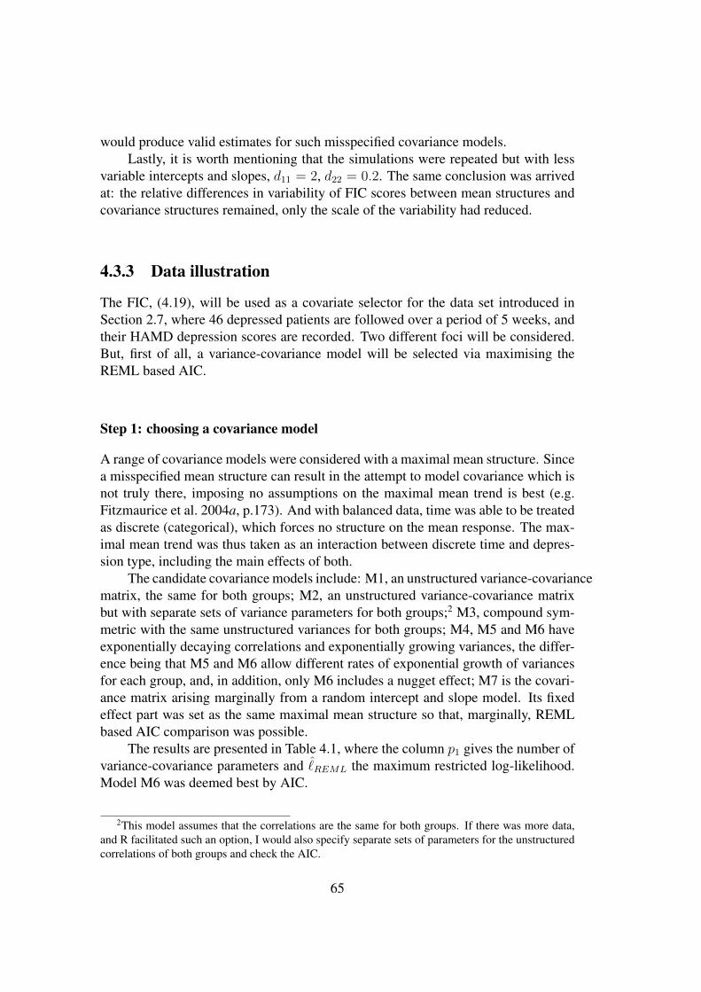
would produce valid estimates for such misspecified covariance models.Lastly, it is worth mentioning that the simulations were repeated but with less

variable intercepts and slopes, d11 = 2, d22 = 0.2. The same conclusion was arrivedat: the relative differences in variability of FIC scores between mean structures andcovariance structures remained, only the scale of the variability had reduced.

4.3.3 Data illustration

The FIC, (4.19), will be used as a covariate selector for the data set introduced inSection 2.7, where 46 depressed patients are followed over a period of 5 weeks, andtheir HAMD depression scores are recorded. Two different foci will be considered.But, first of all, a variance-covariance model will be selected via maximising theREML based AIC.

Step 1: choosing a covariance model

A range of covariance models were considered with a maximal mean structure. Sincea misspecified mean structure can result in the attempt to model covariance which isnot truly there, imposing no assumptions on the maximal mean trend is best (e.g.Fitzmaurice et al. 2004a, p.173). And with balanced data, time was able to be treatedas discrete (categorical), which forces no structure on the mean response. The max-imal mean trend was thus taken as an interaction between discrete time and depres-sion type, including the main effects of both.

The candidate covariance models include: M1, an unstructured variance-covariancematrix, the same for both groups; M2, an unstructured variance-covariance matrixbut with separate sets of variance parameters for both groups;2 M3, compound sym-metric with the same unstructured variances for both groups; M4, M5 and M6 haveexponentially decaying correlations and exponentially growing variances, the differ-ence being that M5 and M6 allow different rates of exponential growth of variancesfor each group, and, in addition, only M6 includes a nugget effect; M7 is the covari-ance matrix arising marginally from a random intercept and slope model. Its fixedeffect part was set as the same maximal mean structure so that, marginally, REMLbased AIC comparison was possible.

The results are presented in Table 4.1, where the column p1 gives the number ofvariance-covariance parameters and ˆ

REML the maximum restricted log-likelihood.Model M6 was deemed best by AIC.

2This model assumes that the correlations are the same for both groups. If there was more data,and R facilitated such an option, I would also specify separate sets of parameters for the unstructuredcorrelations of both groups and check the AIC.

65

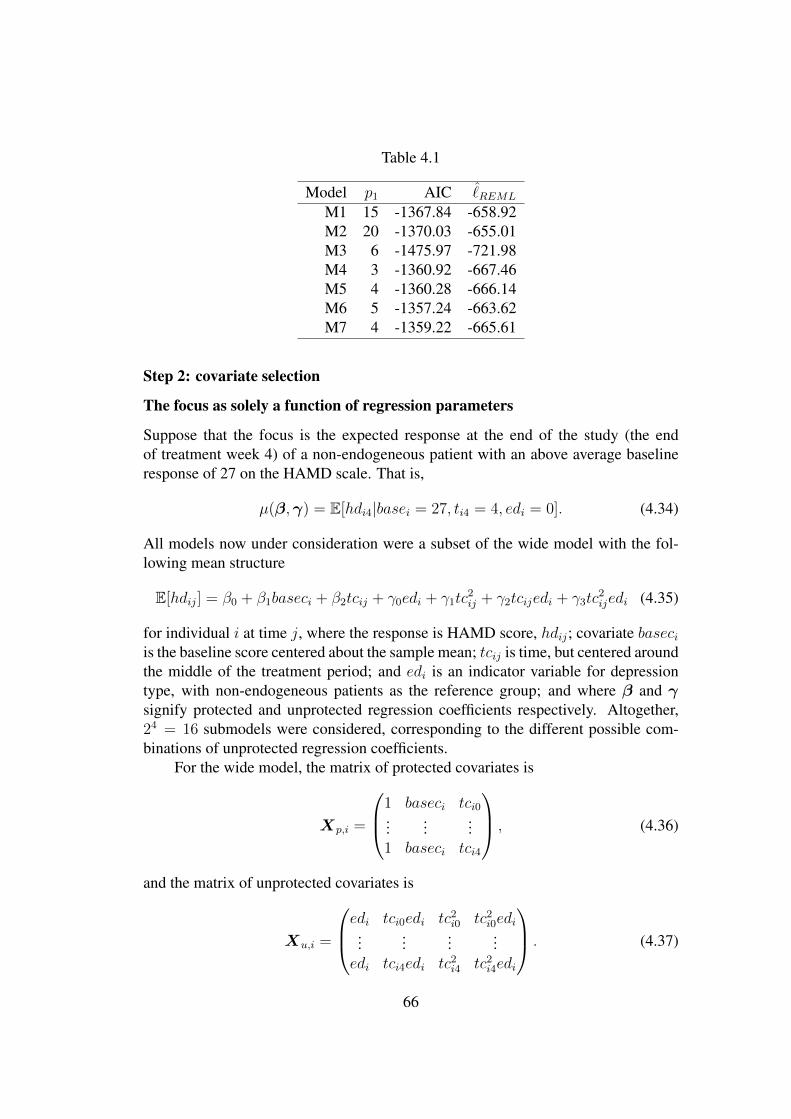
Table 4.1

Model p1 AIC ˆREML

M1 15 -1367.84 -658.92M2 20 -1370.03 -655.01M3 6 -1475.97 -721.98M4 3 -1360.92 -667.46M5 4 -1360.28 -666.14M6 5 -1357.24 -663.62M7 4 -1359.22 -665.61

Step 2: covariate selection

The focus as solely a function of regression parameters

Suppose that the focus is the expected response at the end of the study (the endof treatment week 4) of a non-endogeneous patient with an above average baselineresponse of 27 on the HAMD scale. That is,

µ(β,γ) = E[hdi4|basei = 27, ti4 = 4, edi = 0]. (4.34)

All models now under consideration were a subset of the wide model with the fol-lowing mean structure

E[hdij] = β0 + β1baseci + β2tcij + γ0edi + γ1tc2ij + γ2tcijedi + γ3tc

2ijedi (4.35)

for individual i at time j, where the response is HAMD score, hdij; covariate baseciis the baseline score centered about the sample mean; tcij is time, but centered aroundthe middle of the treatment period; and edi is an indicator variable for depressiontype, with non-endogeneous patients as the reference group; and where β and γsignify protected and unprotected regression coefficients respectively. Altogether,24 = 16 submodels were considered, corresponding to the different possible com-binations of unprotected regression coefficients.

For the wide model, the matrix of protected covariates is

Xp,i =

1 baseci tci0...

......

1 baseci tci4

, (4.36)

and the matrix of unprotected covariates is

Xu,i =

edi tci0edi tc2i0 tc2

i0edi...

......

...edi tci4edi tc2

i4 tc2i4edi

. (4.37)

66

The covariance matrix (pattern M6) for endogenous, Σ1, and non-endogenous pa-tients, Σ2, as estimated using REML by the wide model are

Σ1 =

21.82 15.65 14.12 12.75 11.5015.65 28.27 20.27 18.29 16.5114.12 20.27 36.61 26.26 23.7012.75 18.29 26.26 47.42 34.0111.50 16.51 23.70 34.01 61.42

and

Σ0 =

19.76 13.48 11.58 9.94 8.5413.48 23.17 15.81 13.58 11.6611.58 15.81 27.17 18.55 15.939.94 13.58 18.55 31.87 21.758.54 11.66 15.93 21.75 37.38

respectively. That the variances are different for each group is clear. When the cov-ariances are standardised into correlations one can see that they are in fact the samefor both groups. These matrices give estimates for the required components (4.23) ofthe expected information matrix of the wide model. These, along with partial deriv-atives of the focus evaluated at the null model, give estimates of the quantities (4.27),(4.28) and (4.29), which, in turn, combined with DN and the relevant projectionmatrices, πS , give the FIC scores (4.19).

The results from the analysis of this focus, (4.34), are shown in Table 4.2. Thefirst column states which unprotected covariates have been included. For example,an entry of 1100 corresponds to including edi and tc2 but excluding the interactionterms. Column |S| is the number of unprotected parameters included in the model;column µ contains the estimate of the focus parameter for each model; column bias2

contains the estimates of the squared bias of the limiting distribution of the focus foreach model; Var is the estimated variance of the limiting distribution of the focus foreach model; the column AIC gives the (ML based) AIC scores of all models; rAICand rFIC rank the AIC and FIC scores from best (=1) to worst (=16) respectively.

Model 1000 is the FIC favourite for this focus. With smallest FIC score itsestimate appears furthest to the left on part (a) of Figure 4.4. That is, the modelincluding only the main effect for group, edi, as an additional term produced thebest estimate for this particular focus as judged by FIC. Table 4.2 shows that thereis disagreement between AIC and FIC in terms of covariate selection. Part (a) ofFigure 4.4, displaying two groups distinguished by similar sized confidence intervalsand similar point estimates, shows that FIC is happy to accept some bias in exchangefor smaller confidence intervals here.

When the focus is changed to the expected response at the end of treatment foran endogeneous patient with a below average baseline score of 18, the narrow model

67

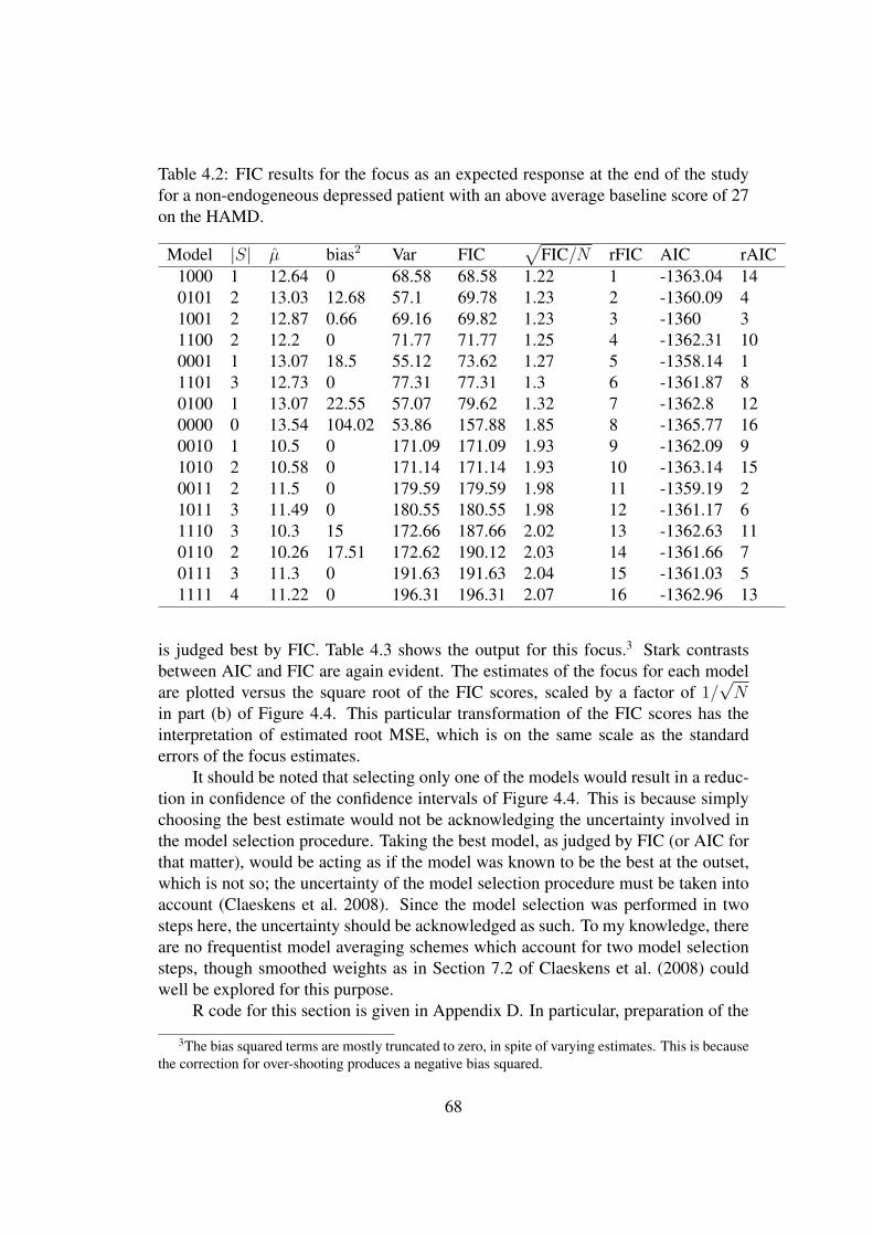
Table 4.2: FIC results for the focus as an expected response at the end of the studyfor a non-endogeneous depressed patient with an above average baseline score of 27on the HAMD.

Model |S| µ bias2 Var FIC√

FIC/N rFIC AIC rAIC1000 1 12.64 0 68.58 68.58 1.22 1 -1363.04 140101 2 13.03 12.68 57.1 69.78 1.23 2 -1360.09 41001 2 12.87 0.66 69.16 69.82 1.23 3 -1360 31100 2 12.2 0 71.77 71.77 1.25 4 -1362.31 100001 1 13.07 18.5 55.12 73.62 1.27 5 -1358.14 11101 3 12.73 0 77.31 77.31 1.3 6 -1361.87 80100 1 13.07 22.55 57.07 79.62 1.32 7 -1362.8 120000 0 13.54 104.02 53.86 157.88 1.85 8 -1365.77 160010 1 10.5 0 171.09 171.09 1.93 9 -1362.09 91010 2 10.58 0 171.14 171.14 1.93 10 -1363.14 150011 2 11.5 0 179.59 179.59 1.98 11 -1359.19 21011 3 11.49 0 180.55 180.55 1.98 12 -1361.17 61110 3 10.3 15 172.66 187.66 2.02 13 -1362.63 110110 2 10.26 17.51 172.62 190.12 2.03 14 -1361.66 70111 3 11.3 0 191.63 191.63 2.04 15 -1361.03 51111 4 11.22 0 196.31 196.31 2.07 16 -1362.96 13

is judged best by FIC. Table 4.3 shows the output for this focus.3 Stark contrastsbetween AIC and FIC are again evident. The estimates of the focus for each modelare plotted versus the square root of the FIC scores, scaled by a factor of 1/

√N

in part (b) of Figure 4.4. This particular transformation of the FIC scores has theinterpretation of estimated root MSE, which is on the same scale as the standarderrors of the focus estimates.

It should be noted that selecting only one of the models would result in a reduc-tion in confidence of the confidence intervals of Figure 4.4. This is because simplychoosing the best estimate would not be acknowledging the uncertainty involved inthe model selection procedure. Taking the best model, as judged by FIC (or AIC forthat matter), would be acting as if the model was known to be the best at the outset,which is not so; the uncertainty of the model selection procedure must be taken intoaccount (Claeskens et al. 2008). Since the model selection was performed in twosteps here, the uncertainty should be acknowledged as such. To my knowledge, thereare no frequentist model averaging schemes which account for two model selectionsteps, though smoothed weights as in Section 7.2 of Claeskens et al. (2008) couldwell be explored for this purpose.

R code for this section is given in Appendix D. In particular, preparation of the

3The bias squared terms are mostly truncated to zero, in spite of varying estimates. This is becausethe correction for over-shooting produces a negative bias squared.

68

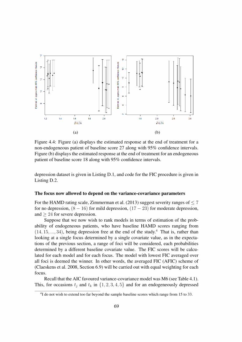
(a) (b)

Figure 4.4: Figure (a) displays the estimated response at the end of treatment for anon-endogeneous patient of baseline score 27 along with 95% confidence intervals.Figure (b) displays the estimated response at the end of treatment for an endogeneouspatient of baseline score 18 along with 95% confidence intervals.

depression dataset is given in Listing D.1, and code for the FIC procedure is given inListing D.2.

The focus now allowed to depend on the variance-covariance parameters

For the HAMD rating scale, Zimmerman et al. (2013) suggest severity ranges of≤ 7for no depression, (8− 16) for mild depression, (17− 23) for moderate depression,and ≥ 24 for severe depression.

Suppose that we now wish to rank models in terms of estimation of the prob-ability of endogeneous patients, who have baseline HAMD scores ranging from(14, 15, ..., 34), being depression free at the end of the study.4 That is, rather thanlooking at a single focus determined by a single covariate value, as in the expecta-tions of the previous section, a range of foci will be considered, each probabilitiesdetermined by a different baseline covariate value. The FIC scores will be calcu-lated for each model and for each focus. The model with lowest FIC averaged overall foci is deemed the winner. In other words, the averaged FIC (AFIC) scheme of(Claeskens et al. 2008, Section 6.9) will be carried out with equal weighting for eachfocus.

Recall that the AIC favoured variance-covariance model was M6 (see Table 4.1).This, for occasions tj and tk in 1, 2, 3, 4, 5 and for an endogeneously depressed

4I do not wish to extend too far beyond the sample baseline scores which range from 15 to 33.

69

Table 4.3: FIC results for the focus as the expected response at the end of the studyof an endogeneous depressed patient with (a below average) baseline score of 18 onthe HAMD.

Model |S| µ bias2 Var FIC√

FIC/N rFIC AIC rAIC0000 0 8.94 0 61.72 61.72 1.16 1 -1365.77 160100 1 8.96 0 61.76 61.76 1.16 2 -1362.8 120001 1 11.02 0 89.67 89.67 1.4 3 -1358.14 10101 2 10.93 0 99.62 99.62 1.47 4 -1360.09 41000 1 10.38 0 102.29 102.29 1.49 5 -1363.04 141100 2 10.42 0 102.33 102.33 1.49 6 -1362.31 101001 2 11.25 0 109.07 109.07 1.54 7 -1360 31101 3 11.16 0 112.16 112.16 1.56 8 -1361.87 80011 2 9.19 0 256.37 256.37 2.36 9 -1359.19 20111 3 8.87 0 287.34 287.34 2.5 10 -1361.03 51110 3 7.87 27.03 286.8 313.83 2.61 11 -1362.63 111011 3 9.33 0 318.67 318.67 2.63 12 -1361.17 61111 4 9.11 0 329.42 329.42 2.68 13 -1362.96 131010 2 7.64 53.63 285.89 339.52 2.72 14 -1363.14 150110 2 6.25 208.09 166.05 374.14 2.85 15 -1361.66 70010 1 6.05 253.67 165.5 419.17 3.02 16 -1362.09 9

individual i, can be written as

Cov(yij, yik) =

σ2e2tjδ1 , if j = k,

σ2(1− κ)e2(tj+tk)δ1−|tj−tk|R , if j 6= k,

(4.38)

in terms of parameter vector θ = (σ, δ1, δ0, R, κ)ᵀ, where σ is a scaling parameter; δ1

regulates the exponential growth of the variances; R regulates the exponential decayof correlations; and κ is a nugget effect. The corresponding variance-covariancemodel of a non-endogeneous patient is found by replacing δ1 with rate δ0.

Recall also that the covariance matrix of an endogeneous patient was labelledΣ1, and that of a non-endogenous patient was labelled Σ0. Since the protected andunprotected design matrices, (4.36) and (4.37), are determined by baseline covari-ate score and depression type respectively, for a patient of baseline score b, denotethe matrix of protected covariates as Xp,b and the unprotected covariates by Xu,1

or Xu,0 depending on the depression type (1 =endogenous, 0 =non-endogenous).These quantities will determine the probability of a patient with a specific baselinescore being depression free at the end of the study.

Thus, the foci of an endogeneous patient, indexed by baseline score b in the set

70

14, ..., 34, are

µb = P (yi4 ≤ y∗) (4.39)

=

∫Ω∗

(2π)−52 |Σ1(θ)|−

12 exp

(− 1

2wᵀΣ−1

1 (θ)w)dy, (4.40)

wherew = y −Xp,bβ −Xu,1γ,

Ω∗ = (−∞,∞)× (−∞,∞)× (−∞,∞)× (−∞,∞)× (−∞, y∗), with y∗ = 7 theno depression threshold value and 5 the number of measurement occasions.

The chosen variance-covariance model, given by (4.38), has parameter vectorθ = (σ, δ1, δ0, R, κ)ᵀ. In order to carry out AFIC for foci that are functions of theseparameters, an estimate of the quantity Jθθ will be needed. Therefore, making useof the explicit expression (4.24), the derivatives of Σ1 and Σ0 with respect to θ arerequired. We have, for example, the (i, j)th element of the partial derivative of Σ1

with respect to σ as

(∂Σ1(θ)

∂σ

)i,j

=

2σe2tjδ1 , if i = j,

2(1− κ)σe|ti−tj |δ1−|ti−tj |R otherwise.

Similar calculations can be performed for the other variance-covariance parametersand likewise for Σ0 (see (A.4) in Appendix A), and using the estimates of the widemodel, Jθθ may be estimated.

In addition, forω and τ 20 , we require the partial derivatives of the focus evaluated

at the narrow model. Differentiating under the integral sign of (4.40) with respect tothe regression parameters, we get

∂µb∂β

=

∫Ω∗Xᵀ

p,bΣ−11 (θ)ε(y)fy(y)dy, (4.41)

∂µb∂γ

=

∫Ω∗Xᵀ

u,1Σ−11 (θ)ε(y)fy(y)dy,

wherefy(y) = (2π)−

52 |Σ1(θ)|−

12 exp

(− 1

2εᵀ(y)Σ−1

1 (θ)ε(y)),

and ε(y) = y −Xp,bβ.The partial derivatives of µb with respect to the kth element of θ may be written

as

∂µb∂θk

=

∫Ω∗

1

2

(−Tr

Σ−1

1 (θ)∂Σ1

∂θk

+ εᵀ(y)Σ−1

1 (θ)∂Σ1

∂θkΣ−1

1 (θ)ε(y)

)fy(y),

where the derivative of the determinant was found by (A.3), and (A.1) was appliedto the derivative of the inverse.

71

Table 4.4: For the set of foci (4.40), the AIC and AFIC scores are given for eachmodel along with their relative ranking.

model AFIC rAFIC AIC rAIC0000 0.131 1 -1363.50 160100 0.135 2 -1365.96 120001 0.168 3 -1361.45 10101 0.169 4 -1363.35 31000 0.18 5 -1366.25 131100 0.188 6 -1365.35 91001 0.192 7 -1363.4 41101 0.193 8 -1365.21 80011 0.236 9 -1362.67 20111 0.241 10 -1364.44 51110 0.279 11 -1365.86 111011 0.286 12 -1364.67 61111 0.286 13 -1366.38 140110 0.286 14 -1365.18 71010 0.346 15 -1366.56 150010 0.447 16 -1365.8 10

These three integrals, the first two of which have integrands of dimension p2 = 3and q = 4 respectively, were approximated via Monte Carlo integration. In order todo this, each integral was re-expressed as an expectation with respect to a multivariatenormal distribution over the unrestricted domain of integration, Ω. For example, it ispossible to write (4.41) as

∂µb∂β

=

∫Ω

Xᵀp,bΣ

−11 (θ)ε(y)1yi4≤y∗fy(y)

= Ef [Xᵀp,bΣ

−11 (θ)ε(y)1yi4≤y∗]. (4.42)

Furthermore, since the true β, Σ and its derivatives are unknown, β, Σ etc. as estim-ated under the wide model via REML were used as direct substitutes.

Using the rmvnorm command of the mvtnorm package in R (Genz & Bretz2009, Genz et al. 2017), 1000 samples were drawn from the appropriate multivari-ate normal density. The function Xᵀ

p,bΣ−1e ε(y)1yi4≤y∗ was then evaluated at these

samples and the mean of these evaluations was calculated to give an approximationto (4.41). This process was repeated for each of the required integrals, and, within aloop, for each of the foci.

The FIC scores for each foci and for each model were then calculated by plug-ging in the estimated and approximated quantities into (4.10), (4.12), and (4.13) (orrather, their cluster versions). Estimates of the focus, (4.40), were produced usingthe pmvnorm command of the mvtnorm package. These are displayed in Figure 4.5

72

Figure 4.5: The estimated probabilities for each model of being depression free bythe end of study for endogeneous patients against baseline score. The estimates fromthe favourite AFIC model is shown with a dashed line.

15 20 25 30

0.1

0.2

0.3

0.4

0.5

HDRS score at baseline

Pro

babi

lity

of n

o de

pres

sion

at e

nd o

f stu

dy

for each of the baseline scores. The results are, of course, not continuous, but aredisplayed as such for the purpose of illustration.

The FIC scores averaged over all foci are displayed in Table 4.4 which shows,again, difference between the rankings of the ML based AIC and the AFIC scores.The model with smallest FIC averaged over all baseline situations is the narrowmodel and is shown in Figure 4.5 with a dashed line. This model estimates that allpatients classified as severely depressed (HAMD ≥ 24) at baseline have a probabil-ity smaller than 0.26 of no depression by the end of study, and a probability between0.43 and 0.26 for those moderately depressed (17 ≤ HAMD ≤ 23) at baseline.

73

4.4 FIC for generalised linear mixed models

Since for GLMMs an expression for the marginal density of each cluster (3.2) isavailable, the FIC formula (4.19) for selection of covariates in GLMMs can be setto work with a chosen link function and random effect structure. As by Section 4.2,the vector of protected parameters ν includes the protected regression parameters,the variance-covariance parameters of the random effects and any scale parameter.As with LME models, the focus parameter, µ, should not include a random effectsince random effects are random variables. By defining odds ratios, or rate ratios forexample, one can arrive at sensible focus parameters.

The expected information matrix for the canonical class of GLMMs is givenfor general random effect structures with potentially numerous hierarchies in Wand(2007). Computing expected information matrices for GLMMs involves numericalintegration, the complexity of which depends on the dimension of the random effectsand the number of units within clusters. The observed information, which servesas an approximation, may be more readily available as output from software fittedmodels, and simpler to calculate, particularly so when there is missing data. Forexample, the observed information matrix of a logistic GLMM is readily availableafter calling glmmML in R, as the inverse of N times the variance-covariance matrixof the model parameters. Nevertheless, it is interesting to see exact expressions forthese matrices.

4.4.1 Derivations of information matrices of a logistic GLMMwith a random intercept.

The logistic GLMM of Section 3.2.1, but with only a random intercept, will be con-sidered here and expressions for its expected and observed information matrices arederived.

Define parameters α =

(βγ

)as the vector of protected and unprotected re-

gression coefficients. In addition, define the fixed effect design matrix as X i =(Xp,i Xu,i) to be the concatenation of protected and unprotected design matrices,with jth row xᵀ

ij . Then the wide model is

fyij |bi(yij|bi) =pyijij (1− pij)(1−yij), (4.43)

log( pij

1− pij

)=xᵀ

ijα+ bi, (4.44)

bi ∼ N(0, σ2b ),

where pij = P (yij = 1|bi) is the probability of unit j of cluster i taking value one,and 1− pij is the probability of unit j of cluster i taking value zero.

First of all, note that from (3.4) and (4.44) we have that (4.43) can be re-written

74

asfyij |bi(yij|bi) = exp

(yij(x

ᵀijα+ bi)− log(1 + ex

ᵀijα+bi)

),

and by conditional independence we have

fyi|bi(yi|bi) =

ni∏j=1

fyij |bi(yij|bi)

= exp

(ni∑j=1

yij(xᵀijα+ bi)− log(1 + ex

ᵀijα+bi)

). (4.45)

The marginal log-likelihood of a single cluster is

`i(α|y) = log

(∫fyi|bi(yi|bi)fbi(bi)dbi

),

where fbi(bi) is the N(0, σ2b ) density of the random effects.

The score function of protected and unprotected regression coefficients for theith cluster is thus

∂`i∂α

=

∫ ∂fyi|bi (yi|bi)∂α

fbi(bi)dbi∫fyi|bi(yi|bi)fbi(bi)dbi

, (4.46)

where∂fyi|bi(yi|bi)

∂α= fyi|bi(yi|bi)

ni∑j=1

[yij −

exᵀijα+bi

1 + exᵀijα+bi

]xᵀij.

Similarly we have

∂`i∂σb

=

∫fyi|bi(yi|bi)

∂fbi (bi)

∂σbdbi∫

fyi|bi(yi|bi)fbi(bi)dbi, (4.47)

where∂fbi(bi)

∂σb=

1√2πσ2

b

( b2i

σ2b

− 1)e− b2i

2σ2b = v(bi)fbi(bi),

with

v(bi) =1

σb

( b2i

σ2b

− 1). (4.48)

Expected information matrix

For the expected information, what we are interested in is the covariance of thescores. Since the scores are mean zero under the wide model (4.44), when aver-aged over all clusters, the covariance of the scores corresponding to the regression

75

coefficients becomes (i.e. the component of the expected information correspondingto the regression coefficients is)

1

N

N∑i=1

E[(∂`i∂α

(yi))ᵀ ∂`i∂α

(yi)

]. (4.49)

Similarly the component corresponding to the standard deviation parameter of therandom effects is

1

N

N∑i=1

E[( ∂`i∂σb

(yi))2], (4.50)

and the cross-term is

1

N

N∑i=1

E[(∂`i∂α

(yi))ᵀ ∂`i∂σb

(yi)

], (4.51)

which are averages of expectations with respect to yi. These expectations, whichgive expressions for the components of the expected information matrix of the lo-gistic model, can be evaluated at the narrow (βnarr,0) or at the wide estimate (β, γ)(Claeskens et al. 2008, p.154) for use in the FIC framework.

In practice, there are integrals within integrals to be approximated here. MonteCarlo methods are typically more suited for the outer integrals (the expectations withrespect to the data), since the number of units within each cluster may be relativelylarge. However, samples cannot be drawn directly from the marginal of yi. Instead,one may draw from the distribution of bi, and then subsequently from the conditionaldistribution of yi given the sampled bi. The inner integrals consist of integratingout bi which, in this case, are univariate. Deterministic approaches such as Gauss-Hermite quadrature are therefore acceptable for the inner integrals. If this is the ap-proach to be taken, integration with respect to the random effects has to be performedfor each of the sampled yi.

Observed information matrix

By the quotient rule, the component of the observed information corresponding tothe regression parameters, found by taking the sum and derivative of (4.46) under theintegral sign, is

− 1

N

∂2`N∂α∂αᵀ

= − 1

N

1

(fyi(yi))2

(∂h(yi)

∂αᵀfyi(yi)−

∂fyi(yi)

∂αᵀh(yi)

), (4.52)

76

where∂fyi(yi)

∂αᵀis the transpose of (4.46), h(yi) is the numerator of (4.46), and

∂h(yi)

∂αᵀ=∫ (

∂f(yi)

∂αᵀ

ni∑j=1

[yij −

exᵀijα+bi

1 + exᵀijα+bi

]xᵀij − f(yi|bi)

ni∑j=1

[ex

ᵀijα+bi

(1 + exᵀijα)2

]xijxᵀij

])fbi(bi)dbi.

Similarly, for the component corresponding to the standard deviation of the ran-dom effects, we have

− 1

N

∂2`N∂σ2

b

= − 1

N

1

(f(yi))2

(∂2f(yi)

∂σ2b

f(yi)−(∂fyi(yi)

∂σb

)2), (4.53)

where∂2fyi(yi)

∂σ2b

=

∫fyi|bi(yi|bi)

[v(bi) +

∂v(bi)

∂σb

]fbi(bi)dbi,

with v(bi) as in (4.48),∂v(bi)

∂σb=

1

σ2b

(1− 3bi

σ2b

),

and∂fyi(yi)

∂σbthe score function given in (4.47). Finally, for the cross-term we have

− 1

N

∂`N∂σb∂α

= − 1

N

1

(fyi(yi))2

(∂2f(yi)

∂σb∂αfyi(yi)−

∂fyi(yi)

∂α

fyi(yi)

∂σb

), (4.54)

where∂2f(yi)

∂σb∂α=

∫fyi|bi(yi|bi)h(yi)v(bi)fbi(bi)dbi.

The integrals in (4.52), (4.53) and (4.54) are all with respect to a univariate normaldensity. Thus, in application, Gauss-Hermite integration may be suitable for approx-imating these quantities.

4.4.2 Data illustrationRecall the binary dataset introduced in Section 3.4 of Chapter 3. Suppose that thefocus of interest is the following odds ratio:

Odds of onycholysis|groupi = A, bi, t = tkOdds of onycholysis|groupi = B, bi, t = tk

. (4.55)

That is, the focus is an odds ratio comparing an individual of Treatment A to anindividual of Treatment B at time j, both of which happen to share the same random

77

effect, bi. In other words, the same tendency (whatever strength that might be, butthat persists throughout the study) to be observed as moderately or severely infectedis shared by both individuals.

The widest model under consideration is the logistic cubic

log( pij

1− pij

)= β0 + β1tij + γ0t

2ij + γ1t

3ij

+ γ2tijgroupi + γ3t2ijgroupi + γ4t

3ijgroupi + bi,

where time, t, was centered about its mean. The focus (4.55) can be written as

exᵀA,ijα+bi

exᵀB,ijα+bi

,

where xᵀA,ij is the jth row of the design matrix of individual i from treatment group

A, and similarly for xᵀB,ij . Since both individuals under comparison are assumed to

have measurements observed at the same set of scheduled occasions (at 1, 2, 3, 6, 9and 12 months), and also share the same random effect, bi, this reduces to

e(xA,ij−xB,ij)ᵀα = eγ3tij+γ4t2ij+γ5t

3ij . (4.56)

For this set-up, there are four potential models (the narrow, 00000, and 10000, 01000,11000), which all set γ3 = γ4 = γ5 = 0 and thus estimate the focus to take value 1with zero variance. Of these four, only the narrow is included as a candidate.

The derivatives of (4.56) with respect to the model parameters, evaluated at thenarrow model, give estimates for the required partial derivatives in the cluster versionof (4.13).

The observed information matrix [see formulas (4.52), (4.54), (4.53)] of thewide model was used as an approximation of the expected information matrix. Doingso is advantageous since this dataset contains missing data which has to be accoun-ted for by the expected information matrix. 60 quadrature points were used in theGauss-Hermite quadrature for approximating the integrals of the observed informa-tion matrix. The command gauss.quad from the R package statmod (Smyth 2005)was used to create the quadrature points. In addition, the observed information mat-rix was evaluated at the wide estimate (rather than the narrow), which builds in acertain model robustness (Claeskens et al. 2008, p.154).

This focus, (4.55), was estimated by each model for each of the scheduled timepoints, producing corresponding FIC scores. The AFIC was then calculated over all7 time points. Table 4.5 presents the AFIC scores (divided by the number of patientsN = 294) and the AIC scores of the top five models (out of 29) as rated by AFIC.Once again, there are disagreements between the rankings of AIC and AFIC.5

5Admittedly, the conditional AIC would be more appropriate than the AIC since the focus is atthe level of the individual. However, implementation of this is a slow process in R package cAIC4(Saefken et al. 2018a,b) for Bernoulli models due to the number of model-refits required.

78

Table 4.5: The AFIC (divided by N) and AIC scores for the top 5 models (as judgedby AFIC) for the onycholysis data set with focus given in (4.55).

model AFIC/N AIC10001 0.027 -1243.6400000 0.029 -1261.8401001 0.035 -1244.5811001 0.036 -1241.700100 0.062 -1260.75

Figure 4.6 shows the focus estimates of the favoured AFIC model, 10001, foreach of the 7 time points along with 95% confidence intervals (which are optim-istic as they neglect the uncertainty in the model selection procedure). Under theassumptions of model 10001 and assuming an all-available data analysis is appro-priate, this figure suggests that, since the 95% confidence intervals include the no-difference between treatment line, there is no significant difference between the oddsof onycholysis of two individuals from both treatments who happen to have the samerandom effect.

4.5 Chapter summaryIn this chapter, the focussed information criterion for independent data as in inClaeskens & Hjort (2003) was introduced. How this generalises to clustered datawithin a multivariate misspecified framework was then made explicit. In particular,the framework formulated in Section 4.2.1 opens the door to application of the FICfor covariate selection in multivariate LMs, LME models and GLMMs. With re-gard to the Normal model, a simulation study was carried out to see how influentialthe uncertainty in over-parametrised variance-covariance models is upon the limitingdistribution of focus parameters that are only a function of the regression coefficients.As examples of the framework in Section 4.2.1, the FIC was applied to select cov-ariates in the multivariate Normal model and a logistic GLMM for two clinical trialdatasets. Explicit formulae for the information matrices of the multivariate linearmodel and the logistic GLMM were also given.

79

Figure 4.6: The focus [see (4.55)] as estimated by model 10001 for each scheduledmeasurement occasion 1, 2, 3, 6, 9 and 12. The dashed red line is where no differencebetween treatments would be observed i.e. the odds of treatment A is a factor ofone time the odds of Treatment B. The solid green lines give upper and lower 95%confidence intervals (albeit optmistic).

0 2 4 6 8 10 12

0.5

1.0

1.5

Month

Odd

s ra

tio T

reat

men

t A v

s Tr

eatm

ent B

80

Chapter 5

Derivations of Mean Squared ErrorFormulae

For the Normal model, an alternative approach to constructing FIC scores is avail-able for a subset of foci. The method, described in the appendix of Cunen et al.(2017), begins with finding the expected value and covariance of the generalisedleast squares (GLS) estimator for each candidate model, under the assumption thatthe wide model’s first two moments are correctly specified, and, thereby, the biassquared and variance of the focus estimator of each model. This method was used inCunen et al. (2017) to construct FIC formulas for linear mixed effect (LME) mod-els, albeit only for the bias squared term. Since the focus of interest in Cunen et al.(2017) was a single regression coefficient, the formulas were given for that specificcase, and noted to be readily available for more general functions of the regressioncoefficients.

In this chapter, the approach will be demonstrated for a general linear combina-tion of regression coefficients and for a multivariate linear combination of regressioncoefficients. An extension, following the work of Kackar & Harville (1984), whichalso takes into account the uncertainty in the variance-covariance parameters is alsopresented. Lastly, a similar approach is demonstrated for ranking LME models interms of the precision of predictors of cluster-specific trajectories.

5.1 MSE formula for a focus that is a general linearcombination of regression parameters

For this chapter, the slightly misspecified framework of (4.15) is not needed. Rather,an alternative, but similar setup is required. It will be assumed that a wide model,with fullest mean structure is the true model. The form of its covariance matrixdepends on whether we are considering a model with random effects (the marginalmodel), or no random effects at all. Then, independent vector responses yi are gen-

81

erated byyi ∼ N(Xp,iβ +Xu,iγ,Σi(θ)). (5.1)

In the same way as the FIC setup, let model (say) S be a function of the protectedregression parameters β of dimension p and the unprotected regression parametersγS of dimension |S|, a subset of the wide models γ, which is of dimension q.

In terms of design matrices for each individual i, all models will include a matrixof protected covariates,Xp,i, but only the wide model will additionally include all ofthe unprotected covariates,Xu,i. So, the wide model has an ni×(p+q) design matrix,X i = (Xp,i Xu,i), which is the concatenation of the protected and unprotectedcovariates. Candidate model S has design matrix XS,i = (Xp,iXuS ,i) where XuS ,i

is the matrix of columns of Xu,i whose indices are in the set S (S denotes a set;model S refers to that model which includes the unprotected covariates whose indicesappear in set S).

Let α =

(βγ

)be the vector of all regression coefficients. For a focus µ that is

a linear combination of the elements of α, whose weights are defined by the (p+ q)row vector m, we may write µ = mα. Also required is the p + |S| row vectormS whose first p entries correspond to the first p entries of m (i.e. the protectedregression weights) and the remaining |S| entries are the weights of the unprotectedγs that appear in set S. It is assumed that the variance-covariance model, Σi(θ), isthe same across candidate models. Furthermore, its parameter values are consideredknown, with superscript o used to denote this. Mean squared error formulae will nowbe derived.

We have that the generalised least squares estimator of α for model S is

αoS =

(βo

S

γoS

)=

(N∑i=1

XᵀS,iΣ

−1i (θo)XS,i

)−1 N∑i=1

XᵀS,iΣ

−1i (θo)yi. (5.2)

Then, the estimate of µ produced by model S is µoS = mSαoS .

Since, under the wide model, E[yi] = X iα, where α is the true parametervalue, taking the expected value of (5.2) gives

E[αoS] =

(N∑i=1

XᵀS,iΣ

−1i (θo)XS,i

)−1( N∑i=1

XᵀS,iΣ

−1i (θo)X i

)α (5.3)

=Bo−1S Do

Sα,

with

BoS =

N∑i=1

XᵀS,iΣ

−1i (θo)XS,i, and Do

S =N∑i=1

XᵀS,iΣ

−1i (θo)X i. (5.4)

In addition, defineAoS = Bo−1

S DoS. (5.5)

82

For the bias squared term, we have that the bias in the estimator µoS is

biasS = E[µoS − µ] = E[mSαoS −mα]

=mSE[αoS]−mα = (mSAoS −m)α, (5.6)

where the fourth equality follows from (5.3) combined with (5.5).A naive estimator of bias squared for model S is then

biaso2

S = ((mSAoS −m)αo)2,

where αo is the estimator of the wide model. Since for any random variable say b,E[b2] = E[b]2−Var(b), this naive estimator overshoots by the amount Var(bias

o

S). Animproved estimator is therefore

(mS(AoS −m)αo)2 − Var(bias

o

S),

where, by (5.6),

Var(biaso

S) = (mSAoS −m)Cov(αo)(mSA

oS −m)ᵀ.

We have that

Cov(αo) =

(N∑i=1

XiΣ−1i (θo)X i

)−1

=·· Bo−1,

and so, along with truncating at zero to avoid a negative bias squared, we get

max[0, ((mS A

oS − m)αo)2 − (mSA

oS − m)Bo−1(mSA

oS − m)ᵀ

](5.7)

as an improved estimator of bias squared.As for the variance term, note that under the wide model, the variance-covariance

of αoS isCov(αoS) = Bo−1

S . (5.8)

Therefore, the variance in estimation of the true focus µ = mα for model S is

Var(µoS) = mSCov(αoS)mᵀS

= mSBo−1S mᵀ

S. (5.9)

Summing (5.9) and (5.7) together then gives an estimator for the MSE of modelS in estimation of µ = mα as

MSEo

S = mSBo−1S mᵀ

S + max[0, ((mSA

oS −m)αo)2

− (mSAoS −m)Bo−1(mSA

oS −m)ᵀ

], (5.10)

83

which, for known θ, the variance term is exact and the bias squared term is unbiasedprior to truncation.

The same derivation when θ has to be estimated does not hold: the uncertaintyin the estimates of θ needs to be taken into account. Therefore, for such a situation,a plausible option is to use the estimates of θ based on the widest mean structure andsimply plug them into the relevant quantities of formula (5.10). That is, to use theestimators

AS = B−1

S

N∑i=1

XᵀS,iΣ

−1i (θ)X i, B

−1

S =

(N∑i=1

XᵀS,iΣ

−1i (θ)XS,i

)−1

, (5.11)

and

B−1

=

(N∑i=1

XᵀiΣ−1i (θ)X i

)−1

. (5.12)

Plugging in estimates into (5.10) could, for example, rank models in terms oftheir estimation of the focus µ, which is the expected marginal response given avector of covariates m, E[yij|xᵀ

ij = m]. Or, similar to Cunen et al. (2017), toestimate the kth regression coefficient, in which case m = ∂β

∂βk, i.e. a vector of

zeroes with a single entry of one in the kth slot. Furthermore, although this methodhas been presented in the multivariate linear regression setting, equivalent formulascan equally be derived for univariate linear regression.

As a final comment, note that one could consider a similar situation for choosingbetween covariance models, which should be done based on a maximal mean (orfixed effect) structure. For such a situation, with the maximal mean structure assumedtrue, the bias squared term would be zero; the variance term is the only contributingfactor. However, there would be no guarantee that the favoured models would becorrectly specified, so no formula is given here.

5.1.1 Data illustrationAs an illustration of formula (5.10) consider the depression data set introduced inSection 2.7. Consider also the first focus of Section 4.3.3, namely

µ(β,γ) = E[hdi4|basei = 27, tci4 = 2, edi = 0],

the expected response of a non-endogeneous depressed (edi = 0) individual withan above average depression score at baseline (basei = 27) by the end of the study(tci4 = 2). The same variance-covariance matrix M6 chosen in Section 4.3.3 wasused here. The plug-in estimators in (5.11) and (5.12) were used to generate estimatesof (5.10) for each of the candidate models that are submodels of the wide modelwhich is given in (4.35). REML was used for estimation of the variance-covarianceof the wide model.

84

Table 5.1 displays the results, ranging from the model with smallest MSE at thetop, to the largest at the bottom. The columns bias2 and Var give the estimated biassquared [see (5.7)] and variance [see (5.9)], MSE gives the estimated mean squarederror [see (5.10)], which is in agreement with the FIC/N scores to 12 decimal places.This is unsurprising since the FIC, being asymptotic, neglects the uncertainty in thevariance components, and the asymptotic covariance of the regression coefficientsunder the wide model, (5.12), was used as an estimator in the MSE formula. Thisconnection between FIC and exact MSE formulas under a Normal model is discussedin Claeskens et al. (2008, p.172).1

Table 5.1: Mean squared error estimates by formula (5.10) for a focus that is theexpected response at the end of the study of a non-endogeneous patient with baselinescore 27 on the HAMD scale.

model bias2 Var MSE FIC/N1000 0 1.4908 1.4908 1.49080101 0.2756 1.2414 1.517 1.5171001 0.0144 1.5035 1.5179 1.51791100 0 1.5602 1.5602 1.56020001 0.4021 1.1983 1.6004 1.60041101 0 1.6806 1.6806 1.68060100 0.4902 1.2407 1.7308 1.73080000 2.2614 1.1708 3.4322 3.43220010 0 3.7194 3.7194 3.71941010 0 3.7205 3.7205 3.72050011 0 3.9041 3.9041 3.90411011 0 3.925 3.925 3.9251110 0.3261 3.7535 4.0796 4.07960110 0.3806 3.7526 4.1331 4.13310111 0 4.1658 4.1658 4.16581111 0 4.2677 4.2677 4.2677

5.2 Extension to a multivariate focus

Often, the research question to be answered will be a hypothesis about the regressioncoefficients consisting of more than one constraint. In other words, a null hypothesismay be of the form H0 : Mβ = r, where r is a vector of constants and M is amatrix of weights for the regression coefficients which define the constraints of the

1A detail implicitly assumed in Claeskens et al. (2008, p.172) is that the variance parameter σ2

should be known.

85

hypothesis. For example, β1 = β2 = 0 may be the null hypothesis that two non-reference group treatment effects coincide with that of the reference group. This canbe expressed as (

−1 10 1

)(β1

β2

)=

(00

).

Such hypotheses can be addressed via multivariate Wald tests, for example. One mayalso be interested in simultaneously predicting all entries of a multivariate response.In such situations, the focus is multivariate.

The MSE formula (5.10) can be extended to the situations just described, al-lowing the statistician to rank models in terms of mean squared error in estimationof a multivariate focus. Such a formula will be derived here, when working with afixed, known, variance-covariance matrix.2 Choice is between unprotected regres-sion parameters. And, one should ensure that inclusion or exclusion of unprotectedregression parameters does not affect the interpretation of those parameters of in-terest. In particular, interpreting the parameters of interest as by the wide model maybe suitable.

Define the multivariate focus as µ = Mα, where M is a matrix of dimensionk × (p + q) and whose entries are constants. As discussed, they could define theweights of the linear constraints of a hypothesis, or the values of covariates used tomake a prediction of a vector response. In the former case, k defines the number ofconstraints in a hypothesis. In the latter, it is the length of the response vector to bepredicted.

When Σ(θ) is considered fixed and known, the estimator of µ by the modelwith mean structure S is µoS = MSα

oS , where MS is a k × (p + |S|) matrix whose

first p columns correspond to the weights of β. If the aim is to test a hypothesisabout β alone, the additional |S| columns would be columns of zeros. If the aim isprediction of a multivariate response, then the additional |S| columns correspond tothe weights of γS .

The mean squared error for estimator µoS of the multivariate focus µ by modelwith mean structure S is

MSE(µoS) = TrCov(µoS)+ (E[µoS]− µ)ᵀ(E[µoS]− µ).

The first term can be thought of as the sum of the variances of each entry of the focus,and the second as the sum of the squared bias in each entry of the focus. Both termscan be estimated in a similar fashion to the univariate case. The bias, as in (5.6) butnow a vector of length k, is

biasS =E[µoS − µ] = MSE[αoS]−Mα

=(MSAoS −M )α,

2The word ‘fixed’ is used in the sense of chosen, the same across candidate models, and couldarise marginally from a random effect structure.

86

whereAoS is as in (5.5). A naive estimator of the bias squared term is thus

biasoᵀ

S biaso

S = αoᵀ(MSAoS −M )ᵀ(MSA

oS −M )αo.

This, akin to the univariate case, overshoots by

TrCov(biaso

S) = Tr(MSAoS −M )Cov(αo)(MSA

oS −M )ᵀ.

So, a better estimator of bias squared, truncated to avoid being negative, is

max

[0, αoᵀ(MSA

oS −M)ᵀ(MSA

oS −M )αo

− Tr

(MSAoS −M)

(N∑i=1

XᵀiΣ−1i (θo)X i

)−1

(MSAoS −M )ᵀ

]. (5.13)

The variance part of the MSE formula is also derived in a similar fashion to theunivariate case. The covariance of µoS is

Cov(µoS) = MSBo−1S M ᵀ

S (5.14)

of which the diagonal elements are of interest, and whereBoS is as in (5.4).

So, an estimator of the MSE in estimation of the multivariate focus for eachmodel, found by taking the trace of (5.14) and summing with (5.13), is

MSEo

S = TrMSB

o−1S M ᵀ

S

+ max

[0, αoᵀ(MSA

oS −M )ᵀ(MSA

oS −M )αo

− Tr

(MSAoS −M)Bo−1(MSA

oS −M )ᵀ

], (5.15)

and when k = 1 we are back to formula (5.10). Thus, under the assumption thatthe wide model is true, candidate models may be ranked according to their MSE inestimation of the multivariate linear combination of protected regression parameters,with direct application to ranking models in terms of ability to reject/fail to reject amultivariate hypothesis, or for predicting a multivariate response.

5.3 Accounting for uncertainty in the variance com-ponents

A limitation of of the previously considered MSE formulae (5.10) and (5.15) is thatuncertainty in the variance-covariance parameters is neglected. Following the workof Kackar & Harville (1984), approximate MSE formula for both of these but thataccount for uncertainty in the variance-covariance parameters may be constructed.The method will be shown here for adjusting formula (5.10). The true focus is µ =

87

mα, and, from candidate model S, has estimators µoS and µS , which treat θ as knownand unknown respectively.

By Kackar & Harville (1984, p.854), we have that

µS − µ = (µoS − µ) + (µS − µoS), (5.16)

and both terms on the right hand side are independently distributed. Thus, the actualmean squared error in estimation by model S is

E[(µS − µ)2] = E[(µoS − µ)2] + E[(µS − µoS)2]. (5.17)

Formula (5.10) provides an estimator for the first term on the right hand side of(5.17), which is, in fact, a lower bound for the actual MSE (Kackar & Harville 1984).The second term captures the additional MSE due to uncertainty in estimation of θ.

Using a second order Taylor expansion for µ2diff,S = (µS − µoS)2 = (µS(θ) −

µS(θo))2 as a function of θ about θo as in Kackar & Harville (1984), and supposingθ is the REML estimator to ensure unbiasedness, an approximation to the secondterm on the right hand side of (5.17) is

E[µ2diff,S] ≈ 1

2E[(θ − θo)ᵀ

∂µ2diff,S

∂θ∂θᵀ

∣∣∣∣θ0

(θ − θo)]

=1

2Tr∂µ2

diff,S

∂θ∂θᵀ

∣∣∣∣θ0

Cov(θ)

= Tr(∂µS

∂θ

)(∂µS∂θ

)ᵀ∣∣∣∣θ0

Cov(θ), (5.18)

where the first equality is a consequence of (A.5) and the second is explained inSection A.5 of Appendix A.

So, given estimates for the quantities in (5.18) an approximation of the amountby which (5.10) undershoots the actual MSE is available. The Cov(θ) may be estim-ated asymptotically as the inverse of the expected information corresponding to thevariance-covariance parameters (Kackar & Harville 1984) (for which, an expressionis given (4.24)). For the partial derivatives, note that as a function of the variance-covariance parameters, the focus estimator for model S is expressible as

µS(θ) = mSαS(θ) = mSB−1S (θ)CS(θ),

where

BS(θ) =N∑i=1

XᵀS,iΣ

−1i (θ)XS,i and CS(θ) = CS(θ,y) =

N∑i=1

XᵀS,iΣ

−1i (θ)yi.

The required partial derivatives in (5.18) are thenµS(θ)

∂θk= mS

∂αS(θ)

∂θk

= mS

(∂B−1

S (θ)

∂θkCS(θ) +B−1

S (θ)∂CS(θ)

∂θk

),

88

where,

∂B−1S (θ)

∂θk= −B−2

S (θ)

(N∑i=1

XᵀS,i

∂Σ−1i (θ)

∂θkXS,i

),

∂CS(θ)

∂θk=

N∑i=1

Xᵀs,i

∂Σ−1i (θ)

∂θkyi,

and∂Σ−1

i (θ)

∂θkis given by (A.1) in Appendix A.

Therefore, given an estimate of the asymptotic variance-covariance of the cov-ariance parameters and estimates of the partial derivatives of the variance-covariancematrix of the wide model, an approximate MSE formula for model selection whichaccounts for the uncertainty in the variance-covariance parameters is available. Thisis obtained by summing (5.10) with (5.18).

5.3.1 A simulation studyTo see how useful formula (5.18) might be in practice, a small simulation study wascarried out.

500 balanced longitudinal datasets were generated from a random intercept andslope model for a fixed number of measurement occasions n = 5, and for each of thenumber of individuals N = 10, 20, 30, 100, 250. Four models (M1-M4), each withthe same random intercept and slope, were under consideration.

The mean structure of the widest model (M4) was

E[yij] = β0 + γ0tij + γ1tijgroupi,

where covariate group was binary and generated by the command rbinom in R. ModelM2 was the true data generating model, and given by

yij = β0 + bi,0 + (γ0 + bi,1)tij + εij,

with (biεi

)∼ N

(0,

(D 00 σ2In

)).

The true values of the regression parameters were (β0, γ0, γ1) = (1,−0.1, 0), and thetrue values of the variance-covariance parameters were (σ2, d11, d12, d22) = (4, 1, 0.2, 0.1).

The mean structure of model M3 was

E[yij] = β0 + γ1tijgroupi,

and that of the narrowest model, M1, was

E[yij] = β0.

The focus under consideration was the marginal mean response of non-referencegroup individuals by the end of study. That is

µ = E[yi5|groupi = 1] = β0 + γ0t5 + γ1t5,

where t5 = 4 is the time at the fifth measurement occasion. The focus had true value1 + (−0.1× 4) = 0.6.

89

Results

For N = 10, 51 models out of 2000 failed to converge (4 mean structures times 500datasets). No other complications arose.

It has been drawn to my attention (Cunen et al. 2018, p.14), that not truncatingbias squared at zero (for both FIC and (5.10)) leads to nicer results computation-ally, in spite of the conceptual issue of a negative estimate of a squared term. Thiscertainly proved true for these simulations. Therefore, it was thought sensible tocompare the MSE estimates, (5.10), but whose bias squared had not been truncatedat zero, with the same estimates (that is, also not truncating bias squared) but sub-sequently adjusted by formula (5.18). To see this, compare Tables 5.3, 5.2, and 5.4,which show the average MSE estimates (over all 500 datasets) of formula (5.10)without truncation, with truncation, and the true MSE values for each mean struc-ture and for each value of N respectively. In particular, for smaller N and narrowermean structures formula (5.10) with truncation of bias squared, overestimates thetrue MSE.3

With regard to comparison with accounting for uncertainty in the variance com-ponents, note that the estimates of Table 5.3, especially as N grows, are close tothe true MSEs shown in Table 5.4. Thus, it is only really for smaller N that thereis potential room for improvement. However, as shown in Table 5.5, adjusting foruncertainty in θ via (5.18) did not make any improvement. Except for model M1,the estimates are poor for small N , which could be due to the use of the asymptoticvariance-covariance matrix of the variance components in formula (5.18).

Table 5.2: MSE error estimates produced from formula (5.10) truncating bias squaredat zero.

N M1 M2 M3 M410 0.4976 0.7610 0.6112 0.804220 0.2819 0.3351 0.2875 0.338230 0.2142 0.2237 0.1955 0.2247

100 0.1179 0.0666 0.0674 0.0671250 0.0917 0.0266 0.0321 0.0267

3In practice, when working with a single dataset, it may still be desirable to truncate bias squared,but in the simulation setting this is less so.

90

Table 5.3: MSE error estimates produced from formula (5.10) without truncatingbias squared at zero.

N M1 M2 M3 M410 0.2233 0.6957 0.4065 0.804220 0.1948 0.3320 0.2379 0.338230 0.1644 0.2228 0.1650 0.2247

100 0.1100 0.0661 0.0603 0.0671250 0.0906 0.0266 0.0307 0.0267

Table 5.4: The true MSE errors: averages (over 500 simulations) of the observedsquared errors (µM,N,j − µN,true)

2, for simulation j, mean structure M, and samplesize N .

N M1 M2 M3 M410 0.3588 0.6322 0.4178 0.745120 0.1948 0.3138 0.2304 0.317930 0.1635 0.2195 0.1685 0.2194

100 0.1104 0.0690 0.0634 0.0696250 0.0899 0.0270 0.0307 0.0270

Table 5.5: The average estimates produced by the adjusted MSE which accounts foruncertainty in variance components by formula (5.18).

N M1 M2 M3 M410 0.2523 5.7666 8.7159 33.224120 0.2042 0.7902 0.8867 2.222730 0.1693 0.3614 0.3911 0.7086

100 0.1109 0.0774 0.0721 0.0845250 0.0909 0.0296 0.0319 0.0289

91

5.4 Mean squared prediction error formulaeIn some situations, the focus may not be to estimate a true value, but to predict futurebehaviour of a random variable. Suppose that there are a list of LME models withthe same random effect structure, but different fixed effect structures. Which modelproduces the best predictor of the multivariate response of single cluster, or for acollection of clusters from the current dataset?

To this end, define the focus as the multivariate response of cluster i,

µi = X iα+Zibi, (5.19)

which arises from the LME model

yi|bi ∼ N(X iα+Zibi, σ2Ini). (5.20)

Note that the focus is considered to be a random variable, and until realised, does nothave a true value.

With variance-covariance parameters assumed known, the predictor from thewidest model (which is assumed true) is

µoi = X iαo +Zib

o

i ,

with αoS as in (5.2), and bo

i as in (2.21) but with known variance components. Inaddition, model S produces predictor

µoS,i = XS,iαoS +Zib

o

S,i,

wherebo

S,i = DoZᵀiΣ

o−1i (yi −XS,iα

oS). (5.21)

As a measure of precision in prediction of µi, the mean squared prediction error(MSPE) of model S is given by

MSPES,i = E[(µoS,i − µi)ᵀ(µoS,i − µi)]. (5.22)

For which, an estimator of the MSPE in prediction of µi by model S, assumingknown variance components, is

MSPEo

S,i = TrXS,iBo−1S Xᵀ

S,i +ZiCov(bo

S,i)Zᵀi + αoᵀW oᵀ

S,iWoS,iα

o

− 2[

TrZiVoiZiD

oZᵀi + (Ini −ZiV

oi )XS,iB

o−1S Xᵀ

S,iVoᵀi Z

ᵀi

+ αoᵀW oᵀS,iX iα

o]

+ TrZiDoZᵀ

i + αoᵀXᵀiX iα

o, (5.23)

whereW o

S,i = XS,iAoS +ZiV

oi (X i −XS,iA

oS);

92

Cov(bo

S,i) is as in (C.3); α is estimated by the wide model; and for which the deriva-tion, largely inspired by previous methods of this chapter, is given in Appendix C.

The above formula could, in theory, be used for ranking models in terms ofprediction of the multivariate response of a given individual, or for ranking modelsin terms of predictions of the collection of responses of a group of individuals: theMSPE estimated for each of them, and then averaged accordingly. In practice, aswith formulae (5.10) and (5.15), the variance components must be estimated, and soestimating θ from the wide model may be, in general, acceptable.

5.5 Chapter summaryIn this chapter, mean squared error formulas have been derived for foci that are eitherunivariate or multivariate linear combinations of the regression parameters. This con-trasts with Chapter 4, where linearity of the focus in the regression coefficients wasnot required. Note also that, for formulas (5.10), (5.15), and indeed (5.23) an identitylink function is essential. The form of the wide model’s first two moments must alsobe correctly specified. However, normality is not necessary. By derivation, the meansquared error formulas (5.10) and (5.15) are exact for the variance term and unbiasedfor the bias squared term (provided no truncating at zero takes place) when the vari-ance components are known. However, in practice these are to be estimated, and indoing so from the wide model one arrives at the same estimates as produced by FIC.In Section 5.3, the uncertainty in the variance components was taken into considera-tion. A simulation study showed that the suggested formulas provided no gain whenthe asymptotic variance-covariance of the variance components was utilised. Lastly,a mean squared prediction error formula was introduced, with potential applicationsfor model selection between LME models when interest is in predicting responses ofclusters from the current dataset.

93

Chapter 6

Summary and Further Topics

6.1 Summary of thesisThis thesis began with a detailed overview of linear models for longitudinal data.That is, in Chapter 2, the well-established theory of LMs and LME models waspresented in the context of longitudinal data. Chapter 3 explained the theory andprincipal ideas behind GLMMs. For both Chapter 2 and Chapter 3, clinical trialdatasets were used as illustrative examples. In Chapter 4, the focussed informationcriterion as in (Claeskens & Hjort 2003, Claeskens et al. 2008) was introduced, andthe main steps underlying the limiting distribution theory was exhibited. Buildingupon this theory, a multivariate slightly misspecified framework was put forwardwhich permits application of the FIC for selection of covariates in the multivari-ate LM, LME models, and GLMMs. A simulation study was then conducted andshowed that, even if in theory the limiting distribution of the regression coefficientsis independent of the uncertainty in the variance components, in practice it is stillworthwhile to acknowledge the uncertainty. The rest of Chapter 4 was dedicated toillustrations of this FIC setup for multivariate models. In particular, examples of FICand AFIC were given for the multivariate LM and a logistic GLMM. In addition,expressions for the relevant information matrices were derived. Chapter 5 presentedalternative formulae for estimating the MSE of foci that are a linear combination ofthe regression coefficients in the context of multivariate linear models. An extensionto multivariate foci was also suggested. Then, even if perhaps of limited practicalvalue, an approximation that accounts for uncertainty in the variance components,making use of Kackar & Harville (1984), was put forward. Lastly, a mean squaredprediction error formula for selection of fixed effects in LME models was proposed.

6.2 Further topicsThe framework introduced in Section 4.2.1 assumes that any variance-covarianceparameters or scaling parameters are protected. However, this assumption could po-

95

tentially be relaxed. Random effect structures are typically nested in the FIC sense,whereby setting a parameter (or parameters) equal to a null value gives a simplifiedstructure (e.g. setting d12 = d22 = 0 in the variance-covariance matrix of a randomintercept and slope gives a random intercept model). The covariance pattern mod-els of Section 2.3.1 are not necessarily nested, though may be in some cases, foran example see Claeskens et al. (2008, p.259). However, since variance-covarianceparameters and scale parameters are constrained to be non-negative, the issue ofasymptotic normality about border parameters arises. For the Normal model, dueto asymptotic independence of regression coefficients and variance-covariance para-meters, as discussed in Section 4.3.1, asymptotic normality of variance-covarianceparameters is not required if the focus is purely a function of the regression paramet-ers. So treating variance-covariance parameters as unprotected is acceptable for theNormal model if the focus is purely a function of the regression parameters. How-ever, in general, this is not so. In addition, if choice between variance-covarianceis to be considered, model robust inference would be required, as the FIC may notfavour models with correctly-specified variances.

The FIC of Cunen et al. (2018) for LME models is not within the slightly mis-specified framework, and so avoids the issue of asymptotic normality of variance-covariance parameters about null values. This makes choice between covariatesand different random effect structures possible even for foci that are functions ofthe variance-covariance parameters, provided that the true values of the variance-covariance parameters are not on the border of their parameter space. The asymptoticdistribution of ML estimators with boundary restrictions is given in Claeskens et al.(2008, p.278) and could offer an avenue of future research for the FIC.

The multivariate MSE error formulas of Section 5.2 are not restricted to theNormal model. In particular, it is possible to assess the MSE for multivariate focivia the FIC, where the multivariate delta method would be required. This could haveapplications for multivariate hypothesis testing for both univariate and multivariatemodels, and for predicting multivariate responses of non-Normal multivariate data.In particular, after application of the multivariate delta method, the limiting distribu-tion of a k-dimensional multivariate focus as estimated by model S for independentdata, can be written [similar to (4.11)] as:

√n(µS − µ0)

d→ Nk(ωᵀ(I −GS)δ, τ 2

0 + ωᵀGSQGᵀSω),

whereω = J10J

−100

(∂µ∂ν

)ᵀ−(∂µ∂γ

)ᵀis of dimension q × k, and similarly

τ 20 =

(∂µ∂ν

)J−1

00

(∂µ∂ν

)ᵀis now a matrix of dimension k × k.

96

Model averaging is a topic that has not been covered in this thesis. So it is per-haps hypocritical to say that, in my view, the "quiet scandal" of statistics remains ascandal as long as remedies to resolve it do not become part of mainstream practice(Breiman 1992). Nevertheless, for statisticians to remain confident that the confid-ence in their confidence intervals is as confident as claimed, continued application ofestimation post model selection is problematic (see Claeskens et al. (2008, p.199) formore details). Model averaging approaches are a method to account for loss of con-fidence after model selection (Claeskens et al. 2008, Ch. 7). With regard to this, thereare as yet (to my knowledge) no smoothed frequentist model averaging weights thataccount for more than one stage of model selection (as illustrated in Section 4.3.3for the LM, or say for separate stages of choice of link, random effect structure andcovariates in a GLMM).

97

Appendices

99

Appendix A

A.1 Results on derivatives of the determinant and in-verse of a matrix

From Section 15.9 of Harville (1997), provided sufficient smoothness of a matrixΣ(θ) in the domain of its parameters θ, the first and second derivatives of the inverseof Σ(θ) are given by

∂Σ−1(θ)

∂θk= −Σ−1(θ)

∂Σ(θ)

∂θkΣ−1(θ), (A.1)

and

∂2Σ−1(θ)

∂θl∂θk=

Σ−1(θ)

(∂Σ(θ)

∂θlΣ−1(θ)

∂Σ(θ)

∂θk+∂Σ(θ)

∂θkΣ−1(θ)

∂Σ(θ)

∂θl− ∂2Σ(θ)

∂θl∂θk

)Σ−1(θ)

(A.2)

respectively. Furthermore, the first derivatives of the determinant and the logarithmof the determinant of Σ(θ) are given by

∂|Σ(θ)|∂θk

= |Σ(θ)|Tr

Σ−1(θ)∂Σ(θ)

∂θk

, (A.3)

and∂ log |Σ(θ)|

∂θk= Tr

Σ−1(θ)

∂Σ(θ)

∂θk

(A.4)

respectively.

A.2 Expectation of a quadratic form of mean-zero vari-ables

Let ε be a mean zero random vector with covariance matrix Σ and letA be a genericmatrix, then (Searle 1971, p.56):

E[εᵀAε] = TrAΣ. (A.5)

101

A.3 Derivation of Jθθ,NTo find the expression for the (k, l)th element of Jθθ,N , (4.24), substitute equation(A.2) into the second term of (4.21). Then sum (4.21) over all clusters, multiply byminus one and take the expectation to get

E

[N∑i=1

1

2Tr

Σi(θ)−1∂2Σi(θ)

∂θl∂θk+∂Σ−1

i (θ)

∂θl

∂Σi(θ)

∂θk

+

1

2εᵀiAεi

], (A.6)

where

A = Σ−1i (θ)

(∂Σi(θ)

∂θlΣ−1i (θ)

∂Σi(θ)

∂θk+∂Σi(θ)

∂θkΣ−1i (θ)

∂Σi(θ)

∂θl− ∂2Σi(θ)

∂θl∂θk

)Σ−1i (θ).

Since that which is inside the trace of (A.6) is considered fixed (even if unknown),the trace can move outside of the expected value to give

N∑i=1

1

2Tr

Σ−1i (θ)

∂2Σi(θ)

∂θl∂θk+∂Σ−1

i (θ)

∂θl

∂Σi(θ)

∂θk

+ E

[1

2εᵀiAεi

]. (A.7)

By application of Equation (A.5) the expected value of 12εᵀiAεi is

1

2Tr

Σ−1i (θ)

∂Σi(θ)

∂θlΣ−1i (θ)

∂Σi(θ)

∂θk

+ Σ−1i (θ)

∂Σi(θ)

∂θkΣ−1i (θ)

∂Σi(θ)

∂θl−Σ−1

i (θ)∂2Σi(θ)

∂θl∂θk

.

Applying Equation (A.1) to the first two terms of this gives

E[1

2εᵀiAεi] =

1

2Tr

−∂Σ−1

i (θ)

∂θl

∂Σi(θ)

∂θk− ∂Σ−1

i (θ)

∂θk

∂Σi(θ)

∂θl−Σ−1

i (θ)∂2Σi(θ)

∂θl∂θk

.

(A.8)Trace being a linear operator, the first and third terms of (A.8) cancel with the traceof (A.7). What remains is

N∑i=1

1

2Tr− ∂Σ−1

i (θ)

∂θk

∂Σi(θ)

∂θl

,

and by applying (A.1) once more, we get (4.24).

102

A.4 Derivatives of Σ1(θ) and Σ0(θ) with respect to θ

The (i, j)th element of the partial derivative of Σ1(θ) with respect to the parameterthat regulates the exponential growth of variances of the endogenous response, δ1; theparameter that regulates the exponential growth of variances of the non-endogenousresponse, δ0; the range of exponentially decaying correlations R; and the nuggeteffect κ are(∂Σ1(θ)

∂δ1

)i,j

=

2σ2tjσ

2e2tjδ1 , if i = j,

σ2(1− κ)(ti + tj)e(ti+tj)δ1−

|ti−tj |R if i 6= j,(∂Σ1(θ)

∂δ0

)i,j

= 0 for all i and j,(∂Σ1(θ)

∂R

)i,j

=

0, if i = j,σ2(1−κ)|tj−ti|

R2 e(ti+tj)δ1−|ti−tj |R if i 6= j,(∂Σ1(θ)

∂κ

)i,j

=

0, if i = j,

−σ2e(ti+tj)δ1−|ti−tj |R if i 6= j,

respectively. Similarly, for Σ0 we have(∂Σ0(θ)

∂δ1

)i,j

= 0 for all i and j;(∂Σ0(θ)

∂δ0

)i,j

=

2σ2tje

2tjδ0 , if i = j,

σ2(1− κ)(ti + tj)e(ti+tj)δ0−

|ti−tj |R if i 6= j;(∂Σ0(θ)

∂R

)i,j

=

0, if i = j,σ2(1−κ)|ti−tj |

R2 e(ti+tj)δ0−|ti−tj |R if i 6= j;(∂Σ0(θ)

∂κ

)i,j

=

0, if i = j,

−σ2e(ti−tj)δ0−|ti−tj |R if i 6= j;

and the derivative of Σ0(θ) with respect to the scaling parameter σ is,(∂Σ0(θ)

∂σ

)i,j

=

2σe2tjδ0 , if i = j,

2(1− κ)σe(ti+tj)δ0−|ti−tj |R if i 6= j.

A.5 Result (5.18)

For the second equality in (5.18), note that, for µ2diff,S as a function of θ,

∂µ2diff,S(θ)

∂θk= 2(µS(θ)− µS(θo))

∂µS(θ)

∂θk,

103

so,∂2µ2

diff,S(θ)

∂θl∂θk= 2(∂µS(θ)

∂θk

∂µS(θ)

∂θl+ (µS(θ)− µS(θo))

∂2µS(θ)

∂θl∂θk

)which equates to 2∂µS(θ)

∂θk

∂µS(θ)∂θl

∣∣∣∣θ0

when evaluated at θo. Hence, (5.18) follows.

104

Appendix B

B.1 Figures from the simulations of Section 4.3.2

Figure B.1: In this figure showing a grid of box plots in 4 × 4 = 16 cells, eachcolumn of the grid represents a specific size for n, and each row a specific N . Ineach individual cell, the y-axis gives the values of FIC/N for the mean structure M2;the values of the x-axis (0, 1, 2, 3) correspond to the indices of the different variance-covariance matrices, Σ.

3 4 5 6

3050

100200

0 1 2 3 0 1 2 3 0 1 2 3 0 1 2 3

0

10

20

30

0

10

20

30

40

0

10

20

30

10

20

Variance−covariance model

FIC

/N

105

Figure B.2: The FIC/N of mean structure M4 for each situation, plotted for differentcovariance matrices Σ.

3 4 5 6

3050

100200

0 1 2 3 0 1 2 3 0 1 2 3 0 1 2 3

1

2

3

4

5

1

2

3

0.3

0.6

0.9

1.2

1.5

0.2

0.3

0.4

0.5

0.6

Variance−covariance model

FIC

/N

106

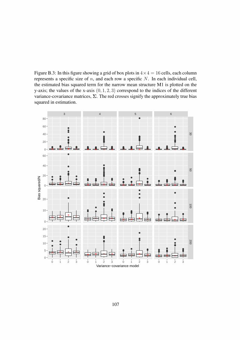
Figure B.3: In this figure showing a grid of box plots in 4×4 = 16 cells, each columnrepresents a specific size of n, and each row a specific N . In each individual cell,the estimated bias squared term for the narrow mean structure M1 is plotted on they-axis; the values of the x-axis (0, 1, 2, 3) correspond to the indices of the differentvariance-covariance matrices, Σ. The red crosses signify the approximately true biassquared in estimation.

3 4 5 6

3050

100200

0 1 2 3 0 1 2 3 0 1 2 3 0 1 2 3

0

20

40

60

80

0

20

40

60

0

10

20

0

5

10

15

20

Variance−covariance model

Bia

s sq

uare

d/N

107

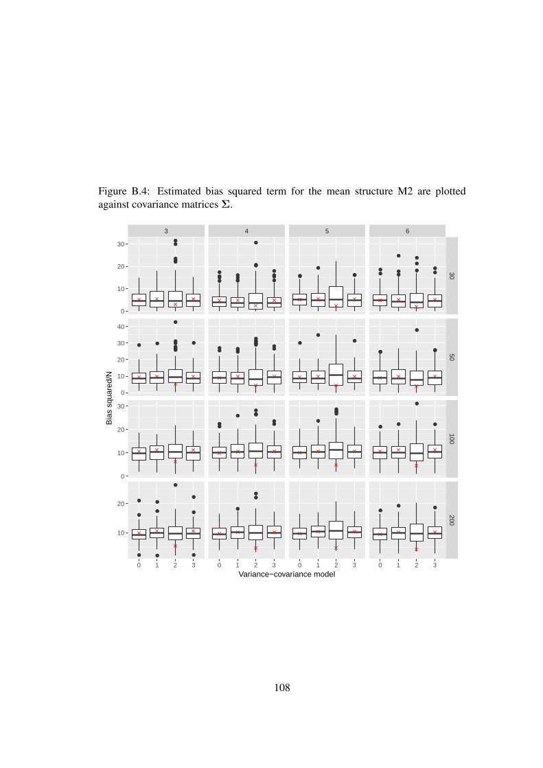
Figure B.4: Estimated bias squared term for the mean structure M2 are plottedagainst covariance matrices Σ.

3 4 5 6

3050

100200

0 1 2 3 0 1 2 3 0 1 2 3 0 1 2 3

0

10

20

30

0

10

20

30

40

0

10

20

30

10

20

Variance−covariance model

Bia

s sq

uare

d/N

108

Figure B.5: Estimated bias squared term for the mean structure M3 plotted againstcovariance matrices Σ.

3 4 5 6

3050

100200

0 1 2 3 0 1 2 3 0 1 2 3 0 1 2 3

0

1

2

3

0.0

0.2

0.4

0.6

0.8

0.00

0.05

0.10

0.15

0.20

0.000

0.025

0.050

0.075

0.100

Variance−covariance model

Bia

s sq

uare

d/N

109

Figure B.6: Estimated bias squared term for the mean structure M4 plotted againstcovariance matrices Σ.

3 4 5 6

3050

100200

0 1 2 3 0 1 2 3 0 1 2 3 0 1 2 3

0.000

0.005

0.010

0.000

0.002

0.004

0.006

0.008

0.00

0.01

0.02

0.03

0.0000

0.0025

0.0050

0.0075

0.0100

0.0125

Variance−covariance model

Bia

s sq

uare

d/N

110

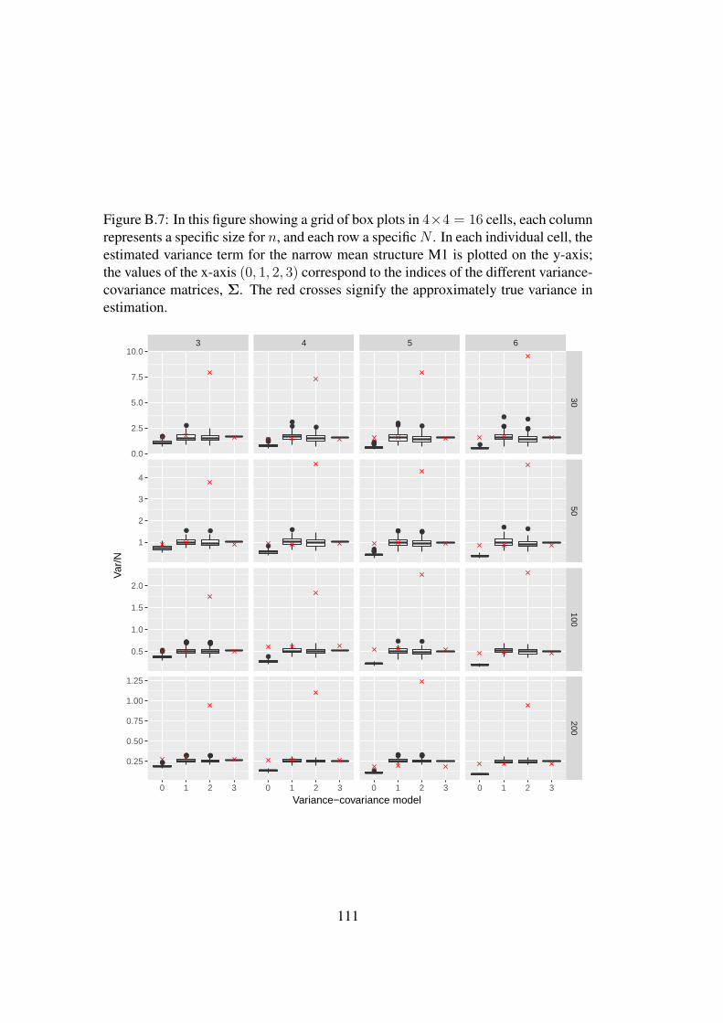
Figure B.7: In this figure showing a grid of box plots in 4×4 = 16 cells, each columnrepresents a specific size for n, and each row a specificN . In each individual cell, theestimated variance term for the narrow mean structure M1 is plotted on the y-axis;the values of the x-axis (0, 1, 2, 3) correspond to the indices of the different variance-covariance matrices, Σ. The red crosses signify the approximately true variance inestimation.

3 4 5 6

3050

100200

0 1 2 3 0 1 2 3 0 1 2 3 0 1 2 3

0.0

2.5

5.0

7.5

10.0

1

2

3

4

0.5

1.0

1.5

2.0

0.25

0.50

0.75

1.00

1.25

Variance−covariance model

Var

/N

111

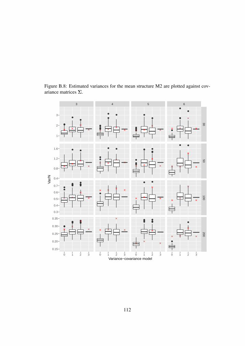
Figure B.8: Estimated variances for the mean structure M2 are plotted against cov-ariance matrices Σ.

3 4 5 6

3050

100200

0 1 2 3 0 1 2 3 0 1 2 3 0 1 2 3

1

2

3

0.4

0.8

1.2

1.6

0.3

0.4

0.5

0.6

0.7

0.15

0.20

0.25

0.30

0.35

Variance−covariance model

Var

/N

112

Figure B.9: Estimated variances for the mean structure M3 are plotted against cov-ariance matrices Σ.

3 4 5 6

3050

100200

0 1 2 3 0 1 2 3 0 1 2 3 0 1 2 3

1

2

3

4

5

1

2

3

0.5

1.0

1.5

0.2

0.3

0.4

0.5

0.6

Variance−covariance model

Var

/N

113

Figure B.10: Estimated variances for the mean structure M4 are plotted against cov-ariance matrices Σ.

3 4 5 6

3050

100200

0 1 2 3 0 1 2 3 0 1 2 3 0 1 2 3

1

2

3

4

5

1

2

3

0.3

0.6

0.9

1.2

1.5

0.2

0.3

0.4

0.5

0.6

Variance−covariance model

Var

/N

114

B.2 Tables from the simulations of Section 4.3.2

Σ 1 2 3 4

N n | M 1 2 1 2 1 2 1 2

30 3 2.3 (1.69) 6.5 (3.63) 3 (2.09) 6.9 (4.19) 7.4 (9.92) 8.1 (6.30) 2.8 (1.77) 6.7 (3.81)4 1.5 (1.41) 6 (3.80) 2.3 (1.36) 6.2 (3.74) 7.1 (8.60) 6.9 (5.49) 2.3 (1.49) 6.3 (4.03)5 1.1 (1.04) 6.5 (3.68) 2.1 (1.22) 6.9 (3.94) 8.7 (11.26) 8.2 (5.90) 2.1 (1.10) 6.9 (3.90)6 1.2 (1.12) 6.4 (4.10) 2.4 (1.46) 7.2 (4.85) 7.3 (10.24) 7 (5.48) 2.2 (1.14) 6.9 (4.33)

50 3 4 (3.12) 10 (4.85) 4.6 (3.51) 11 (5.36) 7.9 (9.45) 12 (7.45) 4.4 (3.33) 10 (5.14)4 2.8 (2.59) 10 (5.19) 3.4 (2.79) 11 (5.60) 6.8 (8.75) 11 (8.25) 3.3 (2.79) 11 (5.53)5 2.2 (2.32) 10 (5.16) 2.8 (2.68) 11 (5.72) 7.6 (8.75) 13 (9.04) 2.7 (2.48) 11 (5.50)6 2.1 (2.29) 10 (5.56) 2.8 (2.63) 11 (6.24) 4.6 (5.51) 11 (7.29) 2.7 (2.44) 11 (5.98)

100 3 3.9 (2.22) 10 (3.59) 4.3 (2.45) 11 (3.88) 6 (4.87) 11 (4.68) 4.2 (2.40) 10 (3.83)4 3 (2.10) 11 (4.00) 3.4 (2.31) 11 (4.31) 5 (4.81) 12 (5.52) 3.4 (2.28) 11 (4.25)5 2.3 (1.86) 11 (3.86) 2.7 (2.13) 11 (4.23) 5.1 (5.52) 12 (6.01) 2.7 (2.03) 11 (4.11)6 1.8 (1.48) 11 (3.75) 2.2 (1.66) 11 (4.07) 3.3 (4.06) 11 (5.48) 2.2 (1.62) 11 (3.99)

200 3 3.7 (1.80) 9.6 (2.90) 4.1 (1.94) 10 (3.07) 4.6 (3.75) 10 (3.89) 4 (1.95) 10 (3.09)4 2.5 (1.38) 10 (2.63) 2.9 (1.57) 11 (2.94) 3.7 (3.43) 11 (3.85) 2.9 (1.51) 11 (2.80)5 1.9 (1.15) 10 (2.56) 2.3 (1.26) 11 (2.70) 3.7 (3.62) 11 (3.97) 2.2 (1.27) 11 (2.73)6 1.5 (1.15) 9.8 (2.87) 1.8 (1.31) 10 (3.11) 2.3 (2.53) 10 (3.72) 1.8 (1.27) 10 (3.05)

Table B.1: The mean FIC scores (over all 100 simulations) divided byN as estimatesof the MSE for mean structures M1 and M2 and each situation (N, n,Σ) are shownalong with the corresponding standard deviation in brackets.

Σ 1 2 3 4

N n | M 3 4 3 4 3 4 3 4

30 3 1.5 (0.33) 1.6 (0.35) 2.4 (0.61) 2.4 (0.61) 2.4 (0.62) 2.4 (0.61) 2.4 (0.02) 2.4 (0.00)4 1.3 (0.27) 1.4 (0.30) 2.5 (0.66) 2.5 (0.66) 2.4 (0.66) 2.4 (0.67) 2.4 (0.02) 2.4 (0.00)5 1.1 (0.23) 1.2 (0.27) 2.4 (0.71) 2.4 (0.71) 2.2 (0.69) 2.3 (0.70) 2.4 (0.03) 2.4 (0.00)6 .96 (0.18) 1.1 (0.21) 2.5 (0.71) 2.5 (0.71) 2.3 (0.78) 2.3 (0.71) 2.4 (0.03) 2.4 (0.00)

50 3 1.1 (0.18) 1.2 (0.20) 1.8 (0.34) 1.8 (0.34) 1.8 (0.35) 1.8 (0.35) 1.9 (0.02) 1.9 (0.00)4 .93 (0.15) 1.1 (0.18) 1.9 (0.36) 1.9 (0.36) 1.8 (0.38) 1.8 (0.37) 1.8 (0.03) 1.8 (0.00)5 .76 (0.13) .9 (0.15) 1.8 (0.41) 1.8 (0.41) 1.7 (0.40) 1.7 (0.41) 1.8 (0.02) 1.8 (0.00)6 .68 (0.11) .83 (0.13) 1.9 (0.42) 1.9 (0.41) 1.7 (0.41) 1.8 (0.42) 1.8 (0.03) 1.8 (0.00)

100 3 .61 (0.07) .67 (0.08) .97 (0.15) .97 (0.15) .96 (0.15) .97 (0.16) .98 (0.01) .99 (0.00)4 .49 (0.05) .57 (0.06) .99 (0.13) .99 (0.13) .97 (0.14) .98 (0.14) .98 (0.01) .98 (0.00)5 .41 (0.04) .49 (0.06) .98 (0.15) .99 (0.15) .95 (0.15) .96 (0.15) .97 (0.02) .98 (0.00)6 .36 (0.04) .44 (0.05) .99 (0.15) 1 (0.14) .96 (0.15) .97 (0.15) .97 (0.02) .97 (0.00)

200 3 .3 (0.03) .33 (0.03) .48 (0.05) .48 (0.05) .48 (0.05) .48 (0.05) .48 (0.00) .48 (0.00)4 .24 (0.02) .28 (0.02) .48 (0.05) .48 (0.05) .47 (0.05) .47 (0.05) .47 (0.01) .48 (0.00)5 .2 (0.02) .24 (0.02) .48 (0.05) .48 (0.05) .47 (0.05) .48 (0.05) .47 (0.01) .47 (0.00)6 .17 (0.01) .21 (0.01) .47 (0.04) .48 (0.04) .47 (0.04) .47 (0.04) .47 (0.01) .47 (0.00)

Table B.2: The mean FIC scores (over all 100 simulations) divided byN as estimatesof the MSE for M3 and M4 and each situation (N, n,Σ) are shown along with thecorresponding standard deviation in brackets.

115

Appendix C

Derivation of the MSPE formula (5.23)

The mean squared error in prediction (5.22), unlike the MSE, is not expressible as asum of variances and squared biases. It can, however, be written as

E[µoᵀS,iµoS,i − 2µoᵀS,iµi + µᵀ

iµi]

=E[µoᵀS,iµoS,i]− E[µoS,i]

ᵀE[µoS,i] + E[µoS,i]ᵀE[µoS,i]− 2E[µoᵀS,iµi] + E[µᵀ

iµi]

= TrCov(µoS,i)+ E[µoS,i]ᵀE[µoS,i]− 2E[µoᵀS,iµi] + E[µᵀ

iµi], (C.1)

where the first two terms on the right hand side of the first equality have been ex-pressed as the sum of the uncertainties in each entry of the predictor. In the fol-lowing, expressions will be derived for the above four terms. And, thereby, formula(5.23), for comparison of LME models (with different fixed effects) in terms of meansquared prediction error, is arrived at.

For the uncertainty in the predictor, we have

Cov(µoS,i) = Cov(XS,iαoS +Zib

o

S,i) = XS,iCov(αoS)XᵀS,i +ZiCov(b

o

S,i)Zᵀi

= XS,iBo−1S Xᵀ

S,i +ZiCov(bo

S,i)Zᵀi , (C.2)

where the second equality follows since Cov(αoS, bo

S,i) = 0 (Henderson 1975); thethird equality by (5.8); and where, as in (2.22),

Cov(bo

S,i) = V oi

Σoi −XS,i

(N∑i=1

XS,iΣo−1i Xᵀ

S,i

)−1

XᵀS,i

V oᵀi , (C.3)

where V oi = DoZᵀ

iΣo−1i .

For the second term of (C.1), we will require E[µoS,i], which, by (5.3), (5.21),and assuming (5.20) is the true model, is equal to

E[XS,iαoS +Zib

o

S,i] = XS,iAoSα+ZiD

oZᵀiΣ

o−1i E[yi −XS,iα

oS]

= [XS,iAoS +ZiV

oi (X i −XS,iA

oS)]α =··W o

S,iα, (C.4)

whereAoS is as in (5.5).

It is fruitful to express the cross-term in (C.1) as

E[µoᵀS,iµi] = TrCov(µoS,i,µi)+ E[µoS,i]ᵀE[µi], (C.5)

117

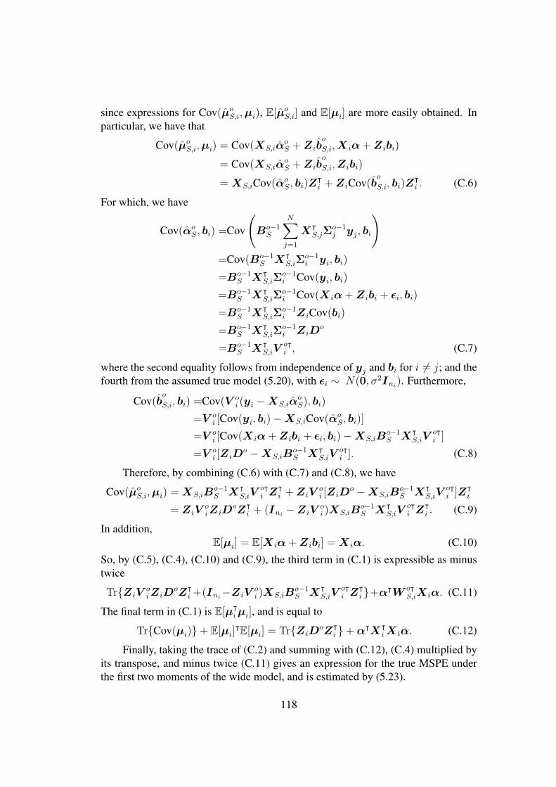
since expressions for Cov(µoS,i,µi), E[µoS,i] and E[µi] are more easily obtained. Inparticular, we have that

Cov(µoS,i,µi) = Cov(XS,iαoS +Zib

o

S,i,X iα+Zibi)

= Cov(XS,iαoS +Zib

o

S,i,Zibi)

= XS,iCov(αoS, bi)Zᵀi +ZiCov(b

o

S,i, bi)Zᵀi . (C.6)

For which, we have

Cov(αoS, bi) =Cov

(Bo−1S

N∑j=1

XᵀS,jΣ

o−1j yj, bi

)=Cov(Bo−1

S XᵀS,iΣ

o−1i yi, bi)

=Bo−1S Xᵀ

S,iΣo−1i Cov(yi, bi)

=Bo−1S Xᵀ

S,iΣo−1i Cov(X iα+Zibi + εi, bi)

=Bo−1S Xᵀ

S,iΣo−1i ZiCov(bi)

=Bo−1S Xᵀ

S,iΣo−1i ZiD

o

=Bo−1S Xᵀ

S,iVoᵀi , (C.7)

where the second equality follows from independence of yj and bi for i 6= j; and thefourth from the assumed true model (5.20), with εi ∼ N(0, σ2Ini). Furthermore,

Cov(bo

S,i, bi) =Cov(V oi (yi −XS,iα

oS), bi)

=V oi [Cov(yi, bi)−XS,iCov(αoS, bi)]

=V oi [Cov(X iα+Zibi + εi, bi)−XS,iB

o−1S Xᵀ

S,iVoᵀi ]

=V oi [ZiD

o −XS,iBo−1S Xᵀ

S,iVoᵀi ]. (C.8)

Therefore, by combining (C.6) with (C.7) and (C.8), we have

Cov(µoS,i,µi) = XS,iBo−1S Xᵀ

S,iVoᵀi Z

ᵀi +ZiV

oi [ZiD

o −XS,iBo−1S Xᵀ

S,iVoᵀi ]Zᵀ

i

= ZiVoiZiD

oZᵀi + (Ini −ZiV

oi )XS,iB

o−1S Xᵀ

S,iVoᵀi Z

ᵀi . (C.9)

In addition,E[µi] = E[X iα+Zibi] = X iα. (C.10)

So, by (C.5), (C.4), (C.10) and (C.9), the third term in (C.1) is expressible as minustwice

TrZiVoiZiD

oZᵀi +(Ini−ZiV

oi )XS,iB

o−1S Xᵀ

S,iVoᵀi Z

ᵀi +αᵀW oᵀ

S,iX iα. (C.11)

The final term in (C.1) is E[µᵀiµi], and is equal to

TrCov(µi)+ E[µi]ᵀE[µi] = TrZiD

oZᵀi +αᵀXᵀ

iX iα. (C.12)

Finally, taking the trace of (C.2) and summing with (C.12), (C.4) multiplied byits transpose, and minus twice (C.11) gives an expression for the true MSPE underthe first two moments of the wide model, and is estimated by (5.23).

118

Appendix D

D.1 R code

The code for the data illustrations in this thesis, written using the software R (RDevelopment Core Team 2008), were all of a similar form. The narrow and widemodels are typically fit to the data first. The wide model provides estimates of thenecessary quantities for the FIC. The narrow is dealt with separately, then all othermodels are fit within a loop and the FIC scores are simultaneously calculated. Anexample is given in Listing D.2. For the AFIC this procedure is repeated withina bigger loop for the different foci. Listing D.1 gives the data preparation for theRiesby depression dataset.

Listing D.1: Prepare Riesby depression dataset.r i e sbynow <− read . t a b l e ( " h t t p : / / h e d e k e r . p e o p l e . u i c . edu / RIESBY .DAT.

t x t " , nrows = 396 , na . s t r i n g s = " . " )

colnames ( r i e sbynow ) <− c ( " i d " , " hd " , " i n t c p t " , " week " , " endo " , "i n t e r a c t i o n " ) #0=’NonEndog ’ 1=’Endog ’

l i b r a r y ( p l y r )

s e a r c h c o l s <− c ( ’ hd ’ ) # d e l e t e i n d i v i d u a l s w i t h m i s s i n g da tar i e s b y <−ddp ly ( r iesbynow , " i d " , f u n c t i o n ( x ) i f ( any ( i s . na ( x [ ,

s e a r c h c o l s ] ) ) ) NULL e l s e x )r i e s b y $ i d 2 <−rep ( 1 : 4 6 , each =6)

# s e t b a s e l i n e as c o v a r i a t ebase <− ddp ly ( r i e s b y , " i d 2 " , f u n c t i o n ( x ) rep ( x [ 1 , 2 ] , l e n g t h ( x [ , 2 ] )

) )colnames ( ba se )<− c ( " i d 2 " , " y1 " , " y2 " , " y3 " , " y4 " , " y5 " , " y6 " )base . now <− r e s h a p e ( base , d i r e c t i o n =" long " , v a r y i n g = c ( " y1 " , " y2 "

, " y3 " , " y4 " , " y5 " , " y6 " ) , sep = " " , i d v a r = " i d 2 " )base . now <− base . now [ order ( ba se . now$ i d 2 ) , ]r i e s b y $ base <− base . now [ , 3 ]

r i e s b y <− s u b s e t ( r i e s b y , week >0) # o n l y da ta from t r e a t m e n t p e r i o d

# c ( " nonendo " , " endo " ) = c ( 0 , 1 )r i e s b y $ endo . f <− f a c t o r ( r i e s b y $ endo , l a b e l s = c ( "Non−endo " , " Endo " )

)r i e s b y $week . f <− f a c t o r ( r i e s b y $week , l a b e l s = 0 : 4 )

r i e s b y $ time <− r i e s b y $week # c e n t e r t i m er i e s b y $ t i m e c <− r i e s b y $ time − mean ( r i e s b y $ time )r i e s b y $ t i m e s q <− r i e s b y $ t i m e c ^2

119

r i e s b y $ b a s e c <− r i e s b y $ base − mean ( r i e s b y $ base ) # c e n t e r b a s e l i n e

Listing D.2: FIC for depression data set predictions.l i b r a r y ( nlme )

b0 <− 27− mean ( r i e s b y $ base ) # h igh s c o r e r a t b a s e l i n et 0 <− 2 # end o f week 4 # c e n t r e d t i m e i s 2e0 <− 0 #non−endogeneous

# needed f o r e s t i m a t e o f f o c u sxu0xp0 <− c ( 1 , b0 , t0 , e0 , e0 * t0 , t 0 ^2 , e0 * t 0 ^2 )

# narrown a r r . f <− formula ( hd~ 1 + b a s e c + t i m e c )nar row <− g l s ( n a r r . f , c o r r e l a t i o n = corExp ( form=~ time | id2 , n ug ge t

= T ) ,weight s = varExp ( form=~ time | endo ) , #AIC

f a v o u r e dmethod = "ML" , data = r i e s b y )

# widewide . f <− formula ( hd~ 1 + b a s e c + t i m e c + endo + t i m e s q + t i m e c :

endo + t i m e s q : endo )wide <− g l s ( wide . f , c o r r e l a t i o n = corExp ( form=~ time | id2 , n ug ge t =

T ) , weight s = varExp ( form=~ time | endo ) , #AIC f a v o u r e ddata = r i e s b y ) #By REML

Sigma . non <− getVarCov ( wide , i n d i v i d u a l = " 2 " ) #non−endoSigma . endo <− getVarCov ( wide , i n d i v i d u a l = " 3 " ) # endo

# p r o t e c t e d and u n p r o t e c t e d d e s i g n m a t r i c e sXP <− cbind ( 1 , r i e s b y $ basec , r i e s b y $ t i m e c )XU <− cbind ( r i e s b y $ endo , r i e s b y $ t imesq , r i e s b y $ t i m e c * r i e s b y $ endo ,

r i e s b y $ t i m e s q * r i e s b y $ endo )XX <− cbind (XP , XU) # wide d e s i g n

NN <− 46 # number o f i n d i v i d u a l snn <− 5 # each o f 5 measurementsp1 <− 5 # 1 sigma , 2 v a r i a n c e , 1 corr , 1 nu gge tp2 <− 3 # p r o t e c t e d r e g r e s s i o n p a r a m e t e r sqq <− 4 # u n p r o t e c t e d r e g r e s s i o n p a r a m e t e r spp <− p1+p2

MM <− 2^ qq # number o f models

# g e t e s t i m a t e o f J h a tJ h a t <− matrix ( rep (NA, ( pp+qq ) * ( pp+qq ) ) , nrow = ( pp+qq ) , nco l = ( pp

+qq ) )J r e g <− NULLsumnow <− l i s t ( )

120

f o r ( i i n 1 :NN) XXnow <− s u b s e t (XX, r i e s b y $ i d 2 == i )Sigmanow <− getVarCov ( wide , i n d i v i d u a l = i )sumnow [ [ i ] ] <− t (XXnow) %*% s o l v e ( Sigmanow ) %*% XXnow

J r e g <− (1 /NN) * Reduce ( "+" , sumnow )J h a t [− (1 : p1 ) ,− (1 : p1 ) ] <− J r e g

JBB <− J h a t [ ( p1 +1) : pp , ( p1 +1) : pp ]JGB <− J h a t [ ( pp +1) : ( pp+qq ) , ( p1 +1) : pp ]JGG <− J h a t [ ( pp +1) : ( pp+qq ) , ( pp +1) : ( pp+qq ) ]JBG <− t ( JGB )

# p a r t i a l d e r i v a t i v e sdmudbeta <− c ( 1 , b0 , t 0 )dmudgamma <− c ( e0 , t 0 *e0 , t 0 ^2 , ( t 0 ^2 ) * e0 )

#FIC q u a n t i t i e st a u 0 s q <− t ( dmudbeta ) %*% s o l v e ( JBB ) %*% dmudbetat a u 0 <− s q r t ( t a u 0 s q )omega <− ( JGB %*% s o l v e ( JBB ) %*% dmudbeta ) − dmudgammaQQ <− s o l v e ( JGG − JGB %*% s o l v e ( JBB ) %*% JBG )Dn <− s q r t (NN) * ( c o e f ( wide ) [ ( p2 +1) : ( p2+qq ) ] )I <− diag ( qq )

c o m b i n a t i o n s = f u n c t i o n ( n ) # as from l e c t u r e s comb = NULL

f o r ( i i n 1 : n )comb = rbind ( cbind ( 0 , comb ) , cbind ( 1 , comb ) )re turn ( comb )

s u b s e t s <− c o m b i n a t i o n s ( qq )

# s t o r a g e spacemodout <− l i s t ( ) ; FIC <− NULL; AIC <− NULL b i a s <− NULL ;b i a s . sq <− NULL ; b i a s . sq . t <− NULL ; var <− NULL ;muhat <− NULL ; num . param <− NULL ; num . qq <− NULL

# narrowb i a s [ 1 ]<− t ( omega ) %*% Dnb i a s . sq [ 1 ] <− t ( omega )%*% ( Dn %*% t ( Dn ) − QQ ) %*% omegab i a s . sq . t [ 1 ] <− max ( 0 , b i a s . sq [ 1 ] )var [ 1 ]<− t a u 0 ^2FIC [ 1 ] <− b i a s . sq . t [ 1 ] + var [ 1 ]AIC [ 1 ] <− −(AIC ( narrow ) )num . param [ 1 ] <− ppnum . qq [ 1 ] <− 0muhat [ 1 ] <− t ( xu0xp0 )%*% c ( c o e f ( nar row ) , rep ( 0 , qq ) )

f o r ( k i n 2 : nrow ( s u b s e t s ) ) # f o r r e s t o f models

# d e f i n e s u b s e t o f u n p r o t e c t e d params

121

where <− ( 1 : qq ) [ s u b s e t s [ k , ] == 1]dims <− l e n g t h ( where )

# f i t modelsp r o t <− c ( " 1 " , " b a s e c " , " t i m e c " )u n p r o t <− c ( " endo " , " t i m e s q " , " t i m e c : endo " , " t i m e s q : endo " )vec <− c ( p r o t , u n p r o t [ s u b s e t s [ k , ] == 1 ] )

meannow <− p a s t e ( vec , c o l l a p s e = "+" )formula <− as . formula ( p a s t e ( " hd ~ " , meannow , sep = " " ) )

modout [ [ k ] ] <− g l s ( formula ,c o r r e l a t i o n = corExp ( form=~ time | id2 , n ug ge t = T ) ,weight s = varExp ( form=~ time | endo ) , #AIC

f a v o u r i t e c o v a r i a n c emethod = "ML" , data = r i e s b y )

#FICpiS <− I [ where , ] # p r o j e c t i o n m a t r i c e sdim ( p iS ) <− c ( dims , qq )QS <− s o l v e ( p iS %*% s o l v e (QQ) %*% t ( p iS ) )GS <− t ( p iS ) %*% QS %*% p iS %*% s o l v e (QQ)#b i a s . sq [ k ] <− t ( omega ) %*% ( I − GS) %*% ( Dn %*% t ( Dn ) − QQ ) %*%

t ( I − GS) %*% omegab i a s . sq . t [ k ] <− max ( 0 , b i a s . sq [ k ] )b i a s [ k ] <− t ( omega ) %*% ( I − GS) %*% Dnvar [ k ] <− t a u 0 ^2 + t ( omega ) %*% GS %*% QQ %*% t (GS) %*% omega#FIC [ k ] <− b i a s . sq . t [ k ] + var [ [ k ] ]

# f o c u s e s t i m a t eMLest <− 0* ( 1 : ( p2+qq ) )MLnow <− c o e f ( modout [ [ k ] ] )MLest [ 1 : p2 ] <− MLnow [ 1 : p2 ]MLest [ p2+where ] <− MLnow [ ( p2 +1) : l e n g t h (MLnow) ]muhat [ k ] <− t ( xu0xp0 ) %*% MLest#AIC [ k ] <− −AIC ( modout [ [ k ] ] )num . param [ k ] <− pp + dimsnum . qq [ k ] <− dims

122

Bibliography

Breiman, L. (1992), ‘The little bootstrap and other methods for dimensionality selec-tion in regression: X-fixed prediction error’, Journal of the American StatisticalAssociation 87(419), 738–754.

Broström, G. (2017), glmmML: Generalized Linear Models with Clustering. R pack-age version 1.0.2.URL: https://CRAN.R-project.org/package=glmmML

Bryk, A. S. & Raudenbush, S. W. (1992), Hierarchical linear models: applicationsand data analysis methods, Sage Publications.

Casella, G. & Berger, R. L. (2002), Statistical inference, Vol. 2, Duxbury PacificGrove, CA.

Claeskens, G. & Hjort, N. L. (2003), ‘The focused information criterion’, Journal ofthe American Statistical Association 98(464), 900–916.

Claeskens, G., Hjort, N. L. et al. (2008), Model selection and model averaging, Vol.330, Cambridge University Press Cambridge.

Cressie, N. & Wikle, C. K. (2011), Statistics for Spatio-Temporal Data, John Wiley& Sons.

Cunen, C., Walloe, L. & Hjort, N. L. (2017), ‘Decline in energy storage in antarcticminke whales during the jarpa period: Assessment via the focussed informationcriterion (fic)’.

Cunen, C., Walloe, L. & Hjort, N. L. (2018), ‘Focused model selection for linearmixed models, with an application to whale ecology’.

De Jong, P., Heller, G. Z. et al. (2008), Generalized linear models for insurance data,Vol. 10, Cambridge University Press Cambridge.

Demidenko, E. (2013), Mixed models: theory and applications with R, John Wiley& Sons.

Fitzmaurice, G. M., Laird, N. M. & Ware, J. H. (2004a), Applied longitudinal ana-lysis, John Wiley & Sons.

Fitzmaurice, G. M., Laird, N. M. & Ware, J. H. (2004b), ‘Applied longitudinal ana-lysis toenail dataset’.URL: https://content.sph.harvard.edu/fitzmaur/ala2e/

123

Galecki, A. & Burzykowski, T. (2013), Linear Mixed-Effects Models Using R: AStep-by-Step Approach, Springer Science & Business Media.

Genz, A. & Bretz, F. (2009), Computation of Multivariate Normal and t Probabilit-ies, Lecture Notes in Statistics, Springer-Verlag, Heidelberg.

Genz, A., Bretz, F., Miwa, T., Mi, X., Leisch, F., Scheipl, F. & Hothorn, T. (2017),mvtnorm: Multivariate Normal and t Distributions. R package version 1.0-6.URL: https://CRAN.R-project.org/package=mvtnorm

Gregoire, T. G., Brillinger, D. R., Diggle, P., Russek-Cohen, E., Warren, W. G. &Wolfinger, R. D. (2012), Modelling longitudinal and spatially correlated data,Vol. 122, Springer Science & Business Media.

Greven, S. & Kneib, T. (2010), ‘On the behaviour of marginal and conditional aic inlinear mixed models’, Biometrika 97(4), 773–789.

Gumedze, F. & Dunne, T. (2011), ‘Parameter estimation and inference in the linearmixed model’, Linear Algebra and its Applications 435(8), 1920 – 1944.

Hamilton, M. (1960), ‘A Rating Scale for Depression’, Journal of Neurology,Neurosurgery & Psychiatry 23(1), 56–62.

Harville, D. A. (1997), Matrix algebra from a statistician’s perspective, Vol. 1,Springer.

Hedeker, D. (2006), ‘Riesby depression dataset’.URL: http://hedeker.people.uic.edu/long.html

Hedeker, D. & Gibbons, R. D. (2006), Longitudinal Data Analysis, John Wiley &Sons.

Henderson, C. R. (1975), ‘Best linear unbiased estimation and prediction under aselection model’, Biometrics pp. 423–447.

Hjort, N. L. & Claeskens, G. (2003), ‘Frequentist model average estimators’, Journalof the American Statistical Association 98(464), 879–899.

Hlavac, M. (2015), stargazer: Well-Formatted Regression and Summary StatisticsTables, Harvard University, Cambridge, USA. R package version 5.2.URL: http://CRAN.R-project.org/package=stargazer

Hofert, M. & Mächler, M. (2016), ‘Parallel and other simulations in R made easy:An end-to-end study’, Journal of Statistical Software 69(4), 1–44.

Kackar, R. N. & Harville, D. A. (1984), ‘Approximations for standard errors of estim-ators of fixed and random effects in mixed linear models’, Journal of the AmericanStatistical Association 79(388), 853–862.

124

Laird, N. M. & Ware, J. H. (1982), ‘Random-Effects Models for Longitudinal Data’,Biometrics 38(4), 963–974.

Liang, K.-Y. & Zeger, S. L. (1986), ‘Longitudinal data analysis using generalizedlinear models’, Biometrika 73(1), 13–22.

Mardia, K. V. & Marshall, R. J. (1984), ‘Maximum likelihood estimation of modelsfor residual covariance in spatial regression’, Biometrika 71(1), 135–146.

McCulloch, C. E. & Searle, S. R. (2001), Generalized, Linear, and Mixed Models,Wiley Series in Probability and Statistics.

McNeish, D., Stapleton, L. M. & Silverman, R. D. (2017), ‘On the unnecessaryubiquity of hierarchical linear modeling’, Psychological Methods 22(1), 114–140.

Pinheiro, J., Bates, D., DebRoy, S., Sarkar, D. & R Core Team (2016), nlme: Linearand Nonlinear Mixed Effects Models. R package version 3.1-128.URL: http://CRAN.R-project.org/package=nlme

R Development Core Team (2008), R: A Language and Environment for StatisticalComputing, R Foundation for Statistical Computing, Vienna, Austria.URL: http://www.R-project.org

Rosenthal, R. & Rosnow, R. L. (1991), Essentials of Behavioral Research: Methodsand Data Analysis, McGraw-Hill.

Saefken, B., Ruegamer, D., Kneib, T. & Greven, S. (2018a), cAIC4: ConditionalAkaike information criterion for lme4.

Saefken, B., Ruegamer, D., Kneib, T. & Greven, S. (2018b), ‘Conditional modelselection in mixed-effects models with caic4’, ArXiv e-prints .

Sarkar, D. (2008), Lattice: Multivariate Data Visualization with R, Springer, NewYork. ISBN 978-0-387-75968-5.URL: http://lmdvr.r-forge.r-project.org

Searle, S. (1971), Linear Models, number v. 1 in ‘Wiley Publication in MathematicalStatistics’, John Wiley & Sons.

Smyth, G. K. (2005), ‘Numerical integration’, Encyclopedia of Biostatisticspp. 3088–3095.

Stroup, W. W. (2012), Generalized linear mixed models: modern concepts, methodsand applications, CRC press.

Vaida, F. & Blanchard, S. (2005), ‘Conditional akaike information for mixed-effectsmodels’, Biometrika 92(2), 351–370.

125

Wand, M. (2007), ‘Fisher information for generalised linear mixed models’, Journalof Multivariate Analysis 98(7), 1412–1416.

Wickham, H. (2009), ggplot2: Elegant Graphics for Data Analysis, Springer-VerlagNew York.URL: http://ggplot2.org

Wickham, H. (2011), ‘The split-apply-combine strategy for data analysis’, Journalof Statistical Software 40(1), 1–29.URL: http://www.jstatsoft.org/v40/i01/

Yang, H., Lin, P., Zou, G. & Liang, H. (2017), ‘Variable selection and modelaveraging for longitudinal data incorporating gee approach’, Statistica Sinica27(1), 389–413.

Zimmerman, M., Martinez, J. H., Young, D., Chelminski, I. & Dalrymple, K. (2013),‘Severity classification on the hamilton depression rating scale’, Journal of affect-ive disorders 150(2), 384–388.

126