Fluctuation effects in rotating Bose-Einstein condensates with broken SU(2) and U(1)× U(1)symmetries in the presence of intercomponent density-density interactions.

Peder Notto Galteland,1 Egor Babaev,2 and Asle Sudbø1

1Department of Physics, Norwegian University of Science and Technology, N-7491 Trondheim, Norway2Department of Theoretical Physics, The Royal Institute of Technology, 10691 Stockholm, Sweden

(Dated: February 3, 2015)

Thermal fluctuations and melting transitions for rotating single-component superfluids have been intensivelystudied and are well understood. In contrast, the thermal effects on vortex states for two-component superfluidswith density-density interaction, which have a much richer variety of vortex ground states, have been muchless studied. Here, we investigate the thermal effects on vortex matter in superfluids with U(1)× U(1) brokensymmetries and intercomponent density-density interactions, as well as the case with a larger SU(2) brokensymmetry obtainable from the U(1) × U(1)-symmetric case by tuning scattering lengths. In the former casewe find that, in addition to first-order melting transitions, the system exhibits thermally driven phase transitionsbetween square and hexagonal lattices. Our main result, however, concerns the case where the condensateexhibits SU(2)-symmetry, and where vortices are not topological. At finite temperature, the system exhibitseffects which do not have a counter-part in single component systems. Namely, it has a state where thermallyaveraged quantities show no regular vortex lattice, yet the system retains superfluid coherence along the axisof rotation. In such a state, the thermal fluctuations result in transitions between different (nearly)-degeneratevortex states without undergoing a melting transition. Our results apply to multi-component Bose-Einsteincondensates, and we suggest how to experimentally detect some of these unusual effects in such systems.

PACS numbers: 67.25.dk, 67.60.Bc,67.85.Fg,67.85.Jk

I. INTRODUCTION

Bose-Einstein condensates (BECs) with a multicomponentorder parameter, and the topological defects such systems sup-port, represent a topic of great current interest in condensedmatter physics.1–15 Such multicomponent condensates may berealized as mixtures of different atoms, mixtures of differentisotopes of an atom, or mixtures of different hyperfine spinstates of an atom. The interest in such condensates from afundamental physics point of view is mainly attributed to thefact that one may tune various interaction parameters over awide range in a BEC. This enables the study of a variety ofphysical effects which are not easily observed in other super-fluid systems such as He3 and He4.

The behavior of a single-component BEC under rotation iswell known. The ground state is a hexagonal lattice of vortexdefects which melts to a vortex liquid via a first-order phasetransition. This is well described by the London model, whereamplitude fluctuations may be ignored. Over the years, in thecontext of studying vortex lattice melting in high-Tc super-conductors, many works have confirmed this through numeri-cal Monte Carlo simulations for systems in the frozen gauge,three-dimensional (3D) XY and Villain approximations,16–25

as well as in the lowest-Landau-level approximation,26 andby mapping it to a model of 2D bosons.27 Single compo-nent condensates have been available experimentally for quitesome time28,29, and the hexagonal lattice ground state has beenverified.30

Condensates with two components of the order parameterhave also been studied extensively. Analytical works focus-ing on determining the T = 0 ground states have demon-strated interesting vortex solutions and a range of unusuallattice structures5,6,10,13,14,31,32. By varying the ratio betweeninter- and intra-component couplings, the ground-state lat-

tice undergoes a structural change from hexagonal symmetrythrough square symmetry to double-core lattices and interwo-ven sheets of vortices. Similar systems with three compo-nents have also been studied.15 Experimentally, spinor con-densates have been realized in two general classes of systems.The first option is to use one species of atoms, usually rubid-ium, and prepare it in two separate hyperfine spin states.1,2

Vortices3 and vortex lattices7 have been realized in these bi-nary mixtures, where both hexagonal and square vortex latticestates were observed. The other option is to mix condensatesof two different species of atoms.4,12 The use of Feshbachresonances33,34 allows direct tuning of the scattering lengths,and by extension the inter- and intracomponent interactions ofmulticomponent condensates.8,9,11

In this paper, we consider a specific model of a two-component BEC, which has the full range of fluctuations ofthe order parameter field included, as well as intercompo-nent density-density interactions. We consider the model withU(1)×U(1)- and as SU(2) symmetries. For the U(1)×U(1)case, we find a succession of square and hexagonal vor-tex ground-state patterns as the intercomponent interactionstrength is varied, along with the possibility of thermal re-construction from a square to a hexagonal vortex lattice astemperature is reduced.

The SU(2)-symmetric case is interesting and experimen-tally realizable. In this case U(1)-vortices are no longer topo-logical, in contrast to the U(1)×U(1)-symmetric case. In thiscase, when fluctuation effects are included we find a highlyunusual vortex state where there is no sign of any vortex lat-tice. Nonetheless, global phase coherence persists. This stateof vortex matter is a direct consequence of massless amplitudefluctuations in the order parameter, when the broken symme-try of the system is SU(2). At the SU(2) point, but at lowertemperatures, we also observe dimerized vortex ground-state

arX

iv:1

501.

0727

8v1

[co

nd-m

at.q

uant

-gas

] 2

8 Ja

n 20

15

2

patterns.The paper is organized as follows. The model and defini-

tions of relevant quantities are presented in Section II. Thetechnical details of the Monte Carlo simulations are brieflyconsidered in Section III. In Section IV, the results are pre-sented and discussed. In Section V, we discuss how to ex-perimentally verify the results we find. Some technical de-tails, and the investigation of the order of the melting transi-tions with full amplitude distributions included, for the casesN = 1 and N = 2, are relegated to Appendixes.

II. MODEL AND DEFINITIONS

In this section we present the model used in the paper, firstin a continuum description and then on a three-dimensionalcubic lattice appropriate for Monte Carlo simulations. Therelevant quantities for the discussion are also defined.

A. Continuum model

We consider a general Ginzburg-Landau(GL) model of anN -component Bose-Einstein condensate, coupled to a uni-form external field, which in the thermodynamical limit is de-fined as

Z =

∫ N∏i

Dψ′ie−βH , (1)

where

H =

∫d3r

[N∑i=1

3∑µ=1

~2

2mi

∣∣∣∣(∂µ − i2π

Φ0A′µ)ψ′i

∣∣∣∣2

+

N∑i

α′i |ψ′i|2

+

N∑i,j=1

g′ij |ψ′i|2 ∣∣ψ′j∣∣2

](2)

is the Hamiltonian. Here, the field A′µ formally appears as anon-fluctuating gauge-field and parametrizes the angular ve-locity of the system. The fields ψ′i are dimensionful complexfields, i and j are indices running from 1 to N denoting thecomponent of the order parameter (a “color” index), α′i andg′ij are Ginzburg-Landau parameters, Φ0 = h/2e is the thecoupling constant to the rotation induced vector potential, andmi is the particle mass of species i. For mixtures consisting ofdifferent atoms or different isotopes of one atom, the masseswill depend on the index i, while for mixtures consisting ofatoms in different hyperfine spin states, the masses are inde-pendent of i. The inter- and intracomponent coupling parame-ters g′ij are related to real inter- and intracomponent scatteringlengths, aij , in the following way

g′ii =4π~2aiimi

, (3)

g′ij =8π~2aijmij

, (i 6= j) (4)

where mij = mi mj/(mi + mj) is the reduced mass. Inthis paper we focus on using BECs of homonuclear gaseswith several components in different hyperfine states, hencemi = m ∀ i. Inter-component drag in BEC mixtures has beenconsidered in previous works using Monte-Carlo simulation(ignoring amplitude fluctuations), but we will not consider thiscase here.35–39

We find it convenient for our purposes to rewrite (2) onthe following form, the details of which are relegated to Ap-pendix A,

H =

∫d3r

[1

2(DµΨ)†(DµΨ) + V (Ψ)

]. (5)

Here, Ψ is an N -component spinor of dimensionless com-plex fields, which consists of an amplitude and a phase, ψi =|ψi| exp (iθi), Dµ = ∂µ − i 2π

Φ0A′µ is the covariant derivative,

and summation over repeated spatial indices is implied. Weneglect, for simplicity, the presence of a trap and the centrifu-gal part of the potential. We consider only the case where thevector potential is applied to each component of Ψ, as followsfrom the fact that the masses are independent of species-indexi.

We have studied this model in detail withN = 2, where wewrite the potential in the form

V (Ψ) = η(|Ψ|2 − 1)2 + ω(Ψ†σzΨ)2. (6)

This formulation is more relevant for our discussion, as it im-mediately highlights the symmetry of Ψ, as well as the softconstraints applied to it. The details of the reparametrizationare shown in Appendix A.

Note that Eq. 6 may also be rewritten in the form (correctup to an additive constant term)

V = (η + ω)(|ψ1|4 + |ψ2|4) + 2(η − ω) |ψ1|2 |ψ2|2 . (7)

Comparing with Eq. 2, we have g11 = g22 ≡ g = η + ω andg12 = η − ω. The model features repulsive inter-componentinteractions provided η − ω > 0, and this is the case we willmainly focus on. We will however briefly touch upon the caseη − ω < 0 corresponding to an attractive inter-componentdensity-density interaction, which leads to ground states withoverlapping vortices in components 1 and 2. Normalizabilityof the individual order parameter components, or equivalentlyboundedness from below of the free energy, requires that η +ω > 0. Thus, while ω > η makes physical sense, ω < −ηdoes not. In this paper, we assume η > 0 and ω ≥ 0.

Two-component BECs feature considerably richer physicsthan a single-component BEC. Since the gauge-fieldparametrizing the rotation of the system is non-fluctuating,there is no gauge-field-induced current-current interaction be-tween the two condensates (unlike in multi-component su-perconductors). The only manner in which the two super-fluid condensates interact is via the inter-component density-density interaction 2(η − ω)|ψ1|2|ψ2|2. In the limit wherethe amplitudes of each individual component are completelyfrozen and uniform throughout the system, one recovers the

3

physics of two decoupled 3DXY models, with a globalU(1) × U(1) symmetry. The density-density interaction be-tween ψ1 and ψ2 leads to interactions between the topologicaldefects excited in each component. As a result, a first ordermelting of two decoupled hexagonal lattices is not the onlypossible phenomenon that could take place. Previous experi-ments and numerical studies have reported a structural changeof the ground state from a hexagonal to a square lattice of vor-tices as the effective inter-component coupling is increased.5–7

This corresponds to increasing the ratio η/ω in our case. Aswe will see below, other unusual phenomena can also occur,notably when thermal fluctuations are included.

One special case of the model deserves some extra atten-tion. If one takes the limit ω → 0 in Eq. (6) the symmetryof the model is expanded to a global SU(2) symmetry. Onemay then shift densities from one component to the other withimpunity, as long as |ψ1|2 + |ψ2|2 is left unchanged. This ef-fectively leads to massless amplitude-fluctuations in the com-ponents of the order parameter. Therefore, it is possible tounwind a 2π phase winding in one component by letting theamplitude of the same component vanish. The introductionof this higher symmetry leads to very different vortex groundstates than what are found in the U(1)×U(1)-symmetric casewith ω 6= 0.

B. Separation of variables

In multicomponent GL models complex objects, such ascombinations of vortices of different colors, are often of in-terest. In general, it is possible to rewrite an N -componentmodel coupled to a gauge field, fluctuating or not, in terms ofone mode coupled to the field and N − 1 neutral modes.40,41

For a more general discussion of charged and neutral modesin the presence of amplitude fluctuations see Refs. 42 and43. Considering only the kinetic part of the two-componentHamiltionian, Hk, we have the following expression:

Hk =1

2 |Ψ|2∣∣∣ψ∗1∂µψ1 + ψ∗2∂µψ2 − iAµ |Ψ|2

∣∣∣2+

1

2 |Ψ|2|ψ1∂µψ2 − ψ2∂µψ1|2 . (8)

Hence, the first mode couples to the applied rotation, while thesecond does not. This corresponds to the phase combinationsθ1 + θ2 and θ1 − θ2, respectively.

C. Lattice regularization

In order to perform simulations of the continuum model,we define the field Ψ on a discrete set of coordinates, i.eΨ(r) → Ψr, where r ∈ (ix + jy + kz|i, j, k = 1, . . . , L).Here, L is the linear size in all dimensions; the system sizeis V = L3. We use periodic boundary conditions in all di-rections. By replacing the differential operator by a gauge-invariant forward difference

(∂

∂rµ−iAµ(r)

)Ψ(r)→ 1

a

(Ψr+aµe−i 2π

Φ0aA′

µ,r−Ψr

), (9)

and introducing real phases and amplitudes ψr,i = |ψr,i| eiθr,iwe can rewrite the Hamiltonian.

H =∑r,µi

∣∣ψr+µ,i

∣∣∣∣ψr,i

∣∣ cos(θr+µ,i − θr,i −Aµ,r)

+∑r

V (Ψr). (10)

The lattice spacing is chosen so that it is smaller than therelevant length scale of variations of the amplitudes. A di-mensionless vector potential, Aµ, has also been introduced.See Appendix A for details. We denote the argument of thecosine as χµr,i, as a shorthand.

D. Observables

An important and accessible quantity when exploring phasetransitions is the specific heat of the system,

cV = β2 〈H2〉 − 〈H〉2

L3. (11)

While crossing a first order transition there is some amountof latent heat in the system, manifesting itself as a δ-functionpeak of the specific heat in the thermodynamic limit. On thelattice one expects to see a sharp peak, or anomaly, at the tran-sition. This is used to characterize the transition as first order.

A useful measure of the global phase coherence of the sys-tem, is the helicity modulus, which is proportional to the su-perfluid density. It serves as a probe of the transition froma superfluid to a normal fluid. In the disordered phase, themoduli in all directions are zero, characterizing an isotropicnormal-fluid phase. The cause of this is a vortex loop blowout.Moving to the ordered phase, all moduli evolve to a finitevalue. If we turn on the external field we still have zero coher-ence in all directions in the disordered phase. In the orderedphase, however, the helicity modulus along the direction ofthe applied rotation jumps to the finite value through a first or-der transition. The value of the transverse moduli will remainzero. Formally, the helicity modulus is defined as a deriva-tive of the free energy with respect to a general, infinitesimalphase twist along rµ,44. That is, we perform the replacement

θr,i → θ′r,i = θr,i − biδµrµ (12)

in the free energy, and calculate

Υµ,(b1,b2) =∂2F [θ′]

∂δ2µ

∣∣∣∣δµ=0

. (13)

4

Here, b = (b1, b2) represents some combination of the phasesθ1 and θ2, b1θ1 + b2θ2. To probe the individual moduli, bi ischosen as bi = (1, 0) or bi = (0, 1). The composite, phasesum variable is represented by the choice bi = (1, 1), whilebi = (1,−1) is the phase difference. Generally, for a two-component model, the helicity modulus can be written as thesum of two indivudual moduli, and a cross term,37,41

Υµ,(b1,b2) = b21Υµ,(1,0) + b22Υµ,(0,1) + 2b1b2Υµ,12. (14)

For the model considered in this paper, the individual helicitymoduli can be written as

〈Υµ,i〉 =1

V

[⟨∑r

ψriψr+µ,i cos(χµr,i)

⟩

− β⟨(∑

r

ψr,iψr+µ,i sin(χµr,i)

)2⟩], (15)

while the mixed term has the form

〈Υµ,12〉 = −β⟨(∑

r

|ψr,1| |ψr+µ,1| sin(χµr,1)

)(∑

r

|ψr,2| |ψr+µ,2| sin(χµr,2)

)⟩. (16)

We denote the helicity modulus of the phase sum Υµ,(1,1) asΥ+µ as a short hand.The structure factor, Si(q⊥), can be used to determine the

underlying symmetry of the vortex lattice. Square and hexag-onal vortex structures will manifest themselves as four or sixsharp Bragg peaks in reciprocal space. In a vortex liquid phaseone expects a completely isotropic structure factor. The struc-ture factor is defined as the Fourier transform of the longi-tudinally averaged vortex density, 〈ni(r⊥)〉, which is subse-quently thermally averaged,

Si(q⊥) =1

LxLyf

⟨∣∣∣∣∑r⊥

ni(r⊥)e−ir⊥·q⊥

∣∣∣∣⟩. (17)

Here ni(r⊥) is the denisity of vortices of color i averaged overthe z-direction

ni(r⊥) =1

Lz

∑z

ni(r⊥, z), (18)

and r⊥ is r projected onto a layer of the system with a givenz-coordinate. The vortex density is calculated by traversingeach plaquette of the lattice, adding the factor χµi,r of eachlink. Each time we have to add (or subtract) a factor of 2πin order to bring this sum back into the primary interval of(−π, π] a vortex of color i and charge +1(-1) is added to thisplaquette.

In addition to the structure factor, we look at thermally av-eraged vortex densities, 〈ni(r⊥)〉, as well as thermally andlongitudinally averaged amplitude densities, 〈|ψi|2 (r⊥)〉, de-fined similarly to Eq. (18),

|ψi|2 (r⊥) =1

Lz

∑z

|ψi|2 (r⊥, z). (19)

This provides an overview of the real space configuration ofthe system.

When including amplitude fluctuations, which, when thepotential term is disregarded, are unbounded from above, itis of great importance to make sure all energetically allowedconfigurations are included. To this end, we measured theprobability distribution of |ψi|2, P (|ψi|2) during the simula-tions by making a histogram of all field configurations at eachmeasure step, and normalizing its underlying area to unity inpost-processing.

The uniform rotation applied to the condensates is imple-mented in the Landau gauge:

A = (0, 2πfx, 0), (20)

where f is the density of vortices in a single layer. Note thatthis implies a constraint Lf ∈ (1, 2, 3, . . .) due to the periodicboundary conditions. When probing a first order melting tran-sition, it is important to choose a filling fraction large enoughthat an anomaly in the specific heat is detectable. However,if the filling fraction is too large, one may transition directlyfrom a vortex liquid into a pinned solid, completely missingthe floating solid phase of interest. This scenario is character-ized by a sharp jump in not only the longitudinal, but also thetransverse helicity modulus.45,46 One must therefore chose fsmall enough, to assure that the vortex line lattice is in a float-ing solid phase when it melts.

III. DETAILS OF THE MONTE CARLO SIMULATIONS

The simulations were performed using the Metropolis-Hastings algorithm.47,48 Phase angles were defined as θ ∈(−π, π], and amplitudes as |ψ|2 ∈ (0, 1 + δψ]. The choiceof δψ will be discussed further, as it is important to ensureinclusion of the full spectrum of fluctuations. Both the phasesand the amplitudes were discretized to allow the use of ta-bles for trigonometric and square root functions in order tospeed up computations. We typically simulated systems ofsize L3 = 643, with sizes up to L3 = 1283 used to resolveanomalies in the specific heat. We used 106 Monte Carlosweeps per inverse temperature step, and up to 107 close to thetransition. 105 additional sweeps were typically used to ther-malize the system. In the simulations, we examined time se-ries of the internal energies taken during both the thermaliza-tion runs and the measurements runs to make sure the simula-tion converged. One sweep consists of picking a new randomconfiguration for each of the four field variables separately insuccession, at each lattice site. Measurements were usuallyperformed with a period of 100 sweeps, in order to avoid cor-relations. Ferrenberg-Swendsen multi-histogram reweightingwas used to improve statistics around simulated data points,and jackknife estimates of the errors are used.

5

0.0 0.5 1.0 1.5 2.0 2.5

|ψi |2

0.0

0.2

0.4

0.6

0.8

1.0

1.2

1.4

1.6P

( |ψi|2

)ω=0.0

ω=0.5

ω=1.0

ω=2.0

ω=3.0

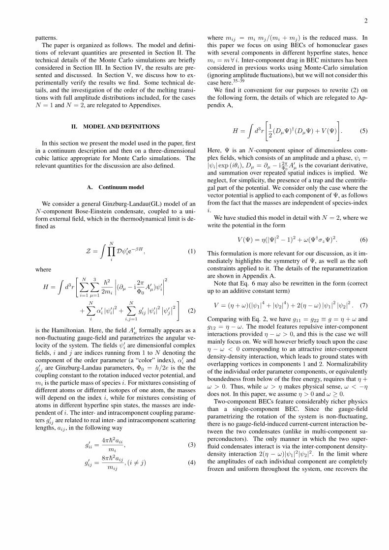
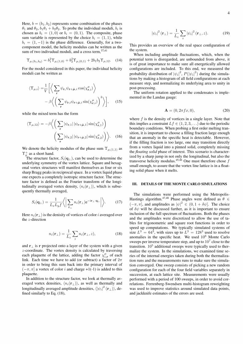
FIG. 1: (Color online) The probability distribution of theamplitudes, P(|ψi|2), for N = 2, at inverse temperatureβ = 1.20, f = 1/32, and η = 2, with ω values from 0 to 3.

The distribution is completely symmetric in i.

Fig. 1 shows the probability distribution of the amplitudes,P(|ψi|2). We get a peaked distribution for finite ω. On theother hand, when ω = 0, this is no longer the case. The dis-tribution now approaches a uniform distribution on the inter-val (0, 1]. In this case the parameter η serves to control theapproach to uniformity, η → ∞ corresponding to the CP 1

limit.With these initial simulation runs as a basis, we choose δψ

appropriately in order to capture the entire spectrum of fluctu-ations.

IV. RESULTS OF THE MONTE CARLO SIMULATIONS

In this section, the η − ω phase diagram of ground statesis explored by slow cooling and examination of vortex andamplitude densities, as well as structure factors. In additionto the expected hexagonal and square vortex ground states,several interesting regions of the parameter space are inves-tigated further. A special case between the square and thehexagonal region of the phase diagram is discovered, wherethe lattice first forms a square structure, but thermally recon-structs into a hexagonal lattice as the temperature is decreasedfurther. Furthermore, we consider in detail the ω = 0 line inthe phase diagram, where we discover additional vortex fluc-tuation effects. For ω = 0, the system features an SU(2) sym-metry. An unusual feature is an interesting state with globalphase coherence, but without a regular vortex lattice. In thiscase ordinary vortices do not have topological character due toSU(2) symmetry. Additionally, we obtain several interestingvortex structures characterized by dimer-like configurations atlower temperatures. Here, we observe honeycomb lattices, ordouble-core lattices, and stripe configurations, consistent withprevious T = 0 results.6

We also examine the melting transitions of the square and

hexagonal lattices with the full amplitude distribution in-cluded, as well as the melting of the hexagonal lattice in amodel with N = 1 as a benchmark of the method. To classifythe transition, we look at thermal averages of the specific heat,helicity moduli, and vortex structure factors. These results arepresented in Appendixes B and C.

A. The η − ω phase diagram

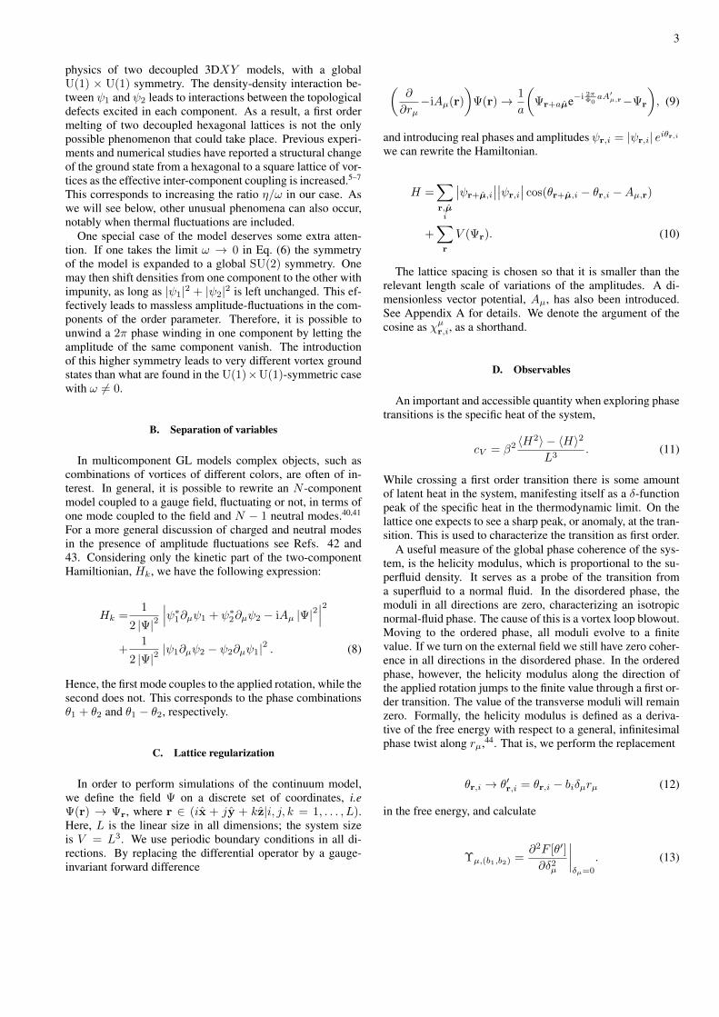
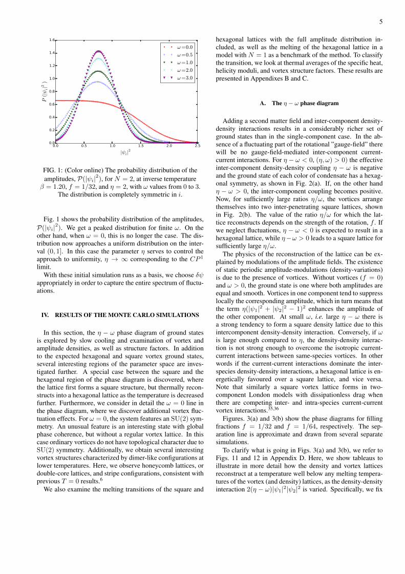
Adding a second matter field and inter-component density-density interactions results in a considerably richer set ofground states than in the single-component case. In the ab-sence of a fluctuating part of the rotational ”gauge-field” therewill be no gauge-field-mediated inter-component current-current interactions. For η − ω < 0, (η, ω) > 0) the effectiveinter-component density-density coupling η − ω is negativeand the ground state of each color of condensate has a hexag-onal symmetry, as shown in Fig. 2(a). If, on the other handη − ω > 0, the inter-component coupling becomes positive.Now, for sufficiently large ratios η/ω, the vortices arrangethemselves into two inter-penetrating square lattices, shownin Fig. 2(b). The value of the ratio η/ω for which the lat-tice reconstructs depends on the strength of the rotation, f . Ifwe neglect fluctuations, η − ω < 0 is expected to result in ahexagonal lattice, while η−ω > 0 leads to a square lattice forsufficiently large η/ω.

The physics of the reconstruction of the lattice can be ex-plained by modulations of the amplitude fields. The existenceof static periodic amplitude-modulations (density-variations)is due to the presence of vortices. Without vortices (f = 0)and ω > 0, the ground state is one where both amplitudes areequal and smooth. Vortices in one component tend to suppresslocally the corresponding amplitude, which in turn means thatthe term η(|ψ1|2 + |ψ2|2 − 1)2 enhances the amplitude ofthe other component. At small ω, i.e. large η − ω there isa strong tendency to form a square density lattice due to thisintercomponent density-density interaction. Conversely, if ωis large enough compared to η, the density-density interac-tion is not strong enough to overcome the isotropic current-current interactions between same-species vortices. In otherwords if the current-current interactions dominate the inter-species density-density interactions, a hexagonal lattice is en-ergetically favoured over a square lattice, and vice versa.Note that similarly a square vortex lattice forms in two-component London models with dissipationless drag whenthere are competing inter- and intra-species current-currentvortex interactions.35,36

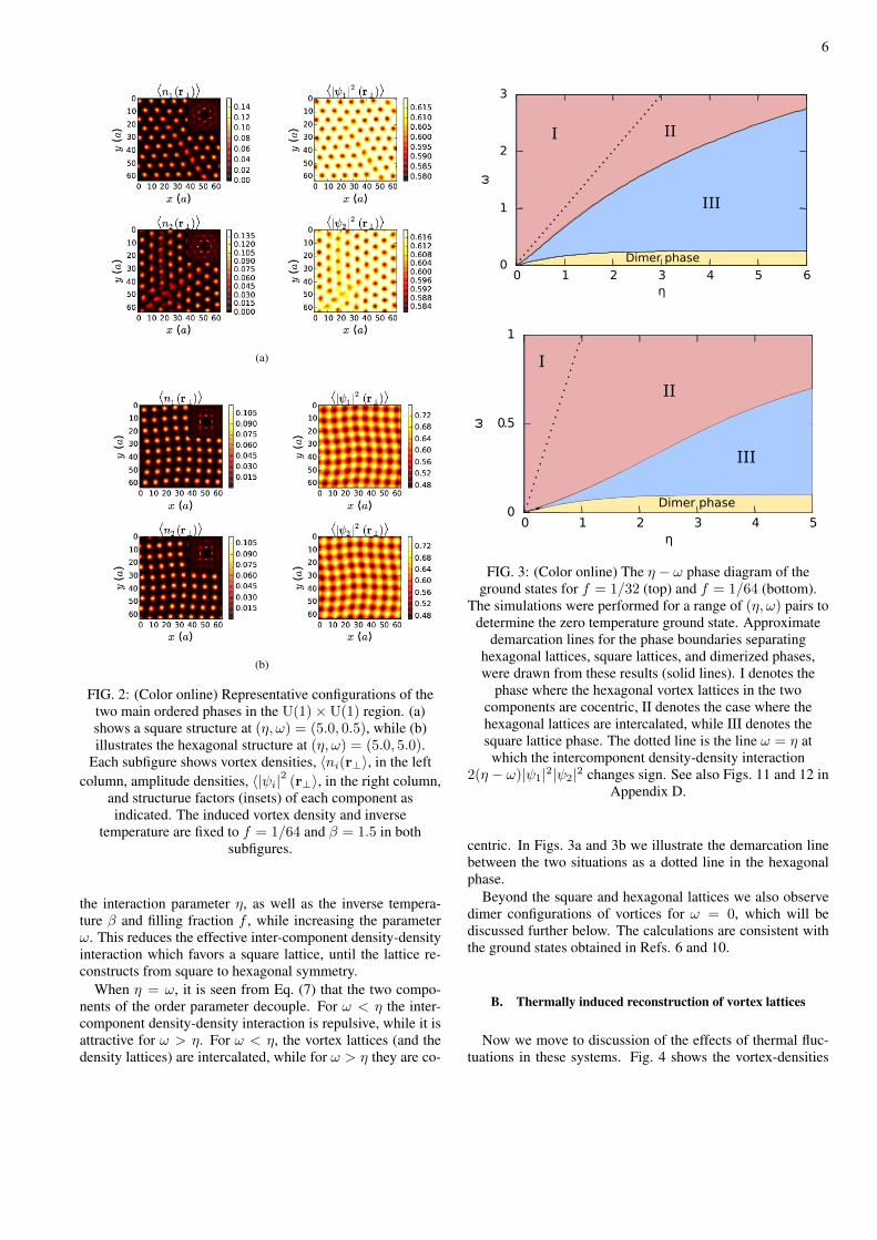
Figures. 3(a) and 3(b) show the phase diagrams for fillingfractions f = 1/32 and f = 1/64, respectively. The sep-aration line is approximate and drawn from several separatesimulations.

To clarify what is going in Figs. 3(a) and 3(b), we refer toFigs. 11 and 12 in Appendix D. Here, we show tableaus toillustrate in more detail how the density and vortex latticesreconstruct at a temperature well below any melting tempera-tures of the vortex (and density) lattices, as the density-densityinteraction 2(η − ω)|ψ1|2|ψ2|2 is varied. Specifically, we fix

6

(a)

(b)

FIG. 2: (Color online) Representative configurations of thetwo main ordered phases in the U(1)×U(1) region. (a)shows a square structure at (η, ω) = (5.0, 0.5), while (b)illustrates the hexagonal structure at (η, ω) = (5.0, 5.0).

Each subfigure shows vortex densities, 〈ni(r⊥〉, in the leftcolumn, amplitude densities, 〈|ψi|2 (r⊥〉, in the right column,

and structurue factors (insets) of each component asindicated. The induced vortex density and inverse

temperature are fixed to f = 1/64 and β = 1.5 in bothsubfigures.

the interaction parameter η, as well as the inverse tempera-ture β and filling fraction f , while increasing the parameterω. This reduces the effective inter-component density-densityinteraction which favors a square lattice, until the lattice re-constructs from square to hexagonal symmetry.

When η = ω, it is seen from Eq. (7) that the two compo-nents of the order parameter decouple. For ω < η the inter-component density-density interaction is repulsive, while it isattractive for ω > η. For ω < η, the vortex lattices (and thedensity lattices) are intercalated, while for ω > η they are co-

Dimer phase0

1

2

3

0 1 2 3 4 5 6

ω

η

I II

III

0

0.5

1

0 1 2 3 4 5

ω

η

Dimer phase

I

II

III

FIG. 3: (Color online) The η − ω phase diagram of theground states for f = 1/32 (top) and f = 1/64 (bottom).

The simulations were performed for a range of (η, ω) pairs todetermine the zero temperature ground state. Approximate

demarcation lines for the phase boundaries separatinghexagonal lattices, square lattices, and dimerized phases,were drawn from these results (solid lines). I denotes the

phase where the hexagonal vortex lattices in the twocomponents are cocentric, II denotes the case where thehexagonal lattices are intercalated, while III denotes thesquare lattice phase. The dotted line is the line ω = η at

which the intercomponent density-density interaction2(η − ω)|ψ1|2|ψ2|2 changes sign. See also Figs. 11 and 12 in

Appendix D.

centric. In Figs. 3a and 3b we illustrate the demarcation linebetween the two situations as a dotted line in the hexagonalphase.

Beyond the square and hexagonal lattices we also observedimer configurations of vortices for ω = 0, which will bediscussed further below. The calculations are consistent withthe ground states obtained in Refs. 6 and 10.

B. Thermally induced reconstruction of vortex lattices

Now we move to discussion of the effects of thermal fluc-tuations in these systems. Fig. 4 shows the vortex-densities

7

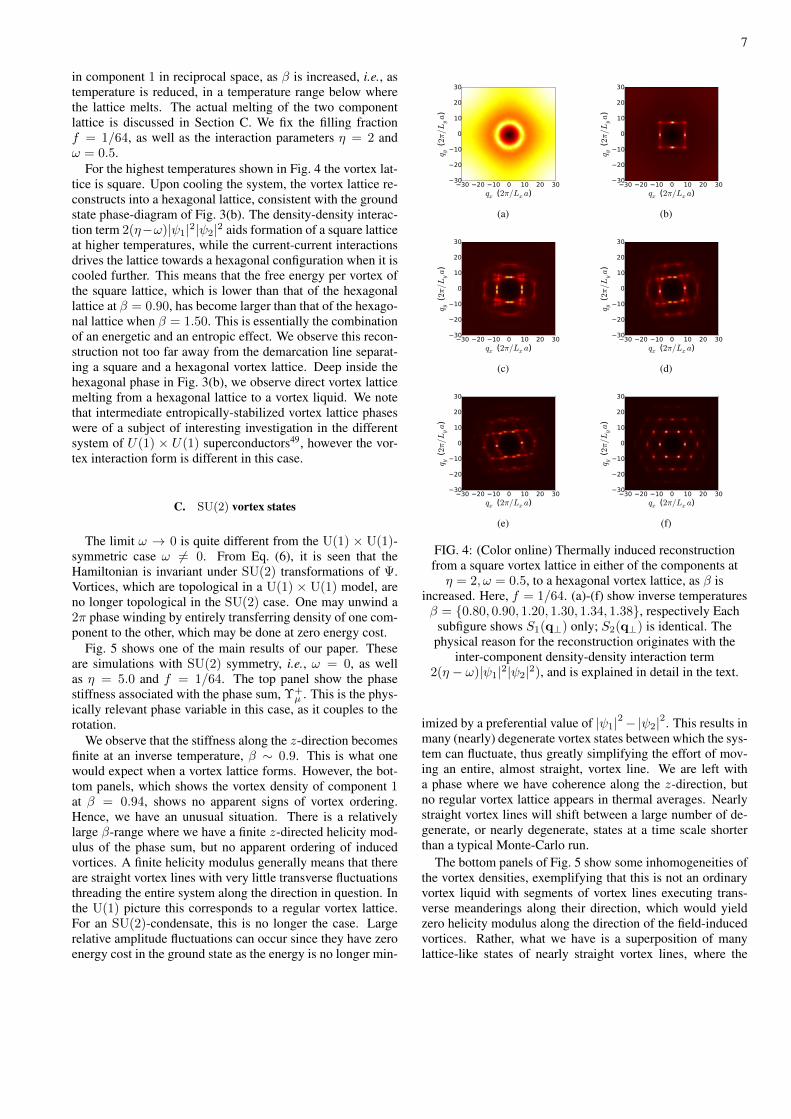
in component 1 in reciprocal space, as β is increased, i.e., astemperature is reduced, in a temperature range below wherethe lattice melts. The actual melting of the two componentlattice is discussed in Section C. We fix the filling fractionf = 1/64, as well as the interaction parameters η = 2 andω = 0.5.

For the highest temperatures shown in Fig. 4 the vortex lat-tice is square. Upon cooling the system, the vortex lattice re-constructs into a hexagonal lattice, consistent with the groundstate phase-diagram of Fig. 3(b). The density-density interac-tion term 2(η−ω)|ψ1|2|ψ2|2 aids formation of a square latticeat higher temperatures, while the current-current interactionsdrives the lattice towards a hexagonal configuration when it iscooled further. This means that the free energy per vortex ofthe square lattice, which is lower than that of the hexagonallattice at β = 0.90, has become larger than that of the hexago-nal lattice when β = 1.50. This is essentially the combinationof an energetic and an entropic effect. We observe this recon-struction not too far away from the demarcation line separat-ing a square and a hexagonal vortex lattice. Deep inside thehexagonal phase in Fig. 3(b), we observe direct vortex latticemelting from a hexagonal lattice to a vortex liquid. We notethat intermediate entropically-stabilized vortex lattice phaseswere of a subject of interesting investigation in the differentsystem of U(1) × U(1) superconductors49, however the vor-tex interaction form is different in this case.

C. SU(2) vortex states

The limit ω → 0 is quite different from the U(1) × U(1)-symmetric case ω 6= 0. From Eq. (6), it is seen that theHamiltonian is invariant under SU(2) transformations of Ψ.Vortices, which are topological in a U(1) × U(1) model, areno longer topological in the SU(2) case. One may unwind a2π phase winding by entirely transferring density of one com-ponent to the other, which may be done at zero energy cost.

Fig. 5 shows one of the main results of our paper. Theseare simulations with SU(2) symmetry, i.e., ω = 0, as wellas η = 5.0 and f = 1/64. The top panel show the phasestiffness associated with the phase sum, Υ+

µ . This is the phys-ically relevant phase variable in this case, as it couples to therotation.

We observe that the stiffness along the z-direction becomesfinite at an inverse temperature, β ∼ 0.9. This is what onewould expect when a vortex lattice forms. However, the bot-tom panels, which shows the vortex density of component 1at β = 0.94, shows no apparent signs of vortex ordering.Hence, we have an unusual situation. There is a relativelylarge β-range where we have a finite z-directed helicity mod-ulus of the phase sum, but no apparent ordering of inducedvortices. A finite helicity modulus generally means that thereare straight vortex lines with very little transverse fluctuationsthreading the entire system along the direction in question. Inthe U(1) picture this corresponds to a regular vortex lattice.For an SU(2)-condensate, this is no longer the case. Largerelative amplitude fluctuations can occur since they have zeroenergy cost in the ground state as the energy is no longer min-

30 20 10 0 10 20 30

qx (2π/Lx a)

30

20

10

0

10

20

30

q y (

2π/L

ya)

(a)

30 20 10 0 10 20 30

qx (2π/Lx a)

30

20

10

0

10

20

30

q y (

2π/L

ya)

(b)

30 20 10 0 10 20 30

qx (2π/Lx a)

30

20

10

0

10

20

30

q y (

2π/L

ya)

(c)

30 20 10 0 10 20 30

qx (2π/Lx a)

30

20

10

0

10

20

30

q y (

2π/L

ya)

(d)

30 20 10 0 10 20 30

qx (2π/Lx a)

30

20

10

0

10

20

30

q y (

2π/L

ya)

(e)

30 20 10 0 10 20 30

qx (2π/Lx a)

30

20

10

0

10

20

30

q y (

2π/L

ya)

(f)

FIG. 4: (Color online) Thermally induced reconstructionfrom a square vortex lattice in either of the components atη = 2, ω = 0.5, to a hexagonal vortex lattice, as β is

increased. Here, f = 1/64. (a)-(f) show inverse temperaturesβ = {0.80, 0.90, 1.20, 1.30, 1.34, 1.38}, respectively Each

subfigure shows S1(q⊥) only; S2(q⊥) is identical. Thephysical reason for the reconstruction originates with the

inter-component density-density interaction term2(η − ω)|ψ1|2|ψ2|2), and is explained in detail in the text.

imized by a preferential value of |ψ1|2−|ψ2|2. This results inmany (nearly) degenerate vortex states between which the sys-tem can fluctuate, thus greatly simplifying the effort of mov-ing an entire, almost straight, vortex line. We are left witha phase where we have coherence along the z-direction, butno regular vortex lattice appears in thermal averages. Nearlystraight vortex lines will shift between a large number of de-generate, or nearly degenerate, states at a time scale shorterthan a typical Monte-Carlo run.

The bottom panels of Fig. 5 show some inhomogeneities ofthe vortex densities, exemplifying that this is not an ordinaryvortex liquid with segments of vortex lines executing trans-verse meanderings along their direction, which would yieldzero helicity modulus along the direction of the field-inducedvortices. Rather, what we have is a superposition of manylattice-like states of nearly straight vortex lines, where the

8

0.4 0.6 0.8 1.0 1.2 1.4 1.6 1.8

β (1/J0 )

0.0

0.1

0.2

0.3

0.4

0.5

0.6

0.7

0.8Υ

+ µ (J

0)

Υ+x

Υ+y

Υ+z

0 10 20 30 40 50 60

x (a)

0

10

20

30

40

50

60

y (a

)

106 MC sweeps

0 10 20 30 40 50 60

x (a)

0

10

20

30

40

50

60

y (a

)

107 MC sweeps

0.0140

0.0145

0.0150

0.0155

0.0160

0.0165

0.0170

0.0175

0.0140

0.0145

0.0150

0.0155

0.0160

0.0165

0.0170

0.0175

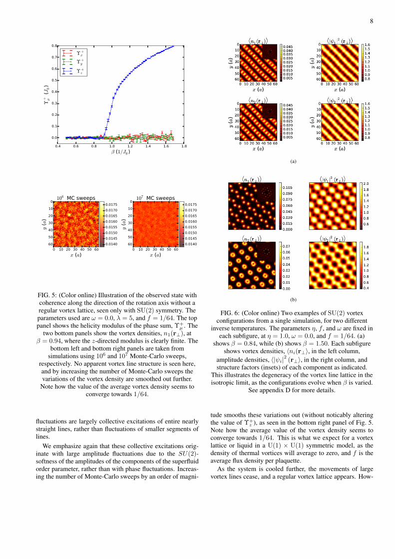
FIG. 5: (Color online) Illustration of the observed state withcoherence along the direction of the rotation axis without aregular vortex lattice, seen only with SU(2) symmetry. Theparameters used are ω = 0.0, λ = 5, and f = 1/64. The toppanel shows the helicity modulus of the phase sum, Υ+

µ . Thetwo bottom panels show the vortex densities, n1(r⊥), at

β = 0.94, where the z-directed modulus is clearly finite. Thebottom left and bottom right panels are taken from

simulations using 106 and 107 Monte-Carlo sweeps,respectively. No apparent vortex line structure is seen here,and by increasing the number of Monte-Carlo sweeps thevariations of the vortex density are smoothed out further.

Note how the value of the average vortex density seems toconverge towards 1/64.

fluctuations are largely collective excitations of entire nearlystraight lines, rather than fluctuations of smaller segments oflines.

We emphasize again that these collective excitations orig-inate with large amplitude fluctuations due to the SU(2)-softness of the amplitudes of the components of the superfluidorder parameter, rather than with phase fluctuations. Increas-ing the number of Monte-Carlo sweeps by an order of magni-

(a)

(b)

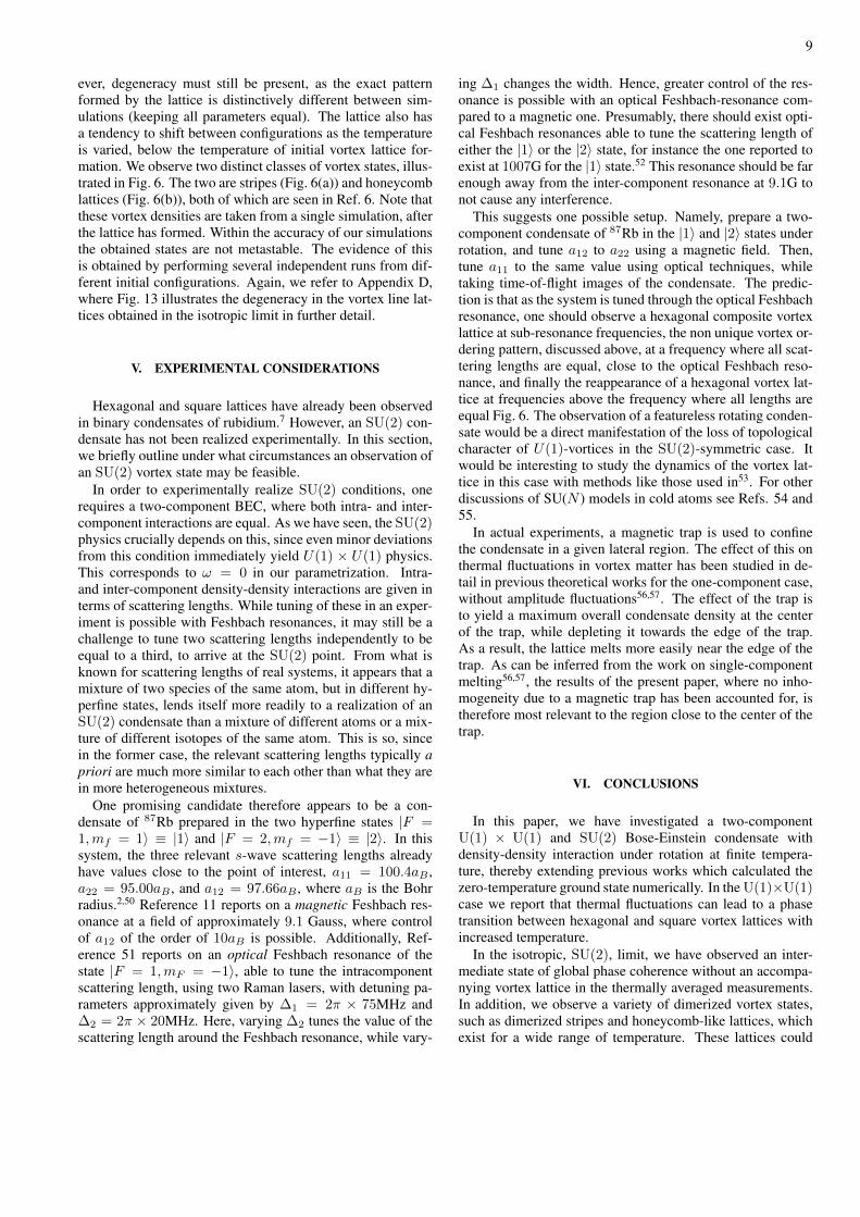
FIG. 6: (Color online) Two examples of SU(2) vortexconfigurations from a single simulation, for two different

inverse temperatures. The parameters η, f , and ω are fixed ineach subfigure, at η = 1.0, ω = 0.0, and f = 1/64. (a)

shows β = 0.84, while (b) shows β = 1.50. Each subfigureshows vortex densities, 〈ni(r⊥〉, in the left column,

amplitude densities, 〈|ψi|2 (r⊥〉, in the right column, andstructure factors (insets) of each component as indicated.

This illustrates the degeneracy of the vortex line lattice in theisotropic limit, as the configurations evolve when β is varied.

See appendix D for more details.

tude smooths these variations out (without noticably alteringthe value of Υ+

z ), as seen in the bottom right panel of Fig. 5.Note how the average value of the vortex density seems toconverge towards 1/64. This is what we expect for a vortexlattice or liquid in a U(1) × U(1) symmetric model, as thedensity of thermal vortices will average to zero, and f is theaverage flux density per plaquette.

As the system is cooled further, the movements of largevortex lines cease, and a regular vortex lattice appears. How-

9

ever, degeneracy must still be present, as the exact patternformed by the lattice is distinctively different between sim-ulations (keeping all parameters equal). The lattice also hasa tendency to shift between configurations as the temperatureis varied, below the temperature of initial vortex lattice for-mation. We observe two distinct classes of vortex states, illus-trated in Fig. 6. The two are stripes (Fig. 6(a)) and honeycomblattices (Fig. 6(b)), both of which are seen in Ref. 6. Note thatthese vortex densities are taken from a single simulation, afterthe lattice has formed. Within the accuracy of our simulationsthe obtained states are not metastable. The evidence of thisis obtained by performing several independent runs from dif-ferent initial configurations. Again, we refer to Appendix D,where Fig. 13 illustrates the degeneracy in the vortex line lat-tices obtained in the isotropic limit in further detail.

V. EXPERIMENTAL CONSIDERATIONS

Hexagonal and square lattices have already been observedin binary condensates of rubidium.7 However, an SU(2) con-densate has not been realized experimentally. In this section,we briefly outline under what circumstances an observation ofan SU(2) vortex state may be feasible.

In order to experimentally realize SU(2) conditions, onerequires a two-component BEC, where both intra- and inter-component interactions are equal. As we have seen, the SU(2)physics crucially depends on this, since even minor deviationsfrom this condition immediately yield U(1) × U(1) physics.This corresponds to ω = 0 in our parametrization. Intra-and inter-component density-density interactions are given interms of scattering lengths. While tuning of these in an exper-iment is possible with Feshbach resonances, it may still be achallenge to tune two scattering lengths independently to beequal to a third, to arrive at the SU(2) point. From what isknown for scattering lengths of real systems, it appears that amixture of two species of the same atom, but in different hy-perfine states, lends itself more readily to a realization of anSU(2) condensate than a mixture of different atoms or a mix-ture of different isotopes of the same atom. This is so, sincein the former case, the relevant scattering lengths typically apriori are much more similar to each other than what they arein more heterogeneous mixtures.

One promising candidate therefore appears to be a con-densate of 87Rb prepared in the two hyperfine states |F =1,mf = 1〉 ≡ |1〉 and |F = 2,mf = −1〉 ≡ |2〉. In thissystem, the three relevant s-wave scattering lengths alreadyhave values close to the point of interest, a11 = 100.4aB ,a22 = 95.00aB , and a12 = 97.66aB , where aB is the Bohrradius.2,50 Reference 11 reports on a magnetic Feshbach res-onance at a field of approximately 9.1 Gauss, where controlof a12 of the order of 10aB is possible. Additionally, Ref-erence 51 reports on an optical Feshbach resonance of thestate |F = 1,mF = −1〉, able to tune the intracomponentscattering length, using two Raman lasers, with detuning pa-rameters approximately given by ∆1 = 2π × 75MHz and∆2 = 2π × 20MHz. Here, varying ∆2 tunes the value of thescattering length around the Feshbach resonance, while vary-

ing ∆1 changes the width. Hence, greater control of the res-onance is possible with an optical Feshbach-resonance com-pared to a magnetic one. Presumably, there should exist opti-cal Feshbach resonances able to tune the scattering length ofeither the |1〉 or the |2〉 state, for instance the one reported toexist at 1007G for the |1〉 state.52 This resonance should be farenough away from the inter-component resonance at 9.1G tonot cause any interference.

This suggests one possible setup. Namely, prepare a two-component condensate of 87Rb in the |1〉 and |2〉 states underrotation, and tune a12 to a22 using a magnetic field. Then,tune a11 to the same value using optical techniques, whiletaking time-of-flight images of the condensate. The predic-tion is that as the system is tuned through the optical Feshbachresonance, one should observe a hexagonal composite vortexlattice at sub-resonance frequencies, the non unique vortex or-dering pattern, discussed above, at a frequency where all scat-tering lengths are equal, close to the optical Feshbach reso-nance, and finally the reappearance of a hexagonal vortex lat-tice at frequencies above the frequency where all lengths areequal Fig. 6. The observation of a featureless rotating conden-sate would be a direct manifestation of the loss of topologicalcharacter of U(1)-vortices in the SU(2)-symmetric case. Itwould be interesting to study the dynamics of the vortex lat-tice in this case with methods like those used in53. For otherdiscussions of SU(N ) models in cold atoms see Refs. 54 and55.

In actual experiments, a magnetic trap is used to confinethe condensate in a given lateral region. The effect of this onthermal fluctuations in vortex matter has been studied in de-tail in previous theoretical works for the one-component case,without amplitude fluctuations56,57. The effect of the trap isto yield a maximum overall condensate density at the centerof the trap, while depleting it towards the edge of the trap.As a result, the lattice melts more easily near the edge of thetrap. As can be inferred from the work on single-componentmelting56,57, the results of the present paper, where no inho-mogeneity due to a magnetic trap has been accounted for, istherefore most relevant to the region close to the center of thetrap.

VI. CONCLUSIONS

In this paper, we have investigated a two-componentU(1) × U(1) and SU(2) Bose-Einstein condensate withdensity-density interaction under rotation at finite tempera-ture, thereby extending previous works which calculated thezero-temperature ground state numerically. In the U(1)×U(1)case we report that thermal fluctuations can lead to a phasetransition between hexagonal and square vortex lattices withincreased temperature.

In the isotropic, SU(2), limit, we have observed an inter-mediate state of global phase coherence without an accompa-nying vortex lattice in the thermally averaged measurements.In addition, we observe a variety of dimerized vortex states,such as dimerized stripes and honeycomb-like lattices, whichexist for a wide range of temperature. These lattices could

10

be observed in binary Bose-Einstein condensates in two sep-arate hyperfine states, by precisely tuning the inter- and intra-component scattering lengths to the SU(2) point through theuse of Feshbach resonances.

Acknowledgments

We thank Erich Mueller for useful discussions. P. N. G.thanks NTNU and the Norwegian Research Council for finan-cial support. E. B. was supported by by the Knut and AliceWallenberg Foundation through a Royal Swedish Academyof Sciences Fellowship, by the Swedish Research CouncilGrants No. 642-2013-7837 and No. 325-2009-7664, and bythe National Science Foundation under the CAREER AwardNo. DMR-0955902, A. S. was supported by the ResearchCouncil of Norway, through Grants No. 205591/V20 andNo. 216700/F20. This work was also supported through theNorwegian consortium for high-performance computing (NO-TUR).

Appendix A: Rewriting the general Hamiltionian

Here we present the details of rewriting Eq. 2 into Eq.5,which is more suited for our purposes. We repeat the startingpoint here for convenience.

H =

∫d3r

[N∑i=1

3∑µ=1

~2

2mi

∣∣∣∣(∂µ − i2π

Φ0A′µ)ψ′i

∣∣∣∣2

+

N∑i

α′i |ψ′i|2

+

N∑i,j=1

g′ij |ψ′i|2 ∣∣ψ′j∣∣2

](A1)

First, we scale the field variables and Ginzburg-Landau pa-rameters, to obtain some dimensionless quantities.

α′i = α0αi, (A2)g′ij = g0gij , (A3)

|ψ′i| =√α0

g0|ψi| . (A4)

This gives us the Hamiltonian,

H =α2

0

g0

∫d3r

[N∑i=1

3∑µ=1

~2

2miα0

∣∣∣∣(∂µ − iΦ0

2πA′µ)ψi

∣∣∣∣2

+

N∑i

αi |ψi|2 +

N∑i,j=1

gij |ψi|2 |ψj |2],

(A5)

which on the lattice reads

H =α2

0a3

g0

∑r

[N∑i=1

3∑µ=1

~2

miα0a2

×(∣∣ψr,i

∣∣2 − ∣∣ψr+µ,i

∣∣∣∣ψr,i

∣∣ cos(θr+µ,i − θr,i −Aµ,r))

+

N∑i

αi |ψr,i|2 +

N∑i,j=1

gij |ψr,i|2 |ψr,j |2], (A6)

where a is the lattice constant, and we have introduced

Aµ =2π

Φ0aA′µ. (A7)

Next, we specialize to the case N = 2, α1 = α2, g11 =g22 ≡ g, and m1 = m2, and define a2 to be equal to~2/mα0, which sets our length scale. Note that it should notbe confused with the coherence length in the multi-componentcase without intercomponent density-density interaction. Forthe definition of coherence lengths in the presence of multi-ple components and inter-component density-density interac-tions, see Refs. 58 and 59. The energy scale is defined as J0

as follows

J0 =α2

0a3

g0. (A8)

The coupling parameters η and ω used in this paper are de-fined by comparing the potential term of Eq. (A6) to theform where the soft constraints |ψ1|2 + |ψ2|2 = 1 and|ψ1|2 − |ψ2|2 = 0 are implemented. Thus, we have

V (Ψ) = η(|ψ1|2 + |ψ2|2 − 1)2 + ω(|ψ1|2 − |ψ2|2)2, (A9)

with

η = −α2− 3

2. (A10)

ω =g − g12

2(A11)

The lattice version of the Hamiltionian reads

H =∑r,µi

∣∣ψr+µ,i

∣∣∣∣ψr,i

∣∣( cos(θr+µ,i − θr,i −Aµ,r))

+∑r

η(|ψ1|2 + |ψ2|2 − 1)2

+∑r

ω(|ψ1|2 − |ψ2|2)2. (A12)

This model will then have the following continuum form,

H =

∫d3r

[N∑i

1

2|(∂µ − iAµ)ψi|2 + V (Ψ)

]. (A13)

11

Appendix B: First order lattice melting for N = 1 reconsidered

As a benchmark on simulations with amplitude fluctuationsincluded, we verify the well-established first-order meltingtransition on this model with only a single component of theorder-parameter field, in the presence of amplitude fluctua-tions. The added feature of the computation is that the com-plete amplitude-distribution function was utilized, through themethods described in Section III. In this case, the term in thepotential proportional to ω in Eq. 6 is absent, and the potentialreduces to

V (Ψ) = η(|Ψ|2 − 1)2. (B1)

With amplitude fluctuations neglected, this model reduces tothe much studied uniformly frustrated 3DXY model, withwell known results as mentioned in the Introduction of thepaper. The model features a first-order phase transition mani-fested as a melting of the frustration-induced hexagonal latticeof vortices.16,18–25 The fluctuations responsible for driving thistransition are massless transverse phase fluctuations of the or-der parameter.

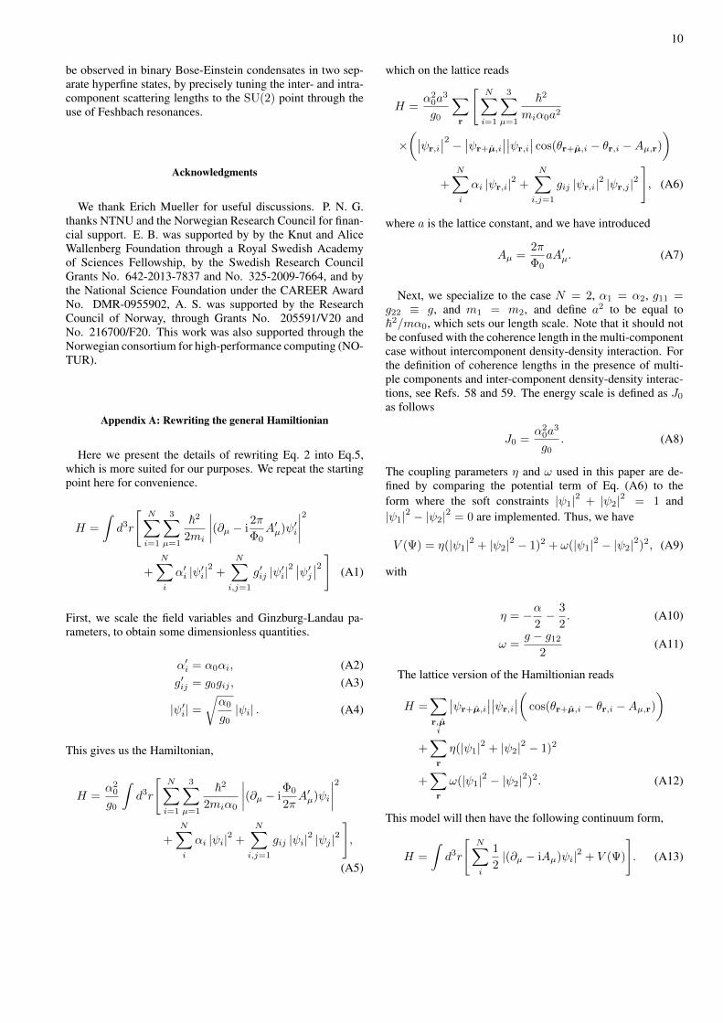
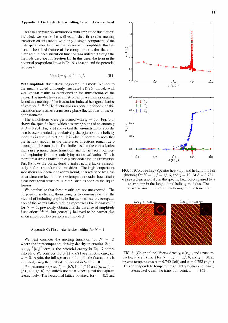
The simulations were performed with η = 10. Fig. 7(a)shows the specific heat, which has strong signs of an anomalyat β = 0.751. Fig. 7(b) shows that the anomaly in the specificheat is accompanied by a relatively sharp jump in the helicitymodulus in the z-direction. It is also important to note thatthe helicity moduli in the transverse directions remain zerothroughout the transition. This indicates that the vortex latticemelts in a genuine phase transition, and not as a result of ther-mal depinning from the underlying numerical lattice. This istherefore a strong indication of a first-order melting transition.Fig. 8 shows the vortex density and structure factor immedi-ately before and after the transition. The high-temperatureside shows an incoherent vortex liquid, characterized by a cir-cular structure factor. The-low temperature side shows that aclear hexagonal structure is established as soon as the liquidfreezes.

We emphasize that these results are not unexpected. Thepurpose of including them here, is to demonstrate that themethod of including amplitude fluctuations into the computa-tion of the vortex lattice melting reproduces the known resultfor N = 1, previously obtained in the absence of amplitudefluctuations16,18–25, but generally believed to be correct alsowhen amplitude fluctuations are included.

Appendix C: First order lattice melting for N = 2

We next consider the melting transition for N = 2,where the intercomponent density-density interaction 2(η −ω) |ψ1|2 |ψ2|2-term in the potential energy in Eq. 7 comesinto play. We consider the U(1) × U(1)-symmetric case, i.e.ω 6= 0. Again, the full spectrum of amplitude fluctuations isincluded, using the methods described in Section III.

For parameters (η, ω, f) = (0.5, 1.0, 1/16) and (η, ω, f) =(2.0, 1.0, 1/16) the lattices are clearly hexagonal and square,respectively. The hexagonal lattice obtained for η = 0.5 and

0.60 0.65 0.70 0.75 0.80

β (1/J0 )

1.0

1.5

2.0

2.5

3.0

3.5

c V (kB

)

0.60 0.65 0.70 0.75 0.80

β (1/J0 )

0.0

0.2

0.4

0.6

0.8

Υµ (J

0)

Υx

Υy

Υz

FIG. 7: (Color online) Specific heat (top) and helicity moduli(bottom) for N = 1, f = 1/16, and η = 10. At β = 0.751

we see a clear anomaly in the specific heat accompanied by asharp jump in the longitudinal helicity modulus. The

transverse moduli remain zero throughout the transition.

FIG. 8: (Color online) Vortex density, n(r⊥), and structurefactor, S(q⊥), (inset) for N = 1, f = 1/16, and η = 10, at

inverse temperatures β = 0.749 (left) and β = 0.752 (right).This corresponds to temperatures slightly higher and lower,

respectively, than the transition point, β = 0.751.

12

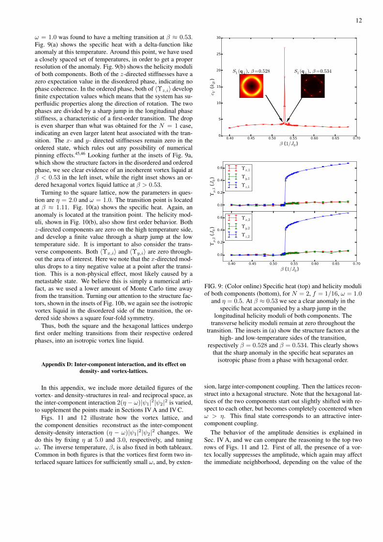
ω = 1.0 was found to have a melting transition at β ≈ 0.53.Fig. 9(a) shows the specific heat with a delta-function likeanomaly at this temperature. Around this point, we have useda closely spaced set of temperatures, in order to get a properresolution of the anomaly. Fig. 9(b) shows the helicity moduliof both components. Both of the z-directed stiffnesses have azero expectation value in the disordered phase, indicating nophase coherence. In the ordered phase, both of 〈Υz,i〉 developfinite expectation values which means that the system has su-perfluidic properties along the direction of rotation. The twophases are divided by a sharp jump in the longitudinal phasestiffness, a characteristic of a first-order transition. The dropis even sharper than what was obtained for the N = 1 case,indicating an even larger latent heat associated with the tran-sition. The x- and y- directed stiffnesses remain zero in theordered state, which rules out any possibility of numericalpinning effects.45,46 Looking further at the insets of Fig. 9a,which show the structure factors in the disordered and orderedphase, we see clear evidence of an incoherent vortex liquid atβ < 0.53 in the left inset, while the right inset shows an or-dered hexagonal vortex liquid lattice at β > 0.53.

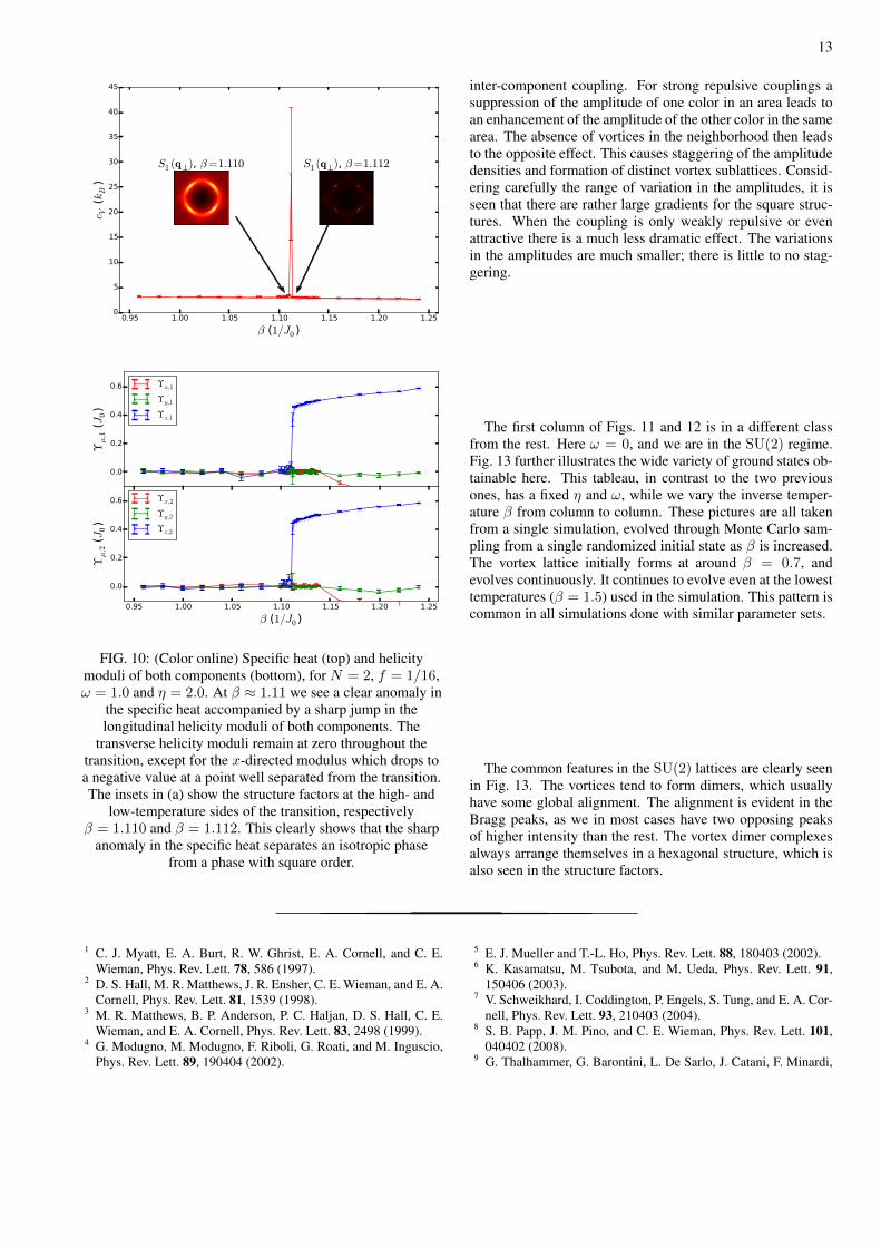
Turning to the square lattice, now the parameters in ques-tion are η = 2.0 and ω = 1.0. The transition point is locatedat β ≈ 1.11. Fig. 10(a) shows the specific heat. Again, ananomaly is located at the transition point. The helicity mod-uli, shown in Fig. 10(b), also show first order behavior. Bothz-directed components are zero on the high temperature side,and develop a finite value through a sharp jump at the lowtemperature side. It is important to also consider the trans-verse components. Both 〈Υx,i〉 and 〈Υy,i〉 are zero through-out the area of interest. Here we note that the x-directed mod-ulus drops to a tiny negative value at a point after the transi-tion. This is a non-physical effect, most likely caused by ametastable state. We believe this is simply a numerical arti-fact, as we used a lower amount of Monte Carlo time awayfrom the transition. Turning our attention to the structure fac-tors, shown in the insets of Fig. 10b, we again see the isotropicvortex liquid in the disordered side of the transition, the or-dered side shows a square four-fold symmetry.

Thus, both the square and the hexagonal lattices undergofirst order melting transitions from their respective orderedphases, into an isotropic vortex line liquid.

Appendix D: Inter-component interaction, and its effect ondensity- and vortex-lattices.

In this appendix, we include more detailed figures of thevortex- and density-structures in real- and reciprocal space, asthe inter-component interaction 2(η − ω)|ψ1|2|ψ2|2 is varied,to supplement the points made in Sections IV A and IV C.

Figs. 11 and 12 illustrate how the vortex lattice, andthe component densities reconstruct as the inter-componentdensity-density interaction (η − ω)|ψ1|2|ψ2|2 changes. Wedo this by fixing η at 5.0 and 3.0, respectively, and tuningω. The inverse temperature, β, is also fixed in both tableaux.Common in both figures is that the vortices first form two in-terlaced square lattices for sufficiently small ω, and, by exten-

0.40 0.45 0.50 0.55 0.60 0.65 0.70

β (1/J0 )

0

5

10

15

20

25

30

c V (kB

)

S1 (q ), β=0.528 S1 (q ), β=0.534

0.0

0.2

0.4

0.6

Υµ,1 (J

0)

Υx,1

Υy,1

Υz,1

0.40 0.45 0.50 0.55 0.60 0.65 0.70

β (1/J0 )

0.0

0.2

0.4

0.6

Υµ,2 (J

0)

Υx,2

Υy,2

Υz,2

FIG. 9: (Color online) Specific heat (top) and helicity moduliof both components (bottom), for N = 2, f = 1/16, ω = 1.0

and η = 0.5. At β ≈ 0.53 we see a clear anomaly in thespecific heat accompanied by a sharp jump in the

longitudinal helicity moduli of both components. Thetransverse helicity moduli remain at zero throughout the

transition. The insets in (a) show the structure factors at thehigh- and low-temperature sides of the transition,

respectively β = 0.528 and β = 0.534. This clearly showsthat the sharp anomaly in the specific heat separates an

isotropic phase from a phase with hexagonal order.

sion, large inter-component coupling. Then the lattices recon-struct into a hexagonal structure. Note that the hexagonal lat-tices of the two components start out slightly shifted with re-spect to each other, but becomes completely cocentered whenω > η. This final state corresponds to an attractive inter-component coupling.

The behavior of the amplitude densities is explained inSec. IV A, and we can compare the reasoning to the top tworows of Figs. 11 and 12. First of all, the presence of a vor-tex locally suppresses the amplitude, which again may affectthe immediate neighborhood, depending on the value of the

13

0.95 1.00 1.05 1.10 1.15 1.20 1.25

β (1/J0 )

0

5

10

15

20

25

30

35

40

45c V

(kB

)

S1 (q ), β=1.110 S1 (q ), β=1.112

0.0

0.2

0.4

0.6

Υµ,1 (J

0)

Υx,1

Υy,1

Υz,1

0.95 1.00 1.05 1.10 1.15 1.20 1.25

β (1/J0 )

0.0

0.2

0.4

0.6

Υµ,2 (J

0)

Υx,2

Υy,2

Υz,2

FIG. 10: (Color online) Specific heat (top) and helicitymoduli of both components (bottom), for N = 2, f = 1/16,ω = 1.0 and η = 2.0. At β ≈ 1.11 we see a clear anomaly in

the specific heat accompanied by a sharp jump in thelongitudinal helicity moduli of both components. The

transverse helicity moduli remain at zero throughout thetransition, except for the x-directed modulus which drops toa negative value at a point well separated from the transition.The insets in (a) show the structure factors at the high- and

low-temperature sides of the transition, respectivelyβ = 1.110 and β = 1.112. This clearly shows that the sharp

anomaly in the specific heat separates an isotropic phasefrom a phase with square order.

inter-component coupling. For strong repulsive couplings asuppression of the amplitude of one color in an area leads toan enhancement of the amplitude of the other color in the samearea. The absence of vortices in the neighborhood then leadsto the opposite effect. This causes staggering of the amplitudedensities and formation of distinct vortex sublattices. Consid-ering carefully the range of variation in the amplitudes, it isseen that there are rather large gradients for the square struc-tures. When the coupling is only weakly repulsive or evenattractive there is a much less dramatic effect. The variationsin the amplitudes are much smaller; there is little to no stag-gering.

The first column of Figs. 11 and 12 is in a different classfrom the rest. Here ω = 0, and we are in the SU(2) regime.Fig. 13 further illustrates the wide variety of ground states ob-tainable here. This tableau, in contrast to the two previousones, has a fixed η and ω, while we vary the inverse temper-ature β from column to column. These pictures are all takenfrom a single simulation, evolved through Monte Carlo sam-pling from a single randomized initial state as β is increased.The vortex lattice initially forms at around β = 0.7, andevolves continuously. It continues to evolve even at the lowesttemperatures (β = 1.5) used in the simulation. This pattern iscommon in all simulations done with similar parameter sets.

The common features in the SU(2) lattices are clearly seenin Fig. 13. The vortices tend to form dimers, which usuallyhave some global alignment. The alignment is evident in theBragg peaks, as we in most cases have two opposing peaksof higher intensity than the rest. The vortex dimer complexesalways arrange themselves in a hexagonal structure, which isalso seen in the structure factors.

1 C. J. Myatt, E. A. Burt, R. W. Ghrist, E. A. Cornell, and C. E.Wieman, Phys. Rev. Lett. 78, 586 (1997).

2 D. S. Hall, M. R. Matthews, J. R. Ensher, C. E. Wieman, and E. A.Cornell, Phys. Rev. Lett. 81, 1539 (1998).

3 M. R. Matthews, B. P. Anderson, P. C. Haljan, D. S. Hall, C. E.Wieman, and E. A. Cornell, Phys. Rev. Lett. 83, 2498 (1999).

4 G. Modugno, M. Modugno, F. Riboli, G. Roati, and M. Inguscio,Phys. Rev. Lett. 89, 190404 (2002).

5 E. J. Mueller and T.-L. Ho, Phys. Rev. Lett. 88, 180403 (2002).6 K. Kasamatsu, M. Tsubota, and M. Ueda, Phys. Rev. Lett. 91,

150406 (2003).7 V. Schweikhard, I. Coddington, P. Engels, S. Tung, and E. A. Cor-

nell, Phys. Rev. Lett. 93, 210403 (2004).8 S. B. Papp, J. M. Pino, and C. E. Wieman, Phys. Rev. Lett. 101,

040402 (2008).9 G. Thalhammer, G. Barontini, L. De Sarlo, J. Catani, F. Minardi,

14

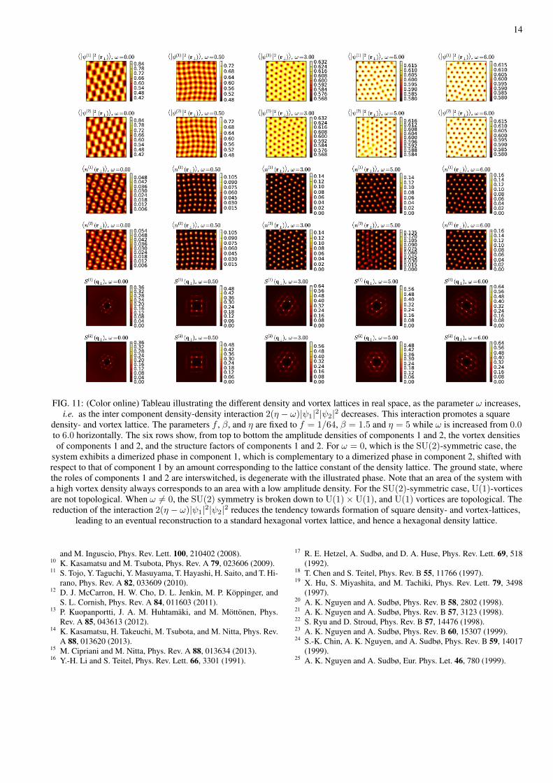
FIG. 11: (Color online) Tableau illustrating the different density and vortex lattices in real space, as the parameter ω increases,i.e. as the inter component density-density interaction 2(η − ω)|ψ1|2|ψ2|2 decreases. This interaction promotes a square

density- and vortex lattice. The parameters f , β, and η are fixed to f = 1/64, β = 1.5 and η = 5 while ω is increased from 0.0to 6.0 horizontally. The six rows show, from top to bottom the amplitude densities of components 1 and 2, the vortex densitiesof components 1 and 2, and the structure factors of components 1 and 2. For ω = 0, which is the SU(2)-symmetric case, the

system exhibits a dimerized phase in component 1, which is complementary to a dimerized phase in component 2, shifted withrespect to that of component 1 by an amount corresponding to the lattice constant of the density lattice. The ground state, wherethe roles of components 1 and 2 are interswitched, is degenerate with the illustrated phase. Note that an area of the system witha high vortex density always corresponds to an area with a low amplitude density. For the SU(2)-symmetric case, U(1)-vorticesare not topological. When ω 6= 0, the SU(2) symmetry is broken down to U(1)×U(1), and U(1) vortices are topological. Thereduction of the interaction 2(η − ω)|ψ1|2|ψ2|2 reduces the tendency towards formation of square density- and vortex-lattices,

leading to an eventual reconstruction to a standard hexagonal vortex lattice, and hence a hexagonal density lattice.

and M. Inguscio, Phys. Rev. Lett. 100, 210402 (2008).10 K. Kasamatsu and M. Tsubota, Phys. Rev. A 79, 023606 (2009).11 S. Tojo, Y. Taguchi, Y. Masuyama, T. Hayashi, H. Saito, and T. Hi-

rano, Phys. Rev. A 82, 033609 (2010).12 D. J. McCarron, H. W. Cho, D. L. Jenkin, M. P. Koppinger, and

S. L. Cornish, Phys. Rev. A 84, 011603 (2011).13 P. Kuopanportti, J. A. M. Huhtamaki, and M. Mottonen, Phys.

Rev. A 85, 043613 (2012).14 K. Kasamatsu, H. Takeuchi, M. Tsubota, and M. Nitta, Phys. Rev.

A 88, 013620 (2013).15 M. Cipriani and M. Nitta, Phys. Rev. A 88, 013634 (2013).16 Y.-H. Li and S. Teitel, Phys. Rev. Lett. 66, 3301 (1991).

17 R. E. Hetzel, A. Sudbø, and D. A. Huse, Phys. Rev. Lett. 69, 518(1992).

18 T. Chen and S. Teitel, Phys. Rev. B 55, 11766 (1997).19 X. Hu, S. Miyashita, and M. Tachiki, Phys. Rev. Lett. 79, 3498

(1997).20 A. K. Nguyen and A. Sudbø, Phys. Rev. B 58, 2802 (1998).21 A. K. Nguyen and A. Sudbø, Phys. Rev. B 57, 3123 (1998).22 S. Ryu and D. Stroud, Phys. Rev. B 57, 14476 (1998).23 A. K. Nguyen and A. Sudbø, Phys. Rev. B 60, 15307 (1999).24 S.-K. Chin, A. K. Nguyen, and A. Sudbø, Phys. Rev. B 59, 14017

(1999).25 A. K. Nguyen and A. Sudbø, Eur. Phys. Let. 46, 780 (1999).

15

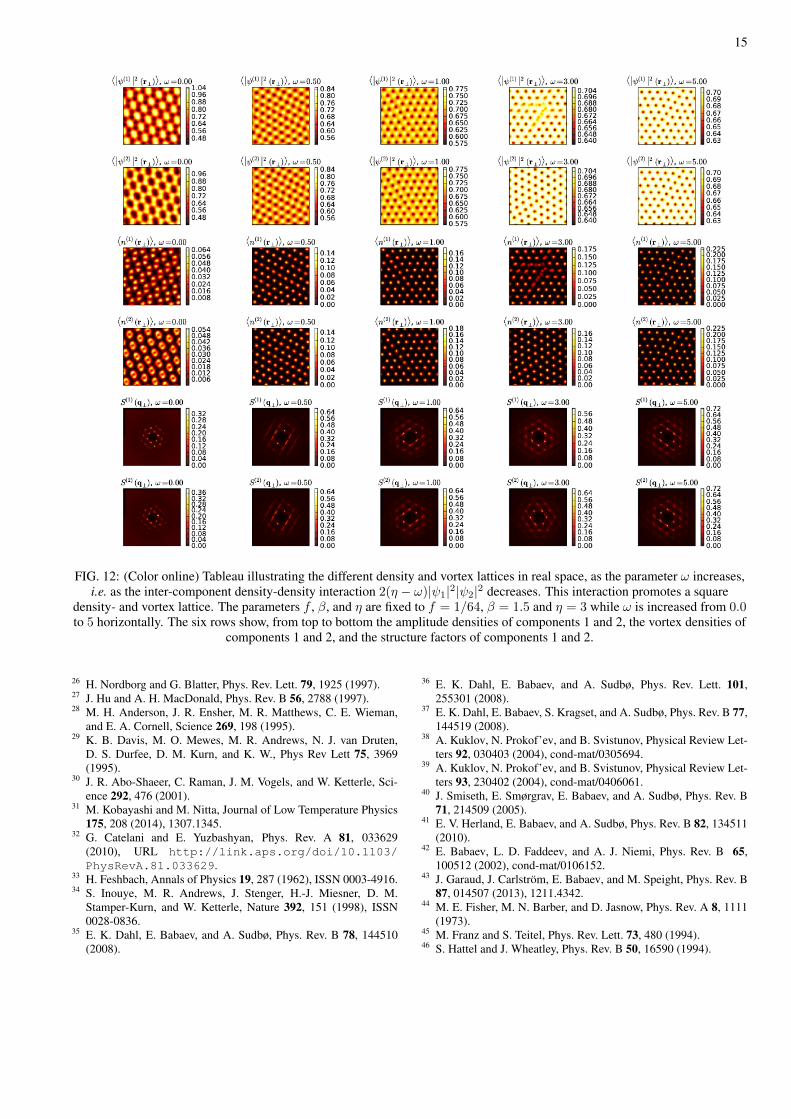
FIG. 12: (Color online) Tableau illustrating the different density and vortex lattices in real space, as the parameter ω increases,i.e. as the inter-component density-density interaction 2(η − ω)|ψ1|2|ψ2|2 decreases. This interaction promotes a square

density- and vortex lattice. The parameters f , β, and η are fixed to f = 1/64, β = 1.5 and η = 3 while ω is increased from 0.0to 5 horizontally. The six rows show, from top to bottom the amplitude densities of components 1 and 2, the vortex densities of

components 1 and 2, and the structure factors of components 1 and 2.

26 H. Nordborg and G. Blatter, Phys. Rev. Lett. 79, 1925 (1997).27 J. Hu and A. H. MacDonald, Phys. Rev. B 56, 2788 (1997).28 M. H. Anderson, J. R. Ensher, M. R. Matthews, C. E. Wieman,

and E. A. Cornell, Science 269, 198 (1995).29 K. B. Davis, M. O. Mewes, M. R. Andrews, N. J. van Druten,

D. S. Durfee, D. M. Kurn, and K. W., Phys Rev Lett 75, 3969(1995).

30 J. R. Abo-Shaeer, C. Raman, J. M. Vogels, and W. Ketterle, Sci-ence 292, 476 (2001).

31 M. Kobayashi and M. Nitta, Journal of Low Temperature Physics175, 208 (2014), 1307.1345.

32 G. Catelani and E. Yuzbashyan, Phys. Rev. A 81, 033629(2010), URL http://link.aps.org/doi/10.1103/PhysRevA.81.033629.

33 H. Feshbach, Annals of Physics 19, 287 (1962), ISSN 0003-4916.34 S. Inouye, M. R. Andrews, J. Stenger, H.-J. Miesner, D. M.

Stamper-Kurn, and W. Ketterle, Nature 392, 151 (1998), ISSN0028-0836.

35 E. K. Dahl, E. Babaev, and A. Sudbø, Phys. Rev. B 78, 144510(2008).

36 E. K. Dahl, E. Babaev, and A. Sudbø, Phys. Rev. Lett. 101,255301 (2008).

37 E. K. Dahl, E. Babaev, S. Kragset, and A. Sudbø, Phys. Rev. B 77,144519 (2008).

38 A. Kuklov, N. Prokof’ev, and B. Svistunov, Physical Review Let-ters 92, 030403 (2004), cond-mat/0305694.

39 A. Kuklov, N. Prokof’ev, and B. Svistunov, Physical Review Let-ters 93, 230402 (2004), cond-mat/0406061.

40 J. Smiseth, E. Smørgrav, E. Babaev, and A. Sudbø, Phys. Rev. B71, 214509 (2005).

41 E. V. Herland, E. Babaev, and A. Sudbø, Phys. Rev. B 82, 134511(2010).

42 E. Babaev, L. D. Faddeev, and A. J. Niemi, Phys. Rev. B 65,100512 (2002), cond-mat/0106152.

43 J. Garaud, J. Carlstrom, E. Babaev, and M. Speight, Phys. Rev. B87, 014507 (2013), 1211.4342.

44 M. E. Fisher, M. N. Barber, and D. Jasnow, Phys. Rev. A 8, 1111(1973).

45 M. Franz and S. Teitel, Phys. Rev. Lett. 73, 480 (1994).46 S. Hattel and J. Wheatley, Phys. Rev. B 50, 16590 (1994).

16

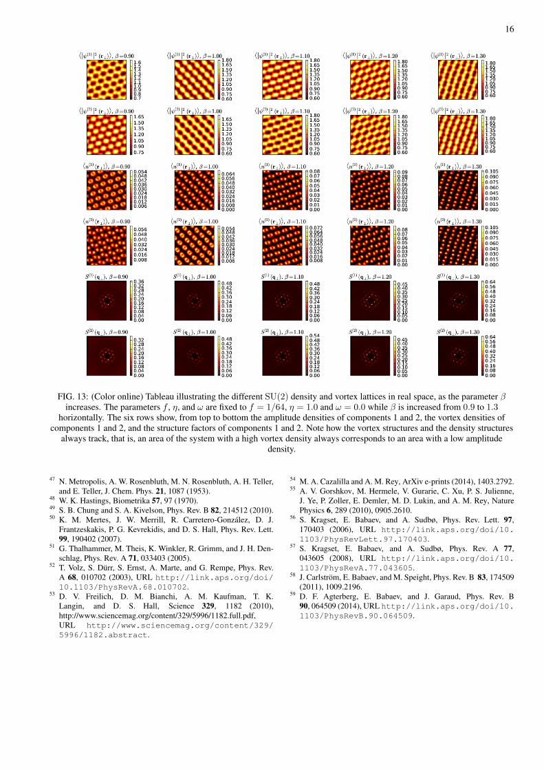
FIG. 13: (Color online) Tableau illustrating the different SU(2) density and vortex lattices in real space, as the parameter βincreases. The parameters f , η, and ω are fixed to f = 1/64, η = 1.0 and ω = 0.0 while β is increased from 0.9 to 1.3

horizontally. The six rows show, from top to bottom the amplitude densities of components 1 and 2, the vortex densities ofcomponents 1 and 2, and the structure factors of components 1 and 2. Note how the vortex structures and the density structures

always track, that is, an area of the system with a high vortex density always corresponds to an area with a low amplitudedensity.

47 N. Metropolis, A. W. Rosenbluth, M. N. Rosenbluth, A. H. Teller,and E. Teller, J. Chem. Phys. 21, 1087 (1953).

48 W. K. Hastings, Biometrika 57, 97 (1970).49 S. B. Chung and S. A. Kivelson, Phys. Rev. B 82, 214512 (2010).50 K. M. Mertes, J. W. Merrill, R. Carretero-Gonzalez, D. J.

Frantzeskakis, P. G. Kevrekidis, and D. S. Hall, Phys. Rev. Lett.99, 190402 (2007).

51 G. Thalhammer, M. Theis, K. Winkler, R. Grimm, and J. H. Den-schlag, Phys. Rev. A 71, 033403 (2005).

52 T. Volz, S. Durr, S. Ernst, A. Marte, and G. Rempe, Phys. Rev.A 68, 010702 (2003), URL http://link.aps.org/doi/10.1103/PhysRevA.68.010702.

53 D. V. Freilich, D. M. Bianchi, A. M. Kaufman, T. K.Langin, and D. S. Hall, Science 329, 1182 (2010),http://www.sciencemag.org/content/329/5996/1182.full.pdf,URL http://www.sciencemag.org/content/329/5996/1182.abstract.

54 M. A. Cazalilla and A. M. Rey, ArXiv e-prints (2014), 1403.2792.55 A. V. Gorshkov, M. Hermele, V. Gurarie, C. Xu, P. S. Julienne,

J. Ye, P. Zoller, E. Demler, M. D. Lukin, and A. M. Rey, NaturePhysics 6, 289 (2010), 0905.2610.

56 S. Kragset, E. Babaev, and A. Sudbø, Phys. Rev. Lett. 97,170403 (2006), URL http://link.aps.org/doi/10.1103/PhysRevLett.97.170403.

57 S. Kragset, E. Babaev, and A. Sudbø, Phys. Rev. A 77,043605 (2008), URL http://link.aps.org/doi/10.1103/PhysRevA.77.043605.

58 J. Carlstrom, E. Babaev, and M. Speight, Phys. Rev. B 83, 174509(2011), 1009.2196.

59 D. F. Agterberg, E. Babaev, and J. Garaud, Phys. Rev. B90, 064509 (2014), URL http://link.aps.org/doi/10.1103/PhysRevB.90.064509.