Five centuries of Stockholm winter/spring temperatures reconstructed from documentary evidence and...

Climatic ChangeDOI 10.1007/s10584-009-9650-y

Five centuries of Stockholm winter/spring temperaturesreconstructed from documentary evidenceand instrumental observations

Lotta Leijonhufvud · Rob Wilson · Anders Moberg ·Johan Söderberg · Dag Retsö · Ulrica Söderlind

Received: 14 July 2008 / Accepted: 14 July 2009© Springer Science + Business Media B.V. 2009

Abstract Historical documentary sources, reflecting different port activities inStockholm, are utilised to derive a 500-year winter/spring temperature reconstruc-tion for the region. These documentary sources reflect sea ice conditions in theharbour inlet and those series that overlap with the instrumental data correlatewell with winter/spring temperatures. By refining dendroclimatological methods,the time-series were composited to a mean series and calibrated (1756–1841;r2 = 66%) against Stockholm January–April temperatures. Strong verification was

L. Leijonhufvud (B) · A. MobergDepartment of Physical Geography and Quaternary Geology,Stockholm University, 106 91 Stockholm, Swedene-mail: [email protected]

A. Moberge-mail: [email protected]

R. WilsonSchool of Geography & Geosciences, University of St Andrews,St Andrews, FIFE, KY16 9AL, Scotland, UKe-mail: [email protected]

J. Söderberg · D. Retsö · U. SöderlindDepartment of Economic History, Stockholm University,106 91 Stockholm, Sweden

J. Söderberge-mail: [email protected]

D. Retsöe-mail: [email protected]

U. Söderlinde-mail: [email protected]

Climatic Change

confirmed (1842–1892; r2 = 60%; RE/CE = 0.55). By including the instrumentaldata, the quantified (QUAN) reconstruction indicates that recent two decadeshave been the warmest period for the last 500 years. Coldest conditions occurredduring the 16th/17th and early 19th centuries. An independent qualitative (QUAL)historical index was also derived for the Stockholm region. Comparison betweenQUAN and QUAL shows good coherence at inter-annual time-scales, but QUALdistinctly appears to lack low frequency information. Comparison is also made toother winter temperature based annually resolved records for the Baltic region.Between proxy coherence is generally good although it decreases going back in timewith the 1500–1550 period being the weakest period—possibly reflecting data qualityissues in the different reconstructions.

1 Introduction

“And all through the months that in other days had been beautiful with flowers thesnow fell steadily, and the cold winds blew fiercely, while eyes grew sad and heartsheavy with waiting for a summer that did not come. And it never came again; forthis was the terrible Fimbul-winter. . . ” (Norse stories retold from the Eddas. WrightMabie 1901).

In pre-industrial societies, most economic activities were dependent upon andconstrained by the natural environment—including climate (Brázdil et al. 2006).Stockholm, located near 59◦N, 18◦E, at the interior of an archipelago in the BalticSea (Fig. 1), is a city where the sailing season was strongly dependent on ice-freeconditions before the invention of steel hulled ships, steam engines and ice-breakers.

Swedish archives are well-known to be rich (Pfister and Brázdil 1999), anddocuments concerning Stockholm, the capital, are particularly abundant. Thus, withdocumentary evidence concerning sailing activities going back to the beginning of the16th century (Retsö 2002; Leijonhufvud et al. 2008) and a long instrumental recordof meteorological observations starting in 1756 (Moberg et al. 2002), Stockholm iswell suited for studying the relationship between the sailing season and climate for along time period.

Leijonhufvud et al. (2008) showed that the start of the sailing season each year, asdeduced from custom ledgers and other documents related to harbour activities inStockholm harbour, can be used as robust proxy variables for winter/spring temper-atures, at least until the beginning of the 1870s. In that study (henceforth referredto as L08), we showed how information gleaned from the administrative recordsmay be interpreted as a January–April temperature proxy, and how statisticalmethods commonly used in dendrochronology may be used to derive a temperaturereconstruction back to 1692. Unlike the approach of L08 and a few other studies(e.g. Tarand and Nordli 2001), most previous studies in historical climatology useclimatic indices, defined as discrete numbers on an ordinal scale, to describe climaticconditions in the past (see e.g. Brázdil et al. 2005). In the current study, we willmake an extension of the L08 January–April temperature reconstruction back tothe early 16th century, but also present an independent winter/spring climate seriesusing the more traditional indexing method. Additionally, we compare these twoclimate records with previously published five-century long series reflecting cold-season climate conditions in the southern Baltic Sea region.

Climatic Change

Fig. 1 Location map, showing Stockholm and other key locations discussed in the paper.Luterbacher grid box (LUT; see Section 6) shown in red while other winter proxy records arehighlighted in yellow

It should be made clear that the Stockholm quantitative and qualitative win-ter/spring climate series developed here are based on entirely independent data. Theraw data used for the quantitative reconstruction are strictly numeric, consisting ofdates (days after 1st January, Gregorian calendar) that indicate the start of the sailingseason, whereas the qualitative index is based on interpretation of various types ofdescriptive information. We regard the quantitative series as our main reconstruc-tion (being calibrated to temperatures and consisting of continuous numeric data),whereas the qualitative index series (being uncalibrated and consisting of discretenumeric data) contributes with additional independent information.

As the qualitative reconstruction, as well as two other series within the quanti-tative reconstruction, are composite series, it is possible to test how well compositeseries from historical documents stand up against more homogenous quantitatively-derived series.

2 Start of sailing season deduced from economic-administrative sources

Stockholm, with its superior geographical location as well as being the capital,was the principal trading port in Sweden (Wikberg 2006, p. 21). The economic-

Climatic Change

Fig. 2 Map of Stockholm AD 1642 (or possibly 1640). The central city island guards the inlet to lakeMälaren (to the west) and the innermost fringe of the Baltic Sea (to the east). Several of the harbourfacilities and other important places mentioned in the text are marked: A the eastern harbour, B thewestern harbour, C the pole fence, D bridges; were raised, at least for larger vessels, E the locationof the lock, built in late 1642. F (near upper frame) the hill where the Astronomical observatorywas built in 1753, i.e. where the thermometer has been placed from 1756 onwards, G the Årstamanor (located slightly southwards from the letter G, near lower frame, close to Årsta Bay). Source:National Library, Stockholm 51:30

administrative records related to shipping and harbour activities in Stockholmcontain information about most ships that sailed to and from the city, thus providingthe means with which to estimate when the sailing season started each year. Figure 2shows the physical geography of Stockholm in 1642 (1640), as well as several of theharbour facilities and other places mentioned later in Section 3.

The basic premise of this study (from L08) is simple; each documentary sourceis scrutinized in order to find the date that indicates when the sailing season hadstarted for a given year. The main factor constraining sailing in spring is the icecover of the Baltic, which is, in turn, closely related to the annual mean winterair temperature (Hansson and Omstedt 2007). For each source, a time series ofdates, regarded as proxies for winter/spring temperatures, are constructed. Theresulting set of time series is then used as raw data for producing the quantitativetemperature reconstruction. We have transformed all relevant days into days afterNew Year according to the Gregorian Calendar for the whole period 1500 onwards

Climatic Change

(see Haldorsson 1996 for further explanations on the particular Gregorian calendarreform in Sweden).

The various economic-administrative sources are ordered chronologically, withthe first date each year when the administration of the respective source began beingtaken as the basis for discrimination. The records were kept continuously throughoutthe sailing season. This means that, usually, when the sailing season had begun(or more correctly, when the administrative recording of sailing/harbour activitieshad begun), ships were recorded every day or every second day, which makes it easyto estimate the date for the start of the sailing season. In years when sailing startedlate in spring, the first date of entry usually contains several transactions; i.e., severalships arrived, or departed, at the same time.

The information about ship activities in various economic-administrative sourcesis the main indicator of the start of the sailing season used for the quantitativereconstruction in L08 and in this study. (Our qualitative index is based on otherinformation, see Sections 3.12 and 3.14 and 4.3). Further discussion on problemsrelated to determining the start of sailing season is provided in L08.

3 Sources: description and criticism

The source critical discussion which was initiated in L08 is continued here. As hasbeen noted by several studies, the importance of such analyses is vital for all studiesusing documentary data as climatic proxies (Bell and Ogilivie 1978; Pfister et al. 1999;Brázdil et al. 2005). The L08 reconstruction, which covers the period 1692–1892, wasbased on data from seven different sets of administrative records. Four of the sourcesextend back before 1692. Two of them, the ballast and the sea passports, do not formcontinuous series, and have large gaps.

For the period 1502–1636 we are faced with a problem of having sources thatcannot be calibrated and verified against instrumental records. This type of difficulty,is also faced in dendrochronological studies that use sub-fossil (Luckman and Wilson2005; Wilson et al. 2007; Grudd 2008) or historical (Wilson et al. 2004, 2005; Wilsonand Topham 2004; Büntgen et al. 2006) tree-ring material to extend living chronolo-gies. In those cases, the underlying assumption is that a specific species of treesresponds in a similar way to climate over time, even if the climatic regime changes.An equivalent assumption has to be made for documentary evidence. It is thereforeessential that sources are carefully evaluated, in order to judge whether or not theearly sources are likely to contain climatic information comparable to sources usedin the calibration and verification periods. In addition to source criticism, it is alsoimportant to undertake statistical cross-comparisons among time series derived fromdifferent sources.

Sections 3.1–3.11 describe sources used only for the quantitative reconstruction.Sections 3.12, 3.13 describe sources containing information used for both the quanti-tative reconstruction and qualitative index. Section 3.14 describes sources used onlyfor constructing the qualitative index. Table 1 summarizes general information aboutthe sources used for the quantitative reconstruction. Table 2 presents correlationcoefficients between each series in Table 1 and the mean of all other series havingsimultaneous data.

Climatic Change

Tab

le1

Adm

inis

trat

ive

sour

ces

wit

hco

rres

pond

ing

prox

yla

bels

refle

ctin

gop

enin

gof

saili

ngse

ason

inSt

ockh

olm

Arc

hive

/sou

rce

Pro

xyla

bel

Bri

efde

scri

ptio

nP

erio

dof

cove

rage

RA

/Lok

ala

tullr

äken

skap

erna

GST

AF

irst

arri

vala

ccor

ding

toG

reat

Sea

Tol

lled

gers

1533

–162

2/16

64R

A/L

okal

atu

llräk

ensk

aper

naG

STD

Fir

stde

part

ure

acco

rdin

gto

Gre

atSe

aT

olll

edge

rs15

37–1

622/

1673

SSA

/Sta

dska

mre

rare

nT

olag

AF

irst

arri

vala

ccor

ding

tolo

cali

mpo

rtta

x16

36–1

841

SSA

/Sta

dska

mre

rare

nT

olag

DF

irst

depa

rtur

eac

cord

ing

tolo

cale

xpor

ttax

1636

–184

1R

A/S

tock

holm

svå

gböc

ker

Bal

ance

Bal

ance

acco

unts

from

the

grea

tiro

nba

lanc

e15

46–1

668

SSA

/Bor

gmäs

tare

&R

ådR

A/L

illa

tulle

n&

skep

psgå

rdsh

andl

,Sa

SD

iver

seso

urce

sof

shor

tadm

inis

trat

ive

seri

es16

20–1

692

SSA

/Sta

dska

mre

rare

nco

ncer

ning

diff

eren

tfee

sin

Stoc

khol

mha

rbou

rSS

A/F

rakt

böck

erF

reig

htSe

afr

eigh

tcon

trac

ts,s

peci

fyin

gda

teof

cont

ract

1551

–159

0SS

A/B

orgm

ästa

re&

Råd

,H

arbo

urfe

eH

arbo

urfe

esin

Stoc

khol

m&

Vax

holm

,fee

sfo

r16

08–1

692

Stad

skam

rera

ren

gett

ing

thro

ugh

the

lock

ofSt

ockh

olm

SSA

/Bor

gmäs

tere

&R

ådP

ole

Fee

for

the

open

ing

ofth

epo

leba

rric

ade

arou

ndth

eci

ty16

03–1

620

RA

/KoK

,pas

sdia

rier

and

SSA

,Hak

Sea

pass

port

Insu

ranc

edo

cum

entf

orsh

ips

trav

ellin

gto

the

1689

–183

1M

edit

erra

nean

and

beyo

nd.S

tock

holm

isho

me-

port

SSA

/Hak

/Sjö

folk

skon

trol

len

Ship

reco

rds

Reg

iste

rsof

sailo

rsle

avin

gSt

ockh

olm

1692

–184

2SS

A/H

ak/H

uvud

prot

okol

lB

alla

stP

lank

sgr

ante

dfo

rba

llast

byth

eci

tyco

unci

l16

73–1

734

Hild

ebra

ndss

on(1

915)

Väs

terå

sD

educ

tion

for

the

Bay

ofV

äste

rås

inla

ke17

12–1

892

Mäl

aren

:‘w

hen

the

lake

Mäl

aren

isso

open

and

free

ofic

eth

atth

esa

iling

seas

onbe

twee

nV

äste

rås

and

Stoc

khol

mha

sbe

gun’

Ber

ätte

lse

angå

ende

Stoc

khol

ms

Off

.sta

rtO

ffici

alst

atis

tics

ofth

eop

enin

gof

the

saili

ngse

ason

1815

–189

2K

omm

unal

förv

altn

ing

År

1894

(189

6)R

A/K

MT

regi

stra

tur,

DeS

prin

gL

ette

rsfr

omth

eG

over

nmen

tor

the

Adm

iral

tyB

oard

1502

–178

3K

rA/A

dmir

alit

etsk

olle

giet

desc

ribi

ngic

eco

ndit

ions

and

the

star

tofs

ailin

gre

gist

ratu

r,et

c(n

oco

ntin

uous

seri

esof

ship

ping

traf

fic)

NM

A/Å

rsta

frun

sda

gböc

ker

Års

tadi

ary

Not

esin

diar

yw

hen

the

ice

brea

k-up

occu

rred

inth

eÅ

rsta

bay

1793

–183

7

Climatic Change

Tab

le2

Cor

rela

tion

sbe

twee

nea

chpr

oxy

seri

esas

labe

lled

inT

able

1ag

ains

tthe

mea

nof

allo

ther

sim

ulta

neou

sse

ries

Väs

terå

sO

ff.s

tart

Tol

agA

Tol

agD

Ship

reco

rds

Års

tadi

ary

Sea

pass

port

Bal

last

SaS

Har

bour

fee

GST

DB

alan

ceG

STA

Pol

eF

reig

htD

eSpr

ing

A.C

orre

lati

ons

wit

hm

ean

ofal

loth

erse

ries

R0.

700.

890.

820.

810.

760.

570.

490.

330.

580.

610.

620.

380.

440.

620.

170.

77P

0.00

0.00

0.00

0.00

0.00

0.00

0.00

0.02

0.01

0.00

0.00

0.06

0.00

0.01

0.43

0.00

N14

946

159

136

150

5410

048

1920

5626

6517

2419

B.C

orre

lati

onw

ith

QU

AL

R−0

.64

−0.6

5−0

.63

−0.5

1−0

.53

−0.4

6−0

.33

−0.0

8−0

.62

−0.8

0−0

.58

−0.3

7−0

.58

−0.3

0−0

.32

−0.7

4P

0.00

0.00

0.00

0.00

0.00

0.00

0.00

0.58

0.00

0.00

0.00

0.05

0.00

0.22

0.11

0.00

N14

946

159

137

150

4110

048

2020

5829

6918

2655

Climatic Change

3.1 Custom ledgers: the Great Sea Toll (1533–1622 with few gaps, 1636–1673with many gaps) and the Tolag (1636–1841 with few gaps)

Two custom ledger series, the Great Sea Toll and the Tolag are the longest and mostcomplete data sources used in the quantitative reconstruction. They were levelledupon import (arriving ships) and export (departing ships). The revenues of theGreat Sea Toll accrued to the Crown (Wikberg 2006, p. 17), while the Tolag wasa municipal custom, mainly used for building activities and payment of salaries tothe city’s administration (Sandström 1990, p. 81). The dates for the first arrival anddeparture of ships after each winter documented in these sources are treated asindependent proxy series, labelled ‘GSTA’ and ‘TolagA’ for first arrivals and ‘GSTD’and ‘TolagD’ for first departures. Although both types of sources are fairly rich, ithas not been possible to build complete series of sailing season start dates. There aresome gaps in all four series.

The Great Sea Toll was initiated in 1533 when the Hanseatic League lost their toll-freedom in Sweden (Smith 1934, p. 111). Government administrative control endedin 1726, when it was leased to a half-private society; Generaltullarrendesocieteten(Wikberg Lindroth 2004). However, after 1622 only a few surviving Great Sea Tollregisters from Stockholm exist, because the specifications were requested by thearmy as wadding for artillery and most of this record was destroyed. Some data fromthe port of Nyköping (∼70 km south of Stockholm) have therefore been used for afew years between 1660 and 1673 in an attempt to make an inter-correlation betweenthe calibrated and verified Tolag series with the older source.

An instruction to the Director-General of customs from 19 December 1636 statedthat all customs were to be manned with clerks and writers, visitation officers, rowersand other servants (Smith 1950, p. 133). The circumstance that the customs employedvisitation officers indicates that they did inspect the ships. ‘Rowers’ indicate that itwas sometimes necessary to access ships not docked at the quays.

In the statutes for the Tolag it was stated that a city was only allowed the Tolag oncondition that it also administrated the Great Sea Toll for the Crown (Dalhede 2005,p. 22). The administrative routines for the Tolag should therefore be the same as theones for the Great Sea Toll. This suggests that if the Tolag picks up a climatic signal,the Great Sea Toll would do likewise. However, it cannot be assumed a priori thatlegislative ordinances were followed; Sandström (1990, p. 36) points out that the twodifferent customs are not entirely comparable with each another. Differences stemmostly from the fact that some people set sail before they had paid; especially theTolag seems to have been comparably easy to evade. This problem does not concernthe present analysis as tax-evaders were accounted for with their “restantier”—i.e.their rest—and if they dared to return to the city the following year, they had to paythen. Most importantly for this investigation; neither the Tolag nor the Great SeaToll are maintained with respect to when the captains paid their dues, but rather towhen the ship arrived at the custom station (Sandström 1990, p. 87; this is obvious inmost of the original documents—SSA, RA).

The registers of the Great Sea Toll are divided between import-custom andexport-custom; such that there is one register for arriving and another for departingships. The registers are written chronologically for each provenance or destination.When the last ship had arrived (or departed), a summary of how much custom hadbeen gathered from that port was made. This practice, with separate accounts for

Climatic Change

the different ports, indicates that the custom-accounts also were made for reasons oftrade statistics. If so, this heightens the value of the custom accounts as a source forclimate proxy information.

The Tolag series begin in 1636 and end in the mid 19th century (Table 1). Becauseof practical problems of abstracting the Tolag, we did not abstract data from after1841. Nevertheless, our Tolag series are sufficiently long to allow for calibrationagainst instrumental temperature data (see L08).

As the Great Sea Toll from Stockholm ends in effect in 1622, it is impossible tocheck the inter-correlation between the series of sailing season derived from thatsource and the corresponding series derived from the Tolag. The few data fromthe Great Sea Toll that are part of the series between 1636 and 1673—where fiveout of nine data originate from the port of Nyköping—are too few for meaningfulcorrelation analysis with the corresponding Tolag data from Stockholm. However,we assume that trading conditions, as far as they are determined by whether thesea was open or not, are similar for the two harbours. Nevertheless, there might besome differences in trading practises because Nyköping was a much smaller port thanStockholm.

The correlation between the sailing season start deduced from each of the twoTolag series and the mean of other simultaneous series is ∼0.8 (Table 2), implyinga high degree of linear coherence between data series during 1636–1841. Thecorresponding values for the earlier Great Sea Toll data are lower (r = 0.62 forGSTD, r = 0.44 for GSTA). This does not necessarily imply that the Great Sea Tolldata are inferior as indicators of the start of the sailing season compared with theTolag, but is more likely mainly a consequence of poorer quality (from our point ofview) of other data sources used in the 16th century, in particular the Freight books(see Section 3.4).

3.2 Weigh books (1546–1668, with many gaps)

Weigh books are the journals which document goods that were weighed in the town’sweigh house. There is a difference between the early weigh books from the 1540s,placed in KA, and the later books from the 1570s, placed in SSA; the former werekept in an attempt to track trade, while the latter were made as a foundation fortaxation (Odén 1959). The earlier weigh books therefore probably have a highersource value than the latter ones.

In 1604, King Karl IX commanded that weighing should occur in immediateconnection with the paying of duties when goods were exported and imported.However, the use of the balance was not only a duty, but also a privilege andmerchants could be forbidden the use of the balance as punishment for crimes (Odén1959). These properties of the weigh books render them suitable for establishing thebeginning of the sailing season.

From a practical point of view, however, it turned out to be difficult to workwith the weigh books. The hand-writing of the records is cramped, so it is notcertain that it has been possible to ascertain correctly whether a certain personhas “bought, “sold”, “exported” or simply “weighed” his goods. Furthermore, thecity law stated that not only goods for export or import should be weighted, butalso goods which were sold in the city. This implies that goods sold in the citymight later have been exported, but we cannot know when or how this occurred

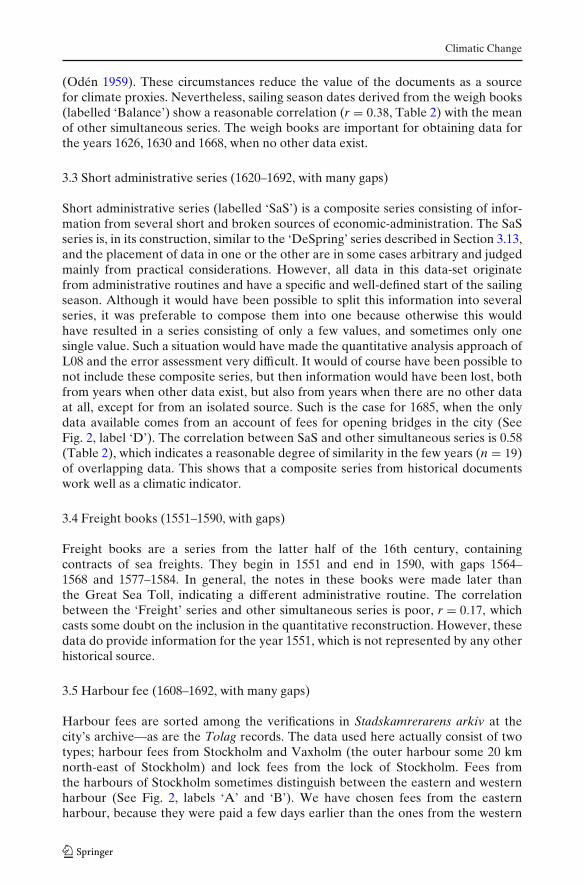
Climatic Change

(Odén 1959). These circumstances reduce the value of the documents as a sourcefor climate proxies. Nevertheless, sailing season dates derived from the weigh books(labelled ‘Balance’) show a reasonable correlation (r = 0.38, Table 2) with the meanof other simultaneous series. The weigh books are important for obtaining data forthe years 1626, 1630 and 1668, when no other data exist.

3.3 Short administrative series (1620–1692, with many gaps)

Short administrative series (labelled ‘SaS’) is a composite series consisting of infor-mation from several short and broken sources of economic-administration. The SaSseries is, in its construction, similar to the ‘DeSpring’ series described in Section 3.13,and the placement of data in one or the other are in some cases arbitrary and judgedmainly from practical considerations. However, all data in this data-set originatefrom administrative routines and have a specific and well-defined start of the sailingseason. Although it would have been possible to split this information into severalseries, it was preferable to compose them into one because otherwise this wouldhave resulted in a series consisting of only a few values, and sometimes only onesingle value. Such a situation would have made the quantitative analysis approach ofL08 and the error assessment very difficult. It would of course have been possible tonot include these composite series, but then information would have been lost, bothfrom years when other data exist, but also from years when there are no other dataat all, except for from an isolated source. Such is the case for 1685, when the onlydata available comes from an account of fees for opening bridges in the city (SeeFig. 2, label ‘D’). The correlation between SaS and other simultaneous series is 0.58(Table 2), which indicates a reasonable degree of similarity in the few years (n = 19)of overlapping data. This shows that a composite series from historical documentswork well as a climatic indicator.

3.4 Freight books (1551–1590, with gaps)

Freight books are a series from the latter half of the 16th century, containingcontracts of sea freights. They begin in 1551 and end in 1590, with gaps 1564–1568 and 1577–1584. In general, the notes in these books were made later thanthe Great Sea Toll, indicating a different administrative routine. The correlationbetween the ‘Freight’ series and other simultaneous series is poor, r = 0.17, whichcasts some doubt on the inclusion in the quantitative reconstruction. However, thesedata do provide information for the year 1551, which is not represented by any otherhistorical source.

3.5 Harbour fee (1608–1692, with many gaps)

Harbour fees are sorted among the verifications in Stadskamrerarens arkiv at thecity’s archive—as are the Tolag records. The data used here actually consist of twotypes; harbour fees from Stockholm and Vaxholm (the outer harbour some 20 kmnorth-east of Stockholm) and lock fees from the lock of Stockholm. Fees fromthe harbours of Stockholm sometimes distinguish between the eastern and westernharbour (See Fig. 2, labels ‘A’ and ‘B’). We have chosen fees from the easternharbour, because they were paid a few days earlier than the ones from the western

Climatic Change

harbour (SSA, Stadskamrerarens arkiv, Verifikationer 1641, 1644). In principle, thesedata could have been added to the SaS series, but since there are data from severalyears simultaneously, it was convenient to develop a separate series from the harbourfees (labelled ‘Harbourfee’). From 1608 to 1623, the series comprise data concerningfees paid for passage through the lock of Stockholm. At that time, there was no actuallock, but boats were dragged upstream against the flow of the channel between theBaltic and the lake Mälaren. (See Fig. 2, label ‘E’). For the latter period, 1636–1681,data are true harbour fees. The last datum, 1692, concerns the lock fee (i.e. whenthere was a lock.). The correlation of Harbourfee with other series is quite strong(r = 0.61, Table 2) for the 20 years of overlapping data.

3.6 Pole penny (1603–1620, complete)

Stockholm was surrounded by a defence blockade of piles in the waters surroundingthe main city island (See Fig. 2, very faint dots in water indicated by label ‘C’). Thesepiles were connected with bars, which could be raised to allow incoming (departing)ships to enter (leave) the harbours. This procedure has generated a short, but well-preserved, series of data from the early seventeenth century, called pålpenning (polepenny). The time series (labelled ‘Pole’) is complete 1603–1620. Its correlation withthe mean of other series is r = 0.62 (Table 2).

3.7 Drafts of Sjöpass (“Sea Passports”) (1689–1706 scattered values, 1733–1831nearly complete)

From 1665, there exist drafts of sea passports in the main archive of the NationalBoard of Trade, RA. The documents are very well preserved and begin with theform that should be used for the passports. They are written in Latin. The passportsspecify; (1) a date, (2) who the captain was and where he came from, (3) the ship’sname and its capacity, (4) from which harbour the ship was sailing from and whereit was sailing to, and (5) what goods it brought. The passport is signed with the samedate as was given in the very beginning of the letter.

The main problem with these drafts as indicators of the start of the sailing seasonis that there were few passports issued. We have not been able to include any of thevery first drafts still existing, because there were very few of them and the few existingones were issued in the middle of the sailing season (in the summer months). The firstyear, which may contain relevant climatic information, as well as being consistentwith the calibrated and verified sea passports, is 1689. During 1733–1831 the dataseries (labelled ‘Sea passport’) is nearly complete. Its correlation with the mean ofother series is relatively modest (r = 0.49), but highly statistically significant beingcalculated for 100 overlapping years.

3.8 Planks granted for ballast (1673–1734, nearly complete from 1689)

As described in L08, records of planks (or ‘wood’) may be found among the mainrecords of proceedings of the Chamber of Commerce, SSA. The application forballast could be made well in advance of a planned journey, as was also the case forthe sea passports. The number of ships is fewer than those registered in the Tolag andship-records accounts. The correlation between the series (‘Ballast’) derived from

Climatic Change

this source and the other simultaneous series is 0.33, making this one of the weakercontributors to the common signal. Further information is provided in L08.

3.9 Ice break-up in Västerås (1712–1892, complete)

A series of deduced ice break-up dates for the lake waters outside the town ofVästerås, covering the period 1712–1892, has been developed by Hildebrandsson(1915). Västerås is located at a bay of Lake Mälaren, ∼90 km west of Stockholm.Although this published series does not relate directly to port activities in Stockholm,it is included in our quantitative reconstruction (and L08) because it is stronglycorrelated with Stockholm temperatures in all months from January to April (seeFig. 2 in L08 and their associated extensive discussion concerning this source). Thecorrelation between this series (here labelled ‘Västerås’, also to enhance that thisseries probably does not so much reflect ice break-up as the name implies, but ratherthe beginning of the sailing season in Västerås) and the mean of other simultaneousseries is quite strong, r = 0.70.

3.10 Official port statistics (1815–1892, complete)

As described in L08, official port statistics on the beginning of the sailing season arepublished in a series of the City Council’s Working Committee (Berättelse angåendeStockholms Kommunalförvaltning 1894). This data series (here labelled ‘Off.start’) iscomplete for the period 1815–1892, and correlate with the other simultaneous seriesat the high level of r = 0.89. See L08 for further information.

3.11 Ship records (1692–1841, complete)

Ship records were drawn up in the city’s Chamber of Commerce, SSA, and couldbe arranged well in advance of the planned travel. The data series (labelled ‘shiprecords’) are complete for the period 1692 to 1841 and correlates at high level ofr = 0.76. See L08 for an extensive description and discussion of this source.

3.12 Descriptive sources I—The Årsta Diary (1793–1837, nearly complete)

The diary kept by Lady Märta Helena Reenstierna, concerns her daily life for nearly40 years at the Årsta manor, just to the south of Stockholm (See Fig. 2, label ‘G’). Shemade more or less daily descriptive weather observations, not only because she wasinterested in the weather but because she was dependent upon climatic conditionsfor the manorial management. Among these notes, c. 14,500 weather observations,are information on the ice break-up in the Årsta Bay. Notices of ice break-up occurfor nearly every year. Information from the Årsta Diary is used both to derive a timeseries of ice break-up dates 1793–1837 (labelled ‘Årsta diary’), which is included inthe quantitative reconstruction, and as a contribution to the qualitative index series.

The diary observations on ice break-up may be regarded as being similar toscientific observations of ice break-up. As they were written by the same chroniclerthey constitute the most consistent data set used in this study. Nevertheless, thecorrelation between the Årsta diary ice break-up dates and observed January–Apriltemperatures for Stockholm is lower than that between the start of the sailing

Climatic Change

season as suggested in some other series available for the period 1793–1837. (TolagDcorrelates at r = −0.91 and Ship records at r = −0.70 with JFMA temperatures,compared to r = −0.52 for the Årsta diary). The correlation between the Årstadiary ice break-up dates with the “ice break-up” series from Västerås, is 0.58. Thisrelatively low correlation is probably a consequence of the fact that the series fromVästerås reflect the start of sailing season in the western part of lake Mälaren, whilethe Årsta series is a series of true ice break-up in the easternmost part of the lake.As was shown earlier, the series from Västerås has an excellent correlation withStockholm winter temperatures.

The correlation between the Årsta diary ice-break up series and the mean ofthe other simultaneous series contributing to the quantitative reconstruction isr = 0.57, which is comparable to some of the early series derived from economic-administrative sources.

Additional descriptive climatic information from Lady Reenstierna’s diary, wasused to construct the qualitative index series. However, any one particular piece ofinformation was never used for both series, in order to guarantee full independencebetween the two reconstructions. For example, entries in the diary such as ‘verymild today and the lake has become open’ are only used for the quantitativereconstruction, whereas keywords relating to the diarist’s perception of temperature(e.g. ‘cold’, ‘very cold’, ‘mild’ etc.) entered the database used to derive the index.

3.13 Descriptive sources II—descriptive spring data (1502–1637 with gaps,1652–1783 very sparse)

None of the administrative-economic records described above provide any informa-tion before 1533. Hence, to extend the quantitative reconstruction back to the earliest16th century, it is necessary to deduce the start of sailing season from a variety ofother sources. For this purpose, a dataset labelled ‘DeSpring’ (descriptive springdata) was developed. Among the series used for the quantitative reconstruction,this is the most distinct of the datasets. DeSpring has similarities to the SaS series,both being composite series, but unlike the SaS, DeSpring does not originate fromeconomic-administrative routines. Therefore, the start of the sailing season might notbe determined as directly as is the case with most of the administrative sources.

Governmental letters used in these series consist of requests that ships shouldset sail to or from Stockholm that are made by an official, for example, the Kingor Regent. A key expression is första öppna vatten, i.e. ‘first open water’, referringto the break-up of ice in the archipelago in the spring. Together with the dating ofthe letter in which the key expression occurs, the first dated mentioning of actualshipping provides an approximation of the onset of the period of navigable waters toand from Stockholm, and hence the reopening of the sailing season.

This type of source does not necessarily include a chronological sequence of navalactivities, such as those related to economic administration. Neither do they provide adaily sequence of general weather observations, such as the Årsta diary. Informationderived from the various sources is used both for the quantitative and the qualitativereconstructions. To some extent it has been arbitrary to which of those two datasetsa particular piece of information was assigned. As with the Årsta diary, however, thesame item of information is never used in both datasets.

Climatic Change

Perhaps surprisingly, the correlation between DeSpring and the mean of otherseries in the quantitative dataset is quite strong (r = 0.77). The correlation, however,is estimated from only 19 common years, so it is difficult to judge whether the highvalue is fully representative, but it is another indication that composite series fromdocumentary sources work.

The quantitative DeSpring series has most of its data in the period 1502–1637and only very few scattered values for 1652–1783. It could, in principle, have beenpossible to construct a much longer quantitative DeSpring, but that would have lefttoo few pieces of evidence to allow the qualitative index series to be constructedin some periods. As we attempted to develop two independent reconstructions, wedecided to let DeSpring remain incomplete rather than optimize the informationentering the quantitative reconstruction.

3.14 Descriptive sources III—information used only for the qualitative index

Most of the data used to derive the index series stem from observations relatingto winter and spring climatic conditions in Stockholm and its vicinity. However,information relating to other parts of south-eastern Sweden, especially from thecoastal regions and the Lake Mälaren valley, has also been used. In some cases,data from towns as far southwards as Kalmar (∼400 km from Stockholm), and Visby(∼200 km southeast) and as far westwards as Karlstad (∼300 km) have been included(Fig. 1). The use of data from such distant places is justified by instrumental obser-vations, which indicate that winter and spring temperatures between Stockholm andother stations within this area are very highly correlated. For example, StockholmJanuary–May (JFMAM) temperatures correlate with Kalmar, Visby and Karlstadinstrumental temperatures for the period 1890–2001 at r = 0.97 (as calculated fromdata in Tuomenvirta et al. 2001).

Figure 3 shows the amount of information forming the basis for the qualitativeindex in each year during 1502–1860. Compared to the earlier part of the periodfor which data are collected, the density of data grows substantially after the mid18th century. This is because of a general upsurge in the number of journalsand other publications. One useful source for the latter half of the 18th century

Fig. 3 Number of observations forming the basis of the qualitative index

Climatic Change

is the meteorological observation diary from the old astronomical observatory inStockholm, which not only contains the instrumental temperatures used to derivedaily temperature and air pressure records back to 1756 (Moberg et al. 2002), butalso many pieces of descriptive information. The very high values (>100) during1793–1841 mainly stem from the Årsta diary (see Section 3.11), revealing that this isan exceptionally rich source. The amount of observations per year in earlier periodsis more modest, typically being less than 10, but for some years and periods peakingto around 50 or even 100 observations.

The preserved Chancery Registers of the central administration, containingmostly outgoing correspondence, begin in 1521 (Konung Gustaf den förstes regis-tratur 1861–1916). Prior to this year, the preserved archives of the Sture regents—mostly containing incoming correspondence—have been used. In both bodies ofadministrative correspondence, the climatological proxy data are mostly associatedwith transport and communication, particularly sea transport.

Despite the great importance to Sweden’s foreign trade of ice break-up, its exactdate for a particular year is almost never stated in these older sources. At best, theyprovide either a date before which the ice is certain to have obstructed shipping,or a date on which shipping is certain to have started. Hence, only a time-spanduring which the break-up of the ice is certain to have occurred can be deduced.This implies that some data in the index could have been included in the quantitativeDeSpring series. However, most data forming the foundation for the index, can notbe expressed parametrically (interval or ratio scale) but only at an ordinal (index)scale.

From 1560 to about 1720, the outgoing letters of the King and the Governmentare an important source, though available only in archival form (Riksregistraturet,RA). The correspondence of the Board of the Admiralty (Amiralitetskollegietsregistratur, Krigsarkivet) has also been consulted. Official reports to the Government,in particular from the provincial governors, are indispensable, especially in years ofcrisis when governors had to call upon support from the Government (Kollegiersm.fl. skrivelser till Kungl. Maj:t, RA).

Towards the end of the 16th century, the making of weather annotations appearsto have become somewhat more widespread, at least among the clergy. Theseobservations were seldom recorded on a daily basis, or they have not been preservedin that format. Rather, they focus on extreme events such as harvest failures,floods, famines and plagues, but also present summary statements on weather ona seasonal or annual basis. Several examples of such annotations are found in GustafUtterström’s pioneering essay on historical climatology in Sweden (Utterström1955). However, qualitative descriptions of Stockholm winters presented byUtterström for the period after the mid 18th century are derived from instrumentalmeasurements (Liliequist 1943), and thus cannot be used for the qualitative indexconstructed here.

In addition to the Årsta diary, a few other diaries have also been used (Rosenhane1995; Hausen 1880). The newspaper, Post och inrikes tidningar, reported on iceconditions and sailing at the Sound (Öresund) as well as at Dalarö in the southernpart of the Stockholm archipelago for considerable periods during the 18th century.For the period 1840–1860, the most important source is a public database of medicalhistory (Medicinhistoriska databasen). In particular, the reports of the provincialdoctors often contain good weather descriptions. Even though a large number

Climatic Change

of these reports are not used, their quality clearly surpasses the average of thequalitative statements as a whole over the period 1500–1860. Finally, qualitativeinformation has been found in a large number of publications on local history,military history, agricultural history, etc. (Among others, Allén 1965; Edman 1985;Ekman 1783; Collmar 1960; von Dalin 1761–1762; Palme 1942; Strömbeck 1993;Waaranen 1863–1864; Barkman 1939; Zettersten 1890; Swederus 1911; Ekström1949; Gullander 1971; Bååth 1916; Utterström 1957).

4 Reconstruction methods

Sections 4.1, 4.2 describe the method for constructing the quantitative temperaturereconstruction, whereas Section 4.3 explains how the qualitative index series isderived.

4.1 Derivation of a dimensionless composite of the sailing season series

The L08 study provided quantifiable evidence that the dominant climate signal ofthe historical series of the start of the sailing season during the 18th/19th centuriesis January–April temperatures. Figure 4a plots the time series for all the individualsources. The mean inter-series correlation (MIC; also called RBAR) (Wigley et al.1984) between the proxy records over the 17th–19th centuries is 0.65 highlighting thegenerally strong common signal between the series. Although it is not possible tocompare the pre-1756 data to instrumental data, the strong correlation between theproxy records in this period, together with the fact that there is a strong correlationbetween the proxies and instrumental data in the period of overlap, implies thatthe proxies on average portray a similar winter temperature signal. The MIC forthe 16th century is, however, markedly weaker. This is partially related to the non-continuous nature of the historical series used over this period, but also because theFreight series is included in the reconstruction. Excluding this series, implying that1551 would become a gap, would increase MIC to 0.35. For the reconstruction, weinclude the Freight data in the knowledge that it is not a particularly strong proxy,but adjust the error bars (see later) accordingly to represent the weaker commonsignal between the proxy records for this period.

Although similar common longer-term trends may be observed in the variousproxy series (Fig. 4a), differences in year-to-year variance exist between the indi-vidual records. For example, over the period 1817–1841, the standard deviation ofthe time series ranges from 14.1 days (Västerås) to 22.2 days (TolagA). L08, intheir analysis, recognised these source-related differences, and when compositing thesource time-series together, normalised the data to z-scores (zero mean and standarddeviation of one) prior to averaging. As the multiple historical sources cover differentperiods (see Section 3 and Table 1), such an approach could theoretically reducethe amount of low-frequency information gleaned from the final composite series.Figure 4b presents the mean time-series of all the historical source time-series afterthey have been normalised to their respective period of coverage (hereafter referredto as the ‘simple’ composite series). It is clear that compared to the raw data (Fig. 4a),

Climatic Change

Fig. 4 a Individual raw data series with replication histogram. MIC mean inter-correlation betweenall possible bivariate pairs; meanN the average number of historical proxy sources per century, EPSExpressed Population Statistic (see Section 4 for details). Due to the discontinuous nature of many ofthe series, correlations were only calculated using data with three consecutive values. The final meancorrelation value was weighted relative to the number of observations in each bivariate pair for eachcentury—so allowing greater weight to a correlation derived from more observations. b Simple meanof normalised series with 2 sigma error envelope. The raw data have individually been transformedto z-scores with respect to their own period as well as the variance being stabilised using the Osbornet al. (1997) method (see main text). c As (b) but the raw data have been transformed to modifiedz-scores using the evolutive normalisation approach (see Section 4)

potential longer-term low-frequency information has been lost as the ‘level’ of eachof the individual historical time series have been adjusted towards the long termmean of zero.

Climatic Change

In order to attempt to capture as much low frequency information as possible fromthe data, an evolutive approach to time series normalisation was therefore employed;the final composite series was derived using the following steps:

The historical source data were ordered relative to their end dates (i.e. Västeråsfirst, Off.start second and so on until the final series—Freight—see Table 1).The Västerås data were normalised to z-scores over their full period (1712–1892). The next series (Off.start) was then transformed in order to have the samemean and standard deviation as the Västerås data over their period of overlap(1815–1860).

This same procedure was undertaken for each historical time series going back-ward in time, but the transformation of each series was always relative to the meanand standard deviation of all preceding transformed time-series for the years ofgreatest overlap. Due to this procedure, each individual transformed proxy series(except the first one—Västerås) was allowed to have a mean value different fromzero and a standard deviation that was not equal to one. Hence, they are not purez-score series, but rather ‘modified’ z-scores—in contrast to the ‘simple’ approachwhich forces each transformed proxy series towards zero mean and unit variance.Consequently, the evolutive approach better allows preservation of long term varia-tions in climate mean and variance.

Once all the constituent historical time series had been normalised to modifiedz-scores, they were averaged together to derive the final mean composite series.Following similar procedures detailed in L08, to minimise variance artefacts due tothe changing number of observations through time (see Fig. 4a) as well as the changein common signal, the variance of the final mean composite series was adjusted usingthe following equation (Osborn et al. 1997):

Y(t) = X(t)

√n(t)

1 + (n(t) − 1)r

where X(t) is the simple mean value at time t, n(t) is the number of series at timet, r̄ is the inter-series correlation between all pairs of time series (MIC), and Y(t) isthe adjusted mean value at time t. As a slight refinement to the original L08 method,and following suggestions outlined in Frank et al. (2007), the MIC for each century(Fig. 4a) was utilised so that the weaker common signal between the historicalarchives would not bias (downwards) the variance of the final mean series in the16th century.

The final, dimensionless, composite mean series is shown in Fig. 4c. Unlikethe reconstruction of L08, (which at its corresponding step was found to differsignificantly from a normal distribution, determined by a Kolmogorov–Smirnov testfor normality and the Lilliefors significance correction), the final composite serieswas found to be normally distributed, so no further transformation of the time-series was deemed necessary for further analysis. From Fig. 4c, the final compositeseries shows more low frequency variability compared to the ‘simple’ version(Fig. 4b). Spectral analysis (not shown) reveals that there is more spectral powerat frequencies >∼100 years in the ‘evolutive’ version.

Climatic Change

Fig. 5 a Calibration (1756–1841) and verification (1842–1892) against Stockholm JFMA temper-atures. DW Durbin Watson statistic (Durbin and Watson 1951) measuring autocorrelation in themodel residuals; Lin r is the linear trend of the residuals measured by the correlation between theresidual values and time. RMSE root mean square error. RE reduction of error statistic, while CEthe coefficient of efficiency (Cook et al. 1994). b Full reconstruction with 2 sigma (i.e. 1.96 multipliedby the SE of the estimate from the calibration and error modelling) error bars (see text for details onderivation)

4.2 Calibration/verification and error bar estimation for the quantitativereconstruction

The final dimensionless composite series was calibrated (using ordinary linear regres-sion) against January–April (JFMA) mean Stockholm temperatures (Moberg et al.2002) over the period 1756–1841, while model verification, using the square of thePearson’s correlation coefficient (r2), the reduction of error (RE) statistic, and thecoefficient of efficiency (CE) (Cook et al. 1994), was made over the 1842–1892 period.For consistency’s sake, these calibration/verification periods are the same as in L08.Unsurprisingly, as the data sets used since the 18th century in this study are similarto those used by L08 (except for the addition of the Årsta diary data), the calibrationresults are comparable to the original study, with the regression model explaining66% of JFMA temperature variance (Fig. 5a) and the model residuals showing no

Climatic Change

autocorrelation (DW= 2.08) or long term linear trend (Lin r = 0.16). Verificationresults are also highly robust, similar to L08, with r2 = 0.60 and RE/CE = 0.55.

As the early proxy time series do not overlap with the instrumental data it isimpossible to quantify the calibration/verification error prior to 1756. However, itis important to make some estimate of the decrease in reconstruction confidenceback in time. To achieve this, we hypothesised that the MIC between the proxyrecords provides an estimate of the common signal between the series. Therefore,as the MIC is lower in the 16th century than later centuries, the common signal isweaker and therefore the confidence of the reconstruction must therefore be reducedover this period. In addition to the MIC, a further factor that needs to be taken intoaccount is the number of historical proxy variables included for any particular period.Following Wigley et al. (1984) this issue may be considered as a signal-to-noise ratioproblem. When the signal (as measured by the MIC) is high, then only relativelyfew series are needed to derive a robust mean function. When the MIC is low (as inthe 16th century), then more series are theoretically needed. The appropriateness ofaveraging a sample of proxy records together to represent the theoretical populationtime-series can therefore be quantified using both the number of proxy sources (n)

and the MIC to calculate the Expressed Population Statistic (EPS—Wigley et al.1984). In simple terms, the EPS can be thought of as an empirical assessment ofhow the average of a sample of time-series correlates with the theoretical populationtime-series. The derivation of the EPS may be described as dividing the signal by thetotal variance (signal + noise). The EPS is calculated using the following equation:

EPS(t) = n(t)rn(t)r + (1 − r)

≈ signaltotal variance

where EPS(t) is the Expressed Population Statistic at time t, n(t) is the number ofseries at time t and r̄ is the inter-series correlation between all pairs of time series(MIC). For this study time t relates to mean estimates calculated over each century(see Fig. 4a).

To estimate the decrease in confidence of the reconstruction back in time, theseven historical proxy records (Västerås, Off.start, TolagA, TolagD, Ship records,Årsta diary and Sea passport) that cover the 1756–1841 period were analyzed andwhite noise was added to the data prior to normalising and compositing. This wasdone multiple times, steadily increasing the amount of noise added to the individualproxy records (10%, 20%, up to 90%). By adding noise, it is possible to model thedecrease in signal strength (as measured by the EPS). For every level of noise, a newcomposite series was derived and calibration tests made against JFMA Stockholmtemperatures over the period 1756–1841, to analyse how the calibration r2 decreasesand the standard error (SE) of the estimate increases with increasing amount of noiseadded.

Figure 6 shows the derived modelled linear relationship between the EPS andcalibration r2 (6A) and between the EPS and standard error of the regressionestimate (6B) for each noise level. Using these near linear relationships, the decreasein calibration r2 and increase in SE prior to 1756 was estimated relative to the EPScalculated for each century (see Fig. 4a). Over the calibration period (1756–1841),the EPS is 0.89 (SE = 1.18◦C; r2 = 0.66). In contrast, during the 16th century, theEPS is 0.34 which equates to an estimated r2 of 0.34 and a SE of 1.67◦C. The fullreconstruction with its 2 sigma error estimates is shown in Fig. 5b.

Climatic Change

Fig. 6 Error modelling to derive error estimates. Percentage values denote how much random whitenoise was added to the individual proxy records. a Relationship between the EPS and the calibrationr2. b Relationship between the EPS and the calibration standard error of the estimate. The linearregression equations between the variables is shown

4.3 Construction of a qualitative temperature index series on an ordinal scale

To derive a separate index for winter/spring temperature conditions in Stockholmand nearby locations in south-eastern Sweden, we used a variant of the traditionalindexing approach in historical climatology. At the core of the method is thesearch and extraction of keywords from a digital text database that holds all theavailable information from sources described in Sections 3.12 and 3.14. Descriptiveclimate information from all sources was extracted through cross-tabulating selectedkeywords, or combinations of keywords, relating to the various authors’ perceptionof temperature (e.g. ‘cold’, ‘very cold’, ‘mild’, etc.). An example of another linguisticmarker for winter weather conditions is menföre or oföre, which refers to inappropri-ate conditions for land surface transport (too little snow for sledges). When it occursin letters in the first months of the year it actually describes early thaw (See Retsö2002).

The descriptive information extracted for a particular winter/spring season issubjectively interpreted and transformed into an index value, defined on a widely-used seven-point ordinal classification (−3 extremely cold, −2 very cold, −1 cold,0 normal, +1 warm, +2 very warm, +3 extremely warm) (Brázdil et al. 2005). Ourindex roughly conforms to a normal distribution, which is close to the real distribu-tion of seasonal mean temperatures, but differs from the distribution normally usedin index-constructions (e.g. Pfister 1992). It should be made clear that the mappingof information onto the index scale is subjective; due to the disparate sources andtypes of information, it has not yet been possible to define an objective algorithm fortranslating the descriptive information to an index scale.

The total number of observations (Fig. 3) is about 7,300, with the data densitybeing much higher in the last ∼100 years of the study period (1502–1860). Hence itis likely that the quality of the index, in terms of reflecting average winter to springtemperatures, improves in the later part of the series.

Climatic Change

5 Comparisons between Stockholm reconstructions

In this section, the occurrence of warm and cold decades and single years in the quan-titative reconstruction, extended to the present by a combination with instrumentaldata is briefly analysed. The qualitative index series is then analysed. This is followedby a discussion of similarities and differences between the two series. For practicalpurposes, the quantitative reconstruction (as defined in Section 5.1) is henceforwardlabelled as QUAN and the qualitative index as QUAL.

5.1 The full reconstruction based on quantitative data (QUAN), AD 1502–2008

To derive a continuous reconstructed time series for the period 1502–2008, the timeseries obtained by linear regression in Section 4.2 was scaled to have the same meanand variance as the instrumental JFMA temperatures over the 1756–1892 period.The instrumental data were then spliced onto the proxy record to allow an effectiverepresentation of Stockholm winter temperature for the last 500 years (Fig. 7).The instrumental temperatures are taken from Moberg et al. (2002), being updatedthrough April 2008 with recent data obtained from the Swedish Meteorological andHydrological Institute, corrected for the urban heat island effect as in Moberg et al.(2002).

Of the five warmest non-overlapping complete decades in the whole QUANrecord, four are within the 20th century (1989–1998 (1st), 1999–2008 (2nd), 1930–1939 (4th) and 1905–1914 (5th)); the most recent 20-year period 1989–2008 thusstands out as the longest and warmest period of the whole 500 years. Within this mostrecent period are three of the ten warmest years on record (1990 (2nd), 1989 (5th)

Fig. 7 QUAN—full Stockholm winter temperature reconstruction. Instrumental data have beenspliced onto recent period after the reconstruction was appropriately scaled to have same meanand variance over the 1756–1892 period. The five warmest and coldest non-overlapping decadesare shown—analysis made for all decades with at least seven values per decade. Smoothed line isa 20 year spline

Climatic Change

and 2008 (10th)—see Table 3 and Fig. 7). Interestingly, the warmest reconstructedyear is 1863, which the proxy data have markedly over predicted (Fig. 5a) comparedto the instrumental data. The extreme nature of this year in L08 was diminished bytheir transformation of the composite data-set to reduce skewness in the data (seeFig. 4 in L08). Such a transformation could not be statistically justified in this presentstudy due to the extended length of the full composite series.

The coldest decade in QUAN is 1567–1576 in which four of the coldest years arefound (1569 (1st), 1573 (2nd), 1572 (5th) and 1574 (9th). The early 17th centuryhas two complete cold decades (1614–1623 (2nd) and 1624–1633 (4th), with 1592–1601 (5th) further highlighting how cold the ∼1560–1650 period was. The 3rd coldestdecade is 1804–1813, which is roughly centred on 1809 which L08 discussed in greatdetail. Outside of the very cold 16th–17th centuries, the next coldest years are 1942(6th) and 1940 (10th) highlighting the extremity of this period during the secondworld war.

As a result of to the calibrated error (>2.3◦C) in the reconstruction (Fig. 4b)caution is advised when comparing such extreme years. For example, at the 95%C.L. there is no statistical difference between the 10 warmest years and likewise forthe 10 coldest years (Table 3).

5.2 The qualitative index series (QUAL), AD 1502–1860, and comparisonwith QUAN

In contrast to QUAN, which depicts a notable degree of low-frequency variability,QUAL mainly depicts high- and mid-frequency variability (Fig. 9, first and secondpanels). One reason why much of the low frequency information appears to be lost in

Table 3 Ten coldest/warmestJFMA seasons in QUAN(temperature anomalies in ◦Cfrom 1961–90 average)

Rank Year Value

10 coldest years1 1569 −7.262 1573 −6.473 1557 −5.874 1595 −5.835 1572 −5.436 1942 −5.327 1614 −4.968 1600 −4.819 1574 −4.5310 1940 −4.24

10 warmest years1 1863 5.682 1990 4.713 1743 4.584 1525 4.335 1989 4.116 1605 4.087 1822 4.048 1790 3.939 1762 3.8110 2008 3.80

Climatic Change

QUAL is likely that contemporary observers’ assessments of the severity of wintersrelate to their own lifetime’s experience (Glaser et al. 1999). In a warm period, theobservers may perceive some winters as cold, even though the same winters wouldnot be described as cold if they had appeared in a cold period. The effect of this isthat the index values are forced towards a zero average, even if climate itself deviatedfrom the long-term average during long periods (Fig. 9).

Although QUAN by construction has advantages over QUAL in the low-frequency domain, the descriptive sources used in QUAL can potentially containinformation that the administrative-economic ones used in QUAN cannot cap-ture, or may capture wrongly (as e.g. in the record-warm year 1863 mentioned inSection 5.1).

Figure 8 shows how strongly both QUAL and QUAN correlate with Stockholmmonthly temperatures for January to May during 1756–1860. Both series correlatemost strongly (r ∼ 0.6–0.7) with temperatures in February and March. QUAN’sthird strongest month is April (r ∼ 0.5; QUAL correlates notably less), whileQUAL’s third strongest month is January (r ∼ 0.5). Both series show their weakestcorrelations in May (r ∼ 0.2)—the QUAN correlation not being significant at the95% C.L. The stronger correlation for QUAL, compared to QUAN, with Januarytemperatures is likely because QUAL can better include information from the earlypart of winters, whereas the information in QUAN focuses on the start of thesailing season, which generally occurred in March or April. This is reflected by thestronger correlation between QUAN and April temperatures. Perhaps surprisingly,both series have virtually identical strong correlations with both JFMA and JFMAMtemperatures (r ∼ 0.8), explaining about 64% of the seasonal temperature variability.The correlation between QUAL and QUAN is substantially weaker, being r = 0.59.

It is tempting to investigate how much the predictive skill of winter/spring temper-atures can be increased by combining QUAN and QUAL in a multiple regressionapproach. This was tested (i.e. with QUAN and QUAL as predictors and Stockholmtemperatures as the predictand) for 1756–1860 and observed 78% explained temper-ature variance for JFMA and 77% for JFMAM, with both predictors being highlysignificant in the model. Hence, there is a potential for improving the reconstructionskill by combining the two series. This is not attempted here as the two series clearlyhave different properties in the frequency domain. The discrete nature of QUAL

Fig. 8 Correlations between instrumental Stockholm January to May temperature, 1756–1860 andthe QUAL and QUAN reconstructions. Correlation 95% significance level = 0.19

Climatic Change

and the continuous nature of QUAN is another difficulty from a technical point ofview. However, these preliminary results are encouraging.

6 Comparison of QUAN and QUAL with similar series

Despite the strong calibration and verification results of the quantitative recon-struction (Fig. 5), and the similar strong correlations with instrumental data for thequalitative index (Fig. 8), no true validation of our datasets can be made prior to1756. However, cross-comparison of the two independently derived series QUANand QUAL, and comparison of both of them to other winter temperature proxyrecords for the Baltic region will provide some estimate as to the robustness ofour reconstructions, especially if strong coherence is identified with independentdata. Figure 9 compares our reconstructions with several other winter related proxyreconstructions (see Fig. 1 for their locations):

The relevant 0.5 × 0.5 degree grid box (18-18.5E/59-59.5N) from the Luterbacheret al. (2004) temperature reconstruction for the December–May season forEurope. Hereafter referred to as LUT.The Tallinn December–March temperature reconstruction (Tarand and Nordli2001). Hereafter referred to as TAL.The Riga ice break-up date series (Jevrejeva 2001). Hereafter referred to as RIG.The end of winter ice break-up data for the western Baltic (Koslowski and Glaser1995). Hereafter referred to as IWB.

Overall, the inter-proxy comparison of the Baltic winter temperature relatedseries (Fig. 9), broadly show (after some disagreement in the early 16th century)cool conditions from ∼1550–1700 (QUAN shows ∼2◦C cooler than the 1961–1990reference period), a warm pulse from ∼1710–1750, another cool period from ∼1760–1900, a short warm period in the early 20th century and marked warming over thelast two decades, which in QUAN are the two warmest decades over the last fivecenturies.

Running 31-year correlations between all of these series are shown in Fig. 10.These running correlations do not only provide information about the quality of ournew reconstructions, but they also tell us something about the reliability of the otherfour series, as all six are compared against the five others in a similar manner.

QUAN and QUAL correlate quite strongly against each other, which nicelyvalidates the high-frequency coherence between these two independent proxy seriesrepresenting Stockholm temperatures. Notably, the correlations from the late 16thcentury to the mid 17th century (r ∼ 0.6–0.8) are as high, or even higher, than inthe QUAN calibration period. However, when comparing the longer-term trends be-tween the time series (Fig. 9), QUAL shows distinctly less low frequency informationthan QUAN, which is likely to be related to limitations of the derivation of historicalindices in capturing secular-scale information as briefly discussed in Section 5.2.

Comparison with LUT is particularly interesting, as this gridded series shouldrepresent the Stockholm region (Fig. 1). From ∼1900 to the present, QUAN andLUT agree well (r > 0.8). These strong correlations are certainly a result of thefact that both series are constructed from instrumental data in this period. Thecorrelations are also high from ∼1750 to 1900 (r ∼ 0.6–0.8). However, LUT data for

Climatic Change

Fig. 9 Stack plot comparing the Stockholm reconstruction with other winter temperature recon-structions around the Baltic. Smoothed black series are a moving 21-year average

Climatic Change

the chosen grid point are expected to be dominated by the Stockholm temperaturesafter 1756, i.e. from the time when LUT includes instrumental Stockholm data.Hence, the high correlations in this period add no new information about QUANcompared to our own calibration/verification results.

Correlations between QUAN and LUT are generally weaker before the mid 18thcentury. For three periods, the first half of the 16th century, and the first decades inthe 17th and 18th centuries, coherence is insignificant. Given the strong correlationsbetween QUAN and QUAL in these periods, the simultaneous low correlationsbetween QUAN and LUT cast doubts on the reliability of the early LUT data,which are exclusively derived from proxy data before 1659. Notably, no data in LUTcomes from sites nearby Stockholm before 1722, when the Uppsala temperatureseries of Bergström and Moberg (2002) is included. The weak correlation betweenQUAN and LUT before the late 17th century may thus be because there is toolittle information from this area in LUT to provide a good estimate of Stockholmtemperatures. On the other hand, simultaneously with the insignificant QUAN/LUTcorrelation in the early 17th century, the correlations between QUAL and LUT aresignificant. Interestingly, the QUAL/LUT running correlations are at a relativelystable level of r ∼ 0.6–0.7 from around 1600 to 1750, suggesting that there is relevantinformation concerning Stockholm winter/spring temperatures in LUT also beforethe inclusion of the Uppsala temperatures. These results from the comparison ofQUAL, QUAN and LUT are counter-indicative, and hence difficult to interpret.

The inclusion of Uppsala temperatures in LUT, however, can explain why LUTportrays warmer temperatures than QUAN around the 1730s (Fig. 9). L08 suggestedthat Uppsala temperatures may be biased ‘too warm’ prior to 1739 due to thethermometer being located indoors (in un-heated rooms; see discussions also inMoberg et al. 2000, 2002). In the 17th and 16th centuries there is a clear deviationbetween cooler reconstructed temperatures in QUAN compared to near 1961–90average temperatures in LUT. The LUT series is, interestingly, strongly weightedtowards IWB (see high correlations in Fig. 10) and the Low Countries winterreconstruction (Shabalova and van Engelen 2003; running correlations analysed butnot shown) before ∼1750, which both infer temperatures near the 1961–90 average;hence explaining the character of long-term trends in the first half of the LUTseries. This suggests that LUT may possibly suffer from the kind of low-frequencyproblems which seems inherent in our QUAL series, and perhaps in many otherindex-based reconstructions. The different long-term trends depicted in the varioushistorical proxies point to a need for better assessing the reliability of these trends,considering both the raw data used and the methodology for development of climatereconstructions.

TAL, which is derived from similar sources as QUAN—port records portrayingthe start of the sailing season (although using a simpler technique, Tarand and Nordli2001)—agrees with QUAN concerning cooler temperatures during the 16th and 17thcenturies. Despite the similar low-frequency trends, there is a distinct weakening ina common signal seen as generally insignificant correlations between QUAN andTAL during the first half of the 16th century and also around 1600 and 1700. The twoseries show strongest correlations after ∼1750, but in this period TAL is constructedfrom instrumental data (including Stockholm and St Petersburg temperatures). Thealmost complete deterioration of correlation between QUAN and TAL for the firsthalf of the 16th century may reflect the use of economic-administrative sources in

Climatic Change

Climatic Change

� Fig. 10 Running 31-year correlations between the different proxy records shown in Fig. 6. The lowerpanel is the mean (MIC) of the correlation in each of the upper panels. The horizontal grey dashedline denotes the 95% C.L

this period (Tarand and Nordli 2001) while such data do not exist for Stockholm forthis period. On the other hand, the independent QUAN and QUAL series correlatequite strongly in this period, which suggests that it is possibly TAL that is based onless detailed proxy data in this period. Generally, the problem with TAL is that itonly uses one datum for each year; i.e. it is a single composite series. Again (as withLUT), there is some counter-indicative information as correlations between QUALand LUT are significant (although rather weak) in the first few decades.

Running correlations between QUAN and RIG are overall quite similar to thosebetween QUAN/LUT or QUAN/TAL, although the long term trends of the RIGseries (Fig. 9) appear quite different compared to all other series—with inferredwarmth peaking in the early 20th century. The RIG series seems fraught withdifficulties (e.g. large gaps) and more archival research appears to be needed in orderto develop a more robust temperature reconstruction for Riga.

Weak coherence between QUAN and the IWB record is also noted in the early16th century. However, compared to the other proxy records, this weak coherencecontinues up to the mid-19th century. In the 20th century, the correlation betweenIWB and QUAN (i.e. instrumental Stockholm JFMA temperatures) varies between0.6 and 0.8. The weak coherence between QUAN and IWB might to some (or large)extent be because ice/climatic conditions in the south of the Baltic being ratherdifferent compared to those in the Stockholm area. The highest correlation betweenQUAN and IWB occur in the 1930s and 40s, which were quite extreme periods(very warm in the 1930s and very cold in the 1940s). After the 1950s, temperaturefluctuations were not that large, and correlation falls.

Finally, the bottom panel of Fig. 10 shows the average mean inter-series correla-tion (MIC) for each of the six series against the other five. Overall the correlations areweaker in the early part of the series, and increases towards the end; hence indicatinga general decrease in data coherence backwards in time. This most likely reflects ageneral decrease of data quality—in all series—in the earlier period.

7 Discussion and conclusion

How well do the data discussed in this paper portray five centuries of winter/springtemperature in the Stockholm region? One difficulty with the custom ledgers isthat the sheer volume of trade falls as they go back in time. The total numberof vessels registered in records is more than 700 in the late 18th and early 19thcenturies, but drops to ca. 100 in the 16th century (RA, Lokala tullräkenskaper, SSA,Stadskamrerarens arkiv, Tolagsjournaler). Clearly, the more trade, the more likely itis that the first ship will have come (or left) the Stockholm harbour as soon as thewater was ice-free. On the other hand, the number of ships do vary even within thecalibration period, where harbour activity during the mid 1780s and the Napoleonicwars (early 19th century) was dramatically lower than the decades preceding andfollowing these years.

Whilst economic-administrative records show when the sailing season began, theycannot tell to what degree factors other than climatic ones influenced the start of the

Climatic Change

sailing season. For example, the year 1569, which according to Table 3 was the coldestyear for the past 500 years, may not have been really that cold. Sweden was at warwith the Danes during that time, and the start of the sailing season being put backto late in spring could partly be a consequence of military activity. The descriptiveinformation used to derive QUAN confirms that 1569 was likely to have been a coldwinter, but not necessarily extremely cold (index value = −2).

We have assumed that the timing of the start of the sailing season was at itsearliest possible date in order to ensure that the season’s length was as long aspossible, thereby allowing for maximum profit from trade conducted by individualship owners and captains. We are, however, dealing with human beings and it mightbe argued that considerations other than purely economic ones might contribute tothe selection of the first sailing date, for example religious festivals or other eventsthat might preclude sailing on otherwise propitious days. Such considerations mightalso be more valid as one goes back to less secular times. Fortunately there is noevidence to sustain this argument since the running correlations between QUANand QUAL (Fig. 9) do not show any trend over the full span of the record, whichcould otherwise have been suspected to be the case.

Comparison between QUAN and QUAL shows reasonable coherence, withgenerally strong correlations (Fig. 9) between the two series. However, our resultsindicate problems with the index approach for capturing the low frequency trends inwinter temperatures. The index appears to have its relative strength in the estimationof inter-annual variations. We have also presented a tentative analysis that indicatesthat an improved reconstruction could be developed by combining the QUAN andQUAL data, but future explorative work must take into account differences inspectral properties of the different data-sets.

Another important result concerns the use of composite series; SaS, DeSpringand most particularly QUAL, which are constructed from a variety of sources. Wehave been fortunate to have had access to continuous series of data that stretchover centuries and which we also, for good reasons, may assume to have beenprepared in similar ways throughout time, e.g. the Tolag, the Great Sea Toll, andship records. Analyses between the composite series and the more homogenousones, like the Tolag or the Great Sea Toll, show that the former series are inagreement with the latter ones, although QUAL has limitations in capturing lowfrequency. However, our analyses support the validity of composite series fromhistorical documents; something that would be very hard indeed to propose in otherbranches of paleoclimatology.

Our quantitative reconstruction displays both high and low frequency variability.The low-frequency variations are in broad agreement with other winter temperaturereconstructions from the Baltic Region (Tarand and Nordli 2001; Luterbacher et al.2004). Our data indicate the 16th and 17th centuries as a prolonged cold period,while the 20th/21st century seems warmer. Four of the five coldest periods occurredin the 16th and 17th centuries, while four of the five warmest periods occurred in thepast century. These data strongly indicate that the past 20 years form the warmestperiod of the past half millennium. Although there have been other warm periods,particularly the 1730s, which might have been as warm as it is today, but they werenot as prolonged as the recent warm period.

Acknowledgements This work is done as part of the EU-project MILLENNIUM (contract no017008-2) and as a contribution from the Bert Bolin Centre for Climate Research, funded by

Climatic Change

Vetenskapsrådet (VR), the Swedish Research Council, and Formas. Additional grants from VR aregiven to Anders Moberg and Johan Söderberg.

References

Allén S (ed) (1965). Johan Ekeblads brev till brodern Claes Ekeblad, 1639–1655. GöteborgBååth LM (1916) Helgeandsholmen och Norrström, I. Tiden till 1718. Uppsala och StockholmBarkman BC (1939) Kungl. Svea livgardes historia II. 1560–1611, StockholmBell WT, Ogilivie AEJ (1978) Weather compilations as a source of data for the reconstruction of

European climate during the medieval period. Clim Change 1(1978):331–348Berättelse angående Stockholms Kommunalförvaltning År (1894) Jämte statistiska uppgifter för

samma och föregående tid. 1896. K.L. Beckmans boktryckeri, StockholmBergström H, Moberg A (2002) Daily air temperature and pressure series for Uppsala (1722–1998).

Clim Change 53:213–252Brázdil R, Pfister C, Wanner H, von Storch H, Luterbacher J (2005) Historical climatology in

Europe—the state of the art. Clim Change 70:363–430Brázdil R, Valášek H, Chromá K (2006) Documentary evidence of an economic character as a source

for the study of meteorological and hydrological extremes and their impacts on human activities.Geogr Ann 88(2):79–86

Büntgen U, Frank DC, Nievergelt D, Esper J (2006) Summer temperature variations in the EuropeanAlps, A.D. 755–2004. J Climate 19:5606–5623

Collmar M (1960) Olycksåren 1596–1603, Sörmlandsbygden 29Cook ER, Briffa KR, Jones PD (1994) Spatial regression methods in dendroclimatology: a review

and comparison of two techniques. Int J Climatol 14:379–402Dalhede C (2005) Tolagsjournaler under tidigmodern tid i Göteborg: källmaterial och möjligheter.

Göteborg: Ekonomisk-historiska inst., Handelshögsk. vid Göteborgs univ, 64 ppDurbin J, Watson GS (1951) Testing for serial correlation in least squares regression. Biometrika

38:159–178Edman B (1985) . . . äro fem valar vid Ronnö: ur Ålems äldsta kyrkbok. Kalmar län 70Ekman E (1783) Undersökning om årsväxtens förhållande, och i synerhet missväxt-åren i Sverige,

från år 1523 til år 1781. StockholmEkström G (1949) Västerås stifts herdaminne I. Medeltiden och reformationstiden.2 Återstående

församlingar. VästeråsFrank D, Esper J, Cook ER (2007) Adjustment for proxy number and coherence in a large-scale

temperature reconstruction. Geophys Res Lett 34, L16709. doi:10.1029/2007GL030571Glaser R, Brázdil R, Pfister C, Dobrovolný P, Barriendos Vallvé M, Bokwa A, Camuffo D, Kotyza O,

Limanówka D, Rácz L, Rodrigo FS (1999) Seasonal temperature and precipitation fluctuationsin selected parts of Europe during the sixteenth century. Clim Change 43:169–200

Grudd H (2008) Torneträsk tree-ring width and density AD 500–2004: a test of climatic sensi-tivity and a new 1500-year reconstruction of north Fennoscandian summers. Clim Dynam.doi:10.1007/s00382-007-0358-2

Gullander B (ed) (1971) Linné på Gotland. StockholmHansson D, Omstedt A (2007) Modelling the Baltic Sea ocean climate on centennial time scale:

temperature and sea ice. Clim Dynam 30:763–778. doi:10.1007/s00382-007-0321-2Hausen R (ed) (1880) Diarium Gyllenianum eller Petrus Magni Gyllenii dagbok 1622–1677. Hels-

ingforsHildebrandsson HH (1915) Sur le prétendu changement du climat européen en temps historiques.

Nova Acta R Soc Sci Upps 4(4):5Jevrejeva S (2001) Severity of winter seasons in the northern Baltic Sea between 1529 and 1990:

reconstruction and analysis. Clim Res 17:55–62Konung Gustaf den förstes registratur 1–29 (1861–1916). StockholmKoslowski G, Glaser R (1995) Reconstruction of the ice winter severity since 1701 in the western

Baltic. Clim Change 31:79–98Leijonhufvud L, Wilson R, Moberg A (2008) Documentary data as proxy variables for Stockholm

late winter to early spring temperatures in the 18th and 19th centuries. The Holocene 18:333–343Liliequist GH (1943) The severity of winters at Stockholm 1757–1942. Geogr Ann 25:81–104Luckman BH, Wilson RJS (2005) Summer temperature in the Canadian Rockies during the last

millennium? A revised record. Clim Dyn 24:131–144. doi:10.1007/s00382-004-0511-0

http://dx.doi.org/10.1029/2007GL030571

http://dx.doi.org/10.1007/s00382-007-0358-2

http://dx.doi.org/10.1007/s00382-007-0321-2

http://dx.doi.org/10.1007/s00382-004-0511-0

Climatic Change

Luterbacher J, Dietrich D, Xoplaki E, Grosjean M, Wanner H (2004) European seasonal and annualtemperature variability, trends, and extremes since 1500. Science 303:1499–1503

Moberg A, Bergström H, Ruiz Krigsman J, Svanered O (2002) Daily air temperature and pressureseries for Stockholm (1756–1998). Clim Change 53:171–212

Moberg A, Jones PD, Barriendos M, Bergström H, Camuffo D, Cocheo C, Davies TD, DemaréeG, Martin-Vide M, Maugeri M, Rodriguez R, Verhoeve T (2000) Day-to-day temperaturevariability trends in 160- to 275-year-long European instrumental records. J Geophys Res—Atmospheres 105(D18):22849–22868

Odén B (1959) Stockholms äldre vågböcker. Scandia 25:113–171Osborn TJ, Briffa KB, Jones PD (1997) Adjusting variance for sample size in tree-ring chronologies

and other regional mean timeseries. Dendrochronologia 15:89–99Palme SU (1942) Sverige och Danmark 1596–1611. UppsalaPfister C (1992) Monthly temperature and precipitation in central Europe 1529–1979: quantifying

documentary evidence on weather and its effects. In: Bradley RS, Jones PD (ed) Climate sinceA.D. 1500. Routledge, New York

Pfister C, Brázdil R (1999) Climatic variability in sixteenth-century Europe and its social dimension:a synthesis. Clim Change 43:5–53

Pfister C, Brázdil R, Glaser R, Barriendos M, Camuffo D, Deutsch M, Dobrovolný P, Enzi S,Guidoboni E, Kotyza O, Militzer S, Rácz L, Rodrigo FS (1999) Documentary evidence onclimate in sixteenth century Europe. Clim Change 43:55–110

Retsö D (2002) A contribution to the history of European winters: some climatological proxy datafrom early sixteenth century Swedish documentary sources. Clim Change 52:137–173

Rosenhane J (1995) Johan Rosenhanes dagbok 1652–1661. In: Jansson A. Stockholm (ed)Samfundet. för utgivande av handskrifter rörande Skandinaviens historia

Sandström Å (1990) Mellan Torneå och Amsterdam : en undersökning av Stockholms roll somförmedlare av varor i regional- och utrikeshandel 1600–1650. Dissertation, Stockholm Univer-sity. Atlantis, Solna

Shabalova MV, van Engelen AFV (2003) Evaluation of a reconstruction of winter and summertemperatures in the low countries, AD 764-1998. Clim Change 58(1–2):219–242. doi:10.1023/A:1023474032539

Smith W (1934) Äldre svenskt tullväsen. StockholmSmith W (1950) Studier i svensk tulladministration. D. 1, Från äldsta tid till omkring 1718. StockholmStrömbeck G (1993) Herr Mårten i Borgby eller Martinus Laurentii Aschaneus som kyrkoherde i

Fresta och Hammarby 1620–1641: dokumentarisk sammanställning. Upplands, VäsbySwederus MB (1911) Bidrag till Sveriges bergshandtering 1612–1654. StockholmTarand A, Nordli PØ (2001) The Tallinn temperature series reconstructed back half a millennium

by use of proxy data. Clim Change 48:189–99Tuomenvirta H, Drebs A, Førland E, Tveito OE, Alexandersson H, Laursen EV, Jónsson T (2001)

Nordklim data set 1.0—descriptions and illustrations, DNMI-Report 08/01, Norwegian Meteo-rological Institute. Blindern, Norway

Utterström G (1955) Climatic fluctuations and population problems in early modern history. Scan-dinavian Economic History Review 3

Utterström G (1957) Jordbrukets arbetare II. Tiden, StockholmWaaranen JE (ed) (1863–1864) Handlingar upplysande Finlands historia under Karl IX:s tid; 1–2.

HelsingforsWigley TML, Briffa KR, Jones PD (1984) On the average value of correlated time series, with

applications in dendroclimatology and hydrometeorology. J Clim Appl Meteorol 23:201–213Wikberg K (2006) Alla dessa tullar—en arkivguide. Riksarkivet 26. StockholmWilson R, Wiles G, D’Arrigo R, Zweck C (2007) Cycles and Shifts: 1300-years of multi-decadal tem-

perature variability in the Gulf of Alaska. Clim Dyn 28:425–440. doi:10.1007/s00382-006-0194-9Wilson RJS, Topham J (2004) Violins and climate. Theor Appl Climatol 77:9–24Wilson RJS, Esper J, Luckman BH (2004) Utilising historical tree-ring data for dendroclimatology:

a case study from the Bavarian Forest, Germany. Dendrochronologia 21(2):53–68Wilson RJS, Luckman BH, Esper J (2005) A 500-year dendroclimatic reconstruction of spring/

summer precipitation from the Lower Bavarian Forest Region, Germany. Int J Climatol 25:611–630

von Dalin O (1761–1762) Svea rikes historia, 3:2. StockholmWright Mabie H (1901) Norse stories retold from the EddasZettersten A (1890) Svenska flottans historia åren 1522–1634. Stockholm

http://dx.doi.org/10.1023/A:1023474032539

http://dx.doi.org/10.1023/A:1023474032539

http://dx.doi.org/10.1007/s00382-006-0194-9

Climatic Change

Manuscripts

Riksarkivet, RA, (The National Archive of Sweden)Wikberg Lindroth, K. (2004) Centrala tullarkiv före 1825. (Archive register)

Riksregistraturet, RRKollegiers m.fl. skrivelser till K Maj:t.Landshövdingars skrivelser till Kungl. Maj:tSturearkivetRA A4 (Svante Nilsson’s copy book)RA A5 (Sten Sture the younger’s copy book).The Medieval Charter CollectionKommerskollegium, KoK, (The National Board of Trade), Huvudarkivet, (Main archive),

SjöpassdiarierKammararkivet, KA, (the Chancellor’s archive), Stockholms vågböcker, Lilla tullen

Stockholms Stadsarkiv, SSA, (The City archive of Stockholm)Stadskamrerarens arkiv, Verifikationer & TolagsjournalerHandelskollegium, Hak,

SjöfolkskontrollenHuvudprotokollInkomna Sjöpass

Borgmästare och Råds arkivFraktböckerVågböcker

Nordiska museets arkiv, NMAÅrstafruns dagböcker, avskrift, band 1–39

Krigsarkivet:Amiralitetskollegiets registratur,

National LibraryKart- och bildsektionen, Stockholm 51:30. Map. Probably from 1642 (or 1640)

DatabasesMedicinhistoriska databasen, http://www2.ep.liu.se/databaser/medhist/. Cited 15 Oct 2007

http://www2.ep.liu.se/databaser/medhist/

Five centuries of Stockholm winter/spring temperatures reconstructed from documentary evidence and...

Documents

Transcript of Five centuries of Stockholm winter/spring temperatures reconstructed from documentary evidence and...