Fisheries Assessment Plenary - Ministry for Primary Industries
608
Fisheries Assessment Plenary May 2022 Stock Assessments and Stock Status Volume 2: Horse Mussel to Red Crab
-
Upload
khangminh22 -
Category
Documents
-
view
0 -
download
0
Transcript of Fisheries Assessment Plenary - Ministry for Primary Industries
Fisheries Assessment PlenaryMay 2022Stock Assessments and Stock StatusVolume 2: Horse Mussel to Red Crab


Fisheries New Zealand Tini a Tangaroa
Fisheries Science and Information
Fisheries Assessment Plenary
May 2022
Stock Assessments and Stock Status Volume 2: Horse mussel to Red crab

ISBN (print): 978-1-99-103900-2 ISBN (online): 978-1-99-103901-9
© Crown Copyright May 2022 – Ministry for Primary Industries
The written material contained in this document is protected by Crown copyright. This document is published by Fisheries New Zealand, a branded business unit within the Ministry for Primary Industries. All references to Fisheries New Zealand in this document should, therefore, be taken to refer to the Ministry for Primary Industries.
The information in this publication is not governmental policy. While all reasonable measures have been made to ensure the information is accurate, the Ministry for Primary Industries does not accept any responsibility or liability for any error, inadequacy, deficiency, flaw in or omission from the information provided in this document or any interpretation or opinion that may be present, nor for the consequences of any actions taken or decisions made in reliance on this information. Any view or opinion expressed does not necessarily represent the view of the Ministry for Primary Industries.
Compiled and published by Fisheries New Zealand Fisheries Science and Information Charles Fergusson Building, 34–38 Bowen House PO Box 2526, Wellington 6140 New Zealand
Requests for further copies should be directed to: Fisheries Science Editor Fisheries New Zealand Ministry for Primary Industries PO Box 2526 Wellington 6140 NEW ZEALAND Email: [email protected] Telephone: 0800 00 83 33 This publication is also available on the Ministry for Primary Industries websites at: http://www.mpi.govt.nz/news-and-resources/publications http://fs.fish.govt.nz go to Document library/Research reports
Cover images credit: National Institute of Water and Atmospheric Research
Top left: Dave Allen
Top right: Dave Allen
Bottom: Stuart MacKay
Preferred citation Fisheries New Zealand (2022). Fisheries Assessment Plenary, May 2022: stock assessments and stock status. Compiled by the Fisheries Science Team, Fisheries New Zealand, Wellington, New Zealand. 1886 p.

MAY 2022 PLENARY VOLUME CONTENTS
Volume 1 Volume 2 Volume 3 Introductory sections and Alfonsino to Hoki Horse mussel to Red crab
Red gurnard to Yellow-eyed mullet
Alfonsino (BYX) Horse mussel (HOR) Red gurnard (GUR) Anchovy (ANC) Jack mackerels (JMA) Red snapper (RSN) Arrow squid (SQU) John dory (JDO) Ribaldo (RIB) Barracouta (BAR) Kahawai (KAH) Rig (SPO) Black cardinalfish (CDL) Kina (SUR) Rubyfish (RBY) Bladder kelp attached (KBB G) King crab (KIC) Scampi (SCI) Blue cod (BCO) Kingfish (KIN) School shark (SCH) Blue mackerel (EMA) Knobbed whelk (KWH) Sea cucumber (SCC) Blue moki (MOK) Leatherjacket (LEA) Sea perch (SPE) Blue warehou (WAR) Ling (LIN) Silver warehou (SWA) Bluenose (BNS) Lookdown dory (LDO) Skates Butterfish (BUT) Orange roughy (ORH) Rough Skate (RSK) Cockles (COC) ORH Introduction Smooth Skate (SSK) COC Introduction ORH 1 Snapper (SNA) COC 1A ORH 2A/2B/3A SNA Introduction COC 3 ORH 3B SNA 1 COC 7A ORH 7A SNA 2 Deepwater (King) clam (PZL) ORH 7B SNA 7 Elephant fish (ELE) ORH ET SNA 8 Flatfish (FLA) Oreos (OEO) Southern blue whiting (SBW) Freshwater eels (SFE, LFE) OEO Introduction Spiny dogfish (SPD) Frostfish (FRO) OEO 3A Sprat (SPR) Garfish (GAR) OEO 4 Stargazer (STA) Gemfish (SKI) OEO 1 and 6 Surf Clams Ghost shark Paddle crabs (PAD) Surf Clams Introduction Dark ghost shark (GSH) Parore (PAR) Deepwater tuatua (PDO) Pale ghost shark (GSP) Pāua (PAU) Fine (Silky) dosinia (DSU) Giant spider crab (GSC) PAU Introduction Frilled venus shell (BYA) Green-lipped mussel (GLM) PAU 2 Large trough shell (MMI) Grey mullet (GMU) PAU 3A Ringed dosinia (DAN) Groper (HPB) PAU 3B Triangle shell (SAE) Hake (HAK) PAU 4 Trough shell (MDI) Hoki (HOK) PAU 5A Tarakihi (TAR) PAU 5B Toothfish (TOT) PAU 5D Trevally (TRE) PAU 7 Trumpeter (TRU) Pilchard (PIL) Tuatua (TUA) Pipis (PPI) White warehou (WWA) PPI Yellow-eyed mullet (YEM) PPI 1A Porae (POR) Prawn killer (PRK) Queen scallops (QSC) Redbait (RBT) Red cod (RCO) Red crab (CHC)


CONTENTS
Volume 2: Horse mussel to Red crab Page Horse mussel (HOR)……………………………………………………..…………………………….... 635 Jack mackerels (JMA) .……………………………………………….....………………………………. 639 John dory (JDO)…………………………………………………...………………….……………….... 665 Kahawai (KAH) ………………………………………………..………...……………………………... 693 Kina (SUR) ……………………………………………………..………...…………………………….. 719 King crab (KIC) …………………………………………………..……...……………………………... 735 Kingfish (KIN) ………...…………………………………………...……...……………………………. 739 Knobbed whelk (KWH)……………………………………………...…...……………………………... 761 Leatherjacket (LEA) .…………………………………………………….…………………………….... 765 Ling (LIN) ……..……………………………………………………….....…………………………….. 775 Lookdown dory (LDO)..……………………………………………….....……………………………... 821 Orange roughy (ORH) ORH Introduction…….…….……………………………………...…..…………………………... 835 ORH 1……………………….……………………………………...……..……………………...... 851 ORH 2A/2B/3A……………………..……………………………...………..…………………….. 859 ORH 3B…………………………………..………………………...………..…………………….. 883 ORH 7A……………………………………..……………………...………..…………………….. 923 ORH 7B…………………………………………..………………...…………..………………….. 937 ORH ET…………………………………………….……………...……………..………………... 947 Oreos (OEO) OEO Introduction…………………………………………..……...……………….……………... 955 OEO 3A………………………………………………………..…...………………....…………… 971 OEO 4………………………………………………………...........……………….……………... 985 OEO 1 and 6……………………………………………………….……………….……………... 999 Paddle crabs (PAD)…………………………………………………...…………………..……………. 1021 Parore (PAR)…………………………………………………………...…………………..…………... 1029 Paua (PAU) Paua Introduction………………………………………………….……………………..………... 1035 PAU 2…………………………………………….……………………..………...……………….. 1049 PAU 3A……………………………………………………………………………………….….… 1065 PAU 3B……………………………………………………………………………………….….… 1077 PAU 4……….……………………………………………………...……………………..……….. 1087 PAU 5A…………..…………………………………………………...………………………..….. 1093 PAU 5B………………..…………………………………………...…………………………..….. 1111 PAU 5D…………………..………………………………………...…………………………..….. 1127 PAU 7……………………….……………………………………...…………………………..….. 1143 Pilchard (PIL) …………………………………………………………….…………………………..…. 1163 Pipi (PPI).…………………………………………………………...…………………………..….......... PPI ……………………………………………………………...…………………...…………….. 1171 PPI 1A.……………………………………………………………...……………………………... 1181 Porae (POR).…………………………………………………………....………………………….......... 1189 Prawn killer (PRK).................................................................................................................................... 1193 Queen scallops (QSC)............................................................................................................................... 1197 Redbait (RBT)........................................................................................................................................... 1203 Red cod (RCO).………………………………………………………...……………………………...... 1207 Red crab (CHC)……………………………………………………….....…………………………….... 1229


HORSE MUSSEL (HOR)
635
HORSE MUSSEL (HOR)
(Atrina zelandica) Kukuroroa, Kupa, Hururoa
1. FISHERY SUMMARY 1.1 Commercial fisheries Horse mussels (Atrina zelandica) were introduced into the Quota Management System on 1 April 2004, with a combined TAC of 105 t and TACC of 29 t. Customary non-commercial and recreational allowances are 9 t each, and 58 t was allowed for other sources of mortality. The fishing year is from 1 April to 31 March and commercial catches are measured in greenweight. TACCs have been allocated in HOR 1–HOR 9. Most reported landings have been from HOR 1, and, apart from 1994–95 and 2002–03 when catches of about 5 t and 7 t respectively were reported, reported landings have all been small (Table 1). About 90% of the catch is taken as a bycatch during bottom trawling and the remainder is taken as a bycatch of dredge and Danish seine. It is likely that there is a reasonably high level of unreported discarded horse mussel catch. 1.2 Recreational fisheries A. zelandica do not appear in records from recreational fishing surveys (Bradford 1998) but are nevertheless taken from time to time by recreational fishers. There are no estimates of recreational take for this species. 1.3 Customary non-commercial fisheries A traditional food of Mäori, this mussel is probably under-represented in midden shell counts because of the fragile and short-lived nature of the shell. Māori customary fishers can utilise the provisions under both the recreational fishing regulations and the various customary regulations. Tangata whenua can harvest horse mussels under their recreational allowance and these are not included in records of customary catch. Customary reporting requirements vary around the country. Customary fishing authorisations issued in the South Island and Stewart Island would be under the Fisheries (South Island Customary Fishing) Regulations 1999. Many rohe moana / areas of the coastline in the North Island and Chatham Islands are gazetted under the Fisheries (Kaimoana Customary Fishing) Regulations 1998 which require reporting on authorisations. In the areas not gazetted, customary fishing permits would be issued would be under the Fisheries (Amateur Fishing) Regulations 2013, where there is no requirement to report catch.

HORSE MUSSEL (HOR)
636
Table 1: TACCs and reported landings (t) of horse mussel by Fishstock from 1990–91 to present from CELR and CLR data. There have never been any reported landings in HOR 4, 5, 6, or 8. These fishstocks each have a TACC of 1 t and are not reported in here.
Fishstock HOR 1 HOR 2 HOR 3 HOR 7 Landings TACC Landings TACC Landings TACC Landings TACC 1990–91 0.834 – 0 – 0 – 0 – 1991–92 0 – 0 – 0 – 0 – 1992–93 0 – 0 – 0 – 0 – 1993–94 0.003 – 0 – 0.016 – 0 – 1994–95 5.525 – 0 – 0 – 0 – 1995–96 0 – 0.019 – 0 – 0 – 1996–97 0.024 – 0 – 0 – 0 – 1997–98 0 – 0 – 0 – 0 – 1998–99 0 – 0 – 0 – 0 – 1999–00 0 – 0 – 0 – 0.81 – 2000–01 0 – 0 – 0 – 0.128 – 2001–02 0 – 0.002 – 0 – 0 – 2002–03 7.153 – 0 – 0 – 0 – 2003–04 0.026 4 0 2 0 2 0 16 2004–05 0.217 4 0 2 0 2 1.017 16 2005–06 0.026 4 0 2 0 2 0 16 2006–07 0 4 0 2 0 2 0.06 16 2007–08 0 4 0 2 0 2 0.451 16 2008–09 0.068 4 0 2 0 2 0 16 2009–10 0.289 4 0 2 0 2 0.112 16 2010–11 0 4 0 2 0 2 0.857 16 2011–12 0 4 0 2 0 2 0.605 16 2012–13 0 4 0 2 0 2 0 16 2013–14 0 4 0 2 0 2 0.214 16 2014–15 0 4 0 2 0 2 0.117 16 2015–16 0 4 0 2 0.005 2 0.380 16 2016–17 0 4 0 2 0.018 2 0.630 16 2017–18 0 4 0 2 0.018 2 0.211 16 2018–19 0 4 0 2 0.090 2 0 16 2019–20 0 4 0 2 0.500 2 0 16 2020–21 0 4 0 2 0 2 0.03 16 HOR 9 Total Landings TACC Landings TACC 1990–91 0 – 0.834 – 1991–92 0 – 0 – 1992–93 0 – 0 – 1993–94 0 – 0.019 – 1994–95 0 – 5.525 – 1995–96 0 – 0.019 – 1996–97 0 – 0.024 – 1997–98 0 – 0.128 – 1998–99 0 – 0 – 1999–00 0 – 0.1 – 2000–01 0 – 0.128 – 2001–02 0 – 0 – 2002–03 0 – 7.155 – 2003–04 0 1 0.026 29 2004–05 0.065 1 1.299 29 2005–06 0.942 1 0.968 29 2006–07 0.261 1 0.321 29 2007–08 0 1 0.451 29 2008–09 0 1 0.068 29 2009–10 0 1 0.401 29 2010–11 0 1 1 29 2011–12 0 1 0.605 29 2012–13 0 1 0 29 2013–14 0 1 0.214 29 2014–15 0 1 0.117 29 2015–16 0 1 0.385 29 2016–17 0 1 0.0648 29 2017–18 0 1 0.329 29 2018–19 0 1 0.090 29 2019–20 0 1 0.500 29 2020–21 0 1 0.030 29
The information on Māori customary harvest under the provisions made for customary fishing can be limited (Table 2). These numbers are likely to be an underestimate of customary harvest as only the catch approved and harvested in kilograms and numbers are reported in the table.

HORSE MUSSEL (HOR)
637
Table 2: Fisheries New Zealand records of customary harvest of horse mussel (approved and reported as weight (kg) and in numbers) since 2005–06. – no data.
Weight (kg) Numbers Stock Fishing year Approved Harvested Approved Harvested HOR 1 2005–06 – – 2 000 150 2006–07 220 220 150 150 2007–08 200 150 – – 2008–09 150 70 90 90 2009–10 – – – – 2010–11 – – 100 0 2011–12 – – 50 0 2012–13 – – – – 2013–14 – – – – 2014–15 – – – – 2015–16 – – – – 2016–17 100 50 80 0 2017–18 40 40 – – 2018–19 – – – – 2019–20 – – – – 2020–21 – – – –
1.4 Illegal catch There is no known illegal catch of this mussel. 1.5 Other sources of mortality There is no quantitative information on other sources of mortality, although widespread die-offs appear to be characteristic of this species. Storm scour, shell damage and subsequent predation, and exceeding carrying capacity have been suggested as possible reasons for this. 2. BIOLOGY The horse (or fan) mussel, Atrina zelandica, is a widespread endemic bivalve that lives mainly on muddy-sand substrates in the lowest inter-tidal and sub-tidal shallows of mainly sheltered waters. Horse mussels are also found in deeper waters (to 50 m) off open coasts. The horse mussel is a flattened, emergent, filter-feeding mollusc, particularly conspicuous because of its size and abundance. Although more usually 260−300 mm long (110−120 mm wide) it can reach 400 mm in length and is New Zealand’s largest bivalve. Horse mussels often live in groups, forming patches of up to 10 m2 or more. The shell remains firmly embedded in the substrate by its pointed anterior end, the animal anchored to particles in the sediment by its byssus. The crenellated posterior edge projects a few centimetres above the substrate, keeping the water intake clear of surface deposits and providing attachment for an array of algae and invertebrates such as sponges and sea squirts. Horse mussels are dioecious broadcast spawners. Although spawning may take place throughout much of the year it is probably mainly during summer. There is no information on the size or age at which breeding begins. A pelagic larva is free swimming for several days or weeks but nothing is known of its primary settlement locations, which may not necessarily be within the adult beds (some bivalves including soft sediment ones such as pipi settle in one area but later migrate to another where adult beds develop). Recruitment events can be sporadic and short-lived. There is little published information on age, growth, and mortality for horse mussels. It appears that Atrina grows rapidly for at least the first 2−4 years: shells about 120 mm long in a northern bed increased about 40 mm per year until 166 mm, after which growth slowed dramatically (Hay C. pers. comm. in Hayward et al. 1999). Large shells are at least 5 y and possibly up to 15 y old. Widespread die-offs seem to be a feature of this species (Allan & Walshe 1984, Hayward et al. 1999). For example, in the Rangitoto Channel, densities of 200–300 per m2 reduced to 1−35 per m2 over 2−3 y, with storm scour, shell damage and subsequent predation, and exceeding carrying capacity being possible reasons (Hayward et al 1999). Horse mussels have widespread effects on ecosystem structure and function (Lohrer et al. 2013). They provide shelter and refuge for invertebrates and fish (Townsend et al. 2015) and act as substrata for the settlement of epifauna such as sponges and soft corals. They also affect boundary layer dynamics and

HORSE MUSSEL (HOR)
638
facilitate productivity and biodiversity by depositing pseudofaeces. The horse mussel community in most northern harbours is almost entirely subtidal, in medium to fine muddy, but fairly stable, sand with moderate current velocities and no wave action. Similar communities have been observed in the Hauraki Gulf and Marlborough Sounds. Scallops, dredge oysters, and green lipped mussels are the main commercial shellfish species with beds that sometimes broadly overlap with the horse mussel distribution. 3. STOCKS AND AREAS For management purposes stock boundaries are based on FMAs; however, there is no biological information on stock structure, recruitment patterns, or other biological characteristics which might indicate stock boundaries. 4. STOCK ASSESSMENT 4.1 Estimates of fishery parameters and abundance There are no estimates of fishery parameters or abundance for any horse mussel fishstock. 4.2 Biomass estimates There are no biomass estimates for any horse mussel fishstock. 4.3 Yield estimates and projections There are no estimates of MCY for any horse mussel fishstock. There are no estimates of CAY for any horse mussel fishstock. 5. STATUS OF THE STOCKS There are no estimates of reference or current biomass for any horse mussel fishstock. It is not known whether horse mussel stocks are at, above, or below a level that can produce MSY. 6. FOR FURTHER INFORMATION Allan, L; Walshe, K (1984) Update on New Zealand horse mussel research. Catch ’84 11(8): 14. Booth, J D (1983) Studies on twelve common bivalve larvae, with notes on bivalve spawning seasons in New Zealand. New Zealand Journal
of Marine and Freshwater Research 17: 231–265. Bradford, E (1998) Harvest estimates from the 1996 national recreational fishing surveys. New Zealand Fisheries Assessment Research
Document 1998/16. 27 p. (Unpublished report held by NIWA library, Wellington.) Cummings, V J; Thrush, S F; Hewitt, J E; Turner, S J (1998) The influence of the pinnid bivalve Atrina zelandica Gray on benthic
macroinvertebrate communities in soft-sediment habitats. Journal of Experimental Marine Biology and Ecology 228: 227–240. Estcourt, I N (1967) Distributions and associations of benthic invertebrates in a sheltered water soft-bottom environment (Marlborough
Sounds, New Zealand). New Zealand Journal of Marine and Freshwater Research 1: 352–370. Hayward, B W; Morley, M S; Hayward, J J; Stephenson, A B; Blom, W M; Hayward, K A; Grenfell, H R (1999) Monitoring studies of the benthic
ecology of Waitemata Harbour, New Zealand. Records of the Auckland Museum 36: 95–117. Lohrer, A M; Rodil, I F; Townsend, M; Chiaroni, L D; Hewitt, J E; Thrush, S F (2013) Biogenic habitat transitions influence facilitation in a
marine soft-sediment ecosystem. Ecology 94(1): 136 – 145. McKnight, D G (1969) An outline distribution of the New Zealand shelf fauna. Benthos survey, station list, and distribution of the Echinoidea.
New Zealand Oceanographic Institute Memoir No. 47. Paul, L J (1966) Observations on past and present distribution of mollusc beds in Ohiwa Harbour, Bay of Plenty. New Zealand Journal of
Science 9: 30–40. Townsend, N; Lohrer, A M; Rodil, I F; Chiaroni, L D (2015) The targeting of large-sized benthic macrofauna by an invasive portunid predator:
evidence from a caging study. Biological Invasions 17(1): 231–244. Warwick, R M; McEvoy, A J; Thrush, S F (1997) The influence of Atrina zelandica Gray on meiobenthic nematode diversity and community
structure. Journal of Experimental Marine Biology and Ecology 214: 231–247.

JACK MACKERELS (JMA)
639
JACK MACKERELS (JMA)
(Trachurus declivis, Trachurus novaezelandiae, Trachurus murphyi) Hauture
1. FISHERY SUMMARY The jack mackerel fisheries catch three species: two endemic species, Trachurus declivis and T. novaezelandiae, and T. murphyi which appeared in New Zealand in the 1980s. Jack mackerels have been included in the QMS since 1 October 1996, with four QMAs. Previously jack mackerels were considered part of the QMS, although ITQs were issued only in JMA 7. In JMA 1 and JMA 3, quota for the fishery was fully allocated as IQs by regulation with the exception of the 20% allocated to customary non-commercial catch. Before the 1995 jack mackerel regulations were issued, catch in JMA 1 taken in the Muriwhenua area north of 36° S to the limit of the Territorial Sea was not covered by the JMA 1 regulations. Allowances for customary non-commercial fishers, recreational fishers, and an allowance for other sources of mortality have only been set in JMA 3 (Table 1). Table 1: TACs, TACCs, and allowances (t) for jack mackerels by fishstock.
Fishstock TAC TACC Customary allowance
Recreational allowance
Other mortality JMA 1 – 10 000 – – – JMA 3 9 000 8 780 20 20 180 JMA 7 – 32 537 – – – JMA 10 – 10 – – –
1.1 Commercial fisheries In JMA 1, the jack mackerel catch is largely taken by the target purse seine fishery operating in the Bay of Plenty in Statistical Area 009 during March–November, with minor catches taken as a bycatch of kahawai and blue mackerel purse seine fisheries, and as a bycatch from trawl fisheries. In most years, relatively small catches were taken from off the east Northland coast (Statistical Areas 002 and 003), although this area accounted for a substantial proportion of the total catch in 1993–94 and 1994–95. Since 1991–92, jack mackerel targeted landings in JMA 1 have represented more than 80% of total catch. The highest rates of bycatch are from kahawai and blue mackerel targeted operations which each account for about 7% of the total jack mackerel catch. The majority of JMA 1 catch over these years has been taken from Statistical Areas 008 and 009 (Bay of Plenty) between June and November;
JMD
JM
JMN

JACK MACKERELS (JMA)
640
considerably less has been taken in Statistical Areas 002 and 003, although high catches were recorded from these areas in 1993–94 and 1994–95. In JMA 3 little targeting occurred before 1992–93. During the 1990s targeting increased and accounted for the majority of catch (about 50% between 1991–92 and 1996–97), but, after a peak of more than 80% in 1997–98 and 1998–99, the catch has decreased again to about 50–60% in recent years. The balance of the catch in this area comes from trawl bycatch (squid 15–30%, barracouta 15–20%) on the Chatham Rise and in the Southland/Sub-Antarctic region. A purse seine fishery has operated between the Clarence River mouth and the Kaikōura Peninsula, which peaked at 4400 t in 1992–93 and averaged more than 3000 t between 1989–90 and 1993–94. Purse seine catches have shown a steady decline since, dropping from 1000 t in 1994–95, to 100 t in 2001–02 and 2002–03; no catch was recorded for 2003–04, and purse seine catch has subsequently been rare. Increased availability of jack mackerels caused by the influx of T. murphyi resulted in increased quotas in JMA 1 and JMA 3, to 8000 t and 9000 t, respectively, for the 1993–94 fishing year, and a further increase to 10 000 t and 18 000 t, respectively, for the 1994–95 year. The latter increases were made under the proviso that they be accounted for by increased catches of T. murphyi only; combined landings of T. declivis and T. novaezelandiae in JMA 1 and JMA 3 must not exceed the original quotas of 5970 t and 2700 t, respectively. Industry agreed to these limits and voluntarily introduced monitoring programmes to provide the information necessary for them to be met. For the 2016–17 fishing year, the TACC for JMA 3 was reduced to 8780 t, approximating the 1993–94 TACC level, on the basis that recent catches had been considerably lower than the TACC and that catches of T. murphyi were minimal, indicating low abundance of the species in New Zealand waters in recent years. The three species occur in each of the Fishstocks but have not been individually identified in catch records. Historical estimated and recent reported jack mackerel landings and TACCs are shown in Tables 1 and 2, and Figure 1 shows the historical landings and TACC values for the main JMA stocks. Total annual landings have ranged between 21 059 t and 50 388 t since 1986–87 (Table 3). Table 2: Reported landings (t) for the main QMAs from 1931 to 1982.
Year JMA 1 JMA 3 JMA 7 Year JMA 1 JMA 3 JMA 7 1931–32 0 0 0 1957 0 0 6 1932–33 0 0 0 1958 0 0 9 1933–34 0 0 0 1959 2 0 0 1934–35 0 0 0 1960 2 0 5 1935–36 0 0 0 1961 1 0 5 1936–37 0 0 0 1962 5 0 5 1937–38 0 0 0 1963 7 2 13 1938–39 0 0 0 1964 5 4 10 1939–40 1 0 0 1965 14 0 8 1940–41 1 1 2 1966 47 0 54 1941–42 0 0 2 1967 213 0 250 1942–43 3 0 2 1968 172 505 4 558 1943–44 0 0 0 1969 128 388 7 065 1944 9 0 0 1970 75 1 029 7 274 1945 7 0 0 1971 473 776 12 684 1946 3 0 6 1972 350 5 450 15 581 1947 14 0 4 1973 395 1 238 14 648 1948 3 0 6 1974 1 236 2 016 16 943 1949 5 0 22 1975 204 3 615 10 043 1950 7 6 3 1976 838 5 690 14 228 1951 4 4 1 1977 1 317 5 228 13 729 1952 1 4 7 1978 1 250 1 547 4 657 1953 0 3 9 1979 2 158 516 4 475 1954 3 0 1 1980 2 504 104 3 533 1955 3 0 12 1981 2 815 110 8 665 1956 1 0 2 1982 1 607 119 8 364
Notes: 1. The 1931–1943 years are April–March but from 1944 onwards are calendar years. 2. Data up to 1985 are from fishing returns: data from 1986 to 1990 are from Quota Management Reports. 3. Data for the period 1931 to 1982 are based on reported landings by harbour and are likely to be underestimated as a result of under-
reporting and discarding practices. Data include both foreign and domestic landings.

JACK MACKERELS (JMA)
641
Table 3: Reported landings (t) of jack mackerel by Fishstock from 1983–84 to present and actual TACCs (t) for 1986–87 to present. QMS data from 1986 to present.
JMA 1 JMA 3 JMA 7 JMA 10 Total Landings TACC Landings TACC Landings TACC Landings TACC Landings§ TACC 1983–84* 3 682 – 715 – 12 464 – 0 – 16 861 – 1984–85* 1 857 – 1 223 – 16 013 – 0 – 19 093 – 1985–86* 1 173 – 2 228 – 10 002 – 0 – 13 403 – 1986–87 4 056 5 970 1 638 2 700 19 815 20 000 0 10 25 509 28 680 1987–88 3 108 5 970 1 883 2 700 17 879 22 697 0 10 22 870 31 377 1988–89 2 986 5 970 1 919 2 700 17 403 26 008 0 10 22 308 34 688 1989–90 4 226 5 970 4 013 2 700 21 776 32 027 0 10 30 015 40 707 1990–91 6 472 5 970 6 403 2 700 17 786 32 069 0 10 30 661 40 749 1991–92 7 017 5 970 5 779 2 700 25 880 32 069 0 10 38 676 40 749 1992–93 7 529 5 970 15 399 2 700 24 659 32 537 0 10 47 587 41 216 1993–94‡ 14 256 8 000 9 115 9 000 22 377 32 537 0 10 45 748 49 546 1994–95‡ 7 832 10 000 11 519 18 000 18 912 32 537 0 10 38 263 60 547 1995–96 6 874 10 000 19 803 18 000 12 270 32 537 0 10 38 947 60 547 1996–97 6 912 10 000 15 687 18 000 12 056 32 537 0 10 34 655 60 547 1997–98 7 695 10 000 15 452 18 000 14 293 32 537 0 10 37 440 60 547 1998–99 5 641 10 000 15 111 18 000 13 629 32 537 0 10 34 381 60 547 1999–00 2 864 10 000 10 306 18 000 7 889 32 537 0 10 21 059 60 547 2000–01 8 360 10 000 2 744 18 000 15 703 32 537 0 10 26 807 60 547 2001–02 5 247 10 000 5 000 18 000 22 338 32 537 0 10 32 585 60 547 2002–03 6 172 10 000 2 225 18 000 26 084 32 537 0 10 34 481 60 547 2003–04 7 396 10 000 705 18 000 28 888 32 537 0 10 36 989 60 547 2004–05 9 418 10 000 716 18 000 36 507 32 537 0 10 46 641 60 547 2005–06 9 924 10 000 5 000 18 000 27 782 32 537 0 10 42 706 60 547 2006–07 5 293 10 000 1 857 18 000 32 039 32 537 0 10 39 189 60 547 2007–08 11 167 10 000 2 629 18 000 34 059 32 537 0 10 47 855 60 547 2008–09 9 791 10 000 1 964 18 000 28 828 32 537 0 10 40 583 60 547 2009–10 9 086 10 000 2 706 18 000 31 152 32 537 0 10 42 944 60 547 2010–11 8 262 10 000 3 592 18 000 28 177 32 537 0 10 40 031 60 547 2011–12 8 911 10 000 3 085 18 000 28 266 32 537 0 10 40 261 60 547 2012–13 8 054 10 000 3 830 18 000 31 776 32 537 0 10 43 659 60 547 2013–14 10 520 10 000 4 693 18 000 35 175 32 537 0 10 50 388 60 547 2014–15 10 177 10 000 4 115 18 000 33 970 32 537 0 10 48 262 60 547 2015–16 6 989 10 000 2 756 18 000 30 875 32 537 0 10 40 621 60 547 2016–17 8 890 10 000 4 665 8 780 33 802 32 537 0 10 47 357 51 327 2017–18 5 553 10 000 5 559 8 780 34 190 32 537 0 10 45 302 51 327 2018–19 4 332 10 000 4 651 8 780 31 752 32 537 0 10 40 735 51 327 2019–20 6 478 10 000 5 355 8 780 31 451 32 537 0 10 43 284 51 327 2020–21 6 777 10 000 5 601 8 780 31 810 32 537 0 10 44 188 51 327
* FSU data. § Includes landings from unknown areas before 1986–87. ‡ JMA 1 & 3 landings are totals from CLR and CELR data. Landings in JMA 1 before 1989–90 were generally well below the quota of 5970 t (Table 3), with the maximum in 1986–87 only slightly above 4000 t. Landings increased to 7529 t in 1992–93, followed by a substantial increase to the highest recorded value of 14 256 t in 1993–94, which was more than twice the original quota and exceeded the quota of 8000 t set for that year. In 1994–95 reported landings (7832 t) were half those of 1993–94. Landings from 1994–95 to 1997–98 were around 7000 t. Over the period 1997–98 to 2004–05, annual catches from JMA 1 increased to near the level of the TACC (10 000 t) and, until 2014–15, annual catches fluctuated about 8000–10 000 t, with the exception of a considerably lower catch in 2006–07 and a peak catch of 11 200 t in 2007–08. JMA 1 landings since 2015–16 have been consistently less than the TACC of 10 000 t. The 2018–19 JMA 1 landings were the lowest since 1999–00, at 4332 t, but have increased since then to 6777 t in 2020–21. Estimates of the species composition of the JMA 1 purse seine catches are available from 1989–90 to 2019–20 (Figure 2, Table 4). During 1989–90 and 1990–91, annual catches were dominated by T. novaezelandiae, but included a small component of T. declivis. The proportion of T. murphyi in the catch increased considerably over the following years, accounting for 65% of the total catch in 1993–94 and continued to account for a considerable proportion of the JMA 1 catch during 1994–95 to 1998–99. Since 1999–00, annual catches of T. murphyi have been small. From 1999–00 to 2016–17, annual catches from JMA 1 were generally dominated by T. novaezelandiae. The annual catch of this species increased from about 2000 t to 5000 t during the 1990s to an average of 8150 t in 2007–08 to 2016–17. Correspondingly, cumulative catches of T. declivis and T. murphyi were low during this period (7% and 2%, respectively). Trachurus novaezelandiae annual catches dominated the JMA 1 purse seine fishery from 2014–15 to 2016–17, ranging from 6488 t to 8858 t, but dropped to 2432 t and 52% of the catch

JACK MACKERELS (JMA)
642
in 2017–18. Catches of T. declivis increased in 2017–18 and ranged from 1521 t to 2313 t from 2017–18 to 2019–20.
Figure 1: Reported commercial landings and TACC for the three main JMA stocks. From top: JMA 1 (Auckland East, Central East), JMA 3 (South East coast, South East Chatham Rise, Sub-Antarctic, Southland), and JMA 7 (Challenger, Central Egmont, Auckland West).

JACK MACKERELS (JMA)
643
Figure 2: The time series of annual species catch estimates from the JMA 1 purse seine fishery (JMN, T. novaezelandiae;
JMD, T. declivis; JMM, T. murphyi). Table 4: Total JMA 1 purse seine catches and the time series of annual estimates of the species composition of the catch
(JMN, T. novaezelandiae; JMD, T. declivis; JMM, T. murphyi) (compiled from various sources, see appendix 5 Langley et al 2016 and Middleton in prep).
Fishing year
Catch (t) Species proportion JMD JMM JMN
1989–90 1 433 0.15 0.04 0.81 1990–91 7 147 0.15 0.10 0.76 1991–92 6 921 0.11 0.32 0.58 1992–93 8 629 0.11 0.33 0.56 1993–94 13 710 0.17 0.65 0.18 1994–95 8 530 0.13 0.45 0.42 1995–96 5 643 0.03 0.13 0.84 1996–97 6 256 0.05 0.30 0.65 1997–98 7 009 0.05 0.42 0.53 1998–99 5 077 0.14 0.30 0.56 1999–00 2 416 0.01 0.01 0.98 2000–01 7 896 0.02 0.01 0.97 2001–02 5 146 0.17 0.01 0.82 2002–03 5 518 0.30 0.02 0.68 2003–04 6 838 0.46 0.11 0.43 2004–05 8 919 0.11 0.07 0.82 2005–06 9 568 0.11 0.00 0.89 2006–07 4 803 0.44 0.26 0.31 2007–08 11 270 0.23 0.01 0.76 2008–09 9 579 0.06 0.07 0.87 2009–10 8 714 0.00 0.00 1.00 2010–11 7 936 0.00 0.00 1.00 2011–12 8 765 0.13 0.00 0.86 2012–13 7 841 0.06 0.01 0.93 2013–14 10 543 0.07 0.01 0.92 2014–15 9 968 0.05 0.01 0.94 2015–16 6 721 0.01 0.00 0.99 2016–17 8 439 0.00 0.00 1.00 2017–18 5 140 0.46 0.03 0.52 2018–19 4 111 0.37 0.01 0.62 2019–20 6 208 0.34 0.00 0.66
Total landings in JMA 3 over the period 1984–85 to 1988–89 were relatively constant, at a level below the quota of 2700 t. Landings increased over subsequent years to peak in 1992–93 at almost three times that of the preceding year and more than five times the quota. Under the first of two consecutive annual

JACK MACKERELS (JMA)
644
increases to the JMA 3 TACC in 1993–94, landings were slightly above the limit set, but dropped well below the higher TACC level in 1994–95. The lower 1994–95 catch relative to that in 1992–93 has been attributed to the delayed implementation of the quota, less targeting of jack mackerel, and low bycatch in the squid trawl fishery. The reduced effort is thought to be a result of marketing difficulties for the relatively lower valued T. murphyi. Landings in JMA 3 increased markedly in 1995–96 (19 803 t) to a value exceeding the quota, with catches remaining stable around 15 500 t over three subsequent years. More recently, landings have decreased to levels well below the TACC, fluctuating between 700 t and 5000 t since 2000–01. Declines in landings are attributed to declining abundance of T. murphyi, which historically comprised the bulk of JMA 3 landings. JMA 3 landings in 2020–21 were 5601 t. Landings in JMA 7 represent the greatest proportion of total landings and were mainly taken by bottom trawlers in the early 1990s but are now mainly taken by midwater trawlers. Landings fluctuated between 17 403 t and 25 880 t from 1986–87 to 1994–95. From 1995–96 to 1998–99, landings were in the range of 12 056–14 293 t. Subsequently, landings increased steadily from 15 703 t in 2000–01, to 28 888 t in 2003–04, and to 36 507 t in 2004–05. The 2004–05 landings were 3971 t in excess of the TACC. This increase in JMA 7 landings has been attributed to market demand and a lack of availability of preferred species quota as a result of cuts in quotas for other species and taking the lower-cost option of targeting jack mackerel instead of hoki. The 2007–08 landings were 34 059 t, about 1500 t larger than the TACC. In 2008–09 catches decreased below the TACC by nearly 4000 t but increased again in 2009–10 and have fluctuated around a level very close to the TACC since this time. A number of factors have been identified that can influence landing volumes in the jack mackerel fisheries. In the purse seine fishery during the 1990s, jack mackerel was often mixed with kahawai. Fishing companies tend to avoid these mixed schools to conserve kahawai quota, particularly at the beginning of the fishing year. When mixing of the two species is prevalent, a low kahawai TACC can result in the targeting of jack mackerel being inhibited. Both skipjack tuna and blue mackerel have been fished in preference to jack mackerel in the purse seine fishery, with the jack mackerel season being influenced by the availability of these species. However, global increases in the market price for jack mackerel have increased its importance in the purse seine fishery to a level similar to that for blue mackerel, and, as a result, the seasonal catch for jack mackerel has broadened considerably in recent years. This has provided fishers with a cost-effective alternative to traditional purse seine targets, particularly skipjack tuna, which incurs higher costs related to onboard storage and handling. In recent years, there has been a change in the operation of the JMA 1 purse-seine fleet. In response to market requirements, fish are no longer stored in brine on board the vessel. This has resulted in shorter trip durations and consequently a concentration of fishing effort in the Bay of Plenty (where T. novaezelandiae dominate) near the processing facilities in Tauranga. Market requirements for fish size also affect the jack mackerel species targeted, and consequently the areas fished. 1.2 Recreational fisheries Jack mackerels do not rate highly as a recreational target species although they are popular as bait. Recreational catch in the northern region (JMA 1) was estimated at 333 000 fish (CV 0.13) by a diary survey in 1993–94 (Bradford 1996), 79 000 fish (CV 0.16) in a national recreational survey in 1996 (Bradford 1998), 349 000 fish (CV 39%) in the 2000 survey (Boyd & Reilly 2002) and 295 000 fish (CV 0.2%) in the 2001 survey (Boyd et al 2004). The surveys suggest a harvest of 80–110 t per year for JMA 1, insignificant in the context of the commercial catch. Estimates from other areas are very low (between 500 and 47 000 fish) and are insignificant in the context of the commercial catch The harvest estimates provided by telephone/diary surveys between 1993 and 2001 are no longer considered reliable for various reasons. A Recreational Technical Working Group concluded that these harvest estimates should be used only with the following qualifications: a) they may be very inaccurate; b) the 1996 and earlier surveys contain a methodological error; and c) the 2000 and 2001 estimates are implausibly high for many important fisheries. In response to these problems and the cost and scale challenges associated with onsite methods, a national panel survey was conducted for the first time throughout the 2011–12 fishing year (Wynne-Jones et al 2014). The panel survey used face-to-face interviews of a random sample of 30 390 New Zealand households to recruit a panel of fishers and non-

JACK MACKERELS (JMA)
645
fishers for a full year. The panel members were contacted regularly about their fishing activities and harvest information collected in standardised phone interviews. The national panel survey was repeated during the 2017–18 fishing year using very similar methods to produce directly comparable results (Wynne-Jones et al 2019). Recreational catch estimates from the two national panel surveys are given in Table 5. Note that national panel survey estimates do not include recreational harvest taken under s111 general approvals. Table 5: Recreational harvest estimates for jack mackerel stocks (Wynne-Jones et al 2014, 2019). Mean fish weights
were obtained from boat ramp surveys (Hartill & Davey 2015, Davey et al 2019).
Stock Year Method Number of fish Total weight (t) CV JMA 1 2011–12 Panel survey 101 076 32.2 0.20 2017–18 Panel survey 62 710 18.6 0.24 JMA 3 2011–12 Panel survey 50 <1 1.01 2017–18 Panel survey 0 0 – JMA 7 2011–12 Panel survey 11 194 10.2 0.57 2017–18 Panel survey 20 026 6.2 0.51
1.3 Customary non-commercial fisheries Quantitative information on the current level of Māori customary non-commercial catch is not available. 1.4 Illegal catch There is no information on illegal activity or catch but it is considered to be insignificant. 1.5 Other sources of mortality There is no information on other sources of mortality. 2. BIOLOGY The three species of jack mackerel in New Zealand have different geographical distributions, but their ranges partially overlap. T. novaezelandiae predominates in waters shallower than 150 m and warmer than 13 oC; it is uncommon south of latitude 42o S. T. declivis generally occurs in deeper (but less than 300 m) waters cooler than 16 oC, north of latitude 45o S (Robertson 1978). T. murphyi occurs to depths of least 500 m and has a wide latitudinal range (0o S at the Galapagos Islands and coastal Ecuador, to south of 40o S off the Chilean coast) (Kawahara et al 1988). T. murphyi was first described from New Zealand waters in 1987 (Kawahara et al 1988). Its presence was recorded off the south and east coasts of the South Island. Its distribution expanded to off the west coast of the South Island and the North and South Taranaki bights by the late 1980s, reaching the Bay of Plenty in appreciable quantities by 1992 and becoming common off the east coast of Northland by June 1994. However, this extensive distribution has decreased in more recent years and, since the late 1990s, its presence north of Cook Strait has been sporadic with occasional landings in the JMA 1 purse seine fishery north of East Cape and from the JMA 1 inshore trawl fishery south of East Cape. The total range of T. murphyi extends along the west coast of South America, across the South Pacific, to the New Zealand EEZ, and into waters off south-eastern Australia. All species can be caught by bottom trawl, midwater trawl, or by purse seine nets targeting surface schools. The vertical and horizontal movement patterns are poorly understood. Jack mackerels are presumed to be generally off the bottom at night, and surface schools can be quite common during the day. Jack mackerels have a protracted spring-summer spawning season. T. novaezelandiae probably matures at about 26–30 cm fork length (FL) at an age of 3–4 years, and T. declivis matures when about 26–30 cm FL at an age of 2–4 years. Spawning occurs in the North and South Taranaki bights, and probably in other areas as well.

JACK MACKERELS (JMA)
646
The reproductive biology of T. murphyi in New Zealand waters is not well understood. Pre- and post-spawning fish have been recorded from the Chatham Rise, Stewart-Snares shelf, Northland east coast, and off Kaikoura in summer, but it is unknown whether there has been any resulting recruitment in New Zealand waters. A study by Taylor (2002a) showed that older size/age groups become increasingly dominant in catches westward from the South American coast, suggesting that an eastward migration of oceanic spawned larvae and juveniles occurs in the South Pacific Ocean. Initial ageing of T. murphyi taken in New Zealand waters has been completed, but the estimates are yet to be validated. Initial growth is rapid, slowing at 6–7 years, and T. murphyi is a moderately long-lived species with a maximum observed age of 32 years. T. novaezelandiae and T. declivis have moderate initial growth rates that slow after about 6 years. Both species reach a maximum age of 25+ years. The best available estimate of M for T. novaezelandiae and T. declivis is 0.18 based on the age-frequency distributions of lightly exploited populations in the Bay of Plenty. Assuming M = 0.18, estimates of Z made in 1989 suggest that F is less than 0.05 for both endemic species off the central west coast (the main jack mackerel fishing ground). Biological parameters relevant to the stock assessment are shown in Table 6. Table 6: Estimates of biological parameters.
Fishstock Estimate Source 1. Natural mortality (M) All 0.18
Considered best estimate for both endemic species from all areas. Horn (1991a) 2. Weight = a(length)b (Weight in g, length in cm fork length) All a b T. declivis 0.023 2.84 Horn (1991a) T. novaezelandiae 0.028 2.84 Horn (1991a) 3. von Bertalanffy growth parameters All L∞ k t0 T. declivis 46 cm 0.28 -0.40 Horn (1991a) T. novaezelandiae 36 cm 0.30 -0.65 Horn (1991a) T. s. murphyi 51.2 cm 0.155 -1.4 Taylor et al (2002b)
3. STOCKS AND AREAS There is no new information that would alter the stock boundaries given in previous assessment documents. For assessment purposes the three jack mackerel species are treated separately where possible. There are two possible hypotheses on the stock structure of T. murphyi in New Zealand waters: it is either a separate stock established by fish migrating from South America, or part of a single, extensive trans-Pacific stock. Although successful recruitment in New Zealand waters would indicate the establishment of a separate stock, current evidence favours the latter hypothesis with an extensive stock between latitudes 35–50o S linking the coasts of Chile and New Zealand across what has been described as ‘the jack mackerel belt’. Few detailed data are available to document the process of range expansion by T. murphyi or indicate the relative abundance of the three species in particular areas. As a requirement of the increased TACCs introduced in 1994–95, improvements to jack mackerel catch monitoring were made to provide adequate data for quantifying species composition and relative abundance in JMA 1 and JMA 3.

JACK MACKERELS (JMA)
647
4. ENVIRONMENTAL AND ECOSYSTEM CONSIDERATIONS This section was updated for the 2022 Fisheries Assessment Plenary based on Fisheries New Zealand data updates for jack mackerel fisheries interaction tables in this section. Fishery interactions are described more fully issue-by-issue in the Aquatic Environment and Biodiversity Annual Review 2021 (Fisheries New Zealand 2021), online at https://www.mpi.govt.nz/dmsdocument/51472-Aquatic-Environment-and-Biodiversity-Annual-Review-AEBAR-2021-A-summary-of-environmental-interactions-between-the-seafood-sector-and-the-aquatic-environment. 4.1 Role in the ecosystem A study of fish assemblages using research trawls suggested that Trachurus novaezelandiae is part of an inshore assemblage that prefers shallow northern waters (centred on about 60 m depth and latitude about 38.7° S). All three species overlap spatially, but T. declivis is part of a deeper assemblage around central New Zealand (centred on about 130 m and about 40.1° S), and T. murphyi occurs deeper still and further south (centred on about 220 m and about 44.7° S) (Francis et al 2002). T. novaezelandiae and T. declivis range through the water column from surface to the sea floor. The behaviour of T. murphyi in New Zealand is less well known but studies off Chile suggest that this species tends to aggregate at night and that this could reflect nocturnal foraging (Bertrand et al 2004, 2006). The effect on the ecosystem of extracting, for example, between 5000 and 10 000 t of jack mackerels from JMA 1 and about 30 000 t from JMA 3 per year over the past decade is unknown. 4.1.1 Trophic interactions Stevens et al (2011) reported the diet of T. novaezelandiae and T. declivis from the Bay of Plenty, Northland, and off the west coast South Island to be predominantly euphausiids with fewer amphipods and fish (see also Hurst 1980). Crustaceans (several groups) were the dominant prey of T. novaezelandiae in the Hauraki Gulf, with fewer fish and polychaetes (Godfriaux 1968, 1970). The diet of T. murphyi from research trawls on shelf areas around New Zealand, mainly down to 500 m depth, included: crustaceans (55%, mainly euphausiids 38%, amphipods 12%, and Munida 6%); salps (36%); and teleosts (11% frequency of occurrence in non-empty stomachs, Stevens et al 2011). Predators of jack mackerels are likely to include many fishes, seabirds, and marine mammals given the relatively high abundance of jack mackerels. The diet of gemfish from research trawls in Southland included Trachurus spp. (6% of total, Stevens et al 2011). T. declivis and T. murphyi were identified from the stomachs of leafscale gulper shark and Plunket’s shark and T. declivis from the stomachs of school shark (Dunn et al 2010). The diet of spiny dogfish included scavenged jack mackerel (Dunn et al 2013). 4.2 Bycatch (fish and invertebrates) Between 2009 and 2011, T. novaezelandiae dominated 97% of purse seine landings in JMA 1 (Walsh et al 2012). The estimated proportions by year were 1–17% for T. declivis, 0–3% for T. murphyi, and 81–99% for T. novaezelandiae. There was spatial and temporal heterogeneity in size and abundance; T. novaezelandiae dominated landings from the Bay of Plenty throughout the year and large T. declivis and T. murphyi were common in east Northland during winter (Walsh et al 2016). Finucci et al (2020) used data from scientific observers and commercial catch-effort returns to estimate the rates and annual levels of fish and invertebrate bycatch and discards in the jack mackerel trawl fisheries, from 2002–03 to 2018–19. Jack mackerel species (Trachurus spp.) accounted for 78% of the total estimated catch from trawls targeting jack mackerels between 1 October 2002 and 30 September 2019. The remaining 22% comprised mostly other commercial species, including barracouta (Thyrsites atun, 11%), blue mackerel (Scomber australasicus, 3.1%), and frostfish (Lepidopus caudatus, 3.0%) (Table 7). Over 90% of reported catch was of QMS species, although altogether 370 taxa were identified by observers. Species with notable levels of discards included spiny dogfish (68%), kingfish (50%), porcupine fish (83%), and sunfish (100%).

JACK MACKERELS (JMA)
648
Table 7: Bycatch and discards from all observer records for the target trawl fishery for jack mackerel from 1 October 2002 to 30 September 2019 for species or species groups with a total catch of 100 kg or more, ordered by decreasing percentage of catch (Finucci et al in 2020).
Species code Common name Scientific name Estimated catch (kg) % of catch % discarded
JMA/JDM/JMM/JMN Jack mackerel Trachurus declivis, T. murphyi, T. novaezelandiae 279 209.8 77.7 0.0 BAR Barracouta Thyrsites atun 40 004.0 11.1 0.1 EMA Blue mackerel Scomber australasicus 11 140.8 3.1 0.0 FRO Frostfish Lepidopus caudatus 10 776.2 3.0 0.3 RBT Redbait Emmelichthys nitidus 8451.9 2.4 0.5 STU Slender tuna Allothunnus fallai 1057.6 0.3 3.1 SPD Spiny dogfish Squalus acanthias 845.6 0.2 68.1 SWA Silver warehou Seriolella punctata 786.5 0.2 0.0 PIL Pilchard Sardinops sagax 747.7 0.2 3.6 RBM Ray’s bream Brama brama 698.2 0.2 0.0 KIN Kingfish Seriola lalandi 682.4 0.2 50.2 WAR Blue warehou Seriolella brama 525.5 0.1 0.0 SNA Snapper Chrysophrys auratus 485.4 0.1 0.3 SDO Silver dory Cyttus novaezealandiae 285.2 0.1 1.2 TRE Trevally Pseudocaranx georgianus 246.6 0.1 0.0 JDO John dory Zeus faber 225.9 0.1 0.0 POP Porcupine fish Allomycterus jaculiferus 219.0 0.1 82.7 HOK Hoki Macruronus novaezelandiae 193.3 0.1 0.1 GUR Gurnard Chelidonichthys kumu 178.0 <0.1 0.1 ATT Kahawai Arripis trutta, A. xylabion 160.2 <0.1 0.0 MAK Mako shark Isurus oxyrinchus 145.4 <0.1 34.4 NMP Tarakihi Nemadactylus macropterus & N. rex 144.9 <0.1 0.2 SUN Sunfish Mola mola 136.5 <0.1 100.0 THR Thresher shark Alopias vulpinus 129.2 <0.1 100.0 4.3 Incidental capture of protected species (mammals, seabirds, and protected fish) For protected species, capture estimates presented here include all animals recovered to the deck (alive, injured, or dead) of fishing vessels but do not include any cryptic mortality, e.g., seabirds that are struck by a warp but not brought onboard the vessel (Middleton & Abraham 2007). 4.3.1 Marine mammal captures Jack mackerel trawlers occasionally catch marine mammals, primarily common dolphin, long-finned pilot whale, and New Zealand fur seal (which are all classified as ‘Not Threatened’ under the New Zealand Threat Classification System in 2019 (Baker et al 2019)). Between 2002–03 and 2019–20, there were 198 observed captures of whales and dolphins in jack mackerel trawl fisheries: common dolphin (183), long-finned pilot whale (13), dusky dolphin (1), and long-beaked common dolphin (1). Estimated captures for 2002–03 to 2019–20 are shown in Table 8, and show a strong declining trend. Common dolphins were observed captured off the Taranaki coast or off the west coast of the North Island (Abraham et al 2016, 2021). The 2002–03 to 2017–18 average of the estimated capture rate for common dolphins is 1.5 captures per 100 tows (range 0 to 4.62) in the jack mackerel fishery. 4.3.2 Seabird captures Annual observed seabird capture rates ranged from 0 to 1.4 per 100 tows in jack mackerel fisheries between 2002–03 and 2019–20 (Abraham & Thompson 2009, Abraham & Thompson 2011, Thompson et al 2013, Abraham et al 2016). Capture rates have fluctuated without obvious trend at this low level (Table 9). Total estimated seabird captures in the jack mackerel trawl fishery varied from 3 to 27 between 2002–03 and 2019–20 (Table 9). Observed seabird captures since 2002–03 have been mostly prions, shearwaters, and petrels (83 of the 111 observed seabird captures), with 28 observed albatross captures (Table 10). Seabird captures in the jack mackerel fishery have been observed mostly on the Stewart-Snares shelf, off Taranaki, and off the east coast South Island. These numbers should be regarded as only a general guide on the distribution of captures because the numbers are small, and the observer coverage is not uniform across areas and may not be representative.

JACK MACKERELS (JMA)
649
Table 8: Number of tows by fishing year and observed common dolphin captures in jack mackerel trawl fisheries, 2002–03 to 2019–20. Annual fishing effort (tows), number of observed tows and observer coverage (%) in jack mackerel trawl fisheries; number of observed captures and observed capture rate (captures per hundred tows) of common dolphin; estimated captures and capture rate of common dolphin (mean and 95% credible interval). Estimates are based on methods described by Abraham et al (2021), available online at https://protectedspeciescaptures.nz/PSCv6/released/. Observed and estimated protected species captures in this table derive from the PSC database version PSCV6.
Fishing effort Obs. captures Est. captures
Est. capture rate
Fishing year Tows No. Obs % obs Captures Rate Mean 95% c.i. Mean 95% c.i. 2002–03 3 067 346 11.3 21 6.07 141 60-259 4.59 1.96-8.44 2003–04 2 383 152 6.4 17 11.18 99 45-181 4.17 1.89-7.6 2004–05 2 509 558 22.2 21 3.76 85 46-139 3.39 1.83-5.54 2005–06 2 809 709 25.2 2 0.28 12 2-33 0.43 0.07-1.17 2006–07 2 711 802 29.6 11 1.37 55 23-102 2.04 0.85-3.76 2007–08 2 652 818 30.8 20 2.44 42 24-70 1.60 0.9-2.64 2008–09 2 169 813 37.5 11 1.35 23 11-43 1.05 0.51-1.98 2009–10 2 406 786 32.7 4 0.51 17 4-42 0.69 0.17-1.75 2010–11 1 882 593 31.5 7 1.18 53 18-108 2.82 0.96-5.74 2011–12 2 032 1 548 76.2 5 0.32 7 5-13 0.32 0.25-0.64 2012–13 2 213 1 940 87.7 15 0.77 16 15-20 0.71 0.68-0.9 2013–14 2 447 2 187 89.4 28 1.28 29 28-35 1.21 1.14-1.43 2014–15 1 750 1 512 86.4 19 1.26 21 19-28 1.21 1.09-1.6 2015–16 1 544 1 383 89.6 2 0.14 3 2-7 0.17 0.13-0.45 2016–17 1 407 1 024 72.8 0 0.00 1 0-5 0.05 0-0.36 2017–18 1 688 1 474 87.3 0 0.00 0 0-4 0.03 0-0.24 2018–19 1 627 1 278 78.5 0 0.00 2019–20 1 747 1 352 77.4 0 0.00
Table 9: Number of tows by fishing year and observed seabird captures in jack mackerel trawl fisheries, 2002–03 to
2019–20. No. obs, number of observed tows; % obs, percentage of tows observed; Rate, number of captures per 100 observed tows. Estimates are based on methods described by Abraham & Richard (2020) and are available online at https://protectedspeciescaptures.nz/PSCv6/released/. Observed and estimated protected species captures in this table derive from the PSC database version PSCV6.
Fishing effort Obs. captures Est. captures
Est. capture rate
Fishing year Tows No. Obs % obs Captures Rate Mean 95% c.i. Mean 95% c.i. 2002–03 3 067 346 11.3 4 1.16 22 10-42 0.72 0.33-1.37 2003–04 2 383 152 6.4 0 0.00 7 1-17 0.29 0.04-0.71 2004–05 2 509 558 22.2 8 1.43 16 9-27 0.63 0.36-1.08 2005–06 2 809 709 25.2 0 0.00 20 5-45 0.70 0.18-1.6 2006–07 2 711 802 29.6 1 0.12 8 2-19 0.31 0.07-0.7 2007–08 2 652 818 30.8 1 0.12 9 2-20 0.32 0.08-0.75 2008–09 2 169 813 37.5 6 0.74 14 7-26 0.63 0.32-1.2 2009–10 2 406 786 32.7 9 1.15 15 9-27 0.63 0.37-1.12 2010–11 1 882 593 31.5 7 1.18 15 8-28 0.78 0.43-1.49 2011–12 2 032 1 548 76.2 6 0.39 9 6-18 0.47 0.3-0.89 2012–13 2 213 1 940 87.7 26 1.34 27 26-31 1.22 1.17-1.4 2013–14 2 447 2 187 89.4 7 0.32 7 6-13 0.30 0.25-0.53 2014–15 1 750 1 512 86.4 12 0.79 14 12-22 0.81 0.69-1.26 2015–16 1 544 1 383 89.6 6 0.43 7 6-12 0.47 0.39-0.78 2016–17 1 407 1 024 72.8 4 0.39 6 4-13 0.45 0.28-0.92 2017–18 1 688 1 474 87.3 10 0.68 11 10-16 0.67 0.59-0.95 2018–19 1 627 1 278 78.5 3 0.23 5 3-10 0.28 0.18-0.61 2019–20 1 747 1 352 77.4 1 0.07 3 1-9 0.16 0.06-0.52
The jack mackerel target trawl fishery contributes to the total risk posed by New Zealand commercial fishing to seabirds (Table 11). The species to which the fishery poses the most risk is Southern Buller’s albatross; this target fishery posing 0.002 of PST (Table 11). Southern Buller’s albatross was assessed at high risk (Richard et al 2017). Mitigation methods such as streamer (tori) lines, Brady bird bafflers, warp deflectors, and offal management are used in the jack mackerel trawl fishery. Warp mitigation was voluntarily introduced from about 2004 and made mandatory in April 2006 (Department of Internal Affairs 2006). The 2006

JACK MACKERELS (JMA)
650
Notice mandated that all trawlers over 28 m in length use a seabird scaring device while trawling (“paired streamer lines”, “bird baffler” or “warp deflector” as defined in the Notice). Table 10: Number of observed seabird captures in jack mackerel trawl fisheries, 2002–03 to 2019–20, by species and
area. Observed protected species captures in this table derive from the PSC database version PSCV6.
Species Risk category
Taranaki WCNI Chatham Rise
Stewart- Snares
shelf ECSI WCSI Total
Salvin's albatross High 0 0 0 0 3 0 3 Southern Buller's albatross High 0 0 1 3 2 0 6 New Zealand white-capped albatross Medium
5 0 0 10 4 0 19
Total albatrosses – 5 0 1 13 9 0 28 Westland petrel High 0 0 0 0 0 1 1 White-chinned petrel Negligible 0 0 1 32 5 0 38 Sooty shearwater Negligible 1 0 0 10 2 0 13 Common diving petrel Negligible 0 0 0 1 0 1 2 White-faced storm petrels Negligible 0 3 1 0 0 0 4 Australasian gannet Negligible 1 0 0 0 0 0 1 Fairy prion Negligible 5 0 0 1 1 0 7 Cape petrels – 2 0 0 0 0 1 3 Cook’s petrel – 1 0 0 0 0 0 1 Fulmar prion – 10 0 0 0 0 0 10 Grey-backed storm petrel – 1 0 1 0 0 0 2 Large seabird – 1 0 0 0 0 0 1 Total other birds – 22 3 3 44 8 3 83
Table 11: Risk ratio of seabirds predicted by the level two risk assessment for the jack mackerel and all fisheries
included in the level two risk assessment, 2006–07 to 2016–17, showing seabird species with a risk ratio of at least 0.001 of PST (Richards et al 2020). The risk ratio is an estimate of aggregate potential fatalities across trawl and longline fisheries relative to the Population Sustainability Threshold, PST (from Richard et al 2017, where full details of the risk assessment approach can be found). The DOC threat classifications are shown (Robertson et al 2017 at http://www.doc.govt.nz/documents/science-and-technical/nztcs19entire.pdf).
Species name PST
(mean)
Risk ratio MAC risk
ratio Total Risk category DOC Threat Classification
Southern Buller's albatross 1 368.4 0.002 0.392 High At Risk: Naturally Uncommon New Zealand white-capped albatross 10 900.3 0.001 0.353 High At Risk: Declining
4.3.3 Protected fish species captures Mobulid rays (spinetail devilrays, Mobula mobular, and manta rays, Mobula birostris, both protected since 2010 under the Wildlife Act 1953) occur mainly in north-eastern North Island waters during summer and could potentially be caught in purse seine nets along the north-east coast of North Island. However, observers monitoring mackerel purse seine fisheries (coverage 0–17.8% per year, 2002–18) have not reported any captures of mobulid rays to date. 4.4 Benthic interactions Jack mackerel are taken using trawls that are sometimes fished on or near the seabed. The spatial extent of seabed contact by trawl fishing gear in New Zealand’s EEZ and Territorial Sea has been estimated and mapped in numerous studies for trawl fisheries targeting deepwater species (Baird et al 2011, Black et al 2013, Black & Tilney 2015, Black & Tilney 2017, Baird & Wood 2018, and Baird & Mules 2019, 2021a, 2021b), species in waters shallower than 250 m (Baird et al. 2015, Baird & Mules 2021a, 2021b), and all trawl fisheries combined (Baird & Mules 2021a, 2021b). The most recent assessment of the deepwater trawl footprint was for the period 1989‒90 to 2018‒19 (Baird & Mules 2021b).

JACK MACKERELS (JMA)
651
During 1989–90 to 2018–19, about 55 100 bottom-contacting jack mackerel trawls were reported on TCEPRs and ERS (Baird & Mules 2021b); this represents about 1200–3300 tows in most years up to 2013–14 and an average of 880 tows per year from 2014–15 to 2018–19. The total footprint generated from these tows was estimated at about 46 697 km2. This footprint represented coverage of 1.1% of the seafloor of the combined EEZ and the Territorial Sea areas; 3.4% of the ‘fishable area’, that is, the seafloor area open to trawling, in depths of less than 1600 m. For the 2018–19 fishing year, 870 jack mackerel bottom-contacting tows had an estimated footprint of 2825 km2 which represented coverage of 0.1% of the EEZ and Territorial Sea and 0.2% of the fishable area (Baird & Mules 2021b). The overall trawl footprint for jack mackerel (1989–90 to 2018–19) covered 16% of the seafloor in < 200 m, 6% of 200–400 m seafloor, and < 0.05% of the 400–600 m seafloor (Baird & Mules 2021b). The jack mackerel footprint contacted 1%, 0.1%, and < 0.01% of those depth ranges, respectively, in 2018‒19 (Baird & Mules 2021b). The BOMEC class C (off the west coast of the North Island) had the highest proportion of area covered by the jack mackerel footprint in 2018–19 (4%), with the remainder of the footprint covering about 0.3% of the 61 000 km2 of class E (Stewart-Snares shelf) and 0.2% of the 138 550 km2 of class H (Chatham Rise) (Baird & Mules 2021b). Trawling for jack mackerel with some or all of the gear contacting the bottom, like trawling for other species, is likely to have effects on benthic community structure and function (e.g., Rice 2006) and there may be consequences for benthic productivity (e.g., Jennings et al 2001, Hermsen et al 2003, Hiddink et al 2006, Reiss et al 2009). These consequences are not considered in detail here but are discussed in the Aquatic Environment and Biodiversity Annual Review 2021 (Fisheries New Zealand 2021). 4.5 Other considerations 4.5.1 Spawning disruption Fishing may disrupt spawning activity or success. Canadian research carried out on Atlantic cod (Gadus morhua) concluded that “Cod exposed to a chronic stressor are able to spawn successfully, but there appears to be a negative impact of this stress on their reproductive output, particularly through the production of abnormal larvae” (Morgan et al 1999). Morgan et al (1997) also reported disruption of a spawning shoal of Atlantic cod: “Following passage of the trawl, a 300-m-wide "hole" in the aggregation spanned the trawl track. Disturbance was detected for 77 min after passage of the trawl.” There have been no specific studies for jack mackerel in New Zealand waters, but information on the timing and location of spawning and fishing exists. T. declivis and T. novaezelandiae are serial spawners with a protracted spring-summer spawning season (Hurst et al 2000). T. murphyi appears to spawn from late winter through to summer (Horn 1991b, Hurst et al 2000). The JMA 7 trawl fishery has peaks of catch and effort in spring-summer (October–March) and in winter (April–September) (McKenzie 2008), the former overlapping with spawning. Most of the purse seine catch from the Bay of Plenty is taken in September–October, but an increasing proportion has been caught in November–December since 2005–06 (Walsh et al 2012), also overlapping the spring-summer spawning. 4.5.2 Habitat of particular significance to fisheries management Habitat of particular significance for fisheries management (HPSFM) does not have a policy definition (Ministry for Primary Industries 2016), although work is underway to generate one. Studies of potential relevance have identified areas of importance for spawning and juveniles (Hurst et al 2000). T. declivis spawning was found to be common on the southwest and northwest North Island outer shelf, and moderate to high abundance of juveniles was recorded from northwest North Island, Hauraki Gulf, and Bay of Plenty outer shelf. T. novaezelandiae spawning was found to be common on the southwest and northwest inner and outer shelf of the North Island, and moderate to high abundance of juveniles was recorded from Hauraki Gulf and Bay of Plenty inner and outer shelf, East Cape inner shelf, and Tasman Bay/Golden Bay. T. murphyi spawning was found to be common on the southwest outer shelf and only low abundance of juveniles was recorded from the outer Southland shelf and at 300–600 m on the Chatham Rise.

JACK MACKERELS (JMA)
652
4.5.3 Genetic effects Fishing and environmental changes, including those caused by climate change or pollution, could alter the genetic composition or diversity of a species. There are no known studies of the genetic diversity of jack mackerels in New Zealand. 4.5.4 Marine heatwave The effects of the marine heatwave on jack mackerel fisheries that was experienced in New Zealand waters in the summer months of 2017–18 are unknown. 5. STOCK ASSESSMENT Stock assessments for jack mackerel are complicated by the reporting and management of three species under a single code. Preliminary stock assessments for T. declivis and T. novaezealandiae in JMA 7 were undertaken in 2007 based on outputs from a Bayesian analysis for splitting the recorded commercial catch into T. declivis, T. novaezealandiae, and T. murphyi components. This analysis was based on species proportions sampled by fishery observers and was used to derive CPUE indices and a catch history for the T. declivis fishery in JMA 7, which were incorporated along with a proportions-at-age series into stock assessments. However, work in 2020 concluded that the observer data (stored in the Centralised Observer Database cod) were inadequate for deriving species splits in JMA 7 (Webber & Starr 2022) rendering the previous analyses unusable. 5.1 Challenger, Central West, and Auckland West (JMA 7)
Species proportion estimates Previously a species proportion model fitted to observer data was used to estimate the proportion of T. declivis in the reported (TCEPR) catch for the JMA 7 fishery from 1989–90 to 2004–05 (Rohan et al 2006). In the model the species proportions are estimated for six strata each year (1989–90 to 2004–05). However, work in 2020 concluded that the cod data were inadequate for deriving species splits in JMA 7 (Webber & Starr 2022) rendering this analysis unusable. Currently, there do not appear to be any alternative data for estimating species proportions in JMA 7. The main issue with the observer data is the representativeness of samples. Samples will often be unrepresentative of the entire catch in a tow because observers will usually take a single sample (i.e., a few bins of fish) at the beginning of unloading the tow. Because JMA, both within and between species, are not homogeneously mixed within a tow, such a sample is likely to be unrepresentative of the entire tow. CPUE Although the species proportion model could not be used, a set of CPUE standardisations of all three species combined was done for positive catches of JMA only (i.e., the CPUE series could be assumed to track the abundance of all three species). This was done because 98% of observed targeted JMA tows caught JMA. Three different series were produced: a bottom trawl (BT) series from 1990–2002 based on the Electronic Data Warehouse (EDW), a midwater (MW) series 2001–19 also based on the EDW, and a MW series 2007–19 based on the cod database (Figure 3, Table 12). The earlier BT series seems to fluctuate more from year to year when compared with the two MW trawl series. The two MW trawl series, based on different data sets, align reasonably well, lending some credibility to these series. All three series suggest a generally increasing trend in CPUE over the past 30 years.

JACK MACKERELS (JMA)
653
Figure 3: Standardised catch per unit effort (CPUE) indices of all three JMA species combined (i.e., JMD, JMM, and
JMN) in JMA 7 from 1990-2019. Three series are presented: a bottom trawl (BT) series from 1990–2002 based on data held in the Electronic Data Warehouse (EDW); a midwater (MW) series from 2001–19 also based on EDW data; and a MW series from 2007–19 based on data held in the Centralised Observer Database cod). Points represent the median, and shaded region represents the 95% credible interval. The MW EDW series is scaled to have a geometric mean of 1, and the MW COD and BT EDW series are scaled to have the same geometric mean as the MW EDW series for the overlapping years. Data plotted as first year (i.e., 1990–91 plotted as 1990).
Table 12: Standardised CPUE indices (i.e., relative year effects, each series is rescaled to have a geometric mean of 1)
from 1990–91 to 2019–20. The mean and CV for each series are provided. [Continued on next page] EDW BT EDW MW COD MW Fishing year CPUE CV CPUE CV CPUE CV 1990–91 1.2925 0.069 – – – – 1991–92 1.0691 0.067 – – – – 1992–93 0.9256 0.065 – – – – 1993–94 0.8735 0.066 – – – – 1994–95 0.7855 0.067 – – – – 1995–96 0.6372 0.078 – – – – 1996–97 0.6818 0.068 – – – – 1997–98 1.3209 0.082 – – – – 1998–99 1.3870 0.070 – – – – 1999–00 1.1105 0.095 – – – – 2000–01 0.7498 0.176 – – – – 2001–02 1.8005 0.166 0.899 0.073 – – 2002–03 0.9550 0.141 0.886 0.072 – – 2003–04 – – 0.770 0.070 – – 2004–05 – – 0.809 0.072 – – 2005–06 – – 0.980 0.072 – – 2006–07 – – 0.917 0.072 – – 2007–08 – – 0.859 0.071 0.708 0.115 2008–09 – – 0.904 0.071 0.812 0.092 2009–10 – – 0.942 0.072 0.931 0.089 2010–11 – – 0.874 0.072 0.807 0.094 2011–12 – – 0.966 0.074 0.905 0.093 2012–13 – – 0.955 0.074 0.929 0.087 2013–14 – – 1.031 0.074 1.046 0.086 2014–15 – – 0.900 0.075 0.870 0.085

JACK MACKERELS (JMA)
654
Table 12: [Continued] EDW BT EDW MW COD MW Fishing year CPUE CV CPUE CV CPUE CV 2015–16 – – 1.209 0.076 1.075 0.086 2016–17 – – 1.218 0.076 1.169 0.087 2017–18 – – 1.495 0.078 1.379 0.088 2018–19 – – 1.244 0.080 1.272 0.087 2019–20 – – 1.498 0.082 1.374 0.090 Catch History Catch records for jack mackerel extend back to 1946, although landings are small until the mid-1960s. Recreational catch, illegal catch, and customary non-commercial catch are not well known, though are small relative to the commercial catch, so no components are included for these in the catch history. Catch at Age Catch-at-age data were used from the commercial fishery in the years 1989–90, 1990–91, 1995–96, 2004–05, and 2005–06 to 2016–17, but proportions have been scaled on the discredited species proportions in 2020. 5.2 Biomass estimates Estimates of current biomass are not available. 5.3 Other yield estimates and stock assessment results For T. declivis and T. novaezelandiae catch-at-age proportions are available for the years 2006–07 to 2008–09 in JMA 7. These were used to estimate instantaneous total mortality Z values by the Chapman-Robson maximum likelihood method (Chapman & Robson 1960). As a sensitivity analysis, the assumed age of recruitment was varied between 3 and 6 years (Smith 2011). For T. declivis estimates of Z varied between 0.17 y-1 and 0.23 y-1. For T. novaezelandiae, Z varied between 0.23 y-1and 0.43 y-1. Estimates were lowest in the 2008–09 fishing year for both species. The accepted value of natural mortality for both species is 0.18 y-1, indicating that estimates of average instantaneous fishing mortality (F) were well below M for T. declivis and about equal to M for T. novaezelandiae.
Figure 4: Estimates of instantaneous total mortality (Z) by year for T. declivis and T. novaezelandiae in JMA 7. 5.4 Other factors T. murphyi has been known at times to comprise a substantial proportion of the purse seine catches in the area between Cook Strait and Kaikoura, in the Bay of Plenty, and off the east Northland coast, although the proportion of this component has declined considerably since the late 1990s. T. murphyi has also been an important component of the west coast North Island jack mackerel trawl fishery but
0.0
0.1
0.2
0.3
0.4
0.5
JMD
Z es
timat
e
2006–07 2007–08 2008–09
Recr. age = 3Recr. age = 4Recr. age = 5Recr. age = 6
0.0
0.1
0.2
0.3
0.4
0.5
JMN
Z es
timat
e
2006–07 2007–08 2008–09
Recr. age = 3Recr. age = 4Recr. age = 5Recr. age = 6

JACK MACKERELS (JMA)
655
has declined in recent years. Thus, there has been a contraction in the range of this species in New Zealand waters, although it is unknown yet whether this represents a decrease in its overall abundance here. The effect of T. murphyi on the range and abundance of the other two species is unknown. Aerial sightings data were used to produce a time series of relative abundance indices for jack mackerel. The time series covered the period from the beginning of the purse seine fishery in 1976 to 1993. It indicated an increase in abundance in JMA 1 from the early 1990s, and, although the result is not as clear, a similar trend in JMA 3 and JMA 7. These increases were attributed to the invasion of T. murphyi. The validity of this early aerial sightings abundance index is uncertain. Further analysis of these data has been the focus of considerable effort in recent years and the Northern Inshore Working Group has not yet accepted revised abundance indices due to data and model concerns. The stipulation that catches in JMA 1 and JMA 3 above the original TACs (5970 t and 2700 t, respectively) be accounted for by increases in T. murphyi only, is a method of managing this species independently of the other two. This approach was introduced as a means of maintaining stocks of the endemic species while allowing exploitation of increased stocks of T. murphyi resulting from its invasion. The increase in T. novaezelandiae catch has predominantly occurred within the Bay of Plenty fishery area. There has been a small decrease in the length of fish caught from the fishery since 2006–07 to 2008–09, although it is unknown whether the decline in fish size is attributable to an increase in fishing mortality rates, changes in fishing operation, or variation in annual recruitment. Age composition data are available for the T. novaezelandiae catch from 2006–07 to 2008–09, but age-based sampling was discontinued due to the relatively high inter-annual variability in the age compositions, with the fishery targeting size classes based on market demand. Future Research Considerations
• Develop and implement new sampling and data recording protocols to enable the Fisheries New Zealand observer programme to adequately sample and record the species composition of the JMA complex from commercial catches in the main JMA fisheries. The current practice of taking a sample of JMA from the beginning of a bag is not adequate because species are not homogeneously mixed within a tow. Instead, samples need to be collected throughout a bag all the way to the cod-end.
• The utility of shed sampling for some of the JMA fisheries should be explored. Although shed sampling would not help split the catch on a tow-by-tow basis, it could help determine the proportion of each species on a trip-by-trip basis and could be applicable to observed and unobserved trips. If done after observed trips, the observer sampling could be confirmed.
• Develop a custom stock assessment model to overcome the lack of historic species split information. This should model all three species combined and be fitted to combined data for those years without known species-splits, and to standard data for the remaining years. A simulation model to ensure that the ‘custom model’ is capable of producing outputs useful to management may also be required.
• A simpler, alternative approach to the ‘custom’ assessment described above, would be to use a standard assessment model and test a wide variety of assumed historical catch histories for the three species. The historical species split may be informed by Australian catch information for JMM (assuming that this will also reflect the same timing of influxes into New Zealand waters) and/or from historical New Zealand sales data where price or market differences by species may have existed.

JACK MACKERELS (JMA)
656
6. STATUS OF THE STOCKS Assessment of the status of JMA is complicated by the reporting and management of three species under a single code. This is further complicated by the uncertain ‘status’ of T. murphyi. The effect of the T. murphyi invasion on stocks of the New Zealand jack mackerels is unknown. Stock Structure Assumptions The three species have different levels of mobility and different spatial distributions within New Zealand. T. murphyi has been extremely mobile, with a widespread distribution throughout New Zealand during the 1990s but is now rarely seen in areas where once it was common. The degree to which its biomass has actually declined is difficult to determine and there are no recent reliable estimates of its current spatial distribution. There are reports from hoki surveys in Cook Strait of aggregations of T. murphyi lying in deeper water. T. declivis is also believed to be highly mobile within New Zealand. Because of this, a single biological stock is assumed, but this has not yet been reliably determined. The mobility of T. novaezelandiae is assumed to be lower, given that it is a smaller animal with a more northerly and inshore distribution than T. declivis. Consequently, there is a higher probability of multiple independent breeding populations for T. novaezelandiae.
• JMA 1
Stock Status Year of Most Recent Assessment -
Reference Points
Target(s): Not established but BMSY assumed Soft Limit: 20% B0 Hard Limit: 10% B0 Overfishing threshold: Not established
Status in relation to Target Unknown Status in relation to Limits Unknown Status in relation to Overfishing - Historical Stock Status Trajectory and Current Status - Fishery and Stock Trends Recent Trend in Biomass or Proxy An index for JMA 1 is not available at this time. Recent
work and discussions concerning the use of aerial sightings data for annual relative abundance indices concluded that the inter-annual variation was too great for these data to provide a reliable index.
Recent Trend in Fishing Mortality or Proxy -
Trends in other Relevant Indicators or Variables -
Projections and Prognosis Stock Projections or Prognosis It is not known whether catches at the level of the current
TACCs or recent catch levels are sustainable in the long-term.
Probability of Current Catch or TACC causing Biomass to remain below or to decline below Limits
Soft Limit: Unknown Hard Limit: Unknown
Probability of Current Catch or TACC causing Overfishing to continue or to commence
-

JACK MACKERELS (JMA)
657
Assessment Methodology and Evaluation Assessment Type Level 3 — Qualitative Evaluation: Fishery characterisation
with evaluation of fishery trends (e.g., catch, effort and nominal CPUE, length-frequency information) - there is no agreed index of abundance
Assessment Method - Assessment Dates Latest assessment: Next assessment: Unknown Overall assessment quality rank - Main data inputs (rank) Species proportions
estimates
Data not used (rank) Changes to Model Structure and Assumptions
-
Major Sources of Uncertainty - Qualifying Comments - Fishery Interactions JMA 1 catches are primarily taken by targeted purse seine. Because jack mackerel often occur in mixed schools with kahawai, particularly towards the end of the fishing year, this can inhibit jack mackerel targeting in this fishery at this time. Interactions with other species are currently being characterised.
• JMA 3
Stock Status Year of Most Recent Assessment - Reference Points
Management Target: 40% B0
Soft Limit: 20% B0 Hard Limit: 10% B0
Overfishing threshold: Not established Status in relation to Target Unknown Status in relation to Limits Unknown Status in relation to Overfishing - Historical Stock Status Trajectory and Current Status - Fishery and Stock Trends Recent Trend in Biomass or Proxy - Recent Trend in Fishing Intensity or Proxy
-
Other Abundance Indices - Trends in Other Relevant Indicators or Variables - Projections and Prognosis Stock Projections or Prognosis It is not known whether catches at the level of the current
TACCs or recent catch levels are sustainable in the long-term.
Probability of Current Catch or TACC causing Biomass to remain below or to decline below Limits
Soft Limit: Unknown Hard Limit: Unknown

JACK MACKERELS (JMA)
658
Probability of Current Catch or TACC causing Overfishing to continue or to commence
-
Assessment Methodology and Evaluation Assessment Type Level 4: Low information evaluation — there are only data on
catch and TACC, with no other fishery indicators. Catch is qualified with species proportions estimates from MPI observer data. Some length-frequency information is available.
Assessment Method - Assessment Dates Latest assessment: - Next assessment: - Overall assessment quality rank Main data inputs (rank) - Data not used (rank) - Changes to Model Structure and Assumptions
-
Major Sources of Uncertainty
-
Qualifying Comments - Fishery Interactions JMA 3 catches are primarily taken by midwater trawl. Non-target species captured in this fishery include barracouta and redbait. Incidental captures of protected species have been recorded for New Zealand fur seals and cetaceans. Trawls on or near the seabed interact with benthic habitats.
• JMA 7
Stock Status Year of Most Recent Assessment 2020 Reference Points
Management Target: 40% B0
Soft Limit: 20% B0 Hard Limit: 10% B0
Overfishing threshold: F40% B0 Status in relation to Target Unknown Status in relation to Limits Unknown Status in relation to Overfishing Unknown

JACK MACKERELS (JMA)
659
Historical Stock Status Trajectory and Current Status
Standardised catch per unit effort (CPUE) indices of all three JMA species combined (i.e., JMD, JMM, and JMN) in JMA 7 from 1990-2019. Three series are presented: a bottom trawl (BT) series from 1990–2002 based on data held in the Electronic Data Warehouse (EDW); a midwater (MW) series from 2001–19 also based on EDW data; and a MW series from 2007–19 based on data held in the Centralised Observer Database cod). Points represent the median, and shaded region represents the 95% credible interval. The MW EDW series is scaled to have a geometric mean of 1, and the MW COD and BT EDW series are scaled to have the same geometric mean as the MW EDW series for the overlapping years. Data plotted as first year (i.e., 1990–91 plotted as 1990). Fishery and Stock Trends Recent Trend in Biomass or Proxy CPUE for all 3 species combined has shown a long-term
increase. Recent Trend in Fishing Intensity or Proxy Unknown
Other Abundance Indices - Trends in Other Relevant Indicators or Variables - Projections and Prognosis Stock Projections or Prognosis Unknown Probability of Current Catch or TACC causing Biomass to remain below or to decline below Limits
Soft Limit: Unknown Hard Limit: Unknown
Probability of Current Catch or TACC causing Overfishing to continue or to commence
Unknown
Assessment Methodology and Evaluation Assessment Type Level 2 - Partial quantitative stock assessment Assessment Method CPUE analysis Assessment Dates Latest assessment: 2020 Next assessment: 2022 Overall assessment quality rank 2 – Medium or mixed quality: combined index for 3 species Main data inputs (rank) - combined CPUE
- age frequency - length frequency
1 – High Quality 1 – High Quality 1 – High Quality

JACK MACKERELS (JMA)
660
Data not used (rank) - species split data 3 – Low Quality: representativeness of data are questionable
Changes to Model Structure and Assumptions
- Catch curve analysis replaced with CPUE analyses
Major Sources of Uncertainty - The catch split between the 3 species cannot be reliably estimated.
Qualifying Comments - Although abundance indices are available for the 3 species combined, it is not possible to undertake a full stock assessment with the current sources of data. Fishery Interactions JMA 7 catches are primarily taken by midwater trawl. A number of bycatch issues exist with blue mackerel, an important component of this fishery, and the non-availability of ACE for kingfish, blue mackerel, and snapper potentially influences targeting in some sub-areas. Incidental captures of protected species have been recorded for New Zealand fur seals and cetaceans. Trawls on or near the seabed interact with benthic habitats.
7. FOR FURTHER INFORMATION Abraham, E R; Berkenbusch, K; Richard, Y; Thompson, F (2016) Summary of the capture of seabirds, mammals, and turtles in New Zealand
commercial fisheries, 2002–03 to 2012–13. New Zealand Aquatic Environment and Biodiversity Report No. 169. 205 p. Abraham, E R; Richard, Y (2017) Summary of the capture of seabirds in New Zealand commercial fisheries, 2002–03 to 2013–14. New
Zealand Aquatic Environment and Biodiversity Report No. 184. 88 p. Abraham, E R; Richard, Y (2018) Estimated capture of seabirds in New Zealand trawl and longline fisheries, 2002–03 to 2014–15. New
Zealand Aquatic Environment and Biodiversity Report No. 197. 97 p. Abraham, E R; Richard, Y (2020) Estimated capture of seabirds in New Zealand trawl and longline fisheries, to 2017–18. New Zealand
Aquatic Environment and Biodiversity Report No. 249. 86 p Abraham, E R; Tremblay-Boyer, L; Berkenbusch, K (2021) Estimated captures of New Zealand fur seal, common dolphin, and turtles in New
Zealand commercial fisheries, 2002–03 to 2012–13. New Zealand Aquatic Environment and Biodiversity Report No. 258. 98 p. Abraham, E R; Thompson, F N (2009) Capture of protected species in New Zealand trawl and longline fisheries, 1998–99 to 2006–07 New
Zealand Aquatic Environment and Biodiversity Report No. 32. 197 p. Abraham, E R; Thompson, F N (2011) Summary of the capture of seabirds, marine mammals, and turtles in New Zealand commercial fisheries,
1998–99 to 2008–09. New Zealand Aquatic Environment and Biodiversity Report No. 80. Abraham, E R; Thompson, F N; Berkenbusch, K (2013) Estimated capture of seabirds in New Zealand trawl and longline fisheries, 2002–03
to 2010–11. Final Research Report for Ministry for Primary Industries project PRO2010-01 (Unpublished report held by Fisheries New Zealand, Wellington).
Abraham, E R; Thompson, F N; Oliver, M D (2010) Summary of the capture of seabirds, mammals, and turtles in New Zealand commercial fisheries, 1998–99 to 2007–08. New Zealand Aquatic Environment and Biodiversity Report No.45. 149 p.
Anderson, O F; Edwards, C T T; Roux, M-J (2017) Fish and invertebrate bycatch and discards in New Zealand jack mackerel trawl fisheries from 2002–03 until 2013–14. New Zealand Aquatic Environment and Biodiversity Report No. 177. 71 p.
Baird, S J (2001) Estimation of the incidental capture of seabird and marine mammal species in commercial fisheries in New Zealand waters, 1998–99. New Zealand Fisheries Assessment Report 2001/14. 43 p.
Baird, S J (2004a) Estimation of the incidental capture of seabird and marine mammal species in commercial fisheries in New Zealand waters, 1999–2000. New Zealand Fisheries Assessment Report 2004/41.56 p.
Baird, S J (2004b) Incidental capture of seabird species in commercial fisheries in New Zealand waters, 2000–01. New Zealand Fisheries Assessment Report 2004/58. 63 p.
Baird, S J (2004c) Incidental capture of seabird species in commercial fisheries in New Zealand waters, 2001–02. New Zealand Fisheries Assessment Report 2004/60. 51 p.
Baird, S J (2005) Incidental capture of seabird species in commercial fisheries in New Zealand waters, 2002–03. New Zealand Fisheries Assessment Report 2005/2. 50 p.
Baird, S J; Hewitt, J E; Wood, B A (2015) Benthic habitat classes and trawl fishing disturbance in New Zealand waters shallower than 250 m. New Zealand Aquatic Environment and Biodiversity Report No. 144. 184 p.
Baird, S J; Mules, R (2019) Extent of bottom contact by New Zealand commercial trawl fishing for deepwater Tier 1 and Tier 2 target species determined using CatchMapper software, fishing years 2008–17. New Zealand Aquatic Environment and Biodiversity Report No. 229. 106 p.
Baird, S J; Mules, R (2021a) Extent of bottom contact by commercial fishing activity in New Zealand waters, for 1989–90 to 2017–18. New Zealand Aquatic Environment and Biodiversity Report No. 259. 143 p.
Baird, S J; Mules, R (2021b) Extent of bottom contact by commercial trawling and dredging in New Zealand waters, 1989–90 to 2018–19. New Zealand Aquatic Environment and Biodiversity Report No. 260. 157 p.
Baird, S J; Smith, M H (2007) Incidental capture of New Zealand fur seals (Arctocephalus forsteri) in commercial fisheries in New Zealand waters, 2003–04 to 2004–05. New Zealand Aquatic Environment and Biodiversity Report No. 14. 98 p.
Baird, S J; Wood, B A (2012) Extent of coverage of 15 environmental classes within the New Zealand EEZ by commercial trawling with seafloor contact. New Zealand Aquatic Environment and Biodiversity Report 89. 43 p.
Baird, S J; Wood, B A (2018) Extent of bottom contact by New Zealand commercial trawl fishing for deepwater Tier 1 and Tier 2 target fishstocks, 1989–90 to 2015–16. New Zealand Aquatic Environment and Biodiversity Report No. 193. 102 p

JACK MACKERELS (JMA)
661
Baird, S J; Wood, B A; Bagley, N W (2011) Nature and extent of commercial fishing effort on or near the seafloor within the New Zealand 200 n. mile Exclusive Economic Zone, 1989–90 to 2004–05. New Zealand Aquatic Environmental and Biodiversity Report No. 73. 143 p.
Baker, C S; Boren, L; Childerhouse, S; Constantine, R; van Helden, A; Lundquist, D; Rayment, W; Rolfe, J R (2019) Conservation status of New Zealand marine mammals, 2019. New Zealand Threat Classification Series 29. Department of Conservation, Wellington. 18 p.
Baker, C S; Chilvers, B L; Constantine, R; DuFresne, S; Mattlin, R H; van Helden, A; Hitchmough, R (2010) Conservation status of New Zealand marine mammals (suborders Cetacea and Pinnipedia), 2009. New Zealand Journal of Marine and Freshwater Research 44: 101–115.
Baker, C S; Chilvers, B L; Childerhouse, S; Constantine, R; Currey, R; Mattlin, R; van Helden, A; Hitchmough, R; Rolfe, J (2016) Conservation status of New Zealand marine mammals, 2013. New Zealand Threat Classification Series 14. Department of Conservation, Wellington. 18 p.
Ballara, S L; Anderson, O F (2009) Fish discards and non-target fish catch in the trawl fisheries for arrow squid and scampi in New Zealand waters. New Zealand Aquatic Environment and Biodiversity Report No. 38. 102 p.
Bertrand, A; Barbieri, M A; Córdova, J; Hernández, C; Gómez, F; Leiva, F (2004) Diel vertical behaviour, predator-prey relationships, and occupation of space by jack mackerel (Trachurus murphyi) off Chile. ICES Journal of Marine Science 61: 1105–1112.
Bertrand, A; Barbieri, M A; Gerlotto, F; Leiva, F; Córdova, J (2006) Determinism and plasticity of fish schooling behaviour as exemplified by the South Pacific jack mackerel Trachurus murphyi. Marine Ecology Progress Series 311: 145–156.
Black, J; Tilney, R (2015) Monitoring New Zealand’s trawl footprint for deepwater fisheries: 1989– 1990 to 2010–2011. New Zealand Aquatic Environment and Biodiversity Report No. 142. 56 p.
Black, J; Tilney, R (2017) Monitoring New Zealand’s trawl footprint for deepwater fisheries: 1989–90 to 2012–13. New Zealand Aquatic Environment and Biodiversity Report No. 176. 65 p.
Black, J; Wood, R; Berthelsen, T; Tilney, R (2013) Monitoring New Zealand’s trawl footprint for deepwater fisheries: 1989–1990 to 2009–2010. New Zealand Aquatic Environment and Biodiversity Report No. 110. 57 p.
Boyd, R O; Gowing, L; Reilly, J L (2004) 2000–2001 National marine recreational fishing survey: diary results and harvest estimates. Draft New Zealand Fisheries Assessment Report (Unpublished report held by Fisheries New Zealand.)
Boyd, R O; Reilly, J L (2002) 1999/2000 National marine recreational fishing survey: harvest estimates. Draft New Zealand Fisheries Assessment Report. (Unpublished report held by Fisheries New Zealand.)
Bradford, E (1996) A comparison of the 1993-94 diary and boat ramp surveys of recreational fishing in the Ministry of Fisheries North region New Zealand Fisheries Assessment Research Document 96/5. 21 p. (Unpublished report held by NIWA library.)
Bradford, E (1997) Estimated recreational catches from Ministry of Fisheries North region marine recreational fishing surveys, 1993–94. New Zealand Fisheries Assessment Research Document 1997/7. 16 p. (Unpublished document held by NIWA library, Wellington.)
Bradford, E (1998) Harvest estimates from the 1996 national recreational fishing surveys. New Zealand Fisheries Assessment Research Document. 1998/16. 27 p. (Unpublished report held by NIWA library.)
Bradford, E; Taylor P R (1995) Trends in pelagic fish abundance from aerial sightings data. New Zealand Fisheries Assessment Research Document 1995/8. 60 p. (Unpublished document held by NIWA library, Wellington.)
Brothers, N; Duckworth, A R; Safina, C; Gilman, E L (2010) Seabird bycatch in pelagic longline fisheries is grossly underestimated when using only haul data. PloS One 5: e12491. doi: 10.1371/journal.pone.001249.
Chapman, D G; Robson, D S (1960) The analysis of a catch curve. Biometrics 16: 354–368. Davey, N; Hartill, B; Carter, M (2019) Mean weight estimates for recreational fisheries in 2017–18. New Zealand Fisheries Assessment Report
2019/25. 32 p. Department of Internal Affairs (2006) Seabird Scaring Devices – Circular Issued Under Authority of the Fisheries (Commercial Fishing)
Amendment Regulations 2006 (No. F361). New Zealand Gazette 6 April 2006: 842–846. Dunn, M R; Stevens, D W; Forman, J S; Connell, A (2013) Trophic Interactions and Distribution of Some Squaliforme Sharks, Including
New Diet Descriptions for Deania calcea and Squalus acanthias. PLoS ONE 8(3): e59938. doi:10.1371/journal.pone.0059938. Dunn, M R; Szabo, A; McVeagh, M S; Smith, P J (2010) The diet of deepwater sharks and the benefits of using DNA identification of prey.
Deep-Sea Research I 57: 923–930. Elizarov, A A; Grechina, A S; Botenev, B N; Kuzetsov, A N (1993) Peruvian jack mackerel, Trachurus symmetricus, in the open waters of
the South Pacific. Journal of Ichthyology 33(3): 86–104. Finucci, B.; Anderson, O.F.; Edwards, C.T.T. (2020). Non-target fish and invertebrate catch and discards in New Zealand jack mackerel trawl
fisheries from 2002‒03 to 2018‒19. New Zealand Aquatic Environment and Biodiversity Report 279. 81 p. Francis, M P; Hurst, R J; McArdle, B; Bagley, N W; Anderson, O F (2002) New Zealand demersal fish assemblages. Environmental Biology
of Fishes 65: 215–234. Fisheries New Zealand (2021) Aquatic Environment and Biodiversity Annual Review 2021. Compiled by the Aquatic Environment Team,
Fisheries Science and Information, Fisheries New Zealand, Wellington, New Zealand. 779 p. Godfriaux, B L (1968) The food and feeding relationships of snapper (Chrysophrys auratus) and some other fish-species trawled in Hauraki
Gulf. Unpublished MSc (Hons) thesis, Victoria University of Wellington. Godfriaux, B L (1970) Food of predatory demersal fish in Hauraki Gulf. II. Five fish species associated with snapper. New Zealand Journal
of Marine and Freshwater Research 4: 248−266. Hartill, B; Davey, N (2015) Mean weight estimates for recreational fisheries in 2011–12. New Zealand Fisheries Assessment Report 2015/25.
37 p. Hermsen, J M; Collie, J S; Valentine, P C (2003) Mobile fishing gear reduces benthic megafaunal production on Georges Bank. Marine
Ecology Progress Series 260: 97–108. Hiddink, J G; Jennings, S; Kaiser, M J; Queiros, A M; Duplisea, D E; Piet, G J (2006) Cumulative impacts of seabed trawl disturbance on
benthic biomass, production, and species richness in different habitats. Canadian Journal of Fisheries and Aquatic Sciences 63: 721–36.
Horn, P L (1991a) Assessment of jack mackerel stocks off the central west coast, New Zealand, for the 1990–91 fishing year. New Zealand Fisheries Assessment Research Document 1991/6. 14 p. (Unpublished report held in NIWA library, Wellington.)
Horn, P L (1991b) Trawl survey of jack mackerels (Trachurus spp.) off the central west coast, New Zealand, February-March 1990. New Zealand Fisheries Technical Report No. 28. 39 p.
Horn, P L (1993) Growth, age structure, and productivity of jack mackerels (Trachurus spp.) in New Zealand waters. New Zealand Journal of Marine and Freshwater Research 27: 145–155.
Hurst, R J (1980) Studies on the life cycle of some New Zealand Anisakidae (Nematoda). Unpublished PhD thesis, Victoria University of Wellington, New Zealand. 212 p.
Hurst, R J; Stevenson, M L; Bagley, N W; Griggs, L H; Morrison, M A; Francis, M P (2000) Areas of importance for spawning, pupping or egg-laying, and juveniles of New Zealand coastal fish. Final Research Report for Ministry of Fisheries Research Project ENV1999/03. (Unpublished report held by Fisheries New Zealand, Wellington).
Jennings, S; Dinmore, T A; Duplisea, D E; Warr, K J; Lancaster, J E (2001) Trawling disturbance can modify benthic production processes. Journal of Animal Ecology 70: 459–475.

JACK MACKERELS (JMA)
662
Jones, J B (1988) Jack mackerels. New Zealand Fisheries Assessment Research Document 1988/19. 19 p. (Unpublished report held in NIWA library, Wellington.)
Jones, J B (1990) Jack mackerels (Trachurus spp.) in New Zealand waters. New Zealand Fisheries Technical Report No. 23. 28 p. Kawahara, S; Uozumi, Y; Yamada, H (1988) First record of a carangid fish, Trachurus murphyi from New Zealand. Japanese Journal of
Ichthyology 35(2): 212–214. Langley, A D; Middleton, D A J; Wilson, O L (2016) Species composition of the jack mackerel (genus Trachurus) catch from the JMA 1
purse seine fishery, 2005/06 to 2013/14. New Zealand Fisheries Assessment Report 2016/11. 33 p. Langley, A D; Middleton, D A J (2019) Determination of the species composition of the JMA 1 purse seine catch. NINSWG-2019-04.
(Unpublished report held by Fisheries New Zealand, Wellington.)
Leathwick, J R; Rowden, A; Nodder, S; Gorman, R; Bardsley, S; Pinkerton, M; Baird, S J; Hadfield, M; Currie, K; Goh, A (2012) A Benthic–optimised Marine Environment Classification (BOMEC) for New Zealand waters. New Zealand Aquatic Environment and Biodiversity Report No. 88. 54 p.
McKenzie, A (2008) Standardised CPUE analyses for Trachurus declivis and Trachurus novaezealandiae in the JMA 7 jack mackerel fishery to 2004–05. New Zealand Fisheries Assessment Report 2008/46.
MacKenzie, D; Fletcher, D (2006) Characterisation of seabird captures in commercial trawl and longline fisheries in New Zealand 1997/98 to 2003/04. Final Research Report for ENV2004/04, held by Ministry of Fisheries, New Zealand. 102 p. (Unpublished report held by Fisheries New Zealand, Wellington.)
Middleton, D A J (in prep) Characterisation of the JMA 1 fishery and species composition of the jack mackerel catch from the JMA 1 purse seine fishery, 2014/15 to 2019/20. Draft New Zealand Fisheries Assessment Report
Middleton, D A J; Abraham, E R (2007) The efficacy of warp strike mitigation devices: Trials in the 2006 squid fishery. Final Research Report for research project IPA2006/02. (Unpublished report held by Fisheries New Zealand, Wellington).
Ministry for Primary Industries (2016) Aquatic Environment and Biodiversity Annual Review 2016. Compiled by the Fisheries Management Science. Ministry for Primary Industries, Wellington, New Zealand. 790 p.
Morgan, M J; Deblois, E M; Rose, G A. (1997) An observation on the reaction of Atlantic cod (Gadus morhua) in a spawning shoal to bottom trawling. Conference - Symposium on the Biology and Ecology of Northwest Atlantic Cod, St. John's, NF (Canada), 24–28 Oct 1994.
Morgan, M J; Wilson, C E; Crim, L W (1999) The effect of stress on reproduction in Atlantic cod. Journal of Fish Biology 54(3): 477–488. Reiss, H; Greenstreet, S P R; Seibe, K; Ehrich, S; Piet, G J; Quirijns, F; Robinson, L; Wolff, W K; Kronke, I (2009) Effects of fishing
disturbance on benthic communities and secondary production within an intensively fished area. Marine Ecology Progress Series 394: 201–213.
Rice, J (2006) Impacts of Mobile Bottom Gears on Seafloor Habitats, Species, and Communities: A Review and Synthesis of Selected International Reviews. Canadian Science Advisory Secretariat Research Document 2006/057. 35 p. (available from http://www.dfo-mpo.gc.ca/CSAS/Csas/DocREC/2006/RES2006_057_e.pdf).
Richard, Y; Abraham, E R (2013) Risk of commercial fisheries to New Zealand seabird populations. New Zealand Aquatic Environment and Biodiversity Report No. 109. 58 p.
Richard, Y; Abraham, E R (2015) Assessment of the risk of commercial fisheries to New Zealand seabirds, 2006–07 to 2012–13. New Zealand Aquatic Environment and Biodiversity Report 162. 85 p
Richard, Y; Abraham, E R; Berkenbusch, K (2017). Assessment of the risk of commercial fisheries to New Zealand seabirds, 2006–07 to 2014–15. New Zealand Aquatic Environment and Biodiversity Report No. 191. 133 p.
Richard, Y; Abraham, E R; Berkenbusch, K (2020) Estimated capture of seabirds in New Zealand trawl and longline fisheries, to 2017–18. New Zealand Aquatic Environment and Biodiversity Report No. 249. 90 p.
Robertson, D A (1978) The New Zealand jack mackerel fishery. In Habib, G. and Roberts, P.E. (Eds.). Proceedings of the pelagic fisheries conference, July 1977. FRD Occasional Publication No. 15. pp. 43–47.
Robertson, H A; Baird, K; Dowding J E; Elliott, G P; Hitchmough, R A; Miskelly, C M; McArthur, N; O’Donnell, C F J; Sagar, P M; Scofield, R P; Taylor, G A (2017) Conservation status of New Zealand birds, 2016. New Zealand Threat Classification Series 19.
Rohan, V M; Mittinty, M; Taylor, P R (2006) Aspects of estimating species proportions in the jack mackerel fishery: JMA 7 estimates using a Bayesian approach and examination of sampling bias in JMA 1 resulting from automated grading. Final Research Report for Specific Objective 7 of project JMA2004/01: Stock monitoring of jack mackerels. PELWG06/09. 26 p. (Unpublished report held by Ministry for Primary Industries, Wellington.)
Smith, M H (2011) Catch curves for JMA species in JMA 7. DWWG-2011/27. 6 p. (Unpublished report held by Fisheries New Zealand, Wellington.)
Stevens, D W; Hurst, R J; Bagley, N W (2011) Feeding habits of New Zealand fishes: a literature review and summary of research trawl database records 1960 to 2000. New Zealand Aquatic Environment and Biodiversity Report No. 85. 218 p.
Taylor, P R (2000) Species composition and seasonal variability in commercial catches and aerial sightings of jack mackerel, Trachurus declivis, T. symmetricus murphyi, and T. novazelandiae, in JMA 1, JMA 3, and JMA 7. New Zealand Fisheries Assessment Report 2000/45. 25 p
Taylor, P R (2002a) Stock structure and population biology of the Peruvian jack mackerel, Trachurus symmetricus murphyi. New Zealand Fisheries Assessment Report 2002/21. 78 p.
Taylor, P R (2002b) Species composition and seasonality of jack mackerel (Trachurus declivis, T. symmetricus murphyi, and T. novaezelandiae) in commercial catches from JMA 1, 3, and 7 during 1998–99 and 1999–2000, with a summary of biological information from 1990–91 to 1999–2000. New Zealand Fisheries Assessment Report 2002/51. 72 p.
Taylor, P R (2004) Species composition and seasonal variability in commercial catches of jack mackerel (Trachurus declivis, T. symmetricus murphyi, and T. novaezelandiae) in JMA 1, JMA 3, and JMA 7 during 2000–01. New Zealand Fisheries Assessment Report 2004/28. 22 p.
Taylor, P R (2008) Factors affecting fish size and landed volumes in the purse-seine and TCEPR charter-boat fisheries in 2004–05 and 2005–06. New Zealand Fisheries Assessment Report 2008/32. 17 p.
Taylor, P R; Horn, P L; O’Maolagain, C (2012) Commercial catch sampling for species proportion, sex, length, and age of jack mackerels in JMA 1 in the 2006–07, 2007–08 and 2008–09 fishing years. New Zealand Fisheries Assessment Report 2012/48. 36 p.
Taylor, P R; Julian, K A (2008) Species composition and seasonal variability in commercial catches of jack mackerel (Trachurus declivis, T. murphyi and T. novaezelandiae) in JMA 1, 3, and 7 during 2004–05. New Zealand Fisheries Assessment Report 2008/25. 24 p.
Teirney, L D; Kilner, A R; Millar, R E; Bradford, E; Bell, J D (1997) Estimation of recreational catch from 1991/92 to 1993/94. New Zealand Fisheries Assessment Research Document 1997/15. 43 p. (Unpublished document held by NIWA library, Wellington.)
Thompson, F N; Abraham, E R (2009) Dolphin bycatch in New Zealand trawl fisheries, 1995–96 to 2006–07. New Zealand Aquatic Environment and Biodiversity Report No.36. 24 p.
Thompson, F N; Abraham, E R; Oliver, M D (2010) Estimation of fur seal bycatch in New Zealand trawl fisheries, 2002–03 to 2007–08. New Zealand Aquatic Environment and Biodiversity Report No. 56. 39 p.
Thompson, F N; Berkenbusch, K; Abraham, E R (2013) Marine mammal bycatch in New Zealand trawl fisheries, 1995–96 to 2010–11. New Zealand Aquatic Environment and Biodiversity Report No. 105. 73 p.

JACK MACKERELS (JMA)
663
Tuck, I; Cole, R; Devine, J (2009) Ecosystem indicators for New Zealand fisheries. New Zealand Aquatic Environment and Biodiversity Report No. 42. 188 p.
Walsh, C; Bian, R; McKenzie, J M; Miller, A; Spong, K; Armiger, H (2012) Species composition and seasonal variability in commercial purse-seine catches of jack mackerel (Trachurus declivis, T. murphyi, and T. novaezelandiae) in JMA 1 between January 2009 and September 2011. New Zealand Fisheries Assessment Report 2012/46. 41 p.
Walsh, C; Bian, R; McKenzie, J; Spong, K, Armiger, H (2016) Species composition and seasonal variability in commercial purse-seine catches of jack mackerel (Trachurus declivis, T. murphyi, and T. novaezelandiae) in JMA 1 between January 2011 and September 2013. New Zealand Fisheries Assessment Report 2016/10. 44 p.
Webber, D N; Starr, P J (2022) Characterisation and CPUE from 1989–90 to 2018–19 of jack mackerel off the west coast of New Zealand (JMA 7). New Zealand Fisheries Assessment Report 2022/06. 65p
Wynne-Jones, J; Gray, A; Heinemann, A; Hill, L; Walton, L (2019) National Panel Survey of Marine Recreational Fishers 2017–2018. New Zealand Fisheries Assessment Report 2019/24. 104 p.
Wynne-Jones,J; Gray, A; Hill, L; Heinemann, A (2014) National Panel Survey of Marine Recreational Fishers 2011–12: Harvest Estimates. New Zealand Fisheries Assessment Report 2014/67. 139 p.


JOHN DORY (JDO)
665
JOHN DORY (JDO)
(Zeus faber) Kuparu
1. FISHERY SUMMARY John dory was introduced into the QMS on 1 October 1986; current allowances, TACCs, and TACs are summarised in Table 1. The TACCs for JDO 1, JDO 2, and JDO 3 were increased gradually during the late 1980s and early 1990s, but they have remained unchanged since 1994–95. The TACC for JDO 7 was increased from 131 to 150 t in October 2012, and to 190 t on 1 October 2016. The TACC for JDO 10 has remained unchanged since 1986. Table 1: TACs, TACCs, and allowances (t) for John dory.
1.1 Commercial fisheries John dory are taken mainly as a bycatch of the trawl and Danish seine fisheries. In recent years, around 50–65% of the total reported catch has been taken in JDO 1 and around 20% taken in JDO 2. Reported landings for the main QMAs from 1931 to 1982 are given in Table 2. Recent reported landings by Fishstock are given in Table 3, and the historical landings and TACC values for the three main JDO stocks are depicted in Figure 1. The increase in JDO 1 landings after 1986–87 is largely attributed to increased targeting of John dory by trawl and Danish seine. Annual catches reached a peak during 1994–95 to 1996–97, at about the level of the TACC of 704 t. There was a general decline in annual landings over the subsequent years. In recent years (2009–10 to 2017–18), landings were maintained at about 350 t per annum, but in 2018–19 (when the TACC was lowered to 354 t) landings dropped below 300 t for the first time since 1975. Landings remained at this level in 2019‒20 and 2020‒21. Most of the decline in John dory catch occurred in the Hauraki Gulf-East Northland fishery. Annual catches from the west coast (FMA 9) have been maintained at about 80–140 t over the last 25 years (from 1990–91),
Fishstock Recreational allowance
Customary non-commercial allowance
Other mortality
TACC TAC
JDO 1 – – – 354 354 JDO 2 – – – 270 270 JDO 3 – – – 32 32 JDO 7 4 2 11 230 247 JDO 10 – – – 10 10

JOHN DORY (JDO)
666
predominantly as a bycatch of the snapper, red gurnard, and trevally trawl fisheries. Annual catches from the Bay of Plenty fishery (trawl and Danish seine) were about 80–120 t during the same period. Annual landings in JDO 2 have never exceeded the TACC and, in the mid-90s, were around 50% of the TACC in each year (Figure 1). From 1999–00 to 2002–03 landings were above 200 t, but, in recent years landings have decreased, being below 150 t since 2009–10, with the lowest landings recorded in the last two years. Landings from JDO 2 are considered to be approximately equally split between FMAs 2 and 8. Substantial proportions of John dory landings are taken as bycatch in target trawl fisheries for jack mackerels in FMA 8, and as tarakihi and red gurnard bycatch in FMA 2. Landings from JDO 7 increased markedly after 1999–2000, as a result of increasing abundance. JDO 7 catch is taken largely as a bycatch of FMA 7 trawl fisheries. The JDO 7 TACC has been increased six times since 2003–04 and is currently 230 t (Table 3). Landings in 2017–18 exceeded the TACC by 13 t but have remained below the increased TACCs since then. Table 2: Reported landings (t) for the main QMAs from 1931 to 1982. Year JDO 1 JDO 2 JDO 3 JDO 7 Year JDO 1 JDO 2 JDO 3 JDO 7 1931–32 70 0 0 0 1957 110 37 0 20 1932–33 60 0 0 0 1958 132 54 0 40 1933–34 57 0 0 0 1959 157 64 0 50 1934–35 42 0 0 0 1960 158 81 0 53 1935–36 92 0 0 0 1961 156 76 0 52 1936–37 105 4 0 1 1962 150 87 0 38 1937–38 80 3 0 0 1963 114 96 0 44 1938–39 78 3 1 0 1964 112 85 1 30 1939–40 40 5 0 0 1965 111 101 0 32 1940–41 0 2 1 1 1966 148 110 0 37 1941–42 0 7 1 3 1967 162 102 0 41 1942–43 3 4 3 3 1968 203 83 0 36 1943–44 12 4 3 3 1969 189 96 0 19 1944 11 7 2 5 1970 259 137 0 24 1945 12 6 0 1 1971 234 141 1 38 1946 27 7 0 3 1972 213 122 0 34 1947 23 12 2 12 1973 259 99 0 30 1948 21 20 1 1 1974 340 101 0 28 1949 22 79 0 4 1975 261 92 0 22 1950 17 65 0 6 1976 362 135 0 55 1951 5 38 0 2 1977 315 141 0 73 1952 34 50 0 5 1978 392 119 0 24 1953 163 62 0 7 1979 503 121 0 29 1954 181 52 0 25 1980 563 173 0 26 1955 162 50 0 24 1981 646 186 0 38 1956 175 46 0 24 1982 577 162 0 28 Notes:
1. The 1931–1943 years are April–March but from 1944 onwards are calendar years. 2. Data up to 1985 are from fishing returns: data from 1986 to 1990 are from Quota Management Reports. 3. Data for the period 1931 to 1982 are based on reported landings by harbour and are likely to be underestimated as a result of
under-reporting and discarding practices. Data includes both foreign and domestic landings. Data were aggregated to FMA using methods and assumptions described by Francis & Paul (2013).
Table 3: Reported landings (t) of John dory by Fishstock from 1983–84 to present and actual TACCs (t) for 1986– 8 7
to present. QMS data from 1986–present. [Continued on next page]
Fishstock JDO 1 JDO 2 JDO 3 JDO 7 FMA (s) 1 & 9 2 & 8 3, 4, 5 & 6 7 Landings TACC Landings TAC Landings TACC Landings TACC 1983–84* 659 – 131 – 1 – 35 – 1984–85* 620 – 110 – 0 – 36 – 1985–86* 531 – 158 – 1 – 45 – 1986–87 409 510 168 240 3 30 57 70 1987–88 476 633 192 246 1 30 89 75 1988–89 480 662 151 253 6 30 47 82 1989–90 494 704 152 262 1 30 54 88 1990–91 505 704 171 269 1 31 53 88 1991–92 562 704 214 269 1 31 60 88 1992–93 578 704 217 269 8 31 50 91 1993–94 640 704 186 269 2 32 37 91 1994–95 721 704 140 270 3 32 30 91 1995–96 696 704 139 270 < 1 32 42 91

JOHN DORY (JDO)
667
Table 3 [Continued]
Fishstock JDO 1 JDO 2 JDO 3 JDO 7 FMA (s) 1 & 9 2 & 8 3, 4, 5 & 6 7 Landings TACC Landings TACC Landings TACC Landings TACC 1996–97 689 704 140 270 < 1 32 35 91 1997–98 651 704 134 270 < 1 32 26 91 1998–99 672 704 182 270 < 1 32 34 91 1999–00 519 704 235 270 < 1 32 71 91 2000–01 497 704 217 270 1 32 104 91 2001–02 453 704 240 270 4 32 124 91 2002–03 440 704 239 270 2 32 114 91 2003–04 492 704 184 270 < 1 32 155 91 2004–05 561 704 182 270 1 32 133 114 2005–06 549 704 159 270 1 32 124 114 2006–07 544 704 143 270 1 32 127 114 2007–08 482 704 133 270 < 1 32 110 114 2008–09 411 704 136 270 < 1 32 116 114 2009–10 359 704 152 270 < 1 32 109 125 2010–11 386 704 138 270 < 1 32 112 125 2011–12 351 704 131 270 < 1 32 126 125 2012–13 365 704 138 270 < 1 32 128 150 2013–14 349 704 142 270 < 1 32 151 150 2014–15 354 704 147 270 < 1 32 150 150 2015–16 342 704 129 270 < 1 32 151 190 2016–17 361 704 139 270 1 32 177 190 2017–18 322 704 135 270 1 32 203 190 2018–19 279 354 135 270 1 32 197 209 2019–20 255 354 124 270 1 32 178 230 2020–21 287 354 101 270 2 32 189 230 Fishstock JDO 10 FMA (s) 10 Total Landings TACC Landings TACC 1983–84* 0 – 826 – 1984–85* 0 – 766 – 1985–86* 0 – 735 – 1986–87 < 1 10 638 860 1987–88 0 10 758 994 1988–89 0 10 684 1 037 1989–90 0 10 701 1 094 1990–91 0 10 730 1 102 1991–92 0 10 837 1 102 1992–93 0 10 853 1 105 1993–94 0 10 865 1 106 1994–95 0 10 894 1 107 1995–96 0 10 877 1 107 1996–97 0 10 864 1 107 1997–98 0 10 811 1 107 1998–99 0 10 889 1 107 1999–00 0 10 826 1 107 2000–01 0 10 819 1 107 2001–02 0 10 819 1 107 2002–03 0 10 795 1 107 2003–04 0 10 832 1 107 2004–05 0 10 877 1 129 2005–06 0 10 833 1 129 2006–07 0 10 815 1 129 2007–08 0 10 725 1 129 2008–09 0 10 663 1 129 2009–10 0 10 620 1 140 2010–11 0 10 637 1 140 2011–12 0 10 609 1 140 2012–13 0 10 633 1 165 2013–14 0 10 642 1 165 2014–15 0 10 652 1 165 2015–16 0 10 622 1 205 2016–17 0 10 678 1 205 2017–18 0 10 661 1 205 2018–19 0 10 612 874 2019–20 0 10 558 895 2020–21 0 10 579 895
* FSU data.

JOHN DORY (JDO)
668
Overall, the majority of John dory catch is reported from the snapper bottom trawl fishery (16%), followed by the John dory bottom trawl (14%), and the tarakihi bottom trawl fisheries (14%). Danish seine accounts for the second largest John dory catch across fishing methods (Figure 2). Catches of John dory in JDO 1 are predominantly taken by bottom trawl in the snapper (23%), John dory (19%), and trevally (10%) target fisheries. Danish seine, bottom pair trawl, and bottom longline comprise the remaining John dory catch by fishing method (Figure 3). John dory in JDO 2 are taken predominantly by bottom trawl targeting tarakihi (30%) and gurnard (25%), with midwater and set net fishing methods comprising the remainder of the catch (Figure 4). John dory in JDO 7 is predominantly caught by bottom trawl targeting flatfish (25%), barracouta (23%), and tarakihi (18%) (Figure 5). Throughout the North Island, the trawl and Danish seine fisheries targeting John dory take the majority of their catch targeting snapper (33%) followed by the John dory target fishery (23%) (Figure 6). No data were available for JDO set net fisheries in the South Island.
Figure 1: Reported commercial landings and TACC for the three main JDO stocks. JDO 1 (Auckland East), JDO 2
(Central East), and JDO 7 (Challenger).

JOHN DORY (JDO)
669
Figure 2: A summary of the proportion of landings of John dory (all QMAs) taken by each target fishery and
fishing method. The area of each circle is proportional to the percentage of landings taken using each combination of fishing method and target species. The number in the bubble is the percentage. BT = bottom trawl, DS = Danish seine, BPT = bottom pair trawl, BLL = bottom longline (Bentley et al 2012).
Figure 3: A summary of the proportion of landings of JDO 1 taken by each target fishery and fishing method. The
area of each circle is proportional to the percentage of landings taken using each combination of fishing method and target species. The number in the bubble is the percentage. BT = bottom trawl, DS = Danish seine, BPT = bottom pair trawl, BLL = bottom longline (Bentley et al 2012).
Figure 4: A summary of the proportion of landings of JDO 2 taken by each target fishery and fishing method. The
area of each circle is proportional to the percentage of landings taken using each combination of fishing method and target species. The number in the bubble is the percentage. BT = bottom trawl, MW = mid-water, SN = setnet (Bentley et al 2012).
Figure 5: A summary of the proportion of landings of JDO 7 taken by each target fishery and fishing method. The
area of each circle is proportional to the percentage of landings taken using each combination of fishing method and target species. The number in the bubble is the percentage. BT = bottom trawl, MW = mid-water (Bentley et al 2012).

JOHN DORY (JDO)
670
Figure 6: A summary of species composition of the reported trawl and Danish seine catch in trips targeting John
dory off the North Island. Catch is expressed as the percentage by weight of each species calculated for a ll trawl and Danish seine trips (Bentley et al 2012).
1.2 Recreational fisheries John dory is an important recreational species in the north of New Zealand. They are caught using line fishing methods, predominantly on rod and reel with some longline catch. 1.2.1 Management controls The main method used to manage recreational harvests of John dory is daily bag limits. Fishers can take up to 20 John dory as part of their combined daily bag limit in the Auckland and Kermadec, Central, and Challenger Fishery Management Areas. 1.2.2 Estimates of recreational harvest There are two broad approaches to estimating recreational fisheries harvest: the use of onsite or access point methods where fishers are surveyed or counted at the point of fishing or access to their f ishing activity; and, offsite methods where some form of post-event interview and/or diary are used to collect data from fishers. The first estimates of recreational harvest for John dory were calculated using an offsite approach, the offsite regional telephone and diary survey approach. Estimates for 1996 came from a national telephone and diary survey (Bradford 1998). Another national telephone and diary survey was carried out in 2000 (Boyd & Reilly 2004). The harvest estimates provided by these telephone diary surveys (Table 4) are no longer considered reliable. In response to the cost and scale challenges associated with onsite methods, in particular the difficulties in sampling other than trailer boat fisheries, offsite approaches to estimating recreational fisheries harvest have been revisited. This led to the development and implementation of a national panel survey for the 2011–12 fishing year (Wynne-Jones et al 2014). The panel survey used face-to-face interviews of a random sample of New Zealand households to recruit a panel of fishers and non-fishers for a full year. The panel members were contacted regularly about their fishing activities and catch information in standardised phone interviews. The national panel survey was repeated during the 2017–18 fishing year using very similar methods to produce directly comparable results (Wynne-Jones et al 2019). Recreational catch estimates from the two national panel surveys are given in Table 4. Note that national panel survey estimates do not include recreational harvest taken under s111 general approvals. 1.3 Customary non-commercial fisheries No quantitative information is available on the current level of Māori customary non-commercial catch. 1.4 Illegal catch No quantitative information is available. 1.5 Other sources of mortality No quantitative information is available.

JOHN DORY (JDO)
671
Table 4: Recreational harvest estimates for John dory stocks. The telephone/diary surveys ran from December to November but are denoted by the January calendar year. National panel surveys ran throughout the October to September fishing year but are denoted by the January calendar year. Mean fish weights were obtained from boat ramp surveys (see Hartill & Davey 2015, Davey et al 2019 for panel survey mean weights).
Stock Year Method Number of fish Total weight (t) CV JDO 1 1996 Telephone/diary 49 000 87 0.09 2000 Telephone/diary 129 000 227 0.23 2012 Panel survey 28 863 36 0.13 2018 Panel survey 22 595 26 0.20 JDO 2 2000 Telephone/diary 9 000 16 0.43 2012 Panel survey 2 000 3 0.33 2018 Panel survey 2 587 3 0.34 JDO 3 2012 Panel survey 88 < 1 1.00 2018 Panel survey 183 < 1 1.00 JDO 7 2012 Panel survey 1 351 2 0.52 2018 Panel survey 699 1 0.47
2. BIOLOGY John dory are widespread, being found in the eastern Atlantic Ocean, the Mediterranean Sea, and around New Zealand, Australia, and Japan. They are common in the inshore coastal waters of northern New Zealand, and to a lesser extent in Tasman Bay, to depths of 50 m. In the Hauraki Gulf , adults move to deeper waters during summer, and occasional feeding aggregations occur during winter. John dory are serial spawners (spawning more than once in a season). There appears to be substantial variation in the time of spawning in New Zealand, with spawning occurring between December and April on the northeast coast. The eggs are large and pelagic, taking 12–14 days to hatch. Initially John dory grow rapidly with both males and females reaching 12 to 18 cm standard length (SL) after the first year. From the second year onwards females grow faster than males and reach a greater maximum length. Females mature at a size of 29 to 35 cm SL and in general, larger females mature earlier in the season and are more fecund. Males mature at 23 to 29 cm SL. M was estimated using the equation M = loge100/maximum age, where maximum age is the age to which 1% of the population survives in an unexploited stock. Using a maximum observed age of 12 years, M was estimated to equal 0.38. Biological parameters relevant to the stock assessment are shown in Table 5. Table 5: Estimates of biological parameters of John dory.
Fishstock Estimate Source 1.Weight = a (length)b (Weight in g, length in cm total length) Combined sexes a b JDO 1 0.048 2.7 from Ikatere 2003 2. von Bertalanffy growth parameters Females Males K t0 L∞ K t0 L∞ JDO 1 0.425 -0.223 41.13 0.48 -0.251 36.4 Hore (1982)

JOHN DORY (JDO)
672
3. STOCKS AND AREAS In 2012 the stock structure of John dory was reviewed (Dunn & Jones 2013). The approach evaluated patterns in the distribution of catch and CPUE, research survey biomass trends, location of spawning and nursery grounds, size and age compositions, and anecdotal information from the fishery. John dory have been caught around most of the North Island and the northern South Island, indicating that the QMA boundaries are not biologically appropriate. The analysis suggested five stocks around New Zealand: (1) Hauraki Gulf and east Northland; (2) Bay of Plenty; (3) west coast North Island; (4) southeast North Island; and (5) northern South Island. Spawning fish and nursery grounds are found in all five stocks. In addition, off the east coast North Island, CPUE analyses support the separation of the Hauraki Gulf, Bay of Plenty, and Hawke’s Bay fisheries, and research trawl survey biomass estimates had different trends in Hauraki Gulf and the Bay of Plenty. Very few John dory are found south of Hawke’s Bay on the southeast North Island, providing a gap between the east and west coast components of JDO 2. There is relatively strong evidence to separate the northeast and northwest coasts of JDO 1, including fishery CPUE analyses, length and age compositions, and research trawl survey biomass trends. The distribution of John dory off the west coast North Island is continuous between JDO 1 and the northern part of the west coast JDO 2, and the combination of these areas is also supported by CPUE analyses. There is evidence to separate the northern South Island from stocks to the north including the occurrence of unusually large fish off the northern South Island, and CPUE analyses. John dory appear to reach the southern limit of their range off the north and northwest coasts of the South Island. 4. STOCK ASSESSMENT
4.1 Estimates of fishery parameters and abundance An investigation into the stock structure of New Zealand John dory (Dunn & Jones 2013) supported five biological stocks: (1) Hauraki Gulf and east Northland, (2) Bay of Plenty, (3) west coast North Island, (4) southeast North Island, and (5) northern South Island. The first three stocks are found within JDO 1, the fourth consists of the east coast portion of JDO 2, and the fif th of JDO 7 and the portion of JDO 2 located off the south and east coast of the North Island. JDO 1 Relative abundance indices have been obtained from trawl surveys of the Bay of Plenty, west coast North Island, and Hauraki Gulf within the JDO 1 Fishstock (Table 6, Figure 7). However, there was a change in the configuration of the trawl gear following the 1988 trawl survey. Modifications to the trawl gear may have resulted in a change in the catchability of John dory part way through the time series. Therefore, surveys conducted between 1982 and 1988 and from 1989 onwards should be considered separately for comparisons of biomass indices to be valid. In 2022, the CPUE indices for the three sub-areas within JDO 1 (Hauraki Gulf and east Northland, Bay of Plenty, and west coast North Island) were updated to 2020–21. The catch and effort data set included individual bottom trawl records from trawls targeting a range of inshore finfish species (BAR, TAR, TRE, GUR, SNA, and JDO). The landed catch of John dory from a trip was allocated to the individual trawl records in proportion to the estimated catch. The analyses used a delta-lognormal CPUE model incorporating positive catch (lognormal) and presence/absence (binomial) components. In a previous analysis (Langley 2018), different trends were apparent between the lognormal and binomial CPUE models. Further investigation indicated that the differences may have been attributable to changes in the recording of smaller John dory catches over the time period. Potential biases introduced by changes in catch reporting are likely to be adequately accounted for by applying the delta-lognormal approach.

JOHN DORY (JDO)
673
Table 6: Estimates of John dory biomass (t) from Kaharoa trawl surveys. Estimates are recruited biomass (length ≥ 25 cm TL) for trawl surveys around the North Island, and total biomass for the west coast South Island survey. For the west coast North Island trawl survey, core strata are north of New Plymouth.
Year Trip code Biomass (t) CV(%) Bay of Plenty 1983 KAH8303 105 25 1985 KAH8506 91 15 1990 KAH9004 123 18 1992 KAH9202 213 12 1996 KAH9601 172 49 1999 KAH9902 148 15 2020 KAH2001 81 24 2021 KAH2101 92 22
Hauraki Gulf 1984 KAH8421 136 16 1985 KAH8517 131 13 1986 KAH8613 100 19 1988 KAH8810 385 39 1989 KAH8917 206 20 1990 KAH9016 192 18 1992 KAH9212 166 37 1993 KAH9311 320 27 1994 KAH9411 221 13 1997 KAH9720 287 20 2000 KAH0012 188 29 2019 KAH1907 187 15 2020 KAH2006 156 31
West coast North Island (core strata) 1989 KAH8918 237 12 1991 KAH9111 455 29 1994 KAH9410 116 31 1996 KAH9615 320 16 1999 KAH9915 182 9 2018 KAH1806 280 27 2019 KAH1906 229 20 2020 KAH2005 154 18
West coast South Island 1992 KAH9204 102 29 1994 KAH9404 59 26 1995 KAH9504 27 36 1997 KAH9701 17 31 2000 KAH0004 141 16 2003 KAH0304 288 19 2005 KAH0503 222 14 2007 KAH0704 174 26 2009 KAH0904 269 23 2011 KAH1104 378 18 2013 KAH1305 231 21 2015 KAH1503 486 16 2017 KAH1703 431 12 2019 KAH1902 274 31 2021 KAH2103 227 16

JOHN DORY (JDO)
674
Figure 7: Estimates of recruited (length ≥ 25 cm) John dory biomass (t) from Kaharoa trawl surveys. Error bars a re
± two standard deviations. Hauraki Gulf and east Northland (HG, part of JDO 1) In Hauraki Gulf and east Northland, the standardised CPUE indices fluctuated during the 1990s and 2000s and then steadily declined from 2004–05 to 2012–13 and then increased relatively slowly during 2013–14 to 2020–21 (Figure 8).
Figure 8: CPUE indices of abundance for Hauraki Gulf and east Northland (part of JDO 1) (combined model of
catch rates in mixed species bottom trawl tows). Error bars are ± two standard deviations.

JOHN DORY (JDO)
675
Bay of Plenty (BoP, part of JDO 1) The standardised CPUE series declined during the late 1990s, remained relatively stable during the 2000s, dropped in 2012–13 to 2013–14, then increased from 2015–16 to 2016–17 to be above or close to the series mean, and then declined to 2019–20 and increased in 2020–21 (Figure 9).
Figure 9: CPUE indices of abundance for the Bay of Plenty (part of JDO 1) (combined model of catch rates in mixed
species bottom trawl tows). Error bars are ± two standard deviations. West coast North Island (WCNI, western JDO 1 and western JDO 2) The standardised CPUE series suggests that biomass has fluctuated over the study period. CPUE indices were at a high level in 2010–11 to 2012–13, declined over the subsequent four years (to 2016–17) to below the series mean, then slowly increased after this to be at the series mean in 2020–21 (Figure 10).
Figure 10: CPUE indices of abundance for the West coast North Island (western JDO 1 and western JDO 2)
(combined model of catch rates in mixed species bottom trawl tows). Error bars are ± two standard deviations.

JOHN DORY (JDO)
676
Establishing BMSY compatible reference points for JDO 1 In 2012, the Working Group accepted arithmetic mean standardised bottom trawl CPUE for the period 1995–96 to 2010–11 as BMSY-compatible proxies for each of the three JDO 1 sub-stocks. All three series were based on combined positive catch and probability of capture models derived from event scale fishing events (i.e., tow). JDO abundance tends to fluctuate in cycles, according to recruitment, and the period chosen included two periods of high abundance and high catch. The Working Group accepted the default Harvest Strategy Standard definitions that the Soft and Hard Limits would be one half and one quarter the target for each sub-stock, respectively. Future Research Considerations
• Consider constructing a pseudo-CELR series that goes back to 1989‒90 to increase overlap of CPUE with WCNI, HG, and BoP trawl survey series.
Southeast North Island (part of JDO 2) The standardised CPUE series suggests an increase in abundance from a low in the mid-1990s to a peak in 2000–01, followed by a steady decline to a series low in 2010–11 (Figure 11).
Figure 11: CPUE indices of abundance for the Southeast North Island (part of JDO 2), combined model of catch
rates in mixed species bottom trawl tows (Dunn & Jones 2013). Vertical lines show the 95% credible intervals. Years labeled as year-ending (i.e., 1990 is 1989–90).
Northern South Island (JDO 7, and part of JDO 2) In 2014, the CPUE indices for the Northern South Island zone (JDO 7, and part of JDO 2) were revised and updated to include data to 2012–13 (Langley 2014). The CPUE index was based on JDO bycatch from the following bottom trawl targets: BAR, FLA, GUR, JDO, JMA, RCO, and TAR, in Statistical Areas 033–039. The Southern Inshore Working Group agreed that the west coast South Island (WCSI) inshore trawl survey series appears to monitor trends in abundance of John dory, particularly recruited biomass (defined as fish of at least 25 cm TL) (Figure 12). The John dory biomass estimate of 227 t in 2021 had declined from the time series highs in 2015 and 2017 but was above the time series mean of 222 t (Table 6). Biomass was low in the 1990s and increased from the 2000s, peaking in 2015. In most years, more biomass has been from the west coast, but more came from Tasman Bay and Golden Bay in 2021 (MacGibbon et al 2022). Biomass decreased on the west coast but increased slightly in Tasman Bay and Golden Bay—the long-term trend in the bays has been fairly constant.
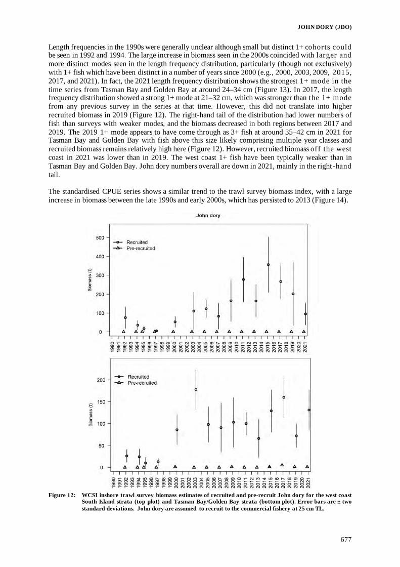
JOHN DORY (JDO)
677
Length frequencies in the 1990s were generally unclear although small but distinct 1+ cohorts could be seen in 1992 and 1994. The large increase in biomass seen in the 2000s coincided with larger and more distinct modes seen in the length frequency distribution, particularly (though not exclusively) with 1+ fish which have been distinct in a number of years since 2000 (e.g., 2000, 2003, 2009, 2015, 2017, and 2021). In fact, the 2021 length frequency distribution shows the strongest 1+ mode in the time series from Tasman Bay and Golden Bay at around 24–34 cm (Figure 13). In 2017, the length frequency distribution showed a strong 1+ mode at 21–32 cm, which was stronger than the 1+ mode from any previous survey in the series at that time. However, this did not translate into higher recruited biomass in 2019 (Figure 12). The right-hand tail of the distribution had lower numbers of fish than surveys with weaker modes, and the biomass decreased in both regions between 2017 and 2019. The 2019 1+ mode appears to have come through as 3+ fish at around 35–42 cm in 2021 for Tasman Bay and Golden Bay with fish above this size likely comprising multiple year classes and recruited biomass remains relatively high here (Figure 12). However, recruited biomass off the west coast in 2021 was lower than in 2019. The west coast 1+ fish have been typically weaker than in Tasman Bay and Golden Bay. John dory numbers overall are down in 2021, mainly in the right-hand tail. The standardised CPUE series shows a similar trend to the trawl survey biomass index, with a large increase in biomass between the late 1990s and early 2000s, which has persisted to 2013 (Figure 14).
Figure 12: WCSI inshore trawl survey biomass estimates of recruited and pre-recruit John dory for the west coast
South Island strata (top plot) and Tasman Bay/Golden Bay strata (bottom plot). Error bars are ± two standard deviations. John dory are assumed to recruit to the commercial fishery at 25 cm TL.

JOHN DORY (JDO)
678
Figure 13: Scaled population length frequency distributions for John dory in 30–400 m for west coast (white bars)
and Tasman Bay/Golden Bay (blue bars), from WCSI surveys. n = number of fish measured, no. = scaled population number, CV = coefficient of variation (%). [Continued on next page]

JOHN DORY (JDO)
679
Figure 13 [Continued]

JOHN DORY (JDO)
680
Figure 14: CPUE indices of abundance for the northern South Island (JDO 7 and part of JDO 2), combined model o f
catch rates in mixed species bottom trawl tows (Langley 2014). Vertical lines show the 95% credible intervals.
4.2 Biomass estimates Estimates of absolute reference and current biomass are not available.
4. STATUS OF THE STOCKS
• JDO 1 (Hauraki Gulf and east Northland) Stock Status Year of Most Recent Assessment 2022 Assessment Runs Presented Standardised CPUE Reference Points
Interim Target: Arithmetic mean of the CPUE indices for John dory in Hauraki Gulf and east Northland from combined binomial and lognormal models from 1995–96 to 2010–11
Soft Limit: 50% of target Hard Limit: 25% of target
Overfishing threshold: FMSY Status in relation to Target About as Likely as Not (40‒60%) to be at or above the target Status in relation to Limits Soft Limit: Unlikely (< 40%) to be below
Hard Limit: Very Unlikely (< 10%) to be below Status in relation to Overfishing Very Unlikely (< 10%) that overfishing is occurring

JOHN DORY (JDO)
681
Historical Stock Status Trajectory and Current Status
Standardised CPUE indices for John dory in Hauraki Gulf and east Northland from combined binomial and lognormal models of catch rate in bottom trawl tows in a mixed target fishery (blue line). Solid horizontal lines indicate the target (green), soft limit (orange), and hard limit (red). The commercial catch from the area is also presented (dashed brown line), and trawl survey recruited biomass indices (purple with error bars ± two standard deviations). Fishery and Stock Trends Recent Trend in Biomass or Proxy The CPUE indices steadily declined from the mid-2000s to slightly
below the soft limit in 2012–13, then increased to be just below the target in 2019–20 and 2020–21.
Recent Trend in Fishing Intensity or Proxy
Relative fishing mortality proxy derived from total area catch divided by CPUE indices from the recent CPUE analysis (black points). The dashed horizontal line represents the average fishing mortality in the period used to define the reference points (vertical green dotted lines). The fishing mortality proxy indicates that fishing mortality has declined since 2006–07. Since 2011–12, total catch has remained stable or declined, while CPUE has increased, leading to a decrease in the fishing mortality proxy.
Other Abundance Indices There is good correspondence between the Hauraki Gulf trawl survey and CPUE series.
Trends in Other Relevant Indicators or Variables -
Projections and Prognosis Stock Projections or Prognosis Annual catches and fishing mortality have been relatively low since
2011–12. There has been an approximate doubling of CPUE indices

JOHN DORY (JDO)
682
since 2011–12 and the 2020–21 CPUE index is just below target. Probability of Current Catch or TAC causing Biomass to remain below or to decline below Limits
Soft Limit: Unlikely (< 40%) at the current catch levels (which are the lowest of the time series) Hard Limit: Very Unlikely (< 10%) over the next five years at current catch levels
Probability of Current Catch or TAC causing Overfishing to continue or to commence
Current catch is Very Unlikely (< 10%) to cause overfishing
Assessment Methodology and Evaluation Assessment Type Level 2 - Partial Quantitative Stock Assessment Assessment Method Standardised CPUE Assessment Dates Latest assessment: 2022 Next assessment: 2025 Overall assessment quality rank 1 – High Quality Main data inputs (rank) - Catch and effort data 1 – High Quality Data not used (rank) N/A Changes to Model Structure and Assumptions
-
Major Sources of Uncertainty - Qualifying Comments - Fishery Interactions John dory is taken on the east coast by bottom trawl and Danish seine targeted at John dory and snapper. • JDO 1 (Bay of Plenty)
Stock Status Year of Most Recent Assessment 2022 Assessment Runs Presented Standardised CPUE Reference Points
Interim Target: Arithmetic mean of the CPUE indices for John dory in Bay of Plenty from combined binomial and lognormal models from 1995–96 to 2010–11
Soft Limit: 50% of target Hard Limit: 25% of target
Overfishing threshold FMSY Status in relation to Target About as Likely as Not (40‒60 %) to be at or above the target Status in relation to Limits Soft Limit: Unlikely (< 40%) to be below
Hard Limit: Very Unlikely (< 10%) to be below Status in relation to Overfishing Unlikely (< 40%) that overfishing is occurring

JOHN DORY (JDO)
683
Historical Stock Status Trajectory and Current Status
Standardised CPUE indices for John dory in Bay of Plenty from combined binomial and lognormal models of catch rate in bottom trawl tows in a mixed target fishery (blue line). Solid horizontal lines indicate the target (green), soft limit (orange), and hard limit (red). The commercial catch from the area is also presented (dashed brown line), and trawl survey recruited biomass indices (purple with error bars ± two standard deviations). Fishery and Stock Trends Recent Trend in Biomass or Proxy The CPUE indices declined to minimum in 2018–19, and increased
after that to be slightly below target in 2020–21. Recent Trend in Fishing Mortality or Proxy
Relative fishing mortality proxy derived from total area catch divided by CPUE indices from the recent CPUE analysis (black points). The dashed horizontal line represents the average fishing mortality in the period used to define the reference point (vertical green dotted lines). The fishing mortality proxy was a minimum in 2011–12, increased to be above the threshold (FMSY proxy) level from 2016–17 to 2018–19, then declined to be below the reference for the last two years.
Other Abundance Indices There is good correspondence between the Bay of Plenty trawl survey and CPUE series.
Trends in Other Relevant Indicators or Variables -

JOHN DORY (JDO)
684
Projections and Prognosis Stock Projections or Prognosis From 2018–19 annual catches have been relatively low, and
the CPUE indices have increased. The current lower level of the fishing mortality may cause the stock to increase.
Probability of Current Catch or TAC causing Biomass to remain below or to decline below Limits
Soft Limit: Unlikely (< 40%) at current catch levels Hard Limit: Very Unlikely (< 10%) at current catch levels
Probability of Current Catch or TACC causing Overfishing to continue or to commence
Unlikely (< 40%) at the current level of catch
Assessment Methodology and Evaluation Assessment Type Level 2 - Partial Quantitative Stock Assessment Assessment Method Fishery characterisation and standardised CPUE Assessment Dates Latest assessment: 2022 Next assessment: 2025 Overall assessment quality rank 1 – High Quality Main data inputs (rank) - 2022 CPUE analysis 1 – High Quality Data not used (rank) N/A Changes to Model Structure and Assumptions -
Major Sources of Uncertainty - Qualifying Comments - Fishery Interactions John dory is taken in the Bay of Plenty by bottom trawl targeted at John dory, snapper, trevally, tarakihi, and red gurnard and by Danish seine targeted at snapper and red gurnard. • JDO 1 (West Coast North Island) Stock Status Year of Most Recent Assessment 2022 Assessment Runs Presented Standardised CPUE
Reference Points
Interim Target: Arithmetic mean of the CPUE indices for John dory on West Coast North Island from combined binomial and lognormal models from 1995–96 to 2010–11
Soft Limit: 50% of target Hard Limit: 25% of target
Overfishing threshold: FMSY Status in relation to Target About as Likely as Not (40‒60%) to be at or above the target
Status in relation to Limits Soft Limit: Unlikely (< 40%) to be below Hard Limit: Very Unlikely (< 10%) to be below
Status in relation to Overfishing Unlikely (< 40%) to be occurring

JOHN DORY (JDO)
685
Historical Stock Status Trajectory and Current Status
Standardised CPUE indices for John dory in West Coast North Island from combined binomial and lognormal models of catch rate in bottom trawl tows in a mixed target fishery (blue line). Solid horizontal lines indicate the target (green), soft limit (orange), and hard limit (red). The commercial catch from the area is also presented (dashed brown line), and trawl survey recruited biomass indices (purple with error bars ± two standard deviations). Fishery and Stock Trends Recent Trend in Biomass or Proxy From 2016–17 the CPUE indices have increased to be just above
target in 2020–21. Recent Trend in Fishing Intensity or Proxy
Relative fishing mortality proxy derived from total area catch divided by CPUE indices from the recent CPUE analysis (black points). The dashed horizontal line represents the average fishing mortality in the period used to define the reference points (vertical green dotted lines). Fishing mortality increased to the threshold during 2014–15 and then declined to be below the threshold in 2020–21.
Other Abundance Indices There is good correspondence between the WCNI trawl survey and CPUE series
Trends in Other Relevant Indicators or Variables -

JOHN DORY (JDO)
686
Projections and Prognosis Stock Projections or Prognosis Likely to fluctuate around the target Probability of Current Catch or TACC causing Biomass to remain below or to decline below Limits
Soft Limit: Unlikely (< 40%) at current catch levels Hard Limit: Very Unlikely (< 10%) at current catch levels
Probability of Current Catch or TACC causing Overfishing to continue or to commence
Unlikely (< 40%) at current catch levels
Assessment Methodology and Evaluation Assessment Type Level 2 - Partial Quantitative Stock Assessment Assessment Method Fishery characterisation and standardised CPUE Assessment Dates Latest assessment: 2022 Next assessment: 2025 Overall assessment quality rank 1 – High Quality Main data inputs (rank) 2022 CPUE analysis 1 – High Quality Data not used (rank) N/A Changes to Model Structure and Assumptions -
Major Sources of Uncertainty - The stock relationship between JDO 1 and JDO 2 Qualifying Comments - Fishery Interactions John dory is taken off the west coast by bottom trawl targeted at snapper trevally, gurnard, and tarakihi.
• JDO 2 (Southeast North Island)
Stock Status Year of Most Recent Assessment 2013 Assessment Runs Presented Standardised CPUE Reference Points
Interim Target: Mean of the CPUE indices for John dory in South East coast of the North Island from combined binomial and lognormal models from 1989–90 to 2010–11 Soft Limit: 50% of target Hard Limit: 25%of target Overfishing threshold FMSY
Status in relation to Target Unlikely (< 40%) to be at or above the target Status in relation to Limits Soft Limit: About as Likely as Not (40–60%) to be below
Hard Limit: Unlikely (< 10%) to be below Status in relation to Overfishing Unknown

JOHN DORY (JDO)
687
Historical Stock Status Trajectory and Current Status
Standardised CPUE indices for John dory in Southeast North Island from combined binomial and lognormal models of catch rate in bottom trawl trips in a mixed target fishery (Dunn & Jones 2013). Broken horizontal line indicates the mean from 1989–90 to 2010–11; Bars represent catch from this area. Fishery and Stock Trends Recent Trend in Biomass or Proxy The CPUE series has fluctuated with a cyclical trend. The data
points since 2006–07 have been below the long-term mean. 2010–11 is the lowest in the series.
Recent Trend in Fishing Intensity or Proxy Unknown
Other Abundance Indices - Trends in Other Relevant Indicators or Variables - Projections and Prognosis Stock Projections or Prognosis Without information on recruitment, it is not possible to predict how
the stock will respond in the next few years. Probability of Current Catch or TACC causing Biomass to remain below or to decline below Limits
Soft Limit: Likely (> 60%) Hard Limit: About as Likely as Not (40–60%)
Probability of Current Catch or TACC causing Overfishing to continue or to commence
Unknown
Assessment Methodology and Evaluation Assessment Type Level 2 - Partial Quantitative Stock Assessment Assessment Method Fishery characterisation and standardised CPUE Assessment Dates Latest assessment: 2013 Next assessment: Unknown Overall assessment quality rank 1 – High Quality Main data inputs (rank) - Catch and effort data 1 – High Quality Data not used (rank) N/A Changes to Model Structure and Assumptions -
Major Sources of Uncertainty - The stock relationship between JDO 1 and JDO 2 - Lack of information on incoming recruitment

JOHN DORY (JDO)
688
Qualifying Comments Because the John dory fishery in FMAs 1 and 9 has a long history, it is not possible to infer stock status from abundance trends from only the last 22 years. This sub-stock appears to be cyclical, probably in response to recruitment variation. This makes it difficult to predict future trends without recruitment information. Fishery Interactions John dory is taken off the east coast by bottom trawl targeted primarily at tarakihi and red gurnard. Interactions with other species are currently being characterised.
• JDO 7 (Northern South Island)
Stock Status Year of Most Recent Assessment 2022 Assessment Runs Presented Trawl survey biomass index (2021) and standardised CPUE (2014) Reference Points
Interim Target: Arithmetic mean of total biomass from the West Coast South Island trawl survey (WCSI and TBGB) from 1992 to 2011
Soft Limit: 50% of target Hard Limit: 25% of target Overfishing threshold: FMSY
Status in relation to Target About as Likely as Not (40‒60%) to be at or above the target Status in relation to Limits Soft Limit: Very Unlikely (< 10%) to be below
Hard Limit: Very Unlikely (< 10%) to be below Status in relation to Overfishing About as Likely as Not (40‒60%) that overfishing is occurring Historical Stock Status Trajectory and Current Status
Biomass trends from the west coast South Island inshore trawl survey time series. Error bars are ± two standard deviations, assuming a lognormal distribution. The agreed BMSY proxy (arithmetic average: 1992–2011 WCSI survey biomass estimates=168 t) is shown as a green dashed line; the calculated Soft Limit (=50% BMSY proxy) is shown as a purple dashed line; the calculated Hard Limit (=25% BMSY proxy) is shown as a grey dashed line.

JOHN DORY (JDO)
689
Relative fishing pressure for JDO 7 based on the ratio of QMR/MHR landings to the corresponding WCSI total biomass trawl survey index which has been normalised so that the geometric mean=1.0 overall index values. Horizontal green dashed line is the arithmetic mean fishing pressure from 1992 to 2011 (1.239). Fishery and Stock Trends Recent Trend in Biomass or Proxy
The series has been at or above the agreed BMSY proxy since the 2003 survey. However, recent index values have declined steadily since 2015, the highest observed index value.
Recent Trend in Fishing Intensity or Proxy
Commercial catch has tracked a rising TACC since 2010, when catches were 109 t to the four years from 2018 to 2021, when catches averaged 192 t/y.
Other Abundance Indices The trend in BT CPUE (1989‒90 to 2012‒13) is comparable with that for trawl survey series.
Trends in Other Relevant Indicators or Variables
- Length frequency analysis from the West Coast South Island trawl survey showed very good recruitment in 2000, 2003, and 2009 and these are probably supporting the high biomass at that time. - Recruitment from the 2011 and 2013 surveys was more modest but recruitment was again high in 2015 and 2017. Recruitment appears to be modest again in 2019. The 2021 recruitment is greater than seen in 2019, especially for females, but does not approach the high levels seen in 2015 and 2017.
Projections and Prognosis Stock Projections or Prognosis The stock was near the BMSY proxy target biomass level in 2020‒21, and
previous high catches appear to have been sustained by good recruitment. The 2021 recruitment appears to be average or slightly above average.
Probability of Current Catch or TACC causing Biomass to remain below or to decline below Limits
Soft Limit: Unlikely (< 40%) Hard Limit: Very Unlikely (< 10%)
Probability of Current Catch or About as Likely as Not (40–60%), for current catch and Unknown for

JOHN DORY (JDO)
690
TACC causing Overfishing to continue or to commence
TACC
Assessment Methodology and Evaluation Assessment Type Level 2 - Partial Quantitative Stock Assessment Assessment Method Evaluation of survey biomass and length frequencies and standardised
CPUE Assessment Dates Latest assessment: 2022
(Survey) 2014 (CPUE) Next assessment: 2024 (survey)
Overall assessment quality rank 1 – High Quality Main data inputs (rank) - West Coast South Island
trawl survey - Survey length frequency - CPUE
1 – High Quality 1 – High Quality 1 – High Quality
Data not used (rank) N/A Changes to Model Structure and Assumptions
-
Major Sources of Uncertainty - The stock relationship between JDO 7 and the western part of JDO 2 Qualifying Comments - Fishery Interactions John dory are primarily taken in conjunction with the following QMS species: barracouta, red cod, stargazer, red gurnard, snapper, and tarakihi in the Northern South Island bottom trawl fishery. 6. FOR FURTHER INFORMATION Bentley, N; Langley, A D; Lallemand, P (2012) Commercial fisheries of New Zealand, 1989/90–2010/11. Trophia Ltd. http://finz.trophia. com.
[Accessed 15 March 2013]. Boyd, R O; Reilly, J L (2004) 1999–2000 National Marine Recreational Fishing Survey: harvest estimates. (Unpublished draft New
Zealand Fisheries Assessment Report for the Ministry of Fisheries Project REC9803 held by Fisheries New Zealand.) 28 p. Bradford, E (1998) Harvest estimates from the 1996 national recreational fishing surveys. New Zealand Fisheries Assessment Research
Document 1998/16. 27 p. (Unpublished document held in NIWA library, Wellington.) Davey, N; Hartill, B; Carter, M (2019). Mean weight estimates for recreational fisheries in 2017–18. New Zealand Fisheries Assessment
Report 2019/25. 32 p. Dunn, M R; Jones, E (2013). Stock structure and fishery characterisation for New Zealand John dory. New Zealand Fisheries Assessment
Report 2013/40. 99 p. Francis, M P; Paul, L J (2013) New Zealand inshore finfish and shellfish commercial landings, 1931–82. New Zealand Fisheries Assessment
Report 2013/55. 136 p. Fu, D; Gilbert, D J; Baird, S J; Manning, M J (2008) CPUE analysis of John dory (Zeus faber) in New Zealand’s main fishery (JDO1). N ew
Zealand Fisheries Assessment Report 2008/14. 42 p. Hanchet, S M; Francis, M P; Horn, P L (2001) Age and growth of John dory (Zeus faber). New Zealand Fisheries Assessment Report
2001/10. 26 p. Hartill, B; Davey, N (2015) Mean weight estimates for recreational fisheries in 2011–12. New Zealand Fisheries Assessment Report
2015/25. Hore, A J (1982) The age growth and reproduction of the John dory, Zeus faber. (Unpublished MSc thesis, University of Auckland.) Hore, A J (1985) John dory In: Colman, J A; McKoy, J L; Baird, G G (1985) Background papers for the 1985 Total Allowable Catch
recommendations, pp. 117–122. (Unpublished report held by NIWA library, Wellington.) Hore, A J (1988) John dory. New Zealand Fisheries Assessment Research Document 1988/39. 8 p. (Unpublished document held by NIWA
library, Wellington.) Horn, P L; Hanchet, S M; Stevenson, M J; Kendrick, T H; Paul, L J (1999) Catch history, CPUE analysis, and stock assessment of John dory
(Zeus faber) around the North Island (Fishstocks JDO1 and JDO2). New Zealand Fisheries Assessment Research Document 99/33. 58 p. (Unpublished document held by NIWA library, Wellington.)
Kendrick, T H; Bentley, N (2011) Fishery characterisation and catch-per-unit-effort indices for three sub-stocks of John dory in JDO 1, 1989–90 to 2008–09. New Zealand Fisheries Assessment Report 2011/38.
Langley, A D (2014) Updated CPUE analyses for selected South Island inshore finfish stocks. New Zealand Fisheries Assessment Report 2014/40. 116 p.
Langley, A D (2018) Fishery characterisation and Catch-Per-Unit-Effort indices for John dory in JDO 1. New Zealand Fisheries Assessment Report 2018/36. 84 p.
MacGibbon, D J; Stevenson, M L (2013) Inshore trawl survey of the west coast South Island and Tasman and Golden Bays, March-April 2013 (KAH1305). New Zealand Fisheries Assessment Report 2013/66. 115 p.
MacGibbon, D J; Walsh, C; Buckthought, D; Bian, R (2022) Inshore trawl survey off the west coast South Island and in Tasman Bay and Golden Bay, March‒April 2021 (KAH2103). New Zealand Fisheries Assessment Report 2022/11. 97 p.

JOHN DORY (JDO)
691
Morrison, M A; Francis, M P; Parkinson, D M (2002) Trawl survey of them Hauraki Gulf, 2000 (KAH0012). New Zealand Fisheries Assessment Report 2002/46. 49 p.
Stevenson, M L (2007) Inshore trawl surveys of the west coast of the South Island and Tasman and Golden Bays, March-April 2007 (KAH0704). New Zealand Fisheries Assessment Report 2007/41. 64 p.
Stevenson, M L (2010) Inshore trawl surveys of the west coast of the South Island and Tasman and Golden Bays, March-April 2009 (KAH0704). New Zealand Fisheries Assessment Report 2010/11.
Stevenson, M L (2012) Inshore trawl survey of the west coast of the South Island and Tasman and Golden Bays, March-April 2011. New Zealand Fisheries Assessment Report 2012/50. 77 p.
Stevenson, M L; MacGibbon, D J (2015) Inshore trawl survey of the west coast South Island and Tasman and Golden Bays, March-April 2015 (KAH1503). New Zealand Fisheries Assessment Report 2015/67. 94 p.
Teirney, L D; Kilner, A R; Millar, R E; Bradford, E; Bell, J D (1997) Estimation of recreational catch from 1991/92 to 1993/94 New Zealand Fisheries Assessment Research Document 1997/15. 43 p. (Unpublished document held by NIWA library, Wellington.)
Wynne-Jones, J; Gray, A; Heinemann, A; Hill, L; Walton, L (2019) National Panel Survey of Marine Recreational Fishers 2017–2018. N ew Zealand Fisheries Assessment Report 2019/24. 104 p.
Wynne-Jones, J; Gray, A; Hill, L; Heinemann, A (2014) National Panel Survey of Marine Recreational Fishers 2011–12: Harvest Estimates. New Zealand Fisheries Assessment Report 2014/67. 139 p.


KAHAWAI (KAH)
693
KAHAWAI (KAH)
(Arripis trutta and Arripis xylabion) Kahawai
1. FISHERY SUMMARY Kahawai (Arripis trutta) and Kermadec kahawai (Arripis xylabion) were introduced into the QMS on 1 October 2004 under a single species code, KAH. Within the QMS, kahawai management is based on six QMAs (KAH 1, KAH 2, KAH 3, KAH 4, KAH 8, and KAH 10). These QMAs differ from the management areas used before kahawai were introduced into the QMS. The definitions of KAH 1, KAH 2, and KAH 10 remain unchanged, but KAH 4 was formerly part of KAH 3, as was the part of KAH 8 south of Tirua Point. The area of KAH 8 north of Tirua point was formerly called KAH 9. TACs totalling 7612 t were set on introduction into the QMS. These TACs were based on a 15% reduction from both the level of commercial catch and assumed recreational use prior to introducing kahawai into the QMS. The Minister reviewed the TACs for kahawai for the 2005–06 fishing year. Subsequently, he decided to reduce TACs, TACCs, and allowances by a further 10% as shown in Table 1. Table 1: KAH allowances, TACCs, and TACs, from 1 October 2010 to present. Fishstock Recreational Allowance Customary Non-Commercial Allowance Other mortality TACC TAC KAH 1 900 200 45 1 075 2 200 KAH 2 610 185 30 705 1 530 KAH 3 390 115 20 410 935 KAH 4 4 1 0 9 14 KAH 8 385 115 20 520 1 040 KAH 10 4 1 0 9 14 1.1 Commercial fisheries Commercial fishers take kahawai by a variety of methods. Purse seine vessels take most of the catch; however, substantial quantities are also taken seasonally in set net fisheries and as a bycatch in surface longline and trawl fisheries. The kahawai purse seine fishery cannot be understood without taking into account the other species that the vessels target. The fleet, which is based in Tauranga, preferentially targets skipjack tuna (Katsuwonus pelamis) between December and May, with very little bycatch. When skipjack are not available, usually from June to November, the fleet fishes for a mix of species including kahawai, jack

KAHAWAI (KAH)
694
mackerels (Trachurus spp.), trevally (Pseudocaranx dentex), and blue mackerel (Scomber australasicus). These are caught ‘on demand’ as export orders are received (to reduce product storage costs). However, since the mackerels and kahawai school together there is often a bycatch of kahawai resulting from targeting of mackerels. Historical estimated kahawai landings are shown in Table 2, from 1931 to 1982. Reported landings, predominantly of A. trutta, are shown for 1962 up to and including 1982 in Table 3 by calendar year for all areas combined, and from 1983–84 onwards by fishing year and by historic management areas in Table 4 and by QMAs in Table 5. The historical landings and TACC for the main KAH stocks are depicted in Figure 1. Table 2: Reported landings (t) for the main QMAs from 1931 to 1982.
Year KAH 1 KAH 2 KAH 3 KAH 4 KAH 8
1931–32 1 0 0 0 0 1932–33 1 0 0 0 0 1933–34 0 0 1 0 0 1934–35 0 0 0 0 3 1935–36 0 0 0 0 0 1936–37 0 0 0 0 0 1937–38 2 1 1 0 0 1938–39 2 2 1 0 0 1939–40 1 1 1 0 0 1940–41 1 4 2 0 1 1941–42 2 1 1 0 0 1942–43 21 1 2 0 0 1943–44 58 3 4 0 3 1944 90 7 4 0 6 1945 102 2 3 0 1 1946 94 0 4 0 9 1947 54 0 4 0 1 1948 58 2 1 0 1 1949 23 3 0 0 1 1950 34 2 1 0 1 1951 22 1 0 0 2 1952 27 2 0 0 3 1953 14 1 0 0 4 1954 18 2 0 0 2 1955 19 6 0 0 7 1956 16 3 0 0 7 1957 25 6 0 0 13 1958 33 13 0 0 12 1959 31 2 0 0 14 1960 40 1 0 0 10 1961 40 0 0 0 12 1962 54 7 0 0 16 1963 60 11 0 0 11 1964 75 4 1 0 7 1965 85 13 0 0 4 1966 143 106 0 0 5 1967 147 303 0 0 5 1968 107 159 29 0 7 1969 163 29 12 0 33 1970 141 59 22 0 74 1971 185 258 10 0 119 1972 168 151 22 0 53 1973 295 132 13 0 147 1974 357 206 17 0 226 1975 140 28 18 0 154 1976 401 108 30 0 186 1977 631 385 218 0 224 1978 1 237 487 279 0 217 1979 1 642 552 608 0 267 1980 1 213 885 810 0 350 1981 659 625 1301 0 498 1982 1 133 639 980 0 484
Notes: The 1931–1943 years are April–March but from 1944 onwards are calendar years. Data up to 1985 are from fishing returns: data from 1986 to 1990 are from Quota Management Reports.Data for the period 1931 to 1982 are based on reported landings by harbour and are likely to be underestimated as a result of under-reporting.

KAHAWAI (KAH)
695
Table 3: Reported total landings (t) of kahawai from 1970 to 1982. Note that these data include est ima tes o f ka ha wa i from data where kahawai were reported within a general category of ‘mixed fish’ rather tha n sepa ra tely a s kahawai.
Year Landings Year Landings Year Landings 1962 76 1969 234 1976 729 1963 81 1970 294 1977 1 461 1964 86 1971 572 1978 2 228 1965 102 1972 394 1979 3 782 1966 254 1973 586 1980 5 101 1967 457 1974 812 1981 3 794 1968 305 1975 345 1982 5 398
Source: 1962 to 1969, Watkinson & Smith (1972); 1970 to 1982, Sylvester (1989). Before 1988 there were no restrictions in place for the purse seine fishery. Table 4: Reported landings (t) of kahawai by management areas as defined prior to 2004, from 1 9 8 3– 84 to 2 0 0 3– 04 .
Estimates of fish landed as bait or as ‘mixed fish’ are not included. Data for the distribution of catches a mo ng management areas and total catch are from the FSU database up to 1987–88 and from the CELR database after that date. Total LFRR or MHR values are the landings reported by Licensed Fish Receivers (to 2000–01 ) or on Monthly Harvest returns (to 2003–04). Unknown Total Total Fishstock KAH 1 KAH 2 KAH 3 KAH 9 KAH 10 Area Catch LFRR/MHR FMA(s) 1 2 3–8 9 10 1983–84 1 941 919 813 547 0 46 4 266 – 1984–85 1 517 697 1 669 299 0 441 4 623 – 1985–86 1 597 280 1 589 329 0 621 4 416 – 1986–87 1 890 212 3 969 253 0 1 301 7 525 6 481 1987–88 4 292 1 655 2 947 135 0 581 9 610 9 218 1988–89 2 170 779 4 301 179 0 – 7431 7 377 1989–90 2 049 534 5 711 156 0 16 8 466 8 696 1990–91 1 617 872 2 950 242 0 4 5 687 5 780 1991–92 2 190 807 1 900 199 < 1 7 5 104 5 071 1992–93 2 738 1 132 1 930 832 2 0 6 639 6 966 1993–94 2 054 1 136 1 861 98 15 0 5 164 4 964 1994–95 1 918 1 079 1 290 168 0 24 4479 4 532 1995–96 1 904 760 1 548 237 7 46 4 502 4 648 1996–97 2 214 808 938 194 1 3 4 158 3 763 1997–98 1 601 291 525 264 0 19 2 700 2 823 1998–99 1 833 922 1 209 468 0 3 4 435 4 298 1999–00 1 616 1 138 718 440 0 < 1 3 912 3 941 2000–01 1 746 886 925 272 0 1 3 829 3 668 2001–02 1 354 816 377 271 0 < 1 2 819 2 796 2002–03 933 915 933 221 0 < 1 3 001 2 964 2003–04 1 624 807 109 205 0 0 2 745 2 754
A total commercial catch limit for kahawai was set at 6500 t for the 1990–91 fishing year, with 4856 t set aside for those harvesting kahawai by purse seine (Table 6). Before the 2002–03 fishing year a high proportion of the purse seine catch was targeted, but in recent years approximately half of the landed catch has been reported as bycatch while targeting other species with purse seine gear. In KAH 1, a voluntary moratorium was placed on targeting kahawai by purse seine in the Bay of Plenty from 1 December 1990 to 31 March 1991; this was extended from 1 December to the Tuesday after Easter in subsequent years. Although total landings decreased in 1991–92, landings in KAH 1 increased, and in 1993–94 the competitive catch limit for purse seining in KAH 1 was reduced from 1666 t to 1200 t. Purse seine catches reported for KAH 9 were also included in this reduced catch limit, although seining for kahawai off the west coast of the North Island ceased after the reduction in the KAH 1 purse seine limit. Purse seine catch limits were reached in KAH 1 between 1998–99 and 2000–01 and in 2003–04. Prior to the introduction to the QMS, no change was made to the purse seine limit of 851 t for KAH 2. The KAH 2 purse seine fishery was closed early due to the catch limit being reached before the end of the season in each year between 1991–92 and 1995–96 and in 2000–01 and 2001–02.

KAHAWAI (KAH)
696
Table 5: Prorated landings (t) of kahawai by the Fishstocks (and FMA) defined in 2004 for the fishing years from 1998–
99 to the present. Distribution of data were derived by linking through the trip code, catch landing data (CLD), statistical areas, and landing points and prorating to CLD totals. Landings since 2004–05 are from QMS MHR data. The TACC is provided for those years since the introduction to the QMS.
KAH 1 KAH 2 KAH 3 KAH 4 KAH 8 KAH 10
Fishing 1 2 3, 5, 7 4 8, 9 10 Total year Catch TACC Catch TACC Catch TACC Catch TACC Catch TACC Catch TACC Catch TACC 1998–99 1 652 – 975 – 697 – 0 – 1 120 – 0 – 4 444 – 1999–00 1 677 – 973 – 499 – 0 – 768 – 0 – 3 917 – 2000–01 1 678 – 922 – 425 – 0 – 581 – 0 – 3 606 – 2001–02 1 326 – 857 – 156 – 0 – 489 – 0 – 2 831 – 2002–03 869 – 855 – 650 – 0 – 542 – 0 – 2 916 – 2003–04 1 641 – 806 – 33 – 0 – 342 – 0 – 2 822 – 2004–05 1 147 1 195 708 785 129 455 < 1 10 544 580 0 10 2 529 3 025 2005–06 903 1 075 530 705 233 410 0 9 346 520 0 9 2 013 2 728 2006–07 1 046 1 075 672 705 382 410 < 1 9 407 520 0 9 2 507 2 728 2007–08 1 002 1 075 564 705 152 410 0 9 570 520 0 9 2 288 2 728 2008–09 945 1 075 823 705 157 410 0 9 381 520 0 9 2 306 2 728 2009–10 988 1 075 518 705 38 410 < 1 9 451 520 0 9 1 995 2 728 2010–11 1 002 1 075 719 705 46 410 0 9 454 520 0 9 2 221 2 728 2011–12 1 004 1 075 498 705 310 410 0 9 514 520 0 9 2 326 2 728 2012–13 1 095 1 075 502 705 195 410 0 9 468 520 0 9 2 260 2 728 2013–14 1 062 1 075 196 705 372 410 <1 9 472 520 0 9 2 102 2 728 2014–15 992 1 075 523 705 59 410 0 9 607 520 0 9 2 181 2 728 2015–16 1 086 1 075 611 705 44 410 <1 9 481 520 0 9 2 222 2 728 2016–17 1 021 1 075 399 705 58 410 0 9 316 520 0 9 1 794 2 728 2017–18 983 1 075 752 705 59 410 0 9 346 520 0 9 2 139 2 728 2018–19 1 045 1 075 635 705 41 410 0 9 321 520 0 9 2 042 2 728 2019–20 998 1 075 128 705 150 410 0 9 361 520 0 9 1 637 2 728 2020–21 1 017 1 075 670 705 202 410 < 1 9 300 520 0 9 2 188 2 728
Within KAH 3, the kahawai purse seine fleet has voluntarily agreed, since 1991–92, not to fish in a number of near-shore areas around Tasman Bay and Golden Bay, the Marlborough Sounds, Cloudy Bay, and Kaikoura. The main purpose of this agreement is to minimise local depletion of schools of kahawai found in areas where recreational fisheries occur, and to minimise catches of juveniles. The purse seine catch limit for KAH 3 was reduced from 2339 to 1500 tonnes from 1995–96. Purse seine catch limits have never been reached in KAH 3. Table 6: Reported catches (t) by purse seine method and competitive purse seine catch limit (t) from 1990–91 to
2003–04. All data are from weekly reports furnished by permit holders to the Ministry of Fisheries except those for 1993–94 which are from the CELR database. Fishstocks are as defined prior to 2004.
KAH 1 KAH 2 KAH 3 KAH 9 KAH 10 Total Catch Catch Catch Catch Catch Catch Year Catch limit Catch limit Catch limit Catch limit Catch limit Catch limit 1990–91 1 422 1 666 493 851 n/a# 2 839* 0 none 0 none n/a 5 356 1991–92 1 613 1 666 735* 851 1 714 2 339 0 none 0 none 4 080 4 856 1992–93 1 547 1 666 795* 851 1 808 2 339 140 none 0 none 4 290 4 856 1993–94 1 262 1 200 1 101* 851 1 714 2 339 15 § 0 none 4 092 4 390 1994–95 1 225 1 200 821* 851 1 644 2 339 0 § 0 none 3 690 4 390 1995–96 1 077 1 200 805* 851 1 146 1 500 0 § 0 none 3 028 3 551 1996–97 1 017 1 200 620 851 578 1 500 0 § 0 none 2 784 3 551 1997–98 969 1 200 175 851 153 1 500 0 § 0 none 1 297 3 551 1998–99 1 416* 1 200 134 851 463 1 500 2 § 0 none 2 015 3 551 1999–00 1 371* 1 200 553 851 520 1 500 0 § 0 none 2 444 3 551 2000–01 1 322* 1 200 954* 851 430 1 500 0 § 0 none 2 706 3 551 2001–02 838 1 200 747* 851 221 1 500 0 § 0 none 1 806 3 551 2002–03 514 1 200 819 851 816 1 500 0 § 0 none 2 149 3 551 2003–04 1 203* 1 200 714 851 1 1 500 0 § 0 none 1 918 3 551
# By March 1991 when the catch limit was imposed, the purse seine catch had already exceeded 2339 t and the fishery was immediately closed. Because this occurred before the Minister’s decision was announced, an extra 500 t was allocated to cover kahawai bycatch only. * Purse seine fishery for kahawai closed. § Combined landings from KAH 9 and KAH 1 were limited to 1200 t. Since kahawai entered the Quota Management System on 1 October 2004, the purse seine catch limits no longer apply, and landings (regardless of fishing method) are now restricted by quota availability and fishing company policies. KAH 1 landings have ranged between 903 t and 1095 t since the introduction of the current TACC of 1075 t in 2005 (Figure 1). Landings in KAH 2 have been more variable, falling to just 399 t in 2016–17 and 128 t in 2019–20, but exceeding the TACC of 705 t in 2008–09, 2010–11,

KAHAWAI (KAH)
697
and 2017–18. KAH 3 landings have been well below the TACC since 2014–15, with just 41 t landed in 2018–19, but increasing to 150 t in 2019–20 and 202 t in 2010–21. KAH 8 landings exceeded the TACC of 520 t in 2007–08 and 2014–15, but have recently declined, ranging between 300 t and 361 t between 2016–17 to 2020–21.
Figure 1: Total commercial landings and TACC for the four main KAH stocks. From top: KAH 1 (Auckland East),
KAH 2 (Central East), KAH 3 (South East Coast, South East Chatham Rise, Sub-Antarctic, Southland, Challenger). [Continued on next page]

KAHAWAI (KAH)
698
Figure 1: [Continued] Total commercial landings and TACC for the four main KAH stocks: KAH 8 (Central
Egmont, Auckland West). 1.2 Recreational fisheries Kahawai is the second most important recreational species in FMA 1 (after snapper). Kahawai are highly prized by many recreational fishers, who employ a range of shore and boat-based fishing methods to target and/or catch the species. Kahawai is one of the fish species more frequently caught by recreational fishers, and recreational groups continue to express concern about the state of kahawai stocks in some areas. Historical kahawai recreational catches are poorly known. The current allowances within the TAC for each fishstock are shown in Table 1. Information from the 2017–18 national panel survey (Wynne-Jones et al 2019) show that kahawai were mainly caught by rod or line (95.2%), with just over half of the landed catch taken from trailer boats (50.5%), and a third were taken off land, with very similar percentages seen previously in 2011–12 (Wynne-Jones et al 2014). 1.2.1 Management controls The main method used to manage recreational harvests of kahawai is the daily bag limit. The current limits for kahawai are: up to 20 kahawai within a multi-species bag limit of 20 fish in the Auckland, Kermadec, Central, and Challenger management areas; up to 15 kahawai within a multi-species bag limit of 30 fish in the South-East, Southland, and Fiordland management areas; and up to 10 kahawai within a multi-species bag limit of 30 fish in the Kaikoura management area. There is no minimum legal size limit for any kahawai stock. A minimum net mesh size applies in all areas (the mesh sizes do vary by management area and net type). 1.2.2 Harvest estimates There are two broad approaches to estimating recreational fisheries harvest: the use of onsite or access point methods, where fishers are surveyed or counted at their fishing location, or at an access point when they return to land after their fishing trip; and offsite methods, where some form of post-event interview and/or diary is used to collect data from fishers. The first estimates of recreational harvest for kahawai were generated using an offsite regional telephone and diary survey approach in: MAF Fisheries South (1991–92), Central (1992–93), and North (1993–94) regions (Teirney et al 1997). Estimates for 1996 came from a national telephone and diary survey (Bradford 1998). Another national telephone and diary survey was carried out in 2000 (Boyd & Reilly 2002) and a rolling replacement of diarists in 2001 (Boyd et al 2004) provided estimates for a further year (mean weights were not re-estimated in 2001). Other than for the 1991–92 MAF Fisheries South survey, the diary method used mean weights of kahawai obtained from fish measured at boat ramps. The harvest estimates provided by telephone-diary surveys between 1993 and 2001 are no longer considered reliable for various reasons. A Recreational Technical Working Group concluded that

KAHAWAI (KAH)
699
these harvest estimates should be used only with the following qualifications: a) they may be very inaccurate; b) the 1996 and earlier surveys contain a methodological error; and c) the 2000 and 2001 estimates are implausibly high for many important fisheries. This led to the development of an alternative maximum count aerial-access onsite method that provides a more direct means of estimating recreational harvests for boat-based fisheries. The maximum count aerial-access approach combines data collected concurrently from two sources: a creel survey of recreational fishers returning to a subsample of ramps throughout the day; and an aerial survey count of vessels observed to be fishing at the approximate time of peak fishing effort on the same day. The ratio of the aerial count in a particular area relative to the number of interviewed parties who claimed to have f ished in that area at the time of the overflight was used to scale up harvests observed at surveyed ramps, to estimate harvest taken by all fishers returning to all ramps (Hartill et al 2007b). This aerial-access method was first used to estimate the recreational snapper harvest in the Hauraki Gulf in 2003–04 (Hartill et al 2007b), which was subsequently extended to survey the wider SNA 1 fishery in 2004–05 (Hartill et al 2007c). One benefit of this method is that it also provides harvest estimates for other key species, in particular kahawai (Table 7). The Marine Amateur Fisheries Working Group has concluded that this approach generally provides broadly reliable estimates of recreational harvest for KAH 1. It is not, however, possible to reliably quantify shore-based fishing from the air and it is necessary to derive scalars from recent offsite surveys to account for the shore-based kahawai catch. Aerial-access surveys, focusing on snapper, provided kahawai harvest estimates for the Hauraki Gulf in 2003–04 and for all of FMA 1 in 2004–05, 2011–12, and 2017–18. Aerial-access surveys in FMA 1 in 2011–12 and 2017–18 (Hartill et al 2013, 2019) provided independent harvest estimates for comparison with those generated from national panel surveys in those years. In response to problems with previous telephone-diary surveys and the cost and scale challenges associated with onsite methods, a National Panel Survey was conducted for the first time throughout the 2011–12 fishing year. The panel survey used face-to-face interviews of a random sample of 30 390 New Zealand households to recruit a panel of fishers and non-fishers for a full year. The panel members were contacted regularly about their fishing activities and harvest information collected in standardised phone interviews. The two 2011–12 surveys appear to provide plausible results that corroborate each other for KAH 1 and are therefore considered to be broadly reliable (Hartill et al 2013). The panel survey and corroborating aerial-access survey were repeated over the 2017–18 fishing year. Recreational harvest estimates from offsite surveys up to and including 2017–18 are given in Table 8 (from Wynne-Jones et al 2014, 2019, and Hartill & Davey 2015 and Hartill et al 2019), noting that the QMAs do not all match up with the strata used for the older harvest estimates (in particular for KAH 3 and 8). Table 7: Summary of kahawai harvest estimates (t) derived from an aerial overflight survey of the Hauraki Gulf in
2003–04 (1 December 2003 to 30 November 2004, Hartill et al 2007b) and a similar KAH 1 wide survey conducted in 2004–05 (1 December 2004 to 30 November 2005, Hartill et al 2007c) and in 2011–12 and 2017–18 (1 October to 30 October, Hartill et al 2013, 2019). Values in brackets denote CVs associated with each estimate.
Year East Northland Hauraki Gulf Bay of Plenty KAH 1 2003–04 – 56 (0.15) – – 2004–05 129 (0.14) 98 (0.18) 303 (0.14) 530 (0.09) 2011–12 191 (0.16) 483 (0.13) 268 (0.12) 942 (0.08) 2017–18 312 (0.13) 517 (0.09) 390 (0.11) 1 219 (0.06)
1.2.3 Monitoring harvest In addition to estimating absolute harvests, a system to provide relative estimates of harvest over time for key fishstocks has been designed and implemented for some key recreational fisheries. The system uses web cameras to continuously monitor trends in trailer boat traffic at key boat ramps complemented by creel surveys that provide estimates of the proportion of observed boats that were used for f ishing and the average harvest of snapper and kahawai per boat trip (Hartill et al. 2020). These data are combined to provide relative harvest estimates for KAH 1, that have been scaled by concurrent region wide aerial-access harvest estimates, to estimate annual harvest tonnages landed by recreational f ishers by substock (Table 9).

KAHAWAI (KAH)
700
Table 8: Recreational catch estimates for kahawai stocks. The surveys ran from October or December to September o r November but are denoted by the January calendar year. Mean fish weights were obtained f ro m bo a t ra mp surveys (for the telephone/diary and panel survey catch estimates). Totals are given in bold.
Stock Year Method Number of fish
(thousands) Mean weight (g) (summer/winter)
Total weight (t) CV
KAH 1 1994 Telephone/diary 727 1 978 – 1996 Telephone/diary 666 960 0.06 2000 Telephone/diary 1 860 2 195 0.13 2001 Telephone/diary 1 905 2 2 248 0.13 Hauraki Gulf only 2004 Aerial-access 56 0.15 East Northland 2005 Aerial-access 129 0.14 Hauraki Gulf 2005 Aerial-access 98 0.18 Bay of Plenty 2005 Aerial-access 303 0.14 Total 2005 Aerial-access 530 0.09 East Northland 2012 Aerial-access 1 473/1 2203
191 0.16 Hauraki Gulf 2012 Aerial-access 1 565/1 4753 483 0.13 Bay of Plenty 2012 Aerial-access 1 477/1 6283,4 268 0.12 Total 2012 Aerial-access 3,4,5 942 0.08 East Northland 2012 Panel survey 139 1 473/1 2203
198 0.14 Hauraki Gulf 2012 Panel survey 245 1 565/1 4753 377 0.09 Bay of Plenty 2012 Panel survey 238 1 477/1 6283,4 238 0.11 Total 2012 Panel survey 638 3,4,5 958 0.07 East Northland 2018 Aerial-access 312 0.13 Hauraki Gulf 2018 Aerial-access 517 0.09 Bay of Plenty 2018 Aerial-access 390 0.11 Total 2018 Aerial-access 1 219 0.06 East Northland 2018 Panel survey 130 1 717 224 0.14 Hauraki Gulf 2018 Panel survey 219 1 702/1 794 378 0.10 Bay of Plenty 2018 Panel survey 215 1 693 364 0.11 Total 2018 Panel survey 565 966 0.07 KAH 2 1993 Telephone/diary 195 298 - 1996 Telephone/diary 142 217 0.09 2000 Telephone/diary 1 808 2 937 0.74 2001 Telephone/diary 492 2 799 0.20 2012 Panel survey 146 1 583/1 4493 228 0.12 2018 Panel survey 132 1 698 224 0.14 KAH 3 1992 Telephone/diary 231 210 - 1994 Telephone/diary 6 6 8.4 - 1996 Telephone/diary 226 137 0.07 2000 Telephone/diary 413 667 0.16 2001 Telephone/diary 353 2 570 0.18 2012 Panel survey 105 1 279/2 3403 147 0.18 2018 Panel survey 68 1 056 72 0.15 KAH 8 1994 Telephone/diary 254 1 340 - 1996 Telephone/diary 199 204 0.09 2000 Telephone/diary 337 441 0.20 2001 Telephone/diary 466 2 609 0.24 2012 Panel survey 282 1 664/1 3183 452 0.11 2018 Panel survey 245 1 872/1 505 439 0.11
1 Mean weight obtained from 1992–93 boat ramp sampling. 2 The 2000 mean weights were used in the 2001 estimates. 3 Separate mean weight estimates were used for summer (1 October 2011 to 30 April 2012) and for winter (1 May to 30 September 2012). 4 Separate mean weight estimates were used for the eastern and western Bay of Plenty. 5 Temporally and spatially separate mean weight estimates used as per notes 3 and 4. 6 No harvest estimate available in the survey report, estimate presented is calculated as average fish weight for all years and areas by the number of fish estimated caught.

KAHAWAI (KAH)
701
Trends inferred from this monitoring programme were initially very similar to that inferred from aerial-access harvest estimates in the Hauraki Gulf in 2004–05, 2006–07, and 2011–12, but the camera/creel kahawai harvest estimate for the Hauraki Gulf in 2017–18 is substantially lower than concurrent aerial-access and national panel surveys estimates for the same year (Table 9 c.f. Table 8). This difference appears to be due to a recent substantial increase in recreational fishing effort and catch around expanding mussel farms in the Firth of Thames, coinciding with a lesser increase in effort in the north-western gulf. Additional creel survey monitoring has been initiated to monitor changes in the recreational fishery in these areas, which had not been adequately monitored from boat ramps in the Auckland metropolitan area up until 2019–20. There is, however, a good correspondence between trends inferred from camera/creel survey based indices and aerial-access survey and/or national panel survey harvest estimates, for recreational harvesting of kahawai for East Northland and the Bay of Plenty. In East Northland, the kahawai catch landed at the two monitored ramps has gone through similar fluctuations, with no apparent long-term trend evident. In the Bay of Plenty the recreational kahawai halved immediately after 2011–12 and remained at this level before spiking up to the highest estimated harvest tonnage in 2017–18, before declining back to the level seen in the years immediately after 2011–12. These estimates show the variability of recreational harvests between years and, in particular , that harvest levels can be driven not only by stock abundance but also by changes in localised availability. Table 9: Recreational catch estimates (t) for kahawai in different parts of the KAH 1 stock area calcula ted f ro m web
camera and creel monitoring at key ramps combined with aerial-access estimates for each area in 2004–05 and 2006–07 (Hauraki Gulf only) and 2011–12 and 2017–18 (all areas within KAH 1) (from H a rt ill et a l. 2 0 20 ). Recent estimates, especially for the Hauraki Gulf, are lower than expected but the reasons for this are still being investigated.
Year East Northland CV Hauraki Gulf CV Bay of Plenty CV Total KAH 1 CV 2004–05 149 0.20 88 0.26 229 0.15 465 0.11 2006–07 – – 69 0.30 – – – – 2011–12 217 0.18 541 0.19 259 0.21 1017 0.12 2012–13 207 0.22 212 0.20 139 0.21 558 0.12 2013–14 175 0.19 229 0.18 167 0.24 571 0.12 2014–15 86 0.20 191 0.19 107 0.26 384 0.13 2015–16 241 0.17 298 0.18 184 0.17 723 0.10 2016–17 158 0.22 181 0.19 170 0.24 509 0.13 2017–18 275 0.15 260 0.16 404 0.15 938 0.09 2018–19 227 0.16 245 0.17 174 0.16 646 0.10
Web camera and creel monitoring has commenced in other kahawai QMAs but the results have not yet been used to infer trends in those fisheries, although levels of recreational harvesting from these stocks are relatively low. 1.3 Customary non-commercial fisheries Kahawai is an important traditional and customary food fish for Maori. The level of customary catch has not been quantified and an estimate of the current customary non-commercial catch is not available. Some Maori have expressed concern over the state of their traditional fisheries for kahawai, especially around the river mouths in the eastern Bay of Plenty (Maxwell, 2019). 1.4 Illegal catch Estimates of illegal catch are not available, but are probably insignificant. 1.5 Other sources of mortality There is no information on other sources of mortality. Juvenile kahawai may suffer from habitat degradation due to run-off, situation and loss of shelter in estuarine areas.

KAHAWAI (KAH)
702
2. BIOLOGY Kahawai (Arripis trutta) are a schooling pelagic species belonging to the family Arripididae. Kahawai are found around the North Island, the South Island, the Kermadec Islands and Chatham Islands. They occur mainly in coastal seas, harbours, and estuaries and will enter the brackish water sections of rivers. A second species, A. xylabion, has been described (Paulin 1993). It is known to occur in the northern EEZ, at the Kermadec Islands and seasonally around Northland. Kahawai feed mainly on fishes but also on pelagic crustaceans, especially krill (Nyctiphanes australis). Kahawai smaller than 100 mm mainly eat copepods. Although kahawai are principally pelagic feeders, they will take food from the seabed. The spawning habitat of kahawai is unknown but is thought to be associated with the seabed offshore. Schools of females with running ripe ovaries have been caught by bottom trawl in 60–100 m in Hawke Bay (Jones et al 1992). Other females with running ripe ovaries have been observed in east coast purse seine landings sampled in March and April 1992, and between January and April in 1993 (McKenzie, NIWA, unpublished data). Length-maturation data collected from thousands of samples in the early 1990s suggest that the onset of sexual maturity in males occurs at around 39 cm (fork length) and in females at 40 cm (McKenzie, NIWA, unpublished data). This closely matches an estimate of 39 cm used for Australian A. trutta (Morton et al 2005). This length roughly corresponds to fish of four years of age in both countries. Eggs have been found in February in the outer Hauraki Gulf. Juvenile fish (0+ year class) can be found in shallow water over eelgrass meadows (Zostera spp. ) and in estuaries. Kahawai are usually aged using otoliths, following an ageing technique that has been validated (Stevens & Kalish 1998). Kahawai grow rapidly, attaining a length of around 15 cm at the end of their first year, and mature after 3–5 years at about 35–40 cm, after which their growth rate slows. The longest recorded A. trutta had a fork length of 79 cm and was caught by a recreational fisher in the Waitangi Estuary in Hawke Bay in August 1997 (Duffy & Petherick 1999). Northern kahawai, Arripis xylabion, grow considerably bigger than kahawai and attain a maximum length of at least 94 cm, but beyond this, little is known about the biology of A. xylabion. Male and female von Bertalanffy growth curves appear to be broadly similar, with females attaining a slightly higher value for L∞, although statistical comparison of sex specific curves using a likelihood ratio test (Kimura 1980) suggests that they are statistically different (Hartill & Walsh 2005). Combined-sex growth curves are probably adequate for modelling purposes and are provided for some areas in Table 10. Sex specific growth parameters given for KAH 1 in previous plenary documents have higher estimates for L∞ (56.93 for males and 55.61 for females). The maximum recorded age of kahawai is 26 years and this age has been previously used to estimate the instantaneous rate of natural mortality (M) using the equation M=loge100/maximum age (Jones et al 1992). The resulting estimate of M of 0.18 assumes that this maximum observed age equates to that at which 1% of the population would survive in an unexploited stock, but a higher value for M is now considered more likely. This is because a re-analysis of purse seine catch-at-age data collected by Eggleston from KAH 2 & 3 between 1973 and 1975 suggested that 1% of the unexploited population would have lived for 20 years, which equates to an M of 0.23. A Chapman-Robson estimate of M of 0.22 was also derived from these catch-at-age data. Likelihood profiling of M undertaken during the 2021 stock assessment also suggested that values around 0.23 were most likely. Estimates of M ranging from 0.20 to 0.24 were therefore considered in the 2021 stock assessment and the assumed value used in the base case model was 0.22.

KAHAWAI (KAH)
703
Table 10: Estimates of biological parameters.
Fishstock Estimate Source 1. Natural mortality (M) All 0.22 Hartill & Doonan (in prep) 2. Weight = a(length)b (weight in g, length in cm fork length) a b KAH 1 (resting) 0.0306 2.82 Hartill & Walsh (2005) KAH 1 (mature) 0.0103 3.14 Hartill & Walsh (2005)
KAH 1 & 3 (all) 0.0236 2.89 Hartill & Walsh (2005)
3. von Bertalanffy growth parameters K t0 L∞ KAH 1 0.35 0.13 54.6 Hartill & Bian (2016) KAH 2 0.34 0.60 53.5 Drummond (1995) KAH 3 0.30 0.25 54.2 Drummond & Wilson (1993) KAH 9 0.23 -0.26 55.9 McKenzie, NIWA, unpubl. data
3. STOCKS AND AREAS Kahawai are presently defined as separate units for the purpose of fisheries management: KAH 1 (FMA 1); KAH 2 (FMA 2); KAH 3 (FMAs 3, 5, 6, & 7); KAH 4 (FMA 4); KAH 8 (FMAs 8 & 9), and KAH 10 (FMA 10). Returns from tagging programmes do not provide definitive information on the level of potential mixing between KAH QMAs, but tagging returns suggest that most kahawai (A. trutta) remain in the same area for several years, but some move throughout the kahawai habitat. The pattern of kahawai movement around New Zealand is poorly understood and there are regional differences in age structure and abundance that are consistent with limited mixing between regions. Smith et al (2008) compared otolith micro-chemistry (multi-element chemistry and stable isotopes) and meristics (e.g., fin counts) from 0-group kahawai from two regions (Okahu Bay, Waitematä Harbour and Hakahaka Bay, Port Underwood). Two distant sites were chosen to provide the best chance of successful discrimination. Neither meristics nor stable isotopes provided any discrimination, and magnesium and barium concentrations provided only weak discriminatory power. On balance it seems possible that there are least two stocks of kahawai (A. trutta) within New Zealand waters with centres of concentration around the Bay of Plenty and the northern tip of the South Island. These two areas could be assumed to be separate for management purposes. Tagging data show that there is some limited mixing between these areas. Due to the shared QMA boundaries in the lower North Island and South Island, there is likely to be more mixing between the southern KAH QMAs than with the northern QMA (KAH 1). There is no information about stock structure of A. xylabion. 4. STOCK ASSESSMENT The first age-structured assessment of the KAH 1 stock was first undertaken in 2007 (Hartill 2009), which was updated and revised in 2015 (Hartill & Bian 2016) and then again in 2021 (Hartill & Doonan in prep). Both assessments were undertaken using CASAL (Bull et al 2012). The 2021 assessment is reported below. There are no accepted assessments for kahawai stocks outside KAH 1, although there are some catch curve estimates of Z from these areas from the early 1990s, which are reported here.

KAHAWAI (KAH)
704
4.1 KAH 1 4.1.1 Estimates of catch, selectivity, and abundance indices (i) Commercial catch The commercial catch history used in the assessment is provided in Table 11. Annual catch by method landings statistics up until 1981–82 were provided by Francis & Paul (2013), and Fisheries Statistics Unit data were used to generate landings statistics for 1982–83 to 1988–89. It is noted that catches during these early years are less certain due to reporting issues (e.g., see Table 4 legend). Table 11: Commercial catch (t) time series used in the 2021 stock assessment of KAH 1.
Purse seine Set net
Bottom trawl Other KAH 1
Purse seine Set net
Bottom trawl Other KAH 1
1930–31 – – – – – 1975–76 140 148 65 48 401 1931–32 – 1 – – 1 1976–77 271 163 123 74 631 1932–33 – – – – – 1977–78 432 461 200 145 1 238 1933–34 – – – – – 1978–79 875 228 380 159 1 642 1934–35 – – – – – 1979–80 561 270 250 132 1 213 1935–36 – – – – – 1980–81 292 159 131 76 658 1936–37 – 2 – – 2 1981–82 440 356 202 135 1 133 1937–38 – – – – – 1982–83 169 527 105 181 982 1938–39 – 1 – – 1 1983–84 1 445 321 65 111 1 942 1939–40 – – – – – 1984–85 882 410 82 141 1 515 1940–41 – 1 – – 1 1985–86 1 191 263 53 91 1 598 1941–42 – 12 4 4 20 1986–87 1 544 224 45 77 1 890 1942–43 – 35 12 12 59 1987–88 3 964 212 43 72 4 291 1943–44 – 53 18 18 89 1988–89 1 644 340 69 117 2 170 1944–45 – 62 21 21 104 1989–90 1 699 351 70 121 2 241 1945–46 – 55 19 19 93 1990–91 1 563 333 82 62 2 040 1946–47 – 32 11 11 54 1991–92 1 726 322 49 75 2 172 1947–48 – 35 11 11 57 1992–93 2 473 628 176 162 3 439 1948–49 – 14 4 4 22 1993–94 1 162 596 80 137 1 975 1949–50 – 20 7 7 34 1994–95 1 053 436 65 157 1 711 1950–51 – 13 4 4 21 1995–96 1 098 350 127 135 1 710 1951–52 – 16 5 5 26 1996–97 921 691 113 105 1 830 1952–53 – 8 3 3 14 1997–98 712 351 116 72 1 251 1953–54 – 11 4 4 19 1998–99 1 374 217 149 85 1 825 1954–55 – 12 4 4 20 1999–00 1 222 243 106 43 1 614 1955–56 – 9 3 3 15 2000–01 1 393 217 79 57 1 746 1956–57 – 16 5 5 26 2001–02 957 292 59 45 1 353 1957–58 – 20 7 7 34 2002–03 608 236 49 37 930 1958–59 – 19 7 7 33 2003–04 1 361 200 51 25 1 637 1959–60 – 24 8 8 40 2004–05 834 178 48 38 1 098 1960–61 – 24 8 8 40 2005–06 535 216 72 82 905 1961–62 – 33 12 12 57 2006–07 696 267 40 43 1 046 1962–63 – 36 12 12 60 2007–08 668 261 57 36 1 022 1963–64 – 45 15 15 75 2008–09 602 274 31 48 955 1964–65 – 51 17 17 85 2009–10 555 329 60 47 991 1965–66 – 86 28 28 142 2010–11 541 306 58 61 966 1966–67 – 88 29 29 146 2011–12 707 185 68 85 1 045 1967–68 – 64 21 21 106 2012–13 707 232 115 54 1 108 1968–69 – 98 33 33 164 2013–14 645 220 132 66 1 063 1969–70 – 84 28 28 140 2014–15 490 212 106 198 1 006 1970–71 – 111 38 38 187 2015–16 717 184 72 121 1 094 1971–72 – 100 33 33 166 2016–17 667 182 87 86 1 022 1972–73 – 177 58 58 293 2017–18 661 161 59 100 981 1973–74 – 214 71 71 356 2018–19 640 200 111 101 1 052 1974–75 38 64 19 20 141 2019–20 682 161 80 81 1 004 (ii) Recreational catch The recreational catch history in KAH 1 is poorly known. Aerial overflight estimates are available for the Hauraki Gulf in 2003–04 (Hartill et al 2007b) and for all three regions of KAH 1 in 2004–05 (Hartill et al 2007c), in 2011–12 (Hartill et al 2013) and in 2017–18 (Hartill et al 2019). Recreational harvest estimates for all three regions of KAH 1 are also available from National Panel Surveys undertaken in 2011–12 and 2017–18 (Wynne-Jones et al 2014, 2019), which were of a broadly similar magnitude to those provided by the aerial-access survey (see Table 8). Zero inflated negative binomial (ZINB) generalised linear modelling of observations of the number of kahawai landed per complete hour of interviewing at selected boat ramps surveyed since 1990 was used to reconstruct recreational catch histories for all three regions of KAH 1 from that time onward

KAHAWAI (KAH)
705
(Hartill & Doonan in prep). Environmental covariates (wind speed and tidal state) and temporal factors (fishing year, month, and day type) were offered to separate regional models which were used to predict the number of kahawai landed at each of the surveyed ramps since 1990. These predictions were used to calculate estimates of the annual number of kahawai landed across all of the boat ramps that were surveyed in each region, which were then combined with regional annual mean weight estimates. The resulting annual landed weight index was regarded as a relative index, because only a sample of boat ramps were surveyed in each region in each year. These regional relative harvest indices were therefore scaled to aerial-access harvest estimates for each region for 2004–05, 2011–12 and 2017–18, to provide estimates of the total recreational harvest of kahawai taken from each region of KAH 1 (Figure 2). Estimates of recreational harvest were required back to 1930–31, however, and the harvest at that time was assumed to be 10% of that in 1974–75, which was then ramped up to that value over the intervening years.
0
100
200
300
400
500
600
700
1991
1992
1993
1994
1995
1996
1997
1998
1999
2000
2001
2002
2003
2004
2005
2006
2007
2008
2009
2010
2011
2012
2013
2014
2015
2016
2017
2018
2019
2020
Recr
eatio
nal h
arev
est (
t)
East Northland
Scaled ZINB index NPS estimate A-A estimate
0
200
400
600
800
1000
1200
1991
1992
1993
1994
1995
1996
1997
1998
1999
2000
2001
2002
2003
2004
2005
2006
2007
2008
2009
2010
2011
2012
2013
2014
2015
2016
2017
2018
2019
2020
Recr
eatio
nal h
arev
est (
t)
Hauraki Gulf
0
100
200
300
400
500
600
700
1991
1992
1993
1994
1995
1996
1997
1998
1999
2000
2001
2002
2003
2004
2005
2006
2007
2008
2009
2010
2011
2012
2013
2014
2015
2016
2017
2018
2019
2020
Recr
eatio
nal h
arev
est (
t)
Fishing year (2nd)
Bay of Plenty
Figure 2: Regional recreational catch histories for KAH 1 based on zero inflated negative binomial modelling of creel survey landings data (kahawai landed per complete creel survey hour). The relative harvest indices generated from regional model predictions were scaled up by regional harvest estimates provided by aeria l-access surveys of KAH 1 in 2004–05, 2011–12 and 2017–18, to account for the catch landed by all recreational fishers, at all access points including those which had not been surveyed.

KAHAWAI (KAH)
706
(iii) Catch composition data and selectivity estimates The earliest catch-at-age data that are available were collected from single trawl and purse seine landings sampled in 1991, 1992, and 1993. Purse seine landings were also sampled in 2005, 2011, and 2012. Catch-at-age data were available from set net landings from the Hauraki Gulf in 2011 and 2012, which were sampled so that the selectivity for this method could be estimated. Recreational landings sampled during each of 13 years between 2001 and 2018 provided the most consistently sampled source of catch-at-age data used in the assessment (Hartill et al 2007a, 2007d, 2008, Armiger et al 2006, 2009, 2014, 2019). Boat ramp surveys were conducted in East Northland, the Hauraki Gulf, and the Bay of Plenty between January and April in each year, and regional age composition data were fitted in a fleets-as-areas model in 2021. The Hauraki Gulf catch-at-age data were separated out into two time series; an “early” period between 2001 and 2008 when landings were dominated by 3 and 4-year-olds, and a “late” period from 2009 to 2018, when recreational catches of kahawai were dominated by much older fish, which was thought to be due episodic immigration of larger fish from the Bay of Plenty All age composition data were iteratively reweighted following the Francis method TA1.8 (Francis 2011), which resulted in effective sample sizes being down weighted by a range between 86 and 97% across regions and years for the recreational catch-at-age, 97% for the purse seine catch-at-age data and by 93% for the single trawl data. This process maintained CVs for the abundance indices at the level originally estimated outside of the model. Logistic selectivity ogives were estimated for the purse seine, East Northland recreational, “late” Hauraki Gulf recreational and Bay of Plenty recreational fisheries, and double-normal selectivities were estimated for the “early” Hauraki Gulf recreational and single trawl fisheries. The single trawl selectivity ogive was also used when accounting for the relatively small tonnage landed by other methods such as bottom longlining and beach seine. A double normal selectivity was estimated from the set net catch-at-age data and subsequently fixed at MPD parameter values. (iv) Indices of abundance Four indices of abundance were available for the assessment; three regional recreational CPUE indices and an aerial Sightings per Unit Effort (SPUE) index. Set net CPUE indices used in the 2007 assessment are no longer considered reliable because ring net fishing is often reported as set net fishing. Recreational CPUE indices The recreational CPUE indices used in the 2021 model were based on creel survey data collected at boat ramps during surveys conducted intermittently since 1991. Separate standardised indices of the number of kahawai caught per angler trip (rod & line methods only) were calculated for the three regions of KAH 1 (Figure 3) (Hartill & Doonan in prep). Because the catch data used for these standardisations were counts of the number of fish landed per boat trip, and the majority of anglers did not catch kahawai during their trip in any given region or fishing year, negative binomial (NB) and zero inflated negative binomial (ZINB) CPUE generalised linear modelling methods were used to standardise catch rates and generate relative abundance indices. With the ZINB standardisations the same terms were offered to both the left hand (negative binomial) and right hand (additional zero) components of the model. Rootogram diagnostic plots suggested that the ZINB models for East Northland and the Bay of Plenty provided better fits to the data than the NB models, but the ZINB model for the Hauraki Gulf fishery did not converge, and the NB index was used for this region. The Hauraki Gulf CPUE index was truncated at 2008 because CPUE at length analyses suggested that there was a sudden episodic influx of large kahawai into the Gulf sometime after 2008, which could not be explained by the subsequent growth of much smaller 3 and 4 year old fish that dominated recreational landings between 2001 and 2008.

KAHAWAI (KAH)
707
East Northland
1990 1995 2000 2005 2010 2015 2020
0.0
0.5
1.0
1.5
2.0
2.5
3.0
CP
UE
inde
x
Zero infl Negative binomialNegative binomialUnstandardised
Hauraki Gulf
1990 1995 2000 2005 2010 2015 2020
0.0
0.5
1.0
1.5
2.0
2.5
3.0
CP
UE
inde
x
Negative binomialUnstandardised
Bay of Plenty
1990 1995 2000 2005 2010 2015 2020
0.0
0.5
1.0
1.5
2.0
Fishing year (second year)
CP
UE
inde
x
Zero infl Negative binomialNegative binomialUnstandardised
Figure 3: Standardised recreational CPUE (number of fish/angler trip). Vertical lines are bootstrap 95% confidence
intervals. Aerial sightings index In 2012, an index of abundance [sightings per unit effort (SPUE)] based on commercial aerial sightings data was accepted by the Northern Inshore Working Group. This index was calculated using data from the aer_sight database and applying a generalised additive model (GAM) to produce standardised annual relative abundance indices (Taylor 2014). Flights were restricted to those that were exclusive to the Bay of Plenty (BoP) (i.e., those having flight paths that remained within an area defined as the BoP), only flown by pilot #2 and were the first flight of the day (apart from some defined exceptions, e.g., short refuelling flights at the start of the day). Estimates of relative year effects were obtained using a forward stepwise GAM, where the data were fitted using two models: 1) the probability of a flight having a positive sighting modelled using a binomial regression; and 2) the tonnage sighted on positive flights modelled using a lognormal regression. These two models were combined into a single index. The data used for the SPUE analyses consisted of aerial sightings of kahawai, trevally, jack mackerel, blue mackerel, and skipjack tuna collected over the period 1986–87 to 2010–11, with missing years in 1988–89, from 1994–95 to 1996–97, and in 2006–07. Most of these missing years were the result of there being no available

KAHAWAI (KAH)
708
data. By contrast, 2006–07 was dropped because the working group identified a bias in the annual index for that year because of the low number of available flights. The first year of the original series (1985–86) was dropped by the working group for the same reason. The species with the maximum daily purse seine catch from the vessels that the pilot was working with in the BoP was used as a proxy for target species. Catch data before 1989 were from the fsu-new database and data from 1989 to 2013 were from the warehou database. The working group accepted the combined model of SPUE for kahawai as an index of abundance in the BoP. The BoP combined SPUE index for kahawai shows substantial inter-annual variation with an overall gradual declining trend from 1986–87 to 2002–03; thereafter increasing sharply to a peak in 2007–08, and then declining to points above the long-term mean (Table 12, Figure 4). Table 12: Standardised sightings per unit effort (SPUE) indices for the Bay of Plenty KAH 1 stock, derived as a
combination of year effect estimates from a lognormal and a binomial regression for 1986–87 to 2012–13.
Fishing year Combined CV 1986–87 1.14 0.31 1987–88 0.86 0.27 1988–89 No data No data 1989–90 0.58 0.27 1990–91 0.78 0.27 1991–92 0.66 0.28 1992–93 1.19 0.27 1993–94 1.17 0.30 1994–95 No data No data 1995–96 No data No data 1996–97 No data No data 1997–98 0.81 0.28 1998–99 0.45 0.28 1999–00 0.47 0.54 2000–01 0.70 0.29 2001–02 0.66 0.29 2002–03 0.36 0.29 2003–04 1.30 0.35 2004–05 1.67 0.30 2005–06 1.93 0.29 2006–07 Insufficient data Insufficient data 2007–08 2.45 0.27 2008–09 1.25 0.28 2009–10 1.49 0.28 2010–11 2011–12 2012–13
1.72 1.78 1.43
0.27 0.32 0.28
Figure 4: Standardised sightings per unit effort (SPUE) indices for the Bay of Plenty KAH 1 stock, derived as a combination of year effect estimates from a lognormal and a binomial regression. Vertical lines are 95% confidence intervals.

KAHAWAI (KAH)
709
4.1.2 Model structure The stock assessment was restricted to KAH 1 because this is the QMA where most of the observational data have been collected. Future assessments may consider a broader stock definition, but improved understanding of the movement dynamics of this species and further development of this model are required before this can be attempted. Even within KAH 1 there is little information on connectivity between the three main areas of the fishery: East Northland, Hauraki Gulf, and the Bay of Plenty. There are few tag data available that can be used to estimate these migration processes, because almost all of the kahawai that have been tagged have been released in the Bay of Plenty. This provides little information about emigration from the Hauraki Gulf and East Northland. Recreational catch-at-age data collected since the 2007 assessment suggests that size-based migration between areas may vary more considerably and unpredictably than previously thought. A fleets-as-areas model structure was therefore used for the 2021 stock assessment for KAH 1, where separate selectivities and catch histories for the three regional recreational fisheries were used to account for the differing impact of these regional fisheries on the combined KAH 1 stock. A single selectivity and catch history was used for each of the commercial method fisheries, as they were either focused on a single region of KAH 1, or their catch histories were relatively small. The stock assessment model assumes KAH 1 is a single biological stock exploited by several fisheries. Deviations from the spawner-recruitment curve were estimated for those years when there were three or more years of observational catch-at-age data and were constrained to a mean of 1.0 across all years from 1994 to 2020. Year-class strengths were estimated from the recreational landing composition data, because the Working Group concluded that year-class strengths could not be inferred from the limited purse seine, single trawl and set net catch composition data that were available. It is acknowledged that there is a potential mismatch between the recreational CPUE indices and the associated age structure of landed fish, because count data for unlanded catches were also used when generating these CPUE indices. The selectivity of the purse seine fishery appears to vary annually. The more recent purse seine and set net age compositional data that might have influenced the estimation of the 1994 to 2020 year classes were therefore heavily down-weighted so they had little influence on year class strength estimation. A single annual time step was used, in which ageing was followed by recruitment, maturation, growth, and then mortality (natural and fishing). The relationships between length and age, and length and weight, were both assumed to be constant through time and were based on updated parameter values given in Table 10. Annual abundances of the age classes 1 to 20 were estimated in the model, with 20-year-olds representing all fish older than 19 years. The model was not sex specific. Maturation was knife-edged at four years of age. There is no information on the relationship between stock size and recruitment. The rate of natural mortality is uncertain, although there was evidence to suggest it was higher than previously assumed. It was assumed that the population was at an unfished equilibrium state (B0) in 1930, as reported commercial landings between 1930 and 1940 were only in the order of 1 to 2 tonnes per year. Key model outputs are probably robust to this assumption because commercial landings before the early 1970s were only of the order of a few hundred tonnes and recreational landings were assumed to be low relative to stock size prior to this time. Total fishing mortality was apportioned between fisheries according to observed catches and estimated selectivities. Method specific annual landings from seven fishing methods were considered: purse seine, single trawl, set net, other minor commercial f ishing methods, and for the three regional recreational fisheries. 4.1.3 Evaluation of uncertainty Evaluations of preliminary models focused on the assumed value for natural mortality (M). An M of 0.22 was assumed for the base case model. Two sensitivity models were also considered for two alternative values for M: 0.20 and 0.24. MCMCs were run for all three of these models, with three concatenated chains of 1 million iterations that had been burnt in for half a million iterations. MCMC traces for some of the selectivity parameters for the M = 0.20 and 0.24 sensitivities fluctuated markedly, with the best diagnostics achieved by the base case (M = 0.22) model.

KAHAWAI (KAH)
710
The base case model was projected for a five-year period (2021–22 to 2025–26), with future catches for these years and the recently completed 2020–21 fishing year all being set to the average annual catch by fishery for the three year period from 2017–18 to 2019–20. Year-class strengths were drawn from the 10-year period, 2005–2014. 4.1.4 Results The trajectory of the spawning stock biomass estimated by the base case model broadly followed the abundance indices offered to the model, given the extent of interannual variability (Figure 5). All models suggest that the stock was gradually fished down until the late 1970s, followed by a steeper decline that coincided with the development of the purse seine fishery during the 1980s (Figure 6). These models suggest that the biomass of the KAH 1 stock started to rebuild during the ear ly 2000s, followed by a decline in abundance in recent years due to lower levels of recruitment. Higher assumed values for M produced higher estimates of stock abundance and stock status.
o
o
o
o
oo
oo
oooo
o
ooo
o
o
o
o
o
o
1990 1995 2000 2005 2010 2015 2020
0.0
0.5
1.0
1.5
2.0
2.5
3.0
3.5 Rec ENLD CPUE index
o o
o o
oo
oo
ooo
1990 1995 2000 2005 2010 2015 2020
0.0
0.1
0.2
0.3
0.4
Rec HAGU_early CPUE ind
o o
oo
oo
oo
o
o
oo
o
ooo
oo
o
o
oo
1990 1995 2000 2005 2010 2015 2020
0.0
0.5
1.0
1.5
2.0
Rec BPLE CPUE index
oo
ooo
ooo
oooo
o
oo
o
o
oooo
o
1990 1995 2000 2005 2010 2015 2020
01
23
45
BPLE SPUE index
Figure 5: Base case model fits to the three regional recreational CPUE abundance indices (number of fish caught per boat trip - see Figure 4) and a western Bay of Plenty aerial Sightings Per Unit Effort index (total school tonnage observed per flight - see Figure 5).

KAHAWAI (KAH)
711
M = 0.24M = 0.22 (Base case - resampling 10 years)M = 0.22 (Base case - resampling 21 years)
M = 0.20
0
10000
20000
30000
40000
1950 1975 2000 2025Year
SSB
(tonn
es)
52% B0 target
Soft limit
0.00
0.25
0.50
0.75
1.00
1950 1975 2000 2025Year
SSB/
B0
Figure 6: Comparison of spawning stock biomass (upper panel) and stock status trajectories (lower panel) for the
base case (where M was assumed to be 0.22) and for two model sensitivities where higher and lower values for M were assumed. Two projections are shown for the base case; where most recent estimated year classes were resampled empirically, and where all of the estimated year classes were resampled. The vertical dashed line denotes first year of the projection period (2020–21). The spawning stock biomass estimates shown are MCMC medians.
The median MCMC estimate for %B0 in 2020 was estimated to be 56% for the base case, 50% when a lower M of 0.20 was assumed, and 60% when M was 0.24 (Table 13). In 2010 the Minister of Fisheries set a target reference point of 52% B0 for this shared fishery, and although two of the sensitivity runs suggest that the KAH 1 stock biomass has fallen below this level at times, there is a high probability that the current biomass predicted by each model is close to or above this level (Tables 13 & 14).

KAHAWAI (KAH)
712
Table 13: Biomass (t) and stock status estimates derived from MCMC runs for the base model (three chains combined) and two sensitivity models (medians with 95% credible intervals in parentheses).
Model SSB0 SSB2020 SSB52% SSB2020/SSB0 SSB2020/SSB52% M = 0.22 37 549 20 880 19 524 0.556 1.069 (Base case) (34 151–43 205) (17 050–26 796) (17 759–22 467) (0.499–0.620) (0.960–1.193) M = 0.20 37 665 18 975 19 586 0.504 0.969 (34 873–41 824) (15 533–23 661) (18 134–21 748) (0.445–0.566) (0.857–1.088) M = 0.24 37 131 22 299 19 319 0.600 1.154 (33 583–43 599) (18 115–29 016) (17 463–22 671) (0.534–0.666) (1.037–1.278)
Table 14: Probability of the KAH 1 stock in 2020 being below soft and hard limits and being at or a bo v e the ta rg et
reference point. The target reference point of 52% B0 was set by the Minister of Fisheries for this sto ck in 2010. Probabilities are calculated from the distribution of MCMC estimates calculated from each model.
Model Pr (SSB2020<10% SSB0) Pr (SSB2020<20% SSB0) Pr (SSB2020>52% SSB0)
M = 0.22 (Base case) 0.000 0.000 0.854
M = 0.20 0.000 0.000 0.303
M = 0.24 0.000 0.000 0.985
4.1.5 Projections and yield estimates The base and sensitivity models were projected forward five years, with empirical resampling from both the 10 most recently estimated year classes (2005–2014) and the full time series (1994–2014), using the average catch taken by each fishery annually over the three-year period from 2017–18 to 2019–20. These projections suggest that current stock status is likely to improve over the projected period (Table 15, Figure 7). The probability of the stock being at or above 52% B0 in 2026 is 0.654 when the 10 most recently estimated year classes were resampled, and 0.839 when all 21 estimated year classes were resampled. Table 15: Probability of the KAH 1 stock in 2026 falling below soft and hard limits and being at or a bo v e the ta rg et
reference point. The target reference point of 52% B0 was set by the Minister of Fisheries for this stock in 2010. Probabilities are calculated from the distribution of MCMC estimates calculated from each model (three chains combined for the base model).
Model SSB2026/SSB0 Pr (SSB2026<10%
SSB0) Pr (SSB2026<20% SSB0)
Pr (SSB2026>52% SSB0)
M = 0.22 (21 YCSs resampled)
0.608 (0.460–0.728) 0.000 0.000 0.840
M = 0.22 (10 YCSs resampled)
0.556 (0.401–0.682) 0.000 0.987 0.646
The deterministic yield corresponding to 52% B0 from the base case model is 2785 t.

KAHAWAI (KAH)
713
52% B0 target
Soft limit
0.00
0.25
0.50
0.75
1.00
1950 1975 2000 2025Year
SSB/
B0
Figure 7: Spawning stock biomass relative to B0 for the base model (M = 0.22; three chains combined). The 52% B0
target set by the Minister of Fisheries in 2010 is denoted by a black dashed line and the 20% B0 soft limit is denoted by the grey dashed line. The grey shaded area denotes 95% credible intervals derived from the MCMC model run and the black line denotes the median estimate for each year. The projection shown here is based on empirical resampling of the 10 most recently estimated year class strengths. The vertical dashed line denotes the first year of the projection period (2021). These projections are based on resampling of the 10 most recent years for which year class strengths were estimated.
4.1.7 Future research considerations
• Examine the sensitivity of model outputs and perception of stock status to potential underestimation of historical catch data.
• Incorporate uncertainty in the recreational catch history (mean weight, estimated numbers caught per year, aerial access estimates).
• Further explore the standardisation of recreational fishery CPUE indices for inclusion within the stock assessment model.
• Investigate patterns in recreational selectivity and address the potential mismatch between recreational CPUE and the age composition of landed catch (e.g., sensitivity using only landed catch for the recreational CPUE series, consider fitting the model to age 4 and older, split discards as a separate fishery with its own selectivity). Gather a better understanding of the size of released kahawai, and those used for bait.
• A spatial model should be considered if there are data to inform it on movements of different age/size classes between sub-areas. This may reduce the patterns in residuals for model f its to recreational catch at age.
• Research is required to better understand movement and stock structure. 5. STATUS OF THE STOCKS KAH 1 Stock Structure Assumptions Two stocks of kahawai (A. trutta) are assumed to exist within New Zealand waters with centres of concentration around the Bay of Plenty (KAH 1) and the northern tip of the South Island. Tagging data show that there is limited mixing between these areas. Stock Status Year of Most Recent Assessment 2022 Assessment Runs Presented Base case model with M=0.22 Reference Points
Target: 52% B0 (set by Minister of Fisheries in 2010) Soft Limit: 20% B0 Hard Limit: 10% B0 Overfishing threshold: U52%B0
Status in relation to Target About As Likely as Not (40–60%) to be at or above

KAHAWAI (KAH)
714
Status in relation to Limits Soft Limit: Exceptionally Unlikely (< 1%) to be below Hard Limit: Exceptionally Unlikely (< 1%) to be below
Status in relation to Overfishing Overfishing is Very Unlikely (< 10%) to be occurring Historical Stock Status Trajectory and Current Status
0.0 0.5 1.0 1.5
0.00
0.05
0.10
0.15
0.20
0.25
Proportion SSB0
Ann
ual e
xplo
itatio
n ra
te (U
)
1930
2020
1988
2000
2011
2008
52%
B0
20%
B0
10%
B0
U 52% B0
Trajectory of spawning stock biomass relative to B0 for the base model (M = 0.22) and annual fishing intensity. The 52% B0 target set by the Minister of Fisheries in 2010 is denoted by a black dashed line and the 20% B0 soft limit and 10% B0 hard limit are denoted by the grey dashed lines. Annual exploitation rates where calculated as the total tonnage of all fish four years and older divided by the biomass of all fish four years and older in each year. Fishery and Stock Trends Recent Trend in Biomass or Proxy Little change in stock biomass since 2016 Recent Trend in Fishing Mortality or Proxy
The exploitation rate has fluctuated without trend since 2009 and remains well below the overfishing threshold.
Other Abundance Indices - Trends in Other Relevant Indicators or Variables -
Projections and Prognosis Stock Projections or Prognosis The KAH 1 stock is likely to increase slightly over the next five
years at recent catch levels. Probability of Current Catch or TAC causing biomass to remain below or to decline below Limits
Soft Limit: Exceptionally Unlikely (< 1%) Hard Limit: Exceptionally Unlikely (< 1%)
Probability of current catch or TAC causing overfishing to continue or to commence
Very Unlikely (< 10%)
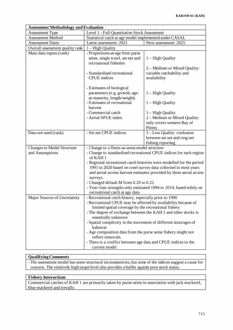
KAHAWAI (KAH)
715
Assessment Methodology and Evaluation Assessment Type Level 1 - Full Quantitative Stock Assessment Assessment Method Statistical catch at age model implemented under CASAL Assessment Dates Latest assessment: 2021 Next assessment: 2025 Overall assessment quality rank 1 – High Quality Main data inputs (rank) - Proportions-at-age from purse
seine, single trawl, set net and recreational fisheries
- Standardised recreational CPUE indices
- Estimates of biological parameters (e.g. growth, age-at-maturity, length/weight)
- Estimates of recreational harvest
- Commercial catch - Aerial SPUE index
1 – High Quality 2 – Medium or Mixed Quality: variable catchability and availability 1 – High Quality 1 – High Quality 1 – High Quality 2 – Medium or Mixed Quality: only covers western Bay of Plenty
Data not used (rank) - Set net CPUE indices 3 – Low Quality: confusion between set net and ring net fishing reporting
Changes to Model Structure and Assumptions
- Change to a fleets-as-areas model structure - Change to standardised recreational CPUE indices for each region
of KAH 1 - Regional recreational catch histories were modelled for the period
1991 to 2020 based on creel survey data collected in most years and aerial-access harvest estimates provided by three aerial access surveys
- Changed default M from 0.20 to 0.22 - Year class strengths only estimated 1994 to 2014, based solely on
recreational catch at age data Major Sources of Uncertainty - Recreational catch history, especially prior to 1990
- Recreational CPUE may be affected by availability because of limited spatial coverage by the recreational fishery
- The degree of exchange between the KAH 1 and other stocks is essentially unknown
- Spatial complexity in the movement of different sizes/ages of kahawai
- Age composition data from the purse seine fishery might not reflect removals.
- There is a conflict between age data and CPUE indices in the current model
Qualifying Comments - The assessment model has some structural inconsistencies, but none of the indices suggest a cause for concern. The relatively high target level also provides a buffer against poor stock status.
Fishery Interactions Commercial catches of KAH 1 are primarily taken by purse-seine in association with jack mackerel, blue mackerel and trevally.

KAHAWAI (KAH)
716
All other KAH regions No accepted assessment is available that covers these regions. It is not known if the current catches, allowances or TACCs are sustainable. The status of KAH 2, 3 and 8 relative to BMSY is unknown. 6. FOR FURTHER INFORMATION Armiger, H; Hartill, B; Rush, N; Buckthought, D; Smith, M (2014) Length and age compositions of recreational landings of kahawai in KAH 1
in January to April in 2011 and 2012. New Zealand Fisheries Assessment Report 2014/60. 39 p. Armiger, H; Hartill, B; Rush, N; Vaughan, M; Smith, M; Buckthought, D (2009) Length and age compositions of recreational landings of
kahawai in KAH 1 in January to April 2008 and KAH 8 in January to April 2007. New Zealand Fisheries Assessment Report 2009/36 . 40 p.
Armiger, H; Hartill, B; Tasker, R; Smith, M (2006) Length and age compositions of recreational landings of kahawai in KAH 1 in January to April 2003–04 and 2004–05. Final Research Report for Ministry of Fisheries Research Project KAH2003/01 Objectives 1 & 2. 33 p. (Unpublished report held by Fisheries New Zealand, Wellington.)
Boyd, R O; Gowing, L; Reilly, J L (2004) 2000–2001 National marine recreational fishing survey: diary results and harvest estimates. Draft New Zealand Fisheries Research Report. (Unpublished report held by Fisheries New Zealand, Wellington.)
Boyd, R O; Reilly, J L (2002) 1999/2000 National marine recreational fishing survey: harvest estimates. Draft New Zealand Fisheries Research Report. (Unpublished report held by Fisheries New Zealand, Wellington.)
Bradford, E (1997) Estimated recreational catches from Ministry of Fisheries North region marine recreational fishing surveys, 1993–94. New Zealand Fisheries Assessment Research Document 1997/7. 16 p. (Unpublished report held by NIWA library, Wellington.)
Bradford, E (1998) Harvest estimates from the 1996 national recreational fishing surveys. New Zealand Fisheries Assessment Research Document. 1998/16. 27 p. (Unpublished report held by NIWA library, Wellington.)
Bradford, E; Fisher, D; Bell, J (1998) National recreational fishing survey 1996: overview of catch and effort results. NIWA Technical Report 18. 55 p.
Bull, B; Francis, R I C C; Dunn, A; McKenzie, A; Gilbert, D J; Smith, M H; Bian, R; Fu, D (2012) CASAL (C++ algorithmic stock assessment laboratory): CASAL User Manual v2.30.2012/03/21. NIWA Technical Report 135. 280 p.
Drummond, K L (1995) Report on investigations into the Central New Zealand kahawai purse seine fishery over the 1992/93 summer. C ent ral Fisheries Region Internal Report 25. 33 p.
Drummond, K L; Wilson, A L (1993) The biology and purse-seine fishery of kahawai (Arripis trutta Bloch and Schneider) from central New Zealand, during 1990/91–1991/92. Central Fisheries Region Internal Report 22. 42 p.
Duffy, C A J; Petherick, C (1999) A new size record for kahawai (Arripis trutta) from New Zealand. New Zealand Journal of Marine and Freshwater Research 33: 565–569.
Francis, M P; Paul, L J (2013) New Zealand inshore finfish and shellfish commercial landings, 1931–82. New Zealand Fisheries Assessment Report 2013/55. 136 p.
Francis, R.I.C.C (2011) Data weighting in statistical fisheries stock assessment models. Canadian Journal of fisheries and Aquatic Sci ence 68: 1124–1138.
Hartill, B (2009) Assessment of the KAH 1 fishery for 2006. New Zealand Fisheries Assessment Report 2009/24. 43 p. Hartill, B; Armiger, H; Tasker, R; Middleton, C; Fisher, D (2007a) Monitoring the length and age composition of recreational landings of
kahawai in KAH 1 in 2000–01, 2001–02 and 2002–03. New Zealand Fisheries Assessment Report 2007/6. 38 p. Hartill, B; Armiger, H; Vaughan, M; Rush, N; Smith, M (2008) Length and age compositions of recreational landings of kahawai i n KAH 1
from January to April 2007. New Zealand Fisheries Assessment Report 2008/63. 40 p. Hartill, B.; Bian, R. (2016). Stock assessment of kahawai (Arripis trutta) in KAH 1. New Zealand Fisheries Assessment Report 2016/26. 42 p. Hartill, B; Bian, R; Armiger, H; Vaughan, M; Rush, N (2007c) Recreational marine harvest estimates of snapper, kahawai, and kingfish in QMA
1 in 2004–05. New Zealand Fisheries Assessment Report 2007/26. 44 p. Hartill, B; Bian, R; Rush, N; Armiger, H (2013) Aerial-access recreational harvest estimates for snapper, kahawai, red gurnard, tarakihi and
trevally in FMA 1 in 2011–12. New Zealand Fisheries Assessment Report 2013/70. 44 p. Hartill, B.; Bian, R.; Rush, N.; Armiger, H. (2019). Aerial-access recreational harvest estimates for snapper, kahawai, red gurnard, tarakihi and
trevally in FMA 1 in 2017–18. New Zealand Fisheries Assessment Report 2019/23. 39 p. Hartill, B; Davey, N (2015) Mean weight estimates for recreational fisheries in 2011–12. New Zealand Fisheries Assessment Report
2015/25. 37 p. Hartill, B. Doonan, I. (in prep) Stock assessment for KAH 1 for 1930—31 to 2020–21. Draft New Zealand Fisheries Assessment Report
2022/xx. Hartill, B.; Rush, N.; Payne, G.; Davey, N.; Bian, R.; Millar, A.; Armiger, H.; Spong, K. (2020). Camera and creel survey monitoring of
trends in recreational effort and harvest from 2004–05 to 2018–19. New Zealand Fisheries Assessment Report 2020/18. 54 p. Hartill, B; Smith, M; Rush, N; Vaughan, M; Armiger, H (2007d) Length and age composition of recreational landings of kahawai i n KAH 1
from January to April 2005–06. New Zealand Fisheries Assessment Report 2007/28. 30 p. Hartill, B; Walsh, C (2005) Characterisation of kahawai fisheries of New Zealand and a review of biological knowledge. Final Research Report
for Ministry of Fisheries Research Project KAH200401. 160 p. (Unpublished report held by Fisheries New Zealand, Wellington.) Hartill, B; Watson, T; Cryer, M; Armiger, H (2007b) Recreational marine harvest estimates of snapper and kahawai in the Hauraki Gulf in
2003–04. New Zealand Fisheries Assessment Report 2007/25 55 p. Jones, J B; Cresswell, P; Drummond, K; McKenzie, J (1992) Kahawai. New Zealand Fisheries Assessment Research Document 1992/2. 27 p.
(Unpublished report held by NIWA library, Wellington.) Kimura, D K (1980) Likelihood methods for the von Bertalanffy growth curve. Fishery Bulletin 77: 765–776. Maxwell, K. (2019) Informing Ecosystem-Based Fisheries Management from an Indigenous Perspective: The Mōtū Kahawai Fishery. PhD
Thesis, Victoria University of Wellington. https://researcharchive.vuw.ac.nz/xmlui/handle/10063/8624 Morton, A; Lyle, J; Welsford, D (2005) Biology and status of key recreational finfish species in Tasmania. Tasmanian Aquaculture and
Fisheries Institute Technical Report Series 25. 52 p. Paulin, C (1993) Review of Australasian fish family Arripididae (Percomorpha), with the description of a new species. Austral ian Journal of
Marine and Freshwater Research 44: 459–471. Reilly, J L (2002) 1999/2000 National marine recreational fishing survey: weighting methodology for harvest estimates. Draft report by
Statistical Insights Ltd. 25 p. Smith, P J; Hartill, B; Hamer, P; McKenzie, A (2008) Stock structure of kahawai, Arripis trutta. New Zealand Fisheries Assessment Repor t
2008/20. 42 p. Stevens, D W; Kalish, J (1998) Validated age and growth of kahawai (Arripis trutta) in the Bay of Plenty and Tasman Bay. N IWA T echnical
Report 11. 33 p.

KAHAWAI (KAH)
717
Sylvester, C T A (1989) Kahawai fishery assessment 1989. New Zealand Fisheries Assessment Research Document 1989/10. 17 p. (Unpublished report held by Fisheries New Zealand, Wellington.)
Taylor, P R (2014) Developing indices of relative abundance from observational aerial sightings of inshore pelagic finfish; step 1, exploring the data. New Zealand Fisheries Assessment Report 2014/44. 66 p.
Teirney, L D; Kilner, A R; Millar, R E; Bradford, E; Bell, J D (1997) Estimation of recreational catch from 1991/92 to 1993/94. New Zealand Fisheries Assessment Research Document 1997/15. 43 p. (Unpublished report held by Fisheries New Zealand, Wellington.)
Watkinson, J G; Smith, R (1972) New Zealand Fisheries. New Zealand Government Print. 91 p. Wright, P; McClary, D; Boyd, R O (2004) 2000/2001 National Marine Recreational Fishing Survey: direct questioning of fishers compared with
reported diary data. Final Research Report for Ministry of Fisheries Project REC2000–01: Objective 2. Wynne-Jones, J; Gray, A; Heinemann, A; Hill, L; Walton, L (2019). National Panel Survey of Marine Recreational Fishers 2017–2018. N ew
Zealand Fisheries Assessment Report 2019/24. 104 p. Wynne-Jones, J; Gray, A; Hill, L; Heinemann, A (2014) National Panel Survey of Marine Recreational Fishers 2011–12: Harvest estimates. New
Zealand Fisheries Assessment Report 2014/67. 139 p.


KINA (SUR)
719
KINA (SUR)
(Evechinus chloroticus) Kina
1. FISHERY SUMMARY South Island kina was introduced into the Quota Management System in October 2002. North Island kina was introduced into the Quota Management System from October 2003. Five Quota Management Areas based on the FMAs 3, 4, 5, 7A (Marlborough Sounds) and 7B (west coast) were created in the South Island and seven Quota Management Areas based on the FMAs 1A (Auckland-North), 1B (Auckland-South), 2A (Central (East-North)), 2B (Central (East-South)), 8, 9 and 10 were created in the North Island. Current allowances, TACCs and TACs are summarised in Table 1. The historical landings and TACC values for the main SUR stocks are depicted in Figure 1. Table 1: Current Total allowable catches (TAC, t) allowances for customary fishing, recreational fishing, and other
sources of mortality (t) and Total Allowable Commercial Catches (TACC, t) for kina.
TAC Customary Recreational Other Mortality TACC SUR 1A 172 65 65 2 40 SUR 1B 324 90 90 4 140 SUR 2A 204 60 60 4 80 SUR 2B 102 35 35 2 30 SUR 3 42 10 10 1 21 SUR 4 255 20 7 3 225 SUR 5 480 10 10 5 455 SUR 7A 238 80 20 3 135 SUR 7B 26 10 5 1 10 SUR 8 26 12 12 1 1 SUR 9 33 11 11 1 10 SUR 10 0 0 0 0 0
1.1 Commercial fisheries Most kina are found in waters less than 10 m deep and are harvested by breath-hold diving, although some is taken by target dredge in SUR 7 (Marlborough Sounds). There is no minimum legal size for kina. Almost all roe harvested in this fishery is consumed on the domestic market. In 1988–89, competitive TACCs were established in the more important FMAs but not in east Northland (SUR 1) or at the Chatham Islands (SUR 4), both of which developed into productive fisheries in the 1990s (Table 2). On 1 October 1992 the Ministry of Fisheries placed a moratorium on the issue of permits to commercially harvest kina. The kina fishery has evolved considerably since the imposition of the moratorium. Where present, the competitive TACCs were either not caught or were exceeded, both by wide margins. Much of the increase in catch observed in SUR 5 in the early 1990s can be attributed to an experimental fishery developed in SUR 5, between Puysegur Point and Breaksea Island. The short-

KINA (SUR)
720
lived Kina Development Programme harvested kina from Dusky Sound in 1993 under special permit. In recent years landings have fluctuated around the TACCs for SUR 1A, 1B, 5 and 7A. Landings have generally remained well below the TACCs in other FMAs but increased to 17 t (TACC 20 t) in SUR 3 in 2019–20, and have exceeded 170 t in 2016–17, 2017–18 and 2019–20 in SUR 4 (TACC 225 t). Table 2: Total reported landings (t greenweight) of kina (SUR) by FMA and fishing year by all methods and target
species. [Continued on next page].
SUR 1 SUR 1A SUR 1B Year Landings TACC Landings TACC Landings TACC 1983 66.2 – – – – – 1984 81.4 – – – – – 1985 64.5 – – – – – 1986 72.0 – – – – – 1987 52.1 – – – – – 1988 22.1 – – – – – 1989 35.5 – – – – – 1990 10.0 – – – – – 1991 71.5 – – – – – 1992 78.7 – – – – – 1993 89.7 – – – – – 1994 150.7 – – – – – 1995 155.9 – – – – – 1996 174.5 – – – – – 1997 161.6 – – – – – 1998 134.8 – – – – – 1999 201.4 – – – – – 2000 297.4 – – – – – 2001 184.5 – – – – – 2001–02 237.0 – – – – – 2002–03 211.2 – – – – – 2003–04 1.7 – 26.9 40 111.0 140 2004–05 – – 20.9 40 131.1 140 2005–06 – – 41.0 40 138.6 140 2006–07 – – 37.1 40 147.3 140 2007–08 – – 31.7 40 140.4 140 2008–09 – – 30.5 40 130.6 140 2009–10 – – 40.8 40 129.9 140 2010–11 – – 31.7 40 122.1 140 2011–12 – – 37.9 40 134.2 140 2012–13 – – 38.7 40 145.4 140 2013–14 – – 43.4 40 139.3 140 2014–15 – – 39.7 40 147.5 140 2015–16 – – 40.9 40 131.6 140 2016–17 – – 39.6 40 142.7 140 2017–18 – – 38.7 40 136.2 140 2018–19 – – 36.5 40 133.3 140 2019–20 – – 35.1 40 143.7 140 2020–21 – – 41.9 40 150.6 140 SUR 2 SUR 2A SUR 2B Fishing year Landings TACC Landings TACC Landings TACC 1983 33.0 – – – – – 1984 180.3 – – – – – 1985 83.8 – – – – – 1986 139.1 – – – – – 1987 142.6 – – – – – 1988 154.1 – – – – – 1989 92.8 – – – – – 1990 282.4 – – – – – 1991 87.2 – – – – – 1992 37.3 – – – – – 1993 170.4 – – – – – 1994 176.7 – – – – – 1995 129.7 – – – – – 1996 41.2 – – – – – 1997 49.9 – – – – – 1998 36.5 – – – – – 1999 20.2 – – – – – 2000 14.5 – – – – – 2001 11.4 – – – – – 2001–02 3.0 – – – – –

KINA (SUR)
721
Table 2 [Continued] SUR 2 SUR 2A SUR 2B Fishing year Landings TACC Landings TACC Landings TACC 2002–03 30.4 – – – – – 2003–04 0 – 14.5 80 4.6 30 2004–05 – – 6.5 80 1.4 30 2005–06 – – 22.1 80 0.2 30 2006–07 – – 13.8 80 < 0.1 30 2007–08 – – 18.0 80 0.2 30 2008–09 – – 19.8 80 < 0.1 30 2009–10 – – 0.1 80 0.3 30 2010–11 – – 4.1 80 < 0.1 30 2011–12 – – 5.9 80 1.1 30 2012–13 – – 10.6 80 0 30 2013–14 – – 10.1 80 3.8 30 2014–15 – – 18.8 80 2.3 30 2015–16 – – 17.8 80 2.5 30 2016–17 – – 9.3 80 13.4 30 2017–18 – – 21.8 80 7.9 30 2018–19 – – 13.4 80 13.2 30 2019–20 – – 13.4 80 7.8 30 2020–21 – – 7.0 80 25.4 30 SUR 3 SUR 4 SUR 5 Fishing year Landings TACC Landings TACC Landings TACC 1983 4.8 – 11.3 – 0.5 – 1984 14.4 – 4.0 – 0.9 – 1985 4.0 – 7.4 – 4.6 – 1986 6.2 – 52.7 – 0.2 – 1987 2.4 – 28.4 – 4.3 – 1988 1.7 – 76.5 – 2.3 – 1989 0.8 – 216.6 – 19 – 1990 4.1 – 190.0 – 13.4 – 1991 21.3 – 35.3 – 166.9 – 1992 15.8 – 192.9 – 272.2 – 1993 9.9 – 21.8 – *530.3 – 1994 8.8 – 55.3 – 327.2 – 1995 7.1 – 100.7 – 342.9 – 1996 6.0 – 99.5 – 446.4 – 1997 5.4 – 225.7 – 171.6 – 1998 3.8 – 303.1 – 91.2 – 1999 38.4 – 168.2 – 120.6 – 2000 50.4 – 396.5 – 106.3 – 2001 11.2 – 472.6 – 69.8 – 2001–02 5.2 – 368.0 – 184.9 – 2002–03 0.3 21 167.3 225 132.5 245 2003–04 0.3 21 114.8 225 199.1 245 2004–05 0.5 21 91.7 225 350.4 455 2005–06 < 0.1 21 70.2 225 473 455 2006–07 3.2 21 108.3 225 423 455 2007–08 2.1 21 147.4 225 276.2 455 2008–09 4.2 21 135.6 225 294.9 455 2009–10 5.1 21 89.7 225 320.4 455 2010–11 5.2 21 134.9 225 339.2 455 2011–12 4.3 21 137.7 225 402 455 2012–13 4.8 21 76.2 225 474.8 455 2013–14 0.4 21 101.2 225 462.8 455 2014–15 0.2 21 75.2 225 458.4 455 2015–16 4.1 21 116.3 225 453.1 455 2016–17 8.6 21 220.0 225 460.1 455 2017–18 < 0.1 21 189.4 225 421.6 455 2018–19 2.3 21 94.8 225 466.7 455 2019–20 17.6 21 173.4 225 439.5 455 2020–21 16.1 21 141.8 225 464.1 455 SUR 7 SUR 7A SUR 7B Fishing year Landings TACC Landings TACC Landings TACC 1983 26.3 – – – – – 1984 55.1 – – – – – 1985 99.6 – – – – – 1986 86.6 – – – – – 1987 52.6 – – – – – 1988 175.6 – – – – – 1989 6.2 – – – – – 1990 41.5 – – – – – 1991 56.3 – – – – – 1992 114.4 – – – – – 1993 210.2 – – – – – 1994 98.2 – – – – –

KINA (SUR)
722
Table 2 [Continued] SUR 7 SUR 7A SUR 7B Fishing year Landings TACC Landings TACC Landings TACC 1995 149 – – – – – 1996 142.2 – – – – – 1997 121.7 – – – – – 1998 144.7 – – – – – 1999 113.9 – – – – – 2000 87.9 – – – – – 2001 80.1 – – – – – 2001–02 31.7 – – – – – 2002–03 1.3 – 63.2 135 0 10 2003–04 0 – 85.4 135 0 10 2004–05 – – 101.3 135 - 10 2005–06 – – 72.1 135 5.3 10 2006–07 – – 117.3 135 9.2 10 2007–08 – – 134.6 135 6.5 10 2008–09 – – 128.7 135 6.1 10 2009–10 – – 119.7 135 3.5 10 2010–11 – – 97.4 135 7.2 10 2011–12 – – 131.6 135 6 10 2012–13 – – 115.5 135 5 10 2013–14 – – 126.3 135 0 10 2014–15 – – 142.8 135 0 10 2015–16 – – 134.0 135 2.5 10 2016–17 – – 138.6 135 0 10 2017–18 – – 121.3 135 0 10 2018–19 – – 131.0 135 0 10 2019–20 – – 136.1 135 0 10 2020–21 – – 141.8 135 0 10 SUR 6, 8 & 9 Total Fishing year Landings TACC Landings TACC 1983 3.6 – 157 1984 0.3 – 342 1985 0.9 – 275 1986 2 – 360 1987 0.1 – 283 1988 – – 432 1989 1.5 – 372 1990 6.5 – 548 1991 4.4 – 443 1992 5 – 717 1993 – – 1 032 1994 2.3 – 820 1995 89.5 – 975 1996 0.1 – 910 1997 0.2 – 736 1998 1.4 – 716 1999 0.5 – 663 2000 0.1 – 956 2001 3.1 – 832 2001–02 – – 829.7 2002–03 0.9 – 607.4 636 2003–04 3.8 11 562.3 937 2004–05 0.9 11 704.7 1 147 2005–06 4.0 11 826.5 1 147 2006–07 8.6 11 868 1 147 2007–08 5.8 11 762.9 1 147 2008–09 3.4 11 753.8 1 147 2009–10 2.3 11 711.9 1 147 2010–11 2.5 11 741.9 1 147 2011–12 8.2 11 862.1 1 147 2012–13 4.0 11 875 1 147 2013–14 9.1 11 896 1 147 2014–15 7.9 11 885 1 147 2015–16 2.5 11 901 1 147 2016–17 10.3 11 952 1 147 2017–18 0.5 11 947 1 147 2018–19 4.8 11 891.5 1 147 2019–20 5.9 11 972.5 1 147 2020–21 1.2 11 989.9 1 147
Data from 1989 and 1990 are combined from the FSU and CELR databases. − indicates no recorded catch. Data for the period 1983 to 1999 are from Andrew (2001), and have been groomed. Catch estimates for 2000 and 2001 are taken directly from MFish. * includes 133 t caught in Dusky Sound experimental fishery. Catches from SUR 6, 8, and 9 have been pooled because too few permit holders recorded catches in these FMAs to report them singly.

KINA (SUR)
723
Figure 1:Reported commercial landings and TACC for the nine main SUR stocks. From top: SUR 1A (Northland),
SUR 1B (Hauraki Gulf, Bay of Plenty) and SUR 2A (East Coast). Note that these figures do not show data prior to entry into the QMS for SUR 1A to SURB 2A [Continued on next page]

KINA (SUR)
724
Figure 1:Reported commercial landings and TACC for the nine main SUR stocks. From top: SUR 2B (Wairarapa,
Wellington), SUR 3 (South East Coast) and SUR 4 (South East Chatham Rise). Note that these figures do not show data prior to entry into the QMS for SUR 2B. [Continued next page]

KINA (SUR)
725
Figure 1:[Continued]: Reported commercial landings and TACC for the nine main SUR stocks. From top: SUR 5
(Southland), SUR 7A (Challenger Nelson Marlborough) and SUR 7B (Challenger Westland). Note that these figures do not show data prior to entry into the QMS for SUR 7A and SUR 7B.
1.2 Recreational fisheries Recreational catch was estimated using telephone-diary surveys in 1993–94, 1996 (Fisher & Bradford 1998, Bradford 1998) and 2000 (Boyd & Reilly 2002, Boyd et al 2004) (Table 3). There are no estimates of recreational catch from the Chatham Islands. In many instances, insufficient kina were caught to provide reliable estimates of the error associated with the estimates of total harvest. The harvest estimates provided by these telephone-diary surveys are no longer considered reliable for various

KINA (SUR)
726
reasons. A Recreational Technical Working Group concluded that these harvest estimates should be used only with the following qualifications: a) they may be very inaccurate; b) the 1996 and earlier surveys contain a methodological error; and c) the 2000 and 2001 estimates are implausibly high for many important fisheries. In response to these problems and the cost and scale challenges associated with onsite methods, a National Panel Survey was conducted for the first time throughout the 2011–12 fishing year. The panel survey used face-to-face interviews of a random sample of 30 390 New Zealand households to recruit a panel of fishers and non-fishers for a full year. The panel members were contacted regularly about their fishing activities and harvest information collected in standardised phone interviews. The panel survey was repeated in 2017–18. Harvest estimates for kina (in numbers) are given in Table 3 (from Wynne-Jones et al 2014, no estimates of mean weight were available from boat ramp surveys, Hartill & Davey 2015, Wynne-Jones et al 2019). For the early telephone-diary surveys, catches in numbers were converted to catch in tonnes by assuming an average whole weight of 248.3 g per kina based on equal proportions across a size range 60–110 mm Test Diameter (TD) and a test diameter-weight relationship (W = (6.27×10⁻⁴)TD2.88) from Dusky Sound (unpublished data). These estimates of catch in tonnes should be considered as indicative only and may be very inaccurate. No estimates of mean weight were available to convert catches in numbers from the national panel survey to catch in tonnes. Table 3: Estimates of recreational harvest of kina using telephone-diary surveys (1993–94, 1996, and 2000 surveys)
and the national panel surveys (2011–12 and 2017–18).
Area Number (thousands) CV Catch (t)* 1993–94 (telephone-diary) East Northland 109 0.60 27.1 Hauraki Gulf 14 - 3.5 Bay of Plenty 648 0.49 160.9 SUR 1 801 0.41 198.9 SUR 9 30 0.72 7.4 1996 (telephone-diary) SUR 1 316 0.24 78.5 SUR 2 61 - 15.1 SUR 3 12 - 3.0 SUR 5 20 - 5.0 SUR 7 2 - 0.5 SUR 8 43 - 10.7 SUR 9 30 - 7.4 2000 (telephone-diary) SUR 1 1 793 0.35 445.2 SUR 2 1 026 0.57 254.7 SUR 3 8 0.58 2.0 SUR 5 70 1.01 17.4 SUR 7 2 1.01 0.5 SUR 8 85 0.85 21.1 SUR 9 82 0.67 20.4 2011–12 (national panel survey) SUR 1 2 019 0.86 - SUR 2 107 0.32 - SUR 3 12 0.59 - SUR 5 10 0.73 - SUR 7 12 0.67 - SUR 8 61 0.43 - SUR 9 58 0.62 - SUR total 2 279 0.73 - 2017–18 (national panel survey) SUR 1 296 0.21 - SUR 2 181 0.24 - SUR 3 5 0.68 - SUR 5 10 0.44 - SUR 7 2 0.95 - SUR 8 34 0.38 - SUR 9 12 0.85 - SUR total 540 -
*Data as numbers caught supplied by Ngai Tahu Development Corporation. Catch in kilograms was estimated using the conversion rules described in the paragraph above.

KINA (SUR)
727
1.3 Customary non-commercial fisheries There is an important customary non-commercial harvest of kina by Māori for food. Cockles form an important fishery for customary non-commercial, but the total annual catch is not known. Māori customary fishers utilise the provisions under both the recreational fishing regulations and the various customary regulations. Many tangata whenua harvest kina under their recreational allowance and these are not included in records of customary catch. Customary reporting requirements vary around the country. Customary fishing authorisations issued in the South Island and Stewart Island would be under the Fisheries (South Island Customary Fishing) Regulations 1999. Many rohe moana / areas of the coastline in the North Island and Chatham Islands are gazetted under the Fisheries (Kaimoana Customary Fishing) Regulations 1998 which require reporting on authorisations. In the areas not gazetted, customary fishing permits would be issued would be under the Fisheries (Amateur Fishing) Regulations 2013, where there is no requirement to report catch. The information on Māori customary harvest under the provisions made for customary fishing can be limited (Table 4). These numbers are likely to be an underestimate of customary harvest as only the catch approved and harvested in kilograms and numbers are reported in the table. Table 4: Fisheries New Zealand records of customary harvest of kina (approved and reported as weight (kg) and in
numbers), since 1998-99. – no data. [Continued next page]
SUR 1A SUR 1B Weight (kg) Numbers Weight (kg) Numbers Fishing year Approved Harvested Approved Harvested Approved Harvested Approved Harvested 1998–99 – – – – – – – – 1999–00 – – – – – – – – 2000–01 – – – – – – – – 2001–02 – – – – – – – – 2002–03 – – – – – – – – 2003–04 – – – – – – 1 200 750 2004–05 – – – – – – 400 210 2005–06 – – – – 1 790 1 040 – – 2006–07 850 850 7 300 7 300 12 055 9 785 6 025 5 475 2007–08 2 890 2 890 6 900 6 900 11 225 9 285 12 230 10 130 2008–09 3 290 3 290 1 900 1 900 11 540 8 940 10 524 9 924 2009–10 1 760 1 760 1 400 1 400 11 615 8 995 9 500 7 750 2010–11 3 570 3 570 – – 26 582 20 142 21 890 19 050 2011–12 9 575 8 775 900 600 4 990 2 900 1 450 1 400 2012–13 9 704 9 210 2 300 2 170 4 325 3 460 400 400 2013–14 610 610 3 900 3 900 480 360 – – 2014–15 – – – – 16 495 15 265 2 700 2 150 2015–16 – – – – 5 550 3 950 1 260 383 2016–17 – – – – 1 885 1 175 5 950 3 173 2017–18 – – – – 410 130 8 875 5 700 2018–19 – – – – 2 120 1 883 4 020 2 845 2019–20 – – – – 100 100 380 355 2020–21 – – – – 500 450 SUR 2A SUR 2B Weight (kg) Numbers Weight (kg) Numbers Fishing year Approved Harvested Approved Harvested Approved Harvested Approved Harvested 1998–99 – – 200 200 – – – – 1999–00 – – 2 350 460 – – – – 2000–01 – – – – – – – – 2001–02 – – 100 80 – – – – 2002–03 – – – – – – – – 2003–04 – – – – – – 1 350 1 350 2004–05 – – 600 440 – – 900 900 2005–06 – – 7 500 4 940 – – 200 200 2006–07 – – 55 806 41 546 – – – – 2007–08 – – 60 546 46 599 – – – – 2008–09 – – 54 050 46 427 – – 18 055 14 940 2009–10 – – 17 100 13 640 – – 2 700 1 510 2010–11 1 300 1 000 71 950 66 222 – – – – 2011–12 – – 102 160 87 639 – – – – 2012–13 – – 127 090 101 162 – – – – 2013–14 – – 132 715 98 129 – – – – 2014–15 – – 63 410 52 181 – – 200 130 2015–16 – – 20 030 16 072 – – 460 420 2016–17 300 300 50 400 33 483 – – – – 2017–18 – – 11 400 5 950 – – – – 2018–19 – – 33 020 12 894 – – – –

KINA (SUR)
728
Table 4 [Continued] SUR 2A SUR 2B Weight (kg) Numbers Weight (kg) Numbers Fishing year Approved Harvested Approved Harvested Approved Harvested Approved Harvested 2019–20 – – – – – – – – 2020–21 – – – – – – – – SUR 3 SUR 4 Weight (kg) Numbers Weight (kg) Numbers Fishing year Approved Harvested Approved Harvested Approved Harvested Approved Harvested 1998–99 – – – – – – – – 1999–00 – – – – – – – – 2000–01 – – – – – – – – 2001–02 – – 2 070 819 – – – – 2002–03 – – 650 150 – – – – 2003–04 – – – – – – – – 2004–05 – – – – – – – – 2005–06 – – 1 075 401 – – – – 2006–07 – – 2 020 1 417 – – – – 2007–08 – – 4 880 4 134 – – – – 2008–09 – – 3 099 968 – – – – 2009–10 – – 1 600 1 283 – – 460 429 2010–11 – – 17 170 16 092 – – – – 2011–12 – – 3 660 2 436 17 17 – – 2012–13 – – 5 600 4 629 – – – – 2013–14 – – 3 850 1 160 – – 90 88 2014–15 – – 1 910 1 382 – – 40 40 2015–16 – – 3 006 2 265 – – 162 102 2016–17 – – 1 805 1 570 – – 310 310 2017–18 – – 300 192 24 24 125 125 2018–19 – – – – 50 50 – – 2019–20 – – 7 351 4 646 – – – – 2020–21 – – 3 150 2 662 – – – –
SUR 5 SUR 7A Weight (kg) Numbers Weight (kg) Numbers Fishing year Approved Harvested Approved Harvested Approved Harvested Approved Harvested 1998–99 – – – – – – – – 1999–00 – – – – – – – – 2000–01 – – 730 520 – – – – 2001–02 – – 4 810 4 039 – – – – 2002–03 – – 3 440 2 255 – – – – 2003–04 – – – – – – – – 2004–05 – – – – – – – – 2005–06 – – 700 700 – – – – 2006–07 – – 260 260 50 10 – – 2007–08 – – 7 715 7 715 – – 1 220 960 2008–09 – – 7 450 7 125 – – 1 570 1 198 2009–10 – – 2 380 1 706 – – 2 170 2 040 2010–11 – – 300 300 – – – – 2011–12 – – 2 659 2 659 – – – – 2012–13 – – 5 680 5 680 – – – – 2013–14 – – 1 000 910 – – – – 2014–15 – – – – – – – – 2015–16 – – 3 840 3 170 – – – – 2016–17 – – 2 500 2 410 – – – – 2017–18 – – 2 150 2 150 – – – – 2018–19 – – – – – – – – 2019–20 – – 900 900 – – – – 2020–21 – – 2 220 2 001 SUR 7B SUR 8 Weight (kg) Numbers Weight (kg) Numbers Fishing year Approved Harvested Approved Harvested Approved Harvested Approved Harvested 1998–99 – – – – – – – – 1999–00 – – – – – – – – 2000–01 – – – – – – – – 2001–02 – – – – – – – – 2002–03 – – – – – – – – 2003–04 – – – – – – – – 2004–05 – – – – – – – – 2005–06 – – – – – – – – 2006–07 – – 250 250 – – – – 2007–08 – – – – – – – – 2008–09 – – – – – – – – 2009–10 – – – – – – – – 2010–11 – – – – – – – – 2011–12 – – – – – – – –

KINA (SUR)
729
Table 4 [Continued] SUR 7B SUR 8 Weight (kg) Numbers Weight (kg) Numbers Fishing year Approved Harvested Approved Harvested Approved Harvested Approved Harvested 2012–13 – – – – – – 300 80 2013–14 – – – – – – – – 2014–15 – – – – – – – – 2015–16 – – – – – – – – 2016–17 – – 70 70 – – – – 2017–18 – – – – – – – – 2018–19 – – – – – – 300 150 2019–20 – – – – – – – – 2020–21 – – – – – – – – SUR 9 Weight (kg) Numbers Fishing year Approved Harvested Approved Harvested 1998–99 – – – – 1999–00 – – – – 2000–01 – – – – 2001–02 – – – – 2002–03 – – – – 2003–04 – – – – 2004–05 – – – – 2005–06 – – – – 2006–07 – – – – 2007–08 50 50 – – 2008–09 – – 1 400 900 2009–10 100 80 – – 2010–11 120 120 – – 2011–12 350 320 – – 2012–13 40 40 3 150 3 150 2013–14 400 280 500 380 2014–15 80 80 – – 2015–16 – – – – 2016–17 – – – – 2017–18 – – – – 2018–19 – – – – 2019–20 – – – – 2020–21 – – – –
There are several types of customary management areas:
• mātaitai reserves – areas closed to commercial fishing, that may have bylaws affecting recreational and customary fishing
• taiāpure – local fisheries of special significance, that may have additional fishing rules • temporary closures – issued under sections 186A or 186B of the Fisheries Act 1996
There are many of them in place around New Zealand which allow for the management of kina. Locations are listed in Table 5. Table 5: Locations of the customary management areas relevant to kina. [Continued next page]
Mātaitai reserves Taiāpure Temporary closures Bylaw SUR 1A Te Puna Waikare Inlet Maunganui Bay Marsden Bank and Mair Bank SUR 1B Te Maunga o Mauao Maketu Waiheke Island Te Rae o Kohi East Coromandel Raukokere Te Mata and Waipatukahu Te Kopa o Rongokānapa Umupuia Beach SUR 2A Te Kopa o Rongokānapa Hakihea Horokaka Toka Tamure Te Hoe Moremore (a) Moremore (b) SUR 2B Porangahau Waimārama Palliser Bay (a) Palliser Bay (b) SUR 3 Kahutara Akaroa Harbour Moeraki (Tapuiri) Tutaeputaputa East Otago Lyttelton Harbour/Whakaraupō Te Taumanu o Te Waka a Mäui Oaro (freshwater and marine) Oaro-Haumuri Koukourarata Wairewa/Lake Forsyth Ōpihi

KINA (SUR)
730
Table 5 [Continued] Mātaitai reserves Taiāpure Temporary closures Bylaw Te Ahi Tarakihi Waitarakao Tuhawaiki Te Kaio Waihao Waikouaiti Otakou Moeraki Puna-wai-Toriki Waikawa Harbour/Tumu Toka SUR 5 Mataura River Oreti Waitutu Motupöhue (Bluff Hill) Te Whaka a Te Wera Kaihuka Horomamae SUR 7A Te Tai Tapu (West Coast Kaihoka) Whakapuaka (Delaware Bay) Te Tai Tapu (West Ciast – Anatori) SUR 7B Okuru/Mussel Point Popotai Taumaka Tauparikaka Mahitahi/Bruce Bay Manakaiaua/Hunts Beach Okarito Lagoon
1.4 Illegal catch There is qualitative data to suggest significant illegal, unreported, unregulated (IUU) activity in this Fishery. 1.5 Other sources of mortality Although there is no minimum legal size for kina, some incidental mortality is likely because roe quality (recovery rate and colour) is commonly assessed by opening ‘test’ kina underwater. These animals are not subsequently landed. There are no estimates of the magnitude to this incidental mortality. 2. BIOLOGY The biology and ecology of kina has been extensively studied; this literature has most recently been reviewed by Barker (2001). Evechinus chloroticus is found throughout New Zealand and the sub-Antarctic Islands. Kina has an annual reproductive cycle which culminates in spawning between November and March (Dix 1970, Walker 1984, McShane et al 1994a, 1996, Lamare & Stewart 1998, Lamare 1998). Size at maturity appears to vary considerably and may be as small as 30 mm and as large as 75 mm TD (Dix 1970, Barker et al 1998). In Dusky Sound, kina are reproductively mature at 50–60 mm TD (McShane et al 1996). Within these seemingly consistent patterns in the seasonality of the reproductive cycle there are many differences in the gonad size at small spatial scales. Settlement is likely to vary between years and appears to differ among locations and habitats (Dix 1972, Walker 1984). Laboratory work has shown that kina larval mortality increased with increasing concentrations of suspended sediment at realistic concentrations (Phillips & Shima 2006). In the field, but not in the laboratory, development abnormalities were found associated with suspended sediment concentrations; this suggests the importance of other environmental factors associated with terrestrial runoff (Schwarz et al 2006). Juvenile settlement and mortality have also been observed to increase with sediment at realistic concentrations in a size-specific manner in the laboratory; this agrees with juvenile patterns of distribution observed in the field (Walker 2007). Few small kina were observed in any of the surveys in Dusky Sound (McShane et al 1993). These results suggest that the productivity of stocks in Fiordland may be low and that recruitment over-fishing is a real possibility. There is relatively little information available on the interactions between kina and its predators and competitors. Although a wide range of fish and invertebrates eat kina, there is limited evidence that these species control or limit populations of kina in Fiordland. Work in a marine reserve, where large predators such as reef fishes and crayfish are abundant, indicates that predators can control numbers of kina surviving the transition from crevice-bound to open substratum grazing (Cole & Keuskamp 1998, Babcock et al 1999). Babcock et al (1999) have drawn a direct link between the increases in snapper

KINA (SUR)
731
and crayfish populations and the long-term decline in kina populations in the Leigh Marine Reserve. There is, however, no evidence that high kina densities limit rock lobster populations (Andrew & MacDiarmid 1991). It is likely, however, that changes in the abundance of kina, and the consequent changes in habitat representation, are part of a complex set of interacting processes, including but not exclusively, increased predation. Kina compete with a range of invertebrate herbivores, including paua. There is no published evidence that high densities of kina limit paua populations in Fiordland. McShane (1997) reported that paua are abundant in Dusky Sound, and in Chalky and Preservation Inlets, but are rare in the fjords. Lamare & Mladenov (2000) estimate that kina grow 8–10 mm in their first year of life. Growth rates will vary considerably depending on local conditions, but kina may take 8–9 years to reach 100 mm TD, and very large individuals may reach ages of more than 20 years (Lamare & Mladenov 2000). 3. STOCKS AND AREAS There appear to be few genetic differences in kina populations from Leigh (North Auckland) and Stewart Island (Mladenov et al 1997), which suggests that there is some mixing among populations. There is no direct evidence that populations of kina at the Chatham Islands differ genetically from those on the mainland, nor is there evidence that “populations” of kina at the Chatham Islands are dependent on the dispersal of larvae from the mainland. 4. STOCK ASSESSMENT Although there is a wealth of information on the biology and ecology of this species (see Barker 2001 for reviews), there is relatively little that can be used to assess the status of exploited stocks. There have been no assessments of sustainable yield nor are there estimates of biomass or trends in relative abundance for any Fishstock (Annala 1995). 4.1 Estimates of fishery parameters and abundance Andrew (2001) reported catch rates from both dive and dredge fisheries but advised caution in the interpretation of catch rate information for sedentary invertebrates, like kina, gathered at broad spatial scales. Indices of relative abundance using timed swims have been reported for Ariel Reef in SUR 2 (Anderson & Stewart 1993), Chatham Islands (Schiel et al 1995, Naylor & Andrew 2002), and D’Urville Island and Arapawa Island in SUR 7 (McShane et al 1994a). Numerous surveys of kina have been done over the last 30 years in fished areas, mostly by university-based researchers (e.g., Dix 1970, Choat & Schiel 1982, Schiel et al 1995, Cole & Keuskamp 1998, Babcock et al 1999, Wing et al 2001). Naylor & Andrew (2002) reported a range of densities for kina around Chatham Island from 0.17/m2 (northwest Chatham Island) to 1.6/m2 (south east Chatham Island). These were generally lower than estimates made in the mid-1990s by Schiel et al (1995) (0.2/m2 to 6/m2). By contrast, even lower kina densities of around 0.1/m2 were reported by McShane et al (1994a) for both Arapawa and D'Urville Island. Dix (1970) reported much higher mean relatively high densities of kina ranging from 2.2/m2 in Queen Charlotte Sound to 6/m2 at Kaikōura. 4.2 Biomass estimates McShane & Naylor (1993) reported biomass estimates of 2500 t and 500 t respectively for D’Urville and Arapawa Islands (SUR 7), presumably based on an expansion of density estimates reported in McShane et al (1994a) by an area estimate, however, the methods are not detailed. Biomass was estimated for Dusky Sound and Chalky Inlet (SUR 5) prior to Dusky Sound being opened as an experimental fishery in May 1993 (McShane & Naylor 1991, 1993). Productivity and biomass was to be estimated by depletion methods but this was unsuccessful because only 133 t of the projected

KINA (SUR)
732
1000 t was caught (McShane et al 1994b) and this catch was insufficient to cause a measurable change in the estimated biomass of kina. 4.3 Yield estimates and projections MCY has not been estimated for any SUR fishstock. Within SUR 5, an MCY estimate of sustainable yield within Dusky Sound and Chalky Inlet was reported in Annala (1995). This estimate used Method 1 of Annala (1995) for new fisheries based on surveys done by McShane & Naylor (1991, 1993) and an estimate of a reference fishing mortality derived from McShane et al (1994a). The estimated annual sustainable yield of 275 t for these two areas has never been harvested because they are closed to commercial fishing except under special permit. CAY has not been estimated for any SUR fishstock. 5. STATUS OF THE STOCKS For all Fishstocks it is not known if current catch levels or TACCs are sustainable, or if they are at levels which will allow the stocks to move towards a size that will support sustainable yields. 6. FOR FURTHER INFORMATION Anderson, O; Stewart, R (1993) Gisborne kina survey. (Unpublished report held in the NIWA library, Wellington.) 2 p. Andrew, N L (1986) The interaction between diet and density in influencing reproductive output in the echinoid Evechinus chloroticus (Val.).
Journal of Experimental Marine Biology and Ecology 97: 63–79. Andrew, N L (2001) Sea urchin fisheries: their status and management with special reference to the New Zealand kina fishery. (Unpublished
report to the Ministry of Fisheries and Te Ohu Kai Moana , available at http://www.doc.govt.nz/documents/science-and-technical/casn266.pdf) 124 p.
Andrew, N L; Choat, J H (1985) Habitat related differences in the survivorship and growth of juvenile sea urchins. Marine Ecology Progress Series 27: 155–161.
Andrew, N L; MacDiarmid, A B (1991) Interrelations among sea urchins (Evechinus chloroticus) and spiny lobsters (Jasus edwardsii) in northern New Zealand. Marine Ecology Progress Series 70: 211–222.
Annala, J H (1995) Report from the Fishery Assessment Plenary, May 1995. Stock assessments and yield estimates. 277 p. Babcock, R C; Kelly, S; Shears, N T; Walker, J W; Willis, T J (1999) Changes in community structure in temperate marine reserves. Marine
Ecology Progress Series 189: 125–134. Barker, M F (2001) The ecology of Evechinus chloroticus. In: Lawrence, J. (ed.). Edible Sea Urchins: Biology and Ecology. Elsevier Science,
Amsterdam. 245−260 p. Barker, M F; Keogh, J A; Lawrence, J M; Lawrence, A L (1998) Feeding rate, absorption efficiencies, growth, and enhancement of gonad
production in the New Zealand sea urchin Evechinus chloroticus Valenciennes (Echinoidea: Echinometridae) fed prepared and natural diets. Journal of Shellfish Research 17: 1583–1590.
Boyd, R O; Gowing, L; Reilly, J L (2004) 2000–2001 national marine recreational fishing survey: diary results and harvest estimates. Final Research Report for Ministry of Fisheries Project REC2000/03 (Unpublished report held by Fisheries New Zealand, Wellington).
Boyd, R O; Reilly, J L (2002) 1999/2000 National marine recreational fishing survey: harvest estimates. Final Research Report for Ministry of Fisheries project REC98/03. 28 p. (Unpublished report held by Fisheries New Zealand, Wellington).
Bradford, E (1998) Harvest estimated from the 1996 national marine recreational surveys. New Zealand Fisheries Assessment Research Document 1998/16: 27p. (Unpublished report held by NIWA library, Wellington).
Brewin, P E; Lamare, M D; Keogh, J A; Mladenov, P V (2000) Reproductive variability over a four-year period in the sea urchin Evechinus chloroticus (Echinoidea: Echinodermata) from differing habitats in New Zealand. Marine Biology 137: 543–557.
Choat, J H; Schiel, D R (1982) Patterns of distribution and abundance of large brown algae and invertebrate herbivores in subtidal regions of northern New Zealand. Journal of Experimental Marine Biology and Ecology 60: 129–162.
Cole, R G; Keuskamp, D (1998) Indirect effects of protection from exploitation: patterns from populations of Evechinus chloroticus (Echinoidea) in northeastern New Zealand. Marine Ecology Progress Series 173: 215–226.
Dix, T G (1970) Biology of Evechinus chloroticus (Echinodermata: Echinometridae) from different localities. 3. Reproduction. New Zealand Journal of Marine and Freshwater Research 4: 385–405.
Dix, T (1972). Biology of Evechinus chloroticus (Echinoidea: Echinometridae) from different localities.4. Age, growth, and size. New Zealand Journal of Marine and Freshwater Research 6: 48–68.
Fisher, D; Bradford, E (1998) National marine recreational fishing survey 1996: catch and effort results by fishing zone. Final Research Report for Ministry of Fisheries Research Project REC9701. 38 p. (Unpublished report held by Fisheries New Zealand, Wellington).
Hartill, B; Davey, N (2015) Mean weight estimates for recreational fisheries in 2011–12. New Zealand Fisheries Assessment Report 2015/25. Lamare, M (1998). Origin and transport of larvae of the sea urchin Evechinus chloroticus (Echinodermata: Echinoidea) in a New Zealand
fiord. Marine Ecology Progress Series 174: 107–121. Lamare, M; Stewart, B (1998) Mass spawning by the sea urchin Evechinus chloroticus (Echinodermata: Echinoidea) in a New Zealand fiord.
Marine Biology 132(1): 135–140. Lamare, M D; Mladenov, P V (2000) Modelling somatic growth in the sea urchin Evechinus chloroticus (Echinoidea: Echinometridae).
Journal of Experimental Marine Biology and Ecology 243: 17–43. MacDiarmid, A B; Breen, P A (1993) Spiny lobster population changes in a marine reserve. In: Battershill, C N; Schiel, D R; Jones, G P;
Creese, R G; MacDiarmid, A B (eds.). Proceedings of the Second International Temperate Reef Symposium. 47–56. NIWA Marine, Wellington.
McShane, P E (1992) Sea urchins in Dusky Sound-Prospects for a major kina industry in New Zealand. New Zealand Professional Fisherman December 92: 34–40.

KINA (SUR)
733
McShane, P E (1997) A summary of commercial catch data and biological information for kina (Evechinus chloroticus). New Zealand Fisheries Assessment Research Document. 1997/16: 7 p. (Unpublished report held by Fisheries New Zealand, Wellington).
McShane, P E; Anderson, O F; Gerring, P K; Stewart, R A; Naylor, J R (1994a) Fisheries biology of kina (Evechinus chloroticus). New Zealand Fisheries Assessment Research Document. 1994/17: 34 p. (Unpublished report held by NIWA library, Wellington).
McShane, P; Gerring, P; Anderson, O; Stewart, R (1996). Population differences in the reproductive biology of Evechinus chloroticus (Echinoidea: Echinometridae). New Zealand Journal of Marine and Freshwater Research 30: 333–339.
McShane, P E; Naylor, J R (1991) A survey of kina populations (Evechinus chloroticus) in Dusky Sound and Chalky Inlet, southwest New Zealand. New Zealand Fisheries Assessment Research Document 1991/17 (Unpublished report held in the NIWA library, Wellington.) 34 p.
McShane, P E; Naylor, J R (1993) SUR 7 - Prospects for development of a kina fishery. Seafood New Zealand 1: 33–34. McShane, P; Naylor, J; Anderson, O; Gerring, P; Stewart, R (1993) Pre-fishing surveys of kina (Evechinus chloroticus) in Dusky Sound,
Southwest New Zealand. New Zealand Fisheries Assessment Research Document 93/11. 27 p. (Unpublished report held in NIWA library, Wellington).
McShane, P E; Stewart, R; Anderson, O; Gerring, P K (1994b) Failure of kina fishery leaves bitter taste. Seafood New Zealand 2: 35–36. Mead, S (1996) Fertilization success, sustainable management and commercial development of the New Zealand sea urchin, Evechinus
chloroticus. Unpublished M.Sc. Thesis, University of Auckland. Mladenov, P V; Allibone, R M; Wallis, G P (1997) Genetic differentiation in the New Zealand sea urchin Evechinus chloroticus
(Echinodermata: Echinoidea). New Zealand Journal of Marine and Freshwater Research 31: 261–269. Naylor, R; Andrew, N (2002) Relative abundance and size frequency of kina (Evechinus chloroticus) in the Chatham Islands in the 2001–02
fishing year. New Zealand Fisheries Assessment Report 2002/35. 8 p. Phillips, N E; Shima, J (2006) Differential effects of suspended sediments on larval survival and settlement of New Zealand urchins Evechinus
chloroticus and abalone Haliotis iris. Marine Ecology Progress Series 314: 149–158. Schiel, D R (1990) Macroalgal assemblages in New Zealand: structure, interactions and demography. Hydrobiologia 192: 59–76. Schiel, D R; Andrew, N L; Foster, M S (1995) The structure of subtidal algal and invertebrate assemblages at the Chatham Islands, New
Zealand. Marine Biology 123: 355–367. Schwarz, A; Cole, R; Budd, R; Taylor, R; Hewitt, J; Hunt, L; Shima, J; Phillips, N (2006) Impacts of terrestrial runoff on the biodiversity of
rocky reefs. New Zealand Aquatic Environment Biodiversity Report 7 109 p. Walker, J (2007) Effects of fine sediments on settlement and survival of the sea urchin Evechinus chloroticus in northeastern New Zealand.
Marine Ecology Progress Series 331: 109–118. Walker, M (1984) Larval life span, larval settlement, and early growth of Evechinus chloroticus (Valenciennes). New Zealand Journal of
Marine and Freshwater Research 18: 393–397. Wing, S R; Lamare, M D; Vasques, J (2001) Population structure of sea urchins (Evechinus chloroticus) along gradients in benthic productivity
in the New Zealand fjords. In: Barker, M F (ed.). Proceedings of the 10th International Echinoderm Conference. University of Otago, Dunedin. A.A. Balkema, Rotterdam. Pp 569−576.
Wynne-Jones, J; Gray, A; Heinemann, A; Hill, L; Walton, L (2019) National Panel Survey of Marine Recreational Fishers 2017–2018. New Zealand Fisheries Assessment Report 2019/24. 104 p.
Wynne-Jones, J; Gray, A; Hill, L; Heinemann, A (2014) National Panel Survey of Marine Recreational Fishers 2011–12: Harvest Estimates. New Zealand Fisheries Assessment Report 2014/67.


KING CRAB (KIC)
735
KING CRAB (KIC)
(Lithodes aotearoa, Neolithodes brodiei)
1. FISHERY SUMMARY 1.1 Commercial fisheries King crabs (Lithodes aotearoa and Neolithodes brodiei) were introduced into the Quota Management System on 1 April 2004 with a combined TAC of 90 t and TACC of 90 t (Table 1). There are no allowances for customary, recreational, or other sources of mortality. The fishing year is from 1 April to 31 March and commercial catches are measured in greenweight. The two crabs are relatively distinct, and are found at different depths, but may be confused with other species of Lithodes. Table 1: TACCs and reported landings (t) of king crab by Fishstock from 1993–94 to present. [Continued on next page] Fishstock KIC 1 KIC 2 KIC 3 KIC 4 KIC 5 Landing
TACC Landing
TACC Landing
TACC Landing
TACC Landing
TACC
1993–94 0 – 0.12 – 0.06 – 0 – 0 – 1994–95 0 – 0 – 0 – 0 – 0 – 1995–96 0 – 0 – 0.06 – 0 – 0 – 1996–97 0 – 0.08 – 0 – 0 – 0 – 1997–98 0 – 0 – 0 – 0 – 0 – 1998–99 0 – 0 – 0 – 0 – 0 – 1999–00 0 – 0 – 0.02 – 0 – 0 – 2000–01 0 – 0 – 0 – 0 – 0 – 2001–02 0.14 – 0.26 – 0 – 0 – 0 – 2002–03 0.01 – 0.01 – 0 – 0 – 0.03 – 2003–04 0 – 0 – 0.01 – 0.01 – 0 – 2004–05 0.01 10 0.08 10 0.12 10 0.02 10 0.03 10 2005–06 0 10 0.21 10 0.12 10 0.18 10 0.03 10 2006–07 0 10 0.04 10 0.24 10 0.9 10 0.13 10 2007–08 0.08 10 0.41 10 0.21 10 1.46 10 0.07 10 2008–09 0.01 10 0.19 10 0.24 10 1.57 10 0.07 10 2009–10 0 10 0.2 10 0.35 10 1.49 10 0.03 10 2010–11 0.02 10 0.18 10 0.25 10 1.9 10 0.14 10 2011–12 0 10 2.48 10 0.07 10 0.02 10 0.04 10 2012–13 0 10 3.76 10 0.13 10 0.02 10 0.11 10 2013–14 0 10 10.31 10 0.11 10 0.12 10 0.33 10 2014–15 0.01 10 8.09 10 0.12 10 0.02 10 0.09 10 2015–16 0 10 2.08 10 0.08 10 0.04 10 0.04 10 2016–17 0.02 10 0.03 10 0.05 10 0.29 10 0.02 10 2017–18 0.01 10 0.02 10 0.08 10 0.05 10 0.05 10 2018–19 0 10 0.02 10 0.45 10 0.05 10 0.41 10 2019–20 0.10 10 0.81 10 0.11 10 0.08 10 0.11 10 2020–21 0.01 10 0.05 10 0.44 10 0.05 10 0.01 10
Lithodes aotearoa
Neolithodes brodiei

KING CRAB (KIC)
736
Table 1 [Continued] Fishstock KIC 6 KIC 7 KIC 8 KIC 9 Total Landing
TACC Landing
TACC Landing
TACC Landing
TACC Landing
TACC
1993–94 0 – 0 – 0 – 0 – 0.12 – 1994–95 0 – 0 – 0 – 0 – 0 – 1995–96 0 – 0 – 0 – 0 – 0.10 – 1996–97 4.00 – 0 – 0 – 0 – 4.10 – 1997–98 0 – 0 – 0 – 0 – 0 – 1998–99 0.03 – 0 – 0 – 0 – 0.01 – 1999–00 0.04 – 0 – 0.07 – 0 – 0.12 – 2000–01 0.06 – 0 – 0 – 0 – 0.04 – 2001–02 0.03 – 0 – 0 – 0 – 0.45 – 2002–03 0.05 – 0 – 0 – 0 – 0.06 – 2003–04 0.46 – 0 – 0 – 0 – 0.48 – 2004–05 0.57 10 0 10 0 10 0 10 0.83 90 2005–06 0.51 10 0 10 0 10 0 10 1.05 90 2006–07 0.31 10 0 10 0 10 0.02 10 1.62 90 2007–08 0.49 10 0.08 10 0 10 0 10 2.82 90 2008–09 0.42 10 0.06 10 0 10 0.06 10 2.56 90 2009–10 0.34 10 0 10 0 10 0 10 2.47 90 2010–11 1.04 10 0 10 0.2 10 0.03 10 3.73 90 2011–12 0.34 10 0 10 0 10 0 10 2.98 90 2012–13 0.14 10 0 10 0 10 0.04 10 4.16 90 2013–14 0.70 10 0 10 0 10 0 10 11.61 90 2014–15 0.50 10 0.01 10 0 10 0 10 8.84 90 2015–16 0.27 10 0 10 0 10 0.01 10 2.51 90 2016–17 0.21 10 0 10 0 10 0 10 0.63 90 2017–18 0.85 10 0.01 10 0 10 0 10 1.07 90 2018–19 0.74 10 0 10 0 10 0.01 10 1.66 90 2019–20 0.54 10 0.01 10 0 10 0.01 10 1.76 90 2020–21 0.61 10 0.02 10 0 10 0 10 1.19 90 *In 1995–96 and 1998–99, 47 kg and 1 kg of LMU were landed respectively, but no FMA was assigned to the landings. In 1996–97, 24 kg of NEB was landed but no FMA was assigned to this landing. These reported landings by species are included in the total landings for KIC in those years. Landings have been reported from all QMAs, however these landings are small and may not reflect the actual catch. Most of the landed catch has been reported under the aggregated code KIC, although there are a few records by species (i.e., L. aotearoa [LMU] and N. brodiei [NEB]) mainly by the fisheries observers. Most of the reported landings have come from KIC 2 from 2011–12 to 2015–16, which was fished under a special permit during that time; catches of 2.15 tonnes in 2013–14 and 2.3 tonnes in 2014–15 were taken under special permit. A special permit was also issued for KIC 6 in the 1996–97 fishing year (Table 1). Target fishing is by potting, although small quantities of crabs are taken as bycatch in fisheries such as orange roughy and squid. Figure 1 shows the historical landings and TACC for KIC 2. There was no target fishery between 2015–16 and 2018-19.
Figure 1: Reported commercial landings and TACC for KIC 2 (east coast North Island). Note that this figure does
not show data prior to entry into the QMS and does not include the catch taken under special permits. 1.2 Recreational fisheries There are no records of recreational use of these crabs and, because of their depth range, recreational catch is unlikely.

KING CRAB (KIC)
737
1.3 Customary non-commercial fisheries There are no known records of customary use of these crabs and, because of their depth range, customary take is unlikely. 1.4 Illegal catch There is no known illegal catch of these crabs. 1.5 Other sources of mortality There is no quantitative information on other sources of mortality, although the crabs are sometimes taken as bycatch in orange roughy and squid fishing. 2. BIOLOGY King crabs belong to the infra order Anomura, and differ from true crabs (Brachyura) in that the last pair of walking legs is reduced and folded inside the carapace. L. aotearoa is a large, pear-shaped, dark purplish-red or brick red crab that has been found at depths between 120 m and 700 m, from the east coast of Northland to southern parts of the Campbell Plateau. It is a circumpolar, Southern Ocean species growing so large that the distance between the tips of the second legs can reach 1.25 m. The carapace width in males of this species may exceed 200 mm. Females are smaller. N. brodiei is also pear-shaped and typically a uniform brick to bright red colour. It is widely distributed from the Three Kings Islands to the Campbell Plateau, where it occurs on soft and rocky bottom between about 800 m and 1100 m. Carapace width in this species is up to about 180 mm. King crabs are thought to aggregate for protection during breeding and moulting. Migrations between shallow and deep waters also probably occur in response to moulting and mating, at least in near-shore populations. They occur mainly on soft substrates but have also been found on rocky bottoms. They are probably omnivorous, although animal food (sessile, sedentary, and mobile invertebrates, and small fish), including dead material, is their predominant food. Their principal predators are fish and seals. Sexes are separate in all species of king crabs and they appear to be seasonal spawners, probably spawning in summer or autumn. 3. STOCKS AND AREAS For management purposes stock boundaries are based on FMAs, however, there is currently no biological or fishery information which could be used to identify stock boundaries. 4. STOCK ASSESSMENT 4.1 Estimates of fishery parameters and abundance There are no estimates of fishery parameters or abundance for any king crab fishstock. 4.2 Biomass estimates There are no biomass estimates for any king crab fishstock. 4.3 Yield estimates and projections There are no estimates of MCY and CAY for any king crab fishstock.

KING CRAB (KIC)
738
5. STATUS OF THE STOCKS There are no estimates of reference or current biomass for any king crab fishstock. 6. FOR FURTHER INFORMATION Arnaud, P M; Do-Chi, T (1977) Donnees biologiques et biometriques sur les lithodes Lithodes aotearoa (Crustacea: Decapoda: Anomura) des
Iles Crozet (SW Ocean Indien). Marine Biology 39: 147–159. Clark, M R; King, K J (1989) Deepwater fish resources off the North Island, New Zealand: results of a trawl survey, May 1985 to June 1986. New
Zealand Fisheries Technical Report No. 11. Dawson, E W (1989) King crabs of the world (Crustacea: Lithodidae) and their fisheries. A comprehensive bibliography. New Zealand
Oceanographic Institute Miscellaneous Publication 101. Food and Agriculture Organisation (1985) Southern Ocean CCAMLR Convention area, fishing areas 48, 58 and 88. pp. 89–92. FAO species
identification sheets for fishery purposes. Vol. 1. McClay, C L (1988) Brachyura and crab-like Anomura of New Zealand. Leigh Laboratory Bulletin No. 22. Macpherson, E (2001) New species and new records of lithodid crabs (Crustacea, Decapoda) from the southwestern and central Pacific Ocean.
Zoosystema. Paris 23: 797–805. Melville-Smith, R (1982) A brief exploitation of the stone crab Lithodes aotearoa (Henderson) off South West Africa, 1979/80. Fisheries
Bulletin of South Africa 16: 45–55. Miquel, J C; Arnaud, P M (1987) Aspects de la biologie de Lithodes aotearoa (Crustacea : Decapoda) aux Iles Crozet, Ocean Indien
Subantarctique. CNFRA 57: 81–89. Miquel, J C; Arnaud, P M; Do-Chi, T (1985) Population structure and migration of the stone crab Lithodes aotearoa in the Crozet Islands,
Subantarctic Indian Ocean. Marine Biology 89: 263–269. Naylor, J R; Webber, W R; Booth, J D (2005) A guide to common offshore crabs in New Zealand waters. New Zealand Aquatic Environment and
Biodiversity Report No. 2. 47 p. O’Driscoll, R L; Booth, J D; Bagley, N W; Anderson, O F; Griggs, L H; Stevenson, M L; Francis, M P (2001) Areas of importance for
spawning, pupping or egg-laying, and juveniles of New Zealand deepwater fish, pelagic fish, and invertebrates. NIWA Technical Report 119. 377 p.
Webb, B F (1972) Report on the investigations of the ‘Lloret Lopez II’ - 8 January to 2 April 1970. Section 3 Crab survey - 18 February to 27 February 1970. Fisheries Technical Report No. 97.
Webber, R (1997) The royal family: king crabs at home and abroad. Seafood New Zealand May 1997: 81–84.

KINGFISH (KIN)
739
KINGFISH (KIN)
(Seriola lalandi) Haku
1. FISHERY SUMMARY Kingfish were introduced into the QMS on 1 October 2003. Current allowances, TACCs, and TACs are given in Table 1. Table 1: Recreational and customary non-commercial allowances, TACCs, and TACs by Fishstock (t), as at 1 October
2021.
Fishstock Recreational
Allowance
Customary non-commercial Allowance
Other sources of fishing related mortality TACC TAC
KIN 1 459 76 47 91 673 KIN 2 79 18 19 69 185 KIN 3 6 4 2 11 23 KIN 4 1 1 0 1 3 KIN 7 40 6 8 44 98 KIN 8 55 19 13 80 167 KIN 10 1 0 0 1 2
1.1 Commercial fisheries Historical estimated and recent reported kingfish landings and TACCs are shown in Tables 2 and 3, and Figure 1 shows the historical and recent landings and TACC values for the main kingfish stocks. Commercial landings of kingfish have been reported since the 1930s, with landings peaking at 144 t in 1940–41 before dropping to 11–41 t per annum between the mid-1940s and mid-1960s (Figure 1, Table 2). Landings increased from the late-1960s, exceeding 200 t per annum from the early 1970s, and reaching 532 t in 1992–93. Walsh et al (2003) note that landings for 1985 to 1988 are likely to be underestimated because of the change from the FSU to QMS reporting systems. In the mid-1980s the commercial targeting of kingfish was restricted to certain methods and only fishers with 'kingfish' designated on their fishing permits could target the species (Walsh et al 2003). In the Auckland Fishery Management Area (FMAs 1 and 9), kingfish could be targeted by pole, troll, longline, and set net. After 1988, no new targeting permits were issued for kingfish. Although kingfish could be taken as bycatch, only fishers who had been granted targeting rights before 1988 could continue to target kingfish. In 1992 a moratorium was imposed on the catching of all non-QMS species. Fishers could only

KINGFISH (KIN)
740
continue to target a non-QMS species if they held a target authorisation for that species as at September 1992 and they had taken the species at least once in the previous two years. A minimum legal size (MLS) of 65 cm was established for kingfish in October 1993. This restriction applied to kingfish taken by all methods except trawling between 1993 and 2000. In December 2000, the Minister of Fisheries revoked the trawl MLS exemption (Walsh et al 2003).
Figure 1: Reported commercial landings and TACC for the four largest KIN stocks. From top to bottom: KIN 1
(Auckland East), KIN 2 (Central East), and KIN 7 (Challenger). [Continued on next page]

KINGFISH (KIN)
741
Figure 1: [Continued] Reported commercial landings and TACC for the four largest KIN stocks. KIN 8 (Central
Egmont). Table 2: Reported landings (t) for the main QMAs from 1931 to 1982.
Year KIN 1 KIN 2 KIN 8 Year KIN 1 KIN 2 KIN 8 1931–32 10 0 0 1957 18 2 2 1932–33 5 0 0 1958 13 2 2 1933–34 3 0 0 1959 10 4 2 1934–35 1 0 0 1960 11 5 0 1935–36 0 0 0 1961 18 7 0 1936–37 0 0 0 1962 20 10 1 1937–38 3 1 0 1963 18 9 1 1938–39 1 1 0 1964 18 6 1 1939–40 13 0 0 1965 21 13 0 1940–41 80 1 0 1966 32 20 1 1941–42 141 2 1 1967 40 17 3 1942–43 90 1 0 1968 58 23 4 1943–44 28 2 1 1969 75 29 6 1944 20 2 3 1970 93 34 7 1945 31 0 2 1971 111 40 8 1946 16 0 1 1972 129 46 9 1947 11 1 3 1973 189 48 10 1948 8 1 2 1974 214 63 12 1949 16 3 2 1975 66 46 9 1950 19 4 2 1976 114 51 11 1951 17 3 2 1977 109 38 14 1952 33 2 1 1978 299 43 26 1953 35 2 1 1979 242 46 63 1954 23 17 1 1980 161 37 35 1955 14 5 1 1981 195 25 54 1956 12 3 1 1982 247 25 45
Notes: 1. The 1931–1943 years are April–March but from 1944 onwards are calendar years. 2. Data up to 1985 are from fishing returns: data from 1986 to 1990 are from Quota Management Reports. 3. Data for the period 1931 to 1982 are based on reported landings by harbour and are likely to be underestimated as a result of under-
reporting and discarding practices. Data includes both foreign and domestic landings. The main fishing areas for kingfish are the east (KIN 1 and KIN 2) and west coast (KIN 8) of the North Island of New Zealand (Table 2). In recent years an increasing amount of landings have been taken off the west coast of the South Island (KIN 7). Of the peak landings in 1992–93 of 532 t, 71% was from KIN 1. From 1993–94 to 2002–03 the reported landings of kingfish decreased substantially in both KIN 1 and KIN 2. Possible reasons for this decrease include: the effect of the October 1993 introduction of a MLS of 65 cm on all methods other than trawl; changes in fishing patterns in the snapper and trevally target set net, trawl, and bottom longline fisheries (that were responsible for most of the non-target catch of kingfish); decreased target fishing for kingfish; and set net area closures in FMA 1 from October 1993.
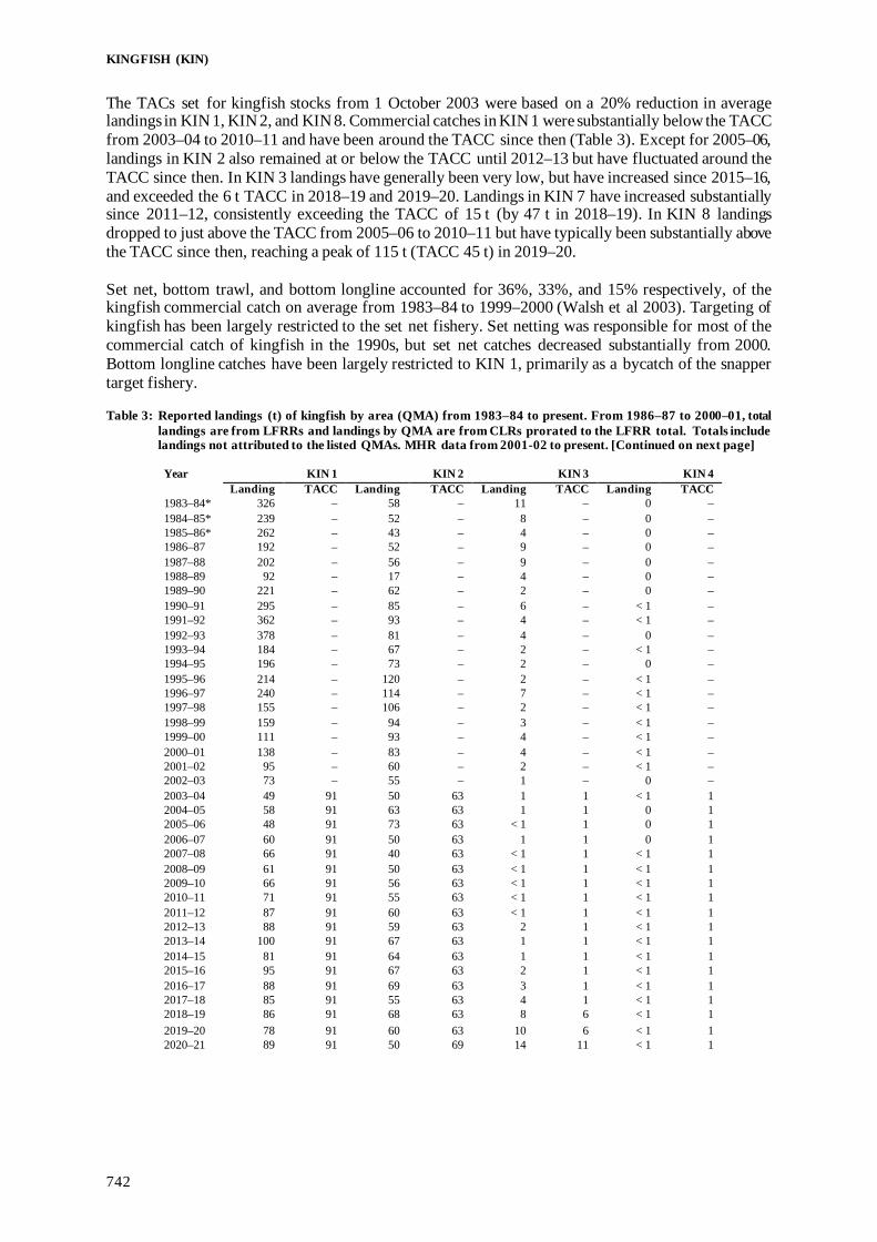
KINGFISH (KIN)
742
The TACs set for kingfish stocks from 1 October 2003 were based on a 20% reduction in average landings in KIN 1, KIN 2, and KIN 8. Commercial catches in KIN 1 were substantially below the TACC from 2003–04 to 2010–11 and have been around the TACC since then (Table 3). Except for 2005–06, landings in KIN 2 also remained at or below the TACC until 2012–13 but have fluctuated around the TACC since then. In KIN 3 landings have generally been very low, but have increased since 2015–16, and exceeded the 6 t TACC in 2018–19 and 2019–20. Landings in KIN 7 have increased substantially since 2011–12, consistently exceeding the TACC of 15 t (by 47 t in 2018–19). In KIN 8 landings dropped to just above the TACC from 2005–06 to 2010–11 but have typically been substantially above the TACC since then, reaching a peak of 115 t (TACC 45 t) in 2019–20. Set net, bottom trawl, and bottom longline accounted for 36%, 33%, and 15% respectively, of the kingfish commercial catch on average from 1983–84 to 1999–2000 (Walsh et al 2003). Targeting of kingfish has been largely restricted to the set net fishery. Set netting was responsible for most of the commercial catch of kingfish in the 1990s, but set net catches decreased substantially from 2000. Bottom longline catches have been largely restricted to KIN 1, primarily as a bycatch of the snapper target fishery. Table 3: Reported landings (t) of kingfish by area (QMA) from 1983–84 to present. From 1986–87 to 2000–01, total
landings are from LFRRs and landings by QMA are from CLRs prorated to the LFRR total. Totals include landings not attributed to the listed QMAs. MHR data from 2001-02 to present. [Continued on next page]
Year KIN 1 KIN 2 KIN 3 KIN 4
Landing
TACC Landing
TACC Landing
TACC Landing
TACC 1983–84* 326 – 58 – 11 – 0 – 1984–85* 239 – 52 – 8 – 0 – 1985–86* 262 – 43 – 4 – 0 – 1986–87 192 – 52 – 9 – 0 – 1987–88 202 – 56 – 9 – 0 – 1988–89 92 – 17 – 4 – 0 – 1989–90 221 – 62 – 2 – 0 – 1990–91 295 – 85 – 6 – < 1 – 1991–92 362 – 93 – 4 – < 1 – 1992–93 378 – 81 – 4 – 0 – 1993–94 184 – 67 – 2 – < 1 – 1994–95 196 – 73 – 2 – 0 – 1995–96 214 – 120 – 2 – < 1 – 1996–97 240 – 114 – 7 – < 1 – 1997–98 155 – 106 – 2 – < 1 – 1998–99 159 – 94 – 3 – < 1 – 1999–00 111 – 93 – 4 – < 1 – 2000–01 138 – 83 – 4 – < 1 – 2001–02 95 – 60 – 2 – < 1 – 2002–03 73 – 55 – 1 – 0 – 2003–04 49 91 50 63 1 1 < 1 1 2004–05 58 91 63 63 1 1 0 1 2005–06 48 91 73 63 < 1 1 0 1 2006–07 60 91 50 63 1 1 0 1 2007–08 66 91 40 63 < 1 1 < 1 1 2008–09 61 91 50 63 < 1 1 < 1 1 2009–10 66 91 56 63 < 1 1 < 1 1 2010–11 71 91 55 63 < 1 1 < 1 1 2011–12 87 91 60 63 < 1 1 < 1 1 2012–13 88 91 59 63 2 1 < 1 1 2013–14 100 91 67 63 1 1 < 1 1 2014–15 81 91 64 63 1 1 < 1 1 2015–16 95 91 67 63 2 1 < 1 1 2016–17 88 91 69 63 3 1 < 1 1 2017–18 85 91 55 63 4 1 < 1 1 2018–19 86 91 68 63 8 6 < 1 1 2019–20 78 91 60 63 10 6 < 1 1 2020–21 89 91 50 69 14 11 < 1 1

KINGFISH (KIN)
743
Table 3 [Continued] Year KIN 7
KIN 8
KIN 10
Total
Landings TACC Landings TACC Landings TACC Landings TACC 1983–84* 3 – 50 – 0 – 448
– 1984–85* < 1 – 46 – 0 – 345 – 1985–86* 1 – 70 – 0 – 380 – 1986–87 1 – 49 – 0 – 356 – 1987–88 1 – 49 – 0 – 373 – 1988–89 < 1 – 16 – 0 – 460 – 1989–90 3 – §26 – < 1 – 428 – 1990–91 2 – §37 – < 1 – 448 – 1991–92 2 – §32 – 9 – 512 – 1992–93 1 – §56 – < 1 – 532 – 1993–94 4 – 29 – < 1 – 288 – 1994–95 6 – 25 – < 1 – 302 – 1995–96 7 – 45 – < 1 – 380 – 1996–97 11 – 48 – 6 – 427 – 1997–98 7 – 42 – 1 – 326 – 1998–99 16 – 49 – < 1 – 323 – 1999–00 10 – 51 – 0 – 270 – 2000–01 11 – 69 – < 1 – 304 – 2001–02 22 – 52 – 0 – 231 – 2002–03 20 – 143 – 0 – 292 – 2003–04 3 7 57 36 0 1 160 200 2004–05 19 7 53 36 0 1 195 200 2005–06 7 7 40 36 < 1 1 169 200 2006–07 13 7 39 36 0 1 161 200 2007–08 5 7 45 36 0 1 157 200 2008–09 5 7 38 36 0 1 154 200 2009–10 7 7 43 36 0 1 172 200 2010–11 6 7 37 36 0 1 171 200 2011–12 15 7 72 45 0 1 235 209 2012–13 12 7 66 45 0 1 226 209 2013–14 26 15 89 45 0 1 283 217 2014–15 20 15 68 45 0 1 235 217 2015–16 21 15 63 45 0 1 248 217 2016–17 27 15 48 45 0 1 235 217 2017–18 47 15 63 45 0 1 255 217 2018–19 62 15 93 45 0 1 317 222 2019–20 46 15 115 45 0 1 309 222 2020–21 27 44 98 80 0 1 279 297
* FSU data (Area unknown data prorated in proportion to recorded catch). § Some data included in FMA 1. Kingfish were added to Schedule 6 of the Fisheries Act (1996) in October 2005 for all fishing methods except set net and in all areas. A special reporting code for Schedule 6 releases was introduced on 1 October 2006 to allow monitoring of releases. Kingfish released in accordance with Schedule 6 conditions and reported against this code are not counted against ACE. Use of Schedule 6 provisions to release kingfish alive was adopted from 2008 in KIN 8 and has been used in KIN 7 since 2012 as catches increased; Schedule 6 returns in KIN 7 have exceeded the retained catch since 2016 (Table 4). Use of Schedule 6 provisions is more recent in KIN 1 and is associated with a decision in parts of the bottom longline fishery to only retain fish that exceed the recreational MLS of 75 cm. 1.2 Recreational fisheries Kingfish is highly regarded by recreational fishers in New Zealand for its sporting attributes and as a table fish. Kingfish are most often caught by recreational fishers from private boats and from charter boats but are also a prized catch for spearfishers and shore-based game fishers. Kingfish (defined as southern yellowtail kingfish) are recognised internationally as a sport fish, and kingfish caught in New Zealand waters hold 34 of the 36 International Gamefish Association World Records. 1.2.1 Management controls The main methods used to manage recreational harvests of kingfish are minimum legal size limits, method restrictions, and daily bag limits. Fishers can retain and land up to three kingfish as part their daily bag limit. An increased MLS to 75 cm (from 65 cm) for recreationally caught kingfish was introduced on 15 January 2004.

KINGFISH (KIN)
744
Many clubs, competitions, and charter boats have implemented a voluntary limit of one kingfish retained per person per day, and a number of gamefish clubs have also adopted a minimum size limit of 100 cm for kingfish. A high proportion of private and charter recreational catch is released (Holdsworth et al 2016b) Table 4: Groomed landings (t) of kingfish by area (QMA) from 2006–07 to 2018–19 by destination. Landing code ‘L’
represents normal landings to a licensed fish receiver, code ‘X’ indicates returns to the sea under Schedule 6, and ‘Other’ includes all other non-intermediate landing codes.
Fishing KIN 1 KIN 2 KIN 3 KIN 7 KIN 8 year L X Other L X Other L X Other L X Other L X Other 2006–07 62 0 1 50 0 0 1 0 0 12 0 1 37 0 3 2007–08 67 0 2 43 0 0 0 0 0 8 0 1 44 10 2 2008–09 62 0 2 52 0 0 0 0 0 4 0 1 36 1 3 2009–10 68 0 2 56 0 0 1 0 0 5 1 1 39 13 5 2010–11 70 0 2 55 0 0 1 0 0 5 1 1 34 8 4 2011–12 90 0 2 59 1 0 1 0 0 13 4 3 64 36 7 2012–13 87 0 2 56 0 0 1 0 0 8 4 4 63 44 8 2013–14 99 0 2 69 3 0 1 0 0 22 11 5 83 17 7 2014–15 80 1 2 64 7 0 1 1 1 15 12 5 63 9 6 2015–16 95 30 4 67 1 0 2 1 1 16 29 6 58 29 6 2016–17 87 50 4 69 6 0 3 1 2 21 21 4 42 36 7 2017–18 84 70 5 55 8 3 3 0 1 41 100 8 55 61 7 2018–19 82 34 5 66 6 3 6 2 2 59 103 4 88 103 7 2019–20 77 30 3 60 15 1 8 4 3 41 34 4 103 103 9
1.2.2 Tag and release A voluntary recreational tagging programme has released 23 684 kingfish in New Zealand (1975 to 2019). Anglers feel they are contributing to research and conservation of stocks, while still getting recognition of their catch. The research objectives are to collect detailed information on released fish to help characterise the fishery and collect growth and movement information from recaptured fish. There have been 1608 tagged kingfish recaptured in New Zealand (1977 to 2019), with an average of 36 recaptures (and 679 releases) per year over the last 10 years (Table 5) (Holdsworth & Saul 2019). Most kingfish are caught close to their release location, even after many years. Ninety four percent of recaptures for fish at liberty for 30 days or more were within 100 nautical miles of the release point (Figure 2). The proportion of recaptured kingfish at distances (over 100 nautical miles) increases after 3 years. Although kingfish are also capable of extensive movements, with three trans-Tasman recaptures recorded, few recaptures are made outside the QMAs in which the fish were released. Table 5: The number of kingfish tagged and recaptured by fishing year for the last 10 years.
2009–10 2010–11 2011–12 2012–13 2013–14 2014–15 2015–16 2016–17 2017–18 2018–19 Releases 1 381 1 123 613 761 649 723 607 598 546 509 Recaptures 46 54 44 38 31 30 28 31 23 32
Figure 2:Kingfish straight line distance (nautical miles) from release location by days at liberty 1977 to 2018.

KINGFISH (KIN)
745
1.2.3 Estimates of recreational harvest Recreational catch estimates are given in Table 6. There are two broad approaches to estimating recreational fisheries harvest: the use of onsite or access point methods where fishers are surveyed or counted at the point of fishing or access to their fishing activity; and offsite methods where some form of post-event interview and/or diary are used to collect data from fishers. The first estimates of recreational harvest for kingfish were calculated using an offsite approach, the offsite regional telephone and diary survey approach. Estimates for 1996 came from a national telephone and diary survey (Bradford 1998). Another national telephone and diary survey was carried out in 2000 (Boyd & Reilly 2002) and a rolling replacement of diarists in 2001 (Boyd et al 2004) allowed estimates for a further year (population scaling ratios and mean weights from 2000 were not re-estimated in 2001). The harvest estimates provided by these telephone/diary surveys are no longer considered reliable for various reasons. With the early telephone/diary method, fishers were recruited to fill in diaries by way of a telephone survey that also estimates the proportion of the population that is eligible (likely to fish). A ‘soft refusal’ bias in the eligibility proportion arises if interviewees who do not wish to co-operate falsely state that they never fish. The proportion of eligible fishers in the population (and, hence, the harvest) is thereby under-estimated. Pilot studies for the 2000 telephone/diary survey suggested that this effect could occur when recreational fishing was established as the subject of the interview at the outset. Another equally serious cause of bias in telephone/diary surveys was that diarists who did not immediately record their day’s catch after a trip sometimes overstated their catch or the number of trips made. There is some indirect evidence that this may have occurred in all the telephone/diary surveys (Wright et al 2004). The recreational harvest estimates provided by the 2000 and 2001 telephone diary surveys are thought to be implausibly high for many species, which led to the development of an alternative maximum count aerial-access onsite method that provides a more direct means of estimating recreational harvests for suitable fisheries. The maximum count aerial-access approach combines data collected concurrently from two sources: a creel survey of recreational fishers returning to a subsample of boat ramps throughout the day; and an aerial survey count of vessels observed to be fishing at the approximate time of peak fishing effort on the same day. The ratio of the aerial count in a particular area to the number of interviewed parties who claimed to have fished in that area at the time of the overflight was used to scale up harvests observed at surveyed ramps, to estimate harvest taken by all fishers returning to all ramps. The methodology is further described by Hartill et al (2007). This aerial-access method was first employed and optimised to estimate snapper harvests in the Hauraki Gulf in 2003–04. It was then extended to survey the wider SNA 1 fishery in 2004–05 and to provide estimates for other species, including kingfish. The PELWG (Pelagic Working Group) indicated that the kingfish estimate should be considered with considerable caution due to the limited overlap between this method’s sampling technique and the fisheries for kingfish, e.g., the target fisheries for kingfish are often in offshore areas from launches which were not sampled by the boat ramp survey. For this reason, the results from this survey have not been accepted or included in the working group report at this time.
In response to the cost and scale challenges associated with onsite methods, in particular the difficulties in sampling other than trailer boat fisheries, offsite approaches to estimating recreational fisheries harvest have been revisited. This led to the development and implementation of a national panel survey for the 2011–12 fishing year and repeated in 2017–18 (Wynne-Jones et al 2014, 2019). The panel surveys used face-to-face interviews of a random sample of New Zealand households to recruit a panel of fishers and non-fishers for a full year. The panel members were contacted regularly about their fishing activities and catch information collected in standardised phone interviews. Note that the national panel survey estimate does not include recreational harvest taken under s111 general approvals on commercial vessels. The estimates of harvest from the 2011–12 panel survey were compared with direct estimates (using onsite surveys) for key stocks in FMA 1 (Edwards & Hartill 2015) and are considered reliable.
The point estimates of recreational harvest for KIN 1, KIN 7, and KIN 8 in 2012 and 2018 were above the allowances; recreational harvests in KIN 2 increased from 2012 to 2018 and exceeded the allowance in 2018.

KINGFISH (KIN)
746
Table 6: Recreational harvest estimates for kingfish stocks. The telephone/diary surveys ran from December to November but are denoted by the January calendar year. The national panel surveys ran throughout the October to September fishing year but are denoted by the January calendar year. Mean fish weights were obtained from boat ramp surveys (for the telephone/diary and panel survey harvest estimates). (Source: Tierney et al 1997, Bradford 1997, Bradford 1998, Boyd & Reilly 2002, Boyd et al 2004, Wynne-Jones et al 2014).
Stock Year Method Number of fish Total weight (t) CV
KIN 1 1992 Telephone/diary 186 000 260 – 1994 Telephone/diary 180 000 228# 0.09 1996 Telephone/diary 194 000 234 0.07 2000 Telephone/diary 127 000 800 0.18 2001 Telephone/diary 109 000 683 0.17 2012 Panel survey 52 056 535 0.13 2018 Panel survey 69 473 571 0.16 KIN 2 1992 Telephone/diary 68 000 92 – 1994 Telephone/diary 62 000 78 0.18 1996 Telephone/diary 67 000 70 0.11 2000 Telephone/diary 25 000 138 0.38 2001 Telephone/diary 21 000 113 0.33 2012 Panel survey 4 025 41 0.24 2018 Panel survey 9 602 79 0.28 KIN 7 1992 Telephone/diary 10 000 20 – 1994 Telephone/diary – – – 1996 Telephone/diary 9 000 13 0.19 2000 Telephone/diary 2 000 11 0.55 2001 Telephone/diary 1 000 9 0.86 2012 Panel survey 2 079 21 0.38 2018 Panel survey 3 289 27 0.25 KIN 8 1992 Telephone/diary 6 000 #8 – 1994 Telephone/diary – – – 1996 Telephone/diary 2 000 #3 – 2000 Telephone/diary 9 000 65 0.45 2001 Telephone/diary 14 000 108 0.46 2012 Panel survey 6 252 63 0.25 2018 Panel survey 6 672 55 0.22
#No harvest estimate available in the survey report; estimate presented is calculated as average fish weight for all years and areas by the number of fish estimated caught. 1.3 Customary non-commercial fisheries Kingfish is an important traditional food fish for Māori, but no quantitative information on the level of Māori customary non-commercial catch is available. The extent of the traditional fisheries for kingfish in the past is described by the Muriwhenua Fishing Report (Waitangi Tribunal 1988). Because of the coastal distribution of the species and its inclination to strike lures, it is likely that historically Māori caught considerable numbers of kingfish. 1.4 Illegal catch There is no known illegal catch of kingfish. 1.5 Other sources of mortality The extent of any other sources of mortality is unknown, however, handling mortality for sub-MLS size fish is likely to occur in both the recreational (sub 75 cm) and commercial (sub 65 cm) fisheries. Recreational fishers also release a large proportion of legal-size kingfish, and the use of Schedule 6 provisions to return legal-size kingfish to the sea if they are likely to survive has increased in commercial fisheries since 2010. 2. BIOLOGY In New Zealand, kingfish are predominantly found around the northern half of the North Island but also occur from 29° to 46° S, Kermadec Islands to Foveaux Strait (Francis 1988) and to depths of 200 m. Kingfish are large predatory fish with adults exceeding one and a half metres in length. They usually

KINGFISH (KIN)
747
occur in schools ranging from a few fish to well over a hundred fish. Kingfish tend to occupy a semi-pelagic existence and occur mainly in open coastal waters, preferring areas of high current and or tidal flow adjacent to rocky outcrops, reefs, and pinnacles. However, kingfish are not restricted to these habitats and are sometimes caught or observed in open sandy bottom areas and within shallow enclosed bays. Estimates of age have been derived from opaque-zone counts in sagittal otolith thin sections. Estimates of von Bertalanffy growth parameters for kingfish were also derived from recreational tagging data and otoliths collected from the eastern Bay of Plenty. Estimates of K and L∞ were similar being 0.128 and 130 cm from the otolith age data and 0.130 and 142 cm from the tagging increment data, respectively (Table 7). The hard-structure ageing techniques have yet to be validated for New Zealand kingfish, although the position of the first annulus has been validated using regular samples of 0+ year old fish from a fish aggregating device (Holdsworth et al 2013, Francis et al 2005). A Bayesian analysis of length and maturity data suggests that the length of 50% maturity is 97 cm in females and 83 cm in males (McKenzie et al 2014). Estimates of M ranged from 0.20 to 0.25, however, these estimates are thought to represent an upper bound because the samples were taken from an exploited population. Available biological parameters relevant to stock assessment are given in Table 7. Table 7: Estimates of biological parameters.
3. STOCKS AND AREAS Kingfish are widespread, occurring in temperate waters around South Australia, Japan, South Africa, and the western coast of the Americas (British Columbia to Chile) (Walsh et al 2003). Although previously considered a single species, Martinez-Takeshita et al (2015) suggest that southern hemisphere kingfish should be considered a separate species, and that “a combination of dynamics in the sub-tropical and temperate regions permits a low-level of connectivity among S. lalandi sampled in South Africa, New Zealand, and Chile”. Within New Zealand, a study based on meristic characters and parasite loads suggests two stocks of kingfish off the west and east coasts (Smith et al 2004). These stocks are contained within the Tasman Current off the west coast and the East Auckland Current and East Cape Current off the east coast, with little mixing between them. The east coast stock may be further subdivided into northeast and Hawke’s Bay stocks based on limited exchange from tagging studies and parasite marker prevalence. Tagging results suggest that most adult kingfish do not move outside local areas, with many tag returns close to the release site (Figure 2). However, some tagged kingfish have been found to move very long distances; there are validated reports of New Zealand tagged kingfish being caught in Australian waters and Australian tagged kingfish being recaptured in New Zealand waters.
Fishstock Estimate Source 1. Weight = a(length)b (Weight in g, length in cm fork length). Both sexes a b KIN 1 0.03651 2.762 Walsh et al (2003) 2. von Bertalanffy growth parameters
Females Males Combined L∞ k t0 L∞ k t0 L∞ k t0
Bay of Plenty (2002) 135.79 0.119 -0.976 123.81 0.137 -0.911 130.14 0.128 -0.919 McKenzie et al (2014) East Northland (2010) 124.48 0.232 -0.890 113.69 0.279 -0.790 Holdsworth et al (2013) Bay of Plenty (2010) 125.63 0.211 -0.987 119.32 0.226 -0.976 Holdsworth et al (2013)

KINGFISH (KIN)
748
In addition to the results from tagging studies, the age structure of recreational catches (Holdsworth et al 2016a) suggests that kingfish off the East Northland/Hauraki Gulf region and in the Bay of Plenty/East Cape region may comprise separate stocks. 4. STOCK ASSESSMENT 4.1 CPUE analyses Standardised CPUE analyses were developed for KIN 1, 2, 7, and 8 during 2019 and 2020, and the key indices for KIN 7 and 8 were updated in 2021. Statutory catch, effort, and landings data from the commercial fisheries were used to develop indices for the mixed-target inshore bottom trawl fisheries in the Bay of Plenty and East Northland sub-areas of KIN 1, and for KIN 2 and KIN 8. Indices were also developed for the snapper-target bottom longline fishery in East Northland, and the offshore midwater trawl fishery that targets jack mackerels in KIN 7 and KIN 8 off the western North Island and north-western South Island (from trips where an observer was present on the vessel). Additional indices were developed for the midwater fishery in KIN 7 and 8 from trips where an observer was present on the vessel, and for the recreational fisheries in the KIN 1 sub-areas using ramp survey data. Indices using data from kingfish catches reported from amateur charter vessels were also considered but were rejected by the Working Group because (i) the recorded catches included fish returned to the sea without distinguishing returns of fish above and below the MLS, (ii) kingfish were targeted on features, where they aggregated, and CPUE was likely to be hyperstable, and (iii) charter boats targeting SNA mostly caught small kingfish. In KIN 2, 7, and 8, and the bottom trawl fisheries in KIN 1, the proportion of the trip-level landed catches represented in aggregated event-level catch estimates can be low, especially where reporting used the CELR or TCEPR forms where estimated catches are limited to the top five species by weight per event. As a result, the CPUE analyses for the trawl fisheries used trip-level data where kingfish landings were modelled using covariates that were trip-level summaries of the effort data. These included number of tows, modal statistical area, mean hours per tow, mean bottom depth, and mean headline height and, for the midwater fishery in KIN 7 and 8, the proportion of jack mackerel target tows. Delta-lognormal models were fitted to the trip-level catch and effort data from bottom trawl fishers operating in East Northland, the Bay of Plenty, KIN 2, and KIN 8. For the midwater fishery in KIN 7 and 8 there were few trips without kingfish landings and a lognormal model of positive catches was fitted. Analyses were restricted to the period after kingfish was introduced to the QMS and, for the midwater trawl fishery, data were only used from trips where an observer was present on the vessel. For the East Northland bottom longline fishery, the working group noted that kingfish was a valuable bycatch of the snapper longline fishery and that they appeared to have been consistently reported in estimated catches and landings since the QMS catch-effort data systems were introduced in the 1990 fishing year. As a result, four indices were prepared for this fishery: (i) a daily level index with the fine scale data available since 2008 aggregated to match the previous CELR-resolution data, and landings allocated to events using the approach of Starr (2007); (ii) a trip level index using landings data and aggregated effort data; (iii) an event level index using data from the LTCER form from 2008 onwards and landings allocated to events; and (iv) an index that was restricted to trips with a single set. For the observed trips from the midwater trawl fishery in KIN 7 and 8, modelling used tow-level data and a delta-lognormal model was fitted using tow-level covariates. Negative-binomial GLMMs were fitted to the number of fish caught during recreational bait-fishing trips recorded in the ramp survey data. Data were aggregated to location-month-target strata and the covariates offered to the models were: location, month, target species (KIN or SNA), number of events, mean number of fishers per event, and mean event duration. Location was included as a random effect. Separate trip-level models fitted to recreational fishing trips where the fishing method was reported as jigging and trolling were also presented to the working group. The indices derived from jigging and trolling models were more variable than the bait-fishing index because of lower numbers of surveyed

KINGFISH (KIN)
749
events. Jigging and trolling are usually used to target kingfish aggregations on features, and there is believed to be a degree of learned hook avoidance associated with these catch methods. A key consideration in the working group’s evaluation of the resulting series and indices of relative abundance was the size composition of the kingfish catch in each fishery. Aggregated observer data (Figure 3) indicated that the bottom trawl fisheries primarily catch immature kingfish, whereas the midwater trawl fishery catches both juvenile and adult fish. No observer data were available from the bottom longline fishery, but packing data were used to examine the weight composition of kingfish landed from this fishery (Figure 4). This indicates that the bottom longline fishery also catches adult fish. The working group concluded that the bottom trawl indices were best regarded as indices of immature kingfish, whereas the midwater trawl and bottom longline indices included adult fish and were the better indices for the kingfish populations in the areas for which these indices are available.
Figure 3: Raw aggregate length-frequency distributions for kingfish by area and method for kingfish using observer
data collected from 2000–01 onwards, for strata where at least 200 fish were sampled. The red vertical line indicates the minimum legal size of kingfish for the commercial fishery.
Figure 4: Weight frequency of (a) all kingfish and (b) single kingfish packed from the East Northland bottom longline
fishery by Leigh Fisheries Limited between 2010 and 2016.

KINGFISH (KIN)
750
The different treatments of data from the East Northland bottom longline fishery result in similar indices (Figure 5), and indices from all three East Northland fisheries show a significant increase since 2010 (Figure 6) despite significant inter-annual variability in the longline index in this period. In the Bay of Plenty, the bottom trawl index increases consistently from 2004 to 2016 before declining somewhat to 2019 (Figure 7), whereas the recreational bait fishing index shows an increasing trend, but considerable year to year variation. The trip based index from the statutory catch and effort data for the midwater trawl fishery in KIN 7 and 8 and the tow based observer index showed similar trends. The main index from observer data in the KIN 7 and 8 midwater trawl fishery showed a gradual increase from 2008 to 2014, before increasing rapidly. The index has fluctuated at this increased level from 2016 to 2020 (Figure 8). The index from the KIN 8 bottom trawl fishery demonstrated a more cyclic pattern around a steadily increasing trend from 2009 to 2020.
Figure 5: CPUE indices for the East Northland bottom longline fishery.
Figure 6: CPUE indices for the different East Northland fisheries.
1
2
3
2008
2009
201020
1120
1220
1320
1420
1520
1620
1720
1820
1919
9319
9419
9519
9619
9719
9819
9920
0020
0120
0220
0320
0420
0520
0620
07
Fishing year
CPU
E in
dex
seriesenld_bll_setenld_bll_single_set_tripsenld_bll_tripenld_bll_vd
1
2
3
2008
2009
2010
2011
2012
2013
2014
2015
2016
2017
2018
2019
1993
1994
1995
1996
1997
1998
1999
2000
2001
2002
2003
2004
2005
2006
2007
Fishing year
CPU
E in
dex
seriesenld_bll_setenld_bll_vdenld_bt_tripenld_hg_baitfishing

KINGFISH (KIN)
751
Figure 7: CPUE indices for the two Bay of Plenty fisheries.
Figure 8: CPUE indices for the west coast North Island fisheries. Establishing BMSY compatible reference points The working group accepted the trip-level bottom longline index as the primary index of abundance for KIN 1 (East Northland) and the observer data based tow-level model for KIN 7 and KIN 8. Most of the available CPUE series start in the early 2000s and show steeply increasing trends in abundance for all areas. With the lack of stable periods of high catch and abundance, the working group concluded that the only defensible approach to determining reference points was to choose stable periods of low abundance early in the series as representing soft limits. 4.2 Catch at age sampling (KIN 1) The age composition of the KIN 1 target recreational charter boat fleet catch was sampled in 2010–11 and in 2014–15 for the purpose of estimating total mortality (Z). Sampling was stratified into two regions, East Northland and Bay of Plenty, and two strata based on distance from the shore: inshore on the North Island continental shelf (shallower than 200 m) and around four offshore islands and pinnacles. Representative samples of kingfish over the MLS were obtained from the offshore Bay of Plenty and inshore East Northland with 831 and 863 kingfish measured over 75 cm in these two strata in 2014–15 (Table 8). Sampling was less successful in the inshore Bay of Plenty and the offshore East Northland but deemed usable by the Inshore Working Group. All kingfish were measured and recorded per trip on participating vessels. Age length keys were developed using otoliths from retained fish. Bay of Plenty offshore samples in 2010–11 included more
0
1
2
3
2004
2005
2006
2007
2008
2009
2010
2011
2012
2013
2014
2015
2016
2017
2018
2019
2001
2002
2003
Fishing year
CPU
E in
dex
seriesbple_bt_tripbplebaitfishing

KINGFISH (KIN)
752
old fish than those from inshore (Holdsworth et al 2013). The Bay of Plenty offshore age distribution in 2014–15 was similar to that observed from the Bay of Plenty in 2010–11, although more older fish were evident in the 2014–15 sample. In 2014–15 there was a mode at age 5 in East Northland and age 6 in Bay of Plenty (Figure 9). Table 8: Number of kingfish lengths and otolith sets collected in 2014–15 from the recreational fishery.
KIN measured > 75 cm Otoliths collected Otoliths used in the
age-length-key Inshore Bay of Plenty 211 57 212 Offshore Bay of Plenty 831 156 Inshore EN/HGU 863 217 271 Offshore East Northland 318 55
The Inshore Working Group agreed there was no valid method for combining inshore and offshore age frequencies by region for the purpose of estimating regional total mortality (Z), recommending instead that total mortality estimates be derived solely from the offshore age frequencies. Total mortality estimates for offshore areas ranged from 0.19 to 0.25 for 2014–15 (Table 9). The FSB40% target reference point for kingfish is 0.1, as derived by SSB/R methods (Holdsworth et al 2013). Assuming an instantaneous natural mortality rate (M) of 0.2, the target total mortality (Z) rate for kingfish is 0.3. None of the 2014–15 derived Z estimates given in Table 9 are higher than 0.3, suggesting that overfishing of kingfish in offshore areas of the Bay of Plenty and East Northland was unlikely. Although movement has been recorded between inshore and offshore areas, the relationship between these areas is unknown.
Figure 9: Kingfish age composition by region for inshore and offshore samples in 2014–15. Table 9: Total mortality (Z) estimates for KIN 1 sub-regions as derived from catch-curve analysis (Chapman &
Robson) of recreational charter boat catch-at-age data by fishing year, assuming 6 years is the age at full recruitment. The offshore estimate for the Bay of Plenty in 2009–10 was for the White Island area only and the offshore estimate for Northland in 2014–15 was for the Three Kings area only. Bootstrap CVs are shown in parentheses. EN/HG is East Northland/Hauraki Gulf, BoP is Bay of Plenty.
EN/HG BoP Sub-Region 2009–10 2014–15 2009–10 2014–15 Inshore 0.87 (0.12) 0.49 (0.08) 0.50 (0.14) 0.29 (0.09) Offshore – 0.19 (0.08) 0.30 (0.14) 0.25 (0.07)

KINGFISH (KIN)
753
4.3 Biomass estimates Few kingfish are encountered in trawl surveys because they are capable of swimming faster the nets, suggesting that trawling is not a suitable method for monitoring changes in kingfish abundance. Kingfish are amenable to mark-recapture studies. However, up to now, tagging studies have been conducted solely to describe kingfish movement patterns and to estimate growth. Data from these programmes are inadequate to estimate stock biomass because tag releases and recoveries are voluntary, not systematic. 4.4 Other factors It was recognised that if the increases in abundance represented a regime shift, or a significant change in productivity levels, with an associated increase in B0, then the use of historical levels of relative abundance to establish a soft limit may not be appropriate. 4.5 Future research considerations
CPUE analyses
• Further investigation of the implications of modelling catch-effort data aggregated to trip levels vs finer scale data is needed, along with consideration of the range of descriptors that can be constructed for trip models (including weighting by catch). Consideration should also be given to the choice of modal values for area and month, and investigation of alternatives such as where fisheries spend the most time vs where the influence is greatest.
• Further consider the benefits/pitfalls of smoothing CPUE indices (and alternative smoothing methods) when generating reference points from partial quantitative stock assessments. Consider the period where smoothing is the most needed or appropriate, which will generally be the recent period, because this enables better interpretations of current stock status relative to reference periods when recent CPUE indices are fluctuating, and it may be more appropriate to calculate simple moving averages over recent years.
• Revisit the bottom longline CPUE for the Bay of Plenty; although the spatial extent of this fishery may be limited, it may be the best option for an index that monitors immature and adult fish in this area.
• Full catch histories by area (recreational and commercial) are required to estimate the relative exploitation rate.
• Consider finer scale information (particularly spatial information) on fishing effort patterns in the East Northland commercial longline fishery; however such information is only available from 2004–05.
Catch curve analysis
• Sensitivity analyses to determine the effect of progressively increasing the age of full recruitment on the estimates should be conducted.
• Improved data to better understand inshore–offshore movements should be collected. General
• Develop full catch (removals) histories, including those for recreational fisheries. • The CPUE based on charter boat catch and effort forms should be improved by reporting
released kingfish less than the MLS separately from larger released kingfish. • For KIN 7&8, there are observer length-frequency data, and some otoliths have been collected,
in addition to an accepted CPUE index. The length-frequency and ageing data should be fully analysed with a view toward evaluating the feasibility of conducting a fully quantitative stock assessment in the future.
• Scaled observer length-frequency data, and confirmation of sampling representativeness, would also be informative.

KINGFISH (KIN)
754
5. STATUS OF THE STOCKS Stock Structure Assumptions Meristic characteristics and parasite loads suggest that there are two stocks of kingfish off the west and east coasts. Extensive, opportunistic mark-recapture programmes indicate that most kingfish are recaptured close to the site of release, regardless of time at liberty, and there is little movement between the east and west coasts of the North Island. The age structure of recreational catches suggests that kingfish off East Northland/Hauraki Gulf and in the Bay of Plenty/East Cape regions may comprise separate stocks, consistent with movement patterns recorded from tagging studies. There is broad similarity in CPUE trends for East Northland and the west coast (KIN 7 and 8). Recruitment indices have shown similar trends for East Northland and the west coast, and the Bay of Plenty and FMA 2 since 2012. For assessment purposes it is assumed that New Zealand kingfish comprise several biological stocks: East Northland, Bay of Plenty & KIN 2; KIN 7 & KIN 8. KIN 3 and KIN 4 are not considered here.
• KIN 1 – East Northland/Hauraki Gulf
Stock Status Year of Most Recent Assessment 2020 Assessment Runs Presented Standardised CPUE from the East Northland bottom longline
fishery (trip index) Reference Points
Target: 40% B0, interpreted as twice the smoothed mean CPUE for the period 2003–2007 Soft Limit: Mean smoothed CPUE from 2003–2007 Hard Limit: 50% of the soft limit
Overfishing threshold: Twice the relative exploitation rate in 2003–2007
Status in relation to Target Likely (> 60%) to be above the target Status in relation to Limits Very Unlikely (< 10%) to be below both the soft and hard
limits Status in relation to Overfishing Unknown
Historical Stock Status Trajectory and Current Status-
Standardised catch per unit effort (CPUE) index for KIN 1 ENLD from bottom longlining targeting snapper, relative to the agreed reference points, and a loess smooth curve—the values from which were used to define the reference period.

KINGFISH (KIN)
755
Fishery and Stock Trends
Recent Trend in Biomass or Proxy CPUE decreased from 1993 to 2006 and then increased to 2018. The index has shown greater year to year variation since 2015 and it decreased in 2019.
Recent Trend in Fishing Mortality or Proxy
In 2016, total mortality estimates from catch curve analyses indicated that F was unlikely to be at or below FSB40% in inshore areas but likely to be at or below FSB40% in offshore areas
Other Abundance Indices The bait fishing (fishing with bait) index for the recreational fishery shows a similar long-term trend to the bottom longline index.
Trends in Other Relevant Indicators or Variables
An index for immature fish using data from the bottom trawl fishery declined from 2008 to 2014 before increasing.
Projections and Prognosis Stock Projections or Prognosis Because the index for immature kingfish shows a substantial
increase in the last three years, it is anticipated that the recruited stock will continue to increase at current catch levels.
Probability of Current Catch or TACC causing Biomass to remain below or to decline below Limits
Soft Limit: Very unlikely (< 10%) Hard Limit: Very unlikely (< 10%)
Probability of Current Catch or TACC causing Overfishing to continue or commence
Unlikely (< 40%)
Assessment Methodology and Evaluation Assessment Type Level 2 - Partial Quantitative Stock Assessment Assessment Method Standardised CPUE based on a delta-lognormal index from
bottom longline Assessment dates Latest assessment: 2020 Next assessment: Unknown Overall assessment quality rank 1 – High Quality Main data inputs (rank) Commercial catch and effort
data Ramp survey data used to generate a secondary index of abundance Observer length frequency data used to interpret indices of abundance Packing data used to interpret indices of abundance
1 – High Quality 2 – Medium or Mixed Quality: spatial coverage is an issue 2 – Medium or Mixed Quality: data is not fully representative 2 – Medium or Mixed Quality: a detailed analysis of these data has not been completed
Data not used (rank) N/A Changes to Model Structure and Assumptions
CPUE analyses were performed rather than catch curve analysis
Major Sources of Uncertainty It is unknown if all fish above the MLS returned to the sea are reported using the destination code X; such returns may be higher than reported

KINGFISH (KIN)
756
Qualifying Comments It was recognised that if the increases in abundance represented a regime shift, or a significant change in productivity levels, with an associated increase in B0, then the use of historical levels of relative abundance to establish a soft limit may not be appropriate. The method of smoothing the CPUE trajectory may need further development and should be interpreted with caution. The bottom longline fishery catches immature and adult fish and so is not an index solely of the spawning stock biomass.
Fishery Interactions Commercial kingfish catch is almost all bycatch in fisheries for other species.
• KIN 1 – Bay of Plenty and KIN 2
Stock Status Year of Most Recent Assessment 2016 with recruitment indices added in 2020 Assessment Runs Presented Total mortality estimates from catch curve analysis for Inshore
BPLE and Offshore BPLE Recruitment index of abundance based on bottom trawl CPUE
Reference Points
Target: FSB40% (current estimate is FSB40% = 0.1) Soft Limit: 20% B0 Hard Limit: 10% B0
Overfishing threshold: FSB40% Status in relation to Target Inshore BPLE: F in 2016 was Likely (> 60%) to be at or below
the target Offshore BPLE: F in 2016 was Likely (> 60%) to be at or below the target
Status in relation to Limits Soft Limit: Unknown for both Inshore BPLE and Offshore BPLE Hard Limit: Unknown for both Inshore BPLE and Offshore BPLE
Status in relation to Overfishing Inshore BPLE: Overfishing is Unlikely (< 40%) to be occurring Offshore BPLE: Overfishing is Unlikely (< 40%) to be occurring
Historical Stock Status Trajectory and Current Status-
Fishery and Stock Trends Recent Trend in Biomass or Proxy Unknown Recent Trend in Fishing Intensity or Proxy
F appeared to have declined between 2010 and 2016 for Inshore BPLE and Offshore BPLE (although White Island was the only BPLE area assessed in 2010); likely to have been low for the decade to 2016 in all BPLE areas
Other Abundance Indices The bait fishing index for the recreational fishery in the Bay of Plenty shows significant inter-annual fluctuations but has a generally increasing trend from 2001 to 2019.
Trends in Other Relevant Indicators or Variables
The CPUE indices for immature fish from the bottom trawl fisheries in the Bay of Plenty and KIN 2 show a steady increase from 2004 to 2016, before declining to 2019.
Projections and Prognosis Stock Projections or Prognosis Catch curve analysis from catch sampling in 2014–15
indicated that total mortality was low for both the inshore and offshore regions, with fishing mortality below natural mortality and close to the target. The indices for immature fish are above average from 2013 to 2019 so the stock is expected to increase in the short term.

KINGFISH (KIN)
757
Probability of Current Catch or TACC causing Biomass to remain below or to decline below Limits
Soft Limit: Unknown for both inshore and offshore areas Hard Limit: Unknown for both inshore and offshore areas
Probability of Current Catch or TACC causing Overfishing to continue or to commence
Unlikely (< 40%) for both inshore and offshore areas
Assessment Methodology and Evaluation Assessment Type Level 2 - Partial Quantitative Stock Assessment Assessment Method Estimates of total mortality using Chapman-Robson
estimator Assessment dates Latest assessment: 2016 (the
2020 update added recruit series for BoP and KIN 2)
Next assessment: 2021
Overall assessment quality rank 1 – High Quality Main data inputs (rank) Commercial catch and effort
data Age structure of recreational catch in 2014–15 - Instantaneous rate of natural mortality (M) of 0.20 based on a maximum age of 23 years. - Age at 50% maturity (6 yr) - Age at MLS (4 yr) - Growth rate
1 – High Quality 1 – High Quality 1 – High Quality 1 – High Quality 1 – High Quality 1 – High Quality
Data not used (rank) N/A Changes to Model Structure and Assumptions -
Major Sources of Uncertainty - Uncertainty in the estimate of M - Uncertain relationship between inshore and offshore areas; available data do not support much movement of inshore fish to offshore areas. Information from KIN 2 recreational catch at age is limited to the northern part of the QMA
Qualifying Comments The Z estimates are unweighted by relative catch by method (bait, jig) and area. The selectivity of the two capture methods differs substantially. The indices from the bottom trawl fisheries do not provide indices of abundance for the whole population
Fishery Interactions Commercial kingfish catch is almost all bycatch in fisheries for other species.
• KIN 7 and KIN 8
Stock Status Year of Most Recent Assessment 2021 Assessment Runs Presented Standardised CPUE from observer tow data in the jack
mackerel target mid-water trawl fishery Reference Points
Target: 40% B0, interpreted as twice the mean CPUE in the period 2005–2009 Soft Limit: Mean CPUE from 2005–2009 Hard Limit: 50% of the soft limit

KINGFISH (KIN)
758
Overfishing threshold: Twice the relative exploitation rate in 2005– 2009
Status in relation to Target Very Likely (> 90%) to be at or above the target
Status in relation to Limits Very Unlikely (< 10%) to be below both the soft and hard limits
Status in relation to Overfishing Unknown Historical Stock Status Trajectory and Current Status-
Standardised catch per unit effort (CPUE) index for KIN 7 and KIN 8 from midwater trawling targeting jack mackerel (observer tow-level index), relative to the agreed reference points.
Fishery and Stock Trends Recent Trend in Biomass or Proxy
CPUE increased considerably from 2006/2007 to 2016 and has been relatively stable at a high level since.
Recent Trend in Fishing Mortality or Proxy -
Other Abundance Indices - Trends in Other Relevant Indicators or Variables
An index for immature fish using data from the bottom trawl fishery shows an increasing trend from 2009 to 2020. Unscaled observer length-frequency data are indicative of strong recruitment in 2015.
Projections and Prognosis Stock Projections or Prognosis Because there are indications of recent high recruitment, it is
anticipated that the spawning stock will remain high at current catch levels, and the vulnerable biomass is expected to remain above the target level.
Probability of Current Catch or TACC causing Biomass to remain below or to decline below Limits
Soft Limit: Very unlikely (< 10%) Hard Limit: Very unlikely (< 10%)
Probability of Current Catch or TACC causing Overfishing to continue or commence
Unknown

KINGFISH (KIN)
759
Assessment Methodology and Evaluation Assessment Type Level 2 - Partial Quantitative Stock Assessment Assessment Method Standardised CPUE based on a lognormal index from observed
midwater trawl tows targeting jack mackerel Assessment dates Latest assessment: 2021 Next assessment: Unknown Overall assessment quality rank 1 – High Quality Main data inputs (rank) Observer catch and effort data
Commercial catch and effort data Observer length-frequency data
1 – High Quality 1 – High Quality 2 – Medium or Mixed Quality: data were unscaled
Data not used (rank) N/A Changes to Model Structure and Assumptions -
Major Sources of Uncertainty - Qualifying Comments It was recognised that if the increases in abundance represented a regime shift or a temporary or permanent increase in productivity, with an associated increase in B0, then the use of historical levels of relative abundance to establish a soft limit may not be appropriate.
Fishery Interactions Commercial kingfish catch is almost all bycatch in fisheries for other species.
6. FOR FURTHER INFORMATION Bradford, E (1997) Estimated recreational catches from Ministry of Fisheries North region marine recreational fishing surveys, 1993–94. New
Zealand Fisheries Assessment Research Document 1997/7. 16 p. (Unpublished report held by NIWA library, Wellington.) Bradford, E (1998) Harvest estimates from the 1996 national recreational fishing surveys. New Zealand Fisheries Assessment Research Document.
1998/16. 27 p. (Unpublished report held by NIWA library, Wellington.) Boyd, R O; Gowing, L; Reilly, J L (2004) 2000/2001 National marine recreational fishing survey: diary results and harvest estimates.
(Unpublished draft New Zealand Fisheries Assessment Report held by Fisheries New Zealand, Wellington.) 93 p. Boyd, R O; Reilly, J L (2002) 1999/2000 National Marine Recreational Fishing Survey: recreational harvest estimates. (Unpublished New
Zealand Fisheries Assessment Report held by Fisheries New Zealand, Wellington.) Edwards, C T T; Hartill, B H (2015) Calibrating between offsite and onsite amateur harvest estimates. New Zealand Fisheries Assessment Report
2015/49. 23 p. Hartill, B; Bian, R; Armiger, H; Vaughan, M; Rush, N (2007) Recreational marine harvest estimates of snapper, kahawai, and kingfish in
QMA 1 in 2004–05. New Zealand Fisheries Assessment Report 2007/26. 44 p. Hartill, B; Davies, N M (1999) New Zealand billfish and gamefish tagging, 1997–98. NIWA Technical Report 57. 39 p. Francis, M; McKenzie, J; Ó Maolagáin, C (2005) Attempted validation of the first annual growth zone in kingfish (Seriola lalandi) otoliths. Final
Research Report for Ministry of Fisheries research project SAP2004-04, Objective 1. 22 p. (Unpublished report held by Fisheries New Zealand, Wellington.)
Francis, R I C C (1988) Maximum likelihood estimation of growth and growth variability from tagging data. New Zealand Journal of Marine and Freshwater Research 22: 42–51.
Holdsworth, J C; McKenzie, J R; Walsh, C; van der Straten, K M; Ó Maolagáin, C (2013) Catch-at-age of yellowtail kingfish (Seriola lalandi) caught by recreational fishers in KIN 1, New Zealand. New Zealand Fisheries Assessment Report 2013/3. 31 p.
Holdsworth, J C; McKenzie, J R; Walsh, C; Bian, R; Ó Maolagáin, C (2016a) Catch-at-age of yellowtail kingfish (Seriola lalandi) caught by recreational fishers 2014-15. New Zealand Fisheries Assessment Report 2016/45. 35 p.
Holdsworth, J C; Saul, P J (2019) New Zealand billfish and gamefish tagging, 2016–17 to 2018–19. New Zealand Fisheries Assessment Report 2019/65. 30 p.
Holdsworth, J C; Saul, P J; Boyle, T; Sippel, T (2016b) Synthesis of New Zealand gamefish tagging data, 1975 to 2014. New Zealand Fisheries Assessment Report 2016/24. 63 p.
Martinez-Takeshita, N; Purcell, C M; Chabot, C L; Craig, M T; Paterson, C N; Hyde, J R; Allen, L G (2015) A tale of three tails: cryptic speciation in a globally distributed marine fish of the genus Seriola. Copeia 103: 357–368.
McKenzie, J R (2014) Review of productivity parameters and stock assessment options for kingfish (Seriola lalandi lalandi) New Zealand Fisheries Assessment Report 2014/04. 17 p.
McKenzie, J; Smith, M; Watson, T; Francis, M; Ó Maolagáin, C; Poortenaar, C; Holdsworth, J (2014) Age, growth, maturity and natural mortality of New Zealand kingfish (Seriola lalandi lalandi). New Zealand Fisheries Assessment Report 2014/03. 36 p.
Smith, P J; Diggles, B; McKenzie, J; Kim, S; Ó Maolagáin, C; Notman, P; Griggs, L H (2004) Kingfish stock structure. (Unpublished Final Research Report for Ministry of Fisheries Project KIN2002/01 Objective 1 held by Fisheries New Zealand, Wellington.) 29 p.
Starr, P J (2007) Procedure for merging MFish landing and effort data, V2.0. Document AMPWG/07/04. (Unpublished report held by Fisheries New Zealand, Wellington.)

KINGFISH (KIN)
760
Teirney, L D; Kilner, A R; Millar, R E; Bradford, E; Bell, J D (1997) Estimation of recreational catch from 1991/92 to 1993/94. New Zealand Fisheries Assessment Research Document 1997/15. 43 p. (Unpublished report held by NIWA library, Wellington.)
Waitangi Tribunal (1988) Muriwhenua fishing report. Department of Justice, Wellington. Walsh, C; McKenzie, J; McGregor, G; Poortenaar, C; Hartill, B; Smith, M (2003) Information available for the management of New Zealand
kingfish (Seriola lalandi lalandi) stocks. New Zealand Fisheries Assessment Report 2003/25. 57 p. Wright, P; Gowing, L; McClary, D; Boyd, R O (2004) 2000–2001 National Marine recreational fishing survey: direct questioning of fishers
compared with reported diary data. (Unpublished Final Research Report for Ministry of Fisheries Research Project REC2000-01: Objective 2 held by Fisheries New Zealand, Wellington.) 28 p.
Wynne-Jones, J; Gray, A; Heinemann, A; Hill, L; Walton, L (2019) National Panel Survey of Marine Recreational Fishers 2017–18. New Zealand Fisheries Assessment Report 2019/24. 104 p.
Wynne-Jones, J; Gray, A; Hill, L; Heinemann, A (2014) National Panel Survey of Marine Recreational Fishers 2011–12: Harvest Estimates. New Zealand Fisheries Assessment Report 2014/67. 139 p.

KNOBBED WHELK (KWH)
761
KNOBBED WHELK (KWH)
(Austrofusus glans)
1. FISHERY SUMMARY Knobbed whelks (Austrofusus glans) were introduced into the Quota Management System on 1 October 2006. The fishing year is from 1 October to 30 September and commercial catches are measured in greenweight. TACs have been allocated in 10 QMAs (Table 1). This species is managed under Schedule 6 of the Fisheries Act for all stocks, which allows for them to be returned to where they were taken (as soon as practicable after being taken) providing they are likely to survive. Table 1: Current TAC, TACC, and allowances for customary fishing, recreational fishing, and other sources of
mortality for Austrofusus glans.
QMA TAC (t) TACC (t) Customary fishing Recreational fishing Other sources of mortality KWH1 3 1 1 1 0 KWH 2 3 1 1 1 0 KWH 3 5 3 1 1 0 KWH 4 8 6 1 1 0 KWH 5 3 1 1 1 0 KWH 6 4 2 1 1 0 KWH 7A 53 50 1 1 1 KWH 7B 3 1 1 1 0 KWH 8 3 1 1 1 0 KWH 9 3 1 1 1 0
1.1 Commercial fisheries Target fishing for knobbed whelks is by baited pots. Because economic returns for whelk fishing are poor, most of the historical catch is bycatch from oyster and scallop dredging and from bottom trawling. Due to the low value of this species it is likely that there is a high level of unreported discarded catch. Landings shown in Table 2 for the period 1990–91 to 2005–06 were recorded under the generic code for whelks (WHE); however, the Ministry considers that in FMA 1, 2, 7, and 8 most reported landings were of the knobbed whelk Austrofusus glans. In FMA 3, 4, 5, and 6, the Ministry considers that about a third of reported landings were of the knobbed whelk, whereas the remainder were the large ostrich foot shell Struthiolaria papulosa. Reported landings of knobbed whelk in FMA 1, FMA 2, and FMA 8 have been relatively low and variable since the 1990s and have been (largely or all) accounted for as bycatch. In FMA 7 in the early 1990s higher catches were reported as part of experimental fisheries in Golden Bay and Tasman Bay to provide stock assessment information in these areas (Tables 2 and 3). In the period 2011–12 to 2019–20 total

KNOBBED WHELK (KWH)
762
reported landings averaged just 0.39 t, although 1.78 t was landed in 2020–21. Landings are split into two tables (before and after the 2006 fishing year) because reporting requirements changed when knobbed whelks entered the QMS. Table 2: Reported landings (t) of whelks (WHE) by FMA from 1990–91 to 2005–06 from landing returns. See section
1.1 for an explanation of the proportion of WHE that are considered to be knobbed whelks.
Fishing year WHE 1 WHE 2 WHE 3 WHE 4 WHE 5 WHE 6 WHE 7 WHE 8 WHE 9 Total 1990–91 0 0 0 0 0 0 44.976 0 0 44.976 1991–92 0 0 0 0 0 0 26.935 0 0 26.935 1992–93 0.021 0 0.018 0 0 0 1.762 0 0 1.801 1993–94 0 0.135 0 0 0 0 49.278 0 0 49.413 1994–95 0 0.707 0.545 0 0 0 21.458 0.593 0 23.303 1995–96 0 0.089 0.178 0 0 0 27.596 0 0 27.863 1996–97 0.002 0.174 0.144 0 0.003 0 8.959 0 0 9.282 1997–98 0 0 0.102 0.150 0 0 0.884 0 0 1.136 1998–99 0 0 0.223 2.205 2.470 0.150 0.570 0 0 5.618 1999–00 0 0 2.286 7.953 3.250 0.790 0.080 0 0 14.359 2000–01 0 0 10.467 17.497 3.538 4.765 0.141 0 0 36.408 2001–02 0 0 1.474 3.995 0.515 1.755 0.002 0 0 7.741 2002–03 0 0 0.212 0.020 0.004 0.780 0.077 0 0 1.093 2003–04 0.035 0 0.491 0 0 0.335 4.217 0 0 5.078 2004–05 0.008 0 0.021 0 0 0.335 0.234 0 0.047 0.639 2005–06 0 0 0.163 0 0 0 0.032 0 0 0.195
Table 3: Landings of Knobbed whelk (KWH) by QMA from 2006–07 to present from monthly harvest returns (MHR). QMA KWH 1 KWH 2 KWH 3 KWH 4 KWH 5 Landing
TACC Landing
TACC Landing
TACC Landing
TACC Landing
TACC
2006–07 0.080 1 0 1 0.010 3 0 6 0 1 2007–08 0.077 1 0 1 0.006 3 0 6 0 1 2008–09 0.103 1 0 1 0.121 3 0 6 0 1 2009–10 0.088 1 0 1 0.053 3 0 6 0 1 2010–11 0.473 1 0.036 1 0 3 0 6 0 1 2011–12 0.721 1 0.070 1 0.088 3 0 6 0 1 2012–13 0.551 1 0 1 0.003 3 0 6 0.001 1 2013–14 0.116 1 0 1 0.159 3 0 6 0.002 1 2014–15 0.039 1 0 1 0.020 3 0 6 0 1 2015–16 0.011 1 0 1 0.031 3 0 6 0 1 2016–17 0 1 0 1 0.210 3 0 6 0 1 2017–18 0 1 0 1 0.140 3 0.020 6 0 1 2018–19 0 1 0 1 0.375 3 0.001 6 0.001 1 2019–20 0 1 0 1 0.871 3 0 6 0 1 2020–21 0 1 0 1 0.255 3 1.443 6 0.082 1 QMA KWH 6 KWH 7A KWH 7B KWH 8 Total Landing
TACC Landing
TACC Landing
TACC Landing
TACC Landing
TACC
2006–07 0 2 0.046 50 0 1 0 1 0.136 67 2007–08 0 2 9.174 50 0.104 1 0 1 9.361 67 2008–09 0.001 2 0.226 50 0.008 1 0 1 0.459 67 2009–10 0 2 18.500 50 0 1 0 1 18.614 67 2010–11 0 2 16.033 50 0 1 0 1 16.542 67 2011–12 0 2 0 50 0.008 1 0 1 0.887 67 2012–13 0 2 0 50 0.014 1 0 1 0.569 67 2013–14 0 2 0 50 0 1 0 1 0.277 67 2014–15 0 2 0 50 0 1 0.108 1 0.167 67 2015–16 0 2 0 50 0 1 0 1 0.032 67 2016–17 0 2 0 50 0 1 0 1 0.210 67 2017–18 0 2 0 50 0 1 0.010 1 0.170 67 2018–19 0 2 0 50 0 1 0 1 0.377 67 2019–20 0 2 0 50 0 1 0 1 0.871 67 2020–21 0 2 0.002 50 0 1 0 1 1.782 67 1.2 Recreational fisheries There are no estimates of recreational catch. 1.3 Customary non-commercial fisheries There are no estimates of current customary catch. 1.4 Illegal catch There is no known illegal catch of this whelk.

KNOBBED WHELK (KWH)
763
1.5 Other sources of mortality There is no information on other sources of mortality for this whelk. 2. BIOLOGY The knobbed whelk, A. glans, is a widely distributed gastropod found from low tide to about 600 m (Powell 1979). This carnivorous whelk grows up to 5 cm long and occurs throughout New Zealand where it is found on sandy/silt/mud substrate. There is very little published about the biology of this species; most references are identification notes or records of occurrence. It is a scavenger that buries in the substrate when not feeding. A wide variety of invertebrates including polychaetes, gastropods, and bivalves occur within the wide depth range of the knobbed whelk, but no interdependent relationships are documented with A. glans. 3. STOCKS AND AREAS For management purposes stock boundaries are based on FMAs. There is no biological information on stock structure, recruitment patterns, or other biological characteristics which might indicate alternative stock boundaries. 4. STOCK ASSESSMENT 4.1 Estimates of fishery parameters and abundance There are no estimates of fishery parameters or abundance for any knobbed whelk fishstock. 4.2 Biomass estimates There are no biomass estimates for any knobbed whelk fishstock. 4.3 Yield estimates and projections There are no estimates of MCY for any knobbed whelk fishstock. There are no estimates of CAY for any knobbed whelk fishstock. 5. STATUS OF THE STOCKS • KWH 7A - Austrofusus glans
Stock Status Year of Most Recent Assessment No formal assessment done for any of the stocks Assessment Runs Presented – Reference Points
Target: None Soft Limit: None Hard Limit: None Overfishing threshold: None
Status in relation to Target Unknown Status in relation to Limits Unknown Status in relation to Overfishing Unknown Historical Stock Status Trajectory and Current Status Unknown Fishery and Stock Trends Recent Trend in Biomass or Proxy
Unknown

KNOBBED WHELK (KWH)
764
Recent Trend in Fishing Mortality or Proxy
In 1990–96 the landings for KWH 7 averaged 28.7 t. However, since that time, landings have declined considerably. Landings in all other Fishstocks have been variable but total catch across all Fishstocks has been less than 19 t per year since 2001–02.
Other Abundance Indices – Trends in Other Relevant Indicators or Variables – Projections and Prognosis Stock Projections or Prognosis – Probability of Current Catch or TACC causing Biomass to remain below or to decline below Limits
Soft Limit: Unknown Hard Limit: Unknown It is unknown what effect fishing to date has had on Austrofusus glans stocks
Probability of Current Catch or TACC causing Overfishing to continue or to commence
–
Assessment Methodology Assessment Type – Assessment Method – Assessment Dates Latest assessment: – Next assessment: – Overall assessment quality rank
–
Main data inputs (rank) – Data not used (rank) – Changes to Model Structure and Assumptions
–
Major Sources of Uncertainty – Qualifying Comments – Fishery Interactions –
6. FOR FURTHER INFORMATION Morton, J; Miller, M (1968) The New Zealand sea shore. Collins, Auckland. 638 p. Powell, A W B (1979) New Zealand Mollusca. Marine, land and freshwater shells. Collins, Auckland. 500 p.

LEATHERJACKET (LEA)
765
LEATHERJACKET (LEA)
(Meuschenia scaber) Kokiri, Hiriri
1. FISHERY SUMMARY Leatherjacket was introduced into the QMS on 1 October 2003. Current allowances, TACCs, and TACs are given in Table 1. Table 1: Recreational and Customary non-commercial allowances (t), TACCs (t), and TACs (t) for leatherjacket by
Fishstock.
Fishstock Recreational Allowance Customary Non-Commercial Allowance Other sources of
mortality TACC TAC LEA 1 5 1 9 188 203 LEA 2 2 1 57 1 136 1 196 LEA 3 2 1 5 140 138 LEA 4 1 1 1 7 10 LEA 10 0 0 0 0 0 Total 10 4 72 1 431 1 517
1.1 Commercial fisheries Nationally, very small landings were first reported in 1948. Most of the current leatherjacket catch is taken as a bycatch, and it is very likely that leatherjacket has always been primarily a bycatch species. From less than 2 t in the early 1960s, reported landings increased to 200–400 t in the mid-1970s, 1980s, and early 1990s (Table 2). It is possible actual catches were higher than reported prior to the 1970s, but that some catches were discarded without being reported due to low market demand in this period. Landings increased further in the late 1990s to around 1000 to 1300 t, but have decreased to less than 500 t since 2012–13 (Table 3). In 2018–19 320 t of leatherjacket were landed. On average over the last five years total landings have only been 23% of the total TACC. Figure 1 shows the historical landings and TACC values for the main leatherjacket stocks. LEA 1 landings fluctuated around the TACC from the fishing year 2003–04 to 2012–13, but have since dropped to approximately half, with 78 t landed in 2019–20. LEA 2 landings have always been much lower than the TACC of 1136 t, with landings averaging 73 t from 2014–15 to 2019–20. LEA 3 landings exceeded the 100 t TACC between 2008–09 and 2012–13, and have fluctuated at or above the 130 t TACC since 2013–14. The LEA 3 TACC was increased to 140 t in 2020–21.

LEATHERJACKET (LEA)
766
Table 2: Reported landings (t) for the main QMAs from 1931 to 1982. Year LEA 1 LEA 2 LEA 3 LEA 4 Year LEA 1 LEA 2 LEA 3 LEA 4 1931–32 0 0 0 0 1957 0 0 0 0 1932–33 0 0 0 0 1958 0 0 0 0 1933–34 0 0 0 0 1959 0 0 0 0 1934–35 0 0 0 0 1960 0 0 0 0 1935–36 0 0 0 0 1961 1 0 0 0 1936–37 0 0 0 0 1962 1 0 0 0 1937–38 0 0 0 0 1963 3 0 0 0 1938–39 0 0 0 0 1964 3 0 0 0 1939–40 0 0 0 0 1965 16 0 0 0 1940–41 0 0 0 0 1966 17 0 0 0 1941–42 0 0 0 0 1967 4 0 0 0 1942–43 0 0 0 0 1968 26 4 0 0 1943–44 0 0 0 0 1969 26 13 0 0 1944 0 0 0 0 1970 34 11 0 0 1945 0 0 0 0 1971 49 11 0 0 1946 0 0 0 0 1972 34 32 0 0 1947 0 0 0 0 1973 31 46 0 0 1948 14 0 0 0 1974 51 46 0 0 1949 14 0 0 0 1975 39 29 0 0 1950 8 0 0 0 1976 59 155 0 0 1951 1 0 0 0 1977 49 163 0 0 1952 7 0 0 0 1978 85 85 0 0 1953 7 0 0 0 1979 81 179 0 0 1954 7 0 0 0 1980 81 232 173 0 1955 4 0 0 0 1981 93 199 68 0 1956 0 0 0 0 1982 111 111 5 0 Notes: 1. The 1931–1943 years are April–March but from 1944 onwards are calendar years. 2. Data up to 1985 are from fishing returns: data from 1986 to 1990 are from Quota Management Reports. 3. Data for the period 1931 to 1982 are based on reported landings by harbour and are likely to be underestimated as a result of under-
reporting and discarding practices. Data includes both foreign and domestic landings. Data were aggregated to FMA using methods and assumptions described by Francis & Paul (2013).
Table 3: Reported commercial landings (tonnes) of leatherjacket by Fishstock for the fishing years from 1989–90 to
present. Landings for LEA 10 have not been shown as these were negligible and were rounded to zero. Fishstock LEA 1
LEA 2
LEA 3 LEA 4
FMA (s) 1&9 2&8 3, 5 & 6 4 Total Landings TACC Landings TACC Landings TACC Landings TACC Landings TACC 1989–90 114 - 169 - 42 - - - 325 - 1990–91 143 - 178 - 61 - - - 382 - 1991–92 160 - 85 - 100 - - - 345 - 1992–93 154 - 98 - 41 - - - 293 - 1993–94 188 - 62 - 37 - - - 287 - 1994–95 186 - 148 - 50 - - - 384 - 1995–96 152 - 296 - 38 - - - 486 - 1996–97 128 - 908 - 70 - - - 1 106 - 1997–98 151 - 165 - 66 - - - 382 - 1998–99 110 - 413 - 30 - - - 553 - 1999–00 115 - 1 136 - 35 - - - 1 286 - 2000–01 131 - 880 - 41 - - - 1 052 - 2001–02 185 - 953 - 43 - - - 1 181 - 2002–03 162 - 568 - 67 - 0 - 797 - 2003–04 189 188 396 1 136 28 100 0 7 613 1 431 2004–05 223 188 221 1 136 56 100 < 1 7 500 1 431 2005–06 173 188 172 1 136 60 100 0 7 405 1 431 2006–07 191 188 215 1 136 49 100 0 7 454 1 431 2007–08 135 188 258 1 136 73 100 0 7 466 1 431 2008–09 178 188 282 1 136 122 100 0 7 582 1 431 2009–10 181 188 455 1 136 117 100 0 7 754 1 431 2010–11 185 188 276 1 136 112 100 < 1 7 573 1 431 2011–12 167 188 277 1 136 127 100 < 1 7 571 1 431 2012–13 178 188 150 1 136 114 100 0 7 442 1 431 2013–14 147 188 105 1 136 132 130 0 7 384 1 461 2014–15 140 188 91 1 136 143 130 0 7 374 1 461 2015–16 151 188 75 1 136 133 130 4 7 363 1 461 2016–17 141 188 80 1 136 122 130 0 7 343 1 461 2017–18 92 188 67 1 136 135 130 0 7 294 1 461 2018–19 97 188 70 1 136 154 130 0 7 320 1 461 2019–20 79 188 59 1 136 131 130 0 7 269 1 461 2020–21 64 188 64 1 136 124 140 0 7 252 1 471

LEATHERJACKET (LEA)
767
Figure 1: Reported commercial landings and TACCs for the main LEA stocks. From top to bottom: LEA 1
(Auckland), LEA 2 (Central), and LEA 3 (South East). 1.2 Recreational fisheries Leatherjackets are seldom caught by hook and line but recreational fishers, especially in the northern region, take some leatherjacket by spear fishing, in rock lobster pots, and in set nets. No estimates of recreational harvest of leatherjacket were generated from the telephone/diary surveys conducted in 1994, 1996, and 2000 because so few were reported. A National Panel Survey was conducted for the first time throughout the 2011–12 fishing year. The panel survey used face-to-face interviews of a random sample of 30 390 New Zealand households to recruit a panel of fishers and non-fishers for a full year (from Wynne-Jones et al 2014). The panel members were contacted regularly about their fishing activities and harvest information collected in standardised phone interviews. The national panel survey was repeated during the 2017–18 fishing year using very similar methods to produce directly comparable results (Wynne-Jones et al 2019). Recreational catch estimates from the two national panel

LEATHERJACKET (LEA)
768
surveys are given in Table 4. Note that national panel survey estimates do not include recreational harvest taken under s111 general approvals. Table 4: Recreational harvest estimates (in numbers of fish) for leatherjacket stocks (Wynne-Jones et al 2014, 2019).
Stock Year Method Number of fish Total weight (t) CV LEA 1 2011–12 Panel survey 1 599 – 0.68 2017–18 Panel survey 2 398 – 0.44 LEA 2 2011–12 Panel survey 831 – 0.58 2017–18 Panel survey 178 – 0.81 LEA 3 2011–12 Panel survey 506 – 0.65 2017–18 Panel survey 133 – 1.00
1.3 Customary non-commercial fisheries There is no quantitative information available to allow the estimation of the amount of leatherjacket taken by customary non-commercial fishers. 2. BIOLOGY The New Zealand leatherjacket (Meuschenia scaber) is present around much of New Zealand, but is most common in the north. Trawl survey records show it to be widespread over the inner shelf north of East Cape and Cape Egmont, in the South Taranaki Bight, in Tasman Bay and Golden Bay, Pegasus Bay, and the South Canterbury Bight, extending to depths below 100 m, but with greatest abundance at 10−60 m (Anderson et al 1998). It was less commonly caught along the east coast of the North Island south of East Cape, off the northeast South Island (Cook Strait to Pegasus Bay), northwest South Island (Cape Farewell to Cape Foulwind), and around the South Otago and Southland coast. It has not been taken by trawl off the west coast south of Cape Foulwind. The New Zealand leatherjacket also occurs in Australia, from New South Wales to the southern coast of West Australia. In the Australian southeast trawl fishery, Meuschenia scaber is the main leatherjacket species caught (Yearsley et al 1999). It was once believed that two similar species of leatherjacket occurred in New Zealand − ‘rough’ and ‘smooth’ − but these are now considered to be a single species with variable colouring. Kokiri is the Maori name, but is not in common usage. ‘Creamfish’ is a New Zealand trade name for the processed (headed/gutted/skinned) product, rather than a name for the fish itself. Leatherjacket usually occur near reefs and over rough seafloor, but may be found over sand or some distance above the bottom. Although not a schooling species, it does occur in small groups. A recent study showed that fifty percent sexual maturity was attained at 19 cm and 1.5 y in the Hauraki Gulf, and there were not significant differences between sexes (Visconti et al 2017, 2018). Maximum age was 9.8 y for males and 18.1 y for females. Males defend territories and eggs are laid within nests on the seafloor from late winter to early summer (Ayling & Cox 1982, Milicich 1986, Visconti et al 2017, 2018). 3. STOCKS AND AREAS 3.1 Biomass estimates There have been no biological studies directly relevant to the recognition of separate stocks. The west coast South Island (WCSI) trawl survey probably monitors adult biomass and most of the survey catch comes from Tasman Bay and Golden Bay. The total biomass estimates are shown in Figure 2. Biomass estimates have been relatively stable throughout the time series but increased substantially in 2019 and again in 2021 to the time series high. These higher estimates in 2019 and 2021 are however associated with higher CVs of 44 and 46% respectively. CVs have been less than 35% in most other surveys.

LEATHERJACKET (LEA)
769
Figure 2: Leatherjacket biomass estimates from the WCSI inshore trawl survey time series. Error bars are ± two standard deviations.
East coast South Island (ECSI) winter trawl survey biomass estimates in the core strata (30–400 m) are probably do not track abundance because so few fish were caught, and coefficients of variations are generally high ranging from 36 to 76% (mean = 55%, up to 2012). There is nevertheless an increase in abundance from 2009 (Figure 3). Most of the biomass is captured in the 10–30 m depth indicating that the core plus shallow strata (10–400 m) is the only valid depth range within which to monitor leatherjacket biomass; although it is doubtful that these surveys index leatherjacket abundance well because they are also found over foul ground and hence not fully available to trawl gear (Beentjes & MacGibbon 2013). There was no trend in biomass in the 10–400 m depth range.
Figure 3: Leatherjacket total biomass for the ECSI winter surveys in core strata (30–400 m), and core plus shallow
strata (10–400 m) in 2007, 2012, 2014, 2016, 2018, and 2021. Error bars are 2 Standard Deviations. 3.2 Length distributions Leatherjacket were not caught in significant numbers in the ECSI winter surveys until 2007 when the shallow strata were included in the surveys. The length distributions in the core plus shallow strata (10–400 m show three clear modes at about 10 cm, 16 cm, and 23 cm, and these vary in strength and appearance among surveys (combined males, females, and unsexed) (Beentjes & MacGibbon 2013); only the 23 cm mode was present in the 2021 survey. The core plus shallow strata survey is monitoring both pre-recruited cohorts, and fish in the recruited size range.

LEATHERJACKET (LEA)
770
4. STOCK ASSESSMENT There has been no scientific assessment of the maximum sustainable yield, reference, or current biomass of any of the leatherjacket stocks. A characterisation and CPUE analysis for the LEA 3 fishery was undertaken by Langley (2013). Leatherjacket in LEA 3 are landed throughout the year, taken almost exclusively by bottom trawl gear in Statistical Areas 021–025 and 030 (Figure 4). Almost all of the LEA catch is taken in the 10–50 m depth range. The characterisation revealed that most of the increase in LEA 3 catch since 2005–06 is attributable to increased landings of leatherjacket catch from bottom trawls targeting spiny dogfish in Foveaux Strait (025).
Figure 4: Distribution of reported catch for bottom trawl by Statistical Area in LEA 3 and fishing year from trips
which landed leatherjacket in LEA 3 (Langley 2013). A CPUE standardisation was undertaken using catch and effort data that included all trips that landed or targeted LEA 3, but did not include trips that did not catch LEA 3. Landed catch was assigned to effort records proportional to estimated catch, following the Starr (2007) methodology, with some refinements where the data were aggregated to CELR equivalent format (vessel/day/method/statistical area/target species) and then the records were defined as CELR equivalent. This method was somewhat problematic due to differences in the reliability of reporting of fishing location and target species between the CELR and TCER form types. The Foveaux Strait and Canterbury Bight fisheries were analysed separately. The Foveaux Strait analysis was rejected by the Working Group and is therefore not reported further. The Canterbury Bight analysis was limited to the bottom trawl (BT) fishery in Statistical Areas 020 and 022, targeting a range of target species (RCO, BAR, FLA, ELE, TAR, WAR, and GUR). The dataset included trips where 1 kg or more of LEA 3 were landed. The analysis had large numbers of very small catches. Eight vessels accounted for 80% of the catch. The Working Group requested that the Canterbury Bight delta lognormal model targeting FLA, ELE, GUR from 2002 (Target FLA, GUR, ELE post QMS) be used because these are the years when the reporting is likely to be more reliable. There was an indication that CPUE from the Canterbury Bight fishery has increased since the early 2000s, and these indices were robust to some key assumptions. The index (Figure 5) showed that the CPUE remained low at the start of the series and then began to increase from 2007–08 to 2011–12. However, some concerns were raised about the low number of vessels in the analysis and the

LEATHERJACKET (LEA)
771
development of new markets for this species that may have increased targeting or retention of this species in recent years, suggesting that the index may not be reliable as an index of abundance. The Working Group concluded that this analysis only pertains to the stock unit for the East Coast of the South Island; is the best available information on the stock abundance at this stage, but trawl survey data may provide better information in the medium and long term; and that this is a Level 2 assessment and should be given a medium or mixed (2) overall assessment quality rank.
Figure 5: A comparison of three standardised CPUE indices for leatherjacket on the East Coast South Island Langley (2013).
5. STATUS OF THE STOCK Stock Structure Assumptions Stock structure is unknown but for management purposes the QMA boundaries are assumed to represent the stock boundaries for this species. There are two distinct areas of catch distribution within LEA 3 (Foveaux Strait and East Coast South Island) and these may represent distinct biological stocks.
• LEA 3 (East Coast South Island only)
Stock Status Year of Most Recent Assessment 2013 Assessment Runs Presented CPUE: Target FLA, GUR, ELE post QMS
ECSI winter inshore survey Reference Points
Target: 40% B0 Soft Limit: 20% B0 Hard Limit: 10% B0 Overfishing threshold: FMSY
Status in relation to Target Unknown Status in relation to Limits Soft Limit: Unknown
Hard Limit: Unlikely (< 40%) Status in relation to Overfishing Unknown
02
46
810
Fishing year
CP
UE
inde
x
1989/90 1992/93 1995/96 1998/99 2001/02 2004/05 2007/08 2010/11
Target FLA,GUR,ELE, post QMSTarget FLA,GUR,ELETarget All

LEATHERJACKET (LEA)
772
Historical Stock Status Trajectory and Current Status
The 2013 standardised CPUE index for leatherjacket on the East Coast South Island.
Biomass and 95% confidence intervals (total biomass only) for leatherjacket caught by the ECSI winter trawl
survey core strata (30–400), and core plus shallow strata (10–400 m).
Fishery and Stock Trends
Recent Trend in Biomass or Proxy
CPUE remained low at the start of the series (2002) and then began to increase from 2007–08 to 2011–12. The biomass index from the East Coast South Island trawl survey 30–400 m strata has increased since 2008, but there was no trend in biomass in the valid 10–400 m strata.
Recent Trend in Fishing Intensity or Proxy
Unknown because new markets for this species may have increased targeting or retention in recent years.
Other Abundance Indices - Trends in Other Relevant Indicators or Variables
-
Projections and Prognosis Stock Projections or Prognosis Unknown Probability of Current Catch or TACC causing Biomass to remain below or to decline below Limits
Soft Limit: Unknown Hard Limit: Unknown
Probability of Current Catch or TACC causing Overfishing to continue or to commence Unknown
02
46
810
Fishing year
CP
UE
inde
x
2002/03 2004/05 2006/07 2008/09 2010/11

LEATHERJACKET (LEA)
773
Assessment Methodology and Evaluation Assessment Type Level 2 - Partial Quantitative Stock Assessment Assessment Method Standardised CPUE Assessment Dates Latest assessment: 2013 Next assessment: Unknown Overall assessment quality rank 2 - Medium or Mixed Quality: CPUE may be
compromised by the low number of vessels in the analysis and trends in targeting or retention of leatherjacket; the trawl survey has only covered the entire habitat since 2007.
Main data inputs (rank) - catch and effort data from bottom trawl sets targeting FLA, GUR and ELE - trawl survey biomass index
2 - Medium or Mixed Quality: few vessels in analysis 2 - Medium or Mixed Quality: limited years with full coverage of LEA area
Data not used (rank) - Foveaux Strait CPUE index - Trawl survey biomass estimates from the 10–400 m strata.
3 – Low Quality: based on only a single vessel that has recently started targeting LEA 3 – Low Quality: confidence intervals large and only six data points
Changes to Model Structure and Assumptions New model
Major sources of Uncertainty The low number of vessels in the analysis and new markets for this species may have increased targeting or retention in recent years. Trends in CPUE may therefore be a result of changes in reporting and retention rather than abundance. Total trawl survey biomass estimates for the entire survey area (10–400 m) have large confidence intervals for most surveys.
Qualifying Comments - Fishery Interactions Leatherjacket are landed in fisheries targeting RCO, BAR, FLA, ELE, TAR, WAR and GUR, but are most commonly caught in FLA, GUR and ELE target bottom trawl sets. Some concerns have been raised about catch being taken in “hay paddocks”; these are polychaete worm beds that are biologically sensitive, habitat forming areas, which appear to be diminishing in areal extent as a consequence of disturbance from bottom trawling. Interactions with other species are currently being characterised.
Research Needs Fishery characterisations that include interviews with fishers and processors are required to assess the degree to which changes in fishing practices and economic drivers may have influenced CPUE trends. Trawl surveys need to continue to include the shallow strata in order to monitor the abundance of leatherjacket on the east coast of the South Island.

LEATHERJACKET (LEA)
774
6. FURTHER INFORMATION Anderson, O F; Bagley, N W; Hurst, R J; Francis, M P; Clark, M R; McMillan, P J (1998) Atlas of New Zealand fish and squid distributions
from research bottom trawls. NIWA Technical Report 24. 303 p. Ayling, A M; Cox, G J (1982) Collins guide to the sea fishes of New Zealand. Collins, Auckland. 343 p. Beentjes, M P; MacGibbon, D J (2013) Review of QMS species for inclusion in the east coast South Island winter trawl survey reports. New
Zealand Fisheries Assessment Report 2013/35. 102 p. Beentjes, M.P.; MacGibbon, D.J.; Ladroit, Y. (in prep). Inshore trawl survey of Canterbury Bight and Pegasus Bay, April–June 2021
(KAH2104). New Zealand Fisheries Assessment Report 2022/XX. XX p Beentjes, M P; MacGibbon, D; Lyon, W S (2015) Inshore trawl survey of Canterbury Bight and Pegasus Bay, April–June 2014 (KAH1402).
New Zealand Fisheries Assessment Report 2015/14. 136 p. Francis, M P (1996) Coastal fishes of New Zealand. An identification guide. Revised edition. Reed books, Auckland. Francis, M (2012) Coastal Fishes of New Zealand. Fourth edition. Craig Potton Publishing, Nelson. 268 p. Francis, M P; Paul, L J (2013) New Zealand inshore finfish and shellfish commercial landings, 1931–82. New Zealand Fisheries Assessment
Report 2013/55. 136 p. Hartill, B; Davey, N (2015) Mean weight estimates for recreational fisheries in 2011–12. New Zealand Fisheries Assessment Report 2015/25. Langley, A (2013) Characterisation and CPUE analysis for the LEA 3 fishery. SINS-WG-2013-27. 37 p. (Unpublished Working Group
document held by Fisheries New Zealand.). MacGibbon, D J; Stevenson, M L (2013) Inshore trawl survey of the west coast South Island and Tasman and Golden Bays, March-April 2013
(KAH1305) New Zealand Fisheries Assessment Report 2013/66. 115 p. MacGibbon, D.J.; Beentjes, M.P.; Lyon, W.L.; Ladroit, Y. (2019). Inshore trawl survey of Canterbury Bight and Pegasus Bay, April–June
2018 (KAH1803). New Zealand Fisheries Assessment Report 2019/03. 136 p. Milicich, M J (1986) Aspects of the early life history of Paricka scaber (Pisces: Monacanthidae). M.Sc. thesis, University of Auckland. Starr, P J (2007) Procedure for merging MFish Landing and Effort data. V2.0. Adaptive Management Programme Working Group paper
07/04. 17 p. (Unpublished document held by Fisheries New Zealand, Wellington.) Visconti, V; Trip, E D L; Griffiths, M H; Clements, K (2017) Reproductive biology of the leatherjacket, Meuschenia scaber (Monacanthidae)
(Forster1801) in the Hauraki Gulf, New Zealand. New Zealand Journal of Marine and Freshwater Research 52: 82–99. Visconti, V; Trip, E D L; Griffiths, M H; Clements, K (2018) Life-history traits of the leatherjacket Meuschenia scaber, a long-lived
monacanthid. Journal of Fish Biology 92: 470–486. Yearsley, G K; Last, P R; Ward, R D (Eds) (1999) Australian seafood handbook. An identification guide to domestic species. CSIRO Marine
Research, Australia. 461 p. Wynne-Jones, J; Gray, A; Heinemann, A; Hill, L; Walton, L (2019) National Panel Survey of Marine Recreational Fishers 2017–2018. New
Zealand Fisheries Assessment Report 2019/24. 104 p. Wynne-Jones,J; Gray, A; Hill, L; Heinemann, A (2014) National Panel Survey of Marine Recreational Fishers 2011–12: Harvest Estimates. New
Zealand Fisheries Assessment Report 2014/67. 139 p.

LING (LIN)
775
LING
(Genypterus blacodes) Hoka
1. FISHERY SUMMARY Ling was introduced into the Quota Management System on 1 October 1986. TACs, TACCs, and allowances as of 1 October 2021 are given in Table 1. Table 1: TACs (t), TACCs (t) and allowances (t) for ling.
Fishstock Recreational
Allowance
Customary non-commercial Allowance
Other sources of mortality TACC TAC
LIN 1 40 20 3 400 463 LIN 2 – – – 982 – LIN 3 0 0 0 2 060 2 060 LIN 4 0 0 0 4 200 4 200 LIN 5 1 1 97 4 735 4 834 LIN 6 0 0 85 8 505 8 590 LIN 7 1 2 68 3 387 3 458 Total 42 22 – 23 182 22 493
1.1 Commercial fisheries Ling was introduced into the Quota Management System (QMS) on 1 October 1986. Ling are widely distributed throughout the middle depths (200–800 m) of the New Zealand EEZ, particularly south of latitude 40° S. From 1975 to 1980 there was a substantial longline fishery on the Chatham Rise (and to a lesser extent in other areas) carried out by Japanese and Korean longliners. Since 1980 ling have been caught by large trawlers, both domestic and foreign owned, and by small domestic longliners and trawlers. In the early 1990s the domestic fleet was increased by the addition of several larger longliners with autoline equipment, resulting in a large increase in the catches of ling off the east and south of South Island (LIN 3, 4, 5, and 6). Following the 2000–01 fishing year there was a declining trend in catches taken by longline vessels in most areas, offset, to some extent, by increased trawl landings. Potting for ling in LIN 3&4 represented less than 1% of the catch up until 2013; since then, the use of this method has increased, and potting represented 15% of the catch in that area over the 2019–2021 fishing years. The principal grounds for smaller domestic vessels are off the west coast of South Island (WCSI) and the east coast of both main islands south of East Cape. For the large trawlers the main sources of ling are Puysegur Bank and the slope of the Stewart-Snares shelf and waters in the Auckland Islands area, and the Chatham Rise, primarily as bycatch of target fisheries for hoki. Longliners fish mainly in LIN 3, 4, 5, and 6.

LING (LIN)
776
Under the Adaptive Management Programme (AMP), the TACC for LIN 1 was increased to 400 t from 1 October 2002, and it remained at this level when LIN 1 was removed from the AMP on 30 September 2009. In a proposal for the 1994–95 fishing year, TACCs for LIN 3 and 4 were increased to 2810 t and 5720 t, respectively. These stocks were removed from the AMP from 1 October 1998, with TACCs maintained at the increased level. However, from 1 October 2000, the TACCs for LIN 3 and 4 were reduced to 2060 t and 4200 t, respectively. From 1 October 2004, the TACCs for LIN 5 and LIN 6 were increased by about 20% to 3595 t and 8505 t, respectively, and the LIN 5 was increased by a further 10% (to 3955 t) from 1 October 2013. From 1 October 2009, the TACC for LIN 7 was increased from 2225 t to 2474 t, and further increased to 3080 t from 1 October 2013. All other TACC increases since 1986–87 in all stocks are the result of quota appeals. From 1 October 2018, a TACC of 4735 t applies for LIN 5, and from 1 October 2019 a TACC of 3387 t applies for LIN 7. In 2020–21, landings from Fishstocks LIN 2, LIN 3, LIN 4, and LIN 6 were substantially lower than their TACCs; the LIN 1 and LIN 7 catches were slightly under the TACCs; and the LIN 5 catch was slightly over the TACC. Reported landings for the main QMAs from 1931 to 1982 are given in Table 2. Table 2: Reported landings (t) for the main QMAs from 1931 to 1982.
Year LIN 1 LIN 2 LIN 3 LIN 4 LIN 5 LIN 6 LIN 7 1931–32 0 0 11 0 1 0 0 1932–33 0 63 14 0 2 0 35 1933–34 0 146 59 0 1 0 67 1934–35 0 217 70 0 1 0 94 1935–36 0 146 124 0 1 0 66 1936–37 0 133 103 0 1 0 61 1937–38 0 91 320 0 1 0 57 1938–39 0 66 280 0 24 0 37 1939–40 0 40 320 0 16 0 26 1940–41 1 85 286 0 21 0 46 1941–42 0 64 308 0 22 0 40 1942–43 0 54 254 0 24 0 29 1943–44 0 83 264 0 19 0 40 1944 0 103 224 0 13 0 46 1945 1 122 199 0 13 0 80 1946 0 153 348 0 9 0 78 1947 0 203 474 0 24 0 96 1948 0 120 403 0 24 0 66 1949 0 108 402 0 20 0 67 1950 0 84 352 0 29 0 61 1951 0 60 230 0 16 0 34 1952 0 69 235 0 16 0 36 1953 0 62 212 0 19 0 34 1954 0 75 208 0 7 0 44 1955 0 48 160 0 6 0 27 1956 0 27 155 0 4 0 15 1957 0 34 175 0 8 0 19 1958 0 43 178 0 15 0 28 1959 0 39 157 0 13 0 27 1960 0 26 196 0 21 0 19 1961 0 25 230 0 20 0 19 1962 1 27 211 0 13 0 16 1963 1 17 213 0 14 0 11 1964 1 20 223 0 16 0 13 1965 1 21 195 0 24 0 13 1966 5 52 141 0 16 0 17 1967 7 40 106 0 14 0 36 1968 7 55 88 0 11 0 42 1969 5 52 154 0 10 0 23 1970 6 67 167 0 14 0 51 1971 4 49 203 0 20 1 37 1972 6 37 522 6 22 0 33 1973 18 73 1 425 0 23 0 41 1974 9 102 575 42 335 44 82 1975 3 70 1 770 15 1 513 344 224 1976 2 60 1 567 14 2 630 0 1 739 1977 9 100 1 149 466 1 683 0 2 810 1978 24 144 487 0 2 515 391 240 1979 82 228 799 246 4 400 1 431 454 1980 114 205 265 182 4 064 933 928 1981 208 429 427 444 3 576 636 1 020 1982 320 625 924 435 2 109 317 1 208

LING (LIN)
777
Reported landings by nation from 1975 to 1987–88 are given in Table 3, and reported landings by Fishstock from 1983–84 onwards are given in Table 4. Figure 1 shows the historical landings and TACC values for the main LIN stocks. Table 3: Reported landings (t) from 1975 to 1987–88. Data from 1975 to 1983 from MAF; data from 1983–84 to 1985–
86 from FSU; data from 1986–87 to 1987–88 from QMS. –, no data available.
Fishing Foreign Licensed year New Zealand Longline Trawl Grand Domestic Chartered Total (Japan + Korea) Japan Korea USSR Total total 1975* 486 0 486 9 269 2 180 0 0 11 499 11 935 1976* 447 0 447 19 381 5 108 0 1 300 25 789 26 236 1977* 549 0 549 28 633 5 014 200 700 34 547 35 096 1978–79# 657 24 681 8 904 3 151 133 452 12 640 13 321 1979–80# 915 2 598 3 513 3 501 3 856 226 245 7 828 11 341 1980–81# 1 028 – – – – – – – – 1981–82# 1 581 2 423 4 004 0 2 087 56 247 2 391 6 395 1982–83# 2 135 2 501 4 636 0 1 256 27 40 1 322 5 958 1983† 2 695 1 523 4 218 0 982 33 48 1 063 5 281 1983–84§ 2 705 2 500 5 205 0 2 145 173 174 2 491 7 696 1984–85§ 2 646 2 166 4 812 0 1 934 77 130 2 141 6 953 1985–86§ 2 126 2 948 5 074 0 2 050 48 33 2 131 7 205 1986–87§ 2 469 3 177 5 646 0 1 261 13 21 1 294 6 940 1987–88§ 2 212 5 030 7 242 0 624 27 8 659 7 901
* Reported by calendar year. # Reported April 1 to March 31(except domestic vessels, which reported by calendar year). † Reported April 1 to September 30 (except domestic vessels, which reported by calendar year). § Reported October 1 to September 30. Table 4: Reported landings (t) of ling by Fishstock from 1983–84 to present and actual TACCs (t) from 1986–87 to
present. Estimated landings for LIN 7 from 1987–88 to 1992–93 include an adjustment for ling bycatch of hoki trawlers, based on records from vessels carrying observers. QMS data from 1986-present. [Continued on next page]
Fishstock LIN 1 LIN 2 LIN 3 LIN 4 LIN 5 FMA (s) 1 & 9 2 3 4
5
Landings TACC Landings TACC Landings TACC Landings TACC Landings TACC 1983–84* 141 – 594 – 1 306 – 352 – 2 605 – 1984–85* 94 – 391 – 1 067 – 356 – 1 824 – 1985–86* 88 – 316 – 1 243 – 280 – 2 089 – 1986–87 77 200 254 910 1 311 1 850 465 4 300 1 859 2 500 1987–88 68 237 124 918 1 562 1 909 280 4 400 2 213 2 506 1988–89 216 237 570 955 1 665 1 917 232 4 400 2 375 2 506 1989–90 121 265 736 977 1 876 2 137 587 4 401 2 277 2 706 1990–91 210 265 951 977 2 419 2 160 2 372 4 401 2 285 2 706 1991–92 241 265 818 977 2 430 2 160 4 716 4 401 3 863 2 706 1992–93 253 265 944 980 2 246 2 162 4 100 4 401 2 546 2 706 1993–94 241 265 779 980 2 171 2 167 3 920 4 401 2 460 2 706 1994–95 261 265 848 980 2 679 2 810 5 072 5 720 2 557 3 001 1995–96 245 265 1 042 980 2 956 2 810 4 632 5 720 3 137 3 001 1996–97 313 265 1 187 982 2 963 2 810 4 087 5 720 3 438 3 001 1997–98 303 265 1 032 982 2 916 2 810 5 215 5 720 3 321 3 001 1998–99 208 265 1 070 982 2 706 2 810 4 642 5 720 2 937 3 001 1999–00 313 265 983 982 2 799 2 810 4 402 5 720 3 136 3 001 2000–01 296 265 1 105 982 2 330 2 060 3 861 4 200 3 430 3 001 2001–02 303 265 1 034 982 2 164 2 060 3 602 4 200 3 295 3 001 2002–03 246 400 996 982 2 529 2 060 2 997 4 200 2 939 3 001 2003–04 249 400 1 044 982 1 990 2 060 2 618 4 200 2 899 3 001 2004–05 283 400 936 982 1 597 2 060 2 758 4 200 3 584 3 595 2005–06 364 400 780 982 1 711 2 060 1 769 4 200 3 522 3 595 2006–07 301 400 874 982 2 089 2 060 2 113 4 200 3 731 3 595 2007–08 381 400 792 982 1 778 2 060 2 383 4 200 4 145 3 595 2008–09 320 400 634 982 1 751 2 060 2 000 4 200 3 232 3 595 2009–10 386 400 584 982 1 718 2 060 2 026 4 200 3 034 3 595 2010–11 438 400 670 982 1 665 2 060 1 572 4 200 3 856 3 595 2011–12 384 400 504 982 1 292 2 060 2 305 4 200 3 649 3 595 2012–13 383 400 579 982 1 475 2 060 2 181 4 200 3 610 3 595 2013–14 380 400 673 982 1 442 2 060 2 373 4 200 3 935 3 955 2014–15 374 400 673 982 1 325 2 060 2 246 4 200 3 924 3 955 2015–16 422 400 702 982 1 440 2 060 2 659 4 200 3 868 3 955 2016–17 404 400 1 022 982 1 808 2 060 2 565 4 200 3 356 3 955
2017–18 415 400 1 106 982 2 171 2 060 2 636 4 200 4 034 3 955 2018–19 383 400 939 982 2 016 2 060 2 044 4 200 4 596 4 735 2019–20 371 400 756 982 1 685 2 060 1 778 4 200 4 678 4 735 2020–21 319 400 645 982 1 489 2 060 2 103 4 200 4 950 4 735

LING (LIN)
778
Table 4 [Continued] Fishstock LIN 6 LIN 7 LIN 10 FMA (s) 6 7 & 8 10
Total
Reported Estimated Landings TACC Landings Landings TACC Landings TACC Landings§ TACC 1983–84* 869 – 1 552 – – 0 – 7 696 – 1984–85* 1 283 – 1 705 – – 0 – 6 953 – 1985–86* 1 489 – 1 458 – – 0 – 7 205 – 1986–87 956 7 000 1 851 – 1 960 0 10 6 940 18 730 1987–88 1 710 7 000 1 853 1 777 2 008 0 10 7 901 18 988 1988–89 340 7 000 2 956 2 844 2 150 0 10 8 404 19 175 1989–90 935 7 000 2 452 3 171 2 176 0 10 9 028 19 672 1990–91 2 738 7 000 2 531 3 149 2 192 < 1 10 13 506 19 711 1991–92 3 459 7 000 2 251 2 728 2 192 0 10 17 778 19 711 1992–93 6 501 7 000 2 475 2 817 2 212 < 1 10 19 065 19 737 1993–94 4 249 7 000 2 142 – 2 213 0 10 15 961 19 741 1994–95 5 477 7 100 2 946 – 2 225 0 10 19 841 22 111 1995–96 6 314 7 100 3 102 – 2 225 0 10 21 428 22 111 1996–97 7 510 7 100 3 024 – 2 225 0 10 22 522 22 113 1997–98 7 331 7 100 3 027 – 2 225 0 10 23 145 22 113 1998–99 6 112 7 100 3 345 – 2 225 0 10 21 034 22 113 1999–00 6 707 7 100 3 274 – 2 225 0 10 21 615 22 113 2000–01 6 177 7 100 3 352 – 2 225 0 10 20 552 19 843 2001–02 5 945 7 100 3 219 – 2 225 0 10 19 561 19 843 2002–03 6 283 7 100 2 918 – 2 225 0 10 18 903 19 978 2003–04 7 032 7 100 2 926 – 2 225 0 10 18 760 19 978 2004–05 5 506 8 505 2 522 – 2 225 0 10 17 189 21 977 2005–06 3 553 8 505 2 479 – 2 225 0 10 14 184 21 977 2006–07 4 696 8 505 2 295 – 2 225 0 10 16 102 21 977 2007–08 4 502 8 505 2 282 – 2 225 0 10 16 264 21 977 2008–09 2 977 8 505 2 223 – 2 225 0 10 13 137 21 977 2009–10 2 414 8 505 2 446 – 2 474 0 10 12 609 22 226 2010–11 1 335 8 505 2 800 – 2 474 0 10 12 337 22 226 2011–12 2 047 8 505 2 771 – 2 474 0 10 12 953 22 226 2012–13 3 102 8 505 3 010 – 2 474 0 10 14 339 22 226 2013–14 3 221 8 505 3 200 – 3 080 0 10 15 224 23 192 2014–15 3 115 8 505 3 343 – 3 080 0 10 15 002 23 192 2015–16 2 222 8 505 3 340 – 3 080 0 10 14 654 23 192 2016–17 2 473 8 505 3 428 – 3 080 0 10 15 056 23 192 2017–18 4 846 8 505 3 487 – 3 080 0 10 18 694 23 192 2018–19 3 706 8 505 3 059 – 3 080 0 10 16 743 23 972 2019–20 3 972 8 505 3 216 – 3 387 < 1 10 16 456 24 279 2020–21 3 916 8 505 3 308 3 387 < 1 10 16 730 24 279
* FSU data. § Includes landings from unknown areas before 1986–87, and areas outside the EEZ since 1995–96.
Figure 1: Reported commercial landings and TACC for the seven main LIN stocks. LIN 1 (Auckland East). [Continued
on next page]

LING (LIN)
779
Figure 1: [Continued] Reported commercial landings and TACC for the seven main LIN stocks. From top to bottom: LIN 2 (Central East), LIN 3 (South East Coast), and LIN 4 (South East Chatham Rise). [Continued on next page]

LING (LIN)
780
Figure 1: [Continued] Reported commercial landings and TACC for the seven main LIN stocks. From top to bottom:
LIN 5 (Southland), LIN 6 (Sub-Antarctic), and LIN 7 (Challenger). 1.2 Recreational fisheries The 1993–94 North region recreational fishing survey (Bradford 1996) estimated the annual recreational catch from LIN 1 as 10 000 fish (CV 0.23). With a mean weight likely to be in the range of 1.5 to 4 kg, this equates to a harvest of 15–40 t. Recreational catch was recorded from LIN 1, 5, and 7 in the 1996 national diary survey. The estimated harvests (LIN 1, 3000 fish; LIN 5, less than 500; LIN 7, less than 500) were too low to provide reliable estimates. The harvest estimates provided by telephone/diary surveys between 1993 and 2001 are no longer considered reliable for various reasons. A Recreational Technical Working Group concluded that these harvest estimates should be used only with the following qualifications: a) they may be very inaccurate; b) the 1996 and earlier surveys contain a methodological error; and c) the 2000 and 2001 estimates are implausibly high for many important fisheries. In response to these problems and the cost and scale challenges associated with onsite methods, a national panel survey was conducted for the first time

LING (LIN)
781
throughout the 2011–12 fishing year. The panel survey used face-to-face interviews of a random sample of 30 390 New Zealand households to recruit a panel of fishers and non-fishers for a full year (Wynne-Jones et al 2014). The panel members were contacted regularly about their fishing activities and harvest information collected in standardised phone interviews. The national panel survey was repeated during the 2017–18 fishing year using very similar methods to produce directly comparable results (Wynne-Jones et al 2019). In 2011–12, only three fishers reported catching ling in LIN 1 (4 trips) and only four fishers reported catching ling in LIN 2 (5 trips). In 2017–18, only two fishers reported catching ling in LIN 2 (2 trips), one fisher reported catching ling in LIN 3 (1 trip), and three fishers reported catching ling in LIN 7 (3 trips). Estimates of total nationwide catch were 1334 and 320 fish in 2011–12 and 2017–18, respectively, both with wide CVs. Note that national panel survey estimates do not include recreational harvest taken under s111 general approvals. 1.3 Customary non-commercial fisheries Quantitative information on the level of Māori customary non-commercial take is not available. Ling bones have been recovered from archaic middens throughout the South Island and southern North Island, and on Chatham Island (Leach & Boocock 1993). In the South Island and Chatham Island, ling comprised about 4% (by number) of recovered fish remains. 1.4 Illegal catch It is believed that up to the mid-1990s some ling bycatch from the west coast hoki fishery was not reported. Estimates of total catch including non-reported catch are given in Table 4 for LIN 7. It is believed that in the early 1990s, some catch from LIN 7 was reported against other ling stocks (probably LIN 3, 5, and 6). The likely levels of misreporting are moderate, being about 250–400 t in each year from 1989–90 to 1991–92 (Dunn 2003). 1.5 Other sources of mortality There is likely to be some mortality associated with escapement from trawl nets, mostly from small fish that can escape through the trawl mesh. The mortality of ling associated with escapement is not known. In the Sub-Antarctic, the catch and effort records for ling suggest that small ling are uncommon in areas where the hoki/hake/ling fishery occurs with only very low proportions of small ling recorded by observers (Mormede et al 2021a). Hence the level of mortality of ling associated with escapement is likely to be low over the history of the fishery and is assumed to be negligible. The other sources of mortality from the longline fishery are likely to be insignificant. 2. BIOLOGY The maximum age recorded for New Zealand ling is 46 years, although only 0.5% of successfully aged ling have been older than 30 years. A growth study of ling from five areas (west coast South Island, Chatham Rise, Bounty Plateau, Campbell Plateau, and Cook Strait) showed that females grew significantly faster and reached a greater size than males in all areas, and that growth rates were significantly different between areas. Ling grow fastest in Cook Strait and slowest on the Campbell Plateau (Horn 2005). M was initially estimated from the equation M = loge100/maximum age, where maximum age is the age to which 1% of the population survives in an unexploited stock. The mean M calculated from five samples of age data was 0.18 (range = 0.17–0.20) (Horn 1993). However, a review of M and results of modelling conducted in 2007 suggested that this parameter may vary between stocks (Horn 2008). The M for Chatham Rise ling was estimated to be lower than 0.18, whereas for Cook Strait and west coast South Island the value was potentially higher than 0.18. M was evaluated again in 2017 (Edwards 2017). In the new study all available life-history data were re-analysed and sex-specific M values derived. For a variety of reasons female M values were estimated with much greater confidence than those for males, the results for females being: west coast South Island 0.15, Cook Strait 0.12, Chatham Rise 0.13, and Sub-Antarctic 0.16. However, all credibility intervals overlapped such that assuming a common value of 0.14 in all areas was also credible. M has been estimated in assessment model runs for some stocks (see section 4).

LING (LIN)
782
Ling in spawning condition have been reported in a number of localities throughout the EEZ (Horn 2005, 2015). Time of spawning appears to vary between areas: August to October on the Chatham Rise, September to December on Campbell Plateau and Puysegur Bank, September to February on the Bounty Plateau, and July to September off west coast South Island and in Cook Strait. Little is known about the distribution of juveniles until they are about 40 cm total length, when they begin to appear in trawl samples over most of the adult range. Ling appear to be mainly bottom dwellers, feeding on crustaceans such as Munida and scampi and also on fish, with commercial fishing discards being a significant dietary component (Dunn et al 2010). However, they may at times be caught well above the bottom, for example when feeding on hoki during the hoki spawning season. Biological parameters relevant to the stock assessment are shown in Table 5. These were updated in 2021 for LIN 5&6 (Mormede et al 2021a), and in 2022 for LIN 3&4 (Mormede et al in prep a), and showed no indication of change in the length-weight or growth parameters over time for LIN 3&4 or LIN 5&6. Table 5: Estimates of biological parameters. See section 3 for definitions of Fishstocks.
1. Natural mortality
Both
FMA All stocks 0.18
2. Weight = a (length)b (Weight in g, length in cm total length)
F l
Male Combined Area
FMA a b a b a b
LIN 3&4 0.00138
3.271 0.00128 3.294 – – Chatham Rise
LIN 5&6 0.00132
3.293 0.00213 3.179 – – Southern Pl t
LIN 6B 0.00114
3.318 0.001 3.354 – – Bounty Plateau
LIN 7WC
0.000934
3.368 0.001146 3.318 0.00104
3.318 West Coast S.I.
LIN 7CK 0.000934
3.368 0.001146 3.318 – – Cook Strait
3. von Bertalanffy growth
Female Male Combined Area
FMA K t0 L¥ CV K t0 L¥ CV K t0 L¥
LIN 3&4 0.090 -0.71 153.3 0.09 0.130 -0.65 112.2 0.09 – – – Chatham Rise LIN 5&6 0.14 -1.09 111.2 0.08 0.14 -0.71 91.2 0.07 – – – Southern Plateau LIN 6B 0.101 -0.53 146.2 0.141 0.02 120.5 – – – Bounty Plateau LIN 7WC 0.078 -0.87 169.3 0.067 -2.37 159.9 0.07 -1.5 168.5 West Coast S.I. LIN 7CK 0.097 -0.54 163.6 0.08 -1.94 158.9 – – – Cook Strait
3. STOCKS AND AREAS A review of ling stock structure (Horn 2005) examined diverse information from studies of morphometrics, genetics, growth, population age structures, and reproductive biology and behaviour, and indicated that there are at least five ling stocks, i.e., west coast South Island, Chatham Rise, Cook Strait, Bounty Plateau, and the Southern Plateau (including the Stewart-Snares shelf and Puysegur Bank). Stock affinities of ling north of Cook Strait are unknown, but spawning is known to occur off Northland, Cape Kidnappers, and in the Bay of Plenty. An analysis of the length and sex structure in space of ling suggested LIN 6B could be considered a part of the LIN 5&6 stock but did not suggest any other changes to the stock structured proposed above (Mormede et al 2021a).

LING (LIN)
783
4. STOCK ASSESSMENT LIN 1 was previously managed and assessed under the Adaptive Management Programme, and the stocks off the east and west coasts (LIN 1E and LIN 1W) have been assessed separately. An updated CPUE analysis for the eastern part of the stock (LIN 1E) was attempted in 2020 but was not accepted as an index of abundance due to sparse data, the influence of vessels with particularly low catch rates in the early part of the series, and inconsistent trends in different statistical areas. A CPUE analysis for the ling target bottom longline fishery in LIN 2 was conducted in 2014. The characterisation and stock assessments for the ling stock in LIN 3&4 (Chatham Rise) was updated in 2022, and that for LIN 5&6 (Sub-Antarctic) was last updated in 2021. Assessments for other stocks were updated in 2007 (LIN 6B, Bounty Plateau, with a CPUE update in 2014), 2010 (LIN 7CK, Cook Strait, with an assessment in 2013 rejected), and 2020 (LIN 7WC, west coast South Island). All assessments (excluding LIN 1 and LIN 2) were updated using a Bayesian stock model implemented using the general-purpose stock assessment program CASAL (Bull et al 2012). The stock assessment of ling in LIN 5&6 was also run in Stan (Webber et al 2021). Catch histories by stock and fishery are presented in Table 6, and other model input parameters are given in Table 7. Estimates of relative abundance from standardised CPUE analyses (Table 8) and trawl surveys (Table 9) are also presented below. In 2022, the Deepwater Working Group recommended that the model year start for all current and future ling assessments be set at 1st January, matching the calendar year. This matches the biology and fisheries better and allows uniformity in the assessments rather than a different model year for each stock. Table 6: Estimated catch histories (t) for LIN 2 (ECNI), LIN 3&4 (Chatham Rise), LIN 5&6 (Campbell Plateau),
LIN 6B (Bounty Platform), LIN 7WC (WCSI section of LIN 7), and LIN 7CK (Cook Strait). Landings have been separated by fishing method (trawl or longline). The catch histories for LIN 5&6 are expressed in model years, whereby 1990 is the model year from 1st September 1989 to 31st August 1990. The catch histories for LIN 3&4 are expressed in calendar year. ‘–‘ denotes no update to the stock assessment and therefore catch histories. [Continued on next page]
LIN 2
LIN 3&4
LIN 5&6
LIN 6B
LIN 7WC
LIN 7CK
Year trawl line trawl line pot trawl line line trawl line trawl line 1972 – – 0 0 0 0 0 0 0 0 0 0 1973 – – 250 0 0 500 0 0 85 20 45 45 1974 – – 382 0 0 1 120 0 0 144 40 45 45 1975 – – 953 8 439 0 900 118 0 401 800 48 48 1976 – – 2 100 17 436 0 3 402 190 0 565 2 100 58 58 1977 – – 2 055 23 994 0 3 100 301 0 715 4 300 68 68 1978 – – 1 400 7 577 0 1 945 494 10 300 323 78 78 1979 – – 2 380 821 0 3 707 1 022 0 539 360 83 83 1980 – – 1 340 360 0 5 200 0 0 540 305 88 88 1981 – – 673 160 0 4 427 0 10 492 300 98 98 1982 – – 1 183 339 0 2 402 0 0 675 400 103 103 1983 – – 1 210 326 0 2 778 5 10 1 040 710 97 97 1984 – – 1 366 406 0 3 203 2 6 924 595 119 119 1985 – – 1 351 401 0 4 480 25 2 1 156 302 116 116 1986 – – 1 494 375 0 3 182 2 0 1 082 362 126 126 1987 – – 1 313 306 0 3 962 0 0 1 105 370 97 97 1988 – – 1 636 290 0 2 065 6 0 1 428 291 107 107 1989 – – 1 397 488 0 2 923 10 9 1 959 370 255 85 1990 85 134 3 170 243 2 2 795 11 12 2 205 399 362 121 1991 162 185 3 979 1 786 16 4 311 187 33 2 163 364 488 163 1992 110 299 3 851 3 388 37 6 229 637 908 1 631 661 498 85 1993 97 381 2 836 3 963 13 7 445 1 280 969 1 609 716 307 114 1994 96 397 2 374 4 241 11 4 475 1 066 1 149 1 136 860 269 84 1995 97 398 2 680 5 391 7 6 060 2 497 396 1 750 1 032 344 70 1996 149 350 3 375 4 699 1 6 194 1 932 381 1 838 1 121 392 35 1997 168 269 3 901 4 182 38 7 394 3 386 340 1 749 1 077 417 89 1998 148 387 5 140 3 299 40 7 278 3 932 395 1 887 1 021 366 88 1999 169 257 4 306 2 994 41 5 364 2 887 563 2 146 1 069 316 216 2000 166 286 3 826 3 228 23 6 839 2 179 991 2 247 923 317 131 2001 216 344 2 941 3 082 2 7 005 2 181 1 064 2 304 977 258 80 2002 212 366 3 637 2 330 1 7 164 1 692 629 2 250 810 230 171 2003 124 344 3 563 2 150 1 7 513 1 135 922 1 980 807 280 180 2004 82 420 2 714 1 731 4 7 468 1 195 853 2 013 814 241 227 2005 54 335 2 250 2 259 10 7 562 1 153 49 1 558 871 200 282 2006 45 365 1 890 1 489 54 6 517 887 43 1 753 666 129 220 2007 87 425 2 841 1 571 55 8 021 770 236 1 306 933 107 189

LING (LIN)
784
Table 6 [continued]
LIN 2
LIN 3&4
LIN 5&6 LIN
6B
LIN 7WC
LIN 7CK Year trawl line trawl line pot trawl line line trawl line trawl line 2008 37 457 2 432 2 034 15 7 295 1 243 503 1 067 1 170 115 110 2009 49 394 1 459 1 897 12 5 372 661 232 1 089 1 009 108 39 2010 37 409 1 530 1 973 39 4 498 1 358 1 1 346 1 063 74 14 2011 51 426 1 030 1 658 33 4 392 795 51 1 733 1 011 115 67 2012 57 288 1 470 2 087 11 4 372 1 524 2 1 744 976 96 47 2013 44 317 1 125 2 394 24 6 222 474 3 1 915 1 045 104 106 2014 78 337 1 349 2 443 58 5 856 1 195 265 1 420 1 190 71 71 2015 68 385 1 513 1 685 46 5 830 1 067 23 1 561 1 157 68 63 2016 69 386 1 551 2 695 164 5 439 816 220 1 669 1 149 52 81 2017 – – 1 811 2 432 201 4 783 1 226 – 1 998 1 187 – – 2018 – – 1 330 2 870 543 7 971 1 340 – 1 940 1 230 – – 2019 – – 1 347 1 877 674 6 821 1 465 – 1 487 1 347 – – 2020 – – 1 060 1 627 402 6 565 1 988 – – – – – 2021 – – 765 1 598 360 – – – – – – –
Table 7: Input parameters for the assessed stocks.
Parameter LIN 3&4 LIN 5&6 LIN 6B LIN 7WC LIN 7CK Stock-recruitment steepness 0.84 0.84 0.9 0.84 0.9 Recruitment variability CV 0.6 0.6 1.0 0.7 0.7 Ageing error CV 0.05 0.06 0.05 0.1 0.07 Proportion male at birth 0.5 0.5 0.5 0.5 0.5 Proportion of mature that spawn 1.0 1.0 1.0 1.0 1.0 Maximum exploitation rate (Umax) 0.6 0.6 0.6 0.6 0.6
Maturity ogives (from Horn 2005)
Age 3 4 5 6 7 8 9 10 11 12 13 14 15 LIN 3&4 (and assumed for LIN 6B) Male 0.0 0.03 0.063 0.14 0.28 0.48 0.69 0.85 0.93 0.97 0.99 1.00 1.0 Female 0.0 0.00 0.003 0.01 0.014 0.033 0.08 0.16 0.31 0.54 0.76 0.93 1.0 LIN 5&6 Male 0.0 0.00 0.10 0.30 0.50 0.80 1.00 1.00 1.00 1.00 Female 0.0 0.00 0.05 0.10 0.30 0.50 0.80 1.00 1.00 1.00 LIN 7WC (and assumed for LIN7CK) Male 0.0 0.015 0.095 0.39 0.77 0.94 1.00 1.00 1.00 1.00 Female 0.0 0.004 0.017 0.06 0.18 0.39 0.65 0.85 0.94 1.00 Combined 0.0 0.010 0.056 0.23 0.48 0.67 0.83 0.93 0.97 1.00
Table 8: Standardised CPUE indices (with CVs) for the ling longline and trawl fisheries. Year refers to calendar year,
apart from LIN 5&6 where year refers to model year (1st September to 31st August). ‘–‘ denotes no update to the stock assessment and therefore catch histories. Note that the LIN 3&4 line CPUE was not standardised to 1 to avoid minimisation issues in CASAL (Mormede et al 2021b, Webber et al 2021) but instead expressed in standardised catch in kilograms per hook. [Continued on next page]
LIN 2 line LIN 3&4 line LIN 5&6 line LIN 6B line Year CPUE CV CPUE CV CPUE CV CPUE CV 1991 – – 6 520 0.03 1.18 0.08 – – 1992 1.64 0.09 9 090 0.02 1.09 0.06 1.74 0.15 1993 1.40 0.08 6 520 0.02 1.42 0.04 1.41 0.13 1994 1.55 0.09 6 010 0.02 1.42 0.04 0.95 0.16 1995 1.54 0.07 5 450 0.03 1.28 0.04 1.24 0.13 1996 1.34 0.07 4 350 0.03 1.11 0.05 1.15 0.12 1997 1.29 0.07 2 830 0.04 1.34 0.04 0.92 0.14 1998 1.27 0.07 2 810 0.04 1.14 0.04 1.06 0.12 1999 1.13 0.07 2 430 0.05 0.87 0.05 1.07 0.11 2000 0.80 0.07 2 710 0.04 0.91 0.04 0.95 0.10 2001 0.60 0.08 2 700 0.04 1.11 0.04 0.76 0.11 2002 0.97 0.08 2 360 0.04 1.05 0.04 0.69 0.11 2003 0.88 0.07 2 640 0.04 1.14 0.04 0.78 0.10 2004 1.07 0.07 2 430 0.04 0.69 0.07 0.74 0.16 2005 1.00 0.08 2 600 0.04 0.65 0.07 – – 2006 0.88 0.07 2 230 0.05 0.76 0.06 – – 2007 0.95 0.07 2 400 0.04 0.90 0.07 – – 2008 0.85 0.07 3 100 0.03 1.00 0.05 – – 2009 0.89 0.08 2 150 0.04 0.94 0.06 – – 2010 0.90 0.07 2 590 0.04 1.17 0.04 – – 2011 0.82 0.06 1 900 0.05 0.78 0.05 – – 2012 0.56 0.07 2 420 0.04 0.93 0.04 – – 2013 0.65 0.08 2 660 0.04 0.74 0.07 – – 2014 – – 2 400 0.04 0.84 0.05 – – 2015 – – 2 150 0.05 0.85 0.05 – – 2016 – – 2 350 0.04 0.62 0.07 – – 2017 – – 2 380 0.04 0.87 0.04 – –

LING (LIN)
785
Table 8 [Continued] LIN 2 line LIN 3&4 line LIN 5&6 line LIN 6B line Year CPUE CV CPUE CV CPUE CV CPUE CV 2018 – – 2 400 0.04 1.02 0.05 – – 2019 – – 2 170 0.05 1.06 0.04 – – 2020 – – 2 260 0.05 1.09 0.04 – – 2021 – – 3 030 0.04 – – – –
LIN 7WC line LIN 7CK line LIN 7CK trawl LIN 7WC trawl Year CPUE CV CPUE CV CPUE CV CPUE CV 1987 0.34 0.07 – – – – 0.58 0.07 1988 0.7 0.06 – – – – 1.01 0.06 1989 1.45 0.07 – – – – 1.43 0.07 1990 1.39 0.06 1.29 0.15 – – 1.37 0.06 1991 0.77 0.07 1.44 0.13 – – 0.88 0.07 1992 0.82 0.08 1.43 0.11 – – 0.95 0.08 1993 0.96 0.08 1.11 0.11 – – 1.10 0.07 1994 0.74 0.06 0.90 0.11 1.25 0.05 0.94 0.06 1995 1.14 0.07 0.83 0.12 1.16 0.04 1.29 0.07 1996 1.28 0.05 0.97 0.13 1.12 0.04 1.71 0.05 1997 1.24 0.06 1.32 0.18 1.00 0.04 1.62 0.06 1998 1.23 0.05 0.83 0.15 1.01 0.04 1.32 0.05 1999 1.69 0.04 1.54 0.18 1.02 0.03 1.60 0.04 2000 0.96 0.04 1.45 0.19 1.27 0.04 1.22 0.04 2001 0.99 0.04 1.27 0.18 1.46 0.04 0.98 0.04 2002 1.26 0.04 2.04 0.11 1.27 0.05 1.22 0.04 2003 0.67 0.05 1.66 0.10 1.27 0.04 0.70 0.05 2004 1.28 0.04 1.45 0.09 1.13 0.04 1.21 0.04 2005 0.95 0.04 1.16 0.10 1.18 0.04 0.83 0.04 2006 0.71 0.04 0.97 0.15 1.10 0.05 0.77 0.04 2007 0.53 0.06 0.70 0.12 0.73 0.06 0.57 0.06 2008 0.55 0.06 0.82 0.22 0.90 0.06 0.57 0.06 2009 0.42 0.06 0.60 0.28 0.44 0.07 0.54 0.06 2010 0.80 0.06 0.35 0.30 0.44 0.07 0.75 0.06 2011 1.05 0.05 0.22 0.30 0.23 0.09 1.10 0.05 2012 0.97 0.04 – – – – 0.88 0.05 2013 1.04 0.03 – – – – 0.98 0.03 2014 0.96 0.03 – – – – 0.94 0.03 2015 1.06 0.03 – – – – 1.09 0.03 2016 1.44 0.03 – – – – 1.32 0.03 2017 1.05 0.03 – – – – – – 2018 1.30 0.03 – – – – – – 2019 1.26 0.03 – – – – – –
Table 9: Trawl survey biomass indices (t) and estimated coefficients of variation (CV). [Continued on next page]
Fishstock Area Vessel Trip code Date Biomass
CV (%) LIN 3 ECSI (winter) Kaharoa KAH9105* May–Jun 1991 1 009 35 KAH9205* May–Jun 1992 525 17 KAH9306* May–Jun 1993 651 27 KAH9406* May–Jun 1994 488 19 KAH9606* May–Jun 1996 488 21 KAH0705* May–Jun 2007 283 17 KAH0806* May–Jun 2008 351 22 KAH0905* May–Jun 2009 262 19 KAH1207* May–Jun 2012 265 21 LIN 3 & 4 Chatham Rise Tangaroa TAN9106 Jan–Feb 1992 8 930 5.8 TAN9212 Jan–Feb 1993 9 360 7.9 TAN9401 Jan 1994 10 130 6.5 TAN9501 Jan 1995 7 360 7.9 TAN9601 Jan 1996 8 420 8.2 TAN9701 Jan 1997 8 540 9.8 TAN9801 Jan 1998 7 310 8.0 TAN9901 Jan 1999 10 310 16.1 TAN0001 Jan 2000 8 350 7.8 TAN0101 Jan 2001 9 350 7.5 TAN0201 Jan 2002 9 440 7.8 TAN0301 Jan 2003 7 260 9.9 TAN0401 Jan 2004 8 250 6.0 TAN0501 Jan 2005 8 930 9.4 TAN0601 Jan 2006 9 300 7.4 TAN0701 Jan 2007 7 800 7.2 TAN0801 Jan 2008 7 500 6.8 TAN0901 Jan 2009 10 620 11.5 TAN1001 Jan 2010 8 850 10.0 TAN1101 Jan 2011 7 030 13.8 TAN1201 Jan 2012 8 098 7.4 TAN1301 Jan 2013 8 714 10.1 TAN1401 Jan 2014 7 489 7.2

LING (LIN)
786
Table 9 [continued]
Fishstock Area Vessel Trip code Date Biomass CV (%) LIN 3 & 4 Chatham Rise Tangaroa TAN1601 Jan 2016 10 201 7.2 TAN1801 Jan 2018 8 758 11.5 TAN2001 Jan 2020 7 577 7.9 TAN2201 Jan 2022 7 293 10.7 LIN 5 & 6 Southern Plateau Amaltal Explorer AEX8902* Oct–Nov 1989 17 490 14.2 AEX9002* Nov–Dec 1990 15 850 7.5 LIN 5 & 6 Southern Plateau Tangaroa TAN9105 Nov–Dec 1992 24 090 6.8 (summer) TAN9211 Nov–Dec 1992 21 370 6.2 TAN9310 Nov–Dec 1993 29 750 11.5 TAN0012 Dec 2000 33 020 6.9 TAN0118 Dec 2001 25 060 6.5 TAN0219 Dec 2002 25 630 10.0 TAN0317 Nov–Dec 2003 22 170 9.7 TAN0414 Nov–Dec 2004 23 770 12.2 TAN0515 Nov–Dec 2005 19 700 9.0 TAN0617 Nov–Dec 2006 19 640 12.0 TAN0714 Nov–Dec 2007 26 492 8.0 TAN0813 Nov–Dec 2008 22 840 9.5 TAN0911 Nov–Dec 2009 22 710 9.6 TAN1117 Nov–Dec 2011 23 178 11.8 TAN1215 Nov–Dec 2012 27 010 11.3 TAN1412 Nov–Dec 2014 30 010 7.7 TAN1614† Nov–Dec 2016 26 656 16.0 TAN1811 Nov–Dec 2018 21 276 10.4 TAN2014 Nov–Dec 2020 22 343 12.4 LIN 5 & 6 Southern Plateau Tangaroa TAN9204 Mar–Apr 1992 42 330 5.8 (autumn) TAN9304 Apr–May 1993 37 550 5.4 TAN9605 Mar–Apr 1996 32 130 7.8 TAN9805 Apr–May 1998 30 780 8.8 LIN 7WC WCSI Tangaroa TAN0007 Aug 2000 1 861 17.3 TAN1210 Aug 2012 2 169 14.8 TAN1308 Aug 2013 2 000 18.4 TAN1608 Aug 2016 1 635 12.7 TAN1807 Jul–Aug 2018 1 682 18.3 LIN 7WC WCSI Kaharoa KAH9204* Mar–Apr 1992 280 19 KAH9404* Mar–Apr 1994 261 20 KAH9504* Mar–Apr 1995 373 16 KAH9701* Mar–Apr 1997 151 30 KAH0004* Mar–Apr 2000 95 46 KAH0304* Mar–Apr 2003 150 33 KAH0503* Mar–Apr 2005 274 37 KAH0704* Mar–Apr 2007 180 27 KAH0904* Mar–Apr 2009 291 37 KAH1104* Mar–Apr 2011 234 43 KAH1305* Mar–Apr 2013 405 44 KAH1503* Mar–Apr 2015 472 53
* Not used in the reported assessment. † The core survey strata were unable to be completed and biomass estimates were scaled up using factors based on the proportion of biomass of each species in ‘missing strata’ in previous surveys from 2000–14 (O’Driscoll et al 2018). 4.1 LIN 1 In October 2002, the TACC for LIN 1 was increased from 265 t to 400 t within an Adaptive Management Plan (AMP). Reviews of the LIN 1 AMP were carried out in 2007 and 2009. The AMP programme was discontinued by the Minister of Fisheries in 2009–10. Updates of LIN 1 CPUE analyses were carried out in 2013, 2017, and 2020. The early CPUE analyses were given a reduced data quality ranking; in 2020 the Inshore Working Group concluded that the CPUE analyses did not provide a reliable index of abundance. 4.1.1 Fishery characterisation • Around two thirds of LIN 1 landings come from the LIN target bottom longline fishery with most
of the remainder from a mixed target bottom trawl fishery. The proportion of the catch taken by longline increased in 2005.
• The ling longline fishery has operated consistently in the Bay of Plenty (primarily Statistical Areas 009 and 010). Longline catches increased in East Northland from the mid-1990s, then off the west coast of the North Island from 2008.

LING (LIN)
787
• The majority of bottom trawl catches are taken in Statistical Areas 008 to 010, although there have been significant bottom trawl catches of ling off the west coast of the North Island in Statistical Areas 045 to 047. There were substantial ling bycatches made by trawl off the North Island west coast from 1996–97 to 2000–01 in the gemfish fishery (which has since ceased).
• Target bottom trawl catches of LIN 1 have increased since 2005 and represent about a third of trawl catches. Bycatch in the gemfish trawl fishery was important from the mid-1990s to early 2000s. Prior to 1995, bycatch of ling in the scampi fishery represented the majority of ling trawl catches, and, though the volume has reduced, the scampi fishery remains a consistent part of the LIN 1 trawl fishery. Ling catches in the hoki target trawl fishery have increased since 2010.
• The bottom longline landings of LIN 1 are taken mainly in the final two months of the fishing year, probably due to the economics of the vessels switching from tuna longlining to cleaning up available quota at the end of the fishing year. Bottom trawl catches of ling tend to be more evenly distributed across the year and reflect the fishing patterns of the diverse trawl targets, such as scampi which is also a consistent fishery over the entire year. Both the major fishing methods which take ling have sporadic seasonal patterns, reflecting the small landings in most years and the bycatch nature of many of the fisheries, although the ling target longline fishery has operated more consistently since 2005.
• The depth distribution of ling catches in the trawl fisheries show two main depths associated with the target species. Most ling are caught in the scampi/hoki/ling fisheries at about 400 m depth, but some are taken in the tarakihi/snapper/barracouta/trevally fisheries around 100 m depth. Bottom longline depth records indicate that target ling fishing (as well as target bluenose fishing) takes place at even deeper depths, with most of the records at between 500 and 600 m.
4.1.2 Abundance indices A variety of different CPUE analyses have been carried out for LIN 1 (see Starr & Kendrick 2017) but no indices are currently accepted. 4.2 East Coast North Island, (LIN 2, Statistical Areas 011–015) In 2014 a catch-per-unit-effort (CPUE) analysis was conducted on data from the LIN 2 fishery (Roux 2015). Estimated catch data and effort data from bottom longliners that fished in FMA 2 Statistical Areas 011–015 (ECNI) targeting ling where there was a positive catch were used. The estimated catch and effort data were rolled up by vessel/day/statistical area after a filter was applied to individual fishing events to retain estimated catch from the top five species together with all effort. A GLM model (model 1) was fitted using a core vessel fleet where individual vessels had to have fished for four or more years in the fishery and fished a minimum of 10 days per year. One auto-longlining vessel was excluded because it was an outlier in terms of numbers of hooks set and created patterns in the residuals. The sensitivity of the CPUE time series was tested for a range of alternative sets of input data: vessels using very large numbers of hooks per day (over 10 000) were either included or excluded; changes in fishing power and fleet were minimised by fitting only the most recent time series (2000–2013); data from Statistical Area 016 (Cook Strait) were either included or excluded; and fitting was carried out with or without the use of interaction terms. An all-target model using bottom longline data that targeted or caught ling was also developed with ‘target species’ included as an explanatory variable. The GLM trend was robust to all sensitivities investigated. The standardised CPUE index for ling from the ECNI demonstrates an initial decline consistent with the previous assessment (Horn 2004), followed by a period of stability (2002–2010) with lower CPUE in 2011–12 and 2012–13 (Figure 2). This pattern was consistent across all GLM scenarios examined.

LING (LIN)
788
Figure 2: Estimated ling catch (bars) and standardised CPUE indices for LIN 2. Blue line and triangles from Horn
(2004). Red line and circles for ECNI Statistical Areas 011–015 for core bottom longline vessels targeting ling, from Roux (2015). The two CPUE series were normalised to the overlapping fishing years (1992–2001).
4.3 Chatham Rise, LIN 3 & LIN 4 4.3.1 Model structure and inputs The stock assessment for LIN 3&4 (Chatham Rise) was updated in 2022 (Mormede et al in prep b). For final model runs, the full posterior distribution was sampled using Markov chain Monte Carlo (MCMC) methods, based on the Metropolis-Hastings algorithm. Bounded estimates of spawning stock virgin (B0) and current (B2022) biomass were obtained. Year class strengths and fishing selectivity ogives were estimated in the model. All selectivities were fitted as logistic curves. Trawl fishery and research survey selectivity ogives used to be fitted as double normal curves (Holmes 2019) but the right-hand limb was highly uncertain and estimated towards logistic, hence the change. Due to the low numbers of young fish aged in the fishery, the age frequency was truncated at age 5 for both commercial fisheries and age 3 for the trawl survey. The trawl fishery male left-hand limb of the selectivity was fixed at its MPD values due to its high uncertainty (the trawl fishery selects fish younger than 5 years old which is when the age frequency starts). Because only one potting trip was observed and no age data are available, the potting fishery was assumed to have the same selectivity as the longline fishery based on the trip length frequency (Mormede et al in prep b). Selectivities were assumed constant over all years in each fishery/survey. Instantaneous natural mortality (M) was estimated as sex specific and constant at ages in the model, parameterised as the average morality value (Mavg) and the male-female difference (Mdiff). MCMCs were estimated using a burn-in length of 1×10⁶ iterations, with every 1000th sample kept from the next 4×10⁶ iterations (i.e., a final sample of length 3000 was taken from the Bayesian posterior). For LIN 3&4, model input data included catch histories for trawl, longline, and pot fisheries separately, biomass, and sexed catch-at-age data from a summer trawl survey series, sexed catch-at-age from the trawl and longline fisheries, and longline fishery standardised CPUE used in a sensitivity run (Table 10). Data used in the base case model are shown in bold. The catch history, biological input parameters, and estimates of relative abundance used in the model are given in Tables 5–9. The stock assessment model partitioned the population into two sexes, and age groups 3 to 25 with age 25 being a plus group. The survey age frequency was provided as ages 3 to 25 (with 25 as a plus group) and in the fishery as ages 5 to 25 (with 25 as a plus group). The longline age frequency for 2019 was not included due to low sample size and large uncertainty. To align more closely with the spawning season and seasons of the fishery of the various ling stocks, the model year was set as January to December, rather than the fishing year (October to September) as previously done. The model’s annual cycle is described in Table 11.
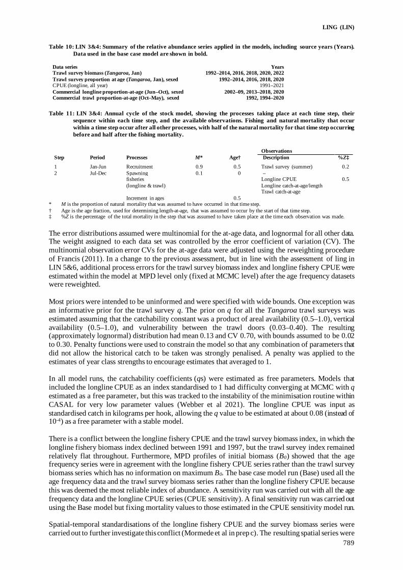
LING (LIN)
789
Table 10: LIN 3&4: Summary of the relative abundance series applied in the models, including source years (Years). Data used in the base case model are shown in bold.
Data series Years Trawl survey biomass (Tangaroa, Jan) 1992–2014, 2016, 2018, 2020, 2022 Trawl survey proportion at age (Tangaroa, Jan), sexed 1992–2014, 2016, 2018, 2020 CPUE (longline, all year) 1991–2021 Commercial longline proportion-at-age (Jun–Oct), sexed 2002–09, 2013–2018, 2020 Commercial trawl proportion-at-age (Oct–May), sexed 1992, 1994–2020
Table 11: LIN 3&4: Annual cycle of the stock model, showing the processes taking place at each time step, their
sequence within each time step, and the available observations. Fishing and natural mortality that occur within a time step occur after all other processes, with half of the natural mortality for that time step occurring before and half after the fishing mortality.
Step Period Processes M* Age†
Observations
Description %Z‡
1 Jan-Jun Recruitment 0.9 0.5 Trawl survey (summer) 0.2 2 Jul-Dec Spawning 0.1 0 – fisheries Longline CPUE 0.5 (longline & trawl) Longline catch-at-age/length Trawl catch-at-age Increment in ages 0.5
* M is the proportion of natural mortality that was assumed to have occurred in that time step. † Age is the age fraction, used for determining length-at-age, that was assumed to occur by the start of that time step. ‡ %Z is the percentage of the total mortality in the step that was assumed to have taken place at the time each observation was made. The error distributions assumed were multinomial for the at-age data, and lognormal for all other data. The weight assigned to each data set was controlled by the error coefficient of variation (CV). The multinomial observation error CVs for the at-age data were adjusted using the reweighting procedure of Francis (2011). In a change to the previous assessment, but in line with the assessment of ling in LIN 5&6, additional process errors for the trawl survey biomass index and longline fishery CPUE were estimated within the model at MPD level only (fixed at MCMC level) after the age frequency datasets were reweighted. Most priors were intended to be uninformed and were specified with wide bounds. One exception was an informative prior for the trawl survey q. The prior on q for all the Tangaroa trawl surveys was estimated assuming that the catchability constant was a product of areal availability (0.5–1.0), vertical availability (0.5–1.0), and vulnerability between the trawl doors (0.03–0.40). The resulting (approximately lognormal) distribution had mean 0.13 and CV 0.70, with bounds assumed to be 0.02 to 0.30. Penalty functions were used to constrain the model so that any combination of parameters that did not allow the historical catch to be taken was strongly penalised. A penalty was applied to the estimates of year class strengths to encourage estimates that averaged to 1. In all model runs, the catchability coefficients (qs) were estimated as free parameters. Models that included the longline CPUE as an index standardised to 1 had difficulty converging at MCMC with q estimated as a free parameter, but this was tracked to the instability of the minimisation routine within CASAL for very low parameter values (Webber et al 2021). The longline CPUE was input as standardised catch in kilograms per hook, allowing the q value to be estimated at about 0.08 (instead of 10-4) as a free parameter with a stable model. There is a conflict between the longline fishery CPUE and the trawl survey biomass index, in which the longline fishery biomass index declined between 1991 and 1997, but the trawl survey index remained relatively flat throughout. Furthermore, MPD profiles of initial biomass (B0) showed that the age frequency series were in agreement with the longline fishery CPUE series rather than the trawl survey biomass series which has no information on maximum B0. The base case model run (Base) used all the age frequency data and the trawl survey biomass series rather than the longline fishery CPUE because this was deemed the most reliable index of abundance. A sensitivity run was carried out with all the age frequency data and the longline CPUE series (CPUE sensitivity). A final sensitivity run was carried out using the Base model but fixing mortality values to those estimated in the CPUE sensitivity model run. Spatial-temporal standardisations of the longline fishery CPUE and the survey biomass series were carried out to further investigate this conflict (Mormede et al in prep c). The resulting spatial series were

LING (LIN)
790
similar to the corresponding series that were used in the model and insufficient to explain the discrepancy between the CPUE and trawl survey series between 1991 and 1997. 4.3.2 Model estimates The fits to the catch-at-age data were all reasonable, and almost indistinguishable between model runs. The fits to the survey biomass series (Base model) or the CPUE series (sensitivity) were reasonable. Estimated year class strengths were not widely variable, although they were poorly estimated prior to 1980 (Figure 3). Fixing year class strengths to 1 prior to 1980 resulted in almost identical model results (see Mormede et al in prep b). All year class strengths estimated from 2000 have been less than 1, apart from that for 2007. Ling are first caught by the trawl survey (age at full selectivity 5–6 years), then the trawl fishery (age 6–8 years), and then the longline fishery (age 12–15 years). Males were estimated to be less vulnerable than females to the trawl and longline fisheries but equally vulnerable as females in the survey. The estimated median Mavg was 0.156 and Mdiff -0.015 (male-female difference) for the base case model, and 0.137 and -0.011, respectively, for the sensitivity run with CPUE series. A further sensitivity run was carried out using the base case model observations but fixing mortality values to those estimated in the CPUE sensitivity run. Lag correlation of the MCMC for the base case model were above 1 for all lags instead of below 1 from lag two onwards, highlighting the conflict between the datasets within the model. Lag correlation was acceptable for the model with fixed M values and for the sensitivity run. Median relative jump size was acceptable for all models once the selectivities were set to logistic.
Figure 3: LIN 3&4. Estimated posterior distributions of year class strength from the base case run, with median (line and individual points) and 95% credible interval (grey band). The horizontal line indicates a year class strength of one.
Base case estimates indicated that it was unlikely that B0 was lower than 100 000 t for this stock, or that biomass in 2022 was less than 46% of B0 (Table 12, Figure 4). Annual exploitation rates (catch over vulnerable biomass) were estimated to be lower than 0.15 (often much lower) since 1979 (Figure 5). The sensitivity model based on the longline CPUE estimated a lower initial biomass (88 450–96 520 t), with biomass in 2022 estimated between 27 and 41% B0. The WG considered the sensitivity run not likely to be a reliable representation of the biomass because the longline fishery CPUE showed a sharp drop in the early 1990s when the trawl survey biomass showed no such trend. Although the trawl survey biomass index was in conflict with the age data in the model (including the survey age data), the survey is considered of high quality and therefore should be trusted over the longline CPUE or the age data. Further spatial-temporal analyses of the survey data did not indicate a change in ling distribution or any other process which might have rendered the survey biomass calculation inadequate. Furthermore, the CV on the survey biomass estimation is low (Table 9), indicating the survey is likely to be adequate for this species.

LING (LIN)
791
The CPUE sensitivity model estimated natural mortality at a lower value of M than was estimated in the base case. An additional sensitivity run of the base case model but with natural mortality fixed at the sensitivity estimates of Mavg = 0.137 and Mdiff = -0.011 resulted in a lower biomass estimate and status than the base case model, with the biomass in 2022 estimated at about 45% of initial biomass rather than 56% as estimated by the base case model. This model also presented acceptable diagnostics in terms of lag, which the base case did not. A natural mortality of 0.137 is akin to that estimated by Edwards (2017) but much lower than that estimated by Horn (2008) at 0.18. Simulations were carried out whereby natural mortality was fixed at either MPD or MCMC values, 100 simulated observations derived, and then used to back-estimate mortality parameters. Those simulations showed neither the base case model nor the CPUE sensitivity model showed bias in the estimate of the natural mortality parameters or undue uncertainty (Mormede et al 2022 in prep b). Table 12: LIN 3&4: Bayesian median and 95% credible intervals (in parentheses) of B0 and B2022 (in tonnes, and as a
percentage of B0) for the Base model run and two sensitivities, and the probability that B2022 is below 40% of B0 from the Base model run.
Model run B0 B2022 B2022 (%B0) P(>40%
B0) P(<20%
B0) Base case model (survey)
110 040 (100 660–129 890) 61 380 (47 400–85 810) 55.8 (46.9–66.3) 1.000 0.000
Sensitivity (CPUE)
92 190 (88 450–96 520) 30 860 (24 720–39 080) 33.5 (27.1–41.2) 0.052 0.000
The model indicated a relatively flat biomass trajectory from about 2009 (Figure 4). Annual landings from the LIN 3&4 stock have been less than 4600 t since 2004, markedly lower than the 6000–8000 t taken annually between 1992 and 2003. Biomass projections derived from this assessment are shown below (section 4.3.3).
Figure 4: LIN 3&4 base model. Estimated median trajectories (with 95% credible intervals shown as grey band) for
absolute biomass and biomass as a percentage of B0. The red horizontal line at 10% B0 represents the hard limit, the orange line at 20% B0 is the soft limit, and the green line is the %B0 target (40% B0).
Figure 5: LIN 3&4 base model: Exploitation rates (catch over vulnerable biomass) with 95% credible intervals shown
in grey.

LING (LIN)
792
Prior to the introduction of the QMS and before the establishment of the EEZ, catch reporting was not required and as such catches are uncertain but are assumed to have been low during this period. A sensitivity model was run based on the base case model that assumed 5% additional fishery mortality for years before the introduction of the QMS (1986) and 2% thereafter. The inclusion of estimates of incidental mortality and pre-QMS unreported catch resulted in very similar status, and biomass in 2022 from the base model. 4.3.3 Projections Four scenarios were carried out, all using the base case model. Recent catches have been much lower than the TACC so the future catches were assumed to be either the average of the 2019–2021 catches or the TACC, keeping the ratio of catches between the fisheries to that of the 2019–2021 fisheries (52% longline, 33% trawl, and 15% pot). Furthermore, year class strengths have been mostly low since 2000 so the year class strengths for the projections were either resampled from the full 1975–2013 range, or from the 2003–2013 range. For LIN 3&4, using the base case model, stock size is likely to remain about the same or increase by about 5%, assuming future catches equal recent catch levels and year class strengths are consistent with recent (2003–2013) or all year class strengths, respectively, or decrease to around 83–89% of the 2022 biomass by 2027 if catches reach the TACC with the same year class strength assumptions (Table 13). The probability of biomass in 2027 being above 40% B0 is 0.85–1.0 and the probability of being below 20% B0 is zero for all projection scenarios. Table 13: LIN 3&4. Bayesian median and 95% credible intervals (in parentheses) of projected B2027, B2027 as a
percentage of B0, and as a percentage of B2022 for the base case run and various assumptions of future catches and year class strengths (YCS). The probability of B2027 being above 40% B0 (p40) and of B2027 being below 20%B0 (p20) are also reported.
YCS Catch Future catch (t)
range range Trawl Line Pot B2027 (t) B2027 (%B0) B2027 (%B2022) p40 p20
All 2019–2021 1 057 1 701 479 65 150 (49 150– 91 170) 59 (48–72) 105 (95–119) 1.00 0
2003–2013 2019–2021 1 057 1 701 479 60 620 (46 160– 84 560) 55 (45–66) 99 (93–106) 0.90 0
All TACC 2 044 3 290 926 55 150 (39 050– 81 380) 50 (38–64) 89 (78–103) 0.95 0
2003–2013 TACC 2 044 3 290 926 50 560 (35 980– 74 560) 46 (35–58) 83 (74–91) 0.85 0
4.4 Sub-Antarctic, LIN 5 & LIN 6 (excluding Bounty Plateau) 4.4.1 Model structure and inputs An age-based total catch history stock assessment model assuming a Beverton-Holt stock-recruit relationship for LIN 5&6 (Sub-Antarctic) was updated in 2021 (Mormede et al 2021b). For final runs, the full posterior distribution was sampled using Markov chain Monte Carlo (MCMC) methods, based on the Metropolis-Hastings algorithm. Bounded estimates of spawning stock virgin (B0) and current (B2021) biomass were obtained. Year class strengths and fishing selectivity ogives were also estimated in the model. Trawl fishery selectivity ogives were fitted as double normal curves with the right-hand limb fixed at 100 (i.e., a flat-topped selectivity); longline fishery and research survey ogives were fitted as logistic curves. Selectivities were assumed constant over all years in each fishery/survey. MCMC chains with a total length of 4×10⁶ iterations were constructed. A burn-in length of 1×10⁶ iterations was used, with every 1000th sample taken from the final 3×10⁶ iterations (i.e., a final sample of length 3000 was taken from the Bayesian posterior). For LIN 5&6, model input data include catch histories, biomass and catch-at-age data from summer and autumn trawl survey series, longline fishery CPUE series, catch-at-age data from the longline and trawl fisheries, and estimates of biological parameters. The stock assessment model partitions the population into two sexes and age groups 3 to 25 with a plus group. The base model’s annual cycle is described in Table 14. To align more closely with the spawning

LING (LIN)
793
season (September to December), and to the season of the fishery (particularly in the early years), the model year was set as September to August, rather than the fishing year (October to September). A summary of all observations used in this assessment and the associated time series is given in Table 15. Lognormal errors, with known CVs, were assumed for all relative biomass observations. The CVs available for those observations of relative abundance allow for sampling error only. However, additional variance, assumed to arise from differences between model simplifications and real-world variation, was added to the sampling variance. The additional variance, termed process error, was estimated in the models at MPD-level only. Multinomial errors were assumed for all age composition observations. The effective sample sizes for the composition samples were estimated following method TA1.8 as described in appendix A of Francis (2011). Table 14: LIN 5&6. Annual cycle of the stock model, showing the processes taking place at each time step, their
sequence within each time step, and the available observations. Fishing and natural mortality that occur within a time step occur after all other processes, with half of the natural mortality for that time step occurring before and half after the fishing mortality.
Step Period Processes M* Age† Observations Description %Z‡
1 Sep–Dec Recruitment
Trawl and longline fisheries Increment ages
0.33 0.0 Longline CPUE Longline catch-at-age Trawl catch-at-age Trawl survey (summer)
0.5 0.5 0.5 0.9
2 Jan–Aug 0.67 0.5 Trawl survey (autumn) 0.5
* M is the proportion of natural mortality that was assumed to have occurred in that time step. † Age is the age fraction, used for determining length-at-age, that was assumed to occur in that time step. ‡ %Z is the percentage of the total mortality in the step that was assumed to have taken place at the time each observation was made. Table 15: LIN 5&6. Summary of the relative abundance series applied in the models, including source years (Model
years).
Data series Model years Trawl survey biomass (Tangaroa, Nov–Dec) 1992–94, 2001–10, 2012–13, 2015, 2017, 2019, 2021 Trawl survey proportion at age (Tangaroa, Nov–Dec) 1992–94, 2001–10, 2012–13, 2015, 2017, 2019 Trawl survey biomass (Tangaroa, Mar–May) 1992–93, 1996, 1998 Trawl survey proportion at age (Tangaroa, Mar–May) 1992–93, 1996, 1998 CPUE (longline) 1991–2020 Commercial longline proportion-at-age 1994, 1996, 1998–2012, 2014, 2017, 2018 Commercial trawl proportion-at-age 1992, 1994, 1996, 1998–2019
The assumed prior distributions used in the assessment are given in Table 16. Most priors were intended to be relatively uninformed and were specified with wide bounds. The exceptions were the choice of informative priors for the trawl survey q. The priors on q for all the Tangaroa trawl surveys were estimated assuming that the catchability constant was a product of areal availability (0.5–1.0), vertical availability (0.5–1.0), and vulnerability between the trawl doors (0.03–0.40). The resulting (approximately lognormal) distribution had mean 0.13 and CV 0.70, with bounds assumed to be 0.02 to 0.30. The prior for M was chosen based on a 2017 study of ling mortality (Edwards 2017). Table 16: LIN 5&6. Assumed prior distributions and bounds for estimated parameters in the assessments. The
parameters for lognormal priors are mean (in log space) and CV.
Parameter description Distribution Parameters Bounds
B0 Uniform-log – – 50 000 800 000 Year class strengths Lognormal 1.0 0.70 0.01 100 Trawl survey q Lognormal 0.13 0.70 0.02 0.3 Trawl survey process error Uniform-log – – 0.001 2 CPUE q Uniform-log – – 1e-6 1e-3 Selectivities Uniform – – 0 20–200* M † Lognormal 0.16 0.2 0.05 0.5
* A range of maximum values were used for the upper bound. † Constant, estimated natural mortality used in some sensitivity models. Penalty functions were used to constrain the model so that any combination of parameters that did not allow the historical catch to be taken was strongly penalised. A small penalty was applied to the estimates of year class strengths to encourage estimates that averaged to 1. The catch history, biological input parameters, and estimates of relative abundance used in the model are given in Tables 5–9.

LING (LIN)
794
The base model for 2021 was quite different from that of the previous assessment in 2018 (Masi 2019). In 2018 the base case had three fisheries, estimated natural mortality, a revised annual cycle for the spawning and non-spawning longline fisheries, free survey q parameters, and excluded the longline CPUE index. In 2021, the base case run had two fisheries (and associated updated annual cycle), a fixed natural mortality of 0.18 y-1, nuisance survey q parameters, fixed the right-hand limb trawl selectivity parameters, and included the longline standardised CPUE index. The process which led to these changes in parameters are detailed below.
• Two fisheries – New spatial analyses carried out in 2021 concluded that splitting the LIN 5&6 stock between trawl and longline fisheries would achieve more consistent length frequencies and sex ratios in those two fisheries over time than the previous split of trawl, spawning, and home ground longline fisheries (Mormede et al 2021a). These new splits also cover the entire year rather parts of the year as previously done (Ballara 2019). The models were therefore updated to have a longline and a trawl fishery as opposed to two longline (spawning and non-spawning) and a trawl fishery. The effect of this change was minor at the MPD level.
• Fixed M – M used to be estimated as a U-shaped natural mortality (Roberts 2016), then a single
natural mortality with uniform prior (Masi 2019). The models run in 2021 with an estimated mortality parameter presented very poor MCMC diagnostics (including mixing and stability) and were deemed unacceptable by the Deepwater Working Group (DWWG). The base case model and sensitivities reverted to fixed M values. Values of 0.16 y-1 (based on Edwards 2017), 0.18 y-1 (based on Horn 2005 and value previously used in models), and 0.20 y-1 (MPD estimated value) were used as bounding values. A simulation was also carried out whereby M was fixed at 0.17 y-1, observations simulated using the MCMC parameters, and M then back-estimated at MPD level; M was over-estimated by about 0.015 on average. Therefore, M of 0.18 y-1 was the chosen base case.
• Nuisance qs – The survey qs were set as nuisance in 2015 (Roberts 2016) and then changed to free
qs in 2018 (Masi 2019). The models run in 2021 with free survey qs presented poor MCMC diagnostics, which were greatly improved when switching back to nuisance qs. Fixing the right-hand limb trawl selectivity to 100 (mean of the MCMC values) stabilised the models further and was adopted by the Deepwater Working Group. The effect of changing from free qs to nuisance qs increased the initial biomass slightly, as was seen in 2018 (Masi 2019, table 12).
• Longline CPUE index – The ling longline fishery is a target fishery which almost exclusively
catches ling. The DWWG felt it was a suitable index of abundance to use in the models, if the MCMC for these models converged adequately. Furthermore, the DWWG felt that the 2018 model presented a very large confidence interval on the value of B0 due to the lack of information about how large the stock might be. Further investigations through MPD profiles showed that the CPUE index did contain some bounding information on stock size. The longline CPUE index was added to the model with annual CVs calculated from the CPUE standardisation (Table 8) and a process error estimated within CASAL at about 0.16. This compares favourably with the process error of the trawl survey which CASAL estimated at about 0.13, confirming that the CPUE series is consistent with the expected biomass trajectory of the model. In 2018 the longline CPUE was included in some sensitivity runs but not kept in the base case model because the spawning CPUE was not well fitted; this could have been a spatial issue and was resolved by grouping non-spawning and spawning together (see ‘Two fisheries’ above). A sensitivity run was carried out without the CPUE index and with M fixed at 0.18.
4.4.2 Model estimates Description of the base model run reported is as follows: The base case is considered to be a reference model because it was the most stable model obtained and uses all of the trusted information available. Other model runs which led to this base case (e.g., with estimated M values, free qs) are not reported here. The base case model comprised two fisheries (and associated updated annual cycle), a fixed natural mortality of 0.18 y-1, nuisance survey q parameters, fixed the right-hand limb trawl selectivity parameters, and the longline standardised CPUE series.

LING (LIN)
795
Three sensitivities are reported: (1) M fixed at 0.16, (2) M fixed at 0.20, and (3) M fixed at 0.18 and excluding the longline standardised CPUE series. From the sensitivity runs trialled, MPD estimates of current stock status were between 61–80% B0. Steepness was assumed to be 0.84 (Table 7); sensitivities to this were not conducted due to the consistently high stock status. Posterior distributions of year class strength estimates from the base case model run are shown in Figure 6; the distribution from the base case model differed little from the sensitivity models. Year classes were generally weak from 1985 to 1992, strong from 1994 to 1996 and 2005 to 2010, and average since then. Overall, estimated year class strengths were not widely variable, with all medians being between 0.5 and 1.5. Biomass estimates for the stock declined through the 1990s but have been stable since the early 2000s (Figure 7). The biomass trajectory from the base case model was little different to those derived from the sensitivity models, although the 95% credible interval varied between model runs (see Table 17). Stock status estimates for 2021 from three reported models were between 61–80% of B0 (Figure 7, Table 17), with the lowest stock status linked to the lowest value of M. Annual exploitation rates (catch over vulnerable biomass) were low (less than 0.1) in all years as a consequence of the high estimated stock size in relationship to the level of relative catches (Figure 8).
Figure 6: LIN 5&6. Estimated posterior distributions of year class strength from the base case run, with median (line
and individual points) and 95% credible interval (grey band). The horizontal line indicates a year class strength of one.
Figure 7: LIN 5&6 base model. Estimated median trajectories (with 95% credible intervals shown as grey band) for
absolute biomass and biomass as a percentage of B0. The red horizontal line at 10% B0 represents the hard limit, the orange line at 20% B0 is the soft limit, and the green line is the % B0 target (40% B0).

LING (LIN)
796
Table 17: LIN 5&6. Bayesian median and 95% credible intervals (in parentheses) of B0 and B2021 (in tonnes), and B2021 as a percentage of B0, and the probability that B2021 is above 40% and below 20% of B0 from the Base model and sensitivity runs with TACC as future catches.
Model run B0 B2021 B2021 (%B0) P(>40% B0)
P(<20% B0)
Base case model
187 350 (163 190–226 090) 132 780 (104 630–177 230) 70.8 (63.1–79.3) 0.934 0.000
M = 0.16 157 800 (144 500–175 820) 96 520 (79 080–119 840) 61.2 (54.1–69.1) 0.671 0.008 M = 0.20 258 770 (203 270–361 080) 208 840 (150 460–318 790) 80.6 (72.2–89.7) 0.995 0.000 M = 0.18 and no CPUE
197 130 (166 520–246 370) 147 690 (109 610–209 350) 75.0 (64.8–86.0) 0.962 0.000
Figure 8: LIN 5&6 base model exploitation rate (catch over vulnerable biomass) with 95% credible intervals shown in
grey.
Resource survey and fishery selectivity ogives were relatively tightly defined. The survey ogive suggested that ling were fully selected by the research gear at about age 7–9 years. Estimated fishing selectivities indicated that ling were fully selected by the trawl fishery at about age 9 years, and by the longline fisheries at about age 12–16. The assessments indicated a general drop in biomass to 2000, and a flat trend since then. Fixing M, the trawl right-hand limb trawl selectivities have reduced the uncertainty around the estimate of biomass which was present in the 2018 assessment (Masi 2019), although this uncertainty increases with the value of M in the model (Table 17). Biomass projections derived from this assessment are shown below. The effect of possible incidental mortality associated with escapement from trawl nets and potential unreported catch from before the introduction of the QMS was evaluated in a sensitivity model. Discards from the hoki/hake/ling target fishery were likely to be very low (< 0.3%, Anderson 2019). Incidental mortality of small fish associated with escapement also is assumed to be low because the ling fishery occurs in areas away from locations where small ling are found. Unreported catch prior to the introduction of the QMS is not known but assumed to be low due to the high commercial value of ling at that time. A sensitivity model was run that assumed 5% additional fishery mortality for years before the introduction of the QMS (1986) and 2% thereafter. The inclusion of estimates of incidental mortality and pre-QMS unreported catch resulted in a very similar status, and similar estimates of current biomass. 4.4.3 Projections For LIN 5&6, the probability of B2021 being below 40% of B0 is very small when assuming either one of two future annual catch scenarios (the average catch of 6320 t for trawl and 1370 t for longline between 2016 and 2020 or the TACC of 13 240 t split 82% trawl and 18% longline reflecting the average proportion of catches between the two fisheries between 2016 and 2020) (Table 18).

LING (LIN)
797
Table 18: LIN 5&6. Bayesian median and 95% credible intervals (in parentheses) of projected B2026, B2026 as a percentage of B0, and B2026/B2021(%) for the base case runs.
Stock and Future catch (t) model run Trawl Longline B2026 (t) B2026 (%B0) B2026/B2021 (%)
LIN 5&6 Base 6 320 1 370 129 080 (81 670–205 590) 68 (46– 104) 95 (72–133) 10 860 2 380 110 340 (63 330–186 650) 58 (36 – 94) 81 (57–117)
4.5 Bounty Plateau, LIN 6B (Bounty Plateau only) 4.5.1 Model structure and inputs The stock assessment for the Bounty Plateau stock (part of LIN 6) was updated in 2007 (Horn 2007b). For final runs, the full posterior distribution was sampled using Markov chain Monte Carlo (MCMC) methods, based on the Metropolis-Hastings algorithm. Bounded estimates of spawning stock virgin (B0) and current (B2006) biomass were obtained. Year class strengths and fishing selectivity ogives were also estimated in the model. Longline fishery ogives were fitted as logistic curves. MCMC chains were constructed using a burn-in length of 5×10⁵ iterations, with every 1000th sample taken from the next 106 iterations (i.e., a final sample of length 1000 was taken from the Bayesian posterior). For LIN 6B, model input data include catch histories, longline fishery CPUE, catch-at-age, and catch-at-length from the longline fishery, and estimates of biological parameters. In the absence of sufficient stock-specific data, maturity ogives were assumed to be the same as for LIN 3&4, a stock with comparable growth parameters to LIN 6B. Only a base case model run is presented. The stock assessment model partitions the population into two sexes and age groups 3 to 35 with a plus group. There is one fishery (longline) in the stock. The model’s annual cycle is described in Table 19. Lognormal errors, with observation-error CVs, were assumed for all relative biomass, proportions-at-age, and proportions-at-length observations. Additional process error was estimated in MPD runs of the model (Table 20) and fixed in all subsequent runs. The assumed prior distributions used in the assessment are given in Table 21. All priors were intended to be relatively uninformed and were estimated with wide bounds. Penalty functions were used to constrain the model so that any combination of parameters that did not allow the historical catch to be taken was strongly penalised. A small penalty was applied to the estimates of year class strengths to encourage estimates that averaged to 1. The catch history, biological input parameters, and estimates of relative abundance used in the model are shown in Tables 5–8. Table 19: LIN 6B. Annual cycle of the stock model, showing the processes taking place at each time step, their sequence
within each time step, and the available observations. Fishing and natural mortality that occur within a time step occur after all other processes, with half of the natural mortality for that time step occurring before and half after the fishing mortality.
Step Period Processes M* Age† Observations Description %Z‡
1 Dec–Sep Recruitment 0.9 0.5 Longline CPUE 0.5 fishery (line) Longline catch-at-age/length 0.5
2 Oct–Nov increment ages 0.1 0 –
* M is the proportion of natural mortality that was assumed to have occurred in that time step. † Age is the age fraction, used for determining length-at-age that was assumed to occur in that time step. ‡ %Z is the percentage of the total mortality in the step that was assumed to have taken place at the time each observation was made. Table 20: LIN 6B. Summary of the relative abundance series applied in the models, including source years (Years),
and the estimated process error (CV) added to the observation error.
Data series Years Process error CV CPUE (longline, all year) 1992–2004 0.15 Commercial longline length-frequency (Nov–Feb) 1996, 2000–04 0.50 Commercial longline proportion-at-age (Dec–Feb) 2000–01, 2004 0.40

LING (LIN)
798
Table 21: LIN 6B. Assumed prior distributions and bounds for estimated parameters for the assessments. The parameters are mean (in log space) and CV for lognormal.
Parameter description Distribution Parameters Bounds B0 uniform-log – – 5 000 100 000 Year class strengths lognormal 1 0.7 0.01 100 CPUE q uniform-log – – 1.00E-08 1.00E-03 Selectivities uniform – – 0 20–200* Process error CV uniform-log – – 0.001 2
4.5.2 Model estimates Only a base case model run was completed. Posterior distributions of year class strength estimates from the base case model run are shown in Figure 9.
Figure 9: LIN 6B. Estimated posterior distributions of year class strength from the base case run. The horizontal line
indicates a year class strength of one. Individual distributions show the marginal posterior distribution, with horizontal lines indicating the median.
The assessment was driven largely by the catch-at-age and catch-at-length series from the longline fishery; the first two years of CPUE data were not well fitted. Biomass estimates are listed in Table 22 and the biomass trajectory is shown in Figure 10. The assessment indicates a declining biomass throughout the history of the fishery. Estimates of current and virgin stock size are not well known, but current biomass is very likely to be above 50% of B0. Table 22: LIN 6B. Bayesian median and 95% credible intervals (in parentheses) of B0 and B2006 (in t), and B2006 as a
percentage of B0 for the base case model run.
Model run B0 B2006 B2006 (%B0) Base case 13 570 (10 850–19 030) 8 330 (4 860–14 730) 61 (45–79)
Figure 10: LIN 6B. Estimated posterior distributions of biomass trajectories as a percentage of B0, from the base case
model run (including 5-year projections through to 2011 with assumed constant annual catch of 400 t). Distributions are the marginal posterior distribution, with horizontal lines indicating the median.
01
23
45
true_
YC
S
1980 1985 1990 1995 2000
050
100
150
200
Biom
ass (
%B
1980 1985 1990 1995 2000 2005 2010

LING (LIN)
799
4.5.3 Projections Projections for LIN 6B from the 2006 assessment are given in Table 23. The LIN 6B stock (Bounty Plateau) was projected to decline out to 2011, but probably still be higher than 50% of B0. Table 23: LIN 6B. Bayesian median and 95% credible intervals (in parentheses) of projected B2011, B2011 as a percentage
of B0, and B2011/B2006 (%) for the 2006 base case.
Stock and model run Future catch (t) B2011 B2011 (%B0) B2011/B2006 (%)
LIN 6B Base 600 7 460 (2 950–18 520) 53 (26–116) 86 (51–168)
4.6 West coast South Island, LIN 7WC 4.6.1 Model structure and inputs The stock assessment for LIN 7WC (west coast South Island) was updated in 2020 (Kienzle 2021). The assessment model partitioned the population into age groups 3 to 28 with a plus group, and immature and mature fish, with no sex in the partition. The model’s annual cycle is described in Table 24. The reported model runs were developed following the investigation of numerous previous model runs. These evaluated the sensitivity of the model fit to assumptions about indices of abundance, natural mortality rate, trawl survey and fishery selectivity ogives, and weights assigned to different observational data sets. Year class strengths and fishing selectivity ogives were estimated in the model. The longline fishery and mature fish research trawl survey selectivity ogives were assumed to be logistic. The selectivity of immature fish by the research trawl survey was estimated as a capped logistic curve. Commercial trawl fishery selectivity ogive was set as a double normal function. Two analyses were carried to test the sensitivity of the results of the LIN 7 stock assessment (base case) to some of the assumptions (Table 25): models 2 and 3 were used to investigate the effect of using alternative indices of abundance into the assessment; models 4 and 5 assessed the effect of using different values of natural mortality. Table 24: LIN 7WC. Annual cycle of the stock model, showing the processes taking place at each time step, their
sequence within each time step, and the available observations. Fishing and natural mortality that occur within a time step occur after all other processes, with half of the natural mortality for that time step occurring before and half after the fishing mortality.
Step Period Processes M* Age† Observations
Description %Z‡
1 Oct–May Recruitment 0.75 0.5 Longline catch-at-age 0.5 fishery (longline)
2 Jul–Sep fishery (trawl) 0.25 0.8 Trawl catch-at-age 0.5 Trawl CPUE Trawl survey biomass and catch-at-age 3 End of Sep Increment ages 0 0
* M is the proportion of natural mortality that was assumed to have occurred in that time step. † Age is the age fraction, used for determining length-at-age, that was assumed to occur in that time step. ‡ %Z is the percentage of the total mortality in the step that was assumed to have taken place at the time each observation was made. Table 25: LIN 7WC. Settings of the models exploring the sensitivity of the base case stock assessment to the index of
abundance (columns) and the value of natural mortalities (rows). Indices of abundance
Natural mortality (per year) Survey Survey + CPUE CPUE
0.14 Model 4 0.18 Base case Model 2 Model 3 0.22 Model 5

LING (LIN)
800
The full posterior distributions of the parameters of the base case model and model 15 were sampled using Markov chain Monte Carlo (MCMC) methods, based on the Metropolis-Hastings algorithm. Bounded estimates of spawning stock virgin (B0) and current (B2020) biomass were obtained. Four MCMC chains were constructed using a burn-in length of 2×10⁶ iterations, with every 2000th sample taken from the next 6×10⁶ iterations (i.e., four final samples of length 2000 each were taken from the Bayesian posterior totally 8000 samples to describe the posterior distributions of the models parameters). Visual inspections of the chains were used to determine the acceptability of the MCMC procedure. The final model runs (section 4.6.2) were considered acceptable for providing management advice. For LIN 7WC, available data to model the fishery included catch histories, trawl fishery CPUE, extensive catch-at-age data from the trawl fishery, sparse catch-at-age data from the longline fishery, biomass estimates, proportion-at-age from Tangaroa surveys in 2000, 2012, 2013, 2016, and 2018, and estimates of constant biological parameters (Table 26 and Table 5). A longline fishery CPUE series was available but was rejected as unlikely to be indexing stock abundance. The Kaharoa inshore trawl survey biomass estimates and proportion-at-length estimates were not considered to be useful because they have been rejected in previous sittings of the DWWG because few ling older than age nine were caught in surveys, and inclusion of the data made negligible contribution to the estimation of model parameters. The error distributions assumed were multinomial for the proportions-at-age and lognormal for all other data. Biomass indices had assumed CVs set equal to the sampling CV plus an additional process error of 0.4, estimated following Francis (2011). The multinomial observation error effective sample sizes for the trawl fishery at-age data were adjusted using the reweighting procedure of Francis (2011). An ad hoc procedure was used for the at-age data from the longline fishery and Tangaroa survey at-age data, giving the longline fishery a relatively low weighting and the trawl survey a relatively high weighting. The assumed prior distributions used in the assessment are given in Table 27. Most priors were intended to be relatively uninformed and were specified with wide bounds. The prior for the survey q was informative and was estimated using the Sub-Antarctic ling survey priors as a starting point because the survey series in both areas used the same vessel and fishing gear. However, the WCSI survey area in the 200–650 m depth range in strata 0004 A–C and 0012 A–C comprised 6619 km2; seabed area in that depth range in the entire LIN 7 WC biological stock area (excluding the Challenger Plateau) is estimated to be about 20 100 km2. So, because biomass from only 33% of the WCSI ling habitat was included in the indices, the Sub-Antarctic prior on µ was modified accordingly (i.e., 0.13 × 0.33 = 0.043), and the bounds were also reduced from [0.02, 0.30] to [0.01, 0.20]. Priors for survey selectivity parameters, both immature and mature ling, and trawl fishery were changed from uninformed to informed because of lack of convergence in the MCMC. The prior for those parameters was set to a lognormal distribution with mean set at the estimate from a log-likelihood minimisation fit and coefficient of variation of 0.2. The prior distributions for the longline fishery selectivity parameters were assumed to be uniform. Penalty functions were used to constrain the model so that any combination of parameters that did not allow the historical catch to be taken was strongly penalised. A small penalty was applied to the estimates of year class strengths to encourage estimates that averaged to 1. The catch history, biological input parameters, and estimates of relative abundance used in the model are shown in Tables 5–9. Table 26: LIN 7WC. Summary of the relative abundance and stock composition series applied in the models, including
source years (Years).
Data series Years
CPUE (hoki trawl, Jun–Sep) 1987–2019 Commercial trawl proportion-at-age (Jun–Sep) 1991, 1994–2008, 2012–2019 Commercial longline proportion-at-age 2003, 2006, 2007, 2012, 2015 Trawl survey biomass (Tangaroa, Jul) 2000, 2012–13, 2016, 2018 Trawl survey age data 2000, 2012–13, 2016, 2018

LING (LIN)
801
Table 27: LIN 7WC. Assumed prior distributions and bounds for parameters estimated in the models. For lognormal distributions the figures are the log-space mean and the CV, and for normal distributions the figures are the mean and standard deviation.
Parameter description Distribution Parameters Bounds
B0 uniform-log – – 10 000 500 000 Year class strengths lognormal 1.0 0.7 0.01 100 Tangaroa survey q lognormal 0.043 0.70 0.001 1 CPUE q uniform-log – – 1e-8 1e-3 Trawl fishery selectivity par 1 Lognormal 10 0.2 1 30 Trawl fishery selectivity par 2 Lognormal 5.5 0.2 1 30 Trawl survey selectivity immature par 1 Lognormal 2.8 0.2 1 30 Trawl survey selectivity immature par 2 Lognormal 0.77 0.2 0.1 30 Trawl survey selectivity immature par 3 Lognormal 0.03 0.2 0.001 0.20 Trawl survey selectivity mature par 1 Lognormal 13.6 0.2 1 30 Trawl survey selectivity mature par 2 Lognormal 7.2 0.2 1 30 Longline fishery selectivity uniform – – 0 30–200*
* A range of maximum values was used for the upper bound. 4.6.2 Model estimates The results of the sensitivity analyses showed that the stock assessment model is not sensitive to using alternative indices of abundance. Spawning stock biomass estimates do vary as a function of the magnitude of natural mortality assumed in the model in a predictable way: the best estimate of M is 0.18. Of the five models presented in this section, only two were brought to MCMC. Those two models estimated the median virgin biomass to be equal between 55 000–56 000 t (Table 28), and the ling SSB to have declined by 2020 to approximately 50% of its virgin biomass (B0) (Figure 11). Table 28: LIN 7WC Bayesian median and 95% credible intervals (in parentheses) of B0 and B2020 (in tonnes) and B2020
as a percentage of B0 for all model runs.
Model run B0 B2020 B2020 (%B0) Base case 54 546 (50 463–59 833) 25 556 (17 877–35 527) 47 (35–60) Adding CPUE index of abundance (model 2) 56 159 (51 964–61 580) 28 393 (21 034–38 047) 50 (40–62) Model run P(B2020 >0.4B0) P(B2020 < 0.2B0) P(B2020 < 0.1B0) Base case 87 0 0 Adding CPUE index of abundance (model 2)
97 0 0
Figure 11: LIN 7WC. Estimated posterior distribution of the spawning stock biomass (SSB in tonnes) trajectory and
estimated virgin spawning stock biomass reference points (40%, 20%, and 10% B0) for the base case model (left panel) and the model 2 (right panel). The solid black line represents the median values and the shaded areas the 95% confidence intervals.
4.6.3 Projections Projections out to 2022 for LIN 7WC indicated that biomass was likely to remain about the same with future catches equal to the average of catch in 2012–2016 (2980 t), or if catches for LIN 7WC were to increase modestly (by around 10%, 3300 t) to the overall LIN 7 fishstock level (Table 29).

LING (LIN)
802
Table 29: LIN 7WC. Bayesian median and 95% credible intervals (in parentheses) of projected B2022, B2022 as a percentage of B0, and B2022/B2016 (%) for the model runs.
Stock and model run
Future catch (t)
B2022
B2022 (%B0)
B2022/B2016 (%)
LIN 7WC Combined CPUE 2 980 77 300 (37 800–185 500) 79 (56–106) 100 (83–126) 3 300 76 600 (35 500–183 700) 78 (54–104) 98 (80–123)
Lognormal CPUE 2 980 47 400 (21 600–97 300) 70 (41–100) 104 (81–134) 3 300 45 900 (20 700–96 900) 68 (37–97) 102 (77–133)
Lognormal CPUE 2 980 38 100 (17 300–97 900) 57 (33–85) 100 (76–126) & M = 0.18 3 300 36 400 (15 900–95 900) 54 (32–82) 97 (73–124)
4.7 Cook Strait, LIN 7CK 4.7.1 Model structure and inputs A stock assessment of ling in Cook Strait (LIN 7CK) was completed in 2013 (Dunn et al 2013). Because it is believed that the true M for the Cook Strait stock is higher than the ‘default’ value of 0.18, it was considered desirable to estimate M in the model, and so incorporate the effect of this uncertainty in M in the assessment. However, the simultaneous estimation of B0 and M was not successful owing to the adoption of a multinomial likelihood (rather than lognormal) for proportions-at-age. Consequently, models with fixed M values were run, and, although the age data were reasonably well fitted, the model failed to accurately represent declines in resource abundance that appear evident from CPUE values, which have been declining since 2001. The model was considered unsuitable for the provision of management advice. The last stock assessment for LIN 7CK (Cook Strait) accepted by the Working Group was completed in 2010 (Horn & Francis 2013), and it is reported here. The stock assessment model partitions the population into two sexes and age groups 3 to 25 with a plus group. The model’s annual cycle is described in Table 30. Year class strengths and fishing selectivity ogives were also estimated in the model. Commercial trawl selectivity was fitted as double normal curves; longline fishery ogives were fitted as logistic curves. For final runs, the full posterior distribution was sampled using Markov chain Monte Carlo (MCMC) methods, based on the Metropolis-Hastings algorithm. Bounded estimates of spawning stock virgin (B0) and current (B2008) biomass were obtained. MCMC chains were constructed using a burn-in length of 4×10⁶ iterations, with every 2000th sample taken from the next 20×106 iterations (i.e., a final sample of length 1000 was taken from the Bayesian posterior). For LIN 7CK, model input data include catch histories, trawl and longline fishery CPUE, extensive catch-at-age data from the trawl fishery, sparse catch-at-age data from the longline fishery, and estimates of biological parameters. Initial modelling investigations found that the longline CPUE produced implausible results; this series was rejected as a useful index. The base case used all catch-at-age data from the fisheries, and the trawl CPUE series. Instantaneous natural mortality was estimated in the model. Lognormal errors, with observation-error CVs, were assumed for all CPUE and proportions-at-age observations. Additional process error, assumed to arise from differences between model simplifications and real world variation, was added to the sampling variance (Table 31). Table 30: LIN 7CK. Annual cycle of the stock model, showing the processes taking place at each time step, their
sequence within each time step, and the available observations. Fishing and natural mortality that occur within a time step occur after all other processes, with half of the natural mortality for that time step occurring before and half after the fishing mortality.
Step Period Processes M* Age† Observations
Description %Z‡
1 Oct–May Recruitment 0.67 0.5 Longline CPUE 0.5 fishery (line) Longline catch-at-age
2 Jun–Sep increment ages 0.33 0 Trawl CPUE 0.5 fishery (trawl) Trawl catch-at-age
* M is the proportion of natural mortality that was assumed to have occurred in that time step. † Age is the age fraction, used for determining length-at-age, that was assumed to occur in that time step. ‡ %Z is the percentage of the total mortality in the step that was assumed to have taken place at the time each observation was made.

LING (LIN)
803
Table 31: LIN 7CK. Summary of the available data including source years (Years), and the estimated process error (CV) added to the observation error.
Data series Years Process error CV
CPUE (hoki trawl, Jun–Sep) 1994–2009 0.2 Commercial trawl proportion-at-age (Jun–Sep) 1999–2009 1.1 Commercial longline proportion-at-age 2006–07 1.1
The assumed prior distributions used in the assessment are given in Table 32. Most priors were intended to be relatively uninformed and were specified with wide bounds. Table 32: LIN 7CK: Assumed prior distributions and bounds for estimated parameters in the assessments. The
parameters are mean (in log space) and CV for lognormal, and mean and standard deviation for normal.
Parameter description Distribution Parameters Bounds
B0 uniform-log – – 2 000 60 000 Year class strengths lognormal 1.0 0.9 0.01 100 CPUE q uniform-log – – 1e-8 1e-2 Selectivities uniform – – 0 20–200* M lognormal 0.18 0.16 0.1 0.3 * A range of maximum values was used for the upper bound.
Penalty functions were used to constrain the model so that any combination of parameters that did not allow the historical catch to be taken was strongly penalised. A small penalty was applied to the estimates of year class strengths to encourage estimates that averaged to 1. The catch history, biological input parameters, and estimates of relative abundance used in the model are shown in Tables 5–8 4.7.2 Model estimates A single model was presented incorporating a catch history, trawl and longline fishery catch-at-age, trawl CPUE series, with double-normal ogives for the trawl fishery and logistic ogives for the longline fishery, and M estimated in the model. Posterior distributions of LIN 7CK year class strength estimates from the base case model run are shown in Figure 12.
Figure 12: LIN 7CK. Estimated posterior distributions of year class strength. The horizontal line indicates a year
class strength of one. Individual distributions show the marginal posterior distribution, with horizontal lines indicating the median.
The assessment is driven by the trawl fishery catch-at-age data and tuned by the trawl CPUE. Both input series contain information indicative of an overall stock decline in the last two decades. The confidence bounds around biomass estimates are wide (Table 33, Figure 13). Probabilities that current and projected biomass will drop below selected management reference points are given in Table 34. Median M was estimated to be 0.24 (95% confidence interval 0.16–0.30). Estimates of biomass are very sensitive to small changes in M, but clearly there is information in the model encouraging an M higher than the ‘default’ value of 0.18. The model indicated a slight overall biomass decline to about 2000, followed by a much steeper decline from 2000 to 2010. Exploitation rates (catch over vulnerable biomass) were very low up to the late 1980s and have been low to moderate (up to about 0.12 y–1) since
01
23
45
true_
YC
S
1968 1972 1976 1980 1984 1988 1992 1996 2000 2004

LING (LIN)
804
then. Since the early 1990s, trawl fishing pressure has generally declined, whereas longline pressure has generally increased. Table 33: LIN 7CK. Bayesian median and 95% credible intervals (in parentheses) of B0 and B2010 (in tonnes), and B2010
as a percentage of B0 for all model runs.
Model run B0 B2010 B2010 (%B0) Base case 8 070 (5 290–53 080) 4 370 (1 250–40 490) 54 (23–80)
Figure 13: LIN 7CK. Estimated median trajectories (with 95% credible intervals shown as dashed lines) for absolute
biomass and biomass as a percentage of B0. Table 34: LIN 7CK. Probabilities that current (B2010) and projected (B2015) biomass will be less than 40%, 20%, or 10%
of B0. Projected biomass probabilities are presented for two scenarios of future annual catch (i.e., 220 t and 420 t).
Management reference points Biomass 40% B0 20% B0 10% B0 B2010 0.248 0.006 0.000 B2015, 220 t catch 0.179 0.010 0.000 B2015, 420 t catch 0.328 0.094 0.019
4.7.3 Projections Projections out to 2015 for LIN 7CK indicated that biomass was likely to increase with future catches equal to recent previous catch levels or decline slightly if catches were equal to the mean since 1990 (Table 35). Table 35: LIN 7CK. Bayesian median and 95% credible intervals (in parentheses) of projected B2015, B2015 as a
percentage of B0, and B2015/B2010 (%) for the base case.
Stock and model run Future catch (t) B2015 B2015 (%B0) B2015/B2010 (%) LIN 7CK Base 220 5 030 (1 310–43 340) 59 (24–97) 110 (82–158) 420 4 320 (590–42 910) 52 (11–92) 95 (45–136)
5. FUTURE RESEARCH CONSIDERATIONS For all stocks, the potential change in growth or spawning over time should be investigated to keep track of potential climate change signals. LIN 2
• A review of the ling stock structure for LIN 2 should be completed before further assessments
are conducted for this QMA.
1980 1990 2000 2010
020
4060
80
Bio
mas
s ('0
00 t)
1980 1990 2000 2010
2040
6080
100
140
Bio
mas
s (%
B0)

LING (LIN)
805
LIN 3&4
• The potting fishery has been developing since 2018. One trip was observed in 2020 and length data collected. Additional observer length data and age readings are required in order to develop an age-frequency and associated selectivity for this fishery.
• Spatial-temporal standardisation of commercial and Chatham Rise survey data provided different indices worthy of further investigation.
LIN 5&6
• It would be beneficial to improve biological understanding and species distribution for this area. Further work on the spatial-temporal structure of LIN 5&6 needs to be carried out to refine the spatial structure used for modelling this stock.
• The relationship of this stock with LIN 6B needs further investigation. • The longline CPUE standardisation should be investigated further, in particular with regards to
the spatial structure defined. • If future models continue fixing M, further work on the most appropriate value of M should
also be considered. • Additional representative longline length frequency and age data would be useful. • Given that making adjustments to correct the Tangaroa Sub-Antarctic trawl survey biomass
estimate for 2017 will introduce some undefinable uncertainty, the Working Group recommends that this single data point is excluded in all future stock assessments.
6. STATUS OF THE STOCKS Stock Structure Assumptions Ling are assessed as six independent biological stocks, based on the presence of spawning areas and some differences in biological parameters between areas (Horn 2005). A spatial length and sex ratio analysis suggested that LIN 6B might be part of the LIN 5&6 stock but otherwise did not suggest any change to the stock assumptions for ling (Mormede et al 2021b). The Chatham Rise biological stock comprises all of Fishstock LIN 4, and LIN 3 north of the Otago Peninsula. The Sub-Antarctic biological stock comprises all of Fishstock LIN 5, all of LIN 6 excluding the Bounty Plateau, and LIN 3 south of the Otago Peninsula. The Bounty Plateau (part of Fishstock LIN 6) holds another distinct biological stock. The WCSI biological stock occurs in Fishstock LIN 7 west of Cape Farewell. The Cook Strait biological stock includes those parts of Fishstocks LIN 7 and LIN 2 between the northern Marlborough Sounds and Cape Palliser. Ling around the northern North Island (Fishstock LIN 1) are assumed to comprise another biological stock, but there is no information to support this assumption. The stock affinity of ling in LIN 2 between Cape Palliser and East Cape is unknown. East and west coast LIN 1 are regarded as separate stocks, but no assessments are available for either stock.
• East coast North Island (part of LIN 2, Statistical Areas 011–015)
Stock Status Year of Most Recent Assessment 2014 Assessment Runs Presented CPUE time series based on bottom longline ling target
fishing Reference Points
Target: 40% B0 Soft Limit: 20% B0 Hard Limit: 10% B0 Overfishing threshold: F corresponding to 40% B0
Status in relation to Target Unknown. CPUE has declined by between about 50–60% since the start of the time series in 1992.

LING (LIN)
806
Status in relation to Limits B2014 is Unlikely (< 40%) to be below the Soft Limit and Very Unlikely (< 10%) to be below the Hard Limit
Status in relation to Overfishing Unknown Historical Stock Status Trajectory and Current Status
Standardised CPUE index (± 95% CI) for bottom longline vessels targeting ling from the ECNI Statistical Areas 011–015 (1992–2013). The dashed horizontal line is the time series mean. Fishery and Stock Trends Recent Trend in Biomass or Proxy Biomass is estimated to have declined from 1992 by 50–
60%. Recent Trend in Fishing Intensity or Proxy Unknown
Other Abundance Indices - Trends in Other Relevant Indicators or Variables -
Projections and Prognosis (2014) Stock Projections or Prognosis Unknown Probability of Current Catch or TACC causing Biomass to remain below or to decline below Limits
Soft Limit: Unknown Hard Limit: Unknown
Probability of Current Catch or TACC causing Overfishing to continue or to commence
CPUE has declined while catches have been below the TACC. There is some probability that fishing at the TACC or current catch may lead to overfishing.
Assessment Methodology and Evaluation Assessment Type Level 2 - Partial Quantitative Stock Assessment Assessment Method Evaluation of a CPUE time series from 1992–2013 for bottom
longliners targeting ling in Statistical Areas 011–015. Assessment Dates Latest assessment: 2014 Next assessment: Unknown Overall assessment quality rank 1 – High Quality Main data inputs (rank) - Bottom longline effort& estimated catch 1 – High Quality Data not used (rank) N/A Changes to Model Structure and Assumptions - Major Sources of Uncertainty - It is assumed that the longline CPUE time series tracks the
entire biomass of ling in this stock. - The boundaries of this biological stock, particularly towards Cook Strait, are uncertain.

LING (LIN)
807
Qualifying Comments -
Fishery Interactions Ling are often taken as bycatch in hoki target trawl fisheries in this region. The main bycatch species of hoki-hake-ling-silver warehou-white warehou target fisheries are rattails, javelinfish, and spiny dogfish. Additional information on trawl bycatch can be found in the Environmental and Ecosystem Considerations section of the hoki plenary chapter. Model-based analysis of observer and effort data shows that, in the target longline fisheries for ling across all stocks, the main bycatch species (those constituting over 1% of the observed catch) are: spiny dogfish, ribaldo, skates (smooth and rough), black cod, sea perch, pale ghost shark, red cod, and shovelnose dogfish. Incidental captures of protected species are reported for seabirds.
• Chatham Rise (LIN 3 & 4)
Stock Status Year of Most Recent Assessment 2022 Assessment Runs Presented Base case Reference Points
Management Target: 40% B0
Soft Limit: 20% B0 Hard Limit: 10% B0
Overfishing threshold: U40% Status in relation to Target B2022 was estimated to be 56% B0; Very Likely (> 90%) to be at
or above the above the target Status in relation to Limits B2022 is Exceptionally Unlikely (< 1%) to be below the Soft
Limit and Exceptionally Unlikely (< 1%) to be below the Hard Limit
Status in relation to Overfishing Overfishing is Very Unlikely (< 10%) to be occurring
Historical Stock Status Trajectory and Current Status (a) Resampling all year class strengths (b) Resampling 2003-13 year class strengths
Trajectory over time of relative spawning biomass (with 95% credible intervals in grey or blue) for the base case model for the Chatham Rise ling stock from the start of the assessment period in 1972 to the most recent assessment in 2022 (vertical grey line) and projected to 2027 with future catches as either the average of the catch from 2019-2021 (solid) or TACC (dashed). Biomass estimates are based on MCMC results. The red horizontal line at 10% B0 represents the hard limit, the orange line at 20% B0 is the soft limit, and green line is the %B0 target (40% B0). Projections were undertaken by resampling all year class strengths (left) or from the 2003 to 2013 year class strengths (right).

LING (LIN)
808
Trajectory over time of exploitation rate (U) and spawning biomass (% B0), for the LIN 3&4 base model from the start of the assessment period in 1972 to 2022. The red vertical line at 10% B0 represents the hard limit, the orange line at 20% B0 is the soft limit, and green lines are the % B0 target (40% B0) and the corresponding exploitation rate (U40 = 0.14 calculated using CASAL CAY function). Biomass and exploitation rate estimates are medians from MCMC posteriors for the base model. The blue cross represents the limits of the 95% confidence intervals of the estimated ratio of the SSB to B0 and exploitation rate in 2022.
Fishery and Stock Trends Recent Trend in Biomass or Proxy Biomass is estimated to have been increasing or stable since
2003. Recent Trend in Fishing Mortality or Proxy
Fishing pressure is estimated to have been stable since about 2008.
Other Abundance Indices - Trends in Other Relevant Indicators or Variables
Recruitment since about 2000 is estimated to have been lower than the long-term average for this stock.
Projections and Prognosis (2022) Stock Projections or Prognosis Current catch or catches at the TACC are Very Unlikely to cause
the stock to decline below the target by 2027. Probability of Current Catch or TACC causing Biomass to remain below or to decline below Limits
Soft Limit: Exceptionally Unlikely (< 1%) at current catch Hard Limit: Exceptionally Unlikely (< 1%) at current catch Soft Limit: Exceptionally Unlikely (< 1%) at TACC Hard Limit: Exceptionally Unlikely (< 1%) at TACC
Probability of Current Catch or TACC causing Overfishing to continue or to commence
Very Unlikely (< 10%)
Assessment Methodology and Evaluation Assessment Type Level 1 - Full Quantitative Stock Assessment Assessment Method Age-structured CASAL model with Bayesian estimation of
posterior distributions Assessment Dates Latest assessment: 2022 Next assessment: 2025 Overall assessment quality rank 1 – High Quality Main data inputs (rank) - Summer research trawl survey
series, 1992–2014, 2016, 2018, 2020, 2022
- Proportions-at-age data from the commercial fisheries and trawl survey
- Longline fishery CPUE series (annual indices since 1991): series
1 – High Quality 1 – High Quality 2 – Medium or Mixed Quality: likely

LING (LIN)
809
not used in the base assessment model
- Estimates of biological parameters (but note that M was estimated in the models)
unreliable in the early 1990s. 1 – High Quality
Data not used (rank) Kaharoa ECSI trawl survey abundance index
3 – Low Quality: inadequate spatial coverage of the stock distribution
Changes to Model Structure and Assumptions
- Commercial age frequencies age 5–25 - Commercial selectivities logistic rather than double normal
Major Sources of Uncertainty - Lack of contrast in survey indices
Qualifying Comments -
Fishery Interactions Ling are often taken as bycatch in hoki target trawl fisheries in this region. The main bycatch species of hoki-hake-ling-silver warehou-white warehou target fisheries are rattails, javelinfish, and spiny dogfish. Additional information can be found in the Environmental and Ecosystem Considerations section of the hoki plenary chapter. Model-based analysis of observer and effort data shows that, in the target longline fisheries for ling across all stocks, the main bycatch species (those making up over 1% of the observed catch) are: spiny dogfish, ribaldo, skates (smooth and rough), black cod, sea perch, pale ghost shark, red cod, and shovelnose dogfish. All these species are a significant part of the longline fishery bycatch on the Chatham Rise. Spiny dogfish is particularly represented in the longline bycatch (14.8% of catch across all LIN QMAs), with an estimated average annual catch of 1238 t (minimum 281 t, maximum 2405 t) between 2002–03 and 2017–18 in LIN 3 & 4. In the 2019–20 fishing year, protected species captures consisted of 4 seabirds and no marine mammals.
• Sub-Antarctic (LIN 5 & 6, excluding the Bounty Plateau)
Stock Status Year of Most Recent Assessment 2021 Assessment Runs Presented One base case Reference Points
Management Target: 40% B0 Soft Limit: 20% B0 Hard Limit: 10% B0
Overfishing threshold: F40%B0 Status in relation to Target B2021 was estimated to be 71% B0; Virtually Certain (> 99%) to
be above the target Status in relation to Limits B2021 is Exceptionally Unlikely (< 1%) to be below the Soft
Limit and Exceptionally Unlikely (< 1%) to be below the Hard Limit
Status in relation to Overfishing Overfishing is Exceptionally Unlikely (< 1%) to be occurring

LING (LIN)
810
Historical Stock Status Trajectory and Current Status
Trajectory over time of relative spawning biomass (with 95% credible intervals in grey or blue) for the base case model for the Sub-Antarctic ling stock from the start of the assessment period in 1972 to the most recent assessment in 2021 (vertical grey line) and projected to 2026 with future catches as either the average of the catch from 2016-2020 (7690 t) (black) or TACC (13 240 t)(blue). Years on the x-axis are model year with ‘1990’ representing the 1989–90 model year from 1 September 1989 to 31 August 1990. Biomass estimates are based on MCMC results. The red horizontal line at 10% B0 represents the hard limit, the orange line at 20% B0 is the soft limit, and green line is the %B0 target (40% B0). Projections were undertaken by resampling all year class strengths for 2014–2026.
Trajectory over time of exploitation rate (U) and spawning biomass (% B0), for the LIN 5&6 base model from the start of the assessment period in 1972 (represented by a red point), to 2021 (in blue). The red vertical line at 10% B0 represents the hard limit, the orange line at 20% B0 is the soft limit, and green lines are the % B0 target (40% B0) and the corresponding exploitation rate (U40 = 0.15 calculated using CASAL CAY calculation). Biomass and exploitation rate estimates are medians from MCMC results. The blue cross represents the limits of the 95% confidence intervals of the estimated ratio of the SSB to B0 and exploitation rate in 2021.
Fishery and Stock Trends Recent Trend in Biomass or Proxy Biomass appears to have changed little in recent years. Recent Trend in Fishing Mortality or Proxy
Fishing pressure is estimated to have been low, with little change.

LING (LIN)
811
LIN 5&6 base model: Exploitation rates (catch over vulnerable biomass) with 95% credible intervals shown as dashed lines. Other Abundance Indices - Trends in Other Relevant Indicators or Variables -
Projections and Prognosis Stock Projections or Prognosis Stock status is unlikely to change over the next 5 years at
recent catch levels (7690 t) or the level of the TACC (13 240 t).
Probability of Current Catch or TACC causing Biomass to remain below or to decline below Limits
Soft Limit: Exceptionally Unlikely (< 1%) at current catch or catches at the level of the catch limit Hard Limit: Exceptionally Unlikely (< 1%) at current catch or TACC
Probability of Current Catch or TACC causing Overfishing to continue or to commence
Exceptionally Unlikely (< 1%)
Assessment Methodology and Evaluation Assessment Type Level 1 - Full Quantitative Stock Assessment Assessment Method Age-structured CASAL model with Bayesian estimation of
posterior distributions Assessment Dates Latest assessment: 2021 Next assessment: 2024 Overall assessment quality rank 1 – High Quality Main data inputs (rank) - Summer and autumn Tangaroa
trawl survey series - Proportions-at-age data from the commercial fisheries and trawl surveys
- Estimates of biological parameters (but note that M was estimated in the models)
- Longline fishery CPUE series (annual indices since 1991)
1 – High Quality 1 – High Quality 1 – High Quality 1 – High Quality
Data not used (rank) - Changes to Model Structure and Assumptions
- The longline fishery was assumed to be a single fishery (it was previously split as spawning and non-spawning) - M was fixed at 0.18 - Nuisance qs were used instead of free qs - The longline CPUE index was used in the base case
Major Sources of Uncertainty - The value at which M is fixed has the biggest bearing on the estimate of past and current biomass.

LING (LIN)
812
Qualifying Comments The current assessment assumes that LIN 5 and LIN 6 (except Bounty Islands LIN 6B) are a single biological stock. Fishery Interactions Ling are often taken as bycatch in hoki target trawl fisheries in this region. The main bycatch species of hoki-hake-ling-silver warehou-white warehou target trawl fisheries are rattails, javelin fish, and spiny dogfish. Additional information can be found in the Environmental and Ecosystem Considerations section of the hoki plenary. Model-based analysis of observer and effort data shows that, in the target longline fisheries for ling across all stocks, the main bycatch species (those comprising over 1% of the observed catch) are: spiny dogfish, ribaldo, skates (smooth and rough), black cod, sea perch, pale ghost shark, red cod, and shovelnose dogfish.
• Bounty Plateau (part of LIN 6)
Stock Status Year of Most Recent Assessment 2006 Assessment Runs Presented A single model run Reference Points
Management Target: 40% B0
Soft Limit: 20% B0 Hard Limit: 10% B0 Overfishing threshold: Not defined
Status in relation to Target B2006 was estimated to be 61% B0; Very Likely (> 90%) to be at or above the target
Status in relation to Limits B2006 is Very Unlikely (< 10%) to be below the Soft Limit and Exceptionally Unlikely (< 1%) to be below the Hard Limit.
Status in relation to Overfishing -
Historical Stock Status Trajectory and Current Status
Trajectory over time of spawning biomass (absolute, and % B0, with 95% credible intervals shown as broken lines) for the Bounty Plateau ling stock from the start of the assessment period in 1980 to the most recent assessment in 2006. Years on the x-axis are fishing year with “1995” representing the 1994–95 fishing year. Biomass estimates are based on MCMC results.
Fishery and Stock Trends Recent Trend in Biomass or Proxy
Median estimates of biomass are unlikely to have been below 61% B0. Biomass is estimated to have been declining since 1999.
Recent Trend in Fishing Mortality or Proxy
Fishing pressure is estimated to have been low, but erratic, since 1980.
1980 1985 1990 1995 2000 2005
05
1015
20
Bio
mas
s ('0
00 t
)
1980 1985 1990 1995 2000 2005
020
4060
8010
0
Bio
mas
s (%
B0)

LING (LIN)
813
Other Abundance Indices - Trends in Other Relevant Indicators or Variables
Recruitment was above average in the early 1990s, but below average in the late 1990s. No estimates of recruitment since 1999 are available.
Projections and Prognosis (2006) Stock Projections or Prognosis Stock status is predicted to continue declining slightly over the
next 5 years at a catch level equivalent to the average since 1991 (i.e., 600 t per year).
Probability of Current Catch or TACC causing Biomass to remain below or to decline below Limits
Note that there is no specific TACC for the Bounty Plateau stock. Soft Limit: Very Unlikely (< 10%) Hard Limit: Very Unlikely (< 10%)
Probability of Current Catch or TACC causing Overfishing to continue or to commence
-
Assessment Methodology and Evaluation Assessment Type Level 1 - Full Quantitative Stock Assessment Assessment Method Age-structured CASAL model with Bayesian estimation of
posterior distributions Assessment Dates Latest assessment: 2006 Next assessment:
Unknown Overall assessment quality rank 1 – High Quality Main data inputs (rank) - Proportions-at-age data from the
commercial longline fishery - Longline fishery CPUE series (annual indices since 1992)
- Estimates of biological parameters
1 – High Quality 3 – Low Quality: fishery-dependent with possible changes in q over time 1 – High Quality
Data not used (rank) N/A Changes to Model Structure and Assumptions - No significant changes since the previous assessment
Major Sources of Uncertainty - There are no fishery-independent indices of relative abundance, so the assessment is driven largely by the longline fishery CPUE series. - Stock projections are based on a constant future catch of 600 t per year. However, historic catches from this fishery have fluctuated widely, so future catches could be markedly different from 600 t per year.
Qualifying Comments There is no separate TACC for this stock; it is part of the LIN 6 Fishstock that has a TACC of 8505 t. Fishery Interactions Target longline fisheries for ling have the main bycatch species of spiny dogfish, ribaldo, skates (smooth and rough), sea perch, and sharks (school shark and shovelnose dogfish).
• West coast South Island (LIN 7)
Stock Status Year of Most Recent Assessment 2020 Assessment Runs Presented Base case Reference Points Target: 40% B0

LING (LIN)
814
Soft Limit: 20% B0 Hard Limit: 10% B0 Overfishing threshold: U40%B0
Status in relation to Target B2020 was estimated to be about 47% B0. Likely (> 60%) to be at or above the target
Status in relation to Limits B2020 is Very Unlikely (< 10%) to be below the Soft Limit and Exceptionally Unlikely (< 1%) to be below the Hard Limit
Status in relation to Overfishing Overfishing is Unlikely (< 40%) to be occurring Historical Stock Status Trajectory and Current Status
Trajectory over time of relative spawning biomass (with 95% credible intervals in grey) for the base case model for the WCSI ling stock from the start of the assessment period in 1972 to the most recent assessment in 2020 and projected to 2025 (in yellow). Years on the x-axis are fishing year with ‘1990’ representing the 1989–90 fishing year. Biomass estimates are based on MCMC results.
Trajectory over time of exploitation rate (U) and spawning biomass (% B0), for the LIN 7 base model from the start of the assessment period in 1974 (represented by a red point), to 2020 (in blue). The red vertical line at 10% B0 represents the hard limit, the orange line at 20% B0 is the soft limit, and green lines are the %B0 target (40% B0) and the corresponding exploitation rate (U40). Biomass and exploitation rate estimates are medians from MCMC results. The blue cross represents the limits of the 95% confidence intervals of estimated the ratio of the SSB to B0 and exploitation rate in 2020.
Fishery and Stock Trends Recent Trend in Biomass or Proxy Biomass is estimated to have slowly declined since 2012. Recent Trend in Fishing Intensity or Proxy
Exploitation rates have been increasing bout are well below the overfishing threshold.
Other Abundance Indices Inclusion of the trawl fishery CPUE led to the same conclusions.

LING (LIN)
815
Trends in Other Relevant Indicators or Variables -
Projections and Prognosis Stock Projections or Prognosis Stock status is declining but Likely (> 60%) to remain above
the target over the next 5 years at the current TACC. Probability of Current Catch or TACC causing Biomass to remain below or to decline below Limits
At TACC Soft Limit: Very Unlikely (< 10%) Hard Limit: Exceptionally Unlikely (< 1%)
Probability of Current Catch or TACC causing Overfishing to continue or to commence
About as Likely as Not (40–60%)
Assessment Methodology and Evaluation Assessment Type Level 1 - Full Quantitative Stock Assessment Assessment Method Age-structured CASAL model with Bayesian estimation of
posterior distributions Assessment Dates Latest assessment: 2020 Next assessment: 2023 Overall assessment quality rank 1 – High Quality Main data inputs (rank) - Catch history
- Abundance index from WCSI trawl surveys
- Proportions at age data from the commercial fisheries and trawl surveys
- Estimates of fixed biological parameters
1 – High Quality 1 – High Quality 1 – High Quality 1 – High Quality
Data not used (rank) - Abundance index from the commercial trawl hoki-hake-ling target fishery CPUE
- Commercial longline fishery CPUE
- Kaharoa trawl survey abundance index
1 – High Quality: used in sensitivity 3 – Low Quality: does not track stock biomass 3– Low Quality: inadequate spatial coverage of the stock distribution
Changes to Model Structure and Assumptions
-time step added to place the age increment at the end of the year cycle -changed survey and trawl fishery selectivity to improve the behaviour of the model at MCMC
Major Sources of Uncertainty - There is a lack of contrast in the biomass indices to inform the absolute level of biomass. - Although the catch history used in the assessment has been corrected for some misreported catch (see Section 1.4), it is possible that additional misreporting exists. - Age data do not track cohorts well.
Qualifying Comments - Longline age data may not be representative of fishery
Fishery Interactions Ling are often taken as a bycatch in hoki target trawl fisheries in this region. The main bycatch species of hoki-hake-ling-silver warehou-white warehou target trawl fisheries are rattails, javelinfish, and spiny dogfish. Additional information can be found in the Environmental and Ecosystem Considerations section of the hoki plenary.

LING (LIN)
816
Model-based analysis of observer and effort data shows that, in the target longline fisheries for ling across all stocks, the main bycatch species (those comprising over 1% of the observed catch) are: spiny dogfish, ribaldo, skates (smooth and rough), black cod, sea perch, pale ghost shark, red cod, and shovelnose dogfish.
• Cook Strait (LIN 2 [Statistical Area 016] & part of LIN 7)
Stock Status Year of Most Recent Assessment 2010 (an assessment in 2013 was rejected) Assessment Runs Presented Base case Reference Points
Target: 40% B0 Soft Limit: 20% B0 Hard Limit: 10% B0 Overfishing threshold: F corresponding to 40% B0
Status in relation to Target B2010 was estimated to be 54% B0; Likely (> 60%) to be at or above the target
Status in relation to Limits B2010 is Exceptionally Unlikely (< 1%) to be below the Soft Limit and Exceptionally Unlikely (< 1%) to be below the Hard Limit
Status in relation to Overfishing Overfishing is Very Unlikely (< 10%) to be occurring Historical Stock Status Trajectory and Current Status
Trajectory over time of spawning biomass (absolute, and % B0, with 95% credible intervals shown as broken lines) for the Cook Strait ling stock from the start of the assessment period in 1972 to the most recent assessment in 2010. Years on the x-axis are fishing year with ‘1990’ representing the 1989–90 fishing year. Biomass estimates are based on MCMC results. Fishery and Stock Trends Recent Trend in Biomass or Proxy Biomass is estimated to have been declining since 1999, but
is unlikely to have dropped below 30% B0. Recent Trend in Fishing Intensity or Proxy
Overall fishing pressure is estimated to have been relatively constant since the mid-1990s, but has trended down for trawl and up for longline.
Other Abundance Indices – Trends in Other Relevant Indicators or Variables
Recruitment from 1995 to 2006 was low relative to the long-term average for this stock. There are no estimates for the more recent year classes.
Projections and Prognosis Stock Projections or Prognosis Stock status is predicted to improve slightly over the next 5
years at a catch level equivalent to that since 2006 (i.e., 220 t per year), or remain relatively constant at a catch equivalent to the mean since 1990 (i.e., 420 t per year).
1980 1990 2000 2010
020
4060
80
Biom
ass
('000
t)
1980 1990 2000 2010
020
4060
8010
014
0
Biom
ass
(%B0
)

LING (LIN)
817
Probability of Current Catch or TACC causing Biomass to remain below or to decline below Limits
Note that there is no specific TACC for the Cook Strait stock. Soft Limit: Catch 220 t, Very Unlikely (< 10%); Catch 420 t,
Very Unlikely (< 10%) Hard Limit: Catch 220 t, Exceptionally Unlikely (< 1%);
Catch 420 t, Very Unlikely (< 10%) Probability of Current Catch or TACC causing Overfishing to continue or to commence
Very Unlikely (< 10%)
Assessment Methodology and Evaluation Assessment Type Level 1 - Full Quantitative Stock Assessment Assessment Method Age-structured CASAL model with Bayesian estimation of
posterior distributions Assessment Dates Latest assessment: 2010 Next assessment: 2020 Overall assessment quality rank 3 – Low Quality: The only accepted relative abundance series
(trawl fishery CPUE) was not well fitted. A subsequent assessment in 2013 was rejected by the Working Group.
Main data inputs (rank) - Proportions-at-age data from the commercial trawl fishery
- Proportions-at-age data from the commercial longline fishery
- Trawl fishery CPUE series (annual indices since 1994)
- Estimates of biological parameters
1 – High Quality 3 – Low Quality: not representative of entire fishery 2 – Medium or Mixed Quality: not well-fitted by model 1 – High Quality
Data not used (rank) Longline fishery CPUE
3 – Low quality: does not track stock biomass
Changes to Model Structure and Assumptions
- No significant changes since the previous assessment.
Major Sources of Uncertainty - There are no fishery-independent indices of relative abundance. It is not known if the trawl CPUE series is a reliable abundance index. - The stock structure of Cook Strait ling is uncertain. While ling in this area are almost certainly biologically distinct from the WCSI and Chatham Rise stocks, their association with ling off the lower east coast of the North Island is unknown. - It is possible that trawl selectivity has varied over time, resulting in poor fits to some age classes in some years. - Longline fishery selectivity is based on only two years of catch-at-age data from the auto longline fishery. No information is available from the ‘hand-baiting’ longline fishery. - The model is moderately sensitive to small changes in M, and M is poorly estimated.
Qualifying Comments There is no separate TACC for this stock; it comprises parts of Fishstocks LIN 7 and LIN 2.

LING (LIN)
818
Fishery Interactions Ling are often taken as a bycatch in hoki target trawl fisheries in this region. The main bycatch species of hoki-hake-ling-silver warehou-white warehou target trawl fisheries are rattails, javelinfish, and spiny dogfish. Additional information can be found in the Environmental and Ecosystem Considerations section of the hoki plenary. Model-based analysis of observer and effort data shows that, in the target longline fisheries for ling across all stocks, the main bycatch species (those comprising over 1% of the observed catch) are: spiny dogfish, ribaldo, skates (smooth and rough), black cod, sea perch, pale ghost shark, red cod, and shovelnose dogfish.
7. FOR FURTHER INFORMATION Anderson, O F; Edwards, C T T; Ballara, S (2019) Non-target fish and invertebrate catch and discards in New Zealand hoki, hake, ling, silver
warehou, and white warehou trawl fisheries from 1990–91 to 2016–17. New Zealand Aquatic Environment and Biodiversity Report No. 220. 117 p.
Ballara, S L (2019) A descriptive analysis of all ling (Genypterus blacodes) fisheries, and CPUE for ling longline fisheries for LIN 5&6, from 1990 to 2017. New Zealand Fisheries Assessment Report 2019/49. 92 p.
Ballara, S L; Horn, P L (2015) A descriptive analysis of all ling (Genypterus blacodes) fisheries, and CPUE for ling longline fisheries for LIN 3&4 and LIN 5&6, from 1990 to 2013. New Zealand Fisheries Assessment Report 2015/11. 55 p.
Bull, B; Francis, R I C C; Dunn, A; McKenzie, A; Gilbert, D J; Smith, M H; Bian, R (2012) CASAL (C++ algorithmic stock assessment laboratory): CASAL user manual v2.30-2012/03/21. NIWA Technical Report 135. 280 p.
Bradford, E (1996) Marine recreational fishery survey in the Ministry of Fisheries North region, 1993–94. New Zealand Fisheries Data Report No. 80. 83 p.
Dunn, A (2003) Investigation of evidence of area misreporting of landings of ling in LIN 3, 4, 5, 6, and 7 from TCEPR records in the fishing years 1989–90 to 2000–01. Final Research Report. (Unpublished document held by Fisheries New Zealand, Wellington.)
Dunn, M R; Ballara, S L (2018) Fishery description and stock assessment for ling off the West Coast South Island (LIN 7) to the 2015–16 fishing year. New Zealand Fisheries Assessment Report 2019/40. 112 p.
Dunn, M R; Connell, A; Forman, J; Stevens, D W; Horn, P L (2010) Diet of two large sympatric teleosts, the ling (Genypterus blacodes) and hake (Merluccius australis). PLoS ONE 5(10): e13647. doi:10.1371/journal.pone.0013647
Dunn, M R; Edwards, C T T; Ballara, S L; Horn, P L (2013) Stock assessment of ling (Genypterus blacodes) in Cook Strait and off the West Coast South Island (LIN 7), and a descriptive analysis of all ling fisheries, for the 2012–13 fishing year. New Zealand Fisheries Assessment Report 2013/63. 102 p.
Edwards, C T T (2017) Development of natural mortality priors for ling (Genypterus blacodes) stock assessments in New Zealand. New Zealand Fisheries Assessment Report 2017/55. 32 p.
Francis, R I C C (2011) Data weighting in statistical fisheries stock assessment models. Canadian Journal of Fisheries and Aquatic Sciences 68: 1124–1138.
Francis, R I C C; Hurst, R J; Renwick, J A (2001) An evaluation of catchability assumptions in New Zealand stock assessments. New Zealand Fisheries Assessment Report 2001/1. 37 p.
Holmes, S J (2019) Stock assessment of ling (Genypterus blacodes) on the Chatham Rise (LIN 3&4) for the 2018–19 fishing year. New Zealand Fisheries Assessment Report 2019/70. 45 p.
Horn, P L (1993) Growth, age structure, and productivity of ling, Genypterus blacodes (Ophidiidae), in New Zealand waters. New Zealand Journal of Marine and Freshwater Research 27: 385–397.
Horn, P L (2003) CPUE from commercial fisheries for ling (Genypterus blacodes) around the North Island, New Zealand: an evaluation of series for LIN 1, LIN2, and Cook Strait. New Zealand Fisheries Assessment Report 2003/13. 49 p.
Horn, P L (2004) CPUE from commercial fisheries for ling (Genypterus blacodes) in Fishstocks LIN 3,4,5,6, and 7 from 1990 to 2003. New Zealand Fisheries Assessment Report 2004/62. 40 p.
Horn, P L (2004) A review of the auto-longline fishery for ling (Genypterus blacodes) based on data collected by observeers from 1993 to 2003. New Zealand Fisheries Assessment Report 2004/47. 28 p.
Horn, P L (2005) A review of the stock structure of ling (Genypterus blacodes) in New Zealand waters. New Zealand Fisheries Assessment Report 2005/59. 41 p.
Horn, P L (2007a) A descriptive analysis of commercial catch and effort data for ling from New Zealand waters in Fishstocks LIN 2, 3, 4, 5, 6, and 7. New Zealand Fisheries Assessment Report 2007/22. 71 p.
Horn, P L (2007b) Stock assessment of ling (Genypterus blacodes) on the Bounty Plateau and in Cook Strait for the 2006–07 fishing year. Final Research Report for Ministry of Fisheries Research Project LIN2005-01, Objective 3. 51 p. (Unpublished document held by Fisheries New Zealand, Wellington.)
Horn, P L (2008) Stock assessment of ling (Genypterus blacodes) on the Chatham Rise, Campbell Plateau, and in Cook Strait for the 2007–08 fishing year. New Zealand Fisheries Assessment Report 2008/24. 76 p.
Horn, P L (2009) Stock assessment of ling (Genypterus blacodes) off the west coast of South Island for the 2008–09 fishing year. New Zealand Fisheries Assessment Report 2009/16. 42 p.
Horn, P L (2010) CPUE from commercial fisheries for ling (Genypterus blacodes) in Fishstocks LIN 3, 4, 5, 6, and 7 from 1990 to 2008, and a descriptive analysis update. New Zealand Fisheries Assessment Report 2010/25. 54 p.
Horn, P L (2015) Spatial and temporal changes in ling (Genypterus blacodes) population structure on the Chatham Rise and off West Coast South Island. New Zealand Fisheries Assessment Report 2015/3. 23 p.
Horn, P L; Dunn, M R; Ballara, S L (2013) Stock assessment of ling (Genypterus blacodes) on the Chatham Rise (LIN 3&4) and in the Sub-Antarctic (LIN 5&6) for the 2011–12 fishing year. New Zealand Fisheries Assessment Report 2013/6. 87 p.
Horn, P L; Francis, R I C C (2013) Stock assessment of ling (Genypterus blacodes) in Cook Strait for the 2010–11 fishing year. New Zealand Fisheries Assessment Report 2013/7. 35 p.
Kienzle, M (2021) Stock assessment for ling off the west coast South Island (LIN 7WC) to the 2018–19 fishing year. New Zealand Fisheries Assessment Report 2021/18. 22 p.
Leach, B F; Boocock, A S (1993) Prehistoric fish catches in New Zealand. British Archaeological Reports International Series 584. 38 p. Masi, M (2019) Stock assessment of ling (Genypterus Blacodes) in the Sub-Antarctic (LIN 5&6) for the 2017–18 Fishing Year. New Zealand
Fisheries Assessment Report 2019/30. 35 p.

LING (LIN)
819
McGregor, V (2015) Stock assessment of ling (Genypterus blacodes) on the Chatham Rise (LIN 3&4) for the 2014–15 fishing year. New Zealand Fisheries Assessment Report 2015/82. 50 p.
Mormede, S; Dunn, A; Webber, D N (in prep a) Descriptive analysis and stock assessment model inputs of ling (Genypterus blacodes) on the Chatham Rise (LIN 3&4) for the 2021–22 fishing year. Draft New Zealand Fisheries Assessment Report.
Mormede, S; Dunn, A; Webber, D N (in prep b) Stock assessment of ling (Genypterus blacodes) on the Chatham Rise (LIN 3&4) for the 2021–22 fishing year. Draft New Zealand Fisheries Assessment Report.
Mormede, S; Dunn, A; Webber, D N (in prep c) Spatial-temporal standardisation of commercial longline and trawl survey catches of ling (Genypterus blacodes) on the Chatham Rise (LIN 3&4). Draft New Zealand Fisheries Assessment Report.
Mormede, S; Dunn, A; Webber, D N (2021a) Descriptive analysis and stock assessment model inputs of ling (Genypterus blacodes) in the Sub-Antarctic (LIN 5&6) for the 2020–21 fishing year. New Zealand Fisheries Assessment Report 2021/60. 113 p.
Mormede, S; Dunn, A; Webber, D N (2021b) Stock assessment of ling (Genypterus blacodes) in the Sub-Antarctic (LIN5&6) for the 2020–21 fishing year. New Zealand Fisheries Assessment Report 2021/61. 40 p.
O’Driscoll, R L; Ballara, S L; MacGibbon, D J; Schimel, A C G (2018) Trawl survey of hoki and middle depth species in the Southland and Sub-Antarctic, November–December 2016 (TAN1614). New Zealand Fisheries Assessment Report 2018/39. 84 p.
Roberts, J (2016) Stock assessment of ling (Genypterus blacodes) in the Sub-Antarctic (LIN 5&6) for the 2014–15 fishing year. New Zealand Fisheries Assessment Report 2016/05. 35 p.
Roux, M-J (2015) Review of the longline fishery for ling (Genypterus blacodes) in LIN 2, and an update of the CPUE index. New Zealand Fisheries Assessment Report 2015/6. 26 p.
Starr, P J; Kendrick, T H (2017) Fishery Characterisation and CPUE Analysis of LIN 1. New Zealand Fisheries Assessment Report 2017/48. 81 p. Starr, P J; Kendrick, T H; Lydon, G J; Bentley, N (2007) Full term review of the LIN 1 adaptive management programme. Report to the Adaptive
Management Fishery Assessment Working Group. (Unpublished document held by Fisheries New Zealand, Wellington.) Vignaux, M (1994) Catch per unit effort (CPUE) analysis of west coast South Island and Cook Strait spawning hoki fisheries, 1987–93. New
Zealand Fisheries Assessment Research Document 94/11. 29 p. (Unpublished report held by NIWA library, Wellington.) Webber, D N; A Dunn; Mormede S (2021) Stan-ASD: A new age-structured stock assessment model, with an application to sub-Antarctic hake
(Merluccius australis) and ling (Genypterus blacodes). New Zealand Fisheries Assessment Report 2021/59. 43 p. Wynne-Jones, J; Gray, A; Heinemann, A; Hill, L; Walton, L (2019) National Panel Survey of Marine Recreational Fishers 2017–2018. New
Zealand Fisheries Assessment Report 2019/24. 104 p. Wynne-Jones, J; Gray, A; Hill, L; Heinemann, A (2014) National Panel Survey of Marine Recreational Fishers 2011–12: Harvest Estimates. New
Zealand Fisheries Assessment Report 2014/67. 139 p.


LOOKDOWN DORY (LDO)
821
LOOKDOWN DORY (LDO)
(Cyttus traversi)
1. FISHERY SUMMARY Lookdown dory was introduced into the Quota Management System (QMS) on 1 October 2004 with the allowances, TACs and TACCs in Table 1. It is currently managed as three stocks: LDO 1 which comprises FMAs 1–2 and 7–9; LDO 3 which comprises FMAs 3–6; and LDO 10 (Kermadec region). Table 1: Recreational and customary non-commercial allowances, TACCs and TACs, by Fishstock, for lookdown dory.
Fishstock Recreational Allowance Customary non-commercial Allowance TACC TAC LDO 1 0 0 168 168 LDO 3 0 0 614 614 LDO 10 0 0 1 1 Total 0 0 783 783
1.1 Commercial fisheries Reliable landings data are available from 1989–90 onwards, after the introduction of Catch Landing Returns (CLRs) in the previous year (Table 2, Table 3). Annual landings are also available from Licensed Fish Receiver Returns (LFRRs), and these agree well with CLR figures in most years (within 10%), but differ by 20–27% in 4 of the 12 years with comparable data (Table 2). Total landings (CLR) have increased steadily from 127 t in 1989–90 to 760 t in 2001–02. Estimated catch as a percentage of recorded landings were moderate in the early 1990s at 60–70%, but subsequently declined to around 30%. Lookdown dory will often not be included within the top five species in a trawl haul, but the reason for the declining percentage of landings recorded as catch is unknown. Since entering the QMS, landings in LDO 1 slightly exceeded the TACC in 2005–06 and 2007–08; by an average of 30 t in 2012–13 to 2014–15; and by 76 t in 2017–18 (Table 4). The TACC in LDO 3 has never been caught, with landings fluctuating around half the TACC. This probably reflects the reduction in the size of the trawl fishery on the Chatham Rise where the greatest proportion of lookdown dory has been taken as bycatch. No landings have been reported from LDO 10. Figure 1 shows the historical landings and TACC values for LDO 1 and LDO 3. There is a seasonal pattern of catch of lookdown dory on the west coast South Island in relation to target fishing for spawning hoki and hake in winter. Catches elsewhere are also dependent on fishing activity in target fisheries but, other than a slight decline in winter months in relation to the shift in area of operation of the hoki fleet, they tend to be less seasonal.

LOOKDOWN DORY (LDO)
822
Table 2: Reported landings and estimated catch (t) of lookdown dory by fishing year from 1989–90 to 2001–02. Also, percentage of landings recorded as catch in the catch effort databases.
Year Landings (CLR) Landings (LFRR) Estimated catch (t) % of CLR landings recorded as
estimated catch 1989–90 127 161 80 63 1990–91 164 182 105 64 1991–92 249 216 177 71 1992–93 275 264 159 58 1993–94 188 226 117 62 1994–95 283 277 125 44 1995–96 260 276 107 41 1996–97 354 426 173 49 1997–98 564 557 265 47 1998–99 625 640 228 36 1999–00 637 605 215 34 2000–01 694 504 157 23 2001–02 760 - 254 33
-, data not available Table 3: Reported historical landings (rounded to nearest tonne) of lookdown dory by FMA and fishing year 1989–90
to 2003–04.
Year FMA 1 FMA 2 FMA 3 FMA 4 FMA 5 FMA 6 FMA 7 FMA 8 FMA 9 FMA 10 1989–90 2 1 40 20 12 2 51 - - - 1990–91 3 4 46 59 10 11 33 < 1 - - 1991–92 1 2 96 75 17 3 55 - - - 1992–93 1 4 63 112 10 2 83 - - - 1993–94 < 1 2 62 50 4 3 67 - < 1 - 1994–95 1 6 73 108 7 3 85 - < 1 - 1995–96 2 4 99 78 11 3 62 - < 1 - 1996–97 7 10 108 110 11 7 100 < 1 < 1 - 1997–98 5 8 159 272 11 25 82 - < 1 - 1998–99 3 3 161 295 21 17 124 < 1 10 - 1999–00 3 5 161 295 21 17 124 < 1 10 - 2000–01 2 6 203 318 24 25 111 < 1 4 - 2001–02 10 10 181 331 26 28 170 3 2 - 2002–03 8 8 261 365 48 32 167 1 2 - 2003–04 13 8 135 210 22 24 113 3 1 -
Table 4: Reported domestic landings (t) of lookdown dory by Fishstock and TACC from 2004–05 to present.
Fishstock LDO 1 LDO 3 LDO 10 FMA 1,2,7,8&9 3,4,5&6 10 Total Landings TACC Landings TACC Landings TACC Landings TACC 2004–05 110 168 272 614 0 1 382 783 2005–06 180 168 290 614 0 1 470 783 2006–07 147 168 284 614 0 1 431 783 2007–08 174 168 256 614 0 1 430 783 2008–09 144 168 315 614 0 1 459 783 2009–10 161 168 274 614 0 1 435 783 2010–11 165 168 216 614 0 1 380 783 2011–12 153 168 229 614 0 1 382 783 2012–13 185 168 309 614 0 1 494 783 2013–14 204 168 256 614 0 1 460 783 2014–15 207 168 357 614 0 1 564 783 2015–16 166 168 342 614 0 1 507 783 2016–17 160 168 339 614 0 1 499 783 2017–18 244 168 320 614 0 1 564 783 2018–19 133 168 288 614 0 1 421 783 2019–20 122 168 277 614 0 1 399 783 2020–21 141 168 316 614 0 1 457 783
Lookdown dory is generally caught by bottom trawling in depths of 200 to 800 m mainly as bycatch in the hoki fishery, but also in a variety of other target fisheries such as barracouta, hake, ling, scampi, squid and jack mackerel. A small amount of target fishing is reported from FMA 7. Most of the landings have historically come from FMA 3 (east coast South Island), FMA 4 (Chatham Rise), and FMA 7 (west coast South Island) (Table 3, Table 4). Landings from around the North Island have been restricted mostly to a few tonnes each year from FMAs 1, 2, 8 and 9. In FMA 5 (Southland) and FMA 6 (Sub-Antarctic) landings averaged 28 t and 25 t respectively in 1999–00 to 2003–04. 123 kg of lookdown dory were reported to have been caught from outside the New Zealand EEZ in the 2012–13 fishing year.

LOOKDOWN DORY (LDO)
823
Figure 1: Reported commercial landings and TACC for the two main LDO stocks. Left to right: LDO 1 (Challenger, Central, Auckland), and LDO 3 (South East Chatham Rise, South East Coast, Sub Antarctic, Southland). Note that this figure does not show data prior to entry into the QMS.
1.2 Recreational fisheries There is no quantitative information on recreational harvest levels of lookdown dory. Due to the offshore location and depth distribution of lookdown dory recreational catch is thought to be negligible. 1.3 Customary non-commercial fisheries An estimate of current catch is not available but given the offshore location and depth distribution of lookdown dory customary non-commercial catch is thought to be negligible. 1.4 Illegal catch Estimates of illegal catch are not available. 1.5 Other sources of mortality There is no quantitative information on the level of other sources of mortality. 2. BIOLOGY Lookdown dory (Cyttus traversi) belongs to the family Zeidae. This family includes 13 species in seven genera distributed among the Atlantic and Pacific Oceans and the Mediterranean Sea. Lookdown dory also occurs in Australian waters, mostly east and south of Tasmania (where it is known as king dory), and also in South Africa. It is widely distributed throughout New Zealand waters with most records from the Chatham Rise. The geographical and depth distribution of immature (less than 33 cm) fish is similar to that of adults (Hurst et al 2000).

LOOKDOWN DORY (LDO)
824
It is one of the less abundant members of a loosely associated group of about 23 common species, which together form the upper slope assemblage of New Zealand’s continental shelf (Francis et al 2002). The main species in this group are hoki, javelin fish, ling, pale ghostshark, sea perch, hake, and longnose spookfish (chimaerid). It was identified as a key species characterising the demersal fish community 350–550 m on the Chatham Rise (Bull et al 2001). Juveniles are found in surface waters up to a length of approximately 12 cm (May & Maxwell 1986), at which stage a metamorphosis occurs associated with the transition from a pelagic to a demersal habitat (James 1976). Adults are most common between 400 to 600 m, but have a wide depth range, from 50 to 1200 m (Anderson et al 1998). Immature fish less than 33 cm have a similar geographical and depth distribution to adults (Hurst et al 2000, O’Driscoll et al 2003). The main prey of lookdown dory are natant decapod crustaceans, followed by euphausid, mysid, galatheid, and nephropsid crustaceans, and fish (Clark & King 1989, Forman & Dunn, 2010). Lookdown dory is likely to be prey of larger fish and have occasionally been recorded in the stomachs of large ling. Trawl survey catch distribution across the Chatham Rise is fairly even, with females ranging from 10 to 55 cm total length, and males ranging from 10 to 45 cm. Lookdown dory show early signs of ripening to spawn in the January surveys (Livingston et al 2002). Catch distribution across the Sub-Antarctic is patchier than across the Chatham Rise, particularly during autumn surveys (O’Driscoll & Bagley 2001). Lookdown dory appear to grow larger in the Sub-Antarctic than on the Chatham Rise with females ranging from 12 to 60 cm total length, and males ranging from 12 to 45 cm. There are no known aggregations or migrations associated with spawning lookdown dory. Around the North Island, female lookdown dory were reported to mature at about 35 cm (May & Maxwell 1986). Ripe specimens are usually seen in autumn and winter but have also been observed in summer (Clark & King 1989). Livingston et al (2002) reported early signs of ripening in January Chatham Rise trawl surveys. Observer records from the east coast South Island and Chatham Rise show that ripe females are more common in summer months and spent females are more common in winter (MacGibbon et al 2012). Females on the west coast South Island are mostly resting, immature or spent in winter. Although most spawning takes place in autumn and winter it is likely that it is not a discrete event but occurs over much of the year. Research data from other areas are sparse, but show the presence of fish in spawning condition in most months of the year. Although there are no published studies of validated age and growth of lookdown dory, preliminary work in Australia suggests that this species may live to over 30 years (Stewart & Smith 1992). Tracey et al (2007) attempted to use lead-radium techniques to validate ageing by zone counts of otoliths but were unsuccessful. Based on unvalidated zone counts, they observed maximum ages of 38 and 25 years for males and females respectively for New Zealand lookdown dory from the Chatham Rise. Von Bertalanffy growth parameters are given in Table 5 and length-weight parameters are given in Table 6. Table 5: Summary of von Bertalanffy growth parameters for Chatham Rise lookdown dory. Source : Tracey et al 2007.
NB : Ageing in this study used unvalidated methods.
Sex N L∞ SE 95% CI K SE 95% CI t0 SE 95% CI All 382 50.72 2.53 (45.75, 55.68) 0.058 0.007 (0.044, 0.073) -3.53 0.67 (-4.84, -2.21) Males 191 38.78 1.68 (35.49, 42.06) 0.074 0.011 (0.053, 0.095) -4.28 0.87 (-5.97, -2.57) Females 191 69.94 5.71 (58.75, 81.13) 0.039 0.006 (0.027, 0.051) -3.90 0.72 (-5.31, -2.49)
Table 6: Length-weight parameters for Chatham Rise and Sub-Antarctic lookdown dory.
Fishstock Estimate Source 1.Weight = a(length)b (Weight in g, length in cm total length) FMA 3 & 4 Females Males Tracey et al ( 2007) a b a b 0.022 2.98 0.025 2.96 FMA 5 & 6 Sexes combined Bagley et al (unpublished data) a b 0.022 3.02

LOOKDOWN DORY (LDO)
825
3. STOCKS AND AREAS A catch-effort characterisation carried out in 2010 (MacGibbon et al 2012) identified three main fishing areas where lookdown dory are caught. These are the east coast South Island (FMA 3), Chatham Rise (FMA 4), and west coast South Island (FMA 7). It was found that these are still the main relevant fishing areas when this work was updated in 2012 (Ballara 2014). There is little information on stock structure, recruitment patterns, or other biological characteristics on which to base any biological fishstock boundaries. MacGibbon et al (2012) found that both sexes grow to a larger size in the Sub-Antarctic compared with the Chatham Rise suggesting the possibility of different stocks. There is also a difference in abundance between males and females in both areas with females nearly always outnumbering males (Figure 2).
Figure 2: Doorspread biomass estimates of lookdown dory by sex from the Chatham Rise 1991 to 2014 (upper) and
Sub-Antarctic 1991 to 1993 and 2000 to 2012 (lower), from Tangaroa surveys. 4. STOCK ASSESSMENT In December 2013 the Middle Depths Working Group agreed that for the west coast South Island (FMA 7, which accounts for the vast majority of the LDO 1 catch), acceptable methods of monitoring abundance are relative biomass estimates from the west coast South Island winter trawl survey carried out by R.V. Tangaroa. Catch-per-unit-effort indices from daily processed commercial catches and from the scientific observer programme were also accepted as indices of abundance for the west coast of the South Island.

LOOKDOWN DORY (LDO)
826
The Middle Depths Working Group agreed in February 2011 that relative biomass estimates of lookdown dory from middle depth trawl surveys on the Chatham Rise and the Sub-Antarctic were suitable for monitoring major changes in lookdown dory abundance for LDO 3. Standardised CPUE indices from a mixed target species trawl fishery on the ECSI and Chatham Rise area were not accepted by the Working Group. 4.1 Estimates of fishery parameters and abundance Lookdown dory biomass is usually in the top 10 species on the Chatham Rise and CVs are relatively precise (usually less than 15%) (Table 7). Females have consistently comprised more of the biomass than males (Figure 2). Biomass indices on the Sub-Antarctic have higher but still acceptable CVs (generally less than 30%). Relative biomass has been lower in the last two surveys. Biomass indices from the west coast South Island are considerably lower than those for the Chatham Rise and Sub-Antarctic but are still thought to be reliable measures of abundance. Table 7: Biomass indices (t) and coefficients of variation (CV) for lookdown dory from Tangaroa trawl surveys
(Assumptions: areal availability, vertical availability and vulnerability = 1). NB: estimates are for the core strata only for the respective time series.
Trip code Date Reference Biomass (t) % CV TAN9106 Dec 1991–Feb 1992 Horn (1994a) 4 797 5.6 TAN9212 Dec 1992–Feb 1993 Horn (1994b) 6 439 5.2 TAN9401 Jan 1994 Schofield & Horn (1994) 7 664 7.2 TAN9501 Jan–Feb 1995 Schofield & Livingston (1995) 5 270 6.5 TAN9601 Dec 1995–Jan 1996 Schofield & Livingston (1996) 7 540 8 TAN9701 Jan 1997 Schofield & Livingston (1997) 6 568 7.6 TAN9801 Jan 1998 Bagley & Hurst (1998) 7 019 6 TAN9901 Jan 1999 Bagley & Livingston (2000) 7 417 8.2 TAN0001 Dec 1999–Jan 2000 Stevens et al (2001) 7 655 7 TAN0101 Dec 2000–Jan 2001 Stevens et al (2002) 7 713 6.5 TAN0201 Dec 2001–Jan 2002 Stevens & Livingston (2003) 8 821 11.1 TAN0301 Dec 2002–Jan 2003 Livingston et al (2004) 5 853 7 TAN0401 Dec 2003–Jan 2004 Livingston & Stevens (2005) 6 304 8 TAN0501 Dec 2004–Jan 2005 Stevens & O’Driscoll (2006) 6 351 9.3 TAN0601 Dec 2005–Jan 2006 Stevens & O’Driscoll (2007) 7 818 8.5 TAN0701 Dec 2006–Jan 2007 Stevens et al (2008) 5 714 7.7 TAN0801 Dec 2007–Jan 2008 Stevens et al (2009a) 5 230 9.3 TAN0901 Dec 2008–Jan 2009 Stevens et al (2009b) 7 789 8.7 TAN1001 Jan 2010 Stevens et al (2011) 4 896 9.7 TAN1101 Jan 2011 Stevens et al (2012) 3 257 21.4 TAN1201 Jan 2012 Stevens et al (2013) 5 913 13.2
TAN1301 Jan 2013 Stevens et al (2014) 7 141 11 TAN1401 Jan 2014 Stevens et al (2015) 5 560 6.9 Sub-Antarctic TAN0012 Nov–Dec 2000 O’Driscoll et al (2001) 877 15.2 TAN0118 Nov–Dec 2001 O’Driscoll & Bagley (2003a) 566 19.7 TAN0219 Nov–Dec 2002 O’Driscoll & Bagley (2003b) 446 22.1 TAN0317 Nov–Dec 2003 O’Driscoll & Bagley (2004) 636 23.7 TAN0414 Nov–Dec 2004 O’Driscoll & Bagley (2006a) 614 27.9
TAN0515 Nov–Dec 2005 O’Driscoll & Bagley (2006b) 703 19.1 TAN0617 Nov–Dec 2006 O’Driscoll & Bagley (2008) 509 35.3 TAN0714 Nov–Dec 2007 Bagley et al (2009) 725 20 TAN0813 Nov–Dec 2008 O’Driscoll & Bagley (2009) 811 24.7 TAN0911 Nov–Dec 2009 Bagley & O’Driscoll (2012) 820 25.1
TAN1117 Nov–Dec 2011 Bagley et al 2013 327 34.9 TAN1215 Nov–Dec 2012 Bagley & et al 2014 436 29.1 WCSI core TAN0007 Jul–Aug 2000 O’Driscoll et al (2004) 169 14.4 TAN1210 Jul–Aug 2012 O’Driscoll et al (2014) 155 11.9 TAN1308 Aug 2013 O’Driscoll et al (2015) 198 11.7 WCSI all TAN1210 Jul–Aug 2012 O’Driscoll et al (2014) 181 10.8 TAN1308 Aug 2013 O’Driscoll et al (2015) 228 12.1

LOOKDOWN DORY (LDO)
827
CPUE indices for lookdown dory on the WCSI were developed using the daily processed catch data and a smaller subset of observed vessels in the hoki and hake target fisheries. Both series show a similar trend, flat since 1995 (Figures 3 and 4). Length frequency distributions of Chatham Rise lookdown dory suggest that recruitment is variable (MacGibbon et al, 2012, Ballara, 2014). Generally, when a strongly recruiting year class is present, the male length frequencies are often bimodal and females show two or three modes. Length frequency plots show that females are usually more numerous than males with a mean ratio for the time series of 1.15 females to every male (range 0.98–1.52). Males don’t grow as large as females, with few males growing larger than 40 cm. Length frequency distributions from the summer Sub-Antarctic series are less informative and no tracking of cohorts is possible. Overall, scaled population numbers are much lower for both sexes here than on the Chatham Rise but, again, females are more numerous than males with a mean ratio for the time series of 1.8 females for every male (range 0.55–3.9). Females also grow to a larger size than males and both sexes grow to a larger size on the Sub-Antarctic than on the Chatham Rise, which suggests that it may be a separate biological stock. This could also potentially be due to real differences in fishing pressure.
Figure 3: Lognormal CPUE indices for WCSI daily processed catch, bottom trawl target hoki or hake, showing
catches (scaled to same mean as indices), and lognormal standardised and unstandardised indices. Bars indicate 95% confidence intervals. Year defined as June–September.
Figure 4: CPUE lognormal indices for WCSI observer programme data, target hoki or hake, bottom and midwater
trawl, showing catches (scaled to same mean as indices), and lognormal standardised and unstandardised indices. Bars indicate 95% confidence intervals. Year defined as June–September.

LOOKDOWN DORY (LDO)
828
4.2 Yield estimates and projections MCY cannot be estimated. CAY cannot be estimated. 4.3 Other yield estimates and stock assessment results No information is available. 5. STATUS OF THE STOCK There are no known sustainability concerns in the lookdown dory fishery. For LDO 1, the area which accounts for the vast majority of the lookdown dory catch is thought to be well monitored by trawl surveys which are currently too short to suggest any pattern, but CPUE indices suggest that abundance has been stable since the mid-1990s. For LDO 3, trawl surveys on the Chatham Rise and Sub-Antarctic indicate abundance has fluctuated in both areas LDO 1 • LDO 1 (west coast South Island, west and east coast North Island)
Stock Status Year of Most Recent Assessment 2013 Assessment runs presented - Reference Points
Target: Not established but 40% B0 assumed Soft Limit: 20% B0 Hard Limit: 10% B0 Overfishing threshold: -
Status in relation to Target Unknown Status in relation to Limits Unknown for Soft limit
Unlikely (< 40%) to be below the Hard Limit Status in relation to Overfishing -
Historical Stock Status Trajectory and Current Status
Doorspread biomass estimates for lookdown dory (error bars are ± two standard deviations) from the winter WCSI Tangaroa surveys 2000, and 2012–2013.

LOOKDOWN DORY (LDO)
829
Fishery and Stock Trends Recent Trend in Biomass or Proxy
Within LDO 1, FMA 7 biomass indices from the trawl survey time series are similar for 2000 and 2012, with an increase in 2013. This time series is only three points, but is thought to cover an appropriate depth and geographical range for lookdown dory. CPUE indices have been relatively flat since the mid-1990s.
Recent Trend in Fishing Mortality or Proxy
Unknown
Other Abundance Indices - Trends in Other Relevant Indicators or Variables
-
Projections and Prognosis Stock Projections or Prognosis Stock size is unlikely (< 40%) to change much at current catch
levels in FMA 7. Probability of Current Catch or TACC causing Biomass to remain below or to decline below Limits
Soft Limit: Unknown Hard Limit: Unlikely (< 40%)
Probability of Current Catch or TACC causing Overfishing to continue or to commence
-
Assessment Methodology Assessment Type Level 2: Partial quantitative stock assessment Assessment Method Evaluation of agreed CPUE indices and trawl survey indices
thought to index abundance within FMA 7 of LDO 1. The vast majority of the LDO 1 catch is taken in FMA 7, catches in other areas of LDO 1 are minor.
Assessment dates Latest assessment: 2013 Next assessment: Unknown Overall assessment quality rank - Main data inputs (rank) - Data not used (rank) - Changes to Model Structure and Assumptions
-
Major Sources of Uncertainty - Qualifying Comments Fishery Interactions In LDO 1, lookdown dory are taken primarily as bycatch in the bottom trawl west coast South Island hoki and hake target fisheries. Smaller catches are reported by midwater trawl. Interactions are the same as those for the hoki fishery. The east coast North Island scampi fishery also catches lookdown dory. A variety of other target fisheries also report catching lookdown dory but in very small amounts. A small amount of lookdown dory is targeted on the west coast of the South Island by smaller trawlers.
• LDO 3 (Chatham Rise & Sub-Antarctic)
Stock Status Year of Most Recent Assessment 2013 Reference Points
Target: Not established but 40% B0 assumed Soft Limit: 20% B0 Hard Limit: 10% B0 Overfishing threshold: -
Status in relation to Target Unknown

LOOKDOWN DORY (LDO)
830
Status in relation to Limits Unknown for Soft limit Unlikely (< 40%) to be below the Hard Limit
Status in relation to Overfishing - Historical Stock Status Trajectory and Current Status
Doorspread biomass estimates of lookdown dory (error bars are ± two standard deviations) from the Chatham Rise, from Tangaroa surveys from 1991 to 2013.
Doorspread biomass estimates of lookdown dory (error bars are ± two standard deviations) from the Sub-Antarctic, from Tangaroa surveys from 1991 to 1993, 2000 to 2009, and 2011–12.

LOOKDOWN DORY (LDO)
831
Fishery and Stock Trends Recent Trend in Biomass or Proxy
Within LDO 3, FMAs 3 & 4 biomass indices have been fairly flat throughout the time series of Chatham Rise trawl surveys with the exception of 2010 and 2011 which show a decline. The 2012–14 surveys are more in line with previous years. For FMAs 5 & 6 biomass indices from the Sub-Antarctic series declined to 2002, steadily increased until 2009, and has dropped to the lowest estimates in the time series in 2011 and 2012.
Recent Trend in Fishing Intensity or Proxy
Unknown
Other Abundance Indices - Trends in other Relevant Indicators or Variables
-
Projections and Prognosis Stock Projections or Prognosis Stock size is Unlikely (< 40%) to change much at current catch
levels in FMAs 5 & 6. Probability of Current Catch or TACC causing Biomass to remain below or to decline below Limits
Soft Limit: Unknown Hard Limit: Unlikely (< 40%)
Probability of Current Catch or TACC causing Overfishing to continue or to commence
-
Assessment Methodology Assessment Type Level 2: Partial quantitative stock assessment Assessment Method Evaluation of agreed trawl survey indices thought to index FMA
3 & 4, and FMA 5 & 6 abundance Assessment Dates Latest assessment: 2013 Next assessment: unknown Overall assessment quality rank - Main data inputs (rank) - Data not used (rank) - Changes to Model Structure and Assumptions
-
Major Sources of Uncertainty - Qualifying Comments There is some indication that lookdown dory on the Chatham Rise may be a different stock to the Sub-Antarctic (i.e. different maximum sizes, evidence of some spawning activity in the Sub-Antarctic, as well as more extensively on the Chatham Rise) Fishery Interactions In LDO 3 lookdown dory are mainly caught as bycatch in the hoki target bottom trawl fishery but also in many other middle depth fisheries. Interactions are the same as those for the hoki fishery.
6. FOR FURTHER INFORMATION Anderson, O F; Bagley, N W; Hurst, R J; Francis, M P; Clark, M R; McMillan, P J (1998) Atlas of New Zealand fish and squid distribution
from research bottom trawls. NIWA Technical Report 42. 303 p. Anderson, O F; Gilbert, D J; Clark, M R ( 2001) Fish discards and non-target catch in the trawl fisheries for orange roughy and hoki in New
Zealand waters for the fishing years 1990–91 to 1998–99. New Zealand Fisheries Assessment Report 2001/16. 57 p. Bagley, N.W.; Hurst, R.J. (1998). Trawl survey of hoki and middle depth species on the Chatham Rise, January 1998 (TAN9801). NIWA
Technical Report 44. 54 p. Bagley, N.W.; Livingston, M.E. (2000). Trawl survey of hoki and middle depth species on the Chatham Rise, January 1999 (TAN9901).
NIWA Technical Report 81. 52 p. Bagley, N W; O’Driscoll, R L (2012) Trawl survey of middle depth species in the Southland and Sub-Antarctic areas, November–December
2009 (TAN0911). New Zealand Fisheries Assessment Report 2012/05. 70 p.

LOOKDOWN DORY (LDO)
832
Bagley, N.W.; O’Driscoll, R.L.; Francis, R.I.C.C; Ballara, S.L. (2009). Trawl survey of middle depth species in the Southland and Sub-Antarctic areas, November−December 2007 (TAN0714). New Zealand Fisheries Assessment Report 2009/9. 63 p.
Bagley, N.W.; O’Driscoll, R.L.; Oeffner, J. (2013). Trawl survey of hoki and middle-depth species in the Southland and Sub-Antarctic areas, November–December 2011 (TAN1117). New Zealand Fisheries Assessment Report 2013/23. 70 p
Bagley, N.W.; O’Driscoll, R.L.; Oeffner, J. (2014). Trawl survey of hoki and middle-depth species in the Southland and Sub-Antarctic areas, November–December 2012 (TAN1215). New Zealand Fisheries Assessment Report 2014/12. 69 p.
Ballara, S L (2014) Fishery characterisation and standardised CPUE analyses for lookdown dory, Cyttus traversi (Hutton, 1872) (Zeidae), 1989–90 to 2011–12. New Zealand Fisheries Assessment Report 2014/62.
Bull, B; Livingston, M E; Hurst, R J; Bagley, N (2001) Upper-slope fish communities on the Chatham Rise, New Zealand, 1992–99. New Zealand Journal of Marine and Freshwater Research 35 (3): 795–815.
Clark, M R; King, K J (1989) Deepwater fish resources off the North Island, New Zealand: results of a trawl survey, May 1985 to June 1986. New Zealand Fisheries Technical Report 11. 56 p.
Forman, J S; Dunn, M R (2010) The influence of ontogeny and environment on the diet of lookdown dory, Cyttus traversi. New Zealand Journal of Marine and Freshwater Research. 44: 329–42. Francis, M P; Hurst, R J; McArdle, B; Bagley, N W; Anderson, O F (2002) New Zealand demersal fish assemblages. Environmental Biology of Fishes 62(2): 215–234. Horn, P.L. (1994a). Trawl survey of hoki and middle depth species on the Chatham Rise, December 1991- January 1992 (TAN9106). New
Zealand Fisheries Data Report No. 43. 38 p. Horn, P.L. (1994b). Trawl survey of hoki and middle depth species on the Chatham Rise, December 1992- January 1993 (TAN9212). New
Zealand Fisheries Data Report No. 44. 43 p. Hurst, R J; Bagley, N W; Anderson, O F; Francis, M P; Griggs, L H; Clark, M R; Paul, L J; Taylor, P R (2000) Atlas of juvenile and adult
fish and squid distributions from bottom and midwater trawls and tuna longlines in New Zealand waters. NIWA Technical Report 84. 162 p.
James, G D (1976) Cyttus traversi Hutton: Juvenile form of C. ventralis Barnard and Davies (Pisces: Zeidae). Journal of the Royal Society of New Zealand 6(4): 493–498.
Livingston, M E; Bull, B; Stevens, D W; Bagley, N W (2002) A review of hoki and middle depth trawl surveys of the Chatham Rise, January 1992–2001. NIWA Technical Report 113. 146 p.
Livingston, M E; Clark, M; Baird, S J (2003) Trends in incidental catch of major fisheries on the Chatham Rise for fishing years 1989–90 to 1998–99. New Zealand Fisheries Assessment Report 2003/52. 74 p.
Livingston, M E; Stevens, D W (2005) Trawl survey of hoki and middle depth species on the Chatham Rise, January 2004 (TAN0401). New Zealand Fisheries Assessment Report 2005/21. 62 p.
Livingston, M.E.; Stevens, D.W.; O’Driscoll, R.L.; Francis, R.I.C.C. (2004). Trawl survey of hoki and middle depth species on the Chatham Rise, January 2003 (TAN0301). New Zealand Fisheries Assessment Report 2004/16. 71 p.
MacGibbon, D J; McGregor, V; Hurst, R J (2012) Fishery characterisation and standardised CPUE analyses for lookdown dory, Cyttus traversi (Hutton, 1872) (Zeidae), 1989–90 to 2008–09. New Zealand Fisheries Assessment Report 2012/07. 143 p.
May, J L; Maxwell, J G H (1986) Trawl fish from temperate waters of Australia. CSIRO Division of Fisheries Research, Tasmania. 492 p. Nelson, J S (1994) Fishes of the world. Third edition. J. Wiley, New York. 600 p. O'Driscoll, R L; Bagley, N W (2001) Review of summer and autumn trawl survey time series from the Southland and Sub-Antarctic area
1991–98. NIWA Technical Report 102. 115 p. O'Driscoll, R.L.; Bagley, N.W. (2003a). Trawl survey of middle depth species in the Southland and Sub-Antarctic areas, November−December
2001 (TAN0118). New Zealand Fisheries Assessment Report 2003/01. 53 p. 41 O'Driscoll, R.L.; Bagley, N.W. (2003b). Trawl survey of middle depth species in the Southland and Sub-Antarctic areas, November−December
2002 (TAN0219). New Zealand Fisheries Assessment Report 2003/46. 57 p. O'Driscoll, R.L.; Bagley, N.W. (2004). Trawl survey of middle depth species in the Southland and Sub-Antarctic areas, November−December
2003 (TAN0317). New Zealand Fisheries Assessment Report 2004/49. 58 p. O'Driscoll, R.L.; Bagley, N.W. (2006a). Trawl survey of middle depth species in the Southland and Sub-Antarctic areas, November−December
2004 (TAN0414). New Zealand Fisheries Assessment Report 2006/2. 60 p. O'Driscoll, R.L.; Bagley, N.W. (2006b). Trawl survey of middle depth species in the Southland and Sub-Antarctic areas, November−December
2005 (TAN0515). New Zealand Fisheries Assessment Report 2006/45. 64 p. O'Driscoll, R.L.; Bagley, N.W. (2008). Trawl survey of hoki, hake, and ling in the Southland and Sub-Antarctic areas, November−December
2006 (TAN0617). New Zealand Fisheries Assessment Report 2008/30. 61 p. O'Driscoll, R.L.; Bagley, N.W. (2009). Trawl survey of middle depth species in the Southland and Sub-Antarctic areas, November−December
2008 (TAN0813). New Zealand Fisheries Assessment Report 2009/56. 67 p O’Driscoll, R.L.; Bagley, N.W.; Ballara, S.L.; Ladroit, Y. (2015). Trawl and acoustic survey of hoki and middle depth fish abundance on the
west coast South Island, July–August 2013 (TAN1308). New Zealand Fisheries Assessment Report 2015/20. 104 p. O’Driscoll, R.L.; Bagley, N.W.; Ballara, S.L.; Oeffner, J. (2014). Trawl and acoustic survey of hoki and middle depth fish abundance on the
west coast South Island, July–August 2012 (TAN1210). New Zealand Fisheries Assessment Report 2014/09. 102 p. O'Driscoll, R.L.; Bagley, N.W.; Dunn, A. (2004). Further analysis of an acoustic survey of spawning hoki off west coast South Island in winter
2000. New Zealand Fisheries Assessment Report 2004/2. 53 p. O’Driscoll, R L; Booth, J D; Bagley, N W; Anderson, O F; Griggs, L H; Stevenson, M L; Francis, M P (2003) Areas of importance for
spawning, pupping or egg-laying, and juveniles of New Zealand deepwater fish, pelagic fish, and invertebrates. NIWA Technical Report 119. 377 p.
Schofield, K.A.; Horn, P.L. (1994). Trawl survey of hoki and middle depth species on the Chatham Rise, January 1994 (TAN9401). New Zealand Fisheries Data Report 53. 54 p.
Schofield, K.A.; Livingston, M.E. (1995). Trawl survey of hoki and middle depth species on the Chatham Rise, January 1995 (TAN9501). New Zealand Fisheries Data Report 59. 53 p.
Schofield, K.A.; Livingston, M.E. (1996). Trawl survey of hoki and middle depth species on the Chatham Rise, January 1996 (TAN9601). New Zealand Fisheries Data Report 71. 50 p
Schofield, K.A.; Livingston, M.E. (1997). Trawl survey of hoki and middle depth species on the Chatham Rise, January 1997 (TAN9701). NIWA Technical Report 6. 50 p.
Stevens, D.W.; Livingston, M.E. (2003). Trawl survey of hoki and middle depth species on the Chatham Rise, January 2002 (TAN0201). New Zealand Fisheries Assessment Report 2003/19. 57 p.
Stevens, D.W.; Livingston, M.E.; Bagley, N.W. (2001). Trawl survey of hoki and middle depth species on the Chatham Rise, January 2000 (TAN0001). NIWA Technical Report 104. 55 p.
Stevens, D.W.; Livingston, M.E.; Bagley, N.W. (2002). Trawl survey of hoki and middle depth species on the Chatham Rise, January 2001 (TAN0101). NIWA Technical Report 116. 61 p.
Stevens, D.W.; O’Driscoll, R.L. (2006). Trawl survey of hoki and middle depth species on the Chatham Rise, January 2005 (TAN0501). New Zealand Fisheries Assessment Report 2006/13. 73 p.

LOOKDOWN DORY (LDO)
833
Stevens, D.W.; O’Driscoll, R.L. (2007). Trawl survey of hoki and middle depth species on the Chatham Rise, January 2006 (TAN0601). New Zealand Fisheries Assessment Report 2007/5. 73 p.
Stevens, D.W.; O’Driscoll, R.L.; Dunn, M.R.; Ballara, S.L.; Horn, P.L. (2012). Trawl survey of hoki and middle depth species on the Chatham Rise, January 2011 (TAN1101). New Zealand Fisheries Assessment Report 2012/10. 98 p.
Stevens, D.W.; O’Driscoll, R.L.; Dunn, M.R.; Ballara, S.L.; Horn, P.L. (2013). Trawl survey of hoki and middle depth species on the Chatham Rise, January 2012 (TAN1201). New Zealand Fisheries Assessment Report 2013/34. 103 p.
Stevens, D.W.; O’Driscoll, R.L.; Dunn, M.R.; MacGibbon, D.; Horn, P.L.; Gauthier, S. (2011). Trawl survey of hoki and middle depth species on the Chatham Rise, January 2010 (TAN1001). New Zealand Fisheries Assessment Report 2011/10. 112 p.
Stevens, D.W.; O’Driscoll, R.L.; Gauthier, S (2008). Trawl survey of hoki and middle depth species on the Chatham Rise, January 2007 (TAN0701). New Zealand Fisheries Assessment Report 2008/52. 81 p.
Stevens, D.W.; O’Driscoll, R.L.; Horn, P.L. (2009a). Trawl survey of hoki and middle depth species on the Chatham Rise, January 2008 (TAN0801). New Zealand Fisheries Assessment Report 2009/18. 86 p.
Stevens, D.W.; O’Driscoll, R.L.; Horn, P.L. (2009b). Trawl survey of hoki and middle depth species on the Chatham Rise, January 2009 (TAN0901). New Zealand Fisheries Assessment Report 2009/55. 91 p.
Stevens, D.W.; O’Driscoll, R.L.; Oeffner, J.; Ballara, S.L.; Horn, P.L. (2014). Trawl survey of hoki and middle depth species on the Chatham Rise, January 2013 (TAN1301). New Zealand Fisheries Assessment Report 2014/02. 110 p
Stevens, D W; O’Driscoll, R L; Ladroit, Y; Ballara, S L; MacGibbon, D J; Horn, P L (2015) Trawl survey of hoki and middle depth species on the Chatham Rise, January 2014 (TAN1401). New Zealand Fisheries Assessment Report 2015/19. 119 p.
Stewart, B D; Smith, D (1992) Development of methods to age commercially important dories and oreos. Newsletter of the Australian Society for Fish Biology 22 (2): 53–54.
Tracey, D M; Horn, P L; Andrews, A H; Marriott, P M; Dunn, M R (2007) Age and growth, and an investigation of age validation of lookdown dory (Cyttus traversi). Final Research Report for Ministry of Fisheries Project LDO2004-01 Objective 1. 36 p. (Unpublished report held by Fisheries New Zealand, Wellington.)F


ORANGE ROUGHY (ORH)
835
INTRODUCTION – ORANGE ROUGHY (ORH)
(Hoplostethus atlanticus)
1. INTRODUCTION Orange roughy was introduced into the Quota Management System (QMS) on 1 October 1986. The main orange roughy fisheries have been treated separately for assessment and management purposes, and individual reports have been produced for each of six areas consisting of one or more stocks as follows:
1. Northern North Island (ORH 1) • Mercury-Colville stock • Other stocks
2. Cape Runaway to Banks Peninsula (ORH 2A, 2B, & 3A) • East Cape stock • Mid-East Coast stock
3. Chatham Rise and Puysegur (ORH 3B) • Northwest Chatham Rise stock • East and South Chatham Rise stock • Puysegur stock • Other stocks or subareas
4. Challenger Plateau (ORH 7A) 5. West coast South Island (ORH 7B) 6. Outside the EEZ
• Lord Howe • Northwest Challenger • North, Central, and Southern Louisville stocks • West Norfolk • South Tasman
Recent orange roughy stock assessments have been conducted for the Mid-East Coast (2022), East and South Chatham Rise (2020), Northwest Chatham Rise (2018) and Puysegur (2017), Challenger Plateau (2019), and West coast South Island (a preliminary assessment in 2020). These assessments used a generally similar approach, with the preferred method for monitoring stock biomass being acoustic surveys of spawning plumes. The methods common to these assessments are described later in this introduction.

ORANGE ROUGHY (ORH)
836
2. BIOLOGY Orange roughy inhabit depths between about 700 m and 1500 m within the New Zealand EEZ. They are most abundant between about 800 m and 1200 m. Their maximum depth range is less well known. Knowledge of orange roughy biology and fisheries was most recently reviewed by Tingley & Dunn (2018). Orange roughy are slow-growing, long-lived fish. On the basis of otolith ring counts and radiometric isotope studies, orange roughy may live to at least 100 years. Age determination from otolith rings has been validated by length-mode analysis for juveniles up to four years of age (Mace et al., 1990), and adult ages have been validated using radiometric techniques in a study by Andrews et al. (2009). Orange roughy otoliths have a marked transition zone in banding which is believed to be associated with the onset of maturity (Francis & Horn 1997). The estimates of transition-zone maturity range from 23 to 31.5 years for fish from various New Zealand fishing grounds (Horn et al., 1998). However, spawning fish appear to be an older subset of the transition-zone mature fish as evidenced by the older ages and the larger sizes of fish caught on the spawning grounds. Orange roughy in New Zealand waters reach a maximum size of about 50 cm standard length (SL), and 3.6 kg in weight, but the maximum size varies among assumed stocks. Average size is around 35 cm SL, although there is variation between areas. Spawning occurs once each year between June and early August in several areas within the New Zealand EEZ, from the northwest coast of the North Island and Bay of Plenty in the north, to the Auckland Islands in the south. Spawning occurs in dense aggregations at depths of 700–1000 m and may be associated with bottom features such as pinnacles and canyons. Spawning fish are also found outside the EEZ on the Challenger Plateau, Lord Howe Rise, and Norfolk Ridge to the west, and the Louisville Ridge to the east. Fecundity is relatively low, with females carrying on average about 40 000–60 000 eggs. The eggs are large (2–3 mm in diameter), are fertilised in the water column, and then drift upwards towards the surface and remain planktonic until they hatch close to the bottom after about 10 days. Details of larval biology are poorly known. Orange roughy juveniles are first available to bottom trawls at age about 6 months, when they exhibit a mean length of about 2 cm. Early juveniles have been found in large numbers in only one area to date, at a depth of 800–900 m about 150 km east of the main spawning ground on the north Chatham Rise. Larger juveniles are widespread and have been caught by bottom trawls around most of New Zealand (Dunn et al., 2009). Orange roughy also form aggregations outside the spawning period, presumably for feeding. Their main prey species include mesopelagic and benthopelagic prawns, fish and squid, with other organisms such as mysids, amphipods and euphausiids occasionally being important. Natural mortality (M) has been estimated to be 0.045 yr-1. This was based on otolith age data from a 1984 research survey of the Chatham Rise that used an estimation technique based on mean age. A similar estimate (0.037 yr-1) was obtained from a lightly fished population in the Bay of Plenty in 1996. Biological parameters used in the following assessments (Tables 1 and 2) were estimated by Doonan (1994) with modifications of Ar, Am, Sr, and Sm for the 1998 stock assessment meetings by Francis & Horn (1997), Horn et al. (1998), and Doonan et al. (1998), and further modifications by Hicks (2006), and for the Mid-East Coast 2022 assessment (Dunn, pers.comm.).

ORANGE ROUGHY (ORH)
837
Biases in reading ages from otoliths were identified, leading to a recommendation by reviewers of orange roughy workshops in October 2005 and February 2006 that no age data should be used in assessments until the biases were quantified and corrected. Stemming from this recommendation, a new ageing methodology was developed for orange roughy in 2007, associated with an international ageing workshop for this species (Tracey et al., 2007; Horn et al., 2016). In stock assessments since 2014, age-frequency data were only used if the otoliths had been read using the new ageing protocol. It is believed that ages derived from otoliths collected during the 1984 and 1990 trawl surveys of the East Chatham Rise, which were aged under the old NIWA protocol do not contain serious biases. The single-sex growth curve, the length-weight parameters and the maturity ogive based on transition zones, which are all based on ageing using the old-protocol data are still believed to be valid. The estimates of these biological parameters (Table 1) were used for both the East Chatham Rise and the Northwest Chatham Rise stock assessments, although the otoliths used were collected from the East Chatham Rise only (of which most were from the Spawning Box). The transition-zone maturity estimates are not used in current stock assessments as maturity was estimated in each of the models. Table 1: Biological parameters as used for orange roughy assessments. -, not estimated. Fish length is standard length.
Parameter Symbol Male Female Both sexes Natural mortality M - - 0.045 yr-1 Age of recruitment Ar (a50) - - =Am
Gradual recruitment Sr (ato95) - - =Sm Age at maturity Am (a50) - - Table 2 Gradual maturity Sm (ato95) - - Table 2 von Bertalanffy parameters - Chatham Rise (default) L∞ 36.4 cm 38.0 cm - - Northwest Chatham Rise L∞ - - 37.78 cm - East Chatham Rise L∞ - - 37.78 cm - Mid-East Coast L∞ 36.8 cm 39.0 cm 37.63 cm - Challenger Plateau L∞ 33.4 cm 35.0 cm - - All areas (default) k 0.070 yr -1 0.061 yr-1 - - Northwest Chatham Rise k - - 0.059 yr-1 - East Chatham Rise k - - 0.059 yr-1 - Mid-East Coast k 0.059 0.053 0.065 yr-1 - All areas (default) t0 -0.4 yr -0.6 yr - - East Chatham Rise t0 - - -0.491 yr - Northwest Chatham Rise t0 - - -0.491 yr - Mid-East Coast t0 -0.5 yr -0.5 yr -0.5 yr Length-weight parameters - default a - - 0.0921 - East and Northwest Chatham Rise a 0.0800 - Mid-East Coast a 0.064 0.049
- default b - - 2.71 - East and Northwest Chatham Rise b 2.75 - Mid-East Coast b 2.81 2.89 Recruitment steepness h - - 0.75

ORANGE ROUGHY (ORH)
838
Table 2: Estimates of Am and Sm by area for New Zealand orange roughy from transition zone observations.
Am Sm Area M F Both sexes M F Both sexes Chatham Rise (default) - - 29 - - 3 Northwest Chatham Rise - - 28.51 - - 4.56 East Chatham Rise - - 28.51 - - 4.56 Ritchie Bank - - 31.5 - - 7.11 Challenger Plateau - - 23 - - 3 Puysegur Bank - - 27 - - 3 Bay of Plenty 26 27 - 4 5 -
3. ENVIRONMENTAL AND ECOSYSTEM CONSIDERATIONS The tables and accompanying text in this section were updated for the 2021 Fishery Assessment Plenary. A more detailed summary from an issue-by-issue perspective is available in the Aquatic Environment and Biodiversity Annual Review 2021 (Fisheries New Zealand 2021), online at https://www.mpi.govt.nz/dmsdocument/51472-Aquatic-Environment-and-Biodiversity-Annual-Review-AEBAR-2021-A-summary-of-environmental-interactions-between-the-seafood-sector-and-the-aquatic-environment. Some tables in this section have not been updated as data were unavailable at the time of publication.
3.1 Role in the ecosystem Orange roughy are the dominant bottom trawl-caught demersal fish at depths of 750–1100 m on the north and east Chatham Rise, the east coast of the North Island south of about East Cape, and the Challenger Plateau (Clark et al., 2000; Doonan & Dunn 2011; Tracey et al., 1990). An analysis of New Zealand demersal fish assemblages using research trawl data showed that orange roughy was the most frequently occurring species (found in more than 40 % of tows) in the mid slope assemblage (Francis et al., 2002). Fishing has reduced the abundance of orange roughy since the 1980s, and the effects of removing, for example, an average of about 18 000 t per year from ORH 3B between 1979–80 and 2009–10 are largely unknown. There are likely to have been ecosystem implications (Tracey et al., 2012). 3.1.1 Trophic interactions The main prey species of orange roughy include mesopelagic and benthopelagic prawns, fish and squid, with other organisms such as mysids, amphipods and euphausiids occasionally being important (Rosecchi et al., 1988). Koslow (1997) showed that orange roughy have a faster metabolism than deepwater fishes that are typically dispersed over the flat seafloor, and their food consumption is higher. Ontogenetic shifts occur in their feeding preferences with the smaller fish (up to 20 cm) feeding on crustaceans, and larger fish (31 cm and above) feeding on teleosts and cephalopods (Stevens et al., 2011). Relative proportions of the three prey groups were similar between areas. Bulman & Koslow (1992) found that teleosts were more important than crustaceans by weight in the prey of Australian orange roughy, and that this dominance increased in adult-sized fish. Dunn & Forman (2011) inferred from diet analysis that juveniles feed more on the benthos compared with the benthopelagic foraging of adults. Where they co-occur, orange roughy and black oreo may compete for teleost and crustacean prey. Predators of orange roughy are likely to change with fish size. Larger smooth oreo, black oreo and orange roughy were observed with healed soft flesh wounds, typically in the dorso-posterior region. Wound shape and size suggest they may be caused by one of the deepwater dogfishes (Dunn et al., 2010). Giant squid and sperm whales have also been found to prey on orange roughy (Gaskin & Cawthorn 1967, Jereb & Roper 2010). 3.1.2 Ecosystem Indicators Tuck et al. (2009, 2014) used data from the Sub-Antarctic and Chatham Rise middle-depth trawl surveys to derive indicators of fish diversity, size, and trophic level. However, fishing for orange roughy occurs mostly deeper than the depth range of these surveys and is only a small component of fishing in the areas considered by Tuck et al. (2009, 2014).

ORANGE ROUGHY (ORH)
839
3.2 Non-target fish and invertebrate bycatch Anderson & Finucci (2022) summarised the bycatch of orange roughy and oreo trawl fisheries from 2002–03 to 2019–20. Total non-target catch in the orange roughy fishery ranged from a low of 535 t in 2012–13 to a high of 4834 t in 2003–04. Levels dropped sharply for a few years after 2009–10, then increased thereafter, but with a declining trend overall. Total non-target catch was strongly correlated with effort, with effort also having generally decreased over time. During the period 2015-16 to 2019-2020, orange roughy accounted for approximately 80% of the total observed catch and the remainder comprised mainly smooth oreo (4.8%), rattails (1.7%), shovelnose dogfish (1.3%) and ribaldo (1.0%). More than 700 species or species groups were recorded by observers, including various deepwater dogfishes (2%), morid cods (1%), rattails (<1%), and slickheads (0.5%). Total estimated annual discards of non-target QMS species were very low, ranging from only 1 t in 2007–08 to 46 t in 2015–16, while discards of non-QMS species ranged from 108 t in 2013–14 to 1504 t in 2017–18, both showed no obvious trend over time. Invertebrate species are caught in low numbers in the orange roughy fishery (Anderson & Finucci 2022) with squid (0.3%; mostly warty squid, Onykia spp., 0.22%) being the largest component of invertebrate catch followed by various echinoderms (0.3%) and cnidarians (0.2%). . Tracey et al. (2011) analysed the distribution of nine groups of protected corals based on bycatch records from observed trawl effort from 2007–08 to 2009–10, primarily from 800–1000 m depth. For the orange roughy target fishery, about 10% of observed tows in FMAs 4 and 6 included coral bycatch, but a higher proportion of tows in northern waters included coral (28% in FMA 1, 53% in FMA 9, Tracey et al. 2011). Finucci et al. (2019) analysed bycatch trends in deepwater fisheries, including orange roughy trawl, from 1990–91 until 2016–17. They found that the most common bycatch species by weight (t) were smooth oreo (Pseudocyttus maculatus, SSO), black oreo (BOE), and unspecified sharks (SHA). Moreover, among the 557 bycatch species examined, 94 showed a decrease in catch over time (29 were statistically significant) and 62 showed an increase (14 were significant). The species showing the greatest decline were dark ghost shark (Hydrolagus novaezealandiae, GSH), black oreo (Allocyttus niger, BOE), and lanternshark (Etmopterus sp., ETM), while the greatest increases were found for longnose velvet dogfish (Centroscymnus crepidater, CYP), Portuguese dogfish (Centroscymnus coelolepis, CYL), and Owston’s dogfish (Centroscymnus owstonii, CYO).
3.3 Incidental Capture of Protected Species (seabirds, mammals, and protected fish) For protected species, capture estimates presented here include all animals recovered to the deck (alive, injured or dead) of fishing vessels but do not include any cryptic mortality (e.g., seabirds struck by a warp but not brought on board the vessel, Middleton & Abraham 2007, Brothers et al., 2010).
3.3.1 Marine mammal captures Trawlers targeting orange roughy, oreo, and black cardinalfish occasionally catch New Zealand fur seal (which were classified as “Not Threatened” under the New Zealand Threat Classification System in 2010, Baker et al., 2016; Baker et al., 2019). Between 2002–03 and 2007–08, there were 15 observed captures of New Zealand fur seal in orange roughy, oreo, and black cardinalfish trawl fisheries. There have been two observed captures in the period between 2008–09 and 2019–20, during which time the average level of annual observer coverage was 26.2% (Table 3). Corresponding mean annual estimated captures in this period ranged 0–3 (mean 1.25) based on statistical capture models (Thompson et al., 2013; Abraham et al., 2016). All observed fur seal captures occurred in the Sub-Antarctic region.

ORANGE ROUGHY (ORH)
840
Table 3: Number of tows by fishing year and observed and model-estimated total New Zealand fur seal captures in
orange roughy, oreo, and cardinalfish trawl fisheries, 2002–03 to 2019–20. Annual fishing effort (tows), and observer coverage (%) in deepwater trawl fisheries; number of observed captures and observed capture rate (captures per hundred tows) of New Zealand fur seal; estimated captures and capture rate of New Zealand fur seal (mean and 95% credible interval). Estimates are based on methods described by Abraham et al (2021), available online at https://data.dragonfly.co.nz/psc. Observed and estimated protected species captures in these tables derive from the PSC database version PSCV6. [Continued on next page]
Fishing effort Obs. captures Est. captures
Est. capture rate
Fishing year Tows No. Obs % obs Captures Rate Mean 95% c.i. Mean 95% c.i. 2002–03 8 871 1 384 15.6 0 0 4 0–12 0.04 0.00–0.14 2003–04 8 007 1 262 15.8 2 0.16 9 3–23 0.12 0.04–0.29 2004–05 8 420 1 619 19.2 4 0.25 14 6–28 0.16 0.07–0.33 2005–06 8 292 1 359 16.4 2 0.15 10 3–23 0.13 0.04–0.28 2006–07 7 365 2 324 31.6 2 0.09 3 2–7 0.05 0.03–0.10 2007–08 6 731 2 811 41.8 5 0.18 8 5–13 0.12 0.07–0.19 2008–09 6 130 2 372 38.7 0 0 2 0–7 0.03 0.00–0.11 2009–10 6 008 2 133 35.5 0 0 3 0–8 0.05 0.00–0.13 2010–11 4 178 1 205 28.8 0 0 3 0–10 0.08 0.00–0.24 2011–12 3 655 923 25.3 0 0 1 0–5 0.04 0.00–0.14 2012–13 3 098 346 11.2 0 0 0 0–2 0.02 0.00–0.06 2013–14 3 606 434 12.0 0 0 1 0–3 0.02 0.00–0.08 2014–15 3 814 978 25.6 1 0.1 2 1–4 0.04 0.03–0.10 2015–16 4 088 1 421 34.8 0 0 1 0–3 0.01 0.00–0.07 2016–17 3 962 1 226 30.9 0 0 0 0–2 0.01 0.00–0.05 2017–18 3 753 903 24.1 0 0 1 0–3 0.01 0.00–0.08 2018–19 3 906 1 190 30.5 1 0.1 2019–20 3 952 1 171 29.6 0 0
3.3.2 Seabird captures Annual observed seabird capture rates in the orange roughy, oreo and cardinalfish trawl fisheries have ranged from 0 to 0.9 per 100 tows between 2002–03 and 2019–20 (Table 4). The average observed capture rate in deepwater trawl fisheries (including orange roughy, oreo and cardinalfish) for the period from 2002–03 to 2019–20 is about 0.33 birds per 100 tows, a very low rate relative to other New Zealand trawl fisheries, e.g., for scampi (4.43 birds per 100 tows) and squid (13.79 birds per 100 tows) over the same years. Table 4: Number of tows by fishing year and observed seabird captures in orange roughy, oreo, and cardinalfish trawl
fisheries, 2002–03 to 2019–20. No. obs, number of observed tows; % obs, percentage of tows observed; Rate, number of captures per 100 observed tows. Estimates are based on methods described by Abraham & Richard (2020) and are available online at https://protectedspeciescaptures.nz/PSCv6/released/. Observed and estimated protected species captures in this table derive from the PSC database version PSCV6.
Fishing effort Obs. captures Est. captures
Est. capture rate Fishing year Tows No. Obs % obs Captures Rate Mean 95% c.i. Mean 95% c.i. 2002–03 8 871 1 384 15.6 0 0.00 36 17-60 0.40 0.19-0.68 2003–04 8 007 1 262 15.8 3 0.24 33 17-54 0.41 0.21-0.67 2004–05 8 420 1 619 19.2 7 0.43 44 25-68 0.52 0.3-0.81 2005–06 8 292 1 359 16.4 8 0.59 42 25-66 0.51 0.3-0.8 2006–07 7 365 2 324 31.6 2 0.09 22 10-40 0.30 0.14-0.54 2007–08 6 731 2 811 41.8 7 0.25 24 13-40 0.35 0.19-0.59 2008–09 6 130 2 372 38.7 8 0.34 26 15-42 0.42 0.24-0.69 2009–10 6 008 2 133 35.5 19 0.89 36 25-51 0.60 0.42-0.85 2010–11 4 178 1 205 28.8 1 0.08 17 7-33 0.42 0.17-0.79 2011–12 3 655 923 25.3 2 0.22 13 5-26 0.37 0.14-0.71 2012–13 3 098 346 11.2 2 0.58 15 6-30 0.50 0.19-0.97 2013–14 3 606 434 12.0 2 0.46 18 7-33 0.49 0.19-0.92 2014–15 3 814 978 25.6 0 0.00 15 5-30 0.40 0.13-0.79 2015–16 4 088 1 421 34.8 4 0.28 15 7-28 0.38 0.17-0.68 2016–17 3 962 1 226 30.9 2 0.16 14 5-26 0.35 0.13-0.66 2017–18 3 753 903 24.1 4 0.44 17 8-29 0.44 0.21-0.77 2018–19 3 906 1 190 30.5 9 0.76 21 13-34 0.55 0.33-0.87 2019–20 3 952 1 171 29.6 2 0.17 13 5-25 0.34 0.13-0.63

ORANGE ROUGHY (ORH)
841
Table 5: Number of observed seabird captures in orange roughy, oreo, and cardinalfish fisheries, 2002–03 to 2019–20,
by species and area. The risk category is an estimate of aggregate potential fatalities across trawl and longline fisheries relative to the Population Sustainability Thresholds, PST (from Richard et al., 2017, where full details of the risk assessment approach can be found). It is not an estimate of the risk posed by fishing for black cardinalfish. Observed protected species captures in this table derive from the PSC database version PSCV6.
Species Risk Category Chatham
Rise East coast
South Island
Fiordland Sub-Antarctic
Stewart- Snares
shelf
West coast South Island
West coast North
Island
Total
Salvin's albatross High 12 4 0 3 0 0 0 19
Southern Buller's albatross High 3 0 1 0 0 0 0 4
Chatham Island albatross Medium 11 0 0 1 0 0 0 12 New Zealand white-capped albatross Medium
4 0 0 0 0 2 0 6
Gibson's albatross High 1 0 0 0 0 0 0 1
Antipodean albatross Medium 1 0 0 0 0 0 0 1
Northern royal albatross Low 1 0 0 0 0 0 0 1
Southern royal albatross Negligible 2 1 0 1 0 0 0 4
Albatrosses – 2 1 0 0 0 0 0 3
Total albatrosses – 37 6 1 5 0 2 0 51
Black petrel Very High 0 0 0 0 0 0 1 1
Northern giant petrel Medium 1 0 0 0 0 0 0 1 White-chinned petrel Low 3 2 0 0 1 0 0 6
Grey petrel Negligible 1 0 0 1 0 0 0 2
Sooty shearwater Negligible 1 3 0 0 0 1 0 5
Common diving petrel Negligible 3 0 0 0 0 0 0 3
White-faced storm petrels Negligible 3 0 0 0 0 0 0 3 Cape petrel – 8 1 0 0 0 0 0 9
Petrels, prions, and shearwaters – 0 0 0 1 0 0 0 1
Total other birds – 20 6 0 2 1 1 1 31 Salvin’s albatross was the most frequently captured albatross (38% of observed albatross captures) but eight different albatross species have been observed captured since 2002–03. Cape petrels were the most frequently captured other taxon (29% of observed captures of taxa other than albatross, Table 5). Seabird captures in the orange roughy, oreo, and cardinalfish fisheries have been observed mostly around the Chatham Rise and off the east coast South Island. These numbers should be regarded as only a general guide on the distribution of captures because the observer coverage is not uniform across areas and may not be representative. The deepwater trawl fisheries (including the cardinal fish target fishery) contributes to the total risk posed by New Zealand commercial fishing to seabirds (see Table 6). The two species to which the fishery poses the most risk are Chatham Island albatross and Salvin’s albatross, with this suite of fisheries posing 0.06 and 0.022 respectively of Population Sustainability Threshold (PST) (Table 6). Chatham albatross and Salvin’s albatross were assessed at high risk (Richard et al., 2020). Mitigation methods such as streamer (tori) lines, Brady bird bafflers, warp deflectors, and offal management are used in the orange roughy, oreo, and cardinalfish trawl fisheries. Warp mitigation was voluntarily introduced from about 2004 and made mandatory in April 2006 (Department of Internal Affairs 2006). The 2006 notice mandated that all trawlers over 28 m in length use a seabird scaring device while trawling (being “paired streamer lines”, “bird baffler” or “warp deflector” as defined in the notice).

ORANGE ROUGHY (ORH)
842
Table 6: Risk ratio of seabirds predicted by the level two risk assessment for the orange roughy and all fisheries
included in the level two risk assessment, 2006–07 to 2016-17, showing seabird species with a risk ratio of at least 0.001 of PST (from Richard et al., 2017 and Richard et al., 2020 where full details of the risk assessment approach can be found). The risk ratio is an estimate of aggregate potential fatalities across trawl and longline fisheries relative to the PBR. The DOC threat classifications are shown (Robertson et al., 2017 at http://www.doc.govt.nz/documents/science-and-technical/nztcs19entire.pdf).
Species name PST
(mean)
Risk ratio Risk category
ORH, OEO, CDL
target trawl* TOTAL DOC Threat Classification Chatham Island albatross 428 0.060 0.28 High At Risk: Naturally Uncommon Salvin's albatross 3 460 0.022 0.65 High Threatened: Nationally Critical Northern giant petrel 337 0.005 0.15 Medium At Risk: Naturally Uncommon Northern Buller's albatross 1 640 0.002 0.26 Medium At Risk: Naturally Uncommon Black petrel 447 0.002 1.23 Very high Threatened: Nationally Vulnerable Antipodean albatross 369 0.002 0.17 Medium Threatened: Nationally Critical Gibson's albatross 497 0.002 0.31 High Threatened: Nationally Critical Northern royal albatross 723 0.001 0.05 Low At Risk: Naturally Uncommon Flesh-footed shearwater 1 450 0.001 0.49 High Threatened: Nationally Vulnerable Southern Buller's albatross 1 360 0.001 0.37 High At Risk: Naturally Uncommon Grey petrel 5 460 0.000 0.03 Negligible At Risk: Naturally Uncommon Common diving petrel 137 000 0.000 <0.01 Negligible At Risk: Relict New Zealand white-faced storm petrel 331 000 0.000 <0.01 Negligible At Risk: Relict New Zealand white-capped albatross 10 800 0.000 0.29 Medium At Risk: Declining Buller's shearwater 56 200 0.000 <0.01 Negligible At Risk: Naturally Uncommon Westland petrel 351 0.000 0.54 High At Risk: Naturally Uncommon Sooty shearwater 622 000 0.000 <0.01 Negligible At Risk: Declining Hutton's shearwater 14 900 0.000 <0.01 Negligible At Risk: Declining Otago shag 283 0.000 0.13 Medium Threatened: Nationally Vulnerable White-headed petrel 34 400 0.000 <0.01 Negligible Not Threatened
*ORH, OEO, CDL from Richard et al 2017 3.3.3 Protected fish species captures Deepwater trawling for orange roughy and oreo typically exceeds the depth at which protected fish species are usually found. Fisheries-reported records include the capture of a basking shark (Cetorhinus maximus) in 2019, a species classified as “Endangered” by IUCN in 2013 and as “Threatened – Nationally Vulnerable” in 2016, under the New Zealand Threat Classification System (Duffy et al 2018). Basking shark has been a protected species in New Zealand since 2010, under the Wildlife Act 1953, and is also listed in Appendix II of the CITES convention. However, basking sharks have been occasionally confused with bluntnose sixgill shark (Hexanchus griseus), a “Not Threatened” species according to the DOC latest assessment (Duffy et al., 2018), and this report is being verified. An observer reported capture includes the smalltooth sandtiger shark (deepwater nurse shark) Odontaspis ferox in 2012, classified as “Critically Endangered” by the IUCN Red List and “At Risk- Naturally Uncommon” under the New Zealand Threat Classification System (Duffy et al., 2018).
3.4 Benthic interactions The spatial extent of seabed contact by trawl fishing gear in New Zealand’s EEZ and Territorial Sea has been estimated and mapped in numerous studies for trawl fisheries targeting deepwater species (Baird et al., 2011, Black et al., 2013, Black & Tilney 2015, Black & Tilney 2017, Baird & Wood 2018, and Baird & Mules 2019, 2021a, 2021b), species in waters shallower than 250 m (Baird et al., 2015, Baird & Mules 2020a), and all trawl fisheries combined (Baird & Mules 2021a, 2021b). The most recent assessment of the deepwater trawl footprint was for the period 1989‒90 to 2018‒19 (Baird & Mules 2021b). Orange roughy, oreo, and cardinalfish are taken using bottom trawls and accounted for about 15% of all tows reported on TCEPR forms that fished on or close to the bottom between 1989–90 and 2019–20 (Baird & Mules 2021b). From 1989–90 to 2018‒19, about 168 000 orange roughy bottom trawls were reported on TCEPRs and ERS (Baird & Mules 2021b): with between 5000 and at least 8000 tows

ORANGE ROUGHY (ORH)
843
reported most years up to 1999–2000; 3000–4500 annual tows between 2000–01 and 2009–10; and 1500–3500 tows a year during 2010–11 to 2018‒19. The total footprint generated from these tows was estimated at about 41 175 km2. This footprint represented coverage of 1% of the seafloor of the combined EEZ and the Territorial Sea areas; 3% of the ‘fishable area’, that is, the seafloor area open to trawling, in depths of less than 1600 m. For the 2018‒19 fishing year, 3135 orange roughy bottom tows had an estimated footprint of 3008 km2 which represented coverage of < 0.1% of the EEZ and Territorial Sea and 0.2% of the fishable area (Baird & Mules 2021b). The overall trawl footprint for orange roughy (1989–90 to 2018‒19) covered 11% of the seafloor in 800–1000 m, 9% of 1000–1200 m seafloor, and 3% of the 1200–1600 m seafloor (Baird & Mules 2021b). In 2018–19, the orange roughy footprint contacted 1%, 0.6%, and 0.2% of those depth ranges, respectively (Baird & Mules 2021b). Deepsea corals in the New Zealand region are diverse and, because of their fragility, are at risk from anthropogenic activities such as bottom trawling (Clark & O’Driscoll 2003, Clark & Rowden 2009, Williams et al., 2010). All deepwater hard corals are protected under Schedule 7A of the Wildlife Act 1953. Baird et al. (2013) mapped the likely coral distributions using predictive models and concluded that the fisheries that pose the most risk to protected corals are these deepwater trawl fisheries. Tows are located in Benthic-optimised Marine Environment Classification (BOMEC, Leathwick et al., 2012) classes J, K (mid-slope), M (mid-lower slope), N, and O (lower slope and deeper waters) (Baird & Wood 2012), and 94% were between 700 and 1200 m depth (Baird et al., 2011). The BOMEC areas with the highest proportion of area covered by the orange roughy footprint were classes J (comprising mainly the Challenger Plateau and northern and southern slopes of the Chatham Rise) and N (deeper areas around the North Island and Chatham Rise). In 2018–19, the orange roughy footprint represented 0.69% of the 312 645 km2 in class J and 0.1% of the 495 154 km2 of class N (Baird & Mules 2021b). Trawling for orange roughy, like trawling for other species, is likely to have effects on benthic community structure and function (e.g., Rice 2006) and there may be consequences for benthic productivity (e.g., Jennings et al., 2001, Hermsen et al., 2003, Hiddink et al., 2006, Reiss et al., 2009). These consequences are not considered in detail here but are discussed in the Aquatic Environment and Biodiversity Annual Review 2021 (Fisheries New Zealand 2021). The New Zealand EEZ contains Benthic Protection Areas (BPAs) and seamount closures that are closed to bottom trawl fishing for the protection of benthic biodiversity. These combined areas include 28% of underwater topographic features (including seamounts), 52% of all seamounts over 1000 m elevation and 88% of identified hydrothermal vents.
3.5 Other considerations Fishing during spawning may disrupt spawning activity or success. There is no research on the disruption of spawning orange roughy by fishing in New Zealand. Some orange roughy spawning aggregations were historically abundant but depleted by fishing, predominantly during the 1980s and 1990s, and no longer seem to occur. This includes the large aggregations on Strawberry Mountain in the Mid-East Coast stock, and on Central Flats in the Challenger stock. On Chatham Rise, the main spawning aggregation no longer occurs in the Spawning Box but at Rekohu. The relationship between different spawning aggregations within the same assumed stock, and the implications of the loss of spawning aggregations for orange roughy and the wider ecosystem, is unknown. 3.5.2 Genetic effects Fishing, environmental changes, including those caused by climate change or pollution, could alter the genetic composition or diversity of a species. There are no known studies of the genetic diversity of orange roughy from New Zealand. Genetic studies for stock discrimination are reported under “stocks and areas”.

ORANGE ROUGHY (ORH)
844
3.5.3 Habitat of particular significance to fisheries management Habitat of particular significance for fisheries management (HPSFM) does not have a policy definition (MPI, 2013). Mace et al. (1990) identified only one area of high abundance for juvenile orange roughy at 800–900 m depth about 150 km east of the main spawning ground on the north Chatham Rise. Orange roughy from 9 cm SL have also been located on the Challenger Plateau and O’Driscoll et al (2003) show other areas where immature fish are relatively common. Dunn et al. (2009) showed that orange roughy juveniles are generally found close to the seabed, and in shallower water than the adults, starting off at depths of around 850–900 m and spreading deeper, and over a wider depth range, as they grow. Dunn & Forman (2011) also suggested that juveniles start on flat grounds shallower than the adults, that they shift deeper as they grow, and that seamounts and other features tend to be dominated by the largest orange roughy. It is not known if there are any direct linkages between the congregation of orange roughy around features and the corals found on those features. Bottom trawling for orange roughy has the potential to affect features of the habitat that could qualify as habitat of particular significance to fisheries management. 4. RECENT STOCK ASSESSMENTS In this section, methods and assumptions common to stock assessments since 2014 are described. 4.1 Methods The methods used in recent orange roughy assessments were different from those used prior to 2014. The major differences were in the application of a more stringent data quality threshold, in model structure, and in the use of age data to estimate year class strengths in base model runs. 4.1.1 Data quality and model structure A high-quality threshold imposed on data before they were used in an assessment resulted in the exclusion of biomass estimates that had previously been used. In particular, CPUE indices were not used in any of the assessments because, despite often pronounced trends, they were considered unlikely to be monitoring stock-wide abundance. Estimates of biomass from egg surveys were not used as assumptions of the survey design were not met, and/or there were major difficulties in analysing the survey data. Acoustic-survey estimates of biomass were only used when mainly single-species aggregations were surveyed with suitable equipment. Estimates of spawning orange roughy biomass were accepted for plumes on the flat surveyed using hull-mounted transducers or towed systems. On underwater features, estimates were accepted when the shadow zone estimate was no more than about 10% of the total estimate. For hull-mounted transducers, this requires that the plumes are high in the water column or near the top of the feature (and not on the side of the feature where shadow zone corrections are often large). The model structure assumed was similar across the assessments. In particular, maturity was estimated within the model from age-frequencies of spawning fish. This is different to earlier assessments where maturity was estimated from otolith transition-zones. The ogive used to define Spawning Stock Biomass (SSB) is therefore explicitly a spawning ogive, and the SSB is not necessarily the same as mature biomass. The recent assessment models now include more reliable age data using the new ageing methodology (Tracey et al., 2007, Horn et al., 2016). This has allowed recruitment (year class strengths) to be more plausibly estimated. Previously, deterministic recruitment produced stock biomass rebuilds that were found to be insensitive to the recent abundance data; i.e., results did not change whether or not recent abundance indices were included because the model assumptions, particularly the assumption of deterministic recruitment, overwhelmed the data. 4.1.2 Acoustic q priors The major sources of recent abundance information in the models are from acoustic surveys of spawning biomass. For each survey, the spawning biomass estimate was included in the appropriate assessment as an estimate of relative spawning biomass rather than absolute spawning biomass. The reason that the

ORANGE ROUGHY (ORH)
845
estimates are not used as absolute estimates of biomass is because there are two major potential sources of bias: (i) the estimates may be biased low or high because the estimate of orange roughy target strength is incorrect, and (ii) the survey is unlikely to have covered all of the spawning stock biomass. The unknown proportionality constant, or q, for each survey was estimated in the model using an informed prior for each q. Each prior was constructed from two components: orange roughy target strength and availability to the survey. The target strength (TS) prior was derived from the estimates of Macaulay et al. (2013) and Kloser et al. (2013) who both obtained TS estimates (at 38 kHz) from visually verified orange roughy as they were herded by a trawl net (the “AOS” was mounted on the head of the net and acoustic echoes and stereo photos were obtained simultaneously). Macaulay et al. (2013) estimated a TS (for 33.9 cm fish) of -52.0 dB with a 95% CI of -53.3 to -50.9 dB; Kloser et al. (2013) gave a point estimate of -51.1 dB and gave a range, that allowed for the artificial tilt angles of the herded fish, from -52.2 to -50.7 dB. The prior was taken to be normal with a mean of -52.0 dB with 99% of the distribution covered by ± 1.5 dB (which covers both ranges). This results in a tight distribution for informed acoustic q priors, reflecting a high confidence in the target strength estimates. For surveys that covered “most” of the spawning stock biomass (e.g., ESCR where in some years surveys covered the Old plume1, the Rekohu plume, and the “Crack”), availability was modelled with a Beta(8,2) distribution (this has a mean of 0.8 – i.e., it is assumed a priori that 80% of the spawning stock biomass is being indexed). The acoustic q prior is the combination of the availability and TS priors (assuming they are independent). This was approximately normal with a mean of 0.8 and a CV of 19%. 4.1.3 Year class strength estimation The number of year class strengths (YCSs) estimated within each model depends on the timing and number of age frequency observations available. In general, a YCS is estimated provided it is observed in at least one age frequency. The Haist parameterisation for estimating YCS is used for all models (Bull et al., 2012). 5. FUTURE RESEARCH CONSIDERATIONS The research considerations below are generic to all or most of the orange roughy assessments.
• Continue to improve methods to reduce contamination by swim bladder species when using current AOS technology to estimate orange roughy acoustic biomass, and determine the potential magnitude of possible errors.
• Greater detail is needed on the performance of tows or transects from surveys, especially when there are issues with them. Such detail should be included in the comment field and will enable analysts to determine how or whether to include them in models.
• Provide a more detailed protocol for otolith collections in surveys to ensure sufficient otoliths are collected. For example, it may be useful to oversample in case insufficient samples are collected subsequently.
• Re-examine the M=0.045 and h=0.75 assumptions for each orange roughy assessment, including estimation within and outside models and the determination of appropriate priors.
• Review the appropriateness of assuming a 5% catch overrun for current and recent years. • Adequate age information is needed for all stocks including from commercial fisheries. • Locate data on Enterprise Allocation (the system used to award quota for deepwater species in
the 3 years prior to the full introduction of the QMS – a precursor to the QMS) catches and limits for 1983–86 and include these in Plenary catch tables and graphs, as well as in stock assessments.
1For clarity, what was previously described as the ‘Spawning plume’ located in the Spawning Box has been renamed the ‘Old-plume’ so as to differentiate it from the Rekohu plume, which is also a spawning plume.

ORANGE ROUGHY (ORH)
846
• Review the Management Strategy Evaluation and the resulting Harvest Control Rule, along with their application, in a technical Working Group to ensure that the approach still represents best practice.
• Re-evaluate stock structure assumptions as new data become available, potentially making use of relevant novel techniques (genetics, tagging).
• Further investigate the relationship between maturity and spawning, and the potential for age-dependent skipped spawning.
6. FOR FURTHER INFORMATION Abraham, E R; Richard, Y (2017) Summary of the capture of seabirds in New Zealand commercial fisheries, 2002–03 to 2013–14. New
Zealand Aquatic Environment and Biodiversity Report No. 184. 88 p. Abraham, E R; Richard, Y (2018) Estimated capture of seabirds in New Zealand trawl and longline fisheries, 2002–03 to 2014–15. New
Zealand Aquatic Environment and Biodiversity Report No. 197. 97 p. Abraham, E.R.; Richard, Y. (2020). Estimated capture of seabirds in New Zealand trawl and longline fisheries, to 2017–18. New Zealand
Aquatic Environment and Biodiversity Report No. 249. 86 p Abraham, E R; Richard, Y; Berkenbusch, K; Thompson, F (2016) Summary of the capture of seabirds, marine mammals, and turtles in New
Zealand commercial fisheries, 2002–03 to 2012–13. New Zealand Aquatic Environment and Biodiversity Report No. 169. 205 p. Abraham, E R; Thompson, F N (2011) Summary of the capture of seabirds, marine mammals, and turtles in New Zealand commercial fisheries,
1998–99 to 2008–09. New Zealand Aquatic Environment and Biodiversity Report No. 80. Abraham, E R; Thompson, F N; Berkenbusch, K (2013) Estimated capture of seabirds in New Zealand trawl and longline fisheries, 2002–03
to 2010–11. Final Research Report for Ministry for Primary Industries project PRO2010-01 (Unpublished report held by Fisheries New Zealand, Wellington).
Abraham, E R; Thompson, F N; Oliver, M D (2010) Summary of the capture of seabirds, mammals, and turtles in New Zealand commercial fisheries, 1998–99 to 2007–08. New Zealand Aquatic Environment and Biodiversity Report No.45. 149 p.
Anderson, O F; Dunn, M R (2007) Descriptive analysis of catch and effort data from New Zealand orange roughy fisheries in ORH 1, 2A, 2B, 3A, 3B and 7B to the end of the 2004–05 fishing year. New Zealand Fisheries Assessment Report 2007/29. 71 p.
Anderson, O F; Finucci, B (2022) Non-target fish and invertebrate catch and discards in New Zealand orange roughy and oreo trawl fisheries from 2002–03 to 2019–20. New Zealand Aquatic Environment and Biodiversity Report No. 282.
Anderson, O F; Gilbert, D J; Clark, M R (2001) Fish discards and non-target catch in the trawl fisheries for orange roughy and hoki in New Zealand waters for the fishing years 1990–91 to 1998–99. New Zealand Fisheries Assessment Report 2001/16. 57 p.
Andrews, A H; Tracey, D M (2003) Age validation of orange roughy, oreos, and black cardinalfish. Final Research Report for Ministry of Fisheries Research Project DEE2000/02. 25 p. (Unpublished report held by Fisheries New Zealand, Wellington.)
Andrews, A.H.; Tracey, D.M.; Dunn, M.R. (2009). Lead-radium dating of orange roughy (Hoplostethus atlanticus): validation of a centenarian lifespan. Canadian Journal of Fisheries and Aquatic Science 66: 1130–1140.
Baird, S J (2004a) Estimation of the incidental capture of seabird and marine mammal species in commercial fisheries in New Zealand waters, 1999–2000. New Zealand Fisheries Assessment Report 2004/41. 56 p.
Baird, S J (2004b) Incidental capture of seabird species in commercial fisheries in New Zealand waters, 2000–01. New Zealand Fisheries Assessment Report 2004/58. 63 p.
Baird, S J (2004c) Incidental capture of seabird species in commercial fisheries in New Zealand waters, 2001–02. New Zealand Fisheries Assessment Report 2004/60. 51 p.
Baird, S J (2005) Incidental capture of seabird species in commercial fisheries in New Zealand waters, 2002–03. New Zealand Fisheries Assessment Report 2005/2. 50 p.
Baird, S J; Hewitt, J E; Wood, B A (2015) Benthic habitat classes and trawl fishing disturbance in New Zealand waters shallower than 250 m. New Zealand Aquatic Environment and Biodiversity Report No. 144. 184 p
Baird, S J; Mules, R (2019) Extent of bottom contact by New Zealand commercial trawl fishing for deepwater Tier 1 and Tier 2 target species determined using CatchMapper software, fishing years 2008–17. New Zealand Aquatic Environment and Biodiversity Report No. 229. 106 p.
Baird, S J; Mules, R (2021a) Extent of bottom contact by commercial fishing activity in New Zealand waters, for 1989–90 to 2017–18. New Zealand Aquatic Environment and Biodiversity Report No. 259. 143 p.
Baird, S J; Mules, R (2021b) Extent of bottom contact by commercial trawling and dredging in New Zealand waters, 1989–90 to 2018–19. New Zealand Aquatic Environment and Biodiversity Report. No. 260. 157 p
Baird, S J; Smith, M H (2007) Incidental capture of New Zealand fur seals (Arctocephalus forsteri) in commercial fisheries in New Zealand waters, 2003–04 to 2004–05. New Zealand Aquatic Environment and Biodiversity Report No. 14. 98 p.
Baird, S J; Tracey, D; Mormede, S; Clark, M (2012) The distribution of protected corals in New Zealand waters DOC12303 / POP2011-06. NIWA Client Report No: WLG2012-43. Prepared for Marine Conservation Services, Department of Conservation and Te Papa Atawhai 93 p. http://www.doc.govt.nz/conservation/marine-and-coastal/commercial-fishing/conservation-services -programme/meetings-and-project-updates/27-november-2012/
Baird, S J; Wood, B A (2012) Extent of coverage of 15 environmental classes within the New Zealand EEZ by commercial trawling with seafloor contact. New Zealand Aquatic Environment and Biodiversity Report 89. 43 p.
Baird, S.J.; Wood, B.A. (2018). Extent of bottom contact by New Zealand commercial trawl fishing for deepwater Tier 1 and Tier 2 target fishstocks, 1989–90 to 2015–16. New Zealand Aquatic Environment and Biodiversity Report No. 193. 102 p.
Baird, S J; Wood, B A; Bagley, N.W. (2011) Nature and extent of commercial fishing effort on or near the seafloor within the New Zealand 200 n. mile Exclusive Economic Zone, 1989–90 to 2004–05. New Zealand Aquatic Environment and Biodiversity Report 73. 143 p.
Baker, C S; Boren, L; Childerhouse, S; Constantine, R; van Helden, A; Lundquist, D; Rayment, W; Rolfe, J R (2019) Conservation status of New Zealand marine mammals, 2019. New Zealand Threat Classification Series 29. Department of Conservation, Wellington. 18 p.
Baker, C S; Chilvers, B L; Constantine, R; DuFresne, S; Mattlin, R H; van Helden, A; Hitchmough, R (2010) Conservation status of New Zealand marine mammals (suborders Cetacea and Pinnipedia), 2009. New Zealand Journal of Marine and Freshwater Research 44: 101–115.
Baker, C S; Chilvers, B L; Childerhouse, S; Constantine, R; Currey, R; Mattlin, R; van Helden, A; Hitchmough, R; Rolfe, J (2016) Conservation status of New Zealand marine mammals 2013. New Zealand Threat Classification Series 14. Department of Conservation. 22 p.

ORANGE ROUGHY (ORH)
847
Ballara, S L; Anderson, O F (2009) Fish discards and non-target fish catch in the trawl fisheries for arrow squid and scampi in New Zealand waters. New Zealand Aquatic Environment and Biodiversity Report No. 38. 102 p.
Black, J; Tilney, R (2015) Monitoring New Zealand’s trawl footprint for deepwater fisheries: 1989– 1990 to 2010–2011. New Zealand Aquatic Environment and Biodiversity Report No. 142. 56 p.
Black, J; Tilney, R (2017) Monitoring New Zealand’s trawl footprint for deepwater fisheries: 1989–90 to 2012–13. New Zealand Aquatic Environment and Biodiversity Report No. 176. 65 p.
Black, J; Wood, R; Berthelsen, T; Tilney, R (2013) Monitoring New Zealand’s trawl footprint for deepwater fisheries: 1989–1990 to 2009–2010. New Zealand Aquatic Environment and Biodiversity Report No. 110. 57 p.
Brothers, N; Duckworth, A R; Safina, C; Gilman, E L (2010) Seabird bycatch in pelagic longline fisheries is grossly underestimated when using only haul data. PloS One 5: e12491. doi: 10.1371/journal.pone.001249
Bull, B; Francis, R I C C; Dunn, A; Gilbert, D J; Bian, R; Fu, D (2012) CASAL (C++ algorithmic stock assessment laboratory): CASAL User Manual v2.30-2012/03/21. NIWA Technical Report 135. 280 p.
Bulman, C M; Koslow, J A (1992). Diet and food consumption of a deep-sea fish, orange roughy Hoplostethus atlanticus (Pisces: Percichthyidae). of southeastern Australia. Marine Ecology Progress Series 82, 115–129.
Clark, M R (1999) Fisheries for orange roughy (Hoplostethus atlanticus) on seamounts in New Zealand. Oceanologica Acta 22(6): 593–602. Clark, M R (2006) Descriptive analysis of orange roughy fisheries in the New Zealand region outside the EEZ: Lord Howe Rise, Northwest
Challenger Plateau, West Norfolk Ridge, South Tasman Rise, and Louisville Ridge to the end of the 2004–05 fishing year. New Zealand Fisheries Assessment Report 2006/56. 38 p.
Clark, M R (2008) Descriptive analysis of orange roughy fisheries in the New Zealand region outside the EEZ: Lord Howe Rise, northwest Challenger Plateau, west Norfolk Ridge, south Tasman Rise and Louisville Ridge to the end of the 2005–06 fishing year. New Zealand Fisheries Assessment Report 2008/12. 45 p.
Clark, M R; Anderson, O F; Francis, R I C C; Tracey, D M (2000) The effects of commercial exploitation on orange roughy (Hoplostethus atlanticus) from the continental slope of the Chatham Rise, New Zealand, from 1979 to 1997. Fisheries Research, 45(3), 217–238.
Clark, M R; Fincham, D J; Tracey, D M (1994) Fecundity of orange roughy (Hoplostethus atlanticus) in New Zealand waters. New Zealand Journal of Marine and Freshwater Research 28: 193–200.
Clark, M; O'Driscoll, R (2003) Deepwater fisheries and aspects of their impact on seamount habitat in New Zealand. Journal of Northwest Atlantic Fisheries Science 31: 441–458.
Clark, M R; Rowden, A A (2009) Effect of deepwater trawling on the macro-invertebrate assemblages of seamounts on the Chatham Rise, New Zealand. Deep Sea Research Part I: Oceanographic Research Papers, 56(9), 1540–1554.
Cordue, P.L. (2014a) The 2014 orange roughy stock assessments. New Zealand Fisheries Assessment Report 2014/50. 135 p. Cordue, P L (2014b) A Management Strategy Evaluation for orange roughy. ISL Client Report for Deepwater Group. (Unpublished report
held by Fisheries New Zealand, Wellington.) Department of Internal Affairs (2006) Seabird Scaring Devices – Circular Issued Under Authority of the Fisheries (Commercial Fishing)
Amendment Regulations 2006 (No. F361). New Zealand Gazette 6 April 2006 : 842–846. Doonan, I J (1994) Life history parameters of orange roughy; estimates for 1994. New Zealand Fisheries Assessment Research Document:
1994/19. 14 p. (Unpublished document held in NIWA library, Wellington.) Doonan, I J; Dunn, M R (2011) Trawl survey of Mid-East Coast orange roughy, March-April 2010. New Zealand Fisheries Assessment Report
2011/20. 62 p. Doonan, I J; Francis, R I C C; Horn, P; Tracey, D M (1998) Update of biological parameters for orange roughy. Report to Deepwater Stock
Assessment Working Group, 98/16. (Unpublished report held by Fisheries New Zealand, Wellington.) Doonan, I J; Tracey, D M (1997) Natural mortality estimates for orange roughy in ORH 1 (Bay of Plenty). New Zealand Fisheries Assessment
Research Document 1997/26. 9 p. (Unpublished document held in NIWA library, Wellington.) Duffy, C; Francis, M; Dunn; M; Finucci, B; Ford, R; Hitchmough, R; Rolfe, J (2018) Conservation status of New Zealand chondrichthyans
(chimaeras, sharks and rays), 2016. New Zealand Threat Classification Series 23. Department of Conservation, Wellington. 13 p. Dunn, M R; Forman, J S (2011) Hypotheses of spatial stock structure in orange roughy Hoplostethus atlanticus inferred from diet, feeding,
condition, and reproductive activity. PLoS ONE 6(11): e26704. Dunn, M R; Rickard, G J; Sutton, P J H; Doonan, I J (2009) Nursery grounds of the orange roughy around New Zealand. ICES Journal of
Marine Science 66: 871–885. Dunn, M R; Stevens, D W; Forman, J S; Connell, A (2013) Trophic Interactions and Distribution of Some Squaliforme Sharks, Including
New Diet Descriptions for Deania calcea and Squalus acanthias.PLoS ONE 8(3):e59938.doi:10.1371/journal.pone.0059938 Dunn, M R; Szabo, A; McVeagh, M S; Smith, P J (2010) The diet of deepwater sharks and the benefits of using DNA identification of prey.
Deep-Sea Research I 57 923–930. Finucci, B; Edwards, C T T; Anderson, O F; Ballara, S L (2019) Fish and invertebrate bycatch in New Zealand deepwater fisheries from
1990–91 until 2016–17. New Zealand Aquatic Environment and Biodiversity Report No. 210. 77 p. Fisheries New Zealand (2021) Aquatic Environment and Biodiversity Annual Review 2021. Compiled by the Aquatic Environment Team,
Fisheries Science and Information, Fisheries New Zealand, Wellington, New Zealand. 779 p. Francis, M P; Hurst, R J; McArdle, B H; Bagley, N W; Anderson, O F (2002) New Zealand demersal fish assemblages. Environmental Biology
of Fishes, 65(2), 215–234. Francis, R I C C (1992) Recommendations concerning the calculation of maximum constant yield (MCY) and current annual yield (CAY).
New Zealand Fisheries Assessment Research Document 1992/8. 27 p. (Unpublished document held in NIWA library, Wellington.) Francis, R I C C; Horn, P L (1997) The transitions zone in otoliths of orange roughy (Hoplostethus atlanticus) and its relationship to the onset
of maturity. Marine Biology 129: 681–687. Francis, R I C C; Robertson, D A; Clark, M R; Doonan, I J; Coburn, R P; Zeldis, J R (1993) Assessment of the ORH 3B orange roughy fishery
for the 1993/94 fishing year. New Zealand Fisheries Assessment Research Document 1993/7. 44 p. (Unpublished document held in NIWA library, Wellington.)
Gaskin, D E; Cawthorn, M W (1967) Diet and feeding habits of the sperm whale (Physeter catodon L.) in the Cook Strait region of New Zealand. New Zealand Journal of Marine and Freshwater Research 1: 156–179.
Hallet, C S; Daley, R K (2011) Feeding ecology of the southern lanternshark (Etmopterus baxteri) and the brown lanternshark (E. unicolor) off southeastern Australia. ICES Journal of Marine Science 68: 157–165.
Hermsen, J M; Collie, J S; Valentine, P C (2003) Mobile fishing gear reduces benthic megafaunal production on Georges Bank. Marine Ecology Progress Series 260: 97–108.
Hicks, A C (2006) Growth, length-weight, and maturity estimates for the Northeast Chatham Rise. WG-Deepwater-06/13. (Unpublished .report held by Fisheries New Zealand, Wellington.)
Hiddink, J G; Jennings, S; Kaiser, M J; Queiros, A M; Duplisea, D E; Piet, G J (2006) Cumulative impacts of seabed trawl disturbance on benthic biomass, production, and species richness in different habitats. Canadian Journal of Fisheries and Aquatic Sciences 63:721–36.
Hilborn, R; Walters, C J (1992) Quantitative fisheries stock assessment: choice, dynamics, and uncertainty. Chapman and Hall, New York, 570 p.

ORANGE ROUGHY (ORH)
848
Horn, P L; Tracey, D M; Clark, M R (1998) Between-area differences in age and length at first maturity of orange roughy (Hoplostethus atlanticus). Marine Biology 132 (2): 187–194.
Horn, P L; Tracey, D M; Doonan, I J; Krusic-Golub, K (2016) Age determination protocol for orange roughy (Hoplostethus atlanticus). New Zealand Fisheries Assessment Report 2016/03. 30 p.
Jennings, S; Dinmore, T A; Duplisea, D E; Warr, K J; Lancaster, J E (2001) Trawling disturbance can modify benthic production processes. Journal of Animal Ecology, 70: 459–475.
Jereb, P; Roper, C F E (2010) (eds) Cephalopods of the world. An annotated and illustrated catalogue of cephalopod species known to date. Volume 2. Myopsid and Oegopsid Squids. FAO Species Catalogue for Fishery Purposes. No. 4, Vol. 2. Rome, FAO. 2010. 605 p.
Kloser, R J; Macaulay, G J; Ryan, T E; Lewis, M (2013) Identification and target strength of orange roughy (Hoplostethus atlanticus) measured in situ. Journal of the Acoustical Society of America, 134: 97–108.
Koslow, J A (1997) Seamounts and the Ecology of Deep-sea Fishes. American Scientist. Vol. 85. 168–176. Leathwick, J R; Rowden, A; Nodder, S; Gorman, R; Bardsley, S; Pinkerton, M; Baird, S J; Hadfield, M; Currie, K; Goh, A (2012) Benthic-
optimised marine environment classification for New Zealand waters. New Zealand Aquatic Environment and Biodiversity Report No. 88. 54 p.
Macaulay, G J; Kloser, R J; Ryan, T E (2013) In situ target strength estimates of visually verified orange roughy. ICES Journal of Marine Science, 70: 215–222.
Mace, P M; Fenaughty, J F; Coburn, R P; Doonan, I J (1990) Growth and productivity of orange roughy (Hoplostethus atlanticus) on the north Chatham Rise. New Zealand Journal of Marine and Freshwater Research 24: 105–119.
MacKenzie, D; Fletcher, D (2006) Characterisation of seabird captures in commercial trawl and longline fisheries in New Zealand 1997/98 to 2003/04. Final Research Report for Ministry of Fisheries project ENV2004/04. (Unpublished report held by Fisheries New Zealand, Wellington.) 102 p.
Middleton, D A J; Abraham, E R (2007) The efficacy of warp strike mitigation devices: Trials in the 2006 squid fishery. Final Research Report for Ministry of Fisheries project IPA2006/02. (Unpublished report held by Fisheries New Zealand, Wellington).
Morgan, M J; Wilson, C E; Crim, L W (1999) The effect of stress on reproduction in Atlantic cod. Journal of Fish Biology, 54(3), 477–488. MPI (2013) Aquatic Environment and Biodiversity Annual Review 2013. Complied by the Fisheries Management Science Team, Ministry
for Primary Industries, Wellington, New Zealand. 538 p. O’Driscoll, R L; Booth, J D; Bagley, N W; Anderson, O F; Griggs, L H; Stevenson, M L; Francis, M P (2003) Areas of importance for
spawning, pupping or egg-laying, and juveniles of New Zealand deepwater fish, pelagic fish, and invertebrates. NIWA Technical Report 119. 377 p.
O’Driscoll, R L; MacGibbon, D; Fu, D; Lyon, W; Stevens, D W (2011) A review of hoki and middle depth trawl surveys of the Chatham Rise, January 1992–2010. New Zealand Fisheries Assessment Report 2011/47. 814 p.
Pankhurst, N W (1988) Spawning dynamics of orange roughy, Hoplostethus atlanticus, in mid-slope waters of New Zealand. Environmental biology of fishes 21: 101–116.
Paul, L J; Tracey, D M; Francis, R I C C (2002) Age validation of deepwater fish species, with particular reference to New Zealand orange roughy and oreos: a literature review. Final Research Report for Ministry of Fisheries Research Project DEE200002. 33 p. (Unpublished report held by Fisheries New Zealand, Wellington)
Ramm, K (2012) Conservation Services Programme Observer Report: 1 July 2010 to 30 June 2011. FINAL REPORT. Conservation Services Programme, Department of Conservation, November 2012. (Unpublished report held by Department of Conservation, Wellington.)
Reiss, H, Greenstreet, S P R, Siebe, K, Ehrich, S, Piet, G J, Quirijns, F, Robinson, L, Wolff, W J, Kronke, I (2009) Effects of fishing disturbance on benthic communities and secondary production within an intensely fished area. Marine Ecology Progress Series 394:201–213.
Rice, J (2006) Impacts of Mobile Bottom Gears on Seafloor Habitats, Species, and Communities: A Review and Synthesis of Selected International Reviews. Canadian Science Advisory Secretariat Research Document 2006/057. 35 p. (available from http://www.dfo-mpo.gc.ca/CSAS/Csas/DocREC/2006/RES2006_057_e.pdf).
Richard, Y; Abraham, E R (2013) Risk of commercial fisheries to New Zealand seabird populations. New Zealand Aquatic Environment and Biodiversity Report No. 109. 58 p.
Richard, Y; Abraham, E R (2015) Assessment of the risk of commercial fisheries to New Zealand seabirds, 2006–07 to 2012–13. New Zealand Aquatic Environment and Biodiversity Report 162. 85 p.
Richard, Y; Abraham, E R; Berkenbusch, K (2017) Assessment of the risk of commercial fisheries to New Zealand seabirds, 2006–07 to 2014–15. New Zealand Aquatic Environment and Biodiversity Report 191. 133 p.
Richard, Y; Abraham, E R; Berkenbusch, K (2020) Assessment of the risk of commercial fisheries to New Zealand seabirds, 2006–07 to 2016–17. New Zealand Aquatic Environment and Biodiversity Report No. 237. 57 p.
Robertson, H A; Baird, K; Dowding, J E; Elliott, G P; Hitchmough, R A; Miskelly, C M; McArthur, N; O’Donnell, C F J; Sagar, P M; Scofield, R P; Taylor, G A (2017) Conservation status of New Zealand birds, 2016. New Zealand Threat Classification Series 19. Department of Conservation, Wellington.
Rossechi, E; Tracey, D M; Weber, W R (1988) Diet of orange roughy, Hoplosthethus atlanticus (Pisces: Trachichthyidae), on the Challenger Plateau, New Zealand. Marine Biology 99: 293–306.
Stevens, D W; Hurst, R J; Bagley, N W (2011) Feeding habits of New Zealand fishes: a literature review and summary of research trawl database records 1960 to 2000. New Zealand Aquatic Environment and Biodiversity Report No. 85.
Thompson, F N; Abraham, E R; Oliver, M D (2010) Estimation of fur seal bycatch in New Zealand sea lions trawl fisheries, 2002–03 to 2007–08. New Zealand Aquatic Environment and Biodiversity Report No. 56. 29 p.
Thompson, F N; Berkenbusch, K; Abraham, E R (2013) Marine mammal bycatch in New Zealand trawl fisheries, 1995–96 to 2010–11. New Zealand Aquatic Environment and Biodiversity Report No. 105. 73 p.
Tingley, G., & Dunn, M., Eds. (2018). Global review of orange roughy (Hoplostethus atlanticus), their fisheries, biology and management. FAO Fisheries and Aquaculture Technical Paper No. 622. Rome. 128. Licence: CC BY-NC-SA 3.0 IGO.
Tracey, D M; McMillan, P J; Armstrong, J M; Banks, D A (1990) Orange roughy trawl survey: Challenger Plateau and west coast South Island, 1983. New Zealand Fisheries Technical Report No. 22. 34 p.
Tracey, D; Baird, S J; Sanders, B M; Smith, M H (2011) Distribution of protected corals in relation to fishing effort and assessment of accuracy of observer identification. NIWA Client Report No: WLG2011-33 prepared for Department of Conservation, Wellington. 74 p.
Tracey, D; Clark, M; Bull, B; Mackay, K (2004) Fish species composition on seamounts and adjacent slope in New Zealand waters. New Zealand Journal of Marine and Freshwater Research 38: 163–182.
Tracey, D M; Clark, M R; Anderson, O F; Kim, S W (2012) Deep-Sea Fish Distribution Varies between Seamounts: Results from a Seamount Complex off New Zealand. PLoS ONE 7(6): e36897. oi:10.1371/journal.pone.0036897
Tracey, D M; Horn, P L (1999) Background and review of ageing orange roughy (Hoplostethus atlanticus, Trachichthyidae) from New Zealand and elsewhere. New Zealand Journal of Marine and Freshwater Research 33: 67–86.
Tracey, D; Horn, P; Marriott, P; Krusic-Golub, K; Gren, C; Gili, R; Mieres L C (2007) Orange Roughy Ageing Workshop: otolith preparation and interpretation. Draft report to DWFAWG.
Tuck, I; Cole, R; Devine, J (2009) Ecosystem indicators for New Zealand fisheries. New Zealand Aquatic Environment and Biodiversity Report No. 42. 188 p.

ORANGE ROUGHY (ORH)
849
Tuck, I D; Pinkerton, M H; Tracey, D M; Anderson, O A; Chiswell, S M (2014) Ecosystem and environmental indicators for deepwater fisheries. New Zealand Aquatic Environment and Biodiversity Report No. 127. 143 p.
Williams, A; Schlacher, T A; Rowden, A A; Althaus, F; Clark, M R; Bowden, D A; Stewart, R; Bax, N J; Consalvey, M; Kloser, R J (2010) Seamount megabenthic assemblages fail to recover from trawling impacts. Marine Ecology, 31: 183–199.
Zeldis, J R; Grimes, P J; Ingerson, J K V (1994) Ascent rates, vertical distribution, and a thermal history model of development of orange roughy (Hoplostethus atlanticus) eggs in the water column. Fishery Bulletin (United States) 93: 373–385.


ORANGE ROUGHY (ORH 1)
851
ORANGE ROUGHY NORTHERN NORTH ISLAND (ORH 1) 1. FISHERY SUMMARY 1.1 Commercial fisheries The ORH 1 region extends northwards from west of Wellington around to Cape Runaway. Prior to 1993–94 there was no established fishery, and reported landings were generally small (Table 1). A new fishery developed in winter 1994, when aggregations were fished on two hill complexes in the western Bay of Plenty. In 1996 catches were also taken off the west coast of Northland. Figure 1 shows the historical landings and TACC values for ORH 1. A TACC of 190 t was set from 1989–90. Prior to that there had been a 10 t TAC and various levels of exploratory quota. From 1995–96, ORH 1 became subject to a five year adaptive management programme, and the TACC was increased to 1190 t. A catch limit of 1000 t was applied to an area in the western Bay of Plenty (Mercury-Colville ‘box’), with the former 190 t TACC applicable to the remainder of ORH 1. In 1994 and 1995, research fishing was also carried out under Special Permit (not included in the TACC). For the period June 1996–June 1997, a Special Permit was approved for exploratory fishing. This allowed an additional 800 t (not included in the TACC) to be taken in designated areas, although catches were limited from individual features (hills and seamounts etc). Table 1: Reported landings (t) and TACCs (t) from 1982–83 to present. - no TACC. The reported landings do not
include catches taken under an exploratory special permit of 699 t in 1998–99 and 704 t in 1999–2000. QMS data from 1986-present.
Reported landings Fishing year West coast North-east coast Total TACC 1982–83* < 0.1 0 < 0.1 - 1983–84* 0.1 0 0.1 - 1984–85* < 0.1 96 96 - 1985–86* < 1 2 2 - 1986–87* 0 < 0.1 < 0.1 10 1987–88 0 0 0 10 1988–89 0 19 19 10 1989–90 37 49 86 190 1990–91 0 200 200 190 1991–92 + + 112 190 1992–93 + + 49 190 1993–94 0 189 189 190 1994–95 0 244 244 190 1995–96 55 910 965 1 190 1996–97 + + 1 021 1 190 1997–98 + + 511 1 190 1998–99 + + 845 1 190 1999–00 + + 771 1 190 2000–01 + + 858 800 2001–02 + + 1 294 1 400 2002–03 + + 1 123 1 400 2003–04 + + 986 1 400 2004–05 + + 1 151 1 400 2005–06 + + 1 207 1 400 2006–07 + + 1 036 1 400 2007–08 + + 1 104 1 400 2008–09 + + 905 1 400 2009–10 + + 825 1 400 2010–11 + + 772 1 400 2011–12 + + 1 114 1 400 2012–13 + + 1 171 1 400 2013–14 + + 1 055 1 400 2014–15 + + 1 181 1 400 2015–16 + + 1 004 1 400 2016–17 + + 775 1 400 2017–18 + + 881 1 400 2018–19 + + 592 1 400 2019–20 + + 679 1 400 2020–21 + + 680 1 400
* FSU data. + Unknown distribution of catch.

ORANGE ROUGHY (ORH 1)
852
Reported landings have varied considerably between years, and the location of the catch in the late 1980s/early 1990s is uncertain, as some may have been taken from outside the EEZ, as well as misreported from other areas. Research fishing carried out under Special Permit in 1994 and 1995 resulted in catches of 45.2 t and 200.7 t, respectively (not included in Table 1). Based on an evaluation of the results of an Adaptive Management Programme (AMP) for the Mercury-Colville box initiated in 1995, the AMP was concluded and the TACC was reduced to 800 t for the 2000–01 fishing year. Catch limits of 200 t were established in each of four areas in ORH 1, with an individual seamount feature limit of 100 t. From 1 October 2001, ORH 1 was reintroduced into the AMP with different design parameters for the five years, and the TACC was increased from 800 to 1400 t and allocated an allowance of 70 t for other mortality caused by fishing. The AMP was discontinued in 2007, with the TACC remaining at 1400 t. In recent years the fishery has also developed off the west coast and sizeable catches have been taken off the Tauroa Knoll and West Norfolk Ridge. However overall landings have declined, remaining well below the current TACC since its introduction in 2001–02. In 2018–19 landings dropped to levels last recorded in 1997–98 (592 t), but increased in 2019–20 (679 t).
Figure 1: Reported commercial landings and TACC for ORH 1 (Auckland). 1.2 Recreational fisheries There is no known non-commercial fishery for orange roughy in this area. 1.3 Customary non-commercial fisheries No customary non-commercial fishing for orange roughy is known in this area. 1.4 Illegal catch No quantitative information is available on the level of illegal catch in this area. 1.5 Other sources mortality There may be some overrun of reported catch because of fish loss with trawl gear damage and ripped nets. In other orange roughy fisheries, a level of 5% has been estimated. 2. STOCKS AND AREAS Orange roughy are distributed throughout the area. Spawning is known from several hills in the western Bay of Plenty as well as from features in the western regions of ORH 1. Stock status/affinities within the QMA are unknown. The Mercury-Colville grounds in the Bay of Plenty are about 120 n. miles from fishing grounds at East Cape (ORH 2A North), and spawning occurs at a similar time. Hence, it is likely that these are separate stocks. The Mercury and Colville Knolls in the Bay of Plenty are about 25 miles apart and may form a single stock. Stock affinities with other fishing hills in the southern and central

ORANGE ROUGHY (ORH 1)
853
Bay of Plenty are unknown. The Tauroa Knoll and outer Colville Ridge seamounts are distant from other commercial grounds, and these fish may also represent separate stocks. 3. STOCK ASSESSMENT An assessment for the Mercury-Colville box was carried out in 2001 and is repeated here. A deterministic stock reduction technique (after Francis 1990) was used to estimate virgin biomass (B0) and current biomass (Bcurrent) for the Mercury-Colville orange roughy stock. The model was fitted to the biomass indices using maximum likelihood and assuming normal errors. In common with other orange roughy assessments, the maximum exploitation rate was set at 0.67. The model treats sexes separately, and assumes a Beverton-Holt stock-recruit relationship. Confidence intervals of the biomass estimates were derived from bootstrap analysis (Cordue & Francis 1994). 3.1 Estimates of fishery parameters and abundance A series of trawl surveys of the Mercury-Colville box to estimate relative abundance were agreed under an Adaptive Management Programme. The first survey was carried out in June 1995 with a second survey in winter 1998 (Table 2). The biomass index of the latter survey was much lower than 1995, and because of warmer water temperatures it was uncertain whether the 1998 results were directly comparable to the 1995 results. They were not incorporated in the decision rule for the adaptive management programme. A third survey was carried out in June 2000, with the results suggesting that the abundance of orange roughy in the box had decreased considerably and was at low levels. However, these estimates are uncertain because of the suggestion that environmental factors may have influenced the distribution of orange roughy. The abundance indices from trawl survey and commercial catch-effort data used in the assessment are given in Table 2. The trawl survey indices had CVs of 0.27, 0.39 and 0.29 for 1995, 1998, and 2000 respectively. Table 2: Biomass indices and reported catch used in estimation of B0. Values in square brackets are included for
completeness; they are not used in the assessment.
Year 1993–94 1994–95 1995–96 1996–97 1997–98 1998–99 1999–00 Trawl survey - 76 200 - - [2 500] - 3 800 CPUE 8.3 9.1 5.4 4.2 [0.5] 1.5 (2.0) Catch (t) 230 440 915 895 295 140 250
The CPUE series is mean catch per tow (sum of catches divided by number of tows, target ORH) from Mercury Knoll in the month of June. This is the only month when adequate data exist from the fishery to compare over time. A CV of 0.30 was assigned to the CPUE data. Catch history information is derived from TCEPR records, scaled to the reported total catch for ORH 1. Overrun of reported catch (e.g., burst bags, inappropriate conversion factors) was assumed to be zero, as even if there was some, it is likely that it was similar between years. The catch in 1999–00 was assumed to be 250 t. Assessments were carried out for three alternative sets of biomass indices (Table 3). Table 3: Three alternative sets of biomass indices used in the stock assessment.
Alternative Trawl survey indices CPUE indices 1 1995, 2000 All except 1998 2 1995, 2000 None 3 1995, 2000 All except 1998 and 2000
Biological parameters used are those for the Chatham Rise stock, except for specific Bay of Plenty values for the maturity and recruitment ogives (Annala et al 2000). 3.2 Biomass estimates The estimated virgin biomass (B0) is very similar for all three alternative assessments (Table 4). With alternative 1 the estimated B0 is 3200 t, with a current biomass of 15% B0. For both alternatives 2 and 3, the estimated B0 is 3000 t, which is Bmin, the minimum stock size which enables the catch history to be taken given a maximum exploitation rate of 0.67.

ORANGE ROUGHY (ORH 1)
854
Table 4: Biomass estimates (with 95% confidence intervals in parentheses) for stock assessments with the three alternatives of Table 3. B0 is virgin biomass; BMSY is interpreted as BMAY, which is 30%B0; Bcurrent is mid-season 1999–00; and Bbeg is the biomass at the beginning of the 2000–01 fishing year. Estimates are rounded to the nearest 100 t (for B0), 10 t (for other biomasses), or 1%.
Biomass Alternative 1 Alternative 2 Alternative 3 B0 (t) 3 200 (3 000, 3 600) 3 000 (3 000, 3 500) 3 000 (3 000, 3 300) BMSY (t) 960 (900, 1080) 900 (900, 1050) 900 (900, 990) Bcurrent (t) 490 (290, 890) 290 (290, 790) 290 (290, 590) Bcurrent (%B0) 15 (10, 25) 10 (10, 23) 10 (10, 18) Bbeg (t) 480 (270, 900) 270 (270, 800) 270 (270, 590)
The model fits the CPUE data reasonably well but estimates a smaller decline than is implied by the two trawl survey indices. 3.3 Yield estimates and projections Yield estimates were determined using the simulation method described by Francis (1992) and the relative estimates of MCY, ECAY and MAY, as given by Annala et al (2000). Yield estimates are all much lower than recent catches (Table 5). Estimates of current yields (MCYcurrent and CAY) lie between 16 t and 35 t; long-term yields (MCYlong-term and MAY) lie between 44 t and 67 t. Table 5: Yield estimates (t) for stock assessments with the three alternatives of Table 3.
Yield Alternative 1 Alternative 2 Alternative 3 MCYcurren 35 (22, 53) 22 (22, 51) 22 (22, 44) MCYlong-term 47 (44, 53) 44 (44, 51) 44 (44, 49) CAY 29 (16, 54) 16 (16, 48) 16 (16, 36) MAY 67 (58, 70) 58 (58, 68) 58 (58, 64)
CSP for this stock is just under 100 t for any B0 between 3000 t and 3600 t. 4. ANALYSIS OF ADAPTIVE MANAGEMENT PROGRAMME The ORH 1 TACC was increased from 800 to 1400 t in October 2001/02 under the Adaptive Management Programme. The objectives of this AMP were to determine stock size, geographical extent, and long-term sustainable yield of the ORH 1 stock. This is a complex AMP, with ORH 1 divided into four sub-areas (see Figure 2), each with total catch and “feature” catch limits (Table 6) (a “feature” was defined as being within a 10 n. mile radius of the shallowest point). Table 6: Description of control rules implemented in the ORH 1 AMP.
ORH 1 Subarea Proposed Catch Limit Feature Limit (t/fishing year) Area A 200 t 100 t Area B 500 t 150 t Area C 500 t 150 t Area D 200 t 75 t
Feature limits also serve as limits to the total catch in any area due to the limited number of available productive features. The Mercury-Colville “Box” (located within Area D) has been given a specific limit of 30 t per year to allow for the bycatch of orange roughy when fishing for black cardinalfish. The catch of orange roughy in the Mercury-Colville “Box” is included in the overall limit for Area D.

ORANGE ROUGHY (ORH 1)
855
Figure 2: Four sub-management areas for the ORH 1 AMP (labelled A-D). Dotted lines enclose the exploratory fishing
areas defined in the special permit issued on 6 July 1998. Solid lines enclose seamount closures and the Mercury-Colville Ohena ‘box’ (labelled at their top). Trawls (dots) where orange roughy were reported as the target species and caught during 1997–98 and 1998–99 are shown. Note that the lines separating Areas A and D from Areas B and C are incorrectly drawn at 36° S latitude rather than 35°30’ S latitude.
From 1 October 2007 the stock is no longer part of the Adaptive Management Programme but stakeholders have agreed to continue with the sub-area and feature limits within the overall ORH 1 TACC. Review of ORH 1 AMP in 2007 In 2007 the AMP Assessment Working Group reviewed the performance of the AMP after the full 5-year term. Fishery Characterisation • In most years, the total catch has been less than the TACC (Table 7). • The area splits into A, B, C and D only occurred in 2001. • Main fishery is in area B; the fishery in area A only began in 2002. • Two main goals of the AMP:
o Reduce fishing in area D, in particular the Mercury-Colville “box”. o Look for new fishing areas, distributing effort across the QMA, with feature limits to
reduce the possibility of localised overfishing. Table 7: Estimated target catches by sub-area, scaled to landings, reported landings, and TACC for ORH 1. The
scaling factor is calculated as reported catch/estimated (all target) catch (source: Anderson 2007b)
Sub-area target catch (t) Total target Reported TACC Scaling A B C D catch(t) landings (t) (t) factor 1998 0.5 5.6 0.0 491.0 497 511 1 190 0.99 1999 5.2 575.2 165.0 724.5 1 470 1 543 1 190 0.99 2000 0.8 644.6 164.8 597.5 1 408 1 476 1 190 1.03 2001 8.5 166.3 99.4 164.6 439 858 800 1.11 2002 122.7 440.5 265.8 227.1 1 056 1 294 1 400 1.06 2003 196.7 508.1 237.9 72.2 1 015 1 123 1 400 0.98 2004 223.2 421.7 117.0 110.1 872 986 1 400 1.01 2005 277.0 389.8 173.4 174.1 1 014 1 151 1 400 1.13 2006 151.0 473.2 372.6 186.0 1 183 1 201 1 400 1.13
CPUE Analysis • Unstandardised CPUE is in kg/tow. The short time series, the nature of the fishery (fishing
aggregations spread over a wide area in different seasons) and the impact of catch limits on features and sub-areas prevent any useful relative abundance indices from being developed at this point for ORH 1.

ORANGE ROUGHY (ORH 1)
856
• Where features are less than 10 n. mile apart, catch is apportioned according to the distance to the feature. Industry in-season reporting is based on the feature closest to the start of the tow.
• Possible problems with the area A observations in 2005–06, as there seem to be more reported tows than expected given the number of vessels operating in the area.
Observer Programme • 50% observer coverage prior to 1 October 2006 (a high level relative to that for other deepwater
stocks, with a large number of samples taken relative to the size of the fishery). From 1 October 2006, 100% coverage was requested by the Minister, but this has not been fully achieved, as some ORH 1 is taken as bycatch on trips that do not predominantly target ORH.
• The size frequency data show high levels of stock variability between fisheries on features or feature groups. Size variation does not seem to be linked to exploitation rate.
Environmental Effects • Observer data from 2000 to 2003 indicated that incidental captures of seabirds did not occur in the
ORH 1 target fishery (Baird 2005). Marine mammal interactions are also not a problem. • Only three non-fish bycatch records have been reported from observed trips (in 1994 and 1995).
All were shearwaters that landed on deck and were released alive. It was verified that observers were briefed in the same way as for other MFish trips including recording non-fish bycatch i.e. seabirds and marine mammals. Note that this does not include benthic organisms.
• The overall impact of bottom trawling on seamounts in ORH 1 is not known. A number of seamounts have been closed to fishing and the Norfolk Deep BPA is included in the industry accord relating to benthic protection areas within New Zealand's EEZ.
Sub-area D Directed Adaptive Exploratory Fishing Programme • The purpose of this exercise was to establish whether fish populations shift between features in different
years in sub-area D. • Based on the results from the exploratory fishing from 2002 to 2005 it is evident that catches from all
features contained a high proportion of ripe or ripe running females and that synchronised spawning occurs on a range of hills during winter.
• In 2006 the AMP Working Group recommended some changes to the design of the exploratory survey; however, this was not achieved during the 2006 survey.
The abbreviated checklist questions for full- and mid-term reviews are:
1. Is stock abundance adequately monitored? The working group concluded that CPUE does not seem to be a proportional measure of abundance for this stock. However, CPUE is used in ORH 1 as a management tool. When CPUE drops on a feature, fishers are meant to move to another feature.
2. Is logbook coverage sufficient? As there are Ministry fisheries observers on these vessels, fishers are not required to complete detailed logbooks for the AMP. This is the highest level of monitoring of any ORH fishery in New Zealand.
3. Are additional analyses of current data necessary? No. The Working Group concluded that no other information can currently be extracted from the existing data that will provide insight into the status of the ORH 1 stocks. However, a potential problem with the 2005–06 catch records from Area A still needs to be checked.
4. Based on the biomass index, is current harvest sustainable? Unknown. The purpose of the AMP was to spread effort in an attempt to reduce fishing pressure on any one sub-area or feature (and Area D in particular). ORH 1 is a large area, with orange roughy aggregations spread across a number of areas and features. The amount of fishing in some areas appears to be low, but without any indication of current abundance, there is no way to determine if this level of fishing is in fact sustainable, or if current feature limits will avoid overexploitation of localised areas.
5. Where is stock, based on weight of evidence, in relation to BMSY? Unknown. In 2001, when the AMP was initiated, the Working Group stated that the stock was likely to be above BMSY; while the information collected since that time has

ORANGE ROUGHY (ORH 1)
857
not improved the understanding about the status of the stock, the intent of the AMP design for ORH 1 was to spread effort to reduce the likelihood of the biomass declining below BMSY. ORH 1 is unlikely to be a single biological stock, and probably includes a number of constituent stocks. The Working Group concluded that it is not possible to estimate BMSY for any of the individual stocks, let alone aggregate up to an estimate for ORH 1 as a whole. Moreover, a better understanding is not possible in the near future. BMSY is difficult to estimate in situations involving an unknown number of constituent stocks.
6. Are the effects of fishing adequately monitored? Yes, there is good observer coverage. The Working Group noted that one consequence of deliberately spreading effort was to increase the possible benthic impact.
7. Are rates of non-fish bycatch acceptable? Yes.
8. Should the AMP be reviewed by the Plenary? This AMP does not need to be reviewed by the Plenary.
5. STATUS OF THE STOCKS From 1 October 2001, the TACC for ORH 1 was increased to 1400 t within the AMP, with sub-area and feature limits. From 1 October 2007 the stock is no longer part of the Adaptive Management Programme but stakeholders have agreed to continue with the sub-area and feature limits within the overall ORH 1 TACC. In most years the total catch has been less than the TACC. However, it is not known if recent catch levels or current TACCs are sustainable in the long term. Except for the small area of the Mercury-Colville box no assessment of stock status is currently available. An assessment of the Mercury-Colville box in 2001 indicated that biomass had been reduced to 10–15% B0 (compared to an assumed BMSY of 30% B0). As the stock was considered to be well below BMSY, a catch limit of 30 t was set for the box. The assessment indicated that a catch level of about 100 t would probably maintain the stock at the 2000 stock size (assuming deterministic recruitment) and catch levels from 16 to 35 t (consistent with CAY or MCY strategies) might allow the stock to rebuild slowly. In other areas of ORH 1 the status of the constituent stocks is unknown. The amount of fishing in some areas appears to be low, but without any indication of current abundance, there is no way to determine if this level of fishing is in fact sustainable or if current feature limits will avoid overexploitation of localised areas. 6. FOR FURTHER INFORMATION Anderson, O F (2007a) Descriptive analysis of catch and effort data from New Zealand orange roughy fisheries in ORH 1 to the end of the
2005–06 fishing year.. Deepwater-WG-07/39. 11 p. (Unpublished paper held by Fisheries New Zealand, Wellington.) Anderson, O F (2007b) Report to SeaFIC on the orange roughy Adaptive Management Programme in ORH 1. (Unpublished document held at
NZ Seafood Industry Council Library, Wellington). Anderson, O F; Dunn, M R (2006) Descriptive analysis of catch and effort data from New Zealand orange roughy fisheries in ORH 1, 2A, 2B,
3A, 3B, and 7B to the end of the 2003–04 fishing year. New Zealand Fisheries Assessment Report 2006/20. 59 p. Annala, J H; Sullivan, K J; O’Brien, C J (2000) Report from the Fishery Assessment Plenary, May 2000: stock assessments and yield estimates.
(Unpublished report held in NIWA library, Wellington.) Baird, S J (2005) Incidental capture of seabird species in commercial fisheries in New Zealand waters, 2002–03. New Zealand Fisheries
Assessment Report 2005/2. 50 p. Clark, M R (1999) Fisheries for orange roughy (Hoplostethus atlanticus) on seamounts in New Zealand. Oceanologica Acta 22(6): 593–602. Clark, M R (2001) A description of the orange roughy fishery in northern North Island waters (ORH 1) for 1997–98 to 1999–2000: an update
of commercial catch and effort information. New Zealand Fisheries Assessment Report 2001/76. 23 p. Clark, M R; Field, K D (1998) Distribution, abundance and biology of orange roughy in the western Bay of Plenty: results of a trawl survey,
June 1995 (SMT9501). NIWA Technical Report 14. 29 p. Clark, M R; King, K J (1989) Deepwater fish resources off the North Island, New Zealand: results of a trawl survey, May 1985 to June 1986.
New Zealand Fisheries Technical Report No. 11. 56 p. Clark, M R; Tracey, D M (1988) Assessment of the west coast South Island and northern North Island orange roughy fisheries. New Zealand
Fisheries Assessment Research Document 1988/20. 11 p. (Unpublished document held by NIWA library, Wellington.) Cordue, P L; Francis, R I C C (1994) Accuracy and choice in risk estimation for fisheries assessment. Canadian Journal of Fisheries and
Aquatic Sciences 51: 817–829.

ORANGE ROUGHY (ORH 1)
858
Francis, R I C C (1990) A maximum likelihood stock reduction method. New Zealand Fisheries Assessment Research Document 1990/4. 8 p. (Unpublished document held in NIWA library, Wellington.)
Francis, R I C C (1992) Recommendations concerning the calculation of maximum constant yield (MCY) and current annual yield (CAY). New Zealand Fisheries Assessment Research Document 1992/8. 27 p. (Unpublished document held in NIWA library, Wellington.)
SeaFIC (2006) Report to the Adaptive Management Programme Fishery Assessment Working Group:Full Term Review of the ORH1 Adaptive Assessment Programme. AMP-WG-06 (Unpublished report held by Fisheries New Zealand.)
Starr, P; Clark, M R; Francis, R I C C (1996) ORH 1: blueprint for controlled development of an orange roughy fishery? Seafood New Zealand 4(2): 29–31.

ORANGE ROUGHY (ORH 2A, 2B, 3A)
859
ORANGE ROUGHY, CAPE RUNAWAY TO BANKS PENINSULA (ORH 2A, 2B, 3A) 1. FISHERY SUMMARY 1.1 Commercial fisheries The first reported landings of orange roughy between Cape Runaway and Banks Peninsula were in 1981–82 occurring with the development of the Wairarapa fishery. Total reported landings and TACCs grouped into the three orange roughy Fishstocks from 1981–82 to 2020–21 are shown in Table 1. The historical landings and TACCs for these stocks are shown in Figure 1. Table 1: Reported landings (t) and TACCs (t) from 1981–82 to present. QMS data from 1986–present.
Fishing QMA 2A QMA 2B QMA 3A All areas Year (Ritchie + E.Cape) (Wairarapa) (Kaikōura) combined
(1 Oct–30 Sep)
Landings TACC
Landings TACC
Landings TACC
Landings TACC or
catch limit 1981–82* – – 554 – – – 554 – 1982–83* – – 3 510 – 253 – 3 763 – 1983–84† 162 – 6 685 – 554 – 7 401 – 1984–85† 1 862 – 3 310 3 500 3 266 § 8 438 – 1985–86† 2 819 4 576 867 1 053 4 326 2 689 8 012 8 318 1986–87 5 187 5 500 963 1 053 2 555 2 689 8 705 9 242 1987–88 6 239 5 500 982 1 053 2 510 2 689 9 731 9 242 1988–89 5 853 6 060 1 236 1 367 2 431 2 839 9 520 10 266 1989–90 6 259 6 106 1 400 1 367 2 878 2 879 10 537 10 352 1990–91 6 064 6 106 1 384 1 367 2 553 2 879 10 001 10 352 1991–92 6 347 6 286 1 327 1 367 2 443 2 879 10 117 10 532 1992–93 5 837 6 386 1 080 1 367 2 135 2 879 9 052 10 632 1993–94 6 610 6 666 1 259 1 367 2 131 2 300 10 000 10 333 1994–95 6 202 7 000 754 820 1 686 1 840 8 642 9 660 1995–96 4 268 4 261 245 259 612 580 5 125 5 100 1996–97 3 761 4 261 272 259 580 580 4 613 5 100 1997–98 3 827 4 261 254 259 570 580 4 651 5 100 1998–99 3 335 3 761 257 259 582 580 4 174 4 600 1999–00 3 120 3 761 234 259 617 580 3 971 4 600 2000–01 1 385 1 100 190 185 479 415 2 054 1 700 2001–02 1 087 1 100 180 185 400 415 1 667 1 700 2002–03 782 680 105 99 235 221 1 122 1 000 2003–04 703 680 103 99 250 221 1 056 1 000 2004–05 1 120 1 100 206 185 416 415 1 742 1 700 2005–06 1 076 1 100 172 185 415 415 1 663 1 700 2006–07 1 131 1 100 203 185 401 415 1 736 1 700 2007–08 1 068 1 100 209 185 432 415 1 709 1 700 2008–09 1 114 1 100 173 185 414 415 1 701 1 700 2009–10 1 117 1 100 213 185 390 415 1 720 1 700 2010–11 1 113 1 100 158 185 420 415 1 690 1 700 2011–12 876 875 140 140 428 415 1 445 1 430 2012–13 727 #875 102 #140 296 #415 1 124 #1 430 2013–14 732 875 108 140 331 415 1 171 1 430 2014–15 483 488 54 60 156 177 693 725 2015–16 474 488 59 60 178 177 710 725 2016–17 505 488 57 60 174 177 736 725 2017–18 485 488 46 60 117 177 647 725 2018–19 491 488 60 60 129 177 680 725 2019–20 377 488 61 60 138 177 576 725 2020–21 503 488 59 60 182 177 744 725
* Ministry data, † FSU data. § Included in QMA 3B TAC. # In 2012–13, shelving (an agreement that transfers ACE to a third party to effectively reduce the catch without adjusting the TACC) occurred (ORH 2A 165 t, ORH 2B 34 t, and ORH 3A 101 t). There was a major change in the ORH 2A fishery in 1993–94 with a shift of effort from the main spawning hill on Ritchie Bank to hills off East Cape. Although these hills had apparently only been lightly fished in the past, during 1993–94 52% of the total catch from ORH 2A was taken from the East Cape area (Table 2). This led to an agreement between industry and the Minister responsible for fisheries that, from 1994–95, the traditionally fished areas within ORH 2A (south of 38° 23' S, hereafter referred to as “2A South”) would be managed separately from the new East Cape fishery (north of 38° 23' S, “2A North”). ORH 2A South was combined with ORH 2B and ORH 3A to form the Mid-East Coast (MEC) stock for management purposes.

ORANGE ROUGHY (ORH 2A, 2B, 3A)
860
The catch limits for these two areas changed several times in the following years, including a subdivision of 2A North (Table 3). Catches in the exploratory sub-area of 2A North never approached the catch limit, with only 37 t being caught in 1996–97 and less in subsequent years.
Figure 1: Reported commercial landings and TACCs for ORH 2A (Central (Gisborne)), ORH 2B (Central
(Wairarapa)), and ORH 3A (Central/Challenger/South-East (Cook Strait/Kaikōura)). For the 2000–01 fishing year, the TACC for ORH 2A was reduced to 1100 t, that for ORH 2B to 185 t, and that for ORH 3A to 415 t. Within the TACC for ORH 2A, the catch limit for all of 2A North was reduced to 200 t, without specifying separate catch limits for the East Cape Hills and the exploratory area, while the catch limit for 2A South was reduced to 900 t. This gave a catch limit for the MEC stock of 1500 t. The catch limit for MEC was reduced to 800 t (and ORH 2A South to 480 t) for the 2002–03 and 2003–04 fishing years. From 1 October 2004 there was an increase in the TACC to 1100 t, 185 t, and 415 t in 2A, 2B, and 3A, respectively. Furthermore, an allowance of 58 t, 9 t, and 21 t, for other mortality was allocated to 2A, 2B, and 3A in 2004 as well.

ORANGE ROUGHY (ORH 2A, 2B, 3A)
861
In 2012–13 the fishing industry voluntarily shelved (an agreement that transfers ACE to a third party to effectively reduce the catch without adjusting the TACC) approximately 25% of the MEC quota, resulting in effective catch limits of 510 t, 106 t, and 314 t for 2A South, 2B, and 3A, respectively. In 2014–15 TACCs were lowered further, to 488 t, 60 t, and 177 t in 2A, 2B, and 3A, respectively. Reported commercial landings have closely followed the decreasing TACCs in all three orange roughy stocks and totalled 576 t in 2019–20 and 744 t in 2020–21, slightly over the TACC of 725 t. Table 2: North Mid-East Coast + East Cape (ORH 2A) catches by area, in tonnes and by percentage of the total
ORH 2A catch. (Percentages up to 1993–94 and from 2007–08 calculated from Ministry data; 1994–95 to 1996–97 from NZFIB data, and 1997–98 to 2020–21 from Orange Roughy Management Co.) Mid-East Coast (MEC) stock (ORH 2A South, ORH 2B, and ORH 3A combined) catches in tonnes.
Fishing year 2A North 2A South MEC (t) t % t % 1983–84 0 0 162 100 7 401 1984–85 4 < 1 1 858 99 8 434 1985–86 41 1 2 778 99 7 971 1986–87 253 5 4 934 95 8 452 1987–88 36 < 1 6 203 99 9 695 1988–89 143 2 5 710 98 9 377 1989–90 20 < 1 6 239 99 10 517 1990–91 13 < 1 6 051 99 9 988 1991–92 18 < 1 6 329 99 10 099 1992–93 30 < 1 5 807 99 9 022 1993–94 3 437 52 3 173 48 6 563 1994–95 2 921 47 3 281 53 5 721 1995–96 3 235 76 1 033 24 1 890 1996–97 2 491 66 1 270 34 2 122 1997–98 2 411 63 1 416 37 2 240 1998–99 1 901 57 1 434 43 2 273 1999–00 1 456 47 1 666 53 2 517 2000–01 302 22 1 083 78 1 752 2001–02 186 17 901 83 1 480 2002–03 173 24 546 76 886 2003–04 170 24 533 76 886 2004–05 271 24 849 76 1 471 2005–06 216 20 859 80 1 445 2006–07 229 20 902 80 1 506 2007–08 200 24 868 76 1 509 2008–09 230 21 884 79 1 471 2009–10 267 24 850 76 1 453 2010–11 207 19 906 81 1 484 2011–12 184 21 692 79 1 260 2012–13 190 26 537 74 935 2013–14 176 25 530 75 5 315 2014–15 179 42 248 58 458 2015–16 186 40 280 60 466 2016–17 188 37 317 63 626 2017–18 196 41 280 59 444 2018–19 197 39 304 61 493 2019–20 173 41 204 59 423 2020–21 217 41 285 59 524
Table 3: Catch limits (t) by sub-area within ORH 2A, as agreed between the industry and the Minister responsible for
fisheries since 1994–95 and the catch limit for the Mid-East Coast (MEC) stock (ORH 2A South, ORH 2B, ORH 3A combined). (Note that 2A North was split, for the years 1996–97 to 1999–2000, into the area round the East Cape Hills and the remaining area, which is called the exploratory area). [Continued on next page]
Fishing year 2A North 2A South MEC 1994–95 3 000 4 000 6 660 1995–96 3 000 1 261 2 100 1996–97 3 000* 1 261 2 100 1997–98 3 000* 1 261 2 100 1998–99 2 500* 1 261 2 100 1999–00 2 500* 1 261 2 100 2000–01 200 900 1 500 2001–02 200 900 1 500

ORANGE ROUGHY (ORH 2A, 2B, 3A)
862
Table 3 [Continued] Fishing year 2A North 2A South MEC 2002–03 200 480 800 2003–04 200 480 800 2004–05 200 900 1 500 2005–06 200 900 1 500 2006–07 200 900 1 500 2007–08 200 900 1 500 2008–09 200 900 1 500 2009–10 200 900 1 500 2010–11 200 900 1 500 2011–12 200 675 1 230 2012–13 200 510 930 2013–14 200 510 930 2014–15 200 288 525 2015–16 200 288 525 2016–17 200 288 525
*Catch limit for East Cape Hills including 500 t for the exploratory area. 1.2 Recreational fisheries Recreational fishing for orange roughy is not known in this area. 1.3 Customary non-commercial fisheries No information on customary non-commercial fishing for orange roughy is available for this area. 1.4 Illegal catch No information is available about illegal catch in this area. 1.5 Other sources of mortality There has been a history of catch overruns in this area because of lost fish and discards, particularly in the early years of the fishery. In the assessments presented here total removals were assumed to exceed reported catches by the overrun percentages in Table 4. All yield estimates and forward projections presented make an allowance for the current estimated level of overrun of 5%. Table 4: Catch overruns (%) by QMA and year. -, no catches reported.
Year 2A (North and South) 2B 3A 1981–82 – 30 – 1982–83 – 30 30 1983–84 50 30 30 1984–85 50 30 30 1985–86 50 30 30 1986–87 40 30 30 1987–88 30 30 30 1988–89 25 25 25 1989–90 20 20 20 1990–91 15 15 15 1991–92 10 10 10 1992–93 10 10 10 1993–94 10 10 10 1994–95 and subsequent years 5 5 5
2. BIOLOGY Biological parameters used in this assessment are presented in the Biology section at the beginning of the Introduction – Orange roughy chapter.
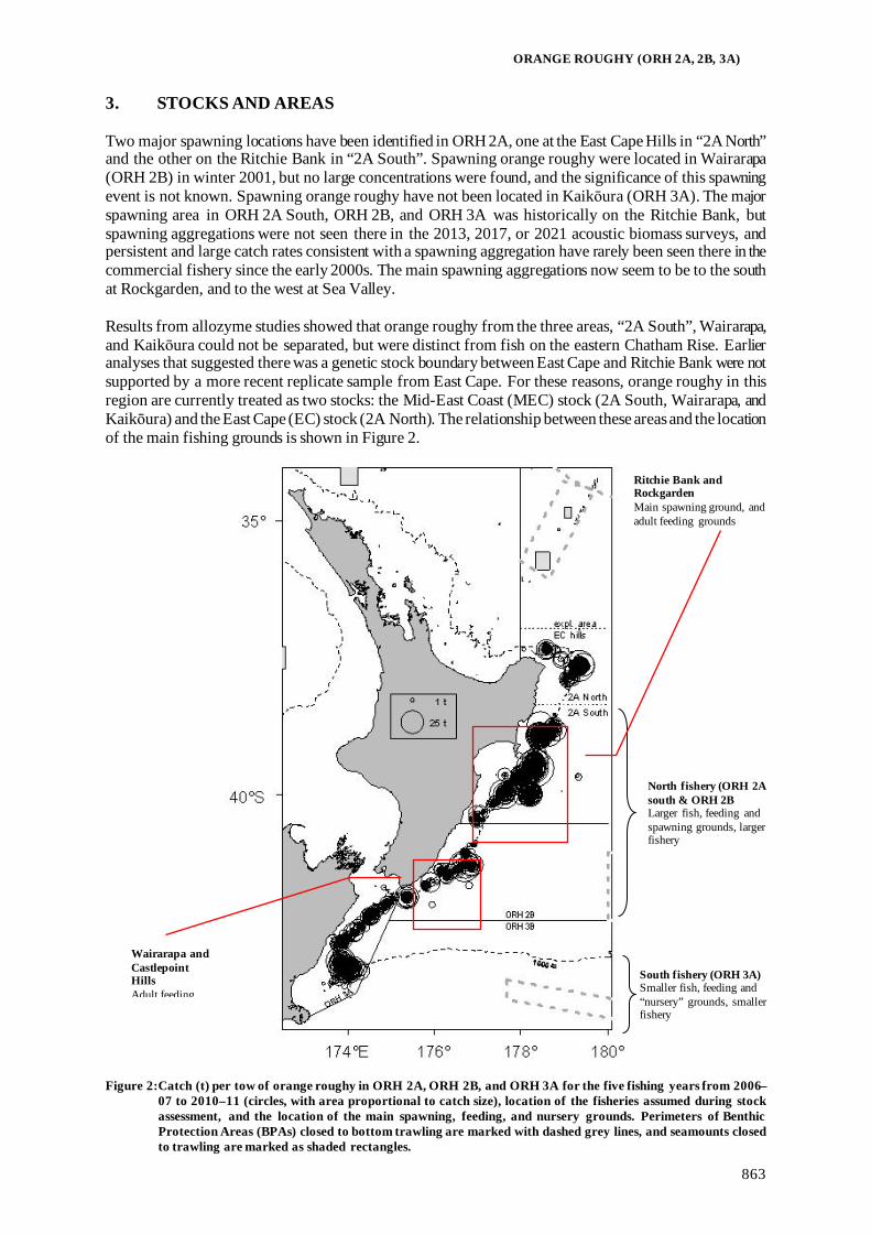
ORANGE ROUGHY (ORH 2A, 2B, 3A)
863
3. STOCKS AND AREAS Two major spawning locations have been identified in ORH 2A, one at the East Cape Hills in “2A North” and the other on the Ritchie Bank in “2A South”. Spawning orange roughy were located in Wairarapa (ORH 2B) in winter 2001, but no large concentrations were found, and the significance of this spawning event is not known. Spawning orange roughy have not been located in Kaikōura (ORH 3A). The major spawning area in ORH 2A South, ORH 2B, and ORH 3A was historically on the Ritchie Bank, but spawning aggregations were not seen there in the 2013, 2017, or 2021 acoustic biomass surveys, and persistent and large catch rates consistent with a spawning aggregation have rarely been seen there in the commercial fishery since the early 2000s. The main spawning aggregations now seem to be to the south at Rockgarden, and to the west at Sea Valley. Results from allozyme studies showed that orange roughy from the three areas, “2A South”, Wairarapa, and Kaikōura could not be separated, but were distinct from fish on the eastern Chatham Rise. Earlier analyses that suggested there was a genetic stock boundary between East Cape and Ritchie Bank were not supported by a more recent replicate sample from East Cape. For these reasons, orange roughy in this region are currently treated as two stocks: the Mid-East Coast (MEC) stock (2A South, Wairarapa, and Kaikōura) and the East Cape (EC) stock (2A North). The relationship between these areas and the location of the main fishing grounds is shown in Figure 2.
Figure 2:Catch (t) per tow of orange roughy in ORH 2A, ORH 2B, and ORH 3A for the five fishing years from 2006–
07 to 2010–11 (circles, with area proportional to catch size), location of the fisheries assumed during stock assessment, and the location of the main spawning, feeding, and nursery grounds. Perimeters of Benthic Protection Areas (BPAs) closed to bottom trawling are marked with dashed grey lines, and seamounts closed to trawling are marked as shaded rectangles.
North fishery (ORH 2A south & ORH 2B Larger fish, feeding and spawning grounds, larger fishery
South fishery (ORH 3A) Smaller fish, feeding and “nursery” grounds, smaller fishery
Wairarapa and Castlepoint Hills Adult feeding
Ritchie Bank and Rockgarden Main spawning ground, and adult feeding grounds

ORANGE ROUGHY (ORH 2A, 2B, 3A)
864
4. STOCK ASSESSMENT Stock assessments are reported below for East Cape (EC) from 2003 and for Mid-East Coast (MEC) from 2022. 4.1 East Cape stock (2A North) The stock assessment for the East Cape was last updated in 2003 and is summarised here (Anderson 2003b). An attempt to update the assessment with a new set of CPUE indices was made in 2006 but was rejected by the Working Group because of changes in the fishery which invalidated the utility of the CPUE series as an index of abundance. With no other abundance estimates available, an updated stock assessment was not possible. 4.1.1 Assessment Inputs A CPUE analysis was performed in 2006 but was considered unreliable because of a change in fishing patterns and fleet size corresponding to the reduction of the catch limit to 200 t in 2000–01. The CPUE analysis was updated in 2011 and was considered more reliable by the Working Group due to the increase in the number of trawls per year since 2006. The 2011 analysis showed that standardised CPUE decreased after a peak in 2003–04 and has subsequently remained at a level similar to that in the late 1990s to early 2000s (Table 5). Previous concerns by the Working Group that the fishery was dominated by a single vessel were alleviated somewhat by the return or entry of three other vessels to the fishery since 2003–04, but the utility of CPUE analyses in fisheries where substantial catch limit reductions have caused major changes in fishing patterns remains an issue for this stock. The model inputs for the 2003 stock assessment were catches, an egg survey, and CPUE indices (Table 5). The biological parameters used are presented in the Biology section at the beginning of the Introduction – Orange roughy chapter. 4.1.2 Stock assessment A stock assessment analysis for the East Cape stock was performed in 2003 using the stock assessment program, CASAL (Bull et al 2002) to estimate virgin and current biomass. • The model was fitted using Bayesian estimation and partitioned the EC stock population by sex,
maturity (the fishery was assumed to act on mature fish only) and age (age-groups used were 1–70, with a plus group).
• The model estimated virgin biomass, B0, and the process error for the CPUE indices. Catchability, q, was treated as a nuisance parameter by the model.
• The stock was considered to reside in a single area, and to have a single maturation episode modelled by a logistic-producing ogive where 50% of fish of both sexes were mature at age 26 and 95% at age 29.
• The catch equation used was the instantaneous mortality equation from Bull et al (2002) whereby half the natural mortality was applied, followed by the fishing mortality, then the remaining natural mortality.
• The size at age model used was the von Bertalanffy. • No stock recruitment relationship was assumed. • A Bayesian estimation procedure was used with a penalty function included to discourage the
model from allowing the stock biomass to drop below a level at which the historical catch could not have been taken.
• Lognormal errors, with known (sampling error) CVs were assumed for the CPUE and egg survey indices. Additionally, process error variance was estimated by the model and added to the CVs from the CPUE indices.
• Confidence intervals were calculated from the posterior profile distribution of B0 estimates, where the process error parameter was fixed at the value previously estimated.

ORANGE ROUGHY (ORH 2A, 2B, 3A)
865
Table 5: Standardised CPUE and egg survey indices, and CVs for the East Cape stock, as used in the 2003 assessment, and an updated standardised CPUE index derived in 2011. -, no data.
CPUE index 2003 CV (%) Egg survey CV (%) CPUE index 2011 CV (%) 1993–94 1.00 12 – – 0.95 23 1994–95 0.69 8 29 000 69 0.76 22 1995–96 0.60 8 – – 0.61 23 1996–97 0.41 8 – – 0.47 22 1997–98 0.25 7 – – 0.27 23 1998–99 0.25 7 – – 0.28 23 1999–00 0.22 9 – – 0.23 23 2000–01 0.21 15 – – 0.28 26 2001–02 0.22 16 – – 0.23 27 2002–03 – – – – 0.51 32 2003–04 – – – – 0.50 30 2004–05 – – – – 0.29 27 2005–06 – – – – 0.37 28 2006–07 – – – – 0.36 29 2007–08 – – – – 0.27 28 2008–09 – – – – 0.24 28 2009–10 – – – – 0.20 27
4.1.3 Biomass estimates Biomass estimates for this stock are given in Table 6 and the biomass trajectories, plotted against the scaled indices, are shown in Figure 3. The base case assessment of the EC stock included only the CPUE indices. An alternative assessment was carried out including the point estimate of biomass from the 1995 egg survey along with the CPUE indices. The CPUE indices agree well with the biomass estimates, with only the 1993–94 and 1997–98 indices departing from the biomass 95% confidence intervals. The egg survey biomass estimate, with the large associated CV, has little effect on the biomass trajectory. Table 6: Estimates of virgin biomass (B0), BMSY (calculated as BMAY, the mean biomass under a CAY policy), and B2003,
for the EC stock (with 95% confidence intervals in parentheses). B2003
Assessment Index B0 (t) BMSY (t) (t) % B0 Base case CPUE 21 100 (19 650–23 350) 6 300 5 100 24 (20–32) Alternative CPUE + Egg survey 21 200 (19 700–23 550) 6 380 5 200 25 (20–33)
The base case estimate of BCURRENT (the mid-year biomass in 2002–03) is 5100 t (24% B0) with a 95% confidence interval of 3800 to 7550 t. This is almost twice the value of B2003 estimated for mid-year 1999–2000 in the previous assessment (Anderson 2000). The alternative assessment gives a very similar estimate of B2003.
Figure 3: Estimated biomass trajectories for the base case and alternative model runs for the EC stock. Annual biomass
estimates are mean posterior density (MPD) values and 95% confidence intervals (grey dashed lines) are calculated from the posterior profile distribution of B0 estimates. The CPUE index CVs (sampling error plus process error) are shown, as is the CV calculated for the egg survey biomass estimate.

ORANGE ROUGHY (ORH 2A, 2B, 3A)
866
4.1.4 Yield estimates and projections Estimates of MCY and CAY for the EC stock were calculated from large numbers of simulation runs using posterior profile sampling of B0 and a series of trial harvest levels. These estimates, together with MAY (the mean catch with a CAY harvesting strategy) and CSP (current surplus production) are given in Table 7. CSP is driven by recruitment of fish spawned before the fishery began. Table 7: Estimates of MCY, CAY, MAY, and CSP for the EC stock, with 95% confidence intervals in parentheses (all
corrected for an assumed overrun of 5%).
Assessment MCY (t) CAY (t) MAY (t) CSP (t) Base case 350 370 410 550 Alternative 350 370 410 550
4.2 Mid-East Coast stock (2A South, 2B, 3A) A new stock assessment was conducted in 2022. The previous assessment was 2014 (Cordue 2014c). There was no new information available that would change the accepted stock definition of the MEC orange roughy stock as comprising ORH 2A South, ORH 2B, and ORH 3A. 4.2.1 Model structure The model was sex and age-structured (1–120 years with a plus group) with sex and maturity in the partition (i.e., fish were classified by age, sex, and as mature or immature). A single area and a single time step were used with four year-round fisheries defined by different selectivities (a “south” fishery catching young fish (double-normal selectivity), a “north” fishery catching older fish (logistic selectivity), a “Pegasus” fishery at the Pegasus Canyon since 1999 (logistic selectivity), and a “Spawn” fishery focused on spawning aggregations (logistic selectivity). The spawning season was assumed to occur after 75% of the mortality and 100% of spawning fish were assumed to spawn each year. The spawning ogive (which defines SSB and may be different from the maturity ogive in orange roughy) was assumed to be the same as the selectivity for the Spawn fishery, and therefore described the age composition of the spawning fish (Spawning Stock Biomass). The catch history was constructed by scaling the catches in Table 1 by the catch overrun percentages in Table 4 and partitioning using estimated catch and effort data (Table 8). Catches for 2021–22 were assumed to be same as 2020–21. Natural mortality was assumed to be fixed at 0.045 and the stock-recruitment relationship was assumed to follow a Beverton-Holt function with steepness of 0.75. Growth was modelled by sex and used empirical length-at-age (Figure 4). An ageing error of 0.1 was assumed. All fitted observations were unsexed. Table 8: Mid-East Coast orange roughy catch (t) history by fishery, including catch overruns, as used in the 2022 stock
assessment model.
Fishing year Spawn North South Pegasus
Fishing year Spawn North South Pegasus 1981–82 0 153 567 0
2002–03 201 446 181 101
1982–83 38 1 000 3 854 0
2003–04 250 370 223 86 1983–84 214 2 025 7 414 0
2004–05 356 677 371 141
1984–85 2 000 2 599 6 738 0
2005–06 518 497 346 157 1985–86 2 907 2 689 5 323 0
2006–07 409 661 368 144
1986–87 4 132 3 744 3 605 0
2007–08 459 586 411 128 1987–88 4 753 4 272 3 578 0
2008–09 460 597 329 158
1988–89 4 224 3 883 3 613 0
2009–10 512 563 289 163 1989–90 4 871 3 484 4 266 0
2010–11 533 549 238 238
1990–91 3 424 4 500 3 562 0
2011–12 591 240 339 154 1991–92 4 371 3 681 3 057 0
2012–13 374 290 195 124
1992–93 4 570 2 749 2 606 0
2013–14 499 138 217 163 1993–94 2 493 2 095 2 632 0
2014–15 229 69 143 39
1994–95 3 097 1 221 1 688 0
2015–16 275 73 120 75 1995–96 925 419 640 0
2016–17 157 197 143 79
1996–97 1 126 477 626 0
2017–18 128 199 117 21 1997–98 859 835 658 0
2018–19 269 105 120 23
1998–99 638 1 108 492 149
2019–20 132 132 118 41 1999–00 1 154 809 488 192
2020–21 225 120 89 118
2000–01 592 723 366 158
2021–22 225 120 89 118 2001–02 637 452 383 83

ORANGE ROUGHY (ORH 2A, 2B, 3A)
867
Figure 4: Mid-East Coast orange roughy median length-at-age by sex estimated using a smoother and the length-weight
relationship used in the assessment model. The parameters are of the length (L) to weight (W) relationship W = aLb. The red line represents females and the dashed blue line represents males.
4.2.2 Input data and statistical assumptions There were four main data sources for observations fitted in the assessment: spawning biomass estimate from acoustic surveys (2013, 2017, and 2021); a trawl survey time series of relative biomass indices (1992–1994, 2010) with associated age frequencies (1993 and 2010) and length frequencies (1992, 1994), age frequencies from the Spawn fishery (commercial 1989, 1990, 1991 and 2010; research 2017 and 2021), and length frequencies (LFs) collected from the commercial fisheries. Estimates of proportions mature-at-age were used in the previous assessment (2014) but excluded in 2022 because they were inconsistent with the spawning age frequencies. Research surveys The MEC area has been surveyed using acoustic and trawl methods, and egg surveys have also been conducted. Not all survey data were used in the 2022 assessment. The egg survey estimates have some quality issues associated with them; the 1993 survey data were post-stratified and “corrected” for turnover of fish (Zeldis et al 1997). The 1993 egg survey estimate was used in the 2013 assessment but was not considered to be reliable enough for assessments since 2014 (which had a higher “quality threshold”). Similarly, the wide-area acoustic survey estimates from 2001 and 2003 (Doonan et al 2003, 2004a) have been rejected since 2014 as being not sufficiently reliable (in particular, the biomass estimates primarily came from mixed species marks and “orange roughy” marks identified subjectively; rather than being from easily identified spawning plumes). Trawl survey data A time series of pre-spawning season, random, stratified trawl surveys were conducted in March–April on RV Tangaroa in 1992–94 and 2010 (Grimes et al 1994, 1996a, 1996b; Doonan & Dunn 2011). The 2010 survey was specifically designed to be comparable with the earlier surveys and to produce an abundance index for the MEC home grounds (Doonan & Dunn 2011). In addition to the relative biomass indices (Table 9), the survey data were analysed to produce length frequencies from all years and age frequencies from 1993 and 2010 (Doonan et al 2011). Table 9: Mid-East Coast orange roughy biomass indices and CVs used in the 2022 stock assessment.
Year Trawl index (t) CV (%) Acoustic index (t) CV (%) 1992 20 838 29 1993 15 102 27 1994 12 780 14 2010 7 074 19 2013 4 225 20 2017 6 969 14 2021 6 326 20

ORANGE ROUGHY (ORH 2A, 2B, 3A)
868
The biomass indices were fitted as relative biomass with a double-normal selectivity on the immature fish, and a constant selectivity on the mature fish, with an uninformed prior on the proportionality constant (q). A process error of 20% was added to the CVs. The length frequencies from 1992 and 1994 were fitted as multinomial, as were the age frequencies from 1993 and 2010 (length frequencies from 1993 and 2010 had been used in the production of the age frequencies). Acoustic survey estimate The only reliable acoustic estimates of spawning biomass for MEC came from multi-frequency “AOS” surveys (acoustic and optical gear mounted on the trawl headline, e.g., see Kloser et al. 2011). Four areas were visited in 2013, but the only substantial spawning plume was seen in the “Sea Valley”. A similar search for spawning aggregations was completed in 2017 and 2021, when spawning plumes were found at both Sea Valley and Rockgarden. All valid snapshot estimates from 38 kHz were averaged to produce the biomass index (see Table 9). No process error was added to the CVs. A base assumption used for all orange roughy acoustic spawning biomass estimates was that they collectively covered “most” of the spawning biomass, where “most” was taken to be 80%. The previous (2014) assessment for the Mid-East Coast stock reduced this to 60%. Because 2017 and 2021 surveys searched all known substantial spawning grounds for Mid-East Coast orange roughy, in 2022 “most” was revised back to 80%, and sensitivities were conducted for 60% and 100%. The acoustic estimates were therefore fitted as relative biomass with an informed prior: lognormal (mean = 0.8, CV = 19%) for the base model. Commercial age and length frequencies Twelve length frequencies between 1991 and 2018 were available for the North fishery, four between 1994 and 2016 for the South fishery, seven between 1990 and 2017 for the Spawn fishery, and two samples, in 2000 and 2016, for the Pegasus fishery. For the Spawn fishery, the length frequency (seven LFs between 1990 and 2017) and age frequency (AF) samples (five AFs from 1989–91, 2010, and 2017) were assumed to represent spawning fish, with selectivity set equal to estimated logistic maturity. The spawning age frequency from 2021 contained a greater proportion of younger fish and was inconsistent with the earlier samples, and so was fitted with its own logistic selectivity. The composition data were all assumed to be multinomial, with effective sample sizes initially based upon Cordue (2014a) for age frequencies, and the number of tows for LFs, but then down-weighted to ensure primacy of the biomass data and more balanced patterns of residuals. Final effective samples sizes for the Spawn AFs were between 13 and 25 (mean 20), the trawl survey AFs were 20, and the LFs were between 1 and 10 (mean 3.2). 4.2.3 Model runs and results In the base model, natural mortality (M) was fixed at 0.045 yr-1. There were numerous MPD sensitivity runs and three main sensitivities are presented in this chapter: M = 0.035 yr-1; mean acoustics q prior = 0.6; and mean acoustics q prior = 1.0. The latter assumed all the spawning biomass was observed by the acoustic surveys. In the base model, the main parameters estimated were virgin spawning stock biomass (SSB0), the spawning ogive, three fishery selectivities (North, South, Pegasus), the trawl survey selectivities (immature and mature), the 2021 age frequency selectivity, and year class strengths (YCS) from 1881 to 1996 (with the Haist parameterisation and lognormal priors with CV=0.8). Additional estimated parameters were the CV of the length-at-age parameters and the proportionality constants (qs) for the trawl survey time series and the acoustic biomass estimates. Model fits The MPD fits to data were similar to the MCMC implied fits. The fits to the biomass indices were acceptable, although the decline in the trawl surveys could not be fitted well (Figure 5).

ORANGE ROUGHY (ORH 2A, 2B, 3A)
869
Figure 5: Mid-East Coast orange roughy MPD fit to biomass indices for the base model run: left: acoustic spawning
biomass indices (estimated q of 0.68); right: Tangaroa trawl survey indices. Vertical broken lines are 95% CIs.
The spawning season age frequencies were noisy, but the general shape was fitted well (Figure 6). The fit to the trawl survey age frequencies was good (Figure 6). The MPD fits to the commercial length frequencies were adequate considering the length frequencies showed substantial year-to-year variability (Figure 7). The spawning ogive (which was different from the maturity ogive) was estimated with an A50 of 55.2 years and Ato95 of 18.1 years. The spawning season age frequency for 2021 had a greater proportion of younger fish, with an A50 of 35.6 years and Ato95 of 11.0 years. The age of 50% maturity of orange roughy has been estimated from transition zones on otoliths to be at around 30 years, but assessments have shown that the age of 50% spawning is typically greater. One hypothesis to explain this difference is skipped spawning, where younger mature fish spawn less often. The relatively high proportion of young mature fish observed for 2021 could have been sample bias, or a due to a temporal change in the prevalence of skipped spawning. A separate selectivity was used for this age frequency. MPD model runs showed that the results were relatively insensitive to changes in the growth model, alternative CVs on the year class strength priors, changes to the weight given to the length frequencies, and alternative selectivity models for the trawl survey data. Simplifying the model to have two fisheries, following the previous assessment (2014), estimated a larger stock at a similar level of depletion, but incurred catch penalties with a poorer fit to data and less plausible YCS and biomass trends. Assuming a higher M of 0.06 year-1 estimated a smaller and less depleted stock but fitted the data less well, with several implausible selectivity parameters. Using the 2021 spawn age frequency and proportion mature data (as used in 2014) to estimate spawning selectivity, with a separate selectivity then used for the base model “spawn” fishery, estimated a larger and more depleted stock, with a markedly poorer fit to data. MPD runs across a range of M and stock-recruitment steepness values indicated the base assumption of M was supported by data, and could plausibly be a little lower, and that the model had no information to determine steepness. A sensitivity run estimating M was not completed because of the noisy age data with substantial uncertainties in the spawning and fishery selectivity ogives.

ORANGE ROUGHY (ORH 2A, 2B, 3A)
870
Figure 6: Mid-East Coast orange roughy MPD fits of the base model run to age frequencies (N is the assumed effective
sample size). Observations are grey points; model predictions are the black lines.
Figure 7: Mid-East Coast orange roughy base model example MPD fits to length frequencies (N is the assumed effective
sample size). Observations are grey points; model predictions are the black lines.

ORANGE ROUGHY (ORH 2A, 2B, 3A)
871
MCMC results MCMC convergence diagnostics were acceptable for the base model and sensitivities. In all model runs, the spawning stock biomass was reduced through the 1980s to below 10% SSB0 in the 1990s, and then slowly rebuilt. Virgin spawning biomass (SSB0) was estimated to be about 53 000 t for the base case, and the current stock status 22% SSB0 (Table 10). When the mean of the acoustic q was reduced (q = 0.6), the spawning stock was estimated to be slightly larger and currently less depleted, and vice versa when the higher q was assumed (q = 1.0). The base and acoustic q sensitivity runs all estimated the current stock status to be at or above the soft limit (20% SSB0). Assuming a lower M estimated a larger SSB0 and stock status just below the soft limit. Table 10: Mid-East Coast orange roughy MCMC estimates of virgin spawning biomass (SSB0) and stock status (SSB2022
as % SSB0), and overall vulnerable biomass (VB0) and status (VB2022 as % VB0) calculated assuming a logistic selectivity with parameters averaged from base model run MPD selectivity estimates, for the base model and the three sensitivity runs: a) reducing the mean acoustic catchability coefficient, q, from 0.8 to 0.6; b) increasing the mean acoustic q from 0.8 to 1.0; c) decreasing M to 0.035 year-1.
Spawning biomass Assessment SSB0 (000 t) 95% CI SSB2022 (% SSB0) 95% CI Base model 53 350 46 550 – 63 670 22.4 16.7 – 29.2 Acoustic q = 0.6 57 590 49 070 – 69 120 26.3 20.2 – 33.5 Acoustic q = 1.0 51 280 45 480 – 60 010 19.8 14.7 – 26.4 M = 0.035 69 060 60 340 – 79 860 16.7 12.2 – 22.1 Vulnerable biomass Assessment VB0 (000 t) 95% CI VB2022 (% VB0) 95% CI Base model 144 720 121 180 – 171 900 47.0 31.8 – 66.6 Acoustic q = 0.6 149 390 122 160 – 178 370 52.8 37.4 – 72.6 Acoustic q = 1.0 143 170 118 310 – 171 430 44.0 30.2 – 62.1 M = 0.035 136 130 114 500 – 156 910 36.3 23.3 – 51.7
The estimates of stock size and status were relatively precise given that some selectivities were relatively poorly estimated, particularly for the South fishery, the mature fish in the trawl survey, and the Spawn 2021 age frequency. A sensitivity run was completed with normal priors placed on the parameters of the South fishery selectivity, with mean values taken from the MPD estimates and assumed CVs, and while this prevented the improbable capture of very young fish it made almost no difference to the estimates of stock size and status. The use of model estimates to construct priors for use in the same model is statistically incorrect, so the base run was preferred. Orange roughy were estimated to first recruit to the South fishery, then the Pegasus and North fisheries, and then the Spawn fishery (Figure 8). The spawning ogive was relatively precisely estimated, indicating spawning started at about age 40 and all fish spawned by about age 80. Assuming a logistic selectivity with parameters averaged from base model run MPD estimates, the overall vulnerable biomass (VB0) did not decline as much as the spawning biomass, reaching just below 40% VB0 in the late 1990s and then slowly rebuilding (Table 10, Figure 9). The biomass vulnerable to the southern fisheries, where recruitment was at a younger age, declined to about 50% and then remained steady from the early 2000s until the last five years, when it slowly declined. The recent decline in vulnerable biomass for the South fishery (VBs) was because recruitment was estimated to be approaching an historical low, caused by the reduction of the spawning biomass in the 1980s (Figure 10). The estimated YCS showed a slight decrease from about 1940, a peak around 1970, and then lowest levels of YCS between 1980 and 1993 with a minimum in 1989 (Figure 10).

ORANGE ROUGHY (ORH 2A, 2B, 3A)
872
Figure 8: Mid-East Coast orange roughy base case MCMC estimates of selectivities and the spawning ogive. The
estimated selectivity model parameters (and 95% credible intervals) are shown on each panel. The light shaded area covers the 95% credible intervals, the darker shaded area the 50% credible intervals, and the solid line the median.

ORANGE ROUGHY (ORH 2A, 2B, 3A)
873
Figure 9: Mid-East Coast orange roughy base case MCMC estimates of upper panels: the Spawning Stock Biomass
(SSB), and vulnerable biomass trends estimated using logistic selectivity parameters averaged across all fisheries (average vulnerable biomass, VB0; A50 = 34, Ato95 = 8), and in the southern fisheries (South and Pegasus, VBs; A50 = 24, Ato95 = 2). Lower panels, biomass in each year as a proportion of initial biomass. The light shaded area covers the 95% credible intervals, the darker shaded area the 50% credible intervals, and the solid line the median. The horizontal broken lines indicate the hard limit (10% of virgin biomass), soft limit (20% of virgin biomass), and 40% of virgin biomass.
Figure 10: Mid-East Coast orange roughy base case MCMC estimates “true” YCS (Ry/R0). Upper panel: The light
shaded area covers the 95% credible intervals, the darker shaded area the 50% credible intervals, the solid black line the median, and the solid red line the mean. The vertical blue line (to the right) indicates the year class estimated to by 50% recruited to the Pegasus fishery in 2022 (the second largest fishery, after the spawn fishery, in 2022). The vertical red line (to the left) indicates the year class 50% recruited to the spawning stock in 2022. Lower panel: mean “true” YCS.
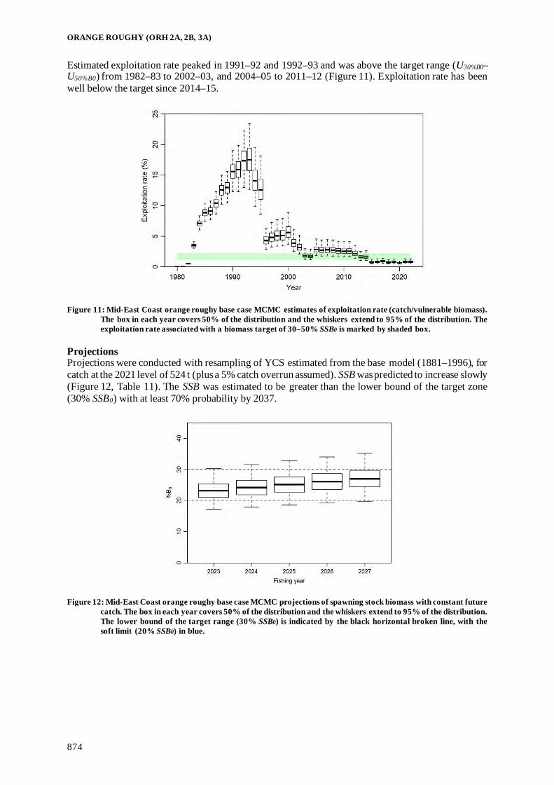
ORANGE ROUGHY (ORH 2A, 2B, 3A)
874
Estimated exploitation rate peaked in 1991–92 and 1992–93 and was above the target range (U30%B0–U50%B0) from 1982–83 to 2002–03, and 2004–05 to 2011–12 (Figure 11). Exploitation rate has been well below the target since 2014–15.
Figure 11: Mid-East Coast orange roughy base case MCMC estimates of exploitation rate (catch/vulnerable biomass).
The box in each year covers 50% of the distribution and the whiskers extend to 95% of the distribution. The exploitation rate associated with a biomass target of 30–50% SSB0 is marked by shaded box.
Projections Projections were conducted with resampling of YCS estimated from the base model (1881–1996), for catch at the 2021 level of 524 t (plus a 5% catch overrun assumed). SSB was predicted to increase slowly (Figure 12, Table 11). The SSB was estimated to be greater than the lower bound of the target zone (30% SSB0) with at least 70% probability by 2037.
Figure 12: Mid-East Coast orange roughy base case MCMC projections of spawning stock biomass with constant future catch. The box in each year covers 50% of the distribution and the whiskers extend to 95% of the distribution. The lower bound of the target range (30% SSB0) is indicated by the black horizontal broken line, with the soft limit (20% SSB0) in blue.

ORANGE ROUGHY (ORH 2A, 2B, 3A)
875
Table 11: Mid-East Coast orange roughy MCMC estimates of projected spawning stock biomass (SSB) for the base model, and the probability of above the hard limit (10% SSB0), soft limit (20% SSB0), and lower bound of the target range (30% SSB0).
p(SSB<X% SSB0) Fishing year X=10% X=20% p(SSB>30% B0) 2021–22 0.00 0.21 0.01 2022–23 0.00 0.16 0.03 2023–24 0.00 0.10 0.05 2024–25 0.00 0.06 0.09 2025–26 0.00 0.04 0.15 2026–27 0.00 0.03 0.23
5. FUTURE RESEARCH CONSIDERATIONS Relationship between maturity and spawning and prevalence of skipped spawning
• The estimated age of 50% spawning was unexpectedly high (about 55 years) given that orange roughy have generally been estimated to have an age of 50% maturity of about 30–35 years. To be plausible, the later age of 50% spawning relative to maturity requires an assumption of skipped spawning that is more prevalent in younger fish. There is theoretical support for this assumption and evidence from Mid-East Coast trawl survey gonad samples that not all female Mid-East Coast orange roughy were spawning by age 50.
o The theoretical expectations for skipped spawning, and the availability of existing data to inform skipped spawning estimates, need to be investigated.
o A simulation model to investigate the skipped spawning hypothesis should be constructed.
Collection of biological data including aged otoliths
• Additional biological samples should be collected, including maturity evaluations and aged otoliths, to better inform assumptions about maturity and spawning. Because variability in biological characteristics seems to be greater between than within catches, sample collection should focus on collecting adequate samples from many catches (including surveys). Sampling across years is also required to allow temporal variability in the age structure of spawning aggregations, and potential skipped spawning, to be investigated.
• Obtain more data on macroscopic versus histological staging for a range of known ages including those beyond 50. Ensure historical data are fully utilised.
• Obtain further samples from research or commercial trawls to investigate maturity outside the main spawning areas. Review the overall approach to collecting age frequencies, length frequencies, and maturity data both from spawning and non-spawning fisheries, and research surveys and commercial fisheries to improve coverage and representativeness.
• Collect age data from both acoustic and commercial catches in the same year. Stock structure
• Review the existing information with respect to stock structure, including genetic, morphometric, and other information, including from adjacent stock areas. This review could then be used to guide the development of stock structure assumptions in assessment models.
Age frequencies for commercial fisheries
• The estimates of selectivity for three of the four fisheries in the 2022 assessment model were informed only by length frequency samples, and estimated selectivity parameters were particularly uncertain. Aged otolith samples from the non-spawning fisheries are needed to improve these estimates of fishery selectivity.
• Re-age the 2002 otolith samples using the new protocol.

ORANGE ROUGHY (ORH 2A, 2B, 3A)
876
Loss of some historical spawning aggregations
• Some historical spawning aggregations have been depleted, and no longer seem to occur. For the Mid-East Coast, this includes the aggregation on Strawberry Mountain. The relationship between different spawning aggregations within the same assumed stock, and the implications of the loss of spawning aggregations for orange roughy and the wider ecosystem, should be investigated.
Catch history
• Investigate whether alternative assumptions about historical catches could result in better model fits, posteriors, and other outputs, specifically with reference to uncertainty in catch overruns relating to discarding and lost fish.
CPUE
• The existing fisheries catch and -effort data are not considered to be useful for generating a relative abundance index for this stock. However, given the sparsity of relative abundance information from formal surveys, an exploration of existing fisheries catch rate information, standardising for the effects of vessel, month, and location, etc., may yield longer time series of abundance information for specific locations that can be used to compare with model outputs.
Fishing intensity
• Reconsider how a consistent, combined U or F is best calculated. East Cape stock assessment
• Options for updating the assessment of ORH 2A North (East Cape) should be investigated. 6. STATUS OF THE STOCKS Stock Structure Assumptions Orange roughy in ORH 2A, 2B, and 3A are treated as two biological stocks based on the location of spawning grounds. These stocks are managed and assessed separately, however some genetic mixing has been shown to occur. The 2A North stock spawns around the East Cape hills off of the North Island. The 2A South, 2B, and 3A stock is assumed to spawn on Ritchie Bank and surrounding areas (Rockgarden, Sea Valley). • ORH East Cape Stock (2A North) Stock Status Year of Most Recent Assessment 2003 Assessment Runs Presented A base case with one alternative Reference Points
Management Target: 30–50% B0 Soft Limit: 20% B0 Hard Limit: 10% B0
Overfishing threshold:- Status in relation to Target B2003 was 24% B0, which was Unlikely (< 40%) to be at or
above the target. Status in relation to Limits B2003 was Unlikely (< 40%) to be below the Soft Limit, and
Very Unlikely (< 10%) to be below the Hard Limit

ORANGE ROUGHY (ORH 2A, 2B, 3A)
877
Historical Stock Status Trajectory and Current Status
Estimated biomass trajectory for the base model run for the EC stock. Annual biomass estimates are mean posterior density (MPD) values and 95% confidence intervals (grey dashed lines) are calculated from the posterior profile distribution of B0 estimates. The CPUE index CVs (sampling error plus process error) are shown.
Fishery and Stock Trends Recent Trend in Biomass or Proxy Biomass declined in the early 1990s but appeared to
stabilise at around 5000 t. Recent Trend in Fishing Mortality or Proxy
F has declined along with the agreed catch limit and remains stable at the current catch level of 200 t.
Other Abundance Indices - Trends in Other Relevant Indicators or Variables
-
Projections and Prognosis (2003) Stock Projections or Prognosis The estimated CAY (370 t) and MAY (410 t) were both greater
than the catch limit of 200 t, and this suggested the stock would start to rebuild.
Probability of Current Catch or TACC causing Biomass to remain below or to decline below Limits
Soft Limit: Unlikely (< 40%) Hard Limit: Very Unlikely (< 10%)
Probability of Current Catch or TACC causing Overfishing to continue or to commence
-
Assessment Methodology and Evaluation Assessment Type Level 1 – Full Quantitative Stock Assessment Assessment Method Statistical catch-at-age model implemented in CASAL with
Bayesian estimation of posterior distributions Assessment Dates Latest assessment: 2003 Next assessment: Unknown Overall assessment quality rank - Main data inputs - Catch
- Standardised CPUE - 1994–95 egg survey
Data not used (rank) - Changes to Model Structure and Assumptions
-
Major Sources of Uncertainty -

ORANGE ROUGHY (ORH 2A, 2B, 3A)
878
Qualifying Comments The most recent assessment (2003) is now 11 years out-of-date. In recent years, the ability of stock assessment models that assume deterministic recruitment for orange roughy stocks to reflect current or projected stock status has been called into question.
Fishery Interactions The main bycatch species are cardinalfish and alfonsino. Low productivity bycatch species include deepwater sharks, deepsea skates, and corals. Protected species bycatch includes seabirds and corals.
• ORH Mid-East Coast Stock (2A South, 2B, 3A)
Stock Status Year of Most Recent Assessment 2022 Assessment Runs Presented Base model Reference Points
Management Target: Biomass range 30–50% B0
Soft Limit: 20% B0 Hard Limit: 10% B0
Overfishing threshold: Fishing intensity range U30%B0–U50%B0 Status in relation to Target B2022 was estimated to be 22% B0
Very Unlikely (< 10%) to be at or above the lower end of the management target range
Status in relation to Limits B2022 is About as Likely as Not (40–60%) to be below the Soft Limit B2022 is Unlikely (< 40%) to be below the Hard Limit
Status in relation to Overfishing Fishing intensity in 2022 was estimated to be 0.8% (37% of U30%B0) Overfishing is Very Unlikely (< 10%) to be occurring
Historical Stock Status Trajectory and Current Status
Historical trajectory over time of exploitation rate (U) and spawning biomass (% B0), for the Mid-East Coast orange roughy base model, from the start of the fishery (represented by a red point), to 2022. The red vertical line at 10% B0 represents the hard limit, the orange line at 20% B0 is the soft limit, and green shaded areas are the % B0 target (30–50% B0) and the corresponding exploitation rate (U30– U50). Biomass and exploitation rate estimates are medians from MCMC results.

ORANGE ROUGHY (ORH 2A, 2B, 3A)
879
Fishery and Stock Trends Recent Trend in Biomass or Proxy Estimated spawning biomass has been slowly increasing since
about 2000. Average vulnerable biomass has also been increasing over the same period.
Recent Trend in Fishing Intensity or Proxy
Estimated fishing intensity has been low and stable since 2014–15.
Other Abundance Indices - Trends in Other Relevant Indicators or Variables -
Projections and Prognosis Stock Projections or Prognosis At the current catch limit, the stock is projected to increase
slowly over the next five years and to be above the soft limit but below the lower bound of the target in 2027.
Probability of Current Catch or TACC causing Biomass to remain below or to decline below Limits
For the current catch and catch limit (over the next 5 years): Soft Limit: Unlikely (< 40%) Hard Limit: Very Unlikely (< 10%)
Probability of Current Catch or TACC causing Overfishing to continue or to commence
For the current catch and catch limit: Very Unlikely (< 10%)
Assessment Methodology and Evaluation Assessment Type Level 1 - Full Quantitative Stock Assessment Assessment Method Age-structured CASAL model with Bayesian estimation of
posterior distributions Assessment Dates Latest assessment: 2022 Next assessment: 2025 Overall assessment quality rank 1 – High Quality Main data inputs (rank) - Acoustic biomass estimates (2013, 2017,
2021) - Trawl survey biomass indices (1992–94, 2010), age frequencies (1993, 2010), length frequencies (1992, 1994), proportion spawning at age (1993, 2010) - Spawning season age frequencies (1989–91, 2010, 2017, 2021) - Commercial length frequencies (1989–90 to 2017–18)
1 – High Quality 1 – High Quality 1 – High Quality 1 – High Quality
Data not used (rank) - CPUE indices - 2002 spawning season age frequency - Wide-area acoustic estimates - Egg survey estimates
3 – Low Quality: unlikely to be indexing stock-wide abundance 2 – Medium or Mixed Quality: needs to be re-aged with new protocol 2 – Medium or Mixed Quality: too much potential bias due to target identification and mixed species issues 2 – Medium or Mixed Quality: too much potential bias due to survey design assumptions not being met
Changes to Model Structure and Assumptions
- Four fisheries instead of two, including a spawning fishery - Spawning ogive set equal to the spawning fishery selectivity (with an assumption of mature fish skipping spawning) - CV of YCS prior set at 0.8, rather than “nearly uniform” - Acoustic q mean set in the base case at 0.8 rather than 0.6 - Growth parameters have been updated - Sex is now included in the partition, but only for estimating

ORANGE ROUGHY (ORH 2A, 2B, 3A)
880
growth - Trawl survey fitted with double-normal (immature) and constant (mature) selectivity
Major Sources of Uncertainty - The proportion of the spawning stock biomass that was indexed by the acoustic surveys - Recent recruitment, where a lack of observational data meant year class strengths were assumed to be average since 1997 - The age-specific proportion of mature fish that spawn - Spatial population structure - Historical catches uncertain
Qualifying Comments - Fishery Interactions Fish bycatch is estimated to make up about 20% of the total catch in this fishery. The main bycatch species are alfonsino, smooth oreo, and hoki. Low productivity bycatch species include deepwater sharks, deepsea skates, and corals. Observed incidental captures of protected species include corals, low numbers of seabirds, and a New Zealand fur seal. Orange roughy are caught using bottom trawl gear. Bottom trawling interacts with benthic habitats.
6. FOR FURTHER INFORMATION Anderson, O F (2000) Assessment of the East Cape hills (ORH 2A North) orange roughy fishery for the 2000–01 fishing year. New Zealand
Fisheries Assessment Report 2000/19. 29 p. Anderson, O F (2003a) A summary of biological information on the New Zealand fisheries for orange roughy (Hoplostethus atlanticus) for
the 2001–02 fishing year. New Zealand Fisheries Assessment Report 2003/21. 25 p. Anderson, O F (2003b) CPUE analysis and stock assessment of the East Cape hills (ORH 2A North) orange roughy fishery for 2003. New
Zealand Fisheries Assessment Report 2003/24. 20 p. Anderson, O F (2005) CPUE analysis and stock assessment of the South Chatham Rise orange roughy fishery for 2003–04. New Zealand
Fisheries Assessment Report. 2005/07. Anderson, O F; Dunn, M R (2007a) Descriptive analysis of catch and effort data from New Zealand orange roughy fisheries in ORH 1, 2A,
2B, 3A, 3B, and 7B to the end of the 2003–04 fishing year. New Zealand Fisheries Assessment Report. 2006/20. Anderson, O F; Dunn, M R (2007b) Descriptive analysis of catch and effort data from New Zealand orange roughy fisheries in ORH 1, 2A,
2B, 3A, 3B, and 7B to the end of the 2004–05 fishing year. New Zealand Fisheries Assessment Report. 2007/29. Anderson, O F; Francis, R I C C; Hicks, A C (2002) CPUE analysis and assessment of Mid-East Coast orange roughy stock (ORH 2A South,
2B, 3A). New Zealand Fisheries Assessment Report 2002/56. 23 p. Bull, B; Francis, R I C C; Dunn, A; Gilbert, D J (2002) CASAL (C++ algorithmic stock assessment laboratory): CASAL user manual
v1.02.2002/10/21. NIWA Technical Report 117. 199 p. Bull, B; Francis, R I C C; Dunn, A; Gilbert, D J; Bian, R; Fu, D (2012) CASAL (C++ algorithmic stock assessment laboratory): CASAL User
Manual v2.30-2012/03/21. NIWA Technical Report 135. 280 p. Clark, M; Anderson, O; Dunn, M (2003) Descriptive analysis of catch and effort data from New Zealand orange roughy fisheries in ORH 1,
2A, 2B, 3A, 3B, and 7B to the end of the 2001–02 fishing year. New Zealand Fisheries Assessment Report 2003/60. 51 p. Clark, M R; Taylor, P; Anderson, O F; O’Driscoll, R (2002) Descriptive analysis of catch and effort data from New Zealand orange roughy
fisheries in ORH 1, 2A, 2B, 3A, 3B, and 7B to the end of the 2000–01 fishing year. New Zealand Fisheries Assessment Report. 2002/62.
Cordue, P L (2012) Fishing intensity metrics for use in overfishing determination. ICES Journal of Marine Science, 69: 615–623 Cordue, P L (2014a) A 2013 stock assessment of Mid-East Coast orange roughy. New Zealand Fisheries Assessment Report 2014/32. Cordue, P L (2014b) A Management Strategy Evaluation for orange roughy. ISL Client Report for Deepwater Group. (Unpublished report
held by Fisheries New Zealand, Wellington.) Cordue, P L (2014c) The 2014 orange roughy stock assessments. New Zealand Fisheries Assessment Report 2014/50. 135 p. Cordue, P L (2017) A stock assessment update to the end of the 2017–18 fishing year for the Mid-East Coast orange roughy stock. ISL Client
Report for Deepwater Group. 45 p. Doonan, I J (1994) Life history parameters of orange roughy: estimates for 1994. New Zealand Fisheries Assessment Research Document
1994/19. 13 p. (Unpublished document held by NIWA library, Wellington.) Doonan, I J; Coburn, R P; Hart, A C (2004a) Acoustic estimates of the abundance of orange roughy for the Mid-East Coast fishery, June 2003.
New Zealand Fisheries Assessment Report 2004/54. 21 p. Doonan, I J; Dunn, M R (2011) Trawl survey of Mid-East Coast orange roughy, March-April 2010. New Zealand Fisheries Assessment Report
2011/20. Doonan, I J; Hicks, A C; Coombs, R F; Hart, A C; Tracey, D (2003) Acoustic estimates of the abundance of orange roughy in the Mid-East
Coast fishery, June–July 2001. New Zealand Fisheries Assessment Report 2003/4. 22 p. Doonan, I J; Horn, P L; Krusic-Golub, K (2013) Comparison of age between 1993 and 2010 for mid-east coast orange roughy (ORH 2Asouth,
2B & 3A). New Zealand Fisheries Assessment Report 2013/44. Doonan, I J; Tracey, D M; Grimes, P J (2004b) Relationships between macroscopic staging and microscopic observations of oocyte
progression in orange roughy during and after the mid-winter spawning period, Northwest Hills, Chatham Rise, July 2002. New Zealand Fisheries Assessment Report 2004/6. 28 p.
Dunn, M R (2005) CPUE analysis and assessment of the Mid-East Coast orange roughy stock (ORH 2A South, 2B, 3A) to the end of the 2002–03 fishing year. New Zealand Fisheries Assessment Report 2005/18. 35 p.

ORANGE ROUGHY (ORH 2A, 2B, 3A)
881
Dunn, M R; Anderson, O F; McKenzie, A (2005) Descriptive analysis of catch and effort data from New Zealand orange roughy fisheries in ORH 1, 2A, 2B, 3A, 3B, and 7B to the end of the 2002–03 fishing year. New Zealand Fisheries Assessment Report 2005/19. 60 p.
Field, K D; Francis, R I C C; Zeldis, J R; Annala, J H (1994) Assessment of the Cape Runaway to Banks Peninsula (ORH 2A, 2B, and 3A) orange roughy fishery for the 1994–1995 fishing year. New Zealand Fisheries Assessment Research Document 1994/20. 24 p. (Unpublished document held by NIWA library, Wellington.)
Francis, R I C C (1992) Recommendations concerning the calculation of maximum constant yield (MCY) and current annual yield (CAY). New Zealand Fisheries Assessment Research Document 1992/8. 27 p. (Unpublished document held by NIWA library, Wellington.)
Francis, R I C C (2011) Data weighting in statistical fisheries stock assessment models. Canadian Journal of Fisheries and Aquatic Sciences 68: 1124–1138.
Francis, R I C C; Clark, M R; Coburn, R P; Field, K D; Grimes, P J (1995) Assessment of the ORH 3B orange roughy fishery for the 1994–95 fishing year. New Zealand Fisheries Assessment Research Document 1995/4. 43 p. (Unpublished document held by NIWA library, Wellington.)
Francis, R I C C; Field, K D (2000) CPUE analysis and assessment of the Mid-East Coast orange roughy stock (ORH 2A South, 2B, 3A). New Zealand Fisheries Assessment Report 2000/29. 20 p.
Francis, R I C C; Horn, P L (1997) Transition zone in otoliths of orange roughy (Hoplostethus atlanticus) and its relationship to the onset of maturity. Marine Biology 129: 681–687.
Francis, R I C C; Hurst, R J; Renwick, J A (2001) An evaluation of catchability assumptions in New Zealand stock assessments. New Zealand Fisheries Assessment Report 2001/1. 37 p.
Grimes, P (1994) Trawl survey of orange roughy between Cape Runaway and Banks Peninsula, March–April 1992 (TAN9203). New Zealand Fisheries Data Report No. 42. 36 p.
Grimes, P (1996a) Trawl survey of orange roughy between Cape Runaway and Banks Peninsula, March–April 1993 (TAN9303). New Zealand Fisheries Data Report No. 76. 31 p.
Grimes, P (1996b) Trawl survey of orange roughy between Cape Runaway and Banks Peninsula, March–April 1994 (TAN9403). New Zealand Fisheries Data Report No. 82. 31 p.
Hart, A; Doonan, I J; Coombs, R F (2003) Classification of acoustic fish marks for the 2001 Mid-East Coast orange roughy fishery, June–July 2001. New Zealand Fisheries Assessment Report. 2003/18.
Kloser, R J; Macaulay, G; Ryan, T; Lewis, M (2011) Improving acoustic species identification and target strength using frequency difference and visual verification: example for a deep-sea fish orange roughy. DWWG 2011-52. (Unpublished report held by the Fisheries New Zealand, Wellington).
Tracey, D; Ayers, D (2005) Biological data from the orange roughy abundance surveys in the Mid-East Coast fishery. New Zealand Fisheries Assessment Report. 2005/10.
Tracey, D; Horn, P; Marriott, P; Krusic-Golub, K; Gren, C; Gili, R; Mieres, L C (2007) Orange Roughy Ageing Workshop: otolith preparation and interpretation. Draft report to DWWG. (Unpublished report held by Fisheries New Zealand, Wellington.)
Zeldis, J R; Francis, R I C C; Field, K D; Clark, M R; Grimes, P J (1997) Description and analyses of the 1995 orange roughy egg surveys at East Cape and Ritchie Bank (TAN9507), and reanalyses of the 1993 Ritchie Bank egg survey. New Zealand Fisheries Assessment Research Document 1997/28. 34 p. (Unpublished document held by NIWA library, Wellington.)


ORANGE ROUGHY (ORH 3B)
883
ORANGE ROUGHY, CHATHAM RISE AND SOUTHERN NEW ZEALAND (ORH 3B)
1. FISHERY SUMMARY 1.1 Commercial fisheries Orange roughy are found in waters deeper than 750 m throughout Quota Management Area 3B. Historically, the main fishery has been concentrated on the Chatham Rise. Annual reported orange roughy catches in ORH 3B ranged between 24 000–33 000 t in the 1980s, progressively decreased from 1989–90 to 1995–96 because of a series of TACC reductions, were stable over the mid-1990s to mid-2000s, and decreased further from 2005–2006 as TACCs were further reduced (Table 1 and Figure 1). Table 1: Annual reported catches and TACCs of orange roughy from ORH 3B. Catches from 1979–80 to 1985–86 are
from Robertson & Mace (1988) and from 1986–87 to present from Fisheries Statistics Unit and Quota Monitoring System data.
Fishing year Reported
catch (t) TACC (t) Agreed catch
limit (t) § 1979–80† 11 800 – – 1980–81† 31 100 – – 1981–82† 28 200 23 000 – 1982–83* 32 605 23 000 – 1983–84* 32 535 30 000 – 1984–85 29 340 30 000 – 1985–86 30 075 29 865 – 1986–87 30 689 38 065 – 1987–88 24 214 38 065 – 1988–89 32 785 38 300 – 1989–90 31 669 32 787 – 1990–91 21 521 23 787 – 1991–92 23 269 23 787 – 1992–93 20 048 21 300 – 1993–94 16 960 21 300 – 1994–95 11 891 14 000 – 1995–96 12 501 12 700 – 1996−97 9 278 12 700 – 1997–98 9 638 12 700 – 1998–99 9 372 12 700 – 1999–00 8 663 12 700 – 2000–01 9 274 12 700 – 2001–02 11 325 12 700 – 2002–03 12 333 12 700 – 2003–04 11 254 12 700 – 2004–05 12 370 12 700 – 2005–06 12 554 12 700 – 2006–07 11 271 11 500 – 2007–08 10 291 10 500 – 2008–09 8 758 9 420 – 2009–10 6 662 7 950 – 2010–11 3 486 4 610 3 860 2011–12 2 765 3 600 2 850 2012–13 2 515 3 600 2 850 2013–14 4 492 4 500 – 2014–15 4 747 5 000 – 2015–16 4 529 5 000 – 2016–17 4 486 5 197 – 2017–18 4 942 5 197 – 2018–19 5 157 6 091 – 2019–20 5 624 6 772 – 2020–21 6 525 7 967 –
† Catches for 1979–80 to 1981–82 are for an April–March fishing year. * Catches for 1982–83 and 1983–84 are 15 month totals to accommodate the change over from an April–March fishing year to an October–
September fishing year. The TACC for the interim season, March to September 1983, was 16 125 t. ‡ Catches from 1984–85 onwards are for a 1 October–30 September fishing year. § Agreed, non-regulatory catch limits between industry and MPI, which includes ‘shelving’ (an agreement that transfers ACE to a third
party to effectively reduce the catch without adjusting the TACC).

ORANGE ROUGHY (ORH 3B)
884
There have been major changes in the distribution of catch and effort over the history of this fishery (Table 2). Initially, it was confined to the Chatham Rise and, until 1982, most of the catch was taken from areas of relatively flat bottom on the northern slopes of the Rise (in the Spawning Box), between mid-June and mid-August, when the fish form large aggregations for spawning (Figure 2). From 1983 to 1989 about one third of the catch was taken from the south and east Chatham Rise, where new fishing grounds developed on and around knolls and hill features. Much of the catch from these areas was taken outside the spawning season as the fishery extended to most months of the year.
Figure 1: Reported commercial landings and TACCs for ORH 3B. Table 2: ORH 3B catches by area, to the nearest 10 t or 100 t, and by percentage (to the nearest percent) of the total
ORH 3B reported catch. Catches are equivalent to those shown in Table 1 but are allocated to an area using the ratio of estimated catches, and revised such that all years are from 1 October–30 September. Note that catches for the East Rise are given by the sum of Spawning Box and Rest of East Rise. [Continued on next page]
Year Northwest Rise South Rise Spawning box Rest of East Rise Non-Chatham t % t % t % t % t % 1978–79 0 0 0 0 11 500 98 300 2 0 0 1979–80 1 200 4 800 3 27 900 90 1 200 4 0 0 1980–81 8 400 30 3 700 13 16 000 57 100 0 0 0 1981–82 7 000 28 500 2 16 600 67 800 3 0 0 1982–83 5 400 35 4 800 31 4 600 30 600 4 0 0 1983–84 3 300 13 5 100 21 15 000 61 1 500 6 0 0 1984–85 1 800 6 7 900 27 18 400 63 1 100 4 0 0 1985–86 3 700 12 5 300 18 17 000 56 4 100 13 0 0 1986–87 3 200 10 4 900 16 20 200 66 2 400 8 0 0 1987–88 1 600 7 6 800 28 13 500 56 2 300 10 0 0 1988–89 3 800 12 9 200 28 16 700 51 3 100 9 0 0 1989–90 3 300 10 11 000 35 16 200 51 1 100 3 200 1 1990–91 1 500 7 6 900 32 6 100 28 6 100 29 900 4 1991–92 300 1 2 200 9 1 000 4 12 000 51 7 800 34 1992–93 3 800 19 5 400 27 100 0 4 700 23 6 100 30 1993–94 3 500 21 5 100 30 0 0 4 900 29 3 500 20 1994–95 2 400 20 1 600 13 500 5 3 500 30 3 800 32 1995–96 2 400 19 1 300 10 1 600 13 2 200 17 5 000 40 1996–97 2 200 24 1 400 15 1 700 19 1 900 21 1 900 21 1997–98 2 300 23 1 700 17 2 400 24 2 200 22 1 600 16 1998–99 2 700 28 1 200 13 1 100 11 2 500 27 1 900 21 1999–00 2 100 24 1 100 13 1 500 17 3 100 36 800 9 2000–01 2 600 27 1 700 18 1 200 13 2 300 24 1 500 17 2001–02 2 200 19 1 100 10 3 100 28 3 600 31 1 300 12 2002–03 2 200 19 1 500 13 3 200 27 3 900 33 1 500 7 2003–04 2 000 18 1 400 12 4 300 38 2 600 23 1 000 9 2004–05 1 600 13 1 700 14 4 100 33 3 000 24 2 000 16 2005–06 1 400 11 1 300 10 3 900 31 3 900 31 2 100 16 2006–07 700 7 1 200 11 4 200 37 3 700 32 1 500 16 2007–08 800 8 1 300 13 3 800 37 2 700 26 1 600 16 2008–09 750 8 1 170 14 3 400 39 2 150 25 1 290 15 2009–10 720 11 940 14 3 120 47 1 260 19 620 9 2010–11 40 1 460 13 1 860 53 740 21 380 11 2011–12 70 3 300 11 1 520 55 770 28 100 3 2012–13 110 4 290 12 1 450 58 590 24 70 3 2013–14 800 18 500 12 1 420 33 1 240 29 540 12 2014–15 800 17 370 8 1 990 43 700 15 630 14

ORANGE ROUGHY (ORH 3B)
885
Table 2 [continued]
Year Northwest Rise South Rise Spawning box Rest of East Rise
Non-Chatham
t % t % t t % t % 2015–16 700 16 360 8 1 220 28 1 800 42 460 11 2016–17 730 16 530 12 1 310 29 1 150 26 590 13 2017–18 840 17 445 9 1 285 26 1 532 31 840 17 2018–19 304 7 455 10 2 556 55 651 14 684 15 2019–20 342 6 307 6 3 233 59 1 144 21 596 11 2020–21 385 5.9 235 3.6 4 241 65.0 1 311 20.1 346 5.3
In the early 1990s, effort within the Chatham Rise shifted further from the Spawning Box to eastern and northwestern parts of the Rise. The Spawning Box was closed to fishing from 1992–93 to 1994–95. Since it was reopened, the annual catch has mostly come from the Spawning Box and the Rest of the East Rise (Table 2). The early 1990s also saw the Puysegur fishery develop, followed by other fishing grounds near the Auckland Islands and on the Pukaki Rise, which was also a focus for the fishery south of the Chatham Rise. Since 1992–93, the distribution of the catch within ORH 3B has been affected by a series of catch limit agreements between the fishing industry and the Minister responsible for fisheries. Initially, the agreement was that at least 5000 t be caught south of 46° S. Subsequently, the catch limits, and the designated sub-areas to which they apply, have changed from year to year. The TACC was reduced to 3600 t in 2011–12 but has since been increased (Table 1). The agreed catch limit for the East and South Chatham Rise has increased in each year since 2017–18 (Table 3). The catch limit for the Sub-Antarctic has been substantially under-caught since 2009–10. However, the combined East and South Rise sub-area catch limits were exceeded by 450 t in 2005–06 and by 350 t in 2006–07 (100 t were taken against the allowance for research surveys). Taking the research allowance into account, catch limits for the combined East and South Rise sub-area have not been exceeded in subsequent years. On five occasions, 250 t of the ORH 3B TACC has been set aside for industry research surveys (Table 3), although this has sometimes been used in areas outside the East and South Chatham Rise.
Figure 2: ORH 3B fishery sub-areas and the approximate position of other named fisheries. The recognised stocks are
indicated by bold text. The rectangles mark the main fishing grounds, with those on Chatham Rise shaded: A, Graveyard (180) hills; B, Spawning Box; C, Smith’s City NE hills; D, Andes; E, Chiefs; F, South Rise (Mt. Kiso & Hegerville).

ORANGE ROUGHY (ORH 3B)
886
Outside the Spawning Box, catches increased in the 1990s and catch rates have been highly variable, sustained largely by the discovery of new fishing areas. Flat areas on the Northwest Rise and several major hills on the South Rise were important in the late 1980s, but currently do not support their previous levels of catch, now accounting for less than 5% of the estimated catch (Table 4). High catch rates can still occur, but these are less frequent than observed in the early years of the fishery. Catches from the Northwest Rise fell to near zero in 2010–11 as a result of an agreement among quota owners to avoid fishing in this area (Table 2). This agreement was extended to the 2011–12 and 2012–13 fishing years. Quota owners then agreed to shelve 207 tonnes of Northwest Chatham Rise ACE for 2014–15 to 2017–18. The catch limit was set at 1150 t from 1 October 2018. Table 3: Catch limits (t) by designated sub-area within ORH 3B, as agreed between the industry and the Ministers
responsible for fisheries since 1992–93. Note that East Rise includes the Spawning Box, closed between 1992–93 and 1994–95. Sub-area boundaries have varied somewhat between years. * South Rise included in East Rise catch limit. ** Arrow Plateau included in Sub-Antarctic.
Year Northwest
Chatham Rise East
Chatham Rise South
Chatham Rise Puysegur Arrow Plateau Sub-Antarctic 1992–93 3 500 4 500 6 300 5 000 – 2 000 1993–94 3 500 4 500 6 300 5 000 – 2 000 1994–95 2 500 3 500 2 000 2 000 3 000 1 000 1995–96 2 250 4 950 * 1 000 ** 4 500 1996–97 2 250 4 950 * 500 ** 5 000 1997–98 2 250 4 950 * 0 1 500 4 000 1998–99 2 250 4 950 * 0 1 500 4 000 1999–00 2 250 4 950 * 0 1 500 4 000 2000–01 2 250 4 950 * 0 1 500 4 000 2001–02 2 000 7 000 1 400 0 1 000 1 300 2002–03 2 000 7 000 1 400 0 1 000 1 300 2003–04 2 000 7 000 1 400 0 1 000 1 300 2004–05† 1 500 7 250 1 400 0 1 000 1 300 2005–06† 1 500 7 250 1 400 0† 1 000 1 300 2006–07 750 8 650‡ * 0 0 1 850 2007–08† 750 7 650# * 0 0 1 850 2008–09† 750 6 570§ * 0 0 1 850 2009–10† 750 5 100 * 0 0 1 850 2010–11 750β 2 960† * 150 0 500 2011–12 750β 1 950† * 150 0 500 2012–13 750 β 1 950† * 150 0 500 2013–14 750 3 100 * 150 0 500 2014–15 1 250 δ 3 100 * 150 0 500 2015–16 1 250 δ 3 100 * 150 0 500 2016–17 1 250 δ 3 100 * 347 0 500 2017–18 1 250 δ 3 100 * 347 0 500 2018–19 1 150 4 095 * 347 0 500 2019–20 1 150 4 775 * 347 0 500 2020–21 1 150 5 670 * 347 0 500 † An additional 250 t set aside for industry research surveys. ‡ 8650 t allocated to the East and South Chatham Rise combined, with no more than 2000 t from the South Rise, and no more than 7250 t from the East Rise. # Combined East and South Rise catch not to exceed 7650 t; East Rise not to exceed 6500 t; South Rise catch not to exceed 1750 t. § In 2008–09, the catch from the spawning plume was not to exceed 3285 t. β From 2010–11 to 2012–13, quota owners agreed to avoid fishing the Northwest Rise. δ Quota owners agreed to shelve 207 tonnes of Northwest Chatham Rise ACE for 2014–15 to 2017–18. This left 1043 tonnes available to catch. Between 1991–92 and 2000–01, more than half of the Chatham Rise catch came from four hill complexes: the Andes, Smith City and neighbours, Graveyard, and Big Chief and neighbours (Table 4). All of these have shown a decline in unstandardised catch rate since the early years of the fishery, and in recent years, catch rates in these hill complexes have remained relatively low. After 2000–01, the proportion of the catch from these hill complexes decreased, as a greater proportion of the catch came from the Spawning Box (about 39% in 2008–09). In addition, in recent years large catches have been made outside the spawning season, in recently developed areas of the southeast Rise. Catches from the Spawning Box taken during the spawning season (which peaks in July) have been relatively high since 2001–02, although unstandardised catch rates have been variable (Table 4).

ORANGE ROUGHY (ORH 3B)
887
Table 4: Orange roughy estimated catches (to nearest 10 t) and unstandardised median catch rates (to nearest 0.1 t/tow) for four important hill complexes and the Spawning Box In season (spawning plume area, May-August) and Out season (September-April) on the Chatham Rise (letters indicating subareas, as in Table 3, in parentheses), using catch and effort data held by NIWA. Only tows targeted at orange roughy are included. (Approximate positions are: Big Chief, 44.7° S, 175.2° W; Smiths City and near-neighbours, 43.1° S, 174.2° W; Andes, 44.2° S, 174.6° W; Graveyard, 42.8° S, 180° W). –, catch < 10 t. NA means catch >10 t but there were fewer than 3 vessels in the fishery. [Continued on next page]
Andes (E) Smith’s City NE Hills (E) Spawning Box In (E) Spawning Box Out (E) Year Catch Tows t/tow Catch Tows t/tow Catch Tows t/tow Catch Tows t/tow 1979–80 – – – 110 36 3.1 9 800 968 10.7 7 400 795 6.1 1980–81 – – – – 2 – 11 100 890 11.5 6 240 462 11.5 1981–82 – – – 40 11 3.6 4 750 470 4.5 4 450 604 4.9 1982–83 – – – 40 2 17.8 3 980 227 13.4 3 840 386 8.1 1983–84 – – – 60 7 6.3 6 590 378 13.4 8 630 836 7.7 1984–85 – – – 10 3 3.2 9 320 676 10.4 7 460 537 10.0 1985–86 – – – 670 52 11.4 8 521 659 10.0 7 650 859 6.1 1986–87 – – – 210 34 3.9 8 090 597 8.9 12 010 1 036 6.2 1987–88 – – – 160 33 4.5 7 870 622 8.0 5 820 701 5.1 1988–89 30 18 0.3 310 48 3.9 7 070 598 9.6 6 500 811 5.0 1989–90 90 13 1.5 40 9 4.0 6 830 403 12.5 4 960 602 5.3 1990–91 80 12 3.2 4 890 633 3.5 2 820 238 8.0 2 810 206 8.0 1991–92 7 080 724 5.0 1 270 222 2.0 650 85 6.0 300 54 5.7 1992–93 2 940 345 5.0 600 84 2.0 50 2 27.0 – – – 1993–94 3 320 605 1.8 560 109 2.8 – – – – – – 1994–95 1 650 573 1.0 1 140 345 1.0 490 86 0.3 10 25 0.1 1995–96 1 120 418 0.5 410 145 1.0 1 360 127 5.0 140 27 0.8 1996–97 730 260 1.0 720 164 1.0 930 101 3.0 620 130 2.3 1997–98 1 140 476 0.5 400 146 0.4 1 580 118 6.0 630 148 1.6 1998–99 1 260 448 1.0 810 272 1.0 510 73 2.7 490 139 2.0 1999–00 1 990 529 1.0 680 210 0.8 910 34 25.0 510 111 2.0 2000–01 980 354 1.1 650 191 1.0 810 59 5.5 430 123 2.0 2001–02 2 040 546 1.5 490 167 0.9 2 120 159 4.0 980 222 1.8 2002–03 2 230 872 1.0 400 124 0.5 2 150 166 8.0 1 000 216 2.3 2003–04 1 170 677 0.5 360 160 0.8 1 880 163 6.0 1 050 278 2.5 2004–05 1 090 518 0.6 310 127 0.9 1 910 214 4.4 850 230 3.8 2005–06 1 340 727 0.5 370 119 0.7 1 630 117 9.0 1 740 257 2.6 2006–07 1 160 583 0.5 570 201 0.7 1 980 121 11.2 1 720 356 2.5 2007–08 NA NA NA NA NA NA 2 550 200 5.0 750 192 3.0 2008–09 NA NA NA NA NA NA 2 020 121 18.0 1 010 209 2.4 2009–10 440 243 0.5 160 84 0.5 1 980 136 8.5 850 248 1.7 2010–11 460 151 1.2 90 27 0.4 1 230 75 15.0 70 28 2.0 2011–12 450 164 1.0 130 26 0.5 660 39 22.5 80 24 3.8 2012–13 NA NA NA – – – NA NA NA NA NA NA 2013–14 790 218 1.0 140 39 0.9 390 40 4.9 30 18 2.0 2014–15 460 162 1.0 NA NA NA NA NA NA NA NA NA 2015–16 1 180 438 0.4 130 75 0.2 NA NA NA 390 96 3.0 2016–17 700 438 0.2 68 37 0.4 – 0 – 320 104 1.7 2017–18 761 505 0.2 202 76 0.9 – 0 – 396 113 2.0 2018–19 465 423 0.2 188 81 0.4 42 10 1.0 258 95 2.0 2019–20 437 346 0.3 224 106 0.4 21 21 0.6 554 152 2.0 2020–21 180 281 0.2 139 85 0.5 1 216 167 4.2 1 526 303 3.0
Rest of East (E) Graveyard (NW) Rest of Northwest (NW) Hegerville (S) Year Catch Tows t/tow Catch Tows t/tow Catch Tows t/tow Catch Tows t/tow 1979–80 560 206 2.2 – – – 840 81 7.7 20 2 8.1 1980–81 30 10 3.5 50 7 4.0 7 960 2 074 2.3 980 235 3.3 1981–82 360 77 4.0 90 12 6.4 3 830 616 4.4 40 9 4.3 1982–83 1 030 63 8.5 90 11 5.0 8 500 1 484 3.6 7 440 856 7.1 1983–84 1 190 139 6.4 – – – 2 780 657 2.9 3 370 493 4.5 1984–85 990 80 9.5 – – – 1 640 314 3.3 5 660 824 4.5 1985–86 3 030 306 8.1 30 11 2.5 3 400 564 2.8 3 660 840 1.8 1986–87 1 950 296 4.6 30 11 2.0 2 920 660 2.3 2 470 601 1.6 1987–88 2 100 324 5.3 130 19 4.7 1 360 386 2.4 2 020 673 0.8 1988–89 2 080 299 4.5 130 25 3.2 2 780 782 1.8 1 170 568 0.6 1989–90 360 86 3.0 160 28 5.5 2 100 602 2.0 470 237 0.6 1990–91 480 87 1.0 10 2 4.2 1 230 261 2.6 170 75 0.3 1991–92 3 050 366 5.0 70 25 1.3 180 60 2.0 30 52 < 0.1 1992–93 570 75 2.0 3 300 297 5.1 170 69 1.4 290 83 1.5 1993–94 510 122 1.9 2 180 363 1.9 1 120 213 1.0 220 129 0.5 1994–95 440 195 1.0 1 510 363 1.0 720 268 1.0 100 95 < 0.1 1995–96 450 120 0.5 1 790 355 1.0 430 212 0.8 80 104 < 0.1 1996–97 370 117 1.0 870 243 0.5 1 210 400 2.0 170 75 0.2 1997–98 450 259 0.3 830 305 0.4 1 290 487 1.0 60 52 0.1 1998–99 350 214 0.3 930 186 0.8 1 510 550 1.0 50 1
0.5 1999–00 390 162 0.3 630 239 0.5 1 280 353 1.0 50 10 0.3 2000–01 580 155 1.0 1 010 301 0.5 1 310 613 1.0 100 21 3.0 2001–02 900 240 1.1 730 206 0.9 1 260 645 0.8 30 18 0.6 2002–03 1 280 397 0.8 1 080 253 0.8 1 050 593 0.8 150 42 1.4 2003–04 840 394 0.6 740 126 0.7 1 030 586 1.0 100 48 0.4 2004–05 1 330 405 0.9 920 170 1.1 560 331 0.7 100 23 2.2 2005–06 1 810 533 0.8 960 188 0.6 380 238 0.7 90 53 0.5 2006–07 1 540 573 0.9 590 78 1.8 80 29 0.2 160 38 0.6 2007–08 NA NA NA 390 176 0.6 320 109 0.8 280 107 0.6

ORANGE ROUGHY (ORH 3B)
888
Table 4: [Continued] Rest of East (E) Graveyard (NW) Rest of Northwest (NW) Hegerville (S) Year Catch Tows t/tow Catch Tows t/tow Catch Tows t/tow Catch Tows t/tow 2008–09 1 170 443 1.0 390 75 1.3 280 110 0.5 500 182 0.5
2009–10 560 217 1.2 290 90 0.8 360 193 1.2 470 120 1.0 2010–11 130 43 0.6 NA NA NA 30 5 1.0 150 32 2.0 2011–12 120 61 0.7 – – – 30 4 1.5 NA NA NA 2012–13 NA NA NA – – – 30 7 1.6 NA NA NA 2013–14 260 82 1.0 570 102 1.1 110 67 0.7 NA NA NA 2014–15 200 52 1.4 550 164 0.5 180 106 0.7 – – – 2015–16 360 263 0.3 400 165 0.5 180 215 0.5 – – – 2016–17 269 154 0.4 187 137 0.5 473 329 0.7 21 34 0.1 2017–18 450 166 0.8 402 185 0.5 3338 216 0.6 NA NA NA 2018–19 391 187 0.8 136 81 0.8 179 146 0.4 NA NA NA 2019–20 451 227 1.0 133 69 0.5 144 114 0.5 NA NA NA 2020–21 899 235 1.0 121 69 0.6 238 141 1.1 NA NA NA
Big Chief (S) Rest of South (S) Rekohu Year Catch Tows t/tow Catch Tows t/tow Catch Tows t/tow 1979–80 – – – 20 12 < 0.1 30 8 3.1 1980–81 – – – 110 25 3.4 60 4 14.1 1981–82 – – – 30 28 1.1 – – – 1982–83 – – – 180 31 < 0.1 30 4 3.9 1983–84 – – – 120 86 0.1 – – – 1984–85 – – – 870 289 0.6 – – – 1985–86 – – – 530 198 0.6 40 2 2.3 1986–87 – – – 1 440 433 1.1 NA NA NA 1987–88 – – – 3 180 924 0.7 40 5 0.4 1988–89 1 010 199 1.7 4 650 1 768 0.3 60 5 0.6 1989–90 2 830 529 1.5 4 090 1 121 1.0 NA NA NA 1990–91 3 150 453 2.1 1 620 500 0.3 NA NA NA 1991–92 820 138 2.5 780 308 0.3 – – – 1992–93 3 310 703 2.0 1 190 462 < 0.1 – – – 1993–94 2 350 698 0.6 2 060 1 129 0.1 – – – 1994–95 510 242 0.8 880 937 < 0.1 – – – 1995–96 580 151 1.0 460 553 < 0.1 – – – 1996–97 560 195 0.5 440 304 < 0.1 – – – 1997–98 950 285 0.4 410 503 0.1 – – – 1998–99 560 215 0.5 390 258 0.3 – – – 1999–00 380 123 0.5 430 173 0.5 – – – 2000–01 1 020 213 0.8 400 203 0.5 – – – 2001–02 660 234 0.9 280 186 0.5 – – – 2002–03 660 276 0.5 480 204 0.5 – – – 2003–04 570 300 0.5 460 266 0.4 1 030 151 4.0 2004–05 790 308 0.5 490 231 0.6 1 030 200 2.9 2005–06 500 303 0.4 400 281 0.4 160 65 1.1 2006–07 510 282 0.4 200 187 0.3 80 43 0.7 2007–08 690 335 0.5 170 189 0.3 NA NA NA 2008–09 330 307 0.2 120 158 0.1 NA NA NA 2009–10 180 121 0.3 40 68 0.2 60 28 1.3 2010–11 210 60 0.5 30 34 < 0.1 400 31 6.5 2011–12 180 72 0.5 10 20 0.5 670 36 19.5 2012–13 NA NA NA 50 19 0.3 710 39 25.0 2013–14 350 77 1.0 90 40 0.9 950 40 24.2 2014–15 250 56 0.9 40 11 0.5 1 780 89 21.7 2015–16 190 159 0.1 110 61 0.1 700 54 10.8 2016–17 393 139 0.2 69 74 0.1 868 115 5.0 2017–18 340 1 802 0.2 20 33 0.4 801 83 5.5 2018–19 312 219 0.1 43 72 0.3 2005 162 7.5 2019–20 156 156 0.2 56 70 0.2 2563 269 5.0 2020–21 103 92 0.2 NA NA NA 1 201 202 2.2
The first fishery to be developed south of the Chatham Rise was on Puysegur Bank, where spawning aggregations of orange roughy were found during a joint industry-Ministry exploratory fishing survey in 1990–91. The fishery developed rapidly, but from 1993–94 catch limits were substantially under-caught. Catch limits were subsequently reduced from the initial level of 5000 t, and the industry implemented a catch limit of 0 t beginning in the 1997–98 fishing year (reported catches in 2004–05 and 2005–06 were taken during industry surveys). A catch limit of 150 t was provided for research purposes at Puysegur from 2010–11 (Table 3). Following a stock assessment of Puysegur in 2017, a commercial catch limit was set at 347 t from 1 October 2017. Exploratory fishing on the Macquarie Ridge south of Puysegur in 1993 led to the development of a fishery off the Auckland Islands. Total catch rose to around 900 t in 1994–95, but then dropped to less than 200 t by 1999–2000, and catches remained low until an increase in 2013–14. In 1993–94, catches were taken on the ‘Arrow Plateau’, which became the first major fishery to develop on the easternmost section of the Chatham Rise. A catch limit of 3000 t was put in place for 1994–95, with an additional limit of 500 t for each hill. Only a few hills in this area have been fished successfully, and the catch has
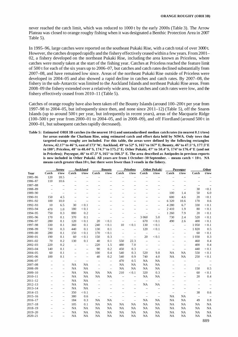
ORANGE ROUGHY (ORH 3B)
889
never reached the catch limit, which was reduced to 1000 t by the early 2000s (Table 3). The Arrow Plateau was closed to orange roughy fishing when it was designated a Benthic Protection Area in 2007 Table 5). In 1995–96, large catches were reported on the southeast Pukaki Rise, with a catch total of over 3000 t. However, the catches dropped rapidly and the fishery effectively ceased within a few years. From 2001–02, a fishery developed on the northeast Pukaki Rise, including the area known as Priceless, where catches were mostly taken at the start of the fishing year. Catches at Priceless reached the feature limit of 500 t for each of the six years up to 2006–07, but catches and catch rates declined substantially from 2007–08, and have remained low since. Areas of the northeast Pukaki Rise outside of Priceless were developed in 2004–05 and also showed a rapid decline in catches and catch rates. By 2007–08, the fishery in the sub-Antarctic was limited to the Auckland Islands and northeast Pukaki Rise areas. From 2008–09 the fishery extended over a relatively wide area, but catches and catch rates were low, and the fishery effectively ceased from 2010–11 (Table 5). Catches of orange roughy have also been taken off the Bounty Islands (around 100–200 t per year from 1997–98 to 2004–05, but infrequently since then, and none since 2011–12) (Table 5), off the Snares Islands (up to around 500 t per year, but infrequently in recent years), areas of the Macquarie Ridge (100–500 t per year from 2000–01 to 2004–05, and in 2008–09), and off Fiordland (around 500 t in 2000–01, but subsequent catches rapidly decreased). Table 5: Estimated ORH 3B catches (to the nearest 10 t) and unstandardised median catch rates (to nearest 0.1 t/tow)
for areas outside the Chatham Rise, using estimated catch and effort data held by NIWA. Only tows that targeted orange roughy are included. For this table, the areas were defined by the following rectangles: Arrow, 42.17° to 46° S, east of 173° W; Auckland, 49° to 52° S, 165° to 167° E; Bounty, 46° to 47.5° S, 177.5° E to 180°; Priceless, 48° to 48.44° S, 174.7° to 175.2° E; Other Pukaki, 47° to 50.4° S, 174° to 176.4° E (and not in Priceless); Puysegur, 46° to 47.5° S, 165° to 166.5° E. The area described as Antipodes in previous reports is now included in Other Pukaki. All years are from 1 October–30 September. – means catch < 10 t. NA means catch greater than 10 t, but there were fewer than 3 vessels in the fishery.
Arrow Auckland Bounty Priceless Other Pukaki Puysegur Other Year Catch t/tow Catch t/tow Catch t/tow Catch t/tow Catch t/tow Catch t/tow Catch t/tow 1985–86 120 18.5 – – – – – – – – – – – – 1986–87 110 10.6 – – – – – – – – – – – – 1987–88 – – – – – – – – – – – – – – 1988–89 – – – – – – – – – – – – 30 <0.1 1989–90 – – – – – – – – – – 100 1.4 50 6.0 1990–91 150 4.5 – – – – – – – – 600 4.6 20 <0.1 1991–92 100 10.0 – – – – – – – – 6 320 10.6 170 0.6 1992–93 10 6.5 30 < 0.1 – – – – – – 4 280 6.7 330 < 0.1 1993–94 470 1.0 180 < 0.1 – – – – – – 2 410 1.9 80 < 0.1 1994–95 750 0.3 880 0.2 – – – – – – 1 260 7.9 20 < 0.1 1995–96 170 0.1 370 0.1 – – – – 3 060 5.0 730 2.4 520 < 0.1 1996–97 280 0.1 120 < 0.1 20 < 0.1 – – 670 < 0.1 490 2.6 400 < 0.1 1997–98 330 0.1 360 0.1 240 < 0.1 10 < 0.1 130 < 0.1 – – 1 050 < 0.1 1998–99 730 0.3 440 0.1 130 0.1 – – 120 < 0.1 – – 1 820 0.5 1999–00 280 0.1 150 < 0.1 170 < 0.1 – – – – – – 60 < 0.1 2000–01 190 0.1 60 < 0.1 150 0.3 – – 20 < 0.1 – – 1 030 0.3 2001–02 70 0.2 130 0.1 40 0.1 550 22.3 – – – – 460 0.4 2002–03 220 0.2 – – 220 1.5 480 7.0 – – – – 400 0.4 2003–04 140 0.1 – – 90 0.2 450 0.3 – – – – 440 < 0.1 2004–05 60 0.1 – – 100 0.4 540 0.3 520 9.8 NA NA 550 < 0.1 2005–06 100 0.1 – – 40 0.2 540 0.9 740 4.0 NA NA 250 < 0.1 2006–07 – – – – – – 470 0.5 NA NA – – – – 2007–08 – – NA NA – – NA NA NA NA – – – – 2008–09 – – NA NA – – NA NA NA NA – – 150 0.5 2009–10 – – NA NA NA NA 210 < 0.1 320 0.3 – – 60 < 0.1 2010–11 – – NA NA NA NA – – NA NA – – 20 0.4 2011–12 – – NA NA – – – – – – – – – – 2012–13 – – NA NA – – – – NA NA – – – – 2013–14 – – NA NA – – – – – – – – – – 2014–15 – – 350 < 0.1 – – – – – – – – 38 0.6 2015–16 – – 380 0.6 – – – – – – NA NA – – 2016–17 – – 184 0.3 NA NA – – NA NA NA NA 49 0.8 2017–18 – – 105 0.1 NA NA NA NA NA NA NA NA NA NA 2018–19 – – NA NA NA NA NA NA NA NA NA NA NA NA 2019–20 – – NA NA NA NA NA NA NA NA NA NA NA NA 2020–21 – – NA NA NA NA NA NA NA NA NA NA NA NA

ORANGE ROUGHY (ORH 3B)
890
1.2 Recreational fisheries No recreational fishing for orange roughy is known in this quota management area. 1.3 Customary non-commercial fisheries No customary non-commercial fishing for orange roughy is known in this quota management area. 1.4 Illegal catch No information is available on illegal catch in this quota management area. 1.5 Other sources of mortality There has been a history of catch overruns on the Chatham Rise because of lost fish and discards, and discrepancies in tray weights and conversion factors. In assessments, total removals from each part of the Chatham Rise were assumed to exceed reported catches by the overrun percentages in Table 6. For Puysegur and other southern fisheries there is no reason to believe that, if there was an overrun in catches, this shows any trend over time. For this reason, it was assumed that there was no overrun for this area. Table 6: Chatham Rise catch overruns (%) by fishing year. Year 1978–79 1979–80 1980–81 1981–82 1982–83 1983–84 1984–85 1985–86 1986–87 1987–88 Overrun 30 30 30 30 30 30 30 28 26 24 Year 1988–89 1989–90 1990–91 1991–92 1992–93 1993–94 1994–95 and subsequently Overrun 22 20 15 10 10 10 5 Within the TAC, an allowance of 5% of the TACC is allocated for other sources of mortality (currently 225 t). 2. BIOLOGY Biological parameters used in this assessment are presented in the Biology section in the Introduction – Orange roughy chapter. 3. STOCKS AND AREAS For the purposes of this report the term ‘stock’ refers to a biological unit with a single major spawning ground, in contrast to a ‘Fishstock’ which refers to a management unit. Genetically two main stocks are recognised within ORH 3B (Chatham Rise and Puysegur; Smith & Benson 1997) and these are considered to be distinct from stocks in adjacent areas (Cook Canyon and Ritchie Bank). However, it is likely, because of their geographical separation and discontinuities in the distribution of orange roughy, that concentrations of spawning fish on the Arrow Plateau, near the Auckland Islands, and west of the Antipodes Islands also form separate stocks. Genetic data have been applied to define stock boundaries, both within ORH 3B, and between it and adjacent areas. Mitochondrial DNA shows that there are considerable differences between Puysegur fish and fish from the geographically adjacent areas Cook Canyon and Chatham Rise. Allozyme frequency studies suggest that Chatham Rise fish are distinct from those on the Ritchie Bank (ORH 2A). These data also suggest multiple stocks within the Chatham Rise, but do not indicate clear stock boundaries. Although there is significant heterogeneity amongst allozyme frequencies from different areas of the Rise, these frequencies varied as much in time (samples from the same location at different times) as in space (samples from different locations at the same time).

ORANGE ROUGHY (ORH 3B)
891
Chatham Rise The stock structure of orange roughy on the Chatham Rise was comprehensively reviewed in 2008 (Dunn & Devine 2010). This review evaluated all available data because no single dataset seemed to provide definitive information about likely stock boundaries. The analysed data included: catch distribution and CPUE patterns; location of spawning and nursery grounds; inferred migrations; size, maturity, and condition data; genetic studies; and habitat and natural boundaries. There is evidence that a separate stock exists on the Northwest Rise. The Northwest Rise contains a large spawning ground on the Graveyard Hills, and also nursery grounds around, and primarily to the west of, the Graveyard Hills. There is a gap in the distribution of early juveniles (under 15 cm standard length) between the Graveyard area and the Spawning Box at approximately 178° W. A research trawl survey found post-spawning adult fish to the west, but not to the east, of the Graveyard Hills, and a westerly post-spawning migration was inferred. Analyses of median length from commercial and research trawls found that orange roughy on the Northwest Chatham Rise and Graveyard Hills were smaller than those on the East Rise. A substantial decline in the size of 50% maturity after 1992 was found for both the Graveyard Hills and the Northwest Rise, but not for other areas. The only information that does not support the Northwest Rise being a separate stock is an indication from patterns in commercial catch rates that some fish arriving to spawn in the Spawning Box may come from the west (Coburn & Doonan 1994, 1997). Catch data and genetic studies do not shed any further light on stock structure. Oceanographic models suggest that a gyre to the east of the Graveyard may provide a mechanism for a separation between the Northwest Chatham Rise and the East Rise. Based on the available data, the Northwest Chatham Rise is considered to be a separate stock. The separation of the Northeast Hills and Andes as separate stocks from the Spawning Box and Eastern Flats was based on observations of simultaneous spawning aggregations occurring on these hills, and because stock assessment models indicated a mismatch between the standardised CPUE trends. However, the following suggest that all these areas are a single stock: the occurrence of a continuous nursery ground throughout the area, similar trends in size of 50% maturity in each area, the essentially continuous habitat with similar environmental conditions, and inferred post-spawning migrations from the Spawning Box towards the east Rise. Analyses of median lengths from commercial catches showed no obvious differences between areas. In addition, the spawning aggregations found on the Northeast Hills and Andes appear to have been minor compared with those in the Spawning Box. The spawning aggregation on the Northeast Hills has also exhibited an increase in mean length and catch rates, suggesting that fish spawning on these hills are not resident, and thus are not separate from the surrounding area. Based on the available data the Northeast Hills and Andes are therefore considered to be from the same stock as the Spawning Box and Eastern Flats. The only evidence to separate the eastern area of the South Rise (Big Chief and surrounds) from the East Rise is the lack of spawning migrations inferred from an absence of a seasonal effect in standardised CPUE analyses. The evidence that the Big Chief area is the same stock as the East Rise includes: the fact that the nursery grounds and habitat are continuous, there were no splits between the areas identified from analyses of median length, and the fisheries are similar. The reports of spawning fish around Big Chief have been infrequent, and so are considered equivocal on stock structure. The Big Chief area is therefore considered part of the East Rise stock. There is weak evidence that the area of the South Rise west of, and including, Hegerville is a separate stock. The evidence includes median length analyses which indicated a split in this area, and an oceanographic front at 177° W. However, very few catches of spawning orange roughy have been reported in this area, and there appears to be no substantial nursery ground. Both of these factors support the idea that this area does not have a separate stock. In the area to the west of the suggested split, the fish are relatively small during spawning and relatively large during non-spawning. Combined with a standardised CPUE which shows a decline in abundance around July (peak spawning), and a somatic condition factor which declines during September–November (post-spawning), this supports an hypothesis of adult fish leaving the area to spawn elsewhere.

ORANGE ROUGHY (ORH 3B)
892
The South Rise could provide feeding habitat for the stock, which is estimated to have had an initial biomass of over 300 000 t, an amount that was probably too large to inhabit only the East Rise. There is more evidence to support the idea of orange roughy in this area being part of the East Rise stock than there is to the contrary. The current hypothesis is that the area to the west of the current convergence zone may be relatively marginal habitat, where larger juvenile, maturing and adult orange roughy were once predominant, and there is little spawning and few juveniles because the water is relatively cold. Based on these analyses, the Chatham Rise has been divided into two areas: the Northwest, and the East and South Rise combined (Figure 2). The centre of the Northwest stock is the Graveyard Hills. The centre of the East and South Rise stock is the Spawning Box during spawning, and the southeast corner of the Rise during non-spawning. 4. STOCK ASSESSMENT No model-based stock assessments were conducted for ORH 3B stocks from 2007 to 2013. This was primarily because the 2006 stock assessment, which assumed deterministic recruitment, showed an increasing trend in biomass which was not supported by recent biomass indices. Deterministic recruitment was assumed because ageing data were considered to be unreliable. With the successful assessment of the MEC stock in 2013, which used age data from the new ageing methodology (Tracey et al 2007, Horn et al 2016), there was a return to model-based assessment in 2014. Recruitment in all of these assessments has been derived from limited age data. 4.1 Northwest Chatham Rise A Bayesian stock assessment was conducted for the Northwest Chatham Rise (NWCR) stock in 2018, using data up to 2016–17. This used an age-structured population model fitted to acoustic survey estimates of spawning biomass, proportion-at-age from a trawl survey and targeted trawling on a spawning aggregation, proportion-spawning-at-age from a trawl survey, and length frequencies from the commercial fishery. 4.1.1 Model structure The model was single-sex and age-structured (1–100 years with a plus group), with maturity estimated separately (i.e., fish were classified by age and as mature or immature). A single time step was used, and the single fishery was assumed to be year-round on mature fish. Spawning was taken to occur after 75% of the mortality and 100% of mature fish were assumed to spawn each year. The catch history was constructed from the Northwest catches in Table 2 using the catch over-run percentages in Table 6. Natural mortality was assumed to be fixed at 0.045 and the stock-recruitment relationship was assumed to follow a Beverton-Holt function with steepness of 0.75. The remaining fixed biological parameters are given in tables 1 and 2 of the Introduction – Orange roughy chapter. 4.1.2 Input data and statistical assumptions There were three main data sources for observations fitted in the assessment: acoustic-survey spawning biomass estimates from the main spawning hills (Graveyard and Morgue); an age frequency and an estimate of proportion-spawning-at-age taken from a 1994 wide-area trawl survey; an age frequency taken from targeted trawls above Morgue, and length frequencies collected from the commercial fishery covering 1989–2005. Acoustic estimates Three types of acoustic survey estimates were available for use in the assessment: AOS estimates (from a multi-frequency towed system, e.g., see Kloser et al 2011); 38 kHz estimates from a towed-body system; and 38 kHz estimates from a hull-mounted system. The reliability of the data from the different systems in each year was considered and estimates from the AOS and towed-body systems were used in the base model (Table 7). An alternative treatment of the available acoustic data was to include additional survey estimates from 2002 and 2004 (Table 7). All of the data in Table 7 were used in the sensitivity run labelled ‘Extra acoustics’.
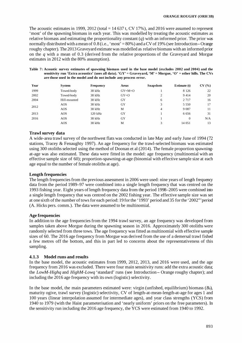
ORANGE ROUGHY (ORH 3B)
893
The acoustic estimates in 1999, 2012 (total = 14 637 t, CV 17%), and 2016 were assumed to represent ‘most’ of the spawning biomass in each year. This was modelled by treating the acoustic estimates as relative biomass and estimating the proportionality constant (q) with an informed prior. The prior was normally distributed with a mean of 0.8 (i.e., ‘most’ = 80%) and a CV of 19% (see Introduction – Orange roughy chapter). The 2013 Graveyard estimate was modelled as relative biomass with an informed prior on the q with a mean of 0.3 (derived from the relative proportions of the Graveyard and Morgue estimates in 2012 with the 80% assumption). Table 7: Acoustic survey estimates of spawning biomass used in the base model (excludes 2002 and 2004) and the
sensitivity run ‘Extra acoustics’ (uses all data). ’GY’ = Graveyard, ‘M’ = Morgue, ‘O’ = other hills. The CVs are those used in the model and do not include any process error.
Year System Frequency Areas Snapshots Estimate (t) CV (%) 1999 Towed-body 38 kHz GY+M+O 1 8 126 22 2002 Towed-body 38 kHz GY+O 2 9 414 20 2004 Hill-mounted 38 kHz GY 6 2 717 16
2012 AOS 38 kHz GY 3 5 550 17 AOS 38 kHz M 4 9 087 11
2013 AOS 120 kHz GY 1 6 656 31 2016 AOS 38 kHz GY 1 0 N/A AOS 38 kHz M 3 14 051 13
Trawl survey data A wide-area trawl survey of the northwest flats was conducted in late May and early June of 1994 (72 stations, Tracey & Fenaughty 1997). An age frequency for the trawl-selected biomass was estimated using 300 otoliths selected using the method of Doonan et al (2014). The female proportion spawning-at-age was also estimated. These data were fitted in the model: age frequency (multinomial with an effective sample size of 60); proportion-spawning-at-age (binomial with effective sample size at each age equal to the number of female otoliths at age). Length frequencies The length frequencies from the previous assessment in 2006 were used: nine years of length frequency data from the period 1989–97 were combined into a single length frequency that was centred on the 1993 fishing year. Eight years of length frequency data from the period 1998–2005 were combined into a single length frequency that was centred on the 2002 fishing year. The effective sample size was set at one sixth of the number of tows for each period: 19 for the ‘1993’ period and 35 for the ‘2002”’period (A. Hicks pers. comm.). The data were assumed to be multinomial. Age frequencies In addition to the age frequencies from the 1994 trawl survey, an age frequency was developed from samples taken above Morgue during the spawning season in 2016. Approximately 300 otoliths were randomly selected from three tows. The age frequency was fitted as multinomial with effective sample sizes of 60. The 2016 age frequency from Morgue was derived from the use of a demersal trawl fished a few metres off the bottom, and this in part led to concerns about the representativeness of this sampling. 4.1.3 Model runs and results In the base model, the acoustic estimates from 1999, 2012, 2013, and 2016 were used, and the age frequency from 2016 was excluded. There were four main sensitivity runs: add the extra acoustic data; the LowM-Highq and HighM-Lowq ‘standard’ runs (see Introduction – Orange roughy chapter); and including the 2016 age frequency with its own (logistic) selectivity. In the base model, the main parameters estimated were: virgin (unfished, equilibrium) biomass (B0), maturity ogive, trawl survey (logistic) selectivity, CV of length-at-mean-length-at-age for ages 1 and 100 years (linear interpolation assumed for intermediate ages), and year class strengths (YCS) from 1940 to 1979 (with the Haist parameterisation and ‘nearly uniform’ priors on the free parameters). In the sensitivity run including the 2016 age frequency, the YCS were estimated from 1940 to 1992.

ORANGE ROUGHY (ORH 3B)
894
Model diagnostics The model provided good MPD fits to the data (Figures 3 and 4). The acoustic indices, free to ‘move’ somewhat as they are relative, were fitted well (Figure 3). The posterior estimates for the acoustic qs were not very different from the priors, but there was some movement in the Graveyard and Morgue q, with the posterior slightly lower (and therefore SSB slightly higher) than expected (Figure 5). Numerous MPD sensitivity runs were performed. These showed that the main drivers of the estimated stock status were natural mortality (M) and the means of the acoustic q priors (lower M and higher mean q give lower stock status; higher M and lower mean q give higher stock status).
Figure 3: NWCR, base, (left) MPD fits to the acoustic biomass indices; broken line, spawning biomass trajectory;
scaled acoustic indices for x, Graveyard survey, and ∆ , Graveyard and Morgue surveys; (right) MCMC normalised residuals for the acoustic biomass indices. The box in each year covers 50% of the distribution and the whiskers extend to 95% of the distribution.
Figure 4: NWCR, base, MPD fits: (x, observations; lines, predictions): (top) commercial catch-at-length samples (n is
the effective sample size); (bottom) trawl survey catch-at-age and proportion mature at age.

ORANGE ROUGHY (ORH 3B)
895
When the Morgue age frequency was fitted assuming that the selectivity on Morgue was equal to maturity the fit was poor, particularly to the left-hand side of the age frequency distribution. When the Morgue age frequency was fitted assuming a separate logistic selectivity ogive, the fit was acceptable (Figure 6). The Morgue age frequency had an unexpectedly high proportion of older fish, and the sampling methodology was also unusual. As a result, it was agreed to exclude the Morgue age frequency data from the base model.
Figure 5: NWCR base, MCMC diagnostics: prior (solid line) and posterior (broken line) distributions for the two
acoustic qs (left, mean q-prior = 0.8; right, mean q-prior = 0.3).
Figure 6: NWCR, base, MPD fits: (x, observations; lines, predictions) to the Morgue age frequency (effective sample
size n = 60). MCMC Results For the base model, and the sensitivity runs, MCMC convergence diagnostics indicated no lack of convergence. Virgin biomass, B0, was estimated to be between 64 000–67 300 t for all runs (Table 8). Current stock status was similar across the base and the first two sensitivity runs (Table 8). For the two ‘bounding’ runs, where M and the mean of the acoustic q priors were shifted by 20%, median current stock status was estimated to be close to the lower bound, or upper bound, of the target range of 30–50% B0 (Table 8). Table 8: NWCR, MCMC estimates of virgin biomass (B0), and stock status (B2017 as %B0) for the base model and four
sensitivity runs. M B0 (000 t) 95% CI B2017 (% B0) 95% CI Base 0.045 65.2 59.9–75.0 38 31–48 Extra acoustics 0.045 64.0 60.0–76.7 36 31–43 Include Morgue AF 0.045 65.1 58.6–76.5 38 30–48 Low M-High q 0.036 67.3 63.0–73.9 29 23–36 High M-Low q 0.054 65.5 58.2–77.7 48 40–58
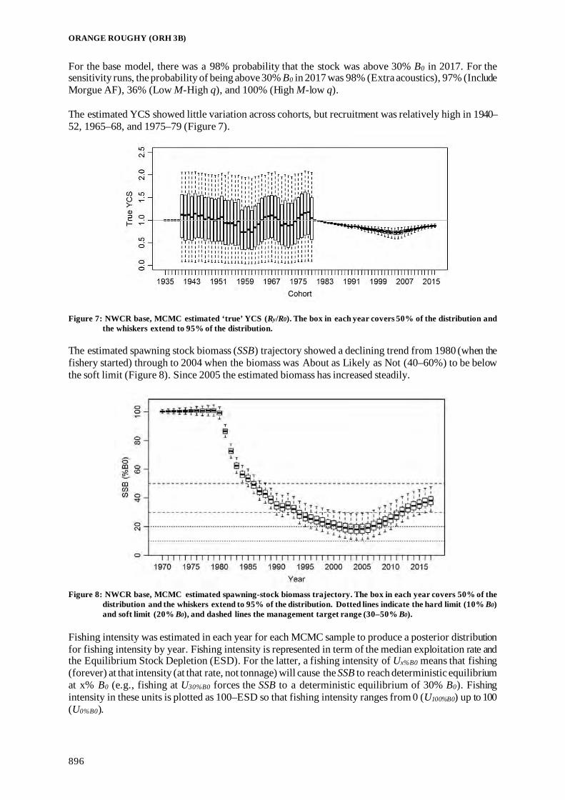
ORANGE ROUGHY (ORH 3B)
896
For the base model, there was a 98% probability that the stock was above 30% B0 in 2017. For the sensitivity runs, the probability of being above 30% B0 in 2017 was 98% (Extra acoustics), 97% (Include Morgue AF), 36% (Low M-High q), and 100% (High M-low q). The estimated YCS showed little variation across cohorts, but recruitment was relatively high in 1940–52, 1965–68, and 1975–79 (Figure 7).
Figure 7: NWCR base, MCMC estimated ‘true’ YCS (Ry/R0). The box in each year covers 50% of the distribution and
the whiskers extend to 95% of the distribution. The estimated spawning stock biomass (SSB) trajectory showed a declining trend from 1980 (when the fishery started) through to 2004 when the biomass was About as Likely as Not (40–60%) to be below the soft limit (Figure 8). Since 2005 the estimated biomass has increased steadily.
Figure 8: NWCR base, MCMC estimated spawning-stock biomass trajectory. The box in each year covers 50% of the
distribution and the whiskers extend to 95% of the distribution. Dotted lines indicate the hard limit (10% B0) and soft limit (20% B0), and dashed lines the management target range (30–50% B0).
Fishing intensity was estimated in each year for each MCMC sample to produce a posterior distribution for fishing intensity by year. Fishing intensity is represented in term of the median exploitation rate and the Equilibrium Stock Depletion (ESD). For the latter, a fishing intensity of Ux%B0 means that fishing (forever) at that intensity (at that rate, not tonnage) will cause the SSB to reach deterministic equilibrium at x% B0 (e.g., fishing at U30%B0 forces the SSB to a deterministic equilibrium of 30% B0). Fishing intensity in these units is plotted as 100–ESD so that fishing intensity ranges from 0 (U100%B0) up to 100 (U0%B0).

ORANGE ROUGHY (ORH 3B)
897
Estimated fishing intensity was above U20%B0 for most of the history of the fishery; it was briefly in the target range (U30%B0–U40%B0) from 2009–2010 before dropping substantially when the industry agreed to curtail fishing the NWCR in 2011, and has been in or just below the target range since 2014 (Figure 9). There was less than a 1% probability that the exploitation rate in 2017 was below U30%B0.
Figure 9: NWCR base, MCMC estimated fishing intensity trajectory. The box in each year covers 50% of the
distribution and the whiskers extend to 95% of the distribution. The fishing intensity range associated with the biomass target of 30–50% B0 is marked by horizontal lines.
Projections Five-year biomass projections were made for the Base model run assuming future catches to be the TACC (1250 t), or the current agreed catch limit (1043 t; 207 t has been shelved). For each projection scenario, future recruitment variability was sampled from actual estimates between 1940 and 1979. At the TACC (1250 t) and the current agreed catch limit (1043 t), SSB is predicted to remain stable or slowly increase over the next five years, and the probability of the SSB going below the soft or hard limits is zero (Table 9). Table 9: ORH 3B NWCR Bayesian median and 95% credible intervals (in parentheses) of projected B2022, B2022 as a
percentage of B0, and B2022/B2017 (%) for the model runs.
Model run
Catch (t)
B2022 B2022 (%B0) B2022/B2017 (%) p(B2022 < 0.2 B0) p(B2022 < 0.1 B0)
Base 1 043 26 500 (20 000–38 100) 41 (33–51) 107 (104–111) 0 0 1 250 25 600 (19 100–37 200) 39 (31–50) 104 (101–107) 0 0
Biological reference points, management targets and yield Orange roughy stocks with model based stock assessments are managed according to the Harvest Control Rule (HCR) that was developed in 2014 using a Management Strategy Evaluation (MSE) (Cordue 2014b). The HCR has a target management range of 30–50% B0. Yield estimates are not reported for this stock.

ORANGE ROUGHY (ORH 3B)
898
4.2 East and South Chatham Rise The East and South Chatham Rise (ESCR) stock was assessed in 2014 (Cordue 2014a). The assessment was updated in 2018 using data up to 2016–17 (Dunn & Doonan 2018). That assessment was then updated to the end of 2017–18 to allow application of the orange roughy Harvest Control Rule (HCR) (Cordue 2014b, 2018). The assessment has been updated in 2020 to apply the HCR to calculate a catch recommendation for 2020–21. In each assessment the model was an age-structured population model fitted to acoustic survey estimates of spawning biomass, trawl survey biomass indices, age frequencies from spawning aggregations, and length frequencies from trawl surveys and commercial fisheries. 4.2.1 Model structure The model was single-sex and age-structured (1–100 years with a plus group), with maturity estimated separately (i.e., fish were classified by age and as mature or immature). A single time step was used and, in the updated base model, four year-round fisheries with logistic selectivities were modelled: Box & flats, Eastern hills, Andes, and South Rise. These fisheries were chosen following Dunn (2007) who assessed the Box & flats, Eastern hills, and Andes as separate stocks and hence had already prepared length frequency data for those fisheries. No length frequencies were available from the South Rise fishery and its selectivity was assumed to be the same as the Andes (so effectively there were three fisheries in the model). Spawning was taken to occur after 75% of the mortality and 100% of mature fish were assumed to spawn each year. The catch history was constructed by apportioning the total ORH 3B reported catch across areas using catch proportions from estimated catch on TCEPR forms (Table 2). The over-run percentages in Table 6 were applied. Natural mortality was assumed fixed at 0.045 and the stock-recruitment relationship was assumed to follow a Beverton-Holt function with steepness of 0.75. The remaining fixed biological parameters are given in tables 1 and 2 of the Introduction – Orange roughy chapter. 4.2.2 Input data and statistical assumptions There were four main data sources for observations fitted in the assessment: acoustic survey spawning biomass estimates from the Old-plume (2002–2014, 2016), Rekohu (2011–2014, 2016), and the Crack (2011, 2013, 2016); age frequencies from the spawning areas (2012, 2013, and 2016); trawl survey biomass indices and length frequencies; and length frequencies collected from the commercial fisheries. Acoustic estimates The Old plume was acoustically surveyed as early as 1996, but the survey estimates are only considered to represent a consistent time series from 2002–2012 (see Cordue 2008, Hampton et al 2008, 2009, 2010, Doonan et al 2012). Like the Rekohu plume, which was first noted in 2010 and first surveyed in 2011, the Old plume occurs on an area of flat bottom and can be adequately surveyed using a hull-mounted transducer. In 2011, 2013, and 2016, an additional (but known historically) spawning area was surveyed; known as the Crack (also known as Mt. Muck), it is an area of rough terrain which requires a towed-body or trawl-mounted system to be used to reduce the height of the shadow or dead zone (i.e., with the transducer at a depth of about 500–700 m). The estimates selected by the DWWG for use in the stock assessment are shown in Table 10. To make the estimates as comparable as possible across years, only biomass estimates from 38 kHz transducers were used and those from the hull-mounted system were weather-adjusted in the same way as earlier estimates. A key question evaluated in the 2014 assessment was how long the Rekohu plume has been in existence (Cordue 2014a). If the Rekohu plume had always existed (and was not discovered until 2010) then it would be one of three major spawning sites and could be modelled as such along with the Old plume and the Crack. This would imply that the Old plume time series was tracking a consistent part of the spawning biomass (and its decline over time was therefore an important indicator of stock status). If the Rekohu plume had very recently formed, this would imply that the Old plume time series was a biomass index only up until the year before the Rekohu plume came into existence. Following Cordue (2014a), it is assumed that the Old plume time series cannot be relied on to provide a consistent index for any part of the spawning biomass. In 2011, 2013, and 2016, the estimates of average spawning biomass across the three areas were summed to form comparable indices for each

ORANGE ROUGHY (ORH 3B)
899
year. The 2012 and 2014 estimates from Rekohu and the Old plume were summed to provide a 2012 and 2014 index with a different proportionality constant q. The Old plume indices from 2002–2010 were used, but each point in the time series was given its own q. Informed priors were used for all of the qs in the Old plume series, for the 2012 and 2014 biomass indices, and the indices comprising 2011, 2013, and 2016 observations. For 2011, 2013, and 2016, it was assumed that ‘most’ of the biomass was being indexed so the ‘standard’ acoustic q prior was used for this proportionality constant (q1): lognormal (mean = 0.8, CV = 19%) (see Introduction – Orange roughy chapter). The mean of the q prior for 2012 and 2014 was derived from the observed biomass proportions across the three areas and the assumption that 80% of the spawning biomass was indexed in 2011, 2013, and 2016. This gave a mean of 0.7 for the proportionality constant (q2) of the 2012 and 2014 indices, a reflection that this index did not include an estimate for the Crack. For 2002 to 2010 the means of the q priors were assumed to decrease linearly from 0.7 (2002) down to 0.30 (2010), reflecting the gradual increase in the relative importance of the Rekohu plume. The linear sequence was derived by assuming 0.7 in 2002 (i.e., assuming that the Rekohu plume did not exist and only the Crack was missing from the survey estimate) and using the observed biomass proportions in 2011 with the 80% assumption (which gave the Old plume being about 25% of the total spawning biomass). To reflect the increased uncertainty in the acoustic qs in years other than 2011 and 2013, the priors were given an increased CV of 30%. Table 10: Acoustic estimates of average pluming spawning biomass in the three main spawning areas as used in the
assessment. All estimates were obtained from surveys on FV San Waitaki from 38 kHz transducers. Each estimate is the average of a number of snapshots as reflected by the estimated CVs. Some estimates have been revised since the 2014 assessment (Dunn & Doonan 2018).
Old plume Rekohu Crack Year Estimate (t) CV (%) Estimate (t) CV (%) Estimate (t) CV (%) 2002 63 950 6 – – – – 2003 44 316 6 – – – – 2004 44 968 8 – – – – 2005 43 923 4 – – – – 2006 47 450 10 – – – – 2007 34 427 5 – – – – 2008 31 668 8 – – – – 2009 28 199 5 – – – – 2010 21 205 7 – – – – 2011 16 422 8 28 113 18 6 794 21 2012 19 392 7 27 121 10 – – 2013 15 554 14 33 348 10 5 471 16 2014 19 360 18 44 421 25 – – 2015 – – – – – – 2016 11 192 13 27 027 13 5 341 10
As well as updating the base model, two additional runs were made which had different assumptions with regard to the acoustic qs. In the standard LowMhighq sensitivity run, the means of the acoustic q priors were all increased by 20% (and the value of M was decreased by 20%). In the ‘q-ratio model’ a prior was placed on the ratio q1/q2. The standard lognormal prior was used for q1 and a uniform prior for q2. A lognormal prior was used for the ratio with the mean equal to 1.14 (0.8/0.7) and a CV of 7.5% which strongly encouraged the ratio to be greater than 1 (reflecting that three areas had been surveyed for the first time series but only two of those areas for the second time series). There was no agreement in the DWWG as to whether the updated base model or the q-ratio model was to be preferred. The LowMhighq model was run relative to the updated base model because that had the lowest estimated stock status and therefore the LowMhighq model would be a ‘worst case’ scenario as intended. The updated base model is denoted as the ‘current model’ rather than the base model. Trawl survey data Research trawl surveys of the Spawning Box during July were completed from 1984 to 1994, using three different vessels: FV Otago Buccaneer, FV Cordella, and RV Tangaroa (Figure 10). A consistent area was surveyed using fixed station positions (with some random second phase stations each year).

ORANGE ROUGHY (ORH 3B)
900
The biomass indices were fitted as relative indices with a separate time series for each vessel (with uninformed priors on the qs). The second point in the Tangaroa time series, although very large (driven by a single high catch), has a large CV and so is unlikely to have had much effect on the assessment results. Data from two wide-area surveys by Tangaroa in 2004 and 2007 were also used. These surveys covered the area which extends from the western edge of the Spawning Box around to the northern edge of the Andes. The area surveyed did not include the Old plume, the Northeast Hills, or the Andes. The survey used a random design over sixteen strata grouped into five sub-areas. The trawl net used was the full-wing and relatively fine mesh ‘ratcatcher’ net. The surveys covered the same survey area as the Spawning Box trawl surveys from 1984 to 1994 as well as additional strata to the east. In 2007, the survey ran from 4 to 27 July and 62 trawl tows were completed. In 2004, the survey ran from 7 to 29 July and 57 trawl tows were completed.
Figure 10: The Spawning Box trawl survey biomass indices (assuming a catchability of 1 for each vessel), with 95%
confidence intervals shown as vertical lines. Vessels indicated as B, FV Otago Buccaneer; C, FV Cordella; T, RV Tangaroa.
The surveys had almost identical estimates of total biomass in each year (17 000 t) with low CVs (10% and 13% respectively). They were fitted as relative biomass with an uninformed prior on the q. Length frequencies The length frequencies from all of the trawl surveys were fitted in the model as multinomial random variables. Effective sample sizes (N) were taken from Dunn (2007) for the Spawning Box surveys and were assumed equal to the number of tows for the wide-area surveys (across all surveys the effective Ns ranged from about 20–80). Trawl survey length frequencies were fitted assuming that all mature fish were selected, but immature fish were selected assuming capped-logistic ogives. One selectivity ogive for immature fish was shared by the Buccaneer, Cordella, and Tangaroa Spawning Box surveys, with a second ogive for the immature fish caught in the Tangaroa wide-area survey. Length frequencies from the commercial fisheries were developed by Hicks (2006) and also fitted in the model. For the Spawning Box and associated flat ground fishery, three years of length frequency data from the period 1989–91 were combined into a single length frequency that was centred on 1990, and four years 2002–05 were combined and centred on 2004. In a similar way, for Andes four years 1992–95 were combined and centred on 1993, three years 1997–99 combined and centred on 1998, and five years combined 2001–05 and centred on 2003. For the eastern hills, seven years 1991–97 were combined and centred on 1995, and five years 2001–05 combined and centred on 2003. These were fitted as multinomial with effective sample sizes ranging from 8 to 38. Age frequencies Age frequencies were developed for the Old plume and Rekohu plume in 2012, and for the Old plume, Rekohu, and the Crack in 2013 and 2016 (Doonan et al 2014a, b; 2018). Approximately 300 otoliths were randomly selected from each area in 2012 and 2016, and 250 from each area in 2013. The fish in

ORANGE ROUGHY (ORH 3B)
901
the Old plume were noted to be generally older than those in the Rekohu plume. The fish from the Crack, showed a mixture of ages from new spawners (20–30 years) to much older fish (80–100 years). In the base model, the age frequencies were combined across areas and fitted as multinomial with effective sample sizes of 50 (2012) and 60 (2013 and 2016), respectively, reflecting the low number of trawls from which samples were taken. 4.2.3 Model runs and results As well as the updated base model (denoted as the ‘current model’) there were two additional models: the q-ratio model which assumed a single fishery on mature fish, had a prior on q1/q2, and added 20% process error to the associated acoustic biomass indices; and the standard LowMhighq model (see Introduction – Orange roughy chapter). In all three models, the main parameters estimated were: virgin (unfished, equilibrium) biomass (B0), the maturity ogive, trawl survey selectivities, fisheries selectivities, CV of length-at-mean-length-at-age for ages 1 and 100 years (linear relationship assumed for intermediate ages), and year class strengths (YCS) from 1930 to 1990 (with the Haist parameterisation and ‘nearly uniform’ priors on the free parameters). There were also the numerous acoustic and trawl survey qs. MCMC chain diagnostics For each model, three chains of fifteen million iterations were run. One sample in each one thousand iterations were stored and the first one thousand samples were discarded as a ‘burn-in’ (the chains start near the MPD estimate and early samples may be unrepresentative of the posterior distribution). The traces of the main free parameters were checked to make sure that they did not exhibit any long-term trends, and the estimates of B0 and current stock status (SS2020 = B2020/B0) from each chain were checked to see that they were the same to two significant figures. Point estimates (median) and 95% credibility intervals (95% CIs) were constructed using all three chains combined after the burn-in (a total of 42 000 samples). Model diagnostics MPD fits and MCMC fits and residuals and marginal posterior distributions for the qs were examined for the current model and the q-ratio model. In general, the fits were excellent and the q posterior distributions and standardised residuals were acceptable (see Figures 11–13). The main exception was for the current model where the normalised residuals for the 2016 acoustic estimate are well outside the expected range (Figure 14). In the q-ratio model the residuals are much improved because of the addition of 20% process error (the CV is only 10% in the current model which is just a measure of observation error).
Figure 11: Current model: the MCMC fits and normalised residuals for the trawl survey biomass estimates in the
spawning box. The observations are plotted with 95% confidence intervals (left plot, red vertical lines). The MCMC predictions (left plot) and normalised residuals (right plot) are plotted as a ‘box and whiskers’. The middle 50% of the distribution is in the box with the whiskers extending to a 95% C.I.

ORANGE ROUGHY (ORH 3B)
902
Figure 12: Current model: the MCMC fits and normalised residuals for the 2016 spawning population age frequency
(left plot, histogram in black). The MPD fit is shown as the red line in the left plot. The MCMC predictions (left plot) and Pearson residuals (right plot) are plotted as a “box and whiskers”. The middle 50% of the distribution is in the box with the whiskers extending to a 95% C.I.
Figure 13: Current model: the MCMC fits and normalised residuals for the 2007 wide-area trawl survey length
frequency (left plot, histogram in black). The MPD fit is shown as the red line in the left plot. The MCMC predictions (left plot) and Pearson residuals (right plot) are plotted as a ‘box and whiskers’. The middle 50% of the distribution is in the box with the whiskers extending to a 95% C.I.

ORANGE ROUGHY (ORH 3B)
903
Figure 14: Current model: the MCMC fits and normalised residuals for the acoustic survey biomass estimates since
2011. The observations are plotted with 95% confidence intervals (left plot, red vertical lines). The MCMC predictions (left plot) and normalised residuals (right plot) are plotted as a ‘box and whiskers’. The middle 50% of the distribution is in the box with the whiskers extending to a 95% C.I.
The marginal posterior distributions for the two main acoustic qs are well within their prior distributions (Figure 15). However, in the current model the ratio of the two qs has a probability of being less than 1 of 39%. A value less than 1 must be considered very unlikely because an extra area is surveyed for the q1 time series. This is the main reason for the q-ratio model which corrects this diagnostic through the informed prior (and has a marginal posterior distribution with only a 5% probability of being less than 1).
Figure 15: Current model: the prior distributions (red lines) and marginal posterior distributions (histograms) for the
two main acoustic qs. MCMC results Virgin biomass, B0, was estimated to be about 300 000–350 000 t for the three models (Table 11). Current stock status was similar for the current and q-ratio models, both having the 95% CIs above 30% B0 (Table 11). The pessimistic LowMhighq run has stock status estimated just below 30% B0 (Table 11). Table 11: ESCR, MCMC estimates of virgin biomass (B0), current biomass (B2020), and stock status (B2020 as % B0) for
the three models. B0 (000 t) B2020 (000 t) Stock status (% B0) Median 95% CI Median 95% CI Median 95% CI Current model 312 281–346 111 91–135 36 30–41 q-ratio model 354 331–380 135 109–164 38 32–44 LowMhighq 337 308–363 90 71–111 27 22–32
The estimated YCS show little variation across cohorts but do exhibit a long-term trend (Figure 16). The stock status trajectory shows a steady decline from the start of fishery until the mid-1990s, where it remained in the 20–30% range until an upturn in about 2010 (Figure 17).

ORANGE ROUGHY (ORH 3B)
904
Figure 16: ESCR current model, MCMC estimated ‘true’ YCS (Ry/R0). The box in each year covers 50% of the
distribution and the whiskers extend to 95% of the distribution. Year classes between 1930 and 1990 were estimated.
Figure 17: ESCR current model, MCMC estimated spawning-stock biomass trajectory. The box in each year covers
50% of the distribution and the whiskers extend to 95% of the distribution. Horizontal lines are plotted at the hard limit (10% B0), the soft limit (20% B0), and the biomass target range (30–50% B0).
Fishing intensity was approximated using an average exploitation rate (total catch divided by catch-weighted beginning-of-year vulnerable biomass). Estimated exploitation rates were within or above the target range (U30%B0–U50%B0) up to 2009–10. Since 2010–11 they have generally been below the target range (Figure 18).

ORANGE ROUGHY (ORH 3B)
905
Figure 18: ESCR current model, MCMC estimated exploitation rates. The box in each year covers 50% of the
distribution and the whiskers extend to 95% of the distribution. The exploitation rates associated with the biomass target of 30–50% B0 are marked by horizontal lines at U30%B0 and U50%B0.
Biological reference points, management targets and yield Catch limits for the ESCR stock are recommended from the Harvest Control Rule (HCR) that was developed in 2014 using a Management Strategy Evaluation (MSE) (Cordue 2014b). The HCR has a target management range of 30–50% B0. Within that range there is a linear relationship between current estimated stock status and the instantaneous fishing mortality (exploitation rate) that is applied to next year’s beginning-of-year vulnerable biomass to obtain the recommended catch limit (Figure 19).
Figure 19: The orange roughy HCR showing the relationship between current estimated stock status and the
instantaneous fishing mortality rate (or exploitation rate) applied to next year’s beginning-of-year vulnerable biomass to derive the recommended catch limit. The target biomass range is 30–50% B0 and the limit reference point (LRP) is 20% B0 (see Cordue 2014b).
The HCR was applied to the current model and the q-ratio model. The medians of the marginal posterior distributions are used in the calculation. Because estimated stock status is less than 40% B0 in both runs the exploitation rates are less than Fmid = 0.045 (Figure 19, Table 12). The slightly higher stock status for the q-ratio model gives a higher exploitation rate than the current model but, because of the lower vulnerable biomass, the recommended catch limit from both models is similar (Table 12).

ORANGE ROUGHY (ORH 3B)
906
Table 12: The estimated stock status in 2019–20, the catch-weighted vulnerable biomass at the beginning of 2020–21, and the associated exploitation rate and recommended catch limit from the HCR for the current model and the q-ratio model.
Model Stock status (% B0) Exploitation rate Vulnerable biomass (t) Catch limit (t) Current model 36 0.04050 156 735 6 348 q-ratio model 38 0.04275 146 977 6 283
Projections Projections at the recommended catch limits (plus 5% to allow for incidental mortality) were performed for the current model and the q-ratio model. The highest of the two catch limits was used in a projection for the LowMhighq model. This was to check that the highest HCR recommended catch limit was still safe even if the pessimistic scenario represented by the LowMhighq model was true. Projections were done over 8 years because the HCR is meant to be applied every four years. Random recruitment was brought in from 1991 by resampling from the last ten years of estimated YCS (1981–1990). In each case, stock status was projected to rise slowly from the current estimated stock status and there was close to zero probability of the stock status being below 20% B0 over the next 8 years (Figure 20).
Figure 20: Projected stock status for catches at the HCR recommended catch limits plus 5% to allow for incidental
mortality. Top: q-ratio model projected at 6283 t (plus 5%). Bottom: current model projected at 6348 t (plus 5%). Each box covers the middle 50% of the distribution and the whiskers extend to 95% CIs. [Continued on next page]

ORANGE ROUGHY (ORH 3B)
907
Figure 20 [Continued]: Projected stock status for catches at the HCR recommended catch limits plus 5% to allow for
incidental mortality. LowMhighq model projected at 6348 t (plus 5%). Each box covers the middle 50% of the distribution and the whiskers extend to 95% CIs.
4.3 Puysegur A Bayesian stock assessment was conducted for the Puysegur stock in 2017 using very similar methods to those used in the 2014 orange roughy stock assessments of ESCR, NWCR, MEC, and ORH 7A (Cordue 2014a). An age-structured population model was fitted to an acoustic survey estimate of spawning biomass, two trawl survey indices and associated length frequencies, two spawning season age frequencies, and a small number of length frequencies from the commercial fishery. 4.3.1 Model structure The model was single-sex and age-structured (1–120 years with a plus group), with maturity estimated separately (i.e., fish were classified by age and as mature or immature). Two time steps were used to model a non-spawning season fishery and a spawning season fishery. Spawning was taken to occur after 50% of the spawning season mortality and 100% of mature fish were assumed to spawn each year. The catch history as reported in Table 5 (see above) was split into a spawning (June–August) and a non-spawning season (September–May) using the ratio of estimated catches, with the addition of catches during 2005, 2006, and 2015 when fish were caught during acoustic surveys. The catch for 2016–17 was assumed to be zero. Natural mortality was fixed at 0.045 and the stock-recruitment relationship was assumed to follow a Beverton-Holt function with steepness of 0.75. The remaining fixed biological parameters are given in table 2 of the Introduction – Orange roughy chapter (ESCR growth parameters were assumed). 4.3.2 Input data and statistical assumptions There were four main data sources used in the assessment: an acoustic-survey spawning biomass estimate in 2015 from the main spawning hill (Goomzy); two age frequencies during the spawning seasons in 1992 and 2015; biomass indices and length frequencies from trawl surveys in 1992 and 1994; and scaled length frequencies developed from Scientific Observer data collected from the commercial fishery in 1994 and 1997. Acoustic estimate Two types of acoustic survey estimates were available for use in the assessment: an estimate from a 38 kHz hull-mounted system during an AOS survey (AOS is a multi-frequency towed system, see for example Kloser et al 2011) and 38 kHz estimates from a hull-mounted system. The reliability of the data from the different surveys and the two main hills was considered and only the estimate from the 2015 survey on Goomzy was used in the base model (Table 13). The estimates from Godiva were unreliable because the surveyed marks contained a mix of species (Hampton et al 2005, 2006). In 2005 and 2006 it was not clear that the marks on Goomzy were exclusively orange roughy, but in 2015 there

ORANGE ROUGHY (ORH 3B)
908
was strong evidence from both trawling and the multi-frequency system that the surveyed marks were almost exclusively orange roughy (Ryan & Tilney 2016). Table 13: Acoustic survey estimates of spawning biomass available to the stock assessment. Only the 2015 estimate
from Goomzy was used in the base model.
Year Area Snapshots Estimate (t) CV (%) 2005 Godiva 3 2 600 23 Goomzy 4 4 000 22 2006 Godiva 4 900 51 Goomzy 3 3 200 50 2015 Godiva 2 180 Not calculated Goomzy 2 4 200 26
The acoustic estimate in 2015 from Goomzy was assumed to represent ‘most’ of the spawning biomass in that year. This was modelled by treating the acoustic estimate as relative biomass and estimating the proportionality constant (q) with an informed prior. The prior was lognormally distributed with a mean of 0.8 (i.e., ‘most’ = 80%) and a CV of 19% (see Introduction – Orange roughy chapter). Age frequencies Age frequencies were developed for the Giljanes spawning season trawl survey in 1992 (Clark & Tracey 1993) and the targeted trawling on spawning marks during the 2015 acoustic survey (Ryan & Tilney 2016) (Ian Doonan, NIWA, pers. comm.). Approximately 400 otoliths were used for each age frequency and CVs were calculated for each proportion-at-age from bootstrapping. In 2015, the mode (for the smoothed distribution) is at about 40 years whereas in 1992 the mode is closer to 60 years (Figure 21). It is notable that in both years the ages extend out to at least 130 years (Figure 21). In the base model, the age frequencies were fitted as multinomial with effective sample sizes of 80 and 60, respectively. The sample size of 80 is the approximate number of trawl stations during the survey in 1992 and the value of 60 was derived from the between year ratio of equivalent multinomial sample sizes derived from the bootstrap CVs.
Figure 21: Puysegur: age frequencies from 1992 and 2015 used in the base model. The red lines were produced using
the lowess smoother in R. Trawl survey data Trawl surveys of the Puysegur area were undertaken on Tangaroa in 1992 and 1994 (Clark & Tracey 1994, Clark et al 1996). However, the timing of the surveys was not ideal with the second survey being
20 40 60 80 100 120 140
0.00
0.01
0.02
0.03
0.04
Den
sity AF 1992
20 40 60 80 100 120 140
0.00
0.02
0.04
0.06
Age
Den
sity
AF 2015

ORANGE ROUGHY (ORH 3B)
909
more than a month later than the first (Puysegur strata occupied in 1992: 8 August–11 September, and in 1994: 24 September–23 October). An analysis of seasonal CPUE suggested that catch rates in the later period could be expected to be 50% of those in the earlier period. Also, an analysis of fish length data suggested that larger fish were caught in June–August period—the period taken to be the ‘spawning season’ in the model (although spawning occurs in July). It appears that during the June–August period larger fish are more available to the fishing fleet and could have been more available to the trawl survey. There was a very large reduction in the biomass indices for such a short period (Table 14). To allow for a possible reduction in availability between the 1992 and 1994 surveys, due to the change in timing, the selectivity for the trawl survey was modelled separately for mature and immature fish and an availability parameter for mature fish was estimated for the 1994 survey. The length frequencies from the trawl surveys are bimodal which could be partly explained by two groups of fish distinguished by maturity (Figure 22). Table 14: Trawl survey biomass indices for all fish from the Tangaroa trawl surveys of the Puysegur area in 1992 and
1994. The CVs given are those used in the modelling and include no process error.
Biomass index (t) CV (%) 1992 6 630 28 1994 1 160 24
Figure 22: Puysegur: length frequencies for the Tangaroa trawl surveys in 1992 and 1994 (fitted in the model as
beginning of year in 1993 and 1995). The effective samples sizes of N = 70 were the approximate number of stations in each survey.
Length frequencies (commercial fishery) Scientific observer coverage of the Puysegur fishery was very patchy over the small number of years when the fishery operated. The best coverage was in the 1993–94 fishing year when there were 15 samples in the non-spawning season and 44 samples in the spawning season. The next best year, when more than one month was sampled in the non-spawning season, was 1996–97 when there were 6 non-spawning season samples and 3 spawning season samples. Scaled length frequencies were produced in those two years for the spawning and non-spawning seasons. The data were assumed to be multinomial with effective sample sizes equal to the number of samples.
15 20 25 30 35 40 45
0.00
0.04
0.08
Den
sity
Year: 1993 N = 70
15 20 25 30 35 40 45
0.00
0.02
0.04
0.06
0.08
Length (cm)
Den
sity
Year: 1995 N = 70

ORANGE ROUGHY (ORH 3B)
910
4.3.3 Model runs and results In the base model, the acoustic estimate from Goomzy in 2015 was used, with the Tangaroa trawl survey data, and natural mortality (M) was fixed at 0.045. There were six main sensitivity runs: exclude the Tangaroa trawl survey data, low weight on the age frequencies, high weight on the age frequencies, estimate M, and the LowM-Highq and HighM-Lowq ‘standard’ runs (see Introduction – Orange roughy chapter). There were additional sensitivities: treating the trawl surveys as strictly comparable, using lognormal priors on the free year class strength parameters, alternative fixed non-spawning season fishing selectivities, adding a 5% overrun to the catch history, and using a higher CV on the acoustic q prior. In the base model, the main parameters estimated were: virgin (unfished, equilibrium) spawning biomass (B0), maturity ogive, trawl-survey selectivity, CV of length-at-mean-length-at-age for ages 1 and 120 years (linear relationship assumed for intermediate ages), and year class strengths (YCS) from 1917 to 1990 (with the Haist parameterisation and ‘nearly uniform’ priors on the free parameters). Model diagnostics The model provided good MPD fits to the data. Residuals were examined mainly at the MCMC level and these were all acceptable suggesting that the data weightings (CVs and effective sample sizes) were reasonable. The marginal posterior distribution of the acoustic q shifted somewhat to the left of the prior but remains well within the distribution of the prior (Figure 23). The MPD sensitivity runs where the trawl surveys were assumed strictly comparable, despite the difference in timing, were unable to fit the decline in the trawl indices and showed poorer fits to the trawl survey length frequencies than the base model. The objective function decreased by 7 likelihood units when the availability parameter for 1994 was estimated (which supports the inclusion of the single additional parameter). When lognormal priors were used for the free YCS parameters the trawl survey indices were fitted adequately (because the availability parameter was estimated) but the fits to the composition data (length and age frequencies) were degraded compared with the base model (which used nearly uniform priors on the free YCS parameters). The worst example of the poor fits was for the Tangaroa trawl survey length frequency in 1994. The reason for the poorer fits to the composition data was because the use of a lognormal prior severely constrained the estimated YCS. The near uniform prior allows much more freedom in the pattern of estimated YCS. Behaviour in the MCMC runs is much improved for the lognormal priors but there is the issue that the choice of sigmaR is arbitrary (see Introduction – Orange roughy chapter).
Figure 23: Puysegur: the marginal posterior distribution of the acoustic q (histogram) compared to its prior (red line).
The black dot marks the median of the marginal posterior.
Acoustic q
Den
sity
0.4 0.6 0.8 1.0 1.2
0.0
0.5
1.0
1.5
2.0
2.5
3.0

ORANGE ROUGHY (ORH 3B)
911
MCMC Results For the base model, and the sensitivity runs, MCMC convergence diagnostics for virgin biomass (B0) and stock status were very good. B0 was estimated to be between 12 000–26 000 t for all runs (Table 15). Current stock status was similar across the base and the first four sensitivity runs (Table 15). The slightly lower stock status when M was estimated reflects the lower estimates of M (0.040 rather than 0.045). For the two ‘bounding’ runs, where M and the mean of the acoustic q prior were shifted by 20%, median current stock status was within or above the biomass target range of 30–50% B0 for both runs (Table 15). The sensitivity with a higher CV on the acoustic q prior gave similar results to the base model with a slighter higher B0 and stock status. The 5% overrun model gave almost identical results to the base model. All other sensitivity runs gave stock status estimates within the range covered by the LowM-Highq and HighM-Lowq models. Table 15: Puysegur: MCMC estimates of virgin biomass (B0) and stock status (B2017 as % B0) for the base model and
six sensitivity runs. M B0 (000 t) 95% CI B2017 (% B0) 95% CI Base 0.045 17 13–23 49 36–62 No trawl 0.045 17 13–24 51 39–64 Low AF 0.045 15 12–21 46 34–61 High AF 0.045 18 14–26 51 39–63 Estimate M 0.040 18 13–25 47 34–61 LowM-Highq 0.036 18 14–23 42 30–55 HighM-Lowq 0.054 17 12–25 57 44–69
For the base model, (and all sensitivities) the stock is considered to be fully rebuilt according to the Harvest Strategy Standard (at least a 70% probability that the lower end of the management target range of 30–50% B0 has been achieved). The estimated YCS show a trend across cohorts with above average recruitment prior to 1950 with below average recruitment up until about 1980 (Figure 24). The variation in the more recent (true) YCS is due to variation in depletion levels across the MCMC samples (and hence different levels of recruitment were generated from the stock-recruitment relationship).
Figure 24: Puysegur base, MCMC estimated ‘true’ YCS (Ry/R0). The box in each year covers 50% of the distribution
and the whiskers extend to 95% of the distribution. The estimated spawning-stock biomass (SSB) trajectory showed a declining trend from 1990 (when the fishery started) through to 1998 when the fishery was closed (Figure 25). Since 1998 the estimated biomass has increased steadily and has been well within the target range for the last decade (Figure 25).
Cohort
True
YC
S
0.0
0.5
1.0
1.5
2.0
2.5
1909 1919 1929 1939 1949 1959 1969 1979 1989 1999 2009 2019

ORANGE ROUGHY (ORH 3B)
912
Fishing intensity was estimated in each year for each MCMC sample to produce a posterior distribution for fishing intensity by year. Fishing intensity is represented in terms of the median exploitation rate and the Equilibrium Stock Depletion (ESD). For the latter, a fishing intensity of Ux%B0 means that fishing (forever) at that intensity will cause the SSB to reach deterministic equilibrium at x% B0 (e.g., fishing at U30%B0 forces the SSB to a deterministic equilibrium of 30% B0). Fishing intensity in these units is plotted as 100–ESD so that fishing intensity ranges from 0 (U100%B0) up to 100 (U0%B0). Estimated fishing intensity was above U20%B0 for most of the history of the fishery before it was closed in 1998; it was briefly in the target range (U30%B0–U50%B0) in 2006 when there was a combined acoustic and trawl survey (Figure 26).
Figure 25: Puysegur base, MCMC estimated spawning-stock biomass trajectory. The box in each year covers 50% of
the distribution and the whiskers extend to 95% of the distribution. The hard limit (red), soft limit (blue), and biomass target range (green) are marked by horizontal lines.
Figure 26: Puysegur base, MCMC estimated fishing-intensity trajectory. The box in each year covers 50% of the
distribution and the whiskers extend to 95% of the distribution. The fishing-intensity range associated with the biomass target of 30–50% B0 is marked by horizontal lines.
Fishing year
SS
B (%
B0)
020
4060
8010
012
0
1947 1952 1957 1962 1967 1972 1977 1982 1987 1992 1997 2002 2007 2012 2017
Exp
loita
tion
rate
(%)
1990 1995 2000 2005 2010 2015
0
1
2
3
4
6
10
20
U100
U80
U60
U40
U20
U0
Fish
ing
inte
nsity
(100
- E
SD
)

ORANGE ROUGHY (ORH 3B)
913
Biological reference points, management targets and yield Orange roughy stocks with model based stock assessments are managed according to the Harvest Control Rule (HCR) that was developed in 2014 using a Management Strategy Evaluation (MSE) (Cordue 2014b). The HCR has a target biomass range of 30–50% B0. Yield estimates are not reported for this stock. 5. STATUS OF THE STOCKS 5.1 Chatham Rise Stock Structure Assumptions Chatham Rise orange roughy are believed to comprise two biological stocks; these are assessed and managed separately: one on the Northwest of the Chatham Rise and the other ranging throughout the East and South Rise. This assumed stock structure is based on the presence of two main areas where spawning takes place simultaneously, and observed and inferred migration patterns of adults and juveniles. These two biological stocks form the bulk of the ORH 3B Fishstock. They are geographically separated from all other ORH 3B biological stocks.
• Northwest Chatham Rise
Stock Status Year of Most Recent Assessment 2018 Assessment Runs Presented Base model only Reference Points
Management Target: Biomass range 30–50% B0 Soft Limit: 20% B0 Hard Limit: 10% B0
Overfishing threshold: Fishing intensity range U30%B0–U50%B0 Status in relation to Target B2017 was estimated at 38% B0. Very Likely (> 90%) to be at or
above the lower end of the management target range Status in relation to Limits B2017 is Exceptionally Unlikely (< 1%) to be below the Soft
Limit. B2017 is Exceptionally Unlikely (< 1%) to be below the Hard Limit
Status in relation to Overfishing Overfishing is Exceptionally Unlikely (< 1%) to be occurring Historical Stock Status Trajectory and Current Status
Historical trajectory of spawning biomass (% B0), median exploitation rate (%), and fishing intensity (100-ESD) (base model, medians of the marginal posteriors). The biomass target range of 30–50 % B0 and the corresponding exploitation rate range are marked in green. The soft limit (20% B0) is marked in blue and the hard limit (10% B0) in red. Note that the Y-axis is non-linear.

ORANGE ROUGHY (ORH 3B)
914
Fishery and Stock Trends Recent Trend in Biomass or Proxy Biomass reached its lowest point in 2004 and has increased
consistently since then. According to the Harvest Strategy Standard, the stock is considered to be fully rebuilt (at least a 70% probability that the lower end of the management target range of 30–50% B0 has been achieved).
Recent Trend in Fishing Intensity or Proxy
Fishing intensity decreased sharply from 2010 to 2011 and has remained below the overfishing threshold since then.
Other Abundance Indices - Trends in Other Relevant Indicators or Variables -
Projections and Prognosis Stock Projections or Prognosis At both the TACC (1250 t) and current agreed catch (1043 t),
the biomass is expected to stay steady or increase over the next 5 years.
Probability of Current Catch or TACC causing Biomass to remain below or to decline below Limits
At both TACC and current agreed catch limit: Soft Limit: Exceptionally Unlikely (< 1%) Hard Limit: Exceptionally Unlikely (< 1%)
Probability of Current Catch or TACC causing Overfishing to continue or to commence
Exceptionally Unlikely (< 1%) at both TACC and current agreed catch limit.
Assessment Methodology and Evaluation Assessment Type Level 1 - Full Quantitative Stock Assessment Assessment Method Age-structured CASAL model with Bayesian estimation of
posterior distributions Assessment Dates Latest assessment: 2018 Next assessment: 2021 Overall assessment quality rank 1 – High Quality Main data inputs (rank) - Acoustic estimates of spawning
biomass on Graveyard (1999, 2012–13) and Morgue (1999, 2012, 2016). - Trawl survey age frequency and proportion-spawning-at-age (1994). - 17 years of length frequency data. - Morgue age frequency (2016); only as a sensitivity
1 – High Quality 1 – High Quality 1 – High Quality 2 – Medium or Mixed Quality: potential non-representative sampling
Data not used (rank) - CPUE - Trawl surveys of hills (1990–2002) - Wide-area acoustic survey estimates - Chatham Rise trawl survey deepwater stations (2010–2016) - Egg survey estimate
3 – Low Quality: unlikely to be indexing stock-wide abundance 3 – Low Quality: unlikely to be indexing stock-wide abundance 2 – Medium or Mixed Quality: large potential bias due to mixed-species 2 – Medium or Mixed Quality: variable indices 3 – Low Quality: survey design assumptions not met
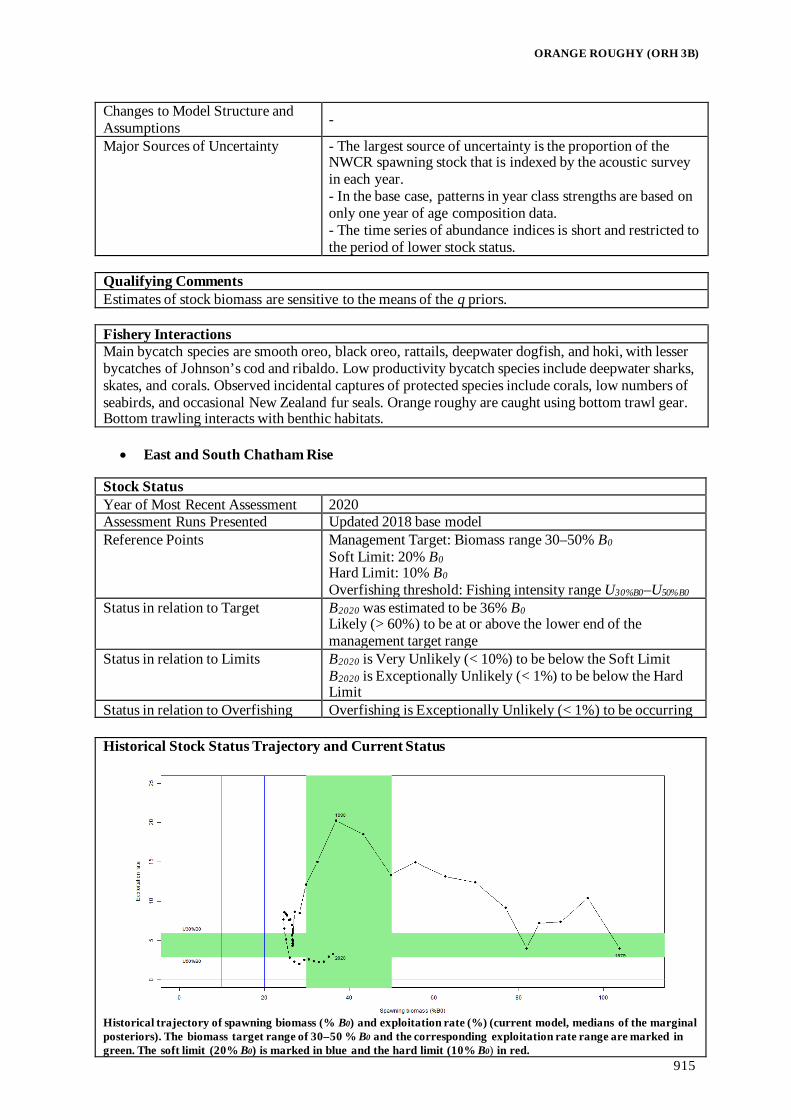
ORANGE ROUGHY (ORH 3B)
915
Changes to Model Structure and Assumptions -
Major Sources of Uncertainty - The largest source of uncertainty is the proportion of the NWCR spawning stock that is indexed by the acoustic survey in each year. - In the base case, patterns in year class strengths are based on only one year of age composition data. - The time series of abundance indices is short and restricted to the period of lower stock status.
Qualifying Comments Estimates of stock biomass are sensitive to the means of the q priors. Fishery Interactions Main bycatch species are smooth oreo, black oreo, rattails, deepwater dogfish, and hoki, with lesser bycatches of Johnson’s cod and ribaldo. Low productivity bycatch species include deepwater sharks, skates, and corals. Observed incidental captures of protected species include corals, low numbers of seabirds, and occasional New Zealand fur seals. Orange roughy are caught using bottom trawl gear. Bottom trawling interacts with benthic habitats.
• East and South Chatham Rise
Stock Status Year of Most Recent Assessment 2020 Assessment Runs Presented Updated 2018 base model Reference Points
Management Target: Biomass range 30–50% B0
Soft Limit: 20% B0 Hard Limit: 10% B0
Overfishing threshold: Fishing intensity range U30%B0–U50%B0 Status in relation to Target B2020 was estimated to be 36% B0
Likely (> 60%) to be at or above the lower end of the management target range
Status in relation to Limits B2020 is Very Unlikely (< 10%) to be below the Soft Limit B2020 is Exceptionally Unlikely (< 1%) to be below the Hard Limit
Status in relation to Overfishing Overfishing is Exceptionally Unlikely (< 1%) to be occurring Historical Stock Status Trajectory and Current Status
Historical trajectory of spawning biomass (% B0) and exploitation rate (%) (current model, medians of the marginal posteriors). The biomass target range of 30–50 % B0 and the corresponding exploitation rate range are marked in green. The soft limit (20% B0) is marked in blue and the hard limit (10% B0) in red.

ORANGE ROUGHY (ORH 3B)
916
Fishery and Stock Trends Recent Trend in Biomass or Proxy The spawning biomass is estimated to have been slowly
increasing since 2009–10. Recent Trend in Fishing Intensity or Proxy
Fishing intensity (exploitation rate) is estimated to have been near or below the lower end of the target range since 2010–11.
Other Abundance Indices - Trends in Other Relevant Indicators or Variables -
Projections and Prognosis Stock Projections or Prognosis Biomass is expected to increase slowly at catches equal to the
current catch limit (4775 t) or the HCR recommended catch limit (6348 t).
Probability of Current Catch or TACC causing Biomass to remain below or to decline below Limits
At the current catch limit (4775 t) or the HCR recommended catch limit (6348 t): Soft Limit: Very Unlikely (< 10%) Hard Limit: Exceptionally Unlikely (< 1%)
Assessment Methodology and Evaluation Assessment Type Level 1 - Full Quantitative Stock Assessment Assessment Method Age-structured CASAL model with Bayesian estimation of
posterior distributions Assessment Dates Latest assessment: 2020 Next assessment: 2022 Overall assessment quality rank 1 – High Quality Main data inputs (rank) - Four short time series of biomass
indices from research trawl surveys - Acoustic indices from research surveys of spawning plumes (Old plume, Rekohu plume, Crack) - Age frequencies from the spawning plumes in 2012, 2013, and 2016 - Length frequencies from commercial fisheries
1 – High Quality 1 – High Quality 1 – High Quality 1 – High Quality
Data not used (rank) - CPUE - Acoustic surveys of hills (hull-mounted transducers) - Wide-area acoustic survey estimates - Chatham Rise deepwater trawl survey stations (2010–2020)
3 – Low Quality: unlikely to be indexing stock-wide abundance 3 – Low Quality: major species identification and dead zone issues 2 – Medium or Mixed Quality: large potential bias due to mixed-species 2 – Medium or Mixed Quality: variable indices
Changes to Model Structure and Assumptions None
Major Sources of Uncertainty - The largest source of uncertainty is the proportion of the ESCR spawning stock that is indexed by the acoustic survey in each year. - Stock status is dependent on the timing of the appearance of the Rekohu spawning plume, which is unknown. - Patterns in year class strengths are based on only 3 years of age composition data.

ORANGE ROUGHY (ORH 3B)
917
Qualifying Comments - Estimates of stock biomass are sensitive to the means of the q priors. - Lack of fit to the 2016 acoustic biomass estimate.
Fishery Interactions Main bycatch species are smooth oreo, black oreo, deepwater dogfish, hoki, and rattails, with lesser bycatches of slickhead, Johnson’s cod, and morids. Low productivity bycatch species include deepwater sharks and dogfish and also corals. Observed incidental captures of protected species include corals, low numbers of seabirds, and occasional New Zealand fur seals. Orange roughy are caught using bottom trawl gear. Bottom trawling interacts with benthic habitats.
• 5.2 Southern ORH 3B fisheries
There are several other small fisheries in ORH 3B in the southern waters of which Puysegur appears to be the largest stock.
o Puysegur Stock Status Year of Most Recent Assessment 2017 Assessment Runs Presented Base model only Reference Points
Management Target: Biomass range 30–50% B0
Soft Limit: 20% B0 Hard Limit: 10% B0
Overfishing threshold: Fishing intensity range U30%B0 Status in relation to Target B2017 was estimated at 49% B0. Very Likely (> 90%) to be at
or above the lower end of the management target range Status in relation to Limits B2017 is Exceptionally Unlikely (< 1%) to be below the Soft or
Hard Limits Status in relation to Overfishing An agreed closure of the fishery was in place until 2017.
Overfishing in 2017 is Exceptionally Unlikely (< 1%) to be occurring
Historical Stock Status Trajectory and Current Status
Historical trajectory of spawning biomass (% B0), median exploitation rate (%) and fishing intensity (100-ESD) (base model, medians of the marginal posteriors). The biomass target range of 30–50% B0 and the corresponding exploitation rate range are marked in green. The soft limit (20% B0) and the hard limit (10% B0) are marked in red. Note that the left-hand Y-axis is non-linear.

ORANGE ROUGHY (ORH 3B)
918
Fishery and Stock Trends Recent Trend in Biomass or Proxy
Biomass reached its lowest point in 1998 and has increased steadily since then. According to the Harvest Strategy Standard, the stock is now considered to be fully rebuilt (at least a 70% probability that the lower end of the management target range of 30–50% B0 has been achieved).
Recent Trend in Fishing Intensity or Proxy
Fishing intensity has been close to zero since the fishery was closed in 1997-98 with the exception of 2005, 2006, and 2015 when surveys were conducted.
Other Abundance Indices - Trends in Other Relevant Indicators or Variables -
Projections and Prognosis Stock Projections or Prognosis No projections were conducted Probability of Current Catch or TACC causing Biomass to remain below or to decline below Limits
Current catch is zero
Probability of Current Catch or TACC causing Overfishing to continue or to commence
Current catch is zero
Assessment Methodology and Evaluation Assessment Type Level 1 - Full Quantitative Stock Assessment Assessment Method Age-structured CASAL model with Bayesian estimation of
posterior distributions
Assessment Dates Latest assessment: 2017 Next assessment: 2022 Overall assessment quality rank 1 – High Quality Main data inputs (rank) - Acoustic estimate of spawning
biomass on Goomzy (2015) - Trawl survey indices and length frequencies (1992, 1994) - Age frequencies (1992, 2015) - 2 years of length frequency data
1 – High Quality 1 – High Quality 1 – High Quality 1 – High Quality
Data not used (rank) - CPUE - Winter trawl surveys (1991, 1992, 2006) - Acoustic survey estimates (2005, 2006) - Additional commercial length frequencies
3 – Low Quality: unlikely to be indexing stock-wide abundance 2 – Medium or Mixed Quality: unlikely to be indexing stock-wide abundance 2 – Medium or Mixed Quality: large potential bias due to mixed species 2 – Medium or Mixed Quality: not enough months sampled within each year

ORANGE ROUGHY (ORH 3B)
919
Changes to Model Structure and Assumptions
- The previous assessment was in 1998. - Model now based on spawning biomass rather than transition-zone mature biomass. - Age data included to enable estimation of year class strengths rather than assuming deterministic recruitment. - Trawl survey indices better modelled to allow for difference in timing - A more stringent data quality threshold was imposed on data inputs (e.g., CPUE indices not used)
Major Sources of Uncertainty -The largest source of uncertainty is the proportion of the Puysegur spawning stock that is indexed by the acoustic survey in 2015. - The single acoustic estimate is the only recent biomass index. - Patterns in year class strengths are based on only two years of age frequencies.
Qualifying Comments -
Fishery Interactions Historically the Puysegur orange roughy fishery included black and smooth oreos, deepwater dogfish, black cardinal fish, slickheads, and rattails as significant bycatch. Interactions with other species are currently being characterised. Orange roughy are caught using bottom trawl gear. Bottom trawling interacts with benthic habitats.
• Auckland Islands (Pukaki South)
The Deepwater Working Group examined the data on orange roughy catch and effort from the Auckland Islands area in 2006 and found that there had been relatively little fishing activity in this area in the previous few years. There were insufficient data to conduct a standardised CPUE analysis, and it was believed that unstandardised CPUE did not provide a suitable index of relative abundance. Therefore, a stock assessment could not be carried out.
• Other fisheries
In 2006 the Deepwater Working Group examined the data on orange roughy catch and effort from other parts of ORH 3B – the Bounty Islands, Pukaki Rise, Snares Island, and the Arrow Plateau – and agreed that there were insufficient data to carry out standardised CPUE analyses for any of these areas. 6. FOR FURTHER INFORMATION Annala, J H; Sullivan, K J; O’Brien, C J; Iball, S D (Comps) (1998) Report from the Fishery Assessment Plenary, May 1998: stock assessments
and yield estimates. 409 p. (Unpublished report held by NIWA library, Wellington.) Bull, R; Doonan, I J; Tracey, D M; Coombs, R F (2000) An acoustic estimate of orange roughy abundance on the Northwest Hills, Chatham
Rise, June–July 1999. New Zealand. Fisheries Assessment Research Document 2000/20. 36 p. (Unpublished report held in NIWA Greta Point library, Wellington.)
Bull, B; Francis, R I C C; Dunn, A; McKenzie, A; Gilbert, D J; Smith, M H (2003) CASAL (C++ algorithmic stock assessment laboratory): CASAL User Manual v2.01-2003/08/01. NIWA Technical Report 124. 223 p.
Clark, M R; Anderson, O F; Dunn, M (2003) Descriptive analysis of catch and effort data from New Zealand orange roughy fisheries in ORH 1, 2A, 2B, 3A, 3B, and 7B to the end of the 2001–02 fishing year. New Zealand Fisheries Assessment Report 2003/60. 51p.
Clark, M R; Anderson, O F; Francis, R I C C; Tracey, D M (2000) The effects of commercial exploitation on orange roughy (Hoplostethus atlanticus) from the continental slope of the Chatham Rise, New Zealand, from 1979 to 1997. Fisheries Research 45(3): 217–238.
Clark, M R; Tracey, D M (1993) Orange roughy off the southeast coast of the South Island and Puysegur Bank: exploratory and research fishing, June-August l992. New Zealand Fisheries Technical Report No. 35. 30 p.
Clark, M R; Tracey, D M (1994) Trawl survey of orange roughy, black oreo, and smooth oreo in southern New Zealand waters August-September l992 (TAN9208). New Zealand Fisheries Data Report No. 40. 37 p.
Clark, M R; Anderson, O F; Tracey, D M (1996) Trawl survey of orange roughy, black oreo, and smooth oreo in southern New Zealand waters September-October 1994 (TAN9409). New Zealand Fisheries Data Report No. 72. 39 p.
Coburn, R P; Doonan, I J (1994) Orange roughy fishing on the North East Chatham Rise: a description of the commercial fishery, 1979–1988. New Zealand Fisheries Technical Report 38.
Coburn, R P; Doonan, I J (1997) The fishery for orange roughy on the northeast Chatham Rise, 1988–99 to 1993–94. New Zealand Fisheries Technical Report 48. 28 p.

ORANGE ROUGHY (ORH 3B)
920
Coombs, R F; Barr, R (2007) In situ measurements of orange roughy (Hoplostethus atlanticus) target strength. ICES Journal of Marine Science 64: 1220–1234.
Cordue, P L (2008) Review of estimates of Chatham Rise orange roughy biomass from plume surveys. Report prepared for the New Zealand Ministry of Fisheries. 39 p. (Unpublished report held by Fisheries New Zealand, Wellington.)
Cordue, P L (2010) Linear-model derived bottom-referenced weather corrections for the CR ORH plume time series (2002–2009). Report to the DWWG, DWWG2010-30, New Zealand Ministry of Fisheries. 71 p. (Unpublished report held by Fisheries New Zealand, Wellington.)
Cordue, P L (2014a) The 2014 orange roughy stock assessments. New Zealand Fisheries Assessment Report 2014/50. 135 p. Cordue, P L (2014b) A Management Strategy Evaluation for orange roughy. ISL Client Report for Deepwater Group. (Unpublished report
held by Fisheries New Zealand, Wellington.) Cordue, P L (2018) A brief update of the ORH3B ESCR and NWCR stock assessments to the end of the 2016–17 and 2017–18 fishing years
with application of the Harvest Control Rule in both years. ISL Client Report for Deepwater Group Ltd. 59 p. (Unpublished report held by Fisheries New Zealand, Wellington.)
Doonan, I J (1991) Orange roughy fishery assessment, CPUE analysis - linear regression, NE Chatham Rise 1991. New Zealand Fisheries Assessment Research Document 1991/9. 48 p. (Unpublished report held in NIWA Greta Point library, Wellington.)
Doonan, I J (1994) Life history parameters of orange roughy; estimates for 1994. New Zealand Fisheries Assessment Research Document 1994/19. 13 p. (Unpublished report held in NIWA Greta Point library, Wellington.)
Doonan, I (2009) Re-analysis of the spawning plume biomass, towbody acoustics surveys 1998 & 2000. Deepwater Working Group document 2009/16. (Unpublished report held by Fisheries New Zealand, Wellington.)
Doonan, I; Bull, B (2001) Absolute biomass for 1999, NE and East Chatham Rise. WG-Deepwater-01/27. (Unpublished report held by Fisheries New Zealand, Wellington.)
Doonan, I; Bull, B; Dunford, A; Coombs, R; Tracey, D; Hart, A (2001) Acoustic estimates of the biomass of aggregations of orange roughy in the Spawning Box and on the Northeastern and Eastern Hills, Chatham Rise, July 2000. New Zealand Fisheries Assessment Report 2001/70. 31 p.
Doonan, I J; Dunn, M; Dunford, A; Hart, A C; Tracey, D (2006) Acoustic estimates of orange roughy abundance on the Northeastern and Eastern Chatham Rise, July 2004: wide-area survey and hill survey. New Zealand Fisheries Assessment Report 2006/58. 45 p.
Doonan, I J; Dunn, M; Hart, A C (2009) Abundance estimates of orange roughy on the Northeastern and Eastern Chatham Rise, July 2007: wide-area trawl survey and hill acoustic survey (TAN0709). New Zealand Fisheries Assessment Report 2009/20. 38 p.
Doonan, I; Hart, A C (2003) Notes on the abundance of mature orange roughy on the NW Chatham Rise and Graveyard Hills, ORH 3B, 20 June - 7 July 2002. WG-Deepwater- 03/01. (Unpublished report held by Fisheries New Zealand, Wellington.)
Doonan, I J; Hart, A C; Bagley, N; Dunford, A (2012) Orange roughy abundance estimates of the north Chatham Rise Spawning Plumes (ORH3B), San Waitaki acoustic survey, June-July 2011. New Zealand Fisheries Assessment Report 2012/28. 35 p.
Doonan, I J; Horn, P L; Ó Maolagáin, C (2014a) Orange roughy age estimates: Chatham Rise (ORH 3B) spawning plumes in 2012, and mid-east coast North Island (ORH 2A) fishery from 1989–91 and 2010. New Zealand Fisheries Assessment Report 2014/24. 19 p.
Doonan, I J; Horn, P L; Ó Maolagáin, C (2014b) Age composition of orange roughy from ORH 3B (Chatham Rise: northwest ,1994, and northeast,2013), and from ORH 7A (Challenger Plateau in 1987, 2006 and 2009). New Zealand Fisheries Assessment Report 2014/59. 33 p.
Doonan, I J; Horn, P L; Ó Maolagáin, C; Datta, S (2018) Age composition of orange roughy from ORH 3B, Chatham Rise, 2016: Mount Muck, Old Plume, Rekohu Plume, and Morgue. New Zealand Fisheries Assessment Report 2018/48. 17 p.
Dunn, M R (2007) CPUE analysis and assessment of the Northeast Chatham Rise orange roughy stock (part of ORH 3B) to the end of 2004–05 fishing year. New Zealand Fisheries Assessment Report 2007/8. 75 p.
Dunn, M R; Anderson, O F; Doonan, I J (2008) Evaluation of stock status for orange roughy on the east and south Chatham Rise for 2008. New Zealand Fisheries Assessment Report 2008/65. 30 p.
Dunn, M R; Devine, J A (2010) An holistic approach to determining stock structure of orange roughy on the Chatham Rise. New Zealand Fisheries Assessment Report 2010/17. 65 p.
Dunn, M R; Doonan, I J (2018) Assessment of the Chatham Rise orange roughy stocks for 2017. New Zealand Fisheries Assessment Report 2018/59. 60 p.
Dunn, M R; Rickard, G J; Sutton, P J H; Doonan, I J (2009) Nursery grounds of orange roughy around New Zealand. ICES Journal of Marine Science 66: 871–885.
Francis, R I C C (1992) Recommendations concerning the calculation of maximum constant yield (MCY) and current annual yield (CAY). New Zealand Fisheries Assessment Research Document 1992/8. 26 p. (Unpublished report held by NIWA library, Wellington.)
Francis, R I C C (1995) The longevity of orange roughy: a reinterpretation of the radiometric data. New Zealand Fisheries Assessment Research Document 1995/2. 13 p. (Unpublished report held by NIWA library, Wellington.)
Francis, R I C C (1996) Orange roughy sex ratios and catch rate distributions in the Chatham Rise Spawning Box. New Zealand Fisheries Assessment Research Document 1996/13. 27 p. (Unpublished document held by NIWA library.)
Francis, R I C C (2006) Some recent problems in New Zealand orange roughy assessments. New Zealand Fisheries Assessment Report 2006/43. 65 p.
Francis, R I C C (2001a) Orange roughy CPUE on the South and east Chatham Rise. New Zealand Fisheries Assessment Report 2001/26. 30 p. Francis, R I C C (2001b) Stock Assessment of orange roughy on the South Chatham Rise. New Zealand Fisheries Assessment Report 2001/27.
25 p. Francis, R I C C (2001c) Stock assessment for 2001 of orange roughy on the northeast Chatham Rise. New Zealand Fisheries Assessment
Report 2001/41. 32 p. Francis, R I C C; Bull, B (2000) Assessment of the northwest Chatham Rise orange roughy stock (part of ORH 3B). New Zealand Fisheries
Assessment Report 2000/21. 17 p. Francis, R I C C; Clark, M R; Coburn, R P; Field, K D; Grimes, P J (1995) Assessment of the ORH 3B orange roughy fishery for the 1994–
95 fishing year. New Zealand Fisheries Assessment Research Document 1995/4. 43 p. (Unpublished report held in NIWA Greta Point library, Wellington.)
Francis, R I C C; Clark, M R; Grimes, P J (1997) Calculation of the recruited biomass of orange roughy on the northwest Chatham Rise using the 1996 Graveyard Hill egg survey (TAN9608). New Zealand Fisheries Assessment Research Document 1997/29. 18 p. (Unpublished report held by NIWA library, Wellington.)
Francis, R I C C; Horn, P L (1997) Transition zone in otoliths of orange roughy (Hoplostethus atlanticus) and its relationship to the onset of maturity. Marine Biology 129: 681–687.
Francis, R I C C; Hurst, R J; Renwick, J A (2001) An evaluation of catchability assumptions in New Zealand stock assessments. New Zealand Fisheries Assessment Report 2001/1. 37 p.
Hampton, I; Soule, M A; Nelson, J C (2005) Acoustic survey of orange roughy on Graveyard hill and in the spawning plume, North Chatham Rise, and on Puysegur Bank, New Zealand, June/July 2005. 98 p. (Unpublished report held by Fisheries New Zealand, Wellington.)
Hampton, I; Soule, M A; Nelson, J C (2006) Acoustic and trawl survey of orange roughy on Puysegur Bank, and in the spawning plume and northeast hills on the North Chatham Rise, New Zealand, July 2006. 91 p. (Unpublished report held by Fisheries New Zealand, Wellington.)

ORANGE ROUGHY (ORH 3B)
921
Hampton, I; Soule, M; Nelson, J (2008) Standardisation of acoustic estimates of orange roughy biomass in the North Chatham Rise Spawning Plume between 1996 and 2007, made with vessel-mounted transducers. 26 p. (Unpublished report held by Fisheries New Zealand, Wellington.)
Hampton, I; Soule, M; Nelson, J (2009) Corrections to time series of acoustic estimates of orange roughy spawning biomass in the Spawning Plume in area ORH3B from vessel-mounted transducers, 1996 to 2008. 29 p. WG-Deepwater-09/14. (Unpublished report held by Fisheries New Zealand, Wellington.)
Hampton, I; Soule, M A; Nelson, J C (2010) Standardised acoustic estimates of orange roughy biomass in the Spawning Plume in area ORH 3B from vessel-mounted and towed transducers, 1996–2009. (Unpublished report held by Fisheries New Zealand, Wellington.)
Hicks, A C (2006) Changes in lengths from the commercial catch in the Spawning Box. WG-Deepwater-06/ (Unpublished report held by Fisheries New Zealand, Wellington.)
Hilborn, R; Walters, C J (1992) Quantitative fisheries stock assessment: choice, dynamics, and uncertainty. Chapman and Hall, New York, 570 p.
Horn, P L; Tracey, D M; Clark, M R (1998) Between-area differences in age and length at first maturity of the orange roughy Hoplostethus atlanticus. Marine Biology 132 (2): 187–194.
Horn, P L; Tracey, D M; Doonan, I J; Krusic-Golub, K (2016) Age determination protocol for orange roughy (Hoplostethus atlanticus). New Zealand Fisheries Assessment Report 2016/03. 30 p
Kloser, R J; Horne, J K (2003) Characterizing uncertainty in target-strength measurements of a deepwater fish: orange roughy (Hoplostethus atlanticus). ICES Journal of Marine Science 60: 516–523.
Kloser, R J; Macaulay, G; Ryan, T; Lewis, M (2011) Improving acoustic species identification and target strength using frequency difference and visual verification: example for a deep-sea fish orange roughy. DWWG 2011-52. (Unpublished report held by Fisheries New Zealand, Wellington.)
Macaulay, G; Kloser, R J; Ryan, T (2009) Visually verified in situ target strength measurements of orange roughy from the Chatham Rise, July 2007. Final Research Report for Ministry of Fisheries Research Project ORH2006-01A, Objective 2. (Unpublished report held by Fisheries New Zealand, Wellington.) 45 p.
Mace, P M; Fenaughty, J M; Coburn, R P; Doonan, I J (1990) Growth and productivity of orange roughy (Hoplostethus atlanticus) on the north Chatham Rise. New Zealand Journal of Marine and Freshwater Research 24: 105–119.
McKenzie, A (2003) Standardised CPUE analysis and stock assessment of the northwest Chatham Rise orange roughy stock (part of ORH 3B). New Zealand Fisheries Assessment Report 2003/61. 24 p.
McKenzie, A (2005) Standardised CPUE analysis and stock assessment of the northwest Chatham Rise orange roughy stock (part of ORH 3B). Final Research Report for Ministry of Fisheries Project (ORH2003-02). 42 p (Unpublished report held by Fisheries New Zealand, Wellington.)
Robertson, D A; Mace, P M (1988) Assessment of the Chatham Rise orange roughy fishery for 1987/88. New Zealand Fisheries Assessment Research Document 1988/37. 5 p. (Unpublished report held by NIWA library, Wellington.)
Ryan, T E; Tilney, R L (2016) Biomass surveys of orange roughy and oreo species using a net-attached acoustic optical system for New Zealand ORH7B and ORH3B Puysegur management zones in June, July 2015. 67 p. (Copy held at CSIRO Marine and Atmospheric Research, Hobart.)
Smith, M H (2006) Northwest Chatham Rise mature biomass estimate for the stock assessment. WG-Deepwater-06/17. (Unpublished report held by Fisheries New Zealand, Wellington.)
Smith, P J; Benson, P G (1997) Genetic diversity in orange roughy from the east of New Zealand. Fisheries Research 31(3): 197–213. Soule, M A; Hampton, I; Nelson, J C; Tilney, R L (2010) Acoustic survey of orange roughy on the North Chatham Rise (ORH 3B), New
Zealand. June/July 2010. Report prepared for New Zealand Deepwater Group Ltd. Soule, M A; Nelson, J C; Hampton, I (2007) Acoustic survey of orange roughy in the spawning plume on the North Chatham Rise, New
Zealand. DWWG-2008/83. (Unpublished report held by Fisheries New Zealand, Wellington.) Taylor, P (2001) Assessment of orange roughy fisheries in southern New Zealand for 2000. New Zealand Fisheries Assessment Report
2001/24. 30 p. Tracey, D M; Fenaughty, J M (1997) Distribution and relative abundance of orange roughy on the Chatham Rise, May–July 1994. New
Zealand Fisheries Technical Report No. 44. 43 p. Tracey, D; Horn, P; Marriott, P; Krusic-Golub, K; Gren, C; Gili, R; Mieres, L C (2007) Orange Roughy Ageing Workshop: otolith preparation
and interpretation. (Unpublished report to the Deepwater Fisheries Assessment Working Group; held by Fisheries New Zealand, Wellington.)


ORANGE ROUGHY (ORH 7A)
923
ORANGE ROUGHY CHALLENGER PLATEAU (ORH 7A) 1. FISHERY SUMMARY 1.1 Commercial fisheries Historically, the fishery mainly occurred in the south-western region of the Challenger Plateau, both inside and outside the EEZ. Fish were caught throughout the year, with most effort in winter when the orange roughy form aggregations for spawning. Domestic vessels caught most of the quota. Total landings peaked at 10 000–12 000 t annually from 1986–87 to 1988–89 (Table 1). Total landings and ORH 7A landings were less than 2100 t annually from 1990–91 until the closure in 2000–01 (Table 1, Figure 1), when the TACC for this stock was reduced to 1 t. Recent surveys have shown an increase in biomass in the area. On 1 October 2010 the TACC was increased from 1 t to 500 t, with a 25 t allowance for other mortality, raising the TAC to a total of 525 t. This was to allow research surveys to be conducted using commercial fishing vessels. The TACC was further increased to 1600 t following a stock assessment in 2014. Total landings have closely followed the TACCs in recent years, averaging 1595 t in 2014–15 to 2018–19. Table 1: Reported landings (t) and TACCs (t) from 1980–81 to present. QMS data from 1986-present. The last two
columns are for research surveys on commercial vessels and give the research catch that was not recorded against ACE (WP = Westpac Bank).
Fishing year EEZ Outside
Total landings TACC EEZ extra WP extra
1980–81† 1 32 33 - 0 0 1981–82† 3 539 709 4 248 - 0 0 1982–83† 4 535 7 304 11 839 - 0 0 1983–84† 6 332 3 195 9 527 - 0 0 1984–85† 5 043 74 5 117 - 0 0 1985–86† 7 711 42 7 753 - 0 0 1986–87† 10 555 937 11 492 10 000 0 0 1987–88 10 086 2 095 12 181 12 000 0 0 1988–89 6 791 3 450 10 241 12 000 0 0 1989–90 3 709 600 *4 309 2 500 0 0 1990–91 1 340 17 1 357 1 900 0 0 1991–92 1 894 17 1 911 1 900 0 0 1992–93 1 412 675 2 087 1 900 0 0 1993–94 1 594 138 1 732 1 900 0 0 1994–95 1 554 82 1 636 1 900 0 0 1995–96 1 206 463 1 669 1 900 0 0 1996–97 1 055 253 1 308 1 900 0 0 1997−98 + + 1 502 1 900 0 0 1998−99 + + 1 249 1 425 0 0 1999−00 + + 629 1 425 0 0 2000−01 + + 0.2 1 0 0 2001−02 + + 0.1 1 0 0 2002−03 + + 4 1 0 0 2003−04 + + < 0.1 1 0 0 2004−05 + + < 1 1 141 17 2005−06 + + < 1 1 196 22 2006–07 + + < 0.1 1 0 0 2007–08 + + < 0.1 1 0 0 2008–09 + + 0.12 1 218 22 2009–10 + + < 0.1 1 339 5 2010–11 476 0 476 500 0 5 2011–12 504 7 511 500 0 0 2012–13 513 0 513 500 259 4 2013–14 484 13 497 500 0 50 2014–15 1 594 0 1 594 1 600 0 0 2015–16 1 248 320 1 568 1 600 0 0 2016–17 1 595 28 1 623 1 600 0 0 2017–18 1 026 575 1 601 1 600 126 53 2018–19 + + 1 589 1 600 0 0 2019–20 + + 1 897 2 058 0 0 2020–21 + + 2 074 2 058 0 0
†FSU data *This is a minimum value, because of unreported catches by foreign vessels fishing outside the EEZ. +Unknown distribution of catch between inside and outside the EEZ

ORANGE ROUGHY (ORH 7A)
924
Figure 1: Reported commercial landings and TACC for ORH 7A. 1.2 Recreational fisheries There is no known recreational fishing for orange roughy in this area. 1.3 Customary non-commercial fisheries There is no known customary non-commercial fishing for orange roughy in this area. 1.4 Illegal catch There is no quantitative information available on illegal catch which is likely to be negligible. 1.5 Other sources of mortality Catch overruns from various sources (including lost and/or discarded fish, use of nominal tray weights and low conversion factors) have been estimated as: 1980–81 to 1987–88, 30%; 1988–89, 25%; 1989–90, 20%; 1990–91, 15%; 1991–92 to 1992–93, 10%; 1993–94 onwards, 5%. These estimates are used in the current stock assessment. 2. BIOLOGY Biological parameters used in this assessment are presented in the Biology section at the beginning of the Introduction – Orange Roughy chapter. 3. STOCKS AND AREAS There is no new information on orange roughy stock structure beyond that presented in previous assessment documents. Orange roughy on the southwest Challenger Plateau (Area 7A, including Westpac Bank) are regarded as a single stock. Size structure, parasite composition, flesh mercury levels, allozyme frequency and mitochondrial DNA studies show differences to other major fisheries. Spawning occurs at a similar time to fish on the Chatham Rise, Puysegur Bank, Ritchie Banks, Cook Canyon and Lord Howe Rise. 4. STOCK ASSESSMENT From 2010 to 2013, assessments were conducted using an ad hoc approach which combined the virgin biomass estimate from the 2000 assessment (Annala et al 2000, Field & Francis 2001) and current biomass estimates from annual combined acoustic and trawl surveys (see Clark et al 2006, NIWA & FRS 2009, Doonan et al 2010, Hampton et al 2013, Hampton et al 2014, Cordue 2010a, 2012, 2013).

ORANGE ROUGHY (ORH 7A)
925
A model-based Bayesian stock assessment was carried out for this stock in 2019 following a similar assessment conducted in 2014 (Cordue 2014a). The 2014 assessment for this stock was one of four orange roughy assessments carried out in 2014 which all used similar methods (see Introduction – Orange Roughy chapter). The same approach was continued in 2019 although there was a review of previous data inputs and a substantial amount of new data were available. An age-structured population model was fitted to acoustic and trawl-survey estimates of spawning biomass and six age frequencies. 4.1 Model structure The model was single-sex and age-structured (1–100 years with a plus group), with maturity estimated separately (i.e., fish were classified by age and as mature or immature). Two time steps were used: a full year of natural mortality followed by an instantaneous spawning season and fishery on the spawning fish. Two fisheries were modelled, one within the EEZ and one on Westpac Bank (which is outside of the EEZ). The fishery selectivity for the EEZ was uniform across ages (for spawning fish) while a logistic selectivity (on spawning fish) was used for Westpac Bank where slightly older fish are caught. 100% of mature fish were assumed to spawn each year. The catch history was constructed from the catches in Table 1 and the over-run percentages in Section 1.5. Natural mortality was assumed to be constant across ages at 0.045 and the stock-recruitment relationship was assumed to follow a Beverton-Holt function with steepness of 0.75. The remaining fixed biological parameters are given in the Introduction – Orange Roughy chapter. 4.2 Input data and statistical assumptions There were three main data sources for observations fitted in the assessment: spawning biomass estimates from acoustic and trawl surveys (2005, 2006, 2009–2014, 2018); an early trawl survey time series of relative spawning biomass (1987–1989); four age frequencies from the trawl surveys (1987, 2006, 2009, and 2018); and two age frequencies from Volcano (a UTF on the Westpac Bank) (2014 and 2018). 4.2.1 Research surveys Trawl surveys of orange roughy on the Challenger Plateau were conducted regularly from 1983 to 1990. However, a variety of vessels and survey strata were used which makes comparisons problematic (Dunn et al 2010). Wingtip biomass estimates in 1983–1986 ranged from 100 000–185 000 t but the 1989 and 1990 survey estimates were much lower at approximately 10 000 t. From these early trawl surveys a “comparable area” time series, defined by Clark & Tracey (1994) and covering the period 1987–89, was selected for use in the assessment to provide some information on the early rate of spawning biomass decline (see the Amaltal Explorer time series in Table 3). In 2005, a new series of combined trawl and acoustic surveys was begun using the FV Thomas Harrison with a survey area comparable to that used from 1987–1990 (Clark et al 2005). The survey was repeated in 2006 (with an enlarged survey area) and was then conducted annually from 2009–2013 (Clark et al 2006, NIWA & FRS 2009, Doonan et al 2010, Hampton et al 2013, Hampton et al 2014) with another survey in 2018. It was apparent from the later surveys that the 2005 survey did not cover an appropriate area as the spawning biomass distribution had shifted somewhat in the intervening years. The surveys from 2006 onwards appear to have covered the bulk of the spawning biomass. Also, in 2014 an acoustic survey of Volcano was conducted using an Acoustic Optical System (AOS) (Ryan et al 2015) in addition to a hull-mounted transducer. The data from all of the surveys since 2005 have been analysed to produce acoustic and trawl survey indices of spawning biomass. Acoustic survey indices For the 2014 assessment, the method of Cordue (2010a, 2012) was used to produce combined acoustic and trawl survey indices for 2010 and 2013. This method used an estimate of orange roughy trawl vulnerability to allow the trawl survey estimates to be combined with the acoustic estimates (trawl estimates were essentially scaled down by a vulnerability distribution with a mean of 1.66). This assumed that the scalar (1.66) had been reliably estimated. To avoid this assumption in the 2019 assessment the acoustic data and trawl data were used separately.

ORANGE ROUGHY (ORH 7A)
926
The acoustic biomass estimates from 2005 to 2018 were reviewed and a number of adjustments were required to ensure that the time series of estimates were consistent. Acoustic estimates of spawning aggregations on Volcano and in the west and east of the flats within the EEZ were used in three separate time series (Table 2). Estimates from the hull-mounted transducer were adjusted as necessary so that they all used the latest length to target strength relationship, the Doonan et al (2003) absorption coefficient, and a combined motion and bubble layer correction (1.33) borrowed from work done on the Chatham Rise (Cordue 2010b, Doonan et al 2012). The estimates from the AOS (2014 and 2018) were adjusted to use the Doonan et al (2003) absorption coefficient. In 2005, 2011, and 2013, the motion corrections applied to the snapshots were not documented and a factor of 1.06 (the mean for snapshots in 2006 and 2009) was used in the adjustment calculations. In those years the acoustic indices were assigned an additional 20% of process error to account for the approximate adjustment. Table 2: Acoustic biomass estimates of spawning aggregations surveyed on Volcano, and the West and the East within
the EEZ. The model CV is the observation error CV with an additional 20% of process error in the years when the vessel motion correction was unknown (2005, 2011, and 2013).
West East Volcano Year Biomass (t) Model CV (%) Biomass (t) Model CV (%) Biomass (t) Model CV (%) 2005 4 210 53 2682 39 2006 4 383 59 6329 39 2009 13 555 22 8471 61 2010 8 114 14 1707 34 2011 13 340 33 2013 10 183 22 5365 26 4559 34 2014 3954 29 2018 9 966 9
The acoustic biomass estimate for each aggregation in each year is an average of a number of “snapshots” (individual surveys/estimates) of the aggregation in that year. Some of the snapshots in some years were not used in the average because they appeared to have been taken before the aggregation was fully formed (judged on the basis of female gonad stages from trawl catches at the time of the snapshot). Some snapshots in the eastern area (in 2010 and 2011) were not used as an examination of the distribution of backscatter on the transects showed that a genuine spawning aggregation was not surveyed (e.g., just a single transect on which positive backscatter was recorded). In 2018 there were a number of snapshots of Volcano which showed substantial biomass (about 4000 t) but it was unclear from the gonad staging whether spawning was underway. These snapshots were not used in the assessment (and there is no estimate for Volcano in 2018). In 2009, there was a single snapshot on Volcano which satisfied the timing criteria but it was a very low estimate (671 t) compared to all of the other years. It was considered that this estimate was unlikely to be representative of the spawning biomass on Volcano in 2009. It was not used in the base model but was used in a sensitivity run. Informed priors on the proportionality constants (q) were used for the acoustic time series. The means of the priors were derived from the 2013 proportions across aggregations and the assumption that all three aggregations combined represented “most” of the spawning biomass (80%). The prior used in this case for orange roughy assessments (since 2014) is LN(mean=0.8, CV=19%) (Cordue 2014a). Splitting this prior into three components gave priors for the West, East, and Volcano qs respectively: LN(0.41, 30%), LN(0.22, 30%), LN(0.18, 30%). Trawl survey indices The spawning biomass estimates from the Thomas Harrison trawl surveys (Table 3) were used as relative biomass with an informed prior. They excluded the rough terrain strata 9–11 and the mean of the informed prior was: 0.9 × 0.85 × 1.25 = 0.95 (allowing for total-survey availability (0.9), exclusion of strata 9–11 (0.85) and trawl vulnerability – adjusted mean of estimated vulnerability distribution = 1.25). Given the problematic nature of these trawl surveys (fish pluming and moving within the area), a process error CV of 20% was added to the estimated CVs (Table 3).

ORANGE ROUGHY (ORH 7A)
927
Table 3: Biomass indices from trawl surveys used in the stock assessment. The model CV is the observation error CV with an additional 20% of process error.
Vessel Year Biomass (t) Model CV (%) Amaltal Explorer 1987 75 040 33 1988 28 954 34 1989 11 062 23 Thomas Harrison 2006 13 987 34 2009 34 864 31 2011 18 425 33 2012 22 451 27 2013 18 993 55 2018 48 038 55
Age frequencies Age frequencies were available from four of the trawl surveys for use in the assessment. A previous analysis produced age frequencies for the 1987 Amaltal Explorer survey and the 2009 Thomas Harrison survey (Doonan et al 2013), although that study was based on a relatively small number of otoliths, it showed that the 2009 age frequency had much younger fish than the 1987 age frequency. For the 2014 stock assessment, the existing age frequencies were augmented with an increased number of otoliths (for a total of about 300 for each survey) and a new age frequency (from about 300 otoliths) was produced for the 2006 Thomas Harrison survey. For the 2019 assessment the age data from the 2018 survey were used to produce an age frequency for the EEZ (750 otoliths) and Volcano (150 otoliths). An age frequency was also produced from the 2014 survey of Volcano (470 otoliths) (Doonan et al 2015). The age frequencies were assumed to be multinomial and were mainly assigned effective sample sizes of 300/5 = 60 (with the sample size reflecting the number of trawl stations rather than the number of otoliths). However, the 2018 age frequency from Volcano was obtained from only one targeted trawl and this was given a much lower effective sample size of 30 (to reflect that it may not have been representative of the spawning plume). No reweighting was attempted because of the short time series. There are no age frequencies from the commercial fishery. 4.3 Model runs and results In the base model, natural mortality (M) was fixed at 0.045. There were numerous MPD and MCMC sensitivity runs but four main sensitivities are presented in this report: “All trend” (informed priors removed), estimate M, and the LowM-Highq and HighM-Lowq runs (see the Introduction – Orange Roughy chapter for specifications). In the base model the main parameters estimated were: virgin biomass (B0), the maturity ogive, the selectivity for Westpac Bank and year class strengths (YCS) from 1925 to 1995 (with the Haist parameterisation and “nearly uniform” priors on the free parameters). There were also the five proportionality constants (q) for the two trawl and three acoustic survey time series. 4.3.1 Model diagnostics The MCMC (and MPD) fits to the data in the base model were very good except in two cases. The Amaltal Explorer time series shows a very steep decline over only three years in the late 1980s (Figure 2). The steep decline cannot be fitted by the model unless a very high weight is placed on the time series and all other data are down-weighted. In this case the estimate of the minimum stock status is reduced to about 5% B0 (compared to 15% B0 for the base) but the estimate of current stock status is unchanged from the base model. It is likely that the Amaltal Explorer indices do not reflect true stock abundance in those years. There are good fits to the main biomass indices, the West aggregation (Figure 3) and the Thomas Harrison trawl indices (Figure 4). Both sets of indices and the fits show an increase from 2005/2006 through to 2018.

ORANGE ROUGHY (ORH 7A)
928
Figure 2: Base, MCMC: fit to the Amaltal Explorer trawl indices (top panel) and the associated normalised residuals
(bottom panel). Each box covers the middle 50% of the distribution and the whiskers extend to 95% CIs. The indices are plotted in the top panel (open circles) with 95% CIs (dashed red lines).
Figure 3: Base, MCMC: fit to the West spawning aggregation (top panel) and the associated normalised residuals
(bottom panel). Each box covers the middle 50% of the distribution and the whiskers extend to 95% CIs. The indices are plotted in the top panel (open circles) with 95% CIs (dashed red lines).
The second poor fit is for the 2018 Volcano age frequency (Figure 5). This age frequency was obtained from a single large catch on Volcano and only 150 otoliths. It has much older fish than the age frequency from Volcano in 2014 which was obtained from samples from six trawl catches on Volcano. It is

ORANGE ROUGHY (ORH 7A)
929
possible that the 2018 age frequency is not representative of the age distribution of the spawning aggregation on Volcano in 2018. Compared to 2018, the fit and associated residuals for the 2014 age frequency are excellent (Figure 6).
Figure 4: Base, MCMC: fit to the Thomas Harrison trawl indices (top panel) and the associated normalised residuals
(bottom panel). Each box covers the middle 50% of the distribution and the whiskers extend to 95% CIs. The indices are plotted in the top panel (open circles) with 95% CIs (dashed red lines).
Figure 5: Base, MCMC: fit to the 2018 Volcano age frequency (top panel) and the associated Pearson residuals (bottom
panel). Each box covers the middle 50% of the distribution and the whiskers extend to 95% CIs. The indices are plotted in the top panel (open circles) with 95% CIs (dashed red lines). The MPD fit is shown in red (top panel).

ORANGE ROUGHY (ORH 7A)
930
Figure 6: Base, MCMC: fit to the 2014 Volcano age frequency (top panel) and the associated Pearson residuals (bottom
panel). Each box covers the middle 50% of the distribution and the whiskers extend to 95% CIs. The indices are plotted in the top panel (open circles) with 95% CIs (dashed red lines). The MPD fit is shown in red (top panel).
The posterior distributions of the qs, which had informed priors, show movement to lower values of q for Thomas Harrison, the West, and the East aggregations, with a shift to higher values for Volcano (Figure 7). Although there is a substantial move to the left (for West and East), the posterior distributions are still within the range of the prior distributions and so the estimates of q are credible. For Volcano, the move to higher values probably reflects the nature of the associated selectivity which is to the right of maturity (which is the selectivity for the West and East aggregations).
Figure 7: Base, MCMC: Prior distributions (solid red lines) and marginal posterior distributions (histograms) for the
Thomas Harrison and acoustic qs.

ORANGE ROUGHY (ORH 7A)
931
MCMC results For the base model, and the sensitivity runs, MCMC convergence diagnostics were excellent. Virgin biomass (B0) was estimated to be about 95 000 t for all runs except when the informed priors on the qs were removed (Table 4). When the informed priors were removed, virgin biomass was estimated to be higher than in the base model (Table 4). This indicates that the trend in the biomass indices, and to some extent the age frequencies, support a higher virgin biomass than was implied by information on the scale of the stock from the informed priors. The base model estimates are to be preferred as the informed priors contain information on orange roughy target strength and spawning biomass areal availability that is not otherwise available to the model. For all runs, current stock status was estimated to be within or above the target biomass range of 30–50% B0 (Table 4). Table 4: MCMC estimates of virgin biomass (B0) and stock status (B2019 as %B0) for the base model and four sensitivity
runs.
M B0 (000 t) 95% CI B2019 (%B0) 95% CI Base 0.045 94 86–104 47 39–55 All trend 0.045 107 94–126 57 46–67 Estimate M 0.037 97 89–106 40 31–51 LowM-Highq 0.036 95 88–103 37 30–45 HighM-Lowq 0.054 94 85–106 56 48–65
The estimated YCS show little variation across cohorts but exhibit a long-term trend (Figure 8). The cohorts from 1989–1995 were spawned when SSB was at about 20% B0 (Figure 9). It is encouraging that the YCS estimates for these cohorts was about average (Figure 8). This suggests that steepness in the assumed Beverton-Holt stock recruitment relationship for this stock is not particularly low.
Figure 8: Base, MCMC estimated YCS. The box in each year covers 50% of the distribution and the whiskers extend
to 95% of the distribution. The stock status trajectory shows a steep decline to about 15% B0 in 1990, reflecting the large removals during the initial fish-down phase of this stock (Figure 9). From 1990 stock status remains at about 15% B0 until an upturn in the late 1990s (Figure 9). Biomass is estimated to have peaked in 2015, near the top of the target biomass range, before the increased catches (enabled by a TACC increase) caused a levelling out of the biomass trajectory (Figure 9).

ORANGE ROUGHY (ORH 7A)
932
Figure 9: Base, MCMC estimated spawning-stock biomass trajectory. The box in each year covers 50% of the
distribution and the whiskers extend to 95% of the distribution. The hard limit 10% B0 (red), soft limit 20% B0 (blue), and biomass target range 30–50% B0 (green) are marked by horizontal lines.
Fishing intensity was estimated in each year as the total exploitation rate (total catch over beginning of fishing season spawning biomass) for each MCMC sample to produce a posterior distribution for fishing intensity by year. The fishing intensity reference points U30%B0 and U50%B0 were also calculated in terms of exploitation rate (for the assumed catch split in the 2018–19 fishing year). Estimated fishing intensity was generally well above the target range (U30%B0–U50%B0) up until the closure of the fishery in 2001. Subsequently, it was well below the target range up until 2014, and from 2015 until now it is at the lower end of the range (Figure 10).
Figure 10: Base, MCMC estimated fishing-intensity trajectory. The box in each year covers 50% of the distribution
and the whiskers extend to 95% of the distribution. The fishing-intensity range associated with the biomass target of 30–50% B0 is marked by horizontal lines.

ORANGE ROUGHY (ORH 7A)
933
Projections Five-year projections were conducted (with resampling from the last 10 estimated YCS, 1986–1995) for a constant catch of 1600 t (the current TACC). A 5% catch over-run was assumed. Projections were done for the base model and for the LowM-Highq sensitivity model (as a “worst case” scenario). At the current TACC (1600 t), SSB is predicted to decrease slowly over the next five years for both models, while staying within the target biomass range (Figure 11). For both models the estimated probability of SSB going below either the soft limit (20% B0) or the hard limit (10% B0) is zero. For the base model projection, exploitation rates are predicted to slowly increase but still be at the lower end of the fishing intensity target range in 2024 (95% CI 0.030–0.054 compared to the target range of 0.033–0.067).
Figure 11: MCMC projections for a constant catch of 1600 t (plus a 5% allowance for incidental catch) for the base
model and the LowM-Highq model. The box in each year covers 50% of the distribution and the whiskers extend to 95% of the distribution. The target biomass range (30–50% B0) is indicated by horizontal green lines, the hard limit (10% B0) by a red line and the soft limit (20% B0) by a blue line.
5. FUTURE RESEARCH CONSIDERATIONS
• Revise the acoustic survey design and implementation to ensure (i) improved estimation of the abundance in the ‘East’ aggregation and (ii) abundance estimates are obtained for all three aggregations (‘East’, ‘West’ and Volcano) in the same year.
• Reconsider the otolith sampling approach from acoustic surveys to ensure that adequate otoliths are obtained from each aggregation and that these are obtained from multiple tows to support the stock assessment.
• Review current arrangements for sampling commercial catches for age to ensure that adequate samples are being obtained from both spawning and non-spawning fisheries.
6. STATUS OF THE STOCK Orange roughy on the southwest Challenger Plateau (Area 7A, including Westpac Bank) are regarded as a single stock.

ORANGE ROUGHY (ORH 7A)
934
Stock Status Year of Most Recent Assessment 2019 Assessment Runs Presented Base model only Reference Points Management Target: Biomass range 30–50% B0
Soft Limit: 20% B0 Hard Limit: 10% B0
Overfishing threshold: Fishing intensity range U30%B0–U50%B0 Status in relation to Target B2014 was estimated to be 47% B0
Very Likely (> 90%) to be at or above the lower end of the management target range and About as Likely as Not (40–60%) to be at or above the upper end of the management target range
Status in relation to Limits B2019 is Exceptionally Unlikely (< 1%) to be below the Soft Limit
B2019 is Exceptionally Unlikely (< 1%) to be below the Hard Limit
Status in relation to Overfishing Fishing intensity in 2018–2019 was estimated to be below or within the fishing intensity range. Overfishing is Very Unlikely (< 10%) to be occurring.
Historical trajectory of spawning biomass (%B0) and fishing intensity (exploitation rate) (base model, medians of the marginal posteriors). The biomass target range of 30–50% B0 and the corresponding exploitation rate (fishing intensity) target range are marked in green. The soft limit (20% B0) is marked in blue and the hard limit (10% B0) in red. Fishery and Stock Trends Recent Trend in Biomass or Proxy Spawning biomass is estimated to have peaked in 2014–2015
near the top of the target biomass range and to have declined slightly since then.
Recent Trend in Fishing Intensity or Proxy
Fishing intensity has been near the bottom of the fishing intensity target range since 2014–15.
Other Abundance Indices - Trends in Other Relevant Indicators or Variables -
Projections and Prognosis Stock Projections or Prognosis Biomass is expected to slowly decrease at the current TACC
(1600 t) over the next 5 years, but to remain within the target range.

ORANGE ROUGHY (ORH 7A)
935
Probability of Current Catch or TACC causing Biomass to remain below, or to decline below, Limits
Soft Limit: Exceptionally Unlikely (< 1%) within the next 5 years Hard Limit: Exceptionally Unlikely (< 1%) within the next five years
Probability of Current Catch or TACC causing Overfishing to continue or to commence
Very Unlikely (< 10%) within the next five years
Assessment Methodology and Evaluation Assessment Type Level 1 - Full Quantitative Stock Assessment Assessment Method Age-structured CASAL model with Bayesian estimation of
posterior distributions Assessment Dates Latest assessment: 2019 Next assessment: 2023 Overall assessment quality rank
1 – High Quality
Main data inputs (rank) - Acoustic survey indices for West, East, and Volcano aggregations - Two trawl survey time series: 1987–1989 and 2006, 2009–2012 - Age frequencies from the trawl surveys in 1987, 2006, 2009, and 2018 - Age frequencies from Volcano in 2014 and 2018
1 – High Quality 1 – High Quality 1 – High Quality 1 – High Quality
Data not used (rank) - commercial CPUE - Acoustic surveys of UTFs other than Volcano - Other acoustic estimates which did not meet the selection criteria - Early trawl surveys with different vessels covering different areas
3 – Low Quality: unlikely to be indexing stock-wide abundance 2 – Medium or Mixed Quality: species identification and dead zone problems 2 – Medium or Mixed Quality: not surveys of a spawning aggregation or timing too early 2 – Medium or Mixed Quality: not a consistent time series
Changes to Model Structure and Assumptions
- Acoustic biomass estimates were adjusted using a combined correction for vessel motion and the bubble layer estimated for a different vessel on the Chatham Rise. In the 2014 assessment, estimates were not corrected for the bubble layer. - Two fisheries were modelled instead of a single fishery.
Major Sources of Uncertainty
- The proportion of the stock that is indexed by the acoustic and trawl surveys.
Qualifying Comments -
Fishery Interactions Since the fishery re-opened with a low level of catch and effort, bycatch levels have been relatively low at about 4 to 5%, with spiky oreo being 1.4% of the average catch for 2008-09 to 2013-14. The bycatch of low productivity species over this period includes a number of deepwater shark and coral species. There were no observed incidental captures of seabirds or marine mammals between 2002–03 and 2017–18. Orange roughy are caught using bottom trawl gear. Bottom trawling interacts with benthic habitats.

ORANGE ROUGHY (ORH 7A)
936
6. FOR FURTHER INFORMATION Annala, J H; Sullivan, K J; O’Brien, C J (Comps.) (2000) Report from the Fishery Assessment Plenary, May 2000: stock assessments and yield
estimates. 495 p. (Unpublished report held in NIWA Greta Point library, Wellington.) Clark, M R (1991) Assessment of the Challenger Plateau (ORH 7A) orange roughy fishery for the 1991/92 fishing year. New Zealand Fisheries
Assessment Research Document 1991/2. 19 p. (Unpublished document held in NIWA library, Wellington.) Clark, M R (1992) Assessment of the Challenger Plateau (ORH 7A) orange roughy fishery for the 1992/93 fishing year. New Zealand Fisheries
Assessment Research Document 1992/6. 14 p. (Unpublished document held in NIWA library, Wellington.) Clark, M R; O’Driscoll, R L; Macaulay, G (2005) Distribution, abundance, and biology of orange roughy on the Challenger Plateau: results
of a trawl and acoustic survey, June–July 2005 (THH0501). NIWA Client Report WLG2005-64. Clark, M R; O’Driscoll, R L; Macaulay, G; Bagley, N W; Gauthier, S (2006) Distribution, abundance, and biology of orange roughy on the
Challenger Plateau: results of a trawl and acoustic survey, June–July 2006. NIWA Client Report WLG2006-83. Clark, M R; Tracey, D M (1994) Changes in a population of orange roughy, Hoplostethus atlanticus, with commercial exploitation on the
Challenger Plateau, New Zealand. Fishery Bulletin, U.S. 92: 236–253. Cordue, P L (2010a) Estimation of absolute biomass from the 2009 trawl and acoustic survey of Challenger orange roughy. ISL Client Report.
For Deepwater Group Ltd. 24 p. Cordue, P.L. (2010b) Linear-model derived bottom-referenced corrections for the Chatham Rise orange roughy plume acoustic time series
2002–2009 (Unpublished report held by Fisheries New Zealand, Wellington). Cordue, P L (2012) Estimation of absolute biomass from the time series of trawl and acoustic surveys of Challenger orange roughy. ISL Client
Report. For MAF. 30 p. (Unpublished document held by Fisheries New Zealand, Wellington.) Cordue, P L (2013) Estimating absolute orange roughy biomass for the southwest Challenger Plateau: 2005-2012. DWWG document 2013_25
Draft Report to MPI on ORH 7A.15 p. (Unpublished document held by Fisheries New Zealand, Wellington.) Cordue, P.L. (2014a) The 2014 orange roughy stock assessments. New Zealand Fisheries Assessment Report 2014/50. 135 p. Cordue, P L (2014b) A Management Strategy Evaluation for orange roughy. ISL Client Report for Deepwater Group. (Unpublished report
held by Fisheries New Zealand, Wellington.) Doonan, I J; Coombs, R; McClatchie, S (2003). The absorption of sound in seawater in relation to the estimation of deep-water fish biomass.
ICES Journal of Marine Science 60: 1047–1055. Doonan, I J; Hart A C; Bagley, N; Dunford, A (2012) Orange roughy abundance estimates of the north Chatham Rise Spawning Plumes
(ORH3B), San Waitaki acoustic survey, June-July 2011. New Zealand Fisheries Assessment Report 2012/28. 35 p. Doonan, I J; Horn, P L; Krusic-Golub, K (2013) Comparison of Challenger Plateau (ORH 7A) orange roughy age estimates between 1987
and 2009. New Zealand Fisheries Assessment Report 2013/2. 19 p. Doonan, I J; Parkinson, D; Gauthier, S (2010) Abundance, distribution, and biology of orange roughy on the southwest Challenger Plateau
(area ORH 7A): results of a trawl and acoustic survey, June-July 2010. NIWA Client Report WLG2010-63. Dunn, M R; Cordue, P L; Langley, A; Stokes, K (2010) Review of data and potential stock assessment approaches for orange roughy on the
Challenger Plateau (ORH 7A). (Draft New Zealand Fisheries Assessment Report held by Fisheries New Zealand, Wellington.) 41 p.
Field, K D (1999) Assessment of the Challenger Plateau (ORH 7A) orange roughy fishery for the 1998–99 fishing year. New Zealand Fisheries Assessment Research Document 1999/9. 19 p. (Unpublished document held in NIWA library, Wellington.)
Field, K D; Clark, M R (1996) Assessment of the ORH 7A orange roughy fishery for the 1996–97 fishing year. New Zealand Fisheries Assessment Research Document 1996/20. 16 p. (Unpublished document held in NIWA library, Wellington.)
Field, K D; Francis, R I C C (2001) CPUE analysis and stock assessment of the Challenger Plateau orange roughy stock (ORH 7A) for the 2000–01 fishing year. New Zealand Fisheries Assessment Report 2001/25. 19 p.
Francis, R I C C (1992) Recommendations concerning the calculation of maximum constant yield (MCY) and current annual yield (CAY). New Zealand Fisheries Assessment Research Document 1992/8. 27 p. (Unpublished document held in NIWA library, Wellington.)
Francis, R I C C; Clark, M R; Coburn, R P; Field, K D; Grimes, P J (1995) Assessment of the ORH 3B orange roughy fishery for the 1994–95 fishing year. New Zealand Fisheries Assessment Research Document 1995/4. 44 p. (Unpublished document held in NIWA library, Wellington.)
Francis, R I C C; Robertson, D A; Clark, M R; Coburn, R P (1992) Assessment of the ORH 3B orange roughy fishery for the 1992–93 fishing year. New Zealand Fisheries Assessment Research Document 1992/4. 46 p. (Unpublished document held in NIWA library, Wellington.)
Hampton, I (2010) Re-analysis of data from acoustic surveys of orange roughy on the Challenger Plateau (Area ORH7A) in 2005, 2006 and 2009. DWWG document 2010/38. 9 p. (Unpublished document held by Fisheries New Zealand, Wellington.)
Hampton, I; Boyer, D C; Leslie, R W; Nelson, J C (2014) Acoustic and trawl estimates of orange roughy (Hoplostethus atlanticus) biomass on the southwest Challenger Plateau, June/July 2012. New Zealand Fisheries Assessment Report. 2014/15. 43 p.
Hampton, I; Boyer, D C; Leslie, R W; Nelson, J C; Soule, M A; Tilney, R L (2013) Acoustic and trawl estimates of orange roughy (Hoplostethus atlanticus) biomass on the southwest Challenger Plateau, June/July 2011. New Zealand. Fisheries Assessment Report. 2013/48. 45p.
NIWA & FRS (2009) Abundance, distribution, and biology of orange roughy on the southwest Challenger Plateau (area ORH7A): results of a trawl and acoustic survey, June–July 2009. NIWA Client Report: 2009-59. FRS Client Report. 73 p.
Tracey, D; Horn, P; Marriott, P; Krusic-Golub, K; Gren, C; Gili, R; Mieres, L C (2007) Orange Roughy Ageing Workshop: otolith preparation and interpretation. Draft report to DWWG. (Unpublished document held by Fisheries New Zealand, Wellington.)

ORANGE ROUGHY (ORH 7B)
937
ORANGE ROUGHY WEST COAST SOUTH ISLAND (ORH 7B) 1. FISHERY SUMMARY 1.1 Commercial fisheries The orange roughy west coast South Island Fishstock was introduced into the Quota Management System with a TACC of 1558 t on 1 October 1986. The TACC was increased to 1708 t for the fishing year 1988–89. Landings ranged from 1139 t to 1763 t in the mid-1980s and early 1990s, before decreasing rapidly to just 290 t by 1994–95. The TACC was lowered to 430 t in 1995 and 110 t in 2001, before being reduced to just 1 t in 2007. Landings averaged just 0.68 t during the fishing years 2008–09 to 2018–19. The fishery was initially centred on an area near the Cook Canyon in Statistical Areas 033, 034 and 705. Up until 1996–97 approximately 80% of the catch was taken in winter (June–July) when fish form aggregations for spawning. From 1997–98 onwards about 50% of the catch was taken in winter. Reported domestic landings and TACCs are shown in Table 1, while the historical landings and TACC for ORH 7B are depicted in Figure 1. Table 1: Reported landings (t) of orange roughy and TACCs (t) for ORH 7B from 1983–84 to present. QMS data from
1986–present. Catches (t) taken under special permits during winter research surveys after 2013–14 are also noted.
Fishing year Reported landings TACC Research catch 1983–84* 2 - 1984–85* 282 - 1985–86* 1 763 1 558 1986–87* 1 446 1 558 1987–88 1 413 1 558 1988–89 1 750 1 708 1989–90 1 711 1 708 1990–91 1 683 1 708 1991–92 1 604 1 708 1992–93 1 139 1 708 1993–94 701 1 708 1994–95 290 1 708 1995–96 446 430 1996–97 425 430 1997–98 330 430 1998−99 405 430 1999–00 284 430 2000–01 161 430 2001–02 95 110 2002–03 90 110 2003–04 119 110 2004–05 106 110 2005–06 77 110 2006–07 125 110 2007–08 5.95 1 2008–09 1.44 1 2009–10 0.04 1 2010–11 0.14 1 2011–12 0.06 1 2012–13 0.25 1 2013–14 0.62 1 2014–15 1.67 1 21.7 2015–16 0.27 1 19.2 2016–17 0.58 1 11.0 2017–18 1.42 1 - 2018–19 1.00 1 57.0 2019–20 0.32 1 56.6 2020–21 0.54 1 -
*FSU data.

ORANGE ROUGHY (ORH 7B)
938
Figure 1: Reported commercial landings and TACC for ORH 7B (Challenger South). 1.2 Recreational fisheries There is no known recreational fishery for orange roughy in this area. 1.3 Customary non-commercial fisheries There is no known customary non-commercial fishing for orange roughy in this area. 1.4 Illegal catch There is no quantitative information available on illegal catch. 1.5 Other sources of mortality There is no quantitative information available on other sources of mortality in this fishery. 2. STOCKS AND AREAS There is no new information which would alter the stock boundaries given in previous assessment documents. Orange roughy in this fishery are thought to be a single stock. Genetic studies have shown that samples of Cook Canyon orange roughy are significantly different from Challenger Plateau and Puysegur Bank samples (Smith et al 1996). Moreover, the size structure and parasite composition differ from fish on the Challenger Plateau (Lester et al 1988). Spawning occurs at a similar time to fish on the Challenger Plateau and the Puysegur Bank. 3. STOCK ASSESSMENT The previous assessment for this stock was carried out in 2004 and is summarised in the 2006 Plenary Report. Virgin biomass (B0) was estimated to be approximately 12 000 t with 2004 stock status at 17% B0 (95% confidence interval 14–23%) when CPUE was assumed to be directly proportional to abundance (McKenzie 2005). An updated assessment was attempted in 2007 with the addition of catch data up to 2005–06 and new standardised CPUE indices (McKenzie 2008). The Working Group rejected the assessment because of the poor fit to the CPUE data. The results were similar to those from the 2004 assessment; namely a slow rebuild up to 2006, which was not supported by the CPUE data. A preliminary stock assessment was carried out in 2020 and some results from that assessment are reported here. Results from this assessment were inconclusive.

ORANGE ROUGHY (ORH 7B)
939
Results from the 2007 CPUE analysis and the previous assessments are retained below as they are relevant to the decision to effectively close the fishery from 1 October 2007. The use of CPUE analysis for an orange roughy fishery, to provide indices of biomass for use in stock assessment, has not been considered appropriate for more than a decade. Also, the previous assessments assume deterministic recruitment which is also inappropriate for orange roughy stock assessments (Cordue 2014) 3.1 The 2007 analysis of catch and effort data Commercial catch and effort data are available from 1985. In 2007, these data were examined using both an unstandardised and a standardised analysis. Unstandardised catch rates declined substantially over the course of the fishery but showed no clear trend in the latter years of the fishery to 2005–06 (Table 2). The standardised CPUE analysis was divided into two series to address reporting form changes: (i) using TCEPR data from 1985–86 through to 1996–97, and (ii) using CELR data from 1990–91 through to 2005–06. In addition, in order to increase vessel linkage across years, it was decided to use all months of data not just that from the winter fishery (June–July) as had been done for previous standardisations. The standardised analysis for the TCEPR data used catch per tow in a linear regression model. Indices from this model (Table 3, Figure 2) show a steep decline after the first two years, followed by a more gradual decline and a slight increase in catch rates in 1995–96 and 1996–97. Table 2: Summary of groomed data from TCEPR and CELR forms.
Fishing year Number of vessel
days
Number of tows
Total estimated
catch (t)
Mean daily catch rate
(t/tow)
Mean daily catch rate
(t/h) 1985–86 138 357 1 544 4.5 2.9 1986–87 132 405 1 250 4.0 2.7 1987–88 132 420 1 250 3.4 2.3 1988–89 133 368 827 2.5 1.6 1989–90 123 356 1 282 4.5 5.6 1990–91 208 632 1 657 2.8 3.3 1991–92 238 810 1 601 2.0 1.4 1992–93 258 784 1 128 1.5 2.3 1993–94 298 708 660 1.1 0.9 1994–95 162 361 320 0.9 1.6 1995–96 66 150 275 2.2 1.7 1996–97 90 182 244 1.3 7.5 1997–98 96 228 170 0.7 0.3 1998–99 188 566 359 0.6 0.2 1999–00 213 647 259 0.4 0.1 2000–01 149 442 162 0.4 0.1 2001–02 117 282 76 0.3 0.1 2002–03 97 292 112 0.4 0.2 2003–04 90 252 118 0.4 0.2 2004–05 121 393 102 0.3 0.1 2005–06 87 257 73 0.3 0.2
Table 3: Standardised CPUE indices (relative year effect) based on TCEPR data with number of vessel tows from
1985–86 to 1996–97.
CPUE Number of CPUE Number of Year index CV tows Year index CV tows 1985–86 1.99 0.20 153 1991–92 0.48 0.23 231 1986–87 2.13 0.23 150 1992–93 0.29 0.23 230 1987–88 1.11 0.26 212 1993–94 0.14 0.25 341 1988–89 0.58 0.22 310 1994–95 0.13 0.27 172 1989–90 0.61 0.22 236 1995–96 0.51 0.33 37 1990–91 0.76 0.23 238 1996–97 0.41 0.26 104
The standardised analysis for the CELR data used daily catch in a linear regression model. Indices from this model (Table 4, Figure 2) show a steep decline for the first four years, followed by an increase to a peak in 1995–96, and subsequent low catch rates after then.

ORANGE ROUGHY (ORH 7B)
940
Table 4: Standardised CPUE indices (relative year effect) based on CELR data with number of days from 1990–91 to 2005–06.
CPUE Number of CPUE Number of Year index CV days Year index CV days 1990–1991 2.17 0.27 110 1999–2000 0.34 0.27 131 1991–1992 1.11 0.27 108 2000–2001 0.34 0.28 88 1992–1993 0.74 0.27 126 2001–2002 0.33 0.28 73 1993–1994 0.28 0.28 81 2002–2003 0.61 0.26 67 1994–1995 0.53 0.30 46 2003–2004 0.59 0.25 75 1995–1996 1.16 0.33 29 2004–2005 0.35 0.24 114 1996–1997 0.53 0.38 19 2005–2006 0.36 0.26 80 1997–1998 0.36 0.30 52 1998–1999 0.39 0.28 112
3.2 Stock assessment estimates in 2004 Based on previous stock assessments using CPUE data the TACC was cut back severely from about 1700 t in 1994–95 to 110 t in 2000–01. By the late 1990s the stock was believed to be well below BMSY where it continued until at least 2004 (17% B0 in the 2004 assessment, Figure 3). Despite the large reduction in annual removals from the stock after 2001–02, catch rates did not increase over the subsequent 5 years. An updated assessment was attempted in 2007 with the addition of catch data up to 2005–06 and new standardised CPUE indices (Figure 2) based on TCEPR data (1986 to 1997) and a separate CELR series (1991 to 2006). These data were incorporated in a Bayesian stock assessment with deterministic recruitment to estimate stock size. The Working Group rejected the assessment because of the poor fit to the recent CPUE data. The model was insensitive to the recent CPUE data and predicted a rebuild (driven by the recruitment assumptions) that was not supported by any observations in the fishery.
Figure 2: The CPUE indices based on: (i) TCEPR data (solid line and crosses) covering 1985–86 to 1996–97, and (ii)
CELR data (triangles and dashed line) covering 1990–91 to 2005–06. The CELR index has been scaled so that it has the same mean value as the TCEPR index in the years that they overlap.

ORANGE ROUGHY (ORH 7B)
941
Figure 3: Biomass trajectory derived from Maximum Posterior Density (MPD) estimate of the model parameters
(2004 stock assessment). The biomass trajectory is shown by the solid line; crosses denote the CPUE index scaled to biomass.
3.3 Survey biomass estimates There were three random trawl surveys on the WCSI: two used the FV Arrow (October 1983, and in late July-early August 1986); and another by the RV Tangaroa in October 1991 (Tracey et al 1990, Armstrong & Tracey 1987, Clark 1991). All three used different stratification, but they broadly covered the same total area. Estimates from these trawl surveys are not used for assessment. Since 2015, surveys have been regularly conducted in Cook Canyon aimed at locating and acoustically surveying spawning orange roughy plumes. In 2015 an orange roughy plume was seen in Cook Canyon during a search by FV Amaltal Explorer but it was transitory and could not be acoustically surveyed (Ryan & Tilney 2016). Another attempt was made from FV Cook Canyon from 8 to 11 July 2016 (Doonan et al 2016). There were two parts to the work in 2016: a search for spawning aggregations (plumes); and a random trawl survey in the area around the Cook Canyon, where most of the historical catch was caught. One main spawning plume was found on two consecutive nights, but it dispersed during daylight hours which is its historical behaviour. The plume was mapped using the vessel’s echosounder (a fishing rather than a scientific echosounder), so it was not possible to perform acoustic integration and, hence, no acoustic abundance estimate was calculated. One short tow on the main plume produced about 18 t of spawning orange roughy with little bycatch. Most orange roughy catches in the random trawl survey (22 tows) were small (median 19 kg) with a wide size range (15 to 40 cm, mode at 22 cm), but there was one larger survey catch (600 kg) near the plume location which was composed of mainly spent (post-spawning) fish. A successful acoustic survey was conducted on FV Amaltal Explorer in 2017 using a CSIRO acoustic-optical towed system (AOS) (Ryan & Tilney 2017). Three snapshots of a single spawning plume in Cook Canyon gave an average estimate of 824 t (Table 5). The timing of the snapshots was not ideal as they appeared to be late relative to the spawning cycle with 40–50% of sampled fish having spent gonads (Ryan & Tilney 2017). In 2019, on FV Amaltal Mariner a plume at the same location as in 2017 was surveyed with a hull mounted system (Ryan & Tilney 2019). The snapshots spanned the main spawning season and there was no trend in the estimates with the increasing percentage of spent fish, which reached 45–65% on 10–11 July (Table 6). The average estimate in 2019 of 877 t was very similar to that in 2017 (Table 6).

ORANGE ROUGHY (ORH 7B)
942
Table 5: Biomass estimates from CSIRO’s AOS system (38 kHz) during the 2017 acoustic survey. For each snapshot the date, number of transects, the biomass estimate, and the CV are given. It is also noted that for each snapshot orange roughy marks were seen on more than two transects (indicating that a genuine spawning plume was surveyed).
Snapshot Date Transects Biomass (t) CV (%) Transects with
marks 1 4 July 17 5 627 53 > 2 2 5 July 17 7 930 32 > 2 3 6 July 17 7 915 50 > 2 Average 824 26 Table 6: Biomass estimates from the FV Amaltal Mariner 38 kHz hull-mounted system during the 2019 acoustic survey.
For each snapshot the date, number of transects, the biomass estimate, and the CV are given. The number of transects on which orange roughy marks were seen is also given (1 transect indicates a poor-quality snapshot; 2 transects may be adequate but more than 2 indicates that a genuine spawning plume was surveyed).
Snapshot Date Transects Biomass (t) CV (%) Transects with
marks 1 26 June 19 6 318 48 2 2 26 June 19 6 1393 35 2 3 3 July 19 9 927 21 > 2 4 4 July 19 9 746 31 > 2 5 9 July 19 6 511 64 1 6 9 July 19 5 473 38 2 7 10 July 19 10 958 33 > 2 8 16 July 19 4 198 58 1 Average (2 or >2) 803 14 Average (>2) 877 17
3.4 Age frequency data Orange roughy otoliths have routinely been collected during research surveys of Cook Canyon but they have only been aged for the 2019 acoustic survey. There are some otoliths from early trawl surveys in 1983 and 1986 but the first survey “took place before the spawning distribution was well known” and the second survey was “carried out after spawning was finished” (O’Driscoll 2001). For the 2015 acoustic survey there are 360 otoliths available for Cook Canyon but there was probably only 1 trawl in the spawning plume (which caught 18 t of orange roughy) (Ryan & Tilney 2016). In 2016, there are 476 otoliths available, but 299 of these were from a single trawl catch of 18 t on the plume (Doonan et al. 2016). The otoliths collected in the 2017 acoustic survey are also likely to be unrepresentative of the spawning population that year as they were collected late in the spawning cycle and are heavily skewed towards females (452 female, 150 male) (Ryan & Tilney 2017). The age frequencies that could be created from these various collections of otoliths are likely not to be representative of the surveyed spawning fish population. The 2019 age frequency was constructed using the method of Doonan et al (2013) from 500 otoliths collected over 6 trawls that targeted the plume. The trawls took place from 26 June to 16 July and caught from 2.5–18 t of orange roughy (Ryan & Tilney 2019). Males and females were almost equally represented and the age frequency across the 6 stations was similar. The scaled age frequency shows a large plus group at 100 years (Figure 4). The Working Group accepted that this sample was likely to be representative of the spawning plume.

ORANGE ROUGHY (ORH 7B)
943
Figure 4: The proportion of orange roughy at age for the scaled age frequency from trawls targeting the spawning
plume in the 2019 acoustic survey. There is a plus-group at 100 years. 3.5 The 2020 stock assessment A preliminary stock assessment was performed in 2020 fitting to the acoustic biomass estimates in 2017 and 2019 and the 2019 age frequency. A single stock, single sex, single area, age-structured model was implemented in CASAL. There were three main model runs which used Bayesian estimation to estimate marginal posterior distributions for virgin biomass (B0) and current stock status (SS2020). Two of the models were constructed as “worst case” scenarios in an attempt to determine the lowest possible stock status consistent with the data and model assumptions. The other model used the standard approach for orange roughy stock assessments (e.g., Cordue 2014). The estimates of B0 were consistent with previous estimates of virgin biomass. These estimates are driven by the total removals from the fishery. The estimates of current biomass and stock status varied widely across the three preliminary models. The standard model adequately fitted the data. However, a low estimate of the acoustic q implied that the acoustic surveys had missed one or more spawning plumes. The other two models had lower stock status but were unable to fit the acoustic estimates and predicted much more spawning biomass in those years than had been observed (even allowing for the scaling effect of an acoustic q of about 0.6). Therefore, all three of the models implied that the acoustic surveys may have missed one or more spawning plumes. It should be noted that since the ORH 7A stock has rebuilt spawning plumes have developed in areas where they were not previously seen (e.g., Cordue 2019). Also, for the ESCR orange roughy stock, there is an “old plume” which has been found in the same location for many years and a “new plume” which developed in a different location and consists of younger fish (Doonan et al 2017). The Working Group was unwilling to accept an assessment where current stock status depends on the existence of spawning biomass that has not been observed. The main alternative to an additional unobserved spawning plume is that there has been little recruitment to the spawning population since the closure of the fishery. 3.6 Future research considerations The preliminary stock assessment results highlight the discrepancy between the expected increase in spawning stock biomass due to a lack of fishing and the observed acoustic survey spawning biomass estimates. Either there are spawning fish that have not been found or there has been an extended period of very low recruitment to the spawning population. The next survey of Cook Canyon should include more time for searching than has been allocated previously in order to:
• Obtain multiple snapshot estimates of the Cook Canyon spawning plume, • Perform targeted trawling on the spawning plume to obtain a representative age frequency,

ORANGE ROUGHY (ORH 7B)
944
• Search for additional spawning plumes in new areas near but outside Cook Canyon (in orange roughy depths but not necessarily associated with a feature or previous fishing for orange roughy).
4. STATUS OF THE STOCK Stock Structure Assumptions The ORH 7B stock has been treated as a single spawning stock located around the Cook Canyon area. It is assessed and managed separately from other stocks and is assumed to be non-mixing with orange roughy stocks outside of the Cook Canyon area. Stock Status Year of Most Recent Assessment 2020 (preliminary) Assessment Runs Presented N/A Reference Points
Target: 30–50% B0 Soft Limit: 20% B0 Hard Limit: 10% B0 Overfishing threshold: -
Status in relation to Target Unknown Status in relation to Limits Unknown Fishery and Stock Trends Recent Trend in Biomass or Proxy Unknown, but biomass is likely to have increased since the
closure of the fishery in 2007. Recent Trend in Fishing Mortality or Proxy
Fishing mortality has been very low, limited to research catches, as the fishery has been closed since October 2007.
Other Abundance Indices Acoustic surveys carried out in 2017 and 2019 showed no change in abundance
Trends in Other Relevant Indicators or Variables
-
Projections and Prognosis Stock Projections or Prognosis Unknown but likely to be increasing at current catch levels Probability of Current Catch or TACC causing Biomass to remain below or to decline below Limits
Soft Limit: Unknown Hard Limit: Unknown
Assessment Methodology and Evaluation Assessment Type N/A Assessment Method N/A Assessment Dates Latest assessment: 2020
(preliminary) Next assessment: 2021
Overall assessment quality rank N/A Main data inputs (rank) - Catch history
- Acoustic biomass 2017, 2019 - Survey age frequency 2019
1 – High Quality 1 – High Quality 1 – High Quality
Data not used (rank) - CPUE Trawl surveys 1983, 1986, 1991, 2016
3 – Low Quality: not considered to be an index of abundance 3 – Low Quality: not considered to be an index of abundance
Changes to Model Structure and Assumptions
N/A

ORANGE ROUGHY (ORH 7B)
945
Major Sources of Uncertainty - The predicted spawning population, based on the estimated virgin biomass, catch history, and the expected increase with the lack of fishing since 2008, has not been detected by recent acoustic surveys
Qualifying Comments - Fishery Interactions Historically, the main bycatch species were oreos and deepwater dogfish. Other bycatch species recorded include deepwater sharks, deepsea skates and corals. The fishery is currently closed.
5. FOR FURTHER INFORMATION Anderson, O F; Dunn, M R (2012) Descriptive analysis of catch and effort data from New Zealand orange roughy fisheries in ORH 1, 2A,
2B, 3A, 3B, 7A, and 7B to the end of the 2008–09 fishing year. New Zealand Fisheries Assessment Report 2012/20. 82 p. Armstrong, J H; Tracey, D M (1987) Arrow orange roughy charter-for-quota cruise, west coast South Island, July–August 1986. Fisheries
Research Division Internal Report 58. 31 p. (Unpublished report held in NIWA library, Wellington.) Clark, M (1991) Voyage report West Coast South Island orange roughy, DEOR06. (Unpublished report, held in the CDF repository, NIWA,
Greta Point.) Clark, M R; Tracey, D M (1988) Assessment of the west coast South Island and northern North Island orange roughy fisheries. New Zealand.
Fisheries Assessment Research Document 1988/20. 11 p. (Unpublished report held in NIWA library, Wellington.) Clark, M R; Field, K D (1995) Assessment of the ORH 7B orange roughy fishery for the 1995–96 fishing year. New Zealand Fisheries
Assessment Research Document 1995/19. 15 p. (Unpublished report held in NIWA library, Wellington.) Cordue, P L (2014) The 2014 orange roughy stock assessments. New Zealand Fisheries Assessment Report 2014/50. 135 p. Cordue, P L (2019) A 2019 stock assessment of ORH 7A including Westpac Bank. New Zealand Fisheries Assessment Report 2019/33.
45 p. Doonan, I J; Hart, A; Wood, B (2016) Orange roughy trawl survey and plume search, west coast South Island, ORH 7B. NIWA Client Report
2016-155WN for Talleys Group Limited. 22 p. Doonan, I J; Horn, P L; Krusic-Golub, K (2013) Comparison of Challenger Plateau (ORH 7A) orange roughy age estimates between 1987
and 2009. New Zealand Fisheries Assessment Report 2013/2. 19 p. Doonan, I J; Horn, P L; Ó Maolagáin, C; Datta, S (2017) Age composition of orange roughy from ORH 3B, Chatham Rise, 2016: Mount
Muck, Old Plume, Rekohu Plume, and Morgue. New Zealand Fisheries Assessment Report 2018/48. 15 p. O’Driscoll, R L (2001) Assessment of the west coast South Island orange roughy fishery (ORH 7B) for the 2001–02 fishing year. New Zealand
Fisheries Assessment Report 2001/31. 29 p. Lester, R J G; Sewell, K B; Barnes, A; Evans, K (1988) Stock discrimination of orange roughy Hoplostethus atlanticus by parasite analysis.
Marine Biology 99: 137–143. McKenzie, A (2005) CPUE analysis and updated assessment for the west coast South Island orange roughy fishery (ORH 7B). New Zealand
Fisheries Assessment Report 2005/24. 35 p. McKenzie, A (2008) CPUE analysis and stock assessment for the west coast South Island orange roughy fishery (ORH 7B) to 2005-06. New
Zealand Fisheries Assessment Report 2008/21. 37 p. Ryan, T E; Tilney, R (2016) Biomass surveys of orange roughy and oreo species using a net-attached acoustic optical system for New
Zealand ORH7B and ORH3B Puysegur management zones in June, July 2015. Final report to Deepwater Group Ltd. 67 p. Ryan, T E; Tilney, R (2017) Biomass estimates of orange roughy spawning aggregations in ORH7B using a net-attached acoustic optical
system, July 2017. Final report to Deepwater Group Ltd and Fisheries New Zealand. Ryan, T E; Tilney, R (2019) 2019 abundance of orange roughy in ORH7B management zone -analysis and biomass estimation report. Final
report to Deepwater Group Ltd and Fisheries New Zealand. 21 p. Smith, P J; McVeagh, S M; Ede, A (1996) Genetically isolated stocks of orange roughy (Hoplostethus atlanticus) but not hoki (Macraronus
novaezelandiae) in the Tasman Sea and Southwest Pacific Ocean around New Zealand. Marine Biology 173: 783–793. Tracey, D M; McMillan, P J; Armstrong, J M; Banks, D A (1990) Orange roughy trawl survey: Challenger Plateau and West Coast South
Island, 1983. New Zealand Fisheries Technical Report 22. 34 p.


ORANGE ROUGHY (ORH ET)
947
ORANGE ROUGHY OUTSIDE THE EEZ (ORH ET)
1. FISHERY SUMMARY 1.1 Commercial fisheries Fisheries outside the EEZ in the New Zealand region occur on ridge systems and seamount chains in the Tasman Sea and southwest Pacific Ocean. There are five main fishing areas: Lord Howe Rise, Northwest Challenger Plateau, West Norfolk Ridge, South Tasman Rise, and Louisville Ridge (see figure above). The first orange roughy fishery outside the EEZ developed on the Westpac Bank close to the main fishing grounds on the southwest Challenger Plateau in the early-mid 1980s. Catches were recorded as part of the straddling stock crossing into ORH 7A, and therefore excluded from this chapter, up until 2007. Further exploration in the region resulted in the development of commercial fisheries on the Lord Howe Rise in 1987–88, Northwest Challenger Plateau in 1988–89, Louisville Ridge in 1993–94, South Tasman Rise in 1997–98, and West Norfolk Ridge in 2001–02. Catches from all these fisheries are tabulated by fishing year up to 2006–07, excluding Westpac Bank catches (Table 1), and by calendar year from 2007 to present (Table 2), as required by the South Pacific Fisheries Management Organisation (SPRFMO). Table 1: Estimated catches (t) of orange roughy for ORH ET fisheries from 1987–88 to 2006–07. (Data from New
Zealand (FSU, QMS), Australia (AFMA), and various sources for other countries. Note that the fishing year for South Tasman Rise is March to February, all others are October to September). See Table 2 for catches from 2007 onwards.
Fishing year Lord Howe NW Challenger Louisville West Norfolk South Tasman Total ET 1987–88 4 000 5 0 0 0 4 005 1988–89 2 430 297 0 0 0 2 727 1989–90 927 425 0 0 0 1 352 1990–01 282 123 0 0 0 405 1991–02 859 620 0 0 0 1 479 1992–03 2 300 2 463 0 0 0 4 763 1993–04 840 1 731 689 0 0 3 260 1994–05 761 1 138 13 252 0 0 15 151 1995–06 5 500 8 816 0 0 9 321 1996–07 139 332 3 209 0 5 3 685 1997–08 26 397 1 404 0 3 930 5 757 1998–09 440 961 3 164 0 705 5 270 1999–00 52 473 1 369 0 4 110 6 004 2000–01 428 1 228 1 598 10 830 4 094 2001–02 120 2 075 1 004 649 170 3 729 2002–03 272 1 010 1 296 94 110 2 782 2003–04 324 654 1 419 90 3 2 490 2004–05 430 464 1 510 277 55 2 736 2005–06 240 201 675 727 12 1 855 2006–07 40 96 323 552 0 1 011

ORANGE ROUGHY (ORH ET)
948
Catch totals include data from New Zealand and Australian vessels available from tow by tow fishing records, with estimated catches added for vessels from Japan, USSR, Korea, Norway, South Africa, and China. Catch statistics are likely to be incomplete. These fisheries were historically unregulated, with the exception of the South Tasman Rise area, where catches by Australian and New Zealand vessels have at times been restricted by a TAC imposed under a Memorandum of Understanding between the two countries. The South Tasman Rise fishery is currently closed by SPRFMO. South Pacific Regional Fisheries Management Organisation (SPRFMO) Convention Area Regulation of these fisheries was implemented following adoption of the SPRFMO interim measures in May 2007, and specific high sea fishing permits for the SPRFMO Area have been issued since 2007–08. Table 3 shows the number of New Zealand vessels that fished and their orange roughy catch by area. From 2007 to 2019, an orange roughy catch limit was applied for New Zealand vessels, being the average annual catch between 2002 and 2006 (1852 t). Australia implemented analogous limits for its vessels, and no other nations fished orange roughy in the SPRFMO area. From 2019, SPRFMO has implemented orange roughy catch limits that are subsequently allocated to SPRFMO Members who are permitted to fish under SPRFMO Conservation and Management Measures. In 2019 and 2020, catch limits were set for the Tasman Sea (comprises NW Challenger, W. Norfolk Ridge, and Lord Howe Rise), for the Louisville Ridge, and for the Westpac Bank. For 2021, the catch limit in the Tasman Sea was divided to represent the three Tasman Sea stocks. Table 2: Annual effort and catch (t) data for orange roughy from New Zealand vessels, by area, for the SPRFMO Area
(calendar years). Westpac Bank is on the Challenger Plateau but is considered part of the straddling stock ORH 7A so landings from that area are tabulated separately. Australian catches over this period, mostly from the Tasman Sea, ranged from 0 to 148 t, mean 46 t per annum). No other nations fished in this area.
Year Number
of Vessels Number of tows
Lord Howe
NW Challenger
West Norfolk Westpac Louisville Other
All areas
2007 8 415 34 36 515 – 280 – 866 2008 4 208 380 31 426 – – – 837 2009 6 545 403 238 233 23 – 31 928 2010 7 1 170 385 415 79 5 584 6 1 474 2011 7 1 158 1 675 113 5 285 – 1 079 2012 6 652 121 247 49 8 288 8 721 2013 5 760 344 230 19 3 565 3 1 164 2014 5 403 79 57 – 54 754 54 998 2015 5 959 157 530 20 118 462 – 1 287 2016 6 943 208 486 – 234 27 – 954 2017 5 1 423 215 307 22 129 420 – 1 093 2018 6 858 180 399 5 569 81 – 1 232 2019 4 221 38 171 0 111 139 – 460 2020 3 329 2 76 3 88 133 – 301
Table 3: New Zealand catch and catch limits (t) from 2019.
Year Lord Howe
NW Challenger
West Norfolk
Tasman Sea
catch total
Tasman Sea NZ
limit Westpac Westpac NZ limit Louisville
Louisville NZ limit Other
All areas
2019 38 171 0 210 277 111 245 139 1 026 – 460 2020 2 76 3 80 277 88 245 133 1 026 301
The SPRFMO Convention was closed for signature in January 2011 and formally entered into force in August 2012. Since that time, monitoring and assessment of catches and fisheries, including for orange roughy, has been overseen by the SPRFMO Scientific Committee. New Zealand reports annual catch and effort information in an Annual Report available on the SPRFMO website. South Tasman Rise Exploratory fishing south of Tasmania located aggregations of orange roughy on the South Tasman Rise just outside the Australian Fishing Zone (AFZ) in late 1997. The fishery rapidly increased in the next four years (Table 4), with Australian and New Zealand vessels working several small hill features on the rise. However, New Zealand vessels have not fished the South Tasman Rise since 2000–01. Effort dropped continuously from 2001–02, and mean catch per tow in 2004–05 was about 1 t/tow.
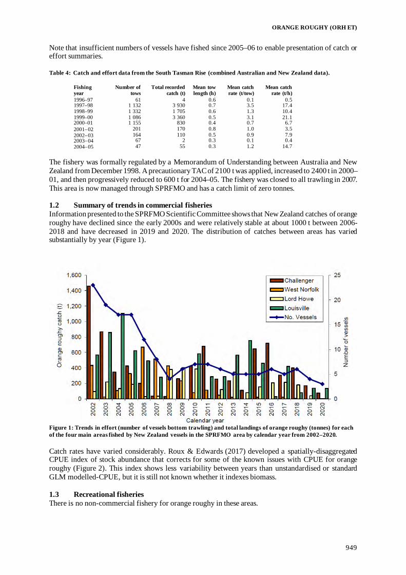
ORANGE ROUGHY (ORH ET)
949
Note that insufficient numbers of vessels have fished since 2005–06 to enable presentation of catch or effort summaries. Table 4: Catch and effort data from the South Tasman Rise (combined Australian and New Zealand data).
Fishing year
Number of tows
Total recorded catch (t)
Mean tow length (h)
Mean catch rate (t/tow)
Mean catch rate (t/h)
1996–97 61 4 0.6 0.1 0.5 1997–98 1 132 3 930 0.7 3.5 17.4 1998–99 1 332 1 705 0.6 1.3 10.4 1999–00 1 086 3 360 0.5 3.1 21.1 2000–01 1 155 830 0.4 0.7 6.7 2001−02 201 170 0.8 1.0 3.5 2002−03 164 110 0.5 0.9 7.9 2003−04 67 2 0.3 0.1 0.4 2004−05 47 55 0.3 1.2 14.7
The fishery was formally regulated by a Memorandum of Understanding between Australia and New Zealand from December 1998. A precautionary TAC of 2100 t was applied, increased to 2400 t in 2000–01, and then progressively reduced to 600 t for 2004–05. The fishery was closed to all trawling in 2007. This area is now managed through SPRFMO and has a catch limit of zero tonnes. 1.2 Summary of trends in commercial fisheries Information presented to the SPRFMO Scientific Committee shows that New Zealand catches of orange roughy have declined since the early 2000s and were relatively stable at about 1000 t between 2006-2018 and have decreased in 2019 and 2020. The distribution of catches between areas has varied substantially by year (Figure 1).
Figure 1: Trends in effort (number of vessels bottom trawling) and total landings of orange roughy (tonnes) for each of the four main areas fished by New Zealand vessels in the SPRFMO area by calendar year from 2002–2020. Catch rates have varied considerably. Roux & Edwards (2017) developed a spatially-disaggregated CPUE index of stock abundance that corrects for some of the known issues with CPUE for orange roughy (Figure 2). This index shows less variability between years than unstandardised or standard GLM modelled-CPUE, but it is still not known whether it indexes biomass. 1.3 Recreational fisheries There is no non-commercial fishery for orange roughy in these areas.

ORANGE ROUGHY (ORH ET)
950
1.4 Customary non-commercial fisheries There is no customary non-commercial fishing for orange roughy in these areas. 1.5 Illegal catch In most of these areas, there were no regulations regarding limits on catch in international waters before 2007. The South Tasman Rise region has been subject to catch restrictions for Australian and New Zealand vessels under a Memorandum of Understanding between the two countries. In 1999–2000 vessels registered in South Africa and Belize fished the region. The estimated catch of at least 750 t has been included in the catch total for that year. No other information is available on any possible illegal catch on the South Tasman Rise, or the Westpac Bank part of ORH 7A. 1.6 Other sources of mortality There may be some overrun of reported catch because of fish loss with trawl gear damage, ripped nets, discards, and conversion factor inaccuracies. In a number of other orange roughy fisheries, a current level of 5% has been applied (higher in the past). No corrections are made here because of limited information on the sources which may differ with each fishery. 2. STOCKS AND AREAS Stock structure is uncertain but Clark et al (2016) analysed multiple data sets and recommended that fishing grounds in the following areas be considered as separate units for the purpose of stock assessment: Lord Howe Rise; NW Challenger; SW Challenger; West Norfolk Ridge; South Tasman Rise; and North, Central, and South Louisville (Figure 2). Orange roughy on the South Tasman Rise are regarded as a straddling stock with fish inside the AFZ. Those on the Westpac Bank on the SW Challenger Plateau are regarded as a straddling stock with fish inside New Zealand’s EEZ and the ORH 7A stock.
Figure 2: Comparison of new areas assumed for stock assessment purposes (in red) and previous areas (in blue)
overlaid on the total distribution of catch rates for orange roughy. Where both areas are coincident, red boxes overlay blue boxes. See Clark et al (2016) for details.

ORANGE ROUGHY (ORH ET)
951
3. STOCK ASSESSMENT Several low-information stock assessments were presented to the SPRFMO Scientific Committee in 2015 and 2016 but these were not used by the committee to frame advice to the SPRFMO Commission until the 2017 meeting. The following is an extract from the report of the Scientific Committee’s meeting in August 2017. 98. Noting the urgent need to collect information to support robust assessments of orange roughy in the
SPRFMO Area for sound management advice, the Scientific Committee considered the three approaches to assess SPRFMO orange roughy stocks as detailed in SC5-DW11 to DW14, SC5-INF03, and the Report of the 2nd Deepwater Workshop of the Scientific Committee (Annex 5). Although none of the methods is ideal for the assessment of SPRFMO orange roughy stocks, the SC considered them to be collectively indicative of stock status and potential yields. The development of advice on catch limits for individual stocks was considered but, because of the level of uncertainty in estimates of status and yield by stock, it was considered better to group the stocks for the development of advice.
99. The SC used the lower 95% CIs of estimated stock status to inform the level of precaution that might
be appropriate. The group of stocks to the west of New Zealand (in the Tasman Sea) have a greater potential for low stock status than those to the east (Louisville Ridge) and a more precautionary approach was considered appropriate there.
Papers adopted and cited by the Scientific Committee in framing this advice were as follows:
• Roux et al (2017), FAR 2017/01, tabled as paper SC5-DW11: Low information stock assessment of orange roughy in the SPRFMO Area. Available at: http://www.sprfmo.int/assets/SC5-2017/SC5-DW11-NZFAR-2017-01-Orange-roughy-SPRFMO-area.pdf
• Edwards & Roux (2017), tabled as paper SC5-DW12: A simple delay-difference model for assessment of data-poor orange roughy stocks. Available at: http://www.sprfmo.int/assets/SC5-2017/SC5-DW12-Edwards-Roux-Delay-difference-ORY-model.pdf
• Roux & Edwards (2017), tabled as paper SC5-DW13: A data limited approach for assessing small scale fisheries for orange roughy in the SPRFMO Area. Available at: http://www.sprfmo.int/assets/SC5-2017/SC5-DW13-rev1-Roux-Edwards-BDM-method-ORY.pdf
• Cordue (2017a), tabled as paper SC5-DW14: Catch-history based stock assessments of seven SPRFMO orange roughy stocks. Available at: http://www.sprfmo.int/assets/SC5-2017/SC5-DW14-Cordue-catch-history-method-ORY.pdf
• Cordue (2017b), tabled as paper SC5-INF03: A CPUE based stock assessment of the Louisville Central orange roughy stock. Available at: http://www.sprfmo.int/assets/SC5-2017/SC5-INF03-LouisCentralAssess.pdf
• Galvez et al (2017), tabled as paper SC5-Doc08: Report from the Deepwater Workshop in Hobart, May 2017. Available at: http://www.sprfmo.int/assets/SC5-2017/SC5-Doc08-rev1-DWG-Workshop-Report-Final27Sep17.pdf
In 2019, a Bayesian stock assessment model for the Louisville Central orange roughy stock using age and length compositions and constraints on maximum exploitation rates was developed. The biological parameters and year class strengths for Louisville Central were then used to update assessments based on catch history for Louisville North and South. Although stock status remains uncertain, the models suggest that Louisville Central is likely to be above 50% B0 and Louisville North is likely to be above 30% B0. In 2020, a Bayesian stock assessment was presented for the NW Challenger using age frequency data collected in 1993, 2013, and 2018. The maturity parameters and year class strengths estimated for NW Challenger were then used in a catch-history based assessment for Lord Howe Rise. For both stocks, current stock status was estimated to be higher than in the 2017 stock assessment. The addition of the age frequencies has reduced the estimated probability of low B0 and associated low stock status. There is also qualitative evidence from the fishery that current stock status is not seriously depleted because catch rates have been maintained or slightly increased since a low point in 2005. Although current stock status for each of the stocks is uncertain, it was considered likely that NW Challenger is above 40% B0 whereas Lord Howe Rise is likely to be above 30% B0.

ORANGE ROUGHY (ORH ET)
952
4. STATUS OF THE STOCKS The status of the stocks in the SPRFMO Convention Area is not well-known. The SPRFMO Scientific Committee has accepted stock assessments for the main stocks (Tables 5 and 6). Table 5: Summary results for the Louisville Ridge stocks from SC7-DW05 presented in October 2019.
Bo (000 t) SS2019 (%B0) Long term yield (t) Median 95% CI Median 95% CI Median 95% CI P(SS19<20% B0) P(SS19>30% B0) Central 71 34–117 82 61–93 710 340–1 170 0.00 1.00 North 26 8–80 78 32–96 260 82–800 0.00 0.98 South 25 11–55 64 18–86 250 110–550 0.04 0.89
Table 6: Summary results for the Tasman Sea stocks from SC8-DW10.
Bo (000 t) SS2020 (% Bo) Long-term yield (t) Median 95% CI Median 95% CI Median 95% CI NW Challenger 33 19–43 68 46–81 396 228–516 Lord Howe Rise 29 11–75 72 29–93 348 132–900 West Norfolk Ridge 9 4–21 63* 19–84* 108 48–252
* 2015 stock status, noting that the yield estimate for West Norfolk Ridge differs from that given in SC5-DW14 based on application of the 1.2% B0 calculation 5. FOR FURTHER INFORMATION Anderson, O F (2006) A summary of biological information on the New Zealand fisheries for orange roughy (Hoplostethus atlanticus) for the
2003–04 fishing year. New Zealand Fisheries Assessment Report 2006/16. 25 p. Clark, M R (2003) Estimation of orange roughy biomass on the Louisville Ridge: application of “Seamount Meta-analysis” results. Final Research
Report to the Ministry of Fisheries for ORH2002/03. (Unpublished report held by Fisheries New Zealand, Wellington.) Clark, M R (2004) Descriptive analysis of orange roughy fisheries in the New Zealand region outside the EEZ: Lord Howe Rise, Northwest
Challenger Plateau, West Norfolk Ridge, South Tasman Rise, and Louisville Ridge to the end of the 2002–03 fishing year. New Zealand Fisheries Assessment Report 2004/51. 36 p.
Clark, M R (2006a) Descriptive analysis of orange roughy fisheries in the New Zealand region outside the EEZ: Lord Howe Rise, Northwest Challenger Plateau, West Norfolk Ridge, South Tasman Rise, and Louisville Ridge to the end of the 2003–04 fishing year. New Zealand Fisheries Assessment Report 2006/25. 37 p.
Clark, M R (2006b) Descriptive analysis of orange roughy fisheries in the New Zealand region outside the EEZ: Lord Howe Rise, Northwest Challenger Plateau, West Norfolk Ridge, South Tasman Rise, and Louisville Ridge to the end of the 2004–05 fishing year. New Zealand Fisheries Assessment Report 2006/56. 38 p.
Clark, M R (2008) Descriptive analysis of orange roughy fisheries in the New Zealand region outside the EEZ: Lord Howe Rise, Northwest Challenger Plateau, West Norfolk Ridge, South Tasman Rise, and Louisville Ridge to the end of the 2005–06 fishing year. New Zealand Fisheries Assessment Report 2008/12. 45 p.
Clark, M R; Anderson, O F (2001) The Louisville Ridge orange roughy fishery: an update of commercial catch-effort data and CPUE analysis of the fishery to the end of the 1999–2000 fishing year. New Zealand Fisheries Assessment Report 2001/74. 31 p.
Clark, M R; Anderson, O F (2003) The Louisville Ridge orange roughy fishery: an analysis of commercial catch-effort data and stock assessment of the fishery to the end of the 2000–01 fishing year. New Zealand Fisheries Assessment Report 2003/3. 26 p.
Clark, M R; O’Driscoll, R L (2002) Descriptive analysis of orange roughy fisheries in the Tasman Sea outside the New Zealand EEZ: Lord Howe Rise, Northwest Challenger Plateau, and South Tasman Rise from 1986–87 to the end of the 2000–01 fishing year. New Zealand Fisheries Assessment Report 2002/59. 26 p.
Clark, M R; McMillan, P J; Anderson, O F; Roux, M-J (2016) Stock management areas for orange roughy (Hoplostethus atlanticus) in the Tasman Sea and western South Pacific Ocean. New Zealand Fisheries Assessment Report 2016/19. 27 p.
Clark, M; Tilzey, R (1996) A summary of stock assessment information for orange roughy fisheries on the Lord Howe Rise: 1996. Bureau of Resource Sciences, Canberra. 23 p. (Available from BRS, P.O. Box E11, Canberra, Australia).
Clark, M; Tilzey, R (2001) A summary of commercial catch and effort information for the orange roughy (Hoplostethus atlanticus) fishery on the South Tasman Rise from 1987 to 1999. New Zealand Fisheries Assessment Report 2001/3. 16 p.
Cordue, P L (2017a) Catch-history based stock assessments of seven SPRFMO orange roughy stocks. Paper SC05-DW14 for the Scientific Committee of the South Pacific Regional Fisheries Management Organisation, Shanghai, 23–28 August 2017.
Cordue, P L (2017b) A CPUE based stock assessment of the Louisville Central orange roughy stock. Paper SC05-INF03 for the Scientific Committee of the South Pacific Regional Fisheries Management Organisation, Shanghai, 23–28 August 2017.
Cordue, P L (2019) A 2019 orange roughy stock assessment for Louisville Ridge. Paper SC7-DW05 for the Scientific Committee of the South Pacific Regional Fisheries Management Organisation, La Havana, Cuba. 7-12 October 2019.
Cordue, P L (2020) A 2020 orange roughy stock assessment for Northwest Challenger and Lord Howe Rise. Paper SC8-DW10 for the Scientific Committee of the South Pacific Regional Fisheries Management Organisation, Wellington, NZ. 3-8 October 2020.
Cryer, M; Bock, T; Nicol, S (2017) Potential scientific advice for Orange roughy stocks / management units within the Western SPRFMO Area. Paper SC05-DW15_rev2 for the Scientific Committee of the South Pacific Regional Fisheries Management Organisation, Shanghai, 23–28 August 2017.
Edwards, C T T; Roux, M-J (2017) A simple delay-difference model for assessment of data-poor orange roughy stocks. Paper SC05-DW12 for the Scientific Committee of the South Pacific Regional Fisheries Management Organisation, Shanghai, 23–28 August 2017.
Galvez, M; Cryer, M; Nicol, S; Loveridge, C (2017) Report of the SPRFMO Deep Water Working Group Workshop. Paper SC05-Doc08 for the Scientific Committee of the South Pacific Regional Fisheries Management Organisation, Shanghai, 23-28 August 2017.
O’Driscoll, R L (2001) CPUE analysis of orange roughy fisheries outside the New Zealand EEZ: Lord Howe Rise and Northwest Challenger Plateau, to the end of the 1999–2000 fishing year. New Zealand Fisheries Assessment Report 2001/36. 26 p.
O’Driscoll, R L (2003) Catch-per-unit-effort analysis of orange roughy fisheries outside the New Zealand EEZ: Lord Howe Rise and Northwest Challenger Plateau to the end of the 2001−02 fishing year. New Zealand Fisheries Assessment Report 2003/36. 38 p.

ORANGE ROUGHY (ORH ET)
953
Roux, M-J; Doonan, I; Edwards, C T T; Clark, M R (2017) Low information stock assessment of orange roughy Hoplostethus atlanticus in the South Pacific Regional Fisheries Management Organisation Convention area. New Zealand Fisheries Assessment Report 2017/01. 62 p.
Roux, M-J; Edwards, C T T (2017) A data-limited approach for assessing small-scale fisheries for orange roughy Hoplostethus atlanticus in the South Pacific Regional Fisheries Management Organisation Convention Area (SPRFMO). Paper SC05-DW13 for the Scientific Committee of the South Pacific Regional Fisheries Management Organisation, Shanghai, 23-28 August 2017.
Smith, P J; Robertson, S; Horn, P; Bull, B; Anderson, O; Stanton, B R; Oke, C S (2002) Multiple techniques for determining stock relationships between orange roughy Hoplostethus atlanticus fisheries in the eastern Tasman Sea. Fisheries Research 58: 119–140.
Tilzey, R (2000) South Tasman Rise trawl fishery. In: Caton, A.,McLoughlin, K. (eds) Fishery status reports 1999: resource assessments of Australian Commonwealth fisheries. BRS, Canberra.
Wayte, S; Bax, N; Clark, M; Tilzey, R (2003) Analysis of orange roughy catches on the South Tasman Rise, 1997–2002. Report provided to the Orange Roughy Assessment Group. 14 p. (Unpublished report held by CSIRO, Hobart.)

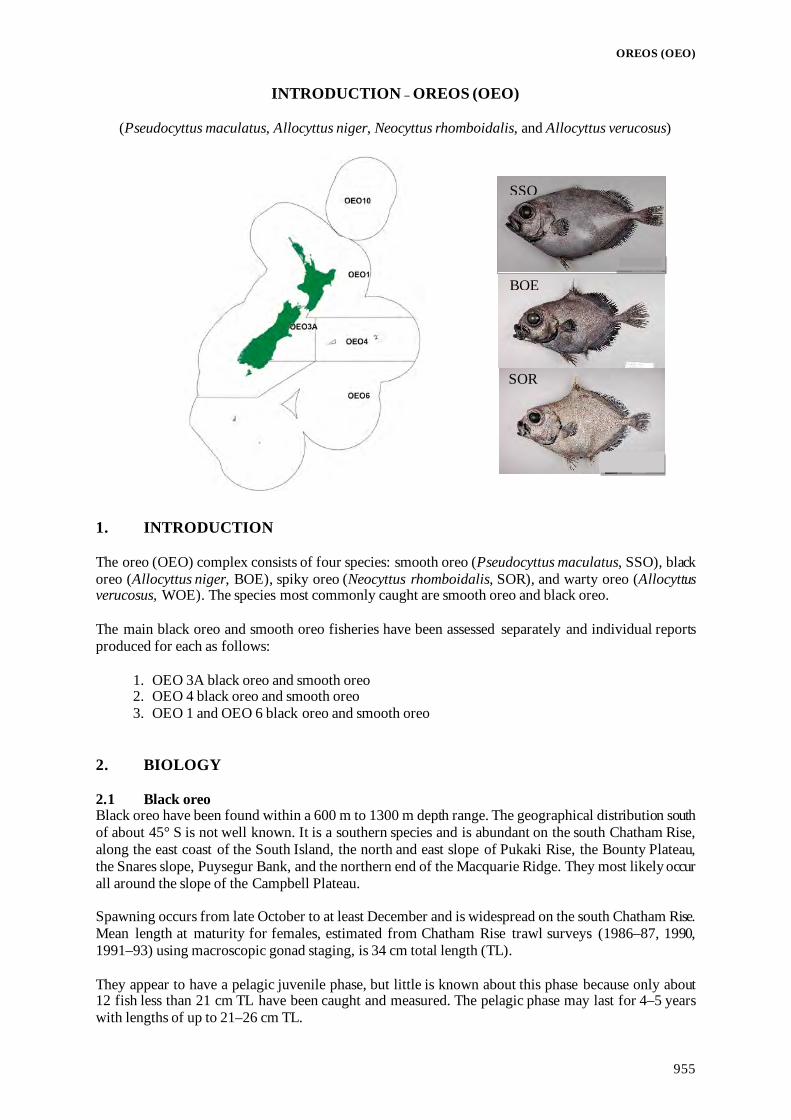
OREOS (OEO)
955
INTRODUCTION – OREOS (OEO)
(Pseudocyttus maculatus, Allocyttus niger, Neocyttus rhomboidalis, and Allocyttus verucosus)
1. INTRODUCTION The oreo (OEO) complex consists of four species: smooth oreo (Pseudocyttus maculatus, SSO), black oreo (Allocyttus niger, BOE), spiky oreo (Neocyttus rhomboidalis, SOR), and warty oreo (Allocyttus verucosus, WOE). The species most commonly caught are smooth oreo and black oreo. The main black oreo and smooth oreo fisheries have been assessed separately and individual reports produced for each as follows:
1. OEO 3A black oreo and smooth oreo 2. OEO 4 black oreo and smooth oreo 3. OEO 1 and OEO 6 black oreo and smooth oreo
2. BIOLOGY 2.1 Black oreo Black oreo have been found within a 600 m to 1300 m depth range. The geographical distribution south of about 45° S is not well known. It is a southern species and is abundant on the south Chatham Rise, along the east coast of the South Island, the north and east slope of Pukaki Rise, the Bounty Plateau, the Snares slope, Puysegur Bank, and the northern end of the Macquarie Ridge. They most likely occur all around the slope of the Campbell Plateau. Spawning occurs from late October to at least December and is widespread on the south Chatham Rise. Mean length at maturity for females, estimated from Chatham Rise trawl surveys (1986–87, 1990, 1991–93) using macroscopic gonad staging, is 34 cm total length (TL). They appear to have a pelagic juvenile phase, but little is known about this phase because only about 12 fish less than 21 cm TL have been caught and measured. The pelagic phase may last for 4–5 years with lengths of up to 21–26 cm TL.
SSO
BOE
SOR

OREOS (OEO)
956
Unvalidated age estimates were obtained for Chatham Rise and Puysegur-Snares samples in 1995 and 1997, respectively, using counts of the zones (assumed to be annual) observed in thin sections of otoliths. These estimates indicate that black oreo is slow growing and long lived. The maximum estimated age was 153 years (45.5 cm TL fish). Australian workers used the same methods, i.e., sections of otoliths, and reported similar results. A von Bertalanffy growth curve was fitted to the Puysegur samples only (Table 1). Estimated age at maturity for females was 27 years. Table 1: Biological parameters for black oreo and smooth oreo stock assessments. Values not estimated are indicated
by –. Some parameters may be estimated in specific stock assessments. Fishstock Estimate 1. Natural Mortality - M (y-1) Females Males Unsexed Black oreo (McMillan et al 1997) 0.044 (0.028–0.075) 0.044 (0.028–0.075) 0.044 Smooth oreo (Doonan et al 1997) 0.063 (0.042–0.099) 0.063 (0.042–0.099 2. Age at recruitment - Ar (y) Black oreo – – – Smooth oreo 21 21 3. Age at maturity AM (y) Black oreo 27 – – Smooth oreo 31 – 4. von Bertalanffy parameters Females Males Unsexed L∞ (cm, TL) k(y1) t0 (y) L∞ (cm, TL) k(y1) t0 (y) L∞ (cm, TL) k(y1) t0 (y) Black oreo 39.9 0.043 -17.6 37.2 0.056 -16.4 38.2 0.05 -17.0 Smooth oreo 50.8 0.047 -2.9 43.6 0.067 -1.6 – – – 5. Length-weight parameters (Weight = a(length)b (Weight in g, length in cm fork length)) Females Males Unsexed a b a b a b Black oreo 0.008 3.28 0.016 3.06 0.0078 3.27 Smooth oreo 0.029 2.90 0.032 2.87 – – 6. Length at recruitment (cm, TL) Females Males Unsexed Black oreo – – – Smooth oreo 34 – – 7. Length at maturity (cm, TL) Black oreo 34 – – Smooth oreo 40 – – 8. Recruitment variability (σR) Black oreo 0.65 0.65 0.65 Smooth oreo 0.65 0.65 – 9. Recruitment steepness Black oreo 0.75 0.75 0.75 Smooth oreo 0.75 0.75 –
A first estimate of natural mortality (M), 0.044 (y-1), was made in 1997 using the Puysegur growth data only. This estimate is uncertain because it appeared that the otolith samples were taken from a well fished part of the Puysegur area. Black oreo appear to settle over a wide range of depths on the south Chatham Rise but appear to prefer to live in the depth interval 600–800 m that is often dominated by individuals with a modal size of 28 cm TL. 2.2 Smooth oreo Smooth oreo occur from 650 m to about 1500 m depth. It is a southern species and is abundant on the south Chatham Rise, along the east coast of the South Island, the north and east slope of Pukaki Rise, the Bounty Plateau, the Snares slope, Puysegur Bank, and the northern end of the Macquarie Ridge. They most likely occur all around the slope of the Campbell Plateau, but the geographical distribution south of about 45° S is not well known.

OREOS (OEO)
957
Spawning occurs from late October to at least December and is widespread on the south Chatham Rise in small aggregations. Mean length at maturity for females, estimated from Chatham Rise trawl surveys (1986–87, 1990, 1991–93) using macroscopic gonad staging, is 40 cm TL. They appear to have a pelagic juvenile phase, but little is known about this phase because only about six fish less than 16 cm TL have ever been caught. The pelagic phase may last for 5–6 years with lengths of up to 16–19 cm TL. Unvalidated age estimates were obtained for Chatham Rise and Puysegur-Snares fish in 1995 and 1997, respectively, using counts of the zones (assumed to be annual) observed in thin sections of otoliths. These estimates indicate that smooth oreo is slow growing and long lived. The maximum estimated age was 86 years (51.3 cm TL fish). Australian workers used the same methods, i.e., sections of otoliths, and reported similar results. A von Bertalanffy growth curve was fitted to the age estimates from Chatham Rise and Puysegur-Snares fish combined and the parameters estimated for the growth curve are in Table 1. Estimated age at maturity for females was 31 years. An estimate of natural mortality, 0.063 (y-1), was made in 1997 (Doonan et al 1997). The estimate was from a moderately exploited population of fish from the Puysegur region. There are concentrations of recently settled smooth oreo south and southwest of Chatham Island, although small individuals (16–19 cm TL) occur widely over the south Chatham Rise at depths of 650–800 m. 3. STOCKS AND AREAS 3.1 Black oreo The stock structure of Australian and New Zealand samples was examined using genetic (allozyme and mitochondrial DNA) and morphological counts (fin rays, etc.). It was concluded that the New Zealand samples constituted a stock distinct from the Australian sample based on “small but significant difference in mtDNA haplotype frequencies (with no detected allozyme differences), supported by differences in pyloric caeca and lateral line counts”. The genetic methods used may not be suitable tools for stock discrimination around New Zealand. A New Zealand pilot study examined stock relationships using samples from four management areas (OEO 1, OEO 3A, OEO 4, and OEO 6) of the New Zealand EEZ. Techniques used included genetic (nuclear and mitochondrial DNA), lateral line scale counts, settlement zone counts, parasites, otolith microchemistry, and otolith shape. Lateral line scale and pyloric caeca counts were different between samples from OEO 6 and the other three areas. The relative abundance of three parasites differed significantly between all areas. Otolith shape from OEO 3A samples was different to that from OEO 1 and OEO 4, but OEO 1, OEO 4, and OEO 6 otolith samples were not morphologically different. Genetic, otolith microchemistry, and settlement zone analyses showed no regional differences. 3.2 Smooth oreo Stock structure of Australian and New Zealand samples was examined using genetic (allozyme and mitochondrial DNA) and morphological counts (fin rays, etc.). No differences between New Zealand and Australian samples were found using the above techniques. A broad scale stock is suggested by these results, but this seems unlikely given the large distances between New Zealand and Australia. The genetic methods used may not be suitable tools for stock discrimination around New Zealand. A New Zealand pilot study examined stock relationships using samples from four management areas (OEO 1, OEO 3A, OEO 4, and OEO 6) of the New Zealand EEZ. Techniques used included genetic (nuclear and mitochondrial DNA), lateral line scale counts, settlement zone counts, parasites, otolith microchemistry, and otolith shape. Otolith shape from OEO 1 and OEO 6 was different to that from OEO 3A and OEO 4 samples. Weak evidence from parasite data, one gene locus, and otolith microchemistry suggested that northern OEO 3A samples were different from other areas. Lateral line scale and otolith settlement zone counts showed no differences between areas.

OREOS (OEO)
958
These data suggest that the stock boundaries given in previous assessment documents should be retained until more definitive evidence for stock relationships is obtained, i.e., retain the existing areas OEO 1, OEO 3A, OEO 4, and OEO 6. The four species of oreos (black oreo, smooth oreo, spiky oreo, and warty oreo) are managed with separate catch limits for black and smooth in some areas. Each species could be managed separately. They have different depth and geographical distributions, different stock sizes, rates of growth, and productivity. 4. FISHERY SUMMARY 4.1 Commercial fisheries Commercial fisheries occur for black oreo (BOE) and smooth oreo (SSO). Oreos are managed as a species group, which also includes warty and spiky oreo (SOR). The Chatham Rise (OEO 3A and OEO 4) is the main fishing area, but other fisheries occur off Southland on the east coast of the South Island (OEO 1/OEO 3A) and on the Pukaki Rise, Macquarie Ridge, and Bounty Plateau (OEO 6). In the past, oreo catch has been taken as bycatch of the more valuable orange roughy fisheries but target fisheries for smooth or black oreo are now much more common in most areas. Total reported landings and TACCs are shown in Table 2, and Figure 1 depicts the historical landings and TACC values for the main OEO stocks. OEO 3A and OEO 4 were introduced into the QMS in 1982–83, and OEO 1 and OEO 6 were introduced later in 1986–87. Reported estimated catches by species from tow-by-tow data recorded in catch and effort logbooks and electronic reporting forms, and the ratio of estimated to landed catch reported, are given in Table 3. OEO 1 was fished under the adaptive management programme up to the end of 1997–98. The OEO 1 TACC reverted back to pre-adaptive management levels from 1998–99. Landings have declined since then, and from 1 October 2007 the TACC was reduced to 2500 t; other sources of mortality were allocated 168 t. Oreo landings from OEO 3A were less than the TACC from 1992–93 to 1995–96, substantially so in 1994–95 and 1995–96. The OEO 3A TACC was reduced from 10 106 t to 6600 t in 1996–97. A voluntary agreement between the fishing industry and the Minister of Fisheries to limit catch of smooth oreo from OEO 3A to 1400 t of the total oreo TACC of 6600 t was implemented in 1998–99. Subsequently the total OEO 3A TACC was reduced to 5900 t in 1999–00, 4400 in 2000–01, 4095 in 2001–02, and 3100 t in 2002–03. In 2009–10 the OREO 3A TACC was increased slightly to 3350 t and landings have been close to the TACC since then, averaging 3340 t between 2009–10 and 2018–19, although landings reduced to 2731 t in 2019–20 and increased to 3095 in 2020–21. Total oreo landings from OEO 4 exceeded the TACC from 1991–92 to 1994–95 and were close to the TACC from 1995–96 to 2000–01 (Table 2). Landings remained high in OEO 4, whereas the orange roughy fishery declined. The OEO 4 TACC was reduced from 7000 t to 5460 t in 2001–02 but was restored to 7000 t in 2003–04. In 2015–16, following an assessment of SSO 4, the OEO 4 TACC was reduced to 3000 t and the landings of smooth oreo were approximately 2000 t. The OEO 4 TACC was increased to 3600 t for the fishing year 2018–19, and just under 3300 t of all oreo species combined were landed, but landings reduced again to 2951 t in 2019–20 and increased to 3542 in 2020–21. Landings from the Sub-Antarctic area (OEO 6) increased substantially in 1994–95 and exceeded the TACC in 1995–96. The OEO 6 TACC was increased from 3000 t to 6000 t in 1996–97. Landings exceeded the TACC slightly in 2002–03 and in 2005–06 but dropped substantially after 2009–10. Following a period of very low landings ranging from just 136 t to 367 t in 2012–13 to 2014–15, landings recovered slightly, averaging just over 1575 t between 2015–16 and 2020–21. There was also a voluntary agreement in 1998–99 not to fish for oreo in the Puysegur area. More recently there was a voluntary agreement not to fish parts of the Pukaki and Bounty areas to allow fish to increase in size. This agreement was initially for 3 years starting 1 October 2012. It was reinstated on 1 October 2015 for a further 2 years until 1 October 2017.

OREOS (OEO)
959
Table 2: Total reported landings (t) for all oreo species combined by Fishstock from 1978–79 to present and TACCs (t) from 1982–83 to present.
Fishing OEO 1 OEO 3A OEO 4 OEO 6 Totals
year Landings TACC Landings TACC Landings TACC Landings TACC Landings TACC 1978–79* 2 808 – 1 366 – 8 041 – 17 – 12 231 – 1979–80* 143 – 10 958 – 680 – 18 – 11 791 – 1980–81* 467 – 14 832 – 10 269 – 283 – 25 851 – 1981–82* 21 – 12 750 – 9 296 – 4 380 – 26 514 – 1982–83* 162 – 8 576 10 000 3 927 6 750 765 – 13 680 17 000 1983–83# 39 – 4 409 # 3 209 # 354 – 8 015 # 1983–84† 3 241 – 9 190 10 000 6 104 6 750 3 568 – 22 111 17 000 1984–85† 1480 – 8 284 10 000 6 390 6 750 2 044 – 18 204 17 000 1985–86† 5 390 – 5 331 10 000 5 883 6 750 126 – 16 820 17 000 1986–87† 532 4 000 7 222 10 000 6 830 6 750 0 3 000 15 093 24 000 1987–88† 1 193 4 000 9 049 10 000 8 674 7 000 197 3 000 19 159 24 000 1988–89† 432 4 233 10 191 10 000 8 447 7 000 7 3 000 19 077 24 233 1989–90† 2 069 5 033 9 286 10 106 7 348 7 000 0 3 000 18 703 25 139 1990–91† 4 563 5 033 9 827 10 106 6 936 7 000 288 3 000 21 614 25 139 1991–92† 4 156 5 033 10 072 10 106 7 457 7 000 33 3 000 21 718 25 139 1992–93† 5 739 6 044 9 290 10 106 7 976 7 000 815 3 000 23 820 26 160 1993–94† 4 910 6 044 9 106 10 106 8 319 7 000 983 3 000 23 318 26 160 1994–95† 1 483 6 044 6 600 10 106 7 680 7 000 2 528 3 000 18 291 26 160 1995–96† 4 783 6 044 7 786 10 106 6 806 7 000 4 435 3 000 23 810 26 160 1996–97† 5 181 6 044 6 991 6 600 6 962 7 000 5 645 6 000 24 779 25 644 1997–98† 2 681 6 044 6 336 6 600 7 010 7 000 5 222 6 000 21 249 25 644 1998–99† 4 102 5 033 5 763 6 600 6 931 7 000 5 287 6 000 22 083 24 633 1999–00† 3 711 5 033 5 859 5 900 7 034 7 000 5 914 6 000 22 518 23 933 2000–01† 4 852 5 033 4 577 4 400 7 358 7 000 5 932 6 000 22 719 22 433 2001–02† 4 197 5 033 3 923 4 095 4 864 5 460 5 737 6 000 18 721 20 588 2002–03† 3 034 5 033 3 070 3 100 5 402 5 460 6 115 6 000 17 621 19 593 2003–04† 1 703 5 033 2 856 3 100 6 735 7 000 5 811 6 000 17 105 21 133 2004–05† 1 025 5 033 3 061 3 100 7 390 7 000 5 744 6 000 17 220 21 133 2005–06† 850 5 033 3 333 3 100 6 829 7 000 6 463 6 000 17 475 21 133 2006–07† 903 5 033 3 073 3 100 7 211 7 000 5 926 6 000 17 113 21 133 2007–08† 947 2 500 3 092 3 100 7 038 7 000 5 902 6 000 16 979 18 600 2008–09† 582 2 500 2 848 3 100 6 907 7 000 5 540 6 000 15 877 18 600 2009–10† 464 2 500 3 550 3 350 7 047 7 000 5 730 6 000 16 791 18 850 2010–11† 381 2 500 3 370 3 350 7 061 7 000 3 610 6 000 14 422 18 860 2011–12† 581 2 500 3 324 3 350 6 858 7 000 2 325 6 000 13 088 18 860 2012–13† 652 2 500 3 245 3 350 6 944 7 000 136 6 000 10 977 18 860 2013–14† 386 2 500 3 473 3 350 7 024 7 000 367 6 000 11 251 18 860 2014–15† 277 2 500 3 352 3 350 7 274 7 000 156 6 000 11 059 18 860 2015–16† 523 2 500 3 334 3 350 2 898 3 000 1 357 6 000 8 111 14 860 2016–17† 603 2 500 3 206 3 350 3 011 3 000 1 200 6 000 8 020 14 860 2017–18† 601 2 500 3 177 3 350 2 867 3 000 2 138 6 000 8 783 14 860 2018–19† 689 2 500 3 365 3 350 3 283 3 600 1 613 6 000 8 950 15 460 2019–20† 604 2 500 2 731 3 350 2 951 3 600 1 446 6 000 7 733 15 460 2020–21† 357 2 500 3 095 3 350 3 542 3 600 1 711 6 000 8 705 15 460
Source: FSU from 1978–79 to 1987–88; QMS/MFish/MPI from 1988–89 to 2013–14. *, 1 April to 31 March. #, 1 April to 30 September. Interim TACs applied. †, 1 October to 30 September. Data prior to 1983 were adjusted up due to a conversion factor change.
Figure 1: Reported commercial landings and TACC for the four main OEO stocks. OEO 1 (Central East - Wairarapa,
Auckland, Central Egmont, Challenger, Southland, South East Catlin Coast). [Continued on next page]

OREOS (OEO)
960
Figure 1: [Continued] Reported commercial landings and TACC for the four main OEO stocks. From top: OEO 3A
(South East Cook Strait/Kaikōura/Strathallan), OEO 4 (South East Chatham Rise), and OEO 6 (Sub-Antarctic).

OREOS (OEO)
961
Table 3: Reported estimated catch (t) by species (smooth oreo (SSO), black oreo (BOE)) by Fishstock from 1978–79 to present and the ratio (percentage) of the total estimated SSO plus BOE, to the total reported landings (from Table 2). –, less than 1 t.
SSO BOE Total estimated
Estimated landings (%) Year OEO 1 OEO 3A OEO 4 OEO 6 OEO 1 OEO 3A OEO 4 OEO 6
1978–79* 0 0 0 0 9 0 0 0 9 – 1979–80* 16 5 075 114 0 118 5 588 566 18 11 495 98 1980–81* 1 1 522 849 2 66 8 758 5 224 215 16 637 64 1981–82* 21 1 283 3 352 2 0 11 419 5 641 4 378 26 096 98 1982–83* 28 2 138 2 796 60 6 6 438 1 088 705 13 259 97 1983–83# 9 713 1 861 0 1 3 693 1 340 354 7 971 100 1983–84† 1 246 3 594 4 871 1 315 1 751 5 524 1 214 2 254 21 769 99 1984–85† 828 4 311 4 729 472 544 3 897 1 651 1 572 18 004 99 1985–86† 4 257 3 135 4 921 72 1 060 2 184 961 54 16 644 99 1986–87† 326 3 186 5 670 0 163 4 026 1 160 0 14 531 96 1987–88† 1 050 5 897 7 771 197 114 3 140 903 0 19 072 100 1988–89† 261 5 864 6 427 – 86 2 719 1 087 0 16 444 86 1989–90† 1 141 5 355 5 320 – 872 2 344 439 – 15 471 83 1990–91† 1 437 4 422 5 262 81 2 314 4 177 793 222 18 708 87 1991–92† 1 008 6 096 4 797 2 2 384 3 176 1 702 15 19 180 88 1992–93† 1 716 3 461 3 814 529 3 768 3 957 1 326 69 18 640 78 1993–94† 2 000 4 767 4 805 808 2 615 4 016 1 553 35 20 599 88 1994–95† 835 3 589 5 272 1 811 385 2 052 545 230 14 719 81 1995–96† 2 517 3 591 5 236 2 562 1 296 3 361 364 1 166 20 093 84 1996–97† 2 203 3 063 5 390 2 492 2 578 3 549 530 1 950 21 755 88 1997–98† 1 510 4 790 5 868 2 531 1 027 1 623 811 1 982 20 142 95 1998–99† 2 958 2367 5 613 3 462 820 3 147 844 1 231 20 442 93 1999–00† 2 487 1 230 5 879 4 427 953 2 773 627 1 036 19 412 86 2000–01† 4 117 1 288 6 009 4 241 316 2 423 803 1 128 20 325 89 2001–02† 3 135 1 272 3 860 4 471 709 1 906 515 983 16 851 90 2002–03† 2 402 1 025 4 090 3 952 470 1 144 862 1 642 15 587 88 2003–04† 958 884 5 098 3 771 457 1 095 973 1 496 14 732 86 2004–05† 622 1 150 6 013 3 863 209 1 163 852 1 618 15 490 90 2005–06† 412 1 005 5 202 3 292 218 1 336 763 2 633 14 861 85 2006–07† 509 989 5 978 2 214 262 1 223 796 3 071 15 042 88 2007–08† 414 1 402 6 171 2 182 429 1 469 592 3 022 15 681 92 2008–09† 435 1 258 5 703 2 703 143 1 388 766 2 832 15 228 96 2009–10† 319 1 581 6 204 2 487 67 1 781 942 3 032 16 413 98 2010–11† 107 1 558 6 472 1 672 235 1 563 539 1 501 13 647 95 2011–12† 210 1 442 6 183 562 326 1 620 487 1 540 12 370 95 2012–13† 319 1 408 5 920 104 224 1 582 973 31 10 561 96 2013–14† 214 1 391 6 000 286 114 1 722 988 50 10 765 96 2014–15† 75 1 369 6 447 119 170 1 783 961 16 10 940 99 2015–16† 248 1 480 1 948 583 259 1 782 858 809 7 967 98 2016–17† 367 1 520 2 357 1 000 182 1 727 678 156 7 987 100 2017–18† 363 1 539 2 095 1 123 130 1 550 758 850 8 408 96 2018–19† 400 1 522 2 479 908 199 1 737 671 586 8 502 95 2019–20† 272 1 394 2 327 824 221 1 326 538 430 7 332 95 2020–21† 200 1 566 2 565 878 136 1 212 793 745 8 096 93
Source: FSU from 1978–79 to 1987–88 and MFish from 1988–89 to 2006–07. *, 1 April to 31 March. #, 1 April to 30 September. †, 1 October to 30 September. 4.2 Recreational fisheries There are no known recreational fisheries for black oreo and smooth oreo. 4.3 Customary non-commercial fisheries There is no known customary non-commercial fishing for black oreo and smooth oreo. 4.4 Illegal catch Estimates of illegal catch are not available. 4.5 Other sources of mortality Dumping of unwanted or small fish and accidental loss of fish (lost codends, ripped codends, etc.) were features of oreo fisheries in the early years. These sources of mortality were probably substantial in those early years but are now thought to be relatively small. No estimate of mortality from these sources has been made because of the lack of hard data and because mortality now appears to be small. Estimates of discards of oreos were made for 1994–95 and 1995–96 from MFish observer data. This involved calculating the ratio of discarded oreo catch to retained oreo catch and then multiplying the annual total oreo catch from the New Zealand EEZ by this ratio. Estimates were 207 t and 270 t for 1994–95 and 1995–96, respectively.

OREOS (OEO)
962
5. ENVIRONMENTAL AND ECOSYSTEM CONSIDERATIONS This section was updated for the 2020 Fishery Assessment Plenary (Fisheries New Zealand 2020). A more detailed summary from an issue-by-issue perspective is available in the Aquatic Environment and Biodiversity Annual Review 2021 (Fisheries New Zealand 2021), available online athttps://www.mpi.govt.nz/dmsdocument/51472-Aquatic-Environment-and-Biodiversity-Annual-Review-AEBAR-2021-A-summary-of-environmental-interactions-between-the-seafood-sector-and-the-aquatic-environment. Some tables in this section have not been updated because the data were unavailable at the time of publication. 5.1 Role in the ecosystem Smooth and black oreo dominate trawl survey relative abundance estimates of demersal fish species at 650–1200 m on the south and southwest slope of the Chatham Rise (e.g., Hart & McMillan 1998). They are probably also dominant at those depths on the southeast slope of the South Island and other southern New Zealand slope areas including Bounty Plateau and Pukaki Rise. They are replaced at depths of about 700–1200 m on the east and northern slope of Chatham Rise by orange roughy. The south Chatham Rise oreo fisheries are relatively long-standing, dating from Soviet fishing in the 1970s, but the effects of extracting approximately 6000 t per year of smooth oreo from the south Chatham Rise (OEO 4) ecosystem between 1983–84 and 2012–13 are unknown. 5.1.1 Trophic interactions Smooth oreo feed mainly on salps (80%), molluscs (9%, of which 8% are squids but also including octopods), and teleosts (5%) (percentage frequency of occurrence in stomachs with food, Stevens et al 2011). Black oreo feed on teleosts (48%), crustaceans (36%), salps (24%), and cephalopods (mainly squid, 6%) (Stevens et al 2011). Diet varies with fish size but salps remained the main prey for smooth oreo in the largest fish with small numbers of Scyphozoa, fish, and squids. Salps were the main prey for smaller black oreo, but amphipods and natant decapod crustaceans were important for intermediate sized fish (Clark et al 1989). Smooth oreo and black oreo occur with orange roughy at times. Orange roughy diet was mainly crustaceans (58%), teleosts (41%), and molluscs (10%, particularly squids) (frequency of occurrence, Stevens et al 2011) suggesting little overlap with the salp-dominated diet of smooth oreo. Where they co-occur, orange roughy and black oreo may compete for teleost and crustacean prey. Predators of oreos probably change with fish size. Larger smooth oreo, black oreo, and orange roughy were observed with healed soft flesh wounds, typically in the dorso-posterior region. Wound shape and size suggest they may be caused by one of the deepwater dogfishes (Dunn et al 2010). 5.1.2 Ecosystem indicators Tuck et al (2009, 2014) used data from the Sub-Antarctic and Chatham Rise middle-depth trawl surveys to derive indicators of fish diversity, size, and trophic level. However, fishing for oreos occurs mostly deeper than the depth range of these surveys and is only a small component of fishing in the areas considered by Tuck et al (2009, 2014). 5.2 Non-target fish and invertebrate catch Anderson & Finucci (2022) summarised the bycatch of oreo trawl fisheries from 2002–03 to 2019–20. Since 2002–03, oreo species (five species, mainly smooth oreo and black oreo) accounted for about 95% of the total estimated catch from all observed trawls targeting oreos. In total, over 500 species or species groups were identified by observers in the target fishery. Total annual fish bycatch in the oreo fishery ranged from a low of 135 t in 2019–20 to a high of 1457 t in 2002–03, with a general declining trend through time and the five lowest values in the last seven years. Orange roughy (2.3%) was the main bycatch species, with no other species or group of species accounting for more than 0.5% of the total catch. Other recorded bycatch species included Baxter’s lantern dogfish (Etmopterus granulosus, 0.49%), hoki (0.37%), and rattails (0.27%), all of which were usually discarded. Estimated annual bycatch of non-QMS species was roughly equal to that of QMS species. From 2002–03 to 2019–20, the overall discard fraction value was 0.014 kg (range of 0.01–0.05 kg) and tended to be lower after 2005–06 (Anderson & Finucci 2022).

OREOS (OEO)
963
Non-QMS invertebrate bycatch made up a very small fraction of the overall catch (0.3%) and included warty squid (0.07%), and bushy hard coral (0.07%, Anderson & Finucci 2022). Other observed species or species groups each accounted for less than 0.01% of the observed catch. Tracey et al (2011) analysed the distribution of nine groups of protected corals based on bycatch records from observed trawl effort from 2007–08 to 2009–10, primarily from 800–1000 m depth. For the oreo target fishery, the highest catches were reported from the north and south slopes of the Chatham Rise, east of the Pukaki Rise, and on the Macquarie Ridge. Finucci et al (2019) analysed bycatch trends in deepwater fisheries, including oreo trawl, from 1990–91 until 2016–17. They found that the most common bycatch species by weight (t) were orange roughy (ORH), unspecified sharks (SHA), and Baxter’s dogfish (ETB). Moreover, among the 228 bycatch species examined, 40 showed a decrease in catch over time (7 were statistically significant) and 44 showed an increase (9 were significant). The species showing the greatest decline were dark ghost shark (Hydrolagus novaezealandiae, GSH), unspecified shark (SHA), and lanternshark (Etmopterus sp., ETM), whereas the greatest increases were found for longnose velvet dogfish (Centroscymnus crepidater, CYP), ridge scaled rattail (Macrourus carinatus, MCA), and Baxter’s dogfish (Etmopterus granulosus, ETB). The decline in unspecified shark could be linked to better identification of specimens through time, which would match the increases seen in other deepwater shark bycatch. 5.3 Incidental capture of Protected Species (seabirds, mammals, and protected fish) For protected species, capture estimates presented here include all animals recovered to the deck of fishing vessels (alive, injured, or dead), but do not include any cryptic mortality (e.g., a seabird struck by a warp but not brought on board the vessel, Middleton & Abraham 2007, Brothers et al 2010). Ramm (2011, 2012a, 2012b) summarised observer data for combined bottom trawl fisheries for orange roughy, oreos, and cardinalfish and listed annual captures of seabirds and mammals from 2008–09 to 2010–11. 5.3.1 Marine mammal captures Trawlers targeting orange roughy, oreo, and black cardinalfish occasionally catch New Zealand fur seal (which were classified as ‘Not Threatened’ under the New Zealand Threat Classification System in 2009, Baker et al 2010). Between 2002–03 and 2007–08, there were 14 observed captures of New Zealand fur seal in orange roughy, oreo, and black cardinalfish trawl fisheries. There have been two observed captures in the period between 2008–09 and 2019–20, during which time the average level of annual observer coverage was 26.2% (Table 4). Corresponding annual estimated captures between 2008–09 and 2015–16 ranged 0–4 (mean 1.75) based on statistical capture models (Thompson et al 2013, Abraham et al 2016). All observed fur seal captures occurred in the Sub-Antarctic region. Table 4: Number of tows by fishing year and observed and model-estimated total New Zealand fur seal captures in
orange roughy, oreo, and cardinalfish trawl fisheries, 2002–03 to 2019–20. Annual fishing effort (tows), and observer coverage (%) in deepwater trawl fisheries; number of observed captures and observed capture rate (captures per hundred tows) of New Zealand fur seal; estimated captures and capture rate of New Zealand fur seal (mean and 95% credible interval). Estimates are based on methods described by Abraham et al (2021), available online at https://protectedspeciescaptures.nz/PSCv6/released/. Observed and estimated protected species captures in these tables derive from the PSC database version PSCV6. [Continued on next page]
Fishing effort Obs. captures Est. captures
Est. capture rate
Fishing year Tows No. Obs % obs Captures Rate Mean 95% c.i. Mean 95% c.i. 2002–03 8 871 1 384 15.6 0 0 4 0–12 0.04 0.00–0.14 2003–04 8 007 1 262 15.8 2 0.16 9 3–23 0.12 0.04–0.29 2004–05 8 420 1 619 19.2 4 0.25 14 6–28 0.16 0.07–0.33 2005–06 8 292 1 359 16.4 2 0.15 10 3–23 0.13 0.04–0.28 2006–07 7 365 2 324 31.6 2 0.09 3 2–7 0.05 0.03–0.10 2007–08 6 731 2 811 41.8 5 0.18 8 5–13 0.12 0.07–0.19 2008–09 6 130 2 372 38.7 0 0 2 0–7 0.03 0.00–0.11 2009–10 6 008 2 133 35.5 0 0 3 0–8 0.05 0.00–0.13 2010–11 4 178 1 205 28.8 0 0 3 0–10 0.08 0.00–0.24 2011–12 3 655 923 25.3 0 0 1 0–5 0.04 0.00–0.14 2012–13 3 098 346 11.2 0 0 0 0–2 0.02 0.00–0.06 2013–14 3 606 434 12.0 0 0 1 0–3 0.02 0.00–0.08 2014–15 3 814 978 25.6 1 0.1 2 1–4 0.04 0.03–0.10 2015–16 4 088 1 421 34.8 0 0 1 0–3 0.01 0.00–0.07 2016–17 3 962 1 226 30.9 0 0 0 0–2 0.01 0.00–0.05 2017–18 3 753 903 24.1 0 0 1 0–3 0.01 0.00–0.08
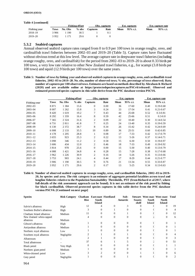
OREOS (OEO)
964
Table 4 [continued] Fishing effort Obs. captures Est. captures
Est. capture rate
Fishing year Tows No. Obs % obs Captures Rate Mean 95% c.i. Mean 95% c.i. 2018–19 3 906 1 190 30.5 1 0.1 2019–20 3 952 1 171 29.6 0 0
5.3.2 Seabird captures Annual observed seabird capture rates ranged from 0 to 0.9 per 100 tows in orange roughy, oreo, and cardinalfish trawl fisheries between 2002–03 and 2019–20 (Table 5). Capture rates have fluctuated without obvious trend at this low level. The average capture rate in deepwater trawl fisheries (including orange roughy, oreo, and cardinalfish) for the period from 2002–03 to 2019–20 is about 0.33 birds per 100 tows, a very low rate relative to other New Zealand trawl fisheries, e.g., for scampi (3.8 birds per 100 tows) and squid (12.9 birds per 100 tows) over the same years. Table 5: Number of tows by fishing year and observed seabird captures in orange roughy, oreo, and cardinalfish trawl
fisheries, 2002–03 to 2019–20. No. obs, number of observed tows; % obs, percentage of tows observed; Rate, number of captures per 100 observed tows. Estimates are based on methods described by Abraham & Richard (2020) and are available online at https://protectedspeciescaptures.nz/PSCv6/released/. Observed and estimated protected species captures in this table derive from the PSC database version PSCV6.
Fishing effort Obs. captures Est. captures
Est. capture rate
Fishing year Tows No. Obs % obs Captures Rate Mean 95% c.i. Mean 95% c.i. 2002–03 8 871 1 384 15.6 0 0.00 36 17-60 0.40 0.19-0.68 2003–04 8 007 1 262 15.8 3 0.24 33 17-54 0.41 0.21-0.67 2004–05 8 420 1 619 19.2 7 0.43 44 25-68 0.52 0.3-0.81 2005–06 8 292 1 359 16.4 8 0.59 42 25-66 0.51 0.3-0.8 2006–07 7 365 2 324 31.6 2 0.09 22 10-40 0.30 0.14-0.54 2007–08 6 731 2 811 41.8 7 0.25 24 13-40 0.35 0.19-0.59 2008–09 6 130 2 372 38.7 8 0.34 26 15-42 0.42 0.24-0.69 2009–10 6 008 2 133 35.5 19 0.89 36 25-51 0.60 0.42-0.85 2010–11 4 178 1 205 28.8 1 0.08 17 7-33 0.42 0.17-0.79 2011–12 3 655 923 25.3 2 0.22 13 5-26 0.37 0.14-0.71 2012–13 3 098 346 11.2 2 0.58 15 6-30 0.50 0.19-0.97 2013–14 3 606 434 12.0 2 0.46 18 7-33 0.49 0.19-0.92 2014–15 3 814 978 25.6 0 0.00 15 5-30 0.40 0.13-0.79 2015–16 4 088 1 421 34.8 4 0.28 15 7-28 0.38 0.17-0.68 2016–17 3 962 1 226 30.9 2 0.16 14 5-26 0.35 0.13-0.66 2017–18 3 753 903 24.1 4 0.44 17 8-29 0.44 0.21-0.77 2018–19 3 906 1 190 30.5 9 0.76 21 13-34 0.55 0.33-0.87 2019–20 3 952 1 171 29.6 2 0.17 13 5-25 0.34 0.13-0.63
Table 6: Number of observed seabird captures in orange roughy, oreo, and cardinalfish fisheries, 2002–03 to 2019–
20, by species and area. The risk category is an estimate of aggregate potential fatalities across trawl and longline fisheries relative to the Population Sustainability Thresholds, PST (from Richard et al 2017, where full details of the risk assessment approach can be found). It is not an estimate of the risk posed by fishing for black cardinalfish. Observed protected species captures in this table derive from the PSC database version PSCV6. [Continued on next page]
Species Risk Category Chatham
Rise East coast
South Island
Fiordland Sub-Antarctic
Stewart- Snares
shelf
West coast South Island
West coast North
Island
Total
Salvin's albatross High 12 4 0 3 0 0 0 19 Southern Buller's albatross High 3 0 1 0 0 0 0 4
Chatham Island albatross Medium 11 0 0 1 0 0 0 12 New Zealand white-capped albatross Medium
4 0 0 0 0 2 0 6
Gibson's albatross High 1 0 0 0 0 0 0 1
Antipodean albatross Medium 1 0 0 0 0 0 0 1
Northern royal albatross Low 1 0 0 0 0 0 0 1
Southern royal albatross Negligible 2 1 0 1 0 0 0 4
Albatrosses – 2 1 0 0 0 0 0 3
Total albatrosses – 37 6 1 5 0 2 0 51
Black petrel Very High 0 0 0 0 0 0 1 1
Northern giant petrel Medium 1 0 0 0 0 0 0 1
White-chinned petrel Low 3 2 0 0 1 0 0 6 Grey petrel Negligible 1 0 0 1 0 0 0 2

OREOS (OEO)
965
Table 6 [continued]
Species Risk Category
Chatham Rise
East coast South Island
Fiordland Sub-Antarctic
Stewart-Snares
shelf
West coast South Island
West coast North
Island
Total
Sooty shearwater Negligible 1 3 0 0 0 1 0 5
Common diving petrel Negligible 3 0 0 0 0 0 0 3
White-faced storm petrels Negligible 3 0 0 0 0 0 0 3 Cape petrel – 8 1 0 0 0 0 0 9
Petrels, prions, and shearwaters – 0 0 0 1 0 0 0 1
Total other birds – 20 6 0 2 1 1 1 31
Salvin’s albatross was the most frequently captured albatross (38% of observed albatross captures), but eight different species have been observed captured since 2002–03. Cape petrels were the most frequently captured other taxon (29%, Table 6). Seabird captures in the orange roughy, oreo, and cardinalfish fisheries have been observed mostly around the Chatham Rise and off the east coast South Island. These numbers should be regarded as only a general guide on the distribution of captures because the observer coverage is not uniform across areas and may not be representative. The deepwater trawl fisheries (including the cardinalfish target fishery) contributes to the total risk posed by New Zealand commercial fishing to seabirds (see Table 7). The two species to which the fishery poses the most risk are Chatham Island albatross and Salvin’s albatross, with this suite of fisheries posing 0.06 and 0.022 of Population Sustainability Threshold (PST) (Table 7). Chatham Island albatross and Salvin’s albatross were assessed as high risk (Richard et al 2020). Table 7: Risk ratio of seabirds predicted by the level two risk assessment for the oreo and all fisheries included in the
level two risk assessment, 2006–07 to 2016–17, showing seabird species with a risk ratio of at least 0.001 of PST (from Richard et al 2017 and Richard et al 2020, where full details of the risk assessment approach can be found). The risk ratio is an estimate of aggregate potential fatalities across trawl and longline fisheries relative to the PST. The Department of Conservation threat classifications are shown (Robertson et al 2017 at http://www.doc.govt.nz/documents/science-and-technical/nztcs19entire.pdf).
Species name PST (mean)
Risk ratio
Risk category
OEO, ORH, CDL
target trawl* TOTAL DOC Threat Classification Chatham Island albatross 428 0.060 0.28 High At Risk: Naturally Uncommon Salvin's albatross 3 460 0.022 0.65 High Threatened: Nationally Critical Northern giant petrel 337 0.005 0.15 Medium At Risk: Naturally Uncommon Northern Buller's albatross 1 640 0.002 0.26 Medium At Risk: Naturally Uncommon Black petrel 447 0.002 1.23 Very high Threatened: Nationally Vulnerable Antipodean albatross 369 0.002 0.17 Medium Threatened: Nationally Critical Gibson's albatross 497 0.002 0.31 High Threatened: Nationally Critical Northern royal albatross 723 0.001 0.05 Low At Risk: Naturally Uncommon * OEO, ORH, CDL target trawl from Richard et al 2017.
Mitigation methods such as streamer (tori) lines, Brady bird bafflers, warp deflectors, and offal management are used in the orange roughy, oreo, and cardinalfish trawl fisheries. Warp mitigation was voluntarily introduced from about 2004 and made mandatory in April 2006 (Department of Internal Affairs 2006). The 2006 notice mandated that all trawlers over 28 m in length use a seabird scaring device while trawling (being “paired streamer lines”, “bird baffler” or “warp deflector” as defined in the Notice). 5.4 Benthic interactions The spatial extent of seabed contact by trawl fishing gear in New Zealand’s EEZ and Territorial Sea has been estimated and mapped in numerous studies for trawl fisheries targeting deepwater species (Baird et al 2011, Black et al 2013, Black & Tilney 2015, Black & Tilney 2017, Baird & Wood 2018, and Baird & Mules 2019, 2021a, b), species in waters shallower than 250 m (Baird et al 2015, Baird & Mules 2021a, b), and all trawl fisheries combined (Baird & Mules 2021a, b). The most recent assessment of the deepwater trawl footprint was for the period 1989‒90 to 2018‒19 (Baird & Mules 2021b).

OREOS (OEO)
966
Orange roughy, oreo, and cardinalfish are taken using bottom trawls and accounted for about 15% of all tows reported on TCEPR forms that fished on or close to the bottom between 1989–90 and 2018–19 (Baird & Mules 2021b). From 1989–90 to 2018‒19, about 62 900 bottom trawls targeting oreo species were reported on TCEPRs and ERS (Baird & Mules 2021b): between 1600–2500 tows were reported a year during 1989–90 to 1994–95; 2000–3300 tows between 1995–96 and 2009–10; and annual tows decreased from almost 2000 tows in 2010–11 to under 800 tows in 2018–19. The total footprint generated from these tows was estimated at about 17 480 km2. This footprint represented coverage of 0.4% of the seafloor of the combined EEZ and the Territorial Sea areas; 1.3% of the ‘fishable area’, that is, the seafloor area open to trawling, in depths of less than 1600 m. For the 2018–19 fishing year, 796 oreo bottom tows had an estimated footprint of 300 km2 which represented coverage of less than 0.1% of the EEZ and Territorial Sea and less than 0.1% of the fishable area (Baird & Mules 2021b). The overall trawl footprint for oreo (1989–90 to 2018–19) covered 5% of the seafloor in 800–1000 m, 3% of 1000–1200 m seafloor, and 0.8% of the 1200–1600 m seafloor (Baird & Mules 2021b). The oreo footprint contacted 0.1%, less than 0.1%, and less than 0.1% of those depth ranges in 2018‒19, respectively (Baird & Mules 2021b). The BOMEC areas with the highest proportion of area covered by the oreo footprint were classes J (comprising mainly the Challenger Plateau and northern and southern slopes of the Chatham Rise) and M (shallower waters of the Southern Plateau). In 2018–19, the oreo footprint covered about 0.04% of the 311 360 km2 of class J and 0.04% of the 233 825 km2 of class M (Baird & Mules 2021b). Trawling for orange roughy, oreo, and cardinalfish, like trawling for other species, is likely to have effects on benthic community structure and function (e.g., Rice 2006) and there may be consequences for benthic productivity (e.g., Jennings et al 2001, Hermsen et al 2003, Hiddink et al 2006, Reiss et al 2009). These consequences are not considered in detail here but are discussed in the Aquatic Environment and Biodiversity Annual Review 2021 (Fisheries New Zealand 2021). The New Zealand EEZ contains Benthic Protection Areas (BPAs) and seamount closures that are closed to bottom trawl fishing for the protection of benthic biodiversity. These combined areas include 28% of underwater topographic features (including seamounts), 52% of all seamounts over 1000 m elevation, and 88% of identified hydrothermal vents. 5.5 Other considerations 5.5.1 Spawning disruption Fishing during spawning may disrupt spawning activity or success. Morgan et al (1999) concluded that Atlantic cod (Gadus morhua) “exposed to a chronic stressor are able to spawn successfully, but there appears to be a negative impact of this stress on their reproductive output, particularly through the production of abnormal larvae”. Morgan et al (1997) also reported that “Following passage of the trawl, a 300-m-wide "hole" in the [cod spawning] aggregation spanned the trawl track. Disturbance was detected for 77 min after passage of the trawl.” There is no research on the disruption of spawning smooth oreo and black oreo by fishing in New Zealand, but spawning of both species appears to be over a protracted period (October to February) and over a wide area (O’Driscoll et al 2003). Fishing continues during the spawning period, possibly because localised spawning schools of smooth oreo, in particular, may provide good catch rates. 5.5.2 Genetic effects Fishing and environmental changes, including those caused by climate change or pollution, could alter the genetic composition or diversity of a species. There are no known studies of the genetic diversity of smooth or black oreo from New Zealand. Genetic studies for stock discrimination are reported under Section 3. 5.5.3 Habitat of particular significance to fisheries management Habitat of particular significance for fisheries management does not have a policy definition. O’Driscoll et al (2003) identified the south Chatham Rise as important for smooth oreo spawning, and the north, east, and south slopes as important for juveniles. The south Chatham Rise is also important for black oreo spawning and juveniles. Deepsea corals such as the reef-forming scleractinian corals and gorgonian sea fan corals are thought to provide prey and refuge for deep-sea fish (Fosså et al 2002,

OREOS (OEO)
967
Stone 2006, Mortensen et al 2008). Large aggregations of deepwater species like orange roughy, oreos, and cardinalfish occur above seamounts with high densities of such ‘reef-like’ taxa, but it is not known if there are any direct linkages between the fish and corals. Bottom trawling for orange roughy, oreos, and cardinalfish has the potential to affect features of the habitat that could qualify as habitat of particular significance to fisheries management. 6. FOR FURTHER INFORMATION Abraham, E R; Berkenbusch, K; Richard, Y; Thompson, F (2016) Summary of the capture of seabirds, mammals, and turtles in New Zealand
commercial fisheries, 2002–03 to 2012–13. New Zealand Aquatic Environment and Biodiversity Report No.169. 205 p. Abraham, E R; Richard, Y (2017) Summary of the capture of seabirds in New Zealand commercial fisheries, 2002–03 to 2013–14. New
Zealand Aquatic Environment and Biodiversity Report No. 184. 88 p. Abraham, E R; Richard, Y (2018) Estimated capture of seabirds in New Zealand trawl and longline fisheries, 2002–03 to 2014–15. New
Zealand Aquatic Environment and Biodiversity Report No. 197. 97 p. Abraham, E R; Richard, Y (2020) Estimated capture of seabirds in New Zealand trawl and longline fisheries, to 2017–18. New Zealand
Aquatic Environment and Biodiversity Report No. 249. 86 p Abraham, E R; Thompson, F N (2009) Capture of protected species in New Zealand trawl and longline fisheries, 1998–99 to 2006–07. New
Zealand Aquatic Environment and Biodiversity Report No. 32. 197 p. Abraham, E R; Thompson, F N (2011) Summary of the capture of seabirds, marine mammals, and turtles in New Zealand commercial fisheries,
1998–99 to 2008–09. New Zealand Aquatic Environment and Biodiversity Report No. 80. Abraham, E R; Thompson, F N; Berkenbusch, K (2013) Estimated capture of seabirds in New Zealand trawl and longline fisheries, 2002–03
to 2010–11. Final Research Report for Ministry for Primary Industries project PRO2010-01 (Unpublished report held by Fisheries New Zealand, Wellington.)
Abraham, E R; Tremblay-Boyer, L; Berkenbusch, K (2021) Estimated captures of New Zealand fur seal, common dolphin, and turtles in New Zealand commercial fisheries, to 2017–18. New Zealand Aquatic Environment and Biodiversity Report No. 258. 94 p.
Anderson, O F; Finucci, B (2022) Non-target fish and invertebrate catch and discards in New Zealand orange roughy and oreo trawl fisheries from 2002–03 to 2019–20. New Zealand Aquatic Environment and Biodiversity Report No. 282. 117 p.
Baird, S J (2001) Estimation of the incidental capture of seabird and marine mammal species in commercial fisheries in New Zealand waters, 1998–99. New Zealand Fisheries Assessment Report 2001/14.43 p.
Baird, S J (2004a) Estimation of the incidental capture of seabird and marine mammal species in commercial fisheries in New Zealand waters, 1999–2000. New Zealand Fisheries Assessment Report 2004/41. 56 p.
Baird, S J (2004b) Incidental capture of seabird species in commercial fisheries in New Zealand waters, 2000–01. New Zealand Fisheries Assessment Report 2004/58. 63 p.
Baird, S J (2004c) Incidental capture of seabird species in commercial fisheries in New Zealand waters, 2001–02. New Zealand Fisheries Assessment Report 2004/60. 51 p.
Baird, S J (2005) Incidental capture of seabird species in commercial fisheries in New Zealand waters, 2002–03. New Zealand Fisheries Assessment Report 2005/2. 50 p.
Baird, S J; Hewitt, J E; Wood, B A (2015) Benthic habitat classes and trawl fishing disturbance in New Zealand waters shallower than 250 m. New Zealand Aquatic Environment and Biodiversity Report No. 144. 184 p.
Baird, S J; Mules, R (2019) Extent of bottom contact by New Zealand commercial trawl fishing for deepwater Tier 1 and Tier 2 target species determined using CatchMapper software, fishing years 2008–17. New Zealand Aquatic Environment and Biodiversity Report No. 229. 106 p.
Baird, S J; Mules, R (2021a) Extent of bottom contact by commercial fishing activity in New Zealand waters, for 1989–90 to 2017–18. New Zealand Aquatic Environment and Biodiversity Report No. 259. 143 p.
Baird, S J; Mules, R (2021b) Extent of bottom contact by commercial trawling and dredging in New Zealand waters, 1989–90 to 2018–19. New Zealand Aquatic Environment and Biodiversity Report No. 260. 157 p.
Baird, S J; Smith, M H (2007) Incidental capture of New Zealand fur seals (Arctocephalus forsteri) in commercial fisheries in New Zealand waters, 2003–04 to 2004–05. New Zealand Aquatic Environment and Biodiversity Report No. 14. 98 p.
Baird, S J; Tracey, D; Mormede, S; Clark, M (2013) The distribution of protected corals in New Zealand waters. (Unpublished NIWA Client Report No: WLG2012-43 Prepared for the Department of Conservation.) 93 p. Available online at https://www.doc.govt.nz/Documents/conservation/marine-and-coastal/marine-conservation-services/pop-2011-06-coral-distribution.pdf
Baird, S J; Wood, B A (2012) Extent of coverage of 15 environmental classes within the New Zealand EEZ by commercial trawling with seafloor contact. New Zealand Aquatic Environment and Biodiversity Report No. 89. 43 p.
Baird, S J; Wood, B A (2018) Extent of bottom contact by New Zealand commercial trawl fishing for deepwater Tier 1 and Tier 2 target fishstocks, 1989–90 to 2015–16. New Zealand Aquatic Environment and Biodiversity Report No. 193. 102 p
Baird, S J; Wood, B A; Bagley, N W (2011) Nature and extent of commercial fishing effort on or near the seafloor within the New Zealand 200 n. mile Exclusive Economic Zone, 1989–90 to 2004–05. New Zealand Aquatic Environmental and Biodiversity Report No. 73. 48 p.
Baker, C S; Boren, L; Childerhouse, S; Constantine, R; van Helden, A; Lundquist, D; Rayment, W; Rolfe, J. R (2019) Conservation status of New Zealand marine mammals, 2019. New Zealand Threat Classification Series 29. Department of Conservation, Wellington. 18 p.
Baker, C S; Chilvers, B L; Childerhouse, S; Constantine, R; Currey, R; Mattlin, R; van Helden, A; Hitchmough, R; Rolfe, J (2016) Conservation status of New Zealand marine mammals, 2013. New Zealand Threat Classification Series 14. Department of Conservation, Wellington. 18 p.
Baker, C S; Chilvers, B L; Constantine, R; DuFresne, S; Mattlin, R H; van Helden, A; Hitchmough, R (2010) Conservation status of New Zealand marine mammals (suborders Cetacea and Pinnipedia), 2009. New Zealand Journal of Marine and Freshwater Research 44: 101–115.
Ballara, S L; Anderson, O F (2009) Fish discards and non-target fish catch in the trawl fisheries for arrow squid and scampi in New Zealand waters. New Zealand Aquatic Environment and Biodiversity Report No. 38. 102 p.
Black, J; Wood, R; Berthelsen, T; Tilney, R (2013) Monitoring New Zealand’s trawl footprint for deepwater fisheries: 1989–1990 to 2009–2010. New Zealand Aquatic Environment and Biodiversity Report No. 110. 57 p.
Black, J; Tilney, R (2015) Monitoring New Zealand’s trawl footprint for deepwater fisheries: 1989– 1990 to 2010–2011. New Zealand Aquatic Environment and Biodiversity Report No. 142. 56 p.
OREOS (OEO)
968
Black, J; Tilney, R (2017) Monitoring New Zealand’s trawl footprint for deepwater fisheries: 1989–90 to 2012–13. New Zealand Aquatic Environment and Biodiversity Report No. 176. 65 p.
Brothers, N; Duckworth, A R; Safina, C; Gilman, E L (2010) Seabird bycatch in pelagic longline fisheries is grossly underestimated when using only haul data. PLoS One 5(8): e12491.
Clark, M R; Anderson, O F; Gilbert, D J (2000) Discards in trawl fisheries for southern blue whiting, orange roughy, hoki, and oreos in waters around New Zealand. NIWA Technical Report 71. 73 p.
Clark, M R; King, K J; McMillan, P J (1989) The food and feeding relationships of black oreo, Allocyttus niger, smooth oreo, Pseudocyttus maculatus, and eight other fish species from the continental slope of the south-west Chatham Rise, New Zealand. Journal of Fish Biology 35: 465–484.
Clark, M; O'Driscoll, R (2003) Deepwater fisheries and aspects of their impact on seamount habitat in New Zealand. Journal of Northwest Atlantic Fishery Science 31: 441–458.
Clark, M R; Rowden, A A (2009) Effect of deepwater trawling on the macro-invertebrate assemblages of seamounts on the Chatham Rise, New Zealand. Deep Sea Research I 56: 1540–1554.
Coburn, R P; McMillan, P J (2006) Descriptions of the black oreo and smooth oreo fisheries in OEO 1, OEO 3A, OEO 4, and OEO 6 from 1977–78 to the 2004–05 fishing years. New Zealand Fisheries Assessment Report 2006/60. 70 p.
Coburn, R P; McMillian, P J; Gilbert, D J (2007) Inputs for a stock assessment of smooth oreo, Pukaki Rise (part of OEO 6). New Zealand Fisheries Assessment Report 2007/23. 32 p.
Department of Internal Affairs. (2006) Seabird Scaring Devices – Circular Issued Under Authority of the Fisheries (Commercial Fishing) Amendment Regulations 2006 (No. F361). New Zealand Gazette 6 April 2006: 842–846.
Doonan, I J; McMillan, P J; Hart, A C (1997) Revision of smooth oreo life history parameters. New Zealand Fisheries Assessment Research Document 1997/9. 11 p. (Unpublished document held by NIWA library, Wellington.)
Doonan, I J; McMillian, P J; Hart, A C (2008) Ageing of smooth oreo otoliths for stock assessment. New Zealand Fisheries Assessment Report 2008/08. 29 p.
Doonan, I J; McMillan, P J; Kalish, J M; Hart, A C (1995) Age estimates for black oreo and smooth oreo. New Zealand Fisheries Assessment Research Document. 1995/14. 26 p. (Unpublished document held in NIWA library, Wellington.)
Duffy, C; Francis, M; Dunn; M; Finucci, B; Ford, R; Hitchmough, R; Rolfe, J (2018) Conservation status of New Zealand chondrichthyans (chimaeras, sharks and rays), 2016. New Zealand Threat Classification Series 23. Department of Conservation, Wellington. 13 p.
Dunn, M R; Szabo, A; McVeagh, M S; Smith, P J (2010) The diet of deepwater sharks and the benefits of using DNA identification of prey. Deep-Sea Research I 57: 923–930.
Finucci, B; Edwards, C T T; Anderson, O F; Ballara, S L (2019) Fish and invertebrate bycatch in New Zealand deepwater fisheries from 1990–91 until 2016–17. New Zealand Aquatic Environment and Biodiversity Report No. 210. 77 p.
Fisheries New Zealand (2019) Aquatic Environment and Biodiversity Annual Review 2018. Compiled by Fisheries Science, Fisheries New Zealand. 704 p.
Fisheries New Zealand (2020) Fisheries Assessment Plenary, May 2020: stock assessments and stock status. Compiled by the Fisheries Science and Information Group, Fisheries New Zealand, Wellington, New Zealand. 1746 p.
Fisheries New Zealand (2021) Aquatic Environment and Biodiversity Annual Review 2019–20. Compiled by the Aquatic Environment Team, Fisheries Science and Information, Fisheries New Zealand, Wellington, New Zealand. 765 p.
Fosså, J H; Mortensen, P B; Furevik, D M (2002) The deep-water coral Lophelia pertusa in Norwegian waters: distribution and fishery impacts. Hydrobiologia 471: 1–12.
Hart, A C; McMillan, P J (1998) Trawl survey of oreos and orange roughy on the south Chatham Rise, October–November 1995 (TAN9511). NIWA Technical Report 27. 48 p.
Hart, A C; McMillan, P J (2006) A summary of observer biological information on the New Zealand black oreo and smooth oreo fisheries from 1979–80 to 2004–05. New Zealand Fisheries Assessment Report 2006/55. 39 p.
Hermsen, J M; Collie, J S; Valentine, P C (2003) Mobile fishing gear reduces benthic megafaunal production on Georges Bank. Marine Ecology Progress Series 260: 97–108.
Hiddink, J G; Jennings, S; Kaiser, M J; Queiros, A M; Duplisea, D E; Piet, G J (2006) Cumulative impacts of seabed trawl disturbance on benthic biomass, production, and species richness in different habitats. Canadian Journal of Fisheries and Aquatic Sciences 63: 721–36.
Jennings, S; Dinmore, T A; Duplisea, D E; Warr, K J; Lancaster, J E (2001) Trawling disturbance can modify benthic production processes. Journal of Animal Ecology 70: 459–475.
Leathwick, J R; Rowden, A; Nodder, S; Gorman, R; Bardsley, S; Pinkerton, M; Baird, S J; Hadfield, M; Currie, K; Goh, A (2012) A Benthic–optimised Marine Environment Classification (BOMEC) for New Zealand waters. New Zealand Aquatic Environment and Biodiversity Report No. 88. 54 p.
McKenzie, A (2007) Stock assessment for east Pukaki Rise smooth oreo (part of OEO 6). New Zealand Fisheries Assessment Report 2007/34. 27 p.
McMillan, P J; Doonan, I J; Hart, A C (1997) Revision of black oreo life history parameters. New Zealand Fisheries Assessment Research Document 1997/8. 13 p. (Unpublished document held by NIWA library, Wellington.)
Middleton, D A J; Abraham, E R (2007) The efficacy of warp strike mitigation devices: Trials in the 2006 squid fishery. Final Research Report for research project IPA2006/02. (Unpublished report held by Fisheries New Zealand, Wellington).
Morgan, M J; Deblois, E M; Rose, G A (1997) An observation on the reaction of Atlantic cod (Gadus morhua) in a spawning shoal to bottom trawling. Canadian Journal of Fisheries and Aquatic Sciences 54(Suppl. 1): 217–223.
Morgan, M J; Wilson, C E; Crim, L W (1999) The effect of stress on reproduction in Atlantic cod. Journal of Fish Biology 54: 477–488. Mortensen, P B; Buhl-Mortensen, L; Gebruk, A V; Krylova, E M (2008) Occurrence of deep-water corals on the Mid-Atlantic Ridge based
on MAR-ECO data. Deep Sea Research Part II: Topical Studies in Oceanography 55: 142–152. MPI (2017) Aquatic Environment and Biodiversity Annual Review 2017. Compiled by the Fisheries Management Science Team, Ministry
for Primary Industries, Wellington, New Zealand. 724 p. O’Driscoll, R L; Booth, J D; Bagley, N W; Anderson, O F; Griggs, L H; Stevenson, M L; Francis, M P (2003) Areas of importance for
spawning, pupping or egg-laying, and juveniles of New Zealand deepwater fish, pelagic fish, and invertebrates. NIWA Technical Report 119. 377 p.
Ramm, K C (2011) Conservation Services Programme Observer Report for the period 1 July 2008 to 30 June 2009. Available at: www.doc.govt.nz/documents/science-and-technical/2008-09-csp-observer-report.pdf
Ramm, K (2012a) Conservation Services Programme Observer Report: 1 July 2009 to 30 June 2010. Department of Conservation, Wellington. 130 p.
Ramm, K (2012b) Conservation Services Programme Observer Report: 1 July 2010 to 30 June 2011. Department of Conservation, Wellington. 121 p.
Reiss, H; Greenstreet, S P R; Siebe, K; Ehrich, S; Piet, G J; Quirijns, F; Robinson, L; Wolff, W J; Kronke, I (2009) Effects of fishing disturbance on benthic communities and secondary production within an intensively fished area. Marine Ecology Progress Series 394: 201–213.

OREOS (OEO)
969
Rice, J (2006) Impacts of Mobile Bottom Gears on Seafloor Habitats, Species, and Communities: A Review and Synthesis of Selected International Reviews. Canadian Science Advisory Secretariat Research Document 2006/057. 35 p. (available from http://www.dfo-mpo.gc.ca/CSAS/Csas/DocREC/2006/RES2006_057_e.pdf).
Richard, Y; Abraham, E R (2013) Risk of commercial fisheries to New Zealand seabird populations. New Zealand Aquatic Environment and Biodiversity Report No. 109. 62 p.
Richard, Y; Abraham, E R (2015) Assessment of the risk of commercial fisheries to New Zealand seabirds, 2006–07 to 2012–13. New Zealand Aquatic Environment and Biodiversity Report No. 162. 85 p.
Richard, Y; Abraham, E R; Berkenbusch, K (2017) Assessment of the risk of commercial fisheries to New Zealand seabirds, 2006–07 to 2014–15. New Zealand Aquatic Environment and Biodiversity Report No. 191. 133 p.
Richard, Y; Abraham, E R; Berkenbusch, K (2020) Assessment of the risk of commercial fisheries to New Zealand seabirds, 2006–07 to 2016–17. New Zealand Aquatic Environment and Biodiversity Report No. 237. 57 p.
Richard, Y; Abraham, E R; Filippi, D (2011) Assessment of the risk to seabird populations from New Zealand commercial fisheries. Final Research Report for Ministry of Fisheries research projects IPA2009-19 and IPA2009-20. (Unpublished report held by Fisheries New Zealand, Wellington.) 66 p.
Robertson, H A; Baird, K; Dowding J E; Elliott, G P; Hitchmough, R A; Miskelly, C M; McArthur, N; O’Donnell, C F J; Sagar, P M; Scofield, R P; Taylor, G A (2017) Conservation status of New Zealand birds (2016). New Zealand Threat Classification Series 19. 23 p.
Smith, P; McMillan, P; Proctor, C; Robertson, S; Knuckey, I; Diggles, B; Bull, B (1999) Stock relationships of smooth oreo in New Zealand waters. Final Research Report for Ministry of Fisheries Research Project DEE9801. (Unpublished report held by Fisheries New Zealand, Wellington.) 76 p.
Smith, P; Proctor, C; Robertson, S; McMillan, P; Bull, B; Diggles, B (2000) Stock relationships of black oreo in New Zealand waters. Final Research Report for Ministry of Fisheries Research Project DEE9801. Objective 1 (Part two). (Unpublished report held by Fisheries New Zealand, Wellington.) 79 p.
Stevens, D W; Hurst, R J; Bagley, N W (2011) Feeding habits of New Zealand fishes: a literature review and summary of research trawl database records 1960 to 2000. New Zealand Aquatic Environment and Biodiversity Report No. 85. 218 p.
Stewart, B D; Smith, D C (1994) Development of methods to age commercially important dories and oreos. Final Report to the Fisheries Research and Development Corporation, Australia.
Stone, R P (2006) Coral habitat in the Aleutian Islands of Alaska: depth distribution, fine-scale species associations, and fisheries interactions. Coral Reefs 25: 229–238.
Thompson, F N; Berkenbusch, K; Abraham, E R (2013) Marine mammal bycatch in New Zealand trawl fisheries, 1995–96 to 2010–11. New Zealand Aquatic Environment and Biodiversity Report No. 105. 73p.
Tracey, D M; Rowden, A A; Mackay, K A; Compton, T (2011) Habitat-forming cold-water corals show affinity for seamounts in the New Zealand region. Marine Ecology Progress Series 430: 1–22.
Tuck, I; Cole, R; Devine, J (2009) Ecosystem indicators for New Zealand fisheries. New Zealand Aquatic Environment and Biodiversity Report No. 42. 188 p.
Tuck, I D; Pinkerton, M H; Tracey, D M; Anderson, O A; Chiswell, S M (2014) Ecosystem and environmental indicators for deepwater fisheries. New Zealand Aquatic Environment and Biodiversity Report No. 127. 143 p.
Ward, R D; Elliot, N G; Yearsley, G K; Last, P R (1996) Species and stock delineation in Australasian oreos (Oreosomatidae). Final Report to Fisheries Research and Development Corporation. 144 p. (Report held by National Library of Australia.)
Williams, A; Schlacher, T A; Rowden, A A; Althaus, F; Clark, M R; Bowden, D A; Stewart, R; Bax, N J; Consalvey, M; Kloser, R J (2010) Seamount megabenthic assemblages fail to recover from trawling impacts. Marine Ecology 31 (Suppl. 1): 183–199.


OREOS (OEO 3A)
971
OREOS — OEO 3A BLACK OREO AND SMOOTH OREO 1. FISHERY SUMMARY This is presented in the Fishery Summary section at the beginning of the Introduction – Oreos chapter. 2. BIOLOGY This is presented in the Biology section at the beginning of the Introduction – Oreos chapter. 3. STOCKS AND AREAS This is presented in the Stocks and Areas section at the beginning of the Introduction – Oreos chapter. 4. STOCK ASSESSMENT The smooth oreo stock assessment is unchanged from 2009. The black oreo stock assessment for 2008 has been withdrawn but the CPUE series has been updated to 2012. 4.1 Introduction The following assumptions were made in the stock assessment analyses to estimate biomasses and yields for black oreo and smooth oreo. (a) The acoustic abundance estimates were unbiased absolute values. (b) The CPUE analyses provided indices of abundance for either black oreo or smooth oreo in the whole
of OEO 3A. Most of the oreo commercial catches came from the CPUE study areas. Research trawl surveys indicated that there was little habitat for, and biomass of, black oreo or smooth oreo outside those areas.
(c) The ranges used for the biological values covered their true values. (d) The maximum fishing mortality (FMAX) was assumed to be 0.9, varying this value from 0.5 to 3.5
altered B0 for smooth oreo in OEO 3A by only about 6% in the 1996 assessment. (e) Recruitment was deterministic and followed a Beverton and Holt relationship with steepness of 0.75. (f) Catch overruns were 0% during the period of reported catch. (g) The populations of black oreo and smooth oreo in OEO 3A were discrete stocks or production units. (h) The catch histories were accurate.
4.1.1 Black oreo The last accepted assessment was in 2008. A three-area population model was used to accommodate the structure of the catch and length data, with age-dependent migration between areas. However, new age data collected within each area suggest that, based on 2013 analyses, assumptions made by this model are incorrect. Specifically, differences in the size distribution between areas now seem likely to be due to differential growth rates, rather than to movement. The model applied in 2008 was therefore considered inadequate and has been withdrawn. No stock assessment is presented here; a new approach needs to be developed. 4.1.2 Smooth oreo A new assessment of smooth oreo in OEO 3A was completed in 2009. This used a CASAL age-structured population model employing Bayesian methods. Input data included research and observer-collected length data, one absolute abundance estimate from a research acoustic survey carried out in 1997 (TAN9713), and three relative abundance indices from standardised catch per unit effort analyses.

OREOS (OEO 3A)
972
4.2 Black oreo Partition of the main fishery into 3 areas The main fishery area was split into three areas: a northern area that contained small fish and was generally shallow (Area 1), a southern area that contained large fish in the period before 1993 and which was generally deeper (Area 3), and a transition area (Area 2) that lay between Areas 1 and 3 (Figure 1).
Figure 1: The three spatial areas used in the CASAL model and 2002 acoustic abundance survey. Area 1 at the top
with right sloping shading; Area 2 in the middle with vertical shading; Area 3 at the bottom with left sloping shading. The thick dark line encloses management area OEO 3A.
The boundary between Areas 1 and 2 was defined in terms of the northern edge of the area that enclosed 90% of the total catch from the fishery. Areas 2 and 3 contained most of the fishery while Area 1 consisted of lightly fished and unfished ground. The boundary between Areas 2 and 3 was defined by the 32.5 cm contour in mean fish length for data before 1993 so that the fishery is split into an area containing smaller fish and another that has larger fish. The population outside the main fishery was assumed to follow the same relative dynamics. Rejection of spatial model based on migration The previous model reconciled the differences in commercial length distribution by using three areas. No age data were incorporated and instead lengths were used as a proxy for age. The dynamics were assumed to be recruitment in the shallow area (Area 1), with migration from Area 1 to Area 2, and also from Area 2 to Area 3, i.e., a one way movement to generally deeper water. The differences in the length distributions between areas drove the estimated migration rates by age. The stock assessment predicted that mature fish in the relatively unfished area (Area 1) comprised about 25% B0 and so there were no sustainability concerns as this area was largely not fished. To test the above migration hypothesis, otoliths sampled from acoustic survey mark identification trawls were aged and age distributions estimated for Area 1 and for the combined Areas 2 and 3 (Doonan, pers. comm.). The results showed deficiencies in the use of length data as a proxy for age in the stock assessment model. The age frequency in Area 1 was similar to that from Areas 2 and 3, but the model predicted them to be very different. Growth in Areas 2 and 3 appears to be faster than in Area 1 and this may drive the observed differences in length distributions. The migration model assumed the same growth in all areas. Maturity may be related to length rather than age, but it is age-based in the model. For these reasons, the Working Group rejected the stock assessment model in 2013. No formal stock assessment is presented here.

OREOS (OEO 3A)
973
4.2.1 Estimates of fishery parameters and abundance Catches by area Catches were partitioned into the three areas by scaling up the estimated catch of black oreo from each area to the total reported catch (see tables 2 and 3 in the Fishery Summary section at the beginning of the Introduction – Oreos chapter) and are given in Table 1. Table 1: Estimated black oreo catch (tonnes) for each fishing year in the three spatial model areas.
Year Area 1 Area 2 Area 3 Total 1972–73 110 2 010 1 320 †3 440 1973–74 130 2 214 1 456 †3 800 1974–75 170 2 970 1 960 †5 100 1975–76 40 736 484 †1 260 1976–77 130 2 260 1 490 †3 880 1977–78 190 3 350 2 210 †5 750 1978–79 27 750 30 806 1979–80 39 2 189 4 762 6 990 1980–81 793 7 813 4 090 12 696 1981–82 12 7 616 3 851 11 479 1982–83 57 3 384 2 577 6 018 1983–84 682 5 925 3 192 9 800 1984–85 148 1 478 2 218 3 844 1985–86 13 814 1 112 1 938 1986–87 33 1 863 1 908 3 805 1987–88 49 2 399 1 439 3 888 1988–89 244 3 532 811 4 588 1989–90 696 1 164 1 288 3 148 1990–91 753 1 947 1 330 4 030 1991–92 289 1 250 1 816 3 355 1992–93 180 2 221 1 717 4 117 1993–94 339 2 509 1 353 4 200 1994–95 139 1 894 845 2 878 1995–96 231 2 744 1 099 4 074 1996–97 418 2 095 1 035 3 548 1997–98 257 874 1 267 2 397 1998–99 138 2 047 572 2 756 1999–00 133 2 246 906 3 285 2000–01 89 1 804 761 2 653 2001–02 58 1 447 620 2 126 2002–03 82 997 236 1 314 2003–04 233 775 464 1 471 2004–05 61 766 360 1 187 2005–06 55 1 315 312 1 682 2006–07 48 914 698 1 659 2007–08 53 926 629 1 607 2008–09 59 920 671 1 649 2009–10 115 973 885 1 973 2010–11 38 859 762 1 659 2011–12 31 534 910 1 475
† Soviet catch, assumed to be mostly from OEO 3A and to be 50:50 black oreo: smooth oreo. Observer length frequencies by area Catch at length data collected by observers in Areas 1, 2, and 3 were extracted from the obs_lfs database (Table 2). Derived length frequencies for each group were calculated from the sample length frequencies weighted by the catch weight of each sample.

OREOS (OEO 3A)
974
Table 2: Number of observed commercial tows where black oreo was measured for length frequency. A total of 60 tows were excluded because they had fewer than 30 fish measured, extreme mean lengths or missing catch information.
Year Area 1 Area 2 Area 3 Other 1985–86 0 1 0 0 1986–87 0 2 6 0 1987–88 0 6 3 0 1988–89 30 8 4 2 1989–90 12 6 1 0 1990–91 2 5 7 1 1991–92 0 10 1 0 1992–93 0 0 0 0 1993–94 8 16 2 5 1994–95 0 4 2 2 1995–96 2 3 2 6 1996–97 0 1 1 2 1997–98 13 2 5 0 1998–99 2 1 0 3 1999–00 7 94 11 6 2000–01 3 110 22 2 2001–02 8 23 8 5 2002–03 3 17 4 4 2003–04 9 1 2 3 2004–05 3 5 3 1 2005–06 0 38 7 7 2006–07 6 1 2 5 2007–08 0 9 5 7 2008–09 4 16 9 3 2009–10 4 14 4 2 2010–11 1 15 7 2 2011–12 3 6 1 0
Research acoustic survey length frequencies by area The 1997, 2002, 2006 and 2011 acoustic survey abundance at length data were converted to a length frequency using the combined sexes fixed length-weight relationship (“unsexed” in table 1, Biology section above) to convert the abundance to numbers at length (Table 3). Absolute abundance estimates from the 1997, 2002, 2006 and 2011 acoustic surveys Absolute estimates of abundance for black oreo are available from four acoustic surveys of oreos carried out from 10 November to 19 December 1997 (TAN9713), 25 September to 7 October 2002 (TAN0213), 17–30 October 2006 (TAN0615) and 17 November to 1 December 2011 (SWA1102). The 1997 survey covered the “flat” with a series of random north-south transects over six strata at depths of 600–1200 m. Seamounts were also sampled using parallel and “starburst” transects. Targeted and some random (background) trawling was carried out to identify targets and to determine species composition. The 2002 survey was limited to flat ground with 77 acoustic transect and 21 mark identification tows completed. The 2006 (78 transects and 22 tows) and 2011 (72 transects and 25 tows) surveys were very similar to the 2002 survey and covered the main area of the black oreo fishery. The estimated total abundance (immature plus mature) for each survey by area is shown in Table 4. Relative abundance estimates from standardised CPUE analysis Standardised CPUE indices were obtained for each area. Because of the apparent changes in fishing practice attributable to the introduction of GPS, the data were split into pre- and post-GPS series. There were also major changes in the fishery from 1998–99 to 2001–02 when there were TACC reductions and the start of a voluntary industry catch limit on smooth oreo (1998–99). Two post-GPS series were therefore developed. The first of these was from 1992–93 to 1997–98 (early series) and the second was from 2002–03 onwards (late series) with data from the intervening years ignored. Since there are no new data for either the pre-GPS series or the post-GPS early series, these are left unchanged from previous standardisation results. Only the post-GPS late series is updated here, using data that extends from 2002–03 to 2011–12.

OREOS (OEO 3A)
975
Table 3: Research length frequency proportions for the model area for the 1997, 2002, 2006 and 2011 acoustic surveys. - no data for 1997 to 2006, lengths below 25 cm and greater than 38 were pooled.
1997 2002 2006 2011 Length (cm)
Area 1 Area 2 Area 3 Area 1 Area 2 Area 3 Area 1 Area 2 Area 3 Area 1 Area 2 Area 3
22 - - - - - - - - - 0.001 0.001 0.000 23 - - - - - - - - - 0.007 0.008 0.002 24 - - - - - - - - - 0.021 0.019 0.007 25 0.015 0.013 0.009 0.022 0.016 0.008 0.009 0.017 0.015 0.031 0.029 0.010 26 0.035 0.027 0.019 0.039 0.030 0.013 0.026 0.035 0.032 0.027 0.027 0.019 27 0.113 0.061 0.029 0.051 0.038 0.018 0.066 0.073 0.055 0.044 0.047 0.032 28 0.165 0.090 0.038 0.085 0.062 0.029 0.118 0.105 0.077 0.083 0.086 0.055 29 0.153 0.104 0.064 0.117 0.091 0.044 0.152 0.143 0.113 0.112 0.114 0.072 30 0.143 0.105 0.065 0.139 0.119 0.060 0.175 0.153 0.132 0.153 0.154 0.107 31 0.131 0.119 0.089 0.123 0.122 0.086 0.156 0.157 0.154 0.159 0.157 0.125 32 0.102 0.121 0.105 0.137 0.133 0.127 0.117 0.136 0.169 0.121 0.119 0.153 33 0.046 0.094 0.098 0.112 0.123 0.141 0.073 0.089 0.119 0.121 0.118 0.175 34 0.041 0.086 0.097 0.065 0.084 0.138 0.059 0.056 0.076 0.069 0.067 0.126 35 0.029 0.058 0.083 0.054 0.064 0.100 0.032 0.026 0.037 0.026 0.029 0.057 36 0.015 0.043 0.091 0.021 0.052 0.104 0.014 0.009 0.014 0.018 0.018 0.034 37 0.006 0.037 0.080 0.015 0.025 0.049 0.001 0.001 0.004 0.005 0.005 0.018 38 0.006 0.042 0.131 0.020 0.041 0.083 0.003 0.001 0.003 0.002 0.002 0.005 39 - - - - - - - - - 0.000 0.000 0.002 40 - - - - - - - - - 0.000 0.000 0.000 41 - - - - - - - - - 0.000 0.000 0.000 42 - - - - - - - - - 0.000 0.000 0.000
Table 4: Total (immature plus mature) black oreo abundance estimates (t) and CVs for the 1997, 2002, 2006 and 2011
acoustic surveys for the three model areas in OEO 3A.
Acoustic survey Area 1 Area 2 Area 3 Total
1997 148 000 (29) 10 000 (26) 5 240 (25) 163 000 (26) 2002 43 300 (31) 15 400 (27) 4 710 (38) 64 000 (22) 2006 56 400 (37) 16 400 (30) 5 880 (34) 78 700 (30) 2011 138 100 (27) 36 800 (30) 7 400 (34) 182 300 (25)
Only data within a pre-defined spatial area were considered useful for assessing abundance (Figure 2).
Figure 2: Spatial areas from which CPUE data were collected for inclusion in the standardisation. Areas A1 and A3
are shown, with A2 being the area between the two. This area corresponds to the main fishing area and overlaps with the acoustic survey area (Figure 1). Tows were initially selected for inclusion in the CPUE standardisation if they targeted or caught black oreo within this area.
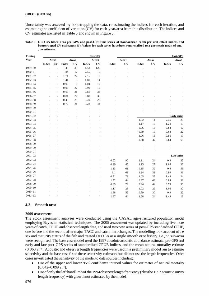
OREOS (OEO 3A)
976
Uncertainty was assessed by bootstrapping the data, re-estimating the indices for each iteration, and estimating the coefficient of variation (CV) for each year/area from this distribution. The indices and CV estimates are listed in Table 5 and shown in Figure 3. Table 5: OEO 3A black oreo pre-GPS and post-GPS time series of standardised catch per unit effort indices and
bootstrapped CV estimates (%). Values for each series have been renormalized to a geometric mean of one. -, no estimate.
Fishing Y
Pre-GPS Post-GPS Year Area1 Area2 Area3 Area1 Area2 Area3 Index CV Index CV Index CV Index CV Index CV Index CV 1979–80 - - 1.45 39 1.52 125 - - - - - - 1980–81 - - 1.84 17 2.55 15 - - - - - - 1981–82 - - 1.71 22 2.15 9 - - - - - - 1982–83 - - 1.41 8 1.80 14 - - - - - - 1983–84 - - 0.99 8 1.04 19 - - - - - - 1984–85 - - 0.95 27 0.99 12 - - - - - - 1985–86 - - 0.63 31 0.66 33 - - - - - - 1986–87 - - 0.81 22 0.88 36 - - - - - - 1987–88 - - 0.45 20 0.49 23 - - - - - - 1988–89 - - 0.72 21 0.23 44 - - - - - - 1989–90 - - - - - - - - - - - - 1990–91 - - - - - - - - - - - - 1991–92 - - - - - - - - Early series 1992–93 - - - - - - - - 1.62 14 2.46 20 1993–94 - - - - - - - - 1.17 17 1.20 15 1994–95 - - - - - - - - 0.96 13 0.82 17 1995–96 - - - - - - - - 0.89 15 0.68 22 1996–97 - - - - - - - - 1.06 18 0.96 17 1997–98 - - - - - - - - 0.58 47 0.64 63 1998–99 - - - - - - - - - - - - 1999–00 - - - - - - - - - - - - 2000–01 - - - - - - - - - - - - 2001–02 - - - - - - Late series 2002–03 - - - - - - 0.62 90 1.11 24 0.9 38 2003–04 - - - - - - 0.99 45 1.15 27 1.05 37 2004–05 - - - - - - 1.33 63 0.85 32 0.8 56 2005–06 - - - - - - 1.1 63 1.34 23 0.99 31 2006–07 - - - - - - 0.51 78 1.05 27 1.49 24 2007–08 - - - - - - 1.52 44 0.67 66 0.84 33 2008–09 - - - - - - 0.65 73 0.84 44 0.75 30 2009–10 - - - - - - 1.17 29 1.02 26 1.06 30 2010–11 - - - - - - 1.38 52 0.89 30 0.9 22 2011–12 - - - - - - 1.37 44 1.28 24 1.49 18 4.3 Smooth oreo 2009 assessment The stock assessment analyses were conducted using the CASAL age-structured population model employing Bayesian statistical techniques. The 2005 assessment was updated by including five more years of catch, CPUE and observer length data, and used two new series of post-GPS standardised CPUE, one before and the second after major TACC and catch limit changes. The modelling took account of the sex and maturity status of the fish and treated OEO 3A as a single smooth oreo fishery, i.e., no sub-areas were recognised. The base case model used the 1997 absolute acoustic abundance estimate, pre-GPS and early and late post-GPS series of standardised CPUE indices, and the mean natural mortality estimate (0.063 yr-1). Acoustic and observer length frequencies were used in a preliminary model run to estimate selectivity and the base case fixed these selectivity estimates but did not use the length frequencies. Other cases investigated the sensitivity of the model to data sources including:
• Use of the upper and lower 95% confidence interval values for estimates of natural mortality (0.042–0.099 yr-1);
• Use of only the left hand limb of the 1994 observer length frequency (plus the 1997 acoustic survey length frequency) with growth not estimated by the model.

OREOS (OEO 3A)
977
Figure 3: Standardised commercial CPUE series for black oreo in each area within OEO 3A. Pre-GPS and post-GPS
(early and late) series are shown, each renormalized to a geometric mean of one. Error bars represent the 95% confidence intervals assuming a lognormal error distribution and using the CVs listed in Table 5.
4.3.1 Estimates of fishery parameters and abundance Catch history The estimated catches were scaled up to the total reported catch (see tables 2 and 3 in the Fishery Summary section at the beginning of the Introduction – Oreos chapter) and are given in Table 6. Table 6: Reconstructed catch history (t)
Year Catch Year Catch Year Catch Year Catch 1972–73 †3 440 1981–82 1 288 1990–91 5 054 1999–00 1 789 1973–74 †3 800 1982–83 2 495 1991–92 6 622 2000–01 1 621 1974–75 †5 100 1983–84 3 979 1992–93 4 334 2001–02 1 673 1975–76 †1 260 1984–85 4 351 1993–94 4 942 2002–03 1 412 1976–77 †3 880 1985–86 3 142 1994–95 4 199 2003–04 1 254 1977–78 †5 750 1986–87 3 190 1995–96 4 022 2004–05 1 457 1978–79 650 1987–88 5 905 1996–97 3 239 2005–06 1 445 1979–80 5 215 1988–89 6 963 1997–98 4 733 2006–07 1 306 1980–81 2 196 1989–90 6 459 1998–99 2 474 2007–08 1 526
† Soviet catch, assumed to be mostly from OEO 3A and to be 50:50 black oreo:smooth oreo. Observer length frequencies Observer length data were extracted from the observer database. These data represent proportional catch at length and sex. All length samples were from the CPUE study area (see Figure 4). Only samples where 30 or more fish were measured, and the catch weight and a valid depth were recorded, were included in the analysis. Data from adjacent years were pooled because of the paucity of data in some years. The pooled length frequencies were applied in the model at the year that the median observation of the grouped samples was taken (Table 7).

OREOS (OEO 3A)
978
Figure 4: Locations of all tows in OEO 3A with a reported catch of smooth oreo from 1979–80 to 2002–03 (dots).
The study area is shown along with the line chosen to split north from south Chatham rise catches. Table 7: Observer length frequencies; numbers of length samples (tows sampled), number of fish measured, groups of
pooled years, and the year that the length data were applied in the stock assessment model. -, not applicable.
Year Number of Number of Year group Year the grouped length samples fish measured code data were applied 1979–80 32 3 499 1 Applied 1980–81 0 0 - - 1981–82 0 0 - - 1982–83 0 0 - - 1983–84 0 0 - - 1984–85 0 0 - - 1985–86 1 106 2 - 1986–87 4 387 2 - 1987–88 10 1 300 2 Applied 1988–89 14 1 512 2 - 1989–90 0 0 - - 1991–92 9 919 3 - 1992–93 0 0 - - 1993–94 13 1 365 4 Applied 1994–95 7 752 4 - 1995–96 2 207 4 - 1996–97 3 365 5 - 1997–98 13 1 720 5 - 1998–99 5 770 5 - 1999–00 77 7 595 5 Applied 2000–01 93 9 389 6 Applied 2001–02 20 3 030 7 Applied 2002–03 14 1 427 8 Applied 2003–04 4 321 8 - 2004–05 9 840 8 - 2005–06 26 3 207 9 Applied 2006–07 2 205 9 - 2007–08 8 816 9 -
Length frequency data from the 1997 acoustic survey Length data collected during the 1997 survey were used to generate a population length frequency by sex. A length frequency was generated from the trawls in each mark-type and also for the seamounts. These frequencies were combined using the fraction of smooth oreo abundance in each mark-type. The overall frequency was normalised over both male and female frequencies so that the sum of the frequencies over both sexes was 100%. The CV for each length class was given by the regression, log(CV) = 0.86 + 8.75/log(proportion). This regression was estimated from the CVs obtained by
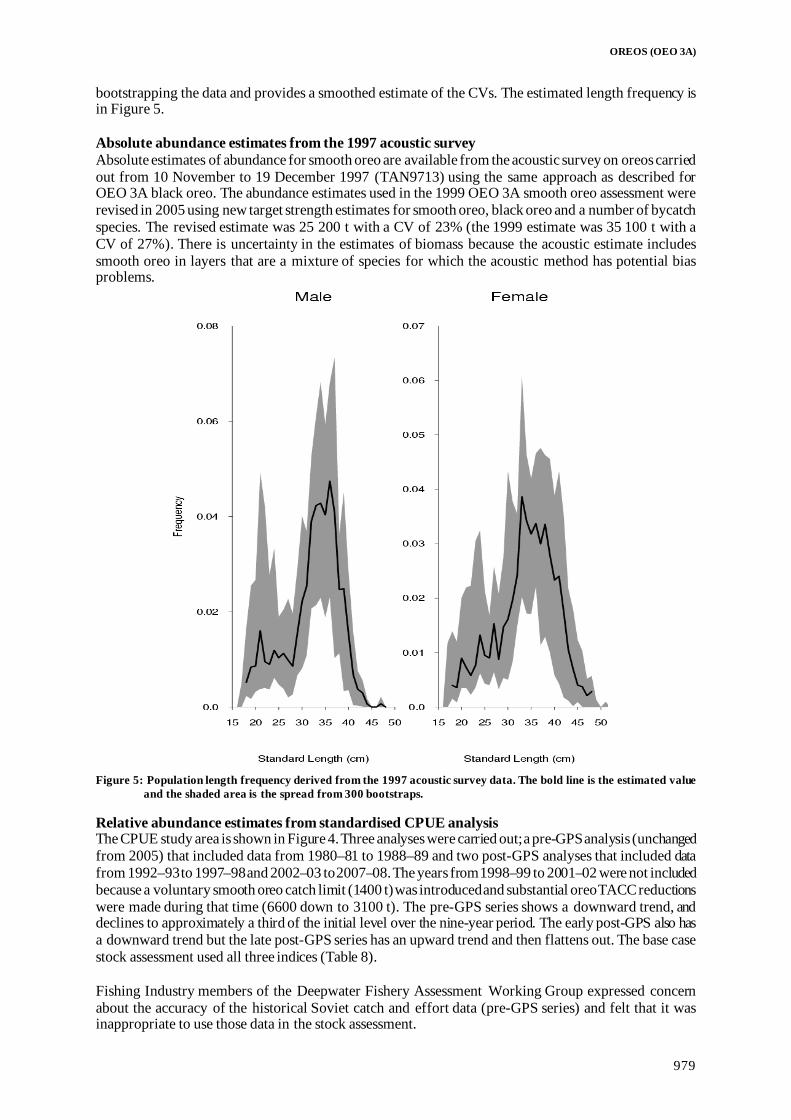
OREOS (OEO 3A)
979
bootstrapping the data and provides a smoothed estimate of the CVs. The estimated length frequency is in Figure 5. Absolute abundance estimates from the 1997 acoustic survey Absolute estimates of abundance for smooth oreo are available from the acoustic survey on oreos carried out from 10 November to 19 December 1997 (TAN9713) using the same approach as described for OEO 3A black oreo. The abundance estimates used in the 1999 OEO 3A smooth oreo assessment were revised in 2005 using new target strength estimates for smooth oreo, black oreo and a number of bycatch species. The revised estimate was 25 200 t with a CV of 23% (the 1999 estimate was 35 100 t with a CV of 27%). There is uncertainty in the estimates of biomass because the acoustic estimate includes smooth oreo in layers that are a mixture of species for which the acoustic method has potential bias problems.
Figure 5: Population length frequency derived from the 1997 acoustic survey data. The bold line is the estimated value
and the shaded area is the spread from 300 bootstraps. Relative abundance estimates from standardised CPUE analysis The CPUE study area is shown in Figure 4. Three analyses were carried out; a pre-GPS analysis (unchanged from 2005) that included data from 1980–81 to 1988–89 and two post-GPS analyses that included data from 1992–93 to 1997–98 and 2002–03 to 2007–08. The years from 1998–99 to 2001–02 were not included because a voluntary smooth oreo catch limit (1400 t) was introduced and substantial oreo TACC reductions were made during that time (6600 down to 3100 t). The pre-GPS series shows a downward trend, and declines to approximately a third of the initial level over the nine-year period. The early post-GPS also has a downward trend but the late post-GPS series has an upward trend and then flattens out. The base case stock assessment used all three indices (Table 8). Fishing Industry members of the Deepwater Fishery Assessment Working Group expressed concern about the accuracy of the historical Soviet catch and effort data (pre-GPS series) and felt that it was inappropriate to use those data in the stock assessment.

OREOS (OEO 3A)
980
Table 8: CPUE indices by year and jackknife CV (%) estimates from the pre-GPS and the two post-GPS analyses. Pre-GPS Post-GPS Year Index CV Year Index CV Year Index CV 1980–81 1.00 27 1992–93 1.00 24 2002–03 0.55 23 1981–82 0.82 26 1993–94 0.88 11 2003–04 0.77 22 1982–83 0.72 62 1994–95 0.74 14 2004–05 0.99 22 1983–84 0.59 61 1995–96 0.48 17 2005–06 0.96 31 1984–85 0.72 22 1996–97 0.56 15 2006–07 1.00 20 1985–86 0.61 19 1997–98 0.50 19 2007–08 0.92 21 1986–87 0.46 16 1987–88 0.42 16 1988–89 0.26 28
4.3.2 Biomass estimates The posterior distributions from the MCMC on the base case are shown in Figure 6. The probability that the current mature biomass (2008–09) and the biomass 5 years out (2013–14) are above 20% B0 is 1 for both.
Figure 6: Smooth oreo OEO 3A: posterior distribution for the virgin biomass (top plot) and the mature biomass
trajectories as a percentage of virgin biomass (bottom plot) from the MCMC analysis of the “NoLF” case with M = 0.063 (base case). In the top plot, the vertical line is the median of the distribution. In the bottom plot, the grey area is the point-wise 95% confidence intervals of the trajectories and the solid line is the median.
Biomass estimates derived from the MCMC are in Table 9. Total mature biomass for 2008–09 was estimated to be 36% of the initial biomass (B0). Sensitivity case results for the base case using the lower and upper 95% confidence interval value estimates for M gave estimates of current biomass between 26% and 49% of B0. The sensitivity case that used the left hand limb of the 1994 observer length frequency (plus the 1997 acoustic survey length frequency) with growth not estimated by the model gave estimates of current biomass for the mean estimate of M (0.063 yr-1) of 30 % of B0 while estimates using the lower and upper 95% confidence interval value estimates for M gave estimates of 2008 biomass between 12% and 59% of B0. Projections were carried out for five years with the current catch limit of 1400 t. The trajectory shows increasing biomass (Figure 6).

OREOS (OEO 3A)
981
Table 9 (a): Base case (in bold) and sensitivity to M values (biomass estimates). Bcurr is 2008.
M = 0.063 †M = 0.042 †M = 0.099 Median CI.05 CI.95 Median CI.05 CI.95 Median CI.05 CI.95 B0 85 000 77 300 96 500 97 700 90 100 110 000 68 500 60 300 79 600 B_cur 30 900 22 400 43 000 26 300 18 000 38 800 33 800 25 000 45 500 B_cur(%B0) 36 29 45 27 20 35 49 41 57
(b) Sensitivity (biomass estimates). In these runs the left hand limb of the 1994 observer length was fitted, the 1997 acoustic survey length frequency was included and growth was not estimated by the model:
†M = 0.063 †M = 0.042 †M = 0.099 Median CI.05 CI.95 Median CI.05 CI.95 Median CI.05 CI.95 B0 77 400 74 800 80 200 82 800 81 600 84 200 82 300 76 700 89 200 B_cur 23 100 19 900 26 400 10 200 8 480 12 100 48 800 42 900 56 200 B_cur(%B0) 30 27 33 12 10 14 59 56 63
4.3.3 Other factors Because of differences in biological parameters between the species, it would be appropriate to split the current TACC for black oreo and smooth oreo. The WG noted that separate species catch limits are in place to reduce the risk of over- or under-fishing either smooth oreo or black oreo. The model estimates of uncertainty are unrealistically low. Uncertainties that are not included in the model include:
• the assumption that recruitment is deterministic; • that the acoustic index is assumed to be an absolute estimate of abundance; • the selectivity in the base case is fixed at the MPD estimate from the preliminary case where
all length data is used; • uncertainty in the estimate of M.
In addition, the growth is fixed and known. The WG has previously noted the impact of the different ages of maturity for males and females. Due to the fact that males mature at a much smaller size than females (age at 50% maturity is 18–19 years for males and 25–26 for females), the sex ratio needs to be taken into account when assessing the sustainability of any particular catch level. 5. STATUS OF THE STOCKS The smooth oreo stock assessment is unchanged from 2009. The black oreo stock assessment is updated using CPUE data up to 2011–12. Stock Structure Assumptions The two oreo stocks in FMA 3A are assessed separately but managed as a single stock. For both the black oreo and smooth oreo stocks it is assumed that there is potential mixing with stocks outside of the OEO 3A area.
• OEO 3A (Black Oreo) Stock Status Year of Most Recent Assessment 2013 Assessment Runs Presented Age-structured CASAL spatial assessment model rejected by
the Working Group; CPUE accepted Reference Points
Target: 40% B0 Soft Limit: 20% B0 Hard Limit: 10% B0 Overfishing threshold: F40% B0
Status in relation to Target Unknown Status in relation to Limits Unknown Status in relation to Overfishing Unknown

OREOS (OEO 3A)
982
Historical Stock Status Trajectory and Current Status -
Fishery and Stock Trends Recent Trend in Biomass or Proxy Unknown Recent Trend in Fishing Intensity or Proxy
Catch has decreased with TACC since the early 1990s and remained low and relatively constant over the last 10 years.
Other Abundance Indices CPUE since 2002–03 has stabilised in all three areas after significant declines in the two deeper areas in the 1980s and 1990s.
Trends in Other Relevant Indicators or Variables
-
Projections and Prognosis Stock Projections or Prognosis - Probability of Current Catch or TACC causing Biomass to remain below or to decline below Limits
Soft Limit: Unknown Hard Limit: Unknown
Probability of Current Catch or TACC causing Overfishing to continue or to commence
Unknown
Assessment Methodology and Evaluation Assessment Type Level 2 – Partial Quantitative Stock Assessment Assessment Method CPUE Assessment Dates Latest assessment: 2013 Next assessment: 2019 Overall assessment quality rank
1 – High Quality Main data inputs (rank) CPUE abundance 1 – High Quality Data not used (rank) Changes to Model Structure and Assumptions
The three area model with migration based on age is thought to be flawed and the previous model has been withdrawn.
Major Sources of Uncertainty - Qualifying Comments - Fishery Interactions Both species of oreo are sometimes taken as bycatch in orange roughy target fisheries, mostly in other areas e.g. OEO 4. The main bycatch species in the OEO 3A black oreo target fishery include smooth oreo, hoki, javelinfish, Baxter’s dogfish, pale ghost shark, ridge scaled rattail, and basketwork eel. Bycatch species that may be vulnerable to overfishing include deepwater sharks and rays. Protected species catches include seabirds and deepwater corals. Oreo are caught using bottom trawl gear. Bottom trawling interacts with benthic habitats.
• OEO 3A (Smooth Oreos)
Stock Status Year of Most Recent Assessment 2009 Assessment Runs Presented One base case and 5 sensitivity runs Reference Points Target: 40% B0
Soft Limit: 20% B0 Hard Limit: 10% B0
Overfishing threshold:

OREOS (OEO 3A)
983
Status in relation to Target For the base case, B2009 was estimated at 36% B0, About as Likely as Not (40–60%) to be at or above the target.
Status in relation to Limits B2009 is Unlikely (< 40%) to be below the Soft Limit and Very Unlikely (< 10%) to be below the Hard Limit.
Historical Stock Status Trajectory and Current Status
Mature biomass trajectories as a percentage of virgin biomass from the base case. The grey area is the point-wise 95% confidence intervals of the trajectories and the solid line is the median.
Fishery and Stock Trends Recent Trend in Biomass or Proxy Biomass is projected to have been increasing since the late
1990s. Recent Trend in Fishing Mortality or Proxy
Unknown
Other Abundance Indices - Trends in Other Relevant Indicators or Variables
-
Projections and Prognosis (2009) Stock Projections or Prognosis The biomass is expected to increase over the next 5 years
given the current catch limit of 1400 t. Probability of Current Catch or TACC causing Biomass to remain below or to decline below Limits
Soft Limit: Very Unlikely (< 10%) Hard Limit: Very Unlikely (< 10%)
Probability of Current Catch or TACC causing Overfishing to continue or to commence
-
Assessment Methodology Assessment Type Level 1 - Quantitative stock assessment Assessment Method Age-structured CASAL model with Bayesian estimation of
posterior distributions Assessment dates Latest assessment: 2009 Next assessment: Unknown Overall assessment quality rank - Main data inputs (rank) - One acoustic absolute abundance estimate (1997)
- three standardised CPUE indices (1981–82 to 1988–89, 1992–93 to 1997–98, 2002–03 to 2007–08) - Natural mortality estimate (0.063) - Selectivity estimated from acoustic and observer length frequencies New information from previous (2005) assessment: - Updated with additional catch, CPUE, observer length data collected since last assessment - two new standardised post-GPS CPUE series
Changes to Model Structure and Assumptions
-

OREOS (OEO 3A)
984
Major Sources of Uncertainty - The single acoustic index (1997) is assumed to be an absolute estimate of abundance - Sex ratio needs to be taken into account, as males mature at a much smaller size than females. - Recruitment is assumed to be deterministic. - Uncertainty in the estimates of natural mortality (M) - Selectivity is fixed in the base case at the MPD estimate from the preliminary study
Qualifying Comments - Fishery Interactions Both species of oreo are sometimes taken as bycatch in orange roughy target fisheries, mostly in other areas e.g. OEO 4. The main bycatch species in the OEO 3A smooth oreo target fishery include black oreo, hoki, javelinfish, Baxter’s dogfish, pale ghost shark, ridge scaled rattail and basketwork eel. Low productivity bycatch species include deepwater sharks and rays. Protected species catches include seabirds and deepwater corals. Oreo are caught using bottom trawl gear. Bottom trawling interacts with benthic habitats.
6. FOR FURTHER INFORMATION Coburn, R P; Doonan, I J; McMillan, P J (1999) Black oreo abundance indices from standardised catch per unit of effort data for OEO 3A.
New Zealand Fisheries Assessment Research Document 1999/32. 18 p. (Unpublished document held by NIWA library, Wellington.)
Coburn, R P; Doonan, I J; McMillan, P J (2006) Smooth oreo OEO 3A abundance estimates from standardised catch per unit of effort data, 1979–80 to 2002–03. New Zealand Fisheries Assessment Report 2006/35. 38 p.
Coburn, R P; McMillan, P J; Gilbert, D J (2007) Inputs for a stock assessment of smooth oreo, Pukaki Rise (part of OEO 6). New Zealand Fisheries Assessment Report 2007/23. 32 p.
Cordue, P L (1996) A model-based method for bounding virgin biomass using a catch history, relative biomass indices, and ancillary information. New Zealand Fisheries Assessment Research Document 1996/8. 48 p. (Unpublished document held by NIWA library, Wellington.)
Doonan, I J; Coburn, R P; McMillan, P J (2009) Assessment of OEO 3A black oreo for 2006–07. New Zealand Fisheries Assessment Report 2009/12. 46 p.
Doonan, I J; Coburn, R P; McMillan, P J; Hart, A C (2004) Assessment of OEO 3A black oreo for 2002–03. New Zealand Fisheries Assessment Report 2004/52. 54 p.
Doonan, I J; Coombs, R F; McMillan, P J; Dunn, A (1998) Estimate of the absolute abundance of black and smooth oreo in OEO 3A and 4 on the Chatham Rise. Final Research Report for Ministry of Fisheries Research Project OEO9701. 47 p. (Unpublished document held by Fisheries New Zealand, Wellington.)
Doonan, I J; McMillan, P J (2001) A non-parametric age selectivity ogive for OEO 3A black oreo for 2001–02. New Zealand Fisheries Assessment Report 2001/40. 17 p.
Doonan, I J; McMillan, P J; Coburn, R P; Hart, A C (1996) Assessment of Chatham Rise smooth oreo (OEO 3A and OEO 4) for 1996. New Zealand Fisheries Assessment Research Document 1996/17. 21 p. (Unpublished document held by NIWA library, Wellington.)
Doonan, I J; McMillan, P J; Coburn, R P; Hart, A C (1997) Assessment of Chatham Rise smooth oreo (OEO 3A and OEO 4) for 1997. New Zealand Fisheries Assessment Research Document 1997/21. 26 p. (Unpublished document held by NIWA library, Wellington.)
Doonan, I J; McMillan, P J; Coburn, R P; Hart, A C (1999a) Assessment of OEO 3A smooth oreo for 1999–2000. New Zealand Fisheries Assessment Research Document 1999/45. 21 p. (Unpublished document held by NIWA library, Wellington.)
Doonan, I J; McMillan, P J; Coburn, R P; Hart, A C (1999b) Assessment of OEO 3A black oreo for 1999–2000. New Zealand Fisheries Assessment Research Document 1999/52. 30 p. (Unpublished document held by NIWA library, Wellington.)
Doonan, I J; McMillan, P J; Coburn, R P; Hart, A C (2003) Assessment of OEO 4 smooth oreo for 2002–03. New Zealand Fisheries Assessment Report 2003/50. 55 p.
Doonan, I J; McMillan, P J; Coburn, R P; Hart, A C; Cordue, P L (1995) Assessment of smooth oreo for 1995. New Zealand Fisheries Assessment Research Document 1995/12. 31 p. (Unpublished document held by NIWA library, Wellington.)
Doonan, I J; McMillan, P J; Hart, A C (2008) Ageing of smooth oreo otoliths for stock assessment. New Zealand Fisheries Assessment Report 2008/08. 29 p.
Doonan, I J; McMillan, P J; Hart, A H (2016) Comparison of the fraction of mature black oreo between Area 1 and Area 2&3 (OEO 3A). New Zealand Fisheries Assessment Report 2016/20.
Doonan, I J; McMillan, P J; Hart, A C; Coombs, R F (2003) Smooth oreo abundance estimates from the October–November 2001 acoustic survey of the south Chatham Rise (OEO 4). New Zealand Fisheries Assessment Report 2003/26. 21 p.
Francis, R I C C (1992) Recommendations concerning the calculation of maximum constant yield (MCY) and current annual yield (CAY). New Zealand Fisheries Assessment Research Document 1992/8. 27 p. (Unpublished document held by NIWA library, Wellington.)
McKenzie, A (2007) Stock assessment for east Pukaki Rise smooth oreo (part of OEO 6). New Zealand Fisheries Assessment Report 2007/34. 27 p.
McMillan, P J; Doonan, I J; Hart, A C; Coburn, R P (1998) Oreo stock assessment. Final Research Report for Ministry of Fisheries Research Project OEO9702. 16 p. (Unpublished document held by Fisheries New Zealand, Wellington.)
McMillan, P J; Hart, A C (1991) Assessment of black and smooth oreos for the 1991–92 fishing year. New Zealand Fisheries Assessment Research Document 1991/10. 29 p. (Unpublished document held by NIWA library, Wellington.)
Smith, M H; Doonan, I J; McMillan, P J; Hart, A C (2006) Black oreo abundance estimates from the September–October 2002 acoustic survey of the south Chatham Rise (OEO 3A). New Zealand Fisheries Assessment Report 2006/33. 20 p.

OREOS (OEO 4)
985
OREOS – OEO 4 BLACK OREO AND SMOOTH OREO 1. FISHERY SUMMARY This is presented in the Fishery Summary section at the beginning of the Introduction – Oreos chapter. 2. BIOLOGY This is presented in the Biology section at the beginning of the Introduction – Oreos chapter. 3. STOCKS AND AREAS This is presented in the Stocks and Areas section at the beginning of the Introduction – Oreos chapter. 4. STOCK ASSESMENT 4.1 Introduction In 2018, the stock assessment was updated for smooth oreo in OEO 4. 4.2 Black oreo Investigations were carried out in 2009 using age-based single sex single step preliminary models in CASAL. The data used in these models were four standardised CPUE indices (pre– and post–GPS in the east and west), and observer length frequencies. Growth and maturity were also estimated in some of the runs. 4.2.1 Estimates of fishery parameters and abundance Absolute abundance estimates from the 1998 acoustic survey Absolute estimates of abundance were available from an acoustic survey on oreos which was carried out from 26 September to 30 October 1998 on Tangaroa (voyage TAN9812). Transects on flat ground were surveyed to a stratified random design and a random sample of seamounts were surveyed with either a random transect (large seamounts) or a systematic “star” transect design. For some seamounts the flat ground nearby was also surveyed to compare the abundance of fish on and near the seamount either by extending the length of the star transects or by extra parallel transects. Acoustic data were collected concurrently for flat and seamounts using both towed and hull mounted transducers. The OEO 4 survey covered 59 transects on the flat and 29 on seamounts. A total of 95 tows were carried out for target identification and to estimate target strength and species composition. In situ and swimbladder samples for target strength data were collected and these have yielded revised estimates of target strength for both black oreo and smooth oreo. Acoustic abundance estimates for recruit black oreo from seamounts and flat for the whole of OEO 4 are in Table 1. About 59% of the black oreo abundance came from the background mark-type. This mark-type is not normally fished by the commercial fleet and this implies that the abundance estimate did not cover the fish normally taken by the fishery. In addition the scaling factor to convert the acoustic area estimate to the trawl survey area estimate was 4.3, i.e., the acoustic survey area only had about 23% of the abundance. The magnitude of this ratio suggests that the size of the area surveyed was borderline for providing a reliable abundance estimate. Relative abundance estimates from standardised CPUE analyses – 2009 analysis The CPUE analysis method involved regression based methods on the positive catches only. Sensitivities were run where the positive catch tow data and the zero catch tow data were analysed separately to produce positive catch and zero catch indices. All data were included, whether they were target or bycatch fisheries, with the target offered to the model (and not accepted).

OREOS (OEO 4)
986
Table 1: OEO 4 recruit black oreo seamount, flat, and total acoustic abundance estimates (t) and recruit CV (%) based on knife-edge recruitment (23 years).
Abundance (t) CV (%) Seamount 127 91 Flat 13 800 56 Total 13 900 55
The best data-split was investigated using the Akaike Information Criteria (AIC) on a number of potential regressions. Four indices were subsequently used, pre- and post-GPS in the east and west areas respectively. These two areas are very distinct: the west consists of flat fishing and the east of hill fishing, the west area was fished 10 years prior to the east, and there has been a move by the fishery since the early 1990s from the west to the east. However, despite these differences, the two series present almost identical patterns of decline in relative standardised CPUEs from the time fishing started in earnest (1980 in the west and 1992 in the east) which would suggest that for this fishery CPUE might be a reasonable index of abundance (because less influenced by technology, fishing patterns, hills or flats etc). The standardised CPUE series and CVs are described in Table 2. Over comparable time periods and data sets, the trends from the updated series were similar to those from the 2000 analyses (Coburn et al 2001b). The west CPUE reduced to between 5% of the 1980 value and 15% of the 1981 value by 1990. The post-GPS west series is either flat or slightly increasing. The east CPUE reduced to 4% of the 1984 value and 21% of the 1985 value by 1990 even though catches were low. The post-GPS east series showed a further steep initial decline with total reduction to 15% of the 1993 value by 2008. Table 2: OEO 4 black oreo standardised CPUE analyses in 2009 (expressed in t / tow).
Fishing year
Pre-GPS east
Pre-GPS west
Fishing year
Post-GPS east
Post-GPS west
Index CV Index CV Index CV Index CV 1980
8.97 0.17 1993 0.71 0.15 0.73 0.41
1981
4.00 0.11 1994 0.63 0.13 0.45 0.32 1982
2.24 0.10 1995 0.31 0.15 0.41 0.31
1983
2.20 0.09 1996 0.21 0.15 0.28 0.27 1984 0.47 0.95 1.54 0.10 1997 0.24 0.12 0.61 0.27 1985 0.41 0.28 1.51 0.07 1998 0.20 0.11 0.45 0.23 1986 0.38 0.32 1.28 0.10 1999 0.16 0.12 0.46 0.23 1987 0.65 0.30 0.67 0.10 2000 0.17 0.12 0.68 0.25 1988 0.10 0.18 0.54 0.13 2001 0.14 0.08 0.62 0.24 1989 0.02 0.20 0.48 0.12 2002 0.18 0.07 0.47 0.29
2003 0.13 0.06 0.49 0.24 2004 0.13 0.06 0.93 0.24 2005 0.14 0.07 0.91 0.26 2006 0.13 0.07 0.68 0.26 2007 0.12 0.07 1.00 0.27 2008 0.10 0.09 0.88 0.24
Relative abundance estimates from trawl surveys The estimates, and their CVs, from the four standard Tangaroa south Chatham Rise trawl surveys are treated as relative abundance indices (Table 3). Table 3: OEO 4 black oreo research survey abundance estimates (t). N is the number of stations. Estimates were made
using knife-edge recruitment set at 33 cm TL. Previously knife-edge recruitment was set at 27 cm and estimates of abundance based on that value are also provided for comparison.
Observer length frequencies Observer length frequencies were available for about 20% of the yearly catch from 1989 to 2008. Analyses conducted on these data indicated that they were not representative of the spatial spread of the fishery. When stratified by depth, the length frequencies had double-modes, centred around 28 cm and
Year Mean abundance CV (%) N 27 cm 33 cm 1991 34 407 13 065 40 105 1992 29 948 12 839 46 122 1993 20 953 6 515 30 124 1995 29 305 9 238 30 153

OREOS (OEO 4)
987
38 cm, with inconsistent trends in the modes between years. Alternative stratification by subarea, hill, etc, did not resolve the problem; some tows showed bimodality. These patterns in length frequencies were an issue because the yearly shifts in length frequencies and double mode cannot be representative of the underlying fish population since black oreo is a slow growing long-lived fish. They are more likely linked with discrete spatial sub-groups of the population. A similar double mode was reported for some strata in the same area from the 1994 Tangaroa trawl survey (Tracey & Fenaughty 1997). It is likely that there is further spatial stock structure that is currently unaccounted for. 4.2.2 Biomass estimates The 2009 stock assessment of OEO 4 black oreo was inconclusive as assessment models were unable to represent the observer length frequency structure, and were considered unreliable. The CPUE was fitted satisfactorily under a two-stock model but could not be fitted in a single homogeneous stock model. However, the WG agreed that:
1. The CPUE indices are consistent with a two-stock structure or at least a minimally-mixing single stock.
2. The updated CPUE estimates were probably a reasonable indicator of abundance (at the spatial scale of the east and west analyses).
4.2.3 Estimation of Maximum Constant Yield (MCY) In 2000, MCY was estimated using the equation, MCY = c*YAV (Method 4). There was no trend in the annual catches, nominal CPUE, or effort from 1982–83 to 1987–88 so that period was used to calculate the MCY estimate (1200 t). The MCY calculation was not updated in 2009. 4.2.4 Estimation of Current Annual Yield (CAY) CAY cannot be estimated because of the lack of current biomass estimates. 4.3 Smooth oreo Smooth oreo was assessed in 2018 using a CASAL age-structured population model with Bayesian estimation, incorporating stochastic recruitment, life history parameters (table 1 of the Biology section at the beginning of the Introduction – Oreos chapter), and catch history up to 2017–18. In early assessments (Doonan et al 2001, 2003, 2008), the stock area was split at 178° 20′ W into a west and an east fishery based on an analysis of commercial catch, standardised CPUE, and research trawl and acoustic result, and data fitted in the model included acoustic survey abundance estimates, standardised CPUE indices, observer length data, and the acoustic survey length data. In 2012, the Deepwater Working Group decided that using CPUE to index abundance should be discontinued, due to changes in fishing patterns over time within the stock area. With no CPUE indices, the 2012 assessment was simplified to a single area model using only the observations of vulnerable biomass from acoustic surveys carried out in 1998, 2001, 2005, and 2009. A 2014 stock assessment updated the 2012 assessment model using the same single area model structure and used an additional observation of biomass from the research acoustic survey carried out in 2012. The assessment also revised the previous assessments by including the age frequency estimates from the 1998 and 2005 acoustic surveys and by estimating relative year class strengths. The 2018 assessment updated the 2014 assessment with the inclusion of an additional acoustic survey biomass estimate in 2016 and the associated age frequency. An age frequency from a 1991 trawl survey was also included together with an age frequency from the commercial fishery in 2009. With the addition of three new age frequencies natural mortality was estimated within the model (with a Normal prior with the mean equal to 0.063 and CV=25% – see table 1 in the Biology section). Year class strengths (YCS) were estimated for 1940–2005 (based on the range of age estimates in the age frequency data). A “near uniform” prior was used (parameterised as a lognormal distribution with a mode of 1 and sigma of 4), which places minimum constraint on the free YCS parameters (Haist parameterisation).

OREOS (OEO 4)
988
An informed prior was used for the acoustic survey proportionality constant q (lognormal with mean of 0.83 and CV of 0.3). The prior was based on limited information on target strength, the QMA scaling-factor, and the proportion of vulnerable biomass in the vulnerable acoustic marks (Fu & Doonan 2013). A brief description of the base case and sensitivity runs presented are summarised in Table 4. The following assumptions were made in the stock assessment analyses:
(a) Recruitment followed a Beverton–Holt relationship with steepness of 0.75. (b) Catch overruns were 0% during the period of reported catch. (c) The population of smooth oreo in OEO 4 was a discrete stock or production unit. (d) The acoustic biomass selectivity and the commercial fishery selectivity were assumed to be
identical (logistic, estimated within the model). (e) A separate selectivity was estimated for the age frequencies that were derived from trawl
catches during the acoustic surveys (double normal, estimated within the model).
Bayesian estimation was used in the assessment to capture the uncertainties in model estimates of biomass and other parameters:
1. Model parameters were estimated using maximum likelihood and the prior probabilities; 2. Samples from the joint posterior distribution of parameters were generated with the Monte Carlo
Markov Chain procedure (MCMC) using the Hastings-Metropolis algorithm;
3. A marginal posterior distribution was found for each quantity of interest by integrating the product of the likelihood and the priors over all model parameters; each marginal posterior distribution was described by its median and a 95% credibility interval (95% CI).
Bayesian estimates were based on results from three 15 million long MCMC chains. After a burn-in of 1 million, the last 14 million of the chain was sampled at each 1000th value. Posterior distributions were obtained from samples combined over the three chains (after the burn-in). Table 4: Descriptions of the model runs of the 2018 smooth oreo assessment. LN, lognormal distribution with mean
and CV given in the bracket. N, normal distribution with mean and CV in the bracket. All use Haist parameterisation for YCS.
Model run Description
Base Acoustic q estimated with a LN(0.83, 0.3) prior, nearly uniform prior on YCS, M estimated with a N(0.063, 0.25) prior, adult biomass indices (school marks)
LowM-Highq M fixed at 0.0632 (20% less than the base estimate) and the mean of the acoustic q prior 20% higher HighM-Lowq M fixed at 0.0948 (20% higher than the base estimate) and the mean of the acoustic q prior 20% lower Plus LFs Base but with commercial length frequencies included Fixed M Base but with fixed M = 0.063 (as assumed in the 2014 assessment)
4.3.1 Estimates of fishery parameters and abundance The 2018 assessment incorporated the catch history and the adult acoustic biomass indices. Five age frequencies were fitted. Commercial length frequencies (five scaled length frequencies between 1996 and 2008) were not included in the base model but were fitted in a sensitivity run (see Table 4). Catch history A catch history for smooth oreo in OEO 4 was developed by scaling the estimated catch to the QMS values (Table 5). A catch of 2876 t was recorded for 2017–18. Biomass estimates from the 1998, 2001, 2005, 2009, 2012, and 2016 acoustic surveys Estimates of biomass were available from six acoustic surveys:
(i) 26 September to 30 October 1998 on Tangaroa (voyage TAN9812); (ii) 16 October to 14 November 2001 using Tangaroa for acoustic work (voyage TAN0117) and
Amaltal Explorer (voyage AEX0101) for trawling;

OREOS (OEO 4)
989
(iii) 3–22 November 2005 using Tangaroa for acoustic work (voyage TAN0514) and 3–20 November 2005 using San Waitaki (SWA0501) for mark identification trawling;
(iv) 2–18 November 2009 using Tangaroa for acoustic work (voyage TAN0910) and 2–18 November 2009 using San Waitaki (SWA0901) for mark identification trawling;
(v) 8–26 November 2012 using Tangaroa for acoustic work (voyage TAN01214) and 8–26 November 2012 using San Waitaki (SWA1201) for mark identification trawling;
(vi) 16 October to 17 November 2016 on Amaltal Explorer (AEX1602). Table 5: Catch history for OEO 4 smooth oreo.
Year Catch (t) Year Catch (t) 1978–79 1 321 1999–00 6 357 1979–80 112 2000–01 6 491 1980–81 1 435 2001–02 4 291 1981–82 3 461 2002–03 4 462 1982–83 3 764 2003–04 5 656 1983–84 5 759 2004–05 6 473 1984–85 4 741 2005–06 5 955 1985–86 4 895 2006–07 6 363 1986–87 5 672 2007–08 6 422 1987–88 7 764 2008–09 6 090 1988–89 7 223 2009–10 6 118 1989–90 6 789 2010–11 6 518 1990–91 6 019 2011–12 6 357 1991–92 5 508 2012–13 5 964 1992–93 5 911 2013–14 6 016 1933–94 6 283 2014–15 6 318 1994–95 6 936 2015–16 1 992 1995–96 6 378 2016–17 2 279 1996–97 6 359 2017–18 2 867 1997–98 6 248 1998–99 6 030
The method of estimating variance and bias was the same as in previous oreo surveys (Doonan et al 1998, 2000). Variance was estimated separately for the flat and for hills and then combined. Sources of variance were:
• sampling error in the mean backscatter • the proportion of smooth oreo and black oreo in the acoustic survey area • sampling error in catches which affects the estimate of the proportion of smooth oreo • error in the target strengths of other species in the mix • variance in the estimate of smooth oreo target strength • sampling error of fish lengths (negligible) • variance of the mean weight, for smooth oreo
Vulnerable smooth oreo was estimated based on the acoustic mark types, where vulnerable biomass was the sum over two flat mark types: DEEP SCHOOLS and SHALLOW SCHOOLS, with the hill biomass added on. These estimates were made for smooth oreo in the whole of OEO 4 (Table 6). One major source of uncertainty in the 2012 survey estimates was that about 25% of the total estimate came from one school mark on the flat. The species composition of this mark was not able to be verified by trawling. Excluding this mark, i.e., assuming they were not smooth oreo, reduced the total biomass for smooth oreos to 36 550 t. However, the consensus of skippers consulted about the mark is that it was likely to be smooth oreo. Table 6: Estimated smooth oreo vulnerable biomass (t) and CV (%, after the addition of 20% process error) from
acoustic surveys in 1998, 2001, 2005, and 2009, 2012, and 2016; includes school marks and hills. Year Biomass (t) CV (%) 1998 65 679 33 2001 81 633 33 2005 63 237 32 2009 26 953 33 2012 58 603 36 2016 34 022 38

OREOS (OEO 4)
990
Age frequencies from the 1998, 2005, and 2016 acoustic surveys Age frequency distributions were derived from trawl samples taken for smooth oreo in OEO 4 during three acoustic surveys carried out in 1998 and 2005 (Doonan et al 2008) and 2016. All of the sampled otoliths (n = 546) from the 1998 survey and randomly selected otoliths (n = 500) from the 1800 otoliths collected during the 2005 survey were read, with 398 otoliths used from the 2016 survey. The age frequency distribution was estimated using the aged otoliths from tows in each mark-type weighted by the catch rates and the proportion of abundance in the mark-type. Age frequencies were estimated by sex and combined over sexes. The variance was estimated by bootstrapping the tows within mark-types (e.g., Doonan et al 2008). The ageing error was estimated by comparing age estimates from two readers and also by using repeated readings from the same reader. The age frequencies had a mean weighted CV of 36% (1998) and 45% (2005). The ageing error was estimated to be about 8.5% which was used in the assessment. The age frequencies (male and female combined) were included in order to estimate year class strength. Other age frequencies Two additional age frequencies were constructed for the 2018 assessment. The first was for the commercial catch in 2008–2009. The 1284 otoliths available from the observer programme were sampled at random (with replacement) until 400 unique otoliths were obtained. The probability of selection was proportional to the tow catch and inversely proportional to the number of otoliths sampled in the tow. The mean weighted CV was 30% (obtained by bootstrapping). The second age frequency was constructed for the 1991 trawl survey of OEO 4 (TAN9104). Otoliths collected during the trawl survey were sampled at random until 400 unique otoliths were obtained. The probability of selection was proportional to the stratum biomass estimate and by tow catch within stratum, divided by the number of otoliths available from the tow. The mean weighted CV was 35% (obtained by bootstrapping). Observer length frequencies Observer length data were extracted from the observer database. These data were stratified by season (October-March and April-September) and into west and east parts. The length frequencies were combined over strata by the proportion of catch in each stratum. Five scaled length frequencies from 1996 to 2008 were used in a sensitivity run but not used in the base model. 4.3.2 Biomass estimates, year class strengths, and exploitation rates For the base model, and all of the sensitivities, B0 was estimated at about 140 000 t with 95% CIs ranging from about 110 000 t to 210 000 t (Table 7). Current stock status is estimated to be at the target level of 40% for the base case. However, it is estimated to be just above 30% B0 for the LowM-Highq and Fixed M runs (Table 7). For all of the runs the estimated probability of current stock status being below the soft limit of 20% B0 is less than 5% (Table 7). The probability of current stock status being below the hard limit of 10% B0 was estimated at 0 for all runs (Table 7). Table 7: Bayesian estimates of M, B0, and current stock status (B18/B0) for the base model and sensitivities (the median
and 95% CIs are given). The probability of current stock status being below 10% or 20% B0 is also given.
M (yr-1) B0 (000 t) ss18 (%B0) P(ss18 < 10%) P(ss18 < 20%) Base 0.079 (0.057–0.01) 138 (111–184) 40 (23–59) 0.00 0.01 LowM-Highq 0.0632 138 (118–173) 31 (19–46) 0.00 0.04 HighM-Lowq 0.0948 146 (111–208) 50 (33–67) 0.00 0.00 Incl. LFs 0.085 (0.067–0.011) 133 (111–172) 42 (26–60) 0.00 0.00 Fixed M 0.063 143 (121–184) 33 (21–50) 0.00 0.02
The spawning biomass trajectory for the base model shows a decreasing trend from the start of the fishery in the 1980s with a flattening off in 2015–16 when catches were substantially reduced (Figure 1, Table 5). Current stock status is estimated to be at the target biomass although the 95% CIs are very wide (Figure 1, Table 7).

OREOS (OEO 4)
991
The estimated year class strengths show a pattern (in the medians) from 1972 to 1987 of above average cohort strength with below average cohort strength from 1990 to 2005 (Figure 2), consistent with the age composition data.
Figure 1: Base, MCMC estimated spawning-stock biomass trajectory. The box in each year covers 50% of the
distribution and the whiskers extend to 95% of the distribution. The soft limit (red) and target biomass (green) are marked by horizontal lines.
Figure 2: Base, MCMC estimated “true” YCS (Ry/R0). The box in each year covers 50% of the distribution and the
whiskers extend to 95% of the distribution. Exploitation rates in the fishery were estimated to be generally increasing from the start of the fishery up until 2014–15 (Figure 3). Catches in the years immediately prior to the TACC reduction in 2015–16 were at a level increasingly above the exploitation rate corresponding to the target biomass, U40%B0. With the substantial catch reduction in 2015–16 the estimated exploitation rate (median) dropped to below 5% where it has remained (Figure 3).
Year
SS
B (%
B0)
020
4060
8010
012
0
1940 1950 1960 1970 1980 1990 2000 2010 2020
Cohort
True
YC
S
0.0
0.5
1.0
1.5
2.0
2.5
1939 1949 1959 1969 1979 1989 1999 2009 2019

OREOS (OEO 4)
992
Figure 3: Base, MCMC estimated exploitation rate trajectory. The box in each year covers 50% of the distribution and
the whiskers extend to 95% of the distribution. The exploitation rate, U40%B0, corresponding to the biomass target of 40% B0 is marked by the middle horizontal line (Ux%B0 is the exploitation rate that will drive deterministic spawning biomass to x% B0). U30%B0 and U50%B0 are also marked by horizontal lines.
4.3.3 Yield estimates and projections Five year projections were made from the base model at a constant catch of 2300 t which is the approximate level of the last reported annual catch (2279 t in 2016–17) and also at 3000 t (the TACC for OEO 4). Year class strengths from 2006 onwards were sampled at random from the last 10 estimated year class strengths (1996–2005). Based on the projections, stock status is expected to stay fairly constant over the next five years for annual catches in the range 2300–3000 t (Figures 4 and 5, Table 8). There is a small upward trend in median stock status at annual catches of 2300 t (Figure 4, Table 8).
Figure 4: Base, MCMC projections at a constant annual catch of 2300 t. The box in each year covers 50% of the
distribution and the whiskers extend to 95% of the distribution. The target biomass (40% B0) is marked by the horizontal green line and the soft limit (20% B0) by the horizontal red line.
1970 1980 1990 2000 2010
05
1015
20
Fishing year
Exp
loita
tion
rate
(%)
U30%B0
U50%B0
U40%B0
Year
SS
B (%
B0)
020
4060
80
2018 2019 2020 2021 2022 2023

OREOS (OEO 4)
993
Figure 5: Base, MCMC projections at a constant annual catch of 3000 t. The box in each year covers 50% of the
distribution and the whiskers extend to 95% of the distribution. The target biomass (40% B0) is marked by the horizontal green line and the soft limit (20% B0) by the horizontal red line.
Table 8: The expected value of stock status in 2023 (E(ss23)) and the probabilities of being above the target biomass
(40% B0) or below the soft limit (20% B0) or below the hard limit (10% B0) under projected annual catches of 2300 t or 3000 t.
Annual catch (t) E(ss23) (%B0) P(ss23 > 40%) P(ss23 < 20%) P(ss23 < 10%) 2300 42 0.57 0.01 0.00 3000 40 0.49 0.02 0.00
4.3.4 Other factors The Working Group considered that there were a number of other factors that should be considered in relation to the stock assessment results presented here. These include:
• uncertainty in the estimates of species composition of catch histories, • confounding of estimates of M with others parameters in the model, and • the assumption that acoustic selectivity is the same as the commercial selectivity.
4.3.5 Future research considerations
• Regular acoustic surveys are required to monitor the trend in adult biomass. • Improved estimates of smooth oreo target strength would reduce the uncertainty in the
assessment as would additional age frequency data. • A continued emphasis on mark identification of large schools during the surveys is important. • Sensitivities to assumptions about the species composition in deriving catch histories could be
insightful. • It would also be useful to investigate correlations between model parameters. • A more generic research consideration, possibly to be undertaken by the Stock Assessment
Methods Working Group, is to develop guidelines for when M should be estimated in models, and when (and how) it should be independently estimated.
5. STATUS OF THE STOCKS There is an updated stock assessment in 2018 for the smooth oreo stock in OEO 4.
Year
SS
B (%
B0)
020
4060
80
2018 2019 2020 2021 2022 2023

OREOS (OEO 4)
994
Stock Structure Assumptions Black and smooth oreo in OEO 4 are assessed separately but managed as a single stock (although catches are often estimated separately). For black oreos the population has been found to be genetically similar to other oreo stocks and it is likely that some mixing occurs. Smooth oreos in OEO 4 are assumed to be distinct from OEO 1 and 6 stocks but may mix with the 3A stock.
• OEO 4 (Black Oreos)
Stock Status Year of Most Recent Assessment 2009 Assessment Runs Presented No quantitative stock assessment model Reference Points
Target: 40% B0 Soft Limit: 20% B0 Hard Limit: 10% B0 Overfishing threshold: Not defined
Status in relation to Target Unknown Status in relation to Limits Unknown Status in relation to Overfishing -
Historical Stock Status Trajectory and Current Status <No plot available>
Fishery and Stock Trends Recent Trend in Biomass or Proxy CPUE has been stable for the last 5 years, after initial
substantial decline during the 1980s and 1990s. Recent Trend in Fishing Mortality or Proxy
Unknown
Other Abundance Indices - Trends in Other Relevant Indicators or Variables
-
Projections and Prognosis Stock Projections or Prognosis Unknown Probability of Current Catch or TACC causing Biomass to remain below or to decline below Limits
Soft Limit: Unknown Hard Limit: Unknown
Probability of Current Catch or TACC causing Overfishing to continue or to commence
Unknown
Assessment Methodology and Evaluation Assessment Type Level 2 – Partial Quantitative Stock Assessment Assessment Method Age-based model in CASAL Period of Assessment Latest assessment: 2009 Next assessment: Unknown Overall assessment quality rank - Main data inputs (rank) - 4 standardised CPUE
indices (pre/post GPS and east/west) - Observer length frequencies
- -
Data not used (rank) N/A Changes to Model Structure and Assumptions
None
Major Sources of Uncertainty - Assessments unable to represent observer length frequency data.

OREOS (OEO 4)
995
- CPUE could be fitted to a two-stock model but not a homogenous model. - A portion of the abundance estimates were based on data from areas not normally covered by the trawl fishery, and the surveyed area was scaled by a factor of 4.3 – the area surveyed was borderline for providing a reliable abundance estimate.
Qualifying Comments The Working Group agreed that the stock might be split into east and west areas that were independent or at least minimally mixing for future assessments. Fishery Interactions Both species of oreo are sometimes taken as bycatch in orange roughy target fisheries and in smaller numbers in hoki target fisheries. Target fisheries for oreos do exist, with main bycatch being orange roughy, rattails and deepwater sharks. Bycatch species recorded include deepwater sharks and rays, seabirds and deepwater corals. Oreo are caught using bottom trawl gear. Bottom trawling interacts with benthic habitats.
• OEO 4 (Smooth Oreos)
Stock Status Year of Most Recent Assessment 2018 Assessment Runs Presented Base model fitted to vulnerable acoustic biomass estimates,
based on school marks, and age frequencies Reference Points
Target: 40% B0 Soft limit: 20% B0 Hard limit: 10% B0
Overfishing threshold: U40%B0 Status in relation to Target B2018 was estimated at 40% B0 for the base model. B2018 is
About as Likely as Not (40-60%) to be at or above the target.
Status in relation to Limits B2018 is Very Unlikely (< 10%) to be below the Soft limit and Exceptionally Unlikely (< 1%) to be below the Hard Limit.
Status in relation to Overfishing Overfishing is Unlikely (< 40%) to be occurring. Historical Stock Status and Exploitation Rate Trajectory
Historical trajectory of spawning biomass (%B0) and exploitation rate (%) (base model, medians of the marginal posteriors). A reference range of 30-50% B0 and the corresponding exploitation rate range are coloured in green. The soft limit (20% B0) is marked by a red line and the target biomass (40% B0) and corresponding exploitation rate are marked by blue lines.
0 20 40 60 80 100
05
1015
SSB (%B0)
Exp
loita
tion
rate
(%)
1970
2018

OREOS (OEO 4)
996
Fishery and Stock Trends Recent Trend in Biomass or Proxy There has been little change in estimated biomass in the
last 4 years. Recent Trend in Fishing Intensity or Proxy
Following the large reduction in TACC and catch in 2015–16, estimated exploitation rates declined.
Other Abundance Indices - Trends in Other Relevant Indicators or Variables
Below average cohort strength was estimated from 1990 to 2005.
Projections and Prognosis Stock Projections or Prognosis Little change in projected biomass over the next five
years at annual catches of 2300–3000 t Probability of Current Catch or TACC causing Biomass to remain below or to decline below Limits
Soft Limit: Very Unlikely (< 10%) Hard Limit: Exceptionally Unlikely (< 1%)
Probability of Current Catch or TACC causing Overfishing to continue or to commence
Unlikely (< 40%) for the current catch or TACC
Assessment Methodology and Evaluation Assessment Type Type 1 – Full Quantitative Stock Assessment Assessment Method Age-structured CASAL model with Bayesian estimation
of posterior distributions Assessment Dates Latest assessment : 2018 Next assessment: 2022 Overall assessment quality rank 1 – High Quality Main data inputs (rank) - Six acoustic biomass indices
(1998, 2001, 2005, 2009, 2012, 2016) - Age frequencies from acoustic surveys (1998, 2005, 2016) - Trawl survey age frequency (1991) - Commercial age frequency (2009) - Observer length data (used in a sensitivity)
1 – High Quality 1 – High Quality 1 – High Quality 1 – High Quality 1 – High Quality
Data not used (rank) - Commercial CPUE
3 – Low Quality: substantial changes in fishing patterns over time
Changes to Model Structure and Assumptions
- Added age data (trawl survey and commercial) and estimated M in the model
Major Sources of Uncertainty
- Uncertainties in the prior for the survey catchability (q) o estimated target strength o scaling factor from the trawl survey area to
acoustic area o scaling factor from acoustic area to the QMA area o proportion of vulnerable biomass in the surveyed
marks o acoustic mark identification
- Single commercial age frequency - Confounding of estimates of M with other parameters in the model - Assumption that acoustic selectivity is the same as the commercial selectivity

OREOS (OEO 4)
997
Qualifying Comments - Fishery Interactions Both species of oreo are sometimes taken as bycatch in orange roughy target fisheries and in smaller numbers in hoki target fisheries. Target fisheries for oreos do exist, with main bycatch being orange roughy, rattails and deepwater sharks. Low productivity species taken in oreo fisheries include orange roughy, rattails, and deepwater sharks and rays. Incidental captures have also been recorded for seabirds and deepwater corals. Oreo are caught using bottom trawl gear. Bottom trawling interacts with benthic habitats.
6. FOR FURTHER INFORMATION Bull, B; Francis, R I C C; Dunn, A; Gilbert, D J (2002) CASAL (C++ algorithmic stock assessment laboratory): CASAL User Manual
v1.02.2002/10/21. NIWA Technical Report 117. 199 p. Coburn, R P; Doonan, I J; McMillan, P J (2001a) Smooth oreo abundance indices from standardised catch per unit of effort data for OEO 4.
New Zealand Fisheries Assessment Report 2001/11. 39 p. Coburn, R P; Doonan, I J; McMillan, P J (2001b) Black oreo abundance indices from standardised catch per unit of effort data for OEO 4.
New Zealand Fisheries Assessment Report 2001/39. 24 p. Doonan, I J; Coombs, R F; McMillan, P J; Dunn, A (1998) Estimate of the absolute abundance of black and smooth oreo in OEO 3A and 4
on the Chatham Rise. Final Research Report for Ministry of Fisheries Research Project OEO9701. 47 p. (Unpublished report held by Fisheries New Zealand, Wellington.)
Doonan, I.J.; Hart, A.C.; Ladroit, Y.; McMillan, P.J. (2018). Smooth oreo abundance estimates from the October-November 2016 acoustic survey of the south Chatham Rise (OEO 4). New Zealand Fisheries Assessment Report 2018/XX. XX p.
Doonan, I J; McMillan, P J (2011) Final Research Report for Ministry of Fisheries Research Project OEO2009-01. 10 p. (Unpublished report held by Fisheries New ZealandWellington.)
Doonan, I J; McMillan, P J; Coburn, R P; Hart, A C (1996) Assessment of Chatham Rise smooth oreo (OEO 3A and OEO 4) for 1996. New Zealand Fisheries Assessment Research Document 1996/17. 21p. (Unpublished document held by NIWA library.)
Doonan, I J; McMillan, P J; Coburn, R P; Hart, A C (1997) Assessment of Chatham Rise smooth oreo (OEO 3A and OEO 4) for 1997. New Zealand Fisheries Assessment Research Document 1997/21. 26p. (Unpublished document held by NIWA library.)
Doonan, I J; McMillan, P J; Coburn, R P; Hart, A C (2001) Assessment of OEO 4 black oreo for 2000–01. New Zealand Fisheries Assessment Report 2001/30. 32p.
Doonan, I J; McMillan, P J; Coburn, R P; Hart, A C (2001) Assessment of OEO 4 smooth oreo for 2000–01. New Zealand Fisheries Assessment Report 2001/21. 37 p.
Doonan, I J; McMillan, P J; Coburn, R P; Hart, A C (2003) Assessment of OEO 4 smooth oreo for 2002–03. New Zealand Fisheries Assessment Report 2003/50. 55 p.
Doonan, I J; McMillan, P J; Coburn, R P; Hart, A C (2008) Assessment of OEO 4 smooth oreo for 2006–07. New Zealand Fisheries Assessment Report 2008/40. 45 p.
Doonan, I J; McMillan, P J; Coburn, R P; Hart, A C; Cordue, P L (1995) Assessment of smooth oreo for 1995. New Zealand Fisheries Assessment Research Document 1995/12. 31p. (Unpublished document held by NIWA library.)
Doonan, I J; McMillan, P J; Hart, A C (2001) The use of mean length data for stock assessments of black oreo and smooth oreo in OEO 4. New Zealand Fisheries Assessment Report 2001/34. 16 p.
Doonan, I J; McMillan, P J; Hart, A C (2008) Ageing of smooth oreo otoliths for stock assessment. New Zealand Fisheries Assessment Report 2008/8. 29 p.
Francis, R I C C (1999) The impact of correlations in standardised CPUE indices. New Zealand Fisheries Assessment Research Document 1999/42. 30p. (Unpublished document held by NIWA library.)
Francis, R I C C (1992) Recommendations concerning the calculation of maximum constant yield (MCY) and current annual yield (CAY). New Zealand Fisheries Assessment Research Document 1992/8. 27p. (Unpublished document held by NIWA library.)
Fu, D; Doonan, I J (2013) Assessment of OEO 4 smooth oreo for 2009–10. New Zealand Fisheries Assessment Report 2013/22. 35 p. Fu, D.; Doonan, I J (2015). Assessment of OEO 4 smooth oreo for 2012–13. New Zealand Fisheries Assessment Report 2015/7. 41 p. McMillan, P J; Doonan, I J; Coburn, R P; Hart, A C (1996) Is the south Chatham Rise trawl survey providing an index of smooth oreo
abundance in OEO 4?. New Zealand Fisheries Assessment Research Document 1996/16. 18p. (Unpublished document held by NIWA library.)
McMillan, P J; Doonan, I J; Hart, A C; Coburn, R P (1998) Oreo stock assessment. Final Research Report for Ministry of Fisheries Research Project OEO9702. 16p. (Unpublished document held by Fisheries New Zealand Wellington.)
McMillan, P J; Hart, A C (1991) Assessment of black and smooth oreos for the 1991–92 fishing year. New Zealand Fisheries Assessment Research Document 1991/10. 29p. (Unpublished document held by NIWA library.)
Tracey, D M; Fenaughty, J M (1997). Distribution and relative abundance of orange roughy on the Chatham Rise, May-July 1994. N.Z. Fisheries Technical Report No. 44. 43 p.


OREOS (OEO 1&6)
999
OREOS – OEO 1 AND OEO 6 BLACK OREO AND SMOOTH OREO 1. FISHERY SUMMARY This is presented in the Fishery Summary section at the beginning of the Introduction – Oreos chapter. 2. BIOLOGY This is presented in the Biology section at the beginning of the Introduction – Oreos chapter. 3. STOCKS AND AREAS This is presented in the Stocks and Areas section at the beginning of the Introduction – Oreos chapter. 4. STOCK ASSESSMENT 4.1 Introduction New assessments for Pukaki Rise black oreo and Pukaki Rise smooth oreo were attempted in 2013 but were rejected by the Working Group and are only briefly discussed here. The previously reported assessments for Southland (OEO 1/OEO 3A) and Bounty Plateau smooth oreo (only MPD results) are repeated. 4.2 Southland smooth oreo fishery This assessment was updated in 2007 and applies only to the study area as defined in Figure 1 and does not include areas to the north (Waitaki) and east (Eastern canyon) of the main fishing grounds. This fishery is mostly in OEO 1 off the east coast of the South Island but catches at the northern end of the fishery straddle and cross the boundary line between OEO 1 and OEO 3A at 46º S. This is an old fishery with catch and effort data available from 1977–78. Smooth oreo catch from Southland was about 480 t (mean of 2003–04 to 2005–06). There is an industry catch limit of 400 t smooth oreo which was implemented after the previous (2003) assessment. There were no fishery-independent abundance estimates, so relative abundance estimates from pre- and post-GPS (Global Positioning System) standardised CPUE analyses and length frequency data collected by Ministry (SOP) and industry (ORMC) observers were used. The following assumptions were made in this analysis. 1. The CPUE analysis indexed the abundance of smooth oreo in the study area of OEO 1/3A. 2. The length frequency samples were representative of the population being fished. 3. The ranges used for the biological values covered their true values. 4. Recruitment was deterministic and followed a Beverton-Holt relationship with steepness of 0.75. 5. The population of smooth oreo in the study area was a discrete stock or production unit. 6. Catch overruns were 0% during the period of reported catch. 7. The catch histories were accurate. 8. The maximum fishing pressure (UMAX) was 0.58. An age-structured CASAL model employing Bayesian statistical techniques was developed. A two-fishery model was employed with a split into deep and shallow fisheries because of a strong relationship found between smaller fish in shallow water and large fish in deeper water. The boundary between deep and shallow was 975 m. The 2007 analysis used five extra years of catch and observer length frequency data compared with the 2003 assessment. The model was partitioned by the sex and maturity status of the fish and used population parameters previously estimated from fish sampled on the Chatham Rise

OREOS (OEO 1&6)
1000
and Puysegur Bank fisheries. The maturity ogive used was estimated from Chatham Rise research samples. 4.2.1 Estimates of fishery parameters and abundance Catch history A catch history (Table 1) was derived using declared catches of OEO from OEO 1 (see table 2 in the Fishery Summary section at the beginning of the Introduction – Oreos chapter) and tow-by-tow records of catch from the study area (Figure 1). The tow-by-tow data were used to estimate the species ratio (SSO/BOE) and therefore the amount of SSO taken. It was assumed that the reported landings provided the best information on total catch quantity and that the tow-by-tow data provided the best information on the species and area breakdown of catch. Table 1: Catch history of smooth oreo from Southland rounded to the nearest 10 t.
Fishing year Shallow Deep
Fishing year Shallow Deep
1977–78 210 0 1992–93 410 250 1978–79 10 0 1993–94 220 150 1979–80 40 0 1994–95 80 150 1980–81 0 0 1995–96 600 500 1981–82 0 0 1996–97 440 70 1982–83 0 0 1997–98 320 230 1983–84 480 660 1998–99 480 620 1984–85 170 510 1999–00 650 480 1985–86 480 3 760 2000–01 400 610 1986–87 30 160 2001–02 580 1 470 1987–88 130 860 2002–03 130 1 320 1988–89 0 240 2003–04 330 420 1989–90 210 430 2004–05 140 290 1990–91 410 420 2005–06 120 140 1991–92 530 380
Figure 1:Smooth oreo estimated catch from all years up to (and including) 2005–06. The area was divided into cells
that are 0.1 degrees square and catches were summed for each cell. Circles proportional in area to the catch are plotted centred on the cells. Catches less than 10 tonnes per cell are not shown. Circles are layered so that smaller circles are never hidden by larger ones. The assessment area and bottom topography are also shown.

OREOS (OEO 1&6)
1001
Length data All SOP records where smooth oreo were measured from within the assessment area are shown in Table 2: 78 samples were shallow and 51 were deep. Only 13 shallow and 4 deep samples were collected before 1999–2000 (Table 2). Composite length frequency distributions were calculated for each year. Each sample was weighted by the catch weight of the tow from which the sample was taken. This was modified slightly by estimating the number of fish that would be in a unit weight of catch and multiplying by that. Table 2: Summary of length frequency data for smooth oreo available for the study area. Year group, year applied,
and the total number of length frequency samples (lfs) for the shallow and deep year groups.
Year group Year applied No. of
lfs Shallow a=1993–94 to 1997–98 1995–96 13 b=1999–2000 1999–00 30 c=2000–01 to 2001–02 2001–02 22 d=2002–03 to 2005–06 2004–05 13 Deep e=1997–98 to 2001–02 2001–02 27 f=2002–03 to 2004–05 2003–04 21
Relative abundance estimates from CPUE analyses The standardised CPUE analyses used a two part model which separately analysed the tows which caught smooth oreo using a log-linear regression (referred to as the positive catch regression) and a binomial part which used a Generalised Linear Model with a logit link for the proportion of successful tows (referred to as the zero catch regression). The binomial part used all the tows but considered only whether or not the species was caught and not the amount caught. The yearly indices from the two parts of the analysis (positive catch index and zero catch index) were multiplied together to give a combined index. The pre-GPS data for 1983–84 to 1987–88 have been left unmodified since 2003 and were used as an index of the deep fishery because most fishing in that period was deep (Table 3). The post-GPS data covered 1992–93 to 2005–06 split into shallow and deep fisheries, but the indices for the last two years (2004–05, 2005–06) were dropped because catch was constrained by the industry catch limit of 400 t for smooth oreo introduced after the 2003 assessment (Table 4). Table 3: Smooth oreo pre-GPS combined index estimates by year, and jackknife CV estimates from analysis of all
tows in the study area that targeted smooth oreo, black oreo, or unspecified oreo.
Fishing year Combined index Jackknife CV (%) 1983–84 1.75 22 1984–85 1.65 29 1985–86 1.19 33 1986–87 0.48 23 1987–88 0.61 27
Table 4: Smooth oreo post-GPS combined index estimates by year, and jackknife CV estimates from analysis of all
tows in the study area that targeted smooth oreo, black oreo, or unspecified oreo.
Shallow Deep Fishing year Index (kg/tow) Bootstrap CV (%) Index (kg/tow) Bootstrap CV (%) 1992–93 1 489 57 1 401 73 1993–94 956 47 916 53 1994–95 1 521 72 428 121 1995–96 1 173 37 1 862 84 1996–97 511 84 2 117 41 1997–98 1 477 39 502 59 1998–99 939 42 915 50 1999–00 842 44 611 48 2000–01 758 46 385 72 2001–02 573 44 658 53 2002–03 303 48 406 76 2003–04 480 57 719 218

OREOS (OEO 1&6)
1002
4.2.2 Biomass estimates Biomass estimates were made based on a Markov chain Monte Carlo analysis which produced a total of about 1.4 million iterations. The first 100 000 iterations were discarded and every 1000th point was retained, giving a final converged chain of about 1300 points. Biomass estimates for the base case are given in Table 5 and Figure 2. These biomass estimates are uncertain because of the reliance on commercial CPUE data for abundance indices. Table 5: Biomass estimates (t) for the base case.
5% Median Mean 95% CV (%) Free parameters Virgin mature biomass (B0) 15 600 17 400 17 900 21 700 12 Selectivity, shallow a1 17.2 19.0 19.0 21.0 6 sL 3.9 4.8 4.8 5.8 12 sR 5.9 8.3 8.4 11.2 20 Selectivity, deep a50 22.1 26.0 26.2 30.8 10 to95 1.9 7.1 7.0 11.0 37 Derived quantities Current mature biomass (% initial) 19 27 28 41 25 Current selected shallow biomass (% initial) 56 65 65 73 8 Current selected deep biomass (% initial) 12 20 22 36 36
Figure 2:Estimated biomass trajectories from the 2007 base case assessment — mature biomass and selected biomass
for the shallow and deep fisheries. Also shown are the CPUE indices from the pre- and post-GPS analysis for the deep fishery (in green) and the post-GPS analyses for the shallow fishery (in black). CPUE indices are shown with ±2 s.e. confidence interval indicated by the vertical lines (the post-GPS CPUE data are slightly offset to avoid over plotting). The CPUE data were scaled by catchability coefficients to match the biomass scale.
4.3 Pukaki Rise smooth oreo fishery (part of OEO 6) A second assessment for this fishery was attempted in 2013, applying only to the assessment area as defined in Figure 3. The first assessment for this fishery was in 2006–07 (Coburn et al 2007, McKenzie
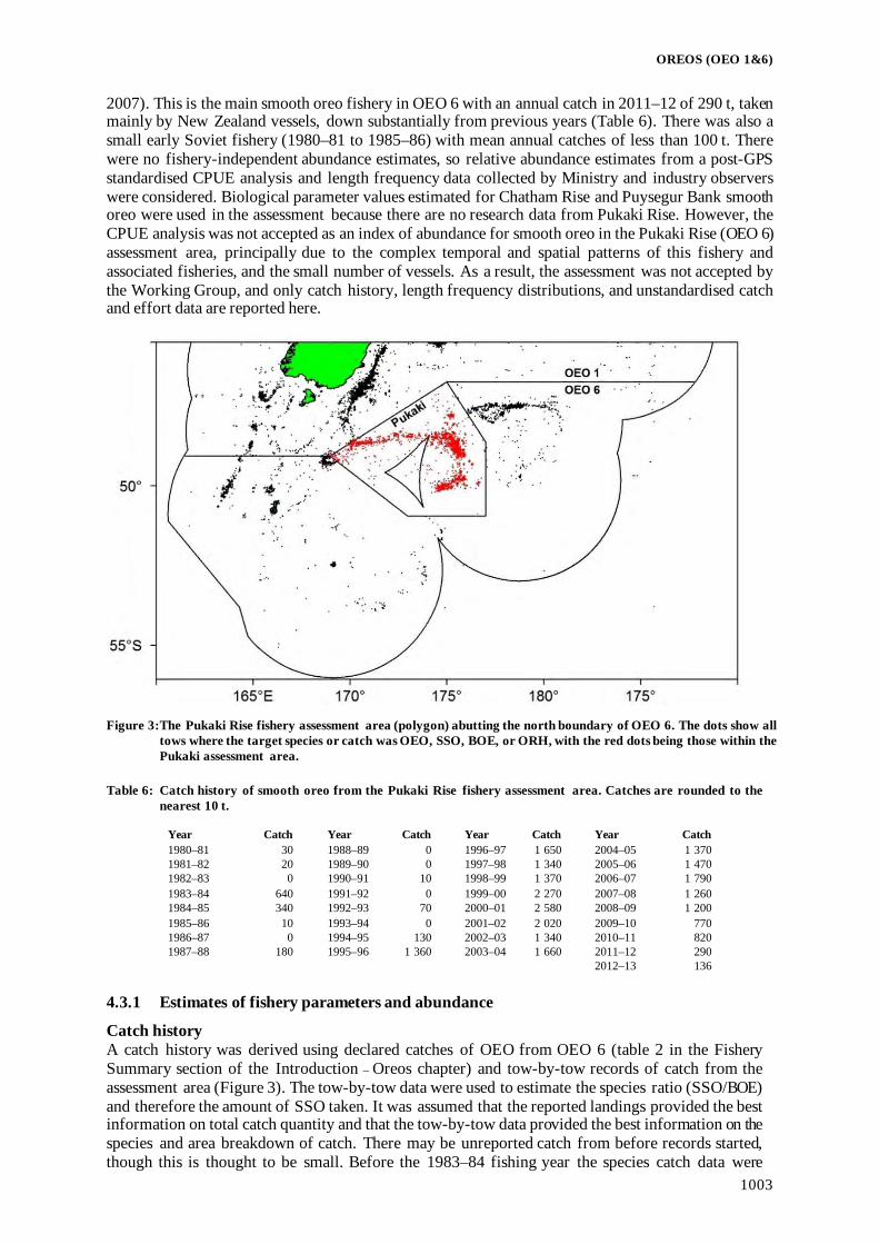
OREOS (OEO 1&6)
1003
2007). This is the main smooth oreo fishery in OEO 6 with an annual catch in 2011–12 of 290 t, taken mainly by New Zealand vessels, down substantially from previous years (Table 6). There was also a small early Soviet fishery (1980–81 to 1985–86) with mean annual catches of less than 100 t. There were no fishery-independent abundance estimates, so relative abundance estimates from a post-GPS standardised CPUE analysis and length frequency data collected by Ministry and industry observers were considered. Biological parameter values estimated for Chatham Rise and Puysegur Bank smooth oreo were used in the assessment because there are no research data from Pukaki Rise. However, the CPUE analysis was not accepted as an index of abundance for smooth oreo in the Pukaki Rise (OEO 6) assessment area, principally due to the complex temporal and spatial patterns of this fishery and associated fisheries, and the small number of vessels. As a result, the assessment was not accepted by the Working Group, and only catch history, length frequency distributions, and unstandardised catch and effort data are reported here.
Figure 3:The Pukaki Rise fishery assessment area (polygon) abutting the north boundary of OEO 6. The dots show all
tows where the target species or catch was OEO, SSO, BOE, or ORH, with the red dots being those within the Pukaki assessment area.
Table 6: Catch history of smooth oreo from the Pukaki Rise fishery assessment area. Catches are rounded to the
nearest 10 t.
Year Catch Year Catch Year Catch Year Catch 1980–81 30 1988–89 0 1996–97 1 650 2004–05 1 370 1981–82 20 1989–90 0 1997–98 1 340 2005–06 1 470 1982–83 0 1990–91 10 1998–99 1 370 2006–07 1 790 1983–84 640 1991–92 0 1999–00 2 270 2007–08 1 260 1984–85 340 1992–93 70 2000–01 2 580 2008–09 1 200 1985–86 10 1993–94 0 2001–02 2 020 2009–10 770 1986–87 0 1994–95 130 2002–03 1 340 2010–11 820 1987–88 180 1995–96 1 360 2003–04 1 660 2011–12 290 2012–13 136
4.3.1 Estimates of fishery parameters and abundance
Catch history A catch history was derived using declared catches of OEO from OEO 6 (table 2 in the Fishery Summary section of the Introduction – Oreos chapter) and tow-by-tow records of catch from the assessment area (Figure 3). The tow-by-tow data were used to estimate the species ratio (SSO/BOE) and therefore the amount of SSO taken. It was assumed that the reported landings provided the best information on total catch quantity and that the tow-by-tow data provided the best information on the species and area breakdown of catch. There may be unreported catch from before records started, though this is thought to be small. Before the 1983–84 fishing year the species catch data were

OREOS (OEO 1&6)
1004
combined over years to get an average figure that was then applied in each of those early years. For the years from 1983–84 onwards, each year’s calculation was made independently. The catch history used in the population model is given in Table 6. Length data Smooth oreo length frequency data collected by observers are available for the years 1997–98 to 2011–12 (Table 7). An in-depth analysis of these data in the previous assessment (covering fishing years 1998–2005) indicated that they were reasonably representative of the fishery in terms of spatial, depth, and temporal coverage in those years that had adequate data (Coburn et al 2007). The depths fished by the sampled fleet varied between years, so the length data were stratified by depth resulting in shallow (less than 900 m), middle (900–990 m), and deep strata (greater than 990 m). The data from adjacent years were also grouped because some years had few samples. The resulting length frequency distributions are shown in Figure 4. Table 7: Summary of length frequency data for smooth oreo available for the assessment area. The table shows the
number of tows sampled by year, the sample source, and the year group. –, no data.
Number of tows sampled Year Year group ORMC SOP All 1997–98 98–99 – 15 15 1998–99 98–99 64 9 73 1999–00 00–01 5 36 41 2000–01 00–01 37 17 54 2001–02 01–02 42 22 64 2002–03 03–04 4 12 16 2003–04 03–04 – 19 19 2004–05 05–06 – 30 30 2005–06 05–06 – 20 20 2006–07 06–07 – 205 205 2007–08 07–08 – 124 124 2008–09 08–09 – 66 66 2009–10 09–10 – 46 46 2010–11 10–11 – 107 107 2011–12 10–11 – 21 21 Totals 152 149 301
Catch and effort data Core vessels for the fishery were defined to develop a standardised CPUE series, but the standardised series was rejected by the Working Group. Unstandardised catch and effort data are presented in Table 8. Table 8: Catch and effort data for vessels with three or more consecutive fishing years with at least 10 records from
1995–96 (1996) to 2011–12 (2012).
Fishing year No. of tows No. of vessels Estimated catch (t) Mean t/tow Zero catch tows (%) SSO target (%) 1996 193 2 810 4.20 - 6 1997 322 3 1 270 3.90 4 4 1998 264 4 1 020 3.90 6 9 1999 262 4 1 050 4 1 15 2000 528 5 2 030 3.90 32 37 2001 588 7 2 280 3.90 49 52 2002 409 5 1 920 4.70 9 9 2003 498 5 1 230 2.50 14 18 2004 512 4 1 300 2.50 9 13 2005 588 6 1 170 2 21 27 2006 656 5 1 260 1.90 13 14 2007 806 5 1 550 1.90 23 25 2008 933 2 1 110 1.20 13 16 2009 918 3 1 200 1.30 21 23 2010 948 3 740 0.80 8 11 2011 593 3 720 1.20 22 25 2012 397 2 260 0.70 10 12

OREOS (OEO 1&6)
1005
Figure 4: Length frequencies for Pukaki Rise smooth oreo, stratified by depth (see text), and grouped by years.
[Continued on next page]

OREOS (OEO 1&6)
1006
Figure 4: [Continued].

OREOS (OEO 1&6)
1007
4.4 Bounty Plateau smooth oreo fishery (part of OEO 6) The first assessment for this fishery was developed in 2008 and applies only to the study area as defined in Figure 5. There were no fishery-independent abundance estimates, so relative abundance estimates from a post-GPS standardised CPUE analysis and length frequency data collected by Ministry (SOP) and industry (ORMC) observers were considered. Biological parameter values estimated for Chatham Rise and Puysegur Bank smooth oreo were used in the assessment because there are no research data from Bounty Plateau. The following assumptions were made in this analysis. 1. The CPUE analysis indexed the abundance of smooth oreo in the Bounty Plateau (OEO 6)
assessment area. 2. The length frequency samples were representative of the population being fished. 3. The biological parameters values used (from other assessment areas) are close to the true values. 4. Recruitment was deterministic and followed a Beverton & Holt relationship with steepness of 0.75. 5. The population of smooth oreo in the assessment area was a discrete stock or production unit. 6. Catch overruns were 0% during the period of reported catch. 7. The catch histories were accurate. 8. The maximum exploitation rate (EMAX) was 0.58. Data inputs included catch history, relative abundance estimates from a standardised CPUE analysis, and length data from SOP and ORMC observers. The observational data were incorporated into an age-based Bayesian stock assessment (CASAL) with deterministic recruitment to estimate stock size. The stock was considered to reside in a single area, with a partition by sex. Age groups were 1–70 years, with a plus group of 70+ years. The length-weight and length-at-age population parameters are from fish sampled on the Chatham Rise and Puysegur Bank fisheries (table 1 of the Biology section of the Introduction – Oreos chapter). The natural mortality estimate is based on fish sampled from the Puysegur Bank fishery. The maturity ogive is from fish sampled on the Chatham Rise, and the age at which 50% are mature is between 18 and 19 years for males and between 25 and 26 years for females. 4.4.1 Estimates of fishery parameters and abundance
Catch history Table 9: Catch history (t) of smooth oreo from the Bounty Plateau fishery assessment area. Catches are rounded to the
nearest 10 t.
Fishing year Catch Fishing year Catch 1983–84 620 1996–97 610 1984–85 0 1997–98 650 1985–86 0 1998–99 1 200 1986–87 0 1999–00 870 1987–88 10 2000–01 550 1988–89 0 2001–02 980 1989–90 0 2002–03 1 530 1990–91 20 2003–04 1 420 1991–92 0 2004–05 2 190 1992–93 110 2005–06 1 790 1993–94 490 2006–07 670 1994–95 1 450 2007–08 670 1995–96 900
A catch history was derived using declared catches of oreo from OEO 6 (table 2 in the Fishery Summary section of the Introduction – Oreos chapter) and tow-by-tow records of catch from the assessment area (Figure 5). The tow-by-tow data were used to estimate the species ratio (SSO/BOE) and therefore the amount of SSO taken. The catch history used in the population model is given in Table 9.

OREOS (OEO 1&6)
1008
Figure 5: The Bounty Plateau fishery assessment study area. Length data Smooth oreo length frequency data collected by SOP and ORMC observers are available from 1991–92. An in-depth analysis indicated that these data were reasonably representative of the fishery in terms of spatial, depth, and temporal coverage in those years that had adequate data. Length frequencies were based on tows from the core area (a subset of the study area where about 80% of the catch is taken). The data from adjacent years were grouped because some years had few samples (Table 10). The resulting length frequency distributions are shown in Figure 6. In the final model runs the 1994–95 year of the length frequency series was omitted because it contained very few samples. Table 10: Core length analysis year group, year applied and the number of length frequency samples (lfs). Smooth oreo
sample catch weight, fishery catch, and sample catch as percentage of the fishery.
Year group Year applied No. of lfs Catch sampled (t) Fishery catch (t) % fishery 1991–92 to 1995–96 1994–95 7 88 1 505 6
1998–99 to 1999–2000 1998–99 30 246 1 121 22 2000–2001 to 2002–03 2001–02 25 398 2 261 18 2003–04 to 2004–05 2004–05 29 261 2 280 11 2005–06 2005–06 32 379 1 121 34 2006–07 to 2007–08 2006–07 17 168 494 34
Relative abundance estimates from CPUE analyses The small early Soviet fishery had too few data for a standardised CPUE analysis. The standardised CPUE analysis was, therefore, from the New Zealand vessel fishery and only included data from those vessels that had fished at least three years. A single vessel put in significant continuous effort from 1995 to 2007, with the effort of the rest of the vessels confined to mainly either 1995–2000 (early) or 2001–2007 (late). Because of this, in addition to the single standardised CPUE covering the entire time period, two separate standardised CPUE indices were calculated for the early and late periods. The final indices are shown in Tables 11 and 12. 4.4.2 Biomass estimates In all preliminary model runs the length-frequency data series were not well fitted and gave a strong but contrasting biomass signal relative to the CPUE indices. Therefore, for final model runs, the length frequency data were down-weighted by using just the 1999 length frequency data. The base case model used early and late period CPUE indices and the 1999 length frequency data. Current mature biomass was estimated to be 33% of a virgin biomass of 17 400 t (Figure 7).

OREOS (OEO 1&6)
1009
Figure 6: Length frequency distribution plots for core data only (thick lines) with 95% confidence interval (thin lines). Table 11: Early and late period CPUE combined index estimates by fishing year, with bootstrap CV estimates.
Early period
Kg/tow CV Late period Kg/tow CV 1995–96 3 551 0.423 2000–01 850 0.487 1996–97 3 322 0.496 2001–02 2 976 0.274 1997–98 2 306 0.980 2002–03 1 489 0.243 1998–99 781 0.391 2003–04 1 727 0.260 1999–2000 1 536 0.306 2004–05 1 604 0.227 2005–06 1 386 0.310
2006–07 966 0.232 Table 12: Single period CPUE combined index estimates by fishing year, and bootstrap CV estimates.
Fishing year
Kg/tow CV 1995–96 7 472 0.286 1996–97 4 453 0.735 1997–98 3 366 1.264 1998–99 1 444 0.406 1999–2000 2 835 0.286 2000–01 2 817 0.436 2001–02 632 0.680 2002–03 1 973 0.663 2003–04 1 296 0.615 2004–05 1 284 0.445 2005–06 1 289 0.563 2006–07 1 056 1.200

OREOS (OEO 1&6)
1010
Figure 7:Model run showing the MPD fit to the CPUE data (vertical lines are the 95% confidence intervals for the
indices) and the trajectory of mature biomass. Two sensitivity model runs were carried out with the 1999 length frequency data dropped from the model but retaining the fishery selectivity estimated using the length data. The first model run used the early and late period CPUE indices and current biomass was estimated to be 39% of a virgin biomass of 19 300 t. The second model run used the single CPUE series covering the same period and current biomass was estimated to be 17% of a virgin biomass of 13 900 t. No MCMC runs were carried out with the base case model because the sensitivity runs showed that the assessment was quite different if the CPUE analysis was not split into two series. Biomass estimates are uncertain because of the reliance on commercial CPUE data, the use of biological parameter estimates from other oreo stocks, and because of contrasting biomass signals from using either a single, or split, CPUE indices. 4.4.3 Projections No projections were made because of the uncertainty in the assessment. 4.5 Pukaki Rise black oreo stock (part of OEO 6) A second assessment for this fishery was attempted in 2013, applying only to the assessment area as defined in Figure 8. The first assessment for this fishery was in 2009 (Doonan et al 2010). This is currently the largest black oreo fishery in the New Zealand EEZ with both current (2011–12) and mean (1994–95 to 2011–12) annual catches of 1900 t, but with annual catches of 2800–3400 t between 2005–06 and 2009–10. There was an early Soviet and Korean fishery (1980–81 to 1984–85) with mean annual catches of about 1700 t. Fishery-independent abundance estimates were not available, so a series of relative abundance indices, based on an analysis of post-GPS standardised CPUE, was developed. Length frequency data collected by Ministry (SOP) and industry (ORMC) observers were included in the model. The assessment used biological parameter values estimated for Chatham Rise and Puysegur Bank black oreo because no biological data from Pukaki Rise are available. As stated above, the Pukaki Rise smooth oreo CPUE was thought to be unreliable until further investigations are conducted. Since the black oreo fishery is in the same area, the Working Group determined that the black oreo CPUE analysis also could not be accepted as an index of abundance of black oreo in the Pukaki Rise (OEO 6) assessment area, and as a result the assessment was rejected. Therefore, only catch history, length frequency distributions, and unstandardised catch and effort data are reported here. 4.5.1 Estimates of fishery parameters and abundance Catch history A catch history for black oreo was derived (Table 13) using declared catches of OEO from OEO 6 (table 2 in the Fishery Summary section of the Introduction – Oreos chapter) and tow-by-tow records of catch from the assessment area (Figure 8). The catch history used in the assessment is given in Table 13.

OREOS (OEO 1&6)
1011
Table 13: Catch history (t) of black oreo from the Pukaki Rise fishery assessment area.
Fishing year Catch Fishing year Catch Fishing year Catch 1978–79 17 1990–91 15 2002–03 1 701 1979–80 5 1991–92 27 2003–04 1 530 1980–81 283 1992–93 27 2004–05 1 588 1981–82 4 180 1993–94 10 2005–06 2 811 1982–83 1 084 1994–95 242 2006–07 3 434 1983–84 1 150 1995–96 1 352 2007–08 3 346 1984–85 1 704 1996–97 2 413 2008–09 2 818 1985–86 46 1997–98 2 244 2009–10 3 093 1986–87 0 1998–99 1 181 2010–11 1 641 1987–88 0 1999–00 1 061 2011–12 1 671 1988–89 0 2000–01 1 158 1989–90 0 2001–02 988
Length data Black oreo length frequency data collected by SOP and ORMC observers are available for 1996–97 to 2011–12 (Table 14). An analysis indicated that there was a trend in fish size across years (with smaller mean lengths in more recent years) and with depth (deeper fish being larger). The length data were considered to be representative of the fishery in terms of the spatial, depth, and temporal coverage for those years that had adequate data. The length data were stratified into two depth bins: shallow (less than 900 m) and deep (greater than 900 m). Length data from adjacent years were grouped because of the low number of samples in some years (Figure 9). There is no trend in mean length over the first six year groups, but fish sizes appear to be generally smaller in the later year groups, with the mode of the distributions shifting to the left between 2005–06 and 2007–08. Table 14: Summary of length frequency data for black oreo available from the assessment area. The table shows the
number of tows sampled by year, the sample source, and the year group.
Number of tows sampled Fishing year Year group SOP ORMC All 1996–97 97–98 7 0 7 1997–98 97–98 25 0 25 1998–99 99–00 7 44 51 1999–00 99–00 6 0 6 2000–01 01–02 8 18 26 2001–02 01–02 2 8 10 2002–03 03–05 7 2 9 2003–04 03–05 18 0 18 2004–05 03–05 21 0 21 2005–06 06 21 42 63 2006–07 07 154 11 165 2007–08 08 31 9 40 2008–09 08 61 9 70 2009–10 09 46 0 46 2010–11 10 57 0 57 2011–12 11–12 13 0 13 Total 477 134 611
Catch and effort data The fishery taking Pukaki Rise black oreo is divided into two distinct periods: a pre-GPS period 1980–81 to 1984–85, when much of the catch was taken by Soviet and Korean vessels, and a post-GPS period, 1995–96 to 2011–12 when most of the catch was taken by New Zealand vessels. The intervening period was characterised by low catches and the introduction of GPS technology in the fleet. Standardisation of CPUE for the pre-GPS period was attempted but rejected due to poor linkage of vessels across years and the shifting of fishing effort between areas. For the post-GPS period, the Working Group rejected CPUE as an index of abundance because of the variability in recorded target species over time and space in the overlapping Pukaki fisheries for black oreo, smooth oreo, and orange roughy. The Working Group believed that recording of target species in these fisheries was likely to have been inconsistent between vessels and skippers over time and that the practice of separately examining these fisheries according to recorded target species was inappropriate. Unstandardised catch and effort data for defined core vessels are presented in Table 15.

OREOS (OEO 1&6)
1012
Figure 8: The Pukaki Rise fishery black oreo assessment area (polygon) abutting the boundary of OEO 6/OEO 1 in the north-west. The dots show tow positions where black oreo catch was reported between 1980–81 and 2011–12. A, B, and C are the three areas defined in the standardised CPUE analysis.
Figure 9: Observer length frequencies for Pukaki Rise black oreo, stratified by depth (see text), and grouped by years
(in the legends 1997=1996–97, etc.). The vertical dashed lines indicate the approximate overall mean length as an aid to comparing the distributions.

OREOS (OEO 1&6)
1013
Table 15: Catch and effort data for vessels fishing in the eastern areas (B and C in Figure 8) with a minimum of 15 successful tows for black oreo in at least three years from 1995–96 to 2011–12.
Fishing year No. of tows CPUE
CV Fishing year No. of tows CPUE
CV
1995–96 63 1.94 0.09 2004–05 309 0.73 0.13 1996–97 55 1.44 0.13 2005–06 481 0.88 0.09 1997–98 219 1.53 0.07 2006–07 650 0.80 0.09 1998–99 235 0.98 0.11 2007–08 795 0.62 0.12 1999–00 252 0.82 0.12 2008–09 734 0.61 0.12 2000–01 199 1.11 0.10 2009–10 979 0.33 0.21 2001–02 175 1.07 0.11 2010–11 450 0.51 0.16 2002–03 320 0.91 0.10 2011–12 430 0.72 0.12 2003–04 343 0.97 0.09
No projections were made because the assessment was not accepted by the Working Group. 4.5.2 Biomass estimates No biomass estimates are reported. 4.5.3 Yield estimates and projections No yield estimates were made.
4.6 Other oreo fisheries in OEO 1 and OEO 6 4.6.1 Estimates of fishery parameters and abundance Relative abundance estimates from trawl surveys Two comparable trawl surveys were carried out in the Puysegur area of OEO 1 (TAN9208 and TAN9409). The 1994 oreo abundance estimates are markedly lower than the 1992 values (Table 16). 4.6.2 Biomass estimates Estimates of virgin and current biomass are not yet available. 4.6.3 Yield estimates and projections MCY cannot be estimated because of the lack of current biomass estimates for the other stocks. CAY cannot be estimated because of the lack of current biomass estimates for the other stocks. 4.6.4 Other factors Recent catch data from this fishery may be of poor quality because of area misreporting. Table 16: OEO 1. Research survey abundance estimates (t) for oreos from the Puysegur and Snares areas. N is the
number of stations. Estimates for smooth oreo were made based on a recruited length of 34 cm total length. Estimates for black oreo were made using knife-edge recruitment set at 27 cm total length.
Smooth oreo Puysegur area (strata 0110–0502) Mean biomass Lower bound Upper bound CV (%) N 1992 1 397 736 2 058 23 82 1994 529 86 972 41 87 Snares area (strata 0801–0802) Mean biomass Lower bound Upper bound CV (%) N 1992 2 433 0 5 316 59 8 1994 118 0 246 54 7 Black oreo Puysegur area (strata 0110–0502) Mean biomass Lower bound Upper bound CV (%) N 1992 2 009 915 3 103 27 82 1994 618 0 1 247 50 87 Snares area (strata 0801–0802) Mean biomass Lower bound Upper bound CV (%) N 1992 3 983 0 8 211 53 8 1994 1 564 0 3 566 64 7

OREOS (OEO 1&6)
1014
5. STATUS OF THE STOCKS Stock Structure Assumptions Oreos in the OEO 1 and 6 FMAs are managed as a single stock but assessed as four separate stocks, separated by species and geography. The Southland smooth oreo stock is based off the east coast of the South Island in OEO 1 but extends slightly into OEO 3. It does not include the Waitaki and Eastern canyon areas but is likely to have some level of mixing with other smooth oreo fishstocks. The Pukaki Rise smooth oreo stock comprises the major part of OEO 6 stocks and is centred on its namesake. Some mixing with other smooth oreo fishstocks is thought to occur. The Bounty Plateau smooth oreo stock is located across the Bounty Plateau. Some mixing is thought to occur with other smooth oreo fishstocks. The Pukaki Rise black oreo stock is the main black oreo fishstock in OEO 6 and the largest black oreo fishstock in the New Zealand EEZ. It extends the entire length of the Pukaki Rise towards OEO 1. It is assessed separately to other fishstocks but managed as a part of OEO 6. Black oreo on the Pukaki Rise are thought to be non-mixing with other black oreo fishstocks. • OEO 1 and OEO 3A Southland (Smooth Oreo)
Stock Status Year of Most Recent Assessment 2007 Assessment Runs Presented One base case only Reference Points
Target: 40% B0 Soft Limit: 20% B0 Hard Limit: 10% B0
Overfishing threshold: Status in relation to Target B2007 was estimated at 27% B0, Unlikely (< 40%) to be at or
above the target. Status in relation to Limits B2007 was estimated to be Unlikely (< 40%) to be below the
Soft Limit and Very Unlikely (< 10%) to be below the Hard Limit.
Status in relation to Overfishing -
Historical Stock Status Trajectory and Current Status
Predicted biomass trajectories for the 2007 base case assessment— mature biomass and selected biomass for the shallow and deep fisheries. Also shown are the CPUE indices from the pre- and post-GPS analysis for the deep fishery (in green) and the post-GPS analyses for the shallow fishery (in black). CPUE indices are shown with ±2 s.e. confidence interval indicated by the vertical lines (the post-GPS CPUE data are slightly offset to avoid over plotting). The CPUE data were scaled by catchability coefficients to match the biomass scale.

OREOS (OEO 1&6)
1015
Fishery and Stock Trends Recent Trend in Biomass or Proxy
Biomass has been declining at a steady rate since the late 1980s.
Recent Trend in Fishing Mortality or Proxy
Unknown
Other Abundance Indices - Trends in Other Relevant Indicators or Variables
-
Projections and Prognosis Stock Projections or Prognosis None because of assessment uncertainty. Probability of Current Catch or TACC causing Biomass to remain below or to decline below Limits
Soft Limit: Unknown Hard Limit: Unknown
Probability of Current Catch or TACC causing Overfishing to continue or to commence
-
Assessment Methodology Assessment Type Type 1 - Quantitative Stock Assessment Assessment Method Age-structured CASAL model with Bayesian estimation of
posterior distributions. Assessment Dates Latest assessment: 2007 Next assessment: Unknown Overall assessment quality rank - Main data inputs (rank) - Length-frequency data
collected by SOP and ORMC observers - A second, earlier fishery based on Soviet vessels was included in the assessment using historical catch data. - Standardised CPUE indices were derived from the historical and modern datasets.
Data not used (rank) - Changes to Model Structure and Assumptions
-
Major Sources of Uncertainty - Scarcity of observer length frequency data - Poor quality area catch data due to significant misreporting - Lack of fishery-independent abundance estimates creates reliance on commercial CPUE data.
Qualifying Comments - Fishery Interactions Both species of oreo are sometimes taken as bycatch in orange roughy target fisheries and in smaller numbers in hoki target fisheries. Target fisheries for oreos do exist, with main bycatch being orange roughy, rattails, and deepwater sharks and rays. Other bycatch species recorded include seabirds and deepwater corals. Oreo are caught using bottom trawl gear. Bottom trawling interacts with benthic habitats.
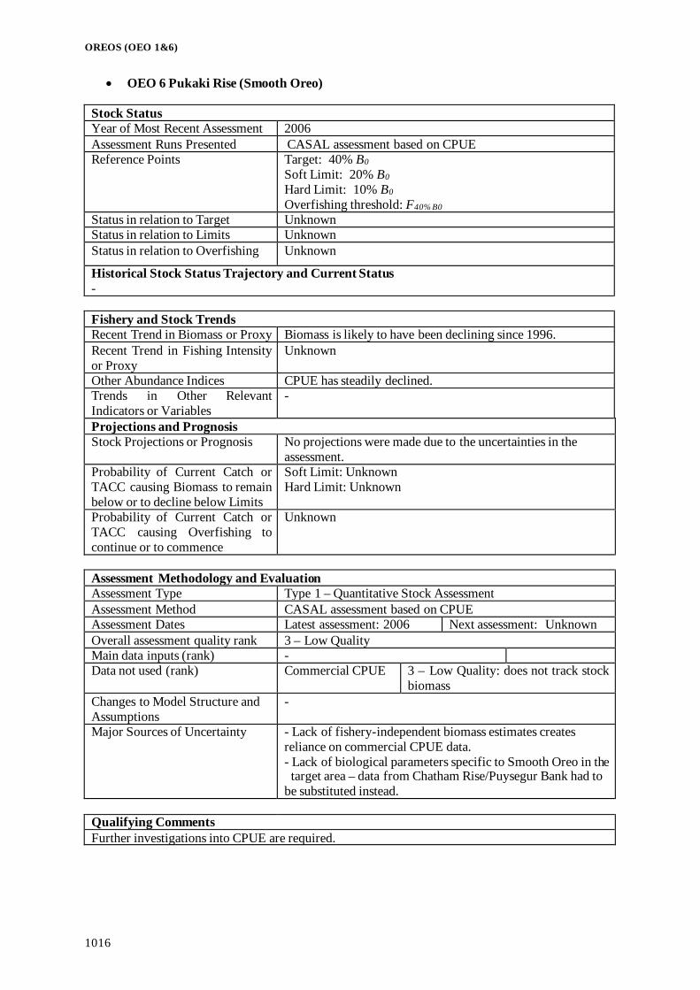
OREOS (OEO 1&6)
1016
• OEO 6 Pukaki Rise (Smooth Oreo) Stock Status Year of Most Recent Assessment 2006 Assessment Runs Presented CASAL assessment based on CPUE Reference Points
Target: 40% B0 Soft Limit: 20% B0 Hard Limit: 10% B0 Overfishing threshold: F40% B0
Status in relation to Target Unknown Status in relation to Limits Unknown Status in relation to Overfishing Unknown
Historical Stock Status Trajectory and Current Status - Fishery and Stock Trends Recent Trend in Biomass or Proxy Biomass is likely to have been declining since 1996. Recent Trend in Fishing Intensity or Proxy
Unknown
Other Abundance Indices CPUE has steadily declined. Trends in Other Relevant Indicators or Variables
-
Projections and Prognosis Stock Projections or Prognosis No projections were made due to the uncertainties in the
assessment. Probability of Current Catch or TACC causing Biomass to remain below or to decline below Limits
Soft Limit: Unknown Hard Limit: Unknown
Probability of Current Catch or TACC causing Overfishing to continue or to commence
Unknown
Assessment Methodology and Evaluation Assessment Type Type 1 – Quantitative Stock Assessment Assessment Method CASAL assessment based on CPUE Assessment Dates Latest assessment: 2006 Next assessment: Unknown Overall assessment quality rank 3 – Low Quality Main data inputs (rank) - Data not used (rank) Commercial CPUE 3 – Low Quality: does not track stock
biomass Changes to Model Structure and Assumptions
-
Major Sources of Uncertainty - Lack of fishery-independent biomass estimates creates reliance on commercial CPUE data. - Lack of biological parameters specific to Smooth Oreo in the target area – data from Chatham Rise/Puysegur Bank had to be substituted instead.
Qualifying Comments Further investigations into CPUE are required.

OREOS (OEO 1&6)
1017
Fishery Interactions Both species of oreo are sometimes taken as bycatch in orange roughy target fisheries and in smaller numbers in hoki target fisheries. Target fisheries for oreos do exist, with main bycatch being orange roughy, rattails, and deepwater sharks. Low productivity bycatch species include deepwater sharks and rays. Protected species interactions occur with seabirds and deepwater corals.
• OEO 6 Bounty Plateau (Smooth Oreo)
Stock Status Year of Most Recent Assessment 2008 Assessment Runs Presented A base case with two sensitivity runs Reference Points
Target: 40% B0 Soft Limit: 20% B0 Hard Limit: 10% B0
Status in relation to Targe B2008 was estimated at 33% B0; Unlikely (< 40%) to be at or above the target.
Status in relation to Limits B2008 is Unlikely (< 40%) to be below the Soft Limit and Very Unlikely (< 10%) to be below the Hard Limit.
Status in relation to Overfishing -
Historical Stock Status Trajectory and Current Status
Model run showing the MPD fit to the CPUE data (vertical lines are the 95% confidence intervals for the indices) and the trajectory of mature biomass. Fishery and Stock Trends Recent Trend in Biomass or Proxy Biomass is estimated to have been decreasing rapidly since
1995. Recent Trend in Fishing Mortality or Proxy Unknown
Other Abundance Indices - Trends in Other Relevant Indicators or Variables
-
Projections and Prognosis Stock Projections or Prognosis No projections were made because of the uncertainty of the
assessment. Probability of Current Catch or TACC causing Biomass to remain below or to decline below Limits
Soft Limit: Unknown Hard Limit: Unknown
Probability of Current Catch or TACC causing overfishing to continue or to commence
Unknown

OREOS (OEO 1&6)
1018
Assessment Methodology and Evaluation Assessment Type Type 1 - Quantitative Stock Assessment Assessment Method Age-structured CASAL model with Bayesian estimation of
posterior distributions Assessment Dates Latest assessment: 2008 Next assessment: Unknown Overall assessment quality rank Main data inputs (rank) - Catch history
- Abundance estimates derived from a standardised CPUE - Length data from SOP and ORMC observers
Data not used (rank) - Changes to Model Structure and Assumptions -
Major Sources of Uncertainty - Reliance on commercial CPUE data - To estimate biological parameters, data was used from
different stocks (Puysegur Bank + Chatham Rise) to the target stock
- Using a single CPUE index instead of split indices gives contrasting biomass signals
Qualifying Comments - Fishery Interactions Both species of oreo are sometimes taken as bycatch in orange roughy target fisheries and in smaller numbers in hoki target fisheries. Target fisheries for oreos do exist, with main bycatch being orange roughy, rattails, and deepwater sharks. Other bycatch species recorded include deepwater sharks and rays, seabirds, and deepwater corals. Oreo are caught using bottom trawl gear. Bottom trawling interacts with benthic habitats.
• OEO 6 Pukaki Rise (Black Oreo)
Stock Status Year of Most Recent Assessment 2009 Assessment Runs Presented CASAL assessment based on CPUE Reference Points
Target: 40% B0 Soft Limit: 20% B0 Hard Limit: 10% B0 Overfishing threshold: F40% B0
Status in relation to Target Unknown Status in relation to Limits Unknown Status in relation to Overfishing Unknown Historical Stock Status Trajectory and Current Status Fishery and Stock Trends Recent Trend in Biomass or Proxy Biomass is likely to have been decreasing since the 1980s
with a major decline starting about 1995. Recent Trend in Fishing Intensity or Proxy
Unknown
Other Abundance Indices CPUE declined, but has levelled out in the last four years. Trends in Other Relevant Indicators or Variables
-

OREOS (OEO 1&6)
1019
Projections and Prognosis Stock Projections or Prognosis - Probability of Current Catch or TACC causing Biomass to remain below or to decline below Limits
Soft Limit: Unknown Hard Limit: Unknown
Probability of Current Catch or TACC causing Overfishing to continue or to commence
Unknown
Assessment Methodology and Evaluation Assessment Type Type 1 - Quantitative Stock Assessment Assessment Method CASAL assessment based on CPUE Assessment Dates Latest assessment: 2009 Next assessment: Unknown Overall assessment quality rank 3 – Low Quality Main data inputs (rank) - Data not used (rank) Commercial CPUE 3 – Low Quality: does not track stock
biomass Changes to Model Structure and Assumptions
-
Major Sources of Uncertainty - Lack of fisheries-independent data causes reliance on commercial CPUE data - Lack of biological parameter estimates specific to black oreo in this assessment area
Qualifying Comments Further investigations into CPUE are needed. Fishery Interactions Both species of oreo are sometimes taken as bycatch in orange roughy target fisheries and in smaller numbers in hoki target fisheries. Target fisheries for oreos do exist, with main bycatch being orange roughy, rattails, and deepwater sharks. Low productivity bycatch species include deepwater sharks and rays. Protected species interactions occur with seabirds and deepwater corals. Oreo are caught using bottom trawl gear. Bottom trawling interacts with benthic habitats.
6. FOR FURTHER INFORMATION Coburn, R P; Doonan, I J; McMillan, P J (2002) CPUE analyses for the Southland black oreo and smooth oreo fisheries, 1977–78 to 1999–
2000. New Zealand Fisheries Assessment Report 2002/3. 28 p. Coburn, R P; Doonan, I J; McMillan, P J (2002) CPUE analyses for the major black oreo and smooth oreo fisheries in OEO 6, 1980–81 to
1999–2000. New Zealand Fisheries Assessment Report 2002/6. 29 p. Coburn, R P; Doonan, I J; McMillan, P J (2003) Stock assessment of smooth oreo in the Southland fishery (OEO 1 and 3A) for 2003. New
Zealand Fisheries Assessment Report 2003/62. 32 p. Coburn, R P; Doonan, I J; McMillan, P J (2008) A stock assessment of smooth oreo in Southland (part of OEO 1 & OEO 3A). New Zealand
Fisheries Assessment Report 2008/37. 43 p. Coburn, R P; McMillan, P J; Gilbert, D J (2007) Inputs for a stock assessment of smooth oreo, Pukaki Rise (part of OEO 6). New Zealand
Fisheries Assessment Report 2007/23. 32 p Doonan, I J; Anderson, O F; McMillan, P J (2010) Assessment of Pukaki (OEO 6) black oreo for 2008–09. New Zealand Fisheries Assessment
Report 2010/39. McKenzie, A (2007) Stock assessment for east Pukaki Rise smooth oreo (part of OEO 6). New Zealand Fisheries Assessment Report 2007/34.
27 p. McMillan, P J; Coburn, R P; Hart, A C; Doonan, I J (2002) Descriptions of black oreo and smooth oreo fisheries in OEO 1, OEO 3A, OEO
4, and OEO 6 from 1977–78 to the 2000–01 fishing year. New Zealand Fisheries Assessment Report 2002/40. 54 p.


PADDLE CRABS (PAD)
1021
PADDLE CRABS (PAD)
(Ovalipes catharus) Papaka
1. FISHERY SUMMARY 1.1 Commercial fisheries Paddle crabs were introduced into the QMS from 1 October 2002 with recreational and customary non-commercial allowances, TACCs and TACs summarised in Table 1. Table 1: Current Total allowable catches (TAC, t) allowances for customary fishing, recreational fishing (t) and Total
Allowable Commercial Catches (TACC, t) for paddle crabs, by Fishstock.
Fishstock TAC Customary Recreational TACC PAD 1 250 10 20 220 PAD 2 125 5 10 110 PAD 3 110 2 8 100 PAD 4 30 1 4 25 PAD 5 55 1 4 50 PAD 6 0 0 0 0 PAD 7 105 1 4 100 PAD 8 65 1 4 60 PAD 9 130 10 20 100 PAD 10 0 0 0 0
Commercial interest in paddle crabs was first realised in New Zealand in 1977–78 when good numbers of large crabs were caught off Westshore Beach, Napier in baited lift and set-pots. Annual catches have varied, mainly due to marketing problems, and estimates are likely to be conservative. Landings increased in the early fishery, from 775 kg in 1977 to 306 t in 1985, and ranging from 403 t to 519 t from 1995–96 to 1999-00, but have since generally decreased. In 2018–19, 2019–20 and 2020-21 landings (mostly originating from PAD 3) dropped to the lowest levels since the 1980s, with just 22 t,13 t and 5t recorded respectively. Paddle crabs are known to be discarded from inshore trawl operations targeting species such as flatfish, and this may have resulted in under-reporting of catches. Crabs are marketed live, as whole cooked crabs, or as crab meat. Attempts were made to establish a soft-shelled crab industry in New Zealand in the late 1980s. Bycatch is commonly taken during trawl, dredge and set netting operations. Catch rates vary considerably with method, season and area, and there is no clear seasonal trend to paddle crab landings. It is likely that catches are related to the availability of fishers and/or market demands. Commercial landings from 1989–90 until the present are shown in Table 2, while Figure 1 shows the historical landings and TACC for the six main PAD stocks.

PADDLE CRABS (PAD)
1022
Table 2: Reported landings (t) of paddle crabs by QMA and fishing year, from CLR and CELRlanded data since 1989–90. [Continued on next page]
QMA PAD 1 PAD 2 PAD 3 PAD 4 PAD 5 Landing
TACC Landing
TACC Landing
TACC Landing
TACC Landing
TACC
1989–90 20 - 57 - 38 - < 1 - < 1 - 1990–91 34 - 37 - 26 - 0 - 6 - 1991–92 96 - 32 - 31 - < 1 - < 1 - 1992–93 175 - 14 - 36 - 0 - < 1 - 1993–94 277 - 18 - 46 - 0 - < 1 - 1994–95 237 - 6 - 36 - < 1 - < 1 - 1995–96 183 - 5 - 18 - < 1 - 1 - 1996–97 165 - 25 - 36 - 0 - 1 - 1997–98 158 - 126 - 18 - < 1 - 13 - 1998–99 195 - 197 - 21 - < 1 - 2 - 1999–00 265 - 21 - 27 - 1 - 14 - 2000–01 32 - 10 - 17 - 0 - 0 - 2001–02 221 - 34 - 22 - 0 - 2 - 2002–03 145 220 65 110 18 100 < 1 25 < 1 50 2003–04 239 220 46 110 20 100 0 25 0 50 2004–05 163 220 44 110 30 100 0 25 0 50 2005–06 109 220 49 110 11 100 0 25 < 1 50 2006–07 53 220 21 110 13 100 0 25 3 50 2007–08 86 220 9 110 19 100 0 25 < 1 50 2008–09 36 220 14 110 37 100 0 25 1 50 2009–10 35 220 17 110 37 100 0 25 < 1 50 2010–11 49 220 18 110 47 100 0 25 <1 50 2011–12 12 220 41 110 47 100 < 1 25 < 1 50 2012–13 < 1 220 36 110 39 100 < 1 25 < 1 50 2013–14 3 220 6 110 74 100 1 25 < 1 50 2014–15 23 220 1 110 45 100 0 25 < 1 50 2015–16 69 220 6 110 48 100 0 25 < 1 50 2016–17 36 220 12 110 18 100 < 1 25 < 1 50 2017–18 3 220 5 110 17 100 < 1 25 0 50 2018–19 < 1 220 3 110 15 100 < 1 25 < 1 50 2019–20 < 1 220 4 110 9 100 0 25 0 50 2020–21 < 1 220 < 1 110 4 100 < 1 25 < 1 50 QMA PAD 6 PAD 7 PAD 8 PAD 9 PAD 10 Landing
TACC Landing
TACC Landing
TACC Landing
TACC Landing
TACC
1989–90 0 - 94 - 22 - 0 - 0 - 1990–91 0 - 68 - 12 - 0 - 0 - 1991–92 0 - 83 - 21 - 0 - 0 - 1992–93 0 - 59 - 24 - 0 - 0 - 1993–94 0 - 49 - 27 - 5 - 0 - 1994–95 0 - 71 - 46 - < 1 - 0 - 1995–96 55 - 82 - 58 - < 1 - < 1 - 1996–97 25 - 106 - 44 - < 1 - 1 - 1997–98 7 - 63 - 25 - < 1 - < 1 - 1998–99 10 - 59 - 34 - 0 - 1 - 1999–00 14 - 45 - 50 - 0 - < 1 - 2000–01 0 - 0 - < 1 - 0 - 0 - 2001–02 22 - 33 - 24 - 0 - 0 - 2002–03 < 1 0 42 100 11 60 0 100 0 0 2003–04 0 0 50 100 17 60 < 1 100 0 0 2004–05 0 0 40 100 14 60 1 100 0 0 2005–06 0 0 48 100 14 60 1 100 0 0 2006–07 0 0 32 100 11 60 < 1 100 0 0 2007–08 0 0 47 100 7 60 0 100 0 0 2008–09 0 0 35 100 11 60 0 100 0 0 2009–10 0 0 17 100 13 60 0 100 0 0 2010–11 0 0 11 100 14 60 0 100 0 0 2011–12 0 0 7 100 14 60 0 100 0 0 2012–13 0 0 11 100 17 60 0 100 0 0 2013–14 0 0 4 100 13 60 0 100 0 0 2014–15 0 0 0 100 1 60 0 100 0 0 2015–16 0 0 0 100 4 60 0 100 0 0 2016–17 0 0 < 1 100 3 60 0 100 0 0 2017–18 0 0 < 1 100 1 60 0 100 0 0 2018–19 0 0 0 100 1 60 0 100 0 0 2019–20 0 0 < 1 100 < 1 60 0 100 0 0 2020–21 < 1 0 < 1 100 < 1 60 0 100 0 0

PADDLE CRABS (PAD)
1023
Table 2 [Continued]: Reported landings (t) of paddle crabs by QMA and fishing year, from CLR and CELRlanded data since 1989–90.
QMA Total Landings TACC 1989–90 231 - 1990–91 183 - 1991–92 264 - 1992–93 308 - 1993–94 423 - 1994–95 397 - 1995–96 403 - 1996–97 403 - 1997–98 410 - 1998–99 519 - 1999–00 437 - 2000–01 59 - 2001–02 358 - 2002–03 281 765 2003–04 372 765 2004–05 292 765 2005–06 232 765 2006–07 132 765 2007–08 168 765 2008–09 134 765 2009–10 120 765 2010–11 140 765 2011–12 121 765 2012–13 103 765 2013–14 101 765 2014–15 71 765 2015–16 127 765 2016–17 66 765 2017–18 27 765 2018–19 22 765 2019–20 13 765 2020–21 5 765
Figure 1: Reported commercial landings and TACCs for the six main PAD stocks: PAD 1 (Auckland East) and PAD
2 (Central East). [Continued on next page]

PADDLE CRABS (PAD)
1024
Figure 1 [Continued]: Reported commercial landings and TACCs for the six main PAD stocks: PAD 3 (south East
Coast), PAD 5 (Southland), PAD 7 (Challenger) and PAD 8 (Central Egmont).

PADDLE CRABS (PAD)
1025
1.2 Recreational fisheries Paddle crabs are taken as a bycatch of beach and estuarine seining and in setnets throughout much of their geographical range. A National Panel Survey of recreational fishers was conducted for the first time throughout the 2011–12 fishing year (Wynne-Jones et al. 2014). The panel survey used face-to-face interviews of a random sample of 30 390 New Zealand households to recruit a panel of fishers and non-fishers for a full year. The panel members were contacted regularly about their fishing activities and harvest information collected in standardised phone interviews. A repeat of the National Panel Survey was conducted over the 2017–18 October fishing year with 34 431 households contacted (Wynne-Jones et al 2019). Harvest estimates for the two National Panel Surveys are given in Table 3 (from Wynne-Jones et al 2014, Wynne-Jones et al 2019; no estimates of mean weight were available from ramp surveys). These estimates are all very uncertain because of the small number of fishers reporting catch. Table 3: Recreational harvest estimates for paddle crab stocks from the national panel surveys (2011–12 and 2017–
18). *: no estimates of mean weights were available to convert catches in numbers to tonnes. From Wynne-Jones et al. 2014 and Wynne-Jones et al. 2019.
Area Number (thousands) CV Catch (t)* 2011–12 (national panel survey)
PAD 1 2 003 0.86 - PAD 2 827 1.02 - PAD 3 1 768 1.01 - PAD 5 2 532 1.02 - PAD 8 2 225 0.71 - PAD total 9 354 0.43 - 2017–18 (national panel survey) PAD 1 775 0.84 - PAD 7 5 139 1.00 - PAD total 5 914
1.3 Customary non-commercial fisheries Paddle crabs form a fishery for customary non-commercial, but the total annual catch is not known. Māori customary fishers can utilise the provisions under both the recreational fishing regulations and the various customary regulations. Many tangata whenua may harvest paddle crabs under their recreational allowance and these are not included in records of customary catch. Customary reporting requirements vary around the country. Customary fishing authorisations issued in the South Island and Stewart Island would be under the Fisheries (South Island Customary Fishing) Regulations 1999. Many rohe moana / areas of the coastline in the North Island and Chatham Islands are gazetted under the Fisheries (Kaimoana Customary Fishing) Regulations 1998 which require reporting on authorisations. In the areas not gazetted, customary fishing permits would be issued would be under the Fisheries (Amateur Fishing) Regulations 2013, where there is no requirement to report catch. The information on Māori customary harvest under the provisions made for customary fishing is very limited (Table 4). These numbers are likely to be an underestimate of customary harvest as only the catch approved and harvested in kilograms and numbers are reported in the table. Table 4: Fisheries New Zealand records of customary harvest of paddle crabs (approved and reported as weight (kg)
and numbers), since 2007-08. – no data.
Weight (kg) Numbers Stock Fishing year Approved Harvested Approved Harvested PAD 1 2010–11 10 0 50 0 PAD 3 2007–08 – – 50 0
1.4 Illegal catch There is qualitative data to suggest illegal, unreported, unregulated (IUU) activity in this Fishery. 1.5 Other sources of mortality There is no quantitative information available on other sources of mortality, although unknown quantities of paddle crabs have been discarded from commercial fishing operations such as the inshore trawl, setnet and dredge fisheries.

PADDLE CRABS (PAD)
1026
2. BIOLOGY Paddle crabs are found off sandy beaches and in harbours and estuaries throughout mainland New Zealand, the Chatham Islands, and east and South Australia. They are abundant from the intertidal zone to at least 10 m depth, although they do occur in much deeper water. Paddle crabs are mainly active in early evening or at night, when they move into the shallow intertidal zone to feed. Paddle crabs are versatile and opportunistic predators. They feed mainly on either molluscs or crustaceans, but also on polychaetes, several fish species, cumacean crustaceans, and occasionally on algae. A high proportion of the molluscs eaten are Paphies species. These include: tuatua (P. subtriangulata); pipi (P. australis); and toheroa (P. ventricosa). The burrowing ghost shrimp Callianassa filholi, isopods and amphipods are important crustacean prey items. Cannibalism is common, particularly on small crabs and during the winter moulting season. Anecdotal information suggests there has been a significant increase in paddle crab numbers since the 1970s. Concern has been expressed as to the impact of an increased number of paddle crabs on bivalve shellfish stocks in coastal waters. Feeding studies have shown that although paddle crabs do eat large adult toheroa and other shellfish, they more usually eat bivalve shellfish spat which are found in abundance. Mating generally occurs during winter and spring (May to November) in sheltered inshore waters. Female paddle crabs can only mate when they are soft-shelled. Male crabs protect and carry pre-moult females to ensure copulation. Female crabs are thought to migrate to deeper water to spawn over the warmer months (September to March). After spawning, the eggs are incubated until they hatch. Paddle crab (Ovalipes catharus) has an extended larval life characterised by eight zoea stages and a (crab-like) megalopa. The larvae are thought to live offshore in deeper water, migrating inshore in the megalopa stage to settle from January to May. Two spawning mechanisms have been observed in O. catharus. In Wellington, Tasman Bay, and Canterbury, spawning does not appear to be synchronised and females may spawn several times during the season (non-synchronous spawning). In Blueskin Bay, Otago, paddle crabs are group-synchronous, with one clutch of eggs developing to maturity over winter and spawned from September to February. Annual fecundity is determined by the number of eggs per brood (brood fecundity) and the number of broods per year. Both these parameters are size dependent and highly variable. Brood fecundity estimates vary considerably geographically from between 82 000–638 000 in Wellington waters, to 100 000–1 200 000 in Canterbury waters, and 931 000–2 122 807 in Otago waters. The number of broods per year also varies geographically from 1.2–3.3 in Wellington waters, to 1.2–2.2 in Canterbury waters, and 1 brood per year in Otago waters (group synchronous spawning). O. catharus is a relatively large and fast-growing species of Ovalipes. In Canterbury waters, paddle crabs reach a maximum size of 130 mm carapace width (CW - males only) after 13 postlarval moults and 3 to 4 years after settlement. Other studies have reported maximum sizes up to 150 mm CW. In Wellington waters, crabs of approximately 100 mm carapace width, of either sex, would be at least 3 years old, while larger crabs could be 4 or 5 years old. The differences in growth rate, size at first maturity, and fecundity (particularly the number of broods) appear to be largely environmentally regulated. At lower temperatures and higher latitudes, paddle crabs grow slower, mature at a larger size, have a shorter breeding season, and produce fewer broods per year. Estimates of biological parameters relevant to stock assessment are presented in Table 5.

PADDLE CRABS (PAD)
1027
Table 5: Estimates of biological parameters.
Fishstock Estimate Source 1. Natural mortality (females only) (Percentage mortality at each instar stage) Instar Tasman Bay (QMA 7) Canterbury (QMA 3) 8 15.3 15.0 Osborne (1987) 9 31.2 30.0 10 (68–75 mm CW) 78.1 39.1 11 30.7 38.9 12 55.6 18.2 13 (> 100 mm CW) 100 100 2. log10(weight) = a + b* log10(CW) (carapace width)
Females Males Canterbury (QMA 3) a b a b Davidson & Marsden (1987) -3.32 2.79 -3.46 2.89
3. STOCKS AND AREAS It is not known whether biologically distinct stocks occur, although this seems unlikely given that the species is found throughout New Zealand waters, and from tagging experiments, appears to be highly migratory. There is probably also widespread larval dispersal as larvae spend two months offshore in deeper water (to at least 700 m). Genetically distinct populations may occur in isolated areas such as the Chatham Islands. 4. STOCK ASSESSMENT 4.1 Estimates of fishery parameters and abundance None are available at present. 4.2 Biomass estimates No estimates of current or virgin biomass are available. The landings, CPUE, and area data are considered too unreliable or incomplete to allow modelling. 4.3 Yield estimates and projections MCY cannot be estimated. CAY cannot be estimated because of the lack of current biomass estimates. 5. STATUS OF THE STOCKS Estimates of current and reference biomass are not available. Landings have fluctuated significantly in most QMAs, mainly due to market variations. Anecdotally Paddle crabs are abundant throughout most of their range and the fishery is probably only lightly exploited. Commercial catch in recent years has declined to low levels compared to historic catches. 6. FOR FURTHER INFORMATION Armstrong, J H (1985) Aspects of the biology of the swimming crab, Ovalipes catharus (White, 1843) in the Otago region. Unpublished MSc
thesis, University of Otago, Dunedin. Clark, M R (1978) Aspects of the population biology of the swimming crab Ovalipes catharus (White, 1843) (Crustacea; Decapoda;
Portunidae) in the Plimmerton Area, Wellington. Unpublished BSc (Hons). Zoology Department, Victoria University, Wellington. 115 p.
Davidson, R J (1987) Natural food and predatory activity of the paddle crab, Ovalipes catharus. Unpublished MSc thesis. Zoology Department, University of Canterbury, Christchurch, New Zealand. 110 p.
Davidson, R J; Marsden, I D (1987) Size relationships and relative growth of the New Zealand swimming crab Ovalipes catharus (White, 1983). Journal of Crustacean Biology 7: 308–317.
Haddon, M (1988) Impact of paddle crabs on shellfish. Catch 15: 9–11.

PADDLE CRABS (PAD)
1028
Kung, H T (1973) Some aspects of the biology of the swimming crab Ovalipes catharus (White, 1843) in Paremata Harbour, New Zealand. Unpublished MSc thesis, Victoria University, Wellington.
McLay, C L (1988) Brachyura and crab-like Anomura of New Zealand. Leigh Laboratory Bulletin No: 22, University of Auckland. 463 p. NZFIB (1996) The New Zealand seafood industry economic review 1994–1996. New Zealand Fishing Industry Board, Wellington. 65 p. Osborne, T A (1987) Life history and population biology of the paddle crab, Ovalipes catharus. Unpublished PhD thesis. Zoology Department,
University of Canterbury, Christchurch, New Zealand. 156 p. Stead, D (1983) Paddle crab investigations. Catch 10: 14–15. Stead, D (1984) Crab fishery expansion possible. Catch 11: 13–14. Stevens, D W (1999) A summary of biology and commercial landings and a stock assessment of paddle crabs Ovalipes catharus White, 1843
(Crustacea, Portunidae) in New Zealand waters. New Zealand Fisheries Assessment Research Document 1999/18. 26 p. (Unpublished document held by NIWA library, Wellington.)
Wear, R G (1988a) Paddle crab fishery has potential in New Zealand. Catch 15: 11 p. Wear, R G (1988b) Paddle crabs eat small shellfish. Catch 15: 12–13. Wear, R G; Haddon, M (1987) Natural diet of the crab Ovalipes catharus (Crustacea, Portunidae) around central and northern New Zealand.
Marine Ecology (Progress series) 35: 39–49. Wynne-Jones, J; Gray, A; Heinemann, A; Hill, L; Walton, L (2019) National Panel Survey of Marine Recreational Fishers 2017–2018. New
Zealand Fisheries Assessment Report 2019/24. 104 p. Wynne-Jones, J; Gray, A; Hill, L; Heinemann, A (2014) National Panel Survey of Marine Recreational Fishers 2011–12: Harvest Estimates. New
Zealand Fisheries Assessment Report 2014/67.

PARORE (PAR)
1029
PARORE (PAR)
(Girella tricuspidata) Parore
1. FISHERY SUMMARY Parore was introduced into the Quota Management System (QMS) on 1 October 2004 with the TACs, TACCs and allowances shown in Table 1. Table 1: TACs (t), TACCs (t) and allowances (t) for parore.
Fishstock Recreational
Allowance
Customary non-commercial Allowance
Other sources of mortality TACC TAC
PAR 1 6 3 4 61 74 PAR 2 1 1 0 2 4 PAR 9 2 1 1 21 25 PAR 10 0 0 0 0 0 Total 9 5 5 84 103
1.1 Commercial fisheries Parore is principally caught as a bycatch in the grey mullet, flatfish and trevally setnet fisheries in northern New Zealand. Most of the catch comes from eastern Northland and the Firth of Thames (FMA 1) and the Kaipara and Manukau Harbours (FMA 9) (Figure 1). Highest catch rates occur during September to October. Few parore are caught in the other FMAs. Historical estimated and recent reported parore landings and TACCs are shown in Tables 2, 3 and 4. Between 2004–05 and 2019–20 total landings ranged between 56 t and 92 t. Landings exceeded the PAR 1 TACC by 9 t in 2009–10 and slightly in 2010-11 and 2012-13, and were at the TACC in 2019–20. In PAR 9 landings have remained below the TACC in most years, only slightly exceeding the TACC in 2009-10 and 2018–19 (Table 4). Fishers may confuse the codes PAR (parore) and POR (porae) when reporting catches, but given that both species occur in shallow northern waters, misreporting is difficult to discern. 1.2 Recreational fisheries Parore is taken by recreational fishers in northern areas as a bycatch when targeting other species such as snapper, trevally, and mullet using rod and line or set net. There is some opportunistic targeting by

PARORE (PAR)
1030
spear fishers. No estimates of recreational harvest of parore were generated from the telephone-diary surveys conducted in 1994, 1996 and 2000 because so few were reported. A National Panel Survey was conducted for the first time throughout the 2011–12 fishing year. The panel survey used face-to-face interviews of a random sample of 30 390 New Zealand households to recruit a panel of fishers and non-fishers for a full year (Wynne-Jones et al 2014). The panel members were contacted regularly about their fishing activities and harvest information collected in standardised phone interviews. The national panel survey was repeated during the 2017–18 fishing year using very similar methods to produce directly comparable results (Wynne-Jones et al 2019). Recreational catch estimates from the two national panel surveys are given in Table 1. Note that national panel survey estimates do not include recreational harvest taken under s111 general approvals. 1.3 Customary non-commercial fisheries There is no quantitative information on customary harvest of parore. Customary fishers are likely to catch small quantities of parore when targeting other species such as snapper, trevally, and mullet. Parore is considered to be a low value customary species and current catches are likely to be low. Table 2: Reported landings (t) for the main QMAs from 1931 to 1982.
Year PAR 1 PAR 2 PAR 9 Year PAR 1 PAR 2 PAR 9 1931–32 0 0 0 1957 19 0 0 1932–33 0 0 0 1958 22 0 1 1933–34 0 0 0 1959 13 0 1 1934–35 0 0 0 1960 6 0 0 1935–36 0 0 0 1961 12 0 1 1936–37 0 0 0 1962 28 0 2 1937–38 0 0 0 1963 29 0 2 1938–39 1 0 0 1964 62 0 2 1939–40 0 0 0 1965 56 0 2 1940–41 0 0 0 1966 42 0 2 1941–42 0 0 0 1967 19 0 2 1942–43 15 0 0 1968 39 0 0 1943–44 13 0 0 1969 67 0 2 1944 21 0 0 1970 69 1 4 1945 41 0 0 1971 82 0 3 1946 75 0 0 1972 67 0 3 1947 31 0 0 1973 50 0 5 1948 4 0 0 1974 55 0 2 1949 7 0 0 1975 37 1 7 1950 13 0 0 1976 67 1 13 1951 7 0 0 1977 65 0 7 1952 20 0 0 1978 62 0 3 1953 11 0 0 1979 53 0 5 1954 16 0 0 1980 40 6 6 1955 12 0 1 1981 50 0 6 1956 7 0 0 1982 52 1 12
Notes: 1. The 1931–1943 years are April–March but from 1944 onwards are calendar years. 2. Data for the period 1931 to 1982 are based on reported landings by harbour and are likely to be underestimated as a result of under-
reporting and discarding practices. Data includes both foreign and domestic landings Table 3: Reported landings (t) of parore by FMA, fishing years 1989–90 to 2003–04.
FMA 1 FMA 2 FMA 3 FMA 4 FMA 5 FMA 7 FMA 8 FMA 9 1989–90 18 < 1 0 0 < 1 < 1 0 < 1 1990–91 81 2 < 1 < 1 < 1 < 1 < 1 0 1991–92 100 < 1 < 1 0 0 2 0 0 1992–93 109 < 1 < 1 0 < 1 < 1 0 0 1993–94 95 < 1 0 < 1 0 < 1 < 1 0 1994–95 95 < 1 < 1 0 0 < 1 0 3 1995–96 89 < 1 0 0 0 < 1 < 1 9 1996–97 70 < 1 < 1 < 1 0 3 < 1 6 1997–98 73 < 1 < 1 0 0 < 1 < 1 5 1998–99 73 < 1 < 1 < 1 0 < 1 < 1 6 1999–00 79 < 1 < 1 0 < 1 < 1 < 1 4 2000–01 91 < 1 < 1 0 0 < 1 < 1 9 2001–02 67 1 < 1 0 < 1 < 1 0 3 2002–03 89 0 0 0 0 0 0 4 2003–04 49 < 1 < 1 0 0 0 < 1 6

PARORE (PAR)
1031
Table 4: Reported domestic landings (t) of Parore Fishstocks and TACC, fishing years 2004–05 to present.
Fishstock PAR 1 PAR 2 PAR 9 FMA 1 2,3,4,5,6,7&8 9 Total Landings TACC Landings TACC Landings TACC Landings TACC 2004–05 42 61 < 1 2 14 21 56 84 2005–06 48 61 < 1 2 15 21 63 84 2006–07 52 61 < 1 2 10 21 61 84 2007–08 57 61 < 1 2 11 21 68 84 2008–09 59 61 < 1 2 20 21 79 84 2009–10 70 61 < 1 2 22 21 92 84 2010–11 62 61 < 1 2 18 21 80 84 2011–12 61 61 < 1 2 18 21 78 84 2012–13 65 61 < 1 2 18 21 83 84 2013–14 53 61 < 1 2 18 21 72 84 2014–15 49 61 < 1 2 19 21 68 84 2015–16 49 61 < 1 2 17 21 66 84 2016–17 49 61 0 2 20 21 70 84 2017–18 50 61 0 2 15 21 65 84 2018–19 60 61 < 1 2 22 21 82 84 2019–20 61 61 0 2 17 21 78 84 2020–21 56 61 < 1 2 18 21 74 84
Figure 1: Reported commercial landings and TACC for the two main PAR stocks. From top PAR 1 (Auckland East)
and PAR 9 (Auckland West). Table 5: Recreational harvest estimates (in numbers of fish) for parore stocks (Wynne-Jones et al 2014, 2019).
Stock Year Method Number of fish Total weight (t) CV PAR 1 2011–12 Panel survey 4 328 - 0.50 2017–18 Panel survey 7 302 - 0.34 PAR 2 2011–12 Panel survey - - - 2017–18 Panel survey 109 - 1.01 PAR 9 2011–12 Panel survey - - - 2017–18 Panel survey 834 - 0.70

PARORE (PAR)
1032
2. BIOLOGY Parore (Girella tricuspidata) occur along both east and west coasts of the North Island, from North Cape to Cook Strait (Anderson et al 1998). It has not been recorded around the Chatham Islands. They usually occur in schools, ranging from half a dozen to several hundred individuals. Although there is evidence that large individuals display territorial behaviour on some reef systems, work in Australia has shown that parore are capable of moving distances of hundreds of kilometres (Pollock 1981). Parore grow to a maximum size of at least 600 mm, but most adult fish are around 300–400 mm in length. The maximum age for this species on the North Island east coast, as estimated by scale ring counts (validated by seasonal increments), is 10 years (Morrison 1990). As scales tend to provide underestimates of the age of older fish, maximum age could be considerably higher. Growth is relatively rapid in the first year of life, with fish reaching a size of about 100 mm at age one. Fish reach a length of 300 mm by age five, at which time growth slows. Growth rates of males and females, and of open coast and estuarine populations, appear similar. No growth studies have been undertaken on the west coast of the North Island, but large parore (about 600 mm) are sometimes taken in harbour set-nets as bycatch. Parore reach sexual maturity at a length of 280 mm and spawning takes place in late spring to early summer (Morrison 1990). Larvae are neustonic, occurring near the ocean’s surface, often in association with drifting material such as seaweed clumps. Juveniles enter estuaries in January at a length of about 11 mm. They are initially found on seagrass meadows and beds of Neptune’s Necklace (Hormosira banksii) on shallow reefs, but after 3–4 months move down the estuary to other habitats e.g., brown kelp beds. At approximately one year old, they move out to coastal reefs in the immediate vicinity of estuary mouths and over the following 2–3 years move to reef systems further off- and along-shore (Morrison 1990). Parore are important herbivores in coastal systems and may play a major role in structuring algal assemblages (Morrison 1990). Juvenile parore have been found in the stomachs of kahawai and John dory. 3. STOCKS AND AREAS There is insufficient biological information available on this species to indicate the existence of separate stocks around New Zealand. However, reliance on localized nursery areas suggests that more than one biological stock may exist. 4. STOCK ASSESSMENT There has been no scientific assessment of the maximum sustainable yield for parore stocks. 5. STATUS OF THE STOCK There is no fishery independent information to determine the stock status of parore. Biomass estimates cannot be determined for this species with existing data. Estimates of current and reference biomass are not available. It is not known if recent catch levels or TACs are sustainable. The status of PAR 1, 2 and 9 relative to BMSY is unknown. 6. FOR FURTHER INFORMATION Anderson, O F; Bagley, N W; Hurst, R J; Francis, M P; Clark, M R; McMillan, P J (1998) Atlas of New Zealand fish and squid distributions
from research bottom trawls. NIWA Technical Report 42. 303 p. Morrison, M A (1990) Ontogenetic shifts in the ecology of the parore, Girella tricuspidata. Unpublished MSc thesis, University of Auckland.
66 p.

PARORE (PAR)
1033
Pollock, B R (1981) Age determination and growth of luderick, Girella tricuspidata (Quoy and Gaimard), taken from Moreton Bay, Australia. Journal of Fisheries Biology 19: 475–485.
Wynne-Jones, J; Gray, A; Heinemann, A; Hill, L; Walton, L (2019). National Panel Survey of Marine Recreational Fishers 2017–2018. Draft New Zealand Fisheries Assessment Report held by Fisheries New Zealand.
Wynne-Jones,J; Gray, A; Hill, L; Heinemann, A (2014) National Panel Survey of Marine Recreational Fishers 2011–12: Harvest Estimates. New Zealand Fisheries Assessment Report 2014/67.


PĀUA (PAU)
1035
INTRODUCTION – PĀUA (PAU)
(Haliotis iris, Haliotis australis)
1. INTRODUCTION Specific Working Group reports are given separately for PAU 2, PAU 3A, PAU 3B, PAU 4, PAU 5A, PAU 5B, PAU 5D, and PAU 7. The TACC for PAU 1, PAU 6, and PAU 10 is 1.93 t, 1 t, and 1 t, respectively. Commercial landings for PAU 10 since 1983 have been 0 t. 1.1 Commercial fisheries The commercial fishery for pāua dates from the mid-1940s. In the early years of this commercial fishery the meat was generally discarded and only the shell was marketed, however by the late 1950s both meat and shell were being sold. Since the 1986–87 fishing season, the Quota Management Areas have been managed with an individual transferable quota system and a total allowable catch (TAC) that is made up of total allowed commercial catch (TACC), recreational and customary catch, and other sources of mortality. Fishers gather pāua by hand while free diving. The use of underwater breathing apparatus (UBA) is not permitted except in the PAU 4 fishery. Due to safety concerns of great white shark interactions, the use of UBAs has been permitted in the Chatham Island pāua fishery (PAU 4) since 2012. Most of the catch is from the Wairarapa coast southwards: the major fishing areas are in the Chatham Islands (PAU 4) and the South Island, Marlborough (PAU 7), Stewart Island (PAU 5B) and Fiordland (PAU 5A). Virtually the entire commercial fishery is for the black-foot pāua, Haliotis iris, with a minimum legal size for harvesting of 125 mm shell length. The yellow-foot pāua, H. australis is less abundant than H. iris and is caught only in small quantities; it has a minimum legal size of 80 mm. Catch statistics include both H. iris and H. australis. Concerns about the status of some stocks led to the commercial fishers agreeing to voluntarily reduce their Annual Catch Entitlement (ACE). This management tool is still in place in some QMAs. Up until the 2002 fishing year, catch was reported by general statistical areas, however from 2002 onwards, a finer scale system of pāua specific statistical areas was put in place throughout each QMA (refer to the QMA specific Plenary chapters). Figure 1 shows the historical landings for the main PAU stocks. On 1 October 1995 PAU 5 was divided into three separate QMAs: PAU 5A, PAU 5B, and PAU 5D. On 1 October 2021 PAU 3 was divided into two separate QMAs: PAU 3A and PAU 3B.

PĀUA (PAU)
1036
Figure 1: Historic landings for the major pāua QMAs from 1986–87 to 1995–96 (top) and from 1986–87 to present
(lower). Landings for PAU 1, PAU 6, PAU 10, and PAU 5 (prior to 1995) are shown in Table 1. PAU 1 landings have been below the TACC since its introduction to the QMS in 1986–87 with an average of 0.58 t caught per year and with no landings recorded for 2017–18. Landings increased to 1.36 t in 2019–20, close to the TACC of 1.93 t and at a level not seen since 1992–93. In contrast PAU 6 landings have been close to the TACC since the fishing year 2006–07. For information on landings specific to other pāua QMAs refer to the specific chapters.
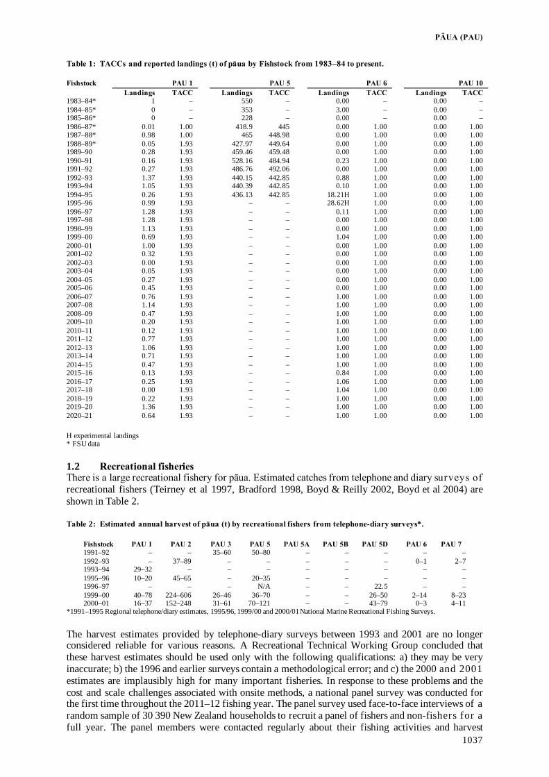
PĀUA (PAU)
1037
Table 1: TACCs and reported landings (t) of pāua by Fishstock from 1983–84 to present. Fishstock PAU 1 PAU 5 PAU 6 PAU 10 Landings TACC Landings TACC Landings TACC Landings TACC 1983–84* 1 – 550 – 0.00 – 0.00 – 1984–85* 0 – 353 – 3.00 – 0.00 – 1985–86* 0 – 228 – 0.00 – 0.00 – 1986–87* 0.01 1.00 418.9 445 0.00 1.00 0.00 1.00 1987–88* 0.98 1.00 465 448.98 0.00 1.00 0.00 1.00 1988–89* 0.05 1.93 427.97 449.64 0.00 1.00 0.00 1.00 1989–90 0.28 1.93 459.46 459.48 0.00 1.00 0.00 1.00 1990–91 0.16 1.93 528.16 484.94 0.23 1.00 0.00 1.00 1991–92 0.27 1.93 486.76 492.06 0.00 1.00 0.00 1.00 1992–93 1.37 1.93 440.15 442.85 0.88 1.00 0.00 1.00 1993–94 1.05 1.93 440.39 442.85 0.10 1.00 0.00 1.00 1994–95 0.26 1.93 436.13 442.85 18.21H 1.00 0.00 1.00 1995–96 0.99 1.93 – – 28.62H 1.00 0.00 1.00 1996–97 1.28 1.93 – – 0.11 1.00 0.00 1.00 1997–98 1.28 1.93 – – 0.00 1.00 0.00 1.00 1998–99 1.13 1.93 – – 0.00 1.00 0.00 1.00 1999–00 0.69 1.93 – – 1.04 1.00 0.00 1.00 2000–01 1.00 1.93 – – 0.00 1.00 0.00 1.00 2001–02 0.32 1.93 – – 0.00 1.00 0.00 1.00 2002–03 0.00 1.93 – – 0.00 1.00 0.00 1.00 2003–04 0.05 1.93 – – 0.00 1.00 0.00 1.00 2004–05 0.27 1.93 – – 0.00 1.00 0.00 1.00 2005–06 0.45 1.93 – – 0.00 1.00 0.00 1.00 2006–07 0.76 1.93 – – 1.00 1.00 0.00 1.00 2007–08 1.14 1.93 – – 1.00 1.00 0.00 1.00 2008–09 0.47 1.93 – – 1.00 1.00 0.00 1.00 2009–10 0.20 1.93 – – 1.00 1.00 0.00 1.00 2010–11 0.12 1.93 – – 1.00 1.00 0.00 1.00 2011–12 0.77 1.93 – – 1.00 1.00 0.00 1.00 2012–13 1.06 1.93 – – 1.00 1.00 0.00 1.00 2013–14 0.71 1.93 – – 1.00 1.00 0.00 1.00 2014–15 0.47 1.93 – – 1.00 1.00 0.00 1.00 2015–16 0.13 1.93 – – 0.84 1.00 0.00 1.00 2016–17 0.25 1.93 – – 1.06 1.00 0.00 1.00 2017–18 0.00 1.93 – – 1.04 1.00 0.00 1.00 2018–19 0.22 1.93 – – 1.00 1.00 0.00 1.00 2019–20 1.36 1.93 – – 1.00 1.00 0.00 1.00 2020–21 0.64 1.93 – – 1.00 1.00 0.00 1.00 H experimental landings * FSU data 1.2 Recreational fisheries There is a large recreational fishery for pāua. Estimated catches from telephone and diary surveys of recreational fishers (Teirney et al 1997, Bradford 1998, Boyd & Reilly 2002, Boyd et al 2004) are shown in Table 2. Table 2: Estimated annual harvest of pāua (t) by recreational fishers from telephone-diary surveys*.
Fishstock PAU 1 PAU 2 PAU 3 PAU 5 PAU 5A PAU 5B PAU 5D PAU 6 PAU 7 1991–92 – – 35–60 50–80 – – – – – 1992–93 – 37–89 – – – – – 0–1 2–7 1993–94 29–32 – – – – – – – – 1995–96 10–20 45–65 – 20–35 – – – – – 1996–97 – – – N/A – – 22.5 – – 1999–00 40–78 224–606 26–46 36–70 – – 26–50 2–14 8–23 2000–01 16–37 152–248 31–61 70–121 – – 43–79 0–3 4–11
*1991–1995 Regional telephone/diary estimates, 1995/96, 1999/00 and 2000/01 National Marine Recreational Fishing Surveys. The harvest estimates provided by telephone-diary surveys between 1993 and 2001 are no longer considered reliable for various reasons. A Recreational Technical Working Group concluded that these harvest estimates should be used only with the following qualifications: a) they may be very inaccurate; b) the 1996 and earlier surveys contain a methodological error; and c) the 2000 and 2001 estimates are implausibly high for many important fisheries. In response to these problems and the cost and scale challenges associated with onsite methods, a national panel survey was conducted for the first time throughout the 2011–12 fishing year. The panel survey used face-to-face interviews of a random sample of 30 390 New Zealand households to recruit a panel of fishers and non-fishers for a full year. The panel members were contacted regularly about their fishing activities and harvest

PĀUA (PAU)
1038
information collected in standardised phone interviews. The panel survey was repeated in 2017–18 (Wynne-Jones et al 2019). Harvest estimates for pāua are given in Table 3 (from Wynne-Jones et al 2014 using mean weights from Hartill & Davey 2015 and from Wynne-Jones et al 2019). Table 3: Recreational harvest estimates for pāua stocks from the national panel survey in 2011–12 (Wynne-Jones et
al 2014) and 2017–18 (Wynne-Jones et al 2019). Mean fish weights were obtained from boat ramp surveys (Hartill & Davey 2015).
Stock Fishers Events Number of pāua CV Total weight (t) CV 2011–12 (national panel survey) PAU 1 39 63 43 480 12.16 0.27 PAU 2 158 378 286 182 81.85 0.15 PAU 3 35 67 60 717 16.98 0.31 PAU 5A 2 3 1 487 0.42 0.76 PAU 5B 5 5 2 945 0.82 0.50 PAU 5D 41 84 80 290 22.45 0.30 PAU 7 19 41 50 534 14.13 0.34 PAU total 299 641 525 635 148.82 0.11 2017–18 (national panel survey) PAU 1 27 41 27 707 0.34 8.74 0.34 PAU 2 151 367 283 240 0.15 83.22 0.15 PAU 3 21 46 28 140 0.35 8.79 0.35 PAU 5A 3 4 2 419 0.76 0.85 0.76 PAU 5B 10 21 15 361 0.45 9.85 0.45 PAU 5D 48 88 55 0.21 19.28 0.21 PAU 6 E e 3 076 0.60 0.95 0.61 PAU 7 11 16 10 576 0.36 3.02 0.36 PAU total 274 590 425 661 134.70
1.3 Customary fisheries Pāua is a taonga species and as such there is an important customary use of pāua by Maori for food, and the shells have been used extensively for decorations and fishing devices. Pāua forms an important fishery for customary non-commercial, but the total annual catch is not known. Māori customary fishers utilise the provisions under both the recreational fishing regulations and the various customary regulations. Many tangata whenua harvest pāua under their recreational allowance and these are not included in records of customary catch. Customary reporting requirements vary around the country. Customary fishing authorisations issued in the South Island and Stewart Island would be under the Fisheries (South Island Customary Fishing) Regulations 1999. Many rohe moana / areas of the coastline in the North Island and Chatham Islands are gazetted under the Fisheries (Kaimoana Customary Fishing) Regulations 1998 which require reporting on authorisations. In the areas not gazetted, customary fishing permits would be issued would be under the Fisheries (Amateur Fishing) Regulations 2013, where there is no requirement to report catch. The information on Māori customary harvest under the provisions made for customary fishing can be limited (Table 4). These numbers are likely to be an underestimate of customary harvest as only the catch approved and harvested in kilograms and numbers are reported in the table. 1.4 Illegal catch There are qualitative data to suggest significant illegal, unreported, unregulated (IUU) activity in this fishery. Current quantitative levels of illegal harvests are not known. In the past, annual estimates of illegal harvest for some Fishstocks were provided by MFish Compliance based on seizures. In the current pāua stock assessments, nominal illegal catches are used.

PĀUA (PAU)
1039
Table 4: Fisheries New Zealand records of customary harvest of pāua (approved and reported as weight (kg) and in numbers), since 1998-99. – no data. [Continued on next page]
PAU 1 PAU 2 Weight (kg) Numbers Weight (kg) Numbers Fishing year Approved Harvested Approved Harvested Approved Harvested Approved Harvested 1998–99 – – – – 40 40 – – 1999–00 – – – – – – 1 400 820 2000–01 – – – – – – – – 2001–02 – – – – – – – – 2002–03 – – 30 30 – – – – 2003–04 – – 184 146 – – 4 805 4 685 2004–05 – – 240 220 – – 2 780 2 440 2005–06 125 100 40 40 – – 5 349 4 385 2006–07 705 581 2 175 1 925 – – 7 088 3 446 2007–08 460 413 2 155 1 618 – – 11 298 6 164 2008–09 491 191 2 915 2 228 – – 30 312 24 155 2009–10 184 43 2 825 2 225 – – 5 505 4 087 2010–11 154 129 5 915 3 952 – – 20 570 17 062 2011–12 25 8 470 470 243 243 29 759 23 932 2012–13 20 20 1 305 1 193 10 6 51 275 27 653 2013–14 – – – – – – 61 486 30 129 2014–15 45 33 700 536 – – 25 215 16 449 2015–16 50 9 1 425 756 – – 11 540 6 383 2016–17 – – 2 190 618 100 100 13 698 6 877 2017–18 15 15 4 632 3 162 – – 6 960 1 942 2018–19 – – 1 368 710 – – 8 585 3 209 2019–20 60 20 120 115 – – – – 2020–21 40 0 66 8 – – – – PAU 3* PAU 4 Weight (kg) Numbers Weight (kg) Numbers Fishing year Approved Harvested Approved Harvested Approved Harvested Approved Harvested 1998–99 – – – – – – – – 1999–00 – – – – – – – – 2000–01 – – 300 230 – – – – 2001–02 – – 6 239 4 832 – – – – 2002–03 – – 3 422 2 449 – – – – 2003–04 – – – – – – – – 2004–05 – – – – – – – – 2005–06 – – 1 580 1 220 – – – – 2006–07 – – 5 274 4 561 – – – – 2007–08 – – 7 515 5 790 – – – – 2008–09 – – 10 848 8 232 – – – – 2009–10 – – 8 490 6 467 – – 635 635 2010–11 – – 8 360 7 449 – – – – 2011–12 – – 5 675 4 242 – – – – 2012–13 – – 15 036 12 874 – – – – 2013–14 – – 10 259 7 566 – – 110 110 2014–15 – – 8 761 7 035 – – 150 150 2015–16 – – 14 801 11 808 – – 320 120 2016–17 – – 11 374 9 217 – – 366 366 2017–18 – – 2 708 1 725 50 50 820 764 2018–19 – – 480 278 330 330 – – 2019–20 – – 30 288 21 527 – – – – 2020–21 – – 4 960 3 242 – – – – PAU 5A PAU 5B Weight (kg) Numbers Weight (kg) Numbers Fishing year Approved Harvested Approved Harvested Approved Harvested Approved Harvested 1998–99 – – – – – – – – 1999–00 – – – – – – – – 2000–01 – – – – – – 50 50 2001–02 – – 80 70 – – 610 590 2002–03 – – – – – – – – 2003–04 – – – – – – – – 2004–05 – – – – – – – – 2005–06 – – – – – – 140 90 2006–07 – – – – – – 485 483 2007–08 – – 100 100 – – 2 685 2 684 2008–09 – – 100 100 – – 3 520 3 444 2009–10 – – 150 150 – – 2 680 2 043 2010–11 – – 150 150 – – 2 053 1 978 2011–12 – – 512 462 – – 495 495 2012–13 – – 590 527 – – 1 875 1 828 2013–14 – – – – – – 130 130 2014–15 – – – – – – – – 2015–16 – – 255 50 – – 2 195 2 003

PĀUA (PAU)
1040
Table 4 [continued] PAU 5A PAU 5B Weight (kg) Numbers Weight (kg) Numbers Fishing year Approved Harvested Approved Harvested Approved Harvested Approved Harvested 2016–17 – – – – – – 75 75 2017–18 – – 200 200 – – 2 245 2 245 2018–19 – – – – – – 1 405 1 337 2019–20 – – – – – – 835 815 2020–21 – – 850 820 – – 2 080 1 930 PAU 5D PAU 6 Weight (kg) Numbers Weight (kg) Numbers Fishing year Approved Harvested Approved Harvested Approved Harvested Approved Harvested 1998–99 – – – – – – – – 1999–00 – – – – – – – – 2000–01 – – 665 417 – – – – 2001–02 – – 5 530 3 553 – – – – 2002–03 – – 2 435 1 351 – – – – 2003–04 – – – – – – – – 2004–05 – – – – – – – – 2005–06 – – 1 560 1 560 – – – – 2006–07 – – 2 845 2 126 – – 100 100 2007–08 – – 5 600 5 327 – – 60 60 2008–09 – – 6 646 6 094 – – – – 2009–10 – – 4 840 4 150 – – – – 2010–11 – – 15 806 15 291 – – 230 130 2011–12 – – 7 935 7 835 – – – – 2012–13 – – 10 254 8 782 – – – – 2013–14 – – 5 720 5 358 – – – – 2014–15 – – – – – – – – 2015–16 – – 15 922 13 110 – – 50 50 2016–17 – – 3 676 3 576 – – 80 80 2017–18 – – 3 588 3 310 – – – – 2018–19 – – 950 894 – – – – 2019–20 – – 6 905 6 439 – – – – 2020–21 – – 9 247 9 020 – – – – PAU 7 Weight (kg) Numbers Fishing year Approved Harvested Approved Harvested Approved Harvested Approved Harvested 1998–99 – – – – 1999–00 – – – – 2000–01 – – – – 2001–02 – – – – 2002–03 – – – – 2003–04 – – – – 2004–05 – – – – 2005–06 – – – – 2006–07 – – – – 2007–08 – – 1 110 808 2008–09 – – 1 270 1 014 2009–10 – – 1 085 936 2010–11 – – 60 31 2011–12 – – 20 20 2012–13 – – – – 2013–14 – – – – 2014–15 – – – – 2015–16 – – – – 2016–17 – – – – 2017–18 – – – – 2018–19 – – – – 2019–20 – – – – 2020–21 – – – –
* Data before 2010–11 exclude the area between the Hurunui River and the South Shore (just north of Banks Peninsula) , as Tangata Tiaki were not appointed there until November 2009. 1.5 Other sources of mortality Pāua may die from wounds caused by removal desiccation or osmotic and temperature stress if they are brought to the surface. Sub-legal pāua may be subject to handling mortality by the fishery if they are removed from the substrate to be measured. Further mortality may result indirectly from being returned to unsuitable habitat or being lost to predators or bacterial infection. Gerring (2003) observed pāua (from PAU 7) with a range of wounds in the laboratory and found that only a deep cut in the foot caused significant mortality (40% over 70 days). In the field this injury reduced the ability of pāua to right themselves and clamp securely onto the reef, and consequently made them more vulnerable to

PĀUA (PAU)
1041
predators. The tool generally used by divers in PAU 7 is a custom-made stainless-steel knife with a rounded tip and no sharp edges. This design makes cutting the pāua very unlikely (although abrasions and shell damage may occur). Gerring (2003) estimated that in PAU 7, 37% of pāua removed from the reef by commercial divers were undersize and were returned to the reef. His estimate of incidental mortality associated with fishing in PAU 7 was 0.3% of the landed catch. Incidental fishing mortality may be higher in areas where other types of tools and fishing practices are used. Mortality may increase if pāua are kept out of the water for a prolonged period or returned onto sand. To date, the stock assessments developed for pāua have assumed that there is no mortality associated with capture of undersize animals. 2. BIOLOGY Pāua are herbivores which can form large aggregations on reefs in shallow subtidal coastal habitats. Movement is over a sufficiently small spatial scale that the species may be considered sedentary. Pāua are broadcast spawners and spawning is usually annual. Habitat related factors are an important source of variation in the post-settlement survival of pāua. Growth, morphometrics, and recruitment can vary over short distances and may be influenced by factors such as water temperature, wave exposure, habitat structure and the availability of food. Naylor et al (2016) analysed demographic variation in pāua in New Zealand. They concluded that there were large differences in the growth rates and maximum size over a large latitudinal range. Their analysis indicated that water temperature, as indicated by sea surface temperature, was an important determinant of these. Pāua become sexually mature when they are about 70–90 mm long, or 3–5 years old. A summary of generic estimates for biological parameters for pāua is presented in Table 5. Parameters specific to individual pāua QMAs are reported in the specific Working Group reports. Table 5: Estimates of biological parameters for pāua (H. iris). Fishstock Estimate Source 1. Natural mortality (M) All 0.02–0.25 Sainsbury (1982) 2. Weight = a (length)b (weight in kg, shell length in mm) a = 2.99E—08 b = 3.303 Schiel & Breen (1991) 3. STOCKS AND AREAS Using both mitochondrial and microsatellite markers Will & Gemmell (2008) found high levels of genetic variation within samples of H. Iris taken from 25 locations spread throughout New Zealand. They also found two patterns of weak but significant population genetic structure. Firstly, H. iris individuals collected from the Chatham Islands were found to be genetically distinct from those collected from coastal sites around the North and South Islands. Secondly a genetic discontinuity was found loosely associated with the Cook Strait region. Genetic discontinuities within the Cook Strait region have previously been identified in sea stars, mussels, limpets, and chitons and are possibly related to contemporary and/or past oceanographic and geological conditions of the region. This split may have some implications for management of the pāua stocks, with populations on the south of the North Island, and the north of the South Island potentially warranting management as separate entities; a status they already receive under the zonation of the current fisheries regions, PAU 2 in the North Island, and PAU 7 on the South Island.

PĀUA (PAU)
1042
4. ENVIRONMENTAL AND ECOSYSTEM CONSIDERATIONS This section was updated for the 2021 Fishery Assessment Plenary. A more detailed summary from an issue-by-issue perspective is available in the Aquatic Environment and Biodiversity Annual Review 2021 (Fisheries New Zealand 2021), online at https://www.mpi.govt.nz/dmsdocument/51472-Aquatic-Environment-and-Biodiversity-Annual-Review-AEBAR-2021-A-summary-of-environmental-interactions-between-the-seafood-sector-and-the-aquatic-environment. 4.1 Ecosystem role Pāua are eaten by a range of predators, and smaller pāua are generally more vulnerable to predation. Smaller pāua are consumed by blue cod (Carbines & Beentjes 2003), snapper (Francis 2003), banded wrasse (Russell 1983), spotties (McCardle 1983), triplefins (McCardle 1983) and octopus (Andrew & Naylor 2003). Large pāua are generally well protected by their strong shells but are still vulnerable to rock lobsters (McCardle 1983) and the large predatory starfishes Astrostole scabra and Coscinasterias muricata (Andrew & Naylor 2003). Large pāua are also vulnerable to predation by eagle rays (McCardle 1983), but Ayling & Cox (1982) suggested that eagle rays feed almost exclusively on Cook’s turban. There are no known predators that feed exclusively on pāua. Pāua feed preferentially on drift algae but at high densities they also feed by grazing attached algae. They are not generally considered to have a large structural impact upon algal communities but at high densities they may reduce the abundance of algae. There are no recognised interactions with pāua abundance and the abundance or distribution of other species, except for kina which, at very high densities, appear to exclude pāua (Naylor & Gerring 2001). Research at D’Urville Island and on Wellington’s south coast suggests that there is some negative association between pāua and kina (Andrew & MacDiarmid 1999). 4.2 Fish and invertebrate bycatch Because pāua are harvested by hand gathering, incidental bycatch is limited to epibiota attached to, or within the shell. The most common epibiont on pāua shell is non-geniculate coralline algae, which, along with most other plants and animals which settle and grow on the shell, such as barnacles, oysters, sponges, bryozoans, and algae, appears to have general habitat requirements (i.e., these organisms are not restricted to the shells of pāua). Several boring and spiral-shelled polychaete worms are commonly found in and on the shells of pāua. Most of these are found on several shellfish species, although within New Zealand’s shellfish, the onuphid polychaete Brevibrachium maculatum has been found only in pāua shell (Read 2004). This species, however, has also been reported to burrow into limestone, or attach its tube to the holdfasts of algae (Read 2004). It is also not uncommon for pāua harvesters to collect predators of pāua (mainly large predatory starfish) while fishing and to effectively remove these from the ecosystem. The levels of these removals are unlikely to have a significant effect on starfish populations (nor, in fact, on the mortality of pāua caused by predation). 4.3 Incidental catch (seabirds, mammals, and protected fish) There is no known bycatch of threatened, endangered, or protected species associated with the hand gathering of pāua. 4.4 Benthic interactions The environmental impact of pāua harvesting is likely to be minimal because pāua are selectively hand gathered by free divers. Habitat contact by divers at the time of harvest is limited to the area of pāua foot attachment, and pāua are usually removed with a blunt tool to minimise damage to the flesh. The diver’s body is also seldom in full contact with the benthos. Vessels anchoring during or after fishing have the potential to cause damage to the reef depending on the type of diving operation (in many cases, vessels do not anchor during fishing). Damage from anchoring is likely to be greater in areas with fragile species such as corals than it is on shallow temperate rocky reefs. Corals are relatively abundant at shallow depths within Fiordland, but there are seven areas within the sounds with significant populations of fragile species where anchoring is prohibited.

PĀUA (PAU)
1043
4.5 Other considerations 4.5.1 Genetic effects Fishing, and environmental changes, including those caused by climate change or pollution, could alter the genetic composition or diversity of a species and there is some evidence to suggest that genetic changes may occur in response to fishing of abalones. Miller et al (2009) suggested that, in Haliotis rubra in Tasmania, localised depletion will lead to reduced local reproductive output which may, in turn, lead to an increase in genetic diversity because migrant larval recruitment will contribute more to total larval recruitment. Enhancement of pāua stocks with artificially-reared juveniles has the potential to lead to genetic effects if inappropriate broodstocks are used. 4.5.2 Biosecurity issues Undaria pinnatifida is a highly invasive opportunistic kelp which spreads mainly via fouling on boat hulls. It can form dense stands underwater, potentially resulting in competition for light and space which may lead to the exclusion or displacement of native plant and animal species. Undaria may be transported on the hulls of pāua dive tenders to unaffected areas. Bluff Harbour, for example, supports a large population of Undaria, and is one of the main ports of departure for fishing vessels harvesting pāua in Fiordland, which appears to be devoid of Undaria (R. Naylor pers. comm.). In 2010, a small population of Undaria was found in Sunday Cove in Breaksea Sound, and attempts to eradicate it appear to have been successful (see https://www.mpi.govt.nz/biosecurity/marine-pest-disease-management/fiordland-marine-biosecurity-programme/). 4.5.3 Kaikōura Earthquake Research was undertaken to investigate the influence of the November 2016 Kaikōura earthquake on pāua stocks along the Kaikōura coastline. The results estimated that the seabed uplift led to a loss of up to 50% of the pre-earthquake fished area across PAU 3 statistical areas. Annual biomass surveys have showed a recovery of the stock which has led to the reopening of the fishery in 2021-22 for 3 months. More details can be found in the PAU 3 Working Group report. 4.5.4 Marine heatwave A baseline report summarising trends in climatic and oceanographic conditions in New Zealand that are of potential relevance for fisheries and marine ecosystem resource management in the New Zealand region was completed by Hurst et al (2012). There is also an updated chapter on oceanic trends in the Aquatic Environment and Biodiversity Annual Review 2021 (Fisheries New Zealand 2021). Any effects of recent warmer temperatures (such as the high surface temperatures off the WCSI during the 2016 and 2017 spawning seasons, marine heatwaves, and general warming of the Tasman Sea (Sutton & Bowen 2019) on fish distribution, growth, or spawning success have yet to be determined. Shellfish fisheries have been identified as likely to be vulnerable to ocean acidification (Capson & Guinotte 2014). A recent project that has just reached completion describes the state of knowledge of climate change-associated predictions for components of New Zealand’s marine environment that are most relevant to fisheries (Cummings et al 2021). Past and future projected changes in coastal and ocean properties, including temperature, salinity, stratification and water masses, circulation, oxygen, ocean productivity, detrital flux, ocean acidification, coastal erosion and sediment loading, wind and waves are reviewed. Responses to climate change for these coastal and ocean properties are discussed, as well as their likely impact on the fisheries sector, where known. A range of decision support tools in use overseas were evaluated with respect to their applicability for dissemination of the state of knowledge on climate change and fisheries. Three species, for which there was a relatively large amount of information available were chosen from the main fisheries sectors for further analysis. These were pāua, snapper, and hoki (shellfish, inshore, and middle-depths/deepwater fisheries, respectively). An evaluation of the sensitivity and exposure of pāua to climate change-associated threats, based on currently available published literature and expert opinion, assessed pāua vulnerability to climate change effects as ‘low’ (Cummings et al 2021).

PĀUA (PAU)
1044
5. STOCK ASSESSMENT The dates of the most recent survey or stock assessment for each QMA are listed in Table 6. Table 6: Recent survey and stock assessment information for each pāua QMA.
QMA Type of survey or assessment Date Comments
PAU 1 No surveys or assessments have been undertaken
PAU 2 Base case: length-based Bayesian stock assessment
2021 A large proportion of PAU 2, including the Wellington south coast and west of Turakirae, is either a Marine Reserve or voluntarily closed to commercial fishing. This means that the data collected from the commercial fishery are exclusive of this large area and therefore the assessment only applies to the south east component of PAU 2 (Wairarapa). Lack of contrast in catch, CPUE, and length frequency makes estimation of stock status and biomass trajectories difficult. The 2019–20 year was excluded from the PCELR CPUE series becaus e o f concerns about the comparability with previous years due to the effects o f COVID-19 on export markets, and ERS reporting issues. This may continue into the future.
PAU 3A Biomass survey 2021 Biomass surveys have been conducted since the 2016 Kaikōura earthquakes. They have showed a recovery of the stock and led to the reopening of the fishery in 2021-22 for a duration of 3 months only. Th ere are not enough data to attempt a stock assessment at this stage.
PAU 3B CPUE Standardisation 2022 A stock assessment for the PAU 3B area was attempted in 2021–22, bas ed on estimates of historical catches, CPUE trends and commercial length frequency data. CPUE trends were found to be stable despite steady increases in catch over the past decades.
PAU 4 CPUE Standardisation 2016 In February 2010 the Shellfish Working Group (SFWG) agreed that, due to the lack of data of adequate quality to use in the Bayesian length-based model, a stock assessment for PAU 4 using this model was not appropriate. In 2016 an analysis of the last 14 years of CPUE data was done. This report showed a potential decline in the fishery since the early 2000s, however the poor data quality is causing considerable uncertainty about the real trend in the fishery.
PAU 5A Quantitative assessment using a Bayesian length-based model
2020 The 2020 stock assessment was implemented as a single area model together with a three-area spatial model to corroborate findings from the single area model. The status of the stock was estimated to b e 5 1 % B 0 . At current levels of catch spawning stock biomass is projected to remain nearly unchanged at 51% B0 after 3 years, with an equilibrium value of 50% of B0.
PAU 5B Quantitative assessment using a Bayesian length-based model
2018 The 2018 Plenary accepted this assessment as best scientific info rm ation . The status of the stock was estimated to be 47% B0.
PAU 5D Quantitative assessment using a Bayesian length-based model
2019 The reference case model estimated that the unfished spawning stock biomass (B0) was about 2029 t (1673–2535 t) and the spawning stock population in 2018 (B2018) was about 40% (25–65%) of B0. The model projection made for three years assuming 2018 catch levels (which includes commercial catch) and using recruitment re-sampled from the recent model estimates, suggested that the spawning stock abundance would remain at 42% (28–52%) B0 over the following three years. The projection also indicated that the probability of the spawning stock biomass being above the target (40% B0) will decrease from about 52% in 2018 to 49% by 2021.
PAU 6 Biomass estimate 1996 This fishery has a TACC of 1 t.
PAU 7 Quantitative assessment using a Bayesian length-based model
2022 The SFWG agreed that the stock assessment was reliable for Cook Strait based on the available data. Currently, spawning stock biomass is estimated to be 33% B0 and is Unlikely to be at or above the target. It is also Very Unlikely to be below the soft and hard limits. Overfishing is About as Likely as Not to be occurring.
PAU 10 No surveys or assessments have been undertaken

PĀUA (PAU)
1045
5.1 Estimates of fishery parameters and abundance For further information on fishery parameters and abundance specific to each pāua QMA refer to the specific Working Group report. In QMAs where quantitative stock assessments have been undertaken, standardised CPUE is used as input data for the Bayesian length-based stock assessment model. There is however a large amount of literature on abalone which suggests that any apparent stability in CPUE should be interpreted with caution and CPUE may not be proportional to abundance because it is possible to maintain high catch rates despite a falling biomass. This occurs because pāua tend to aggregate and, to maximise their catch rates, divers move from areas that have been depleted of pāua to areas with higher density. The consequence of this fishing behaviour is that overall abundance is decreasing while CPUE is remaining stable. This process of hyperstability is believed to be of less concern in most commercial areas because fishing in these QMAs is consistent across all fishable areas. An exception are the D’Urville Island and Northern Faces areas of PAU 7, where catches have declined substantially, and CPUE now only reflects a few remaining areas. Other areas may be highly depleted but fishery dependent CPUE does not reflect abundance in these areas any longer. In PAU 4, 5A, 5B, 5D, and 7 the relative abundance of pāua was also estimated from independent research diver surveys (RDS) for a number of years. In PAU 7, seven surveys have been completed over a number of years but only two surveys have been conducted in PAU 4. In 2009 and 2010 several reviews were conducted (Cordue 2009, Haist 2010) to assess: i) the reliability of the research diver survey index as a proxy for abundance; and ii) whether the RDS data, when used in the pāua stock assessment models, results in model outputs that do not adequately reflect the status of the stocks. The reviews concluded that:
• Due to inappropriate survey design the RDS data appear to be of very limited use for constructing relative abundance indices.
• There was clear non-linearity in the RDS index, the form of which is unclear and could be potentially complex.
• CVs of RDS index ‘year’ effects are likely to be underestimated, especially at low densities. • Different abundance trends among strata reduces the reliability of RDS indices, and the CVs
are likely to be uninformative about this. • It is unlikely that the assessment model can determine the true non-linearity of the RDS
index-abundance relationship because of the high variability in the RDS indices. • The non-linearity observed in the RDS indices is likely to be more extreme at low densities,
so the RDSI is likely to mask trends when it is most critical to observe them. • Existing RDS data is likely to be most useful at the research stratum level.
For these reasons, RDS data are not used in any recent PAU stock assessments. 5.2 Biomass estimates Biomass was estimated for PAU 6 in 1996 (McShane et al 1996). However, the survey area was limited to the area from Kahurangi Point to the Heaphy River. Biomass has been estimated, as part of the stock assessments, for PAU 2, 5A, 5B, 5D, and 7 (Table 6). For further information on biomass estimates specific to each pāua QMA refer to the specific Working Group report. 5.3 Yield Estimates and Projections Yield estimates and projections are estimated as part of the stock assessment process. Both are available for PAU 2, PAU 5A, PAU 5B, PAU 5D, and PAU 7. For further information on yield estimates and projections specific to each pāua QMA refer to the specific Working Group report. 5.4 Other factors In the last few years, the commercial fisheries have been implementing voluntary management actions in the main QMAs. These management actions include raising the minimum harvest size, subdividing QMAs into smaller management areas, and capping catch in the different areas and in some QMAs, not catching the full Annual Catch Entitlement (ACE) in a particular fishing year.

PĀUA (PAU)
1046
6. STATUS OF THE STOCKS The status of pāua stocks PAU 2, PAU 3A, PAU3B, PAU 4, PAU 5A, PAU 5B, PAU 5D, and PAU 7 are given in the relevant Working Group reports. 7. FOR FURTHER INFORMATION Andrew, N L; Breen, P A; Naylor, J R; Kendrick, T H; Gerring, P K (2000a) Stock assessment of paua Haliotis iris in PAU 7 in 1998–99.
New Zealand Fisheries Assessment Report. 2000/49. Andrew, N L; MacDiarmid, A B (1999) Sea urchin fisheries and potential interactions with a kina fishery in Fiordland. Conservation
Advisory Science Notes No. 266, Department of Conservation, Wellington. Andrew, N; Naylor, R (2003) Paua. In: Andrew, N & Francis, M (Eds)The Living reef. The ecology of New Zealand’s rocky reefs. Craig
Potton Publishing, Nelson, New Zealand. Andrew, N L; Naylor, J R; Gerring, P; Notman, P R (2000b) Fishery independent surveys of paua (Haliotis iris) in PAU 5B and 5D. New
Zealand Fisheries Assessment Report 2000/3. 21 p. Andrew, N L; Naylor, J R; Gerring, P (2000c) A modified timed-swim method for paua stock assessment. New Zealand Fisheries
Assessment Report 2000/4. 23 p. Andrew, N L; Naylor, J R; Kim, S W (2002) Fishery independent surveys of the relative abundance and size-structure of paua (Haliotis iris)
in PAU 5B and PAU 5D. New Zealand Fisheries Assessment Report 2002/41. Annala, J H; Sullivan, K J; O’Brien, C; Iball, S (Comps.) (1998) Report from the Fishery Assessment Plenary, May 1998: Stock assessments
and yield estimates. 409 p. (Unpublished report held in NIWA library, Wellington). Ayling, T; Cox, G J (1982) Collins' guide to sea fishes of New Zealand. Collins. Auckland. 343 p. Boyd, R O; Gowing, L; Reilly, J L (2004) 2000–2001 National Marine Recreational Fishing Survey: diary results and harvest estimates.
Draft New Zealand Fisheries Assessment Report. (Unpublished report held by Fisheries New Zealand, Wellington). Boyd, R O; Reilly, J L (2002) 1999/2000 National Marine Recreational Fishing Survey: harvest estimates. Draft New Zealand Fisheries
Assessment Report. (Unpublished report held by Fisheries New Zealand, Wellington). Bradford, E (1998) Harvest estimates from the 1996 national recreational fishing surveys. New Zealand Fisheries Assessment Research
Document 1998/16. 27 p. (Unpublished report held by NIWA library, Wellington). Breen, P A; Andrew, N L; Kendrick, T H (2000b) Stock assessment of paua (Haliotis iris) in PAU 5B and PAU 5D using a new length-based
model. New Zealand Fisheries Assessment Report. 2000/33. Breen, P A; Andrew, N L; Kendrick, T H (2000c) The 2000 stock assessment of paua (Haliotis iris) in PAU 5B using an improved Bayes i an
length-based model. New Zealand Fisheries Assessment Report. 2000/48. Breen, P A; Andrew, N L; Kim, S W (2001) The 2001 stock assessment of paua Haliotis iris in PAU 7. New Zealand Fisheries Assessment
Report. 2001/55. Breen, P A; Kim, S W (2004) The 2004 stock assessment of paua Haliotis iris in PAU 5A. New Zealand Fisheries Assessment Report.
2004/40. Breen, P A; Kim, S W (2005) The 2005 stock assessment of paua Haliotis iris in PAU 7. New Zealand Fisheries Assessment Report.
2005/47. Breen, P A; Kim, S W (2007) The 2006 stock assessment of paua (Haliotis iris) stocks PAU 5A (Fiordland) and PAU 5D (Otago). New
Zealand Fisheries Assessment Report. 2007/09. Breen, P A; Smith, A N (2008a) The 2007 stock assessment of paua (Haliotis iris) stock PAU 5B (Stewart Island). New Zealand Fisheries
Assessment Report. 2008/05. Breen, P A; Smith, A N (2008b) Data used in the 2007 stock assessment for paua (Haliotis iris) stock 5B (Stewart Island). New Zealand
Fisheries Assessment Report. 2008/06. Capson, T L; Guinotte, J (Eds) (2014) Future proofing New Zealand’s shellfish aquaculture: monitoring and adaptation to ocean
acidification. New Zealand Aquatic Environment and Biodiversity Report No. 136. 42 p. Carbines, G D; Beentjes, M P (2003) Relative abundance of blue cod in Dusky Sound in 2002. New Zealand Fisheries Assessment Report
2003/37. 25 p. Cordue, P L (2009) Analysis of PAU 5A diver survey data and PCELR catch and effort data. SeaFic and PAUMac 5 report. 45 p.
(Unpublished report held by Fisheries New Zealand, Wellington). Cummings, V J; Lundquist, C J; Dunn, M R; Francis, M; Horn, P; Law, C; Pinkerton, M H; Sutton, P; Tracey, D; Hansen, L; Mielbrecht, E (2021)
Assessment of potential effects of climate-related changes in coastal and offshore waters on New Zealand’s seafood sector. New Zealand Aquatic Environment and Biodiversity Report No. 261. 153 p.
Francis, R I C C (1990) A maximum likelihood stock reduction method. New Zealand Fisheries Assessment Research Document 1990/4. 8 p . (Unpublished report held by NIWA library, Wellington).
Francis, M (2003) Snapper. In: Andrew, N & Francis, M (Eds), pp. 186–191, The Living reef. The ecology of New Zealand’s rocky reefs. Craig Potton Publishing, Nelson, New Zealand.
Fisheries New Zealand (2021) Aquatic Environment and Biodiversity Annual Review 2021. Compiled by the Aquatic Environment Team, Fisheries Science and Information, Fisheries New Zealand, Wellington, New Zealand. 779 p.
Gerring, P K (2003) Incidental fishing mortality of paua (Haliotis iris) in PAU 7. New Zealand Fisheries Assessment Report 2003/56. 13 p. Haist, V (2010) Paua research diver survey: review of data collected and simulation study of survey method. New Zealand Fisheries Assessment
Report 2010/38. Hartill, B; Davey, N (2015) Mean weight estimates for recreational fisheries in 2011–12. New Zealand Fisheries Assessment Report
2015/25. Hurst, R J; Renwick, J A; Sutton, P J H; Uddstrom, M J; Kennan, S C; Law, C S; Rickard, G J; Korpela, A; Stewart, C; Evans, J (2012) Climate and
ocean trends of potential relevance to fisheries in the New Zealand region. New Zealand Aquatic Environment and Biodiversity Repor t No. 90. 202 p.
Kendrick, T H; Andrew, N L (2000) Catch and effort statistics and a summary of standardised CPUE indices for paua (Haliotis iris) in PAU 5A, 5B, and 5D. New Zealand Fisheries Assessment Report 2000/47.
McCardle, I (1983) Young paua in peril. Shellfisheries Newsletter 20. McShane, P E (1992) Paua fishery assessment 1992. New Zealand Fisheries Assessment Research Document 1992/3. 26 p. (Unpublished report
held by NIWA library, Wellington). McShane, P E (1996) Patch dynamics and effects of exploitation on abalone (Haliotis iris) populations. Fisheries Research 25: 191–199. McShane, P E; Mercer, S; Naylor, R (1993) Paua (Haliotis spp.) fishery assessment 1993. New Zealand Fisheries Assessment Research
Document 1993/6. 22 p. (Unpublished report held by NIWA library, Wellington).

PĀUA (PAU)
1047
McShane, P E; Mercer, S F; Naylor, J R; Notman, P R (1994a) Paua fishery assessment 1994. New Zealand Fisheries Assessment Research Document 1994/16. 47 p. (Unpublished report held by NIWA library, Wellington).
McShane, P E; Mercer, S F; Naylor, J R (1994b) Spatial variation and commercial fishing of New Zealand abalone (Haliotis iris and H. australis). New Zealand Journal of Marine and Freshwater Research 28: 345–355.
McShane, P E; Mercer, S F; Naylor, J R; Notman, P R (1996) Paua (Haliotis iris) fishery assessment in PAU 5, 6, and 7. New Zealand Fisheri es Assessment Research Document. 1996/11. (Unpublished report held by NIWA library, Wellington).
McShane, P E; Naylor, J R (1995) Small-scale spatial variation in growth, size at maturity, and yield- and egg-per-recruit relations in the New Zealand abalone Haliotis iris. New Zealand Journal of Marine and Freshwater Research 29: 603–612.
McShane, P E; Schiel, D R; Mercer, S F; Murray, T (1994c) Morphometric variation in Haliotis iris (Mollusca:Gastropoda): analysis of 61 populations. New Zealand Journal of Marine and Freshwater Research 28: 357–364.
Miller, K J, Maynard, B T, Mundy, C N (2009) Genetic diversity and gene flow in collapsed and healthy abalone fisheries. Molecular ecology 18(2): 200-211.
Naylor, J R; Andrew, N L (2000) Determination of growth, size composition, and fecundity of paua at Taranaki and Banks Peninsula. New Zealand Fisheries Assessment Report 2000/51.
Naylor, J R; Andrew, N L (2002) Determination of paua growth in PAU 2, 5A, 5B, and 5D. New Zealand Fisheries Assessment Report 2002/34. Naylor, J R; Andrew, N L; Kim, S W (2003) Fishery independent surveys of the relative abundance, size-structure and growth of paua
(Haliotis iris) in PAU 4. New Zealand Fisheries Assessment Report 2003/08. Naylor, J R; Andrew, N L; Kim, S W (2006) Demographic variation in the New Zealand abalone Haliotis iris. Marine and Freshwater Research
57: 215–224. Naylor, J R; Gerring, P (2001) Interaction between paua and kina. Water & Atmosphere 9(2): 16-17. Naylor, J R; Kim, S W (2004) Fishery independent surveys of the relative abundance and size-structure of paua Haliotis iris in PAU 5D.
New Zealand Fisheries Assessment Report 2004/48. Naylor, J R; Notman, P R; Mercer, S F; Gerring, P (1998) Paua (Haliotis iris) fishery assessment in PAU 5, 6, and 7. New Zealand F i sheri es
Assessment Research Document. 1998/05. (Unpublished report held by NIWA library, Wellington). Pirker, J G (1992) Growth, shell-ring deposition and mortality of paua (Haliotis iris Martyn) in the Kaikoura region. MSc thesis, Univers i t y of
Canterbury. 165 p. Read, G. B. (compiler) 2004. Guide to New Zealand Shell Polychaetes.
http://biocollections.org/pub/worms/nz/Polychaeta/ShellsPoly/NZShellsPolychaeta.htm Russell, B C (1983) The food and feeding habits of rocky reef fish of north‐eastern New Zealand. New Zealand Journal of Marine and
Freshwater Research 17 (2): 121–145. Sainsbury, K J (1982) Population dynamics and fishery management of the paua, Haliotis iris. 1. Population structure, growth, reproduction and
mortality. New Zealand Journal of Marine and Freshwater Research 16: 147–161. Schiel, D R; Breen, P A (1991) Population structure, ageing and fishing mortality of the New Zealand abalone Haliotis iris. Fishery Bulletin 89:
681–691. Schwarz, A.; Taylor, R.; Hewitt, J.; Phillips, N.; Shima, J.; Cole, R.; Budd, R. (2006). Impacts of terrestrial runoff on the biodiversity of
rocky reefs. New Zealand Aquatic Environment and Biodiversity Report No 7. 109 p. Sutton, P J H; Bowen, M (2019) Ocean temperature change around New Zealand over the last 36 years. New Zealand Journal of Marine &
Freshwater Research 53(3): 305–326. doi: 10.1080/0028830.2018.1562945. Teirney, L D; Kilner, A R; Millar, R E; Bradford, E; Bell, J D (1997) Estimation of recreational catch from 1991/92 to 1993/94. New
Zealand Fisheries Assessment Research Document 1997/15. 43 p. (Unpublished report held by NIWA library, Wellington). Will, M C; Gemmell, N J (2008) Genetic Population Structure of Black Foot paua. New Zealand Fisheries Research Report. GEN2007A: 37 p.
(Unpublished report held by Fisheries New Zealand, Wellington). Wynne-Jones, J; Gray, A; Heinemann, A; Hill, L; Walton, L (2019) National Panel Survey of Marine Recreational Fishers 2017–2018. New
Zealand Fisheries Assessment Report 2019/24. 104 p. Wynne-Jones,J; Gray, A; Hill, L; Heinemann, A (2014) National Panel Survey of Marine Recreational Fishers 2011–12: Harvest Estimates.
New Zealand Fisheries Assessment Report 2014/67. 139 p.


PĀUA (PAU 2)
1049
PĀUA (PAU 2) − Wairarapa / Wellington / Taranaki
(Haliotis iris) Pāua
1. FISHERY SUMMARY PAU 2 was introduced into the Quota Management System in 1986–87 with a TACC of 100 t. As a result of appeals to the Quota Appeal Authority, the TACC was increased to 121.19 t in 1989 and has remained unchanged to the current fishing year (Table 1). There is no TAC for this QMA; before the Fisheries Act (1996), a TAC was not required. When changes have been made to a TACC after 1996, stocks have been assigned a TAC. Table 1: Total allowable catches (TAC, t), allowances for customary fishing, recreational fishing, and other sources of
mortality (t), and Total Allowable Commercial Catches (TACC, t) declared for PAU 2 since introduction to the Quota Management System (QMS).
Year TAC Customary Recreational Other mortality TACC 1986–1989 – – – – 100 1989–present – – – – 121.19
1.1 Commercial fisheries The fishing year runs from 1 October to 30 September. Most of the commercial catch comes from the Wairarapa and Wellington South coasts between Castlepoint and Turakirae Head. The western area between Turakirae Head and the Waikanae River is closed to commercial fishing. On 1 October 2001 it became mandatory to report catch and effort on PCELRs using the fine-scale reporting areas that had been developed by the New Zealand Pāua Management Company for their voluntary logbook programme (Figure 1). Landings for PAU 2 are shown in Table 2 and Figure 2. Landings have been at or very close to the TACC since 1988–89. 1.2 Recreational fisheries The most recent recreational fishery survey “The National Panel Survey of Marine Recreational Fishers 2017–18: Harvest Estimates” Wynne-Jones et al (2019), estimated that about 83 t of pāua were harvested by recreational fishers in PAU 2 in 2017–18. Because pāua around Taranaki are naturally small and never reach the minimum legal size (MLS) of 125 mm, a new MLS of 85 mm was introduced for recreational fishers from 1 October 2009. The new length was on a trial basis for five years and now applies between the Awakino and Wanganui rivers. For further information on recreational fisheries refer to the Introduction – Pāua chapter.
PAU 1 PAU 1
PAU 2
Awakino River
Wanganui River
Castle Point
Turakirae Head
Waikanae River

PAUA (PAU 2)
1050
Figure 1:Map of fine-scale statistical reporting areas for PAU 2. Table 2: TACC and reported landings (t) of pāua in PAU 2 from 1983–84 to the present.
Fishing year Landings TACC Fishing year Landings TACC 1983–84* 110 – 2002–03 121.19 121.19 1984–85* 154 – 2003–04 121.06 121.19 1985–86* 92 – 2004–05 121.19 121.19 1986–87* 96.2 100 2005–06 121.14 121.19 1987–88* 122.11 111.33 2006–07 121.20 121.19 1988–89* 121.5 120.12 2007–08 121.06 121.19 1989–90 127.28 121.19 2008–09 121.18 121.19 1990–91 125.82 121.19 2009–10 121.13 121.19 1991–92 116.66 121.19 2010–11 121.18 121.19 1992–93 119.13 121.19 2011–12 120.01 121.19 1993–94 125.22 121.19 2012–13 122.00 121.19 1994–95 113.28 121.19 2013–14 120.00 121.19 1995–96 119.75 121.19 2014–15 115.00 121.19 1996–97 118.86 121.19 2015–16 123.74 121.19 1997–98 122.41 121.19 2016–17 123.69 121.19 1998–99 115.22 121.19 2017–18 113.87 121.19 1999–00 122.48 121.19 2018–19 122.89 121.19 2000–01 122.92 121.19 2019–20 122.28 121.19 2001–02 116.87 121.19 2020–21 126.26 121.19
* FSU data.
Figure 2:Historical landings and TACC for PAU 2 from 1983–84 to the present. QMS data from 1986 to present.

PĀUA (PAU 2)
1051
1.3 Customary fisheries Pāua is a taonga species and as such there is an important customary use of pāua by Maori for food, and the shells have been used extensively for decorations and fishing devices. For information on customary catch regulations and reporting refer to the Introduction – Pāua chapter. Estimates of customary catch for PAU 2 are given in Table 3. These numbers are likely to be an underestimate of customary harvest because only the catch in kilograms and numbers are reported in the table. In addition, many tangata whenua also harvest pāua under their recreational allowance and these are not included in records of customary catch. Table 3: Fisheries New Zealand records of customary harvest of pāua (approved and reported as weight (kg) and in
numbers) in PAU 2 since 1998-99. – no data.
Weight (kg) Numbers Fishing year Approved Harvested Approved Harvested 1998–99 40 40 – – 1999–00 – – 1 400 820 2000–01 – – – – 2001–02 – – – – 2002–03 – – – – 2003–04 – – 4 805 4 685 2004–05 – – 2 780 2 440 2005–06 – – 5 349 4 385 2006–07 – – 7 088 3 446 2007–08 – – 11 298 6 164 2008–09 – – 30 312 24 155 2009–10 – – 5 505 4 087 2010–11 – – 20 570 17 062 2011–12 243 243 29 759 23 932 2012–13 10 6 51 275 27 653 2013–14 – – 61 486 30 129 2014–15 – – 25 215 16 449 2015–16 – – 11 540 6 383 2016–17 100 100 13 698 6 877 2017–18 – – 6 960 1 942 2018–19 – – 8 585 3 209
1.4 Illegal catch It is widely believed that the level of illegal harvesting is high around Wellington and on the Wairarapa coast. For further information on illegal catch refer to the Introduction – Pāua chapter. 1.5 Other sources of mortality For further information on other sources of mortality refer to the Introduction – Pāua chapter. 2. BIOLOGY For further information on pāua biology refer to the Introduction – Pāua chapter. A summary of published estimates of biological parameters for PAU 2 is presented in Table 4.

PAUA (PAU 2)
1052
Table 4: Estimates of biological parameters (H. iris)
Area Estimate Source 1. Size at maturity (shell length) Wellington 50% mature 71.7 mm Naylor et al (2006) Taranaki 50% mature 58.9 mm Naylor & Andrew (2000) Meta-analysis for fished areas (all QMAs)
50% mature 90.5 mm Neubauer & Tremblay-Boyer (2019a)
2. Fecundity = a (length)b (eggs, shell length in mm) Taranaki a = 43.98 b = 2.07 Naylor & Andrew (2000) 3. Exponential growth parameters (both sexes combined) Wellington g50 30.58 mm Naylor et al (2006) g100 14.8 mm Taranaki G25 18.4 mm Naylor & Andrew (2000) G75 2.8 mm Assessment fit for commercially fished area
G75 14.01 mm (SE 1.36mm)
Neubauer (in press)
G125 2.00 mm (SE 0.30 mm)
3. STOCKS AND AREAS For further information on stocks and areas refer to the Introduction – Pāua chapter. 4. STOCK ASSESSMENT In 2020, the Shellfish Fisheries Assessment Working Group evaluated the overall CPUE trend and concluded (given experience with other QMAs) that the data were potentially sufficient to conduct a full length-based stock assessment in line with those run for other QMAs (e.g., Neubauer & Tremblay-Boyer 2019b, Neubauer 2020a). However, the Fisheries Assessment Plenary considered the stock assessment results to be insufficiently robust given concerns about the choice of the base-case scenario and sensitivities, and issues with use of the early CPUE data (i.e., FSU and CELR data). Concerns were also raised about the validity of region-wide CPUE and Catch Sampling Length-Frequency (CSLF) trends given the fine-scale stock structure of pāua. An updated model addressing concerns raised in the 2020 plenary was presented to plenary in May 2021, including updated data to the 2020 fishing year. 4.1 Relative abundance estimates from standardised CPUE analyses A combined series of standardised CPUE indices CELR (1990–2001) data and PCELR (2002–2020) data was considered for the 2021 stock assessment. However, the Plenary concluded that the CELR analysis was unlikely to represent biomass trends and also that the 2019–2020 PCELR data were likely to be inconsistent with earlier years in the series, because of COVID-19 effects on export markets and Electronic Reporting System (ERS) reporting issues, and should therefore be excluded. There was little evidence in the data for serial depletion at statutory reporting scales; all main areas (i.e., excluding sporadically fished northern areas) were fished consistently throughout the time series (Figure 3). CPUE standardisation was carried out using Bayesian Generalised Linear Mixed Models (GLMM) which partitioned variation among fixed (research strata) and random variables. CPUE was defined as the log of daily catch within a statistical area. Variables in the model were fishing year, estimated fishing effort, client number, research stratum, dive condition, diver ID (PCELR), and fine-scale statistical area.

PĀUA (PAU 2)
1053
Figure 3: Relative trend in pāua catch (kg) over time by statistical areas in quota management area PAU 2 for the
period from 2002 to 2020, with mean commercial catch over the same time period (right-hand side). Statistical areas used for the stock assessment within PAU 2 are colour-coded as gold for Statistical Areas 015 & 016 and blue for the northern Statistical Area 014; the latter area is small and less consistently fished, and was excluded from the stock assessment (but included in CPUE analyses).
Following recommendations from the 2020 plenary, the 2021 CPUE analysis introduced a client experience effect, estimated as a smoothing spline across years that individual clients (usually referring to ACE-holders/boat-owners) had been active in the fishery. The latter was determined across CELR and PCELR data. This effect was found to have a large influence on the CPUE index for CELR data, and the plenary chose not to retain this index because it is unclear to what degree changes in abundance and changes in the fishery at the time are confounded, and in how far the standardisation model can correct for the latter, even in the presence of an experience effect (this effect may itself be confounded with trends in biomass). For the retained PCELR index, changes over time in ACE-holders present in the fishery had the strongest influence on CPUE (Figure 4). An initial decline was evident from the early part of the PCELR time series, with relatively stable but fluctuating CPUE since 2007 (Figure 5). In some circumstances, commercial CPUE may not be proportional to abundance because it is possible to maintain catch rates of pāua despite a declining biomass. This occurs because pāua tend to aggregate and divers move between areas to maximise their catch rates. The apparent stability in the CPUE should therefore be interpreted with caution.

PAUA (PAU 2)
1054
Figure 4: Influence of client number (usually ACE holders) turnover on the PCELR CPUE index through time. A
positive influence for any given year suggests that the raw CPUE is inflated because most effort came from clients with higher catch rates in the fishery.
Figure 5: Standardised CPUE index for PCELR data, with posterior mean and standard errors.

PĀUA (PAU 2)
1055
4.2 Stock assessment methods The 2021 stock assessment for PAU 2 used an updated version of the length-based population dynamics model described by Breen et al (2003), catch and commercial length-frequency data up to the 2019–20 fishing year, as well as the above-mentioned CPUE index for fishing years 2002–2019 (Neubauer 2020b). Although the overall population dynamics model remained unchanged from Breen et al (2003), the PAU 2 stock assessment incorporates changes to the previous methodology first introduced in the 2018 assessment of PAU 5D (Neubauer & Tremblay-Boyer 2019b). In addition, illegal and recreational catch were, for the first time, split from commercial catch, and illegal catch was modeled as taking pāua in proportion to abundance rather than according to commercial selectivity. The model structure assumed a single-sex population residing in a single homogeneous area, with length classes from 70 mm to 170 mm in groups of 2 mm, although a spatial version of the assessment model (Neubauer 2020a) was also tried in 2019. The latter provided near identical results to the non-spatial model and was not pursued in 2021. Growth was length-based, without reference to age, mediated through an estimated growth transition matrix that describes the probability of each length class to change at each time step. A growth prior was formulated from a meta-analysis of pāua growth across fished areas in New Zealand (Neubauer & Tremblay-Boyer 2019a), and the functional form of the resulting growth was encoded in a multivariate normal (Gaussian process) prior on the growth transition matrix. Pāua entered the partition following recruitment and were removed by natural mortality and fishing mortality.
Figure 6: Assumed catch histories for southern (gold circles in Figure 3) and northern (blue circles in Figure 3)
statistical areas. Grey shading indicates components of the total catch, with the dotted line showing the base case assumption of total catch, including unreported catches prior to QMS entry of PAU 2, and the dashed line showing a sensitivity with high assumed pre-QMS catches. The reported catches (grey area only) were taken as a second sensitivity.
The model simulates the population from 1965 to 2020. Catches were available for 1974–2020, though catches before 1990 are considered highly uncertain. Interviews with divers at the time suggested that misreporting was prevalent in early years preceding the Quota Management System (i.e., before 1986), and that a considerable amount of catch was unreported at the time. Three different catch levels were tried to account for this uncertainty in the assessment, and catches were assumed to increase linearly from 0 in 1965 to the 1974 catch level (Figure 6). Catches included commercial, recreational, customary, and illegal catch, and all catches occurred within the same time step. Illegal catch was

PAUA (PAU 2)
1056
assumed to be constant at 10 t for the commercially fished area (South Wairarapa), whereas recreational catch increased from the start of the fishery to 1974 and remained at 10 t for the remainder of the time series. Recruitment was assumed to take place at the beginning of the annual cycle, with recruitment deviates estimated from 2000 to 2017, and length-at-recruitment was defined by a uniform distribution with a range between 70 and 80 mm. Natural mortality was fixed at 0.11, with sensitivities at 0.06 and 0.16 bracketing a priori assumptions about natural mortality. The model estimated the commercial fishing selectivity, assumed to follow a logistic curve, with increases in recent years due to changes in the minimum harvest size in some areas. Models with variable (random effect) selectivity were also tried, and though they improved fits to commercial length frequency data, they did not markedly change the overall assessment of biomass trends. The model was initiated with likelihood weights that were found to lead to subjectively appropriate fits to both CPUE and CSLF inputs in other areas (PAU 5, PAU 7), and relative fits for CPUE and CSLF data were examined, based on model fits and residuals. The assessment calculates the following quantities from the marginal posterior distributions of various partitions of the biomass: the equilibrium (unfished) spawning stock biomass (SSB0) assuming that recruitment is equal to the average recruitment, and the relative spawning and available biomass for 2019 (SSB2019 and BProjAvail) and for the projection (Proj) period (SSBProj and 𝐵𝐵𝑝𝑝𝑝𝑝𝑝𝑝𝑝𝑝𝐴𝐴𝐴𝐴𝐴𝐴𝐴𝐴𝐴𝐴). This assessment also reports the following fishery indicators: Relative SSB Estimated spawning stock biomass in the final year relative to unfished spawning stock biomass
Relative BAvail Estimated available biomass in the final year relative to unfished available stock biomass
P(SSB2019 > 40% SSB0) Probability that the spawning stock biomass in 2019 was greater than 40% of the unfished spawning stock
P(SSB2019 > 20% SSB0) Probability that the spawning stock biomass in 2019 was greater than 20% of the unfished spawning stock (soft limit)
P(SSBProj > 40% SSB0) Probability that projected future spawning stock biomass will be greater than 40% of the unfished spawning stock given assumed future catches
P(SSBProj > 20% SSB0) Probability that projected future spawning stock biomass will be greater than 20% of the unfished spawning stock given assumed future catches
P(BProj > B2018) Probability that projected future biomass (spawning stock or available biomass) is greater than estimated biomass for the 2018 fishing year given assumed future catches
4.2.1 Estimated parameters Parameters estimated in the assessment model and their assumed Bayesian priors are summarized in Table 4.
Table 4: A summary of key model parameters, lower bound, upper bound, type of prior, (U, uniform; N, normal; LN = lognormal; Beta = beta distribution), and mean and standard deviation of the prior.
Bounds Parameter Prior µ sd Lower Upper ln(R0) LN 14 10 ln(q) LN -14 100 M fixed 0.11 0.06 0.16 Steepness (h) Beta 0.8 0.17 0 1 Growth MVN From Neubauer & Tremblay-Boyer (2019) D50 (Length at 50% selectivity for recreational and commercial catch before adjustments for commercial minimum harvest size) LN 125 6.25 100 145
D95-50 (Length between 50% and 95% selectivity the commercial catch) LN 5.6 3 0.01 50
ln(ϵ) (Recruitment deviations; 2000-2017) LN 0 0.4 - The observational data were:
• A standardised CPUE series covering 2002–2019 based on PCELR data. • Commercial catch sampling length frequency from 2006 to 2020 • Catches were assumed known at three levels

PĀUA (PAU 2)
1057
4.3 Stock assessment results The base model with M=0.11 and estimated growth gave a relatively good fit to CPUE and CSLF data, although the first year of PCELR CPUE was not fitted well by this model or any sensitivities. This lack of fit is due to constraints on recruitment deviations that were estimated from 2000, given LF data are available in sufficient numbers since 2006. Since recruitment into the model occurs between 70 and 80 mm (assumed to be 3 year olds), these individuals would only appear in the commercial data as about 6 year olds, and recruitment would likely need to be freed up back to 1996 to fit these points. Fits to recent CSLF data (2019, 2020) were also slightly worse than for other years, potentially due to changes in markets and resulting selectivity. Model sensitivities with low M (0.06) fitted CSLF data poorly, and estimated very slow growth, indicating that this assumption is not consistent with data and assumptions about growth in fished areas.
Figure 7: Posterior distributions of relative spawning stock biomass (SSB, left panel) and trends in relative commercial
exploitation rate (right panel) in the base case model. Exploitation rate (U) is relative to the exploitation rate that would result in a stock depletion to 40% of unfished spawning biomass (U40). The dark purple line shows the median of the posterior distribution, the 25th and 75th percentiles are shown as dark ribbons, with light ribbons representing the 95% confidence range of the distribution.
Figure 8: Posterior median of spawning stock biomass (SSB; left panel) from model with different levels of natural
mortality.

PAUA (PAU 2)
1058
Figure 9: Posterior median of relative spawning stock biomass (SSB; left panel) from model with different levels of natural mortality.
Table 5: Projections for key fishery indicators from the base case model: probabilities of being above 40% and 20%
of unfished spawning biomass (SSB) [P(SSBProj > 40% SSB0) and P(SSBProj > 20% SSB0)], the probability that SSB in the projection year is above current SSB, the posterior mean relative to SSB, the posterior mean relative available spawning biomass 𝑩𝑩𝑷𝑷𝑷𝑷𝑷𝑷𝑷𝑷𝑨𝑨𝑨𝑨𝑨𝑨𝑨𝑨𝑨𝑨, and the probability that the exploitation rate (U) in the projection year is above U40% SSB0, the exploitation rate that leads to 40% SSB0. The total commercial catch (TCC) marked with * corresponds to current commercial catch (TACC at 121 t). Other projection scenarios show 20% catch reduction to 97 t and a 20% TACC increase (145 t).
TACC (t) Year P(SSBProj >
40% SSB0) P(SSBProj >
20% SSB0) P(SSBProj >
SSB2020) Median rel.
SSBProj Median rel. 𝐵𝐵𝑃𝑃𝑝𝑝𝑝𝑝𝑝𝑝𝐴𝐴𝐴𝐴𝐴𝐴𝐴𝐴𝐴𝐴
P(U > U40% SSB0)
97 2021 0.96 1 0.04 0.53 0.37 0.04 2022 0.96 1 0.27 0.53 0.37 0.04 2023 0.96 1 0.44 0.54 0.38 0.04 2024 0.96 1 0.54 0.54 0.38 0.03 2025 0.96 1 0.57 0.55 0.39 0.03
121 2021 0.96 1 0.04 0.53 0.37 0.08 2022 0.95 1 0.13 0.53 0.37 0.08 2023 0.94 1 0.22 0.53 0.36 0.09 2024 0.93 1 0.28 0.53 0.36 0.09 2025 0.92 1 0.32 0.53 0.36 0.09
145 2021 0.96 1 0.04 0.53 0.37 0.14 2022 0.94 1 0.05 0.52 0.36 0.16 2023 0.92 1 0.11 0.52 0.35 0.19 2024 0.89 1 0.14 0.51 0.34 0.21 2025 0.86 1 0.15 0.5 0.33 0.23
The base model estimated a steady reduction in spawning biomass from the beginning of the fishing history (assumed to be 1965) to the mid-2000s (Figure 7), with a relatively steady biomass since, reflecting the relatively stable CPUE (Figure 5) and catch (Figure 6) since then. The model estimates that the stock stabilised near 50% of the unfished spawning biomass, with a relatively stable recent exploitation rate (Figure 8). Alternative models investigated uncertainty in M. These models differed in the estimated growth, with the low-M model estimating very slow growth to fit commercial length frequency data. As a consequence, the model estimates much higher biomass than at higher M to sustain observed catches at stable CPUE. Despite these differences, all models suggest that current stock status is above the target

PĀUA (PAU 2)
1059
of 40% of unfished biomass. Projections for the base case model suggest unchanged biomass at current exploitation levels (121 t of commercial catch, Table 5). 4.4 Other factors To run the stock assessment model, a number of assumptions must be made, one of these being that CPUE is a reliable index of abundance. The literature on abalone fisheries suggests that this assumption is questionable and that CPUE is difficult to use in abalone stock assessments due to the serial depletion behaviour of fishers along with the aggregating behaviour of abalone. Serial depletion is when fishers consecutively fish-down beds of pāua but maintain their catch rates by moving to new unfished beds; thus CPUE stays high while the overall population biomass is actually decreasing. The aggregating behaviour of pāua results in the timely re-colonisation of areas that have been fished down, as the cryptic pāua, that were unavailable at the first fishing event, move to and aggregate within the recently depleted area. Both serial depletion and aggregation behaviour cause CPUE to have a hyperstable relationship with abundance (i.e., abundance is decreasing at a faster rate than CPUE) thus potentially making CPUE a poor proxy for abundance. The strength of the effect that serial depletion and aggregating behaviour have on the relationship between CPUE and abundance in PAU 2 is difficult to determine. However, because fishing has been consistent in for a number of years and effort has been reasonably well spread, it could be assumed that CPUE is not as strongly influenced by these factors, relative to the early CPUE series. The assumption of CPUE being a reliable index of abundance in PAU 2 can also be upset by exploitation of spatially segregated populations of differing productivity. This can conversely cause non-linearity and hyper-depletion in the CPUE-abundance relationship, making it difficult to accurately track changes in abundance by using changes in CPUE as a proxy. Another source of uncertainty is the data. The commercial catch is unknown before 1974 and is estimated with uncertainty before 1990. The model assumes that catches were higher than those reported for the early period of the fishery (1980s) to account for large discrepancy between export and reported catch by QMA. Major differences may exist between the catches assumed in the model and what was actually taken. Non-commercial catch trends, including illegal catch, are also very poorly determined and could be substantially different from what was assumed. The model treats the whole of the assessed area of PAU 2 as if it were a single stock with homogeneous biology, habitat, and fishing pressure. The model assumes homogeneity in recruitment and natural mortality. Heterogeneity in growth can be a problem for this kind of model (Punt 2003). Nevertheless, the spatial three area model trialed in 2019 showed near identical trends to the single area model, and variation in growth is likely addressed to some extent by having a stochastic growth transition matrix; similarly the length frequency data are integrated across samples from many places. Nevertheless, length frequency data collected from the commercial catch may not represent the available biomass represented in the model with high precision. The effect of these factors is likely to make model results imprecise at a local scale. For instance, if some local stocks are fished very hard and others not fished, recruitment failure can result because of the depletion of spawners, because spawners must breed close to each other, and the dispersal of larvae is unknown and may be limited. Recruitment failure is a common observation in overseas abalone fisheries, and the current model does not account for such local processes that may decrease recruitment. 4.5 Future research considerations The Plenary considered that the stock assessment model was promising, but that it needed extra work before it could be accepted. Accordingly, the following research considerations are split into those that should be implemented using existing data, and those related to longer term considerations (most of which are also applicable to other PAU stocks). Short term
• Investigation of alternative non-informative priors in CPUE analysis • Explore changes in fisher catachability over time (including changing fisher experience, new
technology, increasing professionalism) across all PAU fisheries
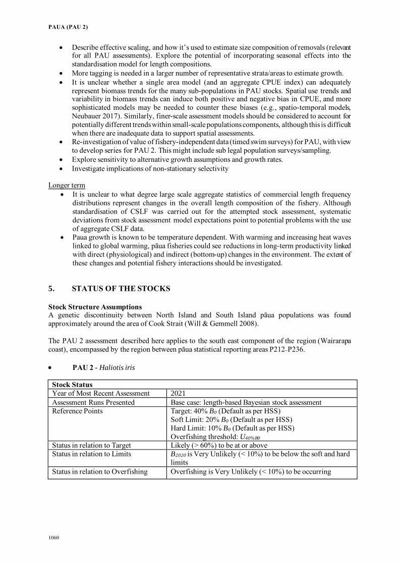
PAUA (PAU 2)
1060
• Describe effective scaling, and how it’s used to estimate size composition of removals (relevant for all PAU assessments). Explore the potential of incorporating seasonal effects into the standardisation model for length compositions.
• More tagging is needed in a larger number of representative strata/areas to estimate growth. • It is unclear whether a single area model (and an aggregate CPUE index) can adequately
represent biomass trends for the many sub-populations in PAU stocks. Spatial use trends and variability in biomass trends can induce both positive and negative bias in CPUE, and more sophisticated models may be needed to counter these biases (e.g., spatio-temporal models, Neubauer 2017). Similarly, finer-scale assessment models should be considered to account for potentially different trends within small-scale populations components, although this is difficult when there are inadequate data to support spatial assessments.
• Re-investigation of value of fishery-independent data (timed swim surveys) for PAU, with view to develop series for PAU 2. This might include sub legal population surveys/sampling.
• Explore sensitivity to alternative growth assumptions and growth rates. • Investigate implications of non-stationary selectivity
Longer term
• It is unclear to what degree large scale aggregate statistics of commercial length frequency distributions represent changes in the overall length composition of the fishery. Although standardisation of CSLF was carried out for the attempted stock assessment, systematic deviations from stock assessment model expectations point to potential problems with the use of aggregate CSLF data.
• Paua growth is known to be temperature dependent. With warming and increasing heat waves linked to global warming, pāua fisheries could see reductions in long-term productivity linked with direct (physiological) and indirect (bottom-up) changes in the environment. The extent of these changes and potential fishery interactions should be investigated.
5. STATUS OF THE STOCKS Stock Structure Assumptions A genetic discontinuity between North Island and South Island pāua populations was found approximately around the area of Cook Strait (Will & Gemmell 2008). The PAU 2 assessment described here applies to the south east component of the region (Wairarapa coast), encompassed by the region between pāua statistical reporting areas P212–P236. • PAU 2 - Haliotis iris Stock Status Year of Most Recent Assessment 2021 Assessment Runs Presented Base case: length-based Bayesian stock assessment Reference Points Target: 40% B0 (Default as per HSS)
Soft Limit: 20% B0 (Default as per HSS) Hard Limit: 10% B0 (Default as per HSS) Overfishing threshold: U40%B0
Status in relation to Target Likely (> 60%) to be at or above Status in relation to Limits B2020 is Very Unlikely (< 10%) to be below the soft and hard
limits Status in relation to Overfishing Overfishing is Very Unlikely (< 10%) to be occurring
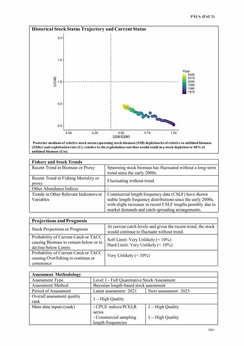
PĀUA (PAU 2)
1061
Historical Stock Status Trajectory and Current Status
Posterior medians of relative stock status (spawning stock biomass (SSB) depletion level relative to unfished biomass (SSB0)) and exploitation rate (U), relative to the exploitation rate that would result in a stock depletion to 40% of unfished biomass (U40).
Fishery and Stock Trends Recent Trend in Biomass or Proxy Spawning stock biomass has fluctuated without a long-term
trend since the early 2000s. Recent Trend in Fishing Mortality or proxy Fluctuating without trend
Other Abundance Indices - Trends in Other Relevant Indicators or Variables
Commercial length frequency data (CSLF) have shown stable length frequency distributions since the early 2000s, with slight increases in recent CSLF lengths possibly due to market demands and catch-spreading arrangements.
Projections and Prognosis
Stock Projections or Prognosis At current catch levels and given the recent trend, the stock would continue to fluctuate without trend.
Probability of Current Catch or TACC causing Biomass to remain below or to decline below Limits
Soft Limit: Very Unlikely (< 10%) Hard Limit: Very Unlikely (< 10%)
Probability of Current Catch or TACC causing Overfishing to continue or commence
Very Unlikely (< 10%)
Assessment Methodology Assessment Type Level 1 - Full Quantitative Stock Assessment Assessment Method Bayesian length-based stock assessment Period of Assessment Latest assessment: 2021 Next assessment: 2025 Overall assessment quality rank 1 – High Quality
Main data inputs (rank) - CPUE indices PCELR series - Commercial sampling length frequencies
1 – High Quality 1 – High Quality

PAUA (PAU 2)
1062
Data not used (rank) CELR CPUE series FSU CPUE series
3 – Low Quality: variable catchability and changes in technology 3 – Low Quality: poor recording
Changes to Model Structure and Assumptions This represents the first accepted assessment model for PAU 2
Major Sources of Uncertainty Growth is known to vary spatially over small scales, and it is unclear how representative the available samples are of the PAU 2 fishery area. Recruitment: length composition data available to the stock assessment provide little information about relative year class strengths. The assessment model is sensitive to natural mortality, which is poorly quantified. Early catch history: Pre QMS pāua exports exceeded catches reported to FMAs, and it is unclear which areas these catches came from. Selectivity in the commercial fishery has varied spatially and over time as voluntarily agreed Minimum Harvest Size (MHS) has changed. Different MHSs have been applied to different statistical areas within the assessed area in the same year.
Qualifying Comments A large proportion of PAU 2, including the Wellington south coast and west of Turakirae, is either a marine reserve or voluntarily closed to commercial fishing. This means that the data collected from the commercial fishery are exclusive of this large area and therefore the assessment only applies to the south east component of PAU 2 (Wairarapa). Lack of contrast in catch, CPUE, and length frequency makes estimation of stock status and biomass trajectories difficult. The 2019–20 year was excluded from the PCELR CPUE series owing to concerns about the comparability with previous years due to the effects of COVID-19 on export markets, and ERS reporting issues. This may continue into the future.
Fishery Interactions -
6. FOR FURTHER INFORMATION Andrew, N L; Naylor, J R; Gerring, P (1999) A modified timed-swim method for paua stock assessment. New Zealand Fisheries Assessment
Report 2000/4. 23 p. Breen, P A; Kim, S W (2004) The 2004 stock assessment of paua (Haliotis iris) in PAU 4. New Zealand Fisheries Assessment Report 2004/55.
79 p. Breen, P A; Kim, S W; Andrew, N L (2003) A length-based Bayesian stock assessment model for abalone. Marine and Freshwater Research
54(5): 619–634. Chen, Y; Breen, P A; Andrew, N L (2000) Impacts of outliers and mis-specification of priors on Bayesian fish stock assessment. Canadian
Journal of Fisheries and Aquatic Science 57: 2293–2305. Fu, D (2014) 2014 PAU 2 stock assessment – Model input. SFWG 14-76. (Unpublished report held by Fisheries New Zealand.) Fu, D; McKenzie, A; Naylor, R (2014a) Summary of input data for the 2013 PAU 3 stock assessment. New Zealand Fisheries Assessment
Report 2014/42. Fu, D; McKenzie, A; Naylor. R (2014b) Summary of input data for the 2013 PAU 5B stock assessment. New Zealand Fisheries Assessment
Report 2014/43. Gerring, P K; Andrew, N L; Naylor, J R (2003) Incidental fishing mortality of paua (Haliotis iris) in the PAU 7 commercial fishery. New
Zealand Fisheries Assessment Report 2003/56. 13 p. Kendrick, T H; Andrew, N L (2000) Catch and effort statistics and a summary of standardised CPUE indices for paua (Haliotis iris) in PAU
5A, PAU 5B, and PAU 5D. New Zealand Fisheries Assessment Report 2000/47. 25 McKenzie, A (2015) Standardised CPUE analyses for paua (Haliotis iris) in PAU 2, 1989–90 to 2013–14 (Draft New Zealand Fisheries
Assessment Report held by Fisheries New Zealand.) McKenzie, A; Naylor, J R; Smith, N H (2009) Characterisation of PAU 2 and PAU 3. Final Research Report. 58 p. (Unpublished report held by
Fisheries New Zealand, Wellington.) Naylor, J R; Andrew, N L (2000) Determination of growth, size composition, and fecundity of paua at Taranaki and Banks Peninsula. New Zealand
Fisheries Assessment Report 2000/51.

PĀUA (PAU 2)
1063
Naylor, J R; Andrew, N L; Kim, S W (2003) Fishery independent surveys of the relative abundance, size-structure, and growth of paua (Haliotis iris) in PAU 4. New Zealand Fisheries Assessment Report 2003/08. 16 p.
Naylor, J R; Andrew, N L; Kim, S W (2006) Demographic variation in the New Zealand abalone Haliotis iris. Marine and Freshwater Research 57: 215–224.
Neubauer, P (2017) Spatial bias in pāua (Haliotis iris) catch-per-unit-effort. New Zealand Fisheries Assessment Report 2017/57. 33 p. Neubauer, P (2020a) The 2020 stock assessment of pāua (Haliotis iris) for PAU 2. Draft New Zealand Fisheries Assessment Report held by
Fisheries New Zealand. Neubauer, P (2020b) Development and application of a spatial stock assessment model for pāua (Haliotis iris). New Zealand Fisheries
Assessment Report 2020/30. 42 p. Neubauer, P (2020c) The 2020 stock assessment of paua (Haliotis iris) for PAU 5A. Draft New Zealand Fisheries Assessment Report held by
Fisheries New Zealand. Neubauer, P (in press) The 2021 stock assessment of pāua (Haliotis iris) for PAU 2. Draft New Zealand Fisheries Assessment Report Neubauer, P; Tremblay-Boyer, L (2019) The 2018 stock assessment of pāua (Haliotis iris) for PAU 5D. New Zealand Fisheries Assessment
Report 2019/39. 58 p. Pirker, J G (1992) Growth, shell-ring deposition and mortality of paua (Haliotis iris Martyn) in the Kaikoura region. MSc thesis, University of
Canterbury. 165 p. Punt, A. E. (2003). The performance of a size-structured stock assessment method in the face of spatial heterogeneity in growth. Fisheries
Research, 65(1), 391–409. Sainsbury, K J (1982) Population dynamics and fishery management of the paua, Haliotis iris. 1. Population structure, growth, reproduction and
mortality. New Zealand Journal of Marine and Freshwater Research 16: 147–161. Schiel, D R (1992) The paua (abalone) fishery of New Zealand. In: Shepherd, S A; Tegner, M J; Guzman del Proo, S (Eds.), Abalone of the World:
Biology, fisheries, and culture. Blackwell Scientific, Oxford. Schiel, D R; Breen, P A (1991) Population structure, ageing and fishing mortality of the New Zealand abalone Haliotis iris. Fishery Bulletin 89:
681–691. Will, M C; Gemmell, N J (2008) Genetic Population Structure of Black Foot paua. Research Report prepared for project GEN2007A. 37 p.
(Unpublished report held by Fisheries New Zealand, Wellington.) Wynne-Jones, J; Gray, A; Heinemann, A; Hill, L; Walton, L (2019) National Panel Survey of Marine Recreational Fishers 2017–2018. New
Zealand Fisheries Assessment Report 2019/24. 104 p.


PĀUA (PAU 3A)
1065
PĀUA (PAU 3A) − Kaikōura
(Haliotis iris) Pāua
1. FISHERY SUMMARY Prior to October 2021, PAU 3A was part of the PAU 3 QMA. The PAU 3 fishery was introduced into the QMS on 1 October 1986 with a TACC of 57 t and later increased to 91.62 t in 1995 as a result of appeals to the Quota Appeal Authority (Table 1). The coastline between the Clarence River and Conway River was closed to commercial and recreational pāua fishing to protect the surviving pāua populations and associated habitats (see coastline in red in Figure above) due to a significant loss of pāua habitat resulting from coastal uplift following the 2016 Kaikōura earthquakes. In addition, the TACC for PAU 3 was lowered to 45.8 t, and the TAC was set at 79.3 t with a customary allowance of 15 t, a recreational allowance of 8.5 t, and other sources of mortality were at 10 t (Table 1). The closure of the Kaikōura coastline to fishing caused fishing effort to move onto the unaffected open Canterbury coastline (now PAU 3B). On 1 October 2021, the PAU 3 QMA was subdivided into two smaller QMAs – PAU 3A (Kaikōura) and PAU 3B (Canterbury) in response to the changed nature of the fishery (see Figure above). At that time, a new TAC, TACC, and allowances were set to reflect the QMA subdivision, pre-earthquake catch levels, and the need to adopt a precautionary approach to enable the fishery to rebuild to continue while providing for utilisation opportunities. Table 1: Total allowable catches (TAC, t) allowances for customary fishing, recreational fishing, and other sources of
mortality (t) and Total Allowable Commercial Catches (TACC, t) declared for PAU 3 and PAU 3A since introduction to the QMS.
Year TAC Customary Recreational
Other mortality TACC
1986–1995* – – – – 57.0 1995–2017* – – – – 91.62 2017–2021* 79.3 15 8.5 10 45.8 2021–present 40.5 7.5 5 5 23.0
*PAU 3 figures
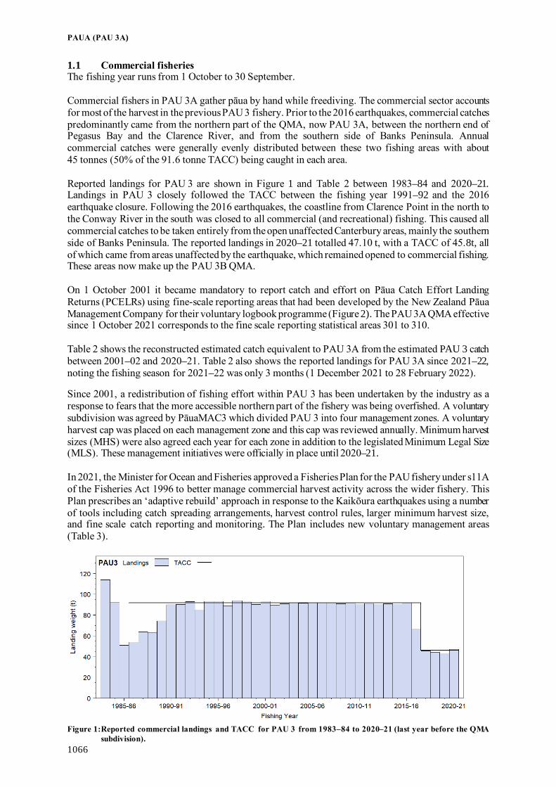
PAUA (PAU 3A)
1066
1.1 Commercial fisheries The fishing year runs from 1 October to 30 September. Commercial fishers in PAU 3A gather pāua by hand while freediving. The commercial sector accounts for most of the harvest in the previous PAU 3 fishery. Prior to the 2016 earthquakes, commercial catches predominantly came from the northern part of the QMA, now PAU 3A, between the northern end of Pegasus Bay and the Clarence River, and from the southern side of Banks Peninsula. Annual commercial catches were generally evenly distributed between these two fishing areas with about 45 tonnes (50% of the 91.6 tonne TACC) being caught in each area. Reported landings for PAU 3 are shown in Figure 1 and Table 2 between 1983–84 and 2020–21. Landings in PAU 3 closely followed the TACC between the fishing year 1991–92 and the 2016 earthquake closure. Following the 2016 earthquakes, the coastline from Clarence Point in the north to the Conway River in the south was closed to all commercial (and recreational) fishing. This caused all commercial catches to be taken entirely from the open unaffected Canterbury areas, mainly the southern side of Banks Peninsula. The reported landings in 2020–21 totalled 47.10 t, with a TACC of 45.8t, all of which came from areas unaffected by the earthquake, which remained opened to commercial fishing. These areas now make up the PAU 3B QMA. On 1 October 2001 it became mandatory to report catch and effort on Pāua Catch Effort Landing Returns (PCELRs) using fine-scale reporting areas that had been developed by the New Zealand Pāua Management Company for their voluntary logbook programme (Figure 2). The PAU 3A QMA effective since 1 October 2021 corresponds to the fine scale reporting statistical areas 301 to 310. Table 2 shows the reconstructed estimated catch equivalent to PAU 3A from the estimated PAU 3 catch between 2001–02 and 2020–21. Table 2 also shows the reported landings for PAU 3A since 2021–22, noting the fishing season for 2021–22 was only 3 months (1 December 2021 to 28 February 2022). Since 2001, a redistribution of fishing effort within PAU 3 has been undertaken by the industry as a response to fears that the more accessible northern part of the fishery was being overfished. A voluntary subdivision was agreed by PāuaMAC3 which divided PAU 3 into four management zones. A voluntary harvest cap was placed on each management zone and this cap was reviewed annually. Minimum harvest sizes (MHS) were also agreed each year for each zone in addition to the legislated Minimum Legal Size (MLS). These management initiatives were officially in place until 2020–21. In 2021, the Minister for Ocean and Fisheries approved a Fisheries Plan for the PAU fishery under s11A of the Fisheries Act 1996 to better manage commercial harvest activity across the wider fishery. This Plan prescribes an ‘adaptive rebuild’ approach in response to the Kaikōura earthquakes using a number of tools including catch spreading arrangements, harvest control rules, larger minimum harvest size, and fine scale catch reporting and monitoring. The Plan includes new voluntary management areas (Table 3).
Figure 1:Reported commercial landings and TACC for PAU 3 from 1983–84 to 2020–21 (last year before the QMA
subdivision).

PĀUA (PAU 3A)
1067
Table 2: TACC and reported landings (t) of pāua in PAU 3 between 1983–84 and 2020–21 and in PAU 3A from 2021–22. * FSU data. † the 2021–22 season was 1 December 2021 to 28 February 2022. The PAU 3A reconstructed landings between 2001–02 and 2020–21 correspond to the PAU 3 estimated catch for statistical areas 301 to 310 which correspond to PAU 3A QMA created in 2021–22.
PAU 3 PAU 3A
Year Landings TACC Reconstructed estimated catch Landings TACC
1983–84* 114.00 – 1984–85* 92.00 – 1985–86* 51.00 – 1986–87* 54.02 57.00 1987–88* 62.99 60.49 1988–89* 57.55 66.48 1989–90 73.46 69.43 1990–91 90.68 77.24 1991–92 90.25 91.50 1992–93 94.52 91.50 1993–94 85.09 91.50 1994–95 93.26 91.50 1995–96 92.89 91.62 1996–97 89.65 91.62 1997–98 93.88 91.62 1998–99 92.54 91.62 1999–00 90.30 91.62 2000–01 93.19 91.62 2001–02 89.66 91.62 71.36 2002–03 90.92 91.62 52.47 2003–04 91.58 91.62 54.64 2004–05 91.43 91.62 52.50 2005–06 91.60 91.62 66.66 2006–07 91.61 91.62 63.27 2007–08 91.67 91.62 60.34 2008–09 90.84 91.62 62.38 2009–10 91.61 91.62 59.01 2010–11 90.40 91.62 56.93 2011–12 91.14 91.62 52.78 2012–13 90.01 91.62 48.54 2013-14 90.85 91.62 46.03 2014–15 90.44 91.62 55.08 2015–16 91.73 91.62 56.90 2016–17 66.29 91.62 17.03 2017–18 45.59 45.80 0 2018–19 44.05 45.80 0 2019–20 43.09 45.80 0 2020–21 47.10 45.80 0 2021–22† 20.74 23.00
Figure 2: Map of fine scale statistical reporting areas for PAU 3.

PAUA (PAU 3A)
1068
Table 3: Summary of the management zones within PAU 3A as initiated by PāuaMAC3.
Management zone (since 2021) Area Statistical area zone 3A1 Paparoa P301–P302 3A2 Rakautara P303–P304 3A3 Omihi P307–P308 3A4 Oaro P309–P310
1.2 Recreational fisheries For further information on recreational fisheries refer to the Introduction – Pāua chapter. The ‘National Panel Survey of Marine Recreational Fishers 2017–18: Harvest Estimates’ estimated that the recreational harvest for PAU 3 was 8.8 t with a CV of 35% (Wynne-Jones et al 2019). For the 2013 stock assessment, the Shellfish Working Group (SFWG) agreed to assume that the recreational catch rose linearly from 5 t in 1974 to 17 t in 2013. Following initial high levels of mortality related to the earthquake, local pāua abundance recovered significantly, and the pāua fishery was re-opened on 1 December 2021, until 1 March 2022. The significant local interest in the fishery and high numbers of easily accessible pāua were considered likely to lead to a very active recreational fishery, once reopened. Therefore, a recreational harvest estimation survey (Holdsworth 2021) using a roving access design was implemented over the December to March fishing period. Preliminary recreational harvest estimates are anticipated by the end of May 2022. 1.3 Customary fisheries Pāua is a taonga species and as such there is an important customary use of pāua by Maori for food, and the shells have been used extensively for decorations and fishing devices. For information on customary catch regulations and reporting refer to the Introduction – Pāua chapter. Estimates of customary catch for PAU 3 are shown in Table 4. These numbers are likely to be an underestimate of customary harvest because only the catch approved and harvested in numbers are reported in the table. In addition, many tangata whenua also harvest pāua under their recreational allowance and these are not included in records of customary catch. Landings before 2010–11 do not include the area between the Hurunui River and the South Shore (just north of Banks Peninsula), because tangata tiaki were not appointed there until November 2009. Estimates of customary take before the 2016 earthquakes ranged from about 7 to 13 tonnes. Customary take then initially declined given the immediate loss of significant pāua abundance along the Kaikoura coastline, but increased in 2019–20 in response to feeding the local communities during the Covid-19 event. Information is not available at the PAU 3A level up to 2020–21. Table 4: Fisheries New Zealand records of customary harvest of pāua (approved and reported in numbers) in PAU 3
since 2000–01. Landings data before 2010–11 exclude the area between the Hurunui River and Pegasus Bay. – no data.
Fishing Numbers Fishing Numbers year Approved Harvested year Approved Harvested 2000–01 300 230 2012–13 15 036 12 874 2001–02 6 239 4 832 2013–14 10 259 7 566 2002–03 3 422 2 449 2014–15 8 761 7 035 2003–04 – – 2015–16 14 801 11 808 2004–05 – – 2016–17 11 374 9 217 2005–06 1 580 1 220 2017–18 2 708 1 725 2006–07 5 274 4 561 2018–19 480 278 2007–08 7 515 5 790 2019–20 30 288 21 527 2008–09 10 848 8 232 2020–21 4 960 3 242 2009–10 8 490 6 467 2010–11 8 360 7 449 2011–12 5 675 4 242

PĀUA (PAU 3A)
1069
1.4 Illegal catch For further information on illegal catch refer to the Introduction – Pāua chapter. For the purpose of the 2013 stock assessment, the SFWG agreed to assume that illegal catches rose linearly from 5 t in 1974 to 15 t in 2000 and remained at 15 t between 2001 and 2013. 1.5 Other sources of mortality The Working Group agreed that handling mortality would not be included in the model. For further information on other sources of mortality refer to the Introduction – Pāua chapter. On 16 November 2016 a 7.8 magnitude earthquake hit the upper east coast of the South Island, causing extensive uplift of about 110 km of coastline by as much as 4 m in some areas. This resulted in the widespread mortality of marine organisms, changes to the structure of intertidal and subtidal rocky reefs, and significant alterations to the structure of nearshore reef communities (Alestra et al 2019). Ongoing monitoring of these nearshore reef communities has revealed signs of recovery in the low intertidal zones, whereas sub-tidally there has been little recovery in areas that were de-vegetated and previously abundant algal stands appear to have become sparser and more fragmented (Alestra et al 2020). The whole northern part of the PAU 3 fishery (Pāua Statistical Areas P301 to P310, now PAU 3A, Figure 3) was impacted to varying degrees by the earthquake. The earthquake caused the direct mortality of a large number of juvenile and adult pāua that became exposed to the terrestrial environment with no means of being able to return to the water. More indirect mortality is also expected from the earthquake due to an immediate loss of pre-earthquake pāua habitat that now lies above the new post-earthquake high tide mark. Although the impacts of the seabed uplift on pāua populations around Kaikōura will only become clear in the longer term, work was undertaken to evaluate the area utilised by the pāua fishery that is now above the post-earthquake low tide mark (Neubauer 2017). The results suggested that the seabed uplift led to a loss of up to 50% of the pre-earthquake fished area in the pāua statistical areas P301 to P310. In area 301, the habitat loss was 7 ha, which corresponds to 52% of the fished area. However, this area has contributed relatively little to the commercial catch. In area 302, which has contributed a larger proportion of the PAU 3 commercial catch, the area lost was 43 ha, which corresponds to 43% of the fished area. In other affected areas, the area lost was generally less than 10%. Across PAU 3 statistical areas, a total of 21% of the fished area (24% of catch weight as recorded on PCELR forms), was impacted by uplift (Figure 3). The immediate loss of area to the fishery, assumed to be good habitat for pāua, is only part of the impact that the seabed uplift associated with the Kaikōura earthquake will have on pāua populations. Juvenile pāua recruit in shallow water, and so the loss of juvenile habitat will have been higher than the loss of adult habitat. This will impact on the number of juvenile pāua growing into the fishery over the coming years. Recent surveys have indicated large scale recovery of pāua populations in the affected areas (McCowan & Neubauer 2021, 2022).

PAUA (PAU 3A)
1070
Figure 3:Percent fished area above the post-earthquake low tide mark for statistical areas within the Kaikōura
earthquake fishery closure zone. Grey indicates that no post-earthquake elevation data were available. 2. BIOLOGY For further information on pāua biology refer to the Introduction – Pāua chapter. A summary of published estimates of biological parameters for PAU 3 is presented in Table 5. Note, that these values are from the most recent stock assessment covering the whole of PAU 3 and may therefore not be appropriate for PAU 3A. No area-specific, representative biological data are available for PAU 3A. Table 5: Estimates of biological parameters (H. iris) in PAU 3. Estimate Source 1. Natural mortality (M) 0.135 (0.120–0.153) Median (5–95% range) of posterior distribution for the base case model 2. Weight = a(length)b (Weight in g, length in mm shell length) All a b 2.99 x 10 -5 3.303 Schiel & Breen (1991) 3. Size at maturity (shell length) 50% maturity at 82 mm (80–84) Median (5–95% range) of posterior distribution for the base case model 95% maturity at 102 mm (96–108) Median (5–95% range) of posterior distribution for the base case model 3. STOCKS AND AREAS For further information on stocks and areas refer to the Introduction – Pāua chapter.

PĀUA (PAU 3A)
1071
4. STOCK ASSESSMENT The last assessment for PAU 3 was conducted in 2014; however, given the potential effects of the earthquake, it is unclear how representative estimates from this assessment are for the current PAU 3A stock. Details of the PAU 3 stock assessment are given by Fu (2014). Since the PAU 3A area has been closed to fishing, no stock assessment has been conducted. The fishery reopened in 2021–22 and several years of landing data will be necessary before a stock assessment can be attempted. 4.1 Biomass survey and monitoring Following the 2016 Kaikōura earthquake, a biomass survey was implemented to estimate and monitor pāua abundance and recruitment in the earthquake-affected area, to inform management decisions relating to the re-opening of the pāua fishery (McCowan & Neubauer 2018, 2022). To estimate abundance, novel methodologies using GPS dive loggers and underwater electronic callipers were developed. Thirty-five sites were initially surveyed to obtain baseline estimates of site- and fishery-level abundance and length-frequency. Pāua were mostly found in aggregations, preferentially in shallow water. This was not just the case for small pāua but also for large individuals (i.e., over 120 mm), although smaller individuals (under 100 mm) showed a strongly decreasing trend with depth. Initially estimated pāua density was 0.028 pāua per square metre (geometric mean; 95% confidence interval (CI) [0.009; 0.08]) across the earthquake-affected fishery closure. Scaling density estimates to total biomass or abundance was difficult due to the lack of robust estimates of habitat area for pāua. In the absence of a defensible solution, only density was calculated. After the first two years, the project has been extended for another three years until mid-2023. As of March 2022, four further rounds of surveys of the 35 initially surveyed sites have been undertaken to monitor pāua abundance and recruitment trends. Initially an assessment was made of the appropriateness of using the number of measurements per unit effort (MPUE) as a proxy for pāua density to overcome issues with missing data from GPS dive units (originally used to delimit area to estimate density) and to enable the use of significantly larger data sets of measurements and counts of pāua at each site. The measurements per unit effort, as well as biomass per unit of survey effort (BPUE, number of measurements multiplied by the length frequency distribution of measured pāua), correlated well (R2=0.86) with density. Therefore, MPUE and BPUE were used as indices of changes in pāua density.
Figure 4: Marginal trend (relative to a geometric mean of 1) in biomass per unit effort (BPUE) across survey years for
QMAs PAU 3 and PAU 7 from the BPUE model after accounting for confounding variables.

PAUA (PAU 3A)
1072
An overall increase in pāua abundance was observed at a QMA-wide level in both QMAs over the four survey periods (Figure 4). Increased abundance was generally more pronounced in PAU 7 than in PAU 3. In PAU 3, abundance trended slightly downwards in the second survey period, which was likely due to the consistently poor survey conditions during the period, as well as a potential bias towards sampling sites with lower rates of increase due to weather conditions. There was high variability in abundance trends across sites. This variability was in part related to variability in the amount of uplift at each site, because sites with a larger increase in abundance were those with less uplift (Figure 5). Variability in abundance trends across sites could also be linked to habitat related factors and pre-earthquake abundance. Comparison of length frequency profiles across the four survey periods showed reasonably stable profiles in larger size classes (125–160 mm, Figure 6), with an increase in the number of individuals in the 80–100 mm size range in both QMAs, which is likely to be indicative of post-earthquake recruitment. Recruitment signals were variable between sites due to differences in available recruitment habitat and variability in uplift.
Figure 5:Marginal trend (relative to a geometric mean of 1 at each site) in biomass per unit effort (BPUE) across survey
years for QMAs PAU 3 and PAU 7 from the BPUE model after accounting for confounding variables.

PĀUA (PAU 3A)
1073
Figure 6: Length-frequency profiles (as relative densities) for all pāua measured over four survey periods in PAU 3
and PAU 7. Vertical lines show the legal size of 125 mm (MLS; solid line), 135 mm (dashed line), and 145 mm (dotted line).
5. STATUS OF THE STOCK • PAU 3A - Haliotis iris Stock Status
Year of Most Recent Assessment The most recent assessment for PAU 3, conducted in 2014, is thought to be of limited use for the PAU 3A area since the 2016 Kaikoura earthquake
Assessment Runs Presented N/A
Reference Points
Target: 40% B0 (Default as per HSS) Soft Limit: 20% B0 (Default as per HSS) Hard Limit: 10% B0 (Default as per HSS) Overfishing threshold: U40%B0
Status in relation to Target Unknown, but likely relatively high given CPUE levels are well above most other mainland QMAs, and a substantial biomass rebuild is evident in surveys post-earthquake
Status in relation to Limits Unknown Status in relation to Overfishing Unknown Fishery and Stock Trends
Recent Trend in Biomass or Proxy Recent trends in the survey index provide evidence of a substantial recovery of biomass since the 2016 earthquake.
Recent Trend in Fishing Intensity or Proxy Unknown
Other Abundance Indices - Trends in Other Relevant Indicators or Variables
Survey length frequencies showed both post-earthquake recruitment and increase in mean length.

PAUA (PAU 3A)
1074
Projections and Prognosis Stock Projections or Prognosis Unknown Probability of Current Catch or TACC causing Biomass to remain below or to decline below Limits
Unknown
Probability of Current Catch or TACC causing Overfishing to continue or to commence
Unknown
Assessment Methodology and Evaluation Assessment Type N/A Assessment Method N/A Assessment Dates Latest: Next: unknown Overall assessment quality (rank) - Main data inputs (rank) - Data not used (rank) N/A Changes to Model Structure and Assumptions -
Major Sources of Uncertainty - Qualifying Comments: The last assessment was conducted in 2014; however, given the potential effects of the earthquake, it is unclear how representative estimates from this assessment are for the current pāua stock.
Fishery Interactions -
6. FOR FURTHER INFORMATION Alestra, T; Gerrity, S; Dunmore, R A; Marsden, I; Pirker, J; Schiel, D R (2019) Rocky reef impacts of the Kaikōura earthquake: quantification
and monitoring of nearshore habitats and communities. New Zealand Aquatic Environment and Biodiversity Report No. 212. 120 p. Alestra, T; Gerrity, S; Dunmore, R A; Schiel, D R (2020) Rocky reef impacts of the Kaikōura earthquake: extended monitoring of nearshore
habitats and communities – Year 1 results. New Zealand Fisheries Assessment Report 2019/01. 40 p. Breen, P A; Kim, S W; Andrew, N L (2003) A length-based Bayesian stock assessment model for abalone. Marine and Freshwater Research
54(5): 619–634. Fu, D (2013) The 2012 stock assessment of paua (Haliotis iris) for PAU 5D. New Zealand Fisheries Assessment Report. 2013/57. Fu, D (2014) The 2013 stock assessment of paua (Haliotis iris) for PAU 3. New Zealand Fisheries Assessment Report 2014/44. Gerring, P K; Andrew, N L; Naylor, J R (2003) Incidental fishing mortality of paua (Haliotis iris) in the PAU 7 commercial fishery. New Zealand
Fisheries Assessment Report 2003/56. 13 p. Gorfine, H K; Dixon, C D (2000) A behavioural rather than resource-focused approach may be needed to ensure sustainability of quota managed
abalone fisheries. Journal of Shellfish Research 19: 515–516. Holdsworth, J C (2021) Pāua amateur harvest survey design for the Kaikōura Marine Area. New Zealand Fisheries Assessment Report 2021/63.
13 p. Kim, S W (2004) CPUE analysis of fine-scale logbook data for PAU 3. Ministry of Fisheries Research Report PAU 2001/01 Obj. 7.
(Unpublished report held by Fisheries New Zealand, Wellington). McCowan, T; Neubauer, P (2018) Paua biomass estimates and population monitoring in areas affected by the November 2016 Kaikoura
earthquake. New Zealand Fisheries Assessment Report 2018/54. 24 p. McCowan, T; Neubauer, P (2021) Pāua abundance trends and population monitoring in areas affected by the November 2016 Kaikōura
earthquake. New Zealand Fisheries Assessment Report 2021/26. 23 p. McCowan, T A; Neubauer, P (2022) Pāua abundance trends and population monitoring in areas affected by the November 2016 Kaikōura
earthquake, December 2021 update. New Zealand Fisheries Assessment Report 2022/15. 20 p. McKenzie, A; Naylor, J R; Smith, N H (2009) Characterisation of PAU 2 and PAU 3. Final Research Report. 58 p. (Unpublished report held by
Fisheries New Zealand, Wellington). Naylor, J R; Andrew, N L (2000) Determination of growth, size composition, and fecundity of paua at Taranaki and Banks Peninsula. New
Zealand Fisheries Assessment Report. 2000/51. 25 p. Naylor, J R; Andrew, N L; Kim, S W (2006) Demographic variation in the New Zealand abalone Haliotis iris. Marine and Freshwater Research
57: 215–224. Neubauer, P (2017) Area lost to the paua fishery from the November 2016 Kaikoura earthquake, 7 p. (Unpublished report held by Fisheries New
Zealand). Pirker, J G (1992) Growth, shell-ring deposition and mortality of paua (Haliotis iris Martyn) in the Kaikoura region. MSc thesis, University of
Canterbury. 165 p. Poore, G C B (1972) Ecology of New Zealand abalones, Haliotis species (Mollusca: Gastropoda). 3. Growth. New Zealand Journal of Marine
and Freshwater Research 6, 534–59. Poore, G C B (1973) Ecology of New Zealand abalones, Haliotis species (Mollusca: Gastropoda). 4. Reproduction. New Zealand Journal of
Marine and Freshwater Research 7 (1&2): 67–84.

PĀUA (PAU 3A)
1075
Sainsbury, K J (1982) Population dynamics and fishery management of the paua, Haliotis iris. 1. Population structure, growth, reproduction and mortality. New Zealand Journal of Marine and Freshwater Research 16: 147–161.
Schiel, D R (1992) The paua (abalone) fishery of New Zealand. In: Shepherd, S A; Tegner, M J; Guzman del Proo, S (Eds.), Abalone of the World: Biology, fisheries, and culture. Blackwell Scientific, Oxford.
Schiel, D R; Breen, P A (1991) Population structure, ageing and fishing mortality of the New Zealand abalone Haliotis iris. Fishery Bulletin 89: 681–691.
Shepherd, S A; Partington, D (1995) Studies on Southern Australian abalone (genus Haliotis). XVI. Recruitment, habitat and stock relations. Marine and Freshwater Research 46: 669–680.
Will, M C; Gemmell, N J (2008) Genetic Population Structure of Black Foot paua. (Unpublished report for GEN2007A, held by Fisheries New Zealand, Wellington.) 37 p.
Wynne-Jones, J; Gray, A; Heinemann, A; Hill, L; Walton, L (2019) National Panel Survey of Marine Recreational Fishers 2017–2018. New Zealand Fisheries Assessment Report 2019/24. 104 p.


PĀUA (PAU 3B)
1077
PĀUA (PAU 3B) − Canterbury
(Haliotis iris) Pāua
1. FISHERY SUMMARY Prior to October 2021, PAU 3B was part of the PAU 3 QMA, which was introduced into the QMS on 1 October 1986 with a TACC of 57 t and later increased to 91.62 t in 1995 as a result of appeals to the Quota Appeal Authority (Table 1). The coastline between the Clarence River and Conway River was closed to commercial and recreational pāua fishing to protect the surviving pāua populations and associated habitats (see coastline in red in figure above) due to a significant loss of pāua habitat resulting from coastal uplift following the 2016 Kaikōura earthquakes. In addition, the TACC was lowered to 45.8 t, and a TAC was set at 79.3 t with a customary allowance of 15 t, a recreational allowance of 8.5 t, and other sources of mortality were at 10 t (Table 1). The closure of the Kaikōura coastline to fishing caused fishing effort to move onto the unaffected open Canterbury coastline, south of statistical area P310 (now PAU 3B). On 1 October 2021, the PAU 3 QMA was subdivided into two smaller QMAs – PAU 3A (Kaikōura) and PAU 3B (Canterbury) in response to the changed nature of the fishery (see figure above). At that time, a new TAC, TACC, and allowances were set to reflect the QMA subdivision, pre-earthquake catch levels, and the need to adopt a precautionary approach to enable the PAU 3A fishery rebuild to continue while providing for utilisation opportunities. Table 1: Total allowable catches (TAC, t) allowances for customary fishing, recreational fishing, and other sources of
mortality (t) and Total Allowable Commercial Catches (TACC, t) declared for PAU 3 and PAU 3B since introduction to the QMS.
Year TAC Customary Recreational
Other mortality TACC
1986–1995* – – – – 57.0 1995–2017* – – – – 91.62 2017–2021* 79.3 15 8.5 10 45.8 2021–present 80 15 9 10 46
*PAU 3 figures

PAUA (PAU 3B)
1078
1.1 Commercial fisheries The fishing year runs from 1 October to 30 September. Commercial fishers in PAU 3B gather pāua by hand while freediving. The commercial sector accounts for most of the harvest in the previous PAU 3 fishery. Prior to the 2016 earthquakes, commercial catches predominantly came from the Kaikōura coastline (now PAU 3A) and Motunau/Banks Peninsula. Annual commercial catches were generally evenly distributed between these two fishing areas with about 45 tonnes (50% of the 91.6 tonne TACC) being caught in each area. Following the 2016 earthquakes, the coastline from Clarence Point in the north to the Conway River in the south was closed to all commercial (and recreational) fishing. This caused all commercial catches to be taken entirely from the open unaffected Canterbury areas, mainly the southern side of Banks Peninsula. Landings in PAU 3 have closely followed the TACC since the fishing year 1991–92 (Table 2). The reported landings in 2020–21 totalled 47.10 t, with a TACC (t) of 45.8 t. Table 2: TACC and reported landings (t) of pāua in PAU 3 since 1983–84. * FSU data. The PAU 3B reconstructed
landings between 2001-02 and 2020-21 correspond to the PAU 3 estimated catch for statistical areas 311 to 339 which correspond to PAU 3B QMA created in 2021–22.
PAU 3 PAU 3B
Year Landings TACC Reconstructed estimated catch
1983–84* 114.00 – 1984–85* 92.00 – 1985–86* 51.00 – 1986–87* 54.02 57.00 1987–88* 62.99 60.49 1988–89* 57.55 66.48 1989–90 73.46 69.43 1990–91 90.68 77.24 1991–92 90.25 91.50 1992–93 94.52 91.50 1993–94 85.09 91.50 1994–95 93.26 91.50 1995–96 92.89 91.62 1996–97 89.65 91.62 1997–98 93.88 91.62 1998–99 92.54 91.62 1999–00 90.30 91.62 2000–01 93.19 91.62 2001–02 89.66 91.62 19.67 2002–03 90.92 91.62 37.29 2003–04 91.58 91.62 35.47 2004–05 91.43 91.62 36.01 2005–06 91.60 91.62 23.80 2006–07 91.61 91.62 26.72 2007–08 91.67 91.62 28.50 2008–09 90.84 91.62 26.73 2009–10 91.61 91.62 31.50 2010–11 90.40 91.62 33.59 2011–12 91.14 91.62 38.15 2012–13 90.01 91.62 40.99 2013-14 90.85 91.62 44.19 2014–15 90.44 91.62 33.73 2015–16 91.73 91.62 32.66 2016–17 66.29 91.62 48.76 2017–18 45.59 45.80 45.49 2018–19 44.05 45.80 44.46 2019–20 43.09 45.80 41.20 2020–21 47.10 45.80 45.54

PĀUA (PAU 3B)
1079
On 1 October 2001 it became mandatory to report catch and effort on Pāua Catch Effort Landing Returns (PCELRs) using fine-scale reporting areas that had been developed by the New Zealand Pāua Management Company for their voluntary logbook programme (Figure 1). Reported landings for PAU 3 are shown in Figure 2 and Table 2 between 1983–84 and 2020–21. The PAU 3B QMA effective since 1 October 2021 corresponds to the fine-scale reporting statistical areas 311 to 339. Table 2 shows the reconstructed estimated catch equivalent to PAU 3B from the estimated PAU 3 catch between 2001–02 and 2020–21.
Figure 1: Map of fine scale statistical reporting areas for PAU 3. Since 2001, a redistribution of fishing effort within PAU 3 has been undertaken by the industry as a response to fears that the more accessible northern part of the fishery was being overfished. A voluntary subdivision was agreed by PāuaMAC3 which divided PAU 3 into four management zones. A voluntary harvest cap was placed on each management zone and this cap was reviewed annually. Minimum harvest sizes (MHS) were also agreed each year for each zone in addition to the legislated Minimum Legal Size (MLS). These management initiatives were officially in place until 2020–21. In 2021, the Minister for Ocean and Fisheries approved a Fisheries Plan for the PAU fishery under s11A of the Fisheries Act 1996 to better manage commercial harvest activity across the wider fishery. This Plan prescribes using an ‘adaptive rebuild’ approach in response to the Kaikōura earthquakes using a number of tools including catch spreading arrangements, harvest control rules, larger minimum harvest size, and fine scale catch reporting and monitoring. The Plan includes new voluntary management areas (Table 3).

PAUA (PAU 3B)
1080
Figure 2: Reported commercial landings and TACC for PAU 3 from 1983–84 to 2020–21 (last year before the QMA
subdivision). Table 3: Summary of the management zones within PAU 3B as initiated by PāuaMAC3.
Management zone (since 2021) Area Statistical area zone 3B1 Conway River to Motunau Island P311–P317 3B2 Motunau Island P318 3B3 Motunau Island to Hickory Bay P319–P329 3B4 Hickory Bay to Te Oka Bay P330–P335 3B5 Te Oka Bay to Waitaki River P336-P339
1.2 Recreational fisheries For further information on recreational fisheries refer to the Introduction – Pāua chapter. The ‘National Panel Survey of Marine Recreational Fishers 2017–18: Harvest Estimates’ estimated that the recreational harvest for PAU 3 was 8.8 t with a CV of 35% (Wynne-Jones et al 2019). For the 2013 stock assessment, the Shellfish Working Group (SFWG) agreed to assume that the recreational catch rose linearly from 5 t in 1974 to 17 t in 2013. 1.3 Customary fisheries Pāua is a taonga species and as such there is an important customary use of pāua by Maori for food, and the shells have been used extensively for decorations and fishing devices. For information on customary catch regulations and reporting refer to the Introduction – Pāua chapter. Estimates of customary catch for PAU 3 are shown in Table 4. These numbers are likely to be an underestimate of customary harvest because only the catch approved and harvested in numbers are reported in the table. In addition, many tangata whenua also harvest pāua under their recreational allowance and these are not included in records of customary catch. Landings before 2010–11 do not include the area between the Hurunui River and the South Shore (just north of Banks Peninsula), because tangata tiaki were not appointed there until November 2009. Estimates of customary take before the 2016 earthquakes ranged from about 7 to 13 tonnes. Customary take then initially declined given the immediate loss of significant pāua abundance along the Kaikōura coastline, but increased in 2019–20 in response to feeding the local communities during the Covid-19 event. Information is not available at the PAU 3B level up to 2020–21.

PĀUA (PAU 3B)
1081
Table 4: Fisheries New Zealand records of customary harvest of pāua (approved and reported in numbers) in PAU 3 since 2000–01. Landings data before 2010–11 exclude the area between the Hurunui River and Pegasus Bay. – no data.
Numbers Fishing year Approved Harvested 2000–01 300 230 2001–02 6 239 4 832 2002–03 3 422 2 449 2003–04 – – 2004–05 – – 2005–06 1 580 1 220 2006–07 5 274 4 561 2007–08 7 515 5 790 2008–09 10 848 8 232 2009–10 8 490 6 467 2010–11 8 360 7 449 2011–12 5 675 4 242 2012–13 15 036 12 874 2013–14 10 259 7 566 2014–15 8 761 7 035 2015–16 14 801 11 808 2016–17 11 374 9 217 2017–18 2 708 1 725 2018–19 480 278 2019–20 30 288 21 527 2020–21 4 960 3 242
1.4 Illegal catch For further information on illegal catch refer to the Introduction – Pāua chapter. Within the 2021 stock assessment process (no accepted assessment was produced), the SFWG agreed to assume that illegal catches rose linearly from 1 t in 1974 to 10 t in 1990 and remained at 10 t between 1990 and 2000. A subsequent decline in illegal fishing from 10 t in 2000 to 2 t by 2010 was assumed due to perceived advances in fisheries enforcement. 1.5 Other sources of mortality For further information on other sources of mortality refer to the Introduction – Pāua chapter. On 16 November 2016 a 7.8 magnitude earthquake hit the upper east coast of the South Island, causing extensive uplift of about 110 km of coastline by as much as 4 m in some areas. This resulted in the widespread mortality of marine organisms, changes to the structure of intertidal and subtidal rocky reefs, and significant alterations to the structure of nearshore reef communities (Alestra et al 2019). The whole northern part of the PAU 3 fishery (Pāua Statistical Areas P301 to P310, now PAU 3A) was impacted to varying degrees by the earthquake; however, the area now included within PAU 3B was largely unaffected. The earthquake caused the direct mortality of a large number of juvenile and adult pāua that became exposed to the terrestrial environment with no means of being able to return to the water. More indirect mortality is also expected from the earthquake due to an immediate loss of pre-earthquake pāua habitat that now lies above the new post-earthquake high tide mark. 2. BIOLOGY For further information on pāua biology refer to the Introduction – Pāua chapter. A summary of published estimates of biological parameters for PAU 3 is presented in Table 5. Note, that these values are from the most recent stock assessment covering the whole of PAU 3 and may therefore not be appropriate for PAU 3B. No area-specific, representative biological data are available for PAU 3B.

PAUA (PAU 3B)
1082
Table 5: Estimates of biological parameters (H. iris) in PAU 3. Estimate Source 1. Natural mortality (M) 0.135 (0.120–0.153) Median (5–95% range) of posterior distribution for the base case model 2. Weight = a(length)b (Weight in g, length in mm shell length) All a b 2.99 x 10 -5 3.303 Schiel & Breen (1991) 3. Size at maturity (shell length) 50% maturity at 82 mm (80–84) Median (5–95% range) of posterior distribution for the base case model 95% maturity at 102 mm (96–108) Median (5–95% range) of posterior distribution for the base case model 3. STOCKS AND AREAS For further information on stocks and areas refer to the Introduction – Pāua chapter. 4. STOCK ASSESSMENT A stock assessment for the PAU 3B area was attempted in 2021–22, based on estimates of historical catches, CPUE trends, and commercial length frequency data. CPUE trends were found to be stable despite steady increases in catch over the past decades. For this reason, all stock assessment models that were attempted estimated an exceedingly high biomass that was judged to be implausible by the Fisheries New Zealand Shellfish Working Group. In the absence of an acceptable assessment model, the Shellfish Working Group explored comparative analyses of absolute CPUE in PAU 3B in comparison with areas of assessed stock status. These analyses were used to gain a qualitative understanding of current biomass level and exploitation rate in the fishery. 4.1 Relative abundance estimates from standardised CPUE analyses PCELR and ERS data from 2002 to 2021 were used to derive a standardised, fishery-dependent index of abundance, initially for use within a stock assessment model, and subsequently to estimate median current absolute CPUE. Data prior to 2002 (CELR, FSU reporting) were not used in the assessment process; as for other recent assessments, changes to the composition of the fleet and gear during the 1990s, combined with inconsistent reporting, mean that the trends in CPUE from CELR data are questionable, and likely hyper-stable to an unknown degree in most PAU QMAs. CPUE standardisation was carried out using Bayesian Generalised Linear Mixed Models (GLMM) which partitioned variation among fixed (research strata) and random variables. CPUE was defined as the log of daily catch. Variables in the model were fishing year, estimated fishing effort, client number, research stratum, diver ID (PCELR). Previous standardisation models for PCELR data routinely used small scale statistical areas as a standardising variable. For the present assessment, this variable was not available with sufficient precision for recent (ERS) data, where it is inferred from position data, and was therefore omitted. Nevertheless, follow-up work on the quality of ERS data for pāua CPUE suggested limited effects of spatial reporting and the inclusion, or not, of statistical areas in the standardisation made little difference to resulting indices before 2021 (Neubauer in prep). Standardised CPUE in all areas suggested increases in recent years, after nearly two decades of stable CPUE (Figure 3), with most notable increase in zone B2 - Motunau Island, and highly variable trends in raw CPUE in other areas. While other zones (B3, B4) also showed increases in raw CPUE in 2020 and 2021, these increases were largely compensated by the standardisation model. Median absolute CPUE (> 50 kg/h) was found to be substantially higher than in all assessed PAU QMAs (< 50 kg/h), suggesting that current PAU densities in PAU 3B are high relative to other QMAs. The latter may be linked to relatively low catches across the PAU 3B area prior to the 2016 Kaikōura earthquake, when most of the commercial catch was located in areas PAU 301–310, which now make up the PAU 3A QMA.

PĀUA (PAU 3B)
1083
4.2 Other factors Another source of uncertainty are the catch data. The commercial catch is known with accuracy since 1985 but is probably not well estimated before that. Furthermore, the recent split of PAU 3 into PAU 3A and PAU 3B following the Kaikōura earthquake and subsequent fishery closure did not match the early (CELR) reporting areas, leading to substantial uncertainties about catch prior to 2002, when PCELR and fine-scale reporting was introduced. In addition, non-commercial catch estimates are poorly determined. Therefore, better information on the scale and trend in recreational catch needs to be collated for more accurate assessment of the stock status.
Figure 3: Raw CPUE (points are median with inter-quartile interval indicated by vertical intervals) and standardised
CPUE index (line) with 95% confidence interval (shaded ribbon) by industry management zone (B1-B5) and overall (All). Shading of points indicates the relative amount of data available for standardisation.
PAUA (PAU 3B)
1084
5. STATUS OF THE STOCK • PAU 3B - Haliotis iris Stock Status
Year of Most Recent Assessment 2022, not successful given conflicting signals in catch and CPUE trends
Assessment Runs Presented -
Reference Points Target: 40% B0 (Default as per HSS) Soft Limit: 20% B0 (Default as per HSS) Hard Limit: 10% B0 (Default as per HSS) Overfishing threshold: U40%B0
Status in relation to Target Unknown, but likely relatively high given that CPUE levels are well above most other mainland QMAs
Status in relation to Limits Unknown Status in relation to Overfishing Unknown Fishery and Stock Trends
Recent Trend in Biomass or Proxy CPUE has been stable or increasing in all management zones, despite increasing catches.
Recent Trend in Fishing Intensity or Proxy
Steady increase in catch over the past decades, but high and stable CPUE suggests low overall exploitation rates.
Other Abundance Indices - Trends in Other Relevant Indicators or Variables -
Projections and Prognosis Stock Projections or Prognosis Unknown Probability of Current Catch or TACC causing Biomass to remain below or to decline below Limits
Unknown
Probability of Current Catch or TACC causing Overfishing to continue or to commence
Unknown
Assessment Methodology and Evaluation Assessment Type None accepted Assessment Method N/A Assessment Dates Latest: 2021 Next: unknown Overall assessment quality (rank) N/A
Main data inputs (rank)
- Catch history 1 – High Quality for commercial catch 2 – Medium or Mixed Quality for recreational catch, which is not believed to be fully representative over the history of the fishery
- CPUE indices early series
2 – Medium or Mixed Quality: not believed to proportional to abundance
- CPUE indices later series (since 2002)
1 – High Quality
- Commercial sampling length frequencies
1 – High Quality

PĀUA (PAU 3B)
1085
- Tag recapture data (to estimate growth)
2 – Medium or Mixed Quality: no area specific data, inferred from meta-analysis of NZ wide data
- Maturity at length data
1 – Medium or Mixed Quality: no area specific data, inferred from meta-analysis of New Zealand wide data
Data not used (rank) N/A Changes to Model Structure and Assumptions No accepted stock assessment model
Major Sources of Uncertainty
- Catch levels and trends uncertain prior to 2002 - CPUE may not be a reliable index of abundance at low exploitation rates - Very little growth data available and growth not well known
Qualifying Comments: -
Fishery Interactions -
6. FOR FURTHER INFORMATION Alestra, T; Gerrity, S; Dunmore, R A; Marsden, I; Pirker, J; Schiel, D R (2019) Rocky reef impacts of the Kaikōura earthquake: quantification
and monitoring of nearshore habitats and communities. New Zealand Aquatic Environment and Biodiversity Report No. 212. 120 p. Alestra, T; Gerrity, S; Dunmore, R A; Schiel, D R (2020) Rocky reef impacts of the Kaikōura earthquake: extended monitoring of nearshore
habitats and communities – Year 1 results. New Zealand Fisheries Assessment Report 2019/01. 40 p. Breen, P A; Kim, S W; Andrew, N L (2003) A length-based Bayesian stock assessment model for abalone. Marine and Freshwater Research
54(5): 619–634. Fu, D (2013) The 2012 stock assessment of paua (Haliotis iris) for PAU 5D. New Zealand Fisheries Assessment Report. 2013/57. Fu, D (2014) The 2013 stock assessment of paua (Haliotis iris) for PAU 3. New Zealand Fisheries Assessment Report 2014/44. Gerring, P K; Andrew, N L; Naylor, J R (2003) Incidental fishing mortality of paua (Haliotis iris) in the PAU 7 commercial fishery. New Zealand
Fisheries Assessment Report 2003/56. 13 p. Gorfine, H K; Dixon, C D (2000) A behavioural rather than resource-focused approach may be needed to ensure sustainability of quota managed
abalone fisheries. Journal of Shellfish Research 19: 515–516. Kim, S W (2004) CPUE analysis of fine-scale logbook data for PAU 3. Ministry of Fisheries Research Report PAU 2001/01 Obj. 7.
(Unpublished report held by Fisheries New Zealand, Wellington). McCowan, T; Neubauer, P (2018) Paua biomass estimates and population monitoring in areas affected by the November 2016 Kaikoura
earthquake. New Zealand Fisheries Assessment Report 2018/54. 24 p. McCowan, T; Neubauer, P (2021) Pāua abundance trends and population monitoring in areas affected by the November 2016 Kaikōura
earthquake. New Zealand Fisheries Assessment Report 2021/26. 23 p. McCowan, T A; Neubauer, P (2022) Pāua abundance trends and population monitoring in areas affected by the November 2016 Kaikōura
earthquake, December 2021 update. New Zealand Fisheries Assessment Report 2022/15. 20 p. McKenzie, A; Naylor, J R; Smith, N H (2009) Characterisation of PAU 2 and PAU 3. Final Research Report. 58 p. (Unpublished report held by
Fisheries New Zealand, Wellington). Naylor, J R; Andrew, N L (2000) Determination of growth, size composition, and fecundity of paua at Taranaki and Banks Peninsula. New
Zealand Fisheries Assessment Report 2000/51. 25 p. Naylor, J R; Andrew, N L; Kim, S W (2006) Demographic variation in the New Zealand abalone Haliotis iris. Marine and Freshwater Research
57: 215–224. Neubauer, P. (2017) Area lost to the paua fishery from the November 2016 Kaikoura earthquake, 7 p. (Unpublished report held by Fisheries New
Zealand). Neubauer, P (in prep) Estimating stock status in PAU 3B. Draft Fisheries Assessment Report (in preparation for Fisheries New Zealand). Pirker, J G (1992) Growth, shell-ring deposition and mortality of paua (Haliotis iris Martyn) in the Kaikoura region. MSc thesis, University of
Canterbury. 165 p. Poore, G C B (1972) Ecology of New Zealand abalones, Haliotis species (Mollusca: Gastropoda). 3. Growth. New Zealand Journal of Marine
and Freshwater Research 6: 534–59. Poore, G C B (1973) Ecology of New Zealand abalones, Haliotis species (Mollusca: Gastropoda). 4. Reproduction. New Zealand Journal of
Marine and Freshwater Research 7 (1&2): 67–84. Sainsbury, K J (1982) Population dynamics and fishery management of the paua, Haliotis iris. 1. Population structure, growth, reproduction and
mortality. New Zealand Journal of Marine and Freshwater Research 16: 147–161. Schiel, D R (1992) The paua (abalone) fishery of New Zealand. In: Shepherd, S A; Tegner, M J; Guzman del Proo, S (Eds.), Abalone of the World:
Biology, fisheries, and culture. Blackwell Scientific, Oxford. Schiel, D R; Breen, P A (1991) Population structure, ageing and fishing mortality of the New Zealand abalone Haliotis iris. Fishery Bulletin 89:
681–691.

PAUA (PAU 3B)
1086
Shepherd, S A; Partington, D (1995) Studies on Southern Australian abalone (genus Haliotis). XVI. Recruitment, habitat and stock relations. Marine and Freshwater Research 46: 669–680.
Will, M C; Gemmell, N J (2008) Genetic Population Structure of Black Foot paua. (Unpublished report GEN2007A held by Fisheries New Zealand, Wellington.) 37 p.
Wynne-Jones, J; Gray, A; Heinemann, A; Hill, L; Walton, L (2019) National Panel Survey of Marine Recreational Fishers 2017–2018. New Zealand Fisheries Assessment Report 2019/24. 104 p.

PAUA (PAU 4)
1087
PĀUA (PAU 4) − Chatham Islands
(Haliotis iris) Pāua
1. FISHERY SUMMARY PAU 4 was introduced into the Quota Management System (QMS) in 1986–87 with a TACC of 261 t. The TACC was increased to 269 t in 1987–88, 271 t in 1988–89, and 287 in 1989–90. As a result of appeals to the Quota Appeal Authority, the TACC was further increased in 1995–96 to 326 t and has remained unchanged to the current fishing year (Table 1). Before the Fisheries Act (1996) a TAC was not required, and only a TACC was required when PAU 4 entered the QMS. As a result of a court injunction a review of sustainability measures was undertaken for the 2019–20 fishing year, beginning 1 October 2019. The agreement reached resulted in a TAC, as well as allowances for Māori customary and recreational fishers being set. The TAC was set at 334 t, the TACC at 326.543 t, other mortality at 2 t, customary allowance at 3 t, and the recreational allowance at 3 t. Because the pāua biomass appears to be declining, the PAU 4 Fishery Plan (approved in 2019 under section 11A of the Fisheries Act 1996) provides a commitment by PAU 4 quota owners to shelve 40% of the PAU 4 ACE. Table 1: Total allowable catches (TAC, t) allowances for customary fishing, recreational fishing, a nd o ther so urces o f
mortality (t) and Total Allowable Commercial Catches (TACC, t) declared for PAU 4 since introduction into the QMS.
Year
TAC Customary Recreational Other
mortality TACC 1986–1987 – – – – 261 1987–1988 – – – – 269 1988–1989 – – – – 271 1989–1995 – – – – 287 1995–2019 – – – – 326 2019 onwards 334 3 3 2 326
1.1 Commercial fisheries The fishing year runs from 1 October to 30 September. On 1 October 2001 it became mandatory to report catch and effort on PCELRs using fine-scale reporting areas that had been developed by the New Zealand Pāua Management Company for their voluntary logbook programme (see figure above).

PĀUA (PAU 4)
1088
At the beginning of the 2009–10 fishing year, reporting of catch in PAU 4 was changed from reporting in greenweight to reporting in meatweight. The TACC is still set in greenweight but fishers are now required to report greenweight catch that is estimated from the meatweight measured by the licensed fish receiver (LFR). The meatweight to greenweight conversion factor is 2.50 (equivalent to 40% meatweight recovery). The change was made to curb the practice of converting meatweight to landed greenweight after shucking to obtain artificially high recovery rates. It was also made to encourage catch spreading by making it commercially viable for fishers to harvest areas where shells are heavily fouled and meatweight recovery is low. Heavy fouling on shells is a problem that occurs in a number of areas around the Chatham Islands. However, this reporting requirement was changed back to greenweight at the beginning of the 2017–18 year. Reported landings have remained below the TACC since 2010–11, averaging 276 t in 2010–11 to 2016–17 before decreasing to an average of 193 t since 2017–18. Landings for PAU 4 are shown in Table 2 and Figure 1. Table 2: TACC and reported landings (t) of pāua in PAU 4 from 1983–84 to the present. Year Landings TACC Year Landings TACC 1983–84* 409.00 – 2002–03 325.62 326.54 1984–85* 278.00 – 2003–04 325.85 326.54 1985–86* 221.00 – 2004–05 319.24 326.54 1986–87* 267.37 261.00 2005–06 322.53 326.54 1987–88* 279.57 269.08 2006–07 322.76 326.54 1988–89* 284.73 270.69 2007–08 323.98 326.54 1989–90 287.38 287.25 2008–09 324.18 326.54 1990–91 253.61 287.25 2009–10 323.57 326.54 1991–92 281.59 287.25 2010–11 262.15 326.54 1992–93 266.38 287.25 2011–12 262.07 326.54 1993–94 297.76 287.25 2012–13 263.33 326.54 1994–95 282.10 287.25 2013–14 291.98 326.54 1995–96 220.17 326.54 2014–15 295.16 326.54 1996–97 251.71 326.54 2015–16 294.73 326.54 1997–98 301.69 326.54 2016–17 264.63 326.54 1998–99 281.76 326.54 2017–18 203.03 326.54 1999–00 321.56 326.54 2018–19 185.06 326.54 2000–01 326.89 326.54 2019–20 188.47 326.54 2001–02 321.64 326.54 2020–21 196.65 326.54 * FSU data
Figure 1: Reported commercial landings and TACC for PAU 4 from 1983–84 to the present. 1.2 Recreational fisheries There are no estimates of recreational catch for PAU 4. The 1996, 1999–2000, and 2000–01 national marine recreational fishing surveys and the 2011–12 and the 2017–18 national panel surveys did not include PAU 4. 1.3 Customary fisheries Pāua is a taonga species and as such there is an important customary use of pāua by Maori for food, and the shells have been used extensively for decorations and fishing devices.

PAUA (PAU 4)
1089
For information on customary catch regulations and reporting refer to the Introduction – Pāua chapter. Estimates of customary catch for PAU 4 are shown in Table 3. These numbers are likely to be an underestimate of customary harvest because only the catch approved and harvested in kilograms and numbers are reported in the table. In addition, many tangata whenua also harvest pāua under their recreational allowance and these are not included in records of customary catch. Table 3: Fisheries New Zealand records of customary harvest of pāua (approved and reported in numbers) o f pā ua in
PAU 4 from 2009–10 to present. – no data.
Weight (kg) Numbers Fishing year Approved Harvested Approved Harvested 2009–10 – – 635 635 2010–11 – – – – 2011–12 – – – – 2012–13 – – – – 2013–14 – – 110 110 2014–15 – – 150 150 2015–16 – – 320 120 2016–17 – – 366 366 2017–18 50 50 820 764 2018–19 330 330 – – 2019–20 – – – – 2020–21 – – – –
For the 2004 stock assessment the customary catch was assumed to be zero. For further information on customary fisheries refer to the Introduction – Pāua chapter. 1.4 Illegal catch There are no estimates of illegal catch for PAU 4. For the 2004 stock assessment this catch was assumed to be zero. For further information on illegal catch refer to the Introduction – Pāua chapter. 1.5 Other sources of mortality For further information on other sources of mortality refer to the Introduction – Pāua chapter. 2. BIOLOGY For further information on pāua biology refer to the Introduction – Pāua chapter. 3. STOCKS AND AREAS For further information on stocks and areas refer to the Introduction – Pāua chapter. 4. STOCK ASSESSMENT 4.1 Estimates of fishery parameters and abundance A standardised CPUE analysis for PAU 4 (Fu 2010) from 1989–90 to 2007–08 was completed in February 2010. The Shellfish Working Group (SFWG) agreed that, because of extensive misreporting of catch in PAU 4, catch and effort data from the Fisheries Statistical Unit and from the CELR and PCELR forms might be misleading in CPUE analyses and therefore, CPUE cannot be used as an index of abundance in this fishery.

PĀUA (PAU 4)
1090
4.2 Stock assessment 2004 The last stock assessment for PAU 4 was completed in 2004 (Breen & Kim 2004). A Bayesian length-based stock assessment model was applied to PAU 4 data to estimate stock status and yield. A reference period from 1991–93 was chosen: this was a period after which exploitation rates increased and then leveled off, and after which biomass declined somewhat and then stabilised. I t was not intended as a target. Assessment results suggested that then-current recruited biomass was just above BAV, but with high uncertainty (83% to 125%). and current spawning biomass appeared higher than SAV, (130%), but with cautions related to maturity ogives. Projections suggested that 2007 recruited and spawning biomasses could be above BAV, but this was uncertain. The SFWG advised that major uncertainties in the assessment required the results to be treated with great caution. The major uncertainties included very sparse research diver survey data, misreported CELR and PCELR data, growth and length frequency data most likely not being representative of the whole population, and the assumption that CPUE was an index of abundance. In February 2010 the SFWG agreed that, because of the lack of adequate data as input into the Bayesian length-based model, a stock assessment for PAU 4 using this model was not appropriate. 4.3 Biomass estimates There are no current biomass estimates for PAU 4. 4.4 Yield estimates and projections There are no estimates of PAU 4. 5. STATUS OF THE STOCKS Stock Structure Assumptions H. iris individuals collected from the Chatham Islands were found to be genetically distinct from those collected from costal sites around the North and South Islands (Will & Gemmell 2008). PAU 4 - Haliotis iris Stock Status Year of Most Recent Assessment 2004 Assessment Runs Presented None Reference Points
Target: 40% B0 (Default as per HSS) Soft Limit: 20% B0 (Default as per HSS) Hard Limit: 10% B0 (Default as per HSS) Overfishing threshold: U40%B0
Status in relation to Target Unknown Status in relation to Limits Unknown
Status in relation to Overfishing Unknown Historical Stock Status Trajectory and Current Status In 2010 the SFWG rejected CPUE as an index of abundance, therefore the 2004 stock assessment (Breen & Kim 2004) is no longer considered reliable. Fishery and Stock Trends Recent Trend in Biomass or Proxy Unknown Recent Trend in Fishing Intensity or Proxy
Unknown
Other Abundance Indices None
Trends in Other Relevant Indicators or Variables None

PAUA (PAU 4)
1091
Projections and Prognosis Stock Projections or Prognosis The 2004 stock assessment is no longer considered reliable
Probability of Current Catch or TACC causing Biomass to remain below or to decline below Limits
Soft Limit: Unknown Hard Limit: Unknown
Probability of Current Catch or TACC causing Overfishing to continue or to commence
Unknown
Assessment Methodology and Evaluation Assessment Type Full Quantitative Stock Assessment, but subsequently rejected Assessment Method Length-based Bayesian model Assessment Dates Last assessment: 2004 Next assessment: No fixed date Overall assessment quality rank 3 - Low Quality Main data inputs (rank) Catch history 3 - Low Quality
CPUE indices 3 - Low Quality
Tag recapture growth data 2- Medium Quality
Research diver abundance survey data
2- Medium Quality
Research diver length frequency data
2- Medium Quality
Data not used (rank) - Changes to Model Structure and Assumptions -
Major Sources of Uncertainty • Potential bias in RDSI • Unreliable reporting of catch and effort data • Assuming CPUE as a reliable index of abundance • Model assumes a homogeneous population • Other model assumptions may be violated
Qualifying Comments The 2004 full quantitative stock assessment is no longer considered reliable, i.e. the previous assessment has been rejected and there is currently no valid assessment for this stock. Fishery Interactions - 6. FOR FURTHER INFORMATION Breen, P A; Kim, S W (2004) The 2004 stock assessment of paua (Haliotis iris) in PAU 4. New Zealand Fisheries Assessment Repor t 2004/55.
79 p. Fu, D (2010) Summary of catch and effort data and standardised CPUE analyses for paua (Haliotis iris) in PAU 4, 1989–90 to 2007–08. N ew
Zealand Fiseries Assessment Report 2008/01. 50 p. Naylor, J R; Andrew, N L; Kim, S W (2003) Fishery independent surveys of the relative abundance, size-structure, and growth of paua (Halioti s
iris) in PAU 4. New Zealand Fisheries Assessment Report 2003/08. 16 p. Pirker, J G (1992) Growth, shell-ring deposition and mortality of paua (Haliotis iris Martyn) in the Kaikoura region. MSc thesis, Univers i t y of
Canterbury. 165 p. Sainsbury, K J (1982) Population dynamics and fishery management of the paua, Haliotis iris. 1. Population structure, growth, reproduction and
mortality. New Zealand Journal of Marine and Freshwater Research 16: 147–161. Schiel, D R (1992) The paua (abalone) fishery of New Zealand. In: Shepherd, S A; Tegner, M J; Guzman del Proo, S (Eds . ), Abalone of t he
World: Biology, fisheries, and culture. Blackwell Scientific, Oxford. Schiel, D R; Breen, P A (1991) Population structure, ageing and fishing mortality of the New Zealand abalone Haliotis iris. Fishery Bulletin 89:
681–691. Will, M C; Gemmell, N J (2008) Genetic Population Structure of Black Foot paua. Final Research Report for project GEN2007A. 37 p.
(Unpublished report held by Fisheries New Zealand).


PAUA (PAU 5A)
1093
PĀUA (PAU 5A) − Fiordland
(Haliotis iris) Pāua
1. FISHERY SUMMARY Prior to 1995, PAU 5A was part of the PAU 5 QMA, which was introduced into the QMS in 1986 with a TACC of 445 t. As a result of appeals to the Quota Appeal Authority, the TACC increased to 492 t in the 1991–92 fishing year; PAU 5 was then the largest QMA by number of quota holders and TACC. Concerns about the status of the PAU 5 stock led to a voluntary 10% reduction in the TACC in 1994–95. On 1 October 1995, PAU 5 was divided into three QMAs (PAU 5A, PAU 5B, and PAU 5D; see the figure above) and the TACC was divided equally among them; the PAU 5A quota was set at 148.98 t. There is no TAC for PAU 5A (Table 1): before the Fisheries Act (1996) a TAC was not required. When changes have been made to a TACC after 1996, stocks have been assigned a TAC. No allowances have been made for customary, recreational or other mortality. Table 1: Total allowable catches (TAC, t) allowances for customary fishing, recreational fishing, and other sources of
mortality (t) and Total Allowable Commercial Catches (TACC, t) declared for PAU 5 and PAU 5A since introduction to the QMS.
Year TAC Customary Recreational Other
mortality TACC
1986–1991* - - - - 445 1991–1994* - - - - 492 1994–1995* - - - - 442.8 1995–present - - - - 148.98
*PAU 5 TACC figures 1.1 Commercial fisheries The fishing year runs from 1 October to 30 September. On 1 October 2001 it became mandatory to report catch and effort on Pāua Catch Effort Landing Returns (PCELRs) using fine-scale reporting areas that had been developed by the New Zealand Pāua Management Company for their voluntary logbook programme (Figure 1).

PAUA (PAU 5A)
1094
Figure 1: Map of Pāua Statistical Areas, and voluntary management strata in PAU 5A. PAU 5A landings were close to the TACC from the fishing year 1995–96 to 2005–06, but dropped to an average of 105 t a year from 2006–07 onwards (Table 2 and Figure 2). Landings for PAU 5 prior to 1995–96 are reported in the Introduction – Pāua chapter. Table 2: TACC and reported landings (t) of pāua in PAU 5A from 1995–96 to the present from MHR returns.
Year Landings TACC Year Landings TACC 1995–96 139.53 148.98 2008–09 104.82 148.98 1996–97 141.91 148.98 2009–10 105.74 148.98 1997–98 145.22 148.98 2010–11 104.40 148.98 1998–99 147.36 148.98 2011–12 106.23 148.98 1999–00 143.91 148.98 2012–13 105.56 148.98 2000–01 147.70 148.98 2013–14 102.30 148.98 2001–02 148.53 148.98 2014–15 106.95 148.98 2002–03 148.76 148.98 2015–16 106.84 148.98 2003–04 148.98 148.98 2016–17 106.50 148.98 2004–05 148.95 148.98 2017–18 107.45 148.98 2005–06 148.92 148.98 2018–19 99.66 148.98 2006–07 104.03 148.98 2019–20 103.03 148.98 2007–08 105.13 148.98 2020–21 106.02 148.98
1.2 Recreational fisheries The National Panel Survey of Marine Recreational Fishers 2011–12: Harvest Estimates Wynne-Jones et al (2014), estimated that about 0.42 t of pāua were harvested by recreational fishers in PAU 5A in 2011–12. The national panel survey was repeated in 2017–18 (Wynne-Jones et al 2019) and the estimated harvest for PAU 5A was 0.85 t (CV = 0.76). For the purpose of the 2020 stock assessment, the SFWG agreed to assume that the recreational catch rose linearly from 1965 to 1 t in 1974, and has remained at 1 t since 1974. For further information on recreational fisheries refer to the Introduction – Pāua chapter.

PAUA (PAU 5A)
1095
Figure 2: Landings and TACC for PAU 5A from 1995–96 to the present. For historical landings in PAU 5 prior to
1995–96, refer to figure 1 and table 1 in the Introduction – Pāua chapter. 1.3 Customary fisheries Pāua is a taonga species and as such there is an important customary use of pāua by Maori for food, and the shells have been used extensively for decorations and fishing devices. For information on customary catch regulations and reporting refer to the Introduction – Pāua chapter. Estimates of customary catch for PAU 5A are shown in Table 3. These numbers are likely to be an underestimate of customary harvest as only the catch approved and harvested in numbers is reported in the table. In addition, many tangata whenua also harvest pāua under their recreational allowance and these are not included in records of customary catch. Table 3: Fisheries New Zealand records of customary harvest of pāua (approved and reported in numbers) in PAU 5A
since 2001–02. – no data. Numbers Fishing year Approved Harvested 2001–02 80 70 2002–03 – – 2003–04 – – 2004–05 – – 2005–06 – – 2006–07 – – 2007–08 100 100 2008–09 100 100 2009–10 150 150 2010–11 150 150 2011–12 512 462 2012–13 590 527 2013–14 – – 2014–15 – – 2015–16 255 50 2016–17 – – 2017–18 200 200 2018–19 – – 2019–20 – – 2020–21 850 820

PAUA (PAU 5A)
1096
Records of customary non-commercial catch taken under the South Island Regulations show that about 70 pāua were taken in 2001–2002, then nothing until 2007–08. From 2007–08 to 2012–13, 100 to 500 pāua were collected each year. Since then, less pāua have been reported as caught (maximum 200 t in 2017–18). For the purpose of the 2020 stock assessment model, the SFWG agreed to assume that customary catch has been constant at 1 t. For further information on customary fisheries refer to the Introduction – Pāua chapter. 1.4 Illegal catch There is qualitative data to suggest Illegal, unreported, unregulated (IUU) activity in this Fishery. There are no quantitative estimates of illegal catch for PAU 5A. For the purpose of the 2020 stock assessment model, the SFWG agreed to assume that illegal catches have been a constant 5 t. 1.5 Other sources of mortality For further information on other sources of mortality refer to the Introduction – Pāua chapter. 2. BIOLOGY For further information on pāua biology refer to the Introduction – Pāua chapter. Biological parameters derived using data collected from PAU 5A are summarised in Table 4. Size-at-maturity, natural mortality and annual growth increment parameters were estimated within the assessment model. Table 4: Estimates of biological parameters (H. iris). All estimates are external to the model.
Stock area Estimate Source 1. Weight = a (length)b (weight in kg, shell length in mm) PAU 5A a = 2.99E-08 b = 3.303 Schiel & Breen (1991) 2. Size at maturity (shell length) PAU 5A 50% mature 91 mm (89–93) Median (5–95% range) estimated outside of
the assessment 95% mature 103 mm (101–105) 3. Estimated annual growth increments (both sexes combined)
PAU 5A At 75 mm 16.65 mm (15.96–24.29) Median (5–95% range) estimated outside of the assessment At 120 mm 4.57 mm (3.27–6.40)
3. STOCKS AND AREAS For further information on stocks and areas refer to the Introduction – Pāua chapter. 4. STOCK ASSESSMENT For 2010 and 2014, the stock assessments for PAU 5A had split PAU 5A into two subareas; the southern area which included the Chalky and South Coast strata, and the northern area which included the Milford, George, Central, and Dusky strata (Figure 1). Separate stock assessments were conducted in each subarea. The division was based on the availability of data, differences in exploitation history and management initiatives. Prior to 2010 the area was assessed as a single area. The 2020 assessment re-evaluated the split of PAU 5A into two subareas, and concluded that the data used for the separate assessments did not adequately reflect the differences in these areas, and the 2020 assessment was therefore run in two configurations: as a single area assessment over all of PAU 5A, and by splitting the area into three areas (statistical areas around Milford Sound (large scale Statistical Area 032) were separated from the previously defined Northern area due to slower growth) and fitting a spatial version of the assessment model (Neubauer 2020a). Initial assessment runs suggested no difference in key estimated quantities between the spatial and single-area models, and the SFWG decided to proceed with the more parsimonious single area model.

PAUA (PAU 5A)
1097
4.1 Estimates of fishery parameters and abundance Parameters estimated in the base case model (for both the southern and northern areas) and their assumed Bayesian priors are summarised in Table 5. Table 5: A summary of estimated model parameters, lower bound, upper bound, type of prior, (U=uniform; N=
normal; LN=lognormal; Beta = beta distribution), mean and CV of the prior. Parameter Prior µ sd Bounds Lower Upper ln(R0) LN 13.5 0.5 10 20 D50(Length at 50% selectivity for the commercial catch) LN 123 0.05 100 145 D95-50(Length between 50% and 95% selectivity the commercial catch) LN 5 0.5 0.01 50 Steepness (h) Beta 0.8 0.17 0 1
ϵ (Recruitment deviations) LN 0 2 0 -
The observational data were: 1. A standardised CPUE series covering 1989–2018 based on combined CELR and PCELR data. 2. A commercial catch sampling length frequency 4.1.1 Relative abundance estimates from standardised CPUE analyses A combined series of standardised CPUE indices that included FSU (1983–1989), CELR data covering 1990–2001, and PCELR data covering 2002–2019 was used for the 2020 stock assessment (Figure 3). CPUE standardisation was carried out using a Bayesian Generalised Linear Mixed Model (GLMM) which partitioned variation among fixed (research strata) and random variables, and between fine-scale reporting (PCELR) and larger scale variables (CELR). The FSU data contained no standardising variables. The variation explained by fine-scale variables (e.g. fine scale statistical areas or divers) in PCELR data was considered unexplained in the CELR and FSU portion of the model and therefore added to observation error.
Figure 3: The standardised CPUE indices with 95% confidence intervals (solid line and vertical error bars) and
unstandardised geometric CPUE (dashed line) for the combined CELR and the PCELR series. There was ambiguity in the CELR data about what was recorded for estimated daily fishing duration: either incorrectly recorded as hours per diver, or correctly as total hours for all divers. For PAU 5A, fishing duration appeared to have been predominantly recorded as hours per diver. A model-based correction procedure was developed to detect and correct for misreporting, using a mixture model that determines the characteristics of each reporting type by fishing crew and assigns years to correct (reporting for all divers) or incorrect (by diver) reporting regimes with some probability. Only records with greater than 95% certainty of belonging to one or the other reporting type were retained for further analysis.

PAUA (PAU 5A)
1098
CPUE was defined as the log of daily catch-per-unit-effort. Variables in the model were fishing year, FIN (Fisher Identification Number), Statistical Area, dive condition, diver ID, and fine-scale statistical area. Variability in CPUE was mostly explained by differences among crews (FINs), with dive conditions also strongly affecting CPUE. The CPUE data showed initially high CPUE in the 1980s, followed by a rapid decline and subsequent increase in the late 1980s. A further decline in the early 1990s was evident, with relatively stable but fluctuating CPUE since 1992. In some circumstances, commercial CPUE may not be proportional to abundance because it is possible to maintain catch rates of pāua despite a declining biomass. This occurs because pāua tend to aggregate and divers move among areas to maximise their catch rates. Apparent stability in CPUE should therefore be interpreted with caution. The assumption of CPUE being proportional to biomass was investigated using the assessment model. 4.1.2 Relative abundance estimates from research diver surveys Relative abundance of pāua in PAU 5A has previously been estimated from research diver surveys conducted in 1996, 2002, 2003, 2006, and 2008−2010. Not every stratum was surveyed in each year, and before 2005–06 surveys were conducted only in the area south of Dusky Sound. Concerns about the reliability of this data as an estimate of relative abundance instigated several reviews in 2009 (Cordue 2009) and 2010 (Haist 2010). The reviews assessed i) the reliability of the research diver survey index as a proxy for abundance and ii) whether the Research Diver Survey Index (RDSI), when used in the pāua stock assessment models, results in model outputs that do not adequately reflect the status of the stocks. Both reviews suggest that outputs from pāua stock assessments using the RDSI should be treated with caution. Consequently, these data were not included in the assessment. For a summary of the conclusions from the reviews refer to the Introduction – Pāua chapter. 4.2 Stock assessment methods The 2020 stock assessment for PAU 5A used an updated version of the length-based population dynamics model described by Breen et al (2003). The stock was last assessed using data up to the 2014 fishing year (Fu 2015a, b) and the most recent assessment uses data up to the 2018–2019 fishing year (Neubauer 2020b). Although the overall population-dynamics model remained unchanged, the most recent iteration of the PAU 5A stock assessment incorporates changes to the previous methodology (first introduced in the 2019 assessment of Pau 5D; Neubauer & Tremblay-Boyer 2019):
1. The base case model considered the entire area of PAU 5A, rather than conducting separate assessments for the PAU 5A northern and PAU 5A southern areas.
2. CPUE likelihood calculations reverted to predicting CPUE from beginning of year biomass since the previous change to mid-year predictions did not affect the assessment and caused potential for error and an increased computational burden.
3. A Bayesian statistical framework across all data inputs and assessments (MPD runs were not performed; all exploration was performed using full Markov chain Monte Carlo runs).
4. The assessment model framework was moved to the Bayesian statistical inference engine Stan (Stan Development Team 2018), including all data input models (the assessment model was previously coded in ADMB).
5. Catch sampling length-frequency (CSLF) data handling was modified to a model-based estimation of observation error with partitioning between observation and process error for CSLF and CPUE, and use of a multivariate normal model for centred-log-ratio-transformed mean CSLF and observation error.
6. The data weighting procedure was to use a scoring rule (log score) and associated divergence measure (Kullbach-Liebler divergence) to measure information loss and goodness of fit for CPUE and CSLF.
7. Growth and maturation were fit to data across all QMAs outside of the assessment model, and the resulting mean growth and estimate of proportions mature at age were supplied as an informed prior on growth to the model; no growth or maturation data were explicitly fitted in the model.

PAUA (PAU 5A)
1099
The model structure assumed a single-sex population residing in a single homogeneous area, with length classes from 70 mm to 170 mm in groups of 2 mm, although a spatial version of the assessment model (Neubauer, 2020a) was also tried. For the latter, the model assumed three areas, with the Southern area identical to the previously assessed Southern stock area, and the Northern areas splitting the previous Northern assessment area south of Milford Sound to account for growth differences to the north of Milford Sound. Growth is length-based, without reference to age, mediated through a growth transition matrix that describes the probability of each length class to change at each time step. Pāua entered the partition following recruitment and were removed by natural mortality and fishing mortality. The model simulates the population from 1965 to 2019. Catches were available for 1974–2019 although catches before 1995 must be estimated from the combined PAU 5 catch, and were assumed to increase linearly between 1965 and 1973 from 0 to the 1974 catch level. Catches included commercial, recreational, customary, and illegal catch, and all catches occurred within the same time step. For the spatial model, it was assumed that 80% of the non-commercial catch was taken from the southern area of PAU 5A, with the remainder being taken from the northern areas. Recruitment was assumed to take place at the beginning of the annual cycle, and length at recruitment was defined by a uniform distribution with a range between 70 and 80 mm. Growth and natural mortalities were estimated within the model from informed prior distributions. The model estimated the commercial fishing selectivity, assumed to follow a logistic curve and to reach an asymptote. Dome-shaped selectivity curves were also investigated for the present assessment. The increase in Minimum Harvest Size since 2006 was modelled as a shift in fishing selectivity. The commercial catch history estimates were made under assumptions about the split of the catch between sub-stocks of PAU 5, and between subareas within PAU 5A. The base case model run assumed that 40% of the catch in Statistical Area 030 was taken from PAU 5A between 1985 and 1996. Estimates made under alternative assumptions (a lower bound of 18% and an upper bound of 61%) were used in sensitivity trials. Commercial catch sampling length-frequency samples before 2002 (1992–1994, 1998, and 2001) were excluded from the base case, because the sample size is low and sampling coverage is dubious. The model was initiated with likelihood weights that were found to lead to subjectively appropriate fits to both CPUE and CSLF inputs in other areas (PAU 5D and PAU 5B) The RDSI and RDLF were excluded from all models, and the CPUE shape parameter was fixed at 1 assuming a linear relationship between CPUE and abundance except for one scenario assuming a hyper-stable CPUE-abundance relationship. The assessment proceeded in three stages (sets): A first set of model runs explored:
• Including the FSU CPUE index or excluding it. • Estimating a trend in catchability, and forcing hyper-stable CPUE. • High and Low Statistical Area 030 catch scenarios prior to 1996. • Lower recruitment variability.
The trend in catchability was implemented as a linear trend in log-space. Data weight parameters were set to values that produced reasonable fits in other assessments. A variation of the first set of model runs explored running the same scenarios as described above, but using the spatial model described in Neubauer (2020a) for each of the three large scale reporting strata (Statistical Areas 030, 031, 032). Natural mortality and steepness were shared parameters, whereas recruitment was estimated independently for each region, and total (PAU 5A-wide) unfished recruitment was partitioned into each of the three regions using a composition vector that was estimated within the model using an informed prior based on relative catch levels. After running the first set of models it was evident that models were using recruitment to adjust the biomass for increases in CPUE after an initial decline in the late 1980s and early 1990s. However, this period of CPUE increase coincides with a period of rapidly increasing efficiency (dive gear, operational aspects, weather forecasts) in all PAU fisheries around the country, which all show some degree of

PAUA (PAU 5A)
1100
CPUE increase during this period. The SFWG therefore decided to fix recruitment for the years until CSLF information became available (2000–01), and to instead use variable catchability by i) splitting catchability into reporting epochs (FSU, CELR and PCELR) and ii) estimating increase in catchability for each epoch. In addition to fixing early recruitment, models using variable selectivity were trialled to account for spatially variable fishing patterns that are likely to drive some of the CPUE variation (rather than variation being recruitment driven): if fishers only fish a subset of available areas in any given year (due to weather or market constraints), variable (and potentially dome-shaped) selectivity would be expected given small scale variation in growth and fishing pressure. Both variable logistic selectivity (variable length at 50% selection), and fixed and variable dome-shaped selectivity (with variable right-hand limb of the inverted quadratic curve used for the dome-shaped selectivity) were implemented. Models with variable dome-shaped selectivity did not converge and were therefore excluded. Lastly, given doubts about accuracy in early FSU reporting, in conjunction with implausible scenarios from excluding FSU data altogether, the working group decided to trial estimating initial depletion in 1984 (and ignoring both catch and CPUE prior to 1984), as well as starting CPUE in 1984 instead of 1983 (reported CPUE was high from 1984, but lower in 1983), but maintaining the catch time-series from 1965. In summary, the second set of models were set up as follows:
• Including the FSU CPUE index, but starting CPUE in 1984, or estimating initial depletion in 1984 (starting catch and CPUE in 1984).
• Estimating a trend in catchability by CPUE reporting period (using separate initial q for FSU, CELR and PCELR).
• Baseline Statistical Area 030 catch scenarios prior to 1996. • Fixed recruitment prior to CSLF data availability (estimated from three years prior to first year
of CSLF data). • Variable logistic selectivity and dome-shaped selectivity (fixed - variable dome-shape did not
converge). The robustness of models from the first two sets that were judged plausible (Baseline catch with FSU CPUE from 1984, with or without recruitment deviations for pre-CSLF period, with variable selectivity or not) was investigated by varying model weights. Three sets of weights were trialled in addition to weights used in sets 1 & 2: all sets down-weight CPUE by a factor of 2 relative to sets 1 & 2, and either doubled (0.2) or halved (0.05) CSLF weights. The assessment calculates the following quantities from the marginal posterior distributions of various partitions of the biomass: the equilibrium (unfished) spawning stock biomass (SSB0) assuming that recruitment is equal to the average recruitment, and the relative spawning and available biomass for 2018 (SSB2018 and 𝐵𝐵2018𝐴𝐴𝐴𝐴𝐴𝐴𝐴𝐴𝐴𝐴BProj
Avail ) and for the projection (Proj) period (SSBProj and 𝐵𝐵𝑝𝑝𝑝𝑝𝑝𝑝𝑝𝑝𝐴𝐴𝐴𝐴𝐴𝐴𝐴𝐴𝐴𝐴 ). This assessment also reports the following fishery indictors: Relative SSB Estimated spawning stock biomass in the final year relative to
unfished spawning stock biomass Relative BAvail Estimated available biomass in the final year relative to unfished
available stock biomass P(SSB2018 > 40% SSB0) Probability that the spawning stock biomass in 2018 was greater
than 40% of the unfished spawning stock P(SSB2018 > 20% SSB0) Probability that the spawning stock biomass in 2018 was greater
than 20% of the unfished spawning stock (soft limit) P(SSBProj > 40% SSB0) Probability that projected future spawning stock biomass will be
greater than 40% of the unfished spawning stock given assumed future catches
P(SSBProj > 20% SSB0) Probability that projected future spawning stock biomass will be greater than 20% of the unfished spawning stock given assumed future catches
P(BProj > B2018) Probability that projected future biomass (spawning stock or available biomass) is greater than estimated biomass for the 2018 fishing year given assumed future catches

PAUA (PAU 5A)
1101
4.3 Stock assessment results The initial set of model runs produced three distinct outcomes: models that did not include FSU data suggested very little depletion since the start of the fishery (final stock status above 60% of SSB0), whereas models with forced hyper-depletion in the CPUE index or estimated increase in catchability lead to higher depletion levels (final stock status near 40% of SSB0). The baseline model with FSU data included, as well as scenarios with low or high catch from Statistical Area 030 all produced intermediate status estimates, as did the model with reduced recruitment variability. The latter model stood out as a model that estimated both much faster growth as well as high M (M>0.1; with M<0.1 for all other runs). Based on these runs the working group decided that model scenarios without FSU data most likely did not adequately capture biomass declines over the initial phase of the fishery, as the estimate of a stock near 75% of un-fished biomass in the early 2000s did not appear compatible with a voluntary 30% shelving of the quota in 2006. Given that models with estimated increase in q produced similar results to those with forced hyper-depletion, the latter were not pursued further. Spatial model runs were able to partition the initial biomass decline and demographic variability into the three regions. The Northern region (north of Milford) had the lowest depletion level owing to sporadic fishing in the region, which has significantly slower growth than the other regions but a similar share of overall recruitment. Overall, aggregate values from the spatial model were nearly identical to the non-spatial model and the more parsimonious single-area model was therefore preferred by the working group. All models in the second set of model runs produced similar outcomes, with the exception of the model with variable selectivity, which appeared to over-fit and produce implausible selectivity patterns. Starting CPUE in 1984 (ignoring the low 1983 year) produced very similar results to model runs that include the first year. It was nevertheless excluded from subsequent model runs given concerns about early CPUE reporting. Estimating initial depletion in 1984 invariably led to low estimated initial depletion (i.e., the mode of the posterior distribution for initial depletion near zero). This depletion level was judged implausible by the working group. As models with estimated initial depletion led to similar inferences about stock status and productivity as models with a longer catch time-series, these models were not explored further. Estimated selectivity in the dome-shaped selectivity model was only slightly domed, with a slight increase in doming after 2006. The (invariable) left-hand limb of the curve was estimated near post-2006 selectivity for models with logistic selectivity. The model with variable logistic selectivity suggested very highly variable selectivity with selection of large individuals in early years to allow the model to fit a steep CPUE decline in the FSU years. However, this pattern was judged implausible by the working group, as it appeared that selectivity was taking the role of other, unknown process error and allowed the model to over-fit. Models with no time-varying process error (i.e., no yearly variable selectivity or recruitment) prior to availability of CSLF data nevertheless provided reasonable fits to CPUE (which shows some high inter-annual variability). Changing the weights for CSLF and CPUE data had comparatively little impact on the stock trajectory: Reducing CSLF weights generally led to a lower stock status, but all estimates remained near or above 40% or B0. A reduction in CSLF weight also led to less extreme variation in estimated selectivity for the variable logistic selectivity model, but the selectivity still suggested selection of large individuals in the early years of the fishery, and a decrease in the fully selected size in more recent years, which is contrary to estimates from a model with a single shift in selectivity in 2006, which suggests a shift in the size-at-50% selection in 2006 in line with an increase in the MHS. The difference from data weights was altogether small compared with differences introduced by estimating (or not) recruitment for pre-CSLF years. Models that included variable recruitment for all CPUE years as well as trends in q suggested a strong recent increase in q over the PCELR period, and a continued decline of the fishery to below 40% of B0. However, this recent increase in catchability was

PAUA (PAU 5A)
1102
judged less likely by the working group, especially since most of the significant innovations in the fishery (better boats, improved wetsuits and fins, and other gear) took place in the CELR period (1990s), and most likely not in the more recent PCELR period. As a suitable base case, the working group selected a model with:
• CPUE starting in 1984, therefore removing the initial FSU record; • estimated recruitment from 2001; • separate catchability for three reporting periods.
The base case suggested a relatively slow but steady downward trend in spawning stock biomass since the 1990s (Figure 4), with a more recent downward trend that was attributed to estimates of recruitment being forced low to compensate for early estimated above-average recruitment (CPUE is slowly increasing most recently). The base case also indicated that the stock is currently above target spawning stock biomass with a high probability, with little to no probability that it is below the soft limit of 0.2 SSB0. This inference was supported by the agreed sensitivity run, which included an estimated trend in catchability (Figure 4). Projections from the base case model (Table 5) suggested little movement in spawning stock biomass over the coming years at current catch levels. The tested sensitivity led to lower recent stock status, but with a slight recent increase, providing a better fit to recent CPUE. In addition, projections from this model were slightly more optimistic about future stock trajectory, even at increased catch levels (Table 6).
Figure 4: Posterior distributions of spawning stock biomass from the base case model, the sensitivity scenario with increasing catchability. The box shows the median of the posterior distribution (horizontal bar), the 25th and 75th percentiles (box), with the whiskers representing the 95% confidence range of the distribution.
Table 6: Projections for key fishery indicators from the base case model: probabilities of being above 40% and 20%
of unfished spawning biomass (SSB) [P(SSBProj > 40% SSB0) and P(SSBProj > 20% SSB0)], the probability that SSB in the projection year is above current SSB, the posterior median relative to SSB, the posterior median relative available spawning biomass 𝑩𝑩𝑷𝑷𝑷𝑷𝑷𝑷𝑷𝑷
𝑨𝑨𝑨𝑨𝑨𝑨𝑨𝑨𝑨𝑨 , and the probability that the exploitation rate (U) in the projection year is above U40% SSB0, the exploitation rate that leads to 40% SSB0. The total commercial catch (TCC) marked with * corresponds to current commercial catch under 30% shelving of the current TACC (149 t). Other TACC scenarios show 50% shelving (83.4 t), 10% shelving (125.1 t) and fishing at the current TACC. Simulation to equilibrium (assumed to have been reached after 50 projection years) are indicated with Eq. in the year column. [Continued on next page]
TACC (t) Year
P(SSBProj > 40% SSB0)
P(SSBProj > 20% SSB0)
P(SSBProj > SSB2018) Median rel. SSBProj
Median rel. 𝐵𝐵𝑃𝑃𝑝𝑝𝑝𝑝𝑝𝑝𝐴𝐴𝐴𝐴𝐴𝐴𝐴𝐴𝐴𝐴
P(U > U40% SSB0)
83.4 2019 0.99 1 0 0.52 0.41 0.6 2020 0.98 1 0.12 0.52 0.4 0.59 2021 0.98 1 0.39 0.52 0.4 0.58 2022 0.98 1 0.46 0.52 0.4 0.57 Eq. 0.85 0.99 0.63 0.59 0.46 0.59 104.3* 2019 0.99 1 0 0.52 0.41 0.6 2020 0.98 1 0.12 0.52 0.4 0.59 2021 0.98 1 0.27 0.51 0.39 0.58 2022 0.96 1 0.34 0.51 0.39 0.57

PAUA (PAU 5A)
1103
Table 6 [continued] TACC (t)
Year P(SSBProj >
40% SSB0) P(SSBProj >
20% SSB0) P(SSBProj >
SSB2018) Median rel. SSBProj Median rel. 𝐵𝐵𝑃𝑃𝑝𝑝𝑝𝑝𝑝𝑝𝐴𝐴𝐴𝐴𝐴𝐴𝐴𝐴𝐴𝐴
P(U > U40% SSB0)
Eq. 0.68 0.95 0.43 0.5 0.36 0.51 125.1 2019 0.99 1 0 0.52 0.41 0.6 2020 0.98 1 0.12 0.52 0.4 0.59 2021 0.97 1 0.19 0.51 0.39 0.57 2022 0.95 1 0.25 0.5 0.37 0.56 Eq. 0.48 0.87 0.24 0.41 0.25 0.42 4.4 Other factors To run the stock assessment model a number of assumptions must be made, one of these being that CPUE is a reliable index of abundance. The literature on abalone fisheries suggests that this assumption is questionable and that CPUE is difficult to use in abalone stock assessments due to the serial depletion behaviour of fishers along with the aggregating behaviour of abalone. Serial depletion is when fishers consecutively fish-down beds of pāua but maintain their catch rates by moving to new unfished beds; thus CPUE stays high while the overall population biomass is actually decreasing. The aggregating behaviour of pāua results in the timely re-colonisation of areas that have been fished down, as the cryptic pāua that were unavailable at the first fishing event, move to and aggregate within the recently depleted area. Both serial depletion and aggregation behaviour cause CPUE to have a hyperstable relationship with abundance (i.e. abundance is decreasing at a faster rate than CPUE) thus potentially making CPUE a poor proxy for abundance. The strength of the effect that serial depletion and aggregating behaviour have on the relationship between CPUE and abundance in PAU 5A is difficult to determine. However, because fishing has been consistent in for a number of years and effort has been reasonably well spread, it could be assumed that CPUE is not as strongly influenced by these factors, relative to the early CPUE series. The assumption of CPUE being a reliable index of abundance in PAU 5A can also be upset by exploitation of spatially segregated populations of differing productivity. This can conversely cause non-linearity and hyper-depletion in the CPUE-abundance relationship, making it difficult to accurately track changes in abundance by using changes in CPUE as a proxy. Another source of uncertainty is the data. The commercial catch is unknown before 1974 and is estimated with uncertainty before 1995. Major differences may exist between the catches assumed in the model and what was actually taken. Non-commercial catch trends, including illegal catch, are also relatively poorly determined and could be substantially different from what was assumed. The model treats the whole of the assessed area of PAU 5A as if it were a single stock with homogeneous biology, habitat and fishing pressure. The model assumes homogeneity in recruitment and natural mortality. Heterogeneity in growth can be a problem for this kind of model (Punt 2003). Nevertheless, the spatial-three area model showed nearly identical trends to the single area model, and variation in growth is most likely addressed to some extent by having a stochastic growth transition matrix based on increments observed in several different places; similarly the length frequency data are integrated across samples from many places. Nevertheless, length frequency data collected from the commercial catch may not represent the available biomass represented in the model with high precision. The effect of these factors is likely to make model results optimistic. For instance, if some local stocks are fished very hard and others not fished, recruitment failure can result because of the depletion of spawners, as spawners must breed close to each other, and the dispersal of larvae is unknown and may be limited. Recruitment failure is a common observation in overseas abalone fisheries, and the current model does not account for such local processes that may decrease recruitment. Another source of uncertainty is that fishing may cause spatial contraction of populations (Shepherd & Partington 1995), or that it may result in some populations becoming relatively unproductive after initial fishing (Gorfine & Dixon 2000). If this happens, the model will overestimate productivity in the population as a whole.

PAUA (PAU 5A)
1104
5. STATUS OF THE STOCKS Stock Structure Assumptions A genetic discontinuity between North Island and South Island pāua populations was found approximately around the area of Cook Strait (Will & Gemmell 2008). • PAU 5A - Haliotis iris
Stock Status Year of Most Recent Assessment 2020 Assessment Runs Presented Base case
Sensitivity with linearly increasing catchability Reference Points
Target: 40% B0 (Default as per HSS) Soft Limit: 20% B0 (Default as per HSS) Hard Limit: 10% B0 (Default as per HSS) Overfishing threshold: U40%B0
Status in relation to Target Base case: B2019 was estimated at 51% (41–63%) B0
Sensitivity: B2019 was estimated at 40% (26–57%) B0 For both cases combined, B2019 was Likely (> 60%) to be at or above the target
Status in relation to Limits B2019 was Very Unlikely (< 10%) to be below both the soft and hard limits.
Status in relation to Overfishing The fishing intensity in 2019 was Very Unlikely (< 10%) to be above the overfishing threshold.
Historical Stock Status Trajectory and Current Status
Posterior distributions from the base case model of spawning stock biomass as a percentage of SSB0. The box shows the median of the posterior distribution (horizontal bar), the 25th and 75th percentiles (box), with the whiskers representing the 2.5th and 97.5th percentiles of the distribution. Dashed horizontal lines show target (40% of SSB0), soft-limit (20% of SSB0) and hard-limit (10% of SSB0) reference points.

PAUA (PAU 5A)
1105
Posterior distributions from the base case model of exploitation rate (posterior median and 95% confidence interval) relative to the exploitation rate that leads to a relative spawning stock biomass of 40% of SSB0.
Posterior distributions from the main sensitivity (increasing catchability) model of spawning stock biomass as a percentage of SSB0. The box shows the median of the posterior distribution (horizontal bar), the 25th and 75th percentiles (box), with the whiskers representing the 2.5th and 97.5th percentiles of the distribution. Dashed horizontal lines show target (40% of SSB0) soft-limit (20% of SSB0) and hard-limit (10% of SSB0) reference points.

PAUA (PAU 5A)
1106
Posterior distributions from the main sensitivity (increasing catchability) of exploitation rate (posterior median and 95% confidence interval) relative to the exploitation rate that leads to a relative spawning stock biomass of 40% of SSB0.
Fishery and Stock Trends Recent Trend in Biomass or Proxy For the base case, spawning stock biomass declined steeply
from the early years up to the early 2000s, with a slow decline since. The more recent trend (since 2015) suggests that biomass remained above 40% SSB0 but trending slightly downward. The latter conflicts with the CPUE index for the most recent years. The decline in the main sensitivity model is more gradual until about 2015, with a slight increase since 2015 from near 40% SSB0. The latter trend is more compatible with recent (standardised) CPUE.
Recent Trend in Fishing Intensity or Proxy
For both the base case and the main sensitivity, the exploitation rate reached a peak near 2006, at which point ACE shelving reduced the exploitation rates significantly. For the base case, the exploitation rate remained well below the exploitation rate that leads to a relative spawning stock biomass of 40% SSB0. In the main sensitivity, the recent exploitation rate has trended upwards in recent years towards the exploitation rate that leads to a relative spawning stock biomass of 40% SSB0.
Other Abundance Indices - Trends in Other Relevant Indicators or Variables -

PAUA (PAU 5A)
1107
Projections and Prognosis Stock Projections or Prognosis At current levels of catch spawning stock biomass is
projected to remain nearly unchanged at 51% B0 after 3 years, with an equilibrium value of 50% B0. If shelving is reduced to 10%, spawning stock biomass is projected to decline to 50% B0 over 3 years, and to 41% B0 in the long term
Probability of Current Catch or TACC causing Biomass to remain below or to decline below Limits
Soft Limit: Very Unlikely (< 10%) Hard Limit: Very Unlikely (< 10%)
Probability of Current Catch or TACC causing Overfishing to continue or to commence
Unlikely (< 40%) at current catch levels Unlikely (< 40%) if shelving reduced by 10% About as Likely as Not (40–60%) if shelving reduced by 20%
Assessment Methodology and Evaluation Assessment Type Level 1 - Full Quantitative Stock Assessment Assessment Method Length-based Bayesian model Assessment Dates Latest assessment: 2020 Next assessment: 2025 Overall assessment quality rank 1 – High Quality Main data inputs (rank) - Catch history 1 – High Quality for commercial
catch 2 – Mixed or Medium Quality for customary catch
- CPUE indices early series
1. No data for recreational or illegal catch 2 – Medium or Mixed Quality: not believed to be fully representative of the entire QMA
- CPUE indices later series
1 – High Quality
- Commercial sampling length frequencies
2 – Medium or Mixed Quality: not believed to be fully representative of the entire QMA
- Tag recapture data (for growth estimation)
1 – High Quality
- Maturity at length data 1 – High Quality Data not used (rank) - Research Dive Survey
Indices 3 – Low Quality: not believed to index the stock
- Research Dive Length Frequencies
3 – Low Quality: not believed to be representative of the entire QMA
Changes to Model Structure and Assumptions
- The base case model was implemented as a single area model rather than the separate PAU 5A northern and PAU 5A southern models of previous years. - A three-area spatial model was also developed to corroborate findings from the single area model. - MPD runs were not performed; all exploration was performed using full Markov Chain Monte Carlo runs. - The assessment model framework was moved to the Bayesian statistical inference engine Stan (Stan Development Team 2018), including all data input models (the assessment model was previously coded in ADMB). - A multivariate normal model was used for centred-log-ratio-transformed mean CSLF and observation error. - The data weighting procedure was based on a scoring rule (log score) and associated divergence measure (Kullbach-

PAUA (PAU 5A)
1108
Liebler divergence) to measure information loss and goodness of fit for CPUE and CSLF. - Growth and maturation were fit to data across all QMAs outside of the assessment model, and the resulting mean growth and estimate of proportions mature at age were supplied as an informed prior on growth to the model; no growth or maturation data were explicitly fitted in the model.
Major Sources of Uncertainty - CPUE may not be a reliable index of abundance. - Any effect of voluntary increases in MHS may not have been adequately captured by the model, which could therefore be underestimating the spawning biomass in recent years.
Qualifying Comments - Fishery Interactions -
6. FOR FURTHER INFORMATION Andrew, N L; Naylor, J R; Gerring, P (1999) A modified timed-swim method for paua stock assessment. New Zealand Fisheries Assessment
Report 2000/4. 23 p. Andrew, N L; Naylor, J R; Kim, S W (2002) Fishery independent surveys of the relative abundance and size structure of paua (Haliotis iris)
in PAU 5B and 5D. New Zealand Fisheries Assessment Report 2002/41. 41 p. Breen, P A; Andrew, N L; Kendrick, T H (2000) The 2000 stock assessment of paua (Haliotis iris) in PAU 5B using an improved Bayesian
length-based model. New Zealand Fisheries Assessment Report 2000/48.36 p. Breen, P A; Kim, S W (2004) The 2004 stock assessment of paua (Haliotis iris) in PAU 5A. New Zealand Fisheries Assessment Report
2004/40. 86 p. Breen, P A; Kim, S W (2005). The 2005 stock assessment of paua (Haliotis iris) in PAU 7. New Zealand Fisheries Assessment Report 2005/47.
114 p. Breen, P A; Kim, S W (2007) The 2006 stock assessment of paua (Haliotis iris) stocks PAU 5A (Fiordland) and PAU 5D (Otago). NewZealand
Fisheries Assessment Report 2007/09. 164 p. Breen, P A; Kim, S W; Andrew, N L (2003) A length-based Bayesian stock assessment model for abalone. Marine and Freshwater Research
54(5): 619–634. Breen, P A; Smith, A N H (2008) Data used in the 2007 assessment for paua (Haliotis iris) stock PAU 5B (Stewart Island). New Zealand
Fisheries Assessment Report 2008/6. 45 p. Chen, Y; Breen, P A; Andrew, N L (2000) Impacts of outliers and mis-specification of priors on Bayesian fish stock assessment. Canadian
Journal of Fisheries and Aquatic Science. 57: 2293–2305. Cordue, P L (2009) Analysis of PAU 5A diver survey data and PCELR catch and effort data. SeaFic and PAUMac 5 report. 45 p. (Unpublished
report held by Fisheries New Zealand, Wellington). Francis, R I C C (2011) Data weighting in statistical fisheries stock assessment models. Canadian Journal of Fisheries and Aquatic Sciences
68: 15. Fu, D. (2013). The 2012 stock assessment of paua (Haliotis iris) for PAU 5D. New Zealand Fisheries Assessment Report. 2013/57. Fu, D. (2014) The 2013 stock assessment of paua (Haliotis iris) for PAU 5B. New Zealand Fisheries Assessment Report 2014/45. Fu, D. (2015a) The 2014 stock assessment of paua (Haliotis iris) for Chalky and South Coast in PAU 5A. New Zealand Fisheries Assessment
Report 2015/64. Fu, D. (2015b) The 2014 stock assessment of paua (Haliotis iris) for Milford, George, Central, and Dusky in PAU 5A. New Zealand Fisheries
Assessment Report 2015/65. Fu, D; McKenzie, A (2010a) The 2010 stock assessment of paua (Haliotis iris) for Chalky and South Coast in PAU 5A. New Zealand Fisheries
Assessment Report 2010/36. Fu, D; McKenzie, A (2010b) The 2010 stock assessment of paua (Haliotis iris) for Milford, George, Central, and Dusky in PAU 5A. New Zealand
Fisheries Assessment Report 2010/46. Fu, D; McKenzie, A; Naylor, R (2010) Summary of input data for the 2010 PAU 5A stock assessment. New Zealand Fisheries Assessment
Report 2010/35. Fu, D.; McKenzie, A; Naylor, R. (2015). Summary of input data for the 2014 PAU 5A stock assessment. New Zealand Fisheries Assessment
Report 2015/68. Gerring, P K; Andrew, N L; Naylor, J R (2003) Incidental fishing mortality of paua (Haliotis iris) in the PAU 7 commercial fishery. New Zealand
Fisheries Assessment Report 2003/56. 13 p. Haist, V (2010) Paua research diver survey: review of data collected and simulation study of survey method. New Zealand Fisheries Assessment
Report 2010/38. Hart, A M (2005) Review of paua research surveys. Final Research Report to the Ministry of Fisheries for project SAP2005-02. 20 p (Unpublished
report held by Fisheries New Zealand, Wellington). Kendrick, T H; Andrew, N L (2000) Catch and effort statistics and a summary of standardised CPUE indices for paua (Haliotis iris) in PAU 5A,
PAU 5B, and PAU 5D. New Zealand Fisheries Assessment Report 2000/47. 25 p. McKenzie, A; Smith, A N H (2009) The 2008 stock assessment of paua (Haliotis iris) in PAU 7. New Zealand Fisheries Assessment Report
2009/34. 84 p. Naylor, J R; Andrew, N L (2002) Determination of paua growth in PAU 2, 5A, 5B, and 5D. New Zealand Fisheries Assessment Report. 2002/34. Naylor, J R; Breen, P A (2008) Fine-scale growth in paua populations. Final Research Report for Ministry of Fisheries Project PAU2006/04. 33
p. (Unpublished report held by Fisheries New Zealand, Wellington).

PAUA (PAU 5A)
1109
Neubauer, P (2020a) Development and application of a spatial stock assessment model for paua (Haliotis iris). Draft New Zealand Fisheries Assessment Report held by Fisheries New Zealand.
Neubauer, P (2020b) The 2020 stock assessment of paua (Haliotis iris) for PAU 5A. Draft New Zealand Fisheries Assessment Report held by Fisheries New Zealand.
Neubauer, P; Tremblay-Boyer, L (2019) The 2018 stock assessment of paua (Haliotis iris) for PAU 5D. New Zealand Fisheries Assessment Report 2019/39. 58 p.
Pirker, J G (1992) Growth, shell-ring deposition and mortality of paua (Haliotis iris Martyn) in the Kaikoura region. MSc thesis, University of Canterbury. 165 p.
Sainsbury, K J (1982) Population dynamics and fishery management of the paua, Haliotis iris. 1. Population structure, growth, reproduction and mortality. New Zealand Journal of Marine and Freshwater Research 16: 147–161.
Schiel, D R (1992) The paua (abalone) fishery of New Zealand. In: Shepherd, S A; Tegner, M J; Guzman del Proo, S (Eds.) Abalone of the World: Biology, fisheries, and culture. Blackwell Scientific, Oxford.
Schiel, D R; Breen, P A (1991) Population structure, ageing and fishing mortality of the New Zealand abalone (Haliotis iris). Fishery Bulletin 89: 681–691.
Will, M C; Gemmell, N J (2008) Genetic Population Structure of Black Foot paua. New Zealand Final Research Report for project GEN2007A: 37 p. (Unpublished report held by Fisheries New Zealand, Wellington).
Wynne-Jones, J; Gray, A; Heinemann, A; Hill, L; Walton, L (2019) National Panel Survey of Marine Recreational Fishers 2017–2018. New Zealand Fisheries Assessment Report 2019/24. 104 p.
Wynne-Jones,J; Gray, A; Hill, L; Heinemann, A (2014) National Panel Survey of Marine Recreational Fishers 2011–12: Harvest Estimates. New Zealand Fisheries Assessment Report 2014/67.


PĀUA (PAU 5B)
1111
PĀUA (PAU 5B) - Stewart Island
(Haliotis iris) Pāua
1. FISHERY SUMMARY Before 1995, PAU 5B was part of the PAU 5 QMA, which was introduced into the QMS in 1986 with a TACC of 445 t. As a result of appeals to the Quota Appeal Authority, the TACC increased to 492 t in the 1991–92 fishing year; PAU 5 was then the largest pāua QMA by number of quota holders and TACC. Concerns about the status of the PAU 5 stock led to a voluntary 10% reduction in the TACC in 1994–95. On 1 October 1995, PAU 5 was divided into three QMAs (PAU 5A, PAU 5B, and PAU 5D; see the figure above) and the TACC was divided equally among them; the PAU 5B TACC was set at 148.98 t. On 1 October 1999 a TAC of 155.98 t was set for PAU 5B, comprising a TACC of 143.98 t (a 5 t reduction) and customary and recreational allowances of 6 t each. The TAC and TACC were subsequently reduced twice, and TAC was set at 105 t in 2002–2018, with a TACC of 90 t, customary and recreational allowances at 6 t each and an allowance of 3 t for other mortality. In 2018 the TACC was increased to 107 t, and the customary allowance to 7 t, bringing the TAC to 123 t but an injunction has been filed (Table 1). Table 1: Total allowable catches (TAC, t) allowances for customary fishing, recreational fishing, and other sources of
mortality (t) and Total Allowable Commercial Catches (TACC, t) declared for PAU 5 and PAU 5B since introduction into the QMS.
Year TAC Customary Recreational Other mortality TACC 1986–1991* - - - - 445 1991–1994* - - - - 492 1994–1995* - - - - 442.8 1995–1999 - - - - 148.98 1999–2000 155.9 6 6 - 143.98 2000–2002 124.87 6 6 - 112.187 2002–Present 105 6 6 3 90
*PAU 5 TACC figures 1.1 Commercial fishery The fishing year runs from 1 October to 30 September. Concerns about the status of the stock led to the commercial fishers agreeing to voluntarily reduce their Annual Catch Entitlement (ACE) by 25 t for the 1999/00 fishing year. This shelving continued for the 2000/01and 2001/02 fishing years at a level of 22 t, but was discontinued at the beginning of the 2002/03 fishing year (Table 2).

PAUA (PAU 5B)
1112
On 1 October 2001 it became mandatory to report catch and effort on Pāua Catch Effort Landing Re-turns (PCELRs) using fine-scale reporting areas that had been developed by the New Zealand Pāua Management Company for their voluntary logbook programme (Figure 1).
Figure 1: Map of fine scale statistical reporting areas for PAU 5B. Table 2: TACC and reported commercial landings (t) of pāua in PAU 5B, 1995–96 to present, from QMR and MHR
returns.
Year Landings TACC Year Landings TACC 1995–96 144.66 148.98 2008–09 90.00 90.00 1996–97 142.36 148.98 2009–10 90.23 90.00 1997–98 145.34 148.98 2010–11 89.67 90.00 1998–99 148.55 148.98 2011–12 89.59 90.00 1999–00 118.07 143.98 2012–13 90.58 90.00 2000–01 89.92 112.19 2013–14 88.84 90.00 2001–02 89.96 112.19 2014–15 89.45 90.00 2002–03 89.86 90.00 2015–16 88.39 90.00 2003–04 90.00 90.00 2016–17 92.99 90.00 2004–05 89.97 90.00 2017–18 89.33 90.00 2005–06 90.47 90.00 2018–19 89.03 90.00 2006–07 89.16 90.00 2019–20 87.19 90.00 2007–08 90.21 90.00 2020–21 89.60 90.00
PAU 5B commercial landings have been close to the TACC in most fishing years since 1995, with the exception of the fishing years 1999–00, 2000–01, and 2001–02, when the TACC was not reached (Table 2 and Figure 2). Landings for PAU 5 prior to 1995 are reported in the Introduction – Pāua chapter. 1.2 Recreational fisheries The ‘National Panel Survey of Marine Recreational Fishers 2011–12: Harvest Estimates’ estimated that the recreational harvest for PAU 5B was 0.82 t with a CV of 50%. For the 2017 assessment model, the SFWG agreed to assume that the recreational catch rose linearly from 1 t in 1974 to 5 t in 2006, and remained at 5 t between 2007 and 2017. The National Panel Survey was repeated in the 2017–18 fishing year (Wynne-Jones et al 2019). The estimated recreational catch for that year was 9.85 tonnes. For further information on recreational fisheries refer to the Introduction – Pāua chapter.

PĀUA (PAU 5B)
1113
Figure 2: Reported commercial landings and TACC for PAU 5B from 1995–96 to present. For reported commercial
landings in PAU 5 before 1995–96 refer to figure 1 and table 1 in the Introduction – Pāua chapter. 1.3 Customary fisheries Pāua is a taonga species and as such there is an important customary use of pāua by Maori for food, and the shells have been used extensively for decorations and fishing devices. For information on customary catch regulations and reporting refer to the Introduction – Pāua chapter. Estimates of customary catch for PAU 5B are shown in Table 3. These numbers are likely to be an underestimate of customary harvest as only the catch approved and harvested in numbers is reported in the table. In addition, many tangata whenua also harvest pāua under their recreational allowance and these are not included in records of customary catch. For the 2017 assessment model the SFWG agreed to assume that customary catch was equal to 1 t from 1974–2017. Table 3: Fisheries New Zealand records of customary harvest of pāua (approved and reported in numbers) in PAU 5B
since 2000–01. – no data.
Numbers Fishing year Approved Harvested 2000–01 50 50 2001–02 610 590 2002–03 – – 2003–04 – – 2004–05 – – 2005–06 140 90 2006–07 485 483 2007–08 2 685 2 684 2008–09 3 520 3 444 2009–10 2 680 2 043 2010–11 2 053 1 978 2011–12 495 495 2012–13 1 875 1 828 2013–14 130 130 2014–15 – – 2015–16 2 195 2 003 2016–17 75 75 2017–18 2 245 2 245 2018–19 1 405 1 337 2019–20 835 815 2020–21 2 080 1 930
1.4 Illegal catch There is qualitative data to suggest significant illegal, unreported, unregulated (IUU) activity in this Fishery. Illegal catch was estimated by the Ministry of Fisheries to be 15 t, but “Compliance express

PAUA (PAU 5B)
1114
extreme reservations about the accuracy of this figure.” The SFWG agreed to assume for the 2013 assessment that illegal catch was zero before 1986, then rose linearly from 1 t in 1986 to 5 t in 2006 and remained constant at 5 t between 2007 and 2013. For further information on illegal catch refer to the Introduction – Pāua chapter. 1.5 Other sources of mortality For further information on other sources of mortality refer to the Introduction – Pāua chapter. 2. BIOLOGY For further information on pāua biology refer to the Introduction – Pāua chapter. A summary of biolog-ical parameters used in the PAU 5B assessment is presented in Table 4. 3. STOCKS AND AREAS For further information on stocks and areas refer to the Introduction – Pāua chapter. Table 4: Estimates of biological parameters (H. iris).
Estimate Source 1. Natural mortality (M) 0.10 (CV 0.10) Assumed prior probability distribution 2. Weight = a(length)b (Weight in g, length in mm shell length). All a b 2.99 x 10 -5 3.303 Schiel & Breen (1991) 3. Size at maturity (shell length) 50% maturity at 91 mm Naylor (NIWA unpub. data) 95% maturity at 133 mm Naylor (NIWA unpub. data) 4. Growth parameters (both sexes combined)
Growth at 75 mm Growth at 120 mm Median (5–95% range) of posterior distributions estimated by the as-sessment model
26.1 mm (24.8 to 27.2) 6.9 mm (6.5–7.3)
4. STOCK ASSESSMENT The stock assessment was done with a length-based Bayesian estimation model, with parameter point estimates based on the mode of the joint posterior distribution and uncertainty estimated from marginal posterior distributions generated from Markov chain-Monte Carlo simulations. The most recent stock assessment was conducted in 2017 for the fishing year ended 30 September 2017. A base case model (0.1) was chosen from the assessment. The SFWG also suggested several sensitivity runs; model 0.4 which assumed an alternate catch history and model 0.6 where a time varying catchability was esti-mated. 4.1 Estimates of fishery parameters and abundance Parameters estimated in the assessment model and their Bayesian prior distributions are summarized in Table 5. 4.1.1 Relative abundance estimates from standardised CPUE analyses The 2017 stock assessment used two sets of standardised CPUE indices: one based on CELR data covering 1990–2001, and another based on PCELR data covering 2002–2017. For both series, standardised CPUE analyses were carried out using Generalised Linear Models (GLMs). A stepwise procedure was used to select predictor variables, with variables entering the model in the order that gave the maximum decrease in the residual deviance. Predictor variables were accepted in the model only if they explained at least 1% of the deviance.

PĀUA (PAU 5B)
1115
Table 5: A summary of estimated model parameters, lower bound, upper bound, type of prior, (U, uniform; N, normal; LN = lognormal), mean and CV of the prior.
Parameter Phase Prior µ CV Lower Upper
ln(𝑹𝑹𝟎𝟎) 1 U – – 5 50 M (natural mortality) 3 U – – 0.01 0.5 g1(Mean growth at 75 mm) 2 U – – 0.01 150 g2(Mean growth at 120 mm) 2 U – – 0.01 150 g50 2 U – – 0.01 150 g50-95% 2 U – – 0.01 150 gmax 1 U – – 0.01 50 α 2 U – – 0.01 10 β 2 U – – 0.01 10 Ln(qI) (catchability coefficient of CPUE) 1 U – – -30 0
Ln(qJ) (catchability coefficient of PCPUE) 1 U – – -30 0
L50 (Length at 50% maturity) 1 U – – 70 145 L95-50(Length between 50% and 95% maturity) 1 U – – 1 50
D50(Length at 50% selectivity for the commercial catch) 2 U – – 70 145
D95-50(Length between 50% and 95% selectivity for the commercial catch) 2 U – – 0.01 50
Ds 1 U – – 0.01 10 ϵ (Recruitment deviations) 1 N 0 0.4 -2.3 2.3
The observational data were: 1. A 1990–2001 standardised CPUE series based on CELR data. 2. A 2002–2017 standardised CPUE series based on PCELR data. 3. A commercial catch sampling length frequency series for 1998, 2002–04, 07, 2009–2012. 4. Tag-recapture length increment data. 5. Maturity at length data
For both the CELR and PCELR data, the Fisher Identification Number (FIN) was used in the standard-isations instead of vessel, because the FIN is associated with a permit holder who may employ a suite of grouped vessels, which implies that there could be linkage in the catch rates among vessels operated under a single FIN. For the CELR data (1990–2001) there is ambiguity in what is recorded for estimated daily fishing duration (total fishing duration for all divers), and it has not been used in past standardisations as a measure of effort; instead the number of divers has been used. However, there is evidence that the fishing duration for a diver changes over time, and because of this, criteria were used to identify records for which the recorded fishing duration should predominantly be recorded correctly. The criteria used to subset the data were: (i) just one diver or (ii) fishing duration ≥ 8 hours and number of divers ≥ 2. For the other records the recorded fishing duration was multiplied by the number of divers. The data set consisting of predominantly correct records for the recorded fishing duration, and others with the recorded fishing duration scaled up by the number of divers was used for the CELR standardisation using estimated daily catch and effort as estimated fishing duration. For the PCELR data (2002–2017) the unit of catch was diver catch, with effort as diver duration. FIN codes were used to select a core group of fishers from the CELR data, with the requirement that there be a minimum of 7 records per year for a minimum of 2 years to qualify for the core fisher group. This retained 84% of the catch over 1990–2001. For the PCELR data the FIN was also used to select a core group of fishers, with the requirement that there be a minimum of 20 records per year for a mini-mum of 3 years. This retained 87% of the catch over 2002–2017. For the CELR data, year was forced into the model and other predictor variables offered to the model were FIN, Statistical Area (025, 027, 029, 030), month and fishing duration (as a cubic polynomial),. For the PCELR data, fishing year was forced into the model and variables offered to the model were month, diver key, FIN statistical area, diver duration (third degree polynomial), and diving conditions.

PAUA (PAU 5B)
1116
The standardised CPUE from the CELR data shows an increase from 1990 to 1991 followed by a steady decline through to 2001 at which point it is 49% of its initial 1990 level (Figure 3-top). The standardised CPUE from the PCELR data shows a 74% increase from 2002 to 2014 then a slight decline from 2014 to 2017. This 13% decline between 2014 and 2017 is not unexpected and is most likely due to the commercial fishers voluntarily increasing the minimum harvest size (Figure 3-bottom). 4.1.2 Relative abundance estimates from research diver surveys The relative abundance of pāua in PAU 5B has also been estimated from a number of independent research diver surveys (RDSI) undertaken in various years between 1993 and 2007. The survey strata included Ruggedy, Waituna, Codfish, Pegasus, Lords, and East Cape. These data were included in the assessment although there is concern that the data are not a reliable index of abundance. Concerns about the ability of the data collected in the independent Research Dive surveys to reflect relative abundance instigated several reviews in 2009 (Cordue 2009) and 2010 (Haist 2010). The re-views assessed the reliability of the research diver survey index as an index of abundance and whether the RDSI, when used in the pāua stock assessment models, results in model outputs that adequately reflect the status of the stocks. Both reviews suggested that outputs from pāua stock assessments using the RDSI should be treated with caution however this data was included in the 2017 assessment based on recommendations arising from the pāua stock assessment review workshop (Butterworth et al 2015).
Figure 3: The standardised CPUE indices with 95% confidence intervals for the CELR series covering 1990–2001 (blue
line for top-figure). The standardised CPUE indices with 95% confidence intervals for the PCELR series covering 2002–2017 (blue line for bottom-figure). For both indices the unstandardised geometric CPUE is calculated as catch divided by fishing duration.
4.2 Stock assessment methods The 2017 PAU 5B stock assessment used the same length-based model as the 2017 PAU 5D assessment (Marsh & Fu 2017). The model was described by Breen et al (2003). PAU 5B was last assessed in 2013 (Fu 2014 and Fu et al 2014a).

PĀUA (PAU 5B)
1117
The model structure assumed a single sex population residing in a single homogeneous area, with length classes from 70 mm to 170 mm in 2 mm bins. Growth is length-based, without reference to age, medi-ated through a growth transition matrix that describes the probability of transitions among length class at each time step. Pāua enter the model following recruitment and are removed by natural mortality and fishing mortality. The model simulates the population from 1965 to 2017. Catches were available for 1974–2017 although catches before 1995 must be estimated from the combined PAU 5 catch. Catches were assumed to increase linearly between 1965 and 1973 from 0 to the 1974 catch level. Catches included commercial, recreational, customary, and illegal catch, and all catches occurred within the same time step. Recruitment was assumed to take place at the beginning of the annual cycle, and length at recruitment was defined by a uniform distribution with a range between 70 and 80 mm. No explicit stock-recruitment relationship was modelled in previous assessments; however, the Shellfish Working Group agreed to use a Beverton-Holt stock-recruitment relationship with steepness (h) of 0.75 for this assessment. Maturity is not required in the population partition but is necessary for estimating spawning biomass. The model estimated proportions mature from length-at-maturity data. Growth and natural mortalities were also estimated within the model. The model estimated the commercial fishing selectivity, assumed to follow a logistic curve and asymptote at 1. The increase in Minimum Harvest Size between 2006 and 2017 was modelled as an annual shift in fishing selectivity. The assessment was conducted in several steps. First, the model was fitted to the data with parameters estimated at the mode of their joint posterior distribution (MPD). Next, from the resulting fit, Markov chain-Monte Carlo (MCMC) simulations were made to obtain a large set of samples from the joint posterior distribution. From this set of samples, forward projections were made and an agreed set of biological indicators obtained. Model sensitivity was explored by comparing MPD fits made under alternative model assumptions. The base case incorporated a number of changes since the last assessment of PAU 5B in 2013. First, a more flexible functional form (inverse logistic) was used to describe the variance associated with the mean growth increment at length. Second, the predicted CPUE is now calculated after 50% of the fish-ing and natural mortality have occurred (previously the CPUE indices were fitted to the vulnerable biomass calculated after 50% of the catch was taken). This is considered to be appropriate if fishing occurs throughout a year (Schnute 1985). The change was recommended by the pāua review workshop held in Wellington in March 2015 (Butterworth et al. 2015). Accordingly, mid-season numbers (and biomass) was calculated after half of the natural mortality and half of the fishing mortality was applied. The third change was made to the likelihood function, fitting the tag-recapture observations so that weights could be assigned to individual data sets. This also followed the pāua review workshop’s rec-ommendation that “the tagging data should be weighted by the relative contribution of average yield from the different areas so that the estimates could better reflect the growth rates from the more pro-ductive areas” (Butterworth et al 2015). Two smaller changes were added in this iteration of the assess-ment model, including: 1) adding a lag between recruitment and spawning for models where the parti-tion was started at > 2 mm; and 2) adding a time varying parameter on the catchability coefficient of the CPUE observations. The base case model (0.1) and the six sensitivities (0.1all and 0.2–0.6) were considered (Table 6): two separate CPUE series (0.2), excluding research diver observations (0.3), alternative catch history (0.4), modelling the partition at 2 mm (0.5), and estimating a time varying catchability (0.6). MCMCs were carried out for the base case and model runs 0.4 and 0.6.

PAUA (PAU 5B)
1118
Table 6: Summary descriptions of base case (0.1) and sensitivity model runs.
Model Description
0.1 inverse logistic growth model, tag-recapture weighted, CSLF data up to 2016, M prior Uniform, tag data > 70 mm, RDLF and RDSI included, Combined CPUE series, Catch history assumption 3
0.1 all The same as model 0.1 with CSLF data up to and including the 2017 fishing year. 0.2 Model 0.1 with split CPUE series, one for the CELR and another for the PCELR 0.3 Model 0.1 but with the RDLF and RDSI data excluded 0.4 Model 0.1 but with catch history assumption 1 0.5 Model 0.1 but start modelling at 2 mm instead of 70 mm 0.6 Model 0.1 but with a time varying catchability coefficient, with an estimated drift parameter ~ Uniform(-0.05, 0.05)
The assessment calculated the following quantities from their posterior distributions: the equilibrium spawning stock biomass with recruitment equal to the average recruitment from the period for which recruitment deviation were estimated (B0,), the mid-season spawning and recruited biomass for 2013 (B2013 and 𝐵𝐵𝑝𝑝𝑝𝑝𝑝𝑝𝑝𝑝2013𝑝𝑝 ) and for the projection period (Bproj and 𝐵𝐵𝑝𝑝𝑝𝑝𝑝𝑝𝑝𝑝𝑝𝑝 ). This assessment also reported the following fishery indictors: •
0%BB Current or projected spawning biomass as a percentage of 0B •
msyBB% Current or projected spawning biomass as a percentage of msyB • )Pr( msyproj BB > Probability that projected spawning biomass is greater than msyB
• )Pr( 2012BBproj > Probability that projected spawning biomass is greater than currentB • rBB 0% Current or projected recruited biomass as a percentage of rB0
• rmsyBB% Current or projected recruited biomass as a percentage of r
msyB
• )Pr( rmsyproj BB > Probability that projected recruit-sized biomass is greater than r
msyB
• )Pr( 2012r
proj BB > Probability that projected recruit-sized biomass is greater than rB2012 • )%40Pr( 0BBproj > Probability that projected spawning biomass is greater than 40% 0B
• )%20Pr( 0BBproj < Probability that projected spawning biomass is less than 20% 0B
• )%10Pr( 0BBproj < Probability that projected spawning biomass is less than 10% 0B
• )Pr( 0%40 Bproj UU > Probability that projected exploitation rate is greater than 0%40 BU 4.3 Stock assessment results The base case model (0.1) estimated that the unfished spawning stock biomass (B0) was about 3948 t (3630–4271 t) (Figure 4), and the spawning stock population in 2017 (B2017) was about 47% (39–58%) of B0 (Table 7). The base case indicated that spawning biomass increased rapidly after 2002 when the stock was at its lowest level. Three-year projections (2018–2020) were run for two alternative recruitment assumptions, with the period of recruitment sampled from the past 10 years of estimates and from the past 5 years of estimates (explored due to recent lower-than-average recruitment), and with four different future harvest levels based on changes to the total allowable catch (TACC), with the TACC increasing by 5% (94.5 t), 10% (99 t), 15% (103.5 t) and 20% (108 t) (Tables 8–11). The base case model suggested that the current stock status was very unlikely to fall below the target of 40% B0. The projections suggested that with an increase of 20% of the current TACC, future biomass was likely to remain constant over the next 3 years. The conclusion was similar across all sensitivity runs. The MCMC simulation started at the MPD parameter values and the traces show good mixing. MCMC chains starting at either higher or lower parameter values also converged after the initial burn-in phase. The base case model estimated an M of 0.10 with a 90% credible interval between 0.08 and 0.12. The midpoint of the commercial fishery selectivity (pre-2006), where selectivity is 50% of the maximum, was estimated to be about 125 mm and the selectivity ogive was very steep. The model estimated an annual shift of about 1.9 mm in selectivity, with a total increase of about 10 mm between 2006 and 2011.

PĀUA (PAU 5B)
1119
Figure 4: Recruitment deviations around the stock recruitment relationship estimated and forecasted for model 0.1.
The red line is the time up to where recruitment deviations were resampled from. The top figure (A) is when we resample from the last 10 years. The bottom figure (B) is when we resample from the last 5 years.
The estimated recruitment deviations showed a period of relatively low recruitment through the 1990s to the early 2000s. From the early 2000s to 2010 recruitment was above the average however, from 2011 until 2015 recruitment has been lower than the long-term average. (Figure 5). Exploitation rates peaked around 2002, but have decreased since then. The base case estimated exploitation rate in 2017 to be about 0.09 (0.07–0.11) (Table 7). Table 7: Summary of the marginal posterior distributions from the MCMC chain from the base case (Model 0.1), and
the sensitivity trials (models 0.4 and 0.6). The columns show the median, the 5th and 95th percentiles values observed in the 1000 samples. Biomass is in tonnes.
MCMC 0.1 MCMC 0.4 MCMC 0.6
B0 3948 (3630–4271) 4470 (4112–4841) 3947 (3608–4287)
B2017 1873 (1513–2360) 2144 (1750–2686) 1711 (1223–2410)
B2017 %B0 47 (39–58) 48 (40–59) 44 (32–59)
rB0 3553 (3221–3876) 4029 (3655–4400) 3569 (3223–3882)
rB2017 1524 (1230–1906) 1755 (1435–2178) 1374 (964–1970)
rB2017 /rB0 0.43 (0.35–0.53) 0.44 (0.36–0.53) 0.39 (0.27–0.54)
U40%B0 16 (13–23) 13 (10–17) 6 (5–9)
Umsy 33 (24–53) 33 (24–53) 30 (21–51)
U2017 9 (7–11) 8 (6–9) 10 (7–14) 4.4 Other factors The assessment used CPUE as an index of abundance. The assumption that CPUE indexes abundance is questionable. The literature on abalone fisheries suggests that CPUE is problematic for stock assessments because of serial depletion. This can happen when fishers deplete unfished or lightly fished beds and maintain their catch rates by moving to new areas. Thus CPUE stays high while the biomass is actually decreasing. For PAU 5B, the model estimate of stock status was strongly driven by the trend in the recent CPUE indices. It is unknown to what extent the CPUE series tracks stock abundance. The SFWG believed that the increasing trend in recent CPUE series are credible, corroborating anecdotal evidence from the commercial divers in PAU 5B that the stock has been in good shape in recent years.

PAUA (PAU 5B)
1120
Natural mortality is an important productivity parameter. It is often difficult to estimate M reliably within a stock assessment model and the estimate is strongly influenced by the assumed prior. For the pāua assessment, the choice of prior has been based on current belief on the plausible range of the natural mortality for pāua, and therefore it is reasonable to incorporate available evidence to inform the estimation of M. The sensitivity of model results to the assumptions on M could be assessed through the use of alternative priors. Another source of uncertainty is the data. The commercial catch is unknown before 1974 and is esti-mated with uncertainty before 1995. Major differences may exist between the catches we assume and what was actually taken. In addition, non-commercial catch estimates are poorly determined and could be substantially different from what was assumed, although generally non-commercial catches appear to be relatively small compared with commercial catch. The estimate of illegal catch in particular is uncertain.
Figure 5: Posterior distributions of spawning stock biomass and spawning stock biomass as a percentage of the unfished
level from MCMC for models 0.1, 0.4 and 06. The box shows the median of the posterior distribution (hori-zontal bar), the 25th and 75th percentiles (box), with the whiskers representing the full range of the distribu-tion.

PĀUA (PAU 5B)
1121
Table 8: Projected quantities for the Base model with an assumed 5% TACC increase and recruitment based on the past 10 years.
2018 2019 2020 Bt 1898 (1460–2528) 1916 (1451–2594) 1936 (1439–2655) %B0 0.48 (0.38–0.63) 0.49 (0.38–0.64) 0.49 (0.37–0.65) rBt 1536 (1176–2031) 1550 (1176–2077) 1569 (1177–2124) %rB0 0.43 (0.34–0.56) 0.44 (0.34–0.58) 0.44 (0.34–0.59) Pr (>Bcurrent) 0.65 0.69 0.71 Pr (>40%B0) 0.93 0.93 0.93 Pr (<20% B0) 0 0 0 Pr (<10% B0) 0 0 0 Pr (>rBcurrent) 0.61 0.64 0.69 Pr (U>U40% B0) 0 0 0.01
Table 9: Projected quantities for the Base model with an assumed 20% TACC increase and recruitment based on the
past 10 years. 2018 2019 2020 Bt 1892 (1453–2521) 1896 (1431–2574) 1904 (1407–2624) % B0 0.48 (0.38–0.62) 0.48 (0.37–0.63) 0.48 (0.37–0.64) rBt 1529 (1169–2024) 1530 (1156–2057) 1537 (1144–2092) %rB0 0.43 (0.34–0.56) 0.43 (0.33–0.57) 0.43 (0.33–0.58) Pr (>Bcurrent) 0.58 0.59 0.59 Pr (>40% B0) 0.93 0.92 0.91 Pr (<20% B0) 0 0 0 Pr (<10% B0) 0 0 0 Pr (>rBcurrent) 0.53 0.51 0.53 Pr (U>U40% B0) 0.02 0.02 0.03
Table 10: Projected quantities for the Base model with an assumed 5% TACC increase and recruitment based on the
past 5 years. 2018 2019 2020 Bt 1876 (1434–2530) 1879 (1406–2571) 1876 (1373–2646) % B0 0.48 (0.37–0.62) 0.48 (0.37–0.64) 0.48 (0.36–0.65) rBt 1536 (1175–2032) 1545 (1167–2073) 1551 (1154–2119) %rB0 0.43 (0.34–0.56) 0.44 (0.34–0.58) 0.44 (0.33–0.59) Pr (>Bcurrent) 0.47 0.49 0.48 Pr (>40% B0) 0.92 0.9 0.88 Pr (<20% B0) 0 0 0 Pr (<10% B0) 0 0 0 Pr (>rBcurrent) 0.6 0.6 0.59 Pr (U>U40% B0) 0 0 0.01
Table 11: Projected quantities for the Base model with an assumed 20% TACC increase and recruitment based on the
past 5 years. 2018 2019 2020 Bt 1869 (1427–2523) 1859 (1386–2551) 1844 (1341–2614) % B0 0.47 (0.37–0.62) 0.47 (0.36–0.63) 0.47 (0.35–0.65) rBt 1529 (1168–2025) 1525 (1147–2053) 1519 (1121–2087) %rB0 0.43 (0.34–0.56) 0.43 (0.33–0.57) 0.43 (0.32–0.58) Pr (>Bcurrent) 0.41 0.39 0.37 Pr (>40% B0) 0.91 0.89 0.85 Pr (<20% B0) 0 0 0 Pr (<10% B0) 0 0 0 Pr (>rBcurrent) 0.52 0.48 0.44 Pr (U>U40% B0) 0.02 0.02 0.03
The model treats the whole of the assessed area of PAU 5B as if it were a single stock with homogeneous biology, habitat and fishing pressures. The model assumes homogeneity in recruitment and natural mortality, and assumes that growth has the same mean and variance throughout. Heterogeneity in growth can be a problem for this kind of model (Punt 2003). Variation in growth is addressed to some extent by having a stochastic growth transition matrix based on increments observed in several different places; similarly the length frequency data are integrated across samples from many places.

PAUA (PAU 5B)
1122
The effect of these factors is likely to make model results optimistic. For instance, if some local stocks are fished very hard and others not fished, recruitment failure can result because of the localized deple-tion of spawners. Spawners must be close to each other to breed and the dispersal of larvae is unknown and may be limited. Recruitment failure is a common observation in overseas abalone fisheries, so local processes may decrease recruitment, an effect that the current model cannot account for. Another source of uncertainty is that fishing may cause spatial contraction of populations (Shepherd & Partington 1995), or that some populations become relatively unproductive after initial fishing (Gorfine & Dixon 2000). If this happens, the model will overestimate productivity in the population as a whole. Past recruitments estimated by the model might instead have been the result of serial depletion. 4.5 Future research considerations
• Continue to develop fisheries-independent survey methodologies that are representative of the PAU 5B area;
• Further investigate q-drift to determine how to quantify it and its implications for assessment outcomes;
• Ensure models are robust to assumptions about, or estimates of, natural mortality and stock-recruitment parameters;
• Review the commercial catch sampling programme in light of the increasing trend of live or frozen-in-shell exports.
5. STATUS OF THE STOCK Stock Structure Assumptions PAU 5B is assumed to be a homogenous stock for purposes of the stock assessment. • PAU 5B - Haliotis iris Stock Status Year of Most Recent Assessment 2018 Assessment Runs Presented MCMC 0.1 (base case) Reference Points
Target: 40% B0 (Default as per HSS) Soft Limit: 20% B0 (Default as per HSS) Hard Limit: 10% B0 (Default as per HSS) Overfishing threshold: U40%B0
Status in relation to Target B2017 was estimated to be 47% B0 for the base case; Likely (> 60%) to be at or above the target
Status in relation to Limits Very Unlikely (< 10%) to be below the soft and hard limits Status in Relation to Overfishing Overfishing is Very Unlikely (< 10%) to be occurring
Historical Stock Status Trajectory and Current Status
Posterior distributions of spawning stock biomass as a percentage of the unfished level from MCMC 0.1. The box shows the median of the posterior distribution (horizontal bar), the 25th and 75th percentiles (box), with the whiskers represent-ing the full range of the distribution.

PĀUA (PAU 5B)
1123
Trajectory of exploitation rate as a ratio U40%B0 and spawning stock biomass as a ratio of B0 from the start of assessment period 1965 to 2017 for MCMC 0.1 (base case). The vertical lines at 10%, 20% and 40% B0 represent the hard limit, the soft limit, and the target respectively. U40%B0 is the exploitation rate at which the spawning stock biomass would stabilise at 40% B0 over the long term. Each point on trajectory represents the estimated annual stock status: the value on x axis is the mid-season spawning stock biomass (as a ratio of B0) and the value on the y axis is the corresponding exploitation rate (as a ratio U40%B0) for that year. The estimates are based on MCMC medians and the 2017 90% CI is shown by the crossed line.
Fishery and Stock Trends Recent Trend in Biomass or Proxy Biomass decreased to its lowest level in 2002 but has increased
since then. Recent Trend in Fishing Intensity or Proxy
Exploitation rate peaked in late 1990s and has since declined.
Other Abundance Indices Standardised CPUE generally declined until the early 2000s, but has shown an overall increase since then.
Trends in Other Relevant Indicators or Variables
Estimated recruitment was relatively low through the 1990s to the early 2000s, increased from 2002 until 2010 and has since fallen below the long-term average.
Projections and Prognosis Stock Projections or Prognosis
At the current catch level biomass is expected to remain at or above the target over the next 3 years.
Probability of Current Catch or TACC causing Biomass to remain below or to decline below Limits
Results from all models suggest it is Very Unlikely (< 10%) that current catch or TACC will cause a decline below the limits.
Probability of Current Catch or TACC to cause Overfishing to con-tinue or to commence
Very Unlikely (< 10%)
Assessment Methodology and Evaluation Assessment Type Full Quantitative Stock Assessment Assessment Method Length-based Bayesian model Assessment Dates Latest: 2018 Next: 2021 Overall assessment quality (rank) 1 – High Quality Main data inputs (rank)
- Catch history
1 – High Quality for commercial catch

PAUA (PAU 5B)
1124
- CPUE indices early series - CPUE indices later series - Commercial sampling length frequencies - Tag recapture data (for growth estimation) - Maturity at length data - Research Dive Survey In-dices
2 – Medium or Mixed Quality for recreational, customary and illegal as catch histories are not believed to be fully representative of the QMA 2 – Medium or Mixed Quality: not believed to be fully representative of the whole QMA 1 – High Quality 2 – Medium or Mixed Quality: not believed to be fully representative of the whole QMA 1 – High Quality 1 – High Quality 2 – Medium or Mixed Quality: un-certain whether it indexes the stock
Data not used (rank) - Research Dive Length Frequencies
2 – Medium or Mixed Quality: not believed to be representative of the entire QMA
Changes to Model Structure and As-sumptions
New model
Major Sources of Uncertainty - M may not be estimated accurately. - CPUE may not be a reliable index of abundance and it is unclear whether catchability has changed over time. - The model treats the whole of the assessed area of PAU 5B as if it were a single stock with homogeneous biology, habitat and fish-ing pressure. - Any effect of voluntary increases in MHS from 125 mm to 137 mm between 2006 and 2017 may not have been adequately cap-tured by the model, which could therefore be underestimating the spawning biomass in recent years.
Qualifying Comments: -
Fishery Interactions -
6. FOR FURTHER INFORMATION Andrew, N L; Naylor, J R; Gerring, P (2000a) A modified timed-swim method for paua stock assessment. New Zealand Fisheries Assessment
Report 2000/4. 23 p. Andrew, N L; Naylor, J R; Gerring, P; Notman, P R (2000b) Fishery independent surveys of paua (Haliotis iris) in PAU 5B and 5D. New
Zealand Fisheries Assessment Report 2000/3. 21 p. Andrew, N L; Naylor, J R; Kim, S W; Doonan, I J (2002) Fishery independent surveys of the relative abundance and size-structure of paua
(Haliotis iris) in PAU 5B and PAU 5D. New Zealand Fisheries Assessment Report 2002/41. 25 p. Bradford, E (1998) Harvest estimates from the 1996 national recreational fishing surveys. New Zealand Fisheries Assessment Research Document.
1998/16. 27 p. (Unpublished document held by NIWA library, Wellington). Breen, P A; Andrew, N L; Kendrick, T H (2000a) Stock assessment of paua (Haliotis iris) in PAU 5B and PAU 5D using a new length-based
model. New Zealand Fisheries Assessment Report 2000/33. 37 p. Breen, P A; Andrew, N L; Kendrick, T H (2000b) The 2000 stock assessment of paua (Haliotis iris) in PAU 5B using an improved Bayesian
length-based model. New Zealand Fisheries Assessment Report 2000/48. 36 p. Breen, P A; Andrew, N L; Kim, S W (2001) The 2001 stock assessment of paua (Haliotis iris) in PAU 7. New Zealand Fisheries Assessment
Report 2001/55. 53 p. Breen, P A; Kim, S W (2005) The 2005 stock assessment of paua (Haliotis iris) in PAU 7. New Zealand Fisheries Assessment Report 2005/47.
114 p. Breen, P A; Kim, S W; Andrew, N L (2003) A length-based Bayesian stock assessment model for abalone. Marine and Freshwater Research
54(5): 619–634. Breen, P A; Smith, A N H (2008) The 2007 assessment for paua (Haliotis iris) stock PAU 5B (Stewart Island). New Zealand Fisheries
Assessment Report 2008/05. 64 p. Butterworth, D; Haddon, M; Haist, V; Helidoniotis, F (2015) Report on the New Zealand Paua stock assessment model; 2015. New Zealand
Fisheries Science Review 2015/4. 31 p.

PĀUA (PAU 5B)
1125
Cordue, P L (2009) Analysis of PAU 5A diver survey data and PCELR catch and effort data. SeaFic and PAUMac 5. (Unpublished report held by Fisheries New Zealand, Wellington.) 45 p.
Fu, D (2013) The 2012 stock assessment of paua (Haliotis iris) for PAU 5D. New Zealand Fisheries Assessment Report 2013/57. Fu, D. (2014). The 2013 stock assessment of paua (Haliotis iris) for PAU 5B. New Zealand Fisheries Assessment Report 2014/45. 51 p. Fu, D; McKenzie, A; Naylor, R (2014). Summary of input data for the 2013 PAU 5B stock assessment. New Zealand Fisheries Assessment
Report 2014/43. 61 p. Gerring, P K (2003) Incidental fishing mortality of paua (Haliotis iris) in the PAU 7 commercial fishery. New Zealand Fisheries Assessment
Report 2003/56. Gorfine, H K; Dixon, C D (2000) A behavioural rather than resource-focused approach may be needed to ensure sustainability of quota
managed abalone fisheries. Journal of Shellfish Research 19: 515–516. Haist, V (2010) Paua research diver surveys: review of data collected and simulation study of survey method. New Zealand Fisheries Assess-
ment Report 2010/38. 54 p. Kendrick, T H; Andrew, N L (2000) Catch and effort statistics and a summary of standardised CPUE indices for paua (Haliotis iris) in PAU 5A,
5B, and 5D. New Zealand Fisheries Assessment Report 2000/47. 25 p. Marsh, C; Fu, D (2017) The 2016 stock assessment of paua (Haliotis iris) for PAU 5D. New Zealand Fisheries Assessment Report 2017/33. Punt, A E (2003) The performance of a size-structured stock assessment method in the face of spatial heterogeneity in growth. Fisheries
Research 65: 391–409. Schiel, D R; Breen, P A (1991) Population structure, ageing and fishing mortality of the New Zealand abalone Haliotis iris. Fishery Bulletin 89:
681–691. Schnute, J (1985) A General Theory for Analysis of Catch and Effort Data. Canadian Journal of Fisheries and Aquatic Sciences, 42(3): 414–429. Shepherd, S A; Partington, D (1995) Studies on Southern Australian abalone (genus Haliotis). XVI. Recruitment, habitat and stock relations.
Marine and Freshwater Research 46: 669–680. Teirney, L D; Kilner, A R; Millar, R E; Bradford, E; Bell, J D (1997) Estimation of recreational catch from 1991/92 to 1993/94. New Zealand
Fisheries Assessment Research Document 1997/15. 43 p. (Unpublished report held by NIWA library, Wellington). Will, M C; Gemmell, N J (2008) Genetic Population Structure of Black Foot paua. New Zealand Fisheries Research Report. GEN2007A: 37 p.
(Unpublished report held by Fisheries New Zealand, Wellington). Wynne-Jones, J; Gray, A; Heinemann, A; Hill, L; Walton, L (2019). National Panel Survey of Marine Recreational Fishers 2017–2018.
Draft New Zealand Fisheries Assessment Report held by Fisheries New Zealand. Wynne-Jones,J; Gray, A; Hill, L; Heinemann, A (2014) National Panel Survey of Marine Recreational Fishers 2011–12: Harvest Estimates.
New Zealand Fisheries Assessment Report 2014/67.


PĀUA (PAU 5D)
1127
PĀUA (PAU 5D) - Southland / Otago
(Haliotis iris) Pāua
1. FISHERY SUMMARY Before 1995, PAU 5D was part of the PAU 5 QMA, which was introduced into the QMS in 1986 with a TACC of 445 t. As a result of appeals to the Quota Appeal Authority, the TACC increased to 492 t for the 1991–92 fishing year; PAU 5 was then the largest QMA by number of quota holders and TACC. Concerns about the status of the PAU 5 stock led to a voluntary 10% reduction in the TACC in 1994–95. On 1 October 1995, PAU 5 was divided into three QMAs (PAU 5A, PAU 5B, and PAU 5D; see figure above) and the TACC was divided equally among them; the PAU 5D quota was set at 148.98 t. On 1 October 2002 a TAC of 159 t was set for PAU 5D, comprising a TACC of 114 t, customary and recreational allowances of 3 t and 22 t respectively, and an allowance of 20 t for other mortality. The TAC and TACC have been changed since then, but customary, recreational and other mortality allowances have remained unchanged (Table 1). Table 1: Total allowable catches (TAC, t) allowances for customary fishing, recreational fishing, and other sources of
mortality (t) and Total Allowable Commercial Catches (TACC, t) declared for PAU 5 and PAU 5D since introduction to the QMS.
Year TAC Customary Recreational Other mortality TACC 1986–1991* - - - - 445 1991–1994* - - - - 492 1994–1995* - - - - 442.8 1995–2002 - - - - 148.98 2002–2003 159 3 22 20 114 2003–present 134 3 22 20 89 *PAU 5 TACC figures 1.1 Commercial fishery The fishing year runs from 1 October to 30 September. On 1 October 2001, it became mandatory to report catch and effort on Paua Catch Effort Landing Return (PCELR) forms using fine-scale reporting areas that had been developed by the New Zealand Pāua Management Company for their voluntary logbook programme (Figure 1). Since 2010, the commercial industry has adopted some voluntary management initiatives which include raising the minimum harvest size for commercial fishers over

PĀUA (PAU 5D)
1128
specific statistical reporting areas. The industry has also voluntarily closed, to commercial harvesting, specific areas that are of high importance to recreational pāua fishers. In recent years commercial fishers have been voluntarily shelving a percentage of their Annual Catch Entitlement (ACE), which is reflected by the annual catch landings falling below the TACC (Figure 2, Table 2).
Figure 1: Map of fine scale statistical reporting areas for PAU 5D. Commercial landings for PAU 5D are shown in Table 2 and Figure 2. Landings matched the TACC until 2012–13, and then declined to an average of 56 t in 2018–19 and 2019-20. Table 2: TACC and reported landings (t) of pāua in PAU 5D from 1995–96 to the present.
Year Landings TACC 1995–96 167.42 148.98 1996–97 146.6 148.98 1997–98 146.99 148.98 1998–99 148.78 148.98 1999–00 147.66 148.98 2000–01 149.00 148.98 2001–02 148.74 148.98 2002–03 111.69 114.00 2003–04 88.02 89.00 2004–05 88.82 89.00 2005–06 88.93 89.00 2007–08 88.98 89.00 2006–07 88.97 89.00 2008–09 88.77 89.00 2009–10 89.45 89.00 2010–11 88.70 89.00 2011–12 89.23 89.00 2012–13 87.91 89.00 2013–14 84.59 89.00 2014–15 71.87 89.00 2015–16 65.95 89.00 2016–17 63.12 89.00 2017–18 62.48 89.00 2018–19 55.55 89.00 2019–20 56.55 89.00 2020–21 57.78 89.00

PĀUA (PAU 5D)
1129
Figure 2: Reported commercial landings and TACC for PAU 5D from 1995–96 to present. For reported commercial
landings in PAU 5 prior to 1995–96 refer to Figure 1 and Table 1 of the Introduction – Pāua chapter. 1.2 Recreational fisheries The ‘National Panel Survey of Marine Recreational Fishers 2011–12: Harvest Estimates’ estimated that the recreational harvest for PAU 5D was 80 290 pāua and of 22.45 t with a CV of 30% (Wynne-Jones et al 2014). The National Panel Survey was repeated in the 2017–18 fishing year (Wynne-Jones et al 2019). The estimated recreational catch for that year was 55 pāua and 19.28 tonnes with a CV of 21%. For the purpose of the 2019 stock assessment model, the SFWG agreed to assume that the recreational catch in 1974 was 2 t and that it increased linearly to 10 t by 2005, where it has remained unchanged to date. For further information on recreational fisheries refer to the Introduction – Pāua chapter. 1.3 Customary fisheries Pāua is a taonga species and as such there is an important customary use of pāua by Maori for food, and the shells have been used extensively for decorations and fishing devices. For information on customary catch regulations and reporting refer to the Introduction – Pāua chapter. Estimates of customary catch for PAU 5D are shown in Table 3. These numbers are likely to be an underestimate of customary harvest as only the catch approved and harvested in numbers is reported in the table. In addition, many tangata whenua also harvest pāua under their recreational allowance and these are not included in records of customary catch. Table 3: Fisheries New Zealand records of customary harvest of pāua (approved and reported in numbers) in PAU 5D
since 2000-01. – no data.
Numbers Fishing year Approved Harvested 2000–01 665 417 2001–02 5 530 3 553 2002–03 2 435 1 351 2003–04 – – 2004–05 – – 2005–06 1 560 1 560 2006–07 2 845 2 126 2007–08 5 600 5 327 2008–09 6 646 6 094 2009–10 4 840 4 150 2010–11 15 806 15 291 2011–12 7 935 7 835 2012–13 10 254 8 782 2013–14 5 720 5 358 2014–15 – – 2015–16 15 922 13 110 2016–17 3 676 3 576 2017–18 3 588 3 310 2018–19 950 894 2019–20 6 905 6 439 2020–21 9 247 9 020

PĀUA (PAU 5D)
1130
For the purpose of the stock assessment model, the SFWG agreed to assume that, for PAU 5D, the customary catch has been constant at 2 t from 1974 to the current stock assessment. The reported customary catch in 2018–19 was 894 kg. 1.4 Illegal catch For the purpose of the stock assessment model, the SFWG agreed to assume that, for PAU 5D, illegal catches have been constant at 10 t from 1974 to the current stock assessment. For further information on illegal catch refer to the Introduction – Pāua chapter. 1.5 Other sources of mortality For further information on other sources of mortality refer to the Introduction – Pāua chapter. 2. BIOLOGY For further information on pāua biology refer to the Introduction – Pāua chapter. A summary of biological parameters used in the PAU 5D assessment is presented in Table 4. 3. STOCKS AND AREAS For further information on stocks and areas refer to the Introduction – Pāua chapter. Table 4: Estimates of biological parameters (H. iris). Estimate Source 1. Natural mortality (M) 0.15(0.12-0.19) Median (5–95% range) of posterior estimated by the base case
model 2. Weight = a(length)b (Weight in g, length in mm shell length)
All a b 2.99 x 10 -5 3.303 Schiel & Breen (1991)
3. Size at maturity (shell length) 50% maturity at 91 mm (89–93) Median (5–95% range) estimated outside of the assessment 95% maturity at 103 mm (103–105) Median (5–95% range) estimated outside of the assessment 4. Estimated annual growth increments (both sexes combined)
16.65 (15.96–24.29)
4.57 (3.27–6.40)
4. STOCK ASSESSMENT The stock assessment was implemented as a length-based Bayesian estimation model, with uncertainty of model estimates investigated using the marginal posterior distributions generated from Markov chain-Monte Carlo simulations. The most recent stock assessment was conducted for the fishing year ended 30 September 2018. A base case model (0.0 - referred to as the reference model henceforth) was chosen from the assessment. Data weighting had the strongest impact on assessment outcomes, and a range of scenarios with varying weights for CPUE and commercial length-frequency data were explored. QMA specific growth patterns remain highly uncertain due to high spatial variability in growth and relatively low spatial coverage of the tag-recapture programme to estimate pāua growth. This uncertainty translates into uncertainty about stock status and stock trajectories. 4.1 Estimates of fishery parameters and abundance indices Parameters estimated in the assessment model and their assumed Bayesian priors are summarized in Table 5.

PĀUA (PAU 5D)
1131
Table 5: A summary of estimated model parameters, lower bound, upper bound, type of prior, (U, uniform; N, normal; LN = lognormal; Beta = beta distribution), mean and CV of the prior.
Parameter Prior µ sd Bounds Lower Upper ln(R0) LN exp(13.5) 0.5 10 20 D50(Length at 50% selectivity for the commercial catch) LN 123 0.0
5 100 145 D95-50(Length between 50% and 95% selectivity the commercial catch) LN 5 0.5 0.01 50 Steepness (h) Beta ϵ (Recruitment deviations) LN 0 2 0 - The observational data were: 1. A standardised CPUE series covering 1989–2018 based on combined CELR and PCELR data. 2. A commercial catch sampling length frequency series for 1991–93, 1997, 1999–2016 3. Tag-recapture length increment data. 4. Maturity at length data 4.1.1 Relative abundance estimates from standardised CPUE analyses The 2019 stock assessment used a combined series of standardised CPUE indices that included both CELR data covering 1990–2001, and PCELR data covering 2002–2018. CPUE standardisation was carried out using a Bayesian Generalised Linear Mixed Model (GLMM) which partitioned variation among fixed (research strata) and random variables, and between fine-scale reporting (PCELR) and larger scale variables (CELR). The variation explained by fine-scale variables (e.g. fine scale statistical areas or divers) in PCELR data was considered unexplained in the CELR portion of the model and therefore added to observation error. For the CELR data, there was ambiguity in what was recorded for estimated daily fishing duration: either incorrectly recorded as hours per diver, or correctly as total hours for all divers. For PAU 5D, fishing duration appeared to have been predominantly recorded as hours per diver. A model-based correction procedure was developed to detect and correct for misreporting, using a mixture model that determines the characteristics of each reporting type by fishing crew and assigns years to correct (reporting for all divers) or incorrect (by diver) reporting regimes with some probability. Only records with greater than 95% certainty of belonging to one or the other reporting type were retained for further analysis. CPUE was defined as the log of daily catch-per-unit-effort. Variables in the model were fishing year, FIN (Fisher Identification Number), Statistical Area (024, 026), dive condition, diver ID, and fine-scale statistical area. Variability in CPUE was mostly explained by differences among divers and crews (FINs), with dive conditions strongly affecting CPUE. The CPUE data showed a slight decline in the 1990s followed by a strong downturn in CPUE in the early 2000s, followed by a strong recovery of CPUE to levels above those seen in the early 1990s (Figure 3). However, CPUE subsequently declined to below-average levels, where it has remained relatively stationary since 2013. In some circumstances, commercial CPUE may not be proportional to abundance because it is possible to maintain catch rates of pāua despite a declining biomass. This occurs because pāua tend to aggregate and divers move among areas to maximise their catch rates. Apparent stability in CPUE should therefore be interpreted with caution. The assumption of CPUE being proportional to biomass was investigated using the assessment model. 4.1.2 Relative abundance estimates from research diver surveys The relative abundance of pāua in PAU 5D has also been estimated from a number of independent research diver surveys (RDSI) undertaken in various years between 1994 and 2004. The survey strata (Catlins East and Catlins West) cover the areas that produced about 25% of the recent catches in PAU 5D. This data was not included in the assessment because there is concern that the data is not a reliable enough index of abundance and the data is not representative of the entire PAU 5D QMA. Concerns about the ability of the data collected in the independent Research Dive surveys to reflect relative abundance instigated reviews in 2009 (Cordue 2009) and 2010 (Haist 2010). The reviews assessed the reliability of the research diver survey index as a proxy for abundance and whether the RDSI, when used in the pāua stock assessment models, results in model outputs that adequately reflect the status of the stocks. Both reviews suggested that outputs from pāua stock assessments using the RDSI should be treated with caution. For a summary of the review’s conclusions refer to the Introduction – Pāua chapter.

PĀUA (PAU 5D)
1132
Figure 3:The standardised CPUE indices with 95% confidence intervals (solid line and vertical error bars) and
unstandardized geometric CPUE (dashed line) for the combined CELR and the PCELR series. 4.2 Stock assessment methods The 2019 PAU 5D stock assessment used the length-based population dynamics model first described by Breen et al (2003). PAU 5D was last assessed using data up to the 2015–2016 fishing year (Marsh & Fu 2017), and the most recent assessment uses data up to the 2017–2018 fishing year (Neubauer & Tremblay-Boyer 2019). Although the overall population-dynamics model remained unchanged, the most recent iteration of the PAU 5D stock assessment incorporates a number of changes to the previous methodology:
1. CPUE likelihood calculations reverted to predicting CPUE from beginning of year biomass since the previous change to mid-year predictions did not affect the assessment and caused potential for error and an increased computational burden.
2. A Bayesian statistical framework across all data inputs and assessments (MPD runs were not performed; all exploration was performed using full Markov Chain Monte Carlo runs).
3. The assessment model framework was moved to the Bayesian statistical inference engine Stan (Stan Development Team 2018), including all data input models (the assessment model was previously coded in ADMB).
4. Catch sampling length-frequency (CSLF) data handling was modified to a model-based estimation of observation error with partitioning between observation and process error for CSLF and CPUE, and use of a multivariate normal model for centred-log-ratio-transformed mean CSLF and observation error.
5. The data weighting procedure was to use a scoring rule (log score) and associated divergence measure (Kullbach-Liebler divergence) to measure information loss and goodness of fit for CPUE and CSLF.
6. Growth and maturation were fit to data across all QMAs outside of the assessment model, and the resulting mean growth and estimate of proportions mature at age were supplied as an informed prior on growth to the model; no growth or maturation data were explicitly fitted in the model.
The model structure assumed a single sex population residing in a single homogeneous area, with length classes from 70 mm to 170 mm, in groups of 2 mm. Growth is length-based, without reference to age, mediated through a growth transition matrix that describes the probability of each length class changing in each year. Pāua entered the partition following recruitment and were removed by natural mortality and fishing mortality.

PĀUA (PAU 5D)
1133
The model simulates the population from 1965 to 2018. Catches were available for 1974–2018 although catches before 1995 must be estimated from the combined PAU 5 catch, and were assumed to increase linearly between 1965 and 1973 from 0 to the 1974 catch level. Catches included commercial, recreational, customary, and illegal catch, and all catches occurred within the same time step. Recruitment was assumed to take place at the beginning of the annual cycle, and length at recruitment was defined by a uniform distribution with a range between 70 and 80 mm. The stock-recruitment relationship is unknown for pāua. However, the Shellfish Working Group agreed to use a Beverton-Holt stock-recruitment relationship, with steepness (h) estimated for this assessment. Growth, maturation and natural mortality were also estimated within the model, although no fitting to raw data was performed, and all inputs were provided as priors with mean and observation error. The model estimated the commercial fishing selectivity, which was assumed to follow a logistic curve and to reach an asymptote. The assessment proceeded iteratively by first replacing the previous growth formulation (i.e. fitting to growth data from PAU 5D only within the model) with an informed prior on mean growth and growth variability. Previous assessments noted that growth collected from a limited number of sites may not represent mean growth and true growth variability across the QMA. It was noted in the current assessment that PAU 5D growth data was almost exclusively from sites with very fast growth, and that alternative assumptions about growth lead to radically different estimates of stock status. To reflect uncertainty about true growth, a prior formulated from a South Island-wide meta-analysis was used in the model. Providing less information about growth to the model meant that more weight was placed on CPUE and CSLF data, and it was found that data weights were now the most influential uncertainty in the model. Previous methods to weight datasets give more weight to CPUE data by default because CPUE has a more direct link to abundance than CSLF data, and one can argue a lower potential for process error. However, for pāua in particular, CPUE is often seen as a risky index of abundance (see qualifications below). The current assessment therefore does not favour either dataset a priori, but rather attempts to explore scenarios where either dataset has high weight relative to the other. To more accurately quantify model fit and information loss from each data source, a new procedure was developed based on the log scoring rule (a scoring rule quantifies the predictive quality of a model). The log score provides a base to weight datasets (i.e. to penalise deviation from any dataset) and to measure information loss from data (e.g. the estimated CPUE and observation error) to model quantities. Models with various divergence penalty configurations for CPUE and CSLF were introduced and the resulting model fit and divergence between model and input were noted until a set of models with satisfactory fits and deviations was found. The reference model (model 0) excluded the RDSI and RDLF data, fitted the combined CPUE series and the mean CSLF and observation error, estimated process error for CPUE and CSLF, updated growth estimates within the model, and estimated M and steepness within the model. The data weights in this model led to slightly increased information loss from CSLF data relative to CPUE data, with satisfactory fits to both datasets. The sensitivity trials carried out used lower weight for the CPUE indices and a more restrictive prior for M as opposed to the base-case. The assessment calculates the following quantities from the marginal posterior distributions of various partitions of the biomass: the equilibrium (unfished) spawning stock biomass (SSB0) assuming that recruitment is equal to the average recruitment, and the relative spawning and available biomass for 2018 (SSB2018 and 𝐵𝐵2018𝐴𝐴𝐴𝐴𝐴𝐴𝐴𝐴𝐴𝐴) and for the projection (Proj) period (SSBProj and 𝐵𝐵𝑝𝑝𝑝𝑝𝑝𝑝𝑝𝑝𝐴𝐴𝐴𝐴𝐴𝐴𝐴𝐴𝐴𝐴. This assessment also reports the following fishery indictors: Relative SSB Estimated spawning stock biomass in the final year relative to unfished spawning stock biomass Relative BAvail Estimated available biomass in the final year relative to unfished available stock biomass

PĀUA (PAU 5D)
1134
P(SSB2018 > 40% SSB0) Probability that the spawning stock biomass in 2018 was greater than 40% of the unfished spawning stock
P(SSB2018 > 20% SSB0) Probability that the spawning stock biomass in 2018 was greater than 20% of the unfished spawning stock (soft limit)
P(SSBProj > 40% SSB0) Probability that projected future spawning stock biomass will be greater than 40% of the unfished spawning stock given assumed future catches
P(SSBProj > 20% SSB0) Probability that projected future spawning stock biomass will be greater than 20% of the unfished spawning stock given assumed future catches
P(BProj > B2018) Probability that projected future biomass (spawning stock or available biomass) is greater than estimated biomass for the 2018 fishing year given assumed future catches
4.3 Stock assessment results The base case model suggested a relatively flat trend in spawning stock biomass over the past seven years, following a slow downwards trend from 2005 to 2011 (Figure 4). The base case also indicated a high probability that the stock is currently near the target spawning stock biomass (Table 6), with little to no probability that it is below the soft limit of 20% SSB. This inference was supported by all sensitivity runs (Table 6). Nevertheless, relative available biomass was markedly lower than the spawning stock biomass, meaning that a considerable part of the spawning biomass was below the minimum harvest size, and is therefore not accessible to the fishery. Projections suggested relatively stable SSB for scenarios of current catch and 10% or 20% increased or decreased catch (Table 7). For all catch scenarios, available biomass was projected to slowly increase, although this increase is somewhat uncertain (there was a 60% likelihood of an increase in three years over current available biomass at current catch). Two sensitivity scenarios were agreed as the main sensitivity scenarios that bracketed estimated stock status in the base-case run. The first scenario was the base case with a more restrictive prior for M (log-normal SD of 0.1 instead of 0.2) which forced M to a lower point in the assessment; it also led to lower recent stock status, all else being equal (Table 6; Figure 4). Nevertheless, this scenario also suggested a recent upturn in the fishery with increasing available biomass, despite a lower stock status estimate. This model run suggested a potentially stronger impact from recent shelving measures than the base case. Projections from this scenario largely agreed with those from the base-case. Table 6: Model runs for the stock assessment of pāua in management area PAU 5D. Posterior quantities for data fits
in terms of the Kullback-Leibler divergence (KLD) for catch-per-unit-effort (CPUE) and catch sampling length frequency (CSLF), stock status (relative spawning stock biomass), relative available biomass and probability of the stock status being above the soft limit (P(SSBproj > 20% SSB0). Numbers are posterior medians, with the 0.025 and 0.975 posterior quantiles in parentheses.
Run KLD CPUE KLD CSLF Stock status Available P(SSBproj > 20% SSB0) Base 0.67 (0.53;0.82) 0.73 (0.66;0.84) 0.40 (0.25;0.65) 0.25 (0.17;0.39) 1.00 Constrain M 0.68 (0.53;0.92) 0.74 (0.66;0.84) 0.36 (0.24;0.56) 0.23 (0.16;0.35) 1.00 Lower CPUE weight
0.84 (0.70;1.05) 0.73 (0.65;0.83) 0.44 (0.28;0.71) 0.29 (0.19;0.46) 1.00
The second main sensitivity scenario did not up-weight the CPUE and, therefore, only down-weighted CSLF data. This sensitivity scenario resulted in declining recent spawning stock biomass trends (Figure 4), despite resulting in slightly higher estimates for current stock status (Table 6). The declining trend continued for projections in this scenario regardless of the applied catch. For both main sensitivity scenarios, the probability of stock status being at or falling below the soft limit was close to zero over the timeframe of projections. For a number of reasons (outlined below) reference points based on deterministic MSY or BMSY are not currently used for managing pāua stocks and were therefore not calculated. There are several reasons why deterministic BMSY is not considered a suitable target for management of the pāua fishery. First, it assumes a harvest strategy that is unrealistic in that it involves perfect knowledge of catch and biology and perfect stock assessments (because current biomass must be known exactly in order to calculate target catch), a constant-exploitation management strategy with annual changes in TACC (which are unlikely to happen in New Zealand and not desirable for most

PĀUA (PAU 5D)
1135
stakeholders), and perfect management implementation of the TACC and catch splits with no under- or over-runs. Second, it assumes perfect knowledge of the stock-recruit relationship, which is actually very poorly known. Third, deterministic MSY is commonly much higher than realised catch for pāua stocks (e.g. Marsh & Fu 2017) and deterministic BMSY is estimated at biomass levels corresponding to very low available biomass levels. Management based on deterministic MSY-based reference points would likely lead to biomass occasionally falling below 20% B0, the default soft limit according to the Harvest Strategy Standard. Thus, the actual target needs to be above this theoretical deterministic biomass, but the extent to which it needs to be above has not been determined. In the meantime, an interim target of 40% B0 is used as a proxy for a more realistic interpretation of BMSY. Table 7: Projections for key fishery indicators from the base case model: probabilities of being above 40% and 20%
of unfished spawning biomass (SSB) [P(SSBProj > 40% SSB0) and P(SSBProj > 20% SSB0)], the probability that SSB in the projection year is above current SSB, the posterior median relative to SSB, the posterior median relative available spawning biomass 𝑩𝑩𝑷𝑷𝑷𝑷𝑷𝑷𝑷𝑷
𝑨𝑨𝑨𝑨𝑨𝑨𝑨𝑨𝑨𝑨 , and the probability that the exploitation rate (U) in the projection year is above U40% SSB0, the exploitation rate that leads to 40% SSB0. The total commercial catch (TCC) marked with * corresponds to current commercial catch under 35% shelving of the current TACC (89 t). Other TACC scenarios show 50% shelving (44.5 t), 20% shelving (71.2 t) and fishing at the current TACC. Simulation to equilibrium (assumed to have been reached after 50 projection years) are indicated with Eq. in the year column.
TACC (t) Year
P(SSBProj > 40% SSB0)
P(SSBProj > 20% SSB0)
P(SSBProj > SSB2018) Median rel. SSBProj
Median rel. 𝐵𝐵𝑃𝑃𝑃𝑃𝑃𝑃𝑃𝑃𝐴𝐴𝐴𝐴𝐴𝐴𝐴𝐴𝐴𝐴
P(U > U40% SSB0)
44.5 2018 0.52 1 0 0.41 0.46 0.46 2019 0.51 1 0.39 0.42 0.48 0.31 2020 0.52 1 0.45 0.43 0.5 0.26 2021 0.53 0.99 0.49 0.44 0.52 0.23 Eq. 0.63 0.87 0.61 0.52 0.53 0.24
57.85 2018 0.52 1 0 0.41 0.46 0.46 2019 0.51 1 0.39 0.42 0.48 0.44 2020 0.5 0.99 0.42 0.42 0.5 0.42 2021 0.5 0.98 0.44 0.42 0.51 0.4 Eq. 0.53 0.81 0.52 0.47 0.48 0.4
71.2 2018 0.52 1 0 0.41 0.46 0.46 2019 0.51 1 0.39 0.42 0.48 0.54 2020 0.48 0.99 0.39 0.41 0.49 0.53 2021 0.46 0.96 0.41 0.41 0.5 0.53 Eq. 0.46 0.75 0.44 0.42 0.42 0.57
89 2018 0.52 1 0 0.41 0.46 0.46 2019 0.51 1 0.39 0.42 0.48 0.64 2020 0.45 0.99 0.36 0.4 0.48 0.66 2021 0.42 0.94 0.37 0.4 0.48 0.68
Eq. 0.37 0.68 0.34 0.36 0.37 0.73

PĀUA (PAU 5D)
1136
Figure 4: Posterior distributions of spawning stock biomass from the base case model, the sensitivity scenario with a
more constrained prior on natural mortality (M), and the sensitivity scenario with lower weight on CPUE. The box shows the median of the posterior distribution (horizontal bar), the 25th and 75th percentiles (box), with the whiskers representing the 95% confidence range of the distribution.

PĀUA (PAU 5D)
1137
4.4 Other factors To run the stock assessment model a number of assumptions must be made, one of these being that CPUE is a reliable index of abundance. The literature on abalone fisheries suggests that this assumption is questionable and that CPUE is difficult to use in abalone stock assessments due to the serial depletion behaviour of fishers along with the aggregating behaviour of abalone. Serial depletion is when fishers consecutively fish-down beds of pāua but maintain their catch rates by moving to new unfished beds; thus CPUE stays high while the overall population biomass is actually decreasing. The aggregating behaviour of pāua results in the timely re-colonisation of areas that have been fished down, as the cryptic pāua, that were unavailable at the first fishing event, move to and aggregate within the recently depleted area. Both serial depletion and aggregation behaviour cause CPUE to have a hyperstable relationship with abundance (i.e. abundance is decreasing at a faster rate than CPUE) thus making CPUE a poor proxy for abundance. The strength of the effect that serial depletion and aggregating behaviour have on the relationship between CPUE and abundance in PAU 5D is difficult to determine. However, because fishing has been consistent in PAU 5D for a number of years and effort has been reasonably well spread, it could be assumed that CPUE is not as strongly influenced by these factors, relative to the early CPUE series. The assumption of CPUE being a reliable index of abundance in PAU 5D can also be upset by exploitation of spatially segregated populations of differing productivity. This can conversely cause non-linearity and hyper-depletion in the CPUE-abundance relationship, making it difficult to track changes in abundance by using changes in CPUE as a proxy. Another source of uncertainty is the data. The commercial catch is unknown before 1974 and is estimated with uncertainty before 1995. Major differences may exist between the catches we assume and what was actually taken. Non-commercial catch estimates, including illegal catch, are also poorly determined and could be substantially different from what was assumed. The model treats the whole of the assessed area of PAU 5D as if it were a single stock with homogeneous biology, habitat and fishing pressure. The model assumes homogeneity in recruitment and natural mortality. Heterogeneity in growth can be a problem for this kind of model (Punt 2003). Variation in growth is addressed to some extent by having a stochastic growth transition matrix based on increments observed in several different places; similarly the length frequency data are integrated across samples from many places. Thus, length frequency data collected from the commercial catch may not represent the available biomass represented in the model with high precision. The effect of these factors is likely to make model results optimistic. For instance, if some local stocks are fished very hard and others not fished, recruitment failure can result because of the depletion of spawners, as spawners must breed close to each other, and the dispersal of larvae is unknown and may be limited. Recruitment failure is a common observation in overseas abalone fisheries, so local processes may decrease recruitment, an effect that the current model does not account for. Another source of uncertainty is that fishing may cause spatial contraction of populations (Shepherd & Partington 1995), or that it may result in some populations becoming relatively unproductive after initial fishing (Gorfine & Dixon 2000). If this happens, the model will overestimate productivity in the population as a whole. Past recruitments estimated by the model might instead have been the result of serial depletion. 5. FUTURE RESEARCH CONSIDERATIONS
• Revisit PAU 5 catch reconstructions. • Examine the effects of removing historical catches from areas that are now closed. • Re-examine the diver surveys and length frequencies to determine their utility. • Further investigate method for representing potential increases in catchability over time; e.g. a
linear trend.

PĀUA (PAU 5D)
1138
• Consider the need for more tagging in certain areas to fill gaps in growth data; e.g. Colac Bay and Moeraki.
• Further investigate data weighting procedures for pāua stocks. The prior on R0 previously used in the PAU 5D assessment implied a prior on stock status that may have biased assessments of pāua stock status high. Check this further and determine whether it may also be an issue for other pāua stocks.
6. STATUS OF THE STOCK Stock Structure Assumptions PAU 5D is assumed in the model to be a discrete and homogenous stock • PAU 5D - Haliotis iris Stock Status Year of Most Recent Assessment 2019 Assessment Runs Presented Reference case MCMC Reference Points Interim Target: 40% B0
Soft Limit: 20% B0 Hard Limit: 10% B0 Overfishing threshold: U40%B0
Status in relation to Target B2018 was estimated to be 42% B0. About as Likely as Not (40–60%) to be at or above the target
Status in relation to Limits Very Unlikely (< 10%) to be below the soft limit and Very Unlikely (< 10%) to be below the hard limit.
Status in Relation to Overfishing Overfishing is About as Likely as Not (40–60%) to be occurring.
Historical Stock Status Trajectory and Current Status
Posterior distributions of spawning stock biomass from the base case model. The box shows the median of the posterior distribution (horizontal bar), the 25th and 75th percentiles (box), with the whiskers representing the 95% confidence range of the distribution.

PĀUA (PAU 5D)
1139
Fishery and Stock Trends Recent Trend in Biomass or Proxy
Biomass decreased up to about 1984 and has been fluctuating moderately around the target subsequently.
Recent Trend in Fishing Mortality or Proxy
Exploitation rate peaked in 2002 and has since declined.
Other Abundance Indices Standardised CPUE generally declined until the early 2000s, recovered in the mid-2000s, and gradually decreased to a recent stable but below average level.
Trends in Other Relevant Indicators or Variables
Recruitment appears to pulse in approximately five year intervals, with two larger than average pulses in the mid-1990s and 2000. Increases in pāua areas closed to commercial fishing and voluntary increases in MHS both create buffers to fishing.
Projections and Prognosis
Stock Projections or Prognosis At the current catch level biomass is About as Likely as Not (40–60%) to remain at current levels. Under the current TACC, biomass is likely to decline in the short term.
Probability of Current Catch or TACC causing Biomass to remain below or to decline below Limits
Results from all model assessment runs presented suggest it is Very Unlikely (< 10%) that current levels of catch will cause a decline below the soft or hard limits.
Probability of Current Catch or TACC causing Overfishing to continue or to commence
About as Likely as Not (40–60%) for current catch; Very Likely (> 90%) for current TACC
Assessment Methodology and Evaluation Assessment Type 1- Full Quantitative Stock Assessment Assessment Method Length based Bayesian model Assessment Dates Latest: 2019 Next: 2022 Overall assessment quality (rank)
1 – High Quality
Main data inputs (rank) - Catch History 2 – Medium or Mixed Quality: not believed to be fully representative of catch in the QMA
- CPUE Indices early series
2 – Medium or Mixed Quality: not believed to be fully representative of CPUE in the QMA
- CPUE Indices later series 1– High Quality - Commercial sampling length frequencies
1 – High Quality
- Tag recapture data 2 – Medium or Mixed Quality: not believed to be representative of the whole QMA
- Maturity at length data 1 – High Quality Data not used (rank) - Research Dive survey
indices 3 – Low Quality: not believed to be a reliable indicator of abundance in the whole QMA
- Research Dive length frequencies
3 – Low Quality: not believed to be a reliable indicator of length frequency in the whole QMA
Changes to Model Structure and Assumptions
- Both CPUE series combined to form a single index - Calculations for the CPUE likelihood were reverted to predicting CPUE from beginning of year biomass since the previous change to mid-year predictions did not affect the

PĀUA (PAU 5D)
1140
assessment and caused potential for error and increased computational burden. - A Bayesian statistical framework across all data inputs and assessments (i.e. MPD runs were not performed, all exploration was performed using full Markov Chain Monte Carlo). - The assessment model framework was moved to the Bayesian statistical inference engine Stan (Stan Development Team 2018), including all data input models (the assessment model was previously coded in ADMB). - Changed CSLF data handling to model-based estimation of observation error and partitioning between observation and process error for CSLF and CPUE, with use of a multivariate normal model for centred-log-ratio-transformed mean CSLF and observation error. - Changed data weighting procedure to use scoring rule (log score) and associated divergence measure (Kullbach-Liebler divergence) to measure information loss and goodness of fit for CPUE and CSLF. - Growth and maturation were fit to data across all QMAs outside of the assessment model, and the resulting mean growth and estimate of proportions mature at age were supplied as an informed prior on growth to the model; no growth or maturation data was explicitly fitted in the model.
Major Sources of Uncertainty - Growth data were limited and may not be representative of growth within the entire QMA. This was mitigated by formulating a weakly informative prior about growth based on meta-analysis for all South Island pāua stocks. - Assuming CPUE is a reliable index of abundance for pāua - Sensitivity of the model to data weighting assumptions - Potential increases in q
Qualifying Comments Uncertainties in the input data and model structure necessitate caution in the interpretation of the assessed status of the stock. However, the high MHS relative to length-at-maturity (along with closed areas) means that a relatively large proportion of the spawning stock is not available to the fishery and provides a buffer from the effects of fishing for the stock.
Fishery Interactions -
6. FOR FURTHER INFORMATION Andrew, N L; Kim, S W; Naylor, J R; Gerring, P; Notman, P R (2002) Fishery independent surveys of paua (Haliotis iris) in PAU 5B and
PAU 5D. New Zealand Fisheries Assessment Report 2002/3. 21 p. Andrew, N L; Naylor, J R; Gerring, P (2000a) A modified timed-swim method for paua stock assessment. New Zealand Fisheries Assessment
Report 2000/4. 23 p. Andrew, N L; Naylor, J R; Gerring, P; Notman, P R (2000b) Fishery independent surveys of paua (Haliotis iris) in PAU 5B and 5D. New
Zealand Fisheries Assessment Report 2000/3. 21 p. Breen, P A; Andrew, N L; Kendrick, T H (2000a) Stock assessment of paua (Haliotis iris) in PAU 5B and PAU 5D using a new length-based
model. New Zealand Fisheries Assessment Report 2000/33. 37 p. Breen, P A; Andrew, N L; Kendrick, T H (2000b) The 2000 stock assessment of paua (Haliotis iris) in PAU 5B using an improved Bayesian
length-based model. New Zealand Fisheries Assessment Report 2000/48. 36 p. Breen, P A; Kim, S W (2005) The 2005 stock assessment of paua (Haliotis iris) in PAU 7. New Zealand Fisheries Assessment Report 2005/47.
114 p. Breen, P A; Kim, S W (2007) The 2006 stock assessment of paua (Haliotis iris) stocks PAU 5A (Fiordland) and PAU 5D (Otago). New Zealand
Fisheries Assessment Report 2007/09. 164 p. Breen, P A; Kim, S W; Andrew, N L (2003) A length-based Bayesian stock assessment model for abalone. Marine and Freshwater Research
54(5): 619–634. Butterworth, D; Haddon, M; Haist, V; Helidoniotis, F (2015) Report on the New Zealand Paua stock assessment model; 2015. New Zealand
Fisheries Science Review 2015/4. 31 p. Cordue, P L (2009) Analysis of PAU 5A diver survey data and PCELR catch and effort data. SeaFic and PAUMac 5 report. 45 p. (Unpublished
report held by Fisheries New Zealand, Wellington).

PĀUA (PAU 5D)
1141
Elvy, D; Grindley, R; Teirney, L (1997) Management Plan for Paua 5. Otago Southland Paua Management Working Group Report. 57 p. (Unpublished document held by Fisheries New Zealand, Dunedin).
Francis, R.I.C.C. (2011). Data weighting in statistical fisheries stock assessment models. Canadian Journal of Fisheries and Aquatic Sciences 68: 15.
Fu, D (2013) The 2012 stock assessment of paua (Haliotis iris) for PAU 5D. New Zealand Fisheries Assessment Report 2013/57. 51 p. Fu, D (2016) The 2015 stock assessment of paua (Haliotis iris) for PAU 7. New Zealand Fisheries Assessment Report 2016/35. 52 p. Fu, D; McKenzie, A; Naylor, J R (2012) Summary of input data for the 2011 PAU 7 stock assessment. New Zealand Fisheries Assessment
Report 2012/26. 46 p. Fu, D; McKenzie, A; Naylor, R (2013) Summary of input data for the 2012 PAU 5D stock assessment. New Zealand Fisheries Assessment
Report 2013/56. 51 p. Gerring, P K (2003) Incidental fishing mortality of paua (Haliotis iris) in PAU 7. New Zealand Fisheries Assessment Report 2003/56. 13 p. Gorfine, H K; Dixon, C D (2000) A behavioural rather than resource-focused approach may be needed to ensure sustainability of quota managed
abalone fisheries. Journal of Shellfish Research 19: 515–516. Haist, V (2010) Paua research diver surveys: review of data collected and simulation study of survey method. New Zealand Fisheries
Assessment Report 2010/38. 54 p. Kendrick, T H; Andrew, N L (2000) Catch and effort statistics and a summary of standardised CPUE indices for paua (Haliotis iris) in PAU
5A, 5B, and 5D. New Zealand Fisheries Assessment Report 2000/47. 25 p. Marsh, C; Fu, D (2017) The 2016 stock assessment of paua (Haliotis iris) for PAU 5D. New Zealand Fisheries Assessment Report 2017/33. McShane, P E; Naylor, J R (1995) Small-scale spatial variation in growth, size at maturity, and yield- and egg-per-recruit relations in the
New Zealand abalone (Haliotis iris). New Zealand Journal of Marine and Freshwater Research 29: 603–612. Neubauer, P; Tremblay-Boyer, L (2019) The 2018 stock assessment of paua (Haliotis iris) for PAU 5 D. New Zealand Fisheries Assessment Report
2019/39. 62 p. Pirker, J G (1992) Growth, shell-ring deposition and mortality of paua (Haliotis iris Martyn) in the Kaikoura region. MSc thesis, University of
Canterbury. 165 p. Punt, A E (2003) The performance of a size-structured stock assessment method in the face of spatial heterogeneity in growth. Fisheries Research
65: 391–409. Sainsbury, K J (1982) Population dynamics and fishery management of the paua, Haliotis iris. 1. Population structure, growth, reproduction and
mortality. New Zealand Journal of Marine and Freshwater Research 16: 147–161. Schiel, D R (1989) Paua fishery assessment 1989. New Zealand Fishery Assessment Research Document 1989/9. 20 p. (Unpublished document
held by NIWA library, Wellington). Schiel, D R (1992) The paua (abalone) fishery of New Zealand. In: Shepherd, S A; Tegner, M J; Guzman del Proo, S (Eds.) Abalone of the World:
Biology, fisheries, and culture. Blackwell Scientific, Oxford. Schiel, D R; Breen, P A (1991) Population structure, ageing and fishing mortality of the New Zealand abalone (Haliotis iris). Fishery Bulletin 89:
681–691. Stan Development Team (2018). RStan: the R interface to Stan. R package version 2.17.3. Retrieved from http://mc-stan.org/. Shepherd, S A; Partington, D (1995) Studies on Southern Australian abalone (genus Haliotis). XVI. Recruitment, habitat and stock relations.
Marine and Freshwater Research 46: 669–680. Will, M C; Gemmell, N J (2008) Genetic Population Structure of Black Foot paua. New Zealand Fisheries Research Report. GEN2007A: 37 p.
(Unpublished report held by Fisheries New Zealand, Wellington). Wynne-Jones, J; Gray, A; Heinemann, A; Hill, L; Walton, L (2019). National Panel Survey of Marine Recreational Fishers 2017–2018.
Draft New Zealand Fisheries Assessment Report held by Fisheries New Zealand. Wynne-Jones,J; Gray, A; Hill, L; Heinemann, A (2014) National Panel Survey of Marine Recreational Fishers 2011–12: Harvest Estimates.
New Zealand Fisheries Assessment Report 2014/67.


PĀUA (PAU 7)
1143
PĀUA (PAU 7) − Marlborough
(Haliotis iris) Pāua
1. FISHERY SUMMARY PAU 7 was introduced into the Quota Management System in 1986–87 with a TACC of 250 t. As a result of appeals to the Quota Appeal Authority, the TACC was increased to 267.48 t by 1989. On 1st October 2001 a TAC of 273.73 t was set with a TACC of 240.73 t, customary and recreational allowances of 15 t each and an allowance of 3 t for other mortality. On 1 October 2002 the TAC was reduced to 220.24 t and the TACC was set at 187.24 t; no changes were made to the customary, recreational, or other mortality allowances. In 2016 the TACC was further reduced to 93.62 t, and the allowance for other mortality was increased to 10 t, setting the TAC to 133.62 t (Table 1). Table 1: Total Allowable Catches (TAC, t) allowances for customary fishing, recreational fishing, and other sources of
mortality (t), and Total Allowable Commercial Catches (TACC, t) declared for PAU 7 since introduction into the QMS.
Year TAC Customary Recreational Other mortality TACC 1986–89 – – – – 250.00 1989–01 – – – – 267.48 2001–02 273.73 15 15 3 240.73 2002–16 220.24 15 15 3 187.24 2016–Present 133.62 15 15 10 93.62
1.1 Commercial fisheries The fishing year runs from 1 October to 30 September. In 2000–01 concerns about the status of the PAU 7 fishery led to a decision by the commercial sector to voluntarily shelve 20% of the TACC for that fishing year. From the 2003–04 to the 2006–07 fishing years, the industry proposed to shelve 15% of the TACC. In the 2012–13 and 2013–14, the industry shelved 20% of the 187.24 t TACC. In 2014–15, PAU 7 stakeholders again agreed to voluntarily shelve 30%. However, some only shelved 20% and some shelved 30%; an average of 28% was shelved overall. In October 2016 the TACC was reduced by 50%. Almost immediately following this, as a result of the Kaikōura earthquake of November 2016, the southern area of the fishery was closed under emergency provisions; this was later replaced by an official s11 closure. This area historically accounted for approximately 10% of the total PAU 7 catch. From 1 October 2017 the TAC was reduced a further 10%, but this decision was set aside by agreement
PAU7
PAU6
PAU3PAU7
036
038
017
018
018
10 km

PĀUA (PAU 7)
1144
following a court injunction so the TAC is still set at 133.63 t for PAU 7. However, PAU 7 stakeholders agreed to a 10% shelving, and annual landings were about 81 t from 2017–18 to 2020–21. The customary and recreational allowances are still set at 15 t. The east coast fishery re-opened on 1 December 2021 and was subsequently fished according to pre-agreed geographical zone limits. On 1 October 2001 it became mandatory to report catch and effort on PCELRs using fine-scale reporting areas (Figure 1) that had been developed by the New Zealand Pāua Management Company for their voluntary logbook programme. Reported landings and TACCs for PAU 7 are shown in Table 2 and Figure 2. The early catches from Schiel (1992) were not considered for the base case in the 2022 stock assessment (Neubauer in prep). Reporting switched to electronic reporting in 2019–20, with no explicit reporting of statistical areas, which were inferred from fishing locations until their explicit re-introduction in 2021–22.
Figure 1: Map of fine scale statistical reporting areas for PAU 7. 1.2 Recreational fisheries A nationwide panel survey of over 7000 marine fishers who reported their fishing activity over the fishing year from 1 October 2011 to 30 September 2012 was conducted by The National Research Bureau Ltd in close consultation with Marine Amateur Fishing Working Group (Wynne-Jones et al 2014). The survey was based on an improved survey method developed to address issues and to reduce bias encountered in past surveys. The survey estimated that about 50 534 pāua, or 14.13 t (CV of 34%), were harvested by recreational fishers in PAU 7 for 2011–12. In 2017–18, the national panel survey was repeated and the estimated recreational catch was 3.02 t (CV of 36%) (Wynne-Jones et al 2019). For further information on recreational fisheries refer to the Introduction – Pāua chapter. For the 2021 stock assessment, the SFWG agreed to assume that recreational catch was 5 t in 1974 and that it increased linearly to 15 t in 2000 and then remained at 15 t until 2008, with a subsequent decline to 2 t by 2018.

PĀUA (PAU 7)
1145
Table 2: Reported landings and TACC in PAU 7 from 1983–84 to the present. The last column shows the TACC after shelving has been accounted for. Catches from 1980–81 to 1986–85 appear to be from Schiel (1992).
Year Landings (t) TACC (t) Shelving Year Landings (t) TACC (t) Shelving
1974–75 197.910 – – 1998–99 265.050 267.48 267.48 1975–76 141.880 – – 1999–00 264.642 267.48 267.48 1976–77 242.730 – – 2000–01 215.920 267.48 *213.98 1977–78 201.170 – – 2001–02 187.152 240.73 240.73 1978–79 304.570 – – 2002–03 187.222 187.24 187.24 1979–80 223.430 – – 2003–04 159.551 187.24 *159.15 1980–81 490.000 – – 2004–05 166.940 187.24 *159.15 1981–82 370.000 – – 2005–06 183.363 187.24 *159.15 1982–83 400.000 – – 2006–07 176.052 187.24 *159.15 1983–84 330.000 – – 2007–08 186.845 187.24 187.24 1984–85 230.000 – – 2008–09 186.846 187.24 187.24 1985–86 236.090 – – 2009–10 187.022 187.24 187.24 1986–87 242.180 250 – 2010–11 187.240 187.24 187.24 1987–88 255.944 250 – 2011–12 186.980 187.24 187.24 1988–89 246.029 250 – 2012–13 149.755 187.24 ∗149.80 1989–90 267.052 267.48 – 2013–14 145.523 187.24 ∗149.80 1990–91 273.253 267.48 – 2014–15 133.584 187.24 ∗134.80 1991–92 268.309 267.48 267.48 2015–16 138.790 187.24 187.24 1992–93 264.802 267.48 267.48 2016–17 93.610 93.620 93.620 1993–94 255.472 267.48 267.48 2017–18 81.880 93.620 ∗84.26 1994–95 247.108 267.48 267.48 2018–19 79.697 93.620 *84.26 1995–96 268.742 267.48 267.48 2019–20 81.983 93.620 *84.26 1996–97 267.594 267.48 267.48 2020–21 81.338 93.620 *84.26 1997–98 266.655 267.48 267.48
* Voluntary shelving
Figure 2: Reported commercial landings and TACC for PAU 7 from 1986–87 to present. 1.3 Customary fisheries Pāua is a taonga species and as such there is an important customary use of pāua by Maori for food, and the shells have been used extensively for decorations and fishing devices. For information on customary catch regulations and reporting refer to the Introduction – Pāua chapter. Customary catch was incorporated into the PAU 7 TAC in 2002 as an allowance of 15 t. Estimates of customary catch for PAU 7 are shown in Table 3. These numbers are likely to be an underestimate of customary harvest because only the catch in numbers approved and harvested are reported in the table. In addition, many tangata whenua also harvest pāua under their recreational allowance and these are not included in records of customary catch.

PĀUA (PAU 7)
1146
Table 3: Fisheries New Zealand records of customary harvest of pāua (reported as numbers) of pāua in PAU 7 between 2007–08 and 2011–12. No reports since. – no data.
Numbers Fishing year Approved Harvested 2007–08 1 110 808 2008–09 1 270 1 014 2009–10 1 085 936 2010–11 60 31 2011–12 20 20
Records of customary catch taken under the South Island Regulations show that about 20 to 1014 pāua were reported to have been collected each year from 2007–08 to 2011–12, with an average of 449 pieces each year. Those numbers were substantially lower than the annual allowances. There have not been any reports since. For the 2021 stock assessment, the Working Group agreed to assume that customary catch was 1 t in 1974, increasing linearly to 2 t between 1974 and 2000 and then remaining at 2 t until 2015, with recent catches around 1 t. 1.4 Illegal catch There are no estimates of illegal catch for PAU 7. For the 2021 stock assessment, the Working Group agreed to assume that illegal catch was 1 t in 1974 and that it increased linearly to 15 t between 1974 and 2000, remaining at 15 t from 2000 to 2005, then decreasing linearly to 2.5 t in 2015, and remaining at 2.5 subsequently. For further information on illegal catch refer to the Introduction – Pāua chapter. 1.5 Other sources of mortality For further information on other sources of mortality refer to the Introduction – Pāua chapter. On 16 November 2016, a 7.8 magnitude earthquake hit the upper east coast of the South Island, uplifting areas of the coast by as much as 4 m. In the PAU 7 fishery, pāua statistical areas P701 to P710 were impacted to varying degrees by the earthquake. The earthquake caused direct mortality of a large number of juvenile and adult pāua that became exposed to the terrestrial environment with no means of being able to return to the water. More indirect mortality occurred from the earthquake due to an immediate loss of pre-earthquake pāua habitat that now lies above the new post-earthquake high tide mark. Impacts of the seabed uplift on pāua populations in PAU 7 will only become clear in the longer term. The immediate loss of area to the fishery, assumed to be good habitat for pāua, is only part of the impact that the seabed uplift associated with the earthquake will have on pāua populations. Juvenile pāua recruit in shallow water, and so the loss of juvenile habitat will have been higher than the loss of adult habitat. Recent surveys, however, have indicated large scale recovery of pāua populations in the affected areas (McCowan & Neubauer 2021, 2022). 2. BIOLOGY For further information on pāua biology refer to the Introduction – Pāua chapter. A summary of biological parameters used in the PAU 7 stock assessment is presented in Table 4. 3. STOCKS AND AREAS For further information on stocks and areas refer to the Introduction – Pāua chapter.

PĀUA (PAU 7)
1147
Table 4: Estimates of biological parameters (H. iris).
Fishstock Estimate Source 1. Natural mortality (M) All 0.02–0.25 Sainsbury (1982) PAU 7 0.12 Fixed in the base case assessment model
based on estimates of M in other areas 2. Weight = a (length)b (weight in g, shell length in mm) a = 2.59E–08 b = 3.322 Schiel & Breen (1991) 3. Size at maturity (shell length) Meta-analysis for fished areas (all QMAs)
50% mature 90.5 mm Neubauer & Tremblay-Boyer (2019a)
4. Growth-increment estimates (both sexes combined) Assessment fit for main commercially fished area (Cook Strait)
G75 17.38 mm (SE 1.44 mm) Neubauer (in prep) G125 2.71 mm (SE 0.36 mm)
4. STOCK ASSESSMENT The stock assessment is implemented as a length-based Bayesian estimation model, with uncertainty of model estimates investigated using the marginal posterior distributions generated from Markov chain-Monte Carlo simulations. In contrast to previous assessments, which assumed a single population across Statistical Areas 017 and 038, the most recent stock assessment split the area into finer scale units that align more closely with industry management units (Figure 3), due to strong differences in catch trends among these regions (Figure 4). In particular, D’Urville Island and Northern Faces statistical areas accounted for approximately 40 t of catch through the early 2000s, with subsequent declines in catch to very low levels in recent years. By contrast, statistical areas in Cook Strait have continuously yielded between 70 and 150 t per year since the early 2000s. This area constitutes over 80% of the fishery in recent years.
Figure 3:Region definition used in the stock assessment; the stock assessment was run for Cook Strait, Northern Faces,
and D’Urville Island only. The East Coast area was closed following the 2016 Kaikōura earthquake; the West Coast is only sporadically fished with relatively small proportions of catch coming from the area.

PĀUA (PAU 7)
1148
Figure 4:Trend in pāua catch (kg) over time by statistical areas in quota management area PAU 7 for the period from
2002 to 2021, with mean commercial catch over the same time period (right-hand side). Statistical reporting areas used for the stock assessment within PAU 7 are colour coded blue (Cook Strait); other areas were excluded from the stock assessment given limited recent catch (but included in catch per unit effort (CPUE) analyses).
4.1 Estimates of abundance indices 4.1.1 Relative abundance estimates from standardised CPUE analyses PCELR and ERS data from 2002 were used to derive a standardised, fishery-dependent index of abundance. Previously used CELR data were not used in the present assessment; as for other recent assessments, changes to the composition of the fleet and gear during the 1990s, combined with inconsistent reporting, mean that the trends in CPUE from CELR data are questionable, and likely hyper-stable to an unknown degree.

PĀUA (PAU 7)
1149
CPUE standardisation was carried out using Bayesian Generalised Linear Mixed Models (GLMM) which partitioned variation among fixed (research strata) and random variables. CPUE was defined as the log of daily catch. Variables in the model were fishing year, estimated fishing effort, client number, research stratum, and diver ID (PCELR). Previous standardisation models for PCELR data routinely used small scale statistical areas as a standardising variable. For the present assessment, this variable was not available with sufficient precision for recent (ERS) data, where it is inferred from position data, and was therefore omitted. Nevertheless, follow-up work on the quality of ERS data for pāua CPUE suggested limited effects of spatial reporting and the inclusion, or not, of statistical areas in the standardisation made little difference to resulting indices for Cook Strait. Indices for other subareas were sensitive to the inclusion of statistical area. Standardised CPUE in all areas suggested increases in recent years (Figure 5), with most notable increase in Cook Strait, and highly variable trends in raw CPUE in other areas. Although initial models were attempted for D’Urville Island and Northern Faces, the Shellfish Working Group decided that, due to recent reductions and spatial concentration of catch in these areas to a limited number of statistical areas, CPUE may not be representative of these areas as a whole anymore. For Cook Strait, standardisation acted to reduce the rate of recent increases relative to raw CPUE alone. Client (ACE-holder) and diver ID had the strongest standardising effects for recent CPUE (Figure 6), due to concentration of ACE in the hands of a smaller number of efficient fishing operations in recent years. Nevertheless, recent increases in standardised CPUE are of the order of 50% since the TACC was reduced in 2016–17. 4.1.2 Relative abundance estimates from research diver surveys The relative abundance of pāua in PAU 7 was also estimated from a number of independent research diver surveys (RDSI) undertaken in various years between 1992 and 2005. Concerns about the reliability of these data to estimate relative abundance instigated reviews in 2009 (Cordue 2009) and 2010 (Haist 2010). The reviews assessed i) the reliability of the research diver survey index as a proxy for abundance and ii) whether the RDSI, when used in the pāua stock assessment models, results in model outputs that adequately reflect the status of the stocks. Both reviews suggested that outputs from pāua stock assessments using the RDSI should be treated with caution. For a summary of the conclusions from the reviews refer to the Introduction – Pāua chapter. 4.1.3 Biomass survey and monitoring for earthquake affected areas Following the 2016 Kaikōura earthquake, a biomass survey was implemented to estimate and monitor pāua abundance and recruitment in the earthquake-affected areas of PAU 7 and PAU 3 (now PAU 3A), to inform management decisions relating to the re-opening of the pāua fishery (McCowan & Neubauer 2018, 2022). To estimate abundance, novel methodologies using GPS dive loggers and underwater electronic callipers were developed. Thirty-five sites were initially surveyed to obtain baseline estimates of site- and fishery-level abundance and length frequency (LF). Pāua were mostly found in aggregations, preferentially in shallow water. This was not just the case for small pāua but also for large individuals (i.e., over 120 mm), although smaller individuals (under 100 mm) showed a strongly decreasing trend with depth. Initially, estimated pāua density was 0.028 pāua per square metre (geometric mean; 95% confidence interval (CI) [0.009; 0.08]) across the earthquake-affected fishery closure. Scaling density estimates to total biomass or abundance was difficult due to the lack of robust estimates of habitat area for pāua. In the absence of a defensible solution, only density was calculated. After the first two years, the project has been extended for another three years until mid-2023. As of March 2022, four further rounds of surveys of the 35 initially surveyed sites have been undertaken to monitor pāua abundance and recruitment trends.

PĀUA (PAU 7)
1150
Figure 5: Raw CPUE (points are median with inter-quartile interval indicated by vertical intervals) and standardised
CPUE index (line) with 95% confidence interval (shaded ribbon). Shading of points indicates the relative amount of data available for standardisation, showing low available data for D’Urville Island and Northern Faces in recent years.

PĀUA (PAU 7)
1151
Figure 6: Relative importance (in terms of proportion of variance explained) of standardising variables in the GLMM
used to standardise PAU 7 CPUE. Initially an assessment was made of the appropriateness of using the number of measurements per unit effort (MPUE) as a proxy for pāua density to overcome issues with missing data from GPS dive units (originally used to delimit area to estimate density) and to enable the use of significantly larger data sets of measurements and counts of pāua at each site. The measurements per unit effort, as well as biomass per unit of survey effort (BPUE; number of measurements multiplied by the length frequency distribution of measured pāua), correlated well (R2=0.86) with density. Therefore, MPUE and BPUE were used as indices of changes in pāua density. An overall increase in pāua abundance was observed at a QMA-wide level in both QMAs over the four survey periods (Figure 7). Increased abundance was generally more pronounced in PAU 7 than in PAU 3. In PAU 3, abundance trended slightly downwards in the second survey period, which was likely due to the consistently poor survey conditions during the period, as well as a potential bias towards sampling sites with lower rates of increase due to weather conditions. There was high variability in abundance trends across sites. This variability was in part related to variability in the amount of uplift at each site, because sites with a larger increase in abundance were those with less uplift (Figure 8). Variability in abundance trends across sites could also be linked to habitat related factors and pre-earthquake abundance. Comparison of length frequency profiles across the four survey periods showed reasonably stable profiles in larger size classes (125–160 mm; Figure 9, with an increase in the number of individuals in the 80–100 mm size range in both QMAs, which is likely to be indicative of post-earthquake recruitment. Recruitment signals were variable between sites due to differences in available recruitment habitat and variability in uplift. 4.2 Stock assessment methods The 2021 stock assessment for PAU 7 used an updated version of the length-based population dynamics model described by Breen et al (2003), and the most recent assessment uses catch and commercial length frequency data up to the 2019–20 fishing year, as well as the above-mentioned CPUE index for years 2002–2021. Although the overall population-dynamics model remained unchanged from Breen et al (2003), the PAU 7 stock assessment incorporates changes to the previous methodology first introduced in the 2018 assessment of PAU 5D (Neubauer & Tremblay-Boyer 2019b). In addition, illegal and recreational catch were, for the first time, split from commercial catch, and illegal catch was modelled as taking pāua in proportion to abundance rather than according to commercial selectivity. Although commercial minimum harvest size (MHS) increased in recent years, recreational catch retained a logistic selectivity centred on the minimum legal size (MLS).

PĀUA (PAU 7)
1152
Figure 7:Marginal trend (relative to a geometric mean of 1) in biomass per unit effort (BPUE) across survey years for
QMAs PAU 3 and PAU 7 from the BPUE model after accounting for confounding variables.
Figure 8:Marginal trend (relative to a geometric mean of 1 at each site) in biomass per unit effort (BPUE) across survey
years for QMAs PAU 3 and PAU 7 from the BPUE model after accounting for confounding variables.

PĀUA (PAU 7)
1153
Figure 9: Length frequency profiles (as relative densities) for all pāua measured over four survey periods in PAU 3 and
PAU 7. Vertical lines show the legal size of 125 mm (MLS; solid line), 135 mm (dashed line), and 140 mm (dotted line).
Due to substantial reductions in catch without evident effects on CPUE in D’Urville Island and Northern Faces, these areas were split from the Cook Strait area in initial assessment runs, which were performed using a spatial assessment model. In addition, the earthquake-affected area on the east coast of PAU 7 was excluded from the assessment, with surveys used to monitor rebuilding of the fishery in that area. Only the model for Cook Strait was accepted by the working group as a reasonable model for the current PAU 7 fishery. This model was subsequently run as a single area assessment. The model structure assumed a single-sex population residing in a single homogeneous area, with length classes from 70 mm to 170 mm in groups of 2 mm. Growth was length-based, without reference to age, mediated through an estimated growth transition matrix that describes the probability of each length class to change at each time step. A growth prior was formulated from a meta-analysis of pāua growth across fished areas in New Zealand (Neubauer & Tremblay-Boyer 2019a), and the functional form of the resulting growth was encoded in a multivariate normal (Gaussian process) prior on the growth transition matrix. Pāua entered the partition following recruitment and were removed by natural mortality and fishing mortality. The model simulated the population from 1965 to 2021. Catches were available for 1974–2021 at a broad spatial scale, although catches before the 1990s are considered highly uncertain. Catches were assumed to increase linearly from 0 in 1965 to the 1974 catch level (Figure 10). Detailed spatial reporting of catches is only available since 2002, when PCELR forms introduced recording of estimated catch for fine-scale statistical areas. Catches prior to 2002 were partitioned into regions using average catch splits for the first 4 years of PCELR data only (2002–2006), to avoid undue influences from reductions in catch from areas other than Cook Strait. Two different catch levels were initially tried to account for overall catch uncertainty in the assessment (Figure 10). Catches included commercial, recreational, customary, and illegal catch, and all catches occurred within the same time step. Recruitment was assumed to take place at the beginning of the annual cycle, with recruitment deviates estimated from 1984 to 2017, and length at recruitment was defined by a uniform distribution with a range between 70 and 80 mm. Natural mortality in the base model was fixed at 0.12. The model estimated the commercial fishing selectivity, assumed to follow a logistic curve, with increases in recent years due to changes in the minimum harvest size in some areas. The model was initiated with likelihood

PĀUA (PAU 7)
1154
weights that were found to lead to subjectively appropriate fits to both CPUE and CSLF inputs in other areas (PAU 5, PAU 7), and relative fits for CPUE and CSLF data were examined based on model fits and residuals.
Figure 10: Assumed catch histories for industry management areas within PAU 7. Grey shading indicates components
of the total catch, with the solid lines showing the base-case assumption of total catch (commercial, recreational, and illegal), including unreported catches prior to QMS entry of PAU 7, and the dashed line showing a sensitivity with high assumed pre-QMS catches.
The assessment calculated the following quantities from the marginal posterior distributions of various partitions of the biomass: the equilibrium (unfished) spawning stock biomass (SSB0) assuming that recruitment is equal to the average recruitment, and the relative spawning and available biomass for 2021 (SSB2021 and ) and for the projection (Proj) period (SSBProj and 𝐵𝐵𝑝𝑝𝑝𝑝𝑝𝑝𝑝𝑝𝐴𝐴𝐴𝐴𝐴𝐴𝐴𝐴𝐴𝐴). This assessment also reported the following fishery indicators:
Relative SSB Estimated spawning stock biomass in the final year relative to unfished spawning stock biomass
Relative BAvail Estimated available biomass in the final year relative to unfished available stock biomass
P(SSB2021 > 40% SSB0) Probability that the spawning stock biomass in 2021 was greater than 40% of the unfished spawning stock
P(SSB2021 < 20% SSB0) Probability that the spawning stock biomass in 2021 was less than 20% of the unfished spawning stock (soft limit)
P(SSBProj > 40% SSB0) Probability that projected future spawning stock biomass will be greater than 40% of the unfished spawning stock given assumed future catches
P(SSBProj < 20% SSB0) Probability that projected future spawning stock biomass will be less than 20% of the unfished spawning stock given assumed future catches
P(BProj > B2018) Probability that projected future biomass (spawning stock or available biomass) is greater than estimated biomass for the 2018 fishing year given assumed future catches
4.2.1 Estimated parameters Parameters estimated in the assessment model and their assumed Bayesian priors are summarised in Table 5.

PĀUA (PAU 7)
1155
Table 5: A summary of key model parameters, lower bound, upper bound, type of prior, (U, uniform; N, normal; LN = lognormal; Beta = beta distribution), mean and standard deviation of the prior. Bounds for fixed parameters represent model sensitivities.
Parameter Prior µ sd Bounds Lower Upper ln(R0) LN 13.5 10 M fixed 0.12 0.08 0.16
Steepness (h) Beta(1,1)
on (0.2;1)
0.6 0.23 0 1
Growth MVN From Neubauer & Tremblay-Boyer 2019b
D50 (Length at 50% selectivity for recreational and commercial catch before adjustments for commercial minimum harvest size) LN 125 6.25 100 145
D95-50 (Length between 50% and 95% selectivity the commercial catch) LN 5.6 3 0.01 50
ln(ϵ) (Recruitment deviations; 1985–2017) LN 0 0.4 - The observational data were:
• A standardised CPUE series covering 2002–2021 based on PCELR and ERS data. • Commercial catch sampling length frequency from 1990 to 2020. • Catches were assumed to be known without error, although a catch penalty was applied in the
model. 4.3 Stock assessment results The base model with M=0.12 estimated a steady reduction in spawning biomass from the beginning of the fishing history (assumed to be 1965) to the early 2000s (Figure 11), with a subsequent increase in biomass driven by trends in CPUE (see Figure 5) after considerable (40%) reductions in catch between 2001 and 2004 (Figure 10). The recovery largely stalled, and the stock started to decline again after a 15% shelving was lifted in 2007–08 (Figure 11). Although subsequent shelving from 2012–13 to 2014–15 reduced fishing pressure somewhat, these reductions did not lead to the desired increases in biomass. Current harvest rates, following the 50% TACC reduction in 2016–17, have approached target levels, and have led to a recent rebuild of the biomass to levels approaching target biomass levels. The base model with M=0.12 and estimated growth gave a relatively good fit to CPUE and CSLF data. Although CPUE responded to reductions in catch in the early 2000s, leading to a strong subsequent increase in biomass, this initial increase in CPUE was partly explained by recruitment in the model. The latter suggests that the assumed productivity was not enough to explain the level of increase in CPUE in the early 2000s. By contrast, recent recruitment estimates were only slightly above average, suggesting that more recent increases were in line with assumed (and estimated) levels of productivity.
Figure 11: Posterior distributions of relative spawning stock biomass (SSB, left panel) and trends in relative commercial
exploitation rate (right panel) in the base case model for Cook Strait in PAU 7. Exploitation rate (U) is relative to the exploitation rate that would result in a stock depletion to 40% of unfished spawning biomass (U40). The dark purple line shows the median of the posterior distribution, the 25th and 75th percentiles are shown as dark ribbons, with light ribbons representing the 95% confidence range of the distribution.

PĀUA (PAU 7)
1156
Alternative models investigated uncertainty in M, early (pre-PCELR) catch levels, steepness, and data weights. All models estimated very similar trends in biomass, with slightly different outcomes in terms of recent stock status; low M and high early catch scenarios had the lowest estimates of recent biomass with 27% and 31% of unfished spawning biomass in 2021. Despite these differences, all models suggested recent increases in biomass, with relatively rapid expected rebuilding under the base model (by 2026, Table 6). Table 6: Projections for key fishery indicators from the base case model: probabilities of being above 40% and 20%
of unfished spawning biomass (SSB) [P(SSBProj > 40% SSB0) and P(SSBProj > 20% SSB0)], the probability that SSB in the projection year is above current SSB, the posterior mean relative to SSB, the posterior mean relative available spawning biomass 𝑩𝑩𝑷𝑷𝑷𝑷𝑷𝑷𝑷𝑷𝑨𝑨𝑨𝑨𝑨𝑨𝑨𝑨𝑨𝑨, and the probability that the exploitation rate (U) in the projection year is above U40% SSB0, the exploitation rate that leads to 40% SSB0. The total commercial catch (TCC) marked with * corresponds to current commercial catch (TACC at 74.6 t). Other projection scenarios show 20% catch reduction to 56 t and a 20% TACC increase (89.5 t). Simulation to equilibrium (assumed to have been reached after 50 projection years) are indicated with Eq. in the year column.
Region 𝑇𝑇𝑇𝑇𝑇𝑇(𝑡𝑡) 𝑌𝑌𝑌𝑌𝑌𝑌𝑌𝑌 𝑃𝑃�𝑆𝑆𝑆𝑆𝐵𝐵𝑦𝑦 > 0.4 ⋅ 𝑆𝑆𝑆𝑆𝐵𝐵0� 𝑃𝑃�𝑆𝑆𝑆𝑆𝐵𝐵𝑦𝑦 < 0.2 ⋅ 𝑆𝑆𝑆𝑆𝐵𝐵0� 𝑃𝑃�𝑆𝑆𝑆𝑆𝐵𝐵𝑦𝑦 > 𝑆𝑆𝑆𝑆𝐵𝐵𝑐𝑐𝑐𝑐𝑝𝑝� 𝑆𝑆𝑆𝑆𝐵𝐵𝑦𝑦 𝐵𝐵𝑦𝑦𝐴𝐴𝐴𝐴𝐴𝐴𝐴𝐴𝐴𝐴 𝑃𝑃�𝐻𝐻𝑦𝑦 > 𝐻𝐻0 .4⋅𝑆𝑆𝑆𝑆𝑆𝑆�
Cook Strait 60 2021 0.09 0 1.00 0.33 0.12 0.51
Cook Strait 60 2022 0.26 0 0.92 0.36 0.14 0.10
Cook Strait 60 2023 0.40 0 0.96 0.38 0.17 0.03
Cook Strait 60 2024 0.49 0 0.97 0.40 0.20 0.01
Cook Strait 60 2025 0.56 0 0.98 0.42 0.23 0.01
Cook Strait 60 2026 0.62 0 0.98 0.43 0.25 0.01
Cook Strait 60 Eq. 0.98 0 1.00 0.58 0.45 0.00
Cook Strait 75 2021 0.09 0 1.00 0.33 0.12 0.51
Cook Strait 75 2022 0.26 0 0.92 0.36 0.14 0.32
Cook Strait 75 2023 0.37 0 0.93 0.38 0.17 0.19
Cook Strait 75 2024 0.43 0 0.93 0.39 0.19 0.13
Cook Strait 75 2025 0.48 0 0.94 0.40 0.21 0.10
Cook Strait 75 2026 0.52 0 0.94 0.41 0.23 0.08
Cook Strait 75 Eq. 0.85 0 0.98 0.51 0.36 0.01
Cook Strait 90 2021 0.09 0 1.00 0.33 0.12 0.51
Cook Strait 90 2022 0.26 0 0.92 0.36 0.14 0.54
Cook Strait 90 2023 0.34 0 0.87 0.37 0.16 0.41
Cook Strait 90 2024 0.39 0 0.85 0.38 0.18 0.33
Cook Strait 90 2025 0.40 0 0.84 0.39 0.19 0.28
Cook Strait 90 2026 0.43 0.01 0.85 0.39 0.20 0.25
Cook Strait 90 Eq. 0.55 0.03 0.81 0.42 0.26 0.18

PĀUA (PAU 7)
1157
4.3.1 Other factors The stock assessment model assumed homogeneity in recruitment, and that natural mortality does not vary by size or year, and that growth has the same mean and variance throughout the entire area. However, it is known that pāua fisheries are spatially variable and that apparent growth and maturity in pāua populations can vary over very short distances. Variation in growth is addressed to some extent by having a stochastic growth transition matrix based on tagging data collected from a range of different locations. Similarly, the length frequency data are integrated across samples from many places. The effect of this integration across local areas is likely to make model results optimistic. For instance, if some local stocks are fished very hard and others not fished, local recruitment failure can result due to the limited dispersal range of this species. Recruitment failure is a common observation in overseas abalone fisheries and may have been experienced in D’Urville and Northern Faces. CPUE provides information on changes in relative abundance. However, CPUE is generally considered to be a poor index of stock abundance for pāua, due to the ability of divers to maintain catch rates by moving from area to area despite a decreasing biomass (hyperstability). Breen & Kim (2003) argued that standardised CPUE might be able to relate to the changes of abundance in a fully exploited fishery such as PAU 7, and a large decline in the CPUE is most likely to reflect a decline in the fishery. Analysis of CPUE currently relies on Pāua Catch Effort Landing Return (PCELR) forms and ERS, which record daily fishing time and catch per diver on a relatively small spatial scale. These data will likely remain the basis for stock assessments and formal management in the medium term. Between October 2010 and 2018, a dive-logger data collection program was operated by the commercial industry to achieve fine-scale monitoring of pāua fisheries (Neubauer et al 2014, Neubauer & Abraham 2014). Using fishing data logged at fine spatial and temporal scales can substantially improve effort calculations and the resulting CPUE indices and allow complex metrics such as spatial CPUE to be developed (Neubauer & Abraham 2014). Data from the loggers have been analysed to provide comprehensive descriptions of the spatial extent of the fisheries and insight on relationships between diver behaviour, CPUE, and changes in abundance on various spatial and temporal scale (Neubauer et al 2014, Neubauer & Abraham 2014). However, the data-loggers, and recent changes to fine-scale electronic statutory reporting, can potentially change how the divers operate such that they may become more effective in their fishing operations (the divers become capable of avoiding areas that have been heavily fished or that have relatively low CPUE without them having to go there to discover this), therefore changing the meaning of diver CPUE (Butterworth et al 2015, Neubauer 2017). Commercial catch length frequencies provide information on changes in population structure under fishing pressure. However, if serial depletion has occurred and fishers have moved from area to area, samples from the commercial catch may not correctly represent the population of the entire stock. For PAU 7, there has been a long time series of commercial catch sampling and the spatial coverage of the available samples is generally considered to be adequate throughout the years. Areas outside Cook Strait are now poorly monitored by CPUE. The declines in CPUE in areas that are fished (D’Urville and Northern Faces) and contribute to CPUE therefore may substantially under-estimate the true extent of declines in these areas. While anecdotal evidence suggests that environmental factors have played a primary role in these declines, no firm conclusion can be reached about the relative contributions of environmental changes and fishing impacts on declines of pāua populations in the areas. Although these areas now only contribute very little to the commercial fishery, it is unclear whether these areas can be expected to recover, and in the absence of CPUE to monitor abundance there is currently a lack of information that can inform about local trends in these areas. 4.4 Future research considerations
• Monitoring of biomass in areas where CPUE does not provide an index of biomass (D’Urville Island and Northern Faces).
• Continued monitoring of growth and maturation to understand effects of changing environment, particularly with respect to SST. This might also be achieved by meta-analysis across stocks and could include consideration of SST effects on CPUE across stocks. Consider including

PĀUA (PAU 7)
1158
more of the east coast in the assessment, noting that this would need to be considered as a separate fishery due to recent earthquake impacts and new management settings.
• Estimate recreational harvest using approaches linked to stock size. • Explore use of smaller time steps within the assessment model to improve fits to LF data.
5. STATUS OF THE STOCKS Stock Structure Assumptions The 2022 assessment was conducted for Cook Strait (pāua statistical areas 711–730), but these include most (more than 90%) of the recent catch.
• PAU 7- Haliotis iris Stock Status Year of Most Recent Assessment 2022 Assessment Runs Presented Base case MCMC Reference Points
Interim Target: 40% B0 Soft Limit: 20% B0 Hard Limit: 10% B0
Overfishing threshold: U40%B0 Status in relation to Target Spawning stock biomass was estimated to be 33% B0 and is
Unlikely (< 40%) to be at or above the target Status in relation to Limits Very Unlikely (< 10%) to be below the soft and hard limits Status in relation to Overfishing About as Likely as Not (40–60%) that overfishing is
occurring Historical Stock Status Trajectory and Current Status
Posterior medians of relative stock status (spawning stock biomass (SSB) depletion level relative to unfished biomass (SSB0)) and exploitation rate (U), relative to the exploitation rate that would result in a stock depletion to 40% of unfished biomass (U40).

PĀUA (PAU 7)
1159
Fishery and Stock Trends
Recent Trend in Biomass or Proxy The stock has rebuilt substantially towards the target biomass level since 2017.
Recent Trend in Fishing Intensity or Proxy
Fishing intensity peaked in the early 2000s but has subsequently declined steadily.
Other Abundance Indices - Trends in Other Relevant Indicators or Variables -
Projections and Prognosis
Stock trajectory and projected stock biomass (2022–2026), colours show median trajectories for current catch, (green) and 20% (50%) increase (decrease) from current catch. Uncertainty intervals show inter-quartile and 95% confidence from the base-case MCMC under observed catch (current catch for projected biomass). Stock Projections or Prognosis Five-year projections suggest that, at current catch
levels, the biomass will be rebuilt to target levels by 2026.
Probability of Current Catch or TACC causing Biomass to remain below or to decline below Limits
Soft Limit: Very Unlikely (< 10%) Hard Limit: Exceptionally Unlikely (< 1%)
Probability of Current Catch or TACC causing Overfishing to continue or commence
Unlikely (< 40%)
Assessment Methodology & Evaluation Assessment Type Level 1 - Full Quantitative Stock Assessment Assessment Method Length based Bayesian model Assessment Dates Latest assessment: 2022 Next assessment: 2027 Overall assessment quality rank 1 – High Quality
Main data inputs (rank)
- CPUE indices PCELR & ERS series 1 – High Quality
- Commercial sampling length frequencies 1 – High Quality
Growth estimate priors
2 – Medium or mixed quality: fine scale spatial (and potentially temporal) variation in growth rates

PĀUA (PAU 7)
1160
Data not used (rank) CELR CPUE series
3 – Low Quality: variable catchability and changes in technology
FSU CPUE series 3 – Low Quality: poor recording
Changes to Model Structure and Assumptions
- Assessment area reduced to Cook Strait only, due to poor representation of other areas in fishery-dependent data in recent years - Changed growth to use a prior derived from meta-analysis, model does not explicitly fit to PAU 7 growth data (deemed poorly representative of spatial growth variation) - Fixed M in base case (estimated M from this model is consistent with previous estimate and current fixed value) - Length frequency likelihood logistic normal, rather than multinomial
Major Sources of Uncertainty - Recruitment: length composition data available to the stock assessment provide little information about relative year class strengths - Assessment model is sensitive to natural mortality, which is poorly quantified - Early catch history: Pre QMS pāua exports exceeded catches reported to FMAs, and it is unclear which areas these catches came from
6. FOR FURTHER INFORMATION Andrew, N L; Breen, P A; Kendrick, T H; Naylor, J R (2000) Stock assessment of PAU 7 for 1998–99. New Zealand Fisheries Assessment
Report 2000/48. 22 p. Andrew, N L; Naylor, J R; Gerring, P (1999) A modified timed–swim method for paua stock assessment. New Zealand Fisheries Assessment.
Report 2000/4. 23 p. Breen, P A; Andrew, N L; Kendrick, T H (2000) Stock assessment of paua (Haliotis iris) in PAU 5B and PAU 5D using a new length-based
model. New Zealand Fisheries Assessment Report 2000/33. 37 p. Breen, P A; Kim, S W (2003) The 2003 stock assessment of paua (Haliotis iris) in PAU 7. New Zealand Fishery Assessment Report. 2003/41.
119 p. Breen, P A; Kim, S W; Andrew, N L (2003) A length-based Bayesian stock assessment model for abalone. Marine and Freshwater Research
54(5): 619–634. Breen, P A; Kim, S W (2005) The stock assessment of paua (Haliotis iris) in PAU 7. New Zealand Fisheries Assessment Report 2005/47.
114 p. Butterworth, D; Haddon, M; Haist, V; Helidoniotis, F (2015) Report on the New Zealand Paua stock assessment model; 2015. New Zealand
Fisheries Science Review 2015/4. 31 p. Cordue, P L (2009) Analysis of PAU 5A diver survey data and PCELR catch and effort data. SeaFic and PAUMac 5 report. 45 p. (Unpublished
report held by Fisheries New Zealand, Wellington.) Chen, Y; Breen, P A; Andrew, N L (2000) Impacts of outliers and mis-specification of priors on Bayesian fish stock assessment. Canadian
Journal of Fisheries and Aquatic Sciences 57: 2293–2305. Francis, R I C C (2011) Data weighting in statistical fisheries stock assessment models. Canadian Journal of Fisheries and Aquatic Sciences
68(6): 1124–1138. Fu, D (2012) The 2011 stock assessment of paua (Haliotis iris) for PAU 7. New Zealand Fisheries Assessment Report 2012/27. 57 p. Fu, D; McKenzie, A; Naylor, R (2012) Summary of input data for the PAU 7 stock assessment for the 2010–11. New Zealand Fisheries
Assessment Report 2012/26. Gerring, P; Andrew, N L; Naylor, J R (2003) Incidental fishing mortality of paua (Haliotis iris) in the PAU 7 commercial fishery. New Zealand
Fisheries Assessment Report 2003/56. 13 p.
Qualifying Comments -This assessment covers only the Cook Strait component of the catch. The stock appears to be depleted in D’Urville and Northern Faces. - The East Coast portion of the QMA was closed to fishing following the Kaikōura earthquake in 2016, and subsequent surveys suggest an appreciable increase. Fishery Interactions -

PĀUA (PAU 7)
1161
Gorfine, H K; Dixon, C D (2000) A behavioural rather than resource-focused approach may be needed to ensure sustainability of quota managed abalone fisheries. Journal of Shellfish Research 19: 515–516.
Haist, V (2010) Paua research diver surveys: review of data collected and simulation study of survey method. New Zealand Fisheries Assessment Report 2010/38. 54 p.
McCowan, T; Neubauer, P (2018) Paua biomass estimates and population monitoring in areas affected by the November 2016 Kaikoura earthquake. New Zealand Fisheries Assessment Report 2018/54. 24 p.
McCowan, T; Neubauer, P (2021) Pāua abundance trends and population monitoring in areas affected by the November 2016 Kaikōura earthquake. New Zealand Fisheries Assessment Report 2021/26. 23 p.
McCowan, T A; Neubauer, P (2022) Pāua abundance trends and population monitoring in areas affected by the November 2016 Kaikōura earthquake, December 2021 update. New Zealand Fisheries Assessment Report 2022/15. 20 p.
McKenzie, A (2004) Alternative CPUE standardisation for PAU 7. NIWA Client Report WLG2004-74. 18 p. McKenzie, A (2010) CPUE standardisation for PAU 7 in 2010. NIWA Client Report, WLG2010-29. 12 p. McKenzie, A; Smith, A N H (2009a) Data inputs for the PAU 7 stock assessment in 2008. New Zealand Fisheries Assessment Report 2009/33.
34 p. McKenzie, A; Smith, A N H (2009b) The 2008 stock assessment of paua (Haliotis iris) in PAU 7. New Zealand Fisheries Assessment Report
2009/34. 86 p. McShane, P E; Naylor, J R (1995) Small-scale spatial variation in growth, size at maturity, and yield- and egg-per-recruit relations in the New
Zealand abalone Haliotis iris. New Zealand Journal of Marine and Freshwater Research 29: 603–612. Neubauer, P.; Abraham, E. (2014). Using GPS logger data to monitor change in the PAU7 pāua (Haliotis iris) fishery. New Zealand Fisheries
Assessment Report 2014/31. 18 p. Neubauer, P; Abraham, E; Knox, C; Richard, Y (2014) Assessing the performance of pāua (Haliotis iris) fisheries using GPS logger data.
Final Research Report for Ministry for Primary Industries project PAU2011-03 (Unpublished report held by Fisheries New Zealand, Wellington.)
Neubauer, P. (2017) Spatial bias in pāua (Haliotis iris) catch-per-unit-effort. New Zealand Fisheries Assessment Report 2017/57. 33p. Neubauer, P; Tremblay-Boyer, L (2019a) Input data for the 2018 stock assessment of pāua (Haliotis iris) for PAU 5D. New Zealand Fisheries
Assessment Report 2019/38. 44 p. Neubauer, P; Tremblay-Boyer, L (2019b) The 2018 stock assessment of pāua (Haliotis iris) for PAU 5D. New Zealand Fisheries Assessment
Report 2019/39. 58 p. Neubauer, P (in prep.) The 2022 stock assessment of pāua (Haliotis iris) for PAU 7. Draft New Zealand Fisheries Assessment Report in
preparation for Fisheries New Zealand. Pirker, J G (1992) Growth, shell–ring deposition and mortality of paua (Haliotis iris Martyn) in the Kaikoura region. MSc thesis, University
of Canterbury. 165 p. Punt, A E (2003) The performance of a size-structured stock assessment method in the face of spatial heterogeneity in growth. Fisheries
Research 65: 391–409. Sainsbury, K J (1982) Population dynamics and fishery management of the paua, Haliotis iris. 1. Population structure, growth, reproduction
and mortality. New Zealand Journal of Marine and Freshwater Research 16: 147–161. Schiel, D R (1989) Paua fishery assessment 1989. New Zealand Fishery Assessment Research Document 1989/9: 20 p. (Unpublished
document held by NIWA library, Wellington.) Schiel, D R (1992) The paua (abalone) fishery of New Zealand. In: Shepherd, S A; Tegner, M J; Guzman del Proo, S (Eds.), Abalone of the
World: Biology, fisheries, and culture. Blackwell Scientific, Oxford. Schiel, D R; Breen, P A (1991) Population structure, ageing and fishing mortality of the New Zealand abalone Haliotis iris. Fishery Bulletin
89: 681–691. Shepherd, S A; Partington, D (1995) Studies on Southern Australian abalone (genus Haliotis). XVI. Recruitment, habitat and stock relations.
Marine and Freshwater Research 46: 669–680. Will, M C; Gemmell, N J (2008) Genetic Population Structure of Black Foot paua. (Unpublished report for GEN2007A, held by Fisheries
New Zealand, Wellington.) 37 p. Wynne-Jones, J; Gray, A; Heinemann, A; Hill, L; Walton, L (2019). National Panel Survey of Marine Recreational Fishers 2017–2018. New
Zealand Fisheries Assessment Report 2019/24. 104 p. Wynne-Jones, J; Gray, A; Hill, L; Heinemann, A (2014) National Panel Survey of Marine Recreational Fishers 2011–12: Harvest Estimates. New
Zealand Fisheries Assessment Report 2014/67. 139 p.


PILCHARD (PIL)
1163
PILCHARD (PIL)
(Sardinops sagax) Mohimohi
1. FISHERY SUMMARY Pilchards were introduced into the QMS in October 2002 with allowances, TACCs and TACs as shown in Table 1. Table 1: Recreational and Customary non-commercial allowances, TACCs and TACs by Fishstock.
Fishstock Recreational Allowance Customary Non-commercial Allowance
TACC TAC
PIL 1 20 10 2 000 2 030 PIL 2 10 5 200 215 PIL 3 5 2 60 67 PIL 4 3 2 10 15 PIL 7 10 5 150 165 PIL 8 10 5 65 80 PIL 10 0 0 0 0
1.1 Commercial fisheries Pilchards occur around most of New Zealand, however, commercial fisheries have only developed in north-eastern waters (east Northland to Bay of Plenty), and in Tasman Bay and Marlborough Sounds at the north of the South Island. Historical estimated and recent reported pilchard landings and TACCs are shown in Tables 2, 3, and 4, while Figure 1 shows the historical and recent landings and TACC values for the main pilchard stocks. The first recorded commercial landings of pilchards were in 1931 (Table 2), but a minor fishery existed before this. Informal sales, mainly as bait, or as food for zoos and public aquariums, were unreported. A fishery for pilchards developed in the Marlborough Sounds in 1939 and operated through the war years providing canned fish for the armed forces. Landings reached over 400 t in 1942, but the fishery was unsuccessful for a variety of reasons and ceased in 1950. Between 1950 and 1990 landings were generally less than 20 t, intermittently reaching 70−80 t. From 1990−91 the northeastern fishery was developed by vessels using both lampara nets and purse seines (Table 4). Lampara netting was the main method in the first couple of years, and continued at a low level through the 1990s. From 1993–94 onwards, purse seining became the dominant method. A diminishing catch (less than 10 t annually) was caught by beach seine. Almost all the pilchard catch (particularly in the northeastern fishery) is targeted. A small catch (less than 10 t annually), has been recorded as a bycatch of jack mackerel targeting.

PILCHARD (PIL)
1164
Table 2: Reported landings (t) for the main QMAs from 1931 to 1990.
Year PIL 1 PIL 2 PIL 3 PIL 4 Year PIL 1 PIL 2 PIL 3 PIL 4 1931–32 5 0 0 0 1957 2 0 0 0 1932–33 4 0 0 0 1958 8 0 0 0 1933–34 2 0 0 0 1959 3 2 0 0 1934–35 0 0 0 0 1960 3 3 0 0 1935–36 0 0 0 0 1961 0 8 0 0 1936–37 0 0 0 0 1962 0 1 0 0 1937–38 0 0 0 0 1963 0 0 0 0 1938–39 0 0 0 0 1964 0 0 0 0 1939–40 0 5 0 0 1965 2 0 0 0 1940–41 3 41 0 0 1966 3 0 0 0 1941–42 15 73 0 0 1967 8 0 0 0 1942–43 0 69 0 0 1968 8 2 0 0 1943–44 0 9 0 0 1969 3 4 0 0 1944 0 0 0 0 1970 1 0 1 0 1945 0 0 0 0 1971 1 0 0 0 1946 0 0 0 0 1972 0 0 8 0 1947 0 0 0 0 1973 0 67 0 0 1948 0 0 0 0 1974 18 1 0 0 1949 0 0 0 0 1975 2 0 0 0 1950 0 0 0 0 1976 6 0 0 0 1951 0 0 0 0 1977 20 0 0 0 1952 0 0 0 0 1978 5 0 0 0 1953 0 0 0 0 1979 1 0 2 0 1954 0 0 0 0 1980 1 16 0 0 1955 0 0 0 0 1981 0 8 0 0 1956 4 0 0 0 1982 0 16 0 0 Year PIL 7 PIL8 Year PIL 7 PIL8 1931–32 0 0 1957 0 0 1932–33 0 0 1958 0 0 1933–34 0 0 1959 2 0 1934–35 0 0 1960 3 0 1935–36 0 0 1961 8 0 1936–37 0 0 1962 1 0 1937–38 0 0 1963 0 0 1938–39 0 0 1964 0 0 1939–40 5 0 1965 1 0 1940–41 49 0 1966 0 0 1941–42 79 0 1967 0 1 1942–43 69 0 1968 0 0 1943–44 9 0 1969 7 0 1944 217 0 1970 81 0 1945 74 0 1971 0 0 1946 61 0 1972 0 0 1947 5 0 1973 3 0 1948 46 0 1974 0 0 1949 11 0 1975 0 0 1950 0 0 1976 0 0 1951 0 0 1977 0 0 1952 9 0 1978 0 0 1953 0 0 1979 0 0 1954 0 0 1980 24 0 1955 0 0 1981 8 0 1956 0 0 1982 16 0
Notes: 1. The 1931–1943 years are April–March but from 1944 onwards are calendar years. 2. Data up to 1985 are from fishing returns: Data from 1986 to 1990 are from Quota Management Reports. 3. Data for the period 1931 to 1982 are based on reported landings by harbour and are likely to be underestimated as a result of under-
reporting and discarding practices. Data includes both foreign and domestic landings. Total annual landings increased steadily from 1990 as the fishery developed in northeastern waters, reaching over 1200 t in 1999–00, and almost 1500 t in 2000–01. Total commercial landings declined consistently after 2003–04, largely influenced by catches from PIL 1, and since 2010–11 have been between 221 and 624t. Landings in PIL 1 have been below the TACC since this stock was introduced to the QMS in 2002, declining to 129 t in 2019–20. Landings in PIL 7 have generally been low, but reached 93 t in 2001–02, and 233 t in 2017–18, exceeding the 150 t TACC. Landings in PIL 8 have fluctuated between 12 t and 162 t since this stock was introduced to the QMS. The sudden increase in catches in PIL 8 from 2000–2001 to 2005–06 was thought to be in part the result of previously unreported catches now being reported due to the species being introduced to the QMS. After 2006 landings in PIL 8 exceeded the TACC in 2007–08, 2013–14, 2017–18 and 2019–20.

PILCHARD (PIL)
1165
Table 3: Reported total New Zealand landings (t) of pilchard from 1931 to 1990.
Year Landings Year Landings Year Landings Year Landings Year Landings Year Landings 1931 5 1941 168 1951 0 1961 17 1971 1 1981 17 1932 4 1942 418 1952 9 1962 2 1972 8 1982 32 1933 2 1943 219 1953 0 1963 0 1973 70 1983 - 1934 0 1944 218 1954 0 1964 1 1974 19 1984 - 1935 0 1945 74 1955 0 1965 3 1975 2 1975 49 1936 0 1946 61 1956 4 1966 3 1976 6 1986 29 1937 0 1947 5 1957 2 1967 9 1977 20 1987 70 1938 0 1948 46 1958 8 1968 10 1978 6 1988 6 1939 10 1949 11 1959 7 1969 15 1979 4 1989 1 1940 93 1950 0 1960 8 1970 83 1980 41 1990 2
Source: Annual reports on fisheries and subsequent MAF data. A 2000 t annual Commercial Catch Limit (CCL) was introduced for FMA 1 from 01 October 2000. The CCL was subject to a logbook programme, a catch spreading arrangement and the avoidance of areas of particular importance to non-commercial fishers. The CCL was superseded when the PIL 1 stock was introduced to the QMS with a TACC of 2000 t on 1st October 2002. Table 4: Reported landings (t) of pilchard by Fishstock from 1990–91 to present.
QMA PIL 1 PIL 2 PIL 3 PIL 7 PIL 8 Total Landings TACC
Landing
TACC
Landings TACC
Landings TACC
Landings TAC
Landings 1990–91 15 - 0 -
0 - 9 - < 1 - 25 1991–92 59 - 0 -
0 - < 1 - 0 - 59 1992–93 163 - 2 - 0 - 0 - 0 - 164 1993–94 258 - 0 - 0 - 0 - 1 - 259 1994–95 317 - 0 - 0 - < 1 - < 1 - 317 1995−96 168 - < 1 - 0 - 2 - 0 - 170 1996−97 419 - 0 - 0 - 2 - < 1 - 421 1997−98 440 - 0 - 0 - 1 - 0 - 447 1998−99 785 - 0 - < 1 - 2 - 1 - 788 1999−00 1 227 - 0 - 0 - 4 - < 1 - 1 231 2000−01 1 290 - 0 - 0 - 12 - 188 - 1 491 2001−02 574 - 0 - 0 - 93 - 129 - 796 2002−03 792 2 000 0 200 0 60 8 150 153 65
953
2003–04 1 284 2 000 0 200 < 1 60 1 150 34 65
1 320 2004–05 853 2 000 0 200 < 1 60 < 1 150 106 65
959
2005–06 892 2 000 < 1 200 < 1 60 2 150 116 65
1 010 2006–07 808 2 000 0 200 0 60 11 150 45 65
864
2007–08 635 2 000 0 200 0 60 10 150 71 65
716 2008–09 644 2 000 < 1 200 0 60 3 150 23 65
670
2009–10 599 2 000 0 200 4 60 10 150 54 65
667 2010–11 319 2 000 < 1 200 < 1 60 2 150 12 65 333 2011–12 178 2 000 0 200 < 1 60 < 1 150 42 65 221 2012–13 332 2 000 < 1 200 0 60 2 150 58 65 391 2013–14 255 2 000 < 1 200 < 1 60 13 150 97 65 365 2014–15 210 2 000 < 1 200 < 1 60 6 150 19 65 235 2015–16 261 2 000 0 200 0 60 19 150 44 65 324 2016–17 226 2 000 0 200 0 60 21 150 37 65 284 2017–18 229 2 000 < 1 200 0 60 233 150 162 65 624
2018–19 203 2 000 < 1 200 0 60 78 150 63 65 343 2019–20 129 2 000 < 1 200 < 1 60 18 150 115 65 262 2020–21 257 2 000 < 1 200 < 1 60 82 150 92 65 431

PILCHARD (PIL)
1166
Figure 1: Reported commercial landings and TACC for the two main PIL stocks. PIL 1 (Auckland East), and PIL 8
(Central Egmont, Auckland West). 1.2 Recreational fisheries Recreational fishers seldom target pilchards, except for bait. However bait is generally bought in commercially frozen packs (the main product of the commercial fishery). Pilchard may be caught accidentally in small mesh nets that are set or dragged to catch mullet, or on small hooks fished from wharves.
Table 5: Recreational harvest estimates for pilchard stocks (Wynne-Jones et al 2014). Mean fish weights were not available from boat ramp surveys to convert these catches to tonnes.
Stock Year Method Number of fish Total weight (t) CV PIL 1 2011–12 Panel survey 12 827 - 0.47 2017–18 Panel survey 14 962 0.46 PIL 2 2011–12 Panel survey 1 022 - 0.83 2017–18 Panel survey 2 875 0.63 PIL 3 2011–12 Panel survey 9 144 - 0.99 2017–18 Panel survey 4 407 1.00 PIL 7 2011–12 Panel survey 101 - 1.05 2017–18 Panel survey 10 346 0.74 PIL 8 2011–12 Panel survey 137 - 1.01 2017–18 Panel survey 27 864 0.91
A National Panel Survey of recreational fishers was conducted for the first time throughout the 2011–12 fishing year. The panel survey used face-to-face interviews of a random sample of 30 390 New Zealand households to recruit a panel of fishers and non-fishers for a full year (Wynne-Jones et al 2014). The panel members were contacted regularly about their fishing activities and harvest information

PILCHARD (PIL)
1167
collected in standardised phone interviews. The national panel survey was repeated during the 2017–18 fishing year using very similar methods to produce directly comparable results (Wynne-Jones et al 2019). Recreational catch estimates from the two national panel surveys are given in Table 5. Note that national panel survey estimates do not include recreational harvest taken under s111 general approvals. 1.3 Customary non-commercial catch Pilchards were known by the early Maori as mohimohi, and could have been taken in fine mesh nets, but there are very few accounts of pilchard capture and use. An estimate of the current customary non-commercial catch is not available. 1.4 Illegal catch There is no known illegal catch of pilchards. 1.5 Other sources of mortality Some accidental captures by vessels purse seining for jack mackerel or kahawai may be discarded if no market is available. Pilchard mortality is known to be high in some places as a result of scale loss resulting from net contact. 2. BIOLOGY The taxonomy of Sardinops is complex. The New Zealand pilchard was previously identified as Sardinops neopilchardus, but there is now considered to be a single species, S. sagax, with several regional subspecies or populations. Pilchard are generally found inshore, particularly in gulfs, bays, and harbours. They display seasonal changes in abundance (e.g. locally abundant in Wellington Harbour during spring), reflecting schooling and dispersal behaviour, localised movement, and actual changes in population size. The geographical extent of their movements in New Zealand is unknown. Their vertical distribution in the water column varies, but on the inner shelf they move between the surface and the seafloor. Pilchards form compact schools (known as ‘meatballs’), particularly during summer, and these are heavily preyed upon by larger fishes, seabirds, and marine mammals and are thought to form an important part of the diet for many species. There have been no biological studies that are directly relevant to the recognition of separate stocks. Spawning is recorded from many coastal regions over the shelf during spring and summer. The pelagic eggs are at times extremely abundant. Otolith readings suggest that pilchard are relatively fast growing and short-lived. They reach a maximum length of about 25 cm, and perhaps 9 years, but the main size range is of 10−20 cm fish, 2 to 6 years old. Maturity is probably at age 2. A study on the feeding of Northland pilchards found that phytoplankton was probably the dominant food, but organic detritus was also important, and small zooplankton - mainly copepods - were taken and at times were the main component. Feeding by females diminished during the spawning season. Although they generally comprise single-species schools, pilchards associate with other small pelagic fishes, particularly anchovy. In northern waters they also occur with juvenile jack mackerel, and in southern waters with sprats. During the 1990s pilchard populations were severely impacted by natural mass mortalities, generally attributed to a herpes virus. The first outbreak occurred in Australia and New Zealand in 1995 and Australia experienced another outbreak in 1998. Biological parameters relevant to stock assessment are shown in Table 6.

PILCHARD (PIL)
1168
Table 6: Estimates of biological parameters.
Fishstock Estimate Source 1. Natural mortality (M) PIL 1 M = 0.66 NIWA, unpublished estimate1 PIL 1 M = 0.46 NIWA, unpublished estimate2 2. Weight = a (length)b Both sexes combined PIL 1 a = 2.2 b = 3.3 Paul et al (2001)3 PIL 7 a = 3.7 b = 3.3 Baker (1972)4
Notes: 1. Hoenig’s rule-of-thumb estimate, maximum age = 7 years. 2. Hoenig’s rule-of-thumb estimate, maximum age = 10 years. 3. Fork length in mm, weight in g, n = 493. 4. Standard length in mm, weight in g, n = 660. 3. STOCKS AND AREAS No biological information is available on which to make an assessment on whether separate pilchard biological stocks exist in New Zealand (in Australia there is evidence of small differences between some populations off the southwest coast). Pilchard and anchovy are often caught together. Pilchard fishstock boundaries are fully aligned with those for anchovy. 4. STOCK ASSESSMENT There have been no stock assessments of New Zealand pilchard. 4.1 Estimates of fishery parameters and abundance No fishery parameters are available. 4.2 Biomass estimates No estimates of biomass are available. 4.3 Yield estimates and projections (i) Northeast North Island (PIL 1)
MCY has been estimated using the equation MCY = cYAV (Method 4). The most appropriate YAV was considered the average of landings for the three years 1998−99 to 2000−01. Although a brief period, three years represents at least half the exploited life span for this species. The mean of these landings is 1101 t. With provisional values of M about 0.4 or 0.6, the value of c becomes 0.6 (i.e. high natural variability).
1998−99 to 2000−01
MCY = 0.6 × 1101 t = 661 t (rounded to 660 t)
However, the MCY approach is considered to be of limited value for pilchards, because this fishery has been developing rapidly, was historically infrequently targeted, and since 2000 has been subject to a CCL and more recently a TACC. The level of risk to the stock by harvesting the northeast North Island population at the estimated MCY value cannot be determined.
(ii) Tasman Bay/Marlborough Sounds (PIL 7) MCY cannot be estimated for this region because the fishery has been largely unexploited since the 1940s, and no appropriate biological parameters exist. (iii) Other regions MCY cannot be estimated because of insufficient information, and absence of fisheries.

PILCHARD (PIL)
1169
Current biomass cannot be estimated, so CAY cannot be determined. 4.4 Other factors It is likely that pilchard, although not strongly migratory, will vary considerably in their regional abundance over time. The larger vessels in the fleet that targets them are capable of travelling moderate distances to the best grounds. Thus, while the resource may have a relatively localised distribution, the catching sector of the fishery does not. Should the pilchard fishery develop again after its recent decline it is likely to become one component of a set of fisheries for small pelagic species (anchovy, sprats, and small jack mackerels). Mixed catches will be inevitable. Pilchard is abundant in some New Zealand regions. However, it is unlikely that the biomass is comparable to the very large stocks of pilchard (sardine) in some world oceans where strong upwelling promotes high productivity. It is more likely that the New Zealand pilchard comprises abundant but localised coastal populations, comparable to those of southern Australia. They appear to be adaptable feeders, able to utilise food items from organic detritus through phytoplankton to zooplankton. East Northland is a region where under neutral to El Niño conditions moderately productive upwelling predominates but, in La Niña years, downwelling and oceanic water incursion will limit recruitment and may affect adult condition and survival. In those regions of the world where small pelagic fishes are particularly abundant and have been well studied, there is often a reciprocal relationship between the stock size of pilchard and anchovy, as well as great variability in their overall abundance. Many pilchard/anchovy fisheries have undergone boom-and-bust cycles. In both Australia and New Zealand, pilchard have been affected by mass mortality events, the two in Australia are estimated to have each killed over 70% of the adult fish. The mortality rate of the 1995 event in New Zealand is not known, but was high. In combination, these features of the pilchard’s biology suggest that the yield from the New Zealand stock will be variable, both short-term (annual) and long-term (decadal). 5. STATUS OF THE STOCKS MCY estimates for PIL are unreliable. It is not known if the current catches or TACCs are sustainable. 6. FOR FURTHER INFORMATION Baker, A N (1972) Reproduction, early life history, and age-growth relationships of the New Zealand pilchard, Sardinops neopilchardus
(Steindachner). Fisheries Research Bulletin No. 5. 64 p. Jacobson, L D; De Oliveira, J A A; Barange, M; Cisneros-Mata, M A; Félix-Uraga, R; Hunter, J R; Kim, J Y; Matsuura, Y; Ñiqueen, M;
Porteiro, C; Rothschild, B; Sanchez, R P; Serra, R; Uriarte, A; Wada, T (2001) Surplus production, variability, and climate change in the great sardine and anchovy fisheries. Canadian Journal of Fisheries and Aquatic Sciences 58(9): 1891−1903.
Paul, L J; Bradford-Grieve, J M; Tasker, R A; Chang, F H; Manning, M J (2005) Guts, gill rakers, and ENSO oceanography: a pilot study on feeding patterns in the New Zealand pilchard, Sardinops sagax, off east Northland. Final Research Report for Ministry of Fisheries Research Project PIL2003/01, Objective 1. 30 p. (Unpublished Report held by Fisheries New Zealand, Wellington).
Paul, L J; Taylor, P R; Parkinson, D M (2001) Pilchard (Sardinops neopilchardus) biology and fisheries in New Zealand, and a review of pilchard (Sardinops, Sardina) biology, fisheries, and research in the main world fisheries. New Zealand Fisheries Assessment Report 2001/37. 44 p.
Schwartzlose, R A; Ahleit, J; Bakun, A; Baumgartner, T R; Cloete, R; Crawford, R J M; Fletcher, W; Green-Ruiz, Y; Hagen, E; Kawasaki, T; Lluch-Belda, D; Lluch-Cota, S E; MacCall, A D; Matsuura, Y; Nevarez-Martínez, M O; Parrish, R H; Roy, C; Serra, R; Shust, K V; Ward, M N; Zuzunaga, J Z (1999) Worldwide large-scale fluctuations of sardine and anchovy populations. South African Journal of Marine Science 21: 289−347.
Ward, T M; Hoedt, F; McLeay, L; Dimmlich, W F; Kinloch, M; Jackson, G; McGarvey, R; Rogers, P J; Jones, K (2001) Effects of the 1995 and 1998 mass mortality events on the spawning biomass of sardine, Sardinops sagax, in South Australian waters. ICES Journal of Marine Science 58(4): 865−875.
Wynne-Jones, J; Gray, A; Heinemann, A; Hill, L; Walton, L (2019). National Panel Survey of Marine Recreational Fishers 2017–2018. Draft New Zealand Fisheries Assessment Report held by Fisheries New Zealand.
Wynne-Jones,J; Gray, A; Hill, L; Heinemann, A (2014) National Panel Survey of Marine Recreational Fishers 2011–12: Harvest Estimates. New Zealand Fisheries Assessment Report 2014/67.


PIPI (PPI)
1171
INTRODUCTION – PIPI (PPI)
(Paphies australis) Pipi
1. FISHERY SUMMARY Pipi are important shellfish both commercially and for non-commercial fishers. PPI 1A (which is located in Whangarei harbour) was introduced into the Quota Management System (QMS) on 1 October 2004; the other PPI stocks listed in Table 1 were introduced in October 2005. The total TAC introduced to the QMS was 713 t. This consisted of a 204 t TACC, an allocation of 242 t for both the recreational and customary allowances, and a 25 t allowance for other sources of mortality (Table 1). No changes have occurred to the TAC since. The fishing year is from 1 October to 30 September. For assessment purposes, an individual report on the largest commercial fishery, PPI 1A, has been produced separately. Table 1: Current Total Allowable Catches (TAC, t) allowances for customary fishing, recreational fishing, and other
sources of mortality (t) and Total Allowable Commercial Catches (TACC, t) for pipi.
Fishstock TAC Customary Recreational Other sources of mortality TACC PPI 1A 250 25 25 0 200 PPI 1B 160 76 76 8 0 PPI 1C 243 115 115 10 3 PPI 2 7 3 3 1 0 PPI 3 19 9 9 1 0 PPI 4 3 1 1 1 0 PPI 5 3 1 1 1 0 PPI 7 4 1 1 1 1 PPI 8 3 1 1 1 0 PPI 9 21 10 10 1 0
Since 1992, Fisheries New Zealand and its predecessors has commissioned biomass surveys for cockles and pipi in the northern North Island on beaches where there is known recreational and customary fishing pressure. The objective of the surveys is to determine the distribution, abundance, and size frequency of cockles and pipi on selected beaches in the Auckland Fisheries Management Areas (FMA 1 and FMA 9).

PIPI (PPI)
1172
Over the years, a total of 35 beaches have been monitored. On average, 12 beaches are sampled each year. The last survey was conducted in 2021 (see Berkenbusch et al. 2021) and only eight sites were surveyed, with access to four of the usual 12 survey sites hampered during the field sampling by travel restrictions through Auckland (in response to COVID-19. Pipi were present at five of the eight survey sites, and data from the field sampling were sufficient to provide pipi population estimates with relatively low uncertainty, i.e., with a CV of less than 20%. Total pipi abundance estimates varied between 7.15 million (CV: 10.26%) pipi at Ōhiwa Harbour and 49.01 million (CV: 7.34%) pipi at Otūmoetai (Tauranga Harbour). The lowest density estimate was at Whangamatā Harbour, with 95 pipi per m2, compared with the highest estimate of 1284 pipi per m2 at Te Mata Bay. The tools employed to manage these fisheries include daily bag limits and seasonal, temporary, and permanent closures. Size limits are also an option, but these are not currently in use. Customary management tools such as 186A closures, taiāpure, and mātaitai may also be implemented at the request of tangata whenua. The fishing pressure within greater Auckland and the depletion of some shellfish beds have led to the introduction of a range of the above measures at finer spatial scales. Temporary closures to shellfish harvesting under s186A of the Act have been implemented at the request of tangata whenua in the following locations: Marsden Bank and Mair Bank, and Te Mata and Waipatukahu. Closures gazetted under s11 sustainability measures are in place for Ngunguru estuary, Whangateau harbour and Cockle Bay. There are also permanent shellfish closures at Cheltenham, Eastern Beach, and Karekare. 1.1 Commercial fisheries Commercial catches are measured in greenweight. The largest commercial fishery was in PPI 1A until Mair Bank was closed to fishing in 2014 due to historically low biomass. Regulations require that all commercial gathering is conducted done by hand. Fishers typically use a mask and snorkel. There is no minimum legal size (MLS) for pipi, although fishers probably favour larger pipi (over 60 mm shell length). There is no apparent seasonality in the pipi fishery, because pipi are available for harvest year-round. Some commercial catch was taken from PPI 1C during the 2005–06 to 2009–10 fishing years, but no landings have been reported since 2010 (Table 2 and Figure 1). The great majority of commercial catch was reported from PPI 1A until 2011-12 (see PPI 1A Working Group report). New Zealand operates a mandatory shellfish quality assurance programme for all areas of commercial growing or harvesting bivalve shellfish for human consumption. Shellfish caught outside this programme can be sold only for bait. This programme is based on international best practice and is managed by Food Safety New Zealand in cooperation with the District Health Board Public Health Units and the shellfish industry1. Before any area can be used to grow or harvest bivalve shellfish, public health officials survey both the water catchment area to identify any potential pollution issues and microbiologically sample water and shellfish over at least a 12-month period, so that all seasonal influences are explored. This information is evaluated and, if suitable, the area is classified and listed by New Zealand Food Safety for harvest. There is then a requirement for regular monitoring of the water and shellfish flesh to verify levels of microbiological and chemical contaminants. Management measures stemming from this testing include closure after rainfall to deal with microbiological contamination from runoff. Natural marine biotoxins can also cause health risks, so testing also occurs for this at regular intervals. If toxins are detected above the permissible level, the harvest areas are closed until the levels fall below the permissible level. Products are also traceable so the source and time of harvest can always be identified in case of contamination.
1 For full details of this programme, refer to the Animal Products (Regulated Control Scheme-Bivalve molluscan Shellfish) Regulations 2006 and the Animal Products (Specifications for Bivalve Molluscan Shellfish) Notice 2006 (both referred to as the BMSRCS), at: http://www.foodsafety.govt.nz/industry/sectors/seafood/bms/growers-harvesters.htm

PIPI (PPI)
1173
Table 2: Reported commercial landings of pipi (t greenweight) from PPI 1C from 2004–05 to present.
Year Reported landings (t)
Limit (t) 2004–05 0 3 2005–06 0.86 3 2006–07 1.69 3 2007–08 1.80 3 2008–09 0.38 3 2009–10 0.62 3 2010–11 0 3 2011–12 0 3 2012–13 0 3 2013–14 0 3 2014–15 0 3 2015–16 0 3 2016–17 0 3 2017–18 0 3 2018–19 0 3 2019–20 0 3 2020–21 0 3
Figure 1:Reported commercial landings and TACC for PPI 1C (Hauraki Gulf and the Bay of Plenty). 1.2 Recreational fisheries The recreational fishery is harvested entirely by hand digging. Large pipi 50 mm (maximum shell length) or greater are probably preferred. The 1996, 1999–2000, and 2000–01 telephone-diary surveys recorded recreational harvests in FMA 1 of 2.1, 6.6, and 7.2 million pipi, respectively, but no mean weight was available to convert these harvest estimates to tonnages. The harvest estimates provided by these telephone-diary surveys are no longer considered reliable for various reasons. A Recreational Technical Working Group concluded that these harvest estimates should be used only with the following qualifications: a) they may be very inaccurate; b) the 1996 and earlier surveys contain a methodological error; and c) the 2000 and 2001 estimates are implausibly high for many important fisheries. In response to these problems and the cost and scale challenges associated with onsite methods, a national panel survey was conducted for the first time throughout the 2011–12 fishing year. The panel survey used face-to-face interviews of a random sample of 30 390 New Zealand households to recruit a panel of fishers and non-fishers for a full year. The panel members were contacted regularly about their fishing activities and harvest information collected in standardised phone interviews. The panel survey was repeated in 2017–18 (Wynne-Jones et al 2019). Harvest estimates (in numbers of pipi) are given in Table 3 (from Wynne-Jones et al 2014 and Wynne-Jones et al 2019).

PIPI (PPI)
1174
Table 3: Recreational harvest estimates for pipi stocks from the national panel survey in 2011–12 (Wynne-Jones et al. 2014) and 2017–18 (Wynne-Jones et al 2019). Mean weights were not available from boat ramp surveys to convert these estimates to weights.
Stock Number of pipi CV 2011–12 (national panel survey) PPI 1A 21 620 0.89 PPI 1B 84 476 0.39 PPI 1C 255 207 0.30 PPI 2 167 155 0.54 PPI 3 5 295 0.51 PPI 7 10 057 0.58 PPI 8 32 632 0.52 PPI 9 45 847 0.48 PPI total 622 288 0.20 2017–18 (national panel survey) PPI 1A 0 -– PPI 1B 46 243 0.44 PPI 1C 315 540 0.38 PPI 2 16 157 0.59 PPI 3 14 892 0.82 PPI 5 12 326 1.00 PPI 7 27 997 0.70 PPI 8 102 037 0.53 PPI 9 112 785 0.63 PPI total 647 978 0.24
1.3 Customary fisheries In common with many other intertidal shellfish, pipi are very important to Māori as a traditional food. Pipi form an important fishery for customary non-commercial, but the total annual catch is not known. Māori customary fishers utilise the provisions under both the recreational fishing regulations and the various customary regulations. Many tangata whenua harvest pipi under their recreational allowance and these are not included in records of customary catch. Customary reporting requirements vary around the country. Customary fishing authorisations issued in the South Island and Stewart Island would be under the Fisheries (South Island Customary Fishing) Regulations 1999. Many rohe moana / areas of the coastline in the North Island and Chatham Islands are gazetted under the Fisheries (Kaimoana Customary Fishing) Regulations 1998 which require reporting on authorisations. In the areas not gazetted, customary fishing permits would be issued would be under the Fisheries (Amateur Fishing) Regulations 2013, where there is no requirement to report catch. The information on Māori customary harvest under the provisions made for customary fishing can be limited (Table 4). These numbers are likely to be an underestimate of customary harvest as only the catch approved and harvested in kilograms and numbers are reported in the table. Table 4: Fisheries New Zealand records of customary harvest of pipi (approved and reported as weight (kg) and in
numbers), since 2001–02. – no data. [Continued on next 2 pages]
PPI 1A PPI 1B Weight (kg) Numbers Weight (kg) Numbers Fishing year Approved Harvested Approved Harvested Approved Harvested Approved Harvested 2001–02 – – – – – – – – 2002–03 – – – – – – – – 2003–04 – – – – – – – – 2004–05 – – – – – – – – 2005–06 – – – – – – – – 2006–07 – – – – 350 350 300 300 2007–08 – – – – 150 150 – – 2008–09 120 120 – – 270 270 450 450 2009–10 235 235 – – 100 100 – – 2010–11 100 100 – – 380 380 – – 2011–12 80 40 – – 350 350 – – 2012–13 110 110 – – 140 140 – – 2013–14 – – – – – – 400 400 2014–15 – – – – – – – – 2015–16 – – – – – – – –

PIPI (PPI)
1175
Table 4: [Continued] PPI 1A PPI 1B Weight (kg) Numbers Weight (kg) Numbers Fishing year Approved Harvested Approved Harvested Approved Harvested Approved Harvested 2016–17 – – – – – – – – 2017–18 – – – – – – – – 2018–19 – – – – – – – – 2019–20 – – – – – – – – 2020–21 – – – – – – – – PPI 1C PPI 2 Weight (kg) Numbers Weight (kg) Numbers Fishing year Approved Harvested Approved Harvested Approved Harvested Approved Harvested 2001–02 – – – – – – – – 2002–03 – – – – – – – – 2003–04 – – 5 000 4 000 – – – – 2004–05 – – – – – – – – 2005–06 763 638 4 500 2 000 – – – – 2006–07 10 411 9 806 12 850 9 850 – – 9 076 8 076 2007–08 5 235 3 360 6 000 3 750 – – 29 576 25 076 2008–09 5 760 4 889 10 000 8 000 – – 30 250 24 350 2009–10 3 585 3 105 6 700 6 700 – – 2 000 2 000 2010–11 4 558 3 741 4 430 4 430 – – 56 000 54 200 2011–12 900 660 500 300 – – 66 100 63 400 2012–13 1 340 950 – – – – 92 600 58 300 2013–14 40 40 – – – – 44 400 20 800 2014–15 3 035 2 800 5 000 5 000 – – – – 2015–16 2 345 1 653 – – – – – – 2016–17 2 675 1 878 30 0 – – – – 2017–18 1 415 1 105 – – – – – – 2018–19 640 450 – – – – – – 2019–20 280 215 800 0 – – – – 2020–21 105 105 – – – – – – PPI 3 PPI 4 Weight (kg) Numbers Weight (kg) Numbers Fishing year Approved Harvested Approved Harvested Approved Harvested Approved Harvested 2001–02 – – 202 202 – – – – 2002–03 – – – – – – – – 2003–04 – – – – – – – – 2004–05 – – – – – – – – 2005–06 – – – – – – – – 2006–07 – – 1 000 30 – – – – 2007–08 – – – – – – – – 2008–09 – – 2 500 1 987 – – – – 2009–10 – – – – – – 400 400 2010–11 – – 100 100 – – – – 2011–12 – – 950 950 – – – – 2012–13 – – – – – – – – 2013–14 – – 120 119 – – – – 2014–15 – – – – – – – – 2015–16 – – 60 60 – – – – 2016–17 – – – – – – – – 2017–18 – – 350 350 – – – – 2018–19 – – – – – – – – 2019–20 – – – – – – – – 2020–21 – – – – – – – – PPI 5 PPI 7 Weight (kg) Numbers Weight (kg) Numbers Fishing year Approved Harvested Approved Harvested Approved Harvested Approved Harvested 2001–02 – – – – – – – – 2002–03 – – – – – – – – 2003–04 – – – – – – – – 2004–05 – – – – – – – – 2005–06 – – – – – – – – 2006–07 – – – – – – 80 80 2007–08 – – – – – – – – 2008–09 – – – – – – – – 2009–10 – – – – – – – – 2010–11 – – – – – – – – 2011–12 – – – – – – – – 2012–13 – – – – – – – – 2013–14 – – – – – – – – 2014–15 – – – – – – – –

PIPI (PPI)
1176
Table 4: [Continued] PPI 5 PPI 7 Weight (kg) Numbers Weight (kg) Numbers Fishing year Approved Harvested Approved Harvested Approved Harvested Approved Harvested 2015–16 – – 50 50 – – – – 2016–17 – – – – – – – – 2017–18 – – – – – – – – 2018–19 – – – – – – – – 2019–20 – – – – – – – – 2020–21 – – – – – – – – PPI 9 Weight (kg) Numbers Fishing year Approved Harvested Approved Harvested 2001–02 – – – – 2002–03 – – – – 2003–04 – – – – 2004–05 – – – – 2005–06 – – – – 2006–07 – – 1 383 883 2007–08 25 25 – – 2008–09 80 80 4 000 3 500 2009–10 350 340 – – 2010–11 60 60 – – 2011–12 450 450 – – 2012–13 390 308 – – 2013–14 580 475 – – 2014–15 670 670 – – 2015–16 110 110 – – 2016–17 230 130 – – 2017–18 – – – – 2018–19 – – – – 2019–20 200 100 – – 2020–21 – – – – – – – –
1.4 Illegal catch No quantitative information on the level of illegal catch is available. 1.5 Other sources of mortality No quantitative nationwide information on the level of other sources of mortality is available. 2. BIOLOGY The pipi (Paphies australis) is a common burrowing bivalve mollusc of the family Mesodesmatidae. Pipi are distributed around the New Zealand coastline, including the Chatham and Auckland Islands (Powell 1979), and are characteristic of sheltered beaches, bays and estuaries (Morton & Miller 1968). Pipi are tolerant of moderate wave action, and commonly inhabit coarse shell sand substrata in bays and at the mouths of estuaries where silt has been removed by waves and currents (Morton & Miller 1968). They have a broad tidal range, occurring intertidally and subtidally in high-current harbour channels to water depths of at least 7 m (Dickie 1986a, Hooker 1995a), and are locally abundant, with densities greater than 1000 m-2 in certain areas (Grace 1972). Pipi reproduce by free-spawning, and most individuals are sexually mature at about 40 mm shell length (SL) (Hooker & Creese 1995a). Gametogenesis begins in autumn, and by late winter many pipi have mature, ready-to-spawn gonads (Hooker & Creese 1995a). Pipi have an extended breeding period from late winter to late summer, with greatest spawning activity occurring in spring and early summer. Fertilised eggs develop into planktotrophic larvae, and settlement and metamorphosis occur about three weeks after spawning (Hooker 1997). In general, pipi have been considered sedentary when settled, although Hooker (1995b) found that pipi may utilise water currents to disperse actively within a harbour. The trigger for movement is unknown, but this ability to migrate may have important implications to their population dynamics.

PIPI (PPI)
1177
Pipi growth dynamics are not well known. Growth appears to be fairly rapid, at least in dynamic, high-current environments such as harbour channels. Hooker (1995a) showed that pipi at Whangateau harbour (northeastern New Zealand) grew to about 30 mm in just over one year (16–17 months), reached 50 mm after about three years, and grew very slowly after attaining 50 mm. There was a strong seasonal component to growth, with rapid growth occurring in spring and summer, and little growth in autumn and winter. Williams et al (2007) used Hooker’s (1995a) tag-recapture and length frequency time series data to generate formal growth estimates for Whangateau harbour pipi (Table 5). Estimates are also available from time series of size frequencies on sheltered Auckland beaches (Table 5; Morrison & Browne 1999, Morrison et al. 1999), although these were likely to have been poorly estimated due to variability in the length data. Growth on the intertidal section of Mair Bank was estimated by Pawley et al. (2013) using the results of a notch-tagging experiment in 2009–10. These estimates are likely to underestimate growth of pipi in the commercial fishery because tagged shells came from the intertidal zone whereas commercial harvesting is conducted primarily in the subtidal (where growth is expected to be quicker). Little is known about the natural mortality or maximum longevity of pipi. Haddon (1989) suggested that pipi are unlikely to live much more than 10 years, and used assumed maximum ages of 10, 15, and 20 years old to estimate maximum constant yield for Mair Bank pipi in 1989. The estimation of the rate of instantaneous natural mortality (M) is difficult for pipi because of the immigration and emigration of individuals from different areas. As the timing and frequency of these movements are largely unknown, the separation of mortality from movement effects is likely to be problematic. Williams et al (2007) assumed values of M = 0.3, 0.4, and 0.5 to estimate yields for Mair Bank in 2005–06. Table 5: Estimates of biological parameters for pipi.
Growth Location Year Source L∞ (mm SL) K 57.3 0.46 Inner Whangateau Harbour site 1992–93 Williams et al (2007) 63.9 0.57 Whangateau Harbour entrance 1992–93 Williams et al (2007) 41.1 0.48 Cheltenham Beach, North Shore 1997–98 Morrison et al (1999) 58.9 0.15 Mill Bay, Manukau Harbour 1997–98 Morrison et al (1999) 84.6 0.09 Mill Bay, Manukau Harbour 1998–99 Morrison & Browne (1999) Natural mortality M = 0.3–0.5 (assumed values) – – Williams et al (2007) Size at maturity 40 mm SL Whangateau Harbour – Hooker & Creese (1995a)
3. STOCKS AND AREAS A molecular study was undertaken to determine patterns of population structure and genetic connectivity in P. australis and the location of any potential barriers to connectivity (Hannan et al 2016). The study suggested that, at a large spatial scale, P. australis could be differentiated into three genetically distinct groups (northern, south eastern, south western), but at a smaller spatial scale there was evidence for genetic differentiation amongst populations separated by only tens to hundreds of kilometres (Figure 2).

PIPI (PPI)
1178
Figure 2: Location of genetically differentiated populations of Paphies australis and barriers to genetic connectivity. Populations are those sampling locations enclosed by red dashed lines. The geographic areas where barriers to genetic connectivity are assumed to occur are indicated by shaded grey boxes (these boxes cover large sections of coastline because it was not possible to pinpoint the exact location of barriers; it is assumed the barrier lies somewhere within the shaded area).
4. STOCK ASSESSMENT A stock assessment has been conducted for PPI 1A. 5. STATUS OF THE STOCKS There were negligible reported landings in 2019–20 for any PPI stocks. The status of all PPI stocks other than PPI 1A are unknown but are assumed to be close to virgin biomass.

PIPI (PPI)
1179
6. FOR FURTHER INFORMATION
Berkenbusch, K; Neubauer, P; Hill-Moana, T. (2021) Intertidal shellfish monitoring in the northern North Island region, 2020–21. New Zealand Fisheries Assessment Report 2021/73. 71 p.
Cranfield, H J; Michael, K P; Stotter, D (1993) Estimates of growth, mortality, and yield per recruit for New Zealand surf clams. New Zealand Fisheries Assessment Research Document 1993/20. 47 p.
Dickie, B N (1986a) Physical and biological survey of a subtidal Paphies australis population in the lower Whangarei Harbour. Whangarei Water Quality Management Plan. Working Report 4. 45 p. (Unpublished report to the Northland Catchment Commission and Regional Water Board, New Zealand).
Dickie, B N (1986b) Topographic survey of three intertidal Paphies australis habitats in the lower Whangarei Harbour. Whangarei Water Quality Management Plan. Working Report 2. 45 p. (Unpublished report to the Northland Catchment Commission and Regional Water Board, New Zealand).
Fournier, D A; Sibert, J R; Majkowski, J; Hampton, J (1990) MULTIFAN: a likelihood-based method for estimating growth parameters and age composition from multiple length frequency data sets illustrated using data for southern bluefin tuna (Thunnus maccoyi). Canadian Journal of Fisheries and Aquatic Sciences 47: 301–317.
Francis, R I C C (1988) Maximum likelihood estimation of growth and growth variability from tagging data. New Zealand Journal of Marine and Freshwater Research 22(1): 43–51.
Grace, R G (1972) The benthic ecology of the entrance to the Whangateau Harbour, Northland, New Zealand. Unpublished PhD thesis. University of Auckland, Auckland, New Zealand.
Haddon, M (1989) Biomass estimate of the pipi Paphies australis on Mair Bank, Whangarei Harbour. 23 p. (Unpublished report to MAF Fisheries North, Auckland, New Zealand).
Hannan, D A; Constable, H B; Silva, C N S; Bell, J J; Ritchie, P A; Gardner, J P A (2016) Genetic connectivity amongst New Zealand’s open sandy shore and estuarine coastal taxa. New Zealand Aquatic Environment and Biodiversity Report No. 172. 93 p.
Hooker, S H (1995a) Life history and demography of the pipi Paphies australis (Bivalvia: Mesodesmatidae) in northeastern New Zealand. Unpublished PhD thesis. University of Auckland, Auckland, New Zealand. 230 p.
Hooker, S H (1995b) Preliminary evidence for post-settlement movement of juvenile and adult pipi, Paphies australis (Gmelin 1790) (Bivalvia: Mesodesmatidae). Marine and Freshwater Behaviour and Physiology 27(1): 37–47.
Hooker, S H (1997) Larval and postlarval development of the New Zealand pipi, Paphies australis (Bivalvia : Mesodesmatidae). Bulletin of Marine Science 61(2): 225–240.
Hooker, S H; Creese, R G (1995a) The reproductive biology of pipi, Paphies australis (Gmelin 1790) (Bivalvia: Mesodesmatidae). I. Temporal patterns of the reproductive cycle. Journal of Shellfish Research 14(1): 7–15.
Hooker, S H; Creese, R G (1995b) The reproductive biology of pipi, Paphies australis (Gmelin 1790) (Bivalvia: Mesodesmatidae). II. Spatial patterns of the reproductive cycle. Journal of Shellfish Research 14(1): 17–24.
Morrison, M A; Browne, G N (1999) Intertidal shellfish population surveys in the Auckland region, 1998–99, and associated yield estimates. New Zealand Fisheries Assessment Research Document 99/43. 21 p. (Unpublished report held in NIWA library, Wellington.)
Morrison, M A; Pawley, M D M; Browne, G N (1999) Intertidal surveys of shellfish populations in the Auckland region, 1997–98, and associated yield estimates. New Zealand Fisheries Assessment Research Document 99/25. 25 p. (Unpublished report held in NIWA library, Wellington.)
Morton, J E; Miller, M C (1968) The New Zealand Sea Shore. Collins, Auckland, New Zealand. 653 p. OtterResearch (1992) MULTIFAN 32(f). User's Guide and Reference Manual. Otter Research Ltd., Nanaimo, Canada. 67 p. Pawley M D; Hannaford O; Morgan, K (2013) Biomass survey and stock assessment of pipi (Paphies australis) on Mair and Marsden Bank,
Whangarei Harbour. New Zealand Fisheries Assessment Report 2013/42. 32 p. Powell, A W B (1979) New Zealand Mollusca: Marine, Land and Freshwater Shells. Collins, Auckland, New Zealand. 500 p. Sullivan, K J; Mace, P M; Smith, N W M; Griffiths, M H; Todd, P R; Livingston, M E; Harley, S J; Key, J M; Connell, A M (Comps.) (2005).
Report from the Fishery Assessment Plenary, May 2005: stock assessments and yield estimates. 792 p. (Unpublished report held in NIWA library, Wellington).
Venus, G C (1984) Paphies australis (pipis) in Whangarei Harbour. Whangarei Harbour Study Technical Report No. 6. 60 p. (Unpublished technical report coordinated by the Northland Harbour Board.)
Williams, J R; Cryer, M; Hooker, S H; Smith, M D; Watson, T G; MacKay, G; Tasker, R (2007) Biomass survey and stock assessment of pipi (Paphies australis) on Mair Bank, Whangarei Harbour, 2005. New Zealand Fisheries Assessment Report 2007/03. 29 p.
Wynne-Jones, J; Gray, A; Heinemann, A; Hill, L; Walton, L (2019) National Panel Survey of Marine Recreational Fishers 2017–2018. New Zealand Fisheries Assessment Report 2019/24. 104 p.
Wynne-Jones, J; Gray, A; Hill, L; Heinemann, A (2014). National Panel Survey of Marine Recreational Fishers 2011–12: Harvest Estimates. New Zealand Fisheries Assessment Report 2014/67. 139 p.


PIPI (PPI 1A)
1181
PPI (PPI 1A) Mair Bank (Whangarei Harbour)
(Paphies australis) Pipi
1. FISHERY SUMMARY PPI 1A was introduced into the Quota Management System (QMS) on 1 October 2004 with a TAC of 250 t, comprising a TACC of 200 t, and customary and recreational allowances of 25 t each. Marsden Bank was closed to the collection of pipi in February 2011, with the subsequent closure of adjacent Mair Bank on 1 October 2014 due to historically low pipi biomass levels. Marsden Bank was included in the monitoring programme in 2009–10, and has been surveyed four times since then (Berkenbusch & Neubauer, 2019). Pipi at this site have also been assessed in other recent surveys, including a community-based monitoring programme led by Patuharakeke iwi (Williams et al. 2017). 1.1 Commercial fisheries Prior to the introduction of pipi in Whangarei Harbour (PPI 1A) and FMA PPI 1 to the QMS in 2004, the commercial fishery area was defined in regulation as the area within 1.5 nautical miles of the coastline from Home Point, at the northern extent of the Whangarei Harbour entrance, to Mangawhai Heads, south of the harbour. The fishery was limited by daily limits which summed to 657 t greenweight in a 365 day year, but there was no explicit annual restriction. Commercial fishers tend to gather pipi from the seaward edge of Mair Bank, particularly the southern end, and avoid the centre of the bank itself where there is a lot of shell debris. Regulations require that all gathering be done by hand, and fishers typically use a mask and snorkel. There is no minimum legal size (MLS) for pipi, although a sample measured from the commercial catch in PPI 1A in 2005 suggested that fishers favour larger pipi (over 60 mm SL, Williams et al. 2007). Pipi are available for harvest year-round, so there is no apparent seasonality in the fishery. Over 99% of the total commercial landings of pipi in New Zealand have been from General Statistical Area 003 and PPI 1. Later on, where a distinction has been made, virtually all the landings have been from PPI 1A (Whangarei Harbour). Total commercial landings of pipi reported on Licensed Fish Receiver Returns (LFRRs) remained reasonably stable through time, averaging 177 t annually in New Zealand from 1986–87 until 2009–10 (Table 1). Landings subsequently decreased to an average of just 71 t in 2010–11 to 2011–12; no landings were reported after 2012. The highest recorded landings were in 1991–92 (326 t). There is no evidence of any consistent seasonal pattern in either the level of effort
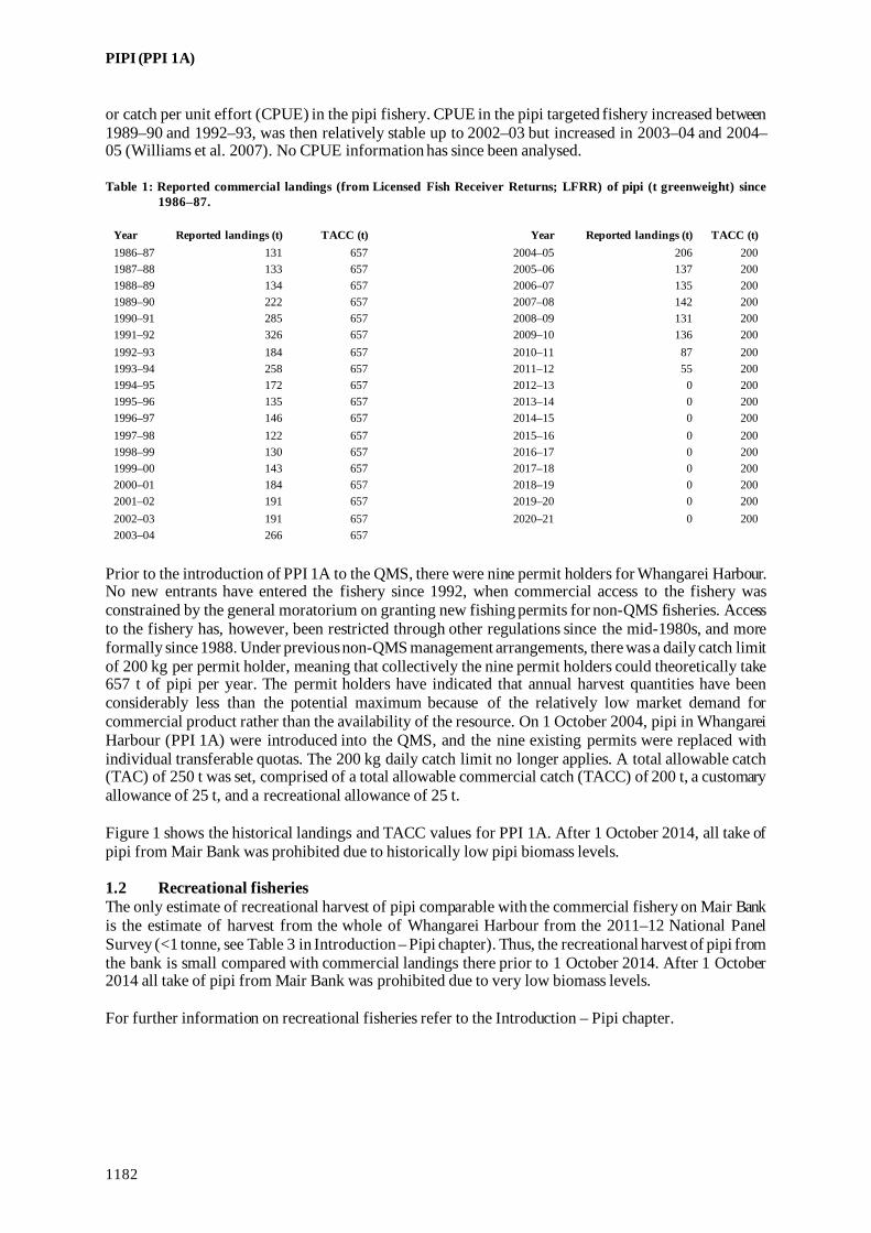
PIPI (PPI 1A)
1182
or catch per unit effort (CPUE) in the pipi fishery. CPUE in the pipi targeted fishery increased between 1989–90 and 1992–93, was then relatively stable up to 2002–03 but increased in 2003–04 and 2004–05 (Williams et al. 2007). No CPUE information has since been analysed. Table 1: Reported commercial landings (from Licensed Fish Receiver Returns; LFRR) of pipi (t greenweight) since
1986–87.
Year Reported landings (t) TACC (t) Year Reported landings (t) TACC (t) 1986–87 131 657 2004–05 206 200 1987–88 133 657 2005–06 137 200 1988–89 134 657 2006–07 135 200 1989–90 222 657 2007–08 142 200 1990–91 285 657 2008–09 131 200 1991–92 326 657 2009–10 136 200 1992–93 184 657 2010–11 87 200 1993–94 258 657 2011–12 55 200 1994–95 172 657 2012–13 0 200 1995–96 135 657 2013–14 0 200 1996–97 146 657 2014–15 0 200 1997–98 122 657 2015–16 0 200 1998–99 130 657 2016–17 0 200 1999–00 143 657 2017–18 0 200 2000–01 184 657 2018–19 0 200 2001–02 191 657 2019–20 0 200 2002–03 191 657 2020–21 0 200 2003–04 266 657
Prior to the introduction of PPI 1A to the QMS, there were nine permit holders for Whangarei Harbour. No new entrants have entered the fishery since 1992, when commercial access to the fishery was constrained by the general moratorium on granting new fishing permits for non-QMS fisheries. Access to the fishery has, however, been restricted through other regulations since the mid-1980s, and more formally since 1988. Under previous non-QMS management arrangements, there was a daily catch limit of 200 kg per permit holder, meaning that collectively the nine permit holders could theoretically take 657 t of pipi per year. The permit holders have indicated that annual harvest quantities have been considerably less than the potential maximum because of the relatively low market demand for commercial product rather than the availability of the resource. On 1 October 2004, pipi in Whangarei Harbour (PPI 1A) were introduced into the QMS, and the nine existing permits were replaced with individual transferable quotas. The 200 kg daily catch limit no longer applies. A total allowable catch (TAC) of 250 t was set, comprised of a total allowable commercial catch (TACC) of 200 t, a customary allowance of 25 t, and a recreational allowance of 25 t. Figure 1 shows the historical landings and TACC values for PPI 1A. After 1 October 2014, all take of pipi from Mair Bank was prohibited due to historically low pipi biomass levels. 1.2 Recreational fisheries The only estimate of recreational harvest of pipi comparable with the commercial fishery on Mair Bank is the estimate of harvest from the whole of Whangarei Harbour from the 2011–12 National Panel Survey (<1 tonne, see Table 3 in Introduction – Pipi chapter). Thus, the recreational harvest of pipi from the bank is small compared with commercial landings there prior to 1 October 2014. After 1 October 2014 all take of pipi from Mair Bank was prohibited due to very low biomass levels. For further information on recreational fisheries refer to the Introduction – Pipi chapter.

PIPI (PPI 1A)
1183
Figure 1:Total commercial landings and TACC for PPI 1A (Whangarei Harbour). QMS data from 2004–05 to present. 1.3 Customary non-commercial fisheries In common with many other intertidal shellfish, pipi are very important to Māori as a traditional food. Māori customary fishers can utilise the provisions under both the Fisheries (Amateur Fishing) Regulations 2013 and the Fisheries (Kaimoana Customary Fishing) Regulations 1998. Patuharakeke gazetted their rohe moana which covers the southern shoreline of the Whangarei harbour in 2009. In 2021, Te Rerenga Parāoa gazetted their rohe moana which covers the northern side of the Harbour and sits adjacent to the Patuharakeke Rohe Moana on the south side of the Harbour. The entire Whangarei Harbour is now a gazetted Rohe Moana. When tangata whenua harvest pipi under their recreational allowance, these are not included in records of customary catch. Estimates of customary catch under the provisions made for customary fishing for PPI 1A are shown in Table 2. These numbers are likely to be an underestimate of customary harvest because only the approved and harvested catch in weight (kg) are reported in the table. In addition, until the closure of Mair Bank to recreational fishing in 2014, tangata whenua may have harvested pipi under their recreational allowance and these are not included in records of customary catch. Table 2: Fisheries New Zealand records of customary harvest of pipi (approved and reported as weight (kg)) in PPI 1A,
since 2008–09. – no data.
Weight (kg) Fishing year Approved Harvested 2008–09 120 120 2009–10 235 235 2010–11 100 100 2011–12 80 40 2012–13 110 110 2013–14 – – 2014–15 – – 2015–16 – – 2016–17 – – 2017–18 – – 2018–19 – – 2019–20 – – 2020–21 – –
For further information on customary fisheries refer to the Introduction – Pipi chapter. 1.4 Illegal catch For further information on illegal catch refer to the Introduction – Pipi chapter.

PIPI (PPI 1A)
1184
1.5 Other sources of mortality There is some concern about the possibility of changes in bank stability that could arise from operations other than fishing in Whangarei Harbour (e.g., harbour dredging, port developments), which could lead to changes in the pipi fishery. Radical changes to the local hydrology could affect the size or substratum of Mair Bank, with consequent effects on its pipi population. Also, as suspension feeders, pipi may be adversely affected by increased sediment loads in the water column. The potential causes of low biomass from the 2014 biomass survey were investigated in the desktop report of Williams & Hume (2014). They concluded that: “potential causes of the pipi decline were high natural mortality of an ageing pipi population and low recruitment, both of which may be related to observed changes in the morphology of Mair Bank. There was no evidence of disease in the population, and the decline did not appear to be associated with potential anthropogenic sources of mortality (e.g., sedimentation, contaminants, harvesting). It is possible that substances not measured in shellfish, sediment, or water quality monitoring work may have influenced the pipi decline.” 2. BIOLOGY This is covered in the Introduction – Pipi chapter. 3. STOCKS AND AREAS Little is known of the stock structure of pipi. The commercial fishery based on Mair Bank in Whangarei Harbour (PPI 1A) forms a geographically discrete area and is assumed for management purposes to be a separate stock. 4. STOCK ASSESSMENT Stock assessment for Mair Bank pipi was conducted in 2005 and 2010 using absolute biomass surveys and yield per recruit and spawning stock biomass per recruit modelling. MPI, in association with Northland Regional Council and the Harbour board, also commissioned a biomass survey in 2014 in response to local concerns about low biomass. Following the closure to the collection of pipi on Marsden Bank in February 2011, the Bank was included in the monitoring programme in 2010–11 and has been surveyed four times since then. The population has fluctuated over time. In view of the population decline recorded in 2013–14, the 2018 survey data indicate some recovery of the pipi population, including the presence of recruits (Berkenbusch and Neubauer, 2018). 4.1 Estimates of fishery parameters and abundance Estimates of the fishing mortality reference point F0.1 are available from yield per recruit modelling (Table 3). Parallel spawning stock biomass per recruit modelling was conducted to estimate the SSBPR corresponding with each estimate of F0.1. These estimates are sensitive to the assumed value of natural mortality (M) and uncertainty in pipi growth parameters. 4.2 Biomass estimates Virgin biomass (B0) and the biomass that will support the maximum sustainable yield (BMSY) are unknown for Mair Bank pipi. Only four biomass estimates have been made for the Mair Bank pipi population: in 1989 using a grid survey, in 2005 using stratified random sampling, in 2010 using a systematic random start and in 2014 using a stratified grid sampling design. The 1989 estimate of 2245 t (± 10%) can be considered conservative because only the intertidal area of the bank was surveyed, and pipi are known to exist in the shallow subtidal area of the bank. Estimates of biomass are available for

PIPI (PPI 1A)
1185
Mair Bank (excluding from the 2014 survey) and are sensitive to the assumed size at recruitment (Table 4). The high CV for the 2014 estimates were due to unexpectedly low and patchy biomass at the time. Table 3: Estimates of the reference rate of fishing mortality F0.1 and corresponding spawning stock biomass per recruit
at three different assumed rates of natural mortality (M) for two harvest strategies (‘no restriction’ and ‘current’). SL, shell length (at recruitment). Estimates from Williams et al (2007).
‘No restriction’ strategy (harvest pipi of a size that maximizes YPR)
Assumed M Optimal age at recruitment (y) SL (mm) F0.1 YPR (g) SSBPR (%) 0.3 3 52 0.437 4.93 44 0.4 2.75 51 0.550 3.50 45 0.5 2.5 49 0.648 2.58 45
‘Current’ strategy (harvest pipi 60 mm and over) Assumed M Age at recruitment (y) SL (mm) F0.1 YPR (g) SSBPR (%) 0.3 5 60 0.564 3.98 62 0.4 5 60 0.755 2.41 70 0.5 5 60 0.949 1.47 76
Table 4: Estimated recruited biomass (B) of pipi on Mair Bank in 2005 and 2010 for different assumed sizes at
recruitment to the fishery. Source: Williams et al (2007), Pawley et al (2013) and Pawley (2014).
Year Assumed shell length at recruitment (mm) Intertidal stratum Subtidal stratum Mair Bank Total B (t) CV (%) B (t) CV (%) B (t) CV (%) 2005 1 (total biomass) 3 602 11.4 6 940 19.5 10 542 13.4 2005 40 3 569 11.4 6 922 19.5 10 490 13.4 2005 45 3 434 11.4 6 791 19.6 10 226 13.6 2005 50 2 986 11.3 5 989 20.1 8 975 14.0 2005 55 2 022 11.1 3 855 23.8 5 877 16.0 2005 60 1 004 13.1 2 013 37.5 3 017 25.4 2010 1 (total biomass) 2 233 17.4 2 218 33.0 4 452 15.2 2010 50 2 001 18.1 1 889 36.0 3 890 16.6 2010 60 1 751 18.3 1 393 33.7 3 145 17.4 2014 5 (total biomass) 46 50.8 28 25.9 73.5 30.8
4.3 Yield estimates and projections Maximum Constant Yield (MCY) was estimated using method 2 (see the guide to biological reference points in the introduction chapter of this plenary document):
𝑀𝑀𝑀𝑀𝑀𝑀 = 0.5𝐹𝐹0.1𝐵𝐵𝑎𝑎𝑎𝑎 where F0.1 is a reference rate of fishing mortality and Bav is the historical average recruited biomass (estimated as the mean recruited biomass from the 2005 and 2010 surveys). M is assumed to be 0.3 and the corresponding F0.1 is 0.564 (Williams et al 2007 revised version). The size at recruitment is assumed to remain at 60 mm and the corresponding Bav is 3081 t.
𝑀𝑀𝑀𝑀𝑀𝑀 = 0.5 × 0.564 × 3 081 𝑡𝑡 = 869 𝑡𝑡
This estimate of MCY would have a CV at least as large as those associated with the 2005 and 2010 estimates of recruited biomass (17–25%), and is sensitive to the assumed size at recruitment to the fishery, the assumed natural mortality, and to uncertainty in F0.1 (arising from the considerable uncertainty in model input values for growth and M) (Table 5). CAY was not estimated because there is no estimate of current biomass.

PIPI (PPI 1A)
1186
Table 5: Sensitivity of maximum constant yield (MCY, method 2) to estimates of size at recruitment and the assumed natural mortality, M. Bav, the historical average recruited biomass, was estimated for two sizes at recruitment (50 and 60 mm SL) using the 2005 and 2010 survey data.
SL at recruitment (mm) Bav M F0.1 MCY (t) 50 6433 0.3 0.40 1 300 0.4 0.54 1 729 0.5 0.68 2 182 60 3081 0.3 0.56 869 0.4 0.76 1 163 0.5 0.95 1 462
5. STATUS OF THE STOCKS
Stock Structure Assumptions For the purpose of this assessment PPI 1A is assumed to be a discrete stock.
Stock Status Year of Most Recent Assessment 2015 Reference Points
Target: Default 40% B0 Soft Limit: 20% B0 Hard Limit: 10% B0 Overfishing threshold: FMSY
Status in relation to Target Very Unlikely (< 10%) to be at or above the target Status in relation to Limits Soft Limit: Very Likely (> 90%) to be below
Hard Limit: Very Likely (> 90%) to be below Status in relation to Overfishing Unknown Historical Stock Status Trajectory and Current Status Biomass has not been measured in consistent units for all surveys, but has declined sharply from a total biomass (> 1 mm) of 10 542 tonnes in 2005 to a total biomass (> 5 mm) of 73.5 tonnes in 2014. Fishery and Stock Trends
Recent Trend in Biomass or Proxy Surveys were conducted in 2005, 2010 and 2014. These surveys have shown a sharp decline in biomass to very low levels.
Recent Trend in Fishing Intensity or Proxy
No commercial landings have been reported since the 2011–12 fishing year.
Other Abundance Indices - Trends in Other Relevant Variables or Indicators -
Projections and Prognosis Stock Projections or Prognosis The stock has declined below limits (causing the fishery to be
closed) due to unknown reasons and the likelihood of recovery is unknown.
Probability of Current Catch or TACC causing Biomass to remain below or to decline below Limits
There is no current legal catch as biomass has declined below the TACC and limits.
Probability of Current catch or TACC causing Overfishing to Continue or to commence
There is no current legal catch as biomass has declined below the TACC and limits. However, the amount of illegal take is unknown.

PIPI (PPI 1A)
1187
Assessment Methodology and Evaluation Assessment Type Level 2 - Partial Quantitative Stock Assessment Assessment Method Reference rate of fishing mortality applied to absolute biomass
estimates from quadrat surveys Assessment Dates Latest assessment: 2012 Next assessment: Unknown Overall assessment quality rank 1 – High Quality Main data inputs (rank) - Two absolute abundance
estimates (quadrat surveys) 1 – High Quality
- Biological parameters for YPR/SSBPR models
1 – High Quality
Data not used (rank) - Changes to Model Structure and Assumptions
-
Major Sources of Uncertainty - Growth for the subtidal portion of this population is poorly known. The available data come from other areas or the intertidal portion, both of which can be expected to support slower growth than the area where the fishery occurs. This, together with poor information on M and the size at recruitment to the fishery, makes the YPR modelling and reference rate of fishing mortality very uncertain.
Qualifying Comments Recruitment appears from the 2005 and 2010 survey length frequency distributions to be variable. This may lead to larger variations in the spawning and recruited biomass than the estimates of biomass suggest. The 2014 survey showed very low biomass levels and the commercial, recreational and customary fisheries have been closed since 1 October 2014. Fishery Interactions This is a hand-gathering fishery with no substantial bycatch or other interactions.
6. FOR FURTHER INFORMATION Berkenbusch, K; Neubauer, P (2018) Intertidal shellfish monitoring in the northern North Island region, 2017–18. New Zealand Fisheries
Assessment Report 2018/28. 103 p. Berkenbusch, K; Neubauer, P (2019) Intertidal shellfish monitoring in the northern North Island region, 2018–19. New Zealand Fisheries
Assessment Report 2019/32. 110 p. Cranfield, H J; Michael, K P; Stotter, D (1993) Estimates of growth, mortality, and yield per recruit for New Zealand surf clams. New Zealand
Fisheries Assessment Research Document 1993/20. 47 p. (Unpublished report held by NIWA library, Wellington). Dickie, B N (1986a) Physical and biological survey of a subtidal Paphies australis population in the lower Whangarei Harbour. Whangarei
Water Quality Management Plan. Working Report 4. 45 p. (Unpublished report to the Northland Catchment Commission and Regional Water Board, New Zealand).
Dickie, B N (1986b) Topographic survey of three intertidal Paphies australis habitats in the lower Whangarei Harbour. Whangarei Water Quality Management Plan. Working Report 2. 45 p. (Unpublished report to the Northland Catchment Commission and Regional Water Board, New Zealand).
Fournier, D A; Sibert, J R; Majkowski, J; Hampton, J (1990) MULTIFAN: a likelihood-based method for estimating growth parameters and age composition from multiple length frequency data sets illustrated using data for southern bluefin tuna (Thunnus maccoyi). Canadian Journal of Fisheries and Aquatic Sciences 47: 301–317.
Francis, R I C C (1988) Maximum likelihood estimation of growth and growth variability from tagging data. New Zealand Journal of Marine and Freshwater Research 22(1): 43–51.
Grace, R G (1972) The benthic ecology of the entrance to the Whangateau Harbour, Northland, New Zealand. Unpublished PhD thesis. University of Auckland, Auckland, New Zealand.
Haddon, M (1989) Biomass estimate of the pipi Paphies australis on Mair Bank, Whangarei Harbour. 23 p. (Unpublished report to MAF Fisheries North, Auckland, New Zealand).
Hooker, S H (1995a) Life history and demography of the pipi Paphies australis (Bivalvia: Mesodesmatidae) in northeastern New Zealand. Unpublished PhD thesis. University of Auckland, Auckland, New Zealand. 230 p.
Hooker, S H (1995b) Preliminary evidence for post-settlement movement of juvenile and adult pipi, Paphies australis (Gmelin 1790) (Bivalvia: Mesodesmatidae). Marine and Freshwater Behaviour and Physiology 27(1): 37–47.
Hooker, S H (1997) Larval and postlarval development of the New Zealand pipi, Paphies australis (Bivalvia : Mesodesmatidae). Bulletin of Marine Science 61(2): 225–240.
Hooker, S H; Creese, R G (1995a) The reproductive biology of pipi, Paphies australis (Gmelin 1790) (Bivalvia: Mesodesmatidae). I. Temporal patterns of the reproductive cycle. Journal of Shellfish Research 14(1): 7–15.

PIPI (PPI 1A)
1188
Hooker, S H; Creese, R G (1995b) The reproductive biology of pipi, Paphies australis (Gmelin 1790) (Bivalvia: Mesodesmatidae). II. Spatial patterns of the reproductive cycle. Journal of Shellfish Research 14(1): 17–24.
Morrison, M A; Browne, G N (1999) Intertidal shellfish population surveys in the Auckland region, 1998–99, and associated yield estimates. New Zealand Fisheries Assessment Research Document 99/43. 21 p. (Unpublished report held in NIWA library, Wellington).
Morrison, M A; Pawley, M D M; Browne, G N (1999) Intertidal surveys of shellfish populations in the Auckland region, 1997–98, and associated yield estimates. New Zealand Fisheries Assessment Research Document 99/25. 25 p. (Unpublished report held in NIWA library, Wellington).
Morton, J E; Miller, M C (1968) The New Zealand Sea Shore. Collins, Auckland, New Zealand. 653 p. OtterResearch (1992). MULTIFAN 32(f). User's Guide and Reference Manual. Otter Research Ltd., Nanaimo, Canada. 67 p. Pawley, M (2014) Population and biomass survey of pipi (Paphies australis) on Mair Bank, Whangarei Harbour, 2014. Report Prepared for
Northland Regional Council. 15 p. Pawley, M D; Hannaford, O; Morgan, K (2013) Biomass survey and stock assessment of pipi (Paphies australis) on Mair and Marsden Bank,
Whangarei Harbour. New Zealand Fisheries Assessment Report 2013/42. 32 p. Powell, A W B (1979) New Zealand Mollusca: Marine, Land and Freshwater Shells. Collins, Auckland, New Zealand. 500 p. Sullivan, K J; Mace, P M; Smith, N W M; Griffiths, M H; Todd, P R; Livingston, M E; Harley, S J; Key, J M; Connell, A M (Comps.) (2005)
Report from the Fishery Assessment Plenary, May 2005: stock assessments and yield estimates. 792 p. (Unpublished report held in NIWA library, Wellington).
Venus, G C (1984) Paphies australis (pipis) in Whangarei Harbour. Whangarei Harbour Study Technical Report No. 6. 60 p. (Unpublished technical report coordinated by the Northland Harbour Board).
Williams, J, Hume, T (2014) Investigation into the decline of pipi at Mair Bank, Whangarei Harbour. Report Prepared for Northland Regional Council. 44 p.
Williams, J R; Cryer, M; Hooker, S H; Smith, M D; Watson, T G; MacKay, G; Tasker, R (2007) Biomass survey and stock assessment of pipi (Paphies australis) on Mair Bank, Whangarei Harbour, 2005. New Zealand Fisheries Assessment Report, 2007/03. 29 p.
Williams, J.; Roberts, C.; Chetham, J. (2017) Initiation of a community-based pipi monitoring programme. Unpublished report prepared for Patuharakeke Te Iwi Trust Board by the National Institute of Water and Atmospheric Research, NIWA Client Report 2017255AK. 47 p.
Wynne-Jones, J; Gray, A; Hill, L; Heinemann, A (2014) National Panel Survey of Marine Recreational Fishers 2011–12: Harvest Estimates. New Zealand Fisheries Assessment Report 2014/67.

PŌRAE (POR)
1189
PŌRAE (POR)
(Nemadactylus douglasii) Pōrae
1. FISHERY SUMMARY Pōrae was introduced into the Quota Management System on 1 October 2004 and current TACs, TACCs, and allowances are presented in Table 1. Table 1: TACs (t), TACCs (t) and allowances (t) for pōrae.
Fishstock Recreational Allowance Customary non-
commercial Allowance Other sources of mortality TACC TAC POR 1 6 3 4 68 75 POR 2 1 1 1 18 9 POR 3 1 1 1 2 5 POR 10 1 1 1 1 4 Total 9 6 7 89 93
1.1 Commercial fisheries Commercial catches of pōrae throughout New Zealand are generally small. Landings were first reported in 1978 (Table 2). The proportion of vessels landing catch declined steadily during the 1990s; annual landings in FMA 1, where the majority of pōrae are caught, have approximately halved since the early 1990s when an average of 110 t were reported annually (Table 3). POR 1 landings have generally been lower than the TACC since its introduction in 2004, only slightly exceeding it in 2006–07, 2010–11, and 2016–17 (Figure 1, Table 4) POR 1 landings have averaged 43 t between 2017–18 and 2019–20. Landings of POR 2 (FMAs 2, 8, and 9) have remained low and below the TACC (except for the fishing year 2016–17), averaging 14 t in 2013–14 to 2019–20. POR 3 landings have consistently remained below 1 t; no landings have been reported from FMAs 4, 5, or 6. POR 10 landings were last reported in 1994–95. Pōrae is principally caught as a bycatch in inshore set net fisheries in northern New Zealand. It is generally taken in association with snapper and trevally off east Northland and Coromandel, and tarakihi and blue moki around Gisborne. Small quantities are taken by bottom longline and trawl fisheries targeting snapper off east Northland and Ninety Mile Beach. Fishers may confuse the codes PAR (parore) and POR (pōrae) when reporting catches, but given that both species occur in shallow northern waters, misreporting is difficult to discern.

PŌRAE (POR)
1190
Table 2: Reported landings (t) for the main QMAs from 1931 to 1982.
Year POR 1 POR 2 POR 3 Year POR 1 POR 2 POR 3 1931–32 0 0 0 1957 0 0 0 1932–33 0 0 0 1958 0 0 0 1933–34 0 0 0 1959 0 0 0 1934–35 0 0 0 1960 0 0 0 1935–36 0 0 0 1961 0 0 0 1936–37 0 0 0 1962 0 0 0 1937–38 0 0 0 1963 0 0 0 1938–39 0 0 0 1964 0 0 0 1939–40 0 0 0 1965 0 0 0 1940–41 0 0 0 1966 0 0 0 1941–42 0 0 0 1967 0 0 0 1942–43 0 0 0 1968 0 0 0 1943–44 0 0 0 1969 0 0 0
1944 0 0 0 1970 0 0 0 1945 0 0 0 1971 0 0 0 1946 0 0 0 1972 0 0 0 1947 0 0 0 1973 0 0 0 1948 0 0 0 1974 0 0 0 1949 0 0 0 1975 0 0 0 1950 0 0 0 1976 0 0 0 1951 0 0 0 1977 0 0 0 1952 0 0 0 1978 191 4 0 1953 0 0 0 1979 107 0 0 1954 0 0 0 1980 83 4 0 1955 0 0 0 1981 82 8 0 1956 0 0 0 1982 92 5 0
Notes: 1. The 1931–1943 years are April–March but from 1944 onwards are calendar years. 2. Data up to 1985 are from fishing returns: Data from 1986 to 1990 are from Quota Management Reports. 3. Data for the period 1931 to 1982 are based on reported landings by harbour and are likely to be underestimated as a result of
under-reporting and discarding practices. Data includes both foreign and domestic landings. Table 3: Reported landings (t) of pōrae by FMA, fishing years 1989–90 to 2003–04.
FMA 1 FMA 2 FMA 3 FMA 7 FMA 8 FMA 9 FMA 10
1989–90 98 4 < 1 < 1 < 1 0 0 1990–91 115 2 0 0 < 1 4 0 1991–92 121 5 < 1 0 0 3 0 1992–93 121 8 0 1 < 1 < 1 0 1993–94 77 12 2 0 < 1 1 < 1 1994–95 109 5 0 0 < 1 1 < 1 1995–96 94 8 < 1 < 1 < 1 4 0 1996–97 80 7 < 1 1 < 1 2 0 1997–98 75 4 < 1 < 1 < 1 3 0 1998–99 58 3 3 < 1 < 1 1 0 1999–00 55 4 < 1 2 < 1 1 0 2000–01 64 2 1 < 1 < 1 2 0 2001–02 55 3 1 < 1 < 1 < 1 0 2002–03 62 2 < 1 0 < 1 2 0 2003–04 32 2 < 1 < 1 < 1 2 0
Figure 1: Reported commercial landings and TACC for POR 1 (Auckland East).

PŌRAE (POR)
1191
Table 4: Reported domestic landings (t) and TACC (t) by pōrae Fishstock, fishing years 2004–05 to present. Fishstock POR 1 POR 2 POR 3 POR 10 FMA 1 2, 8&9 3,4,5,6&7 10 Total Landings TACC Landings TACC Landings TACC Landings TACC Landings TACC 2004–05 52 62 5 6 < 1 2 0 1 57 71 2005–06 47 62 2 6 < 1 2 0 1 49 71 2006–07 64 62 9 6 0 2 0 1 73 71 2007–08 45 62 7 6 < 1 2 0 1 53 71 2008–09 52 62 5 6 0 2 0 1 57 71 2009–10 57 62 11 6 < 1 2 0 1 68 71 2010–11 65 62 7 6 < 1 2 0 1 72 71 2011–12 43 62 7 6 < 1 2 0 1 51 71 2012–13 58 62 9 18 0 2 0 1 67 83 2013–14 55 62 10 18 < 1 2 0 1 66 83 2014–15 58 62 14 18 < 1 2 0 1 72 83 2015–16 57 62 9 18 < 1 2 0 1 66 83 2016–17 66 62 24 18 < 1 2 0 1 90 83 2017–18 41 62 13 18 < 1 2 0 1 55 83 2018–19 43 62 12 18 < 1 2 0 1 55 83 2019–20 43 62 11 18 < 1 2 0 1 54 83 2020–21 41 68 15 18 < 1 2 < 1 1 56 89 1.2 Recreational fisheries A National Panel Survey of recreational fishers was conducted for the first time throughout the 2011–12 fishing year. The panel survey used face-to-face interviews of a random sample of 30 390 New Zealand households to recruit a panel of fishers and non-fishers for a full year (Wynne-Jones et al 2014). The panel members were contacted regularly about their fishing activities and harvest information collected in standardised phone interviews. The national panel survey was repeated during the 2017–18 fishing year using very similar methods to produce directly comparable results (Wynne-Jones et al 2019). Recreational catch estimates from the two national panel surveys are given in Table 5. Note that national panel survey estimates do not include recreational harvest taken under s111 general approvals. Table 5: Recreational harvest estimates for pōrae stocks (Wynne-Jones et al 2014, 2019). Mean fish weights were
obtained from boat ramp surveys (Hartill & Davey 2015, Davey et al 2019).
Stock Year Method Number of fish Total weight (t) CV POR 1 2011–12 Panel survey 12 371 15.4 0.25 2017–18 Panel survey 5 397 6.7 0.36 POR 2 2011–12 Panel survey 695 0.9 0.62 2017–18 Panel survey 1 604 2.0 0.53 POR 3 2011–12 Panel survey 1 938 2.4 0.90 2017–18 Panel survey 0 0 -
1.3 Customary non-commercial fisheries There is no quantitative information on customary non-commercial harvest levels of pōrae. Customary non-commercial fishers are likely to catch small quantities of pōrae when targeting other species such as snapper, tarakihi and trevally. 2. BIOLOGY Pōrae (Nemadactylus douglasii) is a common inshore species of northern New Zealand (Kermadec Islands, west Auckland and Northland, east Northland, Hauraki Gulf, and the Bay of Plenty). It is also found at some localities as far south as Kapiti Island, Cook Strait, and Kaikoura over the summer months, but has not been recorded around the Chatham Islands. Pōrae also occurs in southeast Australia (New South Wales to Tasmania), where it is known as the grey or rubberlip morwong. Pōrae are generally found on reef/sand interfaces in 10–60 m depths, but have been recorded at 100 m. This diurnal species tends to aggregate to form small to large groups over sandy areas. Adults are thought to occupy distinctive home ranges, with individuals residing in the same area for many years. A study along the east coast of Northland recorded an average of 200 pōrae for each kilometre of rocky coastline.

PŌRAE (POR)
1192
Very little is known about the biology of this species. Pōrae spawn in late summer and autumn, and have an extended planktonic post-larval stage. Juveniles settle to the seafloor when 8–10 cm long. Although they attain a maximum length of at least 70 cm, the average size is 40−60 cm. They live to at least 30 years and growth is believed to slow substantially at maturity (Ayling & Cox 1984, Francis 2001). 3. STOCKS AND AREAS There is no biological information to suggest separate stocks around New Zealand. However, evidence of residential behaviour and the fact that they are long-lived, suggests that localised depletion is likely to occur. 4. STOCK ASSESSMENT There is no fishery independent stock assessment information to determine the stock status of pōrae. Biomass estimates have not been determined for pōrae. 5. STATUS OF THE STOCK Estimates of current and reference biomass are not available. It is not known if recent catch levels or TACs are sustainable. The status of POR 1, 2 and 3 relative to BMSY is unknown. 6. FOR FURTHER INFORMATION Ayling, T; Cox, G J (1984) Collins guide to the sea fishes of New Zealand. Collins, Auckland. 343 p. Davey, N; Hartill, B; Carter, M (2019) Mean weight estimates for recreational fisheries in 2017–18. New Zealand Fisheries Assessment
Report 2019/25. 32 p. Francis, M (2001) Coastal fishes of New Zealand. An identification guide. Reed Books, Auckland. 103 p. + pls. Hartill, B; Davey, N (2015) Mean weight estimates for recreational fisheries in 2011–12. New Zealand Fisheries Assessment Report
2015/25. Stewart, P (1993) Morwong, Nemadactylus species. In Kailola et al. (Eds), Australian fisheries resources. pp. 324–326. Bureau of Resource
Sciences, Canberra. 422 p. Thompson, S (1981) Fish of the Marine Reserve. A guide to the identification and biology of common coastal fish of north-eastern New
Zealand. Leigh Laboratory, University of Auckland. 364 p. Wynne-Jones, J; Gray, A; Heinemann, A; Hill, L; Walton, L (2019) National Panel Survey of Marine Recreational Fishers 2017–2018. N ew
Zealand Fisheries Assessment Report 2019/24. 104 p. Wynne-Jones,J; Gray, A; Hill, L; Heinemann, A (2014) National Panel Survey of Marine Recreational Fishers 2011–12: Harvest Estimates. New
Zealand Fisheries Assessment Report 2014/67. 139 p.

PRAWN KILLER (PRK)
1193
PRAWN KILLER (PRK)
(Ibacus alticrenatus)
1. FISHERY SUMMARY 1.1 Commercial fisheries Prawn killer (Ibacus alticrenatus) was introduced into the Quota Management System on 1 October 2007, with a combined TAC of 37.4 t and TACC of 36 t. There are no allowances for customary non-commercial or recreational fisheries, and 1.4 t was allowed for other sources of mortality. Almost all prawn killer are taken as a bycatch in the scampi target bottom trawl fishery in SCI 1 and SCI 2. Reported catches in PRK 1 peaked at 42 t in 1992–93, but declined to less than 0.5 t since 2011–12. Landings in PRK 2 reached a maximum of 8 t in 2002–03, but have been minimal since with less than 0.01 t reported in 2018–19, and no landings reported in 2019–20 or 2020–21 (Table 1). Landings are minimal to non-existent in other QMAs. Years with higher landings coincide with years in which the scampi fleet fished at shallower depths than usual. They can be legally discarded under Schedule 6 of the Fisheries Act but it is still likely that reported catches are lower than actual catches due to non-reporting. Table 1: TACCs and reported landings (t) of prawn killer by Fishstock from 1990–91 until the present from CELR
and CLR data. QMAs are shown as defined in 2007–08. [Continued on next page]
PRK 1 PRK 2 PRK 3 PRK 4A Fishstock Landings TACC Landings TACC Landings TACC Landings TACC 1990–91 11.59 – 0 – 0 – 0 – 1991–92 3.34 – 0.48 – 0 – 0 – 1992–93 42.24 – 6.86 – 0 – 0 – 1993–94 10.95 – 0.03 – 0 – 0 – 1994–95 0.52 – 0 – 0 – 0 – 1995–96 1.78 – 0 – 0 – 0 – 1996–97 23.13 – 0 – 0 – 0 – 1997–98 0 – 0 – 0 – 0 – 1998–99 0 – 0.19 – 0 – 0 – 1999–00 0.08 – 0 – 0 – 0 – 2000–01 0 – 0 – 0 – 0 – 2001–02 6.05 – 0.37 – 0 – 0 – 2002–03 20.99 – 8.09 – 0 – 0 – 2003–04 24.35 – 0.57 – 0.01 – 0.01 – 2004–05 3.25 – 1.15 – 0 – 0 – 2005–06 2.25 – 0.20 – 0 – 0 – 2006–07 4.6 – 0.10 – 0 – 0 – 2007–08 5.36 24.5 0.92 3.5 0.01 1 0.02 1 2008–09 0.22 24.5 0.08 3.5 0 1 0 1 2009–10 0.75 24.5 0.03 3.5 0 1 0 1

PRAWN KILLER (PRK)
1194
Table 1 [Continued] PRK 1 PRK 2 PRK 3 PRK 4A Fishstock Landings TACC Landings TACC Landings TACC Landings TACC 2010–11 3.55 24.5 0.08 3.5 0 1 0 1 2011–12 0.42 24.5 0.17 3.5 0 1 0 1 2012–13 0.26 24.5 0.02 3.5 0 1 0 1 2013–14 0.10 24.5 0.04 3.5 0 1 0 1 2014–15 0.00 24.5 0.04 3.5 0 1 0 1 2015–16 0.02 24.5 0.07 3.5 0 1 0 1 2016–17 0.35 24.5 0.15 3.5 0 1 0.01 1 2017–18 0.45 24.5 0.01 3.5 0 1 0 1 2018–19 0.30 24.5 < 0.01 3.5 0 1 < 0.01 1 2019–20 < 0.01 24.5 0 3.5 < 0.01 1 0 1 2020–21 0.02 24.5 0 3.5 0 1 0 1 PRK 5 PRK 6A PRK 6B PRK 7 Fishstock Landings TACC Landings TACC Landings TACC Landings TACC 1990–91 0 – 0 – 0 – 0 – 1991–92 0 – 0 – 0 – 0 – 1992–93 0 – 0 – 0.02 – 0 – 1993–94 0 – 0 – 0 – 0 – 1994–95 0 – 0 – 0 – 0 – 1995–96 0 – 0 – 0 – 0 – 1996–97 0 – 0 – 0 – 0 – 1997–98 0 – 0 – 0 – 0 – 1998–99 0 – 0 – 0 – 0 – 1999–00 0 – 0 – 0 – 0 – 2000–01 0 – 0 – 0 – 0 – 2001–02 0 – 0 – 0 – 0 – 2002–03 0 – 0 – 0 – 0 – 2003–04 0 – 0 – 0 – 0 – 2004–05 0 – 0 – 0 – 0 – 2005–06 0 – 0 – 0 – 0.01 – 2006–07 0 – 0 – 0 – 0.03 – 2007–08 0 1 0 1 0 1 1.2 1 2008–09 0 1 0 1 0 1 0.88 1 2009–10 0 1 0 1 0 1 0.48 1 2010–11 0 1 0 1 0 1 0.69 1 2011–12 0 1 0 1 0 1 0.73 1 2012–13 0 1 0 1 0 1 0.60 1 2013–14 0.001 1 0 1 0 1 0.66 1 2014–15 0 1 0 1 0 1 1 1 2015–16 0 1 0 1 0 1 1.66 1 2016–17 0 1 0 1 0 1 1.37 1 2017–18 0 1 0 1 0 1 0.55 1 2018–19 0 1 0 1 0 1 0.45 1 2019–20 0 1 0 1 0 1 0.01 1 2020–21 0 1 0 1 0 1 0.04 1 PRK 8 PRK 9 TOTAL Fishstock Landings TACC Landings TACC Landings TACC 1990–91 0 – 0 – 11.58 – 1991–92 0 – 0 – 3.82 – 1992–93 0 – 0 – 49.12 – 1993–94 0 – 0 – 10.98 – 1994–95 0 – 0 – 0.52 – 1995–96 0 – 0 – 1.78 – 1996–97 0 – 0 – 23.13 – 1997–98 0 – 0 – 0 – 1998–99 0 – 0 – 0.19 – 1999–00 0 – 0 – 0.08 – 2000–01 0 – 0 – 0 – 2001–02 0 – 0 – 6.42 – 2002–03 0 – 0 – 29.08 – 2003–04 0 – 0 – 24.94 – 2004–05 0 – 0 – 4.40 – 2005–06 0 – 0.01 – 2.47 – 2006–07 0 – 0 – 4.73 – 2007–08 0 1 0 1 7.51 36 2008–09 0 1 0 1 1.18 36 2009–10 0 1 0 1 1.27 36 2010–11 0.01 1 0 1 4.33 36 2011–12 0 1 0 1 1.32 36 2012–13 0.01 1 0.01 1 0.90 36 2013–14 0.01 1 0.15 1 0.94 36 2014–15 0 1 0 1 1.04 36 2015–16 0.01 1 0.02 1 1.78 36 2016–17 0 1 1.26 1 3.14 36 2017–18 0 1 0 1 1.01 36

PRAWN KILLER (PRK)
1195
Table 1 [Continued] PRK 8 PRK 9 TOTAL Fishstock Landings TACC Landings TACC Landings TACC 2018–19 0 1 0.01 1 0.76 36 2019–20 0 1 0 1 0.01 36 2020–21 0 1 0.02 1 0.08 36
1.2 Recreational fisheries Given the depths and locations at which prawn killer are found recreational catch is likely to be negligible or non-existent. 1.3 Customary non-commercial fisheries Given the depths and locations at which prawn killer are found customary catch is likely to be negligible or non-existent. 1.4 Illegal catch No quantitative information is available on the level of illegal catch of prawn killer. Given the low value and lack of markets illegal catches are unlikely. 1.5 Other sources of mortality There is no quantitative information on other sources of mortality, although analysis of benthic invertebrate samples and the distribution of trawl tows in the Bay of Plenty (PRK 1) suggests that this species is negatively affected by trawling. 2. BIOLOGY Ibacus alticrenatus is widely distributed around the New Zealand coast, principally in depths of 80–300 m. Prawn killers are found on soft sediment seafloors, where they dig into the substrate and cover themselves with sediment. There is not much information about growth and development of I. alticrenatus in New Zealand waters, but females are thought to mature at a carapace length of about 40 mm. Trawl surveys of the Bay of Plenty and Hawke Bay and Wairarapa regions have found maximum carapace length of 46 and 52 mm for males and females respectively. Information from Australia suggests that this species has relatively low fecundity (1700–14 800 eggs, increasing with size) and spawns annually. Larval development takes 4–6 months, an intermediate duration for a Scyllarid lobster. Females of other Ibacus species reach maturity about two years after settlement and longevity is suggested to be five years or more. No ageing work has been carried out on prawn killer in either New Zealand or Australia. Other slipper lobster species may also feature in catches – Ibacus brucei, Antipodarctus aoteanus, and Scyllarus mawsoni (which is thought to be rare). 3. STOCKS AND AREAS For management purposes stock boundaries are based on those used for scampi. There is no biological information on stock structure, recruitment patterns, or other biological characteristics which might indicate stock boundaries, but there are three main fishing areas where they are caught: Bay of Plenty, and to a lesser extent Hawke Bay and Wairarapa and the northern west coast of the South Island. The lack of prawn killer bycatch in the scampi target fisheries on the Mernoo Bank (PRK 3) and around the Auckland Islands (PRK 6A) would suggest the prawn killer numbers are very low to non-existent south of the three main areas.

PRAWN KILLER (PRK)
1196
4. STOCK ASSESSMENT 4.1 Estimates of fishery parameters and abundance There are no estimates of fishery parameters or abundance for any prawn killer fishstock. Sporadic and varying catches by the scampi fleet mean that development of reliable CPUE indices is not possible. 4.2 Biomass estimates There are no reliable biomass estimates for any prawn killer fishstock. Combined trawl and photographic surveys for scampi in the Bay of Plenty (PRK 1) and Hawke Bay and Wairarapa (PRK 2) are the only trawl surveys that catch prawn killer regularly. Prawn killer biomass estimates from these surveys are variable from year to year and have high coefficients of variation. The focus of these surveys has changed over the years to focus more on photographic work and not all strata have been surveyed in all years. 4.3 Yield estimates and projections There are no estimates of MCY or CAY for any prawn killer fishstock. 5. STATUS OF THE STOCKS There are no estimates of reference or current biomass for any prawn killer fishstock. It is not known whether prawn killer stocks are at, above, or below a level that can produce MSY. 6. FOR FURTHER INFORMATION Atkinson, J M; Boustead, N C (1982) The complete larval development of the scyllarid lobster Ibacus alticrenatus Bate, 1888 in New Zealand
waters. Crustaceana 42: 275–287. Booth, J D; Webber, W R; Sekiguchi, H; Coutures, E (2005) Diverse larval recruitment strategies within the Scyllaridae. New Zealand Journal
of Marine and Freshwater Research 39: 581–592. Brown, D E; Holthuis, L B (1998) The Australian species of the genus Ibacus (Crustacea: Decapoda: Scyllaridae), with the description of a
new species and addition of new records. Zoologische Mededelingen (Leiden) 72(10): 113–141. Cryer, M; Hartill, B; O’Shea, S (2002) Modification of marine benthos by trawling: toward a generalization for the deep ocean? Ecological
Applications 12(6): 1824–1839. Haddy, J A; Courtney, A J; Roy, D P (2005) Aspects of the reproductive biology and growth of Balmain bugs (Ibacus spp.) (Scyllaridae).
Journal of Crustacean Biology 25(2): 263–273. MacGibbon, D J (2015) Fishery characterisation for prawn killer, Ibacus alticrenatus (Spence Bate, 1888) (Scyllaridae), 1989–90 to 2012–
13. New Zealand Fisheries Assessment Report 2015/05. 108 p.

QUEEN SCALLOPS (QSC)
1197
QUEEN SCALLOPS (QSC)
(Zygochlamys delicatula)
1. FISHERY SUMMARY Queen scallops were introduced into the QMS in October 2002, with a current TACC (unchanged since its introduction) of 380 t and a 20 t allowance for other sources of fishing related mortality. The fishing year runs from 1 October to 30 September and the catch is reported in greenweight. 1.1 Commercial fisheries The QSC 3 fishery initially developed in the 1984–85 fishing year; it is a small-scale fishery with only a few fishing vessels involved (Michael & Cranfield 2001). Queen scallops (Zygochlamys delicatula) are predominantly harvested commercially off the Otago coast, in depths of 130–200 m (predominately 150–200 m) near the edge of the continental shelf. Reported landings from the QSC 3 fishery peaked at 711 t in the 1985–86 fishing year (not shown in the table below), before decreasing to an average of 33 t in the early 1990s. By the early 2000s landings increased to an average of 135 t, although this is more likely to be associated with economic, rather than biological, factors. Since 2010 landings have fluctuated between 1.9 and 70.5 t. The TACC was set in 2002 at a slightly higher level than recent landings but lower than the non-QMS competitive catch limit of 750 t which applied to FMA 3 from 1990–91; landings have remained well below the TACC since its introduction. Reported landings of queen scallops are given in Table 1, and Figure 1 shows historical landings and the TACC for QSC 3.

QUEEN SCALLOPS (QSC)
1198
Figure 1: Reported commercial landings and TACC for QSC 3 (South East Coast, Southland). The queen scallop fishery is a trawl fishery using specialised gear (including a relatively light ‘tickler’ chain or wire to induce swimming) and the catch is sorted both mechanically and by hand (Michael & Cranfield 2001, R. Belton pers. comm.). Table 1: Reported landings (t greenweight) of queen scallops (QSC) by FMA, QMA and fishing year by all methods
(trawl and dredge) from 1989–90 until the present day from Quota Management Reports (QMR), Monthly Harvest Returns (MHR) and Catch Effort Landing Returns (CELR landed and CELR estimated).
QSC 3 FMA 3 FMA 5 Fishing year Catch (QMR/MHR) TACC* Estimated catch (TCEPR/CELR) Landings (CELR/CLR) 1989–90 11.9 - 288.1 - 1990–91 61.8 - 238.3 22.9 1991–92 77.4 - 193.7 - 1992–93 0.4 - 104.7 - 1993–94 1.1 - 133.6 - 1994–95 23.6 - 146.9 - 1995–96 4.5 - 149.5 0.2 1996–97 20.9 - 118.0 6.6 1997–98 56.0 - 208.3 6.0 1998–99 85.9 - 81.7 - 1999–00 180.2 - 176.8 - 2000–01 162.2 - 162.1 - 2001–02 223.7 - 168.9 - 2002–03 139.0 380 - - 2003–04 114.0 380 - - 2004–05 35.1 380 - - 2005–06 18.6 380 - - 2006–07 6.5 380 - - 2007–08 9.5 380 - - 2008–09 48.7 380 - - 2009–10 25.3 380 - - 2010–11 2.8 380 - - 2011–12 1.9 380 - - 2012–13 70.5 380 - - 2013–14 5.024 380 - - 2014–15 1.788 380 - - 2015–16 13.55 380 - - 2016–17 23.13 380 - - 2017–18 25.74 380 - - 2018–19 12.17 380 - - 2019–20 16.61 380 - - 2020–21 20.35 380 - -
* QMS introduction 1 October 2002 1.2 Recreational fisheries There is no known recreational fishery for queen scallops. 1.3 Customary fisheries There is no known customary harvest of queen scallops.

QUEEN SCALLOPS (QSC)
1199
1.4 Illegal catch Current levels of illegal harvest are not known. 1.5 Other sources of mortality No quantitative estimate of other sources of mortality is available. Some grading of catch may occur (queen scallops may be returned to the sea) and an allowance of 20 t for potential mortality has been set within the current TAC. 2. BIOLOGY The New Zealand queen scallop (Zygochlamys delicatula) is also known as the southern queen scallop, southern fan scallop, and gem scallop. This small pectinid species is distributed on the outer continental shelf along the east coast of the South Island, from Kaikoura down to Macquarie Island. There are nine other species in the genus, none of which have attracted commercial interest, probably because of their small size. Similar species such as Chlamys islandica and Chlamys varia support important fisheries in other countries. New Zealand queen scallops are distributed from Kaikoura to the southern islands including the Snares, Bounty, Antipodes, and Macquarie Islands. There are no records of live queen scallops being caught north of Kaikoura, or on the west coast of the South Island. A dredge survey off Otago in October 1983 showed that queen scallops were distributed in long patches orientated along the slope of the continental shelf. They were most abundant in depths beyond 130 m, on the plateau between the Taiaroa and Papanui Canyons, and south. North of the Taiaroa Canyon catches diminished steadily towards the Karitane Canyon; few were caught north of the canyon. Only low numbers of queen scallops were caught in depths shallower than 110 m. Juvenile queen scallops are frequently found attached to fragments of bryozoa and other biogenic debris, including the shells of other scallops and the dredge oyster. Height frequency distributions of samples show that the size composition of the population differs with area, and it is inferred that settlement probably varies spatially and temporally. The estimated 40−50 days larval life may result in queen scallop larvae being well mixed, both vertically and horizontally, in the water column. Predation of newly settled spat may also affect the pattern of recruitment and add to the variability in year class representation. Estimates of growth for New Zealand queen scallops suggest that they become sexually mature at four years for males and five years for females. As length is slightly less than height, queen scallops are estimated to reach the minimum takeable size of 50 mm at about eight years. However, growth estimates are uncertain, with information from tagging studies suggesting that queen scallops enter the fishery much earlier, at three to five years. 3. STOCKS AND AREAS Queen scallops are distributed throughout the QSC 3 area. From harvest records the scallops inhabit waters between 130 and 200 m depth. The extent to which various beds or populations are separate reproductively or functionally is not known. 4. STOCK ASSESSMENT 4.1 Estimates of fishery parameters and abundance No estimates of fishery parameters or abundance are available at present. 4.2 Biomass estimates A trawl survey, (Jiang et al 2005) carried out in February–April 2004, provided estimates of total and recruited biomass (shells at least 50 mm) available from the fished area of QSC 3, from Moeraki to just north of the Nuggets within the depth range 130 to 200 m, which covers 90% of the fished area within

QUEEN SCALLOPS (QSC)
1200
QSC 3 (Table 2). These estimates assumed that the efficiency of the survey trawl was 100%. However trawl efficiency is unlikely to be 100% and in other scallop fisheries can vary significantly depending on dredge and substrate type. Consequently estimates of current absolute biomass cannot be estimated. The Shellfish Working Group had concerns over methodology and conduct of the survey, and that the reported survey CVs may not be reliable. Table 2: Estimated scallop biomass (recruit and pre-recruit) (t) in fished areas of QSC 3 February–April 2004.
Biomass Recruit (CV) Biomass (CV) Pre-recruit Total Biomass (CV) 1 950.8 (18.2) 363.6 (21.48) 2 314.4 (18.22)
4.3 Yield estimates and projections As absolute biomass has not been estimated, MCY cannot be estimated CAY cannot be estimated. 5. STATUS OF THE STOCKS Stock structure assumptions QSC 3 is assumed to be a single stock. Stock Status Most Recent Assessment Year 2004 Assessment Runs Presented Recruited biomass (shells ≥ 50 mm) Reference Points
Target: Undefined Soft Limit: 20% B0 Hard Limit: 10% B0
Overfishing threshold: - Status in relation to Target - Status in relation to Limits Unknown Historical Stock Status Trajectory and Current Status - Fishery and Stock Trends Recent Trend in Biomass or Proxy
Unknown
Recent Trend in Fishing Mortality or Proxy
Unknown
Other Abundance Indices - Trends in Other Relevant Indicators or Variables
Landings have been less than a 10% of the TACC since 2004-05 expect in 2008-09 and 2012-13.
Projections and Prognosis Stock Projections or Prognosis
Unknown
Probability of Current Catch or TACC causing Biomass to remain below or to decline below Limits
Soft Limit: Unknown Hard Limit: Unknown
Probability of Current Catch or TACC causing Overfishing to continue or to commence
Unknown
Assessment Methodology Assessment Type - Assessment Method - Assessment Dates - Next assessment: Unknown

QUEEN SCALLOPS (QSC)
1201
Overall assessment quality rank - Main data inputs (rank) - Data not used (rank) - Changes to Model Structure and Assumptions
-
Major Sources of Uncertainty - Qualifying Comments Landings are thought to be declining in recent times due to economic rather than biological factors.
Fishery Interactions -
6. FOR FURTHER INFORMATION Jiang, W; Gibbs, M; Hatton, S (2005) Stock assessment of the queen scallop fishery in QSC3. Final Research Report for
Ministry of Fisheries project QSC2002/01. (Unpublished report held by Fisheries New Zealand, Wellington.) Michael, K P; Cranfield, H J (2001) A summary of the fishery, commercial landings, and biology of the New Zealand queen scallop,
Zygochlamys delicatula (Hutton, 1873). New Zealand Fisheries Assessment Report 2001/68. 25p.


REDBAIT (RBT)
1203
REDBAIT (RBT)
(Emmelichthys nitidus)
1. FISHERY SUMMARY 1.1 Commercial fisheries Redbait (Emmelichthys nitidus) was introduced to the Quota Management System on 1 October 2009, with a combined TAC of 5 316 t and TACC of 5 050 t. There are no allowances for customary non-commercial or recreational fisheries, and 266 t was allowed for other sources of mortality. RBT is mainly taken as bycatch of the jack mackerel target trawl fishery, but also widely taken as bycatch of barracouta trawl tows, with some taken in the squid and hoki fisheries. A target fishery developed in the mid-2000s. Reported total landings ranged from 2184 to 4307 t during the 2000s, but declined across all QMAs and target fisheries in 2009–10 and 2010–11 to nearer 1000 t. Since the fishing year 2011–12 total landings have ranged between 1456 and 2856 t. RBT 3 includes the southern fisheries for squid, and fisheries for jack mackerel on the Mernoo Bank and Chatham Rise, and accounted for most of the redbait landed in each year during the 1990s. From 2002–03 to 2009–10 however, the jack mackerel fishery on the west coast expanded into north and south Taranaki Bights, with landings from RBT 7 exceeding those from RBT 3. Since 2010 RBT 3 landings have declined, with RBT 3 catches once again making up the bulk of the landings. In 2019–120 just 22 t of RBT 7 were landed compared to 2459 t of RBT 3. Landings of RBT 1 have been small (less than 5 t) in most years, increasing slightly in the late 2000s. TACs, allowances and TACCs from 1 October 2009 are reported in Table 1. Table 2 and Figure 1 show historical landings from 2001–02 to the present, reported by QMAs. Table 1: TACs, allowances and TACCs of redbait.
Fishstock Other mortality Customary non–commercial and recreational TACC TAC RBT 1 1 0 19 20 RBT 3 115 0 2 190 2 305 RBT 7 150 0 2 841 2 991 RBT 10 0 0 0 0
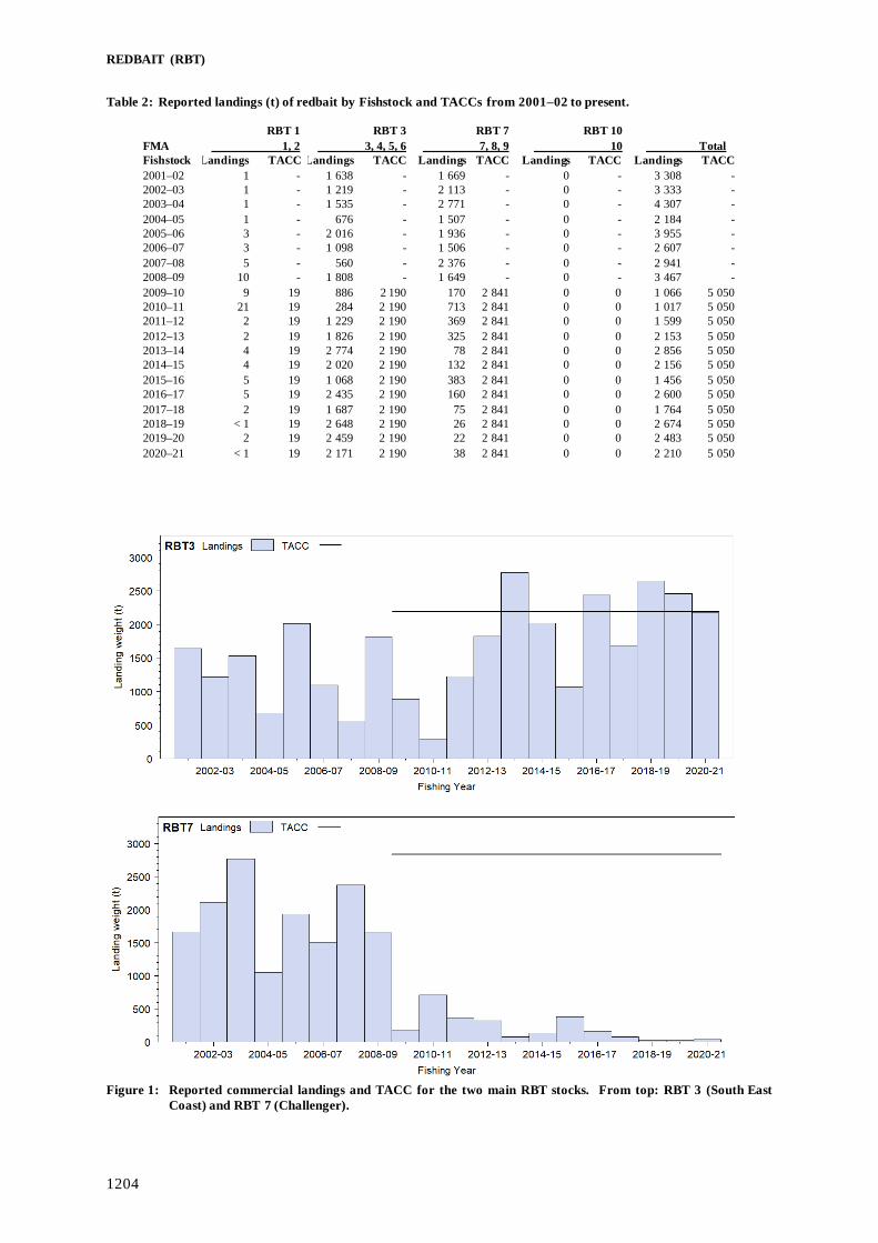
REDBAIT (RBT)
1204
Table 2: Reported landings (t) of redbait by Fishstock and TACCs from 2001–02 to present.
RBT 1 RBT 3 RBT 7 RBT 10 FMA 1, 2 3, 4, 5, 6 7, 8, 9 10 Total Fishstock Landings TACC Landings TACC Landings TACC Landings TACC Landings TACC 2001–02 1 - 1 638 - 1 669 - 0 - 3 308 - 2002–03 1 - 1 219 - 2 113 - 0 - 3 333 - 2003–04 1 - 1 535 - 2 771 - 0 - 4 307 - 2004–05 1 - 676 - 1 507 - 0 - 2 184 - 2005–06 3 - 2 016 - 1 936 - 0 - 3 955 - 2006–07 3 - 1 098 - 1 506 - 0 - 2 607 - 2007–08 5 - 560 - 2 376 - 0 - 2 941 - 2008–09 10 - 1 808 - 1 649 - 0 - 3 467 - 2009–10 9 19 886 2 190 170 2 841 0 0 1 066 5 050 2010–11 21 19 284 2 190 713 2 841 0 0 1 017 5 050 2011–12 2 19 1 229 2 190 369 2 841 0 0 1 599 5 050 2012–13 2 19 1 826 2 190 325 2 841 0 0 2 153 5 050 2013–14 4 19 2 774 2 190 78 2 841 0 0 2 856 5 050 2014–15 4 19 2 020 2 190 132 2 841 0 0 2 156 5 050 2015–16 5 19 1 068 2 190 383 2 841 0 0 1 456 5 050 2016–17 5 19 2 435 2 190 160 2 841 0 0 2 600 5 050 2017–18 2 19 1 687 2 190 75 2 841 0 0 1 764 5 050 2018–19 < 1 19 2 648 2 190 26 2 841 0 0 2 674 5 050 2019–20 2 19 2 459 2 190 22 2 841 0 0 2 483 5 050 2020–21 < 1 19 2 171 2 190 38 2 841 0 0 2 210 5 050
Figure 1: Reported commercial landings and TACC for the two main RBT stocks. From top: RBT 3 (South East
Coast) and RBT 7 (Challenger).

REDBAIT (RBT)
1205
1.2 Recreational fisheries There is no known non-commercial fishery for redbait. 1.3 Customary non-commercial fisheries There is no known customary non-commercial fishery for redbait. 1.4 Illegal catch No quantitative information is available on the level of illegal catch of redbait. 1.5 Other sources of mortality Taylor (2009) described up to 345 tonnes (but usually less than 200 t annually of redbait reported as discarded between 1988–89 and 2008–09. 2. BIOLOGY Emmelichthys nitidus is a schooling, bathypelagic species that is closely related to rubyfish. It is widely distributed around New Zealand in depths from 85 to 500 m. Juveniles are found at the surface and adults near the bottom in deeper waters, including seamounts. There is not much information about growth and development of redbait in New Zealand. Offshore studies suggest regional differences in maximum size with a maximum age of 10 years in east Victoria and 7 years in Tasmania, where the maximum reported size of redbait is 316 mm fork length. Spawning in Tasmania is thought to last 2–3 months during spring, with 50% mature at 24 cm FL and 2–3 years. Von Bertalanffy growth parameters of Tasmanian redbait for both sexes combined are given in Table 3. Research data from New Zealand show that the maximum size of redbait here is about 420 mm FL, which is larger than most other regions where length of this species has been recorded, except South Africa. Recent validation of the ageing of the closely related rubyfish in New Zealand confirms maximum ages of 90+ suggesting that some emmelichthyids may be long-lived, so current estimates of growth and maximum age may not be reliable Table 3 shows estimated biological parameters for redbait. Table 3: Estimates of biological parameters for redbait. Growth is based on Australian studies (Welsford & Lyle
2003).
Fishstock Estimate Source 1. Weight = a (length)b (Weight in g, length in cm fork length) Combined sexes RBT (All) a b 0.004947 3.259168 NIWA (unpub. data) 2. von Bertalanffy growth parameters Combined sexes RBT (Tasmania) L∞ k t0
28.7 0.56 -0.36 Welsford & Lyle (2003) 3. STOCKS AND AREAS There is no information about stock structure, recruitment patterns, or other biological characteristics that would indicate stock boundaries. As the catch of redbait has been mainly (66%) from bycatch in the jack mackerel trawl fisheries, management boundaries have been set the same as those used for jack mackerel. Analysis of encounter rates suggests a north-south seasonal movement of redbait may occur at a spatial scale that is greater than QMAs.

REDBAIT (RBT)
1206
4. STOCK ASSESSMENT 4.1 Estimates of fishery parameters and abundance There are no estimates of fishery parameters or abundance for any redbait fishstock. 4.2 Biomass estimates There are no biomass estimates for any redbait fishstock. 4.3 Yield estimates and projections There are no yield estimates for any redbait fishstock. 5. STATUS OF THE STOCKS There are no estimates of reference or current biomass for any redbait fishstock. It is not known whether redbait stocks are at, above, or below a level that can produce MSY. 6. FOR FURTHER INFORMATION Bentley, N; Kendrick, T H; MacGibbon, D J (2014) Fishery characterisation and catch-per-unit-effort analyses for redbait (Emmelichthys
nitidus), 1989–90 to 2010–11. (2014 Draft New Zealand Fisheries Assessment Report held by Fisheries New Zealand.) Taylor, P R (2009) A summary of information on redbait Emmelichthys nitidus. Final Research Report for Ministry of Fisheries Project
SAP2008-18. (Unpublished report held by Fisheries New Zealand, Wellington.) Welsford, D C; Lyle, J M (2003) Redbait (Emmelichthys nitidus): a synopsis of fishery and biological data. TAFI Technical Report Series
20. 32 p.

RED COD (RCO)
1207
RED COD (RCO)
(Pseudophycis bachus) Hoka
1. FISHERY SUMMARY 1.1 Commercial fisheries Red cod are targeted primarily by domestic trawlers in the depth range between 30 and 200 m and are also a bycatch of deepwater fisheries off the southeast and southwest coasts of the South Island. The domestic red cod fishery is seasonal, usually beginning in November and continuing to May or June, with peak catches around January and May. During spring and summer, red cod are caught inshore before the fishery moves into deeper water during winter. RCO entered the QMS in 1986. Reported annual catches by nation from 1970 to 1986–87 are given in Table 1. Foreign vessel catches declined during the 1980s and were negligible by 1987–88. Reported landings for 1931 to 1982 are given by red cod QMAs 1, 2, 3, and 7 in Table 2. Recent reported landings and TACCs of red cod by Fishstock are shown in Table 3, and Figure 1 depicts historical landings and TACC values for the three main RCO stocks. Table 1: Reported annual catch (t) of red cod by nation from 1970 to 1986–87.
New Zealand Foreign licensed Combined Total Year Domestic Chartered Japan Korea USSR Total 1970* 760 – 995 – – 995 1 755 1971* 393 – 2 140 – – 2 140 2 533 1972* 301 – 2 082 – < 100 2 182 2 483 1973* 736 – 2 747 – < 100 2 847 3 583 1974* 1 876 – 2 950 – < 100 3 050 4 926 1975* 721 – 2 131 – < 100 2 231 2 952 1976* 948 – 4 001 – 600 4 601 5 549 1977* 2 690 – 8 001 1 358 §2 200 11 559 14 249 1978–79* 5 343 124 2 560 151 51 2 762 8 229 1979–80* 5 638 883 537 259 116 912 7 433 1981–82* 3 210 387 474 70 102 646 4 243 1982–83* 4 342 406 764 675 52 1 493 6 241 1983–83† 3 751 390 149 401 3 553 4 694 1983–84† 10 189 1 764 1 364 480 49 1 893 13 846 1984–85† 14 097 2 381 978 829 7 1 814 18 292 1985–86† 9 035 1 014 739 147 5 891 10 940 1986–87‡ 2 620 1 089 197 4 59 261 3 969
Note: 1970–1977 = calendar years; 1978–79 to 1982–83 = 1 April–31 March; 1980–1981=no fishing returns processed this year; 1983–1983 = 1 April–30 September; 1983–84 to 1986–87 = 1 October–30 September; * MAF data; † FSU data; ‡ QMS data; § mainly ribaldo and red cod.

RED COD (RCO)
1208
Table 2: Reported landings (t) for the main QMAs from 1931 to 1982.
1. The 1931–1943 years are April–March but from 1944 onwards are calendar years. 2. Data up to 1985 are from fishing returns: data from 1986 to 1990 are from Quota Management Reports. 3. Data for the period 1931 to 1982 are based on reported landings by harbour and are likely to be underestimated as a result of under-reporting
and discarding practices. Data include both foreign and domestic landings. Data were aggregated to FMA using methods and assumptions described by Francis & Paul (2013).
Table 3: Reported landings (t) and TACCs (t) for red cod by Fishstock. Source: QMR/MHR from 1986–present.
[Continued on next page] Fishstock RCO 1 RCO 2 RCO 3 RCO 7 FMA (s) 1 & 9 2 & 8 3, 4 & 5 7 Landings TACC Landings TACC Landings TACC Landings TACC 1983–84* 12 – 197 – 9 357 – 3 051 – 1984–85* 9 – 126 – 14 751 – 1 442 – 1985–86* 6 – 48 – 9 346 – 408 – 1986–87 5 30 46 350 3 300 11 972 619 2 945 1987–88 8 40 81 357 2 880 12 182 1 609 2 982 1988–89 9 40 85 359 7 840 12 362 1 357 3 057 1989–90 8 42 105 362 6 589 13 018 800 3 105 1990–91 12 42 68 364 4 630 12 299 856 3 125 1991–92 26 42 358 364 6 517 12 299 2 222 3 125 1992–93 46 42 441 364 9 635 12 389 4 088 3 125 1993–94 44 42 477 364 7 977 12 389 2 992 3 125 1994–95 63 42 762 364 12 603 12 389 3 570 3 125 1995–96 28 42 584 500 10 983 12 389 3 712 3 125 1996–97 42 42 396 500 10 037 12 389 3 657 3 125 1997–98 22 42 192 500 9 954 12 389 2 595 3 125 1998–99 10 42 282 500 13 919 12 389 2 055 3 125 1999–00 3 42 130 500 4 824 12 389 632 3 125 2000–01 5 42 112 500 2 776 12 389 1 538 3 125 2001–02 6 42 150 500 2 857 12 396 1 410 3 126 2002–03 8 42 144 500 5 107 12 396 1 657 3 126 2003–04 11 42 225 500 7 724 12 396 2 358 3 126 2004–05 21 42 423 500 4 212 12 396 3 052 3 126 2005–06 24 42 372 500 3 223 12 396 3 061 3 126 2006–07 25 42 256 500 1 877 12 396 3 409 3 126 2007–08 12 42 225 500 3 236 4 600 2 984 3 126 2008–09 12 42 212 500 2 542 4 600 2 131 3 126 2009–10 14 42 364 500 2 994 4 600 1 868 3 126 2010–11 19 42 501 500 4 568 4 600 1 603 3 126 2011–12 8 42 549 500 5 386 4 600 1 681 3 126 2012–13 6 42 300 6191 5 294 4 9441 1 282 3 126 2013–14 6 42 167 500 4 410 5 3911 1 272 3 126 2014–15 7 42 142 500 2 171 4 6002 1 482 3 126 2015–16 15 42 419 500 3 837 4 600 1 417 3 126 2016–17 20 42 385 7332 4 543 4 600 1 929 3 126
Year RCO 1 RCO 2 RCO 3 RCO 7 Year RCO 1 RCO 2 RCO 3 RCO 7 1931–32 0 0 16 6 1957 0 5 189 6 1932–33 0 51 41 67 1958 0 8 84 6 1933–34 0 0 28 21 1959 0 15 95 23 1934–35 0 0 18 0 1960 0 16 165 46 1935–36 0 0 12 0 1961 0 16 184 41 1936–37 0 13 35 14 1962 0 48 193 60 1937–38 0 27 143 32 1963 0 27 248 46 1938–39 0 19 279 27 1964 0 29 377 49 1939–40 5 24 213 19 1965 0 65 339 120 1940–41 0 41 213 50 1966 0 91 500 234 1941–42 0 12 539 61 1967 0 54 1 358 243 1942–43 1 4 728 54 1968 0 13 1 124 87 1943–44 0 3 362 34 1969 0 35 1 645 69 1944 0 2 287 5 1970 0 34 1 536 184 1945 0 5 423 5 1971 0 8 2 453 72 1946 0 13 434 51 1972 1 10 274 19 1947 3 18 322 74 1973 1 44 475 219 1948 9 8 202 17 1974 1 37 6 788 949 1949 0 4 123 19 1975 0 37 4 798 233 1950 0 3 199 13 1976 0 20 10 960 535 1951 0 13 198 23 1977 0 242 12 379 2666 1952 0 11 133 35 1978 4 224 7 069 2296 1953 0 19 205 41 1979 5 76 7 921 1936 1954 0 59 233 48 1980 2 41 3 644 628 1955 0 28 247 37 1981 0 42 2 478 705 1956 0 11 297 18 1982 9 125 5 088 787

RED COD (RCO)
1209
Table 3 [continued]
Fishstock RCO 1 RCO 2 RCO 3 RCO 7 FMA (s) 1 & 9 2 & 8 3, 4 & 5 7 Landings TACC Landings TACC Landings TACC Landings TACC 2017–18 21 42 151 500 2 250 4 600 945 3 126 2018–19 8 42 69 500 1 822 4 600 1 014 3 126 2019–20 5 42 30 500 1 557 4 600 758 3 126 2020–21 11 42 30 500 1 963 4 600 911 3 126 Fishstock RCO 10 Total NZ FMA (s) 10 Total
Landings TACC Landings§ TACC 1983–84* 0 – 13 848 – 1984–85* 0 – 18 292 – 1985–86* 0 – 10 940 – 1986–87 0 10 3 970 15 290 1987–88 0 10 4 506 15 571 1988–89 0 10 9 171 15 828 1989–90 0 10 7 502 16 537 1990–91 0 10 5 549 15 840 1991–92 0 10 9 104 15 840 1992–93 0 10 14 203 15 930 1993–94 0 10 11 491 15 930 1994–95 0 10 16 997 15 930 1995–96 0 10 15 350 16 066 1996–97 0 10 14 204 16 066 1997–98 0 10 12 886 16 066 1998–99 0 10 16 273 16 066 1999–00 0 10 5 590 16 066 2000–01 0 10 4 432 16 066 2001–02 0 10 4 427 16 067 2002–03 0 10 6 916 16 067 2003–04 0 10 10 318 16 067 2004–05 0 10 7 708 16 067 2005–06 0 10 6 679 16 067 2006–07 0 10 5 567 16 067 2007–08 0 10 6 457 8 278 2008–09 0 10 4 897 8 278 2009–10 0 10 5 236 8 278 2010–11 0 10 6 691 8 278 2011–12 0 10 7 627 8 278 2012–13 0 10 6 881 8 278 2013–14 0 10 5 855 9 069 2014–15 0 10 3 804 8 278 2015–16 0 10 5 688 8 278 2016–17 0 10 6 876 8 511 2017–18 0 10 3 367 8 278 2018–19 0 10 2 912 8 278 2019–20 0 10 2 349 8 278 2020–21 0 10 2 915 8 278
1 Commercial catch allowance increased through application of in-season MP with additional ACE provided under S68 of Fisheries Act 1996. 2 Recommended commercial catch allowance increase to 6289 t consulted but not implemented. *FSU data. § Includes landings from unknown areas before 1986–87. The bulk of reported landings are taken from RCO 3, in particular the Canterbury Bight and Banks Peninsula areas. The red cod fishery is characterised by large variations in catches between years. Research indicates that this interannual variation in catch is due to varied recruitment causing biomass fluctuations rather than a change in catchability. The RCO 3 TACC was reduced by 63% from 1 October 2007 to 4600 t, with the TAC being set at 4930 t (customary, recreational, and other sources of mortality were allocated 5 t, 95 t, and 230 t, respectively). All RCO stocks fisheries have been put on to Schedule 2 of the Fisheries Act 1996. Schedule 2 allows that for certain “highly variable” stocks, the Total Annual Catch (TAC) can be increased within a fishing season. Increased commercial catch is provided for through the creation of additional ‘in-season’ ACE. The base TACC is not changed by this process and the ‘in-season’ TAC reverts to the original level at the end of each season. The RCO 2 TAC was increased under Schedule 2 in 2012–13 and 2016–17 and the RCO 3 TAC was increased in 2012–13 and 2013–14 (see Table 3). The 2016–17 RCO 2 increase was not authorised until late August, too late for the fishery to respond. A recommended RCO 3 commercial catch allowance increase to 6289 t in 2014–15

RED COD (RCO)
1210
was not implemented because discussions with commercial operators concluded that the increase was not required for that fishing year and that managemant resources would be better allocated elswhere. RCO 3 landings were below 2000 t in 2018–19, 2019–20, and 2020–21.
Figure 1: Reported commercial landings and TACC for the three main RCO stocks. Top to bottom: RCO 2 (Central East), RCO 3 (South East Coast), and RCO 7 (Challenger). RCO 2 and RCO 3 show in-season adjustments to the commercial limit.

RED COD (RCO)
1211
1.2 Recreational fisheries Recreational fishers take red cod throughout New Zealand. Estimates of harvest from telephone/diary surveys conducted between 1991 and 2000 are given in Table 4a. Table 4a: Estimated number and weight of red cod harvested by recreational fishers, by Fishstock and survey. Surveys
were carried out in different years in the MAF Fisheries regions: South in 1991–92, Central in 1992–93, North in 1993–94 (Teirney et al 1997) and nationally in 1996 (Bradford 1998) and 1999–00 (Boyd & Reilly 2004). Survey harvest is presented as a range to reflect the uncertainty in the estimates.
Fishstock Survey Number CV % Estimated harvest
range (t) Estimated point
estimate (t) 1991–92
RCO 3 South 104 000 16 90–120 – RCO 7 South 1 000 – 0–5 –
1992–93 RCO 2 Central 151 000 19 105–155 – RCO 7 Central 1 100 34 5–15 – 1993–94 RCO 1 North 9000 34 5–15 –
1996 RCO 1 National 11 000 18 5–15 11 RCO 2 National 88 000 11 80–105 92 RCO 3 National 99 000 10 90–115 103 RCO 7 National 38 000 15 30–50 40
1999–00 RCO 1 National 21 000 36 5–11 8 RCO 2 National 39 000 25 8–14 11 RCO 3 National 207 000 25 210–349 280 RCO 7 National 23 000 50 5–14 9
The harvest estimates provided by these telephone/diary surveys are no longer considered reliable for various reasons. A Recreational Technical Working Group concluded that these harvest estimates should be used only with the following qualifications: a) they may be very inaccurate; b) the 1996 and earlier surveys contain a methodological error; and c) the 2000 and 2001 estimates are implausibly high for many important fisheries. In response to these problems and the cost and scale challenges associated with onsite methods, a national panel survey was conducted for the first time throughout the 2011–12 f ishing year. The panel survey used face-to-face interviews of a random sample of 30 390 New Zealand households to recruit a panel of fishers and non-fishers for a full year (Wynne-Jones et al 2014). The panel members were contacted regularly about their fishing activities and harvest information in standardised phone interviews. The national panel survey was repeated during the 2017–18 fishing year using very similar methods to produce directly comparable results (Wynne-Jones et al 2019). Recreational catch estimates from the two national panel surveys are given in Table 4b. Note that national panel survey estimates do not include recreational harvest taken under s111 general approvals. Table 4b: Recreational harvest estimates for red cod stocks (Wynne-Jones et al 2014, 2019). Mean fish weights were
obtained from boat ramp surveys (Hartill & Davey 2015, Davey et al 2019).
Stock Year Method Number of fish Total weight (t) CV RCO 1 2011–12 Panel survey 2 949 3.1 0.32 2017–18 Panel survey 2 300 2.4 0.34 RCO 2 2011–12 Panel survey 20 637 24.7 0.18 2017–18 Panel survey 18 441 19.4 0.28 RCO 3 2011–12 Panel survey 8 192 8.9 0.23 2017–18 Panel survey 6 411 6.8 0.27 RCO 7 2011–12 Panel survey 2 184 2.3 0.46 2017–18 Panel survey 3 049 3.2 0.31
1.3 Customary non-commercial fisheries Quantitative estimates of the current level of customary non-commercial catch are not available.

RED COD (RCO)
1212
1.4 Illegal catch Quantitative estimates of the level of illegal catch are not available. 1.5 Other sources of mortality Processing limits on red cod are sometimes imposed to discourage fishers from landing red cod when the species cannot be processed or when markets are poor. This practice has encouraged dumping. Processing limits are currently less of a problem than in earlier years. 2. BIOLOGY Red cod are a fast-growing, short-lived species with few fish in the commercial fishery older than six years. Red cod grow to about 25 cm total length (TL) in the first year, followed by annual growth increments of around 15, 10, and 5 cm. Growth of sexes is similar for the first two years, after which females tend to grow faster than males and reach a larger overall length. Sexual maturity ranges from 45 to 55 cm TL with a mean value of 52 cm TL for both sexes at an age of 2–3 years. M has been estimated to equal 0.76 for both sexes. In 1995, ageing of red cod was validated using marginal zone analysis. In the 1989–90 to 1992–93 fishing years, 80% of the landings in RCO 3 were 2+ and 3+ fish (50–57 cm TL). The sex ratio of the commercial catch during this period was skewed towards females during November (F:M ratio of 3.4:1) with the ratio tending to even out by May. Schools generally comprise single age cohorts rather than a mix of age classes. Spawning in red cod varies with latitude, with spawning occurring later at higher latitudes. In the Canterbury Bight, spawning occurs from August to October. No definite spawning grounds have been identified off the southeast coast, but there is some evidence that red cod spawn in deeper water (300–750 m). Running ripe fish were caught on the Puysegur Bank in 600 m during the Southland trawl survey in February 1994. Juvenile red cod are found in offshore waters after the spawning period; however, no nursery grounds are known for this species. Red cod are seasonally abundant, with schools appearing in the Canterbury Bight and Banks Peninsula area around November. These schools are feeding aggregations and are not found in these waters after about June. Catch data indicate that they move into deeper water after this time. Recruitment is highly variable resulting in large variations in catches between years. Biological parameters relevant to the stock assessment are shown in Table 5. Table 5: Estimates of biological parameters for red cod.
Fishstock Estimate Source 1. Natural mortality (M) RCO 3 0.76 Beentjes (1992) 2. Weight = a(length)b (Weight in g, length in cm fork length). Females Males a b a b RCO 3 0.0074 3.059 0.0145 2.892 Beentjes (1992) RCO 3 combined sexes
0.009249 3.001 Beentjes (1992)
3. von Bertalanffy growth parameters Females Males L∞ k t0 L∞ k t0 RCO 3 76.5 0.41 -0.03 68.5 0.47 0.06 Horn (1995) RCO 7 79.6 0.49 0.20 68.2 0.53 0.22 Beentjes (2000)
3. STOCKS AND AREAS The number of red cod stocks is unknown. There is no information about stock structure, recruitment patterns, or other biological characteristics that would indicate stock boundaries.

RED COD (RCO)
1213
4. STOCK ASSESSMENT No recent stock assessments have been carried out on any red cod stocks. Previous assessments were undertaken, however, these are now outdated. Details appear in previous versions of the Plenary report. Trawl survey biomass estimates are available from four Southland Tangaroa surveys, five summer and twelve winter east coast South Island (ECSI) Kaharoa surveys, and fourteen west coast South Island (WCSI) autumn Kaharoa surveys (Table 6, Figures 2–4). 4.1 Biomass estimates East coast South Island inshore trawl survey The ECSI winter surveys from 1991 to 1996 in 30–400 m were replaced by summer trawl surveys (1996–97 to 2000–01) which also included the 10–30 m depth range; but in 2001, the Inshore FAWG recommended that the summer ECSI trawl survey be discontinued because of the extreme fluctuations in catchability between surveys (Francis et al 2001). The winter surveys were reinstated in 2007 and this time included additional 10–30 m strata in an attempt to index elephant fish and red gurnard which were officially included in the list of target species in 2012. Six surveys (2007, 2012, 2014, 2016, 2018, and 2021) provide full coverage of the 10–30 m depth range. The winter surveys are currently conducted on a biennial cycle. Red cod core strata biomass from 2007 to 2009 was stable, but was low relative to the period between 1991 and 1996 before a more than six-fold increase in 2012, followed by a decline of the same magnitude in 2014, and then biomass was stable for the next two surveys (Table 6, Figure 2) (MacGibbon et al 2019). The biomass in 2021 then increased by 10-fold and was the highest in the time series, following the lowest in 2018, although the associated CVs were high for both surveys (2018, CV 83%; 2021, CV 69%). The relatively high biomass in 1994 and the low biomass in 2007–09 are consistent with commercial landings in RCO 3, a fishery in which cyclical fluctuating catches are characteristic. The large biomass in 2012 consisted predominantly of 1+ year fish. The proportion of pre-recruit biomass in the core strata varied greatly among surveys ranging from 7% to 59% of the total biomass and in 2021 it was 6%, the time series low. The proportion of juvenile biomass (based on the length-at-50% maturity) also varied greatly among surveys from 27% to 80% and in 2021 it was 27% (Figure 3). The additional red cod biomass captured in the 10–30 m depth range accounted for only 4%, 2%, 4%, 5%, and 0.5% of the biomass in the core plus shallow strata (10–400 m) for 2007, 2012, 2016, 2018, and 2021, respectively, but in 2014 it was 44% indicating the sporadic importance of shallow strata for red cod and the variable nature of red cod catches (Table 6, Figure 2) (Beentjes et al 2016). The addition of the 10–30 m depth range had little effect on the shape of the length frequency distributions in any of the six surveys, except 2014 when the largest fish (over 60 cm) were in 10–30 m. The distribution of red cod hot spots within the ECSI survey area varies, but overall this species is consistently well represented over the entire survey area, most commonly from 30 m to about 300 m, but is also found in waters shallower than 30 m. West coast South Island inshore trawl survey Total biomass estimates were high and fairly stable for the first four surveys (early 1990s), varying from 2546 t to 3370 t. There was a sharp decline in 2000 to 414 t, but the biomass gradually increased to pre-decline levels by 2009. The 2021 survey biomass estimate of 768 t was the third lowest in the time series (MacGibbon et al 2022), up from 666 tonnes in 2019 (the second lowest estimate in the time series) , and was part of an overall declining trend since 2009 (Table 6, Figure 4). Although total red cod biomass increased in 2021, adult biomass decreased, particularly adult males (MacGibbon et al 2022). Adult (over 50 cm TL) biomass was 122 t, about 16% of the total, down from about 36% of the total biomass in 2019. Most of the increase in 2021 was of juveniles. Only small proportion of red cod caught on the survey are from Tasman Bay and Golden Bay, with most coming from the west coast in depths less than 200 m.

RED COD (RCO)
1214
Table 6: Relative biomass indices (t) and coefficients of variation (CV) for red cod for east coast South Island (ECSI) - summer and winter, west coast South Island (WCSI), and Southland survey areas*. Biomass estimates for ECSI in 1991 have been adjusted to allow for non-sampled strata (7 & 9 equivalent to current strata 13, 16, and 17). The sum of pre-recruit a nd recruited biomass values do not always match the total biomass for the earlier surveys because at several stations length frequencies were not measured, affecting the biomass calculations for length intervals. – , not measured; NA, not applicable. Recruited is defined as the size-at-recruitment to the fishery (40 cm).
Region Fishstock Year Trip number
Total Biomass estimate CV (%)
Total Biomass estimate CV (%) Pre-recruit CV (%) Recruited CV (%)
ECSI(winter) RCO 3 30–400m 10–400m 30–400m 30–400m 1991 KAH9105 3 760 40 – – 1 823 45 2 054 37 1992 KAH9205 4 527 40 – – 2 089 50 2 438 33 1993 KAH9306 5 601 30 – – 1 025 51 4 469 27 1994 KAH9406 5 637 35 – – 3 338 40 2 299 36 1996 KAH9606 4 619 30 – – 590 31 4 029 34 2007 KAH0705 1 486 25 1 552 24 190 33 1 295 25 2008 KAH0806 1824 49 – – 129 36 1 695 50 2009 KAH0905 1 871 40 – – 833 50 1 038 41 2012 KAH1207 11 821 79 12 032 78 7 015 97 4 806 55 2014 KAH1402 2 096 39 3 714 41 1 038 58 1 057 23 2016 KAH1605 2 268 54 2 360 52 597 40 1 670 61 2018 KAH1803 1 500 83 1 584 78 137 60 1 363 86 2021 KAH2104 15 096 69 15 177 69 896 56 14 200 73 ECSI(summer) RCO 3 1996–97 KAH9618 10 634 23 – – 4 101 23 – – 1997–98 KAH9704 7 536 23 – – 4 426 24 – – 1998–99 KAH9809 12 823 17 – – 3 770 15 – – 1999–00 KAH9917 6 690 30 – – 2 728 41 – – 2000–01 KAH0014 1 402 82 – – 1 283 89 – – ECNI RCO 2 1993 KAH9304 913 52 197 31 1994 KAH9402 1 298 50 547 52 1995 KAH9502 469 36 47 34 WCSI RCO 7 1992 KAH9204 2 719 13 – – – – 1994 KAH9404 3 169 18 – – – – 1995 KAH9504 3 123 15 – – – – 1997 KAH9701 2 546 23 – – – – 2000 KAH0004 414 26 2003 KAH0304 906 24 – – – – 2005 KAH0503 2610 18 – – – – – 2007 KAH0704 1638 19 – – – – – 2009 KAH0904 2 782 25 – – – – 2011 KAH1104 2 055 28 2013 KAH1305 1 247 38 – – 2015 KAH1503 988 45 2017 KAH1703 1 247 21 2019 KAH1902 666 23 2021 KAH2103 768 26 Southland RCO 3 1993 TAN9301 100 68 1994 TAN9402 707 68 1995 TAN9502 2 554 49 182 66 1996 TAN9604 33 390 94 736 99

RED COD (RCO)
1215
Figure 2: Red cod total biomass for east coast South Island winter surveys in core strata (30–400 m), and core plus
shallow strata (10–400 m). Error bars are ± two standard deviations.
Figure 3: Red cod juvenile and adult biomass for ECSI winter surveys in core strata (30–400 m), where juvenile is
below and adult is equal to or above length at which 50% of fish are mature.

RED COD (RCO)
1216
Figure 4: Biomass estimates from the west coast South Island inshore trawl survey. Error bars are ± two standard deviations.
4.2 Length frequency distributions East coast South Island inshore trawl survey The size distributions of red cod in each of the eleven core strata (30–400 m) ECSI surveys were similar and generally characterised by a 0+ mode (10–20 cm), 1+ mode (30–40 cm), and a less defined r ight- hand tail comprised predominantly of 2+ and 3+ fish (Beentjes et al 2016). The 1996 to 2009 surveys showed poor recruitment of 1+ fish compared with earlier surveys, whereas the 1+ cohort was the largest of all eleven surveys in 2012 and only average in 2014 and 2016. Red cod off the ECSI, sampled during these surveys, were generally smaller than those from Southland, suggesting that this area may be an important nursery ground for juvenile red cod. The addition of the 10–30 m depth range had little effect on the shape of the length frequency distributions in 2007 and 2012, but in 2014 the largest fish were in 10–30 m (Beentjes et al 2016). West coast South Island inshore trawl survey The size distributions of red cod from the WCSI surveys are similar to that seen in the ECSI with a 0+ mode (10–20 cm), 1+ mode (25–40 cm), and a less defined right hand tail that comprised predominantly 2+ and 3+ fish. The length frequency had no obvious modes in 2021, unlike most other years, where 0+, 1+, and occasionally 2+ fish were discernible. Strong cohorts of 1+ fish (approximately 24–35 cm) have been visible in a number of years, particularly in all surveys from 2005 to 2013 but have not been seen since. Assuming that fish under 23 cm are a 0+ cohort, a mode of 0+ fish under 23 cm may be present in the 2021 data, but the right shoulder of the mode blends into the rest of the length frequency distribution. The presumed 0+ 2021 cohort is the largest seen, but most fish are between 18 and 23 cm and smaller fish are lacking, unlike previous years. RCO 2 and RCO 3 in-season management procedure Management procedures (MP), used to inform in-season adjustments to the RCO 2 and RCO 3 commercial catch, were developed in 2013 by Bentley & Langley (2013). These MPs were based on a predictive relationship between annual standardised CPUE for RCO 2 (or RCO 3) with the total annual RCO 2 (or RCO 3) landings which effectively estimate an average exploitation rate in either QMA (Figures 5 and 6, left panels). A standardisation model is used to predict the annual CPUE for the active fishing year based on the accumulated data to the month preceding the evaluation month. The parameters from the predictive regression are then applied to the index based on incomplete data from the final year in the standardised model, resulting in a prediction of the full-season commercial

RED COD (RCO)
1217
catch. The partial year in-season estimate of standardised CPUE is used as a proxy for the final annual index, with the recommended catch defined by the slope of the regression line (Figures 5 and 6) multiplied by the CPUE proxy estimate. The 2013 MP rule stipulated that:
a) only years which were less than 90% of the full-season commercial catch allowance were used in developing the Figure 5 and Figure 6 regressions;
b) the regression would be forced to go through the origin (i.e., estimated without a constant); c) only the positive catch data would be used in developing the standardised index.
Review of the RCO 2 and RCO 3 MPs The RCO 2 and RCO 3 MPs were reviewed on a five-year cycle in 2018 (Starr & Kendrick 2019a). The basic structure of each MP was retained, with the predictive model based on the regression of total annual CPUE with the landings in the corresponding year. Total annual CPUE for the fishing year in progress was estimated from the partial year data accumulated to the end of a specified month. However, the components of the MP were individually evaluated with following changes made:
a) all years were included in the predictive regression (Figures 5 and 6), because no bias was detected among the residuals, even those where the catch exceeded 90% of the full-season commercial catch allowance;
b) the regression was estimated with a constant (Figures 5 and 6). This made little difference for the RCO 3 predictive regression (because the constant in that regression is not statistically significant) but the residuals in the RCO 2 regression were badly skewed when the regression was forced through the origin;
c) a binomial presence/absence standardised model was also fitted and then combined with the positive catch standardised model. This was done because the SINSWG has determined that such models are more likely to capture all components of the CPUE trends.
Figures 7 and 8 show the respective operation of the RCO 2 and RCO 3 MPs up to 2017–18 and predicting the 2018–19 fishing year. These rules have moderate predictive capability as was demonstrated by a retrospective analysis which showed that the absolute relative error for CPUE (=100*abs(prediction-annual)/annual) in the predictions averaged from 32% (December) to 16% (April) (months indicate the final month in the predictive year) for RCO 2 and 24% (December) to 13% (April) for RCO 3. The WG recommended that data be accumulated up to the end of January, if possible, because the drop in absolute relative error between those two months was sufficient to justify the delay (from 32% to 28% for RCO 2 and from 24% to 20% for RCO 3).
Figure 5: Relationship between annual RCO 2 CPUE and total annual RCO 2 QMR/MHR landings from 1989–90 to
2017–18; [left panel]: regression based on TACC and declared landings for all years; [right panel]: residuals from the left panel regression.

RED COD (RCO)
1218
Figure 6: Relationship between annual RCO 3 CPUE and total annual RCO 3 QMR/MHR landings from 1989–90 to
2017–18; [left panel]: regression based on TACC and declared landings for all years; [right panel]: residuals from the left panel regression.
Figure 7: Operation of the 2019 MP for RCO 2, showing the relationship of the fitted catch estimates to the observ ed
MHR/QMR landings and the annual recommended catches for all years to 2017–18 based on the estimated standardised CPUE up to the end of January. The TACC line includes approved additional ACE for the year, if present.

RED COD (RCO)
1219
Figure 8: Operation of the 2019 MP for RCO 3, showing the relationship of the fitted catch estimates to the observ ed
MHR/QMR landings and the annual recommended catches for all years to 2017–18 based on the estimated standardised CPUE up to the end of January. The TACC line includes approved additional ACE for the year, if present.
Operation of the RCO 2 and RCO 3 MPs The 2013 MP for RCO 2 was operated six times from 2013 up to and including 2018 (Table 7). Even though the RCO 2 MP was reviewed in 2018, the operation of the MP preceded the review and thus used the earlier procedure. Only two of the six evaluations resulted in a recommendation for a commercial catch allowance increase in RCO 2 (Table 7), with the other years coming in near to or less than the current TACC of 500 t. The operation of the revised RCO 2 MP in 2019, using data accumulated up to the end of January, resulted in no increase in the commercial catch allowance (Table 7). The 2013 MP for RCO 3 was operated six times from 2013 up to and including 2018 (Table 7). Even though the RCO 3 MP was reviewed in 2018, the operation of the MP preceded the review and thus used the earlier procedure. Four of the six evaluations resulted in a recommendation for a commercial catch allowance increase (Table 7), with the other two years coming in at less than the current TACC of 4600 t. The operation of the revised RCO 3 MP in 2019, using data accumulated up to the end of January, resulted in a recommendation for an increase of 712 t in the commercial catch allowance (which was declined by Industry) (Table 7). Establishing BMSY compatible reference points for RCO 2 and RCO 3 Given the large recruitment driven fluctuations in biomass observed for RCO, a target biomass is not meaningful. In-season adjustments are therefore based on relative fishing mortality, with increases made when this drops below the target value. Fmsy proxies accepted for RCO 2 and RCO 3 are the relative fishing mortality values calculated by dividing the baseline TACCs by the corresponding CPUE values on the landings: CPUE regressions shown in Figures 5 and 6, respectively.

RED COD (RCO)
1220
Table 7: Results of the operation of the RCO 2 and RCO 3 MP by prediction year. NA: not available.
Prediction year
Fishing year
CPUE prediction
CPUE total year1
Recommended commercial
allowance
Approved commercial allowance2
Full-season
catch (t) Date
of approval2
Reference RCO 2 2013* 2012–13 NA3 NA3 NA3 619 300 17 May 2013 – 3 2014 2013–14 NA3 NA3 NA3 500 167 – – 3 2015 2014–15 0.20 0.52 53 500 142 – Bentley 2015 2016 2015–16 1.90 2.55 527 500 419 – Bentley 2016a 2017* 2016–17 3.39 2.32 966 733 385 23 Aug 2017 Bentley 2017a 2018 2017–18 1.56 0.75 448 500 151 – Starr&Bentley 2018a 2019 2018–19 0.75 NA 219 NA NA NA Starr&Kendrick 2019b RCO 3 2013* 2012–13 NA3 NA3 NA3 4 944 5 294 15 May 2013 – 3 2014* 2013–14 NA3 NA3 NA3 5 391 4 410 25 July 2014 – 3 2015* 2014–15 1.19 0.81 6 289 4 600 2 171 not approved Bentley 2015 2016 2015–16 0.48 0.71 2 405 4 600 3 837 – Bentley 2016b 2017 2016–17 0.85 1.15 4 291 4 600 4 543 – Bentley 2017b 20184 2017–18 1.71 1.11 8 912 4 600 2 250 – Starr&Bentley 2018b 20194 2018–19 1.01 NA 5 312 NA NA NA Starr&Kendrick 2019c
1 Calculated in the year following. 2 Information supplied by MPI. 3 Supporting documents are contradictory and inconsistent: requires further research. 4 Recommendation for increase declined by Industry. * MP operation that resulted in a commercial catch allowance increase recommendation. 5. STATUS OF THE STOCKS Yearly fluctuations in red cod catch reflect changes in recruitment. Trawl surveys and catch sampling of red cod have shown that the fishery is based almost exclusively on two and three year old f ish and is highly dependent on recruitment success. RCO 2 and 3 are presently managed using in-season adjustments based on a decision rule and associated management procedure.
• RCO 2 Stock Status Year of Most Recent Assessment 2018 Assessment Runs Presented Standardised CPUE and relative exploitation rate Reference Points
Target: FMSY proxy Soft Limit: to be determined Hard Limit: to be determined Overfishing threshold: FMSY proxy
Status in relation to Target About as Likely as Not (40–60%) to be at or below the target Status in relation to Limits Soft limit: Unknown
Hard Limit: Unknown Status in relation to Overfishing Overfishing is About as Likely as Not (40–60%) to be occurring

RED COD (RCO)
1221
Historical Stock Status Trajectory and Current Status
Combined lognormal/binomial CPUE, TACC, and total annual QMR/MHR landings for RCO 2. Fishing year designated by second year of the pair.
Fishing intensity (catch/CPUE) and a target fishing intensity calculated by dividing the base RCO 2 TACC by the CPUE associated with that base RCO 2 TACC from the catch/CPUE regression (left panel, Figure 5). Also plotted are the annual RCO 2 QMR/MHR landings. Fishery and Stock Trends Recent Trend in Biomass or Proxy Large variation in CPUE in the mid-1990s and after 2010, with
no apparent trend Recent Trend in Fishing Mortality or Proxy
Fishing intensity has fluctuated around the target since 2007–08.
Other Abundance Indices - Trends in Other Relevant Indicators or Variables -

RED COD (RCO)
1222
Projections and Prognosis Stock Projections or Prognosis There are only two or three year classes in the fished
population and the biomass is expected to fluctuate according to recruitment strength.
Probability of Current Catch or TACC causing Biomass to remain below or to decline below Limits
Soft Limit: Unknown Hard Limit: Unknown
Probability of Current Catch or TACC causing Overfishing to continue or to commence
About as Likely as Not (40–60%) with the implementation of the in-season adjustment rule
Assessment Methodology and Evaluation Assessment Type Level 2 - Partial Quantitative Stock Assessment Assessment Method Standardised CPUE series used to operate the RCO 2 in season
MP Assessment Dates Latest assessment: 2018 Next assessment: 2023 MP: latest assessment: 2019 MP: next assessment:
Unknown Overall assessment quality rank 1 – High Quality Main data inputs (rank) - Standardised CPUE series 1 – High Quality Data not used (rank) N/A Changes to Model Structure and Assumptions -
Major Sources of Uncertainty - Qualifying Comments - Fishery Interactions Red cod are landed as bycatch in barracouta, flatfish, squid, and tarakihi bottom trawl fisheries and ling, school shark, spiny dogfish, rig, tarakihi, and moki setnet fisheries. Incidental captures of seabirds occur.
• RCO 3 Stock Status Year of Most Recent Assessment 2018 Assessment Runs Presented Standardised CPUE and relative exploitation rate Reference Points
Target: FMSY proxy Soft Limit: to be determined Hard Limit: to be determined Overfishing threshold: FMSY proxy
Status in relation to Target Fishing mortality is Likely (> 60%) to be at or below the target Status in relation to Limits Soft limit: Not determined
Hard Limit: Not determined Status in relation to Overfishing Overfishing is Unlikely (< 40%) to be occurring

RED COD (RCO)
1223
Historical Stock Status Trajectory and Current Status
Combined lognormal/binomial CPUE, TACC, and total annual QMR/MHR landings for RCO 3. Fishing year designated by second year of the pair.
Fishing intensity (catch/CPUE) and a target fishing intensity calculated by dividing the base RCO 3 TACC by the CPUE associated with that base RCO 3 TACC from the catch/CPUE regression (left panel, Figure 6). Also plotted are the annual RCO 3 QMR/MHR landings.

RED COD (RCO)
1224
Fishery and Stock Trends Recent Trend in Biomass or Proxy Recent catch and survey biomass are much below the
equivalent values from the early to mid-1990s. Recent Trend in Fishing Mortality or Proxy
Although variable, fishing mortality has been relatively low since 2005, exceeding the target only twice during the period: 2004–05 to 2017–18.
Other Abundance Indices - Biomass estimates from the ECSI trawl survey Trends in Other Relevant Indicators or Variables
From 1991 to 1994 large recruitment pulses were seen in the survey catch. Recent surveys (from 2007) have not detected significant recruitment with the possible exception of the 2012 index which had a very high CV.
Projections and Prognosis
Stock Projections or Prognosis There are only two or three year classes in the fished population and the biomass is expected to fluctuate according to recruitment strength.
Probability of Current Catch or TACC causing Biomass to remain below or to decline below Limits
Soft Limit: Unknown Hard Limit: Unknown
Probability of Current Catch or TACC causing Overfishing to continue or to commence
About as Likely as Not (40–60%) with the implementation of the in-season adjustment rule
Assessment Methodology and Evaluation Assessment Type Level 2 - Partial Quantitative Stock Assessment Assessment Method Accepted trawl survey biomass index Assessment Dates Latest assessment: 2018 Next assessment: 2023 MP: latest assessment: 2019 MP: next assessment:
Unknown Overall assessment quality rank 1 – High Quality Main data inputs (rank) Standardised CPUE series 1 – High Quality Data not used (rank) N/A Changes to Model Structure and Assumptions -
Major Sources of Uncertainty - Qualifying Comments - Fishery Interactions Red cod are landed as bycatch in barracouta, flatfish, squid, and tarakihi bottom trawl fisheries and ling, school shark, spiny dogfish, rig, tarakihi, and moki setnet fisheries. Incidental captures of seabirds occur.
• RCO 7 Stock Structure Assumptions Stock boundaries are unknown, but, for the purpose of this summary, RCO 7 is considered to be a single management unit. Stock Status Year of Most Recent Assessment 2019 west coast South Island trawl survey Reference Points
Target: MSY-compatible proxy based on the West Coast South Island trawl survey (to be determined)

RED COD (RCO)
1225
Soft Limit: 50% of target Hard Limit: 25% of target Overfishing threshold: Not defined
Status in relation to Target Unknown Status in relation to Limits Soft limit: Unknown
Hard Limit: Unlikely (< 40%) to be below Status in relation to Overfishing Unknown Historical survey biomass, Catch and TACC Trajectories
Biomass estimates from the west coast South Island inshore trawl survey. Error bars are ± two standard deviations.
Fishery and Stock Trends Trend in Biomass or Proxy The 2019 biomass estimate is the second lowest estimate in the time
series. There is an overall declining trend since 2009. Trend in Fishing Mortality or Proxy Unknown
Other Abundance Indices - Trends in Other Relevant Indicator or Variables
- Continued low numbers of 1+ fish, fairly high numbers of 0+ fish (10–20 cm) in 2017
Projections and Prognosis Stock Projections or Prognosis The continued lack of 1+ fish in 2017 is of concern for a
recruitment-driven fishery. Record numbers of 0+ fish seen in the 2019 survey may help sustain the fishery in the short term.
Probability of Current Catch or TACC causing Biomass to remain below or to decline below Limits
Soft Limit: Unknown Hard Limit: Unknown
Probability of Current Catch or TACC causing Overfishing to continue or to commence
Unknown
Assessment Methodology and Evaluation Assessment Type Level 2 - Partial Quantitative Stock Assessment Assessment Method Evaluation of survey biomass trends and length frequencies. Assessment Date Latest assessment: 2015 Next assessment: Unknown Overall assessment quality rank 1 – High Quality. The Southern Inshore Working Group agreed that
the West Coast South Island survey was a credible measure of biomass.
Main data inputs (rank) West Coast South Island survey biomass length frequency
1 – High Quality

RED COD (RCO)
1226
Data not used (rank) N/A Changes to Model Structure and Assumptions
-
Major Sources of Uncertainty - Qualifying Comments -
Fishery Interactions Red cod are primarily taken in conjunction with the following QMS species: stargazer, red gurnard, tarakihi, and various other species in the west coast South Island target bottom trawl fishery. Smooth skates are caught as a bycatch in this fishery, and the biomass index for smooth skates in the west coast trawl survey has declined substantially since 1997. There may be similar concerns for rough skates but the evidence is less conclusive. Incidental captures of seabirds occur.
6. FOR FURTHER INFORMATION Annala, J H; Sullivan, K J; O’Brien, C; Iball, S (Comps.) (1998) Report from the Fishery Assessment Plenary, May 1998: Stock assessments
and yield estimates. 409 p. (Unpublished report held by NIWA library, Wellington.) Beentjes, M P (1992) Assessment of red cod based on recent trawl survey and catch sampling data. New Zealand Fisheries Assessment
Research Document 1992/16. 41 p. (Unpublished report held in NIWA library, Wellington.) Beentjes, M P (1995a) Inshore trawl survey of the Canterbury Bight and Pegasus Bay, May–June 1992 (KAH9205). New Zealand Fisher i es
Data Report No: 55. Beentjes, M P (1995b) Inshore trawl survey of the Canterbury Bight and Pegasus Bay, May–June 1993 (KAH9306). New Zealand Fisheri es
Data Report No: 56. Beentjes, M P (2000) Assessment of red stocks (RCO 3 and RCO 7) for 1999. New Zealand Fisheries Assessment Report 2000/25. 78 p. Beentjes, M P; MacGibbon, D J; Ladroit, Y (in prep) Inshore trawl survey of Canterbury Bight and Pegasus Bay, April–June 2021
(KAH2104). Draft New Zealand Fisheries Assessment Report. Beentjes, M P; MacGibbon, D J; Parkinson, D (2016) Inshore trawl survey of Canterbury Bight and Pegasus Bay, April–June 2016
(KAH1605). New Zealand Fisheries Assessment Report 2016/61. 135 p. Beentjes, M P; Renwick, J A (2001) The relationship between red cod, Pseudophycis bachus, recruitment and environmental variables in
New Zealand. Environmental biology of fishes, 61(3), 315–328. Beentjes, M P; Wass, R (1994) Inshore trawl survey of the Canterbury Bight and Pegasus Bay, May–June 1991 (KAH9105). New Zealand
Fisheries Data Report No: 48. Bentley, N, Langley, A D (2013) Development and evaluation of management procedures for red cod fisheries in RCO 2, 3, and 7.
Document 2013-09. (Unpublished document held by Fisheries New Zealand, Wellington) Bentley, N (2015) Start-of-season CPUE and in-season adjustment of TACC for RCO 3 and RCO 2 in 2014/2015. Document 2015-6B. 21 p.
(Unpublished document held by Fisheries New Zealand, Wellington.) Bentley, N (2016a) Start-of-season CPUE and in-season adjustment of TACC for RCO 2 in 2015/2016. Document 2016-10. 19 p.
(Unpublished document held by Fisheries New Zealand, Wellington.) Bentley, N (2016b) Start-of-season CPUE and in-season adjustment of TACC for RCO 3 in 2015/2016. Document 2016-11. 20 p.
(Unpublished document held by Fisheries New Zealand, Wellington.) Bentley, N (2017a) Start of season CPUE and in season adjustment of TACC for RCO 2: February 2017 update. Document 2017-09. 23 p.
(Unpublished document held by Fisheries New Zealand, Wellington.) Bentley, N (2017b) Start of season CPUE and in season adjustment of TACC for RCO 3: February 2017 update. Document 2017-10. 23 p.
(Unpublished document held by Fisheries New Zealand, Wellington.) Boyd, R O; Reilly, J L (2004) 1999/2000 National Marine Recreational Fishing Survey: harvest estimates. (Unpublished New Zealand
Fisheries Assessment Research Report for the Ministry of Fisheries Project REC9803 held by Fisheries New Zealand, Wellington.) 28 p.
Bradford, E (1998) Harvest estimates from the 1996 national recreational fishing surveys. New Zealand Fisheries Assessment Research Document 1998/16. 27 p. (Unpublished report held by NIWA library, Wellington.)
Cordue, P L (1998a) An evaluation of alternative stock reduction estimators of virgin biomass and the information content of various research survey scenarios. New Zealand Fisheries Assessment Research Document 1998/22. 35 p. (Unpublished report held by NIWA library, Wellington.)
Cordue, P L (1998b) Designing optimal estimators for fish stock assessment. Canadian Journal of Fisheries and Aquatic Science 55: 376–386.
Davey, N; Hartill, B; Carter, M (2019). Mean weight estimates for recreational fisheries in 2017–18. New Zealand Fisheries Assessment Report 2019/25. 32 p.
Francis, M P; Paul, L J (2013) New Zealand inshore finfish and shellfish commercial landings, 1931–82. New Zealand Fisheries Assessment Report 2013/55. 136 p.
Francis, R I C C (1992) Recommendations concerning the calculation of maximum constant yield (MCY) and current annual yield (CAY). New Zealand Fisheries Assessment Research Document 1992/8. (Unpublished report held by NIWA library, Wellington.)
Francis, R I C C; Hurst, R J; Renwick, J A (2001) An evaluation of catchability assumptions in New Zealand stock assessments. New Zealand Fisheries Assessment Report 2001/1. 37 p.
Habib, G (1975) Aspects of biology of red cod (Pseudophycis bachus). (Unpublished Ph.D thesis, University of Canterbury.) 203 p. Hartill, B; Davey, N (2015) Mean weight estimates for recreational fisheries in 2011–12. New Zealand Fisheries Assessment Report
2015/25. 37 p. Horn, P (1995) A validated ageing methodology, and growth parameters for red cod (Pseudophycis bachus) off the southeast coast of the
South Island, New Zealand. New Zealand Fisheries Assessment Research Document 1995/6. 15 p. (Unpublished report held by NIWA library, Wellington.)
MacGibbon, D J (2019) Inshore trawl survey of the west coast South Island and Tasman and Golden Bays, March-April 2019 (KAH1902).

RED COD (RCO)
1227
New Zealand Fisheries Assessment Report 2019/64. 87 p. MacGibbon, D J; Beentjes, M P; Lyon, W L; Ladroit, Y (2019) Inshore trawl survey of Canterbury Bight and Pegasus Bay, April–June 2018
(KAH1803). New Zealand Fisheries Assessment Report 2019/03. 136 p. MacGibbon, D J; Walsh, C; Buckthought, D; Bian, R (2022) Inshore trawl survey off the west coast South Island and in Tasman Bay and
Golden Bay, March‒April 2021 (KAH2103). New Zealand Fisheries Assessment Report 2022/11. 97 p. Starr, P J; Bentley, N (2018a) Prediction of 2017–18 RCO 2 CPUE and Operation Of RCO 2 Management Procedure. Report to the
Southern Inshore WG SINSWG2018-07. 21 p. (Unpublished document held by Fisheries New Zealand, Wellington.) Starr, P J; Bentley, N (2018b) Prediction of 2017–18 RCO 3 CPUE and Operation Of RCO 3 Management Procedure. Report to the
Southern Inshore WG SINSWG2018-08. 21 p. (Unpublished document held by Fisheries New Zealand, Wellington.) Starr, P J; Kendrick, T H (2019a) RCO 2 and RCO 3 Fishery Characterisation, CPUE and Management Procedure Review. New Zealand
Fisheries Assessment Report 2019/05. 138 p. Starr, P J; Kendrick, T H (2019b) Prediction Of 2018–19 RCO 2 CPUE and Operation of RCO 2 Management Procedure. Report to the
Southern Inshore WG SINSWG2019-18b. 35 p. (Unpublished document held by Fisheries New Zealand, Wellington.) Starr, P J; Kendrick, T H (2019c) Prediction Of 2018–19 RCO 3 CPUE and Operation of RCO 3 Management Procedure. Report to the
Southern Inshore WG SINSWG2019-19b. 33 p. (Unpublished document held by Fisheries New Zealand, Wellington.) Stevenson, M L (2007) Inshore trawl surveys of the west coast of the South Island and Tasman and Golden Bays, March–April 2007
(KAH0704). New Zealand Fisheries Assessment Research Document 2007/41. 64 p. (Unpublished report held by NIWA library, Wellington.)
Stevenson, M L (2012) Inshore trawl survey of the west coast South Island and Tasman and Golden Bays, March–April 2011 (KAH1104). New Zealand Fisheries Assessment Report 2012/50. 77 p.
Stevenson, M L; Beentjes, M P (1999) Inshore trawl survey of the Canterbury Bight and Pegasus Bay, December 1998–January 1999 (KAH9809). NIWA Technical Report 63. 66 p.
Teirney, L D; Kilner, A R; Millar, R E; Bradford, E; Bell, J D (1997) Estimation of recreational catch from 1991/92 to 1993/94. New Zealand Fisheries Assessment Research Document 1997/15. 43 p. (Unpublished report held in NIWA library, Wellington.)
Wynne-Jones, J; Gray, A; Heinemann, A; Hill, L; Walton, L (2019) National Panel Survey of Marine Recreational Fishers 2017–2018. N ew Zealand Fisheries Assessment Report 2019/24. 104 p.
Wynne-Jones, J; Gray, A; Hill, L; Heinemann, A (2014) National Panel Survey of Marine Recreational Fishers 2011–12: Harves t Es t imates . New Zealand Fisheries Assessment Report 2014/67. 139 p.


RED CRAB (CHC)
1229
RED CRAB (CHC)
(Chaceon bicolor)
1. FISHERY SUMMARY 1.1 Commercial fisheries The red crab (Chaceon bicolor) was introduced into the Quota Management System on 1 April 2004 with a combined TAC and TACC of 48 t. There are no allowances for customary, recreational, or other sources of mortality. The fishing year is from 1 April to 31 March and commercial catches are measured in greenweight. There were no reported commercial catches of this crab until 2001–02, when landings of about 1.3 t were reported. C. bicolor, along with several other deepwater crabs, was the focus of an exploratory fishing (potting) permit between 2000 and 2002. Exploratory fisheries have found crabs in the Bay of Plenty, east of Great Barrier Island, and east of Northland. The other region fished has been the east coast of the North Island south of East Cape, where smaller catches were periodically reported. CHC 1 landings have been inconsistent since the introduction to the QMS. Landings reached over 5 t in 2007-08 and 2010-11 fishing years. Since then, captures of over 1 t only occurred during two fishing years (2013-14 and 2019-20). Nil or negligible captures occurred during other years. CHC 2 annual landings have been less than 0.5 t until 2019–20, when 0.85 t were reported. There has been nil or negligible catch from the CHC 3–10 stocks, so only landings for CHC 1 and CHC 2 over time are reported in Table 1. Figure 1 shows the historical landings and TACC for CHC 1. There are two species of Chaceon known from New Zealand waters. C. yaldwyni is almost indistinguishable from C. bicolor, but is a very rarely caught species from the eastern Chatham Rise (fewer than five specimens have ever been caught).

RED CRAB (CHC)
1230
Table 1: TACCs and reported landings (t) of red crab for CHC 1 and CHC 2 from 2004-05 to present from CELR and CLR data. There has been nil or negligible catch from the CHC3–10 stocks, so these are not tabulated; CHC 3–9 have TACCs of 4 t each.
Fishstock CHC 1 CHC 2 Total Landings TACC Landings TACC Landings 2001–02 1.13 – 0.07 – 1.27 – 2002–03 0.60 – 0 – 0.60 – 2003–04 0 – 0.01 – 0.01 – 2004–05 0 10 0.22 10 0.22 48 2005–06 0.02 10 0 10 0.02 48 2006–07 0.02 10 0 10 0.02 48 2007–08 5.87 10 0.08 10 5.95 48 2008–09 0 10 0.07 10 0.07 48 2009–10 0.99 10 0.07 10 1.06 48 2010–11 5.53 10 0.42 10 5.97 48 2011–12 0 10 0.01 10 0.04 48 2012–13 0 10 0.01 10 0.01 48 2013–14 1.05 10 0.06 10 1.14 48 2014–15 0 10 0.11 10 0.11 48 2015–16 0 10 0.06 10 0.06 48 2016–17 0 10 0.06 10 0.06 48 2017–18 0 10 0 10 0.01 48 2018–19 0.02 10 0.02 10 0.04 48 2019–20 2.66 10 0.85 10 3.25 48 2020–21 0.84 10 0.01 10 0.85 48 2021–22 8.89 10 0 10 8.89 48
*In 2001–02 77.5 kg were reportedly landed, but the FMA was not recorded. This amount is included in the total landings for that year.
Figure 1:Reported commercial landings and TACC for CHC 1 (Auckland East) from 2004–05 to present. 1.2 Recreational fisheries There are no known records of recreational catch of this crab. 1.3 Customary non-commercial fisheries There are no known records of customary catch of this crab. 1.4 Illegal catch There is no known illegal catch of this crab. 1.5 Other sources of mortality There is no quantitative information on other sources of mortality, although very small quantities of this crab is sometimes taken as a bycatch of fisheries such as orange roughy. 2. BIOLOGY C. bicolor is a very large, purple and tan to yellowy tan coloured crab that reaches at least 192 mm carapace width. It is found on and north of the Chatham Rise, and particularly along the east coast north of Hawke Bay to North Cape. It has been found on both hard and soft substrates, but is considered to

RED CRAB (CHC)
1231
be a burrowing crab, living in soft sediments. It has been recorded from depths between 800 m and 1100 m around New Zealand, and between 275 m and 1620 m elsewhere in the Pacific. C. bicolor was previously referred to as C. (sometimes Geryon) quinquedens and belongs to the family Geryonidae which has an almost worldwide distribution. There is no information on its reproduction, age, growth, or natural mortality in New Zealand waters, which may or may not be similar to Chaceon species elsewhere. Geryonid crabs such as C. bicolor tend to show partial sex segregation, females being in shallower water than males. Small crabs are usually found in deeper water than the adults, as a result of juvenile settlement in deep water. There can be both seasonal and ontogenetic movements between depth zones. Females carry a single clutch of eggs during the winter, which hatch the following summer. Clutch size increases with female size, and egg numbers are of the order of 100 000 to 400 000. The eggs are small (0.5–0.6 mm diameter), suggesting a relatively long larval life, probably resulting in widespread dispersal. Off Western Australia, however, C. bicolor females may be ovigerous at any time of the year. One study off Western Australia found that the lengths at 50% maturity were 90.5 mm and 94 mm carapace length for females and males respectively. Pot catches usually yield a very biased sex ratio favouring males, which may be due to the fact that ovigerous females remain buried in the substrate during incubation. 3. STOCKS AND AREAS For management purposes, stock boundaries are based on FMAs. There is currently no biological or fishery information that could be used to identify biological stock boundaries. 4. STOCK ASSESSMENT 4.1 Estimates of fishery parameters and abundance There are no estimates of fishery parameters or abundance for any red crab fishstock. 4.2 Biomass estimates There are no biomass estimates for any red crab fishstock. 4.3 Yield estimates and projections There are no estimates of MCY for any red crab fishstock. There are no estimates of CAY for any red crab fishstock. 5. STATUS OF THE STOCKS There are no estimates of reference or current biomass for any red crab fishstock. 6. FOR FURTHER INFORMATION Dawson, E W; Webber, W R (1991) The deep-sea red crab Chaceon (“Geryon”): a guide to information and a reference list of the family
Geryonidae. National Museum of New Zealand Miscellaneous Series No. 24. McLay, C L (1988) Brachyura and crab-like Anomura of New Zealand. Leigh Laboratory Bulletin No. 22. 463 p. Manning, R B; Dawson, E W; Webber, W R (1990) A new species of Chaceon from New Zealand (Crustacea: Decapoda: Geryonidae).
Proceedings of the Biological Society of Washington 103: 602–607. Manning, R B; Holthuis, L B (1989) Two new genera and nine new species of geryonid crabs (Crustacea, Decapoda, Geryonidae). Proceedings
of the Biological Society of Washington 102: 50–77. Melville-Smith, R (1982) A brief exploitation of the stone crab Lithodes murrayi (Henderson) off South West Africa, 1979/80. Fisheries
Bulletin of South Africa 16: 45–55.

RED CRAB (CHC)
1232
Naylor, J R; Webber, W R; Booth, J D (2005) A guide to common offshore crabs in New Zealand waters. New Zealand Aquatic Environment and Biodiversity Report No. 2.
Smith, K D; Potter, I C; Hall, N G (2004) Biological and fisheries data for managing the deep-sea crabs Hypothalassia acerba and Chaceon bicolor in Western Australia. Projects No. 1999/154 and 2001/055. FRDC Australia.
Webber, R; Dawson, E; Stephenson, B (1989) The deep-sea red crab - a new resource? Professional Fisherman 3(6):10–11.


ISBN: 978-1-99-103900-2 (print)ISBN: 978-1-99-103901-9 (online)
Fisheries Assessment PlenaryMay 2022
Stock Assessments and Stock StatusVolume 2: Horse Mussel to Red Crab
Fisheries New ZealandTini a Tangaroa PO Box 2526 Wellington, 6140New Zealandwww.fisheries.govt.nz