Firms in the Global Economy - Pdx

155155

8c h a p t e r

Firms in the Global Economy:Export Decisions, Outsourcing, and Multinational Enterprises

In this chapter, we continue to explore how economies of scale generateincentives for international specialization and trade. We now focus oneconomies of scale that are internal to the firm. As mentioned in the previous

chapter, this form of increasing returns leads to a market structure that featuresimperfect competition. Internal economies of scale imply that a firm’s averagecost of production decreases the more output it produces. Perfect competitionthat drives the price of a good down to marginal cost would imply losses forthose firms because they would not be able to recover the higher costs incurredfrom producing the initial units of output.1 As a result, perfect competition wouldforce those firms out of the market, and this process would continue until anequilibrium featuring imperfect competition is attained.

Modeling imperfect competition means that we will explicitly consider thebehavior of individual firms. This will allow us to introduce two additional char-acteristics of firms that are prevalent in the real world: (1) In most sectors, firmsproduce goods that are differentiated from one another. In the case of certaingoods (such as bottled water, staples, etc.), those differences across productsmay be small, while in others (such as cars, cell phones, etc.), the differences aremuch more significant. (2) Performance measures (such as size and profits) varywidely across firms. We will incorporate this first characteristic (product differ-entiation) into our analysis throughout this chapter. To ease exposition and buildintuition, we will initially consider the case when there are no performance dif-ferences between firms. We will thus see how internal economies of scale andproduct differentiation combine to generate some new sources of gains of tradevia economic integration.

We will then introduce differences across firms so that we can analyze howfirms respond differently to international forces. We will see how economic

1Whenever average cost is decreasing, the cost of producing one extra unit of output (marginal cost) is lowerthan the average cost of production (since that average includes the cost of those initial units that were producedat higher unit costs).

M08_KRUG6654_09_SE_C08.QXD 10/20/10 9:05 PM 55

156 PART ONE International Trade Theory

integration generates both winners and losers among different types of firms. Thebetter-performing firms thrive and expand, while the worse-performing firmscontract. This generates one additional source of gain from trade: As productionis concentrated toward better-performing firms, the overall efficiency of theindustry improves. Lastly, we will study why those better-performing firms havea greater incentive to engage in the global economy, either by exporting, by out-sourcing some of their intermediate production processes abroad, or by becom-ing multinationals and operating in multiple countries.

LEARNING GOALS

After reading this chapter, you will be able to:

• Understand how internal economies of scale and product differentiationlead to international trade and intra-industry trade.

• Recognize the new types of welfare gains from intra-industry trade.• Describe how economic integration can lead to both winners and losers

among firms in the same industry.• Explain why economists believe that “dumping” should not be singled out

as an unfair trade practice, and why the enforcement of antidumping lawsleads to protectionism.

• Explain why firms that engage in the global economy (exporters, outsourcers,multinationals) are substantially larger and perform better than firms that donot interact with foreign markets.

• Understand theories that explain the existence of multinationals and themotivation for foreign direct investment across economies.

The Theory of Imperfect CompetitionIn a perfectly competitive market—a market in which there are many buyers and sellers,none of whom represents a large part of the market—firms are price takers. That is, theyare sellers of products who believe they can sell as much as they like at the current pricebut cannot influence the price they receive for their product. For example, a wheat farmercan sell as much wheat as she likes without worrying that if she tries to sell more wheat,she will depress the market price. The reason she need not worry about the effect of hersales on prices is that any individual wheat grower represents only a tiny fraction of theworld market.

When only a few firms produce a good, however, the situation is different. To take per-haps the most dramatic example, the aircraft manufacturing giant Boeing shares the mar-ket for large jet aircraft with only one major rival, the European firm Airbus. As a result,Boeing knows that if it produces more aircraft, it will have a significant effect on the totalsupply of planes in the world and will therefore significantly drive down the price of air-planes. Or to put it another way, Boeing knows that if it wants to sell more airplanes, it cando so only by significantly reducing its price. In imperfect competition, then, firms areaware that they can influence the prices of their products and that they can sell more onlyby reducing their price. This situation occurs in one of two ways: when there are only afew major producers of a particular good, or when each firm produces a good that is dif-ferentiated (in the eyes of the consumer) from that of rival firms. As we mentioned in theintroduction, this type of competition is an inevitable outcome when there are economies

M08_KRUG6654_09_SE_C08.QXD 10/20/10 9:05 PM Page 156

CHAPTER 8 Firms in the Global Economy 157

of scale at the level of the firm: The number of surviving firms is forced down to a smallnumber and/or firms must develop products that are clearly differentiated from those pro-duced by their rivals. Under these circumstances, each firm views itself as a price setter,choosing the price of its product, rather than a price taker.

When firms are not price takers, it is necessary to develop additional tools to describehow prices and outputs are determined. The simplest imperfectly competitive marketstructure to examine is that of a pure monopoly, a market in which a firm faces no compe-tition; the tools we develop for this structure can then be used to examine more complexmarket structures.

Monopoly: A Brief ReviewFigure 8-1 shows the position of a single monopolistic firm. The firm faces a downward-sloping demand curve, shown in the figure as D. The downward slope of D indicates thatthe firm can sell more units of output only if the price of the output falls. As you may recallfrom basic microeconomics, a marginal revenue curve corresponds to the demand curve.Marginal revenue is the extra or marginal revenue the firm gains from selling an additionalunit. Marginal revenue for a monopolist is always less than the price because to sell anadditional unit, the firm must lower the price of all units (not just the marginal one). Thusfor a monopolist, the marginal revenue curve, MR, always lies below the demand curve.

Marginal Revenue and Price For our analysis of the monopolistic competition modellater in this section, it is important for us to determine the relationship between the pricethe monopolist receives per unit and marginal revenue. Marginal revenue is always lessthan the price—but how much less? The relationship between marginal revenue and pricedepends on two things. First, it depends on how much output the firm is already selling:A firm that is not selling very many units will not lose much by cutting the price it receiveson those units. Second, the gap between price and marginal revenue depends on the slopeof the demand curve, which tells us how much the monopolist has to cut his price to sellone more unit of output. If the curve is very flat, then the monopolist can sell an additionalunit with only a small price cut. As a result, he will not have to lower the price by very

Cost, C andPrice, P

PM

AC

QM Quantity, Q

DMC

MR

ACMonopoly profits

Figure 8-1

Monopolistic Pricing and Production Decisions

A monopolistic firm chooses an output at which mar-ginal revenue, the increase in revenue from selling anadditional unit, equals marginal cost, the cost of pro-ducing an additional unit. This profit-maximizing out-put is shown as ; the price at which this output isdemanded is . The marginal revenue curve MR liesbelow the demand curve D because, for a monopoly,marginal revenue is always less than the price. Themonopoly’s profits are equal to the area of the shadedrectangle, the difference between price and averagecost times the amount of output sold.

PM

QM



much on the units he would otherwise have sold, so marginal revenue will be close to theprice per unit. On the other hand, if the demand curve is very steep, selling an additionalunit will require a large price cut, implying that marginal revenue will be much less thanthe price.

We can be more specific about the relationship between price and marginal revenue ifwe assume that the demand curve the firm faces is a straight line. When this is the case, thedependence of the monopolist’s total sales on the price it charges can be represented by anequation of the form

(8-1)

where Q is the number of units the firm sells, P the price it charges per unit, and A and B areconstants. We show in the appendix to this chapter that in this case, marginal revenue is

(8-2)

implying that

Equation (8-2) reveals that the gap between price and marginal revenue depends on theinitial sales, Q, of the firm and the slope parameter, B, of its demand curve. If sales quan-tity, Q, is higher, marginal revenue is lower, because the decrease in price required to sell agreater quantity costs the firm more. In other words, the greater is B, the more sales fall forany given increase in price and the closer the marginal revenue is to the price of the good.Equation (8-2) is crucial for our analysis of the monopolistic competition model of trade(pages xxx–xxx).

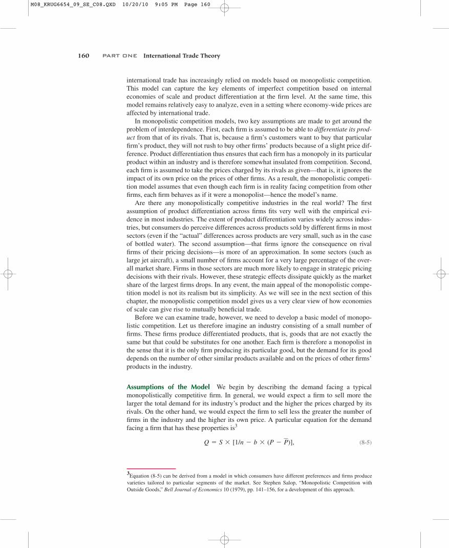
Average and Marginal Costs Returning to Figure 8-1, AC represents the firm’saverage cost of production, that is, its total cost divided by its output. The downwardslope reflects our assumption that there are economies of scale, so the larger the firm’soutput, the lower its costs per unit. MC represents the firm’s marginal cost (theamount it costs the firm to produce one extra unit). In the figure, we assumed that thefirm’s marginal cost is constant (the marginal cost curve is flat). The economies ofscale must then come from a fixed production cost. This fixed cost pushes the averagecost above the constant marginal cost of production, though the difference between thetwo becomes smaller and smaller as the fixed cost is spread over an increasing numberof output units.

If we denote c as the firm’s marginal cost and F as the fixed cost, then we can write thefirm’s total cost (C) as

(8-3)

where Q is once again the firm’s output. Given this linear cost function, the firm’s averagecost is

(8-4)

As we have discussed, this average cost is always greater than the marginal cost c, and de-clines with output produced Q.

If, for example, and , the average cost of producing 10 units is, and the average cost of producing 25 units is .

These numbers may look familiar, because they were used to construct Table 7-1 in the(5/25) + 1 = 1.2(5/10) + 1 = 1.5

c = 1F = 5

AC = C /Q = (F /Q) + c.

C = F + c * Q,

P - MR = Q /B.

Marginal revenue = MR = P - Q /B,

Q = A - B * P,



2The economic definition of profits is not the same as that used in conventional accounting, where any revenueover and above labor and material costs is called a profit. A firm that earns a rate of return on its capital less thanwhat that capital could have earned in other industries is not making profits; from an economic point of view, thenormal rate of return on capital represents part of the firm’s costs, and only returns over and above that normalrate of return represent profits.

previous chapter. (However, in this case, we assume a unit wage cost for the labor input,and that the technology now applies to a firm instead of an industry.) The marginaland average cost curves for this specific numeric example are plotted in Figure 8-2.Average cost approaches infinity at zero output and approaches marginal cost at verylarge output.

The profit-maximizing output of a monopolist is that at which marginal revenue (therevenue gained from selling an extra unit) equals marginal cost (the cost of producing anextra unit), that is, at the intersection of the MC and MR curves. In Figure 8-1 we can seethat the price at which the profit-maximizing output is demanded is , which isgreater than average cost. When , the monopolist is earning some monopoly prof-its, as indicated by the shaded box.2

Monopolistic CompetitionMonopoly profits rarely go uncontested. A firm making high profits normally attractscompetitors. Thus situations of pure monopoly are rare in practice. Instead, the usual mar-ket structure in industries characterized by internal economies of scale is one of oligopoly,in which several firms are each large enough to affect prices, but none has an uncontestedmonopoly.

The general analysis of oligopoly is a complex and controversial subject because in oli-gopolies, the pricing policies of firms are interdependent. Each firm in an oligopoly will,in setting its price, consider not only the responses of consumers but also the expectedresponses of competitors. These responses, however, depend in turn on the competitors’expectations about the firm’s behavior—and we are therefore in a complex game in whichfirms are trying to second-guess each other’s strategies. We will briefly discuss an exampleof an oligopoly model with two firms in Chapter 12. For now, we focus on a special caseof oligopoly known as monopolistic competition. Over the last 30 years, research in

P 7 ACPMQM

Cost per unit

Average cost

Marginal cost

6

5

4

3

2

1

0642

Output

8 10 12 14 16 18 20 22 24

Figure 8-2

Average versus Marginal Cost

This figure illustrates the averageand marginal costs correspon-ding to the total cost function

. Marginal cost isalways 1; average cost declines as output rises.

C = 5 + x



international trade has increasingly relied on models based on monopolistic competition.This model can capture the key elements of imperfect competition based on internaleconomies of scale and product differentiation at the firm level. At the same time, thismodel remains relatively easy to analyze, even in a setting where economy-wide prices areaffected by international trade.

In monopolistic competition models, two key assumptions are made to get around theproblem of interdependence. First, each firm is assumed to be able to differentiate its prod-uct from that of its rivals. That is, because a firm’s customers want to buy that particularfirm’s product, they will not rush to buy other firms’ products because of a slight price dif-ference. Product differentiation thus ensures that each firm has a monopoly in its particularproduct within an industry and is therefore somewhat insulated from competition. Second,each firm is assumed to take the prices charged by its rivals as given—that is, it ignores theimpact of its own price on the prices of other firms. As a result, the monopolistic competi-tion model assumes that even though each firm is in reality facing competition from otherfirms, each firm behaves as if it were a monopolist—hence the model’s name.

Are there any monopolistically competitive industries in the real world? The firstassumption of product differentiation across firms fits very well with the empirical evi-dence in most industries. The extent of product differentiation varies widely across indus-tries, but consumers do perceive differences across products sold by different firms in mostsectors (even if the “actual” differences across products are very small, such as in the caseof bottled water). The second assumption—that firms ignore the consequence on rivalfirms of their pricing decisions—is more of an approximation. In some sectors (such aslarge jet aircraft), a small number of firms account for a very large percentage of the over-all market share. Firms in those sectors are much more likely to engage in strategic pricingdecisions with their rivals. However, these strategic effects dissipate quickly as the marketshare of the largest firms drops. In any event, the main appeal of the monopolistic compe-tition model is not its realism but its simplicity. As we will see in the next section of thischapter, the monopolistic competition model gives us a very clear view of how economiesof scale can give rise to mutually beneficial trade.

Before we can examine trade, however, we need to develop a basic model of monopo-listic competition. Let us therefore imagine an industry consisting of a small number offirms. These firms produce differentiated products, that is, goods that are not exactly thesame but that could be substitutes for one another. Each firm is therefore a monopolist inthe sense that it is the only firm producing its particular good, but the demand for its gooddepends on the number of other similar products available and on the prices of other firms’products in the industry.

Assumptions of the Model We begin by describing the demand facing a typicalmonopolistically competitive firm. In general, we would expect a firm to sell more thelarger the total demand for its industry’s product and the higher the prices charged by itsrivals. On the other hand, we would expect the firm to sell less the greater the number offirms in the industry and the higher its own price. A particular equation for the demandfacing a firm that has these properties is3

(8-5)Q = S * [1/n - b * (P - P)],

3Equation (8-5) can be derived from a model in which consumers have different preferences and firms producevarieties tailored to particular segments of the market. See Stephen Salop, “Monopolistic Competition withOutside Goods,” Bell Journal of Economics 10 (1979), pp. 141–156, for a development of this approach.


where Q is the quantity of output demanded, S is the total output of the industry, n is thenumber of firms in the industry, b is a constant term representing the responsiveness of afirm’s sales to its price, P is the price charged by the firm itself, and is the average pricecharged by its competitors. Equation (8-5) may be given the following intuitive justifica-tion: If all firms charge the same price, each will have a market share 1/n. A firm chargingmore than the average of other firms will have a smaller market share, whereas a firmcharging less will have a larger share.4

It is helpful to assume that total industry output S is unaffected by the average price charged by firms in the industry. That is, we assume that firms can gain customers only ateach other’s expense. This is an unrealistic assumption, but it simplifies the analysis andhelps us focus on the competition among firms. In particular, it means that S is a measureof the size of the market and that if all firms charge the same price, each sells S/n units.

Next we turn to the costs of a typical firm. Here we simply assume that total and averagecosts of a typical firm are described by equations (8-3) and (8-4). Note that in this initialmodel, we assume that all firms are symmetric even though they produce differentiatedproducts: They all face the same demand curve (8-5) and have the same cost function (8-3).We will relax this assumption in the next section.

Market Equilibrium When the individual firms are symmetric, the state of the industrycan be described without describing any of the features of individual firms: All we reallyneed to know to describe the industry is how many firms there are and what price thetypical firm charges. To analyze the industry—for example, to assess the effects ofinternational trade—we need to determine the number of firms n and the average pricethey charge . Once we have a method for determining n and , we can ask how they areaffected by international trade.

Our method for determining n and involves three steps. (1) First, we derive a rela-tionship between the number of firms and the average cost of a typical firm. We showthat this relationship is upward sloping; that is, the more firms there are, the lower theoutput of each firm, and thus the higher each firm’s cost per unit of output. (2) We nextshow the relationship between the number of firms and the price each firm charges, whichmust equal in equilibrium. We show that this relationship is downward sloping: Themore firms there are, the more intense is the competition among firms, and as a result thelower the prices they charge. (3) Finally, we introduce firm entry and exit decisions basedon the profits that each firm earns. When price exceeds average cost, firms earn positiveprofits and additional firms will enter the industry; conversely, when the price is less thanaverage cost, profits are negative and those losses induce some firms to exit. In the longrun, this entry and exit process drives profits to zero, and the number of firms is deter-mined by the intersection of the curve that relates average cost to n and the curve thatrelates price to n.

1. The number of firms and average cost. As a first step toward determining n and, we ask how the average cost of a typical firm depends on the number of firms in the

industry. Since all firms are symmetric in this model, in equilibrium they all willcharge the same price. But when all firms charge the same price, so that ,equation (8-5) tells us that ; that is, each firm’s output Q is a l/n share of thetotal industry sales S. But we saw in equation (8-4) that average cost depends inversely

Q = S/nP = P

P

P

P

PP

P

P


4Equation (8-5) may be rewritten as . If , this equation reduces to .If , while if .P 6 P, Q 7 S/nP 7 P, Q 6 S/n

Q = S/nP = PQ = (S/n) - S * b * (P - P)



on a firm’s output. We therefore conclude that average cost depends on the size of themarket and the number of firms in the industry:

(8-6)

Equation (8-6) tells us that other things equal, the more firms there are in the indus-try, the higher is average cost. The reason is that the more firms there are, the less eachfirm produces. For example, imagine an industry with total sales of 1 million widgetsannually. If there are five firms in the industry, each will sell 200,000 annually. If thereare ten firms, each will sell only 100,000, and therefore each firm will have higheraverage cost. The upward-sloping relationship between n and average cost is shown asCC in Figure 8-3.

2. The number of firms and the price. Meanwhile, the price the typical firm chargesalso depends on the number of firms in the industry. In general, we would expect thatthe more firms there are, the more intense will be the competition among them, and

AC = F/Q + c = (n * F/S ) + c.

Cost C, andPrice, P

P3

AC3

Number of firms, n

n3n2n1

PP

CC

E

AC1

P1

P2, AC2

Figure 8-3

Equilibrium in a Monopolistically Competitive Market

The number of firms in a monopolistically competitive market, and the prices theycharge, are determined by two relationships. On one side, the more firms there are,the more intensely they compete, and hence the lower is the industry price. Thisrelationship is represented by PP. On the other side, the more firms there are, theless each firm sells and therefore the higher is the industry’s average cost. This rela-tionship is represented by CC. If price exceeds average cost (that is, if the PP curveis above the CC curve), the industry will be making profits and additional firms willenter the industry; if price is less than average cost, the industry will be incurringlosses and firms will leave the industry. The equilibrium price and number of firmsoccurs when price equals average cost, at the intersection of PP and CC.



hence the lower the price. This turns out to be true in this model, but proving it takes amoment. The basic trick is to show that each firm faces a straight-line demand curve ofthe form we showed in equation (8-1), and then to use equation (8-2) to determineprices.

First recall that in the monopolistic competition model, firms are assumed to takeeach other’s prices as given; that is, each firm ignores the possibility that if it changesits price, other firms will also change theirs. If each firm treats as given, we canrewrite the demand curve (8-5) in the form

(8-7)

where b is the parameter in equation (8-5) that measured the sensitivity of each firm’smarket share to the price it charges. Now this equation is in the same form as (8-1), with in place of the constant term A and in place ofthe slope coefficient B. If we plug these values back into the formula for marginal rev-enue, (8-2), we have a marginal revenue for a typical firm of

(8-8)

Profit-maximizing firms will set marginal revenue equal to their marginal cost, c, sothat

which can be rearranged to give the following equation for the price charged by a typ-ical firm:

(8-9)

We have already noted, however, that if all firms charge the same price, each will sellan amount . Plugging this back into (8-9) gives us a relationship between thenumber of firms and the price each firm charges:

(8-10)

Equation (8-10) says algebraically that the more firms there are in an industry, thelower the price each firm will charge. This is because each firm’s markup over mar-ginal cost, , decreases with the number of competing firms.Equation (8-10) is shown in Figure 8-3 as the downward-sloping curve PP.

3. The equilibrium number of firms. Let us now ask what Figure 8-3 means. Wehave summarized an industry by two curves. The downward-sloping curve PP showsthat the more firms there are in the industry, the lower the price each firm will charge.This makes sense: The more firms there are, the more competition each firm faces. Theupward-sloping curve CC tells us that the more firms there are in the industry, thehigher the average cost of each firm. This also makes sense: If the number of firmsincreases, each firm will sell less, so firms will not be able to move as far down theiraverage cost curve.

The two schedules intersect at point E, corresponding to the number of firms . Thesignificance of is that it is the zero-profit number of firms in the industry. When thereare firms in the industry, their profit-maximizing price is , which is exactly equal totheir average cost . What we will now argue is that in the long run, the numberof firms in the industry tends to move toward , so that point E describes the industry’s long-run equilibrium.

AC2

P2n2

n2

n2

P - c = 1/(b * n)

P = c + 1/(b * n).

Q = S/n

P = c + Q/(S * b).

MR = P - Q/(S * b) = c,

MR = P - Q/(S * b).

S * b(S/n) + S * b * P

Q = [(S/n) + S * b * P] - S * b * P,

P



5This analysis slips past a slight problem: The number of firms in an industry must, of course, be a whole numberlike 5 or 8. What if turns out to equal 6.37? The answer is that there will be six firms in the industry, all mak-ing small monopoly profits and not being challenged by new entrants because everyone knows that a seven-firmindustry would lose money. In most examples of monopolistic competition, this whole-number or “integer con-straint” problem turns out not to be very important, and we ignore it here.

n2

To see why, suppose that n were less than , say . Then the price charged by firmswould be , while their average cost would be only . Thus firms would be makingmonopoly profits. Conversely, suppose that n were greater than , say . Then firmswould charge only the price , while their average cost would be . Firms would besuffering losses.

Over time, firms will enter an industry that is profitable and exit one in which they losemoney. The number of firms will rise over time if it is less than , fall if it is greater. Thismeans that is the equilibrium number of firms in the industry and that is the equilib-rium price.5

We have just developed a model of a monopolistically competitive industry in whichwe can determine the equilibrium number of firms and the average price that firms charge.We now use this model to derive some important conclusions about the role of economiesof scale in international trade.

Monopolistic Competition and TradeUnderlying the application of the monopolistic competition model to trade is the idea thattrade increases market size. In industries where there are economies of scale, both thevariety of goods that a country can produce and the scale of its production are constrainedby the size of the market. By trading with each other, and therefore forming an integratedworld market that is bigger than any individual national market, nations are able to loosenthese constraints. Each country can thus specialize in producing a narrower range of prod-ucts than it would in the absence of trade; yet by buying from other countries the goodsthat it does not make, each nation can simultaneously increase the variety of goods avail-able to its consumers. As a result, trade offers an opportunity for mutual gain even whencountries do not differ in their resources or technology.

Suppose, for example, that there are two countries, each with an annual market for 1million automobiles. By trading with each other, these countries can create a combinedmarket of 2 million autos. In this combined market, more varieties of automobiles can beproduced, at lower average costs, than in either market alone.

The monopolistic competition model can be used to show how trade improves thetrade-off between scale and variety that individual nations face. We will begin by showinghow a larger market leads, in the monopolistic competition model, to both a lower averageprice and the availability of a greater variety of goods. Applying this result to internationaltrade, we observe that trade creates a world market larger than any of the national marketsthat comprise it. Integrating markets through international trade therefore has the sameeffects as growth of a market within a single country.

The Effects of Increased Market SizeThe number of firms in a monopolistically competitive industry and the prices they chargeare affected by the size of the market. In larger markets there usually will be both morefirms and more sales per firm; consumers in a large market will be offered both lowerprices and a greater variety of products than consumers in small markets.

P2n2

n2

AC3P3

n3n2

AC1P1

n1n2


To see this in the context of our model, look again at the CC curve in Figure 8-3, whichshowed that average costs per firm are higher the more firms there are in the industry. Thedefinition of the CC curve is given by equation (8-6):

Examining this equation, we see that an increase in total industry output S will reduce av-erage costs for any given number of firms n. The reason is that if the market grows whilethe number of firms is held constant, output per firm will increase and the average cost ofeach firm will therefore decline. Thus if we compare two markets, one with higher S thanthe other, the CC curve in the larger market will be below that in the smaller one.

Meanwhile, the PP curve in Figure 8-3, which relates the price charged by firms to thenumber of firms, does not shift. The definition of that curve was given in equation (8-10):

The size of the market does not enter into this equation, so an increase in S does not shiftthe PP curve.

Figure 8-4 uses this information to show the effect of an increase in the size of the mar-ket on long-run equilibrium. Initially, equilibrium is at point 1, with a price and a num-ber of firms n1. An increase in the size of the market, measured by industry sales S, shifts

P1

P = c + 1/(b * n).

AC = F/Q + c = n * F/S + c.


Cost, C andPrice, P

P2

Number of firms, n

n2n1

PP

P1

1

2

CC1

CC2

Figure 8-4

Effects of a Larger Market

An increase in the size of the market allows each firm, other things equal, to pro-duce more and thus have lower average cost. This is represented by a downwardshift from CC1 to CC2. The result is a simultaneous increase in the number of firms(and hence in the variety of goods available) and a fall in the price of each.



the CC curve down from to , while it has no effect on the PP curve. The newequilibrium is at point 2: The number of firms increases from to , while the price fallsfrom to .

Clearly, consumers would prefer to be part of a large market rather than a small one. Atpoint 2, a greater variety of products is available at a lower price than at point 1.

Gains from an Integrated Market: A Numerical ExampleInternational trade can create a larger market. We can illustrate the effects of trade onprices, scale, and the variety of goods available with a specific numerical example.

Imagine that automobiles are produced by a monopolistically competitive industry. Thedemand curve facing any given producer of automobiles is described by equation (8-5),with b = 1/30,000 (this value has no particular significance; it was chosen to make theexample come out neatly). Thus the demand facing any one producer is given by

where Q is the number of automobiles sold per firm, S is the total number sold for theindustry, n is the number of firms, P is the price that a firm charges, and is the averageprice of other firms. We also assume that the cost function for producing automobiles isdescribed by equation (8-3), with a fixed cost and a marginal cost

per automobile (again, these values were chosen to give nice results). Thetotal cost is

The average cost curve is therefore

Now suppose there are two countries, Home and Foreign. Home has annual sales of900,000 automobiles; Foreign has annual sales of 1.6 million. The two countries areassumed, for the moment, to have the same costs of production.

Figure 8-5a shows the PP and CC curves for the Home auto industry. We find that inthe absence of trade, Home would have six automobile firms, selling autos at a price of$10,000 each. (It is also possible to solve for n and P algebraically, as shown in theMathematical Postscript to this chapter.) To confirm that this is the long-run equilibrium,we need to show both that the pricing equation (8-10) is satisfied and that the price equalsaverage cost.

Substituting the actual values of the marginal cost c, the demand parameter b, and thenumber of Home firms n into equation (8-10), we find

so the condition for profit maximization—marginal revenue equaling marginal cost—issatisfied. Each firm sells 900,000 units/6 firms = 150,000 units/firm. Its average cost istherefore

Since the average cost of $10,000 per unit is the same as the price, all monopoly profitshave been competed away. Thus six firms, selling each unit at a price of $10,000, witheach firm producing 150,000 cars, is the long-run equilibrium in the Home market.

AC = ($750,000,000/150,000) + $5,000 = $10,000.

= $5,000 + $5,000,

P = $10,000 = c + 1/(b * n) = $5,000 + 1/[(1/30,000) * 6

AC = (750,000,000/Q) + 5,000.

C = 750,000,000 + (5,000 * Q).

c = $5,000F = $750,000,000

P

Q = S * [(1/n) - (1/30,000) * (P - P)],

P2P1

n2n1

CC2CC1



642 8 10 12

Price per auto,in thousands of dollars

Number of firms, n

64

81012141618202224262830323436

753 9 111

PP

CC

(c) Integrated

642 8 10 12


Number of firms, n

64

81012141618202224262830323436

753 9 111

PP

CC

(a) Home

642 8 10 12


Number of firms, n

64

81012141618202224262830323436

753 9 111

PP

CC

(b) Foreign

Figure 8-5

Equilibrium in the Automobile Market

(a) The Home market: With a market size of 900,000 automobiles, Home’s equilibrium, determined by the intersection of the PP and CC curves, occurs with six firms and an industry price of $10,000 per auto. (b) TheForeign market: With a market size of 1.6 million automobiles, Foreign’s equilibrium occurs with eight firms and an industry price of $8,750 per auto. (c) The combined market: Integrating the two markets creates a market for 2.5 million autos. This market supports ten firms, and the price of an auto is only $8,000.



What about Foreign? By drawing the PP and CC curves (panel (b) in Figure 8-5), wefind that when the market is for 1.6 million automobiles, the curves intersect at

. That is, in the absence of trade, Foreign’s market would support eightfirms, each producing 200,000 automobiles, and selling them at a price of $8,750. We canagain confirm that this solution satisfies the equilibrium conditions:

and

Now suppose it is possible for Home and Foreign to trade automobiles costlessly withone another. This creates a new, integrated market (panel (c) in Figure 8-5) with total salesof 2.5 million. By drawing the PP and CC curves one more time, we find that this inte-grated market will support ten firms, each producing 250,000 cars and selling them at aprice of $8,000. The conditions for profit maximization and zero profits are again satisfied:

and

We summarize the results of creating an integrated market in Table 8-1. The table com-pares each market alone with the integrated market. The integrated market supports morefirms, each producing at a larger scale and selling at a lower price than either national mar-ket does on its own.

Clearly everyone is better off as a result of integration. In the larger market, consumershave a wider range of choices, yet each firm produces more and is therefore able to offerits product at a lower price. To realize these gains from integration, the countries must en-gage in international trade. To achieve economies of scale, each firm must concentrate itsproduction in one country—either Home or Foreign. Yet it must sell its output to cus-tomers in both markets. So each product will be produced in only one country andexported to the other.

This numerical example highlights two important new features about trade with monop-olistic competition relative to the models of trade based on comparative advantage that wecovered in Chapters 3 through 6: (1) First, the example shows how product differentiation

AC = ($750,000,000/250,000) + $5,000 = $8,000.

= $5,000 + $3,000,

P = $8,000 = c + 1/(b * n) = $5,000 + 1/[(1/30,000) * 10]

AC = ($750,000,000/200,000) + $5,000 = $8,750.

P = $8,750 = c + 1/(b * n) = $5,000 + 1/[(1/30,000) * 8] = $5,000 + $3,750,

n = 8, P = 8,750

TABLE 8-1 Hypothetical Example of Gains from Market Integration

Home Market,Before Trade

Foreign Market,Before Trade

Integrated Market,After Trade

Industry output (# of autos)

900,000 1,600,000 2,500,000

Number of firms 6 8 10Output per firm

(# of autos)150,000 200,000 250,000

Average cost $10,000 $8,750 $8,000Price $10,000 $8,750 $8,000



and internal economies of scale lead to trade between similar countries with no comparativeadvantage differences between them. This is a very different kind of trade than the onebased on comparative advantage, where each country exports its comparative advantagegood. Here, both Home and Foreign export autos to one another. Home pays for the importsof some automobile models (those produced by firms in Foreign) with exports of differenttypes of models (those produced by firms in Home)—and vice versa. This leads to what iscalled intra-industry trade: two-way exchanges of similar goods. (2) Second, the examplehighlights two new channels for welfare benefits from trade. In the integrated market aftertrade, both Home and Foreign consumers benefit from a greater variety of automobile mod-els (ten versus six or eight) at a lower price ($8,000 versus $8,750 or $10,000) as firms areable to consolidate their production destined for both locations and take advantage ofeconomies of scale.6

Empirically, is intra-industry trade relevant and do we observe gains from trade in theform of greater product variety and consolidated production at lower average cost? Theanswer is yes.

The Significance of Intra-Industry TradeThe proportion of intra-industry trade in world trade has steadily grown over the last half-century. The measurement of intra-industry trade relies on an industrial classificationsystem that categorizes goods into different industries. Depending on the coarseness ofthe industrial classification used (hundreds of different industry classifications versusthousands), intra-industry trade accounts for one-quarter to nearly one-half of all worldtrade flows. Intra-industry trade plays an even more prominent role in the trade of manu-factured goods among advanced industrial nations, which accounts for the majority ofworld trade.

Table 8-2 shows measures of the importance of intra-industry trade for a number of U.S.manufacturing industries in 2009. The measure shown is intra-industry trade as a proportion of

6Also note that Home consumers gain more than Foreign consumers from trade integration. This is a standardfeature of trade models with increasing returns and product differentiation: A smaller country stands to gain morefrom integration than a larger country. This is because the gains from integration are driven by the associatedincrease in market size; the country that is initially smaller benefits from a bigger increase in market size uponintegration.

TABLE 8-2 Indexes of Intra-Industry Trade for U.S. Industries, 2009

Metalworking Machinery 0.97Inorganic Chemicals 0.97Power-Generating Machines 0.86Medical and Pharmaceutical Products 0.85Scientific Equipment 0.84Organic Chemicals 0.79Iron and Steel 0.76Road Vehicles 0.70Office Machines 0.58Telecommunications Equipment 0.46Furniture 0.30Clothing and Apparel 0.11Footwear 0.10



overall trade.7 The measure ranges from 0.97 for metalworking machinery and inorganicchemicals—industries where U.S. exports and imports are nearly equal—to 0.10 for footwear,an industry in which the United States has large imports but virtually no exports. The measurewould be 0 for an industry in which the United States is only an exporter or only an importer,but not both; it would be 1 for an industry in which U.S. exports exactly equal U.S. imports.

Table 8-2 shows that intra-industry trade is a very important component of trade for theUnited States in many different industries. Those industries tend to be ones that produce sophis-ticated manufactured goods, such as chemicals, pharmaceuticals, and specialized machinery.These goods are exported principally by advanced nations and are probably subject to importanteconomies of scale in production. At the other end of the scale are the industries with very littleintra-industry trade, which typically produce labor-intensive products such as footwear andapparel. These are goods that the United States imports primarily from less-developed countries,where comparative advantage is the primary determinant of U.S. trade with these countries.

What about the new types of welfare gains via increased product variety and economiesof scale? A recent paper by Christian Broda at the Chicago Booth School of Business andDavid Weinstein at Columbia University estimates that the number of available productsin U.S. imports tripled in the 30-year time-span from 1972 to 2001. They further estimatethat this increased product variety for U.S. consumers represented a welfare gain equal to2.6 percent of U.S. GDP!8

Table 8-1 from our numerical example showed that the gains from integration gener-ated by economies of scale were most pronounced for the smaller economy: Prior to inte-gration, production there was particularly inefficient, as the economy could not takeadvantage of economies of scale in production due to the country’s small size. This isexactly what happened when the United States and Canada followed a path of increasingeconomic integration starting with the North American Auto Pact in 1964 (which did notinclude Mexico) and culminating in the North American Free Trade Agreement (NAFTA,which does include Mexico). The Case Study that follows describes how this integrationled to consolidation and efficiency gains in the automobile sector—particularly on theCanadian side (whose economy is one-tenth the size of the U.S. economy).

Similar gains from trade have also been measured for other real-world examples of closereconomic integration. One of the most prominent examples has taken place in Europe overthe last half-century. In 1957 the major countries of Western Europe established a free tradearea in manufactured goods called the Common Market, or European Economic Community(EEC). (The United Kingdom entered the EEC later, in 1973.) The result was a rapid growthof trade that was dominated by intra-industry trade. Trade within the EEC grew twice as fastas world trade as a whole during the 1960s. This integration slowly expanded into what hasbecome the European Union. When a subset of these countries (mostly, those countries thathad formed the EEC) adopted the common euro currency in 1999, intra-industry tradeamong those countries further increased (even relative to that of the other countries in theEuropean Union). Recent studies have also found that the adoption of the euro has led to asubstantial increase in the number of different products that are traded within the Eurozone.

7To be more precise, the standard formula for calculating the importance of intra-industry trade within a given industry is

where min{exports, imports} refers to the smallest value between exports and imports. This is the amount oftwo-way exchanges of goods that is reflected in both exports and imports. This number is measured as a propor-tion of the average trade flow (average of exports and imports). If trade in an industry flows in only one direction,then since the smallest trade flow is zero: There is no intra-industry trade. On the other hand, if a country’sexports and imports within an industry are equal, we get the opposite extreme of .I = 1

I = 0

I =

min{exports, imports}

(exports + imports)/2 ,

8See “Globalization and the Gains from Variety” in Quarterly Journal of Economics, 2006.



Case Study

Intra-Industry Trade in Action: The North American Auto Pact of 1964An unusually clear-cut example of the role of economies of scale in generating benefi-cial international trade is provided by the growth in automotive trade between the

United States and Canada during the second half of the 1960s. Whilethe case does not fit our model exactly since it involves multinationalfirms, it does show that the basic concepts we have developed are use-ful in the real world.

Before 1965, tariff protection by Canada and the United States pro-duced a Canadian auto industry that was largely self-sufficient, neitherimporting nor exporting much. The Canadian industry was controlledby the same firms as the U.S. industry—a feature that we will addresslater on in this chapter—but these firms found it cheaper to have largelyseparate production systems than to pay the tariffs. Thus the Canadianindustry was in effect a miniature version of the U.S. industry, at about1/10 the scale.

The Canadian subsidiaries of U.S. firms found that small scale wasa substantial disadvantage. This was partly because Canadian plantshad to be smaller than their U.S. counterparts. Perhaps more impor-tantly, U.S. plants could often be “dedicated”—that is, devoted toproducing a single model or component—while Canadian plants hadto produce several different things, requiring the plants to shut downperiodically to change over from producing one item to producinganother, to hold larger inventories, to use less specialized machinery,

and so on. The Canadian auto industry thus had a labor productivity about 30 percentlower than that of the United States.

In an effort to remove these problems, the United States and Canada agreed in 1964to establish a free trade area in automobiles (subject to certain restrictions). This al-lowed the auto companies to reorganize their production. Canadian subsidiaries of theauto firms sharply cut the number of products made in Canada. For example, GeneralMotors cut in half the number of models assembled in Canada. The overall level ofCanadian production and employment was, however, maintained. Production levels forthe models produced in Canada rose dramatically, as those Canadian plants became oneof the main (and many times the only) supplier of that model for the whole NorthAmerican market. Conversely, Canada then imported the models from the UnitedStates that it was no longer producing. In 1962, Canada exported $16 million worth ofautomotive products to the United States while importing $519 million worth. By 1968the numbers were $2.4 and $2.9 billion, respectively. In other words, both exports andimports increased sharply: intra-industry trade in action.

The gains seem to have been substantial. By the early 1970s the Canadian industrywas comparable to the U.S. industry in productivity. Later on, this transformation of theautomotive industry was extended to include Mexico. In 1989, Volkswagen consolidatedits North American operations in Mexico, shutting down its plant in Pennsylvania. Thisprocess continued with the implementation of NAFTA (the North American Free TradeAgreement between the United States, Canada, and Mexico). In 1994 Volkswagenstarted producing the new Beetle for the whole North American market in that sameMexican plant. We discuss the effects of NAFTA in more detail later on in this chapter.

The Ambassador bridge connectsDetroit in the United States toWindsor in Canada. On a typicalday, $250 million worth of carsand car parts crosses this bridge.

M08_KRUG6654_09_SE_C08.QXD 10/20/10 9:05 PM 1


Firm Responses to Trade: Winners, Losers, and Industry Performance

In our numerical example of the auto industry with two countries, we saw how economicintegration led to an increase in competition between firms. Of the 14 firms producingautos before trade (6 in Home and 8 in Foreign), only 10 firms “survive” after economicintegration; however, each of those firms now produces at a bigger scale (250,000 autosproduced per firm versus either 150,000 for Home firms or 200,000 for Foreign firms be-fore trade). In that example, the firms were assumed to be symmetric, so exactly whichfirms exited and which survived and expanded was inconsequential. In the real world,however, performance varies widely across firms, so the effects of increased competitionfrom trade are far from inconsequential. As one would expect, increased competition tendsto hurt the worst-performing firms the hardest, because they are the ones who are forced toexit. If the increased competition comes from trade (or economic integration), then it isalso associated with sales opportunities in new markets for the surviving firms. Again, asone would expect, it is the best-performing firms that take greatest advantage of those newsales opportunities and expand the most.

These composition changes have a crucial consequence at the level of the industry:When the better-performing firms expand and the worse-performing ones contract or exit,then overall industry performance improves. This means that trade and economic integra-tion can have a direct impact on industry performance: It is as if there was technologicalgrowth at the level of the industry. Empirically, these composition changes generate sub-stantial improvements in industry productivity.

Take the example of Canada’s closer economic integration with the United States (seethe preceding Case Study and the discussion in Chapter 2). We discussed how this integra-tion led the automobile producers to consolidate production in a smaller number ofCanadian plants, whose production levels rose dramatically. The Canada–U.S. Free TradeAgreement, which went into effect in 1989, extended the auto pact to most manufacturingsectors. A similar process of consolidation occurred throughout the affected Canadianmanufacturing sectors. However, this was also associated with a selection process: Theworst-performing producers shut down, while the better-performing ones expanded vialarge increases in exports to the U.S. market. Daniel Trefler at the University of Torontohas studied the effects of this trade agreement in great detail, examining the variedresponses of Canadian firms.9 He found that productivity in the most affected Canadianindustries rose by a dramatic 14 to 15 percent (replicated economy-wide, a 1 percentincrease in productivity translates into a 1 percent increase in GDP, holding employmentconstant). On its own, the contraction and exit of the worst-performing firms in responseto increased competition from U.S. firms accounted for half of the 15 percent increase inthose sectors.

Performance Differences Across ProducersWe now relax the symmetry assumption that we imposed in our previous development ofthe monopolistic competition model so that we can examine how competition fromincreased market size affects firms differently. The symmetry assumption meant that allfirms had the same cost curve (8-3) and the same demand curve (8-5). Suppose now that

9See “The Long and Short of the Canada-U.S. Free Trade Agreement,” American Economic Review, 2004, andthe summary of this work in the New York Times: “What Happened When Two Countries Liberalized Trade?Pain, Then Gain” by Virginia Postel (January 27, 2005).



firms have different cost curves because they produce with different marginal cost levels .We assume that all firms still face the same demand curve. Product-quality differencesbetween firms would lead to very similar predictions for firm performance as the ones wenow derive for cost differences.

Figure 8-6 illustrates the performance differences between firms 1 and 2 when .In panel (a), we have drawn the common demand curve (8-5) as well as its associated mar-ginal revenue curve (8-8). Note that both curves have the same intercept on the verticalaxis (plug into (8-8) to obtain ); this intercept is given by the price P from(8-5) when , which is . The slope of the demand curve is .As we previously discussed, the marginal revenue curve is steeper than the demand curve.Firms 1 and 2 choose output levels and , respectively, to maximize their profits. Thisoccurs where their respective marginal cost curves intersect the common marginal revenuecurve. They set prices and that correspond to those output levels on the common de-mand curve. We immediately see that firm 1 will set a lower price and produce a higheroutput level than firm 2. Since the marginal revenue curve is steeper than the demandcurve, we also see that firm 1 will set a higher markup over marginal cost than firm 2:

.The shaded areas represent operating profits for both firms, equal to revenue

minus operating costs (for both firms, and ). Here, we have assumedthat the fixed cost F (assumed to be the same for all firms) cannot be recovered and does notenter into operating profits (that is, it is a sunk cost). Since operating profits can be rewritten

i = 2i = 1ci * Qi

Pi * Qi

P1 - c1 7 P2 - c2

P2P1

Q2Q1

1/(S * b)P + [1/(b * n)]Q = 0MR = PQ = 0

c1 6 c2

ci

Cost,Price

P2

C2

C1

P1

Q

D

1 Quantity

MC2

MC1

MR

Intercept = P + [1/(b × n)]

Slope = 1/(S × b)

(P2– Q2) × C2

(P1– Q1) × C1

Q2

(a)

OperatingProfit

C 2 Marginalcost, Ci

C*C 1

(b)

Figure 8-6

Performance Differences Across Firms

(a) Demand and cost curves for firms 1 and 2. Firm 1 has a lower marginal cost than firm 2: . Both firmsface the same demand curve and marginal revenue curve. Relative to firm 2, firm 1 sets a lower price andproduces more output. The shaded areas represent operating profits for both firms (before the fixed cost is deducted). Firm 1 earns higher operating profits than firm 2. (b) Operating profits as a function of a firm’s marginal cost . Operating profits decrease as the marginal cost increases. Any firm with marginal cost above cannot operate profitably and shuts down.c*

ci

c1 6 c2



as the product of the markup times the number of output units sold, , we candetermine that firm 1 will earn higher profits than firm 2 (recall that firm 1 sets a highermarkup and produces more output than firm 2). We can thus summarize all the relevant per-formance differences based on marginal cost differences across firms. Compared to a firmwith a higher marginal cost, a firm with a lower marginal cost will: (1) set a lower price, butat a higher markup over marginal cost; (2) produce more output; and (3) earn higherprofits.10

Panel (b) in Figure 8-6 shows how a firm’s operating profits vary with its marginal cost .As we just mentioned, this will be a decreasing function of marginal cost. Going back topanel (a), we see that a firm can earn a positive operating profit so long as its marginal cost isbelow the intercept of the demand curve on the vertical axis at . Let denote this cost cutoff (shown in panel (b) of Figure 8-6). A firm with a marginal cost above this cutoff is effectively “priced out” of the market and would earn negative operat-ing profits if it were to produce any output. Such a firm would choose to shut down and notproduce (incurring an overall profit loss equal to the fixed cost F ). Why would such a firmenter in the first place? Clearly, it wouldn’t if it knew about its high cost prior to enteringand paying the fixed cost F.

We assume that entrants face some randomness about their future production cost . Thisrandomness disappears only after F is paid and is sunk. Thus, some firms will regret theirentry decision if their overall profit (operating profit minus the fixed cost F) is negative. Onthe other hand, some firms will discover that their production cost is very low and that theyearn high positive overall profit levels. Entry is driven by a similar process as the one wedescribed for the case of symmetric firms. In that previous case, firms entered until profitsfor all firms were driven to zero. Here, there are profit differences between firms, and entryoccurs until expected profits across all potential cost levels are driven to zero.

The Effects of Increased Market SizePanel (b) of Figure 8-6 summarizes the industry equilibrium given a market size S. It tellsus which range of firms survive and produce (with cost below ), and how their profitswill vary with their cost levels . What happens when economies integrate into a singlelarger market? As was the case with symmetric firms, a larger market can support a largernumber of firms than can a smaller market. This also implies more competition in thelarger market. What are the repercussions for different firms of increased competition?

First, consider the effects of increased competition (higher number of firms n) on theindividual firm-demand curves. Panel (a) of Figure 8-7 shows the effect. Recall that the in-tercept on the vertical axis is equal to , which decreases when the numberof firms increases.11 The slope of the demand curve, equal to , decreases fromthe direct effect of the increase in the market size S, so the demand curve also becomesflatter: With increased competition, a producer can gain more market share from a givenprice cut. This produces the shift in the demand curve from D to shown in panel (a) ofFigure 8-7. Notice how the demand curve shifts for the smaller firms (lower-output )that operate on the top part of the demand curve.

Panel (b) of Figure 8-7 shows the consequences of this demand change for the operat-ing profits of firms with different cost levels . The decrease in demand for the smallerfirms translates into a new, lower-cost cutoff, : Some firms with the high cost levelsabove cannot survive the decrease in demand and are forced to exit. On the other hand,c*œ

c*œ

ci

Qi

Dœ

1/(S * b)P + [1/(b * n)]

ci

c*ci

ci

ci

ci

ci

ci

c*P + [1/(b * n)]

ci

(Pi - ci) * Qi

10Recall that we have assumed that all firms face the same nonrecoverable fixed cost F. If a firm earns higheroperating profits, then it also earns higher overall profits (that deduct the fixed cost F).11The intercept will further decrease because the average price will also decrease.



Cost,Price

D

D ′

Quantity

Intercept = P + [1/(b × n)]

Slope = 1/(S × b)

(a)

OperatingProfit

Winners

Marginalcost, Ci

C *

(b)

C *′

Exit

Losers

Figure 8-7

Winners and Losers from Economic Integration

(a) The demand curve for all firms shifts from D to . It is flatter, and has a lower intercept on the vertical axis. (b) Effects of the shift in demand on the operating profits of firms with different marginalcost . Firms with marginal cost between the old cutoff, , and the new one, , are forced to exit.Some firms with the lowest marginal cost levels gain from integration and their profits increase.

c*œc*ci

Dœ

the flatter demand curve is advantageous to some firms with low cost levels: They canadapt to the increased competition by lowering their markup (and hence their price) andgain some additional market share.12 This translates into increased profits for some of thebest-performing firms with the lowest cost levels .13

Figure 8-7 illustrates how increased market size generates both winners and losersamong firms in an industry. The low-cost firms thrive and increase their profits and marketshares, while the high-cost firms contract and the highest-cost firms exit. These composi-tion changes imply that overall productivity in the industry is increasing as production isconcentrated among the more productive (low-cost) firms. This replicates the findings forCanadian manufacturing following closer integration with U.S. manufacturing, as we pre-viously described. These effects tend to be most pronounced for smaller countries thatintegrate with larger ones, but it is not limited to those small countries. Even for a bigeconomy such as the United States, increased integration via lower trade costs leads toimportant composition effects and productivity gains.14

ci

12Recall that the lower the firm’s marginal cost , the higher its markup over marginal cost . High-costfirms are already setting low markups and cannot lower their prices to induce positive demand, as this wouldmean pricing below their marginal cost of production.13Another way to deduce that profit increases for some firms is to use the entry condition that drives averageprofits to zero: If profit decreases for some of the high-cost firms, then it must increase for some of the low-costfirms, since the average across all firms must remain equal to zero.

Pi - cici

14See A. B. Bernard, J. B. Jensen, and P. K. Schott, “Trade Costs, Firms and Productivity,”Journal of MonetaryEconomics 53(5), 2006, pp. 917–937.



Trade Costs and Export DecisionsUp to now, we have modeled economic integration as an increase in market size. This im-plicitly assumes that this integration occurs to such an extent that a single combined mar-ket is formed. In reality, integration rarely goes that far: Trade costs among countries arereduced, but they do not disappear. In Chapter 2, we discussed how these trade costs aremanifested even for the case of the two very closely integrated economies of the UnitedStates and Canada. We saw how the U.S.–Canada border substantially decreases trade vol-umes between Canadian provinces and U.S. states.

Trade costs associated with this border crossing are also a salient feature of firm-leveltrade patterns: Very few firms in the United States reach Canadian customers. In fact, mostU.S. firms do not report any exporting activity at all (because they sell only to U.S. cus-tomers). In 2002, only 18 percent of U.S. manufacturing firms reported undertaking someexport sales. Table 8-3 shows the proportion of firms that report some export sales acrossseveral different U.S. manufacturing sectors. Even in industries where exports represent asubstantial proportion of total production, such as chemicals, machinery, electronics, andtransportation, fewer than 40 percent of firms export. In fact, one major reason why tradecosts associated with national borders reduce trade so much is that they drastically cutdown the number of firms willing or able to reach customers across the border. (The otherreason is that the trade costs also reduce the export sales of firms that do reach those cus-tomers across the border.)

In our integrated economy without any trade costs, firms were indifferent as to the loca-tion of their customers. We now introduce trade costs to explain why firms actually do careabout the location of their customers, and why so many firms choose not to reach cus-tomers in another country. As we will see shortly, this will also allow us to explain impor-tant differences between those firms that choose to incur the trade costs and export, andthose that do not. Why would some firms choose not to export? Simply put, the trade costsreduce the profitability of exporting for all firms. For some, that reduction in profitabilitymakes exporting unprofitable. We now formalize this argument.

To keep things simple, we will consider the response of firms in a world with two iden-tical countries (Home and Foreign). Let the market size parameter S now reflect the size ofeach market, so that now reflects the size of the world market. We cannot analyzethis world market as a single market of size because this market is no longerperfectly integrated due to trade costs.

2 * S2 * S

TABLE 8-3 Proportion of U.S. Firms Reporting Export Sales by Industry, 2002

Printing 5%Furniture 7%Apparel 8%Wood Products 8%Fabricated Metals 14%Petroleum and Coal 18%Transportation Equipment 28%Machinery 33%Chemicals 36%Computer and Electronics 38%Electrical Equipment and Appliances 38%

Source: A. B. Bernard, J. B. Jensen, S. J. Redding, and P. K. Schott, “Firms in International Trade,”Journal of Economic Perspectives 21(3), 2007, pp. 105–130.



Specifically, assume that a firm must incur an additional cost t for each unit of outputthat it sells to customers across the border. We now have to keep track of the firms’ behav-ior in each market separately. Due to the trade cost t, firms will set different prices in theirexport market relative to their domestic market. This will lead to different quantities soldin each market, and ultimately to different profit levels earned in each market. As eachfirm’s marginal cost is constant (does not vary with production levels), those decisions re-garding pricing and quantity sold in each market can be separated: A decision regardingthe domestic market will have no impact on the profitability of different decisions for theexport market.

Consider the case of firms located in Home. Their situation regarding their domestic(Home) market is exactly as was illustrated in Figure 8-6, except that all the outcomes,such as price, output, and profit, relate to the domestic market only.15 Now consider thedecisions of firms 1 and 2 (with marginal costs and ) regarding the export (Foreign)market. They face the same demand curve in Foreign as they do in Home (recall that weassumed that the two countries are identical). The only difference is that the firms’ mar-ginal cost in the export market is shifted up by the trade cost t. Figure 8-8 shows the situa-tion for the two firms in both markets.

What are the effects of the trade cost on the firms’ decisions regarding the export market?We know from our previous analysis that a higher marginal cost induces a firm to raise itsprice, which leads to a lower output quantity sold and lower profits. We also know thatif marginal cost is raised above a threshold level , then a firm cannot profitably operate inthat market. This is what happens to firm 2 in Figure 8-8. Firm 2 can profitably operate in

c*

c2c1

Price,Cost

C2

C1

D

Quantity

MC2

MC1

(a) Domestic (Home) Market

C *

Price,Cost

C2

C1

D

Quantity

C2 + t

C1 + t

C *

(b) Export (Foreign) Market

Figure 8-8

Export Decisions with Trade Costs

(a) Firms 1 and 2 both operate in their domestic (Home) market. (b) Only firm 1 chooses to export to the Foreignmarket. It is not profitable for firm 2 to export given the trade cost t.

15The number of firms n is the total number of firms selling in the Home market. (This includes both firmslocated in Home as well as the firms located in Foreign that export to Home). is the average price across allthose firms selling in Home.

P



its domestic market, because its cost there is below the threshold: . However, it can-not profitably operate in the export market because its cost there is above the threshold:

. Firm 1, on the other hand, has a low enough cost that it can profitably operatein both the domestic and the export markets: . We can extend this prediction toall firms based on their marginal cost . The lowest-cost firms with export; thehigher-cost firms with still produce for their domestic market but do notexport; the highest-cost firms with cannot profitably operate in either market, andthus exit.

We just saw how the modeling of trade costs added two important predictions to ourmodel of monopolistic competition and trade: Those costs explain why only a subset offirms export, and they also explain why this subset of firms will consist of relatively largerand more productive firms (those firms with lower marginal cost ). Empirical analyses offirms’ export decisions from numerous countries have provided overwhelming support forthis prediction that exporting firms are bigger and more productive than firms in the sameindustry that do not export. In the United States in a typical manufacturing industry, anexporting firm is on average more than twice as large as a firm that does not export. Theaverage exporting firm also produces 11 percent more value added (output minus interme-diate inputs) per worker than the average nonexporting firm. These differences acrossexporters and nonexporters are even larger in many European countries.16

DumpingAdding trade costs to our model of monopolistic competition also added another dimen-sion of realism: Because markets are no longer perfectly integrated through costless trade,firms can choose to set different prices in different markets. The trade costs also affect howa firm responds to competition in a market. Recall that a firm with a higher marginal costwill choose to set a lower markup over marginal cost (this firm faces more intense compe-tition due to its lower market share). This means that an exporting firm will respond to thetrade cost by lowering its markup for the export market.

Consider the case of firm 1 in Figure 8-8. It faces a higher marginal cost in theForeign export market. Let and denote the prices that firm 1 sets on its domestic(Home) market and export (Foreign) market, respectively. Firm 1 sets a lower markup

on the export market relative to its markup on the domestic market.This in turn implies that , and that firm 1 sets an export price (net of tradecosts) that is lower than its domestic price.

That is considered dumping by firm 1, and is regarded by most countries as an “unfair”trade practice. Any firm from Foreign can appeal to its local authorities (in the UnitedStates, the Commerce Department and the International Trade Commission are the rele-vant authorities) and seek punitive damages against firm 1. This usually takes the form ofan antidumping duty imposed on firm 1, and would usually be scaled to the price differ-ence between and .17P1

X- tP1

D

P1X

- t 6 P1D

P1D

- c1P1X

- (c1 + t)

P1XP1

Dc1 + t

ci

ci 7 c*c*

- t 6 ci … c*ci … c*

- tci

c1 + t … c*c2 + t 7 c*

c2 … c*

16See A. B. Bernard, J. B. Jensen, S. J. Redding, and P. K. Schott, “Firms in International Trade,” Journal ofEconomic Perspectives 21(3), 2007, pp. 105–130; and T. Mayer and G. I. P. Ottaviano, “The Happy Few: TheInternationalisation of European Firms: New Facts Based on Firm-Level Evidence,”Intereconomics/Review ofEuropean Economic Policy 43(3), 2008, pp. 135–148.17 is called firm 1’s ex factory price for the export market (the price at the “factory gate” before the tradecosts are incurred). If firm 1 incurred some transport or delivery cost in its domestic market, then those costswould be deducted from its domestic price to obtain an ex factory price for the domestic market. Antidumpingduties are based on differences between a firm’s ex factory prices in the domestic and export markets.

P1D

P1X

- t



Dumping is a controversial issue in trade policy; we discuss policy disputes surround-ing dumping in Chapter 10. For now, we just note that firm 1 is not behaving any differ-ently than the foreign firms it is competing against in the Foreign market. In that market,firm 1 sets exactly the same markup over marginal cost as Foreign firm 2 with marginalcost . Firm 2’s pricing behavior is perfectly legal, so why is firm 1’s exportpricing decision considered to represent an “unfair” trade practice? This is one major rea-son why economists believe that the enforcement of dumping claims is misguided (see theCase Study below for other reasons) and that there is no good economic justification fordumping to be considered particularly harmful.

Our model of monopolistic competition highlighted how trade costs have a natural ten-dency to induce firms to lower their markups in export markets, where they face moreintense competition due to their reduced market share. This makes it relatively easy fordomestic firms to file a dumping complaint against exporters in their markets. In practice,those antidumping laws can then be used to erect barriers to trade by discriminatingagainst exporters in a market.

c2 = c1 + t

Case Study

Antidumping as ProtectionismIn the United States and a number of other countries, dumping is regarded as an unfaircompetitive practice. U.S. firms that claim to have been injured by foreign firms that

dump their products in the domestic market at low prices canappeal, through a quasi-judicial procedure, to the CommerceDepartment for relief. If their complaint is ruled valid, an“antidumping duty” is imposed, equal to the calculated differ-ence between the actual and the “fair” price of imports. In prac-tice, the Commerce Department accepts the great majority ofcomplaints by U.S. firms about unfair foreign pricing. The deter-mination that this unfair pricing has actually caused injury,however, is in the hands of a different agency, the InternationalTrade Commission, which rejects about half of its cases.

Economists have never been very happy with the idea of singlingout dumping as a prohibited practice. For one thing, setting differentprices for different customers is a perfectly legitimate businessstrategy—like the discounts that airlines offer to students, senior cit-izens, and travelers who are willing to stay over a weekend. Also, thelegal definition of dumping deviates substantially from the economicdefinition. Since it is often difficult to prove that foreign firms chargehigher prices to domestic than to export customers, the United Statesand other nations instead often try to calculate a supposedly fair

price based on estimates of foreign production costs. This “fair price” rule can interferewith perfectly normal business practices: A firm may well be willing to sell a product for aloss while it is lowering its costs through experience or breaking into a new market.

In spite of almost universally negative assessments from economists, however, formalcomplaints about dumping have been filed with growing frequency since about 1970.China has attracted a particularly large number of antidumping suits, for two reasons. Oneis that China’s rapid export growth has raised many complaints. The other is the fact thatChina is still nominally a communist country, and the United States officially considers it a



“nonmarket economy.” A Business Week story described the difference that China’s statusmakes: “That means the U.S. can simply ignore Chinese data on costs on the assumptionthey are distorted by subsidized loans, rigged markets, and the controlled yuan. Instead, thegovernment uses data from other developing nations regarded as market economies. In theTV and furniture cases, the U.S. used India—even though it is not a big exporter of thesegoods. Since India’s production costs were higher, China was ruled guilty of dumping.”18

As the quote suggests, China has been subject to antidumping duties on TVs and fur-niture, along with a number of other products including crepe paper, hand trucks, shrimp,ironing tables, plastic shopping bags, steel fence posts, iron pipe fittings, and saccharin.These duties are high: as high as 78 percent on color TVs and 330 percent on saccharin.

Multinationals and OutsourcingWhen is a corporation multinational? In U.S. statistics, a U.S. company is considered for-eign-controlled, and therefore a subsidiary of a foreign-based multinational, if 10 percentor more of its stock is held by a foreign company; the idea is that 10 percent is enough toconvey effective control. Similarly, a U.S.-based company is considered multinational if itowns more than 10 percent of a foreign firm. The controlling (owning) firm is called themultinational parent, while the “controlled” firms are called the multinational affiliates.

When a U.S. firm buys more than 10 percent of a foreign firm, or when a U.S. firmbuilds a new production facility abroad, that investment is considered a U.S. outflow offoreign direct investment (FDI). The latter is called greenfield FDI, while the former iscalled brownfield FDI (or cross-border mergers and acquisitions). Conversely, investmentsby foreign firms in production facilities in the United States are considered U.S. FDIinflows. We describe the worldwide patterns of FDI flows in the Case Study that follows.For now, we focus on the decision of a firm to become a multinational parent. Why woulda firm choose to operate an affiliate in a foreign location?

18“Wielding a Heavy Weapon Against China,” Business Week, June 21, 2004.

Case Study

Patterns of Foreign Direct Investment Flows Around the WorldFigure 8-9 shows how the magnitude of worldwide FDI flows has evolved over the last30 years. We first examine patterns for the world, where FDI flows must be balanced:Hence world inflows are equal to world outflows. We see that there was a massive in-crease in multinational activity in the mid- to late 1990s, when worldwide FDI flowsmore than quintupled, and then again in the early 2000s. We also see that the growthrate of FDI is very uneven, with huge peaks and troughs. Those peaks and troughscorrelate with the gyrations of stock markets worldwide (strongly dominated by fluctu-ations in the U.S. stock market). The financial collapse in 2000 (the bursting of the dot-com bubble) and the most recent financial crisis in 2007–2009 also induced hugecrashes in worldwide FDI flows. Most of those FDI flows related to cross-border merg-ers and acquisitions, whereas greenfield FDI remained relatively stable.



–5,00,000

0

5,00,000

10,00,000

15,00,000

$

1980 1985 1990 1995 2000 2005 2010

Transition economies

Developed economies

Developing economies

Figure 8-9

from spreadsheet Inflows of Foreign Direct Investment, 1980–2009 (billions of dollars)

Worldwide flows of FDI have significantly increased since the mid-1990s, though the rates of increasehave been very uneven. Historically, most of the inflows of FDI have gone to developed countries.However, the proportion of FDI inflows going to developing and transition economies has steadily increased over time and accounted for half of worldwide FDI flows in 2009.

Source: UNCTAD, World Investment Report, 2010.

Looking at the distribution of FDI inflows across groups of countries, we see thathistorically, developed countries have been the biggest recipients of inward FDI.However, we also see that those inflows are much more volatile (this is where the FDIrelated to mergers and acquisitions is concentrated) than the FDI going to developedand transition economies (economies in Central/Eastern Europe that used to be part ofthe Soviet Union or Yugoslavia). Finally, we can see that there has been a steady expan-sion in the share of FDI that flows to developing and transition countries. Thisaccounted for half of worldwide FDI flows in 2009, after the most recent contraction inthe flows to developed economies.

Figure 8-10 shows the list of the top-25 countries whose firms engage in FDI out-flows. Because those flows are very volatile, especially with the recent crisis, they havebeen averaged over the past three years. We see that FDI outflows are still dominated bythe developed economies; but we also see that big developing countries, most notablyChina (including Hong Kong), are playing an increasingly important role. In fact, one ofthe fastest-growing FDI segments is flows from developing countries into other develop-ing countries. Multinationals in both China and India play a prominent role in this rela-tively new type of FDI. We also see that international tax policies can shape the locationof FDI. For example, the British Virgin Islands would not figure in that top-25 list wereit not for its status as an international tax haven. Firms from that location that engage inFDI are mainly offshore companies: They are incorporated in the British Virgin Islands,but their productive activities are located elsewhere in the world.

FDI flows are not the only way to measure the presence of multinationals in theworld economy. Other measures are based on economic activities such as sales, value



0

50,000

100,000

150,000

200,000

250,000

300,000

350,000

Average FDIOutflow 2007–09(Billions of Dollars)

United

Sta

tes

United

King

dom

Franc

e

Germ

any

Japa

nSpa

in

Belgium

Canad

aIta

ly

China,

Hon

g Kon

g

Russia

n Fed

erat

ion

Switzer

land

China

Hunga

ry

Sweden

Luxe

mbo

urg

British

Virg

in Isl

ands

Norway

Austri

a

Austra

lia

Nethe

rland

s

Irelan

dIn

dia

Denm

ark

Korea

, Rep

ublic

of

Figure 8-10

Outward Foreign Direct Investment for Top 25 Countries, Yearly Average for 2007–2009 (billions of dollars)

Developed countries dominate the list of the top countries whose firms engage in outward FDI. More recently,firms from some big developing countries such as China and India have performed significantly more FDI.

Source: UNCTAD, World Investment Report, 2010.

added (sales minus purchased intermediate goods), and employment. Sales of FDI affil-iates are often used as the benchmark of multinational activity. This provides the rele-vant benchmark when comparing the activities of multinationals to export volumes.However, the sales of multinationals are also often compared to country GDPs show-ing, for example, that the big multinationals have higher sales volumes than the GDPsof many countries in the world. For the world as a whole in 2000, the total sales of thelargest multinationals (top 200) amounted to more than 27 percent of world GDP.

However striking, this comparison is misleading and overstates the influence ofmultinationals, because country GDP is measured in terms of value added: Intermediategoods used in final production are not double-counted in this GDP measure. On theother hand, the intermediate goods that one multinational sells to another are double-counted in the multinationals’ sales totals (once in the sales of the producer of the inter-mediate goods, and another time as part of the final value of the goods sold by the userof the intermediate goods). As a result, the appropriate comparison between multina-tionals and GDPs should be based on value added. By this metric, the value added pro-duced by the biggest multinationals accounted for 4.3 percent of world GDP in 2000.This is still a big percentage, but not as eye-catching as the 27 percent measure.



The answer depends, in part, on the production activities that the affiliate carries out.These activities fall into two main categories: (1) The affiliate replicates the productionprocess (that the parent firm undertakes in its domestic facilities) elsewhere in the world;and (2) the production chain is broken up, and parts of the production processes are trans-ferred to the affiliate location. Investing in affiliates that do the first type of activities is cat-egorized as horizontal FDI. Investing in affiliates that do the second type of activities iscategorized as vertical FDI.19

Vertical FDI is mainly driven by production cost differences between countries (forthose parts of the production process that can be performed in another location). Whatdrives those cost differences between countries? This is just the outcome of the theory ofcomparative advantage that we developed in Chapters 3 through 7. For example, Intel (theworld’s largest computer chip manufacturer) has broken up the production of chips intowafer fabrication, assembly, and testing. Wafer fabrication and the associated research anddevelopment are very skill-intensive, so Intel still performs most of those activities in theUnited States, as well as in Ireland and Israel (where skilled labor is still relatively abun-dant). On the other hand, chip assembly and testing are labor-intensive, and Intel hasmoved those production processes to countries where labor is relatively abundant, such asMalaysia, the Philippines, and, more recently, Costa Rica and China. This type of verticalFDI is one of the fastest-growing types of FDI, and is behind the large increase in FDI in-flows to developing countries (see Figure 8-9).

In contrast to vertical FDI, horizontal FDI is dominated by flows between developedcountries; that is, both the multinational parent and the affiliates are located in developedcountries. The main reason for this type of FDI is to locate production near a firm’s largecustomer bases. Hence, trade and transport costs play a much more important role than pro-duction cost differences for these FDI decisions. Consider the example of Toyota, which isthe world’s largest motor vehicle producer (at least, at the time of writing). At the start ofthe 1980s, Toyota produced almost all of its cars and trucks in Japan and exported themthroughout the world, but mostly to North America and Europe. High trade costs to thosemarkets (in large part due to trade restrictions; see Chapter 9) and rising demand levelsthere induced Toyota to slowly expand its production overseas. By 2009, Toyota producedover half of its vehicles in assembly plants abroad. Toyota has replicated the productionprocess for its most popular car model, the Corolla, in assembly plants in Japan, Canada,the United States, the United Kingdom, and Turkey: This is horizontal FDI in action.

The Firm’s Decision Regarding Foreign Direct InvestmentWe now examine in more detail the firm’s decision regarding horizontal FDI. We men-tioned that one main driver was high trade costs associated with exporting, which leadsto an incentive to locate production near customers. On the other hand, there are alsoincreasing returns to scale in production. As a result, it is not cost effective to replicatethe production process too many times and operate facilities that produce too little outputto take advantage of those increasing returns. This is called the proximity-concentrationtrade-off for FDI. Empirical evidence on the extent of FDI across sectors strongly con-firms the relevance of this trade-off: FDI activity is concentrated in sectors where tradecosts are high (such as the automobile industry); however, when increasing returns toscale are important and average plant sizes are large, one observes higher export volumesrelative to FDI.

19In reality, the distinctions between horizontal and vertical FDI can be blurred. Some large multinational par-ents operate large networks of affiliates that replicate parts of the production process, but are also vertically con-nected to other affiliates in the parent’s network. This is referred to as “complex” FDI.



Empirical evidence also shows that there is an even stronger sorting pattern for FDI atthe firm level within industries: Multinationals tend to be substantially larger and moreproductive than nonmultinationals in the same country. Even when one compares multina-tionals to the subset of exporting firms in a country, one still finds a large size and produc-tivity differential in favor of the multinationals. We return to our monopolistic competitionmodel of trade to analyze how firms respond differently to the proximity-concentrationtrade-off involved with the FDI decision.

The Horizontal FDI Decision How does the proximity trade-off fit into our model offirms’ export decisions captured in Figure 8-8? There, if a firm wants to reach customersin Foreign, it has only one possibility: export, and incur the trade cost t per unit exported.Let’s now introduce the choice of becoming a multinational via horizontal FDI: A firmcould avoid the trade cost t by building a production facility in Foreign. Of course,building this production facility is costly, and implies incurring the fixed cost F again forthe foreign affiliate. (Note, however, that this additional fixed cost need not equal the fixedcost of building the firm’s original production facility in Home; characteristics that arespecific to the individual country will affect this cost.) For simplicity, continue to assumethat Home and Foreign are similar countries so that this firm could build a unit of a good atthe same marginal cost in this foreign facility. (Recall that horizontal FDI mostly involvesdeveloped countries with similar factor prices.)

The firm’s export versus FDI choice will then involve a trade-off between the per-unitexport cost t and the fixed cost F of setting up an additional production facility. Any suchtrade-off between a per-unit and a fixed cost boils down to scale. If the firm sells Q units inthe foreign market, then it incurs a total trade-related cost to export; this is weighedagainst the alternative of the fixed cost F. If , then exporting is more expensive,and FDI is the profit-maximizing choice.

This leads to a scale cutoff for FDI. This cutoff summarizes the proximity-concentrationtrade-off: Higher trade costs on one hand, and lower fixed production costs on the otherhand, both lower the FDI cutoff. The firm’s scale, however, depends on its performancemeasure. A firm with low enough cost will want to sell more than Q units to foreign cus-tomers. The most cost-effective way to do this is to build an affiliate in Foreign and becomea multinational. Some firms with intermediate cost levels will still want to serve customersin Foreign, but their intended sales Q are low enough that exports, rather than FDI, will bethe most cost-effective way to reach those customers.

The Vertical FDI Decision A firm’s decision to break up its production chain and moveparts of that chain to a foreign affiliate will also involve a trade-off between per-unit andfixed costs—so the scale of the firm’s activity will again be a crucial element determiningthis outcome. When it comes to vertical FDI, the key cost saving is not related to theshipment of goods across borders; rather, it involves production cost differences for theparts of the production chain that are being moved. As we previously discussed, those costdifferences stem mostly from comparative advantage forces.

We will not discuss those cost differences further here, but rather ask why—given thosecost differences—all firms do not choose to operate affiliates in low-wage countries to per-form the activities that are most labor-intensive and can be performed in a different location.The reason is that, as with the case of horizontal FDI, vertical FDI requires a substantialfixed cost investment in a foreign affiliate in a country with the appropriate characteristics.20

ci

Q 7 F/tQ * t

20Clearly, factor prices such as wages are a crucial component, but other country characteristics, such as itstransportation/public infrastructure, the quality of its legal institutions, and its tax/regulation policies towardmultinationals, can be critical as well.



Again, as with the case of horizontal FDI, there will be a scale cutoff for vertical FDI thatdepends on the production cost differentials on one hand, and the fixed cost of operating aforeign affiliate on the other hand. Only those firms operating at a scale above that cutoff willchoose to perform vertical FDI.

OutsourcingOur discussion of multinationals up to this point has neglected an important motive. Wediscussed the location motive for production facilities that leads to multinational forma-tion. However, we did not discuss why the parent firm chooses to own the affiliate in thatlocation and operate as a single multinational firm. This is known as the internalizationmotive.

As a substitute for horizontal FDI, a parent could license an independent firm to pro-duce and sell its products in a foreign location; as a substitute for vertical FDI, a parentcould contract with an independent firm to perform specific parts of the productionprocess in the foreign location with the best cost advantage. This substitute for verticalFDI is known as foreign outsourcing (sometimes just referred to as outsourcing, wherethe foreign location is implied).

Offshoring represents the relocation of parts of the production chain abroad andgroups together both foreign outsourcing and vertical FDI. Offshoring has increased dra-matically in the last decade and is one of the major drivers of the increased worldwidetrade in services (such as business and telecommunications services); in manufacturing,trade in intermediate goods accounted for 40 percent of worldwide trade in 2008. Whenthe intermediate goods are produced within a multinational’s affiliate network, the ship-ments of those intermediate goods are classified as intra-firm trade. Intra-firm trade repre-sents roughly one-third of worldwide trade and over 40 percent of U.S. trade.

What are the key elements that determine this internalization choice? Control over afirm’s proprietary technology offers one clear advantage for internalization. Licensing an-other firm to perform the entire production process in another location (as a substitute forhorizontal FDI) often involves a substantial risk of losing some proprietary technology. Onthe other hand, there are no clear reasons why an independent firm should be able to repli-cate that production process at a lower cost than the parent firm. This gives internalizationa strong advantage, so horizontal FDI is widely favored over the alternative of technologylicensing to replicate the production process.

The trade-off between outsourcing and vertical FDI is much less clear-cut. There aremany reasons why an independent firm could produce some parts of the productionprocess at lower cost than the parent firm (in the same location). First and foremost, anindependent firm can specialize in exactly that narrow part of the production process. As aresult, it can also benefit from economies of scale if it performs those processes for manydifferent parent firms.21 Other reasons stress the advantages of local ownership in thealignment and monitoring of managerial incentives at the production facility.

But internalization also provides its own benefits when it comes to vertical integrationbetween a firm and its supplier of a critical input to production: This avoids (or at leastlessens) the potential for a costly renegotiation conflict after an initial agreement has beenreached. Such conflicts can arise regarding many specific attributes of the input that cannotbe specified in (or enforced by) a legal contract written at the time of the initial agreement.This can lead to a holdup of production by either party. For example, the parent firm can

21Companies that provide outsourced goods and services have expanded their list of clients to such an extent thatthey have now become large multinationals themselves. They specialize in providing a narrow set of services (orparts of the production process), but replicate this many times over for client companies across the globe.



claim that the quality of the part is not exactly as specified and demand a lower price. Thesupplying firm can claim that some changes demanded by the parent led to increased costsand demand a higher price at delivery time.

Much progress has been made in recent research formalizing those trade-offs. This re-search explains how this important internalization choice is made, by describing when aparent firm chooses to integrate with its suppliers via vertical FDI and when it chooses anindependent contractual relationship with those suppliers abroad. Developing those theo-ries is beyond the scope of this textbook; ultimately, many of those theories boil down todifferent trade-offs between production cost savings and the fixed cost of moving parts ofthe production process abroad.

Describing which types of firms pick one offshoring option versus the other is sensitiveto the details of the modeling assumptions. Nonetheless, one robust prediction emergesfrom those models when one compares either offshoring option to that of no offshoring(not breaking up the production chain and moving parts of it abroad). Relative to no off-shoring, both vertical FDI and foreign outsourcing involve lower production costs com-bined with a higher fixed cost. As we saw, this implies a scale cutoff for a firm to chooseeither offshoring option. Thus, only the larger firms will choose either offshoring optionand import some of their intermediate inputs.

This sorting scheme for firms to import intermediate goods is similar to the one wedescribed for the firm’s export choice: Only a subset of relatively more productive (lower-cost) firms will choose to offshore (import intermediate goods) and export (reach foreigncustomers)—because those are the firms that operate at sufficiently large scale to favor thetrade-off involving higher fixed costs and lower per-unit costs (production- or trade-related).

Empirically, are the firms that offshore and import intermediate goods the same set offirms that also export? The answer is a resounding yes. For the United States in 2000, 92 percent of firms (weighed by employment) that imported intermediate goods alsoexported. Those importers thus also shared the same characteristics as U.S. exporters:They were substantially larger and more productive than the U.S. firms that did not engagein international trade.

Consequences of Multinationals and Foreign OutsourcingEarlier in this chapter, we mentioned that internal economies of scale, product differentia-tion, and performance differences across firms combined to deliver some new channels forthe gains from trade: increased product variety, and higher industry performance as firmsmove down their average cost curve and production is concentrated in the larger, moreproductive firms. What are the consequences for welfare of the expansion in multinationalproduction and outsourcing?

We just saw how multinationals and firms that outsource take advantage of cost differ-entials that favor moving production (or parts thereof) to particular locations. In essence,this is very similar to the relocation of production that occurred across sectors when open-ing to trade. As we saw in Chapters 3 through 6, the location of production then shifts totake advantage of cost differences generated by comparative advantage.

We can therefore predict similar welfare consequences for the case of multinationalsand outsourcing: Relocating production to take advantage of cost differences leads tooverall gains from trade, but it is also likely to induce income distribution effects that leavesome people worse off. We discussed one potential long-run consequence of outsourcingfor income inequality in developed countries in Chapter 5.

Yet some of the most visible effects of multinationals and outsourcing occur in theshort run, as some firms expand employment while others reduce employment in response



to increased globalization. We mentioned in Chapter 4 that those employment changes dueto overseas plant relocations (along with plant closures due to import competition) accountfor only a small fraction (2.5 percent) of all involuntary worker displacements in theUnited States. Nevertheless, when such plant relocations do occur, they inevitably gener-ate some substantial costs for those affected workers. As we argued in Chapter 4, the bestpolicy response to this serious concern is still to provide an adequate safety net to unem-ployed workers without discriminating based on the economic force that induced theirinvoluntary unemployment. Policies that impede firms’ abilities to relocate production andtake advantage of these cost differences may prevent these short-run costs for some, butthey also forestall the accumulation of long-run economy-wide gains.

SUMMARY

1. Trade need not be the result of comparative advantage. Instead, it can result from in-creasing returns or economies of scale, that is, from a tendency of unit costs to belower with larger output. Economies of scale give countries an incentive to specializeand trade even in the absence of differences between countries in their resources ortechnology. Economies of scale can be internal (depending on the size of the firm) orexternal (depending on the size of the industry).

2. Economies of scale internal to firms lead to a breakdown of perfect competition; modelsof imperfect competition must be used instead to analyze the consequences of increasingreturns at the level of the firm. An important model of this kind is the monopolistic com-petition model, which is widely used to analyze models of firms and trade.

3. In monopolistic competition, an industry contains a number of firms producing differ-entiated products. These firms act as individual monopolists, but additional firms enter aprofitable industry until monopoly profits are competed away. Equilibrium is affectedby the size of the market: A large market will support a larger number of firms, eachproducing at a larger scale and thus a lower average cost, than a small market.

4. International trade allows for the creation of an integrated market that is larger thanany one country’s market. As a result, it is possible to simultaneously offer consumersa greater variety of products and lower prices. The type of trade generated by thismodel is intra-industry trade.

5. When firms differ in terms of their performance, economic integration generates winnersand losers. The more productive (lower-cost) firms thrive and expand, while the less pro-ductive (higher-cost) firms contract. The least-productive firms are forced to exit.

6. In the presence of trade costs, markets are no longer perfectly integrated through trade.Firms can set different prices across markets. These prices reflect trade costs as well asthe level of competition perceived by the firm. When there are trade costs, only a sub-set of more productive firms choose to export; the remaining firms serve only theirdomestic market.

7. Dumping occurs when a firm sets a lower price (net of trade costs) on exports than itcharges domestically. A consequence of trade costs is that firms will feel competitionmore intensely on export markets because the firms have smaller market shares in thoseexport markets. This leads firms to reduce markups for their export sales relative to theirdomestic sales; this behavior is characterized as dumping. Dumping is viewed as an unfairtrade practice, but it arises naturally in a model of monopolistic competition and tradecosts where firms from both countries behave in the same way. Policies against dumpingare often used to discriminate against foreign firms in a market and erect barriers to trade.

8. Some multinationals replicate their production processes in foreign facilities locatednear large customer bases. This is categorized as horizontal foreign direct investment



(FDI). An alternative is to export to a market instead of operating a foreign affiliate inthat market. The trade-off between exports and FDI involves a lower per-unit cost forFDI (no trade cost) but an additional fixed cost associated with the foreign facility.Only firms that operate at a big enough scale will choose the FDI option over exports.

9. Some multinationals break up their production chain and perform some parts of that chainin their foreign facilities. This is categorized as vertical foreign direct investment (FDI).One alternative is to outsource those parts of the production chain to an independent for-eign firm. Both of those modes of operation are categorized as offshoring. Relative to theoption of no offshoring, offshoring involves lower production costs but an additional fixedcost. Only firms that operate at a big enough scale will choose to offshore.

10. Multinational firms and firms that outsource parts of production to foreign countriestake advantage of cost differences across production locations. This is similar to modelsof comparative advantage where production at the level of the industry is determined bydifferences in relative costs across countries. The welfare consequences are similar aswell: There are aggregate gains from increased multinational production and outsourc-ing, but also changes in the income distribution that leaves some people worse off.

antidumping duty, p. 178average cost, p. 158dumping, p. 178foreign direct investment

(FDI), p. 180foreign outsourcing, p. 185horizontal FDI, p. 183imperfect competition, p. 156

internal economies of scale, p. 155

internalization motive, p. 185

intra-industry trade, p. 169location motive, p. 185marginal cost, p. 158marginal revenue, p. 157

markup over marginal cost, p. 163

monopolistic competition, p. 159

offshoring, p. 185oligopoly, p. 159pure monopoly, p. 157vertical FDI, p. 183

PROBLEMS

1. In perfect competition, firms set price equal to marginal cost. Why can’t firms do thiswhen there are internal economies of scale?

2. Suppose the two countries we considered in the numerical example on pages xxx–xxxwere to integrate their automobile market with a third country, which has an annualmarket for 3.75 million automobiles. Find the number of firms, the output per firm,and the price per automobile in the new integrated market after trade.

3. Suppose that fixed costs for a firm in the automobile industry (start-up costs of facto-ries, capital equipment, and so on) are $5 billion and that variable costs are equal to$17,000 per finished automobile. Because more firms increase competition in themarket, the market price falls as more firms enter an automobile market, or specifi-cally, , where n represents the number of firms in a market.Assume that the initial size of the U.S. and the European automobile markets are 300million and 533 million people, respectively.a. Calculate the equilibrium number of firms in the U.S. and European automobile

markets without trade.b. What is the equilibrium price of automobiles in the United States and Europe if the

automobile industry is closed to foreign trade?c. Now suppose that the United States decides on free trade in automobiles with

Europe. The trade agreement with the Europeans adds 533 million consumers tothe automobile market, in addition to the 300 million in the United States. How

P = 17,000 + (150/n)

KEY TERMS



many automobile firms will there be in the United States and Europe combined?What will be the new equilibrium price of automobiles?

d. Why are prices in the United States different in (c) and (b)? Are consumers betteroff with free trade? In what ways?

1. Go back to the model with firm performance differences in a single integrated market(pages 000–000). Now assume that a new technology becomes available. Any firmcan adopt the new technology, but its use requires an additional fixed-cost investment.The benefit of the new technology is that it reduces a firm’s marginal cost of produc-tion by a given amount.a. Could it be profit maximizing for some firms to adopt the new technology but not

profit maximizing for other firms to adopt that same technology? Which firmswould choose to adopt the new technology? How would they be different from thefirms that choose not to adopt it?

b. Now assume that there are also trade costs. In the new equilibrium with both tradecosts and technology adoption, firms decide whether to export and also whether toadopt the new technology. Would exporting firms be more or less likely to adoptthe new technology relative to nonexporters? Why?

2. In the chapter, we described a situation where dumping occurs between two symmetriccountries. Briefly describe how things would change if the two countries had different sizes.a. How would the number of firms competing in a particular market affect the likeli-

hood that an exporter to that market would be accused of dumping? (Assume thatthe likelihood of a dumping accusation is related to the firm’s price differencebetween its domestic price and its export price: the higher the price difference, themore likely the dumping accusation.)

b. Would a firm from a small country be more or less likely to be accused of dumpingwhen it exports to a large country (relative to a firm from the large country export-ing to the small country)?

3. Which of the following are direct foreign investments?a. A Saudi businessman buys $10 million of IBM stock.b. The same businessman buys a New York apartment building.c. A French company merges with an American company; stockholders in the U.S.

company exchange their stock for shares in the French firm.d. An Italian firm builds a plant in Russia and manages the plant as a contractor to the

Russian government.4. For each of the following, specify whether the foreign direct investment is horizontal

or vertical; in addition, describe whether that investment represents an FDI inflow oroutflow from the countries that are mentioned.a. McDonald’s (a U.S. multinational) opens up and operates new restaurants in Europe.b. Total (a French oil multinational) buys ownership and exploration rights to oil

fields in Cameroon.c. Volkswagen (a German multinational auto producer) opens some new dealerships

in the United States. (Note that, at this time, Volkswagen does not produce any carsin the United States.)

d. Nestlé (a Swiss multinational producer of foods and drinks) builds a new produc-tion factory in Bulgaria to produce Kit Kat chocolate bars. (Kit Kat bars are pro-duced by Nestlé in 17 countries around the world.)

5. If there are internal economies of scale, why would it ever make sense for a firm toproduce the same good in more than one production facility?

6. Most firms in the apparel and footwear industries choose to outsource production tocountries where labor is abundant (primarily, Southeast Asia and the Caribbean)—butthose firms do not integrate with their suppliers there. On the other hand, firms in many



MYECONLAB CAN HELP YOU GET A BETTER GRADEIf your exam were tomorrow, would you be ready? For each chapter,

MyEconLab Practice Tests and Study Plans pinpoint which sections you havemastered and which ones you need to study. That way, you are more efficientwith your study time, and you are better prepared for your exams.

To see how it works, turn to page 9 and then go towww.myeconlab.com/krugman

capital-intensive industries choose to integrate with their suppliers. What could be somedifferences between the labor-intensive apparel and footwear industries on the one handand capital-intensive industries on the other hand that would explain these choices?

7. Consider the example of industries in the previous problem. What would thosechoices imply for the extent of intra-firm trade across industries? That is, in what in-dustries would a greater proportion of trade occur within firms?

FURTHER READINGS

A. Bernard, J. B. Jensen, S. Redding, and P. Schott. “Firms in International Trade.” Journal ofEconomic Perspectives 21(3), 2007. A nontechnical description of empirical patterns of trade atthe firm level that focuses on U.S. firms.

A. B. Bernard, J. B. Jensen, and P. K. Schott. “Importers, Exporters, and Multinationals: A Portraitof Firms in the US that Trade Goods,” in T. Dunne, J. B. Jensen, and M. J. Roberts, eds. ProducerDynamics: New Evidence from Micro Data. Chicago: University of Chicago Press, 2009. A non-technical description of empirical patterns of trade at the firm level that focuses on U.S. firms andmultinationals operating in the United States.

Robert Feenstra. “Integration of Trade and Disintegration of Production in the Global Economy.”Journal of Economic Perspectives (Fall 1998). A description of how the supply chain has beenbroken up into many processes that are then performed in different locations.

Gordon Hanson, Raymond Mataloni, and Matthew Slaughter. “Vertical Production Networks inMultinational Firms.” Review of Economics and Statistics (2005). An empirical description ofvertical FDI patterns based on multinationals operating in the United States.

Keith Head. Elements of Multinational Strategy. publisher’s location. Springer, 2007. A recent text-book focused on multinationals.

Elhanan Helpman. “Trade, FDI, and the Organization of Firms.” Journal of Economic Literature44(3), 2006. A technical survey of recent research on models that incorporate firm performancedifferences, and on multinationals and outsourcing.

Elhanan Helpman. Understanding Global Trade. publisher’s location. Harvard University Press(forthcoming). A nontechnical book that covers both comparative advantage theories of trade andmore recent theories of trade based on the firm.

Elhanan Helpman and Paul Krugman. Market Structure and Foreign Trade. Cambridge: MIT Press,1985. A technical presentation of monopolistic competition and other models of trade witheconomies of scale.

Henryk Kierzkowski, ed. Monopolistic Competition in International Trade. Oxford: ClarendonPress, 1984. A collection of papers representing many of the leading researchers in imperfectcompetition and international trade.

James Markusen. “The Boundaries of Multinational Enterprises and the Theory of InternationalTrade.” Journal of Economic Perspectives (Spring 1995). A nontechnical survey of models oftrade and multinationals.

T. Mayer and G. I. P. Ottaviano. The Happy Few: The Internationalisation of European Firms: NewFacts Based on Firm-Level Evidence. Bruegel Blueprint Series, Volume III, 2007. A nontechni-cal description of empirical patterns of trade at the firm level that focuses on European firms.


191

a p p e n d i x t o c h a p t e r 8

Determining Marginal RevenueIn our exposition of monopoly and monopolistic competition, we found it useful to havean algebraic statement of the marginal revenue faced by a firm given the demand curve itfaced. Specifically, we asserted that if a firm faces the demand curve

(8A-1)

its marginal revenue is

(8A-2)

In this appendix we demonstrate why this is true.Notice first that the demand curve can be rearranged to state the price as a function of

the firm’s sales rather than the other way around. By rearranging (8A-1) we get

(8A-3)

The revenue of a firm is simply the price it receives per unit multiplied by the number ofunits it sells. Letting R denote the firm’s revenue, we have

(8A-4)

Let us next ask how the revenue of a firm changes if it changes its sales. Suppose that thefirm decides to increase its sales by a small amount, dX, so that the new level of sales is

. Then the firm’s revenue after the increase in sales, R', will be

(8A-5)

Equation (8A-5) can be simplified by substituting in from (8A-1) and (8A-4) to get

(8A-6)

When the change in sales dQ is small, however, its square is very small (e.g., thesquare of 1 is 1, but the square of 1/10 is 1/100). So for a small change in Q, the last termin (8A-6) can be ignored. This gives us the result that the change in revenue from a smallchange in sales is

(8A-7)

So the increase in revenue per unit of additional sales—which is the definition of marginalrevenue—is

which is just what we asserted in equation (8A-2).

MR = (Rœ

- R)/dQ = P - (1/B) * Q,

Rœ

- R = [(P - (1/B) * Q)] * dQ.

(dQ )2

Rœ

= R + P * dQ - (1/B) * Q * dQ - (1/B) * (dQ)2.

- (1/B) * Q * dQ - (1/B) * (dQ)2.

= [(A/B) - (1/B) * Q] * Q + [(A/B) - (1/B) * Q] * dQ

Rœ

= P œ

* Qœ

= [(A/B) - (1/B) * (Q + dQ)] * (Q + dQ)

Q = Q + dQ

R = P * Q = [(A/B) - (1/B) * Q] * Q.

P = (A/B) - (1/B) * Q.

MR = P - (1/B) * Q.

Q = A - B * P,


Firms in the Global Economy - Pdx

Documents

Transcript of Firms in the Global Economy - Pdx